eGHWT: The Extended Generalized Haar-Walsh Transform

Abstract

Extending computational harmonic analysis tools from the classical setting of regular lattices to the more general setting of graphs and networks is very important and much research has been done recently. The Generalized Haar-Walsh Transform (GHWT) developed by Irion and Saito (2014) is a multiscale transform for signals on graphs, which is a generalization of the classical Haar and Walsh-Hadamard Transforms. We propose the extended Generalized Haar-Walsh Transform (eGHWT), which is a generalization of the adapted time-frequency tilings of Thiele and Villemoes (1996). The eGHWT examines not only the efficiency of graph-domain partitions but also that of “sequency-domain” partitions simultaneously. Consequently, the eGHWT and its associated best-basis selection algorithm for graph signals significantly improve the performance of the previous GHWT with the similar computational cost, $O(N\log N)$, where $N$ is the number of nodes of an input graph. While the GHWT best-basis algorithm seeks the most suitable orthonormal basis for a given task among more than $(1.5)^{N}$ possible orthonormal bases in $\mathbb{R}^{N}$, the eGHWT best-basis algorithm can find a better one by searching through more than $0.618\cdot(1.84)^{N}$ possible orthonormal bases in $\mathbb{R}^{N}$. This article describes the details of the eGHWT best-basis algorithm and demonstrates its superiority using several examples including genuine graph signals as well as conventional digital images viewed as graph signals. Furthermore, we also show how the eGHWT can be extended to 2D signals and matrix-form data by viewing them as a tensor product of graphs generated from their columns and rows and demonstrate its effectiveness on applications such as image approximation.

1 Introduction

In recent years, research on graphs and networks is experiencing rapid growth due to a confluence of several trends in science and technology: the advent of new sensors, measurement technologies, and social network infrastructure has provided huge opportunities to visualize complicated interconnected network structures, record data of interest at various locations in such networks, analyze such data, and make inferences and diagnostics. We can easily observe such network-based problems in truly diverse fields: biology and medicine (e.g., connectomes); computer science (e.g., social networks); electrical engineering (e.g., sensor networks); hydrology and geology (e.g., ramified river networks); and civil engineering (e.g., road networks), to name just a few. Consequently, there is an explosion of interest and demand to analyze data sampled on such graphs and networks, which are often called “network data analysis” or “graph signal processing”; see e.g., recent books CHUNG-LU ; EASLEY-KLEINBERG ; LOVASZ-BOOK ; NEWMAN2 and survey articles SHUMAN-ETAL ; ORTEGA-ETAL , to see the evidence of this trend. This trend has forced the signal processing and applied mathematics communities to extend classical techniques on regular domains to the setting of graphs. Much efforts have been done to develop wavelet transforms for signals on graphs (or the so-called graph signals) SZLAM-HAAR-GRAPH ; COIF-MAGG-DW ; BREMER-COIF-MAGG-SZLAM ; MURTAGH-Haar ; LEE-NADLER-WASSERMAN ; JANSEN-NASON-SILVERMAN ; COIF-GAVISH ; HAMMOND-VANDERGHEYNST-GRIBONVAL ; RUSTAMOV ; TREMBLAY-BORGNAT . Comprehensive reviews of transforms for signals on graphs have also been written SHUMAN-ETAL ; ORTEGA-ETAL .

The Generalized Haar-Walsh Transform (GHWT) IRION-SAITO-GHWT ; IRION-SAITO-SPIE ; IRION-SAITO-TSIPN , developed by Irion and Saito, has achieved superior results over other transforms in terms of both approximation and denoising of signals on graphs (or graph signals for short). It is a generalization of the classical Haar and Walsh-Hadamard Transforms. In this article, we propose and develop the extended Generalized Haar-Walsh Transform (eGHWT). The eGHWT and its associated best-basis selection algorithm for graph signals significantly improve the performance of the previous GHWT with the similar computational cost, $O(N\log N)$ where $N$ is the number of nodes of an input graph. While the previous GHWT best-basis algorithm seeks the most suitable orthonormal basis (ONB) for a given task among more than $(1.5)^{N}$ possible orthonormal bases in $\mathbb{R}^{N}$, the eGHWT best-basis algorithm can find a better one by searching through more than $0.618\cdot(1.84)^{N}$ possible orthonormal bases in $\mathbb{R}^{N}$. It can be extended to 2D signals and matrix-form data in a more subtle way than the GHWT. In this article, we describe the details of the eGHWT basis-basis algorithm and demonstrate its superiority. Moreover, we showcase the versatility of the eGHWT by applying it to genuine graph signals and classical digital images.

The organization of this article is as follows. In Sect. 2, we review background concepts, including graph signal processing and recursive graph partitioning, which is a common strategy used by researches to develop graph signal transforms. In Sect. 3, the GHWT and its best-basis algorithm are reviewed. In Sect. 4, we provide an overview of the eGHWT. We start by reviewing the algorithm developed by THIELE-VILLEMOES . Then we illustrate how that algorithm can be modified to construct the eGHWT. A simple example illustrating the difference between the GHWT and the eGHWT is given. We finish the section by explaining how the eGHWT can be extended to 2D signals and matrix-form data. In Sect. 5, we demonstrate the superiority of the eGHWT over the GHWT (including the graph Haar and Walsh bases) using real datasets. Section 6 concludes this article and discusses potential future projects.

We note that the most of the figures in this article are reproducible. The interested readers can find our scripts to generate the figures (written in the Julia programming language JULIA ) at our software website:
https://github.com/UCD4IDS/MultiscaleGraphSignalTransforms.jl;
in particular, see its subfolder, test/paperscripts/eGHWT2021.

2 Background

2.1 Basics of Spectral Graph Theory and Notation

In this section, we review some fundamentals of spectral graph theory and introduce the notation that will be used throughout this article.

A graph is a pair $G=(V,E)$, where $V=V(G)=\{v_{1},v_{2},\ldots,v_{N}\}$ is the vertex (or node) set of $G$, and $E=E(G)=\{e_{1},e_{2},\ldots,e_{M}\}$ is the edge set, where each edge connects two nodes $v_{i},v_{j}$ for some $1\leq i\neq j\leq N$. We only deal with finite $N$ and $M$ in this article. For simplicity, we often write $i$ instead of $v_{i}$.

An edge connecting a node $i$ and itself is called a loop. If there exists more than one edge connecting some $i,j$, then they are called multiple edges. A graph having loops or multiple edges is called a multiple graph (or multigraph); a graph with neither of these is called a simple graph. A directed graph is a graph in which edges have orientations while undirected graph is a graph in which edges do not have orientations. If each edge $e\in E$ has a weight (normally nonnegative), then $G$ is called a weighted graph. A path from $i$ to $j$ in a graph $G$ is a subgraph of $G$ consisting of a sequence of distinct nodes starting with $i$ and ending with $j$ such that consecutive nodes are adjacent. A path starting from $i$ that returns to $i$ (but is not a loop) is called a cycle. For any two distinct nodes in $V$, if there is a path connecting them, then such a graph is said to be connected. In this article, we mainly consider undirected weighted simple connected graphs. Our method can be easily adapted to other undirected graphs, but we do not consider directed graphs here.

Sometimes, each node is associated with spatial coordinates in $\mathbb{R}^{d}$. For example, if we want to analyze a network of sensors and build a graph whose nodes represent the sensors under consideration, then these nodes have spatial coordinates in $\mathbb{R}^{2}$ or $\mathbb{R}^{3}$ indicating their current locations. In that case, we write $\bm{x}[i]\in\mathbb{R}^{d}$ for the location of node $i$. Denote the functions supported on graph as $\bm{f}=(f[1],\ldots,f[N])^{\scriptscriptstyle{\mathsf{T}}}\in\mathbb{R}^{N}$. It is a data vector (often called a graph signal) where $f[i]\in\mathbb{R}$ is the value measured at the node $i$ of the graph.

We now discuss several matrices associated with undirected simple graphs. The information in both $V$ and $E$ is captured by the edge weight matrix $W(G)\in\mathbb{R}^{N\times N}$, where $W_{ij}\geq 0$ is the edge weight between nodes $i$ and $j$. In an unweighted graph, this is restricted to be either $0$ or $1$, depending on whether nodes $i$ and $j$ are adjacent, and we may refer to $W(G)$ as an adjacency matrix. In a weighted graph, $W_{ij}$ indicates the affinity between $i$ and $j$. In either case, since $G$ is undirected, $W(G)$ is a symmetric matrix. We then define the degree matrix

$$D(G)\,:=\,\operatorname{diag}(d_{1},\ldots,d_{N}),\text{ where }d_{i}\,:=\,\sum_{j}W_{ij}.$$

With this in place, we are now able to define the (unnormalized) Laplacian matrix, random-walk normalized Laplacian matrix, and symmetric normalized Laplacian matrix respectively, as

$$L(G)\,:=\,D(G)-W(G),$$

$${L_{\mathrm{rw}}}(G)\,:=\,D(G)^{-1}L(G),$$

$${L_{\mathrm{sym}}}(G)\,:=\,D(G)^{-1/2}L(G)D(G)^{-1/2}.$$

See VONLUX for the details of the relationship between these three matrices and their spectral properties. We use $0=\lambda_{0}<\lambda_{1}\leq\ldots\leq\lambda_{N-1}$ to denote the sorted Laplacian eigenvalues and $\bm{\phi}_{0},\bm{\phi}_{1},\ldots,\bm{\phi}_{N-1}$ to denote the corresponding eigenvectors, where the specific Laplacian matrix to which they refer will be clear from either context or subscripts.

Laplacian eigenvectors can then be used for graph partitioning. Spectral clustering VONLUX performs $k$-means on the first few eigenvector coordinates to partition the graph. This approach is justified from the fact that it is an approximate minimizer of the graph-cut criterion called Ratio Cut RATIOCUT (or the Normalized Cut SHI-MALIK ) when $L$ (or ${L_{\mathrm{rw}}}$, respectively) is used. Suppose the nodes in $V(G)$ is partitioned into two disjoint sets $A$ and $A^{c}$, then Ratio Cut and Normalized Cut are defined by

$$\text{Ratio Cut}(A,A^{c}) \,:=\,\frac{\text{cut}(A,A^{c})}{|A|}+\frac{\text{cut}(A,A^{c})}{|A^{c}|}$$

$$\text{Normalized Cut}(A,A^{c}) \,:=\,\frac{\text{cut}(A,A^{c})}{\mathrm{vol}(A)}+\frac{\text{cut}(A,A^{c})}{\mathrm{vol}(A^{c})},$$

where $\text{cut}(A,A^{c})\,:=\,\sum_{i\in A,j\in A^{c}}W_{ij}$ indicates the quality of the cut (the smaller this quantity, the better the cut in general), $\operatorname{vol}(A)\,:=\,\sum_{i\in A}d_{i}$ is the so-called volume of the set $A$, and $|A|$ is the cardinality of (i.e., the number of nodes in) $A$.

To reduce the computational complexity (as we did for the GHWT construction), we only use the Fiedler vector FIEDLER , i.e., the eigenvector $\bm{\phi}_{1}$ corresponding to the smallest nonzero eigenvalue $\lambda_{1}$, to bipartition a given graph (or subgraph) in this article. For a connected graph $G$, Fiedler showed that its Fiedler vector partitions the vertices into two sets by letting

$$V_{1}=\{i\in V\,|\,\bm{\phi}_{1}[i]\geq 0\},\quad V_{2}=V\setminus V_{1},$$

such that the subgraphs induced on $V_{1}$ and $V_{2}$ by $G$ are both connected graphs FIEDLER . In this article, we use the Fiedler vector of ${L_{\mathrm{rw}}}$ of a given graph and its subgraphs unless stated otherwise. See e.g., VONLUX , which suggests the use of the Fiedler vector of ${L_{\mathrm{rw}}}$ for spectral clustering over that of the other Laplacian matrices.

2.2 Recursive Partitioning of Graphs

The foundation upon which the GHWT and the eGHWT are constructed is a binary partition tree (also known as a hierarchical bipartition tree) of an input graph $G(V,E)$: a set of tree-structured subgraphs of $G$ constructed by recursively bipartitioning $G$. This bipartitioning operation ideally splits each subgraph into two smaller subgraphs that are roughly equal in size while keeping tightly-connected nodes grouped together. More specifically, let $G^{j}_{k}$ denote the $k$th subgraph on level $j$ of the binary partition tree of $G$ and $N^{j}_{k}\,:=\,|V(G^{j}_{k})|$, where $j,k\in\mathbb{Z}_{\geq 0}$. Note $G^{0}_{0}=G$, $N^{0}_{0}=N$, i.e., level $j=0$ represents the root node of this tree. Then the two children of $G^{j}_{k}$ in the tree, $G^{j+1}_{k^{\prime}}$ and $G^{j+1}_{k^{\prime}+1}$, are obtained through partitioning $G^{j}_{k}$ using the Fiedler vector of ${L_{\mathrm{rw}}}(G^{j}_{k})$. The graph partitioning is recursively performed until each subgraph corresponding to the leaf contains only one node. Note that $k^{\prime}=2k$ if the resulting binary partition tree is a perfect binary tree.

In general, other spectral clustering methods with different number of eigenvectors or different Laplacian matrices are applicable as well. However, we impose the following five conditions on the binary partition tree:

1. The root of the tree is the entire graph, i.e., $G^{0}_{0}=G$;

2. The leaves of the tree are single-node graphs, i.e., $N^{{j_{\mathrm{max}}}}_{k}=1$, where ${j_{\mathrm{max}}}$ is the height of the tree;

3. All regions (i.e., nodes in the subgraphs) on the same level are disjoint, i.e., $V(G^{j}_{k})\cap V(G^{j}_{k^{\prime}})=\emptyset$ if $k\neq k^{\prime}$;

4. Each subgraph with more than one node is partitioned into exactly two subgraphs;

5. (Optional) In practice, the size of the two children, $N^{j+1}_{k^{\prime}}$ and $N^{j+1}_{k^{\prime}+1}$ should not be too far apart to reduce inefficiency.

Even other (non-spectral) graph cut methods can be used to form the binary partition tree, as long as those conditions are satisfied. The flexibility of a choice of graph partitioning methods in the GHWT/eGHWT construction is certainly advantageous.

We demonstrate two examples illustrating the binary partition tree here. The first one is a simple 6-node path graph, $P_{6}$. It has five edges with equal weights connecting adjacent nodes. Figure 1 is the binary partition tree formed on the graph. In the first iteration, it is bipartitioned into two subgraphs with $3$ nodes each. Then each of those $3$ node graphs is bipartitioned into a $2$-node graph and an $1$-node graph. In the end, the subgraphs are all $1$-node graph.

The second example is the street network of the City of Toronto, which we obtained from its open data portal. Using the street names and intersection coordinates included in the dataset, we constructed the graph representing the street network there with $N=2275$ nodes and $M=3381$ edges. Each edge weight was set as the reciprocal of the Euclidean distance between the endpoints of that edge. Figure 2 gives us a visualization of the first three levels of the binary partition tree on this Toronto street network.

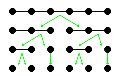
Figure 1: An example of a hierarchical bipartition tree for a path graph with $N=6$ nodes, where the edge weights are equal. The root is the whole graph.

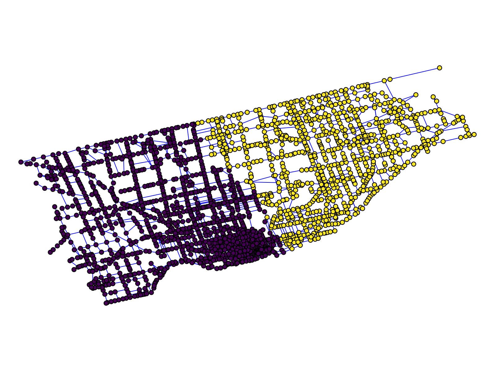
(a) Level $j=1$

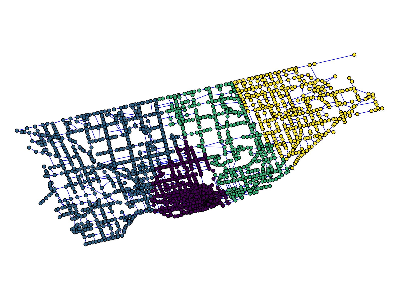
(b) Level $j=2$

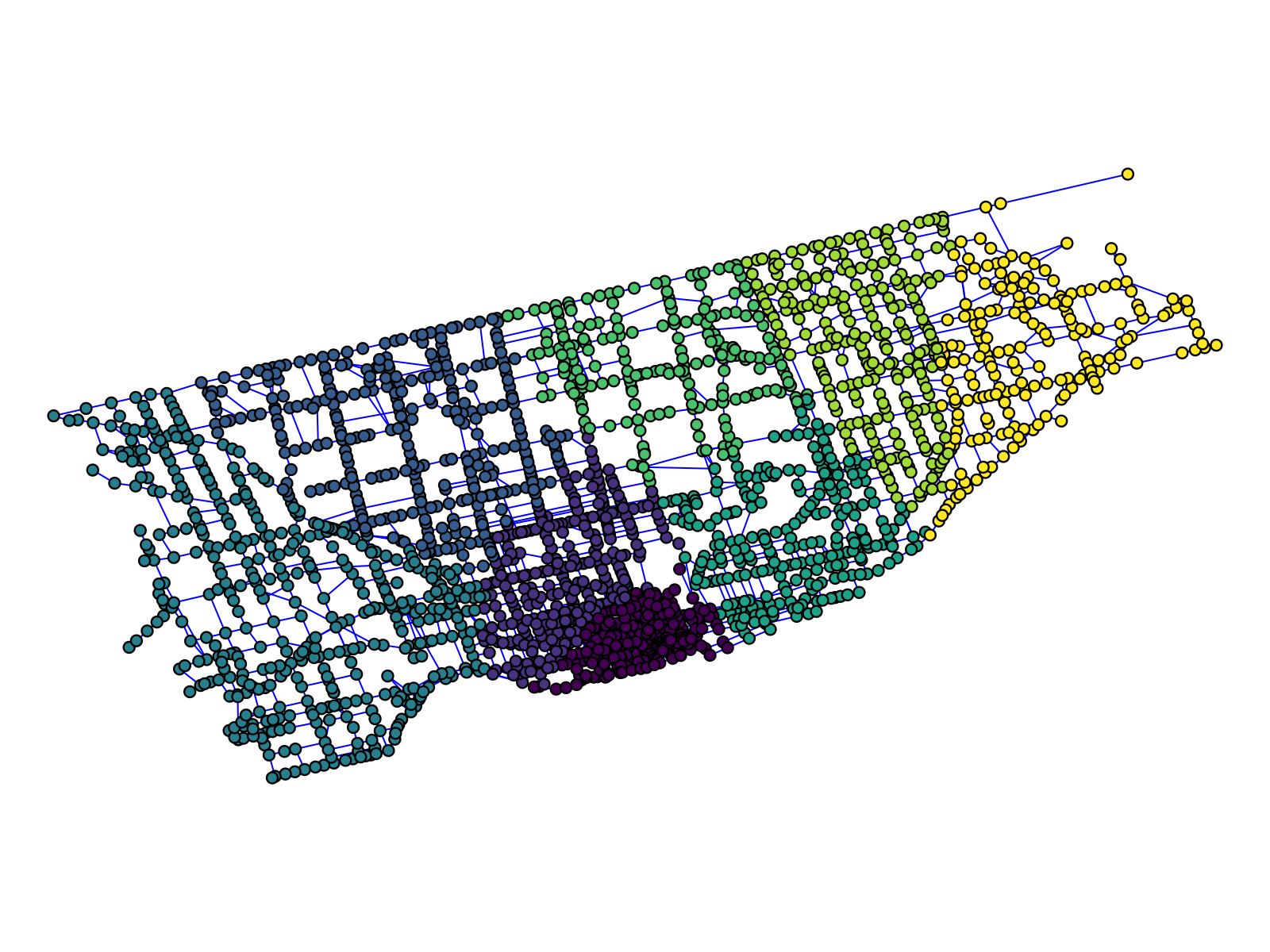
(c) Level $j=3$

Figure 2: A demonstration of hierarchical bipartition tree on the Toronto street network. On the same level, different colors correspond to different regions. The situation at level $j=0$ is not shown since there is no partition at $j=0$.

3 The Generalized Haar-Walsh Transform (GHWT)

In this section, we will review the Generalized Haar-Walsh Transform (GHWT) IRION-SAITO-GHWT ; IRION-SAITO-SPIE ; IRION-SAITO-TSIPN . It is a multiscale transform for graph signals and a true generalization of the classical Haar and Walsh-Hadamard transforms: if an input graph is a simple path graph whose number of nodes is dyadic, then the GHWT reduces to the classical counterpart exactly.

3.1 Overcomplete Dictionaries of Bases

After the binary partition tree of the input graph $G$ with depth ${j_{\mathrm{max}}}$ is generated, an overcomplete dictionary of basis vectors is composed. Each basis vector is denoted as $\bm{\psi}^{j}_{k,l}$, where $j\in[0,{j_{\mathrm{max}}}]$ denotes the level, $k\in[0,K_{j})$ denotes the region, and $l$ denotes the tag. $K_{j}$ is the number of subgraphs of $G$ on level $j$. The tag $l$ assumes a distinct integer value within the range $[0,2^{{j_{\mathrm{max}}}-j})$. The tag $l$, when expressed in binary, specifies the sequence of average and difference operations by which $\bm{\psi}^{j}_{k,l}$ was generated. For example, $l=6$ written in binary is $110$, which means that the basis vector/expansion coefficient was produced by two differencing operations (two $1$s) followed by an averaging operation (one $0$). Generally speaking, a larger value of $l$ indicates more oscillations in $\bm{\psi}^{j}_{k,l}$, with exceptions when imbalances occur in the recursive partitioning. We refer to basis vectors with tag $l=0$ as scaling vectors, those with tag $l=1$ as Haar vectors, and those with tag $l\geq 2$ as Walsh vectors.

The GHWT begins by defining an orthonormal basis on level ${j_{\mathrm{max}}}$ and obtaining the corresponding expansion coefficients. The standard basis of $\mathbb{R}^{N}$ is used here since each region at level ${j_{\mathrm{max}}}$ is a 1-node graph: $\bm{\psi}^{{j_{\mathrm{max}}}}_{k,0}\,:=\,\bm{1}_{V(G^{{j_{\mathrm{max}}}}_{k})}\in\mathbb{R}^{N}$, where $k\in[0,N)$, $N^{{j_{\mathrm{max}}}}_{k}=1$, and $\bm{1}_{i}$ is the indicator vector of node $i$, i.e., $\bm{1}_{i}[m]=0$ if $m\neq i$ and $\bm{1}_{i}[i]=1$. The expansion coefficients $\{d^{{j_{\mathrm{max}}}}_{k,0}\}_{k=0:N-1}$ are then simply the reordered input signal $\bm{f}$. From here the algorithm proceeds recursively, and the basis vectors and expansion coefficients on level $j-1$ are computed from those on level $j$. The GHWT proceeds as in Algorithm 1.

Input: A binary partition tree $\{G^{j}_{k}\}$ of the graph $G$, $0\leq j\leq{j_{\mathrm{max}}}$ and $0\leq k<K_{j}$; Input graph signal $\bm{f}$ supported on $V(G)$; a flag bvecq (default: false) to compute the GHWT basis vectors

Output: The set of expansion coefficients $\{d^{j}_{k,l}\}$ of signal $\bm{f}$ on the overcomplete GHWT dictionary vectors $\{\bm{\psi}^{j}_{k,l}\}$, which are also returned if bvecq is set to true

// The algorithm starts here.

for $k=0:N-1$ do // Basis vectors on level ${j_{\mathrm{max}}}$ are the standard unit vectors of $\mathbb{R}^{N}$

      $d_{k,0}^{j_{\mathrm{max}}}\leftarrow\left\langle{\bm{f}},{\bm{1}_{V(G_{k}^{j_{\mathrm{max}}})}}\right\rangle$ // $\left\langle{\cdot},{\cdot}\right\rangle$ is the standard inner product in $\mathbb{R}^{N}$

      if bvecq $\eqeq$ true then $\bm{\psi}_{k,0}^{j_{\mathrm{max}}}\leftarrow\bm{1}_{V(G_{k}^{j_{\mathrm{max}}})}\in\mathbb{R}^{N}$

      

end for

for $j={j_{\mathrm{max}}}:-1:1$ do // Compute coefficients/basis vectors on level $j-1$ from level $j$

       for $k=0:K_{j-1}-1$ do

             // Compute the scaling coeff’s/vectors $d^{j-1}_{k,0}\leftarrow\left\langle{\bm{f}},{\bm{1}_{V(G^{j-1}_{k})}/\sqrt{N_{k}^{j-1}}}\right\rangle$

            if bvecq $\eqeq$ true then $\bm{\psi}^{j-1}_{k,0}\leftarrow\bm{1}_{V(G^{j-1}_{k})}/\sqrt{N_{k}^{j-1}}$

            

            // Below, we assume $V(G^{j-1}_{k})=V(G^{j}_{k^{\prime}})\sqcup V(G^{j}_{k^{\prime}+1})$

            if $N_{k}^{j-1}>1$ then // Compute the Haar coeff’s/vectors

                   $d^{j-1}_{k,1}\leftarrow\frac{N^{j}_{k^{\prime}+1}\sqrt{N^{j}_{k^{\prime}}}d^{j}_{k^{\prime},0}-N^{j}_{k^{\prime}}\sqrt{N^{j}_{k^{\prime}+1}}d^{j}_{k^{\prime}+1,0}}{\sqrt{N^{j}_{k^{\prime}}(N^{j}_{k^{\prime}+1})^{2}+N^{j}_{k^{\prime}+1}(N^{j}_{k^{\prime}})^{2}}}$

                  if bvecq $\eqeq$ true then  $\bm{\psi}^{j-1}_{k,1}\leftarrow\frac{N^{j}_{k^{\prime}+1}\sqrt{N^{j}_{k^{\prime}}}\bm{\psi}^{j}_{k^{\prime},0}-N^{j}_{k^{\prime}}\sqrt{N^{j}_{k^{\prime}+1}}\bm{\psi}^{j}_{k^{\prime}+1,0}}{\sqrt{N^{j}_{k^{\prime}}(N^{j}_{k^{\prime}+1})^{2}+N^{j}_{k^{\prime}+1}(N^{j}_{k^{\prime}})^{2}}}$

                  

             end if

            

            if $N^{j-1}_{k}>2$ then // Compute the Walsh coeff’s/vectors

                   for $l=1:2^{{j_{\mathrm{max}}}-j}-1$ do

                         if both subregions $k^{\prime}$ and $k^{\prime}+1$ have a basis vector with tag $l$ then

                               $d^{j-1}_{k,2l}\leftarrow(d^{j}_{k^{\prime},l}+d^{j}_{k^{\prime}+1,l})/\sqrt{2}$

                               $d^{j-1}_{k,2l+1}\leftarrow(d^{j}_{k^{\prime},l}-d^{j}_{k^{\prime}+1,l})/\sqrt{2}$

                              if bvecq $\eqeq$ true then

                                     $\bm{\psi}^{j-1}_{k,2l}\leftarrow(\bm{\psi}^{j}_{k^{\prime},l}+\bm{\psi}^{j}_{k^{\prime}+1,l})/\sqrt{2}$

                                     $\bm{\psi}^{j-1}_{k,2l+1}\leftarrow(\bm{\psi}^{j}_{k^{\prime},l}-\bm{\psi}^{j}_{k^{\prime}+1,l})/\sqrt{2}$

                               end if

                              

                        

                        else if (without loss of generality) only subregion $k^{\prime}$ has a basis vector with tag $l$ then

                               $d^{j-1}_{k,2l}\leftarrow d^{j}_{k^{\prime},l}$

                              if bvecq $\eqeq$ true then $\bm{\psi}^{j-1}_{k,2l}\leftarrow\bm{\psi}^{j}_{k^{\prime},l}$

                              

                        

                        else

                              Do nothing // Neither of subregions has a basis vector with tag $l$

                         end if

                        

                   end for

                  

             end if

            

       end for

      

end for

Algorithm 1 Generating expansion coefficients relative to the basis vectors in the GHWT basis dictionary IRION-SAITO-GHWT ; IRION-SAITO-SPIE ; IRION-SAITO-TSIPN

Note that when analyzing the input signal $\bm{f}$, we only need to compute the expansion coefficients without generating the basis vectors in Algorithm 1 in general.

For the dictionary of basis vectors, several remarks are in order.

1. The basis vectors on each level are localized. In other words, $\bm{\psi}^{j}_{k,l}$ is supported on $V(G^{j}_{k})$. If $V(G^{j}_{k})\cap V(G^{j^{\prime}}_{k^{\prime}})=\emptyset$, then the basis vectors $\{\bm{\psi}^{j}_{k,l}\}_{l}$ and $\{\bm{\psi}^{j^{\prime}}_{k^{\prime},l^{\prime}}\}_{l^{\prime}}$ are mutually orthogonal.

2. The basis vectors on $V(G^{j}_{k})$ span the same subspace as the union of those on $V(G^{j+1}_{k^{\prime}})$ and $V(G^{j+1}_{k^{\prime}+1})$, where $V(G^{j}_{k})=V(G^{j+1}_{k^{\prime}})\sqcup V(G^{j+1}_{k^{\prime}+1})$.

3. The depth of the dictionary is the same as the binary partition tree, which is approximately $O(\log N)$ if the tree is nearly balanced. There are $N$ vectors on each level, so the total number of basis vectors is approximately $O(N\log N)$.

Note that Algorithm 1 groups the GHWT basis vectors by region (i.e., the index $k$) and arranges them from the coarse scale to the fine scale, which we call the coarse-to-fine (c2f) dictionary. Alternatively, we can group them by tag (i.e., the index $l$) and reverse the order of the levels (i.e., scales), which we call the fine-to-coarse (f2c) dictionary IRION-SAITO-GHWT ; IRION-SAITO-SPIE ; IRION-SAITO-TSIPN . The c2f dictionary corresponds to a collection of basis vectors by recursively partitioning the “time” domain information of the input graph signal while the f2c dictionary corresponds to those by recursively partitioning the “frequency” (or “sequency”) domain information of the input graph signal. Each dictionary contains more than $(1.5)^{N}$ choosable ONBs; see, e.g., Thiele and Villemoes THIELE-VILLEMOES for the details on how to compute or estimate this number. Note, however, that exceptions can occur when the recursive partitioning generates a highly imbalanced tree. Figure 3 shows these dictionaries for $P_{6}$. Figure 4 shows some basis vectors from the GHWT dictionary computed on the Toronto street network.

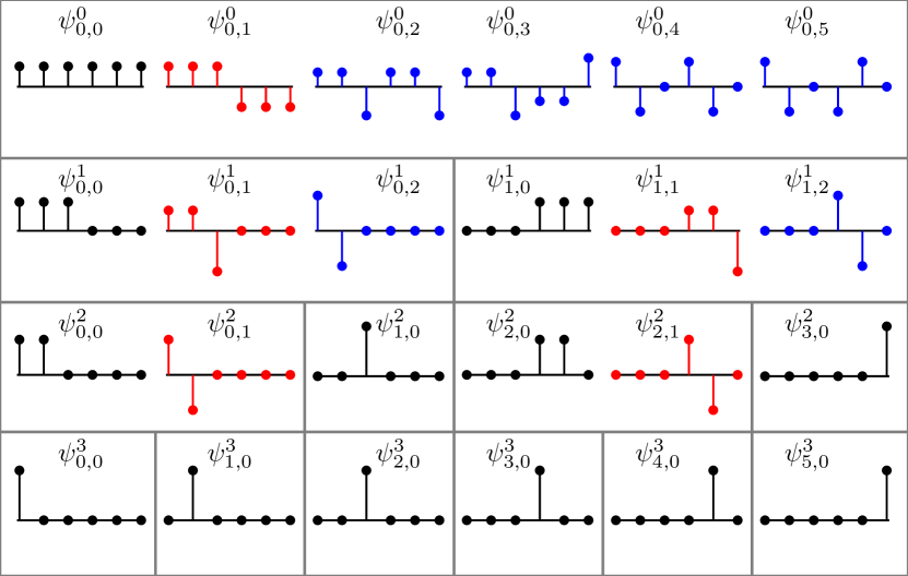
(a) The GHWT c2f dictionary

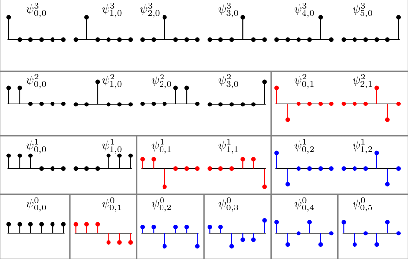
(b) The GHWT f2c dictionary

Figure 3: The GHWT c2f and f2c dictionaries on $P_{6}$. Stem plots with black, red, blue colors correspond to the scaling, Haar, and Walsh vectors, respectively.

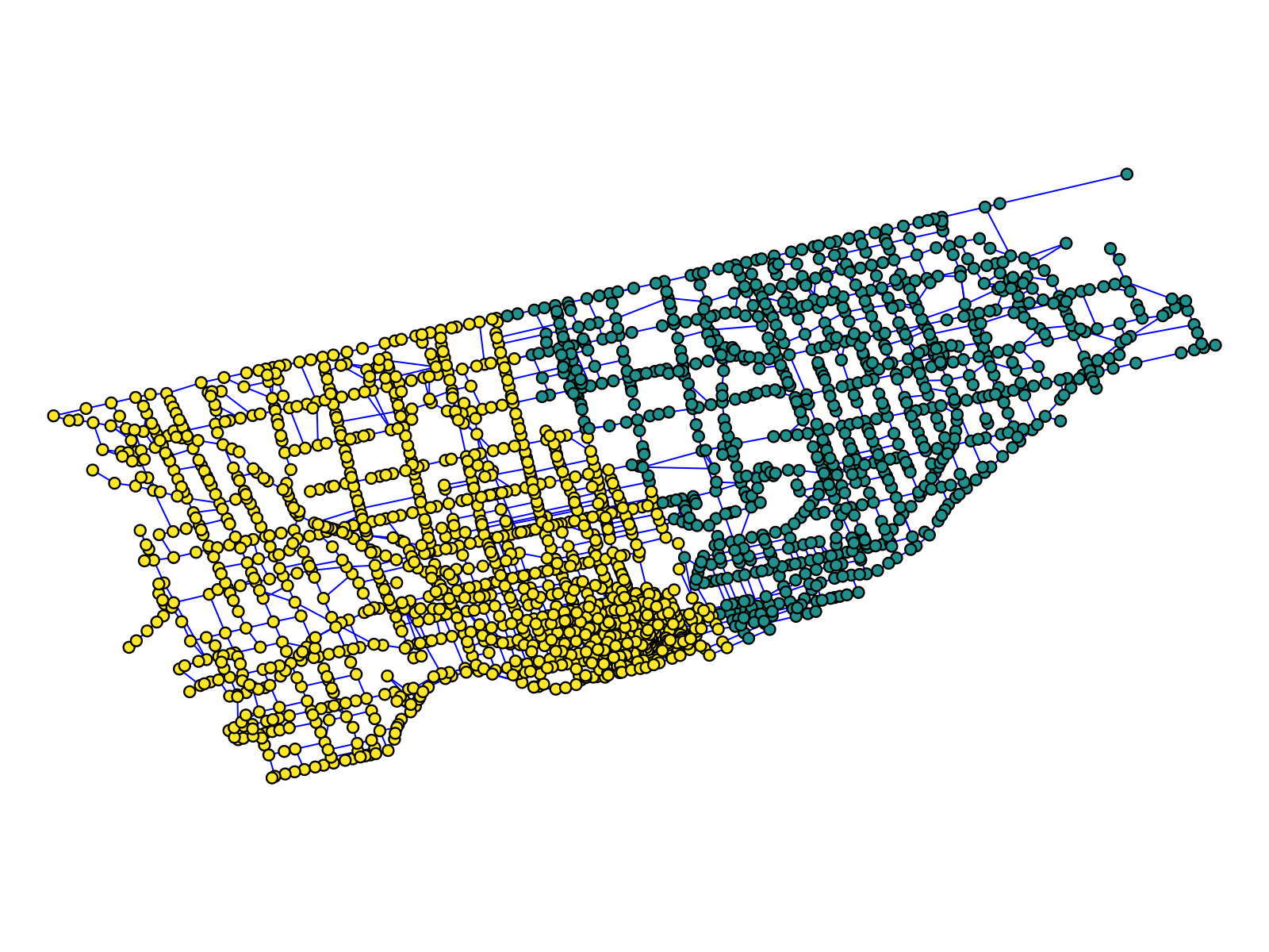
(a) Scaling vector $\bm{\psi}^{1}_{0,0}$

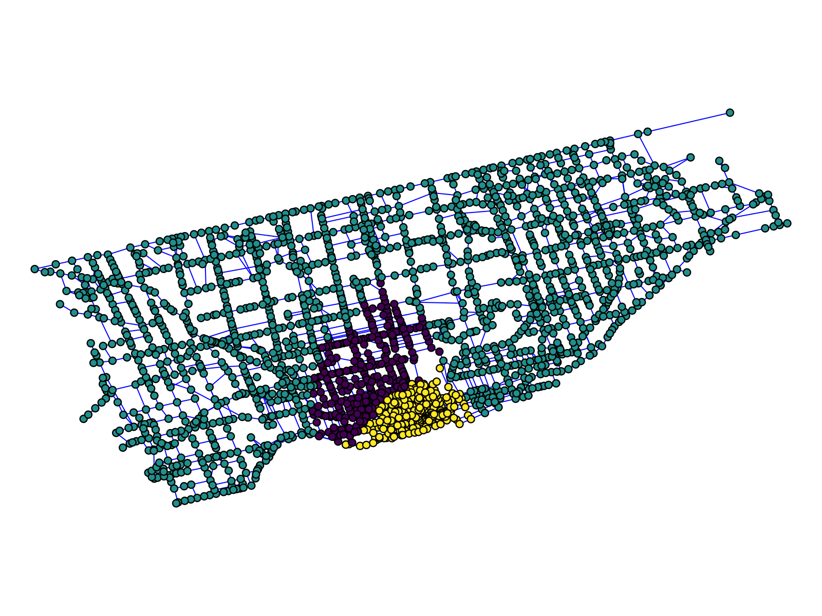
(b) Haar vector $\bm{\psi}^{2}_{0,1}$

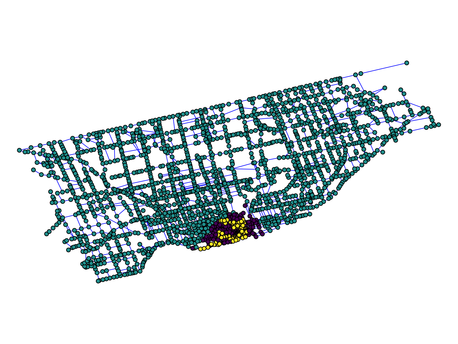
(c) Walsh vector $\bm{\psi}^{3}_{0,9}$

Figure 4: Examples of basis vectors from the GHWT dictionary computed on Toronto street network. The color scheme called viridis VIRIDIS is used to represent the amplitude of these vectors ranging from deep violet (negative) to dark green (zero) to yellow (positive).

3.2 The Best-Basis Algorithm in the GHWT

To select an ONB from a dictionary of wavelet packets that is “best” for approximation/compression, we typically use the so-called best-basis algorithm. The one used for the GHWT in IRION-SAITO-GHWT ; IRION-SAITO-SPIE ; IRION-SAITO-TSIPN was a straightforward generalization of the Coifman-Wickerhauser algorithm COIF-WICK , which was developed for non-graph signals of dyadic length. This algorithm requires a real-valued cost function $\mathcal{J}$ measuring the approximation/compression inefficiency of the subspaces in the dictionary, and aims to find an ONB whose coefficients minimize $\mathcal{J}$, (i.e., the most efficient ONB for approximating/compressing an input signal), which we refer to as the “best basis” chosen from the GHWT dictionary. The algorithm initiates the best basis as the whole set of vectors at the bottom level of the dictionary. Then it proceeds upwards, comparing the cost of the expansion coefficients corresponding to two children subgraphs to the cost of those of their parent subgraph. The best basis is updated if the cost of the parent subgraph is smaller than that of its children subgraphs. The algorithm continues until it reaches the top (i.e., the root) of the binary partition tree (i.e., the dictionary).

The best-basis algorithm works as long as $\mathcal{J}$ is nonnegative and additive  of the form $\mathcal{J}(\bm{d})\,:=\,\sum_{i}g(d_{i})$ with $g:\mathbb{R}\to\mathbb{R}_{\geq 0}$, where $\bm{d}$ is the expansion coefficients of an input graph signal on a region. For example, if one wants to promote sparsity in graph signal representation or approximation, $\mathcal{J}(\bm{d})$ function can be chosen as: either the $p$th power of $\ell^{p}$-(quasi)norm $\sum_{i}|d_{i}|^{p}$ for $0<p<2$ or the $\ell^{0}$-pseudonorm $|\{d_{i}\,|\,d_{i}\neq 0\}|$. Note that the smaller the value of $p$ is, the more emphasis in sparsity is placed.

Note that one can search the c2f and f2c dictionaries separately to obtain two sets of the best bases, among which the one with smaller cost is chosen as the final best basis of the GHWT dictionaries. We also note here that the graph Haar basis is selectable only in the GHWT f2c dictionary while the graph Walsh basis is selectable in either dictionary.

4 The Extended GHWT (eGHWT)

In this section, we describe the extended GHWT (eGHWT): our new best-basis algorithm on the GHWT dictionaries, which simultaneously considers the “time” domain split and “frequency” (or “sequency”) domain split of an input graph signal. This transform will allow us to deploy the modified best-basis algorithm that can select the best ONB for one’s task (e.g., efficient approximation, denoising, etc.) among a much larger set ($>0.618\cdot(1.84)^{N}$) of ONBs than the GHWT c2f/f2c dictionaries could provide ($>(1.5)^{N}$). The previous best-basis algorithm only searches through the c2f dictionary and f2c dictionary separately, but this new method makes use of those two dictionaries simultaneously. In fact, the performance of the eGHWT, by its construction, is always superior to that of the GHWT, which is clearly demonstrated in our numerical experiments in Section 5.

Our eGHWT is the graph version of the Thiele-Villemoes algorithm THIELE-VILLEMOES that finds the best basis among the ONBs of $\mathbb{R}^{N}$ consisting of discretized and rescaled Walsh functions for an 1D non-graph signal (i.e., a signal discretized on a 1D regular grid) of length $N$, where $N$ must be a dyadic integer. Their algorithm operates in the time-frequency plane and constructs its tiling with minimal cost among all possible tilings with dyadic rectangles of area one, which clearly depends on the input signal. Here we adapt their method to our graph setting that does not require dyadic $N$. In addition, the generalization of the Thiele-Villemoes algorithm for 2D signals developed by Lindberg and Villemoes LINDBERG-VILLEMOES can be generalized to the 2D eGHWT, as we will discuss more in Sections 4.5 and 5.2.

4.1 Fast Adaptive Time-Frequency Tilings

In this subsection, we briefly review the Thiele-Villemoes algorithm THIELE-VILLEMOES . First of all, let us define the so-called Walsh system, which forms an ONB for $L^{2}[0,1)$. Let $W_{0}(t)=1$ for $0\leq t<1$ and zero elsewhere, and define $W_{1},W_{2},\ldots$ recursively by

$$\begin{split}W_{2l}(t)&=W_{l}(2t)+(-1)^{l}W_{l}(2t-1),\\ W_{2l+1}(t)&=W_{l}(2t)-(-1)^{l}W_{l}(2t-1).\end{split}$$ (1)

Then $\{W_{l}\}^{\infty}_{l=0}$ is an ONB for $L^{2}[0,1)$ and is referred to as the Walsh system in sequency order. Each basis function, $W_{l}(t)$, is piecewise equal to either $1$ or $-1$ on $[0,1)$. Note that the scaling and Haar vectors at the global scale are included in this Walsh system.

Viewing $S\,:=\,[0,1)\times[0,\infty)$ as a time-frequency plane, the tile corresponding to the rescaled and translated Walsh function (which we also refer to as the Haar-Walsh function),

$$w_{p}(t)\,:=\,2^{j/2}W_{l}(2^{j}t-k),$$

is defined as

$$p=p(j,k,l)\,:=\,[2^{-j}k,2^{-j}(k+1))\times[2^{j}l,2^{j}(l+1)).$$ (2)

Note that the area of $p$ is $1$. Thiele and Villemoes showed that the functions $w_{p}$ and $w_{q}$ are orthogonal if and only if the tiles $p$ and $q$ are disjoint. Moreover, if a collection of tiles form a disjoint covering of a given dyadic rectangle (i.e., a rectangle with dyadic sides) in the time-frequency plane, then the Haar-Walsh functions of those tiles form an ONB of the subspace corresponding to that dyadic rectangle.

Now the 1D discrete signal space $\mathbb{R}^{N}\ (N=2^{n})$ can be identified with the subset $S_{n}\,:=\,[0,1)\times[0,N)$ of $S$ in the time-frequency plane. Given the overcomplete dictionary of Haar-Walsh functions on $\mathbb{R}^{N}$, the best-basis algorithm now is equivalent to finding a set of basis vectors for a given input signal with minimal cost that also generates a disjoint tiling of $S_{n}$. That tiling is called the minimizing tiling.

Lemma 1 (Thiele & Villemoes THIELE-VILLEMOES )

Let $T\subset S$ be a rectangle of area greater or equal to two, with left half $L$, right half $R$, lower half $D$, and upper half $U$. Assume each tile $p\subset T$ has the cost $c(p)$. Define

$$m_{T}\,:=\,\min\left\{\sum_{p\in\mathcal{B}}c(p)\,\Bigg{|}\,\mathcal{B}\text{ is a disjoint covering of }T\right\},$$

and similarly $m_{L}$,$m_{R}$,$m_{D}$,$m_{U}$. Then

$$m_{T}=\min\{m_{L}+m_{R},m_{D}+m_{U}\}.$$

This lemma tells us that the minimizing tiling of $T$ can be split either in the time-direction into two minimizing tilings of $L$ and $R$, or in the frequency-direction into those of $D$ and $U$. It enables a dynamic programming algorithm to find the minimizing tiling of $S_{n}$; see Algorithm 3.3 of THIELE-VILLEMOES .

4.2 Relabeling Region Indices

If the input graph is a simple path graph $P_{N}$ with dyadic $N$ and the partition tree is a balanced complete binary tree, then the GHWT dictionary is the same as the classical Haar-Walsh wavelet packet dictionary for 1D regular signals, on which the Thiele-Villemoes algorithmTHIELE-VILLEMOES can be applied in a straightforward manner. To adapt the algorithm to a graph signal of an arbitrary length or an imperfect binary partition tree of an input graph, we need to modify the GHWT dictionary first.

Specifically, the region index $k$ of $G^{j}_{k}$ and $\bm{\psi}^{j}_{k,l}$ needs to be relabeled. Previously, on level $j$, the region index $k$ takes all the integer values in $[0,K_{j})$ where $K_{j}\leq 2^{j}$ is the total number of subgraphs (or regions) on level $j$. After relabeling, $k$ takes an integer value in $[0,2^{j})$ according to its location in the binary tree. Algorithm 2 precisely describes the whole procedure.

Input: A binary partition tree denoted by $\{G^{j}_{k}\}$, $0\leq j\leq{j_{\mathrm{max}}}$, $0\leq k<K_{j}$

Output: A perfect binary partition tree $\{\widetilde{G}^{j}_{k}\}$ containing $\{G^{j}_{k}\}$ as its subset

// The algorithm starts here.

$\widetilde{G}^{0}_{0}\leftarrow G^{0}_{0}$ // On level $0$, there is only one region $G^{0}_{0}$, so no relabeling is required.

for $j=1:{j_{\mathrm{max}}}$ do

       for $k=0:K_{j-1}-1$ do

             if $G^{j-1}_{k}$ is split into $G^{j}_{k^{\prime}}$ and $G^{j}_{k^{\prime}+1}$ then

                  $\widetilde{G}^{j}_{2k}\leftarrow G^{j}_{k^{\prime}};\quad\widetilde{G}^{j}_{2k+1}\leftarrow G^{j}_{k^{\prime}+1}$

            else // $G^{j-1}_{k}$ is kept as $G^{j}_{k^{\prime}}$

                  $\widetilde{G}^{j}_{2k}\leftarrow G^{j}_{k^{\prime}};\quad\widetilde{G}^{j}_{2k+1}\leftarrow\emptyset$

             end if

            

       end for

      

end for

Algorithm 2 Relabeling the GHWT Dictionary

A couple of remarks are in order. First, the region indices of the basis vectors $\{\bm{\psi}^{j}_{k,l}\}$, $0\leq k<K_{j}$ are also relabeled accordingly as $\{\widetilde{\bm{\psi}}^{j}_{k^{\prime},l}\}$ supported on the subgraph $\widetilde{G}^{j}_{k^{\prime}}$, where $0\leq k^{\prime}<2^{j}$. Note that some of the basis vectors in $\{\widetilde{\bm{\psi}}^{j}_{k^{\prime},l}\}$ that do not have the corresponding basis vectors in the original GHWT dictionary $\{\bm{\psi}^{j}_{k,l}\}$ are “fictitious” (or “non-existent”) ones and can be set as the zero vectors. In practice, however, we even do not need to store them as the zero vectors; we simply do not compute the cost corresponds to such fictitious basis vectors. Second, to simplify our notation, we just assume the $\{\bm{\psi}^{j}_{k,l}\}$ and $\{G^{j}_{k}\}$ are those already relabeled by Algorithm 2 in the rest of our article.

Figure 5(b) shows the result of Algorithm 2 applied to the GHWT c2f dictionary shown in Fig. 5(a) on $P_{6}$. Before the relabeling, the dictionary forms a complete but imperfect binary tree. As one can see, after the relabeling, the initial GHWT c2f dictionary is a subset of a perfect binary tree shown in Fig. 5(b).

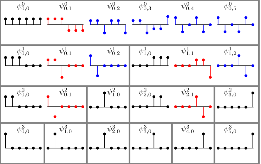
(a) The GHWT c2f dictionary

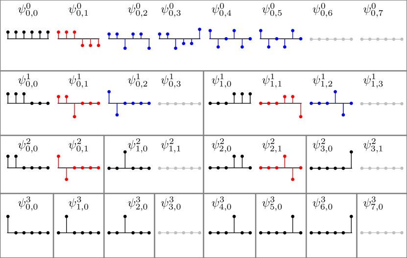
(b) The relabeled GHWT c2f dictionary

Figure 5: (a) The GHWT c2f dictionary on $P_{6}$. Stem plots with black, red, and blue colors correspond to the scaling, Haar, and Walsh vectors, respectively. (b) The relabeled GHWT c2f dictionary by Algorithm 2 applied to the GHWT c2f dictionary shown in (a). The gray stem plots indicate the “fictitious” (or “non-existent”) basis vectors newly generated by Algorithm 2.

4.3 The New Best-Basis (eGHWT) Algorithm

We can now apply Algorithm 3 to search for the best basis in the relabeled GHWT dictionary that have a perfect binary partition tree, similarly to the Thiele-Villemoes algorithm. For simplicity, we refer to this whole procedure as the eGHWT. In order to understand this algorithm, let us first remark that we use the so-called associative array: an abstract data type composed of a collection of (key, value) pairs such that each possible key appears at most once in the collection. The reason why we use the associative arrays instead of the regular arrays is to save storage space while keeping the algorithm flexible and efficient without losing the convenience of manipulating arrays. This point is important since many basis vectors $\bm{\psi}^{j}_{k,l}$ after relabeling via Algorithm 2 may be fictitious, which we need to neither store nor compute: using regular matrices to store them will be wasteful. For example, Algorithm 3 has a statement like $A_{0}[j,k,l]\leftarrow g(\langle{\bm{f}},{\bm{\psi}^{j}_{k,l}}\rangle)$, where $A_{0}$ is an associative array. This actually means that $((j,k,l),g(\langle{\bm{f}},{\bm{\psi}^{j}_{k,l}}\rangle))$ is a pair of (key, value) of the associative array $A_{0}$. Here we write $(j,k,l)\in A_{0}$ to denote that $(j,k,l)$ is a valid key of $A_{0}$. Therefore, $(j,k,l)\in A_{0}$ if and only if non-fictitious $\bm{\psi}^{j}_{k,l}$ exists. Since we relabeled $\bm{\psi}^{j}_{k,l}$, there are fictitious $\bm{\psi}^{j}_{k,l}$’s (i.e., zero vectors) for some triple $(j,k,l)$. In that case, we write $(j,k,l)\notin A_{0}$.

Input: The relabeled GHWT basis vectors $\{\bm{\psi}^{j}_{k,l}\}$ generated by Algorithm 2; a nonnegative function $g:\mathbb{R}\to\mathbb{R}_{\geq 0}$ to evaluate the cost of each expansion coefficient; an input graph signal $\bm{f}\in\mathbb{R}^{N}$.

Output: The eGHWT best basis $B$.

// Initialize two associative arrays $A_{0}$ and $I_{0}$ that store costs and indices for the best basis search, respectively

$A_{0}[j,k,l]\leftarrow g(\langle\bm{f},\bm{\psi}^{j}_{k,l}\rangle)$ if $\bm{\psi}^{j}_{k,l}$ is not fictitious;

$I_{0}[j,k,l]\leftarrow 1$ if $(j,k,l)\in A_{0}$

for $m=0:{j_{\mathrm{max}}}-1$ do // Compute $(A_{m+1},I_{m+1})$ from $(A_{m},I_{m})$

       Initialize $A_{m+1}$ and $I_{m+1}$ as empty associative arrays

      

      for each $(j,k,l)\in A_{m}$ with $j<{j_{\mathrm{max}}}-m$ and $l\equiv 0\pmod{2}$ do

             if $(A_{m}[j,k,l]+A_{m}[j,k,l+1])\leq(A_{m}[j+1,2k,l/2]+A_{m}[j+1,2k+1,l/2])$ then

                  $I_{m+1}[j,k,l/2]\leftarrow 0$

                   $A_{m+1}[j,k,l/2]\leftarrow(A_{m}[j,k,l]+A_{m}[j,k,l+1])$

            else

                  $I_{m+1}[j,k,l/2]\leftarrow 1$

                   $A_{m+1}[j,k,l/2]\leftarrow(A_{m}[j+1,2k,l/2]+A_{m}[j+1,2k+1,l/2])$

             end if

            // Note that any of $A_{m}[j,k,l+1]$, $A_{m}[j+1,2k,l/2]$, $A_{m}[j+1,2k+1,l/2]$ will be replaced by $0$ in the above steps if it corresponds to the fictitious basis vector.

            

       end for

      

end for

$I\leftarrow I_{j_{\mathrm{max}}}$

for $m={j_{\mathrm{max}}}-1:-1:0$ do // Recover the best basis from $\{I_{m}\}$

       Initialize $I_{\mathrm{temp}}$ as an empty associative array

       for each $(j,k,l)\in I$ do

             if $I[j,k,l]\eqeq 0$ then

                  $I_{\mathrm{temp}}[j,k,2l]\leftarrow I_{m}[j,k,2l]$ if $(j,k,2l)\in I_{m}$

                  $I_{\mathrm{temp}}[j,k,2l+1]\leftarrow I_{m}[j,k,2l+1]$ if $(j,k,2l+1)\in I_{m}$

            else // i.e., $I[j,k,l]\eqeq 1$

                  $I_{\mathrm{temp}}[j+1,2k,l]\leftarrow I_{m}[j+1,2k,l]$ if $(j+1,2k,l)\in I_{m}$

                  $I_{\mathrm{temp}}[j+1,2k+1,l]\leftarrow I_{m}[j+1,2k+1,l]$ if $(j+1,2k+1,l)\in I_{m}$

             end if

            

       end for

      $I\leftarrow I_{\mathrm{temp}}$

      

end for

$B\leftarrow\emptyset$; // Initialize $B$ as an empty set

for each $(j,k,l)\in I$ do

      $B\leftarrow B\cup\{\bm{\psi}^{j}_{k,l}\}$

end for

// $B$ is the best basis!

Algorithm 3 The New Best-Basis (eGHWT) Algorithm

Several remarks on this algorithm are in order:

• The associative array, $A_{m}$, holds the minimum cost of ONBs in a subspace. The value of $A_{m}[j,k,l]$ is set to the smaller value between $A_{m-1}[j,k,2l]+A_{m-1}[j,k,2l+1]$ and $A_{m-1}[j+1,2k,l]+A_{m-1}[j+1,2k+1,l]$. The subspace corresponding to $A_{m}[j,k,l]$ is the direct sum of the two subspaces corresponding to $A_{m-1}[j,k,2l]$ and $A_{m-1}[j,k,2l+1]$, which is the same as the direct sum of those corresponding to $A_{m-1}[j+1,2k,l]$ and $A_{m-1}[j+1,2k+1,l]$. In other words, when we compute $A_{m}$ from $A_{m-1}$, we concatenate the subspaces. This process is similar to finding the best tilings for dyadic rectangles from those with half size in Thiele-Villemoes algorithm THIELE-VILLEMOES as described in Sect. 4.1.

• If the input graph $G$ is a simple 1D path $P_{N}$ with dyadic $N$, and if we view an input graph signal $\bm{f}$ as a discrete-time signal, then $(A_{m-1}[j,k,2l],A_{m-1}[j,k,2l+1])$ corresponds to splitting the subspace of $A_{m}[j,k,l]$ in the frequency domain in the time-frequency plane while $(A_{m-1}[j+1,2k,l],A_{m-1}[j+1,2k+1,l])$ does the split in the time domain.

• The subspace of each entry in $A_{0}$ is one dimensional since it is spanned by a single basis vector. In other words, $A_{0}[j,k,l]$ corresponds to $\operatorname{span}\{\bm{\psi}^{j}_{k,l}\}$: the one-dimensional subspace spanned by $\bm{\psi}^{j}_{k,l}$.

• $A_{j_{\mathrm{max}}}$ has only one entry $A_{j_{\mathrm{max}}}[0,0,0]$, which corresponds to the whole $\mathbb{R}^{N}$. Its value is the minimum cost among all the choosable ONBs, i.e., the cost of the best basis.

• If an input graph signal is of dyadic length, Algorithm 3 selects the best basis among a much larger set ($>0.618\cdot(1.84)^{N}$) of ONBs than what each of the GHWT c2f and f2c dictionaries would provide ($>(1.5)^{N}$) THIELE-VILLEMOES . The numbers are similar even for non-dyadic cases as long as the partition trees are essentially balanced. The essence of this algorithm is that at each step of the recursive evaluation of the costs of subspaces, it compares the cost of the parent subspace with not only its two children subspaces partitioned in the “frequency” domain (as the GHWT f2c does), but also its two children subspaces partitioned in the “time” domain (as the GHWT c2f does).

• If the underlying graph of an input graph signal is a simple unweighted path graph of dyadic length, i.e., $P_{2^{n}}$, $n\in\mathbb{N}$, then Algorithm 3 reduces to the Thiele-Villemoes algorithm exactly. Note that in such a case, neither computing the Fiedler vectors of subgraphs nor relabeling the subgraphs via Algorithm 2, is necessary; it is more efficient to force the midpoint partition at each level explicitly in that case.

4.4 The eGHWT illustrated by a simple graph signal on $P_{6}$

The easiest way to appreciate and understand the eGHWT algorithm is to use a simple example. Let $\bm{f}=[2,-2,1,3,-1,-2]^{\scriptscriptstyle{\mathsf{T}}}\in\mathbb{R}^{6}$ be an example graph signal on $G=P_{6}$. The $\ell^{1}$-norm is chosen as the cost function.

Figure 6(a) shows the coefficients of that signal on the GHWT c2f dictionary and Fig. 6(b) corresponds to the relabeled GHWT c2f dictionary by Algorithm 2.

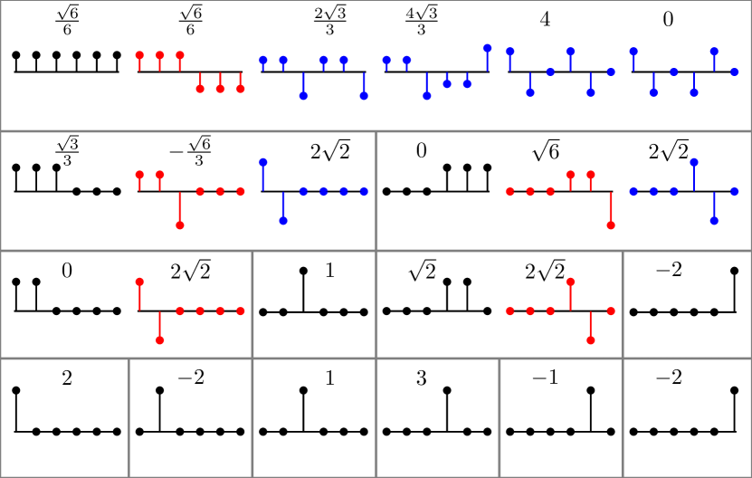
(a) The GHWT c2f dictionary

(b) The GHWT c2f dictionary after relabeling

Figure 6: (a) The expansion coefficients and the basis vectors of the simple graph signal $\bm{f}=[2,-2,1,3,-1,-2]^{\scriptscriptstyle{\mathsf{T}}}$ on $P_{6}$ relative to the GHWT c2f dictionary; (b) those correspond to the GHWT c2f dictionary after relabeling

After the GHWT c2f for $P_{6}$ is relabeled via Algorithm 2, the dictionary tree has the same structure as that of $P_{8}$. Figure 7 illustrates the progression of Algorithm 3 on this simple graph signal. The time-frequency plane in this case is $S_{3}=[0,1)\times[0,8)$ and the frequency axis is scaled in this figure so that $S_{3}$ is a square for visualization purpose. The collection of all 32 tiles and the corresponding expansion coefficients are placed on the four copies of $S_{3}$ in the top row of Fig. 7, which are ordered from the finest time/coarsest frequency partition ($j=3$) to the coarsest time/finest frequency partition ($j=0$). Note that each tile has the unit area.

In the first iteration ($m=1$) in Fig. 7, the minimizing tilings for all the dyadic rectangles of area $2$ are computed from those with unit area. For example, the left most dyadic rectangle (showing its cost $2\sqrt{2}$) at $m=1$, can be composed by either a pair of tiles $(\bm{\psi}^{3}_{0,0},\bm{\psi}^{3}_{1,0})$ or $(\bm{\psi}^{2}_{0,0},\bm{\psi}^{2}_{0,1})$. The corresponding costs are $|2|+|-2|=4$ or $|2\sqrt{2}|+|0|=2\sqrt{2}$, and the minimum of which is $2\sqrt{2}$. The minimizing tiling for that dyadic rectangle is hence $\bm{\psi}^{2}_{0,0}$ and $\bm{\psi}^{2}_{0,1}$ with its cost $2\sqrt{2}$. In the second iteration ($m=2$), the algorithm finds the minimizing tilings for all dyadic rectangles with area $4$. In the third iteration ($m=3$), the algorithm finds the minimizing tiling for the whole $S_{3}$. After the best basis is found in the relabeled GHWT c2f dictionary, we remove those “fictitious” zero basis vectors and undo the relabeling done by Algorithm 2 to get back to the original $(j,k,l)$ indices.

Figure 7: Graphical illustration of Algorithm 3 for the simple signal $\bm{f}=[2,-2,1,3,-1,-2]^{\scriptscriptstyle{\mathsf{T}}}\in\mathbb{R}^{6}$. The cost function is the $\ell^{1}$-norm of the expansion coefficients. The top row contains all possible tiles and coefficients. The bottom row represents the eGHWT best basis.

Figure 8 shows that the GHWT c2f best basis for this simple graph signal is actually the Walsh basis, and its representation is $\frac{\sqrt{6}}{6}\bm{\psi}_{0,0}^{0}+\frac{\sqrt{6}}{6}\bm{\psi}_{0,1}^{0}+\frac{2\sqrt{3}}{3}\bm{\psi}_{0,2}^{0}+\frac{4\sqrt{3}}{3}\bm{\psi}_{0,3}^{0}+4\bm{\psi}_{0,4}^{0}+0\bm{\psi}_{0,5}^{0}$ with its cost $\approx 8.28$ and the f2c-GHWT best basis representation is $\frac{\sqrt{3}}{3}\bm{\psi}_{0,0}^{1}+0\bm{\psi}_{1,0}^{1}+\frac{\sqrt{6}}{3}\bm{\psi}_{0,1}^{1}+\sqrt{6}\bm{\psi}_{1,1}^{1}+4\bm{\psi}_{0,4}^{0}+0\bm{\psi}_{0,5}^{0}$ with its cost $\approx 7.84$ while Fig. 9 demonstrates that the best basis representation chosen by the eGHWT algorithm is $0\bm{\psi}_{0,0}^{2}+1\bm{\psi}_{1,0}^{2}+0\bm{\psi}_{1,0}^{1}+\sqrt{6}\bm{\psi}_{1,1}^{1}+4\bm{\psi}_{0,4}^{0}+0\bm{\psi}_{0,5}^{0}$ with its cost $\approx 7.45$, which is the smallest among these three best basis representations. The indices used here are those of the original ones.

Figure 9 clearly demonstrates that the eGHWT best basis cannot be obtained by simply applying the previous GHWT best basis algorithm on the c2f and f2c dictionaries. More specifically, let us consider the vectors $\bm{\psi}^{1}_{1,0}$ and $\bm{\psi}^{0}_{0,4}$ in the eGHWT best basis. From Fig. 9(a), we can see that $\bm{\psi}^{1}_{1,0}$ is supported on the child graph $G^{1}_{1}$ that was generated by bipartitioning the input graph $G^{0}_{0}$ where $\bm{\psi}^{0}_{0,4}$ is supported. Therefore, they cannot be selected in the GHWT c2f best basis simultaneously. A similar argument applies to $\bm{\psi}^{2}_{1,0}$ and $\bm{\psi}^{1}_{1,0}$ in the eGHWT best basis as shown in Fig. 9(b): they cannot be selected in the GHWT f2c best basis simultaneously.

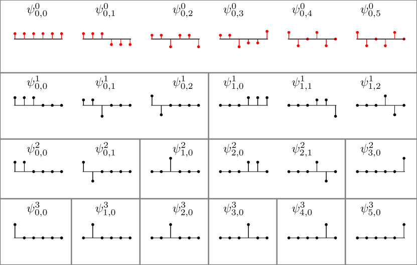
(a) The GHWT c2f best basis

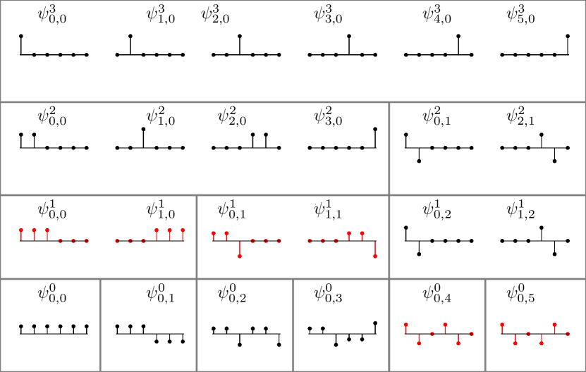
(b) The GHWT f2c best basis

Figure 8: (a) The GHWT c2f best-basis vectors for the input graph signal $\bm{f}=[2,-2,1,3,-1,-2]^{\scriptscriptstyle{\mathsf{T}}}$ (indicated by red); (b) the GHWT f2c best-basis vectors for the same signal.

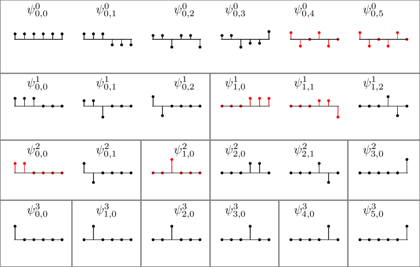
(a) The eGHWT best basis shown in the GHWT c2f dictionary

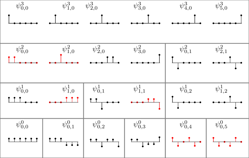
(b) The eGHWT best basis shown in the GHWT f2c dictionary

Figure 9: The eGHWT best-basis vectors for the signal $\bm{f}=[2,-2,1,3,-1,-2]^{\scriptscriptstyle{\mathsf{T}}}$ selected by Algorithm 3 (indicated by red) that are displayed within the GHWT c2f dictionary (a) and the GHWT f2c dictionary (b). Note the orthogonality of these vectors, and compare them with those shown in Fig. 8.

4.5 Generalization to 2D Signals/Matrix Data

The Thiele-Villemoes algorithm THIELE-VILLEMOES has been extended to 2D signals by Lindberg and Villemoes LINDBERG-VILLEMOES . Similarly to the former, the Lindberg-Villemoes algorithm works for only 2D signals of dyadic sides. We want to generalize the Lindberg-Villemoes algorithm for a more general 2D signal or matrix data whose sides are not necessarily dyadic, as we did for the previous GHWT dictionaries in IRION-SAITO-MLSP16 . Before describing our 2D generalization of the eGHWT algorithm, let us briefly review the Lindberg-Villemoes algorithm. As we described in Sect. 4.1, the best tiling in each step in the Thiele-Villemoes algorithm chooses a bipartition with a smaller cost between that of the time domain and that of the frequency domain. For 2D signals, the time-frequency domain has four axes instead of two. It has time and frequency axes on each of the $(x,y)$ components (i.e., columns and rows of an input image). The best tiling comes from the split in the time or frequency directions in either the $x$ or $y$ component. This forces them to choose the best tiling/split among four options instead of two for each split. Similarly to the 1D signal case, dynamic programming is used to find the minimizing tiling for a given 2D signal. We note that our 2D generalized version of the eGHWT algorithm exactly reduces to the Lindberg-Villemoes algorithm if the input graph is a 2D regular lattice of dyadic sizes and the midpoint (or midline to be more precise) partition is used throughout.

For a more general 2D signal or matrix data, we can compose the affinity matrices on the row and column directions separately (see, e.g., IRION-SAITO-MLSP16 ), thus define graphs on which the rows and columns are supported. In this way, the input 2D signal can be viewed as a tensor product of two graphs. Then the eGHWT can be extended to 2D signal from 1D in a similar way as how Lindberg and Villemoes LINDBERG-VILLEMOES extended the Thiele-Villemoes algorithm THIELE-VILLEMOES . Examples will be given in Sect. 5.2.

5 Applications

In this section, we will demonstrate the usefulness and efficiency of the eGHWT using several real datasets, and compare its performance with that of the classical Haar transform, graph Haar basis, graph Walsh basis, and the GHWT c2f/f2c best bases. We note that our performance comparison is to emphasize the difference between the eGHWT and its close relatives. Hence we will not compare the performance of the eGHWT with those graph wavelets and wavelet packets of different nature; see, e.g., IRION-SAITO-TSIPN ; CLONINGER-LI-SAITO for further information.

5.1 Efficient Approximation of a Graph Signal

Here we analyze the eight peak-hour vehicle volume counts on the Toronto street network, which is shown in Fig. 10. We have already described this street network in Sect. 2 and in Fig. 2. The data was typically collected at the street intersections equipped with traffic lights between the hours of 7:30 am and 6:00 pm, over the period of 03/22/2004–02/28/2018. As one can see, the vehicular volume are spread in various parts of this street network with the concentrated northeastern region.

In addition to the eGHWT best basis, the graph Haar basis, the graph Walsh basis, the GHWT c2f/f2c best bases are used to compare the performance. Figure 10(b) shows the performance comparison. The $y$-axis denotes the relative approximation error $\|\bm{f}-{\mathcal{P}}_{n}\bm{f}\|_{2}/\|\bm{f}\|_{2}$, where ${\mathcal{P}}_{n}\bm{f}$ denotes the approximation of $\bm{f}$ with the basis vectors having the $n$ largest coefficients in magnitude. The $x$-axis denotes $n/N$, i.e., the fraction of coefficients retained. We can see that the error of the eGHWT decays fastest, followed by the GHWT f2c best basis, the graph Haar basis, and the GHWT c2f best basis that chose the graph Walsh basis, in that order. In Fig. 11, we display the nine most significant basis vectors (except for the DC vector) for the graph Haar, the GHWT c2f best basis (which selected the graph Walsh basis), the GHWT f2c best basis, and the eGHWT best basis to approximate this traffic volume data.

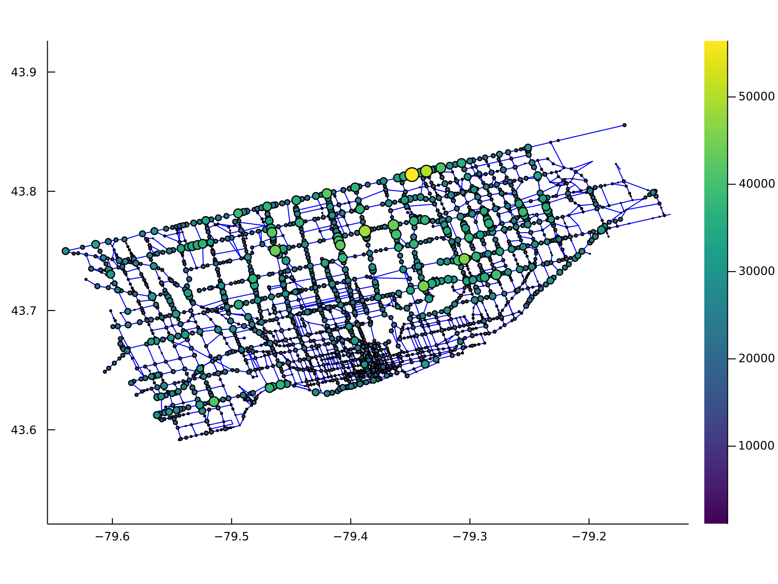
(a) Vehicular volume counts

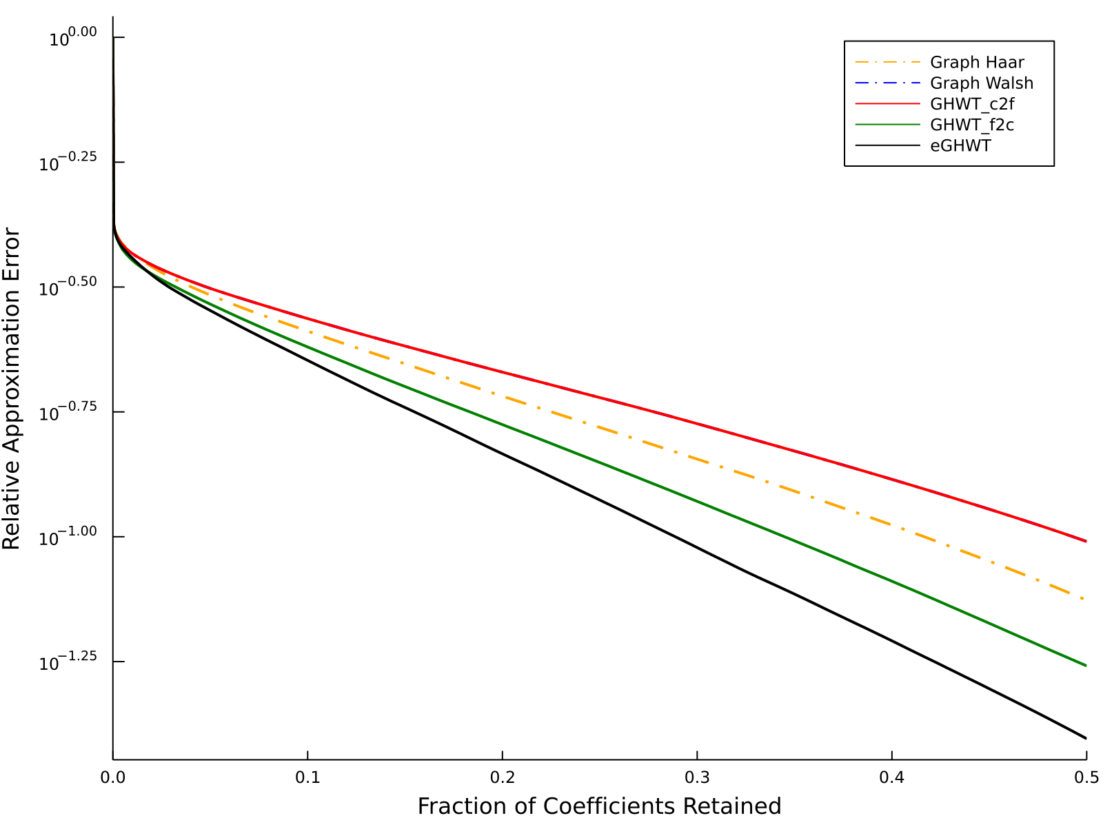
(b) Relative $\ell^{2}$ approximation error

Figure 10: (a) Vehicular volume data in the city of Toronto (the node diameter is proportional to its volume counts for visualization purpose); (b) Relative $\ell^{2}$ approximation errors by various graph bases

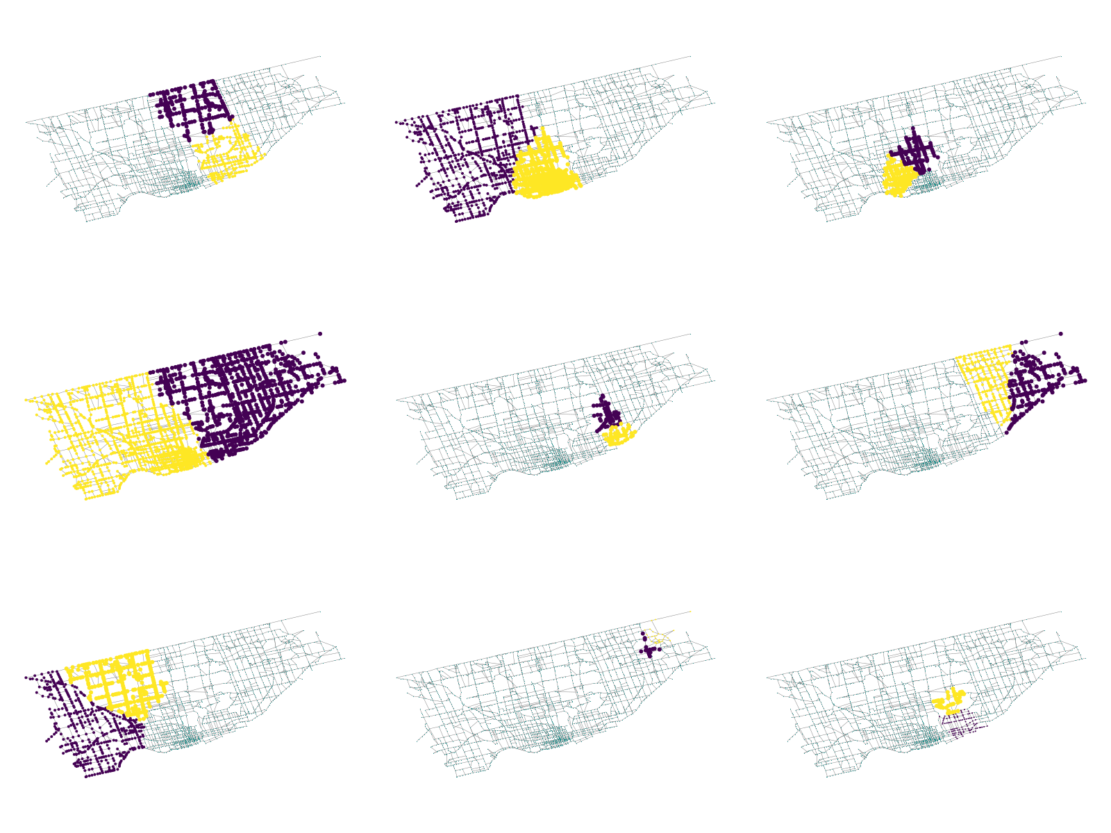
(a) Haar

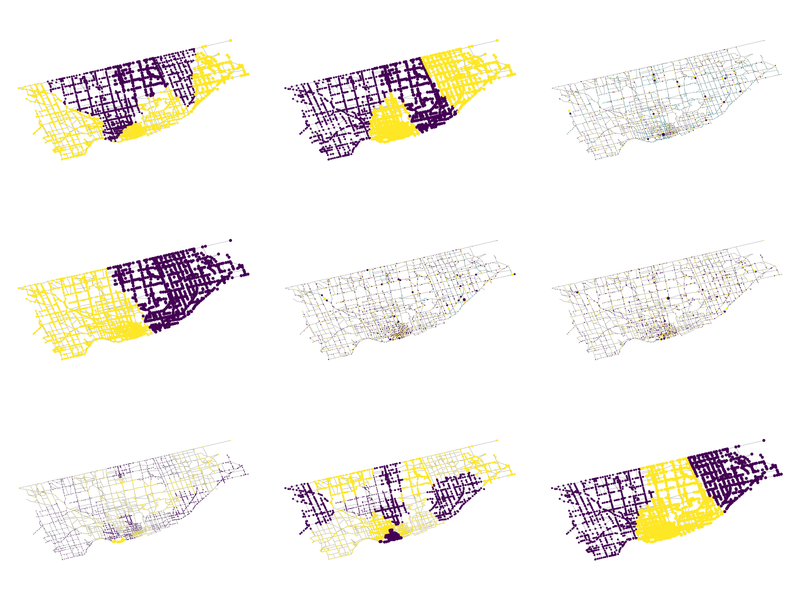
(b) GHWT c2f = Walsh

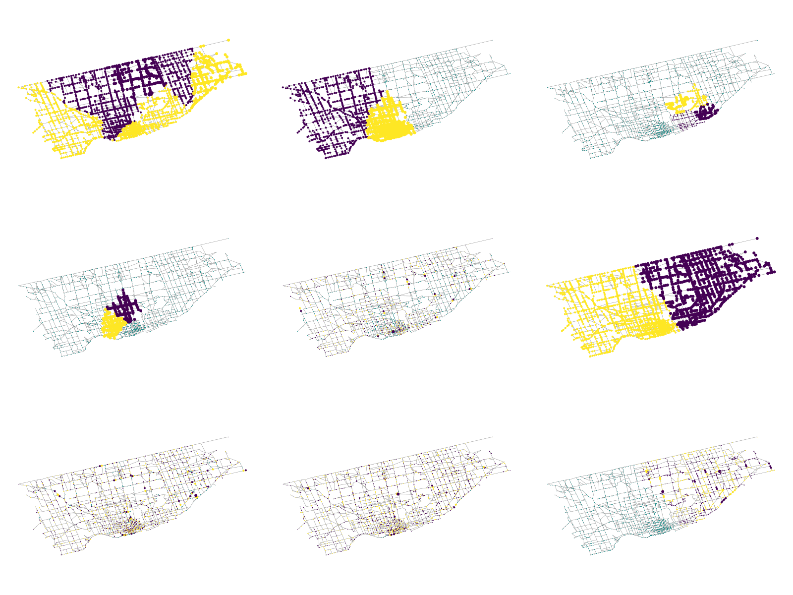
(c) GHWT f2c

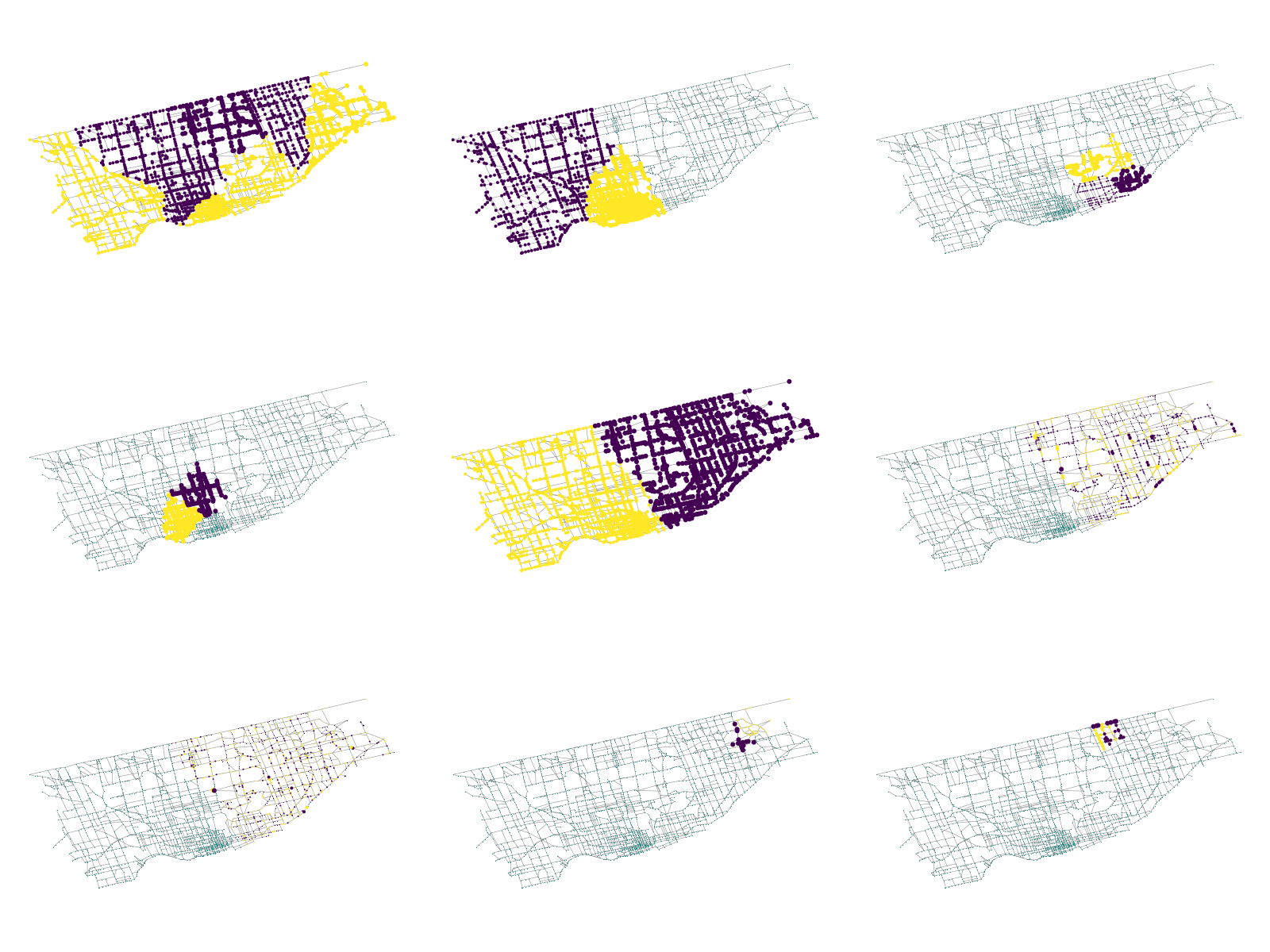
(d) eGHWT

Figure 11: Nine most significant basis vectors of the graph Haar, the GHWT c2f best basis (= the graph Walsh in this case), the GHWT f2c best basis, and the eGHWT best basis. The diameters of the nodes are proportional to the log of the absolute values of the basis vector amplitudes. The basis vector amplitudes within $(-0.001,0.001)$ are mapped to the viridis colormap to emphasize the difference between positive (yellow) and negative (deep violet) components.

These figures clearly demonstrate the superiority of the eGHWT best basis over the graph Haar basis, the graph Walsh basis, and the regular GHWT best bases. The top 9 basis vectors for these bases displayed in Fig. 11 show the characteristics of each basis under consideration. The graph Haar basis vectors are non-oscillatory blocky vectors with positive and negative components at various locations and scales. The graph Walsh basis vectors (= the GHWT c2f best-basis vectors) are all global oscillatory piecewise-constant vectors. The GHWT f2c best-basis vectors and the eGHWT best-basis vectors are similar and can capture the multiscale and multi-frequency features of the input graph signal. Yet, the performance of the eGHWT best basis exceeds that of the GHWT f2c best basis simply because the former can search the best basis among a much larger collection of ONBs than the latter can.

5.2 Viewing a General Matrix Signal as a Tensor Product of Graphs

To analyze and process a single graph signal, we can use the eGHWT to produce a suitable ONB. Then for a collection of signals in a matrix form (including regular digital images), we can also compose the affinity matrix of the rows and that of the columns separately, thus define graphs on which the rows and columns are supported as was done previously COIF-GAVISH ; IRION-SAITO-MLSP16 . Those affinity matrices can be either computed from the similarity of rows or columns directly or can be composed from information outside the original matrix signal. For example, Kalofolias et al. KALOFOLIAS-ETAL used row and column graphs to analyze recommender systems.

After the affinity graphs on rows and columns are obtained, we can use the eGHWT to produce ONBs on rows and columns separately. Then the matrix signal can be analyzed or compressed by the tensor product of those two ONBs. In addition, as mentioned in Sect. 4.5, we have also extended the eGHWT to the tensor product of row and column affinity graphs and search for best 2D ONB on the matrix signal directly. Note that we can also specify or compute the binary partition trees in a non-adaptive manner (e.g., recursively splitting at the middle of each region), typically for signals supported on a regular lattice.

5.2.1 Approximation of the Barbara Image

In this section, we compare the performance of various bases in approximating the famous Barbara image shown in Fig. 12(a), and demonstrate our eGHWT can be applied to a conventional digital image in a straightforward manner, and outperforms the regular GHWT best bases. This image consists of $512\times 512$ pixels, and has been normalized to have its pixel values in $(0,1)$. The partition trees on the rows and columns are specified explicitly: every bipartition is forced at the middle of each region. Therefore, those two trees are perfect binary trees with depth equal to $\log_{2}(512)+1=10$.

Figure 12(b) displays the relative $\ell^{2}$ errors of the approximations by the graph Haar basis, the graph Walsh basis, the GHWT cf2/f2c best bases, and the eGHWT best basis as a function of the fraction of the coefficients retained.

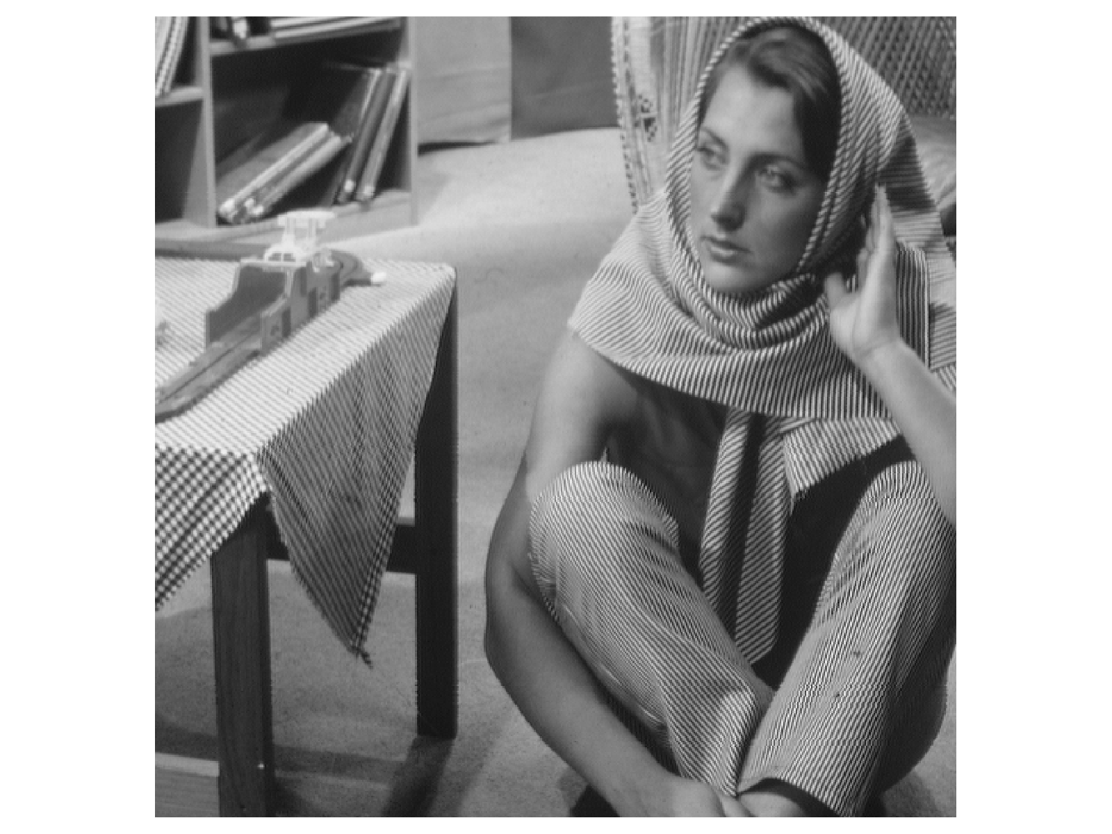
(a) Barbara

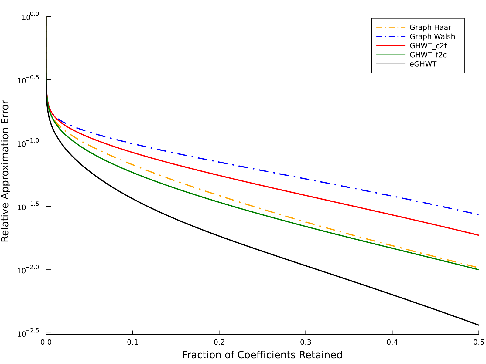
(b) Relative $\ell^{2}$ approximation error

Figure 12: (a) The original Barbara image of size $512\times 512$ pixels; (b) Relative $\ell^{2}$ approximation errors by various graph bases

In order to examine the quality of approximations visually, Fig. 13 displays those approximations using only $1/32=3.125\%$ of the most significant expansion coefficients for each basis. The eGHWT best basis outperforms all the others with least blocky artifacts. To examine the visual quality of these approximations further, Fig. 14 shows the zoomed-up face and left leg of those approximations. Especially for the leg region that has some specific texture, i.e., stripe patterns, the eGHWT outperformed the rest of the methods. The performance is measured by PSNR (peak signal-to-noise ratio). Given an $m\times n$ monochrome image $I$ and its approximation $K$, the PSNR is defined as

$$PSNR =10\log_{10}\frac{(\max_{ij}I_{ij})^{2}}{MSE}$$

$$MSE =\frac{1}{mn}\sum^{m}_{i=1}\sum^{n}_{j=1}(I_{ij}-K_{ij})^{2}$$

(a) Haar, PSNR = 24.50dB

(b) GHWT c2f, PSNR = 23.51dB

(c) GHWT f2c, PSNR = 25.27dB

(d) eGHWT, PSNR = 27.78dB

Figure 13: Approximations of the Barbara image using various bases using only 3.125% of coefficients (online viewing is recommended for the details)

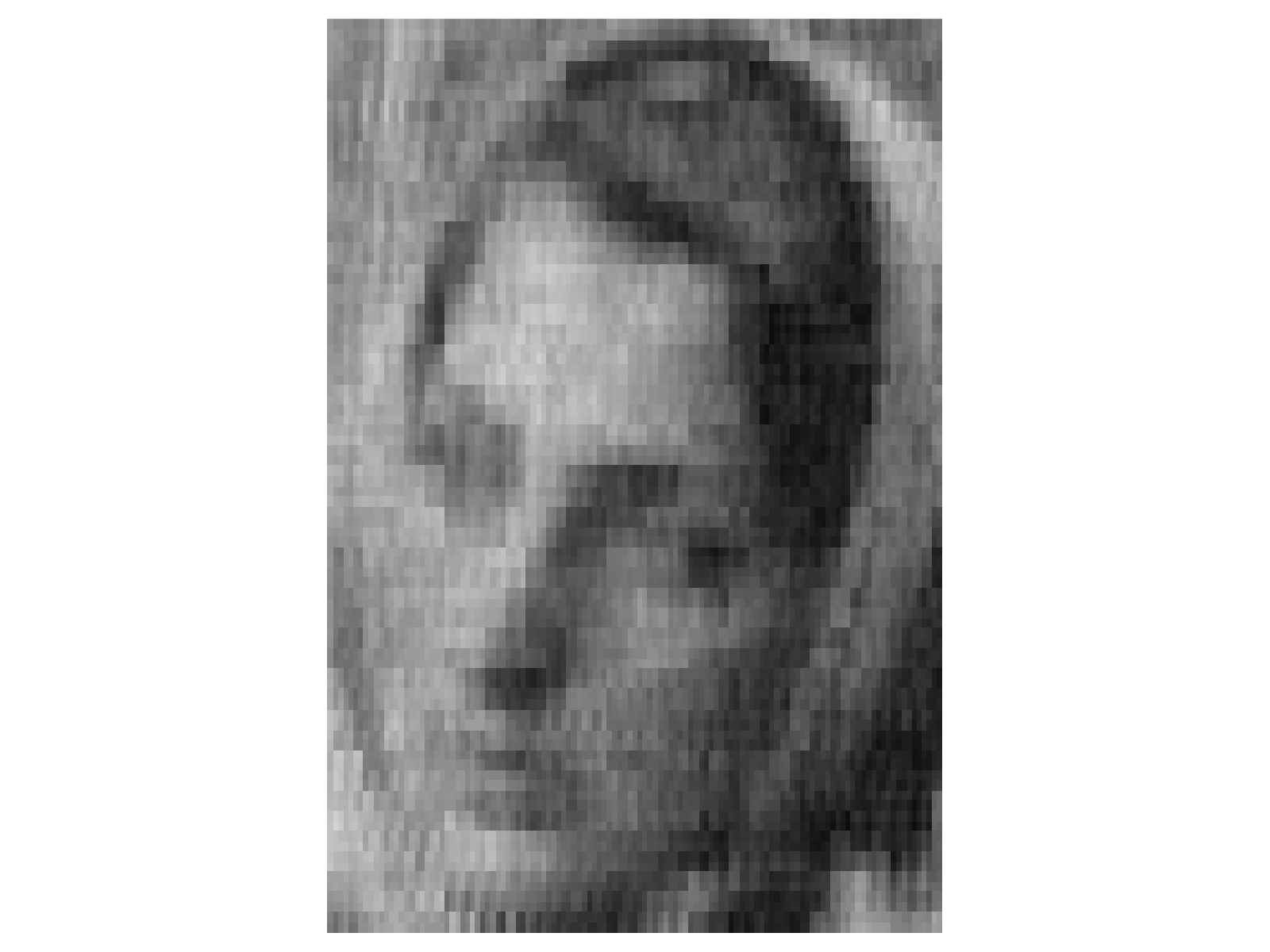
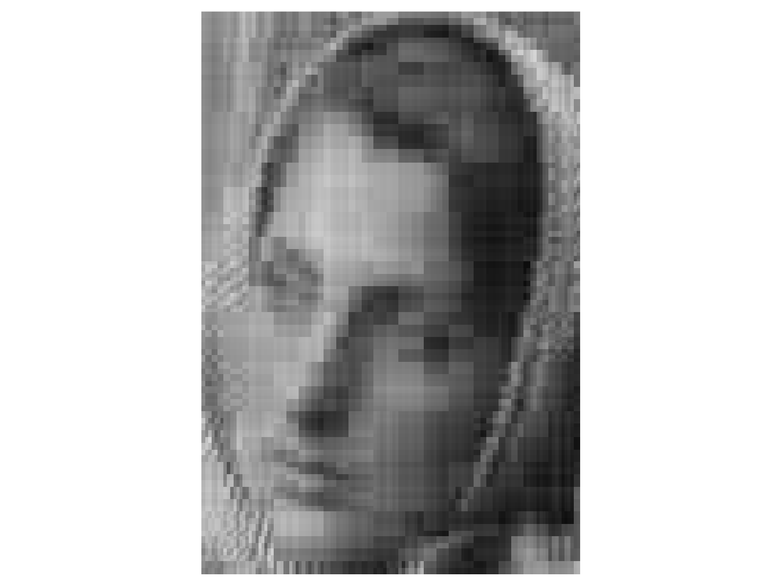
(a) face

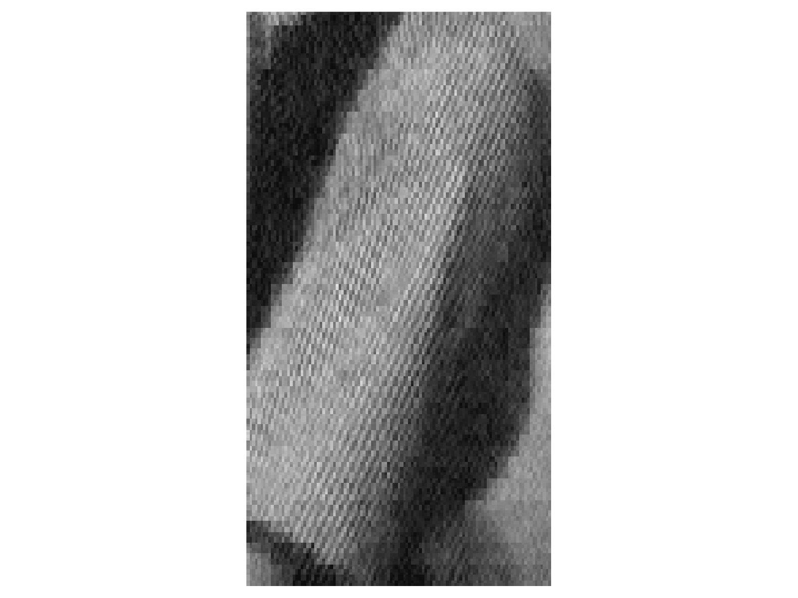
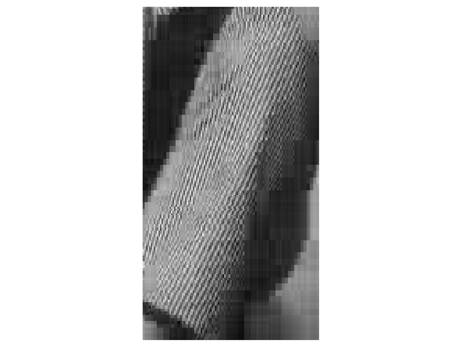
(b) left leg

Figure 14: Zoomed up versions of Fig. 13. Methods used from top left to bottom right are: Haar; GHWT c2f; GHWT f2c; and eGHWT, respectively. Online viewing is recommended for the details.

We note that both this approximation experiment on the Barbara image and that on the vehicular volume count data on the Toronto street network discussed in Sect. 5.1, the order of the performance was the same: eGHWT ¿ GHWT f2c ¿ graph Haar ¿ GHWT c2f $\geq$ graph Walsh. This order in fact makes sense for those input datasets. The eGHWT could simply search much larger ONBs than the GHWT best bases; the graph Haar basis is a part of the GHWT f2c dictionary; and the graph Walsh basis is a part of both the GHWT c2f and f2c dictionaries. The graph Walsh basis for these graph signals was too global while the GHWT c2f best basis tended to select nonlocal features compared to the eGHWT, GHWT f2c, and the graph Haar.

5.2.2 The Haar Transform for Images with Non-Dyadic Size

For images of non-dyadic size, there is no straightforward way to obtain the partition trees in a non-adaptive manner unlike the dyadic Barbara image of $512\times 512$ in the previous subsection. This is a common problem faced by the classical Haar and wavelet transforms as well: they were designed to work for images of dyadic size. Non-dyadic images are often modified by zero padding, even extension at the boundary pixels, or other methods before the Haar transform is applied. We propose to apply the Haar transform on a non-dyadic image without modifying the input image using the eGHWT dictionary.

To obtain the binary partition trees, we need to cut an input image $\bm{I}\in\mathbb{R}^{M\times N}$ horizontally or vertically into two parts recursively. Apart from using the affinity matrices as we did for the vehicular volume count data on the Toronto street network in Section 5.1 and for the term-document matrix analysis in IRION-SAITO-MLSP16 , we propose to use the penalized total variation (PTV) cost to partition a non-dyadic input image. Denote the two sub-parts of $\bm{I}$ as $\bm{I}_{1}$ and $\bm{I}_{2}$. We search for the optimal cut such that

$$\text{Penalized Total Variation Cost}\,:=\,\frac{\|\bm{I}_{1}\|_{\mathrm{TV}}}{|\bm{I}_{1}|^{p}}+\frac{\|\bm{I}_{2}\|_{\mathrm{TV}}}{|\bm{I}_{2}|^{p}}\ (p>0)$$

is minimized, where $\|\bm{I}_{k}\|_{\mathrm{TV}}\,:=\,\sum_{i,j}(|I_{k}[i+1,j]-I_{k}[i,j]|+|I_{k}[i,j+1]-I_{k}[i,j]|)$, and $|\bm{I}_{k}|$ indicates the number of pixels in $\bm{I}_{k}$, $k=1,2$. The denominator is used to make sure that the size of $\bm{I}_{1}$ and that of $\bm{I}_{2}$ are close so that the tree becomes nearly balanced. Recursively applying the horizontal cut on the rows of $\bm{I}$ and the vertical cut on the columns of $\bm{I}$ will give us two binary partition trees. We can then select the 2D Haar basis from the eGHWT dictionary or search for the best basis with minimal cost (note that this cost function for the best-basis search is the $\ell^{1}$-norm of the expansion coefficients, and is different from the PTV cost above).

To demonstrate this strategy, we chose an image patch of size $100\times 100$ around the face part from the original $512\times 512$ Barbara image so that it is non-dyadic. To determine the value of $p$, we need to balance between the total variation and structure of the partition tree. Larger $p$ means less total variation value after split but a more balanced partition tree may be obtained. The value of $p$ can be fine-tuned based on the evaluation of the final task, for example, the area under the curve of the relative approximation error in the compression task IRION-SAITO-TSIPN . In the numerical experiments below, after conducting preliminary partitioning experiments using the PTV cost, we decided to choose $p=3$.

For comparison, we also used the dwt function supplied by the Wavelets.jl package JuliaWavelets for the classical Haar transform. We examined three different scenarios here: 1) directly input the Barbara face image of size $100\times 100$; 2) zero padding to four sides of the original image to make it $128\times 128$; and 3) even reflection at the borders to make it 128 x 128.

Figure 15 shows that the relative $\ell^{2}$-error curves of these five methods. Note that we plotted these curves as a function of the number of coefficients retained instead of the fraction of coefficients retained that were used in Figs. 10(b) and 12(b). This is because the zero-padded version and the even-reflection version have $128$ pixels although the degree of freedom is the same $100\times 100$ throughout the experiments.

Clearly, the graph-based methods, i.e., the graph Haar basis and the eGHWT best basis outperformed the classical Haar transform applied to the three prepared input images. The classical Haar transform applied to the original face image of size $100\times 100$ did perform poorly in the beginning because the dwt function stops the decomposition when the sample (or pixel) size becomes an odd integer. In this case, after two levels of decomposition, it stopped ($100\rightarrow 50\rightarrow 25$). Hence, it did not fully enjoy the usual advantage of deeper decomposition. The classical Haar transform applied to the even-reflected image was the worst performer among these five because the even-reflected image of $128\times 128$ is not periodic. The implementation of the dwt assumes the periodic boundary condition by default, and if it does not generate continuous periodic image, it would generate artificially-large expansion coefficients due to the discontinuous periodic boundary condition; see SAITO-REMY-ACHA ; YAMATANI-SAITO ; SAITO-PLASMA-ENGLISH for further information. We can summarize that our graph-based transforms can handle images of non-dyadic size without any artificial preparations (zero padding and even reflection) with some additional computational expense (the minimization of the PTV cost for recursive partitioning).

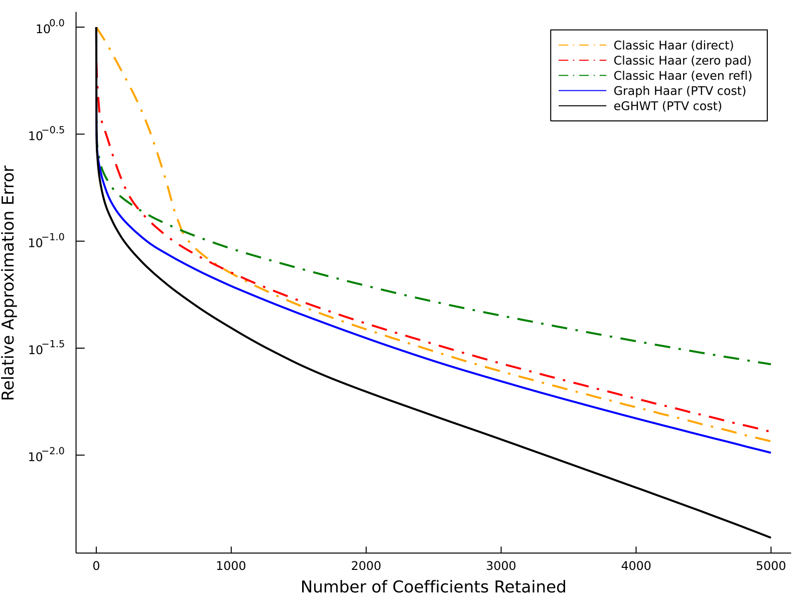
Figure 15: Comparison of approximation performance on the face part (of size $100\times 100$ pixels) of the Barbara image: the classical Haar transform with various setups, the graph Haar basis, and the eGHWT best basis

5.3 Another Way to Construct a Graph from an Image for Efficient Approximation

We can view a digital image of size $M\times N$ as a signal on a graph consisting of $MN$ nodes by viewing each pixel as a node. Note that the underlying graph is not a regular 2D lattice of size $M\times N$. Rather it is a graph reflecting the relationship or affinity between pixels. In other words, $w_{ij}$, the weight of the edge between $i$th and $j$th pixels in that graph should reflect the affinity between local region around these two pixels, and this weight may not be $0$ even if $i$th and $j$th pixels are remotely located. In the classical setting, this idea has been used in image denoising (the so-called bilateral filtering) TOMASI-MANDUCHI and image segmentation SHI-MALIK . On the other hand, Szlam et al. have proposed a more general approach for associating graphs and diffusion processes to datasets and functions on such datasets, which includes the bilateral filtering of TOMASI-MANDUCHI as a special case, and have applied to image denosing and transductive learning. See the review article of Milanfar MILANFAR-IMG-FILTERING for further connections between these classical and modern techniques and much more.

Here we define the edge weight $w_{ij}$ as Szlam et al. SZLAM-MAGG-COIF did:

$$w_{ij}=\exp\left(\frac{-\|\bm{F}[i]-\bm{F}[j]\|^{2}_{2}}{\sigma_{F}}\right)\cdot\begin{cases}\exp\left(\frac{-\|\bm{x}[i]-\bm{x}[j]\|^{2}_{2}}{\sigma_{x}}\right)&\text{if $\|\bm{x}[i]-\bm{x}[j]\|_{2}<r$}\\ 0&\text{otherwise}\end{cases}$$ (3)

where $\bm{x}[i]\in\mathbb{R}^{2}$ is the spatial location (i.e., coordinate) of node (pixel) $i$, and $\bm{F}[i]$ is a feature vector based on intensity, color, or texture information of the local region centered at that node. As one can see in Eq. (3), the pixels located within a disk with center $\bm{x}[i]$ and radius $r$ are considered to be the neighbors of the $i$th pixel. The scale parameters, $\sigma_{F}$ and $\sigma_{x}$ must be chosen appropriately. Once we construct this graph, we can apply the eGHWT in a straightforward manner.

We examine two images here. The first one (Fig. 16(a)) is the subsampled version of the standard ‘cameraman’ image; we subsampled the original cameraman image of size $512\times 512$ to $128\times 128$ in order to reduce computational cost. For the location parameters, we used $r=5$ and $\sigma_{x}=\infty$. Note that $\sigma_{x}=\infty$ means that $w_{i\cdot}$ becomes an indicator/characteristic function of a disk of radius $r$ with center $i$. This setup certainly simplifies our experiments, and could sparsify the weight matrix if $r$ is not too large. On the other hand, the feature vector $\bm{F}[i]$ of the $i$th pixel location, we found that simply choosing raw pixel value as $\bm{F}[i]$ can get good enough results for relatively simple images (e.g., piecewise smooth without too much high frequency textures) like the cameraman image. However, the ‘Gaussian bandwidth’ parameter for the features, $\sigma_{F}$, needs to be tuned more carefully. A possible tuning trick is to start from the median of all possible values of the numerator in the exponential term in Eq. (3), i.e., $-\|\bm{F}[i]-\bm{F}[j]\|^{2}_{2}$ SZLAM-MAGG-COIF , examine several other values around that median, and then choose the value yielding the best result. For more sophisticated approach to tune the Gaussian bandwidth, see LINDENBAUM-ETAL . In this example, we used $\sigma_{F}=0.007$ and $\sigma_{F}=0.07$ after several trials starting from the simple median approach in order to demonstrate the effect of this parameter for the eGHWT best basis.

Figure 16(b) shows our results on the subsampled cameraman image. Figure 16(b) demonstrates that the decay rate of the expansion coefficients w.r.t. the eGHWT best basis is much faster than that of the classical Haar transform. Moreover, the eGHWT best-basis vectors extract some meaningful features of the image. Figure 17 shows the eGHWT best-basis vectors corresponding to the largest nine expansion coefficients in magnitude. We can see that the human part and the camera part are captured by individual basis vectors. Furthermore, in terms of capturing the objects and generating meaningful segmentation, we observe that the results with $\sigma_{F}=0.007$ shown in Fig. 17(a) are better than those with $\sigma_{F}=0.07$ shown in Fig. 17(b). This observation coincides with the better decay rate of the former than that of latter in Fig. 16(b). Therefore, we can conclude that good segmentation (or equivalently, a good affinity matrix setup) is quite important for constructing a basis of good quality and consequently for approximating an input image efficiently.

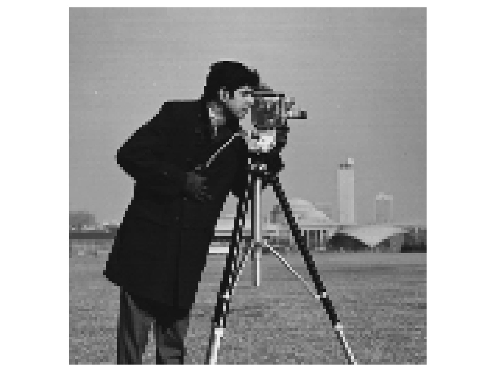
(a) cameraman (subsampled)

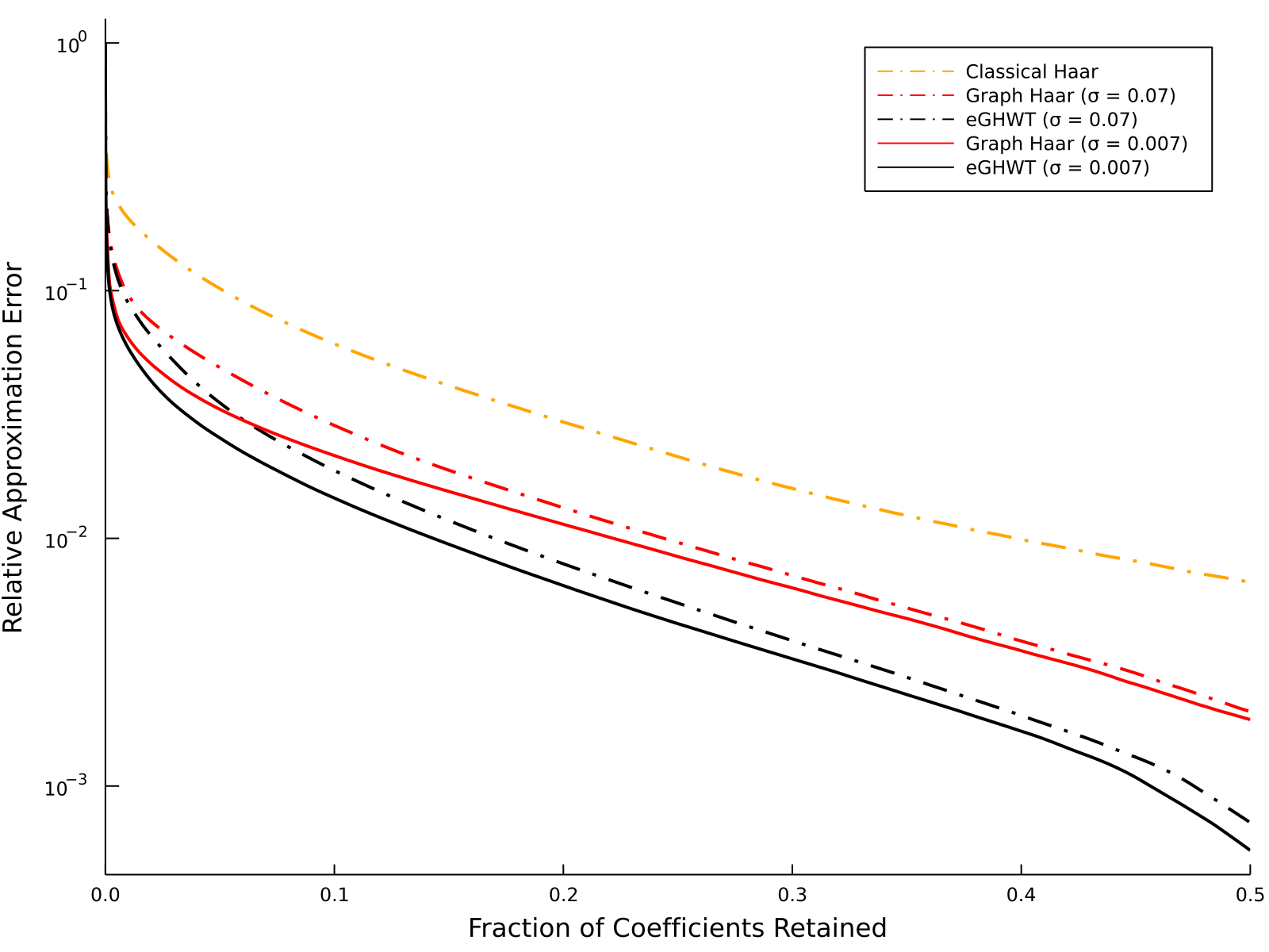
(b) Relative $\ell^{2}$ approximation error

Figure 16: (a) The subsampled cameraman image of size $128\times 128$; (b) Relative $\ell^{2}$ approximation error of (a) using five methods.

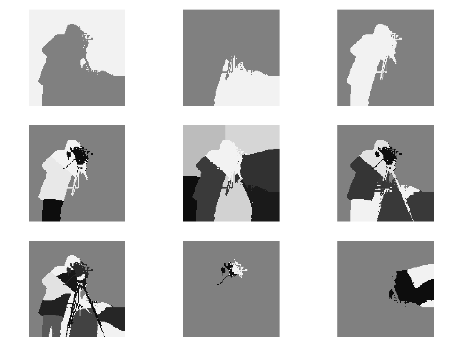
(a) $\sigma_{F}=0.007$

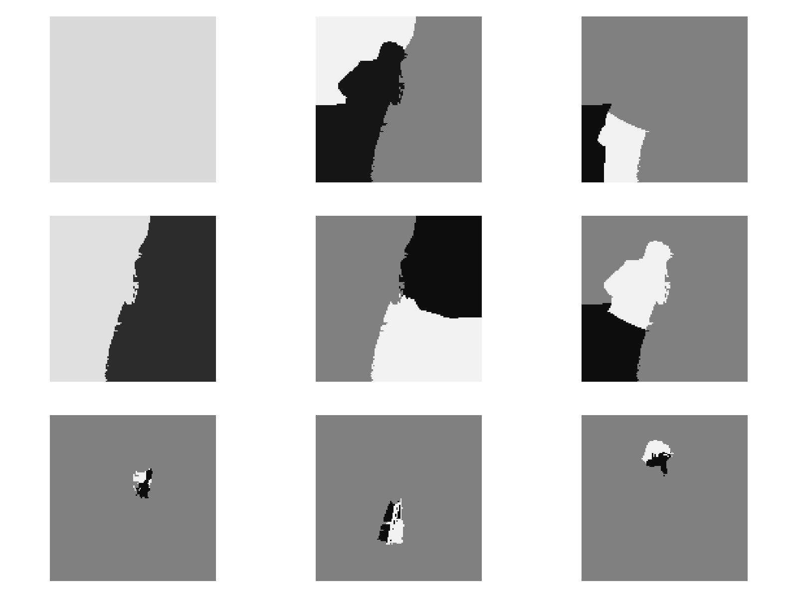
(b) $\sigma_{F}=0.07$

Figure 17: The top nine eGHWT best-basis vectors: (a) $\sigma_{F}=0.007$; (b) $\sigma_{F}=0.07$

Our second example is a composite texture image shown in Fig. 18(a), which was generated and analyzed by Ojala et al. OUTEX . Our method, i.e., applying the eGHWT on an image viewed as a graph, allows us to generate basis vectors with irregular support that is adapted to the structure of the input image as shown in the cameraman example above. This strategy also works well on this composite texture image if we choose the appropriate features in Eq. (3) to generate a good weight matrix. The raw pixel values as the features, which we used for the cameraman example, do not work in this composite texture image, which consists of highly oscillatory anisotropic features. Ideally, we want to use a piecewise constant image delineating each of the five textured regions for the weight matrix computation. To generate such a piecewise constant image (or rather its close approximation), we did the following:

1. Apply a group of (say, $k$) 2D Gabor filters of various frequencies and orientations on the original image of size $M\times N$;

2. Compute the absolute values of each Gabor filtered image to construct a nonnegative vector of length $k$ at each pixel location;

3. Standardize each of these $k$ components so that each component has mean $0$ and variance $1$;

4. Apply Principal Component Analysis (PCA) JOLLIFFE2 on these standardized $MN$ vectors in $\mathbb{R}^{k}$;

5. Extract the first principal component (organized as a single image of the same size as the input image), normalize it to be in the range of $[0,1]$, and use it as features in Eq. (3).

In Step 1, the Gabor filters are used because they are quite efficient to capture high frequency anisotropic features GRIGORESCU-PETKOV-KRUIZINGA . In this particular image, we used four spatial frequencies: $0.2$, $0.3$, $0.4$, and $0.5$ (unit: 1/pixel), and two different orientations: $\pi/3$ and $5\pi/6$, for the Gabor filters. This generated a set of $k=8$ nonnegative matrices in Step 2. We also note that the Gaussian bandwidth or the standard deviation of the Gaussian envelop used in the Gabor filters needs to be tuned appropriately. In our experiments, we used the wavelength-dependent bandwidth, i.e., $\sigma=3/\pi\cdot\sqrt{\ln 2/2}\cdot\lambda$, where $\lambda\in\{0.2,0.3,0.4,0.5\}$, as PETKOV-KRUIZINGA suggests. The normalized first principal component in Step 5 as an image is shown in Fig. 18(b). The pixel values of this ‘mask’ image are used as (scalar) features $\bm{F}[i]$ in Eq. (3). Note that this mask computation was done on the original $512\times 512$ image, which was subsequently subsampled to have $128$ pixels to match the subsampled original image. As for the Gaussian bandwidth, $\sigma_{F}$, in Eq. (3), we set $\sigma_{F}=0.0005$ after several trials. The other parameters, $(r,\sigma_{x})$, were set as $(3,\infty)$. Figure 19(a) compares the performance of five different methods in approximating the composite texture image shown in Fig. 18(a). The order of approximation performance is the same as the previous examples, i.e., the vehicular volume counts on the Toronto street network in Fig. 10(b) and the Barbara image using the predefined dyadic partitions in Fig. 12(b): eGHWT ¿ GHWT f2c ¿ graph Haar ¿ GHWT c2f = graph Walsh. Figure 19(b) displays the top nine eGHWT best-basis vectors. We can see that the support of these basis vectors approximately coincide with the five sections of the composite texture image, and some of the basis vectors, particularly the fourth and eighth ones, exhibit the oscillatory anisotropic features.

(a) Subsampled Original

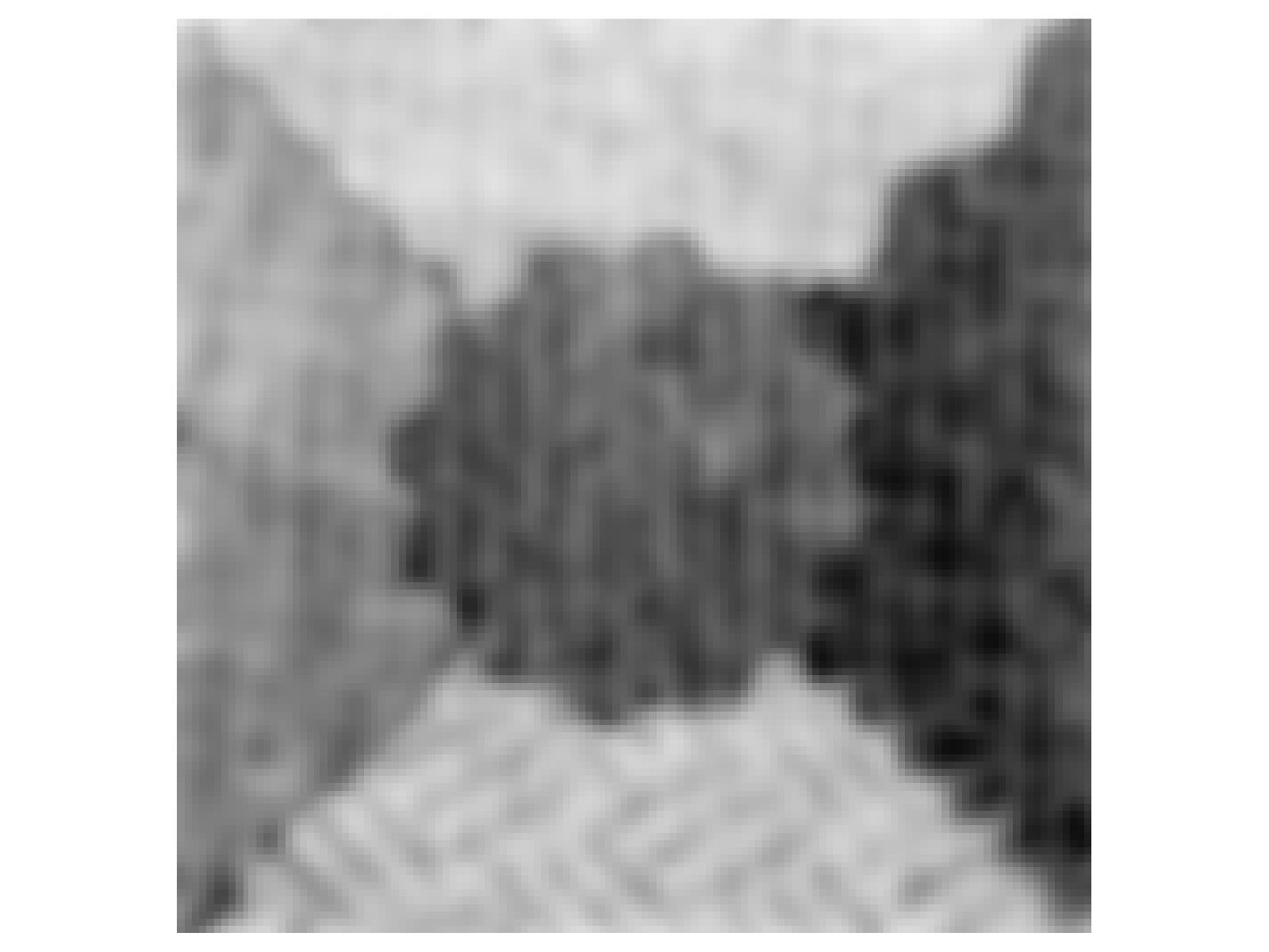
(b) Mask from Gabor + PCA

Figure 18: (a) A composite texture image of size $128\times 128$ after subsampling the original image of size $512\times 512$; (b) Mask image computed from PCA of 8 Gabor filtered images followed by subsampling to $128\times 128$ pixels

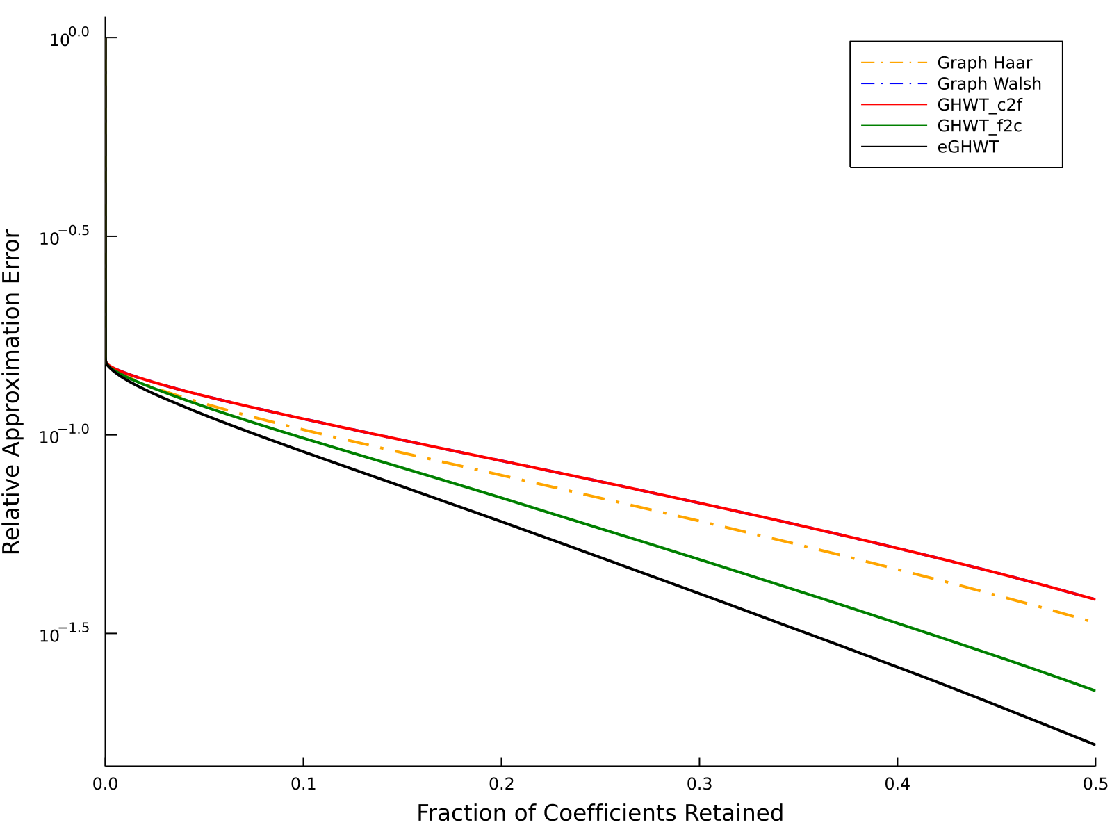
(a) Relative $\ell^{2}$ approximation error

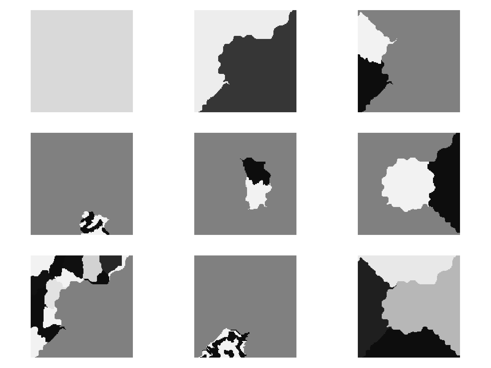
(b) Top 9 eGHWT best-basis vectors

Figure 19: (a) Relative $\ell^{2}$ approximation error of Fig. 18(a) using five methods; (b) Top 9 eGHWT best-basis vectors

6 Discussion

In this article, we have introduced the extended Generalized Haar-Walsh Transform (eGHWT). After briefly reviewing the previous Generalized Haar-Walsh Transform (GHWT), we have described how the GHWT can be improved with the new best-basis algorithm, which is the generalization of the Thiele-Villemoes algorithm THIELE-VILLEMOES for the graph setting. We refer to this whole procedure of developing the extended Haar-Walsh wavelet packet dictionary on a graph and selecting the best basis from it as the eGHWT. Moreover, we have developed the 2D eGHWT for matrix signals by viewing them as tensor products of two graphs, which is a generalization of the Lindberg-Villemoes algorithm LINDBERG-VILLEMOES for the graph setting.

We then showcased some applications of the eGHWT. When analyzing graph signals, we demonstrated the improvement over the GHWT on synthetic and real data. For the simple synthetic 6-node signal, we showed that the best basis from the eGHWT can be selected by neither the GHWT c2f dictionary nor the GHWT f2c dictionary and it had the smaller cost than the GHWT c2f/f2c best bases could provide. On the vehicular volume data on the Toronto street network, the eGHWT had the best approximation performance among the methods we considered. Then we proceeded to the applications to image approximation. After demonstrated the superiority of the eGHWT combined with the predetermined recursive partitioning on the original Barbara image of dyadic size, we proposed the use of the data adaptive recursive partitioning using the penalized total variation for images of non-dyadic size, and again showed the superiority of the eGHWT and the graph Haar transform over the classical Haar transform applied to the preprocessed versions of a non-dyadic input image. Finally, we demonstrated that the eGHWT could be applied to a graph generated from an input image by carefully choosing the edge weights that encode the similarity between pixels and their local neighbors, to get not only superior approximation performance but also meaningful and interpretable basis vectors that have non-rectangular supports and can extract certain features and attributes of an input image.

The eGHWT basis dictionary is constructed upon the binary partition tree (or a tensor product of binary partition trees in the case of 2D signals). Currently, we use the Fiedler vectors of random-walk-normalized Laplacian matrices to form the binary partition tree. However, as we have mentioned earlier, our method is so flexible that any graph cut method or general clustering method can be used, as long as the binary partition tree is formed.

If one is interested in compressing a given graph signal instead of simply approximating it, where the encoding bitrate becomes an important issue, the eGHWT should be still useful and efficient. There is no need to transmit the eGHWT best-basis vectors. If both the sender and the receiver have the eGHWT algorithm, then the only information the sender needs to transmit is: 1) the input graph structure via its adjacency matrix (which is often quite sparse and efficiently compressible); 2) the graph partitioning information to reproduce the hierarchical bipartition tree of the input graph; 3) the indices of the eGHWT best basis within this tree; and 4) the retained coefficients (after appropriate quantization) and their indices within the eGHWT best basis.

Another major contribution of our work is the software package we have developed. Based on the MTSG toolbox written in MATLAB®  by Jeff Irion MTSG , we have developed the MultiscaleGraphSignalTransforms.jl package MultiscaleGraphSignalTransforms written entirely in the Julia programming language JULIA , which includes the new eGHWT implementation for 1D and 2D signals as well as the natural graph wavelet packet dictionaries that our group has recently developed CLONINGER-LI-SAITO . We hope that interested readers will download the software themselves, and conduct their own experiments with it:
https://github.com/UCD4IDS/MultiscaleGraphSignalTransforms.jl.

The readers might feel that the graphs we have used in this article are rather restrictive: we have only used 2D irregular grids (i.e., the Toronto street map) and 2D lattices (i.e., the standard digital images). However, we want to note that applying the eGHWT to more general graphs (e.g., social network graphs, etc.) is quite straightforward, and no algorithmic modification is necessary as long as an input graph is simple, connected, and undirected. As we have discussed earlier, the performance of the eGHWT for even such general graphs is always superior to that of the GHWT, the graph Haar basis, and the graph Walsh basis. We strongly encourage interested readers to try out our software package described above for such general graph signals.

There remains a lot of related projects to be done. The most urgent one is to implement the version of the eGHWT that can handle multiple graph signals (on a given fixed graph). In the classical setting, Wickerhauser proposed the so-called Joint Best Basis (JBB) algorithm (WICK-WPK, , Sect. 11.2) while Saito proposed the so-called Least Statistically-Dependent Basis (LSDB) algorithm SAITO-LSDB3 , which correspond to the fast and approximate version of the PCA and the ICA, respectively. Moreover, our group has also developed the Local Discriminant Basis (LDB) algorithm that can extract distinguishing local features for signal classification problems SAITO-COIF-JMIV ; SAITO-COIF-GESHWIND-WARNER . We have already implemented the HGLET and the GHWT that can handle multiple graph signals and that can compute the JBB, the LSDB, and the LDB. Hence, making that version of the eGHWT is relatively straightforward, and we plan to do so very soon.

Another important project, which we are currently pursuing, is to use an appropriate subset of the scaling vectors in the eGHWT dictionary for estimating good initialization to start the Nonnegative Matrix Factorization (NMF) algorithms that are of iterative nature; see, e.g., NMF-BOOK .

Finally, as a long-term research project, we plan to extend the GHWT and eGHWT beyond matrix-form data, i.e., to tensorial data (see, e.g., QI-LUO ), which seems quite promising and worth trying.

We plan to report our investigation and results on these projects at a later date.

- (1) Bezanson, J., Edelman, A., Karpinski, S., Shah, V.B.: Julia: A fresh approach to numerical computing. SIAM Review 59(1), 65–98 (2017). URL https://doi.org/10.1137/141000671
- (2) Bremer, J.C., Coifman, R.R., Maggioni, M., Szlam, A.: Diffusion wavelet packets. Appl. Comput. Harmon. Anal. 21(1), 95–112 (2006). URL https://doi.org/10.1016/j.acha.2006.04.005
- (3) Chung, F., Lu, L.: Complex Graphs and Networks. No. 107 in CBMS Regional Conference Series in Mathematics. Amer. Math. Soc., Providence, RI (2006). URL https://doi.org/10.1090/cbms/107
- (4) Cloninger, A., Li, H., Saito, N.: Natural graph wavelet packet dictionaries. J. Fourier Anal. Appl. 27, Article #41 (2021). URL https://doi.org/10.1007/s00041-021-09832-3. A part of “Topical Collection: Harmonic Analysis on Combinatorial Graphs”
- (5) Coifman, R.R., Gavish, M.: Harmonic analysis of digital data bases. In: J. Cohen, A.I. Zayed (eds.) Wavelets and Multiscale Analysis: Theory and Applications, Applied and Numerical Harmonic Analysis, pp. 161–197. Birkhäuser, Boston, MA (2011). URL https://doi.org/10.1007/978-0-8176-8095-4_9
- (6) Coifman, R.R., Maggioni, M.: Diffusion wavelets. Appl. Comput. Harmon. Anal. 21(1), 53–94 (2006). URL https://doi.org/10.1016/j.acha.2006.04.004
- (7) Coifman, R.R., Wickerhauser, M.V.: Entropy-based algorithms for best basis selection. IEEE Trans. Inform. Theory 38(2), 713–718 (1992). URL https://doi.org/10.1109/18.119732
- (8) Easley, D., Kleinberg, J.: Networks, Crowds, and Markets: Reasoning and a Highly Connected World. Cambridge Univ. Press, New York (2010)
- (9) Fiedler, M.: A property of eigenvectors of nonnegative symmetric matrices and its application to graph theory. Czechoslovak Math. J. 25, 619–633 (1975). URL http://eudml.org/doc/12900
- (10) Grigorescu, S.E., Petkov, N., Kruizinga, P.: Comparison of texture features based on Gabor filters. IEEE Trans. Image Process. 11(10), 1160–1167 (2002). URL https://doi.org/10.1109/TIP.2002.804262
- (11) Hagen, L., Kahng, A.B.: New spectral methods for ratio cut partitioning and clustering. IEEE Trans. Comput.-Aided Des. 11(9), 1074–1085 (1992). URL https://doi.org/10.1109/43.159993
- (12) Hammond, D.K., Vandergheynst, P., Gribonval, R.: Wavelets on graphs via spectral graph theory. Appl. Comput. Harmon. Anal. 30(2), 129–150 (2011). URL https://doi.org/10.1016/j.acha.2010.04.005
- (13) Irion, J., Li, H., Saito, N., Shao, Y.: Multiscalegraphsignaltransforms.jl. https://github.com/UCD4IDS/MultiscaleGraphSignalTransforms.jl (2021)
- (14) Irion, J., Saito, N.: The generalized Haar-Walsh transform. In: Proc. 2014 IEEE Workshop on Statistical Signal Processing, pp. 472–475 (2014). URL https://doi.org/10.1109/SSP.2014.6884678
- (15) Irion, J., Saito, N.: Applied and computational harmonic analysis on graphs and networks. In: M. Papadakis, V.K. Goyal, D. Van De Ville (eds.) Wavelets and Sparsity XVI, Proc. SPIE 9597 (2015). URL https://doi.org/10.1117/12.2186921. Paper # 95971F
- (16) Irion, J., Saito, N.: MTSG_Toolbox. https://github.com/JeffLIrion//MTSG_Toolbox (2015)
- (17) Irion, J., Saito, N.: Learning sparsity and structure of matrices with multiscale graph basis dictionaries. In: A. Uncini, K. Diamantaras, F.A.N. Palmieri, J. Larsen (eds.) Proc. 2016 IEEE 26th International Workshop on Machine Learning for Signal Processing (MLSP) (2016). URL https://doi.org/10.1109/MLSP.2016.7738892
- (18) Irion, J., Saito, N.: Efficient approximation and denoising of graph signals using the multiscale basis dictionaries. IEEE Trans. Signal Inform. Process. Netw. 3(3), 607–616 (2017). URL https://doi.org/10.1109/TSIPN.2016.2632039
- (19) Jansen, M., Nason, G.P., Silverman, B.W.: Multiscale methods for data on graphs and irregular multidimensional situations. J. R. Stat. Soc. Ser. B, Stat. Methodol. 71(1), 97–125 (2008). URL https://doi.org/10.1111/j.1467-9868.2008.00672.x
- (20) Jolliffe, I.T.: Principal Component Analysis and Factor Analysis, 2nd edn., chap. 7. Springer New York, New York, NY (2002). URL https://doi.org/10.1007/b98835
- (21) Kalofolias, V., Bresson, X., Bronstein, M., Vandergheynst, P.: Matrix completion on graphs. In: Neural Information Processing Systems workshop “Out of the Box: Robustness in High Dimension” (2014). URL https://arxiv.org/abs/1408.1717
- (22) Lee, A., Nadler, B., Wasserman, L.: Treelets—an adaptive multi-scale basis for sparse unordered data. Ann. Appl. Stat. 2, 435–471 (2008). URL https://doi.org/10.1214/07-AOAS137
- (23) Lindberg, M., Villemoes, L.F.: Image compression with adaptive Haar-Walsh tilings. In: A. Aldroubi, A.F. Laine, M.A. Unser (eds.) Wavelet Applications in Signal and Image Processing VIII, Proc. SPIE 4119, pp. 911–921 (2000). URL https://doi.org/10.1117/12.408575
- (24) Lindenbaum, O., Salhov, M., Yeredor, A., Averbuch, A.: Gaussian bandwidth selection for manifold learning and classification. Data Min. Knowl. Discov. 34, 1676–1712 (2020). DOI 10.1007/s10618-020-00692-x. URL https://doi.org/10.1007/s10618-020-00692-x
- (25) Lovász, L.: Large Networks and Graph Limits, Colloquium Publications, vol. 60. Amer. Math. Soc., Providence, RI (2012)
- (26) von Luxburg, U.: A tutorial on spectral clustering. Stat. Comput. 17(4), 395–416 (2007). URL https://doi.org/10.1007/s11222-007-9033-z
- (27) Milanfar, P.: A tour of modern image filtering: New insights and methods, both practical and theoretical. IEEE Signal Processing Magazine 30(1), 106–128 (2013). URL https://doi.org/10.1109/MSP.2011.2179329
- (28) Murtagh, F.: The Haar wavelet transform of a dendrogram. J. Classification 24(1), 3–32 (2007). URL https://doi.org/10.1007/s00357-007-0007-9
- (29) Naik, G.R. (ed.): Non-negative Matrix Factorization Techniques: Advances in Theory and Applications. Springer (2016). URL https://doi.org/10.1007/978-3-662-48331-2
- (30) Newman, M.: Networks, 2nd edn. Oxford Univ. Press (2018)
- (31) Ojala, T., Maenpää, T., Pietikäinen, M., Viertola, J., Kylönen, J., Huovinen, S.: Outex - new framework for empirical evaluation of texture analysis algorithms. In: Proceedings of 16th International Conf. on Pattern Recognition, vol. 1, pp. 701–706 (2002). URL https://doi.org/10.1109/ICPR.2002.1044854
- (32) Ortega, A., Frossard, P., J.Kovačević, Moura, J.M.F., Vandergheynst, P.: Graph signal processing: Overview, challenges, and applications. Proc. IEEE 106(5), 808–828 (2018). URL https://doi.org/10.1109/JPROC.2018.2820126
- (33) Petkov, N., Kruizinga, P.: Computational models of visual neurons specialised in the detection of periodic and aperiodic oriented visual stimuli: bar and grating cells. Biological Cybernetics (1997). URL https://doi.org/10.1007/s004220050323
- (34) Qi, L., Luo, Z.: Tensor Analysis: Spectral Theory and Special Tensors. SIAM, Philadelphia, PA (2019). URL https://doi.org/10.1137/1.9781611974751
- (35) Rudis, B., Ross, N., Garnier, S.: The viridis color palettes. https://cran.r-project.org/web/packages/viridis/vignettes/intro-to-viridis.html (2018)
- (36) Rustamov, R.M.: Average interpolating wavelets on point clouds and graphs. arXiv:1110.2227 [math.FA] (2011)
- (37) Saito, N.: Image approximation and modeling via least statistically dependent bases. Pattern Recognition 34, 1765–1784 (2001)
- (38) Saito, N.: Laplacian eigenfunctions and their application to image data analysis. J. Plasma Fusion Res. 92(12), 904–911 (2016). URL http://www.jspf.or.jp/Journal/PDF_JSPF/jspf2016_12/jspf2016_12-904.pdf. In Japanese
- (39) Saito, N., Coifman, R.R.: Local discriminant bases and their applications. J. Math. Imaging Vis. 5(4), 337–358 (1995). Invited paper
- (40) Saito, N., Coifman, R.R.: Extraction of geological information from acoustic well-logging waveforms using time-frequency wavelets. Geophysics 62(6), 1921–1930 (1997). URL https://doi.org/10.1190/1.1444292
- (41) Saito, N., Coifman, R.R., Geshwind, F.B., Warner, F.: Discriminant feature extraction using empirical probability density estimation and a local basis library. Pattern Recognition 35(12), 2841–2852 (2002)
- (42) Saito, N., Remy, J.F.: The polyharmonic local sine transform: A new tool for local image analysis and synthesis without edge effect. Appl. Comput. Harmon. Anal. 20(1), 41–73 (2006). URL https://doi.org/10.1016/j.acha.2005.01.005
- (43) Shao, Y., Saito, N.: The extended generalized Haar-Walsh transform and applications. In: D. Van De Ville, M. Papadakis, Y.M. Lu (eds.) Wavelets and Sparsity XVIII, Proc. SPIE 11138 (2019). URL https://doi.org/10.1117/12.2528923. Paper #111380C
- (44) Shi, J., Malik, J.: Normalized cuts and image segmentation. IEEE Trans. Pattern Anal. Machine Intell. 22(8), 888–905 (2000). URL https://doi.org/10.1109/34.868688
- (45) Shuman, D.I., Narang, S.K., Frossard, P., Ortega, A., Vandergheynst, P.: The emerging field of signal processing on graphs. IEEE Signal Processing Magazine 30(3), 83–98 (2013). URL https://doi.org/10.1109/MSP.2012.2235192
- (46) Szlam, A.D., Maggioni, M., Coifman, R.R.: Regularization on graphs with function-adapted diffusion processes. Journal of Machine Learning Research 9(55), 1711–1739 (2008). URL http://jmlr.org/papers/v9/szlam08a.html
- (47) Szlam, A.D., Maggioni, M., Coifman, R.R., Bremer Jr., J.C.: Diffusion-driven multiscale analysis on manifolds and graphs: top-down and bottom-up constructions. In: M. Papadakis, A.F. Laine, M.A. Unser (eds.) Wavelets XI, Proc. SPIE 5914 (2005). URL https://doi.org/10.1117/12.616931. Paper # 59141D
- (48) The Julia DSP Team: Wavelets.jl. https://github.com/JuliaDSP/Wavelets.jl (2021)
- (49) Thiele, C.M., Villemoes, L.F.: A fast algorithm for adapted time-frequency tilings. Appl. Comput. Harmon. Anal. 3(2), 91–99 (1996). URL https://doi.org/10.1006/acha.1996.0009
- (50) Tomasi, C., Manduchi, R.: Bilateral filtering for gray and color images. In: Sixth International Conference on Computer Vision (IEEE Cat. No.98CH36271), pp. 839–846 (1998). URL https://doi.org/10.1109/ICCV.1998.710815
- (51) Tremblay, N., Borgnat, P.: Subgraph-based filterbanks for graph signals. IEEE Trans. Signal Process. 64(15), 3827–3840 (2016). URL https://doi.org/10.1109/TSP.2016.2544747
- (52) Wickerhauser, M.V.: Adapted Wavelet Analysis from Theory to Software. A K Peters, Ltd., Wellesley, MA (1994)
- (53) Yamatani, K., Saito, N.: Improvement of DCT-based compression algorithms using Poisson’s equation. IEEE Trans. Image Process. 15(12), 3672–3689 (2006). URL https://doi.org/10.1109/TIP.2006.882005