Detect and Defense Against Adversarial Examples in Deep Learning using Natural Scene Statistics and Adaptive Denoising

Abstract

Despite the enormous performance of deep neural networks, recent studies have shown their vulnerability to adversarial examples, i.e., carefully perturbed inputs designed to fool the targeted DNN. Currently, the literature is rich with many effective attacks to craft such AEs. Meanwhile, many defenses strategies have been developed to mitigate this vulnerability. However, these latter showed their effectiveness against specific attacks and does not generalize well to different attacks. In this paper, we propose a framework for defending DNN classifier against adversarial samples. The proposed method is based on a two-stage framework involving a separate detector and a denoising block. The detector aims to detect AEs by characterizing them through the use of natural scene statistic (NSS), where we demonstrate that these statistical features are altered by the presence of adversarial perturbations. The denoiser is based on block matching 3D (BM3D) filter fed by an optimum threshold value estimated by a convolutional neural network (CNN) to project back the samples detected as AEs into their data manifold. We conducted a complete evaluation on three standard datasets namely MNIST, CIFAR-10 and Tiny-ImageNet. The experimental results show that the proposed defense method outperforms the state-of-the-art defense techniques by improving the robustnessagainst a set of attacks under black-box, gray-box and white-box settings. The source code is available at: https://github.com/kherchouche-anouar/2DAE

1 Introduction

With the availability of large datasets deng2009imagenet ; lin2014microsoft in addition to the increase in computational power, the deep neural networks (DNNs) have shown an outstanding performance in different tasks, such as image classification B0000 ; lecun1998gradient , natural language processing B33333 ; cho2014learning , object detection ren2015faster and speech recognition hinton2012deep . Despite their widespread use and phenomenal success, these networks have shown that they are vulnerable to adversarial attacks. Szegedy et al. illustrated in szegedy2013intriguing that small and almost imperceptible perturbations added to a legitimate input image can easily fool the DNNs models and can make a misclassification with high confidence. The perturbed images are called AEs.

These adversarial attacks raise an important issue of the robustness of DNNs against these attacks, which limits their use and can be an obstacle to deploy them in sensitive applications such as self-driving cars, healthcare, video surveillance, etc. For instance, in Figure 1, the initially clean input image is classified correctly as a stop sign by the DNN model with high confidence. When carefully crafted perturbations are added to the input image, this leads it misclassified as a 120km/hr, which is significantly dangerous and can cause fatal consequences. Therefore, it is of paramount importance to improve the robustness of DNNs models, especially, if they are deployed in such critical applications.

Overall, unlike usual training, where the aim is to minimize the loss of DNN classifier, an attacker tries to carefully craft an adversarial sample $x^{\prime}$ by maximizing the loss with a small amount and thereby produce incorrect output. In other words, the attack tries to find the shortest adversarial direction $\Delta$ to inject the benign sample $x$ from its manifold into another one in order to mislead the DNN model (see Figure 2).

Various attacks are effective to generate an image-dependent AEs B16 , which limits its transferability to other images or models. Other methods moosavi2017universal found some kind of universal perturbations that can fool a target classifier using any clean image. As shown in athalye2018synthesizing , it is also possible in the physical world to add 3D adversarial objects that can attack a DNN model, thus creating a real security risk.

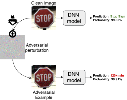
Figure 1: An example of adversarial attack in the context of street sign recognition. The introduction of a small imperceptible perturbation in the input image fools the DNN classifier. The original image is classified as a Stop Sign with 99.85% confidence, while the adversarial example is classified as a 120km/hr with 99.91% confidence.

Consequently, several defense methods have been proposed attempting to correctly classify AEs andthereby increasing model’s robustness. A defensemethod aims to project the malicious sample $x^{\prime}$ into it’s data manifold to make the predicted label the same as the original sample $x$. Adversarial training madry2017towards ; xie2019feature ; carlini2018ground ; kurakin2016adversarial ; lee2017generative is the most adopted technique that attempts to enhance the robustness against these vulnerabilities by integrating AEs to the clean ones into the training phase. However, such defense strategies do not generalize well against new/unknown attack models. Other defense methods try to reconstruct the AEs back to the training distribution by applying transformation on them. One of this approach consists to preprocess the AEs before feeding them to the DNN model. For instance, denoising auto-encoders has been proposed in gu2014towards ; bakhti2019ddsa to remove/attenuate the perturbations. Similar approaches have been proposed based on generative models oord2016pixel . These methods provided substantial results, however, systematically denoising each input image, can negatively impact the performance of clean images. Because, the denoiser can introduce blur if the denoising is incorrectly applied, which reduces the classification performance hendrycks2018benchmarking . One of the possible solutions is to couple a defense strategy with a detection method as realized in the proposed work. Another limitation, generally these denoising-based approaches apply the denoising with a fixed non-adaptive strength, which is not optimal since certain adversarial perturbations are not distributed uniformly.

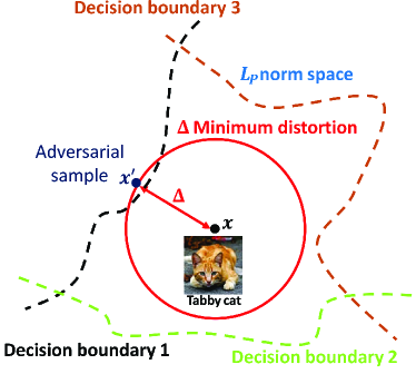
Figure 2: Data distribution over the manifold. We restrict the manifold of benign samples $x$ between decision boundaries (the true class), the attacked sample $x^{\prime}$ is injected out from its data manifold by a minimum $L_{p}$ norm based distance $\Delta$.

Almost all existing defense methods are effective against some specific attacks, but fail to defend new or more powerful ones, especially, when the attacker knows the details of defense mechanism B16 ; B24 ; B29 . Therefore, many recent works have focused on detecting AEs B24 ; B29 ; B25 ; B8 ; B9 ; B15 ; B22 ; B23 ; B26 ; B27 ; lu2017safetynet instead. The detection of AEs may be useful to warn users or to take security measures in order to avoid tragedies. Furthermore, for online machine learning service providers, the detection can be exploited to identify malicious clients and reject their inputs B25 . However, as shown in B29 , the existing AEs detection methods reported high detection accuracy, but have also obtained high false positive rate, meaning that they reject a significant amount of clean images, which can be considered a failure of these detection approaches.

In this paper, we propose a novel approach for defending against AEs, which is classifier-agnostic, i.e., it is designed in such a way that can be used with any classifier without any changes. Our method is two-stage framework comprising a separate detector network and a denoiser block, where the sample detected as adversarial is fed to the denoiser network in order to denoise it. However, for the ones that are detected as clean, they are fed directly to the classifier model. The detector is based on NSS, where we rely on the assumption that the presence of adversarial perturbations alters some statistical properties of natural images. Thus, quantifying these statistical outliers, i.e., deviations from the regularity, using scene statistics enables the building of a binary classifier capable of classifying a given image as legitimate or adversarial. For the denoiser, we used the BM3D filter in order to clean up the attacked image from the adversarial perturbation. BM3D is one of the best denoiser algorithm allowing to tackle non-uniform adversarial perturbations. In addition, we built a CNN model that predicts the adequate strength of denoising, i.e., the parameters filter values, which best mitigate AEs. The experimental results showed that the proposed detection method achieves high detection accuracy, while providing a low false positive rate. In addition, the obtained results showed that the proposed defense method outperforms the state-of-the-art defense techniques under the strongest black-box, gray-box and white-box attacks on three datasets namely MNIST, CIFAR-10 and Tiny-ImageNet.

The rest of this paper is organized as follows: Section 2 reviews some attack techniques and defense methods that have been proposed in the literature. Section 3 describes the proposed approach. The experimental results are presented and analyzed in Section 4. Finally, Section 5 concludes the paper. Table 1 summarizes most of the notations used in this paper.

Table 1: Notations used in the paper.

Notations Description $\xi$ Image space. $I$ Input image. $H\times W\times C$ Height, width, channels of an image. $x$ An instance of clean image. $x^{\prime}$ A modified instance of $x$, adversarial image. $\tilde{x}$ A filtered instance of $x^{\prime}$, denoised image. $c$ The true class label of an input instance $x$. $f_{\theta}(x)$ Output of a classifier model $f$ parameterized by $\theta$, refers specifically to the predicted likelihood for class $c$. $d(x,x^{\prime})$ Distance metric between $x$ and $x^{\prime}$. $\parallel\cdot\parallel_{p}$ $L_{p}$ norm. $\nabla_{x}$ Derivative with respect to $x$ (gradient). $\mathcal{L}$ Loss function. $\mathcal{D}$ Our detector block. $\mathcal{S}$ Our denoiser block. $\widehat{I}$ The mean subtracted contrast normalized (MSCN) coefficients of image $I$. $\beta$ The shape parameter. $\sigma^{2}$ The variance of a probability density function. $\eta$ The Mean of the AGGD. $\tau_{3D}$ 3D linear transform. $\lambda_{3D}$ Threshold parameter of BM3D filter. $f_{X}(x)$ Probability density function.

2 Related work

Adversarial examples are first introduced in this section, then different adversarial attacks are presented, and finally the state-of-the-art defense techniques are described.

2.1 Adversarial examples

Given an image space $\xi=[0,1]^{H\times W\times C}$, a target classification model $f_{\theta}(\cdot)$ and a legitimate input image $x\in\xi$, an adversarial example is a perturbed image $x^{\prime}\in\xi$ such that $f(x^{\prime})\neq f(x)$ and $d(x,x^{\prime})\leq\epsilon$, where $\epsilon\geq 0$. $d$ is a distance metric used to measure the similarity between the perturbed and clean (unperturbed) input images subQomex . Three metrics are commonly used in the literature for generating AEs relying on $L_{p}$ norms, mainly $L_{0}$ distance, the Euclidean distance ($L_{2}$) and the Chebyshev distance ($L_{\infty}$ norm) B16 .

2.2 Adversarial Attacks

Adversarial attacks fall into three main categories including black-box, gray-box and white-box attacks.White-box attacks have a full access to both the defense technique and the target model’s architecture and parameters, while black-box attacks have no access to the model’s architecture and parameters. In this latter configuration, the attacker has only information on the output of the model (label or confidence score) for a given input. Finally, for gray-box attacks also referred as semi black-box attacks, the attacker is unaware of the defense block, but has full access to the architecture and parameters of the model.

In the following, we describe three attacks considered in the evaluation of our defense method. These attacks are widely used in the literature to assess the performance of defense techniques. For more details on adversarial attacks, the reader can refer to the review paper on AEs DBLP:journals/corr/abs-1911-05268 .

2.2.1 fgsm attack

Goodfellow et al. B5 introduced a fast attack method called fast gradient sign method (FGSM). The FGSM performs only one step gradient update along the direction of the sign of gradient at each pixel as follows

$$x^{\prime}=x+\epsilon\,sign(\nabla_{x}\mathcal{L}_{\theta}(x,y)),$$ (1)

where $\theta$ is the set of model’s parameters and $\nabla_{x}\mathcal{L}$ computes the first derivative (gradient) of the loss function $\mathcal{L}$ with respect to the input $x$. The $sign(\cdot)$ function returns the sign of its input and $\epsilon$ is a small scalar value that controls the perturbation magnitude. The authors proposed to bound the adversarial perturbation under the Chebyshev distance $||x-x^{\prime}||_{\infty}<\epsilon$.

2.2.2 pgd attack

The projected gradient descent (PGD) attack was introduced by Madry et al. in B18 to build a robust deep learning models with adversarial training. The authors formulated the generation of an AE as a composition of an inner maximization problem and an outer minimization problem. Specifically, they introduced the following saddle point optimization problem

$$\begin{split}&\min_{\theta}\rho(\theta),\\ \text{where }\;&\rho(\theta)=\mathbf{E}_{(x,y)\sim D}[\max_{\delta\in S}\mathcal{L}_{\theta}(x+\delta,y)],\end{split}$$ (2)

with $\mathbf{E}$ is a risk function, $\delta$ is the magnitude of the perturbation and $S$ is a set of allowed perturbations.

The inner maximization is the same as attacking a neural network by finding an adversarial example that maximizes the loss. On the other hand, the outer minimization aims to minimize the adversarial loss.

2.2.3 Carlini and Wagner attack

Carlini and Wagner B16 introduced an attack that can be used under three different distance metrics: $L_{0}$, $L_{2}$ and $L_{\infty}$. The Carlini and Wagner (CW) attack aims at minimizing a trade-off between the perturbation intensity $||\delta||_{p}$ and the objective function $g(x^{\prime})$, with $x^{\prime}=x+\delta$ and $g(x^{\prime})\leq 0$ if and only if $f(x^{\prime})=c$ and $f(x)\neq c$

$$\begin{split}&\min_{\delta}||\delta||_{p}+\lambda\,g(x+\delta),\\ &\text{such that }\;x+\delta\in[0,1]^{n},\end{split}$$ (3)

where $c$ is the target class and $\lambda>0$ is a constant calculated empirically through a binary search.

In the case of the $L_{2}$ norm, the problem in (3) can be expressed as follows

$$\min_{\omega}\left|\left|\frac{1}{2}\left(\tanh(\omega)+1\right)-x\right|\right|_{2}^{2}+\lambda\,g\left(\frac{1}{2}\left(\tanh(\omega)+1\right)\right),\\$$ (4)

A change of variable introduces a new variable $\omega$ with $\delta=\frac{1}{2}\left(\tanh(\omega)+1\right)-x$ that removes the constraint in (3).

2.3 Defenses against adversarial attacks

As for the attacks, several defense techniques have been proposed in the literature in order to build more robust and resilient DNNs in AE-prone context. Defending against adversarial attacks can fall into three categorizes: (1) adversarial training, (2) preprocessing, and (3) detecting AEs B16b .

2.3.1 Adversarial training

The adversarial training techniques consist in including AEs at the training stage of the model to build a robust classifier. Authors in DBLP:journals/corr/Moosavi-Dezfooli15 ; B4 ; liu2019rob used benign samples with adversarial samples as data augmentation in the training process. In practice, different attacks can be used to generate the AEs. The optimized objective function can be formalized as a weighted sum of two classification loss functions as follows

$$\lambda\;\mathcal{L}_{\theta}(x,c)+(1-\lambda)\;\mathcal{L}_{\theta}(x^{\prime},c)\,$$ (5)

where $\lambda$ is a constant that controls the weighting of the loss terms between normal and AEs.

In madry2017towards , the authors showed that using only the PGD attack for data augmentation can achieve state-of-the-art defense performance on both MNIST and CIFAR-10 datasets. However, as demonstrated in schmidt2018adversarially , achieving a good generalization under adversarial training is hard to achieve, especially against an unknown attack.

2.3.2 Preprocessing

The defense techniques in the preprocessing category process the input sample before its classification by the model. Authors in DBLP:journals/corr/abs-1711-01991 proposed a defense based on random resizing and padding (RRP). The objective of this method is to attenuate the adversarial perturbation and introduce randomness through the transformations applied on the input sample. This randomness at the inference makes the gradient of the loss with respect to the input harder to compute. It has been shown in athalye2018obfuscated that defense techniques relying on randomization liu2018towards ; lecuyer2019certified ; dwork2009differential ; li2019certified ; dhillon2018stochastic are effective under black-box and gray-box attacks, but they fail against the worst case scenario of white-box attack. The total variance minimization and JPEG compression have been investigated in DBLP:journals/corr/DziugaiteGR16 as preprocessing transformations to project back the AE to its original data subspace. To break the effect of these transformations, Athalye et al. DBLP:journals/corr/AthalyeS17 proposed a method named expectation over transformation (EOT) to create adversaries that fool defenses based on such transformations. Other defense techniques rely on denoising process to remove or alleviate the effect of adversarial perturbations. The first denoising-based defense technique was proposed in meng2017magnet as a stack of auto-encoders to mitigate the adversarial perturbations. However, it has been shown in zantedeschi2017efficient that this technique is vulnerable to transferable attack generated by CW attack in black-box setting. Author in DBLP:journals/corr/abs-1710-10766 introduced PixelDefend defense, which aims to process an input sample before passing it to the classifier. The PixelDefend technique trains a generative model such as PixelCNN architecture oord2016pixel only on clean data in order to approximate the distributions of the data. It has also been shown in DBLP:journals/corr/abs-1710-10766 that the generative model can be used to detect AEs by comparing the input sample to the clean data under the generative model. Similar to PixelDefend, Defense-GAN method samangouei2018defense trains a generator for an ultimate goal to learn the distributions of clean images. Therefore, at the inference, this method transforms the AEs by finding a close benign image based on its distribution. Authors in buckman2018thermometer proposed a thermometer encoding to break the linear extrapolation behavior of classifiers by processing the input with an extremely nonlinear function. ME-Net yang2019me uses matrix-estimation techniques to reconstruct the image after randomly dropping pixels in the input image according to a probability $p$. Borkar et al. borkar2020defending introduced trainable feature regeneration units, which regenerate activations of vulnerable convolutional filters into resilient features. They have shown that regenerating only the top 50% ranked adversarial susceptible features in a few layers is enough to restore their robustness.

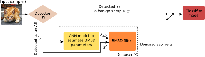
Figure 3: Overview of the proposed defense method workflow composed of detector $\mathcal{D}$ and denoiser $\mathcal{S}$ blocks.

The gradient masking and obfuscated gradients have been explored to design defense techniques robust against gradient based attacks. Meanwhile, backward pass differentiable approximation (BPDA) athalye2018obfuscated technique was proposed as a differentiable approximation for the defended model to obtain meaningful adversarial gradient estimates. The BPDA techniques enables to derive a differentiable approximation for a non-differentiable preprocessing transformation that can be explored with any gradient based attack. It has been shown that BPDA approximation breaks the majority of these preprocessing based defense techniques.

2.3.3 Detecting adversarial samples

Instead of trying to classify AEs correctly, which is difficult to achieve, many contributions have focused on only detecting these AEs. Grosse et al. B23 proposed a technique that rely on statistical hypothesis on the input image to detect AEs, where the distribution of AEs statistically diverges from the data distribution. This hypothesis is explored to distinguish adversarial distributions from legitimate ones. Ma et al. B27 explored the local intrinsic dimensionality (LID) concept for characterizing the dimensional properties of adversarial regions. The authors empirically showed that LID of AEs is significantly higher than LID of clean samples. Thus, they used the LID of images as features to train a machine learning classifier to detect AEs. Xu et al. B25 proposed a detection technique called feature squeezing (FS). Two FS methods were considered to remove non-relevant features from the input: color bit-depth reduction and spatial smoothing, both with local and non-local smoothing. DNN-based predictions of clean and squeezed samples are compared to detect AEs. More specifically, the input sample is labeled as adversarial when the $l_{1}$ distance between the two DNN predictions of squeezed and unsequeezed samples is higher than a threshold value. Ma et al. B15 proposed also another detection approach named neural-network invariant checking (NIC). This latter exploits two invariants in the DNN classifier structure: the provenance channel and the activation value distribution channel. The NIC detector leverage these inveriants extracted from the DNN classifier to perform runtime detection of adversarial samples. Under assumption that adversarial inputs leave activation fingerprints, i.e., the neuron activation values of clean and AEs are different, Eniser et al. eniser2020raid proposed a binary classifier that takes as inputs the differences in neuron activation values between clean and AEs inputs to detect if the input is adversarial or not. In sheikholeslamiprovably , a method for jointly training a provably robust classifier and detector was proposed. The authors proposed a verification scheme for classifiers with detection under adversarial settings. They extend the Interval Bound Propagation (IBP) method to account for robust objective, which enables verification of the network for provable performance guarantees. Authors in aldahdooh2021selective proposed a detection technique called Selective and Feature based Adversarial Detection (SFAD). This latter uses the recent uncertainty method called SelectiveNet selective2019 and integrates three detection modules. The first is selective detection module, which is a threshold-based detection derived from uncertainty of clean training data using SelectiveNet. The second is confidence detection module, which is threshold-based detection derived from softmax probabilities of clean training data from SFAD’s classifiers. SFAD’s classifiers analyze the representative data of last $N$-layers as a key point to present robust features of input data using autoencoding, up/down sampling, bottleneck, and noise blocks. The last module is ensemble prediction, which is mismatch based prediction between the detector and the baseline deep learning classifiers.

The described detectors showed some limitations B29 , for instance they are effective against some specific attacks and lack generalization ability against different types of attacks. Also, they can achieve high accuracy but at the cost of increasing the false positive rate, thus rejecting considerable legitimate inputs, which is not desired in real sensitive applications.

3 Proposed Approach

In this paper, we propose a framework for defending against AEs in the digital domain, e.g., when attacking a computer vision system. The proposed method consists of two main components that process the input sample before passing it to the classifier as shown in Figure 3. First, a detector block $\mathcal{D}$ distinguishes between clean sample $x$ and adversarial sample $x^{\prime}$, and then a denoising block $\mathcal{S}$ alleviates perturbations in a sample detected as AE. In other words, this denoising block $\mathcal{S}$ aims to project the adversarial sample back into the manifold of $x$. Finally, the classifier is fed by a denoised sample in order to predict the sample label. These two blocks will be explored in more detail in the next two sections.

3.1 Detector

The detector $\mathcal{D}$ block relies on the concept of NSS. We assume that clean images possess certain regular statistical properties that are altered by adding adversarial perturbations. Thus, by characterizing these deviations from the regularity of natural statistics using NSS, it is possible to determine whether the input image $x$ is benign or malicious.

In order to extract scene statistics from input samples, we consider the efficient spatial NSS model B0 , referred to as MSCN coefficients. The MSCN coefficients of a given input image $I$ are computed as follows

$$\widehat{I}(i,j)=\frac{I(i,j)-\mu(i,j)}{\sigma(i,j)+c},$$ (6)

where $i$ and $j$ are the pixel coordinates, and $c$ is a tiny constant added to avoid division-by-zero. The local mean $\mu$ and local standard deviation $\sigma$ are computed by (7) and (8), respectively.

$$\mu(i,j)=\sum_{k=-3}^{3}\,\sum_{l=-3}^{3}\,w_{k,l}I_{k,l}(i,j).$$ (7)

$$\sigma(i,j)=\sqrt{\sum_{k=-3}^{3}\,\sum_{l=-3}^{3}\,w_{k,l}(I_{k,l}(i,j)-\mu(i,j))^{2}}.$$ (8)

where $w=\{w_{k,l}|k=-3,...,3,l=-3,...,3\}$ is a 2D circularly-symmetric Gaussian weighting function.

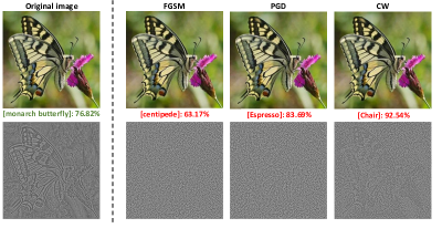
Figure 4: Illustration of the relationship between natural scene statistics and adversarial perturbations. (a) top: the original image and different attacked versions. bottom: the MSCN coefficients of the images shown in the top row. (b) Histogram of MSCN coefficients for the original image and attacked images.

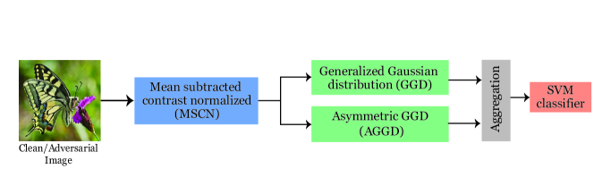
Figure 5: Overview of the proposed detection method workflow.

In order to demonstrate that MSCN coefficients are affected by adversarial perturbations, Figure 4 illustrates the MSCN coefficients of the original (clean) image and its associated attacked versions. We consider three white-box attacks used in the experiments, namely FGSM, PGD and CW. First, according to the obtained class label, it is clear that all attacks have succeeded in fooling the DNN model with high confidence, while the attacked images are visually very close to the original one. From Figure 4, we can also see that the MSCN coefficients of the original image differ significantly from those of adversarial attacks.

In addition, in order to show how the MSCN coefficients vary with the presence of AEs, Figure 4 plots the histogram of MSCN coefficients of images shown in Figure 4 (top row). The original image exhibits a Gaussian-like MSCN distribution, while the same does not hold for the AEs which produce distributions with notable differences.

These results show that each attacked sample is characterized by its own histogram, which does not follow a Gaussian-like MSCN distributions like for the clean image. Based on that, we model these coefficients using the generalized Gaussian distribution (GGD) to estimate the parameters that are extracted from the scene statistics. The GGD function is defined as follows

$$f_{X}(x;\beta,\sigma^{2})=\frac{\beta}{2\alpha\Gamma(1/\beta)}e^{-\big{(}\frac{|x|}{\alpha}\big{)}^{\beta}},$$ (9)

where $\alpha=\sigma\sqrt{\frac{\Gamma\big{(}\frac{1}{\beta}\big{)}}{\Gamma\big{(}\frac{3}{\beta}\big{)}}}$ and $\Gamma\left(\cdot\right)$ is the gamma function: $\Gamma\left(a\right)=\int\limits_{0}^{\infty}{t^{a-1}e^{-t}dt}\>,a>0$.

The value of $\beta$ controls the shape and $\sigma^{2}$ is the variance controller parameter. Due to the symmetry property of the MSCN coefficients, we used the moment-matching B2 to estimate the couple $(\beta,\,\sigma^{2})$. To perform more accurate detection, we add the adjacent coefficients to model the pairwise products of neighboring MSCN coefficients along four directions (1) horizontal $H$, (2) vertical $V$, (3) main-diagonal $D1$ and (4) secondary-diagonal $D2$ B0 . These orientations computed in Equation (10) have also certain regularities, which get altered in presence of adversary perturbations.

$$\begin{split}&H(i,j)=\hat{I}(i,j)\hat{I}(i,j+1),\\ &V(i,j)=\hat{I}(i,j)\hat{I}(i+1,j),\\ &D1(i,j)=\hat{I}(i,j)\hat{I}(i+1,j+1),\\ &D2(i,j)=\hat{I}(i,j)\hat{I}(i+1,j-1).\end{split}$$ (10)

It is clear that the results of these pairwise products lead to an asymmetric distribution, so instead of using GGD, we chose the asymmetric generalized Gaussian distribution (AGGD), which is defined as follows

$$f_{X}(x;\nu,\sigma_{l}^{2},\sigma_{r}^{2})=\begin{cases}\frac{\nu}{(\alpha_{l}+\alpha_{r})\Gamma\big{(}\frac{1}{\nu}\big{)}}e^{\big{(}-\big{(}\frac{-x}{\alpha_{l}}\big{)}^{\nu}\big{)}}&x<0\\ \frac{\nu}{(\alpha_{l}+\alpha_{r})\Gamma\big{(}\frac{1}{\nu}\big{)}}e^{\big{(}-\big{(}\frac{x}{\alpha_{r}}\big{)}^{\nu}\big{)}}&x\geq 0\end{cases}$$ (11)

where $\alpha_{side}=\sigma_{side}\sqrt{\frac{\Gamma\big{(}\frac{1}{\nu}\big{)}}{\Gamma\big{(}\frac{3}{\nu}\big{)}}}$ where $side$ can be either $r$ or $l$, $\nu$ represents the shape parameter and $\sigma_{side}^{2}$ expresses the left or the right variance parameters. So to estimate $(\nu,{\sigma_{l}}^{2},{\sigma_{r}}^{2})$, we use the moment-matching as described in B3 . Another parameter that is not reflected in the previous formula is the mean which is defined as follows

$$\eta=(\alpha_{r}-\alpha_{l})\frac{\Gamma\big{(}\frac{2}{\nu}\big{)}}{\Gamma\big{(}\frac{1}{\nu}\big{)}}$$ (12)

The AGGD can be characterized by 4 features $(\eta,\nu,\sigma_{l}^{2},\sigma_{r}^{2})$ for each of the four pairwise products. The concatenation of the two GGD parameters with the 16 AGGD ones results in 18 features ${\bf f}$ per image

$${\bf f}=\{\beta,\,\sigma^{2},\,\eta_{H},\,\nu_{H},\,\sigma_{l_{H}}^{2},\,\sigma_{r_{H}}^{2},\,\eta_{V},\,\nu_{V},\,\sigma_{l_{V}}^{2},\,\sigma_{r_{V}}^{2},\,\\ \eta_{D1},\,\nu_{D1},\,\sigma_{l_{D1}}^{2},\,\sigma_{r_{D1}}^{2},\,\eta_{D2},\,\nu_{D2},\,\sigma_{l_{D2}}^{2},\,\sigma_{r_{D2}}^{2}\}$$

This low number of considered features motivates the choice to train a support vector machine (SVM) binary classification model for the detector as shown in Figure 5. Thus, the SVM classifies each input image as either benign or AE, where the sample detected as AE is first processed by the denoiser, as detailed in the next section.

3.2 Denoiser

The aim of the denoiser block $\mathcal{S}$ is to alleviate the adversarial perturbations and thus project back the AE into its original data manifold. In other words, the denoiser $\mathcal{S}$ tries to reconstruct from an adversarial example $x^{\prime}$ a new sample $\tilde{x}$ such that $f_{\theta}(\tilde{x})=f_{\theta}(x)$.

The denoiser block processes only input samples detected as AE, whereas, the samples detected as clean are directly passed to the classifier. In this way, we enhance the robustness against these adversarial attacks without affecting the classification accuracy of clean samples.

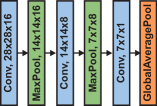
(a) MNIST

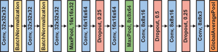
(b) CIFAR-10

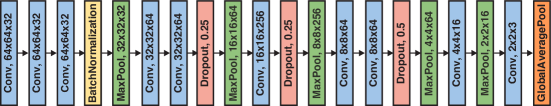
(c) Tiny-ImageNet

Figure 6: The proposed CNN architectures used in the prediction of BM3D parameters $\lambda_{3D}$ for (a) MNIST, (b) CIFAR-10 and (c) Tiny-ImageNet datasets. The GlobalAveragePooling2D layer calculates the average of its input and outputs a single scalar value for each feature map.

The denoiser relies on the block matching 3D (BM3D) filter initially proposed in dabov2007image . This denoiser is considered to be one of the best non-learning-based denoising methods, furthermore, some work has shown that BM3D even out-performs deep learning-based denoising approaches for some real-world applications plotz2017benchmarking . In addition, the BM3D allows locally adaptive parameter tuning based on block or region, making it suitable for non-uniform adversarial perturbations distribution.

The BM3D filter first gathers similar 2D patches $P$ of an image in a 3D-block denoted $\mathbf{P}(P)$. For a given patch $P$ of size $\kappa\times\kappa$, the filter searches for similar patches $Q$ within a window of size $n\times n$ in the image, where $n>\kappa$. The search window is extracted such that the patch $P$ is the window center. The similarity between two patches is measured as follows

$$\mathbf{P}(P)=\left\{Q:d(P,Q)\leq\tau\right\},$$ (13)

where $d$ is the normalized quadratic distance and $\tau$ is a threshold value set to check whether two patches are similar or not. In order to speed up the process, from the similar $Q$ patches within the 3D-block $\mathbf{P}(P)$, only the $N$ closest patches to $P$ are selected to get the $\tilde{\mathbf{P}}(P)$ 3D group, where $P$ is included.

After the grouping step, a 3D linear transform $\tau_{3D}$ is applied on each 3D pile of correlated patches, followed by a shrinkage. Finally, the inverse of this isometric transform is applied to give an estimation of each patch as follows

$$\tilde{\mathbf{P}}(P)=\tau_{3D}^{-1}\left[\gamma\left(\tau_{3D}\left[\tilde{\mathbf{P}}(P)\right]\right)\right],$$ (14)

where $\gamma$ is a thresholding that depends on $\lambda_{3D}$:

$$\gamma(x)=\left\{\begin{array}[]{ll}0&\text{ if }\quad|x|\leq\lambda_{3D}\\ x&\text{ otherwise }\end{array}\right.$$ (17)

The above grouping and filtering procedures are improved in a second step using Wiener filtering. This step is nearly the same as the first one, with only two differences. The first difference consists in comparing the filtered patches instead of the original ones at the grouping step. The second difference relies in using the Wiener filtering to process the new 3D groups, instead of using linear transform and thresholding. For further details about the filtering process, the reader is referred to dabov2007image .

The performance of the BM3D depends on its parameter settings. However, studies conducted in bashar2016bm3d ; lebrun2012analysis ; mukherjee2019cnn showed that the threshold $\lambda_{3D}$ is the most crucial and significant parameter in BM3D’s denoising process. Since AEs can contain different levels of adversarial perturbations, it is therefore important to choose the appropriate $\lambda_{3D}$ parameter to mitigate each level of perturbation. To reach this goal, in this work, we use a CNN to automatically predict the best $\lambda_{3D}$ suited to each AE.

Inspired by the extension of BM3D for color images initially investigated in dabov2007image , we propose to perform the grouping step relying only on the luminance component $Y$ after a color transformation from RGB color space to a luminance-chrominance color space, where $Y$ denotes luminance channel, while $U$ and $V$ refer to the two chrominance components. After building the 3D block on the $Y$ channel, we used it for all three channels, then the remaining BM3D’s processes are applied to each channel separately. Therefore, three parameters of the thresholding $\lambda_{3D}$ must be predicted, one per channel.

Thus, we performed the prediction of these thresholds under the RGB color space using a CNN trained to derive, for each channel, an optimum value of $\lambda_{3D}$. Figures 6(a), 6(b) and 6(c) illustrate the three proposed architectures used to predict the optimal thresholding parameters for the three different image datasets, namely MNIST, CIFAR-10 and Tiny-ImageNet, respectively. These three different architectures have been proposed to adapt the CNN to the complexity of parameters prediction which depends on the characteristics of the dataset including the dataset size, the color space and image resolution. The first architecture illustrated in Figure  6(a) is fed with a grayscale image to predict a single $\lambda_{3D}$ parameter, while architectures in Figures 6(b) and 6(c) are fed with the three RGB components of a color image to predict the three associated thresholding parameters, i.e., three $\lambda_{3D}$ values.

The three networks are trained in a supervised learning fashion by minimizing a mean squared error loss function between the network output and the ground truth. The ground truth consists of a set of adversarial samples and the optimal denoising parameters enabling to back project an attacked image into its data manifold. To build the ground truth, an exhaustive denoising approach is conducted to denoise a set of adversarial samples perturbed by the PGD attack at different $\epsilon$ magnitudes. The PGD attack is selected based on the fact that adversarial training with PGD attack tends to generalize well across a wide range of attacks B18 . So each sample is denoised with a set of $\lambda_{3D}$ parameters in the interval $[0.0,1.0]$ with a step of $0.125$. This denoising process can result in several samples that are correctly classified. Among these samples, only one maximizing the Structural SIMilarity (SSIM) wang2004image image quality metric is retained in the ground truth. The SSIM metric is computed between the original image $x$ and the denoised one $\tilde{x}$.

The SSIM image quality metric assesses the quality of the denoised image with respect to the original one by exploring the structural similarity. Preserving the structural similarity after denoising will contribute to achieve a correct classification by the model with a high confidence score. The $\lambda_{3D}$ parameters selected for each attacked sample with the highest SSIM score are assigned as the training labels for that adversarial sample.

4 Experimental results

We describe in this section the evaluation process of our defense method with respect to the state-of-the-art defense techniques on three well known datasets: MNIST, CIFAR-10 and Tiny-ImageNet. First, we describe the selected datasets and the training stage, then the robustness of the proposed approach is assessed under three types of attacks, namely black-box, gray-box and white-box attacks.

4.1 Datasets

We evaluated the robustness of our defense technique on CNNs models trained on three standard datasets, namely:

• MNIST dataset consists of grayscale hand-written 10 digits images of size $28\times 28$. This dataset contains 70,000 images split into training, validation and testing sets with 50,000, 10,000 and 10,000 images, respectively.

• CIFAR-10 dataset contains color images of size $32\times 32$. It has ten classes and 60,000 images divided into training and testing sets with 50,000 and 10,000 images, respectively.

• Tiny-ImageNet dataset includes also color images of size $64\times 64$ with a greater number of 200 classes. Each class includes 500, 50 and 50 images used for training, validation and testing, respectively.

We built our own CNN classifier for MNIST dataset resulting in a state-of-the-art accuracy of $99.4\%$. For CIFAR-10 and Tiny-ImageNet datasets, we considered existing models achieving accuracy scores of 98.5% cubuk2019autoaugment and 69.2% tiny , respectively.

Table 2: Performance of the proposed defense method under black-box attacks.

Dataset	Method	FGSM	PGD				CW
			7 steps	20 steps	40 steps	100 steps	$\kappa=20$	$\kappa=50$
MNIST	Madry madry2017towards	96.8%	-	-	96.0%	95.7%	96.4%	97.0%
	Thermometer buckman2018thermometer	-	-	-	41.1%	-	-	-
	ME-Net yang2019me	93.2%	-	-	92.8%	92.2%	98.8%	98.7%
	Our method	97.6%	99.4%	99.4%	99.4%	99.4%	99.2%	98.9%
CIFAR-10	Madry madry2017towards	67.0%	64.2%	-	-	-	78.7%	-
	Thermometer buckman2018thermometer	-	77.7%	-	-	-	-	-
	ME-Net yang2019me	92.2%	91.8%	91.8%	91.3%	-	93.6%	93.6%
	Our method	95.7%	98.3%	98.2%	98.2%	97.9%	93.8%	92.8%
Tiny-ImageNet	ME-Net yang2019me	67.1%	66.3%	60.0%	65.8%	-	67.6%	67.4%
	Our method	67.7%	68.8%	69.1%	69.1%	68.9%	68.3%	67.2%

4.2 Training process

Detector The detector is trained with a blend of clean and attacked samples. For MNIST dataset, we have selected 1,000 clean samples and generated adversarial samples with the PGD attack. These 1,000 adversarial images with the associated 1,000 clean images are used for the training. The same process is carried-out for CIFAR-10 and Tiny-ImageNet datasets. The obtained features from each sample are provided as inputs to the SVM classifier. The Sigmoid kernel is used in the SVM model since it achieves a good accuracy for non-linear binary classification problems.
Denoiser A separate CNN model is trained to estimate the denoising parameters for each dataset. As described previously, the denoiser block deals only with attacked samples, based on that, we generated 10,000 samples with the PGD attack. The three CNN architectures for MNIST, CIFAR-10 and Tiny-ImageNet datasets are shown in Figures 6(a), 6(b) and 6(c), respectively. We used the rectified linear unit (ReLU) as an activation function after each convolution layer. Some dropout layers are added to networks of color image datasets, i.e, CIFAR-10 and Tiny-ImageNet, with different rate to prevent over-fitting. The CNNs of CIFAR-10 and Tiny-ImageNet datasets include batch normalization layers to stabilize and accelerate the learning process. We used for the three architectures a learning rate of 0.01 and a large momentum of 0.9. Finally, the architectures are trained using 64 epochs with a batch-size of 128 for MNIST and CIFAR-10 datasets, while 128 epochs with a batch-size of 32 for Tiny-ImageNet dataset.

4.3 Results and analysis

The performance of the proposed defense method are evaluated under $l_{\infty}$ bounded attacks madry2017towards ; buckman2018thermometer ; yang2019me ; song2017pixeldefend . We compare our method with three state-of-the-art defense techniques on the three considered datasets under black-box, gray-box and white-box attacks, as recommended in carlini2019evaluating . The chosen defense techniques include one of the best performing adversarial training defenses developed by Madry et al. madry2017towards and two prepossessing methods including Thermometer buckman2018thermometer and ME-Net yang2019me . Furthermore, we investigate the effectiveness of the proposed detector block to detect the AEs.

4.3.1 Defense block performance

The robustness of the proposed defense method is assessed against three attacks: fast gradient sign method (FGSM), projected gradient descent (PGD) and Carlini and Wagner (CW). The CW implementation B16 provided by the authors is used, while the implementations of FGSM and PGD attacks are from the open-source CleverHans library cleverhans .
Black-box attacks This kind of attack is performed to fool a classifier model when an attacker can not perform back propagation to generate adversarial samples from the network model. Based on this, we train substitute networks for MNIST, CIFAR-10 and Tiny-ImageNet datasets to generate AEs with FGSM, PGD and CW attacks. We set the attacks hyper-parameters as in yang2019me , where we use for MNIST a perturbation magnitude $\epsilon$ of $0.3$ for both FGSM and PGD. This latter is used with two iteration configurations: 40 and 100 steps. Regarding CIFAR-10 and Tiny-ImageNet datasets, the PGD attack is used with a magnitude perturbation $\epsilon$ of $0.03$ and four iteration configurations: 7, 20, 40 and 100 steps. For the CW attack, we consider two different confidence values of $\kappa=20$ and $\kappa=50$.

Table 3: Performance of the proposed defense method under gray-box attacks.

Dataset	Method	FGSM	PGD				CW
			7 steps	20 steps	40 steps	100 steps	$\kappa=20$	$\kappa=50$
MNIST	ME-Net yang2019me	-	-	96.2%	95.9%	95.3%	98.8%	98.7%
	Our method	97.4%	99.4%	99.3%	99.3%	99.3%	99.1%	98.5%
CIFAR-10	ME-Net yang2019me	85.1%	84.9%	84.0%	82.9%	-	84.0%	77.1%
	Our method	88.4%	95.0%	94.8%	94.8%	94.5%	83.7%	75.8%
Tiny-ImageNet	ME-Net yang2019me	66.5%	64.0%	62.6%	59.2%	-	58.3%	58.2%
	Our method	67.7%	69.0%	68.9%	68.9%	68.5%	61.2%	60.1%

Table 2 gives the performance of our defense method compared to the selected defenses under black-box attacks on the three datasets. We can notice that the proposed defense achieves the highest accuracy performance on the three datasets, except against CW attack under $\kappa=50$ on the two color datasets. Moreover, most defense techniques are robust against the considered attacks on MNIST dataset, except the Thermometer defense which achieved the lowest accuracy of 41.1%. We can also note, in MNIST dataset, that Madry’s defense performs better than ME-Net which obtained $92.8\%$ and $92.2\%$ accuracy against PGD attack at 40 and 100 steps, respectively. This can be explained by the fact that the PGD AEs were included in the training set of the Madry defense. However, the preprocessing conducted in the ME-Net allows this method to achieve relatively higher classification accuracy for CW attack compared to Madry’s method. This is particularly true for CIFAR-10 dataset where ME-Net outperforms Madry’s defense for all attacks considered. Finally, it is clear that our defense outperforms the considered defenses, for instance, it obtained the highest accuracies of $97.6\%$ and $98.9\%$ against FGSM and CW ($\kappa=50$) attacks, respectively. In addition, the proposed method achieves a constant accuracy of $99.4\%$ against PGD attack despite the change in the number of iterations.
Gray-box attacks In this setting, an adversary has knowledge of the hyper-parameters of the classifier without any information on the defense technique. This kind of attacks are much stronger than black-box attacks in reducing the robustness of the defense mechanism. Table 3 compares the accuracy performance of the proposed defense against gray-box attacks with respect to ME-Net technique on the three datasets. We can first of all notice that the accuracy is lower compared to the black-box attacks. However, our defense method outperforms the ME-Net defense at all attacks, except against CW attack where similar performance is reported.
White-box attacks In white-box attacks, an adversary has a full access to all hyper-parameters of the classifier architecture and the defense technique. We assessed the robustness of our defense method against such strong attacks using the backward pass differentiable approximation (BPDA) attack athalye2018obfuscated . The proposed defense technique consists of a preprocessing method which is independent from the classifier model as shown in Figure 3. This causes gradient masking for gradient-based attacks. In other words, on the backward pass the gradient of the preprocessing step is non-differentiable and therefore useless for gradient-based attacks. The BPDA approximates the gradient of non-differentiable blocks, which makes it useful for evaluating our defense technique against white-box attacks.

Table 4: Performance of the proposed defense method against BPDA-based PGD under white-box attack at up to 1000 steps on the three datasets.

Dataset	Method	Attack steps
		7	20	40	100	1000
MNIST	Madry madry2017towards	-	-	93.2%	91.8%	91.6%
	ME-Net yang2019me	-	-	94.0%	91.8%	91.0%
	Our method	-	-	95.3%	94.9%	94.7%
CIFAR-10	Madry madry2017towards	50.0%	47.1%	47.0%	46.9%	46.8%
	ME-Net yang2019me	74.1%	61.6%	57.4%	55.9%	55.1%
	Our method	71.2%	70.6%	70.3%	69.9%	69.6%
Tiny-ImageNet	Madry madry2017towards	23.3%	22.4%	22.4%	22.3%	22.1%
	ME-Net yang2019me	38.8%	30.6%	29.4%	29.0%	28.5%
	Our method	36.0%	35.8%	35.7%	35.2%	34.8%

Thereby, we approximate the denoiser block with the identity function $g(x)=x$, which is often effective as reported in tramer2020adaptive . This approach enables to approximate the true gradient and thus to bypass the defense, which allows using a standard gradient-based attack based on BPDA. Similar to yang2019me , we selected the BPDA-based PGD attack to assess the efficiency of our method. Table 4 gives the accuracy performance on the three datasets for different steps of the BPDA-based PGD attack. We can notice that our defense outperforms Madry and ME-Net defense techniques on MNIST dataset. On CIFAR-10 and Tiny-ImageNetdatasets, the accuracy scores of our defense technique are higher than those of Madry and ME-Net defenses, except in the 7 iterations configuration. At this configuration, ME-Net defense outperforms our solution by around 3% benefiting mainly from its randomness operation. However, the ME-Net defense performance would be lower against the EOT technique that estimates the gradient of random components athalye2018obfuscated .

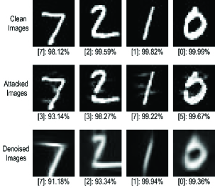
Figure 7: Visual illustration of MNIST images sorted from top to bottom as clean images, attacked images using BPDA-based PGD under white-box attack at 1000 steps with $\epsilon=0.3$, and denoised images by the proposed defense method. The predicted class label and its corresponding probability are provided for each image.

Figure 8: Visual illustration of CIFAR-10 images sorted from top to bottom as clean images, attacked images using BPDA-based PGD under white-box attack at 1000 steps with $\epsilon=0.3$, and denoised by the proposed defense method. The predicted class label and its corresponding probability are provided for each image.

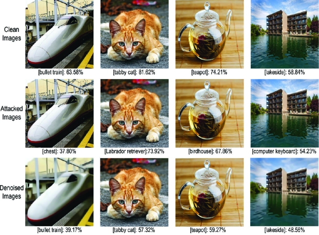
Figure 9: Visual illustration of Tiny-ImageNet images sorted from top to bottom as clean images, attacked images using BPDA-based PGD under white-box attack at 1000 steps with $\epsilon=0.03$, and denoised images by the proposed defense method. The predicted class label and its corresponding probability are provided for each image.

Figures 7, 8 and 9 illustrate four images from MNIST, CIFAR-10 and Tiny-ImageNet datasets, respectively. These images are illustrated in three configurations: clean, attacked with BPDA-based PGD attack and denoised with the proposed denoiser block. We can notice that the adversarial perturbations are filtered by the denoiser block, while a slight blur is introduced to the denoised images. However, through the use of CNN-guided BM3D, the filtering is performed so that the introduced blur does not affect the classification performance.

Furthermore, in order to assess the performance of our defense technique in the worst case scenario, we changed the PGD attack hyper-parameters under a white-box attack to see how the proposed method behaves against these perturbations. Figure 10 illustrates the classification accuracy of the proposed technique against BPDA-based PGD attack at different steps and perturbation magnitudes $\epsilon$. These figures clearly demonstrate the robustness of the proposed defense method vis-à-vis the increasing in both the number of steps and the magnitude of perturbation. The accuracy of the proposed method slightly decreases when increasing the number of steps, while it remains robust regarding the magnitude increase. For MNIST dataset, the classifier performs very well even at high perturbation magnitudes, especially when $\epsilon>0.4$ which generates a very noisy image, making its classification difficult even by a human eye. Despite these hard conditions, our defense method achieves more than $86\%$ accuracy in the case of $\epsilon=0.5$ and $1000$ steps under white-box attack. For the color datasets, which are much more challenging to defend, our technique allows to increase the classification accuracy by approximately more than $40\%$ and $25\%$ for CIFAR-10 and Tiny-ImageNet, respectively.

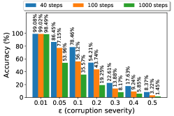
(a) MNIST, without defense

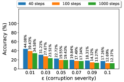
(b) CIFAR-10, without defense

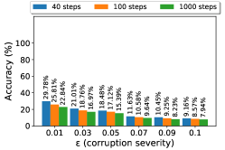
(c) Tiny-ImageNet, without defense

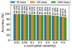
(d) MNIST, with defense

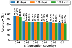
(e) CIFAR-10, with defense

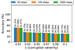
(f) Tiny-ImageNet, with defense

Figure 10: Accuracy of the classifier against BPDA-based PGD attack at three different steps for the three considered datasets.

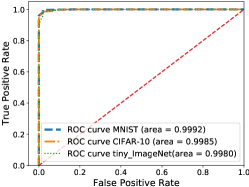
(a) FGSM attack

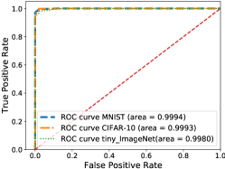
(b) PGD attack

(c) CW attack

Figure 11: ROC performance of the detector block against three attacks under white-box settings.

4.3.2 Detector block performance

The performance of the detector block is evaluated under the same conditions as the defense technique, while half of the images are benign and the other half are crafted using three white-box attacks including FGSM, PGD and CW. Figure 11 summarizes the performance of our detector using receiver operating characteristic (ROC) curves for different detection thresholds. The ROC curves are plotted with true positive rate (TPR) versus the false positive rate (FPR). The area under the ROC curve (AUC) denotes the value measured by the entire two-dimensional area below the entire ROC curve. The higher the AUC, the better the model is to predict clean images as clean and AEs as attacked. In the evaluation of the detector, we only selected images that were successfully attacked, i.e., $f_{\theta}(x^{\prime})\neq f_{\theta}(x)$ , with their benign state. We reach an AUC of about over $0.9970$ for all datasets against the three used attacks, which is not far from an ideal detector.

Furthermore, Table 5 reports the detection accuracy against the three attacks under white-box settings, as well as the false positive (FP), i.e, the detector classifies a benign input as an AE. An efficient and robust detector must achieve high accuracy and at the same time a low FP. Our detector achieves $100\%$ detection accuracy for all white-box attacks and considered datasets, except for Tiny-ImageNet dataset against the strongest iterative CW attack, where an accuracy of $98\%$ is reported. The later is an acceptable score because it is associated with a very low FP of $2.3\%$.

Table 5: Accuracy and FP of the detector against three attacks under white-box settings.

Dataset	FGSM	PGD	CW	FP(%)
MNIST	100%	100%	100%	1.9%
CIFAR-10	100%	100%	100%	2.0%
Tiny-ImageNet	100%	100%	98%	2.3%

5 Conclusion

In this paper, we have proposed a novel two-stage framework to defend against AEs involving detection of AEs followed by denoising. The detector relies on NSS of the input image, which are altered by the presence of adversarial perturbations. The samples detected as malicious are then processed by the denoiser with an adaptive BM3D filter to project them back into there original manifold. The parameters of the BM3D filter used to process the attacked image are estimated by a CNN.

The performance of the proposed defense method is extensively evaluated against black-box, grey-box and white-box attacks on three standard datasets. The experimental results showed the effectiveness of our defense method in improving the robustness of DNNs in the presence of AEs. Moreover, the efficiency of the detector with high detection accuracy and low FP helps to preserve the classification accuracy of the DNN model on clean images. As future work, we plan to extend the proposed defense method to deal with adversarial attacks in the physical world.

Conflict of interest

The authors declare that they have no conflict of interest.

References

- (1) Deng, J., Dong, W., Socher, R., Li, L.J., Li, K., Fei-Fei, L.: Imagenet: A large-scale hierarchical image database. In: 2009 IEEE conference on computer vision and pattern recognition, pp. 248–255. Ieee (2009)
- (2) Lin, T.Y., Maire, M., Belongie, S., Hays, J., Perona, P., Ramanan, D., Dollár, P., Zitnick, C.L.: Microsoft coco: Common objects in context. In: European conference on computer vision, pp. 740–755. Springer (2014)
- (3) Krizhevsky, A., Sutskever, I., Hinton, G.E.: Imagenet classification with deep convolutional neural networks pp. 1097–1105 (2012)
- (4) LeCun, Y., Bottou, L., Bengio, Y., Haffner, P.: Gradient-based learning applied to document recognition. Proceedings of the IEEE 86(11), 2278–2324 (1998)
- (5) Andor, D., Alberti, C., Weiss, D., Severyn, A., Presta, A., Ganchev, K., Collins, M.: Globally normalized transition-based neural networks. arXiv preprint arXiv:1603.06042 (2016)
- (6) Cho, K., Van Merriënboer, B., Gulcehre, C., Bahdanau, D., Bougares, F., Schwenk, H., Bengio, Y.: Learning phrase representations using rnn encoder-decoder for statistical machine translation. arXiv preprint arXiv:1406.1078 (2014)
- (7) Ren, S., He, K., Girshick, R., Sun, J.: Faster r-cnn: Towards real-time object detection with region proposal networks. In: Advances in neural information processing systems, pp. 91–99 (2015)
- (8) Hinton, G., Deng, L., Yu, D., Dahl, G.E., Mohamed, A.r., Jaitly, N., Senior, A., Vanhoucke, V., Nguyen, P., Sainath, T.N., et al.: Deep neural networks for acoustic modeling in speech recognition: The shared views of four research groups. IEEE Signal processing magazine 29(6), 82–97 (2012)
- (9) Szegedy, C., Zaremba, W., Sutskever, I., Bruna, J., Erhan, D., Goodfellow, I., Fergus, R.: Intriguing properties of neural networks. arXiv preprint arXiv:1312.6199 (2013)
- (10) Moosavi-Dezfooli, S.M., Fawzi, A., Fawzi, O., Frossard, P.: Universal adversarial perturbations pp. 1765–1773 (2017)
- (11) Athalye, A., Engstrom, L., Ilyas, A., Kwok, K.: Synthesizing robust adversarial examples. arXiv preprint arXiv:1707.07397 (2017).
- (12) Madry, A., Makelov, A., Schmidt, L., Tsipras, D., Vladu, A.: Towards deep learning models resistant to adversarial attacks. arXiv preprint arXiv:1706.06083 (2017)
- (13) Xie, C., Wu, Y., Maaten, L.v.d., Yuille, A.L., He, K.: Feature denoising for improving adversarial robustness pp. 501–509 (2019)
- (14) Carlini, N., Katz, G., Barrett, C., Dill, D.L.: Ground-truth adversarial examples (2018)
- (15) Kurakin, A., Goodfellow, I., Bengio, S.: Adversarial machine learning at scale. arXiv preprint arXiv:1611.01236 (2016)
- (16) Lee, H., Han, S., Lee, J.: Generative adversarial trainer: Defense to adversarial perturbations with gan. arXiv preprint arXiv:1705.03387 (2017)
- (17) Carlini, N., Wagner, D.: Towards evaluating the robustness of neural networks, IEEE Symposium on Security and Privacy (SP), Vol. 1, pp. 39–57 (2017).
- (18) Ahmed Aldahdooh, Wassim Hamidouche, Sid Ahmed Fezza and Olivier Déforges: Adversarial Example Detection for DNN Models: A Review, arXiv preprint arXiv2105.00203, (2021).
- (19) Meng, D., Chen, H.: Magnet: a two-pronged defense against adversarial examples pp. 135–147 (2017)
- (20) Carlini, N., Wagner, D.: Adversarial examples are not easily detected: Bypassing ten detection methods pp. 3–14 (2017)
- (21) Xu, W., Evans, D., Qi, Y.: Feature squeezing: Detecting adversarial examples in deep neural networks. arXiv preprint arXiv:1704.01155 (2017)
- (22) Hendrycks, D., Gimpel, K.: Early methods for detecting adversarial images. arXiv preprint arXiv:1608.00530 (2016)
- (23) Li, X., Li, F.: Adversarial examples detection in deep networks with convolutional filter statistics pp. 5764–5772 (2017)
- (24) Ma, S., Liu, Y., Tao, G., Lee, W.C., Zhang, X.: Nic: Detecting adversarial samples with neural network invariant checking. (2019)
- (25) Bhagoji, A.N., Cullina, D., Mittal, P.: Dimensionality reduction as a defense against evasion attacks on machine learning classifiers. arXiv preprint arXiv:1704.02654 (2017)
- (26) Grosse, K., Manoharan, P., Papernot, N., Backes, M., McDaniel, P.: On the (statistical) detection of adversarial examples. arXiv preprint arXiv:1702.06280 (2017)
- (27) Feinman, R., Curtin, R.R., Shintre, S., Gardner, A.B.: Detecting adversarial samples from artifacts. arXiv preprint arXiv:1703.00410 (2017)
- (28) Ma, X., Li, B., Wang, Y., Erfani, S.M., Wijewickrema, S., Schoenebeck, G., Bailey, J., et al.: Characterizing adversarial subspaces using local intrinsic dimensionality. arXiv preprint arXiv:1801.02613 (2018)
- (29) Lu, J., Issaranon, T., Forsyth, D.: Safetynet: Detecting and rejecting adversarial examples robustly pp. 446–454 (2017)
- (30) Eniser HF, Christakis M, Wüstholz V: Raid: Randomized adversarial-input detection for neural networks. arXiv preprint arXiv:200202776 (2020)
- (31) Sheikholeslami F, Rezaabad AL, Kolter JZ: Provably robust classification of adversarial examples with detection. In: International Conference on Learning Representations (2021)
- (32) Fezza, S.A., Bakhti, Y., Hamidouche, W., Deforges, O.: Perceptual evaluation of adversarial attacks for cnn-based image classification. In: IEEE Eleventh International Conference on Quality of Multimedia Experience (QoMEX), pp. 1–6 (2019)
- (33) Wiyatno, R.R., Xu, A., Dia, O., de Berker, A.: Adversarial examples in modern machine learning: A review. arXiv preprint arXiv:1911.05268 (2019).
- (34) Goodfellow, I., Shlens, J., Szegedy, C.: Explaining and harnessing adversarial examples. arXiv preprint arXiv:1412.6572 (2014)
- (35) Madry, A., Makelov, A., Schmidt, L., Tsipras, D., Vladu, A.: Towards deep learning models resistant to adversarial attacks. arXiv preprint arXiv:1706.06083 (2017)
- (36) Moosavi-Dezfooli, S., Fawzi, A., Frossard, P.: Deepfool: a simple and accurate method to fool deep neural networks. arXiv preprint arXiv:1511.04599 (2015).
- (37) Szegedy, C., Zaremba, W., Sutskever, I., Bruna, J., Erhan, D., Goodfellow, I., Fergus, R.: Intriguing properties of neural networks. arXiv preprint arXiv:1312.6199 (2013)
- (38) Liu, X., Hsieh, C.J.: Rob-gan: Generator, discriminator, and adversarial attacker pp. 11234–11243 (2019)
- (39) Schmidt, L., Santurkar, S., Tsipras, D., Talwar, K., Madry, A.: Adversarially robust generalization requires more data pp. 5014–5026 (2018)
- (40) Xie, C., Wang, J., Zhang, Z., Ren, Z., Yuille, A.L.: Mitigating adversarial effects through randomization. arXiv preprint arXiv:1711.01991 (2017).
- (41) Aldahdooh, A., Hamidouche, W., Déforges, O.: Revisiting Model’s Uncertainty and Confidences for Adversarial Example Detection. arXiv preprint arXiv:2103.05354v2 (2021).
- (42) Geifman, Y., El-Yaniv, R.: SelectiveNet: A Deep Neural Network with an Integrated Reject Option. In: International Conference on Machine Learning (2019).
- (43) Athalye, A., Carlini, N., Wagner, D.: Obfuscated gradients give a false sense of security: Circumventing defenses to adversarial examples. arXiv preprint arXiv:1802.00420 (2018)
- (44) Gu, S., Rigazio, L.: Towards deep neural network architectures robust to adversarial examples. arXiv preprint arXiv:1412.5068 (2014)
- (45) Bakhti, Y., Fezza, S.A., Hamidouche, W., Déforges, O.: Ddsa: a defense against adversarial attacks using deep denoising sparse autoencoder. IEEE Access 7, 160397–160407 (2019)
- (46) Liu, X., Cheng, M., Zhang, H., Hsieh, C.J.: Towards robust neural networks via random self-ensemble pp. 369–385 (2018)
- (47) Lecuyer, M., Atlidakis, V., Geambasu, R., Hsu, D., Jana, S.: Certified robustness to adversarial examples with differential privacy pp. 656–672 (2019)
- (48) Dwork, C., Lei, J.: Differential privacy and robust statistics pp. 371–380 (2009)
- (49) Li, B., Chen, C., Wang, W., Carin, L.: Certified adversarial robustness with additive noise pp. 9464–9474 (2019)
- (50) Dhillon, G.S., Azizzadenesheli, K., Lipton, Z.C., Bernstein, J., Kossaifi, J., Khanna, A., Anandkumar, A.: Stochastic activation pruning for robust adversarial defense. arXiv preprint arXiv:1803.01442 (2018)
- (51) Dziugaite, G.K., Ghahramani, Z., Roy, D.M.: A study of the effect of JPG compression on adversarial images. arXiv preprint arXiv:1608.00853 (2016).
- (52) Athalye, A., Engstrom, L., Ilyas, A., Kwok, K.: Synthesizing robust adversarial examples. arXiv preprint arXiv:1707.07397 (2017).
- (53) Meng, D., Chen, H.: Magnet: a two-pronged defense against adversarial examples pp. 135–147 (2017)
- (54) Zantedeschi, V., Nicolae, M.I., Rawat, A.: Efficient defenses against adversarial attacks pp. 39–49 (2017)
- (55) Song, Y., Kim, T., Nowozin, S., Ermon, S., Kushman, N.: Pixeldefend: Leveraging generative models to understand and defend against adversarial examples. arXiv preprint arXiv:1710.10766 (2017).
- (56) Samangouei, P., Kabkab, M., Chellappa, R.: Defense-gan: Protecting classifiers against adversarial attacks using generative models. arXiv preprint arXiv:1805.06605 (2018)
- (57) Buckman, J., Roy, A., Raffel, C., Goodfellow, I.: Thermometer encoding: One hot way to resist adversarial examples (2018)
- (58) Yang, Y., Zhang, G., Katabi, D., Xu, Z.: Me-net: Towards effective adversarial robustness with matrix estimation. arXiv preprint arXiv:1905.11971 (2019)
- (59) Borkar T, Heide F, Karam L: Defending against universal attacks through selective feature regeneration. In: Proceedings of the IEEE Conference on Computer Vision and Pattern Recognition, pp 709–719 (2020)
- (60) A. Mittal, A. K. Moorthy, and A. C. Bovik, “No-reference image quality assessment in the spatial domain,” IEEE Transactions on image processing, vol. 21, no. 12, pp. 4695–4708, (2012)
- (61) Sharifi, K., Leon-Garcia, A.: Estimation of shape parameter for generalized gaussian distributions in subband decompositions of video. IEEE Transactions on Circuits and Systems for Video Technology 5(1), 52–56 (1995)
- (62) Lasmar, N.E., Stitou, Y., Berthoumieu, Y.: Multiscale skewed heavy tailed model for texture analysis pp. 2281–2284 (2009)
- (63) Dabov, K., Foi, A., Katkovnik, V., Egiazarian, K.: Image denoising by sparse 3-d transform-domain collaborative filtering. IEEE Transactions on image processing 16(8), 2080–2095 (2007)
- (64) Bashar, F., El-Sakka, M.R.: Bm3d image denoising using learning-based adaptive hard thresholding. pp. 206–216 (2016)
- (65) Lebrun, M.: An analysis and implementation of the bm3d image denoising method. Image Processing On Line 2, 175–213 (2012)
- (66) Mukherjee, S., Kottayil, N.K., Sun, X., Cheng, I.: Cnn-based real-time parameter tuning for optimizing denoising filter performance pp. 112–125 (2019)
- (67) Plotz, T., Roth, S.: Benchmarking denoising algorithms with real photographs. In: Proceedings of the IEEE conference on computer vision and pattern recognition, pp. 1586–1595 (2017)
- (68) Oord, A.v.d., Kalchbrenner, N., Kavukcuoglu, K.: Pixel recurrent neural networks. arXiv preprint arXiv:1601.06759 (2016)
- (69) Cubuk, E.D., Zoph, B., Mane, D., Vasudevan, V., Le, Q.V.: Autoaugment: Learning augmentation strategies from data pp. 113–123 (2019)
- (70) Kurakin, A.: Baseline resnet-v2-50, tiny imagenet (2018). https://github.com/tensorflow/models/tree/master/research/adversarial_logit_pairing.html
- (71) Hendrycks, D., Dietterich, T.G.: Benchmarking neural network robustness to common corruptions and surface variations. arXiv preprint arXiv:1807.01697 (2018)
- (72) Song, Y., Kim, T., Nowozin, S., Ermon, S., Kushman, N.: Pixeldefend: Leveraging generative models to understand and defend against adversarial examples. arXiv preprint arXiv:1710.10766 (2017)
- (73) Papernot, N., Goodfellow, I., Sheatsley, R., Feinman, R., McDaniel, P.: cleverhans v1. 0.0: an adversarial machine learning library. arXiv preprint arXiv:1610.00768 10 (2016)
- (74) Carlini N, Athalye A, Papernot N, Brendel W, Rauber J, Tsipras D, Goodfellow I, Madry A, Kurakin A (2019) On evaluating adversarial robustness. arXiv preprint arXiv:190206705
- (75) Tramer, F., Carlini, N., Brendel, W., Madry, A.: On adaptive attacks to adversarial example defenses. arXiv preprint arXiv:2002.08347 (2020)
- (76) Wang, Z., Bovik, A.C., Sheikh, H.R., Simoncelli, E.P.: Image quality assessment: from error visibility to structural similarity. IEEE transactions on image processing 13(4), 600–612 (2004)