An Interval Arithmetic for Robust Error Estimation

Abstract.

Interval arithmetic is a simple way to compute a mathematical expression to an arbitrary accuracy, widely used for verifying floating-point computations. Yet this simplicity belies challenges. Some inputs violate preconditions or cause domain errors. Others cause the algorithm to enter an infinite loop and fail to compute a ground truth. Plus, finding valid inputs is itself a challenge when invalid and unsamplable points make up the vast majority of the input space. These issues can make interval arithmetic brittle and temperamental.

This paper introduces three extensions to interval arithmetic to address these challenges. Error intervals express rich notions of input validity and indicate whether all or some points in an interval violate implicit or explicit preconditions. Movability flags detect futile recomputations and prevent timeouts by indicating whether a higher-precision recomputation will yield a more accurate result. And input search restricts sampling to valid, samplable points, so they are easier to find. We compare these extensions to the state-of-the-art technical computing software Mathematica, and demonstrate that our extensions are able to resolve 60.3% more challenging inputs, return 10.2$\times$ fewer completely indeterminate results, and avoid 64 cases of fatal error.

1. Introduction

Floating-point arithmetic in scientific, financial, and engineering applications suffers from rounding error: the results of a floating-point expression can differ starkly from those of the analogous mathematical expression (Kahan, 2000; Kahan and Darcy, 1998; Toronto and McCarthy, 2014; Hamming, 1987). Rounding error has been responsible for scientific retractions (Altman et al., 2003; Altman and McDonald, 2003), mispriced financial indices (McCullough and Vinod, 1999; European Commission, 1998), miscounted votes (Weber-Wulff, 1992), and wartime casualties (U.S. General Accounting Office, 1992). Floating-point code thus needs careful validation; sound upper bounds (Izycheva and Darulova, 2017; Solovyev et al., 2015; Das et al., 2020), semidefinite optimization (Magron et al., 2017), input generation (Chiang et al., 2014; Hui Guo, 2020), and statistical methods (Tang et al., 2010) have all been proposed for such validation. Sampling-based error estimation, which can estimate typical, not worst-case, error is especially widely used (Rubio-González et al., 2013; Panchekha et al., 2015; Sanchez-Stern et al., 2018; Boehm, 2020).

Consider the core task of computing the error for a floating-point computation at a given point. This requires computing an error-free ground-truth for a mathematical computation. Interval arithmetic (Boehm, 2020; Toronto and McCarthy, 2014; Melquiond, 2006; Mascarenhas, 2016; Lee and Boehm, 1990a) and its many variations (Minsky, 1967; Boehm, 1987; Jaulin et al., 2001) is the traditional approach to this problem. Interval arithmetic provides sound bounds on the error-free ground truth, and allows for refining those bounds by recomputing at higher precision, until the ground truth can be estimated to any accuracy. Computing the ground truth this way on a large number of sampled points gives a good estimate of the floating-point error of a computation.

In practice, however, even state of the art implementations struggle on invalid or particularly challenging input points. The bounds are meaningless for invalid inputs; the recomputation process may enter an infinite loop; and valid inputs may be too hard to find. Since error estimation requires sampling a large number of points, these challenges arise frequently. As a result, even state of the art interval arithmetic implementations enter infinite loops, give up too early, or in some exceptional cases even experience memory exhaustion and fatal errors.

We identify three particular challenges for sampling-based error estimation: invalid input points, futile recomputations, and low measure. Invalid input points violate explicit or implicit preconditions and cannot meaningfully be evaluated to a ground truth value; consider the square root of a negative number. Validity must thus be soundly tracked and checked, especially for inputs at the borderline between valid and invalid. Futile recomputation afflicts some valid inputs: interval arithmetic recomputes with ever-higher precision but without converging on a ground truth answer. These recomputations must thus be soundly cut off early, warning the user that a ground truth value cannot be computed. Low measure means valid inputs make up a small proportion of the input space, making it difficult for applications to find sufficiently many. Regions of valid input points must thus be efficiently and soundly identified. No general-purpose strategy exists to address these independent issues; yet all three must be addressed for interval arithmetic to be robust.

This paper proposes three improvements to interval arithmetic that address these issues. First, error intervals determine whether all or some of the points in an interval violate implicit or explicit preconditions. Second, movability flags detect most input values for which recomputation will not converge, warning the user and avoiding futile recomputation. Third, input search discards invalid regions of the input space, focusing sampling on valid points. Combined, our improvements soundly address the issues identified above and make interval analysis more robust.

We implement these improvements in the new interval arithmetic library called Rival and compare Rival to Mathematica’s analogous N function on a benchmark suite of 481 floating-point expressions. Rival produces results in dramatically more cases than Mathematica: Rival is able to resolve 18824 inputs, while Mathematica is only able to resolve 11744 (60.3% better). In only 746 cases does Rival return a completely indeterminate result; Mathematica, however, does so in 7617 cases (10.2$\times$ worse), and among those cases sometimes enters an infinite loop, runs out of memory, or hard crashes (64 cases). Furthermore, Rival’s input search saves 74.6% of invalid points from being sampled in the first place. An ablation study shows that error intervals, movability flags, and input search effectively handle even difficult inputs across a range of domains.

This paper contributes three extensions to interval arithmetic:

• Error intervals to track domain errors and rich notions of input validity (Section 4);

• Movability flags to detect when recomputing in higher precision is futile (Section 5);

• Input search to uniformly sample valid inputs with high probability (Section 6).

Sections 7 and 8 demonstrate that these extensions successfully address the issues of invalid inputs, futile recomputations, and low measure. Section 9 discusses our experience deploying these extensions to users.

2. Overview

Imagine a simulation that evaluates $x^{y}/(x^{y}+2)$. How accurate is this expression? This section describes how Rival’s extensions to interval arithmetic help answer the question. For ease of exposition, this section uses two-digit decimal arithmetic as a target precision, with ordinary floating-point as a higher precision arithmetic; targetting single- or double-precision floating-point with arbitrary-precision libraries sees analogous issues.

2.1. Interal Arithmetic

Consider an input like $(x,y)=(3.0,1.1)$. At this input point, the expression $x^{y}/(x^{y}+2)$ can be directly computed with two-digit decimal arithmetic: ${3.0}^{1.1}=3.34\dotsb$, which rounds to $3.3$; then $3.3+2=5.30\dotsb$, which rounds to $5.3$; and finally $3.3/5.3=0.622\dotsb$, which rounds to $0.62$. How accurate is this result? To find out, we must compare the computed result with the true value of this expression.

One might estimate that true value using higher-precision computation. In single-precision floating-point, the input evaluates to $0.62605417$, which rounds to the two-digit decimal $0.63$. Two-digit decimal evaluation therefore has error: it produces $0.62$ instead of the correct $0.63$. Unfortunately, single-precision floating-point itself has rounding error. After all, in double-precision arithmetic the computed value is not $0.626054\underline{17}$ but $0.626054\underline{25\dotsb}$, and even higher precision could produce some third value. So this method of computing the true answer is suspect: how much precision is enough?

Interval arithmetic answers this question using intervals, written $[a,b]$, which represent any real value between $a$ and $b$ (inclusive). Ordinary mathematical operations are then extended to intervals, the two ends always rounded outward to ensure that the resulting interval always contains the mathematically exact value. Returning to the running example, the interval evaluation of $x^{y}$ with $(x,y)=(3.0,1.1)$ is $[3.0,3.0]^{[1.1,1.1]}=[3.3,3.4]$. Next, $[3.3,3.4]+[2.0,2.0]=[5.3,5.4]$. Finally, $[3.3,3.4]/[5.3,5.4]=[0.61,0.65]$, with those two endpoints computed via $3.3/5.4=0.61$ and $3.4/5.3=0.65$. Therefore, the true value is between $0.61$ and $0.65$. A similar interval computation can be done with any precision; with single-precision floating-point, the resulting interval is $[0.626054\underline{17},0.626054\underline{41}]$.

Importantly, this interval is much narrower and both endpoints round to $0.63$ in two-digit decimals, meaning that the true value (which must be in the interval) does the same. These one-value interval therefore provide a way to evaluate the true value of the expression, to a target precision, using a higher but finite precision. If even single-precision floating-point resulted in too wide an interval, double- or higher-precision arithmetic could be tried until a one-value interval is found.

Interval arithmetic thus provides a fast way to compute a ground-truth value for an expression on an input point. This algorithm can be used for a range of purposes. In sampling-based error estimation, a ground truth is computed for many randomly-sampled inputs to a floating-point expression, and the actual floating-point answer is compared to the ground truth to determine how accurate the expression is. However, while this works well on most inputs, on challenging expressions it can throw errors, enter infinite loops, or fail to find valid inputs.

2.2. Invalid Input Points

Not all inputs to $x^{y}/(x^{y}+2)$ are as conceptually simple as $(3,1.1)$; consider $(x,y)=(-1.1,7)$. For this input, the denominator $x^{y}+2$ evaluates to the interval $[0.0,0.1]$ in two-digit decimals, meaning a division by zero error is possible. But single-precision evaluation shows that the error is a mirage: $[-1.1,-1.1]^{[7,7]}+2$ yields the interval $[0.051284\underline{1},0.051284\underline{3}]$ for the denominator, proving that division by zero does not occur. More broadly, in interval arithmetic, an interval may contain both valid and invalid inputs for an operator, in which case an error can be possible without being guaranteed.

Error intervals formalize this reasoning. Each interval is augmented with a boolean interval $[g,p]$, where the $g$ tracks whether an error is guaranteed and the $p$ tracks whether it is possible; the interval $[\top,\bot]$ is illegal, since a guaranteed error implies a possible error. For our running example with $(x,y)=(-1.1,7)$, the error interval is $[\bot,\top]$ in two-digit decimal arithmetic, indicating that error is not guaranteed but is possible, and $[\bot,\bot]$ in single-precision floating-point, guaranteeing that no error occurs. Importantly, error intervals can handle borderline cases with recomputation. For this point, two-digit decimal arithmetic is insufficient to determine whether the input point is valid, but single-precision is. If even single-precision weren’t, double or higher precision could be tried.

Boolean intervals are a type of three-valued logic which can also address expressions with explicit preconditions or with conditionals that branch on floating-point comparisons. In each case a boolean interval indicates whether a condition can, or must, be true, and multiple boolean intervals can be combined with the standard boolean operators. For example, for an expression $E(x)$ with precondition $\sin(x)>0$, the valid inputs $x$ are those where $\sin([x,x])>0\land\neg\text{{err}}(E([x,x]))=[\top,\top]$, where $\text{{err}}(E)$ refers to the error interval of $E$. The key for interval arithmetic is that error and boolean intervals allow expressing rich notions of input validity that integrate with recomputation and provide sound, error-free guarantees.

2.3. Futile Recomputation

Recomputation guarantees soundness but not speed. To the contrary: repeated, futile recomputations present a significant practical problem, most commonly due to overflow.

Consider our running example $x^{y}/(x^{y}+2)$, but with the extreme input $(x,y)=(10^{10},10^{10})$. Now $x^{y}$ is huge—too large for double-precision and even for common arbitrary-precision libraries. So in interval arithmetic, it evaluates to $[\Omega,\infty]$ for some largest finite representable value $\Omega$. Since $\Omega$ is already the largest representable value, $[\Omega,\infty]+2$ results in $[\Omega,\infty]$ again, and since the division $[\Omega,\infty]/[\Omega,\infty]$ can produce a value as small as $\Omega/\infty=0$ or as large as $\infty/\Omega=\infty$, the final interval is $[0,\infty]$. This interval is too wide to be helpful, and since the problem is overflow, not rounding, recomputing at a higher precision will not help. But we need to prevent recomputation from taking futile recourse to higher and higher precisions until an error like timeout, memory exhaustion, or worse occurs.

Movability flags detect such futile recomputations. Movability flags are a pair of boolean flags added to every interval, which track whether overflow influences each endpoint. When $x^{y}$ overflows, for example, the infinite endpoint in $[\Omega,\infty]$ is marked “immovable”, meaning that recomputing it at higher precision would yield the same result. These movability flags are then propagated through interval computations: $[\Omega,\infty]+2$ also has an immovable infinity, and in the final result $[0,\infty]$ both endpoints are immovable. This guarantees that higher-precision evaluation would produce the same uselessly-wide interval and cuts off further recomputation. Importantly, immovable endpoints distinguish harmful overflows that produce timeouts, like these, from benign overflows that still produce accurate results, like in $1/e^{x}$.

Movability flags are sound: if an expression evaluates to a wide immovable interval, recomputation cannot compute an error-free ground truth. This allows distinguishing harmful overflows from difficult expressions that require higher precision to resolve. Movability flags are not complete—the problem is likely undecidable (Boehm, 2020)—but are accurate enough to dramatically cut the number of cases of futile recomputation.

2.4. Low Measure

Many applications of interval arithmetic, such as for error estimation of floating-point expressions, require sampling a large number of valid input points, usually via rejection sampling (repeatedly sampling points and discarding invalid ones). Often a specific distribution, like uniform sampling, is required as well. But for many mathematical expressions the valid, samplable points have low measure: they are a tiny subset of the entire input space. Consider $\sin^{-1}(x+2007)$: the only valid inputs are in $[-2008,-2006]$, a range that contains approximately $0.0001\%$ of double-precision floating-point values. Rejection sampling would yield almost exclusively invalid points! Since restrictions on multiple variables combine multiplicatively, the chance a sample is valid decreases further for more variables.

Input search addresses this issue by identifying and ignoring regions of the input space where all inputs are invalid or unsamplable. Input search recursively subdivides the sample space into axis-aligned hyperrectangles, which assign each variable an interval. For each hyperrectangle, input search then uses error intervals and movability flags to determine whether points in that interval are valid and samplable. In a form of branch-and-bound search, input search then discards hyperrectangles that return $[\bot,\bot]$ and subdivides those that return $[\bot,\top]$. For example, for $\sin^{-1}(x+2007)$, the interval $[0,\infty]$ is discarded but the interval $[-\infty,0]$, whose error interval is $[\bot,\top]$, is subdivided and searched further.

Input search leverages error intervals and movability flags to ensure that difficult regions of the input space are handled soundly. This ensures that input regions that contain valid inputs are never discarded, and that applications can choose to ignore (or include) regions where movability flags prove unsamplability. Input search also offers control over the sampling distribution and tunes the subdivision to the target distribution to ensure fast convergence.

Put together, error intervals, movability flags, and input search overcome practical issues with interval arithmetic that plague state-of-the-art implementations and enable for more effective and robust error estimation.

3. Background

Arbitrary-precision interval arithmetic with recomputation is the standard method for approximating the exact result of a mathematical expression.

3.1. Arbitrary-precision Floating Point

Software libraries like MPFR (Fousse et al., 2007) provide floating-point arithmetic at an arbitrary, user-configurable precision $p$. This arithmetic represents a finite subset $S_{p}$ of the extended reals $\mathbb{R}\cup\{\pm\infty\}$. Any real number $x$ can be rounded $R_{p}(x)$ to precision $p$ by monotonically choosing one of the two values in $S_{p}$ closest to $x$; we write $R_{p}^{\downarrow}$ and $R_{p}^{\uparrow}$ for rounding down and up specifically. Precision $p$ implementations of functions like $\sin$ or $\log$ are correctly rounded: the implementation $f_{p}$ of a function $f$ satisfies $f_{p}(x)=R_{p}(f(x))$. But larger expressions can be inaccurate even in high precision: $(1+x)-x$ evaluates to $0$ for all inputs $x>2^{p}$.

3.2. Interval Arithemtic

Intervals are an abstract domain over the extended reals: the interval $[a,b]\in S_{p}\times S_{p}$ represents the set $\{x\in\mathbb{R}^{*}\mid a\leq x\leq b\}$. Interval versions $f_{p}$ can be constructed for each mathematical function $f$ to guarantee both soundness,

$$\forall x_{1}\in I_{1},x_{2}\in I_{2},\ldots,\quad f(x_{1},x_{2},\ldots)\in f_{p}(I_{1},I_{2},\ldots),$$

and weak completeness,

$$\exists\left.x_{1},y_{1}\in I_{1}\right.,\left.x_{2},y_{2}\in I_{2}\right.,\dotsc,\quad f_{p}(I_{1},\ldots,I_{n})=[R_{S}^{\downarrow}(f(x_{1},\ldots,x_{n})),R_{S}^{\uparrow}(f(y_{1},\ldots,y_{n}))].$$

The points $x_{i}$ and $y_{i}$ are called witness points, For example, since $[a_{1},a_{2}]+[b_{1},b_{2}]$ is at least $a_{1}+b_{1}$ and at most $a_{2}+b_{2}$, the result must be $[R_{p}^{\downarrow}(a_{1}+b_{1}),R_{p}^{\uparrow}(a_{2}+b_{2})]$.

3.3. Recomputation

Consider an expression $e$ over the real numbers, consisting of constants, variables, and function applications. In a target precision $p$, the most accurate representation of its value at $x$ is the ground-truth value $y^{*}=R_{p}(\llbracket e\rrbracket(x))$, where $\llbracket e\rrbracket(x)$ is the error-free real-number result. Interval arithmetic can be used to compute $y^{*}$. Evaluate $e$ to some interval $[y_{1},y_{2}]$ at precision $q>p$; then

$$y_{1}\leq\llbracket e\rrbracket(x)\leq y_{2}\implies R_{p}(y_{1})\leq y^{*}\leq R_{p}(y_{2})$$

by soundness and monotonicity. If $[y_{1},y_{2}]$ is sufficiently narrow, $R_{p}(y_{1})=y^{*}=R_{p}(y_{2})$, which computes $y^{*}$. We call these narrow intervals one-value intervals; computing one just requires finding a large enough precision $q$.

A useful strategy for finding $q$ is to start just a bit past $p$ and then grow $q$ exponentially, which guarantees that large precisions are reached quickly. Under certain assumptions, this exponential growth strategy can also be proved optimal in the sense of competitive analysis. Sometimes, though, the $q$ required is too large to be feasible or may not exist due to limitations like a maximum exponent size. Practical implementations must thus cap the maximum value of $q$ and return indeterminate results when the cap is reached.

4. Boolean and Error Intervals

Interval arithmetic is a method for establishing bounds on the output of a mathematical expression. This section introduces boolean intervals, which incorporate control flow into the interval arithmetic framework, and demonstrate how their application to domain errors (error intervals) allows integrating rich notions of input validity with the soundness and recomputation provided by interval arithmetic.

4.1. Modeling Control Flow

Besides real computations, floating-point expressions contain explicit and implicit control flow. However, since intervals represent a range of inputs, the results of a boolean expression can be indeterminate (true on some inputs in the range and false on others). Boolean intervals (for explicit control flow) and error intervals (for implicit control flow) represent this possibility.

Definition 1.

Boolean intervals $[\top,\top]$, $[\bot,\bot]$, and $[\bot,\top]$ denote the sets $\{\top\}$, $\{\bot\}$, and $\{\bot,\top\}$ of booleans.

Boolean intervals form a standard three-valued logic, with $[\bot,\top]$ representing the indeterminate truth value and with standard semantics for conjunction, negation, and disjunction. Comparison operators on intervals can return boolean intervals: $[1,3]<[4,5]=[\top,\top]$, while $[1,4]<[3,5]=[\bot,\top]$. Explicit control flow like the if operator unions its two branches when the condition is indeterminate.

Expressions also have implicit control flow due to domain errors. As with comparisons, whether a domain error occurs can be indeterminate; each expression thus returns an error interval, a boolean interval describing whether a domain error occurred during the evaluation of the expression; we write $\text{{err}}(e)$ for the error interval of expression $e$. When an error is possible but not guaranteed, the function’s output is still meaningful. For example, the expression $\text{{pow}}(x,y)$ raises a domain error when $x$ is negative and $y$ is non-integral. Thus, $\text{{pow}}([-1,2],[1,5])$ returns $[-1,32]$ with error interval $[\bot,\top]$ because $\text{{pow}}(-1,1)=-1$ is the minimum possible output, $\text{{pow}}(2,5)=32$ is the maximum possible output, and $\text{{pow}}(-1,2.5)$ demonstrates that domain error is possible.

At higher precisions input intervals are narrower, so errors that were once possible may be ruled out. Error intervals make it possible to distinguish those cases (which have error interval $[\bot,\top]$) from cases like $\sqrt{-1}$ (which have error interval $[\top,\top]$) where an error is guaranteed even at higher precision. Consider $\sqrt{\cos(x)}$. At low precisions and with large $x$ values, $\cos(x)$ can evaluate to $[-1,1]$, so that $\sqrt{\cos(x)}$ is possibly invalid. Without error intervals, $\sqrt{\cos(x)}$ would indicate the possible error by returning $[\text{{NaN}},1]$. The error interval $[\bot,\top]$ gives more information: it indicates that the expression could be a valid at a higher precision. But if, at a higher precision, $\cos(x)$ is found to be strictly negative, the error interval will be $[\top,\top]$ and cut off further recomputation.

4.2. Point Validity

Both explicit and implicit control flow can affect whether a point is a valid input. Combinations of boolean and error intervals allow expressing these rich notions of input validity. Consider how four validity requirements, drawn from the Herbie tool (Panchekha et al., 2015), can be formalized as expressions yielding boolean intervals. Each validity requirement applies to the input $(x,y,\dotsc)$ of an expression $E$.

First, Herbie requires each input variable to have a finite value in the target precision. Given the target precision’s smallest and largest finite values $K_{-}$ and $K_{+}$, the comparison $K_{-}\leq x\leq K_{+}$ expresses that requirement for the variable $x$. The constants $K_{-}$ and $K_{+}$ can be computed by ordering all values in the target precision and taking those just after/before $\mp\infty$. Note that the expression $-\infty<x<+\infty$ is equivalent in the target precision, but is much weaker in higher precisions that contain values between $K_{+}$ and $+\infty$.

Second, Herbie requires the output value, when computed without rounding error, to be finite as well. The expression $K_{-}\leq E\leq K_{+}$ enforces this requirement. Note that boolean intervals allow incorporating arbitrary mathematical formulas into validity requirements.

Third, Herbie requires $E$ to not raise a domain error. The expression $\neg\text{{err}}(E)$, which uses err to access the error interval, enforces this requirement. Since interval operations are meaningful even when an input interval contains invalid points, combining this requirement with the second one allows ignoring points that are either too large or invalid without using higher precision to determine which restriction applies.

Fourth, Herbie users can provide a precondition that valid inputs have to satisfy. That precondition can be interpreted as a boolean interval expression to enforce this requirement. Since interval arithmetic already accounts for rounding error, the precondition is checked without rounding error. If the chosen precision isn’t high enough, the precondition returns the indeterminate boolean interval $[\bot,\top]$, and it is automatically recomputed at a higher precision to determine whether the input is in fact valid.

Since boolean intervals admit conjunction, all four of these requirements can be combined into a single formula that for input validity. That single formula is crucial to input search Section 6.

5. Movable and Immovable Intervals

For some inputs, computing a ground-truth value using interval arithmetic and recomputation is impossible; one common problem is an overflow that persists across precisions. When no ground-truth can be computed for certain input points, the user must be warned, and recomputation must be prevented from causing timeouts. Movability flags on each endpoint achieve this goal. Movability flags are set when operations overflow, and track the influence of that overflow on further computation. When overflow prevents the computation of a ground-truth value, movability flags warn the user without timing out.

5.1. Movable and immovable intervals

Formally, an interval is augmented with two movability flags, one associated with each of its endpoints; an endpoint is immovable when its movability flag is set. In examples, we write exclamation marks for immovable endpoints, so that $[0,1!]$ is an interval with a movable left endpoint $0$ and an immovable right endpoint $1$. The movability flags describe how intervals get narrower at higher precision.

Definition 1.

One interval refines another, written $[a^{\prime},b^{\prime}]\prec[a,b]$, when $b^{\prime}=b$ and both are immovable or when $b^{\prime}\leq b$ and $b$ is movable; and likewise $a^{\prime}=a$ and both are immovable or when $a^{\prime}\geq a$ and $a$ is movable.

The goal of movability flags is to determine whether recomputation at higher precision could possibly yield a narrower interval output. Specifically, they guarantee:

Theorem 2.

$\llbracket e\rrbracket_{q}(x)\prec\llbracket e\rrbracket_{p}(x)$ for all $e$, $x$, and $q>p$.

When an expression evaluates to an interval that is not one-value and which has two immovable endpoints, any higher-precision computation will do the same, and recomputation is futile. Alternatively, an interval with a single immovable endpoint is guaranteed to produce that value (if any).

Program inputs and constants (named and numeric) form a particularly simple case of Theorem 2. Program inputs are drawn from the target precision and can be directly represented in higher precision; they are thus represented by intervals $[!x,x!]$ with both endpoints marked immovable. Constants like $\pi$, however, cannot be exactly represented and have both endpoints of their interval marked movable.

For expressions larger than just constants, Theorem 2 is proved by induction. Operators in the tree must properly interpret movability flags on their inputs and set movability flags on their outputs. The key is to ensure that each operator $f$ preserves refinement for its inputs:

Property 3.

$f_{q}(I_{1}^{\prime},\dotsc,I_{n}^{\prime})\prec f_{p}(I_{1},\dotsc,I_{n})$ when $q>p$ and all $I_{i}^{\prime}\prec I_{i}$.

Importantly, if $f_{p}(I,J)$ has an immovable endpoint, then $f_{q}(I^{\prime},J^{\prime})$ must share that immovable endpoint. When all operators satisfy 3, Theorem 2 is preserved by structural induction. The rest of this section describes how to guarantee 3 for various operations.

5.2. Immovability from Overflow

Movability flags are set when the limitations of arbitrary-precision computation make it impossible for higher precision to make the result of a computation more precise.

Consider the $\exp(x)$ function, which computes $e^{x}$. The MPFR library represents arbitrary-precision values as $\pm(1+s)2^{h}$, where the exponent $h$ has a fixed upper bound $H$. It thus cannot represent any values larger than $2^{H+1}$, so inputs $x>\log(2^{H+1})$ to $\exp$ overflow at any precision. This fact allows $\exp$ to set movability flags on its output.

Consider the computation $\exp_{p}([0,10^{10}!])=[1,\infty!]$. The output’s right endpoint is $\exp(10^{10})$, which rounds up to $+\infty$. Since $10^{10}$ exceeds the overflow threshold, the rounding will occur at any precision $p$; and since $10^{10}$ is immovable in the input interval, it will be the right endpoint of any refinement of the input. So it is valid to mark the right output endpoint immovable. Alternatively, for inputs like $[10^{10},10^{11}]$ whose left endpoint exceeds the overflow threshold, the output’s right endpoint can be marked immovable even if both input endpoints are movable. Thus outputs can have immovable endpoints even with entirely movable inputs. Note, however, that in this case the left output endpoint cannot be marked immovable, since it will be the largest representable finite value and that can typically increase with higher precision.

This general logic of overflow extends to the exp2 function with threshold $H+1$, and to pow, which detects overflow via the identity $x^{n}=\exp(n\log x)$.

5.3. Propagating Immovability

Once one operator sets a movability flag, that movability flag must be propagated through later computations. That requires keeping track of the exactness of intermediate computations.

An arbitrary-precision function $f_{p}$ can be thought of as $R_{p}(f(x_{1},\dotsc,x_{n}))$, where $f$ is the exact, real-valued function. But when the exact result $f(x_{1},\dotsc,x_{n})$ is representable in precision $p$, the rounding function $R_{p}$ is the identity. Since $f(x_{1},\dotsc,x_{n})$ is then also representable at all higher precisions $q$, we have $f_{q}(x_{1},\dotsc,x_{n})=f_{p}(x_{1},\dotsc,x_{n})$. This is the key to guaranteeing 3.

In general, an output interval’s endpoint will be immovable if it is the exact result of a computation on immovable inputs. Monotonic functions are a good illustration of the logic. Consider a single-argument, monotonic function $f$. Its behavior on intervals is particularly simple:

$$f_{p}([a,b])=[R_{p}^{\downarrow}(f(a)),R_{p}^{\uparrow}(f(b))].$$

At a higher precision, the rounding behavior could change and then so would the output interval. However, if $a$ is immovable, any refinement $[a^{\prime},b^{\prime}]\prec[a,b]$ must have $a=a^{\prime}$ and $b\leq b^{\prime}$. If $f(a)$ is exactly computed, $R_{p}^{\downarrow}$ is the identity. In this case:

$$f_{q}([a^{\prime},b^{\prime}])=f_{q}([a,b^{\prime}])=[R_{q}^{\downarrow}(f(a)),R_{q}^{\uparrow}(f(b^{\prime}))]\\ =[f(a),R_{q}^{\uparrow}(f(b^{\prime}))]\prec[f(a),R_{p}^{\uparrow}(f(b))]=f_{p}([a,b])$$

In other words, for monotonic functions, exact computations on immovable endpoints result in immovable endpoints. For example, $\text{{sqrt}}_{p}([0,4!])=[0,2!]$ because the square root of $4$ is exactly $2$. However, $\text{{sqrt}}_{p}([0,2!])=[0,1.414\ldots]$ has a movable right endpoint because the square root of $2$ is not exact at any precision. Arbitrary precision libraries such as MPFR report whether a floating-point operator is exact, making this rule easy to operationalize.

For general interval functions, the task is more complex because the endpoints of the output interval need not be computed from input endpoints. General interval functions may be defined as computing $f$ on witness points $a^{\prime}$ and $b^{\prime}$:

$$f_{p}([a_{1},b_{1}],\ldots,[a_{n},b_{n}])=[R_{p}^{\downarrow}(f(a^{\prime}_{1},\ldots,a^{\prime}_{n})),R_{p}^{\uparrow}(f(b^{\prime}_{1},\ldots,b^{\prime}_{n}))]$$

Here, the witness points $a^{\prime}$ and $b^{\prime}$ are computed as an intermediate step to minimize and maximize $f$ over the input intervals. In such a scenario, output endpoints are immovable only if the witness points are guaranteed to be the same in all refinements of the input intervals, and when $f$’s output is representable:

Lemma 4.

Suppose the left output endpoint of $f_{p}$, computed via $f(a^{\prime}_{1},\ldots,a^{\prime}_{n})$, is representable in precision $p$. That endpoint may be marked immovable if, for all $i$, either 1) $a^{\prime}_{i}=a_{i}$ and $a_{i}$ is immovable; 2) $a^{\prime}_{i}=b_{i}$ and $b_{i}$ is immovable; or 3) $a_{i}$ and $b_{i}$ are both immovable and $a^{\prime}_{i}$ is computed exactly. The analogous applies to $f_{p}$’s right endpoint.

Proof.

Since $a^{\prime}_{i}$ minimizes $f$ over the intervals $I_{0}\ldots I_{n}$, $f_{p}(a^{\prime}_{1},\ldots,a^{\prime}_{n})$ bounds $f$ from below. If, furthermore, $f_{p}(a^{\prime}_{1},\ldots,a^{\prime}_{n})$ is exactly computed, then $f_{p}(a^{\prime}_{1},\ldots,a^{\prime}_{n})=f_{q}(a^{\prime}_{1},\ldots,a^{\prime}_{n})$ for any higher precision $q$.

Consider conditions (1) and (2) first. If (1) or (2) holds, $a^{\prime}_{i}$ is guaranteed to be a member of any refinement $I_{i}\prec[a_{i},b_{i}]$ by immovability. Since it is the witness point for $f$ at the lower precision, it is a valid witness point at any higher precision too.

Alternatively, consider condition (3). If (3) holds, the only refinement of $[a_{i},b_{i}]$ is itself, so $a_{i}^{\prime}$ is always a member of that refinement. Since $a_{i}^{\prime}$ is additionally computed exactly, it is computed identically and thus still a witness point at any higher precision.

Since, under (1), (2), or (3), $a^{\prime}_{i}$ is a valid witness point at any higher precision, the left output endpoint computed from it can be marked immovable. ∎

In practice, computing witness points is usually easy. Consider the absolute value function $\text{{fabs}}([a,b])$: the left witness point is $a$, $b$, or $0$, and the right witness point is $a$ or $b$. In some cases, it’s best to avoid computing witness points directly. For example, $\cos$ has a minimum of $-1$ at $\pi$. Instead of computing $\pi$ inexactly, $-1$ can be used directly, so that for example $\cos([!3,4!])=[!{-1},0.653\dotsb]$. In terms of Lemma 4, the witness point $\pi$ is computed at infinite precision and then $\cos(\pi)$ is evaluated exactly. Overflow frequently produces immovable infinite endpoints, but operations on infinities are generally exact, so Lemma 4 retains immovability in these cases too.

5.4. Function-specific Movability Reasoning

Function-specific reasoning sometimes provides additional cases in which movability flags may be set. The most common case is multi-argument functions where individual arguments are special values like zero or infinity. These special values allow setting movability flags even when some of the input intervals are entirely movable.

Addition is an illustrative example. Addition of anything with infinity yields infinity; thus, $[1,+\infty!]+[1,2]=[2,+\infty!]$, with the right output endpoint immovable. Multiplication by an immovable $0$, like addition of infinity, results in an immovable $0$, even if the other argument is movable. Multiplication by infinity is similar but more complex: consider $[-1,1]\times[!1,+\infty!]=[-\infty,+\infty]$, where the output interval is movable because the movable left-hand argument may refine to a strictly positive or a strictly negative interval. Thus, much like overflow detection requires knowing that the input interval is greater than a given threshold, handling infinite values in multiplication requires knowing the sign of the input interval:

Lemma 5.

Let $c=a^{\prime}_{i}\times b^{\prime}_{i}$ be an endpoint of an interval returned by multiplication. The endpoint may be marked immovable if: 1) both $a^{\prime}_{i}$ and $b^{\prime}_{i}$ are immovable and $c$ is computed exactly; or, 2) $a^{\prime}_{i}$ is zero and immovable (or likewise for $b^{\prime}_{i}$); or, 3) $a^{\prime}_{i}$ is infinite and immovable and $[b_{1},b_{2}]$ does not contain zero (or likewise for $b^{\prime}_{i}$).

Proof.

The first case just restates Lemma 4. In the second case, $a^{\prime}_{i}$ is immovable, so $a^{\prime}_{i}=0$ is in any refinement. Since $0\times b^{\prime}_{i}=0$ for any $b^{\prime}_{i}$, the result is immovable. Finally, in the third case, while $b^{\prime}_{i}$ may change when refined, its sign cannot, since $[b_{1},b_{2}]$ does not contain zero. Since $a^{\prime}_{i}$ is immovable, $a^{\prime}_{i}\times b^{\prime}_{i}$ takes on a fixed sign in any refinement. Since $a^{\prime}_{i}$ is additionally infinity, the resulting $+\infty$ or $-\infty$ is immovable. ∎

Immovable infinite endpoints are often caused by overflow, so this multiplication-specific reasoning is essential to detecting immovability for many expressions.

6. Input Search

Most applications of interval arithmetic, whether using pure sampling or input generation or exhaustive testing, start by selecting one or many valid input points. But for many expressions, valid inputs are rare, making finding one challenging. And some applications (such as sampling-based error estimation) further require uniform sampling of valid inputs. Input search addresses this issue by discarding invalid portions of the input space and focusing on valid points.

6.1. Intervals for Uniform Sampling

$$\begin{array}[]{l}T,F,O=\emptyset,\emptyset,\{[-\infty,\infty]^{n}\}\\ \text{{for}}\>i\in[1,\ldots,N]:\\ \left|\begin{array}[]{l}O^{\prime}=\emptyset\\ \text{{for}}\>x\in O:\\ \left|\begin{array}[]{l}y=P(x)\\ \text{{if}}\>\text{{stuck}}(y):\;\text{{warn}}\>\text{``Discarding points in $x$''}\\ \text{{elif}}\>y=[\top,\top]:\;T=T\cup\{x\}\\ \text{{elif}}\>y=[\bot,\bot]:\;F=F\cup\{x\}\\ \text{{else}}:\;O^{\prime}=O^{\prime}\cup(\text{{split}}\>x\>\text{{along}}\>(i\bmod n))\end{array}\right.\\ O=O^{\prime}\end{array}\right.\\ \text{{return}}\>T\cup O\end{array}$$

Figure 1. Pseudo-code for input search. Given a precondition $P$ over $n$ real variables, input search finds a set $T\cup O$ of disjoint hyperrectangles, such that $T\cup O$ contains all valid, samplable input points. The $T$, $F$, and $O$ sets are initialized on the first line and then updated over the course of $N$ search iterations. In each iteration, the hyperrectangles in $O$ are evaluated. Stuck intervals are discarded; intervals where the precondition has undetermined truth value are split into two along a dimension picked by round robin.

Boolean and error intervals can evaluate input validity for interval inputs, as shown in Section 4. They can thus prove a whole range of inputs to be valid or invalid at once. Consider a validity condition $P$ expressed via boolean and error intervals, and input intervals $I_{1},I_{2},\ldots,I_{n}$. Then $P(I_{1},I_{2},\ldots,I_{n})$ can yield $[\top,\top]$, $[\bot,\bot]$, or $[\bot,\top]$, depending on whether these intervals contain only valid points, only invalid points, or a mix.

More formally, with $n$ free variables and a target precision $p$; the total number of input points is then $|S_{p}|^{n}$. The hyperrectangle $I_{1}\times\dotsb\times I_{n}$, where each free variable is bound by an interval, has weight $w=|S_{p}\cap I_{1}|/|S_{p}|\cdot\dotsb\cdot|S_{p}\cap I_{n}|/|S_{p}|$. Now consider a set of hyperrectangles that partition the total input space. Uniformly sampling from the $[\top,\top]$ hyperrectangles and rejection sampling from the $[\bot,\top]$ hyperrectangles, both with probability proportional to $w$, yields valid inputs points, uniformly sampled from the input space. If uniform sampling is unnecessary, the weights can simply be ignored; or if some non-uniform distribution is required the weight $w$ can use the cumulative distribution function in place of the uniform size $|S_{p}\cap I_{k}|$.

This basic idea forms the basis of a branch-and-bound algorithm shown in Figure 1 that iteratively decomposes the complete input space into a subset with a higher proportion of valid points. The search algorithm maintains three sets of hyperrectangles, $F$, $T$, and $O$, initialized with $T=F=\{\}$ and with $O=\{S_{p}^{n}\}$ containing the whole input space. At each step, the validity expression is evaluated on each hyperrectangle in $O$. If the result is $[\bot,\bot]$ or $[\top,\top]$, the interval is moved to $F$ or $T$, but in the $[\bot,\top]$ case the interval is subdivided and both halves are placed back into $O$. At each step, the intervals in $F\cup T\cup O$ cover the input space; the process terminates once no intervals are left in $O$, or after a fixed number of iterations (14 in our implementation). Thus, as the search algorithm proceeds, $T$ and $F$ accumulate hyperrectangles covering valid and invalid regions of the input space, while $O$ contains increasingly small hyperrectangles whose validity is unknown. Once search is finished, points are sampled proportionally to weight from the hyperrectangles in $T\cup O$—from $T$ directly and from $O$ via rejection sampling.

Two special twists are required to make this algorithm effective and maximally general. First, when splitting $[\bot,\top]$ hyperrectangles, the algorithm performs best when the two resulting hyperrectangles contain the same number of values. Since floating-point binary representations are sorted, the best split is midway between the binary representations of the endpoints in the target precision. Second, it is important that the hyperrectangles in $T\cup F\cup O$ strictly partition the input space—no point is in two hyperrectangles. However, recall that intervals are inclusive on both ends, so one point can end up in two hyperrectangles and end up oversampled. The fix for this is to increment one endpoint to the next floating-point value when splitting a hyperrectangle. The split value is represented in the resulting lower hyperrectangle, and the next value is represented in the resulting higher hyperrectangle. This allows input search to guarantees uniform sampling when that is required, such as for sampling-based error estimation.

6.2. Range Analysis

Hyperrectangle subdivision aids sampling because partitioning the input space can model complex relations between variables. However, it is inefficient for the most common type of condition: constant bounds on variables. Input search uses a static analysis of the precondition, called range analysis, to address this issue. The main role of range analysis is to detect comparisons between variables and constants, and propagate these comparisons through boolean operations. For each variable, the result is a set of intervals, where inputs outside the set are provably invalid. Input search then forms the cartesian product of these per-variable interval sets and uses the resulting hyperrectangles as a starting point for the subdivision search.

Formally, range analysis returns disjoint intervals $X_{i1}\cup X_{i2}\cup\ldots\cup X_{in}$ for each variable $x_{i}$, where:

$$\llbracket P\rrbracket(x)\implies\forall i,x_{i}\in X_{i1}\cup X_{i2}\cup\ldots\cup X_{in}.$$

Range analysis traverses the precondition from the bottom up. A comparison $x<C$ becomes the range table $x\mapsto\{[-\infty,C]\}$, and boolean operations correspond to straightforward intersections and unions of range tables. For non-trivial comparisons like $\exp(x)<y$, range analysis just returns a non-restrictive range table; these more complex cases are better handled by branch-and-bound search.

6.3. Unsamplable Inputs

As discussed in Section 5, some valid input points are unsamplable: interval arithmetic cannot compute a ground truth value and so cannot accurately measure error. Input search must warn the user if it finds unsamplable points, ideally providing an example to help the user debug the issue. But unsamplable points often represent unintended inputs; users often react to the warning by adding a precondition ruling the unsamplable points invalid. So many applications of interval arithmetic in fact discard unsamplable points, after issuing a warning. Since unsamplable inputs often come in large contiguous regions, input search ought to detect them, warn the user, and ignore them.

Movability flags let input search do this. Define an interval to be stuck when it has two immovable endpoints but is not one-value. In other words, $x$ is unsamplable if $\text{{stuck}}(\llbracket e\rrbracket_{p}(x))$. Surprisingly, stuck satisfies 3:

Theorem 1.

Suppose $\text{{stuck}}(\llbracket e\rrbracket_{p}(X))$ for a hyperrectangle $X$. Then for any hyperrectangle $X^{\prime}\prec X$ (interpreted pointwise) and precision $q>p$, $\text{{stuck}}(\llbracket e\rrbracket_{q}(X^{\prime}))$ also holds.

As a corollary, if all intervals in a hyperrectangle $X$ have both endpoints movable, and $\llbracket e\rrbracket_{p}(x)$ is stuck, then all points $x\in X$ are unsamplable, because their point intervals $[x,x]$ refine $X$.

Proof.

Any refinement of a stuck interval is also stuck. Now, by Theorem 2, if $X^{\prime}\prec X$, $\llbracket e\rrbracket_{q}(X^{\prime})\prec\llbracket e\rrbracket_{p}(X)$. So if $\llbracket e\rrbracket_{p}(X)$ is stuck, so is $\llbracket e\rrbracket_{q}(X^{\prime})$. ∎

Input search thus marks each hyperrectangle’s endpoints as movable before evaluating the validity condition. When a hyperrectangle evaluates to a stuck interval, a warning is can be raised, informing the user to the presence of unsamplable inputs. To aid in debugging, a point is chosen from $X$ and provided to the user as an example unsamplable input; by Theorem 1, any point in $X$ will do. Applications can configure input search to then discard $X$ by moving it to the $F$ set.

7. Evaluation

We implement error intervals, movability flags, and input search in the Rival interval arithmetic library and evaluate it against the state-of-the-art Mathematica 12.1.1 N function. Mathematica is a proprietary software system advertised as “the world’s definitive system for modern technical computing” and priced at roughly $1 500 per person per year for industrial use; our research is supported by an educational site license. Mathematica is also widely used across all science and engineering domains; a Google Scholar search for ’Mathematica’ yielded 10,000 hits, while an ArXiv search found 200 results for 2021 alone. Being a proprietary system, it’s impossible to know with certainty how N works; however, its maximum precision flag, its configurability for target precision or target accuracy, and its overflow and underflow warnings all suggest that N implements interval arithmetic.

Our results are plotted in Figure 2. We find that among 19895 challenging input points, Rival is able to resolve 60.3% more and has 10.2$\times$ fewer indeterminate results. Its error-handling-first design (with error intervals and movability flags) also avoids infinite loops, memory exhaustion, and hard crashes, which afflict Mathematica in 64 cases. Furthermore, input search can avoid 74.6% of the invalid inputs in the first place.

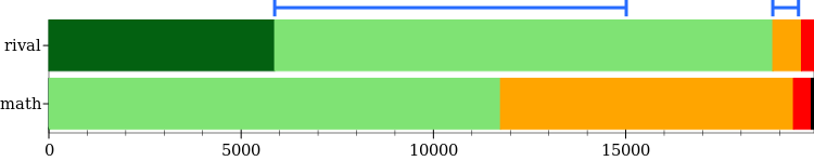
Figure 2. Rival versus Mathematica’s N on approximately 19895 hard inputs from the 481 Herbie 1.4 benchmark suite. Rival achieves better results for each outcome threshold, including successfully sampled points (dark green), points proven invalid (light green), unsamplable points (orange), or points with unknown results (red). Additionally, some points cause Mathematica to run out of memory or crash, shown in black. The blue intervals mark invalid and unsamplable points avoided by input search.

7.1. Methodology

Mathematica’s N function can compute mathematical expressions exactly to an arbitrary precision, precisely the task supported by Rival. We chose Mathematica as our baseline after comparing multiple traditional interval arithmetic libraries. Of all the evaluated libraries, Mathematica was the most robust and supported the most functions. For example, the MPFI library does not handle errors soundly (unlike Rival’s error intervals), has no built-in support for recomputation (unlike Rival’s movability flags), and lacks support for some mathematical functions like pow and erf. For an interval arithmetic library, soundness and weak completeness already require optimal interval endpoints, so traditional interval arithmetic libraries generally have the same results as Rival without its extensions. Meanwhile, Mathematica is a widely-used commercial product with extensive support for all mathematical functions and presumably-robust implementations of all of them. Furthermore, Mathematica’s documentation suggests that N is intended to handle invalid inputs soundly and cut off recomputation in some cases of over- and under-flow, making it at least comparable to Rival.

We model our evaluation task on sampling-based error estimation; that is, on the task of randomly sampling inputs to an expression and determine the ground-truth value of the expression at those inputs. We use a collection of 481 floating-point expressions drawn from sources like numerical methods textbooks, mathematics and physics papers, and surveys of open-source code, collected in the Herbie 1.4 benchmark suite. These benchmarks consist of mathematical expressions with 0–89 operations and 0–16 variables; 4 benchmarks contain conditionals and 47 have user-defined preconditions. Each benchmark is evaluated to double precision at 8 256 randomly sampled input points (for N, to the equivalent decimal precision). Both N and Rival are limited to 10240 bits; Rival is also limited to 31-bit exponents. In error estimation, most inputs to an expressions are “easy” points where any technique will succeed; the crux of the problem are the challenging or marginal points. To focus on these challenging points, we ignore inputs that both Mathematica and Rival can sample, and focus on the remaining more challenging points, which are 19895 out of the overall 126720. Evaluations are performed on a machine with an i7-4790K CPU (at 4.00GHz) and 32GB of DDR3 memory running Debian 10.0 (Buster), Racket 7.9 BC, and MPFR version 4.0.2-1.

The main methodological challenge is matching Mathematica’s and Rival’s semantics. Mathematica’s N function supports floating-point, fixed-precision, and exact computation; we convert the sampled input points to exact rational values to ensure that exact computation is performed. We also wrap each intermediate Mathematica operator to signal an error for Indeterminate or Complex outputs. We compare Mathematica’s and Rival’s outputs, when both tools are able to compute a value, to check that subtleties like atan2 argument order are correctly aligned between the two systems. We also capture warnings and errors, which Mathematica uses to indicate whether its evaluation is sound. These cross-checks give us confidence that Mathematica and Rival are asked to evaluate the same expressions on the same inputs. (Two points fail these cross-checks at the time of this writing. We have investigated these inputs, discovered them to trigger a bug in Mathematica, reported the bug to Wolfram support, and had it confirmed.) Rival’s input search has no direct analog in Mathematica, so for this experiment we randomly selected points without using input search. However, we did test whether input search would have allowed Rival to avoid sampling that point.

Evaluating Rival against Mathematica requires understanding Mathematica’s behavior on invalid and challenging inputs. Unfortunately, unlike Rival, Mathematica is proprietary, and the documentation is not always specific. Like Rival, Mathematica’s N attempts to detect invalid inputs and futile recomputations. In general, for invalid inputs Mathematica either returns a complex number or the special Indeterminate value for some intermediate operator. In Figure 2, these cases are considered proven domain error (light green). Mathematica also raises a variety of warnings, including for overflow and underflow; we conservatively assume these warnings are sound and are reached at low precision, and mark these cases unsamplable (orange in Figure 2). For Rival this status is used only when the interval is proven stuck before the maximum precision is reached. (More broadly, we interpret ambiguous cases as generously as possible toward Mathematica to ensure a fair comparison.) When Rival or Mathematica reach their internal precision limit, we use the unknown result status (red in Figure 2).

7.2. Results

Of the 19895 hard input points across our 481 benchmarks, Mathematica is able to resolve only 11744, while Rival is able to resolve 18824 points (60.3% better). Specifically, Rival samples 5872 points and proves a further 12952 to be invalid; Mathematica samples only 24 and proves only 11720 invalid. Rival’s error intervals, which integrate the detection of invalid inputs with recomputation, account for the difference in the number of points proven invalid.

Not only does Rival resolve more cases, it resolves nearly a superset of the cases resolved by Mathematica. Rival resolves 5877 points not resolved by Mathematica; Mathematica resolves only 26 points that Rival cannot. (Without access to Mathematica’s internals it’s hard to say how Mathematica resolves those 26 points. Our best guess is that it may be simplifying the benchmark expressions before evaluating them at an input.) Furthermore, when Mathematica is unable to resolve an input, it sometimes (64 cases) enters an infinite loop or declares that insufficient memory is available. We render these inputs in black in Figure 2; Rival never crashes in this way. Moreover, in 16 cases, the Mathematica process crashes and must be killed with SIGKILL, which may cause the user to lose work.

Both Rival and Mathematica are unable to resolve some inputs: 1071 points for Rival and 8151 for Mathematica. In these cases it’s important to give additional information to the user: some of these points may be resolvable with more precision, time, or memory, but others cannot be resolved due to algorithmic limitations. Rival’s movability flags, which prove 746 points unsamplable, soundly detect algorithmic constraints; Mathematica’s various warnings affect 7617 points (10.2$\times$ worse) and are unsound, sometimes triggered even for samplable inputs. Mathematica marks unsamplable 5830 points that Rival successfully samples as a result. Thus, unlike Rival’s movability flags, they do not advise whether the user ought to try again with more precision or abandon the computation. At the same time, Mathematica reaches its internal precision limit 1.4$\times$ more often than Rival because Rival’s movability flags allow it to identify unsamplable points at low precision.

For applications that need to sample valid inputs, Rival’s input search is additionally helpful. Input search is able to avoid sampling 9142 invalid inputs and 668 unsamplable inputs, thereby cutting the rate of invalid and unsamplable points by 74.6% (the blue intervals in Figure 2). This means that using Rival for sampling-based error estimation would yield even better results than those suggested by Figure 2, since input search allows Rival to avoid many challenging, invalid points. The overall picture of these results is that Rival is more capable than Mathematica: it is able to sample more points, discard more invalid points, and leave fewer indeterminate cases unresolved. It also does so without timeouts, memory exhaustion, or fatal crashes. Yet it also offers sound guarantees and valuable extensions like input search.

As a result of Rival’s improvements in interval arithmetic, Rival is 9.87$\times$ faster than Mathematica. Mathematica’s timeouts, OOM, and crashes also add to its runtime, but Rival is 9.03$\times$ faster than Mathematica even after excluding these inputs. This is a consequence of Rival’s better handling of invalid inputs and futile recomputation: any interval arithmetic library spends the bulk of its time doing high-precision arithmetic. For one library to be faster than another, then, that library must identify invalid inputs, detect futile recomputation, sample fewer such points, or in some other way do fewer high-precision operations. That’s precisely what Rival ’s extensions do; those extensions ultimately require just a few comparisons, so they add negligible overhead time, but they dramatically cut down on unnecessary computation. In fact, Rival is also (19.2%) faster than MPFI, another commonly-used interval arithmetic library, again due to Rival’s ability to skip unnecessary computation.

8. Detailed Analysis

This section expands on Section 7 to detail the performance of error intervals, movability flags, and input search individually, and to describe particularly challenging benchmarks. The data show that Rival’s extensions are effective, accomplish their task at low precision, and handle challenging inputs from a range of domains.

Figure 3. Counts of valid points (bottom, blue), domain errors (middle, yellow), infinite outputs (top, light blue), and precondition failures (too rare to be visible) for points sampled without input search. 80 bits of precision suffices for most points.

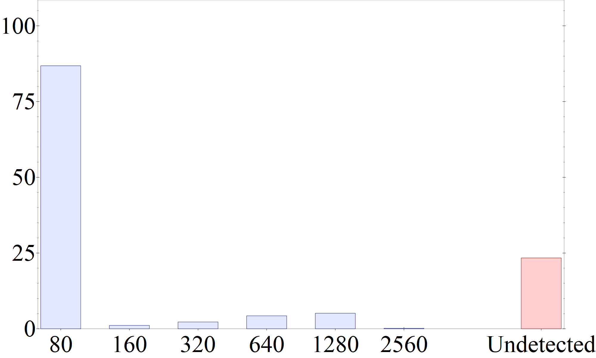
Figure 4. Counts of unsamplable points. Rival’s movability flags detect all but 19.0% of unsamplable points, with the majority detected at just 80 bits of precision. Detecting unsamplable points avoids timeouts and user disappointment.

Figure 5. Size of the $T$ (bottom, green), $O$ (middle, blue), and $F$ (top, red) sets after each iteration of Rival’s input search. The “0” bar shows the results of range analysis; the “$*$” bar shows the results of rejection sampling. On average, input search avoids 68.6% of invalid samples.

8.1. Error Intervals

Error intervals are evaluated by considering the internal precision at which they deem input points valid or invalid. Input search is disabled. Figure 5 counts valid and invalid points by the internal precision required. The vast majority of points are proven valid or invalid at 80 bits of precision, with 1280 bits the second-most common precision. This curious runner-up precision is largely due to trigonometric functions: the largest double-precision values are as large as $2^{1024}$, and 1280 bits is enough precision to identify their period modulo $\pi$. Recomputation automatically increases the precision to this level.

Compared to valid points, a larger fraction of invalid points are detected at 80 bits of precision, likely because for these points, Rival doesn’t need to compute a ground truth value, just prove that the point is invalid. The majority of invalid points result from infinite outputs and domain errors, while user-specified precondition failures are rare. Specifically among expressions with preconditions, 0.1% of sampled points are invalid, suggesting that error intervals work well even under these most challenging conditions.

The benchmark named “Harley’s example” demonstrates the importance of soundness for error and boolean intervals:

$$\begin{array}[]{l}\text{{pre}}\>c_{p}>0\land c_{n}>0\\ \text{{let}}\>a=1/(1+e^{-s}),b=1/(1+e^{-t})\>\text{{in}}\\ \left(a^{c_{p}}\cdot(1-a)^{c_{p}}\right)/\left(b^{c_{n}}\cdot(1-b)^{c_{n}}\right)\end{array}$$

Some inputs to this expression produce outputs just below or just above the point where the output rounds to infinity; error intervals force recomputation until it is clear whether which of the points are valid, which can require as many as 5120 bits.

8.2. Movability Flags

Movability flags are evaluated by considering the precision at which they can prove a point unsamplable. Figure 5 shows that movability flags detect a 81.0% of unsamplable points and thus prevent most futile recomputations. Unsamplable points are found (and warnings issued) for 21 input expressions, mostly involving ratios of exponential functions. For example, the expq2 benchmark involves the expression $\exp(x)/(\exp(x)-1)$; its unsamplable points can be detected with just 80 bits of precision. For more difficult expressions, higher precision is sometimes necessary to prove unsamplability; consider the expq3 benchmark:

$$\frac{\varepsilon\cdot\left(e^{(a+b)\cdot\varepsilon}-1\right)}{\left(e^{a\cdot\varepsilon}-1\right)\cdot\left(e^{b\cdot\varepsilon}-1\right)},\text{ with }{-1}<\varepsilon<1.$$

This benchmark is unsamplable when $a=\varepsilon=10^{-200}$ and $b=10^{200}$: the second term in the denominator overflows, but at low precisions the first rounds down to $0$, making the denominator possibly zero. Only at 2560 bits of precision does it become clear that the denominator is very large, which is necessary to prove the expression unsamplable.

By contrast, cases where movability flags fail often seem like oversights by the benchmark developers or the users those benchmarks are derived from. For example, the regression suite’s exp-w benchmark, $e^{-w}\cdot\text{{pow}}(\ell,e^{w}),$ fails to detect unsamplable points when $\ell$ is negative and $w$ large and positive, $\text{{pow}}(\ell,e^{w})$ raises a negative number to a possibly-infinite power. Since Rival does not track movability for error intervals, it does not detect that recomputation here is futile. But the author of this expression likely intended $\ell$ to be close to $1$, instead of negative. Similarly, movability flags fail on textbook examples of difficult-to-analyze functions like “Kahan’s Monster”:

$$\begin{array}[]{l}\text{{pre}}\>y>0\\ \text{{let}}\>z=\left(|y-\sqrt{y^{2}+1}|-1/(y+\sqrt{y^{2}+1})\right),z_{2}=z\cdot z\>\text{{in}}\\ \text{{if}}\>z_{2}=0\>\text{{then}}\>1\>\text{{else}}\>(\exp{z_{2}}-1)/z_{2}\end{array}$$

In the reals, $z$ is exactly $0$ so the program yields $1$; with interval arithmetic, $z$ is a narrow interval straddling $0$ and Rival cannot rule out a division by zero in the else branch. Of course, since real computation is undecidable, constructing counterexamples like this will be possible for any algorithm.

8.3. Input Search

Input search is evaluated by considering the fraction of the input space in the $T$, $O$, and $F$ sets. Figure 5 shows these fractions as a percentage of the total search space, averaged over all benchmarks, at each input search iteration. Over 15 iterations, input search discards 22.8% of the total input space and proves an additional 54.9% to contain only valid points. As a result, 71.1% of sampled points are guaranteed to be valid and do not need to be rejection-sampled, and 74.6% of invalid points are avoided.

Input search helps Rival sample from benchmarks that would otherwise be infeasible to sample from. Consider Jmat.Real.erfi:

$$\left(\frac{1}{\sqrt{\pi}}e^{x\cdot x}\right)\cdot\left(\frac{1}{|x|}+\frac{1}{2}\frac{1}{|x|^{3}}+\frac{3}{4}\frac{1}{|x|^{5}}+\frac{15}{8}\frac{1}{|x|^{7}}\right),\text{ with }x\geq\frac{1}{2}$$

Inputs above approximately $30$ overflow, so roughly 0.15% of double-precision floating-point values are valid. But input search identifies the valid range with ease, and only 1.4% of samples are ultimately rejected.

Input search can also sometimes prove that there are no valid inputs at all. In the benchmark

$$\sqrt{\log(x)+\sin(x)}/\sin^{-1}(x+2),$$

the term $\sin^{-1}(x+2)$ requires $-3\leq x\leq-1$, while $\log(x)$ requires $x>0$, so the benchmark has no valid points. This benchmark was originally derived from a user submission; input search allows Rival to provide a helpful error message to the (doubtless confused) user.

8.4. Generality

		Error Intervals				Movability Flags		Input Search
Benchmarks	$N$	Valid	Pre.	Inf.	Error	Total	Detected	$|T|$	$|O|$	$|F|$
hamming	$28$	$76.8\%$	$0.0\%$	$6.3\%$	$16.9\%$	$4.6\%$	$100.0\%$	$53.9\%$	$20.1\%$	$26.0\%$
haskell	$270$	$67.1\%$	$0.0\%$	$17.3\%$	$15.6\%$	$0.1\%$	$100.0\%$	$60.5\%$	$25.1\%$	$14.4\%$
libraries	$50$	$69.9\%$	$0.0\%$	$18.2\%$	$11.9\%$	$3.0\%$	$32.8\%$	$60.1\%$	$12.2\%$	$27.7\%$
mathematics	$39$	$65.4\%$	$2.8\%$	$5.0\%$	$26.9\%$	$17.6\%$	$88.1\%$	$36.3\%$	$20.8\%$	$43.0\%$
numerics	$38$	$79.5\%$	$0.0\%$	$15.3\%$	$5.1\%$	$0.7\%$	$90.6\%$	$41.2\%$	$8.2\%$	$50.6\%$
physics	$31$	$51.3\%$	$0.0\%$	$15.9\%$	$32.9\%$	$6.7\%$	$96.9\%$	$32.9\%$	$40.8\%$	$26.3\%$
regression	$13$	$87.3\%$	$0.0\%$	$5.3\%$	$7.4\%$	$8.3\%$	$33.4\%$	$53.0\%$	$21.0\%$	$25.9\%$
tutorial	$3$	$90.1\%$	$0.0\%$	$9.9\%$	$0.0\%$	$0.0\%$	$100.0\%$	$84.8\%$	$6.8\%$	$8.4\%$
Herbie v1.4	$481$	$67.3\%$	$0.3\%$	$14.8\%$	$17.6\%$	$3.0\%$	$81.0\%$	$54.9\%$	$22.3\%$	$22.8\%$
User Inputs	$4888$	$63.5\%$	$0.0\%$	$13.5\%$	$23.0\%$	$5.0\%$	$55.8\%$	$61.1\%$	$17.6\%$	$21.3\%$
FPBench	$126$	$79.9\%$	$14.2\%$	$5.9\%$	$0.0\%$	$2.1\%$	$93.3\%$	$19.8\%$	$7.6\%$	$72.6\%$

Table 1. Rival’s success on subsets and additional benchmark sets. The table shows the percentage of points that are valid or invalid for various reasons; the total fraction unsamplable points and the fraction of those detected by movability flags; and the sizes of $|T|$, $|O|$, and $|F|$ after input search. Results for error intervals and movability flags are with input search disabled to separate the impacts of each extension.

To demonstrate the generality of error intervals, movability flags, and input search across domains, we perform a subgroup analysis. Table 1 breaks down the Herbie 1.4 benchmarks into their 8 component suites.

Rival is effective in a wide variety of circumstances. Different benchmark suites range from 51.3% (physics) to 90.1% (tutorial) valid points, and the effectiveness of input search correspondingly varies. Movability flags are 100.0% effective in the hamming benchmark suite, which has many ratios of exponential functions, but much less effective in the regression suite, which is composed of difficult-to-analyze examples that once triggered timeouts or crashes in the Herbie project that compiled these benchmarks.

We also consider two additional benchmark sets to evaluate Rival’s generality: the 126 standard FPBench benchmarks and 4888 publically-accessible user submissions to the Herbie web demo. The FPBench suite is intended for benchmarking floating-point analysis tools and makes extensive use of preconditions. Despite this, input search samples a valid point with 93.8% probability, discarding 72.6% of the input space, and movability flags are extremely effective at detecting unsamplable points. The user-submitted benchmarks are the other extreme: unorganized, duplicative, and sometimes copied from the other two suites. Rival nonetheless preforms well—especially input search, since there are no preconditions among the user submissions so detecting valid inputs is easier. Both the subset analysis and validation sets thus show that error intervals, movability flags, and input search are effective in general across domains.

9. Discussion

The Rival library, containing error intervals, movability flags, and input search, is publicly available as open source software.

9.1. Implementing Rival

Ensuring soundness and weak completeness in Rival required care. We started by splitting each function’s domain into monotonic regions. For example, fmod has monotonic regions defined by $ky\leq x<(k+1)y$ for some $k$, monotonically increasing in $x$ and decreasing in $y$. Finding the minimum or maximum of a function then requires finding the maximum over all of the monotonic regions in the input intervals. Soundness is guaranteed by the monotonicity of the function within each region, while weak completeness is guaranteed because the output interval’s endpoints come from particular points in some monotonic region. We wrote paper proofs for each function to ensure that we accurately identified the monotonic regions, and verified that we correctly chose the maximum and minimum points using Mathematica.

To catch one-off oversights and typos, we additionally deployed millions of random tests for soundness on both wide and narrow intervals, weak completeness (by subdividing intervals), and movability (by recomputing in higher precision). These tests further improved Rival’s reliability. One random test found that sin internally rounded $\pi$ to nearest instead of rounding $\pi$ differently for the two endpoints; this is a soundness bug. Another random test found that defining $\text{{fmod}}(x,y)$ by $\text{{trunc}}(x/y)\cdot y$ fails to account for the correlation between $x/y$ and $x$; this is a completeness bug fixed with a custom implementation of fmod. Finally, a manual audit found that movability flags weren’t being set when pow underflowed to $0$, which lead to movability flags missing some unsamplable points. We replaced the pow movability logic with the identity $\text{{pow}}(x,y)=\text{{exp}}(y\cdot\text{{log}}(x))$ to avoid duplicating the movability logic.

9.2. Deploying Rival

We began developing Rival three years ago to replace unsound sampling heuristics for a popular floating point analysis and error estimation tool. Rival was deployed to production one year ago and has since been used by thousands of users.

Rival was originally a traditional interval arithmetic library aimed at soundly computing error-free ground truths. At first, our main concern was speed: interval arithmetic generally requires evaluating each function twice (once for each endpoint) while the existing unsound heuristics evaluated each function once, so we expected performance to be twice as bad. These concerns were unfounded. Instead, though “difficult” points needed higher precision in Rival (in order to soundly prove they were correctly sampled), Rival could sample “easy” points with lower precision than the earlier heuristics, so replacing them with Rival did not slow down sampling.

Instead of speed, the core problem with this initial version of Rival was its handling of invalid inputs. Initially, Rival used NaN endpoints to indicate domain errors, much like the open source MPFI library (Revol and Rouillier, 2005). But those NaN endpoints would sometimes be lost in later computations, leading to Rival erroneously computing outputs for invalid inputs. We developed error intervals to guarantee that Rival only sampled valid points. With this problem fixed, we realized that unsamplable points consumed an unjustifiably large share of sampling time. Movability flags were developed out of the realization that overflow was behind most of these unsamplable points and could be easily detected at low precision. This sped up sampling, and allowed samping inputs for many larger expressions that used to time out. But this only revealed that most of those sampled inputs were invalid or unsamplable; input search was developed to address this issue.

All told, Rival is sounder, faster, and more user-friendly than the heuristic approach it replaced. In rare cases, the earlier heuristics computed incorrect ground truth values, even for textbook examples such as $\sqrt{x+1}-\sqrt{x}$; Rival never does. Its input search and movability flags allow estimating error for larger benchmarks than the earlier heuristics could support. And by rigorously handling error cases, algorithmic limitations, and even edge cases like benchmarks with no valid inputs, Rival allows for clearer and more actional error messages for users. Over all, through error intervals, movability flags, and input search, Rival successfully addressed user-visible issues and improved the application it was embedded in.

10. Related Work

Computable Reals

The problem of computing the exact value of a mathematical expression has a long history. Early work (Minsky, 1967; Boehm, 1987; Boehm et al., 1986; Boehm, 2004) explored various representations for “computable real” values and developed algorithms for computing functions over them. One common representation involving scaled 2-adic numbers yields particularly simple implementations (Ménissier-Morain, 2005; Briggs, 2006), but is slow, especially for expressions having certain forms (Li and Yong, 2007). Interval arithmetic was later discovered to be better suited to this task, as it tends to be faster (Lee and Boehm, 1990b).

Interval arithmetic has been widely available since 1967’s XSC (WR-SWT, 2020). Today, the Boost (Melquiond, 2006) and Gaol (Goualard, 2019) libraries are widely used, both providing interval arithmetic with double-precision endpoints. The more modern Moore library (Mascarenhas, 2016) provides arbitrary-precision endpoints as well. The IEEE 1788 standard formalizes several forms of interval arithmetic (iee, 2015), including interval decorations, which could be used to implement Rival’s error intervals and movability flags. Recent work welds computable real algorithms to decision procedures for special cases like as rational arithmetic, and provides an API for supporting the combination (Boehm, 2020). Despite its unique benefits for user-facing calculator applications, general-purpose error estimation generally lies outside the special cases, so Rival’s methods are orthogonal. RealPaver uses interval arithmetic to characterize the solution sets of nonlinear constraints (Jaulin et al., 2001), to aid in pruning for global function optimization (Granvilliers and Benhamou, 2006), similar to Rival’s boolean intervals and input search. However, since RealPaver is targetted specifically at mathematical optimization problems, it neither tracks rounding error nor provides error intervals nor guarantees uniform sampling.

Error Estimation

There is a large literature on measuring floating-point rounding error. One approach (Darulova and Kuncak, 2014; Izycheva and Darulova, 2017; Martel, 2009) uses one interval to track value ranges and another interval to track rounding errors, producing a sound error bound for the whole computation. This approach can be extended to and intraprocedural, modular abstract interpretation (Titolo et al., 2018; Damouche et al., 2015; Martel, 2018). Error Taylor forms can also bound floating-point error (Solovyev et al., 2015; Chiang et al., 2017; Das et al., 2020) and generally providing tighter bounds than interval-based bounds, as does semidefinite programming (Magron et al., 2017). Both error Taylor forms and semidefinite characterize error at a fixed input point and then apply sound global optimization, such as Gelpia (Briggs, 2019), which uses interval arithmetic to compute sound bounds.

An alternative approach to error estimation aims to generate inputs with particularly large rounding error. S3FP (Chiang et al., 2014) treats the expression itself as a black box, while FPGen (Hui Guo, 2020) uses symbolic execution to more efficiently target problematic input ranges. Other tools target rare errors (Zou et al., 2015; Yi et al., 2017, 2019) or attempt to maximize code coverage (Bagnara et al., 2013; Fu and Su, 2017). In each case, these inputs are generated, selected, or mutated by comparing to an error-free ground-truth, usually computed with arbitrary precision or interval arithmetic. Rival’s enhancements to interval arithmetic are especially attractive for input generation methodologies, since they often generate invalid inputs (which they should select against) or unsamplable inputs (which they should ignore).

Error Detection

Some tools aim to localize rounding error within a large program. FpDebug (Benz et al., 2012) and Herbgrind (Sanchez-Stern et al., 2018) use Valgrind to target x86 binaries and detect rounding error using higher-precision shadow values. PositDebug does the same but for posit, rather than floating-point, values (Chowdhary et al., 2020). Bao and Zhang (2013) instead detect control-flow divergence and re-executing the program at higher precision. Herbie (Panchekha et al., 2015), an error repair tool, uses heuristics to select a sufficiently high shadow value precision; the algorithm is unsound and can compute incorrect ground truths. TAFFO replaces user-selected inputs with run-time values to dynamically substitute fixed-point for floating-point computation (Cherubin et al., 2020). All of these need to compute an error-free ground truth and are susceptible to invalid or unsamplable inputs.

11. Conclusion

This paper addresses three problems common to traditional interval arithmetic implementations. Error intervals track the necessity and possibility of domain errors, and can be combined with other boolean constraints to provide a rich description of valid and invalid inputs. Movability flags add another pair of boolean flags to track the impact of overflows, identifying inputs where algorithmic limitations prevent identifying a correct ground-truth value. Finally, input search leverages both error intervals and movability flags to identify regions of valid, samplable points, even when those regions have low measure in the input space. Rival implements all three features and outperforms the state-of-the-art Mathematica 12.1.1 N function, resolving 60.3% more inputs, returning indeterminate results 10.2$\times$ less often, and avoiding all cases of fatal error.

References

- (1)
- iee (2015) 2015. IEEE Standard for Interval Arithmetic. IEEE Std. 1788-2015 (2015).
- Altman et al. (2003) Micah Altman, Jeff Gill, and Michael P. McDonald. 2003. Numerical Issues in Statistical Computing for the Social Scientist. Springer-Verlag. 1–11 pages.
- Altman and McDonald (2003) Micah Altman and Michael P. McDonald. 2003. Replication with attention to numerical accuracy. Political Analysis 11, 3 (2003), 302–307. http://pan.oxfordjournals.org/content/11/3/302.abstract
- Bagnara et al. (2013) R. Bagnara, M. Carlier, R. Gori, and A. Gotlieb. 2013. Symbolic Path-Oriented Test Data Generation for Floating-Point Programs. In 2013 IEEE Sixth International Conference on Software Testing, Verification and Validation. 1–10.
- Bao and Zhang (2013) Tao Bao and Xiangyu Zhang. 2013. On-the-fly Detection of Instability Problems in Floating-point Program Execution. SIGPLAN Not. 48, 10 (Oct. 2013), 817–832. https://doi.org/10.1145/2544173.2509526
- Benz et al. (2012) Florian Benz, Andreas Hildebrandt, and Sebastian Hack. 2012. A Dynamic Program Analysis to Find Floating-point Accuracy Problems (PLDI ’12). ACM, New York, NY, USA, 453–462. http://doi.acm.org/10.1145/2254064.2254118
- Boehm (1987) Hans J. Boehm. 1987. Constructive Real Interpretation of Numerical Programs (SIGPLAN ’87). ACM, 214–221. https://doi.org/10.1145/29650.29673
- Boehm (2004) Hans J. Boehm. 2004. The constructive reals as a Java Library. Journal Logical and Algebraic Programming 64 (2004), 3–11.
- Boehm (2020) Hans-J. Boehm. 2020. Towards an API for the Real Numbers. In Proceedings of the 41st ACM SIGPLAN Conference on Programming Language Design and Implementation (London, UK) (PLDI 2020). Association for Computing Machinery, New York, NY, USA, 562–576. https://doi.org/10.1145/3385412.3386037
- Boehm et al. (1986) Hans J. Boehm, Robert Cartwright, Mark Riggle, and Michael J. O’Donnell. 1986. Exact Real Arithmetic: A Case Study in Higher Order Programming (LFP ’86). ACM, 162–173. https://doi.org/10.1145/319838.319860
- Briggs (2019) Ian Briggs. 2019. Global Extrema Locator Parallelization for Interval Arithmetic. https://github.com/soarlab/gelpia
- Briggs (2006) Keith Briggs. 2006. Implementing exact real arithmetic in python, C++ and C. Theoretical Computer Science 351, 1 (2006), 74 – 81. https://doi.org/10.1016/j.tcs.2005.09.058 Real Numbers and Computers.
- Cherubin et al. (2020) S. Cherubin, D. Cattaneo, M. Chiari, A. D. Bello, and G. Agosta. 2020. TAFFO: Tuning Assistant for Floating to Fixed Point Optimization. IEEE Embedded Systems Letters 12, 1 (2020), 5–8.
- Chiang et al. (2017) Wei-Fan Chiang, Mark Baranowski, Ian Briggs, Alexey Solovyev, Ganesh Gopalakrishnan, and Zvonimir Rakamarić. 2017. Rigorous Floating-point Mixed-precision Tuning (POPL). 300–315. https://doi.org/10.1145/3009837.3009846
- Chiang et al. (2014) Wei-Fan Chiang, Ganesh Gopalakrishnan, Zvonimir Rakamaric, and Alexey Solovyev. 2014. Efficient Search for Inputs Causing High Floating-Point Errors. In Proceedings of the 19th ACM SIGPLAN Symposium on Principles and Practice of Parallel Programming (PPoPP ’14). Association for Computing Machinery, New York, NY, USA, 43–52. https://doi.org/10.1145/2555243.2555265
- Chowdhary et al. (2020) Sangeeta Chowdhary, Jay P. Lim, and Santosh Nagarakatte. 2020. Debugging and Detecting Numerical Errors in Computation with Posits. In Proceedings of the 41st ACM SIGPLAN Conference on Programming Language Design and Implementation (London, UK) (PLDI 2020). Association for Computing Machinery, New York, NY, USA, 731–746. https://doi.org/10.1145/3385412.3386004
- Damouche et al. (2015) Nasrine Damouche, Matthieu Martel, and Alexandre Chapoutot. 2015. Formal Methods for Industrial Critical Systems: 20th International Workshop, FMICS 2015 Oslo, Norway, June 22-23, 2015 Proceedings. (2015), 31–46.
- Darulova and Kuncak (2014) Eva Darulova and Viktor Kuncak. 2014. Sound Compilation of Reals (POPL). 14 pages. http://doi.acm.org/10.1145/2535838.2535874
- Das et al. (2020) Arnab Das, Ian Briggs, Ganesh Gopalakrishnan, Sriram Krishnamoorthy, and Pavel Panchekha. 2020. Scalable yet Rigorous Floating-Point Error Analysis. In 2020 SC20: International Conference for High Performance Computing, Networking, Storage and Analysis (SC). IEEE Computer Society, Los Alamitos, CA, USA, 1–14. https://doi.org/10.1109/SC41405.2020.00055
- European Commission (1998) European Commission. 1998. The introduction of the euro and the rounding of currency amounts. European Commission, Directorate General II Economic and Financial Affairs.
- Fousse et al. (2007) Laurent Fousse, Guillaume Hanrot, Vincent Lefèvre, Patrick Pélissier, and Paul Zimmermann. 2007. MPFR: A Multiple-Precision Binary Floating-Point Library with Correct Rounding. ACM Trans. Math. Software 33, 2 (June 2007), 13:1–13:15. http://doi.acm.org/10.1145/1236463.1236468
- Fu and Su (2017) Zhoulai Fu and Zhendong Su. 2017. Achieving high coverage for floating-point code via unconstrained programming. ACM SIGPLAN Notices 52 (06 2017), 306–319. https://doi.org/10.1145/3140587.3062383
- Goualard (2019) Frederic Goualard. 2019. Gaol: NOT Just Another Interval Library. https://sourceforge.net/projects/gaol/
- Granvilliers and Benhamou (2006) Laurent Granvilliers and Frédéric Benhamou. 2006. Algorithm 852: RealPaver: An Interval Solver Using Constraint Satisfaction Techniques. ACM Trans. Math. Softw. 32, 1 (March 2006), 138–156. https://doi.org/10.1145/1132973.1132980
- Hamming (1987) Richard Hamming. 1987. Numerical Methods for Scientists and Engineers (2nd ed.). Dover Publications.
- Hui Guo (2020) Cindy Rubio-González Hui Guo. 2020. Efficient Generation of Error-Inducing Floating-Point Inputs via Symbolic Execution (ICSE’20).
- Izycheva and Darulova (2017) Anastasiia Izycheva and Eva Darulova. 2017. On sound relative error bounds for floating-point arithmetic (FMCAD). 15–22. https://doi.org/10.23919/FMCAD.2017.8102236
- Jaulin et al. (2001) L. Jaulin, M. Kieffer, O. Didrit, and E. Walter. 2001. Applied Interval Analysis: With Examples in Parameter and State Estimation, Robust Control and Robotics. Springer London. https://books.google.com/books?id=ZG0qXkYUe_AC
- Kahan (2000) William Kahan. 2000. Miscalculating Area and Angles of a Needle-like Triangle. Technical Report. University of California, Berkeley. http://www.cs.berkeley.edu/~wkahan/Triangle.pdf
- Kahan and Darcy (1998) W. Kahan and Joseph D. Darcy. 1998. How Java’s Floating-Point Hurts Everyone Everywhere. Technical Report. University of California, Berkeley. 80 pages. http://www.cs.berkeley.edu/~wkahan/JAVAhurt.pdf
- Lee and Boehm (1990a) Vernon A. Lee and Hans-J. Boehm. 1990a. Optimizing Programs over the Constructive Reals (PLDI ’90). New York, NY, USA. https://doi.org/10.1145/93542.93558
- Lee and Boehm (1990b) Vernon A. Lee, Jr. and Hans J. Boehm. 1990b. Optimizing Programs over the Constructive Reals (PLDI ’90). ACM, 102–111. https://doi.org/10.1145/93542.93558
- Li and Yong (2007) Yong Li and Jun-Hai Yong. 2007. Efficient Exact Arithmetic over Constructive Reals. In The 4th Annual Conference on Theory and Applications of Models of Computation. Shanghai, China. https://hal.inria.fr/inria-00517598
- Magron et al. (2017) Victor Magron, George Constantinides, and Alastair Donaldson. 2017. Certified roundoff error bounds using semidefinite programming. Transactions on Mathematical Software 43, 4 (2017), 34.
- Martel (2009) Matthieu Martel. 2009. Program Transformation for Numerical Precision (PEPM ’09). ACM, New York, NY, USA, 101–110. http://doi.acm.org/10.1145/1480945.1480960
- Martel (2018) Matthieu Martel. 2018. Strongly Typed Numerical Computations. ICFEM (2018), 197–214.
- Mascarenhas (2016) Walter F. Mascarenhas. 2016. Moore: Interval Arithmetic in Modern C++. CoRR abs/1611.09567 (2016). arXiv:1611.09567 http://arxiv.org/abs/1611.09567
- McCullough and Vinod (1999) B. D. McCullough and H. D. Vinod. 1999. The Numerical Reliability of Econometric Software. Journal of Economic Literature 37, 2 (1999), 633–665.
- Melquiond (2006) Guillaume Melquiond. 2006. Boost Interval Arithmetic Library. https://www.boost.org/doc/libs/1_73_0/libs/numeric/interval/doc/interval.htm
- Minsky (1967) Marvin L. Minsky. 1967. Computation: Finite and Infinite Machines. Prentice-Hall, Inc.
- Ménissier-Morain (2005) Valérie Ménissier-Morain. 2005. Arbitrary precision real arithmetic: design and algorithms. The Journal of Logic and Algebraic Programming 64, 1 (2005), 13 – 39. https://doi.org/10.1016/j.jlap.2004.07.003 Practical development of exact real number computation.
- Panchekha et al. (2015) Pavel Panchekha, Alex Sanchez-Stern, James R. Wilcox, and Zachary Tatlock. 2015. Automatically Improving Accuracy for Floating Point Expressions (PLDI).
- Revol and Rouillier (2005) Nathalie Revol and Fabrice Rouillier. 2005. Motivations for an Arbitrary Precision Interval Arithmetic and the MPFI Library. Reliable Computing 11, 4 (2005), 275–290. https://doi.org/10.1007/s11155-005-6891-y
- Rubio-González et al. (2013) Cindy Rubio-González et al. 2013. Precimonious: Tuning assistant for floating-point precision (SC). IEEE, 1–12.
- Sanchez-Stern et al. (2018) Alex Sanchez-Stern, Pavel Panchekha, Sorin Lerner, and Zachary Tatlock. 2018. Finding Root Causes of Floating Point Error (PLDI). 256–269. https://doi.org/10.1145/3192366.3192411
- Solovyev et al. (2015) Alexey Solovyev, Charlie Jacobsen, Zvonimir Rakamaric, and Ganesh Gopalakrishnan. 2015. Rigorous Estimation of Floating-Point Round-off Errors with Symbolic Taylor Expansions (FM).
- Tang et al. (2010) Enyi Tang, Earl Barr, Xuandong Li, and Zhendong Su. 2010. Perturbing Numerical Calculations for Statistical Analysis of Floating-Point Program (in)Stability. In Proceedings of the 19th International Symposium on Software Testing and Analysis (Trento, Italy) (ISSTA ’10). Association for Computing Machinery, New York, NY, USA, 131–142. https://doi.org/10.1145/1831708.1831724
- Titolo et al. (2018) Laura Titolo, Marco A Feliú, Mariano Moscato, and César A Munoz. 2018. An Abstract Interpretation Framework for the Round-Off Error Analysis of Floating-Point Programs (VMCAI). 516–537.
- Toronto and McCarthy (2014) N. Toronto and J. McCarthy. 2014. Practically Accurate Floating-Point Math. Computing in Science Engineering 16, 4 (July 2014), 80–95.
- U.S. General Accounting Office (1992) U.S. General Accounting Office. 1992. Patriot Missile Defense: Software Problem Led to System Failure at Dhahran, Saudi Arabia. http://www.gao.gov/products/IMTEC-92-26
- Weber-Wulff (1992) Debora Weber-Wulff. 1992. Rounding error changes Parliament makeup. http://catless.ncl.ac.uk/Risks/13.37.html#subj4
- Wolfram (2020) Wolfram. 2020. $MaxExtraPrecision—Wolfram Language Documentation. https://reference.wolfram.com/language/ref/$MaxExtraPrecision.html
- WR-SWT (2020) WR-SWT. 2020. History of XSC-Languages and Credits. http://www.xsc.de
- Yi et al. (2017) X. Yi, L. Chen, X. Mao, and T. Ji. 2017. Efficient Global Search for Inputs Triggering High Floating-Point Inaccuracies. In 2017 24th Asia-Pacific Software Engineering Conference (APSEC). 11–20.
- Yi et al. (2019) Xin Yi, Liqian Chen, Xiaoguang Mao, and Tao Ji. 2019. Efficient Automated Repair of High Floating-Point Errors in Numerical Libraries. Proc. ACM Program. Lang. 3, POPL, Article 56 (Jan. 2019), 29 pages. https://doi.org/10.1145/3290369
- Zou et al. (2015) D. Zou, R. Wang, Y. Xiong, L. Zhang, Z. Su, and H. Mei. 2015. A Genetic Algorithm for Detecting Significant Floating-Point Inaccuracies. In 2015 IEEE/ACM 37th IEEE International Conference on Software Engineering, Vol. 1. 529–539.