Two-Loop Rational Terms for Spontaneously Broken Theories

Abstract

Rational counterterms are a key ingredient for the automation of loop calculations through numerical methods. Building on the recently established properties of rational terms of UV origin at two loops, in this paper we present a systematic method for the determination of rational counterterms within spontaneously broken theories. In particular we introduce a generalised vev-expansion approach that makes it possible to obtain the rational counterterms of UV origin for a spontaneously broken theory by means of calculations in the unbroken phase. The drastic simplifications that result from the underlying symmetry open the door to the efficient determination of rational counterterms for the full Standard Model at two loops. The renormalisation-scheme dependence is analysed in detail, and we show that rational counterterms need to be determined only once and for all in a generic renormalisation scheme for the symmetric phase and, a posteriori, they can be easily adapted to a wide range of physical renormalisation schemes for the spontaneously broken phase. As a first application we determine the full set of $\mathcal{O}(\alpha_{\scriptscriptstyle{\mathrm{S}}}^{2})$ rational counterterms of UV origin for the full Standard Model, i.e. for all superficially UV-divergent two-loop vertex functions involving combinations of gluons, quarks, electroweak vector bosons and scalar bosons.

1 Introduction

The ultraviolet (UV) and infrared (IR) singularities of scattering amplitudes in perturbative quantum-field theory are typically regularised dimensionally, i.e. via analytic continuation in the number of space-time dimensions, $D=4-2{\varepsilon}$ tHooft:1972tcz . Within numerical frameworks, the need of computing loop amplitudes as a function of a continuous dimensional parameter $D$ can represent a significant obstacle. For this reason, a variety of methods have been proposed that aim at restricting—in part or entirely—the calculations of loop amplitudes to an integer number of space-time dimensions Bern:1991aq ; Kilgore:2012tb ; Siegel:1979wq ; Signer:2005iu ; Xiao:2006vr ; Binoth:2006hk ; Ossola:2008xq ; Badger:2008cm ; Giele:2008ve ; Abreu:2017hqn ; Pittau:2012zd ; Page:2015zca ; Fazio:2014xea ; Cherchiglia:2010yd ; Soper:1999xk ; Catani:2008xa ; Becker:2010ng ; Anastasiou:2018rib ; Capatti:2019edf .

At one loop, the most efficient and flexible automated tools on the market Buccioni:2019sur ; Denner:2017wsf ; vanHameren:2009dr ; Hirschi:2011pa rely on an implementation of dimensional regularisation based on rational counterterms Ossola:2008xq . The key idea is that loop amplitudes can be computed through numerical algorithms that build the numerator of loop integrands in $D_{\mathrm{n}}=4$ dimensions, while the remaining contributions stemming from the interplay of the $(D_{\mathrm{n}}-4)$-dimensional parts of the loop numerators with UV poles are reconstructed a posteriori by means of process-independent rational counterterms Draggiotis:2009yb ; Garzelli:2009is ; Pittau:2011qp .

This method was a key ingredient for the automation of one-loop calculations, and the foundations for its extension to two loops have been established in Pozzorini:2020hkx ; Lang:2020nnl , where it was shown that renormalised two-loop amplitudes can be constructed through a modified version of the R-operation for loop amplitudes with $D_{\mathrm{n}}=4$ dimensional integrand numerators. In this approach, the usual one-loop and two-loop counterterms for the subtraction of UV poles are supplemented by corresponding rational counterterms, which reconstruct the contributions that arise from the interplay of UV poles with the $(D-4)$-dimensional parts of loop numerators. The subtraction of quadratic one-loop subdivergences in $D_{\mathrm{n}}=4$ dimensions requires additional UV counterterms proportional to $\tilde{q}^{2}/{\varepsilon}$, where $\tilde{q}$ is the $(D-4)$-dimensional part of the loop momentum. All required counterterms are local and process independent. Within a given theoretical model, each potentially UV-divergent 1PI vertex function gives rise to a rational counterterm, which needs to be determined only once and for all. A general method for the determination of two-loop rational counterterms has been presented in Pozzorini:2020hkx ; Lang:2020nnl .

To date, the study of two-loop rational terms was restricted to contributions stemming from UV divergences, assuming that IR divergences are irrelevant. This expectation is supported by the fact that one-loop amplitudes are free from rational terms of IR origin Bredenstein:2008zb . In general, this is not the case beyond one loop. However, we expect that the standard procedure for the subtraction of IR divergences should lead to a cancellation of rational terms of IR origin. This conjecture will be the subject of future investigations, while in this paper we will consider only rational terms of UV origin. For convenience, the latter will be referred to simply as rational terms.

One-loop rational counterterms $\delta\mathcal{R}_{1}$ do not depend on the choice of UV renormalisation scheme, while two-loop rational counterterms $\delta\mathcal{R}_{2}$ are scheme dependent Lang:2020nnl . This dependence involves a trivial contribution, which corresponds to the naive renormalisation of $\delta\mathcal{R}_{1}$ counterterms, plus a non-trivial scheme dependence, which is due to the fact that the multiplicative renormalisation of UV subdivergences does not commute with the projection of loop numerators to $D_{\mathrm{n}}=4$ dimensions. As shown in Lang:2020nnl , both contributions are process independent, and the scheme-dependent part of $\delta\mathcal{R}_{2}$ counterterms can be expressed as a linear combination of generic one-loop renormalisation constants, which can be adapted a posteriori to any desired scheme. The methods presented in Pozzorini:2020hkx ; Lang:2020nnl are briefly reviewed in Section 2 of the present paper.

So far, two-loop rational counterterms are known explicitly only for U(1) and SU($N$) gauge theories Pozzorini:2020hkx ; Lang:2020nnl . In principle, corresponding results for the full Standard Model (SM) can be derived using the same techniques. However, due to symmetry breaking, the required calculations can become prohibitively involved in the electroweak (EW) sector of the SM. In particular, the fact that the various states of SU(2)$\times$U(1) multiplets acquire different masses, can mix with one another, and receive different field- and mass-renormalisation constants, represent major sources of additional complexity as compared to unbroken theories.

In order to circumvent these difficulties, in this paper we present a new method for the efficient derivation of two-loop rational counterterms within spontaneously broken (SB) theories. This approach is based on the systematic expansion of loop amplitudes in the vacuum expectation value (vev). As is well known, the vev expansion of loop amplitudes in a SB theory can be expressed in terms of corresponding amplitudes in the unbroken phase with additional external Higgs lines that carry zero momentum. These so-called vev insertions provide the correct expansion of loop amplitudes in $D_{\mathrm{n}}=D$ dimensions, while in $D_{\mathrm{n}}=4$ dimensions, as we will show, they need to be supplemented by auxiliary vev-insertion counterterms proportional to $\tilde{q}^{2}$. This is due to the fact that the vev expansion of fermionic loop propagators does not commute with the projection to $D_{\mathrm{n}}=4$ dimensions. Based on this approach, in Section 3 we present a vev-expansion formula that relates the rational counterterms for a SB theory to corresponding counterterms in the underlying symmetric theory by means of standard vev insertions and auxiliary vev insertions. This makes it possible to carry out the bulk of the derivations of rational counterterms in the symmetric phase, while symmetry-breaking effects are reconstructed through a few vev insertions.

The effect of renormalisation-scheme transformations on the vev expansion of rational counterterms is investigated in Section 4. In particular we demonstrate that our vev-expansion formula for rational counterterms can be applied to a wide class of non-trivial renormalisation schemes for SB theories, such as schemes of on-shell type. In this context we analyse the connection between the renormalisation of the unbroken and SB phases of the theory, and we discuss subtleties related to the renormalisation of the Higgs sector, with emphasis on the renormalisation of tadpoles and the vev. In a first step we consider SB theories that respect rigid invariance, i.e. theories where the entire vev dependence of the Lagrangian is generated from the symmetric phase via shifts of the Higgs field, $H\to H+v$. Subsequently we extend our analysis to SB gauge theories that violate gauge invariance through the gauge-fixing procedure. This happens, for instance, in the case of the widely used ’t Hooft gauge fixing. As we will show, the vev-dependent parts of the gauge-fixing terms that violate rigid invariance can be accounted for by supplementing our formula for the vev expansion of rational counterterms with a new kind of auxiliary vev insertions. This extends the applicability of our vev-expansion method to a wide range of SB gauge theories, including the full SM with EW and mixed QCD–EW corrections at two loops.

As a first application, in Section 5 we derive all rational counterterms of $\mathcal{O}(\alpha_{\scriptscriptstyle{\mathrm{S}}}^{2})$ for vertices that involve quarks or gluons in combination with at least one EW vector boson or scalar boson in the SM. Together with the counterterms presented in Pozzorini:2020hkx ; Lang:2020nnl this provides the complete set of rational counterterms for two-loop QCD calculations in the full SM.

2 Rational terms at one and two loops

In this section we introduce our notation and we summarise the properties of rational terms that are relevant for this paper. For more details we refer to Pozzorini:2020hkx ; Lang:2020nnl .

2.1 Notation and conventions

For the regularisation of UV divergences, following the ’t Hooft–Veltman scheme tHooft:1972tcz we keep external states in four dimensions, while loop momenta, metric tensors and Dirac matrices inside the loops are extended to $D=4-2{\varepsilon}$ dimensions. For the decomposition of these objects into four-dimensional parts and $(D-4)$-dimensional remnants we use the notation

$$\bar{q}^{\mu} = q^{\mu}+\tilde{q}^{\tilde{\mu}}\,,\qquad\bar{\gamma}^{\mu}=\gamma^{\mu}+\tilde{\gamma}^{\tilde{\mu}}\,,\qquad\bar{g}^{\bar{\mu}\bar{\nu}}=g^{\mu\nu}+\tilde{g}^{\tilde{\mu}\tilde{\nu}}\,,$$ (1)

where the bar and the tilde are used to mark, respectively, the $D$-dimensional and $(D-4)$-dimensional parts, while objects without a bar or tilde are four-dimensional. For $\gamma_{5}$ we use the KKS scheme Korner:1989is ; Kreimer:1993bh ; Korner:1991sx , as detailed in Section 5.3.

The amplitude of a one-loop diagram $\Gamma$ in $D$ dimensions has the form

$${{\bar{\mathcal{A}}}_{{1,\Gamma}}^{\hskip 0.6pt}} = \int\!\mathrm{d}\bar{q}_{1}\,\frac{{\bar{\mathcal{N}}}(\bar{q}_{1})}{D_{0}(\bar{q}_{1})\cdots D_{N-1}(\bar{q}_{1})}\,,$$ (2)

with the integration measure

$$\mathrm{d}\bar{q} = \mu_{0}^{2{\varepsilon}}\frac{\mathrm{d}^{{}^{D}}\!\bar{q}}{(2\pi)^{{}^{D}}}\,,$$ (3)

where $\mu_{0}$ is the scale of dimensional regularisation. The denominators in (2) read

$$D_{j}(\bar{q}_{1}) = (\bar{q}_{1}+p_{j})^{2}-m_{j}^{2}\,,$$ (4)

and $p_{j}$ are combinations of four-dimensional external momenta. The corresponding renormalised amplitude reads

$$\textbf{R}\,{{\bar{\mathcal{A}}}_{{1,\Gamma}}^{\hskip 0.6pt}} = {{\bar{\mathcal{A}}}_{{1,\Gamma}}^{\hskip 0.6pt}}+{{\delta Z}_{{1,\Gamma}}}\,,$$ (5)

where ${{\delta Z}_{{1,\Gamma}}}$ denotes the UV counterterm.

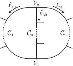
Figure 1: A generic irreducible two-loop diagram consists of three chains $\mathcal{C}_{1}$, $\mathcal{C}_{2}$, $\mathcal{C}_{3}$. Each chain $\mathcal{C}_{i}$ involves the various propagators depending on the loop momenta $\ell_{ia}=q_{i}+p_{ia}$, and $q_{1}+q_{2}+q_{3}=0$. The two connecting vertices, $\mathcal{V}_{0}$, $\mathcal{V}_{1}$, can be triple or quartic vertices.

At two loops, the discussion of rational terms can be restricted to two-loop diagrams of irreducible kind, i.e. diagrams that cannot be factorised into two one-loop diagrams Pozzorini:2020hkx . An irreducible two-loop diagram $\Gamma$ consists of three chains, $\mathcal{C}_{1},\mathcal{C}_{2},\mathcal{C}_{3}$, that are connected to each other by two vertices, $\mathcal{V}_{0},\mathcal{V}_{1}$ (see Fig. 1). Its amplitude in $D$ dimensions has the form

$${{\bar{\mathcal{A}}}_{{2,\Gamma}}^{\hskip 0.6pt}} = \int\mathrm{d}\bar{q}_{1}\int\mathrm{d}\bar{q}_{2}\,\frac{\bar{\mathcal{N}}(\bar{q}_{1},\bar{q}_{2},\bar{q}_{3})}{\mathcal{D}^{(1)}(\bar{q}_{1})\,\mathcal{D}^{(2)}(\bar{q}_{2})\,\mathcal{D}^{(3)}(\bar{q}_{3})}\bigg{|}_{\bar{q}_{3}\,=\,-\bar{q}_{1}-\bar{q}_{2}}\,,$$ (6)

where

$$\mathcal{D}^{(i)}(\bar{q}_{i}) = D^{(i)}_{0}(\bar{q}_{i})\cdots D^{(i)}_{N_{i}-1}(\bar{q}_{i})$$ (7)

is the denominator factor associated with the chain $\mathcal{C}_{i}$, and

$$D^{(i)}_{a}(\bar{q}_{i})\,=\,\bar{\ell}_{ia}^{\,2}-m_{ia}^{2}\,,\qquad\mbox{with}\qquad\bar{\ell}_{ia}\,=\,\bar{q}_{i}+p_{ia}\,.$$ (8)

The form of the loop numerator is

$$\bar{\mathcal{N}}(\bar{q}_{1},\bar{q}_{2},\bar{q}_{3}) = \bar{\Gamma}^{\bar{\alpha}_{1}\bar{\alpha}_{2}\bar{\alpha}_{3}}(\bar{q}_{1},\bar{q}_{2},\bar{q}_{3})\,\bar{\mathcal{N}}^{(1)}_{\bar{\alpha}_{1}}(\bar{q}_{1})\,\bar{\mathcal{N}}^{(2)}_{\bar{\alpha}_{2}}(\bar{q}_{2})\,\bar{\mathcal{N}}^{(3)}_{\bar{\alpha}_{3}}(\bar{q}_{3})\,,$$ (9)

where $\bar{\Gamma}^{\bar{\alpha}_{1}\bar{\alpha}_{2}\bar{\alpha}_{3}}$ embodies the two vertices $\mathcal{V}_{0}$ and $\mathcal{V}_{1}$, which are connected to the numerator factors $\bar{\mathcal{N}}^{(i)}_{\bar{\alpha}_{i}}(\bar{q}_{i})$ of the three chains $\mathcal{C}_{i}$ through multi-indices $\bar{\alpha}_{i}\equiv(\bar{\alpha}_{i1},\bar{\alpha}_{i2})$.

At two loops, UV divergences can be subtracted through the R-operation Bogoliubov:1957gp ; Hepp:1966eg ; Zimmermann:1969jj ; Caswell:1981ek . The renormalised amplitude for a two-loop diagram $\Gamma$ in $D$ dimensions has the form

$${\textbf{R}}\,{{\bar{\mathcal{A}}}_{{2,\Gamma}}^{\hskip 0.6pt}} = {{\bar{\mathcal{A}}}_{{2,\Gamma}}^{\hskip 0.6pt}}+\sum_{\gamma_{i}}{{\delta Z}_{{1,\gamma_{i}}}}\cdot{{\bar{\mathcal{A}}}_{{1,\Gamma/\gamma_{i}}}^{\hskip 0.6pt}}+{{\delta Z}_{{2,\Gamma}}}\,,$$ (10)

where the sum on the rhs runs over the one-loop subdiagrams $\gamma_{i}$, with $i=1,2,3$. The subdiagram $\gamma_{i}$ results from $\Gamma$ by truncating the chain $\mathcal{C}_{i}$, and the associated subdivergence is cancelled by the subtraction term ${{\delta Z}_{{1,\gamma_{i}}}}\cdot{{\bar{\mathcal{A}}}_{{1,\Gamma/\gamma_{i}}}^{\hskip 0.6pt}}$, which is obtained from the original two-loop diagram $\Gamma$ by replacing $\gamma_{i}$ through its one-loop counterterm ${{\delta Z}_{{1,\gamma_{i}}}}$, while keeping unchanged its complement $\Gamma/\gamma_{i}$. The latter corresponds to the chain $\mathcal{C}_{i}$, and the explicit form of such subtraction terms is

$$\sum_{\gamma_{i}}{{\delta Z}_{{1,\gamma_{i}}}}\cdot{{\bar{\mathcal{A}}}_{{1,\Gamma/\gamma_{i}}}^{\hskip 0.6pt}} = \sum_{\gamma_{i}}\int\mathrm{d}\bar{q}_{i}\,{{\delta Z}_{{1,\gamma_{i}}}^{\bar{\alpha}_{i}}(\bar{q}_{i})}\,\frac{\bar{\mathcal{N}}^{(i)}_{\bar{\alpha}_{i}}(\bar{q}_{i})}{\mathcal{D}^{(i)}(\bar{q}_{i})}\,.$$ (11)

The local two-loop divergence that is left after subtraction of all subdivergences is removed by the counterterm ${{\delta Z}_{{2,\Gamma}}}$ in (10).

The renormalisation operator R should be understood as a linear operator. Thus, when $\Gamma$ is a set of diagrams the formulas (5) and (10) should be understood as the sum of the contributions of individual diagrams. When $\Gamma$ is a full vertex function, the linearity of R implies that the rhs of (11) can also be understood as the sum of all possible vertex functions $\gamma_{i}$ that can be inserted into the one-loop vertex function $\mathcal{A}_{1,\Gamma}$. In this case, $\delta Z_{1,\gamma_{i}}$ corresponds to the full one-loop counterterm for the vertex function $\gamma_{i}$, and each term ${{\delta Z}_{{1,\gamma_{i}}}}\cdot{{\bar{\mathcal{A}}}_{{1,\Gamma/\gamma_{i}}}^{\hskip 0.6pt}}$ embodies all possible insertions of $\delta Z_{1,\gamma_{i}}$ into the various one-loop diagrams that contribute to $\mathcal{A}_{1,\Gamma}$.

2.2 Rational terms at one and two loops

The calculation of scattering amplitudes can be automated through numerical algorithms that build the numerators of loop integrands in four dimensions. In this approach, the missing contributions stemming from the interplay of $1/(D-4)$ poles with the $(D-4)$ dimensional parts of loop numerators can be reconstructed by means of rational counterterms. With this motivation in mind, we define rational terms through a splitting of loop numerators into four- and $(D-4)$-dimensional parts.

At one loop, the numerator of the amplitude (2) in $D$-dimensions is split into

$$\bar{\mathcal{N}}(\bar{q}_{1}) = \mathcal{N}(q_{1})+\tilde{\mathcal{N}}(\bar{q}_{1})\,,$$ (12)

where $\mathcal{N}(q_{1})$ is the four-dimensional part, obtained by projecting the metric tensor, Dirac matrices and the loop momentum to four dimensions. The remnant $\tilde{\mathcal{N}}(\bar{q}_{1})$ is of $\mathcal{O}({\varepsilon},\tilde{q}_{1})$ and will be referred to as the $(D-4)$-dimensional part of the numerator. To keep track of the dimensionality of loop numerators we use the parameter $D_{\mathrm{n}}$. The amplitude $\mathcal{A}_{1,\Gamma}$, defined in (2), is referred to as amplitude in $D_{\mathrm{n}}=D$ dimensions, while its counterpart in $D_{\mathrm{n}}=4$ dimensions corresponds to

$$\mathcal{A}_{1,\Gamma} = \int\!\mathrm{d}\bar{q}_{1}\,\frac{\mathcal{N}(q_{1})}{D_{0}(\bar{q}_{1})\cdots D_{N-1}(\bar{q}_{1})}\,.$$ (13)

Note that here the numerator is projected to four dimensions, while retaining the full $D$-dependence of the loop momentum in the denominator. Renormalised one-loop amplitudes in $D_{\mathrm{n}}=D$ and $D_{\mathrm{n}}=4$ dimensions are related to each other by

$$\textbf{R}\,{{\bar{\mathcal{A}}}_{{1,\Gamma}}^{\hskip 0.6pt}} = {{\mathcal{A}}_{{1,\Gamma}}}+{{\delta Z}_{{1,\Gamma}}}+{{\delta\mathcal{R}}_{{1,\Gamma}}}\,,$$ (14)

where ${{\delta Z}_{{1,\Gamma}}}$ are usual UV counterterms, and $\delta\mathcal{R}_{1,\Gamma}$ are rational counterterms Ossola:2008xq ; Draggiotis:2009yb ; Garzelli:2009is ; Pittau:2011qp . Since $\delta\mathcal{R}_{1,\Gamma}$ counterterms originate only from the interplay of $\tilde{\mathcal{N}}(\bar{q}_{1})$ with poles of UV kind Bredenstein:2008zb , they can be derived once and for all by computing

$${{\delta\mathcal{R}}_{{1,\Gamma}}} = {{\bar{\mathcal{A}}}_{{1,\Gamma}}^{\hskip 0.6pt}}-{{\mathcal{A}}_{{1,\Gamma}}}\,,$$ (15)

at the level of UV divergent 1PI vertex functions.

At two loops, in analogy with (12) we split the $D$-dimensional loop numerator (9) into four-dimensional and $(D-4)$ dimensional parts,

$$\bar{\mathcal{N}}(\bar{q}_{1},\bar{q}_{2},\bar{q}_{3}) = \mathcal{N}(q_{1},q_{2},q_{3})+\tilde{\mathcal{N}}(\bar{q}_{1},\bar{q}_{2},\bar{q}_{3})\,.$$ (16)

Similarly as in the one-loop case, the two-loop amplitude ${{\mathcal{A}}_{{2,\Gamma}}}$, defined in (6), is referred to as an amplitude in $D_{\mathrm{n}}=D$ dimensions, and its counterpart in $D_{\mathrm{n}}=4$ dimensions is

$${{\mathcal{A}}_{{2,\Gamma}}} = \int\mathrm{d}\bar{q}_{1}\int\mathrm{d}\bar{q}_{2}\,\frac{\mathcal{N}(q_{1},q_{2},q_{3})}{\mathcal{D}^{(1)}(\bar{q}_{1})\,\mathcal{D}^{(2)}(\bar{q}_{2})\,\mathcal{D}^{(3)}(\bar{q}_{3})}\bigg{|}_{\bar{q}_{3}\,=\,-\bar{q}_{1}-\bar{q}_{2}}\,,$$ (17)

where the numerator is projected to four dimensions, while keeping the denominator in $D$ dimensions. As demonstrated in Pozzorini:2020hkx , renormalised two-loop amplitudes in $D_{\mathrm{n}}=D$ and $D_{\mathrm{n}}=4$ dimensions are related to each other by the following generalisation of the R-operation,

$${\textbf{R}}\,{{\bar{\mathcal{A}}}_{{2,\Gamma}}^{\hskip 0.6pt}} = {{\mathcal{A}}_{{2,\Gamma}}}+\sum\limits_{\gamma_{i}}\left({{\delta Z}_{{1,\gamma_{i}}}}+{{\delta\tilde{Z}}_{{1,\gamma_{i}}}}+{{\delta\mathcal{R}}_{{1,\gamma_{i}}}}\right)\cdot{{\mathcal{A}}_{{1,\Gamma/\gamma_{i}}}}\,+\,{{\delta Z}_{{2,\Gamma}}}+{{\delta\mathcal{R}}_{{2,\Gamma}}}\,,$$ (18)

where the standard UV counterterms, ${{\delta Z}_{{1,\gamma_{i}}}}$ and ${{\delta Z}_{{2,\Gamma}}}$, are supplemented by associated rational counterterms, ${{\delta\mathcal{R}}_{{1,\gamma_{i}}}}$ and ${{\delta\mathcal{R}}_{{2,\Gamma}}}$, which reconstruct the contributions stemming from the interplay of $\tilde{\mathcal{N}}(\bar{q}_{1},\bar{q}_{2},\bar{q}_{3})$ with one-loop subdivergences and local two-loop divergences. The extra counterterms ${{\delta\tilde{Z}}_{{1,\gamma_{i}}}}$ are required for the full cancellation of the UV subdivergences of the one-loop subdiagrams $\gamma_{i}$ in $D_{\mathrm{n}}=4$ dimensions. In renormalisable theories such ${{\delta\tilde{Z}}_{{1,\gamma_{i}}}}$ counterterms are needed only for quadratically divergent self-energy subdiagrams, and their general form is Pozzorini:2020hkx

$${{\delta\tilde{Z}}_{{1,\gamma_{i}}}^{\alpha}(\tilde{q}_{i})} = v^{\alpha}\frac{{\tilde{q}}_{i}^{\hskip 0.6pt2}}{{\varepsilon}}\,,$$ (19)

where $q_{i}$ is the external loop momentum that flows through the complement $\Gamma/\gamma_{i}$ of the subdiagram $\gamma_{i}$

The identity (18) is valid for any renormalisable theory assuming that ${{\bar{\mathcal{A}}}_{{2,\Gamma}}^{\hskip 0.6pt}}$ is free from IR divergences, or that the latter are subtracted in a way that also rational terms of IR origin cancel. This implies that the ${{\delta\mathcal{R}}_{{2,\Gamma}}}$ counterterms in (18) arise only from divergences of UV kind. More precisely, they originate only from local UV divergences. Thus they can be derived once and for all by inverting the master formula (18), i.e. by computing

$${{\delta\mathcal{R}}_{{2,\Gamma}}} = {{\bar{\mathcal{A}}}_{{2,\Gamma}}^{\hskip 0.6pt}}-{{\mathcal{A}}_{{2,\Gamma}}}+\sum\limits_{\gamma}{{\delta Z}_{{1,\gamma}}}\cdot{{\bar{\mathcal{A}}}_{{1,\Gamma/\gamma}}^{\hskip 0.6pt}}-\sum\limits_{\gamma}\left({{\delta Z}_{{1,\gamma}}}+{{\delta\tilde{Z}}_{{1,\gamma}}}+{{\delta\mathcal{R}}_{{1,\gamma}}}\right)\cdot{{\mathcal{A}}_{{1,\Gamma/\gamma}}}\,,\qquad$$ (20)

for all superficially divergent 1PI vertex functions $\Gamma$ in the theory at hand.

Similarly as for UV counterterms, the rational counterterms ${{\delta\mathcal{R}}_{{k,\Gamma}}}$ at one and two loops have the form of homogeneous polynomials of degree $X(\Gamma)$ in the external momenta and internal masses, where $X(\Gamma)$ is the superficial degree of divergence of $\Gamma$.

Finally, we point out that the $(D-4)$-dimensional parts of the loop numerators (12) and (16), as well as the associated rational terms, depend on the employed variant of dimensional regularisation. In this respect we remind the reader that the analysis of Pozzorini:2020hkx ; Lang:2020nnl and the new results presented in this paper are based on the ’t Hooft–Veltman scheme, where all algebraic objects inside the loops live in $D$ dimensions. In other words, the rational terms presented in this paper embody the effects resulting from all $(D-4)$-dimensional parts of loop momenta, $\gamma$-matrices and metric tensors that appear inside loop numerators.

2.3 Derivation of rational counterterms

The derivation of $\delta\mathcal{R}_{2,\Gamma}$ counterterms can be simplified by means of expansions that capture the relevant UV divergences in the form of massive tadpole integrals Pozzorini:2020hkx ; Lang:2020nnl . In the following, as a basis for Section 3, we summarise the Taylor expansion approach presented in App. A.3–A.4 of Lang:2020nnl . The idea is that the local two-loop divergence of degree $X=X(\Gamma)$, which is responsible for $\delta\mathcal{R}_{2,\Gamma}$, can be isolated through a Taylor expansion in the external momenta $\{p_{ia}\}$ and internal masses $\{m_{ia}\}$, which can be applied at the integrand level on the rhs of (20). Technically, one can rescale all external momenta and internal masses by a global parameter $\lambda$,

$$p_{ia}\,\to\,\lambda\,p_{ia}\,,\qquad m_{ia}\,\to\,\lambda\,m_{ia}\qquad\forall\;\;i,a\,,$$ (21)

and the relevant terms of order $\lambda^{X}$ can be selected through the expansion operator

$$\textbf{T}_{X} = \frac{1}{X!}\left(\frac{\mathrm{d}}{\mathrm{d}\lambda}\right)^{X}\Bigg{|}_{\lambda=0}\,=\,\frac{1}{X!}\left(\sum_{a,i}p_{ia}^{\mu}\frac{\partial}{\partial\ell_{ia}^{\mu}}+\sum_{a,i}m_{ia}\frac{\partial}{\partial m_{ia}}\right)^{X}\Bigg{|}_{p_{ia}\;=\;m_{ia}\;=\;0}\,,$$ (23)

where we have used the fact that loop integrands depend on $p_{ia}$ only through $\ell_{ia}=\bar{q}_{i}+p_{ia}$. Applying the $\textbf{T}_{X}$ expansion to generic $k$-loop integrals yields massless tadpole integrals of the form

$$\textbf{T}_{X}\,\bar{\mathcal{A}}_{k,\Gamma}\,=\,\sum_{\vec{P}}\int\prod_{i}\mathrm{d}\bar{q}_{i}\frac{\mathcal{T}_{\vec{P}}(\{\bar{q}_{k},p_{ka},m_{ka}\})}{\prod_{j}(\bar{q}_{j}^{2})^{P_{i}}}\,,$$ (24)

where $\vec{P}=(P_{1},\dots)$ describes the denominator powers of the various loop chains, and $\mathcal{T}_{\vec{P}}(\{\bar{q}_{k},p_{ka},m_{ka}\})$ are polynomials of homogeneous degree $X$ in $\{p_{ia},m_{ia}\}$. The Taylor expansion (24) generates only scaleless tadpole integrals, since all momenta and masses are set to zero in the denominators. This can be avoided by introducing an auxiliary mass $M$ through the identity

$$\frac{1}{\bar{q}_{i}^{2}} = \frac{1}{\left(\bar{q}_{i}^{2}-M^{2}\right)}\left(1+\frac{M^{2}}{\bar{q}_{i}^{2}-M^{2}}\right)^{-1}\,,$$ (25)

and expanding the second term on the rhs in $M^{2}/(\bar{q}_{i}^{2}-M^{2})$, including all terms that are sufficiently UV divergent to contribute to (20). To capture all relevant UV singularities, each loop chain $\mathcal{C}_{i}$ of the two-loop diagram $\Gamma$ needs to be expanded up to relative order

$$\quad X_{i}(\Gamma)\,=\,\text{max}\left\{X(\Gamma),X(\gamma_{j}),X(\gamma_{k})\right\}\,,$$ (26)

in $M/\bar{q}_{i}$, where $X(\Gamma)$, $X(\gamma_{j})$ and $X(\gamma_{k})$ are, respectively, the superficial degrees of divergence of the full two-loop diagram $\Gamma$ and of the one-loop subdiagrams with $j,k\neq i$. In renormalisable theories $X_{i}(\Gamma)\in[0,2]$, and the relevant expansions for the terms $(1/\bar{q}_{i}^{2})^{P_{i}}$ in (24) are

$${\textbf{M}}^{(i)}_{[0,X_{i}]}\,\,\frac{1}{(\bar{q}_{i}^{2})^{P_{i}}}\, = \,\frac{1}{(\bar{q}_{i}^{2}-M^{2})^{P_{i}}}\times\begin{cases}1&\mbox{for}\quad X_{i}\leq 1\,,\\[8.53581pt] 1-P_{i}\,\frac{M^{2}}{\bar{q}_{i}^{2}-M^{2}}&\mbox{for}\quad X_{i}=2\,.\end{cases}$$ (27)

Note that the $\textbf{T}_{X}$ and ${\textbf{M}}_{[0,X_{i}]}^{(i)}$ expansions commute.

In summary, for the derivation of rational counterterms, $k$-loop amplitudes $\bar{\mathcal{A}}_{k,\Gamma}$ (and their counterparts in $D_{\mathrm{n}}=4$ dimensions) can be replaced by

$$\bar{\mathcal{A}}_{k,\Gamma_{\mathrm{tad}}} = \bigg{(}\prod_{i}{\textbf{M}}_{[0,X_{i}]}^{(i)}\bigg{)}\,\textbf{T}_{X}\,\bar{\mathcal{A}}_{k,\Gamma}\,,$$ (28)

where the product includes all relevant loop chains, i.e. one chain at one loop and three chains at two loops. More explicity, applying (28) to (20) yields

$${{\delta\mathcal{R}}_{{2,\Gamma}}} = \textbf{T}_{X}\int\mathrm{d}\bar{q}_{1}\int\mathrm{d}\bar{q}_{2}\left[\bar{\Gamma}^{\bar{\alpha}_{1}\bar{\alpha}_{2}\bar{\alpha}_{3}}(\bar{q}_{1},\bar{q}_{2},\bar{q}_{3})\,\prod_{i=1}^{3}\left({\bf M}^{(i)}_{[0,X_{i}]}\,\frac{\bar{\mathcal{N}}^{(i)}_{\bar{\alpha}_{i}}(\bar{q}_{i})}{\mathcal{D}^{(i)}(\bar{q}_{i})}\right)-\Gamma^{\alpha_{1}\alpha_{2}\alpha_{3}}(q_{1},q_{2},q_{3})\,\right.$$ (29)

$$\left.{}\times\prod_{i=1}^{3}\left({\bf M}^{(i)}_{[0,X_{i}]}\,\frac{\mathcal{N}^{(i)}_{\alpha_{i}}(q_{i})}{\mathcal{D}^{(i)}(\bar{q}_{i})}\right)\right]_{q_{3}=-q_{1}-q_{2}}+\;\sum_{i=1}^{3}\textbf{T}_{X}\int\mathrm{d}\bar{q}_{i}\,\Bigg{[}{{\delta Z}_{{1,\gamma_{i}}}^{\bar{\alpha}_{i}}(\bar{q}_{i})}\,{\bf M}^{(i)}_{[0,X_{i}]}\,\frac{\bar{\mathcal{N}}^{(i)}_{\bar{\alpha}_{i}}(\bar{q}_{i})}{\mathcal{D}^{(i)}(\bar{q}_{i})}$$

$${}-\left({{\delta Z}_{{1,\gamma_{i}}}^{\alpha_{i}}(q_{i})}+{{\delta\tilde{Z}}_{{1,\gamma_{i}}}^{\alpha_{i}}(\tilde{q}_{i})}+{{\delta\mathcal{R}}_{{1,\gamma_{i}}}^{\alpha_{i}}(q_{i})}\right){\bf M}^{(i)}_{[0,X_{i}]}\,\frac{\mathcal{N}^{(i)}_{\alpha_{i}}(q_{i})}{\mathcal{D}^{(i)}(\bar{q}_{i})}\Bigg{]}\,,$$

where $X=X(\Gamma)$ and $X_{i}=X_{i}(\Gamma)$. Here the $\textbf{T}_{X}$ expansion applies to all mass and momentum-dependent terms, including one-loop counterterms. The latter are non-zero only when the corresponding subdiagrams $\gamma_{i}$ are divergent, in which case $X_{i}=X$ Lang:2020nnl . The dependence on the auxiliary mass $M$ cancels in (29). Moreover, all higher-order terms generated by the $M^{2}/\bar{q}_{i}^{2}$ expansions (27) are cancelled by corresponding one-loop counterterm contributions. Thus, as discussed in App A.4 of Lang:2020nnl , the above expansion can be further simplified by setting $X_{i}=0$ throughout and compensating the effect of the missing subdivergences through ad-hoc modifications of the one-loop counterterms ${{\delta Z}_{{1,\gamma_{i}}}}$, ${{\delta\tilde{Z}}_{{1,}}}$, and ${{\delta\mathcal{R}}_{{1,\gamma_{i}}}}$.

3 Symmetry breaking and rational terms

The general properties of rational terms established in Pozzorini:2020hkx ; Lang:2020nnl are valid for any renormalisable theory, but so far the explicit expressions of ${{\delta\mathcal{R}}_{{2,\Gamma}}}$ counterterms have been worked out only for U(1) and SU(N) gauge theories. For such theories, the task of determining ${{\delta\mathcal{R}}_{{2,\Gamma}}}$ via (20) is greatly simplified by the underlying gauge symmetry, which allows one to treat all fields in terms of generic fermion and gauge-boson multiplets. For instance, the rational terms for the quartic gauge-boson vertex $A_{\mu}^{a}A_{\nu}^{b}A_{\rho}^{c}A_{\sigma}^{d}$ in a symmetric SU(N) theory can be derived through a single calculation, where the dependence from the SU(N) indices $a,b,c,d$ can be easily factorised.

In the presence of symmetry breaking this is no longer possible due to the fact that the different states of each multiplet can acquire different masses and can mix with one another. Moreover, also mass and field-renormalisation constants can vary within a multiplet. For these reasons, the direct determination of ${{\delta\mathcal{R}}_{{2,\Gamma}}}$ terms for the entire SM, including contributions of order $\alpha_{S}^{2}$, $\alpha\alpha_{S}$ and $\alpha^{2}$, is a quite arduous task. However, as discussed in the following, this problem can be greatly simplified by relating ${{\delta\mathcal{R}}_{{2,\Gamma}}}$ counterterms in a SB theory to corresponding rational counterterms in the underlying symmetric theory via vev expansions.

3.1 Mass and vev expansions

As discussed in Section 2.3, calculations of ${{\delta\mathcal{R}}_{{2,\Gamma}}}$ counterterms can be simplified by means of Taylor expansion in the external momenta and internal masses. Such expansions, see (21)–(24), involve only contributions from order zero up to $X$ in the internal masses $\{m_{ia}\}$, where $X$ is the superficial degree of divergence of $\Gamma$ and corresponds to its mass dimension. For this reason, all ingredients that enter the calculation of rational terms can be replaced by their expansion in $\{m_{ia}\}$ up to order $X$. Thus, defining the expansion operator

$${\textbf{m}}_{[0,X]} = \sum_{k=0}^{X}\frac{1}{k!}\left(\sum_{a,i}m_{ia}\frac{\partial}{\partial m_{ia}}\right)^{k}\Bigg{|}_{m_{ia}\;=\;0}\,{},$$ (30)

we can turn the formulas (15) and (20) into

$${{\delta\mathcal{R}}_{{1,\Gamma}}} = {\textbf{m}}_{[0,X]}\,\Big{[}{{\bar{\mathcal{A}}}_{{1,\Gamma}}^{\hskip 0.6pt}}-{{\mathcal{A}}_{{1,\Gamma}}}\Big{]}\,,$$ (31)

$${{\delta\mathcal{R}}_{{2,\Gamma}}} = {\textbf{m}}_{[0,X]}\,\Big{[}{{\bar{\mathcal{A}}}_{{2,\Gamma}}^{\hskip 0.6pt}}-{{\mathcal{A}}_{{2,\Gamma}}}+\sum\limits_{\gamma}{{\delta Z}_{{1,\gamma}}}\cdot{{\bar{\mathcal{A}}}_{{1,\Gamma/\gamma}}^{\hskip 0.6pt}}-\sum\limits_{\gamma}\left({{\delta Z}_{{1,\gamma}}}+{{\delta\tilde{Z}}_{{1,\gamma}}}+{{\delta\mathcal{R}}_{{1,\gamma}}}\right)\cdot{{\mathcal{A}}_{{1,\Gamma/\gamma}}}\Big{]}\,.$$

In the following, we consider such mass expansions in the context of a generic SB theory with a scalar multiplet $\Phi_{i}(x)$ that acquires a vev

$$v_{i} = \langle 0|\Phi_{i}(x)|0\rangle\,.$$ (33)

The scalar excitations around the vev are denoted

$$\Phi_{i}(x)=v_{i}+\widetilde{\Phi}_{i}(x)\,.$$ (34)

For simplicity we assume that the scalar sector has a single vev and a single Higgs boson, and for the scalar oscillations in the vev direction we use the notation

$$\phi(x)=v+H(x),\qquad v = \langle 0|\phi(x)|0\rangle\,.$$ (35)

In this Section, we assume that the SB theory is described by a Lagrangian $\mathcal{L}(H)$, which is connected to the Lagrangian $\mathcal{L}_{{\scriptscriptstyle\mathrm{YM}}}(H)$ of an underlying symmetric theory through a shift of the Higgs field, $H\to H+v$ , i.e.

$$\mathcal{L}(H) = \mathcal{L}_{{\scriptscriptstyle\mathrm{YM}}}(H+v)\,.$$ (36)

This implies that the symmetry of $\mathcal{L}_{{\scriptscriptstyle\mathrm{YM}}}$ is inherited by the SB Lagrangian in the form of rigid invariance, i.e. invariance wrt combined gauge transformations of $v_{i}+\widetilde{\Phi}_{i}(x)$. For $\mathcal{L}_{{\scriptscriptstyle\mathrm{YM}}}$ we do not assume any specific symmetry group, and we only assume that in the SB theory all particle masses are generated by the vev of the scalar field $\phi$. Thus all masses are proportional to $v$, and the mass expansion (30) can be identified with a vev expansion,

$${\textbf{m}}_{[0,X]}\,=\,\sum_{k=0}^{X}\frac{v^{k}}{k!}\,\frac{\partial^{k}}{\partial v^{k}}\bigg{|}_{v\;=\;0}\,.$$ (37)

Since UV divergences in the SM are at most quadratic, expansions truncated at second order will be sufficient.

Concerning the propagators of massive particles we will first assume that all mass eigenstates have well defined tree-level propagators, i.e. that the mixing between different fields can be removed by means of appropriate unitary transformations. In this respect we note that in the SM the cancellation of mixing between gauge bosons and Goldstone bosons requires also appropriate gauge choices, and the corresponding gauge-fixing terms can be in conflict with the assumption of rigid invariance, i.e. with the property (36) of the SB Lagrangian. A systematic approach to deal with such violations of rigid invariance is discussed in Section 4.3.

3.2 Vev-expansion in $D_{\mathrm{n}}=D$ dimensions

As is well known, the vev expansion (37) can be implemented at the level of the Feynman rules. This is achieved by turning the usual perturbative expansion in the coupling constants $g_{i}$ into a double expansion in $g_{i}$ and $v$. In this approach, vev-dependent terms of $\mathcal{L}(H)$ are treated as interaction vertices, which can be generated from corresponding vertices of the symmetric theory by replacing external Higgs lines with vev insertions.

To introduce our notation, in the following we consider the mass expansion for the two-point vertex function $\bar{\Gamma}_{aa}(\bar{q},m_{a})$ of a generic field $\varphi_{a}$ with mass $m_{a}$, and for the related propagator $\bar{G}_{aa}(\bar{q},m_{a})$, defined through

$$\bar{G}_{aa}(\bar{q},m_{a})\,\bar{\Gamma}_{aa}(\bar{q},m_{a})=-1\,.$$ (38)

The field $\varphi_{a}$ may be a fermion, a vector boson, or a scalar field. For later convenience, the momentum $\bar{q}$ that flows through the two-point function at hand is assumed to be a $D$-dimensional loop momentum. Possible Lorentz/Dirac indices associated with $\varphi_{a}$ are also assumed to be in $D$ dimensions but are kept implicit. At tree level, the propagator has the form

$$\bar{G}_{aa}(\bar{q},m_{a})=\frac{\bar{g}_{aa}(\bar{q},m_{a})}{\bar{q}^{2}-m_{a}^{2}}\,,$$ (39)

and its numerator fulfils

$$\bar{g}_{aa}(\bar{q},m_{a})\,\bar{\Gamma}_{aa}(\bar{q},m_{a}) = -(\bar{q}^{2}-m_{a}^{2})\,.$$ (40)

The mass dependence of $\bar{\Gamma}_{aa}(\bar{q},m_{a})$ in the SB theory arises from the triple $H\varphi_{a}^{2}$ and/or quartic $H^{2}\varphi_{a}^{2}$ vertices of the symmetric theory,

$$\bar{\Gamma}^{{\scriptscriptstyle\mathrm{YM}}}_{aa\mathrm{H}}(\bar{q})\;\;=\;\;\vbox{\hbox{\raisebox{0.0pt}{\includegraphics[width=47.69846pt]{fermionSH_amp}} }}\qquad\qquad\bar{\Gamma}^{{\scriptscriptstyle\mathrm{YM}}}_{aa\mathrm{H}\mathrm{H}}(\bar{q})\;\;=\;\;\vbox{\hbox{\raisebox{0.0pt}{\includegraphics[width=47.69846pt]{bosonDH_amp}}}}\,,$$ (41)

where solid and dashed lines correspond, respectively, to the $\varphi_{a}$ and Higgs fields. Note that in the SM the triple vertex $\bar{\Gamma}_{aa\mathrm{H}}^{{\scriptscriptstyle\mathrm{YM}}}$ is vanishing for scalars and gauge bosons, while in the case of fermions the quartic vertex $\bar{\Gamma}_{aa\mathrm{H}\mathrm{H}}^{{\scriptscriptstyle\mathrm{YM}}}$ vanishes. As a result of symmetry breaking, the vertices (41) give rise to mass terms of the form $v\varphi_{a}^{2}$ and $v^{2}\varphi_{a}^{2}$, which can be described through the vev-insertion vertices

$$\bar{\Gamma}^{{\scriptscriptstyle\mathrm{YM}}}_{aav}(\bar{q})\; = \;\vbox{\hbox{\raisebox{0.0pt}{\includegraphics[width=47.69846pt]{fermionSVev_amp}} }}\,,\qquad\qquad\bar{\Gamma}^{{\scriptscriptstyle\mathrm{YM}}}_{aavv}(\bar{q})\;=\;\vbox{\hbox{\raisebox{0.0pt}{\includegraphics[width=47.69846pt]{bosonDVev_amp}} }}\,,$$ (42)

where vev insertions are indicated by crossed blobs. Each vev insertion corresponds to a factor $v$ together with the assignment of zero external momentum for the corresponding Higgs line. Moreover, diagrams with $k$ vev insertions receive a $1/k!$ factor. More explicitly, $\bar{\Gamma}^{{\scriptscriptstyle\mathrm{YM}}}_{aav}(\bar{q})=v\,\bar{\Gamma}^{{\scriptscriptstyle\mathrm{YM}}}_{aa\mathrm{H}}(\bar{q})\big{|}_{p_{\mathrm{H}}=0}$ and $\bar{\Gamma}^{{\scriptscriptstyle\mathrm{YM}}}_{aavv}(\bar{q})=\frac{v^{2}}{2}\bar{\Gamma}^{{\scriptscriptstyle\mathrm{YM}}}_{aa\mathrm{H}\mathrm{H}}(\bar{q})\big{|}_{p_{\mathrm{H}}=0}$. With these vev-insertion vertices at hand, the expansion of the $\varphi_{a}$ two-point function up to order $v^{2}$ can be expressed as

$${\textbf{m}}_{[0,2]}\,\bigg{[}\,\vbox{\hbox{\raisebox{-15.0pt}{\includegraphics[width=39.0242pt]{fermion_amp}} }}\bigg{]}_{D_{\mathrm{n}}=D}\!\!\!\!\! = \;\bigg{[}\vbox{\hbox{\raisebox{-22.0pt}{\includegraphics[width=43.36464pt]{fermion_amp}} }}+\vbox{\hbox{\raisebox{0.0pt}{\includegraphics[width=47.69846pt]{fermionSVev_amp}} }}+\vbox{\hbox{\raisebox{0.0pt}{\includegraphics[width=47.69846pt]{bosonDVev_amp}} }}\bigg{]}^{{\scriptscriptstyle\mathrm{YM}}}_{D_{\mathrm{n}}=D}\,,$$ (43)

or, equivalently,

$${\textbf{m}}_{[0,2]}\,\bar{\Gamma}_{aa}(\bar{q},m_{a}) = {\textbf{V}}_{[0,2]}\,\bar{\Gamma}_{aa}(\bar{q},m_{a})\,,$$ (44)

with

$${\textbf{V}}_{[0,2]}\,\bar{\Gamma}_{aa}(\bar{q},m_{a}) = \bar{\Gamma}^{{\scriptscriptstyle\mathrm{YM}}}_{aa}(\bar{q})+\bar{\Gamma}^{{\scriptscriptstyle\mathrm{YM}}}_{aav}(\bar{q})+\bar{\Gamma}^{{\scriptscriptstyle\mathrm{YM}}}_{aavv}(\bar{q})\,.$$ (45)

Note that in (42)–(43) only tree contributions are considered, while (44)–(45) hold to any order in the coupling constant.

With this approach, the vev expansion of any $l$-loop amplitude in $D_{\mathrm{n}}=D$ dimensions can be expressed as a series of vev insertions,

$${\textbf{m}}_{[0,X]}\,{{\bar{\mathcal{A}}}_{{l,\Gamma}}^{\hskip 0.6pt}} = {\textbf{V}}_{[0,X]}\,{{\bar{\mathcal{A}}}_{{l,\Gamma}}^{\hskip 0.6pt}}\,,$$ (46)

with

$${\textbf{V}}_{[0,X]}\,{{\bar{\mathcal{A}}}_{{l,\Gamma}}^{\hskip 0.6pt}} = \sum_{k=0}^{X}{{\bar{\mathcal{A}}}_{{l,\Gamma v^{k}}}^{\hskip 0.6pt{\scriptscriptstyle\mathrm{YM}}}}\qquad\mbox{and}\qquad{{\bar{\mathcal{A}}}_{{l,\Gamma v^{k}}}^{\hskip 0.6pt{\scriptscriptstyle\mathrm{YM}}}}\,:=\,\frac{v^{k}}{k!}\,{{\bar{\mathcal{A}}}_{{l,\Gamma\mathrm{H}^{k}}}^{\hskip 0.6pt{\scriptscriptstyle\mathrm{YM}}}}\Big{|}_{p_{\mathrm{H}}=0}\,,$$ (47)

where amplitudes carrying the superscript YM are defined through the Feynman rules of the symmetric theory with Lagrangian $\mathcal{L}_{{\scriptscriptstyle\mathrm{YM}}}(H)$. The shorthands $v^{k}$ and $\mathrm{H}^{k}$ denote $k$ vev and Higgs insertions, respectively, and $p_{\mathrm{H}}=0$ applies only to such insertions, while it does not apply to possible physical Higgs lines that enter the original vertex $\Gamma$. Note that (46)–(47) apply also to vertices that do not exist at tree level in the symmetric theory and are induced by symmetry breaking, such as the $W^{+}W^{-}H$ vertex in the SM. In the case of vertices $\Gamma$ of order $v^{n}$ at tree level, the vev insertions $\Gamma v^{k}$ with $k<n$ vanish in (47). Note also that when vev insertions are applied to mass-dependent vertices inside the loops, the global degree of singularity is not reduced. However, this happens only when—due to the presence of mass-dependent interactions—the superficial degree of singularity is smaller than what is expected from dimensional analysis. In general, in order to capture all UV singularities, it is sufficient to set the order $X$ of the vev expansion equal to the maximum degree of UV singularity that is allowed by dimensional analysis, i.e.

$$X=4-\mathrm{dim}(\Gamma)\,,$$ (48)

where $\mathrm{dim}(\Gamma)$ is the mass dimension of the vertex function at hand.

As a preparation for the discussion in Section 3.3, let us now consider the vev expansion up to order $v^{2}$ for the propagator defined in (38),

$${\textbf{m}}_{[0,2]}\,\bar{G}_{aa}(\bar{q},m_{a}) = \sum_{k=0}^{2}\frac{m^{k}_{a}}{k!}\,\frac{\partial^{k}}{\partial m_{a}^{k}}\bigg{|}_{m_{a}\,=\,0}\,\bar{G}_{aa}(\bar{q},m_{a})\,.$$ (49)

The vev derivatives of $\bar{G}_{aa}$ on the rhs can be expressed in terms of vev derivatives of the two-point function $\bar{\Gamma}_{aa}$ by using (38) and the related identities

$$\frac{\partial^{k}}{\partial m_{a}^{k}}\left[\bar{G}_{aa}(\bar{q},m_{a})\,\bar{\Gamma}_{aa}(\bar{q},m_{a})\right] = 0\,.$$ (50)

In this way one can show that

$${\textbf{m}}_{[0,2]}\,\bar{G}_{aa}(\bar{q},m_{a}) = \bar{G}_{aa}^{{\scriptscriptstyle\mathrm{YM}}}(\bar{q})\,+\,\bar{G}_{aa}^{{\scriptscriptstyle\mathrm{YM}}}(\bar{q})\,\bar{\Gamma}_{aav}^{{\scriptscriptstyle\mathrm{YM}}}(\bar{q})\,\bar{G}_{aa}^{{\scriptscriptstyle\mathrm{YM}}}(\bar{q})\,+\,\left[\bar{G}_{aa}^{{\scriptscriptstyle\mathrm{YM}}}(\bar{q})\,\bar{\Gamma}_{aav}^{{\scriptscriptstyle\mathrm{YM}}}(\bar{q})\right]^{2}\,\bar{G}_{aa}^{{\scriptscriptstyle\mathrm{YM}}}(\bar{q})$$ (51)

$${}+\,\bar{G}_{aa}^{{\scriptscriptstyle\mathrm{YM}}}(\bar{q})\,\bar{\Gamma}_{aavv}^{{\scriptscriptstyle\mathrm{YM}}}(\bar{q})\,\bar{G}_{aa}^{{\scriptscriptstyle\mathrm{YM}}}(\bar{q})\,,$$

where $\bar{G}_{aa}^{{\scriptscriptstyle\mathrm{YM}}}(\bar{q})$ is the propagator of the symmetric theory, and $\bar{\Gamma}_{aav^{k}}^{{\scriptscriptstyle\mathrm{YM}}}(\bar{q})$ are the vev-insertion vertices defined in (42). This relation can be expressed diagrammatically as

$${\textbf{m}}_{[0,2]}\,\bigg{[}\,\vbox{\hbox{\raisebox{-15.0pt}{\includegraphics[width=39.0242pt]{fermion}} }}\bigg{]}_{D_{\mathrm{n}}=D}\!\!\!\!\! = \;\bigg{[}\vbox{\hbox{\raisebox{-22.0pt}{\includegraphics[width=43.36464pt]{fermion}} }}+\vbox{\hbox{\raisebox{0.0pt}{\includegraphics[width=47.69846pt]{fermionSVev}} }}+\vbox{\hbox{\raisebox{0.0pt}{\includegraphics[width=47.69846pt]{fermionDVev}} }}+\vbox{\hbox{\raisebox{0.0pt}{\includegraphics[width=47.69846pt]{bosonDVev}} }}\bigg{]}^{{\scriptscriptstyle\mathrm{YM}}}_{D_{\mathrm{n}}=D}\,,$$

and analogously as for the expansion of the two-point function $\bar{\Gamma}_{aa}$ it can be directly obtained from (46)–(47) in the form

$${\textbf{m}}_{[0,2]}\,\bar{G}_{aa}(\bar{q},m_{a}) = {\textbf{V}}_{[0,2]}\,\bar{G}_{aa}(\bar{q},m_{a})\,=\,\bar{G}^{{\scriptscriptstyle\mathrm{YM}}}_{aa}(\bar{q})+\bar{G}^{{\scriptscriptstyle\mathrm{YM}}}_{aav}(\bar{q})+\bar{G}^{{\scriptscriptstyle\mathrm{YM}}}_{aavv}(\bar{q})\,,$$ (53)

where $\bar{G}^{{\scriptscriptstyle\mathrm{YM}}}_{aavv}$ embodies the contributions of the last two diagrams in (3.2).

3.3 Vev-expansion in $D_{\mathrm{n}}=4$ dimensions

In order to simplify the calculation of rational counterterms (31)–(3.1) for SB theories, the vev-insertion approach (46)–(47) needs to be extended to amplitudes in $D_{\mathrm{n}}=4$ dimensions. To this end, let us first consider the naive conversions to $D_{\mathrm{n}}=4$ of the lhs and rhs of (46). The $D_{\mathrm{n}}=4$ counterpart of the vev expansion on the lhs of (46) is

$${\textbf{m}}_{[0,X]}\,{{\mathcal{A}}_{{l,\Gamma}}} = {\textbf{m}}_{[0,X]}\,{\textbf{P}}_{4}\,{{\bar{\mathcal{A}}}_{{l,\Gamma}}^{\hskip 0.6pt}}\,,$$ (54)

where the operator ${\textbf{P}}_{4}$ projects loop numerators to $D_{\mathrm{n}}=4$. As for the vev insertion on the rhs of (46) we define its naive $D_{\mathrm{n}}=4$ projection as

$${\textbf{V}}_{[0,X]}\,{{\mathcal{A}}_{{l,\Gamma}}} := {\textbf{P}}_{4}\,{\textbf{V}}_{[0,X]}\,{{\bar{\mathcal{A}}}_{{l,\Gamma}}^{\hskip 0.6pt}}\,=\,\sum_{k=0}^{X}{{\mathcal{A}}_{{l,\Gamma v^{k}}}^{{\scriptscriptstyle\mathrm{YM}}}}\,,$$ (55)

with

$${{\mathcal{A}}_{{l,\Gamma v^{k}}}^{{\scriptscriptstyle\mathrm{YM}}}}\,=\,\frac{v^{k}}{k!}\,{{\mathcal{A}}_{{l,\Gamma\mathrm{H}^{k}}}^{{\scriptscriptstyle\mathrm{YM}}}}\Big{|}_{p_{\mathrm{H}}=0}\,.$$ (56)

As we will see, at variance with the $D_{\mathrm{n}}=D$ case, (54) and (55) are not identical in $D_{\mathrm{n}}=4$. This is due to the fact that the vev expansion (37) and the projection to $D_{\mathrm{n}}=4$ do not commute. Thus, the extension of (46) to $D_{\mathrm{n}}=4$ assumes the form

$${\textbf{m}}_{[0,X]}\,{{\mathcal{A}}_{{l,\Gamma}}} = {\textbf{V}}_{[0,X]}\,{{\mathcal{A}}_{{l,\Gamma}}}+\Delta{\textbf{V}}_{[0,X]}\,{{\mathcal{A}}_{{l,\Gamma}}}\,,$$ (57)

where the second term on the rhs embodies the non-commuting terms. More explicitly, we can write

$$\Delta{\textbf{V}}_{[0,X]}\,{{\mathcal{A}}_{{l,\Gamma}}} = {\textbf{m}}_{[0,X]}\,{{\mathcal{A}}_{{l,\Gamma}}}-{\textbf{V}}_{[0,X]}\,{{\mathcal{A}}_{{l,\Gamma}}}\,=\,\left({\textbf{m}}_{[0,X]}{\textbf{P}}_{4}-{\textbf{P}}_{4}\,{\textbf{V}}_{[0,X]}\right){{\bar{\mathcal{A}}}_{{l,\Gamma}}^{\hskip 0.6pt}}\,,$$ (58)

and using (46) we arrive at

$$\Delta{\textbf{V}}_{[0,X]}\,{{\mathcal{A}}_{{l,\Gamma}}} = \big{[}{\textbf{m}}_{[0,X]}\,,{\textbf{P}}_{4}\big{]}\,{{\bar{\mathcal{A}}}_{{l,\Gamma}}^{\hskip 0.6pt}}\,.$$ (59)

To gain more insights into the commutator $\Delta{\textbf{V}}_{[0,X]}$, we will consider its effect on the basic building blocks of loop diagrams, i.e. loop-momentum dependent tree vertices and propagators. Tree vertices inside loops are simple polynomials of the form $\sum_{k=0}^{n}m^{k}\,\bar{\Lambda}_{k}(\bar{q})$, where the projection to $D_{\mathrm{n}}=4$ acts only on the mass-independent coefficients $\bar{\Lambda}_{k}(\bar{q})$. For this reason the commutator (59) vanishes, which means that, in the case of tree vertices, the mass expansion ${\textbf{m}}_{[0,X]}$ and the ${\textbf{V}}_{[0,X]}$ vev insertions are equivalent to each other both in $D_{\mathrm{n}}=D$ and $D_{\mathrm{n}}=4$. For instance, for the expansion of a two-point vertex function up to order $v^{2}$, in $D_{\mathrm{n}}=4$ we have

$${\textbf{m}}_{[0,2]}\,\Gamma_{aa}(q,m_{a}) \,\stackrel{{\scriptstyle\mathclap{\mbox{{\tiny LO}}}}}{{=}}\, {\textbf{V}}_{[0,2]}\,\Gamma_{aa}(q,m_{a})\,=\,\Gamma^{{\scriptscriptstyle\mathrm{YM}}}_{aa}(q)+\Gamma^{{\scriptscriptstyle\mathrm{YM}}}_{aav}(q)+\Gamma^{{\scriptscriptstyle\mathrm{YM}}}_{aavv}(q)\,.$$ (60)

Let us now discuss the loop propagators (39) and their projection to $D_{\mathrm{n}}=4$,

$$G_{aa}(\bar{q},m_{a})=\frac{g_{aa}(q,m_{a})}{\bar{q}^{2}-m_{a}^{2}}\,.$$ (61)

In this case, due to the non-polynomial dependence on $m_{a}$ and the different effect of the $D_{\mathrm{n}}=4$ projection on the loop momentum in the numerator and denominator, the commutator (59) does not vanish. Its explicit expression can be derived from

$$\Delta{\textbf{V}}_{[0,2]}\,G_{aa}(\bar{q},m_{a}) = {\textbf{m}}_{[0,2]}\,G_{aa}(\bar{q},m_{a})-{\textbf{V}}_{[0,2]}\,G_{aa}(\bar{q},m_{a})\,,$$ (62)

i.e. by comparing the mass expansion

$${\textbf{m}}_{[0,2]}\,G_{aa}(\bar{q},m_{a}) = \sum_{k=0}^{2}\frac{m_{a}^{k}}{k!}\frac{\partial^{k}}{\partial m_{a}^{k}}\bigg{|}_{m_{a}\;=\;0}\,G_{aa}(\bar{q},m_{a})\,,$$ (63)

to the vev insertions

$${\textbf{V}}_{[0,2]}\,G_{aa}(\bar{q},m_{a}) = G^{{\scriptscriptstyle\mathrm{YM}}}_{aa}(\bar{q})+G^{{\scriptscriptstyle\mathrm{YM}}}_{aav}(\bar{q})+G^{{\scriptscriptstyle\mathrm{YM}}}_{aavv}(\bar{q})\,.$$ (64)

The latter can be written, similarly as on the rhs of (51) and (3.2), as

$${\textbf{V}}_{[0,2]}\,G_{aa}(\bar{q},m_{a}) = G_{aa}^{{\scriptscriptstyle\mathrm{YM}}}(\bar{q})\,+\,G_{aa}^{{\scriptscriptstyle\mathrm{YM}}}(\bar{q})\,\Gamma_{aav}^{{\scriptscriptstyle\mathrm{YM}}}(q)\,G_{aa}^{{\scriptscriptstyle\mathrm{YM}}}(\bar{q})\,+\,\left[G_{aa}^{{\scriptscriptstyle\mathrm{YM}}}(\bar{q})\,\Gamma_{aav}^{{\scriptscriptstyle\mathrm{YM}}}(q)\right]^{2}\,G_{aa}^{{\scriptscriptstyle\mathrm{YM}}}(\bar{q})$$ (65)

$${}\,+\,G_{aa}^{{\scriptscriptstyle\mathrm{YM}}}(\bar{q})\,\Gamma_{aavv}^{{\scriptscriptstyle\mathrm{YM}}}(q)\,G_{aa}^{{\scriptscriptstyle\mathrm{YM}}}(\bar{q})\,,$$

where $G_{aa}^{{\scriptscriptstyle\mathrm{YM}}}(\bar{q})$ is the propagator of the symmetric theory, while, according to (60), the vev insertions on the rhs correspond to derivatives of the two-point function,

$$\Gamma_{aav^{k}}^{{\scriptscriptstyle\mathrm{YM}}}(q) = \frac{m_{a}^{k}}{k!}\frac{\partial^{k}}{\partial m_{a}^{k}}\bigg{|}_{m_{a}\;=\;0}\,\Gamma_{aa}(q,m_{a})\,.$$ (66)

Following similarly lines as in the $D_{\mathrm{n}}=D$ case, mass expansions and vev insertions can be related to each other via identities that connect the derivatives of $G_{aa}(q,m_{a})$ in (63) to the ones of $\Gamma_{aa}(q,m_{a})$ in (65)–(66). In $D_{\mathrm{n}}=D$ such identities follow from the trivial relations (38) and (40) between propagator and two-point function, while in $D_{\mathrm{n}}=4$ we have

$$g_{aa}(q,m_{a})\,\Gamma_{aa}(q,m_{a}) = -(q^{2}-m_{a}^{2})\,,$$ (67)

and

$$\quad G_{aa}(\bar{q},m_{a})\,\Gamma_{aa}(q,m_{a}) = -\frac{q^{2}-m_{a}^{2}}{\bar{q}^{2}-m_{a}^{2}}\,=\,\frac{\tilde{q}^{2}}{\bar{q}^{2}-m_{a}^{2}}-1\,.$$ (68)

Here we see that, contrary to the $D_{\mathrm{n}}=D$ case, $G_{aa}(\bar{q},m_{a})$ does not correspond to the inverse of $\Gamma_{aa}(q,m_{a})$. In particular, the $\tilde{q}^{2}$ terms on the rhs of (68) indicate that the inversion of the two-point function does not commute with the projection to $D_{\mathrm{n}}=4$. As shown in Appendix A, such non-commuting terms lead to a $\tilde{q}^{2}$-dependent difference between mass expansion and vev insertions in (62), and for a generic numerator function $g_{aa}(q,m_{a})$ we find

$$\Delta{\textbf{V}}_{[0,2]}\,G_{aa}(\bar{q},m_{a}) = g_{aav}\,\frac{\tilde{q}^{2}}{\bar{q}^{4}}\,-\,g^{2}_{aav}\,\Gamma_{aa}^{{\scriptscriptstyle\mathrm{YM}}}(q)\,\frac{\tilde{q}^{2}}{\bar{q}^{6}}\,+\,g_{aavv}\,\frac{\tilde{q}^{2}}{\bar{q}^{4}}\,,$$ (69)

with

$$g_{aav}\,=\,m_{a}\,\frac{\partial g_{aa}(q,m_{a})}{\partial m_{a}}\bigg{|}_{m_{a}=0}\,,\qquad g_{aavv}\,=\,\frac{m_{a}^{2}}{2}\frac{\partial^{2}g_{aa}(q,m_{a})}{\partial m_{a}^{2}}\bigg{|}_{m_{a}=0}\,.$$ (70)

The above derivations assume propagators of the form (61), where the numerator $g_{aa}(q,m_{a})$ is a polynomial in $q$ and $m_{a}$. In the SM they are applicable to all fermion, scalar and ghost propagators. Explicit expressions for the various types of propagators are easily obtained from the mass derivatives (70) of the corresponding numerators. In the case of fermion propagators we have $g_{ff}(q,m_{f})=\mathrm{i}\,(\not{q}+m_{f})$ and $\Gamma_{ff}^{{\scriptscriptstyle\mathrm{YM}}}(q)=\mathrm{i}\,\not{q}$, which yields

$$\Delta{\textbf{V}}_{[0,2]}\,G_{ff}(\bar{q},m_{f}) = \mathrm{i}m_{f}\,\frac{\tilde{q}^{2}}{\bar{q}^{4}}\,+\,\mathrm{i}m_{f}^{2}\,\frac{\not{q}\,\tilde{q}^{2}}{\bar{q}^{6}}\qquad\mbox{for fermions}\,.$$ (71)

The numerators of scalar and ghost propagators are free from mass terms. Thus

$$\Delta{\textbf{V}}_{[0,2]}\,G_{aa}(\bar{q},m_{a}) = 0\qquad\mbox{for scalars and ghosts}\,.$$ (72)

The same holds also for gauge-boson propagators in the Feynman gauge. For gauge bosons in the $R_{\xi}$ gauge we have

$$\Gamma_{{}_{VV}}^{\mu\nu}(q,m_{V},\xi) = -\mathrm{i}\left[q^{2}g^{\mu\nu}+\left(\frac{1}{\xi}-1\right)q^{\mu}q^{\nu}-m_{V}^{2}\,g^{\mu\nu}\right]\,,$$ (73)

$$G_{{}_{VV}}^{\mu\nu}(\bar{q},m_{V},\xi) = \frac{g_{{}_{VV}}^{\mu\nu}(\bar{q},m_{V},\xi)}{\bar{q}^{2}-m_{V}^{2}}\,,\quad g_{{}_{VV}}^{\mu\nu}(\bar{q},m_{V},\xi)\;=\;-\mathrm{i}\left[g^{\mu\nu}+(\xi-1)\frac{q^{\mu}q^{\nu}}{\bar{q}^{2}-\xi m_{V}^{2}}\right].\qquad$$ (74)

Here the formula (69) is not applicable for $\xi\neq 1$ since $g_{{}_{VV}}^{\mu\nu}(\bar{q},m_{V},\xi)$ involves an additional ($\bar{q}^{2}-\xi m_{V}^{2}$) denominator. An explicit derivation yields,

$$\Delta{\textbf{V}}_{[0,2]}\,G_{{}_{VV}}^{\mu\nu}(\bar{q},m_{V},\xi) = \displaystyle\;-\,\mathrm{i}\,m_{V}^{2}\,(\xi-1)^{2}\,\frac{q^{\mu}q^{\nu}\tilde{q}^{2}}{\bar{q}^{8}}\quad\mbox{for gauge bosons in the $R_{\xi}$ gauge.}$$

This confirms that $\Delta{\textbf{V}}_{[0,2]}\,G_{{}_{VV}}^{\mu\nu}$ vanishes in the Feynman gauge, as expected from (69). Note also that $\Delta{\textbf{V}}_{[0,2]}\,G_{aa}=0$ for any massless propagator since the mass expansion does not generate any term beyond zeroth order.

3.4 Auxiliary vev insertions in $D_{\mathrm{n}}=4$

In $D_{\mathrm{n}}=D$ dimensions the mass expansion (46)–(47) can be generated in a systematic way by supplementing the Feynman rules of the symmetric theory with the vev-insertion vertices (42). As shown in the following, this approach can be easily extended to the expansion (57) in $D_{\mathrm{n}}=4$. To this end, in order to account for the additional $\Delta{\textbf{V}}_{[0,X]}$ corrections to fermion-loop propagators, we introduce auxiliary vev-insertion vertices of the form

$$G_{aa\tilde{v}}^{{\scriptscriptstyle\mathrm{YM}}}(\bar{q})\;=\;\vbox{\hbox{\raisebox{8.0pt}{\includegraphics[width=54.2025pt]{fermiondtVI}} }}\;\;,\qquad\quad G_{aa\tilde{v}\tilde{v}}^{{\scriptscriptstyle\mathrm{YM}}}(\bar{q})\;=\;\vbox{\hbox{\raisebox{8.0pt}{\includegraphics[width=54.2025pt]{fermiondtVII}} }}\;\;.$$ (76)

The crossed blobs carrying a tilde will be referred to as auxiliary vev insertions, or $\tilde{v}$ insertions. Similarly as for standard vev insertions, each $\tilde{v}$ insertion is associated with a zero-momentum external state and with a factor $v$. Using $\tilde{v}$ insertions in the Feynman rules (76) makes it possible to reduce the power counting in $v$ to a trivial counting of the total number of $v$ and $\tilde{v}$ insertions. Otherwise, the external $\tilde{v}$ states have no physical significance. In fact, the diagrams in (76) should be regarded as auxiliary propagators that embody the $\Delta{\textbf{V}}_{[0,2]}$ corrections to standard fermion-loop propagators. In particular, the dots on the two ends of the double lines should be connected to interaction vertices in the same way as for standard fermion propagators.

In this approach, the second-order expansion of loop propagators in $D_{\mathrm{n}}=4$,

$${\textbf{m}}_{[0,2]}\,G_{aa}(\bar{q},m_{a}) = {\textbf{V}}_{[0,2]}\,G_{aa}(\bar{q},m_{a})+\Delta{\textbf{V}}_{[0,2]}\,G_{aa}(\bar{q},m_{a})\,,$$ (77)

can be generated through the extended Feynman rules of the symmetric theory via combinations of $v$ and $\tilde{v}$ insertions up to order $v^{2}$. Pure $v$ insertions yield the part

$${\textbf{V}}_{[0,2]}\,G_{aa}(\bar{q},m_{a}) = G^{{\scriptscriptstyle\mathrm{YM}}}_{aa}(\bar{q})+G^{{\scriptscriptstyle\mathrm{YM}}}_{aav}(\bar{q})+G^{{\scriptscriptstyle\mathrm{YM}}}_{aavv}(\bar{q})\,,$$ (78)

while $\tilde{v}$ insertions and mixed $v\tilde{v}$ insertions yield the remaining part

$$\Delta{\textbf{V}}_{[0,2]}\,G_{aa}(\bar{q},m_{a}) = G^{{\scriptscriptstyle\mathrm{YM}}}_{aa\tilde{v}}(\bar{q})+G^{{\scriptscriptstyle\mathrm{YM}}}_{aav\tilde{v}}(\bar{q})+G^{{\scriptscriptstyle\mathrm{YM}}}_{aa\tilde{v}\tilde{v}}(\bar{q})\,.$$ (79)

Diagrammatically, the latter identity reads

$$\Delta{\textbf{V}}_{[0,2]}\,\bigg{[}\,\vbox{\hbox{\raisebox{-15.0pt}{\includegraphics[width=39.0242pt]{fermion}} }}\bigg{]}_{D_{\mathrm{n}}=4} = \bigg{[}\vbox{\hbox{\raisebox{2.0pt}{\includegraphics[width=47.69846pt]{fermiondtVI}} }}\,+\,\vbox{\hbox{\raisebox{2.0pt}{\includegraphics[width=47.69846pt]{fermiondtVIV}} }}\,+\,\vbox{\hbox{\raisebox{2.0pt}{\includegraphics[width=47.69846pt]{fermionVdtVI}} }}\,+\,\vbox{\hbox{\raisebox{2.0pt}{\includegraphics[width=47.69846pt]{fermiondtVII}} }}\bigg{]}^{{\scriptscriptstyle\mathrm{YM}}}_{D_{\mathrm{n}}=4}\,,$$

and the Feynman rules for $\tilde{v}$ insertions can be obtained by matching (79)–(3.4) to the explicit results (69)–(71). Due to (72), $\tilde{v}$ insertions apply only to fermion propagators, and matching to (71) at first order in $v$ we get

$$G^{{\scriptscriptstyle\mathrm{YM}}}_{ff\tilde{v}}(\bar{q}) \;=\; \vbox{\hbox{\raisebox{2.0pt}{\includegraphics[width=47.69846pt]{fermiondtVI}} }}\;=\;\mathrm{i}m_{f}\,\frac{\tilde{q}^{2}}{\bar{q}^{4}}\,.$$ (81)

Combining this $\tilde{v}$ insertion with a standard $v$ insertions results into

$$G^{{\scriptscriptstyle\mathrm{YM}}}_{ffv\tilde{v}}(\bar{q}) \;=\; \vbox{\hbox{\raisebox{2.0pt}{\includegraphics[width=47.69846pt]{fermiondtVIV}} }}\,+\,\vbox{\hbox{\raisebox{2.0pt}{\includegraphics[width=47.69846pt]{fermionVdtVI}} }}\;=\;2\mathrm{i}m_{f}^{2}\,\frac{\not{q}\,\tilde{q}^{2}}{\bar{q}^{6}}\,.$$ (82)

Finally, matching all terms of order $v^{2}$ yields

$$G^{{\scriptscriptstyle\mathrm{YM}}}_{aa\tilde{v}\tilde{v}}(\bar{q}) \;=\; \vbox{\hbox{\raisebox{2.0pt}{\includegraphics[width=47.69846pt]{fermiondtVII}} }}\;=\;\mathrm{i}m_{f}^{2}\,\frac{\not{q}\,\tilde{q}^{2}}{\bar{q}^{6}}-G^{{\scriptscriptstyle\mathrm{YM}}}_{ffv\tilde{v}}(\bar{q})\,=\,{}-\mathrm{i}m_{f}^{2}\,\frac{\not{q}\,\tilde{q}^{2}}{\bar{q}^{6}}\,.$$ (83)

Since the correction (59) arises only from fermion-loop propagators, at the level of multi-loop amplitudes it can be implemented by applying the $\tilde{v}$ insertions (3.4) to all relevant propagators and restricting the number of $v$ and $\tilde{v}$ insertions according the desired order in $v$. Thus the complete mass expansion (57) in $D_{\mathrm{n}}=4$ can be obtained from the full set of diagrams with $v$ and $\tilde{v}$ insertions including up to a total number $X$ of insertions. More explicitly, for a generic $l$-loop amplitude in $D_{\mathrm{n}}=4$ we have

$${\textbf{m}}_{[0,X]}\,{{\mathcal{A}}_{{l,\Gamma}}} = \sum_{k=0}^{X}\sum_{j=0}^{k}{{\mathcal{A}}_{{l,\Gamma v^{j}\tilde{v}^{k-j}}}^{{\scriptscriptstyle\mathrm{YM}}}}\,,$$ (84)

where the summand on the rhs represent terms of order $v^{k}$ with $j$ vev insertions and $k-j$ auxiliary $\tilde{v}$ insertions, which are controlled, respectively, by the Feynman rules (42) and (76).

3.5 Vev expansion of UV counterterms

Let us now discuss vev expansions for UV counterterms. In this section we assume counterterms of $\overline{\mathrm{MS}}$ or $\mathrm{MS}$ kind, which include only UV poles, while generic renormalisation schemes are discussed in Section 4.

According to (46)–(47), the mass expansion of $l$-loop amplitudes in $D_{\mathrm{n}}=D$ can be expressed as a linear combination of symmetric-theory amplitudes with vev insertions,

$${\textbf{m}}_{[0,X]}\,{{\bar{\mathcal{A}}}_{{l,\Gamma}}^{\hskip 0.6pt}} = \sum_{k=0}^{X}{{\bar{\mathcal{A}}}_{{l,\Gamma v^{k}}}^{\hskip 0.6pt{\scriptscriptstyle\mathrm{YM}}}}\,.$$ (85)

When $X$ is set equal to the superficial degree of divergence of $\Gamma$, its local divergence is entirely captured by the above vev expansion. This implies that the $l$-loop $\overline{\mathrm{MS}}$ counterterms can be obtained through a corresponding vev expansion,

$${{\delta Z}_{{l,\Gamma}}} = \sum_{k=0}^{X}\,{{\delta Z}_{{l,\Gamma v^{k}}}^{{\scriptscriptstyle\mathrm{YM}}}}\,,$$ (86)

where

$${{\delta Z}_{{l,\Gamma v^{k}}}^{{\scriptscriptstyle\mathrm{YM}}}} = \frac{v^{k}}{k!}\,{{\delta Z}_{{l,\Gamma\mathrm{H}^{k}}}^{{\scriptscriptstyle\mathrm{YM}}}}\,\Big{|}_{p_{\mathrm{H}}=0}\,.$$ (87)

In preparation for the discussion of two-loop rational counterterms it is instructive to derive (86) for ${{\delta Z}_{{2,\Gamma}}}$ starting from its definition

$${{\delta Z}_{{2,\Gamma}}} = -\textbf{K}\,\bigg{(}{{\bar{\mathcal{A}}}_{{2,\Gamma}}^{\hskip 0.6pt}}+\sum\limits_{\gamma\in\Omega(\Gamma)}{{\delta Z}_{{1,\gamma}}}\cdot{{\bar{\mathcal{A}}}_{{1,\Gamma/\gamma}}^{\hskip 0.6pt}}\bigg{)}\,.$$ (88)

Here the second term between brackets subtracts all one-loop subdivergences, and the operator K extracts the remaining UV pole. As discussed at the end of Section 2.1, the set $\Omega(\Gamma)$ includes all one-loop vertices $\gamma$ that can be inserted into the one-loop vertex function ${{\bar{\mathcal{A}}}_{{1,\Gamma}}^{\hskip 0.6pt}}$. In the following, the will refer to $\gamma$ as subvertex of the two-loop vertex function ${{\bar{\mathcal{A}}}_{{2,\Gamma}}^{\hskip 0.6pt}}$. Before extracting the local divergence, the terms between brackets in (88) can be replaced by their mass expansions. For the subtraction terms ${{\delta Z}_{{1,\gamma}}}\cdot{{\bar{\mathcal{A}}}_{{1,\Gamma/\gamma}}^{\hskip 0.6pt}}$ this yields

$${\textbf{m}}_{[0,X]}\,\sum\limits_{\gamma\in\Omega(\Gamma)}{{\delta Z}_{{1,\gamma}}}\cdot{{\bar{\mathcal{A}}}_{{1,\Gamma/\gamma}}^{\hskip 0.6pt}} = \sum_{k=0}^{X}\sum_{j=0}^{k}\sum\limits_{\gamma\in\Omega(\Gamma)}\,{{\delta Z}_{{1,\gamma v^{j}}}^{{\scriptscriptstyle\mathrm{YM}}}}\cdot{{\bar{\mathcal{A}}}_{{1,(\Gamma/\gamma)\,v^{k-j}}}^{\hskip 0.6pt{\scriptscriptstyle\mathrm{YM}}}}\,,$$ (89)

where terms of order $v^{k}$ arise from the interplay of $j$ vev insertions into the one-loop vertex $\gamma$ and $k-j$ vev insertions into its complement $\Gamma/\gamma$. For later convenience, such combinations can be recast into

$${\textbf{m}}_{[0,X]}\,\sum\limits_{\gamma\in\Omega(\Gamma)}{{\delta Z}_{{1,\gamma}}}\cdot{{\bar{\mathcal{A}}}_{{1,\Gamma/\gamma}}^{\hskip 0.6pt}} = \sum_{k=0}^{X}\sum\limits_{\gamma^{\prime}\in\Omega(\Gamma v^{k})}\,{{\delta Z}_{{1,\gamma^{\prime}}}^{{\scriptscriptstyle\mathrm{YM}}}}\cdot{{\bar{\mathcal{A}}}_{{1,\Gamma v^{k}/\gamma^{\prime}}}^{\hskip 0.6pt{\scriptscriptstyle\mathrm{YM}}}}\,,$$ (90)

where $\Omega(\Gamma v^{k})$ on the rhs corresponds to the full set of subvertices $\gamma^{\prime}=\gamma\,v^{j}$ with $\gamma\in\Omega(\Gamma)$ and $j\in[0,k]$ vev insertions. With this representation one finds

$${{\delta Z}_{{2,\Gamma}}} = -\textbf{K}\,{\textbf{m}}_{[0,X]}\,\bigg{(}{{\bar{\mathcal{A}}}_{{2,\Gamma}}^{\hskip 0.6pt}}+\sum\limits_{\gamma\in\Omega(\Gamma)}{{\delta Z}_{{1,\gamma}}}\cdot{{\bar{\mathcal{A}}}_{{1,\Gamma/\gamma}}^{\hskip 0.6pt}}\bigg{)}$$ (91)

$$= -\sum_{k=0}^{X}\,\textbf{K}\bigg{(}{{\bar{\mathcal{A}}}_{{2,\Gamma v^{k}}}^{\hskip 0.6pt{\scriptscriptstyle\mathrm{YM}}}}-\sum\limits_{\gamma^{\prime}\in\Omega(\Gamma v^{k})}\,{{\delta Z}_{{1,\gamma^{\prime}}}^{{\scriptscriptstyle\mathrm{YM}}}}\cdot{{\bar{\mathcal{A}}}_{{1,\Gamma v^{k}/\gamma^{\prime}}}^{\hskip 0.6pt{\scriptscriptstyle\mathrm{YM}}}}\bigg{)}\,\,=\,\sum_{k=0}^{X}{{\delta Z}_{{2,\Gamma v^{k}}}^{{\scriptscriptstyle\mathrm{YM}}}}\,,$$

consistently with (86).

Let us now consider the mass expansion of the UV counterterms ${{\delta\tilde{Z}}_{{1,\gamma}}}$, which contribute to (3.1). As discussed in Sect. 4.2 of Pozzorini:2020hkx , such counterterms are required for the subtraction of the UV divergences of the one-loop subdiagrams of two-loop diagrams in $D_{\mathrm{n}}=4$. More precisely,

$${{\delta Z}_{{1,\gamma}}}+{{\delta\tilde{Z}}_{{1,\gamma}}} = -\textbf{K}\,{{\mathcal{A}}_{{1,\gamma}}}\,.$$ (92)

Applying (57) we have

$${{\delta Z}_{{1,\gamma}}}+{{\delta\tilde{Z}}_{{1,\gamma}}} = -\textbf{K}\,{\textbf{m}}_{[0,X]}\,{{\mathcal{A}}_{{1,\gamma}}}\,=\,-\textbf{K}\,\Big{(}{\textbf{V}}_{[0,X]}\,{{\mathcal{A}}_{{1,\gamma}}}+\Delta{\textbf{V}}_{[0,X]}\,{{\mathcal{A}}_{{1,\gamma}}}\Big{)}\,,$$ (93)

and the $\Delta{\textbf{V}}_{[0,X]}$ contribution results into vanishing $\tilde{v}$ insertions,

$$-\textbf{K}\,\Delta{\textbf{V}}_{[0,X]}\,{{\mathcal{A}}_{{1,\gamma}}} = \sum_{k=1}^{X}\sum_{j=1}^{k}\textbf{K}\,{{\mathcal{A}}_{{1,\gamma v^{k-j}\tilde{v}^{j}}}^{{\scriptscriptstyle\mathrm{YM}}}}\,=\,0\,.$$ (94)

This is due to the fact that the $\tilde{v}$ insertions (81) and (83) involve $\tilde{q}^{2}$ factors that lead only to finite rational contributions of order $(D-4)/{\varepsilon}$ at one-loop level. For the ${\textbf{V}}_{[0,X]}$ part of (93) we have

$$-\textbf{K}\,{\textbf{V}}_{[0,X]}\,{{\mathcal{A}}_{{1,\gamma}}}\,=\,-\textbf{K}\,\sum_{k=0}^{X}{{\mathcal{A}}_{{1,\gamma v^{k}}}^{{\scriptscriptstyle\mathrm{YM}}}}\,=\,\sum_{k=0}^{X}\left({{\delta Z}_{{1,\gamma v^{k}}}^{{\scriptscriptstyle\mathrm{YM}}}}+{{\delta\tilde{Z}}_{{1,\gamma v^{k}}}^{{\scriptscriptstyle\mathrm{YM}}}}\right)\,.$$ (95)

Here the terms ${{\delta Z}_{{1,\gamma v^{k}}}}$ correspond to the expansion (86) of ${{\delta Z}_{{1,\gamma}}}$, which implies that

$${{\delta\tilde{Z}}_{{1,\gamma}}} = \sum_{k=0}^{X}{{\delta\tilde{Z}}_{{1,\gamma v^{k}}}^{{\scriptscriptstyle\mathrm{YM}}}}\,.$$ (96)

Given that each $v$ insertion reduces the degree of divergence by one, and $\delta\tilde{Z}_{1}\neq 0$ only for quadratically divergent (sub)diagrams, in renormalisable theories we simply have

$${{\delta\tilde{Z}}_{{1,\gamma}}} = {{\delta\tilde{Z}}_{{1,\gamma}}^{{\scriptscriptstyle\mathrm{YM}}}}\,.$$ (97)

3.6 Vev expansion of rational counterterms in the $\overline{\mathrm{MS}}$ scheme

In the following, exploiting the mass expansions (46) and (57) we show that the rational counterterms of a SB theory can be related to corresponding counterterms of the symmetric theory through general formulas of the form

$$\delta\mathcal{R}_{l,\Gamma} = \sum_{k=0}^{X}\,\sum_{j=0}^{k}\,{{\delta\mathcal{R}}_{{l,\Gamma v^{k-j}\tilde{v}^{j}}}^{{\scriptscriptstyle\mathrm{YM}}}}\,,$$ (98)

where the summands on the rhs involve similar combinations of $v$ and $\tilde{v}$ insertions as in (84).

At one loop, applying (46) and (57) to (31) we have

$${{\delta\mathcal{R}}_{{1,\Gamma}}} = {\textbf{m}}_{[0,X]}\left({{\bar{\mathcal{A}}}_{{1,\Gamma}}^{\hskip 0.6pt}}-{{\mathcal{A}}_{{1,\Gamma}}}\right)\,=\,{\textbf{V}}_{[0,X]}\,\left({{\bar{\mathcal{A}}}_{{1,\Gamma}}^{\hskip 0.6pt}}-{{\mathcal{A}}_{{1,\Gamma}}}\right)-\Delta{\textbf{V}}_{[0,X]}\,{{\mathcal{A}}_{{1,\Gamma}}}\,.$$ (99)

The contribution of the vev-insertion operator ${\textbf{V}}_{[0,X]}$ yields

$${\textbf{V}}_{[0,X]}\,\left({{\bar{\mathcal{A}}}_{{1,\Gamma}}^{\hskip 0.6pt}}-{{\mathcal{A}}_{{1,\Gamma}}}\right) = \sum_{k=0}^{X}\,\bigg{(}{{\bar{\mathcal{A}}}_{{1,\Gamma v^{k}}}^{\hskip 0.6pt{\scriptscriptstyle\mathrm{YM}}}}-{{\mathcal{A}}_{{1,\Gamma v^{k}}}^{{\scriptscriptstyle\mathrm{YM}}}}\bigg{)}\;=\;\sum_{k=0}^{X}{{\delta\mathcal{R}}_{{1,\Gamma v^{k}}}^{{\scriptscriptstyle\mathrm{YM}}}}\,,$$ (100)

where the rhs consists of rational counterterms for vertices $\Gamma$ with extra (static) Higgs insertions in the symmetric theory,

$${{\delta\mathcal{R}}_{{1,\Gamma v^{k}}}^{{\scriptscriptstyle\mathrm{YM}}}} = \frac{v^{k}}{k!}\,{{\delta\mathcal{R}}_{{1,\Gamma\mathrm{H}^{k}}}^{{\scriptscriptstyle\mathrm{YM}}}}\bigg{|}_{p_{\mathrm{H}}=0}\,.$$ (101)

The additional $\Delta{\textbf{V}}_{[0,X]}$ contribution to (99) corresponds to the terms with $j>0$ in (84),

$$\Delta{\textbf{V}}_{[0,X]}\,{{\mathcal{A}}_{{1,\Gamma}}}\;=\;\sum_{k=1}^{X}\sum_{j=1}^{k}{{\mathcal{A}}_{{1,\Gamma v^{k-j}\tilde{v}^{j}}}^{{\scriptscriptstyle\mathrm{YM}}}}\,,$$ (102)

i.e. to one-loop amplitudes in $D_{\mathrm{n}}=4$ with combinations of $v$ and $\tilde{v}$ insertions. For a systematic bookkeeping of such terms we define

$${{\delta\mathcal{R}}_{{1,\Gamma v^{k-j}\tilde{v}^{j}}}^{{\scriptscriptstyle\mathrm{YM}}}} := -{{\mathcal{A}}_{{1,\Gamma v^{k-j}\tilde{v}^{j}}}^{{\scriptscriptstyle\mathrm{YM}}}}\,.$$ (103)

In this way the complete one-loop counterterm can be written as

$${{\delta\mathcal{R}}_{{1,\Gamma}}} = \sum_{k=0}^{X}\sum_{j=0}^{k}\,{{\delta\mathcal{R}}_{{1,\Gamma v^{k-j}\tilde{v}^{j}}}^{{\scriptscriptstyle\mathrm{YM}}}}\,.$$ (104)

At two loops, applying (46) and (57) to (3.1) results into

$${{\delta\mathcal{R}}_{{2,\Gamma}}} = {\textbf{V}}_{[0,X]}\,\Big{[}{{\bar{\mathcal{A}}}_{{2,\Gamma}}^{\hskip 0.6pt}}-{{\mathcal{A}}_{{2,\Gamma}}}+\sum\limits_{\gamma}{{\delta Z}_{{1,\gamma}}}\cdot{{\bar{\mathcal{A}}}_{{1,\Gamma/\gamma}}^{\hskip 0.6pt}}\,-\,\sum\limits_{\gamma}\left({{\delta Z}_{{1,\gamma}}}\,+\,{{\delta\tilde{Z}}_{{1,\gamma}}}+{{\delta\mathcal{R}}_{{1,\gamma}}}\right)\cdot{{\mathcal{A}}_{{1,\Gamma/\gamma}}}\Big{]}$$ (105)

$${}-\Delta{\textbf{V}}_{[0,X]}\,\Big{[}{{\mathcal{A}}_{{2,\Gamma}}}+\sum\limits_{\gamma}\left({{\delta Z}_{{1,\gamma}}}+{{\delta\tilde{Z}}_{{1,\gamma}}}+{{\delta\mathcal{R}}_{{1,\gamma}}}\right)\cdot{{\mathcal{A}}_{{1,\Gamma/\gamma}}}\Big{]}\,.$$

The ${\textbf{V}}_{[0,X]}$ contribution embodies the pure $v$-insertion parts of the expansions of the various amplitudes and the associated subtraction terms. Combining the latter in a similar way as in (89)–(90), for the first line of (105) we obtain

$${\textbf{V}}_{[0,X]}\,\Big{[}\dots\Big{]} = \sum_{k=0}^{X}\bigg{[}{{\bar{\mathcal{A}}}_{{2,\Gamma v^{k}}}^{\hskip 0.6pt{\scriptscriptstyle\mathrm{YM}}}}\,-\,{{\mathcal{A}}_{{2,\Gamma v^{k}}}^{{\scriptscriptstyle\mathrm{YM}}}}\,+\,\sum\limits_{\gamma^{\prime}\in\Omega(\Gamma v^{k})}{{\delta Z}_{{1,\gamma^{\prime}}}^{{\scriptscriptstyle\mathrm{YM}}}}\cdot{{\bar{\mathcal{A}}}_{{1,\Gamma v^{k}/\gamma^{\prime}}}^{\hskip 0.6pt{\scriptscriptstyle\mathrm{YM}}}}$$

$${}-\sum\limits_{\gamma^{\prime}\in\Omega(\Gamma v^{k})}\left({{\delta Z}_{{1,\gamma^{\prime}}}^{{\scriptscriptstyle\mathrm{YM}}}}+{{\delta\tilde{Z}}_{{1,\gamma^{\prime}}}^{{\scriptscriptstyle\mathrm{YM}}}}+{{\delta\mathcal{R}}_{{1,\gamma^{\prime}}}^{{\scriptscriptstyle\mathrm{YM}}}}\right)\cdot{{\mathcal{A}}_{{1,\Gamma v^{k}/\gamma^{\prime}}}^{{\scriptscriptstyle\mathrm{YM}}}}\bigg{]}\,=\,\sum_{k=0}^{X}{{\delta\mathcal{R}}_{{2,\Gamma v^{k}}}^{{\scriptscriptstyle\mathrm{YM}}}}\,,$$

where the summands correspond to the rational counterterms for the vertex $\Gamma$ with $k$ vev insertions in the symmetric theory,

$${{\delta\mathcal{R}}_{{2,\Gamma v^{k}}}^{{\scriptscriptstyle\mathrm{YM}}}} = \frac{v^{k}}{k!}\,{{\delta\mathcal{R}}_{{2,\Gamma\mathrm{H}^{k}}}^{{\scriptscriptstyle\mathrm{YM}}}}\bigg{|}_{p_{\mathrm{H}}=0}\,.$$ (107)

The remaining $\Delta{\textbf{V}}_{[0,X]}$ part of (105) embodies all $\tilde{v}$-insertion contributions to the expansion of the $D_{\mathrm{n}}=4$ dimensional two-loop amplitude ${{\mathcal{A}}_{{2,\Gamma}}}$ and the associated subtraction terms,

$$-\Delta{\textbf{V}}_{[0,X]}\,\Big{[}\dots\Big{]} = -\,\sum_{k=1}^{X}\sum_{j=1}^{k}\Big{[}{{\mathcal{A}}_{{2,\Gamma v^{k-j}\tilde{v}^{j}}}^{{\scriptscriptstyle\mathrm{YM}}}}$$ (108)

$${}+\sum\limits_{\gamma^{\prime}\in\Omega(\Gamma v^{k-j}\tilde{v}^{j})}\left({{\delta Z}_{{1,\gamma^{\prime}}}^{{\scriptscriptstyle\mathrm{YM}}}}+{{\delta\tilde{Z}}_{{1,\gamma^{\prime}}}^{{\scriptscriptstyle\mathrm{YM}}}}+{{\delta\mathcal{R}}_{{1,\gamma^{\prime}}}^{{\scriptscriptstyle\mathrm{YM}}}}\right)\cdot{{\mathcal{A}}_{{1,\Gamma v^{k-j}\tilde{v}^{j}/\gamma^{\prime}}}^{{\scriptscriptstyle\mathrm{YM}}}}\Big{]}\,.$$

Here the first term between square brackets corresponds to the two-loop amplitude in $D_{\mathrm{n}}=4$ with $v^{k-j}\tilde{v}^{j}$ insertions, while in the second term such insertions are distributed between the one-loop subvertices $\gamma^{\prime}\in\Omega(\Gamma v^{k-j}\tilde{v}^{j})$ and their one-loop complements. Since the expansion of UV counterterms (86) is free from $\tilde{v}$ insertions,

$${{\delta Z}_{{1,\gamma v^{n}\tilde{v}^{m}}}^{{\scriptscriptstyle\mathrm{YM}}}} = 0\qquad\mbox{for}\quad m>0\,,$$ (109)

while for renormalisable theories (96)–(97) imply

$${{\delta\tilde{Z}}_{{1,\gamma v^{n}\tilde{v}^{m}}}^{{\scriptscriptstyle\mathrm{YM}}}} = 0\qquad\mbox{for}\quad\mbox{$n>0$\; or\; $m>0$}\,.$$ (110)

Taking this into account, we can recast the $v^{k-j}\,\tilde{v}^{j}$ insertions on the rhs of (108) into

$${{\delta\mathcal{R}}_{{2,\Gamma v^{k-j}\tilde{v}^{j}}}^{{\scriptscriptstyle\mathrm{YM}}}} := {}-{{\mathcal{A}}_{{2,\Gamma v^{k-j}\tilde{v}^{j}}}^{{\scriptscriptstyle\mathrm{YM}}}}\,-\,\sum\limits_{\gamma^{\prime}\in\Omega(\Gamma)}{{\delta\tilde{Z}}_{{1,\gamma^{\prime}}}^{{\scriptscriptstyle\mathrm{YM}}}}\cdot{{\mathcal{A}}_{{1,(\Gamma/\gamma^{\prime})\,v^{k-j}\tilde{v}^{j}}}^{{\scriptscriptstyle\mathrm{YM}}}}$$

$${}\;-\;\sum\limits_{\gamma^{\prime}\in\Omega(\Gamma v^{k-j})}{{\delta Z}_{{1,\gamma^{\prime}}}^{{\scriptscriptstyle\mathrm{YM}}}}\cdot{{\mathcal{A}}_{{1,(\Gamma v^{k-j}/\gamma^{\prime})\,\tilde{v}^{j}}}^{{\scriptscriptstyle\mathrm{YM}}}}\;-\;\!\!\!\!\!\!\!\!\sum\limits_{\gamma^{\prime}\in\Omega(\Gamma v^{k-j}\tilde{v}^{j})}\!\!\!\!\!\!\!\!{{\delta\mathcal{R}}_{{1,\gamma^{\prime}}}^{{\scriptscriptstyle\mathrm{YM}}}}\cdot{{\mathcal{A}}_{{1,\Gamma v^{k-j}\tilde{v}^{j}/\gamma^{\prime}}}^{{\scriptscriptstyle\mathrm{YM}}}}\,,$$

and the full expansion of two-loop rational counterterms becomes

$${{\delta\mathcal{R}}_{{2,\Gamma}}} = \sum_{k=0}^{X}\sum_{j=0}^{k}\,{{\delta\mathcal{R}}_{{2,\Gamma v^{k-j}\tilde{v}^{j}}}^{{\scriptscriptstyle\mathrm{YM}}}}\,.$$ (112)

Here all contributions with $j=0$ correspond to rational counterterms (107) of the symmetric theory with static Higgs insertions, while all other effects of symmetry breaking are accounted for by $\tilde{v}$ insertions, which affect only the propagators of massive fermions. In practice, for logarithmically divergent vertices we have ${{\delta\mathcal{R}}_{{l,\Gamma}}}={{\delta\mathcal{R}}_{{l,\Gamma}}^{{\scriptscriptstyle\mathrm{YM}}}}$, i.e. rational terms are independent of symmetry breaking. Linearly divergent vertices require extra contributions with a single $v$ or $\tilde{v}$ insertion, and in the presence of quadratic divergences also insertions of type $v^{2}$, $v\tilde{v}$ and $\tilde{v}^{2}$ are needed.

Note that the vev-expansion identities (86), (104) and (112) are only applicable to the derivation of UV and rational counterterms, while the other building blocks of the renormalised amplitudes (14) and (18) require exact calculations in the SB phase.

4 Renormalisation-scheme dependence

In the previous section, the relation (98) between rational counterterms in the SB and symmetric phase has been proven assuming rigid invariance and for renormalisation schemes of $\overline{\mathrm{MS}}$ or $\mathrm{MS}$ kind. However, the applicability of (98) is not restricted to such special cases. As demonstrated in Sections 4.1–4.2 the relation (98) is valid in a very wide class of renormalisation schemes, and can be easily adapted to account for mixing effects. Moreover, in Section 4.3 we present an extension of (98) that is applicable also in the presence of gauge-fixing terms that violate rigid invariance, such as in the case of the widely used ’t Hooft gauge.

4.1 Vev expansion of rational counterterms in a generic scheme

As pointed out in Section 2.2, the renormalisation identities (14) and (18) are valid in any renormalisation scheme. Moreover, the calculations of $\delta\mathcal{R}_{l,\Gamma}$ counterterms through (31)–(3.1) can be carried out once and for all in a generic renormalisation scheme, where the finite parts of UV renormalisation constants are treated as free parameters Lang:2020nnl .

Concerning the relation (98) between $\delta\mathcal{R}_{l,\Gamma}$ counterterms in the SB and symmetric phases, the only property of the renormalisation scheme that was assumed in the proof of Section 3.6 is that the UV counterterms should fulfil the mass-expansion identity (86). This requirement is relevant for the two-loop rational counterterms (3.1), whose scheme dependence arises only from the one-loop UV counterterms $\delta Z_{1,\gamma}$. The one-loop rational counterterms (31) are instead scheme-independent. Thus the validity of (98) at one loop is trivially guaranteed for any renormalisation scheme. For these reasons, the presented proof of the relation (98) up to two loops is valid in any scheme where the one-loop counterterms in the SB theory are related to the ones of the symmetric phase via

$${{\delta Z}_{{1,\Gamma}}} = \sum_{k=0}^{X}\,{{\delta Z}_{{1,\Gamma v^{k}}}^{{\scriptscriptstyle\mathrm{YM}}}}\,.$$ (113)

In addition, in the derivation of (98) we have assumed that $l$-loop amplitudes in $D_{\mathrm{n}}=D$ and $D_{\mathrm{n}}=4$ obey the mass-expansion identities

$${\textbf{m}}_{[0,X]}\,{{\bar{\mathcal{A}}}_{{l,\Gamma}}^{\hskip 0.6pt}} = \sum_{k=0}^{X}{{\bar{\mathcal{A}}}_{{l,\Gamma v^{k}}}^{\hskip 0.6pt{\scriptscriptstyle\mathrm{YM}}}}\,,$$ (114)

$${\textbf{m}}_{[0,X]}\,{{\mathcal{A}}_{{l,\Gamma}}} = \sum_{k=0}^{X}\sum_{j=0}^{k}{{\mathcal{A}}_{{l,\Gamma v^{k-j}\tilde{v}^{j}}}^{{\scriptscriptstyle\mathrm{YM}}}}\,,$$ (115)

and that the mass expansion of subdivergences fulfils (89)–(90).

As discussed in the following, the relation (113) is fulfilled in any scheme where the renormalisation of the SB phase is equivalent to a renormalisation of the symmetric phase, where the independent renormalisation constants can assume arbitrary finite parts, provided that the underlying symmetry is preserved, while the vev should be renormalised in the same way as the Higgs field. Since we are only interested in the extension of (113) to generic renormalisation schemes, for simplicity we will restrict ourselves to one loop.

Let us start with the definition of a renormalisation scheme in the symmetric phase. For the renormalisation of fields and parameters we use a similar notation as in Lang:2020nnl . The symmetric phase can be described by a certain set of independent parameters

$$\theta^{{\scriptscriptstyle\mathrm{YM}}}_{b}\in\{\dots,g^{{\scriptscriptstyle\mathrm{YM}}}_{k},\dots,\xi_{j}\,,\dots\}\cup\{\mu\}\,,$$ (116)

which consist of dimensionless couplings $g^{{\scriptscriptstyle\mathrm{YM}}}_{k}$, gauge-fixing parameters $\xi_{j}$, and a mass scale $\mu$ that enters the scalar potential. At one loop their renormalisation reads

$$\theta^{{\scriptscriptstyle\mathrm{YM}}}_{b,0}\,=\,\theta^{{\scriptscriptstyle\mathrm{YM}}}_{b}+\delta\theta^{{\scriptscriptstyle\mathrm{YM}}}_{b}\,,\qquad\delta\theta^{{\scriptscriptstyle\mathrm{YM}}}_{b}\,=\,\delta\mathcal{Z}^{{\scriptscriptstyle\mathrm{YM}}}_{1,\theta_{b}}\,\theta^{{\scriptscriptstyle\mathrm{YM}}}_{b}\,.$$ (117)

As usual, symbols with and without a zero correspond, respectively, to bare quantities and their renormalised counterparts, and $\delta\theta_{b}^{{\scriptscriptstyle\mathrm{YM}}}=\delta\mathcal{Z}^{{\scriptscriptstyle\mathrm{YM}}}_{1,\theta_{b}}\theta_{b}^{{\scriptscriptstyle\mathrm{YM}}}$ can depend on multiple couplings or gauge parameters $\theta_{b^{\prime}}^{{\scriptscriptstyle\mathrm{YM}}}$. To describe the effect of parameter renormalisation at one loop we introduce the differential operator

$$D^{{\scriptscriptstyle\mathrm{YM}}}_{1,\theta} = \sum_{b}\delta\theta^{{\scriptscriptstyle\mathrm{YM}}}_{b}\;\frac{\partial}{\partial\theta^{{\scriptscriptstyle\mathrm{YM}}}_{b}}\,=\,\sum_{b}\delta\mathcal{Z}^{{\scriptscriptstyle\mathrm{YM}}}_{1,\theta_{b}}\;\theta^{{\scriptscriptstyle\mathrm{YM}}}_{b}\frac{\partial}{\partial\theta^{{\scriptscriptstyle\mathrm{YM}}}_{b}}\,.$$ (118)

Similarly as in Lang:2020nnl , we assume that the gauge-fixing parameters are renormalised in such a way that the gauge-fixing part of the Lagrangian remains effectively unrenormalised, both in the symmetric and in the SB phase.

For the fields of the symmetric theory we use the symbols $\widetilde{\varphi}_{i}$, which represent generic multiplets of scalar, fermion, gauge-boson or ghost fields. The tilde is introduced in order to distinguish gauge eigenstates of the symmetric theory from mass eigenstates in the SB phase. The components ${(\widetilde{\varphi}_{i})}_{{\scriptscriptstyle\beta}}$ of a multiplet represent individual fields. For a systematic description of mixing effects, all fields that can possibly mix together are assigned to the same (generalised) multiplet. For instance, in the SM the SU(2)$\times$U(1) gauge bosons are combined in a single multiplet $\widetilde{\varphi}_{i}=\tilde{V}$ with components ${(\tilde{V}^{\mu})}_{{\scriptscriptstyle\beta}}=W_{1}^{\mu},W_{2}^{\mu},W_{3}^{\mu},B^{\mu}$. The renormalisation of a generic multiplet $\widetilde{\varphi}_{i}$ at one loop reads

$$\widetilde{\varphi}_{i,0} = \Big{(}1+\frac{1}{2}\delta\mathcal{Z}^{{\scriptscriptstyle\mathrm{YM}}}_{1,\widetilde{\varphi}_{i}}\Big{)}\,\widetilde{\varphi}_{i}\,,$$ (119)

where $\delta\mathcal{Z}^{{\scriptscriptstyle\mathrm{YM}}}_{1,\widetilde{\varphi}_{i}}$ is a diagonal matrix.

For $l$-loop vertex functions in the symmetric phase we use the notation

$${{\bar{\mathcal{A}}}_{{l,\widetilde{\Gamma}}}^{\hskip 0.6pt{\scriptscriptstyle\mathrm{YM}}}} \equiv {{\bar{\mathcal{A}}}_{{l,\widetilde{\varphi}_{1}\cdots\widetilde{\varphi}_{n}}}^{\hskip 0.6pt{\scriptscriptstyle\mathrm{YM}}}}\,,$$ (120)

where $\widetilde{\varphi}_{1},\dots,\widetilde{\varphi}_{n}$ are the fields associated with the (incoming) external lines of the vertex $\widetilde{\Gamma}$. The one-loop UV counterterm for the generic vertex $\widetilde{\Gamma}$ can be generated via renormalisation of the corresponding tree-level amplitude as

$${{\delta Z}_{{1,\widetilde{\Gamma}}}^{{\scriptscriptstyle\mathrm{YM}}}} = {{\bar{\mathcal{A}}}_{{0,\widetilde{\Gamma}}}^{\hskip 0.6pt{\scriptscriptstyle\mathrm{YM}}}}\,\bigg{(}\sum_{i=1}^{n}\frac{1}{2}\delta\mathcal{Z}^{{\scriptscriptstyle\mathrm{YM}}}_{1,\widetilde{\varphi}_{i}}\bigg{)}+D^{{\scriptscriptstyle\mathrm{YM}}}_{1,\theta}\,{{\bar{\mathcal{A}}}_{{0,\widetilde{\Gamma}}}^{\hskip 0.6pt{\scriptscriptstyle\mathrm{YM}}}}\,,$$ (121)

where the usual field-renormalisation factors are written on the rhs for later convenience, and $D^{{\scriptscriptstyle\mathrm{YM}}}_{1,\theta}\,$ is defined in (118).

Let us now connect the renormalisation of the symmetric theory with the renormalisation of its SB counterpart. The SB phase is described by a set of independent parameters consisting of dimensionless couplings $g_{k}$, gauge-fixing parameters $\xi_{j}$, and physical masses $m_{l}$,

$$\theta_{a}\in\{\dots,g_{k}\,,\dots,\xi_{j}\,,\dots\}\cup\{\dots,m_{l},\dots\}\,.$$ (122)

At one loop the corresponding renormalisation identities read

$$\theta_{a,0}\,=\,\theta_{a}+\delta\theta_{a},\qquad\delta\theta_{a}\,=\,\delta\mathcal{Z}_{1,\theta_{a}}\,\theta_{a}\,,$$ (123)

and the renormalisation of all parameters can be encoded in the operator

$$D_{1,\theta} = \sum_{a}\delta\theta_{a}\;\frac{\partial}{\partial\theta_{a}}\,=\,\sum_{a}\delta\mathcal{Z}_{1,\theta_{a}}\;\theta_{a}\frac{\partial}{\partial\theta_{a}}\,.$$ (124)

The two sets of parameters (116), (122) and their renormalisation are connected through tree-level relations of the following form, which are assumed to hold both for renormalised and bare parameters,

$$\theta_{a}\,=\,f_{a}(\{\theta_{b}^{\scriptscriptstyle\mathrm{YM}}\},v)\,,\qquad\theta_{a,0}=f_{a}(\{\theta_{b,0}^{\scriptscriptstyle\mathrm{YM}}\},v_{0})\,.$$ (125)

In these identities the bare and renormalised vev parameters,

$$v_{0}\,=\,v+\delta v,\qquad\delta v\,=\,\delta\mathcal{Z}_{1,v}\,v\,,$$ (126)

play a special role. The renormalised vev, $v=\phi-H$, is fixed by the requirement that the minimum of the tree-level potential is located at $H=0$. Thus $v$ is connected to the renormalised parameters of the symmetric theory,

$$v = f_{v}(\{\theta_{b}^{\scriptscriptstyle\mathrm{YM}}\})\,.$$ (127)

However, the position of the minimum of the potential is not protected by any symmetry. Therefore the vev can be renormalised in a way that $v_{0}\neq f_{v}(\{\theta_{b,0}^{\scriptscriptstyle\mathrm{YM}}\})$. As discussed below, in order to guarantee the validity of the vev-expansion formula (86), the vev needs to be renormalised in the same way as the Higgs field in the symmetric phase, i.e. by setting

$$\delta\mathcal{Z}_{1,v}=\frac{1}{2}\delta\mathcal{Z}^{{\scriptscriptstyle\mathrm{YM}}}_{1,\phi}\,.$$ (128)

The relations (125) and (126) connect the one-loop renormalisation of the SB and unbroken theories through

$$\delta\theta_{a} = \sum_{b}\delta\theta^{{\scriptscriptstyle\mathrm{YM}}}_{b}\,\frac{\partial\theta_{a}}{\partial\theta^{{\scriptscriptstyle\mathrm{YM}}}_{b}}+\delta v\,\frac{\partial\theta_{a}}{\partial v}\,,$$ (129)

or, equivalently,

$$\delta\mathcal{Z}_{1,\theta_{a}}\,=\,\theta^{-1}_{a}\Bigg{[}\sum_{b}\delta\mathcal{Z}^{{\scriptscriptstyle\mathrm{YM}}}_{1,\theta_{b}}\;\theta^{{\scriptscriptstyle\mathrm{YM}}}_{b}\;\frac{\partial\theta_{a}}{\partial\theta^{{\scriptscriptstyle\mathrm{YM}}}_{b}}\,+\,\delta\mathcal{Z}_{1,v}\,v\,\frac{\partial\theta_{a}}{\partial v}\Bigg{]}\,,$$ (130)

which implies

$$D_{1,\theta} = D_{1,\theta}^{{\scriptscriptstyle\mathrm{YM}}}+\delta\mathcal{Z}_{1,v}\,v\,\frac{\partial}{\partial v}\,.$$ (131)

Let us now turn to the renormalisation of fields in the SB phase. In this case, for multiplets of fields we use the symbols $\varphi_{i}$. Their components ${(\varphi_{i})}_{{\scriptscriptstyle\alpha}}$ correspond to individual mass-eigenstate fields. In general, they are related to the gauge eigenstates ${(\widetilde{\varphi}_{i})}_{{\scriptscriptstyle\beta}}$ through mixing transformations as detailed below. As a consequence, the generic renormalisation of mass-eigenstate fields,

$$\varphi_{i,0} = \Big{(}1+\frac{1}{2}\delta\mathcal{Z}_{1,\varphi_{i}}\Big{)}\,\varphi_{i}\,,\qquad$$ (132)

involves a renormalisation matrix $\delta\mathcal{Z}_{1,\varphi_{i}}$. More explicitly,

$${(\varphi_{i,0})}_{{\scriptscriptstyle\alpha}} = \Big{(}{\delta}_{{\scriptscriptstyle\,\alpha\alpha^{\prime}}}+\frac{1}{2}{\big{(}\delta\mathcal{Z}_{1,\varphi_{i}}\big{)}}_{{\scriptscriptstyle\alpha\alpha^{\prime}}}\Big{)}\,{(\varphi_{i})}_{{\scriptscriptstyle\alpha^{\prime}}}\,,$$ (133)

where $\delta\mathcal{Z}_{1,\varphi_{i}}$ can involve off-diagonal elements.

In the SB phase, an amputated vertex function with external fields $\varphi_{1},\dots,\varphi_{n}$ is written as

$${{\bar{\mathcal{A}}}_{{l,\Gamma}}^{\hskip 0.6pt}} \equiv {{\bar{\mathcal{A}}}_{{l,\varphi_{1}\cdots\varphi_{n}}}^{\hskip 0.6pt}}\,,$$ (134)

where the indices that characterise the individual components ${(\varphi_{i})}_{{\scriptscriptstyle\alpha}}$ of $\varphi_{i}$ are implicitly understood. Similarly as in (121), for one-loop UV counterterms we have

$${{\delta Z}_{{1,\Gamma}}} = {{\bar{\mathcal{A}}}_{{0,\Gamma}}^{\hskip 0.6pt}}\,\bigg{(}\sum_{i=1}^{n}\frac{1}{2}\delta\mathcal{Z}_{1,\varphi_{i}}\bigg{)}+D_{1,\theta}\,{{\bar{\mathcal{A}}}_{{0,\Gamma}}^{\hskip 0.6pt}}\,,$$ (135)

where the product of tree amplitude and field-renormalisation matrices should be understood as

$${{\bar{\mathcal{A}}}_{{0,\varphi_{1}\dots\varphi_{i}\dots\varphi_{n}}}^{\hskip 0.6pt}}\;\delta\mathcal{Z}_{1,\varphi_{i}} \equiv {\Big{(}{{\bar{\mathcal{A}}}_{{0,\varphi_{1}\dots\varphi_{i}\dots\varphi_{n}}}^{\hskip 0.6pt}}\Big{)}}_{{\scriptscriptstyle\alpha_{1}\dots\alpha^{\prime}_{i}\,\dots\alpha_{n}}}\;{\big{(}\delta\mathcal{Z}_{1,\varphi_{i}}\big{)}}_{{\scriptscriptstyle{\alpha^{\prime}_{i}}{\alpha_{i}}}}\,.$$ (136)

Let us now consider the relation between the counterterms (135) of the SB theory and their counterparts (121) in the symmetric phase. To this end we need the mixing transformations that connect the corresponding fields,

$$\varphi_{i} = \mathcal{U}_{i}\,\widetilde{\varphi}_{i}\qquad\mbox{or}\qquad{(\varphi_{i})}_{{\scriptscriptstyle\alpha}}\,=\,{\big{(}\mathcal{U}_{i}\big{)}}_{{\scriptscriptstyle\alpha\beta}}{(\widetilde{\varphi}_{i})}_{{\scriptscriptstyle\beta}}\,.$$ (137)

The mixing angles that enter $\mathcal{U}_{i}$ are fixed such as to diagonalise the related tree-level mass matrix. In practice they depend on the symmetry-breaking pattern and the dimensionless couplings of the symmetric theory, i.e.

$$\mathcal{U}_{i} \equiv \mathcal{U}_{i}(\{\theta^{{\scriptscriptstyle\mathrm{YM}}}_{b}\})\,.$$ (138)

In order to ensure a direct correspondence between the renormalisation of the SB and symmetric phases we require that (137)–(138) hold also for bare quantities, i.e.

$$\varphi_{i,0} = \mathcal{U}_{i,0}\,\widetilde{\varphi}_{i,0}\qquad\mbox{with}\qquad\mathcal{U}_{i,0}\,=\,\mathcal{U}_{i}(\{\theta^{{\scriptscriptstyle\mathrm{YM}}}_{0,b}\})\,=\,\mathcal{U}_{i}(\{\theta^{{\scriptscriptstyle\mathrm{YM}}}_{b}+\delta\theta^{{\scriptscriptstyle\mathrm{YM}}}_{b}\})\,.$$ (139)

For the one-loop renormalisation of the mixing matrix this implies

$$\mathcal{U}_{i,0}\,=\,\mathcal{U}_{i}+\delta\,\mathcal{U}_{i}\qquad\mbox{with}\qquad\delta\,\mathcal{U}_{i}\,=\,\sum_{b}\delta\theta^{{\scriptscriptstyle\mathrm{YM}}}_{b}\,\frac{\partial\,\mathcal{U}_{i}}{\partial\theta^{{\scriptscriptstyle\mathrm{YM}}}_{b}}\,=\,D^{{\scriptscriptstyle\mathrm{YM}}}_{1,\theta}\,\mathcal{U}_{i}\,.$$ (140)

Combining (137) and (139) it is easy to show that the field renormalisation constants in the SB and symmetric phases are connected by

$$\frac{1}{2}\delta\mathcal{Z}_{1,\varphi_{i}} = \Big{(}\delta\,\mathcal{U}_{i}+\frac{1}{2}\,\mathcal{U}_{i}\,\delta\mathcal{Z}_{1,\widetilde{\varphi}_{i}}^{{\scriptscriptstyle\mathrm{YM}}}\Big{)}\,\mathcal{U}^{-1}_{i}\,.$$ (141)

For later convenience, using

$$\delta\,\mathcal{U}_{i}\,\mathcal{U}^{-1}_{i}\,=\,-\mathcal{U}_{i}\,\delta\,\mathcal{U}^{-1}_{i}\,=\,-\mathcal{U}_{i}\,D^{{\scriptscriptstyle\mathrm{YM}}}_{1,\theta}\,\mathcal{U}^{-1}_{i}\,,$$ (142)

the above relation can be turned into

$$\frac{1}{2}\,\mathcal{U}^{-1}_{i}\,\delta\mathcal{Z}_{1,\varphi_{i}} = \Big{[}\frac{1}{2}\,\delta\mathcal{Z}_{1,\widetilde{\varphi}_{i}}^{{\scriptscriptstyle\mathrm{YM}}}-\Big{(}D^{{\scriptscriptstyle\mathrm{YM}}}_{1,\theta}\,\mathcal{U}^{-1}_{i}\Big{)}\,\mathcal{U}_{i}\Big{]}\,\mathcal{U}^{-1}_{i}\,.$$ (143)

We are now ready to derive the relation (113) between the UV counterterms (135) in the SB phase and their counterparts (121) in the symmetric phase. To this end we exploit the fact that in the SB theory $n$-point tree vertices, i.e. 1PI amputated tree amplitudes that connect $n$ lines, obey the simple mixing transformation

$${{\bar{\mathcal{A}}}_{{0,\Gamma}}^{\hskip 0.6pt}} \equiv {{\bar{\mathcal{A}}}_{{0,\varphi_{1}\dots\varphi_{n}}}^{\hskip 0.6pt}}\,=\,{{\bar{\mathcal{A}}}_{{0,\widetilde{\varphi}_{1}\dots\widetilde{\varphi}_{n}}}^{\hskip 0.6pt}}\,\prod_{i=1}^{n}\,\mathcal{U}^{-1}_{i}\,\equiv\,{{\bar{\mathcal{A}}}_{{0,\widetilde{\Gamma}}}^{\hskip 0.6pt}}\,\prod_{i=1}^{n}\,\mathcal{U}^{-1}_{i}\,.$$ (144)

Here the vertex ${{\bar{\mathcal{A}}}_{{0,\widetilde{\Gamma}}}^{\hskip 0.6pt}}\equiv{{\bar{\mathcal{A}}}_{{0,\widetilde{\varphi}_{1}\dots\widetilde{\varphi}_{n}}}^{\hskip 0.6pt}}$ connects multiplets of gauge-eigenstate fields $\widetilde{\varphi}_{i}$ according to the interaction Lagrangian of the SB theory. It is related to the tree vertices of the symmetric phase by means of the vev expansion

$${{\bar{\mathcal{A}}}_{{0,\widetilde{\Gamma}}}^{\hskip 0.6pt}} = \sum_{k=0}^{X}{{\bar{\mathcal{A}}}_{{0,\widetilde{\Gamma}v^{k}}}^{\hskip 0.6pt{\scriptscriptstyle\mathrm{YM}}}}\,,$$ (145)

where $X$ is the mass dimension of the vertex at hand. Applying these identities on the rhs of (135) yields

$${{\delta Z}_{{1,\Gamma}}} = \sum_{k=0}^{X}\bigg{[}{{\bar{\mathcal{A}}}_{{0,\widetilde{\Gamma}v^{k}}}^{\hskip 0.6pt{\scriptscriptstyle\mathrm{YM}}}}\,\prod_{i^{\prime}=1}^{n}\,\mathcal{U}^{-1}_{i^{\prime}}\,\,\bigg{(}\sum_{i=1}^{n}\frac{1}{2}\delta\mathcal{Z}_{1,\varphi_{i}}\bigg{)}+\Big{(}D^{{\scriptscriptstyle\mathrm{YM}}}_{1,\theta}+\delta\mathcal{Z}_{1,v}\,v\,\frac{\partial}{\partial v}\Big{)}\,\Big{(}{{\bar{\mathcal{A}}}_{{0,\widetilde{\Gamma}v^{k}}}^{\hskip 0.6pt{\scriptscriptstyle\mathrm{YM}}}}\,\prod_{i^{\prime}=1}^{n}\,\mathcal{U}^{-1}_{i^{\prime}}\,\Big{)}\bigg{]}$$ (146)

$$= \sum_{k=0}^{X}\bigg{[}{{\bar{\mathcal{A}}}_{{0,\widetilde{\Gamma}v^{k}}}^{\hskip 0.6pt{\scriptscriptstyle\mathrm{YM}}}}\,\Big{\{}k\,\delta\mathcal{Z}_{1,v}+\sum_{i=1}^{n}\Big{[}\frac{1}{2}\,\delta\mathcal{Z}_{1,\widetilde{\varphi}_{i}}^{{\scriptscriptstyle\mathrm{YM}}}-\Big{(}D^{{\scriptscriptstyle\mathrm{YM}}}_{1,\theta}\,\mathcal{U}^{-1}_{i}\Big{)}\,\mathcal{U}_{i}\Big{]}\Big{\}}\prod_{i^{\prime}=1}^{n}\,\mathcal{U}^{-1}_{i^{\prime}}\,$$

$${}+D^{{\scriptscriptstyle\mathrm{YM}}}_{1,\theta}\,\Big{(}{{\bar{\mathcal{A}}}_{{0,\widetilde{\Gamma}v^{k}}}^{\hskip 0.6pt{\scriptscriptstyle\mathrm{YM}}}}\,\prod_{i^{\prime}=1}^{n}\,\mathcal{U}^{-1}_{i^{\prime}}\,\Big{)}\bigg{]}\,,$$

where in the second step we have used (143) and $v\partial_{v}{{\bar{\mathcal{A}}}_{{0,\widetilde{\Gamma}v^{k}}}^{\hskip 0.6pt{\scriptscriptstyle\mathrm{YM}}}}=k\,{{\bar{\mathcal{A}}}_{{0,\widetilde{\Gamma}v^{k}}}^{\hskip 0.6pt{\scriptscriptstyle\mathrm{YM}}}}$. Finally, the term $D^{{\scriptscriptstyle\mathrm{YM}}}_{1,\theta}\,\mathcal{U}^{-1}_{i}$ cancels against an opposite contribution from the last line, and we obtain

$${{\delta Z}_{{1,\Gamma}}} = \sum_{k=0}^{X}\bigg{[}{{\bar{\mathcal{A}}}_{{0,\widetilde{\Gamma}v^{k}}}^{\hskip 0.6pt{\scriptscriptstyle\mathrm{YM}}}}\,\Big{(}k\,\delta\mathcal{Z}_{v}\,+\sum_{i=1}^{n}\frac{1}{2}\,\delta\mathcal{Z}_{1,\widetilde{\varphi}_{i}}^{{\scriptscriptstyle\mathrm{YM}}}\Big{)}+\Big{(}D^{{\scriptscriptstyle\mathrm{YM}}}_{1,\theta}\,{{\bar{\mathcal{A}}}_{{0,\widetilde{\Gamma}v^{k}}}^{\hskip 0.6pt{\scriptscriptstyle\mathrm{YM}}}}\Big{)}\bigg{]}\prod_{i^{\prime}=1}^{n}\,\mathcal{U}^{-1}_{i^{\prime}}\,\,.$$ (147)

Based on (87), (121) and (128), the expressions between squared brackets can be identified with the vev-insertion counterterms ${{\delta Z}_{{1,\widetilde{\Gamma}v^{k}}}^{{\scriptscriptstyle\mathrm{YM}}}}$ in the symmetric theory, i.e.

$${{\delta Z}_{{1,\Gamma}}} = \bigg{(}\sum_{k=0}^{X}\,{{\delta Z}_{{1,\widetilde{\Gamma}v^{k}}}^{{\scriptscriptstyle\mathrm{YM}}}}\bigg{)}\prod_{i=1}^{n}\,\mathcal{U}^{-1}_{i}\,\,.$$ (148)

Note in particular that the vev-renormalisation prescription (128) guarantees that the term $\delta\mathcal{Z}_{v}$ in (147) supplies the required field-renormalisation factors $\frac{1}{2}\delta\mathcal{Z}_{\phi}^{{\scriptscriptstyle\mathrm{YM}}}$ for each of the external Higgs lines associated with vev insertions in ${{\delta Z}_{{1,\widetilde{\Gamma}v^{k}}}^{{\scriptscriptstyle\mathrm{YM}}}}$. This ensures the correct cancellation of the UV divergences of the related vev-insertion amplitudes ${{\bar{\mathcal{A}}}_{{1,\widetilde{\Gamma}v^{k}}}^{\hskip 0.6pt{\scriptscriptstyle\mathrm{YM}}}}$. The above equation is equivalent to (113) with

$$\qquad{{\delta Z}_{{l,\Gamma v^{k}}}^{{\scriptscriptstyle\mathrm{YM}}}}\,=\,{{\delta Z}_{{l,\widetilde{\Gamma}v^{k}}}^{{\scriptscriptstyle\mathrm{YM}}}}\,\prod_{i=1}^{n}\,\mathcal{U}^{-1}_{i}\,,$$ (149)

where the mixing matrices act only on the $n$ external lines corresponding to the vertex $\Gamma$ and not on the additional vev insertions. Within the symmetric theory, where all propagators are massless, the overall effect of the mixing transformation (137) on internal vertices and propagators cancels. Thus loop amplitudes transform as

$${{\bar{\mathcal{A}}}_{{l,\Gamma}}^{\hskip 0.6pt{\scriptscriptstyle\mathrm{YM}}}} = {{\bar{\mathcal{A}}}_{{l,\widetilde{\Gamma}}}^{\hskip 0.6pt{\scriptscriptstyle\mathrm{YM}}}}\,\prod_{i=1}^{n}\,\mathcal{U}^{-1}_{i}\,.\qquad$$ (150)

This holds both in $D_{\mathrm{n}}=D$ and $D_{\mathrm{n}}=4$ dimensions, as well as in the presence of vev insertions. Moreover, in the presence of mixing the mass expansions (114)–(115) remain valid with

$${{\bar{\mathcal{A}}}_{{l,\Gamma v^{k}}}^{\hskip 0.6pt{\scriptscriptstyle\mathrm{YM}}}} = {{\bar{\mathcal{A}}}_{{l,\widetilde{\Gamma}v^{k}}}^{\hskip 0.6pt{\scriptscriptstyle\mathrm{YM}}}}\,\prod_{i=1}^{n}\,\mathcal{U}^{-1}_{i}\,,\qquad{{\mathcal{A}}_{{l,\Gamma v^{k}\tilde{v}^{j}}}^{{\scriptscriptstyle\mathrm{YM}}}}\,=\,{{\mathcal{A}}_{{l,\widetilde{\Gamma}v^{k}\tilde{v}^{j}}}^{{\scriptscriptstyle\mathrm{YM}}}}\,\prod_{i=1}^{n}\,\mathcal{U}^{-1}_{i}\,.$$ (151)

Also here the mixing matrices apply only to the fields associated with $\Gamma$. Concerning $\tilde{v}$ insertions, since their definition in Section 3.4 is based on the propagators of mass eigenstates in the SB phase, the related Feynman rules need to be adapted to gauge eigenstates in order to compute ${{\mathcal{A}}_{{l,\widetilde{\Gamma}v^{k}\tilde{v}^{j}}}^{{\scriptscriptstyle\mathrm{YM}}}}$.

The above analysis demonstrates that the identities (113)–(115) are satisfied. This holds also for (89)–(90). Therefore all prerequisites for the proof in Section 3.6 are fulfilled, and rational counterterms can be obtained through the vev-expansion formula (98). To this end, the required building blocks ${{\delta\mathcal{R}}_{{l,\Gamma v^{k}\tilde{v}^{j}}}^{{\scriptscriptstyle\mathrm{YM}}}}$ can be constructed using the explicit formulas in Section 3.6 together with (150)– (151). Alternatively, the various terms of the vev expansion can be derived in the gauge-eigenstate basis and converted to the mass-eigenstate basis via

$${{\delta\mathcal{R}}_{{l,\Gamma v^{k}\tilde{v}^{j}}}^{{\scriptscriptstyle\mathrm{YM}}}}\,=\,{{\delta\mathcal{R}}_{{l,\widetilde{\Gamma}v^{k}\tilde{v}^{j}}}^{{\scriptscriptstyle\mathrm{YM}}}}\,\prod_{i=1}^{n}\,\mathcal{U}^{-1}_{i}\,.$$ (152)

4.2 Mixing effects, tadpoles and vev renormalisation

As proven in the previous section, rational counterterms can be obtained through the vev expansion (98) in any renormalisation scheme that fulfils the following conditions:

• The field-renormalisation constants in the SB theory are connected to the ones of the symmetric theory via mixing as described in (137)–(141).

• The renormalisation procedure preserves all tree-level relations between parameters in the SB and symmetric theory with the only exception of the relation between the vev and the parameters of the unbroken Higgs sector. See (125)–(127).

• The vev is renormalised in the same way as the Higgs field. See (126)–(128).

In practical calculations of scattering amplitudes, the renormalisation scheme is specified through renormalisation conditions in the SB phase. The corresponding renormalisation constants of the symmetric phase, which enter the vev expansion of rational counterterms (98), need to be adapted to the ones of the SB phase consistently with (a)–(c). However, the above conditions are too restrictive to satisfy the needs of non-trivial renormalisation schemes for SB theories. Nonetheless, such limitations can be easily circumvented as discussed in the following.

In the presence of mixing, such as the mixing between photons and $Z$ bosons in the SM, field-renormalisation constants $\mathcal{Z}_{\varphi_{i}}$ that satisfy (a) do not allow one to achieve an on-shell field renormalisation such that all mixing effects between on-shell states cancel. In general, this requires an additional finite renormalisation,

$$\varphi_{i} = \left(\mathcal{Z}^{(\Delta\mathrm{OS})}_{\varphi_{i}}\right)^{\frac{1}{2}}\varphi_{i}^{(\mathrm{OS})}\qquad\mbox{with}\qquad\mathcal{Z}^{(\Delta\mathrm{OS})}_{\varphi_{i}}\,=\,\mathcal{Z}^{-1}_{\varphi_{i}}\mathcal{Z}^{(\mathrm{OS})}_{\varphi_{i}}\,,$$ (153)

where $\mathcal{Z}^{(\Delta\mathrm{OS})}_{\varphi_{i}}$ are finite non-diagonal renormalisation matrices. Such a finite field renormalisation can be easily implemented at the end of the calculation of the renormalised amplitude by means of appropriate LSZ factors,

$$\textbf{R}\,\bar{\mathcal{A}}_{\Gamma}^{(\mathrm{OS})} = \textbf{R}\,\bar{\mathcal{A}}_{\Gamma}\prod_{i=1}^{n}\left(\mathcal{Z}^{(\Delta\mathrm{OS})}_{\varphi_{i}}\right)^{\frac{1}{2}}\,,$$ (154)

where $\textbf{R}\,\bar{\mathcal{A}}_{\Gamma}=\bar{\mathcal{A}}_{0,\Gamma}+\textbf{R}\,\bar{\mathcal{A}}_{1,\Gamma}+\textbf{R}\,\bar{\mathcal{A}}_{2,\Gamma}$ is the renormalised amplitude in a scheme fulfilling (a)–(c). In practice, $\textbf{R}\,\bar{\mathcal{A}}_{\Gamma}$ can first be computed in $D_{\mathrm{n}}=4$ dimensions using (14) and (18) with the field-renormalisation constants $\mathcal{Z}_{\varphi_{i}}$ and the related UV and rational counterterms. The finite renormalisation $\mathcal{Z}^{(\Delta\mathrm{OS})}_{\varphi_{i}}$ can be applied a posteriori, exploiting the fact that the behaviour of $\textbf{R}\,\bar{\mathcal{A}}_{\Gamma}$ under final renormalisation transformations is the same as in $D_{\mathrm{n}}=D$ dimensions.

Let us now consider the requirements (b)–(c) and their interplay with the vev and tadpole renormalisation in non-trivial schemes, e.g. in schemes where the mass parameters are renormalised through on-shell conditions in the SB phase. To this end, we focus on the tadpole and Higgs-mass terms in the SB scalar sector,

$$\mathcal{L}(H) = -t_{0}H_{0}+\frac{1}{2}m^{2}_{H,0}H_{0}^{2}+\dots$$ (155)

$$= -(t+\delta t)\Big{(}1+\frac{1}{2}\delta\mathcal{Z}_{1,H}\Big{)}H+\frac{1}{2}m^{2}_{H}H^{2}\big{(}1+2\delta\mathcal{Z}_{1,M_{H}}\big{)}\big{(}1+\delta\mathcal{Z}_{1,H}\big{)}+\dots\,,\qquad$$

where $\delta\mathcal{Z}_{1,H}=\delta\mathcal{Z}_{1,\phi}^{{\scriptscriptstyle\mathrm{YM}}}$. As discussed in Section 4.1, we can restrict ourselves to one-loop level. For simplicity we assume that, in the symmetric phase, the scalar potential depends on a dimensionless coupling $\lambda$ and a dimensionful scale $\mu$, which are related to the vev in the same way as in the SM. This implies that the bare and renormalised tadpole parameters are related to the parameters of the unbroken scalar sector via

$$t_{0} = v_{0}\Big{(}\mu_{0}^{2}-\frac{\lambda_{0}}{4}v_{0}^{2}\Big{)}\,,\qquad t\,=\,v\Big{(}\mu^{2}-\frac{\lambda}{4}v^{2}\Big{)}\,,$$ (156)

while for the Higgs mass we have

$$m_{H,0}^{2} = 2\mu_{0}^{2}-3\frac{t_{0}}{v_{0}}\,,\qquad m_{H}^{2}\,=\,2\mu^{2}-3\frac{t}{v}\,.$$ (157)

The requirement that the minimum of the renormalised tree-level potential is located at $H=0$ implies the vanishing of the renormalised tadpole,

$$t = 0\,,$$ (158)

and thus

$$v^{2}\,=\,4\mu^{2}/\lambda\,,$$ (159)

which corresponds to (127). Since the minimum of the potential is shifted by quantum corrections, there is no reason to require that also the bare tadpole should vanish. The associated counterterm, $\delta t=t_{0}-t$, is given by

$$\delta t = v\Big{[}\mu^{2}\big{(}\delta\mathcal{Z}_{1,v}+2\delta\mathcal{Z}_{1,\mu}\big{)}-\frac{\lambda}{4}\big{(}\delta\mathcal{Z}_{1,\lambda}+3\delta\mathcal{Z}_{1,v}\big{)}\Big{]}$$ (160)

$$= v\mu^{2}\big{(}2\delta\mathcal{Z}_{1,\mu}-2\delta\mathcal{Z}_{1,v}-\delta\mathcal{Z}_{1,\lambda}\big{)}\,,\qquad$$

and $\delta t=0$ only if $v_{0}^{2}\,=\,4\mu_{0}^{2}/\lambda_{0}$, which corresponds to $\delta\mathcal{Z}_{1,v}=\delta\mathcal{Z}_{1,\mu}-\delta\mathcal{Z}_{1,\lambda}/2$. As shown above, the choice $\delta\mathcal{Z}_{1,v}=\frac{1}{2}\delta\mathcal{Z}_{1,\phi}$ in combination with the property (36) ensures that each UV counterterm $\delta Z_{l,\Gamma}$ fulfils (86), which guarantees the UV finiteness of all renormalised 1PI vertex functions in the SB theory. This holds also for one-point vertex functions. Thus $\delta t$ as defined in (160) ensures the cancellation of all UV poles stemming from tadpole diagrams. In addition, one can impose that renormalised tadpoles cancel exactly while respecting the conditions (b)–(c). To this end, the finite parts of the independent renormalisation constants that generate the tadpole counterterm, i.e. $\delta\mathcal{Z}_{1,v}$, $\delta\mathcal{Z}_{1,\mu}$ and $\delta\mathcal{Z}_{1,\lambda}$, can be fixed according to the following three renormalisation conditions in the SB phase:

1. Renormalised tadpoles are required to vanish exactly, i.e. $\delta t=-\delta T$ where $\delta T$ stands for the unrenormalised Higgs one-point function.

2. The finite part of $\delta\mathcal{Z}_{1,v}$ is fixed according to a physical renormalisation scheme in the SB phase (e.g. through an on-shell renormalisation condition for a certain gauge-boson mass), and the scalar-field renormalisation is adapted to $\delta\mathcal{Z}_{1,v}$ as required by (128), i.e. $\delta\mathcal{Z}_{1,H}=\delta\mathcal{Z}^{{\scriptscriptstyle\mathrm{YM}}}_{1,\phi}=2\delta\mathcal{Z}_{1,v}$. This unphysical choice for the finite part of $\delta\mathcal{Z}_{1,H}$ can be corrected a posteriori by applying a finite LSZ factor $\sqrt{\mathcal{Z}^{(\Delta\mathrm{OS})}_{H}}$ for each external Higgs particle as in (153)–(154).

3. The above choices fix $\delta\mathcal{Z}_{1,v}$ and the combination $2\delta\mathcal{Z}_{1,\mu}-\delta\mathcal{Z}_{1,\lambda}$, which enters (160). The remaining free parameter in the scalar sector can be fixed through a renormalisation condition for the Higgs mass, whose counterterm reads

   $$\delta m_{H}^{2}=2\mathcal{Z}_{1,m_{H}}m_{H}^{2} = 4\mu^{2}\delta\mathcal{Z}_{1,\mu}-3\frac{\delta t}{v}\,.$$ (161)

   Alternatively a renormalisation condition for the scalar self-coupling can be imposed.

This approach makes it possible to derive the rational counterterms for a SB theory by means of (98), i.e. through calculations in the symmetric phase, for the case of fully realistic renormalisation schemes. In the derivations of rational counterterms, all independent renormalisation constants ($\delta\mathcal{Z}_{1,v}$, $\delta\mathcal{Z}_{1,\mu}$, $\delta\mathcal{Z}_{1,\lambda}$, …) can be handled as free parameters as discussed in Lang:2020nnl . In this way the resulting $\delta\mathcal{R}_{l,\Gamma}$ counterterms can be easily adapted to the desired renormalisation scheme in the SB phase. Finally, the on-shell renormalisation of fields can be imposed at the level of renormalised amplitudes through finite LSZ factors.

4.3 Gauge fixing

The vev-expansion approach introduced in Sections 3.1–4.2 is based on rigid invariance, i.e. on the assumption that the SB Lagrangian is symmetric wrt gauge transformation of the full Higgs multiplet (34), or, equivalently, that the vev dependence of the SB Lagrangian is entirely generated from the symmetric Lagrangian through shifts of the Higgs field, $H(x)\to H(x)+v$. While this property is trivially fulfilled by the classical SB Lagrangian, the gauge-fixing procedure can break rigid invariance.

A well-established approach that preserves rigid invariance at the level of the quantised Lagrangian is the background-field method (BFM) DeWitt:1964yg ; DeWitt:1967ub (see also Abbott:1981ke ). In the BFM the broken phase can be generated through a shift of the Higgs background field, $\widehat{\Phi}_{i}(x)\to\widehat{\Phi}_{i}(x)+v_{i}$, while background-field Ward identities guarantee that, consistently with (128), the vev-renormalisation constant and the field-renormalisation constants associated with the various components of the Higgs doublet are related by Denner:1994xt

$$\mathcal{Z}_{v}\,=\,\left(\mathcal{Z}_{\widehat{\Phi}_{i}}\right)^{\frac{1}{2}}\,.$$ (162)

Although not mandatory, one can impose background-field gauge invariance on the renormalised vertex function that fixes the finite parts of all fields entering the gauge fixing-procedure. This ensures, as assumed in Section 4.1, a consistent renormalisation of fields in the SB and symmetric phases, while differences in the finite parts of the field-renormalisation constants can be implemented a posteriori in the form of LSZ factors (153)–(154). In summary, the BFM ensures that the requirements for the validity of the vev-expansion approach of Sections 3.1–4.2 are fulfilled. Moreover it supports the usual ’t Hooft–Feynman gauge in both the symmetric and SB phase, making practical calculations simple and efficient.

Let us now consider the standard quantisation approach, where all fields are quantised, and let us assume that the vev dependence of the gauge-fixing Lagrangian violates rigid invariance. In this case the vev renormalises differently wrt the Higgs field Sperling:2013eva , and some aspects of our vev-expansion procedure need to be amended. As a concrete example we will consider the ’t Hooft gauge fixing, but the following approach is applicable to a wide range of gauge-fixing procedures. For a generic gauge theory with gauge coupling $g$ and generators $T^{a}$, the ’t Hooft gauge-fixing Lagrangian reads

$$\mathcal{L}_{\mathrm{fix}} = -\frac{1}{2\xi}\sum_{a}\Big{(}\partial^{\mu}A^{a}_{\mu}+\mathrm{i}g\widetilde{\Phi}_{i}T^{a}_{ij}\hat{v}_{j}\Big{)}^{2}\,,$$ (163)

where $\xi$ is the gauge-fixing parameter. As defined in (33)–(35), $\widetilde{\Phi}_{i}=\Phi_{i}-v_{i}$, are the dynamic components of the scalar multiplet, and $\hat{v}_{i}=\xi^{\prime}v_{i}$, where $\xi^{\prime}$ is a gauge-fixing parameter. Similarly we define

$$\hat{v} = \xi^{\prime}v\,.$$ (164)

The combination $\widetilde{\Phi}_{i}T^{a}_{ij}$ in (163) corresponds to the would-be Goldstone bosons associated with the gauge bosons $A^{a}_{\mu}$ of the SB symmetry group. The $\widetilde{\Phi}_{i}\,\partial^{\mu}A^{a}_{\mu}$ bilinear terms resulting from (163) make it possible to cancel the mixing between gauge bosons and Goldstone bosons, thereby ensuring well-defined propagators for these two kinds of fields. This is achieved by identifying the two renormalised gauge parameters,

$$\xi^{\prime} = \xi\,,$$ (165)

while, in general, the associated renormalisation constants are different. We will assume that $\mathcal{Z}_{\xi}$ and $\mathcal{Z}_{\xi^{\prime}}$ are chosen in such a way that the gauge-fixing term (163) remains effectively unrenormalised. This is achieved by setting

$$\mathcal{Z}_{\xi}\,=\,\mathcal{Z}_{A}\,,$$ (166)

and

$$\mathcal{Z}_{\hat{v}} = \mathcal{Z}_{\xi^{\prime}}\mathcal{Z}_{v}\,=\,\frac{1}{\mathcal{Z}_{g}}\left(\frac{\mathcal{Z}_{A}}{\mathcal{Z}_{\phi}}\right)^{\frac{1}{2}}\,.$$ (167)

In the ’t Hooft gauge the ghost Lagrangian reads

$$\mathcal{L}_{\mathrm{ghost}} = -\bar{c}^{a}\Big{(}\partial^{\mu}D^{ab}_{\mu}-g^{2}\hat{v}_{i}T^{a}_{ij}T^{b}_{jk}(v_{k}+\widetilde{\Phi}_{k})\Big{)}c^{b}\,,$$ (168)

and depends, through $v_{k}$ and $\hat{v}_{i}$, on the usual vev parameter $v$ as well as on $\hat{v}$. The former can be generated through a shift $H\to H+v$ of the Higgs component of the scalar multiplet in (168), while this is not possible for the parts of (163) and (168) that depend on $\hat{v}$. Therefore, in the ’t Hooft gauge, the relation (36) between the symmetric and SB Lagrangian needs to be replaced by

$$\mathcal{L}(H) = \mathcal{L}^{\widehat{\scriptscriptstyle\mathrm{YM}}}(\hat{v},v+H)\,,$$ (169)

where $\mathcal{L}^{\widehat{\scriptscriptstyle\mathrm{YM}}}$ is a modified Yang–Mills Lagrangian of the form

$$\mathcal{L}^{\widehat{\scriptscriptstyle\mathrm{YM}}}(\hat{v},H) = \mathcal{L}^{{\scriptscriptstyle\mathrm{YM}}}(H)+\Delta\mathcal{L}_{\mathrm{fix}}(\hat{v},H)\,.$$ (170)

Here $\mathcal{L}^{{\scriptscriptstyle\mathrm{YM}}}(H)$ is the usual symmetric Lagrangian, where the gauge-fixing and ghost terms correspond to the Lorentz gauge, while the dependence on $\hat{v}$ is embodied in the term $\Delta\mathcal{L}_{\mathrm{fix}}(\hat{v},H)$. Its explicit expression in the ‘t Hooft gauge is

$$\Delta\mathcal{L}_{\mathrm{fix}}(\hat{v},H) = -\frac{1}{2\xi}\bigg{[}\Big{(}\partial^{\mu}A^{a}_{\mu}+\mathrm{i}g\widetilde{\Phi}_{i}T^{a}_{ij}\hat{v}_{j}\Big{)}^{2}-\Big{(}\partial^{\mu}A^{a}_{\mu}\Big{)}^{2}\bigg{]}+g^{2}\hat{v}_{i}T^{a}_{ij}T^{b}_{jk}\widetilde{\Phi}_{k}\,\bar{c}^{a}c^{b}\,.\quad$$ (171)

The modified symmetric theory described by the Yang–Mills Lagrangian (170) will be referred to as the $\widehat{\mathrm{YM}}$ theory. According to (169), the SB theory can be related to the $\widehat{\mathrm{YM}}$ theory via standard vev insertions, while the $\widehat{\mathrm{YM}}$ theory is related to the symmetric theory through the $\hat{v}$-dependent terms (171). The Feynman rules of the $\widehat{\mathrm{YM}}$ theory correspond to the ones of the symmetric theory supplemented with the three types of $\hat{v}$-insertion vertices depicted in the first line of Fig. 2.

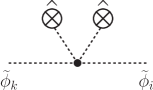
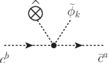
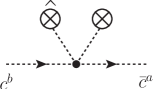
Figure 2: The three $\hat{v}$-insertion vertices on the first line correspond to the $\hat{v}$-dependent two- and three-point vertices associated with the gauge-fixing term $\Delta\mathcal{L}_{\mathrm{fix}}(\hat{v},H)$, defined in (171). The double $v\hat{v}$-insertion vertex on the second line contributes to the $v$ expansion of the SB theory (169). Like for the case of the $\tilde{v}$ insertions introduced in Section 3.4, the (pseudo) external lines associated with $\hat{v}$ insertions do not involve any propagator and do not correspond to any field. Such external lines should be regarded as a technical tool to keep track of the total power in $\hat{v}$ induced by vertices stemming from $\Delta\mathcal{L}_{\mathrm{fix}}(\hat{v},H)$.

Let us now discuss the implications of $\hat{v}$ insertions on the vev-expansion formula (98), which connects rational counterterms in the SB and symmetric phases. As we will show in the following, this formula can be extended to SB theories of type (169) by replacing vev expansions through double expansions in $v$ and $\hat{v}$. In order to demonstrate this, we will generalise the mass-expansion identities (113)–(115) in such a way that all requirements for the derivation of (98) in Section 3.6 remain valid.

The expansion (114) for 1PI vertex functions in $D_{\mathrm{n}}=D$ can be generalised as

$${\textbf{m}}_{[0,X]}\,{{\bar{\mathcal{A}}}_{{l,\Gamma}}^{\hskip 0.6pt}} = \left(\sum_{k=0}^{X}{{\bar{\mathcal{A}}}_{{l,\widetilde{\Gamma}{v^{k}}}}^{\hskip 0.6pt\widehat{\scriptscriptstyle\mathrm{YM}}}}\right)\prod_{i=1}^{n}\,\mathcal{U}^{-1}_{i}\,,$$ (172)

where we have included the effect of mixing as in Section 4.1, and the summands between brackets denote terms of total order $k$ in the vev. They correspond to the result of a double expansion in $v$ and $\hat{v}$, i.e.

$${{\bar{\mathcal{A}}}_{{l,\widetilde{\Gamma}v^{k}}}^{\hskip 0.6pt\widehat{\scriptscriptstyle\mathrm{YM}}}} = \sum_{j=0}^{k}{{\bar{\mathcal{A}}}_{{l,\widetilde{\Gamma}v^{k-j}\hat{v}^{j}}}^{\hskip 0.6pt{\scriptscriptstyle\mathrm{YM}}}}\,=\,\sum_{j=0}^{k}\frac{v^{k-j}}{(k-j)!}\,{{\bar{\mathcal{A}}}_{{l,\widetilde{\Gamma}\mathrm{H}^{k-j}\hat{v}^{j}}}^{\hskip 0.6pt{\scriptscriptstyle\mathrm{YM}}}}\Big{|}_{p_{\mathrm{H}}=0}\,.$$ (173)

Here the subscripts $v^{k-j}$ and $\hat{v}^{j}$ indicate the number of vev insertions of each kind, where the number $j$ of $\hat{v}$ insertions should be understood as the total power in the parameter $\hat{v}$ that results from the insertion of $\hat{v}$-dependent vertices. The expansion (115) in $D_{\mathrm{n}}=4$ can be generalised in a similar way as

$${\textbf{m}}_{[0,X]}\,{{\mathcal{A}}_{{l,\Gamma}}} = \left(\sum_{k=0}^{X}\sum_{j=0}^{k}{{\mathcal{A}}_{{l,\Gamma v^{k-j}\tilde{v}^{j}}}^{\widehat{\scriptscriptstyle\mathrm{YM}}}}\right)\prod_{i=1}^{n}\,\mathcal{U}^{-1}_{i}\,.$$ (174)

Here the terms with fixed $k$ correspond to the various contributions of total order $k$ in $v$, $\hat{v}$ and $\tilde{v}$. The summands between brackets read

$${{\mathcal{A}}_{{l,\widetilde{\Gamma}v^{m}\tilde{v}^{j}}}^{\widehat{\scriptscriptstyle\mathrm{YM}}}} = \sum_{n=0}^{m}{{\mathcal{A}}_{{l,\widetilde{\Gamma}v^{m-n}\hat{v}^{n}\tilde{v}^{j}}}^{{\scriptscriptstyle\mathrm{YM}}}}\,=\,\sum_{m=0}^{n}\frac{v^{m-n}}{(m-n)!}\,{{\mathcal{A}}_{{l,\widetilde{\Gamma}\mathrm{H}^{m-n}\hat{v}^{n}\tilde{v}^{j}}}^{{\scriptscriptstyle\mathrm{YM}}}}\Big{|}_{p_{\mathrm{H}}=0}\,.$$ (175)

As discussed in Section 3.4, the auxiliary $\tilde{v}$ insertions generate the parts of the mass expansion that are not accounted for by $v$ and $\hat{v}$ insertions in $D_{\mathrm{n}}=4$. Finally, the mass expansion (113) for UV counterterms can be generalised as

$${{\delta Z}_{{l,\Gamma}}} = \left(\sum_{k=0}^{X}\,{{\delta Z}_{{l,\widetilde{\Gamma}v^{k}}}^{\widehat{\scriptscriptstyle\mathrm{YM}}}}\right)\prod_{i=1}^{n}\,\mathcal{U}^{-1}_{i}\,,$$ (176)

where ${{\delta Z}_{{l,\Gamma}}}$ is the local counterterm for (172), and the summands on the rhs can be defined as the contributions of order $k$ in its mass expansion, i.e. the terms of total order $k$ in $v$ and $\hat{v}$. This implies that ${{\delta Z}_{{l,\widetilde{\Gamma}v^{k}}}^{\widehat{\scriptscriptstyle\mathrm{YM}}}}$ are the local UV counterterms for ${{\bar{\mathcal{A}}}_{{l,\widetilde{\Gamma}v^{k}}}^{\hskip 0.6pt\widehat{\scriptscriptstyle\mathrm{YM}}}}$. In this way, similarly as for (113)–(115), the identities (172)–(176) are nothing but mass expansions of the corresponding quantities. Moreover, in analogy with (89)–(90), for the mass expansion of subdivergences we have

$${\textbf{m}}_{[0,X]}\,\sum\limits_{\gamma\in\Omega(\Gamma)}{{\delta Z}_{{1,\gamma}}}\cdot{{\bar{\mathcal{A}}}_{{1,\Gamma/\gamma}}^{\hskip 0.6pt}} = \sum_{k=0}^{X}\sum_{j=0}^{k}\sum\limits_{\gamma\in\Omega(\Gamma)}\,{{\delta Z}_{{1,\gamma v^{j}}}^{\widehat{\scriptscriptstyle\mathrm{YM}}}}\cdot{{\bar{\mathcal{A}}}_{{1,(\Gamma/\gamma)\,v^{k-j}}}^{\hskip 0.6pt\widehat{\scriptscriptstyle\mathrm{YM}}}}$$ (177)

$$= \sum_{k=0}^{X}\sum\limits_{\gamma^{\prime}\in\Omega(\Gamma v^{k})}\,{{\delta Z}_{{1,\gamma^{\prime}}}^{\widehat{\scriptscriptstyle\mathrm{YM}}}}\cdot{{\bar{\mathcal{A}}}_{{1,\Gamma v^{k}/\gamma^{\prime}}}^{\hskip 0.6pt\widehat{\scriptscriptstyle\mathrm{YM}}}}\,.$$

The above properties satisfy all assumptions in the derivation of (98). Therefore, rational counterterms can be derived within the $\widehat{\mathrm{YM}}$ theory by means of a generalised expansion of the form

$$\delta\mathcal{R}_{l,\Gamma} = \left(\sum_{k=0}^{X}{{\delta\mathcal{R}}_{{l,\widetilde{\Gamma}v^{k}}}^{\widehat{\scriptscriptstyle\mathrm{YM}}}}\,\right)\prod_{i=1}^{n}\,\mathcal{U}^{-1}_{i}\,,$$ (178)

where ${{\delta\mathcal{R}}_{{l,\widetilde{\Gamma}v^{k}}}^{\widehat{\scriptscriptstyle\mathrm{YM}}}}$ for $l=1,2$ can be obtained from the related formulas in Section 3.6 through the substitutions

$${{\bar{\mathcal{A}}}_{{l,\Gamma v^{m}}}^{\hskip 0.6pt{\scriptscriptstyle\mathrm{YM}}}}\to{{\bar{\mathcal{A}}}_{{l,\widetilde{\Gamma}v^{m}}}^{\hskip 0.6pt\widehat{\scriptscriptstyle\mathrm{YM}}}}\,,\qquad{{\mathcal{A}}_{{l,\Gamma v^{m}\tilde{v}^{j}}}^{{\scriptscriptstyle\mathrm{YM}}}}\to{{\mathcal{A}}_{{l,\widetilde{\Gamma}v^{m}\tilde{v}^{j}}}^{\widehat{\scriptscriptstyle\mathrm{YM}}}}\,,\qquad{{\delta Z}_{{1,\Gamma v^{k}}}^{{\scriptscriptstyle\mathrm{YM}}}}\to{{\delta Z}_{{1,\widetilde{\Gamma}v^{k}}}^{\widehat{\scriptscriptstyle\mathrm{YM}}}}\,,$$ (179)

while $\delta\tilde{Z}^{\widehat{\scriptscriptstyle\mathrm{YM}}}_{1,\gamma}=\delta\tilde{Z}^{{\scriptscriptstyle\mathrm{YM}}}_{1,\gamma}$ since $\delta\tilde{Z}$ counterterms do not receive any vev insertion in renormalisable theories. See (110).

The one-loop counterterms ${{\delta Z}_{{1,\widetilde{\Gamma}v^{k}}}^{\widehat{\scriptscriptstyle\mathrm{YM}}}}$, which are required for the derivation of two-loop rational counterterms, can be generated through multiplicative renormalisation within the $\widehat{\mathrm{YM}}$ theory. In the $\hat{v}=0$ case, according to (147)–(148) we have

$${{\delta Z}_{{1,\widetilde{\Gamma}v^{k}}}^{{\scriptscriptstyle\mathrm{YM}}}} = {{\bar{\mathcal{A}}}_{{0,\widetilde{\Gamma}v^{k}}}^{\hskip 0.6pt{\scriptscriptstyle\mathrm{YM}}}}\,\Big{(}k\,\delta\mathcal{Z}_{v}\,+\sum_{i=1}^{n}\frac{1}{2}\,\delta\mathcal{Z}_{1,\widetilde{\varphi}_{i}}^{{\scriptscriptstyle\mathrm{YM}}}\Big{)}+D^{{\scriptscriptstyle\mathrm{YM}}}_{1,\theta}\,{{\bar{\mathcal{A}}}_{{0,\widetilde{\Gamma}v^{k}}}^{\hskip 0.6pt{\scriptscriptstyle\mathrm{YM}}}}\,,$$ (180)

and this relation can be extended to the $\hat{v}\neq 0$ case following the same derivations as in Section 4.1 with only few modifications as discussed in the following.

Within the SB broken theory (169), the additional $\hat{v}$-dependent UV divergences stemming from the ‘t Hooft gauge fixing can be cancelled through a shift of the vev renormalisation constant Sperling:2013eva , i.e. by turning (128) into

$$\delta\mathcal{Z}_{1,v}=\frac{1}{2}\delta\mathcal{Z}^{{\scriptscriptstyle\mathrm{YM}}}_{1,\phi}+\delta\mathcal{Z}^{\mathrm{fix}}_{1,v}\,,$$ (181)

while all vev-independent renormalisation constants can be kept fixed as in the $\hat{v}=0$ case. The shift $\delta\mathcal{Z}^{\mathrm{fix}}_{1,v}$ should be propagated to all vev-dependent renormalisation constants, such as mass counterterms and the tadpole counterterm (160). For convenience the UV divergent and finite parts of $\delta\mathcal{Z}^{\mathrm{fix}}_{1,v}$ can be chosen in such a way that renormalised tadpoles cancel exactly as discussed in Section 4.2 for the $\hat{v}=0$ case.

The $\hat{v}$-dependent parts of the UV counterterms of the SB and $\widehat{\mathrm{YM}}$ theories can be related to each other using the approach of Section 4.1. To this end, apart from (181) only two aspects need to be adapted to the $\hat{v}\neq 0$ case: in the tree-level mass expansion (145) one should replace

$${{\bar{\mathcal{A}}}_{{0,\widetilde{\Gamma}v^{k}}}^{\hskip 0.6pt{\scriptscriptstyle\mathrm{YM}}}} \to {{\bar{\mathcal{A}}}_{{0,\widetilde{\Gamma}v^{k}}}^{\hskip 0.6pt\widehat{\scriptscriptstyle\mathrm{YM}}}}\,,$$ (182)

and the list of independent parameters of the original symmetric theory has to be supplemented by $\hat{v}=\xi^{\prime}v$. Therefore the renormalisation operator (118) has to be extended as

$$D^{\widehat{\scriptscriptstyle\mathrm{YM}}}_{1,\theta} = D^{{\scriptscriptstyle\mathrm{YM}}}_{1,\theta}+\delta\mathcal{Z}_{1,\hat{v}}\,\hat{v}\,\frac{\partial}{\partial\hat{v}}\,,$$ (183)

with $\delta\mathcal{Z}_{1,\hat{v}}=\delta\mathcal{Z}_{1,\xi^{\prime}}+\delta\mathcal{Z}_{1,v}$. For the parameter-renormalisation operator (131) of the SB theory, which depends also on $v$, we have

$$D_{1,\theta} = D^{\widehat{\scriptscriptstyle\mathrm{YM}}}_{1,\theta}+\delta\mathcal{Z}_{1,v}\,v\,\frac{\partial}{\partial v}\,=\,D^{{\scriptscriptstyle\mathrm{YM}}}_{1,\theta}+\delta\mathcal{Z}_{1,\hat{v}}\,\hat{v}\,\frac{\partial}{\partial\hat{v}}+\delta\mathcal{Z}_{1,v}\,v\,\frac{\partial}{\partial v}\,.$$ (184)

Note that the renormalisation of $\xi$ is included in $D^{{\scriptscriptstyle\mathrm{YM}}}_{1,\theta}$, while $\delta\mathcal{Z}_{1,\hat{v}}\,\hat{v}\,\frac{\partial}{\partial\hat{v}}$ is responsible for the renormalisation of $\xi^{\prime}$. A suitable renormalisation of $\hat{v}$ is given by (167), which guarantees, together with (166), that the gauge-fixing term does not renormalise, and leads to finite vertex functions for physical and unphysical fields. Note that the choice (166)–(167) fixes the renormalisation of the mass terms in the ghost sector, i.e. it correctly cancels all the remaining poles after ghost-field renormalisation.

Applying the above modifications to (147)–(148) it turns out that the one-loop counterterms of the $\widehat{\mathrm{YM}}$ theory can be obtained from the renormalisation identity (180) with the replacements (181) and (182). More explicitly, using a similar $\hat{v}$-expansion as in (173) we have

$${{\delta Z}_{{1,\widetilde{\Gamma}v^{k}}}^{\widehat{\scriptscriptstyle\mathrm{YM}}}} = \sum_{j=0}^{k}{{\delta Z}_{{1,\widetilde{\Gamma}v^{k-j}\hat{v}^{j}}}^{{\scriptscriptstyle\mathrm{YM}}}}\,,$$ (185)

with

$${{\delta Z}_{{1,\widetilde{\Gamma}v^{k-j}\hat{v}^{j}}}^{{\scriptscriptstyle\mathrm{YM}}}} = {{\bar{\mathcal{A}}}_{{0,\widetilde{\Gamma}v^{k-j}\hat{v}^{j}}}^{\hskip 0.6pt{\scriptscriptstyle\mathrm{YM}}}}\,\bigg{(}k\,\delta\mathcal{Z}_{1,v}\,+\sum_{i=1}^{n}\frac{1}{2}\,\delta\mathcal{Z}_{1,\widetilde{\varphi}_{i}}^{{\scriptscriptstyle\mathrm{YM}}}\bigg{)}+\Big{(}D^{{\scriptscriptstyle\mathrm{YM}}}_{1,\theta}+j\delta\mathcal{Z}_{\xi^{\prime}}\Big{)}\,{{\bar{\mathcal{A}}}_{{0,\widetilde{\Gamma}v^{k-j}\hat{v}^{j}}}^{\hskip 0.6pt{\scriptscriptstyle\mathrm{YM}}}}\,,\quad\qquad$$ (186)

where $\delta\mathcal{Z}_{1,v}$ has to be chosen according to (181). Note that the tree-level amplitudes on the rhs are proportional to $v^{k-j}\hat{v}^{j}=(\xi^{\prime})^{j}v^{k}$. The renormalisation of this factor generates the term $k\,\delta\mathcal{Z}_{1,v}$ on the rhs of (186) plus an extra term $j\,\delta\mathcal{Z}_{\xi^{\prime}}$, which originates from $\delta\mathcal{Z}_{1,\hat{v}}=\delta\mathcal{Z}_{1,\xi^{\prime}}+\delta\mathcal{Z}_{1,v}$.

In summary, in the presence of gauge-fixing terms with a $\hat{v}$-dependence of type (169), rational terms can be determined through the generalised vev expansions (178)–(179), where standard vev insertions are supplemented by $\hat{v}$ insertions.

5 Rational counterterms of $\mathcal{O}(\alpha_{\scriptscriptstyle{\mathrm{S}}}^{2})$ for the Standard Model

The full set of two-loop rational counterterms for QCD has been presented in Lang:2020nnl , and in this section we derive all remaining $\delta\mathcal{R}_{2}$ counterterms of $\mathcal{O}(\alpha_{\scriptscriptstyle{\mathrm{S}}}^{2})$ for the full SM. These correspond to two-, three- or four-point counterterms involving quarks ($Q$) and/or gluons ($G$) in combination with one or more EW gauge bosons ($V$) and Higgs or would-be Goldstone bosons ($S$). In practice there are six classes of non-vanishing rational counterterms of this kind: $GGVV$, $GGGV$, $QQV$, $GGSS$, $GGS$ and $QQS$.

All calculations have been implemented twice and independently in two different frameworks. On the one hand we have used Geficom GEFICOM , which is based on Qgraf Nogueira:1991ex , Q2E and Exp Seidensticker:1999bb ; Harlander:1997zb , Form Vermaseren:2000nd ; Tentyukov:2007mu , Matad Steinhauser:2000ry and Color vanRitbergen:1998pn . On the other hand we have employed an in-house framework implemented in Python that uses Qgraf Nogueira:1991ex , Form Vermaseren:2000nd ; Tentyukov:2007mu and python-Form. A more detailed description of the methodology implemented in these two frameworks can be found in Sects. 5.1–5.2 of Lang:2020nnl .

In addition to the cross checks between the two independent calculations, we have verified that our results for one-loop rational counterterms are in agreement with the literature Draggiotis:2009yb , and that the two-loop results fulfil various self-consistency properties described in Sect. 5.1 of Lang:2020nnl .

As a further validation, we have compared two different ways of handling particle masses in the loops: direct calculations with massive quarks and, alternatively, the new vev-expansion technique introduced in this paper. The only massive states that can circulate in the loops at $\mathcal{O}(\alpha_{\scriptscriptstyle{\mathrm{S}}}^{2})$ are quarks, and the only $\delta\mathcal{R}$ counterterms that depend on quark masses are the ones associated with the $Q\bar{Q}$ and $GG$ two-point vertices Lang:2020nnl and with the $GGS$ three-point vertex. For such $\delta\mathcal{R}$ counterterms, in Section 5.4 we demonstrate that the results of explicit calculations with massive quarks are in agreement with the outcome of vev expansions. This should be regarded as a simple illustration of the usage of vev expansions, keeping in mind that the main goal of the vev-expansion approach is the calculation of $\delta\mathcal{R}$ counterterms for two-loop EW and mixed QCD–EW corrections.

5.1 Lagrangian

The presented results are based on the renormalised Lagrangian

$$\mathcal{L}\,=\,-\frac{1}{4}\,G^{a}_{\mu\nu}G^{a,\mu\nu}-\frac{\mathcal{Z}_{{\mathrm{gp}}}}{2\,\xi}\Big{(}\partial^{\mu}G^{a}_{\mu}\Big{)}^{2}-\,\mathcal{Z}_{c}\,\bar{c}^{a}\partial_{\mu}D^{\mu}_{ab}\,c^{b}$$

$${}+\sum_{i=1}^{N_{\mathrm{gen}}}\left[\,\bar{Q}_{i,\mathrm{L}}\Big{(}\mathrm{i}\gamma_{\mu}D^{\mu}\Big{)}\mathcal{Z}_{Q_{i}}Q_{i,\mathrm{L}}+\bar{u}_{i,\mathrm{R}}\Big{(}\mathrm{i}\gamma_{\mu}D^{\mu}\Big{)}\mathcal{Z}_{u_{i}}u_{i,\mathrm{R}}+\bar{d}_{i,\mathrm{R}}\Big{(}\mathrm{i}\gamma_{\mu}D^{\mu}\Big{)}\mathcal{Z}_{d_{i}}d_{i,\mathrm{R}}\right]$$

$${}-\,\sum_{i=1}^{N_{\mathrm{gen}}}\left\{\left[{\mathbf{\lambda}_{u_{i}}}\mathcal{Z}_{{\mathbf{\lambda}_{u_{i}}}}\left(\bar{Q}_{i,\mathrm{L}}\mathcal{Z}_{Q_{i}}^{1/2}\Phi^{\mathrm{c}}\right)\left(\mathcal{Z}_{u_{i}}^{1/2}u_{i,\mathrm{R}}\right)+{\mathbf{\lambda}_{d_{i}}}\mathcal{Z}_{{\mathbf{\lambda}_{d_{i}}}}\left(\bar{Q}_{i,\mathrm{L}}\mathcal{Z}_{Q_{i}}^{1/2}\Phi\right)\left(\mathcal{Z}_{d_{i}}^{1/2}d_{i,\mathrm{R}}\right)\right]\,+\,\mathrm{h.c.}\right\}\,,$$

with the field-strength tensor and the covariant derivatives

$$G^{a}_{\mu\nu} = \mathcal{Z}_{G}^{1/2}\left[\partial_{\mu}G^{a}_{\nu}-\partial_{\nu}G^{a}_{\mu}+\left(\mathcal{Z}_{\alpha_{\scriptscriptstyle{\mathrm{S}}}}\mathcal{Z}_{G}\right)^{1/2}g\,f^{abc}G_{\mu}^{b}G_{\nu}^{c}\right]\,,$$

$$D^{\mu}_{ab} = \partial^{\mu}\delta_{ab}-\left(\mathcal{Z}_{\alpha_{\scriptscriptstyle{\mathrm{S}}}}\mathcal{Z}_{G}\right)^{1/2}g_{\scriptscriptstyle{\mathrm{S}}}\,f^{abc}\,G^{c\mu}\,$$

$$D_{\mu} = \partial_{\mu}-\mathrm{i}\left(\mathcal{Z}_{\alpha_{\scriptscriptstyle{\mathrm{S}}}}\mathcal{Z}_{G}\right)^{1/2}g_{\scriptscriptstyle{\mathrm{S}}}t^{a}\,G^{a}_{\mu}-\mathrm{i}g_{2}T^{b}W^{b}_{\mu}+\mathrm{i}g_{1}\frac{Y}{2}B_{\mu},$$ (188)

where $G^{a}_{\mu}$, $W^{b}_{\mu}$ and $B_{\mu}$ are, respectively, the SU(3), SU(2) and U(1) gauge fields, and $c^{a}$ stands for the SU(3) ghosts. We include $N_{\mathrm{gen}}$ generations of left-chiral quark doublets $Q_{i,\mathrm{L}}=(u_{i,\mathrm{L}},d_{i,\mathrm{L}})^{\mathrm{T}}$ and right-chiral quark singlets $u_{i,\mathrm{R}}$, $d_{i,\mathrm{R}}$. This corresponds to an even number of active quark flavours, $n_{\mathrm{q}}=2N_{\mathrm{gen}}$. For the Higgs doublet and its charge conjugate we use the parametrisation

$$\Phi=\begin{pmatrix}\phi^{+}\\ \frac{1}{\sqrt{2}}\left(v+H+\mathrm{i}\chi\right)\end{pmatrix}\,,\;\quad\Phi^{\mathrm{c}}=\mathrm{i}\sigma^{2}\Phi^{\dagger}=\begin{pmatrix}\frac{1}{\sqrt{2}}\left(v+H-\mathrm{i}\chi\right)\\ \phi^{-}\end{pmatrix}\,.$$ (189)

In (5.1) we assume a diagonal CKM matrix, and quark masses are related to Yukawa couplings via

$$m_{q} = \frac{\lambda_{q}v}{\sqrt{2}}\qquad\mbox{for}\quad q=u_{i},d_{i}\,.$$ (190)

Since we restrict ourselves to QCD corrections, the Higgs sector of the SM Lagrangian is not included in (5.1). The same holds for the kinetic and gauge-fixing terms for the SU(2)$\times$U(1) gauge fields. For the gluon fields we adopt the Feynman gauge, which corresponds to $\xi=1$.

The various renormalisation constants in (5.1) are expanded in the strong coupling $\alpha_{\scriptscriptstyle{\mathrm{S}}}=g_{\scriptscriptstyle{\mathrm{S}}}^{2}/(4\pi)$ up to second order as

$$\mathcal{Z}_{\chi} = 1+\sum_{k=1}^{2}\left(\frac{\alpha_{\scriptscriptstyle{\mathrm{S}}}\,t^{\varepsilon}}{4\pi}\right)^{k}\delta\hat{\mathcal{Z}}_{k,\chi}\qquad\mbox{for}\qquad\chi=\alpha_{\scriptscriptstyle{\mathrm{S}}},\,G,\,c,\,q,\,\lambda_{q},\,{\mathrm{gp}}\,,$$ (191)

where $q=u_{i}$ or $d_{i}$. The scale factor $t=S\mu_{0}^{2}/\mu_{\mathrm{R}}^{2}$ embodies the dependence on the regularisation scale $\mu_{0}$, the renormalisation scale $\mu_{\mathrm{R}}$, and a possible rescaling factor $S$.

At lowest order in the EW and Yukawa interactions, the renormalisation of quark fields is independent of their chirality, and quark-doublet fields are renormalised by the diagonal matrix $\mathcal{Z}_{Q_{i}}=\mathrm{diag}(\mathcal{Z}_{u_{i}},\mathcal{Z}_{d_{i}})$. The gauge-fixing term involves a finite renormalisation constant $\mathcal{Z}_{{\mathrm{gp}}}=\mathcal{Z}_{G}/\mathcal{Z}_{\xi}$, which is kept free in our calculations, but in practical applications one can set $\mathcal{Z}_{{\mathrm{gp}}}=1$.

Explicit expressions for the UV poles of the various renormalisation constants in the $\overline{\mathrm{MS}}$ scheme are listed in Appendix B of Lang:2020nnl . The remaining scheme-dependent parts of all renormalisation constants are handled as free parameters in our calculations, and all results for the two-loop rational counterterms $\delta\mathcal{R}_{2,\Gamma}$ are expressed as linear combinations of one-loop renormalisation constants $\delta\hat{\mathcal{Z}}_{1,\chi}$ in a generic scheme.

The SU(3) generators in the fundamental representation obey

$$\big{[}t^{a},t^{b}\big{]} = \mathrm{i}f^{abc}t^{c},\qquad\mathrm{Tr}\left(t^{a}t^{b}\right)\,=\,T_{\mathrm{F}}\delta^{ab}\,.$$ (192)

Our results depend on the normalisation factor $T_{\mathrm{F}}$ and on the Casimir eigenvalues

$$C_{\mathrm{F}} = T_{\mathrm{F}}\frac{N^{2}-1}{N}\,,\qquad C_{\mathrm{A}}\,=\,N\,,$$ (193)

where $N=3$ is the number of colours.

The SU(2) and U(1) generators in the fundamental representation are

$$T^{b} = \frac{\sigma^{b}}{2}\,\omega_{\mathrm{L}}\,,\qquad Y\,=\,Y_{\mathrm{R}}\,\omega_{\mathrm{R}}+Y_{\mathrm{L}}\,\omega_{\mathrm{L}}\,,$$ (194)

where $\sigma^{b}$ are the Pauli matrices, and

$$\omega_{\mathrm{R}}\,=\,\omega_{+}\,=\,\frac{1}{2}(1+\gamma_{5})\,,\qquad\omega_{\mathrm{L}}\,=\,\omega_{-}\,=\,\frac{1}{2}(1-\gamma_{5})$$ (195)

project fermions on right- and left-chiral states. The $T^{3}$ and $Y$ generators are related to the electric charge $Q$ through

$$Q=T^{3}+\frac{Y}{2}\,,$$ (196)

and the hypercharge eigenvalues for quarks are $Y_{\mathrm{L},q}=1/3$ and $Y_{\mathrm{R},u}=4/3$, $Y_{\mathrm{R},d}=-2/3$.

5.2 Bookkeeping of SU(2)$\times$U(1) interactions

For an efficient bookkeeping of the EW gauge fields and associated generators it is convenient to use an extended multiplet

$$\tilde{V}_{\mu}\,=\,\left(W^{1}_{\mu},W^{2}_{\mu},W^{3}_{\mu},B_{\mu}\right)^{\mathrm{T}}\,,$$ (197)

and to write the EW part of the covariant derivative as

$$g_{2}T^{b}W^{b}_{\mu}-g_{1}\frac{Y}{2}B_{\mu}\,=\,e\,\sum_{\tilde{V}^{a}}\tilde{I}^{\tilde{V}^{a}}\,\tilde{V}^{a}_{\mu}\qquad\mbox{with}\quad\tilde{V}^{a}=W^{1},W^{2},W^{3},B\,.$$ (198)

Here and in the following the tilde is used to denote SU(2)$\times$U(1) eigenstate fields and related quantities. The electromagnetic coupling is given by

$$e\,=\,c_{\mathrm{w}}g_{1}\,=\,s_{\mathrm{w}}g_{2}\,,$$ (199)

where $c_{\mathrm{w}}=\cos{\theta_{\mathrm{w}}}$ and $s_{\mathrm{w}}=\sin{\theta_{\mathrm{w}}}$ are the cosine and sine of the weak mixing angle. The generators on the rhs of (198) correspond to

$$\tilde{I}^{W^{a}}\,=\,\frac{T^{a}}{s_{\mathrm{w}}}\,,\qquad\tilde{I}^{B}\,=\,-\frac{Y}{2c_{\mathrm{w}}}\,.$$ (200)

Diagrams where a SU(2)$\times$U(1) gauge boson couples to a closed quark loop give rise to traces of type

$$\mathrm{Tr}\left(\tilde{I}^{\tilde{V}^{a}}\right) = \mathrm{Tr}\left(\tilde{I}_{\mathrm{R}}^{\tilde{V}^{a}}\omega_{\mathrm{R}}+\tilde{I}_{\mathrm{L}}^{\tilde{V}^{a}}\omega_{\mathrm{L}}\right)\,=\,2\sum_{\lambda=\mathrm{R},\mathrm{L}}\mathrm{Tr}_{q}\left(\tilde{I}_{\lambda}^{\tilde{V}^{a}}\right)$$ (201)

$$= \begin{cases}\;\displaystyle-\frac{4}{c_{\mathrm{w}}}(Q_{u}+Q_{d})&\quad\tilde{V}^{a}=B\\[5.69054pt] \;0&\quad\tilde{V}^{a}=W^{a}\\ \end{cases}\,,$$

where $\mathrm{Tr}_{q}$ denotes the trace in the SU(2) quark-doublet space, the factor two in the second step arises from the traces of $w_{\pm}$, and the expressions on the rhs follow from $\mathrm{Tr}_{q}(T_{\lambda}^{a})=0$ and $\mathrm{Tr}_{q}(Y_{\lambda})=2(Q_{u}+Q_{d})$ for $\lambda=\mathrm{R},\mathrm{L}$. Traces involving a single SU(2)$\times$U(1) generator in combination with $\gamma_{5}$ vanish,

$$\mathrm{Tr}\left(\tilde{I}^{\tilde{V}^{a}}\gamma_{5}\right)\,=\,2\left[\mathrm{Tr}_{q}\left(\tilde{I}_{\mathrm{R}}^{\tilde{V}^{a}}\right)-\mathrm{Tr}_{q}\left(\tilde{I}_{\mathrm{L}}^{\tilde{V}^{a}}\right)\right]\,=\,0\,.$$ (202)

Diagrams where two SU(2)$\times$U(1) gauge boson couple to a closed quark loop yield traces of type

$$\mathrm{Tr}\left(\tilde{I}^{\tilde{V}^{a}}\tilde{I}^{\tilde{V}^{b}}\right) = 2\sum_{\lambda=\mathrm{R},\mathrm{L}}\mathrm{Tr}_{q}\left(\tilde{I}_{\lambda}^{\tilde{V}^{a}}\tilde{I}_{\lambda}^{\tilde{V}^{b}}\right)\,=\,\delta_{\tilde{V}^{a}\tilde{V}^{b}}\times\begin{cases}\;\displaystyle\frac{1}{c_{\mathrm{w}}^{2}}\left[4(Q_{u}^{2}+Q_{d}^{2})-1\right]&\mbox{for}\quad\tilde{V}^{a}=B\\[8.53581pt] \;\displaystyle\frac{1}{s_{\mathrm{w}}^{2}}&\mbox{for}\quad\tilde{V}^{a}=W^{a}\end{cases}\,,$$

where the expressions on the rhs follow from

$$\mathrm{Tr}_{q}\left(T^{a}_{\lambda}T^{b}_{\lambda}\right)\,=\,\frac{\delta_{\lambda\mathrm{L}}}{2}\,,\qquad\mathrm{Tr}_{q}\left(T^{a}_{\lambda}Y_{\lambda}\right)\,=\,0\,,\qquad\mathrm{Tr}_{q}\left(Y^{2}_{\lambda}\right)\,=\,4\mathrm{Tr}_{q}\left[Q^{2}-\left(T^{3}_{\lambda}\right)^{2}\right]\,.\qquad$$ (204)

In the broken phase, EW interactions are parametrised in terms of the mass- and charge-eigenstate gauge bosons

$$V_{\mu}\,=\,\left(W^{+}_{\mu},W^{-}_{\mu},Z_{\mu},A_{\mu}\right)^{\mathrm{T}}\,,$$ (205)

which are related to the gauge-group eigenstates through the mixing transformation

$$V_{\mu}\,=\,U(\theta_{\mathrm{w}})\tilde{V}_{\mu},\qquad U(\theta_{\mathrm{w}})\,=\,\begin{pmatrix}\frac{1}{\sqrt{2}}&\frac{-\mathrm{i}}{\sqrt{2}}&0&0\\ \frac{1}{\sqrt{2}}&\frac{\mathrm{i}}{\sqrt{2}}&0&0\\ 0&0&c_{\mathrm{w}}&s_{\mathrm{w}}\\ 0&0&-s_{\mathrm{w}}&c_{\mathrm{w}}\\ \end{pmatrix}.$$ (206)

The EW part of the covariant derivative assumes the form

$$g_{2}T^{b}W^{b}_{\mu}-g_{1}\frac{Y}{2}B_{\mu}\,=\,e\,\sum_{V^{a}}I^{V^{a}}\,V^{a}_{\mu}\qquad\mbox{with}\quad V^{a}=W^{+},W^{-},Z,A\,,$$ (207)

where

$$I^{V}=\tilde{I}^{\tilde{V}}\,U^{-1}(\theta_{\mathrm{w}})\,,$$ (208)

and the individual generators read

$$\mathrm{I}^{A}\,=\,-Q,\qquad\mathrm{I}^{Z}\,=\,\frac{T^{3}-s_{\mathrm{w}}^{2}Q}{s_{\mathrm{w}}c_{\mathrm{w}}},\qquad\mathrm{I}^{\pm}\,=\,\frac{1}{s_{\mathrm{w}}}T^{\pm}\,=\,\frac{1}{s_{\mathrm{w}}}\frac{T^{1}\pm\mathrm{i}T^{2}}{\sqrt{2}}\,.$$ (209)

Similarly as in (194), the EW generators can be decomposed as $I^{V_{a}}=I_{\mathrm{R}}^{V_{a}}\omega_{\mathrm{R}}+I_{\mathrm{L}}^{V_{a}}\omega_{\mathrm{L}}$, and the components of their building blocks read

$$\left(Q_{\lambda}\right)_{qq^{\prime}}\,=\,\delta_{qq^{\prime}}Q_{q}\,,\quad\left(T^{3}_{\lambda}\right)_{qq^{\prime}}\,=\,\delta_{\lambda\mathrm{L}}\delta_{qq^{\prime}}\,\frac{\delta_{qu}-\delta_{qd}}{2}\,,\quad\left(T^{+}_{\lambda}\right)_{qq^{\prime}}\,=\,\left(T^{-}_{\lambda}\right)_{q^{\prime}q}\,=\,\delta_{\lambda\mathrm{L}}\frac{\delta_{qu}\delta_{q^{\prime}d}}{\sqrt{2}}\,,$$

where $q,q^{\prime}=u$ or $d$.

In the mass-eigenstate basis the traces (201) and (5.2) become

$$\mathrm{Tr}\left(I^{V^{a}}\right) = -4(Q_{u}+Q_{d})\times\begin{cases}\;1&\qquad V^{a}=A\\[2.84526pt] \;\displaystyle\frac{s_{\mathrm{w}}}{c_{\mathrm{w}}}&\qquad V^{a}=Z\\[2.84526pt] \;0&\qquad V^{a}=W^{\pm}\\ \end{cases}\,,$$ (211)

and

$$\mathrm{Tr}\left(I^{V^{a}}I^{V^{b}}\right) = \begin{cases}\;4\left(Q_{u}^{2}+Q_{d}^{2}\right)\,&\mbox{$V^{a}V^{b}=AA$}\\[5.69054pt] \;\displaystyle\frac{1}{s_{\mathrm{w}}c_{\mathrm{w}}}\left(4s_{\mathrm{w}}^{2}\left(Q_{u}^{2}+Q_{d}^{2}\right)-1\right)\,&\mbox{$V^{a}V^{b}=AZ,ZA$}\\[5.69054pt] \;\displaystyle\frac{1}{s_{\mathrm{w}}^{2}c_{\mathrm{w}}^{2}}\left(4s_{\mathrm{w}}^{4}\left(Q_{u}^{2}+Q_{d}^{2}\right)+c_{\mathrm{w}}^{2}-s_{\mathrm{w}}^{2}\right)\,&\mbox{$V^{a}V^{b}=ZZ$}\\[5.69054pt] \;\displaystyle\frac{1}{s_{\mathrm{w}}^{2}}&\mbox{$V^{a}V^{b}=W^{\pm}W^{\mp}$}\\[8.53581pt] \;0&\mbox{otherwise}\end{cases}\,.$$ (212)

5.3 Treatment of $\gamma_{5}$

As is well known, the treatment of $\gamma_{5}$ is delicate in dimensional regularisation (see e.g. Jegerlehner:2000dz ) and various schemes have been proposed tHooft:1972tcz ; Akyeampong:1973xi ; Breitenlohner:1977hr ; Bonneau:1980yb ; Chanowitz:1979zu ; Larin:1993tq ; Korner:1989is . For the derivation of one- and two-loop rational counterterms through (15) and (20) we employ the so-called KKS scheme Korner:1989is ; Kreimer:1993bh ; Korner:1991sx , also known as reading-point prescription. In this scheme, the traces that arise from closed fermion loops are defined as non-cyclic objects, starting with the same open Lorentz index associated with one of the external vector bosons. In addition to the reading-point prescription, the properties that define $\gamma_{5}$ in the KKS scheme are

$$\{\gamma^{\mu},\gamma_{5}\} = 0,$$ (213)

$$\gamma_{5}^{2} = 1{},$$ (214)

$$4\mathrm{i}\epsilon_{\mu\nu\alpha\beta} = \mathrm{Tr}\left[\gamma_{5}\gamma_{\bar{\mu}}\gamma_{\bar{\nu}}\gamma_{\bar{\alpha}}\gamma_{\bar{\beta}}\right],$$ (216)

$$\text{non-cyclic trace},$$

where $\epsilon$ is the four-dimensional Levi-Civita tensor with $\epsilon_{0123}=1=-\epsilon^{0123}$. In the context of the KKS scheme, the identity (216) can be replaced by

$$\gamma_{5} = \frac{\mathrm{i}}{4!}\,\epsilon_{\mu\nu\rho\sigma}\,\gamma^{\mu}\gamma^{\nu}\gamma^{\rho}\gamma^{\sigma}\,.$$ (217)

In the general formulas (15) and (20) for the derivation of rational counterterms, the only ingredients that require the KKS scheme are the $D$-dimensional quantities ${{\bar{\mathcal{A}}}_{{1,\Gamma}}^{\hskip 0.6pt}}$, ${{\delta Z}_{{1,\gamma}}}\cdot{{\bar{\mathcal{A}}}_{{1,\Gamma/\gamma}}^{\hskip 0.6pt}}$ and ${{\bar{\mathcal{A}}}_{{2,\Gamma}}^{\hskip 0.6pt}}$, while in all other ingredients the loop numerator, including $\gamma_{5}$, is four-dimensional. Concerning the ingredients of the master formulas for renormalised amplitudes, (14) and (18), we note that all loop quantities are in $D_{\mathrm{n}}=4$ dimensions. This means that the subtleties related to the treatment of $\gamma_{5}$ in dimensional regularisation are addressed once and for all through the derivation of rational counterterms. We also note that rational counterterms are independent of the $\gamma_{5}$-scheme employed for their derivation. This is a consequence of the fact that renormalised amplitudes, as well as all $D_{\mathrm{n}}=4$ dimensional ingredients on the rhs of (14) and (18), are independent of the $\gamma_{5}$-scheme.

The derivations of the rational counterterms presented in this paper involve at most one quark loop containing a $\gamma_{5}$. Thus in the KKS scheme we never encounter more than one Levi-Civita tensor in the loop amplitude. Furthermore, in our calculations ${\varepsilon}$ tensors appear in the contributions of individual up or down fermions but cancel when summing over opposite quark flows and full SU(2) doublets, which is mandatory for UV and anomaly cancellations in the SM. This observation Denner:2019vbn is consistent with the behaviour of one-loop rational terms in the full SM Draggiotis:2009yb ; Garzelli:2009is , where traces like (216) drop out when combining loops with quarks and leptons of the same generation.

To check the correctness of our results we have implemented the KKS scheme in two different frameworks and independently. Furthermore we have reproduced our results using the naive-dimensional regularisation scheme as defined by Jegerlehner Jegerlehner:2000dz (the quasi self-chiral scheme), where one keeps the anti-commuting $\gamma_{5}$ (213), while giving up on (216) and (216), which are replaced by

$$\mathrm{Tr}\left[\gamma_{5}\gamma_{\bar{\mu}}\gamma_{\bar{\nu}}\gamma_{\bar{\alpha}}\gamma_{\bar{\beta}}\right]\,=\,0\,,$$ (218)

$$\text{cyclic trace}\,.$$ (219)

5.4 Rational counterterms

In the following, we present all rational counterterms for the SM Lagrangian (5.1) at order $\alpha_{\scriptscriptstyle{\mathrm{S}}}$ and $\alpha_{\scriptscriptstyle{\mathrm{S}}}^{2}$. As usual UV singularities are regularised in $D=4-2{\varepsilon}$ dimensions. The rational terms associated with a certain 1PI vertex function $\Gamma$ are presented in the form

$${{\delta\mathcal{R}}_{{k,\Gamma}}^{\alpha_{1}\dots\alpha_{N}}} = \mathrm{i}\left(\frac{\alpha_{\scriptscriptstyle{\mathrm{S}}}\,t^{\varepsilon}}{4\pi}\right)^{k}\sum_{a}\delta\hat{\mathcal{R}}^{(a)}_{k,\Gamma}\,\,\mathcal{T}_{a,\Gamma}^{\alpha_{1}\dots\alpha_{N}}\,\,,$$ (220)

where $k=1,2$ is the loop order, and $\mathcal{T}_{a,\Gamma}^{\alpha_{1}\dots\alpha_{N}}$ are independent tensor structures carrying the indices $\alpha_{1}\dots\alpha_{N}$ of the external lines of the vertex function at hand. Our results are presented in the form of complete Feynman rules, where tree-level contributions are supplemented by UV and rational counterterms. For $k$-loop UV counterterms ${{\delta Z}_{{k,\Gamma}}^{\alpha_{1}\dots\alpha_{N}}}$ a decomposition similar to (220) is used.

In the following all Dirac and colour indices associated with external quark lines are kept implicit. Fermion-loop contributions are either expressed as sums over $q\in\mathcal{Q}$, where the set $\mathcal{Q}$ contains all $n_{\mathrm{q}}=2N_{\mathrm{gen}}$ quarks that circulate in the loops, or are simply proportional to $n_{\mathrm{q}}$.

5.4.1 Vertices involving SU(2)$\times$U(1) vector bosons

The interaction of SU(2)$\times$U(1) gauge bosons with quarks and gluons gives rise to non-vanishing rational counterterms for the $GGVV$, $GGGV$ and $QQV$ vertices. Rational counterterms of this kind are free from any quark-mass dependence, i.e. they can be derived within the symmetric phase of the SM using massless quarks. The results are expressed in terms of the generic SU(2)$\times$U(1) generators introduced in Section 5.2 and are applicable both to the mass-eigenstate and gauge-eigenstate representation.

Four-point GGVV vertex

The Feynman rules for the interaction of two vector bosons and two gluons are

$$= \;\;{}\mathrm{i}\,\delta_{a_{3}a_{4}}\,e^{2}\,\frac{N_{\mathrm{gen}}}{2}\,\mathrm{Tr}\left(I^{V^{b_{1}}}I^{V^{b_{2}}}\right)$$ (221)

$${}\times\,\Bigg{\{}\,\sum_{k=1}^{2}\left(\frac{\alpha_{\scriptscriptstyle{\mathrm{S}}}\,t^{{\varepsilon}}}{4\pi}\right)^{k}\bigg{[}\sum_{\beta=\mathrm{I},\mathrm{II}}\mathcal{V}_{\beta}^{\mu_{1}\mu_{2}\mu_{3}\mu_{4}}\,\delta\hat{\mathcal{R}}^{(\beta)}_{k,\mathrm{ggVV}}\bigg{]}\Bigg{\}}\,,$$

with

$$\mathcal{V}_{\mathrm{I}}^{\mu_{1}\mu_{2}\mu_{3}\mu_{4}} = g^{\mu_{1}\mu_{2}}g^{\mu_{3}\mu_{4}}\,,\qquad\mathcal{V}_{\mathrm{II}}^{\mu_{1}\mu_{2}\mu_{3}\mu_{4}}\,=\,g^{\mu_{1}\mu_{3}}g^{\mu_{2}\mu_{4}}+g^{\mu_{1}\mu_{4}}g^{\mu_{2}\mu_{3}}\,.$$ (222)

Explicit expressions for the traces $\mathrm{Tr}(I^{V^{b_{1}}}I^{V^{b_{2}}})$ in the gauge- and mass-eigenstate basis are given in (5.2) and (212). For the rational counterterms we find

$$\delta\hat{\mathcal{R}}_{1,\mathrm{ggVV}}^{(\mathrm{I})}\;=\; \frac{2}{3}\,T_{\mathrm{F}}\,,$$

$$\delta\hat{\mathcal{R}}_{2,\mathrm{ggVV}}^{(\mathrm{I})}\;=\; -T_{\mathrm{F}}\,\left(\frac{1}{12}\,C_{\mathrm{A}}+\frac{3}{2}\,C_{\mathrm{F}}\right)+\frac{2}{3}\,T_{\mathrm{F}}\,\left(\,\delta\hat{\mathcal{Z}}_{1,\alpha_{\scriptscriptstyle{\mathrm{S}}}}+\,\delta\hat{\mathcal{Z}}_{1,G}\right)\,,$$ (223)

$$\delta\hat{\mathcal{R}}_{1,\mathrm{ggVV}}^{(\mathrm{II})}\;=\; \frac{2}{3}\,T_{\mathrm{F}}\,,$$

$$\delta\hat{\mathcal{R}}_{2,\mathrm{ggVV}}^{(\mathrm{II})}\;=\; \left[\frac{1}{2}\,T_{\mathrm{F}}\,C_{\mathrm{A}}\right]{\varepsilon}^{-1}-T_{\mathrm{F}}\,\left(\frac{1}{2}\,C_{\mathrm{A}}+\frac{3}{2}\,C_{\mathrm{F}}\right)+\frac{2}{3}\,T_{\mathrm{F}}\,\left(\,\delta\hat{\mathcal{Z}}_{1,\alpha_{\scriptscriptstyle{\mathrm{S}}}}+\,\delta\hat{\mathcal{Z}}_{1,G}\right)\,.$$

We note that $\delta\hat{\mathcal{R}}_{1,\mathrm{ggVV}}^{(\mathrm{I})}=\delta\hat{\mathcal{R}}_{1,\mathrm{ggVV}}^{(\mathrm{II})}$, which implies that the one-loop part of the rational counterterm (221) is totally symmetric in the four Lorentz indices $\mu_{1},\mu_{2},\mu_{3},\mu_{4}$. This is due to the fact that the four external vector bosons can be connected through fermionic loops in all permutations. At two loop-level this symmetry is still present in the contributions proportional to $C_{\mathrm{F}}$, while it is broken by the non-abelian contributions proportional to $C_{A}$. The latter involve virtual gluons that couple to fermionic loops and the external gluon lines, thereby breaking the symmetry between external gluons and electroweak bosons.

Four-point $GGSV$ vertex

The quartic vertex with two gluons, a vector boson and a scalar vanishes,

$$\,=\, 0\,.$$ (225)

This is due to the fact that the $GGSV$ vertex has a superficial degree of divergence equal to zero. This would require a dimensionless object carrying three Lorentz indices, which does not exist.

Four-point GGGV vertex

The Feynman rules for the interaction of a vector boson with three gluons are

$$\vbox{\hbox{\raisebox{0.0pt}{\includegraphics[width=95.39693pt]{CTgggVEW} }}}\;= \;\;{}\mathrm{i}\,g_{\scriptscriptstyle{\mathrm{S}}}\,e\,\frac{N_{\mathrm{gen}}}{2}\,\mathrm{Tr}\left(I^{V^{b}}\right)\,d^{\,a_{1}a_{2}a_{3}}\,\mathcal{V}^{\mu_{1}\mu_{2}\mu_{3}\nu}\,\Bigg{\{}\,\sum_{k=1}^{2}\left(\frac{\alpha_{\scriptscriptstyle{\mathrm{S}}}\,t^{{\varepsilon}}}{4\pi}\right)^{k}\,\delta\hat{\mathcal{R}}_{k,\mathrm{gggV}}\Bigg{\}}\,,$$

with

$$d^{abc}=\frac{1}{T_{\mathrm{F}}}\,\mathrm{Tr}\left(\left\{t^{a},t^{b}\right\}\,t^{c}\right)\,,$$ (227)

and

$$\mathcal{V}^{\mu_{1}\mu_{2}\mu_{3}\nu} = g^{\mu_{1}\mu_{2}}g^{\mu_{3}\nu}+g^{\mu_{1}\mu_{3}}g^{\mu_{2}\nu}+g^{\mu_{2}\mu_{3}}g^{\mu_{1}\nu}\,.$$ (228)

Explicit expressions for the traces $\mathrm{Tr}(I^{V^{b}})$ in the gauge- and mass-eigenstate basis are given in (201) and (211). For the rational terms we find

$$\delta\hat{\mathcal{R}}_{1,\mathrm{gggV}}\;=\; \frac{1}{3}\,T_{\mathrm{F}}\,,$$

$$\delta\hat{\mathcal{R}}_{2,\mathrm{gggV}}\;=\; \frac{1}{2}\,T_{\mathrm{F}}\,\left(\,\frac{1}{2}\,C_{\mathrm{A}}\,{\varepsilon}^{-1}-\frac{13}{24}\,C_{\mathrm{A}}-\frac{3}{2}\,C_{\mathrm{F}}+\,\delta\hat{\mathcal{Z}}_{1,\alpha_{\scriptscriptstyle{\mathrm{S}}}}+\,\delta\hat{\mathcal{Z}}_{1,G}\right)\,.$$ (229)

Three-point $GGV$ vertex

The counterterm for the interaction of a vector boson with two gluons vanishes,

$$\,=\, 0\,.$$ (230)

This cancellation results form the vanishing fermion traces in (201)–(202), and from the fact that also the trace of the U(1) generator in (201) cancels upon summation over quarks and anti-quarks in the loops. Note that this cancellation mechanism assumes complete SU(2) quark doublets.

Three-point $QQV$ vertex

The Feynman rules for the SU(2)$\times$U(1) quark interaction read

$$= \;\;{}\mathrm{i}\,e\,\gamma^{\mu}\,\delta_{kk^{\prime}}\sum_{\lambda=\mathrm{R},\mathrm{L}}\left(I^{V^{b}}_{\lambda}\right)_{qq^{\prime}}\omega_{\lambda}\,$$ (231)

$${}\times\bigg{\{}\,1+\sum_{k=1}^{2}\left(\frac{\alpha_{\scriptscriptstyle{\mathrm{S}}}\,t^{{\varepsilon}}}{4\pi}\right)^{k}\left(\delta\hat{Z}_{k,qq^{\prime}\mathrm{V}}+\delta\hat{\mathcal{R}}_{k,qq^{\prime}\mathrm{V}}\right)\bigg{\}}\,,$$

where $q,q^{\prime}\in\{u,d\}$ and $k,k^{\prime}\in\{1,\dots,N_{\mathrm{gen}}\}$ are the generation indices. The explicit components of the EW generators $I^{V^{b}}_{\lambda}$ in the gauge-eigenstate and mass-eigenstate basis can be found in Section 5.2. The UV counterterms correspond to the following combinations of renormalisation constants,

$$\delta\hat{Z}_{1,qq^{\prime}\mathrm{V}}\;=\; \frac{1}{2}\delta\hat{\mathcal{Z}}_{1,\alpha_{\scriptscriptstyle{\mathrm{S}}}}+\frac{1}{2}\left(\delta\hat{\mathcal{Z}}_{1,q}+\delta\hat{\mathcal{Z}}_{1,q^{\prime}}\right)\,,$$

$$\delta\hat{Z}_{2,qq^{\prime}\mathrm{V}}\;=\; \frac{1}{2}\delta\hat{\mathcal{Z}}_{2,\alpha_{\scriptscriptstyle{\mathrm{S}}}}+\frac{1}{2}\left(\delta\hat{\mathcal{Z}}_{2,q}+\delta\hat{\mathcal{Z}}_{2,q^{\prime}}\right)-\frac{1}{8}\delta\hat{\mathcal{Z}}_{1,\alpha_{\scriptscriptstyle{\mathrm{S}}}}^{2}+\frac{1}{4}\left(\delta\hat{\mathcal{Z}}_{1,q}+\delta\hat{\mathcal{Z}}_{1,q^{\prime}}\right)\delta\hat{\mathcal{Z}}_{1,\alpha_{\scriptscriptstyle{\mathrm{S}}}}\,,$$ (232)

and for the rational counterterms we obtain

$$\delta\hat{\mathcal{R}}_{1,qq^{\prime}\mathrm{V}}\;=\; -2\,C_{\mathrm{F}}\,,$$

$$\delta\hat{\mathcal{R}}_{2,qq^{\prime}\mathrm{V}}\;=\; \left[-\frac{29}{9}\,C_{\mathrm{A}}\,C_{\mathrm{F}}+\frac{4}{3}\,C_{\mathrm{F}}^{2}+\frac{7}{9}\,T_{\mathrm{F}}\,n_{\mathrm{q}}\,C_{\mathrm{F}}\right]{\varepsilon}^{-1}-\frac{763}{108}\,C_{\mathrm{A}}\,C_{\mathrm{F}}+\frac{109}{18}\,C_{\mathrm{F}}^{2}+\frac{55}{54}\,T_{\mathrm{F}}\,n_{\mathrm{q}}\,C_{\mathrm{F}}$$

$$-\,C_{\mathrm{F}}\,\left(2\,\delta\hat{\mathcal{Z}}_{1,\alpha_{\scriptscriptstyle{\mathrm{S}}}}+\frac{1}{2}\,\delta\hat{\mathcal{Z}}_{1,G}-\frac{5}{6}\,\delta\hat{\mathcal{Z}}_{1,{\mathrm{gp}}}+\frac{2}{3}\,\left(\delta\hat{\mathcal{Z}}_{1,q}+\delta\hat{\mathcal{Z}}_{1,q^{\prime}}\right)\right)\,.$$

5.4.2 Vertices involving scalar bosons

The Yukawa interactions of the scalar doublet with external quarks and closed quark loops give rise to non-vanishing rational counterterms for the vertices of type $GGSS$, $GGS$ and $QQS$. The $GGSS$ and $QQS$ rational counterterms depend only on the dimensionless Yukawa couplings and can be derived within the symmetric phase of the SM using massless quarks. The $GGS$ counterterm depends on the vev and can be determined in the broken phase, with massive quarks, or using vev expansions.

Four-point $GGSS$ vertex

The Feynman rules for the interaction of two gluons with two scalar fields are

$$\vbox{\hbox{\raisebox{12.0pt}{\includegraphics[width=95.39693pt]{CTggSSEW}} }}\;=\;{}\mathrm{i}\,\delta^{a_{1}a_{2}}\,C_{\mathrm{gg}S_{1}S_{2}}\,g^{\mu_{1}\mu_{2}}\bigg{\{}\,\sum_{k=1}^{2}\left(\frac{\alpha_{\scriptscriptstyle{\mathrm{S}}}\,t^{\varepsilon}}{4\pi}\right)^{k}\delta\hat{\mathcal{R}}_{k,\mathrm{gg\mathrm{H}\mathrm{H}}}\bigg{\}}\,,$$ (234)

with

$$C_{\mathrm{gg}S_{1}S_{2}} = \begin{cases}\;{\displaystyle 1}&\qquad S_{1}S_{2}=HH,\chi\chi,\phi^{\pm}\phi^{\mp}\\[5.69054pt] \;{\displaystyle 0}&\qquad\mbox{otherwise}\end{cases}\,.$$ (235)

For the rational counterterms we find

$$\delta\hat{\mathcal{R}}_{1,\mathrm{gg\mathrm{H}\mathrm{H}}}\;=\; -2\,T_{\mathrm{F}}\sum_{q\in\mathcal{Q}}\lambda_{q}^{2}\,,$$

$$\delta\hat{\mathcal{R}}_{2,\mathrm{gg\mathrm{H}\mathrm{H}}}\;=\; -T_{\mathrm{F}}\sum_{q\in\mathcal{Q}}\,\left[\left(\frac{1}{2}\,C_{\mathrm{A}}+6\,C_{\mathrm{F}}\right){\varepsilon}^{-1}+\frac{11}{24}\,C_{\mathrm{A}}-\frac{37}{4}\,C_{\mathrm{F}}\right]\,\lambda_{q}^{2}$$

$$-2\,T_{\mathrm{F}}\sum_{q\in\mathcal{Q}}\left[\delta\hat{\mathcal{Z}}_{1,\alpha_{\scriptscriptstyle{\mathrm{S}}}}+\delta\hat{\mathcal{Z}}_{1,G}+2\,\delta\hat{\mathcal{Z}}_{1,\lambda_{q}}\right]\,\lambda_{q}^{2}\,.$$ (236)

Four-point $GGGS$ vertices

The quartic vertex with three gluons and a scalar boson vanishes,

$$\,=\, 0\,.$$ (237)

The reason is the same as for (225).

Three-point $GGS$ vertex

The Feynman rules for the interactions of a scalar with two gluons are

$$\vbox{\hbox{\raisebox{12.0pt}{\includegraphics[width=95.39693pt]{CTggSEW}} }}\;=\;{}\mathrm{i}\,\delta_{SH}\,\delta^{a_{1}a_{2}}\,v\,g^{\mu_{1}\mu_{2}}\,\bigg{\{}\,\sum_{k=1}^{2}\left(\frac{\alpha_{\scriptscriptstyle{\mathrm{S}}}\,t^{\varepsilon}}{4\pi}\right)^{k}\delta\hat{\mathcal{R}}_{k,\mathrm{gg\mathrm{H}}}\bigg{\}}\,.$$ (238)

Note that only the Higgs boson, $S=H$, yields a non-zero rational counterterm. The result is proportional to the vacuum expectation value, i.e. it vanishes in the symmetric phase. In the broken phase, i.e. using non-zero quark masses, we find

$$\delta\hat{\mathcal{R}}_{1,\mathrm{gg\mathrm{H}}}\;=\; -2\,T_{\mathrm{F}}\sum_{q\in\mathcal{Q}}\lambda_{q}^{2}\,,$$

$$\delta\hat{\mathcal{R}}_{2,\mathrm{gg\mathrm{H}}}\;=\; -T_{\mathrm{F}}\sum_{q\in\mathcal{Q}}\,\left[\left(\frac{1}{2}\,C_{\mathrm{A}}+6\,C_{\mathrm{F}}\right){\varepsilon}^{-1}+\frac{19}{12}\,C_{\mathrm{A}}-7\,C_{\mathrm{F}}\right]\,\lambda_{q}^{2}$$

$$-2\,T_{\mathrm{F}}\sum_{q\in\mathcal{Q}}\left[\delta\hat{\mathcal{Z}}_{1,\alpha_{\scriptscriptstyle{\mathrm{S}}}}+\delta\hat{\mathcal{Z}}_{1,G}+2\,\delta\hat{\mathcal{Z}}_{1,\lambda_{q}}\right]\,\lambda_{q}^{2}\,.$$ (239)

These results have been cross-checked against calculations in the symmetric phase using vev expansions. For the vertex at hand, the vev-expansion formula (112) reads

$$\delta\mathcal{R}_{k,\mathrm{gg}\mathrm{H}} = \delta\mathcal{R}^{{\scriptscriptstyle\mathrm{YM}}}_{k,\mathrm{gg}\mathrm{H}}+\delta\mathcal{R}^{{\scriptscriptstyle\mathrm{YM}}}_{k,\mathrm{gg}\mathrm{H}v}+\delta\mathcal{R}^{{\scriptscriptstyle\mathrm{YM}}}_{k,\mathrm{gg}\mathrm{H}\tilde{v}}\,=\,v\,\delta\mathcal{R}^{{\scriptscriptstyle\mathrm{YM}}}_{k,\mathrm{gg}\mathrm{H}\mathrm{H}}+\delta\mathcal{R}^{{\scriptscriptstyle\mathrm{YM}}}_{k,\mathrm{gg}\mathrm{H}\tilde{v}}\,,$$ (240)

where $\delta\mathcal{R}^{{\scriptscriptstyle\mathrm{YM}}}_{k,\mathrm{gg}\mathrm{H}\mathrm{H}}=\delta\mathcal{R}_{k,\mathrm{gg}\mathrm{H}\mathrm{H}}$ is given in (234)–(5.4). For the additional $\delta\mathcal{R}^{{\scriptscriptstyle\mathrm{YM}}}_{k,\mathrm{gg}\mathrm{H}\tilde{v}}$ contribution, which is defined by the general identities (103), (3.6) and the rules for $\tilde{v}$ insertions (81)–(84), we find

$$\delta\mathcal{R}^{{\scriptscriptstyle\mathrm{YM}}}_{k,\mathrm{gg}S\tilde{v}}\; = \vbox{\hbox{\raisebox{12.0pt}{\includegraphics[width=95.39693pt]{CTggSdVEW}} }}\;=\;{}\mathrm{i}\,\delta_{SH}\,\delta^{a_{1}a_{2}}\,v\,g^{\mu_{1}\mu_{2}}\,\bigg{\{}\,\sum_{k=1}^{2}\left(\frac{\alpha_{\scriptscriptstyle{\mathrm{S}}}\,t^{\varepsilon}}{4\pi}\right)^{k}\delta\hat{\mathcal{R}}^{{\scriptscriptstyle\mathrm{YM}}}_{k,\mathrm{gg\mathrm{H}}\tilde{v}}\bigg{\}},\qquad$$ (241)

with

$$\delta\hat{\mathcal{R}}_{1,\mathrm{gg\mathrm{H}}\tilde{v}}^{{\scriptscriptstyle\mathrm{YM}}}\;=\; 0\,,$$

$$\delta\hat{\mathcal{R}}_{2,\mathrm{gg\mathrm{H}}\tilde{v}}^{{\scriptscriptstyle\mathrm{YM}}}\;=\; -T_{\mathrm{F}}\sum_{q\in\mathcal{Q}}\,\left[\,\frac{9}{8}\,C_{\mathrm{A}}+\frac{9}{4}\,C_{\mathrm{F}}\,\right]\,\lambda_{q}^{2}\,.$$ (242)

Note that $\delta\mathcal{R}^{{\scriptscriptstyle\mathrm{YM}}}_{k,\mathrm{gg}\mathrm{H}\tilde{v}}\neq 0$ in spite of the fact that $\delta\mathcal{R}^{{\scriptscriptstyle\mathrm{YM}}}_{k,\mathrm{gg}\mathrm{H}}=0$ in the symmetric phase. Rewriting the identity (240) in terms of the $\delta\hat{\mathcal{R}}$ coefficients on the rhs of (238), (234) and (241) we have

$$\delta\hat{\mathcal{R}}_{k,\mathrm{gg\mathrm{H}}} = \delta\hat{\mathcal{R}}_{k,\mathrm{gg\mathrm{H}\mathrm{H}}}+\delta\hat{\mathcal{R}}^{{\scriptscriptstyle\mathrm{YM}}}_{k,\mathrm{gg\mathrm{H}}\tilde{v}}\,,$$ (243)

and combining the explicit ingredients of the vev expansion, (5.4) and (5.4), we find agreement with the result of the explicit derivation in the broken phase (5.4).

Three-point $QQS$ vertex

The Feynman rules for the Yukawa interactions of quarks read

$$= -\mathrm{i}\,\delta_{kk^{\prime}}\,\sum_{\lambda=\mathrm{R},\mathrm{L}}C^{\lambda}_{qq^{\prime}S}\,\omega_{\lambda}$$ (244)

$${}\times\,\bigg{\{}\,1+\sum_{k=1}^{2}\left(\frac{\alpha_{\scriptscriptstyle{\mathrm{S}}}\,t^{{\varepsilon}}}{4\pi}\right)^{k}\bigg{[}\delta\hat{Z}_{k,qq^{\prime}\mathrm{H}}+\delta\hat{\mathcal{R}}_{k,qq^{\prime}\mathrm{H}}\bigg{]}\bigg{\}}\,,$$

where $S=H,\chi,\phi^{\pm}$ are the components of the scalar doublet, while $q,q^{\prime}\in\{u,d\}$, and $k,k^{\prime}\in\{1,\dots,N_{\mathrm{gen}}\}$ are generation indices. The tree-level coupling factors read

$$\begin{array}[]{c@{\quad} ||@{\quad}c@{\quad}|@{\quad}c@{\quad}|@{\quad}c@{\quad}|@{\quad}c@{\quad} }\bar{q}q^{\prime}S&\bar{q}qH&\bar{q}q\chi&\bar{u}d\phi^{+}&\bar{d}u\phi^{-}\\ \hline\cr C^{\mathrm{R}}&\frac{\lambda_{q}}{\sqrt{2}}&s_{q}\frac{\mathrm{i}\lambda_{q}}{\sqrt{2}}&\lambda_{d}&-\lambda_{u}\\ \hline\cr C^{\mathrm{L}}&\frac{\lambda_{q}}{\sqrt{2}}&-s_{q}\frac{\mathrm{i}\lambda_{q}}{\sqrt{2}}&-\lambda_{u}&\lambda_{d}\end{array}$$ (252)

where $s_{q}$ assumes the values $s_{u}=1$ and $s_{d}=-1$. The UV counterterms read

$$\delta\hat{Z}_{1,qq^{\prime}\mathrm{H}} = \frac{1}{2}\left(\delta\hat{\mathcal{Z}}_{1,q}+\delta\hat{\mathcal{Z}}_{1,q^{\prime}}\right)+\delta\hat{\mathcal{Z}}_{1,qq^{\prime}}^{(\mathrm{Yuk})}\,,$$

$$\delta\hat{Z}_{2,qq^{\prime}\mathrm{H}} = \frac{1}{2}\left(\delta\hat{\mathcal{Z}}_{2,q}+\delta\hat{\mathcal{Z}}_{2,q^{\prime}}\right)+\delta\hat{\mathcal{Z}}_{2,qq^{\prime}}^{(\mathrm{Yuk})}\,+\frac{1}{2}\left(\delta\hat{\mathcal{Z}}_{1,q}+\delta\hat{\mathcal{Z}}_{1,q^{\prime}}\right)\,\delta\hat{\mathcal{Z}}_{1,qq^{\prime}}^{(\mathrm{Yuk})}\,,$$ (253)

where

$$\delta\hat{\mathcal{Z}}_{k,qq^{\prime}}^{(\mathrm{Yuk})} = \delta\hat{\mathcal{Z}}_{k,\lambda_{q^{\prime}}}\omega_{\mathrm{R}}+\delta\hat{\mathcal{Z}}_{k,\lambda_{q}}\omega_{\mathrm{L}}\,,$$ (254)

and for the rational counterterms we obtain

$$\delta\hat{\mathcal{R}}_{1,qq^{\prime}\mathrm{H}} = -4C_{\mathrm{F}}\,,$$

$$\delta\hat{\mathcal{R}}_{2,qq^{\prime}\mathrm{H}} = \left(\frac{16}{3}\,C_{\mathrm{F}}^{2}-\frac{293}{36}\,C_{\mathrm{A}}\,C_{\mathrm{F}}+\frac{19}{9}\,T_{\mathrm{F}}\,n_{\mathrm{q}}\,C_{\mathrm{F}}\right){\varepsilon}^{-1}+\frac{20}{9}\,C_{\mathrm{F}}^{2}-\frac{2237}{216}\,C_{\mathrm{A}}\,C_{\mathrm{F}}$$ (255)

$${}+\frac{91}{54}\,T_{\mathrm{F}}\,n_{\mathrm{q}}\,C_{\mathrm{F}}-C_{\mathrm{F}}\Big{[}4\,\delta\hat{\mathcal{Z}}_{1,\alpha_{\scriptscriptstyle{\mathrm{S}}}}+\frac{2}{3}\,\left(\delta\hat{\mathcal{Z}}_{1,q}+\delta\hat{\mathcal{Z}}_{1,q^{\prime}}\right)+4\,\delta\hat{\mathcal{Z}}_{1,qq^{\prime}}^{(\mathrm{Yuk})}$$

$${}-\frac{1}{2}\delta\hat{\mathcal{Z}}_{1,G}-\frac{5}{6}\,\delta\hat{\mathcal{Z}}_{1,{\mathrm{gp}}}\Big{]}\,.$$

5.4.3 Quark and gluon two-point vertices

The QCD rational counterterms for quark and gluon two-point vertices depend on the masses of quarks that circulate in the loops. Explicit derivations with massive quarks have been presented in Lang:2020nnl . In the following we show that such counterterms can be reproduced by means of vev expansions.

Two-point $Q\bar{Q}$ vertex

The Feynman rule for the two-point function of a massive quark reads

$$\;\vbox{\hbox{\raisebox{-28.0pt}{\includegraphics[width=95.39693pt]{CTquarkEW}} }}=\;\mathrm{i}\,\delta_{kk^{\prime}}\delta_{qq^{\prime}}\,\bigg{\{}\,\left(\not{p}-m_{q}\right)$$

$$\qquad+\,\sum_{k=1}^{2}\left(\frac{\alpha_{\scriptscriptstyle{\mathrm{S}}}\,t^{{\varepsilon}}}{4\pi}\right)^{k}\bigg{[}\left(\delta\hat{Z}^{({\scriptscriptstyle\mathrm{P}})}_{k,qq}+\delta\hat{\mathcal{R}}^{({\scriptscriptstyle\mathrm{P}})}_{k,qq}\right)\,\not{p}\,+\left(\delta\hat{Z}^{({\scriptscriptstyle\mathrm{m}})}_{k,qq}+\delta\hat{\mathcal{R}}^{({\scriptscriptstyle\mathrm{m}})}_{k,qq}\right)m_{q}\bigg{]}\bigg{\}}\,,$$ (256)

where $q,q^{\prime}\in\{u,d\}$, and $k,k^{\prime}\in\{1,\dots,N_{\mathrm{gen}}\}$ are generation indices. The direction of the quark momentum $p$ is aligned with the fermion flow. For the UV counterterms we have

$$\delta\hat{Z}_{1,qq}^{({\scriptscriptstyle\mathrm{P}})} \;=\;\delta\hat{\mathcal{Z}}_{1,q}\,, \quad\delta\hat{Z}_{2,qq}^{({\scriptscriptstyle\mathrm{P}})}\;=\; \delta\hat{\mathcal{Z}}_{2,q}\,,$$

$$\delta\hat{Z}_{1,qq}^{({\scriptscriptstyle\mathrm{m}})} \;=\;-\delta\hat{\mathcal{Z}}_{1,q}-\delta\hat{\mathcal{Z}}_{1,\lambda_{q}}\,, \quad\delta\hat{Z}_{2,qq}^{({\scriptscriptstyle\mathrm{m}})}\;=\; -\delta\hat{\mathcal{Z}}_{2,q}-\delta\hat{\mathcal{Z}}_{2,\lambda_{q}}-\delta\hat{\mathcal{Z}}_{1,q}\,\delta\hat{\mathcal{Z}}_{1,\lambda_{q}}\,,$$ (257)

where $\delta\hat{\mathcal{Z}}_{k,\lambda_{q}}=\delta\hat{\mathcal{Z}}_{k,m_{q}}$. For the rational counterterms, the direct derivation with massive quarks yields Lang:2020nnl

$$\delta\hat{\mathcal{R}}_{1,qq}^{({\scriptscriptstyle\mathrm{P}})}\;=\; -C_{\mathrm{F}}\,,$$

$$\delta\hat{\mathcal{R}}_{2,qq}^{({\scriptscriptstyle\mathrm{P}})}\;=\; \left(\frac{7}{6}\,C_{\mathrm{F}}^{2}-\frac{61}{36}\,C_{\mathrm{A}}\,C_{\mathrm{F}}+\frac{5}{9}\,T_{\mathrm{F}}\,n_{\mathrm{q}}\,C_{\mathrm{F}}\right){\varepsilon}^{-1}+\frac{43}{36}\,C_{\mathrm{F}}^{2}-\frac{1087}{216}\,C_{\mathrm{A}}\,C_{\mathrm{F}}+\frac{59}{54}\,T_{\mathrm{F}}\,n_{\mathrm{q}}\,C_{\mathrm{F}}$$

$$-C_{\mathrm{F}}\left(\delta\hat{\mathcal{Z}}_{1,\alpha_{\scriptscriptstyle{\mathrm{S}}}}+\frac{2}{3}\,\delta\hat{\mathcal{Z}}_{1,q}-\frac{2}{3}\,\delta\hat{\mathcal{Z}}_{1,{\mathrm{gp}}}\right)\,,$$ (258)

and

$$\delta\hat{\mathcal{R}}_{1,qq}^{({\scriptscriptstyle\mathrm{m}})}\;=\; 2\,C_{\mathrm{F}}\,,$$

$$\delta\hat{\mathcal{R}}_{2,qq}^{({\scriptscriptstyle\mathrm{m}})}\;=\; \left(-2\,C_{\mathrm{F}}^{2}+\frac{61}{12}\,C_{\mathrm{A}}\,C_{\mathrm{F}}-\frac{5}{3}\,T_{\mathrm{F}}\,n_{\mathrm{q}}\,C_{\mathrm{F}}\right){\varepsilon}^{-1}+C_{\mathrm{F}}^{2}+\frac{199}{24}\,C_{\mathrm{A}}\,C_{\mathrm{F}}-\frac{11}{6}\,T_{\mathrm{F}}\,n_{\mathrm{q}}\,C_{\mathrm{F}}$$

$$+C_{\mathrm{F}}\left(2\,\delta\hat{\mathcal{Z}}_{1,\alpha_{\scriptscriptstyle{\mathrm{S}}}}+4\,\delta\hat{\mathcal{Z}}_{1,\lambda_{q}}-\frac{3}{2}\,\delta\hat{\mathcal{Z}}_{1,G}-\frac{1}{2}\,\delta\hat{\mathcal{Z}}_{1,{\mathrm{gp}}}\right)\,.$$ (259)

The momentum-dependent contributions (5.4) do not depend on quark masses and can be derived in the symmetric phase, using massless quarks. The mass-dependent contributions (5.4) can be cross-checked against calculations in the symmetric phase using vev expansions. For the vertex at hand, the vev-expansion formula (112) yields the mass-dependent contributions

$$\delta\mathcal{R}_{k,qq}\bigg{|}_{p=0} = \delta\mathcal{R}^{{\scriptscriptstyle\mathrm{YM}}}_{k,qqv}+\delta\mathcal{R}^{{\scriptscriptstyle\mathrm{YM}}}_{k,qq\tilde{v}}\,=\,v\,\delta\mathcal{R}^{{\scriptscriptstyle\mathrm{YM}}}_{k,qq\mathrm{H}}+\delta\mathcal{R}^{{\scriptscriptstyle\mathrm{YM}}}_{k,qq\tilde{v}}\,,$$ (260)

where $\delta\mathcal{R}^{{\scriptscriptstyle\mathrm{YM}}}_{k,qq\mathrm{H}}$ is given in (244)–(5.4). For the additional $\tilde{v}$-insertion term $\delta\mathcal{R}^{{\scriptscriptstyle\mathrm{YM}}}_{k,qq\tilde{v}}$, which is defined by (81)–(84), (103) and (3.6), we find

$$\delta\mathcal{R}^{{\scriptscriptstyle\mathrm{YM}}}_{k,qq\tilde{v}}\;=\;\vbox{\hbox{\raisebox{22.0pt}{\includegraphics[width=95.39693pt]{CTqqdVEW}} }}\;=\;-\mathrm{i}\,\delta_{kk^{\prime}}\delta_{qq^{\prime}}\,\frac{v\,\lambda_{q}}{\sqrt{2}}\,\,\bigg{\{}\,\sum_{k=1}^{2}\left(\frac{\alpha_{\scriptscriptstyle{\mathrm{S}}}\,t^{{\varepsilon}}}{4\pi}\right)^{k}\delta\hat{\mathcal{R}}^{{\scriptscriptstyle\mathrm{YM}}}_{k,qq\tilde{v}}\,\bigg{\}}\,,$$ (261)

with

$$\delta\hat{\mathcal{R}}_{1,qq\tilde{v}}^{{\scriptscriptstyle\mathrm{YM}}}\;=\; 2\,C_{\mathrm{F}}\,,$$

$$\delta\hat{\mathcal{R}}_{2,qq\tilde{v}}^{{\scriptscriptstyle\mathrm{YM}}}\;=\; -\left(\frac{10}{3}\,C_{\mathrm{F}}^{2}-\frac{55}{18}\,C_{\mathrm{A}}\,C_{\mathrm{F}}+\frac{4}{9}\,T_{\mathrm{F}}\,n_{\mathrm{q}}\,C_{\mathrm{F}}\right){\varepsilon}^{-1}-\frac{29}{9}\,C_{\mathrm{F}}^{2}+\frac{223}{108}\,C_{\mathrm{A}}\,C_{\mathrm{F}}+\frac{4}{27}\,T_{\mathrm{F}}\,n_{\mathrm{q}}\,C_{\mathrm{F}}$$

$$-C_{\mathrm{F}}\left(-2\,\delta\hat{\mathcal{Z}}_{1,\alpha_{\scriptscriptstyle{\mathrm{S}}}}-\frac{4}{3}\,\delta\hat{\mathcal{Z}}_{1,q}-\delta\hat{\mathcal{Z}}_{1,G}+\frac{1}{3}\,\delta\hat{\mathcal{Z}}_{1,{\mathrm{gp}}}\right)\,.$$ (262)

Rewriting (260) in terms of the $\delta\hat{\mathcal{R}}$ coefficients on the rhs of (244) and (261) we have

$$\delta\hat{\mathcal{R}}^{({\scriptscriptstyle\mathrm{m}})}_{k,{qq}} = -\left(\delta\hat{\mathcal{R}}_{k,{qq}\mathrm{H}}+\delta\hat{\mathcal{R}}^{{\scriptscriptstyle\mathrm{YM}}}_{k,{qq}\tilde{v}}\right)\,,$$ (263)

and combining the explicit ingredients of the vev expansion, (5.4) and (5.4), we find agreement with the result of the explicit derivation in the broken phase (5.4).

Two-point $GG$ vertex

In the $\xi=1$ gauge, the Feynman rule for the gluon two-point vertex reads

$$\vbox{\hbox{\raisebox{-33.0pt}{\includegraphics[width=95.39693pt]{CTgluon}} }}\;=\; {}\mathrm{i}\,\delta^{a_{1}a_{2}}\bigg{\{}-p^{2}g^{\mu_{1}\mu_{2}}+\,\sum_{k=1}^{2}\left(\frac{\alpha_{\scriptscriptstyle{\mathrm{S}}}\,t^{\varepsilon}}{4\pi}\right)^{k}\bigg{[}\left(\delta\hat{Z}^{({\scriptscriptstyle\mathrm{P}})}_{k,\mathrm{gg}}+\delta\hat{\mathcal{R}}^{({\scriptscriptstyle\mathrm{P}})}_{k,\mathrm{gg}}\right)\,p^{\mu_{1}}p^{\mu_{2}}$$

$$\qquad+\left(\delta\hat{Z}^{({\scriptscriptstyle\mathrm{G}})}_{k,\mathrm{gg}}p^{2}+\delta\hat{\mathcal{R}}^{({\scriptscriptstyle\mathrm{G}})}_{k,\mathrm{gg}}\,p^{2}+\delta\tilde{Z}^{({\scriptscriptstyle\mathrm{G}})}_{k,\mathrm{gg}}\,\tilde{p}^{2}+v^{2}\delta\hat{\mathcal{R}}^{({\scriptscriptstyle\mathrm{m}})}_{k,\mathrm{gg}}\right)\,g^{\mu_{1}\mu_{2}}\bigg{]}\bigg{\}}\,.$$ (264)

The coefficients of the standard UV counterterms are given by

$$\delta\hat{Z}_{1,\mathrm{gg}}^{({\scriptscriptstyle\mathrm{P}})} \;=\;\delta\hat{\mathcal{Z}}_{1,G}-\delta\hat{\mathcal{Z}}_{1,{\mathrm{gp}}}\,, \quad\delta\hat{Z}_{2,\mathrm{gg}}^{({\scriptscriptstyle\mathrm{P}})}\;=\; \delta\hat{\mathcal{Z}}_{2,G}-\delta\hat{\mathcal{Z}}_{2,{\mathrm{gp}}}\,,$$

$$\delta\hat{Z}_{1,\mathrm{gg}}^{({\scriptscriptstyle\mathrm{G}})} \;=\;{}-\delta\hat{\mathcal{Z}}_{1,G}\,, \quad\delta\hat{Z}_{2,\mathrm{gg}}^{({\scriptscriptstyle\mathrm{G}})}\;=\; {}-\delta\hat{\mathcal{Z}}_{2,G}\,.$$ (265)

The additional $\tilde{p}^{2}$-dependent UV counterterm is required for the subtraction of one-loop subdivergences (see Section 2.2), and the relevant one-loop coefficients is

$$\delta\tilde{Z}^{({\scriptscriptstyle\mathrm{G}})}_{1,\mathrm{gg}}\;=\;\left(\frac{2}{3}\,C_{\mathrm{A}}+\frac{2}{3}\,T_{\mathrm{F}}\,n_{\mathrm{q}}\right){\varepsilon}^{-1}\,.$$ (266)

Rational counterterms in (264) are split into momentum-dependent and vev-dependent contributions. The former are independent of quark masses, and the corresponding coefficients read Lang:2020nnl

$$\delta\hat{\mathcal{R}}_{1,\mathrm{gg}}^{({\scriptscriptstyle\mathrm{P}})}\;=\; -\frac{C_{\mathrm{A}}}{3}\,,$$

$$\delta\hat{\mathcal{R}}_{2,\mathrm{gg}}^{({\scriptscriptstyle\mathrm{P}})}\;=\; \left[\frac{19}{36}\,C_{\mathrm{A}}^{2}+T_{\mathrm{F}}\,n_{\mathrm{q}}\left(-\frac{32}{9}\,C_{\mathrm{A}}+2\,C_{\mathrm{F}}\right)\right]{\varepsilon}^{-1}+T_{\mathrm{F}}\,n_{\mathrm{q}}\left(\frac{217}{108}\,C_{\mathrm{A}}-\frac{71}{18}\,C_{\mathrm{F}}\right)+\frac{1211}{864}\,C_{\mathrm{A}}^{2}$$

$$+C_{\mathrm{A}}\left(-\frac{1}{3}\,\delta\hat{\mathcal{Z}}_{1,\alpha_{\scriptscriptstyle{\mathrm{S}}}}-\frac{35}{12}\,\delta\hat{\mathcal{Z}}_{1,G}+\frac{3}{4}\,\delta\hat{\mathcal{Z}}_{1,{\mathrm{gp}}}+\frac{1}{6}\,\delta\hat{\mathcal{Z}}_{1,c}\right)+\frac{4}{3}\,T_{\mathrm{F}}\,\sum_{q\in\mathcal{Q}}\delta\hat{\mathcal{Z}}_{1,q}\,,$$

$$\delta\hat{\mathcal{R}}_{1,\mathrm{gg}}^{({\scriptscriptstyle\mathrm{G}})}\;=\; \left(\frac{C_{\mathrm{A}}}{2}+\frac{2}{3}\,T_{\mathrm{F}}\,n_{\mathrm{q}}\right)\,,$$

$$\delta\hat{\mathcal{R}}_{2,\mathrm{gg}}^{({\scriptscriptstyle\mathrm{G}})}\;=\; \left[-\frac{4}{9}\,C_{\mathrm{A}}^{2}+T_{\mathrm{F}}\,n_{\mathrm{q}}\left(\frac{35}{9}\,C_{\mathrm{A}}-2\,C_{\mathrm{F}}\right)\right]{\varepsilon}^{-1}+T_{\mathrm{F}}\,n_{\mathrm{q}}\left(-\frac{193}{108}\,C_{\mathrm{A}}+\frac{109}{36}\,C_{\mathrm{F}}\right)-\frac{541}{432}\,C_{\mathrm{A}}^{2}$$

$$+\left(\frac{C_{\mathrm{A}}}{2}+\frac{2}{3}\,T_{\mathrm{F}}\,n_{\mathrm{q}}\right)\,\delta\hat{\mathcal{Z}}_{1,\alpha_{\scriptscriptstyle{\mathrm{S}}}}+\left(\frac{71}{24}\,C_{\mathrm{A}}+\frac{2}{3}\,T_{\mathrm{F}}\,n_{\mathrm{q}}\right)\,\delta\hat{\mathcal{Z}}_{1,G}-\frac{7}{8}\,C_{\mathrm{A}}\,\delta\hat{\mathcal{Z}}_{1,{\mathrm{gp}}}$$

$$+\frac{C_{\mathrm{A}}}{12}\,\delta\hat{\mathcal{Z}}_{1,c}-\frac{4}{3}\,T_{\mathrm{F}}\sum_{q\in\mathcal{Q}}\delta\hat{\mathcal{Z}}_{1,q}\,,$$ (267)

where $\delta\hat{\mathcal{Z}}_{1,c}$ is the ghost-field renormalisation constant. For the vev-dependent part, the direct derivation of rational counterterms with quark masses $m_{q}=v\,\lambda_{q}/\sqrt{2}$ yields Lang:2020nnl

$$\delta\hat{\mathcal{R}}_{1,\mathrm{gg}}^{({\scriptscriptstyle\mathrm{m}})} = -2\,T_{\mathrm{F}}\sum_{q\in\mathcal{Q}}\,\lambda_{q}^{2}\,,$$

$$\delta\hat{\mathcal{R}}_{2,\mathrm{gg}}^{({\scriptscriptstyle\mathrm{m}})} = -\frac{T_{\mathrm{F}}}{2}\sum_{q\in\mathcal{Q}}\,\Big{[}\left(C_{\mathrm{A}}+6\,C_{\mathrm{F}}\right){\varepsilon}^{-1}+\frac{13}{6}\,C_{\mathrm{A}}-7\,C_{\mathrm{F}}+4\left(\delta\hat{\mathcal{Z}}_{1,\alpha_{\scriptscriptstyle{\mathrm{S}}}}+\delta\hat{\mathcal{Z}}_{1,G}+\delta\hat{\mathcal{Z}}_{1,\lambda_{q}}\right)\Big{]}\,\lambda_{q}^{2}\,.$$

This result can be cross-checked against vev expansions in the unbroken phase. According to (112) the mass-dependent contributions for the gluon–gluon vertex are given by

$$\delta\mathcal{R}_{k,\mathrm{gg}}\bigg{|}_{p=0} = \delta\mathcal{R}^{{\scriptscriptstyle\mathrm{YM}}}_{k,\mathrm{gg}vv}+\delta\mathcal{R}^{{\scriptscriptstyle\mathrm{YM}}}_{k,\mathrm{gg}v\tilde{v}}+\delta\mathcal{R}^{{\scriptscriptstyle\mathrm{YM}}}_{k,\mathrm{gg}\tilde{v}\tilde{v}}$$ (269)

$$= \frac{v^{2}}{2}\delta\mathcal{R}^{{\scriptscriptstyle\mathrm{YM}}}_{k,\mathrm{gg}\mathrm{H}\mathrm{H}}+v\delta\mathcal{R}^{{\scriptscriptstyle\mathrm{YM}}}_{k,\mathrm{gg}\mathrm{H}\tilde{v}}+\delta\mathcal{R}^{{\scriptscriptstyle\mathrm{YM}}}_{k,\mathrm{gg}\tilde{v}\tilde{v}}.$$

Note that single $v$ or $\tilde{v}$ insertions do not contribute since $\delta\mathcal{R}_{k,\mathrm{gg}}$ has mass dimension two. Note also that, according to (101) and (107), double $v$ insertions give rise to a factor $1/2$ when expressed in terms of counterterms with external Higgs lines. This is not the case for double $\tilde{v}$ insertions, since such insertions correspond to the auxiliary loop propagators (81)–(83), which are not related to external Higgs lines. The explicit expressions for $\delta\mathcal{R}^{{\scriptscriptstyle\mathrm{YM}}}_{k,\mathrm{gg}\mathrm{H}\mathrm{H}}=\delta\mathcal{R}_{k,\mathrm{gg}\mathrm{H}\mathrm{H}}$ and $\delta\mathcal{R}^{{\scriptscriptstyle\mathrm{YM}}}_{k,\mathrm{gg}\mathrm{H}\tilde{v}}$ are given, respectively, in (234)–(5.4) and (241)–(5.4). For the additional $\delta\mathcal{R}^{{\scriptscriptstyle\mathrm{YM}}}_{k,\mathrm{gg}\tilde{v}\tilde{v}}$ contribution, applying (81)–(84), (103) and (3.6), we find

$$\delta\mathcal{R}^{{\scriptscriptstyle\mathrm{YM}}}_{k,\mathrm{gg}\tilde{v}\tilde{v}}\;=\;\vbox{\hbox{\raisebox{12.0pt}{\includegraphics[width=95.39693pt]{CTggdVdVEW}} }}\,=\,{}\mathrm{i}\,\delta^{a_{1}a_{2}}\,v^{2}\,g^{\mu_{1}\mu_{2}}\,\bigg{\{}\,\sum_{k=1}^{2}\left(\frac{\alpha_{\scriptscriptstyle{\mathrm{S}}}\,t^{\varepsilon}}{4\pi}\right)^{k}\delta\hat{\mathcal{R}}^{{\scriptscriptstyle\mathrm{YM}}}_{k,\mathrm{gg}\tilde{v}\tilde{v}}\bigg{\}}\,,$$ (270)

with coefficients

$$\delta\hat{\mathcal{R}}^{{\scriptscriptstyle\mathrm{YM}}}_{1,\mathrm{gg}\tilde{v}\tilde{v}}\;=\; -\,T_{\mathrm{F}}\sum_{q\in\mathcal{Q}}\lambda_{q}^{2}\,,$$

$$\delta\hat{\mathcal{R}}^{{\scriptscriptstyle\mathrm{YM}}}_{2,\mathrm{gg}\tilde{v}\tilde{v}}\;=\; -T_{\mathrm{F}}\sum_{q\in\mathcal{Q}}\,\left[\left(\frac{1}{4}\,C_{\mathrm{A}}\right){\varepsilon}^{-1}-\frac{13}{48}\,C_{\mathrm{A}}-\frac{9}{8}\,C_{\mathrm{F}}\right]\,\lambda_{q}^{2}-\,T_{\mathrm{F}}\sum_{q\in\mathcal{Q}}\left[\delta\hat{\mathcal{Z}}_{1,\alpha_{\scriptscriptstyle{\mathrm{S}}}}+\delta\hat{\mathcal{Z}}_{1,G}\right]\,\lambda_{q}^{2}\,.$$ (271)

Finally, rewriting the vev-expansion identity (269) in terms of the $\delta\hat{\mathcal{R}}$ coefficients on the rhs of (234), (241) and (270) we have

$$\delta\hat{\mathcal{R}}^{({\scriptscriptstyle\mathrm{m}})}_{k,\mathrm{gg}} = \frac{1}{2}\delta\hat{\mathcal{R}}_{k,\mathrm{gg\mathrm{H}\mathrm{H}}}+\delta\hat{\mathcal{R}}^{{\scriptscriptstyle\mathrm{YM}}}_{k,\mathrm{gg\mathrm{H}}\tilde{v}}+\delta\hat{\mathcal{R}}^{{\scriptscriptstyle\mathrm{YM}}}_{k,\mathrm{gg}\tilde{v}\tilde{v}}\,,$$ (272)

and combining the explicit ingredients of the vev expansion, (5.4), (5.4) and (5.4), we find full agreement with the result of the explicit derivation in the broken phase (5.4).

6 Summary

The advent of automated numerical algorithms has opened the door to the calculation of a vast range of nontrivial scattering amplitudes at one loop. In this context, rational counterterms have proven to be a key ingredient for the efficient implementation of dimensional regularisation within numerical frameworks. The idea is that all process-dependent parts of the calculations can be carried out with numerical tools that build loop-integrand numerators in $D_{\mathrm{n}}=4$ dimensions, while all contributions stemming from the $(D_{\mathrm{n}}-4)$-dimensional parts of the numerators can be reconstructed through process-independent rational counterterms.

The theoretical framework to extend this approach beyond one loop has been established in Pozzorini:2020hkx ; Lang:2020nnl . In particular, it was shown that renormalised two-loop amplitudes can be constructed through a modified version of the well-known R-operation, where loop amplitudes with $D_{\mathrm{n}}=4$ dimensional loop numerators are combined with UV counterterms and associated rational counterterms.

So far, the required two-loop rational counterterms were known only for U(1) and SU(N) gauge theories Pozzorini:2020hkx ; Lang:2020nnl , where the relevant derivations are largely simplified by the underlying gauge symmetry, which allows one to treat all fields in terms of generic fermion and gauge-boson multiplets. In the case of spontaneously broken (SB) gauge theories, this is no longer possible since, in general, the various states within a multiplet acquire different masses, mix with one another, and are renormalised in a different way. For these reasons, the direct determination of two-loop rational counterterms for the full SM, including EW corrections, can be very challenging.

In order to simplify this task, we have presented a general method that makes it possible to relate the rational counterterms for a SB theory to corresponding counterterms in the underlying symmetric theory via expansions in the vev parameter $v$. This method is based on the fact that, in $D_{\mathrm{n}}=D$ dimensions, the mass dependence of loop amplitudes in the SB phase can be generated through systematic $v$ expansions, where terms of order $v^{k}$ are obtained in the symmetric phase via insertion of $k$ external Higgs lines with zero momentum. These so-called $v$ insertions are not sufficient in order to obtain the correct mass dependence of loop amplitudes in $D_{\mathrm{n}}=4$ dimensions. This is due to the fact that the projection of loop numerators to $D_{\mathrm{n}}=4$ dimensions does not commute with the expansion in the vev parameter. In particular, in $D_{\mathrm{n}}=4$ dimensions the mass dependence of fermionic loop propagators involves additional terms proportional to $v\tilde{q}^{2}/\bar{q}^{4}$ and $v^{2}\not{q}\tilde{q}^{2}/\bar{q}^{6}$, where $\bar{q}$ is the loop momentum in $D$ dimensions and $\tilde{q}$ its $(D-4)$-dimensional part. As shown in Section 3.4, such contributions can be accounted for by means of auxiliary fermion propagators. For their systematic bookkeeping we have extended the Feynman rules by introducing auxiliary vertices where fermion propagators are coupled to one or two pseudo external lines that we have dubbed $\tilde{v}$ insertions.

Based on this approach we have derived general vev-expansion formulas of the form (98), where the one- and two-loop rational counterterms for a generic SB theory are expressed in terms of related counterterms with $v$ and $\tilde{v}$ insertions in the symmetric phase. In this way, the bulk of the derivation of rational counterterms is restricted to the symmetric phase, while all effects of SB are accounted for by adding (in total) at most two $v$ or $\tilde{v}$ insertions.

This method is based on rigid invariance, i.e. on the assumption that the vev dependence of the Lagrangian is entirely generated through shifts of the Higgs field, $H\to H+v$. Moreover, the proof presented in Section 3 is based on the $\overline{\mathrm{MS}}$-scheme. The extension to realistic renormalisation schemes for SB theories, such as the on-shell scheme, has been discussed in Section 4. In a first step we have demonstrated, still assuming rigid invariance, that the vev-expansion formula (98) remains valid for a wide class of renormalisation schemes for SB theories. In particular it remains valid for any scheme that is equivalent to a renormalisation of the symmetric phase, where the independent renormalisation constants can assume arbitrary finite parts, provided that the underlying symmetry is preserved. In this context we have shown that the renormalisation of the parameters of the symmetric phase and the vev can be easily adapted such as to satisfy typical renormalisation conditions for SB theories. We have also discussed how to ensure the cancellation of renormalised tadpoles, and we have shown that residual mixing effects between on-shell mass eigenstates can be easily compensated by means of finite LSZ factors.

Finally we have discussed possible violations of rigid invariance, which can arise when the gauge-fixing Lagrangian involves vev-dependent terms that do not arise from the symmetric phase via $H\to H+v$ shifts. Such terms are present, for instance, in the ‘t Hooft gauge fixing, where they are introduced in order to cancel the mixing between gauge bosons and Goldstone bosons. To keep track of vev-dependent gauge-fixing terms that violate rigid invariance we have defined the parameter $\hat{v}=\xi^{\prime}v$, where $\xi^{\prime}$ is a gauge-fixing parameter, and we have introduced technical $\hat{v}$-insertion Feynman rules that make it possible to generate the $\hat{v}$-dependent parts of loop amplitudes in a controlled way. Gauge-fixing terms that violate rigid invariance give rise to $\hat{v}$-dependent UV divergences that are not present in the symmetric phase. As is known, such divergences can be cancelled through a shift of the vev-renormalisation constant, which can be chosen in such a way that renormalised tadpoles cancel exactly, while keeping all vev- and tadpole-independent renormalisation constants unchanged. As for the rational counterterms, we have shown that the extra $\hat{v}$-dependence that results from violations of rigid invariance can be accommodated in the generalised vev-expansion formula (178), where rational counterterms for the SB phase are connected to the ones of the symmetric phase by means of combinations of $v$, $\tilde{v}$ and $\hat{v}$ insertions.

This approach can be used for the determination of rational counterterms in any SB gauge theory with wide flexibility in the choices of the gauge fixing and the renormalisation scheme. As a first application, we have presented the full set of $\mathcal{O}(\alpha_{\scriptscriptstyle{\mathrm{S}}}^{2})$ rational counterterms for the interactions of quarks or gluons with EW vector bosons and scalars in a generic renormalisation scheme. Together with the counterterms derived in Pozzorini:2020hkx ; Lang:2020nnl these new results provide the complete set of rational counterterms for two-loop QCD calculations in the full SM.

Acknowledgements

This research was supported by the Swiss National Science Foundation (SNSF) under contract BSCGI0-157722. The work of M.Z. was supported through the SNSF Ambizione grant PZ00P2-179877.

Appendix A Commutator of mass expansion and $D_{\mathrm{n}}=4$ projection

In this appendix we consider the commutator of the mass expansion and the projection to four dimensions (59) for the case of generic propagators (62), and we derive the identities (69)–(70) up to second order in the mass expansion.

At zeroth order we simply have

$$\Delta{\textbf{V}}_{0}\,\bar{G}_{aa}(\bar{q},m_{a}) = G_{aa}(\bar{q},0)-G_{aa}(\bar{q},0)\,=\,0\,.$$ (273)

At first order we compute $\Delta{\textbf{V}}_{1}={\textbf{m}}_{1}{\textbf{P}}_{4}-{\textbf{P}}_{4}{\textbf{m}}_{1}$ using (51) and keeping only linear terms in $m_{a}$,

$$\Delta{\textbf{V}}_{1}\,\bar{G}_{aa}(\bar{q},m_{a}) = m_{a}\left(\partial_{m_{a}}G_{aa}-G_{aa}\left(\partial_{m_{a}}\Gamma_{aa}\right)G_{aa}\right)\big{|}_{m_{a}=0}$$ (274)

$$= m_{a}\big{(}\partial_{m_{a}}G_{aa}-G_{aa}\,\partial_{m_{a}}\left(\Gamma_{aa}G_{aa}\right)+G_{aa}\Gamma_{aa}\left(\partial_{m_{a}}G_{aa}\right)\big{)}\big{|}_{m_{a}=0}$$

$$= m_{a}\,\frac{\tilde{q}^{2}}{\bar{q}^{4}}\,\frac{\partial g_{aa}(q,m_{a})}{\partial m_{a}}\bigg{|}_{m_{a}=0}\;,$$

where in the second line we used the product rule

$$(\partial_{m_{a}}\Gamma_{aa})G_{aa} = \partial_{m_{a}}(\Gamma_{aa}G_{aa})-\Gamma_{aa}(\partial_{m_{a}}G_{aa})\,.$$ (275)

To arrive to the last line we eliminate all appearances of $G_{aa}$ and $G_{aa}\Gamma_{aa}$ in favour of $g_{aa}$ using (61) and (68), respectively.

To second order we proceed in the same way, except that it is no longer possible to eliminate all appearances of $\Gamma_{aa}$ without introducing inverse propagators. Instead we choose to eliminate $G_{aa}$, as well as all $\Gamma_{aa}$ with mass derivatives using (275) together with

$$G_{aa}(\partial_{m_{a}}^{2}\Gamma_{aa})G_{aa} = \left[\partial_{m_{a}}^{2}(G_{aa}\Gamma_{aa})-(\partial_{m_{a}}^{2}G_{aa})\Gamma_{aa}-2(\partial_{m_{a}}G_{aa})(\partial_{m_{a}}\Gamma_{aa})\right]G_{aa}$$ (276)

$$= (\partial_{m_{a}}^{2}(G_{aa}\Gamma_{aa}))G_{aa}-(\partial_{m_{a}}^{2}G_{aa})(\Gamma_{aa}G_{aa})$$

$${}-2(\partial_{m_{a}}G_{aa})\left[\partial_{m_{a}}(G_{aa}\Gamma_{aa})-\Gamma_{aa}(\partial_{m_{a}}G_{aa})\right]\,.$$

In this way we find

$$\Delta{\textbf{V}}_{2}\,\bar{G}_{aa}(\bar{q},m_{a}) = \frac{1}{2}\,m_{a}^{2}\left.\left(\partial^{2}_{m_{a}}G_{aa}-2\,\left(G_{aa}\left(\partial_{m_{a}}\Gamma_{aa}\right)\right)^{2}G_{a}-G_{aa}\left(\partial_{m_{a}}^{2}\Gamma_{aa}\right)G_{aa}\right)\right|_{m_{a}=0}$$ (277)

$$= m_{a}^{2}\,\left[\frac{1}{2}\,\frac{\tilde{q}^{2}}{\bar{q}^{4}}\frac{\partial^{2}g_{aa}(q,m_{a})}{\partial m_{a}^{2}}-\frac{\tilde{q}^{2}}{\bar{q}^{6}}\left(\frac{\partial g_{aa}(q,m_{a})}{\partial m_{a}}\right)^{2}\Gamma_{aa}(q,m_{a})\right]_{m_{a}=0}\,.\quad$$

The terms (274) and (277) correspond to the first- and second-order contributions on the rhs of (69). These results are applicable to any propagator of the form (61), where the numerator $g_{aa}(q,m_{a})$ is a polynomial in $q$ and $m_{a}$.