Charged particles interaction in both a finite volume and a uniform magnetic field II: topological and analytic properties of a magnetic system

Abstract

In present work, we discuss some topological features of charged particles interacting a uniform magnetic field in a finite volume. The edge state solutions are presented, as a signature of non-trivial topological systems, the energy spectrum of edge states show up in the gap between allowed energy bands. By treating total momentum of two-body system as a continuous distributed parameter in complex plane, the analytic properties of solutions of finite volume system in a magnetic field is also discussed.

I Introduction

Study of few-body hadron/nuclear particles interaction and properties of few-body resonances is one of important subjects in modern physics. Hadron/nuclear particles provide the only means of understanding quantum Chromodynamics (QCD), the underlying theory of quark and gluon interactions. However, making prediction of hadron/nuclear particle interactions from first principles is not always straightforward, due to the fact that most of theoretical computations are performed in various traps, for instance, periodic cubic box in lattice quantum Chromodynamics (LQCD). As the result of trapped systems, only discrete energy spectrum is observed instead of scattering amplitudes. Hence, extracting infinite volume scattering amplitudes from discrete energy spectrum in a trapped system have became an important subject in LQCD and nuclear physics communities, see e.g. Refs. Lüscher (1991); Rummukainen and Gottlieb (1995); Christ et al. (2005); Bernard et al. (2008); He et al. (2005); Lage et al. (2009); Döring et al. (2011); Guo et al. (2013); Guo (2013); Kreuzer and Hammer (2009); Polejaeva and Rusetsky (2012); Hansen and Sharpe (2014); Mai and Döring (2017, 2019); Döring et al. (2018); Guo (2017); Guo and Gasparian (2017, 2018); Guo and Morris (2019); Mai et al. (2020); Guo et al. (2018); Guo (2020a); Guo and Döring (2020); Guo (2020b); Guo and Long (2020a); Guo (2020c); Guo and Long (2020b); Guo (2020d); Guo and Gasparian (2021); Guo and Long (2021); Guo (2021); Busch et al. (1998); Stetcu et al. (2007, 2010); Rotureau et al. (2010, 2012); Luu et al. (2010); Yang (2016); Johnson et al. (2019); Zhang (2020); Zhang et al. (2020). When the size of a trap is much larger than the range of interactions, the short-range particles dynamics and long-range correlation effect due to the trap can be factorized. The connection between trapped system and infinite volume system are found in a closed form,

$$\det\left[\cot\delta(E)-\mathcal{M}(E)\right]=0\,,$$ (1)

where $\delta(E)$ refers to the diagonal matrix of infinite volume scattering phase shifts, and the matrix function $\mathcal{M}(E)$ is associated to the geometry and dynamics of trap itself. The formula that has the form of Eq.(1) is known as Lüscher formula Lüscher (1991) in LCQD and Busch-Englert-Rzażewski-Wilkens (BERW) formula Busch et al. (1998) in a harmonic oscillator trap in nuclear physics community.

In preceding work Guo and Gasparian (2021), a Lüscher formula-like formalism was presented for a finite volume two-particle system in a uniform magnetic field. To preserve translation symmetry and satisfy periodicity of cubic lattice, the magnetic field must be quantized and given by $\frac{2\pi}{L^{2}}\frac{n_{p}}{n_{q}}$, where $n_{p}$ and $n_{q}$ are integers and relatively prime to each other, and $L$ denotes the size of cubic lattice. In LQCD, few-particle systems in a uniform magnetic field can be studied by using background-field methods in lattice QCD Detmold and Savage (2004); Detmold (2005); Detmold et al. (2008, 2009). Finite volume formalism of a magnetic system thus may be be used to determine the coefficient of the leading local four-nucleon operator in the process of neutral- and charged-current break-up of the deuteron. In addition to LQCD, the few-body interactions in a periodic optical lattice structure may also be simulated and studied by using ultra-cold atoms technology in atomic physics. In condensed matter physics, it is well-known fact Kohmoto (1985) that the magnetic field forces a wavefunction of Bloch particles to develop vortices in $\mathbf{k}$-space, where $\mathbf{k}$ represents the crystal momentum of a Bloch particle. The phase of wavefunction of Bloch particles is not well-defined throughout entire magnetic Brillouin zone, which is associated to a non-trivial topology of a magnetic system. When crystal momentum of a Bloch particle is forced to circle around the vortices, non-zero vorticity is ultimately related to quantized Hall conductance Kohmoto (1985); Thouless et al. (1982). One of consequences of non-trivial topology of a magnetic system is the appearance of gapless topological edge states that show up in the gap between allowed energy bands Hatsugai (1993a, b, 1997). Hence on the one hand the system behaves as an insulator due to the confined circular motion of electrons in the bulk by the strong magnetic field. On the other hand, delocalized edge states on the surface make sure that the system can conduct along the surface. The gapless edges states are associated with the Chern number, which characterizes the topology of filled bands in two-dimensional lattice systems and sheds light on their topological properties of the system. The potential applications of quantum Hall insulators range from precision measurements to quantum information processing and spintronics Hasan and Kane (2010). Ultra-cold quantum gases are a promising experimental platform to explore these effects, the realization of topologically nontrivial band structures and artificial gauge fields Lin et al. (2011) may be feasible. In cold atom systems, the Chern number was measured for the Hofstadter model Aidelsburger et al. (2014) and for the Haldane model Asteria et al. (2019).

In present work, as a continuation to our previous work in Guo and Gasparian (2021), we explore and discuss some topological and analytic properties of a finite volume two-body system in a uniform magnetic field. The total momentum of two-body system is treated as a continuous parameter that is analogous to the crystal momentum $\mathbf{k}$ in condensed matter physics, the continuous distribution of a $\mathbf{k}$ vector over the magnetic Brillouin zone forms a torus. Hence the Berry phase can be introduced on a torus of magnetic Brillouin zone, which has non-zero value of $2\pi$ multiplied by an integer due to non-trivial topology of magnetic systems. The analytic solutions of edge states with a hard wall boundary condition in $x$-direction are also presented and discussed in current work. At last, by further taking $\mathbf{k}$ into a complex plane, the analytic properties of energy spectrum is also discussed.

The paper is organized as follows. The dynamics of finite volume systems in a uniform magnetic field is briefly summarized in Sec. II, the dynamics of finite volume magnetic systems in a plane is reformulated and discussed further in Sec. III. The topological features of a magnetic system, solutions of topological edge states and analytic properties of finite volume solutions are discussed and presented in Sec. IV, Sec. V and Sec. VI respectively. The discussions and summary are given in Sec. VII.

II Finite volume Lippmann-Schwinger equation in a uniform magnetic field

In this section, we only briefly summerize the dynamics of two-particle system in a uniform magnetic field, the details can be found in our previous work in Guo and Gasparian (2021).

The dynamics of relative motion of two-particle system in a uniform magnetic field is described by the finite volume Lippmann-Schwinger (LS) equation,

$$\psi^{(L,\frac{\mathbf{P}_{B}}{2})}_{\varepsilon}(\mathbf{r})=\int_{L_{B}^{3}}d\mathbf{r}^{\prime}G^{(L,\frac{\mathbf{P}_{B}}{2})}_{B}(\mathbf{r},\mathbf{r}^{\prime};\varepsilon)V^{(L)}(\mathbf{r}^{\prime})\psi^{(L,\frac{\mathbf{P}_{B}}{2})}_{\varepsilon}(\mathbf{r}^{\prime}),$$ (2)

where the volume integration over the enlarged magnetic unit cell,

$$n_{q}L\mathbf{e}_{x}\times L\mathbf{e}_{y}\times L\mathbf{e}_{z},$$

is defined by

$$\int_{L_{B}^{3}}d\mathbf{r}^{\prime}=\int_{-\frac{n_{q}L}{2}}^{\frac{n_{q}L}{2}}dr_{x}^{\prime}\int_{-\frac{L}{2}}^{\frac{L}{2}}dr^{\prime}_{y}\int_{-\frac{L}{2}}^{\frac{L}{2}}dr^{\prime}_{z}.$$ (3)

The wavefunction satisfies the magnetic periodic boundary condition,

$$\psi^{(L,\frac{\mathbf{P}_{B}}{2})}_{\varepsilon}(\mathbf{r}+\mathbf{n}_{B}L)=e^{i\frac{\mathbf{P}_{B}}{2}\cdot\mathbf{n}_{B}L}e^{-iqBr_{y}\mathbf{e}_{x}\cdot\mathbf{n}_{B}L}\psi^{(L,\frac{\mathbf{P}_{B}}{2})}_{\varepsilon}(\mathbf{r}),$$ (4)

where

$$\mathbf{n}_{B}=n_{x}n_{q}\mathbf{e}_{x}+n_{y}\mathbf{e}_{y}+n_{z}\mathbf{e}_{z},\ \ \ \ n_{x,y,z}\in\mathbb{Z},$$ (5)

and

$$\mathbf{P}_{B}=\frac{2\pi}{L}\left(\frac{n_{x}}{n_{q}}\mathbf{e}_{x}+n_{y}\mathbf{e}_{y}+n_{z}\mathbf{e}_{z}\right),\ \ \ \ n_{x,y,z}\in\mathbb{Z}.$$ (6)

The finite volume magnetic Green’s function $G^{(L,\frac{\mathbf{P}_{B}}{2})}_{B}$ satisfies equation,

$$\left(\varepsilon-\hat{H}_{\mathbf{r}}\right)G^{(L,\frac{\mathbf{P}_{B}}{2})}_{B}(\mathbf{r},\mathbf{r}^{\prime};\varepsilon)$$

$$=\sum_{\mathbf{n}_{B}}e^{-i\frac{\mathbf{P}_{B}}{2}\cdot\mathbf{n}_{B}L}e^{iqBr_{y}\mathbf{e}_{x}\cdot\mathbf{n}_{B}L}\delta(\mathbf{r}-\mathbf{r}^{\prime}+\mathbf{n}_{B}L),$$ (7)

where the Hamiltonian of relative motion of two charged particles in a uniform magnetic field is given by

$$\hat{H}_{\mathbf{r}}=-\frac{\left(\nabla_{\mathbf{r}}+iq\mathbf{A}(\mathbf{r})\right)^{2}}{2\mu}.$$ (8)

$q$ and $\mu$ stand for effective charge and mass of two particles respectively. The uniform magnetic field is chosen along $z$-axis, $\mathbf{B}=B\mathbf{e}_{z}$, and Landau gauge for vector potential is adopted in this work,

$$\mathbf{A}(\mathbf{x})=B(0,x,0).$$ (9)

To warrant a state that is translated through a closed path remain same, the magnetic flux $qBn_{q}L^{2}$ through the surface of an enlarged magnetic unit cell in $x-y$ plane must be quantized:

$$qBn_{q}L^{2}=2\pi n_{p},$$ (10)

where $n_{p}$ and $n_{q}$ are two relatively prime integers.

The analytic solutions of $G^{(L,\frac{\mathbf{P}_{B}}{2})}_{B}$ can be constructed from its infinite volume counterpart $G^{(\infty)}_{B}$ by,

$$G^{(L,\frac{\mathbf{P}_{B}}{2})}_{B}(\mathbf{r},\mathbf{r}^{\prime};\varepsilon)$$

$$=\sum_{\mathbf{n}_{B}}G^{(\infty)}_{B}(\mathbf{r},\mathbf{r}^{\prime}+\mathbf{n}_{B}L;\varepsilon)e^{i\frac{\mathbf{P}_{B}}{2}\cdot\mathbf{n}_{B}L}e^{-iqBr^{\prime}_{y}\mathbf{e}_{x}\cdot\mathbf{n}_{B}L}$$

$$=\sum_{\mathbf{n}_{B}}e^{-i\frac{\mathbf{P}_{B}}{2}\cdot\mathbf{n}_{B}L}e^{iqBr_{y}\mathbf{e}_{x}\cdot\mathbf{n}_{B}L}G^{(\infty)}_{B}(\mathbf{r}+\mathbf{n}_{B}L,\mathbf{r}^{\prime};\varepsilon),$$ (11)

where the infinite volume magnetic Green’s function $G^{(\infty)}_{B}$ satisfies equation,

$$\left(\varepsilon-\hat{H}_{\mathbf{r}}\right)G^{(\infty)}_{B}(\mathbf{r},\mathbf{r}^{\prime};\varepsilon)=\delta(\mathbf{r}-\mathbf{r}^{\prime}),$$ (12)

The 3D analytic expression of $G^{(\infty)}_{B}$ is related to 2D magnetic Green’s function that is defined in $x-y$ plane, $G^{(\infty,2D)}_{B}$, by

$$G^{(\infty)}_{B}(\mathbf{r},\mathbf{r}^{\prime};\varepsilon)=\int_{-\infty}^{\infty}\frac{dp_{z}}{2\pi}G^{(\infty,2D)}_{B}(\bm{\rho},\bm{\rho}^{\prime};\varepsilon-\frac{p_{z}^{2}}{2\mu})e^{ip_{z}(r_{z}-r^{\prime}_{z})},$$ (13)

where

$$\bm{\rho}=r_{x}\mathbf{e}_{x}+r_{y}\mathbf{e}_{y},\ \ \ \ \bm{\rho}^{\prime}=r^{\prime}_{x}\mathbf{e}_{x}+r^{\prime}_{y}\mathbf{e}_{y}$$

are relative coordinates defined in $x-y$ plane. The various representations of 2D infinite volume magnetic Green’s function, $G^{(\infty,2D)}_{B}$, are given by

$$G^{(\infty,2D)}_{B}(\bm{\rho},\bm{\rho}^{\prime};\varepsilon)$$

$$=\sum_{n=0}^{\infty}\int_{-\infty}^{\infty}\frac{dp_{y}}{2\pi}\frac{\phi_{n}(r_{x}+\frac{p_{y}}{qB})\phi^{*}_{n}(r^{\prime}_{x}+\frac{p_{y}}{qB})e^{ip_{y}(r_{y}-r^{\prime}_{y})}}{\varepsilon-\frac{qB}{\mu}(n+\frac{1}{2})}$$

$$=\frac{qB}{2\pi}e^{-\frac{iqB}{2}(r_{x}+r^{\prime}_{x})(r_{y}-r^{\prime}_{y})}\sum_{n=0}^{\infty}\frac{L_{n}(\frac{qB}{2}|\bm{\rho}-\bm{\rho}^{\prime}|^{2})e^{-\frac{qB}{4}|\bm{\rho}-\bm{\rho}^{\prime}|^{2}}}{\varepsilon-\frac{qB}{\mu}(n+\frac{1}{2})}$$

$$=-\frac{2\mu}{4\pi}e^{-\frac{iqB}{2}(r_{x}+r^{\prime}_{x})(r_{y}-r^{\prime}_{y})}e^{-\frac{qB}{4}|\bm{\rho}-\bm{\rho}^{\prime}|^{2}}\Gamma(\frac{1}{2}-\frac{\mu\varepsilon}{qB})$$

$$\quad\times U(\frac{1}{2}-\frac{\mu\varepsilon}{qB},1,\frac{qB}{2}|\bm{\rho}-\bm{\rho}^{\prime}|^{2}),$$ (14)

where $\phi_{n}(r_{x})$ is eigen-solution of 1D harmonic oscillator potential,

$$\phi_{n}(r_{x})=\frac{1}{\sqrt{2^{n}n!}}\left(\frac{qB}{\pi}\right)^{\frac{1}{4}}e^{-\frac{qB}{2}r_{x}^{2}}H_{n}(\sqrt{qB}r_{x}).$$ (15)

$H_{n}(x)$, $L_{n}(x)$ and $U(a,b,z)$ are standard Hermite polynomial, Laguerre polynomial and Kummer function respectively DLMF .

III Finite volume dynamics of a magnetic system in a plane

From this point on, all the discussions will be restricted in $x-y$ plane, the purpose of this is only to simplify the technical presentations. The conclusions can in principle be extended into 3D as well by using relation in Eq.(13). In this section, the dynamical equations of a magnetic system in a plane will be reformulated in terms of new basis functions that satisfy magnetic periodic boundary conditions. In terms of these magnetic periodic basis functions, reaction amplitudes may be introduced, and LS equation of reaction amplitudes is thus obtained. The relation to Harper’s equation is presented when a specific type of potential is considered. At last, the quantization conditions in 2D plane with contact interactions are presented and discussed.

In $x-y$ plane, similar to Eq.(2), the finite volume LS equation in 2D is given by

$$\psi^{(L,\frac{\mathbf{P}_{B}}{2},2D)}_{\varepsilon}(\bm{\rho})$$

$$=\int_{L_{B}^{2}}d\bm{\rho}^{\prime}G^{(L,\frac{\mathbf{P}_{B}}{2},2D)}_{B}(\bm{\rho},\bm{\rho}^{\prime};\varepsilon)V^{(L)}(\bm{\rho}^{\prime})\psi^{(L,\frac{\mathbf{P}_{B}}{2},2D)}_{\varepsilon}(\bm{\rho}^{\prime}),$$ (16)

where the volume integration over the magnetic unit cell is defined by

$$\int_{L_{B}^{2}}d\bm{\rho}^{\prime}=\int_{-\frac{n_{q}L}{2}}^{\frac{n_{q}L}{2}}dr_{x}^{\prime}\int_{-\frac{L}{2}}^{\frac{L}{2}}dr^{\prime}_{y}.$$ (17)

One of analytic expression of finite volume 2D magnetic Green’s function is explicitly given by

$$G^{(L,\frac{\mathbf{P}_{B}}{2},2D)}_{B}(\bm{\rho},\bm{\rho}^{\prime};\varepsilon)$$

$$=\sum_{n=0}^{\infty}\sum_{n_{x}\in\mathbb{Z}}e^{-i(\frac{P_{Bx}}{2}-qBr_{y})n_{x}n_{q}L}\frac{1}{L}\sum_{\begin{subarray}{c}p_{y}=\frac{2\pi n_{y}}{L}+\frac{P_{By}}{2},n_{y}\in\mathbb{Z}\end{subarray}}$$

$$\times\frac{\phi_{n}(r_{x}+n_{x}n_{q}L+\frac{p_{y}}{qB})\phi^{*}_{n}(r^{\prime}_{x}+\frac{p_{y}}{qB})e^{ip_{y}(r_{y}-r^{\prime}_{y})}}{\varepsilon-\frac{qB}{\mu}(n+\frac{1}{2})}.$$ (18)

By splitting lattice sum of $n_{y}$ in $k_{y}$ in Eq.(18) using identity,

$$\sum_{n_{y}\in\mathbb{Z}}f(n_{y})=\sum_{\alpha=0}^{n_{p}-1}\sum_{\overline{n}_{y}\in\mathbb{Z}}f(n_{p}\overline{n}_{y}+\alpha),$$ (19)

and also performing a shifting in lattice sum of $n_{x}$: $n_{x}\rightarrow n_{x}-\overline{n}_{y}$, the finite volume 2D magnetic Green’s function thus can also be written as

$$G^{(L,\frac{\mathbf{P}_{B}}{2},2D)}_{B}(\bm{\rho},\bm{\rho}^{\prime};\varepsilon)=\sum_{n=0}^{\infty}\sum_{\alpha=0}^{n_{p}-1}\frac{\chi_{n,\alpha}^{(\frac{\mathbf{P}_{B}}{2})}(\bm{\rho})\chi_{n,\alpha}^{(\frac{\mathbf{P}_{B}}{2})*}(\bm{\rho}^{\prime})}{\varepsilon-\frac{qB}{\mu}(n+\frac{1}{2})},$$ (20)

where

$$\chi_{n,\alpha}^{(\frac{\mathbf{P}_{B}}{2})}(\bm{\rho})$$

$$=\frac{1}{\sqrt{L}}\sum_{n_{x}\in\mathbb{Z}}\phi_{n}(r_{x}+\frac{\frac{2\pi(n_{p}n_{x}+\alpha)}{L}+\frac{P_{By}}{2}}{qB})e^{-i\frac{P_{Bx}}{2}n_{x}n_{q}L}$$

$$\times e^{i(\frac{2\pi(n_{p}n_{x}+\alpha)}{L}+\frac{P_{By}}{2})r_{y}}.$$ (21)

The $\chi_{n,\alpha}^{(\frac{\mathbf{P}_{B}}{2})}(\bm{\rho})$ functions are solutions of Schrödinger equation with degeneracy of $n_{p}$ for a fixed $n$ value,

$$\left(\frac{qB}{\mu}(n+\frac{1}{2})-\hat{H}_{\bm{\rho}}\right) \chi_{n,\alpha}^{(\frac{\mathbf{P}_{B}}{2})}(\bm{\rho})=0,$$

$$\alpha =0,1,\cdots,n_{p}-1,$$ (22)

and they too satisfy magnetic periodic boundary condition,

$$\chi_{n,\alpha}^{(\frac{\mathbf{P}_{B}}{2})}(\bm{\rho}+\mathbf{n}_{B}L)=e^{i\frac{\mathbf{P}_{B}}{2}\cdot\mathbf{n}_{B}L}e^{-iqBr_{y}\mathbf{e}_{x}\cdot\mathbf{n}_{B}L}\chi_{n,\alpha}^{(\frac{\mathbf{P}_{B}}{2})}(\bm{\rho}).$$ (23)

Using orthogonality relation of 1D harmonic oscillator basis functions,

$$\int_{-\infty}^{\infty}dr_{x}\phi_{n}(r_{x})\phi^{*}_{n^{\prime}}(r_{x})=\delta_{n,n^{\prime}},$$ (24)

and also completeness of 1D harmonic oscillator basis

$$\sum_{n=0}^{\infty}\phi_{n}(r_{x})\phi^{*}_{n}(r^{\prime}_{x})=\delta(r_{x}-r^{\prime}_{x}),$$ (25)

one can show easily that $\chi_{n,\alpha}^{(\mathbf{P}_{B})}(\bm{\rho})$ functions are orthogonal,

$$\int_{L_{B}^{2}}d\bm{\rho}\chi_{n,\alpha}^{(\frac{\mathbf{P}_{B}}{2})}(\bm{\rho})\chi_{n^{\prime},\alpha^{\prime}}^{(\frac{\mathbf{P}_{B}}{2})*}(\bm{\rho})=\delta_{\alpha,\alpha^{\prime}}\delta_{n,n^{\prime}},$$ (26)

and form a complete magnetic periodic basis as well,

$$\sum_{n=0}^{\infty}\sum_{\alpha=0}^{n_{p}-1}\chi_{n,\alpha}^{(\frac{\mathbf{P}_{B}}{2})}(\bm{\rho})\chi_{n,\alpha}^{(\frac{\mathbf{P}_{B}}{2})*}(\bm{\rho}^{\prime})$$

$$=\sum_{\mathbf{n}_{B}}e^{-i\frac{\mathbf{P}_{B}}{2}\cdot\mathbf{n}_{B}L}e^{iqBr_{y}\mathbf{e}_{x}\cdot\mathbf{n}_{B}L}\delta(\bm{\rho}-\bm{\rho}^{\prime}+\mathbf{n}_{B}L).$$ (27)

Therefore, in presence of magnetic field, it is more convenient to use $\chi_{n,\alpha}^{(\frac{\mathbf{P}_{B}}{2})}(\bm{\rho})$ as basis functions instead of plane wave, such as $e^{i\mathbf{k}\cdot\bm{\rho}}$ with $\mathbf{k}=\frac{2\pi\mathbf{n}}{L}+\frac{\mathbf{P}}{2}$ and $\mathbf{n}\in\mathbb{Z}^{2}$, which are common choice in finite volume.

III.1 Finite volume reaction amplitudes of a magnetic system

In absence of magnetic field, the momentum representation of finite volume LS equation normally has the form of

$$T^{(\frac{\mathbf{P}}{2})}_{\mathbf{p}}(\varepsilon)=\frac{1}{L^{2}}\sum_{\mathbf{p}^{\prime}}\frac{\widetilde{V}_{\mathbf{p},\mathbf{p}^{\prime}}}{\varepsilon-\frac{{\mathbf{p}^{\prime}}^{2}}{2\mu}}T^{(\frac{\mathbf{P}}{2})}_{\mathbf{p}^{\prime}}(\varepsilon),$$ (28)

where

$$(\mathbf{p},\mathbf{p}^{\prime})\in\frac{2\pi\mathbf{n}}{L}+\frac{\mathbf{P}}{2},\ \ \mathbf{n}\in\mathbb{Z}^{2},$$

and $\mathbf{P}=\frac{2\pi\mathbf{d}}{L},\mathbf{d}\in\mathbb{Z}^{2}$ represents the total momentum of particles system. The finite volume scattering amplitude $T^{(\frac{\mathbf{P}}{2})}_{\mathbf{p}}(\varepsilon)$ amplitudes and matrix element of potential are defined in terms of plane wave basis by

$$T^{(\frac{\mathbf{P}}{2})}_{\mathbf{p}}(\varepsilon) =-\int_{L^{2}}d\bm{\rho}^{\prime}e^{-i\mathbf{p}\cdot\bm{\rho}}V^{(L)}(\bm{\rho}^{\prime})\psi^{(L,\frac{\mathbf{P}}{2},2D)}_{\varepsilon}(\bm{\rho}^{\prime}),$$

$$\widetilde{V}_{\mathbf{p},\mathbf{p}^{\prime}} =\int_{L^{2}}d\bm{\rho}e^{-i\mathbf{p}\cdot\bm{\rho}}V^{(L)}(\bm{\rho})e^{i\mathbf{p}^{\prime}\cdot\bm{\rho}},$$ (29)

see e.g. Ref. Guo and Long (2020a).

Similarly, with the magnetic field on, the finite volume reaction amplitude may be introduced in terms of $\chi_{n,\alpha}^{(\frac{\mathbf{P}_{B}}{2})}(\bm{\rho})$ basis functions by

$$T^{(\frac{\mathbf{P}_{B}}{2})}_{n,\alpha}(\varepsilon)=-\int_{L_{B}^{2}}d\bm{\rho}^{\prime}\chi_{n,\alpha}^{(\frac{\mathbf{P}_{B}}{2})*}(\bm{\rho}^{\prime})V^{(L)}(\bm{\rho}^{\prime})\psi^{(L,\frac{\mathbf{P}_{B}}{2},2D)}_{\varepsilon}(\bm{\rho}^{\prime}).$$ (30)

Using Eq.(20), the representation of LS Eq.(16) in terms of finite volume reaction amplitudes is thus obtained

$$T^{(\frac{\mathbf{P}_{B}}{2})}_{n,\alpha}(\varepsilon)=\sum_{n^{\prime}=0}^{\infty}\sum_{\alpha^{\prime}=0}^{n_{p}-1}\frac{V^{(\frac{\mathbf{P}_{B}}{2})}_{n,\alpha;n^{\prime},\alpha^{\prime}}}{\varepsilon-\frac{qB}{\mu}(n^{\prime}+\frac{1}{2})}T^{(\frac{\mathbf{P}_{B}}{2})}_{n^{\prime},\alpha^{\prime}}(\varepsilon),$$ (31)

where

$$V^{(\frac{\mathbf{P}_{B}}{2})}_{n,\alpha;n^{\prime},\alpha^{\prime}}=\int_{L_{B}^{2}}d\bm{\rho}\chi_{n,\alpha}^{(\frac{\mathbf{P}_{B}}{2})*}(\bm{\rho})V^{(L)}(\bm{\rho})\chi_{n^{\prime},\alpha^{\prime}}^{(\frac{\mathbf{P}_{B}}{2})}(\bm{\rho}).$$ (32)

Hence, the energy spectrum of a magnetic system may be determined from homogenous equation, Eq.(31), by

$$\det\left[\delta_{n,\alpha;n^{\prime},\alpha^{\prime}}-\frac{V^{(\frac{\mathbf{P}_{B}}{2})}_{n,\alpha;n^{\prime},\alpha^{\prime}}}{\varepsilon-\frac{qB}{\mu}(n^{\prime}+\frac{1}{2})}\right]=0.$$ (33)

III.2 Relation to Harper’s equation

In this subsection, we will show how the well-known Harper’s equation Harper (1955); Thouless et al. (1982) is obtained from Eq.(31), when a specific type of potential is considered,

$$V^{(L)}(\bm{\rho})=V_{1}\cos\frac{2\pi r_{x}}{L}+V_{2}\cos\frac{2\pi r_{y}}{L}.$$ (34)

Thus, the matrix element of potential term is given by

$$V^{(\frac{\mathbf{P}_{B}}{2})}_{n,\alpha;n^{\prime},\alpha^{\prime}}$$

$$=\delta_{\alpha,\alpha^{\prime}}\frac{e^{-i\frac{\frac{2\pi\alpha}{L}+\frac{P_{By}}{2}}{\frac{L}{2\pi}qB}}+(-1)^{n+n^{\prime}}e^{i\frac{\frac{2\pi\alpha}{L}+\frac{P_{By}}{2}}{\frac{L}{2\pi}qB}}}{2}V^{(1)}_{n,n^{\prime}}$$

$$+\frac{\delta_{\alpha,\alpha^{\prime}+1}V^{(2,-)}_{n,n^{\prime}}+\delta_{\alpha,\alpha^{\prime}-1}V^{(2,+)}_{n,n^{\prime}}}{2},$$ (35)

where

$$V^{(1)}_{n,n^{\prime}} =V_{1}\int_{-\infty}^{\infty}dr_{x}\phi^{*}_{n}(r_{x})e^{i\frac{2\pi r_{x}}{L}}\phi_{n^{\prime}}(r_{x}),$$

$$V^{(2,\pm)}_{n,n^{\prime}} =V_{2}\int_{-\infty}^{\infty}dr_{x}\phi^{*}_{n}(r_{x}\pm\frac{1}{\frac{L}{2\pi}qB})\phi_{n^{\prime}}(r_{x}).$$ (36)

Redefining reaction amplitude by

$$T^{(\frac{\mathbf{P}_{B}}{2})}_{n,\alpha}(\varepsilon)=\left(\varepsilon-\frac{qB}{\mu}(n+\frac{1}{2})\right)d^{(\frac{\mathbf{P}_{B}}{2})}_{n,\alpha}(\varepsilon)e^{i\frac{P_{Bx}}{2}\frac{\frac{2\pi}{L}\alpha}{qB}},$$ (37)

and also adopting nearest neighbour approximation:

$$V^{(1)}_{n,n^{\prime}}\simeq\delta_{n,n^{\prime}}V^{(1)}_{n},\ \ \ \ V^{(2,\pm)}_{n,n^{\prime}}\simeq\delta_{n,n^{\prime}}V^{(2)}_{n},$$ (38)

the LS Eq.(31) can thus be turned into Harper’s equation Harper (1955); Thouless et al. (1982),

$$\left(\varepsilon-\frac{qB}{\mu}(n+\frac{1}{2})\right)d^{(\frac{\mathbf{P}_{B}}{2})}_{n,\alpha}(\varepsilon)$$

$$=V^{(1)}_{n}\cos\left(\frac{\frac{2\pi\alpha}{L}+\frac{P_{By}}{2}}{\frac{L}{2\pi}qB}\right)d^{(\frac{\mathbf{P}_{B}}{2})}_{n,\alpha}(\varepsilon)$$

$$+V^{(2)}_{n}\frac{(\varepsilon)e^{-i\frac{\frac{P_{Bx}}{2}}{\frac{L}{2\pi}qB}}d^{(\frac{\mathbf{P}_{B}}{2})}_{n,\alpha-1}+e^{i\frac{\frac{P_{Bx}}{2}}{\frac{L}{2\pi}qB}}d^{(\frac{\mathbf{P}_{B}}{2})}_{n,\alpha+1}(\varepsilon)}{2}.$$ (39)

The Harper’s equation plays a crucial role in understanding topological features of a magnetic system in condensed matter physics, see e.g. Thouless et al. (1982).

III.3 Contact interaction and quantization condition

The short-range nuclear force may be modeled by contact interaction, in this work, $S$-wave dominance is assumed, so we will adopt a simple periodic contact potential,

$$V^{(L)}(\bm{\rho})=\sum_{\mathbf{n}\in\mathbb{Z}^{2}}V_{0}\delta(\bm{\rho}+\mathbf{n}L).$$ (40)

Hence Eq.(2) is reduced to matrix equation,

$$\psi^{(L,\frac{\mathbf{P}_{B}}{2},2D)}_{\varepsilon}(\eta L\mathbf{e}_{x})$$

$$=\sum_{\eta^{\prime}=0}^{n_{q}-1}G^{(L,\frac{\mathbf{P}_{B}}{2},2D)}_{B}(\eta L\mathbf{e}_{x},\eta^{\prime}L\mathbf{e}_{x};\varepsilon)V_{0}\psi^{(L,\frac{\mathbf{P}_{B}}{2},2D)}_{\varepsilon}(\eta^{\prime}L\mathbf{e}_{x}),$$ (41)

where $\eta=0,\cdots,n_{q}-1$, and $\eta\mathbf{e}_{x}$ stand for the location of $n_{q}$ scattering centers placed in an enlarged magnetic cell in a plane: $n_{q}L\mathbf{e}_{x}\times L\mathbf{e}_{y}$. The eigen-energy spectrum is thus determined by quantization condition,

$$\det\left[\frac{\delta_{\eta,\eta^{\prime}}}{V_{0}}-G^{(L,\frac{\mathbf{P}_{B}}{2},2D)}_{B}(\eta L\mathbf{e}_{x},\eta^{\prime}L\mathbf{e}_{x};\varepsilon)\right]=0.$$ (42)

Both bare strength of potential $V_{0}$ and the diagonal component of finite volume magnetic Green’s function, $G^{(L,\frac{\mathbf{P}_{B}}{2},2D)}_{B}$, are ultra-violet (UV) divergent. Ultimately, UV divergence in both $V_{0}$ and $G^{(L,\frac{\mathbf{P}_{B}}{2},2D)}_{B}$ must be regularized and cancel out explicitly, and quantization condition in Eq.(42) is thus free of UV divergence and well-defined.

III.3.1 Scattering in infinite volume with a contact interaction

In a infinite 2D plane, the two-body scattering by a contact interaction,

$$V^{(\infty)}(\bm{\rho})=V_{0}\delta(\bm{\rho}),$$ (43)

is described by a inhomogeneous LS equation,

$$\psi^{(\infty,2D)}_{\mathbf{k}}(\bm{\rho})=e^{i\mathbf{k}\cdot\bm{\rho}}+V_{0}G^{(\infty,2D)}_{0}(\bm{\rho};\varepsilon)\psi^{(\infty,2D)}_{\mathbf{k}}(\mathbf{0}),$$ (44)

where $\mathbf{k}$ stands for incoming relative momentum of two particles, and it is related to $\varepsilon$ by

$$k^{2}=2\mu\varepsilon.$$

The infinite volume Green’s function is given by

$$G^{(\infty,2D)}_{0}(\bm{\rho};\varepsilon)=\int_{-\infty}^{\infty}\frac{d\mathbf{p}}{(2\pi)^{2}}\frac{e^{i\mathbf{p}\cdot\bm{\rho}}}{\varepsilon-\frac{\mathbf{p}^{2}}{2\mu}}=-\frac{2\mu i}{4}H_{0}^{(1)}(k\rho).$$ (45)

The Eq.(44) can be rewritten as

$$\psi^{(\infty,2D)}_{\mathbf{k}}(\bm{\rho})=e^{i\mathbf{k}\cdot\bm{\rho}}+it^{(\infty)}_{0}(k)H_{0}^{(1)}(k\rho),$$ (46)

where

$$t^{(\infty)}_{0}(k)=-\frac{2\mu}{4}\frac{1}{\frac{1}{V_{0}}-G^{(\infty,2D)}_{0}(\mathbf{0};\varepsilon)}$$ (47)

represents $S$-wave two-body scattering amplitude. $t^{(\infty)}_{0}(k)$ is normally parameterized by a phase shift,

$$t^{(\infty)}_{0}(k)=\frac{1}{\cot\delta_{0}(\varepsilon)-i}.$$ (48)

Hence, $V_{0}$ is related to scattering phase shift in infinite volume by

$$\cot\delta_{0}(\varepsilon)=-\frac{4}{2\mu V_{0}}+\frac{2}{\pi}(\gamma_{E}+\frac{1}{2}\ln\frac{\mu\varepsilon\rho^{2}}{2})|_{\rho\rightarrow 0}.$$ (49)

III.3.2 Quantization condition of a magnetic system in infinite volume

The eigen-energy of the charge particles system in a uniform magnetic field is in fact discretized even in infinite volume. The dynamics of a trapped system by magnetic field in infinite volume is also described by a homogeneous equation similar to Eq.(2). Hence, with a contact interaction given in Eq.(43), the quantization condition of a magnetic system in infinite volume is thus given by

$$\frac{1}{V_{0}}=G^{(\infty,2D)}_{B}(\mathbf{0},\mathbf{0};\varepsilon),$$ (50)

where

$$G^{(\infty,2D)}_{B}(\mathbf{0},\mathbf{0};\varepsilon)=-\frac{2\mu}{4\pi}\Gamma(\frac{1}{2}-\frac{\mu\varepsilon}{qB})U(\frac{1}{2}-\frac{\mu\varepsilon}{qB},1,\frac{qB}{2}\rho^{2})|_{\rho\rightarrow 0}.$$ (51)

Using Eq.(49) and asymptotic form of Kummer function,

$$-\Gamma(\frac{1}{2}-\frac{\mu\varepsilon}{qB})U(\frac{1}{2}-\frac{\mu\varepsilon}{qB},1,\frac{qB}{2}\rho^{2})|_{\rho\rightarrow 0}$$

$$=2\gamma_{E}+\psi(\frac{1}{2}-\frac{\mu\varepsilon}{qB})+\ln\frac{qB\rho^{2}}{2}|_{\rho\rightarrow 0},$$ (52)

where

$$\psi(x)=\frac{d}{dx}\ln\Gamma(x)$$

is logarithmic derivative of the Gamma function, thus, after UV cancellation, we find

$$\cot\delta_{0}(\varepsilon)-\mathcal{M}^{(\infty,2D)}_{B}(\mathbf{0},\mathbf{0};\varepsilon)=0,$$ (53)

where

$$\mathcal{M}^{(\infty,2D)}_{B}(\mathbf{0},\mathbf{0};\varepsilon)=-\frac{1}{\pi}\left[\psi(\frac{1}{2}-\frac{\mu\varepsilon}{qB})+\ln\frac{qB}{\mu\varepsilon}\right],$$ (54)

is UV-free and well-defined function in infinite volume.

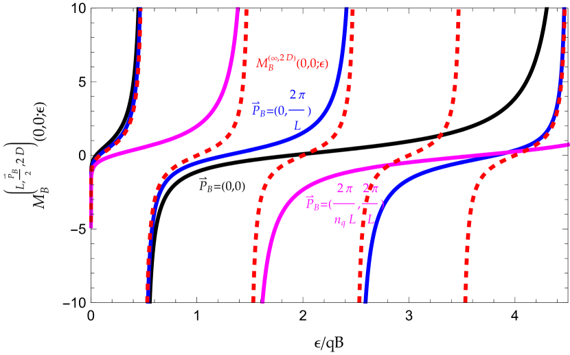
Figure 1: The plot of finite volume magnetic zeta function $\mathcal{M}^{(L,\frac{\mathbf{P}_{B}}{2},2D)}_{B}(\mathbf{0},\mathbf{0};\varepsilon)$ defined in Eq.(55) vs. $\mathcal{M}^{(\infty,2D)}_{B}(\mathbf{0},\mathbf{0};\varepsilon)$ (red dahsed) given in Eq.(59). The solid black, blue and pink curves are corresponding to $\mathbf{P}_{B}=(0,0),(0,\frac{2\pi}{L})$ and $(\frac{2\pi}{n_{q}L},\frac{2\pi}{L})$ respectively. The parameters are chosen as: $L=5$, and $n_{q}=n_{p}=1$.

III.3.3 Quantization condition in finite volume

Using Eq.(49) and also introducing the matrix elements of generalized magnetic zeta function by

$$\mathcal{M}^{(L,\frac{\mathbf{P}_{B}}{2},2D)}_{B}(\eta L\mathbf{e}_{x},\eta^{\prime}L\mathbf{e}_{x};\varepsilon)$$

$$=-\frac{4}{2\mu}G^{(L,\frac{\mathbf{P}_{B}}{2},2D)}_{B}(\eta L\mathbf{e}_{x},\eta^{\prime}L\mathbf{e}_{x};\varepsilon)$$

$$+\delta_{\eta,\eta^{\prime}}\frac{1}{\pi}(\gamma_{E}+\frac{1}{2}\ln\frac{\mu\varepsilon\rho^{2}}{2})|_{\rho\rightarrow 0},$$ (55)

thus, the quantization condition in Eq.(42) now can be recasted in a Lüscher formula-like form Lüscher (1991) ,

$$\det\left[\delta_{\eta,\eta^{\prime}}\cot\delta_{0}(\varepsilon)-\mathcal{M}^{(L,\frac{\mathbf{P}_{B}}{2},2D)}_{B}(\eta L\mathbf{e}_{x},\eta^{\prime}L\mathbf{e}_{x};\varepsilon)\right]=0,$$ (56)

where $(\eta,\eta^{\prime})=0,\cdots,n_{q}-1$.

Using Eq.(11) and Eq.(14), the generalized magnetic zeta function is thus given explicitly by

$$\mathcal{M}^{(L,\frac{\mathbf{P}_{B}}{2},2D)}_{B}(\eta L\mathbf{e}_{x},\eta^{\prime}L\mathbf{e}_{x};\varepsilon)$$

$$=\mathcal{M}^{(\infty,2D)}_{B}(\eta L\mathbf{e}_{x},\eta^{\prime}L\mathbf{e}_{x};\varepsilon)$$

$$+\frac{1}{\pi}\sum_{\mathbf{n}_{B}\neq\mathbf{0}}e^{-i\frac{\mathbf{P}_{B}}{2}\cdot\mathbf{n}_{B}L}e^{iqB\eta n_{x}n_{q}L^{2}}$$

$$\times e^{-\frac{iqB}{2}(\eta L+\eta^{\prime}L+n_{x}n_{q}L)n_{y}L}e^{-\frac{qB}{4}|(\eta-\eta^{\prime})L\mathbf{e}_{x}+\mathbf{n}_{B}L|^{2}}$$

$$\times\Gamma(\frac{1}{2}-\frac{\mu\varepsilon}{qB})U(\frac{1}{2}-\frac{\mu\varepsilon}{qB},1,\frac{qB}{2}|(\eta-\eta^{\prime})L\mathbf{e}_{x}+\mathbf{n}_{B}L|^{2}),$$ (57)

where

$$\mathcal{M}^{(\infty,2D)}_{B}(\eta L\mathbf{e}_{x},\eta^{\prime}L\mathbf{e}_{x};\varepsilon)$$

$$=-\frac{4}{2\mu}G^{(\infty,2D)}_{B}(\eta L\mathbf{e}_{x},\eta^{\prime}L\mathbf{e}_{x};\varepsilon)$$

$$+\delta_{\eta,\eta^{\prime}}\frac{1}{\pi}(\gamma_{E}+\frac{1}{2}\ln\frac{\mu\varepsilon\rho^{2}}{2})|_{\rho\rightarrow 0}.$$ (58)

Only diagonal terms of infinite volume magnetic Green’s function, $G^{(\infty,2D)}_{B}$, are UV divergent. Using Eq.(52) again, thus the UV regularized diagonal terms of $\mathcal{M}^{(\infty,2D)}_{B}$ function is given again by

$$\mathcal{M}^{(\infty,2D)}_{B}(\eta L\mathbf{e}_{x},\eta L\mathbf{e}_{x};\varepsilon)=-\frac{1}{\pi}\left[\psi(\frac{1}{2}-\frac{\mu\varepsilon}{qB})+\ln\frac{qB}{\mu\varepsilon}\right].$$ (59)

The example plot of $\mathcal{M}^{(L,\frac{\mathbf{P}_{B}}{2},2D)}_{B}(\mathbf{0},\mathbf{0};\varepsilon)$ for various of $\mathbf{P}_{B}$’s compared with $\mathcal{M}^{(\infty,2D)}_{B}(\mathbf{0},\mathbf{0};\varepsilon)$ is given in Fig. 1.

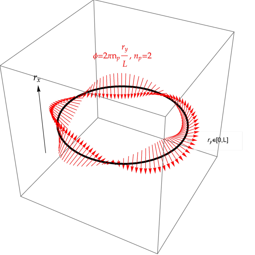
Figure 2: The plot of rotation of phase $\varphi(r_{y})$ defined in Eq.(61) along a cross section of a torus with a fixed $r_{x}$ (black circle). The phase changes of $\varphi(r_{y})$ on the circle of $r_{y}$ is represented by the rotation of red arrows.

IV Topological features of a magnetic system in a finite volume

It has been well-known in condensed matter physics that the Bloch electron in a magnetic field yields a non-trivial topology Xiao et al. (2010). The non-trivial topology of a magnetic system can be visually illustrated simply by using the twisted boundary condition given in Eq.(4). Two edges of enlarged magnetic cubic box at $r_{x}=0$ and $r_{x}=n_{q}L$ are glued together by a twist in the phase of wavefunction:

$$\psi^{(L,\frac{\mathbf{P}_{B}}{2})}_{\varepsilon}(n_{q}L,r_{y})=e^{i\frac{\mathbf{P}_{B}}{2}\cdot\mathbf{n}_{B}L}e^{-i\varphi(r_{y})}\psi^{(L,\frac{\mathbf{P}_{B}}{2})}_{\varepsilon}(0,r_{y}),$$ (60)

where

$$\varphi(r_{y})=qBn_{q}Lr_{y}=2\pi n_{p}\frac{r_{y}}{L}$$ (61)

is the twisted phase of wavefunction along the circle of $r_{y}\in[0,L]$ that is a cross section of a torus with a fixed $r_{x}$. How much of twists in the phase is totally determined by $n_{p}$. Hence, the phase rotation of $\varphi(r_{y})$ along the circle of $r_{y}$ in fact form a geometry of $n_{p}$ times twisted Möbius strip, see an example in Fig.2, which demonstrates a non-trivial topology.

IV.1 $\mathbf{k}$-space and Brillouin zone

Although in LQCD, the parameter $\mathbf{P}_{B}$ is associated with the plane wave of CM motion of two-particle system, $e^{i\mathbf{P}_{B}\cdot\mathbf{R}}$, see Ref. Guo and Gasparian (2021). Requirement of periodic boundary condition in CM motion yields the discrete value of $\mathbf{P}_{B}$’s in Eq.(6), and discrete energy spectra as well. To further examine some non-trivial topological features and analytic properties of a magnetic system in finite volume, from now on, the discrete magnetic lattice vector $\frac{\mathbf{P}_{B}}{2}$ is replaced by a continuous wave vector $\mathbf{k}$ that is analogous to the crystal momentum in condensed matter physics. In current section and also Sec. V, the wave vector $\mathbf{k}$ are limited in real space. The continuous distribution of wave vector $\mathbf{k}$ allows the introduction of Berry phase that is defined in a real $\mathbf{k}$-space Berry (1984); Xiao et al. (2010). The Berry phase is a phase angle that describes the global phase evolution of the wavefunction of a system in a closed path in $\mathbf{k}$-space. Due to the fact that the same physical state is represented by a ray of wavefunctions that differ by a phase, such as $|\psi\rangle$ and $|\psi^{\prime}\rangle=e^{i\phi}|\psi\rangle$, the set of phase factor $e^{i\phi}$ form a $U(1)$ group. Hence the ray of wavefunctions that are connected by a phase factor define a $U(1)$ fibre in a manifold of $\mathbf{k}$-space. Therefore, Berry phase is also recognized as a topological holonomy of the connection defined in a $U(1)$ fibre bundle in a parameter space Simon (1983), which is $\mathbf{k}$-space in our case. Berry phase is an important physical quantity that measures the topological feature of a system in a parameter space.

When $\mathbf{k}$ is varied continuously, the discrete energy spectra are smeared into energy bands, also called bulk energy bands. These energy bands are separated by forbidden gaps between them due to the particle interactions. Each single allowed energy band hence becomes an isolated island in totally periodic systems. It has been known that the edge effects in a non-trivial topological system may allow the gapless energy solutions Hatsugai (1993a, b), which yields a continuous and smooth connection between two isolated energy bands. The topological edge solutions in a magnetic system will be discussed in Sec. V. In addition, when wave vector $\mathbf{k}$ is further extended into a complex plane, given certain paths, the real energy solutions in the gap can also be found, which also connect two isolated energy bands smoothly. The discussion of analytic continuation of solutions in forbidden gaps will be presented in Sec. VI.

Using Eq.(11), one can show easily that

$$G^{(L,\mathbf{k}+\mathbf{G},2D)}_{B}(\bm{\rho},\bm{\rho}^{\prime};\varepsilon)=G^{(L,\mathbf{k})}_{B}(\bm{\rho},\bm{\rho}^{\prime};\varepsilon),$$ (62)

where

$$\mathbf{G}=\frac{2\pi}{n_{q}L}\mathbf{e}_{x}+\frac{2\pi}{L}\mathbf{e}_{y},$$ (63)

hence $\psi^{(L,\mathbf{k}+\mathbf{G},2D)}_{\varepsilon}(\mathbf{r})$ satisfies LS equation

$$\psi^{(L,\mathbf{k}+\mathbf{G},2D)}_{\varepsilon}(\bm{\rho})$$

$$=\int_{L_{B}^{2}}d\bm{\rho}^{\prime}G^{(L,\mathbf{k})}_{B}(\bm{\rho},\bm{\rho}^{\prime};\varepsilon)V^{(L)}(\bm{\rho}^{\prime})\psi^{(L,\mathbf{k}+\mathbf{G},2D)}_{\varepsilon}(\bm{\rho}^{\prime}),$$ (64)

so does $\psi^{(L,\mathbf{k},2D)}_{\varepsilon}(\bm{\rho})$. Therefore $\psi^{(L,\mathbf{k}+\mathbf{G},2D)}_{\varepsilon}(\bm{\rho})$ and $\psi^{(L,\mathbf{k},2D)}_{\varepsilon}(\bm{\rho})$ can only differ by a arbitrary phase factor, such as,

$$\psi^{(L,\mathbf{k}+\mathbf{G},2D)}_{\varepsilon}(\bm{\rho})=\psi^{(L,\mathbf{k},2D)}_{\varepsilon}(\bm{\rho}),$$ (65)

and they both describe the same physical state. Therefore $\mathbf{k}+\mathbf{G}$ and $\mathbf{k}$ are identified as the same point. The wave vector $\mathbf{k}$ hence can be limited in first magnetic Brillouin zone,

$$k_{x}\in[0,\frac{2\pi}{n_{q}L}],\ \ \ \ k_{y}\in[0,\frac{2\pi}{L}],$$ (66)

and the entire Brillouin zone form the geometry of a torus.

IV.2 Berry phase and Berry vector potential

The non-trivial topology of magnetic system in finite volume results in a non-zero Berry phase. The Berry phase is defined crossing over the torus of entire Brillouin zone by

$$\gamma_{\varepsilon} =\int_{0}^{\frac{2\pi}{L}}dk_{y}\left[A_{\varepsilon,y}(\frac{2\pi}{n_{q}L},k_{y})-A_{\varepsilon,y}(0,k_{y})\right]$$

$$-\int_{0}^{\frac{2\pi}{n_{q}L}}dk_{x}\left[A_{\varepsilon,x}(k_{x},\frac{2\pi}{L})-A_{\varepsilon,x}(k_{x},0)\right],$$ (67)

where Berry vector potential $\mathbf{A}(k_{x},k_{y})$ is given by

$$\mathbf{A}_{\varepsilon}(k_{x},k_{y})=\int_{L_{B}^{2}}d\bm{\rho}u^{(\mathbf{k},2D)*}_{\varepsilon}(\bm{\rho})i\nabla_{\mathbf{k}}u^{(\mathbf{k},2D)}_{\varepsilon}(\bm{\rho}),$$ (68)

and $u^{(\mathbf{k},2D)}_{\varepsilon}(\bm{\rho})$ stands for the Bloch wavefunction and is related to $\psi^{(L,\mathbf{k},2D)}_{\varepsilon}(\bm{\rho})$ by

$$\psi^{(L,\mathbf{k},2D)}_{\varepsilon}(\bm{\rho})=e^{i\mathbf{k}\cdot\bm{\rho}}u^{(\mathbf{k},2D)}_{\varepsilon}(\bm{\rho}).$$ (69)

The Berry phase over the torus of entire Brillouin zone is in fact a topological invariant quantity and quantized as $2\pi$ multiplied by an integer that is known as a Chern number Simon (1983).

In general, the Berry phase must be computed numerically by solving eigenvalue problems. In presence of particles interactions, the wavefunction must be given by linear superposition of

$$\psi^{(L,\mathbf{k},2D)}_{\varepsilon}(\bm{\rho})=\sum_{n=0}^{\infty}\sum_{\alpha=0}^{n_{p}-1}c_{n,\alpha}^{(\mathbf{k})}(\varepsilon)\chi_{n,\alpha}^{(\mathbf{k})}(\bm{\rho}).$$ (70)

The coefficient $c_{n,\alpha}^{(\mathbf{k})}(\varepsilon)$ satisfies a matrix equation,

$$H^{(\mathbf{k})}c^{(\mathbf{k})}(\varepsilon)=\varepsilon c^{(\mathbf{k})}(\varepsilon),$$ (71)

where the matrix elements of effective Hamiltonian $H^{(\mathbf{k})}$ are given by

$$H^{(\mathbf{k})}_{n,\alpha;n^{\prime},\alpha^{\prime}}=\delta_{n,\alpha;n^{\prime},\alpha^{\prime}}\frac{qB}{\mu}(n+\frac{1}{2})+V^{(\mathbf{k})}_{n,\alpha;n^{\prime},\alpha^{\prime}},$$ (72)

and $V^{(\mathbf{k})}_{n,\alpha;n^{\prime},\alpha^{\prime}}$ is defined in Eq.(32). The wave vector $\mathbf{k}$ in Eq.(71) is now treated as the parameter of dynamics of system, and ultimately, adiabatic evolution of $\mathbf{k}$ crossing over magnetic Brillouin zone yields a Berry phase Xiao et al. (2010).

Since Berry phase is a topological invariance and also a robust quantity against particle interactions, non-trivial topological feature of a magnetic system in finite volume can be demonstrated by only using solutions of zero particle interactions. For a fixed $n$, there are $n_{p}$ degenerate states,

$$u_{n,\alpha}^{(\mathbf{k})}(\bm{\rho})=e^{-i\mathbf{k}\cdot\bm{\rho}}\chi_{n,\alpha}^{(\mathbf{k})}(\bm{\rho}).$$ (73)

The Berry phase for degenerate states $u_{n,\alpha}^{(\mathbf{k})}(\bm{\rho})$with a fixed $n$ is defined by the trace of Berry phase for each state Vanderbilt (2018),

$$\gamma_{n}=\sum_{\alpha=0}^{n_{p}-1}\gamma_{n,\alpha},$$ (74)

where $\gamma_{n,\alpha}$ is defined in Eq.(67) with Berry vector potential,

$$\mathbf{A}_{n,\alpha}(k_{x},k_{y})=\int_{L_{B}^{2}}d\bm{\rho}u^{(\mathbf{k})*}_{n,\alpha}(\bm{\rho})i\nabla_{\mathbf{k}}u^{(\mathbf{k})}_{n,\alpha}(\bm{\rho}).$$ (75)

Using relations of 1D harmonic oscillator eigen-solutions,

$$\sqrt{qB}r_{x}\phi_{n}(r_{x})=\sqrt{\frac{n+1}{2}}\phi_{n+1}(r_{x})+\sqrt{\frac{n}{2}}\phi_{n-1}(r_{x}),$$

$$\partial_{\sqrt{qB}r_{x}}\phi_{n}(r_{x})=-\sqrt{\frac{n+1}{2}}\phi_{n+1}(r_{x})+\sqrt{\frac{n}{2}}\phi_{n-1}(r_{x}),$$ (76)

we find

$$i\partial_{k_{x}}u_{n,\alpha}^{(\mathbf{k})}(\bm{\rho})$$

$$=\frac{1}{\sqrt{qB}}\left[\sqrt{\frac{n+1}{2}}u_{n+1,\alpha}^{(\mathbf{k})}(\bm{\rho})+\sqrt{\frac{n}{2}}u_{n-1,\alpha}^{(\mathbf{k})}(\bm{\rho})\right]$$

$$-(\frac{\frac{2\pi\alpha}{L}+k_{y}}{qB})u_{n,\alpha}^{(\mathbf{k})}(\bm{\rho}),$$

$$i\partial_{k_{y}}u_{n,\alpha}^{(\mathbf{k})}(\bm{\rho})$$

$$=-\frac{i}{\sqrt{qB}}\left[\sqrt{\frac{n+1}{2}}u_{n+1,\alpha}^{(\mathbf{k})}(\bm{\rho})-\sqrt{\frac{n}{2}}u_{n-1,\alpha}^{(\mathbf{k})}(\bm{\rho})\right].$$ (77)

Also using orthogonality relation given in Eq.(26), we thus obtain

$$A_{n,\alpha,x}(k_{x},k_{y}) =-(\frac{\frac{2\pi\alpha}{L}+k_{y}}{qB}),$$

$$A_{n,\alpha,y}(k_{x},k_{y}) =0.$$ (78)

Hence, the Berry phases are given by

$$\gamma_{n,\alpha}=\frac{2\pi}{n_{p}},\ \ \ \ \frac{\gamma_{n}}{2\pi}=1.$$ (79)

IV.3 Topological properties of $\chi_{n,\alpha}^{(\mathbf{k})}$ functions

The Berry phase of a magnetic system in finite volume can also be understood by simply examining the topological properties of $\chi_{n,\alpha}^{(\mathbf{k})}$ functions.

Using Eq.(21), one can show that how the center of $\chi_{n,\alpha}^{(\mathbf{k})}$ function is pushed along $x$-direction when the wave vector $\mathbf{k}$ is forced to change in $y$-direction,

$$\chi_{n,\alpha}^{(\mathbf{k}+\triangle k_{y}\mathbf{e}_{y})}(\bm{\rho})=e^{i\triangle k_{y}r_{y}}\chi_{n,\alpha}^{(\mathbf{k})}(\bm{\rho}+\frac{\triangle k_{y}}{qB}\mathbf{e}_{x}).$$ (80)

Thus Eq.(80) yields

$$\chi_{n,\alpha}^{(\mathbf{k}+\frac{2\pi}{L}\frac{n_{p}}{n_{q}}\mathbf{e}_{y})}(\bm{\rho})=e^{iqBLr_{y}}\chi_{n,\alpha}^{(\mathbf{k})}(\bm{\rho}+L\mathbf{e}_{x}),$$ (81)

that is to say, to move the center of $\chi_{n,\alpha}^{(\mathbf{k})}$ by length-$L$ in $x$-direction, it requires the change of wave vector $\mathbf{k}$ by $\frac{2\pi}{L}\frac{n_{p}}{n_{q}}$ in y-direction.

When $\mathbf{k}$ is forced to move across entire Brillouin zone in $y$-direction,

$$\chi_{n,\alpha}^{(\mathbf{k}+\frac{2\pi}{L}\mathbf{e}_{y})}(\bm{\rho})=e^{i\frac{2\pi}{L}r_{y}}\chi_{n,\alpha}^{(\mathbf{k})}(\bm{\rho}+\frac{n_{q}L}{n_{p}}\mathbf{e}_{x})=\chi_{n,\alpha+1}^{(\mathbf{k})}(\bm{\rho}),$$ (82)

the center of $\chi_{n,\alpha}^{(\mathbf{k})}$ function is only moved by $\frac{n_{q}L}{n_{p}}$ in $x$-direction, which is then smoothly connected to the $\chi_{n,\alpha+1}^{(\mathbf{k})}$ function. Hence, an array of states

$$\chi_{n}^{(\mathbf{k})}=\left[\chi_{n,0}^{(\mathbf{k})},\chi_{n,1}^{(\mathbf{k})},\cdots,\chi_{n,n_{p}-1}^{(\mathbf{k})}\right],$$ (83)

behaves as a $n_{p}$ components spinor. $\triangle k_{y}=\frac{2\pi}{L}$ plays the role of raising operator which change each individual component of spinor $\chi_{n}^{(\mathbf{k})}$ by one unit,

$$\chi_{n}^{(\mathbf{k}+\frac{2\pi}{L}\mathbf{e}_{y})}=\left[\chi_{n,1}^{(\mathbf{k})},\chi_{n,2}^{(\mathbf{k})},\cdots,\chi_{n,n_{p}}^{(\mathbf{k})}\right].$$ (84)

Operating raising operator $n_{p}$ times, with the help of periodic boundary condition, we can also show that

$$\chi_{n,\alpha}^{(\mathbf{k}+\frac{2\pi}{L}n_{p}\mathbf{e}_{y})}(\bm{\rho}) =e^{i\frac{2\pi}{L}n_{p}r_{y}}\chi_{n,\alpha}^{(\mathbf{k})}(\bm{\rho}+n_{q}L\mathbf{e}_{x})=\chi_{n,\alpha+n_{p}}^{(\mathbf{k})}(\bm{\rho})$$

$$=e^{ik_{x}n_{q}L}\chi_{n,\alpha}^{(\mathbf{k})}(\bm{\rho}).$$ (85)

Therefore,

$$\chi_{n}^{(\mathbf{k}+\frac{2\pi}{L}\mathbf{e}_{y})}=\left[\chi_{n,1}^{(\mathbf{k})},\chi_{n,2}^{(\mathbf{k})},\cdots,e^{ik_{x}n_{q}L}\chi_{n,0}^{(\mathbf{k})}\right],$$ (86)

changing $\mathbf{k}$ by $\frac{2\pi}{L}\mathbf{e}_{y}$ leads to the circulation of all components only once, and only the component sitting at right edge of spinor gains a phase factor, $e^{ik_{x}n_{q}L}$. On the other hand, changing $\mathbf{k}$ by $\frac{2\pi}{L}n_{p}\mathbf{e}_{y}$ however yields that the center of each component of spinor $\chi_{n}^{(\mathbf{k})}$ is forced to wind around entire magnetic unit cell in $x$-direction. Meanwhile, all components of the spinor circulate $n_{p}$ times and come back to the starting point, so each one has a chance to gain a phase factor $e^{ik_{x}n_{q}L}$ when it reaches the right edge of spinor,

$$\chi_{n}^{(\mathbf{k}+\frac{2\pi}{L}n_{p}\mathbf{e}_{y})}=e^{ik_{x}n_{q}L}\chi_{n}^{(\mathbf{k})}.$$ (87)

In addition, when the wave vector $\mathbf{k}$ is forced to move across magnetic Brillouin zone in $x$-direction, the each component of spinor $\chi_{n}^{(\mathbf{k})}$ remains at the same location in a spinor,

$$\chi_{n,\alpha}^{(\mathbf{k}+\frac{2\pi}{n_{q}L}\mathbf{e}_{x})}(\bm{\rho})=\chi_{n,\alpha}^{(\mathbf{k})}(\bm{\rho}),$$ (88)

and

$$\chi_{n}^{(\mathbf{k}+\frac{2\pi}{n_{q}L}\mathbf{e}_{x})}=\chi_{n}^{(\mathbf{k})}.$$ (89)

Now, the non-trivial Berry phase may also be understood simply by using the properties given in Eq.(86) and Eq.(89). Assuming that we start at one corner of Brillouin zone: $\mathbf{k}=(0,0)$ with initial spinor of

$$\chi_{n}^{(i)}=\left[\chi_{n,0}^{(0,0)},\chi_{n,1}^{(0,0)},\cdots,\chi_{n,n_{p}-1}^{(0,0)}\right],$$ (90)

where $i$ is used to label initial state of spinor, then we start moving around the boundary of magnetic Brillouin zone counter-clock wise,

$$\mathbf{k}:(0,0)\stackrel{{\scriptstyle(1)}}{{\rightarrow}}(\frac{2\pi}{n_{q}L},0)\stackrel{{\scriptstyle(2)}}{{\rightarrow}}(\frac{2\pi}{n_{q}L},\frac{2\pi}{L})\stackrel{{\scriptstyle(3)}}{{\rightarrow}}(0,\frac{2\pi}{L})\stackrel{{\scriptstyle(4)}}{{\rightarrow}}(0,0).$$ (91)

At step (1), moving from $\mathbf{k}=(0,0)$ to $(\frac{2\pi}{n_{q}L},0)$ by an increase of $\triangle k_{x}=\frac{2\pi}{n_{q}L}$, there is no phase change,

$$\chi_{n}^{(\frac{2\pi}{n_{q}L},0)}=\chi_{n}^{(i)}.$$ (92)

At step (2), moving from $(\frac{2\pi}{n_{q}L},0)$ to $(\frac{2\pi}{n_{q}L},\frac{2\pi}{L})$ by an increase of $\triangle k_{y}=\frac{2\pi}{L}$, we find

$$\chi_{n}^{(\frac{2\pi}{n_{q}L},\frac{2\pi}{L})}=\left[\chi_{n,1}^{(0,0)},\chi_{n,2}^{(0,0)},\cdots,e^{i\frac{2\pi}{n_{q}L}n_{q}L}\chi_{n,0}^{(0,0)}\right].$$ (93)

At step (3), moving from $(\frac{2\pi}{n_{q}L},\frac{2\pi}{L})$ to $(0,\frac{2\pi}{L})$ by a decrease fo $\triangle k_{x}=-\frac{2\pi}{n_{q}L}$, there is again no phase change, so that

$$\chi_{n}^{(0,\frac{2\pi}{L})}=\chi_{n}^{(\frac{2\pi}{n_{q}L},\frac{2\pi}{L})}.$$ (94)

At last step (4), moving from $(0,\frac{2\pi}{L})$ back to $(0,0)$ by a decrease of $\triangle k_{y}=-\frac{2\pi}{L}$, although there is no phase change at last step, all components of spinor are moved down by one unit, so that the final state of spinor is given by

$$\chi_{n}^{(f)}=\left[\chi_{n,0}^{(0,0)},\chi_{n,1}^{(0,0)},\cdots,e^{i\frac{2\pi}{n_{q}L}n_{q}L}\chi_{n,n_{p}-1}^{(0,0)}\right].$$ (95)

Therefore, the phase difference between initial and final states is given by

$$-\sum_{\alpha=0}^{n_{p}-1}Im\ln\langle\chi_{n,\alpha}^{(f)}|\chi_{n,\alpha}^{(i)}\rangle=\frac{2\pi}{n_{q}L}n_{q}L=2\pi,$$ (96)

which can be identified as Berry phase $\gamma_{n}$.

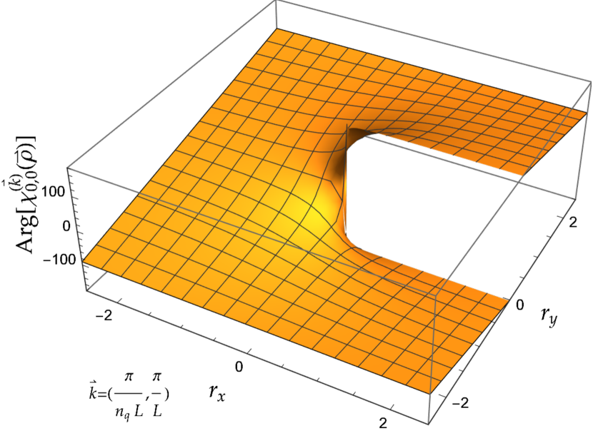
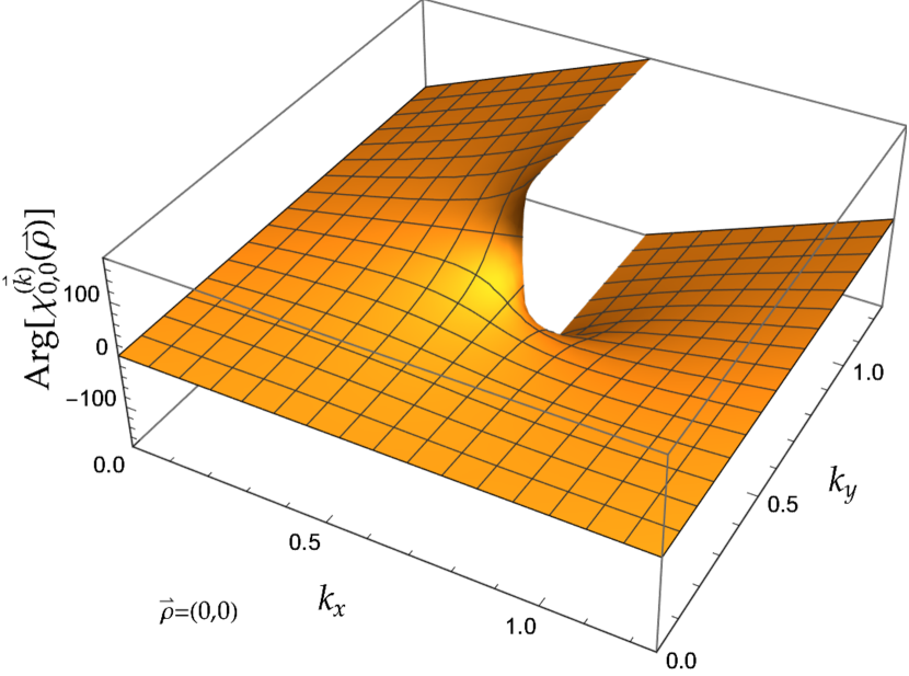
Figure 3: The phase plot of $\chi_{0,0}^{(\mathbf{k})}(\bm{\rho})$ with fixed $\mathbf{k}=(\frac{\pi}{L},\frac{\pi}{L})$ in $\bm{\rho}$-space (upper pannel) vs. phase plot of $\chi_{0,0}^{(\mathbf{k})}(\bm{\rho})$ with fixed $\bm{\rho}=(0,0)$ in $\mathbf{k}$-space (lower panel). The parameters are chosen as: $L=5$ and $n_{p}=n_{q}=1$.

The Berry phase is the quantity that describes the accumulation of a global phase of a system’s wavefunction as the $\mathbf{k}$ is carried around the torus of Brillouin zone, non-zero value of Berry phase hence represents a topological obstruction to the determination of the phase of wavefunction Kohmoto (1985) over entire Brillouin zone. For a magnetic system, the magnetic field create a vortex-like singularities in wavefunctions that attribute to a non-trivial topology of a magnetic system. The vortex-like singularities can be illustrated analytically by $\chi_{0,\alpha}^{(\mathbf{k})}(\bm{\rho})$. Using Eq.(21) and $H_{0}(x)=1$, we find

$$\Theta_{\alpha}^{(\mathbf{k})}(\bm{\rho})$$

$$=e^{-i(k_{y}+\frac{2\pi\alpha}{L})r_{y}}\chi_{0,\alpha}^{(\mathbf{k})}(\bm{\rho})$$

$$=\frac{1}{\sqrt{L}}\left(\frac{qB}{\pi}\right)^{\frac{1}{4}}e^{-\frac{qB}{2}(r_{x}+\frac{k_{y}+\frac{2\pi\alpha}{L}}{qB})^{2}}$$

$$\times\vartheta_{3}\left(\frac{\pi n_{p}}{L}\left[(r_{y}-\frac{k_{x}}{qB})+i(r_{x}+\frac{k_{y}+\frac{2\pi\alpha}{L}}{qB})\right],e^{-\pi n_{p}n_{q}}\right),$$ (97)

where $\vartheta_{3}(z,q)$ is Jacobi’s theta function DLMF , and defined by

$$\vartheta_{3}(z,q)=1+2\sum_{n=1}^{\infty}q^{n^{2}}\cos(2nz).$$ (98)

The zeros of

$$\vartheta_{3}(z,q=e^{i\pi\tau})$$

are determined by linear equation,

$$z=(n_{1}+\frac{1}{2})\pi+(n_{2}+\frac{1}{2})\tau\pi,\ \ \ \ (n_{1},n_{2})\in\mathbb{Z},$$ (99)

hence, the locations of zeros of $\chi_{0,\alpha}^{(\mathbf{k})}(\bm{\rho})$ are given by

$$r_{y}-\frac{k_{x}}{qB}=(n_{1}+\frac{1}{2})\frac{L}{n_{p}},\ \ n_{1}\in\mathbb{Z},$$

$$r_{x}+\frac{k_{y}}{qB}+\frac{\frac{2\pi\alpha}{L}}{qB}=(n_{2}+\frac{1}{2})n_{q}L,\ \ n_{2}\in\mathbb{Z}.$$ (100)

The zeros of $\chi_{0,\alpha}^{(\mathbf{k})}(\bm{\rho})$ present vortex-like singularities, which ultimately create discontinuity of phase of $\chi_{0,\alpha}^{(\mathbf{k})}(\bm{\rho})$ in both $\bm{\rho}$- and $\mathbf{k}$-space. The $\vartheta_{3}(z,q)$ is a real function when $z$ values are real and $|q|<1$, therefore, for a fixed $\mathbf{k}$,

$$Im\left[\Theta_{\alpha}^{(\mathbf{k})}(\bm{\rho})\right]_{\bm{\rho}=(-\frac{k_{y}+\frac{2\pi\alpha}{L}}{qB},r_{y})}=0,$$ (101)

thus the phase of $\chi_{0,\alpha}^{(\mathbf{k})}(\bm{\rho})$ is not well-defined along the line of $(-\frac{k_{y}+\frac{2\pi\alpha}{L}}{qB},r_{y})$ in $\bm{\rho}$-space. On the other hand, for a fixed $\bm{\rho}$,

$$Im\left[\Theta_{\alpha}^{(\mathbf{k})}(\bm{\rho})\right]_{\mathbf{k}=(k_{x},-\frac{2\pi\alpha}{L}-qBr_{y})}=0,$$ (102)

so in $\mathbf{k}$-space, the phase is also not well-defined along the line of $(k_{x},-\frac{2\pi\alpha}{L}-qBr_{y})$. These two lines cut though both entire $\bm{\rho}$- and $\mathbf{k}$-space. Because of asymmetry of $\Theta_{\alpha}^{(\mathbf{k})}(\bm{\rho})$ along these two lines, it creates the mismatch of the phase of $\chi_{0,\alpha}^{(\mathbf{k})}(\bm{\rho})$ on half portion of the line, which starts at the location of zeros of $\chi_{0,\alpha}^{(\mathbf{k})}(\bm{\rho})$, see Fig. 3 as an example of phase mismatch. These vortex-like singularities in wavefunction is similar to the branch point singularities in complex analysis, the vortex creates a cut in both $\bm{\rho}$- and $\mathbf{k}$-space, and phase of wavefunction along the cut has a discontinuity. Hence, when particle is forced to wind around the vortex, the phase of wavefunction has a jump which account how many times the winding number of motion around the vortex.

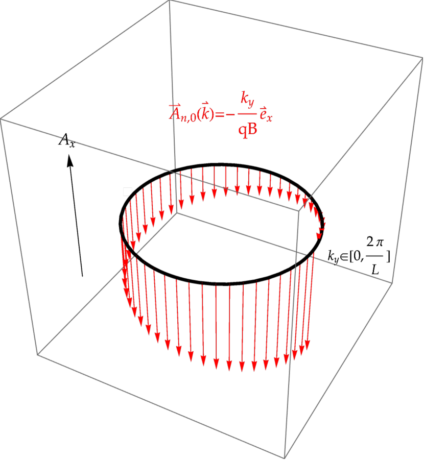
Figure 4: The plot of Berry vector potential $\mathbf{A}_{n,0}(k_{x},k_{y})$ on a cross section of torus of Brillouin zone with a fixed $k_{x}$. The parameters are chosen as: $L=5$ and $n_{p}=n_{q}=1$.

The phase discontinuity of $\chi_{n,\alpha}^{(\mathbf{k})}(\bm{\rho})$ ultimately creates non-trivial topology of the Berry vector potential given in Eq.(78). The vortex-like singularities not only create discontinuity of phase in wavefunction, but also leads to the mismatch of Berry vector potential on the torus of entire magnetic Brillouin zone. Since the torus has no boundary, uniquely and smoothly defined Berry vector potential on the torus results in the trivial topology and vanishing Berry phase. For $\chi_{n,\alpha}^{(\mathbf{k})}(\bm{\rho})$ wavefunction, according to Eq.(78), it is clearly that the Berry vector potential on the lower edge of torus along the line $\mathbf{k}=(k_{x},0)$ is

$$\mathbf{A}_{n,\alpha}(k_{x},0)=-\alpha\frac{n_{q}L}{n_{p}}\mathbf{e}_{x}.$$ (103)

On the upper edge of torus along the line of $\mathbf{k}=(k_{x},\frac{2\pi}{L})$, the Berry vector potential is

$$\mathbf{A}_{n,\alpha}(k_{x},\frac{2\pi}{L})=-(\alpha+1)\frac{n_{q}L}{n_{p}}\mathbf{e}_{x}.$$ (104)

The upper and lower edges of a torus is considered as the same points, hence, magnetic field ultimately cause a mismatch of Berry vector potential on the torus, see Fig. 4 as an example. The discontinuity of Berry vector potential is given by

$$\mathbf{A}_{n,\alpha}(k_{x},\frac{2\pi}{L})-\mathbf{A}_{n,\alpha}(k_{x},0)=-\frac{n_{q}L}{n_{p}}\mathbf{e}_{x},$$ (105)

which ultimately leads to a non-zero Berry phase. The discontinuity of Berry vector potential on a closed path in $\mathbf{k}$-space is known as a holonomy Simon (1983). When wave vector $\mathbf{k}$ is forced to move along a closed path, the Berry vector potential then generates a horizontal lift of the wavefunction along the $U(1)$ fibre of each state, hence, in adiabatic limit, the states along the path in $\mathbf{k}$-space are all connected by

$$u_{n,\alpha}^{(\mathbf{k}(t))}(\bm{\rho})\sim e^{-i\int_{\mathbf{k}(0)}^{\mathbf{k}(t)}\mathbf{A}_{n,\alpha}(\mathbf{k})\cdot d\mathbf{k}}u_{n,\alpha}^{(\mathbf{k}(0))}(\bm{\rho}).$$ (106)

Each state on the path has the memory of previous states along the path. The holonomy of a system detects a topological or geometric nature of the underlying structure of the physical system. The twisting of $U(1)$ fibre bundle results in the non-trivial value of holonomy. The twisting of $U(1)$ fibre bundle in $\mathbf{k}$-space can be understood by the relation given in Eq.(85), which yields

$$u_{n,\alpha}^{(k_{x},\frac{2\pi}{L}n_{p})}(\bm{\rho})=e^{-i\frac{2\pi}{L}n_{p}r_{y}}e^{i\widetilde{\varphi}(k_{x})}u_{n,\alpha}^{(k_{x},0)}(\bm{\rho}),$$ (107)

where

$$\widetilde{\varphi}(k_{x})=k_{x}n_{q}L.$$ (108)

Eq.(107) may be interpreted as twisted boundary condition in enlarged Brillouin zone:

$$k_{x}\in[0,\frac{2\pi}{n_{q}L}],\ \ \ \ k_{y}\in[0,\frac{2\pi}{L}n_{p}].$$ (109)

Hence, similar to twisted boundary condition in Eq.(60) in $\bm{\rho}$-space, when two edges at $k_{y}=0$ and $k_{y}=\frac{2\pi}{L}n_{p}$ of enlarged Brillouin zone are glued together, $\widetilde{\varphi}(k_{x})$ describes the twisted phase of wavefunction along the circle of $k_{x}\in[0,\frac{2\pi}{n_{q}L}]$.

We also remark that noticing that Eq.(77) may be rearranged to

$$\sum_{n^{\prime},\alpha^{\prime}}\left[\delta_{n,\alpha;n^{\prime},\alpha^{\prime}}\nabla_{\mathbf{k}}+i\mathbf{A}_{n,\alpha;n^{\prime},\alpha^{\prime}}(\mathbf{k})\right]u_{n^{\prime},\alpha^{\prime}}^{(\mathbf{k})}(\bm{\rho})=0,$$ (110)

where the matrix elements of Berry vector potential matrix are given by

$$\mathbf{A}_{n,\alpha;n^{\prime},\alpha^{\prime}}(\mathbf{k}) =\int_{L_{B}^{2}}d\bm{\rho}u^{(\mathbf{k})*}_{n,\alpha}(\bm{\rho})i\nabla_{\mathbf{k}}u^{(\mathbf{k})}_{n^{\prime},\alpha^{\prime}}(\bm{\rho})$$

$$=\frac{1}{\sqrt{qB}}\sqrt{\frac{n+1}{2}}\delta_{n+1,n^{\prime}}\delta_{\alpha,\alpha^{\prime}}(\mathbf{e}_{x}-i\mathbf{e}_{y})$$

$$+\frac{1}{\sqrt{qB}}\sqrt{\frac{n}{2}}\delta_{n-1,n^{\prime}}\delta_{\alpha,\alpha^{\prime}}(\mathbf{e}_{x}+i\mathbf{e}_{y})$$

$$-\delta_{n,n^{\prime}}\delta_{\alpha,\alpha^{\prime}}(\frac{\frac{2\pi\alpha}{L}+k_{y}}{qB})\mathbf{e}_{x}.$$ (111)

Non-vanishing off-diagonal terms in Berry vector potential matrix suggest that a magnetic system may experience non-adiabatic transition between different eigen-states. For an example, assuming an non-interacting magnetic system, the general Bloch wavefunction is given by the linear superposition of eigen-states of non-interacting magnetic system,

$$u^{(\mathbf{k}(t))}(\bm{\rho})=\sum_{n,\alpha}c_{n,\alpha}(t)u_{n,\alpha}^{(\mathbf{k}(t))}(\bm{\rho}),$$ (112)

where $t$ is used to parameterize the evolution of wave vector $\mathbf{k}$. Also assuming $u^{(\mathbf{k}(t))}(\bm{\rho})$ satisfies Schrödinger equation

$$i\partial_{t}u^{(\mathbf{k}(t))}(\bm{\rho})=\hat{H}_{eff}(\mathbf{k}(t))u^{(\mathbf{k}(t))}(\bm{\rho}),$$ (113)

where $u_{n,\alpha}^{(\mathbf{k}(t))}(\bm{\rho})$ are eigen-solutions of $\hat{H}_{eff}(\mathbf{k}(t))=e^{-i\mathbf{k}(t)\cdot\bm{\rho}}\hat{H}_{\bm{\rho}}e^{i\mathbf{k}(t)\cdot\bm{\rho}}$,

$$\hat{H}_{eff}(\mathbf{k}(t))u_{n,\alpha}^{(\mathbf{k}(t))}(\bm{\rho})=\frac{qB}{\mu}(n+\frac{1}{2})u_{n,\alpha}^{(\mathbf{k}(t))}(\bm{\rho}),$$ (114)

thus, we find that the coefficient $c_{n,\alpha}(t)$ must satisfy equation,

$$i\frac{dc_{n,\alpha}(t)}{dt} =\frac{qB}{\mu}(n+\frac{1}{2})c_{n,\alpha}(t)$$

$$-\frac{d\mathbf{k}(t)}{dt}\cdot\sum_{n^{\prime},\alpha^{\prime}}\mathbf{A}_{n,\alpha;n^{\prime},\alpha^{\prime}}(\mathbf{k})c_{n^{\prime},\alpha^{\prime}}(t).$$ (115)

Therefore, the diagonal term in Berry vector potential matrix yields the Berry phase in Eq.(79) in the limit of adiabatic process, the off-diagonal terms may describes the transition among different eigen-states when $\mathbf{k}$ is forced to increase or decrease.

V Topological edge states

One of important consequences of a non-trivial topological system is the existence of gapless topological edge states that occur in the energy gap between the bulk bands Hatsugai (1993a, b). The study of conventional edge or surface states in fact has a long history Shockley (1939); Tamm (1932), the boundary effect may cause the localization of state near the edge or surface of material. Though the energy spectrum of a system with a penetrable boundary may protrude into the gap between bulk bands, for topologically trivial systems, the eigen-energies of an impenetrable wall on boundary are only situated on the edge of bulk energy bands. This fact can be illustrated with a 2D system with different boundary conditions. The 2D finite volume Green’s function that satisfies periodic boundary conditions in both $x$ and $y$ directions is given by

$$G_{0}^{(L,\mathbf{k},2D)}(\bm{\rho};\varepsilon)=\frac{1}{L^{2}}\sum_{\mathbf{p}=\frac{2\pi\mathbf{n}}{L}+\mathbf{k},\mathbf{n}\in\mathbb{Z}^{2}}\frac{e^{i\mathbf{p}\cdot\bm{\rho}}}{\varepsilon-\frac{\mathbf{p}^{2}}{2\mu}},$$ (116)

compared with

$$G_{0}^{(h.w.,k_{y}\mathbf{e}_{y},2D)}(\bm{\rho},\bm{\rho}^{\prime};\varepsilon)=\frac{1}{L}\sum_{p_{y}=\frac{2\pi n_{y}}{L}+k_{y},n_{y}\in\mathbb{Z}}e^{ip_{y}(r_{y}-r^{\prime}_{y})}$$

$$\times 2\mu\frac{\sin\sqrt{2\mu\varepsilon-p_{y}^{2}}(r_{y>}-\frac{L}{2})\sin\sqrt{2\mu\varepsilon-p_{y}^{2}}(r_{y<}+\frac{L}{2})}{\sqrt{2\mu\varepsilon-p_{y}^{2}}\sin\sqrt{2\mu\varepsilon-p_{y}^{2}}L},$$ (117)

which satisfies hard wall boundary condition in $x$-direction but still remains periodic in $y$-direction,

$$G_{0}^{(h.w.,k_{y}\mathbf{e}_{y},2D)}(\bm{\rho},\bm{\rho}^{\prime};\varepsilon)|_{\bm{\rho},\bm{\rho}^{\prime}=\pm\frac{L}{2}\mathbf{e}_{x}}=0.$$ (118)

Therefore, with a contact interaction, and using Eq.(116) and identity

$$\frac{1}{L}\sum_{p_{x}=\frac{2\pi n_{x}}{L}+k_{x},n_{x}\in\mathbb{Z}}\frac{1}{q^{2}-p_{x}^{2}}=\frac{\cot\frac{q-k_{x}}{2}L+\cot\frac{q+k_{x}}{2}L}{4q},$$ (119)

the bulk energy band solutions with periodic boundary condition along both directions are determined by

$$\frac{1}{V_{0}}=\frac{2\mu}{L}\sum_{p_{y}=\frac{2\pi n_{y}}{L}+k_{y}}^{n_{y}\in\mathbb{Z}}\!\!\!\!\frac{\cot\frac{\sqrt{2\mu\varepsilon-p_{y}^{2}}-k_{x}}{2}L+\cot\frac{\sqrt{2\mu\varepsilon-p_{y}^{2}}+k_{x}}{2}L}{4\sqrt{2\mu\varepsilon-p_{y}^{2}}}.$$ (120)

Using Eq.(117), the edge solutions with hard wall boundary condition along $x$-direction are determined by

$$\frac{1}{V_{0}}=\frac{2\mu}{L}\sum_{p_{y}=\frac{2\pi n_{y}}{L}+k_{y},n_{y}\in\mathbb{Z}}\frac{\cot\frac{\sqrt{2\mu\varepsilon-p_{y}^{2}}-\frac{\pi}{L}}{2}L}{2\sqrt{2\mu\varepsilon-p_{y}^{2}}}.$$ (121)

We can see clearly that for a fixed $k_{y}$ and $V_{0}$, the edge solution is only part of bulk energy band solutions with special value of wave vector $k_{x}=\frac{\pi}{L}$, which indeed sit at the edge of bulk energy bands.

On the contrary, even with impenetrable walls on the boundary, the topological edge states may appear in the gap between bulk energy bands. In this section, we will show the solutions of various boundary conditions for a 2D magnetic system, and discuss how the boundary condition may affect the spectrum of a magnetic system.

V.1 Various boundary condition solutions of 2D magnetic Green’s function

In this subsection, we study various boundary condition solutions of 2D magnetic Green’s function in $x$-direction, but the boundary condition in $y$-direction remains periodic. Hence, the solutions with different boundary conditions all have the form of

$$G_{B}^{(k_{y}\mathbf{e}_{y},2D)}(\bm{\rho},\bm{\rho}^{\prime};\varepsilon)=\frac{1}{L}\sum_{p_{y}=\frac{2\pi n_{y}}{L}+k_{y},n_{y}\in\mathbb{Z}}e^{ip_{y}(r_{y}-r^{\prime}_{y})}$$

$$\times G_{B}^{(1D)}(r_{x}+\frac{p_{y}}{qB},r^{\prime}_{x}+\frac{p_{y}}{qB};\varepsilon),$$ (122)

where $G_{B}^{(1D)}$ satisfies differential equation

$$\left(\varepsilon+\frac{\partial_{r_{x}}^{2}}{2\mu}-\frac{(qB)^{2}}{2\mu}r_{x}^{2}\right)G_{B}^{(1D)}(r_{x},r^{\prime}_{x};\varepsilon)=\delta(r_{x}-r^{\prime}_{x}).$$ (123)

Before the boundary condition is implemented, Eq.(123) is parabolic cylinder equation type DLMF , the homogeneous parabolic cylinder equation has two independent solutions called parabolic cylinder functions DLMF :

$$U(-\frac{\mu\varepsilon}{qB},\pm\sqrt{2qB}r_{x}).$$

Therefore in general, the solution of $G_{B}^{(1D)}$ is given by

$$G_{B}^{(1D)}(r_{x},r^{\prime}_{x};\varepsilon)$$

$$=\left[aU(-\frac{\mu\varepsilon}{qB},\sqrt{2qB}r_{x<})+bU(-\frac{\mu\varepsilon}{qB},-\sqrt{2qB}r_{x<})\right]$$

$$\times\left[cU(-\frac{\mu\varepsilon}{qB},\sqrt{2qB}r_{x>})+dU(-\frac{\mu\varepsilon}{qB},-\sqrt{2qB}r_{x>})\right],$$ (124)

where $r_{x<}$ and $r_{x<}$ refer to the lesser and greater of $(r_{x},r^{\prime}_{x})$ respectively. All coefficients $(a,b,c,d)$ are determined by boundary conditions and discontinuity relation

$$\partial_{r_{x}}G_{B}^{(1D)}(r_{x},r^{\prime}_{x};\varepsilon)|_{r_{x}=r^{\prime}_{x}-0}^{r_{x}=r^{\prime}_{x}+0}=2\mu.$$ (125)

V.1.1 Open boundary in $x$-direction

With open boundary condition in $x$-direction, using properties of parabolic cylinder functions,

$$U(-\frac{\mu\varepsilon}{qB},z)\stackrel{{\scriptstyle z\rightarrow\infty}}{{\rightarrow}}0,\ \ \ \ U(-\frac{\mu\varepsilon}{qB},-z)\stackrel{{\scriptstyle z\rightarrow\infty}}{{\rightarrow}}\infty,$$ (126)

the coefficients $a=0$ and $d=0$. Also using Eq.(125) and relation

$$\mathcal{W}\{U(-\frac{\mu\varepsilon}{qB},z),U(-\frac{\mu\varepsilon}{qB},-z)\}=\frac{\sqrt{2\pi}}{\Gamma(\frac{1}{2}-\frac{\mu\varepsilon}{qB})},$$ (127)

where $\mathcal{W}(f,g)=fg^{\prime}-gf^{\prime}$ stands for the Wronskian of two functions, so we obtain

$$G_{B}^{(Open,1D)}(r_{x},r^{\prime}_{x};\varepsilon)=-2\mu\frac{\Gamma(\frac{1}{2}-\frac{\mu\varepsilon}{qB})}{\sqrt{2qB}\sqrt{2\pi}}$$

$$\times U(-\frac{\mu\varepsilon}{qB},-\sqrt{2qB}r_{x<})U(-\frac{\mu\varepsilon}{qB},\sqrt{2qB}r_{x>}).$$ (128)

Considering another representation of open boundary condition 2D magnetic Green’s function,

$$G_{B}^{(Open,k_{y}\mathbf{e}_{y},2D)}(\bm{\rho},\bm{\rho}^{\prime};\varepsilon)$$

$$=\sum_{n_{y}}e^{-ik_{y}n_{y}L}G_{B}^{(\infty,2D)}(\bm{\rho}+n_{y}L\mathbf{e}_{y},\bm{\rho}^{\prime};\varepsilon),$$ (129)

we can also conclude that in addition to Eq.(14), another representation of $G_{B}^{(\infty,2D)}$ is given by

$$G_{B}^{(\infty,2D)}(\bm{\rho},\bm{\rho}^{\prime};\varepsilon)$$

$$=-2\mu\frac{\Gamma(\frac{1}{2}-\frac{\mu\varepsilon}{qB})}{\sqrt{2qB}\sqrt{2\pi}}\int_{-\infty}^{\infty}\frac{dp_{y}}{2\pi}e^{ip_{y}(r_{y}-r^{\prime}_{y})}$$

$$\times U(-\frac{\mu\varepsilon}{qB},-\sqrt{2qB}(r_{x<}+\frac{p_{y}}{qB}))$$

$$\times U(-\frac{\mu\varepsilon}{qB},\sqrt{2qB}(r_{x>}+\frac{p_{y}}{qB})).$$ (130)

Similar result and some interesting discussion of quasi-classical approximation of $G_{B}^{(\infty,2D)}$ can be found in Kasamanyan et al. (1985).

V.1.2 Half open boundary in $x$-direction

Next, let’s consider only putting one hard wall on one side, e.g.

$$G_{B}^{(Half,k_{y}\mathbf{e}_{y},2D)}(\bm{\rho},\bm{\rho}^{\prime};\varepsilon)|_{r_{x>}\geqslant\frac{n_{q}L}{2}\mathbf{e}_{x}}=0.$$ (131)

Using Eq.(126) again, we can eliminating $U(-\frac{\mu\varepsilon}{qB},\sqrt{2qB}r_{x<})$ term in Eq.(124). The rest of coefficients can be determined by implementing boundary condition and using Eq.(127) again, we thus find

$$G_{B}^{(Half,1D)}(r_{x},r^{\prime}_{x};\varepsilon)=-2\mu\frac{\Gamma(\frac{1}{2}-\frac{\mu\varepsilon}{qB})}{\sqrt{2qB}\sqrt{2\pi}}$$

$$\times U(-\frac{\mu\varepsilon}{qB},-\sqrt{2qB}r_{x<})\bigg{[}U(-\frac{\mu\varepsilon}{qB},\sqrt{2qB}r_{x>})$$

$$-\frac{U(-\frac{\mu\varepsilon}{qB},\sqrt{2qB}\frac{L_{+}}{2})}{U(-\frac{\mu\varepsilon}{qB},-\sqrt{2qB}\frac{L_{+}}{2})}U(-\frac{\mu\varepsilon}{qB},-\sqrt{2qB}r_{x>})\bigg{]},$$ (132)

where

$$\frac{L_{+}}{2}=\frac{n_{q}L}{2}+\frac{p_{y}}{qB}.$$ (133)

V.1.3 Hard wall boundary in $x$-direction

At last, let’s consider putting hard walls on both sides, e.g.

$$G_{B}^{(h.w.,k_{y}\mathbf{e}_{y},2D)}(\bm{\rho},\bm{\rho}^{\prime};\varepsilon)|_{r_{x<}\leqslant-\frac{n_{q}L}{2}\mathbf{e}_{x},\ r_{x>}\geqslant\frac{n_{q}L}{2}\mathbf{e}_{x}}=0.$$ (134)

Again, implementing boundary condition and using Eq.(127), we find

$$G_{B}^{(h.w.,1D)}(r_{x},r^{\prime}_{x};\varepsilon)$$

$$=\frac{2\mu\frac{\Gamma(\frac{1}{2}-\frac{\mu\varepsilon}{qB})}{\sqrt{2qB}\sqrt{2\pi}}}{\frac{U(-\frac{\mu\varepsilon}{qB},-\sqrt{2qB}\frac{L_{+}}{2})}{U(-\frac{\mu\varepsilon}{qB},\sqrt{2qB}\frac{L_{+}}{2})}-\frac{U(-\frac{\mu\varepsilon}{qB},\sqrt{2qB}\frac{L_{-}}{2})}{U(-\frac{\mu\varepsilon}{qB},-\sqrt{2qB}\frac{L_{-}}{2})}}$$

$$\times\bigg{[}U(-\frac{\mu\varepsilon}{qB},-\sqrt{2qB}r_{x<})$$

$$-\frac{U(-\frac{\mu\varepsilon}{qB},\sqrt{2qB}\frac{L_{-}}{2})}{U(-\frac{\mu\varepsilon}{qB},-\sqrt{2qB}\frac{L_{-}}{2})}U(-\frac{\mu\varepsilon}{qB},\sqrt{2qB}r_{x<})\bigg{]}$$

$$\times\bigg{[}U(-\frac{\mu\varepsilon}{qB},-\sqrt{2qB}r_{x>})$$

$$-\frac{U(-\frac{\mu\varepsilon}{qB},-\sqrt{2qB}\frac{L_{+}}{2})}{U(-\frac{\mu\varepsilon}{qB},\sqrt{2qB}\frac{L_{+}}{2})}U(-\frac{\mu\varepsilon}{qB},\sqrt{2qB}r_{x>})\bigg{]},$$ (135)

where

$$\frac{L_{-}}{2}=\frac{n_{q}L}{2}-\frac{p_{y}}{qB}.$$ (136)

V.2 Spectrum of edge states with a contact interaction

With a contact interaction, the quantization condition for various boundary conditions are also given by the form of Eq.(56). In this section, we will simplify our discussion by setting $n_{q}=1$, hence only a single scatter is placed at origin. Even so, it is sufficient to demonstrate the difference between edge state solutions and bulk state solutions.

The magnetic zeta function for various boundary condition can be defined similarly to Eq.(55). With only a single scatter placed at origin $(n_{q}=1)$, the generalized magnetic zeta functions for various boundary condition in $x$-direction thus all have the form of

$$\mathcal{M}^{(k_{y}\mathbf{e}_{y},2D)}_{B}(\mathbf{0},\mathbf{0};\varepsilon)$$

$$=-\frac{4}{2\mu}\frac{1}{L}\sum_{p_{y}=\frac{2\pi n_{y}}{L}+k_{y},n_{y}\in\mathbb{Z}}G_{B}^{(1D)}(\frac{p_{y}}{qB},\frac{p_{y}}{qB};\varepsilon)$$

$$+\frac{1}{\pi}(2\gamma_{E}+\ln\frac{\mu\varepsilon\rho^{2}}{2})|_{\rho\rightarrow 0}.$$ (137)

V.2.1 Generalized magnetic zeta function for open boundary condition in $x$-direction

The generalized magnetic zeta functions for open boundary condition in $x$-direction is thus explicitly given by

$$\mathcal{M}^{(Open,k_{y}\mathbf{e}_{y},2D)}_{B}(\mathbf{0},\mathbf{0};\varepsilon)$$

$$=4\frac{\Gamma(\frac{1}{2}-\frac{\mu\varepsilon}{qB})}{\sqrt{2qB}\sqrt{2\pi}}\frac{1}{L}\sum_{p_{y}=\frac{2\pi n_{y}}{L}+k_{y},n_{y}\in\mathbb{Z}}$$

$$\times U(-\frac{\mu\varepsilon}{qB},-\sqrt{2qB}\frac{p_{y}}{qB})U(-\frac{\mu\varepsilon}{qB},\sqrt{2qB}\frac{p_{y}}{qB})$$

$$+\frac{1}{\pi}(2\gamma_{E}+\ln\frac{\mu\varepsilon\rho^{2}}{2})|_{\rho\rightarrow 0}.$$ (138)

The infinite momentum sum in Eq.(138) is UV divergent that is cancelled out by UV divergent part in the second term. The UV cancellation can be made explicitly by using Kummer function representation of infinite volume magnetic Green’s function and Eq.(138), thus we find

$$\mathcal{M}^{(Open,k_{y}\mathbf{e}_{y},2D)}_{B}(\mathbf{0},\mathbf{0};\varepsilon)$$

$$=\mathcal{M}^{(\infty,2D)}_{B}(\mathbf{0},\mathbf{0};\varepsilon)$$

$$+\frac{1}{\pi}\sum_{n_{y}\neq 0}e^{-ik_{y}n_{y}L}e^{-\frac{qB}{4}|n_{y}L\mathbf{e}_{y}|^{2}}$$

$$\times\Gamma(\frac{1}{2}-\frac{\mu\varepsilon}{qB})U(\frac{1}{2}-\frac{\mu\varepsilon}{qB},1,\frac{qB}{2}|n_{y}L\mathbf{e}_{y}|^{2}),$$ (139)

where $\mathcal{M}^{(\infty,2D)}_{B}$ is defined in Eq.(59).

V.2.2 Generalized magnetic zeta function for half open boundary condition in $x$-direction

For half open boundary condition in $x$-direction, the UV divergence in infinite momentum sum can be regularized by subtracting by $\mathcal{M}^{(Open,k_{y},2D)}_{B}$, thus we find,

$$\mathcal{M}^{(Half,k_{y}\mathbf{e}_{y},2D)}_{B}(\mathbf{0},\mathbf{0};\varepsilon)$$

$$=\mathcal{M}^{(Open,k_{y}\mathbf{e}_{y},2D)}_{B}(\mathbf{0},\mathbf{0};\varepsilon)-\frac{4}{2\mu}\frac{1}{L}\sum_{p_{y}=\frac{2\pi n_{y}}{L}+k_{y},n_{y}\in\mathbb{Z}}$$

$$\times\left[G_{B}^{(Half,1D)}(\frac{p_{y}}{qB},\frac{p_{y}}{qB};\varepsilon)-G_{B}^{(Open,1D)}(\frac{p_{y}}{qB},\frac{p_{y}}{qB};\varepsilon)\right].$$ (140)

V.2.3 Generalized magnetic zeta function for hard wall boundary condition in $x$-direction

Similarly, for hard wall boundary condition in $x$-direction, by subtracting wtih $\mathcal{M}^{(Open,k_{y},2D)}_{B}$, the UV regularized magnetic zeta function is given by

$$\mathcal{M}^{(h.w.,k_{y}\mathbf{e}_{y},2D)}_{B}(\mathbf{0},\mathbf{0};\varepsilon)$$

$$=\mathcal{M}^{(Open,k_{y}\mathbf{e}_{y},2D)}_{B}(\mathbf{0},\mathbf{0};\varepsilon)-\frac{4}{2\mu}\frac{1}{L}\sum_{p_{y}=\frac{2\pi n_{y}}{L}+k_{y},n_{y}\in\mathbb{Z}}$$

$$\times\left[G_{B}^{(h.w.,1D)}(\frac{p_{y}}{qB},\frac{p_{y}}{qB};\varepsilon)-G_{B}^{(Open,1D)}(\frac{p_{y}}{qB},\frac{p_{y}}{qB};\varepsilon)\right].$$ (141)

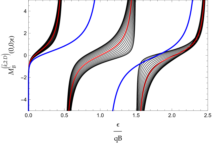
Figure 5: Bulk energy bands (filled with black curves) in finite volume with magnetic periodic boundary condition in both $x$- and $y$-direction is generated by varying $k_{x}$ in magnetic Brillouin zone: $k_{x}\in[0,\frac{2\pi}{n_{q}L}]$ in finite volume magnetic zeta function $\mathcal{M}^{(L,\mathbf{k},2D)}_{B}(\mathbf{0},\mathbf{0};\varepsilon)$ defined in Eq.(55). The wave vector in $y$-direction, $k_{y}$, is fixed at $k_{y}=\frac{\pi}{2n_{q}L}$. Compared with $\mathcal{M}^{(Open,k_{y}\mathbf{e}_{y},2D)}_{B}(\mathbf{0},\mathbf{0};\varepsilon)$ in Eq.(139) (red curve) with open boundary condition along $x$-direction and $\mathcal{M}^{(h.w.,k_{y}\mathbf{e}_{y},2D)}_{B}(\mathbf{0},\mathbf{0};\varepsilon)$ in Eq.(141) (blue curve) with a hard wall boundary condition in $x$-direction. The parameters are chosen as: $L=5$, and $n_{q}=n_{p}=1$.

V.2.4 Edge states vs. bulk energy bands

In general, the energy spectrum for various boundary conditions must be generated by using Eq.(56). The topological edge states in gaps between allowed energy bands in fact can be illustrated by only considering a simple case with $n_{q}=1$. For a single contact interaction in the box with $n_{q}=1$, the quantization condition is thus simply given by

$$\cot\delta_{0}(\varepsilon)=\mathcal{M}^{(2D)}_{B}(\mathbf{0},\mathbf{0};\varepsilon).$$ (142)

For periodic boundary conditions in both $x$-and $y$-direction, with a fixed $k_{y}$, the bulk energy bands can be generated by treating $k_{x}$ as a free parameter in finite volume magnetic zeta function $\mathcal{M}^{(L,\mathbf{k},2D)}_{B}(\mathbf{0},\mathbf{0};\varepsilon)$ that is defined in Eq.(55), see Fig. 5. The bulk energy bands are separated by gaps in betweens. The edge states are produced by replacing the periodic boundary condition in $x$-direction by a hard wall boundary condition, $\mathcal{M}^{(h.w.,k_{y}\mathbf{e}_{y},2D)}_{B}(\mathbf{0},\mathbf{0};\varepsilon)$ in Eq.(141). As shown in Fig. 5, unlike topologically trivial edge states, the solutions of edge states of a magnetic system not only show up in the gap, but also punch through bulk energy bands.

VI Analytic properties of finite volume solutions

The periodicity of lattice structure and particles interaction create the band structures, the energy spectrum split into isolated bands separated by gaps in betweens. Hence, when wave vector $\mathbf{k}$ is changed continuously, the energy of particle must experience a discontinuity when particle jumps from one band to another. It has been shown Kohn (1959); Heine (1963) that when wave vector is taken complex at the edge of Brillouin zone, the real energy solutions in the gap are possible, hence the transition from one band to another can be made smoothly in complex $\mathbf{k}$ plane. The complex wave vector at the edge of Brillouin zone may be interpreted as edge solutions with a penetrable wall on the edge or surface of material. In presence of a magnetic field, the real energy solutions can also be found for complex wave vector, however, the situation is more complicated, the energy solutions not only appear in the gap but also penetrate into bulk energy bands because of non-trivial topology.

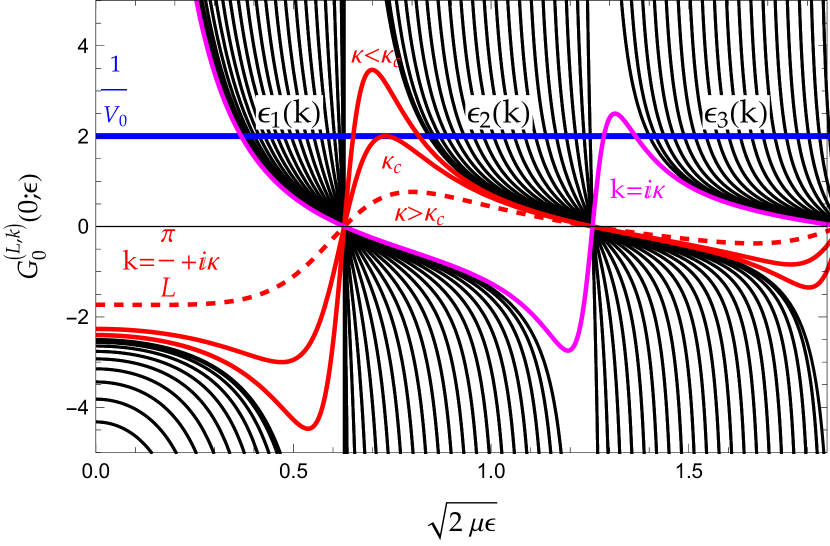
Figure 6: Plot of $G^{(L,k)}_{0}(0;\varepsilon)$ defined in Eq.(144) vs. $\frac{1}{V_{0}}$ (blue solid line): the area of allowed energy bands are filled by black curves (real $k\in[0,\frac{2\pi}{L}]$ values), the energy bands are separated by gaps; The red and purple curves that show up in gaps are generated with complex wave vectors $k=\frac{\pi}{L}+i\kappa$ and $k=i\kappa$ respectively. A pair of energy solutions in the gap can be found for $\kappa<\kappa_{c}$. The parameters are: $V_{0}=0.5$, $\mu=1$ and $L=5$.

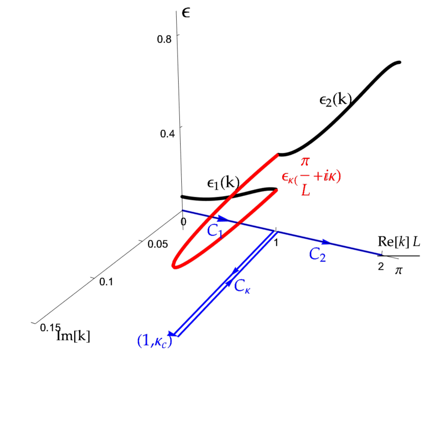
Figure 7: The motion of $\varepsilon(k)$ as the wave vector $k$ moves continuously in complex plane follow the path: $C_{1}\rightarrow C_{\kappa}\rightarrow C_{2}$. $C_{1}$ and $C_{2}$ are on real axis in $k$ plane between $[0,\frac{\pi}{L}]$ and $[\frac{\pi}{L},\frac{2\pi}{L}]$ respectively. $C_{\kappa}$ is on complex plane with $k=\frac{\pi}{L}+i\kappa$, $\kappa:0\rightarrow\kappa_{c}\rightarrow 0$. The energy solutions thus moves continuously from $\varepsilon_{1}(k)$ into $\varepsilon_{\kappa}(\frac{\pi}{L}+i\kappa)$ in the gap, and then connected into $\varepsilon_{2}(k)$.

In this subsection, we first give a brief summary of complex wave vector with a simple 1D example. With a contact interaction, the quantization condition in 1D is given by

$$\frac{1}{V_{0}}=G^{(L,k)}_{0}(0;\varepsilon),$$ (143)

where 1D finite volume Green’s function is given by

$$\frac{1}{2\mu}G^{(L,k)}_{0}(0;\varepsilon) =-\sum_{n\in\mathbb{Z}}\frac{ie^{i\sqrt{2\mu\varepsilon}|nL|}}{\sqrt{2\mu\varepsilon}}e^{-iknL}$$

$$=-\frac{2\mu}{2\sqrt{2\mu\varepsilon}}\frac{\sin\sqrt{2\mu\varepsilon}L}{\cos\sqrt{2\mu\varepsilon}L-\cos kL}.$$ (144)

The finite volume Green’s function $G^{(L,k)}_{0}$ remains real as for the real value of $k$, which yields the real dispersion relation of

$$\varepsilon=\varepsilon(k)=\varepsilon(-k)=\varepsilon(k+\frac{2\pi}{L}).$$ (145)

The band structures is explicitly produced by the bound of $|\cos kL|\leqslant 1$. Using Eq.(144), one can show that for $k=\frac{\pi d}{L}+i\kappa$, $d\in\mathbb{Z}$, Green’s function is still a real function,

$$G^{(L,\frac{\pi d}{L}+i\kappa)}_{0}(0;\varepsilon)=-\frac{2\mu}{2\sqrt{2\mu\varepsilon}}\frac{\sin\sqrt{2\mu\varepsilon}L}{\cos\sqrt{2\mu\varepsilon}L-(-1)^{d}\cosh\kappa L}.$$ (146)

Hence, we can see clearly because of

$$\cosh\kappa L\geqslant 1,$$

the energy solutions of complex wave function, $k=\frac{\pi d}{L}+i\kappa$, only show up in the gaps between bands, see Fig. 6. In the gaps, for a fixed $V_{0}$, a pair of energy solutions can be found for finite value of $\kappa$. The gap between two solutions shrinks when $\kappa$ is increased, until $\kappa$ reach its critical point $\kappa_{c}$, the gap close up, two solutions becomes degenerate. Beyond $\kappa_{c}$, no solutions can be found, see Fig. 6 as an example. Therefore, the complex wave vector can be used as a parameter to navigate across bulk energy bands smoothly. Using Fig. 7 as an example, two allowed energy bands $\varepsilon_{1}(k)$ and $\varepsilon_{2}(k)$ are separated by a gap for real values of $k$’s. Imaging wave vector $k$ start at $k=0$, and is forced to move following the path of $C_{1}\rightarrow C_{\kappa}\rightarrow C_{2}$ in Fig. 7, where both $C_{1}$ and $C_{2}$ are defined on real axis for $k\in[0,\frac{\pi}{L}]$ and $k\in[\frac{\pi}{L},\frac{2\pi}{L}]$ respectively. The contour $C_{\kappa}$ is defined in complex $k$ plane with fixed $Re[k]=\frac{\pi}{L}$ value, and the imaginary part of $Im[k]=\kappa$ is circling around $\kappa_{c}$, $\kappa:0\rightarrow\kappa_{c}\rightarrow 0$. While $k$ is on $C_{1}$, the energy solution stays in energy band $\varepsilon_{1}(k)$ following the motion of $k$, moving from lower edge $\varepsilon_{1}(0)$ up to upper edge $\varepsilon_{1}(\frac{\pi}{L})$. While $k$ is extended into complex plane on $C_{\kappa}$, the energy solution then protrude into the gap between two allowed bands, and continue climbing up to the lower edge of energy band $\varepsilon_{2}(k)$ at $\varepsilon_{2}(\frac{\pi}{L})$. Then, it merged into second band $\varepsilon_{2}(k)$ if $k$ is increased further on $C_{2}$. Similarly, $\varepsilon_{2}(k)$ and $\varepsilon_{3}(k)$ are smoothly connected by taking wave vector into complex plane at the edge of Brillouin zone: $k=\frac{2\pi}{L}+i\kappa$ which is equivalent to $k=i\kappa$, see Fig. 6. We can also see from Fig. 6 that the curves of $G^{(L,\frac{\pi d}{L}+i\kappa)}_{0}(0;\varepsilon)$ with different $d$ values occupy completely different territories, hence there are no denegerate energy solutions for different $d$ values.

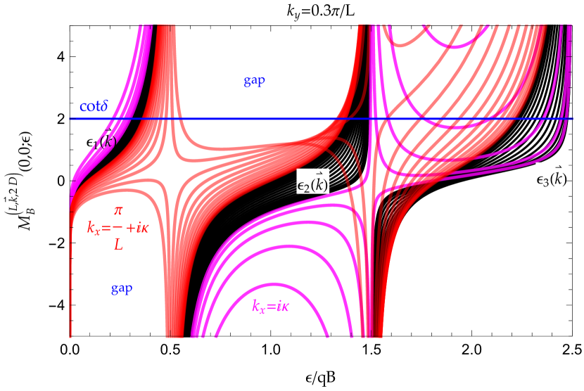
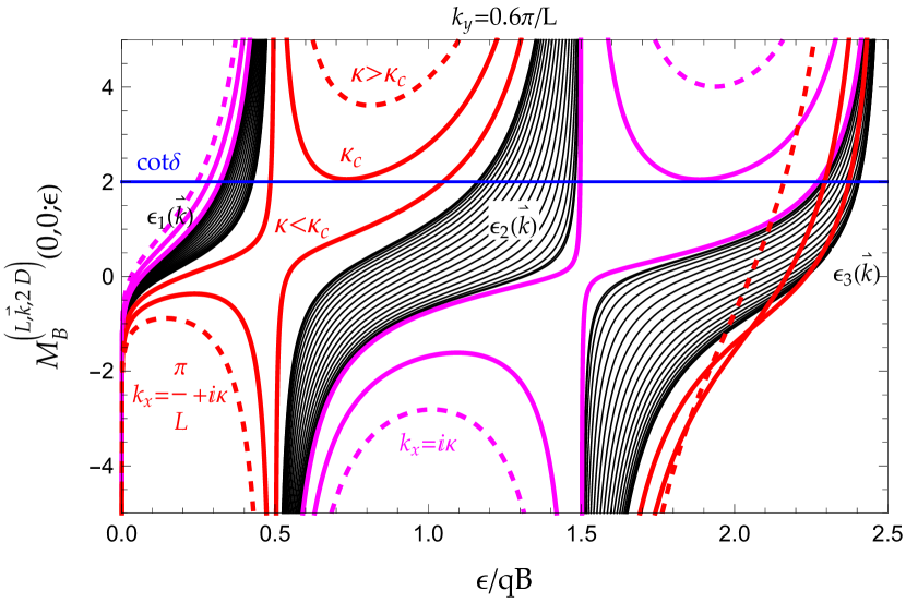
Figure 8: Energy band structure (filled with black curves) is the result of periodicity in both $x$- and $y$-direction, red $(d=1)$ and purple ($d=0$) curves are generated by taking $k_{x}$ into complex plane: $k_{x}=\frac{\pi d}{L}+i\kappa$. $k_{y}$’s are fixed at $k_{y}=0.3\frac{\pi}{L}$ and $k_{y}=0.6\frac{\pi}{L}$ in upper and lower panels respectively. The parameters are chosen as: $L=5$, and $n_{q}=n_{p}=1$. Blue line represents a constant $\cot\delta_{0}(\varepsilon)$ that is used only to help to visualize the energy solutions.

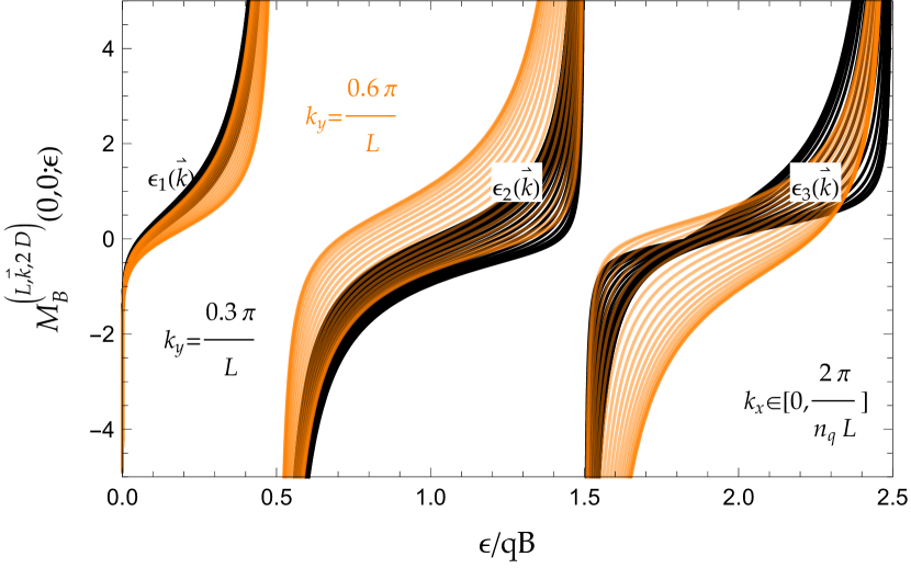
Figure 9: Overlapping energy bands of different $k_{y}$ values: $k_{y}=0.3\frac{\pi}{L}$ (black) vs. $k_{y}=0.6\frac{\pi}{L}$ (orange) .

In presence of magnetic field, with a complex wave vector

$$\mathbf{k}=(\frac{\pi d}{n_{q}L}+i\kappa)\mathbf{e}_{x}+k_{y}\mathbf{e}_{y},\ \ \ \ d\in\mathbb{Z},$$ (147)

similarly, the real energy solutions are also available, however situation becomes much more intriguing. Unfortunately, for a magnetic system, analytic properties cannot be shown easily in a straightforward way, all the discussions heavily rely on numerics. Let’s consider the case of $n_{q}=1$ as a simple example, which corresponds to a single contact interaction placed at origin, thus the magnetic zeta function is given by

$$\mathcal{M}^{(L,(\frac{\pi d}{n_{q}L}+i\kappa)\mathbf{e}_{x}+k_{y}\mathbf{e}_{y},2D)}_{B}(\mathbf{0},\mathbf{0};\varepsilon)$$

$$=\mathcal{M}^{(\infty,2D)}_{B}(\mathbf{0},\mathbf{0};\varepsilon)$$

$$+\frac{1}{\pi}\sum_{\mathbf{n}_{B}\neq\mathbf{0}}(-1)^{dn_{x}}(-1)^{n_{p}n_{x}n_{y}}e^{\kappa n_{x}n_{q}L}e^{-ik_{y}n_{y}L}$$

$$\times e^{-\frac{qB}{4}|\mathbf{n}_{B}L|^{2}}\Gamma(\frac{1}{2}-\frac{\mu\varepsilon}{qB})U(\frac{1}{2}-\frac{\mu\varepsilon}{qB},1,\frac{qB}{2}|\mathbf{n}_{B}L|^{2}),$$ (148)

which is indeed a real function. Compared with previously discussed 1D topologically trivial example, there are some new features in a magnetic system. First of all, as we can see in Fig. 8, for small $k_{y}$, the gap area between allowed energy bands cannot be completely filled by taking $k_{x}$ into complex plane, see gap between $\varepsilon_{1}$ and $\varepsilon_{2}$ bands in upper panel in Fig. 8. Hence, for certain range of $k_{y}$, although complex wave vector $k_{x}$ may narrow the gap, the gap remains. Therefore, using complex $k_{x}$ alone to navigate though gaps are not possible for certain range of $k_{y}$, however, due to overlapping energy bands of different $k_{y}$, see Fig. 9, it may be still possible by using both complex $k_{x}$ and real $k_{y}$ to navigate through different energy bands smoothly by avoiding gap area. Secondly, with complex wave vector $k_{x}=\frac{\pi d}{n_{q}L}+i\kappa$, curves not only show up in the gap areas, some curves punch through the allowed bulk bands, and invade into the gap areas with different $d$ value, see Fig. 8. In addition, the curves with complex wave vectors in gap make up a vortex shape, all the curves are pushed away from a vortex centered at location of Landau level energy: $\varepsilon_{n}=\frac{qB}{\mu}(n+\frac{1}{2})$, see example in Fig. 8. These irregular behaviors of magnetic zeta function with a complex wave vector may have a topological origin.

VII Summary

In summary, we explore and discuss some topological and analytic properties of a finite volume two-body system in a uniform magnetic field in present work. The Berry phase is introduced on a torus of magnetic Brillouin zone in $\mathbf{k}$-space. The analytic solutions of edge states with a hard wall boundary condition in $x$-direction are also presented and discussed. By further taking $\mathbf{k}$ into a complex plane, the analytic properties of energy spectrum is also discussed.