Transporting Causal Mechanisms for Unsupervised Domain Adaptation

Abstract

Existing Unsupervised Domain Adaptation (UDA) literature adopts the covariate shift and conditional shift assumptions, which essentially encourage models to learn common features across domains. However, due to the lack of supervision in the target domain, they suffer from the semantic loss: the feature will inevitably lose non-discriminative semantics in source domain, which is however discriminative in target domain. We use a causal view—transportability theory [41]—to identify that such loss is in fact a confounding effect, which can only be removed by causal intervention. However, the theoretical solution provided by transportability is far from practical for UDA, because it requires the stratification and representation of the unobserved confounder that is the cause of the domain gap. To this end, we propose a practical solution: Transporting Causal Mechanisms (TCM), to identify the confounder stratum and representations by using the domain-invariant disentangled causal mechanisms, which are discovered in an unsupervised fashion. Our TCM is both theoretically and empirically grounded. Extensive experiments show that TCM achieves state-of-the-art performance on three challenging UDA benchmarks: ImageCLEF-DA, Office-Home, and VisDA-2017. Codes are available at https://github.com/yue-zhongqi/tcm.

1 Introduction

Machine learning is always challenged when transporting training knowledge to testing deployment, which is generally known as Domain Adaptation (DA) [38]. As shown in Figure 1, when the target domain ($S=t$) is drastically different (e.g., image style) from the source domain ($S=s$), deploying a classifier trained in $S=s$ results in poor performance due to the large domain gap [5]. To narrow the gap, conventional supervised DA requires a small set of labeled data in $S=t$ [13, 49], which is expensive and sometimes impractical. Therefore, we are interested in a more practical setting: Unsupervised DA (UDA), where we can leverage the abundant unlabelled data in $S=t$ [38, 30]. For example, when adapting an autopilot system trained in one country to another, where the street views and road signs are different, one can easily collect unlabelled street images from a camera-equipped vehicle cruise.

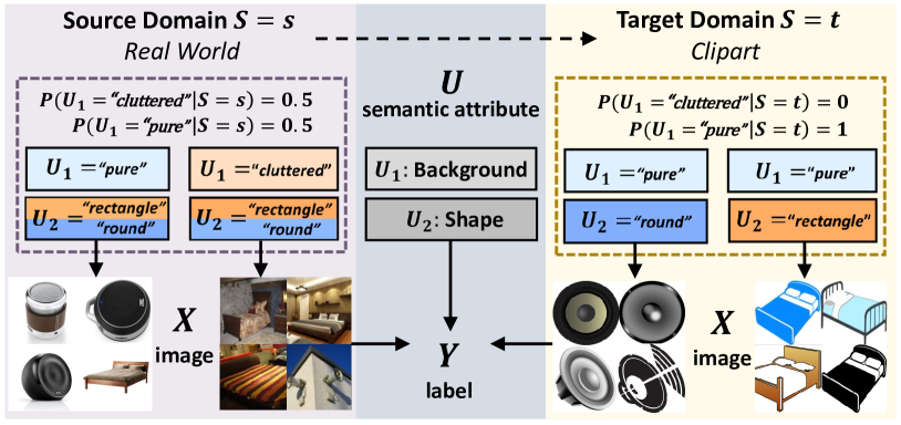
Figure 1: A DA example from source “Real World” to target “Clipart” domain in the Office-Home benchmark [57].

Existing UDA literature widely adopts the following two assumptions on the domain gap: 1) Covariate Shift [54, 4]: $P(X|S=s)\neq P(X|S=t)$, where $X$ denotes the samples, e.g., real-world vs. clip-art images; and 2) Conditional Shift [53, 32]: $P(Y|X,S=s)\neq P(Y|X,S=t)$, where $Y$ denotes the labels, e.g., in clip-art domain, the “pure background” feature extracted from $X$ is no longer a strong visual cue for $Y=$ “speaker” as in real-world domain. To turn “$\neq$” into “$=$”, almost all existing UDA solutions rely on learning invariant (or common) features in both source and target domains [54, 20, 30]. Unfortunately, due to the lack of supervision in target domain, it is challenging to capture such domain invariance.

For example, in Figure 1, when $S=s$, the distribution of “Background = pure” and “Background = cluttered” is already informative for “speaker” and “bed”, a classifier may recklessly tend to downplay the “Shape” features (or attributes) as they are not as “invariant” as “Background”; but, it does not generalize to $S=t$, where all clip-art images have “Background = pure” that is no longer discriminative.

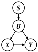
Figure 2: Causal graph of domain adaptation.

A popular approach to make up for the above loss of “Shape” is by imposing unsupervised reconstruction [6]—any feature loss hurts reconstruction. However, it is well-known that discrimination and reconstruction are adversarial objectives, leaving the finding of their ever-elusive trade-off parameter per se an open problem [9, 16, 24].

To systematically understand how domain gap causes the feature loss, we propose to use the transportability theory [41] to replace the above “shift” assumptions that overlook the explicit role of semantic attributes. Before we introduce the theory, we first abstract the DA problem in Figure 1 into the causal graph in Figure 2. We assume that the classification task $X\to Y$ is also affected by the unobserved semantic feature $U$ (e.g., shape and background), where $U\to X$ denotes the generation of pixel-level image samples $X$ and $U\to Y$ denotes the definition process of semantic class. Note that these causalities have been already shown valid in their respective areas, e.g., $U\to X$ and $U\to Y$ can be image [17] and language generation [7], respectively. In particular, the introduction of the domain selection variable $S$ reveals that the fundamental reasons of the covariate shift and conditional shift are both due to $P(U|S=s)\neq P(U|S=t)$.

Note that the domain-aware $U$ is the confounder that prevents the model from learning the domain-invariant causality $X\to Y$. It has been theoretically proven that the confounding effect cannot be eliminated by statistical learning without causal intervention [40]. Fortunately, the transportability theory offers a principled DA solution based on the causal intervention in Figure 2:

$$P(Y|do(X),S)=\sum\nolimits_{u}P(Y|X,U=u)P(U=u|S).$$ (1)

Note that the goal of DA is achieved by causal intervention $P(Y|do(X),S)$ using the $do$-operator [42]. To appreciate the merits of the calculus on the right-hand side of Eq. (1), we need to understand the following two points. First, $P(Y|X,U)$ is domain-agnostic as $S$ is separated from $X$ and $Y$ given $U=u$ [40], thus $P(Y|X,U)$ generalizes to $S=t$ in testing even if it is trained on $S=s$. Second, every stratum of $U$ is fairly adjusted subject to the domain prior $P(U|S)$, i.e., forcing the model to respect “shape” as it is the only “invariance” that distinguishes between “speaker” and “bed” in controlled “cluttered” or “pure” backgrounds. Therefore, the semantic loss is eliminated.

However, Eq. (1) is purely declarative and far from practical, because it is still unknown how to implement the stratification and representation of the unobserved $U$, not mentioning to transport it across domains. To this end, we propose a novel approach to make Eq. (1) practical in UDA:

Identify the number of $U$ by disentangled causal mechanisms. In practice, the number of $U$ can be large due to the combinations of multiple attributes, making Eq. (1) computationally prohibitive (e.g., many network passes). Fortunately, if the attributes are disentangled, we can stratify $U$ according to the much smaller number of disentangled attributes, as the effect of each feature is independent with each other [19], e.g., $P(Y|X,U=(u_{1},u_{2}))\propto P(Y|X,u_{1})+P(Y|X,u_{2})$ if $u_{1}$ and $u_{2}$ are disentangled. As detailed in Section 3.1, this motivates us to discover a small number of Disentangled Causal Mechanisms (DCMs) in unsupervised fashion [39], each of which corresponds to a feature-specific intervention between $X|S=s$ and $X|S=t$, e.g., mapping a real-world “speaker” image to its clip-part counterpart by changing “Background” from “cluttered” to “pure”.

Represent $U$ by proxy variables. Yet, DCMs do not provide vector representations of $U$, leaving difficulties in implementing Eq. (1) as neural networks. In Section 3.2, we show that the transformed output $\hat{X}$ of each DCM taking $X$ as input can be viewed as a proxy of $U$ [36], who provides a theoretical guarantee that we can replace the unobserved $U$ with the observed $\hat{X}$ to make Eq. (1) computable.

Overall, instead of transporting the abstract and unobserved $U$ in the original transportability theory of Eq. (1), we transport the concrete and learnable disentangled causal mechanisms, which generate the observed proxy of $U$. Therefore, we term the approach as Transporting Casual Mechanisms (TCM) for UDA. Through extensive experiments, our approach achieves state-of-the-art performance on UDA benchmarks: 70.7% on Office-Home [57], 90.5% on ImageCLEF-DA [1] and 75.8% on VisDA-2017 [45]. Specifically, we show that learning disentangled mechanisms and capturing the causal effect through proxy variables are the keys to improve the performance, which validates the effectiveness of our approach.

2 Related Work

Existing UDA works fall into the three categories: 1) Sample Reweighing [54, 10]. This line-up adopts the covariate shift assumption. It first models $P(X|S=s)$ and $P(X|S=t)$. When minimizing the classification loss, each sample in $S=s$ is assigned an importance weight $P(X|S=t)/P(X|S=s)$, i.e., a target-like sample has a larger weight, which effectively encourages $P(X|S=s)=P(X|S=t)$. 2) Domain Mapping [20, 37]. This approach focuses on the conditional shift assumption. It first learns a mapping function that transforms samples from $S=s$ to $S=t$ through unpaired image-to-image translation techniques such as CycleGAN [67]. Then, the transformed source domain samples are used to train a classifier. 3) Invariant Feature Learning. This is the most popular approach in recent literature [15, 31, 59]. It maps the samples in $S=s$ and $S=t$ to a common feature space, denoted as domain $S=c$, where the source and target domain samples are indistinguishable. Some works [38, 30] adopted the covariate shift assumption, and aim to minimize the differences in $P(X|S=c)$ using distance measures like Maximum Mean Discrepancy [56, 33] or using adversarial training to fool a domain discriminator [15, 6]. Others used the conditional shift assumption and aim to align $P(Y|X,S=c)$ [32, 31]. As the target domain samples have no labels, their $P(Y|X,S=c)$ is either estimated through clustering [21, 62] or using a classifier trained with the source domain samples [50, 64].

They all aim to make the source and target domain alike while learning a classifier with the labelled data in the source domain, leading to the semantic loss. In fact, there are existing works that attempt to Alleviate Semantic Loss by learning to capture $U$ in unsupervised fashion: One line exploits that $U$ generates $X$ (via $U\to X$) and learns a latent variable to reconstruct $X$ [6, 16]. The other line [8, 11] exploits $S\to U$, and aims to learn a domain-specific representation for each $S=s,S=t$. However, this leads to an ever-illusive trade-off between the adversarial discrimination and reconstruction objectives. Our approach aims to fundamentally eliminate the semantic loss by providing a practical implementation of the transportability theory [41] based on causal intervention [42].

3 Approach

Though Eq. (1) provides a principled solution for DA, it is impractical due to the unobserved $U$. To this end, the proposed TCM is a two-stage approach to make it practical. The first stage identifies the $U$ stratification by discovering Disentangled Causal Mechanisms (DCMs) ( Secton 3.1) and the second stage represents each stratification of $U$ with the proxy variable generated from the discovered DCMs (Section 3.2). The training and inference procedures are summarized in Algorithm 1 and 2, respectively.

Algorithm 1 Two-stage Training of TCM

1:  Input: Labelled domain $S=s$, unlabelled domain $S=t$, pre-trained backbone parameters $\beta$

2:  Output: DCMs $\{(M_{i},M_{i}^{-1})\}_{i=1}^{k}$, fine-tuned backbone parameters $\beta$ and linear functions parameters $\omega$

3:  Randomly initialize $\{(M_{i},M_{i}^{-1})\}_{i=1}^{k},\omega$, VAE parameters $\theta$, discriminator parameters $\gamma$ (see Eq. (8))

4:  repeat

5:     // See Section 3.1 for details

6:     Sample $\mathbf{x}$ randomly from $S=s$ or $S=t$

7:     Calculate $\mathcal{L}_{CycleGAN}^{i}$ for $i\in\{1,\ldots,k\}$

8:     Update $\{(M_{i},M_{i}^{-1})\}_{i=1}^{k}$ with Eq. (2)

9:  until convergence

10:  repeat

11:     // See Section 3.2 for details

12:     Sample $\mathbf{x}_{s},y_{s}$ from $S=s$, $\mathbf{x}_{t}$ from $S=t$

13:     Obtain $\hat{\mathcal{X}}_{s}=\{M_{i}(\mathbf{x}_{s})\}_{i=1}^{k}$,$\hat{\mathcal{X}}_{t}=\{M_{i}^{-1}(\mathbf{x}_{t})\}_{i=1}^{k}$

14:     Calculate $h_{y}(\mathbf{x}_{s},\hat{\mathbf{x}}),\forall\hat{\mathbf{x}}\in\hat{\mathcal{X}_{s}}$ with Eq. (7)

15:     Obtain $P(Y|do(X=\mathbf{x}_{s}),S=s)$ with Eq. (5)

16:     Update $\omega,\beta,\theta,\gamma$ with Eq. (8)

17:  until convergence

Algorithm 2 Inference with TCM

1:  Input: $\mathbf{x}_{t}$, $P(\hat{X}|S=t)$, DCMs $\{M_{i}^{-1}\}_{i=1}^{k}$, backbone parameters $\beta$ and linear functions parameters $\omega$

2:  Output: Predicted label $y_{t}$

3:  Obtain $\hat{\mathcal{X}}_{t}=\{M_{i}^{-1}(\mathbf{x}_{t})\}_{i=1}^{k}$

4:  Calculate $h_{y}(\mathbf{x}_{t},\hat{\mathbf{x}}),\forall\hat{\mathbf{x}}\in\hat{\mathcal{X}}_{t}$ with Eq. (7)

5:  $y_{t}\leftarrow\mathrm{argmax}\;P(Y|do(X=\mathbf{x}_{t}),S=t)$ with Eq. (5)

3.1 Disentangled Causal Mechanisms Discovery

Physicists believe that real-world observations are the outcome of the combination of independent physical laws. In causal inference [19, 55], we denote these laws as disentangled generative factors, such as shape, color, and position. For example, in our causal graph of Figure 2, if the semantic attribute $U$ can be disentangled into generative causal factors $(U_{1},\ldots,U_{k})$, each one will independently contribute to the observation: $P(Y|X)\propto\sum_{i=1}^{k}P(Y|X,U_{i})$. Even though $|U|$ is large, i.e., the number of sum in Eq. (1) is expensive, the disentanglement can still significantly reduce the number to a small $k$.

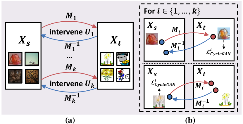
Figure 3: (a) Our DCMs $\{(M_{i},M_{i}^{-1})\}_{i=1}^{k}$, where each $M_{i}:X_{s}\to X_{t}$ and $M_{i}^{-1}:X_{t}\to X_{s}$ correspond to intervention on the disentangled attribute $U_{i}$. (b) CycleGAN [67] loss $\mathcal{L}_{CycleGAN}^{i}$ on each $(M_{i},M_{i}^{-1})$.

However, learning a disentangled representation of $U=(U_{1},\ldots,U_{k})$ without supervision is challenging [29]. Fortunately, we can observe the outcomes of $U$: the source domain samples $X_{s}$ and the target domain samples $X_{t}$ generated from $P(X|U)$. This motivate us to discover $k$ pairs of end-to-end functions $\{(M_{i},M_{i}^{-1})\}_{i=1}^{k}$ in unsupervised fashion, where $M_{i}:X_{s}\to X_{t}$ and $M_{i}^{-1}:X_{t}\to X_{s}$, as shown in Figure 3 (a). Each $(M_{i},M_{i}^{-1})$ corresponds to a counterfactual mapping that transforms a sample to the counterpart domain by intervening a disentangled factor $U_{i}$, i.e., modifying $U_{i}$ w.r.t. the domain shift while fixing the values of other factors $U_{j\neq i}$—this is essentially the definition of independent causal mechanisms [39], each of which corresponds to a disentangled causal factor. Hence we refer to these mapping functions as DCMs.

We first make a strong assumption that the one-to-one correspondence between $(M_{i},M_{i}^{-1})$ and $U_{i}$ has been already established, then we relax this assumption by removing the correspondence for the proposed practical solution. Without loss of generality, we consider a source domain sample $\mathbf{x}_{s}$. For each $M_{i}:X_{s}\to X_{t}$, we obtain a transformed sample $M_{i}(\mathbf{x}_{s})$, corresponding to the interventional outcome of $U_{i}$ drawn from $P(U_{i}|S=s)$ to $P(U_{i}|S=t)$. To ensure that the interventions are disentangled, we use the Counterfactual Faithfulness theorem [3, 60], which guarantees that $M_{i}$ is a disentangled intervention if and only if $M_{i}(\mathbf{x}_{s})\sim P(X_{t})$ (proof in Appendix). Hence, as shown in Figure 3 (b), we use the CycleGAN loss [67] denoted as $\mathcal{L}_{CycleGAN}^{i}$ to make the transformed samples from each $M_{i}:X_{s}\to X_{t}$ indistinguishable from the real samples in $S=t$. Likewise, we apply the CycleGAN loss to each $M_{i}^{-1}:X_{t}\to X_{s}$ such that the transformed samples are close to real samples in $S=s$.

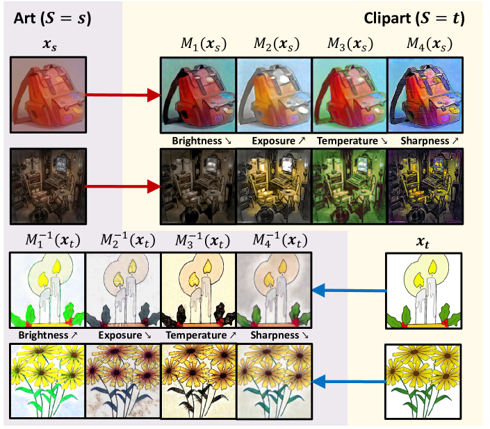
Figure 4: Transformation between “Art” and “Clipart” domain with 4 trained DCMs $\{(M_{i},M_{i}^{-1})\}_{i=1}^{4}$, where each pair of mapping functions specializes in brightness, exposure, color temperature and sharpness, respectively.

Now we relax the above one-to-one correspondence assumption. We begin with a sufficient condition (proof in Appendix): if $(M_{i},M_{i}^{-1})$ intervenes $U_{i}$, the $i$-th mapping function outputs the counterfactual faithful generation, i.e., $i=\mathop{\mathrm{argmin}}_{j\in\{1,\ldots,k\}}\mathcal{L}_{CycleGAN}^{j}$. To “guess” the one-to-one correspondence, we adopt a practical method by using the necessary conclusion: if $i=\mathop{\mathrm{argmin}}_{j\in\{1,\ldots,k\}}\mathcal{L}_{CycleGAN}^{j}$, then $(M_{i},M_{i}^{-1})$ corresponds to $U_{i}$ intervention. Specifically, training samples are fed into all $(M_{i},M_{i}^{-1})$ in parallel to compute $\mathcal{L}_{CycleGAN}^{i}$ for each pair. Only the winning pair with the smallest loss is updated. The objective is given by:

$$\mathop{\mathrm{min}}_{(M_{i},M_{i}^{-1})}\mathcal{L}_{CycleGAN}^{i},$$ (2)

$$\mathrm{where} i=\mathop{\mathrm{argmin}}_{j\in\{1,\ldots,k\}}\mathcal{L}_{CycleGAN}^{j},$$

The functions (e.g., $M_{i}$) in the optimization objective denote their parameters for simplicity. Note that this is not sufficient, hence our approach has limitations. Still, this practice has been empirically justified in [39], and we leave a more theoretically complete approach as future work.

After training, we obtain $k$ DCMs $\{(M_{i},M_{i}^{-1})\}_{i=1}^{k}$, where the $i$-th pair corresponds to $U_{i}$. Hence we identify the number of $U$ as $k$. Figure 4 shows an example with $k=4$, where the 4 DCMs correspond to “Brightness”, “Exposure”, “Temperature” and “Sharpness”, respectively.

3.2 Representing $U$ by Proxy Variables

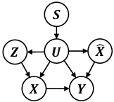
Figure 5: Causal graph with the proxy $\hat{X}$ and $Z$.

While the learned DCMs identify the number of $U$, they do not provide a vector representation of $U$. Hence $P(U|S)$ and $P(Y|X,U)$ in Eq. (1) are still unobserved. Fortunately, $U$ generates two observed variables $\hat{X}$ and $Z$ as shown in Figure 5, which are called proxy variables [36] of $U$ and make $P(U|S)$ and $P(Y|X,U)$ estimable. We will first explain $\hat{X}$ and $Z$ as well as their related causal links.

$\mathbf{\hat{X},U\to\hat{X}\to Y}$. $\hat{X}$ represents the DCMs outputs, i.e., for a sample $\mathbf{x}_{s}$ in $S=s$, $\hat{X}|S=s$ takes value from $\hat{\mathcal{X}}_{s}=\{M_{i}(\mathbf{x}_{s})\}_{i=1}^{k}$; and for a sample $\mathbf{x}_{t}$ in $S=t$, $\hat{X}|S=t$ takes value from $\hat{\mathcal{X}}_{t}=\{M_{i}^{-1}(\mathbf{x}_{t})\}_{i=1}^{k}$. As detailed in Appendix, $M_{i},M_{i}^{-1}$ generates counterfactuals in the other domain by fixing $U_{j\neq i}$ and intervening $U_{i}$, i.e., $\hat{X}$ is generated from $U$. Hence $U\to\hat{X}$ is justified. Moreover, as the other domain is also labelled, $\hat{X}\to Y$ denotes the predictive effects from the generated counterfactuals.

$\mathbf{Z,U\to Z\to X}$. $Z$ is a latent variable encoded from $X$ by a VAE [22]. The link $Z\to X$ is because the latent variable is trained to reconstruct $X$. Furthermore, the latent variable of VAE is shown to capture some information of the underlying $U$ [55], justifying $U\to Z$.

Note that the networks to obtain $\hat{X}$ and $Z$ are trained in an unsupervised fashion. Hence $\hat{X},Z$ are observed in both $S=s$ and $S=t$. Under this causal graph, we have a theoretically grounded solution to Eq. (1) using the theorem below (proof in Appendix as corollary to [36]).

Theorem (Proxy Function). Under the causal graph in Figure 5, any solution $h_{y}(X,\hat{X})$ to Eq. (3) satisfies Eq. (4).

$$P(Y|Z,X,S)=\sum_{\mathbf{\hat{x}}}h_{y}(X,\mathbf{\hat{x}})P(\hat{X}=\mathbf{\hat{x}}|Z,X,S)$$ (3)

$$P(Y|X,U)=\sum_{\mathbf{\hat{x}}}h_{y}(X,\mathbf{\hat{x}})P(\hat{X}=\mathbf{\hat{x}}|U).$$ (4)

Notice that we can set $S=s$ in Eq. (3) and use the labelled data in $S=s$ to learn $h_{y}$ (details given below). We prove in the Appendix that $h_{y}$ is invariant across domains. This leads to the following inference strategy.

3.2.1 Inference

Taking expectation over $U|S=t$ on both sides of Eq. (4) leads to a practical solution to Eq. (1):

$$P(Y|do(X),S=t)=\sum_{\mathbf{\hat{x}}\in\hat{\mathcal{X}}_{t}}h_{y}(X,\mathbf{\hat{x}})P(\hat{X}=\mathbf{\hat{x}}|S=t),$$ (5)

where $P(\hat{X}|S=t)$ is estimable as $\hat{X}$ is observed in $S=t$, and $h_{y}$ is trained in $S=s$ as given below.

3.2.2 Learning $h_{y}$

We detail the training of $h_{y}$, including the representation of its inputs $X$ and $\hat{X}$, the function forms of the terms in Eq. (3) and the training objective.

Representation of $X,\hat{X}$. When $X$ and $\hat{X}$ are images, directly evaluating Eq. (5) in image space can be computationally expensive, not to mention the tendency for severe over-fitting. Therefore, we follow the common practice in UDA [31, 21] to introduce a pre-trained feature extractor backbone (e.g., ResNet [18]). Hereinafter, $X,\hat{X}$ denote their respective $n$-d features. Note that $Z$ of $l$ dimensions is encoded from $X$’s feature form ($l<n$).

Function Forms. We adopt an isotropic Gaussian distribution for $P(\hat{X}|S)$. We implement $P(Y|Z,X,S=s),P(\hat{X}|Z,X,S=s)$ in Eq. (3) with the following linear model $f_{y}(Z,X)$ and $f_{\hat{x}}(Z,X)$, respectively:

$$\begin{split}&f_{y}(Z,X)=\mathbf{W}_{1}Z+\mathbf{W}_{2}X+\mathbf{b}_{1}\\ &f_{\hat{x}}(Z,X)=\mathbf{W}_{3}Z+\mathbf{W}_{4}X+\mathbf{b}_{2},\end{split}$$ (6)

where $f_{y}:(Z,X)\to\mathbb{R}^{c}$ produces logits for $c$ classes, $f_{\hat{x}}:(Z,X)\to\mathbb{R}^{n}$ predicts $\hat{X}$, $\mathbf{W}_{1}\in\mathbb{R}^{c\times l}$, $\mathbf{W}_{2}\in\mathbb{R}^{c\times n}$, $\mathbf{W}_{3}\in\mathbb{R}^{n\times l}$, $\mathbf{W}_{4}\in\mathbb{R}^{n\times n}$, $\mathbf{b}_{1}\in\mathbb{R}^{c}$ and $\mathbf{b}_{2}\in\mathbb{R}^{n}$. With this function form, we can solve $h_{y}:(X,\hat{X})\to\mathbb{R}^{c}$ from Eq. (3) as (derivation in Appendix):

$$\begin{split}h_{y}(X,\hat{X})&=\mathbf{b}_{1}-\mathbf{W}_{1}\mathbf{W}_{3}^{+}\mathbf{b}_{2}+\mathbf{W}_{1}\mathbf{W}_{3}^{+}\hat{X}\\ &+(\mathbf{W}_{2}-\mathbf{W}_{1}\mathbf{W}_{3}^{+}\mathbf{W}_{4})X,\end{split}$$ (7)

where $(\cdot)^{+}$ denotes pseudo-inverse.

Overall Objective. The training objective is given by:

$$\mathop{\mathrm{min}}_{\omega,\beta,\theta}(\mathcal{L}_{c}+\mathcal{L}_{v})+\mathop{\mathrm{min}}_{\beta}\mathop{\mathrm{max}}_{\gamma}\alpha\mathcal{L}_{p},$$ (8)

where $\omega$ denotes the parameters of the linear functions $f_{y}$ and $f_{\hat{x}}$, $\beta$ denotes the parameters of the backbone, $\theta$ denotes the parameters of the VAE, $\mathcal{L}_{c}$ denotes the sum of Cross-Entropy loss to train $f_{y}$ and the mean squared error loss to train $f_{\hat{x}}$ (see Eq. (6)). $\mathcal{L}_{v}$ is the VAE loss, $\mathcal{L}_{p}$ is the proxy loss, $\gamma$ denotes the parameters of the discriminators used in $\mathcal{L}_{p}$, and $\alpha$ is a trade-off parameter.

VAE Loss. $\mathcal{L}_{v}$ is used to train the VAE, which contains an encoder $Q_{\theta}(Z|X)$ and a decoder $P_{\theta}(X|Z)$. Given a feature $\mathbf{x}_{s}$ in $S=s$, $\mathcal{L}_{v}$ is given by:

$$\begin{split}\mathcal{L}_{v}&=-\mathbb{E}_{Q_{\theta}(Z|X=\mathbf{x}_{s})}[P_{\theta}(X=\mathbf{x}_{s}|Z)]\\ &+D_{KL}(Q_{\theta}(Z|X=\mathbf{x}_{s})\mid\mid P(Z)),\end{split}$$ (9)

where $D_{KL}$ denotes KL-divergence and $P(Z)$ is set to the isotropic Gaussian distribution. Note that we only need to learn a VAE in $S=s$, as $h_{y}(X,\hat{X})$ is domain-agnostic.

Proxy Loss. In practice, the generated images from the DCMs $\{(M_{i},M_{i}^{-1})\}_{i=1}^{k}$ may contain artifacts that contaminate the feature outputs from the backbone [34], making $\hat{X}$ as feature no longer resembles the features in the counterpart domain. Hence we regularize the backbone with a proxy loss to enforce feature-level resemblance between the samples transformed by the DCMs and the samples in the counterpart domain. Given feature $\mathbf{x}_{s}$ in $S=s$, $\mathbf{x}_{t}$ in $S=t$ and their corresponding DCMs outputs sets $\hat{\mathcal{X}_{s}},\hat{\mathcal{X}_{t}}$ (as $n$-d features), the loss is given by:

$$\begin{split}\mathcal{L}_{p}&=\mathrm{log}D_{s}(\mathbf{x}_{s})+\frac{1}{k}\sum_{\mathbf{\hat{x}_{s}}\in\hat{\mathcal{X}_{s}}}\mathrm{log}(1-D_{t}(\mathbf{\hat{x}_{s}}))\\ &+\mathrm{log}D_{t}(\mathbf{x}_{t})+\frac{1}{k}\sum_{\mathbf{\hat{x}_{t}}\in\hat{\mathcal{X}_{t}}}\mathrm{log}(1-D_{s}(\mathbf{\hat{x}}_{t})),\end{split}$$ (10)

where $D_{s},D_{t}$ are discriminators parameterized by $\gamma$ that return a large value for features of real samples. Through min-max adversarial training, generated sample features $\hat{X}$ become similar to the sample features in the counterpart domain and fulfill the role as a proxy.

4 Experiment

4.1 Datasets

Method		A$\to$C	A$\to$P	A$\to$R	C$\to$A	C$\to$P	C$\to$R	P$\to$A	P$\to$C	P$\to$R	R$\to$A	R$\to$C	R$\to$P	Avg
ResNet-50 [18]		34.9	50.0	58.0	37.4	41.9	46.2	38.5	31.2	60.4	53.9	41.2	59.9	46.1
DAN [30]		43.6	57.0	67.9	45.8	56.5	60.4	44.0	43.6	67.7	63.1	51.5	74.3	56.3
DANN [15]		45.6	59.3	70.1	47.0	58.5	60.9	46.1	43.7	68.5	63.2	51.8	76.8	57.6
MCD [51]		48.9	68.3	74.6	61.3	67.6	68.8	57.0	47.1	75.1	69.1	52.2	79.6	64.1
MDD [63]		54.9	73.7	77.8	60.0	71.4	71.8	61.2	53.6	78.1	72.5	60.2	82.3	68.1
CDAN [31]		50.7	70.6	76.0	57.6	70.0	70.0	57.4	50.9	77.3	70.9	56.7	81.6	65.8
SymNets [64]		47.7	72.9	78.5	64.2	71.3	74.2	63.6	47.6	79.4	73.8	50.8	82.6	67.2
CADA [25]		56.9	76.4	80.7	61.3	75.2	75.2	63.2	54.5	80.7	73.9	61.5	84.1	70.2
ETD [26]		51.3	71.9	85.7	57.6	69.2	73.7	57.8	51.2	79.3	70.2	57.5	82.1	67.3
GVB-GD [12]		57.0	74.7	79.8	64.6	74.1	74.6	65.2	55.1	81.0	74.6	59.7	84.3	70.4
Baseline		54.3	70.1	75.2	60.4	71.5	72.3	60.1	52.1	74.2	71.5	56.2	81.3	66.6
TCM (Ours)		mygray58.6	mygray74.4	mygray79.6	mygray64.5	mygray74.0	mygray75.1	mygray64.6	mygray56.2	mygray80.9	mygray74.6	mygray60.7	mygray84.7	mygray70.7

Table 1: Accuracy (%) on the Office-Home dataset [57] with 12 UDA tasks, where all methods are fine-tuned from ResNet-50 [18] pre-trained on ImageNet [48].

Method		I $\to$ P	P $\to$ I	I $\to$ C	C $\to$ I	C $\to$ P	P $\to$ C	Avg
ResNet-50 [18]		74.8 $\pm$ 0.3	83.9 $\pm$ 0.1	91.5 $\pm$ 0.3	78.0 $\pm$ 0.2	65.5 $\pm$ 0.3	91.2 $\pm$ 0.3	80.7
DAN [30]		74.5 $\pm$ 0.4	82.2 $\pm$ 0.2	92.8 $\pm$ 0.2	86.3 $\pm$ 0.4	69.2 $\pm$ 0.4	89.8 $\pm$ 0.4	82.5
DANN [15]		75.0 $\pm$ 0.6	86.0 $\pm$ 0.3	96.2 $\pm$ 0.4	87.0 $\pm$ 0.5	74.3 $\pm$ 0.5	91.5 $\pm$ 0.6	85.0
RevGrad [14]		75.0 $\pm$ 0.6	86.0 $\pm$ 0.3	96.2 $\pm$ 0.4	87.0 $\pm$ 0.5	74.3 $\pm$ 0.5	91.5 $\pm$ 0.6	85.0
MADA [44]		75.0 $\pm$ 0.3	87.9 $\pm$ 0.2	96.0 $\pm$ 0.3	88.8 $\pm$ 0.3	75.2 $\pm$ 0.2	92.2 $\pm$ 0.3	85.8
CDAN [31]		77.7 $\pm$ 0.3	90.7 $\pm$ 0.2	97.7 $\pm$ 0.3	91.3 $\pm$ 0.3	74.2 $\pm$ 0.2	94.3 $\pm$ 0.3	87.7
A2LP [62]		79.6 $\pm$ 0.3	92.7 $\pm$ 0.3	96.7 $\pm$ 0.1	92.5 $\pm$ 0.2	78.9 $\pm$ 0.2	96.0 $\pm$ 0.1	89.4
SymNets [64]		80.2 $\pm$ 0.3	93.6 $\pm$ 0.2	97.0 $\pm$ 0.3	93.4 $\pm$ 0.3	78.7 $\pm$ 0.3	96.4 $\pm$ 0.1	89.9
ETD [26]		81.0	91.7	97.9	93.3	79.5	95.0	89.7
Baseline		77.2 $\pm$ 0.5	89.7 $\pm$ 0.2	96.1 $\pm$ 0.3	92.1 $\pm$ 0.4	75.2 $\pm$ 0.3	93.5 $\pm$ 0.4	87.3
TCM (Ours)		mygray79.9 $\pm$ 0.4	mygray94.2 $\pm$ 0.2	mygray97.8 $\pm$ 0.3	mygray93.8 $\pm$ 0.4	mygray79.9 $\pm$ 0.4	mygray96.9 $\pm$ 0.4	mygray90.5

Table 2: Accuracy (%) and the standard deviation on the ImageCLEF-DA dataset [1] with 6 UDA tasks, where all methods are fine-tuned from ResNet-50 [18] pre-trained on ImageNet [48].

We validated TCM on three standard benchmarks for visual domain adaptation:

ImageCLEF-DA [1] is a benchmark dataset for ImageCLEF 2014 domain adaptation challenge, which contains three domains: 1) Caltech-256 (C), 2) ImageNet ILSVRC 2012 (I) and 3) Pascal VOC 2012 (P). For each domain, there are 12 categories and 50 images in each category. We permuted all the three domains and built six transfer tasks, i.e., I$\to$P, P$\to$I, I$\to$C, C$\to$I, C$\to$P, P$\to$C.

Office-Home [57] is a very challenging dataset for UDA with 4 significantly different domains: Artistic images (A), Clipart (C), Product images (P) and Real-World images (R). It contains 15,500 images from 65 categories of everyday objects in the office and home scenes. We evaluated TCM in all 12 permutations of domain adaptation tasks.

VisDA-2017 [45] is a challenging simulation-to-real dataset that is significantly larger than the other two datasets with 280k images in 12 categories. It has two domains: Synthetic, with renderings of 3D models from different angles and with different lighting conditions; and Real with natural real-world images. We followed the common protocol [31, 12] to evaluate on Synthetic$\to$Real task.

4.2 Setup

Evaluation Protocol. We followed the common evaluation protocol for UDA [31, 64, 12], where all labeled source samples and unlabeled target samples are used to train the model, and the average classification accuracy is compared in each dataset based on three random experiments. Following [64, 62], we reported the standard deviation on ImageCLEF-DA. For fair comparison, our TCM and all comparative methods used the backbone ResNet-50 [18] pre-trained on ImageNet [48].

Implementation Details. We implemented each $M_{i},M_{i}^{-1}$ in DCMs $\{(M_{i},M_{i}^{-1})\}_{i=1}^{k}$ as an encoder-decoder network, consisting of 2 down-sampling convolutional layers, followed by 2 ResNet blocks and 2 up-sampling convolutional layers. The loss for training DCMs $\mathcal{L}^{i}_{CycleGAN}$ consists of the adversarial loss, cycle consistency loss, and identity loss following the official code of CycleGAN. The encoder and decoder network in VAE were each implemented with 2 fully-connected layers. The min-max objective in Eq. (8) for the proxy loss was implemented using the gradient reversal layer [14]. The number of DCMs $k$ is a hyperparameter. We used $k=4$ for all Office-Home experiments and the VisDA-2017 experiment and conducted ablation on $k$ with ImageCLEF-DA.

Baseline. As existing domain-mapping methods either focus on the image segmentation task [27], or only evaluate on toy settings (e.g., digit) [20], we implemented a domain-mapping baseline. Specifically, we trained a CycleGAN that transforms $X_{s}\to X_{t}$ and $X_{t}\to X_{s}$, whose network architecture is the same as each DCM in our proposed TCM. Then we learned a classifier on the transformed samples $X_{s}\to X_{t}$ with the standard cross-entropy loss, while using the loss in Eq. (10) to align the features of the transformed samples with the target domain features. In inference, we directly used the learned classifier.

4.3 Results

Overall Results. As shown in Table 1, 2, 3, our method achieves the state-of-the-art average classification accuracy on Office-Home [57], ImageCLEF-DA [1], and VisDA-2017 [45]. Specifically, 1) ImageCLEF-DA has the smallest domain gap, where the 3 domains correspond to real-world images from 3 datasets. Our TCM outperforms existing methods on 4 out of 6 UDA tasks. 2) Office-Home has a much larger domain gap, such as the Artistic domain (A) and Clipart domain (C). Besides improvements in average accuracy, our method significantly outperforms existing methods on the most difficult tasks, e.g., $+1.6\%$ on A$\to$C, $+1.1\%$ on P$\to$C. 3) VisDA-2017 is a large-scale dataset with 280k images, where TCM performs competitively. Note that the training complexity and convergence speed of TCM are comparable with existing methods (details in Appendix). Hence overall, our TCM is generally applicable to small to large-scale UDA tasks with various sizes of domain gaps.

Comparison with Baseline. We have three observations: 1) From Table 1, 2, 3, we notice that the Baseline does not perform competitively on 3 benchmarks. This shows that the improvements from TCM are not the results of superior image generation quality from CycleGAN. 2) Baseline accuracy in Table 2 is much lower compared with our TCM with a single DCM ($k=1$) in Table 4 on ImageCLEF-DA. The only difference between them is that Baseline train a classifier directly with the transformed sample $X_{s}\to X_{t}$, while TCM($k=1$) uses the proxy function $h_{y}(X,\hat{X})$ in Eq. (5). Hence this validates that the proxy theory in Section 3.1 has some effects in removing the confounding effect, even without stratifying $U$. As shown later, this is because $\hat{X}$ can make up for the lost semantic in $X$. 3) On all 3 benchmarks, when using multiple DCMs, TCM significantly outperforms Baseline, which validates our practical implementation of Eq. (5) by combining DCMs and proxy theory to identify the stratification and representation of $U$.

Method	Acc.
DAN [30]	61.6
DANN [15]	57.4
GTA [52]	69.5
MDD [63]	74.6
CDAN [31]	70.0
GVB-GD [12]	75.3
DMRL [58]	75.5
Baseline	72.8
TCM (Ours)	mygray75.8

Table 3: Accuracy (%) of Synthetic$\to$Real task on the VisDA-2017 dataset  [45].

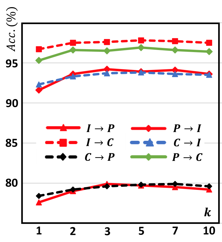
Figure 6: Plot of $k$ against Accuracy (%) on the 6 UDA tasks from ImageCLEF-DA [1].

$k$	I $\to$ P	P $\to$ I	I $\to$ C	C $\to$ I	C $\to$ P	P $\to$ C	Avg
1	77.6	91.6	96.7	92.3	78.4	95.3	88.7
2	79	93.6	97.5	93.3	79.2	96.6	89.9
3	79.9	94.2	97.6	93.7	79.6	96.5	90.3
5	79.7	93.9	97.8	93.8	79.8	96.9	90.3
7	79.5	94.1	97.7	93.6	79.9	96.6	90.2
10	79.2	93.6	97.5	93.5	79.6	96.4	90.0

Table 4: Ablation on the number of DCMs $k$ with accuracy (%) on the 6 UDA tasks from ImageCLEF-DA [1].

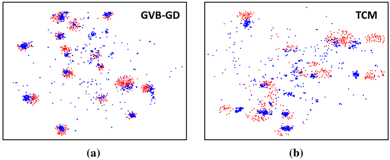
Figure 7: t-SNE [35] plot of features in $S=s$ (red) and in $S=t$ (blue) after training using method: (a) GVB-GD [12], (b) Our TCM. Only samples from the first 15 classes are plotted to avoid clutter.

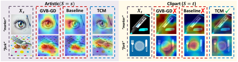
Figure 8: Class Activation Maps (CAMs) [66] of GVB-GD [12], Baseline and TCM on the Artistic$(S=s)\to$Clipart$(S=t)$ task in Office-Home dataset [57]. The left column shows two samples in each domain, whose class name is indicated on the left. In $S=t$, we show two samples predicted wrongly by GVB-GD and Baseline, but correctly with TCM.

Number of DCMs. We performed an ablation on the number of DCMs $k$ with ImageCLEF-DA dataset. The results are shown in Table 4 and plotted in Figure 6. We have three observations: 1) Among each step of $k$, the largest difference occurs between $k=1$ and $k=2$. This means that accounting for 2 disentangled factors can explain much of the domain shift due to $P(U|S=s)\to P(U|S=t)$ in ImageCLEF-DA. 2) Across all tasks, the best performance is usually achieved with $k=5$. This supports the effectiveness of stratifying $U$ according to a small number of disentangled attributes. 3) A large $U$ (e.g., 10) leads to a slight performance drop. In practice, we observed that when $k$ is large, a few DCMs seldom win any sample from Eq. (2), and hence are poorly trained. This can impact their image generation quality, leading to reduced performance. We argue that this is because the chosen $k$ is larger than the number of factors that can be disentangled from the dataset. For example, if there exist $k^{\prime}<k$ factors $(U_{1},\ldots,U_{k}^{\prime})$, once $k^{\prime}$ DCMs establish correspondence with them, the rest $(k-k^{\prime})$ DCMs will never win any sample, as they can never generate images that are more counterfactual faithful compared with intervention on each $U_{i}$ (see Counterfactual Faithfulness theorem in Appendix).

t-SNE Plot. In Figure 7, we show the t-SNE [35] plots of the features in $S=s$ and $S=t$ in Office-Home A$\to$C task after training, for both the current SOTA GVB-GD [12] and our TCM. GVB-GD is based on invariant-feature-learning and focuses on making $X_{s}$ and $X_{t}$ alike, while our TCM does not explicitly align them. We indeed observe a better alignment between the features in $S=s$ and $S=t$ in GVB-GD. However, as shown in Table 1, our method outperforms GVB-GD on A$\to$C. This shows that the current common view on the solution to UDA based on [2], i.e., making domains alike while minimizing source risk, does not necessarily lead to the best performance. In fact, this is in line with the conclusion from recent theoretical works [65]. Our approach is orthogonal to existing approaches and we demonstrate the practicality of a more principled solution to UDA, i.e., establishing appropriate causal assumption on the domain shift and solving the corresponding transport formula (e.g., Eq. (1)).

Alleviating Semantic Loss. We use Figure 8 to reveal the semantic loss problem on existing methods, and how our method can alleviate it. The figure shows the CAM [66] responses on images in $S=s$ and $S=t$ from the $A\to C$ task in Office-Home dataset. We compared with two lines of existing approaches: invariant-feature-learning method (GVB-GD [12]) and domain-mapping method (our Baseline), and we generated CAM for each of them as shown in the red dotted box. For our TCM, the prediction is a linear combination of the effects from the two images: $X$ and the DCMs outputs $\hat{X}$ (see Eq. (7)). As the locations of objects tend to remain the same in $\hat{X}$ as in $X$ (see Figure 4), we visualize the overall CAM of our TCM in the blue box by combining the CAM from $X$ and $\hat{X}$ weighted by their contributions towards softmax prediction probability. On the left, we show the CAMs in $S=s$. By looking at the CAM of GVB-GD and the Baseline, we observe that they focus on the contextual object semantics (e.g., food that commonly appears together with “fork”) to distinguish “marker” and “fork”, where the effect from the object shape is mostly lost. In contrast, our TCM focuses on the marker and fork, i.e., the shape semantic is preserved in training. On the right in $S=t$, the contextual object semantic is no longer discriminative for the two classes. Hence GVB-GD and Baseline either focus on the wrong semantic (e.g., plate) or become confused (focusing on a large area), leading to the wrong prediction. Thanks to the preserved shape semantic, our TCM focuses on the object and makes the correct prediction. This provides an intuitive explanation of how our TCM alleviates the semantic loss (more examples in Appendix).

5 Conclusion

We presented a practical implementation of the transportability theory for UDA called Transporting Causal Mechanisms (TCM). It systematically eliminates the semantic loss from the confounding effect. In particular, we proposed to identify the confounder stratification by discovering disentangled causal mechanisms and represent the unknown confounder representation by proxy variables. Extensive results on UDA benchmarks showed that TCM is empirically effective. It is worth highlighting that TCM is orthogonal to the existing UDA solutions—instead of making the two domains similar, we aim to find how to transport and what can be transported with a causality theoretic viewpoint of the domain shift. We believe that the key bottleneck of TCM is the quality of causal mechanism disentanglement. Therefore, we will seek more effective unsupervised feature disentanglement methods and investigate their causal mechanisms.

6 Acknowledgements

The authors would like to thank all reviewers and ACs for their constructive suggestions, and specially thank Alibaba City Brain Group for the donations of GPUs. This research is partly supported by the Alibaba-NTU Singapore Joint Research Institute, Nanyang Technological University (NTU), Singapore; A*STAR under its AME YIRG Grant (Project No. A20E6c0101); and the Singapore Ministry of Education (MOE) Academic Research Fund (AcRF) Tier 2 grant.

Appendix

This appendix is organized as follows:

• For preliminaries on structural causal model and do-calculus, we refer readers to Section 2 of [41].

• Section A.1 gives the proofs and derivations for Section 3, where we first prove the Counterfactual Faithfulness theorem in Section A.1.1, and then prove the sufficient condition used to establish the correspondence between DCMs and disentangled generative causal factors in Section A.1.2.

• Section A.2 the proofs and derivations for Section 4, where we prove the Proxy Function theorem and its corollary in Section A.2.1, and then derive Eq. (7) in Section A.2.2.

• Section A.3 provides implementation details. Specifically, in Section A.3.1, we provide the network architecture of DCMs, the implementation of CycleGAN loss $\mathcal{L}_{CycleGAN}^{i}$ and DCM training details. In Section A.3.2, we show the network architectures of our backbone, the VAE and discriminators, together with their training details. In Section A.3.3, we attend to some details in the experiment.

• Section A.4 shows additional generated images from our DCMs and additional CAM results.

A.1 Proof and Derivation for Section 3

In this section, we will first derive the Counterfactual Faithfulness theorem. Then we will prove the sufficient condition in Section 3.1.

A.1.1 Counterfactual Faithfulness Theorem

We will first provide a brief introduction to the concept of counterfactual and disentanglement. Causality allows to compute how an outcome would have changed, had some variables taken different values, referred to as a counterfactual. In Section 3.1, we refer to each DCM $(M_{i},M_{i}^{-1})$ in $\{(M_{i},M_{i}^{-1})\}_{i=1}^{k}$ as a counterfactual mapping, where each $M_{i}$ (or $M_{i}^{-1}$) essentially follows the three steps of computing counterfactuals [43] (conceptually): given a sample $X=\mathbf{x}$, 1) In abduction, $(U_{1}=u_{1},\ldots,U_{i}=u_{i},\ldots,U_{k}=u_{k})$ is inferred from $\mathbf{x}$ through $P(U|X)$; 2) In action, the attribute $U_{i}$ is intervened by setting it to $u_{i}^{\prime}$ drawn from $P(U_{i}|S=t)$ (or $P(U_{i}|S=s)$), while the values of other attributes are fixed; 3) In prediction, the modified $(U_{1}=u_{1},\ldots,U_{i}=u_{i}^{\prime},\ldots,U_{k}=u_{k})$ is fed to the generative process $P(X|U)$ to obtain the output of the DCM $M_{i}(\mathbf{x})$ (or $M_{i}^{-1}(\mathbf{x})$). More details regarding counterfactual can be found in [42].

Our definition of disentanglement is based on [19] of group theory. Let $\mathcal{U}$ be a set of (unknown) generative factors, e.g., such as shape and background. There is a set of independent causal mechanisms $\varphi:\mathcal{U}\to\mathcal{X}$, generating images from $\mathcal{U}$. Let $\mathcal{G}$ be the group acting on $\mathcal{U}$, i.e., $g\circ u$ transforms $u\in\mathcal{U}$ using $g\in\mathcal{G}$ (e.g., changing background “cluttered” to “pure”). When there exists a direct product decomposition $\mathcal{G}=\prod_{i=1}^{k}\mathcal{G}_{i}$ and $\mathcal{U}=\prod_{i=1}^{k}\mathcal{U}_{i}$ such that $\mathcal{G}_{i}$ acts on $\mathcal{U}_{i}$, we say that each $\mathcal{U}_{i}$ is the space of a disentangled factor. The causal mechanism $(M_{i},M_{i}^{-1})$ is disentangled when its transformation in $\mathcal{X}$ corresponds to the action of $\mathcal{G}_{i}$ on $\mathcal{U}_{i}$.

We use $\mathcal{U}$ and $\mathcal{X}$ to denote the vector space of $U$ and $X$ respectively. We denote the generative process $P(X|U)$ ($U\to X$) as a function $g:\mathcal{U}\to\mathcal{X}$. Note that we consider the function $g$ as an embedded function [3], i.e., a continuous injective function with continuous inversion, which generally holds for convolution-based networks as shown in [46]. Without loss of generality, we will consider the $S=s\to S=t$ mapping $M_{i}$ for the analysis below, which can be easily extended to $M_{i}^{-1}$. Our definition of disentangled intervention follows the intrinsic disentanglement definition in [3], given by:

Definition (Disentangled Intervention). A counterfactual mapping $M:\mathcal{X}\to\mathcal{X}$ is a disentangled intervention with respect to $U_{i}$, if there exists a transformation $M^{\prime}:\mathcal{U}\to\mathcal{U}$ affecting only $U_{i}$, such that for any $u\in\mathcal{U}$,

$$M(g(u))=g(M^{\prime}(u)).$$ (11)

Then we have the following theorem:

Theorem (Counterfactual Faithfulness Theorem). The counterfactual mapping $M_{i}(X)$ is faithful if and only if $M_{i}$ is a disentangled intervention with respect to $U_{i}$.

Note that by definition, if $M_{i}(X)$ is faithful, $M_{i}(X)\in\mathcal{X}$. To prove the above theorem, one conditional is trivial: if $M_{i}$ is a disentangled intervention, it is by definition an endomorphism of $\mathcal{X}$ so the counterfactual mapping must be faithful. For the second conditional, let us assume a faithful counterfactual mapping $M_{i}(X)$. Given $g$ is embedded, the counterfactual mapping can be decomposed as:

$$M_{i}(X)=g\circ M_{i}^{\prime}\circ g^{-1}(X),$$ (12)

where $\circ$ denotes function composition and $M^{\prime}_{i}:\mathcal{U}\to\mathcal{U}$ affecting only $U_{i}$. Now for any $u\in\mathcal{U}$, the quantity $M_{i}(g(u))$ can be similarly decomposed as:

$$M_{i}(g(u))=g\circ M_{i}^{\prime}\circ g^{-1}\circ g(u)=g\circ M_{i}^{\prime}(u).$$ (13)

Since $M_{i}^{\prime}$ is a transformation in $\mathcal{U}$ that only affects $U_{i}$, we show that faithful counterfactual transformation $M_{i}(X)$ is a disentangled intervention with respect to $U_{i}$, hence completing the proof.

With this theory, faithfulness$=$disentangled intervention. In Section 3.1, we train $M_{i}$ to ensure $M_{i}(\mathbf{x}_{s})\sim P(X_{t})$ (faithfulness) for every sample $\mathbf{x}_{s}$ in $S=s$, hence encouraging $M_{i}$ to be a disentangled intervention. Note that the above analysis can easily generalize to $M_{i}^{-1}$.

A.1.2 Sufficient Condition

We will prove the following sufficient condition: if $(M_{i},M_{i}^{-1})$ intervenes $U_{i}$, the $i$-th mapping function outputs the counterfactual faithful generation, i.e., the smallest $\mathcal{L}_{CycleGAN}^{i}$.

Without loss of generality, we will prove for the $S=s\to S=t$ mapping $M_{i}$, which can be extended to $M_{i}^{-1}$. For a sample $\mathbf{x}_{s}$ in $S=s$, let $g^{-1}(\mathbf{x}_{s})=\mathbf{u}=(u_{1},\ldots,u_{i},\ldots,u_{k})$. We modify $U_{i}$ by changing $u_{i}$ to a value $\hat{u}_{i}$ drawn from $P(U_{i}|S=t)$. Denote the modified attribute as $\hat{\mathbf{u}}=(u_{1},\ldots,\hat{u}_{i},\ldots,u_{k})$. Denote the sample with attribute $\hat{\mathbf{u}}$ as $\hat{\mathbf{x}}$. Given $M_{i}$ intervenes $U_{i}$, $M_{i}(\mathbf{x}_{s})$ corresponds to a counterfactual outcome when $U_{i}$ is set to $\hat{u}_{i}$ through intervention (or $U$ set as $\hat{\mathbf{u}}$). Now as $g^{-1}(\hat{\mathbf{x}})=\hat{\mathbf{u}}$, using the counterfactual consistency rule [40], we have $M_{i}(\mathbf{x}_{s})=\hat{\mathbf{x}}$. As $\hat{\mathbf{x}}$ is faithful with the Counterfactual Faithfulness theorem, we prove that $M_{i}(\mathbf{x}_{s})$, i.e., the output of the $i$-th mapping function, is also faithful,i.e., the smallest $\mathcal{L}_{CycleGAN}^{i}$.

A.2 Proof and Derivation for Section 4

In this section, we will first derive the Proxy Function theorem and the domain-agnostic nature of the proxy function, and then derive Eq. (7) under our chosen function forms in Section 4.

A.2.1 Proxy Function Theorem

We will derive for the general case where $\tilde{X}$ is any continuous proxy. We will assume that the confounder $U$ follows the completeness condition in [36], which accommodates most commonly-used parametric and semi-parametric models such as exponential families.

Given $h_{y}(X,\hat{X})$ solves Eq. (3), we have:

$$\begin{split}&P(Y|Z,X,S)=\int_{-\infty}^{+\infty}h_{y}(X,\hat{X})P(\hat{X}|Z,X,S)d\hat{X}\\ &=\int_{-\infty}^{+\infty}h_{y}(X,\hat{X})\left\{\int_{-\infty}^{+\infty}P(\hat{X}|U)P(U|Z,X,S)dU\right\}d\hat{X}.\end{split}$$ (14)

From the law of total probability, we have:

$$P(Y|Z,X,S)=\int_{-\infty}^{+\infty}P(Y|U,X)P(U|Z,X,S)dU.$$ (15)

With Eq. (14) and Eq. (15) and the completeness condition, we have:

$$P(Y|U,X)=\int_{-\infty}^{+\infty}h_{y}(X,\hat{X})P(\hat{X}|U)d\hat{X},$$ (16)

which proves the Proxy Function theorem.

From Eq. (16), we have:

$$\begin{split}&\int_{-\infty}^{+\infty}h_{y}(X,\hat{X},S=s)P(\hat{X}|U)d\hat{X}\\ &=\int_{-\infty}^{+\infty}h_{y}(X,\hat{X},S=t)P(\hat{X}|U)d\hat{X}.\end{split}$$ (17)

Hence from the completeness condition, we have $h_{y}(X,\hat{X},S=s)=h_{y}(X,\hat{X},S=t)$ [36]. Hence we prove that $h_{y}(X,\hat{X})$ is domain-agnostic.

Note that in Section 4, our proxy $\hat{X}$ is a continuous random variable takes values from $\{M_{i}(\mathbf{x}_{s})\}_{i=1}^{k}$ for sample $\mathbf{x}_{s}$ in $S=s$ or $\{M_{i}^{-1}(\mathbf{x}_{t})\}_{i=1}^{k}$ for sample $\mathbf{x}_{t}$ in $S=t$. This is a special case of the analysis above with the probability mass of $\hat{X}$ centers around the set of its possible values.

A.2.2 Derivation of Eq. (7)

We derive Eq. (7) as a corollary to [36]. The goal is to solve for $h_{y}(X,\hat{X})$ under the function form in Eq. (6) from the formula below:

$$P(Y|Z,X,S=s)=\int_{-\infty}^{\infty}P(\hat{X}|Z,X)h_{y}(X,\hat{X})d\hat{X}.$$ (18)

For simplicity, we define a standard multivariate Gaussian function $\phi(\cdot)$. If $A\sim\mathcal{N}(0,\mathbf{I})$ and $A\in\mathbb{R}^{n}$, we have:

$$P(A)=\phi(A)=\frac{1}{(2\pi)^{n/2}}exp(-\frac{1}{2}A^{T}A).$$ (19)

Our function form for $P(Y|Z,X,S=s)$ is given by $\mathcal{N}(\mathbf{b}_{1}+\mathbf{W}_{1}Z+\mathbf{W}_{2}X,\bm{\Sigma}_{1})$ and for $P(\hat{X}|Z,X,S=s)$ is given by $\mathcal{N}(\mathbf{b}_{2}+\mathbf{W}_{3}Z+\mathbf{W}_{4}X,\bm{\Sigma}_{2})$, where the variance terms are omitted in the main text for brevity, as the final results only depend on the means. Specifically, $\bm{\Sigma}_{2}\in\mathbb{R}^{n\times n}$ is a symmetrical matrix with Eigen-decomposition given by $\bm{\Sigma}_{2}=\bm{\mathcal{U}}\bm{\Lambda}\bm{\mathcal{U}}^{T}$, where $\bm{\mathcal{U}}\in\mathbb{R}^{n\times n}$ is a full-rank matrix containing the eigen-vectors and $\bm{\Lambda}\in\mathbb{R}^{n\times n}$ is a diagonal matrix with eigen-values. We define $\mathbf{B}=\bm{\mathcal{U}}\bm{\Lambda}^{\frac{1}{2}}$, and hence $\bm{\Sigma}_{2}=\mathbf{BB}^{T}$. We can rewrite $P(\hat{X}|Z,X,S=s)$ as:

$$P(\hat{X}|Z,X,S=s)=|\mathbf{BB}^{T}|^{-\frac{1}{2}}\phi(\mathbf{B}^{-1}(\hat{X}-\bm{\hat{\mu}})),$$ (20)

where $\hat{\mu}=\mathbf{b}_{2}+\mathbf{W}_{3}Z+\mathbf{W}_{4}X$. Define $Z^{\prime}=\mathbf{B}^{-1}\bm{\hat{\mu}}$ and $\hat{X}^{\prime}=\mathbf{B}^{-1}\hat{X}$. We define

$$t_{y}(Z^{\prime},X)=P(Y|Z=\mathbf{W}_{3}^{+}(\mathbf{B}Z^{\prime}-\mathbf{W}_{4}X-\mathbf{b}_{1}),X,S=s).$$ (21)

Now we can solve $h_{y}$ from

$$t_{y}(Z^{\prime},X)=\int_{-\infty}^{\infty}\phi(\hat{X}^{\prime}-Z^{\prime})h_{y}(X,\mathbf{B}\hat{X}^{\prime})d\hat{X}^{\prime}.$$ (22)

Specifically, let $h_{1}$ and $h_{2}$ represent the Fourier transform of $\phi$ and $t_{y}$, respectively:

$$\begin{split}h_{1}(\bm{\nu})&=\int_{-\infty}^{\infty}exp(-i\bm{\nu}Z^{\prime})\phi(Z^{\prime})dZ^{\prime}\\ &=\int_{-\infty}^{\infty}exp(-i\bm{\nu}Z)\phi(Z)dZ\end{split}$$ (23)

$$h_{2}(\bm{\nu},X,Y)=\int_{-\infty}^{\infty}exp(-i\bm{\nu}Z^{\prime})t_{y}(Z^{\prime},X)dZ^{\prime},$$ (24)

where $i=(-1)^{\frac{1}{2}}$ is the imaginary unity. Substituting Eq. (22) (23) into Eq. (24), we have:

$$h_{2}(\bm{\nu},X,Y)=h_{1}(\bm{\nu})\int_{-\infty}^{\infty}exp(-i\bm{\nu}\hat{X}^{\prime})h_{y}(X,\mathbf{B}\hat{X}^{\prime})d\hat{X}^{\prime}.$$ (25)

Hence

$$\int_{-\infty}^{\infty}exp(-i\bm{\nu}\hat{X}^{\prime})h_{y}(X,\mathbf{B}\hat{X}^{\prime})d\hat{X}^{\prime}=\frac{h_{2}(\bm{\nu},X,Y)}{h_{1}(\bm{\nu})}.$$ (26)

By Fourier inversion, we have:

$$h_{y}(X,\mathbf{B}\hat{X}^{\prime})=\frac{1}{2\pi}\int_{-\infty}^{\infty}exp(-i\bm{\nu}\hat{X}^{\prime})\frac{h_{2}(\bm{\nu},X,Y)}{h_{1}(\bm{\nu})}d\bm{\nu}$$ (27)

By substituting $\hat{X}=\mathbf{B}\hat{X}^{\prime}$, we have

$$h_{y}(X,\hat{X})=\frac{1}{2\pi}\int_{-\infty}^{\infty}exp(-i\bm{\nu}\mathbf{B}^{-1}\hat{X})\frac{h_{2}(\bm{\nu},X,Y)}{h_{1}(\bm{\nu})}d\bm{\nu}$$ (28)

Solving for Eq. (28) yields:

$$\begin{split}h_{y}(X,\hat{X})&=\mathbf{b}_{1}-\mathbf{W}_{1}\mathbf{W}_{3}^{+}\mathbf{b}_{2}+\mathbf{W}_{1}\mathbf{W}_{3}^{+}\hat{X}\\ &+(\mathbf{W}_{2}-\mathbf{W}_{1}\mathbf{W}_{3}^{+}\mathbf{W}_{4})X,\end{split}$$ (29)

where scaling terms not related with $X,\hat{X}$ are dropped as they do not impact inference. This completes the derivation.

A.3 Implementation Details

In this section, we will first provide a system overview, followed by the implementation details for DCMs in Section 3 and implementation details for backbone, VAE and discriminators in Section 4. Then we will give a more detailed discussion on the experiment design.

A.3.1 Implementation Details for DCMs

System Overview. The two-stage training procedure is depicted in Figure A1. For inference, please refer to Algorithm 2.

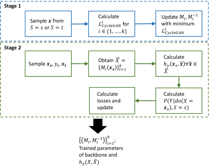
Figure A1: Overview of the two-stage training procedure.

Network Architecture for DCMs. Let Conv2D($n$, $c$) represent 2-d convolutional layer with $n\times n$ as kernel size and $c$ output channels. For Each $M_{i},M_{i}^{-1}$, the network architecture is given by ReflectionPad(3) Conv2D(7,64) InstanceNorm ReLU Conv2D(3,128) InstanceNorm ReLU Conv2D(3,256) InstanceNorm ReLU ResNetBlock$\times$2 ConvTranspose2D(3,128) InstanceNorm ReLU ConvTranspose2D(3,64) InstanceNorm ReLU ReflectionPad(3) Conv2D(7,3) Tanh, where each ResNetBlock is implemented by Conv2D(3,256) ReflectionPad(1) Conv2D(3,256) with skip connection.

Network Architecture for CycleGAN Discriminators. To calculate each $\mathcal{L}_{CycleGAN}^{i}$, two discriminators taking image as input is required for $S=s$ and $S=t$, respectively. We implement each discriminator with Conv2D(4,64) LeakyReLU(0.2) Conv2D(4,128) InstanceNorm LeakyReLU(0.2) Conv2D(4,256) InstanceNorm LeakyReLU(0.2) Conv2D(4,512) InstanceNorm LeakyReLU(0.2) Conv2D(4,1).

CycleGAN Loss. Next, we will detail the implementation of $\mathcal{L}_{CycleGAN}^{i}$, which is given by:

$$\mathcal{L}_{CycleGAN}^{i}=\mathcal{L}_{adv}^{i}+\alpha_{1}\mathcal{L}_{cyc}^{i}+\alpha_{2}\mathcal{L}_{idt}^{i}\,$$ (30)

where $\alpha_{1},\alpha_{2}$ are trade-off parameters. The adversarial loss $\mathcal{L}_{adv}^{i}$ requires the transformed images to look like real images in the opposing domain. For a sample $\mathbf{x}$, $\mathcal{L}_{real}^{i}$ is given by:

$$\mathcal{L}_{adv}^{i}=\begin{cases}\mathrm{log}(1-D^{\prime}_{t}(M_{i}(\mathbf{x}))),&\text{if }\mathbf{x}\text{ from }S=s,\\ \mathrm{log}(1-D^{\prime}_{s}(M_{i}^{-1}(\mathbf{x}))),&\text{otherwise,}\end{cases}$$ (31)

where $D^{\prime}_{s},D^{\prime}_{t}$ are discriminators that return a large value when its input looks like images in $S=s,S=t$, respectively. $\mathcal{L}_{cyc}^{i}$ is the cycle consistency loss [67] given by

$$\mathcal{L}_{cyc}^{i}=\begin{cases}\left\lVert M_{i}^{-1}(M_{i}(\mathbf{x}))-\mathbf{x}\right\rVert,&\text{if }\mathbf{x}\text{ from }S=s,\\ \left\lVert M_{i}(M_{i}^{-1}(\mathbf{x}))-\mathbf{x}\right\rVert,&\text{otherwise,}\end{cases}$$ (32)

where $\left\lVert\cdot\right\rVert$ is implemented using L1 norm. We follow CycleGAN [67] to use an identity loss $\mathcal{L}_{idt}^{i}$ to improve generation quality:

$$\mathcal{L}_{idt}^{i}=\begin{cases}\left\lVert M_{i}^{-1}(\mathbf{x})-\mathbf{x}\right\rVert,&\text{if }\mathbf{x}\text{ from }S=s,\\ \left\lVert M_{i}(\mathbf{x})-\mathbf{x}\right\rVert,&\text{otherwise.}\end{cases}$$ (33)

Discriminator Training. $D^{\prime}_{s},D^{\prime}_{t}$ are trained to maximize the following loss:

$$\mathcal{L}_{d}=\begin{cases}\mathrm{log}D^{\prime}_{s}(\mathbf{x})+\frac{1}{k}\sum_{i=1}^{k}\mathcal{L}^{i}_{adv},&\text{if }\mathbf{x}\text{ from }S=s,\\ \mathrm{log}D^{\prime}_{t}(\mathbf{x})+\frac{1}{k}\sum_{i=1}^{k}\mathcal{L}^{i}_{adv},&\text{otherwise,}\end{cases}$$ (34)

which requires $D^{\prime}_{s},D^{\prime}_{t}$ to recognize real samples and reject fake samples generated by all DCMs.

Training Details. The networks are randomly initialized by sampling from normal distribution with standard deviation of 0.02. We use Adam optimizer [23] with initial learning rate 0.0002, beta1 as 0.5 and beta2 as 0.999. We train the network with the initial learning rate for 100 epochs and decay the learning rate linearly for another 100 epochs on ImageCLEF-DA [1] and OfficeHome [57]. We train the network with the initial learning rate for 20 epochs and decay the learning rate linearly for another 20 epochs on VisDA-2017 [45]. The CycleGAN loss and discriminator loss are updated iteratively. The adopted competitive training scheme to train DCMs can sometimes be sensitive to network initialization. Hence all DCMs are first trained for 8000 iterations, before using the competitive training scheme.

A.3.2 Implementation Details for Section 4

Backbone. We adopt ResNet-50 [18] as our backbone, where the architecture is shown in Figure A2. Specifically, each convolutional layer is described as ($n\times n$ conv, p), where n is the kernel size and p is the number of output channels. Convolutional layers with $/2$ have a stride of 2 and are used to perform down-sampling. The solid curved lines represent skip connection. The batch normalization and ReLU layers are omitted in Figure A2 to highlight the key structure of the backbone. We fine-tuned the pre-trained backbone on ImageNet [48] for our experiments.

VAE. Denote Linear($n$,$m$) as a linear layer with $n$ input channels and $m$ output channels. The encoder $Q_{\theta}$ is implemented with Linear(2048,1200) ReLU Linear(1200,600) ReLU Linear(600,200), where the dimension of $Z$ is 100, the first 100 dimensions of the output are the mean and the last 100 dimensions are the variance. The decoder $P_{\theta}$ is implemented with Linear(100,600) ReLU Linear(600,2048) ReLU.

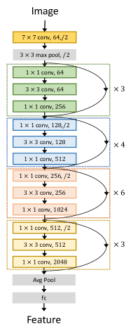
Figure A2: ResNet-50 architecture.

Discriminators. The discriminator $D_{s}$ and $D_{t}$ are implemented with Linear(2048, 1024) ReLU Linear(1024,1024) ReLU Linear(1024,1).

Training Details. The networks are randomly initialized with kaiming initialization with gain as 0.02. We employ mini-batch stochastic gradient descent (SGD) with momentum of 0.9 and nesterov enabled to train our model. We trained the networks for 10000 iterations on VisDA-2017 [45] and OfficeHome [57], and 3000 iterations on ImageCLEF-DA [1]. The linear functions $f_{y},f_{\hat{x}}$, VAE, backbone and discriminators $D_{s},D_{t}$ are updated iteratively.

A.3.3 Discussion on Experiment

Choice of Dataset. While Office-31 [49] is also a popular dataset in UDA, some tasks in the dataset become too trivial, where many UDA algorithms achieve 100% (or almost) accuracy. Moreover, a recent study [47] reveals that the dataset is plagued with wrong labels, ambiguous ground-truth and data leakage, especially in the Amazon domain, which explains the low performance in task DSLR$\to$Amazon and Webcam$\to$Amazon. Hence we followed [64, 31, 62] and performed experiments on ImageCLEF-DA instead, which substitute Office-31 as a small-scale dataset with relatively small domain gap.

Detailed Discussion on t-SNE Plot. Note that the proxy loss in Section 4 aligns the proxy features with the sample features in the counterpart domain, which is different from existing methods that try to align $X_{s}$ and $X_{t}$ directly. Our inference uses the proxy function implemented with Eq. (7), where in training, $X$ takes values of $X_{s}$ and $\hat{X}$ takes values of $M_{i}(X_{s})$, in testing, $X$ takes values of $X_{t}$ and $\hat{X}$ takes values of $M_{i}^{-1}(X_{t})$. While $X_{s}$ and $X_{t}$ (or $M_{i}(X_{s})$ and $M_{i}^{-1}(X_{t})$) are not aligned in TCM, we can still achieve competitive performance by finding how to transport with a causality theoretic viewpoint of the domain shift.

A.4 Additional Results

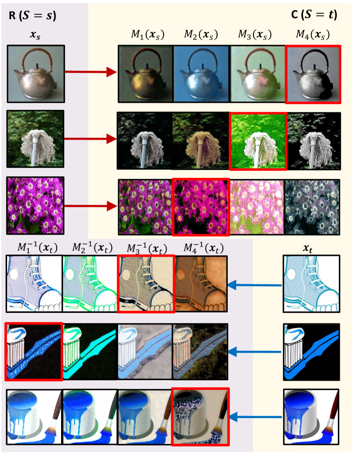
Figure A3: Supplementary to Figure 4.Transformation between “Real World” (R) and “Clipart” (C) domain with 4 trained DCMs $\{(M_{i},M_{i}^{-1})\}_{i=1}^{4}$. The winning DCM is outlined in red.

Additional Visualizations of DCMs Outputs. In Figure A3, we show additional generated images from DCMs in the “Real World” (R)$\to$“Clipart” (C) task of OfficeHome [57], which also has a large domain gap. $\{M_{1},\ldots,M_{4}\}$ (or $\{M_{1}^{-1},\ldots,M_{4}^{-1}\}$) roughly correspond to reducing (increasing) brightness, changing color, increasing (decreasing) saturation and removing (adding) color.

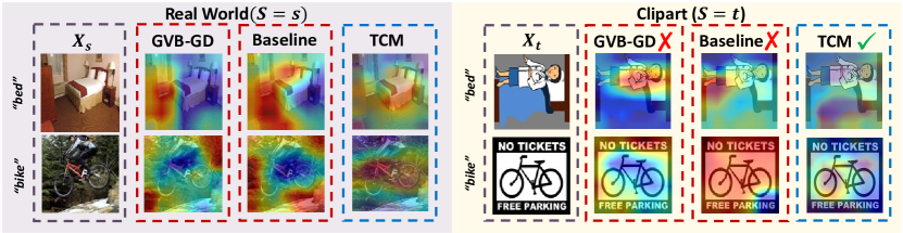
Figure A4: Class Activation Maps (CAMs) [66] of GVB-GD [12], Baseline and TCM on the Real World(S=s)$\to$Clipart$(S=t)$ task in Office-Home dataset [57]. The left column shows two samples in each domain, whose class name is indicated on the top. In $S=t$, we show two samples predicted wrongly by GVB-GD and Baseline, but correctly with TCM. Supplementary to Figure 8

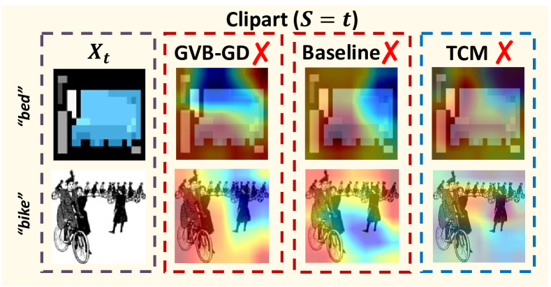
Figure A5: Class Activation Maps (CAMs) [66] of GVB-GD [12], Baseline and TCM on the Real World(S=s)$\to$Clipart$(S=t)$ task in Office-Home dataset [57]. The left column shows two samples in each domain, whose class name is indicated on the left. All methods fail on the two samples. Supplementary to Figure 8.

Additional CAM Responses. In Figure A4, we show the CAM responses in the “Real World”$\to$“Clipart” task, where GVB-GD and baseline focuses on the background to distinguish “bed” and “bike” and the shape semantic is lost, leading to poor generalization in $S=t$. While TCM preserves the foreground object shape semantic. In Figure A5, all three methods fail on the two samples from $S=t$. On the “bed” sample, all methods indeed focus on the object. However, the object itself is not very discriminative, which may explain the failure. On the “bike” sample, the object is small and all methods fail to distinguish it from the context.

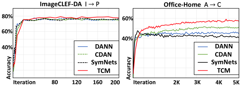
Figure A6: UDA accuracy (%) using DANN, CDAN, SymNets and our TCM, on different training iterations. Batch size is 32.

Method	Backbone GFLOPS	Additional GFLOPS	#Parameters (M)
DANN	133	0.084	1.3
CDAN	133	1.158	18.1
GVB-GD	133	0.092	1.4
Baseline	133	0.072	1.1
TCM	133	0.364	10.1

Table A1: GFLOPS of feature extractor backbone and additional modules (e.g., discriminator networks) as well as #parameters of those additional modules on Office-Home.

Convergence Speed, GFLOPS, #Parameters. The convergence speeds of TCM and related methods are shown in Figure A6. Our TCM (red) converges slightly slower in early iterations (e.g., before 20 on ImageCLEF-DA and 250 on Office-Home) due to the training of VAE in Eq. 9 and the linear layers in Eq. 6. After that, TCM converges to the best performance. The GFLOPS and #Parameters are shown in Table A1. All methods use the same backbone and the backbone fine-tuning takes the major time cost (133), compared with the GFLOPS from additional modules. Regarding the parameters, our TCM has more (but not the most) because of the additional VAE and linear layers.

References

- [1] Imageclef-da. http://imageclef.org/2014/adaptation, 2014.
- [2] Shai Ben-David, John Blitzer, Koby Crammer, Alex Kulesza, Fernando Pereira, and Jennifer Wortman Vaughan. A theory of learning from different domains. Machine learning, 2010.
- [3] M. Besserve, A. Mehrjou, R. Sun, and B. Schölkopf. Counterfactuals uncover the modular structure of deep generative models. In ICLR, 2020.
- [4] Steffen Bickel, Michael Brückner, and Tobias Scheffer. Discriminative learning under covariate shift. Journal of Machine Learning Research, 2009.
- [5] John Blitzer, Mark Dredze, and Fernando Pereira. Biographies, bollywood, boom-boxes and blenders: Domain adaptation for sentiment classification. In Proceedings of the 45th annual meeting of the association of computational linguistics, 2007.
- [6] Konstantinos Bousmalis, George Trigeorgis, Nathan Silberman, Dilip Krishnan, and Dumitru Erhan. Domain separation networks. In NIPS, 2016.
- [7] Tom Brown, Benjamin Mann, Nick Ryder, Melanie Subbiah, Jared D Kaplan, Prafulla Dhariwal, Arvind Neelakantan, Pranav Shyam, Girish Sastry, Amanda Askell, Sandhini Agarwal, Ariel Herbert-Voss, Gretchen Krueger, Tom Henighan, Rewon Child, Aditya Ramesh, Daniel Ziegler, Jeffrey Wu, Clemens Winter, Chris Hesse, Mark Chen, Eric Sigler, Mateusz Litwin, Scott Gray, Benjamin Chess, Jack Clark, Christopher Berner, Sam McCandlish, Alec Radford, Ilya Sutskever, and Dario Amodei. Language models are few-shot learners. In NeurIPS, 2020.
- [8] Ruichu Cai, Zijian Li, Pengfei Wei, Jie Qiao, Kun Zhang, and Zhifeng Hao. Learning disentangled semantic representation for domain adaptation. In IJCAI, 2019.
- [9] Long Chen, Hanwang Zhang, Jun Xiao, Wei Liu, and Shih-Fu Chang. Zero-shot visual recognition using semantics-preserving adversarial embedding networks. In CVPR, 2018.
- [10] Qingchao Chen, Yang Liu, Zhaowen Wang, Ian Wassell, and Kevin Chetty. Re-weighted adversarial adaptation network for unsupervised domain adaptation. In CVPR, 2018.
- [11] Shuhao Cui, Xuan Jin, Shuhui Wang, Yuan He, and Qingming Huang. Heuristic domain adaptation. In NeurIPS, 2020.
- [12] Shuhao Cui, Shuhui Wang, Junbao Zhuo, Chi Su, Qingming Huang, and Qi Tian. Gradually vanishing bridge for adversarial domain adaptation. In CVPR, 2020.
- [13] Lixin Duan, Ivor W Tsang, Dong Xu, and Tat-Seng Chua. Domain adaptation from multiple sources via auxiliary classifiers. In Proceedings of the 26th Annual International Conference on Machine Learning, pages 289–296, 2009.
- [14] Yaroslav Ganin and Victor Lempitsky. Unsupervised domain adaptation by backpropagation. In ICML, 2015.
- [15] Yaroslav Ganin, Evgeniya Ustinova, Hana Ajakan, Pascal Germain, Hugo Larochelle, François Laviolette, Mario Marchand, and Victor Lempitsky. Domain-adversarial training of neural networks. The Journal of Machine Learning Research, 2016.
- [16] Muhammad Ghifary, W Bastiaan Kleijn, Mengjie Zhang, David Balduzzi, and Wen Li. Deep reconstruction-classification networks for unsupervised domain adaptation. In ECCV, 2016.
- [17] Ian Goodfellow, Jean Pouget-Abadie, Mehdi Mirza, Bing Xu, David Warde-Farley, Sherjil Ozair, Aaron Courville, and Yoshua Bengio. Generative adversarial nets. In NeurIPS, 2014.
- [18] Kaiming He, Xiangyu Zhang, Shaoqing Ren, and Jian Sun. Deep residual learning for image recognition. In CVPR, 2016.
- [19] Irina Higgins, David Amos, David Pfau, Sebastien Racaniere, Loic Matthey, Danilo Rezende, and Alexander Lerchner. Towards a definition of disentangled representations. arXiv preprint arXiv:1812.02230, 2018.
- [20] Judy Hoffman, Eric Tzeng, Taesung Park, Jun-Yan Zhu, Phillip Isola, Kate Saenko, Alexei Efros, and Trevor Darrell. Cycada: Cycle-consistent adversarial domain adaptation. In ICML, 2018.
- [21] Guoliang Kang, Lu Jiang, Yi Yang, and Alexander G Hauptmann. Contrastive adaptation network for unsupervised domain adaptation. In CVPR, 2019.
- [22] Diederik Kingma and Max Welling. Auto-encoding variational bayes. In ICLR, 2014.
- [23] Diederik P Kingma and Jimmy Ba. Adam: A method for stochastic optimization. arXiv preprint arXiv:1412.6980, 2014.
- [24] Risi Kondor and Shubhendu Trivedi. On the generalization of equivariance and convolution in neural networks to the action of compact groups. In ICML, pages 2747–2755, 2018.
- [25] Vinod Kumar Kurmi, Shanu Kumar, and Vinay P Namboodiri. Attending to discriminative certainty for domain adaptation. In CVPR, 2019.
- [26] Mengxue Li, Yi-Ming Zhai, You-Wei Luo, Peng-Fei Ge, and Chuan-Xian Ren. Enhanced transport distance for unsupervised domain adaptation. In CVPR, 2020.
- [27] Yunsheng Li, Lu Yuan, and Nuno Vasconcelos. Bidirectional learning for domain adaptation of semantic segmentation. In CVPR, 2019.
- [28] Ziwei Liu, Zhongqi Miao, Xiaohang Zhan, Jiayun Wang, Boqing Gong, and Stella X Yu. Large-scale long-tailed recognition in an open world. In CVPR, 2019.
- [29] Francesco Locatello, Stefan Bauer, Mario Lucic, Gunnar Raetsch, Sylvain Gelly, Bernhard Schölkopf, and Olivier Bachem. Challenging common assumptions in the unsupervised learning of disentangled representations. In ICML, 2019.
- [30] Mingsheng Long, Yue Cao, Jianmin Wang, and Michael Jordan. Learning transferable features with deep adaptation networks. In ICML, 2015.
- [31] Mingsheng Long, ZHANGJIE CAO, Jianmin Wang, and Michael I Jordan. Conditional adversarial domain adaptation. In NeurIPS, 2018.
- [32] Mingsheng Long, Jianmin Wang, Guiguang Ding, Jiaguang Sun, and Philip S Yu. Transfer feature learning with joint distribution adaptation. In ICCV, 2013.
- [33] Mingsheng Long, Jianmin Wang, Guiguang Ding, Jiaguang Sun, and Philip S Yu. Transfer joint matching for unsupervised domain adaptation. In CVPR, 2014.
- [34] Jiajun Lu, Theerasit Issaranon, and David Forsyth. Safetynet: Detecting and rejecting adversarial examples robustly. In ICCV, 2017.
- [35] Laurens van der Maaten and Geoffrey Hinton. Visualizing data using t-sne. Journal of Machine Learning Research, 2008.
- [36] Wang Miao, Zhi Geng, and Eric J Tchetgen Tchetgen. Identifying causal effects with proxy variables of an unmeasured confounder. Biometrika, 2018.
- [37] Zak Murez, Soheil Kolouri, David Kriegman, Ravi Ramamoorthi, and Kyungnam Kim. Image to image translation for domain adaptation. In CVPR, 2018.
- [38] Sinno Jialin Pan, Ivor W Tsang, James T Kwok, and Qiang Yang. Domain adaptation via transfer component analysis. IEEE Transactions on Neural Networks, 2010.
- [39] Giambattista Parascandolo, Niki Kilbertus, Mateo Rojas-Carulla, and Bernhard Schölkopf. Learning independent causal mechanisms. In ICML, 2018.
- [40] Judea Pearl. Causality: Models, Reasoning and Inference. Cambridge University Press, 2nd edition, 2009.
- [41] Judea Pearl and Elias Bareinboim. External validity: From do-calculus to transportability across populations. Statistical Science, 2014.
- [42] J. Pearl, M. Glymour, and N.P. Jewell. Causal Inference in Statistics: A Primer. Wiley, 2016.
- [43] Judea Pearl and Dana Mackenzie. The Book of Why: The New Science of Cause and Effect. 2018.
- [44] Zhongyi Pei, Zhangjie Cao, Mingsheng Long, and Jianmin Wang. Multi-adversarial domain adaptation. In AAAI, 2018.
- [45] Xingchao Peng, Ben Usman, Neela Kaushik, Judy Hoffman, Dequan Wang, and Kate Saenko. Visda: The visual domain adaptation challenge. arXiv preprint arXiv:1710.06924, 2017.
- [46] Michael Puthawala, Konik Kothari, Matti Lassas, Ivan Dokmanić, and Maarten de Hoop. Globally injective relu networks. arXiv preprint arXiv:2006.08464, 2020.
- [47] Tobias Ringwald and Rainer Stiefelhagen. Adaptiope: A modern benchmark for unsupervised domain adaptation. In Proceedings of the IEEE/CVF Winter Conference on Applications of Computer Vision, 2021.
- [48] Olga Russakovsky, Jia Deng, Hao Su, Jonathan Krause, Sanjeev Satheesh, Sean Ma, Zhiheng Huang, Andrej Karpathy, Aditya Khosla, Michael Bernstein, et al. Imagenet large scale visual recognition challenge. International Journal of Computer Vision, 2015.
- [49] Kate Saenko, Brian Kulis, Mario Fritz, and Trevor Darrell. Adapting visual category models to new domains. In ECCV, pages 213–226, 2010.
- [50] Kuniaki Saito, Yoshitaka Ushiku, and Tatsuya Harada. Asymmetric tri-training for unsupervised domain adaptation. In ICML, 2017.
- [51] Kuniaki Saito, Kohei Watanabe, Yoshitaka Ushiku, and Tatsuya Harada. Maximum classifier discrepancy for unsupervised domain adaptation. In CVPR, 2018.
- [52] Swami Sankaranarayanan, Yogesh Balaji, Carlos D Castillo, and Rama Chellappa. Generate to adapt: Aligning domains using generative adversarial networks. In CVPR, 2018.
- [53] Sandeepkumar Satpal and Sunita Sarawagi. Domain adaptation of conditional probability models via feature subsetting. In European Conference on Principles of Data Mining and Knowledge Discovery, 2007.
- [54] Masashi Sugiyama, Matthias Krauledat, and Klaus-Robert Müller. Covariate shift adaptation by importance weighted cross validation. Journal of Machine Learning Research, 2007.
- [55] Raphael Suter, Djordje Miladinovic, Bernhard Schölkopf, and Stefan Bauer. Robustly disentangled causal mechanisms: Validating deep representations for interventional robustness. In ICML, 2019.
- [56] Eric Tzeng, Judy Hoffman, Ning Zhang, Kate Saenko, and Trevor Darrell. Deep domain confusion: Maximizing for domain invariance. arXiv preprint arXiv:1412.3474, 2014.
- [57] Hemanth Venkateswara, Jose Eusebio, Shayok Chakraborty, and Sethuraman Panchanathan. Deep hashing network for unsupervised domain adaptation. In CVPR, 2017.
- [58] Yuan Wu, Diana Inkpen, and Ahmed El-Roby. Dual mixup regularized learning for adversarial domain adaptation. In ECCV, 2020.
- [59] Renjun Xu, Pelen Liu, Liyan Wang, Chao Chen, and Jindong Wang. Reliable weighted optimal transport for unsupervised domain adaptation. In CVPR, 2020.
- [60] Zhongqi Yue, Tan Wang, Hanwang Zhang, Qianru Sun, and Xian-Sheng Hua. Counterfactual zero-shot and open-set visual recognition. In CVPR, 2021.
- [61] Kun Zhang, Bernhard Schölkopf, Krikamol Muandet, and Zhikun Wang. Domain adaptation under target and conditional shift. In ICML, 2013.
- [62] Yabin Zhang, Bin Deng, Kui Jia, and Lei Zhang. Label propagation with augmented anchors: A simple semi-supervised learning baseline for unsupervised domain adaptation. In ECCV, 2020.
- [63] Yuchen Zhang, Tianle Liu, Mingsheng Long, and Michael Jordan. Bridging theory and algorithm for domain adaptation. In ICML, 2019.
- [64] Yabin Zhang, Hui Tang, Kui Jia, and Mingkui Tan. Domain-symmetric networks for adversarial domain adaptation. In CVPR, 2019.
- [65] Han Zhao, Remi Tachet Des Combes, Kun Zhang, and Geoffrey Gordon. On learning invariant representations for domain adaptation. In ICML, 2019.
- [66] Bolei Zhou, Aditya Khosla, Agata Lapedriza, Aude Oliva, and Antonio Torralba. Learning deep features for discriminative localization. In CVPR, 2016.
- [67] Jun-Yan Zhu, Taesung Park, Phillip Isola, and Alexei A Efros. Unpaired image-to-image translation using cycle-consistent adversarial networks. In ICCV, 2017.