Ising-like critical behavior of vortex lattices in an active fluid

Abstract

Turbulent vortex structures emerging in bacterial active fluids can be organized into regular vortex lattices by weak geometrical constraints such as obstacles. Here we show, using a continuum-theoretical approach, that the formation and destruction of these patterns exhibit features of a continuous second-order equilibrium phase transition, including long-range correlations, divergent susceptibility, and critical slowing down. The emerging vorticity field can be mapped onto a two-dimensional (2D) Ising model with antiferromagnetic nearest-neighbor interactions by coarse-graining. The resulting effective temperature is found to be proportional to the strength of the nonlinear advection in the continuum model.

Introduction.

The nature of transitions between qualitatively different collective states of non-equilibrium matter continues to be an open question in many areas of physics and related fields. In classical pattern formation and fluid dynamics, the transition from regular waves and patterns to irregular chaotic or turbulent states has been explored in many different areas ranging from pattern formation in reaction-diffusion and fluid systems to the onset of turbulent flows. In many of these systems the replacement of periodic patterns was found to be linked to instabilities of the regular structures. Prominent examples are different types of waves in extended oscillatory systems [1] or spirals [2, 3] and Turing patterns  [4] in reaction-diffusion systems. For the classical problem of the transition from laminar to turbulent pipe flow this approach cannot be applied, since the laminar flow is stable for arbitrarily large Reynolds numbers. Recent large-scale experimental and numerical studies in pipe flows [5, 6, 7] have instead revealed that the transition bears analogies with a non-equilibrium phase transition in the directed percolation class [8], where the laminar flow corresponds to an absorbing state. Transitions to turbulence in other macroscopic flow systems such as Couette flow [9], channel flow [10] or turbulent liquid crystals [11] are exhibiting similar features. In addition, theoretical studies on other non-equilibrium systems such as coupled chaotic maps have shown that equilibrium-like transitions can occur on larger scales even if the underlying dynamics is deterministic and highly irreversible [12, 13, 14, 15].

Here, we focus on non-equilibrium transitions appearing in active matter, the latter representing a new central field of physics showing intriguing forms of collective motion [16, 17, 18, 19, 20, 21, 22, 23, 24]. In particular, active matter can also display turbulent-like behavior [25]. Remarkably, a recent simulation study [26] of the onset of turbulence in an active nematic has yielded striking analogies to directed percolation. In the present work, we consider, as a key example, the transition between regular vortex patterns [27, 28, 29] and mesoscale turbulence [30, 31] that has been found experimentally in active (bacterial) suspensions such as Bacillus Subtilis and colloidal (e.g., Janus-particle) systems [32]. Mesoscale (or low-Reynolds number) turbulence implies a highly dynamical flow field with spiral-like structures, i.e., vortices, that are characterized by a preferred length scale [33]. Exposing such a suspension to geometrical confinement [34, 35, 36], one may observe regular vortex lattices where both, the vortex centers and their direction of rotation is ordered. A striking example occurs in 2D systems of connected chambers [27, 28, 29] where neighboring vortices exhibit the same (ferromagnetic) or the opposite spinning direction (antiferromagnetic), resembling a non-equilibrium magnetic spin lattice. Intriguingly, however, ordered vortex patterns can also emerge in the presence of small obstacles [37, 38, 39, 35] and even spontaneously [40, 41, 42]. The question then is: How does the vortex pattern arise (or dissolve) from the turbulent state?

In this work we apply a continuum-theoretical approach to investigate an active suspension subject to a square lattice of obstacles with a lattice constant comparable to the intrinsic length scale in the unconfined system. Previous research has shown that such an “external field” can stabilize antiferromagnetic vortex patterns under conditions where the unconstrained system exhibits turbulence [37], with quantitative agreement between continuum theory and experiment [39]. A key parameter is the strength of nonlinear advection, $\lambda$, that crucially depends on the stresses generated by the swimming force and the self-propulsion speed [33, 43], which can be tuned, e.g., by changing the oxygen concentration in experiments [44]. To explore the nature of the transition in the obstacle system, we describe the ordered state as a magnetic spin lattice. We explicitly include the possibility of a disordered (turbulent) state, going beyond earlier work using the spin picture. Because the vortices in our system are spatially “pinned”, the present transition is different from that considered in [40, 41] which focuses on the melting of a spontaneously formed vortex crystal appearing at extreme $\lambda$. Our results provide strong evidence that the non-equilibrium order-disorder transition can be described as a second-order transition with critical exponents consistent with the 2D Ising universality class, and $\lambda$ playing the role of an effective temperature.

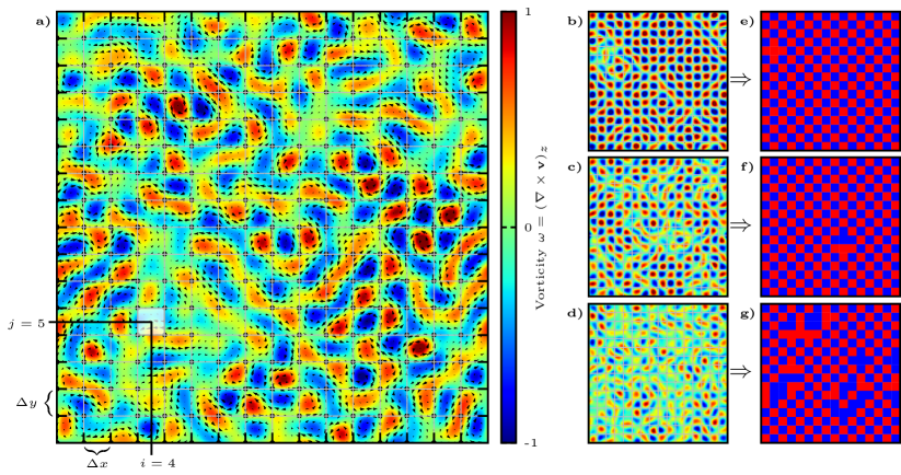
Figure 1: Snapshots of the vorticity field $\omega$ in a system of size $N=16\times 16$ obstacles at a) $\lambda=9.4$ (near the critical point), b) $\lambda=6$, c) $\lambda=8$ and at d) $\lambda=10$. The arrows in a) denote the velocity field $\mathbf{v}$ and the black circles denote the locations of the obstacles. Gray lines indicate the grid used to calculate spin values. The instantaneous spin lattices shown in e), f) and g) (red for positive, blue for negative spins) are obtained from the vorticity fields in b), c) and d).

Model.

We use a well-established minimal model for dense microswimmer suspensions [45, 46, 43, 42, 40], where density fluctuations can be neglected [47, 48, 49] and the dynamics is described on a coarse-grained (order parameter) level via an effective microswimmer velocity field $\mathbf{v}$ [43]. Due to this effective description and the quasi-2D system (where boundaries can act as momentum sinks), momentum is not conserved. We choose this model over different models with momentum conservation or varying density that have been shown to exhibit similar pattern formation [50, 51, 38], because it can be derived from microscopic dynamics [43] and has been shown to capture experiments on bacteria in the absence [30] as well as in the presence of obstacle lattices [39]. The dynamics of $\mathbf{v}$ is given by

$$\displaystyle\partial_{t}\mathbf{v}+\lambda\mathbf{v}\cdot\nabla\mathbf{v}=-\frac{\delta\mathcal{F}}{\delta\mathbf{v}},$$

$$\displaystyle\mathcal{F}=\int d\mathbf{x}\left[q\nabla\cdot\mathbf{v}-\frac{a}{2}|\mathbf{v}|^{2}+\frac{b}{4}|\mathbf{v}|^{4}+\frac{1}{2}\left|(1+\nabla^{2})\mathbf{v}\right|^{2}\right].$$

The dynamics is characterized by the competition between nonlinear advection ($\lambda\mathbf{v}\cdot\nabla\mathbf{v}$) and relaxation governed by the functional $\mathcal{F}$. For sufficiently high activity, $0<a<1$, the minimum of $\mathcal{F}$ is a vortex pattern with square lattice symmetry characterized by two perpendicular modes with characteristic wavelength $\Lambda=2\pi$ (see [42, 40] and Supplemental Material (SM) for details, which includes Refs. [52, 53, 54, 55, 56, 57, 58, 59, 60]). For $\lambda>\lambda^{\star}$, the nonlinear advection term destabilizes this non-fluctuating “ground state” and induces a dynamical state denoted as mesoscale turbulence [30, 45, 33, 43, 61, 40]. Strikingly, recent experiments [37] and numerical calculations [39] have consistently shown that periodic arrangements of small obstacles can stabilize regular patterns for intermediate values of $\lambda\gtrsim\lambda^{\star}$.

Setup.

To investigate the transition to a disordered state, i.e., the breakdown of global order for larger values of $\lambda$, we analyze the dynamics in a 2D periodic system containing $N=n_{x}\times n_{y}$ obstacles of diameter $\ell=0.13\Lambda$ arranged in a square pattern with lattice constant $L=\sqrt{2}\Lambda$, see Fig. 1. This conforms with the “ground state” symmetries and corresponds to the optimal spacing in the sense that it fits to its characteristic scale $\Lambda$ [39]. The results are robust with respect to changes of the setup that preserve the general symmetry, e.g., changing $\ell$ or $L$ or adding defects by removing a few obstacles randomly, see SM. Our study here is confined to the case of square vortex lattices since they have been found to be stable for the case of vanishing nonlinear advection, $\lambda=0$, whereas vortex lattices with different symmetry, e.g., triangular arrangements [39], are unstable already for $\lambda=0$. Hence, the square vortex lattice is the only known example that represents a true minimum of the functional $\mathcal{F}$ and as such may be interpreted as the “ground state” of the system with $\lambda<\lambda^{\star}$. We numerically solve Eq. (Model.) using a pseudo-spectral method and implement the obstacles via a local damping potential for both, velocity $\mathbf{v}$ and vorticity $\omega=(\nabla\times\mathbf{v})_{z}$ (see SM and [39] for more details). We use system sizes of $N=16\times 16$, $N=32\times 32$ and $N=64\times 64$ and set $a=0.5$, $b=1.6$ as in [39]. To characterize the vortex patterns, we divide the system into a quadratic grid with obstacles occupying the nodes and grid cells numbered by their position in $x$- and $y$-direction, i.e., $i=1\dots n_{x}$ and $j=1\dots n_{y}$, respectively. We calculate the mean vorticity $\Omega_{i,j}$ in every grid cell via integration of the vorticity field $\omega(x,y)=\big{[}\nabla\times\mathbf{v}(x,y)\big{]}_{z}$,

$$\Omega_{i,j}=\frac{1}{\Delta x\Delta y}\int_{(i-0.5)\Delta x}^{(i+0.5)\Delta x}\int_{(j-0.5)\Delta y}^{(j+0.5)\Delta y}\omega(x,y)\,dx\,dy\,,$$ (2)

where $\Delta x$ and $\Delta y$ are the dimensions of the cells. Normalization yields a system of discrete spins $S_{i,j}=\Omega_{i,j}/|\Omega_{i,j}|$ with $S_{i,j}=\pm 1$. Using continuous spins $\Omega_{i,j}$ (thus retaining the magnitude of the vorticity) instead of $S_{i,j}$ does not change the nature of the transition, see SM.

Antiferromagnetic order.

In analogy to antiferromagnetic spin models, we divide the system into two sublattices (denoted by ${+}$ and ${-}$) and calculate averages for these sublattices separately. The spatial average of the sublattice spins yields a quantity analogous to a sublattice magnetization per lattice site $m_{\pm}$, i.e,

$$m_{\pm}=\frac{1}{N}\sum_{i=1}^{n_{x}}\sum_{j=1}^{n_{y}}\left(1\pm(-1)^{(i+j)}\right)S_{i,j}\,.$$ (3)

The degree of antiferromagnetic order is measured by the order parameter $\Phi=|\langle m_{+}\rangle-\langle m_{-}\rangle|/2$, where $\langle\dots\rangle$ denotes the temporal average. In Fig. 2a), $\Phi$ is plotted as a function of nonlinear advection strength $\lambda$. The data indicate a continuous transition from antiferromagnetic order ($\Phi=1$) at lower values of $\lambda$ to disorder ($\Phi\approx 0$) upon increase of $\lambda$, see also Figs. 1b) - d). The overall behavior is reminiscent of a second-order phase transition. To locate the critical point occurring at some critical value $\lambda_{\mathrm{c}}$, we calculate the Binder cumulants, defined via $U_{\pm}=1-\langle m_{\pm}^{4}\rangle/(3\langle m_{\pm}^{2}\rangle^{2})$ for the two sublattices, respectively [62]. Fig. 2b) shows the average over the sublattices, $U=(U_{+}+U_{-})/2$, as a function of $\lambda$ for lattices of different size $N$. At the critical point, the Binder cumulant related to an equilibrium system is known to become independent of $N$, i.e., the curves intersect [62]. The clear intersection point visible in Fig. 2b) implies that we can utilize this method in the present case as well, yielding $\lambda_{\mathrm{c}}\approx 9.4$. Moreover, when plotting $\Phi$ as a function of the distance to the critical point $|\lambda-\lambda_{\mathrm{c}}|$, see Fig. 2c), we observe power-law behavior, i.e., $\Phi\propto|\lambda-\lambda_{\mathrm{c}}|^{\beta}$, with an exponent $\beta=1/8$. This conforms with Onsager’s exact solution for the magnetization of the 2D Ising model with nearest-neighbor interactions [63],

$$\langle m\rangle=\left\{1-\sinh^{-4}\left[2J(k_{\mathrm{B}}T)^{-1}\right]\right\}^{\frac{1}{8}}\,,$$ (4)

with $(k_{\mathrm{B}}T)^{-1}$ and $J$ representing the inverse thermal energy and interaction strength, respectively. Due to the bi-partite nature of the square lattice, ferro- or antiferromagnetic interactions lead to the same general behavior (in the absence of an external field); $\langle m\rangle$ thus corresponds to our antiferromagnetic order parameter $\Phi$.

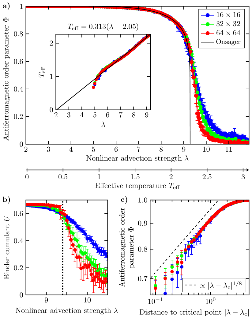
Figure 2: a) Antiferromagnetic order parameter $\Phi$ as a function of $\lambda$ for different $N$. Solid black line: Onsager’s analytical solution as a function of effective temperature $T_{\mathrm{eff}}(\lambda)$ (shown as second x-axis). Inset: $T_{\mathrm{eff}}(\lambda)$. b) Binder cumulant $U$ as a function of $\lambda$. The intersection point of the curves for different $N$ marks the critical point $\lambda_{\mathrm{c}}\approx 9.4$, here denoted by the dotted line. c) $\Phi$ as a function of $|\lambda-\lambda_{\mathrm{c}}|$. Power-law behavior with exponent $\beta=1/8$ is shown as a dashed line. The error bars represent the standard error.

Correlation function.

To further characterize the second-order transition apparent from the order parameter, we consider the 2D spatial correlation function

$$C(n,m)=\frac{2}{N}\left\langle\sum_{i}^{n_{x}}\sum_{j}^{n_{y}}S_{i,j}S_{i+n,j+m}\right\rangle\,,$$ (5)

where $n$ and $m$ are integer steps. In an antiferromagnetic lattice, the full 2D correlation corresponds to a chessboard pattern, see SM. For our purposes, it is sufficient to look at the diagonal ($n=m$) correlation function $C_{\mathrm{diag}}(r)$, which is only a function of distance, $r=\sqrt{n^{2}+m^{2}}$. In Fig 3, $C_{\mathrm{diag}}(r)$ is plotted in a log-log scale at different values of $\lambda$ for the largest system size of $64\times 64$ vortices. The correlation function decays exponentially to zero for $\lambda>\lambda_{\mathrm{c}}$, whereas for $\lambda<\lambda_{\mathrm{c}}$, it reaches a finite value $C_{0}=\langle m_{\pm}\rangle^{2}$. We fit the correlation function via $C_{\mathrm{diag}}(r)-C_{0}=A_{C}\,r^{2-d-\eta}\,e^{-r/\xi}$ [64, 65], where $\xi$ is the correlation length, $A_{C}$ is an additional fitting parameter and $d=2$ the dimension of the system. At $\lambda_{\mathrm{c}}\approx 9.4$, we observe power-law behavior with an exponent $\eta\approx 1/4$, which is shown as a solid line in Fig 3. The correlation length $\xi$ is shown as an inset, indicating divergent behavior. The statistics of $\xi$ does not allow to extract reliably a critical exponent; this would require an extensive finite-size scaling analysis which is outside the scope of the present study. Still, the overall behavior of $C_{\mathrm{diag}}(r)$, particularly the exponent $\eta=1/4$, is reminiscent of a second-order transition in the universality class of the 2D Ising model with nearest-neighbor interactions [64]. This picture is further supported by data of the susceptibility below $\lambda_{\mathrm{c}}$ (see SM), showing power-law behavior with exponent $\gamma=7/4$. Further, as expected close to a second-order transition, we observe critical slowing down, i.e., a profound increase of the extent of temporal correlations of $\Phi(t)$ upon approaching $\lambda_{\mathrm{c}}$ (see SM).

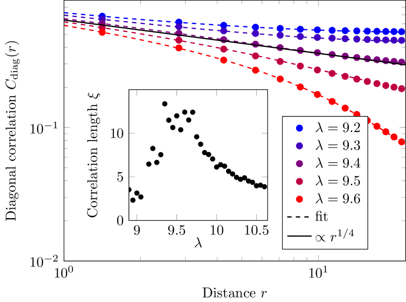
Figure 3: Diagonal correlation function $C_{\mathrm{diag}}(r)$ for different $\lambda$. Below and above $\lambda_{\mathrm{c}}\approx 9.4$, $C_{\mathrm{diag}}(r)$ decays exponentially to zero or $C_{0}=\langle m_{\pm}\rangle^{2}$, respectively. At $\lambda_{\mathrm{c}}$, we observe power-law behavior with an exponent $\eta\approx 1/4$ (slope shown as solid black line). Inset: correlation length $\xi$ as a function of $\lambda$.

Effective temperature.

Given the ”Ising-like” behavior of the order parameter (and the other quantities studied here) as functions of the strength of nonlinear advection, $\lambda$, it is an intriguing question whether we can relate $\lambda$ to an effective temperature $T_{\mathrm{eff}}$ of our non-equilibrium system. As a starting point, we set $T_{\mathrm{eff}}$ equal to $k_{\mathrm{B}}T/J$ entering Eq. (4), solve this equation with respect to $T_{\mathrm{eff}}$ and take the numerical result for $\Phi(\lambda)$ (see Fig. 2) to calculate $T_{\mathrm{eff}}$ as a function of $\lambda$. Clearly, this can only be done in the range $\Phi\neq 0$, i.e., $\lambda<\lambda_{\mathrm{c}}$. The result is shown in the inset of Fig. 2a). Remarkably, in the range of $\lambda$-values where spin fluctuations occur ($\lambda>5$), we find a linear dependence between $T_{\mathrm{eff}}$ and $\lambda$, specifically $T_{\mathrm{eff}}(\lambda)\approx 0.313(\lambda-2.05)$, suggesting that we can indeed consider $\lambda$ as an effective temperature (up to some shift). This correspondence is shown in Fig. 2a) by the second x-axis. Note that the deviation from Onsager’s analytical solution above the critical temperature is expected due to the finite system size. From the relation $T_{\mathrm{eff}}(\lambda)$, it follows that absolute zero, i.e., $T_{\mathrm{eff}}=0$, corresponds to $\lambda^{\star}=2.05$. Remarkably, this value coincides with $\lambda^{\star}\approx 2$, above which the square lattice “ground state” in the unconstrained system becomes unstable to the formation of a dynamic, mesoscale-turbulent state. A further intriguing consequence of the linearity $T_{\mathrm{eff}}\propto\lambda$ appears when we relate $\lambda$ to microscopic parameters (see SM), particular the self-swimming speed $v_{0}$ that is experimentally tunable [44]. In fact, we find $T_{\mathrm{eff}}\propto\lambda\propto v_{0}$, in contrast to studies of spherical active particles where $T_{\mathrm{eff}}\propto D\propto v_{0}^{2}$ [66, 17] (with $D$ being the diffusion constant). We further note that the existence of a linear relation $T_{\mathrm{eff}}(\lambda)$ is robust against details of the setup, which only lead to changes of the quantitative mapping $\lambda\rightarrow T_{\mathrm{eff}}$. The scenarios tested include varying obstacle size $\ell$ and lattice constant $L$ as well as introducing a small amount of disorder into the system by randomly removing a few obstacles, see SM. For example, changing $\ell=0.13\Lambda$ to $\ell=0.11\Lambda$ yields $T_{\mathrm{eff}}(\lambda)\approx 0.46(\lambda-2.08)$.

Conclusions

While antiferromagnetic vortex structures in active fluids are now well established [27, 28, 29, 39], the present study substantially broadens the picture: By considering the strength of nonlinear advection, $\lambda$, as a tunable parameter, we found that the vortex lattice transforms via a second-order phase transition with Ising-like characteristics into a disordered state, namely, mesoscale turbulence. At the critical point, the range of spin-spin correlations (i.e.. correlations between vortex rotation) diverges, indicating pattern formation on much larger scales. Our analysis moreover reveals the presence of an effective temperature directly proportional to $\lambda$, quite different from earlier studies of non-equilibrium systems, where effective temperatures have been defined [67, 68, 69, 70, 71]. From a more general perspective, our study complements recent attempts to relate complex non-equilibrium transitions to (standard) models from statistical physics, other prominent examples being the onset of turbulence in inertial fluids [9] and active nematics [26] viewed as directed percolation. We note that, apart from a different geometry, here we also focused on a different order parameter. Clearly, further work is necessary to elucidate such connections and their practical relevance for the engineering of active and biological fluids.