ReCo1: A Fault resilient technique of Correlation Sensitive Stochastic Designs

Abstract

In stochastic circuits, major sources of error are correlation errors, soft errors and random fluctuation errors that affect the accuracy and reliability of the circuit. The soft error has the effect of changing the correlation status and in turn changes the probability of numbers leading to the erroneous output. This has serious impact on security and medical systems where highly accurate systems are required. We tackle this problem by introducing the fault-tolerant technique of correlation-sensitive stochastic logic circuits. We develop a framework of Remodelling Correlation (ReCo) for Stochastic Logic Elements; AND, XOR and OR for reliable operation. We present two variants of ReCo models in combinational circuits with contradictory requirements by stating two interesting case studies. The proposed technique selects logic elements and places correction blocks based on a priority-based rule that helps to converge to the desired MSE quickly requiring less hardware area. It is shown that this technique does not alter the reliability of the overall circuit. To demonstrate the practical effectiveness of the proposed framework, contrast stretch operation on a standard image in a noisy environment is studied. A high structural similarity index measure of $92.80$ is observed for the output image with the proposed approach compared to the image (with error) $66.43$.

Keywords Stochastic Logic Circuits, Soft errors, Reliability, Remodelling Correlation (ReCo) Framework, Priority-based approach.

1 Introduction

Computation on binary numbers using Stochastic computing [1] is gaining popularity nowadays because it offers several advantages [2] compared to conventional weighted-binary computation. It is a low power and low cost alternative to complex arithmetic functions. With a remarkable reduction in size, circuit complexity and power consumption, stochastic architecture has proved to be noise immune compared to the conventional implementation of binarization algorithms [3] and various other image processing tasks also [4]. Though different types of errors such as soft errors, correlation induced errors and random fluctuation errors are identified that affect the accuracy and reliability of stochastic circuits [5]. Thus to generate the desired function using unreliable components in presence of these errors has become a challenging task.

There are several analytical approaches to assess the reliability of probabilistic circuits with unpredictable behaviours; Probabilistic Gate Models (PGM), Probabilistic Transfer Matrices (PTM), Stochastic computational Model (SCM), Monte Carlo Simulation[6] etc. During analysis we have extensively used PTM throughout the paper. Using PTM, we showed that though the accuracy of an adder using MUX is controlled by select inputs, they must be taken in order with inputs to reduce error. Nevertheless to mention that majority of works are aligned towards reliability assessment and analysis [7, 8].

Transient or soft errors are caused due to exposure to external radiation and are greatly increased by manufacturing defects in a chip. These introduce false logic at the output of the circuit [9]. Thus, if multiple faults strike nodes of a gate, the output may be obtained erroneously. Soft errors are responsible for bit-flips in stochastic bitstream and might induce an undesired correlation between two numbers. This paper emphasizes the inaccurate behaviour of stochastic circuits, contributed mainly due to transient errors under noisy conditions and its methodical correction using correlation in a positive manner. The present study is dedicated to analyzing the behaviour of circuits that are subjected to soft errors. Desired correlations are injected into bitstreams to diminish the effect of transient faults and ensure reliable operation of the circuit. Experiments are conducted on SLEs that are susceptible to changes in correlation. The goal is to create a technology independent framework for complex circuits to observe error-free output using minimum hardware. Studies are also conducted to show that the reliability of a circuit is not affected by correlation alteration between inputs. The contributions in the present work are highlighted as follows:

• We develop a correlation-based framework for correlation sensitive SLEs under transient error scenarios to model the error-free output.

• A priority-based approach in the selection of SLEs is explored to reduce the hardware complexity and improve the accuracy in computation for complex circuits.

• A study on the effect of the proposed framework on reliability of unreliable circuits.

• Evaluation of the proposed work on contrast stretch operations on image under high transient error rates.

In essence, this paper not only contradicts the popular perception with regard to correlation, but firmly establishes that injecting controlled degree of correlation can improve error-resilient behaviour of the circuit. The rest of the paper is organized as follows: In section II, we have analyzed the erroneous behaviour of the multiplexer circuit in the light of PTM. Section III discusses the two major sources of error in stochastic circuits and introduces the proposed methodology in the noisy environment for correlation-sensitive SLEs. With several initial correlation assumptions, we can establish an operating point of the circuit with a suitably injected correlation that could generate an accurate result under the stated conditions. In Section IV, we extended the idea to simulate complex SLCs to show the effectiveness of the proposed model. Two approaches based on a priority-search model are demonstrated following two distinct conditions. Applicability of the proposed methodology in the context of an image processing task is discussed in Section V. In Section VI, highlights of the experimental results are jotted down with the pros and cons of the proposed algorithms.

2 USING PTM FOR ANALYSING STOCHASTIC CIRCUITS

The PTM, which is used in analysing probabilistic logic circuits[10] has proved to be a convenient tool in error[11] and reliability analysis [12] of small stochastic circuits. It can be observed as a conditional probability matrix $M$, so that, $M(i,j)=p(output=j|input=i)$, where $p$ represents the conditional probability of a particular output being true given a certain input combination. For large circuits computation with PTM is tedious. For a circuit with $k$ inputs and $l$ outputs, a circuit PTM is of size $2^{k}\times 2^{l}$. In Ideal Transfer Matrix (ITM), when the gate is assumed to be error free, elements are either 0 or 1, representing exact binary values in place of probabilities. PTM and ITM for a two input AND gate are represented as matrices $J$ and $M$.

$$J=\begin{bmatrix}1&0\\ 1&0\\ 1&0\\ 0&1\end{bmatrix}\hskip 14.22636ptM=\begin{bmatrix}1-p_{e}&p_{e}\\ 1-p_{e}&p_{e}\\ 1-p_{e}&p_{e}\\ p_{e}&1-p_{e}\end{bmatrix}$$

The rows in $J$ and $M$ correspond to input combinations $00,01,10$,$11$. Columns correspond to outputs $0,1$. The PTM for large circuits is computed using two basic operations [10]:

• The overall PTM of two or more gates with PTMs $M_{1},M_{2},...,M_{p}$ connected in series, is obtained by multiplication of individual PTM; $M_{series}=M_{1}.M_{2}...M_{p}$.

• The resultant PTM of gates with PTMs $M_{1},M_{2},...,M_{p}$ connected in parallel is obtained by the Kronecker product of individual PTM; $M_{parallel}=M_{1}\otimes M_{2}\otimes M_{3}...M_{p}$.

PTM can be defined for a single gate as well as for the whole circuit, e.g., the accurate condition for addition and subtraction using MUX can be demonstrated using PTM analysis.

a) Deriving condition for accurate Stochastic Addition: It is reported that the multiplexer performs the addition operation irrespective of the correlation between input bitstreams $A$ and $B$ with the probability of select line being $p_{s}=0.5$ [13]. But the combinations of input bitstreams limit the accuracy. We show that by using PTM analysis of MUX.

Consider a $2:1$ MUX whose output is given as $z=\bar{s}\cdot a+s\cdot b$. PTM is described as a matrix of size $2\times 8$ by considering select line $s$ in MSB and input $b$ in LSB.

$$V_{MUX}=\begin{bmatrix}1&1&0&0&1&0&1&0\\ 0&0&1&1&0&1&0&1\\ \end{bmatrix}^{\intercal}$$

Input matrix A given to the multiplexer is represented as

$$A=\begin{bmatrix}i_{000}&i_{001}&i_{010}&i_{011}&i_{100}&i_{101}&i_{110}&i_{111}\\ \end{bmatrix}$$

The output $Y$ using circuit PTM is represented as,

$$Y=A\times V_{MUX}$$

Definition 1: Scaled addition in the expression, $Y_{sum}=\dfrac{p_{a}+p_{b}}{2}$ between inputs $A$, $B$ must be associated to select line $S$ of a multiplexer to satisfy the probability expression, $i_{001}+i_{110}=i_{010}+i_{101}$.

Consider three inputs $a$, $b$ and $s$ that are represented as Stochastic Number (SN) $A$,$B$ and $S$ respectively. The output of MUX [1] is,

$$Y_{sum}=\dfrac{p_{a}+p_{b}}{2}$$ (1)

Using truth table representation, the output of MUX is

$$Y=i_{010}+i_{011}+i_{101}+i_{111}$$ (2)

The probabilities of each bitstream $A$,$B$, $S$ is given by the number of 1’s occurring in each bitstream. Thus,

$$\begin{aligned} p_{a}=i_{010}+i_{011}+i_{110}+i_{111}\\ p_{b}=i_{001}+i_{011}+i_{101}+i_{111}\\ p_{s}=i_{100}+i_{101}+i_{110}+i_{111}\end{aligned}\Bigg{\}}$$ (3)

Substituting $p_{a}$ and $p_{b}$ from Eq. 3 into Eq. 1.

$$Y_{sum}=\dfrac{i_{001}+i_{010}}{2}+i_{011}+\dfrac{i_{101}+i_{110}}{2}+i_{111}$$ (4)

Comparing Eq. 4 and Eq. 2 we obtain

$$i_{001}+i_{110}=i_{010}+i_{101};$$ (5)

Eq. 5 dictates the accurate condition of addition that eventuate of an association between two inputs and one select line.

Example 1: SN $A$ with $p_{a}=\frac{3}{8}$ as $10000011$ and $B$ with $p_{b}=\frac{5}{8}$ as $01111100$ are inputs to the MUX with $p_{s}=\frac{4}{8}$ as $01100011$ at select line $S$. The output is $11100000$ ($\frac{3}{8}$), whereas the expected output is $p_{y}=\frac{4}{8}$. This fallacy in output occurs as the probability of selection of input combinations is $(p_{010}+p_{101})=3\neq(p_{110}+p_{001})=5$ violating Eq. 5.

However, keeping the input bitstream same if $p_{s}=\frac{4}{8}$ is changed to $01100110$ the output bit stream becomes $11100010$($\frac{4}{8}$) which satisfies $p_{010}+p_{101}=p_{001}+p_{110}$.

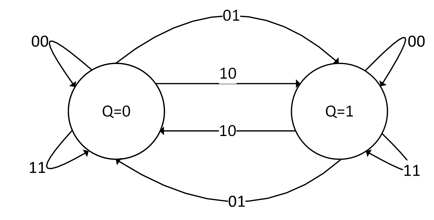
Figure 1: State diagram of adder validating Eq.5.

Thus, there exists a strong dependence of the input bit streams on select line $S$ that must be satisfied to have accurate addition. The state machine (see Fig. 1) satisfying the condition is observed to behave accurately in presence of varying degrees of correlation between SNs. The state variable and the output of the FSM are the same and denoted by Q. It has been reported by Gaines [1] that a T flip-flop gives a constant value of $0.5$ at the output irrespective of the input probability. However, the additional constraint that had to be satisfied is fulfilled by using the XOR gate.

b) Deriving condition for accurate Stochastic Subtraction: A similar approach using the PTM can be adopted to analyze the behaviour of MUX to implement scaled subtraction [14].

Definition 2: Scaled subtraction in the expression, $Y_{sub}$=$\dfrac{p_{a}+1-p_{b}}{2}$ between inputs $A$, $B$ must be associated to select line $S$ of a multiplexer to satisfy the probability expression, $\dfrac{i_{100}+i_{000}}{2}+i_{110}=i_{101}+\dfrac{i_{011}+i_{111}}{2}$.

Consider three inputs $A$, $B$ and $S$. The expression for scaled subtraction is given by $Y_{sub}=\dfrac{p_{a}+(1-p_{b})}{2}$. The probability of finding a ’$0$’ in $p_{b}$ can be given by $(1-p_{b})$, as

$$(1-p_{b})=i_{000}+i_{010}+i_{100}+i_{101}$$ (6)

Substituting $p_{a}$ and $p_{b}$ from Eq. 6 in $Y_{sub}$ we obtain,

$$Y_{sub}=\dfrac{i_{000}+i_{100}}{2}+i_{010}+\dfrac{i_{011}+i_{111}}{2}+i_{110}$$ (7)

Comparing Eq. 7 and Eq. 2 we have,

$$\dfrac{i_{100}+i_{000}}{2}+i_{110}=i_{101}+\dfrac{i_{011}+i_{111}}{2}$$ (8)

which is the condition for accurate subtraction involving MUX. To validate the appropriateness of the condition stated, two examples are cited.

Example $2$: Consider $A$ and $B$ with $p_{a}=\frac{5}{8}$ as $11111000$ and $p_{b}=\frac{4}{8}$ as $10100101$ and the select input $S$ as $00111001$. The output is $01111010$ ($\frac{5}{8}$) which deviates from the expected result i.e., $\frac{9}{16}$. The error is much less in this uncorrelated number. Combinations of $A$, $B$ and $S$ shows that $N_{011}=1$, $N_{010}=1$, $N_{111}=1$, $N_{110}=2$, $N_{001}=1$, $N_{000}=1$ and $N_{101}=1$. Thus the condition given in Definition $2$ is violated.

Now, if we consider correlated numbers the error is increased. Let SN A represented as $11111000$ ($p_{a}=\frac{5}{8}$) and B as $11100000$ ($p_{b}=\frac{3}{8}$) and $S$ as $11110000$, then $Z$ is calculated as $11111111$ ($p_{z}=1$), whereas the expected output was $\frac{5}{8}$. The analysis of the bitstreams with $S$ as MSB and $B$ as LSB shows that $N_{010}=1$, $N_{111}=3$, $N_{110}=1$, and $N_{000}=3$. Placing values in the equation we find $\frac{3}{2}+1\neq 0+\frac{3}{2}$.

Input stochastic signals fed to a combinational circuit can also be represented via PTM. We define an input vector of size $1\times 2^{k}$, where ${}^{\prime}k^{\prime}$ is the total number of input signals which when multiplied by the overall circuit PTM $M_{ckt}$ gives the output PTM. For a combinational circuit with uncorrelated inputs $X$ and $Y$ having probabilities $p_{x}$ and $p_{y}$ and output signal Z having probability $p_{z}$, we can write,

$$I_{in}=\begin{bmatrix}(1-p_{x})&p_{x}\end{bmatrix}\otimes\begin{bmatrix}(1-p_{y})&p_{y}\end{bmatrix}$$

$$Z=\begin{bmatrix}(1-p_{z})&p_{z}\end{bmatrix}=I_{in}.M_{ckt}$$ (9)

$I_{in}$ can also be written as

$$I_{in}=\begin{bmatrix}i_{0}&i_{1}&i_{2}&i_{3}\end{bmatrix}=\begin{bmatrix}n_{00}&n_{01}&n_{10}&n_{11}\end{bmatrix}$$

where $i_{0},i_{1},i_{2},i_{3}$ represents the probability of input bits $xy$ being $00,01,10$ and $11$ respectively. Thus, it can represent a correlation between input signals as well. For two maximally, minimally and uncorrelated inputs, we can write [11]

$$I_{+1}=\begin{bmatrix}(1-p_{x})&0&(p_{x}-p_{y})&p_{y}\end{bmatrix},\,\,p_{x}>p_{y}$$ (10)

$$=\begin{bmatrix}(1-p_{y})&(p_{y}-p_{x})&0&p_{x}\end{bmatrix},\,\,p_{y}>p_{x}$$

$$I_{-1}=\begin{bmatrix}\{1-(p_{x}+p_{y})\}&p_{y}&p_{x}&0\end{bmatrix},\,\,p_{x}+p_{y}\leq 1$$ (11)

$$=\begin{bmatrix}0&(1-p_{x})&(1-p_{y})&((p_{x}+p_{y})-1)\end{bmatrix},\,\,otherwise$$

$$I_{0}=\begin{bmatrix}(1-p_{x})(1-p_{y})&(1-p_{x})p_{y}&p_{x}(1-p_{y})&p_{x}p_{y}\end{bmatrix}$$ (12)

With the help of Eqs. 10-12 we can write the input vector matrix $I_{SCC}$ for any value of SCC.

2.1 Reliability measure for circuits with varying correlation

We are often concerned with the reliability of circuits under noisy conditions. The reliability of a circuit is defined as its ability to produce a correct output on a regular basis. For stochastic circuits, it can be evaluated using the circuit’s ITM(J) and PTM(M). It can be shown that the reliability of the circuit does not change with changes in correlation, rather depends on the probabilistic error in the circuit.

Definition 3: The reliability of a circuit $R_{ckt}$ is invariant to change in correlation between inputs and depends on the probabilistic error rate ’$p_{e}$’.

Circuit reliability[12] is a measure of the similarity between it’s ITM and PTM and is written as:

$$R_{ckt}=\sum_{J(i,j)=1}p(j|i).p(i)$$ (13)

where, $p(j|i)$ is the $(i,j)^{th}$ entry of PTM. Using Eq. 13, reliability of the circuit at $SCC=0$ is obtained as ($1-p_{e}$). For AND gate, $R_{ckt}$ for different ranges of $SCC$ is obtained similarly as:

$$R_{ckt}=\begin{cases}(p_{e}-1)(SCC(1-p_{x}-p_{y}+p_{x}.p_{y})+p_{x}p_{y}-1)+\\ (SCC(p_{x}+p_{y}-1)-p_{x}.p_{y}(SCC+1))(p_{e}-1)\\ =1-p_{e},\hskip 28.45274pt\forall\hskip 5.69054ptSCC<0\vspace{1 mm}\\ (p_{e}-1)(SCC.p_{x}+p_{x}.p_{y}-SCC.p_{x}.p_{y}-1)-\\ (SCC.p_{x}-p_{x}.p_{y}.(SCC-1))(p_{e}-1)\\ =1-p_{e},\hskip 28.45274pt\forall\hskip 5.69054ptSCC>0\end{cases}$$ (14)

Thus from Eq. 14, it is observed that reliability of the circuit is independent of changes in correlation between the input numbers. Thus, error minimization by varying correlation does not affect the reliability of the circuit. This property is helpful in subsequent treatment of SLE to yield a correct output.

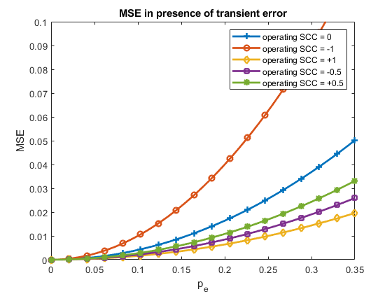
(a)

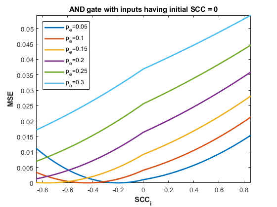
(b)

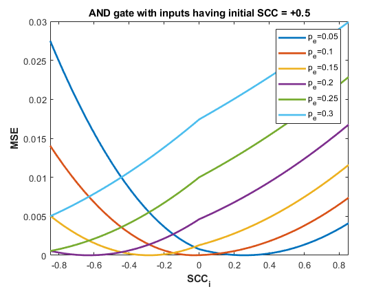
(c)

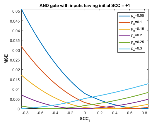
(d)

Figure 2: MSE of AND gate with varying transient errors; Min. MSE with ReCo (b) at $SCC=0$ (c) at $SCC=0.5$ (d) at $SCC=1$.

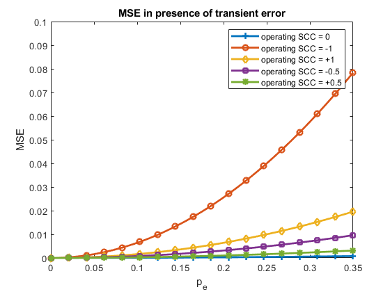
(a)

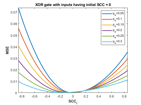
(b)

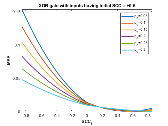
(c)

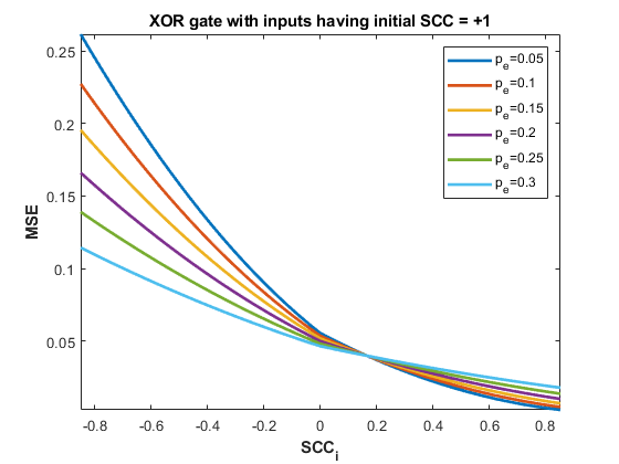
(d)

Figure 3: MSE of XOR gate with varying transient errors; Min. MSE with ReCo (b) at $SCC=0$ (c) at $SCC=0.5$ (d) at $SCC=1$.

3 Handling Errors in Stochastic Circuits using the Proposed technique

3.1 Major Error Sources

3.1.1 Correlation Errors

Correlation between two bitstreams has been identified as a major source of inaccuracy in certain stochastic circuits. Correlation in Stochastic computing indicates that the bitstreams generated by LSFR’s [15] or SNGs [14] inherit some sort of dependence between them (cross correlation) or between the bits of the same bitstream (auto correlation). Earlier, correlation in stochastic circuits could only have been vaguely identified as inaccurate output caused by a pair of bitstream when passed through an AND gate. But, only recently correlation in stochastic computing has been quantified and identified with definiteness [14].

To quantify the correlation between input bitstreams $X$ and $Y$, $SCC$ (Stochastic Correlation Coefficient) which is analogous to the similarity coefficient [16] is represented as

$$SCC(X,Y)=\begin{cases}\frac{p_{X\land Y}-p_{X}\cdot p_{Y}}{min(p_{X},p_{Y})-p_{X}p_{Y}}\text{ , }p_{X\land Y}>p_{X}\cdot p_{Y}\\ \frac{p_{X\land Y}-p_{X}\cdot p_{Y}}{p_{X}p_{Y}-max(p_{X}+p_{Y}-1,0)}\text{ , otherwise }\end{cases}$$

where, $p_{x\land y}$ is obtained by bitwise AND operation between $X$ and $Y$. Other generalized way of representing the SCC is:

$$SCC(X,Y)=\begin{cases}\frac{n_{11}.n_{00}-n_{01}.n_{10}}{n.min(n_{11}+n_{10},n_{11}+n_{01})-(n_{11}+n_{10})(n_{11}+n_{01})}\\ \qquad\qquad\qquad\qquad\text{,}\quad n_{11}.n_{00}>n_{01}.n_{10}\\ \frac{n_{11}.n_{00}-n_{01}.n_{10}}{(n_{11}+n_{10})(n_{11}+n_{01})-n.max(n_{11}-n_{00},0)}\\ \qquad\qquad\qquad\qquad\text{ ,otherwise }\end{cases}$$

where, $n_{11}$, $n_{10}$, $n_{01}$ and $n_{00}$ are respective overlaps of $X$ and $Y$. Thus, the measure of correlation is influenced only by the overlap of similar and dissimilar bits in both the bitstreams. Let, $X=110011110100$, and $Y=010011110100$, then, $SCC=+1$. But, if $X=101100010101$, $Y=111111000101$, $SCC=0.5$. In this case, not every $1$ in Y is influenced by the presence of 1 in that particular position in $X$. There is overlapping of $0^{\prime}s$ in $X$ and $1^{\prime}s$ in $Y$ as well as $1^{\prime}s$ in $X$ and $0^{\prime}s$ in $Y$. Thus, the pair of bitstream is positively correlated to certain degree. Correlation has also been found to impact the circuit’s behaviour in a positive way [17]. XOR gate acts as an absolute subtractor when inputs are positively correlated as shown in Fig. 4. Implementing the same function using binary inputs increased hardware complexity [18].

But for boundary values of probability, either, $0$ or $1$, the measure of SCC becomes indeterminate. To relate to this, consider two SNs $X=00000000$ and $Y=11111111$. Logic operations on these numbers will produce output that will stick to the boundary values itself, either $0$ or $1$ depending on the SLE. Attempts to change the correlation status will result in a change in probability value which is undesired. Using a correlator circuit such as [19] will not be able to alter the degree of correlation between $X$ and $Y$ because only grouping of one kind of bit-pair (here $01$) will be possible and we lose the leverage of pairing other three bit pairs.

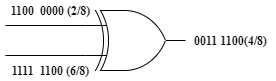
Figure 4: XOR gate as absolute subtractor when inputs are positively correlated.

For any degree of correlation, we can write the output $p_{z}$ as a linear equation[14], given as:

$$p_{z}=(1+\,SCC)F_{0}\,-SCC.F_{-1},\;\;\forall\;SCC<0$$ (15)

$$p_{z}=(1-\,SCC)F_{0}\,+SCC.F_{+1},\;\;\forall\;SCC>0$$ (16)

$F_{0},F_{-1},F{+1}$ are the functions realized by the logic gate with SCC values of 0,-1,+1.

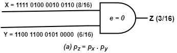
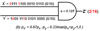
Figure 5: Bit flips at different positions due to transient errors and it’s impact on correlation alteration resulting in different SFs.

3.1.2 Soft Errors

As semiconductor technology advances with reduced feature size and increased scalability, it is becoming more prone to soft errors [9]. The sources of such soft errors have been traced to mainly alpha particles and high energy cosmic rays [20]. Although soft errors are not unique to stochastic circuits, its properties make it more tolerant to soft errors than weighted-binary logic circuits. Soft errors do not affect the circuit physically but it introduces behavioral changes in the circuit in the form of bit flips by introducing false logic[21] [22]. Transient or soft errors are caused due to exposure to external radiation and are greatly increased by manufacturing defects in a chip. These introduce false logic at the output of the circuit [9]. Thus, if multiple faults strike nodes of a gate, the output may be obtained erroneously. Bit flips are modelled as bit flip error $p_{e}$ associated with each gate in the circuit as a Bernoulli variable.

Stochastic numbers are analyzed as Bernoulli random variables (BRV) represented by its probability of success $p_{x}$ to perform similar operations as with other BRVs. Errors in BRV’s are usually analysed using Mean Square Error (MSE) which is written as $E_{z}=E[(p_{ze}-p_{z})^{2}]$, where, $p_{ze}$ and $p_{z}$ represent the estimated and exact value respectively. A lot of applications involving stochastic circuits are carried out in a noisy environment where the circuit is prone to bit-flip errors. For nano-scale devices transient or soft errors are growing prominence as the device features are downscaled to sub-micron ranges. The observed output might exceed the error threshold due to the change in the expected value of signals and also due to unwanted correlation introduced during bit flips. For larger circuits this may be a major concern for accuracy [23].

The presence of soft errors coupled with other inherent error sources may cause models instability in multiple responses. Thus to achieve the desired level of accuracy irrespective of the environment is a dire need in this scenario. Soft errors can change the status of correlation between bitstreams by changing the probability value of the inputs. If equal number of 1s and 0s are flipped on a bitstream on account of transient faults, then the probability value remains unchanged. Fig. 5 shows the effect of transient errors on the behaviour of an AND gate. At zero fault rate, the AND gate implements exact multiplication of two numbers as shown in Fig. 5 (a). This condition is not true for two other cases, when, $p_{e}$ at $0.125$ hit upon the input nodes at different bit positions leading to varied correlation status between two numbers as shown in Fig. 5 (b) and (c).

As we increase the amount of transient errors in the circuit the MSE increases exponentially. In case of inputs operating in the negative range of correlation the error surmounts with the incremental injection of soft error rates as shown in Fig. 2 (a) (red color) when compared to the same bitsreams operating in the positive range of correlation showing reduced MSE with the injection of soft errors (yellow color). These are discussed in detail in the next section, where the motto is to reduce the effect the transient faults on probabilistic circuits by harnessing some of the unique properties of each of these correlation sensitive circuits.

3.2 The proposed Remodelling Correlation (ReCo) Framework

Minimizing errors is crucial since this distorts output logic level of the circuit. We assume that transient faults at the gates caused due to environmental conditions lead to change in the input as well as output probabilities thereby introducing uncertainty in correlation assumption of the circuit. It is observed that bit flips at different positions due to transient errors may lead to different correlation status between the same bitstreams. Undesired correlation can also lead to different stochastic functions being implemented by the same logic circuit as shown in Fig. 5 and impedes the natural function to get implemented. Change in correlation status may also result in the change in probability value if an unequal number of $0^{\prime}s$ and $1^{\prime}s$ are flipped.

Our work suggests Remodelling Correlation (ReCo) technique to cater to the change in the probability assumption at the inputs owing to transient faults. We interpret techniques for correlation-sensitive elements to bring down the MSE to a minimum level. While conducting a study on correlation-sensitive SLEs we demonstrate that every design error can be corrected by introducing correlation to a certain degree at the inputs. We deduce an operating point of the circuit in this incorrect environment with a suitable injection of SCC that reduces MSE to a minimum value. $Algorithm1$ searches for a unique solution of the induced correlation within the range [ -1,1] to find a minimum error for input parameters. We begin our analysis first by considering single SLEs. The flowchart of the proposed method is shown in Fig. 6.

Figure 6: The Flowchart of the Proposed Framework.

3.2.1 ReCo analysis for correlation sensitive elements with zero correlation assumption

. A stochastic circuit implements different real-valued functions when the correlation status between input SNs are altered. We assume the target function to be implemented at $SCC(X,Y)=0$ and any deviation is considered as faulty behaviour of the circuit.

i) AND gate: Consider an AND gate that is inflicted by transient noise. We assume $SCC(X,Y)=0$ , so $p_{z}=p_{x}p_{y}$. As we increase the probability of transient error the observed output deviates more from the original output and there is an exponential increase in MSE, indicated in Fig. 2(a) (blue). So we attempt to reduce the MSE using the proposed method.

We first modify input vectors between $p_{x}$ and $p_{y}$. Assuming $p_{x}$ $<$ $p_{y}$ and $p_{x}$ + $p_{y}$ $\leq$ 1, the modified vectors of $I_{SCC_{m}}$ are,

$$I_{SCC_{m}}=\begin{bmatrix}&1-(p_{x}+p_{y})+p_{x}p_{y}(1+SCC_{i})\\ &-p_{y}(p_{x}+p_{x}SCC_{i}-1)\\ &-p_{x}(p_{y}+p_{y}SCC_{i}-1)\\ &p_{x}p_{y}(SCC_{i}+1)\end{bmatrix}^{\intercal}$$ (17)

For $p_{x}$ + $p_{y}$ $>$ 1,

$$I_{SCC_{m}}=\begin{bmatrix}&-(p_{y}-1)(p_{x}SCC_{i}-p_{x}+1)\\ &p_{y}(SCC_{i}-1)(p_{x}-1)-SCC_{i}(p_{x}-p_{y})\\ &p_{x}(SCC_{i}-1)(p_{y}-1)\\ &p_{x}SCC_{i}-p_{x}p_{y}(SCC_{i}-1)\end{bmatrix}^{\intercal}$$ (18)

1:  Input $p_{x},p_{y},p_{e},input\_Gate$; Output $MSE_{i},SCC_{i}$

2:  $\textit{{ReCo}}(input\_Gate)$

3:  [$p_{x},p_{y}$]= input probabilities of $input\_Gate$;

4:  $p_{e}$= probabilities of transient errors of $input\_Gate$;

5:  $True\_Output=\textbf{{Eval}}(p_{x},p_{y},SCC);$

16:  for $SCC_{i}=-1;SCC_{i}<=+1;SCC_{i}+=0.001$ do

2       $Modified\_Output=\textbf{{Eval}}(p_{x},p_{y},p_{e},SCC_{i});$

3      $MSE_{i}=True\_Output-Modified\_Output$

4      

5      if $MSE_{i}\leq\delta$ then

6             return $MSE_{i}$ , $SCC_{i}$

7       end if

8      

9 end for

7:   return $\operatorname*{\textbf{argmin}}_{MSE_{i}}$ {$MSE_{i}$ , $SCC_{i}$}

Algorithm 1 ReCo analysis for a single gate

For an AND gate with a given error rate $p_{e}$, we write modified output $p_{zm}$ as a function of $I_{SCC_{m}}$.

$$p_{zm}=I_{SCC_{m}}\times\begin{bmatrix}1-p_{e}&p_{e}\\ 1-p_{e}&p_{e}\\ 1-p_{e}&p_{e}\\ p_{e}&1-p_{e}\\ \end{bmatrix}$$ (19)

(a)

(b)

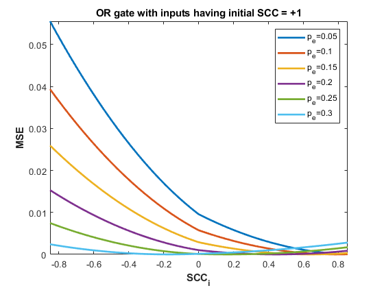
(c)

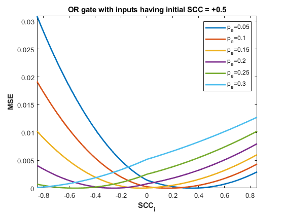
(d)

Figure 7: (a) MSE of OR gate with varying transient errors; Min. MSE with ReCo (b) at $SCC=0$ (c) at $SCC=1$ (d) at $SCC=0.5$.

$p_{zm}$ is observed as $f(SCC_{i})$. We try to make $p_{zm}$ close to $p_{z}$ to reduce the observed error $p_{ze}$. Thus,

$$\begin{multlined}p_{zm}=p_{e}+p_{x}p_{y}(1+SCC_{i})(1-2p_{e})\end{multlined}p_{zm}=p_{e}+p_{x}p_{y}(1+SCC_{i})(1-2p_{e})$$ (20)

The MSE which is $(p_{zm}-p_{z})^{2}$ is calculated as,

$$MSE_{and}=\{p_{e}+p_{x}p_{y}(SCC_{i}-2p_{e}-2p_{e}SCC_{i})\}^{2}$$ (21)

The induced $SCC_{i}$ which reduces MSE to a minimum possible value within the range [-1,+1] is obtained by differentiating Eq. 21 w.r.t $SCC$ and equate it to $0$.

$$\begin{split}2p_{x}p_{y}(1-2p_{e})(p_{e}+p_{x}p_{y}(SCC_{i}-2p_{e}-2p_{e}SCC_{i}))=0\end{split}$$

$$\therefore SCC_{i}=\frac{-(p_{e}-2p_{e}p_{x}p_{y})}{p_{x}p_{y}(1-2p_{e})}$$ (22)

Eq. 22 dictates the condition of reaching a minimum value of MSE for $SCC_{i}$ in the range [-1,0]. Similarly, when $p_{x}+p_{y}>1$ with $p_{x}<p_{y}$, $SCC_{i}$ can be evaluated as,

$$SCC_{i}=\frac{(p_{e}-p_{x}-p_{y}+p_{x}p_{y}-2p_{e}p_{x}p_{y}+1)}{(2p_{e}-1)(p_{x}-1)(p_{y}-1)}$$ (23)

where, $p_{x},p_{y}>0$ and $p_{x}<p_{y}$. Thus, $p_{x}p_{y}>0$. Expressions are derived assuming negative induction of correlation. However, nothing in the derivation prevents $SCC_{i}$ from being positive to achieve minimum MSE.

To exploit the simplicity of equations and to achieve maximum possible accuracy in calculations, parameters appearing in equations are verified graphically. Fig. 2(b) shows different values of induced correlation to obtain zero error at the output. Note that, Eq. 22,23 always hold for $p_{e}<0.5$. Using similar analysis we arrive to different sets of equations for $p_{x}$ $>$ $p_{y}$.

Example $3$: Consider an AND gate with $p_{x}=0.3$ and $p_{y}=0.6$. The error-free output is $p_{z}$ $=0.3\times 0.6=0.18$. The observed output is $p_{ze}=0.28$ at $p_{e}=0.15$. Thus,

$$I_{SCC_{m}}=\begin{bmatrix}&(0.28+0.18SCC_{i})\\ &(0.42-0.18SCC_{i})\\ &(0.12-0.12SCC_{i})\\ &(0.18+0.12SCC_{i})\end{bmatrix}^{\intercal}$$

Thus, $p_{zm}$=$0.18SCC_{i}+0.64p_{e}-0.36p_{e}SCC_{i}+0.18$ and $MSE$ = $\frac{(9SCC_{i}+32p_{e}-18p_{e}SCC_{i})^{2}}{40000}$. Error reduces to $0$ for $SCC_{i}=-0.76$. It is observed that MSE can be reduced to $0$ if $p_{e}\leq 0.2$ (a considerate limit). The results are confirmed graphically considering different values of $p_{x}$ and $p_{y}$ at $p_{e}=0.125$ as shown in Fig. 8(a).

ii) XOR gate: At $SCC=0$, the XOR gate implements $p_{z}=p_{x}(1-p_{y})+p_{y}(1-p_{x})$. Any deviation from the target function on account of transient error is considered as a contribution to MSE. A similar foregoing approach is adopted in the analysis of the XOR gate to operate at minimum MSE under different transient error rates. Now, $p_{zm}$ for $p_{x}<p_{y}$ is written as,

$$p_{zm}=I_{SCC_{m}}\times\begin{bmatrix}1-p_{e}&p_{e}\\ p_{e}&1-p_{e}\\ p_{e}&1-p_{e}\\ 1-p_{e}&p_{e}\\ \end{bmatrix}$$ (24)

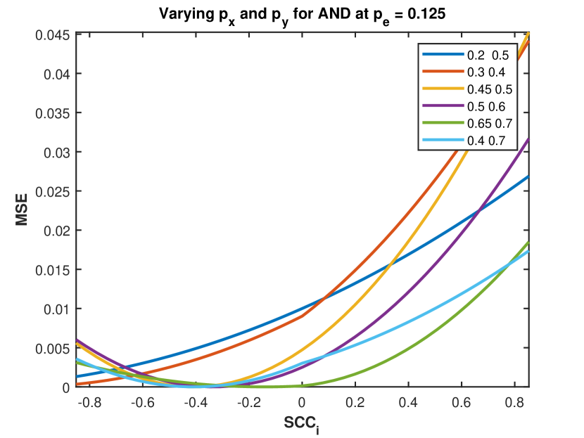
(a)

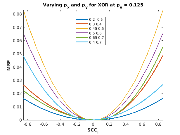
(b)

(c)

Figure 8: MSE after ReCo analysis of correlation sensitive gates for varying input probabilities.

Substituting $I_{SCC_{m}}$ from Eq. 17,

$$\begin{split}p_{zm}=p_{e}-p_{x}p_{y}-2p_{e}(p_{x}+p_{y}-2p_{x}p_{y})-2p_{x}p_{y}SCC_{i}(1-2p_{e})\end{split}$$

$$\begin{split}MSE_{xor}=\{2p_{e}(p_{x}+p_{y})-p_{e}+2p_{x}p_{y}(SCC_{i}-2p_{e}-2p_{e}SCC_{i})\}^{2}\end{split}$$ (25)

We differentiate Eq. 41 w.r.t $SCC_{i}$ and equate it to $0$.

$$\begin{multlined}-2(2p_{x}p_{y}-4p_{e}p_{x}p_{y})(p_{e}-2p_{e}p_{x}-2p_{e}p_{y}-\\ 2p_{x}p_{y}(SCC_{i}+2p_{e}+2p_{e}SCC_{i})=0\end{multlined}-2(2p_{x}p_{y}-4p_{e}p_{x}p_{y})(p_{e}-2p_{e}p_{x}-2p_{e}p_{y}-\\ 2p_{x}p_{y}(SCC_{i}+2p_{e}+2p_{e}SCC_{i})=0$$

$$\therefore SCC_{i}=\frac{p_{e}-2p_{e}(p_{x}+p_{y})+4p_{e}p_{x}p_{y}}{2p_{x}p_{y}-4p_{e}p_{x}p_{y}}$$ (26)

Similarly, for $p_{x}+p_{y}>1$,

$$\begin{multlined}SCC_{i}=\frac{p_{e}-2p_{e}p_{x}-2p_{e}p_{y}+4p_{e}p_{x}p_{y}}{4p_{e}+2(p_{x}+p_{y})(1-2p_{e})-2p_{x}p_{y}(1+2p_{e})-2}\end{multlined}SCC_{i}=\frac{p_{e}-2p_{e}p_{x}-2p_{e}p_{y}+4p_{e}p_{x}p_{y}}{4p_{e}+2(p_{x}+p_{y})(1-2p_{e})-2p_{x}p_{y}(1+2p_{e})-2}$$ (27)

Fig. 3(b) shows different values of $SCC_{i}$ to reach zero MSE at different values of $p_{e}$, which is consistent with Eq. 26.
Example 4: Consider XOR gate with inputs $p_{x}=0.3$ and $p_{y}=0.6$. Thus $p_{z}=0.54$ and $p_{ze}=0.52$ at $p_{e}=0.15$. By substituting $I_{SCC_{m}}$ we find $p_{zm}=0.72p_{e}-0.08p_{e}-0.36SCC_{i}+0.54$ and hence $MSE=\frac{(9SCC_{i}+2p_{e}-18p_{e}SCC_{i})^{2}}{625}$. Thus, $MSE$ reduces to $0$ at $SCC_{i}=0$.

From the experiment (see Fig. 3 (a)) it is inferred that the XOR gate is least responsive to probabilistic errors and hence the smallest contributor to the overall MSE in the circuit. Also, it is evident from Fig. 3 (b) that the XOR gate is most sensitive to changes in correlation. Thus for $0\leq p_{e}\leq 0.3$, the error can be reduced to 0 in contrary to all other gates (see Fig.2(b) and Fig. 7(b)). This is also validated using different values of $p_{x}$ and $p_{y}$ at $p_{e}=0.125$ as shown in Fig. 8(b).

iii) OR gate: For uncorrelated numbers, OR gate implements $p_{z}=p_{x}+p_{y}-p_{x}p_{y}$. In presence of transient error let the function be $p_{ze}$. We eliminate this error by introducing the ReCo block at inputs to inject the desired correlation. The modified output $p_{zm}$ is then calculated using Eq. 17.

$$p_{zm}=I_{SCC_{m}}\times\begin{bmatrix}1-p_{e}&p_{e}\\ p_{e}&1-p_{e}\\ p_{e}&1-p_{e}\\ p_{e}&1-p_{e}\\ \end{bmatrix}$$

$$\begin{split}\therefore p_{zm}=p_{e}+p_{x}+p_{y}-2p_{e}p_{x}-2p_{e}p_{y}-p_{x}p_{y}-\\ p_{x}p_{y}SCC_{i}+2p_{e}p_{x}p_{y}+2p_{e}p_{x}p_{y}SCC_{i}\end{split}$$

$$\begin{split}\therefore MSE_{or}=(p_{e}\{1+p_{x}p_{y}\}-2p_{e}\{p_{x}+p_{y}\}-p_{x}p_{y}SCC_{i}\{1-2p_{e}\})^{2}\end{split}$$ (28)

We differentiate Eq. 28 w.r.t $SCC_{i}$ and equate it to $0$.

$$\begin{split}-2(p_{x}p_{y}-2p_{e}p_{x}p_{y})(p_{e}-2p_{e}p_{x}-2p_{e}p_{y}\\ -p_{x}p_{y}SCC_{i}+2p_{e}p_{x}p_{y}+2p_{e}p_{x}p_{y}SCC_{i})=0\end{split}$$

$$\therefore SCC_{i}=\frac{p_{e}-2p_{e}(p_{x}+p_{y})+2p_{e}p_{x}p_{y}}{p_{x}p_{y}-2p_{e}p_{x}p_{y}}$$ (29)

Similarly for $p_{x}+p_{y}>1$,

$$SCC_{i}=\frac{2p_{e}(p_{y}-p_{x})-p_{e}+p_{x}p_{y}(1-2p_{e})}{p_{x}p_{y}(1-2p_{e})}$$ (30)

Fig. 7(b) shows different values of induced correlation to obtain zero error at the output for different values of $p_{e}$.

Example $5$: Consider an OR gate with inputs $p_{x}=0.3$ and $p_{y}=0.6$ at $p_{e}=0.15$. The error free output $p_{z}=0.72$ and the observed output $p_{ze}=0.654$. Using Eq. 3.2.1 $p_{zm}=0.36p_{e}SCC_{i}-0.44p_{e}-0.18SCC_{i}+0.72$ and $MSE=\frac{(9SCC_{i}+22p_{e}-18p_{e}SCC_{i}-6)^{2}}{2500}$. Thus, MSE can be reduced to zero at $SCC_{i}=-0.5238$.

Thus similar to AND gate, the MSE of the OR gate can be reduced to 0 if the probabilistic error value $p_{e}$ is below a certain limit i.e $0.2$, but the amount of reduction that is achieved is less compared to AND gate.

From the analysis it is observed that the OR gate is least sensitive to changes in correlation, whereas XOR stands highest in the sensitivity list. AND gate is intermediate to them. It is also identified that the XOR gate is least affected by the transient error whereas AND gate is mostly influenced by the presence of transient error. So MSE increases immensely when the error is imposed on an AND gate. These properties of the XOR gate make it a suitable choice for the analysis of an error-resilient circuit design. In the next section, this idea is implemented on complex circuits that focus to minimize MSE using the minimum hardware in the correction circuit using the proposed analysis.

3.2.2 ReCo Analysis for correlation-sensitive logic elements with non-zero correlation assumption

Those SLEs which are sensitive to correlation implement an altogether different stochastic function as in the case of AND gate shown in Fig. 5(b),(c). In this section, we reconsider SLEs with transient errors having an apriori correlation assumption. We invoke ReCo analysis to suppress MSE and formulate the underlying conditions in support of that. Two distinct cases of initial correlation assumption are discussed i.e., $SCC=+0.5$ and $SCC=+1$ and perform a similar analysis to reduce errors at different degrees of transient faults. The target function is obtained considering an initial non-zero and positive value of correlation. It is observed that for an existing negative SCC between input variables the effect of transient errors in the circuit element is enhanced. Thus such cases are excluded in our analysis.

i) AND gate: The analysis begins by setting a non-zero and positive initial correlation between $p_{x}$ and $p_{y}$. The intersection of $p_{e}$ with the previously set positive value of correlation between inputs implicitly assumes that there is a shift in the value of correlation to arrive at the minimum MSE.
a) With existing $SCC(X,Y)=1$: For positively correlated numbers, AND gate implements $p_{z}=min(p_{x},p_{y})$. We counter the effect of transient error on the circuit by introducing a desired $SCC_{i}$ obtained using following derivations.

$$I_{SCC{{}_{m}}(+1)}=\begin{bmatrix}&-(p_{y}-1)(p_{x}SCC_{i}-p_{x}+1)\\ &p_{y}(SCC_{i}-1)(p_{x}-1)-SCC_{i}(p_{x}-p_{y})\\ &p_{x}(SCC_{i}-1)(p_{y}-1)\\ &p_{x}-p_{x}p_{y}SCC_{i}(SCC_{i}-1)\end{bmatrix}^{\intercal}$$ (31)

The modified output $p_{zm}$ is calculated as

$$p_{zm}=I_{SCC_{m(+1)}\times M_{and}=}p_{e}p_{x}-p_{e}(p_{x}+p_{y}-1)+p_{e}p_{y}$$ (32)

For $p_{x}+p_{y}\leq 1$, modified $MSE$ is,

$$\begin{split}MSE_{and}=(p_{e}-p_{x}+p_{x}(1-2p_{e})\{SCC_{i}(1-p_{y})+p_{y}\})^{2}\end{split}$$ (33)

Differentiating Eq. 33 w.r.t $SCC_{i}$ and equate it to $0$,

$$SCC_{i}=\frac{p_{x}-p_{e}-p_{x}p_{y}(1-2p_{e})}{p_{x}(2p_{e}-1)(p_{y}-1)}$$ (34)

$$SCC_{i}=\frac{(p_{x}-p_{e}+2p_{e}p_{x}+p_{x}p_{y})}{p_{x}-2p_{e}p_{x}-p_{x}p_{y}+2p_{e}p_{x}p_{y}},p_{x}+p_{y}>1$$ (35)

b) Any positive intermediate correlation, $SCC(X,Y)=0.5$: Now consider any intermediate positive correlation between the numbers, say $+0.5$. The function implemented by AND logic at $SCC=0.5$ is $p_{z}=0.5p_{x}(1+p_{y})$ for $p_{x}<p_{y}$. In presence of transient error in the circuit, we modify input vectors as $I_{SCC_{m}}$,

$$I_{SCC_{m}(+0.5)}=\begin{bmatrix}&(1-p_{y})(0.5p_{x}SCC_{i}-p_{x}+1)\\ &0.5p_{y}(1-p_{x})-SCC_{i}(0.5p_{x}+0.5p_{y}-p_{x}p_{y})\\ &p_{x}(SCC_{i}-1)(p_{y}-1)\\ &p_{x}.(p_{y}+0.5SCC_{i}-0.5p_{y}SCC_{i})\end{bmatrix}^{\intercal}$$

$$\begin{split}p_{zm}=I_{SCC_{m}(+0.5)}\times M_{and}=0.5SCC_{i}p_{x}(p_{y}-p_{e}+p_{e}p_{y})\\ +SCC_{i}p_{x}(0.5-p_{e}+p_{e}p_{y})+p_{x}p_{y}(1-2p_{e})+p_{e}\end{split}$$ (36)

$$\begin{split}MSE_{and}=p_{e}(1-2p_{x}p_{y})-p_{x}(1-p_{y})\\ (0.5+p_{e}SCC_{i})+0.5p_{x}(1-p_{y})(1-p_{e})SCC_{i}\end{split}$$ (37)

Differentiating Eq. 37 w.r.t $SCC_{i}$ and putting it to $0$, gives

$$SCC_{i}=\frac{0.5p_{x}(1-p_{y})+2p_{e}p_{x}p_{y}-p_{e}}{0.5p_{x}(1-p_{y})(1-3p_{e})}$$ (38)

$$SCC_{i}=\frac{2p_{e}p_{x}-p_{x}-2p_{e}+p_{x}p_{y}+2p_{e}p_{x}p_{y}}{2p_{x}-4p_{e}p_{x}-2p_{x}p_{y}+4p_{e}p_{x}p_{y}},\;p_{x}+p_{y}>1.$$ (39)

Example $6$: Consider $p_{x}=0.3$, $p_{y}=0.6$ and $p_{e}=0.15$. Thus, $p_{z}$ and $p_{ze}$ are $0.3$ and $0.36$. From Eq. 36, $p_{zm}=0.1SCC_{i}+0.64p_{e}-0.24p_{e}SCC_{i}+0.18$. We invoke Eq. 37 to obtain $MSE=1.6\times 10^{-3}(3SCC_{i}+16p_{e}-6p_{e}SCC_{i}-3)^{2}$. Thus, for $p_{e}=0.15$, MSE can be reduced to zero by injecting $SCC_{i}=+0.2857$.

With $SCC=+0.5$ between inputs, $p_{z}$ and $p_{ze}$ are $0.24$ and $0.32$. Using Eq. 37, $p_{zm}=0.1SCC_{i}+0.64p_{e}-0.24p_{e}SCC_{i}+0.18$. Thus, $MSE=\frac{(3SCC_{i}+32p_{e}-9p_{e}SCC_{i}-3)^{2}}{40000}$. Thus unlike the previous case, MSE can be reduced to zero only for $p_{e}<0.15$ by injecting suitable positive $SCC_{i}$.

(ii) XOR gate: We assume a positive definite correlation between inputs of an XOR gate and using similar analysis we derive the condition for minimum MSE.

a) With existing $SCC(X,Y)=1$: With positively correlated inputs, the XOR gate implements $p_{z}=F_{+1}=\lvert p_{x}-p_{y}\rvert$. The deviation under the error scenarios can be encountered by finding a suitable operating point of the circuit by defining $SCC_{i}$ using the following derivations.

We modify the output by introducing the desired correlation $SCC_{i}$ such that,

$$\begin{split}p_{zm}=p_{e}+p_{x}+p_{y}-2SCC_{i}p_{x}-2p_{e}p_{x}-2p_{e}p_{y}-2p_{x}p_{y}\\ +4p_{e}p_{x}SCC_{i}+2p_{x}p_{y}SCC_{i}+4p_{e}p_{x}p_{y}-4p_{e}p_{x}p_{y}SCC_{i}\end{split}$$ (40)

$$\begin{split}MSE_{xor}=(p_{e}+2p_{x}-2p_{e}(p_{x}+p_{y})-\\ 2p_{x}(1-2p_{e})\{SCC_{i}(1+p_{y})+p_{y}\})^{2}\end{split}$$ (41)

Differentiating Eq. 41 w.r.t $SCC_{i}$ and equating it to $0$,

$$\begin{multlined}SCC_{i}=\frac{p_{e}(1-2p_{x})(1-2p_{y})+2p_{x}(1-p_{y})}{2p_{x}(2p_{e}-1)(p_{y}-1)}\end{multlined}SCC_{i}=\frac{p_{e}(1-2p_{x})(1-2p_{y})+2p_{x}(1-p_{y})}{2p_{x}(2p_{e}-1)(p_{y}-1)}$$ (42)

$$\begin{multlined}SCC_{i}=\frac{p_{e}-2p_{x}+2p_{e}.p_{x}-2p_{e}.p_{y}+2p_{x}.p_{y}}{2p_{x}-4p_{e}.p_{x}-2.p_{x}.p_{y}+4p_{e}.p_{x}.p_{y}}\end{multlined}SCC_{i}=\frac{p_{e}-2p_{x}+2p_{e}.p_{x}-2p_{e}.p_{y}+2p_{x}.p_{y}}{2p_{x}-4p_{e}.p_{x}-2.p_{x}.p_{y}+4p_{e}.p_{x}.p_{y}}$$ (43)

Example $7$: Consider $p_{x}$ = 0.3, $p_{y}$ = 0.6, $p_{e}=0.15$. Thus, $p_{z}=0.3$ and $p_{ze}=0.36$ and $p_{zm}=0.48p_{e}SCC_{i}-0.0800p_{e}-0.24SCC_{i}+0.54$. Now, $MSE=\frac{(9SCC+2p_{e}-18p_{e}SCC-6)^{2}}{625}$, which can be reduced to zero when $SCC_{i}=0.933$.

b) Any positive intermediate correlation, $SCC(X,Y)=0.5$: In this case, the resultant function is $p_{z}=F_{+0.5}=-p_{y}(p_{x}-1)$ when $p_{x}<p_{y}$. The error-free output is obtained using modified output defined by input vectors in $I_{SCC_{m(+0.5)}}$.

$$\begin{split}p_{zm}=p_{e}+p_{x}+p_{y}-5SCC_{i}p_{x}-2p_{e}p_{x}-2p_{e}p_{y}-2p_{xp_{y}}\\ +10p_{ep_{x}}SCC_{i}+5SCC_{p_{x}}p_{y}+4p_{e}p_{xp_{y}}-10p_{e}p_{xp_{y}}SCC_{i}\end{split}$$

$$\begin{split}MSE_{xor}=0.25(2p_{e}+2p_{x}-3p_{x}SCC_{i}-4p_{e}p_{x}-4p_{e}p_{y}-2p_{x}p_{y}\\ +5p_{e}p_{x}SCC_{i}+3p_{x}p_{y}SCC_{i}+8p_{e}p_{x}p_{y}-5p_{e}p_{x}p_{y}SCC_{i})^{2}\end{split}$$ (44)

Differentiating Eq. 44 w.r.t $SCC_{i}$ and equate it to $0$,

$$\begin{multlined}SCC_{i}=\frac{2p_{e}(1-2p_{y})(1-2p_{x})+2p_{x}(1-p_{y})}{p_{x}(5p_{e}-3)(p_{y}-1)},p_{x}+p_{y}\leq 1\end{multlined}SCC_{i}=\frac{2p_{e}(1-2p_{y})(1-2p_{x})+2p_{x}(1-p_{y})}{p_{x}(5p_{e}-3)(p_{y}-1)},p_{x}+p_{y}\leq 1$$ (45)

$$\begin{multlined}SCC_{i}=\frac{p_{e}-p_{x}-2p_{e}.p_{y}+p_{x}.p_{y}+2p_{ep_{x}}p_{y}}{2p_{x}-4p_{e}.p_{x}-2p_{x}.p_{y}+4p_{p_{x}}.p_{y}},p_{x}+p_{y}>1\end{multlined}SCC_{i}=\frac{p_{e}-p_{x}-2p_{e}.p_{y}+p_{x}.p_{y}+2p_{ep_{x}}p_{y}}{2p_{x}-4p_{e}.p_{x}-2p_{x}.p_{y}+4p_{p_{x}}.p_{y}},p_{x}+p_{y}>1$$ (46)

With positively correlated inputs the induced $SCC_{i}$ can generally be written in the form,

$$\begin{multlined}SCC_{i}=\frac{p_{e}(1-2p_{x})(1-2p_{y})+2SCCp_{x}(1-p_{y})}{-p_{x}(p_{y}-1)(SCC-p_{e}-3SCCp_{e}+1)}\end{multlined}SCC_{i}=\frac{p_{e}(1-2p_{x})(1-2p_{y})+2SCCp_{x}(1-p_{y})}{-p_{x}(p_{y}-1)(SCC-p_{e}-3SCCp_{e}+1)}$$ (47)

Example $8$: Let $p_{x}=0.3$, $p_{y}=0.6$ and $p_{e}=0.15$. Thus, $p_{z}=0.42$ and $p_{ze}=0.444$. And $p_{zm}=1.12p_{e}SCC-0.08p_{e}-0.56SCC+0.54$. Thus, ${MSE=0.0016(14SCC_{i}+2p_{e}-28p_{e}SCC_{i}-3)^{2}}$, which can be reduced to zero when $SCC_{i}=+0.275$.

(iii) OR gate: Consider an OR gate with positively correlated inputs. With different correlation status OR gate implements different stochastic functions as shown in Fig. 9. Using ReCo analysis we try to derive the condition for achieving minimum MSE when the gate is assumed to be inflicted with transient noise.

(a) $F_{-1}=min(p_{x}+p_{y},1)$

and

(b) $F_{+1}=max(p_{x},p_{y})$

Figure 9: OR gate implementing different functions when inputs have different correlation status.

a) With existing $SCC(X,Y)=1$: The OR gate implements $p_{z}=max(p_{x},p_{y})$ when two numbers are positively correlated. We can similarly find the operating $SCC_{i}$ to obtain minimum $MSE$ under error scenarios.

$$\begin{split}\therefore p_{zm}=p_{e}+p_{y}-p_{e}p_{x}-2p_{e}p_{y}+p_{e}p_{x}SCC_{i}+p_{e}p_{x}p_{y}\\ -p_{e}p_{x}p_{y}SCC_{i}-p_{x}(SCC_{i}-1)(p_{e}-1)(p_{y}-1)\end{split}$$ (48)

$$\begin{split}MSE_{or}=(p_{e}+p_{x}-p_{x}SCC_{i}-2p_{e}p_{x}-2p_{e}p_{y}-p_{x}p_{y}\\ +2p_{e}p_{x}SCC_{i}+p_{x}p_{y}SCC_{i}+2p_{e}p_{x}p_{y}-2p_{e}p_{x}p_{y}SCC_{i})^{2}\end{split}$$ (49)

$$SCC_{i}=\frac{p_{e}+p_{x}-2p_{e}p_{x}-2p_{e}p_{y}-p_{x}p_{y}+2p_{e}p_{x}p_{y}}{p_{x}(2p_{e}-1)(p_{y}-1)}$$

$$\therefore SCC_{i}=\frac{p_{e}-p_{x}-2p_{e}.p_{y}+p_{x}.p_{y}}{p_{x}-2p_{e}.p_{x}-p_{x}.p_{y}+2p_{e}.p_{x}.p_{y}}$$ (50)

Example $9$: Consider $p_{x}$ = 0.3 and $p_{y}$ = 0.6, $p_{z}=0.6$ and $p_{ze}=0.57$ for $p_{e}=0.15$. $p_{zm}$ = $0.24p_{e}SCC-0.44p_{e}-0.12SCC+0.72$ with the help of above equations (70) and (71), $MSE=\frac{(9SCC+22p_{e}-18p_{e}SCC-6)^{2}}{40000}$. Thus, MSE can be reduced to zero for $p_{e}=0.15$ when $SCC_{i}=+0.432$.

b) Any positive intermediate correlation, $SCC(X,Y)=+0.5$: In this case, OR gate implements $p_{z}=0.5p_{x}+p_{y}-0.5p_{x}p_{y}$. To find the operating $SCC_{i}$ to minimize $MSE$ under given error scenarios we take help of following derivations.

$$\begin{split}p_{zm}=p_{e}+p_{y}-p_{e}p_{x}-2p_{e}p_{y}+0.5p_{e}p_{x}SCC_{i}+p_{e}p_{x}p_{y}\\ \-0.5p_{e}p_{x}p_{y}SCC_{i}-p_{x}(SCC_{i}-1)(p_{e}-1)(p_{y}-1)\end{split}$$ (51)

Using $p_{zm}$ from the previous case,

$$\begin{multlined}MSE_{or}=0.25(2p_{e}+p_{x}-2p_{x}SCC_{i}-4p_{e}p_{x}-4p_{e}p_{y}-p_{x}p_{y}\\ +3p_{e}p_{x}SCC_{i}+2p_{x}p_{y}SCC_{i}+4p_{e}p_{x}p_{y}-3p_{e}p_{x}p_{y}SCC_{i})^{2}\end{multlined}MSE_{or}=0.25(2p_{e}+p_{x}-2p_{x}SCC_{i}-4p_{e}p_{x}-4p_{e}p_{y}-p_{x}p_{y}\\ +3p_{e}p_{x}SCC_{i}+2p_{x}p_{y}SCC_{i}+4p_{e}p_{x}p_{y}-3p_{e}p_{x}p_{y}SCC_{i})^{2}$$ (52)

$$\begin{multlined}SCC_{i}=\frac{2p_{e}+p_{x}-4p_{e}p_{x}-4p_{e}p_{y}-p_{x}p_{y}+4p_{e}p_{x}p_{y}}{(2p_{x}-3p_{e}p_{x}-2p_{x}p_{y}+3p_{e}p_{x}p_{y})}\end{multlined}SCC_{i}=\frac{2p_{e}+p_{x}-4p_{e}p_{x}-4p_{e}p_{y}-p_{x}p_{y}+4p_{e}p_{x}p_{y}}{(2p_{x}-3p_{e}p_{x}-2p_{x}p_{y}+3p_{e}p_{x}p_{y})}$$ (53)

Similarly, for $p_{x}+p_{y}>1$

$$\begin{multlined}SCC_{i}=\frac{2p_{e}-p_{x}-2p_{e}p_{x}-4p_{e}p_{y}+p_{x}p_{y}+2p_{e}p_{x}p_{y}}{2p_{x}-4p_{e}p_{x}-2p_{x}p_{y}+4p_{e}p_{x}p_{y}}\end{multlined}SCC_{i}=\frac{2p_{e}-p_{x}-2p_{e}p_{x}-4p_{e}p_{y}+p_{x}p_{y}+2p_{e}p_{x}p_{y}}{2p_{x}-4p_{e}p_{x}-2p_{x}p_{y}+4p_{e}p_{x}p_{y}}$$ (54)

Example $10$: Consider $p_{x}$ = 0.3, $p_{y}$ = 0.6 and $p_{e}=0.15$. Thus, $p_{z}=0.66$ and $p_{ze}=0.612$. $p_{zm}$ = $0.24p_{e}SCC-0.44p_{e}-0.12SCC+0.72$. Using Eq. 52, $MSE=\frac{(9SCC+22p_{e}-18p_{e}SCC-3)^{2}}{40000}$. Thus, MSE can be reduced to zero for above $p_{e}$ when $SCC_{i}=-0.05$.

Thus for an OR gate, induced correlation are mostly obtained in the positive range for the extreme case of initial $SCC=+1$ as shown in Fig. 7(c), while for initial $SCC=+0.5$, the injected $SCC_{i}$ values are mostly obtained in the negative range except for $p_{e}\leq 0.1$. The simulation results for initial $SCC=0.5$ are shown in Fig. 7(d). For any positive correlation $SCC_{1}$ the expressions can be generalized as:

$$SCC_{i}=\frac{p_{e}+SCCp_{x}(1-p_{y})-2p_{e}(p_{x}+p_{y})+2p_{e}p_{x}p_{y}}{p_{x}(1-p_{y})(1-p_{e})-SCC_{1}.p_{e}.p_{x}(1-p_{y})}$$ (55)

3.3 The proposed error detector circuit

Figure 10: The Error Detector Circuit.

Consider an SLE in a noisy environment. The system level representation of the error correction mechanism for such an SLE is shown in Fig. 11. The inputs to the unit are $p_{x}$ and $p_{y}$, error $p_{e}$ and output is the desired value $p_{zm}$. The control circuit or the error detector circuit is used to determine the amount of deviation of an erroneous output from an error-free output. It comprises a subtractor, a squarer and a comparator which determines the amount of error that is to be reduced. Auxiliary circuits like the shuffle buffer and the synchronizer are used to adjust the correlation between the input bitstreams. The output of the control unit is fed to the ReCo block consisting of a correlator circuit that generates the desired $SCC_{i}$ to minimize MSE. The control circuit is described below.

3.3.1 Synchronizer

The synchronizer [19] is a finite state machine that pairs up a maximum number of input bits to $00$ or $11$, restoring their respective probabilities. This unit is placed between two uncorrelated sequences, $p_{ze}$ and $p_{z}$ to introduce positive correlation between sequences $p_{{ze}_{s}}$ and $p_{z_{s}}$. If the bits in $p_{ze}$ and $p_{z}$ are equal, then the corresponding bits are given as output. When bits are dissimilar, depending upon input values $1$ or $0$, if they are in state $S1$, are changed to $S0$ and $S2$, both $0$ or both $1$ are given as output. In this process, the probabilities of $p_{ze}$ and $p_{z}$ are kept unchanged.

3.3.2 Subtractor

The difference between the error value $p_{ze}$ and the actual value $p_{z}$ is calculated to check the amount of deviation. The XOR gate performs absolute subtraction i.e, $p_{diff}=|p_{z_{s}}-p_{ze_{s}}|$, when $p_{z_{s}}$ and $p_{ze_{s}}$ are positively correlated [14] which is done using a synchronizer.

3.3.3 Squarer

Multiplication of two uncorrelated SNs is performed by an AND gate, but fails to implement the squaring operation [14] when the same input sequence is given. When $p_{diff}$ is squared to obtain the MSE, it is necessary to minimize the correlation between SNs. A shuffle buffer circuit is used [19] to reduce the correlation between inputs to obtain the accurate squaring operation. It includes a multiplexer, $3$ D Flip-flops and a Random Number Generator to generate numbers between $0$ and $1$ [19].

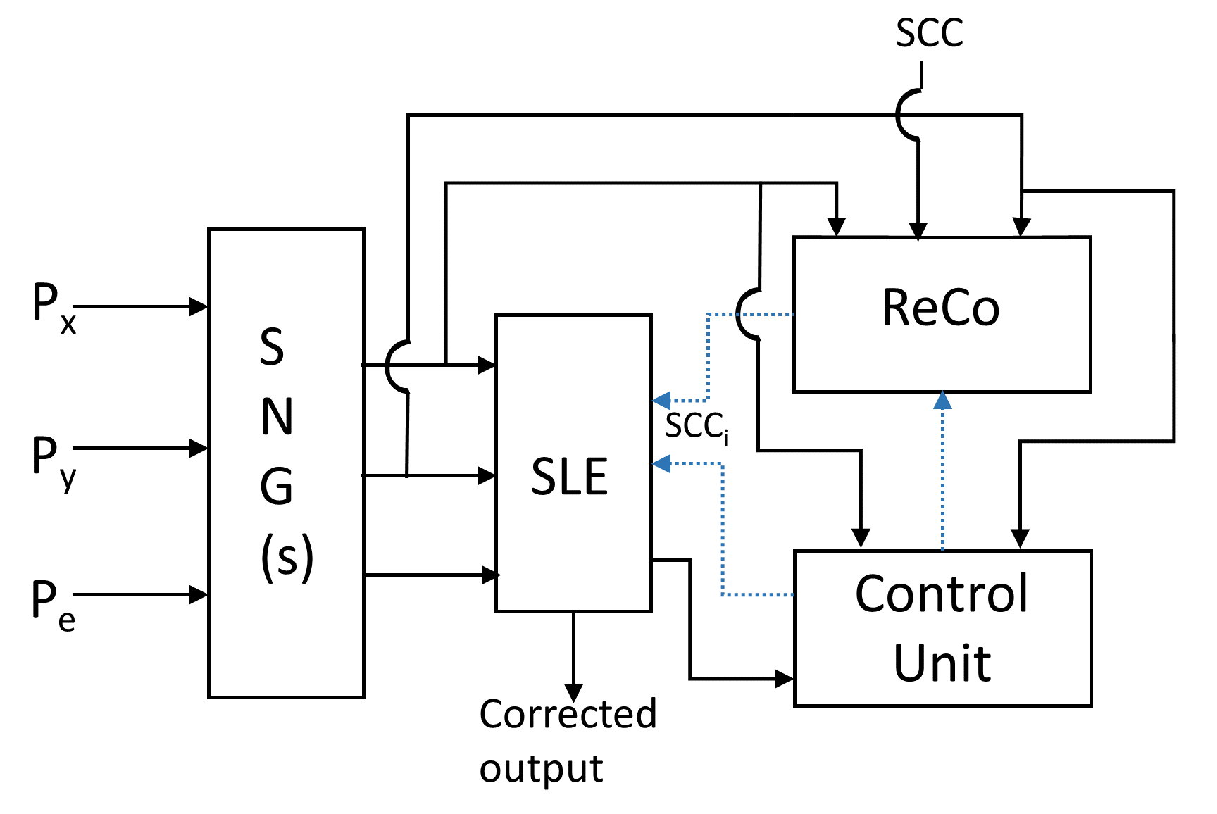
Figure 11: System-Level representation of Error Correction mechanism.

3.3.4 Comparator

The stochastic comparator shown in Fig. 10 compares the obtained MSE with $\delta$ ($0.0001$). It is based on the fact [14] that when two correlated inputs are given to an AND gate with an inverter to one of its inputs the stochastic function implemented is given by $p_{out}=max((MSE-\delta),0)$. Thus, when $MSE$ which is representative of the error in computation is lesser than the error-tolerance of the circuit $\delta$, a bitstream of $0$’s is obtained at the output of the comparator which indicates that the output is obtained satisfactorily.

4 Formalization of Reco Technique for stochastic circuits

The next step is to formally apply the proposed technique in a combinational circuit.

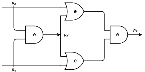
Figure 12: A 2 input multi-level circuit.

For a two-input multilevel circuit as shown in Fig.12, we use circuit PTM obtained as, $M_{ckt}=(F_{2}\otimes F_{2}).(M_{and}\otimes I\otimes I).(F_{2}\otimes I\otimes I).(M_{or}\otimes M_{or}).M_{and}.$

Consider $p_{x}=0.3$ and $p_{y}=0.6$. The error free output is $p_{z}$ = 0.29. If $p_{e}=0.125$, the observed output, $p_{ze}=0.33.$ Using the proposed method, $MSE=(0.066SCC+0.0388)^{2}$ which shows that MSE can be reduced to zero for $SCC\approx-0.58$.

We will now discuss two distinct cases of fault correction in multi-input multi-level circuits.

4.1 ReCo I:Error minimization for Multi-input Single output (MISO) SLCs

Let us consider correlation-sensitive blocks interconnected in a fashion as shown in Fig. 13. The quantification of SCC is only available for two signals in literature, so we consider two input gates in the circuit model. The block diagram consists of $i=1,2,..,n$ levels and each level consists of multiple two input gates. Consider one or more gates at different levels are subject to transient faults which result in an increased MSE at the output. The MSE is minimized by selecting suitable candidates for ReCo analysis using the proposed Algorithm 2 which is discussed below.

Definition 4: An observed error at the primary output(s) driven by one or more gates, can be minimized by injecting correlation at prioritized input gates defined by the faulty gates in the error path P.

Assume correlation between input pairs for gates at level $1$ as $SCC_{11}$,$SCC_{12}$,$SCC_{13}$,..,$SCC_{1p}$, where $p$ is the number of two input gates at level 1. We can represent the output of each gate from level $1$ in terms of $SCC$ to become functions of corresponding $SCC$. Thus, $p_{z_{11}}$=$f(SCC_{11})$, $p_{z_{12}}$=$f(SCC_{12})$, $p_{z_{13}}$=$f(SCC_{13})$,…, $p_{z_{1p}}$=$f(SCC_{1p})$. These outputs are again inputs to certain gates in the next level of the circuit. The output from any gate in the intermediate level, is thus, in turn a function of $SCC$ of primary input pairs.

Let $i^{th}$ intermediate level consists of $q$ interconnected gates. The output $Z_{i1}$ from gate 1 in $i^{th}$ level is $p_{Z_{i1}}=f(p_{Z_{(i-1)k}},p_{Z_{(i-1)j}})$ where $Z_{(i-1)k}$ and $Z_{(i-1)j}$ are the outputs from $k^{th}$ and $j^{th}$ gate at the $(i-1)^{th}$ level. Thus, $p_{Z_{i1}}$=$f(p_{Z_{(i-2)l}},p_{Z_{(i-2)m}},p_{Z_{(i-2)q}},p_{Z_{(i-2)r}})$, where $p_{Z_{(i-2)l}}$ and $p_{Z_{(i-2)m}}$ are the outputs of $l^{th}$ and $m^{th}$ gate of $(i-2)^{th}$ level that are inputs to $k^{th}$ gate in $(i-1)^{th}$ level and $p_{Z_{(i-2)q}}$ and $p_{Z_{(i-2)r}}$ are the outputs from $q^{th}$ and $r^{th}$ gate of $(i-2)^{th}$ level that are connected to $j^{th}$ gate in $(i-1)^{th}$ level. These outputs are again functions of SCCs of their corresponding inputs, such that $p_{{Z}_{i1}}$=$f(SCC_{(i-2)l},SCC_{(i-2)m},SCC_{(i-2)q},SCC_{(i-2)r})$. Thus, tracing the interconnected sub-networks, $p_{{Z}_{i1}}$ is written as, $p_{{Z}_{i1}}=f(SCC_{11}$,$SCC_{12}$,$SCC_{13}$,..,$SCC_{1p})$ of traced inputs at the primary level.

Let transient faults at a certain level contribute to shift in the desired $SCC$ at the input assumption of succeeding levels leading to erroneous results. We take into account the intermediate correlation $SCC_{i-1}$ present between $Z_{(i-1)k}$ and $Z_{(i-1)j}$ if the circuit is non-faulty. Let, $Z^{\prime}_{(i-1)k}$ and $Z^{\prime}_{(i-1)j}$ are the modified values on account of errors from $k^{th}$ and $j^{th}$ faulty gates of level $(i-1)$. These result in a change in the number of 1’s present in the bitstream. Let, probability of $Z_{(i-1)k}$ is changed from $n_{(i-1)k}$ to $n^{\prime}_{(i-1)k}$ and $Z_{(i-1)j}$ is changed from $n_{(i-1)j}$ to $n^{\prime}_{(i-1)j}$. Eventually, $SCC_{i1}$ is modified to $SCC^{\prime}_{i1}$ which modifies the probablity of $Z_{i1}$ from $p_{z_{(i-1)j}}$ to $p_{z^{\prime}_{(i-1)j}}$. Thus, $p_{z^{\prime}_{(i-1)j}}=(1+SCC^{\prime}_{(i-1)j})p_{z^{\prime}0_{(i-1)j}}-SCC^{\prime}_{(i-1)j}p_{z^{\prime}(+1)_{(i-1)j}}=n^{\prime}_{(i-1)j}/n$. Similarly, $p_{z^{\prime}_{(i-1)k}}$ can be written as $p_{z^{\prime}_{(i-1)k}}=(1+SCC^{\prime}_{(i-1)k})p_{z^{\prime}0_{(i-1)k}}-SCC^{\prime}_{(i-1)k}p_{z^{\prime}(+1)_{(i-1)k}}=n^{\prime}_{(i-1)k}/n$.

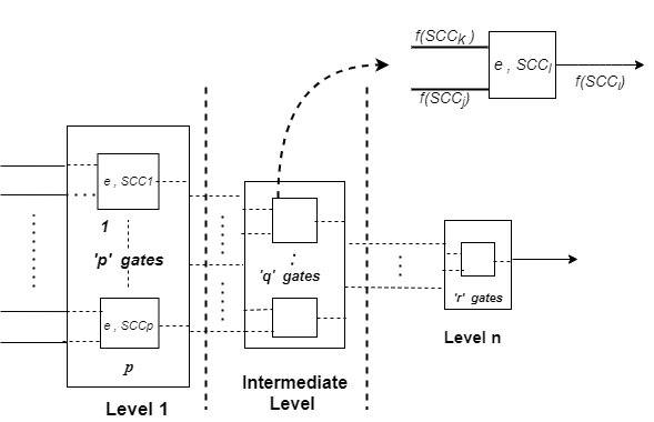
Figure 13: Multi-level block representation of MISO SLC.

Thus the effect of transient error is reflected in an overall change in the probability of SNs. This suggests the dependence of MSE on SCC. This instigated us to find a suitable technique that adapts to the change in the assumption of correlation and try to minimize the observed error at the output by using ReCo. It relocates $SCC$ at several levels to counterbalance the change in initial $SCC$ due to transient faults. We trace faults and determine gates subjected to faults and remodel SCCs by modifying input vectors of the primary inputs of the sub network in level 1.

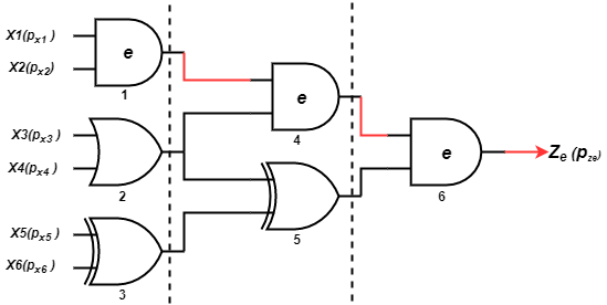
Figure 14: A sample MISO circuit showing gates $G1,G4,G6$ faulty.

In noisy operating conditions, error is assumed to be primarily contributed by one or more faulty gates in the circuit. For a multilevel MISO circuit shown in Fig. 14, the number of SLEs that undergo ReCo correction primarily depend on the number of faulty gates and the probability of error. Thus, it is important to identify faulty paths in the circuit. We generalize the procedure for fault correction in MISO circuits as follows:

1. Check if the MSE of the circuit is within the tolerable limit $\delta(<=10^{-3})$ or not. If not,

2. Determine Faulty gates: Generate T input test vectors n times and the output at each gate is observed. The error rate is estimated by the number of faulty outputs for n inputs using FaultEvaluation($CIRCUIT$).

3. Determine input SLEs corresponding to faulty output node: Input gates that are connected to the faulty output node, denoted by IsConnected(), are selected and are stored in an array $FC\_I\_gate$.

4. Register SLEs based on priority: The gates based on their priority values from left (highest) to right (lowest); {$XOR,AND,OR$} are sorted using $\textit{{PrioritySort}}()$ are then stored in an array $S\_FC\_I\_gate$.

5. Selection of SLEs for ReCo: Pop gate from the priority list and alter $SCC$ using $\textit{{ReCo}}()$ (Algorithm $1$). Calculate if, $MSE\leq\delta$, return corresponding $SCC_{i}$. If not, dual combination of SLEs.

6. Combine SLEs: Store MSE in order of increasing magnitude in the sorted list [ $L\_gate,L\_MSE$] using $\textit{{Sort}}()$. Club next SLEs from the sorted list till the desired MSE is reached.

From the previous discussion, it can be inferred that the XOR gate is most susceptible to changes in correlation and can reduce the overall MSE substantially compared to other correlation sensitive SLEs. So XOR gate line up highest in the correlation-sensitivity index. If a single gate does not suffice then we proceed for combinations from the list L_MSE[]. Suppose, $\textit{{PrioritySort}}()$ list consists of {$XOR,AND1,AND2$} and $AND2$ generates less MSE compared to $AND1$, then we combine $XOR$ and $AND2$ to find minimum MSE. This condition is often guided by the position of the gate(s) in the circuit. The whole analysis is carried out to improve the accuracy and reduce the number of correlators in the circuit.

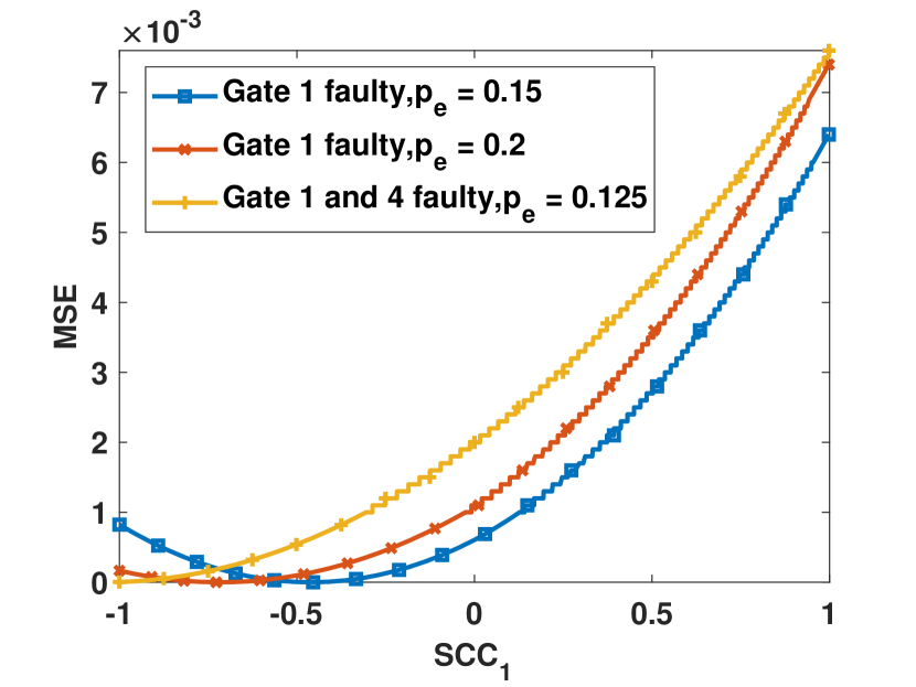
(a)

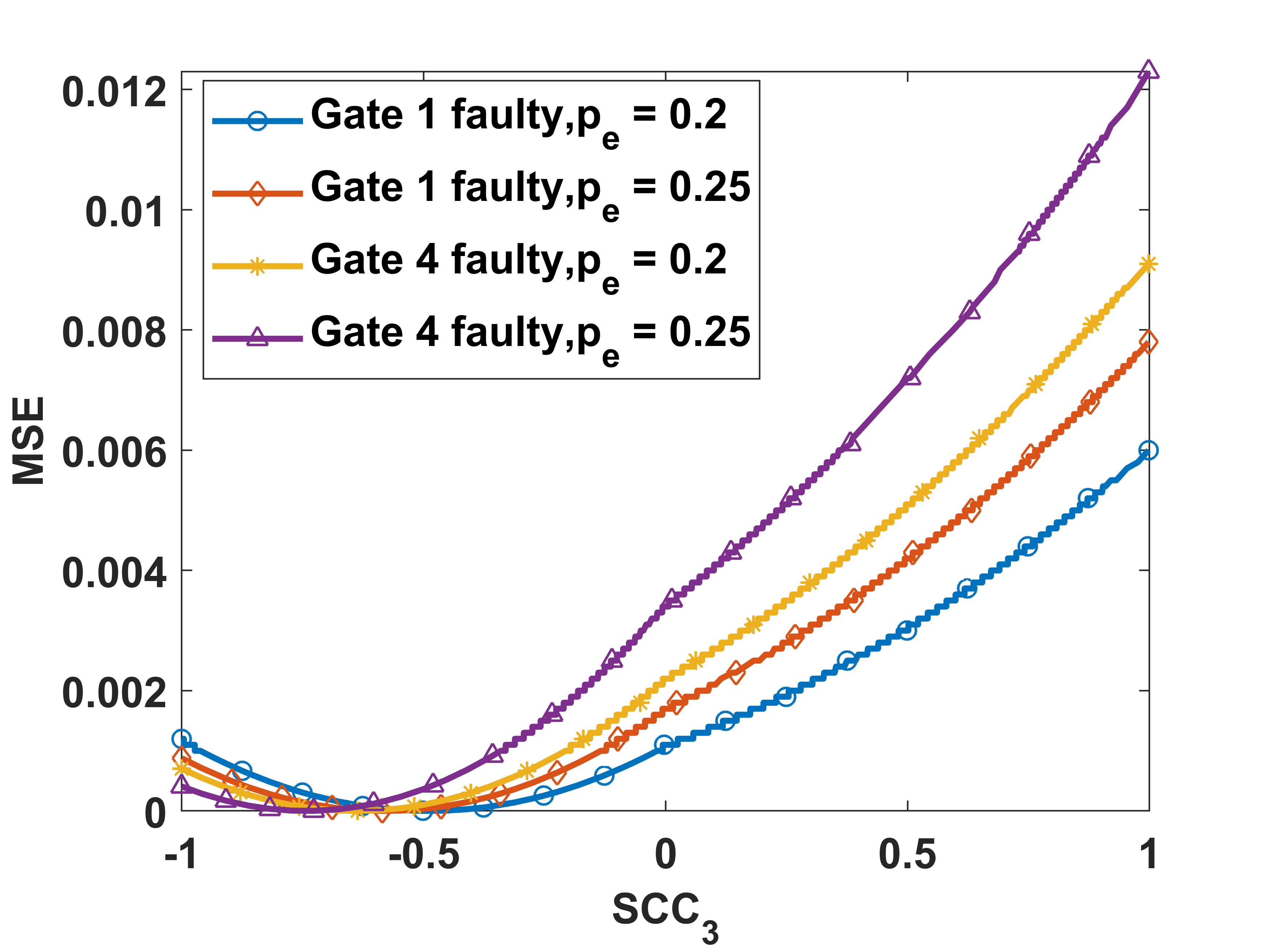
(b)

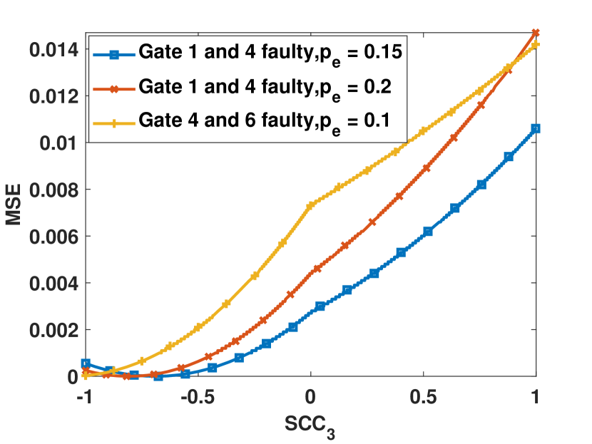
(c)

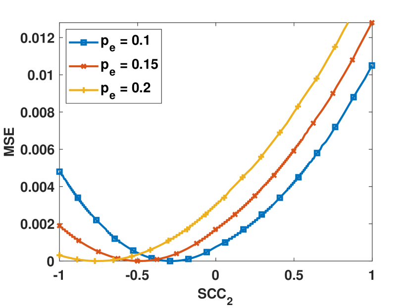
(d)

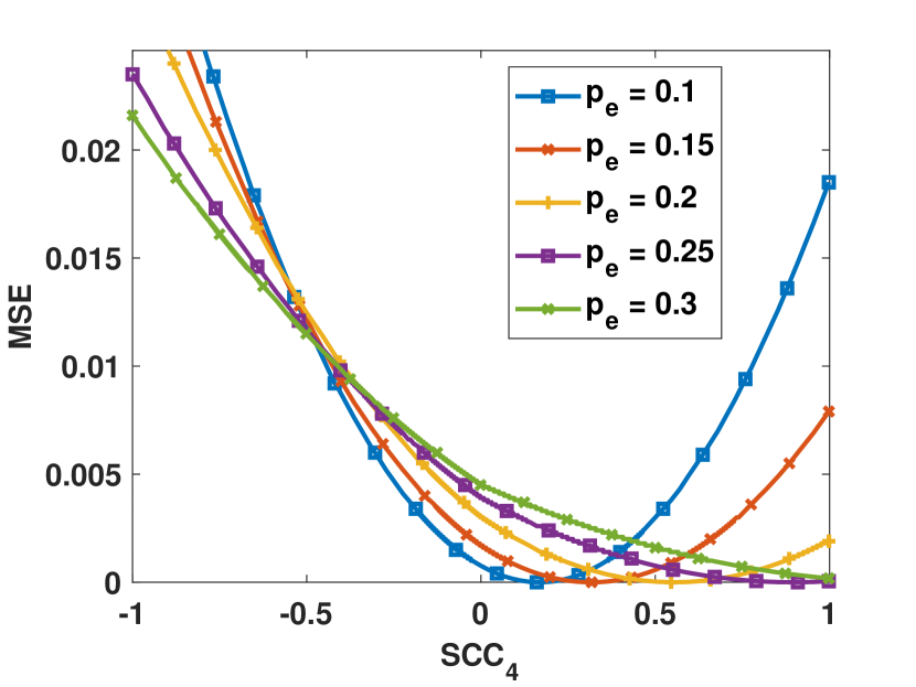
(e)

Figure 15: Graphs showing different values of induced correlation to achieve minimum MSE; (a)-(c) MISO Circuit; (d),(e) MIMO circuit.

It is observed that the MSE is proportional to the number of faulty gates and the error rate $p_{e}$. For any error observed at the output, the error can be due to transient error at the gate itself or due to the error being propagated from the previous stage or the both. We consider different cases of fault propagation in Fig. 14 where the path P is indicated in red color.

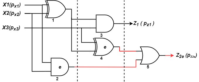
Figure 16: A sample MIMO circuit showing gates $G2,G4$ faulty.

It is observed from Fig. 15(a),(b) that for a single faulty gate, $G1$/$G4$ with $p_{e}\leq 0.20$, single gate ReCo, $SCC_{1}$ or $SCC_{3}$ will suffice to minimize MSE. For multiple $G1,G4$ faulty with $p_{e}\leq 0.125$ same logic can comply. Thus, in both cases, the error can be minimized without being thoroughly guided by the priority-rule of SLE (excluding OR). But $G1,G4$ faulty at $p_{e}=0.2$ fault tolerance can be achieved using prioritized SLE ($SCC_{3}$) only as shown in Fig.15(c) (red).

For a larger number of gates faulty even at low error rates, treatment of prioritized SLE is obligatory. Thus, $G1,G4,G6$ faulty at $p_{e}\leq 0.125$, $MSE$ can be minimized using single gate ReCo ($SCC_{3}$). But the same with $p_{e}=0.20$ we invoke dual ReCo ($SCC_{3},SCC_{1}$) as shown in Fig. 18(d). When $G4$ and $G6$ are faulty with $p_{e}\leq 0.25$ we invoke dual ReCo($SCC_{3},SCC_{1}$) as shown in Fig. 18(a)-(c). It is observed that there is a finite error of $0.01$ when $G1,G4,G6$ are faulty at a rate of $0.25$ even after dual ReCo of prioritized SLEs. Table 1 is given to comprehend the nature of the analysis and the results obtained in the proposed work.

It is observed that the possibility of error reduction is motivated by several factors; the nature and number of faulty gates as well as the arrangement of gates in the circuit. As AND gate is more sensitive to soft errors than the XOR gate, an AND gate in place of the XOR gate would contribute to larger MSE. These factors coupled with the probability of error play a pivotal role in determining the circuits’ resilience towards soft errors. There is also a slight dependence on input probability values i.e $p_{x}$ and $p_{y}$ as indicated in Fig. 8 (a)-(c).

4.2 ReCo II:: Error minimization for Multi-input and Multi-output (MIMO) SLC

We have argued that ReCo analysis of the prioritized SLEs can bring down MSE close to 0. We will see that in particular situations that can deviate from this initial assumption. When non-faulty gates converge to a different output node, ReCo analysis of primary SLEs may give undesired results. The condition can be best described with the help of a Multi-input-Multi-Output circuit shown in Fig. 16. The circuit consists of two distinct outputs $Z_{1}$ and $Z_{2}$ with probabilities $p_{z_{1}}$ and $p_{z_{2}}$. Consider two faulty gates 2 and 4 that converge to $p_{z_{2}}$ i.e., the output of gate 5 and the output is modified to $p_{ze_{2}}$. We assume that there are no faulty gates in the path that converges to $p_{z_{1}}$. One way of suppressing the propagation of faulty results to the non-faulty output node is to perform ReCo analysis at the inputs of faulty gates only. This avoids analysis of primary SLEs that are explicitly connected to non-faulty outputs.

It is interesting to note that for $G2,G4$ faulty with an error rate $\leq 0.2$ the MSE at the output $Z_{2}$ can be reduced to $0$ by doing ReCo at either of the faulty gates $SCC_{2}$ or $SCC_{4}$ as shown in Fig.15 (c),(d). We can choose to ReCo at any of the faulty gates without considering the precedence rule. But for $p_{e}>0.2$ the MSE can only be reduced to $0$ with the condition guided by $Algorithm3$. Modelling $SCC_{3}$ can reduce MSE to $0$ for error rates up to $0.3$. At $p_{e}=0.325$, we invoke dual SCC ($SCC_{4},SCC_{2}$) to observe the error resilient behaviour of the circuit as shown in Fig. 18(e). Thus, ReCo analysis only at inputs of every faulty gate is done to avoid the generation of faulty output at a node that is preceded by non-erroneous outputs. Thus, modelling of SCCs at the primary gates $G1$ is avoided without perturbing the output logic level at $Z_{1}$. As the number of faulty gates increase, the number of correlator circuits also increases. This is contrary to the selection criteria in $Algorithm2$. It attempts to minimize the number of correlator circuits for larger error rates $0.30$ ($l=1$). It is observed that $MSE$ can be reduced to zero for $p_{e}=0.325$ using dual ReCo analysis. The results of analysis are registered in Table II.

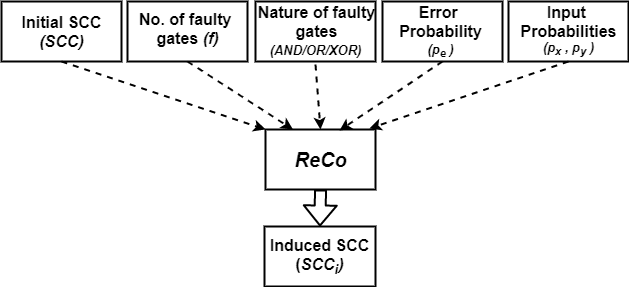
Figure 17: Factors influencing the induced SCC.

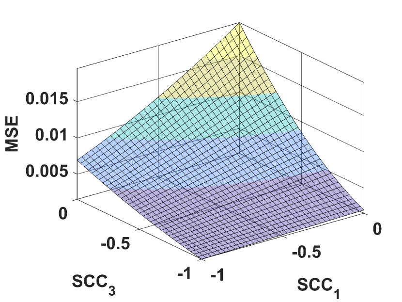
(a) $p_{e}=0.15$

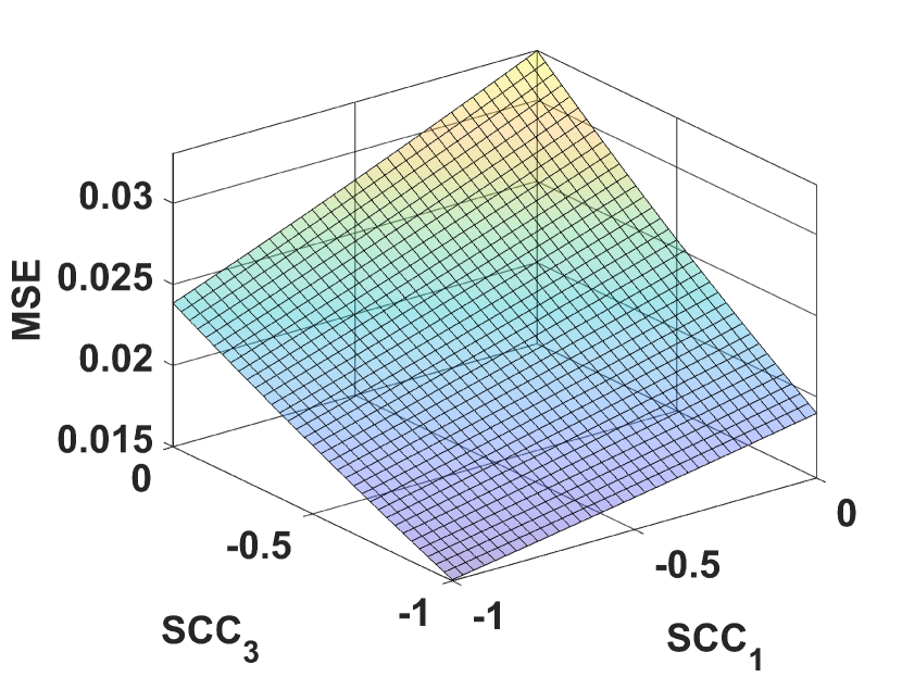
(b) $p_{e}=0.20$

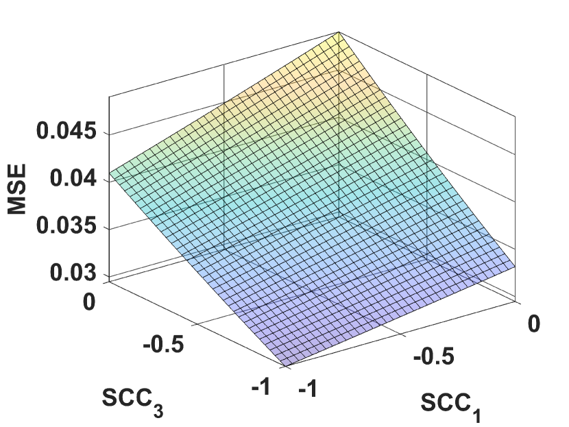
(c) $p_{e}=0.25$

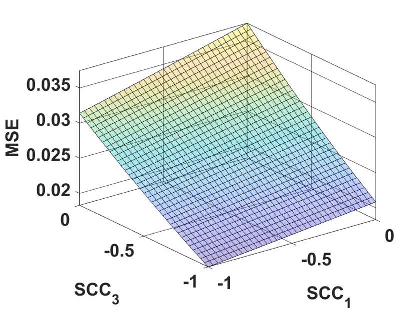
(d) $p_{e}=0.20$

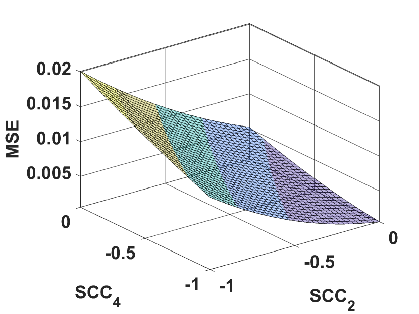
(e) $p_{e}=0.325$

Figure 18: Error minimization using dual ReCo for different error rates; (a),(b),(c) Gates $4,6$ faulty and (d) Gates $1,4,6$ faulty in Fig. 14; (e) Gates $2,4$ faulty in Fig. 16.

Table 1: Comparison of MSE for ReCo at different locations in the circuit in Fig. 14. $MSE_{min}$ represents minimum MSE.

	Faulty gate(s)	MSE Without ReCo	With ReCo (Single/Dual gate)
				$SCC_{1}$	$SCC_{3}$	$SCC_{1}$, $SCC_{3}$	$SCC_{2}$, $SCC_{3}$
Error = 0.125	Gate 1	0.00042	$SCC_{i}$	-0.36	-0.61	-0.19, -0.16	-0.26, 0.33
			$MSE_{min}$	0	0	0	0
	Gate 4	0.00085	$SCC_{i}$	-0.51	-0.45	-0.27, -0.23	-0.34, -0.38
			$MSE_{min}$	0	0	0	0
	Gate 1, 4	0.002	$SCC_{i}$	-1	-0.61	-0.4471, -0.4001	-0.51, -0.82
			$MSE_{min}$	0	0	0	0
	Gate 1, 4, 6	0.016	$SCC_{i}$	-1	-1	-0.9,-0.9	-1,0
			$MSE_{min}$	0.0095	0	0	0.001
Error = 0.20	Gate 1	0.0011	$SCC_{i}$	-0.717	-0.4896	-0.36,-0.27	-0.5,-0.49
			$MSE_{min}$	0	0	0	0
	Gate 4	0.0022	$SCC_{i}$	-1	-0.6385	-0.45,-0.41	-1,-0.1
			$MSE_{min}$	0	0	0	0
	Gate 1, 4	0.0044	$SCC_{i}$	-1	-0.8078	-0.546, -0.7	-0.524, -0.68
			$MSE_{min}$	0.0015	0	0	0
	Gate 1, 4, 6	0.0375	$SCC_{i}$	-1	-1	-1,-1	-1, -0.15
			$MSE_{min}$	0.0314	0.0108	0	0.01
Error = 0.25	Gate 1	0.0017	$SCC_{i}$	-1	-0.5813	-0.44, -0.38	-0.47,-0.83
			$MSE_{min}$	0	0.0114	0	0
	Gate 4	0.0034	$SCC_{i}$	-1	-0.743	-52,-0.55	-1,-0.1
			$MSE_{min}$	0.0004	0	0	0
	Gate 1, 4	0.049	$SCC_{i}$	-1	-0.8987	-1,-1	-1, -0.09
			$MSE_{min}$	0.036	0	0	0.0045
	Gate 1, 4, 6	0.1317	$SCC_{i}$	-1	-1	-1,-1	-1,0
			$MSE_{min}$	0.041	0.023	0.01	0.02

Table 2: Comparison of MSE for ReCo at different locations of circuit in Fig. 16

	Faulty gates	MSE Without ReCo	With ReCo (single or dual gate(s))
				$SCC_{2}$	$SCC_{4}$	$SCC_{2},SCC_{4}$
Error = 0.25	Gates 2,4	0.003	$SCC_{i}$	-0.9	-0.33	-0.2,-0.4
			$MSE_{min}$	0.001	0	0
Error= 0.30	Gates 2,4	0.004	$SCC_{i}$	-0.93	-0.87	-0.15,-1
			$MSE_{min}$	0.002	0	0

5 Case study: Contrast enhancement in images

We have implemented the proposed technique for contrast enhancement [24] on images to establish the practicality and effectiveness of the proposed scheme. A random image has been taken from the standard dataset [25]. A transient error at the rate of $0.2$ is given to certain gates to study the effect of the error on the image. Structural Similarity Index(SSIM)[26] is calculated to measure the similarity between the enhanced images and the ground truth image. It is observed that SSIM of the enhanced image using contrast stretch technique is considerably low, i.e, $66.43$ when exposed to errors. Exploiting the priority-based approach two SLEs are selected for obtaining an error-resilient behaviour of the circuit. From Fig. 20(d), it is observed that the SSIM index using the proposed ReCo method is $92.80$ and is considerably higher compared to the enhanced image with the error which denotes that the proposed methodology gives a faithful result even in transient error scenarios. Thus the proposed methodology can be implemented with lower hardware cost in various image processing applications.

6 Experimental Results and Discussion

We can now identify the key factors on which the whole analysis is hinged upon. The magnitude and polarity of induced correlation and also the number ($l$) of ReCo blocks depend on several underlying factors. The predominant factor is the amount of transient error in the circuit. As transient error increases the MSE increases exponentially (see graphs in Fig. 2(a)). With higher MSE the value of $l$ tends to be larger. For $G1,G4,G6$ faulty at $p_{e}\leq 0.125$ error can be reduced to $0$ using a single ReCo block ($SCC_{3}$). But the same with $p_{e}\geq 0.20$ error can be reduced to $0$ with $l=2$ as shown in Table 1. This is because MSE is higher in the second case.

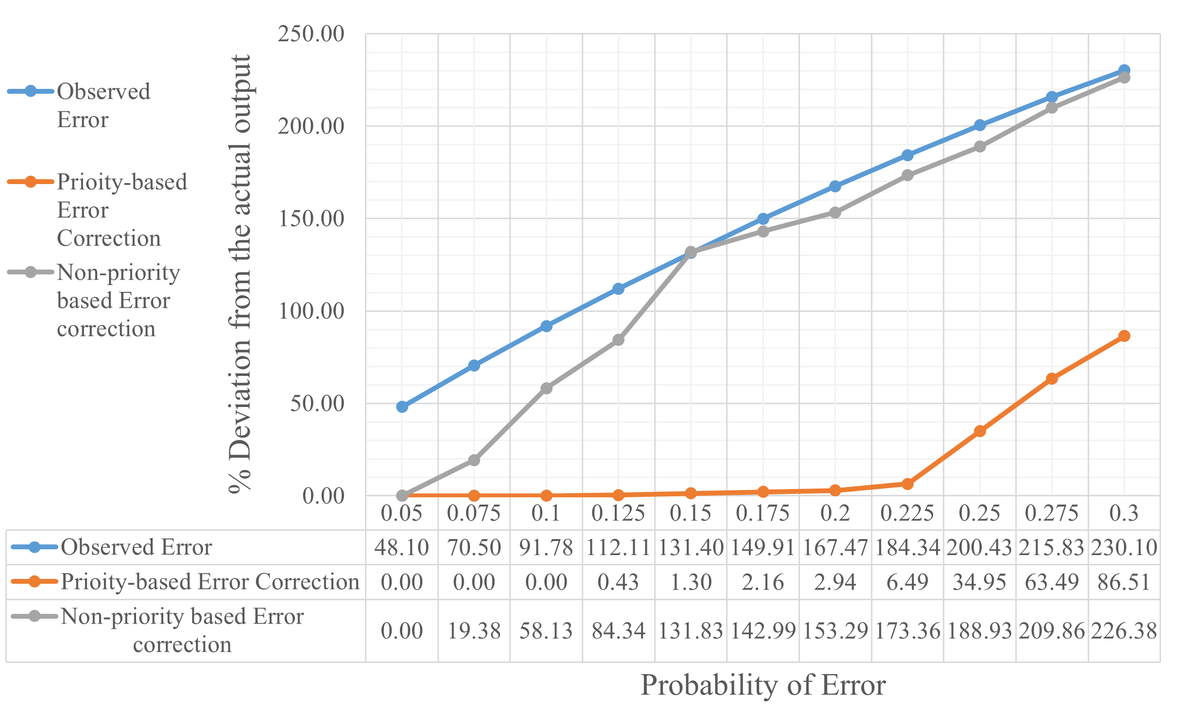
Figure 19: Deviation of two correction approaches from the actual value (without error) of Fig. 14.

It is identified that as the number of faulty gates in the circuit are increased, the value of $l$ is increased to commensurate with the increased MSE. When $G1$ faulty and $G1,G4,G6$ faulty with the same error rate, i.e., $0.20$, the error-free output is obtained respectively with $l=1$ ($SCC_{3}/SCC_{1}$) and $l=2$ ($SCC_{3},SCC_{1}$). Also in the input panel, the proliferation of the highest priority SLE enhances the possibility of reducing the error to zero. Thus, when AND gate $G1$ is replaced by an XOR gate, then MSE can be reduced to $0$, even if, $G1,G4,G6$ are faulty at $p_{e}=0.25$.

There is a strong dependence of overall MSE on the nature of faulty gates. If we replace AND gate $G4$ with an XOR gate , the overall MSE is reduced from $0.0375$ to $0.02$, when $G1,G4,G6$ are faulty at $p_{e}=0.2$. This is because XOR is least sensitive to transient errors. The position of faulty gates in the circuit has also an impact on the overall MSE. A faulty gate distant from the input periphery and closer to the output produces larger MSE. When $G1$ faulty at a rate $p_{e}=0.2$ gives MSE as $0.0011$, whereas $G6$ faulty at the same error rate gives larger MSE ($0.0237$). It is also implicit from Fig. 2(c),(d) and Fig. 3(c),(d) that the initial assumption of SCC also plays a significant role in determining the exact operating point of SCC for the circuit. In the current experimental setup as in Fig. 16 the error rates up to $0.3$ can be handled accurately and this is guided by the number of faulty gates in the circuit $(\leq 2)$ and location of faulty gates (closer to the input side) as shown in Fig. 18(e). A block diagram showing the interdependence of these parameters is shown in Fig. 17.

We have introduced a priority-based selection scheme of SLEs for larger circuits in Section IV with multiple faulty gates and got some encouraging results. XOR gate exhibits precedency in the correlation-sensitivity list and is considered as a prime element in our analysis. It is inferred that to observe minimum $MSE$ using priority-based approach, minimum number of ReCo blocks required is $l=1$. The only exception is $G1,G4,G6$ faulty at $p_{e}=0.25$, where two ReCo blocks are required to achieve minimum $MSE$. The graphs of Fig. 19 are obtained with $G1,G4,G6$ faulty at different error rates. The deviation in output from the actual value (without error) using the proposed scheme is much less compared to the non-priority based approach. It is observed that this approach is able to handle high error rates with reduced number of correlator circuits. The number of iterations required to achieve the desired value is also less compared to the non-priority based approach. The priority-based (red) deviation graph is obtained with one ReCo block whereas the deviation with non-priority based approach (gray) is obtained with two ReCo blocks to model the output. The blue line correspond to the observed error (without ReCo). This shows the efficacy of the proposed priority-based approach in terms of hardware design.

7 CONCLUSION

Recent applications of stochastic computing have involved noisy operating conditions leading to incorrect results at times. The source of inaccuracy has been predominantly traced to transient errors. In this paper, we have progressively varied the transient error probabilities for single gates and observed its effect on the MSE of these gates. Attempts are made to formulate the process within a mathematical framework. In view of the effect of varying correlation on the MSE, we advanced our study into realistic multi-level circuits where single or multiple gates may be prone to transient errors. For such circuits, we have developed the ReCo framework to minimize the overall MSE. Algorithm $2$ introduces a priority-based approach of choosing SLE to reduce the number of correlator circuits and to obtain the desired level of accuracy quickly under noisy operating conditions. Inevitably, there are conflicts in constraints in different applications which is handled using different approaches. Algorithm $3$ recognizes and eliminates this ambiguity for a MIMO circuit by introducing correction blocks at fault specified nodes only. Both these algorithms are observed to handle errors and yield accurate results even at high transient error rates. In our future work, we will explore other variants of these algorithms to achieve better correction using lesser ReCo blocks. Also, we will try to develop some equivalent form of combinational and sequential circuits with a given set of conditions such that the task of error minimization is achieved at a lesser hardware cost and low latency.

Figure 20: Contrast Stretching operations on the images; [25] ground truth, with error, and correction using the proposed methodology.

11:  Input: $CIRCUIT$ // Circuit with n number of inputs.

Output: $MSE,SCC_{i}$

22:  Variable Initialization:

3$p\_arr[\;]=\{XOR,OR,AND\}$ //Priority Sequence

4$F\_gate[\;]=\{0\}\;\;$// number of faulty gates

5$I\_gate[\;]=\{number\;of\;input\;gates\}$

6$FC\_I\_gate[\;]=\{0\}$ // Input gates $\in F\_gate[\;]$

$S\_FC\_I\_gate[\;]=\{0\}$ // Sorted $FC\_I\_gate[\;]$

73:  $F\_gate$=FaultEvaluation($CIRCUIT$)

     // Identify faulty gates in the circuit

4:  $FC\_I\_gate$=IsConnected($I\_gate,F\_gate)$

85:  $S\_FC\_I\_gate$=PrioritySort($FC\_I\_gate$, $p\_arrr)$

96:  for $j=1\>\text{to}\>j<=\textit{{maxElement}}$ ($S\_FC\_I\_gate)$  do

10       $[L\_MSE[j],SCC_{i}[j]]=\textit{{ReCo}}(S\_FC\_I\_gate[j]$)

11      if ($L\_MSE[j]<=\delta$) then

12             return $L\_MSE[j],SCC_{i}[j]$

13       end if

14      

15 end for

7:  $[S\_L\-gate,L\_MSE]=\textbf{{Sort}}(L\_MSE)$ //Sort MSE value along with their gate number

168:  for $j=1\>\text{to}\>j<=\textit{{maxElement}}($S_FC_I_gate$)$ do

17      [$MSE[j],SCC_{i}[j]]=NewReco(S\_L\_gate,j+1)$

18      if ($MSE[j]<=\delta$) then

19             return $MSE[j],SCC_{i}[j]$

20       end if

21      

22 end for

9:   return $\operatorname*{\textbf{argmin}}_{MSE[j]}$ {$MSE[j]$ , $SCC_{i}[j]$}

Algorithm 2 ReCo analysis for MISO Circuits

11:  Input: $CIRCUIT$ // Circuit with n number of inputs

Output: $MSE,SCC_{i}$

22:  Variable Initialization:

3$p\_arr[\;]=\{XOR,OR,AND\}$ //Priority Sequence

4$F\_gate[\;]=\{0\}\;\;$// number of faulty gates

$S\_F\_gate[\;]=\{0\}$ // Sorted $F\_gate[\;]$

53:  $F\_gate$=FaultEvaluation($CIRCUIT$)

     // Identify faulty gates in the circuit

64:  $S\_F\_gate$=PrioritySort($F\_gate$, $p\_arrr)$

75:  for $j=1\>\text{to}\>j<=\textit{{maxElement}}($S_F_gate$)$ do

8       $[L\_MSE[j],SCC_{i}[j]]=\textit{{ReCo}}(S\_F\_gate[j]$)

9      if ($L\_MSE[j]<=\delta$) then

10             return $L\_MSE[j],SCC_{i}[j]$

11       end if

12      

13 end for

6:  $[S\_L\-gate,L\_MSE]=\textbf{{Sort}}(L\_MSE)$ //Sort MSE value along with their gate number

147:  for $j=1\>\text{to}\>j<=\textit{{maxElement}}($S_F_gate$)$ do

15      [$MSE[j],SCC_{i}[j]]=NewReco(S\_L\_gate,j+1)$

16      if ($MSE[j]<=\delta$) then

17             return $MSE[j],SCC_{i}[j]$

18       end if

19      

20 end for

8:   return $\operatorname*{\textbf{argmin}}_{MSE[j]}$ {$MSE[j]$ , $SCC_{i}[j]$}

Algorithm 3 ReCo analysis for MIMO Circuits

References

- [1] Brian R Gaines. Stochastic computing. In Proceedings of the April 18-20, 1967, spring joint computer conference, pages 149–156, 1967.
- [2] Armin Alaghi and John P Hayes. Survey of stochastic computing. ACM Transactions on Embedded computing systems (TECS), 12(2s):1–19, 2013.
- [3] M Hassan Najafi and Mostafa E Salehi. A fast fault-tolerant architecture for sauvola local image thresholding algorithm using stochastic computing. IEEE Transactions on Very Large Scale Integration (VLSI) Systems, 24(2):808–812, 2015.
- [4] Peng Li and David J Lilja. Using stochastic computing to implement digital image processing algorithms. In 2011 IEEE 29th International Conference on Computer Design (ICCD), pages 154–161. IEEE, 2011.
- [5] Armin Alaghi, Weikang Qian, and John P Hayes. The promise and challenge of stochastic computing. IEEE Transactions on Computer-Aided Design of Integrated Circuits and Systems, 37(8):1515–1531, 2017.
- [6] Ran Xiao and Chunhong Chen. Gate-level circuit reliability analysis: A survey. VLSI Design, 2014, 2014.
- [7] A. Vallero, A. Savino, A. Chatzidimitriou, M. Kaliorakis, M. Kooli, M. Riera, M. Anglada, G. Di Natale, A. Bosio, R. Canal, A. Gonzalez, D. Gizopoulos, R. Mariani, and S. Di Carlo. Syra: Early system reliability analysis for cross-layer soft errors resilience in memory arrays of microprocessor systems. IEEE Transactions on Computers, 68(5):765–783, 2019.
- [8] Xingjian Xu, Tian Ban, and Yuehua Li. Splm: A flexible and accurate reliability assessment model for logic circuits. Journal of Circuits, Systems and Computers, 28(02):1950032, 2019.
- [9] Michael Nicolaidis. Design for soft error mitigation. IEEE Transactions on Device and Materials Reliability, 5(3):405–418, 2005.
- [10] Smita Krishnaswamy, George F Viamontes, Igor L Markov, and John P Hayes. Probabilistic transfer matrices in symbolic reliability analysis of logic circuits. ACM Transactions on Design Automation of Electronic Systems (TODAES), 13(1):1–35, 2008.
- [11] Armin Alaghi, Paishun Ting, Vincent T Lee, and John P Hayes. Accuracy and correlation in stochastic computing. In Stochastic Computing: Techniques and Applications, pages 77–102. Springer, 2019.
- [12] Smita Krishnaswamy, George F Viamontes, Igor L Markov, and John P Hayes. Accurate reliability evaluation and enhancement via probabilistic transfer matrices. In Design, Automation and Test in Europe, pages 282–287. IEEE, 2005.
- [13] Armin Alaghi and John P Hayes. On the functions realized by stochastic computing circuits. In Proceedings of the 25th edition on Great Lakes Symposium on VLSI, pages 331–336, 2015.
- [14] A. Alaghi and J. P. Hayes. Exploiting correlation in stochastic circuit design. In 2013 IEEE 31st International Conference on Computer Design (ICCD), pages 39–46. IEEE, 2013.
- [15] Jason H Anderson, Yuko Hara-Azumi, and Shigeru Yamashita. Effect of lfsr seeding, scrambling and feedback polynomial on stochastic computing accuracy. In 2016 Design, Automation & Test in Europe Conference & Exhibition (DATE), pages 1550–1555. IEEE, 2016.
- [16] Per Ahlgren, Bo Jarneving, and Ronald Rousseau. Requirements for a cocitation similarity measure, with special reference to pearson’s correlation coefficient. Journal of the American Society for Information Science and Technology, 54(6):550–560, 2003.
- [17] Rahul Kumar Budhwani, Rengarajan Ragavan, and Olivier Sentieys. Taking advantage of correlation in stochastic computing. In 2017 IEEE International Symposium on Circuits and Systems (ISCAS), pages 1–4. IEEE, 2017.
- [18] Toshiyuki Kanoh. Absolute value calculating circuit having a single adder, August 28 1990. US Patent 4,953,115.
- [19] Vincent T Lee, Armin Alaghi, and Luis Ceze. Correlation manipulating circuits for stochastic computing. In 2018 Design, Automation & Test in Europe Conference & Exhibition (DATE), pages 1417–1422. IEEE, 2018.
- [20] Premkishore Shivakumar, Michael Kistler, Stephen W Keckler, Doug Burger, and Lorenzo Alvisi. Modeling the effect of technology trends on the soft error rate of combinational logic. In Proceedings International Conference on Dependable Systems and Networks, pages 389–398. IEEE, 2002.
- [21] Armin Alaghi, Wei-Ting J Chan, John P Hayes, Andrew B Kahng, and Jiajia Li. Trading accuracy for energy in stochastic circuit design. ACM Journal on Emerging Technologies in Computing Systems (JETC), 13(3):1–30, 2017.
- [22] Te-Hsuan Chen, Armin Alaghi, and John P Hayes. Behavior of stochastic circuits under severe error conditions. it-Information Technology, 56(4):182–191, 2014.
- [23] Te-Hsuan Chen and John P Hayes. Analyzing and controlling accuracy in stochastic circuits. In 2014 IEEE 32nd International Conference on Computer Design (ICCD), pages 367–373. IEEE, 2014.
- [24] Atam P. Dhawan, Gianluca Buelloni, and Richard Gordon. Enhancement of mammographic features by optimal adaptive neighborhood image processing. IEEE Transactions on Medical Imaging, 5(1):8–15, March 1986.
- [25] Muhammad Ali Qureshi, Bilel Sdiri, Mohamed Deriche, Faouzi Alaya-Cheikh, and Azeddine Beghdadi. Contrast Enhancement Evaluation Database (CEED2016). 3, December 2017.
- [26] Zhou Wang, A. C. Bovik, H. R. Sheikh, and E. P. Simoncelli. Image quality assessment: from error visibility to structural similarity. IEEE Transactions on Image Processing, 13(4):600–612, 2004.