Heterogeneously-Distributed Joint Radar Communications: Bayesian Resource Allocation

Abstract

Due to spectrum scarcity, the coexistence of radar and wireless communication has gained substantial research interest recently. Among many scenarios, the heterogeneously-distributed joint radar-communication system is promising due to its flexibility and compatibility of existing architectures. In this paper, we focus on a heterogeneous radar and communication network (HRCN), which consists of various generic radars for multiple target tracking (MTT) and wireless communications for multiple users. We aim to improve the MTT performance and maintain good throughput levels for communication users by a well-designed resource allocation. The problem is formulated as a Bayesian Cramér-Rao bound (CRB) based minimization subjecting to resource budgets and throughput constraints. The formulated nonconvex problem is solved based on an alternating descent-ascent approach. Numerical results demonstrate the efficacy of the proposed allocation scheme for this heterogeneous network.

I Introduction

Although wireless communications and radar systems have developed in parallel for decades, both share many aspects essentially in terms of signal processing algorithms, devices and even architectures [1]. These common grounds, together with spectrum scarcity, have recently motivated substantial research interest in the co-design of the integrated sensing and communications [2]. In general, it can be categorized into two research directions. The first direction aims to develop a dual-functional system which simultaneously performs radar and communication functionalities [3], while the second one focuses on the coexistence of two separated radar and communication systems [4]. For both directions, a well-designed resource allocation (RA) is desired (i.e., transmit power, dwell time, spectrum, etc.) to avoid significant degenerated performance and fully release the potential of this integrated network.

Many works have contributed to the RA of the integrated network. In [5], radar waveform and adaptive communication transmission scheme were designed to maximize signal-to-interference-plus-noise ratio (SINR) while ensuring the communication system meeting certain rate and power constraints. The work [6] proposed to minimize the total noise jamming power by optimizing the multicarrier jamming power allocation. By leveraging the multicarrier waveforms, [7] proposed two co-design paradigms to improve the spectrum efficiency by optimizing the power allocation and the communication throughput. In [8], the compound rate was proposed as the optimization metric, based on which the optimum transmit policies for the coexistence was derived. The RA strategy of distributed radar architecture for the target localization was first analyzed in [9]. Subsequently in [10], asynchronous RA schemes were proposed for the heterogeneous radar architecture, which was further extended in [11] to maximize the number of the targets that can be tracked.

However, the existing works have not considered the heterogeneity inside this integrated network. Throughout this paper, we focus on a heterogeneous radar and communication network (HRCN), which consists of different generic radars for tracking multiple targets and wireless communications for multiple users. the sketch of the HRCN is shown in Figure 1. Through resource allocation, we aim to optimize the multiple target tracking (MTT) performance measured by a Bayesian CRB based metric subject to meeting the communication throughput requirements and the resource budgets. The formulated problem is then recast into a maximin problem, to which we propose the alternating descent-ascent method (ADAM). Numerical results are presented to demonstrate the efficacy of the design allocation for this heterogeneous network. To the best of our knowledge, this is the first paper dealing with the heterogeneous resource allocation for integrated radar and communication network.

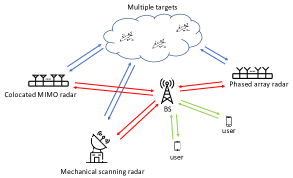
Figure 1: Sketch of the considered scenario.

II HRCN Configurations and Target Tracking Model

II-A Configurations of the HRCN

Configuration of radars

The $N$ radars consist of $N_{cr}$ co-located MIMO radars (MMRs), $N_{pr}$ phased array radars (PARs) and $N_{mr}$ mechanical scanning radars (MSRs) with $N=N_{cr}+N_{pr}+N_{mr}$. These radars are located at the coordinates $\left\{\left(x_{i},y_{i}\right)\right\}_{i=1}^{N}$. The $N$ radars aim to track $Q$ widely separated point-like targets. For each type of radar, we have the following assumptions:

1. Colocated MMR, denoted by $i\in\varphi_{c}\triangleq\left\{1,\ldots,N_{cr}\right\}$, adopts the multiple beams to illuminates multiple targets simultaneously with the same dwell time length but different transmit powers. Hence, the revisit time intervals for all targets are the same.

2. PAR, denoted by $i\in\varphi_{p}\triangleq\left\{N_{cr}+1,\ldots,N_{cr}+N_{pr}\right\}$, adaptively rotates the beam to illuminate multiple targets sequentially, with the same transmit power but different dwell time lengths. Hence, the revisit time intervals for the different targets may not be the same.

3. MSR, dednoted by $i\in\varphi_{m}\triangleq\left\{N_{cr}+N_{pr}+1,\ldots,N\right\}$, rotates mechanically and illuminates all the target sequentially with the same power and dwell time. Hence, the revisit time intervals for all targets are the same.

4. Mutual interference among the $N$ radars is assumed negligible due to the directional beams.

The radar operation schemes are shown in Figure 2, where $M_{i,q,k}$ is the number of measurements for target $q$ by radar $i$ during the $k$-th fusion interval with the length $T_{0}=t_{k+1}-t_{k}$, $t_{i,q,k}^{m},\forall m=1,\ldots,M_{i,q,k}$ is the $m$-th measurement time, and $P_{i,q,k}^{m}$ is the transmit power corresponding to measurements at $t_{i,q,k}^{m}$.

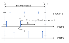
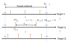
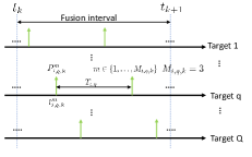
Figure 2: Operation schemes for radars. Left: Colocated MIMO radar; middle: phased array radar; right: mechanical scanning radar.

Configuration of wireless communications

In the cellular communication system, $J$ downlink users are served by a base station with the following configuration:

1. All $J$ users are operating in different frequencies, i.e., no mutual interference among them.

2. During the $k$-th fusion time of the radar networks, the $j$-th downlink lasts with a constant power $P_{c,k}^{j}$.

3. Gaussian codebook based transmission is assumed.

Interference between radars and communications

During a fusion interval, the following assumptions holds for the mutual interference:

1. The $J$ users are affected by the radar signals intermittently. The complex parameter $\alpha_{i,j}^{c}$ accounts for the interference from the $j$-th downlink to the $i$-th radar.

2. The $N$ radars are interfered persistently by the $J$ downlinks. The complex parameter $\alpha_{j,i}^{r}$ accounts for the interference from the $i$-th radar to the $j$-th downlink.

II-B Target Tracking Model

In the $k$-th fusion period, the state of target $q$ at the receiving time $t_{i,q,k}^{m}$ is defined as

$$\boldsymbol{s}_{i,q,k}^{m}=\left[x_{i,q,k}^{m},\dot{x}_{i,q,k}^{m},y_{i,q,k}^{m},\dot{y}_{i,q,k}^{m}\right]^{T},$$ (1)

where $\left(x_{i,q,k}^{m},y_{i,q,k}^{m}\right)$ and $\left(\dot{x}_{i,q,k}^{m},\dot{y}_{i,q,k}^{m}\right)$ denote the target position target velocity, respectively. The state of the target $q$ at the fusion time $t_{k+1}$, denoted by $\boldsymbol{s}_{t_{k+1}}^{q}$, is given by

$$\boldsymbol{s}_{t_{k+1}}^{q}=\left[x_{t_{k+1}}^{q},\dot{x}_{t_{k+1}}^{q},y_{t_{k+1}}^{q},\dot{y}_{t_{k+1}}^{q}\right]^{T}.$$ (2)

It is assumed that the measurements are correctly associated with their radar, i.e., no data-association uncertainty exists. Therefore, the state transition and measurement model is

$$\begin{cases}\boldsymbol{s}_{t_{k+1}}^{q}=f\left(\boldsymbol{s}_{i,q,k}^{m},t_{k+1}-t_{i,q,k}^{m}\right)+\boldsymbol{\gamma}_{k}^{q}\\ \boldsymbol{y}_{i,q,k}^{m}=h\left(\boldsymbol{s}_{i,q,k}^{m},i\right)+\boldsymbol{w}_{i,q,k}^{m},\end{cases}$$ (3)

where $f\left(\cdot\right)$ is the transition function with $f\left(\boldsymbol{s}_{i,q,k}^{m},t_{k+1}-t_{i,q,k}^{m}\right)=\boldsymbol{F}_{k}^{q}\boldsymbol{s}_{i,q,k}^{m}$ and

$$\boldsymbol{F}_{k}^{q}=\text{diag}\left(\left[\boldsymbol{I}_{2}\otimes\left[\begin{array}[]{cc}1&t_{k+1}-t_{i,q,k}^{m}\\ 0&1\end{array}\right]\right]\right),$$ (4)

and $\boldsymbol{\gamma}_{k}^{q}\sim\mathcal{N}\left(\boldsymbol{0},\boldsymbol{\Gamma}_{k}^{q}\right)$ represents the process noise, $h\left(\cdot\right)$ is the measurement function given by

$$\footnotesize{h\left(\boldsymbol{s}_{i,q,k}^{m},i\right)=\left[\begin{array}[]{c}R_{i,q,k}^{m}\\ \theta_{i,q,k}^{m}\end{array}\right]=\left[\begin{array}[]{c}\sqrt{\left(x_{i,q,k}^{m}-x_{i}\right)^{2}+\left(y_{i,q,k}^{m}-y_{i}\right)^{2}}\\ \arctan\left[\frac{y_{i,q,k}^{m}-y_{i}}{x_{i,q,k}^{m}-x_{i}}\right]\end{array}\right],}$$ (5)

and $\boldsymbol{w}_{i,q,k}^{m}\sim\mathcal{N}\left(\boldsymbol{0},\boldsymbol{\Sigma}_{i,q,k}^{m}\right)$ represents the measurement error. We further let $\boldsymbol{\Sigma}_{i,q,k}^{m}=\text{diag}\left(\sigma_{R_{i,q,k}^{m}}^{2},\sigma_{\theta_{i,q,k}^{m}}^{2}\right),$ where $\sigma_{R_{i,q,k}^{m}}^{2}$ and $\sigma_{\theta_{i,q,k}^{m}}^{2}$ are the lower bounds of the MSE error of the corresponding measures. According to [12],

$$\begin{cases}\sigma_{R_{i,q,k}^{m}}^{2}=&\frac{\sum_{j=1}^{J}\left|\alpha_{i,j}^{c}\right|^{2}P_{c,k}^{j}+\sigma_{r,i}^{2}}{P_{i,q,k}^{m}T_{i,q,k}^{m}}\eta_{i,q,k}^{m}\zeta_{i}^{2}c_{R}\\ \sigma_{\theta_{i,q,k}^{m}}^{2}=&\frac{\sum_{j=1}^{J}\left|\alpha_{i,j}^{c}\right|^{2}P_{c,k}^{j}+\sigma_{r,i}^{2}}{P_{i,q,k}^{m}T_{i,q,k}^{m}}\eta_{i,q,k}^{m}B_{i}^{2}c_{\theta},\end{cases}$$ (6)

where $\sigma_{r,i}^{2}$ is the variance of the noise, $\eta_{i,q,k}^{m}$ is the RCS of the target $q$ at the receiving time $t_{i,q,k}^{m}$, $\zeta_{i}$ and $B_{i}$ are the transmit signal bandwidth and the 3dB receive beam width of radar $i$ , respectively, both $c_{R}$ and $c_{\theta}$ account for the unrelated constants. Therefore, we can rewrite $\boldsymbol{\Sigma}_{i,q,k}^{m}$ as

$$\boldsymbol{\Sigma}_{i,q,k}^{m}=\frac{\sum_{j=1}^{J}\left|\alpha_{i,j}^{c}\right|^{2}P_{c,k}^{j}+\sigma_{r,i}^{2}}{P_{i,q,k}^{m}T_{i,q,k}^{m}}\boldsymbol{C}_{i,q,k}^{m}$$ (7)

where $\boldsymbol{C}_{i,q,k}^{m}$ is the constant matrix unrelated to $P_{c,k}^{j}$, $P_{i,q,k}^{m}$ and $T_{i,q,k}^{m}$.

II-C Composition Measurements and the CRB

Recall that all heterogeneous radars work in an asynchronous manner. For target $q$ at the fusion time $t_{k+1}$, a composition measure (CM) denoted by $\hat{\boldsymbol{s}}_{t_{k+1}}^{q}$ will be constructed as an estimate of the true state $\boldsymbol{s}_{t_{k+1}}^{q}$.

We collect all the measurements during the $k$-th fusion interval and define

$$\boldsymbol{y}_{k}^{q}=\left[\left(\boldsymbol{y}_{1,q,k}^{1}\right)^{T},\ldots,\left(\boldsymbol{y}_{1,q,k}^{M_{1,q,k}}\right)^{T},\ldots,\left(\boldsymbol{y}_{N,q,k}^{M_{N,q,k}}\right)^{T}\right]^{T},$$ (8)

Since they are independent, the probability density function conditioned on $\boldsymbol{s}_{t_{k+1}}^{q}$is

$$p\left(\boldsymbol{y}_{k}^{q}|\boldsymbol{s}_{t_{k+1}}^{q}\right)=\prod_{i=1}^{N}\prod_{m}^{M_{i,q,k}}\mathcal{N}\left(h\left(\boldsymbol{s}_{i,q,k}^{m},i\right),\boldsymbol{\Sigma}_{i,q,k}^{m}\right),$$ (9)

which is Gaussian with the mean $h\left(\boldsymbol{s}_{i,q,k}^{m},i\right)$ and covariance matrix $\boldsymbol{\Sigma}_{i,q,k}^{m}$.

The CM $\hat{\boldsymbol{s}}_{t_{k+1}}^{q}$ can be constructed via the maximum likelihood estimation (MLE) as

$$\hat{\boldsymbol{s}}_{t_{k+1}}^{q}=\arg\underset{\hat{\boldsymbol{s}}_{t_{k+1}}^{q}}{\max}\left[\ln\left(p\left(\boldsymbol{y}_{k}^{q}|\hat{\boldsymbol{s}}_{t_{k+1}}^{q}\right)\right)\right],$$ (10)

for which the iterative least square method proposed in [13] is performed.

For any unbiased estimator, the mean squared error of any estimator is bounded by the CRB, i.e.,

$$\mathbb{E}_{\boldsymbol{y}_{k}^{q}}\left[\left(\hat{\boldsymbol{s}}_{t_{k+1}}^{q}-\boldsymbol{s}_{t_{k+1}}^{q}\right)\left(\hat{\boldsymbol{s}}_{t_{k+1}}^{q}-\boldsymbol{s}_{t_{k+1}}^{q}\right)^{T}\right]\succeq\boldsymbol{J}_{\boldsymbol{y}_{k}^{q}}^{-1}\left(\boldsymbol{s}_{t_{k+1}}^{q}\right),$$ (11)

where $\boldsymbol{J}_{\boldsymbol{y}_{k}^{q}}\left(\hat{\boldsymbol{s}}_{t_{k+1}}^{q}\right)$ is the FIM given by

$$\boldsymbol{J}_{\boldsymbol{y}_{k}^{q}}\left(\boldsymbol{s}_{t_{k+1}}^{q}\right)$$ (12)

$$= \sum_{i=1}^{N}\sum_{m}^{M_{i,q,k}}\frac{P_{i,q,k}^{m}T_{i,q,k}^{m}}{\sum_{j=1}^{J}\left|\alpha_{i,j}^{c}\right|^{2}P_{c,k}^{j}+\sigma_{r,i}^{2}}\boldsymbol{H}_{i,q,k}^{mT}\left(\boldsymbol{C}_{i,q,k}^{m}\right)^{-1}\boldsymbol{H}_{i,q,k}^{m},$$

where $\boldsymbol{H}_{i,q,k}^{m}=\nabla_{\boldsymbol{s}_{t_{k+1}}^{q}}h\left(\boldsymbol{s}_{i,q,k}^{m},i\right)|_{\hat{\boldsymbol{s}}_{t_{k+1}}^{q}}$. The estimate $\hat{\boldsymbol{s}}_{t_{k+1}}^{q}$ is statistically efficient [13], and thereby the CRB $\boldsymbol{J}_{\boldsymbol{y}_{k}^{q}}^{-1}\left(\boldsymbol{s}_{t_{k+1}}^{q}\right)$ is an appropriate approximate of the covariance matrix of the CM $\hat{\boldsymbol{s}}_{t_{k+1}}^{q}$.

III Problem Formulation

It is assumed that $P_{i,q,k}\triangleq P_{i,q,k}^{1}=\dots=P_{i,q,k}^{M_{i,q,k}}$ and $T_{i,q,k}\triangleq T_{i,q,k}^{1}=\dots=T_{i,q,k}^{M_{i,q,k}},\forall i=1,\ldots,N$. The CM $\hat{\boldsymbol{s}}_{t_{k+1}}^{q}$ and its CRB matrix $\boldsymbol{J}_{\boldsymbol{y}_{k}^{q}}^{-1}\left(\boldsymbol{s}_{t_{k+1}}^{q}\right)$ serve as the measurement and corresponding covariance matrix to Kalman filter, respectively. The filtered estimate $\tilde{\boldsymbol{s}}_{t_{k+1}}^{q}$ satisfies

$$\mathbb{E}_{\boldsymbol{y}_{k}^{q}}\left[\left(\tilde{\boldsymbol{s}}_{t_{k+1}}^{q}-\boldsymbol{s}_{t_{k+1}}^{q}\right)\left(\tilde{\boldsymbol{s}}_{t_{k+1}}^{q}-\boldsymbol{s}_{t_{k+1}}^{q}\right)^{T}\right]\succeq\boldsymbol{B}^{-1}\left(\boldsymbol{s}_{t_{k+1}}^{q}\right),$$ (13)

where $\boldsymbol{B}\left(\boldsymbol{s}_{t_{k+1}}^{q}\right)$ is the Bayesian FIM given by [14]

$$\footnotesize{\boldsymbol{B}\left(\boldsymbol{s}_{t_{k+1}}^{q}\right)=\sum_{i=1}^{N}\frac{P_{i,q,k}T_{i,q,k}}{\sum_{j=1}^{J}\left|\alpha_{i,j}^{c}\right|^{2}P_{c,k}^{j}+\sigma_{r,i}^{2}}\boldsymbol{D}_{i,q,k}+\tilde{\boldsymbol{B}}\left(\boldsymbol{s}_{t_{k}}^{q}\right),}$$ (14)

where $\boldsymbol{D}_{i,q,k}=\sum_{m}^{M_{i,q,k}}\hat{\boldsymbol{H}}_{i,q,k}^{mT}\left(\boldsymbol{C}_{i,q,k}^{m}\right)^{-1}\hat{\boldsymbol{H}}_{i,q,k}^{m}$, $\hat{\boldsymbol{H}}_{i,q,k}^{m}=\nabla_{\boldsymbol{s}_{t_{k+1}}^{q}}h\left(\boldsymbol{s}_{i,q,k}^{m},i\right)|_{\bar{\boldsymbol{s}}_{t_{k+1|k}}^{q}}$ ($\bar{\boldsymbol{s}}_{t_{k+1|k}}^{q}$ is a priori estimate of $\boldsymbol{s}_{t_{k+1}}^{q}$ by Kalman filter), and $\tilde{\boldsymbol{B}}\left(\boldsymbol{s}_{t_{k}}^{q}\right)=\left[\boldsymbol{\Gamma}_{k}^{q}+\boldsymbol{F}_{k}^{q}\boldsymbol{B}^{-1}\left(\boldsymbol{s}_{t_{k}}^{q}\right)\boldsymbol{F}_{k}^{qT}\right]^{-1}$. Since the diagonal elements of $\boldsymbol{B}^{-1}\left(\boldsymbol{s}_{t_{k+1}}^{q}\right)$ are heterogeneous, by defining $\boldsymbol{\Lambda}=\text{diag}\left(\boldsymbol{I}_{2}\otimes\left[\begin{array}[]{cc}1&0\\ 0&T_{0}\end{array}\right]\right)$, the Bayesian CRB based performance metric is given by

$$\footnotesize{g\left(\left\{P_{c,k}^{j}\right\},\left\{P_{i,q,k}\right\},\left\{T_{i,q,k}\right\}\right)=\sum_{q=1}^{Q}\frac{1}{\text{Tr}\left(\boldsymbol{\Lambda}\boldsymbol{B}^{-1}\left(\boldsymbol{s}_{t_{k+1}}^{q}\right)\boldsymbol{\Lambda}^{T}\right)}.}$$ (15)

For the communications, the throughput of downlink $j$ is

$$r\left(P_{c,k}^{j},\left\{P_{i,q,k}\right\},\left\{T_{i,q,k}\right\}\right)$$ (16)

$$= \text{$\log$}\left(1+\frac{P_{c,k}^{j}T_{0}}{\sum_{i=1}^{N}\sum_{q=1}^{Q}M_{i,q,k}\left|\alpha_{j,i}^{r}\right|^{2}P_{i,q,k}T_{i,q,k}+\sigma_{c}^{2}T_{0}}\right).$$

By defining the optimization vector as

$$\boldsymbol{z}_{k}= \left[P_{1,1,k},\ldots,P_{N_{c},Q,k},T_{N_{c}+1,1,k},\ldots,T_{N_{c}+N_{p},Q,k},\right.$$ (17)

$$\left.P_{c,k}^{1},\ldots,P_{c,k}^{J}\right]^{T},$$

the optimization problem is then formulated as

$$\underset{\boldsymbol{z}_{k}}{\text{maximize}} g\left(\boldsymbol{z}_{k}\right)$$ (18)

subject to $$r\left(\boldsymbol{z}_{k}\right)\geq\epsilon_{k}^{j},\forall j$$

$$\sum_{q=1}^{Q}M_{i,q,k}P_{i,q,k}\leq P_{total}^{i},\forall i\in\varphi_{c}$$

$$\sum_{q=1}^{Q}M_{i,q,k}T_{i,q,k}\leq T_{total}^{i},\forall i\in\varphi_{p},$$

$$\sum_{j=1}^{J}P_{c,k}^{j}\leq P_{total}^{c},$$

where the first constraint represents the throughput requirement on the communication link, and the remaining constraints represent the resource budgets on power and dwell time.

IV Proposed Method for Resource Allocation

Problem (18) is nonconvex due to the objective function. We introduce the slack variables $\left\{\boldsymbol{V}^{q}\right\}$ and recast problem (18) equivalently into, defining $\tilde{\boldsymbol{\Lambda}}=\boldsymbol{\Lambda}^{-1}$,

$$\begin{aligned} \underset{\boldsymbol{z}_{k}}{\text{max}}&\underset{\left\{\boldsymbol{V}^{q}\right\}}{\min}\end{aligned} \sum_{q=1}^{Q}\text{Tr}\left(\left(\boldsymbol{V}^{q}\right)^{T}\tilde{\boldsymbol{\Lambda}}^{T}\boldsymbol{B}^{q}\tilde{\boldsymbol{\Lambda}}\boldsymbol{V}^{q}\right)$$ (19)

subject to $$\text{Tr}\left(\boldsymbol{V}^{q}\right)=1,\forall q$$

$$r\left(\boldsymbol{z}_{k}\right)\geq\epsilon_{k}^{j},\forall j$$

$$\sum_{q=1}^{Q}M_{i,q,k}P_{i,q,k}\leq P_{total}^{i},\forall i\in\varphi_{c}$$

$$\sum_{q=1}^{Q}M_{i,q,k}T_{i,q,k}\leq T_{total}^{i},\forall i\in\varphi_{p},$$

$$\sum_{j=1}^{J}P_{c,k}^{j}\leq P_{total}^{c}.$$

Note that this is a nonconvex maximin problem, which will be solved via the alternating descent-ascent approach [15].

For a fixed $\boldsymbol{z}_{k}$, the inner minimization problem with respect to $\boldsymbol{V}^{q}$ has the closed form solution given by

$$\boldsymbol{V}_{\ell+1}^{q}=\left(\tilde{\boldsymbol{\Lambda}}^{T}\boldsymbol{B}_{\ell}^{q}\tilde{\boldsymbol{\Lambda}}\right)^{-1}/\text{Tr}\left[\left(\tilde{\boldsymbol{\Lambda}}^{T}\boldsymbol{B}_{\ell}^{q}\tilde{\boldsymbol{\Lambda}}\right)^{-1}\right].$$ (20)

For a given $\left\{\boldsymbol{V}_{\ell+1}^{q}\right\}$, the outer maximization problem is

$$\underset{\boldsymbol{z}_{k}}{\text{maximize}} \sum_{q=1}^{Q}\text{Tr}\left[\tilde{\boldsymbol{V}}_{q}^{T}\boldsymbol{B}^{q}\tilde{\boldsymbol{V}}_{q}\right]$$ (21)

subject to $$\frac{P_{c,k}^{j}T_{0}}{\sum_{i=1}^{N}\sum_{q=1}^{Q}M_{i,q,k}\left|\alpha_{j,i}^{r}\right|^{2}P_{i,q,k}T_{i,q,k}+\sigma_{c}^{2}T_{0}}\geq e^{\epsilon_{k}^{j}}-1,\forall j$$

$$\sum_{q=1}^{Q}M_{i,q,k}P_{i,q,k}\leq P_{total}^{i},\forall i\in\varphi_{c}$$

$$\sum_{q=1}^{Q}M_{i,q,k}T_{i,q,k}\leq T_{total}^{i},\forall i\in\varphi_{p},$$

$$\sum_{j=1}^{J}P_{c,k}^{j}\leq P_{total}^{c},$$

where $\tilde{\boldsymbol{V}}_{q}=\tilde{\boldsymbol{\Lambda}}\boldsymbol{V}_{\ell+1}^{q},$ and $\boldsymbol{B}^{q}$ is defined in (14).

The objective function of problem (21) can be rewritten as

$$\footnotesize{\sum_{q=1}^{Q}\text{Tr}\left[\tilde{\boldsymbol{V}}_{q}^{T}\boldsymbol{B}^{q}\tilde{\boldsymbol{V}}_{q}\right]=\sum_{q=1}^{Q}\sum_{i=1}^{N}\frac{P_{i,q,k}T_{i,q,k}\omega_{i,q,k}^{\ell}}{\sum_{j=1}^{J}\left|\alpha_{i,j}^{c}\right|^{2}P_{c,k}^{j}+\sigma_{r,i}^{2}}+const.,}$$ (22)

where $\omega_{i,q,k}^{\ell}=\text{Tr}\left[\left(\tilde{\boldsymbol{\Lambda}}\boldsymbol{V}_{\ell+1}^{q}\right)^{T}\boldsymbol{D}_{i,q,k}\left(\tilde{\boldsymbol{\Lambda}}\boldsymbol{V}_{\ell+1}^{q}\right)\right]\geq 0$, and $const.$ represents a constant term unrelated to $\boldsymbol{z}_{k}$. Note that $\sum_{i=1}^{N}\frac{\sum_{q=1}^{Q}\omega_{i,q}^{\ell}P_{i,q,k}T_{i,q,k}}{\sum_{j=1}^{J}\left|\alpha_{i,j}^{c}\right|^{2}P_{c,k}^{j}+\sigma_{r,i}^{2}}=\sum_{i=1}^{N}\frac{\boldsymbol{c}_{i}^{T}\boldsymbol{z}_{k}+d_{i}}{\boldsymbol{e}_{i}^{T}\boldsymbol{z}_{k}+\sigma_{r,i}^{2}}$, and the constraints of problem (21) can be rewritten as $\boldsymbol{A}\boldsymbol{z}\leq\boldsymbol{b}$, the derivation of which is straightforward and ignored.

Thus, problem (21) is recast into

$$\underset{\boldsymbol{z}_{k}}{\text{maximize}} f\left(\boldsymbol{z}\right)\triangleq\sum_{i=1}^{N}\frac{\boldsymbol{c}_{i}^{T}\boldsymbol{z}_{k}+d_{i}}{\boldsymbol{e}_{i}^{T}\boldsymbol{z}_{k}+\sigma_{r,i}^{2}}$$ (23)

subject to $$\boldsymbol{A}\boldsymbol{z}_{k}\leq\boldsymbol{b},\boldsymbol{z}_{k}\geq\boldsymbol{0},$$

The update rule for $\boldsymbol{z}$ is given by

$$\boldsymbol{z}_{k}^{\ell+1}=\mathcal{P}_{\mathcal{Z}}\left(\boldsymbol{z}_{k}^{\ell}+\eta\nabla_{z}f\left(\boldsymbol{z}_{k}^{\ell}\right)\right).$$ (24)

where $\nabla_{z}f\left(\boldsymbol{z}_{\ell}\right)=\sum_{i=1}^{N}\frac{\left(\boldsymbol{e}_{i}^{T}\boldsymbol{z}+\sigma_{r,i}^{2}\right)\boldsymbol{c}_{i}-\left(\boldsymbol{c}_{i}^{T}\boldsymbol{z}+d_{i}\right)\boldsymbol{e}_{i}}{\left(\boldsymbol{e}_{i}^{T}\boldsymbol{z}_{\ell}+\sigma_{r,i}^{2}\right)^{2}}$, and $\mathcal{P}_{\mathcal{Z}}\left(\cdot\right)$ represents the projection onto the convex set.

The derived algorithm is summarized in Algorithm 1.

Algorithm 1 Proposed Method for Resource Allocation

1:Initial allocation $\mathbf{z}_{0}$, convergence threshold $\varepsilon$, stepsize $\eta$

2:Resource allocation vector $\mathbf{z}$

3:repeat

4:     Calculate $\boldsymbol{B}^{q}$

5:     $\boldsymbol{V}_{\ell+1}^{q}=\left(\tilde{\boldsymbol{\Lambda}}^{T}\boldsymbol{B}_{\ell}^{q}\tilde{\boldsymbol{\Lambda}}\right)^{-1}/\text{Tr}\left[\left(\tilde{\boldsymbol{\Lambda}}^{T}\boldsymbol{B}_{\ell}^{q}\tilde{\boldsymbol{\Lambda}}\right)^{-1}\right]$

6:     update $\boldsymbol{c}_{i},\boldsymbol{d}_{i}\text{ and }\boldsymbol{e}_{i}$

7:     $\boldsymbol{z}_{k}^{\ell+1}=\mathcal{P}_{\mathcal{Z}}\left(\boldsymbol{z}_{k}^{\ell}+\eta\nabla_{z}f\left(\boldsymbol{z}_{k}^{\ell}\right)\right)$

8:     $\ell\leftarrow\ell+1$

9:until $f\left(\boldsymbol{z}_{k}^{\ell}\right)-f\left(\boldsymbol{z}_{k}^{\ell-1}\right)\leq\varepsilon_{obj}$

V Simulation Results

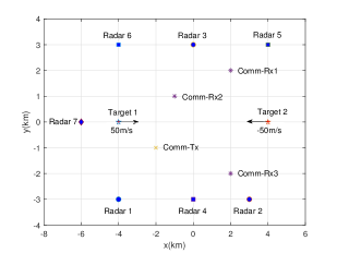
Figure 3: Test scenario of the HRCN. Circle: MMR; square: PAR; diamond: MSR

TABLE I: Initial sampling time and revisit intervals for radars

Radar		1	2	3	4	5	6	7
Target 1	Initial time (s)	2	2.5	3	2.3	3.1	3.5	4
	revisit interval (s)	2	2	2	3	2	2	2
Target 2	Initial time (s)	2	2.5	3	2.6	3.2	3.6	4.2
	revisit interval (s)	2	2	2	3	2	2	2

The deployment of the HRCN is shown in Figure 3. The radar system consists of $N_{cr}=3$ MMRs, $N_{pr}=2$ PARs and $N_{mr}=1$ MSR. The communication system consists of $1$ Tx and $3$ Rx. The radar configurations are shown in Table I.Figure 4 compares the achieved values of $\sum_{q=1}^{Q}1/\text{Tr}\left(\boldsymbol{\Lambda}\boldsymbol{B}_{q,k}^{-1}\boldsymbol{\Lambda}^{T}\right)$ for different allocations, where the optimized allocation is the proposed one, the uniform allocation distributes the resource evenly, and the random allocation is randomly generated, which might be slightly beyond the constraints. It is clear to see that the optimized allocation achieves the largest values over all fusion index. The tracking performances are shown in Figure 5 and Table II, where the RMSE is defined as

$$\text{RMSE}=\sum_{q=1}^{Q}\sqrt{\frac{1}{N_{t}}\left(\sum_{n=1}^{N_{t}}\left\|\boldsymbol{\Lambda}\left(\tilde{\boldsymbol{s}}_{t_{k+1}}^{q\left(n\right)}-\boldsymbol{s}_{t_{k+1}}^{q}\right)\right\|^{2}\right)},$$ (25)

where $N_{t}$ is the number of the Monte Carlo trails. The RMSE of the optimized allocation maintains a low level stably among all intervals and achieves the minimum average RMSE.

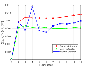
Figure 4: Comparison of the Bayesian CRB based performance.

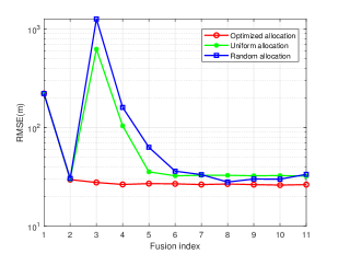
Figure 5: Comparison of the RMSE performance.

TABLE II: Comparison of the Average RMSE For the 10 fusion intervals

Allocation	Optimized	Uniform	Random
RMSE (m)	26.9051	98.9908	171.2642

VI Conclusions

We consider the resource allocation for the heterogeneously-distributed radar and communication network. The allocation aims to minimize the Bayesian CRB based metric of target state estimation subject to some resource budget and communication throughput requirements. The allocation scheme designed by the proposed method shows its efficacy by the numerical experiments.

References

• [1] J. A. Zhang, F. Liu, C. Masouros, R. W. Heath Jr, Z. Feng, L. Zheng, and A. Petropulu, “An overview of signal processing techniques for joint communication and radar sensing,” arXiv preprint arXiv:2102.12780, 2021.
• [2] F. Liu, C. Masouros, A. P. Petropulu, H. Griffiths, and L. Hanzo, “Joint radar and communication design: Applications, state-of-the-art, and the road ahead,” IEEE Transactions on Communications, vol. 68, no. 6, pp. 3834–3862, 2020.
• [3] A. Hassanien, M. G. Amin, E. Aboutanios, and B. Himed, “Dual-function radar communication systems: A solution to the spectrum congestion problem,” IEEE Signal Processing Magazine, vol. 36, no. 5, pp. 115–126, 2019.
• [4] L. Zheng, M. Lops, Y. C. Eldar, and X. Wang, “Radar and communication coexistence: An overview: A review of recent methods,” IEEE Signal Processing Magazine, vol. 36, no. 5, pp. 85–99, 2019.
• [5] B. Li, H. Kumar, and A. P. Petropulu, “A joint design approach for spectrum sharing between radar and communication systems,” in 2016 IEEE International Conference on Acoustics, Speech and Signal Processing (ICASSP), pp. 3306–3310, IEEE, 2016.
• [6] C. Shi, F. Wang, M. Sellathurai, and J. Zhou, “Low probability of intercept based multicarrier radar jamming power allocation for joint radar and wireless communications systems,” IET Radar, Sonar & Navigation, vol. 11, no. 5, pp. 802–811, 2016.
• [7] F. Wang, H. Li, and M. A. Govoni, “Power allocation and co-design of multicarrier communication and radar systems for spectral coexistence,” IEEE Transactions on Signal Processing, vol. 67, no. 14, pp. 3818–3831, 2019.
• [8] L. Zheng, M. Lops, X. Wang, and E. Grossi, “Joint design of overlaid communication systems and pulsed radars,” IEEE Transactions on Signal Processing, vol. 66, no. 1, pp. 139–154, 2017.
• [9] H. Godrich, A. P. Petropulu, and H. V. Poor, “Power allocation strategies for target localization in distributed multiple-radar architectures,” IEEE Transactions on Signal Processing, vol. 59, no. 7, pp. 3226–3240, 2011.
• [10] J. Yan, W. Pu, S. Zhou, H. Liu, and M. S. Greco, “Optimal resource allocation for asynchronous multiple targets tracking in heterogeneous radar networks,” IEEE transactions on signal processing, vol. 68, pp. 4055–4068, 2020.
• [11] J. Yan, J. Dai, W. Pu, H. Liu, and M. Greco, “Target capacity based resource optimization for multiple target tracking in radar network,” IEEE Transactions on Signal Processing, vol. 69, pp. 2410–2421, 2021.
• [12] M. I. Skolnik, “Theoretical accuracy of radar measurements,” IRE Transactions on Aeronautical and Navigational Electronics, no. 4, pp. 123–129, 1960.
• [13] I. Klein and Y. Bar-Shalom, “Tracking with asynchronous passive multisensor systems,” IEEE Transactions on Aerospace and Electronic Systems, vol. 52, no. 4, pp. 1769–1776, 2016.
• [14] J. Yan, B. Jiu, H. Liu, B. Chen, and Z. Bao, “Prior knowledge-based simultaneous multibeam power allocation algorithm for cognitive multiple targets tracking in clutter,” IEEE Transactions on Signal Processing, vol. 63, no. 2, pp. 512–527, 2014.
• [15] M. Razaviyayn, T. Huang, S. Lu, M. Nouiehed, M. Sanjabi, and M. Hong, “Nonconvex min-max optimization: Applications, challenges, and recent theoretical advances,” IEEE Signal Processing Magazine, vol. 37, no. 5, pp. 55–66, 2020.