Nonlinear Helmholtz equations with sign-changing diffusion coefficient

Abstract.

In this paper, we study nonlinear Helmholtz equations with sign-changing diffusion coefficients on bounded domains. The existence of an orthonormal basis of eigenfunctions is established making use of weak $\mathtt{T}$-coercivity theory. All eigenvalues are proved to be bifurcation points and the bifurcating branches are investigated both theoretically and numerically. In a one-dimensional model example we obtain the existence of infinitely many bifurcating branches that are mutually disjoint, unbounded, and consist of solutions with a fixed nodal pattern.

1. Introduction

In this paper, we are interested in nonlinear Helmholtz equations of the form

$$-\operatorname{div}(\sigma(x)\,\nabla u)-\lambda\,c(x)\,u=\kappa(x)\,u^{3}\quad\text{in }\Omega,\qquad u\in\mathrm{H}_{0}^{1}(\Omega)$$ (1)

where $\Omega\subset\mathbb{R}^{N}$ is a bounded domain and the diffusion coefficient $\sigma$ is sign-changing. As we will explain in Section 1.1, such problems occur in the study of time-harmonic wave propagation through metamaterials with negative permeability and nonlinear Kerr-type permittivity. Up to now, the linear theory dealing with the well-posedness of such problems for right-hand sides $f(x)$ instead of $\kappa(x)\,u^{3}$ has been studied to some extent both analytically and numerically [6, 5, 9, 3, 8, 4]. Here, the main difficulty is that the differential operator $u\mapsto-\operatorname{div}(\sigma(x)\,\nabla u)$ is not elliptic on the whole domain $\Omega$. Accordingly, the standard theory for elliptic boundary value problems based on the Lax-Milgram Lemma does not apply. In the papers [6, 5] the (weak) $\mathtt{T}$-coercivity approach was introduced to develop a solution theory for such linear problems. The guiding idea of this method is to require that the strongly indefinite bilinear form

$$\mathrm{H}_{0}^{1}(\Omega)\times\mathrm{H}_{0}^{1}(\Omega)\to\mathbb{R},\qquad(u,v)\mapsto\int_{\Omega}\sigma(x)\,\nabla u\cdot\nabla v\mathop{}\!\mathrm{d}x-\lambda\int_{\Omega}c(x)\,uv\mathop{}\!\mathrm{d}x$$

satisfies the assumptions of the Lax-Milgram Lemma up to some compact perturbation once $v$ is replaced by $\mathtt{T}v$ for some isomorphism $\mathtt{T}:\mathrm{H}_{0}^{1}(\Omega)\to\mathrm{H}_{0}^{1}(\Omega)$. Our intention is to combine this approach with methods from nonlinear analysis to study the nonlinear Helmholtz equation Eq. 1.

Under reasonable assumptions on $\Omega$, $\sigma$, and $c$ our main contributions are the following:

1. There is an orthonormal basis $\left(\phi_{j}\right)_{j\in\mathbb{Z}}$ of $\mathrm{L}^{2}(\Omega)$ that consists of eigenfunctions of the linear differential operator $u\mapsto-{c(x)}^{-1}\operatorname{div}(\sigma(x)\,\nabla u)$. The corresponding eigenvalue sequence $\left(\lambda_{j}\right)_{j\in\mathbb{Z}}$ is unbounded from above and from below. Moreover, the eigenfunctions are dense in $\mathrm{H}_{0}^{1}(\Omega)$.

2. If $\kappa\in\mathrm{L}^{\infty}(\Omega)$ then each of the eigenvalues $\lambda_{j}$ is a bifurcation point for Eq. 1 with respect to the trivial solution family $\left\{(0,\lambda)\ {:}\ \lambda\in\mathbb{R}\right\}$. By definition, this means that for all $j\in\mathbb{Z}$ there is a sequence $\left(u_{j}^{n},\lambda_{j}^{n}\right)_{n\in\mathbb{N}}\subset\mathrm{H}_{0}^{1}(\Omega)\setminus\{0\}\times\mathbb{R}$ of nontrivial solutions such that $(u_{j}^{n},\lambda_{j}^{n})\to(0,\lambda_{j})$ in $\mathrm{H}_{0}^{1}(\Omega)\times\mathbb{R}$ as $n\to\infty$. Our numerical illustrations in Section 3 indicate that these solutions may be located on a smooth and unbounded curve in $\mathrm{H}_{0}^{1}(\Omega)\times\mathbb{R}$ going through the point $(0,\lambda_{j})$. We can also prove this for some one-dimensional model problem.

3. In a one-dimensional case, for any given $\lambda\in\mathbb{R}$ there are infinitely many nontrivial solutions for Eq. 1 provided that $\kappa\in\mathrm{L}^{\infty}(\Omega)$ is uniformly positive or uniformly negative. This result is obtained using variational methods instead of bifurcation theory.

A few comments regarding Items i, ii and iii are in order. As to i, the existence of an orthonormal basis of eigenfunctions in $\mathrm{L}^{2}(\Omega)$ may be considered as a known fact in view of [8, Section 1]. However, we could not find a reference in the literature that covers our setting, so we briefly review this in Section 4. On the other hand, the Weyl law asymptotics seem to be new. Our proofs rely on the weak $\mathtt{T}$-coercivity approach developed in [6, 5]. Under this assumption, the linear theory turns out to be analogous to the linear (Fredholm) Theory for elliptic boundary value problems. The construction of isomorphisms $\mathtt{T}:\mathrm{H}_{0}^{1}(\Omega)\to\mathrm{H}_{0}^{1}(\Omega)$, however, is a research topic on its own and depends on the precise setting, notably on the nature of the interface where the sign of $\sigma$ jumps, see, e.g. [5, 4].

Our main bifurcation theoretical results from ii also rely on the functional analytical framework given by the weak $\mathtt{T}$-coercivity approach. The task is to detect nontrivial solutions of Eq. 1 that bifurcate from the trivial solution family. Being given the linear theory and the Implicit Function Theorem, one knows that such bifurcations can only occur at $\lambda=\lambda_{j}$ for some $j\in\mathbb{Z}$. To prove the occurrence of bifurcations we resort to variational bifurcation theory (see below for references). Here the main difficulty comes from the fact that the associated energy functional

$$\Psi_{\lambda}(u)\coloneqq\frac{1}{2}\int_{\Omega}\sigma(x)\left\lvert\nabla u(x)\right\rvert^{2}\mathop{}\!\mathrm{d}x-\frac{\lambda}{2}\int_{\Omega}c(x)\,{u(x)}^{2}\mathop{}\!\mathrm{d}x-\frac{1}{4}\int_{\Omega}\kappa(x){u(x)}^{4}\mathop{}\!\mathrm{d}x$$ (2)

is strongly indefinite due to the sign change of $\sigma$. Strong indefiniteness means that the quadratic part of $\Psi_{\lambda}$ is positive definite on an infinite-dimensional subspace of $\mathrm{H}_{0}^{1}(\Omega)$, and it is negative definite on another infinite-dimensional subspace. As a consequence, standard results in this area going back to Böhme [2, Satz II.1], Marino [18], and Rabinowitz [23, Theorem 11.4] do not apply. Instead, we demonstrate how to apply the more recent variational bifurcation theory developed by Fitzpatrick, Pejsachowicz, Recht, Waterstraat [14, 21]. Better results are obtained for eigenvalues with odd geometric multiplicity, which is based on Rabinowitz’ Global Bifurcation Theorem [22]. In our one-dimensional model case we significantly improve and numerically illustrate our bifurcation results with the aid of bifurcation diagrams (Section 3). The latter provide a qualitative picture of the bifurcation scenario given that each point in such a diagram corresponds to $(\lambda,\left\lVert u\right\rVert)$ where $(u,\lambda)$ solves Eq. 1.

As to iii, the strong indefiniteness of $\Psi_{\lambda}$ also makes it harder to prove the existence of critical points. Note that critical points $u\in\mathrm{H}_{0}^{1}(\Omega)$ satisfy $\Psi_{\lambda}^{\prime}(u)=0$, which is equivalent to Eq. 1. In the case of positive diffusion coefficients, the Symmetric Mountain Pass Theorem [1, Theorem 10.18] applies and yields infinitely many nontrivial solutions. In the context of strongly indefinite functionals, an analogous result was established only recently by Szulkin and Weth [24, Section 5]. We will show how to apply their abstract results under reasonable extra assumptions in order to obtain infinitely many nontrivial solutions of Eq. 1 for any given $\lambda\in\mathbb{R}$ assuming $\kappa\geq\alpha>0$ or $\kappa\leq-\alpha<0$.

Before commenting on the physical background of Eq. 1 we wish to emphasize that our main goal is to bring (weak) $\mathtt{T}$-coercivity theory and nonlinear analysis together. Accordingly, we do not aim for the most general assumptions for our results to hold true. For instance, we avoid technicalities related to the regularity of the interface where the sign of $\sigma$ jumps. Similarly, we content ourselves with the special nonlinearity $\kappa(x)\,u^{3}$. Only little effort is needed to generalize our bifurcation results as well as our variational existence results to more general nonlinearities in all space dimensions $N\geq 1$.

1.1. Physical motivation

We comment on the physical background of Eq. 1. The propagation of electromagnetic waves with a fixed temporal frequency parameter $\omega\in\mathbb{R}$ is governed by the time-harmonic Maxwell’s equations

$$i\omega D-\operatorname{\mathbf{curl}}H=0\qquad\text{and}\qquad i\omega B+\operatorname{\mathbf{curl}}E=0.$$ (3)

Here, charges and currents are assumed to be absent. The symbols $E,D:\mathbb{R}^{3}\to\mathbb{C}^{3}$ denote the electric field and the electric induction and $H,B:\mathbb{R}^{3}\to\mathbb{C}^{3}$ represent the magnetic field and the magnetic induction, respectively. In nonlinear Kerr media the constitutive relations between these fields are given by

$$D=\varepsilon(x)\,E+\chi(x)\,|E|^{2}E\qquad\text{and}\qquad B=\mu(x)\,H$$ (4)

where $\varepsilon,\mu,\chi$ are real-valued, see [7, Chapter 4]. In physics, these quantities are called permittivity, permeability and third-order susceptibility of the given medium, respectively. Plugging in this ansatz into Eq. 3 one finds

$$\operatorname{\mathbf{curl}}\left({\mu(x)}^{-1}\operatorname{\mathbf{curl}}E\right)=\omega^{2}\varepsilon(x)\,E+\omega^{2}\chi(x)\,|E|^{2}E.$$ (5)

Now we assume that the propagation of electromagnetic waves is considered in a closed waveguide $\Omega\times\mathbb{R}$ having a bounded cross-section $\Omega\subset\mathbb{R}^{2}$ and all material parameters only depend on the cross-section variable. With an abuse of notation, this means $\mu(x)=\mu(y)$, $\varepsilon(x)=\varepsilon(y)$, and $\chi(x)=\chi(y)$ where $x=(y,z)\in\Omega\times\mathbb{R}$. This is a natural assumption for the modelling of layered cylindrical waveguides. If then the electric field is of the special form $E(x)=(0,0,u(y))$ with $u$ real-valued, we infer

$$-\operatorname{div}({\mu(y)}^{-1}\,\nabla u)-\omega^{2}\varepsilon(y)\,u=\omega^{2}\chi(y)\,u^{3}\quad\text{in }\Omega,\qquad u\in\mathrm{H}_{0}^{1}(\Omega),$$

which corresponds to Eq. 1 in the two-dimensional case. For complex-valued $u$ the nonlinearity is given by $|u|^{2}u$. Sign-changing diffusion coefficients $\sigma(y)\coloneqq{\mu(y)}^{-1}$ may occur if one of the layers of the waveguide is filled with a negative-index metamaterial (NIM) where the permeability $\mu$ may be negative, see, e.g., [20]. Note that any such solution $u$ determines $E,D,B,H$ via Eqs. 5 and 4. We mention that one may equally solve for the magnetic field, which leads to Helmholtz-type problems with nonlinear (i.e. solution-dependent) and possibly sign-changing diffusion coefficients.

1.2. Notation

In the following, we equip the Hilbert spaces $\mathrm{H}_{0}^{1}(\Omega)$ and $\mathrm{L}^{2}(\Omega)$ with the inner products

$$\left\langle u,v\right\rangle_{|\sigma|}\coloneqq\int_{\Omega}\left\lvert\sigma(x)\right\rvert\,\nabla u\cdot\nabla v\mathop{}\!\mathrm{d}x,\qquad\text{and}\qquad\left(u,v\right)_{c}\coloneqq\int_{\Omega}c(x)\,uv\mathop{}\!\mathrm{d}x,$$

respectively. Our assumptions on $\Omega$, $c$, and $\sigma$ will imply that the associated norms $\left\lVert\cdot\right\rVert_{|\sigma|}$ and $\left\lVert\cdot\right\rVert_{c}$ are equivalent to the standard norms on these spaces. Moreover, we introduce the bilinear form

$$a:\mathrm{H}_{0}^{1}(\Omega)\times\mathrm{H}_{0}^{1}(\Omega)\to\mathbb{R},\quad(u,v)\mapsto\int_{\Omega}\sigma(x)\,\nabla u\cdot\nabla v\mathop{}\!\mathrm{d}x.$$

1.3. Outline

The paper is organized as follows. Section 2 contains a mathematically rigorous statement of our main results dealing with bifurcations for Eq. 1 from the trivial solution family. These results are illustrated numerically in Section 3 with the aid of bifurcation diagrams. Those illustrate the evolution of solutions along the branches as well the global behavior of the latter. In Section 4, we set up the linear theory that we need to prove our main bifurcation theoretical results in Section 5. Finally, Section 6 contains further existence results for nontrivial solutions of Eq. 1 obtained by a variational approach. The proof is based on the Critical Point Theory from [24, Chapter 4].

2. Main results

We now come to the precise formulation of our main results for Eq. 1, i.e.,

$$-\operatorname{div}(\sigma(x)\,\nabla u)-\lambda\,c(x)\,u=\kappa(x)u^{3}\quad\text{in }\Omega,\qquad u\in\mathrm{H}_{0}^{1}(\Omega).$$

Here, $\Omega$ and the coefficient functions $\sigma$, $c$, $\kappa$ will be chosen as follows:

Assumption (A).

1. $\Omega\subset\mathbb{R}^{N}$ for $N\in\{1,2,3\}$ is a bounded domain and there are nonempty open subsets $\Omega_{+},\Omega_{-}\subset\Omega$ such that $\overline{\Omega_{+}\cup\Omega_{-}}=\overline{\Omega}$ and $\Omega_{+}\cap\Omega_{-}=\varnothing$.

2. $\sigma>0$ on $\Omega_{+}$, $\sigma<0$ on $\Omega_{-}$ and $\left\lvert\sigma\right\rvert+\left\lvert\sigma\right\rvert^{-1}\in\mathrm{L}^{\infty}(\Omega)$.

3. $c\in\mathrm{L}^{\infty}(\Omega)$ with $c(x)\geq\alpha>0$ for almost all $x\in\Omega$.

4. $\kappa\in\mathrm{L}^{\infty}(\Omega)$.

Assumption (B).

There is a bounded linear invertible operator $\mathtt{T}:\mathrm{H}_{0}^{1}(\Omega)\to\mathrm{H}_{0}^{1}(\Omega)$ such that the bilinear form $(u,v)\mapsto a(u,\mathtt{T}v)+\left\langle\mathtt{K}u,v\right\rangle_{|\sigma|}$ is continuous and coercive on $\mathrm{H}_{0}^{1}(\Omega)\times\mathrm{H}_{0}^{1}(\Omega)$ for some compact operator $\mathtt{K}:\mathrm{H}_{0}^{1}(\Omega)\to\mathrm{H}_{0}^{1}(\Omega)$.

Later, in 4.5, we show that Assumptions (A) and (B) ensure the existence of an orthonormal basis $\left(\phi_{j}\right)_{j\in\mathbb{Z}}$ of $\left(\mathrm{L}^{2}(\Omega),\left(\cdot,\cdot\right)_{c}\right)$ consisting of eigenfunctions associated to the linear differential operator $u\mapsto-{c(x)}^{-1}\operatorname{div}(\sigma(x)\,\nabla u)$ appearing in Eq. 1. Due to the sign-change of $\sigma$ the corresponding sequence of eigenvalues $\left(\lambda_{j}\right)_{j\in\mathbb{Z}}$ can be indexed in such a way that $\lambda_{j}\to\pm\infty$ holds as $j\to\pm\infty$. In 2.1 below we show that nontrivial solutions of Eq. 1 bifurcate from the trivial branch $\left\{(0,\lambda)\ {:}\ \lambda\in\mathbb{R}\right\}$ at any of these eigenvalues. If the eigenvalue comes with an odd-dimensional eigenspace, we even find that the bifurcating nontrivial solutions lie on connected sets $\mathcal{C}_{j}\subset\mathrm{H}_{0}^{1}(\Omega)\times\mathbb{R}$ that are unbounded or return to the trivial solution branch $\left\{(0,\lambda)\ {:}\ \lambda\in\mathbb{R}\right\}$ at some other bifurcation point. As in [22], for any given $j\in\mathbb{Z}$, the set $\mathcal{C}_{j}$ is defined as the connected component of $(0,\lambda_{j})$ in $\mathcal{S}$, which in turn is defined as the closure of all nontrivial solutions of Eq. 1 in the space $\mathrm{H}_{0}^{1}(\Omega)\times\mathbb{R}$. Our first main result reads as follows:

Theorem 2.1.

Assume (A) and (B). Let $\left(\lambda_{j}\right)_{j\in\mathbb{Z}}$ denote the unbounded sequence of eigenvalues from 4.5. Then each $(0,\lambda_{j})$ is a bifurcation point for Eq. 1. If $\lambda_{j}$ has odd geometric multiplicity, then the connected component $\mathcal{C}_{j}$ in $\mathcal{S}$ containing $(0,\lambda_{j})$ satisfies Rabinowitz’ alternative:

1. $\mathcal{C}_{j}$ is unbounded in $\mathrm{H}_{0}^{1}(\Omega)\times\mathbb{R}$ or

2. $\mathcal{C}_{j}$ contains another trivial solution $(0,\lambda_{k})$ with $k\neq j$.

Remark 2.2.

1. In Assumption (A) we may as well assume $c(x)\leq-\alpha<0$; it suffices to replace $(c,\lambda)$ by $(-c,-\lambda)$. On the other hand we cannot assume $c$ to be sign-changing since we will need that $\left(\cdot,\cdot\right)_{c}$ is an inner product on $\mathrm{L}^{2}(\Omega)$. In 4.6 (c), we show that one cannot expect our results to hold for general sign-changing $c\in\mathrm{L}^{\infty}(\Omega)$.

2. We need not require a priori smoothness properties of $\Omega$ or the interface $\Gamma\coloneqq\overline{\Omega_{+}}\cap\overline{\Omega_{-}}$, but imposing those are natural when it comes to verify Assumption (B), see the Theorems 2.1, 3.1, 3.3, 3.7, 3.10 from [5]. It is known that Assumption (B) does not always hold, for example in 2D if $\sigma_{-}/\sigma_{+}\in\left[-3,-\frac{1}{3}\right]$ and the interface $\Gamma$ has a right angle corner, see [5, 3].

We strengthen our result in some 1D model example where we can show the following:

• Assumptions (A) and (B) are satisfied.

• The eigenvalues $(\lambda_{j})$ are simple and in particular have odd geometric multiplicity.

• The eigenpairs $(\phi_{j},\lambda_{j})$ are almost explicitly known.

• The case (II) in Rabinowitz’ Alternative is ruled out, hence all $\mathcal{C}_{j}$ are unbounded.

The setting is as follows: Assume that $\overline{\Omega}=\overline{\Omega_{-}}\cup\overline{\Omega_{+}}$ is an interval with precisely two non-void sub-intervals $\Omega_{-}=(a_{-},0)$ and $\Omega_{+}=(0,a_{+})$ with $a_{-}<0<a_{+}$. The coefficient function $c$ and $\sigma$ satisfy $c(x)=c_{\pm}$ resp. $\sigma(x)=\sigma_{\pm}$ on $\Omega_{\pm}$ where $c_{\pm}>0$ and $\sigma_{+}>0>\sigma_{-}$ are constants. For such domains and coefficients we consider the nonlinear problem

$$-\frac{\mathop{}\!\mathrm{d}}{\mathop{}\!\mathrm{d}x}\left(\sigma(x)\,u^{\prime}\right)-\lambda c(x)\,u=\kappa(x)u^{3}\quad\text{in }\Omega,\qquad u\in\mathrm{H}_{0}^{1}(\Omega).$$ (6)

Corollary 2.3.

Assume that $\Omega$, $c$, $\sigma$ are as above, and $\kappa\in\mathrm{L}^{\infty}(\Omega)$. Let ${(\lambda_{j})}_{j\in\mathbb{Z}}$ denote the unbounded sequence of simple eigenvalues from 4.5 ordered according to $\ldots<\lambda_{-2}<\lambda_{-1}<0<\lambda_{1}<\lambda_{2}<\ldots$ and $\lambda_{-1}<\lambda_{0}<\lambda_{1}$ with

$$\lambda_{0}<0\;\Leftrightarrow\;\frac{\sigma_{+}a_{-}}{a_{+}\sigma_{-}}<1,\qquad\lambda_{0}=0\;\Leftrightarrow\;\frac{\sigma_{+}a_{-}}{a_{+}\sigma_{-}}=1.\qquad\lambda_{0}>0\;\Leftrightarrow\;\frac{\sigma_{+}a_{-}}{a_{+}\sigma_{-}}>1,$$

Then the connected component $\mathcal{C}_{j}\subset\mathrm{H}_{0}^{1}(\Omega)\times\mathbb{R}$ in $\mathcal{S}$ containing $(0,\lambda_{j})$ is unbounded, and we have $\mathcal{C}_{j}\cap\mathcal{C}_{k}=\emptyset$ for $j\neq k$. All $(u,\lambda)\in\mathcal{C}_{j}$ with $u\neq 0$ have the following property:

1. If $j\leq-1$ then $u$ has $|j|$ interior zeros in $\Omega_{-}$ and satisfies $\left\lvert u^{\prime}\right\rvert>0$ on $\overline{\Omega_{+}}$.

2. If $j=0$ then $u$ has no interior zeros in $\Omega$ and satisfies $\left\lvert u^{\prime}\right\rvert>0$ on $\overline{\Omega_{\pm}}$.

3. If $j\geq 1$ then $u$ has $j$ interior zeros in $\Omega_{+}$ and satisfies $\left\lvert u^{\prime}\right\rvert>0$ on $\overline{\Omega_{-}}$.

The seemingly complicated ordering of the eigenvalues is exclusively motivated by the nodal patterns given by Items i, ii and iii. Here, $\left\lvert u^{\prime}\right\rvert>0$ on $\overline{\Omega_{\pm}}$ means that the continuous extension of $\left\lvert u^{\prime}\right\rvert:\Omega_{\pm}\to\mathbb{R}$ to $\overline{\Omega_{\pm}}$ is positive. We stress that nontrivial solutions $u$ are smooth away from the interface $x=0$ and continuous at $x=0$, but they are not continuously differentiable at this point. In fact, $\sigma u^{\prime}$ is continuous on $\overline{\Omega}$ so that $u^{\prime}(0)$ does not exist in the classical sense. In the following Section 3 our results are illustrated with the aid of bifurcation diagrams.

3. Visualization of bifurcation results via PDE2path

In this section, we illustrate our theoretical results of 2.1 and 2.3 with numerical bifurcation diagrams. These diagrams show the value of $\lambda$ on the $x$-axis and the $\mathrm{L}^{2}$-norm of solutions $u$ for that $\lambda$ on the $y$-axis. Thereby, (numerical) bifurcation diagrams allow to get an overview of the “structure” of solutions and, in particular, to visualize the connected components $\mathcal{C}_{j}$ of 2.1. The results were obtained with the package pde2path [25, 11], version 2.9b and using Matlab 2018b. The code to reproduce the numerical results is available on Zenodo with DOI 10.5281/zenodo.5707422.

3.1. One-dimensional example

We consider $\Omega=(-5,5)$ with $\Omega_{-}=(-5,0)$, $\Omega_{+}=(0,5)$ and $c\equiv 1$. The diffusion coefficient $\sigma$ is chosen piecewise constant, set $\sigma_{+}=1$ and compare two different values for $\sigma_{-}$, namely $\sigma_{-}\in\{-2,-1.005\}$. We consider Eq. 6 in this special case, i.e.,

$$-\frac{\mathop{}\!\mathrm{d}}{\mathop{}\!\mathrm{d}x}\big{(}\sigma(x)\,u^{\prime}\big{)}-\lambda u=u^{3}\quad\text{in }\Omega,\qquad u\in H_{0}^{1}(\Omega).$$

We choose a tailored finite element mesh which is refined close to $\Gamma=\{0\}$ in the following way. We start with an equidistant mesh with $h=2^{-9}$, i.e., $\Omega$ is divided into $5120$ equal subintervals. Then, we refine all intervals which are closer than $0.1$ to $\Gamma$ five times by halving them. This finally means that intervals close to $\Gamma$ are only $2^{-14}$ long. We point out that this finely resolved mesh is required to faithfully represent the interface behavior at $\Gamma=\{0\}$, especially for $\sigma_{-}=-1.005$. An insufficient mesh resolution does not only influence the numerical quality of the eigenfunctions or solutions along the branches, but also the (qualitative picture) of the bifurcation diagram. We validated our results by assuring that a further refinement of the mesh (halving all intervals) leads to the same results and conclusions.

3.1.1. Bifurcation diagrams and eigenfunctions for different contrasts

We first investigate whether $\frac{\sigma_{+}}{\sigma_{-}}\approx-1$ influences the bifurcation diagrams. For this, we allow $\lambda$ to vary in the interval $[-10,15]$. The bifurcation diagrams are depicted in Fig. 1 for $\sigma_{-}=-2$ and $\sigma_{-}=-1.005$.

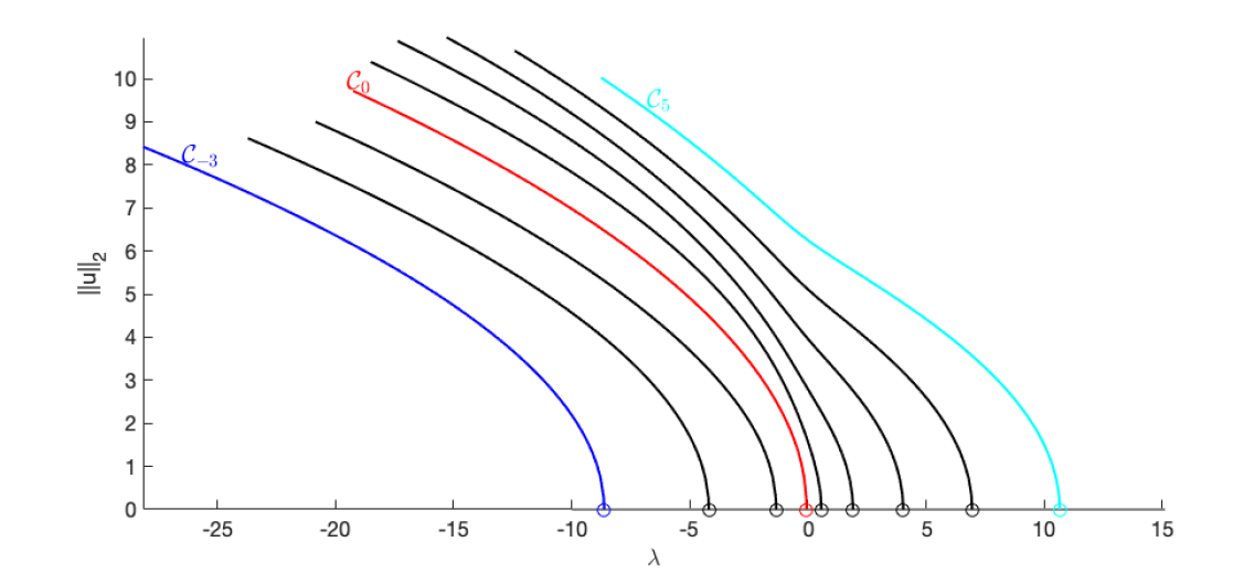
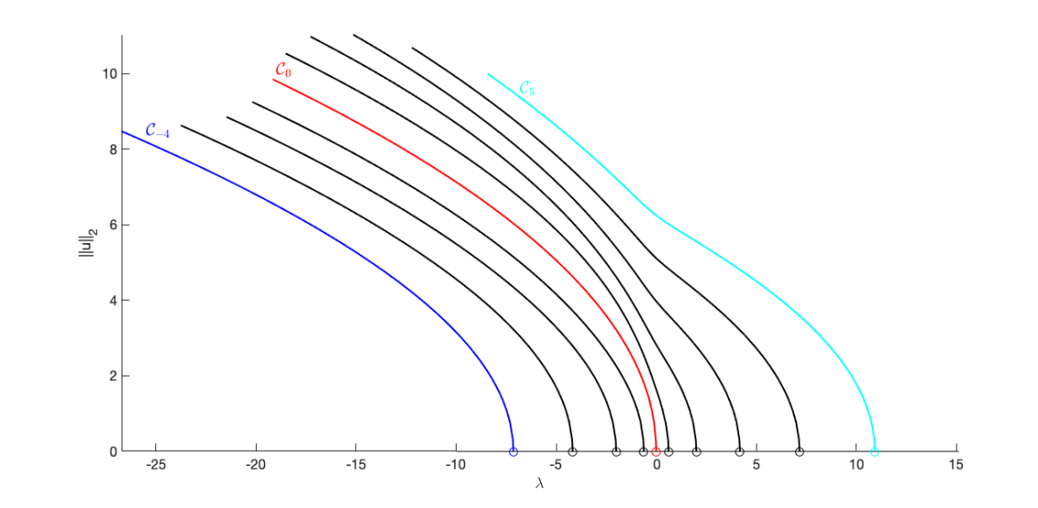
Figure 1. Bifurcation diagrams for $\sigma_{-}=-2$ (top) and $\sigma_{-}=-1.005$ (bottom).

Qualitatively, they are quite similar with clearly separated, apparently unbounded branches without secondary bifurcations. Note that the bending direction of the branches to the left is determined by the sign of the nonlinear term and can be predicted by the bifurcation formulae (I.6.11) in [15]. The first striking phenomenon due to the sign-changing coefficient is the occurrence of eigenvalues and, hence, bifurcation points, with negative value. In fact, for sign-changing $\sigma$, there are two families of eigenvalues diverging to $\pm\infty$, see 2.1. We use the following labeling of branches (cf. Fig. 1): The branch starting closest to zero is labeled as $\mathcal{C}_{0}$ and the branches for negative and positive bifurcation points are labeled as $\mathcal{C}_{-i}$ and $\mathcal{C}_{i}$ with $i\in\mathbb{N}$, respectively. The absolute value of $i$ increases as $|\lambda|\to\infty$. In our setting this labeling of the branches is consistent with the notation introduced in Section 4.

Besides the eigenvalues, we also study the eigenfunctions by considering the solutions at the first point of each branch in Fig. 2. We display the branch name according to Fig. 1 as well as the value of $\lambda$ at the bifurcation point.

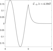
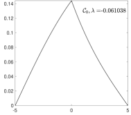
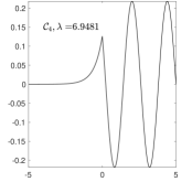
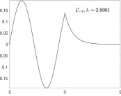
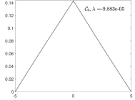
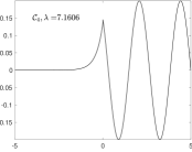
Figure 2. First solution on branches $\mathcal{C}_{-2}$, $\mathcal{C}_{0}$ and $\mathcal{C}_{4}$ (from left to right) for $\sigma_{-}=-2$ (top row) as well as $\sigma_{-}=-1.005$ (bottom row).

As (partly) expected from [8], we make the following observations. Firstly, the solutions are concentrated (w.r.t. the $\mathrm{L}^{2}$-norm) on the “oscillatory part”, which is $\Omega_{-}$ for negative eigenvalues (left column of Fig. 2) and $\Omega_{+}$ for positive eigenvalues (right column of Fig. 2). The eigenvalue closest to zero (from which $\mathcal{C}_{0}$ emanates) plays a special role (middle column of Fig. 2). Secondly, with increasing $|\lambda|$, the number of maxima and minima increases as one observes also for the eigenfunctions of the Laplacian. Thirdly, the transmission condition at $\Gamma$ requires the (normal) derivative of $u$ to change sign, such that the solutions have a “tip” at the interface. Taking a closer look at the bifurcation values and the corresponding solutions in Fig. 2, we note that $\mathcal{C}_{0}$ starts much closer to zero for $\sigma_{-}=-1.005$ than for $\sigma_{-}=-2$. This illustrates the theoretical expectation that due to the symmetry of the domain $\Omega$, we have an eigenvalue approaching zero for the contrast going to $-1$. Moreover, we observe a certain shrinking of the negative bifurcation values towards zero when the contrast approaches $-1$.

3.1.2. Patterns of solutions along branches

We now take a closer look at how solutions evolve along branches — depending on whether the corresponding bifurcation value is negative, close to zero or positive. According to the previous discussion, we focus on $\sigma_{-}=-1.005$ in the following because it shows the phenomena in a particularly pronounced form and is close to the interesting “critical” contrast of $-1$. In general, we observe that a certain limit pattern or profile of the solution evolves on each branch which remains qualitatively stable (values of maxima, minima and plateaus of course change with $\lambda$). As example for a negatively indexed bifurcation branch away from zero, we consider $\mathcal{C}_{-2}$, cf. Fig. 1. The first, $50$th, and $100$th solution on the branch are depicted in Fig. 3. As described above, the solution concentrates in $\Omega_{-}$ where it oscillates, while it decays exponentially in $\Omega_{+}$. This profile remains stable over the branch, but we note that the maxima and minima become wider along the branch. This widening of the extrema in $\Omega_{-}$ is also noted for the other branches emanating from a negative bifurcation point. Yet, the more oscillations occur for the branches as $\lambda\to-\infty$, the less pronounced the effect becomes because we have more extrema over the same interval. We emphasize that this effect of widening extrema is specific to the sign-changing case and especially to bifurcations starting at negative $\lambda$.

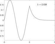
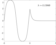
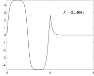
Figure 3. Solution at first, $50$th, $100$th point of $\mathcal{C}_{-2}$ for $\sigma_{-}=-1.005$.

As an example for a positively indexed bifurcation branch away from zero, we study the branch $\mathcal{C}_{5}$, cf. Fig. 1. As expected, we observe in Fig. 4 that the first solution concentrates on $\Omega_{+}$, where it oscillates as typical for an eigenfunction of the Laplacian, and shows an exponential decay in $\Omega_{-}$. The oscillatory pattern in $\Omega_{+}$ is preserved along the branch. The behavior in $\Omega_{-}$ changes when $\lambda$ gets negative: Instead of an exponential decay to zero, we now see an exponential decay to (almost) a plateau (with value $\pm\sqrt{-\lambda}$) and a sharp transition to the zero boundary value. Once this pattern is established, it remains stable as well. This appearance of a plateau different from zero is also a specific phenomenon of the sign-changing case.

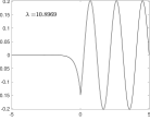
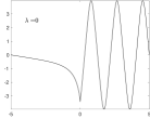
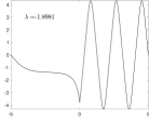
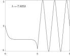
Figure 4. Solution at first, $60$th, $70$th, $100$th point of $\mathcal{C}_{5}$ for $\sigma_{-}=-1.005$.

The occurrence of a plateau in $\Omega_{-}$ is also observed in Fig. 5 for the branch $\mathcal{C}_{0}$ closest to zero, cf. Fig. 1. While the first solution has a similar shape in $\Omega_{+}$ and $\Omega_{-}$ with a linear decay in each subdomain, the ensuing solutions on the branch quickly evolve a plateau in $\Omega_{-}$ and an exponential decay in $\Omega_{+}$. This pattern then remains stable along the branch. All in all, we observe a certain stability of profiles along branches. The form of the profiles depends on where the bifurcation starts. Moreover, we always recognize a concentration to the oscillatory part and further the establishment of plateaus different from zero in $\Omega_{-}$. As already emphasized, both effects are specific to the sign-changing case. This qualitative description of solutions seems to transfer to other contrasts, but the bifurcation points closest to zero and the (quantitative) decay in $\Omega_{\pm}$ significantly depend on the contrast as already discussed above.

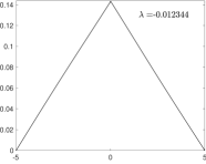
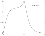
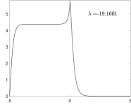
Figure 5. Solution at first, $10$th, $100$th point of $\mathcal{C}_{0}$ for $\sigma_{-}=-1.005$.

3.2. Two-dimensional example

We consider $\Omega={(-2,2)}^{2}$ with $\Omega_{-}=(-2,0)\times(-2,2)$, as well as $\sigma_{+}=1$ and $\sigma_{-}=-2$. The finite element mesh is tailored similar to the one-dimensional experiment: We start with a symmetric uniform mesh with $h=2^{-4}$ and refine three times all elements in the strip of width $0.1$ around the interface $\Gamma=\{0\}\times(-2,2)$. Note that our mesh satisfies the symmetry conditions laid out in [4], which may be challenging in more complicated geometries though.

We focus on the behavior of solutions in this numerical experiment and let $\lambda$ vary in $[-12,15]$. There are three different types of eigenfunctions either concentrated on $\Omega_{-}$, on $\Gamma$, or on $\Omega_{+}$. In contrast to the one-dimensional case, there are several different eigenfunctions concentrated on $\Gamma$. As before, the eigenfunctions concentrated on $\Omega_{-}$ or $\Gamma$ are associated with negative values of $\lambda$. In Figs. 6, 7 and 8, we show the evolution of solutions along a branch for each of the three types described above.

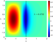
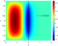
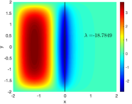
Figure 6. Solution at first, $25$th, and $50$th point of branch associated with an eigenfunction concentrated on $\Omega_{-}$.

Similar to the one-dimensional case, we observe a widening of the extrema along the branch with concentration in $\Omega_{-}$ in Fig. 6, in particular in the $y$-direction.

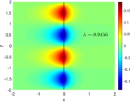
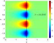
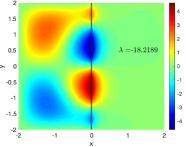
Figure 7. Solution at first, $25$th, and $50$th point of branch associated with an eigenfunction concentrated on $\Gamma$.

Furthermore, plateaus in $\Omega_{-}$ evolve for negative $\lambda$ in Figs. 7 and 8. Due to the second space dimension in the problem, we can have two (or more) different plateaus evolving in $\Omega_{-}$. In Fig. 7 for a branch with concentration on $\Gamma$, we note that the plateaus and the transition between them seems to slightly change the oscillatory pattern on $\Gamma$ as well. While the two maxima have almost the same height for the first and $25$th point (Fig. 7 left and middle), one maximum becomes predominant for the $50$th point on the branch, see Fig. 7 right.

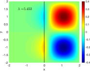
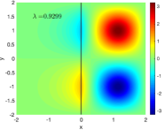
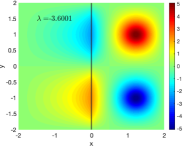
Figure 8. Solution at first, $25$th, and $50$th point of branch associated with an eigenfunction concentrated on $\Omega_{+}$.

Finally, for Fig. 8 and a branch with concentration on $\Omega_{+}$, we emphasize that the solution in $\Omega_{+}$ evolves like a solution of the standard Laplacian along a branch. In particular, the extrema become thinner, i.e., more spatially localized, which should be contrasted with solutions concentrated in $\Omega_{-}$ in Fig. 6.

4. Linear Theory

In this section we want to describe the linear theory for weakly $\mathtt{T}$-coercive problems. As pointed out earlier, this theory is essentially well-known [6, 5, 8]. Since it is short and rather self-contained, we provide the details here, which will moreover allow us to fix the required notation. Furthermore, we prove some Weyl law asymptotics that have not appeared in the literature yet. We want to deal with linear problems of the form

$$\int_{\Omega}\sigma(x)\,\nabla u\cdot\nabla v\mathop{}\!\mathrm{d}x-\lambda\int_{\Omega}c(x)\,u\,v\mathop{}\!\mathrm{d}x=F(v),\qquad\forall v\in\mathrm{H}_{0}^{1}(\Omega).$$ (7)

The a priori unknown solution $u$ is to be found in the Sobolev space $\mathrm{H}_{0}^{1}(\Omega)$ and the coefficient functions $\sigma$ and $c$ are assumed to satisfy the conditions (A) and (B) from Section 1. To develop a solution theory for the variational problem Eq. 7 both in $\mathrm{H}_{0}^{1}(\Omega)$ and $\mathrm{L}^{2}(\Omega)$ we assume $F\in\mathrm{H}^{-1}(\Omega)=\mathrm{H}_{0}^{1}(\Omega)^{\prime}$. We may rewrite Eq. 7 as

$$a(u,v)-\lambda\left(u,v\right)_{c}=F(v)\qquad\forall v\in\mathrm{H}_{0}^{1}(\Omega).$$

We introduce the bounded linear operator $A:\mathrm{H}_{0}^{1}(\Omega)\to\mathrm{H}_{0}^{1}(\Omega)$ and the compact linear operator $C:\mathrm{H}_{0}^{1}(\Omega)\to\mathrm{H}_{0}^{1}(\Omega)$ via the relations

$$\left\langle Au,v\right\rangle_{|\sigma|}\coloneqq a(u,v)\quad\text{and}\quad\left\langle Cu,v\right\rangle_{|\sigma|}\coloneqq\left(u,v\right)_{c}\qquad\text{for }u,v\in\mathrm{H}_{0}^{1}(\Omega).$$ (8)

This is possible by Riesz’ Representation Theorem and $\sigma,c\in\mathrm{L}^{\infty}(\Omega)$, see Assumption (A). We will also use that the operator $C$ can be written as $C=\tilde{C}\iota$ where $\tilde{C}:\mathrm{L}^{2}(\Omega)\to\mathrm{H}_{0}^{1}(\Omega)$ is a bounded linear operator and $\iota:\mathrm{H}_{0}^{1}(\Omega)\to\mathrm{L}^{2}(\Omega)$ denotes the embedding operator which is compact by the Rellich-Kondrachov Theorem.

Proposition 4.1.

Under Assumptions (A) and (B), there exists $\ell\in\mathbb{R}$ such that the bounded linear operator $A_{\ell}\coloneqq A+\ell C:\mathrm{H}_{0}^{1}(\Omega)\to\mathrm{H}_{0}^{1}(\Omega)$ is self-adjoint and invertible.

Proof.

The self-adjointness follows from $a(u,v)=a(v,u)$ and

$$\left\langle Cu,v\right\rangle_{|\sigma|}=\left(u,v\right)_{c}=\left(v,u\right)_{c}=\left\langle Cv,u\right\rangle_{|\sigma|}=\left\langle u,Cv\right\rangle_{|\sigma|}$$

for all $u,v\in\mathrm{H}_{0}^{1}(\Omega)$. To prove the invertibility of $A_{\ell}$ define the family of operators $z\mapsto A_{z}\coloneqq A+zC$ for $z\in\mathbb{C}$ on the complex Hilbert space $\mathrm{H}_{0}^{1}(\Omega;\mathbb{C})$. The bilinear form associated with $A_{z}$ is given by $(u,v)\mapsto a(u,v)+z\left(u,v\right)_{c}$. From Assumption (B) and the Lax-Milgram Lemma we infer that $\mathtt{T}^{*}A+\mathtt{K}$ is invertible. Moreover, we have the relation

$$A_{z}=\left(\mathtt{T}^{*}\right)^{-1}\left[\mathtt{T}^{*}A+\mathtt{K}\right]-\left(\mathtt{T}^{*}\right)^{-1}\mathtt{K}+zC.$$

Here, the first summand is invertible while the other two summands are compact. Therefore, $\left\{A_{z}\ {:}\ z\in\mathbb{C}\right\}$ is a holomorphic family of zero index Fredholm operators. For $z\in\mathbb{C}\setminus\mathbb{R}$, the operator $A_{z}$ is injective. Indeed, if $A_{z}u=0$ then $\left\langle A_{z}u,\overline{u}\right\rangle_{|\sigma|}=0$ and

$$0=\Im\left(\left\langle A_{z}u,\overline{u}\right\rangle_{|\sigma|}\right)=\Im\left(a(u,\overline{u})+z\left\lVert u\right\rVert_{c}^{2}\right)=\Im(z)\left\lVert u\right\rVert_{c}^{2}.$$

So, we have $\ker(A_{z})=\{0\}$, which implies that $A_{z}$ has a bounded inverse as an injective Fredholm operator. Using the analytic Fredholm theorem on $\mathbb{C}$, see [12, Theorem C.8], the set $\left\{A_{z}^{-1}\ {:}\ z\in\mathbb{C}\right\}$ is a meromorphic family of operators with poles of finite rank. Therefore, the operator ${(A+zC)}^{-1}$ exists for all $z\in\mathbb{C}\setminus\Lambda$ for a discrete set $\Lambda\subset\mathbb{R}$. In particular, there exists $\ell\in\mathbb{R}$ such that $A_{\ell}$ is an invertible Fredholm operator. ∎

Regarding Eq. 7 as an equation in $\mathrm{H}_{0}^{1}(\Omega)$, we thus obtain the following:

Proposition 4.2.

Let Assumptions (A) and (B) hold as well as $F\in H^{-1}(\Omega)$. Then Eq. 7 is equivalent to

$$A_{\ell}u-(\lambda+\ell)Cu=\mathcal{F},\qquad u\in\mathrm{H}_{0}^{1}(\Omega)$$ (9)

where $\mathcal{F}\in\mathrm{H}_{0}^{1}(\Omega)$ is uniquely determined via $\left\langle\mathcal{F},v\right\rangle_{|\sigma|}=F(v)$ for all $v\in\mathrm{H}_{0}^{1}(\Omega)$.

To prove the existence of an orthonormal basis of eigenfunctions for Eq. 7 we now turn towards an alternative formulation in $\mathrm{L}^{2}(\Omega)$. From 4.1 and 4.2 we obtain that Eq. 7 is equivalent to

$$u-(\lambda+\ell)K_{c}u=KF,\qquad u\in\mathrm{L}^{2}(\Omega)$$

where

$$K_{c}\coloneqq\iota A_{\ell}^{-1}\tilde{C}\quad\text{and}\quad KF\coloneqq\iota A_{\ell}^{-1}\mathcal{F}.$$ (10)

The compact operator $K_{c}:\mathrm{L}^{2}(\Omega)\to\mathrm{L}^{2}(\Omega)$ is self-adjoint with respect to $\left(\cdot,\cdot\right)_{c}$ because of

$$\left(K_{c}u,v\right)_{c}=\left\langle K_{c}u,Cv\right\rangle_{|\sigma|}=\left\langle A_{\ell}^{-1}Cu,Cv\right\rangle_{|\sigma|}=\left\langle Cu,A_{\ell}^{-1}Cv\right\rangle_{|\sigma|}=\left(u,K_{c}v\right)_{c}$$

for all $u,v\in\mathrm{L}^{2}(\Omega)$. We have thus proved the following.

Proposition 4.3.

Let Assumptions (A) and (B) hold as well as $F\in H^{-1}(\Omega)$. Then Eq. 7 is equivalent to

$$u-(\lambda+\ell)K_{c}u=KF,\qquad u\in\mathrm{L}^{2}(\Omega)$$

where $K_{c},K:\mathrm{L}^{2}(\Omega)\to\mathrm{L}^{2}(\Omega)$ are the compact operators given by Eq. 10. Moreover, $K_{c}$ is self-adjoint with respect to $\left(\cdot,\cdot\right)_{c}$. In particular, the linear problem Eq. 7 satisfies the Fredholm Alternative in $\mathrm{L}^{2}(\Omega)$ in the sense of [13, Appendix D, Theorem 5].

The Spectral Theorem for compact self-adjoint operators [13, Appendix D, Theorem 7] provides an orthonormal basis of eigenfunctions as pointed out in [8]. For notational simplicity we use $\mathbb{Z}^{*}\coloneqq\mathbb{Z}\setminus\{0\}$ as index set for this basis.

Proposition 4.4.

Let Assumptions (A) and (B) hold. Then there is an $(\mathrm{L}^{2}(\Omega),\left(\cdot,\cdot\right)_{c})$-orthonormal basis $\left(\phi_{j}\right)_{j\in\mathbb{Z}^{*}}$ of eigenfunctions with associated eigenvalue sequence ${(\mu_{j})}_{j\in\mathbb{Z}^{*}}$ of the operator $K_{c}$ such that

$$\mu_{-1}\leq\mu_{-2}\leq\cdots\leq\mu_{-n}\nearrow 0\swarrow\mu_{n}\leq\cdots\leq\mu_{2}\leq\mu_{1}.$$

In addition, the family $\left(\phi_{j}\right)_{j\in\mathbb{Z}^{*}}$ is dense in $\mathrm{H}_{0}^{1}(\Omega)$ and

$$\left(\phi_{i},\phi_{j}\right)_{c}=\delta_{i,j}\quad\text{and}\quad a(\phi_{i},\phi_{j})=\left(\mu_{i}^{-1}-\ell\right)\delta_{i,j},\qquad\text{for }i,j\in\mathbb{Z}^{*}.$$ (11)

Moreover, there is $D>0$ such that

$$\left\lvert\mu_{j}\right\rvert\leq D\left\lvert j\right\rvert^{-\frac{2}{N}},\qquad\text{for all }j\in\mathbb{Z}^{*}.$$ (12)

Proof.

By 4.3 the compact operator $K_{c}$ is self-adjoint on $(\mathrm{L}^{2}(\Omega),\left(\cdot,\cdot\right)_{c})$. Therefore, the spectral theorem for self-adjoint compact operators [13, Appendix D, Theorem 7] yields an orthonormal basis ${(\phi_{j})}_{j\in\mathbb{Z}^{*}}$ of $(\mathrm{L}^{2}(\Omega),\left(\cdot,\cdot\right)_{c})$ consisting of eigenfunctions of $K_{c}$ where the corresponding real eigenvalue sequence ${(\mu_{j})}_{j\in\mathbb{Z}^{*}}$ converges to zero. We claim that $\mu_{j}\neq 0$ holds for all $j\in\mathbb{Z}^{*}$. Indeed, assuming the contrary, we get $K_{c}\phi_{j}=0$ and thus $C\phi_{j}=0$, which in turn implies $\left(\phi_{j},v\right)_{c}=\left\langle C\phi_{j},v\right\rangle_{|\sigma|}=0$ for all $v\in\mathrm{H}_{0}^{1}(\Omega)$ because of Eq. 8. But this is impossible given that ${(\phi_{j})}_{j\in\mathbb{Z}^{*}}$ is an orthonormal basis in $\mathrm{L}^{2}(\Omega)$ with respect to $\left(\cdot,\cdot\right)_{c}$ and $\mathrm{H}_{0}^{1}(\Omega)$ is dense in $\mathrm{L}^{2}(\Omega)$.

We now prove Eq. 11. Since $\mu_{j}\neq 0$, the relation $K_{c}\phi_{j}=\mu_{j}\phi_{j}$ implies $\phi_{j}\in\mathrm{H}_{0}^{1}(\Omega)$ and $C\phi_{j}=\mu_{j}A_{\ell}\phi_{j}$. Using Eq. 8 we get for all $v\in\mathrm{H}_{0}^{1}(\Omega)$

$$\left(\phi_{j},v\right)_{c}=\left\langle C\phi_{j},v\right\rangle_{|\sigma|}=\mu_{j}\left\langle A_{\ell}\phi_{j},v\right\rangle_{|\sigma|}=\mu_{j}\left(a(\phi_{j},v)+\ell\left(\phi_{j},v\right)_{c}\right).$$ (13)

In particular, choosing $v=\phi_{i}$ in Eq. 13, we obtain $a(\phi_{j},\phi_{i})=(\mu_{j}^{-1}-\ell)\delta_{i,j}$.

To show that $\left(\phi_{j}\right)_{j\in\mathbb{Z}^{*}}$ is dense in $\mathrm{H}_{0}^{1}(\Omega)$, consider any $u\in\mathrm{H}_{0}^{1}(\Omega)$ such that $\left\langle u,\phi_{j}\right\rangle_{|\sigma|}=0$ for all $j\in\mathbb{Z}^{*}$. We want to show $u=0$. Using $v=A_{\ell}^{-1}u$ in Eq. 13, we get

$$\left(\phi_{j},A_{\ell}^{-1}u\right)_{c}=\mu_{j}\left\langle A_{\ell}\phi_{j},A_{\ell}^{-1}u\right\rangle_{|\sigma|}=\mu_{j}\left\langle\phi_{j},u\right\rangle_{|\sigma|}=0\quad\text{for all }j\in\mathbb{Z}^{*}.$$

However, $\left(\phi_{j}\right)_{j\in\mathbb{Z}^{*}}$ is an orthonormal basis of $(\mathrm{L}^{2}(\Omega),\left(\cdot,\cdot\right)_{c})$, which implies $A_{\ell}^{-1}u=0$ and thus $u=0$. Therefore, the family ${(\phi_{j})}_{j\in\mathbb{Z}^{*}}$ is dense in $\mathrm{H}_{0}^{1}(\Omega)$.

We finally prove the Weyl law asymptotics Eq. 12. This is based on the Courant-Fischer min-max characterization for the eigenvalues $\mu_{j}$ in terms of $K_{c}$. In fact, the formula

$$\frac{\left(K_{c}\phi,\phi\right)_{c}}{\left\lVert\phi\right\rVert_{c}^{2}}=\frac{\sum_{j\in\mathbb{Z}^{*}}\mu_{j}c_{j}^{2}}{\sum_{j\in\mathbb{Z}^{*}}c_{j}^{2}}\quad\text{for }\phi=\sum_{j\in\mathbb{Z}^{*}}c_{j}\phi_{j}\text{ and }{(c_{j})}_{j\in\mathbb{Z}^{*}}\in\ell^{2}(\mathbb{Z}^{*})$$ (14)

implies for $j\in\mathbb{N}$

$$\mu_{j}=\max_{\begin{subarray}{c}X\subset\mathrm{L}^{2}(\Omega)\\ \dim(X)=j\end{subarray}}\min_{\phi\in X\setminus\{0\}}\frac{\left(K_{c}\phi,\phi\right)_{c}}{\left\lVert\phi\right\rVert_{c}^{2}}\quad\text{and}\quad\mu_{-j}=\min_{\begin{subarray}{c}X\subset\mathrm{L}^{2}(\Omega)\\ \dim(X)=j\end{subarray}}\max_{\phi\in X\setminus\{0\}}\frac{\left(K_{c}\phi,\phi\right)_{c}}{\left\lVert\phi\right\rVert_{c}^{2}}.$$ (15)

To prove the upper bound for $|\mu_{j}|,j\in\mathbb{Z}^{*}$ we use

$$\left\lvert\left(K_{c}\phi,\phi\right)_{c}\right\rvert=\left\lvert\left\langle A_{\ell}^{-1}\tilde{C}\phi,\tilde{C}\phi\right\rangle_{|\sigma|}\right\rvert\leq{\left|\kern-1.07639pt\left|\kern-1.07639pt\left|A_{\ell}^{-1}\right|\kern-1.07639pt\right|\kern-1.07639pt\right|}\,\left\lVert\tilde{C}\phi\right\rVert_{|\sigma|}^{2}={\left|\kern-1.07639pt\left|\kern-1.07639pt\left|A_{\ell}^{-1}\right|\kern-1.07639pt\right|\kern-1.07639pt\right|}\left(\iota\tilde{C}\phi,\phi\right)_{c}$$

for all $\phi\in\mathrm{L}^{2}(\Omega)$. Here, the equalities hold due to Eq. 8 and Eq. 10. So the definition of $\tilde{C}$ implies that $|\mu_{j}|,|\mu_{-j}|$ is bounded from above by ${\left|\kern-1.07639pt\left|\kern-1.07639pt\left|A_{\ell}^{-1}\right|\kern-1.07639pt\right|\kern-1.07639pt\right|}{\zeta_{j}(\Omega)}^{-1}$ where $\zeta_{j}(\Omega)$ is the $j$-th smallest Dirichlet eigenvalue of $\phi\mapsto-c^{-1}\operatorname{div}\left(|\sigma|\nabla\phi\right)$ on $\Omega$ and $j\in\mathbb{N}$. Since $c$ and $|\sigma|$ are uniformly positive and bounded, $\zeta_{j}(\Omega)$ is bounded from below by some $j$-independent multiple of the $|j|$-th smallest eigenvalue of the Dirichlet-Laplacian over $\Omega$. We thus conclude that there is $D>0$ such that

$$\left\lvert\mu_{j}\right\rvert\leq{\left|\kern-1.07639pt\left|\kern-1.07639pt\left|A_{\ell}^{-1}\right|\kern-1.07639pt\right|\kern-1.07639pt\right|}{\zeta_{j}(\Omega)}^{-1}\leq D\,|j|^{-\frac{2}{N}}.\qquad(j\in\mathbb{Z}^{*})$$

This finishes the proof of Eq. 12. ∎

To facilitate the application of this result we add a corollary.

Corollary 4.5.

Let Assumptions (A) and (B) hold. Then, there is a sequence $\left(\lambda_{j},\phi_{j}\right)_{j\in\mathbb{Z}}$ consisting of all eigenpairs of the differential operator $\phi\mapsto-{c(x)}^{-1}\operatorname{div}(\sigma(x)\nabla\phi)$ on $\mathrm{H}_{0}^{1}(\Omega)$ that satisfies

$$-\infty\swarrow\cdots\leq\lambda_{-j}\leq\cdots\leq\lambda_{-1}\leq\lambda_{0}\leq\lambda_{1}\leq\cdots\leq\lambda_{j}\leq\cdots\nearrow+\infty$$

and $\left(\phi_{j}\right)_{j\in\mathbb{Z}}$ is an orthonormal basis of $(\mathrm{L}^{2}(\Omega),\left(\cdot,\cdot\right)_{c})$ which is dense in $\mathrm{H}_{0}^{1}(\Omega)$. Moreover, there are constants $m,M>0$ such that

$$1+|\lambda_{j}|\geq m(1+|j|)^{\frac{N}{2}}\;(j\in\mathbb{Z})\quad\text{and}\quad\operatorname{Card}\left\{j\in\mathbb{Z}\ \middle|\ -\Lambda\leq\lambda_{j}\leq\Lambda\right\}\leq M\,\Lambda^{\frac{N}{2}},\;(\Lambda\geq 1).$$

Proof.

We choose the eigenpairs $\left(\lambda_{j},\phi_{j}\right)_{j\in\mathbb{Z}}$ such that

$$\left\{\left(\lambda_{j},\phi_{j}\right)\ {:}\ j\in\mathbb{Z}\right\}=\left\{\left(\mu_{j}^{-1}-\ell,\phi_{j}\right)\ {:}\ j\in\mathbb{Z}^{*}\right\}$$

where the map $j\mapsto\left(\lambda_{j},\phi_{j}\right)$ is injective and $j\mapsto\lambda_{j}$ is nondecreasing. Then, using the estimates for $\mu_{j}$ from Eq. 12, we find $1+|\lambda_{j}|\geq m(1+|j|)^{\frac{N}{2}}$ for some constant $m>0$. Moreover, $|\lambda_{j}|\leq\Lambda$ and $\Lambda\geq 1$ implies

$$\Lambda\geq\left\lvert\mu_{j}^{-1}-\ell\right\rvert\geq\left\lvert\mu_{j}\right\rvert^{-1}-\left\lvert\ell\right\rvert\geq D^{-1}\left\lvert j\right\rvert^{\frac{2}{N}}-\left\lvert\ell\right\rvert.$$

Hence,

$$\operatorname{Card}\left\{j\in\mathbb{Z}\ \middle|\ -\Lambda\leq\lambda_{j}\leq\Lambda\right\}\leq\operatorname{Card}\left\{j\in\mathbb{Z}\ \middle|\ \left\lvert j\right\rvert^{\frac{2}{N}}\leq D(\Lambda+\left\lvert\ell\right\rvert)\right\}\leq M\,\Lambda^{\frac{N}{2}}$$

for some constant $M>0$ as claimed. ∎

Remark 4.6.

1. In 4.5, the ordering of the eigenvalues $\left(\lambda_{j}\right)_{j\in\mathbb{Z}}$ is fixed up to translations of the indices and permutations within eigenspaces. The former ambiguity can be removed by specifying $\lambda_{0}$. A natural way to do this is to require that $\lambda_{0}$ has the smallest absolute value. As mentioned earlier, we do not choose such an ordering in our 1D model example from 2.3 because it is in general not consistent with the $j$-dependent nodal patterns.

2. A reasonable min-max formula for the eigenvalues $\left(\lambda_{j}\right)_{j\in\mathbb{Z}}$ in terms of the bilinear form $a$ does not seem to exist despite the simple formula $a(\phi,\phi)=\sum_{j\in\mathbb{Z}}\lambda_{j}c_{j}^{2}$ for $\phi=\sum_{j\in\mathbb{Z}}c_{j}\phi_{j}$. In fact, the bilinear form $(u,v)\mapsto a(u,v)$ has a totally isotropic subspace of infinite dimension, for example

   $$\operatorname{span}\left\{\left\lvert\lambda_{j}\right\rvert^{\frac{1}{2}}\phi_{-j}+\left\lvert\lambda_{-j}\right\rvert^{\frac{1}{2}}\phi_{j}\ {:}\ j\in\mathbb{N}_{0},\ \lambda_{-j}\lambda_{j}\leq 0\right\}\subset\left\{u\in\mathrm{H}_{0}^{1}(\Omega)\ \middle|\ a(u,u)=0\right\}.$$

3. In [8, Section 1], the authors provide some explicit one-dimensional example showing that all statements in this section may be false when $c\in\mathrm{L}^{\infty}(\Omega)$ is sign-changing. In fact, they showed that for some tailor-made $\sigma$ as in Assumption (A) and $c\coloneqq\sigma$ the operator $u\mapsto-{c(x)}^{-1}\operatorname{div}(\sigma(x)\,\nabla u)$ may have the whole complex plane as spectrum. In particular, the spectral theory of (compact) self-adjoint operators does not apply in this context.

4. We mention some similarities and differences concerning the spectral properties of the differential operator $u\mapsto-{c(x)}^{-1}\operatorname{div}(\sigma(x)\nabla u)$ for

   (I)  sign-changing $\sigma$ and $c=1$,   (II)  $\sigma=1$ and sign-changing $c$.

   In the case (I) 4.4 and 4.5 show that the sequence of eigenvalues is unbounded from above and from below. This is also true for (II), see the Propositions 1.10 and 1.11 in [10]. On the other hand, there are subtle differences. As we will see in 5.5, in our one-dimensional model example for case (I) there is precisely one positive eigenfunction $\phi_{0}$ with associated eigenvalue $\lambda_{0}$, and that one might not have the smallest absolute value among all eigenvalues. In fact, $\left\lvert\lambda_{0}\right\rvert$ can be much larger than $\left\lvert\lambda_{-1}\right\rvert$, see 5.6. In particular, there is little hope to prove the existence of positive eigenvalues via some straightforward application of the Krein-Rutman theorem. This is different for the case (II) where Manes-Micheletti [17] (see also [10, Theorem 1.13]) proved the existence of one positive and one negative principal eigenvalue, i.e., algebraically simple eigenvalues of the smallest absolute value among the positive and negative eigenvalues, respectively, coming with positive eigenfunctions. So here the two models exhibit different phenomena.

5. Proof of 2.1 and 2.3

We now prove the theoretical bifurcation results with the aid of known bifurcation results for equations of the form $F(u,\lambda)=0$ where $F\in\mathscr{C}^{2}(H\times\mathbb{R},H)$ for some Hilbert space $H$. We will consider bifurcation from the trivial solution branch, so $F$ is supposed to satisfy $F(0,\lambda)=0$ for all $\lambda\in\mathbb{R}$. To this end we proceed as follows: First, we present two abstract bifurcation theorems that allow to detect local respectively global bifurcation from the trivial solution. Next, we show how to apply these results to prove 2.1, which is straightforward. Finally, we sharpen our results in the one-dimensional case of Eq. 6 by proving 2.3.

5.1. Known abstract Bifurcation Theorems

5.1.1. Local Variational Bifurcation

We first present a simplified version of [21, Theorem 2.1(i)] (see also [14, Corollary 3]) that allows to detect local bifurcation for equations of the form $\nabla\Psi_{\lambda}(u)=0$ for some $\Psi\in\mathscr{C}^{2}(H\times\mathbb{R},\mathbb{R})$ and $\Psi_{\lambda}\coloneqq\Psi(\cdot,\lambda)$. We denote the Fréchet derivative of $\Psi_{\lambda}$ at $u$ by $\Psi_{\lambda}^{\prime}(u):H\to H,\,\phi\mapsto\left\langle\nabla\Psi_{\lambda}(u),\phi\right\rangle$.

Theorem 5.1.

Suppose $H$ is a separable real Hilbert space and $\Psi\in\mathscr{C}^{2}(H\times\mathbb{R},\mathbb{R})$ satisfies $\nabla\Psi_{\lambda}(u)=Lu-\lambda Ku-\mathcal{G}(u)$ where

• $L:H\to H$ is a linear invertible self-adjoint Fredholm operator,

• $K:H\to H$ is a linear compact and positive self-adjoint operator,

• $\mathcal{G}:H\to H$ satisfies $\mathcal{G}(0)=0$ and $\mathcal{G}^{\prime}(0)=0$.

Then each $\lambda_{\star}\in\mathbb{R}$ such that $\ker(\Psi_{\lambda_{\star}}^{\prime\prime}(0))\neq\{0\}$ is a bifurcation point for $\nabla\Psi_{\lambda}(u)=0$.

Proof.

Our assumptions (i), (ii), (iii) imply that ${(\Psi_{\lambda})}_{\lambda\in\mathbb{R}}$ is a continuous family of $\mathscr{C}^{2}$-functionals in the sense of [21, p.537]. If $\lambda_{\star}\in\mathbb{R}$ is as required, then Theorem 2.1(i) in [21] proves that the interval $[\lambda_{\star}-\varepsilon,\lambda_{\star}+\varepsilon]$ contains a bifurcation point provided that the Hessians $\Psi_{\lambda_{\star}\pm\varepsilon}^{\prime\prime}(0)$ are invertible and the spectral flow of this family over the interval $I\coloneqq[\lambda_{\star}-\varepsilon,\lambda_{\star}+\varepsilon]$ is non-zero. In fact, since $L$ is invertible and $K$ is compact, the linear operator $\Psi_{\lambda}^{\prime\prime}(0)=L-\lambda K$ has a nontrivial kernel only for $\lambda$ belonging to a discrete subset of $\mathbb{R}$. So we may choose $\varepsilon>0$ so small that $\Psi_{\lambda_{\star}+\varepsilon}^{\prime\prime}(0),\Psi_{\lambda_{\star}-\varepsilon}^{\prime\prime}(0)$ are invertible and $\lambda_{\star}$ is the only candidate for bifurcation in $I$ by the Implicit Function Theorem. Using then the positivity of $K$ we get from Remark (3) in [21] that the spectral flow over $I$ is the dimension of $\ker(\Psi_{\lambda_{\star}}^{\prime\prime}(0))$, which is positive by assumption. So $\lambda_{\star}$ is a bifurcation point. ∎

The more classical variational bifurcation theorems by Marino [18], Böhme [2, Satz II.1] and Rabinowitz [23, Theorem 11.4] apply if there is $\mu\in\mathbb{R}$ such that the self-adjoint operator $L+\mu K$ generates a norm. This assumption holds in the context of nonlinear elliptic boundary value problems involving divergence-form operators with diffusion coefficients $\sigma$ having a fixed sign. In our setting with sign-changing $\sigma$, this is not the case.

5.1.2. Global Bifurcation

Rabinowitz’ Global Bifurcation Theorem [22] states that the solutions bifurcating from an eigenvalue of odd algebraic multiplicity lie on solution continua that are unbounded or return to the trivial solution branch $\left\{(0,\lambda)\ {:}\ \lambda\in\mathbb{R}\right\}$ at some other bifurcation point. Here, a solution continuum is a closed and connected set consisting of solutions. Given that the proof of this bifurcation theorem uses Leray-Schauder degree theory, more restrictive compactness properties are required to be compared to 5.1. On the other hand, no variational structure is assumed. In order to avoid technicalities, we state a simplified variant of this result from Theorem II.3.3 in [15]. The set $\mathcal{S}\subset H\times\mathbb{R}$ denotes the closure of nontrivial solutions of $F(u,\lambda)=0$ in $H\times\mathbb{R}$. In particular, the statement $(0,\lambda_{\star})\in\mathcal{S}$ is equivalent to saying that $(0,\lambda_{\star})$ is a bifurcation point for $F(u,\lambda)=0$, i.e., there are solutions $(u^{n},\lambda^{n})\in H\setminus\{0\}\times\mathbb{R}$ such that $(u^{n},\lambda^{n})\to(0,\lambda_{\star})$ in $H\times\mathbb{R}$ as $n\to\infty$.

Theorem 5.2 (Rabinowitz).

Suppose $H$ is a separable real Hilbert space and that $F\in\mathscr{C}^{1}(H\times\mathbb{R},H)$ is given by $F(u,\lambda)=Lu-\lambda Ku-\mathcal{G}(u)$ where

• $L:H\to H$ is a linear invertible self-adjoint Fredholm operator,

• $K:H\to H$ is a linear compact and positive self-adjoint operator,

• $\mathcal{G}:H\to H$ is compact with $\mathcal{G}(0)=0$ and $\mathcal{G}^{\prime}(0)=0$.

Suppose that $\lambda_{\star}\in\mathbb{R}$ is such that the dimension of $\ker(L-\lambda_{\star}K)$ is odd. Then $(0,\lambda_{\star})\in\mathcal{S}$. Moreover, if $\mathcal{C}$ denotes the connected component of $(0,\lambda_{\star})$ in $\mathcal{S}$, then

• $\mathcal{C}$ is unbounded or

• $\mathcal{C}$ contains a point $(0,\lambda^{\star})$ with $\lambda^{\star}\neq\lambda_{\star}$.

A more general version of this result holds in Banach spaces and does not involve any self-adjointness assumption. It then claims the above-mentioned properties of $\mathcal{C}$ assuming that $\lambda_{\star}$ is an eigenvalue of odd algebraic multiplicity. Under our more restrictive assumptions including self-adjointness the algebraic multiplicity of $\lambda_{\star}$ is equal to its geometric multiplicity and hence to the dimension of the corresponding eigenspace.

5.2. Proof of 2.1

It suffices to show that Eq. 1 fits into the abstract framework required by the above theorems. As a Hilbert space we choose $H\coloneqq\mathrm{H}_{0}^{1}(\Omega)$ with inner product $\left\langle\cdot,\cdot\right\rangle_{|\sigma|}$. By 4.2 a solution $(u,\lambda)$ of Eq. 1 is nothing but a solution of $F(u,\lambda)=0$ where

$$F(u,\lambda)\coloneqq A_{\ell}u-(\lambda+\ell)Cu-\mathcal{G}(u).$$ (16)

By 4.1, $A_{\ell}:\mathrm{H}_{0}^{1}(\Omega)\to\mathrm{H}_{0}^{1}(\Omega)$ is a bounded, linear, self-adjoint and invertible operator and $C:\mathrm{H}_{0}^{1}(\Omega)\to\mathrm{H}_{0}^{1}(\Omega)$ is a linear, compact and self-adjoint operator. Moreover, by Sobolev’s Embedding $\mathrm{H}_{0}^{1}(\Omega)\hookrightarrow\mathrm{L}^{4}(\Omega)$ for $N\in\{1,2,3,4\}$, the mapping $\mathcal{G}:\mathrm{H}_{0}^{1}(\Omega)\to\mathrm{H}_{0}^{1}(\Omega)$ given by $\left\langle\mathcal{G}(u),\phi\right\rangle_{|\sigma|}=\int_{\Omega}\kappa(x)u^{3}\phi\mathop{}\!\mathrm{d}x$ is well-defined and smooth with $\mathcal{G}(0)=0$ and $\mathcal{G}^{\prime}(0)=0$. The Rellich-Kondrachov Theorem implies that $\mathcal{G}$ is compact due to $N\in\{1,2,3\}$. Note that for $N=4$ the exponent $4=\frac{2N}{N-2}$ is the Sobolev-critical exponent where compactness fails. We thus conclude that the assumptions (i), (ii), (iii) of both 5.1 and 5.2 hold for $L\coloneqq A_{\ell}$, $K\coloneqq C$ with bifurcation parameter $\widetilde{\lambda}\coloneqq\lambda+\ell$.

The energy functional $\Psi(\cdot,\lambda)\coloneqq\Psi_{\lambda}:\mathrm{H}_{0}^{1}(\Omega)\to\mathbb{R}$ required for 5.1 is given by Eq. 2. Then $\Psi\in\mathscr{C}^{2}(\mathrm{H}_{0}^{1}(\Omega)\times\mathbb{R},\mathbb{R})$ with

$$\Psi_{\lambda}^{\prime}(u)[\phi] =\int_{\Omega}\sigma(x)\nabla u\cdot\nabla\phi\mathop{}\!\mathrm{d}x-\lambda\int_{\Omega}c(x)u\phi\mathop{}\!\mathrm{d}x-\int_{\Omega}\kappa(x)u^{3}\phi\mathop{}\!\mathrm{d}x$$ (17)

$$=\left\langle Au-\lambda Cu-\mathcal{G}(u),\phi\right\rangle_{|\sigma|},$$

so $F(u,\lambda)=\nabla\Psi_{\lambda}(u)=Au-\lambda Cu-\mathcal{G}(u)$. Moreover,

$$\ker(\Psi_{\lambda_{\star}}^{\prime\prime}(0))=\ker(A_{\ell}-(\lambda_{\star}+\ell)C)=\operatorname{span}\left\{\phi_{j}\ {:}\ \lambda_{j}=\lambda_{\star}\right\}$$

for $\lambda_{j}$ as in 4.5. So 5.1 implies that each $\lambda_{j}$ is a bifurcation point for Eq. 1. Finally, 5.2 shows that every such eigenvalue with odd-dimensional eigenspace satisfies Rabinowitz’ Alternative (I) or (II) from above, which finishes the proof of 2.1. ∎

5.3. Proof of 2.3

We now sharpen our results from 2.1 for the one-dimensional boundary value problem

$$-\frac{\mathop{}\!\mathrm{d}}{\mathop{}\!\mathrm{d}x}\left(\sigma(x)\,u^{\prime}(x)\right)-\lambda\,c(x)\,u=\kappa(x)u^{3}\quad\text{in }\Omega,\qquad u\in\mathrm{H}_{0}^{1}(\Omega)$$

from Eq. 6. The assumptions on $\sigma$, $c$, $\kappa$ and $\Omega=(a_{-},a_{+})\subset\mathbb{R}$ were specified in the Introduction. We want to verify that Assumptions (A) and (B) are satisfied in this context. While Assumption (A) is trivial, the verification Assumption (B) dealing with the weak $\mathtt{T}$-coercivity of $(u,v)\mapsto a(u,v)\coloneqq\int_{\Omega}\sigma(x)\,u^{\prime}v^{\prime}\mathop{}\!\mathrm{d}x$ requires some work. The following result seems to be well-known to experts, but a reference appears to be missing in the literature.

Lemma 5.3.

Let $\Omega$, $\sigma$ and $c$ be given as in 2.3. Then the bilinear form $a$ is weakly $\mathtt{T}$-coercive. In particular, Assumption (B) holds.

Proof.

Let $\chi\in\mathscr{C}_{0}^{\infty}(\Omega)$ with $\chi(x)=1$ for $x$ close to $0$. Then define

$$\mathtt{T}u(x)=u(x)\quad\text{if }0<x<a_{+},\qquad\mathtt{T}u(x)=2\chi(x)u(-mx)-u(x)\quad\text{if }a_{-}<x<0,$$

where $m\in\big{(}0,\frac{a_{+}}{|a_{-}|}\big{)}$ will be chosen sufficiently small. Then $\mathtt{T}$ is a well-defined bijective operator on $\mathrm{H}_{0}^{1}(\Omega)$ because of $\mathtt{T}\circ\mathtt{T}=\mathrm{id}$.

Moreover,

$$a(u,\mathtt{T}u) =\left\lVert u\right\rVert_{|\sigma|}^{2}+2m\int_{a_{-}}^{0}\left\lvert\sigma_{-}\right\rvert\chi(x)u^{\prime}(-mx)u^{\prime}(x)\mathop{}\!\mathrm{d}x-2\int_{a_{-}}^{0}\left\lvert\sigma_{-}\right\rvert\chi^{\prime}(x)u(-mx)u^{\prime}(x)\mathop{}\!\mathrm{d}x$$

$$\geq\left\lVert u\right\rVert_{|\sigma|}^{2}-2m\left\lVert\chi\right\rVert_{\infty}|\sigma_{-}|\left\lVert u^{\prime}(-m\,\cdot)\right\rVert_{\mathrm{L}^{2}([a_{-},0])}\left\lVert u^{\prime}\right\rVert_{\mathrm{L}^{2}([a_{-},0])}$$

$$-2\left\lVert\chi^{\prime}\right\rVert_{\infty}|\sigma_{-}|\left\lVert u(-m\,\cdot)\right\rVert_{\mathrm{L}^{2}([a_{-},0])}\left\lVert u^{\prime}\right\rVert_{\mathrm{L}^{2}([a_{-},0])}$$

$$\geq\left\lVert u\right\rVert_{|\sigma|}^{2}-2\sqrt{m}\left\lVert\chi\right\rVert_{\infty}|\sigma_{-}|\left\lVert u^{\prime}\right\rVert_{\mathrm{L}^{2}([0,m|a_{-}|])}\left\lVert u^{\prime}\right\rVert_{\mathrm{L}^{2}([a_{-},0])}$$

$$-2m^{-1/2}\left\lVert\chi^{\prime}\right\rVert_{\infty}|\sigma_{-}|\left\lVert u\right\rVert_{\mathrm{L}^{2}([0,m|a_{-}|])}\left\lVert u^{\prime}\right\rVert_{\mathrm{L}^{2}([a_{-},0])}$$

$$\geq\left\lVert u\right\rVert_{|\sigma|}^{2}-\alpha_{1}\sqrt{m}\left\lVert u\right\rVert_{|\sigma|}^{2}-\alpha_{2}m^{-1/2}\left\lVert u\right\rVert_{|\sigma|}\left\lVert u\right\rVert_{c}$$

$$\geq(1-\alpha_{1}\sqrt{m}-\alpha_{2}\sqrt{m})\left\lVert u\right\rVert_{|\sigma|}^{2}-\alpha_{2}m^{-3/2}\left\lVert u\right\rVert_{c}^{2}$$

for $\alpha_{1},\alpha_{2}>0$. Choosing $m\in\big{(}0,\frac{a_{+}}{|a_{-}|}\big{)}$ such that $(\alpha_{1}+\alpha_{2})\sqrt{m}\leq\frac{1}{2}$ we obtain

$$a(u,\mathtt{T}u)+\left\langle\mathtt{K}u,u\right\rangle_{|\sigma|}\geq\frac{1}{2}\left\lVert u\right\rVert_{|\sigma|}^{2}$$

where $\mathtt{K}\coloneqq\alpha_{2}m^{-3/2}C:\mathrm{H}_{0}^{1}(\Omega)\to\mathrm{H}_{0}^{1}(\Omega)$ is a compact operator, see Eq. 8. Hence, $a$ is weakly $\mathtt{T}$-coercive. ∎

Remark 5.4.

In higher-dimensional settings the verification of the weak $\mathtt{T}$-coercivity condition is much more sensitive with respect to the data. This concerns $\Omega_{+},\Omega_{-}$, the geometric properties of the interface $\Gamma=\overline{\Omega}_{+}\cap\overline{\Omega}_{-}$ and the coefficients $\sigma_{+},\sigma_{-}$. In particular weak $\mathtt{T}$-coercivity may break down for critical ranges of the contrast $\sigma_{+}(x)/\sigma_{-}(x)$, see for instance Theorem 5.1 and Theorem 5.4 in [4].

We thus conclude that the assumptions of 2.1 are verified and hence the existence of infinitely many bifurcating branches $\mathcal{C}_{j}$ is ensured.

To finish the proof of 2.3 it now remains to prove the nodal characterization of all nontrivial solutions $(u,\lambda)\in\mathcal{C}_{j}$ emanating from $\lambda_{j}$. Choosing an appropriate numbering of the eigenvalue sequence $(\lambda_{j})$ we need to prove that nontrivial solutions $(u,\lambda)\in\mathcal{C}_{j}$ have the stated nodal pattern. To prove this we first compute and analyze the eigenpairs of the linear problem.

Step 1: Nodal characterization of the eigenfunctions

Lemma 5.5.

Let $\Omega$, $\sigma$ and $c$ be given as in 2.3 and let $\left(\phi_{j},\lambda_{j}\right)_{j\in\mathbb{Z}}$ denote the sequence of eigenpairs for the one-dimensional boundary value problem Eq. 6 as in 4.5, set $k_{-}\coloneqq\sqrt{c_{-}/|\sigma_{-}|}$, $k_{+}\coloneqq\sqrt{c_{+}/\sigma_{+}}$. Then each eigenvalue $\lambda_{j}$ is simple and in particular

$$-\infty\swarrow\cdots<\lambda_{-2}<\lambda_{-1}<\lambda_{0}<\lambda_{1}<\lambda_{2}<\cdots\nearrow+\infty.$$

This sequence can be ordered in the following way:

• For $j\geq 1$, $\lambda_{j}>0$ is the only eigenvalue in the interval $\left(\frac{j^{2}\pi^{2}}{k_{+}^{2}a_{+}^{2}},\frac{{(2j+1)}^{2}\pi^{2}}{4k_{+}^{2}a_{+}^{2}}\right)$ and $\phi_{j}$ has $j$ interior zeros in $\Omega_{+}$ with $\left\lvert\phi_{j}^{\prime}\right\rvert>0$ on $\overline{\Omega_{-}}$.

• For $j\leq-1$, $\lambda_{j}<0$ is the only eigenvalue in the interval $\left(-\frac{{(2j-1)}^{2}\pi^{2}}{4k_{-}^{2}a_{-}^{2}},-\frac{j^{2}\pi^{2}}{k_{-}^{2}a_{-}^{2}}\right)$ and $\phi_{j}$ has $\left\lvert j\right\rvert$ interior zeros in $\Omega_{-}$ with $\left\lvert\phi_{j}^{\prime}\right\rvert>0$ on $\overline{\Omega_{+}}$.

• $\lambda_{0}$ is the only eigenvalue in the interval $\left(-\frac{\pi^{2}}{4k_{-}^{2}a_{-}^{2}},\frac{\pi^{2}}{4k_{+}^{2}a_{+}^{2}}\right)$ and $\phi_{0}$ has no interior zeros in $\Omega$ with $\left\lvert\phi_{0}^{\prime}\right\rvert>0$ on $\overline{\Omega_{\pm}}$. Moreover,

  $$\lambda_{0}>0\;\Leftrightarrow\;\frac{\sigma_{+}a_{-}}{a_{+}\sigma_{-}}>1,\quad\lambda_{0}<0\;\Leftrightarrow\;\frac{\sigma_{+}a_{-}}{a_{+}\sigma_{-}}<1,\quad\lambda_{0}=0\;\Leftrightarrow\;\frac{\sigma_{+}a_{-}}{a_{+}\sigma_{-}}=1.$$

Proof.

Any eigenpair $(\phi,\lambda)\in\mathrm{H}_{0}^{1}(\Omega)\times\mathbb{R}$ satisfies

$$-\phi^{\prime\prime}(x)=-\lambda k_{-}^{2}\phi(x)\quad\text{on }(a_{-},0),$$

$$-\phi^{\prime\prime}(x)=+\lambda k_{+}^{2}\phi(x)\quad\text{on }(0,a_{+}),$$

$$\phi,\sigma\phi^{\prime}\in\mathscr{C}([a_{-},a_{+}]),\qquad\phi(a_{-})=\phi(a_{+})=0.$$

In the following, $\tau_{j}:=\sqrt{|\lambda_{j}|}$.

(i)  Positive eigenvalues

Solving the ODE and exploiting the continuity of eigenfunctions as well as the homogeneous Dirichlet boundary conditions, we find the following formula for eigenfunctions $\phi_{j}$ associated with positive eigenvalues ($\lambda_{j}>0$)

$$\phi_{j}(x) =\alpha_{j}\begin{dcases}\frac{\sinh(\tau_{j}k_{-}(a_{-}-x))}{\sinh(\tau_{j}k_{-}a_{-})}&\text{if }x\in(a_{-},0)\\ \frac{\sin(\tau_{j}k_{+}(a_{+}-x))}{\sin(\tau_{j}k_{+}a_{+})}&\text{if }x\in(0,a_{+})\end{dcases}$$ (18)

The parameter $\alpha_{j}\in\mathbb{R}\setminus\{0\}$ is chosen such that $\left\lVert\phi_{j}\right\rVert_{c}=1$. The equation for $\lambda_{j}$ now results from the condition that $\sigma\phi_{j}^{\prime}$ has to be continuous. This means

$$\frac{\tan\left(\tau_{j}k_{+}a_{+}\right)}{\tanh\left(\tau_{j}k_{-}a_{-}\right)}\cdot\frac{\sigma_{-}k_{-}}{\sigma_{+}k_{+}}=1,\qquad(\lambda_{j}>0).$$ (19)

By elementary monotonicity considerations one finds that this equation has a unique solution such that $\tau_{j}k_{+}a_{+}\in\left(j\pi,(j+\frac{1}{2})\pi\right)$ for $j\geq 1$. Moreover, it has a unique solution such that $\tau_{0}k_{+}a_{+}\in\left(0,\frac{1}{2}\pi\right)$ if and only if $\frac{\sigma_{+}a_{-}}{\sigma_{-}a_{+}}>1$. No further solutions exist. We thus obtain:

• For $j\geq 1$, there is a unique solution $\lambda_{j}$ in the interval $\left(\frac{j^{2}\pi^{2}}{k_{+}^{2}a_{+}^{2}},\frac{{(2j+1)}^{2}\pi^{2}}{4k_{+}^{2}a_{+}^{2}}\right)$ and $\phi_{j}$ has $j$ interior zeros in $\Omega_{+}$ with $\left\lvert\phi_{j}^{\prime}\right\rvert>0$ on $\overline{\Omega_{-}}$.

• If $\frac{\sigma_{+}a_{-}}{\sigma_{-}a_{+}}>1$, then there is a unique solution $\lambda_{0}$ in the interval $\left(0,\frac{\pi^{2}}{4k_{+}^{2}a_{+}^{2}}\right)$ and $\phi_{0}$ has no interior zeros in $\Omega$ with $\left\lvert\phi_{0}^{\prime}\right\rvert>0$ on $\overline{\Omega_{\pm}}$.

(ii)  Negative eigenvalues

Similarly, we obtain for the negative eigenvalues ($\lambda_{j}<0$)

$$\phi_{j}(x)=\alpha_{j}\begin{dcases}\frac{\sin(\tau_{j}k_{-}(a_{-}-x))}{\sin(\tau_{j}k_{-}a_{-})}&\text{if }x\in(a_{-},0)\\ \frac{\sinh(\tau_{j}k_{+}(a_{+}-x))}{\sinh(\tau_{j}k_{+}a_{+})}&\text{if }x\in(0,a_{+})\end{dcases}$$ (20)

and

$$\frac{\tan\left(\tau_{j}k_{-}a_{-}\right)}{\tanh\left(\tau_{j}k_{+}a_{+}\right)}\cdot\frac{\sigma_{+}k_{+}}{\sigma_{-}k_{-}}=1,\qquad(\lambda_{j}<0).$$ (21)

As for the positive eigenvalues one finds:

• For $j\geq 1$, there is a unique solution $\lambda_{-j}$ in the interval $\left(-\frac{{(2j+1)}^{2}\pi^{2}}{4k_{-}^{2}a_{-}^{2}},-\frac{j^{2}\pi^{2}}{k_{-}^{2}a_{-}^{2}}\right)$ and $\phi_{j}$ has $\left\lvert j\right\rvert$ interior zeros in $\Omega_{-}$ with $\left\lvert\phi_{j}^{\prime}\right\rvert>0$ on $\overline{\Omega_{+}}$.

• If $\frac{\sigma_{+}a_{-}}{\sigma_{-}a_{+}}<1$, then there is a unique solution $\lambda_{0}$ in the interval $\left(-\frac{\pi^{2}}{4k_{-}^{2}a_{-}^{2}},0\right)$ and $\phi_{0}$ has no interior zeros in $\Omega$ with $\left\lvert\phi_{0}^{\prime}\right\rvert>0$ on $\overline{\Omega_{\pm}}$.

(iii)  Zero eigenvalue

The eigenvalue zero only occurs if $\frac{\sigma_{-}}{\sigma_{+}}=\frac{a_{-}}{a_{+}}$. Here the associated eigenfunction is given by ($\lambda_{0}=0$)

$$\phi_{0}(x)=\alpha_{0}\begin{dcases}1-\frac{x}{a_{-}}&\text{if }x\in(a_{-},0)\\ 1-\frac{x}{a_{+}}&\text{if }x\in(0,a_{+})\end{dcases}\qquad(\lambda_{0}=0).$$ (22)

• If $\frac{\sigma_{+}a_{-}}{\sigma_{-}a_{+}}=1$, then $\lambda_{0}=0$ and $\phi_{0}$ has no interior zeros in $\Omega$ with $\left\lvert\phi_{0}^{\prime}\right\rvert>0$ on $\overline{\Omega_{\pm}}$.

∎

Remark 5.6.

This ordering allows for configurations where $\lambda_{0}$ is not of the least absolute value, say $\ldots<\lambda_{-M}<\cdots<\lambda_{-1}<0<\lambda_{0}<\lambda_{1}<\ldots$ with $\lambda_{0}>|\lambda_{-M}|>\cdots>|\lambda_{-1}|$ for any given $M\in\mathbb{N}$. In fact, choose $a_{-}=-1$, $a_{+}=1$, $c_{+}=c_{-}=1$, $\sigma_{-}=-m^{-1}$ and define $\sigma_{+}$ via Eq. 19. This means that we choose $\sigma_{+}=\sigma_{+}(m)\in(\frac{4\lambda_{0}}{\pi^{2}},\infty)$ as the largest positive solution of

$$\frac{\tan(\sqrt{\lambda_{0}/\sigma_{+}})}{\sqrt{\sigma_{+}}}=\frac{\tanh(\sqrt{\lambda_{0}/|\sigma_{-}|})}{\sqrt{|\sigma_{-}|}}=\sqrt{m}\tanh(\sqrt{\lambda_{0}m}).$$

Then 5.5 (iii) and $|k_{-}a_{-}|=m^{1/2}$ imply that all negative eigenvalues converge to 0 and $\sigma_{+}(m)\to\frac{4\lambda_{0}}{\pi^{2}}$ as $m\to\infty$ whereas $\lambda_{0}>0$ is invariant with respect to $m$ by choice of $\sigma_{+}$. In this case clustering of eigenvalues at $0$ occurs.

Step 2: Nodal characterization close to the bifurcation points

Next we deduce that the nontrivial solutions $(u,\lambda)\in\mathcal{C}_{j}$ sufficiently close to $(0,\lambda_{j})$ have the same nodal pattern as $\phi_{j}$. To see this, we first prove that if $(u^{n},\lambda^{n})\in\mathcal{C}_{j}$ converges to $(0,\lambda_{j})$ in $\mathrm{H}_{0}^{1}(\Omega)$, then $\tilde{u}^{n}$ converges uniformly on $\overline{\Omega}$ to $\phi_{j}/\left\lVert\phi_{j}\right\rVert_{|\sigma|}$ where

$$\tilde{u}^{n}\coloneqq\gamma_{n}u^{n}/\left\lVert u^{n}\right\rVert_{|\sigma|}\qquad\text{where }\gamma_{n}:=\operatorname{sign}(\left\langle u^{n},\phi_{j}\right\rangle_{|\sigma|}).$$

By the subsequence-of-subsequence argument, it suffices to prove that a subsequence of $(\tilde{u}^{n})$ has this property. Since $(\tilde{u}^{n})$ is bounded, there is a weakly convergent subsequence with limit $\phi\in\mathrm{H}_{0}^{1}(\Omega)$. Since $u^{n}$ solves Eq. 6 we have by 4.2

$$\tilde{u}^{n}=A_{\ell}^{-1}(\lambda^{n}+\ell)C\tilde{u}^{n}+\left\lVert u^{n}\right\rVert_{|\sigma|}^{2}A_{\ell}^{-1}\mathcal{G}(\tilde{u}^{n})$$

where $A_{\ell}^{-1}$ is bounded and $C,\mathcal{G}$ are compact, see the proof of 2.1. So $\tilde{u}^{n}\rightharpoonup\phi$ and $\left\lVert u_{n}\right\rVert_{|\sigma|}^{2}\to 0$ implies $\tilde{u}^{n}\to\phi$ in $\mathrm{H}_{0}^{1}(\Omega)$ where $\phi=A_{\ell}^{-1}(\lambda_{j}+\ell)C\phi$. In other words, $\phi$ is an eigenfunction of $\phi\mapsto-{c(x)}^{-1}\operatorname{div}(\sigma(x)\nabla\phi)$ associated with the eigenvalue $\lambda_{j}$. Since the eigenspaces are one-dimensional, $\phi$ is a multiple of $\phi_{j}$. Moreover, from $\left\lVert\tilde{u}^{n}\right\rVert_{|\sigma|}=1$ we infer $\left\lVert\phi\right\rVert_{|\sigma|}=1$, so $\left\langle\tilde{u}^{n},\phi_{j}\right\rangle_{|\sigma|}\geq 0$ (by choice of $\gamma_{n}$) implies $\phi=+\phi_{j}/\left\lVert\phi_{j}\right\rVert_{|\sigma|}$. We thus conclude that $\tilde{u}^{n}\to\phi_{j}/\left\lVert\phi_{j}\right\rVert_{|\sigma|}$ in $\mathrm{H}_{0}^{1}(\Omega)$ and hence uniformly on $\overline{\Omega}$ as $n\to\infty$. Integrating Eq. 6 once, one finds that the convergence even holds in $\mathscr{C}^{1}(\overline{\Omega_{+}})$ and $\mathscr{C}^{1}(\overline{\Omega_{-}})$. So if infinitely many $u^{n}$ had more than $j$ interior zeros in $\Omega_{\pm}$, then the collapse of zeros would cause at least one double zero of $\phi_{j}$, but this is false in view of our formulas for these eigenfunctions from above. So almost all $u^{n}$ have at most $j$ interior zeros in $\Omega_{\pm}$. Similarly, almost all $u^{n}$ have at least $j$ zeros. So we conclude that the solutions close to the bifurcation point have exactly $j$ interior zeros in $\Omega_{\pm}$ and are strictly monotone in $\Omega_{\mp}$.

Step 3: Nodal characterization along the whole branch

We finally claim that this nodal property is preserved on connected subsets of $\mathcal{S}$ that do not contain the trivial solution. Indeed, the set of solutions on $\mathcal{C}_{j}\setminus\{(0,\lambda_{j})\}$ with this property is open in $\mathcal{S}$ with respect to the topology of $\mathrm{H}_{0}^{1}(\Omega)\times\mathbb{R}$. It is also closed in $\mathcal{S}$ since double zeros cannot occur (by the same arguments as above) and zeros cannot converge to the interface at $x=0$ as the solutions evolve along the branch. Indeed, in the latter case the equation on the monotone part would imply that the solution has to vanish identically there, whence $u\equiv 0$ on $\Omega$, which is impossible. So we conclude that all elements on $\mathcal{C}_{j}\setminus\{(0,\lambda_{j})\}$ have the claimed property and the proof is finished. ∎

6. Variational methods

We want to show that variational methods can be used to prove further existence and multiplicity results for Eq. 1 under stronger assumptions than before. Our aim is to prove the existence of infinitely many nontrivial solutions of

$$-\operatorname{div}(\sigma(x)\,\nabla u)-\lambda\,c(x)\,u=\kappa(x)u^{3},\qquad u\in\mathrm{H}_{0}^{1}(\Omega)$$ (23)

for any given $\lambda\in\mathbb{R}$. This means that any vertical line in a bifurcation diagram for Eq. 1, say Fig. 1, hits infinitely many nontrivial solutions of Eq. 23. To show this we apply the generalized Nehari manifold approach from [24, Chapter 4]. We start by considering the general case where $\Omega\subset\mathbb{R}^{N}$ is an arbitrary bound domain and $N\in\{1,2,3\}$. In this setting we will need more information about the orthonormal basis of eigenfunctions from 4.5, see Assumption (C) below. Since the latter can be checked in our one-dimensional model example, the general result applies and leads to infinitely many solutions for any given $\lambda\in\mathbb{R}$ for Eq. 6, see 6.5.

6.1. The general case

The variational approach aims at proving the existence of critical points of energy functionals. In our case such a functional is given by $\Psi_{\lambda}:H\to\mathbb{R}$ where

$$\Psi_{\lambda}(u)\coloneqq\frac{1}{2}\int_{\Omega}\sigma(x)\left\lvert\nabla u(x)\right\rvert^{2}\mathop{}\!\mathrm{d}x-\frac{\lambda}{2}\int_{\Omega}c(x)\,{u(x)}^{2}\mathop{}\!\mathrm{d}x-\frac{1}{4}\int_{\Omega}\kappa(x){u(x)}^{4}\mathop{}\!\mathrm{d}x$$

and $\lambda\in\mathbb{R}$ is fixed, see Eq. 2. Of course, $\Psi_{\lambda}$ is a well-defined smooth functional on $\mathrm{H}_{0}^{1}(\Omega)$, but the more natural setting for our analysis involves another Hilbert space $H$ that will be smaller or equal to $\mathrm{H}_{0}^{1}(\Omega)$ under our assumptions. To define it, denote by $M$ the subspace of $\mathrm{H}_{0}^{1}(\Omega)$ consisting of all finite linear combinations of the eigenfunctions $\left(\phi_{j}\right)_{j\in\mathbb{Z}}$ from 4.5. Those exist by Assumptions (A) and (B). We recall

$$\left(\phi_{i},\phi_{j}\right)_{c}=\delta_{i,j},\qquad a(\phi_{i},\phi_{j})=\lambda_{j}\delta_{i,j},\qquad\pm\lambda_{j}\nearrow+\infty\text{ as }j\to\pm\infty.$$ (24)

Then we define $H$ to be the completion of $M$ with respect to the norm $\left\lVert\cdot\right\rVert\coloneqq\left\langle\cdot,\cdot\right\rangle^{1/2}$ generated by the positive definite bilinear form

$$\left\langle\sum_{i\in\mathbb{Z}}c_{i}\phi_{i},\sum_{j\in\mathbb{Z}}\tilde{c}_{j}\phi_{j}\right\rangle\coloneqq\sum_{\lambda_{i}-\lambda\neq 0}c_{i}\tilde{c}_{i}|\lambda_{i}-\lambda|+\sum_{\lambda_{i}-\lambda=0}c_{i}\tilde{c}_{i}.$$ (25)

We will need $H\subset\mathrm{H}_{0}^{1}(\Omega)$ in order to benefit both from Sobolev’s Embedding Theorem and the Rellich-Kondrachov Theorem in our analysis. So we have to ensure that the norm $\left\lVert\cdot\right\rVert$ dominates the norm on $\mathrm{H}_{0}^{1}(\Omega)$. For this reason we add the following hypothesis.

Assumption (C).

There is a $D>0$ such that for all sequences ${(c_{j})}_{j\in\mathbb{Z}}$ with only finitely many non-zero entries we have

$$\sum_{i,j\in\mathbb{Z}}c_{i}c_{j}\left\langle\phi_{i},\phi_{j}\right\rangle_{|\sigma|}\leq D\sum_{i\in\mathbb{Z}}\left\lvert c_{i}\right\rvert^{2}(1+\left\lvert\lambda_{j}\right\rvert)$$

where ${(\phi_{j})}_{j\in\mathbb{Z}}$ denotes the orthonormal basis from 4.5.

Proposition 6.1.

Let $\Omega\subset\mathbb{R}^{N}$ be a bounded domain, $\lambda\in\mathbb{R}$, let Assumptions (A), (B) and (C) hold. Then $(H,\left\langle\cdot,\cdot\right\rangle)$ is a Hilbert space such that $H\subset\mathrm{H}_{0}^{1}(\Omega)$ is dense and $\left\lVert\cdot\right\rVert_{|\sigma|}\lesssim\left\lVert\cdot\right\rVert$.

We emphasize that we do not require the opposite bound $\left\lVert\cdot\right\rVert\lesssim\left\lVert\cdot\right\rVert_{|\sigma|}$, which appears to be much harder to verify. Note that this would imply the opposite inclusion $H\supset\mathrm{H}_{0}^{1}(\Omega)$. We now implement the variational approach in the Hilbert space $(H,\left\langle\cdot,\cdot\right\rangle)$ and prove the existence of critical points of $\Psi_{\lambda}$ in this space. Given that $H$ is dense in $\mathrm{H}_{0}^{1}(\Omega)$, $\Psi_{\lambda}^{\prime}(u)=0$ and $u\in H$ in fact implies that $u\in\mathrm{H}_{0}^{1}(\Omega)$ is a weak solution in the $\mathrm{H}_{0}^{1}(\Omega)$-sense. In other words, critical points of $\Psi_{\lambda}:H\to\mathbb{R}$ provide solutions of Eq. 23.

We first provide the functional analytical framework required by the Critical Point Theory from [24]. Being given the inner product from Eq. 25, we have an orthogonal decomposition $H=E^{+}\oplus_{\perp}E^{0}\oplus_{\perp}E^{-}$ where

$$E^{+} \coloneqq\overline{\operatorname{span}\left\{\phi_{j}\ {:}\ \lambda_{j}-\lambda>0\right\}}^{\left\lVert\cdot\right\rVert},$$

$$E^{0} \coloneqq\operatorname{span}\left\{\phi_{j}\ {:}\ \lambda_{j}-\lambda=0\right\},$$

$$E^{-} \coloneqq\overline{\operatorname{span}\left\{\phi_{j}\ {:}\ \lambda_{j}-\lambda<0\right\}}^{\left\lVert\cdot\right\rVert}.$$

The subspaces $E^{+},E^{-}$ are infinite-dimensional whereas $E^{0}$ is finite-dimensional, which is a consequence of $|\lambda_{j}|\to\infty$ as $|j|\to\infty$, see Eq. 24. Here, $E^{0}=\{0\}$ is admissible. Let $\Pi^{\pm}:H\to E^{\pm}$ denote the corresponding orthogonal projectors, and we will write $u^{\pm}\coloneqq\Pi^{\pm}u$ in the following. The whole point about the inner product Eq. 25 is that $a(u,u)=\|u^{+}\|^{2}-\|u^{-}\|^{2}$, so we may rewrite the functional $\Psi_{\lambda}$ from (2) as

$$\Psi_{\lambda}(u)=\frac{1}{2}\left\lVert u^{+}\right\rVert^{2}-\frac{1}{2}\left\lVert u^{-}\right\rVert^{2}-I(u)\qquad\text{where }I(u)\coloneqq\frac{1}{4}\int_{\Omega}\kappa(x){u(x)}^{4}\mathop{}\!\mathrm{d}x.$$ (26)

Now, $\Psi_{\lambda}$ has the right form to apply the critical point theorem from [24, Theorem 35].

Theorem 6.2 (Szulkin, Weth).

Let $(H,\left\langle\cdot,\cdot\right\rangle)$ be a Hilbert space and suppose that the functional $\Psi_{\lambda}:H\to\mathbb{R}$ satisfies

• $\Psi_{\lambda}(u)=\frac{1}{2}\left\lVert u^{+}\right\rVert^{2}-\frac{1}{2}\left\lVert u^{-}\right\rVert^{2}-I(u)$ where $I(0)=0$, $\frac{1}{2}I^{\prime}(u)[u]>I(u)>0$ for all $u\neq 0$ and $I$ is weakly lower semicontinuous.

• For each $w\in E\setminus(E^{0}\oplus E^{-})$ there exists a unique nontrivial critical point of $\Psi_{\lambda}$ restricted to $\mathbb{R}^{+}w\oplus E^{0}\oplus E^{-}$, which is the unique global maximizer.

• $I^{\prime}(u)=\operatorname{\mathcal{\scriptstyle{}O}}(\left\lVert u\right\rVert)$ as $u\to 0$.

• $I(su)/s^{2}\to\infty$ uniformly for $u$ on weakly compact subsets of $H\setminus\{0\}$ as $s\to\infty$.

• $I^{\prime}$ is completely continuous.

Then $\Psi_{\lambda}^{\prime}(u)=0$ has a least energy solution. Moreover, if $I$ is even, then this equation has infinitely many pairs of solutions.

Applying this result in our setting, we get the following.

Theorem 6.3.

Let $\Omega\subset\mathbb{R}^{N}$ be a bounded domain for $N\in\{1,2,3\}$ and let Assumptions (A), (B) and (C) hold with $\kappa(x)\geq\alpha>0$ for almost all $x\in\Omega$. Then Eq. 23 has infinitely many solutions in $H$, among which a least energy solution $u^{*}\in H\setminus\{0\}$ characterized by

$$\Psi_{\lambda}(u^{*})=\min\left\{\Psi_{\lambda}(u)\ {:}\ u\in H\setminus\{0\}\text{ solves }\eqref{eq:NLeq_general}\right\}.$$

Note that we can also treat $\kappa(x)\leq-\alpha<0$ by considering $(-\sigma,-\lambda)$. In that case, Eq. 23 has infinitely many solutions in $H$ among which a maximal energy solution $u^{*}$ characterized by $\Psi_{\lambda}(u^{*})=\max\left\{\Psi_{\lambda}(u)\ {:}\ u\in H\setminus\{0\}\text{ solves }\eqref{eq:NLeq_general}\right\}$.

Proof.

We check the assumptions (i)-(v) from 6.2. First note that the functional $I$ is continuously differentiable with Fréchet derivative at $u\in H$ given by $I^{\prime}(u)[v]=\int_{\Omega}\kappa(x){u(x)}^{3}v(x)\mathop{}\!\mathrm{d}x$ for $v\in H$. This is a consequence of $H\subset\mathrm{H}_{0}^{1}(\Omega)\subset\mathrm{L}^{4}(\Omega)$ with continuous injections by 6.1 and Sobolev’s Embedding Theorem for $N\in\{1,2,3\}$. From Eq. 26 and $I^{\prime}(u)[u]=4I(u)>0$ for $u\neq 0$ we infer the first part of (i). The weak lower semicontinuity of $I$ follows from Fatou’s Lemma given that $u_{k}\rightharpoonup u$ in $H$ implies $u_{k}\rightharpoonup u$ in $\mathrm{H}_{0}^{1}(\Omega)$ and thus $u_{k}\to u$ pointwise almost everywhere. Hypothesis (iii) is immediate and (iv) holds because $I(su)/s^{2}=s^{2}I(u)$ where $\inf_{B}I>0$ for any weakly compact subset $B\subset H\setminus\{0\}$. Assumption (v) follows from the above formula for $I^{\prime}$ and the compactness of the embedding $H\hookrightarrow\mathrm{H}_{0}^{1}(\Omega)\hookrightarrow\mathrm{L}^{4}(\Omega)$ due to $N\in\{1,2,3\}$. The property (ii) is more difficult to prove. We refer to [24, pp. 31-32] where this has been carried out even in the case of more general nonlinearities. ∎

6.2. An example in 1D

We now show that the general result from above applies in the one-dimensional setting that we already discussed in our bifurcation analysis from 2.3. So we consider the problem Eq. 6, namely

$$-\frac{\mathop{}\!\mathrm{d}}{\mathop{}\!\mathrm{d}x}\left(\sigma(x)\,u^{\prime}(x)\right)-\lambda\,c(x)\,u=\kappa(x)u^{3}\quad\text{in }\Omega,\qquad u\in\mathrm{H}_{0}^{1}(\Omega).$$

Lemma 6.4.

Let $\Omega,\sigma,c,\kappa$ be given as in 2.3 with $\kappa(x)\geq\alpha>0$ for almost all $x\in\Omega$. Then Assumptions (A), (B) and (C) hold.

Proof.

The assumptions of 2.3 imply Assumption (A) and 5.3 yields Assumption (B). So it remains to verify Assumption (C), which is based on the explicit formulas for the eigenpairs from the proof of 5.5. Moreover, we use Eq. 19,Eq. 21 for $\tau_{j}:=\sqrt{|\lambda_{j}|}$, i.e.,

$$\begin{aligned} \frac{\tan\left(\tau_{j}k_{+}a_{+}\right)}{\tanh\left(\tau_{j}k_{-}a_{-}\right)}\cdot\frac{\sigma_{-}k_{-}}{\sigma_{+}k_{+}}=1\quad(\lambda_{j}>0),\qquad\frac{\tan\left(\tau_{j}k_{-}a_{-}\right)}{\tanh\left(\tau_{j}k_{+}a_{+}\right)}\cdot\frac{\sigma_{+}k_{+}}{\sigma_{-}k_{-}}=1,\quad(\lambda_{j}<0).\end{aligned}$$ (27)

Recall $k_{\pm}=\sqrt{c_{\pm}/|\sigma_{\pm}|}$ and that $a_{-},\sigma_{-}$ are negative whereas $a_{+},\sigma_{+},c_{+},c_{-}$ are positive. All the following computations of integrals can be checked using the Python library Sympy [19] and can be found in the Jupyter notebook symbolic_1d (with format IPYNB, HTML, and PDF) supply in the zenodo archive 10.5281/zenodo.5592105.

1st step: Asymptotics for $\tau_{j}$.  In view of Eq. 27 we have

$$\begin{aligned} \tau_{j}&=\frac{j\pi}{k_{+}a_{+}}+\frac{1}{k_{+}a_{+}}\arctan\left(\frac{\sigma_{+}k_{+}}{|\sigma_{-}|k_{-}}\right)+\operatorname{\mathcal{\scriptstyle{}O}}(1)&&(j\to\infty),\\ \tau_{j}&=\frac{|j|\pi}{k_{-}|a_{-}|}+\frac{1}{k_{-}|a_{-}|}\arctan\left(\frac{|\sigma_{-}|k_{-}}{\sigma_{+}k_{+}}\right)+\operatorname{\mathcal{\scriptstyle{}O}}(1)&&(j\to-\infty).\end{aligned}$$ (28)

In particular, plugging in the definition of $k_{+},k_{-}$ and using $\sin(\arctan(z))=z/\sqrt{1+z^{2}}$ we find

$$\begin{aligned} \sin^{2}(\tau_{j}k_{+}a_{+})&=\frac{\sigma_{+}c_{+}}{\sigma_{+}c_{+}+|\sigma_{-}|c_{-}}+\operatorname{\mathcal{\scriptstyle{}O}}(1)&&(j\to\infty),\\ \sin^{2}(\tau_{j}k_{-}|a_{-}|)&=\frac{|\sigma_{-}|c_{-}}{\sigma_{+}c_{+}+|\sigma_{-}|c_{-}}+\operatorname{\mathcal{\scriptstyle{}O}}(1)&&(j\to-\infty).\end{aligned}$$ (29)

2nd step: Formulas and asymptotics for $\alpha_{j}$.  We have for $\lambda_{j}>0$

$$\alpha_{j}^{-2} =\left[\frac{a_{+}c_{+}}{2\sin^{2}(\tau_{j}k_{+}a_{+})}-\frac{c_{+}}{2k_{+}\tau_{j}\tan(\tau_{j}k_{+}a_{+})}\right]+\left[\frac{a_{-}c_{-}}{2\sinh^{2}(\tau_{j}k_{-}a_{-})}-\frac{c_{-}}{2k_{-}\tau_{j}\tan(\tau_{j}k_{-}a_{-})}\right]$$

$$\stackrel{{\scriptstyle\eqref{eq:lambdaj}}}{{=}}\frac{a_{+}c_{+}}{2\sin^{2}(\tau_{j}k_{+}a_{+})}+\frac{a_{-}c_{-}}{2\sinh^{2}(\tau_{j}k_{-}a_{-})}\;\stackrel{{\scriptstyle\eqref{eq:LimitsTauj}}}{{=}}\;\frac{a_{+}(\sigma_{+}c_{+}+|\sigma_{-}|c_{-})}{2\sigma_{+}}+\operatorname{\mathcal{\scriptstyle{}O}}(1)\qquad(j\to\infty).$$

Similarly, for $\lambda_{j}<0$,

$$\alpha_{j}^{-2} =\frac{|a_{-}|c_{-}}{2\sin^{2}(\tau_{j}k_{-}|a_{-}|)}-\frac{a_{+}c_{+}}{2\sinh^{2}(\tau_{j}k_{+}a_{+})}\stackrel{{\scriptstyle\eqref{eq:LimitsTauj}}}{{=}}\frac{|a_{-}|(\sigma_{+}c_{+}+|\sigma_{-}|c_{-})}{2|\sigma_{-}|}+\operatorname{\mathcal{\scriptstyle{}O}}(1)\qquad(j\to-\infty).$$

3rd step: Formulas and asymptotics for $\left\lVert\phi_{j}\right\rVert_{|\sigma|}$.  For $\lambda_{j}>0$ we compute

$$\frac{\left\lVert\phi_{j}\right\rVert_{|\sigma|}^{2}}{\alpha_{j}^{2}} =\tau_{j}^{2}\left[\frac{a_{+}k_{+}^{2}\sigma_{+}}{2\sin^{2}(\tau_{j}k_{+}a_{+})}+\frac{k_{+}\sigma_{+}}{2\tau_{j}\tan(\tau_{j}k_{+}a_{+})}\right]$$

$$+\tau_{j}^{2}\left[\frac{a_{-}k_{-}^{2}\sigma_{-}}{2\sinh^{2}(\tau_{j}k_{-}a_{-})}+\frac{k_{-}\sigma_{-}}{2\tau_{j}\tanh(\tau_{j}k_{-}a_{-})}\right]$$

$$\stackrel{{\scriptstyle\eqref{eq:lambdaj}}}{{=}}\tau_{j}^{2}\left[\frac{a_{+}c_{+}}{2\sin^{2}(\tau_{j}k_{+}a_{+})}+\frac{|a_{-}|c_{-}}{2\sinh^{2}(\tau_{j}k_{-}|a_{-}|)}+\frac{c_{-}}{k_{-}\tau_{j}\tanh(\tau_{j}k_{-}|a_{-}|)}\right].$$

Similarly, for $\lambda_{j}<0$,

$$\frac{\left\lVert\phi_{j}\right\rVert_{|\sigma|}^{2}}{\alpha_{j}^{2}}=\tau_{j}^{2}\left[\frac{|a_{-}|c_{-}}{2\sin^{2}(\tau_{j}k_{-}|a_{-}|)}+\frac{a_{+}c_{+}}{2\sinh^{2}(\tau_{j}k_{+}a_{+})}+\frac{c_{+}}{k_{+}\tau_{j}\tanh(\tau_{j}k_{+}a+)}\right].$$

Using the precise expressions for $\alpha_{j}^{-2}$ from the second step and Eq. 28 we get

$$\left\lVert\phi_{j}\right\rVert_{|\sigma|}^{2} =\tau_{j}^{2}+\operatorname{\mathcal{O}}(\tau_{j})=\frac{\pi^{2}}{k_{+}^{2}a_{+}^{2}}\,j^{2}+\operatorname{\mathcal{O}}(j) (j\to\infty),$$

$$\left\lVert\phi_{j}\right\rVert_{|\sigma|}^{2} =\tau_{j}^{2}+\operatorname{\mathcal{O}}(\tau_{j})=\frac{\pi^{2}}{k_{-}^{2}|a_{-}|^{2}}\,j^{2}+\operatorname{\mathcal{O}}(|j|) (j\to-\infty).$$

By the first step, there is $F>0$ such that $\left\lVert\phi_{j}\right\rVert_{|\sigma|}^{2}\leq F(1+|\lambda_{j}|)$ for all $j\in\mathbb{Z}$.

4th step: Formulas and bounds for $\left\langle\phi_{i},\phi_{j}\right\rangle_{|\sigma|}$.  For $i\neq j$ explicit computations exploiting Eq. 27 reveal

$$\frac{\left\langle\phi_{i},\phi_{j}\right\rangle_{|\sigma|}}{\alpha_{i}\alpha_{j}} =\frac{2\tau_{i}\tau_{j}}{\tau_{i}^{2}-\tau_{j}^{2}}\left[\frac{k_{-}\sigma_{-}\tau_{i}}{\tanh{\left(a_{-}k_{-}\tau_{j}\right)}}-\frac{k_{-}\sigma_{-}\tau_{j}}{\tanh{\left(a_{-}k_{-}\tau_{i}\right)}}\right], \text{for }\lambda_{i}>0,\lambda_{j}>0,$$

$$\frac{\left\langle\phi_{i},\phi_{j}\right\rangle_{|\sigma|}}{\alpha_{i}\alpha_{j}} =\frac{2\tau_{i}\tau_{j}}{\tau_{i}^{2}-\tau_{j}^{2}}\left[\frac{k_{+}\sigma_{+}\tau_{i}}{\tanh{\left(a_{+}k_{+}\tau_{j}\right)}}-\frac{k_{+}\sigma_{+}\tau_{j}}{\tanh{\left(a_{+}k_{+}\tau_{i}\right)}}\right], \text{for }\lambda_{i}<0,\lambda_{j}<0,$$

$$\frac{\left\langle\phi_{i},\phi_{j}\right\rangle_{|\sigma|}}{\alpha_{i}\alpha_{j}} =\frac{2\tau_{i}\tau_{j}}{\tau_{i}^{2}+\tau_{j}^{2}}\left[\frac{k_{+}\sigma_{+}\tau_{j}}{\tanh{\left(a_{+}k_{+}\tau_{i}\right)}}+\frac{k_{-}\sigma_{-}\tau_{i}}{\tanh{\left(a_{-}k_{-}\tau_{j}\right)}}\right], \text{for }\lambda_{i}<0,\lambda_{j}>0,$$

$$\frac{\left\langle\phi_{0},\phi_{j}\right\rangle_{|\sigma|}}{\alpha_{0}\alpha_{j}} =\frac{\sigma_{-}}{a_{-}}+\frac{\sigma_{+}}{a_{+}}, \text{for }\lambda_{0}=0,\lambda_{j}\neq 0.$$

To estimate the first of these terms set $A(z):=z\tanh(z)$. Using the Lipschitz continuity of $A$, the estimate $\tau_{i}\leq\sqrt{1+\lambda_{i}}$ and (28) we get for $\lambda_{i},\lambda_{j}>0$

$$\left|\frac{\left\langle\phi_{i},\phi_{j}\right\rangle_{|\sigma|}}{\alpha_{i}\alpha_{j}}\right| =\frac{\tau_{i}\tau_{j}}{\tau_{i}+\tau_{j}}\,\left|\frac{2\sigma_{-}}{a_{-}\tanh\left(a_{-}k_{-}\tau_{j}\right)\tanh\left(a_{-}k_{-}\tau_{i}\right)}\right|\,\left|\frac{A(k_{-}\sigma_{-}\tau_{i})-A(k_{-}\sigma_{-}\tau_{j})}{\tau_{i}-\tau_{j}}\right|$$

$$\leq C\,\frac{\sqrt{1+\lambda_{i}}\sqrt{1+\lambda_{j}}}{1+i+j}$$

for some $C>0$. Using the asymptotics for $(\alpha_{i})$ from the second step and performing analogous estimates in the other cases we find that there is $G>0$ independent of $i,j$ such that

$$|\left\langle\phi_{i},\phi_{j}\right\rangle_{|\sigma|}|\leq G\,\frac{\sqrt{1+\left\lvert\lambda_{i}\right\rvert}\sqrt{1+\left\lvert\lambda_{j}\right\rvert}}{1+|i|+|j|}\qquad\text{whenever }i\neq j.$$

5th step: Conclusion.  For $\left(c_{j}\right)\in\ell^{\infty}(\mathbb{Z})$ with a finite number of non-zero entries, we define $d_{j}:=\sqrt{1+\left\lvert\lambda_{j}\right\rvert}\,\left\lvert c_{j}\right\rvert$. The third and fourth step yield

$$\sum_{i,j\in\mathbb{Z}}c_{i}c_{j}\left\langle\phi_{i},\phi_{j}\right\rangle_{|\sigma|}\leq F\sum_{j\in\mathbb{Z}}d_{j}^{2}+G\sum_{i\neq j\in\mathbb{Z}}\frac{d_{i}d_{j}}{1+|i|+|j|}.$$

Applying Hilbert’s inequality, see for instance Eq. (2) in [16], gives

$$\sum_{i,j\in\mathbb{Z}}c_{i}c_{j}\left\langle\phi_{i},\phi_{j}\right\rangle_{|\sigma|}\leq F\sum_{j\in\mathbb{Z}}d_{j}^{2}+\tilde{G}\sum_{j\in\mathbb{Z}}d_{j}^{2}=(F+\tilde{G})\sum_{j\in\mathbb{Z}}(1+|\lambda_{j}|)|c_{j}|^{2}$$

for some $\tilde{G}>0$, which is all we had to show. So Assumption (C) holds. ∎

Combining 6.4 and 6.3 we thus obtain:

Corollary 6.5.

Let $\Omega,\sigma,c,\kappa$ be given as in 2.3 and $\lambda\in\mathbb{R}$. Then equation Eq. 6 has infinitely many nontrivial solutions in $H$, among which a least energy solution.

Remark 6.6.

In the one-dimensional case of Eq. 6 numerical investigations (cf. Appendix A) indicate that not only $\left\lVert\cdot\right\rVert_{|\sigma|}\lesssim\left\lVert\cdot\right\rVert$ but also $\left\lVert\cdot\right\rVert\lesssim\left\lVert\cdot\right\rVert_{|\sigma|}$ holds. As a consequence, $\left\lVert\cdot\right\rVert$ and $\left\lVert\cdot\right\rVert_{|\sigma|}$ are equivalent norms, so $H=\mathrm{H}_{0}^{1}(\Omega)$ and the family $\left(\phi_{j}/\sqrt{1+\left\lvert\lambda_{j}\right\rvert}\right)_{j\in\mathbb{Z}}$ is a so-called Riesz basis of $\mathrm{H}_{0}^{1}(\Omega)$.

7. Open problems

We finally address some open problems that we believe to be interesting to study:

1. In 4.5 we showed that the eigenvalues satisfy the bounds $1+|\lambda_{j}|\geq c\left(1+|j|\right)^{2/N}$ for all $j\in\mathbb{N}$. An upper bound for the eigenvalues is unfortunately missing, let alone precise Weyl law asymptotics for the counting function $\Lambda\mapsto\operatorname{Card}\left\{\lambda_{j}\ \middle|\ \left\lvert\lambda_{j}\right\rvert\leq\Lambda\right\}$ that one might compare to well-known ones for the Laplacian. In the 1D case this may be based on Eq. 28. In the higher-dimensional case we expect new difficulties due to “plasmonic” eigenvalues coming from a concentration near the interface.

2. In view of the physical context described in Section 1.1, the case of sign-changing $\sigma$ and $c$ and even $\kappa$ is relevant. As explained in 4.6, there is no hope to get an analogous spectral theory for all $c\in\mathrm{L}^{\infty}(\Omega)$, but it would be interesting to identify those functions that admit such a one.

3. 2.3 relies on the precise knowledge of eigenfunctions in the 1D case, especially regarding their nodal structure. Is there a way to find similar properties in more general one-dimensional problems or even in higher-dimensional settings?

4. In 6.6 we commented on the numerical evidence that $\left(\phi_{j}/\sqrt{1+\left\lvert\lambda_{j}\right\rvert}\right)_{j\in\mathbb{Z}}$ is a Riesz basis of $\mathrm{H}_{0}^{1}(\Omega)$. In our one-dimensional case, a theoretical verification seems doable by extensive analysis of explicit formulas as in 6.4, but we have not found a reasonably short and elegant proof. We believe that such a one could be of interest.

Appendix A Riesz basis property for the 1d example

We numerically illustrate that ${\bigl{(}\phi_{j}\big{/}\sqrt{1+\left\lvert\lambda_{j}\right\rvert}\bigr{)}}_{j\in\mathbb{Z}}$ indeed satisfies the Riesz’ basis property in the one-dimensional setting studied earlier. In other words, we numerically show that both inequalities $\left\lVert\cdot\right\rVert_{|\sigma|}\lesssim\left\lVert\cdot\right\rVert$ and $\left\lVert\cdot\right\rVert\lesssim\left\lVert\cdot\right\rVert_{|\sigma|}$ may be expected to hold. Note that the first inequality was rigorously proven in 6.1. In the following, we use the same notation as in Section 6.

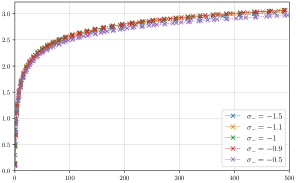
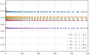
Figure 9. Maximal (left) and minimal (right) numerical eigenvalues of $M_{\Lambda}$ in dependence on $\Lambda$ in the one-dimensional setting.

For the numerical investigation, we choose the one-dimensional setting as in Section 3: We consider the linear operator $\phi\mapsto-\frac{\mathop{}\!\mathrm{d}}{\mathop{}\!\mathrm{d}x}\big{(}\sigma(x)\,\phi^{\prime}\big{)}$ on $\Omega=(-5,5)$ with $\sigma(x)=\sigma_{+}=1$ on $\Omega_{+}=(0,5)$ and various choices for $\sigma(x)=\sigma_{-}<0$ on $\Omega_{-}=(-5,0)$. We numerically compute the eigenvalues of the matrix

$$M_{\Lambda}=\left(\frac{\left\langle\phi_{i},\phi_{j}\right\rangle_{|\sigma|}}{\sqrt{1+\left\lvert\lambda_{i}\right\rvert}\sqrt{1+\left\lvert\lambda_{j}\right\rvert}}\right)_{\left\lvert\lambda_{i}\right\rvert,\left\lvert\lambda_{j}\right\rvert\leq\Lambda}$$

where the $(\lambda_{j},\phi_{j})$ denote the eigenpairs from 4.5. The code is available on Zenodo with DOI 10.5281/zenodo.5707422. Figure 9 shows the maximal and minimal eigenvalues in dependence on $\Lambda$ for different choices of $\sigma_{-}$ on the left and right, respectively. For all considered choices of $\sigma_{-}$, we clearly observe that the maximal and minimal eigenvalues asymptotically tend to a finite, non-zero value. As discussed above, this behavior was rigorously proved for the maximal eigenvalue in 6.1 so that we focus on the minimal eigenvalue. The asymptotic value is reached quickly. Note that for $\left\lvert\sigma_{-}\right\rvert\to 0$ the minimal eigenvalue is expected to degenerate to zero, which explains the dependence on $\sigma_{-}$ observable in Fig. 9 (right). This is in line with 5.6.

Funding

Funded by the Deutsche Forschungsgemeinschaft (DFG, German Research Foundation) — Project-ID 258734477 — SFB 1173.

References

- [1] A. Ambrosetti and A. Malchiodi. Nonlinear analysis and semilinear elliptic problems, volume 104 of Cambridge Studies in Advanced Mathematics. Cambridge University Press, Cambridge, 2007.
- [2] R. Böhme. Die Lösung der Verzweigungsgleichungen für nichtlineare Eigenwertprobleme. Mathematische Zeitschrift, 127:105–126, 1972.
- [3] A.-S. Bonnet-Ben Dhia, C. Carvalho, L. Chesnel, and P. Ciarlet. On the use of Perfectly Matched Layers at corners for scattering problems with sign-changing coefficients. Journal of Computational Physics, 322:224–247, 2016.
- [4] A.-S. Bonnet-Ben Dhia, C. Carvalho, and P. Ciarlet, Jr. Mesh requirements for the finite element approximation of problems with sign-changing coefficients. Numerische Mathematik, 138(4):801–838, 2018.
- [5] A.-S. Bonnet-Ben Dhia, L. Chesnel, and P. Ciarlet, Jr. -coercivity for scalar interface problems between dielectrics and metamaterials. ESAIM. Mathematical Modelling and Numerical Analysis, 46(6):1363–1387, 2012.
- [6] A.-S. Bonnet-Ben Dhia, P. Ciarlet, Jr., and C. M. Zwölf. Time harmonic wave diffraction problems in materials with sign-shifting coefficients. Journal of Computational and Applied Mathematics, 234(6):1912–1919, 2010.
- [7] R. W. Boyd. Nonlinear optics. Elsevier/Academic Press, Amsterdam, third edition, 2008.
- [8] C. Carvalho, L. Chesnel, and P. Ciarlet, Jr. Eigenvalue problems with sign-changing coefficients. Comptes Rendus Mathématique. Académie des Sciences. Paris, 355(6):671–675, 2017.
- [9] L. Chesnel and P. Ciarlet. T-coercivity and continuous Galerkin methods: application to transmission problems with sign changing coefficients. Numerische Mathematik, 124(1):1–29, 2013.
- [10] D. G. de Figueiredo. Positive solutions of semilinear elliptic problems. In Differential equations (Sao Paulo, 1981), volume 957 of Lecture Notes in Math., pages 34–87. Springer, Berlin-New York, 1982.
- [11] T. Dohnal, J. D. Rademacher, H. Uecker, and D. Wetzel. pde2path 2.0: multi-parameter continuation and periodic domains. In ENOC 2014 – Proceedings of 8th European Nonlinear Dynamics Conference, 2014.
- [12] S. Dyatlov and M. Zworski. Mathematical theory of scattering resonances, volume 200 of Graduate Studies in Mathematics. American Mathematical Society, Providence, RI, 2019.
- [13] L. C. Evans. Partial differential equations, volume 19 of Graduate Studies in Mathematics. American Mathematical Society, Providence, RI, second edition, 2010.
- [14] P. M. Fitzpatrick, J. Pejsachowicz, and L. Recht. Spectral flow and bifurcation of critical points of strongly-indefinite functionals. I. General theory. Journal of Functional Analysis, 162(1):52–95, 1999.
- [15] H. Kielhöfer. Bifurcation theory, volume 156 of Applied Mathematical Sciences. Springer, New York, second edition, 2012. An introduction with applications to partial differential equations.
- [16] A. Kufner, L. Maligranda, and L.-E. Persson. The prehistory of the Hardy inequality. Amer. Math. Monthly, 113(8):715–732, 2006.
- [17] A. Manes and A. M. Micheletti. Un’estensione della teoria variazionale classica degli autovalori per operatori ellittici del secondo ordine. Boll. Un. Mat. Ital. (4), 7:285–301, 1973.
- [18] A. Marino. La biforcazione nel caso variazionale. Conferenze del Seminario di Matematica dell’ Università di Bari, 132:14, 1973.
- [19] A. Meurer, C. P. Smith, M. Paprocki, O. Čertík, S. B. Kirpichev, M. Rocklin, A. Kumar, S. Ivanov, J. K. Moore, S. Singh, T. Rathnayake, S. Vig, B. E. Granger, R. P. Muller, F. Bonazzi, H. Gupta, S. Vats, F. Johansson, F. Pedregosa, M. J. Curry, A. R. Terrel, v. Roučka, A. Saboo, I. Fernando, S. Kulal, R. Cimrman, and A. Scopatz. Sympy: symbolic computing in python. PeerJ Computer Science, 3:e103, Jan. 2017.
- [20] S. O'Brien and J. B. Pendry. Photonic band-gap effects and magnetic activity in dielectric composites. Journal of Physics: Condensed Matter, 14(15):4035–4044, 2002.
- [21] J. Pejsachowicz and N. Waterstraat. Bifurcation of critical points for continuous families of functionals of Fredholm type. Journal of Fixed Point Theory and Applications, 13(2):537–560, 2013.
- [22] P. H. Rabinowitz. Some global results for nonlinear eigenvalue problems. Journal of Functional Analysis, 7:487–513, 1971.
- [23] P. H. Rabinowitz. Minimax methods in critical point theory with applications to differential equations, volume 65 of CBMS Regional Conference Series in Mathematics. Published for the Conference Board of the Mathematical Sciences, Washington, DC; by the American Mathematical Society, Providence, RI, 1986.
- [24] A. Szulkin and T. Weth. The method of Nehari manifold. In Handbook of nonconvex analysis and applications, pages 597–632. Int. Press, Somerville, MA, 2010.
- [25] H. Uecker, D. Wetzel, and J. D. M. Rademacher. pde2path—a Matlab package for continuation and bifurcation in 2D elliptic systems. Numerical Mathematics. Theory, Methods and Applications, 7(1):58–106, 2014.