Distributionally Robust Resource Planning Under Binomial Demand Intakes
Abstract
In this paper, we consider a distributionally robust resource planning model inspired by a real-world service industry problem. In this problem, there is a mixture of known demand and uncertain future demand. Prior to having full knowledge of the demand, we must decide upon how many jobs we plan to complete on each day in the planning horizon. Any jobs that are not completed by the end of their due date incur a cost and become due the following day. We present two distributionally robust optimisation (DRO) models for this problem. The first is a non-parametric model with a phi-divergence based ambiguity set. The second is a parametric model, where we treat the number of uncertain jobs due on each day as a binomial random variable with an unknown success probability. We reformulate the parametric model as a mixed integer program and find that it scales poorly with the sizes of the ambiguity and uncertainty sets. Hence, we make use of theoretical properties of the binomial distribution to derive fast heuristics based on dimension reduction. One is based on cutting surface algorithms commonly seen in the DRO literature. The other operates on a small subset of the uncertainty set for the future demand. We perform extensive computational experiments to establish the performance of our algorithms. We compare decisions from the parametric and non-parametric models, to assess the benefit of including the binomial information.
Keywords: Uncertainty modelling, distributionally robust optimisation, heuristics, resource planning.
1 Introduction
In this paper, we consider a resource planning problem motivated by a real-world telecommunications service company. This real problem consists of optimising the use of a large workforce of service engineers, in the face of a mixture of known and uncertain jobs.
1.1 Problem Setting
The planning process for a service company is subject to three stages, named the three stages of planning. Each serves a different purpose, covers a different time horizon, and creates results that feed into the next. The three stages are strategic, tactical, and operational planning. Strategic planning covers a period of multiple years, and concerns long term decisions such as how many employees to be hired and in which skills they should be trained. Tactical planning concerns a period of weeks or months. It involves aggregate decisions such as deciding upon the capacity needed in each period, or how many jobs can and cannot be completed in each period. Operational planning concerns short-term decisions such as scheduling the day-to-day activities of the workforce at the individual level. We focus on the tactical planning stage in this paper. The decisions that we make are at the aggregate level, i.e. we do not plan the specific activities of every worker but we instead aggregate their availability into a daily capacity value. We are tasked with planning the use of this capacity to maximise job completions, or equivalently minimise the number of jobs left incomplete. Since it is typically not possible to move capacity between days, planners manipulate demand to make the best use of what they have.
In the telecommunications industry, jobs can be divided into two categories: repair jobs and installation jobs. Repair jobs correspond to service engineers being tasked with fixing broken equipment for existing customers, such as broadband routers and telephone systems. Installation jobs correspond to engineers installing equipment in order to obtain new customers. For example, this may be installing new cabling cabinets and networks in order to provide broadband to a new geographical area. Repair jobs are treated as emergency jobs and they are given a high priority for completion. Installation jobs are treated as additional jobs that a company can plan to complete in order to generate more profit. In this paper, we will consider planning the activities of a telecommunications workforce carrying out repair jobs. Since breakages in equipment and services are not planned, these jobs offer a source of uncertainty. In particular, for any given planning period we have knowledge of a fixed number of repair jobs that are already in the system at the time of planning (workstack jobs). However, the number of breakages between the time of planning and the date concerned is subject to uncertainty. The jobs generated by these future breakages are referred to as intake jobs or simply intakes.
At the time of planning, we have an aggregate capacity value that gives the number of jobs that our workforce can complete, for each day in a planning horizon of fixed length. This is obtained from the number of engineers working on each day, and the number of hours that they will work. By default, we will use all available capacity on each day to complete jobs that are due on that day. Furthermore, workstack jobs can be completed on or before their due date, and completing them early is referred to as pulling forward. However, the same does not apply to intake jobs. Since the day that they will arrive in the system is unknown, allowing them to be pulled forward could suggest that they will be completed before they even arrive. Hence, intake jobs cannot be pulled forward. If any jobs are still incomplete by the end of their due date, then they will not leave the system but incur a cost, and become due on the following day. This is referred to as rollover. In this paper, since capacity is fixed, our model will optimise the pulling forward decision in order to minimise the total rollover cost over the planning horizon. Pulling forward can be utilised to free up capacity on due dates that we expect to have high intake. This helps to reduce rollover and utilise spare capacity.
In the literature on service industry planning models that are closest to ours, demand uncertainty often results in intractable models due to poor scalability. Examples of this come from Ainslie et al., (2015) and Ainslie et al., (2018). In these papers, models had to be solved heuristically due to their size, even though they were deterministic. However, the demand uncertainty is still acknowledged. In fact, in some cases the plan is passed through a predictive model in order to better assess its performance (Ainslie et al.,, 2017). The closest model to ours that does model uncertain demand comes from Ross, (2016), who used two-stage stochastic programming models for service industry workforce planning. However, this methodology requires the assumption that the demand distribution is known, and this is not an assumption that is reasonable here. The framework that we use to model our problem is distributionally robust optimisation (DRO). This framework allows us to include distributional information in our models, without full knowledge of the distributions themselves.
More specifically, we model intakes as binomial random variables where each distribution is ambiguous. Furthermore, we assume that the intake random variables for any two days in the planning horizon are independent of one another. We assume that we have access to a forecasting model or expert knowledge that gives a point estimate of intake and a range of potential values. Hence, for each day, the number of trials is fixed at the maximum intake. Therefore, the success probability is the only unknown parameter for each distribution. This parameter can be estimated through maximum likelihood estimation, with access to past intake data. Our decision to use the binomial distribution can be justified by the following three reasons:
-
1.
The number of intake jobs due on each day is a discrete quantity and any two jobs arriving on the same day arrive independently of one another.
-
2.
There is a fixed and finite set of values that each intake random variable can take. Other discrete distributions such as the Poisson distribution are unbounded, and hence not fitting for these random variables.
-
3.
Apart from naturality, it gives a concise way of modelling the uncertainty. We can represent each distribution uniquely by one choice of , which is a vector of dimension equal to the number of periods in the plan. Using a non-parametric approach would mean having to analyse the entire distribution, which is a larger vector that has one entry for every realisation of intake.
We emphasize that the binomial assumption is in contrast with much of the DRO literature, in which distributions are usually non-parametric. The reason for this is that parametric distributions often lead to intractable models. However, in the context of our problem, we show that it is possible to derive algorithms which are both tractable and near-optimal. Binomial and negative binomial distributions have often been used for demand modelling, particularly in inventory management. Examples of this include Collins, (2004) for a risk-minimising newsvendor, Gallego et al., (2007) for inventory planning under highly uncertain demand, Dolgui and Pashkevich, (2008) for forecasting demand in slow-moving inventory systems, and Rossi et al., (2014) for confidence-based newsvendor problems.
In this paper, we will use the fact that every distribution in the ambiguity set is binomial in order to find the worst-case expected cost for a fixed pulling forward decision. In general, our methodology consists of three key steps. Firstly, we construct a discrete ambiguity set for the parameters of the true distribution. Secondly, we create a tractable reformulation of the model by replacing the inner objective with a finite number of constraints. In particular, there is one constraint for each distribution in the ambiguity set. Thirdly, we study the objective function as a function of the distribution’s parameters in order to construct a set of extreme parameters. For discrete distributions, the constraints representing the inner objective will always be linear. For continuous distributions, this is not necessarily the case. In such situations, for the second step, one would have to use a linear or quadratic approximation of the objective function. For example, this could be done using piecewise linear approximations or sample average approximations. Doing so would then allow our methodology to be applied.
1.2 Our Contributions
We consider a DRO model for a resource planning problem with an unknown number of intake jobs on each day. Using the problem structure, we model intakes as binomial random variables and study the resulting DRO model. Due to the use of the binomial distribution, the problem is considerably harder from a computational point of view. Our contributions in the paper include the following:
-
1.
A new framework for solving DRO problems with ambiguity sets containing only distributions in the same parametric family as the nominal distribution. A comparison of this framework with a common, non-parametric framework based on the use of -divergences.
-
2.
Three solver-based algorithms for the parametric model: an optimal and a heuristic cutting surface algorithm (named CS_opt and CS, respectively), and another heuristic algorithm named Approximate Objective (AO) (see Sections 3.6.1 and 3.6.2). CS, while not exact, considerably simplifies the main bottleneck step of CS_opt: finding the worst-case distribution for a fixed pulling forward decision (referred to as the distribution separation problem). This makes it much more scalable with the size of the ambiguity set.
-
3.
Extensive computational experiments on a variety of constructed instances which show the efficacy of our methods. See Section 5 for these results.
2 Literature Review
In this section, we review relevant literature relating to our problem and problems of a similar nature. In Section 2.1, we review the workforce planning literature and highlight the methodologies used there. In Section 2.2, we summarise the recent DRO literature and discuss how our research differs from it.
2.1 Workforce and Resource Planning
Workforce planning models of various forms have been studied in the OR literature since the mid 1950’s, with early papers focussing on creating tractable deterministic models (Holt et al.,, 1955, Hanssmann and Hess,, 1960). Demand uncertainty has always been discussed in these early papers, with some authors extending previous models to minimise expected cost rather than cost (Fetter,, 1961). In more recent literature, the modelling of uncertain demand has been developed further. The most common method in the literature has been two-stage stochastic programming. This methodology was applied to nurse scheduling J. Abernathy et al., (1973) and recruitment for a military organisation Martel and Price, (1978) in the early literature. More recent examples of stochastic programming in workforce planning include planning a cyber branch of the US army Bastian et al., (2020), and service industry workforce planning Zhu and Sherali, (2009), Ross, (2016). These authors use stochastic programming due to their assumption that the distribution of the uncertain parameters is known. When this is not the case, or if the planner is risk-averse, robust optimisation (RO) can be used to represent demand uncertainty. This methodology has been used, for example, in healthcare (Holte and Mannino,, 2013) and air traffic control (Hulst et al.,, 2017).
Recently, there have also been some applications of DRO to workforce and resource planning. Liao et al., (2013) used DRO for staffing a workforce to take calls arriving at a call centre at an uncertain rate. The reason for using DRO was cited as being that the true arrival rates of calls are usually subject to fluctuations, meaning that the typical stochastic model with a fixed Poisson distribution was not appropriate. They simulated the DRO solution and the stochastic programming solution and found that the two had similar costs. However, the stochastic programming solution violated more model constraints. Chen et al., (2015) also used DRO for workforce planning in a hospital environment. In particular, they used DRO to determine bed requirements in order to appropriately manage admissions to the hospital. They use DRO due to the difficulty in specifying a distribution to describe patient movements in the hospital, and find that it performs better than a deterministic approach.
Our resource planning problem deals with the management of both planned and unplanned jobs. Similar problems exist in other settings, such as scheduling for gas pipeline maintenance (Angalakudati et al.,, 2014), and operating room scheduling in hospitals (Samudra et al.,, 2016). Particularly, in operating room planning, the workstack and intake jobs as defined in our model are similar to elective (inpatient and outpatient) and non-elective (emergency) surgeries. Similarly, in gas pipeline maintenance the workstack and intake jobs correspond to planned maintenance jobs and emergency gas leak repairs, respectively. The main difference between our research and these papers is the choice of performance measure. For example, Angalakudati et al., (2014) use overtime hours as a performance measure under the assumption that jobs have individual completion times. However, since our model is for tactical and not operational planning, jobs and capacity are aggregated. The duration of each job is not modelled directly. Hence, in our case, the amount of overtime would be inferred by the number of jobs that could not be completed, i.e. rollover. As discussed by Samudra et al., (2016), metrics chosen for optimisation differ based on the underlying context and the stakeholders involved. They emphasize that traditional metrics such as makespan do not work in presence of both planned and emergency demands. In our application, the time taken to complete jobs is not of particular concern. However, leaving jobs incomplete is very costly due to its effects on customer satisfaction. In industries like telecommunications, customer satisfaction is of great importance, and hence rollover may be the most appropriate performance measure.
The literature reviewed here shows that the modelling of uncertain demand in resource and workforce planning has been the subject of a breadth of research in the past. It suggests that the most common approach is to employ two-stage stochastic programming models. However, the assumption that the distribution of demand is known is not reasonable in our setting. In fact, we only have access to samples of demand and a range of potential values that it can take. We do assume, however, that we can take samples of intake in order to estimate the parameters of its distribution. In addition, there are no recourse actions in our problem. In such settings, RO and DRO are the only potential solution approaches. For our problem, a robust model will be shown to lead to more conservative decisions and large costs. We show this in Appendix B.2. Hence, we present a DRO model for our problem, which will extend the previous stochastic programming approaches to the case where the distribution is not known exactly. We find that the model is large and complex, due to the size of the sets of intakes and distributions. Hence, we develop heuristics that apply dimension reduction to these sets in order to reduce solution times. One algorithm considers only a small subset of distributions, and the other operates on a small subset of intakes. While these algorithms perform well on average, they do sacrifice optimality for speed in some large instances.
2.2 Distributionally Robust Optimisation
DRO combines concepts from robust optimisation and stochastic programming in order to protect the decision maker from distributional ambiguity. DRO models are constructed using only limited information on the true distribution of the uncertain parameters. This information is encoded in an ambiguity set, in which the true distribution should lie. The earliest type of ambiguity set in the literature is the moment-based ambiguity set. This set contains all distributions whose moments satisfy a given set of constraints. The simplest moment-based sets consider moments to be fixed and known. The moments concerned have often been the mean and variance. This case was studied by Scarf, (1957) for a newsvendor model. Other papers included models where the first moments were known (Shapiro and Kleywegt,, 2002). Authors have also developed models that did not assume that these values were fixed but that they were known to lie in an interval or that ordinal relationships between probabilities were known (Breton and Hachem,, 1995). Other examples of this come from Ghaoui et al., (2003) and Lotfi and Zenios, (2018), who study a CVaR model where the first two moments are only known to belong to polytopic or interval sets. Methodologies for solving moment-based ambiguity set models include reformulation via bounding the objective function (Scarf,, 1957), reformulating as a second order conic program (Ghaoui et al.,, 2003, Lotfi and Zenios,, 2018), sample average approximations (Shapiro and Kleywegt,, 2002) and sub-gradient decomposition (Breton and Hachem,, 1995).
The second common methodology for constructing ambiguity sets is using distance measures. A distance-based ambiguity set contains all distributions that lie within some pre-prescribed distance of a nominal one. In the literature, many ways to measure this distance have been studied. For example, many papers have used the Wasserstein distance. This distance can lead to tractable reformulations as convex programs (Mohajerin Esfahani and Kuhn,, 2018). Due to this, it has been used in a number of contexts, such as portfolio selection (Pflug and Wozabal,, 2007), least squares problems (Mehrotra and Zhang,, 2013) and statistical learning (Lee and Mehrotra,, 2015, Lee and Raginsky,, 2018).
Another common family of distance measures in DRO has been -divergences. This family contains a number of distance measures, such as the distance, variation distance and Kullback-Leibler divergence. Such measures typically lead to second-order conic programming or even linear programming relaxations via taking the Lagrangian dual of the inner problem (Ben-Tal et al.,, 2013, Bayraksan and Love,, 2015). Due to the convenient reformulations they yield, -divergences have been popular in the DRO literature. There have been numerous examples of -divergences being used to reformulate distributionally robust (DR) chance-constrained programs as chance-constrained programs (Hu et al.,, 2013, Yanıkoğlu and den Hertog,, 2013, Jiang and Guan,, 2016). Another benefit of -divergences is that they can be used to create confidence sets and enforce probabilistic guarantees. Ben-Tal et al., (2013) show how to create confidence sets for the true distribution based on -divergences. This is done by taking a maximum likelihood estimate (MLE) of its parameters and using the resulting distribution as the nominal distribution. Duchi et al., (2016) use DRO models with -divergence ambiguity sets to construct confidence intervals for the optimal values of a stochastic program with an ambiguous distribution. Their intervals asymptotically achieve exact coverage. By studying -divergence balls centred around the empirical distribution, Lam, (2019) shows that DRO problems can recover the same standard of statistical guarantees as the central limit theorem.
In addition to these papers that consider general -divergence functions, the fact that -divergences cover a range of distance measures allows authors to select those that are most appropriate for their models. For example, Hanasusanto and Kuhn, (2013) used divergence ambiguity sets for a distributionally robust dynamic programming problem. They used the divergence, in particular, because it allows the min-max problems in the dynamic programming recursion to be reformulated as tractable conic programs. They also chose this divergence because it does not suppress scenarios. In other words, it does not give scenarios zero probability in the worst-case if they have non-zero probability under the nominal distribution. The Kullback-Leibler divergence was also extensively studied by Hu and Hong, (2013), who used it for DR chance-constrained problems. They showed that, under this divergence, if the nominal distribution was a member of the exponential family then so was the worst-case distribution.
The literature we have reviewed so far concerns models that can be reformulated and solved exactly, due to their ambiguity sets being constructed using distance measures or moment constraints. However, there has also been significant literature studying general DRO models that are not formulated in this way. In general, DRO models are semi-infinite convex programs (SCPs). They have a potentially infinite number of constraints induced by those defining the inner objective value. Typically, iterative algorithms are used to solve SCP models. For example, Kortanek and No, (1993) developed a cutting surface (CS) algorithm for linear SCP problems with differentiable constraints. This algorithm approximates the infinite set of constraints with a sequence of finite sets of constraints. Constraints are iteratively added to the current set considered until stopping criteria are met. The constraint that is most violated by the current solution is added at each iteration. In the context of DRO, adding a constraint corresponds to finding a distribution to add to the current ambiguity set. This is referred to as solving the distribution separation problem. Pflug and Wozabal, (2007) later applied this algorithm to DRO models for portfolio selection under general ambiguity sets. In an extension of Kortanek and No, (1993)’s algorithm, Mehrotra and Papp, (2014) developed a CS algorithm for SCP problems that allowed for non-linear cuts, and did not require differentiable constraints. CS algorithms have since become a common apprach to solving DRO problems that are computationally expensive and do not have tractable reformulations. For example, Rahimian et al., (2019) applied a CS algorithm to a DRO model using the total variation distance. They state that the model becomes expensive to solve to optimality when there are a large number of scenarios. Another example of its use in the literature is given by Bansal et al., (2018), who used a CS algorithm to solve DR knapsack and server location problems. Luo and Mehrotra, (2019) also used a CS algorithm to solve DRO models under the Wasserstein distance.
Our work differs from the cited literature in two key ways. Firstly, we consider demand distributions belonging to some parametric family, and enforce that the worst-case distribution also belongs to this family. We show that the resulting model can be reformulated as a large MIP. This model becomes slow to solve for large ambiguity and uncertainty sets. This is due to the large amounts of computation required and the large number of constraints. Hence, secondly, we present algorithms that make use of the additional distributional information in order to solve the parametric model. Among these algorithms is an optimal CS algorithm, that we will show to be fast for small problems, but to scale poorly with the size of the ambiguity set. We also contribute a heuristic version of this CS algorithm, that solves the distribution separation problem at each iteration over a subset containing only the most extreme parameters. We will show that this allows us to greatly reduce the time taken to solve the distribution separation problem. We also show how to construct a confidence set for the worst-case parameter without the use of -divergences. In addition, we develop the non-parametric model and show how to reformulate it as a second-order conic program. We also compare the results from the parametric and non-parametric models to assess the benefit of incorporating the binomial information.
3 Planning Model
In this section, we introduce our planning model and discuss the different types of ambiguity sets that we will consider. In Section 3.1 we provide a summary of the notation that will be used. Following this, in Section 3.2, we provide the DRO model itself under a general ambiguity set. In the sections following this, we detail the parametric and non-parametric versions of the model that will be studied in this paper.
3.1 Notation and Definitions
We consider a planning horizon of periods, which are days in our setting. The days in the plan are denoted by . The inputs for the model are defined as follows. For each day we have capacity , which gives the number of jobs that we can complete on day . The workstack for day is the number of jobs that are currently due on day , and is denoted . The workstacks are known at the time of planning. The intake for day is denoted . This quantity is the number of jobs that will arrive between the time of planning and the due date and will be due on day . Each is a random variable, and its value is not realised until the end of day . In other words, workstack and intake jobs represent planned and unplanned/emergency jobs in the terminology used in other problems.
The rollover for day is the number of jobs that are due on day but are left incomplete at the end of day . This quantity is denoted by , which is a random variable due to its dependence on . Each unit of rollover on day incurs a cost . The set of realisations of the random variable is denoted by , and a realisation of is denoted by . We use suppression of the subscript to represent the vectors of intakes, workstacks and so on. For example, the vector of workstacks is denoted by . The set of all realisations of the vector is denoted by . We assume that the set is the cartesian product of the marginal sets, i.e. . In the language of robust optimisation, is referred to as an uncertainty set for . For a realisation of the vector of intakes , the corresponding realisation of rollover is denoted by . The objective of our problem is to minimise the worst-case expected rollover cost by pulling forward jobs. Hence, the decision vector in our problem is the pulling forward variable, which we denote by . Jobs can be completed no earlier than periods prior to their due date. Therefore, we use to denote the number of jobs pulled forward from period to period . This corresponds to completing additional jobs on that are due on .
3.2 General Distributionally Robust Model
We now consider the distributionally robust planning model, which is defined as follows. Denote by a general ambiguity set of intake distributions, such that every distribution assigns a probability to every possible intake . Our model aims to minimise the worst-case expected rollover cost by selecting the value of . The model is shown in (1)-(8).
| (1) | ||||
| s.t. | (2) | |||
| (3) | ||||
| (4) | ||||
| (5) | ||||
| (6) | ||||
| (7) | ||||
| (8) |
The general idea in calculating rollover in the -day model is as follows. For a given day , we first compute the number of jobs to be completed on day . To compute this, we take the rollover from day and day ’s intake as a baseline number of jobs. Then we add the number of jobs pulled forward to day , i.e. . We then compute the capacity that can be used to complete these jobs. This is done by taking the capacity and subtracting the capacity required to complete those workstack jobs that are not pulled forward from day , i.e. . If the remaining capacity is enough to complete all jobs on , then the rollover is zero. Otherwise, the rollover is the number of jobs left incomplete.
Constraints (2) and (3) provide upper bounds on the pulling forward totals. Constraint (2) ensures that no jobs are pulled forward if they cannot be completed on the day to which they are moved. Constraint (3) ensures that only workstack jobs can be pulled forward, and that a job cannot be pulled forward multiple times in order to be pulled forward more than days. Constraint (4) reflects that jobs cannot be pulled forward from day 1 and hence we only subtract those jobs pulled forward to day 1 from its remaining capacity. We do not reduce rollover by pulling forward from it. Similarly, constraint (6) reflects that jobs cannot be pulled forward to the final day of the plan. Hence, we only pull forward from this day and not to this day. For every other day, constraint (5) captures that we can pull forward to and from said day. We therefore add and subtract jobs from its capacity to calculate the rollover.
3.3 Non-parametric DRO Model
The non-parametric model is defined by ambiguity sets containing distributions that are not necessarily parametric. To be specific, can be any subset of the set of all distributions over the set of intakes, i.e. .
3.3.1 Phi-divergence Based Ambiguity Sets
As discussed earlier in the paper, it is common to define using -divergences. Adopting similar notation to that of Bayraksan and Love, (2015), suppose that and are two probability distributions. We define a -divergence for -divergence function as:
| (9) |
where is a convex function on the non-negative reals. This function measures the distance between and . In what follows, will be treated as a nominal distribution. Furthermore, we denote by the conjugate of , which can be found via (10).
| (10) |
The conjugate will be useful when finding reformulations later in the paper. Given a nominal distribution , we can define as the set of all distributions that lie within some pre-prescribed distance from as measured by the -divergence. In other words, we can use:
| (11) |
As described by Ben-Tal et al., (2013), this formulation of the ambiguity set allows us to choose such that is a confidence set for the true distribution. Suppose that the true distribution lies in a parameterised set , such that the true value of is . Also suppose that we take samples of intake from and take an MLE of . Then, if we choose using (12), the set is an approximate confidence set for around .
| (12) |
In (12), is the dimension of and is the percentile of the distribution with degrees of freedom. There are many choices for the choice of -divergence function, and some examples can be found in the paper by Ben-Tal et al., (2013).
3.3.2 Reformulation with Modified -divergence
In our model, we will use the modified distance as our -divergence. This uses the -divergence function and is defined in (13).
| (13) |
Here, is the number of potential values of the uncertain parameters. In our problem, we have . We choose this function for the following reasons. Firstly, it leads to a convex quadratic programming (CQP) reformulation. Secondly, squared deviations from the nominal distribution are represented as a proportion of the nominal distribution’s value. This means that small deviations from the nominal distribution can still lead to a large term in the sum in (13). When is large, most values of will be small, and this will help identify significant deviations from small nominal values. Other choices of -divergences that lead to CQP reformulations, such as the distance, Hellinger distance and the Cressie-Read distance, do not have the normalisation effect given by dividing each term by . Following Ben-Tal et al., (2013), defining , we find the following CQP reformulation of our full model with :
| (14) | ||||
| s.t. | (15) | |||
| (16) | ||||
| (17) | ||||
| (18) | ||||
| (19) |
In this formulation, and for are dummy variables defined to ensure that the model is a CQP model. A full derivation of this reformulation can be found in Appendix A, along with how to extract the worst-case distribution from its solution.
3.4 Parametric DRO Model
In this section, we detail a parametric version of the DRO planning model. This is a new modelling framework for DRO problems that allows the ambiguity set to contain only distributions that are members of the same parametric family as the true distribution. This is useful in cases where we know beforehand which family the true distribution lies in, because it ensures that the worst-case distribution implied by the model is also in this family.
3.4.1 Implications of Parametric Ambiguity Sets
Recall from Section 3.3.1 that we can use -divergences to create confidence sets when we know that the true distribution lies in some parametric family . The resulting confidence set (11), however, does not only contain distributions in this family. Therefore, there is no guarantee that the worst-case distribution will lie in this family and hence no guarantee that it is even a distribution that could be equal to . Our methodology involves explicitly using the set in our DRO model instead, which eliminates potential worst-case distributions that are not in the same family as the true distribution. Suppose that we take the ambiguity set given by .
The methodology in Section 3.3.2 relies on being able to represent the requirement that in the constraints of the model. However, representing in the constraints is more challenging. In the case where represents a set of discrete parametric distributions, e.g. binomial or Poisson, the requirement might be represented by:
| (20) |
where is the probability mass function (PMF) of and is the realisation of intake. The only reasonable way that one might attempt to include this in the model is to treat as a dummy variable, and replace in the objective with . However, most PMFs as functions of their parameters are either high order polynomials (such as binomial) or include exponential functions (such as Poisson). Including them in the model through the objective function will hence make the model intractable. As an example, consider our model with independent intakes and for . The objective of the inner problem becomes:
| (21) |
Treating this as a non-linear program, we might consider solving using the Karush-Kuhn-Tucker (KKT) conditions. The derivative of the objective function in (21) with respect to is:
| (22) |
for each , where is the PMF of . Choosing a vector such that for all and all derivatives are equal to zero is a challenging task. This would need to be done numerically, and hence would not result in a tractable objective function for our outer model. Furthermore, using a -divergence to define would not result in a tractable reformulation. This would involve using an ambiguity set for of the form:
| (23) |
where is the success probability vector corresponding to the nominal distribution . Now consider the methodology in Section 3.3.2. This methodology relies on the objective function being separable over (see Appendix A). Following the same steps but with the objective in (21), we arrive at the following dual objective:
| (24) |
Due to the product over inside the operator (which contains each success probability), we see that this objective is not separable over . Thus, the remaining steps in creating a tractable reformulation cannot be carried out. This holds not only for independent distributions, but for any distribution where the PMF of depends on more than one .
Hence, our methodology is as follows. Instead of treating the parameter as a vector of decision variables, we represent it using a discrete, finite set of potential values. In other words, we assume that is a discrete and finite set. This allows us to represent the distributional ambiguity via a finite set of constraints that are linear in the rollover variables. The resulting model has one additional constraint for every , but remains a tractable mixed integer program (MIP). We detail the MIP reformulation of the parametric model in Section 3.4.2.
3.4.2 Mixed Integer Programming Reformulation
To solve this model, we can reformulate it as an MIP as follows. Firstly, we replace the set with and optimise over the parameters directly. Since there is a one-to-one mapping between and , the objective becomes:
| (25) |
Next, we define a dummy variable to represent the worst-case expected cost for a given . Since the set is a discrete set, we can enforce the requirement that a set of linear constraints. Hence, the MIP reformulation of the DRO model is given by:
| (26) | ||||
| s.t. | (27) | |||
| (28) |
This model can be very slow to build and solve. This is mostly due to the amount of computation required to build the model and its constraints. The constraint for requires us to compute the distribution for every . Due to the sizes of and , this can be very slow. To see this, consider an example with distributions and potential intakes. Suppose also that the intakes are independent. Then, for each of 3883 distributions we would need to compute a product of PMF values, for each of 20000 intakes. This means computing PMF values. Furthermore, the model has rollover variables and constraints, and expected value constraints. This also makes the model slow to build and solve for large instances. For this instance with , this corresponds to 103,878 additional constraints, when compared with the deterministic model. Our heuristics therefore employ dimension reduction techniques to make them more tractable.
3.5 Binomial Intakes and Ambiguity Sets
As previously discussed, we will assume that the intakes in our problem our binomially distributed. In other words, we assume that . We assume that is provided to us prior to model building, either by a prediction model or expert knowledge. The true set in which we know that the true , denoted , must lie is . As detailed in Section 3.4.1, we will however use a finite, discrete subset of as an ambiguity set for our model. We consider a discretisation of of the form given in (29), where is chosen by the planner, and details the fineness of the discretisation.
| (29) |
Secondly, we assume that we have access to samples of past intake data, from which we can take an MLE of . The corresponding distribution is given by , which has mean vector . Given the MLE , we consider only that can be considered close to . As mentioned earlier, it is common in the non-parametric DRO literature to use -divergences to measure the distance between two distributions. The main reason for this is that it results in tractable reformulations via dualising the inner problem. However, since our approach does not entail dualising the inner problem, this benefit does not apply to us. Another reason for using -divergences is that they allow us to create confidence sets for the true distribution. However, this is based on applying the -divergence to the distributions themselves, not to the parameters. We could construct a confidence set for by first constructing a confidence set for and then creating by extracting the parameters of each distribution in the confidence set. However, this would entail computing the corresponding distribution for every , which is a large computational task. Hence, we do not use -divergences for the parametric model. We can, however, construct a confidence set for without using -divergences and without needing to compute each distribution . Since is an MLE of based on samples from the true intake distribution, by Millar, (2011), for large we have:
| (30) |
approximately. Therefore, by independence of the different MLE’s, we have that:
| (31) |
approximately. Hence, we have the following discretisation of an approximate confidence set for around :
| (32) |
This may yield a different ambiguity set to the one obtained using the -divergence method. This is because they are two different approximations of the same set.
3.6 Solver-based Solution Algorithms
As described in Section 3.4.2, the model can be solved to optimality by reformulating it as a mixed integer program. However, when and are large, this model has a large number of constraints and decision variables. This can make it very slow to solve. Hence, we develop three dimension reduction algorithms in order to reduce the effects of the sizes of these sets on solution times. In Section 3.6.1, we discuss two cutting surface (CS) algorithms. The first is an optimal CS algorithm that also scales poorly with the size of . The second is a heuristic CS algorithm that applies dimension reduction to . Then, in Section 3.6.2, we describe our final algorithm, Approximate Objective (AO), that applies dimension reduction to .
3.6.1 Cutting Surface Algorithms
In this section, we describe our adaptation of the CS algorithm detailed in the literature review, which has been commonly used in the DRO literature. The algorithm has a number of different forms, but the one that we base our adaptation on is that from the review paper by Rahimian and Mehrotra, (2019). The general idea of the algorithm is as follows. In order to deal with the large number of constraints implied by the ambiguity set, the algorithm uses the following steps. We start with a singleton set containing one distribution, and solve the problem over this ambiguity set. Then, for the generated pulling forward solution, we find the worst-case distribution over the entire ambiguity set. We add this distribution to the current ambiguity set and then repeat the above steps. This procedure repeats until optimality criteria are met.
In more detail, suppose that we have some initial subset of our set of distributions and we solve the full model with ambiguity set , to get an optimal decision . Then, we find the worst-case parameter, , for the fixed solution , and add it to our set to create a new subset of . We then solve the model with ambiguity set , and repeat. We stop the algorithm when we have reached -optimality, i.e. if the solution from the full problem at iteration , , gives a worst-case expected cost over that is within of the worst-case expected cost for over . The algorithm returns an -optimal solution to the DRO model in a finite number of iterations. The issue with this version of CS is that, even if is fixed at , finding the true worst-case distribution can be a very cumbersome task. To do so, this problem is often treated as an LP. In our case, we can simply enumerate all distributions in . Even though this is not a difficult task, it requires a significant amount of computation due to the necessity of calculating the distributions themselves.
From now on, we refer to the optimal CS algorithm described above as CS_opt. We will show that this algorithm suffers from poor scaling with respect to the size of . In order to reduce the computational burden, we apply dimension reduction to . Particularly, we use the simple observation that is increasing in to construct a set of extreme parameters. Intuitively, this result suggests that a higher success probability also leads to no-less expected rollover, due to the fact that is increasing in . Hence, we construct a set of probability vectors such that at least one value is maximised. If this is not the case, then one value can be increased and this would cause higher expected rollover for that day. Furthermore, we also assume that the total success probability is maximised given that one value is maximised. This is to ensure that we take the most extreme probability vectors over all those such that one success probability is maximised. Mathematically, we define the set of extreme parameters as follows. Define for and find the set of parameters such that one value is maximised:
For each , construct a set of the most extreme parameters in and take the union of these sets to form :
In order to reduce the computation required, our heuristic CS algorithm (referred to as CS) solves the distribution separation problem over , rather than the entire ambiguity set . The general framework for both of our CS algorithms is given below, where CS_opt uses in step 2(b) and CS uses .
-
1.
Compute ambiguity set and initialise , where for example.
-
2.
For :
-
(a)
Solve the model to optimality using ambiguity set to generate solution where is worst-case expected cost of over the set passed to the model.
-
(b)
Solve distribution separation problem to get solution :
-
i.
For , calculate .
-
ii.
Choose such that .
-
i.
-
(c)
If or then stop and return solution .
-
(d)
Else, set and .
-
(a)
The logic behind 2(c), where we check if , is that calculation differences might cause and to differ by more than when they should be equal. Solvers use some dimension reduction techniques when building and solving their models. This can lead to objective values that are not the same as the ones given by the function used in 2(b), even for the same arguments. This stopping criterion is also used in the CS algorithms by Pflug and Wozabal, (2007) and Bansal et al., (2018). We now explain why the condition cannot cause early stopping. Firstly, assume that is not a worst-case parameter for in , i.e. it did not give a cost of . Since is generated by the distribution separation problem, it is a worst-case parameter for over the entire set . If we also have then we have the following two facts. Firstly, we have and so is necessarily worse than every . Secondly, must be worse than , because otherwise would be a worst-case parameter in . Hence, is a worst-case parameter in , i.e. . Now suppose that is a worst-case parameter in . If then we must have since is worse than . Hence, whenever occurs, the first stopping criterion should also be met.
3.6.2 Approximate Objective Algorithm
The final algorithm that we describe is named Approximate Objective (AO). When solving the model to optimality, we are required to compute the distribution for each . For each intake we can easily compute:
| (33) |
and then we can consider a new set of intakes in the model defined by:
| (34) |
where is our minimum intake probability. By tuning , we are removing intakes from our set that are very unlikely. When solving the model, we are approximating the expected value by removing some small terms. Since the intakes removed have low probability, this approximation should be strong. We simply solve the MIP reformulation with the full set of parameters but over the reduced set of intakes. For this paper, we use as our initial testing showed that this value led to good improvements in computation time.
3.7 Example: A Two-day Problem
In order to illustrate the logic behind our algorithms, we now give an example of their use for a two-day version of our model. Since there is only one feasible pair of days that we can pull forward jobs between, i.e. , there is now only one decision variable. We refer to this decision variable as . The two-day model is given by (1)-(8) with and .
Suppose that we have , , and . This gives . We construct a 99.5% confidence set for using , and . This gives , and we find that the maximum values of and are both 0.84. This suggests that the above model has rollover constraints and variables, 81 expected value constraints and 2 pulling forward constraints. Hence, it has 1189 constraints and 884 decision variables. We solve this model to optimality in 2.6 seconds, to find the optimal to be and the worst-case to be with an expected cost of .
When we solve this model with CS, we find that and so CS only has to compute 2 PMFs as opposed to P and AO which have to compute 81. We initialise with . In iteration 1, CS solves the MIP reformulation over and finds . It then evaluates the expected costs under each and finds the worst-case to be given by . Hence, we have . In iteration 1, CS solves the model over and finds . It finds the worst-case cost to be given by , and hence takes . In iteration 3, CS finds and . Since , the algorithm ends and returns and with an expected cost of . Hence, CS returned the optimal but slightly underestimated its worst-case cost. This is an example of where CS will be suboptimal because . However, CS returned its solution in 0.17 seconds, as opposed to P’s 2.6 seconds. Note that CS terminated in 2 iterations because .
To solve this model with AO, we construct the reduced set of intakes . In order to do so, we compute the PMFs, which takes 2 seconds. Using , we find the new set of intakes to have , which is a 67% cardinality reduction. Then, we solve the MIP model over and find the solution , , meaning that AO was both -optimal and -optimal in this instance. However, it took 0.71 seconds in total, as opposed to CS’s 0.17 seconds. We can also run this instance with CS_opt. Doing so, CS_opt’s first two iterations are the same as CS’s. In its third iteration it finds and , whereas CS found . Following this, in iteration it finds and breaks since , returning and . This is the same solution as P gave. This took CS_opt a total of 0.43 seconds. It finished in twice as many iterations as CS.
4 Design of Computational Experiments
This section details our experiments evaluating the performance of the algorithms described in Section 3.6 in comparison with the solution from the parametric DRO model. These experiments will also allow us to compare the solutions resulting from the parametric model (P) and the non-parametric model (NP) and the times taken to reach optimality by each model. In this section, we discuss how the parameters for the experiments will be chosen to ensure that they are representative of typical real-life scenarios. To discuss experimental design, we need to define which parameters of the model will be varied and the values that they will take. The vector of inputs to the model for a fixed set of intakes and of distributions is .
4.1 Parameter Hierarchy
It is helpful to consider a hierarchy of parameter choices, which is defined by:
-
1.
defines the difficulty of the problem in terms of the MIP itself.
-
2.
and define the set of solutions that are possible for a given model with fixed and . They need to be constructed for each combination of and to ensure that we have a varied range of instances when it comes to pulling forward opportunities. We create this variety by varying the number of days that have spare capacity and are hence able to receive additional jobs. The values of and used are discussed in Section 4.2.
-
3.
-
(a)
For the parametric model, and define how the uncertainty is encoded in the model, depending on the planner’s attitude to risk. If or is large, solving to optimality will be very slow, and we would like to use a heuristic that is not significantly affected by these sizes. is defined by , and is defined by two parameters. The initial discretisation of the interval in which each lies is defined by . The maximum distance from the nominal distribution that can be is defined by the second parameter, . This is the number of samples that we take from the distribution of in order to calculate . Larger results in smaller distances from being allowed, and hence corresponds to a less risk-averse planner. For these experiments, we use confidence sets, i.e. from (32) with . From now on, we use to represent .
- (b)
-
(a)
-
4.
will be left as the ones vector for these experiments as it has not been seen to have an effect on solutions.
We choose due to it being the number of days in a typical working week. We take the maximum pulling forward window length to be . This is because pulling forward is not enacted until the operational planning phase, where the planning horizon is very short. These choices are partly motivated by usual practices, and also partly by the following fact. We aim to test our heuristics against optimal solutions, and for larger or the model becomes very difficult to solve to optimality. Note that the optimality tolerance for CS/CS_opt, , will be set to 0.01 and it will be run for a maximum of iterations. Initial testing suggested that these parameters are not so important, as CS and CS_opt always terminated due to a repeat parameter (i.e. ) after less than 10 iterations.
4.2 Capacity and Workstacks
The factors affecting the potential solutions of a model the most are and , due to the fact that they define the rollover and pulling forward opportunities. In this section, we detail the capacities and workstacks used in our experiments. These are constructed with the aim of ensuring that a variety of combinations of pulling forward opportunities are represented by at least one pair. We assume for this section that the previous parameters in the hierarchy, i.e. and , are given. We now define how and define pulling forward opportunities mathematically. Firstly, we define the set of pairs of days under consideration for pulling forward as:
| (35) |
and the set of pairs such that the corresponding can feasibly be positive given and as:
| (36) |
This is the set of all pairs of days such that is within pulling forward range of , has spare capacity and has workstack jobs to be completed early. For our experiments, we consider instances where for all . This is because for a short horizon of days, it is very unlikely that any day will have a workstack of zero. Hence, we can control by controlling which days have spare capacity. For example, we can set by setting and and then for . This results in . We do this similarly for other values of . The main effect that and has on decision making is that they define the constraints on , meaning their only important quality is how much pulling forward they do or do not allow. Using this set of values for and we will be able to see how well our algorithms detect and make use of opportunities for pulling forward.
4.3 Uncertainty and Ambiguity Sets
As a reminder, the term “uncertainty set” refers to and “ambiguity set” refers to . We now detail the parameters used to construct these sets in our instances.
4.3.1 Uncertainty Set
We assumed in Section 1.1 that we would be given a set , either by expert knowledge or by a prediction model. We could then extract from this set. However, in these experiments, we do not have access to real intake data or expert knowledge. Thus, it is more convenient to define and then use this to construct . Since there is a one-to-one mapping between the two, both methods achieve the same result. We consider satisfying:
| (37) |
This is reasonable because if the total number of jobs arriving in the system exceeds the RHS of (37) then some intake jobs will always remain incomplete at the end of day , regardless of our pulling forward decision. Furthermore, we can vary the number of high-intake days, through the quantity . This corresponds to the number of days with the potential for spikes in demand. Depending on and , can range between 0 and . However, for these experiments we consider for sufficient coverage of cases. The case of corresponds to a one-day spike caused by an event such as a major weather event. The case of could correspond to an extended spike lasting for multiple consecutive days, for example, a network problem causing lots of service devices to break. The final case of corresponds to small spikes in intake, marking a period of consistently high intake.
4.3.2 Ambiguity Sets
The choice of parametric ambiguity set depends on the choice of discretisation of and also the way we in which we then reduce its size. The choice of discretisation is defined by the parameter , and increasing this value increases the size of the ambiguity set. For these experiments, we consider . In our preliminary testing we found that any value larger than 15 can lead to intractability when solving the parametric model to optimality.
Both ambiguity sets are also defined by the sampling parameter . For the purpose of testing our models, we consider . Clearly, higher leads to better convergence to the true distribution of the MLE/-divergence, but it also leads to much smaller ambiguity sets and typically less conservative decisions. Even for , we obtained some singleton ambiguity sets. Typically, would be chosen by the planner who is in control of the sampling process. However, the results of our testing can be used to understand the tradeoff between the accuracy of the approximation and the conservativeness of the resulting decisions. Hence, it may influence the value of used by the planner. In these experiments, we will assume . Hence, we will obtain . In practice, would be obtained from sampling the true intake distribution. However, without access to true intake data, we set the value somewhat arbitrarily, since it is only used for testing purposes. If these models were used by a real planner, we would suggest that they calculate their own MLE.
5 Results
We now detail the results of our experiments that we used to test the algorithms on 279 problem instances with and . We report the results from all 5 algorithms in terms of times taken, pulling forward decisions and worst-case distributions. Due to space considerations, we present some additional results in the Appendices. We discuss the effects of workstacks on solutions in Appendix B.1. We give a brief comparison of our results with those from the RO version of the model in Appendix B.2. In addition, we present and test a Benders decomposition algorithm for this problem in Appendix C. These experiments were run in parallel on a computing cluster (STORM) which has 486 CPU cores. The solver used in all instances was the Gurobi Python package, gurobipy (Gurobi Optimization, LLC,, 2022). The version of gurobipy used was 9.0.1. The node used on STORM was the Dantzig node, which runs the Linux Ubuntu 16.04.6 operating system, Python version 2.7.12, and 48 AMD Opteron 638 CPUs.
5.1 Summary of Instances and Their Sizes
In Table 1, we summarise the sizes of the sets and , that formed the basis for the constraints and variables in the model. A summary of the sizes of is given in Table 1(a). The table shows 7 of the 31 values considered and the size of the resulting set . The other values considered were permutations of the values shown in the table, and hence led to values that are already listed in the table. Table 1(b) shows the values of and used and the average size of the resulting ambiguity sets. The sizes vary as the construction of the set also depends on . The instances where correspond to instances where was too small to allow any other than to be in the ambiguity set defined by (32).
| (1, 6, 6, 1, 1) | 392 |
|---|---|
| (1, 3, 3, 3, 3) | 512 |
| (2, 2, 2, 6, 2) | 567 |
| (2, 2, 8, 8, 2) | 2187 |
| (5, 5, 1, 5, 5) | 2592 |
| (1, 7, 7, 7, 7) | 8192 |
| (9, 9, 1, 9, 9) | 20000 |
| Average | ||
|---|---|---|
| 100 | 5 | 1.000 |
| 100 | 10 | 1.000 |
| 100 | 15 | 16.871 |
| 50 | 5 | 1.419 |
| 50 | 10 | 14.419 |
| 50 | 15 | 93.129 |
| 10 | 5 | 14.742 |
| 10 | 10 | 504.226 |
| 10 | 15 | 4301.645 |
We can see here that our choices of gave instances with as many distinct intakes (and rollover vectors) as 20000, and as few as 392. The sizes of the ambiguity sets varied between 1 and 8854, where the largest sets resulted from the smallest and values, and the largest values. This is because the criteria for being included in was Clearly the LHS is increasing in and . Hence, larger values lead to a higher distance from the nominal distribution. Large leads to larger because it results in a finer discretisation of , and hence more candidate values.
5.2 Optimality of Algorithms and Times Taken
Comparing results for DRO problems is not as simple as comparing final objective values. Our optimal objective value can be written as . Here, is the total expected rollover cost, i.e. . Suppose we have an instance where but . Then, if CS gives a lower objective value than P, it may appear to have given a better solution to the minimisation problem. However, this means that CS did not successfully choose the worst-case for its chosen . This leads to a lower objective function value but a suboptimal solution with respect to . Similarly, we can say that CS is suboptimal if but and CS gave a higher objective value. Hence, both a higher and a lower objective value can suggest suboptimality for a DRO model. Given this, we summarise the results using 3 optimality criteria. An algorithm is said to be:
-
1.
-optimal if .
-
2.
-optimal for a given if .
-
3.
Optimal if . Note that this is met is the algorithm is both -optimal and -optimal.
We display the number of times each algorithm was optimal, -optimal and -optimal in Table 2.
| No. (%) Optimal Sol | No. (%) -Optimal Sol | No. (%) -Optimal Sol | |
|---|---|---|---|
| CS | 257 (92.11%) | 257 (92.11%) | 272 (97.49%) |
| CS_opt | 279 (100.0%) | 279 (100.0%) | 279 (100.0%) |
| AO | 223 (79.93%) | 263 (94.27%) | 239 (85.66%) |
Table 2 shows that CS was optimal in 92% of instances, and -optimal in 97%. As can be expected, CS_opt was optimal in every instance. AO was only optimal in 80% of instances and -optimal in 86% of instances. In fact, both CS and AO were optimal in selecting in more than 92% of instances. Unsurprisingly, AO performs the best in this regard. This is because it solves the problem over the full set of parameters, unlike CS. However, CS was still -optimal in around 92% of instances. Closeness to optimality of the algorithms is discussed in Section 5.3.
A summary of the computation times of each algorithm is given in Table 3. Firstly, the table shows average and maximum times taken over all instances. CS took around 17 seconds on average. To find the optimal solution, it took approximately 1 minute and 50 seconds on average when using P, which is a large difference. CS_opt found the optimal solution in an average of 20 seconds, which is faster than P. This is only 3 seconds slower than CS on average. However, there are many instances with small ambiguity sets. AO took similar times to CS; it also took around 17 seconds on average. NP solved faster than P, but slower than CS, CS_opt and AO. The fact that NP was slower than CS_opt suggests that the parametric model can be solved to optimality faster than the non-parametric model. AS reports the times taken to compute for the parametric algorithms. This was not included in the solution time for each algorithm, as it is a pre-computation step. It is worth noting that the average of 6 seconds is significantly faster than extracting from the non-parametric confidence set, which can take hours. Please note that, while the differences between the algorithms’ times may seem small, these instances are small compared to real planning instances. We would expect the time differences to be more pronounced when the problems are large. Furthermore, CS_opt requires significantly more memory and computing power than CS. For instances with large ambiguity sets, it stores thousands of distributions, each of which comprises thousands of values. CS only stores around distributions, regardless of the size of the ambiguity set.
| Avg. t.t. (Overall) | Max t.t. (Overall) | Avg. t.t. (Large) | Max t.t. (Large) | |
|---|---|---|---|---|
| P | 0:01:22.85 | 0:19:23.5 | 0:07:57.99 | 0:19:23.5 |
| CS | 0:00:17.48 | 0:01:50.37 | 0:00:06.1 | 0:00:33.82 |
| CS_opt | 0:00:20.17 | 0:02:12.09 | 0:00:24.74 | 0:01:07.84 |
| AO | 0:00:17.29 | 0:03:52.97 | 0:02:08.08 | 0:03:52.97 |
| NP | 0:00:25.35 | 0:03:26.88 | 0:00:07.25 | 0:00:44.4 |
| AS | 0:00:05.95 | 0:00:19.38 | 0:00:14.18 | 0:00:16.59 |
Since there were a large number of small instances that affected the overall averages, Table 3 also shows average and maximum times for instances with the largest ambiguity sets. This corresponds to the largest 10% of instances with respect to or equivalently . From these two columns, we see that CS_opt took more than 4 times longer than CS on average, when was large. We also see that CS_opt took 34 seconds longer to solve its slowest instance than CS took for its slowest instance. The largest time difference was 46 seconds, and this occurred when and . This time difference was due to two main reasons. Firstly, CS never spent more than 0.5 seconds computing PMFs, whereas CS_opt took up to 22 seconds. Hence, CS significantly reduced the amount of computation required. Secondly, CS typically completed in many fewer iterations than CS_opt. This is because its use of meant it identified a repeat parameter in fewer iterations. Based on the optimality counts and time taken, CS is the strongest heuristic. It selected the optimal is 97% of instances, and did so in less time than CS_opt. CS_opt can be used when is small, but it will begin to solve slowly in comparison with CS when is large.
5.3 Performance of Algorithms in Detail
To illustrate further how well the algorithms performed, we define the following two metrics. Note that a positive value for either of these metrics suggests suboptimality.
-
1.
Quality of choices. For a solution that was selected by an algorithm , where , we calculate the worst-case expected cost over all distributions in using brute force. We can then compare this cost with the expected cost obtained by the algorithm, i.e. from , the that the algorithm selected. This allows us to establish how close to worst-case the choices in were. We refer to this difference as the -gap, and it is defined as
-
2.
Quality of choices. For a given solution from algorithm , we compute the worst-case expected cost using brute force, as we did when finding . We can then compare this worst-case cost with that of the optimal , to assess how close is to optimal. This is referred to as the -gap, and is defined as
In Table 4, we summarise the average -gaps and -gaps of the three heuristics, along with the average absolute percentage gaps (APGs). The -APG was obtained by taking the -gap as an absolute percentage of the worst-case expected cost for the chosen solution . The -APG was obtained by taking the -gap as an absolute percentage of the optimal objective value.
| Avg. -gap | Avg. -APG | Avg. -gap | Avg. -APG | |
|---|---|---|---|---|
| CS | 0.0561 | 0.084% | 0.0058 | 0.0101% |
| CS_opt | 0.0000 | 0.0% | 0.0000 | 0.0% |
| AO | 0.0064 | 0.0065% | 0.0233 | 0.1369% |
This suggests that all algorithms perform very well at choosing the worst-case for a fixed , since all had an average -APG of less than 0.09%. AO performed the best at selecting , which supports the observation made from the optimality counts. CS and AO are very good at selecting the optimal , since they both use a solver to do so. Of CS and AO, CS performed the best in this regard, with an average -APG of 0.01%. The solution CS chose had, on average, a worst-case expected cost that was 0.0058 away from the optimal objective value. AO also performed well in selecting , but its average -APG was a factor of 20 larger than that of CS. Due to its optimality in every instance, CS_opt had average gaps and APGs of 0.
We also study the results broken down by the size of the set of distributions. In order to reduce the size of the table, we present results averaged over the categories for given in Table 1(b). We present these results in Table 11, which is in Appendix D.1 due to space considerations. In summary, the table suggests that CS did not return suboptimal s for its chosen until the set reached the average size of 93. CS was consistent in its selection of the optimal across all values of . CS’s -APE stayed very close to 0 in all instances. AO had larger -gaps for the larger values of . Interestingly, AO’s performance in selecting improved as grew larger. CS_opt had zero gaps and APGs for all values of , but its times taken did not scale as well as CS’s and AO’s with large . For small ambiguity sets, CS_opt took similar times to CS, but it took twice as long for the largest ambiguity sets (average size of 4301). We also plot the average times by in Figure 1(a). This plot suggests that the algorithms that use Gurobi on the full set of distributions, i.e. P and AO, do not scale well with in terms of time. CS, CS_opt and NP all scale much better with than AO and P. For CS and CS_opt, this is because they only ever solve an MIP reformulation over a small subset of . For NP, this is because increasing the size of the ambiguity set for the non-parametric model does not result in a more complex model, it only increases the value . This plot supports our conclusion that CS_opt solves in similar times to CS when is small, but begins to take noticeably longer for large .


Finally, we can look at the performance of the algorithms by the size of the set of intakes . These results are shown in Table 12 in Appendix D.2. The -APGs for the heuristics were not significantly affected by , apart from a drop in performance for CS when . This was likely due to other model parameters, since there is no reason for to affect the -APG. AO also began to lose -performance when . This is an intuitive result, because as this set gets larger AO will remove more and more intakes. This reduces the accuracy of its approximation of the objective function. CS does not remove intakes, which explains why its performance was consistent. In fact, CS’s -APG was lower than AO’s when . Again, CS_opt had all zero gaps and APGs. The difference between CS and CS_opt in terms of times taken is less noticeable here. CS_opt consistently took 3-5 seconds longer than CS for all values of . This indicates that was the main factor causing CS_opt to solve slowly. We also plot the average times by in Figure 1(b). This plot suggests that P does not scale well with , and that AO scales very well with . CS, CS_opt and NP scale better than P, but not nearly as well as AO, due to the fact that they do not apply dimension reduction to .
5.4 CS’s Suboptimal Distributions
In this section, we compare the solutions and distributions from CS with those from P. Since CS is only limited by its performance in selecting , we study CS’s worst-case s in order to find ways to improve its performance. We do not study CS’s performance with respect to , since if contains then CS will return the same as P, as evidenced by CS_opt. Hence, improving is sufficient to improve CS with respect to and . We do not analyse AO’s solutions, since improving its performance can only come from tuning .
As shown in Table 2, CS chose the optimal for its selected in 92% of instances, leaving 22 instances where it did not. This indicates that our set did not in fact contain the worst-case in those 22 instances. To compare CS with P, we study only instances where CS selected the same as P, which occurred in 15 of these 22 instances. Firstly, for these 15 instances, we can confirm that was not contained in the set used by CS. This either occurred because no probability was at its maximum, or because the sum of the probability vector was not maximised. We find that one value of was maximised in 13 out of 15 instances. However, in every one of these 13 instances, the sum over the vector was not maximised. This indicates that the main reason why CS did not return the worst-case in every instance was because the worst-case does not need to satisfy this condition. In general, we find that CS both allocated a higher maximum success probability and more success probability in total than P.
In order to see why the worst-case does not need to satisfy the sum-maximisation criterion, we study some examples more closely. For example, in one instance we had and . We see that P and CS both gave maximal probability to day 1. However, P reduced days 2 and 5’s probabilities in order to allocate more to day 4. The resulting rollover vectors were for P and for CS. In this instance, allocating higher probability to day 4 resulted in higher day-4 and also day-5 rollover, and more rollover in total, despite the fact that the total probability was not maximised. Another way that CS can be suboptimal is choosing the wrong day to set to its maximum. For example, in one of the 15 instances P gave and CS gave . Here, CS set to its maximum, while P set at its maximum. For this instance, the closest values of to that were in were and . These two solutions give less expected cost than , and so CS did not allocate maximal probability to day 1. Clearly the maximal cost came from allocating high probability to day 2 as well as day 1, but no such probability vectors were contained in . Finally, in two instances no value of was at its maximum. One example of this occurred when and . CS has allocated day 2 its maximum probability. However, the worst-case parameter spread the success probability more evenly over the first 3 days.
These observations explain why CS did not always return the true worst-case . Clearly, the issue lies in the construction of . In particular, the assumption that the sum over the success probability vector should be maximised is not always required. In fact, sometimes it is worse to reduce the sum in order to give high priority days a higher success probability. In order to assess whether or not this is the case, CS would need to compare the maximum intakes for each day in order to see where the most rollover could be caused.
5.5 Parametric vs. Non-parametric Decisions and Distributions
In this section, we compare NP’s solutions and distributions with those from P. This will allow us to assess the benefits and costs of including the parametric information in the model. As we have seen, incorporating this information creates a model that is larger and computationally more difficult to solve. However, it retains the information on the family of distributions that lies in and ensures that the worst-case distribution from the model is also in this family. This is something that is not guaranteed by the non-parametric model.
5.5.1 Pulling Forward Decisions and Objective Values
We first study the differences in pulling forward decisions between the two models along with their worst-case objective values. We find that the two models gave the same pulling forward decision in 199 of the 279 instances solved. This can be stated as NP being -optimal with respect to the parametric model in 71% of instances. In every one of these instances, it was only optimal to pull forward between either days 2 and 1 or not at all. The worst-case expected cost from NP was higher than that from P in these instances, on average. This suggests that the worst-case distribution from NP for a fixed is typically worse than that from P.
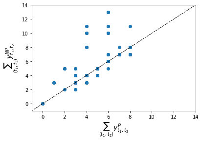
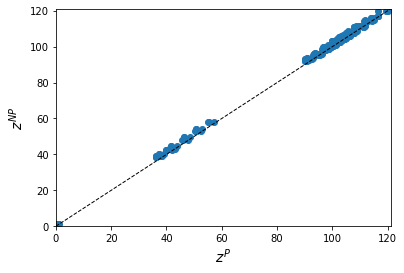
Figure 2(a) shows a scatter plot of the total amount pulled forward under each model in each of the 279 instances. Figure 2(b) shows the corresponding worst-case expected costs. The dashed line corresponds to instances where both models pulled forward the same amount or had the same worst-case cost. The points in Figure 2(a) where the decisions were different suggests that there is no definitive answer to which model’s decision is more conservative. In 42 instances NP pulled forward more, and in 38 instances it pulled forward less. However, when NP pulled forward more than P, it pulled forward up to 7 jobs more. When P pulled forward more, it only pulled forward 1 job more. On average over the instances where the two solutions were different, NP pulled forward 1.24 more jobs. The overall average difference was 0.32. This suggests that NP is generally slightly less conservative than P. However, as shown in Figure 2(b), rarely did NP attain a lower worst-case expected cost than P. The overall average difference between P and NP’s worst-case expected costs was . This suggests that NP’s worst-case distribution typically suggests that there will be 1.21 more jobs being expected to roll over in the worst case. This is surprising since NP typically pulled forward more. Hence, this result indicates that NP’s less conservative nature led to more expected rollover in the majority of these instances.
Since NP results from relaxing the requirement that the worst-case distribution is binomial, we can view NP as a heuristic for solving the parametric model. Hence, it may be beneficial to study the expected cost resulting from under the binomial worst-case distribution that would be given by P, instead of the distribution given by NP. Therefore, for each value of , we compute the worst-case binomial distribution given by a , and the associated expected cost. This allows us to compute the objective value that would attain under the parametric model. Hence, it allows us to assess the quality of in comparison with , as we did for our heuristics. We can also study the difference between ’s worst-case cost under P and NP, via the -gap. This allows us to assess how the two objective functions differ for the same . As a reminder, for an algorithm the -gap is defined as , and the -gap is given by .
| Avg. -gap | Avg. -APG | Avg. -gap | Avg. -APG | -opt. % | |
|---|---|---|---|---|---|
| NP | -1.1764 | 13.0095% | 0.0234 | 0.0429% | 87.1% |
| CS | 0.0561 | 0.084% | 0.0058 | 0.0101% | 97.1% |
The gaps for NP are summarised in Table 5, along with those from CS for comparison. The -gaps show that the worst-case cost for from NP was 1.18 higher than that from P, on average. This indicates that the NP model typically overestimated the worst-case cost associated with . This is consistent with our previous observation that NP’s worst-case objective values were higher for a fixed . In fact, NP overestimated the worst-case cost of in 248 of 279 instances (89%). The most that NP overestimated this cost by was 3.4. These values may seem small, but relative to the true worst-case cost they can be quite large. The largest -APG was 165%, indicating that the worst-case cost from NP was 2.65 times that from P. These results indicate that NP will typically give an objective that makes a decision look worse than it would be in reality. The -APGs suggest that the decisions from NP performed similarly to that of P, under P’s objective. However, they did result in a slight cost increase on average. Based on the results here, we believe that CS is the strongest performing algorithm. CS ran in less time than NP and gave solutions closer to those from P. In fact, we can say that the NP solutions had gaps that were 4 times higher than CS’s on average. Both average gaps were small, but CS was optimal in 92% of instances, as opposed to 71% for NP. Furthermore, if one were to use the NP model, then they would likely overestimate the rollover cost from their decision by approximately 13%, whereas CS would underestimate this cost by approximately 0.084%.
5.5.2 Worst-case Distributions
In order to explain the differences in decisions and costs, we now study the worst-case distributions from P and NP. There are a number of ways in which these distributions can be different. The most obvious one is that P’s worst-case distribution is always binomial, whereas NP’s is not. As well as this, the two approximations of the 95% confidence set for can be different, allowing different distances from . In fact, typically the confidence sets for P were larger. This indicates that the parametric sets had better coverage. We first study the maximum distances from allowed by each ambiguity set and the distances attained by the parametric and non-parametric worst-case distributions, as measured by . We find that the maximum distance allowed by P could be almost twice that allowed by NP. The maximum distance allowed by NP was 1.22, whereas this value was 2.32 for P. This suggests that the parametric ambiguity set can be significantly larger than the non-parametric set. We also find that NP’s worst-case distribution always achieved the maximum distance from . Interestingly, the same does not apply for P. The maximum distance that had from was 2.00, showing that the worst-case binomial distribution was not always as far from as it was allowed to be. In fact, there were 106 instances where P did not reach its maximum distance. As a result, even though the parametric ambiguity sets allowed to be further from , we still find that was further from on average. The fact that NP’s solution was always on the boundary may indicate that the true worst-case distribution was further from than was allowed by NP’s ambiguity set.
In order to compare the worst-case distributions directly, we compute a number of summary statistics for each distribution and present their average values in Table 6. This table also shows the percentage difference between the summary values for the two distributions, which is calculated as . The first two results we show are the average distances from as measured by and by the Kullback-Leibler Divergence (KLD). The KLD value, , can be loosely interpreted as the amount of surprise that would result in simulating from if the true distribution were . These two rows indicate that NP was further from , on average, than P with respect to both distance measures. The values of are quite close, but proportionally the difference in values is much larger. In fact, NP had 52% more surprise than P, on average. This is likely due to the fact that is not binomial, unlike . Entropy also measures surprise, but with respect to the values given by the distribution. We see that both distributions had a similar total entropy, but P had slightly more.
| P | NP | % Gap | |
|---|---|---|---|
| 0.435 | 0.480 | 10.345% | |
| 0.167 | 0.254 | 52.096% | |
| Entropy | 5.379 | 5.227 | -2.826% |
| Total EV | 16.701 | 17.048 | 2.078% |
| Total Variance | 3.670 | 3.590 | -2.18% |
| Total Skewness | -4.274 | -4.431 | 3.673% |
| No. Suppressed | 215.556 | 568.178 | 163.587% |
We also present summaries of the total mean, variance and skewness of each distribution. We see that NP had a higher total expected intake than P on average, but less variance. This can be expected since NP can control the mean and variance separately. P, on the other hand, fixes the variance by fixing the mean. P can therefore have a smaller variance than P, even when the two means are the same. However, P was typically less negatively skewed than NP. These results may explain why NP’s worst-case costs were higher. If NP is more negatively skewed with a higher mean and lower variance, then this suggests that more mass is allocated to the higher intakes and less to the lower ones. Hence, expected costs will necessarily be higher.
Finally, we look at the number of intakes that were popped and suppressed by each worst-case distribution. A distribution popping an intake is defined as when . The distribution suppressing is defined as when . Since is a binomial distribution, technically we will never have popping as . We will also never have suppressing under P, for the same reason. In addition, by Bayraksan and Love, (2015), the modified divergence cannot pop scenarios. Hence, we consider the distributions when rounded to 6 d.p. instead. The table shows that NP popped 55% more intakes than P on average. Both popped only a few intakes, which is consistent with our observation that neither method can technically pop scenarios. This is not the main cause for the difference in the distributions, however. The main difference is from suppressing. We see that NP suppressed 163% more intakes than P on average. This indicates that NP’s worst-case distribution set a large number of ’s positive values to zero. P is much more restricted in this sense, due to the fact that is also binomial. This means that P cannot set any values to be exactly zero. This difference may also explain the increased values of KLD given by NP; some intakes that would be generated by would not be generated by .
6 Conclusions and Further Research
In this paper, we presented parametric and non-parametric DRO models for a workforce planning problem under a mixture of known and uncertain demand. We developed heuristics to solve the parametric model, due to its poor scalability. The general conclusions that we can make from our results are as follows. The full model can be slow to solve to optimality using the MIP reformulation, i.e. using P. CS_opt solves this model to optimality in a short time on average, but begins to solve slowly when the ambiguity set is large. Our heuristics, AO and CS, employ dimension reduction to the sets of intakes and distributions respectively in order to solve the problem in significantly less time than P. The main conclusion we make about these algorithms is that CS performs very well, and takes a fraction of the time that P takes. However, we found that CS can fail to select the worst-case success probability for its chosen pulling forward decision due to its assumption that the total success probability should be maximised. We compared the parametric and non-parametric solutions, and made a number of conclusions. Namely, NP typically pulls forward more than P but it overestimates the worst-case cost of a decision. Our results also suggst that the NP distributions have higher means, lower variance and more negative skewness. They also suppress many more intakes than P’s distributions.
The main contribution that we have made to the existing DRO literature is the new modelling framework of parametric DRO. In real-world planning problems, incorporating distributional ambiguity often results in intractable models. Instead, data-driven estimates of the demand distribution or its parameters are commonly used. However, this can lead to poor solutions when the estimates are poor. Our methodology provides a way that parameter estimates can be utilised in while also hedging against cases when they are inaccurate. It allows planners to build confidence sets around their estimates, that can be adjusted to fit their level of risk aversion. For example, if the planner does not have trust in their estimates then they can choose a large confidence level in order to generate a larger and hence more risk-averse ambiguity set. In addition, our use of parametric distributions instead of non-parametric ones means that the worst-case distribution from our model is more explainable, since it can be summarised by a small number of parameters. This distribution is also less extreme, and less surprising given the estimated distribution. Furthermore, using parametric distributions has allowed us to create fast algorithms for solving the planning problem. This means that planners can incorporate additional uncertainty without having to wait long periods of time for solutions.
There are a number of natural extensions to our work which would be of further interest from a practical viewpoint. Firstly, we have considered a simplified problem in which each job requires one unit of capacity to complete. This is not typically the case in real life workforce planning. Adding more varied completion times would be a clear next step in improving this model. Secondly, the model considers the case where there is only one skill, and is equivalent to assuming all workers can complete any job. In some scenarios this is not the case, and the model could account for this by considering separate demand values and decision variables for each skill. Thirdly, we have treated the capacity as fixed and aimed to optimise its use. In some cases, if not all, however, capacity can be manipulated in the tactical planning phase. For example, one can order extra units of existing resources (overtime) or hire outside resources for a cost (contractors). These ways to manipulate capacity (planning levers) will form the basis of some of our future research. Finally, we have assumed in this paper that the intakes are independent. Extending our model to account for correlated intakes is a promising area for future work.
Acknowledgements
We would like to acknowledge the support of the Engineering and Physical Sciences Research Council funded (EP/L015692/1) STOR-i Centre for Doctoral Training. We would like to thank BT for their funding, and Mathias Kern and Gilbert Owusu from BT for their support. We would also like to thank the 4 anonymous EJOR reviewers for their useful comments that have helped us improve this paper. In addition, we would like to thank Dick den Hertog for his help in developing the CQP reformulation of the non-parametric version of our model.
References
- Ainslie et al., (2017) Ainslie, R., Mccall, J., Shakya, S., and Owusu, G. (2017). Predicting service levels using neural networks. pages 411–416.
- Ainslie et al., (2018) Ainslie, R., McCall, J., Shakya, S., and Owusu, G. (2018). Tactical plan optimisation for large multi-skilled workforces using a bi-level model. 2018 IEEE Congress on Evolutionary Computation (CEC), pages 1–8.
- Ainslie et al., (2015) Ainslie, R. T., Shakya, S., McCall, J., and Owusu, G. (2015). Optimising skill matching in the service industry for large multi-skilled workforces. In Bramer, M. and Petridis, M., editors, Research and Development in Intelligent Systems XXXII, pages 231–243, Cham. Springer International Publishing.
- Angalakudati et al., (2014) Angalakudati, M., Balwani, S., Calzada, J., Chatterjee, B., Perakis, G., Raad, N., and Uichanco, J. (2014). Business analytics for flexible resource allocation under random emergencies. Management Science, 60(6):1552–1573.
- Bansal et al., (2018) Bansal, M., Huang, K.-L., and Mehrotra, S. (2018). Decomposition algorithms for two-stage distributionally robust mixed binary programs. SIAM Journal on Optimization, 28(3):2360–2383.
- Bastian et al., (2020) Bastian, N. D., Lunday, B. J., Fisher, C. B., and Hall, A. O. (2020). Models and methods for workforce planning under uncertainty: Optimizing U.S. army cyber branch readiness and manning. Omega, 92:102171.
- Bayraksan and Love, (2015) Bayraksan, G. and Love, D. K. (2015). Data-driven stochastic programming using phi-divergences. In The Operations Research Revolution, chapter 1, pages 1–19. INFORMS.
- Ben-Tal et al., (2013) Ben-Tal, A., den Hertog, D., De Waegenaere, A., Melenberg, B., and Rennen, G. (2013). Robust solutions of optimization problems affected by uncertain probabilities. Management Science, 59(2):341–357.
- Benders, (1962) Benders, J. (1962). Partitioning procedures for solving mixed-variables programming problems. Numerische mathematik, 4(1):238–252.
- Breton and Hachem, (1995) Breton, M. L. and Hachem, S. E. (1995). Algorithms for the solution of stochastic dynamic minimax problems. Computational Optimization and Applications, 4:317–345.
- Chen et al., (2015) Chen, D., Meng, F., Ang, J., Chu, S., Sim, M., and Kannapiran, P. (2015). A robust optimization model for managing elective admission in hospital. Operations Research, 63.
- Collins, (2004) Collins, R. A. (2004). The behavior of the risk-averse newsvendor for uniform, truncated normal, negative binomial and gamma distributions of demand. In Department of Operations and Management Information Systems, Leavey School of Business Santa Clara University Working paper. Citeseer.
- Dolgui and Pashkevich, (2008) Dolgui, A. and Pashkevich, M. (2008). On the performance of binomial and beta-binomial models of demand forecasting for multiple slow-moving inventory items. Computers & Operations Research, 35(3):893–905.
- Duchi et al., (2016) Duchi, J., Glynn, P., and Namkoong, H. (2016). Statistics of robust optimization: A generalized empirical likelihood approach. Mathematics of Operations Research, 46.
- Fetter, (1961) Fetter, R. B. (1961). A linear programming model for long range capacity planning. Management Science, 7(4):372–378.
- Gallego et al., (2007) Gallego, G., Katircioglu, K., and Ramachandran, B. (2007). Inventory management under highly uncertain demand. Operations Research Letters, 35(3):281–289.
- Ghaoui et al., (2003) Ghaoui, L. E., Oks, M., and Oustry, F. (2003). Worst-case value-at-risk and robust portfolio optimization: A conic programming approach. Operations Research, 51(4):543–556.
- Gurobi Optimization, LLC, (2022) Gurobi Optimization, LLC (2022). Gurobi Optimizer Reference Manual.
- Hanasusanto and Kuhn, (2013) Hanasusanto, G. A. and Kuhn, D. (2013). Robust data-driven dynamic programming. Advances in Neural Information Processing Systems, 26.
- Hanssmann and Hess, (1960) Hanssmann, F. and Hess, S. W. (1960). A linear programming approach to production and employment scheduling. Management Technology, 1(1):46–51.
- Holt et al., (1955) Holt, C. C., Modigliani, F., and Simon, H. A. (1955). A linear decision rule for production and employment scheduling. Management Science, 2(1):1–30.
- Holte and Mannino, (2013) Holte, M. and Mannino, C. (2013). The implementor/adversary algorithm for the cyclic and robust scheduling problem in health-care. European Journal of Operational Research, 226(3):551–559.
- Hu and Hong, (2013) Hu, Z. and Hong, L. J. (2013). Kullback-leibler divergence constrained distributionally robust optimization. Available at Optimization Online: http://www.optimization-online.org/DB_HTML/2012/11/3677.html, pages 1695–1724.
- Hu et al., (2013) Hu, Z., Hong, L. J., and So, A. M.-C. (2013). Ambiguous probabilistic programs. Available at Optimization Online: http://www.optimization-online.org/DB_HTML/2013/09/4039.html.
- Hulst et al., (2017) Hulst, D., den Hertog, D., and Nuijten, W. (2017). Robust shift generation in workforce planning. Computational Management Science, 14.
- J. Abernathy et al., (1973) J. Abernathy, W., Baloff, N., Hershey, J., and Wandel, S. (1973). A three-stage manpower planning and scheduling model – a service-sector example. Operations Research, 21:693–711.
- Jiang and Guan, (2016) Jiang, R. and Guan, Y. (2016). Data-driven chance constrained stochastic program. Math. Program., 158(1–2):291–327.
- Kortanek and No, (1993) Kortanek, K. O. and No, H. (1993). A central cutting plane algorithm for convex semi-infinite programming problems. SIAM Journal on Optimization, 3(4):901–918.
- Lam, (2019) Lam, H. (2019). Recovering best statistical guarantees via the empirical divergence-based distributionally robust optimization. Operations Research, 67(4):1090–1105.
- Lee and Mehrotra, (2015) Lee, C. and Mehrotra, S. (2015). A distributionally-robust approach for finding support vector machine. Optimization Online. Available at http://www.optimization-online.org/DB_HTML/2015/06/4965.html.
- Lee and Raginsky, (2018) Lee, J. and Raginsky, M. (2018). Minimax statistical learning with wasserstein distances. In Proceedings of the 32nd International Conference on Neural Information Processing Systems, NIPS’18, page 2692–2701, Red Hook, NY, USA. Curran Associates Inc.
- Liao et al., (2013) Liao, S., van Delft, C., and Vial, J.-P. (2013). Distributionally robust workforce scheduling in call centres with uncertain arrival rates. Optimization Methods and Software, 28(3):501–522.
- Lotfi and Zenios, (2018) Lotfi, S. and Zenios, S. A. (2018). Robust VaR and CVaR optimization under joint ambiguity in distributions, means, and covariances. European Journal of Operational Research, 269(2):556–576.
- Luo and Mehrotra, (2019) Luo, F. and Mehrotra, S. (2019). Decomposition algorithm for distributionally robust optimization using Wasserstein metric with an application to a class of regression models. European Journal of Operational Research, 278(1):20–35.
- Martel and Price, (1978) Martel, A. and Price, W. (1978). A normative model for manpower planning under risk. In Manpower Planning and Organization Design, pages 291–305. Springer.
- Mehrotra and Papp, (2014) Mehrotra, S. and Papp, D. (2014). A cutting surface algorithm for semi-infinite convex programming with an application to moment robust optimization. arXiv preprint. arXiv:1306.3437.
- Mehrotra and Zhang, (2013) Mehrotra, S. and Zhang, H. (2013). Models and algorithms for distributionally robust least squares problems. Mathematical Programming, 146.
- Millar, (2011) Millar, R. B. (2011). Maximum Likelihood Estimation and Inference: With Examples in R, SAS and ADMB, volume 112 of Statistics in practice. Wiley, New York, 1. aufl. edition.
- Mohajerin Esfahani and Kuhn, (2018) Mohajerin Esfahani, P. and Kuhn, D. (2018). Data-driven distributionally robust optimization using the wasserstein metric: Performance guarantees and tractable reformulations. Mathematical Programming, 171(1):115–166.
- Pflug and Wozabal, (2007) Pflug, G. and Wozabal, D. (2007). Ambiguity in portfolio selection. Quantitative Finance, 7(4):435–442.
- Rahimian et al., (2019) Rahimian, H., Bayraksan, G., and Homem-De-Mello, T. (2019). Identifying effective scenarios in distributionally robust stochastic programs with total variation distance. Mathematical Programming, 173(1–2):393–430.
- Rahimian and Mehrotra, (2019) Rahimian, H. and Mehrotra, S. (2019). Distributionally robust optimization: A review. arXiv preprint. arXiv:1908.05659.
- Ross, (2016) Ross, E. (2016). Cross-trained Workforce Planning Models. PhD thesis, University of Lancaster.
- Rossi et al., (2014) Rossi, R., Prestwich, S., Tarim, S. A., and Hnich, B. (2014). Confidence-based optimisation for the newsvendor problem under binomial, poisson and exponential demand. European Journal of Operational Research, 239(3):674–684.
- Samudra et al., (2016) Samudra, M., Demeulemeester, E., Cardoen, B., Vansteenkiste, N., and Rademakers, F. (2016). Scheduling operating rooms: achievements, challenges and pitfalls. Journal of Scheduling, 19.
- Scarf, (1957) Scarf, H. E. (1957). A Min-Max Solution of an Inventory Problem. RAND Corporation, Santa Monica, CA.
- Shapiro and Kleywegt, (2002) Shapiro, A. and Kleywegt, A. (2002). Minimax analysis of stochastic problems. Optimization Methods and Software, 17(3):523–542.
- Yanıkoğlu and den Hertog, (2013) Yanıkoğlu, I. and den Hertog, D. (2013). Safe approximations of ambiguous chance constraints using historical data. INFORMS Journal on Computing, 25(4):666–681.
- Zhu and Sherali, (2009) Zhu, X. and Sherali, H. D. (2009). Two-stage workforce planning under demand fluctuations and uncertainty. Journal of the Operational Research Society, 60(1):94–103.
Appendix A Derivation of CQP Reformulation of Non-parametric Model
A.1 General Reformulation
For a -divergence ambiguity set with nominal distribution , we can write the inner problem of the DRO model (1)-(8) as:
| (38) | ||||
| s.t. | (39) | |||
| (40) | ||||
| (41) |
The Lagrangian of this model is given by:
| (42) |
The objective function of the dual problem is therefore:
| (43) |
Since and where is a feasible choice of distribution, Slater’s condition holds. Since the primal is concave, we have strong duality. We can hence write the objective of the dual of the inner problem as:
| (44) | ||||
| (45) | ||||
| (46) | ||||
| (47) | ||||
| (48) | ||||
| (49) | ||||
| (50) | ||||
| (51) |
where and . Note that we can replace the sum of maxima with a maximum of sums in (49) because the objective is separable over . Finally, we require the dual feasibility constraint (52):
| (52) |
This ensures that does not grow to infinity. Consider . If as then this constraint can be removed. If not, i.e. , then for we have . Note that, according to the definition given by Ben-Tal et al., (2013), we have , which is zero if and if . Therefore, combining with the outer problem, we have:
| (53) | ||||
| s.t. | (54) | |||
| (55) | ||||
| (56) |
A.2 Modified -divergence
Recall equation (13), which states that for a modified divergence, we have:
A.2.1 Reformulation
The conjugate of is given by:
Using to represent for shorthand, we can expand in order to write:
| (57) | ||||
| (58) | ||||
| (59) |
In order to define using convex quadratic constraints, we first need to remove the max operator from this expression. Hence, we define a dummy variable to represent the value of . We enforce ’s value via (60) and (61).
| (60) | ||||
| (61) |
Then, we can define another dummy variable . We enforce the value of using a conic quadratic constraint as follows:
| (62) | ||||
| (63) | ||||
| (64) | ||||
| (65) |
Hence, with dummy variables for , we can reformulate our inner problem as:
| (66) | ||||
| (67) | ||||
| (68) | ||||
| (69) | ||||
| (70) |
Therefore, combining with the outer model, we have:
| (71) | ||||
| s.t. | (72) | |||
| (73) |
Note that, in the objective function, the comes from the fact that .
A.2.2 Extracting Worst-case Distribution
In order to find the worst-case distribution, we must extract it from the optimal values of . Denote the optimal solution of model (71)-(73) by . As discussed by Bayraksan and Love, (2015), the worst-case distribution satisfies:
| (74) |
Here, the notation is the set of subgradients of at . Suppose that so that is defined. By Bayraksan and Love, (2015), if is differentiable then is a subgradient. This is true in our case, with . This derivative is non-negative, and hence always gives a feasible solution for by taking when . In our experiments we only ever observed and hence always gave a solution. For more detail on how to extract the solution when , see Bayraksan and Love, (2015).
Appendix B Further Analysis of Results
B.1 The Effect of Workstacks on Solutions
In our experiments, we used only one value of the capacity but varied the workstacks to give a variety of possibilities for pulling forward. This was based on the number of pairs between which pulling forward was possible, i.e. from Section 4.2. We give some examples of the values of and the corresponding in Table 7.
| (8, -15, -15, 8, -15) | 3 |
| (8, -15, 8, 8, 8) | 5 |
| (8, 8, 8, 8, 8) | 7 |
Any more pairs than 7 is not possible for and . We present a summary of the results broken down by in Table 8. This table shows three quantities: the average time taken by each algorithm, the average gaps and the average number of pairs of days which had a positive pulling forward decision. The table shows that we did not have any more non-zero decisions than 1, from any algorithm, until reached its maximum value of 7. Days 1 and 2 were typically prioritised for rollover reduction via pulling forward in these cases. This is because jobs due on these days have the potential to roll over the most times. However, when , we see between 1 and 6 pairs of days having a non-zero pulling forward decision.
| Avg. -APG | Avg. -APG | Avg. t.t. | (Avg., Max) Non-zeros | |||
|---|---|---|---|---|---|---|
| Count | Algorithm | |||||
| 3 | 189 | opt | 0.0% | 0.0% | 0:01:00.38 | (1.0, 1) |
| CS | 0.0415% | 0.0029% | 0:00:07.58 | (1.0, 1) | ||
| CS_opt | 0.0% | 0.0% | 0:00:09.75 | (1.0, 1) | ||
| AO | 0.0084% | 0.0059% | 0:00:24.74 | (1.0, 1) | ||
| NP | - | - | 0:00:02.62 | (1.0, 1) | ||
| 5 | 45 | opt | 0.0% | 0.0% | 0:02:12.72 | (1.0, 1) |
| CS | 0.3465% | 0.0506% | 0:00:25.62 | (1.0, 1) | ||
| CS_opt | 0.0% | 0.0% | 0:00:29.35 | (1.0, 1) | ||
| AO | 0.0052% | 0.2903% | 0:00:19.04 | (1.0, 1) | ||
| NP | - | - | 0:00:32.2 | (1.0, 1) | ||
| 7 | 45 | opt | 0.0% | 0.0% | 0:02:44.25 | (2.0, 4) |
| CS | 0.0% | 0.0% | 0:01:27.85 | (2.0, 4) | ||
| CS_opt | 0.0% | 0.0% | 0:01:31.68 | (2.0, 4) | ||
| AO | 0.0% | 0.5332% | 0:00:21.16 | (2.0, 4) | ||
| NP | - | - | 0:01:53.93 | (2.8, 6) |
The APGs are also shown in Table 8. From this, we can see a number of results. Firstly, we see that the average time taken by each algorithm apart from AO was increasing in . This can be expected, since more feasible pairs leads to a more complex feasible region. Furthermore, AO performed the worse in selecting as increases. This is likely because reducing the set of intakes leads to less accurate estimates of the expected rollover. Interestingly, CS did not suffer from the same issue. In fact, for , CS had an average -APG of 0.0% and for all values of this value was below 0.051%. This is because CS does not employ dimension reduction to the set of intakes like AO does. As might be expected, there is no clear pattern in the -APGs. For AO and CS, this value was highest when and lowest when . Finally, the final column shows the average and maximum numbers of pairs that had under each algorithm. The results for suggest that NP’s solution was slightly less conservative than P’s solution on average. We study this in more detail in Section 5.5. Interestingly, NP took almost as long as P in these instances. CS_opt again had all zero gaps and APGs, and its times taken were no more affected by than the times taken by CS.
B.2 Comparison with Robust Optimisation Solutions
In this section, we compare the DRO decisions and objectives with those resulting from the robust optimisation (RO) version of the model. The RO model is obtained by replacing the inner objective with the maximisation of the total rollover cost over all intake vectors. The first result that we find is that the intake vector responsible for the worst-case cost for the chosen value was always . This shows that the RO model can be solved simply by assuming that all intakes take their maximum values at all times. As well as this, the RO model pulled forward less than the DRO model in 227 (82%) of our 279 instances. The RO solution also had a higher cost than the DRO solution in 269 (97%) of instances. This can be expected due to the way that their objective functions differ. These two facts support our claim that the RO model is more conservative than the DRO model.
We present some more detailed results in Table 9. This table compares the objective values, pulling forward decisions and times taken from the three models. Firstly, note that RO took around 16 seconds on average. RO also pulled forward less than DRO. Specifically, it pulled forward 1.3 jobs less than DRO, on average. Also, DRO pulled forward a maximum of 8 jobs whereas RO only pulled forward a maximum of 7 jobs. Furthermore, the objective values from RO were significantly higher than DRO. Comparing the RO objective with the DRO objective, we see that RO’s objective values were around 9.5 higher than DRO’s on average. This corresponds to almost a 200% increase in objective value. The -gap and -APGs assess the expected costs from RO’s decisions when evaluated by DRO’s objective function. This suggests that RO’s decisions would result in around 2 more jobs being expected to roll over in the worst case than DRO’s solution.
| RO Det. | RO | DRO | |
| Avg. Obj. Gap | 9.499 | 9.499 | 0 |
| Avg. % Obj. Gap | 199.662% | 199.662% | 0% |
| Avg. -gap | 1.851 | 1.851 | 0 |
| Avg. -APG | 2.616% | 2.616% | 0% |
| Avg. | 4 | 4 | 5.308 |
| Max. | 7 | 7 | 8 |
| Avg. t.t. | 0:00:00.01 | 0:00:15.89 | 0:01:22.85 |
As already noted, RO is equivalent to the deterministic model under the assumption that with probability 1. The results from this model are shown in the “RO det.” column. This shows that this model took 0.01 seconds to build and solve, on average. Hence, our results indicate that the inclusion of the rollover constraints for the RO model led to around a 16 second increase in solution times. The inclusion of the expected value constraints for the DRO model resulted in over 1 minute of additional solution time. Table 9 also shows that RO had an objective value that was three times larger than DRO’s, on average.
From the results presented here, we can conclude three main results. Firstly, RO is more conservative than DRO for this problem, since it pulled forward fewer jobs on average. Secondly, RO results in significantly higher costs for the same decision. However, the third conclusion is that RO is much faster than DRO. This indicates that the main factor affecting solution times for DRO is the inclusion of the expected value constraints.
Appendix C A Benders Decomposition Approach
Our CS_opt algorithm can be viewed as a specialised Benders decomposition (Benders,, 1962) approach that solves the distribution separation problem as a residual problem. However, it does not require us to create the dual of the distribution separation problem, and in our case we can simply solve this problem by enumeration. For comparison, we now present a classical Benders decomposition approach in order to explain why CS_opt is preferred.
C.1 Residual Problem and its Dual
We create the Benders residual problem by taking as the master problem variable and as the subproblem variables. This is because the model’s complexity comes from and , not . For a fixed , the residual problem can be written as:
| (75) | ||||
| s.t. | (76) | |||
| (77) | ||||
| (78) | ||||
| (79) |
This model has constraints. Hence, we have dual variables for and , and for . The model has variables, and so we have constraints in the dual. The dual is given by:
| (80) | ||||
| (81) | ||||
| (82) | ||||
| (83) | ||||
| (84) |
where and are defined as:
| (85) | |||||
| (86) | |||||
| (87) | |||||
| (88) | |||||
C.2 Benders Decomposition Algorithm
Our Benders decompositon algorithm is as follows.
-
1.
Initialise , , . Set feasible region for as . Set feasible region for as , where indicates that is feasible for the model in (2)-(8).
-
2.
While :
-
(a)
Solve master problem:
(89) to get a solution and objective value .
-
(b)
Set .
- (c)
-
(d)
If subproblem is unbounded, add feasibility cut:
to .
-
(e)
If subproblem is optimal, add optimality cut:
to .
-
(f)
If then set .
-
(a)
-
3.
Find index of binding constraint from the subproblem and use this to find worst-case .
-
4.
Return , .
In the following section we will show that this approach is slow compared with CS_opt.
C.3 Results
We tested the Benders algorithm on each of our 279 instances, for . We present the results in Table 10. From these results, it is clear that was required for optimality. However, with this , the Benders algorithm took almost 6 minutes to solve, on average. In one instance, the algorithm timed out as it took longer than 4 hours. In comparison with CS_opt, which takes approximately 17 seconds on average, this version of Benders decomposition is very slow.
| Avg. -gap | Avg. -APG | Avg. -gap | Avg. -APG | Avg. t.t. | Max t.t. | |
|---|---|---|---|---|---|---|
| 1e-08 | 0.0 | 0.0% | -0.0000 | 0.0% | 0:05:57.798 | 4:00:05.011 |
| 1e-06 | 0.0 | 0.0% | 0.0029 | 0.0% | 0:04:42.6717 | 1:24:55.625 |
| 1e-02 | 0.0 | 0.0% | 0.0141 | 10.1984% | 0:04:36.6348 | 1:21:58.415 |
Appendix D Large Results Tables
D.1 Results by
| Avg. | Count | Algorithm | Avg. -APG | Avg. -APG | Avg. t.t. | |
|---|---|---|---|---|---|---|
| 1.000 | 62 | P | 0.0% | 0.0% | 0:00:14.57 | |
| CS | 0.0% | 0.0% | 0:00:16 | |||
| CS_opt | 0.0% | 0.0% | 0:00:15.81 | |||
| AO | 0.0% | 0.248% | 0:00:01.32 | |||
| NP | - | - | 0:00:25.58 | |||
| 1.419 | 31 | P | 0.0% | 0.0% | 0:00:15.11 | |
| CS | 0.0% | 0.0% | 0:00:16.53 | |||
| CS_opt | 0.0% | 0.0% | 0:00:16.46 | |||
| AO | 0.0% | 0.248% | 0:00:01.35 | |||
| NP | - | - | 0:00:27.13 | |||
| 14.419 | 31 | P | 0.0% | 0.0% | 0:00:14.23 | |
| CS | 0.0% | 0.0% | 0:00:15.05 | |||
| CS_opt | 0.0% | 0.0% | 0:00:15.42 | |||
| AO | 0.0% | 0.248% | 0:00:01.4 | |||
| NP | - | - | 0:00:25.22 | |||
| 14.742 | 31 | P | 0.0% | 0.0% | 0:00:16.14 | |
| CS | 0.0% | 0.0% | 0:00:18.97 | |||
| CS_opt | 0.0% | 0.0% | 0:00:19.42 | |||
| AO | 0.0% | 0.0004% | 0:00:01.76 | |||
| NP | - | - | 0:00:24.66 | |||
| 16.871 | 31 | P | 0.0% | 0.0% | 0:00:16.24 | |
| CS | 0.0% | 0.0% | 0:00:16.48 | |||
| CS_opt | 0.0% | 0.0% | 0:00:16.5 | |||
| AO | 0.0452% | 0.2391% | 0:00:01.57 | |||
| NP | - | - | 0:00:26.12 | |||
| 93.129 | 31 | P | 0.0% | 0.0% | 0:00:24.51 | |
| CS | 0.5029% | 0.0734% | 0:00:20.8 | |||
| CS_opt | 0.0% | 0.0% | 0:00:19.9 | |||
| AO | 0.0105% | 0.0% | 0:00:02.9 | |||
| NP | - | - | 0:00:27.16 | |||
| 504.226 | 31 | P | 0.0% | 0.0% | 0:00:59.36 | |
| CS | 0.0339% | 0.0% | 0:00:17.85 | |||
| CS_opt | 0.0% | 0.0% | 0:00:19.76 | |||
| AO | 0.0% | 0.0% | 0:00:12.77 | |||
| NP | - | - | 0:00:23.47 | |||
| 4301.645 | 31 | P | 0.0% | 0.0% | 0:09:30.88 | |
| CS | 0.219% | 0.0176% | 0:00:19.66 | |||
| CS_opt | 0.0% | 0.0% | 0:00:42.47 | |||
| AO | 0.0031% | 0.0% | 0:02:11.27 | |||
| NP | - | - | 0:00:23.22 |
D.2 Results by
| Count | Algorithm | Avg. -APG | Avg. -APG | Avg. t.t. | |
|---|---|---|---|---|---|
| 392 | 27 | P | 0.0% | 0.0% | 0:00:33.63 |
| CS | 0.0234% | 0.0% | 0:00:06.37 | ||
| CS_opt | 0.0% | 0.0% | 0:00:08.01 | ||
| AO | 0.002% | 0.0% | 0:00:23.53 | ||
| NP | - | - | 0:00:00.84 | ||
| 512 | 45 | P | 0.0% | 0.0% | 0:00:31.88 |
| CS | 0.0952% | 0.0024% | 0:00:06.54 | ||
| CS_opt | 0.0% | 0.0% | 0:00:08.05 | ||
| AO | 0.0% | 0.0% | 0:00:20.86 | ||
| NP | - | - | 0:00:00.78 | ||
| 567 | 45 | P | 0.0% | 0.0% | 0:00:37.09 |
| CS | 0.0572% | 0.0107% | 0:00:06.61 | ||
| CS_opt | 0.0% | 0.0% | 0:00:08.28 | ||
| AO | 0.0116% | 0.0% | 0:00:25.75 | ||
| NP | - | - | 0:00:00.98 | ||
| 2187 | 27 | P | 0.0% | 0.0% | 0:01:42.9 |
| CS | 0.0536% | 0.0% | 0:00:08.72 | ||
| CS_opt | 0.0% | 0.0% | 0:00:11.69 | ||
| AO | 0.0259% | 0.0005% | 0:00:25.93 | ||
| NP | - | - | 0:00:04.25 | ||
| 2592 | 45 | P | 0.0% | 0.0% | 0:01:42 |
| CS | 0.0043% | 0.0% | 0:00:09.69 | ||
| CS_opt | 0.0% | 0.0% | 0:00:12.82 | ||
| AO | 0.0061% | 0.0246% | 0:00:26.58 | ||
| NP | - | - | 0:00:06.18 | ||
| 8192 | 45 | P | 0.0% | 0.0% | 0:02:12.72 |
| CS | 0.3465% | 0.0506% | 0:00:25.62 | ||
| CS_opt | 0.0% | 0.0% | 0:00:29.35 | ||
| AO | 0.0052% | 0.2903% | 0:00:19.04 | ||
| NP | - | - | 0:00:32.2 | ||
| 20000 | 45 | P | 0.0% | 0.0% | 0:02:44.25 |
| CS | 0.0% | 0.0% | 0:01:27.85 | ||
| CS_opt | 0.0% | 0.0% | 0:01:31.68 | ||
| AO | 0.0% | 0.5332% | 0:00:21.16 | ||
| NP | - | - | 0:01:53.93 |
Appendix E Tables of Notation
E.1 General Model Notation
| Notation | Meaning |
|---|---|
| Number of days in a plan | |
| Maximum number of days a job can be pulled forward | |
| , , | A day in the plan, value in |
| Number of jobs to pull forward from day to . | |
| Number of jobs to roll over from day to . | |
| Cost of a job rolling over from day to . | |
| Number of hours of capacity available on day . | |
| Number of jobs currently due on day . | |
| Set of non-negative integers. | |
| Random variable representing number of jobs arriving between the time of planning and day that will be due on day (intake). | |
| Realisation of . | |
| Realisation of corresponding to realisation of . | |
| Set of all possible realisations of . | |
| Set of all possible realisations of the vector of intakes . | |
| General ambiguity set constaining distributions of intake. | |
| A discrete probability distribution over the set of intakes . | |
| Nominal distribution of intake. | |
| The maximum value can take. | |
| A variable representing success probability parameter of the binomial distribution of intake . | |
| True success probability of intake . | |
| MLE of taken from samples of . | |
| Binomial distribution of intake with success probability parameter . | |
| MLE of distribution resulting from . | |
| Set of all probability distributions that are binomial with a value . | |
| Set of vectors obtained from a distribution in . | |
| confidence set for around the MLE . |
E.2 Non-parametric Model Notation
| Notation | Meaning |
|---|---|
| -divergence function. | |
| -divergence measure resulting from -divergence function . | |
| Conjugate of -divergence function . | |
| -divergence function for modified distance. | |
| percentile of distribution with degrees of freedom. | |
| Non-parametric confidence set for true distribution . | |
| Lagrange multipliers for SQP reformulation of NP model. | |
| Dummy variables used to reformulate NP model. | |
| Maximum distance, measured by , from that can be under the non-parametric model. | |
| Set of subgradients of a function at a point . | |
| Optimal value of under the non-parametric model, for . |
E.3 CS/CS_opt/AO Notation
| Notation | Meaning |
|---|---|
| (repeated dummy variable) | Index for the iteration of CS/CS_opt algorithm that we are currently carrying out. |
| Maximum value that takes over . | |
| Set of parameters such that is maximised. | |
| Set of extreme parameters used by CS. | |
| General ambiguity set used by CS algorithms. for CS_opt and for CS. | |
| Maximum number of iterations of CS/CS_opt algorithm allowed to run. | |
| Current subset of being used at iteration of CS/CS_opt. | |
| Pulling forward decision generated by solving outer problem at iteration of CS/CS_opt. | |
| Probability vector generated by solving distribution separation problem at iteration of CS/CS_opt. | |
| Optimality tolerance of CS/CS_opt algorithm. | |
| Objective value of problem obtained by solving outer problem at iteration of CS. | |
| Minimum probability an intake must have of occurring in order to be used in the AO algorithm. | |
| Set of intakes with probability of occurring higher than . |
E.4 Input Parameter and Results Notation
| Notation | Meaning |
|---|---|
| Set of pairs of days between which pulling forward is allowed. | |
| Set of pairs of days between which pulling forward is feasible given and . | |
| Number of days with maximum intake higher than remaining capacity given , , and . | |
| Number of values each probability in can take in our discretised ambiguity set. | |
| MLE of mean intake vector. | |
| Maximum distance from we allow to be under NP, measured by the chosen -divergence. |
| Notation | Meaning |
|---|---|
| Shorthand for expected rollover cost given pulling forward decision and distribution parameter . | |
| An algorithm, namely in . | |
| solution obtained by algorithm . | |
| -gap of algorithm ’s solution. The difference between the worst-case expected cost for and the expected cost obtained by the algorithm. | |
| Overall optimal objective value. | |
| -gap. Difference between worst-case expected cost for over all distributions and the overall optimal objective value. |