On the spectrum of an operator associated with least-squares finite elements for linear elasticity

Abstract.

In this paper we provide some more details on the numerical analysis and we present some enlightening numerical results related to the spectrum of a finite element least-squares approximation of the linear elasticity formulation introduced recently. We show that, although the formulation is robust in the incompressible limit for the source problem, its spectrum is strongly dependent on the Lamé parameters and on the underlying mesh.

Keywords. Eigenvalue problem; linear elasticity; least-squares finite elements.

AMS subject classification. 65N25, 74B05

1. Introduction

In this paper we continue the discussion started in [4, 5] about the spectrum of operators arising from least-squares finite element approximation of partial differential equations. In [4] several least-squares formulations associated with the Laplace problem and in [5] two formulations associated with the linear elasticity problem were considered. Here we continue the analysis of the two-field formulation presented in [5]. The two-field formulation was introduced in [8] for the approximation of the source problem and has the merit of providing a robust discretization also when the system approaches the incompressible limit.

Several methods are available for the computation of the eigenvalues and eigefunctions in linear elasticity and the aim of this paper is not to compete with them. However, a good knowledge of the properties of the spectrum is useful for several applications. For instance, if a transient problem is approximated by using the two-field approach for the space semi-discretization, then the behavior of the solution depends essentially on the discrete eigenvalues of the operator corresponding to the least-squares model. Hence, we believe that a study of the approximation of the eigenvalues and the eigenfunctions may be interesting in view of a better understanding of the scheme under investigation.

The aim of this paper is two-fold. First, we complete the analysis presented in [5] where only a sketch of the main ideas were indicated. Actually, since the least-squares formulation is not symmetric, the convergence analysis should take into account the dual problem for which we provide a careful description in this paper. Second, we present a bunch of numerical experiments that highlight some properties of the spectrum. A peculiarity of our operators is that the continuous problem has positive and real eigenvalues, while its approximation may have eigenvalues everywhere in the complex plane. Our numerical tests show that for small values of the Lamé constant $\lambda$ (i.e., when the considered elastic solid is far from being incompressible) the discrete spectrum is generally well-behaving that is, it is distributed in the right half of the complex plane and has a small imaginary part. On the other hand, when the solid tends to the incompressible limit, as $\lambda$ increases, the distribution of the discrete spectrum is more spread in the entire complex plane, including eigenvalues with negative real part. We present several examples of this behavior and discuss how it may depend on the chosen mesh sequence. We conclude that, although the two-field formulation has been proved to be robust for the approximation of the source problem corresponding to linear elasticity, the spectrum of the discrete solution operator is more stable when a small value of $\lambda$ is considered.

It will be interesting in the future to discuss in more detail the asymptotic exactness of the least-squares operator associated to linear elasticity proved in [9], and to see how it is related to eigenvalue problems and to the situation presented in this paper.

In Section 2 we describe the first order system corresponding to linear elasticity and recall its two-field least-squares representation. Section 3 deals with its finite element discretization and Section 4 develops the convergence analysis. Finally, we report our numerical results in Section 5.

2. The continuous problem

Consider a polytopal domain $\Omega$ in $\mathbb{R}^{d}$ $(d=2,3)$. We partition the boundary of the domain into two open subsets $\Gamma_{D}$ and $\Gamma_{N}$ such that $\partial\Omega=\overline{\Gamma}_{D}\cup\overline{\Gamma}_{N}$ and $\Gamma_{D}\cap\Gamma_{N}=\emptyset$ with $\mathbf{n}$ denoting the outward unit vector normal to $\Gamma_{N}$. The linear elasticity problem that we are going to consider consists of finding a stress tensor $\underline{\bm{\sigma}}=(\sigma_{i,j})_{d\times d}$ and a displacement field $\mathbf{u}=(u_{1},\ldots,u_{d})^{\top}$ for a given body force $\mathbf{f}=(f_{1},\ldots,f_{d})^{\top}$ that satisfy the system

(1) $$\begin{cases}\underline{\bm{\sigma}}-\mathcal{C}\underline{\bm{\epsilon}}(\mathbf{u})=\underline{\bf{0}}&\quad\text{in}\quad\Omega,\\ \bf{div}\underline{\bm{\sigma}}=-\mathbf{f}&\quad\text{in}\quad\Omega,\\ \mathbf{u}=\bf{0}\quad&\quad\text{on}\quad\Gamma_{D},\\ \mathbf{n}\cdot\underline{\bm{\sigma}}=\bf{0}&\quad\text{on}\quad{\Gamma_{N}},\end{cases}$$

where $\underline{\bm{\epsilon}}(\mathbf{v})$ is the symmetric gradient (also known as the strain tensor) given by

$$\underline{\bm{\epsilon}}({\mathbf{v}})=\frac{1}{2}(\underline{\bm{\nabla}}\mathbf{v}+(\underline{\bm{\nabla}}\mathbf{v})^{\top}),$$

and $\mathcal{C}$ is the elasticity tensor (a symmetric operator) for isotropic, homogeneous material defined in terms of the Lamé constants $\mu$ and $\lambda$ as

$$\mathcal{C}\underline{\bm{\epsilon}}({\mathbf{v}})=\lambda\text{tr}(\underline{\bm{\epsilon}}({\mathbf{v}}))\underline{\mathbf{I}}+2\mu\underline{\bm{\epsilon}}({\mathbf{v}}),$$

with $\underline{\mathbf{I}}$ being the identity tensor.

It is well known that there is a relation between stress and strain tensors such that:

(2) $$\underline{\bm{\tau}}=\mathcal{C}\underline{\bm{\epsilon}}(\mathbf{v})\quad\text{or}\quad\underline{\bm{\epsilon}}(\mathbf{v})=\mathcal{A}\underline{\bm{\tau}},$$

where $\mathcal{A}$ is the compliance tensor given by

(3) $$\mathcal{A}\underline{\bm{\tau}}=\frac{1}{2\mu}\bigg{(}\underline{\bm{\tau}}-\frac{\lambda}{d\lambda+2\mu}\text{tr}(\underline{\bm{\tau}})\underline{\mathbf{I}}\bigg{)}.$$

If $\lambda$ is finite, then from (2) we have $\mathcal{A}=\mathcal{C}^{-1}$. However, as $\lambda$ approaches $\infty$ the elasticity tensor blows up and the material becomes nearly incompressible or incompressible. For this reason it may be more convenient to use the relation $\underline{\bm{\epsilon}}(\mathbf{v})=\mathcal{A}{\underline{\bm{\tau}}}$ if we are interested in formulations that are stable uniformly in $\lambda$. We can then rewrite System (1) as: find a symmetric $d\times d$ stress tensor $\underline{\bm{\sigma}}$ and a displacement vector-field $\mathbf{u}$ such that

(4) $$\begin{cases}\mathcal{A}\underline{\bm{\sigma}}-\underline{\bm{\epsilon}}(\mathbf{u})=\underline{\bm{0}}&\quad\text{in}\quad\Omega,\\ \bf{div}\underline{\bm{\sigma}}=-\mathbf{f}&\quad\text{in}\quad\Omega,\\ \mathbf{u}=\bm{0}\quad&\quad\text{on}\quad\Gamma_{D},\\ \mathbf{n}\cdot\underline{\bm{\sigma}}=\bm{0}&\quad\text{on}\quad{\Gamma_{N}}.\end{cases}$$

We are interested in the spectrum of the solution operator associated with (4), hence, we replace the source term $\mathbf{f}$ by $\omega\mathbf{u}$, where $\omega$ is the eigenvalue associated with $\mathbf{u}$. Since our problem is symmetric, we are looking for real eigenvalues $\omega\in\mathbb{R}$ such that for non vanishing $\mathbf{u}$ and some $\underline{\bm{\sigma}}$ the following set of equations is satisfied

(5) $$\begin{cases}\mathcal{A}\underline{\bm{\sigma}}-\underline{\bm{\epsilon}}(\mathbf{u})=\underline{\bm{0}}&\quad\text{in}\quad\Omega,\\ \bf{div}\underline{\bm{\sigma}}=-\omega\mathbf{u}&\quad\text{in}\quad\Omega,\\ \mathbf{u}=\bm{0}\quad&\quad\text{on}\quad\Gamma_{D},\\ \mathbf{n}\cdot\underline{\bm{\sigma}}=\bm{0}&\quad\text{on}\quad{\Gamma_{N}}.\end{cases}$$

The eigenvalue Problem (5) is compact due to the regularity properties of the solution of System (4). Therefore, the eigenvalues are real and positive and form an increasing sequence

$$0<\omega_{1}\leq\omega_{2}\leq\cdots\leq\omega_{i}\leq\cdots\quad\text{with}\quad\lim_{i\to\infty}\omega_{i}=\infty,$$

repeated according to their multiplicity so that each eigenvalue $\omega_{i}$ corresponds to a one dimensional eigenspace $E_{i}$.

We rewrite (4) following the least-squares principle approach introduced in [8]. As stated by the authors and as a consequence of the above considerations, this approach has the important advantage of automatically stabilizing the stress-displacement system in the incompressible limit when comparing it to other approaches, thus being more robust. The so called two-field formulation (in the unknowns $\mathbf{u}$ and $\underline{\bm{\sigma}}$) was achieved by applying the $L^{2}$ norm and minimizing the functional

(6) $$\mathcal{F}(\underline{\bm{\tau}},\textbf{v};\textbf{f})=||\mathcal{A}\underline{\bm{\tau}}-\underline{\bm{\epsilon}}(\textbf{v})||_{0}^{2}+||\textbf{div}\underline{\bm{\tau}}+\textbf{f}||_{0}^{2},$$

in $\underline{\bm{X}}_{N}\times H^{1}_{0,D}(\Omega)^{d}$, where

$$\underline{\bm{X}}=\begin{cases}\textbf{H}(\textbf{div};\Omega)^{d}&\quad\text{if}\quad\Gamma_{N}\neq\emptyset,\\ \{\underline{\bm{\tau}}\in\textbf{H}(\textbf{div};\Omega)^{d}:\int_{\Omega}\text{tr}(\underline{\bm{\tau}})\text{d}\textbf{x}=0\}&\quad\text{if}\quad\Gamma_{N}=\emptyset,\\ \end{cases}$$

and $\underline{\bm{X}}_{N}$ being its subspace

$$\underline{\bm{X}}_{N}=\{\underline{\bm{\tau}}\in\underline{\bm{X}}:\textbf{n}\cdot\underline{\bm{\tau}}=\textbf{0}\quad\text{on}\quad\Gamma_{N}\}.$$

Applying the same strategy to (5) would lead to a non-linear problem. Following the original idea developed in [4] for the Laplace operator, in [5] the spectrum of the operators associated with the least-squares $\it{source}$ formulation was considered.

2.1. The variational formulation.

The minimization of the functional corresponding to the source problem in (6), gives rise to the variational problem: find $(\underline{\bm{\sigma}},\textbf{u})\in\underline{\textbf{X}}_{N}\times H^{1}_{0,D}(\Omega)^{d}$ such that

(7) $$\begin{cases}(\mathbf{\mathcal{A}}\underline{\bm{\sigma}},\mathbf{\mathcal{A}}\underline{\bm{\tau}})+(\textbf{div}\underline{\bm{\sigma}},\textbf{div}\underline{\bm{\tau}})-(\mathbf{\mathcal{A}}\underline{\bm{\tau}},\underline{\bm{\epsilon}}(\textbf{u}))=-(\textbf{f},\textbf{div}\underline{\bm{\tau}})&\quad\forall\underline{\bm{\tau}}\in\underline{\bm{X}}_{N},\\ -(\mathbf{\mathcal{A}}\underline{\bm{\sigma}},\underline{\bm{\epsilon}}(\textbf{v}))+(\underline{\bm{\epsilon}}(\textbf{u}),\underline{\bm{\epsilon}}(\textbf{v}))=\bm{0}&\quad\forall\textbf{v}\in H^{1}_{0,D}(\Omega)^{d},\end{cases}$$

so that the eigenvalue variational problem associated with the two-field formulation reads: find $(\omega,\mathbf{u})\in\mathbb{R}\times H^{1}_{0,D}(\Omega)^{d}$ with $\textbf{u}\neq 0$ such that for some $\underline{\bm{\sigma}}\in\underline{\bm{X}}_{N}$ we have

(8) $$\begin{cases}(\mathbf{\mathcal{A}}\underline{\bm{\sigma}},\mathbf{\mathcal{A}}\underline{\bm{\tau}})+(\textbf{div}\underline{\bm{\sigma}},\textbf{div}\underline{\bm{\tau}})-(\mathbf{\mathcal{A}}\underline{\bm{\tau}},\underline{\bm{\epsilon}}(\textbf{u}))=-\omega(\textbf{u},\textbf{div}\underline{\bm{\tau}})&\quad\forall\underline{\bm{\tau}}\in\underline{\bm{X}}_{N},\\ -(\mathbf{\mathcal{A}}\underline{\bm{\sigma}},\underline{\bm{\epsilon}}(\textbf{v}))+(\underline{\bm{\epsilon}}(\textbf{u}),\underline{\bm{\epsilon}}(\textbf{v}))=\bm{0}&\quad\forall\textbf{v}\in H^{1}_{0,D}(\Omega)^{d}.\end{cases}$$

As discussed in [5, 4], problem (8) has the following non symmetric structure

(9) $$\begin{pmatrix}A&B^{\top}\\ B&C\end{pmatrix}\begin{pmatrix}x\\ y\end{pmatrix}=\omega\begin{pmatrix}0&D\\ 0&0\end{pmatrix}\begin{pmatrix}x\\ y\end{pmatrix},$$

where the operators are associated to the bilinear forms as follows

(10) $$\begin{cases}A:(\mathbf{\mathcal{A}}\underline{\bm{\sigma}},\mathbf{\mathcal{A}}\underline{\bm{\tau}})+(\textbf{div}\underline{\bm{\sigma}},\textbf{div}\underline{\bm{\tau}}),\\ B:-(\mathbf{\mathcal{A}}\underline{\bm{\sigma}},\underline{\bm{\epsilon}}(\textbf{v})),\\ C:(\underline{\bm{\epsilon}}(\textbf{u}),\underline{\bm{\epsilon}}(\textbf{v})),\\ D:-(\textbf{u},\textbf{div}\underline{\bm{\tau}}),\end{cases}$$

such that $x$ and $y$ are associated to $\underline{\bm{\sigma}}$ and u, respectively, in an abstract setting. Compared to the Laplacian case in [4], we can see that the operators $B^{\top}$ and $-D$ are different from each other, being related to the bilinear forms $-(\mathbf{\mathcal{A}}\underline{\bm{\tau}},\underline{\bm{\epsilon}}(\textbf{u}))$ and $(\textbf{u},\textbf{div}\underline{\bm{\tau}})$. In particular, it is not possible to show that (9) corresponds to a symmetric problem. Thus, we might expect complex eigenvalues among the approximation of the solutions of (8) even if the eigenvalues of the continuous problem are real. This is different from the structure of the FOSLS of the Poisson equation in [4] which corresponds to a symmetric problem when applying the integration by part to the bilinear form associated to $-D$ (see [4, Sec. 2.1]).

3. Galerkin discretization

The discrete variational formulation associated with (8) is established by introducing finite dimensional subspaces $\Sigma_{h}\subset\underline{\bm{X}}_{N}$, $U_{h}\subset H^{1}_{0,D}(\Omega)^{d}$ and by considering discrete variables $\underline{\bm{\sigma}}_{h}\subset\Sigma_{h}$ and $\textbf{u}_{h}\subset U_{h}$, respectively. Then the Galerkin approximation of the eigenvalue problem is: find $(\omega_{h},\textbf{u}_{h})\in\mathbb{C}\times U_{h}$ with a non vanishing $\textbf{u}_{h}$ and some $\underline{\bm{\sigma}}_{h}\in\Sigma_{h}$ such that

(11) $$\begin{cases}(\mathbf{\mathcal{A}}\underline{\bm{\sigma}}_{h},\mathbf{\mathcal{A}}\underline{\bm{\tau}})+(\textbf{div}\underline{\bm{\sigma}}_{h},\textbf{div}\underline{\bm{\tau}})-(\mathbf{\mathcal{A}}\underline{\bm{\tau}},\underline{\bm{\epsilon}}(\textbf{u}_{h}))=-\omega_{h}(\textbf{u}_{h},\textbf{div}\underline{\bm{\tau}})&\quad\forall\underline{\bm{\tau}}\in\Sigma_{h},\\ -(\mathbf{\mathcal{A}}\underline{\bm{\sigma}}_{h},\underline{\bm{\epsilon}}(\textbf{v}))+(\underline{\bm{\epsilon}}(\textbf{u}_{h}),\underline{\bm{\epsilon}}(\textbf{v}))=\bm{0}&\quad\forall\textbf{v}\in U_{h}.\end{cases}$$

This discrete eigenvalue problem has the same structure as in (9) with the natural definition of matrices that are associated with the bilinear forms defined in (10). Looking at the problem from an algebraic point of view, the solution of this problem satisfies some properties that are discussed in [5, 4]. In general, our discrete eigenvalue problem in (11) has the form of a generalized eigenvalue problem

(12) $$\mathcal{M}x=\omega\mathcal{N}x,$$

where in our framework the matrix $\mathcal{M}$ is symmetric and invertible, while $\mathcal{N}$ is non-symmetric and singular. The aim of this paper is not to discuss how to solve efficiently our problem. We just indicate that a possible way to resolve the singularity of the system is to switch the roles of the two matrices $\mathcal{M,N}$ and to consider the solutions $(\gamma,x)$ of the problem

$$\mathcal{N}x=\gamma\mathcal{M}x.$$

If $\gamma=0$ we will say that the corresponding eigenvalue of (12) is $\omega=\infty$. The remaining finite eigenmodes are $(\omega,x)$ where $\omega=\frac{1}{\gamma}$.
We report the following proposition from [5] that classifies the eigenvalues of our problem.

Proposition 1.

Consider the matrices associated with the bilinear forms defined in (10). Then the following generalized eigenvalue problem

(13) $$\begin{pmatrix}A&B^{\top}\\ B&C\end{pmatrix}\begin{pmatrix}\hat{\bm{\sigma}}_{h}\\ \hat{\textbf{u}}_{h}\end{pmatrix}=\omega_{h}\begin{pmatrix}0&D\\ 0&0\end{pmatrix}\begin{pmatrix}\hat{\bm{\sigma}}_{h}\\ \hat{\textbf{u}}_{h}\end{pmatrix}$$

has three families of eigenvalues, specifically:

• $\omega_{h}=\infty$ with multiplicity equal to $\text{dim}(\Sigma_{h})$

• $\omega_{h}=\infty$ with multiplicity equal to dim(ker(D)) if $D$ is not full rank

• $\omega_{h}=\text{complex eigenvalues}$ counted with their multiplicity equal to rank($D$)

We are actually interested in the eigenpairs corresponding to a non-zero displacement $\textbf{u}_{h}\neq\textbf{0}$. This can be easily identified by considering the following Schur complement approach. We can rewrite the algebraic linear system of the block matrices in (13) as follows:

(14) $$\begin{cases}A\bm{\hat{\sigma}}_{h}+B^{\top}\hat{\textbf{u}}_{h}=\omega_{h}D\hat{\textbf{u}}_{h},\\ B\hat{\bm{\sigma}}_{h}+C\hat{\textbf{u}}_{h}=\textbf{0}.\end{cases}$$

Looking at the pair of interest, and using the fact that $A$ is invertible, we can rewrite the first equation in (14) as follows:

$$\hat{\bm{\sigma}}_{h}=A^{-1}(\omega_{h}D-B^{\top})\hat{\textbf{u}}_{h}.$$

Now by substituting the value of $\hat{\bm{\sigma}}_{h}$ in the second equation of System (14) and by combining common terms together, we arrive to the Schur complement linked only to the displacement given by

(15) $$(BA^{-1}B^{\top}-C)\hat{\textbf{u}}_{h}=\omega_{h}BA^{-1}D\hat{\textbf{u}}_{h}.$$

Remark 1.

In general, one can deduce two Schur complements associated with System (14), one linked with the $\hat{\bm{\sigma}}_{h}$ variable and another to the variable $\hat{\textbf{u}}_{h}$. That is, we can initially seek for the pair $(\omega_{h},\hat{\bm{\sigma}}_{h})$ and then obtain the eigenpair $(\omega_{h},\hat{\textbf{u}}_{h})$ (see [2, Sec. 3.1]). If one naively picks the Schur complement associated with $\hat{\bm{\sigma}}_{h}$, artificial displacement (that is $\hat{\textbf{u}}_{h}=0$ ) which is not related to our problem occurs, thus, wrong solution would then be present. Hence, one needs to be careful while selecting the proper Schur complement associated to the variable of interest in order to ensure that we are considering only genuine pairs for the displacement.

4. Convergence analysis

The convergence analysis of eigenvalue problems has the standard abstract setting presented in [7, 3]. Usually the analysis is divided into two steps: first considering the convergence of eigenmodes (with the absence of superior modes) that is a consequence of the convergence of the discrete solution operator to the continuous one, then discussing the rate of convergence.

To this end we introduce the solution operator $T:L^{2}(\Omega)\rightarrow L^{2}(\Omega)$ associated with formulation (8). Given $\textbf{f}\in L^{2}(\Omega)^{d}$ we define $T\textbf{f}\in H_{0}^{1}(\Omega)^{d}$ being the second component u of the solution of (7), which solves the following problem for some $\underline{\bm{\sigma}}\in\underline{\bm{X}}_{N}$

(16) $$\begin{cases}(\mathbf{\mathcal{A}}\underline{\bm{\sigma}},\mathbf{\mathcal{A}}\underline{\bm{\tau}})+(\textbf{div}\underline{\bm{\sigma}},\textbf{div}\underline{\bm{\tau}})-(\mathbf{\mathcal{A}}\underline{\bm{\tau}},\underline{\bm{\epsilon}}(T\textbf{f}))=-(\textbf{f},\textbf{div}\underline{\bm{\tau}})&\quad\forall\underline{\bm{\tau}}\in\underline{\bm{X}}_{N},\\ -(\mathbf{\mathcal{A}}\underline{\bm{\sigma}},\underline{\bm{\epsilon}}(\textbf{v}))+(\underline{\bm{\epsilon}}(T\textbf{f}),\underline{\bm{\epsilon}}(\textbf{v}))=\bm{0}&\quad\forall\textbf{v}\in H^{1}_{0,D}(\Omega)^{d}.\end{cases}$$

Since the range of the operator $T$ is included in the space $H_{0}^{1}(\Omega)^{d}$ which is compact in $L^{2}$, then $T$ is compact.

The discrete solution operator $T_{h}:L^{2}(\Omega)\rightarrow L^{2}(\Omega)$ with $\textbf{f}\in L^{2}(\Omega)^{d}$ is defined as the second component $T_{h}\textbf{f}\in U_{h}$ of the solution of the Galerkin approximation of (7) which solves the following problem for some $\underline{\bm{\sigma}}_{h}\in\Sigma_{h}$

(17) $$\begin{cases}(\mathbf{\mathcal{A}}\underline{\bm{\sigma}}_{h},\mathbf{\mathcal{A}}\underline{\bm{\tau}})+(\textbf{div}\underline{\bm{\sigma}}_{h},\textbf{div}\underline{\bm{\tau}})-(\mathbf{\mathcal{A}}\underline{\bm{\tau}},\underline{\bm{\epsilon}}(T_{h}\textbf{f}))=-(\textbf{f},\textbf{div}\underline{\bm{\tau}})&\quad\forall\underline{\bm{\tau}}\in\Sigma_{h},\\ -(\mathbf{\mathcal{A}}\underline{\bm{\sigma}}_{h},\underline{\bm{\epsilon}}(\textbf{v}))+(\underline{\bm{\epsilon}}(T_{h}\textbf{f}),\underline{\bm{\epsilon}}(\textbf{v}))=\bm{0}&\quad\forall\textbf{v}\in U_{h}.\end{cases}$$

In [5] it was stated that the uniform convergence of $T_{h}$ to $T$ holds true, so that the discrete eigenvalues converge to the continuous ones without spurious modes. In the next theorem we will give a rigorous proof of the uniform convergence, by giving more details than what was previously published.

We start by recalling the expression of the generic dual problem associated with the variational formulation of the source problem as follows: given $\textbf{g}\in L^{2}(\Omega)^{d}$ find $\underline{\bm{\chi}}\in\underline{\bm{X}}_{N}$ and $\textbf{p}\in H^{1}_{0}(\Omega)^{d}$ such that

(18) $$\begin{cases}(\mathbf{\mathcal{A}}\underline{\bm{\chi}},\mathbf{\mathcal{A}}\underline{\bm{\xi}})+(\textbf{div}\underline{\bm{\chi}},\textbf{div}\underline{\bm{\xi}})-(\mathbf{\mathcal{A}}\underline{\bm{\xi}},\underline{\bm{\epsilon}}(\textbf{p}))=\bm{0}&\quad\forall\underline{\bm{\xi}}\in\underline{\bm{X}}_{N},\\ -(\mathbf{\mathcal{A}}\underline{\bm{\chi}},\underline{\bm{\epsilon}}(\textbf{v}))+(\underline{\bm{\epsilon}}(\textbf{p}),\underline{\bm{\epsilon}}(\textbf{v}))=(\textbf{g},\textbf{v})&\quad\forall\textbf{v}\in H^{1}_{0,D}(\Omega)^{d}.\end{cases}$$

Theorem 2.

Let $s>1/2$ be such that $\textbf{u}\in H^{1+s}(\Omega)^{d}$, where u is the second component of the solution to (7), and such that the following stability of the dual problem holds true

(19) $$||\textbf{p}||_{s+1}+||\underline{\bm{\chi}}||_{s}+||\textbf{div}\underline{\bm{\chi}}||_{s+1}\leq C||\textbf{g}||_{0}.$$

Let $\textbf{u}_{h}\in U_{h}$ be the numerical solution corresponding to u. Assume that the finite element spaces $\Sigma_{h}$ and $U_{h}$ satisfy the following approximation properties

(20) $$\inf\limits_{\underline{\bm{\tau}}\in\Sigma_{h}}||\underline{\bm{\chi}}-\underline{\bm{\tau}}||_{\textbf{div}}\leq Ch^{s}(||\underline{\bm{\chi}}||_{s}+||\textbf{div}\underline{\bm{\chi}}||_{1+s}),$$

(21) $$\inf\limits_{\textbf{v}\in U_{h}}||\textbf{p}-\textbf{v}||_{1}\leq Ch^{s}||\textbf{p}||_{1+s},$$

then we have

$$||\textbf{u}-\textbf{u}_{h}||_{0}\leq Ch^{s}||\textbf{f}||_{0}.$$

Proof.

Consider the dual problem (18) and recall the stability bound (19). By choosing $\textbf{g}=\textbf{u}-\textbf{u}_{h}$ and taking the test functions in (18) to be $\underline{\bm{\xi}}=\underline{\bm{\sigma}}-\underline{\bm{\sigma}}_{h}$, $\textbf{v}=\textbf{u}-\textbf{u}_{h}$, we have

$$||\textbf{u}-\textbf{u}_{h}||_{0}^{2} =(\mathbf{\mathcal{A}}\underline{\bm{\chi}},\mathbf{\mathcal{A}}(\underline{\bm{\sigma}}-\underline{\bm{\sigma}}_{h}))+(\textbf{div}\underline{\bm{\chi}},\textbf{div}(\underline{\bm{\sigma}}-\underline{\bm{\sigma}}_{h}))$$

$$-(\mathbf{\mathcal{A}}(\underline{\bm{\sigma}}-\underline{\bm{\sigma}}_{h}),\underline{\bm{\epsilon}}(\textbf{p}))-(\mathbf{\mathcal{A}}\underline{\bm{\chi}},\underline{\bm{\epsilon}}(\textbf{u}-\textbf{u}_{h}))$$

$$+(\underline{\bm{\epsilon}}(\textbf{p}),\underline{\bm{\epsilon}}(\textbf{u}-\textbf{u}_{h})).$$

Now using the error equations of (7), for all $\underline{\bm{\tau}}_{h}\in\Sigma_{h}$ and $\textbf{v}_{h}\in U_{h}$ we arrive to

$$||\textbf{u}-\textbf{u}_{h}||_{0}^{2} =(\mathcal{A}(\underline{\bm{\chi}}-\underline{\bm{\tau}}_{h}),\mathcal{A}(\underline{\bm{\sigma}}-\underline{\bm{\sigma}}_{h}))+(\textbf{div}(\underline{\bm{\chi}}-\underline{\bm{\tau}}_{h}),\textbf{div}(\underline{\bm{\sigma}}-\underline{\bm{\sigma}}_{h}))$$

$$-(\mathbf{\mathcal{A}}(\underline{\bm{\sigma}}-\underline{\bm{\sigma}}_{h}),\underline{\bm{\epsilon}}(\textbf{p}-\textbf{v}_{h}))-(\mathbf{\mathcal{A}}(\underline{\bm{\chi}}-\underline{\bm{\tau}}_{h}),\underline{\bm{\epsilon}}(\textbf{u}-\textbf{u}_{h}))$$

$$+(\underline{\bm{\epsilon}}(\textbf{p}-\textbf{v}_{h}),\underline{\bm{\epsilon}}(\textbf{u}-\textbf{u}_{h})).$$

After using the Cauchy–Schwarz inequality, the definitions of $||\cdot||_{\textbf{div}}$, $||\cdot||_{1}$, and collecting common terms, we arrive to

$$||\textbf{u}-\textbf{u}_{h}||_{0}^{2} \leq C(||\underline{\bm{\chi}}-\underline{\bm{\tau}}_{h}||_{\textbf{div}}+||\textbf{p}-\textbf{v}_{h}||_{1})(||\underline{\bm{\sigma}}-\underline{\bm{\sigma}}_{h}||_{\textbf{div}}+||\textbf{u}-\textbf{u}_{h}||_{1})$$

$$\leq C(||\underline{\bm{\chi}}-\underline{\bm{\tau}}_{h}||_{\textbf{div}}+||\textbf{p}-\textbf{v}_{h}||_{1})||\textbf{f}||_{0}.$$

Applying the approximation properties of $\Sigma_{h}$ and $U_{h}$ to the above and using the regularity of the dual problem in (19) we get

$$||\textbf{u}-\textbf{u}_{h}||_{0}^{2}\leq Ch^{s}||\textbf{u}-\textbf{u}_{h}||_{0}||\textbf{f}||_{0}.$$

∎

Remark 2.

The regularity assumed in (19) requires some explanation. Actually, it has been recently observed [10] that a dual problem arising from least-squares formulations does not necessarily share the same regularity properties as the original problem. By inspecting the variational form (18) it can be observed that formally the solution of the dual problem satisfies the following strong formulation

(22) $$\begin{split}\mathcal{A}\underline{\bm{\chi}}=\underline{\bm{\epsilon}}(\textbf{p})-\mathcal{C}\nabla\textbf{w}\\ -\textbf{div}\underline{\bm{\chi}}=\textbf{w}\end{split}$$

where w satisies

$$-\textbf{div}(\mathcal{C}\underline{\bm{\epsilon}}(\textbf{w}))=\textbf{g}.$$

We can then deduce the existence of a suitable $s$ so that (19) is satisfied. However, we cannot conclude that if u is more regular, then the same regularity can be automatically transferred to the solution of the dual problem. We will go back to this discussion when estimating the rate of convergence of the approximation of the eigenvalues.

Remark 3.

The approximation properties (20) and (21) stated in Theorem 2 are satisfied by the most natural finite element spaces that can be used for the approximation of our problem. For instance Raviart–Thomas finite element enjoy (20) and standard Lagrangian finite element achieve (21). An interesting question is whether such estimates depend on the Lamé coefficients. Actually, the constants $C$ are independent of the coefficients, while it can be expected that the norms of the dual solution might be affected by them.

The uniform convergence implies the convergence of the discrete eigenvalues which we recall in the next proposition (see [7] and [3]).

Proposition 3.

Assume that the operator $T_{h}$ converges in norm to $T$ as $h$ goes to zero, that is,

(23) $$||T-T_{h}||_{\mathcal{L}(X)}\to 0.$$

Let $\tilde{\kappa}_{i}=\tilde{\kappa}_{i+1}=\dots=\tilde{\kappa}_{i+m-1}$ be an eigenvalue of multiplicity $m$ of the operator $T$. Then for $h$ small enough, (so that the total number of discrete finite eigenvalues is greater than or equal to $i+m-1$), the $m$ discrete eigenvalues $\tilde{\kappa}_{j,h}$ ($j=i,\dots,i+m-1$) of with $T_{h}$ converge to $\tilde{\kappa}_{j}$. Moreover, let $E=\bigoplus_{j=i}^{i+m-1}E_{j}$ be the continuous eigenspace spanned by $\{u_{i},\dots,u_{i+m-1}\}$, and $E_{h}=\bigoplus_{j=i}^{i+m-1}E_{j,h}$ be the direct sum of the corresponding discrete eigenspaces spanned by $\{u_{i,h},\dots,u_{i+m-1,h}\}$. Then the corresponding eigenfunctions converge, that is

(24) $$\delta(E,E_{h})\to 0,$$

where $\delta$ denotes the gap between Hilbert subspaces.

Moving to the rate of convergence, we start by stating the classical result for the convergence of the eigenfunctions (see, for instance, [3, Thm. 7.1]).

Theorem 4.

Let $X$ be $L^{2}(\Omega)^{d}$ or $H^{1}(\Omega)^{d}$. With the same notation and assumptions of Proposition 3 we have that

$$\delta(E,E_{h})\leq C||(T-T_{h})_{|E}||_{\mathcal{L}(X)}$$

where the gap $\delta$ is evaluated in the norm of $X$.

The estimation of the rate of convergence for the eigenvalues requires a more careful analysis since the discrete eigenvalue problem is not symmetric. To this aim, we embed our problem in the framework of general variationally posed eigenvalue problems as follows. A general variationally posed eigenvalue problem reads: given a Hilbert space $\mathcal{X}$ and suitably defined bilinear forms $\tilde{\mathcal{A}}:\mathcal{X}\times\mathcal{X}\to\mathbb{R}$ and $\tilde{\mathcal{B}}:\mathcal{X}\times\mathcal{X}\to\mathbb{R}$, find eigenvalues $\xi\in\mathbb{C}$ and non vanishing eigenfunctions $\mathcal{U}\in\mathcal{X}$ such that

$$\tilde{\mathcal{A}}(\mathcal{U},\mathcal{V})=\xi\tilde{\mathcal{B}}(\mathcal{U},\mathcal{V})\qquad\forall\mathcal{V}\in\mathcal{X}.$$

We then introduce the solution operator $\mathcal{T}:\mathcal{X}\to\mathcal{X}$ associated with the general formulation so that if $\mathcal{F}\in\mathcal{X}$ then $\mathcal{T}\mathcal{F}\in\mathcal{X}$ is the solution of the problem

$$\tilde{\mathcal{A}}(\mathcal{T}\mathcal{F},\mathcal{V})=\tilde{\mathcal{B}}(\mathcal{F},\mathcal{V})\qquad\forall\mathcal{V}\in\mathcal{X}.$$

For the moment we proceed formally and assume that the operator $\mathcal{T}$ is well defined. It is out of the scope of this paper to recall all the detail of the general theory which we are going to apply to our specific formulation. We identify $\mathcal{X}$ with its dual so that the adjoint operator $\mathcal{T}^{*}:\mathcal{X}\to\mathcal{X}$ is associated with the dual problem, that is, given $\mathcal{G}\in\mathcal{X}$ we have that $\mathcal{T}^{*}\mathcal{G}\in\mathcal{X}$ is equal to the solution of the problem

$$\tilde{\mathcal{A}}(\mathcal{V},\mathcal{T}^{*}\mathcal{G})=\tilde{\mathcal{B}}(\mathcal{V},\mathcal{G})\qquad\forall\mathcal{V}\in\mathcal{X}.$$

Given a finite element space $\mathcal{X}_{h}\subset\mathcal{X}$, we can consider the discrete eigenvalue problem: find eigenvalues $\xi_{h}\in\mathbb{C}$ and non vanishing eigenfunctions $\mathcal{U}_{h}\in\mathcal{X}_{h}$ such that

$$\tilde{\mathcal{A}}(\mathcal{U}_{h},\mathcal{V})=\xi_{h}\tilde{\mathcal{B}}(\mathcal{U}_{h},\mathcal{V})\qquad\forall\mathcal{V}\in\mathcal{X}_{h}.$$

Analogously, we can consider the discrete solution operator $\mathcal{T}_{h}:\mathcal{X}\to\mathcal{X}$ that satisfies $\mathcal{T}_{h}\mathcal{F}\in\mathcal{X}_{h}$ and

$$\tilde{\mathcal{A}}(\mathcal{T}_{h}\mathcal{F},\mathcal{V})=\tilde{\mathcal{B}}(\mathcal{F},\mathcal{V})\qquad\forall\mathcal{V}\in\mathcal{X}_{h},$$

for $\mathcal{F}\in\mathcal{X}$ and its adjoint $\mathcal{T}^{*}_{h}:\mathcal{X}\to\mathcal{X}$ which satisfies $\mathcal{T}_{h}^{*}\mathcal{G}\in\mathcal{X}_{h}$ and

(25) $$\tilde{\mathcal{A}}(\mathcal{V},\mathcal{T}^{*}_{h}\mathcal{G})=\tilde{\mathcal{B}}(\mathcal{V},\mathcal{G})\qquad\forall\mathcal{V}\in\mathcal{X}_{h},$$

for $\mathcal{G}\in\mathcal{X}$.

We assume that the eigenmodes of $\mathcal{T}_{h}$ are approximating correctly the ones of $\mathcal{T}$ and we discuss the rate of convergence. We consider now an eigenvalue $\xi_{i}=\xi_{i+1}=\dots=\xi_{i+m-1}$ of $\mathcal{T}$ of multiplicity $m$ and the corresponding discrete eigenvalues $\xi_{j,h}$ ($j=i,\dots,i+m-1$) of $\mathcal{T}_{h}$ approximating it. We denote by $\mathcal{E}_{j}$ the eigenspace of $\mathcal{T}$ corresponding to $\xi_{j}$ and by $\mathcal{E}_{j}^{*}$ the one of $\mathcal{T}^{*}$. The following theorem summarizes the rate of convergence of the discrete eigenvalues (see, for instance, [3, Thm. 7.3]).

Theorem 5.

Let $\{\mathcal{U}_{i},\dots,\mathcal{U}_{i+m-1}\}$ form a basis for the eigenspace $\mathcal{E}=\bigoplus_{j=i}^{i+m-1}\mathcal{E}_{j}$ and let $\{\mathcal{U}^{*}_{i},\dots,\mathcal{U}^{*}_{i+m-1}\}$ be the dual basis of the corresponding eigenspace $\mathcal{E}^{*}=\bigoplus_{j=i}^{i+m-1}\mathcal{E}^{*}_{j}$ associated with $\mathcal{T}^{*}$. Then for $j=i,\dots,i+m-1$,

(26) $$|\xi_{j}-\xi_{j,h}|\leq C\left\{\sum_{k,\ell=1}^{m}|((\mathcal{T}-\mathcal{T}_{h})\mathcal{U}_{k},\mathcal{U}_{\ell}^{*})|+\|(\mathcal{T}-\mathcal{T}_{h})_{|\mathcal{E}}\|_{\mathcal{L}(\mathcal{X})}\|(\mathcal{T}^{*}-\mathcal{T}^{*}_{h})_{|\mathcal{E}^{*}}\|_{\mathcal{L}(\mathcal{X})}\right\}.$$

Remark 4.

In the general case of non symmetric problems, the previous theorem should take into account also the ascent multiplicities of the eigenvalues. In our case, however, the continuous problem is symmetric so that we know that the ascent multiplicities of our eigenvalues are always equal to one.

We now conclude this section by showing how the abstract results apply to our specific problem. As noted in Section 2, the eigenvalues $\omega_{i}$ of the continuous problem (5) are real, positive and form an increasing sequence with each being repeated according to its multiplicity. One the contrary, the discrete eigenvalues $\omega_{i,h}$ of (11) are complex and can be ordered according to their modules

$$0\leq|\omega_{1,h}|\leq|\omega_{2,h}|\leq|\omega_{3,h}|\leq\cdots$$

and again repeated according to their multiplicities. The convergence of the eigenvalues and absence of spurious modes can, for instance, be stated as follows (see [7, Thm. 9.1]).

Theorem 6.

Let us assume that the convergence in norm (23) is satisfied. For all compact sets $K$ in the complex plane that do not contain any eigenvalue of the continuous problem, there exists $h_{0}$ such that for all $h<h_{0}$ no eigenvalue of the discrete problem belongs to $K$.

As a consequence of the previous theorem, a more concrete representation of the eigenvalue convergence in the complex plane can be given as follows.

Property 1.

Let $B$ be a ball with radius $R>0$ and let $S=\{\omega_{i}\}_{i=1}^{n}$ be the set of $n$ (depending on $R$) eigenvalues, counted with their multiplicity, being inside $B$, (i.e. $|\omega_{i}|<R$). Then, $\forall R>0$ and $\forall\epsilon>0$, $\exists h_{0}$ such that for $h<h_{0}$ exactly $n$ discrete eigenvalues, counted with their multiplicity, are inside $B$, that is $|\omega_{i,h}|<R$. Moreover, the $n$ discrete eigenvalues can be sorted such that

(27) $$|\omega_{i}-\omega_{i,h}|<\epsilon\quad i=1,2\dots,n.$$

In [5] the following theorem was stated concerning the rate of convergence of the eigenvalues. We are now going to prove it rigorously by using the abstract setting that we have introduced.

Theorem 7.

Let $\omega_{i}=\omega_{i+1}=\dots=\omega_{i+m-1}$ be an eigenvalue of (8) of multiplicity $m$ and denote by $E=\bigoplus_{j=i}^{i+m-1}E_{j}$ the corresponding eigenspace. Let $E^{*}$ be the corresponding eigenspace of the adjoint problem. If the discrete spaces $\Sigma_{h}$ and $U_{h}$ satisfy the approximation properties in Theorem 2, then for h small enough (so that $\dim U_{h}\geq i+m-1$) the m discrete eigenvalues $\omega_{i,h},\ \omega_{i+1,h},\dots,\ \omega_{i+m-1,h}$ of (11) converge to $\omega_{i}$. Denote by $E_{h}$ the direct sum of the discrete eigenspaces and consider the following quantities

$$\rho(h)=\sup_{\begin{subarray}{c}\textbf{u}\in E\\ ||\textbf{u}||=1\end{subarray}}\inf_{\begin{subarray}{c}{\underline{\bm{\tau}}\in\Sigma_{h}}\\ \textbf{v}\in U_{h}\end{subarray}}(||\underline{\bm{\sigma}}-\underline{\bm{\tau}}||_{\mathbf{div}}+||\textbf{u}-\textbf{v}||_{1})$$

$$\rho^{*}(h)=\sup_{\begin{subarray}{c}\textbf{p}\in E^{*}\\ ||\textbf{p}||=1\end{subarray}}\inf_{\begin{subarray}{c}{\underline{\bm{\xi}}\in\Sigma_{h}}\\ \textbf{q}\in U_{h}\end{subarray}}(||\underline{\bm{\chi}}-\underline{\bm{\xi}}||_{\mathbf{div}}+||\textbf{p}-\textbf{q}||_{1})$$

where $\underline{\bm{\sigma}}$ is the other component of the solution of (8) corresponding to u and analogously $\underline{\bm{\xi}}$ is the other component corresponding to p for the dual problem.

Then the following error estimates hold true

$$\delta(E,E_{h})\leq C\rho(h),$$

$$|\omega_{j}-\omega_{j,h}|\leq C\rho(h)\rho^{*}(h)\quad j=i,\dots,i+m-1,$$

where the gap $\delta$ is evaluated in the $H^{1}(\Omega)$ norm.

Proof.

The estimate for the eigenspaces is a direct consequence of Theorem 4 and of the a priori estimates for the approximation of the source problem (7). Indeed, since $T$ is the solution operator associated with u (with $T\textbf{f}=\tilde{\kappa}\textbf{f}=\textbf{u}$), by the definition of the operator norm and the standard energy estimates, and by considering the other component $\underline{\bm{\sigma}}$ of the solution of (7), we have

$$\delta(E,E_{h}) \leq C||(T-T_{h})_{|E}||_{\mathcal{L}(H^{1})}$$

$$=C\sup_{\begin{subarray}{c}{\textbf{f}}\in E\\ ||\textbf{f}||_{1}=1\end{subarray}}||(T-T_{h})\textbf{f}||_{1}$$

$$\leq C\sup_{\begin{subarray}{c}{\textbf{u}}\in E\\ ||\textbf{u}||_{1}=1\end{subarray}}||\textbf{u}-\textbf{u}_{h}||_{1}$$

$$\leq C\sup_{\begin{subarray}{c}{\textbf{u}}\in E\\ ||\textbf{u}||_{1}=1\end{subarray}}(||\textbf{u}-\textbf{u}_{h}||_{1}+||\underline{\bm{\sigma}}-\underline{\bm{\sigma}}_{h}||_{\textbf{div}})$$

$$\leq C\sup_{\begin{subarray}{c}{\textbf{u}}\in E\\ ||\textbf{u}||_{1}=1\end{subarray}}\inf_{\begin{subarray}{c}{\underline{\bm{\tau}}\in\Sigma_{h}}\\ \textbf{v}\in U_{h}\end{subarray}}(||\textbf{u}-\textbf{v}||_{1}+||\underline{\bm{\sigma}}-\underline{\bm{\tau}}||_{\textbf{div}})$$

$$=C\rho(h).$$

In order to show the estimate for the eigenvalues we are going to use the results presented in Theorem 5. The correspondence between the abstract setting and our problem is given by the following identifications

$$\mathcal{X}=\underline{\textbf{X}}_{N}\times H^{1}_{0,D}(\Omega)^{d}$$

$$\mathcal{U}=(\underline{\bm{\sigma}},\textbf{u})$$

$$\mathcal{V}=(\underline{\bm{\tau}},\textbf{v})$$

$$\tilde{\mathcal{A}}(\mathcal{U},\mathcal{V})=(\mathbf{\mathcal{A}}\underline{\bm{\sigma}},\mathbf{\mathcal{A}}\underline{\bm{\tau}})+(\textbf{div}\underline{\bm{\sigma}},\textbf{div}\underline{\bm{\tau}})-(\mathbf{\mathcal{A}}\underline{\bm{\tau}},\underline{\bm{\epsilon}}(\textbf{u}))-(\mathbf{\mathcal{A}}\underline{\bm{\sigma}},\underline{\bm{\epsilon}}(\textbf{v}))+(\underline{\bm{\epsilon}}(\textbf{u}),\underline{\bm{\epsilon}}(\textbf{v}))$$

$$\tilde{\mathcal{B}}(\mathcal{U},\mathcal{V})=-(\textbf{u},\textbf{div}\underline{\bm{\tau}}).$$

With these identifications we are now in a position to give a representation of the solution operator $\mathcal{T}$ and of its adjoint $\mathcal{T}^{*}$. It is interesting to remark that the bilinear form $\tilde{\mathcal{A}}$ is symmetric, so that the non symmetry of the problem comes from the fact that the bilinear form on the right hand side $\tilde{\mathcal{B}}$ is not symmetric. For this reason, according to (25), the adjoint operator will be constructed by keeping the same left hand side of our equation and by considering the transpose of the right hand side.

More precisely, given $\mathcal{F}=\mathcal{G}=(\underline{\textbf{G}},\textbf{f})\in\mathcal{X}$, $\mathcal{T}\mathcal{F}$ will be given by $(\underline{\bm{\sigma}},\textbf{u})\in\mathcal{X}$ solution of (7), while $\mathcal{T}^{*}\mathcal{G}$ is given by the solution $(\underline{\bm{\chi}},\textbf{p})\in\mathcal{X}$ of the following dual problem

(28) $$\begin{cases}(\mathbf{\mathcal{A}}\underline{\bm{\chi}},\mathbf{\mathcal{A}}\underline{\bm{\xi}})+(\textbf{div}\underline{\bm{\chi}},\textbf{div}\underline{\bm{\xi}})-(\mathbf{\mathcal{A}}\underline{\bm{\xi}},\underline{\bm{\epsilon}}(\textbf{p}))=\bm{0}&\quad\forall\underline{\bm{\xi}}\in\underline{\bm{X}}_{N},\\ -(\mathbf{\mathcal{A}}\underline{\bm{\chi}},\underline{\bm{\epsilon}}(\textbf{v}))+(\underline{\bm{\epsilon}}(\textbf{p}),\underline{\bm{\epsilon}}(\textbf{v}))=-(\textbf{div}\underline{\textbf{G}},\textbf{v})&\quad\forall\textbf{v}\in H^{1}_{0,D}(\Omega)^{d}.\end{cases}$$

The definition of the discrete operators $\mathcal{T}_{h}$ and $\mathcal{T}^{*}_{h}$ is completely analogous and makes use of the discrete space $\mathcal{X}_{h}=(\Sigma_{h},U_{h})$.

Theorem 5 bounds the error in the eigenvalues with the sum of two terms. The bound for the first term uses the same arguments as in the proof of Theorem 2, together with the definitions of $\rho(h)$ and $\rho^{*}(h)$. Let us focus on the second term.

We have to estimate the product of the following two quantities

$$\|(\mathcal{T}-\mathcal{T}_{h})_{|\mathcal{E}}\|_{\mathcal{L}(\mathcal{X})}$$

$$\|(\mathcal{T}^{*}-\mathcal{T}^{*}_{h})_{|\mathcal{E}^{*}}\|_{\mathcal{L}(\mathcal{X})}$$

Actually, the result will follow by observing that the first term is bounded by $C\rho(h)$ and the second one by $C\rho^{*}(h)$.

If $(\underline{\bm{\sigma}},\textbf{u})$ is an eigenfunction in $\mathcal{E}$, then the following a priori estimate is valid

$$\|\underline{\bm{\sigma}}-\underline{\bm{\sigma_{h}}}\|_{\textbf{div}}+\|\textbf{u}-\textbf{u}_{h}\|_{1}\leq C\rho(h)\|\textbf{u}\|_{0}$$

Since u is an eigenfunction, its $L^{2}(\Omega)$-norm is bounded by the $H^{1}(\Omega)$-norm and we have that $\|\textbf{u}\|_{1}\leq\|\mathcal{U}\|_{\mathcal{X}}$, so that we can conclude the desired result

$$\|(\mathcal{T}-\mathcal{T}_{h})_{|\mathcal{E}}\|_{\mathcal{L}(\mathcal{X})}\leq C\rho(h).$$

The estimate for the adjoint operator is performed analogously observing that, if $(\underline{\bm{\chi}},\textbf{p})$ is an eigenfunction in $\mathcal{E}^{*}$, then the following a priori bound holds true

$$\|\underline{\bm{\chi}}-\underline{\bm{\chi_{h}}}\|_{\textbf{div}}+\|\textbf{p}-\textbf{p}_{h}\|_{1}\leq C\rho^{*}(h)\|\textbf{div}\underline{\bm{\chi}}\|_{0}$$

By the standard relations between the eigenspaces $\mathcal{E}$ and $\mathcal{E}^{*}$ and the fact that $\underline{\bm{\chi}}$ is an eigenfunction of the dual problem we can finally conclude that

$$\|(\mathcal{T}^{*}-\mathcal{T}^{*}_{h})_{|\mathcal{E}^{*}}\|_{\mathcal{L}(\mathcal{X})}\leq C\rho^{*}(h).$$

∎

Remark 5.

A natural question is whether the results of the previous theorem guarantee the double order of convergence for the approximation of the eigenvalues. The double order of convergence would follow if we can show that $\rho^{*}(h)$ is asymptotically equivalent to $\rho(h)$. This is a tricky question because it involves the regularity of the dual problem. In general, as already mentioned in Remark 2, we cannot expect from the solution of the dual problem the same regularity as for the original one. On the other hand, we do not need the regularity of a generic solution, but only of the solution corresponding to an eigenfunction. At the moment, only partial results in this direction are available; in particular, we can prove that the dual solution of the FOSLS approximation of the Poisson equation has the same regularity as the original one when an eigenfunction is considered [4]. The same result can be proved for some DPG formulations [6]. On the other hand, the numerical results of the next section confirm that in our examples the double order of convergence is achieved.

5. Numerical Results

In this section we present several numerical results related to the formulation that we have described. Some preliminary results were already present in [5]. However in that case, for simplicity, a special constitutive law was considered so that the problem was equivalent to a Stokes system. Now we solve the true linear elasticity problem and we are interested in showing how the reported numerical results are robust with respect to the Lamé constants, in particular when tending to the incompressible limit. The behavior of the computed spectrum will give us useful information on some properties of the solution operator.

We are not focusing on the efficiency of the numerical solver, but we are mainly interested in representing the computed spectrum in the complex plane as a function of the mesh and of the Lamé constants.

To this end, we consider a $2\text{D}$ linear elasticity problem with homogeneous Dirichlet boundary conditions, where the compliance tensor is given by

(29) $$\mathcal{A}\underline{\bm{\tau}}=\frac{1}{2\mu}(\underline{\bm{\tau}}-\frac{\lambda}{2\lambda+2\mu}\text{tr}(\underline{\bm{\tau}})\underline{\mathbf{I}}).$$

In all our tests the Lamé constants are $\mu=1$ and $\lambda$ varying from $1$, $100$, $10^{4}$ to $10^{8}$. Moreover, different mesh structures are studied and investigated.

We start by presenting the rate of convergence for the first and second eigenvalues on different meshes. Then, the spread of eigenvalues in the complex plane is explored for each mesh as it is refined.

In order to avoid artifacts introduced by the fact that we are rewriting the elasticity equation as a first order system, we considered only genuine eigenvalues of (8) in the sense that they correspond to eigenfunctions for which the displacement is not zero. These eigenvalues are related to the Schur complement described in (15).

A first order scheme based on Raviart–Thomas elements $(RT_{0})$ for the approximated space $\Sigma_{h}$ is considered with continuous Galerkin of degree one for the space $U_{h}$, with $h$ being the mesh size or step size.

These finite element spaces satisfy the conditions of Theorem 2. The general matrices in System 13 were constructed with FEniCS [1] and then matrices corresponding to the Schur complement in 14 were extracted and used to solve the eigenvalue problem.

5.1. Rate of convergence on the square domain

In order to confirm the convergence rate stated in Section 4, we first consider a square domain $\Omega=]0,1[^{2}$ and three different mesh sequences.

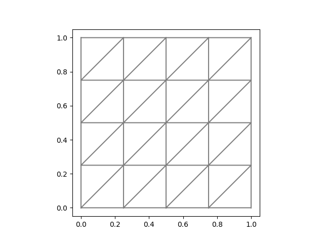
(a) Right

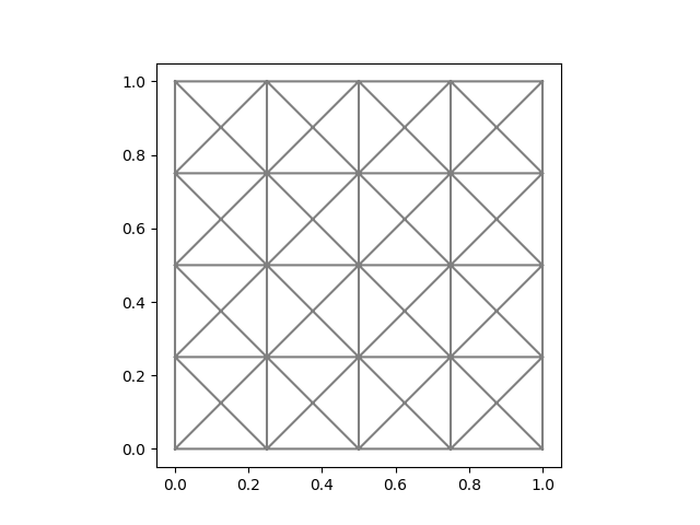
(b) Crossed

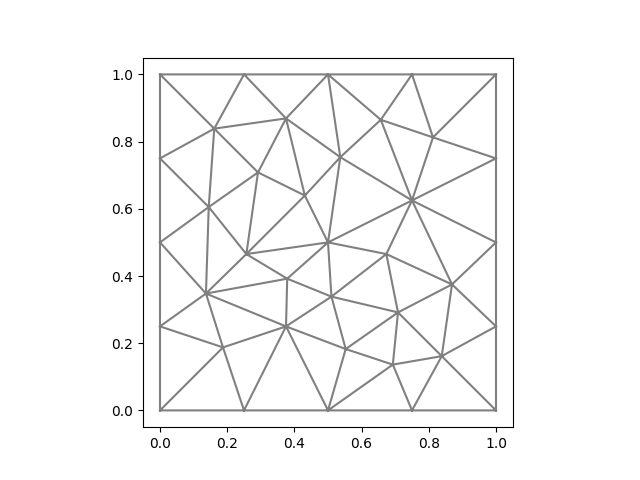
(c) Nonuniform

Figure 1. Meshes on the unit square with N = 4

We use the following meshes: a non-symmetric uniform mesh (Right), a symmetric uniform mesh (Crossed), and a non-symmetric and non-structured mesh (Nonuniform). The integer $N$ refers to the number of subdivisions on each side of the square. An example of such meshes is given in Figure 1.

	$\lambda=1$	$\lambda=100$	$\lambda=10^{4}$	$\lambda=10^{8}$
$\omega_{1}$	37.266072200953786	52.31315105053875	52.3443693	52.344691
$\omega_{2}$	37.2660721997643	91.4778227239564	92.11827609964527	92.12439336305897

Table 1. Estimates of the first and second eigenvalues on a square

We computed with FEniCS the reference solutions providing an estimate of the first and second eigenvalues for the different cases we want to approximate. We used a high order scheme and an adaptive algorithm with the classical SOLVE-ESTIMATE-MARK-REFINE strategy. The values of the reference eigenvalues are reported in Table 1.

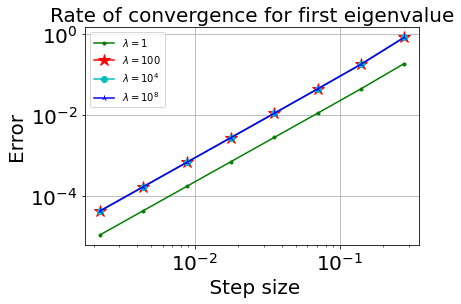
(a) Right mesh

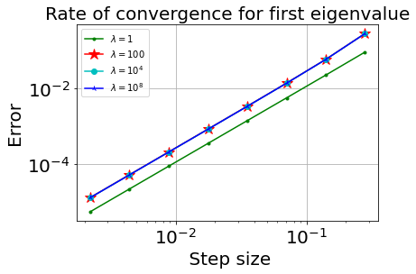
(b) Crossed mesh

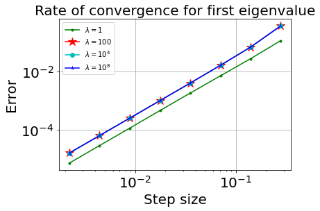
(c) Nonuniform mesh

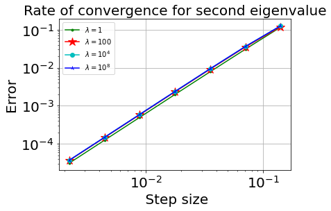
(d) Right mesh

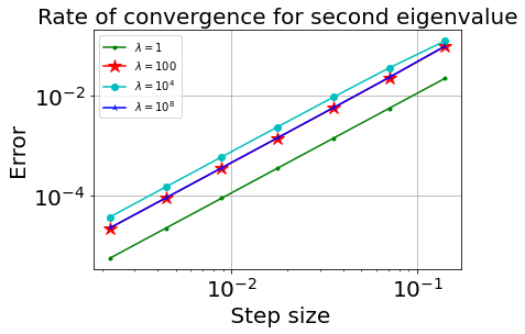
(e) Crossed mesh

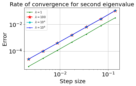
(f) Nonuniform mesh

Figure 2. Rate of convergence for the first and second eigenvalues on squared domain

Figure 2 shows the rate of convergence for both the first and the second approximated eigenvalues. Clearly both eigenvalues match the theoretical result in Theorem 7 with the rate being of second order on all meshes provided.

5.2. Rate of convergence on the L-shaped domain

The second domain that is considered is the L-shaped domain obtained by removing a quarter of the square $]0,1[^{2}$. It is known that on such domain singularities due to the re-entrant corner may occur. We also consider three sequences of triangulations: (Left), (Crossed or Uniform), and (Nonuniform) meshes. These are illustrated in Figure 3 with $N=4$.

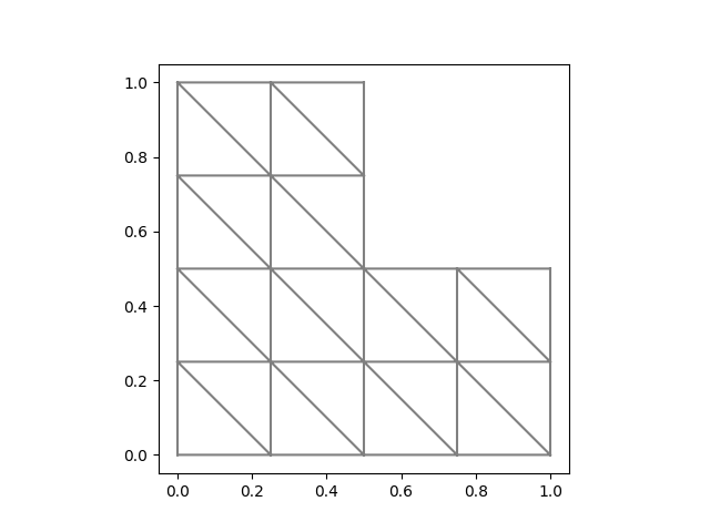
(a) Left

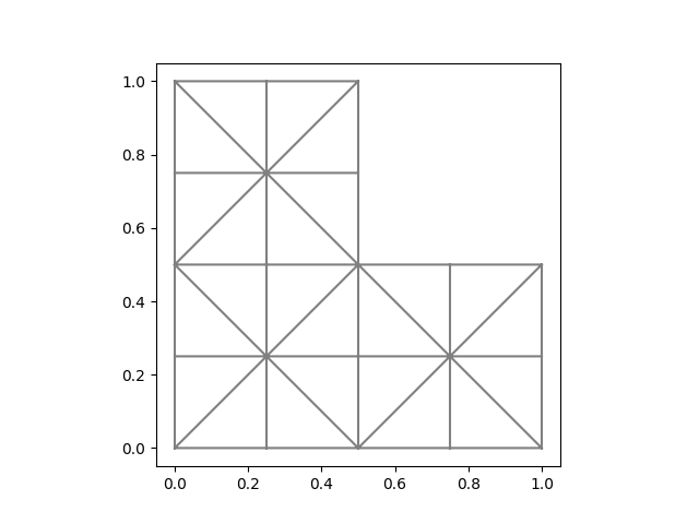
(b) Uniform

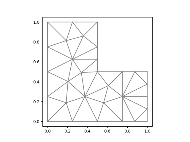
(c) Nonuniform

Figure 3. Meshes for L-shaped domain with $N=4$

In order to compare the approximated eigenvalues with a reference value, the same adaptive code, as in the previous case, was used to find the estimate for the first and second eigenvalues for different $\lambda$.

	$\lambda=1$	$\lambda=100$	$\lambda=10^{4}$	$\lambda=10^{8}$
$\omega_{1}$	54.36578831544661	127.990463	128.52363885700083	128.5293816640767
$\omega_{2}$	69.08352886532845	147.44431322194393	148.06735898422232	148.07344440728022

Table 2. Estimates of the first and second eigenvalues on an L-shaped domain

These estimated values are reported in Table 2.

(a) Left mesh

(b) Uniform mesh

(c) Nonuniform mesh

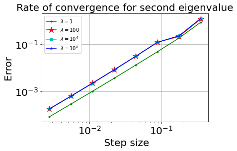
(d) Left mesh

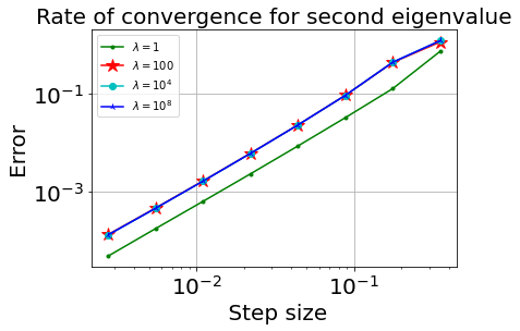
(e) Uniform mesh

(f) Nonuniform mesh

Figure 4. Rate of convergence for the first and second eigenvalues L-shaped domain

It is well known that the rate of convergence is reduced when the eigenfunction is singular. This is expected in particular in the case of the first eigenvalue.

When looking at the computed results, a particular phenomenon is present when approximating the first eigenvalue close to the incompressible limit. This is clearly seen in Figures 4(a), 4(b), and 4(c) for all meshes. Actually, the expected rate of convergence is achieved but there is a strange pre-asymptotic behavior when the value of $\lambda$ increases. By looking at the computed eigenfunctions it looks like this phenomenon is related to a sort of locking caused by the location of the degrees of freedom in the proximity to the re-entered corner.

(a) Left mesh with $N=16$

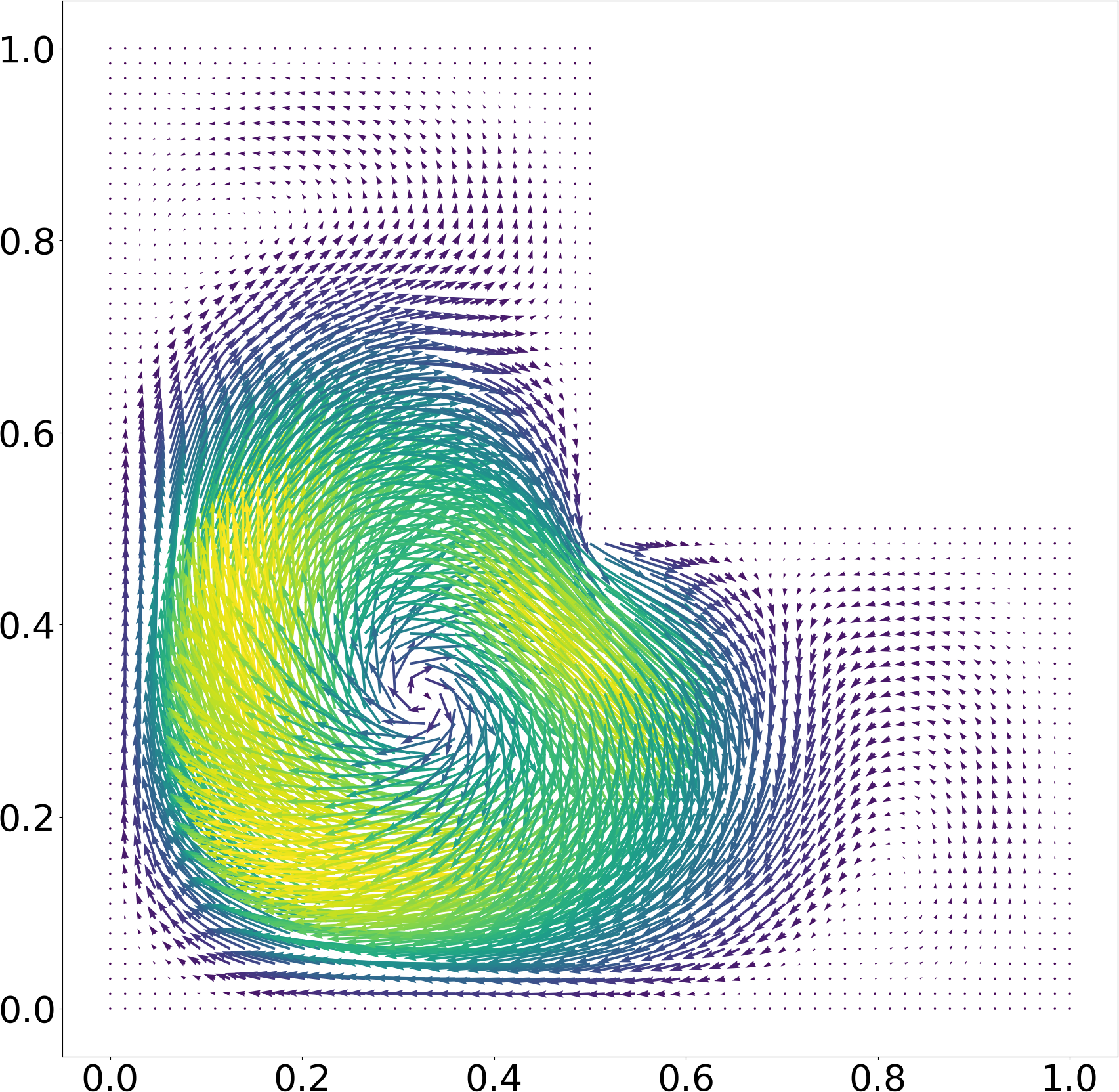
(b) Left mesh with $N=64$

(c) Nonuniform mesh with $N=16$

(d) Nonuniform mesh with $N=64$

Figure 5. First eigenfunction for $\lambda=100$ on L-shaped domain

When the system approaches the incompressible limit, the displacement presents a recirculation close to the re-entrant corner. A coarse mesh is not capable to represent such vortex. For $\lambda=1$ this situation doesn’t occur. In order to better describe this phenomenon, we report in Figures 5(a) and 5(c) the eigenfunction corresponding to the first eigenvalue on the mesh after three refinements for $\lambda=100$. We see that the correct vortex is not well approximated, possibly because of the mesh being coarse so that there are not enough degrees of freedom close to the re-entrant corner. As we refine, specifically starting from the fifth iteration and onwards, the expected circulation is noticed as Figures 5(b) and 5(d) illustrate. This might be the reason why we need a fine mesh to observe the expected rate for the first eigenvalue.

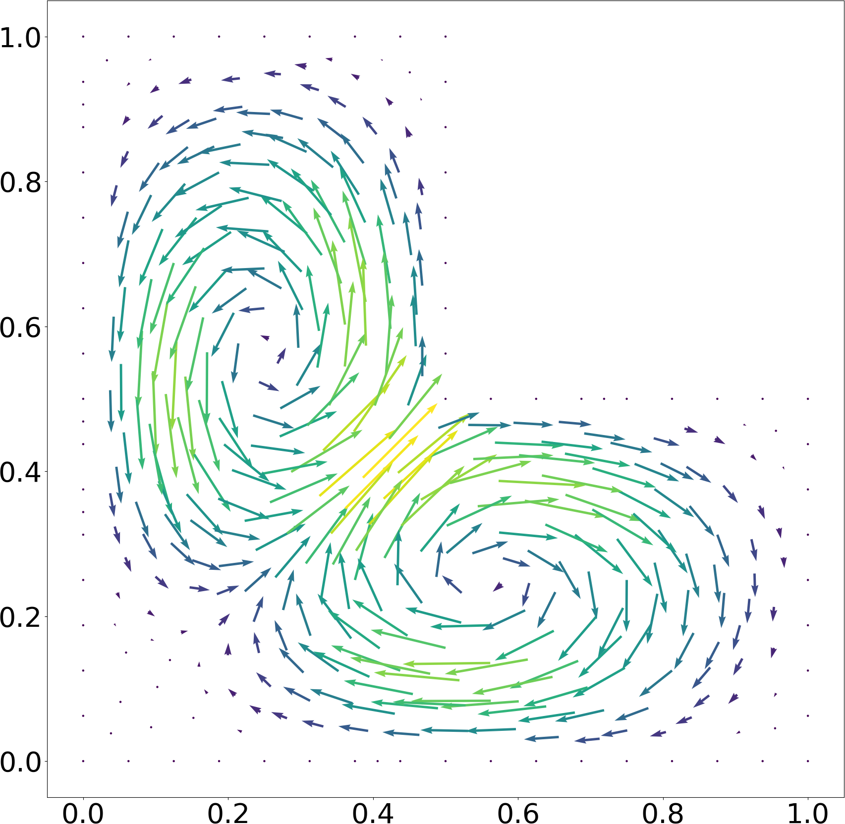
Figure 6. Second eigenfunction for $\lambda=100$ on Nonuniform L-shaped domain

On the contrary, the re-entrant corner has no negative effects on the second eigenvalue even for coarse meshes. This can be seen, for example, in Figure 6 which illustrates the second eigenfunction on a Nonuniform mesh with $N=16$ and $\lambda=100$.

5.3. The distribution of the eigenvalues in the complex plane

In this section we discuss the distribution of the spectrum of the discrete operator in the complex plane. This is the main motivation of our paper and provide us with some properties of the solution operator that are not visible when considering the source problem. Needless to say, the knowledge of the spectrum of the operator has important consequences for the design of numerical schemes, for instance when a transient problem is approximated.

We consider the distribution of the eigenvalues in the case of the two domains previously considered (square and L-shaped) and the same range of Lamé constants.

We note that we are taking specific outer zoom with the values on the axes being large in order to show the spread of a large portion of the spectrum. Moreover, different scales are considered depending on each case in order to better highlight the behavior of the specific approximation.

(a) $\lambda=1$

(b) $\lambda=100$

(c) $\lambda=10^{4}$

(d) $\lambda=10^{8}$

Figure 7. Eigenvalues of a square on a refined Right mesh

We recall that the exact eigenvalues are real positive, so that we would expect that the discrete eigenvalues, for $h$ small enough, distribute along the positive real axis of the complex plane. This is actually a naive interpretation of the convergence results presented in the previous sections. Indeed, by inspecting carefully the result presented in Property 1, it can be seen that computed eigenvalues can also be spread in different regions of the complex plane, as far as they lie outside a ball centered at the origin. The larger the ball, the smaller in general should $h$ be in order to detect this behavior.

Figure 7 shows the spectrum of our operator on the Right mesh for different values of $\lambda$. Each plot reports with different colors the results computed on four successfully refined meshes.

As shown in Figure 7(a), we observe that for a small value of $\lambda$, the spectrum is well behaving close to the positive real axis with some non real eigenvalues appearing as we refine. In this case, all values are located in the right half of the complex plane, that is, they have positive real part.

When $\lambda$ increases, we can see from Figure 7 that eigenvalues with negative real part show up. Also in this case some non real eigenvalues are present, even if their imaginary part is not as large as we will see in the next examples.

(a) $\lambda=1$

(b) $\lambda=100$

(c) $\lambda=10^{4}$

(d) $\lambda=10^{8}$

Figure 8. Eigenvalues of a square on a refined Crossed mesh

The results for the Crossed mesh are reported in Figure 8. In this case, all eigenvalues have positive real part and are located to the right side of the complex plane. The more we refine, the more the scheme produces complex eigenvalues moving away from the region of interest and diverging. For small values of $\lambda$ (Figure 8(a)), most eigenvalues are positive and real with some complex being present for finer meshes. As $\lambda$ becomes larger in Figure 8, the spectrum is spread more and more with complex eigenvalues having positive real part.

(a) $\lambda=1$

(b) $\lambda=100$

(c) $\lambda=10^{4}$

(d) $\lambda=10^{8}$

Figure 9. Eigenvalues of a square on a refined Nonuniform mesh

Finally, the spectrum computed with the Nonuniform mesh has a different structure. The eigenvalues appear to be more spread all over the complex plane as Figure 9 shows. As in the previous observations, the values of the eigenvalues, for $\lambda=1$, are concentrated to the right of the complex plane. However, in this case, the eigenvalues are scattered much more when comparing them to the Right and Crossed meshes for $\lambda=1$. The spectrum gets surprisingly more symmetric with respect to the origin when moving towards the incompressible limit.

(a) $\lambda=1$

(b) $\lambda=100$

(c) $\lambda=10^{8}$

Figure 10. Eigenvalues of a Left L-shaped domain

In what follows we present some results for the L-shaped domain. We only present the cases where $\lambda=10^{r}$ for ($r=0,2,8$) since there are no significant differences between $r=4$ and $8$.

We start by exploring the Left mesh structure in Figure 10. Looking at the spectrum in this case, we see a similar behavior as for the case of the Right mesh on the square.

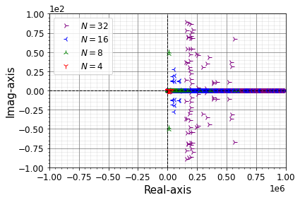
(a) $\lambda=1$

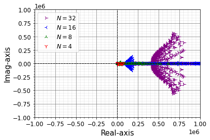
(b) $\lambda=100$

(c) $\lambda=10^{8}$

Figure 11. Eigenvalues of a Uniform L-shaped domain

(a) $\lambda=1$

(b) $\lambda=100$

(c) $\lambda=10^{8}$

Figure 12. Eigenvalues of Nonuniform L-shaped domain

For Uniform meshes, as Figure 11 shows, occurrence of complex eigenvalues for $\lambda=1$ are more present than in the previous case. Moreover, complex eigenvalues appear for higher values of $\lambda$ and grow when refining. The significant eigenvalues are those close to the origin which are positive and real or close to being real in the limit.

The Nonuniform mesh shows again a similar picturesque behavior as in the case of the square domain. Figure 12 shows the distribution of eigenvalues for this case. Even for small $\lambda$ there are eigenvalues with large imaginary part in this case, although with positive real part.

(a) Square domain

(b) L-shaped domain

Figure 13. Eigenvalues within a circle of radius $R$ for Nonuniform mesh on a square and L-shaped domains

An interesting observation, that matches the convergence of eigenvalues in Property 1, is clearly observed on Nonuniform meshes. To show this, we choose a Nonuniform mesh with $\lambda=10^{8}$ for both domains. As seen in Figure 13, when refining the mesh, eigenvalues are distributed allover the complex plane, within a circle of radius $R$ centered at the origin. The more we refine, the larger the circle becomes, indicating that the number of positive and finite eigenvalues of interest are present inside that circle. The circle can be taken larger and larger as the mesh size $h$ approaches zero.

(a) Zoom out

(b) Intermediate zoom

(c) Zoom in

(d) Zoom out

(e) Intermediate zoom

(f) Zoom in

Figure 14. Eigenvalues for meshes zooming to region close to the origin

We conclude our numerical experiments with more pictures for different values of the zoom parameters, so that the convergence behavior corresponding to Property 1 can be better appreciated. Figure 14 reports eigenvalues of both domains with $\lambda=10^{8}$. The outer zoom lens in Figures 14(a) and  14(d) gives a clear picture on the spread of eigenvalues in the complex plane. Looking at an intermediate zoom lens as 14(b) and  14(e) show, the structure of eigenvalues for both domains is still not aliened with the region of interest as the spread is apparent. On the other hand, a zoomed in picture as Figure 14(c) gives eigenvalues, on a square, which are real and positive with respect to the previously reported pictures. Similar level of zoom show the same nice behavior in the case of the L-shaped domain (see Figure 14(f)). Thus, the scheme produces real and positive eigenvalues in the region of interest with no spurious modes as expected.

References

- [1] Alnæs, M., Blechta, J., Hake, J., Johansson, A., Kehlet, B., Logg, A., Richardson, C., Ring, J., Rognes, M.E. and Wells, G.N., 2015. The FEniCS project version 1.5. Archive of Numerical Software, 3(100).
- [2] Alzaben, L., Bertrand, F. and Boffi, D., 2021, March. Computation of Eigenvalues in Linear Elasticity with Least-Squares Finite Elements: Dealing with the Mixed System. In 14th WCCM-ECCOMAS Congress 2020 (Vol. 700).
- [3] Babuška, I. and Osborn, J., 1991. Eigenvalue problems. In Handbook of numerical analysis, Vol. II, pp. 641–787.
- [4] Bertrand, F. and Boffi, D., 2020. First order least-squares formulations for eigenvalue problems. IMA Journal of Applied Mathematics, to appear, arXiv preprint arXiv:2002.08145 [math.NA].
- [5] Bertrand, F. and Boffi, D., 2020. Least-squares formulations for eigenvalue problems associated with linear elasticity. Comput. Math. Appl., 95 (2021), pp. 19–27.
- [6] Bertrand, F., Boffi, D. and Schneider, H. DPG approximation of eigenvalue problems. arXiv preprint arXiv:2012.06623 [math.NA].
- [7] Boffi, D., 2010. Finite element approximation of eigenvalue problems. Acta Numer., 19, pp.1–120.
- [8] Cai, Z. and Starke, G., 2004. Least-squares methods for linear elasticity. SIAM Journal on Numerical Analysis, 42(2), pp.826–842.
- [9] Carstensen, C. and Storn, J., 2018. Asymptotic exactness of the least-squares finite element residual. SIAM Journal on Numerical Analysis, 56(4), pp. 2008–2028.
- [10] Keith, B., 2021. A priori error analysis of high-order LL∗ (FOSLL∗) finite element methods. Computers & Mathematics with Applications, 103, pp. 12–18.