An Extensible Benchmark Suite for Learning to Simulate Physical Systems

Abstract

Simulating physical systems is a core component of scientific computing, encompassing a wide range of physical domains and applications. Recently, there has been a surge in data-driven methods to complement traditional numerical simulations methods, motivated by the opportunity to reduce computational costs and/or learn new physical models leveraging access to large collections of data. However, the diversity of problem settings and applications has led to a plethora of approaches, each one evaluated on a different setup and with different evaluation metrics. We introduce a set of benchmark problems to take a step towards unified benchmarks and evaluation protocols. We propose four representative physical systems, as well as a collection of both widely used classical time integrators and representative data-driven methods (kernel-based, MLP, CNN, nearest neighbors). Our framework allows evaluating objectively and systematically the stability, accuracy, and computational efficiency of data-driven methods. Additionally, it is configurable to permit adjustments for accommodating other learning tasks and for establishing a foundation for future developments in machine learning for scientific computing.

1 Introduction

Computational modeling of physical systems is a core task of scientific computing. Standard methods rely on discretizations of explicit models typically given in the form of partial differential equations (PDEs). Machine learning techniques can extend these techniques in a number of ways. In some cases, a closed system of analytic equations relating all variables may not be available (e.g., a constitutive relation for a material may not be known). In other cases, while a full analytic description of a system is available, a traditional solution may be too costly (e.g., turbulence) or can be sped up substantially using data-driven reduced-order models. However, despite promising results, a successful adoption of these data-driven approaches into scientific computing pipelines requires a solid and exhaustive assessment of their performance—a challenging task given the diversity of physical systems, corresponding data-driven approaches, and the lack of standardized sets of problems, comparison protocols, and metrics.

We focus on the setting where the physical model is unavailable during training, mimicking situations in computational science and engineering with ample data and a lack of models. One can generally distinguish two different flavors of physical simulation with different associated computational cost: those that map a high-dimensional state space into another high-dimensional space (as in temporal integration schemes, mapping the state of the system at one time step to the next), or from a high-dimensional input space to a lower-dimensional output (as in surrogate models, mapping the initial conditions to a functional of the solution). While this distinction also applies to data-driven approaches, another critical aspect emerges from the choice of input data distribution. We identify two extremes: the narrow data regime, where initial conditions are sampled from a low-dimensional manifold (even within a high-dimensional state space), and the wide regime, where initial conditions span a truly high-dimensional space. As could be expected, narrow data regimes define an easier prediction task where data-driven methods can potentially ‘bypass the physics’, whereas wide regimes require models with enough encoded physical priors in order to beat the curse of dimensionality. Therefore, such choice of data distribution is a critical component of any data-driven physical simulation benchmark.

In this work, we introduce an extensible benchmark suite, including: (1) an extensible set of simple, yet representative, physical models with a range of training and evaluation (test) setups, as well as reference, high-accuracy numerical solutions to benchmark data-driven methods, (2) reference implementations of traditional time integration schemes, which are used as baselines for evaluation, and (3) implementations of widely used data-driven methods, including physics-agnostic multi-layer perceptrons (MLPs), convolutional neural networks (CNNs), kernel machines and non-parametric nearest neighbors. Our benchmark suite is modular, permitting extensions with limited code changes, and captures both ‘narrow’ and ‘wide’ regimes by appropriately parametrizing the set of initial conditions.

Our analysis reveals two important conclusions. First, even in the simplest physical models, current data-driven pipelines, while providing qualitatively acceptable solutions, are quantitatively far from directly numerically integrating physical models, and this performance gap appears unfeasible to close by merely scaling up the models and/or the dataset size. In other words, the cost of ignoring the physics is high, even for the simplest physics, and cannot in general be compensated by data, matching insights that have been obtained in other scientific computing settings [5, 55]. Next, and more importantly, our simple $L^{2}$-based nearest neighbor regressor is used to calibrate how ‘narrow’ the learning task is. Our finding is that even for seemingly complex systems, such as the incompressible Navier-Stokes systems, such naive predictor outperforms most deep-learning-based models in the narrow regime—thus providing a simple calibration of the true difficulty of the simulation task, that we advocate should be present in every future evaluation.

2 Related work

Machine learning is used in physical simulation in a number of interrelated ways. Some important uses include reduced-order/surrogate modeling, learning constitutive models or more generally compact analytic representations from data. A unifying theme of these applications of machine learning is automatic construction of parametric models capable of reproducing the behavior of physical systems for a sufficiently broad range of initial data, boundary conditions and other system parameters. The purpose of these representations varies from acceleration (e.g., surrogate machine learning models are used to accelerate optimization), to automatic construction of multiscale models (learning macroscopic constitutive laws from microscopic simulation), to inferring compact descriptions of unknown representations from experimental data.

The purpose of our proposed benchmarks is to enable comparisons of different learning-based methods in terms of their accuracy and efficiency. We briefly review two streams of learning methods for physical systems: (1) One line of work aims to understand how neural networks can be structured and trained to reproduce known physical system behavior, with the goal of designing general methods applicable in a variety of settings [8, 42, 4, 41, 37, 38, 26, 10, 50, 51]. Our benchmark cases fit primarily into this category. (2) Another line of research aims to develop a variety of techniques to accelerate solving PDEs. Typically, these methods are developed for specific PDEs and a specific restricted range of problems: for example, fluid dynamics problems [39, 16, 56], with particular applications to cardiovascular modeling [25, 19] and aerodynamics [53]; or solid mechanics simulation tasks, including stresses [29, 24, 27, 15, 22, 23]. In cases where the governing equations are not given, the learning task becomes approximating them from data [30, 7, 1, 9, 2, 28, 3, 43, 44, 46, 45, 52, 35].

3 Background and problem setup

PDEs, dynamical systems, and time integration

Consider a time-dependent PDE of the form $\partial_{t}u=\mathcal{L}(u)$, where $u$ is the unknown function and $\mathcal{L}$ is a possibly nonlinear operator that includes spatial derivatives of $u$. By discretizing in space, one obtains a dynamical system

$$\dot{x}(t)=f(x(t))$$ (1)

with an $N$-dimensional state $x(t)\in\mathbb{R}^{N}$ at time $t\in[0,T]$. The function $f$ is assumed to be Lipschitz to ensure solution uniqueness and the initial condition is denoted as $x_{0}\in\mathbb{R}^{N}$. A PDE of a higher order in time can be reduced to the first-order form in the standard way, e.g., if we have a second-order system $\ddot{q}(t)=f(q(t))$, then we consider its formulation via position $q$ and momentum $p$ as a first-order system with $x=[q;p]$: $[\dot{q}(t);\dot{p}(t)]=[p(t);f(q(t))]$. To numerically integrate (1), we choose time steps $0=t_{0}<t_{1}<\dots<t_{K}=T$. Then, a time integration scheme (e.g., [49, 12, 11]) gives an approximation $x_{k}\approx x(t_{k})$ of the state $x(t_{k})$ at each time step $k=1,\dots,K$. A list of the schemes we use along with details is given in Appendix A.

Problem setup and learning problems

Given $M$ initial conditions $x^{(1)}_{0},\dots,x^{(M)}_{0}\in\mathbb{R}^{N}$ and the corresponding $M$ trajectories $X^{(i)}=[x^{(i)}_{0},\dots,x^{(i)}_{K}]\in\mathbb{R}^{N\times(K+1)},i=1,\dots,M$ obtained with a time integration scheme from dynamical system (1), we consider the following two learning problems, both of which aim to learn the physical model of the problem, viewed as unknown, from trajectory samples: (1) Learning an approximation $\tilde{f}$ of the right-hand side function $f$ in Eq. (1). This gives an approximate $\dot{\tilde{x}}(t)=\tilde{f}(\tilde{x}(t))$ that is then numerically integrated to produce a trajectory $\tilde{X}$ for an initial condition $\tilde{x}_{0}$. The aim is that $\tilde{X}$ approximates well the true trajectory $X$ obtained with $f$ from (1) for the same initial condition. (2) Directly learning the next steps in the trajectory from the current one, i.e. predict $x^{(i)}_{k}$ given $x^{(i)}_{k-1}$.

To assess the learned models, we evaluate them on their ability to produce good approximate trajectories from randomly sampled initial conditions, by either integration or direct step prediction. During evaluation, we use initial conditions drawn independently from those used to produce training data, both from the same distribution as the training samples, as well as from a distribution with support outside the training range. We train networks on data sets of various sizes. For details, see Appendix B.

4 Benchmark systems

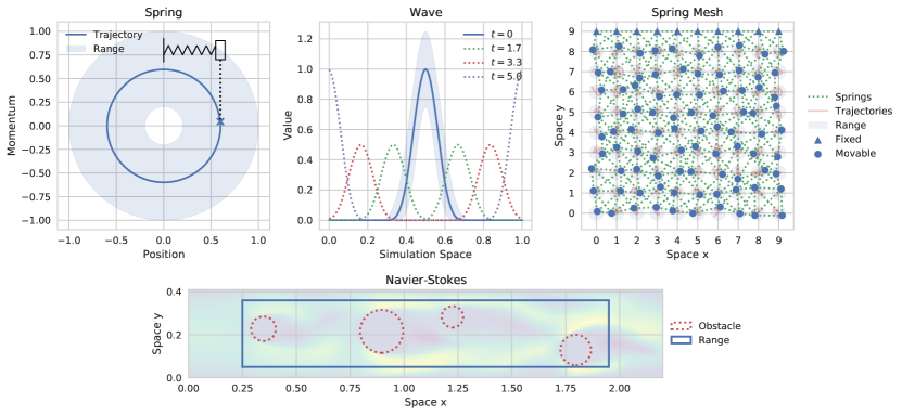
Figure 1: Representative visualizations of the four systems, depicting the results and ranges of initial condition sampling. Each has two state components: for the Navier-Stokes system, a flow velocity and a pressure field, and for the other three a position $q$ and momentum $p$.

We consider four physical systems, illustrated in Figure 1: a single oscillating spring, a one-dimensional linear wave equation, a Navier-Stokes flow problem and a mesh of damped springs. These systems represent a progression of complexity: the spring system is a linear system with low-dimensional space of initial conditions and low-dimensional state; the wave equation is a low-dimensional linear system with a (relatively) high-dimensional state space after discretization; the Navier-Stokes equations are nonlinear and we consider a setup with low-dimensional initial conditions and high-dimensional state space; finally, the spring mesh system has both high-dimensional initial conditions as well as high-dimensional states. Additionally, the proposed spring system and Navier-Stokes problems represent diffusion-dominated and advection-dominated (for sufficiently low viscosity) PDE behaviors, as well as variability in initial conditions with fixed domain (spring system) and variable domain (Navier-Stokes). These varying complexities provide an opportunity to test methods on simpler systems and the ability to examine changing performance as system size increases, both in terms of the state dimension, and the initial condition distribution. The ground truth models for the spring, wave, and spring mesh systems with classical time integrators are implemented using NumPy [13], SciPy [54], and accelerated, where possible, with Numba [21]. The Navier-Stokes snapshots are generated using PolyFEM [47], a finite element library.

These systems were chosen in an effort to reflect the variety of systems used for testing in this area, while unifying choices of particular formulations. Past works have chosen systems of the types featured here: simple oscillators (both spring and pendulum [8]), particle systems with various interaction laws (gravity, spring forces, charges, cloth simulations, etc. [6, 18, 42, 4, 34]), and fluid-flow systems (with various sorts of obstacles, airfoils or cylinders [51, 34]). We make particular selections here in an effort to unify systems of interest and facilitate comparisons across experiments by providing a shared set of tasks which can be used for development and testing of machine learning methods.

Some examples of initial condition selection for each system are illustrated in Figure 1. The ground truth for the spring, wave, and spring mesh systems consists of the state variables $(q,p)$ for position and momentum, and their associated derivatives $(\dot{q},\dot{p})$. For the Navier-Stokes system the state consists of flow velocities, and a pressure field, along with approximated time derivatives for each.

Table 1 lists the parameters used to generate trajectories for training and evaluation. Training sets of three sizes are generated, each containing the specified number of trajectories. The systems are integrated at the listed time step sizes, but the ground truth data is subsampled further by the factor shown after $\div$ in the table: the integration schemes are run at a smaller time step and intermediate computations are discarded. Each larger training set is a strict superset of its predecessor to ensure that previous training samples are never removed.

4.1 Spring

We simulate a simple one-dimensional oscillating spring. In this system, the spring has zero rest length, and both the oscillating mass and spring constant are set to $1$. The spring then exerts a force inversely proportional to the position of the mass $q$: $\dot{p}(t)=-q$ and $\dot{q}(t)=p$.

The energy of the system is proportional to $r=q^{2}+p^{2}$ which is the radius of the circle in phase space. To sample initial conditions, we first sample a radius uniformly, then choose an angle theta uniformly. This produces a uniform distribution over spring system energy levels and starts at an arbitrary point in the cycle. The spring system has a closed-form solution: $(q(t),p(t))=(r\sin(t+\theta_{0}),r\cos(t+\theta_{0}))$ where $r$ is the radius of the circle traced in phase space (the energy of the spring) and $\theta_{0}$ is the phase space angle at which the oscillation will start. While this closed form solution is useful, for consistency with our other systems, we generate snapshots of the spring system by numerical integration. Simulations of the spring system always run through one period. For “in-distribution” training values, the radius is selected in the range $(0.2,1)$ and “out-of-distribution” radii are chosen from $(1,1.2)$.

4.2 Wave

This benchmark system is similar to the one used in Peng and Mohseni [33]. Consider the wave equation with speed $c=0.1$

$$\partial_{tt}u=c^{2}\partial_{xx}u\,,$$ (2)

on a one-dimensional spatial domain $[0,1)$ with periodic boundary conditions. We represent this second-order system as a first-order system and discretize in space to obtain

$$\begin{bmatrix}\dot{q}(t)\\ \dot{p}(t)\end{bmatrix}=\begin{bmatrix}0&I\\ c^{2}D_{xx}&0\end{bmatrix}\begin{bmatrix}q(t)\\ p(t)\end{bmatrix}\,,$$ (3)

where $D_{xx}\in\mathbb{R}^{n\times n}$ corresponds to the three-point central difference approximation of the spatial derivative $\partial_{xx}$ and the matrices $I$ and $0$ are the identity and zero matrix, respectively, of appropriate size. We discretize in space with $n=125$ evenly spaced grid points and evolve the system following the dynamics described above.

Initial conditions are sampled with an initial pulse in the $q$ component centered at $0.5$. All initial conditions have zero momentum. The initial pulse is produced by a spline kernel as described in [33]:

$$s(x)=\frac{10}{p_{w}}\cdot\lvert x-0.5\rvert\,,\qquad h(s)=p_{h}\cdot\begin{cases}1-\frac{3}{2}s^{2}+\frac{3}{4}s^{3}&\text{if $0\leq s\leq 1$}\\ \frac{1}{4}(2-s)^{3}&\text{if $1<s\leq 2$}\\ 0&\text{else}\end{cases}$$

where the width and height of the pulse are scaled by parameters $p_{w}$ and $p_{h}$, respectively. The spline kernel pulse is then $h(s(x))$ for $x\in[0,1)$, evaluated at the discretized grid points.

For “in-distribution” samples, parameters $p_{w},p_{h}$ are both chosen uniformly in the range $(0.75,1.25)$ and “out-of-distribution” runs sample uniformly from $(0.5,0.75)\cup(1.25,1.5)$. All trajectories are integrated until $t=5$ when the wave has traveled through half a period.

4.3 Spring mesh

This system manipulates a square grid of particles connected by springs, in a two dimensional space, and can be considered a simplified version of deformable surface and volume systems (cf. [34]). The particles all have mass $1$, and are arranged into a unit grid. Springs are added along the axis-aligned edges and diagonally across each grid square, with rest lengths selected so that the regularly-spaced particles are in a rest position.

In this work we use a $10\times 10$ grid where the top row of particles is fixed in place. Initial conditions are sampled by choosing a perturbation for the position of each non-fixed spring. These perturbations are chosen as uniform vectors inside a circle with radius $0.35$. Out-of-distribution perturbations are chosen uniformly in a ring with inner radius 0.35 and outer radius 0.45. The sampled initial conditions all have zero momentum.

In this system, a spring between particles $a$ and $b$ exerts a force:

$$F_{ab}=-k\cdot\big{\lparen}\lVert q_{a}-q_{b}\rVert_{2}-\ell_{ab}\big{\rparen}\frac{q_{a}-q_{b}}{\lVert q_{a}-q_{b}\rVert_{2}}-\gamma\dot{q}_{a}$$ (4)

where $\ell_{ab}$ is the rest length of the spring, $\gamma=0.1$ is a parameter controlling the magnitude of an underdamped velocity-based decay, and $k=1$ is the spring constant.

4.4 Navier-Stokes

We consider the standard Navier-Stokes equation over a domain $\Omega$ (cf. [34, 51])

$$\left.\begin{array}[]{l}\displaystyle\rho\frac{\partial u}{\partial t}+\rho(u\cdot\nabla)u-\nu\Delta u+\nabla p=b\\ \nabla\cdot u=0\\ u(0)=u_{0}\end{array}\right\}\text{ on }\Omega\times(0,T)~{},~{}\left.\begin{array}[]{l}u=d\\ \nu\frac{\partial u}{\partial n}+pn=g\end{array}\right\}\text{ on }\partial\Omega_{D}\times(0,T)~{},$$

where $u\colon\Omega\times(0,T)\to R^{2}$ is the velocity at time $t\in(0,T)$ of a fluid with kinematic viscosity $\nu$ and density $\rho$, $p\colon\Omega\times(0,T)\to R$ is the pressure and $\partial\Omega_{D}$ and $\partial\Omega_{N}$ are the Dirichlet and Neumann boundary conditions, respectively. In our setup we use the finite element method (FEM) to solve the PDE using mixed discretization: quadratic polynomial for the velocity and linear for pressure. In our experiment the domain $\Omega$ is a rectangle $0.22\times 0.41$ with a randomly generated set of circular obstacles. We start with $u_{0}=0$ and specify a velocity on the left boundary of $u(0,y)=(6(1-e^{-5t})(0.41-y)y/0.1681,0)$, zero on the top and bottom, and zero Neumann on the right side ($g=0$). We solve the system using PolyFEM [47] using $dt=0.08$ and backward differentiation formula (BDF) of order 3 for the time integration.

We sample obstacles into two configurations: a single obstacle, or a set of four. In each case, we sample the obstacles leaving a margin of 0.05 between each circle, and a margin of 0.25 from the left and right sides, and 0.05 between the top and bottom. Otherwise, each obstacle is determined by first sampling a radius, then sampling a center from the valid space, respecting the margins. If the sampled obstacle is too close to an existing circle, it is discarded and a new sample is drawn. In-distribution obstacles have radii in the range $(0.05,0.1)$ and out-of-distribution radii are drawn from $(0.025,0.05)$.

Table 1: Dataset sizes and simulation parameters

System	# Train Trajectories	# Eval Trajectories	Time Step Size	# Steps
Spring	10, 500, 1000	30	0.00781, $\div 128$	805
Wave	10, 25, 50	6	0.00049, $\div 8$	10204
Spring Mesh	25, 50, 100	15	0.00781, $\div 128$	805
Navier-Stokes	25, 50, 100	5	0.08, $\div 1$	65

5 Numerical experiments

Experimental setup

We apply several basic learning methods to the datasets developed in this work: $k$-nearest neighbor regressors, a neural network kernel method, several sizes of feed-forward MLPs, and a variety of CNNs. Details of the architectures and the training protocol are provided in supplementary material, Appendix B. Each of the neural networks we consider is implemented using PyTorch [31].

The learning methods considered in this work are each trained on one of the two target task formulations described in Section 3. For derivative-based prediction, the training is conducted supervised on ground truth snapshots gathered from the underlying models. For each system we randomly sample initial conditions and each of these is then numerically integrated to produce a trajectory. Each trajectory includes state samples $x$ as well as target derivatives $\dot{x}$ used for training. For direct prediction, we no longer require numerical integration; instead we directly predict the trajectory in a sequential fashion. In this setting, we approximate $\tilde{f}_{\theta}(x(t))\approx x(t+\delta_{t})$ for a discrete time step size $\delta_{t}$. For the derivative prediction task we report results using the leapfrog integrator. Full results using other numerical integration schemes are available in the supplementary materials.

We pick the same set of learning methods and apply it to both tasks independently to judge performance in each. For many systems the state is divided into position and momentum components: $x\equiv(q,p)$. For the Navier-Stokes problem, the state $x$ is made up of the flow velocity field, and the scalar field for pressure. After training, we produce rolled-out trajectories from held-out initial conditions, either by combining with a numerical integrator in the case of derivative prediction, or in a directly recurrent fashion in the case of step prediction. Each neural network is instantiated in three independent copies, each of which is trained and evaluated across all sampled trajectories. We compute a per-step MSE against a ground truth value, average these per-step MSEs to produce a per-trajectory error, and record these errors for analysis. Our experiments are designed to test several aspects of physical simulation. We highlight the most salient ones next, and report more extensive results in Appendix C.

Training set size

In general ML problems, one would expect additional training samples to systematically improve (in-distribution) evaluation performance. However, Figure 2 illustrates a clear saturation of performance on the simplest systems when using neural networks as function approximators, in contrast with non-parametric KNNs and the kernel method. We attribute this saturation to an inherent gap between the training and evaluation objectives. While data-driven methods are optimized to minimise next-step predictions, the final evaluation requires built-in stability to prediction errors. Including regularisation strategies to incorporate stability, such as noise injection [34], is shown to help, but not fully resolve this issue.

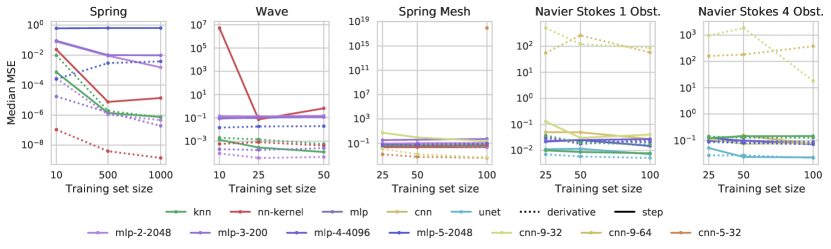
Figure 2: Median MSE error with respect to the training set size for each of our system configurations. We show varying architecture choices for each method.

Out-of-distribution evaluation

For simplicity, we only examine the out-of-distribution error for networks trained on the largest training set size. The added challenge of out-of-distribution samples varies with the construction of each system. It is possible to get some idea of the difficulty increase by examining the accuracy penalty for the KNNs, and comparing it to how well the more advanced models are able to generalize.

Benefits of neural networks for generalization over KNN are visible across several systems in Figure 3, particularly in the spring system for small MLPs for derivative prediction and nn-kernel in both cases. The KNN suffers a significant increase in error while these methods produce only somewhat worse predictions. Benefits are still present, though less pronounced, for the wave system derivative prediction where neural networks increase in error, but the kernel method and small MLP maintain a lower absolute error than the KNN. On the Navier-Stokes systems none of the methods suffers an increase in error for out-of-distribution evaluation. The change in radius distribution for the obstacles did not pose an additional challenge sufficient to produce a measurable change in error distribution. We attribute this to low dimension of the initial condition space.

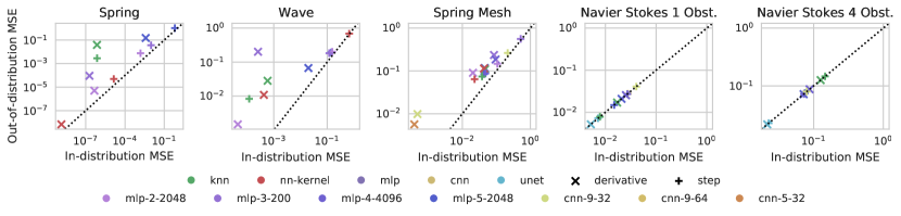
Figure 3: Median MSE for in-distribution evaluation sets vs. out-of-distribution evaluation sets for each system. Colors represent the same method and are varied for different architecture choices. Marker shapes distinguish step and derivative prediction, and the dotted line is the identity line. Outliers for the spring mesh and both Navier-Stokes configurations were removed. Values on both axes were approximately $10^{13}$ for the spring mesh and in the range $10^{2}$–$10^{3}$ for Navier-Stokes.

Step and derivative prediction

The step and derivative prediction instances of each learning problem lead to different accuracy from the learning methods we test. While most physical systems are naturally described in terms of their derivatives through corresponding ODEs/PDEs, data-driven simulations also offer the alternative of bypassing this differential formulation and predict the next state directly. Such ‘cavalier’ approach avoids the compounding error amplification effects across integration steps, at the expense of sample efficiency. Figure 4 illustrates these tradeoffs across our systems.

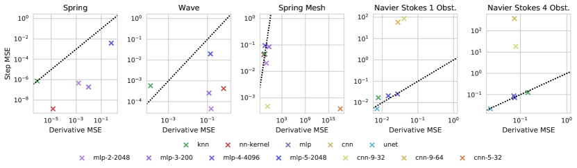
Figure 4: Median MSEs for derivative vs. step prediction on the same evaluation set. Results are displayed for each of our system configurations. The dotted line is the identity line.

An important example of this effect is the performance of CNNs on the spring mesh system (Figure 8 in the Appendix). When working through a numerical integrator and performing derivative prediction they produce the lowest error of all methods tested, but following the same training protocol for step prediction these architectures produce high errors, or are unstable. This case is likely an interaction of the architecture with the specific learning task. For the spring mesh, step prediction requires outputting the position of the particle which requires manipulating its global coordinates, while derivative predictions allow the network to more easily act locally and compute only a relative motion for the particle. The derivative prediction task better takes advantage of the spatial invariance of the CNNs. This difference in performance reflects the importance of tailoring architectures to the specific task, and some potential for neural network architectures to benefit from incorporating knowledge of a system’s behavior.

System and dataset complexity

Several trends we observe correlate with the difficulty of learning to simulate a system, and the variation in its behavior across the training and evaluation samples. This is generally a combination of the system’s state dimension, and variation in its behavior, approximated by the dimension of the distribution from which initial conditions are sampled.

This is particularly visible in Figure 5 in the performance of the KNN methods, and, in many cases, the performance of simpler methods such as the small MLPs. On the simpler systems, such as the spring and wave, the KNNs generally perform well because even though the wave system has a relatively large state dimension of 125, like the spring its initial condition is sampled from only two parameters and its behavior can be readily predicted from these. The Navier-Stokes system with a single obstacle is another instance of this sort of behavior: the KNN is readily able to reproduce flows it has not seen because a sampling of 100 obstacle positions is such that an evaluation sample is close to a trajectory seen at training time. Therefore, small MLPs and the kernel method produce similar performance. When the difficulty is increased by sampling four obstacles, the KNN and MLP performances suffer, and larger networks such as the u-net are needed to maintain approximately the same performance.

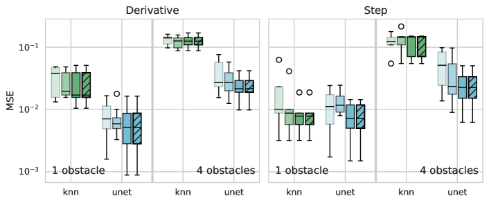
Figure 5: MSE distribution across trajectories in the evaluation set for KNNs and u-nets on our Navier-Stokes system, both the formulation with one obstacle, and the settings with four, as well as for derivative and step prediction. Box plot mid-lines show medians, box area is between first and third quantiles, whiskers extend $1.5\times$ beyond the boxes, outliers are plotted past the whiskers. Darker colors denote increasing training set size. The final hatched box is the same network from the final un-hatched box, tested on an out-of-distribution evaluation set.

Choice of numerical integrator

For our derivative prediction tasks we combine our trained methods with three explicit integrators with orders 1, 2, and 4. In most of our systems these produce at most a small increase in accuracy, holding all other training and evaluation parameters equal. However on the Navier-Stokes system the higher order integrators produce somewhat higher errors, particularly for the u-net and the MLPs. This appears related to the approximated derivatives used for training this system. The learned derivatives produce some small deviations which are compounded when combining multiple derivative samples.

Table 2: Time comparison for derivative prediction against baseline numerical integrators

System	Architecture	Euler		Leapfrog		RK4
		Time Ratio	Scaling	Time Ratio	Scaling	Time Ratio	Scaling
Spring	knn	367.0	1$\times$	405.8	16$\times$	311.3	64$\times$
	nn kernel	180.7	1$\times$	198.6	1$\times$	173.3	1$\times$
	mlp-2-2048	185.8	1$\times$	191.6	16$\times$	177.7	64$\times$
	mlp-3-200	237.6	1$\times$	237.5	16$\times$	227.2	64$\times$
	mlp-5-2048	473.8	4$\times$	369.6	64$\times$	360.9	128$\times$
Wave	knn	24,102.7	8$\times$	16,945.1	256$\times$	16,132.0	256$\times$
	nn kernel	35.3	8$\times$	22.3	256$\times$	19.9	256$\times$
	mlp-2-2048	25.4	8$\times$	16.5	256$\times$	14.2	256$\times$
	mlp-3-200	31.0	16$\times$	19.7	256$\times$	17.8	256$\times$
	mlp-5-2048	60.5	16$\times$	38.0	256$\times$	34.6	256$\times$
Spring Mesh	knn	708.6	8$\times$	626.1	128$\times$	690.4	256$\times$
	nn kernel	5.3	8$\times$	4.4	128$\times$	4.8	256$\times$
	mlp-2-2048	3.0	8$\times$	2.6	128$\times$	2.8	256$\times$
	mlp-3-200	3.4	8$\times$	3.2	128$\times$	3.4	256$\times$
	mlp-4-4096	7.8	16$\times$	7.1	128$\times$	7.7	256$\times$
	mlp-5-2048	7.1	8$\times$	6.2	128$\times$	5.3	256$\times$
	cnn-9-32	11.0	2$\times$	10.5	32$\times$	11.3	64$\times$
	cnn-5-32	7.4	1$\times$	9.2	32$\times$	7.3	64$\times$

Computational overheads

Another important aspect to consider when applying learning methods to physical simulation problems is the time required to compute each step, and the computational overheads introduced by the lack of knowledge of the true system physics. With standard numerical integration methods, it is generally possible to improve the quality of generated trajectories by decreasing the size of the time step used during integration. We take advantage of this in order to estimate the time overheads of our learning methods relative to our baseline numerical integrators at approximately corresponding error levels.

We numerically integrate each system at time step sizes scaled by powers of two. For each trajectory in the derivative prediction setting, we find the smallest scaling factor at which the numerical integrator exceeds the learning method’s error at their final shared time step, approximating the factor by which numerical integration can be made faster until it begins to underperform the learned method.

Table 2 reports the results of these experiments. For each numerical integrator, the “scaling” column reports the most common scaling factor found for each trajectory. The “time ratio” column represents the learned method’s evaluation overhead (median times, counting only per-step network evaluation costs, not numerical integration or data transfers). Note that the numerical integrator makes fewer steps than the learned method so the overall trajectory time must be further adjusted by the scaling factor.

In general, the neural networks are slower per-step by one or two orders of magnitude. KNNs are slower by significantly larger factors, particularly for the wave system. This is likely partially due to the default scikit-learn KNN implementation used, and due to the large size of the wave system training sets (large state dimension and large number of training snapshots). Scaling factors increase with the order of the integrator as higher-order integrators are more tolerant of large step sizes and maintain low error.

It is likely that these overheads could be reduced with more optimized implementations of both the numerical integrators and learned methods. The derivative prediction task is also constrained by its need to interact with the numerical integrator. In this setting the learned methods cannot be expected to outperform the quality of the solutions generated by the true system derivatives. This reflects a penalty resulting from a lack of knowledge of the true underlying system, and a penalty for learning from observations in this case. Step prediction without involving the numerical integrator potentially avoids some of these constraints, if learning is successful.

6 Conclusions and limitations

The results in this work illustrate the performance achievable by applying common machine learning methods to the simulation problems in our proposed benchmark task. We envision three ways in which the results of this work might be used: (1) the datasets developed here can be used for training and evaluating new machine learning techniques in this area, (2) the simulation software can be used to generate new datasets from these systems of different sizes, different initial condition dimensionality and distribution; the training software could be used to assist in conducting further experiments, and (3) some of the trends seen in our results may help inform the design of future machine learning tasks for simulation.

For the first and second groups of downstream users, we have made available the pre-generated datasets used in this work, as well as the software used to produce them and carry out our experiments. These components allow carrying out the measurements we have made here, and permit further adjustments to be made. Documentation on using the datasets and the software is included in Appendix D.

For the third group, we highlighted a few trends that suggest useful steps to take in developing new problems and datasets in this area. First, we advise including several simple baseline methods when designing new tasks. In particular the inclusion of standard numerical integrators (for derivative-type problems) and KNNs are useful to evaluate the difficulty of the proposed task. Specifically, KNNs are useful for examining the performance achievable by memorizing the training set, and are thus witnessing an appropriate design of data distribution that captures the true high-dimensionality of the prediction task. As an example, in the Navier-Stokes examples some task formulations may inadvertently be simple to memorize, even if the complexity of the system itself may not immediately suggest it. The numerical integrators are likewise useful as baselines both to ensure that the derivative learning is feasible even when achieving no error in predictions, and also to evaluate the penalty in accuracy which is incurred by operating without access to the true physics. We believe that in light of these observed trends, including baseline methods such as standard numerical integration schemes and simple learning methods such as the KNN is important in understanding tasks in this area. Including these assists in experiment design by helping to calibrate the difficulty of a target task.

Limitations

While our benchmark provides actionable conclusions on a wide array of simulation domains, it is currently focused on temporal integration, and as such it does not cover important settings in scientific computing. For instance, we do not currently include an instance of a surrogate model, which could provide different tradeoffs benefiting ML models. Additionally, we have focused on two setups for data-driven simulation (differential snapshot prediction and direct snapshot prediction), but other alternatives exist that might mitigate some of the shortcomings we observed; for instance by considering larger temporal contexts (as in [4]), as well as enforcing certain conservation laws into the model [8, 4]. Finally, while we report some measurements of timings and relative computational overheads, there are other dimensions to the time-accuracy tradeoff which remain to be explored and further software optimizations are most likely possible.

Appendix A Numerical integration schemes

We briefly review the time integration schemes that we consider in this study: forward Euler (FE), leapfrog (LF), Runge-Kutta 4 (RK4), and backward Euler (BE). Other sources also discuss these integration schemes, for example Süli and Mayers [49], Hairer et al. [12], Hairer and Wanner [11].

Time integration with the explicit Euler method leads to

$$x_{k}=x_{k-1}+\operatorname{\delta t}f(x_{k-1}),$$

where $\operatorname{\delta t}>0$ is the time step size and $f$ is the right-hand side function. The explicit Runge-Kutta 4 scheme is

$$x_{k}=x_{k-1}+\frac{\operatorname{\delta t}}{6}\left(h_{1}+2h_{2}+2h_{3}+h_{4}\right),$$

where

$$h_{1} =f(x_{k-1}) h_{2} =f(x_{k-1}+\operatorname{\delta t}/2h_{1})$$

$$h_{3} =f(x_{k-1}+\operatorname{\delta t}/2h_{2}) h_{4} =f(x_{k-1}+\operatorname{\delta t}/2h_{3})$$

for $k=1,\dots,K$. For leapfrog integration we separate the components of the state $x=(q,p)$ and $f(q_{k},p_{k})=(\dot{q}_{k},\dot{p}_{k})$ and compute:

$$p_{k+1/2} =p_{k}+\frac{\operatorname{\delta t}}{2}\dot{p}_{k}$$

$$q_{k+1} =q_{k}+\dot{q}(q_{k},p_{k+1/2})\operatorname{\delta t}$$

$$p_{k+1} =p_{k+1/2}+\frac{\operatorname{\delta t}}{2}\dot{p}(q_{k+1},p_{k+1/2})$$

where the notation $\dot{q}(q_{k},p_{k+1/2})$ denotes the $\dot{q}$ component of $f(q_{k},p_{k+1/2})$ and analogously for $\dot{p}$.

We also consider the implicit Euler method, which is given by the potentially nonlinear equation

$$x_{k}-\operatorname{\delta t}f(x_{k})=x_{k-1}$$

that is solved in each time step $k=1,\dots,K$.

We tested another implicit method, BDF2. This is a second order multistep method with the formula given by

$$x_{k}-\frac{4}{3}x_{k-1}+\frac{1}{3}x_{k-2}=\frac{2}{3}\delta tf(t_{k},x_{k})$$

To kickstart this method, which requires two steps of history, we initially do one step of backward Euler. This maintains the stability and error properties of the method.

Appendix B Learning methods

B.1 Training

Training for both step and derivative problem formulations is done with the Adam [17] optimizer for all neural networks, except the neural network kernel which uses standard stochastic gradient descent with learning rate $0.001$ and weight decay $0.0001$. With the Adam optimizer, no weight decay is used, and most networks use a learning rate of $1\times 10^{-3}$. Exceptions to this are: CNNs, MLPs and the u-net for Navier-Stokes, and CNNs and MLPs on the spring mesh. For both of these systems the CNNs and MLPs use a learning rate of $1\times 10^{-4}$ and the u-net uses $4\times 10^{-4}$.

On the Navier-Stokes system we also perturbed each batch of training data with normally-distributed noise with a variance of $1\times 10^{-3}$. For step prediction the previous step was corrupted and the subsequent step left uncorrupted. For derivative prediction, the derivatives were updated to correct for the noise (i.e. $\tilde{x}=x+\mathcal{N}\implies\tilde{\dot{x}}=\dot{x}-\mathcal{N}$ where $\mathcal{N}$ is the sampled noise). This is inspired by the approach taken in Pfaff et al. [34] and we found it to improve stability for neural networks on the Navier-Stokes system.

The number of training epochs varies based on the target system. On spring, wave, and spring mesh the networks are trained for 400, 250, 800, and 800 epochs, respectively. When reporting evaluation errors below, we average errors over all time steps of each randomly-sampled trajectory in the held-out evaluation set.

We train three independent copies of each neural network. When evaluating these, each test trajectory is evaluated with each duplicate neural network and the performance results are collected and processed together. Variance in plots of these results is produced both by the differences in performance for the three duplicated neural networks, and differing performance across the sampled evaluation trajectories.

B.2 KNN regressor

We use a $k$-nearest neighbors regressor to predict the value of the state derivatives, using $k=1$. With this method $\tilde{f}_{\theta}(\tilde{x}^{(i)}_{k})$ finds the closest matching point in the training set, and uses that point’s associated derivatives as its approximation, $\tilde{\dot{x}}^{(i)}_{k}$ in the case of derivative prediction. For direct step prediction, the KNN finds the closest point and returns the next time step from that point’s trajectory in the training set. We use the KNN implemented in scikit-learn [32], along with its default Minkowski metric.

B.3 Kernel methods

Kernel methods provide a nonparametric regression framework [48]. In this benchmark we consider dot-product kernels of the form $k(x,x^{\prime})=\eta(\langle x,x^{\prime}\rangle)$, which can be efficiently implemented in their primal formulation using random feature expansions [36] via the representation

$$k(x,x^{\prime})=\mathbb{E}_{z\sim\nu}[\rho(\langle x,z\rangle)\rho(\langle x^{\prime},z\rangle)]\approx\frac{1}{L}\sum\nolimits_{l=1}^{L}\rho(\langle x,z_{l}\rangle)\rho(\langle x^{\prime},z_{l}\rangle)~{},$$

where $\nu$ is a rotationally-invariant probability distribution over parameters and $z_{l}\sim\nu\text{ iid}$. The resulting maps $x\mapsto\rho(\langle x,z_{l}\rangle)$ are random features, associated with a shallow neural network with ‘frozen’ weights. While further choices of kernel may be considered in the future, dot-product kernels have flexible approximation properties and are easily scalable [40].

In our experiments, we use $\rho=\text{ReLU}$ and $L=32768$ random features and train using kernel ridge regression. We do not apply this approach to our Navier-Stokes system as its large state dimension makes achieving a sufficiently large set of random features infeasible.

B.4 Deep networks

MLPs

We apply simple multilayer perceptron (MLP) networks in a variety of sizes. The configuration of the MLPs used varies with the target system. In particular, we divide our two systems into two classes: those with smaller state dimension (the spring and wave systems), and those with a larger state dimension (the spring mesh, and the Navier-Stokes problem). We describe these architectures in terms of “depth” and “width.” The depth denotes the number of fully-connected operations in the MLP, so that for a depth of $d$ there are $d-1$ hidden layers. The width is the size of each hidden layer; the input and output dimensions are fixed by the state dimension of the system. The MLPs use $\tanh$ activations.

For the small systems we use three MLP architectures: (1) a depth of 2 and a hidden dimension (width) of 2048, (2) a depth of 3 and width of 200, and (3) a depth of 5 and a hidden dimension of 2048. For the large systems, we use two architectures: (1) a depth of 4 and width of 4096, and (2) a depth of 5 and width of 2048. The $10\times 10$ spring mesh merges both sets of MLP architectures.

For the Navier-Stokes and spring mesh systems, the MLP gets as input both the current network state, and a one-hot mask indicating which points in the discrete simulation space are “fixed,” meaning either a boundary point, a point in an obstacle, or an immovable, fixed particle.

CNNs

We also test several feed-forward convolutional neural networks. These use $\mathrm{ReLU}$ activations and we specify their architectures by a kernel size, and internal channel count. We use these simple CNNs only on the larger systems: the spring mesh and the Navier-Stokes. For both of these systems we test two CNN architectures: both have a kernel size of $9\times 9$ and, respectively, 32 and 64 channels internally. The number of input channels is fixed by the system. Both systems have five: for the spring mesh, two channels each for position and momentum; and for the Navier-Stokes system two channels for velocity, one for pressure field, and two more for one-hot masks highlighing boundaries and the obstacles.

U-net

Finally, we implement another convolutional network—only for the Navier-Stokes system—a u-net following the architecture tested in Thuerey et al. [51]. That work applied this architecture to another Navier-Stokes problem, predicting a single step of flow about an airfoil profile. Here we adjust the input and output channels of this architecture, and test on our Navier-Stokes problem, performing several recurrent steps of derivative or step prediction around circular obstacles.

The architecture itself consists of seven convolution operations on both the downsampling and upsampling side. The convolutions have a mix of $4\times 4$ and $2\times 2$ kernels, and have strides of two. The network includes skip connections common to u-net-style architectures. With each downsampling, the number of channels is doubled starting from an internal channel count of 64. Our Navier-Stokes system has a grid size of $221\times 42$. To accommodate the amount of downsampling in this architecture we first upsample to $256\times 256$ with bilinear interpolation.

B.5 Other experimental details

Our experiments were conducted on NYU’s research HPC system, Greene. Neural networks were predominantly trained using NVIDIA RTX8000 GPUs, with a few runs on V100 GPUs. CPU-based runs used Intel Xeon Platinum 8268 CPUs. Our neural networks required, on average, approximately two hours to train and we consumed in total approximately 1785 hours of GPU time, across all our experiments, including some early experimental and exploratory runs not discussed here. Our dataset generation and non-neural network evaluation runs, which do not use GPUs, consumed approximately 2270 core-hours of CPU time, again including some exploratory runs. Datasets were generated using CPUs only. Neural network training and evaluation passes ran using GPUs through PyTorch. Evaluations and trainings of baseline numerical integrators and KNNs ran on CPU only.

Appendix C Experiment results

To illustrate the error distribution for each neural network over the evaluation sampling distribution, we plot the errors as a box plot. Figures 6, 7, 8, 9, and 10 show these error distributions, one plot for each system configuration.

Each plot is divided into two panes: one for derivative, and the other for step prediction. The datasets and training protocols followed are identical between the two task formulations. In each, the boxes are grouped first according to learning method, labeled at the bottom on the $x$-axis. For derivative prediction, the boxes are assembled into sub-groups according to the integrator applied (forward Euler/FE, leapfrog/LF, RK4, backward Euler/BE, or BDF2). These integrators are also indicated by the color of the box. In each group, from left to right the boxes become darker; this indicates the increasing training set size (see Table 1). The final box is hatched; this shows the evaluation results on the out-of-distribution set for the network exposed to the largest training set.

The boxes illustrate the distribution over per-trajectory average errors. For each system configuration (a system, derivative/step prediction, learning method, integrator, and particular training set size) we compute the per-step MSE against a ground truth result; these per-step errors are averaged to produce an error estimate for the trajectory. We also train three independent instantiations of each neural network architecture and evaluate each of these on all trajectories independently. These three repetitions of each trajectory for each network are included as part of the distribution in the box plot. The KNNs and numerical integrators are run a single time each. The errors of these different sampled trajectories form the distribution summarized by the box plot. The variance in the results is produced by a combination of the training results for the three copies of each network, and by the varying performance on each of the sampled evaluation trajectories. These plots were generated using Matplotlib’s [14] box plot routines. The box itself ends at the first and third quartiles of the data and the line in the middle is placed at the median of the data. The whiskers extend past the box by 1.5 times the size of the box. Circles are plotted for outlier points which lie outside the range of the whiskers. The plots here have a logarithmic $y$-axis to accommodate the wide range of error values, thus the boxes do not appear symmetric.

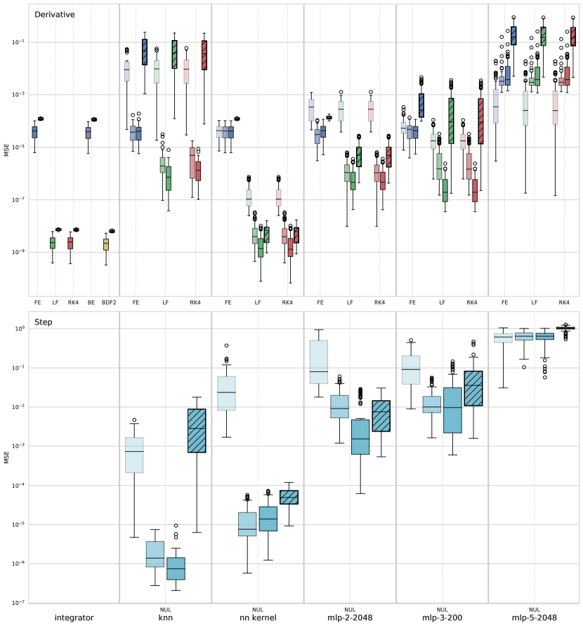
Figure 6: Error distribution for spring system for multiple training set sizes as well as out-of-distribution results.

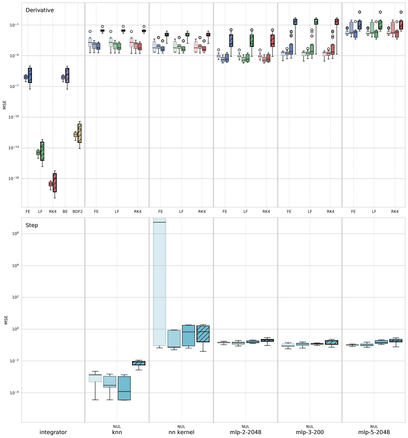
Figure 7: Error distribution for wave system for multiple training set sizes as well as out-of-distribution results.

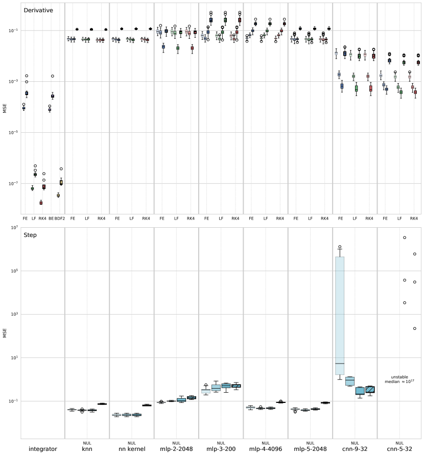
Figure 8: Error distribution for $10\times 10$ spring mesh system for multiple training set sizes as well as out-of-distribution results.

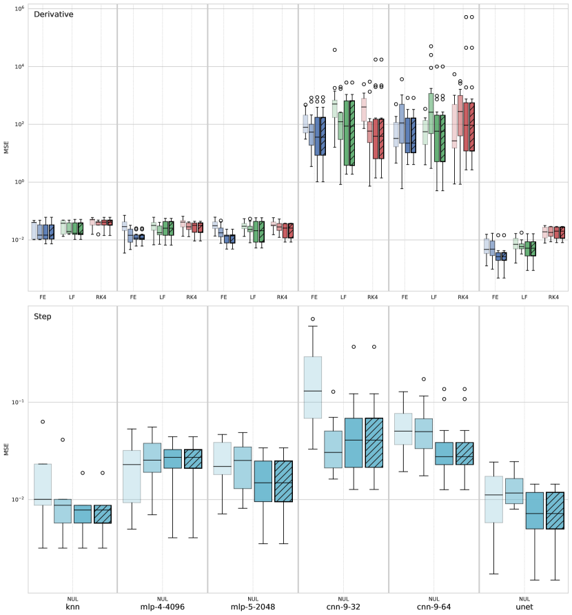
Figure 9: Error distribution for Navier-Stokes system for multiple training set sizes, and out-of-distribution results. Each trajectory has a single randomly-positioned obstacle. Note that this system does not have results for plain numerical integration.

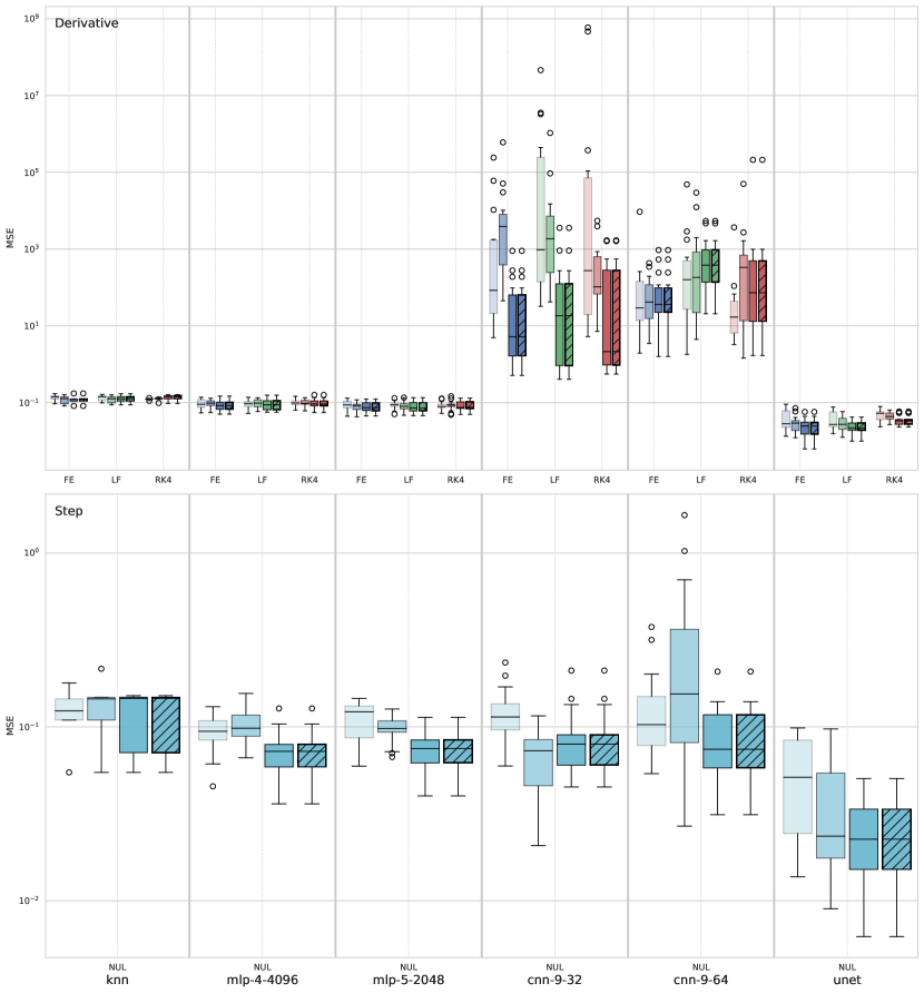
Figure 10: Error distribution for Navier-Stokes system for multiple training set sizes, and out-of-distribution results. Each trajectory has four randomly-positioned obstacles.

C.1 Weighted errors

In most cases, due to accumulated errors, per-step errors increase as numerical integration proceeds away from the initial condition. To compensate for this trend and in an effort to explore the impact of early vs. late step errors, we include several plots of error distributions for which each time step’s MSE has been weighted. To produce these weights, each step’s MSE is scaled by a value $1/\exp(\ln(10^{2})\cdot p_{t})$ where $p_{t}\in[0,1]$ is a scalar representing the proportional time of the step (zero at start of the trajectory, and one at the end). This produces an exponential decay from the initial steps to the end and reduces the contribution of the final steps by two orders of magnitude. These scaled MSEs are then averaged for each trajectory and each neural network retraining as in the plots above.

The results of these distributions for the Navier-Stokes system—both single- and multi-obstacle forms—are included in Figure 11 and Figure 12 below. A change in the relative behavior of the learned methods is most visible in the step prediction results in Figure 12. Without the weighting, many of the learning methods perform comparably to the KNN; however when emphasizing early steps, these methods demonstrate improved errors relative to the re-weighted KNN errors. This indicates that the learned methods outperform the accuracy of the KNN on the early steps, but are somewhat unstable as the simulation progresses.

For other systems, we did not observe significant changes in relative performance of the learned methods. MSE distributions shifted, but roughly in proportion to each other. This represents a greater general stability in the learned methods on other systems, likely reflecting the more predictable long-term behavior of the other systems. The spring system is periodic, the wave system is stable over time, and the spring mesh system has an energy decay term which simplifies and stabilizes its long-term evolution. As a result, in most cases, successfully learning the target task permits the learned methods to maintain some stability over time, which decreases the relative effect of the per-step weighting.

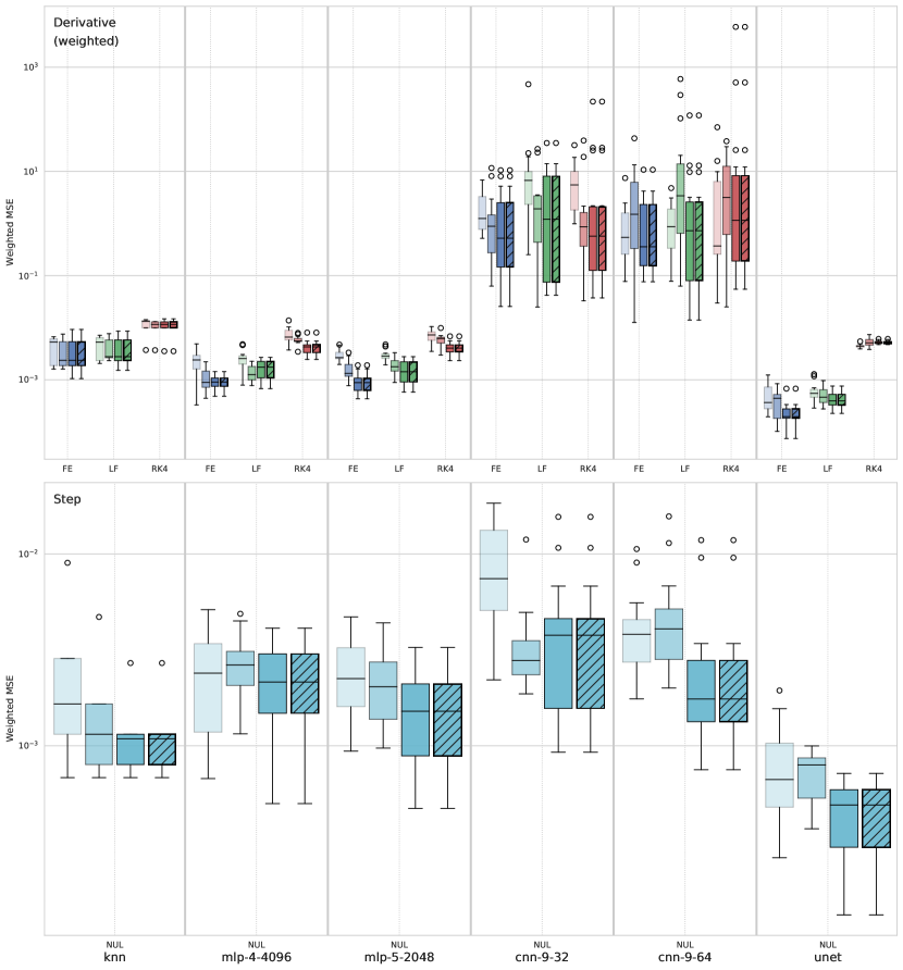
Figure 11: Error distribution for Navier-Stokes system for multiple training set sizes, and out-of-distribution results. Each trajectory has a single randomly-positioned obstacle. Per-step errors are weighted to decrease the contribution of later time steps with higher errors.

Figure 12: Error distribution for Navier-Stokes system for multiple training set sizes, and out-of-distribution results. Each trajectory has four randomly-positioned obstacles. Per-step errors are weighted to decrease the contribution of later time steps with higher errors.

Appendix D Dataset and software documentation

This section contains information documenting the contents, structure, and intended uses of the datasets used in this work.

D.1 Overview

The datasets used in this work consist of snapshots gathered from numerical simulations of dynamical systems. These simulations were carried out as part of this work and the software used to generate them as well as stored outputs are made available for use and further modification. The software source code is available under the MIT license, and the stored data is available under a Creative Commons Attribution 4.0 license (CC BY 4.0).

Simulations are carried out for four system types, described in greater detail in the main work, above: (1) spring, (2) wave, (3) spring mesh, and (4) Navier-Stokes. Each simulation’s outputs are intended to be used for developing and testing machine learning methods for numerical simulations. They include snapshots of each system’s state across several data channels, as well as time derivatives, either of which can be used as learning targets.

An archival copy of the stored data and software source code has been placed in the NYU Faculty Digital Archive (https://archive.nyu.edu/handle/2451/63285) for long-term storage. The source code is also available on GitHub at https://github.com/karlotness/nn-benchmark.

The stored data for each simulation type is stored in two components: a JSON file containing metadata for the particular simulation, and an associated uncompressed NumPy .npz-formatted file containing the numerical results. Details of the contents of these files are provided below. Our experiments were carried out in Python and these files are readable using the Python standard library’s json module and the widely-used NumPy library. For other languages or environments, the .npz files are ZIP archives containing NumPy .npy files whose format is documented by NumPy https://numpy.org/doc/stable/reference/generated/numpy.lib.format.html.

D.2 Stored format

Each dataset is a directory storing two files: “system_meta.json” and “trajectories.npz”. The .npz file contains several NumPy array records with various shapes and data types. The names of each of these records are referenced in the JSON file (documented below). When loading the data from these systems these names should be treated as opaque and always sourced from the JSON-formatted metadata. In some cases, the same name is referenced several times for purposes of data deduplication. The .npz file is used for bulk storage of numerical data, separated from general metadata.

The simulation snapshots are divided into trajectories, each defined by a particular initial condition from which a series of snapshots is taken at several later time steps, by numerical simulation. Each trajectory is divided into several “channels” of data, in particular separating various state quantities, state time derivatives, and masks marking special spatial locations for that trajectory, particular to that system. The JSON file also contains trajectory-level parameter information, and settings for global system-level parameters.

The stored data sets are intended to be used to test against the same snapshots used in this work, without needing to configure the dependencies necessary to generate the snapshots. The process of running the simulations and reproducing the tests described in this work is discussed in a separate section, below.

D.2.1 Top-level object contents

The JSON-formatted metadata file contains important information used when loading these data sets. The contents of certain sections vary by simulated system to reflect differences in relevant parameters and other generic data. However, each has a similar global structure. Each JSON file contains a top-level object with the same four keys: system, system_args, metadata, and trajectories.

The value of system is a string identifying which system is stored in that dataset. Its value will be one of: “spring”, “wave”, “spring-mesh”, or “navier-stokes”.

The value of system_args is another object storing the parameters which were passed to the simulation code to generate these snapshots. These contents vary per system, but may be useful in understanding what settings were configured for the simulators.

The system_args object stores several key-value pairs which vary by system reflecting different global parameters which apply to every trajectory in the set. However it also always contains a key system_args.trajectory_defs whose value is an array of objects which contain parameters which may vary per-trajectory.

In addition to parameters in these objects which vary by system, several are always present with the same meaning: num_time_steps, time_step_size, and subsample. The field num_time_steps is an integer which sets the number of snapshots which are to be generated, including the first snapshot which contains the initial condition. The parameter time_step_size is a floating-point value which sets the time difference between each stored snapshot. The physical effect of the time step varies per system. The parameter subsample is an integer ($1$ or larger) which allows generating the dataset on a finer time grid than is reflected in the stored trajectory. Values greater than $1$ cause the simulator to run at a time step of $\mathtt{time\_step\_size}/\mathtt{subsample}$ for $\mathtt{num\_time\_step}\cdot\mathtt{subsample}$ steps, and to discard intermediate snapshots to produce an output at an un-subsampled stride. This allows generating data sets at a higher simulation quality while keeping the same end time and desired number of steps.

The metadata key stores an object with key-value pairs providing system-dependent information on particular global parameters.

The trajectories key contains an array of objects giving information about the stored trajectory data. These are likely to be the most useful when loading the snapshots as this object also provides a mapping from each system’s data channels to the array in the dataset’s “trajectories.npz” file.

The objects in the trajectories array each contain system-dependent per-trajectory metadata which will be discussed below, but as elsewhere several entries are always present. The first is a name entry which gives a human-readable name for the trajectory. The keys num_time_steps and time_step_size have the same value and function as discussed above. The timing entry contains an object with information on timing of the data generation process. At present this object has one entry of its own: traj_gen_time, which gives the time to generate this trajectory measured in seconds.

Beyond these, each object in the trajectories array contains a key field_keys storing an object. This object has keys for each data channel in this system whose values are strings giving the name of a record stored in the “trajectories.npz” file. These mappings are the best way to determine the correspondence between a trajectory in the dataset and the stored bulk arrays which make up its snapshot data. The names used for keys follow a general pattern, usually prefixed with the name of the trajectory discussed above, but they should be treated as opaque and always sourced from the JSON files. This mapping is in some cases used to reduce duplication and some array records may be referenced multiple times.

Next, we discuss per-system variation in the overall structure listed above, describing the metadata components and data channels which are specific to each system.

D.2.2 Spring

This system is identified by a system entry with value “spring”.

Under system_args this system has no additional global parameters, only per-trajectory parameters in the system_args.trajectory_defs array. These per-trajectory objects have a system-specific initial_condition attribute which is a sub-object with attributes q and p, both of which are floating-point, giving the initial values for the position and momentum of the simulated spring.

The metadata object contains one attribute, n_grid for consistency with the wave system, below. Its value is always the integer 1.

The objects in the trajectories array contain only the standard values defining the number of time steps and the name of each trajectory. The object field_keys defines name mappings for the data channels of this system described below. Some additional details for each channel are included in Table 3.

The channels “q” and “p” give the position and momentum of the spring, respectively. Both values evolve in the one-dimensional space of the system. Channels “dqdt” and “dpdt” are time derivatives of these two quantities. The vector “t” gives the time of each snapshot in the trajectory.

Table 3: Data channels for the Spring system. $N_{t}$ denotes the number of time steps in the trajectory.

Channel name	Shape	Data type
q	$(N_{t},1)$	float64
p	$(N_{t},1)$	float64
dqdt	$(N_{t},1)$	float64
dpdt	$(N_{t},1)$	float64
t	$(N_{t})$	float64

D.2.3 Wave

This system is identified by a system entry with value “wave”.

Under system_args, the wave system has two global parameters: n_grid and space_max. The parameter n_grid controls how many points are sampled on a regular, one-dimensional spatial grid covering the interval $[0,\mathtt{space\_max}]$, with a periodic boundary condition. space_max is a floating-point value controlling the end point of this interval.

System-specific per-trajectory elements in system_args.trajectory_defs are wave_speed, start_type, and start_type_args. The wave_speed parameter is a floating-point value controlling the distance the wave pulses travel in a unit of time.

The other two parameters control the shape and position of the initial pulse. start_type is a string parameter selecting the type of pulse to form; at present only “cubic_splines” is supported. The value of start_type_args is an object with additional parameters which affect the starting pulse. For a cubic spline these are: height, width, and position. Each of these is a floating-point value which scales the height and width of the pulse, and selects its center point in the spatial interval.

The metadata object repeats the values of the n_grid and space_max attributes described above.

Each object in the trajectories array contains the trajectory’s value of the wave_speed parameter discussed above. There are no further system-specific entries in these objects, other than the data channels. Some attributes of these are given in Table 4.

The channels “q” and “p” give the position/height and vertical velocity of the wave at each grid point, respectively. The channels “dqdt” and “dpdt” are time derivatives of these quantities. The vector “t” gives the simulation time for each snapshot in the trajectory.

Table 4: Data channels for the Wave system. $N_{t}$ denotes the number of time steps in the trajectory, and $N_{p}$ denotes the number of points in the spatial grid, determined by n_grid.

Channel name	Shape	Data type
q	$(N_{t},N_{p})$	float64
p	$(N_{t},N_{p})$	float64
dqdt	$(N_{t},N_{p})$	float64
dpdt	$(N_{t},N_{p})$	float64
t	$(N_{t})$	float64

D.2.4 Spring mesh

This system is identified by a system entry with value “spring-mesh”.

Under system_args, this system has a global parameter vel_decay which is a floating-point value configuring the damping applied to the velocity of each mass. Per-trajectory elements in system_args.trajectory_defs objects are particles and springs, which are both arrays of objects.

Each object in particles has three attributes: is_fixed, a boolean indicating whether this particle is fixed in place and immovable; mass, a floating-point value for the particle’s mass; and position, an array of two floating-point values giving the $x$ and $y$ coordinates of the particle’s initial position. The order of the particles is significant and their index in this array is their index referenced in springs, below.

The objects in the springs array have four attributes: a, b, rest_length, and spring_const. The values of a and b are integers specifying which two particles this spring connects in the order of the objects in the particles array. The springs are undirected so the order of a and b is not important. The values rest_length and spring_const are floats giving the rest length of the spring and its spring constant, respectively. In this work, the edges described in the array are one-hop nearest neighbors in each axis-aligned direction, and are the edges of the regular, square grid.

The metadata object has attributes repeating some values from system_args: edges is an array of objects repeating springs as described above, and particles repeats the corresponding array, both sourced from the first entry in system_args.trajectory_defs.

Beyond these in metadata are: n_dim, giving the spatial dimensions in which the particles move (in this work, always 2); n_grid, repeating the same value; n_particles, giving the length of the particles array; and the vel_decay value repeated here as well.

There are no system-specific entries in the objects in the trajectories array, other than the data channels. Some attributes of each of these are given in Table 5.

The channel “q” and “p” give the per-particle position and momentum, respectively. These values are provided in both $x$ and $y$ components for the two-dimensional space. The channels “dqdt” and “dpdt” give time derivatives for these quantities.

The channel “t” provides the simulation time at which each snapshot was taken.

The “edge_indices” gives the locations of the edges (the springs) between each particle. The integers in this channel index in the same order as the per-particle $N_{p}$ dimension in the other channels. The values in this channel are directed so each spring is repeated twice, once with its two end indices in both orders.

The array for “masses” gives the mass of each particle in the same order as the $N_{p}$ dimensions in other channels.

The channel “fixed_mask” is a boolean mask with true for each particle which is fixed in place. The channels “fixed_mask_q” and “fixed_mask_p” are the same, except with repeated values to be suitable for broadcasting.

Table 5: Data channels for the Spring-Mesh system. $N_{t}$ denotes the number of time steps in the trajectory, $N_{p}$ denotes the number of particles, $N_{e}$ denotes the number of edges.

Channel name	Shape	Data type	Notes
q	$(N_{t},N_{p},2)$	float64
p	$(N_{t},N_{p},2)$	float64
dqdt	$(N_{t},N_{p},2)$	float64
dpdt	$(N_{t},N_{p},2)$	float64
t	$(N_{t})$	float64
edge_indices	$(2,N_{e})$	int64
masses	$(N_{p})$	float64
fixed_mask	$(N_{p})$	bool
fixed_mask_q	$(N_{p},2)$	bool
fixed_mask_p	$(N_{p},2)$	bool	Alias: “fixed_mask_q”
extra_fixed_mask	$(N_{p})$	bool	Alias: “fixed_mask”

D.2.5 Navier-Stokes

The Navier-Stokes system is identified by a system entry with value “navier-stokes”.

Under system_args, this system has a global parameter grid_resolution which is a floating-point value, giving the space stride of the regular grid on which the solutions are sampled. Per-trajectory elements in system_args.trajectory_defs objects are viscosity and in_velocity, which are parameters passed to the FEM solver giving the viscosity of the fluid and the velocity of the incoming flow, respectively. Both are floating-point values.

The objects in system_args.trajectory_defs also have a parameter mesh which describes the location of obstacles in the simulated space. Each entry in the array is an object with two keys: radius, a single floating point value for the radius of the circular obstacle, and center, an array of two floating point values giving the $x$ and $y$ position of the center of the circle. These values allow placing multiple obstacles in the simulation space and impact the mesh which is generated and used by the external finite element solver.

The metadata entry for this system contains two values: grid_resolution and viscosity, a copy of the same values as described above. The viscosity value is taken from the first trajectory entry.

The objects in the trajectories array have extra global parameter values: in_velocity, and viscosity, which are as discussed above. Their field_keys entries have mapped names for the data channels listed in Table 6. The “q”- and “p”-related channels are present as aliases for consistency with other systems.

The core values for this system are the “solutions” and “pressures” channels which store the flow velocity of the fluid and the pressure field, respectively. The two channels for the solutions are the $x$ and $y$ flow velocities.

Separately the “grads” and “pressures_grads” channels store approximated time derivatives computed from neighboring time steps from the FEM solver’s output.

The “t” channel is a vector giving the simulation time of each snapshot.

The channels “vertices” and “edge_indices” identify the spatial position and neighboring grid points for each sample point, respectively. “vertices” gives the $x$- and $y$-coordinates as separate channels, and “edge_indices” stores indexes into the per-particle dimension $N_{p}$ of each spatial value. The edges described in the array are one-hop nearest neighbors in each axis-aligned direction, the edges of the regular, square grid.

The “fixed_mask” channels are boolean masks for the sample points, indicating which of them form part of the boundary or an obstacle. “fixed_mask” itself stores a value of true for points which are either a boundary or an obstacle. The arrays “fixed_mask_solutions” and “fixed_mask_pressures” store the same, just repeated to match the dimensions of the corresponding data channels, suitable for broadcasting and masking or other purposes. The “extra_fixed_mask” is like “fixed_mask” except that it provides boolean per-particle masks for two kinds of points. The last dimension of this mask separates the two sub-channels, one for each type of mask. Mask $0$ has true for the obstacles and the boundaries, while mask $1$ has true only for the obstacles.

Table 6: Data channels for Navier-Stokes system. $N_{t}$ denotes the number of time steps in the trajectory, and $N_{p}$ denotes the number of points in the regular grid. $N_{p}=9282$ for the datasets in this work.

Channel name	Shape	Data type	Notes
solutions	$(N_{t},N_{p},2)$	float64
pressures	$(N_{t},N_{p})$	float64
grads	$(N_{t},N_{p},2)$	float64
pressures_grads	$(N_{t},N_{p})$	float64
t	$(N_{t})$	float64
q	$(N_{t},N_{p})$	float64	Alias: “pressures”
p	$(N_{t},N_{p},2)$	float64	Alias: “solutions”
dqdt	$(N_{t},N_{p})$	float64	Alias: “pressures_grads”
dpdt	$(N_{t},N_{p},2)$	float64	Alias: “grads”
edge_indices	$(2,N_{p})$	int64
vertices	$(N_{p},2)$	float64
fixed_mask	$(N_{p})$	bool
fixed_mask_solutions	$(N_{p},2)$	bool
fixed_mask_pressures	$(N_{p})$	bool
fixed_mask_q	$(N_{p})$	bool	Alias: “fixed_mask_pressures”
fixed_mask_p	$(N_{p},2)$	bool	Alias: “fixed_mask_solutions”
extra_fixed_mask	$(N_{p},2)$	bool

D.3 Data generation

The section above discussed how to make use of the stored data sets. Here we document the process used to configure these data sets and invoke the simulators to produce the snapshots. The steps used here cover the very similar process of running the neural network training and evaluation phases. Following the steps here on the run descriptions we have distributed allows recreating the experimental setup used in the report above.

D.3.1 Dependencies

This section includes instructions for configuring the software environment.

While the software we have produced for this work is available under an open source license, the required dependencies are made available under a variety of other licenses. These include some proprietary components such as NVIDIA’s CUDA libraries, and Intel’s Math Kernel Library (MKL). Review the licenses of the required dependencies before installing or running.

Anaconda

The majority of software dependencies can be installed using the Conda package management tool (https://docs.conda.io). The root directory of our software project contains an environment definition in the file “environment.yml”. Using this file will create an environment nn-benchmark containing the Python dependencies needed for this project. If you are obtaining these dependencies from another source, the contents of this file include the names of the packages which will be required.

PolyFEM

In addition to the Python libraries needed for the project, if you wish to generate new Navier-Stokes trajectories, you will also need a copy of PolyFEM. The source code for this software can be obtained from the PolyFEM GitHub repository (https://github.com/polyfem/polyfem/). This portion of the project requires a copy of PolyFEM linked with Intel’s Math Kernel Library (MKL). To do this, locate the root directory of your MKL installation and build PolyFEM from the root directory of its source code with:

mkdir build
cd build
MKLROOT=/path/to/mkl/root/ cmake .. -DPOLYSOLVE_WITH_PARDISO=ON -DPOLYFEM_NO_UI=ON
make

This will produce a binary PolyFEM_bin, required to produce new Navier-Stokes trajectories. This binary must either be placed in the directory from which you will run the simulation software, or you should specify the parent directory of this binary in the environment variable POLYFEM_BIN_DIR so that it can be located.

Singularity container (optional)

It is possible to run the software directly in a manually-created Anaconda environment. However, for convenience we include a build definition file for a Singularity container (https://singularity.hpcng.org). Building a .sif container from this definition will produce an environment suitable for running the software, including PolyFEM and the required environment variables. Consult the Singularity documentation for more information on building these containers in your computing environment.

If you choose to use the Singularity container, either place it in the directory from which you will run the simulation software or provide the path to the resulting nn-benchmark.sif file’s parent directory in the environment variable SCRATCH. The run management scripts (described below) will look in this directory for the container and use it to run jobs if it is found.

D.3.2 Run descriptions

The software used to generate the datasets, train networks, and perform evaluations takes arguments from JSON files, specified on the command line. This makes it possible to provide a large number of arguments, to submit the jobs in batches, and to detect tasks that have failed or that remain outstanding. The structure of these files is relatively complex, so we provide additional tooling to assist in generating them.

These utilities are located in the src/run_generators directory, in utils.py. Examples of their use are included in the other Python scripts in that directory. These tools consist of several object definitions which define jobs to run. These are divided into three phases: data generation, network training, and evaluation. To produce the descriptions of the desired jobs, one constructs Python objects representing each of these, and calls their write_description(dir) methods. This method takes a single argument: the root directory under which the job descriptions and the resulting outputs will be stored. Create a new directory for each experiment.

Each task takes an Experiment object as an argument; this principally sets a prefix on the resulting file names, and records the experiment name in the run description file. This separation is not enforced and results of jobs combining different Experiment objects can freely be mixed.

Datasets are generated by creating various Dataset subclass objects. Each of these takes as an argument an InitialConditionSource which provides the sampling of initial conditions described above. Be aware that these objects cache the initial conditions they have previously generated. This ensures that larger datasets drawn from the same source are always strict supersets of smaller datasets. The initial condition sources have parameters which control the distribution from which samples are drawn, and the datasets themselves have parameters controlling the simulations which are carried out from these samples (such as the time step size, number of steps, etc.). The InitialConditionSource objects do not represent jobs and do not have write_description methods.

Neural network training tasks are created by providing both an Experiment object and two datasets: one for training, and one for validation. The objects representing each dataset are provided as constructor arguments to the objects representing each type of neural network. Most networks have parameters which control their architecture, choosing kernel sizes, hidden dimensions, etc.

Finally, evaluation run descriptions are generated by the NetworkEvaluation object. This takes an Experiment object, the object representing the network training task, an object for the evaluation set to use, and the numerical integrator to combine with the network. The exception to this is configuring runs for the KNNs. These do not have a normal training phase and run entirely at evaluation-time. These evaluation objects take an additional parameter for their training dataset. When run, the job will load this training set, fit the KNN, and then proceed with the rest of the regular evaluation phase. KNNPredictorOneshot runs a KNN for step prediction and KNNRegressorOneshot runs a KNN for derivative prediction with the integrator specified as an argument to its constructor.

As an illustration of configuring jobs using these utilities we provide the Python scripts used to generate the run descriptions for the experiments discussed above. Be aware that running these scripts will sample new datasets from the distributions specified above. Each script takes the name of the directory created for its experiment as an argument and writes the run descriptions to that directory in a descr directory, with three subdirectories, one for each of the three phases.

D.3.3 Launching jobs

Once the run descriptions are generated, running the jobs is in large part managed by the manage_runs.py script. This script can inspect the experiment directory to identify runs which are outstanding, appear possibly incomplete, or whose description files have been modified after the job was launched. The script also runs the jobs from the description file, either serially, or in parallel by submitting to a Slurm queue.

Scanning

Running python manage_runs.py scan <experiment directory> will output information about the state of all jobs in that experiment. The script will indicate whether the jobs are yet to be run (outstanding), appear to be incomplete, or whether their descriptions were modified after the job launched. Jobs in one of the error states (incomplete or mismatched descriptions) can be deleted by adding the --delete=<mismatch or incomplete> argument. This extra flag deletes the jobs in the specified state with no further confirmation.

Launching

python manage_runs.py launch <experiment directory> <phase> where phase is one of data_gen, train, or eval will launch all outstanding jobs for the specified experiment and phase. Wait for all jobs from earlier phases to complete before beginning the next phase. By default the script will attempt to run the jobs locally in serial, but if the sbatch program is detected it will submit jobs to the Slurm queue instead. This selection can be overridden by passing one of slurm or local to the --launch_type argument. If the Singularity container is being used the script may output a warning that the “nn-benchmark” Anaconda environment is not loaded. This warning can be ignored as the container will provide the necessary environment.

D.3.4 Recreating experiments

We provide the JSON run descriptions for the experiments discussed above. Once the software environment is configured, the manage_runs.py script can be used to launch copies of these experiments.

References

- Antoulas and Anderson [1986] A. C. Antoulas and B. D. O. Anderson. On the scalar rational interpolation problem. IMA Journal of Mathematical Control & Information, 3(2-3):61–88, 1986.
- Antoulas et al. [2020] A. C. Antoulas, C. Beattie, and S. Gugercin. Interpolatory Methods for Model Reduction. SIAM, 2020.
- Brunton et al. [2016] S. L. Brunton, J. L. Proctor, and J. N. Kutz. Discovering governing equations from data by sparse identification of nonlinear dynamical systems. Proceedings of the National Academy of Sciences, 113(15):3932–3937, 2016.
- Chen et al. [2020] Z. Chen, J. Zhang, M. Arjovsky, and L. Bottou. Symplectic recurrent neural networks. In International Conference on Learning Representations, 2020.
- Coveney et al. [2016] P. V. Coveney, E. R. Dougherty, and R. R. Highfield. Big data need big theory too. Philosophical Transactions of the Royal Society A: Mathematical, Physical and Engineering Sciences, 374(2080):20160153, 2016. doi: 10.1098/rsta.2016.0153. URL https://royalsocietypublishing.org/doi/abs/10.1098/rsta.2016.0153.
- Cranmer et al. [2020] M. Cranmer, A. Sanchez-Gonzalez, P. Battaglia, R. Xu, K. Cranmer, D. Spergel, and S. Ho. Discovering symbolic models from deep learning with inductive biases. arXiv preprint, 2020. URL https://arxiv.org/abs/2006.11287.
- Crutchfield and Mcnamara [1987] J. P. Crutchfield and B. S. Mcnamara. Equations of motion from a data series. Complex Systems, page 452, 1987.
- Greydanus et al. [2019] S. Greydanus, M. Dzamba, and J. Yosinski. Hamiltonian neural networks. In H. Wallach, H. Larochelle, A. Beygelzimer, F. d’Alché Buc, E. Fox, and R. Garnett, editors, Advances in Neural Information Processing Systems, volume 32, pages 15379–15389. Curran Associates, Inc., 2019. URL https://proceedings.neurips.cc/paper/2019/file/26cd8ecadce0d4efd6cc8a8725cbd1f8-Paper.pdf.
- Gustavsen and Semlyen [1999] B. Gustavsen and A. Semlyen. Rational approximation of frequency domain responses by vector fitting. Power Delivery, IEEE Transactions on, 14(3):1052–1061, Jul 1999.
- Haghighat et al. [2020] E. Haghighat, M. Raissi, A. Moure, H. Gomez, and R. Juanes. A deep learning framework for solution and discovery in solid mechanics, 2020.
- Hairer and Wanner [2009] E. Hairer and G. Wanner. Solving Ordinary Differential Equations II: Stiff and Differential-Algebraic Problems. Springer, 2009.
- Hairer et al. [2009] E. Hairer, S. P. Nørsett, and G. Wanner. Solving Ordinary Differential Equations I: Nonstiff Problems. Springer, 2009.
- Harris et al. [2020] C. R. Harris, K. J. Millman, S. J. van der Walt, R. Gommers, P. Virtanen, D. Cournapeau, E. Wieser, J. Taylor, S. Berg, N. J. Smith, R. Kern, M. Picus, S. Hoyer, M. H. van Kerkwijk, M. Brett, A. Haldane, J. F. del R’ıo, M. Wiebe, P. Peterson, P. G’erard-Marchant, K. Sheppard, T. Reddy, W. Weckesser, H. Abbasi, C. Gohlke, and T. E. Oliphant. Array programming with NumPy. Nature, 585(7825):357–362, 2020. URL https://doi.org/10.1038/s41586-020-2649-2.
- Hunter [2007] J. D. Hunter. Matplotlib: A 2D graphics environment. Computing in Science & Engineering, 9(3):90–95, 2007. doi: 10.1109/MCSE.2007.55.
- Khadilkar et al. [2019] A. Khadilkar, J. Wang, and R. Rai. Deep learning-based stress prediction for bottom-up SLA 3D printing process. The International Journal of Advanced Manufacturing Technology, 102(5):2555–2569, Jun 2019. ISSN 1433-3015. doi: 10.1007/s00170-019-03363-4. URL https://doi.org/10.1007/s00170-019-03363-4.
- Kim et al. [2019] B. Kim, V. C. Azevedo, N. Thuerey, T. Kim, M. Gross, and B. Solenthaler. Deep fluids: A generative network for parameterized fluid simulations. Computer Graphics Forum, 38(2):59–70, 2019.
- Kingma and Ba [2014] D. P. Kingma and J. Ba. Adam: A method for stochastic optimization. arXiv preprint arXiv:1412.6980, 2014.
- Kipf et al. [2018] T. Kipf, E. Fetaya, K.-C. Wang, M. Welling, and R. Zemel. Neural relational inference for interacting systems. In International Conference on Machine Learning, pages 2688–2697. PMLR, 2018.
- Kissas et al. [2020] G. Kissas, Y. Yang, E. Hwuang, W. R. Witschey, J. A. Detre, and P. Perdikaris. Machine learning in cardiovascular flows modeling: Predicting arterial blood pressure from non-invasive 4D flow MRI data using physics-informed neural networks. Computer Methods in Applied Mechanics and Engineering, 358:112623, 2020.
- Kurtzer et al. [2017] G. M. Kurtzer, V. Sochat, and M. W. Bauer. Singularity: Scientific containers for mobility of compute. PLOS ONE, 12(5), 5 2017. doi: 10.1371/journal.pone.0177459.
- Lam et al. [2015] S. K. Lam, A. Pitrou, and S. Seibert. Numba: A LLVM-based Python JIT compiler. In Proceedings of the Second Workshop on the LLVM Compiler Infrastructure in HPC, LLVM ’15, New York, NY, USA, 2015. Association for Computing Machinery. ISBN 9781450340052. doi: 10.1145/2833157.2833162. URL https://doi.org/10.1145/2833157.2833162.
- Li et al. [2018] Y. Li, H. Wang, K. Mo, and T. Zeng. Reconstruction of simulation-based physical field by reconstruction neural network method. arXiv preprint arXiv:1805.00528, 2018.
- Li et al. [2019] Y. Li, H. Wang, W. Shuai, H. Zhang, and Y. Peng. Image-based reconstruction for the impact problems by using DPNNs. arXiv preprint arXiv:1905.03229, 2019.
- Liang et al. [2018] L. Liang, M. Liu, C. Martin, and W. Sun. A deep learning approach to estimate stress distribution: a fast and accurate surrogate of finite-element analysis. Journal of The Royal Society Interface, 15(138):20170844, 2018. doi: 10.1098/rsif.2017.0844. URL https://royalsocietypublishing.org/doi/abs/10.1098/rsif.2017.0844.
- Liang et al. [2020] L. Liang, W. Mao, and W. Sun. A feasibility study of deep learning for predicting hemodynamics of human thoracic aorta. Journal of Biomechanics, 99:109544, 2020.
- Lu et al. [2019] L. Lu, X. Meng, Z. Mao, and G. E. Karniadakis. DeepXDE: A deep learning library for solving differential equations. arXiv preprint arXiv:1907.04502, 2019.
- Maso Talou et al. [2020] G. D. Maso Talou, T. P. Babarenda Gamage, M. Sagar, and M. P. Nash. Deep learning over reduced intrinsic domains for efficient mechanics of the left ventricle. Frontiers in Physics, 8:30, 2020.
- Nakatsukasa et al. [2018] Y. Nakatsukasa, O. Sète, and L. N. Trefethen. The AAA algorithm for rational approximation. SIAM Journal on Scientific Computing, 40(3):A1494–A1522, 2018.
- Nie et al. [2020] Z. Nie, H. Jiang, and L. B. Kara. Stress field prediction in cantilevered structures using convolutional neural networks. Journal of Computing and Information Science in Engineering, 20(1), 2020.
- Packard et al. [1980] N. H. Packard, J. P. Crutchfield, J. D. Farmer, and R. S. Shaw. Geometry from a time series. Physical Review Letters, 45:712–716, 1980.
- Paszke et al. [2019] A. Paszke, S. Gross, F. Massa, A. Lerer, J. Bradbury, G. Chanan, T. Killeen, Z. Lin, N. Gimelshein, L. Antiga, A. Desmaison, A. Kopf, E. Yang, Z. DeVito, M. Raison, A. Tejani, S. Chilamkurthy, B. Steiner, L. Fang, J. Bai, and S. Chintala. PyTorch: An imperative style, high-performance deep learning library. In H. Wallach, H. Larochelle, A. Beygelzimer, F. d’Alché Buc, E. Fox, and R. Garnett, editors, Advances in Neural Information Processing Systems 32, pages 8024–8035. Curran Associates, Inc., 2019.
- Pedregosa et al. [2011] F. Pedregosa, G. Varoquaux, A. Gramfort, V. Michel, B. Thirion, O. Grisel, M. Blondel, P. Prettenhofer, R. Weiss, V. Dubourg, J. Vanderplas, A. Passos, D. Cournapeau, M. Brucher, M. Perrot, and E. Duchesnay. Scikit-learn: Machine learning in Python. Journal of Machine Learning Research, 12:2825–2830, 2011.
- Peng and Mohseni [2016] L. Peng and K. Mohseni. Symplectic model reduction of hamiltonian systems. SIAM Journal on Scientific Computing, 38(1):A1–A27, 2016. URL https://doi.org/10.1137/140978922.
- Pfaff et al. [2020] T. Pfaff, M. Fortunato, A. Sanchez-Gonzalez, and P. W. Battaglia. Learning mesh-based simulation with graph networks. arXiv preprint, 2020. URL https://arxiv.org/abs/2010.03409.
- Qian et al. [2020] E. Qian, B. Kramer, B. Peherstorfer, and K. Willcox. Lift & learn: Physics-informed machine learning for large-scale nonlinear dynamical systems. Physica D: Nonlinear Phenomena, 2020.
- Rahimi and Recht [2008] A. Rahimi and B. Recht. Random features for large-scale kernel machines. In J. Platt, D. Koller, Y. Singer, and S. Roweis, editors, Advances in Neural Information Processing Systems, volume 20. Curran Associates, Inc., 2008. URL https://proceedings.neurips.cc/paper/2007/file/013a006f03dbc5392effeb8f18fda755-Paper.pdf.
- Raissi et al. [2017] M. Raissi, P. Perdikaris, and G. E. Karniadakis. Physics informed deep learning (part ii): Data-driven discovery of nonlinear partial differential equations. arxiv. arXiv preprint arXiv:1711.10561, 2017.
- Raissi et al. [2019] M. Raissi, P. Perdikaris, and G. E. Karniadakis. Physics-informed neural networks: A deep learning framework for solving forward and inverse problems involving nonlinear partial differential equations. Journal of Computational Physics, 378:686–707, 2019.
- Ribeiro et al. [2020] M. D. Ribeiro, A. Rehman, S. Ahmed, and A. Dengel. DeepCFD: Efficient steady-state laminar flow approximation with deep convolutional neural networks. arXiv preprint arXiv:2004.08826, 2020.
- Rudi et al. [2017] A. Rudi, L. Carratino, and L. Rosasco. Falkon: An optimal large scale kernel method. arXiv preprint arXiv:1705.10958, 2017.
- Sanchez-Gonzalez et al. [2018] A. Sanchez-Gonzalez, N. Heess, J. T. Springenberg, J. Merel, M. Riedmiller, R. Hadsell, and P. Battaglia. Graph networks as learnable physics engines for inference and control. In International Conference on Machine Learning, pages 4470–4479. PMLR, 2018.
- Sanchez-Gonzalez et al. [2019] A. Sanchez-Gonzalez, V. Bapst, K. Cranmer, and P. Battaglia. Hamiltonian graph networks with ODE integrators. arXiv preprint, 2019. URL https://arxiv.org/abs/1909.12790.
- Schaeffer [2017] H. Schaeffer. Learning partial differential equations via data discovery and sparse optimization. Proceedings of the Royal Society A: Mathematical, Physical and Engineering Sciences, 473(2197):20160446, 2017.
- Schaeffer et al. [2018] H. Schaeffer, G. Tran, and R. Ward. Extracting sparse high-dimensional dynamics from limited data. SIAM Journal on Applied Mathematics, 78(6):3279–3295, 2018.
- Schmid [2010] P. Schmid. Dynamic mode decomposition of numerical and experimental data. Journal of Fluid Mechanics, 656:5–28, 8 2010. ISSN 1469-7645.
- Schmid and J. [2008] P. Schmid and S. J. Dynamic mode decomposition of numerical and experimental data. In Bull. Amer. Phys. Soc., 61st APS meeting, page 208. American Physical Society, 2008.
- Schneider et al. [2019] T. Schneider, J. Dumas, X. Gao, D. Zorin, and D. Panozzo. PolyFEM. https://polyfem.github.io/, 2019.
- Schölkopf and Smola [1998] B. Schölkopf and A. J. Smola. Learning with Kernels. MIT Press, 1998.
- Süli and Mayers [2003] E. Süli and D. F. Mayers. An Introduction to Numerical Analysis, chapter Initial Value Problems for ODEs, pages 349–353. Cambridge University Press, 2003.
- Tartakovsky et al. [2018] A. M. Tartakovsky, C. O. Marrero, P. Perdikaris, G. D. Tartakovsky, and D. Barajas-Solano. Learning parameters and constitutive relationships with physics informed deep neural networks. arXiv preprint arXiv:1808.03398, 2018.
- Thuerey et al. [2020] N. Thuerey, K. Weißenow, L. Prantl, and X. Hu. Deep learning methods for reynolds-averaged navier–stokes simulations of airfoil flows. AIAA Journal, 58(1):25–36, 2020.
- Tu et al. [2014] J. H. Tu, C. W. Rowley, D. M. Luchtenburg, S. L. Brunton, and J. N. Kutz. On dynamic mode decomposition: Theory and applications. Journal of Computational Dynamics, 1(2):391–421, 2014.
- Umetani and Bickel [2018] N. Umetani and B. Bickel. Learning three-dimensional flow for interactive aerodynamic design. ACM Transactions on Graphics (TOG), 37(4):1–10, 2018.
- Virtanen et al. [2020] P. Virtanen, R. Gommers, T. E. Oliphant, M. Haberland, T. Reddy, D. Cournapeau, E. Burovski, P. Peterson, W. Weckesser, J. Bright, S. J. van der Walt, M. Brett, J. Wilson, K. J. Millman, N. Mayorov, A. R. J. Nelson, E. Jones, R. Kern, E. Larson, C. J. Carey, İ. Polat, Y. Feng, E. W. Moore, J. VanderPlas, D. Laxalde, J. Perktold, R. Cimrman, I. Henriksen, E. A. Quintero, C. R. Harris, A. M. Archibald, A. H. Ribeiro, F. Pedregosa, P. van Mulbregt, and SciPy 1.0 Contributors. SciPy 1.0: Fundamental Algorithms for Scientific Computing in Python. Nature Methods, 17:261–272, 2020. URL https://doi.org/10.1038/s41592-019-0686-2.
- Willcox et al. [2021] K. E. Willcox, O. Ghattas, and P. Heimbach. The imperative of physics-based modeling and inverse theory in computational science. Nature Computational Science, 1(3):166–168, Mar 2021. ISSN 2662-8457. doi: 10.1038/s43588-021-00040-z. URL https://doi.org/10.1038/s43588-021-00040-z.
- Xie et al. [2018] Y. Xie, E. Franz, M. Chu, and N. Thuerey. TempoGAN: A temporally coherent, volumetric GAN for super-resolution fluid flow. ACM Transactions on Graphics (TOG), 37(4):1–15, 2018.