〈⟨

Combining K-means type algorithms with Hill Climbing for
Joint Stratification and
Sample Allocation Designs

Abstract

In this paper we combine the k-means and/or k-means type algorithms with a hill climbing algorithm in stages to solve the joint stratification and sample allocation problem. This is a combinatorial optimisation problem in which we search for the optimal stratification from the set of all possible stratifications of basic strata. Each stratification being a solution the quality of which is measured by its cost. This problem is intractable for larger sets. Furthermore evaluating the cost of each solution is expensive. A number of heuristic algorithms have already been developed to solve this problem with the aim of finding acceptable solutions in reasonable computation times. However, the heuristics for these algorithms need to be trained in order to optimise performance in each instance. We compare the above multi-stage combination of algorithms with three recent algorithms and report the solution costs, evaluation times and training times. The multi-stage combinations generally compare well with the recent algorithms both in the case of atomic and continuous strata and provide the survey designer with a greater choice of algorithms to choose from.

Keywords: Clustering algorithms; hill climbing algorithm; Optimal stratification; Sample allocation; R software.

1 Introduction

In the joint stratification and sample allocation problem we search for a mutually exclusive and exhaustive stratification, from the set of all possible stratifications, of L smaller basic strata (i.e. strata constructed from categorical variables which are known as atomic strata or continuous variables known as continuous strata). The quality of each stratification (or solution) is measured by the its sample cost. Our goal is to arrange the number of strata, H, as well as the number of basic strata, $n_{h}$, within each stratum in order to best minimise cost (or maximise solution quality).

A solution with the maximum solution quality is said to be optimal (there may be more than one) and may be found by computing the sample allocation for each possible stratification. In other words, this optimal solution is unknown or latent. However, this exhaustive evaluation of each candidate solution, or grid-search, quickly becomes intractable for larger sets of possible solutions. This is further compounded by the computation time necessary to evaluate each solution. For this reason a number of heuristic algorithms have been proposed to search for solutions that are of an acceptable quality, e.g. a local minimum that is in close proximity to the global minimum, in a tolerable computing time.

In survey methodology, when clustering is referenced in relation to sampling it usually refers to a two-step process of firstly dividing the population into clusters, and secondly randomly selecting a small number of these in order to take measurements for every unit within. In this paper our focus will be on the first step - as it is applied in the unsupervised machine learning aspect of clustering – where similar units of a population are grouped together into clusters. Indeed the search for the optimal solution resembles clustering in the sense that we seek to group basic strata with similar characteristics together into common groups. Accordingly, for our purposes, clusters are equivalent to strata, and the similarity within each cluster will enable more precise sample allocations.

The equivalency of the stratification aspect of the joint stratification and sample allocation problem to a machine learning clustering technique, the K-means method, was first noted by (Lisic et al., 2018). This refers to a family of algorithms “developed as a result of independent investigations in the 1950s” (Pérez-Ortega et al., 2019) but first given the name K-means by (MacQueen et al., 1967). The K-means algorithm separates observations into K-clusters, so that the within-cluster sum of squared errors (SSE) is minimised (Hartigan, 1979). The purpose of the algorithm is not to find some unique, definitive grouping, but rather to simply aid the investigator in obtaining a qualitative and quantitative understanding of large amounts of N-dimensional data by providing him/her with reasonably good similarity groups (MacQueen et al., 1967).

K-means is a greedy algorithm (Jain, 2010) that finds a local minimum for a problem that is known to be NP hard (Drineas et al., 2004) and this has led to various heuristic approaches being used to solve the problem. K-means algorithms, e.g. (MacQueen et al., 1967), (Lloyd, 1982), (Forgy, 1965) and (Hartigan, 1979) remain commonly used, even though many other similar clustering techniques have been introduced since their inception, e.g. expectation-maximization (EM) (Dempster et al., 1977), fuzzy K-means clustering (Bezdek et al., 1984), self-organising maps (SOM) (Kohonen, 1990) and Neural gas (Martinetz et al., 1991), mainly due to their ease of implementation, computational efficiency and low memory consumption (Morissette and Chartier, 2013).

K-means algorithms are local search heuristics, with a number of choice inputs, such as $K$ and the initial centroids. They are sensitive to the initial centroids chosen and while this is what makes them more likely of finding local minima (more often than global minima) it also means that they sometimes produce counter-intuitive results (Dirgová Luptáková et al., 2016). Secondly, K-means algorithms provide results that are robust in nature with the implication that the local minimum is harder to escape from and the structure of the solution (i.e. number of clusters and constituents of each cluster) may be far from that of the optimal solution.

Thirdly, the algorithm is also known to be sensitive to the order at which basic strata would be re-assigned to clusters (Morissette and Chartier, 2013). Fourthly, K-means also has a tendency to create clusters of equal size even if this does not represent the best clustering of the data (Äyrämö and Kärkkäinen, 2006). Nonetheless, these issues are commonly mitigated by re-starting the algorithm a number of times along with varying the number of $K$, and selecting the best quality solution.

Following (Lisic et al., 2018)’s proposal (Ballin and Barcaroli, 2020) and (O’Luing et al., 2020) used an efficient version of the K-means clustering algorithm (Hartigan, 1979) to determine initial solutions for our problem which are then improved upon or "optimised" using a grouping genetic algorithm and simulated annealing algorithm respectively. (Hartigan, 1979)’s algorithm searches for a solution that is locally optimal and although it is quick, alternative solutions to that found by the algorithm may have the same or smaller within sums of squares.

The proximity of the local optimum to the global optimum as well as the degree of similarity within each cluster will have implications on the search for the latter by the genetic and simulated annealing algorithms. The further the local optimum is from the global optimum, the longer it is likely to take. Furthermore the grouping genetic algorithm and simulated annealing require that their hyperparameters be adequately suited to the problem in order to operate efficiently. Training the hyperparameters can also be computationally expensive.

Using (Hartigan, 1979) also entails that all basic strata within a radius of a centroid will be assigned to a given cluster (Choudhary, 2015). This works well when the natural data groupings are spherical in nature and clusters are linearly separable, with a corresponding high degree of similarity within clusters low degree of similarity between clusters. Indeed it has been shown that K-means can converge to a global minimum when clusters are well-separated (Meilă, 2006).

However, it is not likely to work as well when there is not a clear separation between clusters and also where there is an occurrence of basic strata from exogenous clusters within cluster spheres, i.e. they may be close to a particular cluster centroid, but are more suited to another cluster.

In this paper we explore staged combinations of K-means, expectation maximisation, self-organising map, fuzzy clustering and neural gas algorithms with hill climbing. Our aim is to find better quality solutions in reduced training times when compared to our earlier experiments on the same data with the grouping genetic algorithm and simulated annealing algorithm in (O’Luing et al., 2020).

Chapter 2 defines the objective function. Chapter 3 summarises the K-means algorithm. Chapter 4 discusses Expectation Maximisation. Chapter 5 talks about the self-organising map. Chapter 6 describes the fuzzy clustering algorithm. Chapter 7 outlines the Neural Gas algorithm. The hill climbing algorithm with delta evaluation is described in chapter 8. Chapter 9 provides the details of the computer specifications. This is followed by empirical comparisons for atomic and continuous strata in chapters 10 and 11. The conclusions and suggestions for future work in chapter 12 closes the paper.

2 Objective Function

Our objective function is defined as follows:

$$\begin{array}[]{l}\min n=\sum_{h=1}^{H}n_{h}\\ s.t.\;\;CV\left(\hat{T}_{g}\right)\leq\varepsilon_{g}\;\;\;(g=1,\ldots,G)\\ 2\leq n_{h}\leq N_{h}\end{array}$$

where $n$ is the sample size, $n_{h}$ is the sample size for stratum $h$, $N_{h}$ is the number of units in stratum $h$ and $H$ is the number of strata. $\hat{T}_{g}$ is the estimator of the population total for each one of $G$ target variable columns. The upper limit of precision $\varepsilon_{g}$ is expressed as a coefficient of variation $CV$ for each $\hat{T}_{g}$. We solve the allocation problem for a particular stratification with the Bethel-Chromy algorithm (Bethel, 1985, 1989; Chromy, 1987).

3 The Haritgan-Wong version of the K-means algorithm

As described above (Ballin and Barcaroli, 2020) and (O’Luing et al., 2020) use an efficient version of the K-means algorithm to generate starting solutions for the genetic and simulated annealing algorithms respectively. The (Hartigan, 1979) version seeks to attain the locally optimal minimum sums of squares within each cluster by moving data-points from one cluster to another. This means that although a sample unit might be closer its current cluster centroid, it could still be re-assigned to another cluster, if in doing so the sums of squares was reduced.

Algorithm 1 Haritgan Wong K-means clustering algorithm

1:Initialise solution with $K$ clusters ($k=1,...,K$) and compute centroid, $c_{k}$ for each cluster $C_{k}$

2:For each $\bar{Y_{g}}$, in sample unit $l$, calculate the Euclidean distance, $dist=\sqrt{\sum_{g}^{G}(c_{g}-\bar{Y_{g}})}$, from the centroids $c_{k}$ of $K$ clusters $C_{k}$.

3:Assign basic strata to clusters with the closest centroids

4:Calculate the new centroids of the clusters $c_{k}=\frac{\sum_{\bar{Y}_{g\in c_{k}}}\bar{Y}_{g}}{\left|c_{k}\right|}$

5:Compute $SSE\left(C_{g}\right)=\sum_{g}\sum_{\bar{Y}\in C_{g}}dist^{2}\left(c_{g},\bar{Y}\right)$

6:Repeat Step 2 to Step 5 until convergence.

The algorithm is deemed to have converged when no sample unit changes cluster in the next iteration or there is an increase in SSE in an iteration when compared to its previous one. We did not train any hyperparameters for the K-means algorithm.

4 Expectation Maximisation

A Gaussian Mixtures Model considers whether each sample unit belongs to one of a mixture of, $G$, Gaussian probability distributions (each representing a given stratum). The Expectation-Maximisation, EM, algorithm is an iterative method that we can use to maximise the likelihood a sample unit belongs to each stratum. It is used in clustering problems where the optimal solution is latent. EM is similar to K-means in the action of grouping similar basic strata into strata. It differs from K-means in the sense that each sample unit has a probability of being in each stratum (i.e. soft clustering), whereas in K-means a sample unit in assigned to one stratum (hard clustering). EM is not as sensitive to the initial clustering as K-means and works well in practice. However, it is not guaranteed to find the maximum likelihood. EM works as follows:

Algorithm 2 Expectation-Maximisation clustering algorithm

1:Initialise a random set of parameters $\hat{\theta}$.

2:At the $j_{th}$ step estimate the expected value for each latent stratum in the solution. $Q(\theta,\hat{\theta}^{(j)})=E_{Z\mid X,\theta^{(j)}}[logL(\theta;X,Z)]$

3:Optimize the parameters of this distribution using maximum likelihood. Determine the new estimate $\hat{\theta}^{(j+1)}$ as the maximizer of $Q(\theta,\hat{\theta}^{(j)})$ over $\theta$, where j represents the current step, $Z$ represent the latent stratification, $\theta$ represents the unknown parameters of the distributions and $X$ represents the data.

4:Repeat steps 2 and 3 until convergence.

We used the estep and mstep functions from the mclust package (Scrucca et al., 2016) in R (R Core Team, 2021) iteratively until they converged on a solution. We did not train any hyperparameters for EM.

5 The Self-Organising Map, SOM

In a process that again is similar to K-means, we can use self-organising maps, SOMs, to group similar data together into units (or clusters) on a grid (or map). Indeed SOMs are also known as constrained K-means because in SOMs the centroids are fixed, whereas in K-means they vary according the changing data in each stratum. In SOMs each cluster is arranged in a rectangular or hexagonal grid. The clusters, however, are different to the strata discussed up to now.

A SOM is an artificial neural network algorithm that takes the data as input and transcribes them into an output of lower dimensionality (usually bi-dimensional) (Morissette and Chartier, 2013). In this respect, K-means is harder to visualise if the clusters are multi-dimensional.

SOMs use a Hebbian competitive learning algorithm to build the map. The algorithm begins with initialising a set of weights. It then proceeds to find the nearest (winning) cluster to a randomly selected sample unit. The weights of winning clusters, and those of their neighbourhood, are updated. (Kohonen, 1990) suggests that clusters have a large neighbourhood size to begin with, e.g. a radius of more than half the diameter of the grid. The learning rate (or rate of change of the weight vectors (Asan and Ercan, 2012)) decreases until algorithm converges and the neighbourhood value reduces gradually to $1$ usually as a function of the increase in iterations. The final weights are the referencing codebook vectors between the clusters and their connected basic strata.

Algorithm 3 Self-Organising Maps

1:Initialise a set of weights.

2:Randomly selecting an input (sample unit.

3:Select the nearest (winning) cluster using Euclidean distance.

4:Update the weights for the winning cluster (and an iteratively reducing number of neighbours) ${\displaystyle W_{v}(s+1)=W_{v}(s)+\theta(u,v,s)\cdot\alpha(s)\cdot(X(t)-W_{v}(s))}$ , where s is the current iteration, $\lambda$ is the iteration limit, $t$ is the index of the sample unit in the input data set ${\mathbf{X}}$, ${{X}(t)}$ is a target sample unit, $v$ is the index of the node in the map,$\mathbf{W}_{v}$ is the current weight vector of node $v$,$u$ is the index of the best matching cluster (BMC) in the map, $\theta(u,v,s)$ is a restraint due to distance from BMC, usually called the neighbourhood function, and $\alpha(s)$ is the learning rate which decreases as the iterations progress.

5:Repeat steps 2 to 4 for a set number of iterations.

SOMs better explore the search space and are less prone to local optima than K-means (Bação et al., 2005). SOMs are particularly useful in solving problems where there are multiple optima such as our problem. However, the number of grid clusters in the SOM can be quite large. The visualisations of such grids are more of qualitative importance than quantitative.

The basic principle of our research is that similar basic strata be grouped together. In a detailed grid similar basic strata can be mapped to different grid clusters. It is therefore appropriate that similar clusters are grouped together into larger clusters.

Clustering SOMs was first proposed by (Vesanto and Alhoniemi, 2000) using both agglomerative and partitive clustering techniques, in particular K-means. However, they also refer to expectation maximisation and fuzzy clustering of the SOM. They also suggest using a neural gas algorithm to initially abstract the data (instead of the SOM).

(Vesanto and Alhoniemi, 2000) found that a two-stage process of using SOM to create a prototype which are then clustered provides better quality output in terms of quantitative analysis (e.g. means, medians and ranges) and computation times when compared with direct clustering of the data. Their goal was not to find the optimal clustering for the data but to get good insight into the cluster structure of the data for data mining purposes.

For SOM we use the Kohonen package (Wehrens et al., ) and we train the following hyperparameters: number of iterations, upper and lower $\alpha$ values and the neighbourhood radius.

6 Fuzzy K-means clustering

In K-means clustering a sample unit belongs to one cluster only, whereas in fuzzy K-means it belongs to all clusters (or strata) at varying probabilities. In the fuzzy K-means algorithm (also called the fuzzy c-means algorithm) each centroid of a cluster ($c_{k}$) is the mean of all cases (basic strata) in the dataset, weighted by their degree of belonging to that cluster ($w_{k}$). Like K-means the algorithm is affected by the initial clusters and tends to find local minima (Morissette and Chartier, 2013). Nonetheless, the algorithm is useful in scenarios where there is some degree of overlap between clusters and it would be useful to consider to what degree a sample unit belongs to various clusters. The soft clustering helps to smooth out the likelihood of the algorithm finding inferior quality local minima (Klawonn, 2004). Using the description provided in (Bezdek et al., 1984) as a guide the algorithm operates as follows:

Algorithm 4 Fuzzy K-means

1:Fix $K,m,A,\parallel j\parallel_{A}$. Choose an initial matrix $U^{(0)}\in M_{fK}$ the set of fuzzy partitions. Then at step j, $j,=0,1,...,LMAX$,

2:Compute means $\hat{v}^{(j)},i=1,2,...,K$ using $\hat{v}_{i}=\frac{\sum_{j=1}^{N}(\hat{u}_{ij})^{m}y_{j}}{\sum_{j=1}^{N}(\hat{u}_{ij})^{m}};1\leqq i\leqq K$;

3:Compute an updated membership matrix $\hat{U}^{j+1}=[\hat{u}_{ij}^{j+1}]$ using $\hat{u}_{ij}=\left(\sum_{q=1}^{K}\left(\frac{\hat{d}_{ij}}{\hat{d}_{qj}}\right)^{\frac{2}{m-1}}\right)^{-1}$, where $\hat{d}_{ij}=\parallel y_{j}-\hat{v}_{i}\parallel_{A}$ , $v_{i}=(v_{i1},v_{i2}....,v_{in})$ = centre of cluster $K$

4:If $\parallel\hat{U}^{j+1}-\hat{U}^{j}\parallel<\epsilon$, stop. Otherwise set $\hat{U}^{j}=\hat{U}^{j+1}$ and return to step 2.

The number of clusters is represented by $K$ (or $c$ in (Bezdek et al., 1984)), $x_{j}$ is the $jth$ sample and $v_{i}$ is the centre of the $ith$ cluster. $\parallel\parallel_{A}$ represents the norm function. $U$ is a k by N matrix representation of the partition $Y_{i}$, where $\sum_{i=1}^{k}Y_{i}=Y$, $U$ =$[u_{ij}]$ and $u_{i}(y_{i})=u_{ij}=\{_{0;otherwise}^{1;y_{j}=Y_{i}}$. All clusters must contain at least one sample unit and the weighted probabilities for each sample unit belonging to each cluster sum to 1. $K$ is the number of clusters, $m$ is the weighting exponent, $A$ is the positive-definite $(n$ by $n)$ weight matrix, $LMAX$ is the maximum number of iterations. We use the fuzzy clustering method in the cmeans function in the e1071 package (Meyer et al., 2019) in R. For this we train $m$ the weighting exponent.

7 Neural gas

Developed by (Martinetz et al., 1991) the neural gas algorithm is inspired by the SOM algorithm using a Hebb-like learning rule along with a memory decay term to map multi-dimensional data to typically one or two dimensions. In SOMs the grid for the clusters is fixed and updates are made to the weights of winning clusters and clusters in their neighbourhood. In Neural Gas (NG), however, updates are made to clusters independently of their location on the grid. Instead the algorithm sorts the clusters according to the distance of their reference weights to the basic strata. The level of the adjustment to each weight is determined by their "rank" in this order (Li, 2014). The winning weight takes the largest adjustment. The strength of the adjustment decreases according to a fixed schedule. Because prior knowledge of the grid structure is not required for neural gas, this in tandem with the soft nature of the clusterings may assist the neural gas find better quality clusters than the SOM. The algorithm can be summarised as follows:

Algorithm 5 Neural Gas

1:Assign initial values to the weights $w_{i}\in R^{n}$ and set all $C_{ij}$ to zero.

2:Select an sample unit, or vector v, from the input data

3:for each unit i determine the number $k_{i}$ of clusters $j$ with: $\parallel v-w_{j}\parallel<\parallel v-w_{i}\parallel$ by, e.g., determining the sequence ($i_{0},i_{1},...,i_{N-1}$) of clusters with $\parallel v-w_{i_{0}}\parallel<\parallel v-w_{i_{1}}\parallel<...<\parallel v-w{i_{N-1}}$

4:Adapt the weights accordingly: $w^{new}_{i}=w^{old}_{i}+\epsilon.e^{\frac{-k_{i}}{\lambda}(v-w^{old}_{i})}$, $i=1,...,N$.

5:If $C_{i_{0}i_{1}}=0$, set $C_{i_{0}i_{1}}=1$ and $t_{i_{0}i_{1}}=0$. If $C_{i_{0}i_{1}}=1$, then $t_{i_{0}}{i_{1}}=1$.

6:Set $t_{i_{0}j}=t_{i_{0}j}+1$ for all $j$ with $C_{i_{0}j}=1$

7:Set $C_{i_{0}j}=0$ for all $j$ with $C_{i_{0}j}=1$ and $t_{i_{0}j}>T$. Return to step 2.

where the step size $\epsilon$ $\in[0,1]$, $\lambda$ controls the number of clusters changing their weights, $w_{i}$, in each step, $C_{ij}$ are elements in the matrix $C$ which are set from $0$ to $1$ if clusters $i,j$ are similar, $t_{i,j}$ relates to an iteration within a set number of iterations, $T$. We implement the neural gas method using the cclust function in the cclust package (Dimitriadou et al., 2020) - for which we fine tune the upper and lower values of the $\lambda$ and $\epsilon$ hyperparameters.

8 Hill Climbing Algorithm with delta evaluation

The term hill climbing implies a maximisation problem, however the equivalent optimisation of the cost function can be applied in a downward sense also, i.e. for minimisation problems. Hill climbing is used to describe both types of problems without loss of generality (Michalewicz and Fogel, 2013). We apply hill climbing to search for better neighbouring solutions in our problem. In doing so we create a new solution by randomly taking a sample unit from one stratum in the current solution and moving it to another stratum. We then evaluate the quality of that new solution state and keep the change if its quality is found to be better. If not we return to the previous solution state. This process continues until there has been no further improvement in solution quality after a set number of iterations. The similarity between solutions was used by (O’Luing et al., 2020) to achieve gains in computation times by using delta evaluation for a simulated annealing algorithm.

Hill climbing is analogous with the advanced state of a simulated annealing algorithm when the tunable probability of accepting inferior solutions has decayed to a sufficient degree that the algorithm only accepts better quality solutions. We also apply delta evaluation in the hill-climbing to help speed up computation times.

We compare the outputs from combinations of one or more of the above algorithms with the hill climbing algorithm. As with the (Vesanto and Alhoniemi, 2000) our goal is not to find the optimal solution, but to get better quality clusterings (strata) in terms of sample size than those attained by the GGA and SAA - in less computation and training times.

The reason for using hill climbing is our assumption that the starting solutions attained by various combinations of one or more of the above algorithms will be of a sufficient quality that the hill climbing algorithm need only converge on a local minimum (which will be in close proximity to the global minimum).

We have fixed the number of basic strata to be moved from one stratum to another as $q=1$ and set 1,000 as the stopping-point for the number of iterations without an improvement in solution quality, after which each consecutive pair of solution qualities 1,000 iterations apart are rounded to 2 decimal places and compared. Therefore there will be no training of hyper-parameters required for this algorithm. We base the description of the algorithm below on the summary in (Lin and Kernighan, 1973):

Algorithm 6 Hill Climbing Algorithm

1:Initialise a starting solution, $S$

2:Attempt to find an improved solution $S^{\prime}$ by randomly assigning $q=1$ basic strata from stratum $h$ to stratum $h^{\prime}$.

3:If an improved solution is found using delta evaluation, i.e., $f(S^{\prime})$ $<$ $f(S)$ , then replace $S$ by $S^{\prime}$.

4:If no improved solution can be found after $1,000$ iterations, $S$ is a locally optimum solution, alternatively repeat from Step 2.

9 Computer Specifications

Table 9.1 below is a reproduction of the equivalent table in (O’Luing et al., 2020) and provides details of the processing platform used for these experiments. Further details including including the R version, packages used and number of cores is available in the description provided with the original version of the table.

Table 9.1: Specifications of the processing platform

Specification	Details	Notes
Processor	AMD Ryzen 9 3950X 16-Core Processor, 3493 Mhz
Cores	16 Core(s)
Logical Processors	32 Logical Processor(s)	32 cores in R
System Model	X570 GAMING X
System Type	x64-based PC
Installed Physical Memory (RAM)	16.0 GB
Total Virtual Memory	35.7 GB
OS Name	Microsoft Windows 10 Pro

10 Empirical Comparisons for Atomic Strata

Atomic strata are constructed from the cross product of categorical auxiliary ($X$) variables. Each atomic stratum contains a number of records with values for their constituent numerical target ($Y$) variables. These are summarised by calculating the means and standard deviations for each target variable. For more details see (Ballin and Barcaroli, 2013). We used the mlrMBO package to train the hyperparameters for the experiments below in all cases except for grid size in the SOM which we adjusted according to dataset size.

10.1 Swiss Municipalities

The Swiss municipalities dataset (Barcaroli et al., 2014) has 2,896 records split into 7 regions (domains). We stratify and select a sample for each of these regions with the combined stratification for all regions being the solution and the total sample size indicating the quality of the solution. The target and auxiliary variables are outlined in table 10.2. The auxiliary variables POPTOT.cat and Hapoly.cat are categorical versions of the continuous POPTOT and Hapoly variables. For further details on the target and auxiliary variables refer to (Ballin and Barcaroli, 2020).

Table 10.2: Summary of the Target and Auxiliary variables and number of records for the Swiss municipalities dataset

Dataset	Target Variables	Auxiliary Variables	Number of Records
Swiss Municipalities	Surfacesbois, Airbat	POPTOT.cat , Hapoly.cat	2,896

In setting a seed of 1234 and a maximum number of clusters of 30 we obtained an initial K-means solution ranging between 8 and 20 clusters for the seven domains. For each domain the solution is broken down as follows:

Domain/Region	1	2	3	4	5	6	7
Number of Clusters (Strata)	8	20	13	17	17	15	14	Total
Sample Size	15.96	45.15	28.16	46.18	45.74	29.31	36.41	246.90

A visual examination of the cluster plot for Domain 1 in Figure 10.1 indicates $8$ distinct clusters, i.e. they are linearly separated. However, the majority of clusters (i.e. those in the lower left hand corner) are not well-separated (clearly dissimilar). The sample size of $246.90$ may be further improved by considering some degree of overlap and soft clustering, i.e. whether basic strata would improve solution quality if they were in different clusters to those which they would be assigned under hard clustering.

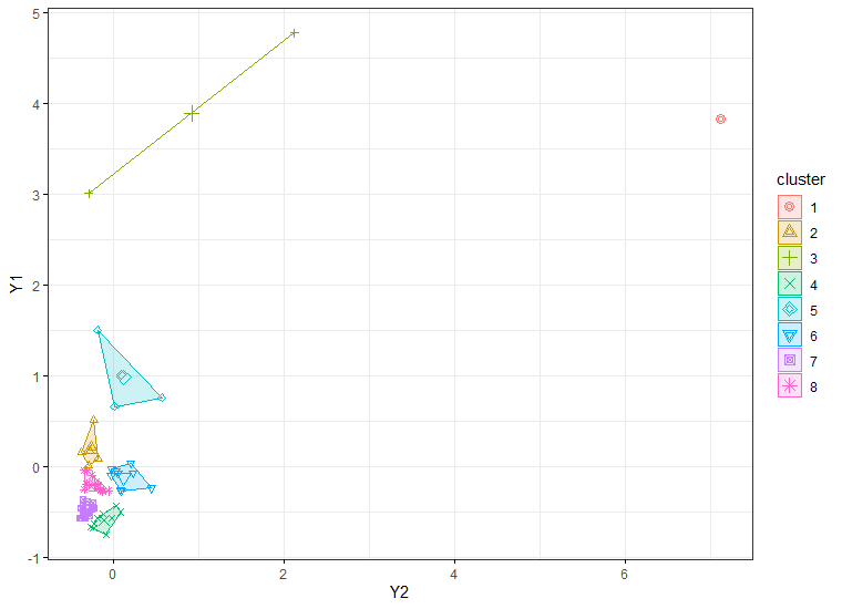
Figure 10.1: Cluster Plot of K-means solution represented as scaled data for Domain 1 of the Swiss Municipalities Dataset

Table 10.3 below provides the sample size, execution time, total execution time and aggregated total time for fine tuning the hyperparameters for each algorithm (or staged combination of algorithms). The Stage variable indicates whether the sample size and times were obtained for the algorithm in one stage or whether the results were obtained through a staged combination of various algorithms. For example the sample size of $246.90$ was obtained after 1 stage by the KmeansSolution algorithm (Ballin and Barcaroli, 2020). This corresponds to the largest sample size. The time of $1.80$ seconds was also the quickest total execution time.
On the other hand the smallest sample size of $130.92$ was obtained after combining three stages of the SOM (stage 1), EM (stage 2) and Hill Climbing (stage 3) algorithms. This was achieved in a time of $178.76$ seconds ($109.84+68.92$). The longest time was $185.97$ seconds for the sample size of $141.46$ obtained through the staged combination of the self-organising map (SOM), K-means and hill climbing algorithms. The smallest sample size of $130.85$ should be considered in the context of the sample size of $125.17$ obtained in $248.91$ seconds after a fine-tuning time of $8,808.63$ seconds by the Simulated Annealing Algorithm (table 10.11).
Depending on the initial quality of the solution the hill climbing algorithm converges on diverse local minima resulting in varying final solution quality. Furthermore, the hill climbing algorithm search for local minima is stochastic in nature - meaning that for the same starting solution the hill climbing algorithm may also find diverse local minima on each attempt.
Notwithstanding the larger differences in final solution quality the same point could be made for training and the multi-stage combination of the above algorithms (or other clustering algorithms) with hill climbing. These results should not be taken as deterministic, rather as a means of providing greater scope for selecting a solution that is "good enough" in a computing time that is "small enough" (Sörensen and Glover, 2013).

Table 10.3: Comparison of Sample Size, Time and Total Execution Time for the various single algorithm or multi-algorithm combinations for the Swiss Municipalities Dataset experiment

Stage	Algorithm	Sample Size	Time (Seconds)	Total Execution Time (Seconds)	Aggregated Total Time (seconds)
1	KmeansSolution	246.90	1.80	1.80
2	Hill Climbing	165.05	33.17	33.17	34.97
1 and 2	SOM and Kmeans	198.03	5.55	116.72
3	HillClimbing	141.46	69.25	69.25	185.97
1 and 2	NG and Kmeans	204.00	3.34	65.30
3	HillClimbing	146.25	58.37	58.37	123.67
1	Expectation Maximisation	196.12	1.34	1.34
2	HillClimbing	133.21	68.98	68.98	70.32
1 and 2	SOM and EM	183.13	5.39	109.84
3	HillClimbing	130.92	68.92	68.92	178.76
1 and 2	NG and EM	178.19	1.47	28.42
3	HillClimbing	134.84	79.07	79.07	107.49
1	Fuzzy Clustering	175.38	0.27	4.89
2	HillClimbing	133.91	91.31	91.31	96.20
1 and 2	SOM and FC	170.64	3.33	64.92
3	HillClimbing	139.87	43.47	43.47	108.39
1 and 2	NG and FC	174.34	0.66	13.63
3	HillClimbing	136.71	71.76	71.76	85.39

Figure 10.2 plots the aggregated total time against sample size by algorithm combination for the Swiss Municipalities dataset. The graph demonstrates that the SOM, EM and hill climbing combination attains the lowest sample size but with the second largest time. On the other hand, the EM and hill climbing combination attained a similar sample size but in less time. The K-means and hill climbing combination was the fastest, but the sample size was of the least quality (highest value). A number of combinations are clustered around similar sample sizes and times.

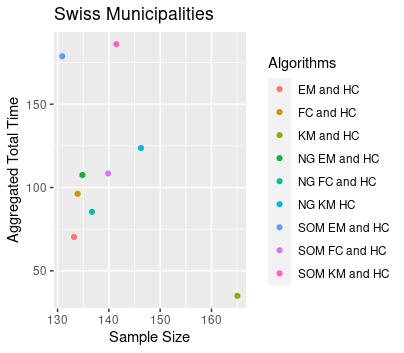
Figure 10.2: Plot of Aggregated Total Time versus Sample Size by Algorithm combination for the Swiss Municipalities Dataset

Table 10.4 summarises the fine-tuned hyper-parameters for the algorithms where fine-tuning was implemented.

Table 10.4: Summary of the fine-tuned hyperparameters for the various single-stage or multi-stage algorithm combinations for the Swiss Municipalities Dataset

	Iterations	Alpha High	Alpha Low	Radius
SOM and K-means	1081	0.809753218616724	0.031088352131124	0.83249740019602
	Lambda High	Lambda Low	Stepsize High	Stepsize Low
NG and K-means	10.6110575335055	0.959806751475908	0.499173569748991	0.016996916064339
	Iterations	Alpha High	Alpha Low	Radius
SOM and EM	7695	0.113771222653394	0.04425198940754	0.061954274246033
	Lambda High	Lambda Low	Stepsize High	Stepsize Low
NG and EM	8.23248667684384	0.67836881950614	0.146985992956907	0.032059727899148
	m
Fuzzy Clustering	3
	Iterations	Alpha High	Alpha Low	Radius
SOM and Fuzzy	1462	0.148577394044338	0.030700312647367	0.008935026169402
	Lambda High	Lambda Low	Stepsize High	Stepsize Low
NG and Fuzzy	8.23248667684384	0.67836881950614	0.146985992956907	0.032059727899148

Figure 10.3 visualises the clusters (strata) for Domain 1 of the Swiss Municipalities Dataset for the solution found after combining SOM, EM and hill climbing when represented as scaled data. This solution has $6$ clusters in contrast to Figure 10.1 which has $8$ clusters for the K-means solution. Clusters 5 and 7 show evidence of the overlap that occurs with soft clustering. Cluster 8 stretches to take in an outlier, which is unlikely to have occurred with hard clustering, or without the hill climbing algorithm.

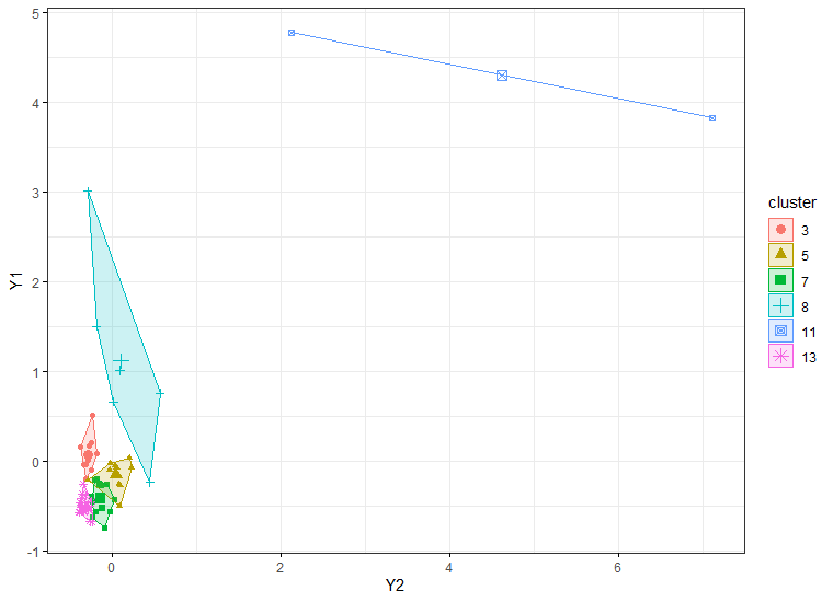
Figure 10.3: Cluster Plot of solution after combining SOM, EM and Hill Climbing represented as scaled data for Domain 1 of the Swiss Municipalities Dataset

10.2 American Community Survey, 2015

A summary of the Target and Auxiliary variables and number of records for the American Survey 2015 dataset is provided in table 10.5 below. For further details on the dataset refer to (O’Luing et al., 2019).

Table 10.5: Summary of the Target and Auxiliary variables, number of records and number of domains for the American Survey 2015 dataset

Dataset	Target Variables	Auxiliary Variables	Number of Records	Number of Domains
American Community Survey, 2015	HINCP, VALP, SMOCP, INSP	BLD, TEN, WKEXREL, WORKSTAT, HFL, YBL	619,747	51

The sample size, execution time and total execution time for fine tuning the hyperparameters for each algorithm (or staged combination of algorithms) are outlined in table 10.6 below. The sample size of 9,065.45 in a time of 8,426.67 seconds for the self-organising maps, fuzzy clustering and hill climbing combination compares favourably with the lowest sample size of 10,136.50 and a total training time of 182,152.46 seconds attained by the grouping genetic algorithm in table 10.11.

Table 10.6: Comparison of Sample Size, Time and Total Execution Time for the various single stage or multi-stage algorithm combinations for the American Community Survey, 2015 Dataset

Stage	Algorithm	Sample Size	Time (Seconds)	Total Execution Time (Seconds)	Total Training Time (seconds)
1	KmeansSolution	11,769.53	36.95	36.95
2	HillClimbing	9,322.07	5,652.85	5,652.85	5,689.80
1 and 2	SOM and K-means	12,787.19	86.48	2,142.86
3	HillClimbing	9,232.31	6,590.34	6,590.34	8,733.20
1 and 2	NG and K-means	12,398.84	107.58	2,181.06
3	HillClimbing	9,290.53	6,019.93	6,019.93	8,200.99
1	Expectation Maximisation	13,136.49	32.94	32.94
2	HillClimbing	9,755.61	5,641.87	5,641.87	5,674.81
1 and 2	SOM and EM	13,018.89	84.94	12,231.26
3	HillClimbing	9,592.40	6,777.39	6,777.39	19,008.65
1 and 2	NG and EM	12,050.93	133.64	2,636.87
3	HillClimbing	9,368.93	5,755.20	5,755.20	8,392.07
1	Fuzzy Clustering	13,350.35	4.89	352.46
2	HillClimbing	9,255.64	6,245.89	6,245.89	6,598.35
1 and 2	SOM and FC	12,088.80	88.87	2,127.86
3	HillClimbing	9,065.45	6,298.81	6,298.81	8,426.67
1 and 2	NG and FC	12,580.33	123.31	2,570.40
3	HillClimbing	9,249.05	5,506.89	5,506.89	8,077.29

Figure 10.4 demonstrates that the SOM, FC and hill climbing combination attains the lowest sample size and with a moderate time. On the other hand, the EM and hill climbing combination attained the largest sample size but in the least time. A number of combinations are clustered around similar sample sizes and times.

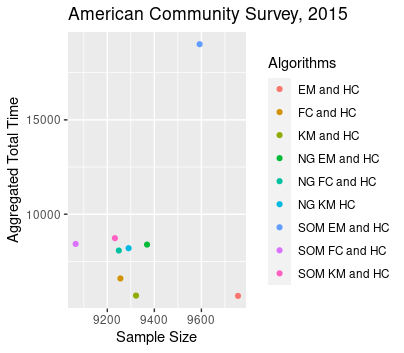
Figure 10.4: Plot of Aggregated Total Time versus Sample Size by Algorithm combination for the American Community Survey, 2015 Dataset

Table 10.7 provides the summary of the fine-tuned hyper-parameters for the relevant algorithms.

Table 10.7: Summary of the fine-tuned hyperparameters for the various single-stage or multi-stage algorithm combinations for the American Community Survey, 2015 Dataset

SOM and K-means	Iterations	Alpha High	Alpha Low	Radius
	1490	0.211798547655744	0.014647548302976	0.569154786943982
NG and K-means	Lambda High	Lambda Low	Stepsize High	Stepsize Low
	27.9195691507683	0.953798242114481	0.22725191488931	0.005327383472354
SOM and EM	Iterations	Alpha High	Alpha Low	Radius
	351	0.165795508368377	0.003116705920671	0.272235491431915
NG and EM	Lambda High	Lambda Low	Stepsize High	Stepsize Low
	6.40801811285783	0.410143870242871	0.11268728621304	0.005130624421989
Fuzzy Clustering	m
	7
SOM and FC	Iterations	Alpha High	Alpha Low	Radius
	351	0.134122729571279	0.002215617049982	0.552123088934338
NG and FC	Lambda High	Lambda Low	Stepsize High	Stepsize Low
	13.0783552149509	0.329139476246046	0.384919628095097	0.005166985979477

10.3 Kiva Loans

A summary of the target and auxiliary variables, number of records and number of domains for the Kiva Loans dataset is provided in table 10.8 below.

Table 10.8: Summary of the Target and Auxiliary variables, number of records and number of domains for the Kiva Loans dataset

Dataset	Target Variables	Auxiliary Variables	Number of Records	Number of Domains
Kiva Loans	term_in_months, lender_count, loan_amount	sector, currency, activity, region, partner_id	614,361	73

The sample size, execution time and total execution times for fine tuning the hyperparameters for each algorithm (or staged combination of algorithms) are outlined in table 10.9 below. The lowest sample size of 6,326.35 and total training time of 6,390.36 seconds for the fuzzy clustering and hill climbing combination compares favourably with the lowest sample size of 6,646.67 and total training time of 7,549.87 seconds attained by the simulated annealing algorithm in table 10.11.

Table 10.9: Comparison of Sample Size, Time and Total Execution Time for the various single stage or multi-stage algorithm combinations for the Kiva Loans Dataset

Stage	Algorithm	Sample Size	Time (Seconds)	Total Execution Time (Seconds)	Total Training Time (seconds)
1	KmeansSolution	7,609.97	32.77	32.77
2	HillClimbing	6,355.91	5,088.25	5,088.25	5,121.02
1 and 2	SOM and K-means	8,235.49	46.69	1,376.00
3	HillClimbing	6,686.45	4,594.16	4,594.16	5,970.16
1 and 2	NG and K-means	7,521.78	68.12	1,368.16
3	HillClimbing	6,352.77	5,379.39	5,379.39	6,747.55
1	Expectation Maximisation	8,016.05	34.89	34.89
2	HillClimbing	6,696.26	9,826.94	9,826.94	9,861.83
1 and 2	SOM and EM	9,040.16	622.99	11,717.33
3	HillClimbing	7,173.30	12,342.69	12,342.69	24,060.02
1 and 2	NG and EM	7,433.73	92.04	1,861.40
3	HillClimbing	6,378.58	5,139.70	5,139.70	7,001.10
1	Fuzzy Clustering	7,532.95	17.81	371.75
2	HillClimbing	6,326.35	6,018.61	6,018.61	6,390.36
1 and 2	SOM and FC	7,707.41	50.03	1,357.19
3	HillClimbing	6,487.29	5,818.46	5,818.46	7,175.65
1 and 2	NG and FC	7,470.76	84.57	1,671.55
3	HillClimbing	6,361.31	5,896.17	5,896.17	7,567.72

Figure 10.5 demonstrates that a number of combinations are clustered around similar low sample sizes and times. The FC and hill climbing combination attained the lowest sample size and with one of the lowest times. On the other hand, the SOM, EM and hill climbing combination attained the largest sample size in the most time.

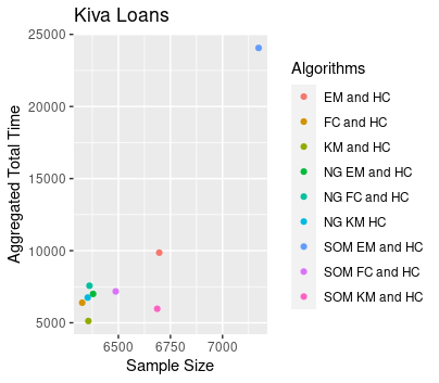
Figure 10.5: Plot of Aggregated Total Time versus Sample Size by Algorithm combination for the Kiva Loans Dataset

Table 10.10 provides the summary of the fine-tuned hyper-parameters for the relevant algorithms.

Table 10.10: Summary of the fine-tuned hyperparameters for the various single-stage or multi-stage algorithm combinations for the American Community Survey, 2015 Dataset

SOM and K-means	Iterations	Alpha High	Alpha Low	Radius
	101	0.92384807669335	0.097029295450863	0.680610206832993
NG and K-means	Lambda High	Lambda Low	Stepsize High	Stepsize Low
	16.2579368586406	0.068847852889988	0.258579228835623	0.005948537735878
SOM and EM	Iterations	Alpha High	Alpha Low	Radius
	9864	0.878176548467018	0.033124931246478	0.462181919813156
NG and EM	Lambda High	Lambda Low	Stepsize High	Stepsize Low
	15.6835266864393	0.906532369809407	0.341722599971882	0.041738065618349
Fuzzy Clustering	m
	2
SOM and FC	Iterations	Alpha High	Alpha Low	Radius
	325	0.178468058524982	0.015586729150577	0.00040918374223
NG and FC	Lambda High	Lambda Low	Stepsize High	Stepsize Low
	20.0046674131416	0.865994203313719	0.23247297228314	0.04890728238225

10.4 Benchmark Results - Atomic Strata

Table 10.11 is a reproduction of the summary by the above datasets of the evaluation time, sample size and number of strata for the Grouping Genetic Algorithm (GGA) and Simulated Annealing Algorithm (SAA) as found by the experiments conducted by (O’Luing et al., 2020). We compare these results with the above results to provide a benchmark for comparing solution quality and total training time.

Table 10.11: Summary by dataset of the evaluation time, sample size and number of strata for the Grouping Genetic Algorithm (GGA) and Simulated Annealing Algorithm (SAA)

	GGA			SAA
Dataset	Sample Size	Execution Time	Total Training Time	Sample Size	Execution Time	Total Training Time
Swiss Municipalities	128.69	753.82	10,434.30	125.17	248.91	8,808.63
American Community Survey, 2015	10,136.50	13,146.25	182,152.46	10,279.44	517.76	6,822.42
Kiva Loans	6,756.19	15,669.11	288,946.79	6,646.67	664.30	7,549.87

11 Empirical Comparisons for Continuous Strata

Unlike the atomic strata above, continuous strata are not numerical or discrete. We use the same methodology and algorithms outlined above to the continuous strata and the results are presented below (i.e. we apply the same procedures on the continuous strata). For each of the experiments below the target and auxiliary variables are the same.

11.1 Swiss Municipalities

The target and auxiliary variables for the Swiss Municipalities dataset are recorded in table 11.12.

Table 11.12: Summary of the Target and Auxiliary variables for the Swiss Municipalities dataset

Dataset	Target Variables	Auxiliary Variables
Swiss Municipalities	Surfacesbois, Airbat	Surfacesbois, Airbat

In table 11.13 the multi-stage combination of the Neural Gas, Expectation Maximisation and HillClimbing algorithms provides the lowest sample size of 110 for both the atomic and continuous methods in an total training time of 95.33 seconds. This compares favourably with the lowest sample size of 120 and total training time of 1,905.82 seconds attained by the simulated annealing algorithm. The longest total training time of 547.11 seconds was for the multi-stage combination of the self-organising maps, expectation maximisation and hill climbing algorithms.

Table 11.13: Comparison of Sample Size, Time and Total Execution Time for the various single stage or multi-stage combinations for the Swiss Municipalities Dataset experiment

Stage	Algorithm	Sample Size	Time (Seconds)	Total Execution Time (Seconds)	Total Training Time (seconds)
1	KmeansSolution	271.07	1.89	1.89
2	K-means and Hill Climbing	229.00	30.05	30.05	31.94
1 and 2	SOM and K-means	150.58	4.03	96.55
3	HillClimbing	125.31	139.69	139.69	236.24
1 and 2	NG and K-means	229.10	3.30	66.10
3	HillClimbing	189.00	26.53	26.53	92.63
1	Expectation Maximisation	174.01	2.02	2.02
2	HillClimbing	132.66	131.44	131.44	133.46
1 and 2	SOM and EM	165.35	14.12	342.86
3	HillClimbing	124.48	204.25	204.25	547.11
1 and 2	NG and EM	124.96	2.90	56.72
3	HillClimbing	110.00	38.61	38.61	95.33
1	Fuzzy Clustering	144.97	0.47	8.55
2	HillClimbing	125.17	49.88	49.88	58.43
1 and 2	SOM and FC	129.64	4.60	94.87
3	HillClimbing	118.09	130.38	130.38	225.25
1 and 2	NG and FC	138.23	1.76	35.85
3	HillClimbing	123.95	67.91	67.91	103.76

The number of iterations for the self-organising maps algorithm in the self-organising maps, expectation maximisation and hill climbing combination is 5,314 and significantly higher than the number of iterations for the self-organising maps algorithm in the other combinations. This (along with the training process) would contribute to explaining the longer total training time for the this multi-stage combination.

Figure 11.1 demonstrates that the NG, EM and hill climbing algorithm attains the smallest sample size in a relatively low time. A number of combinations return similar sample sizes but with varying times. The KM and hill climbing combination returns the largest sample size in the least time.

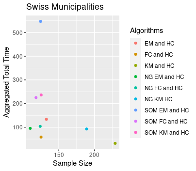
Figure 11.1: Plot of Aggregated Total Time versus Sample Size by Algorithm combination for the Swiss Municipalities Dataset

Table 11.14 contains the the fine-tuned hyperparameters for the various single-stage or multi-stage algorithm combinations for the Swiss Municipalities dataset.

Table 11.14: Summary of the fine-tuned hyperparameters for the various single-stage or multi-stage algorithm combinations for the Swiss Municipalities Dataset

	Iterations	Alpha High	Alpha Low	Radius
SOM and K-means	146	0.955179772565607	0.097093850745587	0.648499123915099
	Lambda High	Lambda Low	Stepsize High	Stepsize Low
NG and K-means	1.92036896656643	0.408302785790299	0.483817725175832	0.016913660635487
	Iterations	Alpha High	Alpha Low	Radius
SOM and EM	5,314	0.860526216045479	0.036380460266579	0.266383153636882
	Lambda High	Lambda Low	Stepsize High	Stepsize Low
NG and EM	1.02031964830343	0.965802849282413	0.49419928787723	0.046602493289255
	m
Fuzzy Clustering	2
	Iterations	Alpha High	Alpha Low	Radius
SOM and FC	361	0.463767154766247	0.003181504371105	0.00137499391567
	Lambda High	Lambda Low	Stepsize High	Stepsize Low
NG and FC	21.617934961514	0.764578349819259	0.133934543593412	0.080908668275684

11.2 American Community Survey, 2015

A summary of the target and auxiliary variables for the American Survey 2015 dataset is provided in table 11.15 below.

Table 11.15: Summary of the Target and Auxiliary variables, number of records and number of domains for the American Survey 2015 dataset

Dataset	Target Variables	Auxiliary Variables	Number of Records	Number of Domains
American Community Survey, 2015	HINCP, VALP, SMOCP, INSP	BLD, TEN, WKEXREL, WORKSTAT, HFL, YBL	619,747	51

The results of the various single stage or multi-stage algorithm combinations for the American Community Survey, 2015 dataset experiment are presented in table 11.16. Note that for the K-means Hartigan-Wong method the R version of the algorithm encountered difficulties and failed to converge for either 100 (initially) or 1,000 iterations . We used the (MacQueen et al., 1967) method instead- moving from 100 to 1,000 iterations in order to attain convergence. The minimum sample size attained was 2,753.55 with a total training time of 41,740.96 seconds for the staged combination of the neural gas, fuzzy clustering and hill climbing algorithms. This compares favourably with the lowest sample size of 3,915.48 and total training time of 169,115.92 seconds attained by the simulated annealing algorithm in table 11.20. The longest total training time was 78,344.99 seconds for the K-means and hill climbing combination.

Table 11.16: Comparison of Sample Size, Time and Total Execution Time for the various single stage or multi-stage algorithm combinations for the American Community Survey, 2015 Dataset

Stage	Algorithm	Sample Size	Time (Seconds)	Total Execution Time (Seconds)	Aggregate Total Time (seconds)	Note
1	KmeansSolution	8,864.89	109.72	109.72
2	HillClimbing	3,015.11	78,235.27	78,235.27	78,344.99
1 and 2	SOM and K-means	3,819.99	313.32	8,322.50
3	HillClimbing	3,310.36	9,882.47	9,882.47	18,204.97
1 and 2	NG and K-means	3,168.46	657.87	13,449.13		*MCQUEEN method 1,000 iterations
3	HillClimbing	2,802.93	6,655.40	6,655.40	20,104.53
1	Expectation Maximisation	5,520.72	141.66	141.66
2	HillClimbing	3,443.64	46,108.23	46,108.23	46,249.89
1 and 2	SOM and EM	4,441.14	287.36	9,301.32
3	HillClimbing	3,350.65	24,693.78	24,693.78	33,995.10
1 and 2	NG and EM	3,137.56	670.08	13,658.88
3	HillClimbing	2,808.22	9,281.39	9,281.39	22,940.27
1	Fuzzy Clustering	5,775.91	24.97	2,090.77
2	HillClimbing	2,825.38	51,268.38	51,268.38	53,359.15
1 and 2	SOM and FC	3,798.98	260.48	7,904.15
3	HillClimbing	3,193.08	12,691.15	12,691.15	20,595.30
1 and 2	NG and FC	3,650.26	653.14	13,108.87
3	HillClimbing	2,753.55	28,632.09	28,632.09	41,740.96

Figure 11.2 plots the aggregated total time against Sample Size by algorithm combination for the Swiss Municipalities dataset. The graph demonstrates that the EM and hill climbing algorithm attains the smallest sample size in a relatively low time. A number of combinations return similar sample sizes but with varying times. SOM, EM and hill climbing combination returns the largest sample size in the longest time.

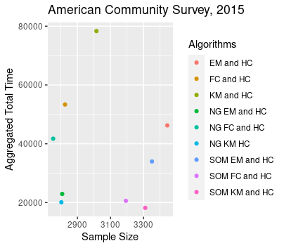
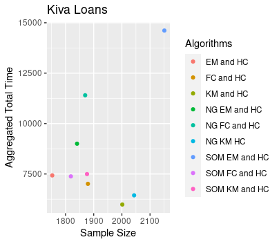
Figure 11.2: Plot of Aggregated Total Time versus Sample Size by Algorithm combination for the American Community Survey, 2015 Dataset

Table 11.17 summarises the hyper-parameters and relevant algorithms for which the above results were attained.

Table 11.17: Summary of the fine-tuned hyperparameters for the various single-stage or multi-stage algorithm combinations for the American Community Survey, 2015 Dataset

SOM and K-means	Iterations	Alpha High	Alpha Low	Radius
	362	0.235757044486596	0.012774618075309	0.484338735244991
NG and K-means	Lambda High	Lambda Low	Stepsize High	Stepsize Low
	22.8202557664311	0.916501772178628	0.499675245659364	0.008470696479746
SOM and EM	Iterations	Alpha High	Alpha Low	Radius
	268	0.170893752936649	0.004722280048395	0.557606799123925
NG and EM	Lambda High	Lambda Low	Stepsize High	Stepsize Low
	29.1800880556926	0.25795004530251	0.266119958357885	0.019287368137506
Fuzzy Clustering	m
	11
SOM and FC	Iterations	Alpha High	Alpha Low	Radius
	249	0.124999162557325	0.052358677482419	0.073764869553736
NG and FC	Lambda High	Lambda Low	Stepsize High	Stepsize Low
	5.09321314570995	0.984287188866795	0.287914934710588	0.00526985258796

11.3 Kiva Loans

In table 11.18 the lowest sample size of 1,752.82 was attained using a combination of Expectation Maximisation and Hill climbing, in a total training time of 7,428.64 seconds. This compares favourably with the lowest sample size of 3,017.79 and total training time of 4,149.06 seconds attained by the simulated annealing algorithm in table 11.20. The longest total training time was 14,613.90 seconds for the self-organising maps, expectation maximisation and hill climbing combination.

Table 11.18: Summary of the Target and Auxiliary variables, number of records and number of domains for the Kiva Loans dataset

Stage	Algorithm	Sample Size	Time (Seconds)	Total Execution Time (Seconds)	Aggregated Total Time (seconds)
1	KmeansSolution	3,901.98	43.60	43.60
2	HillClimbing	2,001.55	5,941.14	5,941.14	5,984.74
1 and 2	SOM and K-means	3,005.53	108.91	2,801.87
3	HillClimbing	1,876.29	4,692.34	4,692.34	7,494.21
1 and 2	NG and K-means	2,636.01	160.70	3,269.08
3	HillClimbing	2,043.52	3,171.44	3,171.44	6,440.52
1	Expectation Maximisation	3,496.17	58.11	58.11
2	HillClimbing	1,752.82	7,370.53	7,370.53	7,428.64
1 and 2	SOM and EM	4,452.22	188.69	3,655.43
3	HillClimbing	2,150.91	10,958.47	10,958.47	14,613.90
1 and 2	NG and EM	3,198.13	125.70	2,484.06
3	HillClimbing	1,840.88	6,517.68	6,517.68	9,001.74
1	Fuzzy Clustering	3,885.66	20.27	452.67
2	HillClimbing	1,879.47	6,559.08	6,559.08	7,011.75
1 and 2	SOM and FC	2,547.45	98.68	2,878.54
3	HillClimbing	1,818.98	4,501.45	4,501.45	7,379.99
1 and 2	NG and FC	3,351.17	93.50	1,875.48
3	HillClimbing	1,869.71	9,528.57	9,528.57	11,404.05

Figure 11.3 plots the aggregated total time against Sample Size by algorithm combination for the Swiss Municipalities dataset. The graph demonstrates that the EM and hill climbing algorithm attains the smallest sample size in a relatively low time. A number of combinations return similar sample sizes but with varying times. SOM, EM and hill climbing combination returns the largest sample size in the longest time.

Figure 11.3: Plot of Aggregated Total Time versus Sample Size by Algorithm combination for the Kiva Loans Dataset

In table 11.19 we provide details of the fine-tuned hyper-parameters for the relevant algorithms.

Table 11.19: Summary of the fine-tuned hyperparameters for the various single-stage or multi-stage algorithm combinations for the American Community Survey, 2015 Dataset

SOM and K-means	Iterations	Alpha High	Alpha Low	Radius
	371	0.277877372112223	0.012899151606656	0.694571047057514
NG and K-means	Lambda High	Lambda Low	Stepsize High	Stepsize Low
	15.1897164925445	0.822356168348829	0.10500027609291	0.005030299354611
SOM and EM	Iterations	Alpha High	Alpha Low	Radius
	914	0.162357069495344	0.040045055053234	0.535640629408619
NG and EM	Lambda High	Lambda Low	Stepsize High	Stepsize Low
	20.9163182787887	0.804910189211671	0.183011407460269	0.076024879621262
Fuzzy Clustering	m
	2
SOM and FC	Iterations	Alpha High	Alpha Low	Radius
	264	0.113939729200586	0.00350977823364	0.003857035322069
NG and FC	Lambda High	Lambda Low	Stepsize High	Stepsize Low
	18.9297597394552	0.643763823658483	0.136589161984179	0.067314184908353

11.4 Benchmark Results - Continuous Strata

For comparison purposes table 11.20 contains the evaluation time, sample size and number of strata for the Grouping Genetic Algorithm (GGA) and Simulated Annealing Algorithm (SAA) for the above datasets.

Table 11.20: Summary by dataset of the evaluation time, sample size and number of strata for the Grouping Genetic Algorithm (GGA) and Simulated Annealing Algorithm (SAA)

Dataset	Sample Size	Execution Time	Total Training Time	Sample Size	Execution Time	Total Training Time
SwissMunicipalities	128.69	753.82	10,434.30	120.00	213.44	1,905.82
American Community Survey, 2015	4,197.68	22,016.95	227,635.51	3915.48	13,351.19	169,115.92
Kiva Loans	3,062.33	3,232.78	48,746.61	3,017.79	300.16	4,149.06

12 Conclusions and Future work

The multi-stage combination of k-means type algorithms with hill climbing performed better, generally, than the grouping genetic algorithm and the simulated annealing algorithm for atomic and continuous strata. The exception being the case of atomic strata for the Swiss Municipalities dataset, where the grouping genetic algorithm performed better- although the survey designer may wish to consider solution quality in the context of training times (as with all the other experiments). The continuous strata provide lower sample samples than the atomic strata method. This is because the stratification variable is the target variable - which results in better efficiency.
The performance of each multi-stage combination of algorithms depends on the dataset and the auxiliary and stratification variables. Therefore there isn’t one combination that suits all experiments. Nonetheless, we have provided the survey designer with a choice of combinations, which can be applied in the context expert knowledge of the particular sampling problem. For future work further combinations of the hill climbing algorithm with other clustering algorithms such as affinity propagation clustering, cobweb clustering algorithm, density-based clustering, divisive hierarchical clustering, simple featureless clustering, farthest first clustering algorithm, mean shift clustering, kernel k-means clustering, mini batch k-means clustering, k-means with automatic determination of k, partitioning around medoids, k-medians clustering, etc. may be considered. Alternative local search algorithms such as tabu search, stochastic hill climbing, local beam search or simulated annealing may also be considered for the final stage. The grouping genetic algorithm may also be applied.

References

- Asan and Ercan (2012) Asan, U. and S. Ercan (2012). An introduction to self-organizing maps. In Computational Intelligence Systems in Industrial Engineering, pp. 295–315. Springer.
- Äyrämö and Kärkkäinen (2006) Äyrämö, S. and T. Kärkkäinen (2006). Introduction to partitioning-based clustering methods with a robust example. Reports of the Department of Mathematical Information Technology. Series C, Software engineering and computational intelligence (1/2006).
- Bação et al. (2005) Bação, F., V. Lobo, and M. Painho (2005). Self-organizing maps as substitutes for k-means clustering. In International Conference on Computational Science, pp. 476–483. Springer.
- Ballin and Barcaroli (2013) Ballin, M. and G. Barcaroli (2013). Joint determination of optimal stratification and sample allocation using genetic algorithm. Survey Methodology 39(2), 369–393.
- Ballin and Barcaroli (2020) Ballin, M. and G. Barcaroli (2020). Optimization of sampling strata with the SamplingStrata package. Accessed 3 May 2021. https://barcaroli.github.io/SamplingStrata/articles/SamplingStrata.html
- Barcaroli et al. (2014) Barcaroli, G. (2014). SamplingStrata: An R package for the optimization of stratified sampling. Journal of Statistical Software 61(4), 1–24.
- Bethel (1985) Bethel, J. W. (1985). An optimum allocation algorithm for multivariate surveys. American Statistical Proceedings of the Survey Research Methods, Section, 209-212.
- Bethel (1989) Bethel, J. (1989). Sample allocation in multivariate surveys. Survey methodology 15(1), 47-57.
- Bezdek et al. (1984) Bezdek, J. C., R. Ehrlich, and W. Full (1984). Fcm: The fuzzy c-means clustering algorithm. Computers & geosciences 10(2-3), 191–203.
- Choudhary (2015) Choudhary, A. (2015, 10). Empirical comparison of performances of k-means, k-means++, weighted k-means and hartigan and wong k-means clustering algorithms.
- Chromy (1987) Chromy, J. R. (1987). Design optimization with multiple objectives. Proceedings of the Survey Research Methods Section.
- Dempster et al. (1977) Dempster, A. P., N. M. Laird, and D. B. Rubin (1977). Maximum likelihood from incomplete data via the em algorithm. Journal of the Royal Statistical Society: Series B (Methodological) 39(1), 1–22.
- Dimitriadou et al. (2020) Dimitriadou, E., K. Hornik, and M. K. Hornik (2020). Package ‘cclust’.
- Dirgová Luptáková et al. (2016) Dirgová Luptáková, I., M. Šimon, L. Huraj, and J. Pospíchal (2016). Neural gas clustering adapted for given size of clusters. Mathematical Problems in Engineering 2016.
- Drineas et al. (2004) Drineas, P., A. Frieze, R. Kannan, S. Vempala, and V. Vinay (2004). Clustering large graphs via the singular value decomposition. Machine learning 56(1), 9–33.
- Forgy (1965) Forgy, E. W. (1965). Cluster analysis of multivariate data: efficiency versus interpretability of classifications. biometrics 21, 768–769.
- Friedman et al. (2001) Friedman, J., T. Hastie, R. Tibshirani, et al. (2001). The elements of statistical learning, Volume 1. Springer series in statistics New York.
- Hartigan (1979) Hartigan, J. A. (1979). A k-means clustering algorithm: Algorithm as 136. Appl. Stat. 28, 126–130.
- Jain (2010) Jain, A. K. (2010). Data clustering: 50 years beyond k-means. Pattern recognition letters 31(8).
- Klawonn (2004) Klawonn, F. (2004). Fuzzy clustering: Insights and a new approach. Mathware & soft computing. 2004 Vol. 11 Num. 3.
- (21) K-Means and SOM: Introduction to Popular Clustering Algorithms - DZone AI. https://dzone.com/articles/k-means-and-som-gentle-introduction-to-worlds-most. Accessed 25th May 2021.
- Kohonen (1990) Kohonen, T. (1990). The self-organizing map. Proceedings of the IEEE 78(9), 1464–1480.
- Li (2014) Li, H. (2014). Smile. https://haifengl.github.io. Accessed 08th June 2021.
- Lin and Kernighan (1973) Lin, S. and B. W. Kernighan (1973). An effective heuristic algorithm for the traveling-salesman problem. Operations research 21(2), 498–516.
- Lisic et al. (2018) Lisic, J., H. Sang, Z. Zhu, and S. Zimmer (2018). Optimal stratification and allocation for the june agricultural survey. Journal of Official Statistics 34(1), 121–148.
- Lloyd (1982) Lloyd, S. (1982). Least squares quantization in pcm. IEEE transactions on information theory 28(2), 129–137.
- MacQueen et al. (1967) MacQueen, J. et al. (1967). Some methods for classification and analysis of multivariate observations. In Proceedings of the fifth Berkeley symposium on mathematical statistics and probability, Volume 1, pp. 281–297. Oakland, CA, USA.
- Martinetz et al. (1991) Martinetz, T., K. Schulten, et al. (1991). A "neural-gas" network learns topologies.
- Meilă (2006) Meilă, M. (2006). The uniqueness of a good optimum for k-means. In Proceedings of the 23rd international conference on Machine learning, pp. 625–632.
- Meyer et al. (2019) Meyer, D., E. Dimitriadou, K. Hornik, A. Weingessel, F. Leisch, C.-C. Chang, C.-C. Lin, and M. D. Meyer (2019). Package ‘e1071’. The R Journal.
- Michalewicz and Fogel (2013) Michalewicz, Z. and D. B. Fogel (2013). How to solve it: modern heuristics. Springer Science & Business Media.
- Morissette and Chartier (2013) Morissette, L. and S. Chartier (2013). The k-means clustering technique: General considerations and implementation in mathematica. Tutorials in Quantitative Methods for Psychology 9(1), 15–24.
- Nayak et al. (2015) Nayak, J., B. Naik, and H. Behera (2015). Fuzzy c-means (fcm) clustering algorithm: a decade review from 2000 to 2014. Computational intelligence in data mining-volume 2, 133–149.
- O’Luing et al. (2019) O’Luing, M., S. Prestwich, and S. Armagan Tarim (2019). A grouping genetic algorithm for joint stratification and sample allocation designs. Survey Methodology 45(3), 513–531.
- O’Luing et al. (2020) O’Luing, M., S. Prestwich, and S. A. Tarim (2020). A simulated annealing algorithm for joint stratification and sample allocation designs. arXiv preprint arXiv:2011.13006.
- Pérez-Ortega et al. (2019) Pérez-Ortega, J., N. N. Almanza-Ortega, A. Vega-Villalobos, R. Pazos-Rangel, C. Zavala-Díaz, and A. Martínez-Rebollar (2019). The k-means algorithm evolution. In Introduction to Data Science and Machine Learning. IntechOpen.
- R Core Team (2021) R Core Team (2021). R: A Language and Environment for Statistical Computing. Vienna, Austria: R Foundation for Statistical Computing.
- Scrucca et al. (2016) Scrucca, L., M. Fop, T. B. Murphy, and A. E. Raftery (2016). mclust 5: clustering, classification and density estimation using Gaussian finite mixture models. The R Journal 8(1), 289–317.
- Sörensen and Glover (2013) Sörensen, K. and F. Glover (2013). Metaheuristics. Encyclopedia of operations research and management science 62, 960–970.
- Silviu (2001) Silviu, B. (2001). Fuzzy clustering. Babes-Bolyai University.