Modeling the unresolved NIR-MIR SEDs of local ($z<0.1$) QSOs

Abstract

To study the nuclear ($\lesssim 1\,$kpc) dust of nearby ($z<0.1$) type 1 Quasi Stellar Objects (QSOs) we obtained new near-infrared (NIR) high angular resolution ($\sim 0.3$ arcsec) photometry in the H and Ks bands, for 13 QSOs with available mid-infrared (MIR) high angular resolution spectroscopy ($\sim 7.5-13.5\,\mu$m). We find that in most QSOs the NIR emission is unresolved. We subtract the contribution from the accretion disk, which decreases from NIR ($\sim 35\%$) to MIR ($\sim 2.4\%$). We also estimate these percentages assuming a bluer accretion disk and find that the contibution in the MIR is nearly seven time larger. We find that the majority of objects ($64\%$, 9/13) are better fitted by the Disk+Wind H17 model (Hönig & Kishimoto, 2017), while others can be fitted by the Smooth F06 ($14\%$, 2/13, Fritz et al., 2006), Clumpy N08 ($7\%$, 1/13, Nenkova et al., 2008a, b), Clumpy H10 ($7\%$, 1/13, Hönig & Kishimoto, 2010b), and Two-Phase media S16 ($7\%$, 1/13, Stalevski et al., 2016) models. However, if we assume the bluer accretion disk, the models fit only 2/13 objects. We measured two NIR to MIR spectral indexes, $\alpha_{NIR-MIR(1.6,8.7\,\mu\text{m})}$ and $\alpha_{NIR-MIR(2.2,8.7\,\mu\text{m})}$, and two MIR spectral indexes, $\alpha_{MIR(7.8,9.8\,\mu\text{m})}$ and $\alpha_{MIR(9.8,11.7\,\mu\text{m})}$, from models and observations. From observations, we find that the NIR to MIR spectral indexes are $\sim-1.1$ and the MIR spectral indexes are $\sim-0.3$. Comparing the synthetic and observed values, we find that none of the models simultaneously match the measured NIR to MIR and $7.8-9.8\,\mu$m slopes. However, we note that measuring the $\alpha_{MIR(7.8,9.8\,\mu\text{m})}$ on the starburst-subtracted Spitzer/IRS spectrum, gives values of the slopes ($\sim-2$) that are similar to the synthetic values obtained from the models.

1 Introduction

The nuclear dust that surrounds the central engine (supermassive black hole, accretion disk, and broad-line region) of the active galactic nuclei (AGNs) is widely known as the dusty torus of AGNs (e.g., Krolik & Begelman, 1988; Antonucci, 1993; Urry & Padovani, 1995; Robson et al., 1995; Peterson, 1997). This structure plays a fundamental role in the description of an AGN since it represents the connection between the central engine and the kiloparsec scales (the narrow line region and the host galaxy Ramos Almeida & Ricci, 2017). Some observations of Seyfert galaxies have suggested that a large fraction of the obscuring material is distributed into a toroidal structure. However, the exact geometry of this structure is still unknown (see e.g., Hönig, 2019; Combes et al., 2019). Some authors have claimed the detection of a dusty structure from mid-infrared (MIR) and sub-millimeter interferometric data (e.g., Jaffe et al., 2004; García-Burillo et al., 2016; Imanishi et al., 2018; Alonso-Herrero et al., 2018). They have found sizes that range from few parsecs to few tens of pc (e.g., Jaffe et al., 2004; Packham et al., 2005b; Radomski et al., 2008; García-Burillo et al., 2016; Imanishi et al., 2018), and sometimes with more than a single component (e.g., López-Gonzaga et al., 2014; Tristram et al., 2014; García-Burillo et al., 2019). Unfortunately, these studies are limited to a small number of nearby AGNs.

The obscuring material in the dusty torus absorbs a significant part of the optical-UV radiation emitted by the accretion disk and re-emits it at infrared (IR) wavelengths between $\sim 1-1000\,\mu$m, (e.g., Krolik & Begelman, 1988; Sanders et al., 1989; Antonucci, 1993; Elvis et al., 1994; Peterson, 1997; Neugebauer et al., 1979), peaking around $\sim 5-35\,\mu$m (e.g., Stein et al., 1974; Rees et al., 1969; Burbidge & Stein, 1970; Rieke & Low, 1972; Sanders et al., 1989). Therefore, fitting the IR spectral energy distribution (SED) of AGNs is a good technique to derive the physical properties of this dusty structure (e.g., González-Martín et al., 2019b). During the last decades, there have been great efforts to understand the assemble of the nuclear dust responsible for the observed IR SED of AGNs. For example, Fritz et al. (2006) proposed a homogeneous distribution of the nuclear dust into a toroidal structure around the central engine (Smooth F06 model hereafter). This model reproduces well the observed IR SEDs of type 1 and 2 Seyfert galaxies and predicts a deep $10\,\mu$m silicate absorption feature, but predicts a narrower IR bump (e.g., Dullemond & van Bemmel, 2005). Nenkova et al. (2002, 2008a, 2008b) proposed a dusty torus model in which the dust is distributed in clumps in a toroidal geometry around the central engine (Clumpy N08 model hereafter). This model predicts a more attenuated $10\,\mu$m silicate emission feature and broader IR bump. However, this model fails in reproducing the apparent “excess” of near-IR (NIR) emission presented in some type 1 AGNs (e.g Mor et al., 2009), which has been attributed to the presence of hot dust in the inner part of the torus (e.g., Braatz et al., 1993; Cameron et al., 1993; Bock et al., 2000; Hönig et al., 2013). Trying to resolve these issues Stalevski et al. (2016) proposed a two-phase medium torus model, composed of high-density clumps immersed into a low-density medium (Two-phase media S16 model hereafter). According to this model, the low-density dust medium significantly contributes to the NIR emission in type 1 AGNs. Feltre et al. (2012) compared the smooth and clumpy models and found that both models can produce similar MIR continuum shapes for different parameters of the models. Additionally, they found that there are very different NIR spectral slopes between the models, probably due to the different dust composition and central radiation assumed.

Due to the difficulties to consistently reproducing the IR SEDs of AGNs with the torus models, and the growing evidence for a component of dust located in the polar region of the AGNs in addition to the equatorial component (e.g., Hönig et al., 2012, 2013; Tristram et al., 2014; López-Gonzaga & Jaffe, 2016; Leftley et al., 2018), Hönig & Kishimoto (2017) proposed a different geometry composed by a compact and geometrically thin clumpy dusty disk in the equatorial region plus an extended and elongated polar structure of dust, which is assumed to be co-spatial with the outermost layers of the outflowing gas (i.e. distributed in a hollow-cone geometry). Hereafter we refer to this model as the Disk+Wind H17 model. They claim that the more compact distribution of dust in the thin disk allows this model to better explain the $3.5-5\,\mu$m bump seen in several type 1 AGNs.

Several groups have used both low angular resolution ($\sim 3-5\,$arcsec) Spitzer/IRS spectra ($\sim 5-35\,\mu$m) and high angular resolution ($\sim 0.3\,$arcsec) data (spectra and photometry) in the infrared range to model the putative dusty torus in AGNs. For example, some authors (e.g., Ramos Almeida et al., 2009, 2011; Alonso-Herrero et al., 2011; Ichikawa et al., 2015; Fuller et al., 2016; García-Bernete et al., 2019) used high angular resolution data to constrain the parameters of the Clumpy N08 model in a sample of Seyfert galaxies. Similar studies in QSOs are limited to low angular resolution data (e.g., Mor et al., 2009; Nikutta et al., 2009; Mateos et al., 2016), partly due to the lack of high angular resolution data at IR wavelength. For example, using the Spitzer/IRS spectrum of 26 QSOs and the Clumpy N08 model Mor et al. (2009) found that to reproduce the data it is necessary to add a hot dust component ($T\sim 1400$ K). Later, using the same model and the Spitzer/IRS spectrum of 25 QSOs at $z\sim 2$, Deo et al. (2011) showed that by adding a hot dust component to the spectral fitting, it is possible to simultaneously fit the NIR SED and $10\,\mu$m silicate feature. Alonso-Herrero et al. (2011) suggested that this hot dust component might not be necessary when using high angular resolution IR data. Nevertheless, they found that some type 1 Seyfert still show an excess of emission at NIR despite the high angular resolution data, which they attributed to a hot dust component (see also Ichikawa et al., 2015; García-Bernete et al., 2019). To model the low angular resolution Spitzer and AKARI ($2.5-5\,\mu$m) spectra of 85 luminous QSOs ($L_{bol}>10^{45.5}$erg s^-1, with a redshift $z$ between 0.17 and 6.42) Hernán-Caballero et al. (2016) assumed a single accretion disk template plus two black-bodies for the dust emission. They successfully reproduced the $0.1-10\,\mu$m SED. However, they noted that the best-fitting model systematically underpredicts the observed flux around $1\,\mu$m. After comparing the NIR excess and the NIR to optical luminosity ratio, they concluded that this excess of emission originates in hot dust near the sublimation radius.

Assuming the Clumpy N08 dusty torus model, Martínez-Paredes et al. (2017) used the starburst-subtracted Spitzer/IRS spectrum ($\sim 8-15\,\mu$m) plus the point spread function (PSF) photometric point at H-band ($1.6\,\mu$m) obtained from NICMOS data on the Hubble Space Telescope (available for 9 out of 20 objects), to investigate the physical and geometrical properties of the dusty torus in a sample of 20 nearby ($z<0.1$) QSOs. They found that by including the spectral range between ($\sim 5-8\,\mu$m), the SEDs modelling results in a bad fit of the $10\,\mu$m silicate feature, producing parameters inconsistent with their optical classification as type 1 AGNs. Therefore, they excluded this part of the spectrum from the fitting. A similar result and approach was reported by Nikutta et al. (2009) for a couple of QSOs. From the good fits Martínez-Paredes et al. (2017) found that 3/9 objects show an excess of emission at H band, probably because the unresolved emission could be still contaminated by emission from the host galaxy (Veilleux et al., 2006, 2009), and/or because in these cases the addition of a hot dust component could be necessary. Additionally, Martínez-Paredes et al. (2017) found that for 50 percent of QSOs the viewing angles range from $\sim 50-88$ degrees. They claimed that the addition of a second photometric point in the NIR would improve the determination of the viewing angle as suggested by Ramos Almeida et al. (2014). They found that to well constrain the six free parameters of the Clumpy N08 model for Seyfert galaxies, it is necessary to build an unresolved IR SED composed of at least two photometric points in the NIR, a photometric point in the MIR, plus the high angular resolution spectrum in the N-band ($\sim 7.5-13.5\mu$m).

On the other hand, recently Martínez-Paredes et al. (2020) investigated which dusty models better reproduce the AGN-dominated Spitzer/IRS spectrum ($\sim 5-35\,\mu$m) of local ($z<0.1$) type 1 AGNs (including some QSOs). They explored the Smooth F06 model, Clumpy N08 model, Clumpy torus model of Hönig et al. (2010a) (hereafter Clumpy H10 model), Two-phase media S16 model, and the Disk+Wind H17 model. They found that in most cases and with all models, it is always necessary to add the stellar component to fit the bluer spectral range ($\sim 5-8\,\mu$m), but that none of the models can well reproduce the spectral shape between $\sim 5-30\,\mu$m. However, they noted that the Disk+Wind H17 model reproduces well the spectrum with flatter residuals, especially at high bolometric luminosities.

Therefore, considering the difficulties in simultaneously modelling the NIR-MIR SEDs of QSOs, we obtain new NIR high angular resolution data ($\sim 0.3$ arcsec) from the NIR cameras on the 10.4m Gran Telescopio CANARIAS (GTC) to build for the first time a set of well-sampled NIR to MIR SEDs of QSOs that allows us to investigate which model, among the Clumpy N08 and H10, Smooth F06, Two-phase media S16, and Disk+Wind H17 better reproduces the data and constrains the parameters.

Throughout this paper, we assume $\Lambda$CDM cosmology with $H_{0}=70$ km s^-1Mpc^-1, $\Omega_{m}=0.3$, and $\Omega_{\Lambda}=0.7$.

Table 1: Basic properties of the sample. Column 1 lists the name of the object, columns 2-3, 4 and 5 list the coordinates, redshift, and angular scale taken from NED. Column 6 list the corrected hard (2-10 keV) x-ray luminosity.

Name	Coord. J2000		$z$	Angular scale	log L${}_{X}^{a}$
	AR	DEC		kpc/′′	(erg s-1)
Mrk 509	20:44:09.7	$-10:43:25$	0.034	0.677	44.68
PG 0050+124	00:53:34.9	$+12:41:36$	0.034	0.677	43.85
PG 2130+099	21:32:27.8	$+10:08:19$	0.0630	1.213	43.51
PG 1229+204	12:32:03.6	$+20:09:29$	0.063	1.213	43.49
PG 0844+349	08:47:42.4	$+34:45:04$	0.064	1.231	43.74
PG 0003+199	00:06:19.5	$+20:12:10$	0.026	0.523	43.28
PG 0804+761	08:10:58.6	$+76:02:43$	0.100	1.844	44.46
PG 1440+356	14:42:07.4	$+35:26:23$	0.08	1.510	43.76
PG 1426+015	14:29:06.6	$+01:17:06$	0.09	1.679	44.11
PG 1411+442	14:13:48.3	$+44:00:14$	0.09	1.679	43.40
PG 1211+143	12:14:17.7	$+14:03:13$	0.081	1.527	43.70
PG 1501+106	15:04:01.2	$+10:26:16$	0.04	0.791	43.89
MR 2251-178	22:54:05.9	$-17:34:55$	0.064	1.231	44.46
	Additional objects observed in the NIR
PG 2214+139	22:17:12.2	$+14:14:21$	0.066	1.266	43.82
PG 0923+129	09:26:03.3	$+12:44:04$	0.029	0.581	43.41
PG 0007+106	00:10:31.0	$+10:58:30$	0.089	1.662	44.15

Note.- ^aThe X-ray luminosity is from Zhou & Zhang (2010), except for PG 0007+1006 and PG 0923+129, for which the value is taken from Piconcelli & Guainazzi (2005) and Shu et al. (2010), respectively.

2 The sample

We selected the 13/20 local type 1 QSOs in the sample of Martínez-Paredes et al. (2017) that have high angular resolution spectroscopy in the N band ($\sim 7.5-13.5\,\mu$m). The 20 QSOs were selected and observed with the MIR camera CanariCam (CC) on GTC. They set the following criteria: 1) a redshift $z<0.1$; 2) a nuclear flux at N-band (aperture $\lesssim 5$ arcsec) $f_{N}>0.02$ Jy; and 3) $\rm L_{X}\,(2-10\,keV)$ $>$ $10^{43}$ erg sec^-1. The redshift combined with the high angular resolution offered by the combo CC/GTC ($\sim 0.3^{\prime\prime}$) allow them to observe the inner nuclear region within 1 kpc, and the MIR flux allow them to detect these objects with CC in the N and Si2 ($8.7\,\mu$m) bands. The hard X-ray flux was used as an intrinsic indicator of the AGN activity. They imaged in the Si2-band 19/20 QSOs, and obtained the spectrum in the N band for 11/13. The data were published by Martínez-Paredes et al. (2017) and Martínez-Paredes et al. (2019). The remaining two objects had high angular resolution spectra at N band from VISIR on the Very Large Telescope (VLT, Hönig et al., 2010a; Burtscher et al., 2013, see Table 1). Note that we include in the sample three additional objects that we observe in the NIR wavelengths, and report in this paper.

3 The data

3.1 New high angular resolution NIR data and reduction

Using the Canarias InfraRed Camera Experiment (CIRCE, Garner et al., 2016; Eikenberry et al., 2018) on the GTC between October 2016 and February 2017 through the open Spain-Mexico collaborative time, we imaged four objects in the H-band ($\lambda_{c}=1.63\,\mu$m) and seven objects in Ks-band ($\lambda_{c}=2.16\,\mu$m), respectively (PI: M. Martínez-Paredes, ID: GTC2-16BIACMEX). CIRCE is a NIR camera that operates in the spectral range between 1 and 2.5 $\mu$m, which has a total field of view of $3.4^{\prime}\times 3.4^{\prime}$ with plate scale of $0.1^{\prime\prime}$/pixel. In order to complete our observations, we used the NIR Espectrógrafo Multiobjeto Infra-Rojo (EMIR, Balcells et al., 2000) on the GTC between September 2018 and May 2019 through the open Mexico time (PI: M. Martínez-Paredes, ID: GTC2-18BMEX). EMIR has a field of view of $6.67^{\prime}\times 6.67^{\prime}$ and a plate scale of $0.2^{\prime\prime}$/pixel. We observed five objects in the Ks-band and one in the H-band. The observations were obtained under good weather conditions. The full width at half maximum (FWHM) of the standard star ranges from $0.50-1.0$ arcsec for the CIRCE observations and from $0.68-0.84$ arcsec for the EMIR observations, while the airmass ranges were $\sim 1-1.6$ and $\sim 1-1.5$, respectively. In Table 2 we list the basic information of the observations.

For all the targets, we imaged a photometric standard star immediately before or after the science observation. The standard star was chosen to be as close as possible in celestial coordinates to the science object. We used the standard star for the flux calibration and to determine the PSF.

We reduced the CIRCE images using a custom pipeline written in Interactive Data Language (IDL). All images got dark-subtracted to account for electronic offsets. For sky-subtraction, a median combination of the sky exposures was used, which was then scaled to the background level of the object exposures. In order to align the images, the offsets were then determined by measuring the centroid of the object. The aligned sky-subtracted images were then mean-combined. Bad pixels were treated by discarding them in the combination. For the EMIR images, we requested the reduced data to the observatory. In general, the reduction includes the following procedures; sky subtraction, cosmic ray cleaning, stacking of the individual images and rejection of bad images (see e.g., Ramos Almeida et al., 2019).

Table 2: NIR observations. Column 1 lists the name of the object. Columns 2, 3, 4, 5, and 6 list the filter used, the date of the observation, the on-source time, the name of the spectro-photometric standard star, and the time offset between the standard and the QSO. Columns 7, 8, and 9 list the full width at half maximum (FWHM) of the standard star, the average airmass during the observation, and the telescope/instrument used.

Name	Filter	Date	$t_{on-source}$	STD	$t_{offset}$	FWHMSTD	Airmass	Telescope/Instrument
		AAAA.MM.DD	(sec)		(min)	(arcsec)
Mrk 509	H	2016.10.31	45	S813-D	25	0.54	1.40	GTC/CIRCE
Mrk 509	Ks	2016.10.31	65.47	S813-D	14	0.56	1.36	GTC/CIRCE
PG 0050+124	Ks	2017.01.09	13.5	FS-102	10	0.50	1.15	GTC/CIRCE
PG 2130+099	Ks	2016.10.31	45	P576-F	4	0.52	1.08	GTC/CIRCE
PG 1229+204	Ks	2019.05.17	2	FS-131	13	0.84	1.02	GTC/EMIR
PG 0844+349	Ks	2017.02.06	45	P0345-R	19	0.68	1.56	GTC/CIRCE
PG 0003+199	H	2016.10.23	15	FS-102	21	0.65	1.11	GTC/CIRCE
PG 0003+199	Ks	2016.10.23	9	FS-102	29	0.64	1.23	GTC/CIRCE
PG 0804+761	H	2017.02.06	90	P0345-R	31	0.84	1.56	GTC/CIRCE
PG 0804+761	Ks	2019.02.12	2	P091-D	23	0.74	1.48	GTC/EMIR
PG 1211+143	Ks	2019.0517	2	S860-D	5	0.74	1.04	GTC/EMIR
MR 2251-178	H	2018.09.27	2	S667-D	4	0.68	1.44	GTC/EMIR
MR 2251-178	Ks	2018.09.27	1.5	FS-32	3	0.68	1.5	GTC/EMIR
PG 2214+139	Ks	2016.10.31	45	FS-31	12	0.62	1.04	GTC/CIRCE
PG 0923+129	H	2017.02.06	45	P0345-R	44	0.84	1.04	GTC/CIRCE
PG 0923+129	Ks	2017.02.09	5	FS-17	7	1.0	1.05	GTC/CIRCE
PG 0007+106∗	Ks	2016.10.23	15	FS-102	8	0.64	1.19	GTC/CIRCE

Notes.-^∗Radio loud quasar.

3.2 GTC/CanariCam imaging in the Si2 filter (8.7 micron) and N-band spectroscopy.

We use the MIR high angular resolution unresolved photometry in the Si2-band ($\lambda_{c}=8.7\,\mu$m) measured within an aperture radius of $1^{\prime\prime}$. We also use the high angular resolution spectra in the N-band ($\sim 7.5-13.5\,\mu$m, slit width $=0.52^{\prime\prime}$) from Martínez-Paredes et al. (2017). These data were obtained with GTC/CC for 19/20 and 11/20 QSOs, respectively. These data were obtained as part of the CC guaranteed time (P.I: C. Packham), ESO-GTC time (P.I: A. Alonso-Herrero), and open Mexico time (P.I: I. Aretxaga and M. Martínez-Paredes).

Table 3: Observational IR information. Column 1 lists the name of the object, columns 2 and 3 list the source of the ground-based high angular resolution spectroscopy in the N band and the Spitzer/IRS spectrum, respectively. Columns 4 and 5 list the source of the spatial (HST/NICMOS) and ground-based high angular resolution data at H and Ks bands. Columns 6 and 7 list the source of the ground-based high angular resolution MIR photometry.

Name	MIR Spectrum		Photometry
	ground-based	Spitzer	NIR		MIR
	($7.5-13.5\,\mu$m)	($5-35\,\mu$m)	H (1.63$\mu$m)	Ks(2.16$\mu$m)	Si-2 (8.7$\mu$m)	Others
Mrk 509	VLT/VISIR	Yes	GTC/CIRCE	GTC/CIRCE	VLT/VISIR	VLT/VISIR: Si2, Si5, NEII, PAH2, SIV
PG 0050+124	VLT/VISIR	Yes	HST/NICMOS	GTC/CIRCE	GTC/CC	VLT/VISIR: PAH2$\_2$; Subaru/COMICS: N11p7
PG 2130+099	GTC/CC	Yes	HST/NICMOS	GTC/CIRCE	GTC/CC	VLT/VISIR: NEII, PAH2, SIV; Subaru/COMICS: N11p7
PG 1229+204	GTC/CC	Yes	HST/NICMOS	GTC/EMIR	GTC/CC	…
PG 0844+349	GTC/CC	Yes	HST/NICMOS	GTC/CIRCE	GTC/CC	Subaru/COMICS: N11p7
PG 0003+199	GTC/CC	Yesa	GTC/CIRCE	GTC/CIRCE	GTC/CC	…
PG 0804+761	GTC/CC	Yes	GTC/CIRCE	GTC/EMIR	GTC/CC	…
PG 1440+356	GTC/CC	Yes	HST/NICMOS	Gemini/QUIRC∗	GTC/CC	…
PG 1426+015	GTC/CC	Yes	HST/NICMOS	Gemini/QUIRC∗	GTC/CC	…
PG 1411+442	GTC/CC	Yes	HST/NICMOS	Gemini/QUIRC∗	GTC/CC	…
PG 1211+143	GTC/CC	Yes	Gemini/QUIRC∗	GTC/EMIR	GTC/CC	…
PG 1501+106	GTC/CC	Yes	…	…	GTC/CC	…
MR 2251-178	GTC/CC	Yesb	GTC/EMIR	GTC/EMIR	GTC/CC	VLT/VISIR: NEII$\_$2, PAH2$\_$2, SIV
	Additional objects observed in the NIR
PG 2214+139	No	Yes	HST/NICMOS	GTC/CIRCE	Bad quality	…
PG 0923+129	No	Yes	GTC/CIRCE	GTC/CIRCE	GTC/CC	…
PG 0007+106	No	Yes	HST/NICMOS	GTC/CIRCE	GTC/CC	…

Note.- The new data are highlighted in boldface. ^∗Corresponding fluxes are considered as upper limits. ^aFor this object the Spitzer/IRS spectrum ranges from $\sim 5-14\,\mu$m. ^bFor this object we use the high spectral resolution Spitzer/IRS spectrum from $\sim 10-35\,\mu$m.

3.3 Ancillary MIR and NIR high angular resolution data

Five objects have high angular resolution photometry in the MIR obtained with the camera VISIR on the Very Large Telescope (VLT) Hönig et al. (2010a) and/or COMICS on Subaru (see Asmus et al., 2016, and references therein). We also used the high angular resolution spectrum in the N-band obtained with VLT/VISIR by Hönig et al. (2010a) and Burtscher et al. (2013) for 2 out of the 13 objects in our sample, see Table 3.

In a previous work, Martínez-Paredes et al. (2017) found that only nine objects have unresolved PSF photometry available in the literature from the HST/NICMOS (Veilleux et al., 2006, 2009) in the H band (F160W, $\lambda=1.6\,\mu$m). From the ground-based observations obtained by Guyon et al. (2006) between November 2000 and April 2002 with the Quick Infrared Camera (QUIRC, Hodapp et al., 1996) on the Gemini telescope, we found that one object has unresolved PSF photometry in the H band, and three in the Ks-band (see Table 3).

3.4 Spitzer/IRS spectra

Low resolution (R $\sim$ 60-127) Spitzer/IRS spectra were retrieved from the Cornell Atlas database of CASSIS v6 (Lebouteiller et al., 2011) for 13 objects, using optimal extraction, i.e, a point source extraction. CASSIS provides the low resolution spectra observed in different modes such as SL1$\sim 7.4-14.5\,\mu$m, SL2$\sim 5.2-7.7\,\mu$m, LL1$\sim 19.9-39.9\,\mu m$ and LL2$\sim 13.9-21.3\,\mu$m with different slit widths ($3.6-11.1$ arcsec), see Table 3. We stitched and scaled the different spectra by setting SL2 as a reference flux to calibrate the effect of different slit widths and the background contamination due to the different slit orientation (see e.g., Martínez-Paredes et al., 2017). Note that because of the lack of the low resolution IRS spectra between $\sim 5-35\,\mu$m, for one object we used the IRS spectrum from $\sim 5-14\,\mu$m, and for another the high spectral resolution spectrum from $\sim 10-35\,\mu$m.

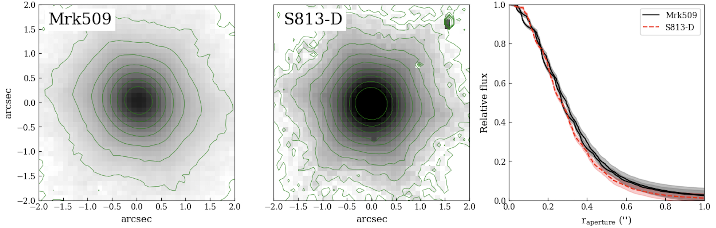
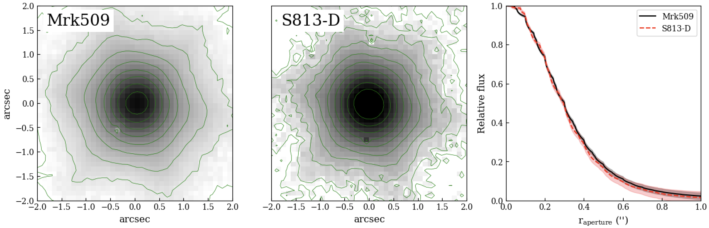
Figure 1: Images and radial profiles of Mrk 509 and S813-Dat H (Upper panel) and Ks (Bottom-panel) bands. From left to are the science image, the standard star, and their radial profiles. The radial profile of the QSO and its uncertainty are plotted as a black solid-line and the grey shaded region. The radial profile of the standard star and its uncertainty are plotted as a red dashed-line and pink shaded region. In all images the lowest contour is 3$\sigma$ over the background. The next contours are traced in 2$\sigma$ steps.

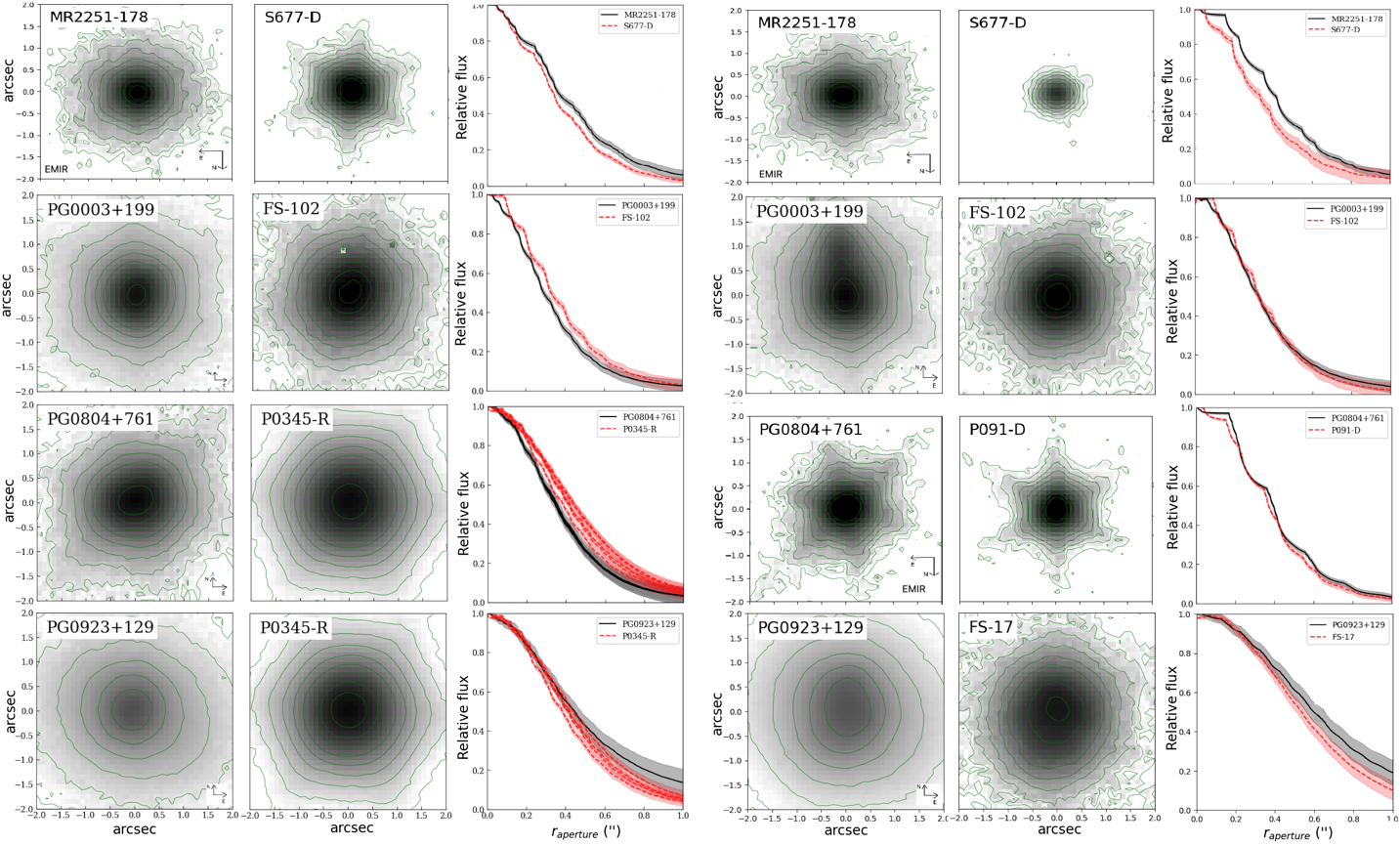
Figure 2: Images and radial profiles of QSOs and the standard at H (left panel) and Ks (right panel) bands. From left to right there are the science image, the standard star, and their radial profiles. The radial profile of the QSO and its uncertainty are plotted as a black solid-line and the grey shaded region. The radial profile of the standard star and its uncertainty are plotted as a red dashed-line and pink shaded region. In all images the lowest contour is $3\sigma$ over the background. The next contours are traced in $2\sigma$ steps.

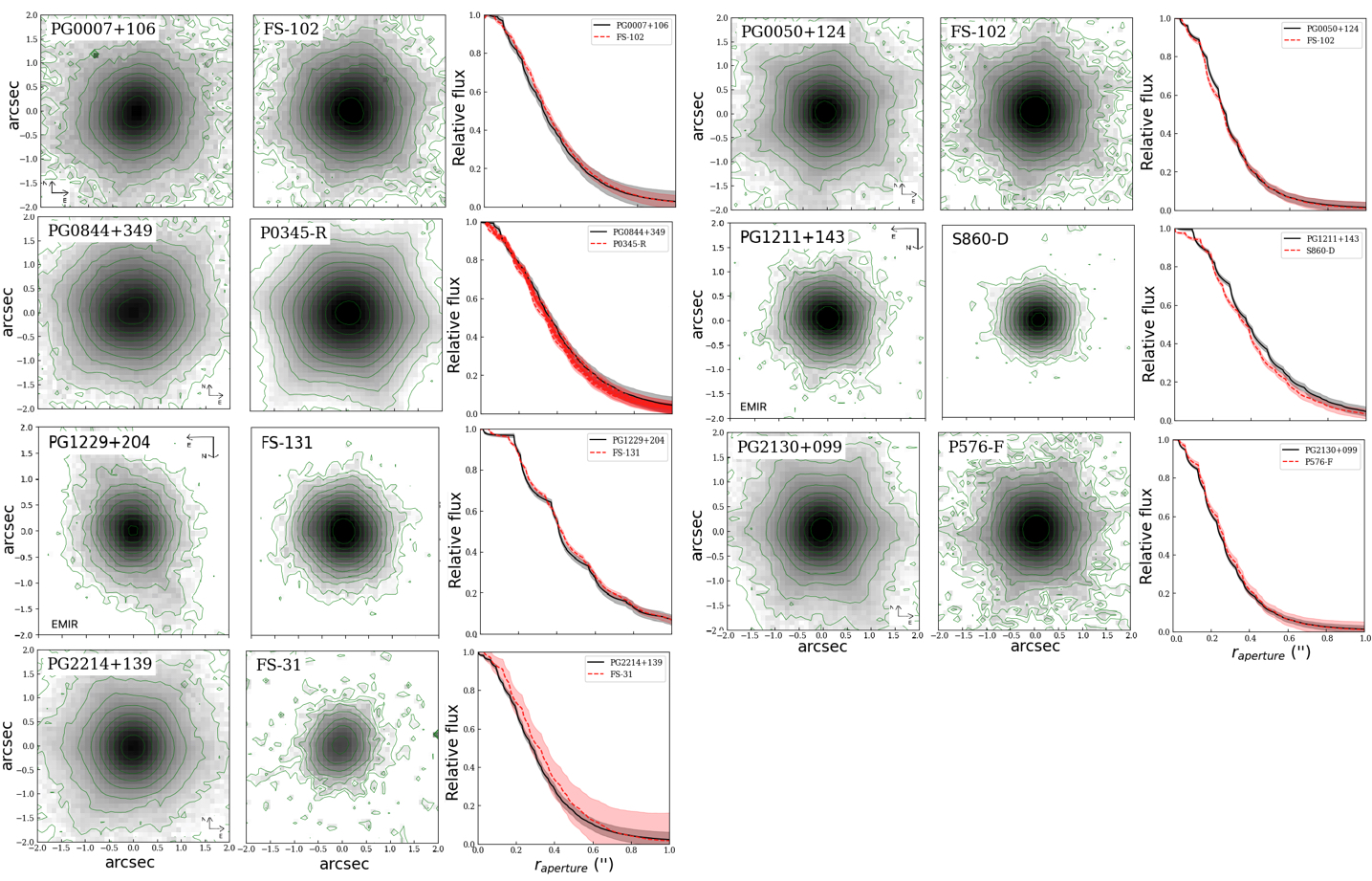
Figure 3: Images and radial profiles of QSOs and the standard in the Ks band. From left to right there are the science image, the standard, and their radial profiles. The radial profile of the QSO and its uncertainty are plotted as a black solid-line and the grey shaded region, respectively. The radial profile of the standard and its uncertainty are plotted as a red dashed-line and pink shaded region. In all images the lowest contour is 3$\sigma$ over the background. The next contours are traced in 2$\sigma$ steps.

Table 4: New NIR unresolved photometry measured within an aperture radius of 1 arcsec. Column 1 lists the name of the objects. Columns 2 and 3 list the flux and the source to standard FWHM ratio in the H band. Columns 4 and 5 list the flux and the source to standard FWHM ratio in the Ks band. In parenthesis we indicate the flux previously measured by Guyon et al. (2006) using QUIRC/Gemini. In the case of Mrk 509 the flux in parenthesis was reported by Fischer et al. (2006) using ISAAC/VLT.

Name	$f_{\nu}$ (mJy)		$f_{\nu}$ (mJy)
	H ($1.63\,\mu$m)	$\frac{FWHM_{target}}{FWHM_{STD}}$	Ks ($2.16\,\mu$m)	$\frac{FWHM_{target}}{FWHM_{STD}}$
Mrk 509	$15.6\pm 2.2$ ($<14.1$)	1.0	$21.1\pm 3.0$ ($<22.3$)	1.0
PG 0050+124	…	…	$26.6\pm 3.8$ ($<39.6$)	1.1
PG 2130+099	…	…	$13.0\pm 1.9$ ($<25.5$)	0.9
PG 1229+204	…	…	$4.3\pm 0.6$ ($<7.0$)	1.0
PG 0844+349	…	…	$10.3\pm 1.5$	1.0
PG 0003+199	$13.5\pm 1.9$	0.9	$20.6\pm 2.9$	1.0
PG 0804+761	$6.8\pm 1.0$ ($<13.2$)	0.8	$9.9\pm 1.4$ ($<26.2$)	1.1
PG 1211+143	…	…	$8.0\pm 1.1$	1.0
MR 2251-178	$7.0\pm 1.0$	1.1	$7.9\pm 1.1$	1.2
PG 2214+139∗	…	…	$9.6\pm 1.4$	1.04
PG 0923+129∗	$6.4\pm 0.9$	1.0	$6.8\pm 1.0$	1.1
PG 0007+106∗	…	…	$4.3\pm 0.6$ ($<19.3$)	0.9

Note.-^∗The object is not modeled because we do not have MIR high angular resolution spectrum.

4 Analysis

4.1 NIR

We performed aperture photometry on the QSOs and its corresponding standard star to look for possible extended emissions and measure the unresolved flux in the H and Ks bands. We use the photometry task tools photutils (Bradley et al., 2019) from the analysis package Astropy. We measure the relative flux through the radius aperture of the standard star and QSOs and build their radial profiles. Figure 1 shows, as an example, the images in the H- and Ks-band of Mrk 509 and its standard star, and their corresponding radial profiles in black and red dashed lines, respectively. Additionally, in Figures 2 and Figure 3 we show the images and radial profiles of the remaining objects observed in both H and Ks bands and of the objects observed only in the Ks-band, respectively. The uncertainties in the radial profiles are estimated according to the following expression, $\sqrt{\sigma_{back}^{2}N_{pix}+\sigma_{back}^{2}N_{pix}^{2}/N_{pix-ring}}$ where $\sigma_{back}$ is the standard deviation of the background level, $N_{pix}$ is the number of pixels within an aperture, and $N_{pix-ring}$ is the number of pixels within a 80-pixel width annulus (see e.g., Reach et al., 2005). Additionally, we add in quadrature the uncertainties due to the PSF-variability ($\sim 14\%$), which is estimated from the standard stars observed within a single night for multiple times with time intervals of few minutes, and the flux calibration ($\sim 6\%$).

Considering that in most cases the radial profile of the QSOs and standard stars are compatible within the uncertainties we assumed that the emission of these QSOs is unresolved and measured the flux within an aperture radius of one arcsecond ($<1$ kpc, see Table 4). The exception is for MR 2251-178, for which we find that $\sim 20\,\%$ of the emission is due to the extended component in both bands. Note that the aperture corrected fluxes measured within an aperture radius of $\sim 2\times FWHM$ gives similar results within the uncertainties. A similar analysis was done by Martínez-Paredes et al. (2017) to estimate the unresolved emission of these QSOs at Si2 band inside a radius aperture of $1^{\prime\prime}$, which correspond to a physical scales $<1$ kpc.

In Table 4 we also list the flux previously reported in the literature (e.g., Guyon et al., 2006; Fischer et al., 2006) from ground-based observations for some objects. In general, we find that our fluxes are lower, probably since their studies being focused on the morphology of the host galaxy more than in the measurement of the PSF, which is the goal in our analysis. In the case of Mrk 509, our measurements in the H and Ks bands are similar to those previously measured by Fischer et al. (2006) within an aperture radius of 1.5 arcsec.

4.2 Disentangling the accretion disk and torus

To decontaminate the IR data from the possible contribution of the accretion disk, especially at NIR wavelengths, we explored two broken power laws as the SED of the accretion disk $\lambda F_{\lambda}\propto\lambda^{\alpha}$. The first one is a classic accretion disk SED, which is in agreement with theoretical predictions and observational evidences (e.g., Hubeny et al., 2001; Davis & Laor, 2011; Slone & Netzer, 2012; Capellupo et al., 2015; Stalevski et al., 2016) ,

$$\lambda F_{\lambda}\propto\left\{\begin{array}[]{ll}\lambda^{1.2}&\,\,\,0.001\leq\lambda\leq 0.01\,\mu\text{m}\\ \lambda^{0}&\,\,\,0.01<\lambda\leq 0.1\,\mu\text{m}\\ \lambda^{-0.5}&\,\,\,0.1<\lambda\leq 5\,\mu\text{m}\\ \lambda^{-3}&\,\,\,5<\lambda\leq 50\,\mu\text{m}\\ \end{array}\right.$$ (1)

The second one is a bluer broken power law derived from QSOs observations (e.g., Zheng et al., 1997; Manske et al., 1998; Vanden Berk et al., 2001; Scott et al., 2004; Kishimoto et al., 2008),

$$\lambda F_{\lambda}\propto\left\{\begin{array}[]{ll}\lambda^{1}&\,\,\,\lambda<0.03\,\mu\text{m}\\ \lambda^{0}&\,\,\,0.03<\lambda\leq 0.3\,\mu\text{m}\\ \lambda^{-4/3}&\,\,\,0.3<\lambda\leq 3\,\mu\text{m}\\ \lambda^{-3}&\,\,\,\lambda>3\,\mu\text{m}\\ \end{array}\right.$$ (2)

We compile the dereddened UV nuclear photometry from the Galaxy Evolution Explorer space telescope (GALEX) at Far-ultraviolet (FUV, 0.153 $\mu$m) and Near-ultraviolet (NUV, 0.231 $\mu$m) bands (Bianchi et al., 2011; Monroe et al., 2016; Bianchi et al., 2017). Two objects do not have GALEX fluxes in the literature. For one of them (PG 0844+349) we use the dereddened PSF photometry in the u band (0.352 $\mu$m) from the SDSS DR12 SkyServer, and for the another one (PG 0804+761) the continuum emission at 110 and 130 $\mu$m reported by Stevans et al. (2014) using the Cosmic Origins Spectrograph on the HST. We use these data to normalise the broken power-law components and subtract it from both the NIR and MIR photometry, and from both the ground-based high angular resolution and Spitzer/IRS spectra.

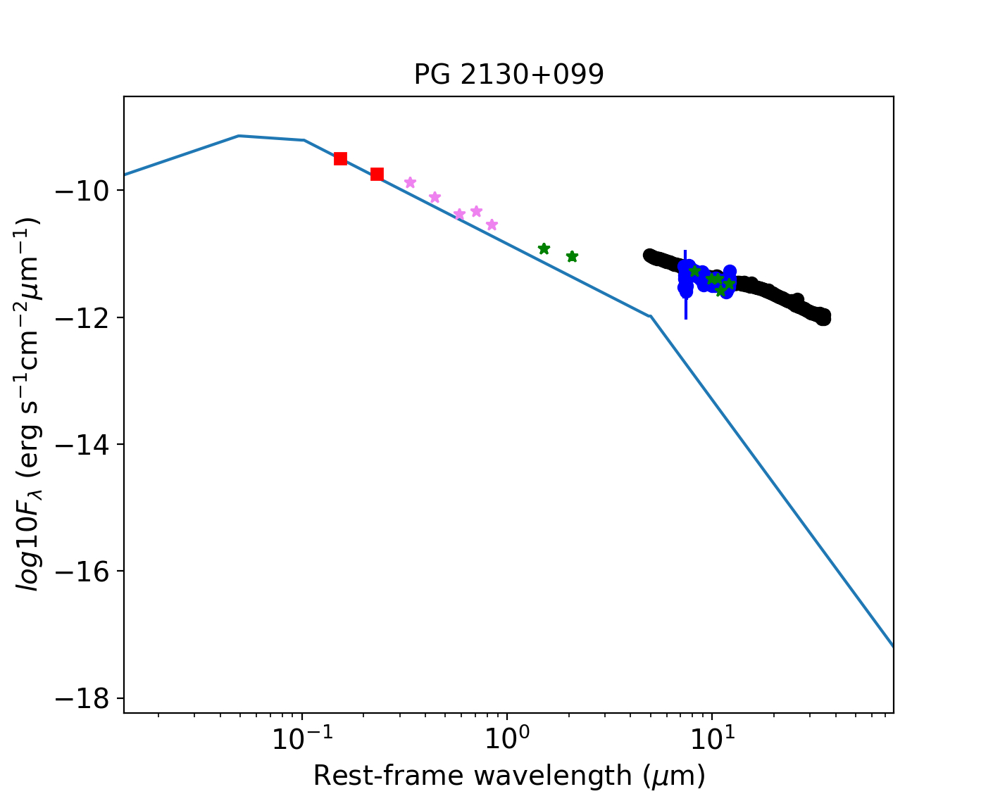
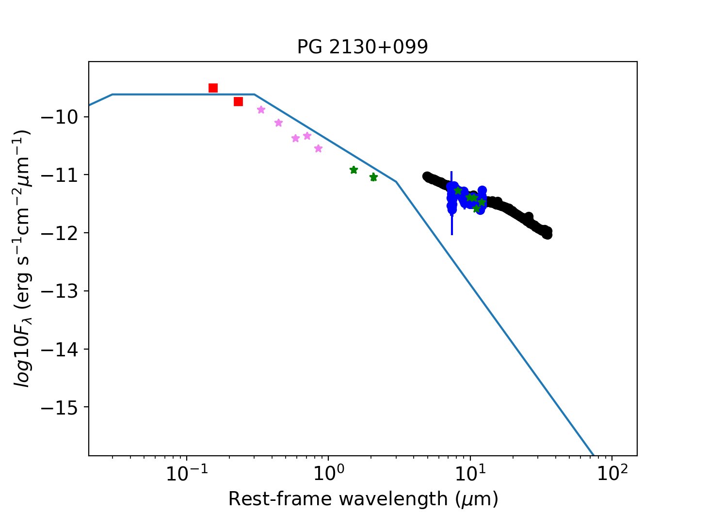
Figure 4: Left panel: The solid blue line is the normalized broken power law from Stalevski et al. (2016), which is scaled to the photometric UV PSF fluxes at FUV (0.153 $\mu$m) and NUV (0.231 $\mu$m) bands from GALEX (red points). Pink symbols are the optical PSF fluxes from the SDSS bands (u, g, r, i, and z), which are included as an indicator of nuclear optical emission. The green photometric points are the NIR fluxes from HST/NICMOS and GTC/CIRCE in the H and Ks bands, and the MIR fluxes from GTC/CC, VLT/VISIR, and Subaru/COMICS. The black and blue points are the Spitzer/IRS and GTC/CC spectra, respectively. Right panel: as left panel but for the bluer accretion disk.

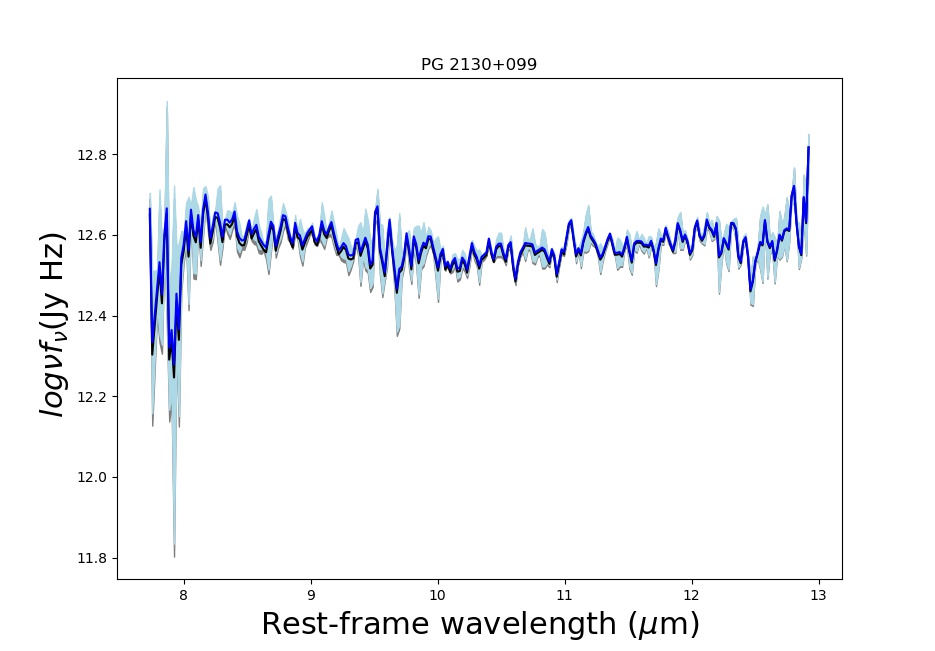
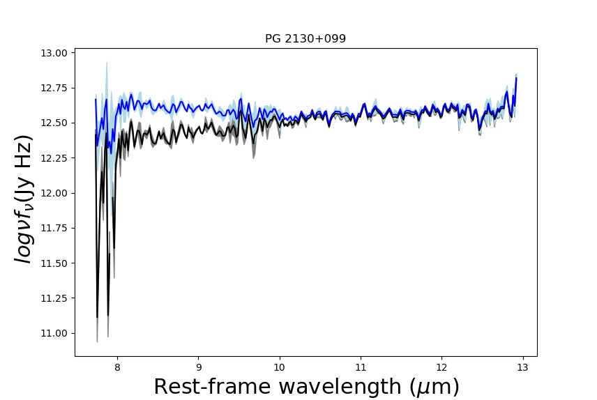
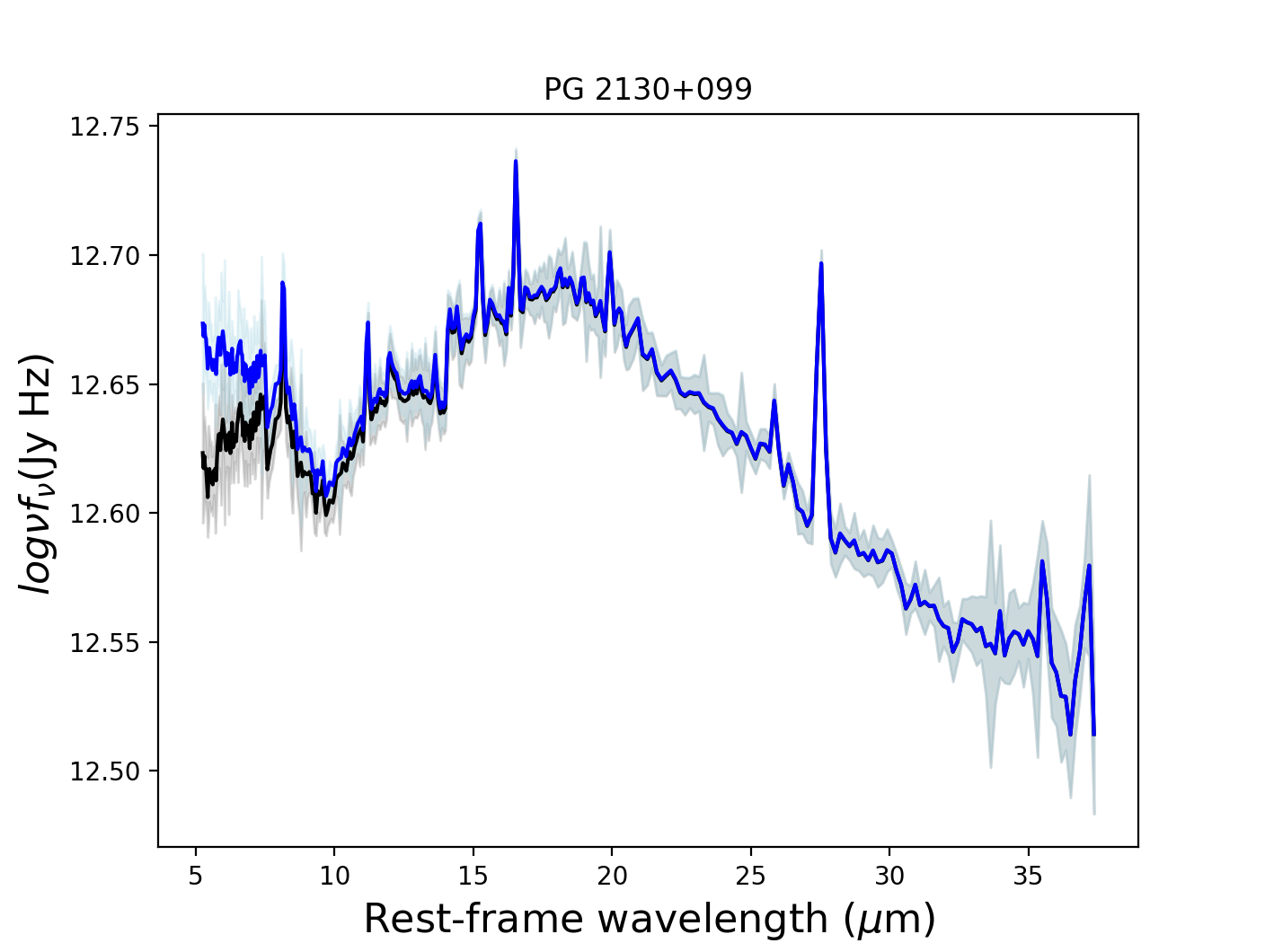
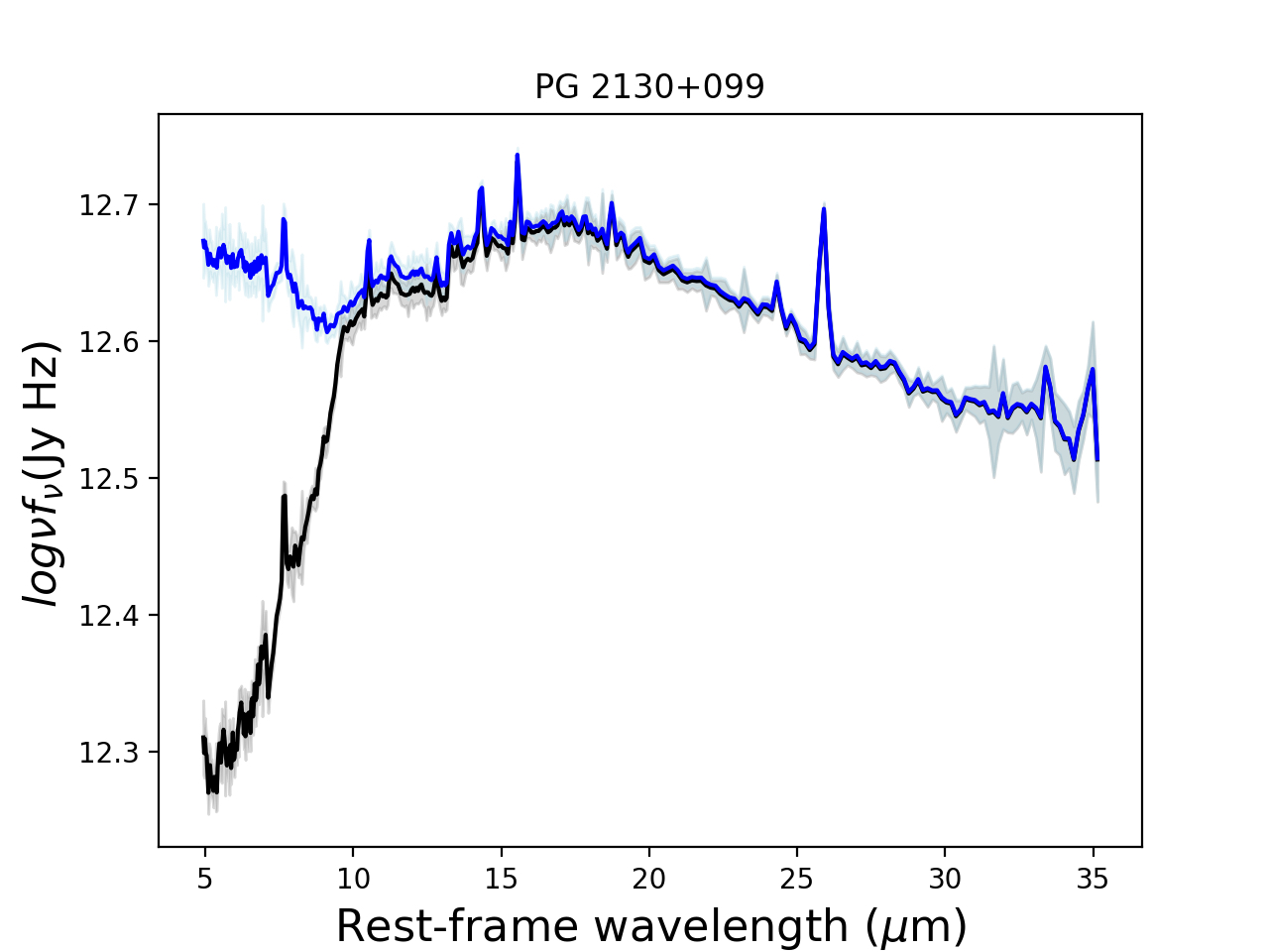
Figure 5: Upper panels: in blue and black is the high angular resolution spectrum before and after we removed the contribution from the classic (left) and bluer (right) accretion disk, respectively. Bottom panels: the same but for the Spitzer/IRS spectra.

As an example, in Figure 4, we show the normalized classic and bluer broken power-law models for PG 2130+099, see Eqs. (1) and (2). The UV photometric points are plotted in red. Additionally, we plot the dereddened PSF fluxes from the SDSS bands (u, g, r, i, and z) obtained from the DR12 SkyServer as an indicator of the PSF emission at optical wavelength. We also plot in green points the NIR and MIR unresolved fluxes, the CC/GTC high angular resolution spectrum (in blue), and the Spitzer/IRS spectrum (in black) before subtracting the accretion disk. As can be seen from the figure, the bluer accretion disk overestimates the emission of the optical and NIR photometric points. The same happens for the rest of QSOs, except for PG 0050+124, PG 1440+356, and PG 1411+442. Although for the two latter objects, only the Ks band is above the extrapolated accretion disk SED. In the case of the classic accretion disk, there are only three objects (PG 1229+204, PG 0844+349, and PG 0804+761) for which the extrapolation of the SED drops slightly above the NIR photometric points.

For those cases in which the accretion disk is above the photometric points, we do not subtract its emission and use the photometry as upper limits.

We aslo compare the spectrum before and after subtracting the accretion disk contribution. As an example, we plot the high angular resolution and Spitzer/IRS spectra of PG 2130+099 in Figure 5. We find that if we assume the classic accretion disk there are no differences between the high angular resolution spectra before and after subtraction. However, in the Spitzer/IRS spectra we find that in most objects (Mrk 509, PG 2130+099, PG 0003+199,PG 1440+356, PG 1426+015, PG 1411+442, PG 1211+143, and PG 1501+106) there is an average contribution from the accretion disk of $\sim 2.4\%$ between $\sim 5-7.5\mu$m. On the other hand, when we assume the bluer accretion disk, then the spectral shape of both the high angular resolution and Spitzer/IRS spectra change after the disk component subtraction. We find that the bluer accretion disk contributes $\sim 17.5\%$ and $\sim 5.5\%$ to the Spitzer and high angular resolution spectra between $\sim 5-10\,\mu$m, respectively. For PG 0804+761 the extrapolation of the bluer accretion disk overstimate the emission of both spectra until $\sim 10\,\mu$m.

On average, we find that the classic accretion disk contributes $\sim 35\%$ and $\sim 30\%$ (12 objects), in the H and Ks bands, respectively. These are lower than the contributions we find assuming the bluer accretion disk, $\sim 41\%$ (two objects) and $\sim 54\%$ (four objects), in the same bands. Hernán-Caballero et al. (2016) found that the contribution of the accretion disk at 1, 2, and 3 $\mu$m (rest-frame wavelength) are 63, 17, and 8 $\%$ for a sample of QSOs with a redshift $z$ between 0.17 and 6.42. On the other hand, García-Bernete et al. (2019) found that the contribution from the accretion disk is $\sim 46$, $\sim 23$, and $\sim 11$ $\%$ in the J, H, and K bands for a sample of type 1 Seyferts.

5 Modeling the NIR to MIR SEDs

5.1 The Dusty Torus Models

5.1.1 Fritz et al. (2006) - Smooth F06 model

The Fritz et al. (2006) model has a flared disk with open polar cone regions. In this model the dust homogeneously and continuously fills the torus volume. The following parameters describe it. First, the inner and outer radius ($\rm Y=R_{out}/R_{in}$) ratio. The inner radius is defined by the dust sublimation temperature (1500 K) under the intense radiation by the central AGN. It is defined as $R_{in}\eqsim 1.3\sqrt{L_{46}^{AGN}}T_{1500}^{-2.8}$ pc, for a typical graphite grain with a radius of 0.05 $\mu$m (Barvainis, 1987). Other parameters are the angular width of the torus $\Theta$, the viewing angle $i$, the index of the polar and radial gas distribution $\gamma$, and $\beta$, respectively, and, the optical depth at $9.7\mu\mbox{m}$. The dust is mainly composed of graphite and silicate grains in nearly equal percentages. The central point-like source is represented by a broken power-law that illuminates the dust.

5.1.2 Nenkova et al. (2008a, b) - Clumpy N08 model

The Nenkova et al. (2008a, b) model assumes that the dust within a torus-like geometry is distributed in the form of identical spherical clumps. They enshroud the central engine emitting the energy following a broken power-law SED and are assumed to have the standard Galactic ISM (i.e. 47 % graphite and 53 % silicate). The following parameters describe the model, the viewing angle ($i$), the number of clouds along the line of sight ($N_{0}$), the angular width of the torus ($\sigma$), the radial extension ($\rm Y=R_{out}/R_{in}$), the index of the radial distribution q, and the optical depth of the clouds ($\tau_{V}$). The inner radius in this model is defined as $R_{in}\eqsim 0.4\sqrt{L_{45}^{AGN}}T_{1500}^{-2.6}$ pc. They argued that the differences in the power of the sublimation temperature reflect the more detailed radiative transfer calculations performed in this model.

5.1.3 Hönig & Kishimoto (2010b)- Clumpy H10 model

The Hönig & Kishimoto (2010b) model inherites the strategy in Nenkova et al. (2008a), however, used a 3D Monte Carlo radiative transfer simulation to treat the dust distribution in a probabilistic manner. It assumes the central point source described by a broken power-law and three different dust compositions: the standard ISM, large ISM grains ($0.1\sim 1~{}\mu$m), and intermediate grains ($0.05\sim 0.25~{}\mu$m) with 70 % graphite and 30 % silicate. The torus parameters are the power-law index of the radial distribution (a), the power-law index of the cloud size distribution (b), the viewing angle ($i$), the number of clouds along the equatorial plane ($N_{0}$), the outer radius ($R_{out}$), and the cloud size at the inner-most torus radius. In this model the inner radius is defined as $R_{in}\eqsim 0.36\sqrt{L_{45}^{AGN}}$ pc assuming ISM dust, while for ISM large grain this is $R_{in}\eqsim 0.5\sqrt{L_{46}^{AGN}}$ pc (see Hönig & Kishimoto, 2010b).

5.1.4 Stalevski et al. (2016) - Two-phase media S16 model

They model the dusty torus with dusty clumps enshrouded by a smooth low-density nebulosity called a two-phase medium. The torus is heated by a central point source with anisotropic emission (Netzer, 1987), which is the strongest for the polar direction and the weakest along the equatorial plane. A power-law dictates the standard ISM dust distribution along the radial ($p$) and polar ($q$) direction. Additionally, the model depends on the viewing angle ($i$), the half-opening angle ($\sigma$), the optical depth at $9.7~{}\mu m$ ($\tau$), and the radial extension ($\rm Y=R_{out}/R_{in}$). The inner radius is defined as in the smooth model of Fritz et al. (2006).

5.1.5 Hönig & Kishimoto (2017) - Disk+Wind H17 model

This model is composed of a clumpy polar wind and a compact disk. The dust clouds are assumed to lie along a radial distance from the central black hole $r$, following a power-law distribution described by the power-law index $a$ (for the disk), and the power-law index $a_{w}$ (for the wind). The disk is also described by the dimensionless scale height $h$ and the number of clouds along the equatorial line $N_{0}$. While the wind by the half-opening angle $\theta$ and the angular width of the hollow cone $\sigma$. Other parameters are the wind-to-disk ratio of the number of clouds $f_{wd}$ and the viewing angle $i$. Different sets of dust composition have been implemented, assuming the standard ISM and the standard ISM plus larger grains dust.

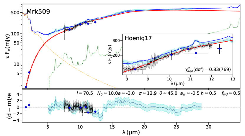
Figure 6: The SED of Mrk 509 fitted by the Disk+Wind H17 model. The high angular resolution photometric points are plotted as blue points with their $1\sigma$ error bars, while the high angular resolution spectrum is plotted with a black solid line, the grey shaded region represent the errors. The Spitzer/IRS spectrum is represented with a dark cyan solid line and its error with a cyan shaded region. The red solid line is the best model resulting from fitting the high angular resolution data. The green and yellow dotted lines are the starburst and stellar components, respectively. The blue solid line represents the sum of the stellar, starburst and torus components that best fit the Spitzer/IRS spectrum.

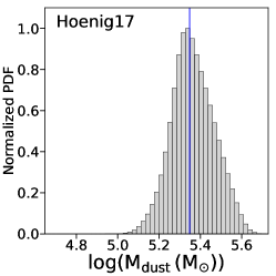
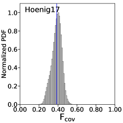
Figure 7: The Disk+Wind H17 model parameters derived for Mrk 509. Upper panels: normal probability distribution function of the eight free parameters. In grey we plot the parameters derived from fit LSR spectrum, while in dark blue the distribution of the parameters obtained from fit FSR spectrum. Bottom panels: normal PDF of the derived parameters. The blue vertical line indicates the mean value.

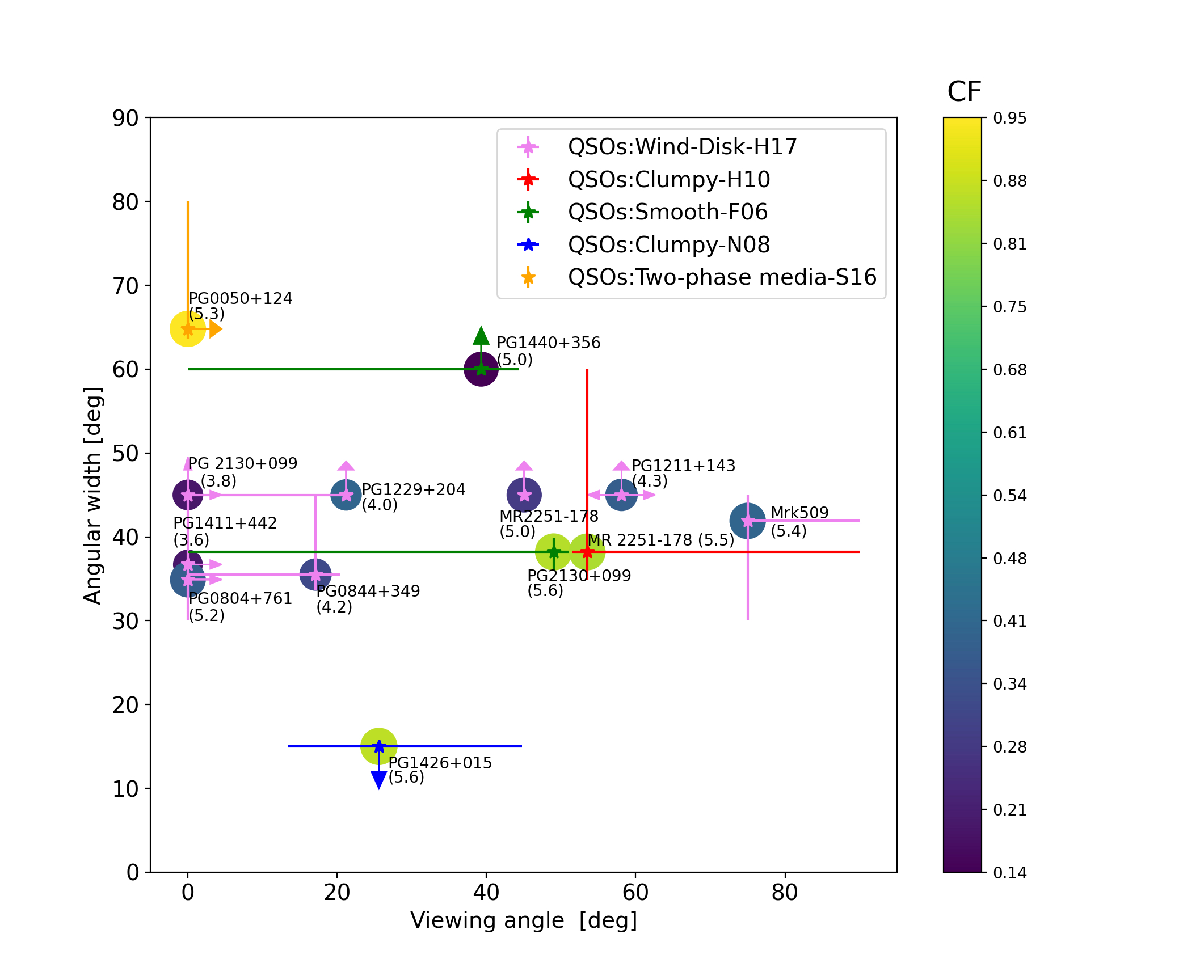
Figure 8: Angular width versus viewing angle $i$ obtained for the good fits of all models. The coloured stars indicate the model that best fits the object, the arrows an upper or lower limit. The covering factor (CF) is represented with a colour-coded circle. The set of values are indicated in the vertical colour bar. Yellow circles indicate large covering factors, while purple circles indicate low covering factors. The value of the logarithm of the dust mass (in $M_{\odot}$) is represented with a size coded circle, and the value is indicated in parenthesis.

5.2 Modeling procedure

In this work we take advantage of the high S/N of the Spitzer/IRS spectra, the high angular resolution of the CC and VISIR spectra, and the ground-based high angular resolution photometry at NIR and MIR to build a well-sampled set of SEDs that allows us to look for the model that better reproduces the data. To model these data we used the interactive spectral fitting program XSPEC (Arnaud, 1996) from the HEASOFT package. XSPEC uploads the dust models as additive tables, which have been previously created using the flx2tab task within HEASOFT. Briefly, a table model is composed of an N-dimensional grid of model spectra, which is calculated for a particular set of values within the N parameters space of the model (for more details on the model inclusion and modelling procedure within XSPEC see González-Martín et al., 2019a). Additionally, we also included the stellar libraries of Bruzual & Charlot (2003), the starburst templates from Smith et al. (2007), and foreground extinction (Pei, 1992).

For the data, we use the flx2xsp task within HEASOFT to read the text file that contains the photometry and the spectroscopy plus their uncertainties, and to write a standard XSPEC pulse height amplitude.

We use $\rm{\chi^{2}}$ statistic to converge to the best fit. However, this approach requires a particular treatment of the data when using different datasets. The different spectral resolution could lead to an overestimation of the spectra compared to the photometry. Simultaneously, the spectral features (e.g., silicate features) are useful to understand the best model for each object. Thus, we develop a procedure able to use both the spectral and photometric data simultaneously. We create spectra, for both Spitzer and ground-based observations, degraded to the spectral resolution of the photometry. To do so, we require that the spectrum matches the average bandpass of the photometric points in the MIR. From now on, we call this degraded spectra the low spectral resolution (LSR) Spitzer and ground-based spectra.

We start fitting the LSR ground-based spectrum and the high angular resolution photometry to the dust models attenuated by foreground extinction. In the case of the photometric set of data, the parameters of the dust models are tied to those of the LSR ground-based spectrum to try to find a single SED reproducing both sets of data. We assume that circumnuclear contributors do not contaminate this data set. After obtaining the best fit to the ground-based high spatial resolution data, we added the LSR Spitzer/IRS spectrum to these data set. We used the parameters derived from fitting the LSR Spitzer/IRS spectrum as an initial guess for the fit of the LSR ground-based spectra/photometry. In this case, and when necessary, we add a stellar and/or starburst component to the LSR Spitzer/IRS spectrum to consider plausible circumnuclear contributors due to the lower spatial resolution of Spitzer/IRS. Once the LSR data are fitted, we computed the 3$\rm{\sigma}$ errors for each parameter involved.

We used these errors to fix the minimum, and maximum allowed range to those parameters obtained from the spectral fit to the LSR data set. Then we replace the LSR spectra (ground-based and Spitzer) for the full spectral resolution (FSR) version of the spectra. Therefore, we imposed these values as the initial guess of the parameters to fit the N band high angular resolution spectrum plus the photometric data. Next, besides the parameters of the models, we also calculate the dust mass and covering factor for all the models. For F06, N08, and S16, we also calculate the radial extension of the torus. To derive the dust mass and covering factor, we used the equations (1) to (6) from Esparza-Arredondo et al. (2019). The outer radius $R_{out}$ is calculated as a function of the radial extent $Y$.

We consider as acceptable fits those with a reduced $\chi_{red}^{2}<2$ for both LSR and FSR spectral fits, see Table 5. Then, to look for the model preferred by the data, we estimate the Akaike Information Criterion (AIC H. Akaike, 1974) for both LSR and FSR spectral fits. The AIC criterion gives the quality of a model by estimating the likelihood of the model to predict futures values. We compute the AIC value in terms of the $\chi^{2}$, the degree of freedom (dof), and the data size (N). The dof is calculated as the total number of points in the spectrum minus the total number of free parameters of the model. In general, a good model is the one with the minimum AIC. However, to better discriminate between the models, we estimate the likelihood that the model with the minimum AIC minimizes the loss of information.

5.3 Spectral fitting

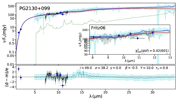
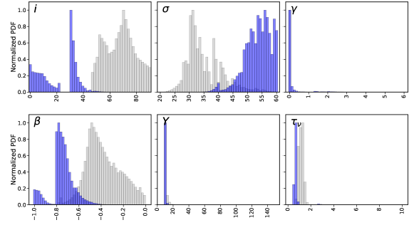
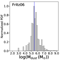
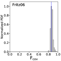
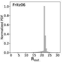
Figure 14: The SED of PG 2130+099 best modeled by the Smooth F06 model. Upper panel: the high angular resolution photometric points are plotted as blue points with their error bars, the black arrows are upper limits. The high angular resolution spectrum is plotted with a black solid line, the grey shaded region represent the errors. The Spitzer/IRS spectrum is plotted with a dark cyan solid line and its error with a cyan shaded region. The red solid line is the best model resulting from fit the high angular resolution data. The green and yellow dotted lines are the starburst and stellar components, respectively. The blue solid line represents the sum of the stellar, starburst and torus components that best fit the Spitzer/IRS spectrum. Middle panel. The model parameters derived: normal probability distribution function of the free parameters. In grey we plot the parameters derived from fit the LSR spectrum, while in dark blue the distribution of the parameters derived from fit the FSR spectrum. Bottom panel: normal PDF of the derived parameters. The blue vertical line indicate the mean.

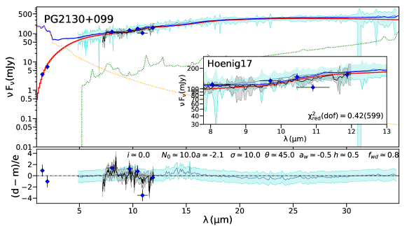
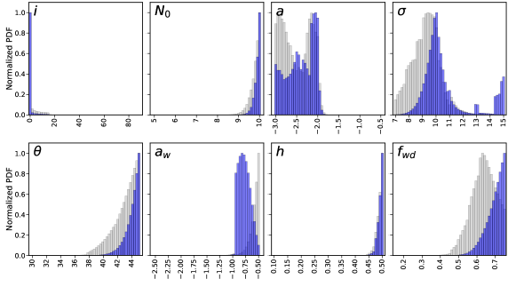
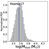
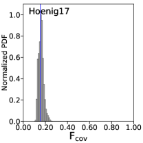
Figure 15: As Figure 14 but for the Disk+Wind H17 model.

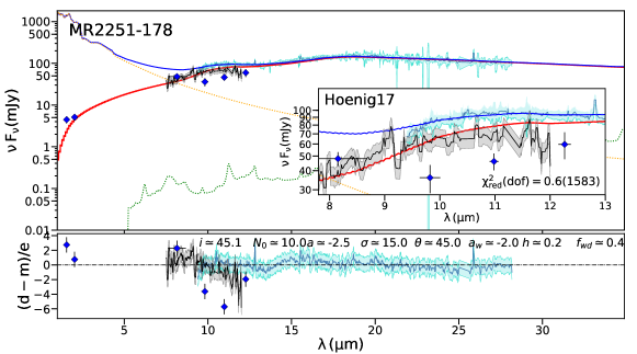
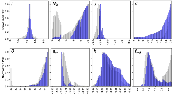
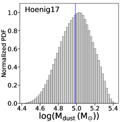
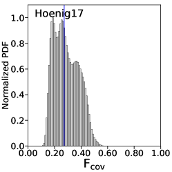
Figure 16: The SED of MR 2251-178 best modeled by the Disk+Wind H17 model. Upper panel: the high angular resolution photometric points are plotted as blue points with their error bars, the black arrows are upper limits. The high angular resolution spectrum is plotted with a black solid line, the grey shaded region represent the errors. The Spitzer/IRS spectrum is plotted with a dark cyan solid line and its error with a cyan shaded region. The red solid line is the best model resulting from fit the high angular resolution data. The green and yellow dotted lines are the starburst and stellar components, respectively. The blue solid line represents the sum of the stellar, starburst and torus components that best fit the Spitzer/IRS spectrum. Middle panel. The model parameters derived: normal probability distribution function of the free parameters. In grey we plot the parameters derived from fit the LSR spectrum, while in dark blue the distribution of the parameters derived from fit the FSR spectrum. Bottom panel: normal PDF of the derived parameters. The blue vertical line indicate the mean.

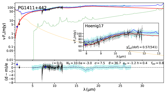
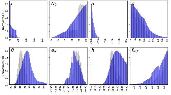
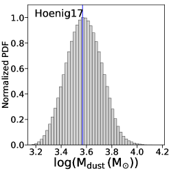
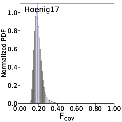
Figure 18: The SED of PG 1411+442 best modeled by the Disk+Wind H17 model. Upper panel: the high angular resolution photometric points are plotted as blue points with their error bars, the black arrows are upper limits. The high angular resolution spectrum is plotted with a black solid line, the grey shaded region represent the errors. The Spitzer/IRS spectrum is plotted with a dark cyan solid line and its error with a cyan shaded region. The red solid line is the best model resulting from fit the high angular resolution data. The green and yellow dotted lines are the starburst and stellar components, respectively. The blue solid line represents the sum of the stellar, starburst and torus components that best fit the Spitzer/IRS spectrum. Middle panel. The model parameters derived: normal probability distribution function of the free parameters. In grey we plot the parameters derived from fit the LSR spectrum, while in dark blue the distribution of the parameters derived from fit the FSR spectrum. Bottom panel: normal PDF of the derived parameters. The blue vertical line indicate the mean.

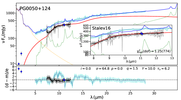
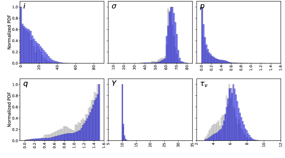
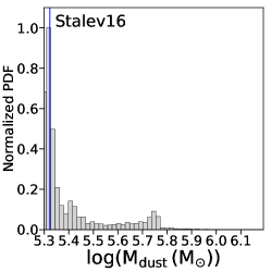
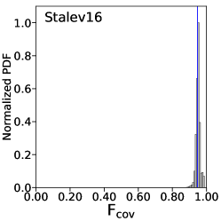
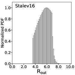
Figure 26: The SED of PG 0050+124 best modeled by the Two-phase Media S16 model. Upper panel: the high angular resolution photometric points are plotted as blue points with their error bars, the black arrows are upper limits. The high angular resolution spectrum is plotted with a black solid line, the grey shaded region represent the errors. The Spitzer/IRS spectrum is plotted with a dark cyan solid line and its error with a cyan shaded region. The red solid line is the best model resulting from fit the high angular resolution data. The green and yellow dotted lines are the starburst and stellar components, respectively. The blue solid line represents the sum of the stellar, starburst and torus components that best fit the Spitzer/IRS spectrum. Middle panel. The model parameters derived: normal probability distribution function of the free parameters. In grey we plot the parameters derived from fit the LSR spectrum, while in dark blue the distribution of the parameters derived from fit the FSR spectrum. Bottom panel: normal PDF of the derived parameters. The blue vertical line indicate the mean.

We find that for all objects, several models can fit the same set of LSR and FSR data with a reduced $\chi^{2}<2$. However, according to the AIC criterion, the model that better reproduces the FSR data for Mrk 509, PG 2130+099, PG 1411+442, PG 1211+143, PG 1501+106, MR 2251-178, PG 1229+204, PG 0844+349, and PG 0804+761 is the Disk+Wind H17 model, while for PG 1440+356 is the Smooth F06 model, for PG 0050+124 is the Two-phase media S16 model, and for PG 1426+015 is the Clumpy N08 model. In the case of PG 0003+199 we find that none of the models can reproduce the FSR data probably because the shape of its ground-based MIR spectrum differs from the Spitzer/IRS spectrum between $\sim 10.5-12.3\mu$m. These differences might be caused for the lost of signal in the border of the ground-based MIR high angular resolution spectrum (see Figure C1 in Martínez-Paredes et al., 2017). In Table 5 we highlight in bold letters the good fits according to the AIC criterion. For PG 2130+099, the data do not permit to distinguish between the Disk+Wind H17 and Smooth F06 models. For MR 2251-178, both the Disk+Wind H17 and Clumpy H10 models are equally valid. However, based on a qualitative analysis, it is possible to note that the residuals obtained assuming the Disk+Wind H17 model are the flattest in both cases (see Figures 14 and 15 for PG 2130+099 and Figure 16 and 17 for MR 2251-178). For the rest of objects and models, the best-fitted SEDs and probability distribution functions (PDFs) of the constrained parameters are shown from Figure 18 to Figure 26.

Considering only the models that resulted selected according to the AIC criterion, we find that the Disk+Wind H17 is the model that better reproduces the data ($64\%$ of the cases, 9/13) followed by the Smooth F06 ($14\%$, 2/13), the Clumpy H10 ($7\%$, 1/13), the Clumpy N08 ($1\%$, 1/13), and the Two-phase media S16 ($7\%$, 1/13) models. As an example, in Figure 6 we show the fits of the NIR-MIR SED for Mrk 509 assuming the Disk+Wind H17 model and in Figure 7 the PDF of the parameters that best reproduce the data, and the PDF of the covering factor and the dust mass of the torus derived. On the other hand, if we assume the bluer accretion disk, none of the models fit the data for most cases. The exceptions are PG 0050+124 and PG 1501+106, for which the Disk+Wind H17 model was the best model in fit the data. This result is consistent with those obtained when assuming the classic accretion disk. Additionally, in all cases we note that although the Spitzer/IRS spectra of these QSOs is mostly dominated by the contribution of the AGN ($>80\%$) and we remove the contribution from the accretion disk it is necessary to add both the stellar and/or starburst components for most objects (see Table 5).

When using the classic accretion disk, the H and Ks bands are well fitted in most cases by the Wind+Disk H17 model. Only in two cases, MR 2251-174 and PG 1411+442, the flux in the H band, from GTC/EMIR and HST/NICMOS, respectively, is above the best fit. This excess could be due to some contamination by the host galaxy. Since in the case of MR 2251-174, the radial profile in the H band (see Section 4.1) is slightly above the radial profile of the standard star, and because in some cases, a marginal emission from the host could be contaminating the PSF flux in the H band from HST/NICMOS (see Veilleux et al., 2006, 2009). We find that the Clumpy N08 model best fitted to PG 1426+015 and reproducers the H photometric point obtained from NICMOS/HST (the Ks flux is an upper limit). We also note that for PG 0050+124, the photometric points in the H band from HST/NICMOS and Ks band from GTC/CIRCE, are above the best fitted model (Two-phase Media S16). Additionally, for PG 1440+356, the photometric point in the H band from HST/NICMOS is slightly above the best fitted model (Smooth F06), the Ks flux is an upper limit. In these two last cases, this is probably due to the limitation of the model in well fit simultaneously the NIR and MIR SEDs (see e.g., Martínez-Paredes et al., 2020) and/or some marginal contamination from the host.

In Tables 7, 9, 11, 13, and 15 we list the mean and $1\sigma$ errors of the parameters derived for these models, while in Tables 8, 10, 12, 14, and 16 we list the derived (covering factor, dust mass, and outer radius) parameters. Additionally, in Figure 8 we plot the angular width (half angular width measured from the equator for the Disk+Wind H17 model) against the viewing angle obtained from the best fits for all models, as well as the dust mass and covering factor in size- and color-code. We note that in all cases, the parameters are consistent with the optical classification as type 1 AGN and that the dust mass is constrained between $\sim 10^{4}-10^{5}\,\text{M}_{\odot}$ for most cases, while the covering factor ranges from $\sim 0.14$ to 0.40 for the Disk+Wind H17 model until 0.95 for the Two-phase media S16 model. These covering factors are consistent with the ones obtained in previous works for type 1 AGNs (see e.g., Martínez-Paredes et al., 2017; González-Martín et al., 2019b; Martínez-Paredes et al., 2020). However, it is important to note that the covering factor is model dependent, as showed by González-Martín et al. (2019b). For example, they found that for the Disk+Wind H17 model the covering factor only ranges from $\sim 0.1-0.6$, while for the rest of models considered here, the parameters allow the covering factor to range from $\sim 0.1-1$, showing a maximum towards the larger values and decreasing until they reach a value of $\sim 0.1$.

Table 5: Statistic of the acceptable fits. Column 1 lists the name of the object. Columns 2 and 3 list the model assumed and the additional component included. Columns 4, 5, and 6 list the red-$\chi^{2}$, degree of freedom, and AIC values for the FSR fits. Column 7 lists the reduced-$\chi^{2}$ for the LSR fits.

		Add.	FSR			LSR			Add.	FSR			LSR
Name	Model	Comp.	$\chi_{red}^{2}$	dof	AIC	$\chi_{red}^{2}$	Name	Model	Comp.	$\chi_{red}^{2}$	dof	AIC	$\chi_{red}^{2}$
Mrk 509	F06	+Ste+SB	1.2	772	584.88	1.05	PG 1211+143	F06	+Ste+SB	1.53	535	834.29	1.96
	H10	+Ste+SB	0.85	773	314.63	0.59		N08	+Ste+SB	1.33	535	727.77	1.58
	H17	+Ste+SB	0.71	770	206.99	0.47		H10	+Ste+SB	1.24	536	680.9	1.27
								H17	+Ste+SB	1.15	533	633.15	1.20
PG 0050+124	F06	+Ste+SB	1.32	774	1038.01	1.77	PG 1501+106	F06	+Ste	1.28	521	638.39	1.26
	S16	+Ste+SB	1.25	774	980.92	1.65		S16	+Ste	1.12	521	599.03	1.02
	H17	+Ste+SB	1.44	772	1131.31	1.71		N08	+Ste	0.89	521	480.88	0.68
								H10	+Ste	0.86	522	465.3	0.81
								H17	+Ste	0.72	519	394.67	0.52
PG 2130+099	F06	+SB	0.42	601	271.49	0.39	MR 2251-178	H10	+Ste	0.6	1586	973.41	1.30
	S16	+Ste+SB	0.73	601	456.48	0.70		H17	+Ste	0.6	1583	964.12	1.09
	H10	+Ste+SB	0.64	602	402.31	0.58
	H17	+Ste+SB	0.42	599	271.03	0.32
PG 1411+442	F06	+Ste+SB	0.93	543	521.12	0.89	PG 1229+204	F06	+Ste	0.6	541	341.19	0.74
	H10	+Ste+SB	0.78	544	437.5	0.78		S16	+Ste	0.5	541	284.18	0.56
	H17	+Ste+SB	0.57	541	328.27	0.27		N08	+Ste+SB	0.56	541	317.12	0.55
								H10	+Ste+SB	0.53	542	302.39	0.51
								H17	+Ste+SB	0.41	539	241.34	0.42
PG 1440+356	F06	+SB	0.58	547	332.65	0.42	PG 0844+349	F06	+Ste	0.61	532	341.56	0.48
	S16	+Ste	1.12	547	628.59	0.91		S16	+Ste	0.65	532	362.13	0.49
	H10	+SB	1.52	548	844.65	1.75		N08	+Ste	0.6	532	335.28	0.49
	H17	+SB	0.65	545	374.16	0.62		H10	+Ste	0.55	533	305.15	0.43
								H17	+Ste	0.37	530	215.15	0.20
PG 1426+015	N08	+Ste+SB	0.91	536	504.47	0.29	PG 0804+761	F06	+Ste	0.8	554	457.7	0.65
								S16	+Ste	1.95	554	1095.3	1.37
								N08	+Ste	1.94	554	1089.87	1.60
								H10	+Ste	1.58	555	893.54	1.72
								H17	—	0.47	552	280.2	0.47

Note.-The best models according to the AIC criterion are highlighted in boldface.

To investigate how well the different models simultaneously reproduce the NIR and MIR SEDs of QSOs, we calculate the average residual from all fits and objects (see Figure 9). From a qualitative analysis, we find that the Two-phase media S16 and the Clumpy N08 models are unable to fit the NIR data, while the Smooth F06 and Clumpy H10 models improve the fits at NIR, especially fitting the photometric point at Ks-band. However, the Disk+Wind H17 model is the best reproducing both photometric points at NIR, within the uncertainties. For the Two-phase media S16 and Clumpy N08 models it is very difficult to reproduce the bluer spectral range between $\sim 5-7.5\,\mu$m, while for the other three models, the residuals look flatter. We observe that all models have difficulties reproducing the range between $\sim 7.5$ and 14 $\mu$m where the $10\,\mu$m silicate feature lies, and none of the models can reproduce the spectral range around $12\,\mu$m. For wavelengths longer than $14\,\mu$m both the Clumpy N08 and H10 models, as well as the Disk+Wind H17 model produces flatter residuals, while the Two-phase media S16 and Smooth F06 models show a steeper residual from the bluer to the redder range.

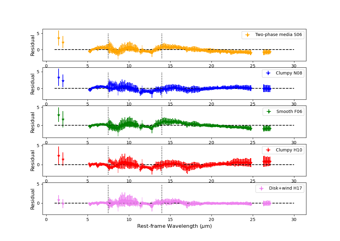
Figure 9: Average residuals for each model. The vertical lines separate the residuals in three parts for a better qualitative analysis (see the text).

6 Discussion

6.1 The NIR and MIR spectral indexes

Using the photometric IR data from the Infrared Space Observatory (ISO) Haas et al. (2003) analyzed the IR SEDs ($5-200\,\mu$m) of 64 PG QSOs. Particularly, they found that the spectral slopes $\alpha_{1,10\,\mu\text{m}}$ range from -0.9 to -2.2, and do not correlate with the inclination-dependent extinction effects in the picture of a dusty torus. They suggested that the diversity of the SEDs that they observed could be explained in terms of an evolutionary scenario, in which those QSOs with a redder MIR SED are in early evolutionary stages among QSOs preceded by a dusty ultraluminous infrared galaxy (ULIRG) phase (e.g., Sanders et al., 1988).

We measured four spectral indexes from ground-based high angular resolution SEDs. The first spectral index is calculated between the H (1.6 $\mu$m) and Si2 (8.7 $\mu$m) bands ($\alpha_{NIR-MIR(1.6,8.7)\mu\text{m}}$), the second between the Ks (2.2 $\mu$m) and Si2 (8.7 $\mu$m) bands ($\alpha_{NIR-MIR(2.2,8.7)\mu\text{m}}$), the third one between 7.8 and 9.8 $\mu$m ($\alpha_{MIR(7.8,9.8\,\mu\text{m})}$), and the last one is calculated between 9.8 and 11.7 $\mu$m ($\alpha_{MIR(9.8,11.7\,\mu\text{m})}$). We measured the two later MIR spectral indexes instead of the $10\,\mu$m silicate strength due to the low S/N of the high angular resolution spectra. The spectral index is estimated according to the following definition $\alpha_{2,1}=-\frac{log(f_{\nu}(\lambda_{2})/f_{\nu}(\lambda_{1}))}{log(\lambda_{2}/\lambda_{1})}$, where $\lambda_{2}>\lambda_{1}$ (see, e.g., Buchanan et al., 2006). In the case of the two MIR spectral indexes $\alpha_{MIR(7.8,9.8\,\mu\text{m})}$ and $\alpha_{MIR(9.8,11.7\,\mu\text{m})}$, the $\lambda_{2}$ and $\lambda_{1}$ wavelengths are chosen to fix the points on the continuum, avoiding the spectral range of low atmospheric transmission around $9\,\mu\text{m}$, and the PAH feature at 11.3 $\mu$m that is present in some objects.

In Table 6, we list the $\alpha_{NIR-MIR(1.6,8.7\,\mu\text{m})}$ and $\alpha_{NIR-MIR(2.2,8.7\,\mu\text{m})}$ spectral indexes measured after subtract the classic accretion disk from the data. On average, we find $\alpha_{NIR-MIR(1.6,8.7\,\mu\text{m})}=-1.1\pm 0.6$ and $\alpha_{NIR-MIR(2.2,8.7\,\mu\text{m})}=-1.2\pm 0.4$. Additionally, we list the values obtained assuming the bluer accretion disk. Note that there are fewer objects in this case because, in most cases, the accretion disk overestimates the emission in the NIR bands (see Section 4.2). For these objects assuming a bluer accretion disk does not affect the estimation of the NIR to MIR spectral indexes within the uncertainties. Our measurements of both NIR-MIR spectral indexes are similar to the ones reported by Haas et al. (2003).

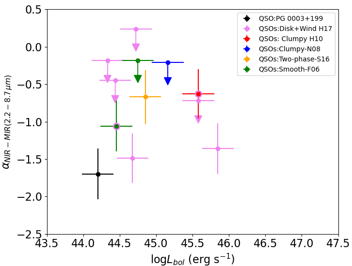
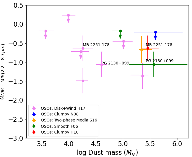
Figure 10: The NIR to MIR spectral index $\alpha_{NIR-MIR(2.2,8.7\,\mu\text{m})}$ versus the bolometric luminosity estimated from the X-ray luminosity (left), and versus the dust mass inferred from the corresponding model (right).

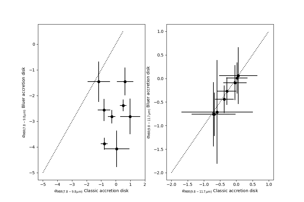
Figure 11: MIR spectral indexes obtained after subtract the bluer and classic accretion disk from the high angular resolution spectrum.

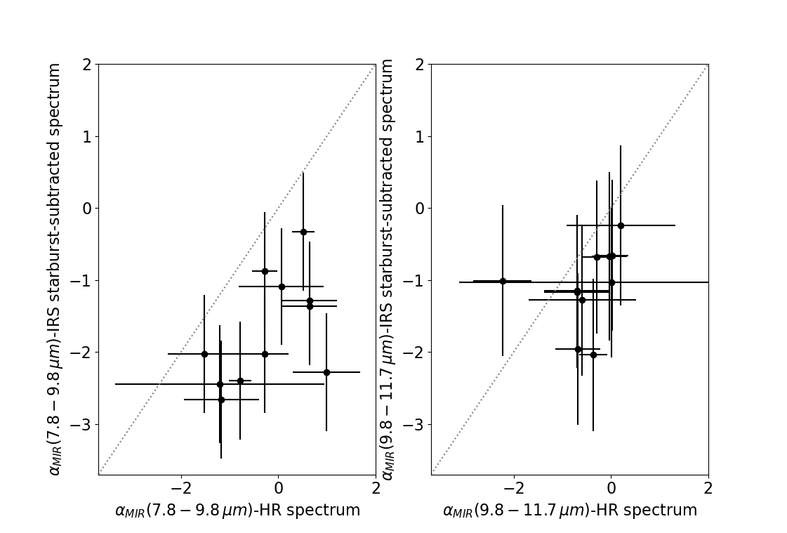
Figure 12: MIR spectral indexes were obtained after subtracting the classic accretion disk and the stellar and starburst components from the Spitzer/IRS spectrum against the MIR spectral indexes measured on the high angular resolution spectrum.

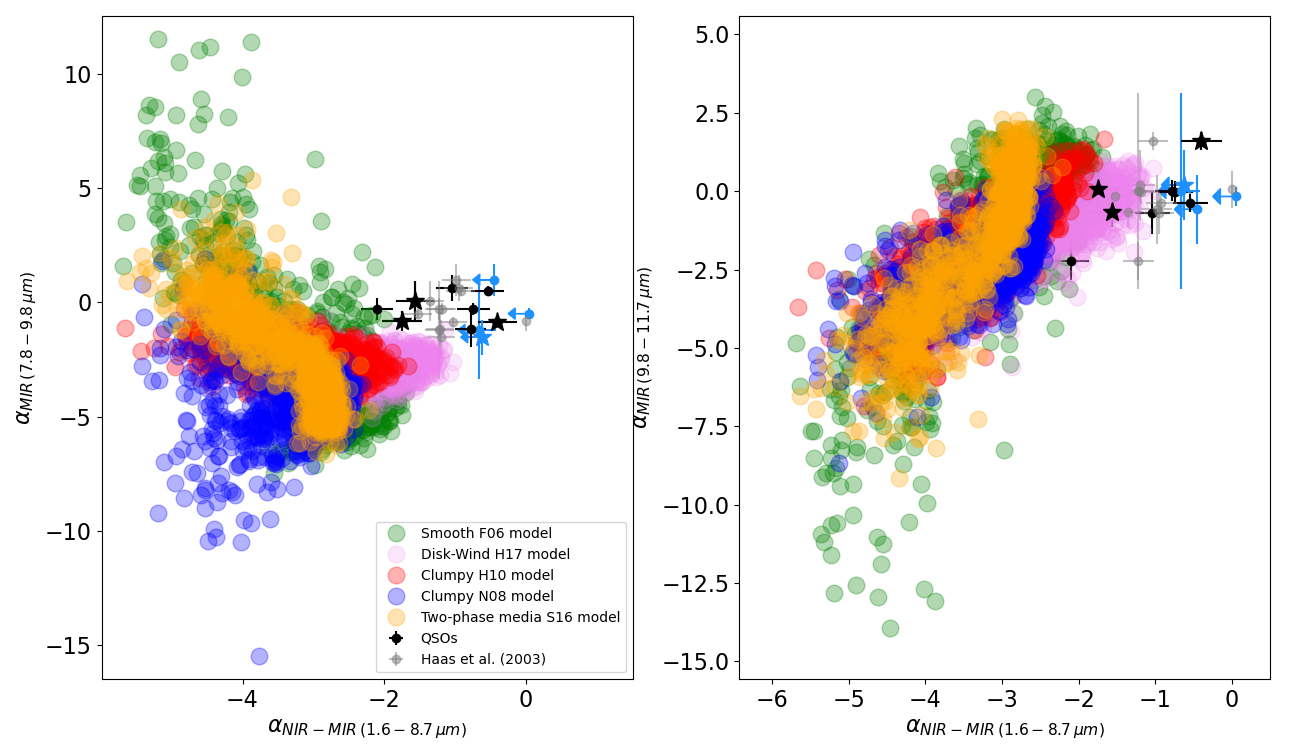
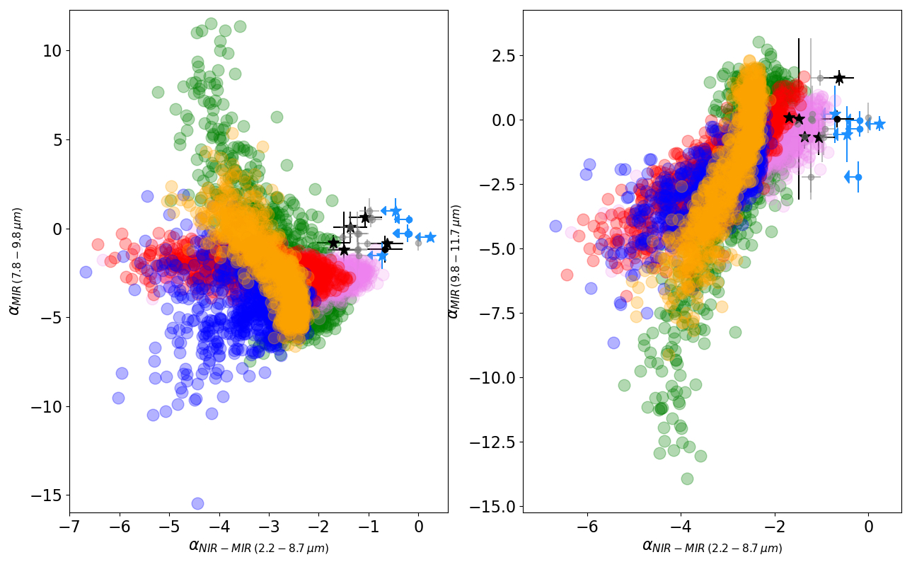
Figure 13: The synthetic and observed spectral indexes $\alpha_{MIR(7.8,9.8\,\mu\text{m})}$ and $\alpha_{MIR(9.8,11.7\,\mu\text{m})}$ versus the NIR to MIR spectral indexes $\alpha_{NIR-MIR(1.6,8.7)}$ and $\alpha_{NIR-MIR(2.2,8.7)}$ for all objects and models. The stars indicate that the spectral index is derived using the new NIR high angular resolution data.

In the left panel of Figure 10 we compare our measurements of the NIR to MIR $\alpha_{NIR-MIR(2.2,8.7)}$ spectral index listed in Table 6, with the AGN bolometric luminosity $L_{bol}$ and the dust mass. We estimated the bolometric luminosity using the hard X-ray (2-10 keV) flux and the relation derived by Marconi et al. (2004), see Martínez-Paredes et al. (2019). In the plots, we identify each object with the model that better fits their data, except for PG 0003+199 for which none of the models can fit with a red-$\chi^{2}<2$. We note that most objects have a NIR to MIR spectral index between $\sim 0$ and $-1.5$, which does not correlate with the bolometric luminosity nor with the dust mass. Haas et al. (2003) estimated the dust mass of some objects in our sample using equation 6 in Stickel et al. (2000) and assuming standard grain properties and a dust emissivity $\beta=2$. The mass that they derived varies from $\sim 10^{6}-10^{8}$ M_⊙, with an uncertainty that can vary up to an order of magnitude. However, due to the large uncertainties in the far-IR fluxes, the dust masses might be overestimated, as pointed out by the authors.

We estimate the MIR spectral indexes for two cases, one in which we subtracted the classic accretion disk from the high angular resolution spectrum and another in which we subtracted the bluer accretion disk. We find that for the MIR spectral index $\alpha_{MIR(9.8-11.7\mu\text{m})}$ both measurements give similar results ($\sim-0.2$). However, for the $\alpha_{MIR(7.8-9.8\mu\text{m})}$ the values obtained by assuming the bluer accretion disk are redder ($\sim-3$) than those obtained by assuming the classic accretion disk ($\sim-0.4$), see Figure 11. Additionally, we investigate if the inner star formation could be affecting our estimations of the MIR spectral indexes. We measure the slopes $\alpha_{MIR(7.8-9.8\mu\text{m})}$ and $\alpha_{MIR(9.8-11.7\mu\text{m})}$ on the starburst subtracted Spitzer/IRS spectrum, and comparing with the slopes measured on the high angular resolution spectra. We find that the starburst subtracted Spitzer/IRS MIR slopes are redder ($\sim-2$ for the slope between $7.8-9.8\mu\text{m}$). Figure 12 shows both spectral indexes, where the measurements are assuming the classic accretion disk.

These results suggest that although the high angular resolution spectrum is mostly dominated by the emission of the AGN, it is possible that the bluer spectral range of the spectrum is being affected by some dust components not directly related with the dust heated by the AGN.

Table 6: NIR-MIR spectral indexes obtained after subtracting the classic accretion disk. Column 1 list the names of the objects. Columns 2, 3 and 4 list the spectral index $\alpha_{NIR-MIR(1.6,8.7\,\mu\text{m})}$ and $\alpha_{NIR-MIR(2.2,8.7\,\mu\text{m})}$ calculated by us, and the spectral index $\alpha_{1,10\,\mu\text{m}}$ reported by Haas et al. (2003), respectively.

Name	This work	This work	Haas et al. (2003)
	$\alpha_{NIR-MIR(1.6,8.7\,\mu\text{m})}$	$\alpha_{NIR-MIR(2.2,8.7\,\mu\text{m})}$	$\alpha_{1,10\,\mu\text{m}}$
Mrk 509	$-1.57\pm 0.27$	$-1.36\pm 0.34$	…
PG 0050+124	$-0.78\pm 0.22$	$-0.67\pm 0.36$	-1.21
	$-1.15\pm 0.25^{*}$	$-0.79\pm 0.36^{*}$
PG 2130+099	$-1.04\pm 0.23$	$-1.06\pm 0.34$	-1.52
PG 1229+204a	$<-0.45$	$<-0.45$	-0.98
PG 0844+349a	$<0.05$	$<0.24$	…
PG 0003+199	$-1.75\pm 0.28$	$-1.70\pm 0.34$	…
PG 0804+761a	$<-0.62$	$<-0.72$	-1.20
PG 1440+356	$-0.54\pm 0.23$	$<-0.18$	-0.92
	…	$<-0.92^{*}$
PG 1426+015	$-2.10\pm 0.23$	$<-0.21$	-1.22
PG 1411+442	$-0.74\pm 0.23$	$<-0.18$	…
	…	$<-0.71^{*}$
PG 1211+143	$<-0.66$	$-1.49\pm 0.33$	-1.22
PG 1501+106	…	…	-1.03
MR 2251-178	$-0.40\pm 0.27$	$-0.63\pm 0.33$	…

Note.- ^aThe accretion disk is not subtracted. ^∗This values correspond to the case assuming the bluer accretion disk.

We measure the same spectral indexes for the five models to investigate how well the different models sampled the observed NIR and MIR spectral slopes. In Figure 13 we compare the synthetic and observed values (measured on the high angular resolution spectrum after subtracting the classic accretion disk). In general, we note that none of the models matches the region of the observed spectral indexes. Although the closer match occurs for the Disk+Wind H17 model, especially when comparing the $\alpha_{MIR(9.8,11.9\,\mu\text{m})}$ and the $\alpha_{NIR-MIR(2.2,8.7\,\mu\text{m})}$. However, it is likely that the limited estimation of the $\alpha_{MIR(7.8,9.8\,\mu\text{m})}$ spectral index is affecting the comparison with the models since a spectral index around -2, as obtained from the starburst subtracted Spitzer/IRS MIR slopes, compares better with the models.

Particularly, we note that the Clumpy N08 and Two-phase media S16 models predict NIR to MIR spectral indexes ($\alpha_{1.6,8.7}$ and $\alpha_{2.2,8.7}$ ) that are $\lesssim-2$, followed by the Clumpy H10 and Smooth F06 models that predict values $\lesssim-1.5$, and the Disk+Wind H17 model that predict values $\lesssim-0.8$. This result is consistent with the one obtained by Hönig & Kishimoto (2017) when compared the NIR to MIR (3, 6 $\mu$m) versus MIR (8, 14 $\mu$m) spectral indexes for the Clumpy H10 and the Disk+Wind H17 models. They showed that the Disk+Wind H17 models predict bluer NIR to MIR (3, 6 $\mu$m) spectral indexes, and claimed that they come from SEDs with a $3-5\,\mu$m bump. Moreover, they say that these SEDs correspond to models where the disk has relatively steep dust cloud distribution ($-2>a>-3$) and the wind shallower clouds distribution ($-0.5>a_{w}>-1.5$). We find that the average index of the cloud distribution in the disk and the wind is $a\sim-2.6$ and $a_{w}\sim-0.7$, respectively, suggesting that the most compact distribution of the clouds in the disk dominates the emission in the NIR, and therefore improves the fitting of this part of the SED.

From our analysis we found that the Disk+Wind SEDs predict the most bluer NIR to MIR spectral indexes. However, it is necessary for all models to better sample the region with NIR to MIR spectral index between $\sim-0.5$ and $\sim-2$, and MIR spectral index around zero, as it can be seen from Figure 13. This highlights the need for different dust distributions/compositions in the current phenomenological models available to the community.

Martínez-Paredes et al. (2020) found that the Disk+Wind H17 model is the best reproducing the AGN-dominated Spitzer/IRS spectrum for a sample of local type 1 AGNs, in which the $10\,\mu$m silicate emission feature is prominent. They obtained, on average, an index for the dust distribution in the disk $a\sim-1.9$ and an index for the dust distribution in the wind $a_{w}\sim-0.7$, which are similar to the values obtained for our sample of QSOs. Therefore, these results suggest that this model has a better treatment on the properties of the hot and warm dust, which dominates the emission between $\sim 1$ and $\sim 14\mu$m.

6.2 Torus/Disk geometry

Mor et al. (2009) used the Spitzer/IRS ($\sim 2-35\,\mu$m) spectra of 26 QSOs ($z\sim 0.06-0.33$) to investigate their main emission component. They found that the SED of these objects can be well reproduced by assuming three model components: 1) the Clumpy N08 model or dusty torus component, 2) the dusty narrow-line region cloud component, and 3) the blackbody-like dust component. They found that a substantial amount of the emission between $\sim 2-7\,\mu$m originates from a hot dust component, likely situated in the innermost part of the torus. Additionally, they found that the dust mass correlates with the bolometric luminosity, while the covering factor seems anti-correlated.

Later, Martínez-Paredes et al. (2017) found that the starburst-subtracted Spitzer/IRS spectrum ($\sim 8-15\,\mu$m) plus the NIR high angular resolution photometric point at H band from the NICMOS/HST of a sample of 20 QSOs ($z<0.1$) could be well modelled assuming only the Clumpy N08 model. However, they noted that the inclusion of the spectral range between $\sim 5-8\mu$m results in a poor fit of the silicate features at $9.7\,\mu$m, and therefore in a set of parameters inconsistent with an optically classified type 1 AGN.

Comparing the average residuals obtained from fitting the AGN-dominated Spitzer/IRS spectra of local type 1 AGNs, Martínez-Paredes et al. (2020) found that in general, none of the models can well reproduce the spectrum from $\sim 5-30\mu$m nor the 10 and 18 $\mu$m, silicate emission features. However, they noted that the Wind+Disk H17 model produces the flattest residuals, especially for objects with higher bolometric luminosities ($\sim 44.8-46.1$ erg s^-1 in log scale). Indeed, using a large sample of AGNs, González-Martín et al. (2019b) found that the Disk+Wind H17 models perform best for high luminosity AGNs ($44<log(L_{X(2-10\,\text{keV})})<44.5$ erg s^-1), while the Clumpy N08 model is better modelling low-luminosity AGNs, and the two-phase media S16 model seems to be better suited for intermediate luminosities.

In this work, we find that the NIR-MIR SED of QSOs is also better modelled by the Disk+Wind H17 model. Curiously, we note that for PG 1440+356 that fitted best with the Smooth F06 model, the next model that best fits the data is the Disk+Wind H17 one, while for PG 0050+124 that is best fitted with the Two-phase Media S16 model, the next model that best fit the data is the Smooth F06 model, suggesting that these QSOs always prefer the wind or smooth models rather than the clumpy models, probably since the former tend to produce bluer NIR SEDs. On the other hand, recently Woo et al. (2020) claimed that AGNs with stronger outflow are hosted by galaxies with higher star formation rates. Curiously, Martínez-Paredes et al. (2019) found that the star formation rate of these QSOs is more centrally concentrated on scales of hundreds of pc as predicted by the evolutionary models. Therefore, it is possible that the outflow, if present, is playing an important role in the geometrical distribution of the central dust of these objects. Recently, Garcia-Bernete et al. (2021) found that the IR high angular resolution SED of local Seyfert 1 also prefer the Wind+Disk H17 model instead of the torus models. These results suggest the presence of a hot dust component in nearby type 1 AGNs. Note that, unlike Seyferts, in QSOs, the unresolved emission comes from a spatial region of $\lesssim 1$ kpc. Considering these objects could be tracing different evolutionary stages (see e.g, Haas et al., 2003; Martínez-Paredes et al., 2019), in which the outflow could be responsible for the presence of polar dust on scales of hundreds of pc, could also explain the results that QSOs being best fitted by the Wind+Disk H17 model.

7 Summary and conclusions

Understanding the nearby QSOs inner molecular dust geometry and dust composition has been partly limited for the lack of a well-sampled SED at IR wavelengths. In this work, we use the cameras CIRCE and EMIR on the 10.4m Gran Telescopio CANARIAS to obtain new high angular resolution ($\sim 0.3$arcsec) photometry in the H (1.6 $\mu$m) and/or Ks (2.1 $\mu$m) bands, for a sample of 13 QSOs. We analyse these NIR high angular resolution images and find that the H- and Ks-band emission is mostly unresolved in most QSOs. We find that only MR 2251-178 shows an extended ($\sim 20\%$) emission in the H and Ks bands. Additionally, we use the high angular resolution and unresolved photometry and spectroscopy at N band ($\sim 7.5-13.5\,\mu$m) available for these objects. We complement these data with the low angular resolution ($\sim 3.5$arcssec) AGN-dominated ($>80\%$) Spitzer/IRS spectrum ($\sim 5-30\,\mu$m) to take advantage of the high S/N ratio offered by these spectra. In this way, we build for the first time well-sampled NIR to MIR SEDs for local QSOs.

To build a set of IR SEDs mainly dominated by the reprocessed emission of the dust, we decontaminate the unresolved high angular resolution data and the Spitzer/IRS spectrum from the emission of the accretion disk. We explore two power laws parametrizations for the accretion disk. The first is a classic accretion disk, for which we find that the contribution decreases from NIR to MIR wavelengths (H band $\sim 35\%$, Ks band $\sim 30\%$, and between $\sim 5-7.5\,\mu$m $\sim 2.4\%$) and becomes negligible at wavelengths $>7.5\mu$m. The second is a bluer accretion disk, for which we find the contribution in the NIR and MIR is larger when compared with the classic accretion disk. In the H and Ks bands, the contribution is $\sim 41\%$ (two objects) and $\sim 54\%$ (four objects), respectively. For the rest of the objects, the extrapolation of the bluer accretion disk overestimates the emission in the NIR. The contribution in the MIR is $\sim 17.5\%$ and $\sim 5.5\%$ for the high angular resolution spectrum and in the Spitzer/IRS spectrum, respectively. This is nearly six to seven times larger than the contribution of the classic accretion disk.

Assuming the Smooth dusty torus model (Fritz et al., 2006, F06), the Clumpy dusty torus models (Nenkova et al., 2008b; Hönig & Kishimoto, 2010b, N08 and H10), the Two-phase media torus model (Stalevski et al., 2016, S16), and the Disk+Wind model (Hönig & Kishimoto, 2017, H17), we investigate which model better reproduces simultaneously the NIR and MIR data. To fit the models we use the interactive spectral fitting program XSPEC from the HEASOFT package and select as acceptable fits those with a red-$\chi^{2}<2$. Then, we use the Akaike Information Criterion (AIC) to investigate the quality of the model. According to this criterion, we find that the Disk+Wind H17 model is the one better fits the objects ($64\%$, 9/13), followed by the Smooth torus model F06 ($14\%$, 2/13), the Clumpy torus H10 model ($7\%$, 1/13), the Clumpy torus N08 model ($7\%$, 1/13), and the Two-phase media S16 model ($7\%$, 1/13). We note that in general these objects prefer the wind and/or smooth models against the clumpy models, likely due to their flatter NIR SEDs. Additionally, we find that there is an object (PG 0003+199) that is not fitted by any model. Curiously this is the object with the lowest hard (2-10 keV) X-ray luminosity and with the poorest IR data set, since the Spitzer/IRS spectrum only covers $\sim 10-35\mu$m, and the flux in the redder border of the ground-based high angular resolution spectrum drops due to the lack of signal.

We make the same analysis using the observed SEDs that resulted from subtracting the bluer accretion disk. However, in this case, we find that the models fitted only 2/13 objects (PG 0050+124 and PG 1501+106). We find that the model that best reproduces the SED of these objects is the Disk+Wind H17 model, which is the same model obtained when assuming the classic accretion disk.

We calculate the average residual for each model. We find that the flattest residuals are obtained from the fits with the Disk+Wind H17 model. Comparing the angular width, viewing angle, covering factor, and dust mass derived from the best fits of each object, we note that the parameters are similar to the values previously obtained for a larger sample of type 1 AGNs using only the AGN-dominated Spitzer/IRS spectra.

Additionally, we use the unresolved fluxes at H ($1.6\,\mu$m), Ks ($2.2\,\mu$m), and Si2 (8.7 $\mu$m) bands after subtracting the contribution from the accretion disk, and calculate two NIR to MIR spectral indexes, one between 1.6 and 8.7 $\mu$m, and another one between 2.2 and 8.7 $\mu$m, and two MIR spectral indexes, one between 7.8 and 9.8 $\mu$m, and another one between 9.8 and 11.7 $\mu$m.

We compare the NIR to MIR spectral index $\alpha_{NIR-MIR\,(2.2,8.7\,\mu\text{m})}$, with the bolometric luminosity and the dust mass derived from the best fit and find no correlation. Additionally, we measure the both NIR to MIR spectral indexes, $\alpha_{NIR-MIR\,(1.6,8.7\,\mu\text{m})}$ and $\alpha_{NIR-MIR\,(2.2,8.7\,\mu\text{m})}$, for all five models. Comparing the synthetic and observed values we find that none of the models simultaneously match the measured NIR to MIR and 7.8-9.8 slopes. However, we note that measuring the MIR slope between 7.8 and 9.8 $\mu$m on the starburst-subtracted Spitzer/IRS spectrum gives values that are more similar to the synthetic ones. Therefore, it is likely that some components not directly related to the dust heated for the AGN could affect the bluer spectral range of the high angular resolution spectrum. Additionally, we note that the Disk+Wind H17 model has the closest values. This result is consistent with the fact that this model successfully reproduces most of the observed SEDs. We conclude that the differences among the synthetic and observed values highlight the need for different dust distributions/compositions in the phenomenological models.

Finally, we point out that a better understanding of the geometry and dust composition of the IR unresolved emission of QSOs will be possible with the forthcoming spectra from the Mid-Infrared Instrument on the James Webb Space Telescope. These spectra offer a similar angular resolution but better sensitivity, allowing to obtain a high angular resolution spectrum with a longer spectral range ($\sim 5-30\,\mu$m) for the faint and bright nearby QSOs. While the future ground-based big-sized optical telescopes, like the European Extremely Large Telescope (40m), the Thirty Meter Telescope (30m), and the Giant Magellan Telescope (25m), will allow observing the inner nuclear dust in more distant objects.

8 Tables of parameters

Table 7: Parameters H17. Column 1 lists the names of QSOs. Column 2 lists the viewing angle along the line of sight. Columns 3-5 list the parameters of the disk: the number of clouds along an equatorial line of sight, the power-law index of the radial distribution of dust clouds, and the dimensionless scale height. Columns 6-8 list the parameters of the wind: the angular width , half-opening angle of the wind, and power-law index of the radial distribution of dust clouds. Column 9 list the ratio between number of dust clouds along the cone and $N_{0}$. See equations in Hönig & Kishimoto (2017).

		Disk			Wind
Name	$i$	$N_{0}$	$a$	$h$	$\sigma_{\theta}$	$\Theta_{w}$	$a_{w}$	$f_{wd}$
	[0,90] deg	[5,10]	[-3.0,-0.5]	[0.1,0.5]	[7,15] deg	[30,45] deg	[-2.5,-0.5]	[0.15,0.75]
	mean (min, max)	mean (min, max)	mean (min, max)	mean (min, max)	mean (min, max)	mean (min, max)	mean (min, max)	mean (min, max)
Good fits according to a $red-\chi^{2}<2$ and the AIC criterion
Mrk509	70.5 (69.8, 90.0)	10.0 (9.9, 10.0)	-3.0 (-3.0, -3.0)	0.5 (0.1, 0.5)	12.9 (7.0, 13.3)	45.0 (44.5, 45.0)	-0.5 (-0.5, -0.5)	0.49 (0.50, 0.50)
PG1411+442	0.01 (0.01, 0.04)	10.0 (9.1, 10.0)	-3.0 (-3.0, -0.5)	0.4 (0.3, 0.5)	7.5 (7.0, 8.8)	36.7 (35.3, 45.0)	-1.2 (-2.5, -1.1)	0.75 (0.68, 0.75)
PG1211+143	58.1 (0.0, 90.0)	10.0 (5.0, 10.0)	-2.5 (-3.0, -2.5)	0.2 (0.1, 0.3)	15.0 (7.0, 15.0)	45.0 (30.0, 45.0)	-2.2 (-2.5, -2.1)	0.75 (0.15, 0.75)
PG1501+106∗	90.0 (89.3, 90.0)	5.0 (5.0, 5.2)	-3.0 (-3.0, -0.5)	0.2 (0.1, 0.5)	15.0 (14.8, 150)	. 45.0 (44.4, 45.0)	-0.5 (-2.5, -0.5)	0.45 (0.44, 0.47)
MR2251-178	45.06 (44.67, 45.56)	10.0 (9.9, 10.0)	-2.50 (-2.51 -2.50)	0.22 (0.19, 0.25)	15.0 (14.8, 15.0)	45.0 (44.9. 45.0)	-2.0 (-2.5, -2.0)	0.39 (0.38, 0.41)
PG1229+204	21.20 (0.01, 21.72)	10.0 (9.8, 10.0)	-2.5 (-2.6, -2.5)	0.50 (0.46, 0.50)	15.0 (14.6, 15.0)	45.0 (44.6, 45.0)	-1.50 (-1.51, -1.46)	0.75 (0.73, 0.75)
PG0844+349	17.11 (0.01, 20.37)	10.0 (5.0, 10.0)	-2.87 (-2.94, -2.67)	0.2 (0.1, 0.5)	15.0 (7.0, 15.0)	35.5 (33.7, 45.0)	-0.5 (-0.8, -0.5)	0.45 (0.33, 0.75)
PG0804+761	0.01 (0.01, 0.01)	9.5 (5.0, 10.0)	-3.0 (-3.0, -3.0)	0.29 (0.10, 0.30)	7.6 (7.0, 8.4)	34.9 (30.0, 35.9)	-0.5 (-0.5, -0.5)	0.75 (0.15, 0.75)
PG 2130+099	0.01 (0.01,0.01)	10.0 (10.0,10.0)	-2.05 (-2.14,-2.00)	0.5 (0.5,0.5)	10.0 (9.7,10.2)	45.0 (44.6,45.0)	-0.5 (-0.5,-0.5)	0.75 (0.72,0.75)
Accepted fits according to a $red-\chi^{2}<2$
PG 0050+124	0.01 (0.01, 0.02)	10.0 (9.9,10.0)	-1.6 (-1.7,-0.5)	0.3 (0.3,0.5)	7.0 (7.0,7.7)	45.0 (44.4,45.0)	-0.50 (-0.53,-0.50)	0.70 (0.62,0.75)
PG 1440+356	0.01 (0.01,0.01)	10.0 (9.9,10.0)	-3.0 (-3.0,-3.0)	0.31 (0.30,0.5)	14.2 (13.3,15.0)	42.0 (40.8,45.0)	-0.5 (-0.5,-0.5)	0.75 (0.74,0.75)

Table 8: Derived parameters H17 and foreground extinction. Column 1 lists the names. Column 2 and 3 list the dust mass in log scale and the covering factor (see the text for references on the equations). Column 4 lists the color excess for the foreground extinction $E(B-V)$.

Name	$log_{10}Dust_{mass}$ (M⊙)	$f_{cov}$	$E(B-V)$
	mean (min, max)	mean (min, max)
Mrk 509	5.36 (5.14;5.47)	0.40 (0.22;0.44)	$<0.08$
PG 1411+442	3.57 (3.44;3.72)	0.19 (0.16;0.23)	0.19 (0.17; 0.22)
PG 1211+143	4.26 (4.13;4.36)	0.38 (0.28;0.45)	$<0.02$
PG 1501+106	4.26 (4.07;4.45)	0.23 (0.18;0.38)	0.18 (0.15; 0.22)
MR 2251-178	5.01 (4.81;5.18)	0.28 (0.19;0.39)	0.22 (0.20; 0.24)
PG 1229+204	3.99 (3.87;4.12)	0.40 (0.32;0.46)	$<0.45$
PG 0844+349	4.22 (4.04;4.37)	0.32 (0.23;0.41)	$<0.06$
PG 0804+761	5.18 (5.03;5.29)	0.38 (0.28;0.45)	$<0.01$
PG 2130+099	3.8 (3.7, 3.9)	0.19 (0.16, 0.23)	0.39 (0.36; 0.43)
PG 0050+124	4.6 (4.5, 4.6)	0.41 (0.39, 0.44)	$<0.01$
PG 1440+356	4.1 (3.9, 4.2)	0.23 (0.18, 0.28)	0.33 (0.30; 0.37)

Table 9: Parameters H10. Column 1 list the names. Columns 2-6 list the viewing angle, number of dust clouds along the equatorial line of the torus, the angular width od the torus, the power-law index of the radial distribution of the dust clouds, and the optical depth of the dust clouds. See equations in Hönig & Kishimoto (2010b).

Name	$i$	$N_{0}$	$\theta$	$a$	$\tau_{\nu}$
	[0,90] deg	[2.5,10.0]	[5,60] deg	[-2.0,0.0]	[30,80]
	mean (min, max)	mean (min, max)	mean (min, max)	mean (min, max)	mean (min, max)
Good fits according to a $red-\chi^{2}<2$ and the AIC criterion
MR 2251-178	53.5 (51.5, 90.0)	7.8 (2.5, 8.2)	38.2 (34.9, 60.0)	-1.00 (-1.02, -0.98)	30.0 (30.0, 30.4)
Accepted fits according to a $red-\chi^{2}<2$
Mrk 509	31.4 (30.3,32.3)	10 (9.5,10.0)	47.4 (46.3,60.0)	-0.91 (-0.98,-0.01)	80 (79.4,80.0)
PG1211+143	52.9 (50.5,54.9)	10.0 (9.6,10.0)	51.9 (5.0,54.9)	-0.9 (-2.0,-0.9)	33.2 (30.1,36.9)
PG1440+356	51.3 (44.0, 90.0)	3.0 (2.7,10.0)	59.5 (5.0,60.0)	-1.7 (-1.7,-1.6)	80.0 (78.5,80.0)
PG 1501+106	89.5 (77.6,90.0)	10 (9.6,10.0)	45.1 (40.2,54.0)	-1.3 (-1.4,-1.3)	60.0 (30.0,65.4)
PG2130+099	45.00 (0.01,47.38)	10.0 (9.8,10.0)	54.5 (5.0,55.5)	-1.8 (-2.0,-1.8)	80.0 (79.2,80.0)
PG 0804+761	42.21 (39.38, 45.07)	6.29 (6.14, 10.0)	60.0 (59.2, 60.0)	-1.4 (-2.0, -1.4)	80.0 (79.7 80.0)
PG 0844+349	29.9 (25.8, 31.3)	8.8 (8.1, 9.5)	57.0 (54.9, 59.1)	-1.1 (-1.1, -1.1)	80.0 (79.2, 80.0)
PG 1229+204	56.69 (0.01, 73.86)	5.8 (4.9, 10.0)	31.5 (5.0, 60.0)	-1.07 (-2.0, -1.03)	66.2 (63.4, 80.0)
PG 1411+442	48.3 (44.7,90.0)	10.0 (9.3,10.0)	60.0 (5.0,60.0)	-1.91 (-1.93,-1.88)	80.0 (79.1,80.0)

Table 10: Derived parameters H10 and foreground extinction. Column 1 lists the names. Column 2 and 3 list the dust mass in log scale and the covering factor (see the text for references on the equations). Column 4 lists the color excess for the foreground extinction $E(B-V)$.

Name	$log_{10}Dust_{mass}$	$f_{cov}$	E(B-V)
	mean (min, max)	mean (min, max)
MR 2251-178	5.46 (5.35;5.66)	0.85 (0.78;0.92)	0.01 (0.01; 0.02)
Mrk 509	5.8 (5.7, 5.9)	0.92 (0.88, 0.93)	0.09 (0.07; 0.10)
PG 1211+143	4.4 (4.1, 4.6)	0.74 (0.46, 0.88)	0.01 (0.01; 0.03)
PG 1440+356	5.0 (4.8, 5.1)	0.93 (0.85, 0.95)	0.45 (0.41; 0.50)
PG 1501+106	4.9 (4.6, 5.1)	0.74 (0.5, 0.92)	0.04 (0.01; 0.09)
PG 2130+099	4.3 (4.2, 4.4)	0.64 (0.53, 0.74)	0.55 (0.53; 0.57)
PG 0804+761	5.3 (4.9, 5.5)	0.64 (0.31, 0.88)	0.01 (0.01; 0.02)
PG 0844+349	4.5 (4.1, 4.8)	0.71 (0.32, 0.9)	0.01 (0.01; 0.02)
PG 1229+204	4.2 (3.9, 4.4)	0.71 (0.44, 0.92)	0.28 (0.19; 0.36)
PG 1411+442	4.61 (4.46;4.69)	0.93 (0.88;0.95)	0.17 (0.15; 0.20)

Table 11: Parameters N08. Column 1 lists the names. Column 2-7 list the viewing angle, the number of clouds along the equatorial line, the angular width, the outer to inner radius ratio of the torus, the index of the power-law distribution, and the optical depth of the dust clouds in the torus. See equations in Nenkova et al. (2008b).

Name	$i$	$N_{0}$	$\sigma$	$Y$	$q$	$\tau_{V}$
	[0,90] deg	[1,15]	[15,70] deg	[5,100]	[0,2.5]	[5,300]
	mean (min,max)	mean (min,max)	mean (min,max)	mean (min,max)	mean (min,max)	mean (min,max)
Good fits according to a $red-\chi^{2}<2$ and the AIC criterion
PG 1426+015	25.6 (13.4, 44.8)	13.9 (9.4, 15.0)	15.0 (15.0, 27.1)	5.0 (5.0, 100)	2.5 (2.4, 2.5)	60.2 (55.4, 78.9)
PG 1426+015a	$64^{+9}_{-8}$	$9^{+3}_{-3}$	$19^{+3}_{-2}$	$60^{+23}_{-27}$	$2^{+0.4}_{-0.4}$	$118^{+14}_{-23}$
PG 1426+015b	30	5	35	33	1	75
Accepted fits according to a $red-\chi^{2}<2$
PG1211+143	80.0 (74.9,90.0)	9.0 (1.0,13.0)	17.5 (15.0,70.0)	5.0 (5.0,5.1)	2.5 (2.4,2.5)	44.01 (38.87,47.62)
PG1211+143a	$80^{+6}_{-10}$	$2^{+13}_{-1}$	$45^{+12}_{-8}$	$40^{+4}_{-3}$	$1.43^{+0.05}_{0.05}$	$38^{+3}_{-3}$
PG1501+106$*$	90.0 (86.6,90.0)	15.0 (14.0, 15.0)	32.3 (15.0,42.2)	9.99 (9.74,10.09)	2.24 (2.15,2.25)	18.49 (17.63,300.0)
PG1501+106a	$40^{+23}_{-21}$	$10^{+3}_{-3}$	$58^{+7}_{-8}$	$40^{+32}_{-18}$	$2.6^{+0.2}_{-0.2}$	$113^{+16}_{-14}$
PG 0804+761	90.0 (88.1, 90.0)	1.0 (1.0, 1.0)	45.1 (40.0, 54.5)	5.5 (5.0, 5.5)	2.5 (2.5, 2.5)	55.0 (10.0, 55.4)
PG 0804+761a	$22^{+15}_{-12}$	$5^{+4}_{-2}$	$22^{+10}_{-4}$	$59^{+23}_{-29}$	$1.8^{+0.1}_{-0.2}$	$42^{+22}_{-17}$
PG 0844+349	90.0 (87.3, 90.0)	3.8 (3.4, 4.4)	34.8 (16.0, 47.6)	100.0 (74.8, 100.0)	2.5 (2.5, 2.5)	19.9 (18.5, 21.8)
PG 0844+349a	$88^{+1}_{-3}$	$2^{+13}_{-1}$	$16^{+1}_{-1}$	$77^{+15}_{30}$	$1.3^{+0.2}_{-0.1}$	$77^{+25}_{-15}$
PG 1229+204	90.0 (78.1, 90.0)	15.0 (14.4, 15.0)	62.3 (47.0, 70.0)	22.0 (19.1, 100.0)	2.2 (2.1, 2.5)	10.0 (10.0, 10.6)
PG 1229+204a	$73^{+2}_{-3}$	$12^{+2}_{-3}$	$16^{+1}_{-1}$	$59^{+20}_{-18}$	$0.53^{+0.10}_{-0.07}$	$20^{+9}_{-5}$
PG 1229+204b	28	5	34	33	2	91
MR2251-178	64.8 (62.2, 72.9)	9.6 (1.0, 9.9)	70.0 (66.6, 70.0)	10.0 (9.8, 10.1)	2.2 (0.0, 2.3)	10.0 (10.0, 10.0)

Note.-^aParameters obtained by Martínez-Paredes et al. (2017). ^bParameters obtained by Mor et al. (2009). ^∗NIR data not available.

Table 12: Derived parameters N08 and foreground extinction. Column 1 list the name. Column 2, 3 and 4 list the dust mass in log scale and the covering factor, and outer radius of the torus (see the text for references on the equations). Column 5 lists the color excess for the foreground extinction $E(B-V)$. Columns 6 and 7 list the covering factor previously derived by Martínez-Paredes et al. (2017) and Mor et al. (2009), respectively.

Name	$log_{10}Dust_{mass}$ (M⊙)	$f_{cov}$	$R_{out}$ (pc)	$E(B-V)$	$f_{cov}^{a}$	$f_{cov}^{b}$
	mean (min, max)	mean (min, max)	mean (min, max)
PG 1426+015	5.6 (5.2; 6.1)	0.87 (0.77; 0.95)	3.4 (3.4; 4.3)	0.13 (0.07; 0.21)	$0.14^{+0.02}_{-0.04}$	0.33
PG 1211+143	3.1 (3.0, 3.5)	0.52 (0.36, 0.66)	1.9 (1.9, 1.9)	0.01 (0.01; 0.02)	$0.4^{+0.1}_{-0.1}$
PG 1501+106∗	5.8 (4.8, 7.3)	0.80 (0.54, 0.93)	19.5 (7.9, 30.3)	0.01 (0.01; 0.02)	$0.9^{+0.1}_{-0.1}$
PG 0804+761	4.0 (3.9, 4.2)	0.84 (0.69, 0.92)	5.5 (5.5, 5.5)	0.09 (0.06; 0.11)	$0.2^{+0.1}_{-0.1}$
PG 0844+349	3.3 (3.0, 3.7)	0.64 (0.44, 0.87)	2.1 (2.1, 2.1)	0.02 (0.01; 0.08)	$0.040^{+0.01}_{0.004}$
PG 1229+204	3.1 (2.9, 3.4)	0.74 (0.52, 0.93)	1.5 (1.5, 1.5)	0.05 (0.01; 0.13)	$0.1^{+0.01}_{-0.01}$	0.31
MR 2251-178	4.0 (3.9, 4.2)	0.64 (0.48, 0.82)	5.5 (5.5, 5.5)	0.01 (0.01; 0.01)	$0.4^{+0.3}_{-0.2}$

Note.-^aParameters obtained by Martínez-Paredes et al. (2017). ^bParameters obtained by Mor et al. (2009). ^∗NIR data not available.

Table 13: Parameters F06. Column 1 lists the names. Columns 2-7 list the viewing angle, the angular width of the torus, the power-law index of the polar density gradient, the power-law index of the radial density gradient, the outer to inner radius ratio of the torus, and the optical depth of the torus. See equations in Fritz et al. (2006).

Name	$90-i^{*}$	$\sigma$	$\gamma$	$\beta$	$Y$	$\tau_{V}$
	[0,90] deg	[20,60] deg	[0,6]	[-1.0,0.0]	[10,150]	[0.3,10]
Good fits according to a $red-\chi^{2}<2$ and the AIC criterion
PG 2130+099	49.0 (0.0, 51.1)	38.2 (35.9, 39.9)	0.01 (0.0, 6.0)	-0.50 (-0.58, -0.46)	10.0 (10.0, 150.0)	0.9 (0.1 1.0)
PG 1440+356	39.3 (0.0, 44.4)	60.0 (57.9, 60.0)	2.0 (1.3, 2.6)	-0.74 (-0.75, -0.74)	11.7 (10.0, 11.9)	0.5 (0.4 10.0)
Good fits according to a $red-\chi^{2}<2$
Mrk 509	69.3 (68.5,70.0)	20.0 (20.0,20.4)	0.07 (0.07,6.0)	-0.05 (-0.07,-0.01)	10.0 (10.0,10.0)	3.6 (3.4,3.7)
PG 0050+124	53.8 (48.4,90.0)	22.1 (20.0,60.0)	6.0 (6.0,6.0)	-0.57 (-0.59,-0.01)	10.1 (10.0,10.2)	6.7 (6.2,6.9)
PG 1211+143	14.48 (0.01,15.75)	20.0 (20.0,20.2)	6.0 (6.0,6.0)	-0.01 (-0.01,-0.01)	10.0 (10.0,10.01)	9.3 (9.0,9.8)
PG 1501+106	0.01 (0.01,0.02)	20.0 (20.0,20.1)	6.0 (5.9,6.0)	-0.15 (-0.16,-0.12)	10.0 (10.0,10.01)	10.0 (10.0,10.0)
PG 0804+761	64.8 (61.4, 69.2)	20.0 (20.0, 21.1)	0.01 (0.01, 0.01)	-0.9 (-1.0, -0.8)	10.0 (10.0, 10.0)	0.60 (0.58, 0.61)
PG 0844+349	0.01 (0.01, 9.62)	20.0 (20.0, 20.9)	3.37 (0.01, 3.62)	-0.25 (-1.0, -0.15)	10.0 (10.0, 10.0)	2.2 (0.1, 2.4)
PG 1229+204	0.51 (0.01, 3.37)	20.0 (20.0, 20.6)	5.85 (0.01, 5.88)	-0.3 (-1.0, -0.2)	10.0 (10.0, 10.0)	10.0 (9.9, 10.0)
PG 1411+442	68.3 (0.0, 68.8)	20.0 (20.0, 20.2)	0.01 (0.0, 6.)	-1.0 (-1.0, 0.0)	10.0 (10.0, 150.0)	0.62 (0.61, 10.0)

Note.-^∗In order to do a proper comparison between the orientation of the viewing angle predicted by the several models we list the $90-i$ angle, since in F06 model the viewing angle increases from the polar to the equatorial axis.

Table 14: Derived parameters F06 and foreground extinction. Column 1 lists the names. Column 2, 3 and 4 list the dust mass in log scale and the covering factor, and outer radius of the torus (see the text for references on the equations). Column 5 lists the color excess for the foreground extinction $E(B-V)$.

Name	$log_{10}Dust_{mass}$ (M⊙)	$f_{cov}$	$R_{out}$ (pc)	E(B-V))
	mean (min, max)	mean (min, max)	mean (min, max)
PG 2130+099	5.6 (5.1;6.2)	0.86 (0.84;0.88)	21.87 (21.87;22.47	0.48 (0.43; 0.52)
PG 1440+356	5.0 (4.8;5.0)	0.14 (0.12;0.16)	3.90 (3.90;4.74)	0.68 (0.66; 0.74)
Mrk 509	10.5 (10.2, 10.5)	0.15 (0.15, 0.17)	13.9 (13.9, 13.9)	0.01 (0.01; 0.02)
PG 0050+124	5.2 (5.1, 5.4)	0.04 (0.02, 0.06)	27.2 (17.7, 39.5)	0.01 (0.01; 0.01)
PG 1211+143	5.0 (5.0, 5.3)	0.20 (0.16, 0.22)	4.4 (3.6, 5.9)	0.01 (0.01; 0.01)
PG 1501+106	7.7 (7.1, 8.3)	0.22 (0.14, 0.35)	25.7 (10.7, 42.7)	0.01 (0.01; 0.03)
PG 0804+761	5.9 (5.8, 6.1)	0.04 (0.02, 0.06)	10.2 (10.2, 12.4)	0.01 (0.01; 0.02)
PG 0844+349	5.1 (4.9, 5.2)	0.04 (0.02, 0.12)	7.1 (5.4, 14.4)	0.01 (0.01; 0.02)
PG 1229+204	7.3 (5.7, 8.5)	0.90 (0.80, 0.96)	19.8 (11.0, 27.5)	0.01 (0.01; 0.03)
PG 1411+442	6.1 (5.9;6.5)	0.92 (0.77;0.96)	21.30 (15.54;26.02)	0.39 (0.36; 0.41)

Table 15: Parameters S16. Column 1 is for the name. Columns 2-7 show the viewing angle, the angular width, the power-law index of the radial density gradient, the power-law index of the polar density gradient, the outer to inner radius ratio of the torus, and the optical depth of the torus. See equations in Stalevski et al. (2016).

Name	$i$	$\sigma$	$p$	$q$	$Y$	$\tau_{\nu}$
	[0,90] deg	[10,80] deg	[0,1.5]	[0,1.5]	[10,30]	[3,11]
Good fits according to a $red-\chi^{2}<2$ and the AIC criterion
PG 0050+124	0.01 (0.01, 0.03)	64.8 (63.6, 80.0)	0.01 (0.01, 0.02)	1.5 (0.0, 1.5)	10.0 (10.0, 30.0)	6.2 (6.0, 6.5)
Good fits according to a $red-\chi^{2}<2$
PG 1440+356	70.0 (69.7,70.3)	10.0 (10.0,10.0)	1.5 (1.5,1.5)	0.01 (0.01,0.01)	10.0 (10.0,10.1)	11.0 (11.0,11.0)
PG 1501+106	11.7 (9.4,12.9)	80.0 (79.8,80.0)	1.45 (1.40,1.50)	0.01 (0.01,0.01)	10.0 (10.0,10.02)	5.02 (4.9,5.2)
PG 2130+099	19.9 (15.4,22.4)	60.0 (59.1,61.2)	1.5 (1.5,1.5)	1.5 (1.5,1.5)	10.0 (10.0,10.0)	8.7 (8.0,11.0)
MR 2251-178	80.0 (79.2, 85.8)	80.0 (79.8, 80.0)	1.5 (1.5, 1.5)	0.84 (0.82, 0.87)	10.0 (10.0, 10.0)	3.0 (3.0, 3.0)
PG0804+761	42.3 (40.7, 43.7)	70.0 (69.8, 70.2)	1.5 (1.5, 1.5)	1.5 (1.5, 1.5)	10.0 (10.0, 10.0)	3.0 (3.0, 3.0)
PG 0844+349	57.6 (44.1, 67.3)	80.0 (69.8, 80.0)	1.5 (1.5, 1.5)	1.5 (1.4, 1.5)	10.0 (10.0, 10.2)	3.8 (3.6, 4.5)
PG 1229+204	63.6 (45.0, 68.0)	79.2 (73.7, 80.0)	1.5 (1.4, 1.5)	0.90 (0.81, 1.50)	10.0 (10.0, 10.2)	6.9 (6.6, 7.2)

Table 16: Derived parameters S16 and foreground extinction. Column 1 is for the name. Column 2, 3 and 4 show the dust mass, the covering factor, and outer radius of the torus (see the text for references on the equations). Column 5 lists the color excess for the foreground extinction $E(B-V)$.

Name	$log_{10}Dust_{mass}$ (M⊙)	$f_{cov}$	$R_{out}$ (pc)	E(B-V)
	mean (min, max)	mean (min, max)	mean (min, max)
PG 0050+124	5.3 (5.3;5.5)	0.95 (0.94;0.96)	5.49 (4.4;6.6)	0.01 (0.01; 0.01)
PG 1440+356	5.4 (5.3, 5.4)	0.87 (0.84, 0.89)	3.3 (3.2, 3.5)	0.68 (0.66; 0.74)
PG 1501+106	6.1 (5.9, 6.2)	0.97 (0.94, 0.98)	5.9 (4.4, 8.7)	0.01 (0.01; 0.03)
PG 2130+099	5.2 (5.0, 5.3)	0.68 (0.66, 0.70)	6.3 (6.0, 6.4)	0.48 (0.43; 0.52)
MR 2251-178	6.0 (6.0, 6.4)	0.95 (0.95, 0.95)	8.9 (8., 15.5)	0.01 (0.01; 0.01)
PG 0804+761	6.7 (6.6, 6.9)	0.98 (0.98, 0.98)	14.5 (11.1, 19.2)	0.01 (0.01; 0.02)
PG 0844+349	5.9 (5.8, 6.0)	0.98 (0.98, 0.98)	6.4 (5.0, 7.8)	0.01 (0.01; 0.02)
PG 1229+204	5.3 (5.1, 5.4)	0.96 (0.94, 0.98)	5.8 (4.9, 6.2)	0.01 (0.01; 0.03)

9 SED modeling

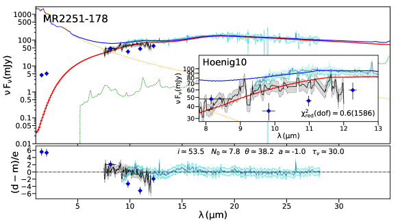
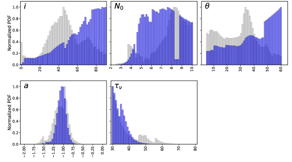
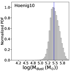
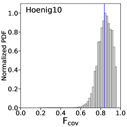
Figure 17: As Figure 16 but for the Clumpy H10 model.

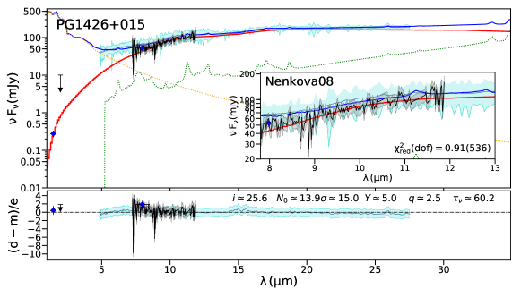
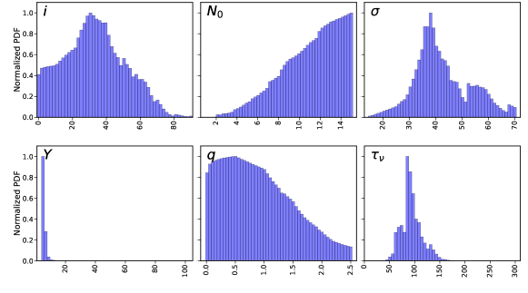
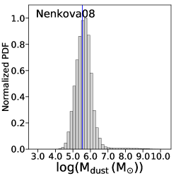
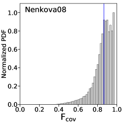
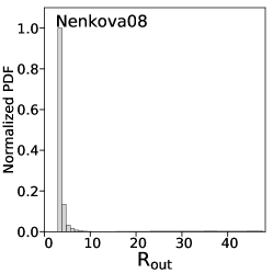
Figure 19: The SED of PG 1426+015 best modeled by the Clumpy N08 model. Upper panel: the high angular resolution photometric points are plotted as blue points with their error bars, the black arrows are upper limits. The high angular resolution spectrum is plotted with a black solid line, the grey shaded region represent the errors. The Spitzer/IRS spectrum is plotted with a dark cyan solid line and its error with a cyan shaded region. The red solid line is the best model resulting from fit the high angular resolution data. The green and yellow dotted lines are the starburst and stellar components, respectively. The blue solid line represents the sum of the stellar, starburst and torus components that best fit the Spitzer/IRS spectrum. Middle panel. The model parameters derived: normal probability distribution function of the free parameters. In grey we plot the parameters derived from fit the LSR spectrum, while in dark blue the distribution of the parameters derived from fit the FSR spectrum. Bottom panel: normal PDF of the derived parameters. The blue vertical line indicate the mean.

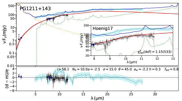
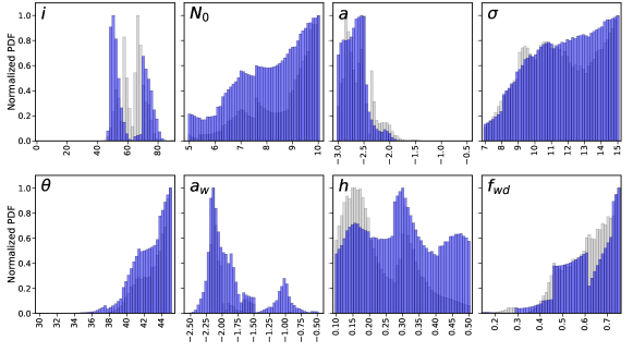
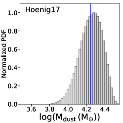
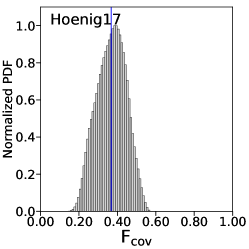
Figure 20: As Figure 18 but for the QSO PG 1211+143.

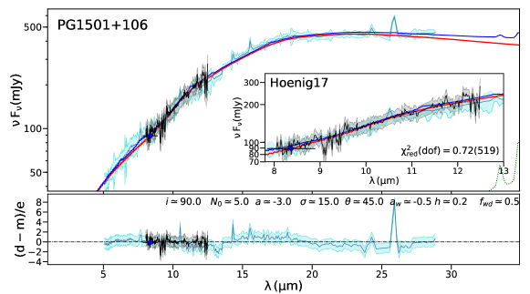
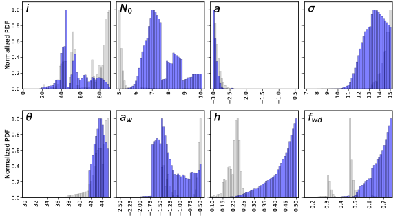
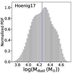
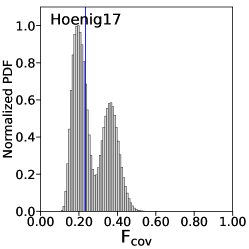
Figure 21: As Figure 18 but for the QSO PG 1501+106.

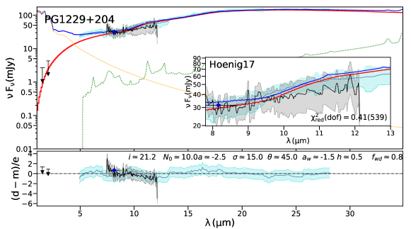
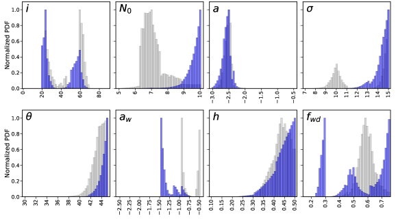
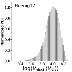
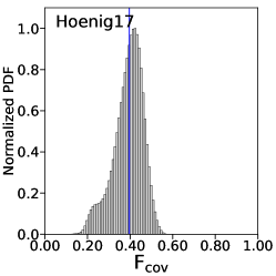
Figure 22: As Figure 18 but for the QSO PG 1229+204.

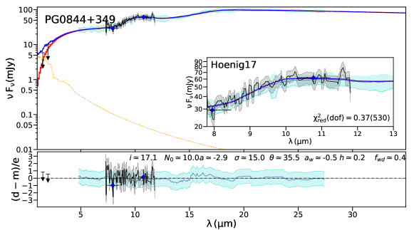
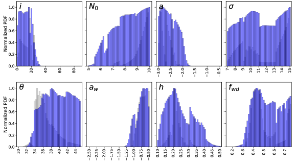
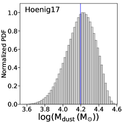
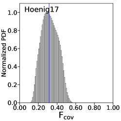
Figure 23: As Figure 18 but for the QSO PG 0844+349.

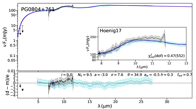
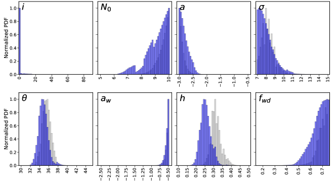
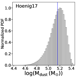
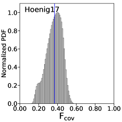
Figure 24: As Figure 18 but for the QSO PG 0804+761.

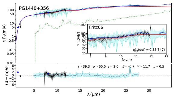
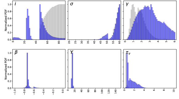
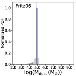
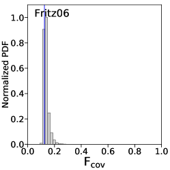
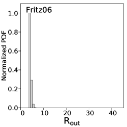
Figure 25: The SED of PG 1440+356 best modeled by the Smooth F06 model. Upper panel: the high angular resolution photometric points are plotted as blue points with their error bars, the black arrows are upper limits. The high angular resolution spectrum is plotted with a black solid line, the grey shaded region represent the errors. The Spitzer/IRS spectrum is plotted with a dark cyan solid line and its error with a cyan shaded region. The red solid line is the best model resulting from fit the high angular resolution data. The green and yellow dotted lines are the starburst and stellar components, respectively. The blue solid line represents the sum of the stellar, starburst and torus components that best fit the Spitzer/IRS spectrum. Middle panel. The model parameters derived: normal probability distribution function of the free parameters. In grey we plot the parameters derived from fit the LSR spectrum, while in dark blue the distribution of the parameters derived from fit the FSR spectrum. Bottom panel: normal PDF of the derived parameters. The blue vertical line indicate the mean.

References

- H. Akaike (1974) Akaike, H., 1974, IEEE Transactions on Automatic Control, 19, 6, 716-723, doi: 10.1109/TAC.1974.1100705.
- Alonso-Herrero et al. (2011) Alonso-Herrero, A., Ramos Almeida, C., Mason, R., et al. 2011, ApJ, 736, 82
- Alonso-Herrero et al. (2018) Alonso-Herrero, A., Pereira-Santaella, M., García-Burillo, S., et al. 2018, ApJ, 859, 144. doi:10.3847/1538-4357/aabe30
- Antonucci (1993) Antonucci, R. 1993, ARA&A, 31, 473
- Arnaud (1996) Arnaud, K. A. 1996, Astronomical Data Analysis Software and Systems V, 101, 17
- Asmus et al. (2016) Asmus, D., Hönig, S. F., & Gandhi, P. 2016, ApJ, 822, 109
- Balcells et al. (2000) Balcells, M., Guzman, R., Patron, J., et al. 2000, Proc. SPIE, 4008, 797. doi:10.1117/12.395538
- Barvainis (1987) Barvainis, R. 1987, ApJ, 320, 537
- Bianchi et al. (2011) Bianchi, L., Herald, J., Efremova, B., et al. 2011, Ap&SS, 335, 161
- Bianchi et al. (2017) Bianchi, L., Shiao, B., & Thilker, D. 2017, ApJS, 230, 24
- Bock et al. (2000) Bock, J. J., Neugebauer, G., Matthews, K., et al. 2000, AJ, 120, 2904
- Braatz et al. (1993) Braatz, J. A., Wilson, A. S., Gezari, D. Y., et al. 1993, ApJ, 409, L5
- Bradley et al. (2019) Bradley, L., Sipocz, B., Robitaille, T., et al. 2019, Zenodo
- Bruzual & Charlot (2003) Bruzual, G. & Charlot, S. 2003, MNRAS, 344, 1000
- Buchanan et al. (2006) Buchanan, C. L., Kastner, J. H., Forrest, W. J., et al. 2006, AJ, 132, 1890
- Burbidge & Stein (1970) Burbidge, G. R., & Stein, W. A. 1970, ApJ, 160, 573
- Burtscher et al. (2013) Burtscher, L., Meisenheimer, K., Tristram, K. R. W., et al., 2013, A&A, 558, AA149
- Cameron et al. (1993) Cameron, M., Storey, J. W. V., Rotaciuc, V., et al. 1993, ApJ, 419, 136
- Capellupo et al. (2015) Capellupo, D. M., Netzer, H., Lira, P., et al. 2015, MNRAS, 446, 3427
- Combes et al. (2019) Combes, F., García-Burillo, S., Audibert, A., et al. 2019, A&A, 623, A79. doi:10.1051/0004-6361/201834560
- Davis & Laor (2011) Davis, S. W., & Laor, A. 2011, ApJ, 728, 98
- Deo et al. (2011) Deo, R. P., Richards, G. T., Nikutta, R., et al. 2011, ApJ, 729, 108
- Dullemond & van Bemmel (2005) Dullemond, C. P., & van Bemmel, I. M. 2005, A&A, 436, 47
- Eikenberry et al. (2018) Eikenberry, S. S., Charcos, M., Edwards, M. L., et al. 2018, Journal of Astronomical Instrumentation, 7, 1850002-264. doi:10.1142/S2251171718500022
- Elvis et al. (1994) Elvis, M., Wilkes, B. J., McDowell, J. C., et al. 1994, ApJS, 95, 1
- Esparza-Arredondo et al. (2019) Esparza-Arredondo, D., González-Martín, O., Dultzin, D., et al. 2019, ApJ, 886, 125
- Feltre et al. (2012) Feltre, A., Hatziminaoglou, E., Fritz, J., & Franceschini, A. 2012, MNRAS, 426, 120
- Fischer et al. (2006) Fischer, S., Iserlohe, C., Zuther, J., et al. 2006, New A Rev., 50, 736
- Fritz et al. (2006) Fritz, J., Franceschini, A., & Hatziminaoglou, E. 2006, MNRAS, 366, 767
- Fuller et al. (2016) Fuller, L., Lopez-Rodriguez, E., Packham, C., et al. 2016, MNRAS, 462, 2618
- García-Bernete et al. (2019) García-Bernete, I., Ramos Almeida, C., Alonso-Herrero, A., et al. 2019, MNRAS, 486, 4917. doi:10.1093/mnras/stz1003
- Garcia-Bernete et al. (2021) Garcia-Bernete, I., et al. 2021, In prep
- García-Burillo et al. (2016) García-Burillo, S., Combes, F., Ramos Almeida, C., et al. 2016, ApJ, 823, L12
- García-Burillo et al. (2019) García-Burillo, S., Combes, F., Ramos Almeida, C., et al. 2019, A&A, 632, A61. doi:10.1051/0004-6361/201936606
- Garner et al. (2016) Garner, A., Eikenberry, S. S., Charcos, M., et al. 2016, Proc. SPIE, 9908, 99084Q. doi:10.1117/12.2232672
- González-Martín et al. (2019a) González-Martín, O., Masegosa, J., García-Bernete, I., et al. 2019, ApJ, 884, 10
- González-Martín et al. (2019b) González-Martín, O., Masegosa, J., García-Bernete, I., et al. 2019, ApJ, 884, 11. doi:10.3847/1538-4357/ab3e4f
- Guyon et al. (2006) Guyon, O., Sanders, D. B., & Stockton, A. 2006, ApJS, 166, 89
- Haas et al. (2003) Haas, M., Klaas, U., Müller, S. A. H., et al. 2003, A&A, 402, 87. doi:10.1051/0004-6361:20030110
- Hernán-Caballero et al. (2016) Hernán-Caballero, A., Hatziminaoglou, E., Alonso-Herrero, A., et al. 2016, MNRAS, 463, 2064
- Hodapp et al. (1996) Hodapp, K.-W., Hora, J. L., Hall, D. N. B., et al. 1996, New A, 1, 177
- Hönig et al. (2010a) Hönig, S. F., Kishimoto, M., Gandhi, P., et al. 2010, A&A, 515, A23
- Hönig & Kishimoto (2010b) Hönig, S. F., & Kishimoto, M. 2010, A&A, 523, A27
- Hönig et al. (2012) Hönig, S. F., Kishimoto, M., Antonucci, R., et al. 2012, ApJ, 755, 149
- Hönig et al. (2013) Hönig, S. F., Kishimoto, M., Tristram, K. R. W., et al. 2013, ApJ, 771, 87
- Hönig & Kishimoto (2017) Hönig, S. F., & Kishimoto, M. 2017, ApJ, 838, L20
- Hönig (2019) Hönig, S. F. 2019, ApJ, 884, 171. doi:10.3847/1538-4357/ab4591
- Hopkins & Quataert (2010) Hopkins, P. F. & Quataert, E. 2010, MNRAS, 407, 1529
- Hubeny et al. (2001) Hubeny, I., Blaes, O., Krolik, J. H., et al. 2001, ApJ, 559, 680
- Ichikawa et al. (2015) Ichikawa, K., Packham, C., Ramos Almeida, C., et al. 2015, ApJ, 803, 57
- Imanishi et al. (2011) Imanishi, M., Imase, K., Oi, N., et al. 2011, AJ, 141, 156
- Imanishi et al. (2018) Imanishi, M., Nakanishi, K., Izumi, T., et al. 2018, ApJ, 853, L25
- Jaffe et al. (2004) Jaffe, W., Meisenheimer, K., Röttgering, H., et al. 2004, The Interplay Among Black Holes, Stars and ISM in Galactic Nuclei, 37
- Kishimoto et al. (2008) Kishimoto, M., Antonucci, R., Blaes, O., et al. 2008, Nature, 454, 492. doi:10.1038/nature07114
- Krolik & Begelman (1988) Krolik, J. H., & Begelman, M. C. 1988, ApJ, 329, 702
- Lebouteiller et al. (2011) Lebouteiller, V., Barry, D. J., Spoon, H. W. W., et al., 2011, ApJS, 196, 8
- Leftley et al. (2018) Leftley, J. H., Tristram, K. R. W., Hönig, S. F., et al. 2018, ApJ, 862, 17
- López-Gonzaga et al. (2014) López-Gonzaga, N., Jaffe, W., Burtscher, L., et al. 2014, A&A, 565, A71. doi:10.1051/0004-6361/201323002
- López-Gonzaga & Jaffe (2016) López-Gonzaga, N., & Jaffe, W. 2016, A&A, 591, A128
- Lyu & Rieke (2018) Lyu, J., & Rieke, G. H. 2018, ApJ, 866, 92
- Manske et al. (1998) Manske, V., Henning, T., & Men’shchikov, A. B. 1998, A&A, 331, 52
- Marconi et al. (2004) Marconi, A., Risaliti, G., Gilli, R., et al. 2004, MNRAS, 351, 169. doi:10.1111/j.1365-2966.2004.07765.x