Electron Dynamics in Noncommutative Geometry with Magnetic Field and Zitterbewegung Phenomenon

Starting from a gauge invariant Dirac Hamiltonian with noncommutativity of space sector in the presence of an external uniform magnetic field, the resulting Dirac equation has been solved for electrons and its corresponding zitterbewegung (ZBW) phenomenon has been studied. The corresponding energy spectrum is shown to be different from previous studies wherein the non-gauge invariant Dirac Hamiltonian has been used. The effects of noncommutativity alter the amplitude as well as the cyclotron and the ZBW frequencies of the average velocity of charge carriers. This result is contrary to previous studies wherein there was no magnetic field and hence, neither the amplitude nor the frequency of the motion was affected. Moreover, all of the ZBW frequencies of the Landau energy-levels appear in the results. Also, in weak magnetic fields, we have calculated the average velocity of charge carriers for two initially localized spin-up and spin-down cases. The plotted trajectories reveal difference between these two cases. In addition, the ZBW phenomenon has been shown that manifests itself as a circular motion whose direction is spin dependent while accompanied by the cyclotron motion.
PACS number: 02.40.Gh; 03.65.-w; 11.10.Nx; 03.65.Sq; 13.40.Em
Keywords: Noncommutative Geometry; Zitterbewegung; Magnetic Field

1 Introduction

One of the outcomes of the Dirac equation is a phenomenon, which has been dubbed ZBW by Schrödinger [1, 2]. It is a trembling/quivering motion which is supposed to be endured by a free Dirac particle while indicates that its velocity and momentum do not coincide and rapidly oscillates with the speed $c$ around its center of mass whereas moves like a relativistic particle with velocity ${\bf p}/m$ [3]–[7]. The amplitude of such a motion is predicted to be of the order of the Compton wavelength, i.e. ${\mathchar 22\relax\mkern-9.0mu\lambda}_{c}=\hbar/(m_{e}c)\simeq 3.86\times{10}^{-13}\,{\rm m}$ for electrons. Through this picture, it has also been suggested that the spin, and in turn the magnetic moment, of an electron (as a point charge) is generated as an intrinsic local motion [8]–[12] such that the direction of its spin is caused via the motion of particle around a circle of radius ${\mathchar 22\relax\mkern-9.0mu\lambda}_{c}/2$ with frequency $\omega^{\rm[zbw]}(\simeq 1.6\times{10}^{21}\,{\rm s}^{-1}$ for electrons). This result leads to the intrinsic magnetic moment of particle with the correct gyromagnetic $g$ factor. Even in this regard, by taking the neutrino as a localized wave packet consisting of positive and negative energies, its chiral ZBW has been studied [13]. Wherein, it has been claimed that it may explain the ‘missing’ solar neutrino experiments. Besides, the chiral oscillations have been interpreted [14] in terms of the ZBW effect. Moreover, the ZBW of massive and massless scalar (spin-$0$) bosons and massive (spin-$1$) bosons have been analyzed in Ref. [15]. Furthermore, the matter of an electron in the presence of an external magnetic field has widely been studied, see, e.g., Refs. [16]–[18], where its ZBW effect has also been considered by us [19].

In addition, the ZBW phenomenon has been investigated in many different contexts, one of which is the Dirac materials [20]. Indeed, many of the relativistic concepts, like the ZBW, have been transferred from the relativistic quantum mechanics to Dirac materials [20]. Interestingly enough, the phenomenon of ZBW for electrons has also been simulated using the trapped ions [21], and it has been shown (e.g., Refs. [22]–[24] and other references mentioned in Refs. [19, 25]) to occur in non-relativistic cases and in two-dimensional Dirac materials (like graphene and silicon [24, 26]–[28]) as well. In the latter cases, as the speed of light is replaced by the Fermi velocity, it leads to lower-frequencies and higher-amplitudes for the ZBW motion that give more hopes of being detected in this framework. In the case of such a detection, it would indirectly support the occurrence of the ZBW in vacuum as well.

Nevertheless, it has been claimed [29] that the ZBW can be avoided by a unitary Foldy-Wouthuysen transformation (FW), in which negative energy components in electron wave functions have been eliminated. In contrast, one should be reminded that the ZBW can occur when both positive and negative energy solutions are considered together. Moreover, the results of such a FW transformation are in contrast with the Darwin term [30] in atomic physics. Also, it has been speculated that an observable ZBW may only occur in curved spacetimes [31].

Another concept in high-energy physics, which can lead to a new vision for spacetime structure, is the noncommutative (NC) geometry, see, e.g., Refs. [32]–[41]. This topic has been discussed thoroughly in the literature both on theoretical and phenomenological aspects, see, e.g., Refs. [42, 43] and references therein. The concept of noncommutativity has also strong motivation in the framework of the string and M-theories, see, e.g., Refs. [44]–[46]. Indeed, it has been claimed [47] that as the standard linear quantum mechanics should be a limiting case of an underlying non-linear quantum theory, a possible approach for such a formalism can be sought through the NC geometry. In this regard, due to changes raised in this picture, the quantum mechanics and quantum field theory (QFT) phenomena have been affected and some researches have been devoted to this sector [48]–[53]. Actually, while considering the NC geometry, the QFT modifies the relativistic wave equation, i.e. the Dirac equation, by which, one can calculate the consequences of NC parameters on different physical phenomena. It is worthwhile to mention that applying the NC effects into the action of a Dirac electron in an external electromagnetic field, via the so called the Seiberg-Witten (SW) map transformations [44], leads to a gauge invariant Dirac equation [52, 53].

The effects of the NC geometry on electron dynamics and the ZBW have been investigated in vacuum [55], and in two-dimensional Dirac materials, and on the quantum Hall effect as well, see, e.g., Refs. [56]–[59]. Besides, in Ref. [60], the effect of $\kappa$-deformation of spacetime on ZBW has also been considered. Furthermore, in Ref. [61], it has been demonstrated that, for an almost-commutative spacetime (it has been mentioned that this situation is different from the NC geometry, see, e.g., Ref. [62]), the upper bound on ZBW frequency cannot be altered by the presence of an electromagnetic field. Also, the effects of the NC geometry on electron dynamics in an external magnetic field in $2+1$ dimensions have been studied in Refs. [38, 54], wherein the Dirac equation used is not gauge invariant [52, 53]. Nevertheless, to our knowledge, the effect of NC geometry on ZBW has not been considered in a gauge invariant Dirac equation. Moreover, a two dimensional Dirac equation does not accommodate the spin and particle-hole degrees of freedom simultaneously in one picture.

In this work, we use the solutions of the gauge invariant Dirac equation, in the presence of an external uniform magnetic field, to study the effect of the NC geometry on the electron ZBW while taking into account the spin degree of freedom. Accordingly, we propose to employ the $3+1$ dimensional representation of the Dirac equation. Hence in the next section, we review the geometry of NC spacetime. The third section has been devoted to consider the Dirac equation in the presence of an external uniform magnetic field in the NC background. In the fourth section, we mainly investigate the effects of NC geometry on the cyclotron and the ZBW motion of an electron in this case. We study these effects via deriving the average velocity of charge carriers for a general wave packet in the presence of generic magnetic fields, and then, for weak magnetic fields with a specific initial condition as well. The summary comes at the end. Meanwhile through the work, the lower-case Latin indices run from one to three and the Greek indices run from zero to three.

2 Noncommutative Geometry

The NC geometry [63] particularly has interesting features on quantum mechanics, and one of approaches toward quantum gravity theory is deformation of the phase-space structure, see, e.g., Ref. [64]. In this geometry, the fundamental commutators are generalized in the NC phase-space as

$$[x_{i},x_{j}]=i\theta_{ij},\qquad\quad[p_{i},p_{j}]=i\beta_{ij}\qquad\quad{\rm and}\qquad\quad[x_{i},p_{j}]=i\hbar\left(\delta_{ij}+\sigma_{ij}\right),$$ (1)

where the NC parameters $\theta_{ij}$ and $\beta_{ij}$ are real constant antisymmetric sectors with dimensions of length squared and momentum squared, respectively, and $\sigma_{ij}$s (that can be written as a combination of $\theta_{ij}$ and $\beta_{ij}$) are dimensionless symmetric constants. Using the Levi-Civita antisymmetric tensor, one can write these parameters as

$${\theta}_{k}\equiv{1\over 2}\,\varepsilon_{ijk}\,{\theta}_{ij}\qquad\quad{\rm and}\qquad\quad{\beta}_{k}\equiv{1\over 2}\,\varepsilon_{ijk}\,{\beta}_{ij},$$ (2)

where the parameters $\theta_{k}$ and ${\beta}_{k}$ are usually supposed to be very small and being considered up to the first-order [37, 39]. Also, it is known that the momentum noncommutativity plays the role of a vector potential for a corresponding external NC uniform magnetic field, and indeed manifests itself as a shift in it [39, 53, 55]. That is, the effect of the NC parameters $\beta_{k}$ in the NC geometry is similar to the presence of a uniform magnetic field in the usual space. Whereas, the space noncommutativity plays an essential role when the gauge invariance of the Dirac equation matters [53], which is the case in this work. Meanwhile, for the NC spacetime case of $\theta_{0\mu}$, it has been shown that the corresponding theory is not unitary [33].

In classical physics, noncommutativity is described by replacing the ordinary product with the Moyal star-product between two arbitrary functions of the phase-space variables as [44, 65]

$$(f*g)(\zeta)=\exp\Bigl{[}\frac{i}{2}\alpha^{ab}\partial_{a}^{(1)}\partial_{b}^{(2)}\Bigr{]}f(\zeta^{(1)})g(\zeta^{(2)}){\Bigr{|}}_{\zeta^{(1)}=\zeta=\zeta^{(2)}},$$ (3)

where $\zeta^{a}\equiv(x^{\prime i},p^{\prime j})$, $a,b=1,2,\cdots,2n$ in $n$-dimensional space, and the symplectic structure is a real matrix as

$$(\alpha_{ab})=\left(\begin{array}[]{cc}\theta_{ij}&\delta_{ij}+\sigma_{ij}\\ -\delta_{ij}-\sigma_{ij}&\beta_{ij}\\ \end{array}\right).$$ (4)

However, to introduce such deformations via the Moyal product, one instead can consider the non-canonical linear transformation

$$x_{i}=x^{\prime}_{i}-{\theta_{ij}\over 2\hbar}p^{\prime}_{j}\qquad\quad{\rm and}\qquad\quad p_{i}=p^{\prime}_{i}+{\beta_{ij}\over 2\hbar}x^{\prime}_{j},$$ (5)

which sometimes is called the Bopp-shift method [32, 33, 40], on the usual phase-space variables, which also gives $\sigma_{ij}=-\theta_{k(i}\beta_{j)l}\delta^{kl}/4$. Such a transformation allows an extension of the commutative space to the NC one. The main advantage of this approach is that the Hamiltonian of system does not need any modification. That is, when one changes the canonical variables through (5), the Hamiltonian in the NC case is still assumed to have the same functional form as in the commutative one, i.e.

$$H^{\rm[NC]}\equiv H(x_{i},p_{j})=H\left(x^{\prime}_{i}-{\theta_{il}\over 2\hbar}p^{\prime}_{l},\,p^{\prime}_{j}+{\beta_{jk}\over 2\hbar}x^{\prime}_{k}\right).$$ (6)

However, although this function is defined on the commutative space, but the effects of NC parameters obviously arise through their equations of motion, see, e.g., Refs. [41, 43, 66, 67].

3 External Magnetic Field in NC Background

The Dirac Hamiltonian in $3+1$ dimensions, in the natural units $c=1=\hbar$, is

$$H_{D}=\left(-i\,\gamma_{0}\gamma^{j}\partial_{j}+m\gamma_{0}\right),$$ (7)

where $m$ is the rest mass of electron. Meanwhile, the matrices $\gamma_{\mu}$ are defined as

$$\gamma_{i}=\left(\begin{array}[]{cc}0&\sigma_{i}\\ -\sigma_{i}&0\\ \end{array}\right)\qquad\quad\ \textrm{and}\qquad\quad\ \gamma_{0}=\left(\begin{array}[]{cc}I&0\\ 0&-I\\ \end{array}\right),$$ (12)

where $\sigma_{i}$ and $I$ are the $2\times 2$ Pauli matrices and the unit matrix, respectively.

Now, consider the Dirac equation in the NC geometry of space sector (i.e., when $\beta_{ij}=0$) with $\theta_{0\mu}=0$, in the presence of an external uniform magnetic field. Using the gauge invariant Dirac equation [52]

$$i\,\partial_{t}\Psi=\left(H_{\mathrm{D}}+H_{\mathrm{SW}}^{[\theta]}\right)\Psi,$$ (13)

where

$$H_{\mathrm{SW}}^{[\theta]}\equiv\frac{e\,Q}{2}\Big{\{}\left(\mathbf{E\times\mbox{\boldmath$\pi$}}\right)\cdot{\mbox{\boldmath$\theta$}}+\left[{\mbox{\boldmath$\theta$}}\times\left({{\mbox{\boldmath$\alpha$}}}\times\mathbf{B}\right)\right]\cdot\mathbf{\mbox{\boldmath$\pi$}}\Big{\}}.$$ (14)

This equation is gauge invariant under $U_{\lambda}\left(1\right)$ gauge transformations. Also, $\mathbf{\mbox{\boldmath$\pi$}}=\mathbf{\mbox{\boldmath$p$}}-eQ\mathchoice{\mbox{\boldmath$A$}}{\mbox{\boldmath$A$}}{\mbox{\boldmath$\scriptstyle A$}}{\mbox{\boldmath$\scriptscriptstyle A$}}$, where $e$ is the positive unit of charge and $Q$ determines its sign, and the corresponding Dirac Hamiltonian is

$$H_{\mathrm{D}}=\mathchoice{\mbox{\boldmath$\alpha$}}{\mbox{\boldmath$\alpha$}}{\mbox{\boldmath$\scriptstyle\alpha$}}{\mbox{\boldmath$\scriptscriptstyle\alpha$}}\cdot\mathbf{\mbox{\boldmath$\pi$}}+m\gamma_{0}.$$ (15)

We proceed with the case of a pure magnetic field, wherein Eq. (13) reduces to

$$i\,\partial_{t}\Psi=\Big{\{}H_{\mathrm{D}}+\frac{e\,Q}{2}\left[{\mbox{\boldmath$\theta$}}\times\left({{\mbox{\boldmath$\alpha$}}}\times\mathbf{B}\right)\right]\cdot\mathbf{\mbox{\boldmath$\pi$}}\Big{\}}\,\Psi.$$ (16)

As in Refs. [16]–[18], we consider the motion of an electron in a uniform classical background magnetic field along the $z$-direction of the coordinate axis. That is, we choose the background gauge field as

$$A^{0}_{\rm B}=A^{y}_{\rm B}=A^{z}_{\rm B}=0\qquad\quad{\rm and}\qquad\quad A^{x}_{\rm B}=-y{B}.$$ (17)

Furthermore, in the case of using the gauge invariant Dirac equation, the second term in Eq. (16) reads

$$H_{\mathrm{SW}}^{[\theta]}=\frac{e\,QB}{2}\left[\alpha_{1}(\pi_{1}\theta_{3}-p_{3}\theta_{1})+\alpha_{2}(p_{2}\theta_{3}-p_{3}\theta_{2})\right].$$ (18)

Therefore, although the Landau problem is known to be two dimensional case [54], it seems that it cannot be in the NC background, when starting from the gauge invariant Hamiltonian (16). Hence to simplify the problem, we choose $p_{3}=0$ and indeed assume the momentum being in the plane perpendicular to $z$-direction. We also take the external magnetic field being perpendicular to the plane of momentum.

Taking these considerations into account, Eq. (16) can be solved using the spinor ansatz

$$\Psi=e^{-iEt}\left(\begin{array}[]{c}\zeta\\ \xi\end{array}\right)$$ (19)

with $\zeta$ and $\xi$ as 2-component objects, to get the coupled differential equations

$$(E-m)\zeta\!\!\!\! = \!\!\!\!\eta\,\mathchoice{\mbox{\boldmath$\sigma$}}{\mbox{\boldmath$\sigma$}}{\mbox{\boldmath$\scriptstyle\sigma$}}{\mbox{\boldmath$\scriptscriptstyle\sigma$}}\cdot(-i\mathchoice{\mbox{\boldmath$\nabla$}}{\mbox{\boldmath$\nabla$}}{\mbox{\boldmath$\scriptstyle\nabla$}}{\mbox{\boldmath$\scriptscriptstyle\nabla$}}-eQ\mathchoice{\mbox{\boldmath$A$}}{\mbox{\boldmath$A$}}{\mbox{\boldmath$\scriptstyle A$}}{\mbox{\boldmath$\scriptscriptstyle A$}})\xi\,,$$

$$(E+m)\xi\!\!\!\! = \!\!\!\!\eta\,\mathchoice{\mbox{\boldmath$\sigma$}}{\mbox{\boldmath$\sigma$}}{\mbox{\boldmath$\scriptstyle\sigma$}}{\mbox{\boldmath$\scriptscriptstyle\sigma$}}\cdot(-i\mathchoice{\mbox{\boldmath$\nabla$}}{\mbox{\boldmath$\nabla$}}{\mbox{\boldmath$\scriptstyle\nabla$}}{\mbox{\boldmath$\scriptscriptstyle\nabla$}}-eQ\mathchoice{\mbox{\boldmath$A$}}{\mbox{\boldmath$A$}}{\mbox{\boldmath$\scriptstyle A$}}{\mbox{\boldmath$\scriptscriptstyle A$}})\zeta,$$ (20)

where $\eta\equiv 1+eQB\theta_{3}/2$ in the natural units. With the choice of vector potential (17), this equation is decoupled to

$$(E^{2}-m^{2})\zeta=\eta^{2}\left[-\mathchoice{\mbox{\boldmath$\nabla$}}{\mbox{\boldmath$\nabla$}}{\mbox{\boldmath$\scriptstyle\nabla$}}{\mbox{\boldmath$\scriptscriptstyle\nabla$}}^{2}+(eQ{B})^{2}y^{2}-eQ{B}\left(2iy{\partial\over\partial x}+\sigma_{3}\right)\right]\zeta.$$ (21)

Accordingly, one can take the solution

$$\zeta=e^{ip_{x}x+ip_{z}z}f(y)$$ (22)

with $f(y)$ as a 2-component matrix, and $p_{x}$ and $p_{z}$ as the eigenvalues of momentum.

Also, without loss of generality, we take $f(y)$ being the eigenstates of $\sigma_{3}$ with the eigenvalues $s=\pm 1$, namely

$$f^{[+]}(y)=\left(\begin{array}[]{c}F^{[+]}(y)\\ 0\end{array}\right)\qquad\quad{\rm and}\qquad\quad f^{[-]}(y)=\left(\begin{array}[]{c}0\\ F^{[-]}(y)\end{array}\right).$$ (23)

Thus, Eq. (21) leads to

$$a^{2}F^{[s]^{\prime\prime}}-\eta^{2}(eQ{B}y+p_{x})^{2}F^{[s]}+(E^{2}-m^{2}+\eta^{2}eQ{B}s)F^{[s]}=0,$$ (24)

where prime denotes derivative with respect to the argument. With the aid of a dimensionless variable

$$\chi\equiv\sqrt{e|Q|{B}}\left(y+{p_{x}\over eQ{B}}\right),$$ (25)

Eq. (24) becomes a special form of the Hermite equation, namely

$$\left({d^{2}\over d\chi^{2}}-\chi^{2}+b^{[s]}\right)F^{[s]}=0,$$ (26)

where

$$b^{[s]}\equiv{(E^{2}-m^{2})/\eta^{2}+eQ{B}s\over e|Q|{B}}\,.$$ (27)

If $b^{[s]}$ being odd integers, then the solution to this equation will exist. Hence, for $b^{[s]}=2k+1$, with $k=0,1,2,\cdots$, it leads to the energy eigenvalues

$$E^{2}=m^{2}+\eta^{2}(2k+1)e|Q|{B}-\eta^{2}eQ{B}s$$ (28)

and the solutions $F_{k}^{[s]}=C_{k}e^{-\chi^{2}/2}H_{k}(\chi)$, where $H_{k}$ is the Hermite polynomials and $C_{k}\equiv\left[{\sqrt{e|Q|{B}}/(\sqrt{\pi}k!\,2^{k})}\,\right]^{1/2}$ is a normalization factor. In addition, the functions $F_{k}^{[s]}$ satisfy the completeness relation

$$\int_{-\infty}^{\infty}F_{k}^{[s]}(\chi)F_{k^{\prime}}^{[s]}(\chi)d\chi=\sqrt{e|Q|{B}}\;\delta_{kk^{\prime}}.$$ (29)

By concentrating on the case of electrons with $Q=-1$, the energy eigenvalues (in the natural units) are

$$E_{n}^{[e^{-}]}=\left(m^{2}+2ne\eta^{[e^{-}]2}B\right)^{\frac{1}{2}},$$ (30)

which are the relativistic forms of the Landau energy-levels with $\eta^{[e^{-}]}=1-eB\theta_{3}/2$. Let us compare the obtained spectrum with the corresponding one (if any) in the literature. For simplicity, we perform it for the lowest Landau level of (30) (i.e. for $n=1$) and up to the first order on the space NC parameter, i.e. $E_{1}^{[e^{-}]}\simeq\left(m^{2}+2eB-2e^{2}B^{2}\theta_{3}\right)^{\frac{1}{2}}$. In this regard, we noticed two papers [38, 54] almost in this case, wherein their results in this level are the same and (after changing their notations and conventions to the ones used here) they obtained $E_{1}^{[e^{-}]}\simeq\left(m^{2}+2eB+e^{2}B^{2}\theta_{3}\right)^{\frac{1}{2}}$. It should be noted that the starting point of these two references is the non-gauge invariant Hamiltonian, and hence, the difference in the energy spectrum in this case is due to the gauge invariant action that we have employed.

Furthermore, as $\theta_{3}$ is very small, the energy eigenvalues actually are

$$E_{n}^{[e^{-}]}=\left[(m^{2}+2neB)-2ne^{2}B^{2}\theta_{3}\right]^{1/2}\simeq(m^{2}+2neB)^{1/2}-\frac{ne^{2}B^{2}\theta_{3}}{(m^{2}+2neB)^{1/2}}\,.$$ (31)

However in general, the energy levels are two-fold degenerates, i.e. for $s=1$ with $n=k+1$, and for $s=-1$ with $n=k$. Representing the solutions related to the $n$-th Landau-level by a subscript $n$, one can thus write solutions (23) for the positive energy for spin-up and spin-down as

$$f_{n}^{[+]}(\chi)=\left(\begin{array}[]{c}F_{n-1}(\chi)\\ 0\end{array}\right)\qquad\quad{\rm and}\qquad\quad f_{n}^{[-]}(\chi)=\left(\begin{array}[]{c}0\\ F_{n}(\chi)\end{array}\right),$$ (32)

where $F_{-1}(\chi)=0=H_{-1}(\chi)$, and hence $n\geq 1$. Solutions (32) determine the upper-component of the spinor through Eq. (22). The lower-component, denoted by $\xi$, can be solved by substituting solution $\zeta$ into the second equation of Eqs. (3). Finally, the positive energy solutions of the corresponding Dirac equations (3) are

$$U_{E>0}^{[+]}(p_{x},y,n)=\left(\begin{array}[]{c}F_{n-1}(\chi)\\[8.61108pt] 0\\[8.61108pt] 0\\[8.61108pt] -\,\eta^{[e^{-}]}{\textstyle\sqrt{2ne{B}}\over\textstyle E_{n}^{[e^{-}]}+m}F_{n}(\chi)\end{array}\right)\qquad{\rm and}\qquad U_{E>0}^{[-]}(p_{x},y,n)=\left(\begin{array}[]{c}0\\[8.61108pt] F_{n}(\chi)\\[8.61108pt] -\,\eta^{[e^{-}]}{\textstyle\sqrt{2ne{B}}\over\textstyle E_{n}^{[e^{-}]}+m}F_{n-1}(\chi)\\[8.61108pt] 0\end{array}\right),$$ (33)

where $U^{[\pm]}_{E>0}(p_{x},y,n)$ are related to solution (22) via solutions (32) and the corresponding one for $\xi$.

For the case of positrons, which are positively charged with negative energy solutions of the Dirac equation, one has to put $Q=1$. In this case, the energy of the relativistic Landau-levels read

$$E_{n}^{[e^{+}]}=-\left(m^{2}+2ne\eta^{[e^{+}]2}B\right)^{\frac{1}{2}}$$ (34)

with $\eta^{[e^{+}]}=1+eB\theta_{3}/2$. Hence, it actually is

$$E_{n}^{[e^{+}]}=-\left[(m^{2}+2neB)+2ne^{2}B^{2}\theta_{3}\right]^{1/2}\simeq-\left[(m^{2}+2neB)^{1/2}+\frac{ne^{2}B^{2}\theta_{3}}{(m^{2}+2neB)^{1/2}}\right]$$ (35)

with two-fold degeneracy for $s=-1$ with $n=k+1$ and for $s=1$ with $n=k$. A similar procedure (as used for solving the positive energy spinor) can be adopted to solve for the negative energy spinor, and the solutions are

$$U_{E<0}^{[+]}(p_{x},y,n)=\left(\begin{array}[]{c}0\\[8.61108pt] \eta^{[e^{+}]}{\textstyle\sqrt{2ne{B}}\over\textstyle E_{n}^{[e^{+}]}+m}F_{n}(\hat{\chi})\\[8.61108pt] F_{n-1}(\hat{\chi})\\[8.61108pt] 0\end{array}\right)\qquad{\rm and}\qquad U_{E<0}^{[-]}(p_{x},y,n)=\left(\begin{array}[]{c}\eta^{[e^{+}]}{\textstyle\sqrt{2ne{B}}\over\textstyle E_{n}^{[e^{+}]}+m}F_{n-1}(\hat{\chi})\\[8.61108pt] 0\\[8.61108pt] 0\\[8.61108pt] F_{n}(\hat{\chi})\end{array}\right),$$ (36)

where $U^{[\pm]}_{E<0}(p_{x},y,n)$ are also related to solution (22) and the corresponding one for $\xi$, and $\hat{\chi}$ is obtained from $\chi$ by changing the sign of the $p_{x}$-term in definition (25).

4 NC Effects on Cyclotron Motion and ZBW

In this section, we intend to investigate the effects of NC geometry on the cyclotron and the ZBW motion of an electron in the presence of an external uniform magnetic field. In this respect, we deal with the most general wave packet, and calculate the average velocity of charge carriers. Then, in two subsections, we consider these effects first with generic magnetic fields and subsequently with weak magnetic fields limit while using a specific initial condition.

In this regard, the solution of Eq. (16) can be written as a general wave packet expanded in terms of momentum eigenfunctions via solutions (33) and (36) as [8]

$$\!\!\!\!\!\Psi(x,y,z,t)=\int\sum_{\rm n,s}c_{n}(p_{x},z)\Bigl{[}e^{-ip_{x}x}a_{s}U_{E>0}^{[s]}(p_{x},y,n)\exp(-i\omega_{n}^{[e^{-}]}t)+e^{ip_{x}x}a^{\prime}_{s}U_{E<0}^{[s]}(p_{x},y,n)\exp(i\omega_{n}^{[e^{+}]}t)\Bigr{]}d{p}_{x},$$ (37)

where $\omega_{n}^{{[e^{\pm}]}}=|E_{n}^{[e^{\pm}]}|$, and $a_{s}$ and $a^{\prime}_{s}$ are arbitrary coefficients. Also, following Ref. [27], we choose $c_{n}(p_{x},z)=\sqrt{1/(\pi\sqrt{\sigma}D_{p_{x}}\,D_{z})}\exp\left[\frac{-(p_{x}^{2}-p_{0_{x}}^{2})}{2D_{p_{x}}^{2}}-\frac{z^{2}}{2D_{z}^{2}}\right]\exp\left[\frac{-(n-n_{0})^{2}}{2\sigma}\right]$ with $D_{p_{x}}$ and $D_{z}$ respectively indicating the widths of wave packet in the corresponding momentum and spatial coordinates, $\sigma$ is the standard deviation, and the fixed values $p_{0_{x}}$ and $n_{0}$ are the expectations of distribution of momentum and Landau-level, respectively. Actually, solution $\Psi$ is a linear combination of the spin-up and spin-down amplitudes of the free particle Dirac waves with positive/negative energies, whose momentum is distributed around $p_{0_{x}}$.

Now, we derive the average of the velocity operator $\langle\dot{{\bf r}}\rangle=\int\Psi^{\ast}(x,y,z,t)(c\mbox{\boldmath$\alpha$})\Psi(x,y,z,t)\,dxdydz$. However, not to digress from the main issue, we put the results in the Appendix. As it is obvious in those averages (i.e., Eqs. (55)), there are two types of frequencies involved in these relations. To explore their nature and find out how these are affected by the noncommutativity of space sector, we look through the case when only the positive energy charge carriers are involved. In this respect, after some manipulations, the average velocity operators are

$$\langle\dot{x}\rangle=\sqrt{2eB}\,\eta^{[e^{-}]}\!\!\int\!\sum_{\rm n=1}\Big{\{}\!\!\!\!\!\! - \!\!\!\!\!V_{n,n+1}K_{n}^{[e^{-}]}F_{n}^{2}(\chi)\sqrt{n}\cos{[(\omega_{n+1}^{[e^{-}]}-\omega_{n}^{[e^{-}]})t]}$$

$$- \!\!\!\!\!V_{n,n-1}K_{n-1}^{[e^{-}]}F^{2}_{n-1}(\chi)\sqrt{(n-1)}\cos{[(\omega_{n}^{[e^{-}]}-\omega_{n-1}^{[e^{-}]})t]}$$

$$- \!\!\!\!i\,V_{n,n+1}K_{n}^{[e^{-}]}F_{n}^{2}(\chi)\sqrt{n}\sin{[(\omega_{n+1}^{[e^{-}]}-\omega_{n}^{[e^{-}]})t]}$$

$$+ \!\!\!\!iV_{n,n-1}K_{n-1}^{[e^{-}]}\,F_{n-1}^{2}(\chi)\sqrt{(n-1)}\sin{[(\omega_{n}^{[e^{-}]}-\omega_{n-1}^{[e^{-}]})t]}\Big{\}}\,dy,$$ (39)

$$\langle\dot{y}\rangle=\!\!\!\!\!\!\!\! \!\!\!\!\sqrt{2eB}\,\eta^{[e^{-}]}\!\!\int\!\sum_{\rm n=1}\Big{\{}i\,V_{n,n+1}K_{n}^{[e^{-}]}F_{n}^{2}(\chi)\sqrt{n}\cos{[(\omega_{n+1}^{[e^{-}]}-\omega_{n}^{[e^{-}]})t]}$$

$$- \!\!\!\!iV_{n,n-1}K_{n-1}^{[e^{-}]}\,F_{n-1}^{2}(\chi)\sqrt{(n-1)}\cos{[(\omega_{n}^{[e^{-}]}-\omega_{n-1}^{[e^{-}]})t]}$$

$$- \!\!\!\!V_{n,n+1}K_{n}^{[e^{-}]}F_{n}^{2}(\chi)\sqrt{n}\sin{[(\omega_{n+1}^{[e^{-}]}-\omega_{n}^{[e^{-}]})t]}$$

$$- \!\!\!\!V_{n,n-1}K_{n-1}^{[e^{-}]}F_{n-1}^{2}(\chi)\sqrt{(n-1)}\sin{[(\omega_{n}^{[e^{-}]}-\omega_{n-1}^{[e^{-}]})t]}\Big{\}}\,dy,$$

and $\langle\dot{z}\rangle=0$ as expected. However, after making a shift $n\rightarrow n+1$ in the second and forth terms of each relation, the imaginary terms cancel out. Then, using the completeness relation (29), these relations read

$$\langle\dot{x}\rangle\!\!\! = \!\!\!\!-2\sqrt{2eB}\sum_{\rm n=1}V_{n,n+1}\,\eta^{[e^{-}]}\!K_{n}^{[e^{-}]}\sqrt{n}\cos{[(\omega_{n+1}^{[e^{-}]}-\omega_{n}^{[e^{-}]})t]},$$

$$\langle\dot{y}\rangle\!\!\! = \!\!\!-2\sqrt{2eB}\sum_{\rm n=1}V_{n,n+1}\,\eta^{[e^{-}]}\!K_{n}^{[e^{-}]}\sqrt{n}\sin{[(\omega_{n+1}^{[e^{-}]}-\omega_{n}^{[e^{-}]})t]}.$$ (41)

As it is expected, in this case, the frequencies, which govern the oscillation, are the cyclotron (intraband) frequencies, i.e. $\omega^{[\rm c]}_{n}\equiv\omega_{n+1}^{[e^{\pm}]}-\omega_{n}^{[e^{\pm}]}$, whereas the ZBW (interband) frequencies, $\omega^{[\rm zbw]}_{n}\equiv\omega_{n+1}^{[e^{\pm}]}+\omega_{n}^{[e^{\mp}]}$, are absent. The result is similar to the case of graphene [26], wherein intraband frequencies are due to the band quantization by the magnetic field and are absent in the field-free situation. Whereas, the interband frequencies, which appear due to the interference of the positive and negative energy states, are the characteristic of ZBW.

Besides, in another work [55], we have shown that, in the absence of magnetic field, neither the amplitude nor the frequency of the ZBW motion is affected by the noncommutativity. However, as it is obvious, when an external uniform magnetic field is introduced, the amplitude and both the cyclotron and the ZBW frequencies are altered. In this case, let us find out estimations of the order of the corrections caused due to the space noncommutativity on these frequencies in the following subsections, where in the latter one, we also pay more attention to the ZBW phenomenon itself.

4.1 Generic Magnetic Fields

In this short subsection, we just consider an external uniform generic magnetic field and mainly focus only on the effects of the NC term. For this purpose, using relations (31) and (35), and due to the smallness of the NC parameter, we have

$$\delta^{\rm[NC]}\omega_{n}^{[e^{\pm}]}\approx\pm\frac{2neB}{m}\delta\eta,$$ (42)

where $\delta\eta\equiv eB\theta_{3}/2$ in the natural units. Consequently, the NC effects on the cyclotron frequency is $\delta^{\rm[NC]}\omega^{[c]}\approx\pm\frac{2eB}{m}\delta\eta$ (i.e., independent of the Landau-level), and on the ZBW frequencies are $\delta^{\rm[NC]}\omega_{n}^{[\rm zbw]}\approx\pm 2(2n+1)\frac{eB}{m}\delta\eta$. For a generic magnetic field of about $10\,{\rm Tesla}$, the corrections on all frequencies, when units are recovered and with the upper bound $\theta_{3}\approx 10^{-30}\,{\rm m}^{2}$, amount to the order of $\approx 10^{-1}\,{\rm s}^{-1}$, which is negligible since

$$\omega_{n}^{[\rm zbw]}+\delta^{\rm[NC]}\omega_{n}^{[\rm zbw]}\!\!\!\! \approx \!\!\!\!\omega_{n}^{[\rm zbw]}\left(1\pm 10^{-22}\right),$$ (43)

$$\omega_{n}^{[\rm c]}+\delta^{\rm[NC]}\omega_{n}^{[\rm c]}\!\!\!\! \approx \!\!\!\!\omega_{n}^{[\rm c]}\left(1\pm 10^{-14}\right).$$ (44)

However, for a very strong external magnetic field of order $10^{10}\,{\rm Tesla}$, e.g., at the surface of neutron stars, the corrections on all frequencies become of the order of $10^{17}\,{\rm s}^{-1}$, which though is still small but noticeable, namely

$$\omega_{n}^{[\rm zbw]}+\delta^{\rm[NC]}\omega_{n}^{[\rm zbw]}\!\!\!\! \approx \!\!\!\!\omega_{n}^{[\rm zbw]}\left(1\pm 10^{-4}\right),$$ (45)

$$\omega_{n}^{[\rm c]}+\delta^{\rm[NC]}\omega_{n}^{[\rm c]}\!\!\!\! \approx \!\!\!\!\omega_{n}^{[\rm c]}\left(1\pm 10^{4}\right).$$ (46)

This result may perhaps lead to a possible detection of the NC effects on the electron dynamics in this situation. In addition, the amplitudes of the average velocity oscillation are also affected by the noncommutativity of space sector, whose amount, for a very strong external magnetic field of order $10^{10}\,{\rm Tesla}$, is of the order $\delta\eta\approx 10^{3}\,{\rm ms}^{-1}$.

4.2 Weak Magnetic Fields Limit

As we have indicated in the previous subsection, an interesting point is that the NC effect on the cyclotron and the ZBW frequencies, and on the amplitude of the oscillations, is magnetic field dependent. However, it is very small even for a strong magnetic field. Thus, in this subsection, to simplify the calculations and lending more attention to the ZBW phenomenon itself, we choose to work in the weak magnetic fields limit. Besides, in this approximation, as the NC effects are quite negligible, we also neglect the corresponding terms in relations (31) and (35). Accordingly, in this limit, it remains

$$\omega_{n}^{[e^{\pm}]}\approx m+\frac{neB}{m}\equiv\omega_{n}.$$ (47)

Therefore, the cyclotron frequency is independent of the Landau-level, i.e. $\omega^{[c]}\approx eB/m$, as expected, and the ZBW frequencies are

$$\omega_{n}^{[\rm zbw]}\approx 2m+(2n+1)\frac{eB}{m}.$$ (48)

Furthermore, in the weak-field limit, one has $K_{n}^{[e^{\pm}]}\approx 1/(2m)\equiv K$ and $\eta^{[e^{\pm}]}\approx 1$. Also, we have neglected the terms including $eBK_{n}^{2}$, in this limit.

To proceed while being more concrete, we choose a specific initial condition at $t=0$ for solutions (33) that being a localized spin-up electron in the $z$-direction in the form of a Gaussian wave packet in phase space, while its center is at rest in the origin, namely

$$\Psi(x,y,z,0)=\int\sum_{n=1}c_{n}(p_{x},z)F_{n-1}(\chi)\left(\begin{array}[]{c}1\\ 0\\ 0\\ 0\\ \end{array}\right)e^{{-i{p}_{x}x}}dp_{x}.$$ (49)

Thus, in this case, the wave packet (37), which consists of both positive and negative energies, reads

$$\Psi(x,y,z,t)\simeq\int\sum_{n=1}c_{n}(p_{x},z)\left(\!\!\!\!\begin{array}[]{c}F_{n-1}(\chi)e^{-i\omega_{n}t}\\[8.61108pt] 0\\[8.61108pt] 0\\[8.61108pt] \,K{\textstyle\sqrt{2ne{B}}}F_{n}(\chi)(e^{i\omega_{n}t}-e^{-i\omega_{n}t})\end{array}\!\!\!\!\right)e^{{-i{p}_{x}x}}dp_{x}.$$ (50)

This rough solution satisfies the Dirac equation when the aforementioned approximations are taken into account. Now, let us calculate the average velocity of charge carriers, and get

$$\langle\dot{x}\rangle\!\!\! \simeq \!\!\!2\sqrt{2eB}K\sum_{n=1}V_{n,n+1}\sqrt{n}\Big{[}\cos{(\omega_{n+1}+\omega_{n})t}-\cos{(\omega_{n+1}-\omega_{n})t}\Big{]}$$ (51)

$$\simeq \!\!\!2\sqrt{2eB}K\sum_{\rm n=1}V_{n,n+1}\sqrt{n}\Big{[}\cos(\omega_{n}^{[\rm zbw]}t)-\cos(\omega^{[\rm c]}t)\Big{]}$$

and

$$\langle\dot{y}\rangle\simeq 2\sqrt{2eB}K\sum_{\rm n=1}V_{n,n+1}\sqrt{n}\Big{[}\sin(\omega^{[\rm zbw]}_{n}t)-\sin(\omega^{[\rm c]}t)\Big{]}.$$ (52)

If we specify the initial wave packet in the same procedure, but for a localized spin-down electron as

$$\Psi(x,y,z,0)=\int\sum_{n=1}c_{n}(p_{x},z)F_{n}(\chi)\left(\begin{array}[]{c}0\\ 1\\ 0\\ 0\\ \end{array}\right)e^{{-i{p}_{x}x}}dp_{x},$$ (53)

then, we will obtain

$$\langle\dot{x}\rangle\!\!\! = \!\!\!2\sqrt{2eB}K\sum_{\rm n=1}V_{n,n-1}\sqrt{n}\Big{[}\cos(\omega^{[\rm zbw]}_{n}t)-\cos(\omega^{[\rm c]}t)\Big{]},$$

$$\langle\dot{y}\rangle\!\!\! = \!\!\!-2\sqrt{2eB}K\sum_{\rm n=1}V_{n,n-1}\sqrt{n}\Big{[}\sin(\omega^{[\rm zbw]}_{n}t)+\sin(\omega^{[\rm c]}t)\Big{]}.$$ (54)

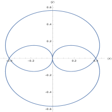
Figure 1: The trajectory of the average velocity of charge carriers, relations (51) and  (52) for the initially localized spin-up electron, has been depicted only for Landau-level centered around $n=1$ with $\sigma=3$ and $2\sqrt{2eB}K\equiv 1$. It consists of the cyclotron and the ZBW motions for the first $10^{-6}$ seconds.

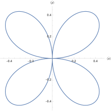
Figure 2: The trajectory of the average velocity of charge carriers, relations (4.2) for the initially localized spin-down electron, has been depicted only for Landau-level centered around $n=1$ with $\sigma=3$ and $2\sqrt{2eB}K\equiv 1$. It consists of the cyclotron and the ZBW motions for the first $10^{-6}$ seconds.

As it is obvious, in the both cases, both of the cyclotron and the ZBW frequencies are involved. The trajectories of the average velocity of charge carriers have been plotted in Figs. 1 and 2 for the both initially localized spin-up and spin-down cases. Of course, the plots have been drawn only for Landau-level centered around $n=1$ as the main part of the issue, with the data of $\sigma=3$ and $2\sqrt{2eB}K\equiv 1$. The figures reveal difference between the spin-up and spin-down cases. Besides, the ZBW phenomenon leads to a circular motion whose direction is opposite for these two cases. Also, due to the approximations used, the motions are unaffected from the NC parameter. Interestingly, when electrons are prepared in the form of wave packets, with $B\neq 0$, all the ZBW frequencies for the Landau-levels appear. Also, both of the interband and intraband frequencies are at work. Furthermore, although in the case at hand, the amplitude of the oscillation is proportional to the external magnetic field, but it is already known [18] that one cannot simply put $B=0$ and expect to get back to the free Dirac solutions.

5 Conclusions

The issue of dynamics of an electron in the presence of an external uniform magnetic field in the NC background, in vacuum, has been considered. First, the related $(3+1)$-dimensional Dirac equation, achieved from the gauge invariant action, has been solved. Then, it has been shown that the solutions and the energy spectrum are both affected by the NC effects of the space sector. However, the change in the energy spectrum is affected is different from previous results in Refs. [38, 54], where the non-gauge invariant Hamiltonian has been employed. In this regard, the ZBW motion in the NC background, without any external magnetic field, has been investigated [55] before and it has been indicated that neither the frequency nor the amplitude of the oscillation gets affected by the NC effects. Also in Ref. [38], the change of the spectrum due to the NC effects has been mentioned however, the solutions of the Dirac equation and dynamics of the electron have not been considered in detail.

In this research, by using the extracted solutions of the Dirac equation, we have calculated the average velocity of charge carriers first for a general wave packet consisted of both positive and negative energies, and then, just for a positive energy electron. An interesting result of these parts is that both the amplitude and the frequency of the ZBW motion are affected by the NC space parameter. Even for a positive energy electron, regardless of the ZBW phenomenon, the space NC effects are present and manifest themselves as a shift in the cyclotronic motion of electron, which, although very small, are in principle detectable. By the way, as mentioned, since the momentum noncommutativity leads to a NC uniform magnetic field, we have not considered its effects in this work.

We have given some estimations for these kinds of shifts as well. Indeed, the calculations suggest that the stronger the external magnetic field is (e.g., at the surface of neutron stars) the relatively larger are the shifts of the corresponding frequencies. In this regard, the amplitude of the oscillation also changes. These results may pave the way for a new class of experiments that can probably exhibit the NC effects on the motion of an electron in a very strong external uniform magnetic field. It should be emphasized that these effects are absent in a field-free region.

To concentrate on the ZBW phenomenon, we have also calculated the average velocity of charge carriers in weak magnetic fields limit for two initially localized spin-up and spin-down cases. In these cases, due to the mentioned approximations, although the NC effects have been neglected, the ZBW manifests itself as a circular motion whose direction is spin dependent. This issue is in line with studies which suggest that the spin of electron might be generated by such a circular motion [8, 19, 55] in vacuum. We have also drawn the plots of the trajectory of the average velocity of the charge carriers for the corresponding Landau-levels centered around a specific level for the both cases. The figures reveal some difference between the spin-up and spin-down cases. Besides, the cyclotron frequency came out to have the same direction for the both cases.

Appendix

The averages of the components of the velocity operator are

$$\langle\dot{x}\rangle\!\!\! =$$ (55)

$$\!\!\!\!\!\!\int\sum_{\rm n,n^{\prime}=1}\!\!V_{n,n^{\prime}}\!\Big{\{}\Big{[}F_{n^{\prime}-1}(\hat{\chi})F_{n}(\chi)+F_{n-1}(\hat{\chi})F_{n^{\prime}}(\chi)\Big{]}\cos[(\omega_{n}^{[e^{+}]}+\omega_{n^{\prime}}^{[e^{-}]})t]$$

$$+ \!\!\!\!\!\!\Big{[}F_{n^{\prime}-1}(\chi)F_{n}(\hat{\chi})+F_{n-1}(\chi)F_{n^{\prime}}(\hat{\chi})\Big{]}\cos[(\omega_{n}^{[e^{-}]}+\omega_{n^{\prime}}^{[e^{+}]})t]$$

$$- \!\!\!\!\!2eB\eta^{[e^{-}]}\eta^{[e^{+}]}K_{n}^{[e^{+}]}K_{n^{\prime}}^{[e^{-}]}\Big{[}F_{n^{\prime}-1}(\hat{\chi})F_{n}(\chi)+F_{n-1}(\hat{\chi})F_{n^{\prime}}(\chi)\Big{]}\cos[(\omega_{n}^{[e^{+}]}+\omega_{n^{\prime}}^{[e^{-}]})t]$$ (56)

$$- \!\!\!\!\!2eB\eta^{[e^{-}]}\eta^{[e^{+}]}K_{n}^{[e^{-}]}K_{n^{\prime}}^{[e^{+}]}\Big{[}F_{n^{\prime}-1}(\chi)F_{n}(\hat{\chi})+F_{n-1}(\chi)F_{n^{\prime}}(\hat{\chi})\Big{]}\cos[(\omega_{n}^{[e^{-}]}+\omega_{n^{\prime}}^{[e^{+}]})t]$$

$$- \!\!\!\!\!\sqrt{2eB}\,\eta^{[e^{-}]}K_{n}^{[e^{-}]}\Big{[}F_{n^{\prime}-1}(\chi)F_{n}(\chi)+F_{n-1}(\chi)F_{n^{\prime}}(\chi)\Big{]}\cos[(\omega_{n}^{[e^{-}]}-\omega_{n^{\prime}}^{[e^{-}]})t]$$

$$+ \!\!\!\!\!\sqrt{2eB}\eta^{[e^{+}]}K_{n}^{[e^{+}]}\Big{[}F_{n-1}(\hat{\chi})F_{n^{\prime}}(\hat{\chi})+F_{n^{\prime}-1}(\hat{\chi})F_{n}(\hat{\chi})\Big{]}\cos[(\omega_{n}^{[e^{+}]}-\omega_{n^{\prime}}^{[e^{+}]})t]$$

$$- \!\!\!\!\!\sqrt{2eB}\,\eta^{[e^{-}]}K_{n^{\prime}}^{[e^{-}]}\Big{[}F_{n^{\prime}-1}(\chi)F_{n}(\chi)+F_{n-1}(\chi)F_{n^{\prime}}(\chi)\Big{]}\cos[(\omega_{n}^{[e^{-}]}-\omega_{n^{\prime}}^{[e^{-}]})t]$$

$$+ \!\!\!\!\!\sqrt{2eB}\,\eta^{[e^{+}]}K_{n^{\prime}}^{[e^{+}]}\Big{[}F_{n-1}(\hat{\chi})F_{n^{\prime}}(\hat{\chi})+F_{n^{\prime}-1}(\hat{\chi})F_{n}(\hat{\chi})\Big{]}\cos[(\omega_{n}^{[e^{+}]}-\omega_{n^{\prime}}^{[e^{+}]})t]$$

$$- \!\!\!\!\!i\Big{[}F_{n^{\prime}-1}(\hat{\chi})F_{n}(\chi)-F_{n-1}(\hat{\chi})F_{n^{\prime}}(\chi)\Big{]}\sin[(\omega_{n}^{[e^{+}]}+\omega_{n^{\prime}}^{[e^{-}]})t]$$

$$+ \!\!\!\!\!i\Big{[}F_{n-1}({\chi})F_{n^{\prime}}(\hat{\chi})-F_{n^{\prime}-1}(\chi)F_{n}(\hat{\chi})\Big{]}\sin[(\omega_{n}^{[e^{-}]}+\omega_{n^{\prime}}^{[e^{+}]})t]$$ (60)

$$+ \!\!\!\!\!2ieB\eta^{[e^{-}]}\eta^{[e^{+}]}K_{n^{\prime}}^{[e^{-}]}K_{n}^{[e^{+}]}\Big{[}F_{n^{\prime}-1}(\hat{\chi})F_{n}(\chi)-F_{n-1}(\hat{\chi})F_{n^{\prime}}(\chi)\Big{]}\sin[(\omega_{n}^{[e^{+}]}+\omega_{n^{\prime}}^{[e^{-}]})t]$$ (61)

$$+ \!\!\!\!\!2ieB\eta^{[e^{-}]}\eta^{[e^{+}]}K_{n}^{[e^{-}]}K_{n^{\prime}}^{[e^{+}]}\Big{[}F_{n-1}({\chi})F_{n^{\prime}}(\hat{\chi})-F_{n^{\prime}-1}(\chi)F_{n}(\hat{\chi})\Big{]}\sin[(\omega_{n}^{[e^{-}]}+\omega_{n^{\prime}}^{[e^{+}]})t]$$

$$+ \!\!\!\!\!i\,\sqrt{2eB}\,\eta^{[e^{-}]}K_{n}^{[e^{-}]}\Big{[}F_{n^{\prime}-1}(\chi)F_{n}(\chi)+F_{n-1}(\chi)F_{n^{\prime}}(\chi)\Big{]}\sin[(\omega_{n}^{[e^{-}]}-\omega_{n^{\prime}}^{[e^{-}]})t]$$

$$+ \!\!\!\!\!i\sqrt{2eB}\,\eta^{[e^{+}]}K_{n}^{[e^{+}]}\Big{[}F_{n-1}(\hat{\chi})F_{n^{\prime}}(\hat{\chi})+F_{n^{\prime}-1}(\hat{\chi})F_{n}(\hat{\chi})\Big{]}\sin[(\omega_{n}^{[e^{+}]}-\omega_{n^{\prime}}^{[e^{+}]})t]$$

$$+ \!\!\!\!\!i\,\sqrt{2eB}\,\eta^{[e^{-}]}K_{n^{\prime}}^{[e^{-}]}\Big{[}F_{n^{\prime}-1}(\chi)F_{n}(\chi)+F_{n-1}(\chi)F_{n^{\prime}}(\chi)\Big{]}\sin[(\omega_{n}^{[e^{-}]}-\omega_{n^{\prime}}^{[e^{-}]})t]$$

$$+ \!\!\!\!\!i\sqrt{2eB}\,\eta^{[e^{+}]}K_{n^{\prime}}^{[e^{+}]}\Big{[}F_{n-1}(\hat{\chi})F_{n^{\prime}}(\hat{\chi})+F_{n^{\prime}-1}(\hat{\chi})F_{n}(\hat{\chi})\Big{]}\sin[(\omega_{n}^{[e^{+}]}-\omega_{n^{\prime}}^{[e^{+}]})t]\Big{\}}\,dy,$$ (64)

$$\langle\dot{y}\rangle\!\!\! =$$ (65)

$$\!\!\!\!\!\!\int\sum_{\rm n,n^{\prime}=1}\!\!V_{n,n^{\prime}}\Big{\{}-\Big{[}F_{n^{\prime}-1}(\hat{\chi})F_{n}(\chi)+F_{n-1}(\hat{\chi})F_{n^{\prime}}(\chi)\Big{]}\sin[(\omega_{n}^{[e^{+}]}+\omega_{n^{\prime}}^{[e^{-}]})t]$$

$$+ \!\!\!\!\!\Big{[}F_{n-1}({\chi})F_{n^{\prime}}(\hat{\chi})+F_{n^{\prime}-1}(\chi)F_{n}(\hat{\chi})\Big{]}\sin[(\omega_{n}^{[e^{-}]}+\omega_{n^{\prime}}^{[e^{+}]})t]$$

$$- \!\!\!\!\!2eB\eta^{[e^{+}]}\eta^{[e^{-}]}K_{n}^{[e^{+}]}K_{n^{\prime}}^{[e^{-}]}\Big{[}F_{n^{\prime}-1}(\hat{\chi})F_{n}(\chi)+F_{n-1}(\hat{\chi})F_{n^{\prime}}(\chi)\Big{]}\sin[(\omega_{n}^{[e^{+}]}+\omega_{n^{\prime}}^{[e^{-}]})t]$$ (66)

$$+ \!\!\!\!\!2eB\eta^{[e^{+}]}\eta^{[e^{-}]}K_{n}^{[e^{-}]}K_{n^{\prime}}^{[e^{+}]}\Big{[}F_{n-1}({\chi})F_{n^{\prime}}(\hat{\chi})+F_{n^{\prime}-1}(\chi)F_{n}(\hat{\chi})\Big{]}\sin[(\omega_{n}^{[e^{-}]}+\omega_{n^{\prime}}^{[e^{+}]})t]$$

$$+ \!\!\!\!\!\sqrt{2eB}\,\eta^{[e^{-}]}K_{n}^{[e^{-}]}\Big{[}F_{n^{\prime}-1}(\chi)F_{n}(\chi)-F_{n-1}(\chi)F_{n^{\prime}}(\chi)\Big{]}\sin[(\omega_{n}^{[e^{-}]}-\omega_{n^{\prime}}^{[e^{-}]})t]$$

$$- \!\!\!\!\!\sqrt{2eB}\,\eta^{[e^{+}]}K_{n}^{[e^{+}]}\Big{[}F_{n-1}(\hat{\chi})F_{n^{\prime}}(\hat{\chi})+F_{n^{\prime}-1}(\hat{\chi})F_{n}(\hat{\chi})\Big{]}\sin[(\omega_{n}^{[e^{+}]}-\omega_{n^{\prime}}^{[e^{+}]})t]$$

$$+ \!\!\!\!\!\sqrt{2eB}\,\eta^{[e^{-}]}K_{n^{\prime}}^{[e^{-}]}\Big{[}F_{n^{\prime}-1}(\chi)F_{n}(\chi)-F_{n-1}(\chi)F_{n^{\prime}}(\chi)\Big{]}\sin[(\omega_{n}^{[e^{-}]}-\omega_{n^{\prime}}^{[e^{-}]})t]$$

$$- \!\!\!\!\!\sqrt{2eB}\,\eta^{[e^{+}]}K_{n^{\prime}}^{[e^{+}]}\Big{[}F_{n-1}(\hat{\chi})F_{n^{\prime}}(\hat{\chi})+F_{n^{\prime}-1}(\hat{\chi})F_{n}(\hat{\chi})\Big{]}\sin[(\omega_{n}^{[e^{+}]}-\omega_{n^{\prime}}^{[e^{+}]})t]$$

$$- \!\!\!\!\!i\Big{[}F_{n^{\prime}-1}(\hat{\chi})F_{n}(\chi)-F_{n-1}(\hat{\chi})F_{n^{\prime}}(\chi)\Big{]}\cos[(\omega_{n}^{[e^{+}]}+\omega_{n^{\prime}}^{[e^{-}]})t]$$

$$+ \!\!\!\!\!i\Big{[}-F_{n-1}({\chi})F_{n^{\prime}}(\hat{\chi})+F_{n^{\prime}-1}(\chi)F_{n}(\hat{\chi})\Big{]}\cos[(\omega_{n}^{[e^{-}]}+\omega_{n^{\prime}}^{[e^{+}]})t]$$ (70)

$$+ \!\!\!\!\!2ieB\eta^{[e^{-}]}\eta^{[e^{+}]}K_{n^{\prime}}^{[e^{-}]}K_{n}^{[e^{+}]}\Big{[}F_{n^{\prime}-1}(\hat{\chi})F_{n}(\chi)-F_{n-1}(\hat{\chi})F_{n^{\prime}}(\chi)\Big{]}\cos[(\omega_{n}^{[e^{+}]}+\omega_{n^{\prime}}^{[e^{-}]})t]$$ (71)

$$+ \!\!\!\!\!2ieB\eta^{[e^{-}]}\eta^{[e^{+}]}K_{n}^{[e^{-}]}K_{n^{\prime}}^{[e^{+}]}\Big{[}-F_{n-1}({\chi})F_{n^{\prime}}(\hat{\chi})+F_{n^{\prime}-1}(\chi)F_{n}(\hat{\chi})\Big{]}\cos[(\omega_{n}^{[e^{-}]}+\omega_{n^{\prime}}^{[e^{+}]})t]$$

$$+ \!\!\!\!\!i\,\sqrt{2eB}\,\eta^{[e^{-}]}K_{n}^{[e^{-}]}\Big{[}F_{n^{\prime}-1}(\chi)F_{n}(\chi)-F_{n-1}(\chi)F_{n^{\prime}}(\chi)\Big{]}\cos[(\omega_{n}^{[e^{-}]}-\omega_{n^{\prime}}^{[e^{-}]})t]$$

$$+ \!\!\!\!\!i\,\sqrt{2eB}\,\eta^{[e^{+}]}K_{n}^{[e^{+}]}\Big{[}F_{n-1}(\hat{\chi})F_{n^{\prime}}(\hat{\chi})-F_{n^{\prime}-1}(\hat{\chi})F_{n}(\hat{\chi}))\Big{]}\cos[(\omega_{n}^{[e^{+}]}-\omega_{n^{\prime}}^{[e^{+}]})t]$$

$$+ \!\!\!\!\!i\,\sqrt{2eB}\,\eta^{[e^{-}]}K_{n^{\prime}}^{[e^{-}]}\Big{[}F_{n^{\prime}-1}(\chi)F_{n}(\chi)-F_{n-1}(\chi)F_{n^{\prime}}(\chi)\Big{]}\cos[(\omega_{n}^{[e^{-}]}-\omega_{n^{\prime}}^{[e^{-}]})t]$$

$$+ \!\!\!\!\!i\,\sqrt{2eB}\,\eta^{[e^{+}]}K_{n^{\prime}}^{[e^{+}]}\Big{[}F_{n-1}(\hat{\chi})F_{n^{\prime}}(\hat{\chi})-F_{n^{\prime}-1}(\hat{\chi})F_{n}(\hat{\chi})\Big{]}\cos[(\omega_{n}^{[e^{+}]}-\omega_{n^{\prime}}^{[e^{+}]})t]\Big{\}}\,dy,$$ (74)

$$\langle\dot{z}\rangle\!\!\! =$$

$$\!\!\!\!\!\!\int\sum_{\rm n,n^{\prime}=1}\!\!V_{n,n^{\prime}}\Big{\{}\Big{[}F_{n^{\prime}-1}(\hat{\chi})F_{n-1}(\chi)+F_{n-1}(\hat{\chi})F_{n^{\prime}-1}(\chi)\Big{]}\cos[(\omega_{n}^{[e^{+}]}+\omega_{n^{\prime}}^{[e^{-}]})t]$$

$$- \!\!\!\!\!\Big{[}F_{n}({\chi})F_{n^{\prime}}(\hat{\chi})+F_{n^{\prime}}(\chi)F_{n}(\hat{\chi})\Big{]}\cos[(\omega_{n}^{[e^{-}]}+\omega_{n^{\prime}}^{[e^{+}]})t]$$

$$- \!\!\!\!\!2eB\eta^{[e^{-}]}\eta^{[e^{+}]}K_{n^{\prime}}^{[e^{-}]}K_{n}^{[e^{+}]}\Big{[}F_{n^{\prime}-1}(\hat{\chi})F_{n-1}(\chi)+F_{n-1}(\hat{\chi})F_{n^{\prime}-1}(\chi)\Big{]}\cos[(\omega_{n}^{[e^{+}]}+\omega_{n^{\prime}}^{[e^{-}]})t]$$

$$+ \!\!\!\!\!2eB\eta^{[e^{-}]}\eta^{[e^{+}]}K_{n^{\prime}}^{[e^{+}]}K_{n}^{[e^{-}]}\Big{[}F_{n}({\chi})F_{n^{\prime}}(\hat{\chi})+F_{n^{\prime}}(\chi)F_{n}(\hat{\chi})\Big{]}\cos[(\omega_{n}^{[e^{-}]}+\omega_{n^{\prime}}^{[e^{+}]})t]$$

$$+ \!\!\!\!\!\sqrt{2eB}\,\eta^{[e^{-}]}K_{n}^{[e^{-}]}\Big{[}-F_{n^{\prime}-1}(\chi)F_{n-1}(\chi)+F_{n-1}(\hat{\chi})F_{n^{\prime}-1}(\hat{\chi})\Big{]}\cos[(\omega_{n}^{[e^{-}]}-\omega_{n^{\prime}}^{[e^{-}]})t]$$

$$+ \!\!\!\!\!\sqrt{2eB}\,\eta^{[e^{+}]}K_{n}^{[e^{+}]}\Big{[}F_{n}(\chi)F_{n^{\prime}}(\chi)-F_{n^{\prime}}(\hat{\chi})F_{n}(\hat{\chi})\Big{]}\cos[(\omega_{n}^{[e^{+}]}-\omega_{n^{\prime}}^{[e^{+}]})t]$$

$$+ \!\!\!\!\!\sqrt{2eB}\,\eta^{[e^{-}]}K_{n^{\prime}}^{[e^{-}]}\Big{[}-F_{n^{\prime}-1}(\chi)F_{n-1}(\chi)+F_{n-1}(\hat{\chi})F_{n^{\prime}-1}(\hat{\chi})\Big{]}\cos[(\omega_{n}^{[e^{-}]}-\omega_{n^{\prime}}^{[e^{-}]})t]$$

$$+ \!\!\!\!\!\sqrt{2eB}\,\eta^{[e^{+}]}K_{n^{\prime}}^{[e^{+}]}\Big{[}F_{n}(\chi)F_{n^{\prime}}(\chi)-F_{n^{\prime}}(\hat{\chi})F_{n}(\hat{\chi})\Big{]}\cos[(\omega_{n}^{[e^{+}]}-\omega_{n^{\prime}}^{[e^{+}]})t]$$

$$- \!\!\!\!\!i\Big{[}F_{n^{\prime}-1}(\hat{\chi})F_{n-1}(\chi)-F_{n-1}(\hat{\chi})F_{n^{\prime}-1}(\chi)\Big{]}\sin[(\omega_{n}^{[e^{+}]}+\omega_{n^{\prime}}^{[e^{-}]})t]$$

$$+ \!\!\!\!\!i\Big{[}F_{n}({\chi})F_{n^{\prime}}(\hat{\chi})-F_{n^{\prime}}(\chi)F_{n}(\hat{\chi})\Big{]}\sin[(\omega_{n}^{[e^{-}]}+\omega_{n^{\prime}}^{[e^{+}]})t]$$ (79)

$$+ \!\!\!\!\!2ieB\eta^{[e^{-}]}\eta^{[e^{+}]}K_{n}^{[e^{+}]}K_{n^{\prime}}^{[e^{-}]}\Big{[}F_{n^{\prime}-1}(\hat{\chi})F_{n-1}(\chi)-F_{n-1}(\hat{\chi})F_{n^{\prime}-1}(\chi)\Big{]}\sin[(\omega_{n}^{[e^{+}]}+\omega_{n^{\prime}}^{[e^{-}]})t]$$ (80)

$$- \!\!\!\!\!2ieB\eta^{[e^{-}]}\eta^{[e^{+}]}K_{n}^{[e^{-}]}K_{n^{\prime}}^{[e^{+}]}\Big{[}F_{n}({\chi})F_{n^{\prime}}(\hat{\chi})-F_{n^{\prime}}(\chi)F_{n}(\hat{\chi})\Big{]}\sin[(\omega_{n}^{[e^{-}]}+\omega_{n^{\prime}}^{[e^{+}]})t]$$

$$+ \!\!\!\!\!i\,\sqrt{2eB}\,\eta^{[e^{-}]}K_{n}^{[e^{-}]}\Big{[}F_{n^{\prime}-1}(\chi)F_{n-1}(\chi)+F_{n-1}(\hat{\chi})F_{n^{\prime}-1}(\hat{\chi})\Big{]}\sin[(\omega_{n}^{[e^{-}]}-\omega_{n^{\prime}}^{[e^{-}]})t]$$

$$- \!\!\!\!\!i\,\sqrt{2eB}\eta^{[e^{+}]}K_{n}^{[e^{+}]}\Big{[}F_{n}(\chi)F_{n^{\prime}}(\chi)-F_{n^{\prime}}(\hat{\chi})F_{n}(\hat{\chi})\Big{]}\sin[(\omega_{n}^{[e^{+}]}-\omega_{n^{\prime}}^{[e^{+}]})t]$$ (82)

$$+ \!\!\!\!\!i\,\sqrt{2eB}\,\eta^{[e^{-}]}K_{n^{\prime}}^{[e^{-}]}\Big{[}F_{n^{\prime}-1}(\chi)F_{n-1}(\chi)+F_{n-1}(\hat{\chi})F_{n^{\prime}-1}(\hat{\chi})\Big{]}\sin[(\omega_{n}^{[e^{-}]}-\omega_{n^{\prime}}^{[e^{-}]})t]$$ (83)

$$- \!\!\!\!\!i\,\sqrt{2eB}\,\eta^{[e^{+}]}K_{n^{\prime}}^{[e^{+}]}\Big{[}F_{n}(\chi)F_{n^{\prime}}(\chi)-F_{n^{\prime}}(\hat{\chi})F_{n}(\hat{\chi})\Big{]}\sin[(\omega_{n}^{[e^{+}]}-\omega_{n^{\prime}}^{[e^{+}]})t]\Big{\}}\,dy,$$ (84)

where $K_{n}^{[e^{\pm}]}\equiv 1/(E_{n}^{[e^{\pm}]}+m)\,$ and $V_{n,n^{\prime}}\equiv\int c_{n^{\prime}}(p_{x},z)c_{n}(p_{x},z)dp_{x}dz=\frac{1}{\sqrt{\sigma}}e^{\frac{-(n-n_{0})^{2}}{2\sigma}}e^{\frac{-(n^{\prime}-n_{0})^{2}}{2\sigma}}$.

References

• [1] E. Schrödinger, Sitz. Preuss. Akad. Wiss. Phys. Math. Kl. 24 (1930), 418; ibid 3 (1931), 1.
• [2] A.O. Barut & A.J. Bracken, Phys. Rev. D 23 (1981), 2454.
• [3] M.E. Rose, Relativistic Electron Theory, (Wiley, New York, 1961).
• [4] J.D. Bjorken & S.D. Drell, Relativistic Quantum Mechanics, (McGraw-Hill, New York, 1964).
• [5] J.J. Sakurai, Advanced Quantum Mechanics, (Pearson Education, Delhi India, 1967).
• [6] W. Greiner, Relativistic Quantum Mechanics, (Springer-Verlag, Berlin, 1990).
• [7] E. Merzbacher, Quantum Mechanics, (Wiley, New York, 3rd ed. 1998).
• [8] K. Huang, Am. J. Phys. 20 (1952), 479.
• [9] A.O. Barut & A.J. Bracken, Phys. Rev. D 24 (1981), 3333.
• [10] D. Hestenes, Found. Phys. 20 (1990), 1213.
• [11] D. Hestenes, Found. Phys. 23 (1993), 365.
• [12] D. Hestenes, Found. Phys. 40 (2010), 1.
• [13] S. De Leo & P. Rotelli, Int. J. Theor. Phys. 37 (1998), 2193.
• [14] A.E. Bernardini, Eur. Phys. J. C 50 (2007), 673.
• [15] A.J. Silenko, Phys. Part. Nuclei Lett. 17 (2020), 116.
• [16] C. Itzykson & J.-B. Zuber, Quantum Field Theory, (McGraw-Hill, Singapore, 1980).
• [17] J.W. van Holten, Phys. A 182 (1992), 279.
• [18] K. Bhattacharya, “Solution of the Dirac equation in presence of an uniform magnetic field”, arXiv: 0705.4275.
• [19] M. Zahiri-Abyaneh & M. Farhoudi, Found. Phys. 41 (2011), 1355.
• [20] T.O. Wehling, A.M. Black-Schaffer & A.V. Balatsky, Adv. Phys. 63 (2014), 1.
• [21] R. Gerritsma, G. Kirchmair, F. Zahringer, E. Solano, R. Blatt & C. F. Roos, Nature (London) 463 (2010), 68.
• [22] L. Ferrari & G. Russo, Phys. Rev. B 42 (1990), 7454.
• [23] A.H. Castro & et al., Rev. Mod. Phys. 81 (2009), 109.
• [24] W. Zawadzki & T.M. Rusin, J. Phys. Condens Matter 23 (2011), 143201.
• [25] S. Sasabe, J. Mod. Phys. 5 (2014), 534.
• [26] T.M. Rusin & W. Zawadzki, Phys. Rev. B 76 (2007), 195439; ibid 78 (2008), 125419; ibid 80 (2009), 045416.
• [27] E. Romera & F. de los Santos, Phys. Rev. B 80 (2009), 165416.
• [28] E. Romera, J.B. Roldán & F. de los Santos, Phys. Lett. A 378 (2014), 2582.
• [29] L.L. Foldy & S.A. Wouthuysen, Phys. Rev. 78 (1950), 29.
• [30] C.G. Darwin, Proc. Roy. Soc. A 118 (1928), 654.
• [31] A. Kobakhidzea, A. Manninga & A. Tureanu, Phys. Lett. B 757 (2016), 84.
• [32] T. Curtright, D. Fairlie & C. Zachos, Phys. Rev. D 58 (1998), 25002.
• [33] M. Chaichian, M.M. Sheikh-Jabbari & A. Tureanu, Phys. Rev. Lett. 86 (2001), 2716.
• [34] S.M. Carroll, J.A. Harvey, V.A. Kostelecky, C.D. Lane & T. Okamoto, Phys. Rev. Lett. 87 (2001), 141601.
• [35] O. Bertolami, J.G. Rosa, C.M.L. de Aragão, P. Castorina & D. Zappalà, Phys. Rev. D 72 (2005), 025010.
• [36] S.M.M. Rasouli, M. Farhoudi & N. Khosravi, Gen. Rel. Grav. 43 (2011), 2895.
• [37] W.O. Santos & A.M.C. Souza, Int. J. Theor. Phys. 51 (2012), 3882.
• [38] L. Mai-Lin, Z. Ya-Bin, Y. Rui-Lin & Z. Fu-Lin, Chinese Phys. C 37 (2013), 063106.
• [39] B. Malekolkalami & M. Farhoudi, Int. J. Theor. Phys. 53 (2014), 815.
• [40] K. Ma, J.-H. Wang & H.-X. Yang, Phys. Lett. B 759 (2016), 306.
• [41] S.M.M. Rasouli, N. Saba, M. Farhoudi, J. Marto & P.V. Moniz, Ann. Phys. 393 (2018), 288.
• [42] I. Hinchliffe, N. Kersting & Y.L. Ma, Int. J. Mod. Phys. A 19 (2004), 179.
• [43] B. Malekolkalami & M. Farhoudi, Class. Quant. Grav. 27 (2010), 245009.
• [44] N. Seiberg & E. Witten, J. High Energy Phys. 09 (1999), 032.
• [45] D.J. Gross & N.A. Nekrasov, J. High Energy Phys. 10 (2000), 021.
• [46] G. Amelino-Camelia, L. Doplicher, S. Nam & Y.S. Seo, Phys. Rev. D 67 (2003), 085008.
• [47] T.P. Singh, Bulg. J. Phys. 33 (2006), 217.
• [48] J. Gamboa, F. Mondez, M. Loewe & J.C. Rojas, Mod. Phys. Lett. A 16 (2001), 2075.
• [49] K. Li & S. Dulat, Eur. Phys. J. C  46 (2006), 825.
• [50] S. Dulat & K. Li, Mod. Phys. Lett. A 21 (2006), 2971.
• [51] S. Cai, T. Jing, G. Guo & R. Zhang, J. Theor. Phys. 49 (2010), 1699.
• [52] T.C. Adorno, M.C. Baldiotti & D.M. Gitman, Phys. Rev. D 82 (2010), 123516.
• [53] O. Bertolami & R. Queiroz, Phys. Lett. A 375 (2011), 4116.
• [54] O. Panella & P. Roy, Phys. Rev. A 90 ( 2014), 042111.
• [55] M.Z. Abyaneh & M. Farhoudi, Int. J. Mod. Phys. A  34 (2019), 1950045.
• [56] O.F. Dayi & A. Jellal, J. Math. Phys. 51 (2010), 063522.
• [57] A. Boumali & H. Hassanabadi, Can. J. Phys. 93 (2015), 542.
• [58] W.O. Santos, G.M.A. Almeida & A.M.C. Souza, “Noncommutative quantum Hall effect in graphene”, arXiv: 1801.03323.
• [59] C. Bastos, O. Bertolami, N. Dias & J. Prata, Int. J. Mod. Phys. A 28 (2013), 1350064.
• [60] R. Verma & A.N. Bose, Euro. Phys. J. Plus 132 (2017), 220.
• [61] M. Eckstein, N. Franco & T. Miller, Phys. Rev. D 95 (2017), 061701.
• [62] K.V.D. Dungen & W.D.V. Suijlekom, Rev. Math. Phys. 24 (2012), 1230004.
• [63] A. Connes, J. Math. Phys. 41 (2000), 3832.
• [64] C.K. Zachos, D.B. Fairlie & T.L. Curtright (editors), Quantum Mechanics in Phase Space, (World Scientific, Singapore, 2005).
• [65] G. Esposito & C. Stornaiolo, Int. J. Geom. Meth. Mod. Phys. 4 (2007), 349.
• [66] B. Malekolkalami & M. Farhoudi, Phys. Lett. B 678 (2009), 174.
• [67] N. Saba & M. Farhoudi, Ann. Phys. 395 (2018), 1.