Quasinormal frequencies of a two-dimensional asymptotically anti-de Sitter black hole of the dilaton gravity theory

Abstract

We numerically calculate the quasinormal frequencies of the Klein-Gordon and Dirac fields propagating in a two-dimensional asymptotically anti-de Sitter black hole of the dilaton gravity theory. For the Klein-Gordon field we use the Horowitz-Hubeny method and the asymptotic iteration method for second order differential equations. For the Dirac field we first exploit the Horowitz-Hubeny method. As a second method, instead of using the asymptotic iteration method for second order differential equations, we propose to take as a basis its formulation for coupled systems of first order differential equations. For the two fields we find that the results that produce the two numerical methods are consistent. Furthermore for both fields we obtain that their quasinormal modes are stable and we compare their quasinormal frequencies to analyze whether their spectra are isospectral. Finally we discuss the main results.

KEYWORDS: Quasinormal frequencies; Klein-Gordon and Dirac fields; 2D AdS black hole; Horowitz-Hubeny method; Asymptotic iteration method

1 Introduction

The quasinormal modes (QNMs) are the oscillations of perturbed black holes that are purely ingoing near the horizon. The boundary condition imposed at the asymptotic region depends on its structure, for example, for asymptotically flat black holes the boundary condition usually imposed is that the perturbation is purely outgoing as $r\to\infty$, whereas for the asymptotic anti-de Sitter black holes (asymptotically adS black holes, in what follows), a common boundary condition demands that the perturbation goes to zero as $r\to\infty$ [1]–[4]. It is convenient to notice that in asymptotically adS spacetimes we can impose a different boundary condition as $r\to\infty$. See Refs. [5]–[7] for some examples. Associated with the QNMs we find a set of complex frequencies called quasinormal frequencies (QNFs). It is well known that the QNFs of black holes are determined by the geometry and the type of perturbation [1]–[3].

Two dimensional gravity allows us to analyze several physical problems in a simple framework. The physical properties of two-dimensional black holes (2D black holes, in what follows) are studied because some aspects of the analysis are simpler than in spacetimes with $D\geq 3$ dimensions [8], [9]. Furthermore, in 2D spacetimes the equations of motion for classical fields simplify and we can study in more detail several physical phenomena, for example, the way in which a 2D black hole reacts when it is perturbed. The QNFs of 2D spacetimes have been studied in recent times [10]–[27]. Exact results for the QNFs have previously found [10]–[27], but for some asymptotically adS 2D backgrounds a numerical calculation is necessary [19].

We notice that the QNFs of asymptotically adS black holes have attracted attention, since they are useful to study its classical stability [1]–[3], [19], [28]–[32] and to calculate the entropy spectrum of the black hole horizon [33]–[37]. Here we exploit the advantages that we find in 2D gravity to implement two numerical methods to calculate the QNFs of a 2D asymptotically adS black hole [38]. Additionally, we carry out this work to understand the properties of this 2D black hole of Ref. [38] and study its classical stability under small perturbations. One of the numerical procedures is the widely used Horowitz-Hubeny method (HH method in what follows) [28] that is appropriate to compute the QNFs of asymptotically adS spacetimes [2], [3]. The other numerical procedure is the asymptotic iteration method (AIM in what follows) [39], that is modified to determine the QNFs of black holes [40]. For the Klein-Gordon field the AIM is exploited in the usual formulation for second order differential equations [39], [40], whereas for the Dirac field we propose to use the formulation of the AIM for coupled systems of first order differential equations [41]. As far as we know, this version of the AIM has not previously used to calculate QNFs of black holes and we think that the computation of the QNFs for 2D black holes is the appropriate setting to test this method.

The rest of the paper is structured as follows. In Sect. 2.1 we give the asymptotically adS 2D black hole that we study in this work and we describe its main properties. In Sect. 2.2 we simplify the equation of motion for the Klein-Gordon field in the 2D black hole that we study. Furthermore, for the Klein-Gordon field in Sects. 2.3 and 2.4 we describe the HH method and the AIM for second order differential equations. For the Dirac field we simplify its equation of motion in Sect. 2.5. Also, for the Dirac field our implementations of the HH method and the AIM for coupled systems of first order differential equations are outlined in Sects. 2.6 and 2.7. In Sect. 3.1 we numerically calculate the QNFs of the Klein-Gordon field moving in the asymptotically adS 2D black hole that we are studying and then the QNFs of the Dirac field are numerically computed in Sect.  3.2. For the two fields we compare the results that produce the two methods. In Sect. 4 we discuss the main results. For the Klein-Gordon and Dirac fields, in Appendix A we give the numerical values of the QNFs with more decimal places. For static 2D spacetimes with diagonal metric in Appendix B we simplify the Dirac equation to a pair of Schrödinger type equations. The simplification uses a basis of null vectors. This method can be exploited in other 2D spacetimes, and as far as we know, it is not already reported. In Appendix C we extend the discussion of the AIM for the Klein-Gordon field and we show how to use the formulation of the AIM for coupled systems of first order differential equations to determine its QNFs. In Appendix D we give the so-called improved formulation of the AIM for second order differential equations [40], [42] and we employ this improved version to calculate the QNFs of the Klein-Gordon field. Furthermore, we develop an improved version of the AIM for coupled systems of first order differential equations. Taking as a basis this improved version we calculate the QNFs of the Dirac field again and we compare with the previous results. Finally in Appendix E we show that the AIM for coupled systems of first order differential equations works for calculating the QNFs of the Dirac field moving in a higher dimensional Lifshitz black hole.

2 Methods

In this section we describe the main properties of the asymptotically adS 2D black hole that we study in this work. Furthermore we give the steps to simplify the equations of motion for the Klein-Gordon field and the Dirac field in the black hole under study. Finally, for both fields, we summarize the HH method and the AIM.

2.1 Two-dimensional asymptotically anti-de Sitter black hole

In Ref. [38] we find several 2D spacetimes representing black holes. These black holes are solutions to the equations of motion for the action

$$S=\frac{1}{2\pi}\int{d^{2}x\sqrt{-g}e^{-2\phi}[\mathcal{R}-4\rho(\partial\phi)^{2}+4\sigma^{2}]},$$ (1)

where $\mathcal{R}$ is the scalar curvature, $\sigma$ is a constant that we interpret as a cosmological constant, $\phi$ is the dilaton, and $\rho$ is a parameter that we take as $\rho=-1/2$. For this value of $\rho$, a solution to the equations of motion is the asymptotically adS 2D black hole that we study in this work and whose metric is [38]

$$ds^{2}=\left(a^{2}r^{2}-\frac{1}{ar}\right)dt^{2}-\left(a^{2}r^{2}-\frac{1}{ar}\right)^{-1}dr^{2},$$ (2)

and the dilaton field is equal to

$$e^{-2\phi}=a^{2}r^{2}.$$ (3)

The event horizon of this black hole is located at $r_{+}=1/a$, where $a$ is related to $\sigma$ by $a=\sqrt{2}|\sigma|/\sqrt{3}$. We notice that the scalar curvature of this 2D black hole is equal to $\mathcal{R}=-4\sigma^{2}/3+4\sigma^{2}/(3a^{3}r^{3})$, hence it is positive inside the horizon and negative outside the horizon [38]. The ADM mass of the 2D black hole (2) is equal to $M=|\sigma|/\sqrt{6}$ [38], [43]. We observe that the metric of the 2D black hole (2) is the $(t,r)$ sector of the metric for the flat horizon Schwarzschild adS black hole in four dimensions [43], but we point out that the behavior of the scalar curvature is different in both solutions. Owing this fact we choose to analyze the stability under perturbations of this asymptotically adS 2D black hole.

As far as we know, the classical stability under perturbations of this 2D black hole has not previously analyzed and to begin this study we calculate its spectrum of QNFs. We have not been able to find exact solutions to the equations of motion for the Klein-Gordon and Dirac fields, hence, in what follows we use the HH method [28] and the AIM [39], [40], [41] to compute numerically the frequencies of its damped oscillations. Furthermore, we evaluate whether the AIM for coupled systems of first order differential equations works to produce the QNFs of the Dirac field.

As usual for asymptotically adS black holes, we define the QNMs as the oscillations that satisfy the boundary conditions [1]–[3], [19], [28]–[32]
a) The field is purely ingoing near the horizon.
b) The field goes to zero as $r\to\infty$.
Note that in the boundary condition b) we assume that the coordinates of the line element (2) are used.

2.2 Equation of motion for the Klein-Gordon field

In the 2D black hole (2) we first calculate the QNFs of a test Klein-Gordon field whose equation of motion is

$$(\square+m^{2})\Phi=0.$$ (4)

As shown in Ref.  [20], if we take a separable solution

$$\Phi=R(r)e^{-i\omega t},$$ (5)

then the Klein-Gordon equation simplifies to a Schrödinger type equation

$$\frac{d^{2}R}{dr_{*}^{2}}+\omega^{2}R=V_{KG}R,$$ (6)

with $r_{*}$ denoting the tortoise coordinate of the 2D black hole (2)

$$r_{*}=\int dr\left(a^{2}r^{2}-\frac{1}{ar}\right)^{-1},$$ (7)

and the effective potential $V_{KG}$ is equal to [20]

$$V_{KG}=m^{2}\left(a^{2}r^{2}-\frac{1}{ar}\right).$$ (8)

From this expression for the effective potential $V_{KG}$, we note that for $m=0$, it goes to zero. Therefore for $m=0$ the solutions of Eq. (6) are sinusoidal functions and since we are interested in damped solutions, in what follows we consider a test massive Klein-Gordon field with $m>0$. Notice that for our problem the physically relevant interval is $r\in(r_{+},\infty)$. It is convenient to comment that in the 2D black hole (2) we have not been able to solve exactly the radial equation (6) and therefore we numerically compute the QNFs of the Klein-Gordon field. Furthermore, we assume the test field approximation for calculating the QNFs of the asymptotically adS 2D black hole (2).

We point out that near the event horizon at $r_{+}=1/a$ the effective potential $V_{KG}$ goes to zero and therefore the radial function near the horizon behaves as

$$R\approx K_{1}\,\,\textrm{e}^{+i\omega r_{*}}+K_{2}\,\,\textrm{e}^{-i\omega r_{*}},$$ (9)

where $K_{1}$, $K_{2}$ are constants. Note that near the horizon the first term of the previous formula is an outgoing wave and the second term is an ingoing wave.

To satisfy the QNMs boundary condition near the horizon, we impose that the field is purely ingoing near the horizon by taking the radial function $R$ as [28]

$$R(r)=e^{-i\omega{r}_{*}}\tilde{R}(r),$$ (10)

to get that the function $\tilde{R}$ must be a solution of the differential equation

$$f\frac{{d}^{2}\tilde{R}}{{dr}^{2}}+\left(\frac{df}{dr}-2i\omega\right)\frac{d\tilde{R}}{dr}-\frac{V}{f}\tilde{R}=0,$$ (11)

where we define $f=a^{2}r^{2}-1/(ar)$.

2.3 Horowitz-Hubeny method for the Klein-Gordon field

The numerical HH method proposed in [28] is widely used to compute the QNFs of asymptotically adS black holes [2], [3], [19]. Following Horowitz-Hubeny, to transform the interval $(r_{+},\infty)$ into a finite interval, we make the change of variable

$$x=\frac{1}{r},$$ (12)

to obtain that Eq.  (11) transforms into a differential equation of the form [28]

$$\tilde{s}(x)\frac{{d}^{2}\tilde{R}}{d{x}^{2}}+\frac{\tilde{t}(x)}{x-{x}_{+}}\frac{d\tilde{R}}{dx}+\frac{u(x)}{{(x-{x}_{+})}^{2}}\tilde{R}=0,$$ (13)

where

$$x_{+}=\frac{1}{r_{+}}=a,$$ (14)

and the functions $\tilde{s}$, $\tilde{t}$, and $u$ are equal to

$$\tilde{s}(x) = {x}^{2}({a}^{2}+ax+{x}^{2}),$$

$$\tilde{t}(x) = \left(\frac{3x^{2}}{a}-2i\omega\right){x}^{2}a,$$ (15)

$$u(x) = a{m}^{2}(x-a).$$

Notice that the function $u$ satisfies $u(a)=0$.

To preserve the purely ingoing radial solution near the horizon, we expand the function $\tilde{R}$ in the form [28]

$$\tilde{R}(x)=\sum_{k=0}^{\infty}{a}_{k}(\omega){(x-{x}_{+})}^{k}.$$ (16)

Furthermore, we expand the function $\tilde{s}$ as

$$\tilde{s}(x)=\sum_{k=0}^{\infty}\tilde{s}_{k}(\omega){(x-{x}_{+})}^{k},$$ (17)

and we make analogous expansions for the functions $\tilde{t}$ and $u$.

Substituting these expansions into the differential equation (13) we obtain that the coefficients ${a}_{k}(\omega)$ are given by the recurrence relation [28]

$${a}_{k}=-\frac{1}{k(k-1)\tilde{s}_{0}+k\tilde{t}_{0}}\sum_{n=0}^{k-1}{a}_{n}(n(n-1)\tilde{s}_{k-n}+n\tilde{t}_{k-n}+u_{k-n}).$$ (18)

Since $a_{0}$ is not determined by the method, in what follows we take $a_{0}=1$ [28].

As $r\to\infty$ the QNMs boundary condition b) imposes that the radial function goes to zero. From the expansion (16), to fulfill this boundary condition and to find the QNFs of the field we must solve

$$\sum_{k=0}^{\infty}{a}_{k}(\omega){(-{x}_{+})}^{k}=0.$$ (19)

We see that the roots of this equation are the QNFs of the 2D black hole (2). Note that we cannot compute the infinite sum of the previous formula, therefore a common method to solve Eq.  (19) is to calculate the sum up to an integer value $N$ and obtain the roots of the resulting polynomial. We repeat the calculation for another integer value $N_{1}>N$ and the common roots are the QNFs of the Klein-Gordon field [28]. In the HH method the repeated roots for different values of $N$ are called stable roots.

2.4 Asymptotic iteration method for the Klein-Gordon field

The asymptotic iteration method is useful to study linear second order differential equations that can be written in the form [39]

$$\phi^{\prime\prime}=\lambda_{0}\phi^{\prime}+s_{0}\phi,$$ (20)

where $\lambda_{0}$ and $s_{0}$ are differentiable functions of the independent variable $x$. As usual, we denote the derivative with respect to the independent variable $x$ with a prime. This method is widely used to solve linear second order differential equations, to find its eigenvalues [39], and more recently is taken as a basis to calculate the QNFs of black holes [40].

We observe that the derivative of the previous equation takes the form [39]

$$\phi^{\prime\prime\prime}=\lambda_{1}\phi^{\prime}+s_{1}\phi,$$ (21)

where

$$\lambda_{1}=\lambda_{0}^{\prime}+s_{0}+\lambda_{0}^{2},\quad\quad s_{1}=s_{0}^{\prime}+s_{0}\lambda_{0},$$ (22)

that is, for the differential equation (20), the structure of its first derivative is similar when we define $\lambda_{1}$ and $s_{1}$ as previously [39]. Furthermore, we find that the $n$-th derivative of Eq. (20) takes an analogous form [39]

$$\phi^{(n+2)}=\lambda_{n}\phi^{\prime}+s_{n}\phi,$$ (23)

where

$$\lambda_{n}=\lambda_{n-1}^{\prime}+s_{n-1}+\lambda_{0}\lambda_{n-1},\quad\quad s_{n}=s_{n-1}^{\prime}+s_{0}\lambda_{n-1}.$$ (24)

To find a solution to Eq. (20), in Ref. [39] is imposed the asymptotic aspect of the AIM by proposing that for $n$ sufficiently large the following equation [39]

$$\frac{s_{n}}{\lambda_{n}}=\frac{s_{n-1}}{\lambda_{n-1}}=\alpha,$$ (25)

is satisfied. From the previous equation we obtain the quantization condition [39]

$$\delta_{n}=\lambda_{n}s_{n-1}-\lambda_{n-1}s_{n}=0.$$ (26)

Usually the previous condition depends on the independent variable $x$ and the oscillation frequency. To get the QNFs from this condition we evaluate the quantity $\delta_{n}$ in a convenient point and the stable roots of the resulting equation are the QNFs [39]. In the AIM for stable roots we understand the common roots of the quantization condition (26) for different values of $N$ where $N$ is the number of times we iterate the expressions (24). Usually to determine the stable roots we take values of $N$ that differ by five, that is, we calculate the quantity $\delta_{N}$ of Eq. (26) for two values of $N$ that differ by 5 and we take the common roots of Eqs. (26) as the QNFs. We point out that to implement the AIM we scale out the behavior of the field near the boundaries before we find the equivalent of Eq. (20) for our problem [40].

In the following we use the AIM to calculate the QNFs of the Klein-Gordon field propagating in the 2D black hole (2). We take as a basis Eq. (11) and we factor out the behavior at the asymptotic region, since the behavior near the horizon is scaled out. As a first step we study Eq. (11) as $r\to\infty$ to get

$$\frac{d^{2}\tilde{R}}{dr^{2}}+\frac{2}{r}\frac{d\tilde{R}}{dr}-\left(\frac{m^{2}}{a^{2}}\right)\frac{\tilde{R}}{r^{2}}=0,$$ (27)

whose solutions are of the form

$$\tilde{R}=K_{1}r^{q_{-}}+K_{2}r^{q_{+}},$$ (28)

where $K_{1}$, $K_{2}$ are constants and the quantities $q_{-}$, $q_{+}$ are equal to

$$q_{-}=-1/2-\sqrt{1+4m^{2}r_{+}^{2}}/2,\qquad\qquad q_{+}=-1/2+\sqrt{1+4m^{2}r_{+}^{2}}/2.$$ (29)

From the expression (28) we observe that the solution satisfying the boundary condition of the QNFs as $r\to\infty$ is $K_{1}r^{q_{-}}$. Therefore we make the ansatz

$$\tilde{R}=r^{q_{-}}\hat{R}$$ (30)

to get that the function $\hat{R}$ satisfies the differential equation

$$f\frac{d^{2}\hat{R}}{dr^{2}} +\left(\frac{2q_{-}f}{r}+\frac{df}{dr}-2i\omega\right)\frac{d\hat{R}}{dr}$$

$$+\left(\frac{q_{-}(q_{-}-1)f}{r^{2}}+\frac{q_{-}}{r}\frac{df}{dr}-\frac{2i\omega q_{-}}{r}-\frac{V}{f}\right)\hat{R}=0.$$ (31)

Owing to the radial variable is defined in a semi-infinite interval, in a similar way to the HH method, it is convenient to use a new independent variable with a finite range. For implementing the AIM we find useful to define the variable

$$z=\frac{r_{+}}{r},$$ (32)

such that $z=1$ for $r=r_{+}$ and $z=0$ as $r\to\infty$. Taking as independent variable to $z$, we obtain that Eq. (2.4) transforms into

$$\frac{d^{2}\hat{R}}{dz^{2}}-\left(\frac{2q_{-}}{z}+\frac{2+z^{3}}{z(1-z^{3})}-\frac{2}{z}-\frac{2i\omega r_{+}}{1-z^{3}}\right)\frac{d\hat{R}}{dz}$$ (33)

$$-\left(\frac{m^{2}r_{+}^{2}}{z^{2}(1-z^{3})}-\frac{q_{-}(q_{-}-1)}{z^{2}}-\left(\frac{2+z^{3}}{z}-2i\omega r_{+}\right)\frac{q_{-}}{z(1-z^{3})}\right)\hat{R}=0.$$

The previous linear second order differential equation is of the form (20) and for the Klein-Gordon field we take this equation as a basis to implement the AIM. Thus, we identify the functions $\lambda_{0}$, $s_{0}$ as follows

$$\lambda_{0}(z) =\frac{2q_{-}}{z}+\frac{2+z^{3}}{z(1-z^{3})}-\frac{2}{z}-\frac{2i\omega r_{+}}{1-z^{3}},$$ (34)

$$s_{0}(z) =\frac{m^{2}r_{+}^{2}}{z^{2}(1-z^{3})}-\frac{q_{-}(q_{-}-1)}{z^{2}}-\left(\frac{2+z^{3}}{z}-2i\omega r_{+}\right)\frac{q_{-}}{z(1-z^{3})},$$

and we use the recurrence relations (24) to calculate the quantities that appear in the quantization condition (26). The stable roots of the condition (26) are the QNFs of the Klein-Gordon field. We note that in Sect. 3.1 to calculate the QNFs of the Klein-Gordon field we follow the procedure described in Ref. [39] instead of the improved AIM proposed in Ref. [40], (but see Appendix D).

2.5 Equation of motion for the Dirac field

The equation of motion for a Dirac field is

$$i{/\negthinspace\negthinspace\negthinspace\nabla}\Psi=m\Psi,$$ (35)

where ${/\negthinspace\negthinspace\negthinspace\nabla}$ is the Dirac operator and $m$ is the mass of the field. In what follows we assume that $m>0$. Reference [20] shows that in a static 2D spacetime whose metric is diagonal, the Dirac equation in the chiral representation simplifies to a pair of Schrödinger type equations with effective potentials

$$V_{\pm}=m^{2}f\mp\frac{m}{2}\sqrt{f}\frac{df}{dr}.$$ (36)

Owing to the factor $\sqrt{f}$ in these effective potentials, our numerical code for the HH method converges slowly. Thus, to get a different pair of effective potentials for the radial equations of the Dirac field, in what follows, to write the Dirac equation in the 2D black hole (2), we exploit a dyad of null vectors (see Appendix B for more details).

In this basis of null vectors, the Dirac equation simplifies to a pair of Schrödinger type equations

$$\frac{d^{2}R_{l}}{dr_{*}^{2}}+\omega^{2}R_{l}=V_{l}R_{l},$$ (37)

with $l=1,2$, and the effective potentials are equal to

$$V_{l}=m^{2}f\mp\frac{i\omega}{2}\frac{df}{dr}-\frac{f}{4}\frac{d^{2}f}{dr^{2}}+\frac{1}{16}\left(\frac{df}{dr}\right)^{2}.$$ (38)

In the previous equation and in what follows, the upper (lower) sign corresponds to $l=1$ ($l=2$). We notice that the two effective potentials (38) do not contain square roots of the function $f$. Also the system of coupled equations (B) for the components of the spinor is an appropriate basis to use the AIM for coupled systems (see Sect. 2.7).

Near the horizon of the black hole, the effective potentials (38) simplify to

$$\lim_{r\to r_{+}}V_{l}=\mp\frac{i\omega}{2}\left.\frac{df}{dr}\right|_{r=r_{+}}+\frac{1}{16}\left(\left.\ \frac{df}{dr}\right|_{r=r_{+}}\right)^{2},$$ (39)

and therefore near the horizon the radial functions $R_{l}$ behave in the form

$$R_{l}\approx K^{I}_{l}\,\,\textrm{e}^{{-i}\left(\omega\pm\frac{i\kappa}{2}\right)r_{*}}+K^{II}_{l}\,\,\textrm{e}^{+{i}\left(\omega\pm\frac{i\kappa}{2}\right)r_{*}},$$ (40)

where $K^{I}_{l}$, $K^{II}_{l}$ are constants and in the previous equation we introduce the surface gravity of the 2D black hole (2) defined by

$$\kappa=\frac{1}{2}\left.\frac{df}{dr}\right|_{r=r_{+}}=\frac{3a}{2}.$$ (41)

Also, we note that near the horizon the first term of the expression (40) is an ingoing wave, whereas the second term is an outgoing wave.

We have not been able to solve exactly the Schrödinger type equations (37) and therefore we use first the HH method to compute the QNFs of the Dirac field in the 2D black hole (2). Thus, in the following subsection, taking as a basis the Schrödinger type equations (37) with the effective potentials (38) and the HH method, we calculate the QNFs of the Dirac field in the 2D black hole (2). Moreover, in Sect. 2.7 we show how to use the AIM for coupled systems of first order equations to compute the QNFs of the Dirac field.

2.6 Horowitz-Hubeny method for the Dirac field

To use the HH method [28] for calculating the QNFs of the Dirac field we make the following transformations to the differential equations (37). Near the horizon, to satisfy the boundary condition of the QNMs we take the functions $R_{l}$ in the form

$$R_{l}=e^{-i\left(\omega\pm\frac{i\kappa}{2}\right)r_{*}}\tilde{R}_{l}(r),$$ (42)

to get that the functions $\tilde{R}_{l}$ must be solutions of the differential equations

$$f\frac{{d}^{2}\tilde{R}_{l}}{{dr}^{2}}+\left(\frac{df}{dr}-2i\omega\pm\kappa\right)\frac{d\tilde{R}_{l}}{dr}+\left(\frac{\kappa^{2}}{4}\mp i\kappa\omega-V_{l}\right)\frac{1}{f}\tilde{R}_{l}=0,$$ (43)

that transform into

$$x^{4}f\frac{d^{2}\tilde{R}_{l}}{dx^{2}} +\left(x^{4}\frac{df}{dx}+2x^{3}f+2i\omega x^{2}\mp\kappa x^{2}\right)\frac{d\tilde{R}_{l}}{dx}$$

$$+\left(\frac{\kappa^{2}}{4}\mp i\kappa\omega-V_{l}\right)\frac{1}{f}\tilde{R}_{l}=0,$$ (44)

when we use the variable $x$ defined in the formula (12).

In a straightforward way we transform Eqs.  (2.6) to the form (13), but the functions $\tilde{s}_{l}$, $\tilde{t}_{l}$, and $u_{l}$ for the Dirac field are given by

$$\tilde{s}_{l}(x) =16x^{2}(x^{2}+ax+a^{2})^{2},$$

$$\tilde{t}_{l}(x) =16a(x^{2}+ax+a^{2})\left(\frac{3x^{4}}{a}-2i\omega x^{2}\pm\kappa x^{2}\right),$$ (45)

$$u_{l}(x) =9a^{4}x^{2}\mp 24i\omega a^{3}x^{2}+8a(2m^{2}-3a^{2})(x^{3}-a^{3})$$

$$+8\left(x^{3}+2a^{3}\right)\left(x^{3}-a^{3}\pm i\omega ax\right)-\left(x^{3}+2a^{3}\right)^{2}.$$

We notice that $u_{l}(a)=0$. From these expressions and taking into account the recurrence relation (18) we get the coefficients $a_{k}$ for the Dirac field moving in the 2D black hole (2). As previously, the QNFs of the Dirac field are the stable roots of the corresponding equations that have the same mathematical form as Eq. (19).

2.7 Asymptotic Iteration Method for the Dirac field

To compute the QNFs of the Dirac field moving in the asymptotically adS 2D black hole (2) we can take as a basis Eqs. (43) and use the AIM for second order differential equations as explained in the previous section for the Klein-Gordon field. Nevertheless an alternative way can be used. As described in Ref. [41] the AIM can be extended to calculate the eigenvalues for coupled systems of first order differential equations of the form

$$\phi^{\prime}_{1}=\Lambda_{0}\phi_{1}+S_{0}\phi_{2},$$

$$\phi^{\prime}_{2}=\Omega_{0}\phi_{1}+P_{0}\phi_{2},$$ (46)

where $\Lambda_{0}$, $S_{0}$, $\Omega_{0}$, $P_{0}$ are functions of the independent variable $x$.

In a similar way to the usual AIM previously described in Sect. 2.4, we notice that the first derivative of Eqs. (2.7) simplifies to [41]

$$\phi^{\prime\prime}_{1}=\Lambda_{1}\phi_{1}+S_{1}\phi_{2},$$

$$\phi^{\prime\prime}_{2}=\Omega_{1}\phi_{1}+P_{1}\phi_{2},$$ (47)

and we observe that the previous system of coupled differential equations is of the same form as the system (2.7) with

$$\Lambda_{1} =\Lambda_{0}^{\prime}+\Lambda_{0}^{2}+S_{0}\Omega_{0},$$

$$S_{1} =S_{0}^{\prime}+\Lambda_{0}S_{0}+S_{0}P_{0},$$ (48)

$$\Omega_{1} =\Omega_{0}^{\prime}+\Lambda_{0}\Omega_{0}+P_{0}\Omega_{0},$$

$$P_{1} =P_{0}^{\prime}+P_{0}^{2}+S_{0}\Omega_{0}.$$

As in the AIM for second order differential equations, we notice that the $(n+1)$-th derivative of the coupled system of first order differential equations (2.7) takes the form [41]

$$\phi^{(n+2)}_{1}=\Lambda_{n+1}\phi_{1}+S_{n+1}\phi_{2},$$

$$\phi^{(n+2)}_{2}=\Omega_{n+1}\phi_{1}+P_{n+1}\phi_{2},$$ (49)

where

$$\Lambda_{n+1} =\Lambda_{n}^{\prime}+\Lambda_{0}\Lambda_{n}+\Omega_{0}S_{n},$$

$$S_{n+1} =S_{n}^{\prime}+P_{0}S_{n}+S_{0}\Lambda_{n},$$

$$\Omega_{n+1} =\Omega_{n}^{\prime}+\Lambda_{0}\Omega_{n}+\Omega_{0}P_{n},$$

$$P_{n+1} =P_{n}^{\prime}+P_{0}P_{n}+S_{0}\Omega_{n}.$$ (50)

In contrast to the AIM for second order differential equations, for which two recurrence relations are obtained (see the expressions (24)), for a system of coupled first order differential equations we find four recurrence relations [41].

Furthermore, for the coupled system of first order differential equations, the asymptotic aspect of the AIM demands that for sufficiently large $n$ [41]

$$\frac{S_{n+1}}{\Lambda_{n+1}}=\frac{S_{n}}{\Lambda_{n}}=\alpha,$$ (51)

which is similar to the expression (25) of the AIM for second order differential equations, but notice that in both expressions the involved functions satisfy different recurrence relations. From the previous formula we obtain that the QNFs are the stable numerical solutions of the equation [41]

$$\Delta_{n}=\Lambda_{n}S_{n+1}-\Lambda_{n+1}S_{n}=0.$$ (52)

For exactly solvable systems the previous quantization condition depends only of $\omega$, but in general depends on the independent variable and $\omega$ [41], hence to calculate the roots of Eq. (52), we evaluate it in a convenient value of the independent variable.

In what follows we use this implementation of the AIM for coupled systems of first order differential equations to calculate the QNFs of the Dirac field propagating in the 2D black hole (2). As far as we know, this procedure is not used before to calculate the QNFs of the Dirac field. To this end we take as a basis the coupled system of equations (B), but we notice that for the 2D black hole (2) the functions $\mathcal{P}$ and $\mathcal{Q}$ defined in Appendix B fulfill $(\mathcal{P}\mathcal{Q})^{2}=1$. Therefore, taking the radial functions $R_{l}$ in the form

$$R_{1}=\frac{(r-r_{+})^{1/4}}{r^{3/4}}U_{1},\qquad\qquad R_{2}=\frac{U_{2}}{(r-r_{+})^{1/4}r^{1/4}},$$ (53)

from Eqs. (B) we obtain that the functions $U_{1}$, $U_{2}$ must be solutions of the coupled differential equations

$$\frac{dU_{1}}{dr}+\left(\frac{1/4}{r-r_{+}}-\frac{i\omega}{f}+\frac{1}{4f}\frac{df}{dr}-\frac{3/4}{r}\right)U_{1} =-\frac{imr^{1/2}}{\sqrt{f}(r-r_{+})^{1/2}}U_{2},$$ (54)

$$\frac{dU_{2}}{dr}+\left(-\frac{1/4}{r-r_{+}}+\frac{i\omega}{f}+\frac{1}{4f}\frac{df}{dr}-\frac{1/4}{r}\right)U_{2} =\frac{im(r-r_{+})^{1/2}}{\sqrt{f}r^{1/2}}U_{1}.$$

To impose at the boundaries the required behavior of the QNMs we propose that the functions $U_{1}$, $U_{2}$ are given by

$$U_{1}=h(r)V_{1},\qquad\qquad U_{2}=h(r)V_{2},$$ (55)

where the function $h(r)$ is equal to

$$h(r)=(r-r_{+})^{-i\omega/2\kappa}r^{-m/2+i\omega/(2\kappa)}.$$ (56)

Substituting into Eqs. (54) we find that the functions $V_{1}$, $V_{2}$ are solutions of

$$\frac{dV_{1}}{dr} +\left(\frac{1/4-i\omega/(2\kappa)}{r-r_{+}}-\frac{i\omega}{f}+\frac{1}{4f}\frac{df}{dr}+\frac{i\omega/(2\kappa)-m/2-3/4}{r}\right)V_{1}$$

$$=-\frac{imr^{1/2}}{\sqrt{f}(r-r_{+})^{1/2}}V_{2},$$

$$\frac{dV_{2}}{dr} +\left(-\frac{1/4+i\omega/(2\kappa)}{r-r_{+}}+\frac{i\omega}{f}+\frac{1}{4f}\frac{df}{dr}+\frac{i\omega/(2\kappa)-m/2-1/4}{r}\right)V_{2}$$

$$=\frac{im(r-r_{+})^{1/2}}{\sqrt{f}r^{1/2}}V_{1}.$$ (57)

Table 1: First ten QNFs of the Klein-Gordon field produced by the HH method and by the AIM. We take $r_{+}=70$ and $m=1/10$.

Mode number	HH method	AIM
0	$0.078-0.136i$	$0.078-0.136i$
1	$0.095-0.168i$	$0.095-0.168i$
2	$0.112-0.200i$	$0.112-0.200i$
3	$0.129-0.232i$	$0.129-0.232i$
4	$0.147-0.265i$	$0.147-0.265i$
5	$0.165-0.297i$	$0.165-0.297i$
6	$0.182-0.329i$	$0.182-0.329i$
7	$0.200-0.362i$	$0.200-0.362i$
8	$0.218-0.394i$	$0.218-0.394i$
9	$0.236-0.427i$	$0.236-0.427i$

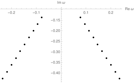
Figure 1: First ten QNFs of the Klein-Gordon field with mass $m=1/10$ propagating in the 2D black hole (2) of radius $r_{+}=70$.

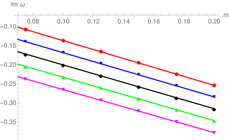
Figure 2: For the first five QNFs of the Klein-Gordon field we show how the imaginary part depends on the mass of the field. We consider a 2D black hole (2) of radius $r_{+}=70$.

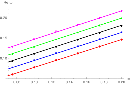
Figure 3: For the first five QNFs of the Klein-Gordon field we show how the real part depends on the mass of the field. We consider a 2D black hole (2) of radius $r_{+}=70$.

Table 2: For the Klein-Gordon field we give the linear fits for the points shown in Figs. 2 and 3. We take $r_{+}=70$.

Mode number	Linear fit for $Im(\omega)$ vs $m$	Linear fit for $Re(\omega)$ vs $m$
0	$-0.0192-1.1720m$	$0.0090+0.6880m$
1	$-0.0522-1.1586m$	$0.0254+0.6936m$
2	$-0.0855-1.1462m$	$0.0420+0.6985m$
3	$-0.1187-1.1363m$	$0.0591+0.7021m$
4	$-0.1520-1.1276m$	$0.0768+0.7030m$

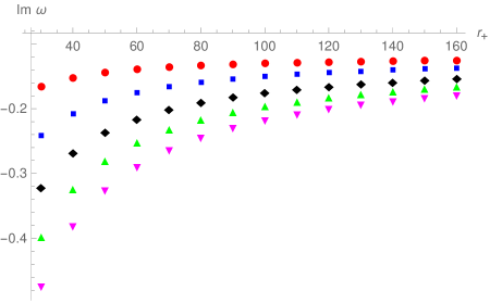
Figure 4: For the first five QNFs of the Klein-Gordon field we show how the imaginary part depends on the radius of the 2D black hole (2). We consider a Klein-Gordon field of mass $m=1/10$.

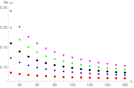
Figure 5: For the first five QNFs of the Klein-Gordon field we show how the real part depends on the radius of the 2D black hole (2). We consider a Klein-Gordon field of mass $m=1/10$.

As we already mentioned, the variable $r$ is defined in the semi-infinite interval $(r_{+},\infty)$, but in the implementation of the AIM, it is convenient to have a finite range of the independent variable. Therefore we use the variable $z$ defined in the formula (32) to write the previous coupled differential equations in the form

$$\frac{dV_{1}}{dz} =\left(-\frac{i\omega r_{+}}{1-z^{3}}+\frac{2+z^{3}}{4(1-z^{3})z}+\frac{1/4-i\omega/(2\kappa)}{z(1-z)}+\frac{i\omega/(2\kappa)-m/2-3/4}{z}\right)V_{1}$$

$$+\frac{imr_{+}}{(1-z)(1+z+z^{2})^{1/2}z}V_{2},$$

$$\frac{dV_{2}}{dz} =\left(\frac{i\omega r_{+}}{1-z^{3}}+\frac{2+z^{3}}{4(1-z^{3})z}-\frac{1/4+i\omega/(2\kappa)}{z(1-z)}+\frac{i\omega/(2\kappa)-m/2-1/4}{z}\right)V_{2}$$

$$-\frac{imr_{+}}{(1+z+z^{2})^{1/2}z}V_{1}.$$ (58)

This coupled system is of the form (2.7) and we can identify the functions $\Lambda_{0}$, $S_{0}$, $\Omega_{0}$, and $P_{0}$ as follows

$$\Lambda_{0}(z) =-\frac{i\omega r_{+}}{1-z^{3}}+\frac{2+z^{3}}{4(1-z^{3})z}+\frac{1/4-i\omega/(2\kappa)}{z(1-z)}+\frac{i\omega/(2\kappa)-m/2-3/4}{z},$$

$$S_{0}(z) =\frac{imr_{+}}{(1-z)(1+z+z^{2})^{1/2}z},$$

$$\Omega_{0}(z) =-\frac{imr_{+}}{(1+z+z^{2})^{1/2}z},$$ (59)

$$P_{0}(z) =\frac{i\omega r_{+}}{1-z^{3}}+\frac{2+z^{3}}{4(1-z^{3})z}-\frac{1/4+i\omega/(2\kappa)}{z(1-z)}+\frac{i\omega/(2\kappa)-m/2-1/4}{z}.$$

From these quantities and taking into account the recurrence relations (2.7) we calculate the quantities $\Delta_{n}$ of Eq. (52), whose stable roots are the QNFs of the Dirac field in the 2D black hole (2). Also we notice that in the functions $S_{0}$, $\Omega_{0}$ appear a factor that includes a square root, but this factor is well defined at the boundaries $z=0$ and $z=1$.

3 Results

In what follows we describe our numerical results for the QNFs of the Klein–Gordon field and of the Dirac field.

3.1 Numerical results for the Klein-Gordon field

For a specific configuration, in Table 1 we show the values of the QNFs for the Klein-Gordon field that produce the HH method and the AIM. For the first ten QNMs, we observe that the two numerical methods yield QNFs which agree to three decimal places. We point out that for all the examples studied in the present work the two methods produce values of the QNFs which agree to three decimal places (see Appendix A where we present some numerical results with more decimal places). We also notice that the two numerical methods yield stable QNFs, that is, frequencies with negative imaginary part.

In Fig. 1 we plot the real part and the imaginary part of the first ten QNFs for the Klein-Gordon field of mass $m=1/10$ propagating in the 2D black hole (2) with radius of the horizon equal to $r_{+}=70$. We notice that the graph $Im(\omega)\,\,\,vs\,\,\,Re(\omega)$ shows a linear relation between the imaginary part and the real part of the QNFs for the Klein-Gordon field as we change the mode number. We notice that in Fig. 1 appear twenty points, but we consider as equivalent the QNFs with the same imaginary part, that is, we find two QNFs with the same imaginary part, but the real part of the first is the negative of the real part of the second.

We notice that in the Figures of this paper (except for Figs. 1, 6) we label the modes of the field as follows: $n=0$, red circle; $n=1$, blue square; $n=2$, black diamond; $n=3$, green triangle; $n=4$, inverted magenta triangle.

For $r_{+}=70$, in Figs. 2 and 3 we present the variation of the imaginary part and the real part of the first five QNFs when we modify the mass of the Klein-Gordon field. In these figures we observe that the imaginary part and the real part of the QNFs change in a linear way as the mass varies. In Figs. 2 and 3 we observe that the imaginary part decreases, whereas the real part increases as the mass of the field increases, thus the QNMs of the Klein-Gordon decay faster and make more oscillations per time unit as the mass of the Klein-Gordon field increases.

Furthermore, in Figs. 2 and 3 we show the plots of the linear fits given in Table 2. From the linear fits of Table 2 we see that for the plots $Im(\omega)$ vs $m$ the absolute value of the slope decreases as the mode number increases. For the plots $Re(\omega)$ vs $m$ we notice that the slope increases as the mode number increases. In both cases the change of slope with the mode number is small.

In Figs. 4 and 5 we draw the behavior of the imaginary part and of the real part for the first five QNFs when the radius of the horizon varies and the mass of the Klein-Gordon field is $m=1/10$. In these figures we see that the imaginary part increases, whereas the real part decreases as the radius of the black hole increases, thus, for a given mode the decay time increases and the oscillation frequency decreases as the horizon radius increases. In both figures we observe that the imaginary part and the real part of the fifth QNFs have the larger variations, whereas the imaginary part and the real part of the fundamental frequency show the smaller changes as the horizon radius increases.

In Figs. 4 and 5 we also notice that the QNFs of the Klein-Gordon field in the 2D black hole (2) are more compactly distributed in the $\omega$ plane for bigger values of the horizon radius.

3.2 Numerical results for the Dirac field

Table 3: First ten QNFs of the Dirac field produced by the HH method and by the AIM for coupled systems of first order differential equations. We take $r_{+}=70$ and $m=1/10$.

Mode number	HH method	AIM coupled
0	$0.078-0.135i$	$0.078-0.135i$
1	$0.095-0.166i$	$0.095-0.166i$
2	$0.112-0.198i$	$0.112-0.198i$
3	$0.130-0.230i$	$0.130-0.230i$
4	$0.148-0.262i$	$0.148-0.262i$
5	$0.166-0.294i$	$0.166-0.294i$
6	$0.184-0.326i$	$0.184-0.326i$
7	$0.202-0.358i$	$0.202-0.358i$
8	$0.220-0.390i$	$0.220-0.390i$
9	$0.238-0.423i$	$0.238-0.423i$

Table 4: We show the QNFs of the Dirac field produced by the effective potentials $V_{1}$ and $V_{2}$. We get these values for the QNFs using the HH method. We take $r_{+}=70$ and $m=1/10$.

Mode number	$V_{2}$	$V_{1}$
0	$0.078-0.135i$	$0.078-0.135i$
1	$0.095-0.166i$	$0.095-0.166i$
2	$0.112-0.198i$	$0.112-0.198i$
3	$0.130-0.230i$	$0.130-0.230i$
4	$0.148-0.262i$	$0.148-0.262i$
5	$0.166-0.294i$	$0.166-0.294i$
6	$0.184-0.326i$	$0.184-0.326i$
7	$0.202-0.358i$	$0.202-0.358i$
8	$0.220-0.390i$	$0.220-0.390i$
9	$0.238-0.423i$	$0.238-0.423i$

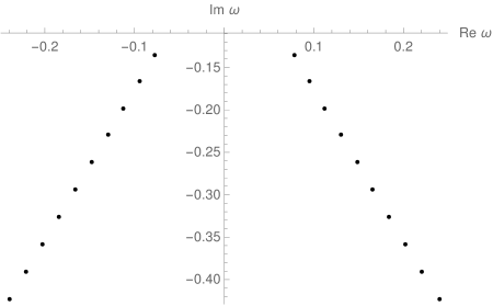
Figure 6: First ten QNFs of the Dirac field with mass $m=1/10$ propagating in the 2D black hole (2) of radius $r_{+}=70$.

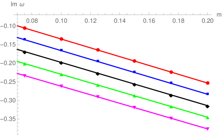
Figure 7: For the first five QNFs of the Dirac field we show how the imaginary part depends on the mass of the field. We consider a 2D black hole (2) of radius $r_{+}=70$.

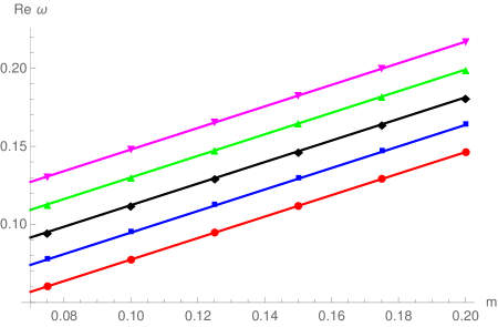
Figure 8: For the first five QNFs of the Dirac field we show how the real part depends on the mass of the field. We consider a 2D black hole (2) of radius $r_{+}=70$.

Table 5: For the Dirac field we give the linear fits for the points shown in Figs. 7 and 8. We take $r_{+}=70$.

Mode number	Linear fit for $Im(\omega)$ vs $m$	Linear fit for $Re(\omega)$ vs $m$
0	$-0.0168-1.1818m$	$0.0087+0.6876m$
1	$-0.0489-1.1717m$	$0.0259+0.6890m$
2	$-0.0816-1.1614m$	$0.0433+0.6898m$
3	$-0.1144-1.1524m$	$0.0610+0.6901m$
4	$-0.1472-1.1450m$	$0.0789+0.6902m$

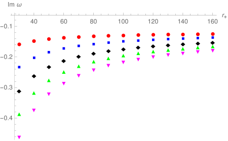
Figure 9: For the first five QNFs of the Dirac field we show how the imaginary part depends on the radius of the 2D black hole (2). We consider a Dirac field of mass $m=1/10$.

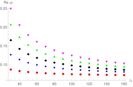
Figure 10: For the first five QNFs of the Dirac field we show how the real part depends on the radius of the 2D black hole (2). We consider a Dirac field of mass $m=1/10$.

For the Dirac field propagating in the 2D black hole (2) we find that, for the first ten modes, the two methods produce QNFs that agree to three decimal places. This fact is observed in Table 3 for a specific configuration (see Appendix A for some numerical results with more decimal places). Furthermore, both methods yield QNFs with negative imaginary part, hence the QNMs of the Dirac field are stable in the 2D black hole (2).

Taking as a basis the HH method, for $r_{+}=70$ and $m=1/10$, in Table 4 we observe that the QNFs produced by the effective potentials $V_{1}$ and $V_{2}$ of Eq. (38) are equal. Also, see the end of Appendix B for another argument pointing out that these effective potentials generate the same QNFs. At present time we only have evidence that the effective potentials of Eq. (38) produce the same spectrum of QNF in the example studied in this work, but we think it would be convenient to show a more general result or find a case where they produce a different spectrum of QNF.

For the Dirac field, in Figs. 6–10 we observe that the behavior of its QNFs is similar to that previously obtained for the QNFs of the Klein-Gordon field, hence we describe briefly the results for the Dirac field.

• For the QNFs of the Dirac field, in Fig. 6 we see that the relation between the imaginary part and the real part of the QNFs is linear as we change the mode number, in a similar way to the QNFs of the Klein-Gordon field.

• In Figs. 7 and 8 we observe that the imaginary part and the real part of the QNFs for the Dirac field change in a linear way when we modify the value of the field’s mass. The linear fits of the data given in Figs. 7 and 8 are written in Table 5. In a similar way to the QNFs of the Klein-Gordon field we see that the imaginary part of the QNFs decreases as the field’s mass increases, whereas the real part of the QNFs increases as the field’s mass increases. As for the Klein-Gordon field, for the plots $Im(\omega)$ vs $m$ the absolute value of the slope decreases as the mode number increases. For the plots $Re(\omega)$ vs $m$ we find that the slope increases as the mode number increases. We also see that in both cases, the changes of the slope with the mode number are small.

• When we change the radius of the horizon, in Figs. 9 and 10 we notice that for the QNFs of the Dirac field the imaginary part increases as the horizon radius increases, while the real part decreases as the horizon radius increases. These behaviors are similar to those for the QNFs of the Klein-Gordon field.

As for the Klein-Gordon field, we also note that the QNFs of the Dirac field are more compactly distributed in the complex $\omega$ plane when the horizon radius is bigger.

4 Discussion

As far as we know, the AIM for coupled systems of first order differential equations has not previously used to calculate the QNFs of black holes. We find that the AIM for coupled systems of first order equations yields QNFs of the Dirac field in agreement with those that produces the HH method (see also Appendices C and D). We believe that this method is appropriate for computing the QNFs of the Dirac field, since in many spacetimes its equation of motion simplifies to a coupled system of first order differential equations [45], [46], [47], and in general the proposed method may be helpful to compute the QNFs of classical fields whose equations of motion simplify to a pair of coupled first order differential equations. Also this method for calculating the QNFs of the Dirac field may be useful to verify the results that are obtained with other numerical procedures. We notice that in Appendix D, taking as a basis the improved formulation of the AIM for second order differential equations [40], [42], we present an improved formulation of the AIM for coupled systems of first order differential equations.

For the two fields propagating in the asymptotically adS 2D black hole (2), we find that the HH method and the AIM produce the same values for their first ten QNFs (see also Appendices C, D). Furthermore, in the numerical results we obtain QNFs with negative imaginary part, therefore the asymptotically adS 2D black hole (2) is stable under the Klein-Gordon and Dirac perturbations. A relevant fact is that its QNFs are complex, in contrast to other asymptotically adS 2D black hole in which purely imaginary QNFs are found [19]. As discussed in Sects. 3.1 and 3.2, in the numerical results we observe that the QNFs of the Klein-Gordon and Dirac fields behave in a similar way as we change the field’s mass or the radius of the horizon. As the mass increases, both fields decay faster and the oscillation frequencies increase. Furthermore, as the radius of the horizon increases the decay time increases, whereas the oscillation frequency decreases.

From the values presented in Tables 1 and 3 we see that the QNFs of the Klein-Gordon and Dirac fields are similar, even though one field is bosonic and the other field is fermionic. Furthermore, in Table 6 we display the numerical values of the QNFs for the Klein-Gordon and Dirac fields propagating in the 2D black holes (2) with radii $r_{+}=30$ and $r_{+}=150$. In this table we observe that for $r_{+}=150$ the QNFs of the two fields are essentially identical, also we note that for $r_{+}=30$ their QNFs are similar but they show more differences than the frequencies of the 2D black holes with radii $r_{+}=70$ and $r_{+}=150$. We also notice that for $r_{+}=30$ the fundamental QNFs are closer in value than the tenth QNFs. Thus the numerical results show that when the horizon radius increases the QNFs of the two fields are more similar. From the viewpoint of the Schrödinger type equations, these results are intriguing, because the analysis of the problem shows that for the two fields their effective potentials are very different. We also note that the effective potentials for the Dirac field fulfill

$$V_{l}=V_{KG}\mp\frac{i\omega}{2}\frac{df}{dr}-\frac{f}{4}\frac{d^{2}f}{dr^{2}}+\frac{1}{16}\left(\frac{df}{dr}\right)^{2}.$$ (60)

Although these differences, for some values of the physical parameters, the effective potentials $V_{l}$, $V_{KG}$ produce almost isospectral QNFs in the asymptotically adS 2D black hole (2). Furthermore, as we previously mentioned, the QNFs of the effective potentials $V_{l}$, $V_{KG}$ behave in a similar way when we change the physical parameters. Thus our numerical results indicate that for the 2D black hole (2) the last terms in the right hand side of the formula (60) have a small contribution to the value of the QNFs for the Dirac field. To start understanding this fact we notice the following facts. Near the horizon the last three terms in the formula (60) only produce a shift in the effective frequency that appears in the Schrödinger type equations, from $\omega$ for the Klein-Gordon field to $(\omega\pm i\kappa/2)$ for the Dirac field. Therefore, near the horizon, for the Klein-Gordon field we get the radial solutions (9) whereas for the Dirac field we obtain the solutions (40). This fact does not prevent us from choosing the relevant solution for the QNMs. As $r\to\infty$, the last three terms in Eq. (60) produce that the dominant behavior of the effective potentials change from $V_{KG}\sim a^{2}r^{2}m^{2}$ for the Klein-Gordon field to $V_{l}\sim a^{2}r^{2}(m^{2}-a^{2}/4)$ for the Dirac field, that is, only produce a shift in the value of the mass. In our case this change does not prevent us from choosing the appropriate solution that satisfies the boundary condition of the QNMs at the asymptotic region.

Table 6: For the 2D black holes (2) with radii $r_{+}=30$ and $r_{+}=150$ we display the QNFs of the Klein-Gordon and Dirac fields of mass $m=1/10$.

	$r_{+}=30$		$r_{+}=150$
Mode number	Klein-Gordon	Dirac	Klein-Gordon	Dirac
0	$0.087-0.166i$	$0.087-0.160i$	$0.073-0.126i$	$0.073-0.126i$
1	$0.123-0.243i$	$0.127-0.235i$	$0.081-0.141i$	$0.081-0.140i$
2	$0.161-0.321i$	$0.167-0.311i$	$0.089-0.155i$	$0.089-0.154i$
3	$0.201-0.398i$	$0.208-0.387i$	$0.097-0.169i$	$0.097-0.169i$
4	$0.241-0.474i$	$0.250-0.462i$	$0.106-0.184i$	$0.106-0.183i$
5	$0.281-0.551i$	$0.291-0.538i$	$0.114-0.199i$	$0.114-0.198i$
6	$0.322-0.627i$	$0.333-0.614i$	$0.122-0.214i$	$0.122-0.213i$
7	$0.364-0.704i$	$0.376-0.689i$	$0.131-0.229i$	$0.131-0.228i$
8	$0.405-0.780i$	$0.418-0.765i$	$0.139-0.244i$	$0.139-0.243i$
9	$0.447-0.856i$	$0.460-0.841i$	$0.148-0.258i$	$0.148-0.257i$

5 Acknowledgments

This work was supported by CONACYT México, SNI México, EDI-IPN, COFAA-IPN, and Research Project IPN SIP 20210485.

Appendix A Additional tables

For the QNFs of the Klein-Gordon field, in Table 7 we present the values that produce the HH method and the AIM to higher digits (compare with Table 1). In Table 7 we observe that for the first seven QNMs both numerical methods produce the same QNFs to seven decimal places, but for the last three QNFs we notice some differences in the last digits.

Table 7: For the Klein-Gordon field we show its QNFs to higher digits. The QNFs are produced by the HH method and the AIM. We take $r_{+}=70$ and $m=1/10$.

Mode number	HH method	AIM
0	$0.0778658-0.1362857i$	$0.0778658-0.1362857i$
1	$0.0948790-0.1678734i$	$0.0948790-0.1678734i$
2	$0.1120717-0.1999259i$	$0.1120717-0.1999259i$
3	$0.1294365-0.2322016i$	$0.1294365-0.2322016i$
4	$0.1469485-0.2645830i$	$0.1469485-0.2645830i$
5	$0.1645814-0.2970118i$	$0.1645814-0.2970118i$
6	$0.1823128-0.3294582i$	$0.1823128-0.3294582i$
7	$0.2001263-0.3619064i$	$0.2001251-0.3619070i$
8	$0.2180128-0.3943701i$	$0.2180044-0.3943504i$
9	$0.2357184-0.4268551i$	$0.2359398-0.4267845i$

In a similar way, in Table 8 we give the QNFs of the Dirac field produced by the HH method and the AIM to higher digits (compare with Table 3). As for the Klein-Gordon field, the first seven QNFs of the Dirac field coincide to seven decimal places and the last three QNFs show differences in the last digits.

Table 8: For the Dirac field we show its QNFs to higher digits. The QNFs are produced by the HH method and the AIM. We take $r_{+}=70$ and $m=1/10$.

Mode number	HH method	AIM
0	$0.0775319-0.1349311i$	$0.0775319-0.1349311i$
1	$0.0948471-0.1659988i$	$0.0948471-0.1659988i$
2	$0.1124024-0.1976164i$	$0.1124024-0.1976164i$
3	$0.1301370-0.2295252i$	$0.1301370-0.2295252i$
4	$0.1480059-0.2615908i$	$0.1480059-0.2615908i$
5	$0.1659765-0.2937427i$	$0.1659765-0.2937427i$
6	$0.1840250-0.3259428i$	$0.1840250-0.3259428i$
7	$0.2021342-0.3581700i$	$0.2021343-0.3581696i$
8	$0.2202862-0.3904068i$	$0.2202922-0.3904111i$
9	$0.2385630-0.4225911i$	$0.2384893-0.4226599i$

Appendix B The Dirac equation in a null dyad

Reference [20] shows that in a static 2D spacetime with diagonal metric and in the chiral representation for the gamma matrices, the Dirac equation (35) simplifies to a pair of Schrödinger type equations with effective potentials involving square roots of the metric functions (see the expressions (36)). Motivated by the Newman-Penrose formalism of four-dimensional spacetimes [48], for a static and diagonal 2D spacetime in what follows we use a null dyad to simplify the Dirac equation to a different pair of Schrödinger type equations with potentials not including square roots.

It is convenient to write the metric of the 2D spacetime under study as

$$ds^{2}=\mathcal{P}^{2}dt^{2}-\mathcal{Q}^{2}dr^{2},$$ (61)

where the functions $\mathcal{P}$, $\mathcal{Q}$ depend on $r$, $\mathcal{P}\geq 0$, $\mathcal{Q}\geq 0$. We choose the basis of null vectors

$$\widehat{e}^{\ \mu}_{1}=\frac{1}{\sqrt{2}}\left(\frac{1}{\mathcal{P}},\frac{1}{\mathcal{Q}}\right),\ \ \ \ \ \widehat{e}^{\ \mu}_{2}=\frac{1}{\sqrt{2}}\left(\frac{1}{\mathcal{P}},-\frac{1}{\mathcal{Q}}\right),$$ (62)

that satisfies

$$\widehat{e}_{a}^{\ \mu}\widehat{e}_{b\mu}=\eta_{ab}$$ (63)

where $a,b=1,2,$ and

$$\left(\eta_{ab}\right)=\left(\eta^{ab}\right)=\begin{pmatrix}0&1\\ 1&0\\ \end{pmatrix}.$$ (64)

Using the representation of the gamma matrices

$$\gamma_{1}=\frac{1}{\sqrt{2}}\begin{pmatrix}0&2\\ 0&0\\ \end{pmatrix},\,\,\qquad\gamma_{2}=\frac{1}{\sqrt{2}}\begin{pmatrix}0&0\\ 2&0\\ \end{pmatrix},$$ (65)

that fulfills $\gamma_{a}\gamma_{b}+\gamma_{b}\gamma_{a}=2\eta_{ab}I$, we find that in the 2D spacetime (61) the Dirac equation simplifies to the coupled system of partial differential equations

$$\begin{split}\frac{1}{\mathcal{P}}\partial_{t}\psi_{2}-\frac{1}{\mathcal{Q}}\partial_{r}\psi_{2}-\frac{1}{2\mathcal{P}\mathcal{Q}}\frac{d\mathcal{P}}{dr}\psi_{2}=-im\psi_{1},\\ \frac{1}{\mathcal{P}}\partial_{t}\psi_{1}+\frac{1}{\mathcal{Q}}\partial_{r}\psi_{1}+\frac{1}{2\mathcal{P}\mathcal{Q}}\frac{d\mathcal{P}}{dr}\psi_{1}=-im\psi_{2},\end{split}$$ (66)

where $\psi_{1}$ and $\psi_{2}$ are the components of the 2-spinor

$$\Psi=\begin{pmatrix}\psi_{1}\\ \psi_{2}\\ \end{pmatrix}.$$ (67)

Taking the components $\psi_{1}$ and $\psi_{2}$ in the form

$$\psi_{1}=R_{1}(r)e^{-i\omega t},\qquad\qquad\psi_{2}=R_{2}(r)e^{-i\omega t},$$ (68)

from the coupled partial differential equations (66) we get that the functions $R_{1}$ and $R_{2}$ must be solutions for the coupled system of first order differential equations

$$\frac{1}{\mathcal{Q}}\frac{dR_{2}}{dr}+\frac{i\omega}{\mathcal{P}}R_{2}+\frac{1}{2\mathcal{P}\mathcal{Q}}\frac{d\mathcal{P}}{dr}R_{2} =imR_{1},$$

$$\frac{1}{\mathcal{Q}}\frac{dR_{1}}{dr}-\frac{i\omega}{\mathcal{P}}R_{1}+\frac{1}{2\mathcal{P}\mathcal{Q}}\frac{d\mathcal{P}}{dr}R_{1} =-imR_{2}.$$ (69)

For 2D spacetimes that fulfill $\left(\mathcal{P}\mathcal{Q}\right)^{2}=1$, as the 2D black hole (2), from the previous system of coupled differential equations for the functions $R_{l}$ we obtain the decoupled equations

$$\mathcal{P}^{4}\frac{d^{2}R_{l}}{dr^{2}}+2\mathcal{P}^{3}\frac{d\mathcal{P}}{dr}\frac{dR_{l}}{dr}$$

$$+\left(\omega^{2}\pm i\omega\mathcal{P}\frac{d\mathcal{P}}{dr}+\frac{\mathcal{P}^{3}}{2}\frac{d^{2}\mathcal{P}}{dr^{2}}+\left(\frac{\mathcal{P}}{2}\frac{d\mathcal{P}}{dr}\right)^{2}-\mathcal{P}^{2}m^{2}\right)R_{l}=0.$$ (70)

We also point out that

$$\frac{d^{2}R_{l}}{dr_{*}^{2}}=\mathcal{P}^{2}\frac{d}{dr}\left(\mathcal{P}^{2}\frac{dR_{l}}{dr}\right)=\mathcal{P}^{4}\frac{d^{2}R_{l}}{dr^{2}}+2\mathcal{P}^{3}\frac{d\mathcal{P}}{dr}\ \frac{dR_{l}}{dr},$$ (71)

and therefore Eqs.  (B) simplify to Schrödinger type equations

$$\frac{d^{2}R_{l}}{dr_{*}^{2}}+\omega^{2}R_{l}=V_{l}R_{l},$$ (72)

with effective potentials

$$V_{l}=m^{2}\mathcal{P}^{2}\mp\frac{i\omega}{2}\frac{d\mathcal{P}^{2}}{dr}-\frac{\mathcal{P}^{2}}{4}\frac{d^{2}\mathcal{P}^{2}}{dr^{2}}+\frac{1}{16}\left(\frac{d\mathcal{P}^{2}}{dr}\right)^{2}.$$ (73)

In contrast to the effective potentials of Ref.  [20] that involve square roots (see the formulas (36)), the previous effective potentials does not involve square roots of the metric functions. Furthermore, we notice that for the 2D black hole (2) it is true that $\mathcal{P}^{2}=f=a^{2}r^{2}-1/(ar)$.

We also notice that taking

$$R_{1}=\frac{1}{P^{1/2}}\hat{R}_{1},\qquad\qquad\qquad R_{2}=\frac{1}{P^{1/2}}\hat{R}_{2},$$ (74)

from the coupled system of differential equations (B) we find that the functions $\hat{R}_{1}$ and $\hat{R}_{2}$ must be solutions of the coupled equations

$$\frac{d\hat{R}_{2}}{dr_{*}}+i\omega\hat{R}_{2}=mP\hat{R}_{1},\qquad\qquad\qquad\frac{d\hat{R}_{1}}{dr_{*}}-i\omega\hat{R}_{1}=mP\hat{R}_{2},$$ (75)

where $r_{*}$ now denotes the tortoise coordinate of the metric (61) and is given by

$$\frac{dr_{*}}{dr}=\frac{Q}{P}.$$ (76)

Defining

$$Z_{\pm}=\hat{R}_{1}\pm\hat{R}_{2},\qquad\qquad\qquad W=mP,$$ (77)

from (75) we get that the functions $Z_{\pm}$ satisfy

$$\frac{dZ_{+}}{dr_{*}}-WZ_{+}=i\omega Z_{-},\qquad\qquad\qquad\frac{dZ_{-}}{dr_{*}}+WZ_{-}=i\omega Z_{+}.$$ (78)

As is well known [50]–[52], from the previous equations we find that the functions $Z_{\pm}$ are solutions of the Schrodinger type equations

$$\frac{d^{2}Z_{\pm}}{dr_{*}^{2}}+\omega^{2}Z_{\pm}-V_{\pm}Z_{\pm}=0,$$ (79)

where the effective potentials $V_{\pm}$ are equal to

$$V_{\pm}=W^{2}\pm\frac{dW}{dr_{*}}.$$ (80)

Explicitly, in the spacetime (61) they are equal to

$$V_{\pm}=m^{2}P^{2}\pm m\frac{dP}{dr_{*}}.$$ (81)

From the expressions (80) we see that the effective potentials $V_{\pm}$ are supersymmetric partners [44], [52] (see Ref. [20] for a similar result in static diagonal 2D black holes, but in a different dyad of basis vectors). As a consequence, we expect that the functions $R_{1}$ and $R_{2}$ have the same spectrum. It is convenient to notice that we have not been able to write the effective potentials (73) in the form (80), that is, we have not found a function $W$ that is a superpotential for the effective potentials (73). Despite this fact, we think that the previous arguments indicate that the two potentials (73) have the same spectrum (see also Sect. 3.2 and Table 4).

Finally, we note that in a similar way to the previous results for 2D static black holes, it is known that in higher dimensional static black holes, the Dirac equation simplifies to a pair of Schrödinger type equations, see Refs. [50]–[55] for some examples.

Appendix C Quasinormal frequencies of the Klein-Gordon field from a coupled system

In Sect. 2.4 we use the formulation of the AIM for second order differential equations [39] to calculate the QNFs of the Klein-Gordon field. Taking into account that a second order linear differential equation can be written as a coupled system of first order differential equations [56], we can exploit the AIM for coupled systems of first order differential equations to compute its QNFs.

To show this fact we rewrite Eq. (33) as

$$\frac{d^{2}\hat{R}}{dz^{2}}=\lambda_{0}\frac{d\hat{R}}{dz}+s_{0}\hat{R},$$ (82)

where $\lambda_{0}$ and $s_{0}$ are given in the expressions (34). Defining the functions $W_{1}$, $W_{2}$ by

$$W_{1}=\hat{R},\qquad\qquad W_{2}=\frac{d\hat{R}}{dz},$$ (83)

that is, $d^{2}\hat{R}/dz^{2}=dW_{2}/dz$, we encounter that Eq. (82) is equivalent to the coupled system of first order differential equations

$$\frac{dW_{1}}{dz} =W_{2},$$ (84)

$$\frac{dW_{2}}{dz} =s_{0}W_{1}+\lambda_{0}W_{2}.$$

Comparing to the system of first order differential equations (2.7) of Sect. 2.7, for the Klein-Gordon field we find that the functions $\Lambda_{0}$, $S_{0}$, $\Omega_{0}$, $P_{0}$ are equal to

$$\Lambda_{0}=0,\qquad\qquad S_{0}=1,\qquad\qquad\Omega_{0}=s_{0},\qquad\qquad P_{0}=\lambda_{0}.$$ (85)

Taking as a basis these functions, we use the recurrence relations (2.7) to calculate the quantities that appear in the quantization condition (52), whose stable roots are the QNFs of the Klein-Gordon field. Implementing for the Klein-Gordon field the AIM for coupled systems of first order differential equations as previously commented, we find that this approach to the problem yields the same values for its QNFs that we present in Sect. 3.1. Therefore we think that this transformation can be used for any second order differential equation of the form (82) and we can calculate its eigenvalues with the AIM for coupled systems of first order differential equations. Moreover, we think that this alternative formulation can be used to verify the results that produces the AIM for second order differential equations.

Appendix D The improved asymptotic iteration method

In the AIM for second order differential equations, the recurrence relations (24) demand the calculation of the derivatives for the functions $\lambda_{n}$, $s_{n}$, a process that requires many resources. To make the AIM more efficient in the computation of QNFs, in Ref. [40] (see also [42]) it is proposed the improved asymptotic iteration method (IAIM in what follows) that allows us to determine the QNFs without computing the derivatives of the functions $\lambda_{n}$, $s_{n}$. In the IAIM we first expand the functions $\lambda_{n}$, $s_{n}$ around a point $\xi$ in the form [40], [42]

$$\lambda_{n}(\xi)=\sum^{\infty}_{i=0}c^{i}_{n}(x-\xi)^{i},\qquad s_{n}(\xi)=\sum^{\infty}_{i=0}d^{i}_{n}(x-\xi)^{i},$$ (86)

and then we substitute these expressions into the recurrence relations (24) to find that the coefficients $c^{i}_{n}$, $d^{i}_{n}$ satisfy [40], [42]

$$c^{i}_{n}=(i+1)c^{i+1}_{n-1}+d^{i}_{n-1}+\sum^{i}_{k=0}c^{k}_{0}c^{i-k}_{n-1},\qquad d^{i}_{n}=(i+1)d^{i+1}_{n-1}+\sum^{i}_{k=0}d^{k}_{0}c^{i-k}_{n-1}.$$ (87)

Using these coefficients, we write the quantization condition (26) as follows [40], [42]

$$d^{0}_{n}c^{0}_{n-1}-d^{0}_{n-1}c^{0}_{n}=0.$$ (88)

In a similar way to the AIM, the stable roots of this equation are the QNFs of the field. Taking as a basis Eq. (33), if we use the IAIM to calculate the QNFs of the Klein-Gordon field in the 2D black hole (2), then we obtain the same numerical results for the QNFs that we expound in Sect. 3.1.

Based on this extension of the AIM for second order differential equations, in what follows we develop an improved version of the AIM for coupled systems of first order differential equations, since in this method we also require the calculation of the derivatives for the functions $\Lambda_{n}$, $S_{n}$, $\Omega_{n}$, $P_{n}$ to evaluate the recurrence relations (2.7) and as previously commented these mathematical operations demand many resources. As far as we know, this extension of the AIM for coupled systems has not previously presented. We first expand the functions $\Lambda_{0}$, $S_{0}$, $\Omega_{0}$, and $P_{0}$ around a point $\xi$ (in a similar way to the formulas (86) for the AIM of second order differential equations)

$$\Lambda_{n}(\xi)=\sum_{i=0}^{\infty}C_{n}^{i}(x-\xi)^{i},\qquad\Omega_{n}(\xi)=\sum_{i=0}^{\infty}E_{n}^{i}(x-\xi)^{i},$$

$$S_{n}(\xi)=\sum_{i=0}^{\infty}D_{n}^{i}(x-\xi)^{i},\qquad P_{n}(\xi)=\sum_{i=0}^{\infty}F_{n}^{i}(x-\xi)^{i},$$ (89)

and then we substitute these expressions in the recurrence relations (2.7), to get that the coefficients $C_{n}^{i}$, $D_{n}^{i}$, $E_{n}^{i}$, $F_{n}^{i}$, satisfy the recurrence relations

$$C_{n}^{i} =\sum_{k=0}^{i}\left(C_{n-1}^{i-k}C_{0}^{k}+D_{n-1}^{i-k}E_{0}^{k}\right)+(i+1)C_{n-1}^{i+1},$$

$$D_{n}^{i} =\sum_{k=0}^{i}\left(C_{n-1}^{i-k}D_{0}^{k}+D_{n-1}^{i-k}F_{0}^{k}\right)+(i+1)D_{n-1}^{i+1},$$

$$E_{n}^{i} =\sum_{k=0}^{i}\left(E_{n-1}^{i-k}C_{0}^{k}+F_{n-1}^{i-k}E_{0}^{k}\right)+(i+1)E_{n-1}^{i+1},$$

$$F_{n}^{i} =\sum_{k=0}^{i}\left(E_{n-1}^{i-k}D_{0}^{k}+F_{n-1}^{i-k}F_{0}^{k}\right)+(i+1)F_{n-1}^{i+1}.$$ (90)

Using these coefficients, we get that the quantization condition (52) of the AIM for systems of coupled first order differential equations takes the form

$$D_{n}^{0}C_{n-1}^{0}-D_{n-1}^{0}C_{n}^{0}=0.$$ (91)

This condition is similar to Eq. (88) of the AIM, but we notice that the coefficients which appear in the last condition satisfy different recurrence relations than the coefficients $c^{i}_{n}$, $d^{i}_{n}$. Taking as a basis the expressions (2.7), if we use this improved formulation of the AIM for coupled systems of first order differential equations to compute the QNFs of the Dirac field propagating in the 2D black hole (2), then we obtain the same QNFs given in Sect. 3.2.

Appendix E Quasinormal frequencies of the massive Dirac field in a $D$-dimensional Lifshitz black hole

The dynamics of classical fields has been studied in the $D$-dimensional Lifshitz black hole with metric [57]-[61]

$$ds^{2}=\frac{r^{4}}{l^{4}}\left(1-\frac{r_{+}^{2}}{r^{2}}\right)dt^{2}-\frac{l^{2}dr^{2}}{r^{2}-r_{+}^{2}}-r^{2}d\Omega^{2},$$ (92)

where $r_{+}$ is the radius of the event horizon, $d\Omega^{2}$ is the metric of a $(D-2)$-dimensional plane, and $l$ is a constant that determines the Lifshitz radius [57], [58]. In this Lifshitz black hole the exact values of the QNFs for several fields are known [58]–[61]. In particular, in the zero momentum limit, the QNFs of the massive Dirac field with mass $m$ are exactly calculated and they are given by [60], [61]

$$\tilde{\omega}=-i\left(n+\frac{\tilde{m}}{2}+\frac{1}{2}\right),$$ (93)

where $\tilde{m}=ml$, $\tilde{\omega}=(\omega l^{3})/r_{+}^{2}$, and $n=0,1,2,\ldots$

To investigate whether the coupled AIM works to determine the QNFs of the massive Dirac field moving in the $D$-dimensional Lifshitz black hole (92), in what follows we show how to transform the coupled radial equations that govern its dynamics. As shown in Ref. [61], in the $D$-dimensional Lifshitz black hole (92) the massive Dirac equation in the zero momentum limit takes the form

$$z(z^{2}-1)\frac{dR_{2}}{dz}+i\tilde{\omega}R_{2} =z(z^{2}-1)^{1/2}i\tilde{m}R_{1},$$ (94)

$$z(z^{2}-1)\frac{dR_{1}}{dz}-i\tilde{\omega}R_{1} =-z(z^{2}-1)^{1/2}i\tilde{m}R_{2},$$

where $z=r/r_{+}$ with $z\in(1,\infty)$.

To transform Eqs. (94) into a convenient form we define the functions $W_{1}$ and $W_{2}$ by

$$R_{1}=\frac{(z^{2}-1)^{1/2}}{z}W_{1},\qquad\qquad R_{2}=W_{2},$$ (95)

to find that they must be solutions of the coupled system of first order differential equations

$$z(z^{2}-1)\frac{dW_{2}}{dz}+i\tilde{\omega}W_{2}=(z^{2}-1)i\tilde{m}W_{1},$$ (96)

$$z(z^{2}-1)\frac{dW_{1}}{dz}+(1-i\tilde{\omega})W_{1}=-z^{2}i\tilde{m}R_{2}.$$

To consider the boundary conditions of the QNMs we take the functions $W_{1}$ and $W_{2}$ as

$$W_{1}=h(z)U_{1},\qquad\qquad W_{2}=h(z)U_{2},$$ (97)

with

$$h(z)=(z-1)^{-i\tilde{\omega}/2}z^{-\tilde{m}+i\tilde{\omega}/2},$$ (98)

to find that the functions $U_{1}$ and $U_{2}$ satisfy the system of differential equations

$$\frac{dU_{1}}{du} =\left(\frac{i\tilde{\omega}}{2u}+\frac{\tilde{m}}{1-u}+\frac{(i\tilde{\omega}-1)(1-u)}{u(2-u)}\right)U_{1}-\frac{i\tilde{m}}{u(2-u)(1-u)}U_{2},$$ (99)

$$\frac{dU_{2}}{du} =\frac{i\tilde{m}}{(1-u)}U_{1}+\left(\frac{i\tilde{\omega}}{2u}+\frac{\tilde{m}}{1-u}-\frac{i\tilde{\omega}(1-u)}{u(2-u)}\right)U_{2},$$

where the variable $u$ is defined by

$$u=\frac{z-1}{z}.$$ (100)

This system of equations is of the form (2.7) and as a consequence, we can identify the functions $\Lambda_{0}$, $S_{0}$, $\Omega_{0}$, and $P_{0}$ as follows

$$\Lambda_{0} =\frac{i\tilde{\omega}}{2u}+\frac{\tilde{m}}{1-u}+\frac{(i\tilde{\omega}-1)(1-u)}{u(2-u)},$$

$$S_{0} =-\frac{i\tilde{m}}{u(2-u)(1-u)},$$

$$\Omega_{0} =\frac{i\tilde{m}}{(1-u)},$$ (101)

$$P_{0} =\frac{i\tilde{\omega}}{2u}+\frac{\tilde{m}}{1-u}-\frac{i\tilde{\omega}(1-u)}{u(2-u)}.$$

From these functions we can use the coupled AIM to determine, in the zero momentum limit, the QNFs of the massive Dirac field propagating in the $D$-dimensional Lifshitz black hole (92). In Table 9 we compare the QNFs that we obtain from the coupled AIM and those that we get from the analytical expression (93). We see the QNFs of the first ten QNMs coincide very well.

Table 9: For the $D$-dimensional Lifshitz black hole (92) we show the QNFs of the Dirac field that produce the analytical expression (93) and the coupled AIM. We take $\tilde{m}=3/7$.

Mode number	Analytical	Coupled AIM
0	$-0.7143i$	$-0.7143i$
1	$-1.7143i$	$-1.7143i$
2	$-2.7143i$	$-2.7143i$
3	$-3.7143i$	$-3.7143i$
4	$-4.7143i$	$-4.7143i$
5	$-5.7143i$	$-5.7143i$
6	$-6.7143i$	$-6.7143i$
7	$-7.7143i$	$-7.7143i$
8	$-8.7143i$	$-8.7143i$
9	$-9.7143i$	$-9.7143i$

References

- [1] K. D. Kokkotas and B. G. Schmidt, Living Rev. Rel. 2, 2 (1999), doi:10.12942/lrr-1999-2 [arXiv:gr-qc/9909058].
- [2] R. Konoplya and A. Zhidenko, Rev. Mod. Phys. 83, 793 (2011), doi:10.1103/RevModPhys.83.793 [arXiv:1102.4014 [gr-qc]].
- [3] E. Berti, V. Cardoso and A. O. Starinets, Class. Quant. Grav. 26, 163001 (2009), doi:10.1088/0264-9381/26/16/163001 [arXiv:0905.2975 [gr-qc]].
- [4] S. J. Avis, C. J. Isham and D. Storey, Phys. Rev. D 18, 3565 (1978) doi:10.1103/PhysRevD.18.3565
- [5] P. Breitenlohner and D. Z. Freedman, Phys. Lett. B 115, 197-201 (1982) doi:10.1016/0370-2693(82)90643-8
- [6] C. P. Burgess and C. A. Lutken, Phys. Lett. B 153, 137-141 (1985) doi:10.1016/0370-2693(85)91415-7
- [7] A. Dasgupta, Phys. Lett. B 445, 279-286 (1999) doi:10.1016/S0370-2693(98)01492-0 [arXiv:hep-th/9808086 [hep-th]].
- [8] D. Grumiller, W. Kummer and D. V. Vassilevich, Phys. Rept. 369, 327 (2002), doi:10.1016/S0370-1573(02)00267-3 [hep-th/0204253].
- [9] D. Grumiller and R. Meyer, Turk. J. Phys. 30, 349 (2006), [hep-th/0604049].
- [10] R. Becar, S. Lepe and J. Saavedra, Phys. Rev. D 75, 084021 (2007), doi:10.1103/PhysRevD.75.084021 [arXiv:gr-qc/0701099].
- [11] A. Lopez-Ortega, Int. J. Mod. Phys. D 18, 1441 (2009), doi:10.1142/S0218271809015199 [arXiv:0905.0073 [gr-qc]].
- [12] Y. S. Myung and T. Moon, Phys. Rev. D 86, 024006 (2012), doi:10.1103/PhysRevD.86.024006 [arXiv:1204.2116 [hep-th]].
- [13] R. Becar, S. Lepe and J. Saavedra, Int. J. Mod. Phys. A 25, 1713 (2010). doi:10.1142/S0217751X10048275
- [14] J. Kettner, G. Kunstatter and A. J. M. Medved, Class. Quant. Grav. 21, 5317 (2004), doi:10.1088/0264-9381/21/23/002 [gr-qc/0408042].
- [15] A. Lopez-Ortega, Int. J. Mod. Phys. D 20, 2525 (2011), doi:10.1142/S0218271811020524 [arXiv:1112.6211 [gr-qc]].
- [16] X. Z. Li, J. G. Hao and D. J. Liu, Phys. Lett. B 507, 312 (2001), doi:10.1016/S0370-2693(01)00437-3 [gr-qc/0205007].
- [17] S. Estrada-Jiménez, J. R. Gómez-Díaz and A. López-Ortega, Gen. Rel. Grav. 45, 2239 (2013), doi:10.1007/s10714-013-1582-1 [arXiv:1308.5943 [gr-qc]].
- [18] M. M. Stetsko, Eur. Phys. J. C 77, 416 (2017), doi:10.1140/epjc/s10052-017-4983-6 [arXiv:1612.09172 [hep-th]].
- [19] R. Cordero, A. Lopez-Ortega and I. Vega-Acevedo, Gen. Rel. Grav. 44, 917 (2012), doi:10.1007/s10714-011-1316-1 [arXiv:1201.3605 [gr-qc]].
- [20] A. Lopez-Ortega and I. Vega-Acevedo, Gen. Rel. Grav. 43, 2631 (2011), doi:10.1007/s10714-011-1185-7 [arXiv:1105.2802 [gr-qc]].
- [21] S. Bhattacharjee, S. Sarkar and A. Bhattacharyya, Phys. Rev. D 103, no.2, 024008 (2021), doi:10.1103/PhysRevD.103.024008 [arXiv:2011.08179 [gr-qc]].
- [22] K. Jusufi, I. Sakallı and A. Ovgün, Gen. Rel. Grav. 50, no.1, 10 (2018) doi:10.1007/s10714-017-2330-8 [arXiv:1709.03923 [gr-qc]].
- [23] İ. Sakallı, K. Jusufi and A. Övgün, Gen. Rel. Grav. 50, no.10, 125 (2018) doi:10.1007/s10714-018-2455-4 [arXiv:1803.10583 [gr-qc]].
- [24] M. Mirbabayi, JCAP 01, 052 (2020) doi:10.1088/1475-7516/2020/01/052 [arXiv:1807.04843 [gr-qc]].
- [25] İ. Sakalli and G. T. Hyusein, Turk. J. Phys. 45, no.1, 43-58 (2021) doi:10.3906/fiz-2012-6 [arXiv:2102.03595 [hep-th]].
- [26] S. Kanzi and İ. Sakallı, doi:10.1140/epjc/s10052-021-09299-y [arXiv:2102.06303 [hep-th]].
- [27] A. Zelnikov, JHEP 0807, 010 (2008), doi:10.1088/1126-6708/2008/07/010 [arXiv:0805.4031 [hep-th]].
- [28] G. T. Horowitz and V. E. Hubeny, Phys. Rev. D 62, 024027 (2000), doi:10.1103/PhysRevD.62.024027 [hep-th/9909056].
- [29] J. Chan and R. B. Mann, Phys. Rev. D 55, 7546 (1997), doi:10.1103/PhysRevD.55.7546 [arXiv:gr-qc/9612026 [gr-qc]].
- [30] J. S. F. Chan, R. B. Mann, Phys. Rev. D 59, 064025 (1999). doi:10.1103/PhysRevD.59.064025
- [31] A. Lopez-Ortega, Rev. Mex. Fis. 56, 44 (2010), [arXiv:1006.4906 [gr-qc]].
- [32] M. Giammatteo and J. Jing, Phys. Rev. D 71, 024007 (2005), doi:10.1103/PhysRevD.71.024007 [arXiv:gr-qc/0403030 [gr-qc]].
- [33] S. Hod, Phys. Rev. Lett. 81, 4293 (1998), doi:10.1103/PhysRevLett.81.4293 [arXiv:gr-qc/9812002 [gr-qc]].
- [34] M. Maggiore, Phys. Rev. Lett. 100, 141301 (2008), doi:10.1103/PhysRevLett.100.141301 [arXiv:0711.3145 [gr-qc]].
- [35] S. Wei and Y. Liu, [arXiv:0906.0908 [hep-th]].
- [36] Y. Kwon and S. Nam, Class. Quant. Grav. 27, 125007 (2010), doi:10.1088/0264-9381/27/12/125007 [arXiv:1001.5106 [hep-th]].
- [37] A. Lopez-Ortega, Gen. Rel. Grav. 42, 2939 (2010), doi:10.1007/s10714-010-1049-6 [arXiv:1006.5039 [gr-qc]].
- [38] J. P. S. Lemos and P. M. Sa, Phys. Rev. D 49, 2897 (1994), doi:10.1103/PhysRevD.49.2897 [gr-qc/9311008]. Erratum: [Phys. Rev. D 51, 5967 (1995)].
- [39] H. Ciftci, R. L. Hall, and N. Saad, J. of Phys. A Math. Gen. 36, 11807 (2003). doi:10.1088/0305-4470/36/47/008
- [40] H. Cho, A. Cornell, J. Doukas and W. Naylor, Class. Quant. Grav. 27, 155004 (2010), doi:10.1088/0264-9381/27/15/155004 [arXiv:0912.2740 [gr-qc]].
- [41] H. Ciftci, R. L. Hall, and N. Saad, Phys. Rev. A 72, 022101 (2005). doi:10.1103/PhysRevA.72.022101
- [42] H. Cho, A. Cornell, J. Doukas, T. Huang and W. Naylor, Adv. Math. Phys. 2012, 281705 (2012), doi:10.1155/2012/281705 [arXiv:1111.5024 [gr-qc]].
- [43] J. P. Lemos, Class. Quant. Grav. 12, 1081 (1995), doi:10.1088/0264-9381/12/4/014 [arXiv:gr-qc/9407024 [gr-qc]].
- [44] F. Cooper, A. Khare and U. Sukhatme, Phys. Rept. 251, 267-385 (1995) doi:10.1016/0370-1573(94)00080-M [arXiv:hep-th/9405029 [hep-th]].
- [45] A. Lopez-Ortega, Lat. Am. J. Phys. Educ. 3, 578 (2009), [arXiv:0906.2754 [gr-qc]].
- [46] G. Gibbons and A. R. Steif, Phys. Lett. B 314, 13 (1993), doi:10.1016/0370-2693(93)91315-E [arXiv:gr-qc/9305018 [gr-qc]].
- [47] I. I. Cotaescu, Mod. Phys. Lett. A 13, 2991 (1998), doi:10.1142/S021773239800317X [arXiv:gr-qc/9808030 [gr-qc]].
- [48] E. Newman and R. Penrose, J. Math. Phys. 3, 556 (1962). doi:10.1063/1.1724257
- [49] A. Lopez-Ortega, Gen. Rel. Grav. 36, 1299 (2004). doi:10.1023/B:GERG.0000022389.05399.6d
- [50] S. Chandrasekhar, The Mathematical Theory of Black Holes. Oxford University Press, Oxford (1992).
- [51] H. T. Cho, Phys. Rev. D 68, 024003 (2003) doi:10.1103/PhysRevD.68.024003 [arXiv:gr-qc/0303078 [gr-qc]].
- [52] A. Lopez-Ortega, Int. J. Mod. Phys. D 21, 1250092 (2012) doi:10.1142/S0218271812500927 [arXiv:1211.1801 [gr-qc]].
- [53] F. Finster, J. Smoller and S. T. Yau, J. Math. Phys. 41, 2173-2194 (2000) doi:10.1063/1.533234 [arXiv:gr-qc/9805050 [gr-qc]].
- [54] J. l. Jing, [arXiv:gr-qc/0502010 [gr-qc]].
- [55] K. Destounis, Phys. Lett. B 795, 211-219 (2019) doi:10.1016/j.physletb.2019.06.015 [arXiv:1811.10629 [gr-qc]].
- [56] W. E. Boyce, R. C. Di Prima, Elementary Differential Equations. John Wiley and Sons, United States of America (2008).
- [57] K. Balasubramanian and J. McGreevy, Phys. Rev. D 80, 104039 (2009) [arXiv:0909.0263 [hep-th]].
- [58] A. Giacomini, G. Giribet, M. Leston, J. Oliva and S. Ray, Phys. Rev. D 85, 124001 (2012) [arXiv: 1203.0582 [hep-th]].
- [59] A. López-Ortega, Gen. Rel. Grav. 46, 1756 (2014) [arXiv:1406.0126 [gr-qc]].
- [60] M. Catalan, E. Cisternas, P. A. Gonzalez and Y. Vasquez, Eur. Phys. J. C 74, 2813 (2014) [arXiv:1312.6451 [gr-qc]].
- [61] A. Lopez-Ortega, Rev. Mex. Fis. 60, no.5, 357 (2014) [arXiv:1407.0966 [gr-qc]].