Modeling of biomolecular machines in non-equilibrium steady states

Abstract

Numerical computations have become a pillar of all modern quantitative sciences. Any computation involves modeling–even if often this step is not made explicit–and any model has to neglect details while still being physically accurate. Equilibrium statistical mechanics guides both the development of models and numerical methods for dynamics obeying detailed balance. For systems driven away from thermal equilibrium such a universal theoretical framework is missing. For a restricted class of driven systems governed by Markov dynamics and local detailed balance, stochastic thermodynamics has evolved to fill this gap and to provide fundamental constraints and guiding principles. The next step is to advance stochastic thermodynamics from simple model systems to complex systems with ten thousands or even millions degrees of freedom. Biomolecules operating in the presence of chemical gradients and mechanical forces are a prime example for this challenge. In this Perspective, we give an introduction to isothermal stochastic thermodynamics geared towards the systematic multiscale modeling of the conformational dynamics of biomolecular and synthetic machines, and we outline some of the open challenges.

I Introduction

Equilibrium statistical mechanics is concerned with configurations and their statistics, which requires as the only input a Hamiltonian assigning every configuration an energy Chandler (1987). These two components, the relevant degrees of freedom captured through the configuration and the Hamiltonian, have to be modeled on physical grounds. From a computational perspective, equilibrium statistical mechanics underlies virtually all existing approaches to model and simulate biomolecules and biomolecular systems Frenkel and Smit (2002). Moreover, statistical mechanics enables a wide range of advanced sampling approaches that have been developed over the last decades such as umbrella sampling Torrie and Valleau (1977), forward flux sampling Allen et al. (2006); Hussain and Haji-Akbari (2020) and variants van Erp and Bolhuis (2005), and transition path sampling Bolhuis et al. (2002); Dellago et al. (2002). Typical tasks of simulations include revealing and sampling microscopic pathways (e.g., folding pathways of proteins and peptides Lindorff-Larsen et al. (2011)), computing free energy differences Pohorille et al. (2010); Shirts and Mobley (2012); Mey et al. (2020), and computing reaction rates. In contrast, for driven systems the arsenal of numerical methods is still restricted and investigations often fall back to “vanilla” molecular dynamics simulations. But even these are confronted with, e.g., the choice of thermostats, which often lack a rigorous theoretical basis out of equilibrium.

Quite clearly do biomolecular machines like ribonucleases, motor proteins such as kinesin, and the various ATPases operate away from thermal equilibrium. Not only are biomolecular machines driven, they are also “small” and have to operate reliably in an aqueous crowded environment in which thermal fluctuations cannot be neglected. Invoking physical and thermodynamic arguments to understand the operation of these machines has a long history, starting with Schrödinger’s “What is life?” Schrödinger (1944). The work of T.L. Hill on the transduction of free energy has been highly influential Hill (1977). Theoretical aspects of the modeling of molecular machines have been reviewed in Refs. 15; 16; 17. Many of these aspects have also entered the development of stochastic thermodynamics Andrieux and Gaspard (2006); Seifert (2011), which has evolved into a comprehensive theoretical framework over the past two decades Seifert (2012); Ciliberto (2017); Horowitz and Gingrich (2019) (see Ref. Brown and Sivak (2019) for an excellent and gentle introduction). Stochastic thermodynamics systematically extends thermodynamic notions like work, heat, entropy (even efficiency Verley et al. (2014)) to individual stochastic trajectories (histories of configurations). It is now established that thinking about these trajectories within the mathematical framework of large deviations Touchette (2009, 2018); Jack (2020) is an extremely powerful way to address small systems driven away from thermal equilibrium.

A recurring theme in modeling complex systems and materials is the need to coarse-grain, i.e., to reduce the degrees of freedom of the original (atomistic) model to make it amenable to numerical investigations Noid et al. (2008); Murtola et al. (2009). Not only are computational capacities limited (though ever-expanding), and therefore the accessible length and time scale, but often certain microscopic details are irrelevant for the question at hand. Coarse-graining methods can be roughly divided into two strategies, one motivated by polymers and one by proteins. The first strategy is structural coarse-graining through combining a number of heavy atoms together with their associated hydrogens into units (called beads) and determining their effective interactions Izvekov and Voth (2005); Noid et al. (2008), which often involves higher-body interactions Scherer and Andrienko (2018). This route has been followed successfully for suspensions of small molecules and polymers, which can be decomposed into a few recurrent chemical motifs represented by these beads. The prototypical example is the MARTINI force field Marrink et al. (2007).

The alternative approach is to think in terms of molecular conformations, dynamically distinguishable sets of structurally similar atomistic configurations. Conformations are stabilized by hydrogen bonds and collective (often hydrophobic) forces. They exhibit long dwell times and sudden transitions between conformations. Underlying this picture is a time-scale separation between the microscopic motion of atomic constituents and the collective reorganization into a different conformation. For dynamics obeying detailed balance, Markov state modeling Pande et al. (2010); Prinz et al. (2011); Chodera and Noé (2014); Husic and Pande (2018) has developed into a powerful computational framework that allows to systematically construct discrete models of conformational dynamics from atomistic molecular dynamics simulations and experimental data. Focusing on the conformational dynamics allows to access much longer timescales than possible in molecular dynamics simulations without having to make an a priori choice on relevant structural features. Markov state modeling has been successfully applied to study the folding kinetics and pathways of small peptides Abella et al. (2020), which might be governed by atomistic details that become lost through structural coarse-graining Rudzinski et al. (2016).

Extending Markov state modeling to biomolecular machines requires to take properly into account mechanical forces and the conversion of chemicals, both breaking detailed balance and implying a steady discharge of heat into the environment. This is exactly the realm of stochastic thermodynamics, which so far, however, has mostly been used to study “top-down” models with a few, rather abstract, conformations. Here we attempt a synthetic review of ideas from stochastic thermodynamics with the perspective of applying it in the systematic “bottom-up” construction of discrete models describing the coarse-grained conformational dynamics of biomolecular machines. The route we take is through accounting for the exchanges of a machine with its environment. Starting from the familiar canonical ensemble in Sec. II, we systematically develop a unified picture of dynamics and energetics of systems in contact with ideal reservoirs, first for currents close to equilibrium (Sec. III) and then more general (Sec. IV). We then review the mathematical tools necessary to treat fluctuations (Sec. V) before sketching three challenges: transferability, coarse-graining, and numerical sampling methods (Sec. VI).

II Fluctuations and large deviations

We first consider conventional statistical mechanics of equilibrium systems coupled to reservoirs to establish some notions. What makes statistical mechanics so successful is the direct connection of statistical partition functions with the corresponding thermodynamic potentials, which depend only on a few thermodynamic variables such as temperature. These variables come in pairs, one extensive (e.g. volume, energy, …) and one intensive (pressure, temperature, …), both of which are related through the thermodynamic potential. A change of variables (corresponding to another ensemble) is achieved through the Fenchel-Legendre transformation.

The extensive quantities can be divided further into conserved quantities $\bar{X}^{\alpha}$, meaning they are constant and thus parameters, and non-conserved quantities. The latter can be represented through dividing a total system into the system proper holding the amounts $\bar{X}^{\alpha}-X^{\alpha}$ and “reservoirs” with $X^{\alpha}$, which is sketched in Fig. 1(a). Diverting from the usual path, we focus on the reservoirs (the reason will become clear in the next section). For example, consider a volume $\bar{V}$ filled with a solvent and holding $\bar{N}$ identical, diffusing molecules. Now split the volume into a (small) system and a (large) reservoir. Clearly, the number $X^{1}=N$ of molecules within the reservoir’s volume $V$ is a stochastic quantity since molecules enter and leave the system randomly. Hence, in general there is a probability $P(X;\bar{X})$ with vector $X=(X^{1},\dots)$ and $X_{t}$ denotes the specific random values at time $t$.

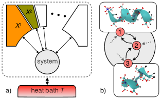
Figure 1: (a) Sketch of the total system (dashed boundary) coupled to a heat bath. The total system is divided into a number of ideal reservoirs, each exchanging an extensive quantity $X^{\alpha}$ with the system proper (gray). (b) The system is further divided into molecular conformations represented as a graph and endowed with a stochastic Markov dynamics. Snapshots show two conformations of deca-alanine, $\alpha$-helix (state 1) and an example for a misfolded intermediate (state 3) Knoch and Speck (2018).

For our example, the probability $P(N)$ for non-interacting molecules is a binomial distribution. Exploiting Stirling’s approximation, we find

$$\ln P(N;V)=-Vh(n)+\cdots$$ (1)

where the additional terms are sublinear in $V$; and

$$h(n)=-\frac{\bar{n}}{\gamma}\ln\frac{\bar{n}}{\gamma}+n[\ln n-\ln\gamma]\\ +\left(\frac{\bar{n}}{\gamma}-n\right)\left[\ln\left(\frac{\bar{n}}{\gamma}-n\right)-\ln(1-\gamma)\right]$$ (2)

with $n\equiv N/V$ the number density, global density $\bar{n}\equiv\bar{N}/\bar{V}$, and $\gamma\equiv V/\bar{V}$ is the fixed volume fraction occupied by the reservoir. Equation (1) is called a large deviation principle and we write $P(N;V)\asymp e^{-Vh(n)}$. The function $h(n)$ is called the rate function. In statistical mechanics, the rate function is related to the thermodynamic potential, in this example to the (Gibbs) free energy $\mathcal{G}(N,V)=Vh(n)$. Throughout, we consider systems at constant temperature $T$ and measure energies in units of the thermal energy $k_{\text{B}}T$ and entropy in units of Boltzmann’s constant $k_{\text{B}}$. The most likely value $\bar{n}$ of the density follows from the minimum, $\partial_{n}h=0$, with $h(n)$ describing the fluctuations of the density $n$ around $\bar{n}$.

Now let us assume that within the system we can fix the chemical potential of the molecules to $\mu$, effectively generating an inhomogeneous density that is different in system and reservoir. This modifies the probability to $P_{\mu}(N;V)=P(N;V)e^{\mu N}/Z$. Although here the partition function

$$Z(\mu;V)=\sum_{N=0}^{\infty}P(N;V)e^{\mu N}\asymp e^{-V\omega(\mu)}$$ (3)

was introduced as a simple normalization factor, it actually contains all the information about the system and arguably is the most important quantity in equilibrium statistical mechanics. In the second step, we have again assumed a large deviation principle, where rate function $h(n)$ and large deviation function $\omega(\mu)$ are related through the Fenchel-Legendre transform

$$\omega(\mu)=\inf_{n}[h(n)-\mu n].$$ (4)

Intuitively, this result can be understood rather easily: For $V\to\infty$ the integrand in Eq. (3) is dominated by a single value of $n$ (treated as a continuous variable), for which the argument $h-\mu n$ of the exponential function becomes the smallest. The infimum is attained for

$$\mu=\frac{\partial h}{\partial n}=\frac{\partial\mathcal{G}}{\partial N},$$ (5)

which simply states that the chemical potential in the reservoir is equal to the prescribed chemical potential of the system as expected for thermal equilibrium. We say that $\mu$ and $N$ are conjugate variables with respect to the potential $\mathcal{G}$. Equation (4) is a variational principle minimizing the biased potential $h(n)-\mu n$.

While this excursion provides the minimal background we will need in the following, for further reading we recommend Ref. 25 as an excellent introduction into the formalism of large deviations.

III Linear response

III.1 Fluctuations of currents

Let us consider the following situation: We have no information about the internal state of our molecular machine (the system proper) but we can resolve the exchange of extensive quantities between the system and the reservoirs. This means we can determine the changes (also called generalized distances)

$$\Delta_{\tau}\equiv X_{\tau}-X_{0}=\int_{0}^{\tau}\mathrm{d}t\;\dot{X}_{t}$$ (6)

over a prescribed time $\tau$. In the following, the dot denotes a rate (but not necessarily a total derivative with respect to time). In equilibrium, there is a free energy $\mathcal{G}(X)$ that depends on the state of the reservoirs. Moreover, random exchanges of $X$ occur also in equilibrium but on average they have to be zero,

$$\langle\Delta^{\alpha}_{\tau}\rangle_{\text{eq}}=\int\mathrm{d}\Delta\;\Delta^{\alpha}P_{\text{eq}}(\Delta;\tau)=0,$$ (7)

since there can be no transport. This implies that the probability distribution of exchanges in equilibrium is symmetric, $P_{\text{eq}}(-\Delta)=P_{\text{eq}}(\Delta)$, and the most likely value is $\Delta=0$. According to the first law, any change of the free energy is due to heat $Q$ exchanged with the heat bath (at unit temperature). Per unit time we find

$$\dot{Q}=-\frac{\mathrm{d}\mathcal{G}}{\mathrm{d}t}=-\frac{\partial\mathcal{G}}{\partial X^{\alpha}}\dot{X}^{\alpha}=f_{\alpha}\dot{X}^{\alpha}$$ (8)

with affinities $f_{\alpha}\equiv-\frac{\partial\mathcal{G}}{\partial X^{\alpha}}$. Each $f_{\alpha}$ and $X^{\alpha}$ form a conjugate pair in analogy with $\mu$ and $N$. We follow Einstein’s sum convention and sum over repeated greek indices. From now on we assume ideal reservoirs for which the affinities $f=(f_{1},\dots)$ are constant and input parameters to the theory. Integration over the time $\tau$ thus yields $Q_{\tau}=f_{\alpha}\Delta^{\alpha}_{\tau}$. Clearly, $\langle Q_{\tau}\rangle_{\text{eq}}=0$.

Even arbitrarily far from equilibrium, the fluctuations captured through the distribution $P(\Delta;\tau)$ are constrained by fluctuation theorems Gallavotti and Cohen (1995); Jarzynski (2007); Kurchan (1998); Lebowitz and Spohn (1999); Crooks (1999); Hatano and Sasa (2001); Andrieux and Gaspard (2007). The physical picture is rather simple: Driving the system requires a non-vanishing dissipation and breaks time-reversal symmetry, which in steady state yields the fluctuation theorem

$$\frac{P(\Delta_{\tau})}{P(-\Delta_{\tau})}\asymp e^{Q_{\tau}}=e^{f_{\alpha}\Delta^{\alpha}_{\tau}}.$$ (9)

It quantifies the likelihood of breaking time-reversal symmetry through the dissipated heat $Q_{\tau}$. A non-zero average $\langle Q_{\tau}\rangle>0$ means that transport occurs from at least one reservoir to another through the system.

III.2 Onsager’s principle

While Eq. (9) is a general result, we now focus on the regime close to equilibrium. We assume that the departure from the symmetric distribution $P_{\text{eq}}(\Delta)$ can be written (justified in appendix F)

$$P(\Delta;\tau)=\frac{P_{\text{eq}}(\Delta;\tau)e^{\frac{1}{2}f_{\alpha}\Delta^{\alpha}}}{Z(f;\tau)},$$ (10)

which manifestly obeys Eq. (9). The function

$$Z(f;\tau)=\int\mathrm{d}\Delta\;P_{\text{eq}}(\Delta;\tau)e^{\frac{1}{2}f_{\alpha}\Delta^{\alpha}}$$ (11)

again ensures that $P(\Delta)$ is a normalized probability distribution. We further assume a large deviation principle for the decay of the probability

$$P_{\text{eq}}(\Delta;\tau)\asymp e^{-\tau\Phi(\mathcal{J})/2},\quad Z(f;\tau)\asymp e^{-\tau\psi(f)/2}$$ (12)

with (macroscopic) currents $\mathcal{J}^{\alpha}\equiv\Delta^{\alpha}/\tau$, but now the trajectory length $\tau$ takes the role of the large parameter. Plugging both expressions into Eq. (11), we find Onsager’s principle Onsager (1931a, b)

$$\psi(f)=\inf_{\mathcal{J}}[\Phi(\mathcal{J})-f_{\alpha}\mathcal{J}^{\alpha}],$$ (13)

which relates affinities and currents through a Fenchel-Legendre transform in analogy with Eq. (4). We thus recover the same structure as for equilibrium statistical mechanics, whereby $\Phi(\mathcal{J})$ and $\psi(f)$ play the role of thermodynamic potentials for currents. This analogy can be exploited to obtain transport coefficients Palmer and Speck (2017).

III.3 Some consequences

Let us expand Eq. (10) to linear order of $Q$, which yields the average $\langle\Delta^{\alpha}_{\tau}\rangle=\tau\chi^{\alpha\beta}f_{\beta}$ with conductivities

$$\chi^{\alpha\beta}=-\left.\frac{\partial^{2}\psi}{\partial f_{\alpha}\partial f_{\beta}}\right|_{\text{eq}}=\lim_{\tau\to\infty}\frac{1}{2\tau}\langle\Delta^{\alpha}_{\tau}\Delta^{\beta}_{\tau}\rangle_{\text{eq}}=\frac{\partial\langle\mathcal{J}^{\alpha}\rangle}{\partial f_{\beta}}.$$ (14)

Since we can change the order of partial derivatives, the matrix $\chi$ is symmetric, which is often referred to as Onsager reciprocal relations. The equilibrium fluctuations of the quantities exchanged with the reservoirs thus determine their non-equilibrium averages. Eq. (14) is called the fluctuation-dissipation theorem. The average dissipation reads

$$\langle Q_{\tau}\rangle=\tau f_{\alpha}\chi^{\alpha\beta}f_{\beta}>0,$$ (15)

from which we conclude that $\chi^{\alpha\beta}$ is a positive semi-definite matrix. The inverse matrix $\chi_{\alpha\beta}$ (resistivities) determining affinities through $f_{\alpha}=\chi_{\alpha\beta}\mathcal{J}^{\beta}$ follows from $\chi^{\alpha\gamma}\chi_{\gamma\beta}=\delta^{\alpha}_{\beta}$.

Note that we can recast Eq. (13) into the variational problem $\inf_{\dot{X}}\mathcal{R}(\dot{X})$ with respect to the rates $\dot{X}$ with function (see appendix A)

$$\mathcal{R}(\dot{X})\equiv\frac{1}{2}\dot{X}^{\alpha}\chi_{\alpha\beta}\dot{X}^{\beta}+\frac{\mathrm{d}\mathcal{G}}{\mathrm{d}t},$$ (16)

which is sometimes called the “Rayleighian” Zhou and Doi (2018). This form more clearly exposes the formal similarities with the Lagrangian in mechanics with a quadratic “mass” term and $-\frac{\mathrm{d}\mathcal{G}}{\mathrm{d}t}$ taking the role of the potential energy.

IV Beyond linear response

IV.1 Discrete state space

To go further away from equilibrium, we need to be more specific about the internal working of the system and in particular its coupling to the reservoirs. Full information is contained in the microstate $\xi$ comprising positions and momenta of all atoms. Practically, it is neither possible nor necessary to fully resolve microstates, which, e.g., for a solvated colloidal particle would contain information about all solvent molecules. We assume that meaningful mesostates $\{i\}$ can be defined, sets of microstates representing for example conformations of a molecule [cf. Fig. 1(b)] or the (discrete) position of a colloidal particle. Moreover, we will assume that the dynamics of these mesostates decouples from the much faster dynamics of microstates yielding a Markov process with stochastic transitions between the mesostates. Such a discrete representation is either obtained “top-down” through general considerations, but can also be constructed systematically, for example through Markov state modeling based on molecular dynamics simulations Prinz et al. (2011). The importance of this step and the challenges of dimensionality reduction cannot be overemphasized Sittel and Stock (2018). However, it is not the focus of this perspective and we will assume in the following that a discrete state space has been constructed.

To make the connection with the discussion so far, we have to realize that during every transition $i\to j$ between mesostates there might be corresponding changes in the environment so that the quantity $X^{\alpha}$ held by the reservoir changes as

$$X^{\alpha}\to X^{\alpha}+d^{\alpha}_{ij}.$$ (17)

Clearly, the couplings $d^{\alpha}_{ij}$ are antisymmetric, $d^{\alpha}_{ji}=-d^{\alpha}_{ij}$, since going back undoes the change. Table 1 summarizes the extensive quantities $X$ and affinities $f$ of interest in the present context.

extensive $X$	intensive affinity $f$	$\chi$
electric charge $Q_{\text{el}}$	electric potential $-\phi_{\text{el}}$	conductivity
number of molecules $N$	chemical potential $-\mu$	mobility
traveled distance $x$	force $-f_{L}$	mobility
angle $\varphi$	torque	rot. mobility
strain	stress	viscosity

Table 1: Summary of the most relevant reservoir types and their corresponding affinities.

IV.2 Illustration: Enzyme

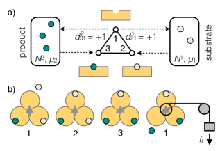
Figure 2: (a) Sketch of an enzyme with three internal states: unbound (1), bound substrate (2), and bound product (3). Two transitions ($1\leftrightarrow 2$ and $1\leftrightarrow 3$) exchange molecules with the reservoirs while $2\leftrightarrow 3$ converts bound molecules between substrate and product. (b) The same internal states applied to F₁-ATPase, a rotary molecular motor consisting of three identical subunits and a central shaft (arrow). The substrate molecule is now ATP, which is hydrolyzed to ADP and phosphate (product), releasing the free energy $\mu_{1}-\mu_{2}$. Part of this free energy is used to rotate the central shaft in the transition $2\leftrightarrow 3$, returning the motor to the unbound state (1) but with the shaft rotated by 120^∘. The last sketch shows the coupling to an ideal work reservoir represented as a weight that is lifted against the force $f_{L}$.

As the canonical example, Fig. 2(a) shows a sketch of an enzyme (the system proper) converting chemical species 1 (the substrate) into species 2 (the product) Seifert (2018). On the coarsest level, the enzyme is modeled with three internal states: unbound (1), bound substrate (2), and bound product (3). It is coupled to two reservoirs holding $N^{\alpha}$ molecules, and we assume that the corresponding chemical potentials $\mu_{\alpha}=-f_{\alpha}$ are functions of temperature and pressure alone and held constant. Note that the two reservoirs are not spatially separated but kinetically separated, with the conversion between product and substrate so slow outside the enzyme that it is neglected. In the transition $1\to 2$ a substrate molecule is bound to the enzyme and thus $d^{1}_{12}=-1$, whereby the substrate molecule is return to the reservoir in $2\to 1$ with $d^{1}_{21}=1$. The transition $2\to 3$ converts the bound substrate into bound product, which is released in the transition $3\to 1$.

Since the total number of molecules is conserved, $\bar{N}=N^{1}+N^{2}$, we find the Gibbs free energy

$$\mathcal{G}(N^{1},N^{2})=-f_{\alpha}N^{\alpha}=\mu_{1}\bar{N}-(\mu_{1}-\mu_{2})N^{2}.$$ (18)

Requiring that the average dissipation rate $\langle\dot{Q}\rangle=(\mu_{1}-\mu_{2})\langle\dot{N}^{2}\rangle$ is positive, we see that for $\mu_{1}>\mu_{2}$ substrate molecules are being converted to product on average. There is thus a macroscopic current from one reservoir to the other which is enabled by the enzyme although the driving force is the difference of chemical potentials. We assume that, even though reservoirs are depleted and filled, they are so big that the chemical potential can be treated as constant over sufficiently long times, during which a steady state ensues.

Things become interesting if a transition involves a conformational change that exerts work on the environment, a power stroke. Consider for example a rotary molecular motor such as F₁-ATPase, a paradigmatic molecular machine that has been studied extensively Noji et al. (1997); Wang and Oster (1998). This motor rotates in 120^∘ steps separated by dwells, hydrolyzing one ATP molecule in each stroke. A coarse sketch of the involved conformations is shown in Fig. 2(b), where now the transition $2\leftrightarrow 3$ involves a conformational change that rotates the shaft. This rotation can be accounted for as a change in the environment with $d^{3}_{23}=2\pi/3$, where $X^{3}=\varphi$ is the total angle the shaft has rotated a spool with radius $R$. We can attach a load represented as a weight that is lifted against the force $f_{L}$, the potential energy of which is $f_{L}R\varphi$. The total free energy now reads

$$\mathcal{G}(N^{1},N^{2},\varphi)=\mu_{1}\bar{N}-(\mu_{1}-\mu_{2})N^{2}+f_{L}R\varphi,$$ (19)

from which we read off the affinity $f_{3}=-f_{L}R$, i.e., the torque applied to the shaft. Note that microscopic reversibility implies that when performing work on the molecular motor (lowering the weight) it is rotating in the opposite direction synthesizing ATP molecules, which is indeed observed Itoh et al. (2004).

IV.3 Local detailed balance

To continue we need to know the evolution equation for the mesostates. Before, however, we ask ourselves how the dynamics of the enzyme is affected by the driving. To answer this question, we first go back to thermal equilibrium, in which the probability to find the system in mesostate $i$ is

$$p_{i}(X)=\sum_{\xi\in i}P(\xi;X)=e^{-[G_{i}(X)-\mathcal{G}(X)]}$$ (20)

with microscopic joint probability

$$P(\xi;X)=e^{-[\mathcal{H}(\xi)-\mathcal{G}(X)]}$$ (21)

given by the Boltzmann weight, where $\mathcal{H}(\xi)$ is the Hamiltonian. Here we have to distinguish the global free energy $\mathcal{G}(X)$ from the “constrained” free energies $G_{i}(X)$ of the mesostates.

Figure 3: Sketch of a free energy landscape $G(x)$ along some continuous reaction coordinate $x$ capturing the slowest mode. Mesostates correspond to “wells”, the vicinity of minima with free energies $G_{i}$ separated by barriers. Relaxation of all other degrees of freedom is faster than barrier crossing so that the distribution of microstates approaches the Boltzmann distribution Eq. (21) on time scales (much) shorter than the lifetime of mesostates.

Most importantly, we assume a timescale separation between the relaxation of microstates within mesostates, and transitions between mesostates, cf. Fig. 3. Since mesostates are a coarse-grained representation, their dynamics is necessarily stochastic and determined by the time-independent non-negative transition rates $w_{ij}$ for each transition $i\to j$. We will call the set of rates $w$ a Markov model. Since the composite system is only coupled to a heat reservoir but otherwise closed, these transition rates obey the detailed balance condition

$$\frac{w_{ij}}{w_{ji}}=\frac{p_{j}}{p_{i}}=e^{-(G_{j}-G_{i})},$$ (22)

which guarantees the absence of dissipation.

Making the changes in the reservoirs explicit, we have

$$\ln\frac{w_{ij}(\{X^{\alpha}\to X^{\alpha}+d^{\alpha}_{ij}\})}{w_{ji}(\{X^{\alpha}+d^{\alpha}_{ij}\to X^{\alpha}\})}\\ =-\left[G_{j}(\{X^{\alpha}+d^{\alpha}_{ij}\})-G_{i}(\{X^{\alpha}\})\right]$$ (23)

after taking the logarithm. We again appeal to the concept of ideal reservoirs, from which follow additive free energies $G_{i}(X)=G^{0}_{i}-f_{\alpha}X^{\alpha}$ with bare free energies $G^{0}_{i}$ independent of $X$. Plugging this sum back into Eq. (23), we obtain

$$\ln\frac{w_{ij}}{w_{ji}}=-(G^{0}_{j}-G^{0}_{i})+f_{\alpha}d^{\alpha}_{ij},$$ (24)

which is known as the local detailed balance condition. The right hand side manifestly is independent of $X$, which implies that also the transition rates $w_{ij}$ are independent of $X$ and we do not have to keep track of the absolute values of the environmental variables.

In this setting, non-equilibrium is achieved by preparing an initial state that exhibits currents between reservoirs (trying to reach equilibrium) which are assumed to persist for a sufficiently long time. While the joint distribution $P(\xi,X)$ diverts from the Boltzmann factor [Eq. (21)], the dynamics of the combined system-reservoirs still obeys detailed balance. These currents necessarily influence the stochastic dynamics of the system proper as captured by the local detailed balance condition Eq. (24).

IV.4 Markov dynamics and graphs

The stochastic dynamics of the system (in continuous time) is determined by the time-independent non-negative transition rates $w_{ij}$. The probability $p_{i}(t)$ to find the system in mesostate $i$ evolves according to the master equation

$$\partial_{t}p_{i}(t)=\sum_{j\neq i}\left[p_{j}(t)w_{ji}-p_{i}(t)w_{ij}\right].$$ (25)

It is helpful to interpret the discrete state space as a graph in which the mesostates correspond to the vertices, $V\equiv\{i\}$, and possible transitions $E\equiv\{i\leftrightarrow j\}$ form the edges of the graph [Fig. 1(b)]. We require two properties: (i) the graph is connected and (ii) for every $w_{ij}>0$ also $w_{ji}>0$ (i.e., every edge can be traversed in both directions). The first property means that any two vertices of the graph are connected by a path. The second property is called microscopic reversibility and guarantees the absence of absorbing states. These properties are sufficient to proof existence and uniqueness of a stationary solution, i.e., the solution $p$ of

$$\sum_{j\neq i}[p_{j}w_{ji}-p_{i}w_{ij}]=0$$ (26)

is reached from any initial distribution after a transient. The proof can be found, e.g., in Ref. 62.

In the following, we will focus on this steady state with probabilities $p$. We define the non-negative fluxes

$$\phi_{ij}\equiv p_{i}w_{ij}$$ (27)

and with these the probability currents and affinities

$$j_{ij}\equiv\phi_{ij}-\phi_{ji},\qquad a_{ij}\equiv\ln\frac{\phi_{ij}}{\phi_{ji}},$$ (28)

respectively. The case where all currents vanish individually with $\phi_{ji}=\phi_{ij}$ corresponds to detailed balance [it immediately leads to Eq. (22)], and the system is in thermal equilibrium. If detailed balance is broken then probability currents and affinities along (at least some) edges are non-zero, and probabilities $p_{i}\neq e^{-G^{0}_{i}}$ are no longer given by Boltzmann weights. Table 2 summarizes most of the symbols introduced so far.

macroscopic	$X^{\alpha}$	quantities in the environment (reservoirs) that are influenced by the system
	$\Delta^{\alpha}$, $\mathcal{J}^{\alpha}$	their changes and currents
mesoscopic	$d^{\alpha}_{ij}$	change of quantity $X^{\alpha}$ due to transition $i\to j$ of the system
	$w_{ij}$	transition rates
	$p_{i}$	probability of mesostate $i$
	$\phi_{ij}$, $j_{ij}$	probability fluxes and currents within system
atomistic	$\xi$	microstate
	$\mathcal{H}$	the Hamiltonian

Table 2: Summary of the most important symbols.

We are concerned with two types of observables, those with one index ($A_{i}$) assigning every mesostate (vertex) a value, and those with two indices ($B_{ij}$) assigning edges a value. Expectation values for the former are obtained as $\langle A_{i}\rangle=\sum_{i}A_{i}p_{i}$ and for the latter $\langle B_{ij}\rangle=\sum_{ij}B_{ij}\phi_{ij}$, where the sum is over all mesostates $i$ and $j$ and thus includes every edge twice ($i\to j$ and $j\to i$). Clearly, $\langle B_{ij}\rangle$ is a rate. For antisymmetric edge observables with $B_{ji}=-B_{ij}$ one finds

$$\langle B_{ij}\rangle=\sum_{ij}B_{ij}\phi_{ij}=\frac{1}{2}\sum_{ij}B_{ij}j_{ij}$$ (29)

with probability currents $j_{ij}=\phi_{ij}-\phi_{ji}$. A very useful relation is Jensen’s inequality

$$\langle g(A_{i})\rangle\geqslant g(\langle A_{i}\rangle)$$ (30)

holding for any convex real function $g(x)$.

IV.5 Cycles

Currents and affinities are antisymmetric by construction. Due to this property it is useful to turn the graph into a directed graph $\vec{G}=(V,E,\nabla)$ by giving every edge $e\in E$ an orientation, which is described by the incidence matrix $\nabla$ with entries

$$\nabla_{i}^{e}\equiv\begin{cases}-1&\text{if edge $e$ enters vertex $i$}\\ +1&\text{if edge $e$ leaves vertex $i$}\\ 0&\text{otherwise (no relation)}\end{cases}$$ (31)

having $|V|$ rows and $|E|$ columns Polettini (2015). The master equation (26) can then be written

$$\sum_{j\neq i}j_{ij}=\sum_{e\in E}\nabla_{i}^{e}j_{e}=0$$ (32)

or $\nabla\cdot\vec{\jmath}=0$, where $j_{e}\equiv j_{ij}$ is the current along the oriented edge $e=i\to j$ and $\vec{\jmath}=(j_{1},\dots,j_{|E|})$ is the vector of all edge currents. Eq. (32) is also known as Kirchhoff’s current law and expresses the conservation of probability through demanding that the total current into a vertex equals the current out of that vertex. Note that the actual orientation of edges does not matter, it merely gives “forward” and “backward” a meaning but we can traverse all edges in both directions. The null space (kernel) of the incidence matrix $\nabla$ is the space of directed simple cycles in the graph $\vec{G}$ Polettini (2015), see appendix B.

An intuitive consequence of Kirchhoff’s law is that in a steady state with time-independent probabilities $p$, all probability currents have to flow in cycles. Cycles set non-equilibrium apart from thermal equilibrium and enable transport, i.e., non-vanishing macroscopic currents $\langle\mathcal{J}^{\alpha}\rangle=\langle d^{\alpha}_{ij}\rangle\neq 0$. This might become clearer when again looking at the enzyme in Fig. 2(a), which forms a single cycle. Traversing the cycle converts substrate into product (or vice versa) while returning the enzyme to its initial state.

IV.6 Stochastic energetics

We finish this section by looking at the energetics of the system, which is at the very heart of stochastic thermodynamics. To account for the fact that mesostates represent finite volumes in phase space Seifert (2019), the bare free energy $G^{0}_{i}=U_{i}-S_{i}$ of mesostates is further split into internal energy

$$U_{i}\equiv\sum_{\xi\in i}\mathcal{H}(\xi)P(\xi|i)$$ (33)

and “intrinsic” entropy

$$S_{i}\equiv-\sum_{\xi\in i}P(\xi|i)\ln P(\xi|i),$$ (34)

respectively, with conditional probability $P(\xi|i)=P(\xi)/p_{i}$ for the system to be in microstate $\xi$ given that it resides in mesostate $i$. While the probabilities of mesostates divert from the Boltzmann factor, the local weight $P(\xi|i)=e^{-[\mathcal{H}(\xi)-G^{0}_{i}]}$ of microstates is assumed to follow the Boltzmann weight in line with the posited scale separation.

Having separated energy and intrinisc entropy of mesostates, the total change of entropy in a single transition $i\to j$ is composed of three contributions,

$$\underbrace{\delta Q_{ij}+(S_{j}-S_{i})}_{\ln(w_{ij}/w_{ji})}-\ln\frac{p_{j}}{p_{i}}=\ln\frac{\phi_{ij}}{\phi_{ji}}=a_{ij},$$ (35)

where $\delta Q_{ij}$ is the heat exchanged with the heat reservoir, the second term is the change of intrinsic entropy, and the last term is the change of (stochastic) entropy associated with the mesostates Seifert (2005, 2019). To recover the established expression for the average entropy production rate

$$\dot{\sigma}=\sum_{ij}\phi_{ij}\ln\frac{\phi_{ij}}{\phi_{ji}}=\langle a_{ij}\rangle\geqslant 0$$ (36)

of Markov processes Schnakenberg (1976); Lebowitz and Spohn (1999); Seifert (2005), we identify the first two terms in Eq. (35) with the transition rates. Combining this identification of the ratio $w_{ij}/w_{ji}$ with the local detailed balance condition Eq. (24), we obtain the balance equation

$$\delta Q_{ij}+(U_{j}-U_{i})=f_{\alpha}d^{\alpha}_{ij}$$ (37)

for the energy exchanged in a transition between mesostates. This result avails itself of the interpretation as the first law $\delta U=\delta W-\delta Q$ across a single transition (the sign of heat is convention), from which we read off the work $\delta W_{ij}=f_{\alpha}d^{\alpha}_{ij}$ performed by the reservoirs on the system. For the three-state enzyme of Sec. IV.2 we find the work

$$W_{\circlearrowright}=\delta W_{12}+\delta W_{23}+\delta W_{31}=\mu_{1}-\mu_{2}-f_{L}R\frac{2\pi}{3}$$ (38)

for completing a single forward cycle.

V Fluctuations

V.1 Trajectory observables

So far we have fixed the stochastic dynamics of mesostates, which is sufficient to calculate average rates and the statistics of state observables ($A_{i}$). However, it is not yet clear how to treat the fluctuations of currents and related time-extensive quantities. We now change our perspective and focus on the stochastic trajectories, i.e., time-ordered sequences

$$\bm{\imath}\equiv(i_{0},0)\to(i_{1},t_{1})\to\cdots\to(i_{K},t_{K})$$ (39)

of mesostates visited within a fixed time $\tau$, whereby mesostates $i_{\nu}$, transition times $0<t_{\nu}<\tau$, and the number of transitions $K$ are random numbers.

Along trajectories we measure trajectory observables like currents, heat, work, etc.; all of which can be written as a functional (exemplified here for the heat)

$$Q_{\tau}[\bm{\imath}]=\sum_{\nu=1}^{K}\delta Q_{i_{\nu-1}i_{\nu}}$$ (40)

summing the contributions of the antisymmetric edge observable $\delta Q_{ij}$ for every transition in the sequence $\bm{\imath}$. Clearly, $Q_{\tau}$ is a random quantity with a probability distribution $P(Q;\tau)$.

We can now come back to our starting point looking at extensive quantities $X$ that are exchanged between the system and reservoirs. Tracing the trajectory of the system’s mesostates together with the knowledge of the couplings $d^{\alpha}_{ij}$ allows to reconstruct the changes

$$\Delta^{\alpha}_{\tau}[\bm{\imath}]=\sum_{\nu=1}^{K}d^{\alpha}_{i_{\nu-1}i_{\nu}}$$ (41)

within the reservoirs. Together with Eq. (37) we thus obtain the heat $Q_{\tau}[\bm{\imath}]=-(U_{i_{K}}-U_{i_{0}})+f_{\alpha}\Delta^{\alpha}_{\tau}[\bm{\imath}]$ dissipated along a single trajectory. The term for the internal energy is a telescoping sum that reduces to a temporal boundary term, which vanishes when averaging over the subset of trajectories compatible with the given changes $\Delta_{\tau}$.

V.2 Time-reversal symmetry

Once we have obtained the rates $w$ of the Markov model it is straightforward to determine the probability of a single trajectory,

$$\mathcal{P}_{\tau}[\bm{\imath}]=p_{i_{0}}e^{-r_{i_{0}}t_{1}}\prod_{\nu=1}^{K}w_{i_{\nu-1}i_{\nu}}e^{-r_{i_{\nu}}(t_{\nu+1}-t_{\nu})},$$ (42)

with $t_{K+1}=\tau$ and exit rates $r_{i}\equiv\sum_{j\neq i}w_{ij}$. Reading from left to right it says: probability to be in the initial mesostate $i_{0}$ times the probability to survive for time $t_{1}$ times the transition probability to a new mesostate $i_{1}$ times the survival probability for time $t_{2}-t_{1}$, and so on. Summing over all trajectories, $\sum_{\bm{\imath}}\mathcal{P}_{\tau}[\bm{\imath}]=1$.

Now suppose we ask for the probability $\mathcal{P}_{\tau}[\tilde{\bm{\imath}}]$ to observe the reversed trajectory $\tilde{\bm{\imath}}$, i.e., the same sequence of mesostates but traversed in the opposite direction. In thermal equilibrium, we could not discern whether a movie is played forward or backward and thus $\mathcal{P}_{\tau}[\bm{\imath}]=\mathcal{P}_{\tau}[\tilde{\bm{\imath}}]$. The ratio of these probabilities thus tells us how strongly this time-reversal symmetry is broken due to the driving. It turns out that the logarithm of the ratio

$$\ln\frac{\mathcal{P}_{\tau}[\bm{\imath}]}{\mathcal{P}_{\tau}[\tilde{\bm{\imath}}]}=\sum_{\nu=1}^{K}\ln\frac{w_{i_{\nu-1}i_{\nu}}}{w_{i_{\nu}i_{\nu-1}}}+\ln\frac{p_{i_{0}}}{p_{i_{K}}}=\sum_{\nu=1}^{K}a_{i_{\nu-1}i_{\nu}}=\mathcal{S}_{\tau}[\bm{\imath}]$$ (43)

equals the sum of the affinities along the trajectory since the survival probabilities cancel (the sojourn times are the same for forward and backward trajectory), and we are left with the product of the transition rates in the first term. Plugging in Eq. (35) followed by the first law Eq. (37) yields the expression

$$\mathcal{S}_{\tau}[\bm{\imath}]=f_{\alpha}\Delta^{\alpha}_{\tau}[\bm{\imath}]-(\Psi_{i_{K}}-\Psi_{i_{0}})$$ (44)

for the total entropy produced along single trajectories with a temporal boundary term given by the effective potential $\Psi_{i}\equiv G^{0}_{i}+\ln p_{i}$. The agreement of the path entropy $\mathcal{S}_{\tau}\asymp Q_{\tau}$ with the actual dissipated heat due to exchanges with the reservoirs is what makes stochastic thermodynamics so powerful since it connects the second with the first law of thermodynamics on the level of stochastic trajectories.

Here is an example what we can do with Eq. (43). Let us look at the distribution of exchanges, $P(\Delta;\tau)$, which can be written

$$P(\Delta) =\sum_{\bm{\imath}}\delta(\{\Delta^{\alpha}-\Delta^{\alpha}_{\tau}[\bm{\imath}]\})\mathcal{P}[\bm{\imath}]$$

$$=\sum_{\tilde{\bm{\imath}}}\delta(\{\Delta^{\alpha}+\Delta^{\alpha}_{\tau}[\tilde{\bm{\imath}}]\})e^{\mathcal{S}}\mathcal{P}[\tilde{\bm{\imath}}]\asymp P(-\Delta)e^{f_{\alpha}\Delta^{\alpha}}.$$

In the first step, we have replaced $\Delta_{\tau}[\bm{\imath}]=-\Delta_{\tau}[\tilde{\bm{\imath}}]$ and used Eq. (43). We can then pull the exponential factor $e^{f_{\alpha}\Delta^{\alpha}}$ in front of the sum, which reduces to the distribution $P(-\Delta;\tau)$ for large $\tau$ (such that bounded boundary terms become negligble). We have thus derived the relation Eq. (9) used previously, which restricts possible fluctuations of the currents. Note that instead of inverting the order of mesostates more general transformations can be considered, leading to a variety of fluctuation theorems. For a comprehensive discussion, see Seifert’s review Seifert (2012).

Intriguingly, the entropy production also bounds fluctuations out of equilibrium. Using only the fluctuation theorem, Hasegawa and Vu Hasegawa and Van Vu (2019) obtained the following lower bound for the Fano factor

$$F^{\alpha}_{\tau}\equiv\frac{\langle(\Delta^{\alpha}_{\tau})^{2}\rangle-\langle\Delta^{\alpha}_{\tau}\rangle^{2}}{\langle\Delta^{\alpha}_{\tau}\rangle^{2}}\geqslant\frac{2}{e^{\tau\dot{\sigma}}-1},$$ (45)

measuring the dispersion (the variance divided by the squared mean) of the changes $\Delta_{\tau}$. Previously, a tighter bound $F^{\alpha}_{\tau}\geqslant 2/(\tau\dot{\sigma})$ holding for continuous-time Markov processes (as considered in this Perspective) has been proposed Barato and Seifert (2015) and subsequently proven Gingrich et al. (2016). Such bounds have been termed thermodynamic uncertainty relations Pietzonka et al. (2017); Dechant (2018); Koyuk and Seifert (2020); Falasco et al. (2020); Hartich and Godec (2021) and demonstrate that precision has a thermodynamic cost, i.e., reducing the dispersion of any process generally requires a larger dissipation with ramifications for biomolecular machines and processes like DNA replication.

V.3 Empirical densities and fluxes

Let us come back to the basic task of Markov State modeling: given an atomistic model and a discrete state space $\{i\}$ of conformations, what are the rates $w_{ij}$ so that the Markov evolution of mesostates follows the time evolution of the atomistic system? To tackle this question, let us assume that we can perform a number of (long) molecular dynamics simulations of the atomistic model, sampling trajectories $\xi_{t}$ of length $\tau$. Along a single finite trajectory $\xi_{t}$ of microstates with mapped sequence $\bm{\imath}$ of mesostates, we measure the empirical populations

$$\hat{p}_{i}[\bm{\imath}]\equiv\frac{1}{\tau}\int_{0}^{\tau}\mathrm{d}t\;\chi_{i}(\xi_{t})$$ (46)

and empirical fluxes ($\delta t\to 0$)

$$\hat{\phi}_{ij}[\bm{\imath}]\delta t\equiv\frac{1}{\tau}\int_{0}^{\tau}\mathrm{d}t\;\chi_{i}(\xi_{t})\chi_{j}(\xi_{t+\delta t})$$ (47)

through counting. Here, $\chi_{i}(\xi)$ is an indicator function that is one if the microstate $\xi$ belongs to mesostate $i$ and zero otherwise. In the limit $\tau\to\infty$ we have that $\hat{p}_{i}\to p_{i}$, but for finite $\tau$, $\hat{p}$ and $\hat{\phi}$ are random quantities with a probability density.

The probability of these empirical quantities can be found through comparing the trajectory probability density of the (unknown) generating Markov model $w$ with those of a fictitious Markov model Maes and Netočný (2008). Skipping the technical details, the joint probability density

$$P_{\tau}(\hat{p}=p^{\ast},\hat{\phi}=\phi^{\ast})\asymp e^{-\tau\mathcal{I}_{w}(p^{\ast},\phi^{\ast})}$$ (48)

obeys a large deviation principle with rate function

$$\mathcal{I}_{w}(p^{\ast},\phi^{\ast})=\sum_{ij}\left[\phi^{\ast}_{ij}\ln\frac{\phi^{\ast}_{ij}}{p^{\ast}_{i}w_{ij}}-\phi^{\ast}_{ij}+p^{\ast}_{i}w_{ij}\right].$$ (49)

Notable, the rate function is independent of the actual steady state probabilities $p$ and only the transition rates $w$ enter the rate function. Put differently, $P_{\tau}$ is the probability density to observe trajectories with empirical populations and fluxes that, in the limit $\tau\to\infty$, are typical for a fictitious model with transition rates $w^{\ast}_{ij}=\phi^{\ast}_{ij}/p^{\ast}_{i}$. As shown in appendix D, the rate function $\mathcal{I}_{w}$ equals the Kullback-Leibler divergence between the underlying process $w$ and the observed empirical densities and fluxes of a single trajectory.

V.4 Estimating rates: The contraction principle

The contraction principle allows to derive the rate function $I(y)$ for another variable $y=g(x)$ from a known rate function $I(x)$,

$$I(y)=\inf_{x}\left\{I(x)\;|\;y=g(x)\right\}.$$ (50)

This result expresses a simple fact: among rare events that with the largest probability (even though very small) will occur almost certainly. For example, the rate function for the probability currents reads

$$I(p^{\ast},j^{\ast})=\inf_{\phi^{\ast}}\left\{\mathcal{I}_{w}(p^{\ast},\phi^{\ast})\;|\;\phi^{\ast}_{ij}-\phi^{\ast}_{ji}=j^{\ast}_{ij}\right\},$$ (51)

i.e., the probability of currents is determined by the most likely realization of the fluxes obeying the constraints.

Here is another example: Assume we have harvested, in equilibrium, a single atomistic trajectory of length $\tau$ with populations $\hat{p}$ and fluxes $\hat{\phi}$. Given this limited data, what is the optimal Markov model $w$ with probabilities $p=\hat{p}$ and fluxes $\phi_{ij}=\hat{p}_{i}w_{ij}$? Exploiting Bayes’ theorem, the probability that the Markov model $w$ has generated the data is $P(\phi|\hat{\phi})\propto P_{\tau}(p,\hat{\phi})$. To maximize this probability (called likelihood in this context), we invoke the contraction principle enforcing detailed balance as constraints on every edge,

$$\inf_{\phi}\left\{\mathcal{I}_{w}(p,\hat{\phi})\;|\;\phi_{ij}-\phi_{ji}=0\right\}.$$ (52)

The constraints can be incorporated through Lagrange multipliers (the antisymmetry of the constraints implies antisymmetric Lagrange multipliers, $\lambda_{ji}=-\lambda_{ij}$),

$$\frac{\partial}{\partial\phi_{ij}}\left[\mathcal{I}_{w}-\frac{1}{2}\sum_{kl}\lambda_{kl}(\phi_{kl}-\phi_{lk})\right]=0,$$ (53)

which is solved by $\phi_{ij}=\hat{\phi}_{ij}/(1-\lambda_{ij})$. Inserting into the constraints yields

$$\frac{\hat{\phi}_{ij}}{1-\lambda_{ij}}=\frac{\hat{\phi}_{ji}}{1+\lambda_{ij}}.$$ (54)

Solving for $\lambda_{ij}$, we thus obtain the optimal fluxes

$$\phi_{ij}=\frac{1}{2}(\hat{\phi}_{ij}+\hat{\phi}_{ji}),$$ (55)

which are manifestly symmetric (and, in hindsight, not very surprising).

We can go a step further and, in a non-equilibrium steady state, consider the local detailed balance condition Eq. (24), which yields the optimal fluxes

$$\phi_{ij}=(\hat{\phi}_{ij}+\hat{\phi}_{ji})\left[1+\frac{p_{j}}{p_{i}}e^{(G^{0}_{j}-G^{0}_{i})-f_{\alpha}d^{\alpha}_{ij}}\right]^{-1}.$$ (56)

We now need to know also the equilibrium free energies $G^{0}_{i}$ of mesostates (which can be obtained from a separate equilibrium simulation using the same discretization) and the couplings $d^{\alpha}_{ij}$ together with the driving affinities.

VI Challenges

VI.1 Variational principles: Caliber, transferability, and numerical sampling

The task of obtaining transition rates for a set of mesostates is also addressed by the method of maximum caliber Jaynes (1980); Pressé et al. (2013); Dixit et al. (2018), which posits that the actual process maximizes the “caliber” or, equivalently, minimizes the distance between path weights as measured by the Kullback-Leibler divergence (cf. appendix D). Here the distance is with respect to a reference process $\tilde{w}$, whereby the minimization

$$\inf_{p,\phi}\left\{\mathcal{I}_{\tilde{w}}(p,\phi)\;|\;\text{constraints}\right\}$$ (57)

is constrained by the normalization of probabilities and available data about the process such as the average macroscopic currents $\langle\mathcal{J}^{\alpha}\rangle$. Introducing again Lagrange multipliers $\psi$, $\lambda_{ji}=-\lambda_{ij}$, and $\zeta_{\alpha}$, we thus have to minimize the function

$$\mathcal{I}_{\tilde{w}}(p,\phi)-\frac{\psi}{2}\left(\sum_{i}p_{i}-1\right)-\frac{1}{2}\sum_{ij}\lambda_{ij}(\phi_{ij}-\phi_{ji}-j_{ij})\\ -\zeta_{\alpha}\left(\sum_{ij}d^{\alpha}_{ij}\phi_{ij}-\langle\mathcal{J}^{\alpha}\rangle\right).$$ (58)

First, taking the derivative with respect to $p_{i}$ and setting it zero yields the condition

$$r_{i}=\tilde{r}_{i}-\frac{\psi}{2}$$ (59)

between the exit rates of target and reference process. Second, taking the derivative with respect to the fluxes $\phi_{ij}$ then yields the rates

$$w_{ij}=\tilde{w}_{ij}e^{\lambda_{ij}+\zeta_{\alpha}d^{\alpha}_{ij}}.$$ (60)

This expression recovers a result obtained by Baule and Evans Baule and Evans (2008) following a different route (as noted previously Monthus (2011); Chetrite and Touchette (2015)), wherein rates obey the product constraint $w_{ij}w_{ji}=\tilde{w}_{ij}\tilde{w}_{ji}$, and Eq. (59) is the exit rate constraint.

The most obvious choice for the reference process is thermal equilibrium with the affinities set to values so that there are no currents between reservoirs. We then have to tune the antisymmetric Lagrange multipliers $\lambda_{ij}$ to fulfill the conditions Eq. (59). However, in general this tuning is not compatible with the local detailed balance condition since Eq. (60) then implies

$$\ln\frac{w_{ij}}{w_{ji}}=-(G^{0}_{j}-G^{0}_{i})+2\lambda_{ij}+2\zeta_{\alpha}d^{\alpha}_{ij},$$ (61)

which disagrees with Eq. (24) except for the special cases $\lambda_{ij}=0$ and $\lambda_{ij}\propto d^{\alpha}_{ij}$. While the resulting Markov model $w$ is driven and exhibits the right macroscopic currents (and entropy production $\mathcal{S}_{\tau}\asymp 2\zeta_{\alpha}\Delta^{\alpha}_{\tau}$), these currents do not obey the constraints derived in Sec. IV.3 due to physical exchanges with reservoirs. This failure points to a more fundamental issue, namely the existence of general variational principles out of equilibrium that fill in missing microscopic information comparable to the maximum entropy principle (see, e.g., Ref. 81 and Landauer’s “blow torch” theorem Landauer (1975, 1993)). Of course, one could constrain the minimization further and further until the desired result is obtained, but this somewhat defies the purpose of a variational principle. Moreover, on the practical side it limits this approach to rather simple systems with the number of mesostates comparable to the number of constraints Otten and Stock (2010).

In fact, there is an exact variational principle if we rephrase the problem in terms of a biased ensemble of trajectories Chetrite and Touchette (2013, 2014, 2015). The large deviation function $\psi(\zeta)$ is defined through $e^{-\tau\psi(\zeta)}\asymp\langle e^{\zeta_{\alpha}\Delta^{\alpha}_{\tau}}\rangle$, where the average is with respect to the original dynamics $w$. Now consider biasing the trajectories by changing their weight so that

$$\langle\Delta^{\alpha}_{\tau}\rangle^{\ast}=\frac{\langle\Delta^{\alpha}_{\tau}e^{\zeta_{\alpha}\Delta^{\alpha}_{\tau}}\rangle}{\langle e^{\zeta_{\alpha}\Delta^{\alpha}_{\tau}}\rangle}=-\tau\frac{\partial\psi}{\partial\zeta_{\alpha}}.$$ (62)

Tuning the parameters $\zeta$ thus promotes trajectories that have as typical exchanges $\langle\Delta_{\tau}\rangle^{\ast}$. This approach has been employed to study dynamic phase transitions Jack (2020) in the Ising model Jack and Sollich (2010); Guioth and Jack (2020), glasses Hedges et al. (2009); Garrahan et al. (2009); Speck and Chandler (2012); Campo and Speck (2020), quantum systems Garrahan and Lesanovsky (2010), and to extract nonlinear transport coefficients Gao and Limmer (2019). Since rate functions encode rare fluctuations they are difficult to compute directly in numerical simulations. To access extremely rare events that do not occur spontaneously on timescales accessible to the simulation, methods like transition path sampling Ray et al. (2018), population dynamics Giardinà et al. (2006); Lecomte and Tailleur (2007); Nemoto et al. (2016), and adaptive sampling Ferré and Touchette (2018) have been developed.

A different approach to calcuating large deviations is to ask for a Markov model $w^{\ast}$ (in this context also called a control process) that exhibits as typical trajectories those with exchanges $\langle\Delta_{\tau}\rangle^{\ast}$ for given $\zeta$. This control process can now be found through minimizing (derived in appendix E)

$$\inf_{p^{\ast},\phi^{\ast}}\left\{\mathcal{I}_{w}(p^{\ast},\phi^{\ast})-\zeta_{\alpha}\sum_{ij}d^{\alpha}_{ij}\phi^{\ast}_{ij}\right\}.$$ (63)

While similiar to Eq. (57) on first glance Chetrite and Touchette (2015), this variational principle is conceptual different as it determines an auxillary control process that is not restricted, e.g., by local detailed balance. Note that this control process looks very different from another process $w^{\prime}$ in which we only tune the affinities $f$ but keep the interparticle forces to achieve the same currents Speck (2016). In particular, the control process $w^{\ast}$ introduces long-range and many-body interactions and thus modifies the underlying atomistic model (cf. appendix F). This insight points to a major challenge that will have to be addressed, namely that of transferability: Can we predict how the transition rates change as we change affinities without repeating the molecular dynamics simulations? As we have seen, local detailed balance [Eq. (24)] constrains the rates and determines the antisymmetric edge affinities $a_{ij}$. Writing the fluxes as $\phi_{ij}=\phi^{0}_{ij}e^{a_{ij}/2}$, it does not constraint the symmetric part $\phi^{0}_{ij}=\phi^{0}_{ji}$, which leaves considerable freedom Zia and Schmittmann (2007). First insights into how driving beyond linear response affects the time-symmetric action have been reviewed in Ref. 102.

The long-range and many-body nature of interactions in the auxillary control process makes the optimization Eq. (63) challenging. Recently, for continuous configuration spaces this has become an active field developing advanced numerical methods including parametric representations Das and Limmer (2019), reinforcement learning Rose et al. (2021), as well as other machine learning techniques Oakes et al. (2020); Yan et al. (2021).

VI.2 Coarse-graining and metastable basins

While here we have discussed continuous-time Markov processes with transition rates $w$, conventional Markov state modeling is rather build around Markov chains characterized by the transition matrix $T$, the entries $T_{ij}$ of which are the probabilities to observe a transition $i\to j$ in a fixed time window $\delta t$. Detailed balance guarantees that all eigenvalues of this matrix are real and positive. The largest eigenvalue is equal to unity and its eigenvector is composed of the steady-state probabilities $p$. Ordering eigenvalues from large (slow) to small (fast), the following eigenvectors describe the large-scale dynamics. A gap in the spectrum of these eigenvalues indiates a further timescale separation and allows to identify metastable basins (disjoint sets of mesostates), cf. Fig. 4(a). These basins correspond to long-lived, in the case of proteins and peptides often misfolded, structural states. It is then straightforward to construct another Markov process between these basins.

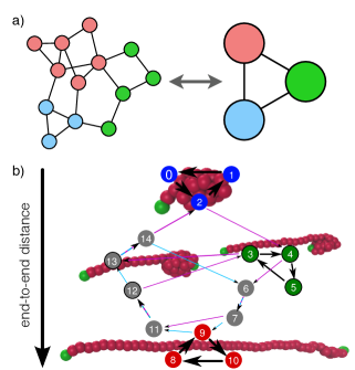
Figure 4: (a) Coarse-graining of mesostates (left) into a few basins (right) corresponding to long-lived structural states. (b) Specific example of a grafted polymer in shear flow Knoch and Speck (2017). Shown is the minimal graph of mesostates together with representative snapshots of the polymer. Clustering of cycles reveals five communities, three of which are local corresponding to dynamics with small fluctuations of the end-to-end distance [globule (blue), stretched (red), and one intermediate (green)], and two global communities cycling through the collapse and stretching of the polymer.

In a non-equilibrium steady state, the largest eigenvalue of the transition matrix is still unity and non-degenerate, but other eigenvalues may become complex (these appear in complex conjugate pairs). More importantly, there are now non-vanishing probability currents coupling to macroscopic currents. Simply combining mesostates into superstates will affect these currents and reduce the entropy production Puglisi et al. (2010). The aim is thus to derive a Markov process with a reduced number of states that yields the same (average) macroscopic currents, and thus entropy production.

In fact, this goal can be achieved rigourously Knoch and Speck (2015). To this end, we focus on the cycles in the graph of mesostates. As shown in appendix C, the probability currents

$$j_{e}=\sum_{c}\varphi_{c}c_{e}$$ (64)

can be decomposed into contributions from cycles, where $\varphi_{c}\geqslant 0$ is the weight of cycle $\vec{c}=(c_{e})$. While the number of cycles can be very large, the number of contributing cycles with $\varphi_{c}>0$ is bound by the Betti number $|E|-|V|+1$. Note that the weights $\varphi_{c}$ do not have a physical meaning but allow to reconstruct currents from a set of contributing cycles.

Conjugate to the edge currents $j_{e}$ are the edge affinities $a^{e}=a_{ij}$ for each $e=i\to j$. Plugging the decomposition Eq. (64) into the entropy production rate Eq. (36), we obtain $\dot{\sigma}=\sum_{e}a^{e}j_{e}=\sum_{c}\varphi_{c}a(\vec{c})$ with cycle affinities

$$a(\vec{c})\equiv\sum_{e}a^{e}c_{e}=f_{\alpha}\sum_{(i\to j)\in\vec{c}}d^{\alpha}_{ij}=f_{\alpha}d^{\alpha}(\vec{c}),$$ (65)

which are given by the net transport between reservoirs (we sum over all directed edges that form the cycle). The next step is to decimate the number of contributing cycles. This is made possible by realizing that the distribution of cycles is far from uniform as many cycles visit neighboring mesostates and thus cluster into communities, which can be identified by well established techniques. Let us assume that we have obtained such a partition into sets $\{\mathcal{C}_{k}\}$ of cycles. We pick one representative cycle $k\in\mathcal{C}_{k}$ for each community. Which cycle is not important for what follows, and representatives can be choosen to be optimal in some sense (e.g., optimize the mean-first passage times between communities Knoch and Speck (2017)). The linearity of the entropy production rate is exploited to split

$$\dot{\sigma}=\sum_{k}\dot{\sigma}_{k},\qquad\dot{\sigma}_{k}\equiv\sum_{c\in\mathcal{C}_{k}}\varphi_{c}a(\vec{c})$$ (66)

into a contribution from each community. Eliminating all cycles except for the representative, it has to carry all the entropy production, which implies the new weight $\varphi^{\prime}_{k}=\dot{\sigma}_{k}/a_{k}$. As a consequence, the new currents are $j^{\prime}_{e}=\sum_{k}\varphi^{\prime}_{k}k_{e}$. However, we still have to determine the symmetric part of the fluxes as well as the probabilities. We know that the local detailed balance condition Eq. (24) fixes the ratio of the transition rates, which can be ensured by fixing the ratio $p^{\prime}_{i}/p^{\prime}_{j}=p_{i}/p_{j}$ and preserving edge affinities

$$e^{a_{ij}}=\frac{\phi_{ij}}{\phi_{ji}}=\frac{\phi^{\prime}_{ij}}{\phi^{\prime}_{ji}}=\frac{\phi^{\prime}_{ji}+j^{\prime}_{ij}}{\phi^{\prime}_{ji}}.$$ (67)

This condition allows us to determine the new fluxes

$$\phi^{\prime}_{ij}=\frac{e^{a_{ij}}}{e^{a_{ij}}-1}\sum_{k}\varphi^{\prime}_{k}k_{ij}$$ (68)

with $k_{ij}=\pm 1$ if the oriented edge $i\to j$ participates in cycle $\vec{k}$. We have thus derived a Markov process with transition rates $w^{\prime}_{ij}=\phi^{\prime}_{ij}/p_{i}$ between the mesostates that are included in one of the representative cycles. This Markov process rigorously preserves the entropy production and the macroscopic currents between reservoirs.

As an illustration, Fig. 4(b) shows the result of this procedure Knoch and Speck (2017) for a grafted model polymer in shear flow Alexander-Katz et al. (2006). For intermediate strain rates, the polymer cycles between globule and extended conformations. A fine-grained Markov model has been obtained through clustering structurally similar configurations harvested from simulations, from which the rates $w$ are obtained through counting. Determining all contributing cycles in this fine-grained model reveals five cycle communities largely determined by the visited end-to-end distances, cf. Fig. 4(b). The minimal coarse-grained model then consists of only 15 mesostates after eliminating further “bridge states” that are unique to their cycles (see also Ref. Seiferth et al. (2020)). Periodically driven molecules (e.g., due to the coupling of a residual dipole moment with an external electric field) have also been addressed Wang and Brady (2015); Knoch and Speck (2019).

VII Conclusions and outlook

Markov state modeling and dimensional reduction techniques Pande et al. (2010); Prinz et al. (2011); Sittel and Stock (2018) have been successfully employed to extract the dynamics of discrete molecular conformations from atomistic models of biomolecules, primarily peptides. Analyzing these Markov models yields a comprehensive picture of possible (e.g., folding) pathways and kinetics. Extending this framework to molecular machines requires to take into account the entropy that is dissipated into the aqueous environment. Splitting the total system into the molecular motor itself and idealized reservoirs [cf. Fig. 1(a)] has the advantage that the entropy production is determined completely by the exchange with the reservoirs [Eq. (8)]. These, typically few, currents take the role of extensive variables in a framework formally equivalent to thermodynamics and based on large deviation theory. Preserving these currents allows to systematically construct a coarse-grained representation of the internal dynamics in terms of molecular conformations.

On the simplest level discussed here, equilibrium detailed balance is replaced by the local detailed balance condition Eq. (24) modeling exchanges with ideal reservoirs. While clearly being a simplification in most situations, the advantage is that we do not have to take these reservoirs into account explicitly. Moreover, as discussed in some detail here, it allows a consistent view on the stochastic energetics and thermodynamics. What we need in addition to equilibrium Markov state models is to identify which conformational transitions involve exchanges with the reservoirs, which requires some physical insight into these conformations. However, one might expect that the matrices $d^{\alpha}_{ij}$ are sparse with only very few transitions being involved. For example, ATP might only bind to a single conformation. Another computational advantage is that we do not need to resolve the quantum-mechanical nature of this binding transition, while thermodynamic consistency is maintained by construction.

There have been tremendous advances, not only in our grasp of biological, but also in the design and synthesis of artificial molecular machines Erbas-Cakmak et al. (2015); Kistemaker et al. (2021). Modeling will play an increasing role but requires robust methods based on rigorous principles out of equilibrium. Here we have sketched how to deploy stochastic thermodynamics for the systematic construction of coarse-grained models, which will complement more detailed atomistic inverstigations.

Appendix A Derivation of Rayleighian

To lowest order in the linear response regime around equilibrium, the generating function reads $\psi(f)=-\frac{1}{2}f_{\alpha}\chi^{\alpha\beta}f_{\beta}$ in agreement with Eq. (14). This is a convex function, and we can thus determine its inverse Legendre transformation (as a functional of $\dot{X}_{t}$),

$$\tau\Phi[\dot{X}_{t}] =\sup_{f}[f_{\alpha}\Delta^{\alpha}+\tau\psi(f)]$$

$$=\sup_{f}\int_{0}^{\tau}\mathrm{d}t\;[f_{\alpha}\dot{X}_{t}^{\alpha}-\tfrac{1}{2}f_{\alpha}\chi^{\alpha\beta}f_{\beta}]$$

$$=\int_{0}^{\tau}\mathrm{d}t\;\sup_{f}[f_{\alpha}\dot{X}_{t}^{\alpha}-\tfrac{1}{2}f_{\alpha}\chi^{\alpha\beta}f_{\beta}]$$

$$=\int_{0}^{\tau}\mathrm{d}t\;\tfrac{1}{2}\dot{X}_{t}^{\alpha}\chi_{\alpha\beta}\dot{X}_{t}^{\beta}.$$

Here, we multiply by the trajectory length $\tau>0$, pull out the integral using Eq. (6), and exploit that we can interchange the supremum with the integration Hafsa and Mandallena (2003). Multiplying the right hand side of Eq. (13) by $\tau$ and inserting the result for $\tau\Phi$, we again interchange

$$\inf_{\dot{X}_{t}}\int_{0}^{\tau}\mathrm{d}t\;[\tfrac{1}{2}\dot{X}_{t}^{\alpha}\chi_{\alpha\beta}\dot{X}_{t}^{\beta}-f_{\alpha}\dot{X}_{t}^{\alpha}]\\ =\int_{0}^{\tau}\mathrm{d}t\;\inf_{\dot{X}}[\tfrac{1}{2}\dot{X}^{\alpha}\chi_{\alpha\beta}\dot{X}^{\beta}-f_{\alpha}\dot{X}^{\alpha}]$$ (69)

yielding $\inf_{\dot{X}}\mathcal{R}$ with the function $\mathcal{R}$ given in Eq. (16).

Appendix B Cycle space

To see that the null space of the incidence matrix $\nabla$ is the space of directed simple cycles pick a starting vertex $i_{0}$ and an edge $e$ connecting it to $i_{1}$. For the vector $\vec{c}$ set $c_{e}=+1$ if the edge enters $i_{1}$ and $c_{e}=-1$ if it leaves $i_{1}$ (all other entries are zero). Applying the incidence matrix then leads to a vector with entry $+1$ for $i_{1}$ and $-1$ for $i_{0}$. Pick a second edge connecting $i_{1}$ with $i_{2}$ and set $c_{e}=\pm 1$ depending on the edge orientation. Again applying the incidence matrix, the entry for $i_{1}$ has become zero and the entry for $i_{2}$ is $+1$. This construction can be continued until the last edge enters the starting vertex $i_{0}$. Now the vector $\nabla\cdot\vec{c}=\nabla_{i}^{e}c_{e}=0$ has all entries zeros and we stop. Hence, a (simple) cycle $i_{0}\to i_{1}\to\cdots\to i_{0}$ in which all visited vertices are unique can be represented as an edge vector with entries $c_{e}=\pm 1$ for edges that are part of the cycle and $c_{e}=0$ for edges that are not part of the cycle. The sign is positive if the cycle edge has the same orientation as the graph edge.

Appendix C Cycle decomposition

Figure 5: Illustration of the cycle decomposition. (a) Simple directed graph $\vec{G}$ with four vertices. The numbers indicate the current along the corresponding edge. Note that the current law Eq. (32) is obeyed. We first consider the cycle through the lower three states (arrow) with smallest current $j_{e}=1$. Subtracting this current from (or, if antiparallel, adding to) all edges of this cycle leads to (b). (c) We thus find two contributing cycles with weights $\varphi_{1}=3$ (top) and $\varphi_{2}=1$ (bottom) that share one edge.

The following algorithm can be used to determine the cycle weights $\varphi_{c}$ iteratively Kalpazidou (2007); Altaner et al. (2012). We enumerate all cycles starting with the first cycle, $c=1$, and we initialize $j_{e}^{(1)}=j_{e}$ with the currents. We go along all edges of the cycle with $c_{e}=+1$ (parallel to graph edge) and pick the smallest current, which we assign as cycle weight,

$$\varphi_{c}=\min_{e\in E}\{j_{e}^{(c)}(\vec{c})|c_{e}=+1\}\geqslant 0.$$ (70)

Remember that $j_{e}\geqslant 0$ by construction and thus also the cycle weight is non-negative. We subtract this cycle weight from all cycle edges,

$$j_{e}^{(c+1)}=j_{e}^{(c)}-\varphi_{c}c_{e}.$$ (71)

Either $\varphi_{c}=0$ (because one or more edges had zero current) and nothing changes, or the new current vector $j_{e}^{(c+1)}$ has one more entry equal to zero with all other entries still non-negative. Note that $\sum_{e}\nabla_{i}^{e}j_{e}^{(c+1)}=0$. We then go to the next cycle $c\leftarrow c+1$ and repeat this procedure. The iteration is stopped when all entries $j_{e}^{(c+1)}$ are zero and thus all contributing cycles have been identified. Fig. 5 illustrates this procedure for a simple system with four mesostates.

Appendix D Kullback-Leibler divergence

The Kullback-Leibler divergence (or relative entropy) is often cited to determine a “distance” between probability measures. In case of trajectories, it can be written

$$\mathcal{D}_{\text{KL}}(\mathcal{P}^{\ast}_{\tau}\parallel\mathcal{P}_{\tau})\equiv\sum_{\bm{\imath}}\mathcal{P}^{\ast}_{\tau}[\bm{\imath}]\ln\frac{\mathcal{P}^{\ast}_{\tau}[\bm{\imath}]}{\mathcal{P}_{\tau}[\bm{\imath}]}=\tau\mathcal{I}_{w}(p^{\ast},\phi^{\ast}),$$ (72)

relating it to the rate function Eq. (49). The final result follows from plugging in the trajectory weight Eq. (42) for $\mathcal{P}_{\tau}$, and the same expression for $\mathcal{P}^{\ast}_{\tau}$ but replacing $w\to w^{\ast}$. For the logarithmic ratio we obtain (ignoring boundary terms)

$$\sum_{\nu=1}^{K}\ln\frac{w^{\ast}_{i_{\nu-1}i_{\nu}}}{w_{i_{\nu-1}i_{\nu}}}-\sum_{\nu=0}^{K}\sum_{j}(w^{\ast}_{i_{\nu}j}-w_{i_{\nu}j})(t_{\nu+1}-t_{\nu}).$$ (73)

Taking the average and dividing by $\tau$ then yields

$$\sum_{ij}\phi^{\ast}_{ij}\ln\frac{w^{\ast}_{ij}}{w_{ij}}-\sum_{ij}p^{\ast}_{i}(w^{\ast}_{ij}-w_{ij})=\mathcal{I}_{w}(p^{\ast},\phi^{\ast}),$$ (74)

namely the rate function Eq. (49) determining the probability to jointly observe populations $p^{\ast}$ and fluxes $\phi^{\ast}$.

Appendix E Optimal control process

To derive Eq. (63), we start from the large deviation function

$$-\tau\psi\asymp\ln\langle e^{\zeta_{\alpha}\Delta^{\alpha}_{\tau}}\rangle=\ln\sum_{\bm{\imath}}e^{\zeta_{\alpha}\Delta^{\alpha}_{\tau}}\frac{\mathcal{P}_{\tau}[\bm{\imath}]}{\mathcal{P}^{\ast}_{\tau}[\bm{\imath}]}\mathcal{P}^{\ast}_{\tau}[\bm{\imath}]$$ (75)

and expand the path weight by the weight $\mathcal{P}^{\ast}_{\tau}[\bm{\imath}]$ of the (unknown) control process. In the limit of large $\tau$, the right hand side is dominated by the saddle-point leading to

$$\ln\left\langle\exp\left\{\zeta_{\alpha}\Delta^{\alpha}_{\tau}+\ln\frac{\mathcal{P}_{\tau}}{\mathcal{P}^{\ast}_{\tau}}\right\}\right\rangle^{\ast}\asymp\sup_{w^{\ast}}\left\langle\zeta_{\alpha}\Delta^{\alpha}_{\tau}+\ln\frac{\mathcal{P}_{\tau}}{\mathcal{P}^{\ast}_{\tau}}\right\rangle^{\ast}$$ (76)

with respect to all admissible Markov processes $w^{\ast}$. Performing the average and using Eq. (72), we thus find

$$\tau\sup_{w^{\ast}}\left\{\zeta_{\alpha}\langle\mathcal{J}^{\alpha}\rangle^{\ast}-\mathcal{I}_{w}(p^{\ast},\phi^{\ast})\right\},$$ (77)

which yields Eq. (63) after pulling out the minus sign.

Appendix F Biasing potential

To see how the biasing of trajectories changes the underlying free energy landscape, we follow Ref. 119. We plug the rates Eq. (60) together with Eq. (59) into the path weight Eq. (42),

$$\mathcal{P}_{\tau}[\bm{\imath}]=\tilde{\mathcal{P}}_{\tau}[\bm{\imath}]\exp\left\{\zeta_{\alpha}\Delta^{\alpha}_{\tau}+\tau\frac{\psi}{2}+\sum_{\nu=1}^{K}\lambda_{i_{\nu-1}i_{\nu}}\right\},$$ (78)

which thus can be written as the original path weight times an exponential factor. Summing over all trajectories and imposing normalization of the biased ensemble yields

$$e^{-\tau\psi(\zeta)/2}=\left\langle\exp\left\{\zeta_{\alpha}\Delta^{\alpha}_{\tau}+\sum_{\nu=1}^{K}\lambda_{i_{\nu-1}i_{\nu}}\right\}\right\rangle_{\text{eq}},$$ (79)

with $\psi(\zeta)$ the large deviation function.

For the antisymmetric Lagrange multipliers $\lambda_{ij}$ we now write $\lambda_{ij}=(v_{i}-v_{j})/2$. Plugging this expression into the ratio Eq. (61) and comparing with the local detailed balance condition Eq. (24), we see that $\zeta_{\alpha}=f_{\alpha}/2$ can be identified with the affinities but the free energies are shifted as $G^{0}_{i}\to G^{0}_{i}+v_{i}$. Hence, the $v_{i}(\zeta)$ constitute a biasing potential that modifies the underlying atomistic model at variance with the local detailed balance condition Eq. (24). The sum

$$\sum_{\nu=1}^{K}\lambda_{i_{\nu-1}i_{\nu}}=v_{i_{0}}-v_{i_{K}}$$ (80)

reduces to a temporal boundary term that does not change $\psi(\zeta)$. Using that the sum $\sum_{(i\to j)\in c}\lambda_{ij}=0$ along any simple cycle $c$ vanishes together with the exit rate constraints [Eq. (59)] allows (in principle) to determine $v$ and $\psi$.

For affinities corresponding to thermal equilibrium, we have $f_{\alpha}\Delta^{\alpha}=0$ and $\psi=0$ as well as $v=0$. Close to equilibrium, we expand

$$e^{-\tau\psi(f)/2}=\left\langle e^{\tfrac{1}{2}f_{\alpha}\Delta^{\alpha}_{\tau}}\right\rangle_{\text{eq}}+\mathcal{O}(v^{2})$$ (81)

since $\langle(v_{i}-v_{j})\rangle=0$. Hence, for a small perturbation of equilibrium no shifts $v$ occur, which justifies the ansatz Eq. (10) for the probability density of the changes $\Delta^{\alpha}_{\tau}$ in the linear response regime.

References

- Chandler (1987) D. Chandler, Introduction to Modern Statistical Mechanics (Oxford University Press, Oxford, 1987).
- Frenkel and Smit (2002) D. Frenkel and B. Smit, Understanding Molecular Simulation: From Algorithms to Applications, 2nd ed. (Academic Press, San Diego, 2002).
- Torrie and Valleau (1977) G. Torrie and J. Valleau, “Nonphysical sampling distributions in monte carlo free-energy estimation: Umbrella sampling,” J. Comput. Phys. 23, 187–199 (1977).
- Allen et al. (2006) R. J. Allen, D. Frenkel, and P. R. ten Wolde, “Forward flux sampling-type schemes for simulating rare events: Efficiency analysis,” J. Chem. Phys. 124, 194111 (2006).
- Hussain and Haji-Akbari (2020) S. Hussain and A. Haji-Akbari, “Studying rare events using forward-flux sampling: Recent breakthroughs and future outlook,” J. Chem. Phys. 152, 060901 (2020).
- van Erp and Bolhuis (2005) T. S. van Erp and P. G. Bolhuis, “Elaborating transition interface sampling methods,” J. Comp. Phys. 205, 157–181 (2005).
- Bolhuis et al. (2002) P. G. Bolhuis, D. Chandler, C. Dellago, and P. L. Geissler, “Transition path sampling: throwing ropes over rough mountain passes, in the dark,” Annu. Rev. Phys. Chem. 53, 291–318 (2002).
- Dellago et al. (2002) C. Dellago, P. G. Bolhuis, and P. L. Geissler, “Transition path sampling,” Adv. Chem. Phys. 123, 1 (2002).
- Lindorff-Larsen et al. (2011) K. Lindorff-Larsen, S. Piana, R. O. Dror, and D. E. Shaw, “How fast-folding proteins fold,” Science 334, 517–520 (2011).
- Pohorille et al. (2010) A. Pohorille, C. Jarzynski, and C. Chipot, “Good practices in free-energy calculations,” J. Phys. Chem. B 114, 10235–10253 (2010).
- Shirts and Mobley (2012) M. R. Shirts and D. L. Mobley, “An introduction to best practices in free energy calculations,” in Methods in Molecular Biology (Humana Press, 2012) pp. 271–311.
- Mey et al. (2020) A. S. Mey, B. K. Allen, H. E. B. Macdonald, J. D. Chodera, D. F. Hahn, M. Kuhn, J. Michel, D. L. Mobley, L. N. Naden, S. Prasad, A. Rizzi, J. Scheen, M. R. Shirts, G. Tresadern, and H. Xu, “Best practices for alchemical free energy calculations [article v1.0],” Living J. Comp. Mol. Sci. 2 (2020), 10.33011/livecoms.2.1.18378.
- Schrödinger (1944) E. Schrödinger, What is life? The physical aspect of the living cell (Cambridge University Press, 1944).
- Hill (1977) T. L. Hill, Free energy transduction in biology: The steady-state kinetic and thermodynamic formalism (Academic Press, 1977).
- Jülicher et al. (1997) F. Jülicher, A. Ajdari, and J. Prost, “Modeling molecular motors,” Rev. Mod. Phys. 69, 1269–1282 (1997).
- Bustamante et al. (2001) C. Bustamante, D. Keller, and G. Oster, “The physics of molecular motors,” Acc. Chem. Res. 34, 412–420 (2001).
- Kolomeisky and Fisher (2007) A. B. Kolomeisky and M. E. Fisher, “Molecular motors: A theorist’s perspective,” Annu. Rev. Phys. Chem. 58, 675–695 (2007).
- Andrieux and Gaspard (2006) D. Andrieux and P. Gaspard, “Fluctuation theorems and the nonequilibrium thermodynamics of molecular motors,” Phys. Rev. E 74, 011906 (2006).
- Seifert (2011) U. Seifert, “Stochastic thermodynamics of single enzymes and molecular motors,” Eur. Phys. J. E 34, 1–11 (2011).
- Seifert (2012) U. Seifert, “Stochastic thermodynamics, fluctuation theorems, and molecular machines,” Rep. Prog. Phys. 75, 126001 (2012).
- Ciliberto (2017) S. Ciliberto, “Experiments in stochastic thermodynamics: Short history and perspectives,” Phys. Rev. X 7, 021051 (2017).
- Horowitz and Gingrich (2019) J. M. Horowitz and T. R. Gingrich, “Thermodynamic uncertainty relations constrain non-equilibrium fluctuations,” Nat. Phys. 16, 15–20 (2019).
- Brown and Sivak (2019) A. I. Brown and D. A. Sivak, “Theory of nonequilibrium free energy transduction by molecular machines,” Chem. Rev. 120, 434–459 (2019).
- Verley et al. (2014) G. Verley, M. Esposito, T. Willaert, and C. V. den Broeck, “The unlikely Carnot efficiency,” Nat. Commun. 5, 4721 (2014).
- Touchette (2009) H. Touchette, “The large deviation approach to statistical mechanics,” Phys. Rep. 478, 1–69 (2009).
- Touchette (2018) H. Touchette, “Introduction to dynamical large deviations of Markov processes,” Physica A 504, 5–19 (2018).
- Jack (2020) R. L. Jack, “Ergodicity and large deviations in physical systems with stochastic dynamics,” Eur. Phys. J. B 93 (2020), 10.1140/epjb/e2020-100605-3.
- Noid et al. (2008) W. G. Noid, J.-W. Chu, G. S. Ayton, V. Krishna, S. Izvekov, G. A. Voth, A. Das, and H. C. Andersen, “The multiscale coarse-graining method. I. A rigorous bridge between atomistic and coarse-grained models,” J. Chem. Phys. 128, 244114 (2008).
- Murtola et al. (2009) T. Murtola, A. Bunker, I. Vattulainen, M. Deserno, and M. Karttunen, “Multiscale modeling of emergent materials: biological and soft matter,” Phys. Chem. Chem. Phys. 11, 1869 (2009).
- Izvekov and Voth (2005) S. Izvekov and G. A. Voth, “A multiscale coarse-graining method for biomolecular systems,” J. Phys. Chem. B 109, 2469–2473 (2005).
- Scherer and Andrienko (2018) C. Scherer and D. Andrienko, “Understanding three-body contributions to coarse-grained force fields,” Phys. Chem. Chem. Phys. 20, 22387–22394 (2018).
- Marrink et al. (2007) S. J. Marrink, H. J. Risselada, S. Yefimov, D. P. Tieleman, and A. H. de Vries, “The MARTINI force field: coarse grained model for biomolecular simulations,” J. Phys. Chem. B 111, 7812–7824 (2007).
- Pande et al. (2010) V. S. Pande, K. Beauchamp, and G. R. Bowman, “Everything you wanted to know about markov state models but were afraid to ask,” Methods 52, 99 – 105 (2010), protein Folding.
- Prinz et al. (2011) J.-H. Prinz, H. Wu, M. Sarich, B. Keller, M. Senne, M. Held, J. D. Chodera, C. Schütte, and F. Noé, “Markov models of molecular kinetics: Generation and validation,” J. Chem. Phys. 134, 174105 (2011).
- Chodera and Noé (2014) J. D. Chodera and F. Noé, “Markov state models of biomolecular conformational dynamics,” Curr. Opin. Struct. Biol. 25, 135–144 (2014).
- Husic and Pande (2018) B. E. Husic and V. S. Pande, “Markov state models: From an art to a science,” J. Am. Chem. Soc. 140, 2386–2396 (2018).
- Abella et al. (2020) J. R. Abella, D. Antunes, K. Jackson, G. Lizée, C. Clementi, and L. E. Kavraki, “Markov state modeling reveals alternative unbinding pathways for peptide–MHC complexes,” Proc. Natl. Acad. Sci. U.S.A. 117, 30610–30618 (2020).
- Rudzinski et al. (2016) J. F. Rudzinski, K. Kremer, and T. Bereau, “Communication: Consistent interpretation of molecular simulation kinetics using markov state models biased with external information,” J. Chem. Phys. 144, 051102 (2016).
- Knoch and Speck (2018) F. Knoch and T. Speck, “Unfolding dynamics of small peptides biased by constant mechanical forces,” Mol. Syst. Des. Eng. 3, 204–213 (2018).
- Gallavotti and Cohen (1995) G. Gallavotti and E. G. D. Cohen, “Dynamical ensembles in nonequilibrium statistical mechanics,” Phys. Rev. Lett. 74, 2694 (1995).
- Jarzynski (2007) C. Jarzynski, “Comparison of far-from-equilibrium work relations,” C. R. Physique 8, 495–506 (2007).
- Kurchan (1998) J. Kurchan, “Fluctuation theorem for stochastic dynamics,” J. Phys. A: Math. Gen. 31, 3719 (1998).
- Lebowitz and Spohn (1999) J. L. Lebowitz and H. Spohn, “A gallavotti-cohen-type symmetry in the large deviation functional for stochastic dynamics,” J. Stat. Phys. 95, 333 (1999).
- Crooks (1999) G. E. Crooks, “Entropy production fluctuation theorem and the nonequilibrium work relation for free energy differences,” Phys. Rev. E 60, 2721 (1999).
- Hatano and Sasa (2001) T. Hatano and S.-i. Sasa, “Steady-state thermodynamics of langevin systems,” Phys. Rev. Lett. 86, 3463–3466 (2001).
- Andrieux and Gaspard (2007) D. Andrieux and P. Gaspard, “Fluctuation theorem for currents and schnakenberg network theory,” J. Stat. Phys. 127, 107–131 (2007).
- Onsager (1931a) L. Onsager, “Reciprocal relations in irreversible processes. i.” Phys. Rev. 37, 405–426 (1931a).
- Onsager (1931b) L. Onsager, “Reciprocal relations in irreversible processes. ii.” Phys. Rev. 38, 2265–2279 (1931b).
- Palmer and Speck (2017) T. Palmer and T. Speck, “Thermodynamic formalism for transport coefficients with an application to the shear modulus and shear viscosity,” J. Chem. Phys. 146, 124130 (2017).
- Weinhold (1975) F. Weinhold, “Metric geometry of equilibrium thermodynamics,” J. Chem. Phys. 63, 2479–2483 (1975).
- Ruppeiner (1979) G. Ruppeiner, “Thermodynamics: A riemannian geometric model,” Phys. Rev. A 20, 1608–1613 (1979).
- Feng and Crooks (2008) E. H. Feng and G. E. Crooks, “Length of time’s arrow,” Phys. Rev. Lett. 101, 090602 (2008).
- Sivak and Crooks (2012) D. A. Sivak and G. E. Crooks, “Thermodynamic metrics and optimal paths,” Phys. Rev. Lett. 108, 190602 (2012).
- Zhou and Doi (2018) J. Zhou and M. Doi, “Dynamics of viscoelastic filaments based on onsager principle,” Phys. Rev. Fluids 3, 084004 (2018).
- Sittel and Stock (2018) F. Sittel and G. Stock, “Perspective: Identification of collective variables and metastable states of protein dynamics,” J. Chem. Phys. 149, 150901 (2018).
- Seifert (2018) U. Seifert, “Stochastic thermodynamics: From principles to the cost of precision,” Physica A 504, 176–191 (2018).
- Noji et al. (1997) H. Noji, R. Yasuda, M. Yoshida, and K. Kinosita, “Direct observation of the rotation of f1-atpase,” Nature 386, 299–302 (1997).
- Wang and Oster (1998) H. Wang and G. Oster, “Energy transduction in the f1 motor of ATP synthase,” Nature 396, 279–282 (1998).
- Itoh et al. (2004) H. Itoh, A. Takahashi, K. Adachi, H. Noji, R. Yasuda, M. Yoshida, and K. Kinosita, “Mechanically driven ATP synthesis by f1-ATPase,” Nature 427, 465–468 (2004).
- Bergmann and Lebowitz (1955) P. G. Bergmann and J. L. Lebowitz, “New approach to nonequilibrium processes,” Phys. Rev. 99, 578–587 (1955).
- Klein et al. (2021) R. Klein, R. E. Viand, F. Höfling, and L. D. Site, “Nonequilibrium induced by reservoirs: Physico-mathematical models and numerical tests,” Adv. Theory Simul. 4, 2100071 (2021).
- Schnakenberg (1976) J. Schnakenberg, “Network theory of microscopic and macroscopic behavior of master equation systems,” Rev. Mod. Phys. 48, 571–585 (1976).
- Polettini (2015) M. Polettini, “Cycle/cocycle oblique projections on oriented graphs,” Lett. Math. Phys. 105, 89–107 (2015).
- Seifert (2019) U. Seifert, “From stochastic thermodynamics to thermodynamic inference,” Annu. Rev. Condens. Matter Phys. 10, 171–192 (2019).
- Seifert (2005) U. Seifert, “Entropy production along a stochastic trajectory and an integral fluctuation theorem.” Phys. Rev. Lett. 95, 040602 (2005).
- Hasegawa and Van Vu (2019) Y. Hasegawa and T. Van Vu, “Fluctuation theorem uncertainty relation,” Phys. Rev. Lett. 123, 110602 (2019).
- Barato and Seifert (2015) A. C. Barato and U. Seifert, “Thermodynamic uncertainty relation for biomolecular processes,” Phys. Rev. Lett. 114, 158101 (2015).
- Gingrich et al. (2016) T. R. Gingrich, J. M. Horowitz, N. Perunov, and J. L. England, “Dissipation bounds all steady-state current fluctuations,” Phys. Rev. Lett. 116, 120601 (2016).
- Pietzonka et al. (2017) P. Pietzonka, F. Ritort, and U. Seifert, “Finite-time generalization of the thermodynamic uncertainty relation,” Phys. Rev. E 96, 012101 (2017).
- Dechant (2018) A. Dechant, “Multidimensional thermodynamic uncertainty relations,” J. Phys. A Math. Theor. 52, 035001 (2018).
- Koyuk and Seifert (2020) T. Koyuk and U. Seifert, “Thermodynamic uncertainty relation for time-dependent driving,” Phys. Rev. Lett. 125, 260604 (2020).
- Falasco et al. (2020) G. Falasco, M. Esposito, and J.-C. Delvenne, “Unifying thermodynamic uncertainty relations,” New J. Phys. 22, 053046 (2020).
- Hartich and Godec (2021) D. Hartich and A. c. v. Godec, “Thermodynamic uncertainty relation bounds the extent of anomalous diffusion,” Phys. Rev. Lett. 127, 080601 (2021).
- Maes and Netočný (2008) C. Maes and K. Netočný, “Canonical structure of dynamical fluctuations in mesoscopic nonequilibrium steady states,” EPL 82, 30003 (2008).
- Jaynes (1980) E. T. Jaynes, “The minimum entropy production principle,” Ann. Rev. Phys. Chem. 31, 579–601 (1980).
- Pressé et al. (2013) S. Pressé, K. Ghosh, J. Lee, and K. A. Dill, “Principles of maximum entropy and maximum caliber in statistical physics,” Rev. Mod. Phys. 85, 1115–1141 (2013).
- Dixit et al. (2018) P. D. Dixit, J. Wagoner, C. Weistuch, S. Pressé, K. Ghosh, and K. A. Dill, “Perspective: Maximum caliber is a general variational principle for dynamical systems,” J. Chem. Phys. 148, 010901 (2018).
- Baule and Evans (2008) A. Baule and R. M. L. Evans, “Invariant quantities in shear flow,” Phys. Rev. Lett. 101, 240601 (2008).
- Monthus (2011) C. Monthus, “Non-equilibrium steady states: maximization of the shannon entropy associated with the distribution of dynamical trajectories in the presence of constraints,” J. Stat. Mech. Theory Exp. 2011, P03008 (2011).
- Chetrite and Touchette (2015) R. Chetrite and H. Touchette, “Variational and optimal control representations of conditioned and driven processes,” J. Stat. Mech. Theory Exp. 2015, P12001 (2015).
- Polettini (2013) M. Polettini, “Fact-checking ziegler’s maximum entropy production principle beyond the linear regime and towards steady states,” Entropy 15, 2570–2584 (2013).
- Landauer (1975) R. Landauer, “Inadequacy of entropy and entropy derivatives in characterizing the steady state,” Phys. Rev. A 12, 636–638 (1975).
- Landauer (1993) R. Landauer, “Statistical physics of machinery: forgotten middle-ground,” Physica A 194, 551–562 (1993).
- Otten and Stock (2010) M. Otten and G. Stock, “Maximum caliber inference of nonequilibrium processes,” J. Chem. Phys. 133, 034119 (2010).
- Chetrite and Touchette (2013) R. Chetrite and H. Touchette, “Nonequilibrium microcanonical and canonical ensembles and their equivalence,” Phys. Rev. Lett. 111, 120601 (2013).
- Chetrite and Touchette (2014) R. Chetrite and H. Touchette, “Nonequilibrium markov processes conditioned on large deviations,” Ann. Henri Poincaré 16, 2005–2057 (2014).
- Jack and Sollich (2010) R. L. Jack and P. Sollich, “Large deviations and ensembles of trajectories in stochastic models,” Prog. Theor. Phys. Suppl. 184, 304–317 (2010).
- Guioth and Jack (2020) J. Guioth and R. L. Jack, “Dynamical phase transitions for the activity biased ising model in a magnetic field,” J. Stat. Mech. Theory Exp. 2020, 063215 (2020).
- Hedges et al. (2009) L. O. Hedges, R. L. Jack, J. P. Garrahan, and D. Chandler, “Dynamic order-disorder in atomistic models of structural glass formers.” Science 323, 1309–1313 (2009).
- Garrahan et al. (2009) J. P. Garrahan, R. L. Jack, V. Lecomte, E. Pitard, K. van Duijvendijk, and F. van Wijland, “First-order dynamical phase transition in models of glasses: an approach based on ensembles of histories,” J. Phys. A: Math. Theor. 42, 075007 (2009).
- Speck and Chandler (2012) T. Speck and D. Chandler, “Constrained dynamics of localized excitations causes a non-equilibrium phase transition in an atomistic model of glass formers,” J. Chem. Phys. 136, 184509 (2012).
- Campo and Speck (2020) M. Campo and T. Speck, “Dynamical coexistence in moderately polydisperse hard-sphere glasses,” J. Chem. Phys. 152, 014501 (2020).
- Garrahan and Lesanovsky (2010) J. P. Garrahan and I. Lesanovsky, “Thermodynamics of quantum jump trajectories,” Phys. Rev. Lett. 104, 160601 (2010).
- Gao and Limmer (2019) C. Y. Gao and D. T. Limmer, “Nonlinear transport coefficients from large deviation functions,” J. Chem. Phys. 151, 014101 (2019).
- Ray et al. (2018) U. Ray, G. K.-L. Chan, and D. T. Limmer, “Importance sampling large deviations in nonequilibrium steady states. i,” J. Chem. Phys. 148, 124120 (2018).
- Giardinà et al. (2006) C. Giardinà, J. Kurchan, and L. Peliti, “Direct evaluation of large-deviation functions,” Phys. Rev. Lett. 96, 120603 (2006).
- Lecomte and Tailleur (2007) V. Lecomte and J. Tailleur, “A numerical approach to large deviations in continuous time,” J. Stat. Mech. Theor. Exp. , P03004 (2007).
- Nemoto et al. (2016) T. Nemoto, F. Bouchet, R. L. Jack, and V. Lecomte, “Population-dynamics method with a multicanonical feedback control,” Phys. Rev. E 93, 062123 (2016).
- Ferré and Touchette (2018) G. Ferré and H. Touchette, “Adaptive sampling of large deviations,” J. Stat. Phys. 172, 1525–1544 (2018).
- Speck (2016) T. Speck, “Thermodynamic formalism and linear response theory for nonequilibrium steady states,” Phys. Rev. E 94, 022131 (2016).
- Zia and Schmittmann (2007) R. K. P. Zia and B. Schmittmann, “Probability currents as principal characteristics in the statistical mechanics of non-equilibrium steady states,” J. Stat. Mech.: Theor. Exp. 2007, P07012 (2007).
- Maes (2020) C. Maes, “Frenesy: Time-symmetric dynamical activity in nonequilibria,” Phys. Rep. 850, 1–33 (2020).
- Das and Limmer (2019) A. Das and D. T. Limmer, “Variational control forces for enhanced sampling of nonequilibrium molecular dynamics simulations,” J. Chem. Phys. 151, 244123 (2019).
- Rose et al. (2021) D. C. Rose, J. F. Mair, and J. P. Garrahan, “A reinforcement learning approach to rare trajectory sampling,” New J. Phys. 23, 013013 (2021).
- Oakes et al. (2020) T. H. E. Oakes, A. Moss, and J. P. Garrahan, “A deep learning functional estimator of optimal dynamics for sampling large deviations,” Mach. Learn.: Sci. Technol. 1, 035004 (2020).
- Yan et al. (2021) J. Yan, H. Touchette, and G. M. Rotskoff, “Learning nonequilibrium control forces to characterize dynamical phase transitions,” arXiv:2107.03348 (2021).
- Knoch and Speck (2017) F. Knoch and T. Speck, “Nonequilibrium markov state modeling of the globule-stretch transition,” Phys. Rev. E 95, 012503 (2017).
- Puglisi et al. (2010) A. Puglisi, S. Pigolotti, L. Rondoni, and A. Vulpiani, “Entropy production and coarse graining in markov processes,” J. Stat. Mech. , P05015 (2010).
- Knoch and Speck (2015) F. Knoch and T. Speck, “Cycle representatives for the coarse-graining of systems driven into a non-equilibrium steady state,” New J. Phys. 17, 115004 (2015).
- Alexander-Katz et al. (2006) A. Alexander-Katz, M. F. Schneider, S. W. Schneider, A. Wixforth, and R. R. Netz, “Shear-flow-induced unfolding of polymeric globules,” Phys. Rev. Lett. 97, 138101 (2006).
- Seiferth et al. (2020) D. Seiferth, P. Sollich, and S. Klumpp, “Coarse graining of biochemical systems described by discrete stochastic dynamics,” Phys. Rev. E 102, 062149 (2020).
- Wang and Brady (2015) M. Wang and J. F. Brady, “Constant stress and pressure rheology of colloidal suspensions,” Phys. Rev. Lett. 115, 158301 (2015).
- Knoch and Speck (2019) F. Knoch and T. Speck, “Non-equilibrium markov state modeling of periodically driven biomolecules,” J. Chem. Phys. 150, 054103 (2019).
- Erbas-Cakmak et al. (2015) S. Erbas-Cakmak, D. A. Leigh, C. T. McTernan, and A. L. Nussbaumer, “Artificial molecular machines,” Chemical Reviews 115, 10081–10206 (2015).
- Kistemaker et al. (2021) J. C. M. Kistemaker, A. S. Lubbe, and B. L. Feringa, “Exploring molecular motors,” Mater. Chem. Front. 5, 2900–2906 (2021).
- Hafsa and Mandallena (2003) O. A. Hafsa and J.-P. Mandallena, “Interchange of infimum and integral,” Calc. Var. Partial Differ. Equ. 18, 433–449 (2003).
- Kalpazidou (2007) S. L. Kalpazidou, Cycle representations of Markov processes, Vol. 28 (Springer Science & Business Media, 2007).
- Altaner et al. (2012) B. Altaner, S. Grosskinsky, S. Herminghaus, L. Katthän, M. Timme, and J. Vollmer, “Network representations of nonequilibrium steady states: Cycle decompositions, symmetries, and dominant paths,” Phys. Rev. E 85, 041133 (2012).
- Speck and Garrahan (2011) T. Speck and J. Garrahan, “Space-time phase transitions in driven kinetically constrained lattice models,” Eur. Phys. J. B 79, 1–6 (2011).