Powering Comparative Classification with Sentiment Analysis via Domain Adaptive Knowledge Transfer

Abstract

We study Comparative Preference Classification (CPC) which aims at predicting whether a preference comparison exists between two entities in a given sentence and, if so, which entity is preferred over the other. High-quality CPC models can significantly benefit applications such as comparative question answering and review-based recommendation. Among the existing approaches, non-deep learning methods suffer from inferior performances. The state-of-the-art graph neural network-based ED-GAT Ma et al. (2020) only considers syntactic information while ignoring the critical semantic relations and the sentiments to the compared entities. We propose Sentiment Analysis Enhanced COmparative Network (SAECON) which improves CPC accuracy with a sentiment analyzer that learns sentiments to individual entities via domain adaptive knowledge transfer. Experiments on the CompSent-19 Panchenko et al. (2019) dataset present a significant improvement on the F1 scores over the best existing CPC approaches.

1 Introduction

Comparative Preference Classification (CPC) is a natural language processing (NLP) task that predicts whether a preference comparison exists between two entities in a sentence and, if so, which entity wins the game. For example, given the sentence: Python is better suited for data analysis than MATLAB due to the many available deep learning libraries, a decisive comparison exists between Python and MATLAB and comparatively Python is preferred over MATLAB in the context.

The CPC task can profoundly impact various real-world application scenarios. Search engine users may query not only factual questions but also comparative ones to meet their specific information needs Gupta et al. (2017). Recommendation providers can analyze product reviews with comparative statements to understand the advantages and disadvantages of the product comparing with similar ones.

Several models have been proposed to solve this problem. Panchenko et al. (2019) first formalize the CPC problem, build and publish the CompSent-19 dataset, and experiment with numerous general machine learning models such as Support Vector Machine (SVM), representation-based classification, and XGBoost. However, these attempts consider CPC as a sentence classification while ignoring the semantics and the contexts of the entities Ma et al. (2020).

ED-GAT Ma et al. (2020) marks the first entity-aware CPC approach that captures long-distance syntactic relations between the entities of interest by applying graph attention networks (GAT) to dependency parsing graphs. However, we argue that the disadvantages of such an approach are clear. Firstly, ED-GAT replaces the entity names with “entityA” and “entityB” for simplicity and hence deprives their semantics. Secondly, ED-GAT has a deep architecture with ten stacking GAT layers to tackle the long-distance issue between compared entities. However, more GAT layers result in a heavier computational workload and reduced training stability. Thirdly, although the competing entities are typically connected via multiple hops of dependency relations, the unordered tokens along the connection path cannot capture either global or local high-quality semantic context features.

In this work, we propose a Sentiment Analysis Enhanced COmparative classification Network (SAECON), a CPC approach that considers not only syntactic but also semantic features of the entities. The semantic features here refer to the context of the entities from which a sentiment analysis model can infer the sentiments toward the entities. Specifically, the encoded sentence and entities are fed into a dual-channel context feature extractor to learn the global and local context. In addition, an auxiliary Aspect-Based Sentiment Analysis (ABSA) module is integrated to learn the sentiments towards individual entities which are greatly beneficial to the comparison classification.

ABSA aims to detect the specific emotional inclination toward an aspect within a sentence Ma et al. (2018); Hu et al. (2019); Phan and Ogunbona (2020); Chen and Qian (2020); Wang et al. (2020). For example, the sentence I liked the service and the staff but not the food suggests positive sentiments toward service and staff but a negative one toward food. These aspect entities, such as service, staff, and food, are studied individually.

The well-studied ABSA approaches can be beneficial to CPC when the compared entities in a CPC sentence are considered as the aspects in ABSA. Incorporating the individual sentiments learned by ABSA methods into CPC has several advantages. Firstly, for a comparison to hold, the preferred entity usually receives a positive sentiment while its rival gets a relatively negative one. These sentiments can be easily extracted by the strong ABSA models. The contrast between the sentiments assigned to the compared entities provides a vital clue for an accurate CPC. Secondly, the ABSA models are designed to target the sentiments toward phrases, which bypasses the complicated and noisy syntactic relation path. Thirdly, considering the scarcity of the data resource of CPC, the abundant annotated data of ABSA can provide sufficient supervision signal to improve the accuracy of CPC.

There is one challenge that blocks the knowledge transfer of sentiment analysis from the ABSA data to the CPC task: domain shift. Existing ABSA datasets are centered around specific topics such as restaurants and laptops, while the CPC data has mixed topics Panchenko et al. (2019) that are all distant from restaurants. In other words, sentences of ABSA and CPC datasets are drawn from different distributions, also known as domains. The difference in the distributions is referred to as a “domain shift” Ganin and Lempitsky (2015); He et al. (2018) and it is harmful to an accurate knowledge transfer. To mitigate the domain shift, we design a domain adaptive layer to remove the domain-specific feature such as topics and preserve the domain-invariant feature such as sentiments of the text so that the sentiment analyzer can smoothly transfer knowledge from sentiment analysis to comparative classification.

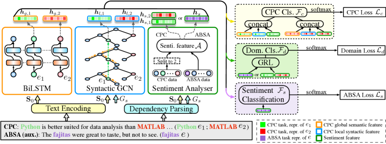
Figure 1: Pipeline of SAECON. Sentences from two domains shown in the gray box are fed into text encoder and dependency parser. The resultant representations of the entities from three substructures are discriminated by different colors (see the legend in the corner). “Cls.” is short for classifier.

2 Related Work

2.1 Comparative Preference Classification

CPC originates from the task of Comparative Sentence Identification (CSI) Jindal and Liu (2006). CSI aims to identify the comparative sentences. Jindal and Liu (2006) approach this problem by Class Sequential Mining (CSR) and a Naive Bayesian classifier. Building upon CSI, Panchenko et al. (2019) propose the task of CPC, release CompSent-19 dataset, and conduct experimental studies using traditional machine learning approaches such as SVM, representation-based classification, and XGBoost. However, they neglect the entities in the comparative context Panchenko et al. (2019). ED-GAT Ma et al. (2020), a more recent work, uses the dependency graph to better recognize long-distance comparisons and avoid falsely identifying unrelated comparison predicates. However, it fails to capture semantic information of the entities as they are replaced by “entityA” and “entityB”. Furthermore, having multiple GAT layers severely increases training difficulty.

2.2 Aspect-Based Sentiment Analysis

ABSA derives from sentiment analysis (SA) which infers the sentiment associated with a specific entity in a sentence. Traditional approaches of ABSA utilize SVM for classification Kiritchenko et al. (2014); Wagner et al. (2014); Zhang et al. (2014) while neural network-based approaches employ variants of RNN Nguyen and Shirai (2015); Aydin and Güngör (2020), LSTM Tang et al. (2016); Wang et al. (2016); Bao et al. (2019), GAT Wang et al. (2020), and GCN Pouran Ben Veyseh et al. (2020); Xu et al. (2020).

More recent works widely use complex contextualized NLP models such as BERT Devlin et al. (2019). Sun et al. (2019) transform ABSA into a Question Answering task by constructing auxiliary sentences. Phan and Ogunbona (2020) build a pipeline of Aspect Extraction and ABSA and used wide and concentrated features for sentiment classification. ABSA is related to CPC by nature. In general, entities with positive sentiments are preferred over the ones with neutral or negative sentiments. Therefore, the performance of a CPC model can be enhanced by the ABSA techniques.

3 SAECON

In this section, we first formalize the problem and then explain SAECON in detail. The pipeline of SAECON is depicted in Figure 1 with essential notations.

3.1 Problem Statement

CPC

Given a sentence $s$ from the CPC corpus $D_{c}$ with $n$ tokens and two entities $e_{1}$ and $e_{2}$, a CPC model predicts whether there exists a preference comparison between $e_{1}$ and $e_{2}$ in $s$ and if so, which entity is preferred over the other. Potential results can be Better ($e_{1}$ wins), Worse ($e_{2}$ wins), or None (no comparison exists).

ABSA

Given a sentence $s^{\prime}$ from the ABSA corpus $D_{s}$ with $m$ tokens and one entity $e^{\prime}$, ABSA identifies the sentiment (positive, negative, or neutral) associated with $e^{\prime}$.

We denote the source domains of the CPC and ABSA datasets by $\mathcal{D}_{c}$ and $\mathcal{D}_{s}$. $D_{c}$ and $D_{s}$ contain samples that are drawn from $\mathcal{D}_{c}$ and $\mathcal{D}_{s}$, respectively. $\mathcal{D}_{c}$ and $\mathcal{D}_{s}$ are similar but different in topics which produces a domain shift. We use $s$ to denote sentences in $D_{c}\cup D_{s}$ and $E$ to denote the entity sets for simplicity in later discussion. $|E|=2$ if $s\in D_{c}$ and $|E|=1$ otherwise.

3.2 Text Feature Representations

A sentence is encoded by its word representations via a text encoder and parsed into a dependency graph via a dependency parser Chen and Manning (2014). Text encoder, such as GloVe Pennington et al. (2014) and BERT Devlin et al. (2019), maps a word $w$ into a low dimensional embedding $\boldsymbol{w}\in\mathbb{R}^{d_{0}}$. GloVe assigns a fixed vector while BERT computes a token representation by its textual context. The encoding output of $s$ is denoted by $\boldsymbol{\mathrm{S}}_{0}=\{\boldsymbol{w}_{1},\ldots,\boldsymbol{e}_{1},\dots,\boldsymbol{e}_{2},\dots,\boldsymbol{w}_{n}\}$ where $\boldsymbol{e}_{i}$ denotes the embedding of entity $i$, $\boldsymbol{w}_{i}$ denotes the embedding of a non-entity word, and $\boldsymbol{w}_{i},\boldsymbol{e}_{j}\in\mathbb{R}^{d_{0}}$.

The dependency graph of $s$, denoted by $G_{s}$, is obtained by applying a dependency parser to $s$ such as Stanford Parser Chen and Manning (2014) or spaCy. $G_{s}$ is a syntactic view of $s$ Marcheggiani and Titov (2017); Li et al. (2016) that is composed of vertices of words and directed edges of dependency relations. Advantageously, complex syntactic relations between distant words in the sentence can be easily detected with a small number of hops over dependency edges Ma et al. (2020).

3.3 Contextual Features for CPC

Global Semantic Context

To model more extended context of the entities, we use a bi-directional LSTM (BiLSTM) to encode the entire sentence in both directions. Bi-directional recurrent neural network is widely used in extracting semantics Li et al. (2019). Given the indices of $e_{1}$ and $e_{2}$ in $s$, the global context representations $\boldsymbol{h}_{g,1}$ and $\boldsymbol{h}_{g,2}$ are computed by averaging the hidden outputs from both directions.

$$\overrightarrow{\boldsymbol{h}_{g,i}},\overleftarrow{\boldsymbol{h}_{g,i}} =\text{BiLSTM}(\boldsymbol{\mathrm{S}}_{0})[e_{i}.\text{index}],\quad i=1,2$$

$$\boldsymbol{h}_{g,i} =\frac{1}{2}\left(\overrightarrow{\boldsymbol{h}_{g,i}}+\overleftarrow{\boldsymbol{h}_{g,i}}\right),\boldsymbol{h}_{g,i}\in\mathbb{R}^{d_{g}}.$$

Local Syntactic Context

In SAECON, we use a dependency graph to capture the syntactically neighboring context of entities that contains words or phrases modifying the entities and indicates comparative preferences. We apply a Syntactic Graph Convolutional Network (SGCN) Bastings et al. (2017); Marcheggiani and Titov (2017) to $G_{s}$ to compute the local context feature $\boldsymbol{h}_{l,1}$ and $\boldsymbol{h}_{l,2}$ for $e_{1}$ and $e_{2}$, respectively. SGCN operates on directed dependency graphs with three major adjustments compared with GCN Kipf and Welling (2017): considering the directionality of edges, separating parameters for different dependency labels, and applying edge-wise gating to message passing.

GCN is a multilayer message propagation-based graph neural network. Given a vertex $v$ in $G_{s}$ and its neighbors $\mathcal{N}(v)$, the vertex representation of $v$ on the $(j+1)$th layer is given as

$$\boldsymbol{h}_{v}^{(j+1)}=\rho\left(\sum_{u\in\mathcal{N}(v)}\boldsymbol{\mathrm{W}}^{(j)}\boldsymbol{h}_{u}^{(j)}+\boldsymbol{b}^{(j)}\right),$$

where $\rho(\cdot)$ denotes an aggregation function such as mean and sum, $\boldsymbol{\mathrm{W}}^{(j)}\in\mathbb{R}^{d^{(j+1)}\times d^{(j)}}$ and $\boldsymbol{b}^{(j)}\in\mathbb{R}^{d^{(j+1)}}$ are trainable parameters, and $d^{(j+1)}$ and $d^{(j)}$ denote latent feature dimensions of the $(j+1)$th and the $j$th layers, respectively.

SGCN improves GCN by considering different edge directions and diverse edge types, and assigns different parameters to different directions or labels. However, there is one caveat: the directionality-based method cannot accommodate the rich edge type information; the label-based method causes combinatorial over-parameterization, increased risk of overfitting, and reduced efficiency. Therefore, we naturally arrive at a trade-off of using direction-specific weights and label-specific biases.

The edge-wise gating can select impactful neighbors by controlling the gates for message propagation through edges. The gate on the $j$th layer of an edge between vertices $u$ and $v$ is defined as

$$g^{(j)}_{uv}=\sigma\left(\boldsymbol{h}_{u}^{(j)}\cdot\boldsymbol{\beta}^{(j)}_{d_{uv}}+\gamma^{(j)}_{l_{uv}}\right),\quad g^{(j)}_{uv}\in\mathbb{R},$$

where $d_{uv}$ and $l_{uv}$ denote the direction and label of edge $(u,v)$, $\boldsymbol{\beta}^{(j)}_{d_{uv}}$ and $\gamma^{(j)}_{l_{uv}}$ are trainable parameters, and $\sigma(\cdot)$ denotes the sigmoid function.

Summing up the aforementioned adjustments on GCN, the final vertex representation learning is

$$\boldsymbol{h}_{v}^{(j+1)}=\rho\left(\sum_{u\in\mathcal{N}(v)}g^{(j)}_{uv}\left(\boldsymbol{\mathrm{W}}^{(j)}_{d_{uv}}\boldsymbol{h}_{u}^{(j)}+\boldsymbol{b}_{l_{uv}}^{(j)}\right)\right).$$

Vectors of $\boldsymbol{\mathrm{S}}_{0}$ serve as the input representations $\boldsymbol{h}^{(0)}_{v}$ to the first SGCN layer. The representations corresponding to $e_{1}$ and $e_{2}$ are the output $\{\boldsymbol{h}_{l,1},\boldsymbol{h}_{l,2}\}$ with dimension $d_{l}$.

3.4 Sentiment Analysis with Knowledge Transfer from ABSA

We have discussed in Section 1 that ABSA inherently correlates with the CPC task. Therefore, it is natural to incorporate a sentiment analyzer into SAECON as an auxiliary task to take advantage of the abundant training resources of ABSA to boost the performance on CPC. There are two paradigms for auxiliary tasks: (1) incorporating fixed parameters that are pretrained solely with the auxiliary dataset; (2) incorporating the architecture only with untrained parameters and jointly optimizing them from scratch with the main task simultaneously Li et al. (2018); He et al. (2018); Wang and Pan (2018).

Option (1) ignores the domain shift between $D_{c}$ and $D_{s}$, which degrades the quality of the learned sentiment features since the domain identity information is noisy and unrelated to the CPC task. SAECON uses option (2). For a smooth and efficient knowledge transfer from $\mathcal{D}_{s}$ to $\mathcal{D}_{c}$ under the setting of option (2), the ideal sentiment analyzer only extracts the textual feature that is contingent on sentimental information but orthogonal to the identity of the source domain. In other words, the learned sentiment features are expected to be discriminative on sentiment analysis but invariant with respect to the domain shift. Therefore, the sentiment features are more aligned with the CPC domain $\mathcal{D}_{c}$ with reduced noise from domain shift.

In SAECON, we use a gradient reversal layer (GRL) and a domain classifier (DC) Ganin and Lempitsky (2015) for the domain adaptive sentiment feature learning that maintains the discriminativeness and the domain-invariance. GRL+DC is a straightforward, generic, and effective modification to neural networks for domain adaptation Kamath et al. (2019); Gu et al. (2019); Belinkov et al. (2019); Li et al. (2018). It can effectively close the shift between complex distributions Ganin and Lempitsky (2015) such as $\mathcal{D}_{c}$ and $\mathcal{D}_{s}$.

Let $\mathcal{A}$ denote the sentiment analyzer which alternatively learns sentiment information from $D_{s}$ and provides sentimental clues to the compared entities in $D_{c}$. Specifically, each CPC instance is split into two ABSA samples with the same text before being fed into $\mathcal{A}$ (see the “Split to 2” in Figure 1). One takes $e_{1}$ as the queried aspect the other takes $e_{2}$.

$$\mathcal{A}(\boldsymbol{\mathrm{S}}_{0},G_{s},E)=\left\{\begin{aligned} &\boldsymbol{h}_{s,1},\boldsymbol{h}_{s,2}&\text{ if }s\in D_{c},\\ &\boldsymbol{h}_{s}&\text{ if }s\in D_{s}.\\ \end{aligned}\right.$$

$\boldsymbol{h}_{s,1}$, $\boldsymbol{h}_{s,2}$, and $\boldsymbol{h}_{s}\in\mathbb{R}^{d_{s}}$. These outputs are later sent through a GRL to not only the CPC and ABSA predictors shown in Figure 1 but also the DC to predict the source domain $y_{d}$ of $s$ where $y_{d}=1$ if $s\in D_{s}$ otherwise $0$. GRL, trainable by backpropagation, is transparent in the forward pass ($\text{GRL}_{\alpha}(\boldsymbol{x})=\boldsymbol{x}$). It reverses the gradients in the backward pass as

$$\frac{\partial\text{GRL}_{\alpha}}{\partial\boldsymbol{x}}=-\alpha\boldsymbol{\mathrm{I}}.$$

Here $\boldsymbol{x}$ is the input to GRL, $\alpha$ is a hyperparameter, and $\boldsymbol{\mathrm{I}}$ is an identity matrix. During training, the reversed gradients maximize the domain loss, forcing $\mathcal{A}$ to forget the domain identity via the backpropagation and mitigating the domain shift. Therefore, the outputs of $\mathcal{A}$ stay invariant to the domain shift. But as the outputs of $\mathcal{A}$ are also optimized for ABSA predictions, the distinctiveness with respect to sentiment classification is retained.

Finally, the selection of $\mathcal{A}$ is flexible as it is architecture-agnostic. In this paper, we use the LCF-ASC aspect-based sentiment analyzer proposed by Phan and Ogunbona (2020) in which two scales of representations are concatenated to learn the sentiments to the entities of interest.

3.5 Objective and Optimization

SAECON optimizes three classification errors overall for CPC, ABSA, and domain classification. For CPC task, features for local context, global context, and sentiment are concatenated: $\boldsymbol{h}_{e_{i}}=[\boldsymbol{h}_{g,i};\boldsymbol{h}_{l,i};\boldsymbol{h}_{s,i}]$, $i\in\{1,2\}$, and $\boldsymbol{h}_{e_{i}}\in\mathbb{R}^{d_{s}+d_{g}+d_{l}}$. Given $\mathcal{F}_{c}$, $\mathcal{F}_{s}$, $\mathcal{F}_{d}$, and $\mathcal{F}$ below denoting fully-connected neural networks with non-linear activation layers, CPC, ABSA, domain predictions are obtained by

$$\hat{y}_{c} =\operatorname{\delta}(\mathcal{F}_{c}([\mathcal{F}(\boldsymbol{h}_{e_{1}});\mathcal{F}(\boldsymbol{h}_{e_{2}})]))$$ (CPC only),

$$\hat{y}_{s} =\operatorname{\delta}(\mathcal{F}_{s}(\boldsymbol{h}_{s}))$$ (ABSA only),

$$\hat{y}_{d} =\operatorname{\delta}(\mathcal{F}_{d}(\text{GRL}(\mathcal{A}(\boldsymbol{\mathrm{S}}_{0},G_{s},E))))$$ (Both tasks),

where $\delta$ denotes the softmax function. With the predictions, SAECON computes the cross entropy losses for the three tasks as $\mathcal{L}_{c}$, $\mathcal{L}_{s}$, and $\mathcal{L}_{d}$, respectively. The label of $\mathcal{L}_{d}$ is $y_{d}$. The computations of the losses are omitted due to the space limit.

In summary, the objective function of the proposed model SAECON is given as follows,

$$\mathcal{L}=\mathcal{L}_{c}+\lambda_{s}\mathcal{L}_{s}+\lambda_{d}\mathcal{L}_{d}+\lambda\text{reg}(L2),$$

where $\lambda_{s}$ and $\lambda_{d}$ are two weights of the losses, and $\lambda$ is the weight of an $L2$ regularization. We denote $\boldsymbol{\lambda}=\{\lambda_{s},\lambda_{d},\lambda\}$. In the actual training, we separate the iterations of CPC data and ABSA data and input batches from the two domains alternatively. Alternative inputs ensure that the DC receives batches with different labels evenly and avoid overfitting to either domain label. A stochastic gradient descent based optimizer, Adam Kingma and Ba (2015), is leveraged to optimize the parameters of SAECON. Algorithm 1 in Section A.1 explains the alternative training paradigm in detail.

4 Experiments

4.1 Experimental Settings

Dataset

CompSent-19 is the first public dataset for the CPC task released by Panchenko et al. (2019). It contains sentences with entity annotations. The ground truth is obtained by comparing the entity that appears earlier ($e_{1}$) in the sentence with the one that appears later ($e_{2}$). The dataset is split by convention Panchenko et al. (2019); Ma et al. (2020): 80% for training and 20% for testing. During training, 20% of the training data of each label composes the development set for model selection. The detailed statistics are given in Table 1.

Three datasets of restaurants released in SemEval 2014, 2015, and 2016 Pontiki et al. (2014, 2015); Xenos et al. (2016) are utilized for the ABSA task. We join their training sets and randomly sample instances into batches to optimize the auxiliary objective $\mathcal{L}_{s}$. The proportions of POS, NEU, and NEG instances are 65.8%, 11.0%, and 23.2%.

Dataset	Better	Worse	None	Total
Train	872 (19%)	379 (8%)	3,355 (73%)	4,606
Development	219 (19%)	95 (8%)	839 (73%)	1,153
Test	273 (19%)	119 (8%)	1,048 (73%)	1,440
Total	1,346 (19%)	593 (8%)	5,242 (73%)	7,199
Flipping labels	1,251 (21%)	1,251 (21%)	3,355 (58%)	5,857
Upsampling	3,355 (33%)	3,355 (33%)	3,355 (33%)	10,065

Table 1: Statistics of CompSent-19. The rows of Flipping labels and Upsampling show the numbers of the augmented datasets to mitigate label imbalance.

Note. The rigorous definition of None in CompSent-19 is that the sentence does not contain a comparison between the entities rather than that entities are both preferred or disliked. Although the two definitions are not mutually exclusive, we would like to provide a clearer background of the CPC problem.

Imbalanced Data

CompSent-19 is badly imbalanced (see Table 1). None instances dominate in the dataset. The other two labels combined only account for 27%. This critical issue can impair the model performance. Three methods to alleviate the imbalance are tested. Flipping labels: Consider the order of the entities, an original Better instance will become a Worse one and vice versa if querying $(e_{2},e_{1})$ instead. We interchange the $e_{1}$ and $e_{2}$ of all Better and Worse samples so that they have the same amount. Upsampling: We upsample Better and Worse instances with duplication to the same amount of None. Weighted loss: We upweight the underpopulated labels Better and Worse when computing the classification loss. Their effects are discussed in Section 4.2.

Evaluation Metric

The F1 score of each label and the micro-averaging F1 score are reported for comparison. We use F1(B), F1(W), F1(N), and micro-F1 to denote them. The micro-F1 scores on the development set are used as the criteria to pick the best model over training epochs and the corresponding test performances are reported.

Reproducibility

The implementation of SAECON is publicly available on GitHub. Details for reproduction are given in Section A.2.

Baseline Models

Seven models experimented in Panchenko et al. (2019) and the state-of-the-art ED-GAT Ma et al. (2020) are considered for performance comparison and described in Section A.3. Fixed BERT embeddings are used in our experiments same as ED-GAT for comparison fairness.

4.2 Performances on CPC

Comparing with Baselines

We report the best performances of baselines and SAECON in Table 2. SAECON with BERT embeddings achieves the highest F1 scores comparing with all baselines, which demonstrates the superior ability of SAECON to accurately classify entity comparisons. The F1 scores for None, i.e., F1(N), are consistently the highest in all rows due to the data imbalance where None accounts for the largest percentage. Worse data is the smallest and thus is the hardest to predict precisely. This also explains why models with higher micro-F1 discussed later usually achieve larger F1(W) given that their accuracy values on the majority class (None) are almost identical. BERT-based models outperform GloVe-based ones, indicating the advantage of contextualized embeddings.

In later discussion, the reported performances of SAECON and its variants are based on the BERT version. The performances of the GloVe-based SAECON demonstrate similar trends.

Model	Micro.	F1(B)	F1(W)	F1(N)
Majority	68.95	0.0	0.0	81.62
SE-Lin	79.31	62.71	37.61	88.42
SE-XGB	85.00	75.00	43.00	92.00
SVM-Tree	68.12	53.35	13.90	78.13
BERT-CLS	83.12	69.62	50.37	89.84
AvgWE-G	76.32	48.28	20.12	86.34
AvgWE-B	77.64	53.94	26.88	87.47
ED-GAT-G	82.73	70.23	43.30	89.84
ED-GAT-B	85.42	71.65	47.29	92.34
SAECON-G	83.78	71.06	45.90	91.05
SAECON-B	86.74	77.10	54.08	92.64

Table 2: Performance comparisons between the proposed model and baselines on F1 scores (%). “-B” and “-G” denote different versions of the model using BERT Devlin et al. (2019) and GloVe Pennington et al. (2014) as the input embeddings, respectively. All reported improvements over the best baselines are statistically significant with $p$-value $<$ 0.01.

Ablation Studies

Ablation studies demonstrate the unique contribution of each part of the proposed model. Here we verify the contributions of the following modules: (1) The bi-directional global context extractor (BiLSTM); (2) The syntactic local context extractor (SGCN); (3) The domain adaptation modules of $\mathcal{A}$ (GRL); (4) The entire auxiliary sentiment analyzer, including its dependent GRL+DC ($\mathcal{A}+$GRL for short). The results are presented in Table 3.

Four points worth noting. Firstly, the SAECON with all modules achieves the best performance on three out of four metrics, demonstrating the effectiveness of all modules (SAECON vs. the rest); Secondly, the synergy of $\mathcal{A}$ and GRL improves the performance ($-(\mathcal{A}+$GRL$)$ vs. SAECON) whereas the $\mathcal{A}$ without domain adaptation hurts the classification accuracy instead ($-$GRL vs. SAECON), which indicates that the auxiliary sentiment analyzer is beneficial to CPC accuracy only with the assistance of GRL+DC modules; Thirdly, removing the global context causes the largest performance deterioration ($-$BiLSTM vs. SAECON), showing the significance of long-term information. This observation is consistent with the findings of Ma et al. (2020) in which eight to ten stacking GAT layers are used for global feature learning; Finally, the performances also drop after removing the SGCN ($-$SGCN vs. SAECON) but the drop is less than removing the BiLSTM. Therefore, local context plays a less important role than the global context ($-$SGCN vs. $-$BiLSTM).

Variants	Micro.	F1(B)	F1(W)	F1(N)
SAECON	86.74	77.10	54.08	92.64
$-$BiLSTM	85.21	72.94	43.86	92.63
$-$SGCN	86.53	76.22	51.38	92.24
$-$GRL	86.53	76.16	49.77	92.93
$-(\mathcal{A}+$GRL$)$	85.97	74.82	52.44	92.45

Table 3: Ablation studies on F1 scores (%) between SAECON and its variants with modules disabled. “$-$X” denotes a variant without module X. Removing $\mathcal{A}$ will also remove GRL+DC.

Hyperparameter Searching

We demonstrate the influences of several key hyperparameters. Such hyperparameters include the initial learning rate (LR, $\eta$), feature dimensions ($\boldsymbol{d}=\{d_{g},d_{l},d_{s}\}$), regularization weight $\lambda$, and the configurations of SGCN such as directionality, gating, and layer numbers.

For LR, $\boldsymbol{d}$, and $\lambda$ in Figures 2(a), 2(b), and 2(c), we can observe a single peak for F1(W) (green curves) and fluctuating F1 scores for other labels and the micro-F1 (blue curves). In addition, the peaks of micro-F1 occur at the same positions of F1(W). This indicates that the performance on Worse is the most influential factor to the micro-F1. These observations help us locate the optimal settings and also show the strong learning stability of SAECON.

Figure 2(d) focuses on the effect of SGCN layer numbers. We observe clear oscillations on F1(W) and find the best scores at two layers. More layers of GCN result in oversmoothing Kipf and Welling (2017) and hugely downgrade the accuracy, which is eased but not entirely fixed by the gating mechanism. Therefore, the performances slightly drop on larger layer numbers.

Table 4 shows the impact of directionality and gating. Turning off either the directionality or the gating mechanism (“✗✓” or “✓✗”) leads to degraded F1 scores. SGCN without modifications (“✗✗”) drops to the poorest micro-F1 and F1(W). Although its F1(N) is the highest, we hardly consider it a good sign. Overall, the benefits of the directionality and gating are verified.

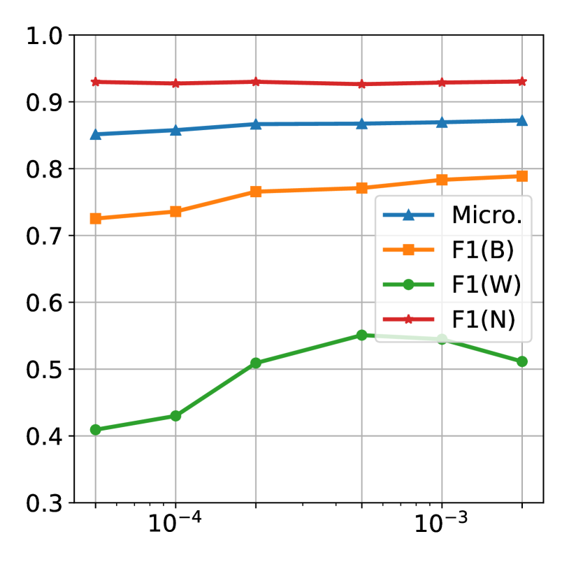
(a) F1 vs. Learning rate ($\eta$)

(b) F1 vs. Feature dims. ($\boldsymbol{d}$)

(c) F1 vs. Reg. weight ($\lambda$)

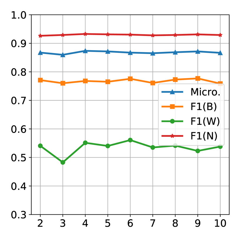
(d) F1 vs. SGCN layers

Figure 2: Searching and sensitivity for four key hyperparameters of SAECON in F1 scores.

Directed	Gating	Micro.	F1(B)	F1(W)	F1(N)
✓	✓	86.74	77.10	54.08	92.64
✗	✓	86.18	75.72	49.78	92.40
✓	✗	85.35	74.03	43.27	92.34
✗	✗	85.35	73.39	35.78	93.04

Table 4: Searching and sensitivity for the directionality and gating of SGCN by F1 scores (%).

Alleviating Data Imbalance

The label imbalance severely impairs the model performance, especially on the most underpopulated label Worse. The aforementioned imbalance alleviation methods are tested in Table 5. The Original (OR) row is a control experiment using the raw CompSent-19 without any weighting or augmentation.

The optimal solution is the weighted loss (WL vs. the rest). One interesting observation is that data augmentation such as flipping labels and upsampling cannot provide a performance gain (OR vs. FL and OR vs. UP). Weighted loss performs a bit worse on F1(N) but consistently better on the other metrics, especially on Worse, indicating that it effectively alleviates the imbalance issue. In practice, static weights found via grid search are assigned to different labels when computing the cross entropy loss. We leave the exploration of dynamic weighting methods such as the Focal Loss Lin et al. (2017) for future work.

Methods	Micro.	F1(B)	F1(W)	F1(N)
Weighted loss (WL)	86.74	77.10	54.08	92.64
Original (OR)	85.97	73.80	46.15	92.90
Flipping labels (FL)	84.93	73.07	42.45	91.99
Upsampling (UP)	85.83	73.11	46.36	92.95

Table 5: Performance analysis with F1 scores (%) for different methods to mitigate data imbalance.

CPC sentences with sentiment predictions by $\mathcal{A}$	Label	$\Delta$
S1: This is all done via the gigabit [Ethernet:POS] interface, rather than the much slower [USB:NEG] interface.	Better	$+2$
S2: Also, [Bash:NEG] may not be the best language to do arithmetic heavy operations in something like [Python:NEU] might be a better choice.	Worse	$-1$
S3: It shows how [JavaScript:POS] and [PHP:POS] can be used in tandem to make a user’s experience faster and more pleasant.	None	$0$
S4: He broke his hand against [Georgia Tech:NEU] and made it worse playing against [Virginia Tech:NEU].	None	$0$

Table 6: Case studies for the effect of the sentiment analyzer $\mathcal{A}$ (see Section 4.3 for details).

Alternative Training

One novelty of SAECON is the alternative training that allows the sentiment analyzer to learn both tasks across domains. Here we analyze the impacts of different batch ratios (BR) and different domain shift handling methods during the training. BR controls the number of ratio of batches of the two alternative tasks in each training cycle. For example, a BR of $2:3$ sends 2 CPC batches followed by 3 ABSA batches in each iteration.

Figure 3(a) presents the entire training time for ten epochs with different BR. A larger BR takes shorter time. For example, a BR of 1:1 (the leftmost bar) takes a shorter time than 1:5 (the yellow bar). Figure 3(b) presents the micro-F1 scores for different BR. We observe two points: (1) The reported performances differ slightly; (2) Generally, the performance is better when the CPC batches are less than ABSA ones. Overall, the hyperparameter selection tries to find a “sweet spot” for effectiveness and efficiency, which points to the BR of 1:1.

(a) BR vs. Training time (s)

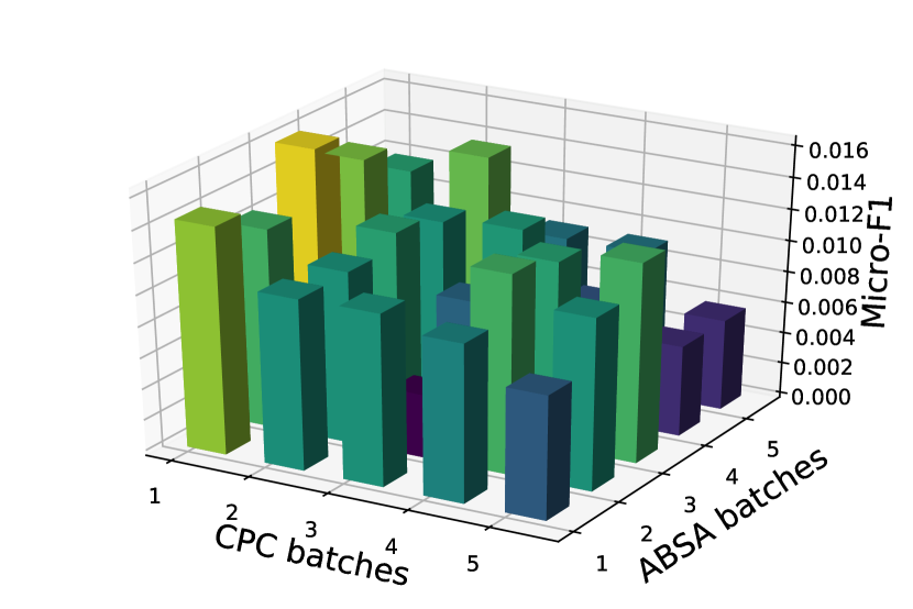
(b) BR vs. Micro-F1

Figure 3: Analyses for batch ration (BR). The values of micro-F1 are actual numbers minus 0.85 for the convenience of visualization.

Figure 4 depicts the performance comparisons of SAECON (green bars), SAECON$-$GRL (the “$-$GRL” in Figure 3, orange bars), and SAECON with pretrained and fixed parameters of $\mathcal{A}$ (the option (1) mentioned in Section 3.4, blue bars). They represent different levels of domain shift mitigation: The pretrained and fixed $\mathcal{A}$ does NOT handle the domain shift at all; The variant $-$GRL only attempts to implicitly handle the shift by alternative training with different tasks to converge in the middle although the domain difference can be harmful to both objectives; SAECON, instead, explicitly uses GRL+DC to mitigate the domain shift between $\mathcal{D}_{s}$ and $\mathcal{D}_{c}$ during training.

As a result, SAECON achieves the best performance especially on F1(W), $-$GRL gets the second, and the “option (1)” gets the worst. These demonstrate that (1) the alternative training (blue vs. green) for an effective domain adaptation is necessary and (2) there exists a positive correlation between the level of domain shift mitigation and the model performance, especially on F1(W) and F1(B). A better domain adaptation produces higher F1 scores in the scenarios where datasets in the domain of interest, i.e., CPC, is unavailable.

Figure 4: Visualization of the domain shift mitigation.

4.3 Case Study

In this section, we qualitatively exemplify the contribution of the sentiment analyzer $\mathcal{A}$. Table 6 reports four example sentences from the test set of CompSent-19. The entities $e_{1}$ and $e_{2}$ are highlighted together with the corresponding sentiment predicted by $\mathcal{A}$. The column “Label” shows the ground truth of CPC. The “$\Delta$” column computes the sentiment distances between the entities. We assign $+1$, $0$, and $-1$ to sentiment polarities of POS, NEU, and NEG, respectively. $\Delta$ is computed by the sentiment polarity of $e_{1}$ minus that of $e_{2}$. Therefore, a positive distance suggests that $e_{1}$ receives a more positive sentiment from $\mathcal{A}$ than $e_{2}$ and vice versa. In S1, sentiments to Ethernet and USB are predicted positive and negative, respectively, which can correctly imply the comparative label as Better. S2 is a Worse sentence with Bash predicted negative, Python predicted neutral, and a resultant negative sentiment distance $-1$. For S3 and S4, the entities are assigned the same polarities. Therefore, the sentiment distances are both zeros. We can easily tell that preference comparisons do not exist, which is consistent with the ground truth labels. Due to the limited space, more interesting case studies are presented in Section A.4.

5 Conclusion

This paper proposes SAECON, a CPC model that incorporates a sentiment analyzer to transfer knowledge from ABSA corpora. Specifically, SAECON utilizes a BiLSTM to learn global comparative features, a syntactic GCN to learn local syntactic information, and a domain adaptive auxiliary sentiment analyzer that jointly learns from ABSA corpora and CPC corpora for a smooth knowledge transfer. An alternative joint training scheme enables the efficient and effective information transfer. Qualitative and quantitative experiments verified the superior performance of SAECON. For future work, we will focus on a deeper understanding of CPC data augmentation and an exploration of weighting loss methods for data imbalance.

Broader Impact Statement

This section states the broader impact of the proposed CPC model. Our model is designed specifically for the comparative classification scenarios in NLP. Users can use our model to detect whether a comparison exists between two entities of interest within the sentences of a particular sentential corpus. For example, a recommender system equipped with our model can tell whether a product is compared with a competitor and, further, which is preferred. In addition, Review-based platforms can utilize our model to decide which items are widely welcomed and which are not.

Our model, SAECON, is tested with the CompSent-19 dataset which has been anonymized during the process of collection and annotation. For the auxiliary ABSA task, we also use an anonymized public dataset from SemEval 2014 to 2016. Therefore, our model will not cause potential leakages of user identity and privacy. We would like to call for attention to CPC as it is a relatively new task in NLP research.

Appendix A Supplementary Materials

This section contains the supplementary materials for Powering Comparative Classification with Sentiment Analysis via Domain Adaptive Knowledge Transfer. Here we provide additional supporting information in four aspects, including additional description for the training, the reproducibility details of SAECON, brief introductions of baselines, and additional case studies.

A.1 Pseudocode of SAECON

In this section, we show the pseudocode of the training of SAECON to provide a comprehensive picture of the alternative training paradigm.

Input: Loss weights $\boldsymbol{\lambda}$; Learning rate $\eta$

Data: $D_{c}$ and $D_{s}$.

1 while not converge do

2       $\{s,E\}$, task $\xleftarrow{}$ getAltSample($D_{c}$, $D_{s}$)

3       $\boldsymbol{\mathrm{S}}_{0}\xleftarrow{}$ TextEncode($s$)

4       $G_{s}\xleftarrow{}$ DepParse($s$)

5       if task is CPC then

6             $\{\boldsymbol{h}_{g,i}\},\{\boldsymbol{h}_{l,i}\}$ $(i=1,2)\xleftarrow{}$ methods in Section 3.3.

7             $\boldsymbol{h}_{s,1},\boldsymbol{h}_{s,2}\xleftarrow{}$ $\mathcal{A}(\boldsymbol{\mathrm{S}}_{0},G_{s},E)$

8             $\mathcal{L}_{c},\mathcal{L}_{d}\xleftarrow{}$ methods in Section 3.5

9             optimize($\{\mathcal{L}_{c},\lambda_{d}\mathcal{L}_{d},\lambda\text{reg}(L2)\},\eta$)

10            

11      else

            // sentiment analysis

12             $\boldsymbol{h}_{s}\xleftarrow{}$ $\mathcal{A}(\boldsymbol{\mathrm{S}}_{0},G_{s},E)$

13             $\mathcal{L}_{s},\mathcal{L}_{d}\xleftarrow{}$ methods in Section 3.5

14             optimize($\{\lambda_{s}\mathcal{L}_{s},\lambda_{d}\mathcal{L}_{d},\lambda\text{reg}(L2)\},\eta$)

15      

Algorithm 1 Optimization of SAECON with two alternative tasks

A.2 Reproducibility

In this section, we provide the instructions to reproduce SAECON and the default hyperparameter settings to generate the performances reported in Section 4.2.

A.2.1 Implementation of SAECON

The proposed SAECON is implemented in Python (3.6.8) with PyTorch (1.5.0) and run with a single 16GB Nvidia V100 GPU. The source code of SAECON is publicly available on GitHub and comprehensive instructions on how to reproduce our model are also provided.

The implementation of SGCN is based on PyTorch Geometric. The implementation of our sentiment analyzer $\mathcal{A}$ is adapted from the official source code of LCF-ASC Phan and Ogunbona (2020). The dependency parser used in SAECON is from spaCy . The pretrained embedding vectors of GloVe are downloaded from the office site. The pretrained BERT model is obtained from the Hugging Face model repository. The implementation of the gradient reversal package is available on GitHub. We would like to appreciate the authors of these packages for their precious contributions.

A.2.2 Default Hyperparameters

The default hyperparameter settings for the results reported in Section 4.2 are given in Table 7

Hyperparameter	Setting
GloVe embeddings	pretrained, 100 dims ($d_{0}$)
BERT version	bert-base-uncased
BERT num.	12 heads, 12 layers, 768 dims ($d_{0}$)
BERT param.	pretrained by Hugging Face
Dependency parser	spaCy, pretrained model
Batch config.	size $=16$, batch ratio $=1:1$
Init. LR ($\eta$)	$5\times 10^{-4}$
CPC loss weight	$2:4:1$ (B:W:N)
$\boldsymbol{\lambda}$ $(\{\lambda,\lambda_{s},\lambda_{d}$})	$\{1\times 10^{-4},1,1\}$
Activation	ReLU ($f(x)=\max(0,x)$)
$\boldsymbol{d}$ $(\{d_{g},d_{l},d_{s}\})$	$\{240,240,240\}$
Optimizer	Adam $(\beta_{1}=0.9,\beta_{2}=0.999)$
LR scheduler	StepLR (steps $=3$, $\gamma=0.8$)
GRL config.	$\alpha=1.0$ (Default setting)
SGCN num.	2 layers (768$\xrightarrow{}$256$\xrightarrow{}$240)
SGCN arch.	Directed, Gated
Data aug.	Off (weighted loss only)

Table 7: Default hyperparameter settings. “LR” is short for learning rate. “num.” shows the numerical configurations and “arch.” shows the architectural configurations. “aug.” is short for augmentation.

Supplementary CPC sentences with sentiment predictions by $\mathcal{A}$	Label	$\Delta$
S1: [Ruby:NEU] wasn’t designed to “exemplify best practices”, it was to be a better [Perl:NEG].	Better	$+1$
S2: And from my experience the ticks are much worse in [Mid Missouri:NEG] than they are in [South Georgia:POS] which is much warmer year round.	Worse	$-2$
S3: As an industry rule, [hockey:NEG] and [basketball:NEG] sell comparatively poorly everywhere.	None	$0$
S4: [Milk:NEG], [juice:NEG] and soda make it ten times worse.	None	$0$

Table 8: Additional case studies for the effect of sentiment analyzer $\mathcal{A}$ (see Section A.4 for details).

A.2.3 Reproduction of ED-GAT

We briefly introduce the reproduction of the state-of-the-art baseline, ED-GAT, in both GloVe and BERT versions. We implement ED-GAT with the same software packages as SAECON such as PyTorch-Geometric, spaCy, and PyTorch, and run it within the same machine environment. The parameters all follow the original ED-GAT setting Ma et al. (2020) except the dimension of GloVe. It is set to 300 in the original paper but 100 in our experiments for the fairness of comparison. The number of layers is select as 8 and the hidden size is set to 300 for each layer with 6 attention heads. We trained the model for 15 epochs with Adam optimizer with a batch size of 32.

A.3 Baseline models

We briefly introduce the compared models in Section 4.2.

Majority-Class A simple model which chooses the majority label in the training set as the prediction of each test instance.

SE Sentence Embedding encodes the sentences into low-dimensional sentence representations using pretrained language encoders Conneau et al. (2017); Bowman et al. (2015) and then feeds them into a classifier for comparative preference prediction. SE has two versions Panchenko et al. (2019) with different classifiers, namely SE-Lin with a linear classifier and SE-XGB with an XGBoost classifier.

SVM-Tree This method Tkachenko and Lauw (2015) applies convolutional kernel methods to CSI task. We follow the experimental settings of (Ma et al., 2020).

AvgWE A word embedding-based method that averages the word embeddings of the sentence as the sentence representation and then feeds this representation into a classifier. The input embeddings have several options, such as GloVe Pennington et al. (2014) and BERT Devlin et al. (2019). These variants are denoted by AvgWE-G and AvgWE-B separately.

BERT-CLS Using the representation of the token “[CLS]” generated by BERT Devlin et al. (2019) as the sentence embedding and a linear classifier to conduct comparative preference classification.

ED-GAT Entity-aware Dependency-based Graph Attention Network Ma et al. (2020) is the first entity-aware model that analyzes the entity relations via the dependency graph and multi-layer graph attention layer.

A.4 Additional Case Studies

In this section, we present four supplementary examples for case study in Table 8 which have different sentiments compared with their counterparts in Table 6. S1 shows a NEU versus NEG comparison which results in a sentiment distance $+1$ and a CPC prediction Better. “Ruby” is not praised in this sentence so it has NEU. But “Perl” is assigned a negative emotion through a simple inference. S2 shows a stronger contrast between the entities. “Mid Missouri” is said “much worse” while the “South Georgia” is “much warmer”, which clearly indicates the sentiments and the comparative classification results.

S3 and S4 are two sentences both with two parallel negative entities. The sport equipment in S3 is sold “poorly” and the drinks in S4 are “ten times worse” both indicating negative sentiments. Therefore, the labels are None.

References

- Aydin and Güngör (2020) Cem Rifki Aydin and Tunga Güngör. 2020. Combination of recursive and recurrent neural networks for aspect-based sentiment analysis using inter-aspect relations. IEEE Access.
- Bao et al. (2019) Lingxian Bao, Patrik Lambert, and Toni Badia. 2019. Attention and lexicon regularized LSTM for aspect-based sentiment analysis. In Proceedings of the 57th Annual Meeting of the Association for Computational Linguistics: Student Research Workshop.
- Bastings et al. (2017) Jasmijn Bastings, Ivan Titov, Wilker Aziz, Diego Marcheggiani, and Khalil Sima’an. 2017. Graph convolutional encoders for syntax-aware neural machine translation. In Proceedings of the 2017 Conference on Empirical Methods in Natural Language Processing.
- Belinkov et al. (2019) Yonatan Belinkov, Adam Poliak, Stuart Shieber, Benjamin Van Durme, and Alexander Rush. 2019. On adversarial removal of hypothesis-only bias in natural language inference. In Proceedings of the Eighth Joint Conference on Lexical and Computational Semantics.
- Bowman et al. (2015) Samuel R. Bowman, Gabor Angeli, Christopher Potts, and Christopher D. Manning. 2015. A large annotated corpus for learning natural language inference. In Proceedings of the 2015 Conference on Empirical Methods in Natural Language Processing.
- Chen and Manning (2014) Danqi Chen and Christopher D Manning. 2014. A fast and accurate dependency parser using neural networks. In Proceedings of the 2014 Conference on Empirical Methods in Natural Language Processing.
- Chen and Qian (2020) Zhuang Chen and Tieyun Qian. 2020. Relation-aware collaborative learning for unified aspect-based sentiment analysis. In Proceedings of the 58th Annual Meeting of the Association for Computational Linguistics, ACL 2020.
- Conneau et al. (2017) Alexis Conneau, Douwe Kiela, Holger Schwenk, Loïc Barrault, and Antoine Bordes. 2017. Supervised learning of universal sentence representations from natural language inference data. In Proceedings of the 2017 Conference on Empirical Methods in Natural Language Processing.
- Devlin et al. (2019) Jacob Devlin, Ming-Wei Chang, Kenton Lee, and Kristina Toutanova. 2019. BERT: pre-training of deep bidirectional transformers for language understanding. In Proceedings of the 2019 Conference of the North American Chapter of the Association for Computational Linguistics: Human Language Technologies.
- Ganin and Lempitsky (2015) Yaroslav Ganin and Victor Lempitsky. 2015. Unsupervised domain adaptation by backpropagation. In International conference on machine learning. PMLR.
- Gu et al. (2019) Shuhao Gu, Yang Feng, and Qun Liu. 2019. Improving domain adaptation translation with domain invariant and specific information. In Proceedings of the 2019 Conference of the North American Chapter of the Association for Computational Linguistics: Human Language Technologies.
- Gupta et al. (2017) Samir Gupta, A. S. M. Ashique Mahmood, Karen Ross, Cathy H. Wu, and K. Vijay-Shanker. 2017. Identifying comparative structures in biomedical text. In BioNLP 2017.
- He et al. (2018) Ruidan He, Wee Sun Lee, Hwee Tou Ng, and Daniel Dahlmeier. 2018. Adaptive semi-supervised learning for cross-domain sentiment classification. In Proceedings of the 2018 Conference on Empirical Methods in Natural Language Processing.
- Hu et al. (2019) Minghao Hu, Yuxing Peng, Zhen Huang, Dongsheng Li, and Yiwei Lv. 2019. Open-domain targeted sentiment analysis via span-based extraction and classification. In Proceedings of the 57th Annual Meeting of the Association for Computational Linguistics.
- Jindal and Liu (2006) Nitin Jindal and Bing Liu. 2006. Identifying comparative sentences in text documents. In Proceedings of the 29th Annual International ACM SIGIR Conference on Research and Development in Information Retrieval.
- Kamath et al. (2019) Anush Kamath, Sparsh Gupta, and Vitor Carvalho. 2019. Reversing gradients in adversarial domain adaptation for question deduplication and textual entailment tasks. In Proceedings of the 57th Annual Meeting of the Association for Computational Linguistics.
- Kingma and Ba (2015) Diederik P. Kingma and Jimmy Ba. 2015. Adam: A method for stochastic optimization. In 3rd International Conference on Learning Representations.
- Kipf and Welling (2017) Thomas N. Kipf and Max Welling. 2017. Semi-supervised classification with graph convolutional networks. In 5th International Conference on Learning Representations.
- Kiritchenko et al. (2014) Svetlana Kiritchenko, Xiaodan Zhu, Colin Cherry, and Saif Mohammad. 2014. NRC-Canada-2014: Detecting aspects and sentiment in customer reviews. In Proceedings of the 8th International Workshop on Semantic Evaluation.
- Li et al. (2016) Yujia Li, Daniel Tarlow, Marc Brockschmidt, and Richard S. Zemel. 2016. Gated graph sequence neural networks. In 4th International Conference on Learning Representations.
- Li et al. (2019) Zeyu Li, Jyun-Yu Jiang, Yizhou Sun, and Wei Wang. 2019. Personalized question routing via heterogeneous network embedding. In Proceedings of the AAAI Conference on Artificial Intelligence.
- Li et al. (2018) Zheng Li, Ying Wei, Yu Zhang, and Qiang Yang. 2018. Hierarchical attention transfer network for cross-domain sentiment classification. In Proceedings of the AAAI Conference on Artificial Intelligence.
- Lin et al. (2017) Tsung-Yi Lin, Priya Goyal, Ross Girshick, Kaiming He, and Piotr Dollár. 2017. Focal loss for dense object detection. In Proceedings of the IEEE international conference on computer vision.
- Ma et al. (2020) Nianzu Ma, Sahisnu Mazumder, Hao Wang, and Bing Liu. 2020. Entity-aware dependency-based deep graph attention network for comparative preference classification. In Proceedings of the 58th Annual Meeting of the Association for Computational Linguistics.
- Ma et al. (2018) Yukun Ma, Haiyun Peng, and Erik Cambria. 2018. Targeted aspect-based sentiment analysis via embedding commonsense knowledge into an attentive LSTM. In Proceedings of the Thirty-Second AAAI Conference on Artificial Intelligence.
- Marcheggiani and Titov (2017) Diego Marcheggiani and Ivan Titov. 2017. Encoding sentences with graph convolutional networks for semantic role labeling. In Proceedings of the 2017 Conference on Empirical Methods in Natural Language Processing.
- Nguyen and Shirai (2015) Thien Hai Nguyen and Kiyoaki Shirai. 2015. PhraseRNN: Phrase recursive neural network for aspect-based sentiment analysis. In Proceedings of the 2015 Conference on Empirical Methods in Natural Language Processing.
- Panchenko et al. (2019) Alexander Panchenko, Alexander Bondarenko, Mirco Franzek, Matthias Hagen, and Chris Biemann. 2019. Categorizing comparative sentences. In Proceedings of the 6th Workshop on Argument Mining.
- Pennington et al. (2014) Jeffrey Pennington, Richard Socher, and Christopher D Manning. 2014. Glove: Global vectors for word representation. In Proceedings of the 2014 Conference on Empirical Methods in Natural Language Processing.
- Phan and Ogunbona (2020) Minh Hieu Phan and Philip O. Ogunbona. 2020. Modelling context and syntactical features for aspect-based sentiment analysis. In Proceedings of the 58th Annual Meeting of the Association for Computational Linguistics.
- Pontiki et al. (2015) Maria Pontiki, Dimitris Galanis, Haris Papageorgiou, Suresh Manandhar, and Ion Androutsopoulos. 2015. SemEval-2015 task 12: Aspect based sentiment analysis. In Proceedings of the 9th International Workshop on Semantic Evaluation (SemEval 2015).
- Pontiki et al. (2014) Maria Pontiki, Dimitris Galanis, John Pavlopoulos, Harris Papageorgiou, Ion Androutsopoulos, and Suresh Manandhar. 2014. SemEval-2014 task 4: Aspect based sentiment analysis. In Proceedings of the 8th International Workshop on Semantic Evaluation (SemEval 2014).
- Pouran Ben Veyseh et al. (2020) Amir Pouran Ben Veyseh, Nasim Nouri, Franck Dernoncourt, Quan Hung Tran, Dejing Dou, and Thien Huu Nguyen. 2020. Improving aspect-based sentiment analysis with gated graph convolutional networks and syntax-based regulation. In Findings of the Association for Computational Linguistics: EMNLP 2020.
- Sun et al. (2019) Chi Sun, Luyao Huang, and Xipeng Qiu. 2019. Utilizing BERT for aspect-based sentiment analysis via constructing auxiliary sentence. In Proceedings of the 2019 Conference of the North American Chapter of the Association for Computational Linguistics: Human Language Technologies.
- Tang et al. (2016) Duyu Tang, Bing Qin, Xiaocheng Feng, and Ting Liu. 2016. Effective LSTMs for target-dependent sentiment classification. In Proceedings of COLING 2016, the 26th International Conference on Computational Linguistics.
- Tkachenko and Lauw (2015) Maksim Tkachenko and Hady Lauw. 2015. A convolution kernel approach to identifying comparisons in text. In Proceedings of the 53rd Annual Meeting of the Association for Computational Linguistics and the 7th International Joint Conference on Natural Language Processing.
- Wagner et al. (2014) Joachim Wagner, Piyush Arora, Santiago Cortes, Utsab Barman, Dasha Bogdanova, Jennifer Foster, and Lamia Tounsi. 2014. DCU: Aspect-based polarity classification for SemEval task 4. In Proceedings of the 8th International Workshop on Semantic Evaluation (SemEval 2014).
- Wang et al. (2020) Kai Wang, Weizhou Shen, Yunyi Yang, Xiaojun Quan, and Rui Wang. 2020. Relational graph attention network for aspect-based sentiment analysis. In Proceedings of the 58th Annual Meeting of the Association for Computational Linguistics.
- Wang and Pan (2018) Wenya Wang and Sinno Jialin Pan. 2018. Recursive neural structural correspondence network for cross-domain aspect and opinion co-extraction. In Proceedings of the 56th Annual Meeting of the Association for Computational Linguistics.
- Wang et al. (2016) Yequan Wang, Minlie Huang, Xiaoyan Zhu, and Li Zhao. 2016. Attention-based LSTM for aspect-level sentiment classification. In Proceedings of the 2016 Conference on Empirical Methods in Natural Language Processing.
- Xenos et al. (2016) Dionysios Xenos, Panagiotis Theodorakakos, John Pavlopoulos, Prodromos Malakasiotis, and Ion Androutsopoulos. 2016. AUEB-ABSA at SemEval-2016 task 5: Ensembles of classifiers and embeddings for aspect based sentiment analysis. In Proceedings of the 10th International Workshop on Semantic Evaluation (SemEval-2016).
- Xu et al. (2020) Kuanhong Xu, Hui Zhao, and Tianwen Liu. 2020. Aspect-specific heterogeneous graph convolutional network for aspect-based sentiment classification. IEEE Access.
- Zhang et al. (2014) Fangxi Zhang, Zhihua Zhang, and Man Lan. 2014. ECNU: A combination method and multiple features for aspect extraction and sentiment polarity classification. In Proceedings of the 8th International Workshop on Semantic Evaluation (SemEval 2014).