Recommend for a Reason: Unlocking the Power of Unsupervised Aspect-Sentiment Co-Extraction

Abstract

Compliments and concerns in reviews are valuable for understanding users’ shopping interests and their opinions with respect to specific aspects of certain items. Existing review-based recommenders favor large and complex language encoders that can only learn latent and uninterpretable text representations. They lack explicit user-attention and item-property modeling, which however could provide valuable information beyond the ability to recommend items. Therefore, we propose a tightly coupled two-stage approach, including an Aspect-Sentiment Pair Extractor (ASPE) and an Attention-Property-aware Rating Estimator (APRE). Unsupervised ASPE mines Aspect-Sentiment pairs (AS-pairs) and APRE predicts ratings using AS-pairs as concrete aspect-level evidences. Extensive experiments on seven real-world Amazon Review Datasets demonstrate that ASPE can effectively extract AS-pairs which enable APRE to deliver superior accuracy over the leading baselines.

1 Introduction

Reviews and ratings are valuable assets for the recommender systems of e-commerce websites since they immediately describe the users’ subjective feelings about the purchases. Learning user preferences from such feedback is straightforward and efficacious. Previous research on review-based recommendation has been fruitful Chin et al. (2018); Chen et al. (2018); Bauman et al. (2017); Liu et al. (2019). Cutting-edge natural language processing (NLP) techniques are applied to extract the latent user sentiments, item properties, and the complicated interactions between the two components.

However, existing approaches have disadvantages bearing room for improvement. Firstly, they dismiss the phenomenon that users may hold different attentions toward various properties of the merchandise. An item property is the combination of an aspect of the item and the characteristic associated with it. Users may show strong attentions to certain properties but indifference to others. The attended advantageous or disadvantageous properties can dominate the attitude of users and consequently, decide their generosity in rating.

Reviews	Microphone	Comfort	Sound
R1 [5 stars]: Comfortable. Very high quality sound. …Mic is good too. There is an switch to mute your mic…I wear glasses and these are comfortable with my glasses on. …	good (satisfied)	comfortable	high quality (praising)
R2 [3 stars]: I love the comfort, sound, and style but the mic is complete junk!	complete junk (angry)	love	love
R3 [5 stars]: …But this one feels like a pillow, there’s nothing wrong with the audio and it does the job. …con is that the included microphone is pretty bad.	pretty bad (unsatisfied)	like a pillow (enjoyable)	nothing wrong

Table 1: Example reviews of a headset with three aspects, namely microphone quality, comfort level, and sound quality, highlighted specifically. The extracted sentiments are on the right. R1 vs. R2: Different users react differently (microphone quality) to the same item due to distinct personal attentions and, consequently, give divergent ratings. R1 vs. R3: A user can still rate highly of an item due to special attention on particular aspects (comfort level) regardless of certain unsatisfactory or indifferent properties (microphone and sound qualities).

Table 1 exemplifies the impact of the user attitude using three real reviews for a headset. Three aspects are covered: microphone quality, comfortableness, and sound quality. The microphone quality is controversial. R2 and R3 criticize it but R1 praises it. The sole disagreement between R1 and R2 is on microphone, which is the major concern of R2, results in the divergence of ratings (5 stars vs. 3 stars). However, R3 neglects that disadvantage and grades highly (5 stars) for its superior comfortableness indicated by the metaphor of “pillow”.

Secondly, understanding user motivations in granular item properties provides valuable information beyond the ability to recommend items. It requires aspect-based NLP techniques to extract explicit and definitive aspects. However, existing aspect-based models mainly use latent or implicit aspects Chin et al. (2018) whose real semantics are unjustifiable. Similar to Latent Dirichlet Allocation (LDA,  Blei et al., 2003), the semantics of the derived aspects (topics) are mutually overlapped Huang et al. (2020b). These models undermine the resultant aspect distinctiveness and lead to uninterpretable and sometimes counterintuitive results. The root of the problem is the lack of large review corpora with aspect and sentiment annotations. The existing ones are either too small or too domain-specific Wang and Pan (2018) to be applied to general use cases. Progress on sentiment term extraction Dai and Song (2019); Tian et al. (2020); Chen et al. (2020a) takes advantage of neural networks and linguistic knowledge and partially makes it possible to use unsupervised term annotation to tackle the lack-of-huge-corpus issue.

In this paper, we seek to understand how reviews and ratings are affected by users’ perception of item properties in a fine-grained way and discuss how to utilize these findings transparently and effectively in rating prediction. We propose a two-stage recommender with an unsupervised Aspect-Sentiment Pair Extractor (ASPE) and an Attention-Property-aware Rating Estimator (APRE). ASPE extracts (aspect, sentiment) pairs (AS-pairs) from reviews. The pairs are fed into APRE as explicit user attention and item property carriers indicating both frequencies and sentiments of aspect mentions. APRE encodes the text by a contextualized encoder and processes implicit text features and the annotated AS-pairs by a dual-channel rating regressor. ASPE and APRE jointly extract explicit aspect-based attentions and properties and solve the rating prediction with a great performance.

Aspect-level user attitude differs from user preference. The user attitudes produced by the interactions of user attentions and item properties are sophisticated and granular sentiments and rationales for interpretation (see Section 4.4 and A.3.5). Preferences, on the contrary, are coarse sentiments such as like, dislike, or neutral. Preference-based models may infer that R1 and R3 are written by headset lovers because of the high ratings. Instead, attitude-based methods further understand that it is the comfortableness that matters to R3 rather than the item being a headset. Aspect-level attitude modeling is more accurate, informative, and personalized than preference modeling.

Note. Due to the page limits, some supportive materials, marked by “†”, are presented in the Supplementary Materials. We strongly recommend readers check out these materials. The source code of our work is available on GitHub at https://github.com/zyli93/ASPE-APRE.

2 Related Work

Our work is related to four lines of literature which are located in the overlap of ABSA and Recommender Systems.

2.1 Aspect-based Sentiment Analysis

Aspect-based sentiment analysis (ABSA) Xu et al. (2020); Wang et al. (2018) predicts sentiments toward aspects mentioned in the text. Natural language is modeled by graphs in Zhang et al. (2019); Wang et al. (2020) such as Pointwise Mutual Information (PMI) graphs and dependency graphs. Phan and Ogunbona (2020) and Tang et al. (2020) utilize contextualized language encoding to capture the context of aspect terms. Chen et al. (2020b) focuses on the consistency of the emotion surrounding the aspects, and Du et al. (2020) equips pre-trained BERT with domain-awareness of sentiments. Our work is informed by these progress which utilize PMI, dependency tree, and BERT for syntax feature extraction and language encoding.

2.2 Aspect or Sentiment Terms Extraction

Aspect and sentiment terms extraction is a presupposition of ABSA. However, manually annotating data for training, which requires the hard labor of experts, is only feasible on small datasets in particular domains such as Laptop and Restaurant Pontiki et al. (2014, 2015) which are overused in ABSA.

Recently, RINANTE Dai and Song (2019) and SDRN Chen et al. (2020a) automatically extract both terms using rule-guided data augmentation and double-channel opinion-relation co-extraction, respectively. However, the supervised approaches are too domain-specific to generalize to out-of-domain or open-domain corpora. Conducting domain adaptation from small labeled corpora to unlabeled open corpora only produces suboptimal results Wang and Pan (2018). SKEP Tian et al. (2020) exploits an unsupervised PMI+seed strategy to coarsely label sentimentally polarized tokens as sentiment terms, showing that the unsupervised method is advantageous when annotated corpora are insufficient in the domain-of-interest.

Compared to the above models, our ASPE has two merits of being (1) unsupervised and hence free from expensive data labeling; (2) generalizable to different domains by combining three different labeling methods.

2.3 Aspect-based Recommendation

Aspect-based recommendation is a relevant task with a major difference that specific terms indicating sentiments are not extracted. Only the aspects are needed Hou et al. (2019); Guan et al. (2019); Huang et al. (2020a); Chin et al. (2018). Some disadvantages are summarized as follows. Firstly, the aspect extraction tools are usually outdated and inaccurate such as LDA Hou et al. (2019), TF-IDF Guan et al. (2019), and word embedding-based similarity Huang et al. (2020a). Second, the representation of sentiment is scalar-based which is coarser than embedding-based used in our work.

2.4 Rating Prediction

Rating prediction is an important task in recommendation. Related approaches utilize text mining algorithms to build user and item representations and predict ratings Kim et al. (2016); Zheng et al. (2017); Chen et al. (2018); Chin et al. (2018); Liu et al. (2019); Bauman et al. (2017). However, the text features learned are latent and unable to provide explicit hints for explaining user interests.

3 ASPE and APRE

3.1 Problem Formulation

Review-based rating prediction involves two major entities: users and items. A user $u$ writes a review $r_{u,t}$ for an item $t$ and rates a score $s_{u,t}$. Let $R^{u}$ denote all reviews given by $u$ and $R^{t}$ denote all reviews received by $t$. A rating regressor takes in a tuple of a review-and-rate event $(u,t)$ and review sets $R^{u}$ and $R^{t}$ to estimate the rating score $s_{u,t}$.

3.2 Unsupervised ASPE

We combine three separate methods to label AS-pairs without the need for supervision, namely PMI-based, neural network-based (NN-based), and language knowledge- or lexicon-based methods. The framework is visualized in Figure 1.

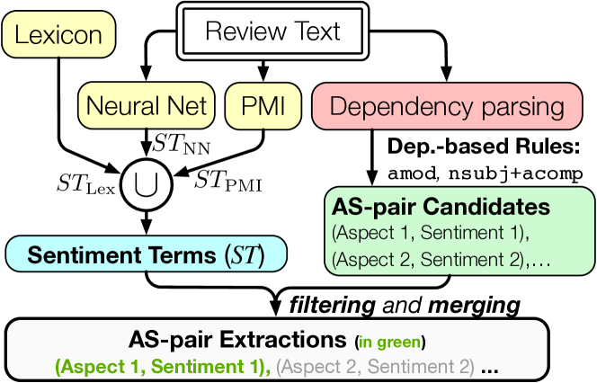
Figure 1: Pipeline of ASPE.

3.2.1 Sentiment Terms Extraction

PMI-based method

Pointwise Mutual Information (PMI) originates from Information Theory and is adapted into NLP Zhang et al. (2019); Tian et al. (2020) to measure statistical word associations in corpora. It determines the sentiment polarities of words using a small number of carefully selected positive and negative seeds ($s^{+}$ and $s^{-}$) Tian et al. (2020). It first extracts candidate sentiment terms satisfying the part-of-speech patterns by Turney (2002) and then measures the polarity of each candidate term $w$ by

$$\text{Pol}(w)=\sum_{s^{+}}\text{{PMI}}(w,s^{+})-\sum_{s^{-}}\text{{PMI}}(w,s^{-}).$$ (1)

Given a sliding window-based context sampler $ctx$, the PMI$(\cdot,\cdot)$ between words is defined by

$$\text{PMI}(w_{1},w_{2})=\log\frac{p(w_{1},w_{2})}{p(w_{1})p(w_{2})},$$ (2)

where $p(\cdot)$, the probability estimated by token counts, is defined by $p(w_{1},w_{2})=\frac{|\{ctx|w_{1},w_{2}\in ctx\}|}{\text{total }\#ctx}$ and $p(w_{1})=\frac{|\{ctx|w_{1}\in ctx\}|}{\text{total }\#ctx}$. Afterward, we collect the top-$q$ sentiment tokens with strong polarities, both positive and negative, as $ST_{\text{PMI}}$.

NN-based method

As discussed in Section 2, co-extraction models Dai and Song (2019) can accurately label AS-pairs only in the training domain. For sentiment terms with consistent semantics in different domains such as good and great, NN methods can still provide a robust extraction recall. In this work, we take a pretrained SDRN Chen et al. (2020a) as the NN-based method to generate $ST_{\text{NN}}$. The pretrained SDRN is considered an off-the-shelf tool similar to the pretrained BERT which is irrelevant to our rating prediction data. Therefore, we argue ASPE is unsupervised for open domain rating prediction.

Knowledge-based method

PMI- and NN-based methods have shortcomings. The PMI-based method depends on the seed selection. The accuracy of the NN-based method deteriorates when the applied domain is distant from the training data. As compensation, we integrate a sentiment lexicon $ST_{\text{Lex}}$ summarized by linguists since expert knowledge is widely used in unsupervised learning. Examples of linguistic lexicons include SentiWordNet Baccianella et al. (2010) and Opinion Lexicon Hu and Liu (2004). The latter one is used in this work.

Building sentiment term set

The three sentiment term subsets are joined to build an overall sentiment set used in AS-pair generation: $ST=ST_{\text{PMI}}\cup ST_{\text{NN}}\cup ST_{\text{Lex}}.$ The three sets compensate for the discrepancies of other methods and expand the coverage of terms shown in Table 10†.

3.2.2 Syntactic AS-pairs Extraction

To extract AS-pairs, we first label AS-pair candidates using dependency parsing and then filter out non-sentiment-carrying candidates using ($ST$). Dependency parsing extracts the syntactic relations between the words. Some nouns are considered potential aspects and are modified by adjectives with two types of dependency relations shown in Figure 2: amod and nsubj+acomp. The pairs of nouns and the modifying adjectives compose the AS-pair candidates. Similar techniques are widely used in unsupervised aspect extraction models Tulkens and van Cranenburgh (2020); Dai and Song (2019). AS-pair candidates are noisy since not all adjectives in it bear sentiment inclination. $ST$ comes into use to filter out non-sentiment-carrying AS-pair candidates whose adjective is not in $ST$. The left candidates form the AS-pair set. Admittedly, the dependency-based extraction for (noun, adj.) pairs is suboptimal and causes missing aspect or sentiment terms. An implicit module is designed to remedy this issue. Open domain AS-pair co-extraction is blocked by the lacking of public labeled data and is left for future work.

We introduce ItemTok as a special aspect token of the nsubj+acomp rule where nsubj is a pronoun of the item such as it and they. Infrequent aspect terms with less than $c$ occurrences are ignored to reduce sparsity. We use WordNet synsets Miller (1995) to merge the synonym aspects. The aspect with the most synonyms is selected as the representative of that aspect set.

amod dependency relation:

[edge style=black,very thick, label style=scale=1.3] [column sep=.5cm, row sep=.1ex] Amazing & sound & and & quality, & all & in & one & headset.    [label style=fill=orange!60]21amod 23cc [label style=fill=purple!30]24conj 26prep 65advmod 68pobj 87nummod [group style=fill=yellow!40, draw=yellow!40]122aspect1 [group style=fill=yellow!40, draw=yellow!40]144aspect2 [group style=fill=green!50, draw=green!50]111sentiment1

Extracted AS-pair candidates:

(sound, amazing), (quality, amazing)

nsubj+acomp dependency relation:

[edge style=black,very thick, label style=scale=1.3] [column sep=.5cm, row sep=.1ex] Sound & quality & is & superior & and & comfort & is & excellent.    [label style=fill=purple!30]21compound [label style=fill=cyan!30]32nsubj [label style=fill=red!50]34acomp 35cc 37conj [label style=fill=cyan!30]76nsubj [label style=fill=red!50]78acomp [group style=fill=yellow!40, draw=yellow!40]112aspect1 [group style=fill=yellow!40, draw=yellow!40]166aspect2 [group style=fill=green!50, draw=green!50]144sentiment1 [group style=fill=green!50, draw=green!50]188sentiment2

Extracted AS-pair candidates:

(Sound quality, superior), (comfort, excellent)

Figure 2: Two dependency-based rules for AS-pair candidates extraction. Effective dependency relations and aspects and sentiments candidates are highlighted.

Discussion

ASPE is different from Aspect Extraction (AE) Tulkens and van Cranenburgh (2020); Luo et al. (2019); Wei et al. (2020); Ma et al. (2019); Angelidis and Lapata (2018); Xu et al. (2018); Shu et al. (2017); He et al. (2017a) which extracts aspects only and infers sentiment polarities in {pos, neg, (neu)}. AS-pair co-extraction, however, offers more diversified emotional signals than the bipolar sentiment measurement of AE.

3.3 APRE

APRE, depicted in Figure 3, predicts ratings given reviews and the corresponding AS-pairs. It first encodes language into embeddings, then learns explicit and implicit features, and finally computes the score regression. One distinctive feature of APRE is that it explicitly models the aspect information by incorporating a $d_{a}$-dimensional aspect representation $\boldsymbol{a}_{i}\in\mathbb{R}^{d_{a}}$ in each side of the substructures for review encoding. Let $\boldsymbol{\mathrm{A}}^{(u)}=\{\boldsymbol{a}_{1}^{(u)},\dots,\boldsymbol{a}_{k}^{(u)}\}$ denotes the $k$ aspect embeddings for users and $\boldsymbol{\mathrm{A}}^{(t)}$ for items. $k$ is decided by the number of unique aspects in the AS-pair set.

Language encoding

The reviews are encoded into low-dimensional token embedding sequences by a fixed pre-trained BERT Devlin et al. (2019), a powerful transformer-based contextualized language encoder. For each review $r$ in $R^{u}$ or $R^{t}$, the resulting encoding $\boldsymbol{\mathrm{H}}^{0}\in\mathbb{R}^{(|r|+2)\times d_{e}}$ consists of $(|r|+2)$ $d_{e}$-dimensional contextualized vectors: $\boldsymbol{\mathrm{H}}^{0}=\{\boldsymbol{h}^{0}_{\text{[CLS]}},\boldsymbol{h}^{0}_{1},\dots,\boldsymbol{h}^{0}_{|r|},\boldsymbol{h}^{0}_{\text{[SEP]}}\}$. [CLS] and [SEP] are two special tokens indicating starts and separators of sentences. We use a trainable linear transformation, $\boldsymbol{h}^{1}_{i}=\boldsymbol{\mathrm{W}}_{\text{ad}}^{T}\boldsymbol{h}^{0}_{i}+\boldsymbol{b}_{\text{ad}}$, to adapt the BERT output representation $\boldsymbol{\mathrm{H}}^{0}$ to our task as $\boldsymbol{\mathrm{H}}^{1}$ where $\boldsymbol{\mathrm{W}}_{\text{ad}}\in\mathbb{R}^{d_{e}\times d_{f}}$, $\boldsymbol{b}_{\text{ad}}\in\mathbb{R}^{d_{f}}$, and $d_{f}$ is the transformed dimension of internal features. BERT encodes the token semantics based upon the context which resolves the polysemy of certain sentiment terms, e.g., “cheap” is positive for price but negative for quality. This step transforms the sentiment encoding to attention-property modeling.

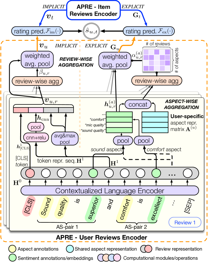
Figure 3: Pipeline of APRE including a user review encoder in the orange dashed box and an item review encoder in the top blue box, each containing an implicit channel (left) and an aspect-based explicit channel (right). Internal details of item encoder are identical to the counterpart of user encoder and hence omitted.

Explicit aspect-level attitude modeling

For aspect $a$ in the $k$ total aspects, we pull out all the contextualized representations of the sentiment words that modify $a$, and aggregate their representations to a single embedding of aspect $a$ in $r$ as

$$\boldsymbol{h}^{(a)}_{u,r}=\sum\boldsymbol{h}^{1}_{j},w_{j}\in ST\cap r\text{ and }w_{j}\text{ modifies }a.$$

An observation by Chen et al. (2020b) suggests that users tend to use semantically consistent words for the same aspect in reviews. Therefore, sum-pooling can nicely handle both sentiments and frequencies of term mentions. Aspects that are not mentioned by $r$ will have $\boldsymbol{h}^{(a)}_{u,r}=\boldsymbol{0}$. To completely picture user $u$’s attentions to all aspects, we aggregate all reviews from $u$, i.e. $R^{u}$, using review-wise aggregation weighted by $\alpha^{(a)}_{u,r}$ given in the equation below. $\alpha_{u,r}^{(a)}$ indicates the significance of each review’s contribution to the overall understanding of $u$’s attention to aspect $a$

$$\alpha_{u,r}^{(a)}=\frac{\exp(\tanh(\boldsymbol{w}_{\text{ex}}^{T}[\boldsymbol{h}_{u,r}^{(a)};\boldsymbol{a}^{(u)}]))}{\sum_{r^{\prime}\in R^{u}}\exp(\tanh(\boldsymbol{w}_{\text{ex}}^{T}[\boldsymbol{h}_{u,r^{\prime}}^{(a)};\boldsymbol{a}^{(u)}]))},$$

where $[\cdot;\cdot]$ denotes the concatenation of tensors. $\boldsymbol{w}_{\text{ex}}\in\mathbb{R}^{(d_{f}+d_{a})}$ is a trainable weight. With the usefulness distribution of $\alpha^{(a)}_{u,r}$, we aggregate the $\boldsymbol{h}_{u,r}^{(a)}$ of $r\in R^{u}$ by weighted average pooling:

$$\boldsymbol{g}_{u}^{(a)}=\sum_{r\in R^{u}}\alpha_{u,r}^{(a)}\boldsymbol{h}_{u,r}^{(a)}.$$

Now we obtain the user attention representation for aspect $a$, $\boldsymbol{g}^{(a)}_{u}\in\mathbb{R}^{d_{f}}$. We use $\boldsymbol{\mathrm{G}}_{u}\in\mathbb{R}^{d_{f}\times k}$ to denote the matrix of $\boldsymbol{g}_{u}^{(a)}$. The item-tower architecture is omitted in Figure 3 since the item property modeling shares the identical computing procedure. It generates the item property representations $\boldsymbol{g}^{(a)}_{t}$ of $\boldsymbol{\mathrm{G}}_{t}$. Mutual attention Liu et al. (2019); Tay et al. (2018); Dong et al. (2020) is not utilized since the generation of user attention encodings $\boldsymbol{\mathrm{G}}_{u}$ is independent to the item properties and vice versa.

Implicit review representation

It is acknowledged by existing works shown in Section 2 that implicit semantic modeling is critical because some emotions are conveyed without explicit sentiment word mentions. For example, “But this one feels like a pillow …” in R3 of Table 1 does not contain any sentiment tokens but expresses a strong satisfaction of the comfortableness, which will be missed by the extractive annotation-based ASPE.

In APRE, we combine a global feature $\boldsymbol{h}^{1}_{\text{[CLS]}}$, a local context feature $\boldsymbol{h}_{\text{cnn}}\in\mathbb{R}^{n_{c}}$ learned by a convolutional neural network (CNN) of output channel size $n_{c}$ and kernel size $n_{k}$ with max pooling, and two token-level features, average and max pooling of $\boldsymbol{\mathrm{H}}^{1}$ to build a comprehensive multi-granularity review representation $\boldsymbol{v}_{u,r}$:

$$\boldsymbol{v}_{u,r} =\left[\boldsymbol{h}^{1}_{\text{[CLS]}};\boldsymbol{h}_{\text{cnn}};\text{{MaxPool}}(\boldsymbol{\mathrm{H}}^{1});\text{{AvgPool}}(\boldsymbol{\mathrm{H}}^{1})\right],$$

$$\boldsymbol{h}_{\text{cnn}} =\text{{MaxPool}}(\text{{ReLU}}(\text{{ConvNN\_1D}}(\boldsymbol{\mathrm{H}}^{1}))).$$

We apply review-wise aggregation without aspects for latent review embedding $\boldsymbol{v}_{u}$

$$\beta_{u,r} =\frac{\exp(\tanh(\boldsymbol{w}_{\text{im}}^{T}\boldsymbol{v}_{u,r}))}{\sum_{r^{\prime}\in R^{u}}\exp(\tanh(\boldsymbol{w}_{\text{im}}^{T}\boldsymbol{v}_{u,r^{\prime}}))},$$

$$\boldsymbol{v}_{u} =\sum\limits_{r\in R^{u}}\beta_{u,r}\boldsymbol{v}_{u,r},$$

where $\beta_{u,r}$ is the counterpart of $\alpha^{(a)}_{u,r}$ in the implicit channel, $\boldsymbol{w}_{\text{im}}\in\mathbb{R}^{d_{im}}$ is a trainable parameter, and $d_{im}=3d_{f}+n_{c}$. Using similar steps, we can also obtain $\boldsymbol{v}_{t}$ for the item implicit embeddings.

Rating regression and optimization

Implicit features $\boldsymbol{v}_{u}$ and $\boldsymbol{v}_{t}$ and explicit features $\boldsymbol{\mathrm{G}}_{u}$ and $\boldsymbol{\mathrm{G}}_{t}$ compose the input to the rating predictor to estimate the score $s_{u,t}$ by

$\mathcal{F}_{\text{im}}:\mathbb{R}^{2d_{im}}\to\mathbb{R}$ and $\mathcal{F}_{\text{ex}}:\mathbb{R}^{2d_{f}\times k}\to\mathbb{R}^{k}$ are multi-layer fully-connected neural networks with ReLU activation and dropout to avoid overfitting. They model user attention and item property interactions in explicit and implicit channels, respectively. $\langle\cdot,\cdot\rangle$ denotes inner-product. $\boldsymbol{\gamma}\in\mathbb{R}^{k}$ and $\{b_{u},b_{t}\}\in\mathbb{R}$ are trainable parameters. The optimization function of the trainable parameter set $\Theta$ with an $L_{2}$ regularization weighted by $\lambda$ is

$$J(\Theta)=\sum_{r_{u,t}\in R}(s_{u,t}-\hat{s}_{u,t})^{2}+L_{2}\text{-reg}(\lambda).$$

$J(\Theta)$ is optimized by back-propagation learning methods such as Adam Kingma and Ba (2014).

4 Experiments

4.1 Experimental Setup

Datasets

We use seven datasets from Amazon Review Datasets He and McAuley (2016) including AutoMotive (AM), Digital Music (DM), Musical Instruments (MI), Pet Supplies (PS), Sport and Outdoors (SO), Toys and Games (TG), and Tools and Home improvement (TH). Their statistics are shown in Table 2.

Dataset	Abbr.	#Reviews	#Users	#Items	Density	Ttl. #W	#R/U	#R/T	#W/R
AutoMotive	AM	20,413	2,928	1,835	3.419$\times 10^{-3}$	1.77M	6.274	10.011	96.583
Digital Music	DM	111,323	14,138	11,707	6.053$\times 10^{-4}$	5.69M	7.087	8.558	56.828
Musical Instruments	MI	10,226	1,429	900	7.156$\times 10^{-3}$	0.96M	6.440	10.226	103.958
Pet Supplies	PS	157,376	19,854	8,510	8.383$\times 10^{-4}$	14.23M	7.134	16.644	100.469
Sports and Outdoors	SO	295,434	35,590	18,357	4.070$\times 10^{-4}$	26.38M	7.471	14.484	99.199
Toys and Games	TG	167,155	19,409	11,924	6.500$\times 10^{-4}$	17.16M	7.751	12.616	114.047
Tools and Home improv.	TH	134,129	16,633	10,217	7.103$\times 10^{-4}$	15.02M	7.258	11.815	124.429

Table 2: The statistics of the seven real-world datasets. (W: Words; U: Users; T: iTems; R: Reviews.)

We use 8:1:1 as the train, validation, and test ratio for all experiments. Users and items with less than 5 reviews and reviews with less than 5 words are removed to reduce data sparsity.

Baseline models

Model	Reference	Cat.	U/T ID	Review
MF	-	Trad.	✓
WRMF	Hu et al. (2008)	Trad.	✓
FM	Rendle (2010)	Trad.	✓
ConvMF	Kim et al. (2016)	Deep	✓	✓
NeuMF	He et al. (2017b)	Deep	✓
D-CNN	Zheng et al. (2017)	Deep		✓
D-Attn	Seo et al. (2017)	Deep		✓
NARRE	Chen et al. (2018)	Deep	✓	✓
ANR	Chin et al. (2018)	Deep		✓
MPCN	Tay et al. (2018)	Deep	✓	✓
DAML	Liu et al. (2019)	Deep		✓
AHN	Dong et al. (2020)	Deep	✓	✓
AHN-B	Same as AHN	Deep	✓	✓

Table 3: Basics of compared baselines. Models’ input is marked by “✓”. “U” and “T” denote Users and iTems. D-CNN represents DeepCoNN. AHN-B denotes the variant of AHN with BERT embeddings.

Thirteen baselines in traditional and deep learning categories are compared with the proposed framework. The pre-deep learning traditional approaches predict ratings solely based upon the entity IDs. Table 3 introduces their basic profiles which are extended in Section A.3.3†. Specially, AHN-B refers to AHN using pretrained BERT as the input embedding encoder. It is included to test the impact of the input encoders.

Evaluation metric

We use Mean Square Error (MSE) for performance evaluation. Given a test set $R_{\text{test}}$, the MSE is defined by

$$\text{MSE}=\frac{1}{|R_{\text{test}}|}\sum_{(u,r)\in R_{\text{test}}}(\hat{s}_{u,r}-s_{u,r})^{2}.$$

Reproducibility

We provide instructions to reproduce AS-pair extraction of ASPE and rating prediction of baselines and APRE in Section A.3.1†. The source code of our models is publicly available on GitHub.

4.2 AS-pair Extraction of ASPE

We present the extraction performance of unsupervised ASPE. The distributions of the frequencies of extracted AS-pairs in Figure 5 follow the trend of Zipf’s Law with a deviation common to natural languages Li (1992), meaning that ASPE performs consistently across domains. We show the qualitative results of term extraction separately.

Sentiment terms

Generally, the AS-pair statistics given in Table 9† on different datasets are quantitatively consistent with the data statistics in Table 2† regardless of domain. Figure 4 is a Venn diagram showing the sources of the sentiment terms extracted by ASPE from AM. All three methods are efficacious and contribute uniquely, which can also be verified by Table 10† in Section A.3.2†.

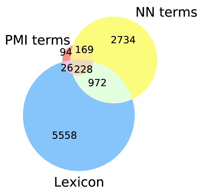
Figure 4: Sources of sentiment terms from AM.

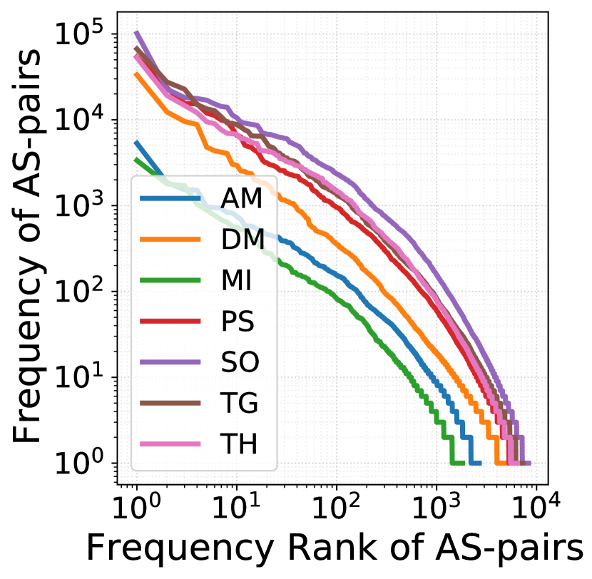
Figure 5: Freq. rank vs. frequency of AS-pairs

Aspect terms

Table 4 presents the most frequent aspect terms of all datasets. ItemTok is ranked top as users tend to describe overall feelings about items. Domain-specific terms (e.g., car in AM) and general terms (e.g., price, quality, and size) are intermingled illustrating the comprehensive coverage and the high accuracy of the result of ASPE.

AM	DM	MI	PS	SO	TG	TH
ItemTok	song	ItemTok	ItemTok	ItemTok	ItemTok	ItemTok
product	ItemTok	sound	dog	knife	toy	light
time	album	guitar	food	quality	game	tool
car	music	string	cat	product	piece	quality
look	time	quality	toy	size	quality	price
price	sound	tone	time	price	child	product
quality	voice	price	product	look	color	bulb
light	track	pedal	price	bag	part	battery
oil	lyric	tuner	treat	fit	fun	size
battery	version	cable	water	light	size	flashlight

Table 4: High frequency aspects of the corpora.

4.3 Rating Prediction of APRE

Comparisons with baselines

For the task of review-based rating prediction, a percentage increase above $1\%$ in performance is considered significant Chin et al. (2018); Tay et al. (2018). According to Table 5, our model outperforms all baseline models including the AHN-B on all datasets by a minimum of 1.337% on MI and a maximum of 4.061% on TG, which are significant improvements. It demonstrates (1) the superior capability of our model to make accurate rating predictions in different domains (Ours vs. the rest); (2) the performance improvement is NOT because of the use of BERT (Ours vs. AHN-B). AHN-B underperforms the original word2vec-based AHN because the weights of word2vec vectors are trainable while the BERT embeddings are fixed, which reduces the parameter capacity. Within baseline models, deep-learning-based models are generally stronger than entity ID-based traditional methods and recent ones tend to perform better.

Ablation study

Ablation studies answer the question of which channel, explicit or implicit, contributes to the superior performance and to what extent? We measure their contributions by rows of w/o EX and w/o IM in Table 5. w/o EX presents the best MSEs of an APRE variant without explicit features under the default settings. The impact of AS-pairs is nullified. w/o IM, in contrast, shows the best MSEs of an APRE variant only leveraging the explicit channel while removing the implicit one (without implicit). We observe that the optimal performances of the single-channel variants all fall behind those of the dual-channel model, which reflects positive contributions from both channels. w/o IM has lower MSEs than w/o EX on several datasets showing that the explicit channel can supply comparatively more performance improvement than the implicit channel. It also suggests that the costly latent review encoding can be less effective than the aspect-sentiment level user and item profiling, which is a useful finding.

Models	AM	DM	MI	PS	SO	TG	TH
Traditional Models
MF	1.986	1.715	2.085	2.048	2.084	1.471	1.631
WRMF	1.327	0.537	1.358	1.629	1.371	1.068	1.216
FM	1.082	0.436	1.146	1.458	1.212	0.922	1.050
Deep Learning-based Models
ConvMF	1.046	0.407	1.075	1.458	1.026	0.986	1.104
NeuMF	0.901	0.396	0.903	1.294	0.893	0.841	1.072
D-Attn	0.816	0.403	0.835	1.264	0.897	0.887	0.980
D-CNN	0.809	0.390	0.861	1.250	0.894	0.835	0.975
NARRE	0.826	0.374	0.837	1.425	0.990	0.908	0.958
MPCN	0.815	0.447	0.842	1.300	0.929	0.898	0.969
ANR	0.806	0.381	0.845	1.327	0.906	0.844	0.981
DAML	0.829	0.372	0.837	1.247	0.893	0.820	0.962
AHN-B	0.810	0.385	0.840	1.270	0.896	0.829	0.976
AHN	0.802	0.376	0.834	1.252	0.887	0.822	0.967
Our Models and Percentage Improvements
Ours	0.791	0.359	0.823	1.218	0.863	0.788	0.936
$\Delta(\%)$	1.390	3.621	1.337	2.381	2.784	4.061	2.350
Val.	0.790	0.362	0.821	1.216	0.860	0.790	0.933
Ablation Studies
w/o EX	0.814	0.379	0.833	1.244.	0.882	0.796	0.965
w/o IM	0.798	0.374	0.863	1.226	0.873	0.798	0.956

Table 5: MSE of baselines, our model (Ours for test and Val. for validation), and variants. The row of $\Delta$ calculates the percentage improvements over the best baselines. All reported improvements over the best baselines are statistically significant with $p$-value $<$ 0.01.

Hyper-parameter sensitivity

A number of hyper-parameter settings are of interest, e.g., dropout, learning rate (LR), internal feature dimensions ($d_{a}$, $d_{f}$, $n_{c}$, and $n_{k}$), and regularization weight $\lambda$ of the $L_{2}$-reg in $J(\Theta)$. We run each set of experiments on sensitivity search 10 times and report the average performances. We tune dropout rate in $[0,0.1,0.2,0.3,0.4,0.5]$ and LR in $[0.0001,0.0005,0.001,0.005,0.01]$ with other hyper-parameters set to default, and report in Figure 6 the minimum MSEs and the epoch numbers (Ep.) on AM. For dropout, we find the balance of its effects on avoiding overfitting and reducing active parameters at 0.2. Larger dropouts need more training epochs. For LR, we also target a balance between training instability of large LRs and overfitting concern of small LRs, thus 0.001 is selected. Larger LRs plateau earlier with fewer epochs while smaller LRs later with more. Figure 7† analyzes hyper-parameter sensitivities to changes on internal feature dimensions ($d_{a}$, $d_{f}$, and $n_{c}$), CNN kernel size $n_{k}$, and $\lambda$ of $L_{2}$-reg weight.

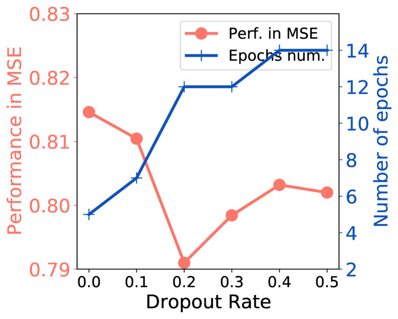
(a) Dropout vs. MSE and Ep.

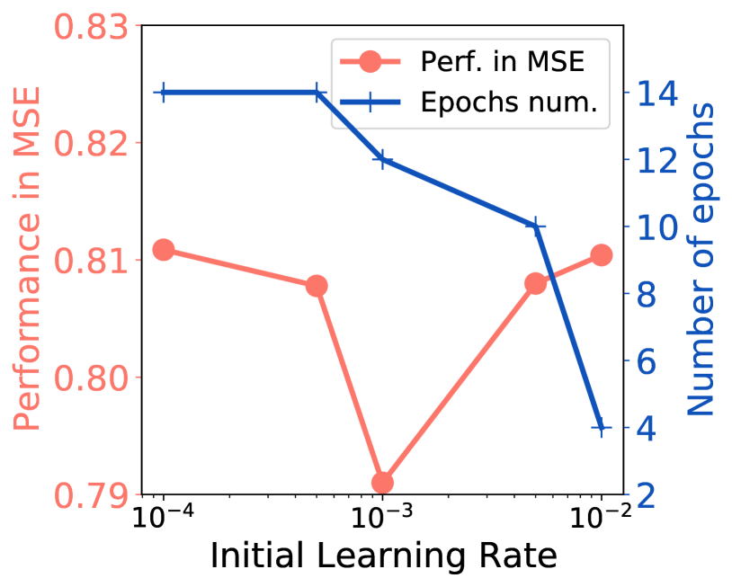
(b) Init. LR vs. MSE and Ep.

Figure 6: Hyper-parameter searching and sensitivity

Efficiency

A brief run time analysis of APRE is given in Table 6. The model can run fast with all data in GPU memory such as AM and MI, which demonstrates the efficiency of our model and the room for improvement on the run time of datasets that cannot fit in the GPU memory. The efficiency of ASPE is less critical since it only runs once for each dataset.

AM	DM	MI	PS	SO	TG	TH
127s∗	31min	90s∗	36min	90min	51min	35min

Table 6: Per epoch run time of APRE on the seven datasets. The run time of AM and MI, denoted by “^∗”, is disproportional to their sizes since they can fit into the GPU memory for acceleration.

4.4 Case Study for Interpretation

Finally, we showcase an interpretation procedure of the rating estimation for an instance in AM: how does APRE predict $u_{*}$’s rating for a smart driving assistant $t_{*}$ using the output AS-pairs of ASPE? We select seven example aspect categories with all review snippets mentioning those categories. Each category is a set of similar aspect terms, e.g., {look, design} and {beep, sound}. Without loss of generality, we refer to the categories as aspects. Table 7 presents the aspects and review snippets given by $u_{*}$ and received by $t_{*}$ with AS-pairs annotations. Three aspects, {battery, install, look}, are shared (yellow rows). Each side has two unique aspects never mentioned by the reviews of the other side: {materials, smell} of $u_{*}$ (green rows) and {price, sound} of $t_{*}$ (blue rows).

APRE measures the aspect-level contributions of user-attention and item-property interactions by the last term of $s_{u,t}$ prediction, i.e., $\langle\boldsymbol{\gamma},\mathcal{F}_{\text{ex}}([\boldsymbol{\mathrm{G}}_{u};\boldsymbol{\mathrm{G}}_{t}])\rangle$. The contribution on the $i$th aspect is calculated by the $i$th dimension of $\gamma$ times the $i$th value of $\mathcal{F}_{\text{ex}}([\boldsymbol{\mathrm{G}}_{u};\boldsymbol{\mathrm{G}}_{t}])$ which is shown in Table 8. The top two rows summarize the attentions of $u_{*}$ and the properties of $t_{*}$. Inferred Impact states the interactional effects of user attentions and item properties based on our assumption that attended aspects bear stronger impacts to the final prediction. On the overlapping aspects, the inferior property of battery produces the only negative score (-0.008) whereas the advantages on install and look create positive scores (0.019 and 0.015), which is consistent with the inferred impact. Other aspects, either unknown to user attentions or to item properties, contribute relatively less: $t_{*}$’s unappealing price accounts for the small score 0.009 and the mixture property of sound accounts for the 0.006.

This case study demonstrates the usefulness of the numbers that add up to $\hat{s}_{u,t}$. Although small in scale, they carry significant information of valued or disliked aspects in $u_{*}$’s perception of $t_{*}$. This process of decomposition is a great way to interpret model prediction on an aspect-level granularity, which is a capacity that other baseline models do not enjoy.

From reviews given by user $u_{*}$. All aspects attended (✓).
battery	[To $t_{1}$] After leaving this attached to my car for two days of non-use I have a dead battery. Never had a dead battery …, so I am blaming this device.
install	[To $t_{2}$] This was unbelievably easy to install. I have done …. The real key …the installation is so easy. [To $t_{3}$] There were many installation options, but once …, they clicked on easily.
look	[To $t_{3}$] It was not perfect and not shiny, but it did look better. [To $t_{4}$] It takes some elbow grease, but the results are remarkable.
material	[To $t_{5}$] The plastic however is very thin and the cap is pretty cheap. [To $t_{6}$] Great value. …. They are very hard plastic, so they don’t mark up panels.
smell	[To $t_{7}$] This has a terrible smell that really lingers awhile. It goes on green. …
From reviews received by item $t_{*}$.
battery	[From $u_{1}$] The reason this won’t work on an iPhone 4 or …because it uses low power Bluetooth, …. (✗)
install	[From $u_{2}$] Your mileage and gas mileage and cost of fuel is tabulated for each trip- Installation is pretty simple - but it …. (✓)
look	[From $u_{3}$] Driving habits, fuel efficiency, and engine health are nice features. The overall design is nice and easy to navigate. (✓)
price	[From $u_{4}$] In fact, there are similar products to this available at a much lower price that do work with …(✗)
sound	[From $u_{5}$] The Link device makes an audible sound when you go over 70 mpg, brake hard, or accelerate too fast. (✓) [From $u_{6}$] Also, the beep the link device makes …sounds really cheapy. (✗)

Table 7: Examples of reviews given by $u_{*}$ and received by $t_{*}$ with Aspect-Sentiment pair mentions as well as other sentiment evidences on seven example aspects.

Aspects	material	smell	battery	install	look	price	sound
Attn. of $u_{*}$	✓	✓	✓	✓	✓	n/a	n/a
Prop. of $t_{*}$	n/a	n/a	✗	✓	✓	✗	✓/✗
Inferred Impact	Unk.	Unk.	Neg.	Pos.	Pos.	Unk.	Unk.
$\boldsymbol{\gamma}_{i}\mathcal{F}_{\text{ex}}(\cdot)_{i}$ ($\times 10^{-2}$)	1.0	0.8	-0.8	1.9	1.5	0.9	0.6

Table 8: Attentions and properties summaries, inferred impacts, and the learned aspect-level contributions.

In Section A.3.5†, another case study indicates that a certain imperfect item property without user attentions only inconsiderably affects the rating although the aspect is mentioned by the user’s reviews.

5 Conclusion

In this work, we propose a tightly coupled two-stage review-based rating predictor, consisting of an Aspect-Sentiment Pair Extractor (ASPE) and an Attention-Property-aware Rating Estimator (APRE). ASPE extracts aspect-sentiment pairs (AS-pairs) from reviews and APRE learns explicit user attentions and item properties as well as implicit sentence semantics to predict the rating. Extensive quantitative and qualitative experimental results demonstrate that ASPE accurately and comprehensively extracts AS-pairs without using domain-specific training data and APRE outperforms the state-of-the-art recommender frameworks and explains the prediction results taking advantage of the extracted AS-pairs.

Several challenges are left open such as fully or weakly supervised open domain AS-pair extraction and end-to-end design for AS-pair extraction and rating prediction. We leave these problems for future work.

Broader Impact Statement

This paper proposes a rating prediction model that has a great potential to be widely applied to recommender systems with reviews due to its high accuracy. In the meantime, it tries to relieve the unjustifiability issue for black-box neural networks by suggesting what aspects of an item a user may feel satisfied or dissatisfied with. The recommender system can better understand the rationale behind users’ reviews so that the merits of items can be carried forward while the defects can be fixed. As far as we are concerned, this work is the first work that takes care of both rating prediction and rationale understanding utilizing NLP techniques.

We then address the generalizability and deployment issues. Reported experiments are conducted on different domains in English with distinct review styles and diverse user populations. We can observe that our model performs consistently which supports its generalizability. Ranging from smaller datasets to larger datasets, we have not noticed any potential deployment issues. Instead, we notice that stronger computational resources can greatly speed up the training and inference and scale up the problem size while keeping the major execution pipeline unchanged.

In terms of the potential harms and misuses, we believe they and their consequences involve two perspectives: (1) the harm of generating inaccurate or suboptimal results from this recommender; (2) the risk of misuse (attack) of this model to reveal user identity. For point (1), the potential risk of suboptimal results has little impact on the major function of online shopping websites since recommenders are only in charge of suggestive content. For point (2), our model does not involve user and item ID modeling. Also, we aggregate the user reviews in the representation space so that user identity is hard to infer through reverse-engineering attacks. In all, we believe our model has little risk of causing dysfunction of online shopping platforms and leakages of user identities.

Appendix A Supplementary Materials

A.1 Introduction

This document is the Supplementary Materials for Recommend for a Reason: Unlocking the Power of Unsupervised Aspect-Sentiment Co-Extraction. It contains supporting materials that are important but unable to be completely covered in the main transcript due to the page limits.

A.2 Methods

A.2.1 Pseudocode of ASPE

Although Section 3.2 is self-explanatory, we would like to explain the AS-pair generation process in Section 3.2.2 in detail by Algorithm 1. It leverages the sentiment term set $ST$ obtained from Section 3.2.1, a dependency parser, and WordNet synsets to build AS-pairs.

Input: Sentiment terms $ST$, dependency parser DepParser, threshold $c$.

Output: AS-pairs

Data: Review-rating corpus $R$; WordNet with synsets.

/* Initialize AS-pair candidate and AS-pair sets */

1 AS-cand, AS-pairs $\xleftarrow{}\emptyset$, $\emptyset$

/* Extract AS-pair candidates. */

2 foreach review $r\in R$ do

3       dep-graph${}_{r}\xleftarrow{}$DepParser$(r)$

4       foreach dependency relation $r_{\text{dep}}$ in dep-graph_r do

5             if $r_{\text{dep}}$ is nsubj+acomp or $r_{\text{dep}}$ is amod then

6                   Add corresponding (noun, adj.) tuple to AS-cand (Figure 2)

7            

8      

/* Merge synonym aspects */

9 foreach (noun,adj.) tuple $\in$ AS-cand do

10       MergeSynAspect(synsets, noun)

/* Filter out non-AS-pairs by $ST$ and frequency threshold $c$. */

11 foreach (noun, adj.) tuple $\in$ AS-cand do

12       if adj.$\in ST$ and Freq$[$noun$]>c$ then

13             Add (noun, adj.) to AS-pairs

14      

return AS-pairs

Algorithm 1 AS-pairs Generation

A.3 Experiments

This section exhibits additional content regarding the experiments such as a detailed experimental setup, the instructions to reproduce the baselines and our model, supplemental experimental results, and another case study. We hope the critical content help readers gain deeper insight into the performance of the proposed framework.

A.3.1 Reproducibility of ASPE and APRE

ASPE+APRE is implemented in Python (3.6.8) with PyTorch (1.5.0) and run with a single 12GB Nvidia Titan Xp GPU. The code is available on GitHub and comprehensive instructions on how to reproduce our model are also provided. The default hyper-parameter settings for the results in Section 4.3 are as follows:

ASPE

In the AS-pair extraction stage, we set the size of $ctx$ to 5 and the PMI term quota $q$ to 400 for both polarities. The counting thresholds $c$ for different datasets are given in Table 9. SDRN Chen et al. (2020a) utilized for term extraction is trained under the default settings in the source code with the SemEval 14/15 datasets mentioned in Section 2. spaCy, a Python package specialized in NLP algorithms, provides the dependency parsing pipeline.

APRE

In the rating prediction stage, we use a pre-trained BERT model with 4 layers, 4 heads, and 256 hidden dimensions (“BERT-mini”) for manageable GPU memory consumption. The BERT parameters (or weights) are fixed. The BERT tokenizer and model are loaded from the Hugging Face model repository. The initial learning rate is set to $0.001$ with two adjusting mechanisms: (1) the Adam optimizer $(\beta_{1},\beta_{2})=(0.9,0.999)$ (the default setting in PyTorch); (2) a learning rate scheduler, StepLR, with step size as 3 and gamma as 0.8. Dropout is set to 0.2 for both towers. $d_{f}$, $d_{a}$, and $n_{c}$ are all set to 200 for consistency. The CNN kernel size is 4. The $L_{2}$-reg weight, $\lambda$, is set globally to 0.0001. We use a clamp function to constrain the predictions in the interval $(1.0,5.0)$.

A.3.2 ASPE: Additional Experimental Results of AS-pair Extraction

We present in Table 9 the statistics of the extracted AS-pairs of the corpora which are quantitatively consistent with the data statistics in Table 2 regardless of domain.

Data	$c$	#AS-pairs/R	#A/U	#A/T	#A	#S
AM	50	3.076	12.681	16.284	291	8,572
DM	100	1.973	5.792	8.380	296	9,781
MI	50	3.358	12.521	16.323	167	8,143
PS	150	3.445	14.886	23.893	529	12,563
SO	250	4.078	19.401	28.314	747	17,195
TG	150	4.482	19.053	26.657	680	13,972
TH	150	5.235	22.833	29.816	659	14,145

Table 9: Statistics of unsupervised AS-pair extraction. $c$: frequency threshold; R: reviews; U: users; T: items.

We provide Table 10 ancillary to the Venn diagram in Figure 4 and the corresponding conclusion in Section 4.2. Table 10 illustrates the contributions of the three distinct sentiment term extraction methods discussed in Section 3.2, namely PMI-based method, neural network-based method, and lexicon-based method. All three methods can extract useful sentiment-carrying words in the domain of Automotive. Their contributions cannot overwhelm each other, which strongly explains the necessity of the unsupervised methods for term extraction in the domain-general usage scenario. Altogether they provide comprehensive coverage of sentiment terms in AM.

$P$ only	$N$ only	$L$ only	$P\cap N\backslash L$	$P\cap L\backslash N$	$N\cap L\backslash P$	$P\cap N\cap L$
countless	therapeutic	fateful	ultimate	uplifting	dazzling	amazing
dreamy	vital	poorest	new	concerned	costly	beautiful
edgy	uncanny	tedious	rhythmic	joyful	devastated	classic
entire	adept	unwell	generic	bombastic	faster	delightful
forgettable	fulfilling	joyous	atmospheric	unforgettable	graceful	enjoyable
melodious	attracted	illegal	greater	phenomenal	affordable	fantastic
moral	celestial	noxious	supernatural	inventive	supreme	gorgeous
propulsive	harmonic	lovable	contemporary	classy	robust	horrible
tasteful	newest	crappy	surprising	insightful	useless	inexpensive
uninspired	enduring	arduous	tremendous	masterful	unpredictable	magnificent

Table 10: Example sentiment terms of each part of the Venn diagram (Figure 4) from AM dataset. We use $P$ (PMI), $N$ (Neural network), and $L$ (Lexicon) to denote the produced sentiment term sets of the three methods, respectively. Operator $\backslash$ denotes set minus, e.g., $P\cap L\backslash N$ refers to the set of terms that are in both $P$ and $L$ but not in $N$. All sets contain commonly-used sentimental adjectives that can modify automotive items. This figure strongly explains why three methods are all necessary for term extraction in non-domain-specific use cases. They all have unique contributions to the sentiment term set for larger coverage.

A.3.3 APRE: Information of Baselines

We introduce baseline models mentioned in Table 3 including the source code of the software and the key parameter settings. For the fairness of comparison, we only compare the models that have open-source implementations.

MF, WRMF, FM, and NeuMF

Matrix factorization views user-item ratings as a matrix with missing values. By factorizing the matrix with the known values, it recovers the missing values as predictions. Weighted Regularized MF Hu et al. (2008) assigns different weights to the values in the matrix. Factorization machines Rendle (2010) consider additional second-order feature interactions of users and items. Neural MF He et al. (2017b) is a combination of generalized MF (GMF) and a multilayer perceptron (MLP). Hyper-parameter settings: The number of factors is 200. Regularization weight is 0.0001. We run for 50 epochs with a learning rate of 0.01 with the exception of MI that uses a learning rate of 0.02 for MF and FM. The dropout of NeuMF is set to 0.2.

ConvMF

A CNN-based model proposed by Kim et al. (2016) that utilizes a convolutional neural network (CNN) for feature encoding of text embeddings. Hyper-parameter settings: The regularization factor is 10 for the user model and 100 for the item model. We used a dropout rate of 0.2.

ANR

Aspect-based Neural Recommender Chin et al. (2018) first proposes aspect-level representations of reviews but its aspects are completely latent without constraints or definitions on the semantics. Hyper-parameter settings: $L_{2}$ regularization is $1\text{\times}{10}^{-6}$. Learning rate is 0.002. Dropout rate is 0.5. We used 300-dimensional pretrained Google News word embeddings.

DeepCoNN

DeepCoNN Zheng et al. (2017) separately encodes user reviews and item reviews by complex neural networks. Hyper-parameter settings: Learning rate is 0.002 and dropout rate is 0.5. Word embedding is the same as ANR.

NARRE

A model similar to DeepCoNN enhanced by attention mechanism Chen et al. (2018). Attentional weights are assigned to each review to measure its importance. Hyper-parameter settings: $L_{2}$ regularization weight is 0.001 Learning rate is 0.002. Dropout rate is 0.5. We used the same word embeddings as described for ANR.

D-Attn

Dual attention-based model Seo et al. (2017) utilizes CNN as text encoders and builds local- and global-attention (dual attention) for user and item reviews. Hyper-parameter settings: In accordance with the paper, we used 100-dimensional word embedding. The factor number is 200. Dropout rate is 0.5. Learning rate and regularization weight are both 0.001.

MPCN

Multi-Pointer Co-Attention Network Tay et al. (2018) selects a useful subset of reviews by pointer networks to build the user profile for the current item. Hyper-parameter settings are the same as D-Attn except that the dropout is 0.2.

DAML

DAML Liu et al. (2019) forces encoders of the user and item reviews to interchange information in the fusion layer with local- and mutual- attention so that the encoders can mutually guide the representation generation. Hyper-parameter settings are the same as MPCN.

AHN

Asymmetrical Hierarchical Networks Dong et al. (2020) that guide the user representation generation using item side asymmetric attentive modules so that only relevant targets are significant. Experiments are reproduced following the settings in the paper.

A.3.4 APRE: Additional Analyses on Hyper-parameter Sensitivity

Continuing Section 3.3, the searching and sensitivity of the feature dimension ($d_{a}$, $d_{f}$, $n_{c}$), the CNN kernel size $n_{k}$, and the regularization weight $\lambda$ is exhibited in Figure 7. We always set $d_{f}=d_{a}=n_{c}$ for the consistency of internal feature dimensions. For $(d_{f},d_{a},n_{c})$ in Figure 7(a), we choose values from $[50,100,150,200]$ since the output dimension of the BERT encoder is 256. The best performance occurs at 200. The training time spent is stable across different values. CNN kernel size $n_{k}$ in Figure 7(b) varies in $[4,6,8,10]$. We observe that generally larger kernel sizes may in turn hurt the performance as the local features are fused with larger sequential contexts in natural language. The epoch numbers are stable as well. Figure 7(c) demonstrates how $\lambda$ affects the performance. As $\lambda$ becomes larger, the “resistance” against the loss minimization increases so that the training epoch number increases. However, there are no clear trends of performance fluctuation meaning that the sensitivity to $L_{2}$-reg weight is insignificant.

Finally, we evaluate the effect of adding non-linearity to embedding adaptation function (EAF) mentioned in Section 3.3 which transforms $\boldsymbol{\mathrm{H}}^{0}$ to $\boldsymbol{\mathrm{H}}^{1}$ by $\boldsymbol{h}^{1}_{i}=\sigma\left(\boldsymbol{\mathrm{W}}^{T}_{\text{ad}}\boldsymbol{h}^{0}_{i}+\boldsymbol{b}_{\text{ad}}\right)$. We try LeakyReLU, tanh, and identity functions for $\sigma(\cdot)$ and report the performances in Figure 7(d). Without non-linear layers, APRE is able to achieve the best results whereas non-linearity speeds up the training.

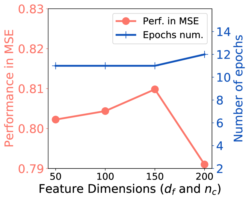
(a) Dims vs. MSE and Ep.

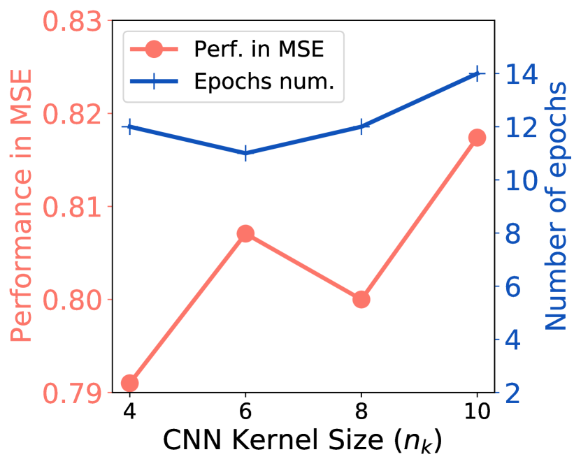
(b) $n_{k}$ vs. MSE and Ep.

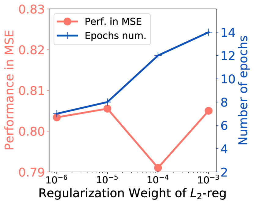
(c) $L_{2}$-reg vs. MSE and Ep.

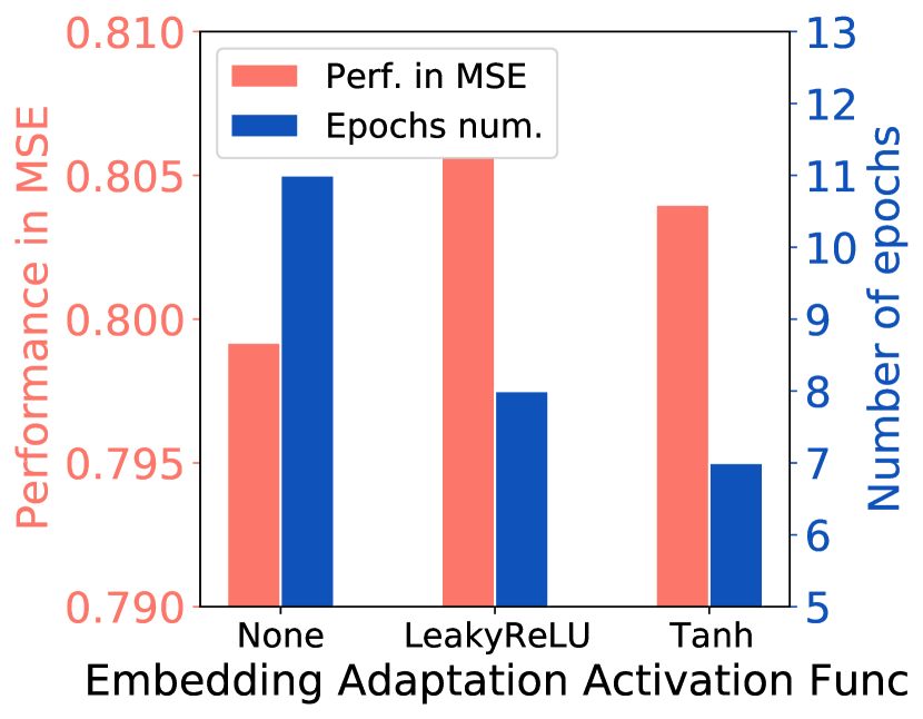
(d) EAF vs. MSE and Ep.

Figure 7: Additional hyper-parameter sensitivity and searching of internal feature dimensions (Dims: $d_{f}$, $d_{a}$, and $n_{c}$), CNN kernel size ($n_{k}$), regularization weight of $L_{2}$-reg, and token embedding adaptation function. EAF is short for embedding adaptation function.

A.3.5 Case Study II for Interpretation

Finally, we show another case study from AM dataset using the same attention-property-score visualization schema as Section 4.4. In this case, our model is predicting the score user $u_{*}$ will give to a color and clarity compound for vehicle surface $t_{*}$. The mentioned aspects of $u_{*}$ and the properties of $t_{*}$ are given in Table 11 including three overlapping aspects (quality, look, cleaning) and one unique aspect of each side (size of $u_{*}$ and smell of $t_{*}$). A summarization table, Table 12, shows the summarized attentions and properties, the inferred impacts, and the corresponding score components of $\langle\boldsymbol{\gamma},\mathcal{F}_{\text{ex}}([\boldsymbol{\mathrm{G}}_{u};\boldsymbol{\mathrm{G}}_{t}])\rangle$.

In this case study, we can observe the interesting phenomenon also exemplified in Table 1 by the contrast between R1 and R3 that the aspect look, which has been mentioned by $u_{*}$ and reviewed negatively as a property of $t_{*}$ (“strange yellow color”), only produces an inconsiderable bad effect (-0.002) on the final score prediction. This indicates that the imperfect look (or color) of the item, although also mentioned by $u_{*}$ in his/her reviews, receives little attention from $u_{*}$ and thus poses a tiny negative impact on the predicted rating decision of the user. The other two overlapping aspects show intuitive correlations between their inferred impacts and the scores. The unique aspects, size and smell, have relatively small influences on the prediction because they are either not attended aspects or not mentioned properties.

It is also notable that some sentences that carry strong emotions may contain few explicit sentiment mentions, e.g., “But for an all in one cleaner and wax I think this outperforms most.” It backs the design of APRE which carefully takes implicit sentiment signals into consideration, and also calls for an advanced way for aspect-based sentiment modeling beyond term level. Different proportions of such sentences in different datasets may account for the inconsistency of better performances between the two variants of the ablation study.

From reviews given by user $u_{*}$.
quality	[To $t_{1}$] As soon as I poured it into the bucket and started getting ready, I can tell the product was already better quality than my previous washing liquid.
look	[To $t_{4}$] I bought [this item] because I had neglected my paint job for too long. …it made my black paint job look dull.
cleaning	[To $t_{2}$] …I was able to dry my car in record time and not have any water marks left on the paint. I just slide the towel over any parts with water and it left no trace of water and a clean shine to my car. [To $t_{3}$] I had completely neglected these areas, except for minor cleaning and protection. Once I applied it, the difference was night and day!
size	[To $t_{6}$] The size was great as well, allowing me to get larger areas in an easier amount of time so that I could wash my car quicker than I have in the past.
From reviews received by item $t_{*}$.
quality	[From $u_{1}$] Adding too little soap will increase the tendency …This thick, high quality soap helps prevent against that. (✓) [From $u_{2}$] …Cons: A bit pricey, but quality matters, and this product absolutely has it. Worth every cent for sure! (✓)
look	[From $u_{3}$] I was a bit disappointed. It is a strange yellow color and it is thick and I personally did not care for the smell. (✗)
cleaning	[From $u_{4}$] As far as cleaning power it does fairly good, …The best cleaning of a car is in steps, but for an all in one cleaner and wax I think this outperforms most. (✓)
smell	[From $u_{5}$] Just giving some useful feedback about the truth behind the product …that it smells good. [From $u_{6}$] I believe this preserves the wax layer longer …This is much thicker than the [some brand] soap, and has a very pleasant smell to it. (✓)

Table 11: Examples of reviews from $u_{*}$ and to $t_{*}$ with Aspect-Sentiment pair mentions as well as other sentiment evidences on five example aspects.

Aspects	size	quality	look	cleaning	smell
Attn. of $u_{*}$	✓	✓	–	✓	n/a
Prop. of $t_{*}$	n/a	✓	✗	✓	✓
Inferred Impact	Unk.	Pos.	Neg.	Pos.	Unk.
$\boldsymbol{\gamma}_{i}\mathcal{F}_{\text{ex}}(\cdot)_{i}$ ($\times 10^{-2}$)	0.5	2.9	-0.2	1.4	0.3

Table 12: Attentions and properties summaries, inferred impacts, and the learned aspect-level contributions on the score prediction.

References

- Angelidis and Lapata (2018) Stefanos Angelidis and Mirella Lapata. 2018. Summarizing opinions: Aspect extraction meets sentiment prediction and they are both weakly supervised. In Proceedings of the 2018 Conference on Empirical Methods in Natural Language Processing (EMNLP).
- Baccianella et al. (2010) Stefano Baccianella, Andrea Esuli, and Fabrizio Sebastiani. 2010. Sentiwordnet 3.0: an enhanced lexical resource for sentiment analysis and opinion mining. In Proceedings of the Seventh International Conference on Language Resources and Evaluation.
- Bauman et al. (2017) Konstantin Bauman, Bing Liu, and Alexander Tuzhilin. 2017. Aspect based recommendations: Recommending items with the most valuable aspects based on user reviews. In Proceedings of the 23rd ACM SIGKDD International Conference on Knowledge Discovery and Data Mining.
- Blei et al. (2003) David M Blei, Andrew Y Ng, and Michael I Jordan. 2003. Latent dirichlet allocation. Journal of machine Learning research.
- Chen et al. (2018) Chong Chen, Min Zhang, Yiqun Liu, and Shaoping Ma. 2018. Neural attentional rating regression with review-level explanations. In Proceedings of the 2018 World Wide Web Conference.
- Chen et al. (2020a) Shaowei Chen, Jie Liu, Yu Wang, Wenzheng Zhang, and Ziming Chi. 2020a. Synchronous double-channel recurrent network for aspect-opinion pair extraction. In Proceedings of the 58th Annual Meeting of the Association for Computational Linguistics.
- Chen et al. (2020b) Xiao Chen, Changlong Sun, Jingjing Wang, Shoushan Li, Luo Si, Min Zhang, and Guodong Zhou. 2020b. Aspect sentiment classification with document-level sentiment preference modeling. In Proceedings of the 58th Annual Meeting of the Association for Computational Linguistics.
- Chin et al. (2018) Jin Yao Chin, Kaiqi Zhao, Shafiq Joty, and Gao Cong. 2018. Anr: Aspect-based neural recommender. In Proceedings of the 27th ACM International Conference on Information and Knowledge Management.
- Dai and Song (2019) Hongliang Dai and Yangqiu Song. 2019. Neural aspect and opinion term extraction with mined rules as weak supervision. In Proceedings of the 57th Annual Meeting of the Association for Computational Linguistics.
- Devlin et al. (2019) Jacob Devlin, Ming-Wei Chang, Kenton Lee, and Kristina Toutanova. 2019. BERT: pre-training of deep bidirectional transformers for language understanding. In Proceedings of the 2019 Conference of the North American Chapter of the Association for Computational Linguistics: Human Language Technologies, NAACL-HLT.
- Dong et al. (2020) Xin Dong, Jingchao Ni, Wei Cheng, Zhengzhang Chen, Bo Zong, Dongjin Song, Yanchi Liu, Haifeng Chen, and Gerard de Melo. 2020. Asymmetrical hierarchical networks with attentive interactions for interpretable review-based recommendation. In Proceedings of the AAAI Conference on Artificial Intelligence.
- Du et al. (2020) Chunning Du, Haifeng Sun, Jingyu Wang, Qi Qi, and Jianxin Liao. 2020. Adversarial and domain-aware bert for cross-domain sentiment analysis. In Proceedings of the 58th Annual Meeting of the Association for Computational Linguistics.
- Guan et al. (2019) Xinyu Guan, Zhiyong Cheng, Xiangnan He, Yongfeng Zhang, Zhibo Zhu, Qinke Peng, and Tat-Seng Chua. 2019. Attentive aspect modeling for review-aware recommendation. ACM Transactions on Information Systems (TOIS), 37(3):1–27.
- He et al. (2017a) Ruidan He, Wee Sun Lee, Hwee Tou Ng, and Daniel Dahlmeier. 2017a. An unsupervised neural attention model for aspect extraction. In Proceedings of the 55th Annual Meeting of the Association for Computational Linguistics.
- He and McAuley (2016) Ruining He and Julian McAuley. 2016. Ups and downs: Modeling the visual evolution of fashion trends with one-class collaborative filtering. In Proceedings of the 25th International Conference on World Wide Web.
- He et al. (2017b) Xiangnan He, Lizi Liao, Hanwang Zhang, Liqiang Nie, Xia Hu, and Tat-Seng Chua. 2017b. Neural collaborative filtering. In Proceedings of the 26th International Conference on World Wide Web.
- Hou et al. (2019) Yunfeng Hou, Ning Yang, Yi Wu, and S Yu Philip. 2019. Explainable recommendation with fusion of aspect information. World Wide Web, 22(1):221–240.
- Hu and Liu (2004) Minqing Hu and Bing Liu. 2004. Mining and summarizing customer reviews. In Proceedings of the 10th ACM SIGKDD International Conference on Knowledge Discovery and Data Mining.
- Hu et al. (2008) Yifan Hu, Yehuda Koren, and Chris Volinsky. 2008. Collaborative filtering for implicit feedback datasets. In 2008 Eighth IEEE International Conference on Data Mining.
- Huang et al. (2020a) Chunli Huang, Wenjun Jiang, Jie Wu, and Guojun Wang. 2020a. Personalized review recommendation based on users’ aspect sentiment. ACM Transactions on Internet Technology (TOIT), 20(4):1–26.
- Huang et al. (2020b) Jiaxin Huang, Yu Meng, Fang Guo, Heng Ji, and Jiawei Han. 2020b. Weakly-supervised aspect-based sentiment analysis via joint aspect-sentiment topic embedding. In Proceedings of the 2020 Conference on Empirical Methods in Natural Language Processing (EMNLP).
- Kim et al. (2016) Donghyun Kim, Chanyoung Park, Jinoh Oh, Sungyoung Lee, and Hwanjo Yu. 2016. Convolutional matrix factorization for document context-aware recommendation. In Proceedings of the 10th ACM Conference on Recommender Systems.
- Kingma and Ba (2014) Diederik P Kingma and Jimmy Ba. 2014. Adam: A method for stochastic optimization. arXiv preprint arXiv:1412.6980.
- Li (1992) Wentian Li. 1992. Random texts exhibit zipf’s-law-like word frequency distribution. IEEE Transactions on information theory, 38(6).
- Liu et al. (2019) Donghua Liu, Jing Li, Bo Du, Jun Chang, and Rong Gao. 2019. Daml: Dual attention mutual learning between ratings and reviews for item recommendation. In Proceedings of the 25th ACM SIGKDD International Conference on Knowledge Discovery and Data Mining.
- Luo et al. (2019) Huaishao Luo, Tianrui Li, Bing Liu, and Junbo Zhang. 2019. DOER: Dual cross-shared RNN for aspect term-polarity co-extraction. In Proceedings of the 57th Annual Meeting of the Association for Computational Linguistics.
- Ma et al. (2019) Dehong Ma, Sujian Li, Fangzhao Wu, Xing Xie, and Houfeng Wang. 2019. Exploring sequence-to-sequence learning in aspect term extraction. In Proceedings of the 57th Annual Meeting of the Association for Computational Linguistics.
- Miller (1995) George A. Miller. 1995. Wordnet: A lexical database for english. Commun. ACM.
- Phan and Ogunbona (2020) Minh Hieu Phan and Philip O Ogunbona. 2020. Modelling context and syntactical features for aspect-based sentiment analysis. In Proceedings of the 58th Annual Meeting of the Association for Computational Linguistics.
- Pontiki et al. (2015) Maria Pontiki, Dimitris Galanis, Haris Papageorgiou, Suresh Manandhar, and Ion Androutsopoulos. 2015. SemEval-2015 task 12: Aspect based sentiment analysis. In Proceedings of the 9th International Workshop on Semantic Evaluation (SemEval 2015).
- Pontiki et al. (2014) Maria Pontiki, Dimitris Galanis, John Pavlopoulos, Harris Papageorgiou, Ion Androutsopoulos, and Suresh Manandhar. 2014. SemEval-2014 task 4: Aspect based sentiment analysis. In Proceedings of the 8th International Workshop on Semantic Evaluation (SemEval 2014).
- Rendle (2010) Steffen Rendle. 2010. Factorization machines. In 2010 IEEE International Conference on Data Mining.
- Seo et al. (2017) Sungyong Seo, Jing Huang, Hao Yang, and Yan Liu. 2017. Interpretable convolutional neural networks with dual local and global attention for review rating prediction. In Proceedings of the 11th ACM Conference on Recommender Systems.
- Shu et al. (2017) Lei Shu, Hu Xu, and Bing Liu. 2017. Lifelong learning CRF for supervised aspect extraction. In Proceedings of the 55th Annual Meeting of the Association for Computational Linguistics.
- Tang et al. (2020) Hao Tang, Donghong Ji, Chenliang Li, and Qiji Zhou. 2020. Dependency graph enhanced dual-transformer structure for aspect-based sentiment classification. In Proceedings of the 58th Annual Meeting of the Association for Computational Linguistics.
- Tay et al. (2018) Yi Tay, Anh Tuan Luu, and Siu Cheung Hui. 2018. Multi-pointer co-attention networks for recommendation. In Proceedings of the 24th ACM SIGKDD International Conference on Knowledge Discovery and Data Mining.
- Tian et al. (2020) Hao Tian, Can Gao, Xinyan Xiao, Hao Liu, Bolei He, Hua Wu, Haifeng Wang, and Feng Wu. 2020. SKEP: sentiment knowledge enhanced pre-training for sentiment analysis. In Proceedings of the 58th Annual Meeting of the Association for Computational Linguistics.
- Tulkens and van Cranenburgh (2020) Stéphan Tulkens and Andreas van Cranenburgh. 2020. Embarrassingly simple unsupervised aspect extraction. In Proceedings of the 58th Annual Meeting of the Association for Computational Linguistics.
- Turney (2002) Peter D. Turney. 2002. Thumbs up or thumbs down? semantic orientation applied to unsupervised classification of reviews. In Proceedings of the 40th Annual Meeting on Association for Computational Linguistics.
- Wang et al. (2020) Kai Wang, Weizhou Shen, Yunyi Yang, Xiaojun Quan, and Rui Wang. 2020. Relational graph attention network for aspect-based sentiment analysis. In Proceedings of the 58th Annual Meeting of the Association for Computational Linguistics.
- Wang et al. (2018) Shuai Wang, Sahisnu Mazumder, Bing Liu, Mianwei Zhou, and Yi Chang. 2018. Target-sensitive memory networks for aspect sentiment classification. In Proceedings of the 56th Annual Meeting of the Association for Computational Linguistics.
- Wang and Pan (2018) Wenya Wang and Sinno Jialin Pan. 2018. Recursive neural structural correspondence network for cross-domain aspect and opinion co-extraction. In Proceedings of the 56th Annual Meeting of the Association for Computational Linguistics.
- Wei et al. (2020) Zhenkai Wei, Yu Hong, Bowei Zou, Meng Cheng, and YAO Jianmin. 2020. Don’t eclipse your arts due to small discrepancies: Boundary repositioning with a pointer network for aspect extraction. In Proceedings of the 58th Annual Meeting of the Association for Computational Linguistics.
- Xu et al. (2020) Hu Xu, Bing Liu, Lei Shu, and Philip Yu. 2020. DomBERT: Domain-oriented language model for aspect-based sentiment analysis. In Proceedings of the 2020 Conference on Empirical Methods in Natural Language Processing (EMNLP).
- Xu et al. (2018) Hu Xu, Bing Liu, Lei Shu, and Philip S. Yu. 2018. Double embeddings and CNN-based sequence labeling for aspect extraction. In Proceedings of the 56th Annual Meeting of the Association for Computational Linguistics.
- Zhang et al. (2019) Chen Zhang, Qiuchi Li, and Dawei Song. 2019. Aspect-based sentiment classification with aspect-specific graph convolutional networks. In Proceedings of the 2019 Conference on Empirical Methods in Natural Language Processing and the 9th International Joint Conference on Natural Language Processing (EMNLP-IJCNLP).
- Zheng et al. (2017) Lei Zheng, Vahid Noroozi, and Philip S Yu. 2017. Joint deep modeling of users and items using reviews for recommendation. In Proceedings of the Tenth ACM International Conference on Web Search and Data Mining.