Recovery of a Space-Time Dependent Diffusion Coefficient in Subdiffusion: Stability, Approximation and Error Analysis

Abstract

In this work, we study an inverse problem of recovering a space-time dependent diffusion coefficient in the subdiffusion model from the distributed observation, where the mathematical model involves a Djrbashian-Caputo fractional derivative of order $\alpha\in(0,1)$ in time. The main technical challenges of both theoretical and numerical analysis lie in the limited smoothing properties due to the fractional differential operator and high degree of nonlinearity of the forward map from the unknown diffusion coefficient to the distributed observation. We establish two conditional stability results using a novel test function, which leads to a stability bound in $L^{2}(0,T;L^{2}(\Omega))$ under a suitable positivity condition. The positivity condition is verified for a large class of problem data. Numerically, we develop a rigorous procedure for recovering the diffusion coefficient based on a regularized least-squares formulation, which is then discretized by the standard Galerkin method with continuous piecewise linear elements in space and backward Euler convolution quadrature in time. We provide a complete error analysis of the fully discrete formulation, by combining several new error estimates for the direct problem (optimal in terms of data regularity), a discrete version of fractional maximal $L^{p}$ regularity, and a nonstandard energy argument. Under the positivity condition, we obtain a standard $\ell^{2}(L^{2}(\Omega))$ error estimate consistent with the conditional stability. Further, we illustrate the analysis with some numerical examples. Keywords: parameter identification, subdiffusion, space-time dependent diffusion coefficient, stability, fully discrete scheme, error estimate

1 Introduction

This work is concerned with a parameter identification problem for the subdiffusion model with a space-time-dependent diffusion coefficient and its rigorous numerical analysis. Let $\Omega\subset\mathbb{R}^{d}$ ($d=1,2,3$) be a convex polyhedral domain with a boundary $\partial\Omega$. Fix $T>0$ the final time. Consider the following initial-boundary value problem for the function $u$:

$$\left\{\begin{aligned} {\partial_{t}^{\alpha}}u-\nabla\cdot(q\nabla u)&=f,&&\mbox{in }\Omega\times(0,T],\\ u(\cdot,0)&=u_{0},&&\mbox{in }\Omega,\\ u&=0,&&\mbox{on }\partial\Omega\times(0,T],\end{aligned}\right.$$ (1.1)

where the functions $f$ and $u_{0}$ are the given source and initial condition, respectively, and the diffusion coefficient $q$ is assumed to be space-time dependent. The notation ${\partial_{t}^{\alpha}}u$ denotes the Djrbashian-Caputo fractional derivative in time $t$ of order $\alpha\in(0,1)$, defined by (see e.g., [33, p. 92] and [23, Section 2.3])

$${\partial_{t}^{\alpha}}u(t)=\frac{1}{\Gamma(1-\alpha)}\int_{0}^{t}(t-s)^{-\alpha}u^{\prime}(s)\ {\rm d}s,$$

where $\Gamma(z)=\int_{0}^{\infty}s^{z-1}e^{-s}{\rm d}s$ (for $\Re(z)>0$) denotes Euler’s Gamma function. The fractional derivative $\partial_{t}^{\alpha}u$ recovers the usual first order derivative $u^{\prime}$ as the order $\alpha\to 1^{-}$ for sufficiently smooth functions $u$. Thus the model (1.1) is a fractional analogue of the classical diffusion model. Below we use the notation $u(q)$ to explicitly indicate the dependence of the solution $u$ on $q$. The model (1.1) has received enormous attention in recent years in physics, engineering, biology and finance, due to their excellent capability for describing anomalously slow diffusion processes, also known as subdiffusion, which displays local motion occasionally interrupted by long sojourns and trapping effects. These transport processes are characterized by a sublinear growth of the mean squared displacement of the particle with the time, as opposed to linear growth for Brownian motion. The model (1.1) has found many successful practical applications, e.g., diffusion in fractal domains (see e.g., [44]), transport column experiments (see e.g., [19]), and subsurface flows (see e.g., [1]); see [43, 42] for physical modeling and a long list of applications.

This work is concerned with recovering the space-time dependent diffusion coefficient $q^{\dagger}(x,t)$ in the model (1.1) from the (noisy) distributed observation

$$z^{\delta}(x,t)=u(q^{\dagger})(x,t)+\xi(x,t),\quad(x,t)\in\Omega\times[0,T],$$ (1.2)

where $\xi(x,t)$ denotes the pointwise additive noise, with a noise level $\delta=\|u(q^{\dagger})-z^{\delta}\|_{L^{2}(0,T;L^{2}(\Omega))}$. The exact diffusion coefficient $q^{\dagger}$ is sought in the following admissible set

$$\mathcal{A}=\{q\in L^{\infty}((0,T)\times\Omega):~{}~{}c_{0}\leq q\leq c_{1},~{}~{}\text{a.e. in}~{}~{}\Omega\times(0,T)\},$$ (1.3)

with $0<c_{0}<c_{1}<\infty$. The inverse problem is a fractional analogue of the inverse conductivity problem for standard parabolic problems, which has been extensively studied both numerically and theoretically (see [21, 6, 9] and the references therein).

The inverse problem of recovering a space-time dependent diffusion coefficient $q(x,t)$ is formally determined for uniqueness / identifiability. Despite its obvious practical relevance (see [14, 16]), to the best of our knowledge, it has not been studied so far. In this work, we contribute to its mathematical and numerical analysis. First, we establish two conditional stability results in Theorems 3.1 and 3.2. These estimates allow deriving the standard $L^{2}(0,T;L^{2}(\Omega))$ stability under a suitable positivity condition that can be verified for a class of problem data. These results are proved using a novel test function (inspired by [7]) together with refined regularity results for the direct problem. Second, we develop a numerical procedure for recovering a space-time dependent diffusion coefficient, using an output least-squares formulation with a space-time $H^{1}$-seminorm penalty at both continuous and discrete levels, and discuss their well-posedness. Third, we derive a weighted $L^{2}(\Omega)$ error estimate for discrete approximations under a mild regularity assumption on the exact diffusion coefficient $q^{\dagger}(x,t)$; see Theorem 5.1 for the precise statement. The analysis is inspired by the conditional stability analysis, assisted with several new nonsmooth data error estimates in the appendix. Further, we provide several numerical experiments to complement the theoretical analysis. Due to the nonlocality of the operator $\partial_{t}^{\alpha}$, the solution operator has only limited smoothing properties (see [35, 23] for the solution theory) and the forward map is highly nonlinear, which represent the main technical challenges in the analysis. To overcome these challenges, we employ the following powerful analytical tools for evolution problems, e.g., maximal $L^{p}$ regularity, nonsmooth data estimates and novel test function $\varphi$.

Now we briefly review existing works. Inverse problems for anomalous diffusion has attracted much interest, and there is a vast literature (see, e.g., the reviews [27] and [38]). A number of works studied recovering a spatially dependent diffusion coefficient (see e.g., [10, 36, 37, 49, 32]). [10] proved the unique recovery of both diffusion coefficient and fractional order $\alpha$ from the lateral Cauchy data for the model (1.1) with a Dirac source in the one-dimensional case using Laplace transform and Sturm-Liouville theory. See also [32] for recovering two coefficients from the Dirichlet-to-Neumann map. [49] proved the unique recovery of $q(t)$ from lateral Cauchy data; see also [39]. Nonetheless, there seems still no known stability result for the inverse problem, and Theorems 3.1 and 3.2 are first known stability results for the concerned inverse problem. We also refer readers to [30, 50] for the closely related inverse potential problem, and [31] for recovering a nonlinear reaction term in a fractional reaction-diffusion equation. [36, 37] discussed the numerical recovery of the diffusion coefficient $q(x)$ and fractional order $\alpha$, but the numerical discretization was not analyzed. See also [48] for further numerical results on recovering the diffusion coefficient from boundary data in the one-dimensional case, using a space-time variational formulation, which allows only a zero initial condition. In summary, existing works have not studied discretization schemes in a proper functional analytic setting, and this represents one gap that this work aims to fill in. Previously [29] analyzed the inverse problem of recovering a spatially-dependent diffusion coefficient $q(x)$ from distributed observation, and provided a convergence (rate) analysis of the discrete approximation; see also [47, 28] for the standard parabolic case. This work substantially extends [29] in the following aspects: (1) we provide novel conditional stability estimates; (2) the error analysis covers the one- to three-dimensional case, whereas that in [29] is restricted to one- and two-dimensional cases, due to certain regularity lifting. This restriction is overcome by using maximal $L^{p}$ regularity for the direct problem and maximal $\ell^{p}$ regularity for the time-stepping scheme. (3) the presence of time-dependence of the diffusion coefficient $q$ poses significant challenge in the analysis and numerics, for which we shall develop the requisite analytic tools below. Thus the extension requires new technical developments that are still unavailable in the existing literature.

The rest of the paper is organized as follows. In Section 2, we give preliminary well-posedness results for the direct problem, especially regularity. In Section 3 we present two conditional stability results. Then in Section 4, we describe the regularized formulation, and its numerical discretization for the recovery of $q(x,t)$. Next, in Section 5, we present an error analysis of the fully discrete scheme. Finally, in Section 6, we present illustrative numerical results to complement the analysis. Throughout, the notation $c$, with or without a subscript, denotes a generic constant which may change at each occurrence, but it is always independent of the following parameters: regularization parameter $\gamma$, mesh size $h$, time stepsize $\tau$ and noise level $\delta$. For a bivariate function $f(x,t)$, we often write $f(t)=f(\cdot,t)$ as a vector valued function.

2 Well-posedness of the forward problem

First we describe some regularity results for the direct problem (1.1). Since it involves the time-dependent coefficient $q(x,t)$, its well-posedness analysis requires extra care [35, Chapter 4] [23, Section 6.3]. Below we revisit the regularity results, which is needed for the analysis in Sections 3 and 4.

First we describe the functional analytic setting. For any $r\geq 1$, we denote by $r^{*}\geq 1$ its conjugate exponent, i.e., $\frac{1}{r}+\frac{1}{r^{*}}=1$. For any $k\geq 0$ and $p\geq 1$, the space $W^{k,p}(\Omega)$ denotes the standard Sobolev space of the $k$th order, and we write $H^{k}(\Omega)$, when $p=2$. The dual spaces of $W_{0}^{1,p}(\Omega)$ and $H_{0}^{1}(\Omega)$ are denoted by $(W_{0}^{1,p})^{\prime}=W^{-1,p^{*}}(\Omega)$ and $(H_{0}^{1}(\Omega))^{\prime}=H^{-1}(\Omega)$, respectively. The notation $(\cdot,\cdot)$ denotes the $L^{2}(\Omega)$ inner product and also the duality between $W^{1,p}_{0}(\Omega)$ and $W^{-1,p^{*}}(\Omega)$. For a UMD space $X$ (see [20, Section 4.2.c] for the definition and examples of UMD spaces, which include Sobolev spaces $W^{s,p}(\Omega)$ with $1<p<\infty$ and $s\geq 0$), we denote by $W^{s,p}(0,T;X)$ the space of vector-valued functions $v:(0,T)\rightarrow X$, with the norm $\|\cdot\|_{W^{s,p}(0,T;X)}$ defined by complex interpolation:

$$\|v\|_{W^{s,p}(0,T;X)} :=\inf_{\widetilde{v}}\|\widetilde{v}\|_{W^{s,p}({\mathbb{R}};X)}:=\inf_{\widetilde{v}}\|\mathcal{F}^{-1}[(1+|\xi|^{2})^{\frac{s}{2}}\mathcal{F}[\widetilde{v}](\xi)]\|_{L^{p}(\mathbb{R};X)},$$

where the infimum is taken over all possible functions $\widetilde{v}$ that extend $v$ from $(0,T)$ to ${\mathbb{R}}$, and $\mathcal{F}$ denotes the Fourier transform. For any $r\in(1,\infty)$, we define a time-dependent elliptic operator $A(t)\equiv A(t;q):W_{0}^{1,r}(\Omega)\rightarrow(W_{0}^{1,r^{*}}(\Omega))^{\prime}=W^{-1,r}(\Omega)$ by

$$(A(t)u,\phi)=(q(t)\nabla u,\nabla\phi),\quad\forall u\in W_{0}^{1,r}(\Omega),\phi\in W_{0}^{1,r^{*}}(\Omega).$$ (2.1)

The dependence of $A(t)$ on $q$ will be suppressed whenever there is no confusion. Also we denote by $A=-\Delta$, the negative Dirichlet Laplacian, i.e., $q(x,t)\equiv 1$. Throughout, for the convex polygonal domain $\Omega\subset\mathbb{R}^{d}$, we assume that there exists $r>\min(d,2)$ such that the full second-order elliptic regularity pickup in $L^{p}(\Omega)$ holds.

Now we can introduce the concept of a weak solution.

Definition 2.1.

For $r\geq 2$ and $p>\frac{2}{\alpha}$, a function $u\in L^{p}(0,T;W_{0}^{1,r}(\Omega))\cap C([0,T];L^{r}(\Omega))$ is said to be a weak solution to problem (1.1) if $\partial_{t}^{\alpha}u\in L^{p}(0,T;W^{-1,r}(\Omega))$ and it satisfies

$$(\partial_{t}^{\alpha}u(t),\phi)+(q(t)\nabla u(t),\nabla\phi)=(f(t),\phi),\quad\forall\phi\in W_{0}^{1,r^{*}}(\Omega),t\in(0,T],$$ (2.2)

with the initial condition $u(0)=u_{0}$ in $L^{r}(\Omega)$.

To study the well-posedness of problem (1.1), we make the following assumption.

Assumption 2.1.

The diffusion coefficient $q$, initial data $u_{0}$ and source $f$ satisfy

• $q\in\mathcal{A}$, $q\in C^{1}([0,T];C(\overline{\Omega}))\cap C([0,T];C^{\mu}(\overline{\Omega}))$, with some $\mu\in(0,1)$;

• $u_{0}\in W_{0}^{1,r}(\Omega)$ and $f\in L^{p}(0,T;W^{-1,r}(\Omega))$ with some $p\in(\frac{2}{\alpha},\infty)$ and $r\in[2,\infty)$.

Now we recall two preliminary results. The first is a perturbation estimate.

Lemma 2.1.

If $q\in\mathcal{A}$ and $|q_{t}(x,t)|\leq M$, then the operator $A(t)\equiv A(t;q)$ satisfies

$$\|(A(t)-A(s))u\|_{W^{-1,r}(\Omega)}\leq c|t-s|\|\nabla u\|_{L^{r}(\Omega)}.$$

Proof.

It follows directly from the definition and the condition $|\partial_{t}q|\leq M$ that

$$\|(A(t)-A(s))u\|_{W^{-1,r}(\Omega)}=\sup_{v\in W_{0}^{1,r^{*}}(\Omega)}\frac{((A(t)-A(s))u,v)}{\|\nabla v\|_{L^{r^{*}}(\Omega)}}$$

$$= \sup_{v\in W_{0}^{1,r^{*}}(\Omega)}\frac{((q(t)-q(s))\nabla u,\nabla v)}{\|\nabla v\|_{L^{r^{*}}(\Omega)}}\leq c|t-s|\|\nabla u\|_{L^{r}(\Omega)}$$

This shows the desired estimate. ∎

The second is the maximal $L^{p}$ regularity for the model (1.1) with a stationary diffusion coefficient.

Lemma 2.2.

If $q$ is independent of $t$ and $q\in C^{\mu}(\overline{\Omega})\cap\mathcal{A}$ with $\mu\in(0,1)$, then for $u_{0}=0$ and $f\in L^{p}(0,T;W^{-1,r}(\Omega))$ with $r\geq 2$ and $p>\frac{2}{\alpha}$, problem (1.1) admits a unique weak solution $u$ and

$$\|\partial_{t}^{\alpha}u\|_{L^{p}(0,T;W^{-1,r}(\Omega))}+\|\nabla u\|_{L^{p}(0,T;L^{r}(\Omega))}\leq c\|f\|_{L^{p}(0,T;W^{-1,r}(\Omega))}.$$

Proof.

For $r=2$ and $p=2$, the estimate can be found in [23, Exercise 6.5], and the case $p\in(1,\infty)$ follows similarly. Thus $u\in W^{\alpha,p}(0,T;H^{-1}(\Omega))\cap L^{p}(0,T;H_{0}^{1}(\Omega))$, and since $p>\frac{2}{\alpha}$, the interpolation between $W^{\alpha,p}(0,T;H^{-1}(\Omega))$ and $L^{p}(0,T;H_{0}^{1}(\Omega))$ [5, Theorem 5.2] and Sobolev embedding theorem [2] imply $u\in C([0,T];L^{2}(\Omega))$. For $r>2$, the condition $q\in C^{\mu}(\overline{\Omega})$ implies that the operator $A$ is $R$-sectorial on $W^{-1,r}(\Omega)$ with an angle $\frac{\pi}{2}$ [3, Lemma 8.5]. Then the maximal $L^{p}$ regularity follows as [23, Theorem 6.11]. ∎

Now we can state the existence and uniqueness of a weak solution to problem (1.1) in the sense of Definition 2.1. See the appendix for the proof.

Theorem 2.1.

Let Assumption 2.1 be fulfilled. Then problem (1.1) admits a unique weak solution in the sense of Definition 2.1. Further, if $r>d$ and $p>\frac{2r}{\alpha(r-d)}$, then $u\in L^{\infty}((0,T)\times\Omega)$.

Next, we derive several improved regularity estimates.

Assumption 2.2.

The diffusion coefficient $q$, initial data $u_{0}$ and source $f$ satisfy the following assumptions.

• $q^{\dagger}\in\mathcal{A}$ and the following condition holds

  $$|\partial_{t}q(x,t)|+|\nabla_{x}q(x,t)|+|\nabla_{x}\partial_{t}q(x,t)|\leq M,\quad\forall(x,t)\in\Omega\times(0,T].$$ (2.3)

• $u_{0}\in W^{2,r}(\Omega)\cap H_{0}^{1}(\Omega)$, with some $r>\max(2,d)$, and $f\in L^{\infty}((0,T)\times\Omega)\cap C^{1}([0,T];L^{2}(\Omega))$.

Under Assumption 2.2, the operator $A(t):=A(t;q)$ satisfies that for $\beta\in[0,1]$ and $t,s\in[0,T]$ [23, Lemma 6.5]

$$\|A(t)^{\beta}(I-A(t)^{-1}A(s))\phi\|_{L^{2}(\Omega)}\leq c|t-s|\|A^{\beta}\phi\|_{L^{2}(\Omega)},\quad\forall\phi\in D(A^{\beta}).$$ (2.4)

The next result gives an improved regularity estimate.

Proposition 2.1.

Under Assumption 2.2, problem (1.1) has a unique solution $u\in L^{p}(0,T;W^{2,r}(\Omega))\cap W^{\alpha,p}(0,T;L^{r}(\Omega))$ for any $p\in(\frac{2}{\alpha},\infty)$.

Proof.

By Theorem 2.1, it suffices to show the regularity. Let $w=u-u_{0}$, which satisfies

$${\partial_{t}^{\alpha}}w-A(t)w=f+A(t)u_{0},\quad\forall t\in(0,T],\quad\mbox{with }w(0)=0.$$

Since $q\in\mathcal{A}$ and satisfies condition (2.3), and $u_{0}\in W^{2,r}(\Omega)\cap H_{0}^{1}(\Omega)$, $f+A(t)u_{0}$ belongs to $L^{p}(0,T;L^{r}(\Omega))$. The standard maximal $L^{p}$ regularity and the argument in [23, Theorem 6.14] imply

$$w\in L^{p}(0,T;W^{2,r}(\Omega))\quad\mbox{and}\quad\partial_{t}^{\alpha}w\in L^{p}(0,T;L^{r}(\Omega)).$$

This and $w(0)=0$ imply $w\in W^{\alpha,p}(0,T;L^{r}(\Omega))$ [24, Lemma 2.4]. So $u=w+u_{0}\in L^{p}(0,T;W^{2,r}(\Omega))\cap W^{\alpha,p}(0,T;L^{r}(\Omega))$. ∎

By Proposition 2.1, interpolation theorem [5, Theorem 5.2] and Sobolev embedding theorem, we deduce that for any $\theta<\frac{1}{2}-\frac{d}{2r}$ and $p>\frac{1}{\alpha\theta}$, there holds

$$u\in W^{\alpha\theta,p}(0,T;W^{2(1-\theta),r}(\Omega))\hookrightarrow C([0,T];W^{1,\infty}(\Omega)).$$ (2.5)

Further, by [23, Theorems 6.15 and 6.16] and the full elliptic regularity pickup, there holds

$$\|u(t)\|_{H^{2}(\Omega)}+\|\partial_{t}^{\alpha}u(t)\|_{L^{2}(\Omega)}+t^{1-\alpha}\|\partial_{t}u(t)\|_{L^{2}(\Omega)}+t\|\partial_{t}u(t)\|_{H^{2}(\Omega)}\leq c,\quad\forall t\in(0,T].$$ (2.6)

The next result gives a weighted bound on $u^{\prime}(t)$. This estimate will play a role in the conditional stability analysis in Section 3 and the error analysis in Section 5.

Proposition 2.2.

Let Assumption 2.1 with $r=2$ and (2.3) hold. Then for $f\in C([0,T];H^{-1}(\Omega))$ with $\int_{0}^{t}(t-s)^{\frac{\alpha}{2}-1}\|f^{\prime}(s)\|_{H^{-1}(\Omega)}\,{\rm d}s<c$, there holds for any small $\epsilon>0$

$$\Big{\|}\int_{s}^{t}(\xi-s)^{-\alpha}u^{\prime}(\xi)\,{\rm d}\xi\Big{\|}_{L^{2}(\Omega)}\leq c_{\epsilon}s^{-\frac{\alpha}{2}-\epsilon}.$$

Proof.

Under the given data regularity assumption, we claim

$$\|u^{\prime}(t)\|_{L^{2}(\Omega)}\leq ct^{\frac{\alpha}{2}-1},\quad\forall t\in(0,T].$$ (2.7)

Then for any $\epsilon>0$, the desired assertion follows directly as

$$\quad\Big{\|}\int_{s}^{t}(\xi-s)^{-\alpha}u^{\prime}(\xi)\,{\rm d}\xi\Big{\|}_{L^{2}(\Omega)}\leq\int_{s}^{t}(\xi-s)^{-\alpha}\|u^{\prime}(\xi)\|_{L^{2}(\Omega)}\,{\rm d}\xi$$

$$\leq c\int_{s}^{t}(\xi-s)^{-\alpha}\xi^{\frac{\alpha}{2}-1}\,{\rm d}\xi\leq cs^{-\frac{\alpha}{2}-\epsilon}\int_{s}^{t}(\xi-s)^{-\alpha}\xi^{\epsilon+\alpha-1}\,{\rm d}\xi$$

$$\leq cs^{-\frac{\alpha}{2}-\epsilon}\int_{s}^{t}(\xi-s)^{\epsilon-1}\,{\rm d}\xi\leq c\epsilon^{-1}s^{-\frac{\alpha}{2}-\epsilon}.$$

It remains to prove the claim (2.7). We fix $t_{*}\in(0,T]$, and represent the solution $u$ by (with $A_{*}\equiv A(t_{*})$)

$$u(t)=F_{*}(t)u_{0}+\!\int_{0}^{t}E_{*}(s)f(t-s){\rm d}s+\!\int_{0}^{t}E_{*}(t-s)(A(t_{*})-A(s))u(s){\rm d}s,$$ (2.8)

where $F_{*}(t)=\frac{1}{2\pi\rm i}\int_{\Gamma_{\theta,\delta}}e^{zt}z^{\alpha-1}(A_{*}+z^{\alpha})^{-1}{\rm d}z$ and $E_{*}(t)=\frac{1}{2\pi\rm i}\int_{\Gamma_{\theta,\delta}}e^{zt}(A_{*}+z^{\alpha})^{-1}{\rm d}z$ denote the solution operators for the initial data and source, respectively, with the contour $\Gamma_{\theta,\delta}=\{z=re^{\pm{\rm i}\theta},r\geq\delta\}\cup\{z=\delta e^{{\rm i}\varphi}:|\varphi|\leq\theta\}$, with $\theta\in(\frac{\pi}{2},\pi)$. The following smoothing properties hold [23, Theorem 6.4]:

$$\|F_{*}^{\prime}(t)v\|_{L^{2}(\Omega)}\leq ct^{\frac{\alpha}{2}-1}\|\nabla v\|_{L^{2}(\Omega)}~{}~{}\text{and}~{}~{}\|E_{*}(t)v\|_{L^{2}(\Omega)}\leq ct^{\beta\alpha-1}\|A^{\beta-1}v\|_{L^{2}(\Omega)}.$$

Meanwhile, it follows from the representation (2.8) of $u$ that

$$u^{\prime}(t) =F_{*}^{\prime}(t)u_{0}+E_{*}(t)f(0)+\int_{0}^{t}E_{*}(s)\frac{{\rm d}}{{\rm d}t}f(t-s)\,{\rm d}s+E_{*}(t)(A_{*}-A(0))u_{0}$$

$$\quad+\int_{0}^{t}E_{*}(s)((A_{*}-A(t-s))\frac{{\rm d}}{{\rm d}t}u(t-s)+[\frac{{\rm d}}{{\rm d}t}A(t-s)]u(t-s))\,{\rm d}s.$$

Taking $L^{2}(\Omega)$ norm on both sides, setting $t$ to $t_{*}$ and the perturbation estimate (2.4) lead to

$$\|u^{\prime}(t_{*})\|_{L^{2}(\Omega)} =ct_{*}^{\frac{\alpha}{2}-1}(\|{\nabla u_{0}}\|_{L^{2}(\Omega)}+\|f(0)\|_{H^{-1}(\Omega)})+c\int_{0}^{t_{*}}\|u^{\prime}(s)\|_{L^{2}(\Omega)}\,{\rm d}s$$

$$\quad+c\int_{0}^{t_{*}}(t_{*}-s)^{\frac{\alpha}{2}-1}\|f^{\prime}(s)\|_{H^{-1}(\Omega)}\,{\rm d}s+c\int_{0}^{t_{*}}({t_{*}}-s)^{\frac{\alpha}{2}-1}\|\nabla u(s)\|_{L^{2}(\Omega)}\,{\rm d}s.$$

Given the regularity of $u_{0}$ and $f$, we have $u\in C([0,T];L^{2}(\Omega))\cap L^{p}(0,T;H_{0}^{1}(\Omega))$ for any $p\in(\frac{2}{\alpha},\infty)$, cf. Theorem 2.1, which implies $\int_{0}^{t}(t-s)^{\frac{\alpha}{2}-1}\|\nabla u(s)\|_{L^{2}(\Omega)}\,{\rm d}s<c$, for $t\in(0,T].$ Thus, we obtain

$$\|u^{\prime}(t_{*})\|_{L^{2}(\Omega)} \leq ct_{*}^{\frac{\alpha}{2}-1}+\int_{0}^{t_{*}}\|u^{\prime}(s)\|_{L^{2}(\Omega)}\,{\rm d}s,\quad\forall t_{*}\in(0,T].$$

Then the standard Gronwall’s inequality implies the desired claim (2.7), completing the proof of the proposition. ∎

3 Conditional stability

In this section, we establish two novel conditional stability results for the concerned inverse problem, which serve as a benchmark for the convergence rates of the numerical approximations. To the best of our knowledge, they represent the first stability results for the concerned inverse problem, and are of independent interest. We introduce a positivity condition, with $\mathrm{dist}(x,\partial\Omega)=\inf_{x^{\prime}\in\partial\Omega}|x-x^{\prime}|$, which will be verified for a class of problem data.

Definition 3.1.

The solution $u$ to problem (1.1) is said to satisfy the $\beta$-positivity condition with $\beta\geq 0$, if for any $(x,t)\in\Omega\times(0,T)$

$$q(x,t)|\nabla u(q)(x,t)|^{2}+(f(x,t)-\partial_{t}^{\alpha}u(q)(x,t))u(q)(x,t)\geq c\,\mathrm{dist}(x,\partial\Omega)^{\beta}.$$

Now we state the first conditional stability estimate for the inverse problem.

Theorem 3.1.

Let $u_{0}$, $f$ and $q_{i}$, $i=1,2$, satisfy Assumption 2.1 with $r>d$ and $p>\frac{2r}{\alpha(r-d)}$, and $\|\nabla q_{i}\|_{L^{2}(0,T;L^{2}(\Omega))}\leq c$, $i=1,2.$ Let $u_{i}\equiv u(q_{i})$ be the solution to problem (1.1). Then there holds

$$\quad\int_{0}^{T}\int_{\Omega}\Big{(}\frac{q_{1}-q_{2}}{q_{1}}\Big{)}^{2}\big{(}q_{1}|\nabla u_{1}|^{2}+(f-\partial_{t}^{\alpha}u_{1})u_{1}\big{)}\,{\rm d}x{\rm d}t$$

$$\leq c\big{(}\|\nabla(u_{1}-u_{2})\|_{L^{2}(0,T;L^{2}(\Omega))}+\|{\partial_{t}^{\alpha}}(u_{1}-u_{2})\|_{L^{2}(0,T;H^{-1}(\Omega))}\big{)}.$$

Further, if the solution $u_{1}$ to problem (1.1) satisfies the $\beta$-positivity condition, then

$$\|q_{1}-q_{2}\|_{L^{2}(0,T;L^{2}(\Omega))}\leq c\big{(}\|\nabla(u_{1}-u_{2})\|_{L^{2}(0,T;L^{2}(\Omega))}+\|{\partial_{t}^{\alpha}}(u_{1}-u_{2})\|_{L^{2}(0,T;H^{-1}(\Omega))}\big{)}^{\frac{1}{2(1+\beta)}}.$$

Proof.

Assumption 2.1 and Theorem 2.1 imply that problem (1.1) has a weak solution $u_{i}\in L^{\infty}(\Omega\times(0,T))\cap L^{2}(0,T;H_{0}^{1}(\Omega))$. This and the assumption $q_{i}\in\mathcal{A}\cap L^{2}(0,T;H_{0}^{1}(\Omega)$ imply $\varphi=\frac{q_{1}-q_{2}}{q_{1}}u_{1}\in L^{2}(0,T;H_{0}^{1}(\Omega))$. Indeed, the choice $\varphi$ gives $\nabla\varphi=\frac{q_{1}-q_{2}}{q_{1}}\nabla u_{1}+\frac{q_{1}\nabla(q_{1}-q_{2})-(q_{1}-q_{2})\nabla q_{1}}{q_{1}^{2}}u_{1}$. Then by the triangle inequality, Assumption 2.1 and the condition $\|\nabla q_{i}\|_{L^{2}(0,T;L^{2}(\Omega))}\leq c$, $i=1,2$, we have

$$\begin{split}\|\nabla\varphi\|_{L^{2}(0,T;L^{2}(\Omega))}^{2}&\leq c\int_{0}^{T}\|\frac{q_{1}-q_{2}}{q_{1}}(t)\|_{L^{\infty}(\Omega)}^{2}\|\nabla u_{1}(t)\|_{L^{2}(\Omega)}^{2}{\rm d}t\\ &\quad+c\int_{0}^{T}\|\frac{q_{1}\nabla(q_{1}-q_{2})-(q_{1}-q_{2})\nabla q_{1}}{q_{1}^{2}}(t)\|_{L^{2}(\Omega)}^{2}\|u_{1}(t)\|_{L^{\infty}(\Omega)}^{2}\,{\rm d}t\\ &\leq c\int_{0}^{T}\|\nabla u_{1}(t)\|_{L^{2}(\Omega)}^{2}\,{\rm d}t+c\|u_{1}\|_{L^{\infty}((0,T)\times\Omega)}^{2}.\end{split}$$

Then by the regularity $u_{1}\in L^{2}(0,T;H_{0}^{1}(\Omega))\cap L^{\infty}((0,T)\times\Omega)$ from Theorem 2.1, we deduce $\|\nabla\varphi\|_{L^{2}(0,T;L^{2}(\Omega))}\leq c.$ By taking $\varphi(t)=(\frac{q_{1}-q_{2}}{q_{1}}u_{1})(t)$ and integration by parts,

$$2((q_{1}-q_{2})\nabla u_{1},\nabla\varphi)(t) =(\tfrac{q_{1}-q_{2}}{q_{1}}q_{1}\nabla u_{1},\nabla\varphi)(t)+((q_{1}-q_{2})\nabla u_{1},\nabla\varphi)(t)$$

$$=-(q_{1}\nabla(\tfrac{q_{1}-q_{2}}{q_{1}})\cdot\nabla u_{1},\varphi)(t)-((\tfrac{q_{1}-q_{2}}{q_{1}})\nabla\cdot(q_{1}\nabla u_{1}),\varphi)(t)$$

$$\quad+((q_{1}-q_{2})\nabla u_{1},\nabla\varphi)(t).$$

Using the identity $-\nabla\cdot(q_{1}\nabla u_{1})=f-\partial_{t}^{\alpha}u_{1}$ and inserting the choice $\varphi=\frac{q_{1}-q_{2}}{q_{1}}u_{1}$ in the third term gives

$$2((q_{1}-q_{2})\nabla u_{1},\nabla\varphi)(t) =-(q_{1}\nabla(\tfrac{q_{1}-q_{2}}{q_{1}})\cdot\nabla u_{1},\tfrac{q_{1}-q_{2}}{q_{1}}u_{1})(t)+((\tfrac{q_{1}-q_{2}}{q_{1}})^{2}{(f-\partial_{t}^{\alpha}u_{1})},u_{1})(t)$$

$$\quad+((q_{1}-q_{2})\nabla u_{1},\nabla(\tfrac{q_{1}-q_{2}}{q_{1}})u_{1}+\tfrac{q_{1}-q_{2}}{q_{1}}\nabla u_{1})(t).$$

Collecting the terms gives the following crucial identity

$$((q_{1}-q_{2})\nabla u_{1},\nabla\varphi)(t) =\frac{1}{2}\int_{\Omega}\Big{(}\frac{q_{1}-q_{2}}{q_{1}}(t)\Big{)}^{2}\big{(}q_{1}(t)|\nabla u_{1}(t)|^{2}+(f(t)-\partial_{t}^{\alpha}u_{1}(t))u_{1}(t)\big{)}\,{\rm d}x.$$ (3.1)

Meanwhile, the variational formulation (2.2) for $u_{i}$ implies that for any fixed $t\in(0,T)$,

$$\quad((q_{1}-q_{2})\nabla u_{1},\nabla\varphi)(t)=(q_{1}\nabla u_{1},\nabla\varphi)(t)-(q_{2}\nabla u_{1},\nabla\varphi)(t)$$

$$=(f,\varphi)(t)-(\partial_{t}^{\alpha}u_{1},\varphi)(t)-(q_{2}\nabla u_{1},\nabla\varphi)(t)$$

$$=(\partial_{t}^{\alpha}u_{2},\varphi)(t)+(q_{2}\nabla u_{2},\nabla\varphi)(t)-(\partial_{t}^{\alpha}u_{1},\varphi)(t)-(q_{2}\nabla u_{1},\nabla\varphi)(t)$$

$$={-(q_{2}\nabla(u_{1}-u_{2}),\nabla\varphi)(t)}-{(\partial_{t}^{\alpha}(u_{1}-u_{2}),\varphi)(t)}.$$ (3.2)

By the Cauchy–Schwarz inequality, we have

$$\begin{split}&((q_{1}-q_{2})\nabla u_{1},\nabla\varphi)(t)\\ \leq&c\big{(}\|\nabla(u_{1}-u_{2})(t)\|_{L^{2}(\Omega)}\|q_{2}\|_{L^{\infty}(\Omega)}\|\nabla\varphi\|_{L^{2}(\Omega)}+\|{\partial_{t}^{\alpha}}(u_{1}-u_{2})(t)\|_{H^{-1}(\Omega)}\|\varphi\|_{H^{1}(\Omega)}\big{)}\\ \leq&c\big{(}\|\nabla(u_{1}-u_{2})(t)\|_{L^{2}(\Omega)}+\|{\partial_{t}^{\alpha}}(u_{1}-u_{2})(t)\|_{H^{-1}(\Omega)}\big{)}\|\nabla\varphi(t)\|_{L^{2}(\Omega)}.\end{split}$$

Since $\|\nabla\varphi(t)\|_{L^{2}(0,T;L^{2}(\Omega))}\leq c$, we obtain

$$\int_{0}^{T}((q_{1}-q_{2})\nabla u_{1},\nabla\varphi)(t){\rm d}t\leq c\big{(}\|\nabla(u_{1}-u_{2})\|_{L^{2}(0,T;L^{2}(\Omega))}+\|{\partial_{t}^{\alpha}}(u_{1}-u_{2})\|_{L^{2}(0,T;H^{-1}(\Omega))}\big{)}.$$

This and (3.1) give the first estimate. Next, we decompose the domain $\Omega$ into two disjoint sets $\Omega=\Omega_{\rho}\cup\Omega_{\rho}^{c}$. with $\Omega_{\rho}=\{x\in\Omega:{\rm dist}(x,\partial\Omega)\geq\rho\}$ and $\Omega_{\rho}^{c}=\Omega\setminus\Omega_{\rho}$, with $\rho>0$ to be chosen. On the subdomain $\Omega_{\rho}$, the $\beta$-positivity condition implies

$$\quad\int_{0}^{T}\int_{\Omega_{\rho}}(q_{1}-q_{2})^{2}{\rm d}x{\rm d}t=\rho^{-\beta}\int_{0}^{T}\int_{\Omega_{\rho}}(q_{1}-q_{2})^{2}\rho^{\beta}{\rm d}x{\rm d}t$$

$$\leq\rho^{-\beta}\int_{0}^{T}\int_{\Omega_{\rho}}(q_{1}-q_{2})^{2}\mathrm{dist}(x,\partial\Omega)^{\beta}dx{\rm d}t$$

$$\leq c\rho^{-\beta}\int_{0}^{T}\int_{\Omega_{\rho}}(q_{1}-q_{2})^{2}(q_{1}(x,t)|\nabla u_{1}|^{2}+(f-\partial_{t}^{\alpha}u_{1})u_{1}){\rm d}x{\rm d}t$$

$$\leq c\rho^{-\beta}c\big{(}\|\nabla(u_{1}-u_{2})\|_{L^{2}(0,T;L^{2}(\Omega))}+\|{\partial_{t}^{\alpha}}(u_{1}-u_{2})\|_{L^{2}(0,T;H^{-1}(\Omega))}\big{)}.$$

By the box constraint of $\mathcal{A}$, we have

$$\int_{0}^{T}\int_{\Omega_{\rho}^{c}}(q_{1}-q_{2})^{2}{\rm d}x{\rm d}t\leq c_{T}|\Omega_{\rho}^{c}|\leq c\rho.$$

Then the desired result follows by balancing the last two estimates with $\rho$. ∎

Next we present an alternative conditional stability estimate without the term $\partial_{t}^{\alpha}(u_{1}-u_{2})$, thereby relaxing the temporal regularity assumption on $u(q^{\dagger})$.

Theorem 3.2.

Let $u_{0}$, $f$, and $q_{i}$, $i=1,2$, satisfy the conditions in Assumption 2.1 with $r>d$ and $p>\frac{2r}{\alpha(r-d)}$ and condition (2.3), and $u_{i}\equiv u(q_{i})$ be the solution to problem (1.1). Then there holds

$$\int_{0}^{T}\!\!\int_{0}^{t}\!\!\int_{\Omega}\Big{(}\frac{q_{1}-q_{2}}{q_{1}}(s)\Big{)}^{2}\big{(}q_{1}(s)|\nabla u_{1}(s)|^{2}+(f(s)-\partial_{s}^{\alpha}u_{1}(s))u_{1}(s)\big{)}\,{\rm d}x\,{\rm d}s\,{\rm d}t\leq c\|\nabla(u_{1}-u_{2})\|_{L^{2}(0,T;L^{2}(\Omega))}.$$

Further, if the solution $u_{1}$ of problem (1.1) satisfies the $\beta$-positivity condition, then

$$\|q_{1}-q_{2}\|_{L^{2}(0,T;L^{2}(\Omega))}\leq c\|\nabla(u_{1}-u_{2})\|_{{L^{2}}(0,T;L^{2}(\Omega))}^{\frac{1}{2(1+\beta)}}.$$

Proof.

By the argument for Theorem 3.1, it suffices to bound the term $\int_{0}^{T}\int_{0}^{t}(\partial_{s}^{\alpha}(u_{1}-u_{2})(s),\varphi(s))\,{\rm d}s\,{\rm d}t$. By applying integration by parts in time $s$, since $u_{1}(0)-u_{2}(0)=0$, we obtain

$$\int_{0}^{t}(\partial_{s}^{\alpha}(u_{1}-u_{2})(s),\varphi(s))\,{\rm d}s= \int_{0}^{t}\big{(}(u_{1}-u_{2})(s),{{{}_{s}\partial^{\alpha}_{t}}}\varphi(s)\big{)}\,{\rm d}s$$

$$+c_{\alpha}\int_{0}^{t}\big{(}(u_{1}-u_{2})(s),{(t-s)^{-\alpha}\varphi(t)}\big{)}\,{\rm d}s:={\rm I}+{\rm II},$$

with $c_{\alpha}=\frac{1}{\Gamma(1-\alpha)}$ and ${{{}_{s}\partial^{\alpha}_{t}}}\varphi(s)=-c_{\alpha}\int_{s}^{t}(\xi-s)^{-\alpha}\varphi^{\prime}(\xi){\rm d}\xi$ denoting the right-sided Djrbashian-Caputo fractional derivative. Upon inserting the test function $\varphi(t)=\frac{q_{1}-q_{2}}{q_{1}}u_{1}(t)$ into the preceding identity, since $u_{1}\in L^{\infty}((0,T)\times\Omega)$ (cf. Theorem 2.1), and $\|q_{i}\|_{L^{\infty}(0,T;L^{\infty}(\Omega))}\leq c_{1}$, by Proposition 2.2, we deduce

$$\|{{}_{s}\partial^{\alpha}_{t}}\varphi(s)\|_{L^{2}(\Omega)}\leq c\int_{s}^{t}(\xi-s)^{-\alpha}(\|u_{1}^{\prime}(\xi)\|_{L^{2}(\Omega)}+\|u_{1}(\xi)\|_{L^{2}(\Omega)})\,{\rm d}\xi\leq c_{\epsilon}s^{-\frac{\alpha}{2}-\epsilon}+c(t-s),$$

for any small $\epsilon>0$. Thus, choosing $\epsilon\in(0,\frac{1-\alpha}{2})$ leads to

$$|{\rm I}| \leq\int_{0}^{T}\int_{0}^{t}\|\nabla(u_{1}-u_{2})(s)\|_{L^{2}(\Omega)}\|{{{}_{s}\partial^{\alpha}_{t}}}\varphi(s)\|_{H^{-1}(\Omega)}\,{\rm d}s\,{\rm d}t$$

$$\leq c_{\epsilon}\int_{0}^{T}\int_{0}^{t}\|\nabla(u_{1}-u_{2})(s)\|_{L^{2}(\Omega)}({s^{-\frac{\alpha}{2}-\epsilon}}+(t-s))\,{\rm d}s\,{\rm d}t$$

$$\leq c\|\nabla(u_{1}-u_{2})\|_{L^{2}(0,T;L^{2}(\Omega))}.$$

Meanwhile, since $q_{i}\in\mathcal{A}$ and $u\in L^{\infty}(0,T;L^{2}(\Omega))$, cf. Theorem 2.1, the bound $\|\varphi\|_{L^{\infty}(0,T;L^{2}(\Omega))}\leq c$ holds. Hence, by Poincaré’s inequality,

$$\begin{split}|{\rm II}|&\leq\int_{0}^{T}\int_{0}^{t}\|(u_{1}-u_{2})(s)\|_{L^{2}(\Omega)}(t-s)^{-\alpha}\,{\rm d}s\,{\rm d}t\leq c\|\nabla(u_{1}-u_{2})\|_{L^{2}(0,T;L^{2}(\Omega))}.\end{split}$$

The second assertion follows directly exactly as in Theorem 3.1, and hence the proof is omitted. ∎

Remark 3.1.

Under a slightly stronger assumption on problem data, i.e. Assumption 2.2, we can derive a stability for $u(q_{i})\in L^{2}(0,T;L^{2}(\Omega))$ using the Gagliardo-Nirenberg interpolation inequality (e.g., [8])

$$\|u\|_{H^{1}(\Omega)}\leq c\|u\|_{L^{2}(\Omega)}^{\frac{1}{2}}\|u\|_{H^{2}(\Omega)}^{\frac{1}{2}}.$$

Under Assumption 2.2, by Proposition 2.1, we have the a priori regularity $u(q_{i})\in L^{2}(0,T;H^{2}(\Omega))$. Then it follows directly from Theorem 3.2 that

$$\quad\int_{0}^{T}\int_{0}^{t}\int_{\Omega}\Big{(}\frac{q_{1}-q_{2}}{q_{1}}(s)\Big{)}^{2}\big{(}q_{1}(s)|\nabla u_{1}(s)|^{2}+(f(s)-\partial_{s}^{\alpha}u_{1}(s))u_{1}(s)\big{)}\,{\rm d}x{\rm d}s{\rm d}t\leq c\|u_{1}-u_{2}\|_{L^{2}(0,T;L^{2}(\Omega))}^{\frac{1}{2}}.$$

Accordingly, if the $\beta$-positivity condition holds, then

$$\|q_{1}-q_{2}\|_{L^{2}(0,T;L^{2}(\Omega))}\leq c\|u_{1}-u_{2}\|_{{L^{2}}(0,T;L^{2}(\Omega))}^{\frac{1}{4(1+\beta)}}.$$

The $\beta$-positivity condition plays a central role in deriving the standard $L^{2}(0,T;L^{2}(\Omega))$ estimate in Theorems 3.1 and 3.2. Thus it is important to verify this condition. Below we give sufficient conditions for the $\beta$-positivity condition, with $\beta=2$ and $\beta=0$, respectively, for a class of problem data. The main analytic tool is the maximum principle (see e.g., [41] and [23, Section 6.5]). The next two results show the condition for the case of a time-independent diffusion coefficient $q$.

Proposition 3.1.

Let $\Omega$ be a bounded Lipschitz domain, $q\in\mathcal{A}$ be time-independent, $u_{0}\in H^{2}(\Omega)\cap H_{0}^{1}(\Omega)$, and $f\in W^{\alpha,p}(0,T;L^{2}(\Omega))$ with $p>\frac{1}{\alpha}$. Meanwhile, assume that $f\geq c_{f}>0$ and $\partial_{t}^{\alpha}f\leq 0$ a.e. in $\Omega\times[0,T]$, and $u_{0}\geq 0$, $f(0)+\nabla\cdot(q\nabla u_{0})\leq 0$ a.e. in $\Omega$. Then the $\beta$-positivity condition holds with $\beta=2$, with the constant $c$ depending only on $c_{0},c_{1},c_{f}$ and $\Omega$.

Proof.

Since $u_{0}\geq 0$ and $f>c_{f}$, the maximum principle for subdiffusion (see [41]) implies $u\geq 0$ in ${\Omega}\times[0,T]$. Let $w=\partial_{t}^{\alpha}u$. Then it satisfies

$$\left\{\begin{aligned} \partial_{t}^{\alpha}w-\nabla\cdot(q\nabla w)&=\partial_{t}^{\alpha}f,&&\mbox{in }\Omega\times(0,T],\\ w&=0,&&\mbox{on }\partial\Omega\times(0,T],\\ w(0)&=f(0)+\nabla\cdot(q\nabla u_{0}),&&\mbox{in }\Omega.\end{aligned}\right.$$ (3.3)

Since $f\in W^{\alpha,p}(0,T;L^{2}(\Omega))$, we deduce $\partial_{t}^{\alpha}f\in L^{p}(0,T;L^{2}(\Omega))$. Thus, the system (3.3) admits a unique solution $w\in C([0,T];L^{2}(\Omega))$. By assumption, $\partial_{t}^{\alpha}f\leq 0$ in $\Omega\times[0,T]$ and $w(0)\leq 0$ in $\Omega$. Then the maximum principle for subdiffusion (see [41]) implies $\partial_{t}^{\alpha}u=w\leq 0$ in $\Omega\times[0,T]$. Therefore, there holds

$$q(x)|\nabla u(x,t)|^{2}+(f(x,t)-\partial_{t}^{\alpha}u(x,t))u(x,t) \geq\min(c_{0},c_{f})(|\nabla u(x,t)|^{2}+u(x,t)).$$ (3.4)

So it suffices to prove $u(x,t)\geq c\,\text{dist}(x,\partial\Omega)^{2}$ for $(x,t)\in\Omega\times(0,T]$. For any fixed $t\in(0,T]$, we have $f(x,t)-\partial_{t}^{\alpha}u(x,t)\in L^{2}(\Omega)$. Now consider the following boundary value problem

$$\left\{\begin{aligned} -\nabla\cdot(q\nabla u(t))&=f(t)-\partial_{t}^{\alpha}u(t),\quad\text{in }\Omega,\\ u(t)&=0,\quad\text{on }\partial\Omega.\end{aligned}\right.$$ (3.5)

Let $G(x,y)$ be Green’s function for the elliptic operator $\nabla\cdot(q\nabla\cdot)$ with a zero Dirichlet boundary condition. Then $G(x,y)$ is nonnegative (by maximum principle) and satisfies ([18, Theorem 1.1] and [7, Lemma 3.7]) $G(x,y)\geq c|x-y|^{2-d}$ for $|x-y|\leq\rho(x):=\text{dist}(x,\partial\Omega)$. Thus, for any $(x,t)\in\Omega\times(0,T]$, there holds

$$u(x,t) =\int_{\Omega}G(x,y)(f(y,t)-\partial_{t}^{\alpha}u(y,t))\,{\rm d}y\geq\int_{\Omega}G(x,y)f(y,t)\,{\rm d}y\geq c_{f}\int_{\Omega}G(x,y)\,{\rm d}y$$

$$\geq c_{f}\int_{|x-y|<\frac{\rho(x)}{2}}G(x,y)\,{\rm d}y\geq c\int_{|x-y|<\frac{\rho(x)}{2}}|x-y|^{2-d}\,{\rm d}y\geq c\rho(x)^{2}.$$

This completes the proof of the proposition. ∎

The next result gives sufficient conditions for the $\beta$-positivity condition with $\beta=0$, under stronger regularity assumptions on the problem data.

Proposition 3.2.

For some $\mu\in(0,1)$, let $\Omega$ be a bounded $C^{2,\mu}$domain, $f\in C^{1}([0,T];C(\overline{\Omega}))\cap C([0,T];C^{\mu}(\overline{\Omega}))$ with $f\geq c_{f}>0$, $\partial_{t}^{\alpha}f\leq 0$ in $\overline{\Omega}\times[0,T]$, and $u_{0}\in C^{2,\mu}(\overline{\Omega})\cap H_{0}^{1}(\Omega)$ with $u_{0}\geq 0$ in $\Omega$. Moreover, let $q\in\mathcal{A}\cap C^{1,\mu}(\overline{\Omega})$ be time-independent with $\|q\|_{C^{1,\mu}(\overline{\Omega})}\leq c_{2}$, and $f(0)+\nabla\cdot(q\nabla u_{0})\leq 0$ in $\Omega$. Then the $\beta$-positivity condition holds with $\beta=0$, with the constant $c$ only depending on $c_{0},c_{1},c_{2},c_{f}$ and $\Omega$.

Proof.

By the Hölder regularity estimate ([34, Theorem 2.1] and [23, Theorem 7.9]), we have $u\in C([0,T];C^{2,\mu}(\overline{\Omega}))$ and $\partial_{t}^{\alpha}u\in C([0,T];C^{\mu}(\overline{\Omega}))$. The argument of Proposition 3.1 implies $\partial_{t}^{\alpha}u\leq 0$ for all $(x,t)\in\overline{\Omega}\times[0,T]$, and the lower bound in (3.4) holds. Next we prove that for any $t\in(0,T]$

$$|\nabla u(t)|^{2}+u(t)\geq c>0,\quad\text{ a.e. in }~{}\Omega.$$ (3.6)

Note that for any $t\in(0,T]$, $u(t)$ solves the boundary value problem (3.5) with a $C^{\mu}(\overline{\Omega})$ source $F(t):=f(t)-\partial_{t}^{\alpha}u(t)\geq f(t)\geq c_{f}$, and the given assumption ensures that equation (3.5) holds in a strong sense. Then the proof of the assertion (3.6) follows from Schauder estimates, Hopf’s lemma, and a standard compactness argument [7, Lemma 3.3]. Next we sketch the proof of the estimate (3.6) for completeness.

Assume the contrary of (3.6), i.e., for any fixed $t\in(0,T)$, there exists a sequence $\{q^{n}\}_{n\geq 0}\subset\mathcal{A}$ with $\|q^{n}\|_{C^{1,\mu}(\overline{\Omega})}\leq c_{2}$, such that, for each $n\geq 0$, there exists a point $x_{n}\in\Omega$ with $|\nabla u(q^{n})(x_{n},t)|^{2}+u(q^{n})(x_{n},t)\leq n^{-1}$. The classical Schauder estimate [17, Theorem 6.6] implies $\|u(q^{n})(t)\|_{C^{2,\mu}(\overline{\Omega})}\leq c$, for some constant $c$ is independent of $n$. Then by compactness, up to a subsequence, we have: (i) $q^{n}$ converges in $C^{1}(\overline{\Omega})$ to a limit $q^{*}$; (ii) $u(q^{n})(t)$ converges in $C^{2}(\overline{\Omega})$ to a limit $u^{*}$ and (iii) $x_{n}$ converges to a limit $x^{*}\in\overline{\Omega}$. Therefore, upon passing to limit, $-q^{*}\Delta u^{*}-\nabla q^{*}\cdot\nabla u^{*}=F(t)$ holds on $\Omega$, with $u^{*}=0$ on $\partial\Omega$, and we have $u^{*}(x^{*})=0$ and $\nabla u^{*}(x^{*})=0$. By the strong maximum principle [17, Theorem 3.5], $x^{*}$ lies on the boundary $\partial\Omega$, and the condition $\nabla u^{*}(x^{*})=0$ contradicts Hopf’s lemma [17, Lemma 3.4]. ∎

For a space-time dependent coefficient $q(x,t)$, the argument in Propositions 3.1 and 3.2 does not work any more: applying the operator $\partial_{t}^{\alpha}$ to both sides of problem (1.1) does not lead to a tractable identity for $\partial_{t}^{\alpha}u$, due to the nonlocality of $\partial_{t}^{\alpha}u$. Nonetheless, if $q^{\dagger}$ is separable, i.e., $q(x,t)=a(x)b(t)$, then the $\beta$-positivity condition does hold with $\beta=2$, under suitable conditions. Below the operator $A:H^{2}(\Omega)\cap H_{0}^{1}(\Omega)\rightarrow L^{2}(\Omega)$ is defined by $Av=-\nabla\cdot(a\nabla v)$.

Proposition 3.3.

Let $\Omega$ be a bounded Lipschitz domain, $q\in\mathcal{A}$, condition (2.3) be fulfilled, and $q(x,t)=a(x)b(t)$ with smooth $a$ and $b$ such that $b(t)\geq b(0)>0$ for all $t\in(0,T]$. Suppose that $u_{0}\in D(A^{2})$ with $u_{0}\geq 0$ a.e. in $\Omega$, and $f\in L^{p}(0,T;D(A))$ with $p>\frac{1}{\alpha}$, with $f\geq c_{f}>0$ and $\partial_{t}^{\alpha}f\leq 0$ a.e. in $\Omega\times(0,T)$. Further, for $F(t):=f(t)-b(t)Au_{0}$, there hold $F\leq 0$ and $AF\geq 0$ a.e. in $\Omega\times(0,T)$. Then the $\beta$-positivity condition holds with $\beta=2$, with the constant $c$ depending only on $c_{0},c_{1},c_{f}$ and $\Omega$.

Proof.

Let $w=u-u_{0}$. Then it satisfies

$$\partial_{t}^{\alpha}w(t)+b(t)Aw(t)=F(t),\quad\forall t\in(0,T],\quad\text{with}~{}~{}w(0)=0.$$ (3.7)

Noting that $F(t)\in L^{p}(0,T;H^{2}(\Omega)\cap H_{0}^{1}(\Omega))$ and applying the operator $A$ to (3.7), we derive that for $v(t)=Aw(t)$,

$$\partial_{t}^{\alpha}v(t)+b(t)Av(t)=AF(t),\quad\forall t\in(0,T],\quad\text{with}~{}~{}v(0)=0.$$

Since $AF\in L^{p}(0,T;L^{2}(\Omega))$ with $p>\frac{1}{\alpha}$, there exists a unique weak solution $v\in L^{p}(0,T;H^{2}(\Omega)\cap H_{0}^{1}(\Omega))$ [23, Theorem 6.14]. Moreover, the assumption $AF\geq 0$ a.e. in $\Omega\times[0,T]$ and the maximum principle (cf. [41]) imply $Aw=v\geq 0$ a.e. in $\Omega\times[0,T]$. This and the assumption $F\leq 0$ in $\Omega\times[0,T]$ imply

$$\partial_{t}^{\alpha}u(t)=\partial_{t}^{\alpha}w(t)=F(t)-b(t)Aw(t)\leq 0\qquad\text{a.e. in}~{}~{}\Omega\times(0,T].$$

Next, let the auxiliary function $\underline{u}$ be defined by

$$\partial_{t}^{\alpha}\underline{u}(t)+b(0)A\underline{u}(t)=f(t),\quad\forall t\in(0,T],\quad\text{with}~{}~{}\underline{u}(0)=u_{0}.$$

Let $\phi=\underline{u}-u$. Then $\phi$ satisfied for all $t\in(0,T]$

$$\partial_{t}^{\alpha}\phi(t)+b(0)A\phi(t)=(b(t)-b(0))Au(t)=(b(t)-b(0))(Aw(t)+Au_{0}).$$

with $\phi(0)=0$. Since $b(t)\leq b(0)$ and $Au_{0},Aw\geq 0$, we apply the maximum principle (see [41]) again to derive $\phi\leq 0$ in $\Omega\times(0,T)$, i.e. $\underline{u}\leq u$ in $\Omega\times(0,T)$. Therefore, there holds

$$q(x)|\nabla u(x,t)|^{2}+(f(x,t)-\partial_{t}^{\alpha}u(x,t))u(x,t) \geq(c_{0},c_{f})\min(|\nabla u(x,t)|^{2},\underline{u}(x,t)).$$

Finally, repeating the argument for Proposition 3.1 on the function $\underline{u}$ leads to the $\beta$-positivity condition with $\beta=2$. ∎

4 Regularized problem and the numerical approximation

In this section, we propose the continuous formulation of the reconstruction approach based on the regularized output least-squares method and develop a fully discrete scheme for practical implementation. The error analysis of the discrete approximations is given in Section 5.

4.1 Output least-square formulation

To recover the diffusion coefficient $q(x,t)$, we employ an output least-squares formulation with an $H^{1}(\Omega\times(0,T))$ seminorm penalty (with the notation $\nabla_{x,t}$ denoting the space and time gradient):

$$\min_{q\in\mathcal{A}}J_{\gamma}(q;z^{\delta})=\tfrac{1}{2}\|u(q)-z^{\delta}\|_{L^{2}(0,T;L^{2}(\Omega))}^{2}+\tfrac{\gamma}{2}\|\nabla_{x,t}q\|_{L^{2}(0,T;L^{2}(\Omega))}^{2},$$ (4.1)

with $u(q)$ satisfying $u(q)(0)=u_{0}$

$$({\partial_{t}^{\alpha}}u(q)(t),\phi)+(q(t)\nabla u(q)(t),\nabla\phi)=(f,\phi),\quad\forall\phi\in H_{0}^{1}(\Omega),\ t\in(0,T].$$ (4.2)

The admissible set $\mathcal{A}$ for $q(x,t)$ is given in (1.3). The scalar $\gamma>0$ is the regularization parameter, controlling the strength of the penalty [11, 22]. The $H^{1}(\Omega\times(0,T))$ seminorm penalty is suitable for recovering a spatially-temporally smooth diffusion coefficient, and it is essential for the error analysis in Section 5. With this penalty term, the numerically recovered diffusion coefficient admits a uniformly bounded (space and time) gradient in the $L^{2}(0,T;L^{2}(\Omega))$ norm, dependent of the regularization parameter $\gamma$ (cf. Lemma 5.1), which is needed in the proof of Theorem 5.1. The dependence of the functional $J_{\gamma}$ on $z^{\delta}$ will be suppressed whenever there is no confusion. To ensure the well-posedness of problem (4.1)–(4.2), we make the following assumption on the given problem data.

Assumption 4.1.

$u_{0}\in L^{2}(\Omega)$, and $f\in L^{2}(0,T;H^{-1}(\Omega))$.

Note that Assumption 4.1 and the condition $q\in\mathcal{A}$ in the regularized formulation are weaker than that in Theorem 2.1. Nonetheless, problem (4.2) does has a unique weak solution $u$, which can be proved using the standard Galerkin procedure, where ${}_{0}I_{t}^{\beta}$ denotes the Riemann-Liouville fractional integral of order $\beta$. For a detailed proof, see, e.g., [35, Chapter 4] and [23, Section 6.1].

Lemma 4.1.

For any $q\in\mathcal{A}$, under Assumption 4.1, problem (4.2) has a unique weak solution $u(q)\in L^{2}(0,T;H_{0}^{1}(\Omega))$ with ${}_{0}I_{t}^{1-\alpha}(u-u_{0})\in{{}_{0}H^{1}}(0,T;H^{-1}(\Omega))$ and

$$\|u(q)\|_{L^{2}(0,T;H_{0}^{1}(\Omega))}\leq c(\|u_{0}\|_{L^{2}(\Omega)}+\|f\|_{L^{2}(0,T;H^{-1}(\Omega))}).$$

The following continuity result for the forward map $u(q)$ is useful.

Lemma 4.2.

Let Assumption 4.1 be fulfilled, and the sequence $\{q^{n}\}\subset\mathcal{A}$ converge to $q\in\mathcal{A}$ in $L^{1}(\Omega\times(0,T))$ and a.e., and let $u(q^{n})$ and $u(q)$ solve problem (4.2) with the diffusion coefficients $q^{n}$ and $q$, respectively. Then

$$\lim_{n\to\infty}\|u(q)-u(q^{n})\|_{L^{2}(0,T;H^{1}(\Omega))}=0.$$

Proof.

Let $v^{n}=u(q)-u(q^{n})$. Then it satisfies $v^{n}(0)=0$ and

$$\partial_{t}^{\alpha}v^{n}-\nabla\cdot(q^{n}\nabla v^{n})=\nabla\cdot((q-q^{n})\nabla u(q)),\quad\forall t\in(0,T].$$

Then by Lemma 4.1 and the definition of the $H^{-1}(\Omega)$-norm, we obtain

$$\|v^{n}\|_{L^{2}(0,T;H^{1}(\Omega))} \leq c\|\nabla\cdot((q-q^{n})\nabla u(q))\|_{L^{2}(0,T;H^{-1}(\Omega))}\leq c\|(q-q^{n})\nabla u(q)\|_{L^{2}(0,T;L^{2}(\Omega))}.$$

Let $\phi^{n}=|q-q^{n}|^{2}|\nabla u(q)|^{2}$, then $\phi^{n}\rightarrow 0$ almost everywhere (a.e.), since $q^{n}\to q$ a.e., and further, since $q,q^{n}\in\mathcal{A}$, we have $0\leq\phi^{n}\leq 4c_{1}^{2}|\nabla u(q)|^{2}\in L^{1}(0,T;L^{1}(\Omega)).$ Then, Lebesgue’s dominated convergence theorem [13, Theorem 1.9] implies

$$\lim_{n\rightarrow\infty}\|(q-q^{n})\nabla u(q)\|_{L^{2}(0,T;L^{2}(\Omega))}^{2}=\lim_{n\rightarrow\infty}\int_{0}^{T}\int_{\Omega}\phi^{n}(x,t)\,{\rm d}x{\rm d}t=\int_{0}^{T}\int_{\Omega}\lim_{n\rightarrow\infty}\phi^{n}(x,t)\,{\rm d}x{\rm d}t=0,$$

which shows the desired estimate. ∎

Lemma 4.2 implies that the forward map $q\in H^{1}((0,T)\times\Omega)\rightarrow u(q)\in L^{2}(0,T;H^{1}(\Omega))$ is weakly sequential closed. Then a standard argument [45, Theorem 1] leads to the existence of a minimizer to problem (4.1)–(4.2), given in the next theorem.

Theorem 4.1.

Under Assumption 4.1, there exists at least one minimizer to problem (4.1)–(4.2).

Using Lemma 4.2, the following continuity results follow from a standard compactness argument [11, 22].

Theorem 4.2.

Under Assumption 4.1, the following two statements hold.

• Let the sequence $\{z_{j}\}_{j\geq 1}$ be convergent to $z^{*}$ in $L^{2}(0,T;L^{2}(\Omega))$, and $q_{j}^{*}\in\mathcal{A}$ the corresponding minimizer to $J_{\gamma}(\cdot;z_{j})$. Then $\{q_{j}^{*}\}_{j\geq 1}$ contains a subsequence convergent to a minimizer of $J_{\gamma}(\cdot;z^{*})$ over $\mathcal{A}$ in $H^{1}(\Omega\times(0,T))$.

• Let $\{\delta_{j}\}_{j\geq 1}\subset\mathbb{R}_{+}$ with $\delta_{j}\to 0$, $\{z^{\delta_{j}}\}_{j\geq 1}\subset L^{2}(0,T;L^{2}(\Omega))$ be a sequence satisfying $\|z^{\delta_{j}}-z^{*}\|_{L^{2}(0,T;L^{2}(\Omega))}=\delta_{j}$ for some exact data $z^{*}$, and $q_{j}^{*}$ be a minimizer to $J_{\gamma_{j}}(\cdot;z^{\delta_{j}})$ over $\mathcal{A}$. If the sequence $\{\gamma_{j}\}_{j\geq 1}\subset\mathbb{R}_{+}$ satisfies $\lim_{j\to\infty}\gamma_{j}=0$ and $\lim_{j\to\infty}\frac{\delta_{j}^{2}}{\gamma_{j}}=0$, then the sequence $\{q_{j}^{*}\}_{j\geq 1}$ contains a convergent subsequence and the limit of every convergent subsequence is a minimum-$H^{1}(\Omega\times(0,T))$ seminorm solution.

Remark 4.1.

Under the $\beta$-positivity condition, the inverse problem has a unique solution, so the minimum-seminorm solution is unique. Then the standard subsequence argument shows that in (ii), actually the whole sequence converges.

4.2 Numerical approximation

Now we describe the discretization of problem (4.1)–(4.2), based on the Galerkin finite element method (FEM) in space (cf. [46]) and backward Euler convolution quadrature (CQ) in time due to [40]. First we recall the Galerkin FEM approximation. Let $\mathcal{T}_{h}$ be a shape regular quasi-uniform triangulation of the domain $\Omega$ into $d$-simplexes, denoted by $K$, with a mesh size $h$. Over $\mathcal{T}_{h}$, we define continuous piecewise linear finite element spaces $X_{h}$ and $V_{h}$, respectively, by

$$X_{h} =\left\{v_{h}\in H_{0}^{1}(\Omega):\ v_{h}|_{K}\mbox{ is a linear function}\ \forall\,K\in\mathcal{T}_{h}\right\},$$

$$V_{h} =\left\{v_{h}\in H^{1}(\Omega):\ v_{h}|_{K}\mbox{ is a linear function}\ \forall\,K\in\mathcal{T}_{h}\right\}.$$

The spaces $X_{h}$ and $V_{h}$ will be employed to approximate the state $u$ and the diffusion coefficient $q$, respectively. Now we introduce useful operators on the spaces $X_{h}$ and $V_{h}$. We define the $L^{2}(\Omega)$ projection $P_{h}:L^{2}(\Omega)\to X_{h}$ by

$$(P_{h}v,\chi)=(v,\chi),\quad\forall v\in L^{2}(\Omega),\chi\in X_{h}.$$

It satisfies the following error estimate [46, p. 32]: for any $s\in[1,2]$

$$\|P_{h}v-v\|_{L^{2}(\Omega)}+h\|\nabla(P_{h}v-v)\|_{L^{2}(\Omega)}\leq h^{s}\|v\|_{H^{s}(\Omega)},\quad\forall v\in H^{s}(\Omega)\cap H_{0}^{1}(\Omega).$$ (4.3)

Let $\mathcal{I}_{h}$ be the Lagrange interpolation operator associated with the finite element space $V_{h}$. It satisfies the following error estimates for $s=1,2$ and $1\leq p\leq\infty$ (with $sp>d$) [12, Theorem 1.103]:

$$\|v-\mathcal{I}_{h}v\|_{L^{p}(\Omega)}+h\|v-\mathcal{I}_{h}v\|_{W^{1,p}(\Omega)} \leq ch^{s}\|v\|_{W^{s,p}(\Omega)},\quad\forall v\in W^{s,p}(\Omega).$$

Further, for any $q\in\mathcal{A}$, we define a discrete operator $A_{h}(q(t)):X_{h}\to X_{h}$ by

$$(A_{h}(q(t))v_{h},\chi)=(q(t)\nabla v_{h},\nabla\chi),\quad\forall v_{h},\chi\in X_{h}.$$ (4.4)

Next we describe time discretization. We partition the interval $[0,T]$ uniformly, with grid points $t_{n}=n\tau$, $n=0,\ldots,N$, and a time step size $\tau=T/N$. The fully discrete scheme for problem (1.1) reads: Given $U_{h}^{0}=P_{h}u_{0}\in X_{h}$, find $U_{h}^{n}\in X_{h}$ such that

$$(\bar{\partial}_{\tau}^{\alpha}(U_{h}^{n}-U_{h}^{0}),\chi)+(q(t_{n})\nabla U_{h}^{n},\nabla\chi)=(f^{n},\chi),\quad\forall\chi\in X_{h},\,\,n=1,2,\ldots,N,$$ (4.5)

where $f^{n}=f(t_{n})$ and $\bar{\partial}_{\tau}^{\alpha}\varphi^{n}$ denotes the backward Euler CQ approximation (with $\varphi^{j}=\varphi(t_{j})$):

$$\bar{\partial}_{\tau}^{\alpha}\varphi^{n}=\tau^{-\alpha}\sum_{j=0}^{n}b_{j}^{(\alpha)},\quad\mbox{ with }(1-\xi)^{\alpha}=\sum_{j=0}^{\infty}b_{j}^{(\alpha)}\xi^{j}.$$ (4.6)

Note that the weights $b_{j}^{(\alpha)}$ are given explicitly by $b_{j}^{(\alpha)}=(-1)^{j}\frac{\Gamma(\alpha+1)}{\Gamma(\alpha-j+1)\Gamma(j+1)}$, and thus

$$b_{j}^{(\alpha)}=(-1)^{j}(j!)^{-1}\alpha(\alpha-1)\cdots(\alpha-j+1),\quad j=1,2,\ldots,$$

from which it can be verified directly that $b_{0}^{(\alpha)}=1$ and $b_{j}^{(\alpha)}<0$ for $j\geq 1$. Using the operator $A_{h}(q(t_{n}))$, the fully discrete scheme (4.5) can be rewritten as

$$\bar{\partial}_{\tau}^{\alpha}(U_{h}^{n}-U_{h}^{0})-A_{h}(q(t_{n}))U_{h}^{n}=P_{h}f^{n},\quad n=1,2,\ldots,N.$$

We use extensively the norm $\|\cdot\|_{\ell^{p}(X)}$, $1\leq p<\infty$, for a finite sequence $(u^{n})_{n=1}^{N}\subset X$ (for a Banach space $X$ equipped with the norm $\|\cdot\|_{X}$):

$$\|(u^{n})_{n=1}^{N}\|_{\ell^{p}(X)}=\Big{(}\tau\|u^{n}\|_{X}^{p}\Big{)}^{\frac{1}{p}}.$$

Now we are ready to give the fully discrete scheme for problem (4.1)–(4.2). Let $z_{n}^{\delta}=\tau^{-1}\int_{t_{n-1}}^{t_{n}}z^{\delta}(t){\rm d}t$. Then the fully discrete formulation for problem (4.1)–(4.2) is given by

$$\min_{q_{h,\tau}\in\mathcal{A}_{h,\tau}}J_{\gamma,h,\tau}(q_{h,\tau}) =\tfrac{1}{2}\|(U_{h}^{n}(q_{h,\tau})-z_{n}^{\delta})_{n=1}^{N}\|_{\ell^{2}(L^{2}(\Omega))}^{2}$$ (4.7)

$$+\tfrac{\gamma}{2}\big{(}\|(\nabla q_{h}^{n})_{n=1}^{N}\|_{\ell^{2}(L^{2}(\Omega))}^{2}+\|(\partial_{\tau}q_{h}^{n})_{n=1}^{N}\|_{\ell^{2}(L^{2}(\Omega))}\big{)},$$

subject to $U_{h}^{n}\equiv U_{h}^{n}(q_{h,\tau})\in X_{h}$ satisfying $U_{h}^{0}=P_{h}u_{0}$ and

$$\bar{\partial}_{\tau}^{\alpha}(U_{h}^{n}-U_{h}^{0})+A_{h}(q_{h}^{n})U_{h}^{n}=P_{h}f^{n},\quad n=1,2,\ldots,N.$$ (4.8)

The discrete admissible set $\mathcal{A}_{h,\tau}$ is taken to be

$$\mathcal{A}_{h,\tau}=\{q_{h,\tau}=(q_{h}^{n})_{n=1}^{N}:q_{h}^{n}\in V_{h},~{}c_{0}\leq q_{h}^{n}\leq c_{1},\,\,1\leq n\leq N\}.$$

Note that we approximate the conductivity $q$ by a finite element function in space and piecewise constant function in time, and in the discrete objective function $J_{\gamma,h,\tau}$, we approximate the first-order time-derivative in the penalty by backward difference. Problem (4.7)–(4.8) is a finite-dimensional nonlinear optimization problem with PDE and box constraints, and can be solved efficiently, e.g., (projected) conjugate gradient method. The existence of a discrete minimizer $q_{h,\tau}^{*}=(q_{h}^{n*})_{n=1}^{N}\in\mathcal{A}_{h,\tau}$ is direct, in view of the norm equivalence in finite-dimensional spaces.

Theorem 4.3.

Under Assumption 4.1, there exists at least one minimizer $q_{h,\tau}^{*}\in\mathcal{A}_{h,\tau}$ to problem (4.7)–(4.8).

5 Error analysis

In this section, we derive an error bound for the approximations $q_{h,\tau}^{*}\in\mathcal{A}_{h,\tau}$ in terms of the noise level $\delta$, the regularization parameter $\gamma$, and the discretization parameters $h$ and $\tau$. The delicate interplay between different parameters and limited regularity of the solution and problem data represent the main challenges in the analysis. The error estimate in Theorem 5.1 involves the weight involving $q^{\dagger}(t_{n})|\nabla u(t_{n})|^{2}+(f(t_{n})-\partial_{t}^{\alpha}u(t_{n}))u(t_{n})$, which arises naturally in the stability analysis. The proof relies crucially on the choice of the test function $\varphi^{n}=\frac{q^{\dagger}(t_{n})-q_{h}^{n*}}{q^{\dagger}}u$, which is inspired by the conditional stability analysis in Section 3, cf. the proofs of Theorems 3.1 and 3.2.

Assumption 5.1.

$q^{\dagger}\in C([0,T];H^{2}(\Omega))$.

Theorem 5.1.

Let $q^{\dagger}$ be the exact diffusion coefficient, $u\equiv u(q^{\dagger})$ the solution to problem (4.2), and $q_{h,\tau}^{*}\in\mathcal{A}_{h,\tau}$ the solution to problem (4.7)–(4.8). Then under Assumptions 2.2 and 5.1, there holds

$$\tau^{2}\sum_{m=1}^{N}\sum_{n=1}^{m}\int_{\Omega}\Big{(}\frac{q^{\dagger}(t_{n})-q_{h}^{n*}}{q^{\dagger}(t_{n})}\Big{)}^{2}\big{(}q^{\dagger}(t_{n})|\nabla u(t_{n})|^{2}+(f(t_{n})-\partial_{t}^{\alpha}u(t_{n}))u(t_{n})\big{)}\,{\rm d}x$$

$$\leq c(h\gamma^{-1}\eta+h\gamma^{-\frac{1}{2}}+h^{-1}\gamma^{-\frac{1}{2}}\eta+\gamma^{-\frac{1}{2}}\eta)\eta,$$

with $\ell_{N}=\ln(N+1)$ and

$$\eta=\begin{cases}c(\tau^{\min(1,\frac{1}{2}+\alpha)}+h^{2}+\delta+\gamma^{\frac{1}{2}}),&\alpha\neq 1/2;\\ c(\tau\ell_{N}^{\frac{1}{2}}+h^{2}+\delta^{2}+\gamma^{\frac{1}{2}}),&\alpha=1/2.\end{cases}$$

The proof of Theorem 5.1 is technical and lengthy, and requires several technical estimates, especially nonstandard nonsmooth data estimates for the discrete scheme for problem (1.1). Due to the time-dependence of the elliptic operator $A(t)$, the requisite estimates are still unavailable, and we develop them in Section B in the appendix.

5.1 Basic estimates

The analysis requires two basic estimates (which in turn depend on nonsmooth data estimates in Section B). The first result gives an a priori bound on $\nabla q_{h,\tau}^{*}$ and $\partial_{\tau}q_{h,\tau}^{*}$ of the discrete minimizer $q_{h,\tau}^{*}$ and an error bound on the state approximation $U_{h}^{n}(q_{h,\tau}^{*})$. This result will play a crucial role in the proof of Theorem 5.1.

Lemma 5.1.

Let $q^{\dagger}$ be the exact coefficient and $u\equiv u(q^{\dagger})$ the solution to problem (4.2). Let $q_{h,\tau}^{*}\in\mathcal{A}_{h,\tau}$ be the solution to problem (4.7)–(4.8), and $\{U_{h}^{n}(q_{h,\tau}^{*})\}_{n=1}^{N}$ the fully discrete solution to problem (4.8). Then under Assumptions 2.2 and 5.1, with $\ell_{N}=\ln(N+1)$, there holds

$$\|(U_{h}^{n}(q_{h,\tau}^{*})-u(t_{n}))_{n=1}^{N}\|_{\ell^{2}(L^{2}(\Omega))}^{2}+\gamma\| (\nabla q_{h,\tau}^{n*})_{n=1}^{N}\|_{\ell^{2}(L^{2}(\Omega))}^{2}+\gamma\|(\partial_{\tau}q_{h,\tau}^{n*})_{n=1}^{N}\|_{\ell^{2}(L^{2}(\Omega))}^{2}$$

$$\leq\begin{cases}c(\tau^{\min(2,1+2\alpha)}+h^{4}+\delta^{2}+\gamma),&\alpha\neq 1/2;\\ c(\tau^{2}\ell_{N}+h^{4}+\delta^{2}+\gamma),&\alpha=1/2.\end{cases}$$

Proof.

First we bound $\|(u(t_{n})-z_{n}^{\delta})_{n=1}^{N}\|_{\ell^{2}(L^{2}(\Omega))}^{2}$. Under the given assumption, we have the a priori regularity $u\in C([0,T];L^{2}(\Omega))$, and thus $u(t_{n})$ is well defined. Let $u_{n}=\tau^{-1}\int_{t_{n-1}}^{t_{n}}u(t)\,{\rm d}t$. Then $u(t_{n})-u_{n}=\tau^{-1}\int_{t_{n-1}}^{t_{n}}\int_{t}^{t_{n}}u^{\prime}(s){\rm d}s{\rm d}t$. For $n\geq 2$, the regularity estimate (2.6) implies

$$\|u(t_{n})-u_{n}\|_{L^{2}(\Omega)} \leq\tau^{-1}\int_{t_{n-1}}^{t_{n}}\int_{t}^{t_{n}}\|u^{\prime}(s)\|_{L^{2}(\Omega)}{\rm d}s{\rm d}t\leq\tau^{-1}\int_{t_{n-1}}^{t_{n}}\int_{t}^{t_{n}}s^{\alpha-1}{\rm d}s{\rm d}t\leq c\tau t_{n-1}^{\alpha-1}.$$

Similarly, we have $\|u(\tau)-u_{1}\|_{L^{2}(\Omega)}\leq c\tau^{\alpha}$. Consequently, we deduce

$$\|(u(t_{n})-u_{n})_{n=1}^{N}\|_{\ell^{2}(L^{2}(\Omega))}^{2}\leq c\Big{(}\tau^{1+2\alpha}+\tau\sum_{n=2}^{N}\tau^{2}t_{n}^{2\alpha-2}\Big{)}\leq\begin{cases}c\tau^{\min(2,1+2\alpha)},&\alpha\neq 1/2;\\ c\tau^{2}\ell_{N},&\alpha=1/2.\end{cases}$$

Meanwhile, by the Cauchy-Schwarz inequality, $\tau|u_{n}|^{2}\leq\int_{t_{n-1}}^{t_{n}}u(t)^{2}{\rm d}t$. This, the definition of $\delta$ and the stability estimate $\|(u_{n}-z_{n}^{\delta})_{n=1}^{N}\|_{\ell^{2}(L^{2}(\Omega))}\leq\|u(t)-z^{\delta}(t)\|_{L^{2}(0,T;L^{2}(\Omega))}\leq\delta$ imply

$$\|(u(t_{n})-z_{n}^{\delta})_{n=1}^{N}\|_{\ell^{2}(L^{2}(\Omega))}^{2}\leq\begin{cases}c\tau^{\min(2,1+2\alpha)}+\delta^{2},&\alpha\neq 1/2;\\ c\tau^{2}\ell_{N}+\delta^{2},&\alpha=1/2.\end{cases}$$ (5.1)

Next by the minimizing property of $q_{h,\tau}^{*}\in\mathcal{A}_{h,\tau}$ and $\hat{q}_{h,\tau}=(\mathcal{I}_{h}q^{\dagger}(t_{n}))_{n=1}^{N}\in\mathcal{A}_{h,\tau}$, we deduce

$$J_{\gamma,h,\tau}(q_{h,\tau}^{*})\leq J_{\gamma,h,\tau}(\hat{q}_{h,\tau}).$$

By the triangle inequality, we derive

$$\|(U_{h}^{n}(q_{h,\tau}^{*})-u(t_{n}))_{n=1}^{N}\|_{\ell^{2}(L^{2}(\Omega))}^{2}\leq c\|(U_{h}^{n}(q_{h,\tau}^{*})-z^{\delta}_{n})_{n=1}^{N}\|_{\ell^{2}(L^{2}(\Omega))}^{2}+c\|(z^{\delta}_{n}-u(t_{n}))_{n=1}^{N}\|_{\ell^{2}(L^{2}(\Omega))}^{2}.$$

The preceding two inequalities imply

$$\|(U_{h}^{n}(q_{h,\tau}^{*})-u(t_{n}))_{n=1}^{N}\|_{\ell^{2}(L^{2}(\Omega))}^{2}+\gamma\|(\nabla q_{h}^{n*})_{n=1}^{N}\|_{\ell^{2}(L^{2}(\Omega))}^{2}+\gamma\|(\bar{\partial}_{\tau}q_{h}^{n*})_{n=1}^{N}\|_{\ell^{2}(L^{2}(\Omega))}^{2}$$

$$\leq c\|(U_{h}^{n}(\mathcal{I}_{h}q^{\dagger})-z^{\delta}_{n})_{n=1}^{N}\|_{\ell^{2}(L^{2}(\Omega))}^{2}+c\gamma\|(\nabla\mathcal{I}_{h}q^{\dagger}(t_{n}))_{n=1}^{N}\|_{\ell^{2}(L^{2}(\Omega))}^{2}$$

$$+c\gamma\|(\bar{\partial}_{\tau}\mathcal{I}_{h}q^{\dagger}(t_{n}))_{n=1}^{N}\|_{\ell^{2}(L^{2}(\Omega))}^{2}+c\|(z^{\delta}_{n}-u(t_{n}))_{n=1}^{N}\|_{\ell^{2}(L^{2}(\Omega))}^{2}.$$

Since $|\nabla q^{\dagger}|+|\partial_{t}q^{\dagger}|\leq c$ by Assumption 2.2, the property of the interpolation operator $\mathcal{I}_{h}$ implies

$$\|(\nabla\mathcal{I}_{h}q^{\dagger}(t_{n}))_{n=1}^{N}\|_{\ell^{2}(L^{2}(\Omega))}^{2}+\|(\bar{\partial}_{\tau}\mathcal{I}_{h}q^{\dagger}(t_{n}))_{n=1}^{N}\|_{\ell^{2}(L^{2}(\Omega))}^{2}\leq c.$$

Meanwhile, by the triangle inequality and Lemma B.3, we deduce

$$\|U_{h}^{n}(\mathcal{I}_{h}q^{\dagger})-z^{\delta}_{n}\|_{L^{2}(\Omega)}^{2} \leq 2\|U_{h}^{n}(\mathcal{I}_{h}q^{\dagger})-u(t_{n})\|_{L^{2}(\Omega)}^{2}+2\|u(t_{n})-z^{\delta}_{n}\|_{L^{2}(\Omega)}^{2}$$

$$\leq c(\tau t_{n}^{\alpha-1}+h^{2})^{2}+c\|u(t_{n})-z^{\delta}_{n}\|_{L^{2}(\Omega)}^{2},$$

Consequently, combining the preceding estimates with (5.1) we derive

$$\|(U_{h}^{n}(\mathcal{I}_{h}q^{\dagger})-z^{\delta}_{n})_{n=1}^{N}\|_{\ell^{2}(L^{2}(\Omega))}^{2} \leq{\begin{cases}c(\tau^{\min(2,1+2\alpha)}+h^{4}+\delta^{2}+\gamma),&\alpha\neq 1/2;\\ c(\tau^{2}\ell_{N}+h^{4}+\delta^{2}+\gamma),&\alpha=1/2.\end{cases}}$$

This completes the proof of the lemma. ∎

Next we give a bound on the backward Euler CQ approximation of the discrete test function $\varphi$.

Lemma 5.2.

Let $q^{\dagger}$ be the exact coefficient, and $u\equiv u(q^{\dagger})$ the solution to problem (1.1). Then for $\varphi^{m}=\frac{q^{\dagger}(t_{m})-q_{h}^{m*}}{q^{\dagger}(t_{m})}u(t_{m})$, there hold for $1\leq j\leq N$

$$\tau\sum_{m=j}^{N}\|\tau^{-\alpha}\sum_{n=j}^{m}b_{n-j}^{(\alpha)}P_{h}(\varphi^{n}-\varphi^{m})\|_{L^{2}(\Omega)}^{2}\leq \begin{cases}c\gamma^{-1}(\tau^{\min(2,1+2\alpha)}+h^{4}+\delta^{2}+\gamma),&\alpha\neq 1/2;\\ c\gamma^{-1}(\tau^{2}\ell_{N}+h^{4}+\delta^{2}+\gamma),&\alpha=1/2.\end{cases}$$

Proof.

By the associativity of backward Euler CQ, i.e., $\bar{\partial}_{\tau}^{\alpha}\varphi^{n}=\bar{\partial}_{\tau}^{\alpha-1}\bar{\partial}_{\tau}\varphi^{n}$, if $\varphi^{0}=0$, then there holds

$${\rm I}_{m}:=\tau^{-\alpha}\sum_{n=j}^{m}b_{n-j}^{(\alpha)}P_{h}(\varphi^{n}-\varphi^{m}) =\tau^{1-\alpha}\sum_{n=j}^{{m-1}}b_{n-j}^{(\alpha-1)}\tfrac{P_{h}\varphi^{n}-P_{h}\varphi^{n+1}}{\tau}.$$

Thus, the $L^{2}(\Omega)$-stability of $P_{h}$ and the definition of $\varphi^{n}$ imply

$$\quad\tau^{-1}\|P_{h}(\varphi^{n}-\varphi^{n+1})\|_{L^{2}(\Omega)}\leq\tau^{-1}\|\varphi^{n}-\varphi^{n+1}\|_{L^{2}(\Omega)}$$

$$\leq \|u(t_{n+1})\bar{\partial}_{\tau}\tfrac{q^{\dagger}(t_{n+1})-q_{h}^{n+1*}}{q^{\dagger}(t_{n+1})}\|_{L^{2}(\Omega)}+\|\tfrac{q^{\dagger}(t_{n})-q_{h}^{n*}}{q^{\dagger}(t_{n})}\bar{\partial}_{\tau}u(t_{n+1})\|_{L^{2}(\Omega)}$$

$$\leq \|u(t_{n+1})\|_{L^{\infty}(\Omega)}\|\bar{\partial}_{\tau}\tfrac{q^{\dagger}(t_{n+1})-q_{h}^{n+1*}}{q^{\dagger}(t_{n+1})}\|_{L^{2}(\Omega)}+\|\tfrac{q^{\dagger}(t_{n})-q_{h}^{n*}}{q^{\dagger}(t_{n})}\|_{L^{\infty}(\Omega)}\|\bar{\partial}_{\tau}u(t_{n+1})\|_{L^{2}(\Omega)}.$$

Since Assumption 2.2 holds, we have $\|u(t_{n+1})\|_{L^{\infty}(\Omega)}\leq c$ and it follows from $q_{h,\tau}^{*},q\in\mathcal{A}$ that

$$\|{\rm I}_{m}\|_{L^{2}(\Omega)} \leq c\tau^{1-\alpha}\sum_{n=j}^{m-1}|b_{n-j}^{(\alpha-1)}|\big{(}\|\bar{\partial}_{\tau}q_{h}^{n+1*}\|_{L^{2}(\Omega)}+\|\bar{\partial}_{\tau}q^{\dagger}(t_{n+1})\|_{L^{2}(\Omega)}+\|\bar{\partial}_{\tau}u(t_{n+1})\|_{L^{2}(\Omega)}\big{)}$$

$$\leq c\tau\sum_{n=j}^{m-1}t_{n-j+1}^{-\alpha}\|\bar{\partial}_{\tau}q_{h}^{n+1*}\|_{L^{2}(\Omega)}+c\tau\sum_{n=j}^{m-1}t_{n-j+1}^{-\alpha}+\tau\sum_{n=j}^{m-1}t_{n-j+1}^{-\alpha}\|\bar{\partial}_{\tau}u(t_{n+1})\|_{L^{2}(\Omega)}.$$

where the last step follows from $|b_{j}^{(\alpha-1)}|\leq c(j+1)^{-\alpha}$ [23, Exercise 6.16]. Note that $c\tau\sum_{n=j}^{m-1}t_{n-j+1}^{-\alpha}\leq ct_{n-m}^{1-\alpha}\leq c$. Then Young’s inequality implies

$$\tau\sum_{m=j}^{N}\bigg{(}\tau\sum_{n=j}^{m-1}t_{n-j+1}^{-\alpha}\|\bar{\partial}_{\tau}q_{h}^{*n+1}\|_{L^{2}(\Omega)}\bigg{)}^{2} \leq c\bigg{(}\tau\sum_{n=j}^{N}t_{n-j+1}^{-\alpha}\bigg{)}^{2}\bigg{(}\tau\sum_{n=j}^{N}\|\bar{\partial}_{\tau}q_{h}^{*n}\|_{L^{2}(\Omega)}^{2}\bigg{)}$$

$$\leq\begin{cases}c\gamma^{-1}(\tau^{\min(2,1+2\alpha)}+h^{4}+\delta^{2}+\gamma),&\alpha\neq 1/2;\\ c\gamma^{-1}(\tau^{2}\ell_{N}+h^{4}+\delta^{2}+\gamma),&\alpha=1/2.\end{cases}$$

Meanwhile, the regularity estimate $\|\partial_{t}u(t)\|_{L^{2}(\Omega)}\leq ct^{\alpha-1}$ from (2.6) and the argument of [29, Lemma 4.6] imply $\tau\sum_{n=j}^{m-1}t_{n-j+1}^{-\alpha}\|\bar{\partial}_{\tau}u(t_{n+1})\|_{L^{2}(\Omega)}\leq c_{\epsilon}t_{j}^{-\epsilon},$ for any small $\epsilon\in(0,\min(\frac{1}{2},1-\alpha))$. Consequently,

$$\tau\sum_{m=j}^{N}\bigg{(}\tau\sum_{n=j}^{m-1}t_{n-j+1}^{-\alpha}\|\bar{\partial}_{\tau}u(t_{n+1})\|_{L^{2}(\Omega)}\bigg{)}^{2}\ \leq c\tau\sum_{m=j}^{N}t_{j}^{-2\epsilon}\leq c.$$

This completes the proof of the lemma. ∎

5.2 The convergence rate

With the basic estimates in Lemmas 5.1 and 5.2, we can prove Theorem 5.1. The proof relies on a novel choice of the test function $\varphi^{n}$, directly inspired by the conditional stability analysis in Section 3, and maximal regularity estimates. Hence, it is still lengthy, and is divided into several steps.

Proof of Theorem 5.1. The proof employs the following identity, analogous to (3.1),

$$((q^{\dagger}(t_{n})-q_{h}^{n*})\nabla u(t_{n}),\nabla\varphi^{n})= \frac{1}{2}\int_{\Omega}\Big{(}\frac{q^{\dagger}(t_{n})-q_{h}^{n*}}{q^{\dagger}(t_{n})}\Big{)}^{2}\big{(}q^{\dagger}(t_{n})|\nabla u(t_{n})|^{2}+(f(t_{n})-\partial_{t}^{\alpha}u(t_{n}))u(t_{n})\big{)}\,{\rm d}x,$$

with the test function $\varphi^{n}=\frac{q^{\dagger}(t_{n})-q_{h}^{n*}}{q^{\dagger}(t_{n})}u(t_{n})\in H_{0}^{1}(\Omega).$ By the box constraint of $\mathcal{A}$, the assumption $|\nabla q^{\dagger}|\leq c$ and the regularity estimate $\|u(t)\|_{H^{2}(\Omega)}\leq c$ from (2.6), we have

$$\|\nabla\varphi^{n}\|_{L^{2}(\Omega)}\leq c(1+\|\nabla q_{h}^{n*}\|_{L^{2}(\Omega)}),$$ (5.2)

Meanwhile, by integration by parts, we have the splitting

$$((q^{\dagger}(t_{n})-q_{h}^{n*})\nabla u(t_{n}),\nabla\varphi^{n}) =-(\nabla\cdot((q^{\dagger}(t_{n})-q_{h}^{n*})\nabla u(t_{n})),\varphi^{n}-P_{h}\varphi^{n})$$

$$\quad+(q_{h}^{n*}\nabla(U_{h}^{n}(q_{h,\tau}^{*})-u(t_{n})),\nabla P_{h}\varphi^{n})$$

$$\quad+(q^{\dagger}(t_{n})\nabla u(t_{n})-q_{h}^{n*}\nabla U_{h}^{n}(q_{h,\tau}^{*}),\nabla P_{h}\varphi^{n})=\sum_{i=1}^{3}{\rm I}_{i}^{n}.$$

Below we bound the terms separately.
Step 1: bound the term ${\rm I}_{1}^{n}$. Since $q^{\dagger},q_{h\tau}^{*}\in\mathcal{A}$, $|\nabla q^{\dagger}|\leq c$, and $\|u(t)\|_{H^{2}(\Omega)}\leq c$ from (2.6) and $\|\nabla u(t)\|_{L^{\infty}(\Omega)}\leq c$ from (2.5), we derive

$$\|\nabla\cdot((q^{\dagger}(t_{n})-q_{h}^{n*})\nabla u(t_{n}))\|_{L^{2}(\Omega)}\leq \|\nabla q^{\dagger}(t_{n})\|_{L^{\infty}(\Omega)}\|\nabla u(t_{n})\|_{L^{2}(\Omega)}+\|q^{\dagger}(t_{n})-q_{h}^{n*}\|_{L^{\infty}(\Omega)}\|\Delta u(t_{n})\|_{L^{2}(\Omega)}$$

$$+\|\nabla q_{h}^{n*}\|_{L^{2}(\Omega)}\|\nabla u(t_{n})\|_{L^{\infty}(\Omega)}\leq c(1+\|\nabla q_{h}^{n*}\|_{L^{2}(\Omega)}).$$

Then the Cauchy-Schwarz inequality and the approximation property of $P_{h}$ in (4.3) imply

$$|{\rm I}_{1}^{n}|\leq c(1+\|\nabla q_{h}^{n*}\|_{L^{2}(\Omega)})\|\varphi^{n}-P_{h}\varphi^{n}\|_{L^{2}(\Omega)}\leq ch(1+\|\nabla q_{h}^{n*}\|_{L^{2}(\Omega)})\|\nabla\varphi^{n}\|_{L^{2}(\Omega)}.$$

Thus, we can bound the term ${\rm I}_{1}^{n}$ by

$$\tau\sum_{n=1}^{N}|{\rm I}_{1}^{n}|\leq ch\tau\sum_{n=1}^{N}(1+\|\nabla q_{h}^{n*}\|_{L^{2}(\Omega)})^{2}\leq ch+ch\|(\nabla q_{h}^{n*})_{n=1}^{N}\|_{\ell^{2}(L^{2}(\Omega))}^{2}\leq c(h+h\gamma^{-1}\eta^{2}).$$ (5.3)

Step 2: bound the term ${\rm I}_{2}^{n}$. For the term ${\rm I}_{2}^{n}$, by the triangle inequality, inverse inequality for functions in $X_{h}$, the $L^{2}(\Omega)$ stability of $P_{h}$ in (4.3), we deduce

$$\|\nabla(u(t_{n})-U_{h}^{n}(q_{h,\tau}^{*}))\|_{L^{2}(\Omega)} \leq\|\nabla(u(t_{n})-P_{h}u(t_{n}))\|_{L^{2}(\Omega)}+h^{-1}\|P_{h}u(t_{n})-U_{h}^{n}(q_{h,\tau}^{*})\|_{L^{2}(\Omega)}$$

$$\leq c(h+h^{-1}\|P_{h}u(t_{n})-U_{h}^{n}(q_{h,\tau}^{*})\|_{L^{2}(\Omega)}).$$

Meanwhile, by the standard energy argument [29, Lemma 3.6], we deduce

$$\|(\nabla U_{h}^{n}(q_{h}^{*}))_{n=1}^{N}\|_{\ell^{2}(L^{2}(\Omega))}^{2}\leq c(\|(f(t_{n}))_{n=1}^{N}\|_{\ell^{2}(H^{-1}(\Omega))}^{2}+\|\nabla u_{0}\|_{L^{2}(\Omega)}^{2})\leq c.$$

This and the regularity estimate (2.6) imply

$$\|(\nabla(u(t_{n})-U_{h}^{n}(q_{h,\tau}^{*})))_{n=1}^{N}\|_{\ell^{2}(L^{2}(\Omega))}^{2}\leq c.$$

Thus, the Cauchy-Schwarz inequality, Lemma 5.1 and (5.2) imply

$$\begin{split}&\quad\tau\sum_{n=1}^{N}|{\rm I}_{2}^{n}|\leq c\tau\sum_{n=1}^{N}\|\nabla(u(t_{n})-U_{h}^{n}(q_{h,\tau}^{*}))\|_{L^{2}(\Omega)}\|\nabla\varphi^{n}\|_{L^{2}(\Omega)}\\ &\leq c\|(\nabla(u(t_{n})-U_{h}^{n}(q_{h,\tau}^{*})))_{n=1}^{N}\|_{\ell^{2}(L^{2}(\Omega))}\|(\nabla\varphi^{n})_{n=1}^{N}\|_{\ell^{2}(L^{2}(\Omega))}\\ &\leq c\min\big{(}1,h+h^{-1}\|(u(t_{n})-U_{h}^{n}(q_{h,\tau}^{*}))_{n=1}^{N}\|_{\ell^{2}(L^{2}(\Omega))}\big{)}(1+\|(\nabla q_{h}^{n*})_{n=1}^{N}\|_{\ell^{2}(L^{2}(\Omega))})\\ &\leq c\min(1,h+h^{-1}\eta)\gamma^{-\frac{1}{2}}\eta.\end{split}$$

Step 3: bound the term ${\rm I}_{3}^{n}$. The estimate of the term ${\rm I}_{3}^{n}$ is more technical. It follows directly from the weak formulations (4.2) and (4.8) that

$${\rm I}_{3}^{n} =(\bar{\partial}_{\tau}^{\alpha}[(U_{h}^{n}(q_{h,\tau}^{*})-U_{h}^{0})-(u(t_{n})-u_{0})],P_{h}\varphi^{n})$$

$$\quad+(\bar{\partial}_{\tau}^{\alpha}(u(t_{n})-u_{0})-\partial_{t}^{\alpha}(u(t_{n})-u_{0}),P_{h}\varphi^{n})=:{\rm I}_{3,1}^{n}+{\rm I}_{3,2}^{n}.$$

Next we bound the two terms ${\rm I}_{3,1}^{n}$ and ${\rm I}_{3,2}^{n}$ separately. By Lemma B.4, there holds

$$|{\rm I}_{3,2}^{n}|\leq\|\bar{\partial}_{\tau}^{\alpha}u(t_{n})-\partial_{t}^{\alpha}u(t_{n})\|_{L^{2}(\Omega)}\|P_{h}\varphi^{n}\|_{L^{2}(\Omega)}\leq c\tau(t_{n}^{-1}+\ell_{n}),\quad n=1,2,\ldots,N.$$

Consequently,

$$|\tau^{2}\sum_{m=1}^{N}\sum_{n=1}^{m}{\rm I}_{3,2}^{n}|\leq c\tau^{3}\sum_{m=1}^{N}\sum_{n=1}^{m}(t_{n}^{-1}+\ell_{n})\ell_{n}\leq c\tau\ell_{N}.$$

Since $U_{h}^{0}(q_{h,\tau}^{*})=P_{h}u_{0}$ and $u(0)=u_{0}$, by summation by parts, we have

$$\tau\sum_{n=1}^{m}{\rm I}_{3,1}^{n} =\tau\sum_{n=0}^{m}(\bar{\partial}_{\tau}^{\alpha}(U_{h}^{n}(q_{h,\tau}^{*})-u(t_{n})),P_{h}\varphi^{n})=\tau\sum_{j=0}^{m}(U_{h}^{j}(q_{h,\tau}^{*})-u(t_{j}),\tau^{-\alpha}\sum_{n=j}^{m}b_{n-j}^{(\alpha)}P_{h}\varphi^{n}).$$

Next we appeal to the splitting

$$\tau^{-\alpha}\sum_{n=j}^{m}b_{n-j}^{(\alpha)}P_{h}\varphi^{n}=\tau^{-\alpha}\sum_{n=j}^{m}b_{n-j}^{(\alpha)}P_{h}(\varphi^{n}-\varphi^{m})+\tau^{-\alpha}\sum_{n=j}^{m}b_{n-j}^{(\alpha)}P_{h}\varphi^{m}:={\rm II}_{j,m}^{1}+{\rm II}_{j,m}^{2}.$$

For the weights $b_{n}^{(\alpha)}$, we have $\sum_{n=0}^{m}b_{n}^{(\alpha)}=b_{m}^{(\alpha-1)}$ and $|\tau^{-\alpha}\sum_{n=0}^{m}b_{n}^{(\alpha)}|\leq ct_{m+1}^{-\alpha}$ [23, Exercise 6.16]. In view of this and the estimate $\|\varphi^{m}\|_{L^{2}(\Omega)}\leq c$, the sum ${\rm II}_{j,m}^{2}$ satisfies

$$\|{\rm II}_{j,m}^{2}\|_{L^{2}(\Omega)} \leq c\|\varphi^{m}\|_{L^{2}(\Omega)}\Big{(}\tau^{-\alpha}\sum_{n=0}^{m-j}b_{n}^{(\alpha)}\Big{)}\leq ct_{m-j+1}^{-\alpha}\|\varphi^{m}\|_{L^{2}(\Omega)}\leq ct_{m-j+1}^{-\alpha}.$$

Then Lemma 5.1, the Cauchy-Schwarz inequality and Young’s inequality for (discrete) convolution imply

$$\tau^{2}\sum_{m=1}^{N}\sum_{j=1}^{m}\|U_{h}^{j}(q_{h,\tau}^{*})-u(t_{j})\|_{L^{2}(\Omega)}\|{\rm II}_{j,m}^{2}\|_{L^{2}(\Omega)}\leq c\tau^{2}\sum_{j=1}^{N}\sum_{m=j}^{N}\|U_{h}^{j}(q_{h,\tau}^{*})-u(t_{j})\|_{L^{2}(\Omega)}t_{m-j+1}^{-\alpha}$$

$$\leq c\|(U_{h}^{j}(q_{h,\tau}^{*})-u(t_{j}))_{j=1}^{N}\|_{\ell^{2}(L^{2}(\Omega))}\leq c\eta,$$

Similarly, by Lemma 5.2 and the Cauchy-Schwarz inequality, we have

$$\tau^{2}\sum_{m=1}^{N}\sum_{j=1}^{m}\|U_{h}^{j}(q_{h,\tau}^{*})-u(t_{j})\|_{L^{2}(\Omega)}\|{\rm II}_{j,m}^{1}\|_{L^{2}(\Omega)}$$

$$\leq c\tau\sum_{m=1}^{N}\|(U_{h}^{j}(q_{h,\tau}^{*})-u(t_{j}))_{j=1}^{m}\|_{\ell^{2}(L^{2}(\Omega))}\|({\rm II}_{j,m}^{1})_{j=1}^{m}\|_{\ell^{2}(L^{2}(\Omega))}$$

$$\leq c\gamma^{-\frac{1}{2}}\eta\|(U_{h}^{j}(q_{h,\tau}^{*})-u(t_{j}))_{j=1}^{N}\|_{\ell^{2}(L^{2}(\Omega))}\leq c\gamma^{-\frac{1}{2}}\eta^{2}.$$

These two estimates and the triangle inequality lead to

$$\Big{|}\tau^{2}\sum_{m=1}^{N}\sum_{n=1}^{m}(\bar{\partial}_{\tau}^{\alpha}(U_{h}^{n}(q_{h,\tau}^{*})-u(t_{n})),P_{h}\varphi^{n})\Big{|}\leq c\eta+c\gamma^{-\frac{1}{2}}\eta^{2}.$$ (5.4)

The three estimates (5.2), (5.3), and (5.4) together imply

$$\Big{|}\tau^{2}\sum_{m=1}^{N}\sum_{n=1}^{m}((q^{\dagger}-q_{h}^{n*})\nabla u(t_{n}),\nabla\varphi^{n})\Big{|}\leq c(h\gamma^{-1}\eta+\gamma^{-\frac{1}{2}}\eta+h^{-1}\gamma^{-\frac{1}{2}}\eta+\gamma^{-\frac{1}{2}}\eta)\eta.$$

Combining the preceding estimates gives the desired error estimate. ∎

Remark 5.1.

Under the $\beta$-positivity condition in Definition 3.1, for any $\delta>0$, with $\eta=\tau+h^{2}+\delta+\gamma^{\frac{1}{2}}$, the argument of Theorem 3.1 gives

$$\|(q^{\dagger}(t_{n})-q_{h}^{n*})_{n=1}^{N}\|_{\ell^{2}(L^{2}(\Omega))}\leq c((h\gamma^{-1}\eta+\gamma^{-\frac{1}{2}}\min(1,h^{-1}\eta))\eta)^{\frac{1}{2(1+\beta)}}.$$

Theorem 5.1 provides useful guidelines for choosing the regularization parameter $\gamma$ and the discretization parameters $h$ and $\tau$. Indeed, by suitably balancing the terms in the estimate, we should choose $\gamma\sim\delta^{2}$, $h\sim\sqrt{\delta}$ and $\tau\sim\delta$ in practical computation in order to effect optimal computational complexity. Under the $\beta$-positivity condition, this choice of $\gamma,h$ and $\tau$ gives

$$\|(q^{\dagger}(t_{n})-q_{h}^{n*})_{n=1}^{N}\|_{\ell^{2}(L^{2}(\Omega))}\leq c\delta^{\frac{1}{4(1+\beta)}}.$$

Note that this result is consistent with Theorem 3.2.

6 Numerical results and discussions

Now we present numerical experiments to illustrate the feasibility of recovering a space-time dependent diffusion coefficient $q^{\dagger}(x,t)$. Throughout, the corresponding discrete optimization problem is solved by the conjugate gradient (CG) method (cf. [4]), with the gradient computed using the standard adjoint technique. The lower and upper bounds in the admissible set $\mathcal{A}$ are taken to be $c_{0}=0.5$ and $c_{1}=5$, respectively, and are enforced by a projection step after each CG iteration. Generally, the algorithm converges within tens of iterations, with the maximum number of iterations fixed at 100. The noisy data $z^{\delta}$ is generated by

$$z^{\delta}(x,t)=u(q^{\dagger})(x,t)+\epsilon\|u(q^{\dagger})\|_{L^{\infty}(0,T;L^{\infty}(\Omega))}\xi(x,t),\quad(x,t)\in\Omega\times(0,T),$$

where $\xi(x,t)$ follows the standard Gaussian distribution, and $\epsilon\geq 0$ denotes the (relative) noise level. The reference data $u(q^{\dagger})$ is computed with a finer mesh. The noisy data $z^{\delta}$ is first generated on a fine spatial-temporal mesh and then interpolated to a coarse spatial/ temporal mesh for the inversion step. The regularization parameter $\gamma$ in the functional $J_{\gamma}$ is determined in a trial and error manner.

6.1 Numerical results in one spatial dimension

First we present numerical results for two examples on unit interval $\Omega=(0,1)$. The first example has a smooth exact coefficient $q^{\dagger}$, and the problem is homogeneous.

Example 6.1.

$u_{0}=x(1-x)$, $f\equiv 0$, $q^{\dagger}=2+\sin(\pi x)e^{-0.1t}$, $T=0.1$.

The numerical results for Example 6.1 with different level $\epsilon$ of noises are shown in Table 1, where the quantities $e_{q}$ and $e_{u}$, respectively, defined by

$$e_{q}=\|(q_{h}^{n*}-q^{\dagger}(t_{n}))_{n=1}^{N}\|_{\ell^{2}(L^{2}(\Omega))}\quad\mbox{and}\quad e_{q}=\|(U_{h}^{n}(q_{h,\tau}^{*})-u(q^{\dagger})(t_{n}))_{n=1}^{N}\|_{\ell^{2}(L^{2}(\Omega))}$$

are used to measure the convergence of the discrete approximations. The results are computed with a fixed small time step size $\tau=1\times 10^{-4}$, and $\gamma\sim O(\delta^{2})$ and $h\sim O(\sqrt{\delta})$, cf. Remark 5.1. It is observed that the $\ell^{2}(L^{2}(\Omega))$ error $e_{q}$ of the reconstruction $q_{h,\tau}^{*}$ decreases steadily as the noise level $\epsilon$ tends to zero with a rate roughly $O(\delta^{0.40})$. This convergence rate is consistently observed for all three fractional orders, and thus the order $\alpha$ does not influence much the convergence rates, provided that the time step size $\tau$ is sufficiently small. The empirical rate is faster than the theoretical one in Theorem 5.1. It remains an outstanding question to obtain the optimal convergence of discrete approximations. Meanwhile, the quantity $e_{u}$ converges also to zero as the noise level $\epsilon\to 0$, at a rate nearly $O(\delta^{0.9})$, which agrees well with the theoretical prediction $O(\delta)$ from Lemma 5.1. We refer to Fig. 1 for exemplary reconstructions: the recoveries are qualitatively comparable with each other and all reasonably accurate for both $\epsilon=\text{1.00e-2}$ and $\epsilon=\text{5.00e-2}$, thereby concurring with the errors in Table 1.

Table 1: The errors $e_{q}$ and $e_{u}$ for Example 6.1.

	$\epsilon$	5.00e-2	3.00e-2	1.00e-2	5.00e-3	3.00e-3	1.00e-3
$\alpha$	$\gamma$	5.00e-10	1.80e-10	2.00e-11	5.00e-12	1.80e-12	2.00e-13	rate
$0.25$	$e_{q}$	1.26e-2	1.28e-2	5.57e-3	4.00e-3	3.27e-3	2.45e-3	0.467
	$e_{u}$	1.65e-5	1.14e-5	5.25e-6	3.31e-6	1.65e-6	4.84e-7	0.880
$0.50$	$e_{q}$	1.07e-2	1.47e-2	6.86e-3	5.15e-3	4.04e-3	3.28e-3	0.375
	$e_{u}$	3.93e-5	2.83e-5	1.48e-5	6.80e-6	3.41e-6	1.22e-6	0.897
$0.75$	$e_{q}$	1.01e-2	9.09e-3	7.06e-3	4.77e-3	3.93e-3	2.50e-3	0.363
	$e_{u}$	6.40e-5	2.71e-5	1.70e-5	5.69e-6	4.37e-6	1.57e-6	0.916

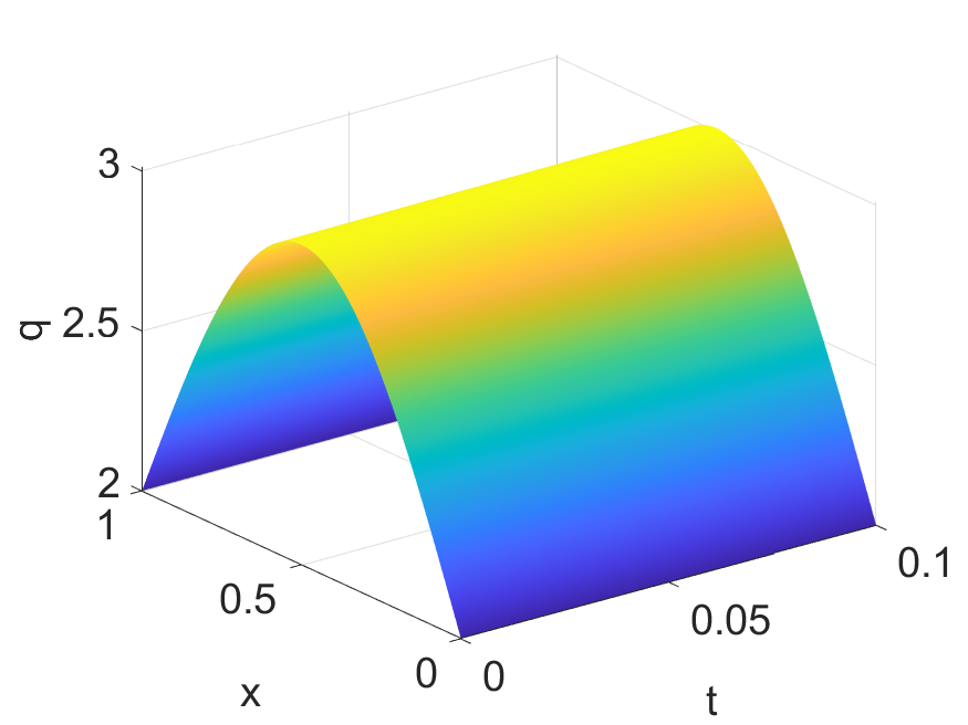
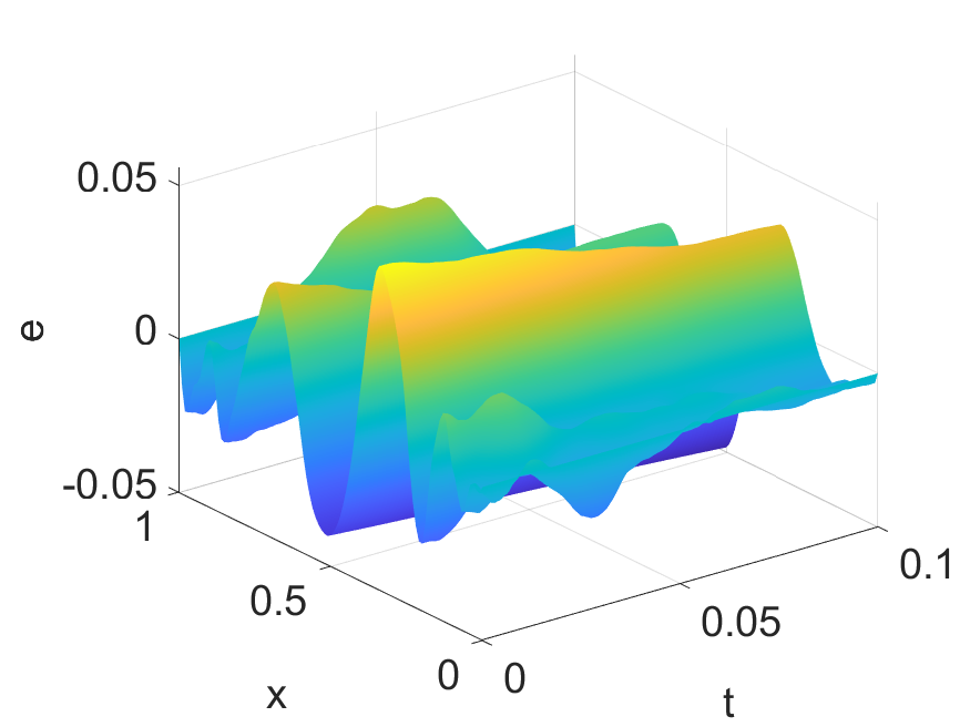
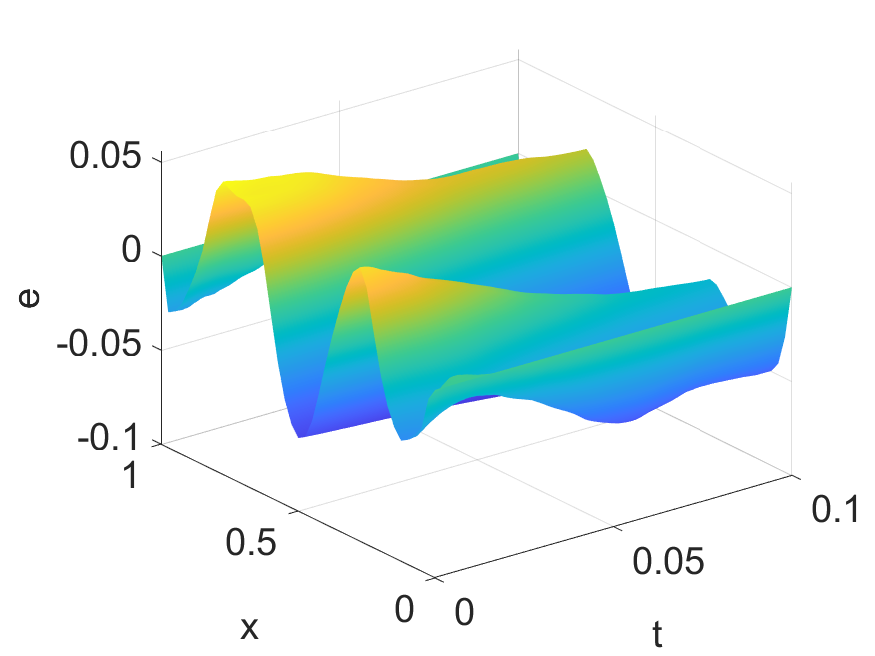
$q^{\dagger}$	$\epsilon=\text{1.00e-2}$		$\epsilon=\text{5.00e-2}$

Figure 1: Numerical reconstructions and the corresponding pointwise error $e=q_{h,\tau}^{*}-q^{\dagger}$ for Example 6.1 with $\alpha=0.5$, at two noise levels $\epsilon=$ 1.00e-2 and 5.00e-2.

The second example has a nonsmooth coefficient $q^{\dagger}$.

Example 6.2.

$u_{0}(x)=x(1-x)$, $f\equiv 0$, $q^{\dagger}=2+\min(x,1-x)(1-t)$, $T=0.1$.

The numerical results for Example 6.2 with different levels of noise are given in Table 2. Note that the exact coefficient $q^{\dagger}$ does not satisfy the regularity condition in Assumption 5.1, and thus one expects the convergence rates of $e_{q}$ and $e_{u}$ suffer from a loss. Indeed, the error $e_{q}$ converges at a slower rate $O(\delta^{0.3})$, which, however, is still higher than that predicted by Remark 5.1. Interestingly, the error $e_{u}$ converges roughly at the rate $O(\delta)$, confirming the estimate in Lemma 5.1. This observation holds for all three fractional orders. Exemplary reconstructions are shown in Fig. 2, which shows clearly the convergence of the discrete approximations as the noise level $\epsilon$ decreases.

Table 2: The errors $e_{q}$ and $e_{u}$ for Example 6.2.

	$\epsilon$	5.00e-2	3.00e-2	1.00e-2	5.00e-3	3.00e-3	1.00e-3
$\alpha$	$\gamma$	1.00e-9	3.60e-10	4.00e-11	1.00e-11	3.60e-12	4.00e-13	rate
$0.25$	$e_{q}$	9.58e-3	7.59e-3	5.77e-3	5.10e-3	4.55e-3	3.71e-3	0.234
	$e_{u}$	1.85e-5	1.15e-5	5.02e-6	3.14e-6	1.51e-6	4.82e-7	0.910
$0.50$	$e_{q}$	1.28e-2	8.17e-3	6.39e-3	4.70e-3	4.11e-3	3.94e-3	0.297
	$e_{u}$	5.44e-5	2.88e-5	1.05e-5	7.79e-6	3.39e-6	1.02e-6	0.977
$0.75$	$e_{q}$	1.17e-2	8.41e-3	6.02e-3	4.07e-3	4.05e-3	3.75e-3	0.301
	$e_{u}$	5.93e-5	3.32e-5	1.44e-5	7.31e-6	4.14e-6	1.33e-6	0.951

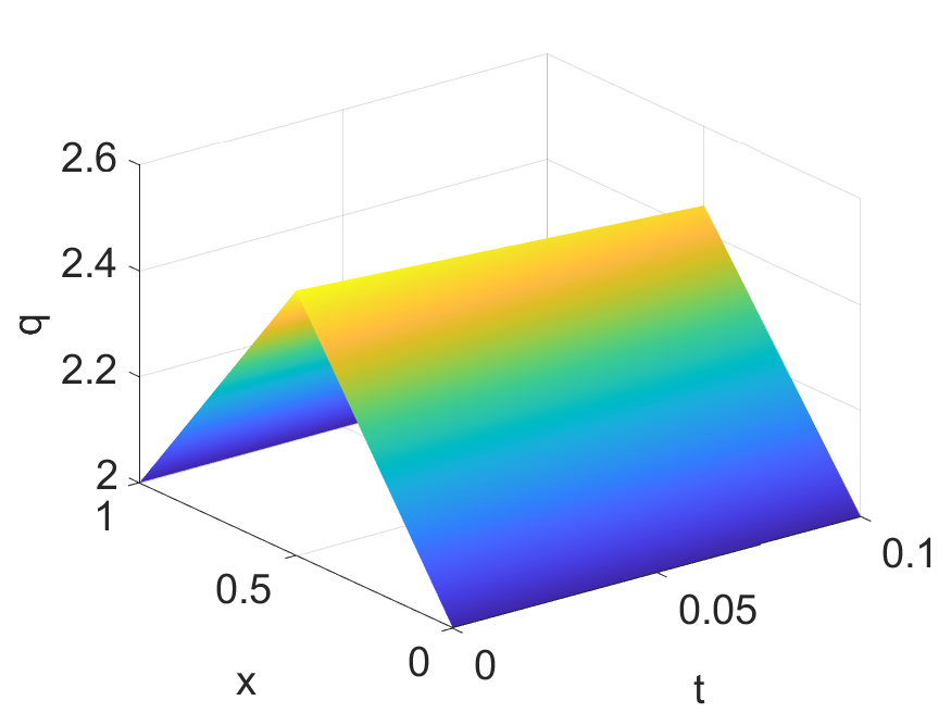
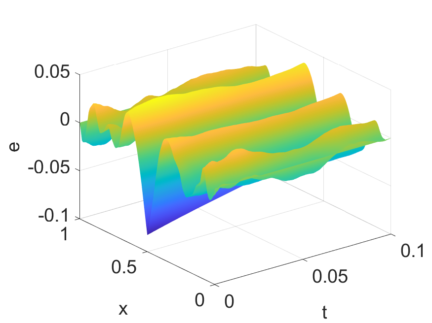
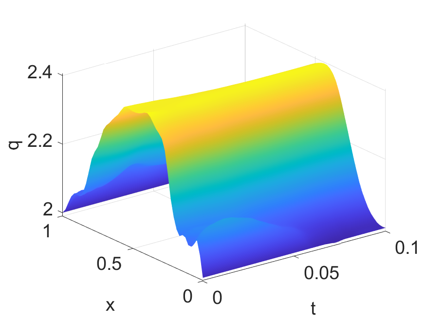
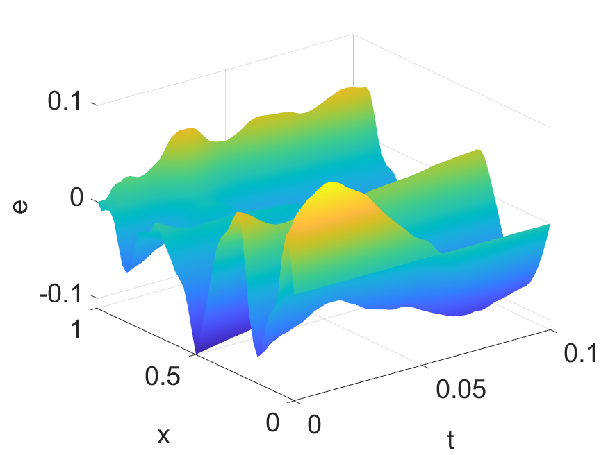
$q^{\dagger}$	$\epsilon=\text{1.00e-2}$		$\epsilon=\text{5.00e-2}$

Figure 2: Numerical reconstructions and the corresponding pointwise error $e=q_{h,\tau}^{*}-q^{\dagger}$ for Example 6.2 with $\alpha=0.5$, at two noise levels $\epsilon=$ 1.00e-2 and 5.00e-2.

6.2 Numerical results in two spatial dimension

Now we present numerical results for the following example on the unit square $\Omega=(0,1)^{2}$. The domain $\Omega$ is first uniformly divided into $M^{2}$ small squares, each with side length $1/M$, and then a uniform triangulation is obtained by connecting the low-left and upper-right vertices of each small square. The reference data is first computed on a finer mesh with $M=100$ and a time step size $\tau=1/2000$. The inversion step is carried out with a mesh $M=40$ and $\tau=1/500$.

Example 6.3.

$u_{0}(x_{1},x_{2})=x_{1}(1-x_{1})\sin(\pi x_{2})$, $f=\sin(\pi x_{1})\sin(\pi x_{2})(1+t)$, $q^{\dagger}(x_{1},x_{2})=1+\sin(\pi x_{1})x_{2}(1-x_{2})$, and $T=1$.

The numerical results for the example with different noise levels are presented in Fig. 3. The empirical observations are in excellent agreement with that for the one-dimensional problem in Example 6.1: we observe a steady convergence as the noise level $\epsilon$ decreases to zero. The plots also indicate that for the pointwise error $e=q_{h}^{*}-q^{\dagger}$, the error in recovering the peak is dominating, however, the overall shape is well resolved.

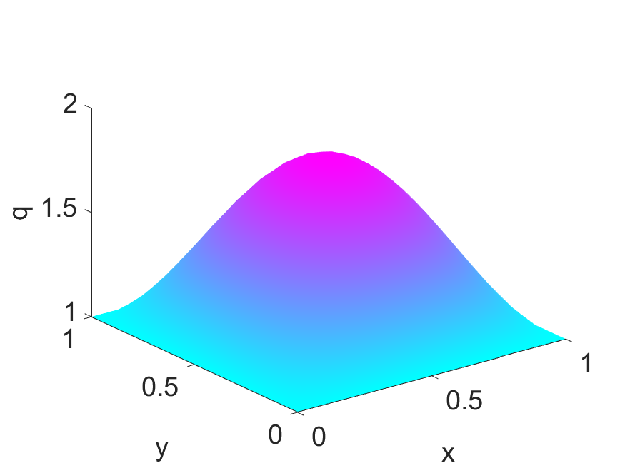
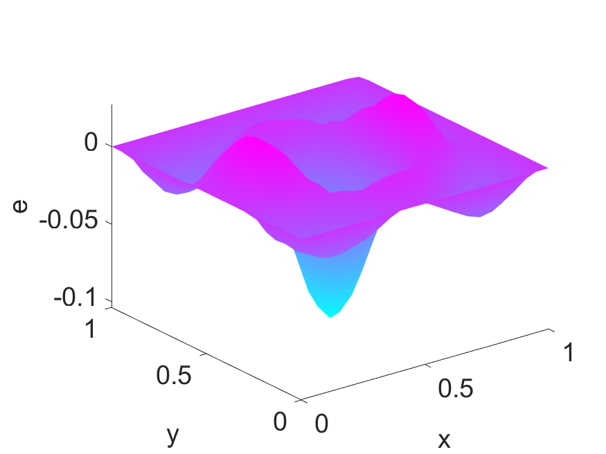
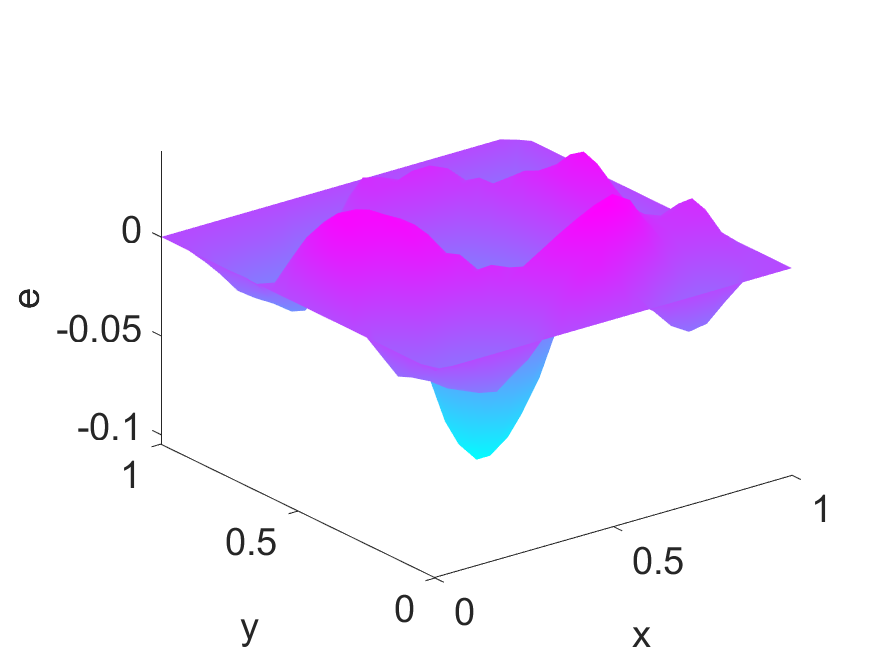
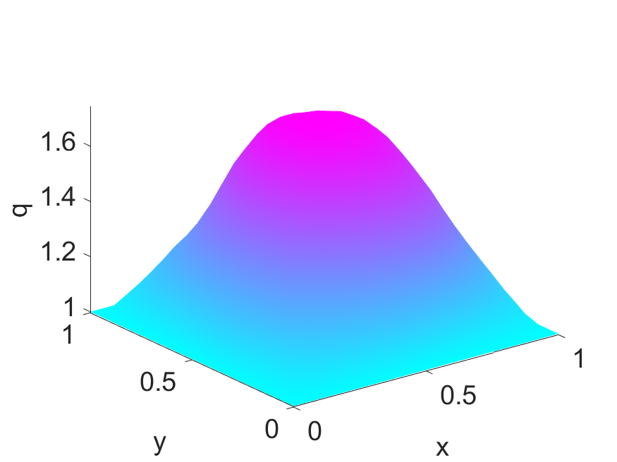
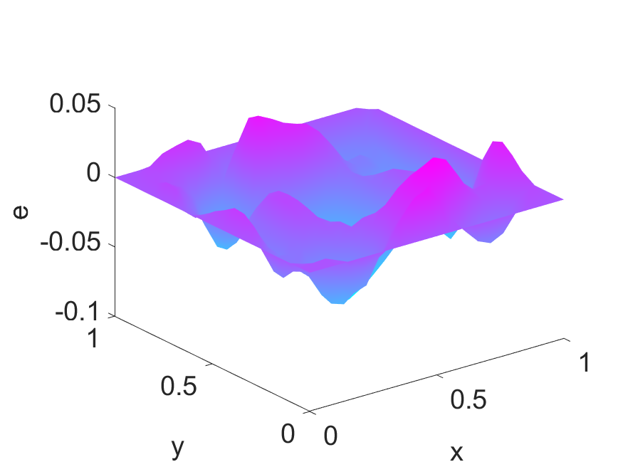
$q^{\dagger}$	$\epsilon=\text{1.00e-2}$		$\epsilon=\text{5.00e-2}$

Figure 3: Numerical reconstructions for Example 6.3 with $\epsilon=$1e-2 and 5.00e-2 and the corresponding pointwise error $e=q_{h,\tau}^{*}-q^{\dagger}$, plotted for $T=0.5$, for $\alpha=0.25$ (top), $\alpha=0.50$ (middle) and $\alpha=0.75$ (bottom).

Appendix A Proof of Theorem 2.1

We give the proof of Theorem 2.1. The argument follows largely that of [23, Theorem 6.14]. It is provided only for completeness.

Proof.

Let $w=u-u_{0}$. Then it suffices to show that there exists a unique solution $w\in L^{p}(0,T;W_{0}^{1,r}(\Omega))\cap C([0,T];L^{r}(\Omega))$ and $\partial_{t}^{\alpha}w\in L^{p}(0,T;W^{-1,r}(\Omega))$, where $w$ satisfies in $W^{-1,r}(\Omega)$

$$\partial_{t}^{\alpha}w(t)+A(t)w(t)=f(t)-A(t)u_{0},\quad t\in(0,T],\quad\text{with}~{}~{}w(0)=0.$$ (A.1)

For any $\theta\in[0,1]$, consider the auxiliary problem

$$\begin{aligned} &{\partial_{t}^{\alpha}}w(t)+A(\theta t)w(t)=f(t)-A(t)u_{0},~{}~{}t\in(0,T],\quad\mbox{with }w(0)=0,\end{aligned}$$ (A.2)

and let $D=\{\theta\in[0,1]:\mbox{\eqref{PDE-theta} has a solution }u\in L^{p}(0,T;W_{0}^{1,r}(\Omega))\mbox{ such that }{\partial_{t}^{\alpha}}w\in L^{p}(0,T;W^{-1,r}(\Omega))\}.$ Next we prove that the set $D$ is a closed subset of $[0,1]$. Since $u_{0}\in W^{1,r}_{0}(\Omega)$, we have $f-A(t)u_{0}\in L^{p}(0,T;W^{-1,r}(\Omega))$, and by Lemma 2.2, we deduce $0\in D$ and $D\neq\emptyset$. Then for any $\theta\in D$ and $t_{0}\in(0,T]$, we rewrite (A.2) as

$$\begin{aligned} &{\partial_{t}^{\alpha}}w(t)+A(\theta t_{0})w(t)=f(t)-A(t)u_{0}+(A(\theta t_{0})-A(\theta t))w(t),\quad t\in(0,T],\quad\mbox{with }w(0)=0.\end{aligned}$$

By the maximal $L^{p}$ regularity in Lemma 2.2 and the perturbation estimate in Lemma 2.1, we obtain

$$\|{\partial_{t}^{\alpha}}w\|_{L^{p}(0,t_{0};W^{-1,r}(\Omega))}+\|\nabla w\|_{L^{p}(0,t_{0};L^{r}(\Omega))}$$

$$\leq c\|f-A(t)u_{0}\|_{L^{p}(0,t_{0};W^{-1,r}(\Omega))}+c\|(A(\theta t_{0})-A(\theta t))w(t)\|_{L^{p}(0,t_{0};W^{-1,r}(\Omega))}$$

$$\leq c\|f-A(t)u_{0}\|_{L^{p}(0,t_{0};W^{-1,r}(\Omega))}+c\|(t_{0}-t)\nabla w\|_{L^{p}(0,t_{0};L^{r}(\Omega))}.$$ (A.3)

Let $g(t)=\|\nabla w\|_{L^{p}(0,t;L^{r}(\Omega))}^{p}$. Since $g^{\prime}(t)=\|\nabla w(t)\|_{L^{r}(\Omega)}^{p}$ and $g(0)=0$, (A.3) and integration by parts gives

$$g(t_{0}) \leq c\|f-A(t)u_{0}\|_{L^{p}(0,t_{0};W^{-1,r}(\Omega))}^{p}+c\int_{0}^{t_{0}}(t_{0}-t)^{p}g^{\prime}(t){\rm d}t$$

$$=c\|f-A(t)u_{0}\|_{L^{p}(0,t_{0};W^{-1,r}(\Omega))}^{p}+cp\int_{0}^{t_{0}}(t_{0}-t)^{p-1}g(t){\rm d}t.$$

Then the standard Gronwall’s inequality implies

$$\|\nabla w\|_{L^{p}(0,t_{0};L^{r}(\Omega))}\leq c\|f-A(t)u_{0}\|_{L^{p}(0,t_{0};W^{-1,r}(\Omega))}.$$

This inequality and (A.3) yield

$$\|{\partial_{t}^{\alpha}}w\|_{L^{p}(0,t_{0};W^{-1,r}(\Omega))}+\|\nabla w\|_{L^{p}(0,t_{0};L^{r}(\Omega))}\leq c\|f-A(t)u_{0}\|_{L^{p}(0,t_{0};W^{-1,r}(\Omega))}.$$ (A.4)

Since this estimate is independent of $\theta\in D$, $D$ is a closed subset of $[0,1]$. Next we show that $D$ is open with respect to the subset topology of $[0,1]$. In fact, for any $\theta_{0}\in D$ and $\theta\in[0,1]$ close to $\theta_{0}$, we rewrite problem (A.2) as

$$\begin{aligned} &{\partial_{t}^{\alpha}}w(t)+A(\theta_{0}t)w(t)+(A(\theta t)-A(\theta_{0}t))w(t)=f(t)-A(t)u_{0},\quad t\in(0,T],\quad\mbox{with }w(0)=0,\end{aligned}$$

which is equivalent to

$$[1+({\partial_{t}^{\alpha}}+A(\theta_{0}t))^{-1}(A(\theta t)-A(\theta_{0}t))]w(t)=({\partial_{t}^{\alpha}}+A(\theta_{0}t))^{-1}(f(t)-A(t)u_{0}).$$

The estimate (A.4) and Lemma 2.1 imply that for any $v\in W_{0}^{1,r}(\Omega)$

$$\|({\partial_{t}^{\alpha}}+A(\theta_{0}t))^{-1}(A(\theta t)-A(\theta_{0}t))v\|_{L^{p}(0,T;W^{1,r}(\Omega))}$$

$$\leq c\|(A(\theta t)-A(\theta_{0}t))v\|_{L^{p}(0,T;W^{-1,r}(\Omega))}\leq c|\theta-\theta_{0}|\|\nabla v\|_{L^{p}(0,T;L^{r}(\Omega))}.$$

Thus for $\theta$ sufficiently close to $\theta_{0}$, the operator $1+({\partial_{t}^{\alpha}}+A(\theta_{0}t))^{-1}(A(\theta t)-A(\theta_{0}t))$ is invertible on $L^{p}(0,T;W_{0}^{1,r}(\Omega))$, which implies $\theta\in D$. Thus $D$ is open with respect to the subset topology of $[0,1]$. Since $D$ is both closed and open respect to the subset topology of $[0,1]$, we deduce $D=[0,1]$. In sum, problem (A.1) has a solution $w$ such that $w\in L^{p}(0,T;W_{0}^{1,r}(\Omega))$ and $\partial_{t}^{\alpha}w\in L^{p}(0,T;W^{-1,r}(\Omega))$. Since $W^{-1,r}(\Omega)$ is UMD [20, Proposition 4.2.17], and $w(0)=0$, we deduce $w\in W^{\alpha,p}(0,T;W^{-1,r}(\Omega))$. By interpolation between $W^{\alpha,p}(0,T;W^{-1,r}(\Omega))$ and $L^{p}(0,T;W_{0}^{1,r}(\Omega))$ [5, Theorem 5.2], we derive $u\in W^{\frac{\alpha}{2},p}(0,T;L^{r}(\Omega))$. This, Sobolev embedding theorem and the condition $p>\frac{2}{\alpha}$ imply $w\in C([0,T];L^{r}(\Omega))$. Similarly, if $r>d$ and $p>\frac{2r}{\alpha(r-d)}$, interpolation [5, Theorem 5.2] and Sobolev embedding theorem imply that for $\frac{1}{\alpha p}<\theta<(\frac{1}{2}-\frac{d}{2r})$

$$\begin{split}u&\in W^{\alpha,p}(0,T;W^{-1,r}(\Omega))\cap L^{p}(0,T;W_{0}^{1,r}(\Omega))\\ &\hookrightarrow W^{\alpha\theta,p}(0,T;W^{1-2\theta,r}(\Omega))\hookrightarrow L^{\infty}((0,T)\times\Omega).\end{split}$$ (A.5)

This completes the proof of the theorem. ∎

Appendix B Nonsmooth data estimates

In this appendix, we collect several nonsmooth data estimates for the numerical approximations of the direct problem (1.1), which are central for deriving the basic estimates in Section 5.1. First, we provide two useful results, i.e., error estimate and maximal $\ell^{p}$ regularity, for the following fully discrete scheme for problem (1.1): find $U_{h}^{n}(q^{\dagger})\in X_{h}$ satisfying $U_{h}^{0}=P_{h}u_{0}$ and

$$\bar{\partial}_{\tau}^{\alpha}U_{h}^{n}(q^{\dagger})+A_{h}(q^{\dagger}(t_{n}))U_{h}^{n}(q^{\dagger})=P_{h}f(t_{n})=:f^{n},\quad n=1,2,\ldots,N.$$ (B.1)

Lemma B.1.

Let $q^{\dagger}$ be the exact coefficient and $u\equiv u(q^{\dagger})$ the solution to problem (4.2), and $\{U_{h}^{n}(q^{\dagger})\}$ the solution to problem (B.1). Then under Assumption 2.2, the following error estimate holds

$$\|u(t_{n})-U_{h}^{n}(q^{\dagger})\|_{L^{2}(\Omega)}\leq c(\tau t_{n}^{\alpha-1}+h^{2}),\quad n=1,\ldots,N.$$

Proof.

The error estimate improves upon a known result from [26], by removing the log factor $\ell_{h}=|\ln h|$, under Assumption 2.2. It suffices to show that for $u_{0}\equiv 0$ and $f\in C^{1}([0,T];L^{2}(\Omega))$

$$\|(u_{h}-u)(t)\|_{L^{2}(\Omega)}\leq ch^{2},\quad\forall t\in[0,T],$$ (B.2)

where $u_{h}$ is the solution to the semidiscrete scheme:

$$\partial_{t}^{\alpha}u_{h}(t)+A_{h}(q^{\dagger}(t))u_{h}(t)=P_{h}f(t),\quad\forall t\in(0,T],\quad\text{with}~{}~{}u_{h}(0)=0.$$ (B.3)

For any $t_{*}\in(0,T]$, let $A_{h*}=A_{h}(q^{\dagger}(t_{*}))$ and $A_{h}(t)=A_{h}(q^{\dagger}(t))$, and further we define the solution operators $F_{h*}$ and $E_{h*}(t)$ by

$$F_{h*}(t)=\frac{1}{2\pi{\rm i}}\int_{\Gamma_{\theta,\delta}}e^{zt}z^{\alpha-1}(z^{\alpha}+A_{h*})^{-1}\,{\rm d}z\quad\mbox{and}\quad E_{h*}(t):=\frac{1}{2\pi{\rm i}}\int_{\Gamma_{\theta,\delta}}e^{zt}(z^{\alpha}+A_{h*})^{-1}\,{\rm d}z.$$

Then the solution $u_{h}$ is given by

$$u_{h}(t)=\int_{0}^{t}E_{h*}(t-s)\big{(}P_{h}f(s)+(A_{h*}-A_{h}(s))u_{h}(s)\big{)}{\rm d}s,$$

Let $e_{h}=P_{h}u-u_{h}$. Then by (2.8), $e_{h}$ is given by

$$e_{h}(t)= \int_{0}^{t}(P_{h}E_{*}(t-s)-E_{h*}(t-s)P_{h})f(s){\rm d}s$$

$$+\int_{0}^{t}(P_{h}E_{*}(t-s)-E_{h*}(t-s)P_{h})(A_{*}-A(s))u(s){\rm d}s$$

$$+\int_{0}^{t}E_{h*}(t-s)\big{(}P_{h}(A_{*}-A(s))u(s)-(A_{h*}-A_{h}(s))u_{h}(s)\big{)}{\rm d}s=:\sum_{i=1}^{3}{\rm I}_{i}(t).$$ (B.4)

The argument in [26, Theorem 3.3] gives

$$\|{\rm I}_{2}(t_{*})\|_{L^{2}(\Omega)} \leq ch^{2}\|f\|_{L^{\infty}(0,t_{*};L^{2}(\Omega))},$$ (B.5)

$$\|{\rm I}_{3}(t_{*})\|_{L^{2}(\Omega)} \leq ch^{2}\|f\|_{L^{\infty}(0,t_{*};L^{2}(\Omega))}+c\int_{0}^{t_{*}}\|e_{h}(s)\|_{L^{2}(\Omega)}{\rm d}s,$$ (B.6)

Now we bound the term ${\rm I}_{1}$ in (B). The identities $E_{*}(t)=-A_{*}^{-1}F_{*}^{\prime}(t)$ and $E_{h*}(t)=-A_{h*}^{-1}F_{h*}^{\prime}(t)$ [23, Lemma 6.1] and integration by parts imply

$${\rm I}_{1}(t)=(P_{h}F_{*}(t)A_{*}^{-1}-F_{h*}(t)A_{h*}^{-1}P_{h})f(0)-\int_{0}^{t}(P_{h}F_{*}(t-s)A_{*}^{-1}-F_{h*}(t-s)A_{h*}^{-1}P_{h})f^{\prime}(s)\,{\rm d}s.$$

For any $v\in L^{2}(\Omega)$, we derive

$$F_{h*}(t)A_{h*}^{-1}P_{h}v =\frac{1}{2\pi{\rm i}}\int_{\Gamma_{\theta,\delta}}\!\!\!e^{zt}z^{\alpha-1}(z^{\alpha}+A_{h*})^{-1}A_{h*}^{-1}P_{h}v\,{\rm d}z=\frac{1}{2\pi{\rm i}}\int_{\Gamma_{\theta,\delta}}\!\!\!e^{zt}z^{-1}\Big{[}A_{h*}^{-1}-(z^{\alpha}+A_{h*})^{-1}\Big{]}P_{h}v\,{\rm d}z.$$

Similarly, $F_{*}(t)A_{*}^{-1}v$ can be represented as

$$F_{*}(t)A_{*}^{-1}v=\frac{1}{2\pi{\rm i}}\int_{\Gamma_{\theta,\delta}}e^{zt}z^{-1}\Big{[}A_{*}^{-1}-(z^{\alpha}+A_{*})^{-1}\Big{]}v\,{\rm d}z.$$

Then the standard finite element approximation yields that for any $z\in\Gamma_{\theta,\delta}$ [15, p. 819–820] $\|(A_{h*}^{-1}P_{h}-A_{*}^{-1})v\|_{L^{2}(\Omega)}\leq ch^{2}\|v\|_{L^{2}(\Omega)}$ and $\|((z^{\alpha}+A_{h*})^{-1}P_{h}-(z^{\alpha}+A_{*})^{-1})v\|_{L^{2}(\Omega)}\leq ch^{2}\|v\|_{L^{2}(\Omega)}$. Consequently, we arrive at

$$\|(P_{h}F_{*}(t)A_{*}^{-1}-F_{h*}(t)A_{h*}^{-1}P_{h})v\|_{L^{2}(\Omega)}\leq ch^{2}\|v\|_{L^{2}(\Omega)},\quad\forall v\in L^{2}(\Omega).$$

Therefore, we obtain

$$\|{\rm I}_{1}(t)\|_{L^{2}(\Omega)}\leq ch^{2}\|f(0)\|_{L^{2}(\Omega)}+ch^{2}\int_{0}^{t}\|f^{\prime}(s)\|_{L^{2}(\Omega)}\,{\rm d}s,$$

which together with (B.5)–(B.6) implies

$$\|e_{h}(t_{*})\|_{L^{2}(\Omega)}\leq ch^{2}+\int_{0}^{t_{*}}\|e_{h}(s)\|_{L^{2}(\Omega)}{\rm d}s.$$

The desired result follows from Gronwall’s inequality and the triangle inequality. ∎

The next result gives the maximal $\ell^{p}$ regularity for the scheme (B.1), where $A_{h}$ denotes the discrete negative Dirichlet Laplacian.

Lemma B.2.

Let $\{U_{h}^{n}\}_{n=1}^{N}$ be the solution to the scheme (B.1) with $u_{0}\equiv 0$. Then for any $p\in(1,\infty)$,

$$\|(\bar{\partial}_{\tau}^{\alpha}U_{h}^{n})_{n=1}^{N}\|_{\ell^{p}(L^{2}(\Omega))}+\|(A_{h}U_{h}^{n})_{n=1}^{N}\|_{\ell^{p}(L^{2}(\Omega))}\leq c\|(f^{n})_{n=1}^{N}\|_{\ell^{p}(L^{2}(\Omega))}.$$

Proof.

For any $m=1,2,\ldots,N$, the scheme (B.1) can be recast into

$$\bar{\partial}_{\tau}^{\alpha}U_{h}^{n}+A_{h}(q^{\dagger}(t_{m}))U_{h}^{n}=P_{h}f^{n}+(A_{h}(q^{\dagger}(t_{m}))-A_{h}(q^{\dagger}(t_{n})))U_{h}^{n}.$$

Since $A_{h}(q^{\dagger}(t_{m}))$ is independent of $n$, there holds the discrete maximal $\ell^{p}$ regularity [25]

$$\begin{aligned} &\quad\|(\bar{\partial}_{\tau}^{\alpha}U_{h}^{n})_{n=1}^{m}\|_{\ell^{p}(L^{2}(\Omega))}^{p}+\|(A_{h}U_{h}^{n})_{n=1}^{m}\|_{\ell^{p}(L^{2}(\Omega))}^{p}\\ &\leq c\big{(}\|(f^{n})_{n=1}^{m}\|_{\ell^{p}(L^{2}(\Omega))}^{p}+\|[(A_{h}(q^{\dagger}(t_{m}))-A_{h}(q^{\dagger}(t_{n})))U_{h}^{n}]_{n=1}^{m}\|_{L^{2}(\Omega)}^{p}\big{)}.\end{aligned}$$

Note that under condition (2.3), there holds [26, Remark 3.1]

$$\|(A_{h}(t)-A_{h}(s))v_{h}\|\leq c\,|t-s|\,\|A_{h}v_{h}\|,\quad\forall v_{h}\in X_{h}.$$

Consequently,

$$\begin{aligned} &\quad\|(\bar{\partial}_{\tau}^{\alpha}U_{h}^{n})_{n=1}^{m}\|_{\ell^{p}(L^{2}(\Omega))}^{p}+\|(A_{h}U_{h}^{n})_{n=1}^{m}\|_{\ell^{p}(L^{2}(\Omega))}^{p}\\ &\leq c\|(f^{n})_{n=1}^{m}\|_{\ell^{p}(L^{2}(\Omega))}^{p}+c\tau\sum_{n=1}^{m}|t_{m}-t_{n}|^{p}\|A_{h}U_{h}^{n}\|_{L^{2}(\Omega)}^{p}.\end{aligned}$$

Let $g^{m}=\|(A_{h}U_{h}^{n})_{n=1}^{m}\|_{\ell^{p}(L^{2}(\Omega))}^{p}$. Then the above estimate implies

$$g^{m} \leq c\|(f^{n})_{n=1}^{m}\|_{\ell^{p}(L^{2}(\Omega))}^{p}+c\tau\sum_{n=1}^{m}|t_{m}-t_{n}|^{p}\frac{g^{n}-g^{n-1}}{\tau}$$

$$\leq c\|(f^{n})_{n=1}^{m}\|_{\ell^{p}(L^{2}(\Omega))}^{p}+c\tau\sum_{n=1}^{m-1}\frac{(t_{m}-t_{n})^{p}-(t_{m}-t_{n+1})^{p}}{\tau}g^{n}$$

$$\leq c\|(f^{n})_{n=1}^{m}\|_{\ell^{p}(L^{2}(\Omega))}^{p}+c\tau\sum_{n=1}^{m-1}t_{m-n}^{p-1}g^{n}.$$

Then the standard discrete Gronwall’s inequality leads to

$$\begin{aligned} \|(A_{h}U_{h}^{n})_{n=1}^{m}\|_{\ell^{p}(L^{2}(\Omega))}^{p}\leq c\|(f^{n})_{n=1}^{m}\|_{\ell^{p}(L^{2}(\Omega))}^{p}.\end{aligned}$$

and the desired result follows immediately by the triangle’s inequality. ∎

The next lemma provides an error estimate of the scheme (B.1) with the (perturbed) coefficient $\mathcal{I}_{h}q^{\dagger}$.

Lemma B.3.

Let $q^{\dagger}$ be the exact diffusion coefficient, $u\equiv u(q^{\dagger})$ the solution to problem (4.2), and $\{U_{h}^{n}(\mathcal{I}_{h}q^{\dagger})\}\subset X_{h}$ the numerical solutions to the scheme (B.1) with $\mathcal{I}_{h}q^{\dagger}$ in place of $q^{\dagger}$. Then under Assumptions 2.2 and 5.1,

$$\begin{split}\|(u(t_{n})-U_{h}^{n}(\mathcal{I}_{h}q^{\dagger}))_{n=1}^{N}\|_{\ell^{2}(L^{2}(\Omega))}^{2}&\leq\begin{cases}c(\tau^{\min(2,1+2\alpha)}+h^{4}),&\alpha\neq 1/2;\\ c(\tau^{2}\ell_{N}+h^{4}),&\alpha=1/2.\end{cases}\end{split}$$

Proof.

Note that $U_{h}^{n}(q^{\dagger})$ and $U_{h}^{n}(\mathcal{I}_{h}q^{\dagger})$ satisfy $U_{h}^{0}(q^{\dagger})=U_{h}^{0}(\mathcal{I}_{h}q^{\dagger})=P_{h}u_{0}$ and

$$\bar{\partial}_{\tau}^{\alpha}U_{h}^{n}(q^{\dagger})+A_{h}(q^{\dagger}(t_{n}))U_{h}^{n}(q^{\dagger}) =P_{h}f(t_{n}),\quad n=1,2\ldots,N,$$

$$\bar{\partial}_{\tau}^{\alpha}U_{h}^{n}(\mathcal{I}_{h}q^{\dagger})+A_{h}(\mathcal{I}_{h}q^{\dagger}(t_{n}))U_{h}^{n}(\mathcal{I}_{h}q^{\dagger}) =P_{h}f(t_{n}),\quad n=1,2,\ldots,N.$$

By subtracting the two identities, we deduce that $\rho_{h}^{n}:=U_{h}^{n}(q^{\dagger})-U_{h}^{n}(\mathcal{I}_{h}q^{\dagger})$ satisfies $\rho_{h}^{0}=0$ and

$$\bar{\partial}_{\tau}^{\alpha}\rho_{h}^{n}+A_{h}(q^{\dagger}(t_{n}))\rho_{h}^{n}=\big{(}A_{h}(\mathcal{I}_{h}q^{\dagger}(t_{n}))-A_{h}(q^{\dagger}(t_{n}))\big{)}U_{h}^{n}(\mathcal{I}_{h}q^{\dagger}),\quad n=1,\ldots,N.$$ (B.7)

The the maximal $\ell^{p}$ regularity in Lemma B.2 implies

$$\|(\rho_{h}^{n})_{n=1}^{N}\|_{\ell^{2}(L^{2}(\Omega))}^{2} \leq c\|(A_{h}(q^{\dagger}(t_{n}))^{-1}\big{(}A_{h}(\mathcal{I}_{h}q^{\dagger}(t_{n}))-A_{h}(q^{\dagger}(t_{n}))\big{)}U_{h}^{n}(\mathcal{I}_{h}q^{\dagger}))_{n=1}^{N}\|_{\ell^{2}(L^{2}(\Omega))}^{2}$$

$$\leq c\|(\big{(}A_{h}(\mathcal{I}_{h}q^{\dagger}(t_{n}))^{-1}-A_{h}(q^{\dagger}(t_{n}))^{-1}\big{)}A_{h}(\mathcal{I}_{h}q^{\dagger}(t_{n}))U_{h}^{n}(\mathcal{I}_{h}q^{\dagger}))_{n=1}^{N}\|_{\ell^{2}(L^{2}(\Omega))}^{2}.$$

By [28, Lemma A.1], we have for any $\epsilon>0$ and $p\geq\max(d+\epsilon,2)$,

$$\|A_{h}(\mathcal{I}_{h}q^{\dagger})^{-1}-A_{h}(q^{\dagger})^{-1}\|_{L^{p}(\Omega)\rightarrow L^{2}(\Omega)}\leq ch^{2}.$$

Consequently,

$$\|(\rho_{h}^{n})_{n=1}^{N}\|_{\ell^{2}(L^{2}(\Omega))}^{2}\leq ch^{4}\|(A_{h}(\mathcal{I}_{h}q^{\dagger}(t_{n}))U_{h}^{n}(\mathcal{I}_{h}q^{\dagger}))_{n=1}^{N}\|_{\ell^{2}(L^{p}(\Omega))}^{2}.$$

Then the maximal $\ell^{p}$ regularity for the backward Euler CQ in Lemma B.2 implies

$$\|(A_{h}(\mathcal{I}_{h}q^{\dagger}(t_{n}))U_{h}^{n}(\mathcal{I}_{h}q^{\dagger}))_{n=1}^{N}\|_{\ell^{2}(L^{p}(\Omega))}^{2}\leq c(\|(f(t_{n}))_{n=1}^{N}\|_{\ell^{2}(L^{p}(\Omega))}^{2}+\|\nabla u_{0}\|_{L^{p}(\Omega)}^{2}).$$

Finally, the desired estimate follows from Lemma B.1 and the triangle inequality. ∎

Last, we give an estimate on the backward Euler CQ approximation of $\partial_{t}^{\alpha}u(t_{n})$.

Lemma B.4.

Let $q^{\dagger}$ be the exact diffusion coefficient and $u\equiv u(q^{\dagger})$ be the solution to problem (4.2). Then under Assumption 2.2, with $\ell_{n}=\ln(1+\frac{t_{n}}{\tau})=\ln(n+1)$, there holds

$$\|\bar{\partial}_{\tau}^{\alpha}u(t_{n})-\partial_{t}^{\alpha}u(t_{n})\|_{L^{2}(\Omega)}\leq c\tau(t_{n}^{-1}+\ell_{n}).$$

Proof.

The proof employs a (different) perturbation argument. Let $A_{0}=A(0)$. Let $F(t)=(A_{0}-A(t))u(t)+f(t)$ and $y(t)=u(t)-u_{0}$. Then $y(t)$ satisfies

$$\partial_{t}^{\alpha}y(t)+A_{0}y(t)=F(t)-A_{0}u_{0},\quad\forall t\in(0,T],\quad\text{with}~{}~{}y(0)=0.$$

Using the identity $F(t)=F(0)+\int_{0}^{t}F^{\prime}(s)\,{\rm d}s$, then Laplace transform gives

$$z^{\alpha}\widehat{y}(z)+A_{0}\widehat{y}(z)=z^{-1}(F(0)-A_{0}u_{0})+z^{-1}\widehat{F^{\prime}}(z),$$

i.e.,

$$\widehat{y}(z)=(z^{\alpha}+A_{0})^{-1}(z^{-1}(F(0)-A_{0}u_{0})+z^{-1}\widehat{F^{\prime}}(z)).$$

Similarly, one can derive a representation for the discrete approximation. By inverse Laplace transform, $w^{n}=\partial_{t}^{\alpha}y(t_{n})-\bar{\partial}_{\tau}^{\alpha}y(t_{n})$ is given by

$$w^{n} =\frac{1}{2\pi\mathrm{i}}\int_{\Gamma_{\theta,\delta}^{\tau}}e^{zt_{n}}K(z)(z^{-1}(F(0)-A_{0}u_{0})+z^{-1}\widehat{F^{\prime}}(z))\,{\rm d}z$$

$$\quad+\frac{1}{2\pi\mathrm{i}}\int_{\Gamma_{\theta,\delta}\setminus\Gamma_{\theta,\delta}^{\tau}}e^{zt_{n}}K(z)(z^{-1}(F(0)-A_{0}u_{0})+z^{-1}\widehat{F^{\prime}}(z))\,{\rm d}z.$$

with $\Gamma_{\theta,\delta}^{\tau}=\{z\in\Gamma_{\theta,\delta},|\rm{Im}(z)|\leq\frac{\pi}{\tau}\}$ and

$$K(z)=(z^{\alpha}-\delta_{\tau}(e^{-z\tau})^{\alpha})(z^{\alpha}+A_{0})^{-1},$$

with $\delta_{\tau}(\xi)=\tau^{-1}(1-\xi)$ being characteristic polynomial of the backward Euler method. Simple computation shows that the following estimates hold

$$\quad c_{1}|z| \leq|\delta_{\tau}(e^{-z\tau})|\leq c_{2}|z|,\qquad|\delta_{\tau}(e^{-z\tau})^{\alpha}-z^{\alpha}|\leq c\tau z^{1+\alpha},\quad\forall z\in\Gamma_{\theta,\delta}^{\tau},$$ (B.8)

$$|\delta_{\tau}(e^{-z\tau})| \leq|z|\sum_{k=1}^{\infty}\frac{|z\tau|^{k-1}}{k!}\leq|z|e^{|z|\tau},\quad\forall z\in\Sigma_{\theta}=\{z\in\mathbb{C}:z\neq 0,|\arg(z)|\leq\theta\},$$ (B.9)

and the resolvent estimate

$$\|(z+A_{0})^{-1}\|\leq c|z|^{-1},\quad\forall z\in\Sigma_{\theta}.$$ (B.10)

We first treat the error involving $(A_{0}u_{0}-F(0))$, and let

$${\rm I}_{1}=\frac{1}{2\pi\mathrm{i}}\int_{\Gamma_{\theta,\delta}^{\tau}}e^{zt_{n}}K(z)z^{-1}(A_{0}u_{0}-F(0)){\rm d}z\quad\mbox{and}\quad{\rm I}_{2}=\frac{1}{2\pi\mathrm{i}}\int_{\Gamma_{\theta,\delta}\setminus\Gamma_{\theta,\delta}^{\tau}}e^{zt_{n}}K(z)z^{-1}(F(0)-A_{0}u_{0}){\rm d}z.$$

By choosing $\delta=c/t_{n}$ in $\Gamma_{\theta,\delta}$ and applying (B.10), the term ${\rm I}_{1}$ is bounded by

$$\|{\rm I}_{1}\|_{L^{2}(\Omega)} \leq c\tau\|F(0)-A_{0}u_{0}\|_{L^{2}(\Omega)}\Big{(}\int_{\frac{c}{t_{n}}}^{\frac{\pi\sin\theta}{\tau}}e^{-c\rho t_{n}}\,{\rm d}\rho+\int_{-\theta}^{\theta}ct_{n}^{-1}\,{\rm d}\theta\Big{)}\leq c\tau t_{n}^{-1}\|F(0)-A_{0}u_{0}\|_{L^{2}(\Omega)}.$$

Further, by (B.9), for any $z=\rho e^{\pm\mathrm{i}\theta}\in\Gamma_{\theta,\delta}\setminus\Gamma_{\theta,\delta}^{\tau}$ and choosing $\theta\in(\pi/2,\pi)$ close to $\pi$,

$$|e^{zt_{n}}(\delta_{\tau}(e^{-z\tau})^{\alpha}-z^{\alpha})z^{-1}| \leq e^{t_{n}\rho\cos\theta}(c|z|^{\alpha}e^{\alpha\rho\tau}+|z|^{\alpha})|z|^{-1}\leq c|z|^{\alpha-1}e^{-c\rho t_{n}}.$$

Then the term ${\rm I_{2}}$ is bounded by

$$\|{\rm I}_{2}\|_{L^{2}(\Omega)}\leq c\|F(0)-A_{0}u_{0}\|_{L^{2}(\Omega)}\int_{\frac{\pi\sin\theta}{\tau}}^{\infty}e^{-c\rho t_{n}}\rho^{-1}\,{\rm d}\rho\leq c\tau t_{n}^{-1}\|F(0)-A_{0}u_{0}\|_{L^{2}(\Omega)}.$$

This argument also bounds for the term involving $\widehat{F^{\prime}}(z)$. Finally, we obtain

$$\begin{split}\|w^{n}\|_{L^{2}(\Omega)}&\leq c\tau t_{n}^{-1}\|F(0)-A_{0}u_{0}\|_{L^{2}(\Omega)}+\int_{\tau}^{t_{n}}(t_{n}-s+\tau)^{-1}\|F^{\prime}(s)\|_{L^{2}(\Omega)}\,{\rm d}s.\end{split}$$

Then the solution regularity (2.6) and the perturbation estimate (2.4) immediately imply

$$\|F^{\prime}(s)\|_{L^{2}(\Omega)} \leq\|f^{\prime}(s)\|_{L^{2}(\Omega)}+\|A^{\prime}(s)u(s)\|_{L^{2}(\Omega)}+\|(A_{0}-A(s))u^{\prime}(s)\|_{L^{2}(\Omega)}$$

$$\leq c(\|f^{\prime}(s)\|_{L^{2}(\Omega)}+\|u(s)\|_{H^{2}(\Omega)}+s\|u^{\prime}(s)\|_{H^{2}(\Omega)})\leq c.$$

This bound and the estimate $\|f(0)-A_{0}u_{0}\|_{L^{2}(\Omega)}\leq c$ imply

$$\|w^{n}\|_{L^{2}(\Omega)}\leq c\tau t_{n}^{-1}+c\int_{\tau}^{t_{n}}(t_{n+1}-s)^{-1}\,{\rm d}s\leq c\tau(t_{n}^{-1}+\ell_{n}).$$

This completes the proof of the lemma. ∎

References

- [1] E. E. Adams and L. W. Gelhar. Field study of dispersion in a heterogeneous aquifer: 2. spatial moments analysis. Water Res. Research, 28(12):3293–3307, 1992.
- [2] R. A. Adams and J. J. F. Fournier. Sobolev Spaces. Elsevier/Academic Press, Amsterdam, second edition, 2003.
- [3] G. Akrivis, B. Li, and C. Lubich. Combining maximal regularity and energy estimates for time discretizations of quasilinear parabolic equations. Math. Comp., 86(306):1527–1552, 2017.
- [4] O. M. Alifanov, E. A. Artyukhin, and S. V. Rumyantsev. Extreme Methods for Solving Ill-Posed Problems with Applications to Inverse Heat Transfer Problems. Begell House, New York, 1995.
- [5] H. Amann. Compact embeddings of vector-valued Sobolev and Besov spaces. Glas. Mat. Ser. III, 35(55)(1):161–177, 2000.
- [6] H. T. Banks and K. Kunisch. Estimation Techniques for Distributed Parameter Systems. Birkhäuser, Boston, MA, 1989.
- [7] A. Bonito, A. Cohen, R. DeVore, G. Petrova, and G. Welper. Diffusion coefficients estimation for elliptic partial differential equations. SIAM J. Math. Anal., 49(2):1570–1592, 2017.
- [8] H. Brezis and P. Mironescu. Gagliardo-Nirenberg inequalities and non-inequalities: the full story. Ann. Inst. H. Poincaré Anal. Non Linéaire, 35(5):1355–1376, 2018.
- [9] G. Chavent. Nonlinear Least Squares for Inverse Problems. Springer, New York, 2009.
- [10] J. Cheng, J. Nakagawa, M. Yamamoto, and T. Yamazaki. Uniqueness in an inverse problem for a one-dimensional fractional diffusion equation. Inverse Problems, 25(11):115002, 16, 2009.
- [11] H. W. Engl, M. Hanke, and A. Neubauer. Regularization of Inverse Problems. Kluwer Academic, Dordrecht, 1996.
- [12] A. Ern and J.-L. Guermond. Theory and Practice of Finite Elements. Springer-Verlag, New York, 2004.
- [13] L. C. Evans and R. F. Gariepy. Measure Theory and Fine Properties of Functions. CRC Press, Boca Raton, FL, 2015.
- [14] K. S. Fa and E. K. Lenzi. Time-fractional diffusion equation with time dependent diffusion coefficient. Phys. Rev. E, 72:011107, 2005.
- [15] H. Fujita and T. Suzuki. Evolution problems. In Handbook of Numerical Analysis, Vol. II, Handb. Numer. Anal., II, pages 789–928. North-Holland, Amsterdam, 1991.
- [16] R. Garra, E. Orsingher, and F. Polito. Fractional diffusions with time-varying coefficients. J. Math. Phys., 56(9):093301, 17, 2015.
- [17] D. Gilbarg and N. S. Trudinger. Elliptic Partial Differential Equations of Second Order. Springer-Verlag, Berlin, third edition, 2001.
- [18] M. Grüter and K.-O. Widman. The Green function for uniformly elliptic equations. Manuscripta Math., 37(3):303–342, 1982.
- [19] Y. Hatano and N. Hatano. Dispersive transport of ions in column experiments: An explanation of long-tailed profiles. Water Res. Research, 34(5):1027–1033, 1998.
- [20] T. Hytönen, J. van Neerven, M. Veraar, and L. Weis. Analysis in Banach Spaces. Vol. I. Martingales and Littlewood-Paley Theory. Springer, Cham, 2016.
- [21] V. Isakov. Inverse Problems for Partial Differential Equations. Springer, New York, second edition, 2006.
- [22] K. Ito and B. Jin. Inverse Problems: Tikhonov Theory and Algorithms. World Scientific Publishing Co. Pte. Ltd., Hackensack, NJ, 2015.
- [23] B. Jin. Fractional Differential Equations. Springer, Switzerland, 2021.
- [24] B. Jin, Y. Kian, and Z. Zhou. Reconstruction of a space-time-dependent source in subdiffusion models via a perturbation approach. SIAM J. Math. Anal., 53(4):4445–4473, 2021.
- [25] B. Jin, B. Li, and Z. Zhou. Discrete maximal regularity of time-stepping schemes for fractional evolution equations. Numer. Math., 138(1):101–131, 2018.
- [26] B. Jin, B. Li, and Z. Zhou. Subdiffusion with a time-dependent coefficient: analysis and numerical solution. Math. Comp., 88(319):2157–2186, 2019.
- [27] B. Jin and W. Rundell. A tutorial on inverse problems for anomalous diffusion processes. Inverse Problems, 31(3):035003, 40, 2015.
- [28] B. Jin and Z. Zhou. Error analysis of finite element approximations of diffusion coefficient identification for elliptic and parabolic problems. SIAM J. Numer. Anal., 59(1):119–142, 2021.
- [29] B. Jin and Z. Zhou. Numerical estimation of a diffusion coefficient in subdiffusion. SIAM J. Control Optim., 59(2):1466–1496, 2021.
- [30] B. Kaltenbacher and W. Rundell. On an inverse potential problem for a fractional reaction-diffusion equation. Inverse Problems, 35(6):065004, 31, 2019.
- [31] B. Kaltenbacher and W. Rundell. On the identification of a nonlinear term in a reaction-diffusion equation. Inverse Problems, 35(11):115007, 38, 2019.
- [32] Y. Kian, L. Oksanen, E. Soccorsi, and M. Yamamoto. Global uniqueness in an inverse problem for time fractional diffusion equations. J. Diff. Equations, 264(2):1146–1170, 2018.
- [33] A. A. Kilbas, H. M. Srivastava, and J. J. Trujillo. Theory and Applications of Fractional Differential Equations. Elsevier Science B.V., Amsterdam, 2006.
- [34] M. V. Krasnoschok. Solvability in Hölder space of an initial boundary value problem for the time-fractional diffusion equation. Zh. Mat. Fiz. Anal. Geom., 12(1):48–77, 2016.
- [35] A. Kubica, K. Ryszewska, and M. Yamamoto. Time-Fractional Differential Equations—a Theoretical Introduction. Springer, Singapore, 2020.
- [36] G. Li, W. Gu, and X. Jia. Numerical inversions for space-dependent diffusion coefficient in the time fractional diffusion equation. J. Inverse Ill-Posed Probl., 20(3):339–366, 2012.
- [37] G. Li, D. Zhang, X. Jia, and M. Yamamoto. Simultaneous inversion for the space-dependent diffusion coefficient and the fractional order in the time-fractional diffusion equation. Inverse Problems, 29(6):065014, 36, 2013.
- [38] Z. Li and M. Yamamoto. Inverse problems of determining coefficients of the fractional partial differential equations. In Handbook of fractional calculus with applications. Vol. 2, pages 443–464. De Gruyter, Berlin, 2019.
- [39] A. O. Lopushanskyi and H. P. Lopushanska. One inverse problem for the diffusion-wave equation in bounded domain. Ukrainian Math. J., 66(5):743–757, 2014. Translation of Ukraïn. Mat. Zh. 66 (2014), no. 5, 666–678.
- [40] C. Lubich. Discretized fractional calculus. SIAM J. Math. Anal., 17(3):704–719, 1986.
- [41] Y. Luchko and M. Yamamoto. On the maximum principle for a time-fractional diffusion equation. Fract. Calc. Appl. Anal., 20(5):1131–1145, 2017.
- [42] R. Metzler, J. H. Jeon, A. G. Cherstvy, and E. Barkai. Anomalous diffusion models and their properties: non-stationarity, non-ergodicity, and ageing at the centenary of single particle tracking. Phys. Chem. Chem. Phys., 16(44):24128–24164, 2014.
- [43] R. Metzler and J. Klafter. The random walk’s guide to anomalous diffusion: a fractional dynamics approach. Phys. Rep., 339(1):1–77, 2000.
- [44] R. R. Nigmatullin. The realization of the generalized transfer equation in a medium with fractal geometry. Phys. Stat. Solid. B, 133(1):425–430, 1986.
- [45] T. I. Seidman and C. R. Vogel. Well-posedness and convergence of some regularisation methods for nonlinear ill posed problems. Inverse Problems, 5(2):227–238, 1989.
- [46] V. Thomée. Galerkin Finite Element Methods for Parabolic Problems. Springer-Verlag, Berlin, second edition, 2006.
- [47] L. Wang and J. Zou. Error estimates of finite element methods for parameter identifications in elliptic and parabolic systems. Discrete Contin. Dyn. Syst. Ser. B, 14(4):1641–1670, 2010.
- [48] T. Wei and Y. S. Li. Identifying a diffusion coefficient in a time-fractional diffusion equation. Math. Comput. Simul., 151:77–95, 2018.
- [49] Z. Zhang. An undetermined coefficient problem for a fractional diffusion equation. Inverse Problems, 32(1):015011, 21, 2016.
- [50] Z. Zhang and Z. Zhou. Recovering the potential term in a fractional diffusion equation. IMA J. Appl. Math., 82(3):579–600, 2017.