A geometric perspective on functional outlier detection

Abstract

We consider functional outlier detection from a geometric perspective, specifically: for functional data sets drawn from a functional manifold which is defined by the data’s modes of variation in amplitude and phase. Based on this manifold, we develop a conceptualization of functional outlier detection that is more widely applicable and realistic than previously proposed. Our theoretical and experimental analyses demonstrate several important advantages of this perspective: It considerably improves theoretical understanding and allows to describe and analyse complex functional outlier scenarios consistently and in full generality, by differentiating between structurally anomalous outlier data that are off-manifold and distributionally outlying data that are on-manifold but at its margins. This improves practical feasibility of functional outlier detection: We show that simple manifold learning methods can be used to reliably infer and visualize the geometric structure of functional data sets. We also show that standard outlier detection methods requiring tabular data inputs can be applied to functional data very successfully by simply using their vector-valued representations learned from manifold learning methods as input features. Our experiments on synthetic and real data sets demonstrate that this approach leads to outlier detection performances at least on par with existing functional data-specific methods in a large variety of settings, without the highly specialized, complex methodology and narrow domain of application these methods often entail.

1 Introduction

1.1 Problem setting and proposal

Outlier detection for functional data is a challenging problem due to the complex and information-rich units of observations, which can be “outlying” or unusual in many different ways. Functional outliers are often categorized into magnitude and shape outliers [12, 3, e.g.], whereas Hubert et al. [25] differentiate between isolated and persistent outliers, the latter further subdivided into shift, amplitude and shape outliers. However, neither of these taxonomies yield precise, explicit, fully general definitions, which makes it difficult to theoretically describe, analyze and compare functional outliers. Magnitude outliers, for example, have been defined as functional observations “outlying in some part or across the whole design domain” [12, p. 1] or as “curves lying outside the range of the vast majority of the data” [3, p. 2], whereas Hubert et al. [25, p. 3] define isolated outliers as observations which “exhibit outlying behavior during a very short time interval”, in contrast to persistent outliers which “are outlying on a large part of the domain”.

To cut through the confusion, we propose a geometric perspective on functional outlier detection based on the well-known “manifold hypothesis” [32, 30]. This refers to the assumption that ostensibly complex, high-dimensional data lies on a much simpler, lower dimensional manifold embedded in the observation space and that this manifold’s structure can be learned and then represented in a low-dimensional space, often simply called embedding space. We argue that such a perspective both clarifies and generalizes the concept of functional outliers, without the need for any strong assumptions or prior knowledge about the underlying data generating process or its outliers. In terms of theoretical development, the approach allows us to consistently formalize and systematically analyze functional outlier detection in full generality. We also demonstrate that procedures based on this perspective simplify and improve functional outlier detection in practice: it suggests a principled, yet flexible approach for applying well-established, highly performant standard outlier detection methods such as local outlier factors (LOF) [6] to functional data, based on embedding coordinates obtained via manifold learning or dimension reduction methods. Our experiments show that doing so performs at least on par with existing functional-data-specific outlier detection methods, without the methodological complexity and limited applicability that methods specific to functional data often entail. Moreover, such lower dimensional representations serve as an easily accessible visualization and exploration tool that helps to uncover complex and subtle data structures which cannot be sufficiently reflected by one-dimensional outlier scores or labels, nor captured by many of the previously proposed 2D diagnostic visualizations for functional outliers.

1.2 Background and related work

Functional data analysis (FDA) [43, e.g.] focuses on data where the units of observation are realizations of stochastic processes over compact domains. In many cases, the intrinsic dimensionality of functional data (FD) is much lower than the observed. First, while FD are infinite dimensional in theory, they are high-dimensional in practice – functional observations are usually recorded on fine and dense grids of argument values. Second, the dominant drivers of differences between functional observations are often comparatively low-dimensional so that just a few modes of variation capture most of the structured variability in the data.
However, FD usually contain both amplitude and phase variation, i.e., “vertical” shape or level variation as well as “horizontal” shape variation. These different kinds of variability contribute to the difficulty to precisely define and differentiate the various forms of functional outliers and to develop methods that can “catch them all”, making outlier detection a highly investigated research topic in FDA. For example, Arribas-Gil and Romo [3] argue that the proposed outlier taxonomy of Hubert et al. [25] can be made more precise in terms of expectation functions $f(t)$ and $g(t)$, with $f(t)$ a “common” process, see Figure 1.

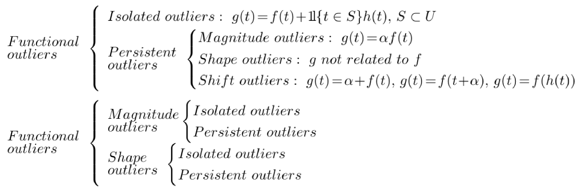
Figure 1: Functional outlier taxonomies. Bottom: standard taxonomy. Top: taxonomy as introduced by Hubert et al. Image taken from Arribas-Gil and Romo [3].

Despite these attempts some fundamental issues remain unsolved. The proposed taxonomies do not provide precise definitions and some of the definitions are contradictory to some extent. Finally, many outlier scenarios for realistic data generating processes are not covered by the described taxonomies at all. As Arribas-Gil and Romo [3] themselves point out, settings with phase-varying data (i.e., “horizontal” variability through elastic deformations of the functions’ domains) are not sufficiently reflected, as functions deviating in terms of phase may be considered as shape outliers in cases where there are only few of such functions but not in settings where all functions display such variation.
In addition, the taxonomy in Figure 1 provides a reasonable conceptual framework only if the non-outlying data from the “common” data generating process is characterized adequately just by its global mean function. This cannot be assumed for many real data sets which often contain highly variable sets of functions which display several modes of phase, shape and/or amplitude variation simultaneously and/or which come from multiple classes with class-specific means and higher moments (see Figure 5, e.g.).

Published research focuses mostly on the development of outlier detection methods specifically for functional data, and a multitude of methods based on a variety of different concepts such as functional data depths [21, 20, e.g.], functional PCA [45], functional isolation forests [47], robust functional archetypoids [49] or functional outlier metrics like directional outlyingness [44, 11], often narrowly focused on detecting specific kinds of functional outliers, have been put forth. Dai et al. [12] propose a transformation-based approach to functional outlier detection and claim that sequentially transforming shape outliers, which “are much more challenging to handle”, into magnitude outliers, makes them easier to detect with established methods [12, p. 2]. The approach allows to define functional outliers more precisely in terms of the transformations being used, like normalizing or centering functions or taking their derivatives, but practitioners still need to be able to come up with appropriate transformations for the data at hand first.
Recently, Xie et al. [50] have introduced a decomposition of functional observations into amplitude, phase and shift components, based on which specific types of outliers can be identified in a more general geometric framework without necessarily requiring functional data to be of comparatively low rank. Similar in spirit to our proposal, Hyndman and Shang [26] used kernel density estimation and half-space depth contours of two-dimensional robustified FPCA scores to construct functional boxplot equivalents and detect outliers, and Ali et al. [1] use data representations in two dimensions obtained from manifold methods for outlier detection and clustering, but the focus of both is on practicalities without considering the theoretical implications and general applicability of embedding-based approaches nor do they consider the necessity of higher dimensional representations.

The remainder of the paper is structured as follows: We provide the theoretical formalization and discussion of the geometric approach in section 2. Based on these theoretical considerations, section 3 presents extensive experiments. Section 3.1 covers a detailed qualitative analysis of real world ECG data, while section 3.2 provides quantitative experiments and systematic comparisons to previously proposed methods on complex synthetic outlier scenarios. We conclude with a discussion in section 4.

2 Functional outlier detection as a manifold learning problem

In this section, we first define two forms of functional outliers from a geometrical view point: off- and on-manifold outliers. We then illustrate how this perspective contains and extends existing outlier taxonomies and how it can be used to formalize a large variety of additional scenarios for functional data with outliers.

2.1 The two notions of functional outliers: off- and on-manifold

Our approach to functional outlier detection rests on the manifold assumption, i.e., the assumption that observed high-dimensional data are intrinsically low-dimensional. Specifically, we put forth that observed functional data $x(t)\in\mathcal{F}$, where $\mathcal{F}$ is a function space, arise as the result of a mapping $\phi:\Theta\to\mathcal{F}$ from a (low-dimensional) parameter space $\Theta\subset\mathbb{R}^{d_{2}}$ to $\mathcal{F}$, i.e., $x(t)=\phi(\theta)$. Conceptually, a $d_{2}$-dimensional parameter vector $\theta\in\Theta$ represents a specific combination of values for the modes of variation in the observed functional data, such as level or phase shifts, amplitude variability, class labels and so on. These parameter vectors are drawn from a probability distribution $P$ over $\mathbb{R}^{d_{2}}$: $\theta_{i}\sim P\;\forall\;\theta_{i}\in\Theta,$ with $\Theta=\{\theta:f_{P}(\theta)>0\}$ and $f_{P}$ the density to $P$. Mapping this parameter space to the function space creates a functional manifold $\mathcal{M}_{\Theta,\phi}$ defined by $\phi$ and $\Theta$: $\mathcal{M}_{\Theta,\phi}=\{x(t):x(t)=\phi(\theta)\in\mathcal{F},\theta\in\Theta\}\subset\mathcal{F}$, an example is depicted in Figure 2. For $\mathcal{F}=L^{2}$ with data from a single functional manifold that is isomorphic to some Euclidean subspace, Chen and Müller [7] develop a notion of a manifold mean and modes of variation. Similarly, Dimelgio et al. [15] develop a robust algorithm for template curve estimation for connected smooth sub-manifolds of $\mathbb{R}^{d}$.

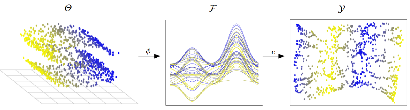
Figure 2: Functional data from a manifold learning perspective. Image taken from Herrmann & Scheipl [22].

Unlike these single manifold settings, our conceptualization of outlier detection is based on two functional manifolds. That is, we assume a data set $X=\{x_{1}(t),\dots,x_{n}(t)\}$ with $n$ functional observations coming from two separate functional manifolds $\mathcal{M}_{c}=\mathcal{M}_{\Theta_{c},\phi_{c}}$ and $\mathcal{M}_{a}=\mathcal{M}_{\Theta_{a},\phi_{a}}$, with $\mathcal{M}_{j}\subset\mathcal{F}$, $j\in\{c,a\}$ and $X\subset\{\mathcal{M}_{c}\cup\mathcal{M}_{a}\}$, with $\mathcal{M}_{c}$ representing the “common” data generating process and $\mathcal{M}_{a}$ containing anomalous data. Moreover, for the purpose of outlier detection and in contrast to the settings with a single manifold described in the referenced literature, we are less concerned with precisely approximating the intrinsic geometry of each manifold. Instead, it is crucial to consider the manifolds $\mathcal{M}_{c}$ and $\mathcal{M}_{a}$ as sub-manifolds of $\mathcal{F}$, since we require not just a notion of distance between objects on a single manifold, but also a notion of distance between objects on different manifolds using the metric in $\mathcal{F}$. Note that function spaces such as $\mathcal{C}$ or $L^{2}$ which are commonly assumed in FDA [9] are naturally endowed with such a metric structure. Both, $\mathcal{C}(D)$ and all $L^{p}(D)$ spaces over compact domain $D$ are Banach spaces for $p\geq 1$ and thus also metric spaces [34].
Finally, we assume that we can learn from the data an embedding function $e:\mathcal{F}\to\mathcal{Y}$ which maps observed functions to a $d_{1}$-dimensional vector representation $y\in\mathcal{Y}\subset\mathbb{R}^{d_{1}}$ with $e(x(t))=y$ which preserves at least the topological structure of $\mathcal{F}$ – i.e., if $\mathcal{M}_{c}$ and $\mathcal{M}_{a}$ are unconnected components of $\mathcal{F}$ their images under $e$ are also unconnected in $\mathcal{Y}$ – and ideally yields a close approximation of the ambient geometry of $\mathcal{F}$.

Definition: Off- and on-manifold outliers in functional data
Without loss of generality, let $r=\frac{|\{x_{i}(t):x_{i}(t)\in\mathcal{M}_{a}\}|}{|\{x_{i}(t):x_{i}(t)\in\mathcal{M}_{c}\}|}\lll 1$ be the outlier ratio, i.e. most observations are assumed to stem from $\mathcal{M}_{c}$. Furthermore, let $\Theta_{c}$ and $\Theta_{a}$ follow the distributions $P_{c}$ and $P_{a}$, respectively. Let $\Omega^{*}_{\alpha,P}$ be an $\alpha$-minimum volume set of $P$ for some $\alpha\in(0,1)$, where $\Omega^{*}_{\alpha,P}$ is defined as a set minimizing the quantile function $V(\alpha)=\inf_{C\in\mathcal{C}}\{\text{Leb}(C):P(C)\geq\alpha\},0<\alpha<1$} for i.i.d. random variables in $\mathbb{R}^{d}$ with distribution $P$, $\mathcal{C}$ a class of measurable subsets in $\mathbb{R}^{d}$ and Lebesgue measure Leb [41], i.e., $\Omega^{*}_{\alpha,P}$ is the smallest region containing a probability mass of at least $\alpha$.

A functional observation $x_{i}(t)\in X$ is then

• an off-manifold outlier if $x_{i}(t)\in\mathcal{M}_{a}$ and $x_{i}(t)\notin\mathcal{M}_{c}$.

• an on-manifold outlier if $x_{i}(t)\in\mathcal{M}_{c}$ and $\theta_{i}\notin\Omega^{*}_{\alpha,P_{c}}$.

To paraphrase, we assume that there is a single “common” process generating the bulk of observations on $\mathcal{M}_{c}$, and an “anomalous” process defining structurally different observations on $\mathcal{M}_{a}$. We follow the standard notion of outlier detection in this, which assumes that there are two data generating processes [38, 12, 52]. Note this does not necessarily imply that off-manifold outliers are similar to each other in any way: $P_{a}$ could be very widely dispersed and/or $\mathcal{M}_{a}$ could consist of multiple unconnected components representing different kinds of anomalous data. The essential assumption here is that the process from which most of the observations are generated yields structurally relatively similar data. This is reflected by the notion of the two manifolds $\mathcal{M}_{c}$ and $\mathcal{M}_{a}$ and the ratio $r$. We consider settings with $r\in[0,0.1]$ as suitable for outlier detection. By definition, the number of on-manifold outliers, i.e., distributional outliers on $\mathcal{M}_{c}$ as opposed to the structural outliers on $\mathcal{M}_{a}$, only depends on the $\alpha$-level for $\Omega^{*}_{\alpha,P_{c}}$.
Note that outlyingness in functional data is often defined only in terms of shape or magnitude, but – as we will illustrate in the following – the concept ought to be conceived much more generally. The most important aspect from a practical perspective is that structural differences are reliably reflected in low dimensional representations that can be learned via manifold methods, as we will show in Section 3. These methods yield embedding coordinates $y\in\mathcal{Y}$ that capture the structure of data and its outliers.

2.2 Methods

To illustrate some of the implications of our general perspective on functional outlier detection and showcase its practical utility, we mostly use metric multi-dimensional scaling (MDS) [8] for dimension reduction and local outlier factors (LOF) [6] for outlier scoring in the following. Note, however, that the proposed approach is not at all limited to these specific methods and many other combinations of outlier detection methods applied to lower dimensional embeddings from manifold learning methods are possible. However, MDS and LOF have some important favorable properties: First of all, both methods are well-understood, widely used and tend to work reliably without extensive tuning since they do not have many hyperparameters. Specifically, LOF only requires a single parameter $\verb|minPts|$ which specifies the number of nearest neighbors used to define the local neighborhoods of the observations, and MDS only requires specification of the embedding dimension.
More importantly, our geometric approach rests on the assumption that functional outlier detection can be based on some notion of distance or dissimilarity between functional observations, i.e., that abnormal or outlying observations are separated from the bulk of the data in some ambient (function) space. As MDS optimizes for an embedding which preserves all pairwise distances as closely as possible (i.e., tries to project the data isometrically), it also retains a notion of distance between unconnected manifolds in the ambient space. This property of the embedding coordinates retaining the ambient space geometry as much as possible is crucial for outlier detection. This also suggests that manifold learning methods like ISOMAP [48], t-SNE [33] or UMAP [35], which do not optimize for preservation of ambient space geometry via isometric embeddings by default, may require much more careful tuning in order to be used in this way. Our experiments support this theoretical consideration as can be see in Figure 11. For LOF, this implies that larger values for $\verb|minPts|$ are to be preferred here, since such LOF scores take into account more of the global ambient space geometry of the data instead of only the local neighborhood structure. In Section 3, we show that $\verb|minPts|=0.75n$, with $n$ the number of functional observations in a data set, seems to be a reliable and useful default for the range of data sets we consider.
Two additional aspects need to be pointed out here. First, throughout this paper we compute most distances using the $L_{2}$ metric. This yields MDS coordinates that are equivalent to standard functional PCA scores (up to rotation). The proposed approach, however, is not restricted to $L_{2}$ distances. Combining MDS with distances other than $L_{2}$ yields embedding solutions that are no longer equivalent to PCA scores, and suitable alternative distance measures may yield better results in particular settings. We illustrate this aspect using the $L_{10}$ metric and two phase specific distance measures in section 3.3, which we apply to simulated data with isolated outliers and a real data set of outlines of neolithic arrowheads, respectively. Similarly, using alternative manifold learning methods could be beneficial in specific settings, as long as they are able to represent not just local neighborhood structure or on-manifold geometry but also the global ambient space geometry.
Second, even though LOF could also be applied directly to the dissimilarity matrix of a functional data set without an intermediate embedding step, most anomaly scoring methods cannot be applied directly to such distance matrices and require tabular data inputs. By using embeddings that accurately reflect the (outlier) structure of a functional data set, any anomaly scoring method requiring tabular data inputs can be applied to functional data as well. In this work, we apply LOF on MDS coordinates to evaluate whether functional data embeddings can faithfully retain the outlier structure. Furthermore, embedding the data before running outlier detection methods often provides large additional value in terms of visualization and exploration, as the ECG data analysis in Section 3.1 shows.

2.3 Examples of functional outlier scenarios

We can now give precise formalizations of different functional outlier scenarios and investigate corresponding low dimensional representations. In this section we first show the geometrical approach is able to describe existing taxonomies (see Figure 1) more consistently and precisely. We then illustrate its ability to formalize a much broader general class of outlier detection scenarios and discuss the choice of distance metric and dimensionality of the embedding.

2.3.1 Outlier scenarios based on existing taxonomies

Structure induced by shape: In the taxonomy depicted in Figure 1, top, the common data generating process is defined by the expectation function $f(t)$. This can be formalized in our geometrical terms as follows: the set of functions defined by the “common process” $f(t)$ defines a functional manifold (in terms of shape), i.e. the structural component is represented by the expectation function of the common process. That means, we can define $\mathcal{M}_{c}=\{x(t):x(t)=\theta f(t)=\phi(\theta,t),\theta\in\mathbb{R}\}$ or $\mathcal{M}_{c}=\{x(t):x(t)=f(t)+\theta=\phi(\theta,t),\theta\in\mathbb{R}\}$. More generally, we can also model this jointly with $\mathcal{M}_{c}=\{x(t):\theta_{1}f(t)+\theta_{2}=\phi(\mathbf{\theta},t),\mathbf{\theta}=(\theta_{1},\theta_{2})^{\prime}\in\mathbb{R}^{2}\}$. In each case, magnitude and (vertical) shift outliers as defined in the taxonomy correspond to on-manifold outliers in the geometrical approach, as such observations are elements of $\mathcal{M}_{c}$. Isolated and shape outliers, on the other hand, are by definition off-manifold outliers, as long as “$g$ is not related to $f$” is specified as $g\neq\theta f\,\forall\,\theta\in\mathbb{R}$. For example, if we define $\mathcal{M}_{a}=\{x(t):x(t)=\theta g(t)\}$, it follows that $\mathcal{M}_{c}\cap\mathcal{M}_{a}=\emptyset$. The same applies to isolated outliers, because $g(t)=f(t)+I_{U}(t)h(t)\neq\theta_{1}f(t)+\theta_{2}$.
Figure 3 shows an example of such an outlier scenario taken from [21]. Following their notation, the two manifolds can be defined as $\mathcal{M}_{c}=\{x(t)|x(t)=b+0.05t+\cos(20\pi t),b\in\mathbb{R}\}$ and $\mathcal{M}_{a}=\{x(t)|x(t)=a+0.05t+\sin(\pi t^{2}),a\in\mathbb{R}\}$ with $t\in[0,1]$ and $a\sim N(\mu=5,\sigma=4)$, $b\sim N(\mu=5,\sigma=3)$. Note that the off-manifold outliers lie within the mass of data in the visual representation of the curves, whereas in the low dimensional embedding they are clearly separable.
However, we argue that the way shape outliers are defined in Figure 1 is too restrictive, as many isolated outliers clearly differ in shape from the main data, but are not captured by the given definition if shape is considered in terms of “$g$ not related to $f$”. In contrast, the geometrical perspective with its concepts of off- and on-manifold outliers reflects that consistently. Another issue with the considered taxonomy concerns horizontal shift outliers $f(t+\alpha)$ or $f(h(t))$. Aribas-Gil and Romo [3] specifically tackle that aspect in their discussion. They distinguish between situations where “all the curves present horizontal variation” (Case I), which is no outlier scenario for them, and situations where only few phase varying observation are present (Case II), which constitutes an outlier scenario. Again, the geometric perspective allows to reflect that consistently. In appendix 0.A.1 we make these two notions explicit by defining manifolds accordingly.

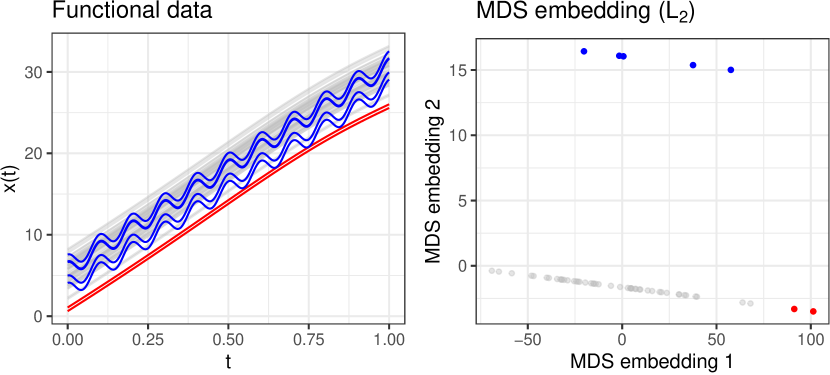
Figure 3: Functional outlier scenario ($n=54,r=.09$) with shape variation inducing structural differences. Off-manifold outliers colored in blue, two on-manifold outliers colored in red.

2.3.2 General functional outlier scenarios

As already noted, the concept of structural difference we propose is much more general. It is straight forward to conceptualize other outlier scenarios with induced structure beyond shape. Consider the following theoretical example: Given a parameter manifold $\Theta\subset[0,\infty]\times[0,\infty]\times[0,\infty]\times[0,\infty]$ and an induced functional manifold $\mathcal{M}=\{f(t);t\in[0,1]:f(t)=\theta_{1}+\theta_{2}t^{\theta_{3}}+I(t\in[\theta_{4}\pm.1])\}$. Each dimension of the parameter space controls a different characteristic of the functional manifold: $\theta_{1}$ the level, $\theta_{2}$ the magnitude, $\theta_{3}$ the shape, and $\theta_{4}$ the presence of an isolated peak around $t=\theta_{4}$.
One can now define a “common” data generating process, i.e. a manifold $\mathcal{M}_{c}$, by holding some of the dimensions of $\Theta$ fixed and only varying the rest, either independently or not. On the other hand, one can define an “anomalous” data generating process, i.e. a structurally different manifold $\mathcal{M}_{a}$, by letting those fixed in $\mathcal{M}_{c}$ vary, or simply setting them to values unequal to those used for $\mathcal{M}_{c}$, or by using different dependencies between parameters than for $\mathcal{M}_{c}$. E.g., if $\theta_{1}=\theta_{2}$ for $\mathcal{M}_{c}$, let $\theta_{1}=-\theta_{2}$ for $\mathcal{M}_{a}$. This implies one can define data generating processes so that any functional characteristic (level, magnitude, shape, “peaks” and their combinations) can be on-manifold or off-manifold outliers, depending on how the “common” data manifold $\mathcal{M}_{c}$ is defined.

Figure 4 shows a setting in which $\mathcal{M}_{c}$ is defined purely in terms of complex shape variation while $\mathcal{M}_{a}$ contains vertically shifted versions of elements in $\mathcal{M}_{c}$: Let $\mathcal{M}_{c}$ be the functional manifold of Beta densities $f_{\text{B}}(t;\theta_{1},\theta_{2})$ with shape parameters $\theta_{1},\theta_{2}\in[1,2]$, and let $\mathcal{M}_{a}$ be the functional manifold of Beta densities with shape parameters $\theta_{1},\theta_{2}\in[1,2]$ shifted vertically by some scalar quantity $\theta_{3}\in[0,0.5]$, that is $\mathcal{M}_{c}=\{f(t);t\in[0,1]:f(t)=f_{\text{B}}(t;\theta_{1},\theta_{2})\}$ with $\Theta_{c}=[1,2]^{2}$ and $\mathcal{M}_{a}=\{f(t);t\in[0,1]:f(t)=f_{\text{B}}(t;\theta_{1},\theta_{2})+\theta_{3}\}$ with $\Theta_{a}=\Theta_{c}\times[0,0.5]$.

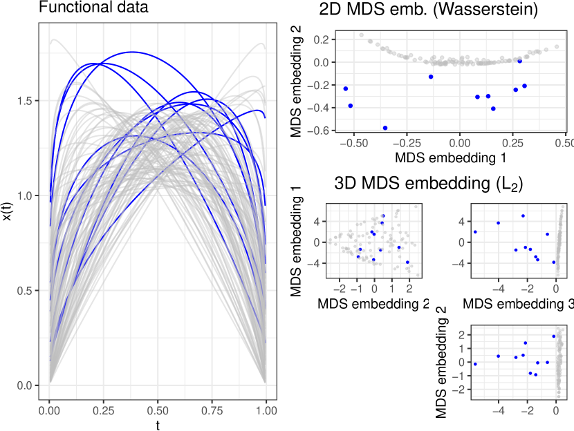
Figure 4: Functional outlier scenario ($n=100,r=.1$) with vertical shifts inducing structural differences. MDS embeddings based on unnormalized $L_{1}$-Wasserstein distances and $L_{2}$ (Euclidean) distances on the right.

As can be seen in Figure 4, both manifolds contain substantial shape variation that is identically structured, but those from $\mathcal{M}_{a}$ are also shifted upwards by small amounts. Note that many shifted observations lie within the main bulk of the data on large parts of the domain. In the 2D embeddings based on unnormalized $L_{1}$-Wasserstein distances [19] (a.k.a. “Earth Mover’s Distance”, top right) and 3D embeddings based on standard $L_{2}$ distances (bottom right), we see that this structure is captured with high accuracy, even though it is hardly visible in the functional data, with most anomalous observations clearly separated from the common manifold data, whose embeddings are concentrated on a narrow sub-region of the embedding space. An observation on $\mathcal{M}_{a}$ which is very close to $\mathcal{M}_{c}$, lying well within the main bulk of functional observations, also appears very close to $\mathcal{M}_{c}$ in both embeddings. This example shows that the two functional manifolds do not need to be completely disjoint nor yield visually distinct observations for our approach to yield useful results. It also shows that the choice of an appropriate dissimilarity metric for the data can make a difference: a 2D embedding is sufficient for the more suitable Wasserstein distance which is designed for (unnormalized) densities (top right panel), while a 3D embedding is necessary for representing the relevant aspects of the data geometry if the embedding is based on the standard $L_{2}$ metric (lower right panels). For a comparison with currently available outlier visualization methods for this example, see Figure 15 in Appendix 0.A.4.

In summary, we propose that the manifold perspective allows to define and represent a very broad range of functional outlier scenarios and data generating processes. We argue that these properties make the geometrical approach very compelling for functional data, because it is flexible, conceptualizes outliers on a much more general level (for example, structural differences not in terms of shape) than before, and allows to theoretically assess a given setting.
Beyond its theoretical utility of providing a general notion of functional outliers, it has crucial practical implications: Outlier characteristics of functional data, in particular structural differences, can be represented and analysed using low dimensional representations provided by manifold learning methods, regardless of which functional properties define the “common” data manifold and which properties are expressed in structurally different observations. From a practical perspective, on-manifold outliers will appear “connected”, whereas off-manifold outliers will appear “separated” in the embedding, and the clearer these structural differences are, the clearer the separation in the embedding will be. Note that this implies that shape outliers, which pose particular challenges to many previously proposed methods, will often be particularly easily detectable. Moreover, all methods for outlier detection that have been developed for tabular data inputs can be (indirectly) applied to functional data as well based on this framework, simply by using the embedding coordinates as feature inputs: The embedding space $\mathcal{Y}$ is typically a low dimensional Euclidean space in which conventional outlier detection works well and the essential geometrical structure encoded in the pairwise functional distance matrix is conserved in these lower-dimensional embeddings. In the next section, we illustrate this practical utility in detail by extensive quantitative and qualitative analyses.

3 Experiments

To illustrate the practical relevance of the outlined geometrical approach, we first qualitatively investigate real data sets. In the second part of this section, we quantitatively investigate the anomaly detection performance of several detection methods based on synthetic data.

3.1 Qualitative analysis of real data

We start with an in-depth analysis of the ECG200 data [4, 40], a functional data set with complex structure: it seems to contain subgroups with phase and amplitude variation and different mean functions. As a result, the data set appears visually complex (Figure 5, left). Without the color coding it would be challenging to identify the three subgroups (see lower left plot in Figure 6). Moreover, there are five left shifted observations (apparent at $t\in[10,25]$) and a single (partly) vertical shift outlier (apparent at $t\in[50,75]$) clearly detectable by the naked eye.

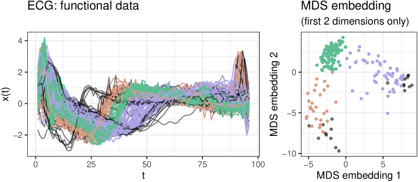
Figure 5: ECG curves and first two embedding dimensions (of five). Colors highlight subgroups apparent in the embeddings. Potential outliers with 5D-embedding LOF scores (minPts = $0.75n$) in top decile shown in black.

Much of the general structure (and the anomaly structure in particular) becomes evident in a 5D MDS embedding. To begin with, in the first two embedding dimensions, depicted on the right-hand side of Figure 5, three subgroups are easily recognizable. Color coding in Figure 5 is based on this visualization. It makes apparent that the substructures correspond to two smaller, horizontally shifted subgroups of curves (red: left-shifted, purple: right-shifted), and a central subgroup encompassing the majority of the observations (green). In addition, we computed LOF scores on the 5D embedding coordinates. The observations with LOF scores in the top decile are shown in black in Figure 5, two which the clearly outlying observations belong.
More importantly, note that these observations are clearly separated from the rest in a 5D embedding: the five clearly left shifted observations in the fourth embedding dimension and the single vertically shifted observation in the subspace spanned by the first and third embedding dimension: Figure 6 shows a scatterplot matrix of all five embedding dimensions with observations color-coded according to the 5D-embedding LOF scores. The clear left shifted outliers obtain the highest LOF scores due their isolation in the subspaces including the fourth embedding dimension. Note, moreover, that other observations with higher LOF scores appear in peripheral regions of the different subspaces, but they are not as clearly separable as the six observations described before. Regarding Figure 7 A, which shows the 20 most outlying curves according to the LOF scores, this can be explained by the fact that these other observations stem from one of the two shifted subgroups and can thus be seen as on-manifold outliers, whereas the six other, visually clearly outlying observation are clear off-manifold outliers.

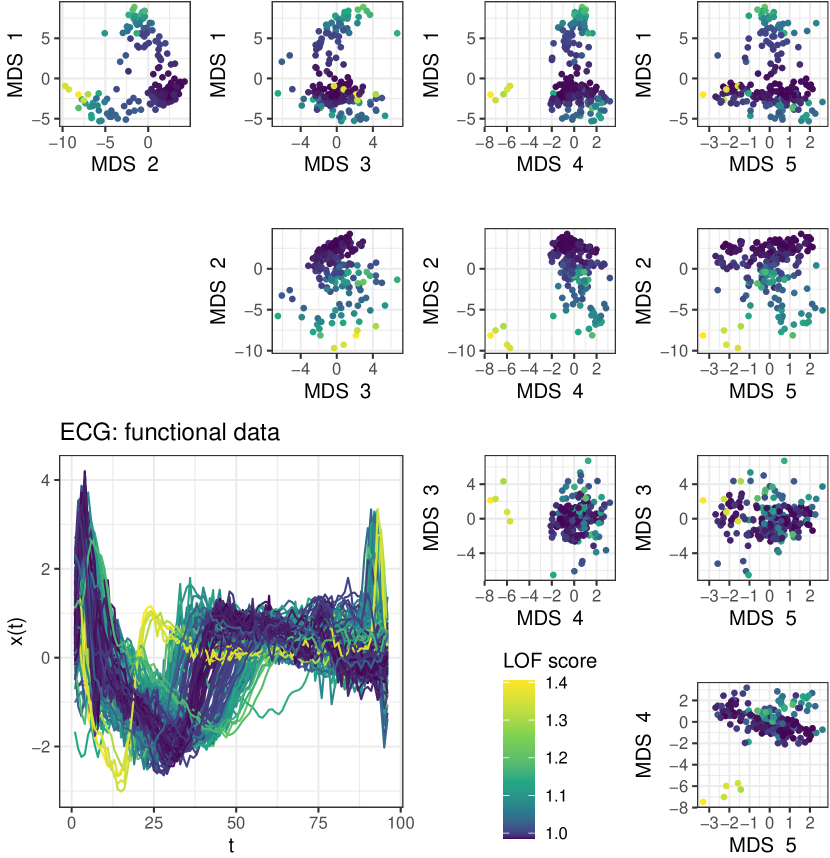
Figure 6: ECG data: Scatterplotmatrix of all 5 MDS embedding dimensions and curves, lighter colors for higher LOF score of 5D embeddings.

We contrast these findings with the results of directional outlyingness [10, 11], which performs very well (see section 3.2) on simple synthetic data sets. Figure 7 shows the ECG curves color-coded by variation of directional outlyingess (B), the 20 most outlying curves by variation of directional outlyingness (C) and the observations labeled as outliers by directional outlyingness respectively by the MS-plot (D). First of all, it can be seen that many observations yield high variation of directional outlyingness and observations in the right shifted subgroup obtain most of the highest values. In fact, among the 20 observations with highest variation of directional outlyingness, only one is from the left shifted group and 13 are from the right-shifted group. Moreover, applying directional outlyingness to this data set results in 72 observations being labeled as outliers, which is about 36 percent of all observations. We would argue that it is questionable whether 36 percent of all observations should be labeled as outliers.
In this regard, the ECG data serves as an example which illustrates the advantages of the geometric approach. First of all, it yields readily available visualizations, which reflect much more of the inherent structure of a data set than only anomaly structure. This is specifically important for data with complex structure (i.e., subgroups or multiple modes and large variability). Moreover, it allows to apply well-established and powerful outlier scoring methods like LOF to functional data. This exemplifies that the approach not only improves theoretical understanding and consideration as outlined in the previous section, it also has large practical utility in complex real data settings in which previously proposed methods may not provide useful answers.

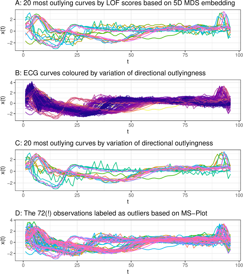
Figure 7: ECG data: LOF on MDS embeddings in contrast to directional outlyingness

In the ECG example, we have seen that a 5D embedding yielded reasonable results and sufficiently reflected many aspects of the data. In particular, the extremely left-shifted observations became clearly separable in the 4th embedding dimension. In appendix 0.A.5 we analyse a synthetic data set in the same way as the ECG data, which yields similar findings. Moreover, note that the Spearman rank correlation between LOF scores computed on the 5D embedding and LOF scores computed directly on the ECG data distances is 0.99. This shows that outlier structure retained in the 5D embedding is highly consistent with the outlier structure in the high dimensional observation space, an important aspect with respect to anomaly scoring methods requiring (low dimensional) tabular inputs.
Finally, note that even fewer than five embedding dimensions may suffice to reflect much of the inherent structure. Consider the examples depicted in Figure 8, which shows the functional observations and the first two embedding dimensions of a corresponding 5D MDS embedding of another four real data sets. The Octane data consist of spectra from 60 gasoline samples [46, 29], the Spanish weather data of annual temperature curves of 73 weather stations [16], the Tecator data of spectrometric curves of meat samples [16, 17], and the Wine data of spectrometric curves of wine samples [23, 4]. As before, the observations are colored according to LOF scores based on the 5D embedding. In addition, the 12 observations with highest LOF scores are depicted as triangles. These data sets are much simpler than the ECG data and the first two embedding dimensions already reflect the (outlier) structure fairly accurately: observations with high LOF scores appear separated in the first two embedding dimensions and more general substructures are revealed as well. The substructure of the weather data is rather obvious already regarding the functional observations, for example, the observations with less variability in terms of temperature, all of which obtain high LOF scores. The substructure of the wine data – for example the small cluster in the lower part of the embedding – is much harder to detect based on visualizations of the curves alone. Figure 16 in appendix 0.A.4 shows results for the “Outliergram” by Aribas-Gil & Romo [2] for shape outlier detection as well as the magnitude-shape plot method of Dai & Genton [10] for these example data sets for comparison. We would argue that the embedding based visualizations offers a much more informative visualization of the structure of these data.
Appendix 0.A.2 summarizes a more detailed analysis of the sensitivity of the approach to the choice of the dimensionality of the embedding. We conclude that sensitivity seems to be fairly low. For all 5 real data sets we consider, the rank order of LOF scores is very similar or even identical whether based on 2, 5 or even 20 dimensional embeddings (c.f. Table 1).
Following Mead [36], we quantify the goodness of fit (GOF) for a $d_{1}$-dimensional MDS embedding as $GOF(d_{1})=\frac{\sum_{i=1}^{d_{1}}\max(0,\lambda_{i})}{\sum_{j=1}^{n}\max(0,\lambda_{j})},$ where $\lambda_{k}$ are the eigenvalues (sorted in decreasing order) of the $k$th eigenvectors of the centered distance matrix. For all of the considered real data sets, a 5D embedding achieved a goodness of fit over 0.8, the four less complex examples even over 0.95 (see Figure 13). As a rule of thumb, the embedding dimension does not seem crucial as long as the goodness of fit (GOF) of the embedding is over 0.8 for $L_{2}$ distances. This rule of thumb also yields compelling quantitative performance results, as shown in section 3.2.

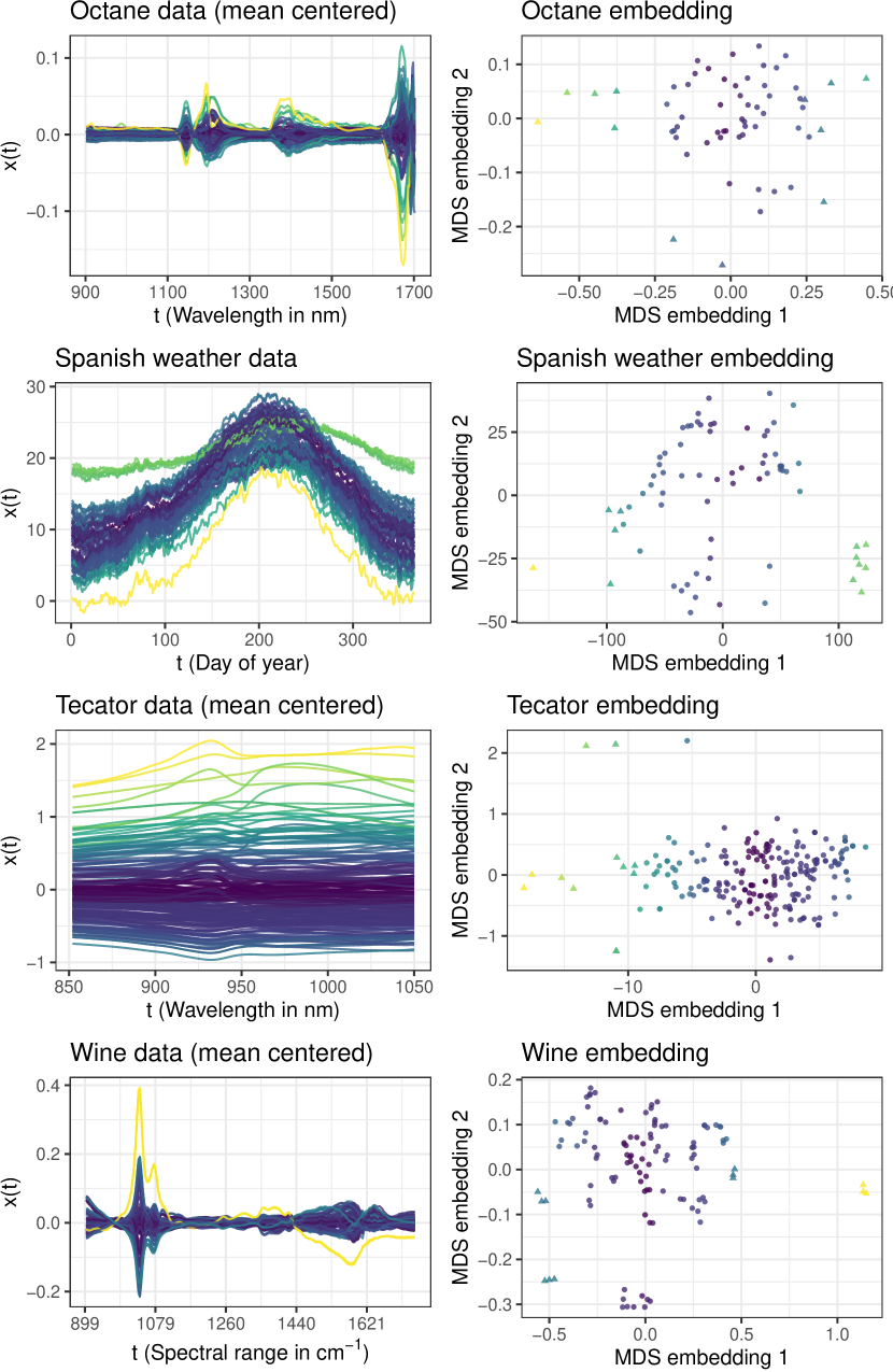
Figure 8: Further examples of real functional data colored by LOF score. The 12 most outyling observations depicted as triangles in the embedding.

3.2 Quantitative analysis of synthetic data

In this section we investigate the outlier detection performance quantitatively, based on synthetic data sets for which the true (outlier) structure is known.

3.2.1 Methods

In addition to applying LOF to 5D embeddings and directly to the functional data, we investigate the performance of two “functional data”-specific outlier detection methods: directional outlyingness (DO) [10, 11] and total variational depth (TV) [24]. We use implementations provided by package fdaoutlier [39] and use the variation of directional outlyingness as returned by function $\verb|dir_out|$ as outlier scores for DO and the total variation depths as returned by function $\verb|total_variation_depth|$ for TV.

3.2.2 Data Generating Processes

The methods are applied to data from four different data generating processes (DGPs), the first two of which are based on the simulation models introduced by Ojo et al. [38] and provided in the corresponding R package $\verb|fdaoutlier|$ [39]. We also provide the results of additional experiments based on the original DGPs from package fdaoutlier in Appendix 0.A.3. However, we consider most of these DGPs as too simple for a realistic assessment, as most methods achieve almost perfect performance on them and we use more complex DGPs here. In both DGP 1 and 2, the inliers from $\verb|simulation_model1|$ from package fdaoutlier serve as $\mathcal{M}_{c}$, i.e. the common data generating process. This results in simple functional observations with a positive linear trend. In addition, $\verb|simulation_model1|$ generates simple shift outliers. Additionally, our DGP 1 also includes shape outliers stemming from $\verb|simulation_model8|$ which serves as $\mathcal{M}_{a}$. In contrast, DGP 2 contains shape outliers from all of the other DGPs in fdaoutlier, which means $\mathcal{M}_{a}$ contains observations from several different data generating processes.
For DGPs 3 and 4, we define $\mathcal{M}_{c}$ by generating a random, wiggly template function over $[0,1]$ for each data set, generated from a B-spline basis with 15 or 25 basis functions, respectively, with i.i.d. $\mathcal{N}(0,1)$ spline coefficients. Functions in $\mathcal{M}_{c}$ are generated as elastically deformed versions of this template, with random warping functions drawn from the ECDFs of $\text{Beta}(a,b)$ distributions with $a,b\sim U[4,6]$ (DGP 3) or $a,b\sim U[3,8]$ (DGP 4). Functions in $\mathcal{M}_{a}$ are also generated as elastically deformed versions of this template, with Beta ECDF random warping functions with $a,b\sim U[3,4]$ for DGP 3 and with 50:50 Beta mixture ECDF random warping functions with $a,b\sim 0.5U[3,8]:0.5U[0.1,3]$ (DGP 4). Finally, white noise with $\sigma=0.1,0.15$, respectively, for DGP 3 and 4 is added to all resulting functions. Appendix 0.A.6 shows visualizations of example data sets drawn from these DGPs.

3.2.3 Performance assessment

From these four DGPs we sampled data $B=500$ times with three different outlier ratios $r\in\{0.1,0.05,0.01\}$. Based on the outlier scores, we computed the Area-under-the-ROC-Curve (AUC) as performance measure and report the results over all 500 replications. Note that, for $r\in\{0.1,0.05\}$, the number of sampled observations is $n=100$, whereas for $r=0.01$ we sampled $n=1000$ observations.

3.2.4 Results

First of all, note that LOF directly applied to functional data as well as LOF applied to 5D embeddings yield very similar results. This agrees with our findings in the qualitative analyses. In the following, we simply refer to the geometrical approach and do not distinguish between LOF based on MDS embeddings and LOF applied directly to the functional distance matrix. Figure 9 shows that the geometrical approach is highly competitive with functional-data-specific outlier detection methods. It yields better results than TV for all of the four DGPs and performs at least on par with DO. In comparison to DO it performs better on DGP 1 and DGP 3, on par on DGP 4, worse on DGP 2. Note that DO struggles to detect simple shift outliers: of all methods it performs worst on the first DGP. Similar conclusions can be reported for other settings, where it performs even worse if there are only shift outliers (c.f. Figures 14, 18).
In summary, based on the conducted experiments the geometrical approach leads to outlier scoring performances at least on par with specialized functional outlier detection methods even if based on fairly basic methods (MDS with $L_{2}$ distances and LOF). Going further, our approach can be adapted to specific settings simply by choosing metrics other than $L_{2}$. As the next section shows, this can improve the outlier detection performance considerably.

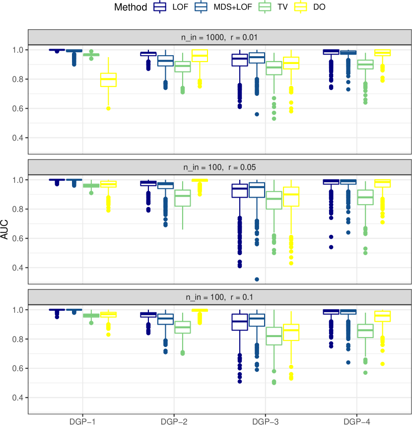
Figure 9: Distribution of AUC over the 500 replications for the different data generating processes (DGP), outlier detection methods, and outlier rations $r$.

3.3 General dissimilarity measures and manifold methods

So far, we have computed MDS embeddings mostly based on $L_{2}$ distances. In the following we show that the approach is more general. The geometric structure of a data set is captured in the matrix of pairwise distances among observations. Different metrics emphasize different aspects of differences in the data and can thus lead to different geometries. MDS based on $L_{2}$ distances yielded compelling results in many of the examples considered above, but other distances are likely to lead to better performance in certain settings. To illustrate the effect, we consider two additional settings – one simulated and one on real data – in the following. The results are displayed in Figure 10.
The simulated setting is based on isolated outliers, i.e. observations which deviate from functions in $\mathcal{M}_{c}$ only on small parts of their domain. In such settings, higher order $L_{p}$ metrics lead to better results, since such metrics amplify the contribution of small segments with large differences to the total distance. We use as an example data generated from $\verb|simulation_model2|$ from package $\verb|fdaoutlier|$. Figure 10 A shows the AUC values of LOF scores on MDS embeddings based on $L_{2}$ and $L_{10}$ distances. Again, 500 data sets were generated form the model over different outlier ratios. In contrast to $L_{2}$-based MDS, using $L_{10}$ distances yields almost perfect detection. In embeddings based on $L_{10}$, isolated outliers are clearly separable in the first two or three embedding dimensions.
As a second example, we consider the ArrowHead data set [13, 51], which contains outlines of three different types of neolithic arrowheads (see Appendix 0.A.7 for visualizations of the data set). Using the 78 structurally similar observations from class “Avonlea” as our data on $\mathcal{M}_{c}$ and sampling outliers from the 126 structurally similar observations from the other two classes, we can compute AUC values based on the given class labels. We generate 500 data sets for each outlier ratio $r\in\{0.05,0.1\}$. Since there are only 78 observations in class “Avonlea”, we do not use $r=0.01$ for this example. Embeddings are computed using three different dissimilarity measures: the standard $L_{2}$ metric, the unnormalized $L_{1}$-Wasserstein metric [19], and the Dynamic Time Warping (DTW) distance [42]. Note that the DTW distance does not define a proper metric [31].

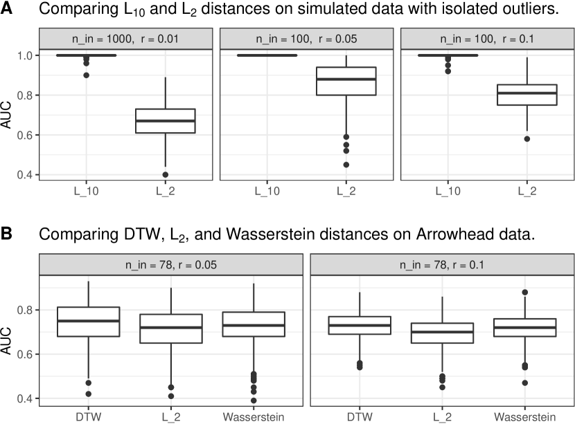
Figure 10: Comparing the effects of different distance measures. Depicted are the distributions of AUC over 500 replications for LOF based on MDS embeddings computed with the respective distance measures for different outlier ratios $r$. A: Comparing $L_{10}$ and $L_{2}$ metric on a data set with isolated outliers generated via simulation model 2 from package fdaoutlier. B: Comparing DTW, $L_{2}$, and unnormalized $L_{1}$-Wasserstein distance measures on real data set ArrowHead. Note: the DTW distance is not a metric.

Figure 10 B shows that small performance improvements can be achieved in this case if one uses dissimilarity measures that are more appropriate for the comparison of shapes, but not as much as in the isolated outlier example. Note that even though DTW distance is not a proper metric, it improves outlier scoring performance in this example. This indicates that, from a practical perspective, general dissimilarity measures can be sufficient for our approach to work. This opens up further possibilities, as there are many general dissimilarity measures for functional data, for example the semi-metrics introduced by Fuchs et al. [18]. Overall, these examples illustrate the generality of the approach: using suitable dissimilarity measures can make the respective structural differences more easily distinguishable.

More complex embedding methods, on the other hand, do not necessarily lead to better or even comparable results as MDS. Figure 11 shows the distribution of AUC for embedding methods ISOMAP and UMAP. Both methods require a parameter that controls the neighborhood size used to construct a nearest neighbor graph from which the manifold structure of the data is inferred. The larger this value, the more of the global structure is retained. For both methods, embeddings were computed for very small and very large neighborhood sizes of 5 and 90.
The results show that neither method performs better than MDS, UMAP even performs considerably worse. Note that ISOMAP is equivalent to MDS based on the geodesic distances derived from the nearest neighbor graph and the larger the neighborhood size the more similar to direct pairwise distances these geodesic distances become. This is also reflected in the results, as ISOMAP-90 performs better than ISOMAP-5 on average. For DGP-2, ISOMAP-90 slightly outperforms MDS, indicating that more complex manifold methods could improve results somewhat in specific settings.
In general, however, these findings confirm the theoretical considerations sketched in section 2.2. Embedding methods which preserve the geometry of the space $\mathcal{F}$ of which $\mathcal{M}_{c}$ and $\mathcal{M}_{a}$ are sub-manifolds, i.e. the ambient space geometry, are more suited for outlier detection than methods which focus on approximating the intrinsic geometry of the manifold(s). Thus, more sophisticated embedding methods which often focus on approximating the intrinsic geometry should not be applied lightly and certainly require careful parameter selection in order to be applicable for outlier detection. Since hyperparameter tuning for unsupervised methods remains an unsolved problem, this is unlikely to be achieved in real-world applications. In particular, consider that both UMAP and t-SNE [33] have been found to be – in general – oblivious to local density, which means that clusters of different density in the observation space tend to become clusters of more equal density in the embedding space [37]. Although there may exist a parameter setting where this effect is reduced (note that there are now density-preserving versions of t-SNE and and UMAP [37]), we are skeptical that outliers can be faithfully represented in such an embedding given the difficulties of hyperparameter tuning in unsupervised settings. Moreover, these methods are not designed to preserve important aspects of the outlier structure. For example, UMAP is subject to a local connectivity constraint which ensures that every observation is at least connected to its nearest neighbor (in more technical terms: that a vertex in the fuzzy graph approximating the manifold is connected by at least one edge with an edge weight equal to one [35]), which makes it unlikely that UMAP can be tuned so that it is able to sensibly embed off-manifold outliers, which should, by definition, not be connected to the common data manifold. The poor performance of UMAP embeddings in our experiments confirms these concerns.

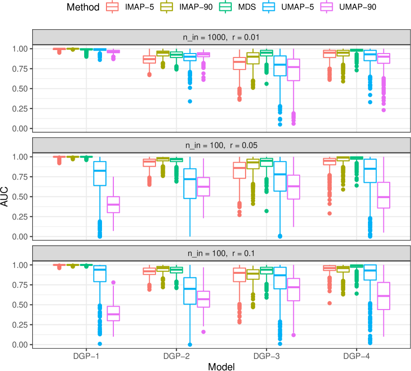
Figure 11: Comparing UMAP and ISOMAP to MDS. UMAP and ISOMAP embeddings have been computed for two different locality parameter values: 5 and 90. Distribution of AUC over 500 replications of the four DGPs for different outlier ratios $r$. AUC computed on LOF scores based on 5D embeddings.

4 Discussion

Based on a geometrical perspective of functional outlier detection, we define two general types of functional outliers: off- and on-manifold outliers. Our investigation shows that this perspective clarifies the theoretical concepts and improves practical results. From a theoretical perspective it allows to formalize functional outlier scenarios in precise and consistent terms, beyond differences in terms of either shape, level or magnitude. This simplifies reasoning about specific outlier settings and provides a fully general theoretical conceptualization of the problem.
From an applied perspective, we formulate two important consequences. First of all, as has been demonstrated with a comprehensive analysis of a complex, real data set of ECG curves, the geometrical approach allows for easily accessible and highly informative visualizations. These are obtained by means of low dimensional embeddings reflecting the inherent structure of a functional data set in much detail. Such visualizations provide more accurate and complete pictures of the (outlier) structure of functional data. In particular, off-manifold outliers reliably appear as clearly separated (groups of) points in the low dimensional embeddings.
Second, the proposed approach makes it possible to apply highly-developed and performant standard outlier detection methods to functional data, since the geometric structure of the data is captured and reflected in their pairwise distance matrices. Outlier detection and scoring methods which can be applied to distance matrices directly can therefore be used for functional data as well. Furthermore, detection methods requiring tabular inputs can also be applied simply by using the embedding coordinates obtained with embedding methods as proxy data for the original functions. Our experiments using LOF scores show that the two approaches yield very similar results. This simultaneously simplifies and improves functional outlier detection: It simplifies, since functional data analysis becomes more accessible to a broader audience with general outlier detection methods that are widely used in other areas and that do not require an understanding of complex methodological details of functional data methods. It improves the state of the art since many functional outlier methods can only detect specific kinds of functional outliers by design, or fail in more complex realistic data that are widely dispersed or that contain multiple non-outlying subgroups like the ECG data. Moreover, note that our proposal is not limited to univariate functional data. Extending it to multivariate functions is completely straightforward, as long as a suitable dissimilarity measure is available to compute pairwise distances.
In this paper, most embeddings were obtained using MDS based on $L_{2}$ distances. This implies a close similarity to functional bagplots and highest density region (HDR) boxplots [26], which are based on the first two robust principal component scores. However, this similarity only applies if our geometrical approach is implemented with 2D MDS embeddings based on $L_{2}$ distances. As outlined, our proposal is neither limited to the $L_{2}$ metric as a distance measure nor to MDS as an embedding method or just two embedding dimensions. Other metrics and (higher-dimensional) embedding methods can be used and the conducted experiments indicate that alternative distance measure can further improve the performance in specific settings, sometimes considerably. In particular, even non-metric dissimilarity measures may be applicable as our results based on DTW distances indicate. On the other hand, the results also show that more sophisticated embedding methods such as ISOMAP and UMAP cannot be used as straightforwardly as MDS. Such methods, which do not take into account the ambient space geometry by default, at least require very careful parameter selection. In terms of practical applicability, the $O(n^{3})$ time complexity and $O(n^{2})$ storage complexity of standard MDS may prove problematic for large data, but generalizations such as Landmark MDS [14], Pivot MDS [5] or multilevel MDS exploiting GPU performance [28] scale much better with the number of available observations.
Finally, we would argue that existing functional outlier detection approaches mostly lack the principled geometrical underpinning and conceptualization presented here. As outlined, we argue that such a conceptualization is necessary to make functional outlier detection tractable in full generality. Specifically, consider that existing methods typically limit themselves to creating a 1D or 2D representation of each curve (e.g., MBD-MEI, MO-VO, functional bagplots, HDR plots), often based on preconceived notions of the characteristics of functional outliers. Our investigations and experiments suggest that this is often not sufficient for real-world functional outlier detection: First, there is no reason to limit representations to two dimensions with modern outlier detection methods, and the geometrical perspective often strongly suggests otherwise in the case of complex functional data. Even more importantly, it is much more flexible to learn maximally informative low dimensional representations directly from data instead of starting with rather a rigid notion of which characteristics to look at and to ignore the rest. The latter is likely to lead to results not capturing the entire (outlier) structure of a given data set, which is essential in real-world unsupervised settings and exploratory analyses.
Based on theoretical considerations and the empirical results outlined above, we conclude that the proposed approach is well suited for both theoretical conceptualization and practical implementation of functional outlier detection. In particular, the choice of embedding method should consider whether it is able to preserve the extrinsic geometry of the function space and simple MDS embeddings based on functional distances provide a very strong baseline for that. On the basis of this work we intend to further investigate the implications of the geometrical perspective, such as the effects of other dissimilarity measures, embedding and outlier detection methods, in future research.

Acknowledgements
This work has been funded by the German Federal Ministry of Education and Research (BMBF) under Grant No. 01IS18036A. The authors of this work take full responsibility for its content.

Reproducibility
All R code and data to fully reproduce the results are freely available on GitHub: https://github.com/HerrMo/fda-geo-out.

Appendix 0.A Appendix

0.A.1 Formalizing phase variation scenarios

Phase variation - Case I: The manifold $\mathcal{M}=\{x(t):x(t)=\theta_{1}\varphi(t-\theta_{2}),\mathbf{\theta}=(\theta_{1},\theta_{2})^{\prime}\in\Theta\}$, with $\varphi(.)$ the standard Gaussian pdf and $\Theta=[0.1,2]\times[-2,2]$, defines a functional data setting with independent amplitude and phase variation. Since there is a single manifold only, there are no structural novelties. Figure 12 top depicts the functional observations on the left and a 2D embedding obtained with MDS on the right. Note, all of the curves are subject to amplitude and phase variation to varying extent, however, there are no clearly “outlying” or “outstanding” observations in terms of either amplitude or phase. This is reflected in the corresponding embedding, which does not show any clearly separated observations in the embedding space, indicating that there are no structurally different observations. The situation in the second case of phase-varying data, however, is different.

Phase variation - Case II: The two manifolds $\mathcal{M}_{c}=\{x(t):x(t)=\theta\varphi(t+1),\theta\in\Theta\}$ and $\mathcal{M}_{a}=\{x(t):x(t)=\theta\varphi(t),\theta\in\Theta\}$, with $\Theta=[0.1,2]$, describe a similar scenario as before, however, there are two structurally different manifolds induced by the shift in the argument of $\varphi$. In contrast to the first case, there are on-manifold and off-manifold outliers. Figure 12 mid depicts the functional observations and the corresponding embedding. Clearly, in this example few (blue) curves, the ones from $\mathcal{M}_{a}$, show a horizontal shift compared to the normal data and consequently those few curves appear horizontally “outlying”. Within the main data manifold, only on-manifold outliers in terms of amplitude exist. These aspects are reflected in the corresponding embedding: the low-dimensional representations of the blue curves are clearly separated from those of the main data in grey.
Of course such clear settings – in particular phase varying functional data with fixed and distinct phase parameters – will seldom be observed in practice. A more realistic example is given by $\mathcal{M}_{c}=\{x(t):x(t)=\theta_{1}\varphi(t-\theta_{2}),(\theta_{1},\theta_{2})^{\prime}\in\Theta_{c}\}$ and $\mathcal{M}_{a}=\{x(t):x(t)=\theta_{1}\varphi(t-\theta_{2}),(\theta_{1},\theta_{2})^{\prime}\in\Theta_{a}\}$, with $\Theta_{c}=[0.1,2]\times[-1.3,-0.7]$ and $\Theta_{a}=[0.1,2]\times[-0.5,0.1]$. Here we have again two structurally different manifolds. This is more realistic, since the “phase parameters” $\theta_{2}$ are not fixed but are subject to random fluctuations. In addition, the structural difference induced by the phase parameters is much smaller. Considering Figure 12 bottom, again this is reflected in the embedding: there are two separable structures, however the differences are not as clear as in the second example above.
The three examples together show that the less similar the processes are and/or the less variability there is within the phase parameters defining the manifolds, the clearer structural differences induced by horizontal variation become visible in the embeddings.

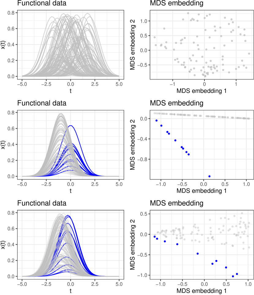
Figure 12: Functional data with phase variation and different levels of structural difference. Top: Scenario with no off-manifold outliers. Mid: Scenario with clear off-manifold outliers. Bottom: Intermediate scenario.

0.A.2 Sensitivity analysis

The differences in complexity among the ECG and the other four real data sets become apparent in Figure 13 as well, which shows how the goodness of fit (GOF) of the embeddings is affected by their dimensionality. For the $L_{2}$ metric, a goodness of fit over 0.9 is achieved with two to three embedding dimensions for the less complex data sets. Moreover, all of them reach a saturation point at five dimensions. This is in contrast to the ECG data, where the first five embedding dimensions lead to a goodness of fit of 0.8. Moreover, the ranking induced by LOF scores is very robust to the number of embedding dimensions. As Table 1 shows, the rank correlations between LOF scores based on five and LOF scores based on 20 embedding dimensions are very high for all data sets.

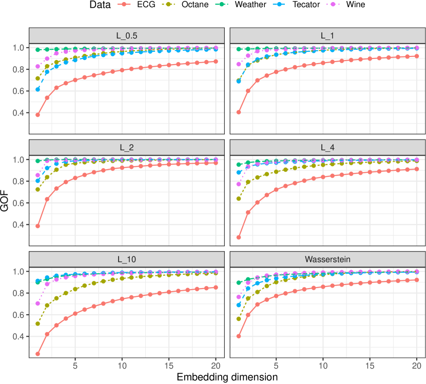
Figure 13: Goodness of fit (GOF) of different embedding dimensions for the five considered real data sets and $L_{0.5},L_{1},L_{2},L_{4},L_{10},$ and unnormalized $L_{1}$-Wasserstein metrics.

Table 1: Spearman correlation between LOF scores based on embeddings of different dimensionality for the 5 considered real data sets and metrics $L_{0.5}$, $L_{1}$, $L_{2}$, $L_{4}$, $L_{10}$, and unnormalized $L_{1}$-Wasserstein. MDS embeddings with 5 dimensions are compared to embeddings with 2 (2vs5) and 20 (5vs20) dimensions.

	$L_{0.5}$		$L_{1}$		$L_{2}$		$L_{4}$		$L_{10}$		Wasserstein
	2vs5	5vs20	2vs5	5vs20	2vs5	5vs20	2vs5	5vs20	2vs5	5vs20	2vs5	5vs20
ECG	0.96	0.97	0.98	0.97	0.97	0.99	0.94	0.98	0.85	0.94	0.98	0.97
Octane	0.94	0.99	0.96	0.98	0.97	0.99	0.98	0.99	0.94	0.97	0.95	0.96
Weather	1.00	1.00	1.00	1.00	1.00	1.00	1.00	1.00	1.00	1.00	1.00	1.00
Tecator	0.97	0.99	0.96	0.99	0.99	1.00	0.99	1.00	0.99	1.00	0.96	0.99
Wine	0.98	0.99	0.99	1.00	1.00	1.00	0.99	1.00	0.98	0.99	0.99	1.00

0.A.3 Quantitative results on fdaoutlier package DGPs

The simulation models presented by Ojo et al. [38] cover different outlier scenarios: vertical shifts (model 1), isolated outliers (model 2), partial magnitude outliers (model 3), phase outliers (model 4), various kinds of shape outliers (models 5 - 8) and amplitude outliers (model 9). A detailed description can be found in the vignette accompanying their R package. The same methods and performance evaluation approach as in section 3.2 are used in the following.
As Figure 14 shows, (almost) perfect performance is achieved by at least two methods for models 1, 3, 4, 8, and 9; DO shows almost perfect performance for all models except model 1. For models 2, 5, 6, and 7 the methods based on the geometric approaches do not perform equally well (as does TV). However, as outlined in section 3.3, perfect performance can be achieved for model 2 by using $L_{10}$ distances instead of $L_{2}$ distances.
Furthermore, for models 5, 6, and 7 it has to be taken into account that the AUC values only reflect detection of “true outliers”, which can now – given the geometric perspective – be specified more precisely as off-manifold outliers (observations from $\mathcal{M}_{a}$). However, this does not take into account possible on-manifold outliers. Due to their distributional nature, by chance some on-manifold outliers (observations on $\mathcal{M}_{a}$) can be “more outlying” than some of the off-manifold outliers and thus correctly obtain higher LOF scores. However, such cases are not correctly reflected in the performance assessment approach, as – in contrast to off-manifold outliers – such on-manifold outliers are not labeled as “true outliers”. The observed lower performance in terms of AUC thus can simply mean that there are on-manifold outliers obtaining relatively high LOF scores. In particular, this also does not imply that off-manifold outliers fail to be separated in a subspace of the embedding, as will be outlined appendix 0.A.5 in more detail, nor that perfect AUC performance cannot be obtained via the geometric approaches for these settings. If the geometric approach is applied to the derivatives instead (depicted in Figure 14 as “deriv”) almost perfect performances can be achieved. Obviously, functions of the same shape (i.e. all observations from $\mathcal{M}_{c}$) are very similar on the level of derivatives regardless of how strongly dispersed they are in terms of vertical shift.

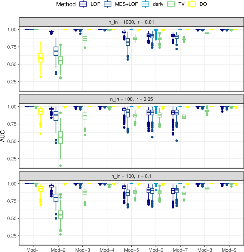
Figure 14: Distribution of AUC over the 500 replications for the different outlier detection methods, simulation models (Mod) from package fdaoutier and outlier ratios $r$.

0.A.4 Comparing embeddings, roahd::outliergram, fdaoutlier::msplot

Figure 16 shows results for the MBD-MEI “Outliergram” by Aribas-Gil & Romo 2; 27, implementation: for shape outlier detection and the magnitude-shape plot method of Dai & Genton [10] for the example data sets shown in Figures 5 and 8.

Both of these visualization methods mostly fail to identify shift outliers (by design, in the case of the outliergram). The outliergram tends to mislabel very central observations as outliers in data sets with little shape variability (e.g. the “shape outliers” detected by MBD-MEI in the central region of the Tecator data) and fails to detect even egregious shape outliers in data sets with high variability (e.g. not a single MBD-MEI outlier for ECG) as well as shape outliers that are also outlying in their level (e.g. the 3 shape outliers identified by msplot in the upper region of the Tecator data). Note that some central functions of the Spanish weather data, which are labeled as outliers by the magnitude-shape-plot (and partly by the outliergram), are also reflected in the 2D embedding in Figure 8. They are fairly numerous relative to the overall sample size and are very similar to each other. As such, they form a clearly defined separate cluster within the data, which can be seen in the middle bottom part of the embedding.

Figure 15 shows the results for the synthetic data example of Figure 4 with 10 true outliers, where the MS plot yields 6 false positives and only 3 true positives, while the Outliergram fails to detect even a single outlier.

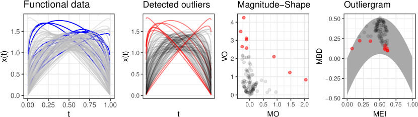
Figure 15: From left: data with true outliers in blue, data with detected outliers in color, magnitude-shape plot of mean directional outlyingness (MO) versus variability of directional outlyingness (VO), outliergram of modified epigraph index (MEI) versus modified band depth (MBD) with inlier region in grey.

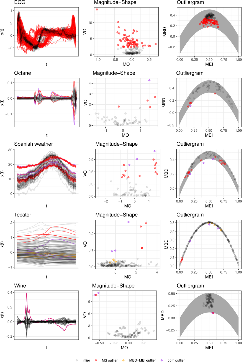
Figure 16: Left column: data, middle column: magnitude-shape plots of mean directional outlyingness (MO) versus variability of directional outlyingness (VO), right column: Outliergram of modified epigraph index (MEI) versus modified band depth (MBD) with inlier region in grey. Curves and points are colored according to outlier status as diagnosed by fdaoutlier::msplot and/or roahd::outliergram.

0.A.5 In-depth analysis of simulation model 7

The analysis of the ECG data in section 3.1 has shown that embeddings can reveal much more (outlier) structure than can be represented by scores and labels. To illustrate the effects described in appendix 0.A.3, we conduct a similar qualitative analysis for an example data set with observations sampled from simulation model 7, see Figure 17. The data set consists of 100 observations with 10 off-manifold or – in more informal terms: “true” – outliers. The functions are evaluated on 50 grid points. The analysis shows that a quantitative performance assessment alone may yield misleading results and again emphasizes the practical value of the geometric perspective and low dimensional embeddings.

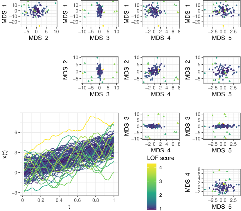
Figure 17: Model 7 data: Scatterplotmatrix of all 5 MDS embedding dimensions and curves, lighter colors for higher LOF score of 5D embeddings. True outliers depicted as triangles. Note that the true outliers are clearly separated from the rest of the data in embedding subspace 3vs4.

First of all, note that the AUC computed for this specific data set is 0.9, thus close to the median AUC value for LOF applied to MDS embeddings of model 7 data, as depicted in Figure 14. Nevertheless, the “true outliers” are clearly separable in a 5D MDS embedding. As Figure 17 shows, they are clearly separable in the subspace spanned by the third and fourth embedding dimension. Note, moreover, that there is an outlying observation with an extreme shift, which also obtains a high LOF score. This observation is not labeled as a “true outlier” as it stems from $\mathcal{M}_{c}$. This example shows that evaluation approaches for outlier detection methods which are based on “true outliers” may not always reflect the outlier structure adequately and may result in misleading conclusions. However, those approaches are frequently used to compare and assess different outlier detection methods. Again, this illustrates the additional value low dimensional embeddings have for outlier detection as such aspects become accessible.
Finally, note that DO/MS-plots are not sensitive to vertical shift outliers as the extreme shift outlier is neither scored high based on DO nor labeled as an outlier based on the MS-plot, see Figure 18.

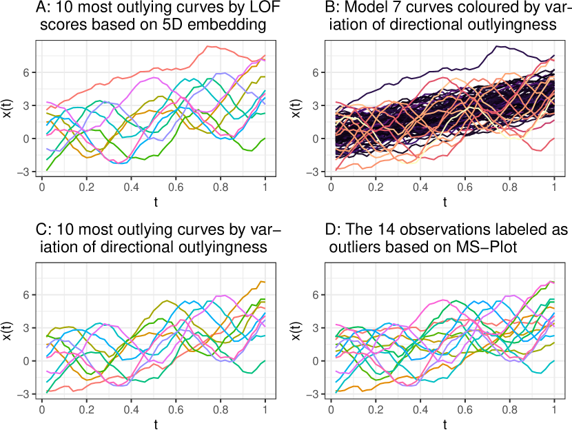
Figure 18: Model 7 data: LOF on MDS embeddings in contrast to directional outlyingness.

0.A.6 Examples for DGPs used for quantitative evaluation

Depicted in Figure 19 are two example data sets for each of the data generating processes (DGP) used in section 3.2 for the comparison of the different outlier detection methods.

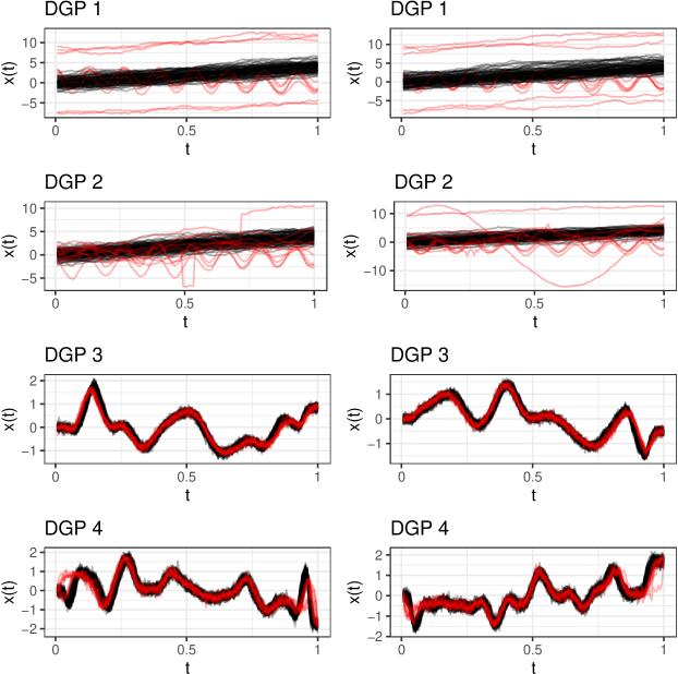
Figure 19: Example data sets for the DGPs used in the simulation study (2 each). Inliers in black, outliers in red. Outlier ratio 0.1, $n=100$.

0.A.7 Arrowhead data

Depicted in Figure 20 are the ArrowHead data used in section 3.3.

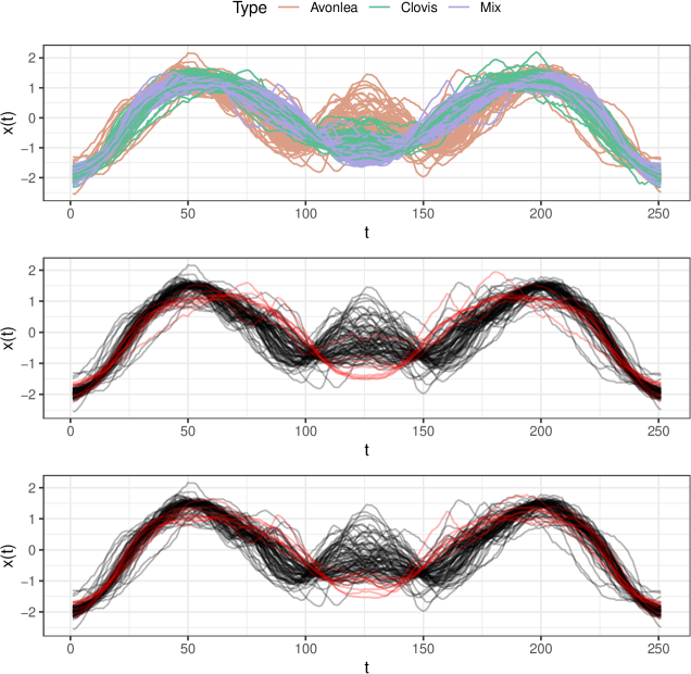
Figure 20: ArrowHead data. Top: The complete data set. Mid and bottom: Two example outlier data sets. Inliers from class ‘Avonlea’ in black, outliers sampled from classes ‘Clovis’ and ‘Mix’ in red. Outlier ratio 0.1.

References

- [1] Ali, M., Jones, M.W., Xie, X., Williams, M.: TimeCluster: dimension reduction applied to temporal data for visual analytics. The Visual Computer 35(6), 1013–1026 (2019)
- [2] Arribas-Gil, A., Romo, J.: Shape outlier detection and visualization for functional data: the outliergram. Biostatistics 15(4), 603–619 (2014)
- [3] Arribas-Gil, A., Romo, J.: Discussion of “Multivariate functional outlier detection”. Statistical Methods & Applications 24(2), 263–267 (2015)
- [4] Bagnall, A., Lines, J., Bostrom, A., Large, J., Keogh, E.: The great time series classification bake off: a review and experimental evaluation of recent algorithmic advances. Data mining and knowledge discovery 31(3), 606–660 (2017)
- [5] Brandes, U., Pich, C.: Eigensolver methods for progressive multidimensional scaling of large data. In: International Symposium on Graph Drawing. pp. 42–53. Springer (2006)
- [6] Breunig, M.M., Kriegel, H.P., Ng, R.T., Sander, J.: LOF: identifying density-based local outliers. In: Proceedings of the 2000 ACM SIGMOD international conference on Management of data. pp. 93–104 (2000)
- [7] Chen, D., Müller, H.G.: Nonlinear manifold representations for functional data. The Annals of Statistics 40(1), 1–29 (2012)
- [8] Cox, M.A., Cox, T.F.: Multidimensional scaling. In: Handbook of data visualization, pp. 315–347. Springer (2008)
- [9] Cuevas, A.: A partial overview of the theory of statistics with functional data. Journal of Statistical Planning and Inference 147, 1–23 (2014)
- [10] Dai, W., Genton, M.G.: Multivariate functional data visualization and outlier detection. Journal of Computational and Graphical Statistics 27(4), 923–934 (2018)
- [11] Dai, W., Genton, M.G.: Directional outlyingness for multivariate functional data. Computational Statistics & Data Analysis 131, 50–65 (2019)
- [12] Dai, W., Mrkvička, T., Sun, Y., Genton, M.G.: Functional outlier detection and taxonomy by sequential transformations. Computational Statistics & Data Analysis 149, 106960 (2020)
- [13] Dau, H.A., Bagnall, A., Kamgar, K., Yeh, C.C.M., Zhu, Y., Gharghabi, S., Ratanamahatana, C.A., Keogh, E.: The UCR time series archive. IEEE/CAA Journal of Automatica Sinica 6(6), 1293–1305 (2019)
- [14] De Silva, V., Tenenbaum, J.B.: Global versus local methods in nonlinear dimensionality reduction. In: NIPS. vol. 15, pp. 705–712 (2002)
- [15] Dimeglio, C., Gallón, S., Loubes, J.M., Maza, E.: A robust algorithm for template curve estimation based on manifold embedding. Computational Statistics & Data Analysis 70, 373–386 (2014)
- [16] Febrero-Bande, M., Oviedo de la Fuente, M.: Statistical computing in functional data analysis: The R package fda.usc. Journal of Statistical Software 51(4), 1–28 (2012)
- [17] Ferraty, F., Vieu, P.: Nonparametric functional data analysis: theory and practice. Springer Science & Business Media (2006)
- [18] Fuchs, K., Gertheiss, J., Tutz, G.: Nearest neighbor ensembles for functional data with interpretable feature selection. Chemometrics and Intelligent Laboratory Systems 146, 186–197 (2015)
- [19] Gangbo, W., Li, W., Osher, S., Puthawala, M.: Unnormalized optimal transport. Journal of Computational Physics 399, 108940 (2019)
- [20] Harris, T., Tucker, J.D., Li, B., Shand, L.: Elastic depths for detecting shape anomalies in functional data. Technometrics pp. 1–11 (2020)
- [21] Hernández, N., Muñoz, A.: Kernel Depth Measures for Functional Data with Application to Outlier Detection. In: Villa, A.E., Masulli, P., Pons Rivero, A.J. (eds.) Artificial Neural Networks and Machine Learning – ICANN 2016. pp. 235–242. Lecture Notes in Computer Science, Springer, Cham
- [22] Herrmann, M., Scheipl, F.: Unsupervised functional data analysis via nonlinear dimension reduction. https://arxiv.org/abs/2012.11987 (2020)
- [23] Holland, J., Kemsley, E., Wilson, R.: Use of fourier transform infrared spectroscopy and partial least squares regression for the detection of adulteration of strawberry purees. Journal of the Science of Food and Agriculture 76(2), 263–269 (1998)
- [24] Huang, H., Sun, Y.: A decomposition of total variation depth for understanding functional outliers. Technometrics 61(4), 445–458 (2019)
- [25] Hubert, M., Rousseeuw, P.J., Segaert, P.: Multivariate functional outlier detection. Statistical Methods & Applications 24(2), 177–202 (2015)
- [26] Hyndman, R.J., Shang, H.L.: Rainbow plots, bagplots, and boxplots for functional data. Journal of Computational and Graphical Statistics 19(1), 29–45 (2010)
- [27] Ieva, F., Paganoni, A.M., Romo, J., Tarabelloni, N.: roahd Package: Robust Analysis of High Dimensional Data. The R Journal 11(2), 291–307 (2019), https://doi.org/10.32614/RJ-2019-032
- [28] Ingram, S., Munzner, T., Olano, M.: Glimmer: Multilevel MDS on the GPU. IEEE Transactions on Visualization and Computer Graphics 15(2), 249–261 (2008)
- [29] Kalivas, J.H.: Two data sets of near infrared spectra. Chemometrics and Intelligent Laboratory Systems 37(2), 255–259 (1997)
- [30] Lee, J.A., Verleysen, M.: Nonlinear Dimensionality Reduction. Springer Science & Business Media (2007)
- [31] Lemire, D.: Faster retrieval with a two-pass dynamic-time-warping lower bound. Pattern recognition 42(9), 2169–2180 (2009)
- [32] Ma, Y., Fu, Y.: Manifold learning theory and applications. CRC press (2011)
- [33] Van der Maaten, L., Hinton, G.: Visualizing data using t-SNE. Journal of machine learning research 9(11), 2579–2605 (2008)
- [34] Malkowsky, E., Rakočević, V.: Advanced functional analysis. CRC Press (2019)
- [35] McInnes, L., Healy, J., Melville, J.: UMAP: Uniform Manifold Approximation and Projection for Dimension Reduction. https://arxiv.org/abs/1802.03426 (2020)
- [36] Mead, A.: Review of the development of multidimensional scaling methods. Journal of the Royal Statistical Society: Series D (The Statistician) 41(1), 27–39 (1992)
- [37] Narayan, A., Berger, B., Cho, H.: Assessing single-cell transcriptomic variability through density-preserving data visualization. Nature Biotechnology 39(6), 765–774 (2021)
- [38] Ojo, O., Lillo, R.E., Anta, A.F.: Outlier Detection for Functional Data with R Package fdaoutlier. https://arxiv.org/abs/2105.05213 (2021)
- [39] Ojo, O.T., Lillo, R.E., Fernandez Anta, A.: fdaoutlier: Outlier Detection Tools for Functional Data Analysis (2021), https://CRAN.R-project.org/package=fdaoutlier, R package version 0.2.0
- [40] Olszewski, R.T.: Generalized feature extraction for structural pattern recognition in time-series data. Carnegie Mellon University (2001)
- [41] Polonik, W.: Minimum volume sets and generalized quantile processes. Stochastic processes and their applications 69(1), 1–24 (1997)
- [42] Rakthanmanon, T., Campana, B., Mueen, A., Batista, G., Westover, B., Zhu, Q., Zakaria, J., Keogh, E.: Searching and mining trillions of time series subsequences under dynamic time warping. In: Proceedings of the 18th ACM SIGKDD international Conference on Knowledge Discovery and Data Mining. pp. 262–270 (2012)
- [43] Ramsay, J.O., Silverman, B.W.: Functional data analysis. Springer series in statistics, Springer, New York, 2nd ed edn. (2005)
- [44] Rousseeuw, P.J., Raymaekers, J., Hubert, M.: A measure of directional outlyingness with applications to image data and video. Journal of Computational and Graphical Statistics 27(2), 345–359 (2018)
- [45] Sawant, P., Billor, N., Shin, H.: Functional outlier detection with robust functional principal component analysis. Computational Statistics 27(1), 83–102 (2012)
- [46] Shang, H.L., Hyndman, R.J.: fds: Functional Data Sets (2018), https://CRAN.R-project.org/package=fds, R package version 1.8
- [47] Staerman, G., Mozharovskyi, P., Clémençon, S., d’Alché Buc, F.: Functional isolation forest. In: Asian Conference on Machine Learning. pp. 332–347. PMLR (2019)
- [48] Tenenbaum, J.B., Silva, V.d., Langford, J.C.: A Global Geometric Framework for Nonlinear Dimensionality Reduction. Science 290(5500), 2319–2323 (2000)
- [49] Vinue, G., Epifanio, I.: Robust archetypoids for anomaly detection in big functional data. Advances in Data Analysis and Classification pp. 1–26 (2020)
- [50] Xie, W., Kurtek, S., Bharath, K., Sun, Y.: A Geometric Approach to Visualization of Variability in Functional data. Journal of the American Statistical Association 112(519), 979–993 (2017)
- [51] Ye, L., Keogh, E.: Time series shapelets: a new primitive for data mining. In: Proceedings of the 15th ACM SIGKDD International Conference on Knowledge Discovery and Data Mining. pp. 947–956 (2009)
- [52] Zimek, A., Filzmoser, P.: There and back again: Outlier detection between statistical reasoning and data mining algorithms. Wiley Interdisciplinary Reviews: Data Mining and Knowledge Discovery 8(6), e1280 (2018)