Simple Post-Training Robustness
Using Test Time Augmentations and Random Forest

Abstract

Although Deep Neural Networks (DNNs) achieve excellent performance on many real-world tasks, they are highly vulnerable to adversarial attacks. A leading defense against such attacks is adversarial training, a technique in which a DNN is trained to be robust to adversarial attacks by introducing adversarial noise to its input. This procedure is effective but must be done during the training phase. In this work, we propose Augmented Random Forest (ARF), a simple and easy-to-use strategy for robustifying an existing pretrained DNN without modifying its weights. For every image, we generate randomized test time augmentations by applying diverse color, blur, noise, and geometric transforms. Then we use the DNN’s logits output to train a simple random forest to predict the real class label. Our method achieves state-of-the-art adversarial robustness on a diversity of white and black box attacks with minimal compromise on the natural images’ classification. We test ARF also against numerous adaptive white-box attacks and it shows excellent results when combined with adversarial training. Code is available at https://github.com/giladcohen/ARFhttps://github.com/giladcohen/ARF.

1 Introduction

Deep neural networks (DNNs) achieve cutting edge performance in many problems and tasks. Yet, it has been shown that small perturbations of the network, which in many cases are indistinguishable to a human observer, may alter completely the network output [23, 61]. This phenomenon poses a great risk when using neural networks in sensitive applications and therefore requires a lot of attention.

Many defense techniques were developed to improve DNN’s robustness to adversarial attacks. Yet, repeatedly, after the proposal of a new successful defense, a new attack was proposed that found new breeches in the DNNs [8, 62, 2].

An example of a very common and successful strategy for improving DNN robustness is adversarial training [23, 41]. In this approach, adversarial examples are added in the network training process along with the regular examples. It is shown to reduce significantly the network vulnerability to attacks.

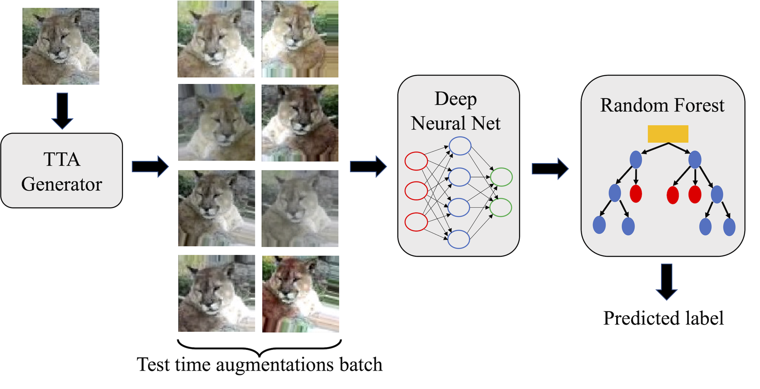
Figure 1: ARF flow chart. Test time augmentations are generated and fed into a pretrained DNN. Its logits are then passed to a random forest classifier to predict the class label.

A major disadvantage of this approach and most of the other existing defense strategies is that they require retraining the network. This puts an additional computational time, which might be significant in some cases, as one needs to update the network frequently to resist novel attacks.

Even in techniques that just fine tune DNNs, there is a need to have an access to all the training data. The same holds for the current leading detection methods that aim at just spotting attacks and alerting about them (without changing the DNN) [40, 37, 16]. Besides storage issues, having access to all data is a problem when a user wants to improve its network robustness to new attacks that were not present during the development of the DNN but does not have access to that data due to privacy or proprietary issues.

Contribution. To mitigate these issues, we propose a novel approach for improving the robustness against adversarial attacks, named Augmented Random Forest (ARF), which only requires storage of logits vectors and not the images themselves. Also, it is very simple to use, does not require retraining, and can be employed with any machine learning classifier that produces logits, including an adversarially trained DNN, to improve its robustness. In addition to our proposed defense, we also introduce a novel white-box attack, A-PGD, that combines the PGD attack [41] with image augmentations. We show this attack is superior than current state-of-the-art (SOTA) attacks on DNN ensembles.

In our approach, for each input image we generate $N$ Test Time Augmentations (TTAs) as shown in Figure 1. We feed this batch of image transformations to the DNN and collect its logits output. In the training phase (done only once), we fit a simple random forest classifier using logits obtained from both natural and adversarial TTAs. The random forest learns to be robust against adversarial images by training on the entire set of TTAs’ logits distribution. In the inference phase, we generate $N$ TTAs for a single image, obtain the DNN logits for it, and pass the logits to the random forest classifier. The inference executes a single forward pass on all the $N$ TTAs at once, and thus is very fast.

We emphasize that the image transformations done in our pre-processing were used in previous works for defense [45, 25, 39, 64]. These TTAs improve classifiers’ robustness due to obfuscated gradients, but this was later shown to be fake robustness which can be circumvented using adaptive attacks in white-box settings [2] (see Section 2). Yet, we utilize TTAs to enrich the input augmentations for the random forest; we find that they improve accuracy on natural (non-adversarial) images and also enhance the robustness.

We compare the adversarial robustness of ARF to SOTA baselines on a diverse set of attack strategies and threat models, for CIFAR-10, CIFAR-100, SVHN, and Tiny-ImageNet. ARF always succeeds to enhance the DNN’s robustness by many folds, without the need to retrain the network (the random forest training is negligible compared to a neural network training) or store the training data. The best results are obtained when applying ARF with an adversarially robust network. We show that this combination achieves SOTA defense and is robust to adaptive white-box attacks.

2 Related works

Various attacks and defense techniques have been proposed for DNNs. Defense techniques may be divided into strategies that aim at increasing the network robustness and approaches that try only detecting the adversarial attacks; In this work we focus on the former ones and describe some of them. For a more a comprehensive survey of the existing strategies one may refer to [18, 69, 42]. We start by describing some of the existing attack strategies.

Adversarial attacks. The core strategy in adversarial attacks is to look for the smallest perturbation of an input that causes the network to change its prediction. The main difference between different existing attacks is the metric used to define the size of the change and the search strategy that is used for finding the perturbation. In addition, attacks may be targeted, i.e., aiming to change the output to a specific given class, or untargeted that just try to flip the network prediction. Another difference is the threat model of the attacks. Black-box adversaries can merely access the network outputs, while white-box adversaries have full access to the network architecture and parameters, algorithm used for training and classification, and training data [11].

We turn to describe some of the existing attacks. The fast gradient sign method (FGSM) changes the input in the direction of the gradient of the cross-entropy loss [23]. It is a fast single-step attack that is very easy to deploy. The Jacobian-based saliency map attack (JSMA) aims to find only a selected few input pixels (i.e., it uses the $L_{0}$ metric), which induce the largest loss increase, and modify only them [49] . It is stronger but iterative and slow.

Deepfool is a non-targeted attack that searches for the closest decision boundary of the network for the given input example [44]. Carlini and Wagner[9] proposed a novel targeted attack (known as CW due to the authors name), which was able to overcome the distillation defense method that was very successful till then [47]. Their approach was further improved in [8], where they formulated an optimization framework to construct loss functions for attacks that are defense specific, i.e., adapted to specific defenses at hand. Madry et. al showed that Projected Gradient Decent (PGD) is an optimal first order adversary, and applying it on a DNN during an adversarial training achieves optimal robustness against any first order attack [41].

Brendel et. al [5] introduced the Boundary attack, a decision based attack used in black-box settings. Their method only requires the final model prediction and can be employed where the output logits do not exist or inaccessible. A more efficient black-box attack was introduced by Andriushchenko et. al [1]. They used much fewer queries than the Boundary attack, and it was shown to even outperform several gradient-based white-box attacks. These two attacks do not rely on gradient information and can be applied on any machine learning classifier.

In order to evaluate the performance of a novel defense approach, it is not sufficient to check robustness on the above attacks but rather design adaptive attacks to the developed defense [7]. In our work, we evaluate our proposed defense against several tailored adaptive attacks.

Adversarial robustness. Many techniques where proposed to improve the adversarial robustness of DNNs.

Some techniques add a regularization during the network training such as penalizing the network input gradients to improve robustness [52]; penalizing the network Jacobian showing that it increases the decision boundary and thus improve robustness [29]; scaling the gradients in a batch based on their magnitude [54]; penalizing the network output so it has a smaller Lipschitz constant [27]; requiring similarity between logits of pairs of input examples [32]; requiring the linear and convoluional layers in the network to be approximately Parseval tight frames [15]; or using the mixup regularization [71, 73].

Other approaches rely on gradient masking [55, 19, 6, 25], i.e., they make it harder for attacks (especially black-box) to be able to find the gradient direction for producing the adversarial examples. However, masking the model gradient’s cannot guarantee robustness in white-box setting against adaptive attacks, as shown by Athalye et. al [2]. They proposed the BPDA attack which estimates masked gradients in the classifier, and replaces them with approximated gradients in the backward pass by replacing any non-differential layer.

Another strategy to improve robustness is adding noise to the data or perturbations to the network features during training [30, 67, 17]. A different approach performs a $k$-NN search, perhaps using external datasets or the web, to make a decision on the input [21, 58].

Papernot et. al proposed to use knowledge distillation to improve adversarial robustness [47]. It was demonstrated that when one wishes to distill a robust network weights to another model (even with different architecture), the information of the gradients can improve the transfer [12, 48].

A leading method is adversarial (re)training with its many variants [23, 41, 35, 63, 57, 43, 65]. It trains the network using adversarial examples in addition to the regular data and thus improves its robustness. It was suggested to add unlabeled data in the adversarial training to improve performance on the clean data [10, 70], which is deteriorated many times due to the adversarial training.

One of the disadvantages of many of the adversarial training methods is that they are computationally demanding. To alleviate that, the “free adversarial training” approach that is fast and leads to robust networks was suggested [56].

Miyato et. al proposed the Virtual Adversarial Training (VAT) [43]. They used a regularization term to smooth the output logits distribution of the model within a small environment surrounding the input image. Note that it is not adversarial training per-se as it does not introduce adversarial images and its regularization does not require labeling, thus making it suitable also for semi-supervised learning.

Zhang et. al proposed TRADES, adding a regularizaion term to the cross-entropy loss in the training phase to improve robustness inside the $\ell_{p}$ ball $\mathbb{B}_{p}(x,\epsilon)=\{x^{\prime}:||x-x^{\prime}||_{p}\leq\epsilon\}$ [72]. By adjusting this term one can control the trade-off between the accuracies on the normal and adversarial samples [59]. It was demonstrated that using robust training in the self-supervised learning regime leads to network robustness also after it is being fine-tuned for the down-stream tasks [14, 31].

Notice that all of the above approaches require changing the DNN training and cannot be used for an already trained network. Indeed, one may use feature squeezing techniques that smooth or quantize the DNN input [68], but these methods are weaker than TRADES or VAT.

Test-time augmentation (TTA). Some works used transformations on the input image to yield a robust classifier [39, 38, 22, 24, 64, 66]. However, Athalye et. al found that these approaches are susceptible to the EoT attack in white-box settings [3], where the distribution of the transformation is considered in the attack loss. In a later work, the BPDA attack was demonstrated to circumvent non-differential transformations as well [2].

Using image augmentations in test time was proved useful for many tasks out of the scope of adversarial robustness. [60] employed TTAs to improve generalization of out-of-distribution images in test time, by fine tuning the model’s parameters before making a prediction. SimCLR [13] showed (among many other self-supervised approaches) that extensive data augmentation as implemented by us in Section 3.1 are very useful for self-supervised learning.

In [25, 4] the KL divergence between a pair of augmentations was computed to detect adversarial attacks. The work in [53] also proposed to utilize TTAs to detect adversarial images. The TTAs were used to aggregate statistics on the input image and detect anomalies associated with adversarial attacks. They showed that in some cases the correct label can also be predicted. Their approach requires an extensive statistical analysis on the dataset and tuning parameters and thresholds. Thus, it is not simple and easy to use with any arbitrary pretrained classifier.

The closest work to ours introduced a random forest classifier after a DNN for improving robustness to adversarial attacks [20]. Unlike our defense, their methodology includes a tedious analysis on the DNN layers. They searched for the ”best” layer to start growing the random forest using a manual observation on the relative $L_{2}$ distance between original and adversarial samples, whereas our method simply attaches the output of any machine learning classifier to a vanilla random forest. This work showed robustness on simple MNIST and CIFAR-10 datasets, whereas our work also exhibits robustness on Tiny Imagenet, a much more complex dataset. In addition, their method does not show robustness to white-box attacks although their masked gradients can be estimated using BPDA. Our Defense is extensively tested on a variety of threat models, including a white-box setting.

3 Method

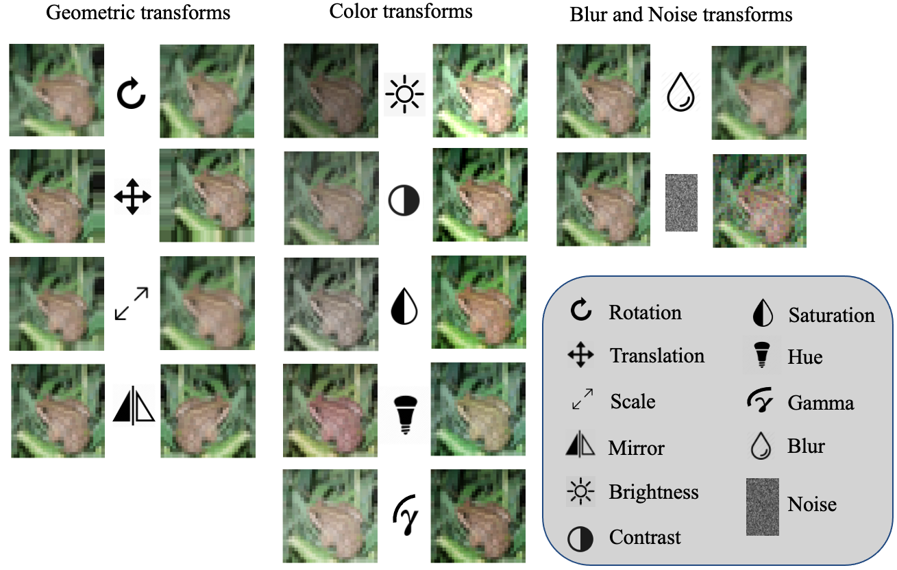
Figure 2: All the transforms used for the test-time augmentation (TTA). The left column illustrates the geometric transforms: Rotation, translation, scaling, and horizontal flips (not used on SVHN). The middle column illustrates the color transforms: Brightness, contrast, saturation, hue, and gamma. The right column illustrates a Gaussian blur and an addition of Gaussian white noise. All the above transforms are randomized to generate $N$ TTAs samples.

We turn now to present our approach. We start by describing how the TTAs are generated prior to feeding them to the DNN. Then we show how the output logits are utilized to train the random forest classifier.

3.1 Test-time augmentations

We hypothesize that even if the adversary succeeds to attack a specific image, the close neighborhood around the image still holds enough information for reverting the predicted (wrong) label back to the correct label. To that end, for each image we generate $N$ TTAs, using a variety of color, geometrical, blur, and noise transforms (see Fig. 2).

The color transforms include: Brightness, contrast, saturation, hue, and gamma; the geometric transforms include: Rotation, translation, scaling, and horizontal flipping; the blur transform convolutes the image with a 2D Gaussian kernel $G_{2D}(u,v;\sigma_{b})$ where $\sigma_{b}$ is uniformly distributed for every TTA image between $0.001$ and a positive constant: $\sigma_{b}\sim\textit{U}(0.001,\sigma_{bmax})$. The noise transform adds a white Gaussian noise to the image, $x_{t}=x+n$, where $n$ is sampled from: $n\sim\textit{N}(0,\sigma)$. and the standard deviation $\sigma$ is uniformly distributed for every TTA image between $0$ and a positive constant $\sigma_{max}$: $\sigma\sim\textit{U}(0,\sigma_{max})$.

All the transforms including their parameters are randomized in test time. More details on the transforms definitions and parameters distributions appear in the Appendix. We chose to apply these transforms because they were shown to improve the classification accuracy significantly in self-supervised and semi-supervised learning [13]. Similarly to them, all the transforms parameters were chosen to alter the image until a human struggles to perceive the images on the dataset. We also added the Gamma transform since it showed small improvement (data not shown).

3.2 TTA classifier

We generate $N$ randomized TTAs and feed them to the DNN (Figure 1), we then collect their logits output ($N$ logits vectors). Formally, for the input TTAs $\{x_{t}[i]\}_{i\in[0,N-1]}$, the DNN outputs are $\{l[i,c]\}_{i\in[0,N-1]}^{c\in[0,\text{\#classes}-1]}$, where $l[i,c]$ is the logit corresponding to class $c$ of the input image $x_{t}[i]$.

When using only the TTAs for making the prediction, the inferred label is a simple argmax of the logits summation:

$$c_{pred}=\operatorname*{argmax}_{c}\sum_{i=0}^{N-1}l[i,c].$$ (1)

3.3 ARF classifier

We split the official test set into two: test and test-val (see Sec. 4 - Random forest training). Let $TV$ be the test size. The augmented random forest (ARF) employs the aforementioned DNN logits of test to train a random forest classifier. We generate $N$ TTAs for the normal (unperturbed) images in test and additional $10N$ TTAs for adversarial images of test generated using ten generic (non-adapted) adversarial attacks we utilized (see Sec. 4 - Adversarial attacks), we denote them by $\{x_{t}[k,i]\}$, $\{x^{\prime}_{t}[k,i]\}_{k\in[0,TV-1],i\in[0,10N-1]}$, respectively.

The above TTAs are fed to the DNN and their logits output for the normal and adversarial images are denoted as $\{l[k,i,c]\}$, $\{l^{\prime}[k,i,c]\}_{k\in[0,TV-1],i\in[0,10N-1]}^{c\in[0,\text{\#classes}-1]}$, respectively, or $\{l[k]\}$ and $\{l^{\prime}[k]\}$ in short for clarity. We then fit the random forest classifier using the pairs $\{l[k],y[k]\}\bigcup\{l^{\prime}[k],y[k]\}$ where $y[k]$ is the true label of the image $x[k]$, i.e., it learns to infer correct labels both from regular and adversarial logits.

The random forest training procedure needs to be carried out only once. For every new (unseen) image we generate TTAs, obtain their logits $l[i,c]$ (as in Section 3.2) and feed them to the random forest classifier to predict the class label.

3.4 Adversarial attacks

To inspect our defense against adversarial images, we employed extensive and diverse attacks in a variety of threat models, and then evaluate them using our ARF classifier and compare them to the robustness obtained using equivalent adversarially trained TRADES/VAT networks, and to an ensemble of networks.

Black-box. A threat model where the adversary has access only to the DNN output, but neither to the DNN nor to the random forest classifier. In this setup we apply targeted Boundary [5] and untargeted Square [1] attacks on the DNN. It is the least interesting setting, but used for attack diversity.

Gray-box. In the Gray-box threat model the adversary has full access the the DNN parameters, but is oblivious to the pre-processing (transformation) and post-processing (random forest) defenses. In this setup we apply the FGSM, JSMA, PGD, Deepfool, and CW attacks on the DNN. All these attack are targeted except of the Deepfool.

Adaptive black-box. In this threat model the adversary does not have any information on the DNN and random forest parameters. They can only query the final output (predicted label) of the random forest classifier and perturb the input image without any gradients knowledge. In this threat model we use the Square attack, which was shown to be much more efficient compared to the popular Boundary attack, and achieved SOTA results, even compared to white-box attacks. Also, we set an untargeted setting since this attack excels on it [1].

Adaptive Gray-box. In this threat model the adversary has access to the DNN’s parameters and has full knowledge about the distributions of the test time augmentations. The adversary is still oblivious to the post-processing (random forest). We formulate two adaptive attacks for this setting:

1) A-FGSM: This attack applies the FGSM attack on every one of the generated TTAs in $\{x_{t}[i]\}_{i\in[0,N-1]}$. All the gradients are then averaged and the mean gradient map is added to the original input image. Formally, we define $X_{t}$ to be the distribution of the generated TTA transforms on an image $x$. Given a loss function $J(x,y;w)$ where $x$ is the input image, $y$ is the adversarial label and $w$ are the DNN weights, the A-FGSM creates an adversarial image $x^{\prime}$ by:

$$\begin{split}x^{\prime}&=x+\mathbb{E}_{x_{t}\sim X_{t}}\big{[}\epsilon\cdot sign\big{(}\nabla_{x_{t}}J(x_{t},y;w)\big{)}\big{]}\\ &=x+\frac{\epsilon}{N}\sum_{i=0}^{N-1}sign\big{(}\nabla_{x_{t}[i]}J(x_{t}[i],y;w)\big{)}.\end{split}$$ (2)

2) A-PGD: Similarly to the gradient averaging shown for A-FGSM, this adaptive attack employs PGD but in every iteration it projects the adversarial perturbations after the addition of the averaged TTAs gradients. Formally, let $\delta_{k}$ be the perturbation added to input image x in step $k$ and $\alpha$ be the perturbation step size. The vanilla PGD attack is:

$$\delta_{k+1}=\mathcal{P}\bigg{[}\delta_{k}+\alpha\cdot sign\big{(}\nabla_{\delta_{k}}J(x+\delta_{k},y;w)\big{)}\bigg{]},$$

where $\mathcal{P}$ is the projection operator, clipping every perturbation inside a ball of interest defined by a given norm $\lVert\cdot\rVert$ (we use $L_{\infty}$). For a general norm $\lVert\cdot\rVert$ it simply reads as:

$$\mathcal{P}(\delta)=\begin{dcases}\frac{\delta}{||\delta||}\epsilon,&\text{if }||\delta||>\epsilon\\ \leavevmode\nobreak\ \leavevmode\nobreak\ \leavevmode\nobreak\ \delta,&\text{otherwise.}\end{dcases}$$

Our adaptive PGD attack is defined as:

$$\begin{split}\delta_{k+1}&=\mathcal{P}\bigg{[}\delta_{k}+\mathbb{E}_{x_{t}\sim X_{t}}\big{[}\alpha\cdot sign\big{(}\nabla_{\delta_{k}}J(x_{t}+\delta_{k},y;w)\big{)}\big{]}\bigg{]}\\ &=\mathcal{P}\bigg{[}\delta_{k}+\alpha\sum_{i=0}^{N-1}sign\big{(}\nabla_{\delta_{k}}J(x_{t}[i]+\delta_{k},y;w)\big{)}\bigg{]},\end{split}$$ (3)

i.e., similar to PGD but averaging the gradients over the batch of augmentations. We initialize $\delta_{0}$ as a zero gradient map and set the generated adversarial image as $x^{\prime}=x+\delta_{N}$.

Adaptive white-box In this threat model the adversary has full knowledge about the DNN, the distribution of the transformations, and the random forest’s parameters. The adversary knows everything about our defense method, including the training data (logits) used to fit the DNN and the random forest classifer. In this harsh settings we employ the BPDA attack [2]. To estimate the random forest gradients, we use knowledge distillation and mimic the random forest classifier (excluding the DNN) to an MLP with 6 layers [48] (see Appendix for full details and MLP architecture). Next, we concatenate the DNN + MLP in tandem to a substitute model. This substitute model is used to generate the BPDA adversarial examples.

4 Experimental setup

We turn to detail the datasets we used, the DNN and random forest training, and inference computation time. Our hardware setup is thoroughly detailed in the Appendix.

Datasets. We perform our tests on four datasets: CIFAR-10, CIFAR-100 [34], SVHN [46] and Tiny ImageNet [36].

DNN training. We randomly split the training set of all the datasets into two subsets, train and train-val. The former is used to back-prop gradients from the loss to the inputs and train the DNN, whereas the latter is used for metric calculation to decay the learning rate. The size of the train-val set is chosen to be 5% of the official training set.

We trained three Resnet architectures [26], Resnet-34, Resnet-50, and Resnet-101, with global average pooling layer before the embedding space. The embedding vector was multiplied by a fully connected layer for the logits calculation. We trained CIFAR-10, CIFAR-100, SVHN, and Tiny ImageNet with 300, 300, 200, and 300 epochs, respectively; For the TRADES method (adversarial training) we trained them with 100, 100, 100, and 300 epochs, respectively, since we observed that fewer epochs obtain higher adversarial accuracy with TRADES (see Appendix). All TRADES adversarial robust networks used $1/\lambda=1$, $\epsilon=0.031$, $\alpha=0.007$ ($\epsilon$ step size), on $L_{\infty}$ norm to match the settings in [72] for fair comparison. The VAT adversarial networks were also trained using $\epsilon$=0.031, with $\alpha=1$ and $\epsilon=1,1,3,1$ for CIFAR-10, CIFAR-100, SVHN, and Tiny ImageNet, respectively [43].

We use an $L_{2}$ weight decay regularization of 0.0001 in all our DNN training, a stochastic gradient decent optimizer with momentum 0.9 with Nesterov updates, and a batch size of 100. The training starts with a learning rate of 0.1, which decreases by a factor of 0.9 after 3 epochs of no improvement on the train-val accuracy (2 epochs for SVHN).

Random forest training. We split the test set of all the datasets into two subsets, test and test-val. The test-val size is 2500, and the test is the official test set without these 2500 samples, i.e., 7500, 7500, 23500, and 7500 for CIFAR-10, CIFAR-100, SVHN, and Tiny ImageNet, respectively. The only exception is the Boundary attack. Due to long processing time, we selected for it only 750, 250 samples from test, test-val , respectively. The random forest classifier was trained with 1000 trees, using the Gini impurity criterion. The training time was 71 seconds and was done only once for all the normal/adversarial images on the test subset.

Adversarial attacks. The adversarial attacks detailed in Sec. 3.4 were set to the following norms and powers: (1) FGSM¹: ($L_{\infty},\epsilon=0.01$); (2) FGSM²: ($L_{\infty},\epsilon=0.031$); (3) JSMA: ($L_{0},\gamma=0.01$); (4) PGD¹: ($L_{\infty},\epsilon=0.01$); (5) PGD²: ($L_{\infty},\epsilon=0.031$); (6) Deepfool: ($L_{2},\epsilon$ is unconstrained); (7) CW${}_{L_{2}}$: ($L_{2},\epsilon$ is unconstrained); (8) CW${}_{L_{\infty}}$: ($L_{\infty},\epsilon=0.031$); (9) Square: ($L_{\infty},\epsilon=0.031$); and (10) Boundary: ($L_{2},\epsilon$ is unconstrained).

Our PGD attacks were applied with a step size of $\alpha=0.003$ with 100 iterations. The above attacks were selected due to their norm diversity, effectiveness, and popularity. Many attacks employ $\epsilon=0.031$ to match the settings in the TRADES baseline [72], which is the current SOTA.

We also apply the following adaptive attacks detailed in Sections 3.4: (i) A-FGSM($L_{\infty},\epsilon=0.031$); (ii) A-PGD($L_{\infty},\epsilon=0.031$); (iii) A-Square ($L_{\infty},\epsilon=0.031$); and (iv) BPDA: BPDA($L_{\infty},\epsilon=0.031$). A-FGSM, A-PGD, A-Square, and BPDA were set with $N=256$ generated TTAs. A-PGD, A-Square and BPDA are very time consuming and thus were set with only 10 iterations; Therefore, we set their step size to $\alpha=0.007$.

Testing. All the metrics we show in this work were calculated on the test-val subset. For both TTA and ARF we set $N=256$ unless stated otherwise, i.e., we generate 256 TTAs in inference time, which allows the models to run in a single forward pass on the GPU. The majority of the computation time is devoted to the TTAs generation, which is done on the CPU and takes 3.32 $\pm$ 0.33 seconds for a single Tiny ImageNet image (calculated over 20 runs). The DNN and random forest forward pass times are negligible - 250 ms and 4 ms, respectively.

5 Results

We evaluate the performance of ARF on adversarial attacks and compare it to other robust methods. We also present ablation studies conducted to improve the model performance and computation time. Lastly, we show accuracies on adaptive black-box and white-box attacks. Alternative simple machine learning classifiers such as logistic regression and SVM were found to be inferior to random forest; This comparison appears in the Appendix.

Transferability. While here we train and test ARF using all non-adaptive attacks (black-box and gray-box), in the Appendix. we demonstrate an excellent generalization to unseen, non-adaptive attacks.

Dataset	Method	Normal	FGSM1	FGSM2	JSMA	PGD1	PGD2	Deepfool	CW${}_{L_{2}}$	CW${}_{L_{\infty}}$	Square	Boundary
CIFAR-10	Plain	94.92	68.52	55.28	68.68	13.72	0.00	4.00	3.12	23.44	59.36	18.40
	Ensemble	96.04	82.00	64.20	84.60	86.68	48.64	86.96	83.64	78.80	89.48	96.00
	TRADES	86.64	85.04	75.80	69.88	85.12	71.84	7.68	0.56	78.24	80.92	22.80
	VAT	94.00	82.68	70.36	80.48	82.12	20.08	4.04	4.24	49.80	81.32	15.20
	TTA	91.68	82.48	68.76	84.84	87.04	72.76	83.16	82.24	81.4	85.32	88.80
	ARF	93.76	83.72	70.20	85.28	90.32	77.88	87.36	84.36	85.64	87.84	91.20
	TRADES + ARF	84.28	82.56	76.72	79.64	82.56	76.24	69.40	68.00	80.48	80.56	81.20
	VAT + ARF	92.60	89.44	81.24	90.60	90.28	82.36	87.72	85.12	88.92	89.00	90.80
CIFAR-100	Plain	74.32	28.96	13.84	43.84	22.52	0.28	9.20	15.84	47.76	28.64	30.40
	Ensemble	78.04	58.20	29.16	52.48	69.64	33.28	76.60	51.08	68.68	65.36	74.40
	TRADES	53.36	51.80	41.52	46.84	52.88	46.44	10.88	5.28	51.04	45.96	24.00
	VAT	70.92	52.56	28.80	59.88	63.00	15.20	10.00	11.20	44.36	54.36	20.80
	TTA	70.76	52.24	28.80	56.36	62.92	42.08	65.92	46.72	62.60	56.28	65.20
	ARF	71.52	54.20	30.80	58.08	66.72	47.60	68.12	49.36	64.44	60.40	68.00
	TRADES + ARF	49.48	49.04	44.16	48.04	48.80	46.28	45.04	36.56	49.96	47.48	43.60
	VAT + ARF	68.96	63.52	48.20	65.76	66.24	59.92	65.56	55.76	62.72	64.04	61.60
SVHN	Plain	97.36	80.56	66.24	49.64	52.32	2.04	2.84	4.80	28.96	66.96	15.60
	Ensemble	98.12	89.52	74.84	85.36	92.80	71.20	71.88	79.76	83.04	93.52	97.20
	TRADES	92.48	90.60	81.20	39.44	90.28	70.88	5.08	0.72	82.36	83.84	19.20
	VAT	94.44	89.00	83.72	65.48	85.16	43.28	4.16	23.60	64.76	87.04	18.80
	TTA	97.08	87.16	73.76	86.36	89.68	61.32	66.84	80.08	80.64	92.24	95.20
	ARF	96.92	87.96	75.24	87.00	90.04	66.16	68.84	80.40	81.28	92.16	96.00
	TRADES + ARF	92.44	90.96	82.20	78.80	91.16	79.96	62.48	48.40	85.84	88.40	88.00
	VAT + ARF	95.64	93.72	86.92	89.84	93.76	81.88	92.08	85.68	90.28	93.24	91.60
Tiny ImageNet	Plain	59.24	25.48	9.92	28.88	30.72	0.40	10.08	16.24	34.76	28.04	19.60
	Ensemble	67.12	58.32	28.64	52.96	63.92	46.24	66.56	54.64	60.08	60.80	58.40
	TRADES	44.44	42.32	31.64	35.32	43.72	38.44	9.16	5.52	41.88	38.76	23.20
	VAT	54.68	47.84	24.52	44.92	52.36	31.80	9.92	6.64	46.24	46.00	23.20
	TTA	52.48	37.12	17.36	39.76	43.84	27.52	46.24	35.08	42.96	40.84	37.60
	ARF	53.36	40.76	21.52	43.76	48.88	33.48	48.88	40.04	45.80	45.92	42.80
	TRADES + ARF	39.24	37.68	33.44	36.20	38.36	35.20	35.12	27.80	38.72	36.80	32.00
	VAT + ARF	47.92	45.52	36.28	45.76	46.32	41.96	43.44	34.84	46.24	44.84	39.20

Table 1: Comparison of accuracies (%) for various classifiers on the non-adaptive attacks. The tested attacks and datasets are detailed in Section 4. We boldface the best results. Ensemble is presented just as a reference as it has an unfair advantage (as explained in the text).

.

5.1 Adversarial Robustness

Table 1 shows the accuracy on the normal (not attacked) and the adversarial accuracies obtained for all the non-adaptive attacks (black-box and gray-box) we employed (see Section 4), on Resnet-34. Tables for Resnet-50 and Resnet-101 are shown in the Appendix.

”Plain” corresponds to the non-robust, simple DNN accuracy, without any adversarial defense method. ”Ensemble” uses nine different DNNs with the same architecture and the predicted label is a majority voting amongst them. It should be emphasized that the adversary does not have access to any of these nine models. Thus, it has an unfair advantage. TTA classifier is applied on the DNN alone (w/o random forest), and ARF classifier is evaluated in two setups, one is applied on a regular (non adversarially robust) DNN, and second is combined with an adversarially robust DNN trained with VAT or TRADES.

We notice that for every dataset both TTA and ARF classifiers achieve higher robustness accuracy than both VAT and TRADES on JSMA, Deepfool, and CW${}_{L_{2}}$. This is not surprising because TRADES employed a regularization term on a ball with an $L_{\infty}$ norm and these attacks use other norms. In addition, VAT regularizes logits distribution smoothness within the image’s local surrounding, which is problematic where the norm is unconstrained in $L_{\infty}$. Nonetheless, it is not trivial that the simple TTA classifier surpasses TRADES’ accuracy on these attacks.

In the vast majority of the attacks and datasets, the ARF classifier outperforms the VAT networks. However, when combined together they usually achieve the highest adversarial robustness accuracy. This robust accuracy trumps even the ensemble score, except for Tiny Imagenet.

Lastly, we observe that the normal accuracy obtained by ARF is much better than the one of TRADES, and is comparable to the normal accuracy obtained by VAT. ARF scores almost as the ”plain” classifier for normal images on CIFAR-10, CIFAR-100, and SVHN.

5.2 Ablation Studies

We conducted two ablation studies to understand better and optimize our ARF and TTA classifiers.

ARF classifier ablation. We tested three parameters governing the ARF accuracy:

1. Features: The inputs to the random forest classifier. We used three candidates: The DNN’s logits, the DNN’s probabilities (softmax over logits), and the embedding vectors in the DNN penultimate layer.

2. Gaussian noise power: We checked three different noise filters with max standard deviation ($\sigma_{max}$) of $0$, $0.005$, and $0.0125$. The $0$ value is equivalent to no noise.

3. Strength of transforms: We tested two sets of transforms from the transforms in Fig. 2: soft vs hard. The soft transforms span over shorter parameter intervals. For example, the hard brightness transform randomizes a brightness factor in the interval $\textit{U}(0.6,1.4)$ whereas the soft transform randomizes it in $\textit{U}(0.8,1.2)$. The full interval sets of the soft and hard transforms are listed in the Appendix.

Features	Transforms	$\sigma_{max}$	Accuracy (%)
			$\mathbb{A}_{norm}$	$\mathbb{A}_{adv}$
Logits	soft	0	94.24	83.56
Logits	soft	0.005	94.20	83.72
Logits	soft	0.0125	93.88	83.96
Logits	hard	0	93.72	84.64
Logits	hard	0.005	93.80	85.00
Logits	hard	0.0125	93.08	84.96
Probs	soft	0	94.16	83.36
Probs	soft	0.005	94.04	83.64
Probs	soft	0.0125	93.80	84.00
Probs	hard	0	93.60	84.52
Probs	hard	0.005	93.80	84.72
Probs	hard	0.0125	93.00	84.96
Embeddings	soft	0	94.16	83.56
Embeddings	soft	0.005	93.96	83.64
Embeddings	soft	0.0125	93.56	83.88
Embeddings	hard	0	93.68	84.88
Embeddings	hard	0.005	93.60	84.80
Embeddings	hard	0.0125	93.04	84.92

Table 2: Ablation study on 3 parameters used for ARF. 1) Random forest input features: Logits, softmax probabilities, and DNN embeddings. 2) Randomization level of transforms: hard for a larger randomization range (coarse transforms) and soft for a smaller range (mellow transforms). 3) Noise transform max power ($\sigma_{max}$).

Table 2 shows the normal and adversarial accuracies ($\mathbb{A}_{norm}$ and $\mathbb{A}_{adv}$) on CIFAR-10, trained by Resnet-34, attacked by CW${}_{L_{2}}$ and evaluated using ARF with $N=1000$. The highest adversarial accuracy was obtained for logits vectors, hard transforms, and $\sigma_{max}=0.005$. Thus these were the parameters we used in this work. It is interesting to point out that the best normal accuracy was obtained for soft transforms with $\sigma_{max}=0$ (for all features). This observation conforms with the high normal accuracy presented in Table 1, as the plain DNN does not apply any transform.

TTA size ablation. The computational bottleneck in our TTA and ARF classifiers is the generation of the $N$ TTAs. Using $N=1000$ images as done for Table 2 requires a long computation time so we searched for the minimal $N$, which achieves sufficient adversarial robustness. Figure 3 shows the adversarial accuracy on CIFAR-10 for three selected attacks: PGD¹, Deepfool, and CW${}_{L_{2}}$ in a logarithmic scale. The width of each line corresponds to the measured standard deviation of five repeated experiments. We select $N=256$ for our experiments since it achieves good robustness with very high confidence (narrow interval). Ablation of the TTA size on CIFAR-100 and SVHN is presented in the Appendix.

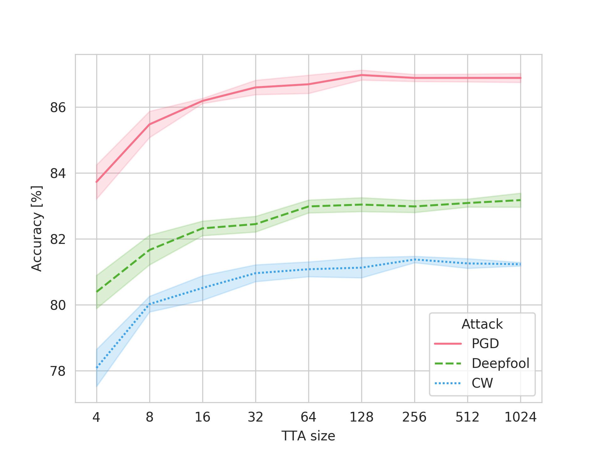
Figure 3: Ablation study on the number of generated TTAs ($N$). We calculate the adversarial accuracies on CIFAR-10 for three attacks as a function of $N$ (logarithmic scale).

5.3 Adaptive Attacks (Limitation)

Table 3 shows the adversarial accuracies for different robust classifiers for all the adaptive attacks shown in Section 3.4. For easy comparison, the performance on the corresponded non-adaptive attack is shown above each accuracy result. We observe that our ARF defense is robust against the black-box adaptive attack, but fails when attacked with an adaptive gray-box or white-box attack. For example, the white-box BPDA attack decreases the ARF accuracy on CIFAR-10 to 8.8%.

The VAT+ARF combination demonstrates SOTA robustness for all non-adaptive attacks, however, the vanilla TRADES or VAT perform better on adaptive attacks. We observe that the combination of TRADES+ARF is usually preferred against adaptive attack, obtaining high robustness for these attacks for all datasets. Note that although the performance of ARF degrades significantly when the BPDA harsh attack is applied, when combined with adversarial training this degradation is minimal.

Our A-PGD attack is much more effective against the ensemble and TTA classifiers, surpassing all other adaptive and non-adaptive attacks by a large margin. Alas, it is not as powerful as the vanilla PGD against plain adversarial robust DNNs (TRADES/VAT). For all the other robust classifiers it achieves comparable results to the strong BPDA attack.

Dataset	Attack	Ensemble	TRADES	VAT	TTA	ARF	TRADES+	TRADES+	VAT+	VAT+
							TTA	ARF	TTA	ARF
CIFAR-10	FGSM	64.20	75.80	70.36	68.76	70.28	73.72	76.72	80.40	81.24
	A-FGSM	41.60	79.20	68.84	33.32	37.80	72.96	74.88	61.88	64.68
	PGD	48.64	71.84	20.08	72.76	78.32	72.84	76.24	79.28	82.36
	A-PGD	5.76	77.76	54.84	5.12	22.32	70.40	73.24	53.20	54.64
	Square	89.48	80.92	81.32	85.32	87.84	77.44	80.56	87.20	89.00
	A-Square	90.80	89.60	95.2	87.60	89.20	84.00	87.20	90.80	92.00
	BPDA	10.40	84.00	58.8	8.40	8.80	74.80	82.80	57.20	63.60
CIFAR-100	FGSM	29.16	41.52	28.80	28.80	30.80	43.28	44.16	46.16	48.20
	A-FGSM	25.04	48.76	40.32	13.20	16.60	45.88	46.44	34.32	37.80
	PGD	33.28	46.44	15.20	42.08	47.60	44.96	46.28	56.76	59.92
	A-PGD	19.24	48.44	39.32	10.16	13.24	45.96	47.28	40.60	43.16
	Square	65.36	45.96	54.36	56.28	60.40	47.88	47.48	61.28	64.04
	A-Square	66.40	52.80	64.00	56.00	58.00	48.40	47.20	63.20	64.80
	BPDA	23.60	50.40	43.60	12.00	12.80	44.40	46.00	38.00	42.40
SVHN	FGSM	74.84	81.20	83.72	73.76	75.24	80.72	82.20	85.92	86.92
	A-FGSM	62.44	82.00	79.52	56.92	59.80	78.44	80.96	79.32	79.68
	PGD	71.20	70.88	43.28	61.32	66.16	77.64	79.96	80.28	81.88
	A-PGD	36.04	78.40	58.32	19.92	34.28	74.68	76.60	64.84	65.36
	Square	93.52	83.84	87.04	92.24	92.16	83.88	88.40	91.88	93.24
	A-Square	96.80	92.40	92.40	96.40	95.60	88.40	91.60	93.20	94.00
	BPDA	45.60	75.60	62.80	32.80	34.80	66.80	72.80	63.60	66.40
Tiny ImageNet	FGSM	28.64	31.64	24.52	17.36	21.52	29.60	33.44	31.24	36.28
	A-FGSM	30.04	40.76	43.12	6.96	10.40	31.44	35.24	28.64	36.16
	PGD	46.24	38.44	31.80	27.52	33.48	31.56	35.20	34.96	41.96
	A-PGD	38.16	40.00	46.28	6.72	10.00	33.60	35.80	35.00	40.56
	Square	60.80	38.76	46.00	40.84	45.92	34.84	36.80	41.32	44.84
	A-Square	56.80	40.80	49.60	40.00	45.60	31.60	38.00	37.20	38.00
	BPDA	39.60	37.60	43.60	11.60	15.20	31.20	35.60	30.00	36.40

Table 3: Adversarial accuracies (%) for various robust classifiers on adaptive attacks: A-Square (black-box), A-FGSM and A-PGD (gray-box) and BPDA (white-box), and their non-adaptive correspondents. FGSM² and PGD² are abbreviated to FGSM and PGD for clarity. TTA and ARF methods can maintain robustness only when combined with an adversarially trained DNN. Ensemble is presented just as a reference as it has an unfair advantage (see text).

6 Conclusions

This work proposes a simple, fast, and easy to use method to classify adversarial images, named ARF. Our approach is applied on pretrained DNNs without the need to carry out adversarial training or updating the model’s parameters. ARF first generates many test-time augmentations, applying a wide variety of random color, geometrical, blur and noise transforms on the input image, and feeds these augmentations to a pretrained DNN. Then it collects the DNN’s logits and feeds them to a vanilla random forest classifier which yields SOTA robust classification when combined with an adversarially trained DNN (VAT). This improvement in robustness comes at the cost of training the random forest model (only once). We tested ARF with a variety of attacks, where some of them were especially designed against ARF. One of them, A-PGD, which we proposed, is of interest by itself as it is very effective against DNN ensemble while not having access to any of its networks.

ARF can be incorporated to work with any machine learning classifier and was shown to perform well even under the harsh white-box threat model when combined with TRADES. Note that white-box setting assumes full knowledge about our defense parameters, which can be easily changed by quickly re-training the simple ARF model. Thus, hiding the ARF model can be considered as holding a secret key for ”security through obscurity” [7, 33]. In addition, defending against new adaptive attacks is feasible by including them into the ARF fitting. Therefore, the use of ARF should be favored over adversarial training alone (although in the white-box setting tailored to ARF it was better alone) as in the non white-box setting ARF leads to a significant improvement. We believe that integrating ARF within the adversarial training can further boost the robustness as was shown for data augmentations in a very recent work [51].

In Appendix A we present adversarial robustness scores of our approach using other architectures: Resnet-50 and Resnet-101, demonstrating that the combination of VAT+ARF achieves SOTA robustness as shown also for Resnet-34 in the main paper.

Appendix B defines in detail the image transformations we used to calculate the Test Time Augmentations (TTAs) in the paper, listing their parameter distribution and randomized ordering protocol.

Appendix C lists the hardware (CPUs & GPUs) we used for training our DNNs and random forest classifiers.

Appendix D shows several parameter searches we conducted to optimize our baselines (TRADES/VAT) to the datasets and architecture in our experiments.

Appendix E shows ARF performance when replacing the random forest classifier with other machine learning models: Logistic regression and SVM.

In Appendix F we show that our ARF model is transferable, generalizing very well to new (unseen) attacks.

Appendix G provides in depth details on the steps we implemented to utilize the BPDA attack in our experiments, since the non-differential random forest had to be mimicked by a substitute model.

Appendix H is a continuation to the TTA size ablation study conducted in Section 5.2 in the main paper. Here, we add the same ”accuracy vs size” results for CIFAR-100 and SVHN.

Appendix I shows the mean $L_{2}$ distortion for some attacks we used in the paper.

Lastly, Appendix J displays adversarial images generated by the adaptive white-box BPDA attack against our defense method. We show that albeit BPDA can circumvent our defense for a vanilla DNN (w/o TRADES/VAT), its generated noise can be observed by the naked eye.

Appendix A Robustness on Resnet-50 and Resnet-101

The main paper shows adversarial robustness results only on Resnet-34. In this section we repeat the results in Section 5.1 also for Resnet-50 and Resnet-101, shown in Table A1 and Table A2, respectively. We omit the black-box Boundary attack from these experiments because it utilizes thousands of search queries, which is not practical for large DNN architectures. The black-box Square attack is reported since it is fast and efficient.

Dataset	Method	Normal	FGSM1	FGSM2	JSMA	PGD1	PGD2	Deepfool	CWL2	CWL∞	Square
CIFAR-10	Plain	94.80	59.12	40.00	76.24	8.16	0.00	3.44	0.08	16.00	51.08
	Ensemble	95.92	78.04	53.00	86.48	79.84	22.00	93.56	85.92	79.48	86.20
	TRADES	86.56	84.40	75.44	71.72	84.52	70.68	8.36	0.24	78.40	81.52
	VAT	95.16	80.40	63.44	84.88	72.56	5.08	3.56	1.16	25.24	79.24
	TTA	90.80	78.64	59.92	84.64	83.52	57.08	87.36	82.80	81.48	82.04
	ARF	93.28	81.92	63.16	85.04	87.76	60.96	91.36	86.24	86.64	85.44
	TRADES + ARF	84.16	82.20	75.96	78.64	82.00	74.60	67.48	67.16	80.16	80.20
	VAT + ARF	93.24	89.36	77.64	90.76	90.48	78.36	89.84	88.00	87.32	88.80
CIFAR-100	Plain	74.52	26.48	11.08	47.64	16.52	0.08	9.44	8.08	36.56	24.52
	Ensemble	78.44	53.60	23.08	56.72	64.48	32.64	76.88	53.84	62.40	60.36
	TRADES	55.08	53.92	44.60	45.92	54.08	48.64	11.08	5.52	52.64	47.96
	VAT	71.56	52.56	28.84	60.04	63.88	13.76	9.72	6.40	40.52	52.96
	TTA	67.32	49.60	26.56	54.84	60.76	46.08	64.20	49.52	58.00	52.56
	ARF	69.24	54.08	31.40	57.40	64.88	52.28	65.68	53.80	62.00	56.36
	TRADES + ARF	50.68	49.80	45.20	47.04	49.32	46.64	46.56	34.60	50.20	47.84
	VAT + ARF	67.28	62.72	48.84	65.60	65.36	59.88	64.24	56.16	61.92	62.40
SVHN	Plain	97.28	81.48	65.12	51.64	51.32	0.88	2.36	2.60	20.24	67.08
	Ensemble	97.88	91.32	75.28	85.48	92.92	71.28	84.80	85.72	85.92	92.72
	TRADES	93.72	92.92	89.76	52.36	92.00	77.76	4.24	0.40	89.08	84.44
	VAT	96.52	87.96	80.92	84.88	48.28	0.20	2.24	0.36	9.36	81.68
	TTA	97.24	89.32	75.04	86.08	91.76	63.92	83.44	86.08	84.52	93.00
	ARF	97.16	89.68	76.72	87.40	92.48	67.44	84.28	86.56	86.36	92.72
	TRADES + ARF	93.72	93.24	89.52	84.88	92.76	83.92	74.60	48.72	90.36	89.32
	VAT + ARF	96.72	95.28	87.96	94.24	95.68	87.96	96.28	95.44	95.08	94.76
Tiny ImageNet	Plain	64.16	25.68	11.68	32.92	30.60	0.08	9.52	17.28	41.60	28.84
	Ensemble	69.08	56.48	28.12	52.44	65.68	46.92	68.24	51.40	61.84	58.60
	TRADES	45.60	45.12	33.92	37.60	44.68	41.12	10.48	6.36	43.84	42.08
	VAT	63.24	53.64	40.96	56.64	23.92	0.52	9.76	18.12	54.28	41.12
	TTA	51.88	36.88	19.08	40.16	43.36	30.20	45.92	33.08	42.80	38.44
	ARF	54.00	41.00	22.64	43.44	47.84	35.56	49.40	37.36	45.56	43.96
	TRADES + ARF	37.52	36.32	31.08	35.48	36.36	33.60	33.52	25.64	37.80	36.80
	VAT + ARF	56.00	54.04	48.16	54.44	56.04	52.84	56.64	48.88	56.76	50.08

Table A1: Comparison of accuracies (%) for various classifiers on CIFAR-10, CIFAR-100, SVHN, and Tiny ImageNet trained on Resnet-50. All attacks are detailed in Section 4 in the main paper. We boldface the best results. Ensemble is presented just as a reference as it has an unfair advantage.

Dataset	Method	Normal	FGSM1	FGSM2	JSMA	PGD1	PGD2	Deepfool	CWL2	CWL∞	Square
CIFAR-10	Plain	94.96	58.08	44.12	77.92	9.04	0.00	3.60	1.32	24.24	56.32
	Ensemble	96.24	78.76	55.56	87.48	77.52	14.36	93.52	83.08	81.16	87.60
	TRADES	85.04	82.76	72.80	70.20	82.88	68.08	8.56	0.16	75.08	77.56
	VAT	94.36	80.24	64.40	83.84	76.76	10.96	3.60	2.12	36.28	82.68
	TTA	91.52	77.92	58.96	84.80	83.04	55.24	86.36	81.60	80.60	83.16
	ARF	93.64	81.64	63.44	84.88	88.00	60.48	91.20	83.96	86.48	86.36
	TRADES + ARF	82.12	81.00	75.24	77.24	81.16	74.04	66.00	67.12	78.88	79.00
	VAT + ARF	93.40	88.92	76.52	90.60	89.76	76.36	88.88	85.48	87.84	89.00
CIFAR-100	Plain	75.56	33.20	17.56	53.44	16.72	0.12	9.40	13.52	46.92	27.64
	Ensemble	79.56	60.48	29.84	59.52	69.64	42.60	78.12	54.96	72.00	63.72
	TRADES	55.52	54.68	44.28	46.64	54.60	49.88	10.36	4.52	53.08	47.32
	VAT	74.28	55.08	31.32	59.72	64.80	10.56	9.44	8.84	41.12	52.12
	TTA	68.48	51.16	32.60	59.04	62.12	48.16	65.16	48.96	62.16	56.48
	ARF	70.60	55.40	35.92	61.20	66.16	53.16	67.64	53.80	66.48	59.52
	TRADES + ARF	50.88	49.76	44.72	46.32	49.40	45.88	43.68	35.00	49.68	46.96
	VAT + ARF	70.52	65.16	48.72	66.12	67.48	60.36	66.56	56.84	62.92	64.52
SVHN	Plain	97.48	80.12	62.12	57.72	53.00	1.52	2.32	4.88	33.36	71.32
	Ensemble	98.08	90.04	72.04	87.80	92.72	64.80	84.12	83.12	88.12	93.24
	TRADES	93.52	93.12	89.32	38.88	92.40	74.12	4.60	0.68	87.92	83.60
	VAT	94.64	89.60	86.24	75.72	71.20	12.64	3.32	12.64	56.32	78.72
	TTA	97.16	87.92	71.00	86.56	90.36	54.92	80.60	81.92	85.36	93.36
	ARF	97.24	88.80	71.72	87.60	91.08	61.56	82.68	82.32	86.28	93.68
	TRADES + ARF	94.04	93.32	89.88	79.52	93.28	82.56	72.68	54.36	90.48	88.64
	VAT + ARF	95.52	93.80	89.04	93.32	94.32	82.28	95.72	91.08	92.24	92.04
Tiny ImageNet	Plain	66.56	25.88	11.76	34.48	30.44	0.24	9.08	14.56	40.60	32.00
	Ensemble	70.20	55.24	27.92	53.16	65.96	46.12	68.80	53.16	61.88	61.84
	TRADES	45.28	43.88	35.72	37.80	44.36	40.92	10.96	5.04	44.20	41.64
	VAT	64.40	43.96	23.84	53.24	48.92	4.68	10.16	26.80	51.84	46.44
	TTA	54.84	39.08	19.52	43.48	46.00	29.96	49.96	34.84	44.76	42.92
	ARF	57.12	41.80	22.16	45.80	50.72	35.04	51.28	37.76	47.68	46.52
	TRADES + ARF	35.64	34.04	30.48	34.56	33.88	31.88	30.56	20.88	35.76	32.88
	VAT + ARF	56.12	50.40	36.72	53.00	53.92	49.68	52.88	46.40	53.32	50.12

Table A2: Comparison of accuracies (%) for various classifiers on CIFAR-10, CIFAR-100, SVHN, and Tiny ImageNet trained on Resnet-101. All attacks are detailed in Section 4 in the main paper. We boldface the best results. Ensemble is presented just as a reference as it has an unfair advantage.

Overall, the results on these DNNs have the same trend as in Resnet-34. ARF’s robustness is on par with TRADES and VAT, however when combined with VAT we surpass the robustness of the vanilla adversarial trained DNN by a large margin. In addition, contrary to TRADES, ARF exhibits very high normal accuracy.

Appendix B Test-time augmentations

Here we detail all the transforms we used to generate our Test-Time Augmentations (TTAs) for our robust classification methods, as described in Section 3.1 in the main paper. We used different parameters for soft transforms and hard transforms in the ablation study in Section 5.2. Both sets of parameters are listed below. The main result in the paper, outside the aforementioned ablation study, were calculated only with the hard set, which proved to achieve better performance in the ablation study. We denote the original and transformed images as $x$ and $x_{t}$, respectively.

1. Rotation: Angle rotation of the image was randomized to be in $\textit{U}(-8^{\circ},8^{\circ})$ for soft and $\textit{U}(-15^{\circ},15^{\circ})$ for hard.

2. Translation: The image was allowed to shift horizontally and vertically up to 2 pixels in every direction for CIFAR-10, CIFAR-100, and SVHN, and up to 4 pixels for Tiny ImageNet. This transform behaves similarly for both soft and hard.

3. Scale: We randomly selected a zoom in ($s>1$) or a zoom out ($s<1$). The image was scaled with $s\sim\textit{U}(0.95,1.05)$ for soft and $s\sim\textit{U}(0.9,1.1)$ for hard.

4. Mirror: The image was horizontally flipped with a probability of 0.5. This transform was omitted for SVHN dataset, and was the same for soft and hard.

5. Brightness: Randomly increase/decrease brightness. Let $b$ denote the brightness factor; the transforms is defined as $x_{t}=b\cdot x$. We randomized $b\sim\textit{U}(0.8,1.2)$ for soft and $b\sim\textit{U}(0.6,1.4)$ for hard.

6. Contrast: The contrast factor $c$ was distributed as $c\sim\textit{U}(0.85,1.15)$ for soft and as $c\sim\textit{U}(0.7,1.3)$ for hard. The transformed image after contrast is: $x_{t}=c\cdot x+(1-c)\cdot\mathbb{E}(x_{G})\cdot\mathbbm{1}_{nxnx3}$, where $\mathbb{E}(x_{G})$ is the mean pixel value on the gray-scale equivalent image and $\mathbbm{1}_{nxnx3}$ is a matrix as the size of the original image, filled with ones. The gray-scale image is defined as: $x_{G}=0.2989\cdot R+0.587\cdot G+0.114\cdot B$ where $(R,G,B)$ are the red, green, and blue channels of $x$, respectively.

7. Saturation: The saturation factor $sat$ was distributed as $sat\sim\textit{U}(0.75,1.25)$ for soft and as $sat\sim\textit{U}(0.5,1.5)$ for hard. It is defined as: $x_{t}=sat\cdot x+(1-sat)\cdot x_{G}$.

8. Hue: The hue factor $h$ was distributed as $h\sim\textit{U}(0.03,0.03)$ for soft and as $h\sim\textit{U}(0.06,0.06)$ for hard. The transform updates the hue in the Hue Saturation Value (HSV) representation by $h$.

9. Gamma: Applying gamma transform on the image. Each channel (r,g,b) on $x$ is transformed to $x_{t}[r,g,b]=x[r,g,b]^{\gamma}$, where $\gamma\sim\textit{U}(0.85,1.15)$ for soft and $\gamma\sim\textit{U}(0.7,1.3)$ for hard.

10. Blur: The blur transform convolutes the image with a 2D Gaussian kernel: $x_{t}=G_{2D}(u,v;\sigma_{b})*x$, where $G_{2D}(u,v;\sigma_{b})=\frac{1}{2\pi\sigma_{b}^{2}}\exp{\frac{-(u^{2}+v^{2})}{2\sigma_{b}^{2}}}$, where $\sigma_{b}$ is uniformly distributed between $0.001$ and a positive constant value $\sigma_{bmax}$: $\sigma_{b}\sim\textit{U}(0.001,\sigma_{bmax})$.

    We set $\sigma_{bmax}=0.25$ for soft and $\sigma_{bmax}=0.5$ for hard.

11. Noise: The Noise transform adds a white Gaussian noise to the image, $x_{t}=x+n$, where n is sampled from $n\sim\textit{N}(0,\sigma)$. The standard deviation of the normal distribution is randomized in our algorithm to be $\sigma\sim\textit{U}(0,\sigma_{max})$. We set $\sigma_{max}=0.005$ in all our experiments (see Section 5.2 in the main paper).

It is important to point out that for all the color transforms, geometric transforms (except Mirror) and Noise, the mean value of the transform change is zero, thus our generated TTAs are unbiased.

The transforms were carried out in the following order:

1. Applying all the color transforms ([5]-[9]). The order of the color transforms was randomized.

2. Padding the image with the last value at the edge of the image. CIFAR-10, CIFAR-100, and SVHN were padded to 64x64x3 and Tiny ImageNet was padded to 128x128x3.

3. Applying the random affine transform (transforms [1]-[3]).

4. Blurring the image ([10]).

5. Croppong the center of the image.

6. Applying random horizontal flip (not for SVHN) ([4]).

7. Adding noise ([11]).

Some of our transforms were implemented using the TorchVision package of PyTorch ([50]).

Appendix C Hardware setup

We trained our Deep Neural Networks (DNNs), Resnet-34, Resnet-50, and Resnet-101, with a GPU of type NVIDIA GeForce RTX 2080 Ti. This GPU has 11 GB of VRAM. We used multi workers setup and utilized 4 threads of Intel Xeon Silver 4114 CPU.

All the adversarial training with TRADES ([72]) required more memory, therefore these DNNs were trained on a different server using NVIDIA RTX A6000 GPU that has 48 GB of VRAM. For training with TRADES we used 4 threads of Intel Xeon Gold 5220R CPU.

All the attacks listed in Section 4 in the paper, including the adapted attacks, were carried out on a single NVIDIA GeForce RTX 2080 Ti GPU. All the DNNs training, adversarial attacks, and evaluations were done using a single GPU.

The TTAs were generated on the CPU alone. After generated them, we fed them to the DNNs with a single forward pass (of 256 TTAs).

The random forest classifier was trained using 20 threads of Intel Xeon Silver 4114 CPU.

Appendix D Adversarial training

We trained some TRADES models for fewer train epochs since we observed this yields more robust classifiers. The normal and adversarial accuracies on CIFAR-10, CIFAR-100, SVHN, and Tiny ImageNet trained on Resnet-34 using TRADES , is shown in Table D1. The attacks listed in the table are PGD($L_{\infty},\epsilon=0.01$), PGD($L_{\infty},\epsilon=0.031$), and CW($L_{\infty},\epsilon=0.031$), which are defined in Section 4 in the main paper, abbreviated to PGD¹, PGD², and CW${}_{L_{\infty}}$, respectively. Based on these results we trained all the adversarial robust TRADES DNN with 100, 100, 100, and 300 epochs for CIFAR-10, CIFAR-100, SVHN, and Tiny ImageNet, respectively. The only exception was training Tiny ImageNet on Resnet-101 with TRADES which was very time consuming, therefore we trained it only for 100 epochs instead of 300 epochs.

Dataset	Epochs	Normal	PGD1	PGD2	CW${}_{L_{\infty}}$
CIFAR-10	100	86.68	85.12	71.88	78.28
	200	87.08	84.00	67.96	74.36
	300	86.92	84.28	68.92	75.12
CIFAR-100	100	53.36	52.88	46.44	51.04
	200	53.00	52.00	47.28	50.20
	300	53.00	52.32	47.16	50.04
SVHN	100	92.48	90.28	70.88	82.36
	200	91.64	84.64	41.04	56.16
Tiny ImageNet	100	41.68	41.04	37.48	40.20
	200	43.88	43.08	37.96	42.60
	300	44.44	43.72	38.44	41.88

Table D1: Normal and adversarial accuracies (%) for adversarially robust DNNs trained with TRADES on Resnet-34, for various number of epochs.

We trained the VAT models with the same number of epochs as the vanilla Resnets: 300, 300, 200, and 300 epochs for CIFAR-10, CIFAR-100, SVHN, and Tiny ImageNet, respectively. Unlike TRADES, the VAT robustness did not degrade in the late epochs, as shown in Table D2.

Dataset	Epochs	Normal	PGD1	PGD2	CW${}_{L_{\infty}}$
CIFAR-10	100	93.04	81.12	15.00	34.32
	200	94.00	81.60	19.44	49.68
	300	94.00	82.12	20.08	49.80
CIFAR-100	100	66.88	58.48	12.12	34.24
	200	70.84	62.12	14.96	42.44
	300	70.92	63.00	15.20	44.36
SVHN	100	81.92	63.77	19.23	45.36
	200	94.90	85.00	42.35	64.68
Tiny ImageNet	100	50.69	49.03	29.90	41.84
	200	54.06	51.86	32.28	45.38
	300	54.67	52.20	32.48	45.94

Table D2: Normal and adversarial accuracies (%) for adversarially robust DNNs trained with VAT on Resnet-34, for various number of epochs.

To optimize the VAT training, we set $\alpha=1$ as suggested in [43], and experimented with different values of $\epsilon$, as listed in Table D3. Based on these results, we chose to optimize VAT for max robustness on PGD² and thus selected $\epsilon$=1, 1, 3, 1 for CIFAR-10, CIFAR-100, SVHN, and Tiny ImageNet, respectively.

Dataset	$\epsilon$	Normal	PGD1	PGD2	CW${}_{L_{\infty}}$
CIFAR-10	0.5	95.16	66.44	1.92	27.52
	1	94.00	82.12	20.08	49.80
	2	94.76	26.28	0.16	22.72
	8	89.80	72.08	11.28	34.28
CIFAR-100	0.5	74.48	54.80	3.32	43.08
	1	70.92	63.00	15.20	44.36
	2	70.48	36.68	1.48	35.64
	8	62.28	55.68	15.16	31.20
SVHN	0.5	95.65	82.70	18.35	44.87
	1	95.19	53.17	5.95	77.18
	3	94.90	85.00	42.35	64.68
Tiny ImageNet	0.5	57.82	53.51	17.71	42.32
	1	54.67	52.20	32.48	45.94
	2	58.11	38.50	1.40	42.39
	8	53.67	47.58	7.30	43.01

Table D3: Normal and adversarial accuracies (%) for adversarially robust DNNs trained with VAT on Resnet-34, for various number of $\epsilon$ values, as defined in [43].

Appendix E Alternative classifiers

We tested three different simple models instead of our random forest classifier in ARF: Logistic regression, linear SVM, and SVM with an RBF kernel. Since our datasets are multi class, we set the classification strategy to be one-vs-rest. Table E1 shows results of normal and adversarial accuracies on CIFAR-10, trained on Resnet-34, and attacked by all the non adaptive attacks described in Section 4 in the main paper.

We observe that the random forest classifier achieves much better performance than the linear classifiers, and overall it is slightly better than SVM with RBF kernel. In addition, the ARF achieves the highest normal accuracy among all the classifiers we tested. Since SVM with RBF has approximately the same computation run time as random forest, there is no reason to favor it over random forest.

Classifier	Normal	FGSM1	FGSM2	JSMA	PGD1	PGD2	Deepfool	CW${}_{L_{2}}$	CW${}_{L_{\infty}}$	Square	Boundary
Logistic regression	92.68	82.40	68.72	82.44	86.24	72.32	84.68	81.20	80.36	83.88	89.60
SVM (linear)	89.40	79.76	67.48	79.84	81.31	65.16	79.12	76.92	75.52	80.24	87.60
SVM (RBF)	93.52	83.52	69.76	84.68	89.76	78.16	87.36	84.80	85.28	87.08	91.60
Random forest	93.76	83.72	70.20	85.28	90.32	77.88	87.36	84.36	85.64	87.84	91.20

Table E1: Normal and adversarial accuracies (%) on CIFAR-10 when training logistic regression or SVM compared to our proposed random forest classifier.

Appendix F Transferability

We show that our ARF defense is characterized with excellent transferability, being able to generalize to new (unseen) attacks. Table F1 compares between two different setups of fitting and testing ARF. The top row shows the accuracies we presented in Table 1 in the main paper, when training ARF on all the attacks (FGSM¹, FGSM², JSMA, PGD¹, PGD², Deepfool, CW${}_{L_{2}}$, CW${}_{L_{\infty}}$, Square, and Boundary) with a global random forest model, obtained by fitting it on all the aforementioned attacks. The second row shows ARF accuracy using the Leave-One-Out Cross-Validation (LOOCV) procedure, where we fit the random forest on all the attacks except the attack we wish to test it on. For example, we calculate the adversarial accuracies on images generated by FGSM¹ and FGSM² after fitting the random forest on images generated by JSMA, PGD¹, PGD², Deepfool, CW${}_{L_{2}}$, CW${}_{L_{\infty}}$, Square, and Boundary. Table F2 lists explicitly which attacks were used to fit the random forest for each tested attack. Since this cross-validation method fits seven random forest models, the displayed normal accuracy is their calculated mean and standard deviation.

Random forest fitting	Normal	FGSM1	FGSM2	JSMA	PGD1	PGD2	Deepfool	CW${}_{L_{2}}$	CW${}_{L_{\infty}}$	Square	Boundary
Global	93.76	83.72	70.20	85.28	90.32	77.88	87.36	84.36	85.64	87.84	91.20
LOOCV	93.71 $\pm$ 0.07	83.48	69.48	84.92	90.16	78.16	87.32	84.92	85.24	87.92	91.60

Table F1: Normal and adversarial accuracies (%) on CIFAR-10 using different setups for fitting the random forest. The top row is the method shown in the main paper, where the random forest is fitted and tested on all the non adaptive attacks. The bottom row shows results for the Leave-One-Out Cross-Validation (LOOCV) method, where the tested attack is excluded from the random forest fitting.

Tested attack	FGSM1	FGSM2	JSMA	PGD1	PGD2	Deepfool	CW${}_{L_{2}}$	CW${}_{L_{\infty}}$	Square	Boundary
FGSM1			✓	✓	✓	✓	✓	✓	✓	✓
FGSM2			✓	✓	✓	✓	✓	✓	✓	✓
JSMA	✓	✓		✓	✓	✓	✓	✓	✓	✓
PGD1	✓	✓	✓			✓	✓	✓	✓	✓
PGD2	✓	✓	✓			✓	✓	✓	✓	✓
Deepfool	✓	✓	✓	✓	✓		✓	✓	✓	✓
CW${}_{L_{2}}$	✓	✓	✓	✓	✓	✓			✓	✓
CW${}_{L_{\infty}}$	✓	✓	✓	✓	✓	✓			✓	✓
Square	✓	✓	✓	✓	✓	✓	✓	✓		✓
Boundary	✓	✓	✓	✓	✓	✓	✓	✓	✓

Table F2: Each row displays which attacks were employed to fit the random forest on the tested attack using the LOOCV procedure.

Appendix G BPDA attack

In the white-box settings, we utilized the Backward Pass Differentiable Approximation (BPDA) attack by [2]. More specifically, we employed the generalized BPDA and replaced the non-differential random forest model with a substitute model that can derive gradients. To that end we used knowledge distillation ([28]) to train a substitute MLP to mimic the random forest functionality. We used a six layer MLP with the following dimensions:

• For CIFAR-10 and SVHN: $N\cdot C$ $\rightarrow$ $N\cdot C$ $\rightarrow$ $\frac{N\cdot C}{2}$ $\rightarrow$ $\frac{N\cdot C}{4}$ $\rightarrow$ $\frac{N\cdot C}{8}$ $\rightarrow$ $\frac{N\cdot C}{16}$ $\rightarrow$ $C$.

• For CIFAR-100 and Tiny ImageNet: $N\cdot C$ $\rightarrow$ $\frac{N\cdot C}{10}$ $\rightarrow$ $\frac{N\cdot C}{20}$ $\rightarrow$ $\frac{N\cdot C}{40}$ $\rightarrow$ $\frac{N\cdot C}{80}$ $\rightarrow$ $\frac{N\cdot C}{160}$ $\rightarrow$ $C$.

$N$ and $C$ are the TTA size and the number of classes in the dataset, respectively. Since CIFAR-100 and Tiny-ImageNet have higher number of logits, we shrink their layer size in the MLP faster to limit the number of parameters.

After each linear layer we used a batch normalization layer and Relu activation (in this order), except for the last layer. We trained this MLP with TTA logits obtained solely from the test set (used for fitting the random forest), and kept the test-val hidden. We train this MLP using the KL divergence loss; we did not add the cross entropy loss (with the ground truth label) to the training since our goal is to mimic the random forest gradients with the highest fidelity, and not to improve classification accuracy.

After the MLP was trained, we used the BPDA attack on the hybrid model encapsulating the original DNN and the substituted MLP, connected in tandem. All our robustness results, including on the BPDA attack, show accuracy calculated for adversarial imaged generated from the test-val set. It should be emphasized that the above hybrid model (DNN+MLP) was only used to generate the adversarial images. For evaluating robustness we pass these images to the ARF model (DNN with random forest).

The EoT attack ([3]) was not used in our experiments because this attack requires a white-box threat model with differential loss. Thus, we could not differentiate the expected value of a loss at the output of the random forest, over our TTA transform distribution. In any rate, we showed in the paper that the transformations alone do not provide protection against adaptive white-box attacks, since our A-PGD attack greatly attenuates the ARF robustness (see Section 5.3 in the paper).

Appendix H TTA size ablation

Here we repeat the TTA size ablation test in Section 5.2 for CIFAR-100 and SVHN datasets. We plot the adversarial accuracies for PGD¹, Deepfool, and CW${}_{L_{2}}$ in a logarithmic scale (Figure H1), and show that $N=256$ TTAs are sufficient also for these datasets.

Figure H1: Ablation study on the number of generated TTAs ($N$). We calculate the adversarial accuracies on CIFAR-100 and SVHN for three attacks as a function of $N$ (logarithmic scale).

Appendix I $L_{2}$ distortion

Table I1 reports the mean $L_{2}$ distortion of the adversarial images, generated by Deepfool (gray-box), CW${}_{L_{2}}$ (gray-box), A-PGD (adaptive gray-box), Boundary (black-box), and BPDA (white-box) attacks. The $L_{2}$ distortion of an adversarial image $x^{\prime}$ from the natural image $x$ is defined by $d_{L_{2}}(x,x^{\prime})=||x-x^{\prime}||_{2}$. In our average distortion calculation we consider only adversarial images that fooled the defense, meaning, the DNN classified $x$ correctly but the defense method misclassified $x^{\prime}$.

This measure is interesting because high $L_{2}$ distortion value correlates to perceptible noises on the images, thus invalidates the attack since humans can easily notice it. The above is relevant especially for the unbounded attacks, Deepfool, CW${}_{L_{2}}$, and Boundary (in our experiments), which are not constrained by the $L_{2}$ norm.

We observe that in the majority of cases, the highest mean $L_{2}$ distortion was obtained by using TRADES, either alone or combined with ARF. This finding supports our conclusions from the main paper advocating the use of ARF on top of an adversarially trained DNN.

Dataset	Attack	Plain	TRADES	VAT	ARF	TRADES+	VAT+
						ARF	ARF
CIFAR-10	Deepfool	0.58	1.48	1.46	0.30	1.08	0.56
	CW${}_{L_{2}}$	0.80	1.99	1.67	2.31	1.98	2.79
	Boundary	0.25	1.47	0.89	0.11	1.37	0.68
	A-PGD	1.36	1.60	1.52	1.35	1.61	1.52
	BPDA	1.27	1.36	1.36	1.27	1.38	1.36
CIFAR-100	Deepfool	0.20	0.85	0.54	0.07	0.50	0.20
	CW${}_{L_{2}}$	1.67	2.92	1.89	2.51	3.01	2.31
	Boundary	0.41	2.29	1.07	0.25	1.99	0.77
	A-PGD	1.40	1.61	1.54	1.40	1.61	1.54
	BPDA	1.24	1.41	1.36	1.24	1.39	1.34
SVHN	Deepfool	1.29	1.07	0.94	1.18	1.09	0.51
	CW${}_{L_{2}}$	1.10	1.37	1.52	2.50	1.32	2.01
	Boundary	0.43	0.97	1.18	0.16	0.61	0.63
	A-PGD	1.35	1.57	1.46	1.34	1.54	1.47
	BPDA	1.22	1.36	1.31	1.21	1.36	1.32
Tiny ImageNet	Deepfool	0.40	1.39	1.22	0.20	0.81	0.73
	CW${}_{L_{2}}$	2.19	5.22	4.80	2.39	4.23	4.75
	Boundary	1.49	7.22	5.34	1.03	2.65	3.07
	A-PGD	2.86	3.19	3.18	2.87	3.20	3.17
	BPDA	2.44	2.80	2.86	2.44	2.82	2.83

Table I1: Mean $L_{2}$ distortion values for adversarial images generated by selected attacks, on a vanilla Resnet34 (Plain), adversarially trained Resnet34 (TRADES/VAT), our ARF defense, and a combination of TRADES/VAT with our ARF.

Appendix J Visual perceptibility

In Section 5.3 in the main paper we show that our ARF defense is susceptible to the BPDA attack, an adaptive white-box attack that was customly tailored to circumvent our specific random forest classifier. In this section we show that this attack fails to generate imperceptible images. We display some images generated using BPDA against ARF and show that a human observer can easily detect an unusual distortion in them.

Figure J1 exhibits clean images and adversarial images generated by BPDA for CIFAR-10, CIFAR-100, SVHN, and Tiny ImageNet. ”Clean” column corresponds to natural (undistorted) images; ”ARF” column denotes images that fool our ARF defense; ”TRADES+ARF” and ”VAT+ARF” columns display images that fool our ARF defense when combined with TRADES and VAT adversarially trained DNNs, respectively. For a fair comparison, we show only images that successfully fool all the three defenses, meaning, the DNN classified the clean image successfully but the adversarial image was able to flip the label despite our random forest classifier.

We note that the most visible noises correspond to attacks on the vanilla ARF method, without incorporating TRADES/VAT into it. This observation is counterintuitive to the reported accuracies in Section 5.3 in the main paper that show better robustness of ARF when combined with TRADES/VAT. In addition, Section I exhibits lower $L_{2}$ distortion for the vanilla ARF defense on the BPDA compared to TRADES+ARF and VAT+ARF. Nonetheless, these visible distortions decrease the efficacy of BPDA towards our defense.

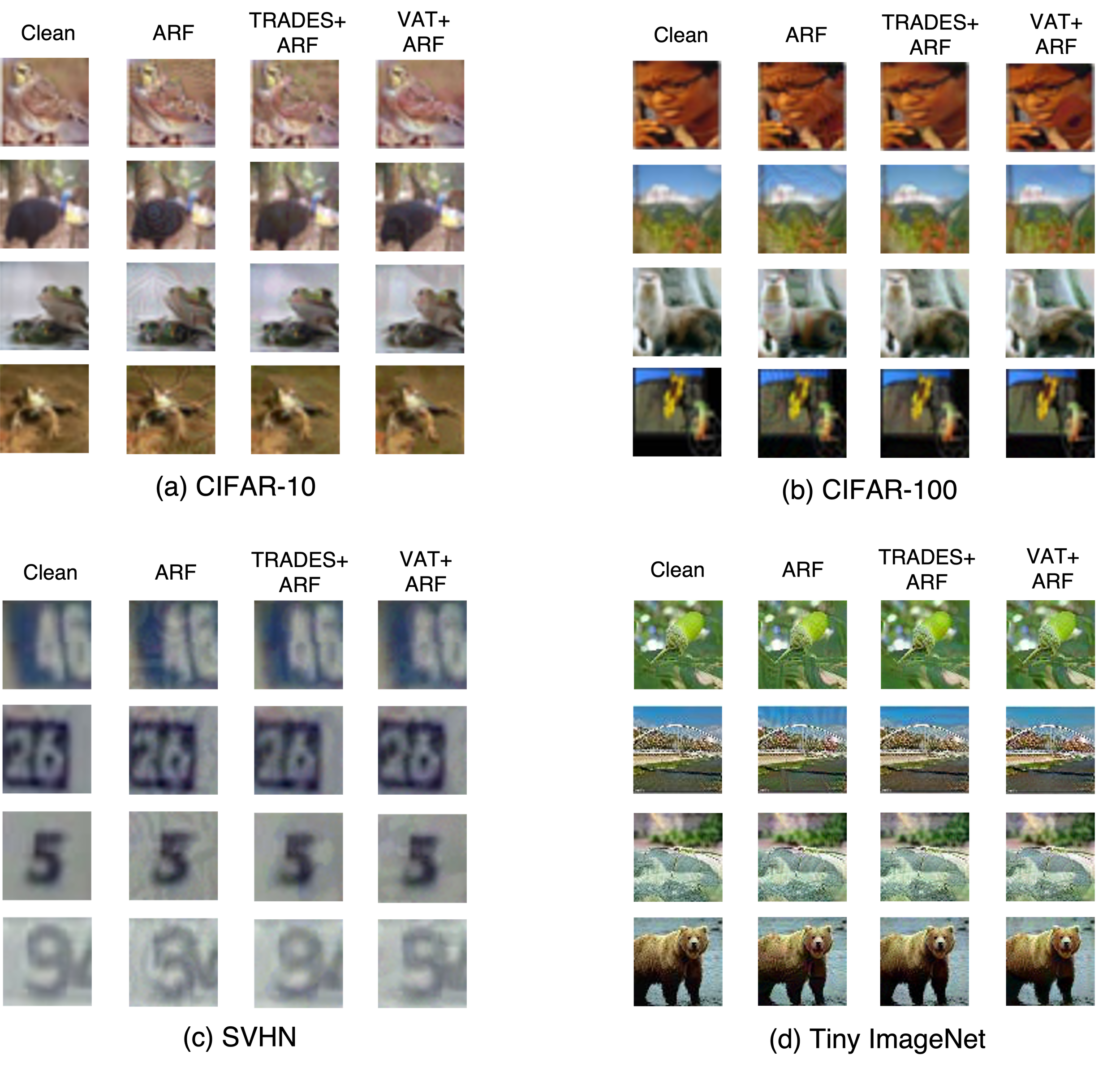
Figure J1: Adversarial images generated by BPDA circumventing our ARF defense. TRADES+ARF and VAT+ARF correspond to our ARF defense when applied on top of an adversarially trained DNN, TRADES/VAT, respectively. Adversarial images that fool our ARF defense can be easily spotted by the naked eye.

References

- [1] Maksym Andriushchenko, Francesco Croce, Nicolas Flammarion, and Matthias Hein. Square Attack: a query-efficient black-box adversarial attack via random search. In ECCV, 2020.
- [2] Anish Athalye, Nicholas Carlini, and David A Wagner. Obfuscated Gradients Give a False Sense of Security: Circumventing Defenses to Adversarial Examples. In ICML, 2018.
- [3] Anish Athalye, Logan Engstrom, Andrew Ilyas, and Kevin Kwok. Synthesizing Robust Adversarial Examples. ArXiv, abs/1707.0, 2018.
- [4] Yuval Bahat, Michal Irani, and Gregory Shakhnarovich. Natural and Adversarial Error Detection using Invariance to Image Transformations. ArXiv, abs/1902.0, 2019.
- [5] Wieland Brendel, Jonas Rauber, and Matthias Bethge. Decision-Based Adversarial Attacks: Reliable Attacks Against Black-Box Machine Learning Models. In ICLR, 2018.
- [6] Jacob Buckman, Aurko Roy, Colin Raffel, and Ian Goodfellow. Thermometer Encoding: One Hot Way To Resist Adversarial Examples. In ICLR, 2018.
- [7] Nicholas Carlini, Anish Athalye, Nicolas Papernot, Wieland Brendel, Jonas Rauber, Dimitris Tsipras, Ian Goodfellow, Aleksander Madry, and Alexey Kurakin. On Evaluating Adversarial Robustness. CoRR, abs/1902.0, 2019.
- [8] Nicholas Carlini and David A Wagner. Adversarial Examples Are Not Easily Detected: Bypassing Ten Detection Methods. In AISec@CCS, 2017.
- [9] Nicholas Carlini and David A Wagner. Towards Evaluating the Robustness of Neural Networks. 2017 IEEE Symposium on Security and Privacy (SP), pages 39–57, 2017.
- [10] Y. Carmon, Aditi Raghunathan, Ludwig Schmidt, Percy Liang, and John C. Duchi. Unlabeled data improves adversarial robustness. In NeurIPS, 2019.
- [11] Anirban Chakraborty, Manaar Alam, Vishal Dey, A Chattopadhyay, and Debdeep Mukhopadhyay. Adversarial Attacks and Defences: A Survey. ArXiv, abs/1810.0, 2018.
- [12] Alvin Chan, Yi Tay, and Yew-Soon Ong. What it thinks is important is important: Robustness transfers through input gradients. In CVPR, June 2020.
- [13] Ting Chen, Simon Kornblith, Mohammad Norouzi, and Geoffrey E Hinton. A Simple Framework for Contrastive Learning of Visual Representations. ArXiv, abs/2002.0, 2020.
- [14] Tianlong Chen, Sijia Liu, Shiyu Chang, Yu Cheng, Lisa Amini, and Zhangyang Wang. Adversarial robustness: From self-supervised pre-training to fine-tuning. In CVPR, June 2020.
- [15] Moustapha Cisse, Piotr Bojanowski, Edouard Grave, Yann Dauphin, and Nicolas Usunier. Parseval networks: Improving robustness to adversarial examples. In ICML, 2017.
- [16] Gilad Cohen, Guillermo Sapiro, and Raja Giryes. Detecting adversarial samples using influence functions and nearest neighbors. In CVPR, June 2020.
- [17] Jeremy Cohen, Elan Rosenfeld, and Zico Kolter. Certified adversarial robustness via randomized smoothing. In ICML, volume 97, pages 1310–1320, 09–15 Jun 2019.
- [18] B. Darvish Rouani, M. Samragh, T. Javidi, and F. Koushanfar. Safe machine learning and defeating adversarial attacks. IEEE Security Privacy, 17(2):31–38, 2019.
- [19] Guneet S. Dhillon, Kamyar Azizzadenesheli, Jeremy D. Bernstein, Jean Kossaifi, Aran Khanna, Zachary C. Lipton, and Animashree Anandkumar. Stochastic activation pruning for robust adversarial defense. In ICLR, 2018.
- [20] Yifan Ding, Liqiang Wang, Huan Zhang, Jinfeng Yi, Deliang Fan, and Boqing Gong. Defending against adversarial attacks using random forest. In IEEE/CVF Conference on Computer Vision and Pattern Recognition Workshops (CVPRW), pages 105–114, 2019.
- [21] Abhimanyu Dubey, Laurens van der Maaten, Zeki Yalniz, Yixuan Li, and Dhruv Kumar Mahajan. Defense against adversarial images using web-scale nearest-neighbor search. CVPR, pages 8759–8768, 2019.
- [22] Gintare Karolina Dziugaite, Zoubin Ghahramani, and Daniel M Roy. A study of the effect of JPG compression on adversarial images. ArXiv, abs/1608.0, 2016.
- [23] Ian Goodfellow, Jonathon Shlens, and Christian Szegedy. Explaining And Harnessing Adversarial Examples. In ICLR, 2015.
- [24] Abigail Graese, Andras Rozsa, and Terrance E Boult. Assessing Threat of Adversarial Examples on Deep Neural Networks. 2016 15th IEEE International Conference on Machine Learning and Applications (ICMLA), pages 69–74, 2016.
- [25] Chuan Guo, Mayank Rana, Moustapha Cisse, and Laurens van der Maaten. Countering Adversarial Images using Input Transformations. In ICLR, 2018.
- [26] Kaiming He, Xiangyu Zhang, Shaoqing Ren, and Jian Sun. Deep Residual Learning for Image Recognition. CVPR, pages 770–778, 2016.
- [27] Matthias Hein and Maksym Andriushchenko. Formal Guarantees on the Robustness of a Classifier against Adversarial Manipulation. In NIPS, 2017.
- [28] Geoffrey E Hinton, Oriol Vinyals, and Jeffrey Dean. Distilling the Knowledge in a Neural Network. ArXiv, abs/1503.0, 2015.
- [29] Daniel Jakubovitz and Raja Giryes. Improving DNN Robustness to Adversarial Attacks Using Jacobian Regularization. In ECCV, 2018.
- [30] Ahmadreza Jeddi, Mohammad Javad Shafiee, Michelle Karg, Christian Scharfenberger, and Alexander Wong. Learn2perturb: An end-to-end feature perturbation learning to improve adversarial robustness. In CVPR, June 2020.
- [31] Ziyu Jiang, Tianlong Chen, Ting Chen, and Zhangyang Wang. Robust pre-training by adversarial contrastive learning. In NeurIPS, 2020.
- [32] Harini Kannan, Alexey Kurakin, and Ian Goodfellow. Adversarial logit pairing. arXiv preprint arXiv:1803.06373, 2018.
- [33] A Kerckhoffs. La cryptographie militaire. Journal des Sciences Militaires, pages 161–191, 1883.
- [34] Alex Krizhevsky. Learning multiple layers of features from tiny images. Technical report, 2009.
- [35] Alexey Kurakin, Ian J Goodfellow, and Samy Bengio. Adversarial Machine Learning at Scale. CoRR, abs/1611.0, 2017.
- [36] Ya Le and X Yang. Tiny ImageNet Visual Recognition Challenge. 2015.
- [37] Kimin Lee, Kibok Lee, Honglak Lee, and Jinwoo Shin. A simple unified framework for detecting out-of-distribution samples and adversarial attacks. NeurIPS, 2018-Decem:7167–7177, 2018.
- [38] Jiajun Lu, Hussein Sibai, Evan Fabry, and David Alexander Forsyth. NO Need to Worry about Adversarial Examples in Object Detection in Autonomous Vehicles. ArXiv, abs/1707.0, 2017.
- [39] Yan Luo, Xavier Boix, Gemma Roig, Tomaso A Poggio, and Qi Zhao. Foveation-based Mechanisms Alleviate Adversarial Examples. ArXiv, abs/1511.0, 2015.
- [40] Xingjun Ma, Bo Li, Yisen Wang, Sarah M Erfani, Sudanthi N R Wijewickrema, Michael E Houle, Grant Schoenebeck, Dawn Song, and James Bailey. Characterizing Adversarial Subspaces Using Local Intrinsic Dimensionality. CoRR, abs/1801.0, 2018.
- [41] Aleksander Madry, Aleksandar Makelov, Ludwig Schmidt, Dimitris Tsipras, and Adrian Vladu. Towards Deep Learning Models Resistant to Adversarial Attacks. In ICLR, 2018.
- [42] D. J. Miller, Z. Xiang, and G. Kesidis. Adversarial learning targeting deep neural network classification: A comprehensive review of defenses against attacks. IEEE, 108(3):402–433, 2020.
- [43] Takeru Miyato, Shin-ichi Maeda, Masanori Koyama, Ken Nakae, and Shin Ishii. Distributional Smoothing with Virtual Adversarial Training. In ICLR 2016, 2015.
- [44] Seyed-Mohsen Moosavi-Dezfooli, Alhussein Fawzi, and Pascal Frossard. DeepFool: A simple and accurate method to fool deep neural networks. CVPR, pages 2574–2582, 2016.
- [45] Federico Nesti, Alessandro Biondi, and Giorgio C Buttazzo. Detecting Adversarial Examples by Input Transformations, Defense Perturbations, and Voting. IEEE transactions on neural networks and learning systems, PP, 2021.
- [46] Yuval Netzer, Tao Wang, Adam Coates, Alessandro Bissacco, Bo Wu, and Andrew Y Ng. Reading Digits in Natural Images with Unsupervised Feature Learning. In NIPS Workshop on Deep Learning and Unsupervised Feature Learning 2011, 2011.
- [47] N. Papernot, P. McDaniel, X. Wu, S. Jha, and A. Swami. Distillation as a defense to adversarial perturbations against deep neural networks. In IEEE Symposium on Security and Privacy (SP), 2016.
- [48] Nicolas Papernot, Patrick D McDaniel, and Ian J Goodfellow. Transferability in Machine Learning: from Phenomena to Black-Box Attacks using Adversarial Samples. CoRR, abs/1605.0, 2016.
- [49] Nicolas Papernot, Patrick D McDaniel, Somesh Jha, Matt Fredrikson, Z Berkay Celik, and Ananthram Swami. The Limitations of Deep Learning in Adversarial Settings. 2016 IEEE European Symposium on Security and Privacy (EuroS&P), pages 372–387, 2016.
- [50] Adam Paszke, Sam Gross, Francisco Massa, Adam Lerer, James Bradbury, Gregory Chanan, Trevor Killeen, Zeming Lin, Natalia Gimelshein, Luca Antiga, Alban Desmaison, Andreas Kopf, Edward Yang, Zachary DeVito, Martin Raison, Alykhan Tejani, Sasank Chilamkurthy, Benoit Steiner, Lu Fang, Junjie Bai, and Soumith Chintala. Pytorch: An imperative style, high-performance deep learning library. In H. Wallach, H. Larochelle, A. Beygelzimer, F. d'Alché-Buc, E. Fox, and R. Garnett, editors, Advances in Neural Information Processing Systems 32, pages 8024–8035. Curran Associates, Inc., 2019.
- [51] Sylvestre-Alvise Rebuffi, Sven Gowal, Dan Andrei Calian, Florian Stimberg, Olivia Wiles, and Timothy Mann. Data Augmentation Can Improve Robustness. In NeurIPS, 2021.
- [52] Andrew Slavin Ross and Finale Doshi-Velez. Improving the Adversarial Robustness and Interpretability of Deep Neural Networks by Regularizing Their Input Gradients. In AAAI, 2017.
- [53] Kevin Roth, Yannic Kilcher, and Thomas Hofmann. The Odds are Odd: A Statistical Test for Detecting Adversarial Examples. In ICML, 2019.
- [54] Andras Rozsa, Manuel Gunther, and Terrance E. Boult. Towards robust deep neural networks with bang. In WACV, 2018.
- [55] Pouya Samangouei, Maya Kabkab, and Rama Chellappa. Defense-GAN: Protecting classifiers against adversarial attacks using generative models. In ICLR, 2018.
- [56] Ali Shafahi, Mahyar Najibi, Mohammad Amin Ghiasi, Zheng Xu, John Dickerson, Christoph Studer, Larry S Davis, Gavin Taylor, and Tom Goldstein. Adversarial training for free! In NeurIPS, pages 3358–3369, 2019.
- [57] Uri Shaham, Yutaro Yamada, and Sahand Negahban. Understanding adversarial training: Increasing local stability of supervised models through robust optimization. Neurocomputing, 307:195–204, 2018.
- [58] Chawin Sitawarin and Dávid Wágner. Defending against adversarial examples with k-nearest neighbor. ArXiv, abs/1906.09525, 2019.
- [59] David Stutz, Matthias Hein, and Bernt Schiele. Disentangling Adversarial Robustness and Generalization. In CVPR, 6 2019.
- [60] Yu Sun, X Wang, Zhuang Liu, John Miller, Alexei A Efros, and Moritz Hardt. Test-Time Training with Self-Supervision for Generalization under Distribution Shifts. In ICML, 2020.
- [61] Christian Szegedy, Wojciech Zaremba, Ilya Sutskever, Joan Bruna, Dumitru Erhan, Ian Goodfellow, and Rob Fergus. Intriguing properties of neural networks. In ICLR, 2014.
- [62] Florian Tramer, Nicholas Carlini, Wieland Brendel, and Aleksander Madry. On adaptive attacks to adversarial example defenses. In NeurIPS, 2020.
- [63] Florian Tramèr, Alexey Kurakin, Nicolas Papernot, Ian Goodfellow, Dan Boneh, and Patrick McDaniel. Ensemble Adversarial Training: Attacks and Defenses. In ICLR, 2018.
- [64] Qinglong Wang, Wenbo Guo, Kaixuan Zhang, Alexander Ororbia, Xinyu Xing, C Lee Giles, and Xue Liu. Learning Adversary-Resistant Deep Neural Networks. ArXiv, abs/1612.0, 2016.
- [65] Eric Wong, Leslie Rice, and J Zico Kolter. Fast is better than free: Revisiting adversarial training. In ICLR, 2019.
- [66] Cihang Xie, Jianyu Wang, Zhishuai Zhang, Zhou Ren, and Alan Yuille. Mitigating Adversarial Effects Through Randomization. In ICLR, 2018.
- [67] Cihang Xie, Yuxin Wu, Laurens van der Maaten, Alan L Yuille, and Kaiming He. Feature denoising for improving adversarial robustness. In CVPR, pages 501–509, 2019.
- [68] Weilin Xu, David Evans, and Yanjun Qi. Feature Squeezing: Detecting Adversarial Examples in Deep Neural Networks. CoRR, abs/1704.0, 2018.
- [69] X. Yuan, P. He, Q. Zhu, and X. Li. Adversarial examples: Attacks and defenses for deep learning. IEEE Transactions on Neural Networks and Learning Systems, 30(9):2805–2824, 2019.
- [70] Runtian Zhai, Tianle Cai, Di He, Chen Dan, Kun He, John Hopcroft, and Liwei Wang. Adversarially robust generalization just requires more unlabeled data. arXiv preprint arXiv:1906.00555, 2019.
- [71] Hongyi Zhang, Moustapha Cissé, Yann N. Dauphin, and David Lopez-Paz. mixup: Beyond empirical risk minimization. In ICLR, 2018.
- [72] Hongyang Zhang, Yaodong Yu, J Jiao, E Xing, L Ghaoui, and Michael I Jordan. Theoretically Principled Trade-off between Robustness and Accuracy. In ICML, 2019.
- [73] Linjun Zhang, Zhun Deng, Kenji Kawaguchi, Amirata Ghorbani, and James Zou. How does mixup help with robustness and generalization? arXiv preprint arXiv:2010.04819, 2020.