Multi-Objective Bayesian Optimization over High-Dimensional Search Spaces

Abstract

Many real world scientific and industrial applications require optimizing multiple competing black-box objectives. When the objectives are expensive-to-evaluate, multi-objective Bayesian optimization (BO) is a popular approach because of its high sample efficiency. However, even with recent methodological advances, most existing multi-objective BO methods perform poorly on search spaces with more than a few dozen parameters and rely on global surrogate models that scale cubically with the number of observations. In this work we propose MORBO, a scalable method for multi-objective BO over high-dimensional search spaces. MORBO identifies diverse globally optimal solutions by performing BO in multiple local regions of the design space in parallel using a coordinated strategy. We show that MORBO significantly advances the state-of-the-art in sample efficiency for several high-dimensional synthetic problems and real world applications, including an optical display design problem and a vehicle design problem with $146$ and $222$ parameters, respectively. On these problems, where existing BO algorithms fail to scale and perform well, MORBO provides practitioners with order-of-magnitude improvements in sample efficiency over the current approach.

1 Introduction

The challenge of identifying optimal trade-offs between multiple complex objective functions is pervasive in many fields, including machine learning [Sener and Koltun, 2018], science [Gopakumar et al., 2018], and engineering [Marler and Arora, 2004, Mathern et al., 2021]. For instance, Mazda recently proposed a vehicle design problem in which the goal is to optimize the widths of $222$ structural parts in order to minimize the total weight of three different vehicles while simultaneously maximizing the number of common gauge parts [Kohira et al., 2018]. Additionally, this problem has $54$ black-box constraints that enforce important performance requirements such as collision safety. Evaluating a design requires either crash-testing a physical prototype or running computationally demanding simulations. In fact, the original problem was solved on what at the time was the world’s fastest supercomputer and took around $3$,$000$ CPU years to compute [Oyama et al., 2017]. Another example is designing optical components for AR/VR applications, which requires optimizing complex geometries described by hundreds of parameters in order to identify designs that yield optimal trade-offs between image quality and efficiency of the optical device. Evaluating a design involves either fabricating and measuring prototypes or running computationally intensive simulations. For such problems, sample-efficient optimization is paramount.

Bayesian optimization (BO) has emerged as an effective, general, and sample-efficient approach for “black-box” optimization [Jones et al., 1998] and is highly effective for machine learning hyperparameter tuning [Turner et al., 2021]. However, in its basic form, BO is subject to important limitations. In particular, (i) successful applications typically consider low-dimensional search spaces, usually with less than $20$ tunable parameters [Frazier, 2018], (ii) inference with the typical Gaussian Process (GP) surrogate models incurs cubic time complexity with respect to the number of data points, which prevents usage in the large-sample regime that is often necessary for high-dimensional problems, and (iii) most methods focus on single objective unconstrained problems. As a result, BO cannot easily be applied to either of the aforementioned Mazda vehicle design or the AR/VR optical design problems. Moreover, high dimensional multi-objective problems requiring sample-efficient optimization are prevalent in many real-world settings such as groundwater remediation [Akhtar and Shoemaker, 2015], cell network configuration [Dreifuerst et al., 2021], and water resource management [Bai et al., 2017]. The state-of-the-art approach for this class of problems is NSGA-II [Deb et al., 2002], a popular evolutionary strategy, but with poor sample-efficiency, which hinders the progress of the scientists running these experiments.

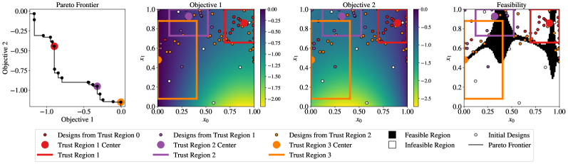
Figure 1: An illustration of MORBO on: 2-objective benchmark problem with 2 parameters and 2 constraints called MW7 [Ma and Wang, 2019] with $3$ TRs. The left-most plot illustrates how MORBO’s center selection technique centers the TRs at Pareto optimal points across different parts of the Pareto frontier. This encourages MORBO to explore diverse parts of the Pareto Frontier, which is important to identifying the multiple disconnected regions on this MW7 problem. The three right-most plots illustrate the TRs over the design space along with contours of, respectively, the 2 objective metrics and the feasibility metric indicating whether all black-box constraints are satisfied. Note that the TRs overlap with one another and contain data points that were collected by other TRs. Hence, sharing observations collected by different TRs provides local models with more observations than if each local model were only fitted to data collected by its corresponding TR.

In this paper, we close this gap by making BO applicable to challenging high-dimensional multi-objective problems. To do so, we propose an algorithm called MORBO (“Multi-Objective Regionalized Bayesian Optimization”) that optimizes diverse parts of the global Pareto frontier in parallel using a coordinated set of local trust regions (TRs). As shown in Figure 1 (left), TRs are located at different solutions with diverse trade-offs between objectives. MORBO performs local BO in each TR to mitigate over-exploration, a phenomenon that plagues many algorithms in high-dimensional settings [Eriksson and Poloczek, 2021]. To enable scaling to large evaluation budgets, MORBO leverages local GP surrogate models of the objective function, which reduces the time complexity for GP inference from $O(n^{3})$, where $n$ is the number of data points, to $O(n_{\mathcal{T}}^{3})$, where $n_{\mathcal{T}}\ll n$ is the number of local data points for a TR $\mathcal{T}$. To facilitate efficient and collaborative global optimization, MORBO passes information between TRs in the following two ways: (1) Observations collected by one TR are shared with the others—which is particularly important when the TRs overlap as shown in Figure 1, (2) MORBO selects a batch of candidates by leveraging the TRs to collaboratively maximize a global utility. To ensure efficient global optimization, MORBO terminates under-performing TRs and allocates new TRs according to a global policy with a theoretical performance guarantee—a property that sets MORBO apart from most existing methods.

The significance of MORBO is that it is the first multi-objective BO method that scales to hundreds of tunable parameters and thousands of evaluations, a setting where practitioners have previously had to fall back on alternative methods with much lower sample-efficiency, such as NSGA-II. Our comprehensive evaluation demonstrates that MORBO yields order-of-magnitude savings in terms of time and resources compared to state-of-the-art methods on challenging high-dimensional multi-objective problems.

2 Background

2.1 Preliminaries

2.1.1 Multi-Objective Optimization

In multi-objective optimization (MOO), the goal is to maximize (without loss of generality) a vector-valued objective function $\bm{f}(\bm{x})=[f^{(1)}(\bm{x}),...,f^{(M)}(\bm{x})]\in\mathbb{R}^{M}$, where $M\geq 2$ while satisfying black-box constraints $\bm{g}(\bm{x})\geq\bm{0}\in\mathbb{R}^{V}$ where $V\geq 0$, $\bm{x}\in\mathcal{X}\subset\mathbb{R}^{d}$, and $\mathcal{X}$ is a compact set. Usually, there is no single solution $\bm{x}^{*}$ that simultaneously maximizes all $M$ objectives and satisfies all $V$ constraints. Hence, objective vectors are compared using Pareto domination.

Definition 2.1.

An objective vector $\bm{f}(\bm{x})$ Pareto-dominates $\bm{f}(\bm{x}^{\prime})$, denoted as $\bm{f}(\bm{x})\succ\bm{f}(\bm{x}^{\prime})$, if $f^{(m)}(\bm{x})\geq f^{(m)}(\bm{x}^{\prime})$ for all $m=1,...,M$ and there exists at least one $m\in\{1,\dotsc,M\}$ such that $f^{(m)}(\bm{x})>f^{(m)}(\bm{x}^{\prime})$.

Definition 2.2.

The Pareto frontier (PF) is the set of optimal trade-offs $\mathcal{P}(X)$ over a set of designs $X\subseteq\mathcal{X}$:

$$\mathcal{P}(X)=\{\bm{f}(\bm{x}):\bm{x}\in X,\nexists\leavevmode\nobreak\ \bm{x}^{\prime}\in X\leavevmode\nobreak\ s.t.\leavevmode\nobreak\ \bm{f}(\bm{x}^{\prime})\succ\bm{f}(\bm{x})\}$$

Under black-box constraints, the feasible Pareto frontier is defined as $\mathcal{P}_{\text{feas}}(X)$ = $\mathcal{P}(\{\bm{x}\in X:\bm{g}(\bm{x})\geq\bm{0}\})$.

The goal of a MOO algorithm is to identify an approximate PF $\mathcal{P}(X_{n})$ of the true PF $\mathcal{P}(\mathcal{X})$ within a pre-specified budget of $|X_{n}|=n$ function evaluations. The quality of a PF is often evaluated using the hypervolume (HV) indicator.

Definition 2.3.

The hypervolume indicator, $\textsc{HV}{}(\mathcal{P}(X)|\bm{r})$ is the $M$-dimensional Lebesgue measure $\lambda_{M}$ of the region dominated by $\mathcal{P}(X)$ and bounded from below by a reference point $\bm{r}\in\mathbb{R}^{M}$.

The reference point is typically provided by the practitioner based on domain knowledge [Yang et al., 2019]. MOO problems are often addressed using evolutionary algorithms (EA) such as NSGA-II [Deb et al., 2002]. However, EAs generally suffer from high sample-complexity, rendering them inapplicable under small evaluation budgets.

2.1.2 Bayesian Optimization

When high sample-efficiency is required, Bayesian optimization (BO) is a popular approach [Frazier, 2018]. BO relies on a probabilistic surrogate model and an acquisition function that uses the surrogate model to provide the utility of evaluating a set of design points on the black-box function. The acquisition function is responsible for balancing exploration and exploitation. In the multi-objective setting, a common approach is to optimize random scalarizations of the objectives [Knowles, 2006, Paria et al., 2020] using a single-objective acquisition function. A more principled approach is to directly optimize the Pareto frontier by selecting candidates with maximum hypervolume improvement either in expectation under the GP posterior [Emmerich et al., 2006] or using Thompson sampling (TS) [Bradford et al., 2018].

2.2 Related Work

2.2.1 Multi-objective Bayesian optimization

There have been many recent contributions to multi-objective BO, e.g., Konakovic Lukovic et al. [2020], Daulton et al. [2020, 2022], Bradford et al. [2018]), but very few methods consider the high-dimensional setting and with large evaluation budgets. All of these methods described below rely on global GP models. As a result, these methods have mostly been evaluated on low-dimensional problems, typically $d\ll 10$ [Konakovic Lukovic et al., 2020, Bradford et al., 2018]. In the multi-objective BO literature, the largest search space we have found consists of $27$ parameters [Paria et al., 2020]. Nevertheless, for completeness we review multi-objective BO methods that support generating large batches of designs. DGEMO [Konakovic Lukovic et al., 2020] uses a hypervolume-based objective with heuristics to encourage diversity while exploring the PF.

Parallel expected hypervolume improvement ($q$EHVI) [Daulton et al., 2020] has strong empirical performance, but its computational complexity scales exponentially with the batch size. $q$NEHVI [Daulton et al., 2021] improves scalability with respect to the batch size, but like DGEMO and $q$EHVI, $q$NEHVI has only been evaluated on low-dimensional search spaces. TSEMO [Bradford et al., 2018] optimizes approximate GP function samples using NSGA-II and uses a hypervolume-based objective for selecting a batch of points from the NSGA-II population. ParEGO [Knowles, 2006] and TS-TCH [Paria et al., 2020] use random Chebyshev scalarizations with parallel expected improvement [Jones et al., 1998] and Thompson sampling—where a design is sampled with probability proportional to a design being optimal [Thompson, 1933]—respectively. ParEGO has been extended to the batch setting in various ways including: (i) MOEA/D-EGO [Zhang et al., 2010], an algorithm that optimizes multiple scalarizations in parallel using MOEA/D [Zhou et al., 2012], and (ii) $q$ParEGO [Daulton et al., 2020], which uses composite objectives with sequential greedy batch selection under different scalarization weights. Information-theoretic methods, e.g., Hernández-Lobato et al. [2015], Suzuki et al. [2020] have also garnered recent interest.

LaMOO [Zhao et al., 2021] is a recent work that partitions the search space into “good“ and “bad“ regions and samples new designs from “good“ regions using $q$EHVI or CMA-ES [Hansen, 2007]. However, LaMOO-$q$EHVI relies on global GPs and is therefore prohibitively time-consuming with large evaluation budgets. In addition, the authors propose to use rejection sampling to enforce that samples are from the, typically non-rectangular, "good" region, but rejection sampling is prohibitively time-consuming in high-dimensional search spaces (see Appendix D.1.1 for further discussion).

2.2.2 High-dimensional Bayesian optimization

Two popular approaches for high-dimensional BO are (1) mapping the high-dimensional inputs to a low-dimensional space via a random embedding [Wang et al., 2016, Munteanu et al., 2019, Letham et al., 2020] and (2) exploiting additive structure [Kandasamy et al., 2015, Gardner et al., 2017]. However, both families of methods require strong assumptions on the structure of the problem (low-dimensional linear or additive structure, respectively), and often perform poorly if the assumptions do not hold [Eriksson and Jankowiak, 2021]. This is especially problematic when optimizing multiple objectives since all objectives need to have the same assumed structure, which is unlikely in practice. Eriksson and Jankowiak [2021] leverage a weaker assumption that the objective only depends on a small subset of the parameters and Eriksson et al. [2021] extended this approach to the multi-objective setting, but this approach requires using computationally-demanding Markov Chain Monte Carlo methods for fitting the model, which is only feasible in the small data regime.

2.2.3 Trust Region Bayesian Optimization

Another popular method for high-dimensional BO is TuRBO [Eriksson et al., 2019], which performs BO in local trust regions (TRs) to avoid over-exploration. In contrast with [Zhao et al., 2021] which uses non-rectangular "good" regions, TuRBO uses hyperrectangular TRs, where each TR $\mathcal{T}$ has a center point $\bm{x}_{\text{center}}$ and an edge-length $L\in[L_{\text{min}},L_{\text{max}}]$. Each TR maintains success and failure counters that record the number of consecutive samples generated from the TR that improved or failed to improve (respectively) the objective. If the success counter exceeds a predetermined threshold $\tau_{\text{succ}}$, the TR length is increased to $\min\{2L,L_{\text{max}}\}$ and the counter is reset to zero. Similarly, after $\tau_{\text{fail}}$ consecutive failures the TR length is set to $L/2$ and the failure counter is set to zero. Finally, if the length $L$ drops below a minimum edge length $L_{\text{min}}$, the TR is terminated and a new TR is initialized.

In contrast with aforementioned methods, TuRBO makes no strong assumptions about the objectives. Although TuRBO has been extended to handle black-box constraints [Eriksson and Poloczek, 2021], to our knowledge, all existing TR-based BO methods target single-objective optimization. In addition, TuRBO does not pass information between TRs, which results in an inefficient use of the evaluation budget; these methods have not observed significant improvement from using multiple TRs. Lastly, even though optimization is restricted to a local TR, TuRBO fits GP models to the entire history of data collected by a single TR which can lead to poor scalability in settings where TRs restart infrequently.

2.3 Issues with Scalarized TuRBO

Since ParEGO is a well-established method (in low-dimensional settings) that optimizes random Chebyshev scalarizations, a reasonable approach would be to extend TuRBO to the MOO setting by using multiple TRs in parallel where each TR optimizes a different random Chebyshev scalarization of the objectives. However, as we demonstrate in the left subplot of Figure 2, this approach results in a PF with very poor coverage. This is because a single scalarization is used for the lifetime of each TR in order to maintain a stable objective. Optimizing a single scalarization per trust region often leads to better solutions with respect to that scalarization than optimizing the entire PF using a hypervolume-based acquisition functions, which requires exploration of different objective trade-offs. However, if TRs are not restarted frequently (e.g. because TuRBO continues to find better solutions with respect to that scalarization), only a small number of scalarizations will be used, which can lead to poor coverage of the PF. As shown in Figure 2, we observe that MORBO yields PFs with better coverage (diversity of trade-offs). In addition, the TRs in TuRBO are independent; they do not pass information about evaluated designs and observations, and they do not collaboratively aim to optimize the global PF—rather, they act in isolation to optimize their own objectives. Together, this leads to an inefficient use of the sample budget.

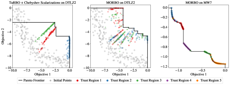
Figure 2: Objective values achieved on a $2$-objective DTLZ2 function with $d=100$ after $600$ evaluations, batch size $50$, and $3$ TRs. The scatter plot illustrates the search behavior. The grey circles indicate the initial space-filling design, which is the same for both methods. The other marker shapes and colors indicate which of the $3$ TRs obtained a given solution. The black line indicates the approximate Pareto frontier identified by each method. (Left) A straightforward extension of TuRBO where each TR optimizes a random Chebyshev scalarization of the objectives does not explore the trade-offs between the objectives because the TRs are rarely terminated under this approach, which leads only a few scalarizations being used. (Center) In contrast, MORBO employs a center selection strategy that actively targets under-explored regions of the Pareto frontier and uses a hypervolume-based acquisition function that is known to reward to high quality Pareto frontiers [Zitzler et al., 2003, Couckuyt et al., 2014, Yang et al., 2019] and explores the entirety of the PF. (Right) MORBO can discover disconnected regions of global PF on the MW7 function ($d=10$, with $2$ constraints) by using $5$ TRs to locally optimize disjoint regions of PF collaboratively, in parallel. This is stark contrast with TuRBO with Chebyshev scalarizations which the left plot shows yield approximate Pareto frontiers with poor coverage and diversity, even when the true PF is connected and simple.

3 MORBO

We now introduce MORBO, a collaborative multi-TR approach for constrained high-dimensional multi-objective BO. Rather than following TuRBO’s approach of employing multiple independent TRs, MORBO shares observations across TRs to provide each TR with all available information about the objectives and constraints relevant for local optimization in the TR. Moreover, MORBO further departs from TuRBO by (1) selecting TR center points in a coordinated fashion to encourage identifying Pareto frontiers with good coverage, (2) choosing new candidate designs by collaboratively optimizing a shared global utility, and (3) employing local models to reduce computational complexity and improve scalability in large data regimes. As shown in the center plot of Figure 2, MORBO identifies a high quality PF with much better coverage than the aforementioned simple TuRBO extension. For the remainder of this section, we describe the core components of MORBO, which are also summarized in Algorithm 1.

Input: Objective functions $f$, Number of trust region $n_{\text{TR}}$, Initial trust region length $L_{\text{init}}$, Maximum trust region length $L_{\max}$, Minimum trust region length $L_{\min}$.

Output: Approximate Pareto frontier $\mathcal{P}_{n}$

1 Evaluate an initial set of points and initialize the trust regions $\mathcal{T}_{1},...,\mathcal{T}_{n_{\text{TR}}}$ using the center selection procedure described in Section 3.2 and mark center points as unavailable for other trust regions.

2 $X_{0}\leftarrow\emptyset{},Y_{0}=\emptyset{},t\leftarrow 1$

3 while budget not exhausted do

4       Fit a local model within each trust region.

5       Select $q$ candidates using the sequential greedy HVI procedure described in Section 3.1.

6       Evaluate candidates on the true objective functions and obtain new observations.

7       for $j=1,...,n_{\text{TR}}$ do

8             Update trust regions with new observations as described in Section 3.

9             Increment success/failure counters as described in Section 3 for observations from $T_{j}$.

10             Update edgelength $L_{j}$ for $\mathcal{T}_{j}$.

11             if $L_{j}<L_{\text{min}}$ then

12                   Terminate $\mathcal{T}_{j}$.

13                   Fit GP to restart points $\mathcal{D}_{t-1}=(X_{t-1},Y_{t-1})$: $\bm{f}_{t-1}\sim P(\bm{f}|\mathcal{D}_{t-1})$.

14                   Sample $\bm{\lambda}\sim S_{+}^{M-1}$ and $\tilde{\bm{f}}_{t-1}\sim P(\bm{f}|\mathcal{D}_{t-1})$, where $S_{+}^{M-1}=\{\bm{w}\in\mathbb{R}_{+}^{M}:||\bm{w}||_{2}=1\}$.

15                   $\bm{x}_{t}\leftarrow\operatorname*{arg\,max}_{\bm{x}\in\mathcal{X}}s_{\bm{\lambda}}[\tilde{\bm{f}}_{t-1}(\bm{x})]$, where $s_{\bm{\lambda}}[\bm{y}]=\min_{m}(\max(\frac{y_{m}}{\lambda_{m}},0))^{M}$ and $\cdot_{i}$ denotes the $i^{\text{th}}$ element.

16                   Evaluate $\bm{x}_{t}$ on the true objective functions and obtain new observation $\bm{y}_{t}$.

17                   Reinitialize $\mathcal{T}_{j}$ with edgelength $L_{\text{init}}$ centered at the $\bm{x}_{t}$.

18                   Set $X_{t}\leftarrow X_{t-1}\cup\{\bm{x}_{t}\},Y_{t}\leftarrow Y_{t-1}\cup\{\bm{y}_{t}\}$, $t\leftarrow t+1$.

19            Update center to the available point with maximum HVC (globally if $\mathcal{T}_{j}$ was terminated otherwise within $\mathcal{T}_{j}$).

20      

return Approximate PF across observed function values.

Algorithm 1 Summary of MORBO

3.1 Collaborative Batch Selection via Global Utility Maximization

Maximizing hypervolume improvement (HVI) has been shown to produce high-quality and diverse PFs [Emmerich et al., 2006]. Given a reference point, the hypervolume improvement from a set of points is the increase in HV when adding these points to the previously selected points. Expected HVI (EHVI) is a popular acquisition function that integrates HVI over the GP posterior. However, maximizing EHVI directly requires re-computing the GP posterior and sampling from it in each gradient step, which becomes prohibitively slow as the number of objectives (and constraints) and in-sample data points increases.

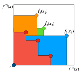
Figure 5: A visualization of our batch selection using HVI with $q=4$. The red points represent the current PF. Blue, orange, and green points show the function values for the $3$ selected points under the next posterior sample. To select the $4$th point, the HVI of each candidate is evaluated jointly with the red, blue, orange, and green points.

To allow scalability to large batch sizes $q$, we instead use Thompson sampling (TS) to draw $q$ posterior samples from the GP and optimize HVI under each realization. This approach can be viewed as a single-sample approximation of EHVI [Daulton et al., 2021]. We select $q$ points $\bm{x}_{1},...,\bm{x}_{q}$ for the next batch in a sequential greedy fashion and condition upon the previously selected points in the batch by computing the HVI with respect to the current PF $\mathcal{P}$. In particular, to select the $i^{\text{th}}$ point from a set of $r$ candidate points $\hat{\bm{x}}_{1},\ldots,\hat{\bm{x}}_{r}$ we draw a sample from the joint posterior over $\bm{f}(\{\bm{x}_{1},\ldots,\bm{x}_{i-1}\}\cup\{\hat{\bm{x}}_{1},\ldots,\hat{\bm{x}}_{r}\})$, which yields the realization $\{\tilde{\bm{f}}(\bm{x}_{1}),\ldots,\tilde{\bm{f}}(\bm{x}_{i-1}),\tilde{\bm{f}}(\hat{\bm{x}}_{1}),\ldots,\tilde{\bm{f}}(\hat{\bm{x}}_{r})\}$. We select the $i^{\text{th}}$ point as the candidate point that maximizes the HVI jointly with the realizations $\tilde{\bm{f}}(\bm{x}_{1}),\ldots,\tilde{\bm{f}}(\bm{x}_{i-1})$ of the previously selected points as shown in Figure 5. Conditioning on the previously selected points and computing the HVI under a sample from the joint posterior over the previously selected points and the discrete set of candidates leads to more diverse batch selection compared to selecting each point independently. Moreover, this approach effectively lets TRs collaboratively maximize the global HVI utility function. Using this global utility, an individual TR considers the iteration a success if at least one proposed candidate improves the global HV and a failure otherwise.

Another benefit of HV-based acquisition functions is that they naturally provide utility values for set of points, which enables the TRs to target different parts of the PF. This is particularly appealing in settings where the PF may be disjoint or may require exploring different parts of the search space. As shown in the right plot of Figure 2, MORBO recovers diverse regions of a disconnected PF. Lastly, we note that this batch selection strategy also allows to straightforwardly implement fully asynchronous optimization, where evaluations are dispatched to different “workers” and new candidates are generated whenever there is capacity in the worker pool. In the asynchronous setting, success/failure counters and TRs can be updated after every $q$ observations are received, and intermediate observations can immediately be used to update the local models.

3.2 Coordinated Trust Region Center Selection

In (constrained) single-objective optimization, previous work centers the local TR at the best (feasible) observed point. However, in the multi-objective setting, there is typically no single best solution. Assuming noise-free observations, MORBO selects the center to be the feasible point on the PF with maximum hypervolume contribution (HVC) [Beume et al., 2007, Loshchilov et al., 2011]. If there is no feasible point, MORBO chooses the point with the smallest total constraint violation (see Appendix B for details on center selection with constraints). Given a reference point, the HVC of a point on the PF is the reduction in HV if that point were to be removed; that is, the HVC of a point is its exclusive contribution to the PF. Centering a TR at the point with maximal HVC collected by that TR promotes coverage across the PF, as points in crowded regions will have lower contribution. MORBO selects TR centers based on their HVCs in a sequential greedy fashion, excluding points that have already been selected as the center for another TR.

3.3 Local Modeling

Most BO methods use a single global GP model, often with a stationary kernel (e.g. Matérn-$5/2$) using automatic relevance determination (ARD) fitted to all observations collected so far. While a global model is necessary for most BO methods, MORBO only requires each model to be accurate within the corresponding TR. To increase scalability, we employ local modeling where we only include the observations contained within a local modeling hypercube with edge length $2L$. The motivation for using the observations from a slightly larger hypercube is to improve the model close to the TR boundary.

In previous trust region BO works [Eriksson et al., 2019, Eriksson and Poloczek, 2021, Wan et al., 2021], each TR uses a GP that is fitted to the all observations collected by that TR (rather than only a set of local observations in or near the TR), which leads to scalability issues due to the cubic time complexity of GP inference if the TR collects many observations. In addition, fitting a GP solely to data collected by a single TR ignores observations collected by other TRs and makes inefficient use of the sampling budget. In contrast, MORBO shares observations across TRs and employs local models, where models are fit to all observations within a hypercube with edge length $2L$. This significantly reduces the computational cost since exact GP fitting scales cubically with the number of data points. Under limited assumptions on the distribution of data across TRs, using local models results in speedups of $O(n_{\text{TR}}^{2}/\eta^{3})$, where $\eta$ is the average number of TR modeling spaces a data point resides in. Empirically, we demonstrate (see Figure 7 in Appendix F) that $\eta<1$ as the optimization progresses and the TRs shrink, and we find that this translates into speedups of two orders of magnitude relative to global modeling as shown in Appendix F.2. See Appendix E for more details on the complexity.

3.4 Re-initialization Strategy

Although MORBO performs local optimization within a TR, we ensure global optimization by re-initializing TRs using a principled technique based on hypervolume scalarizations [Zhang and Golovin, 2020]. A HV scalarization is defined as $s_{\bm{\lambda}}[\bm{y}]=\min_{m}(\max(\frac{y_{m}}{\lambda_{m}},0))^{M}$, where $\cdot_{m}$ denotes the $m^{\text{th}}$ component [Zhang and Golovin, 2020]. Let $\mathcal{D}_{t-1}=(X_{t-1},Y_{t-1})$ be the set of previous re-initialization (restart) points $X_{t-1}=\{\bm{x}_{i}\}_{i=1}^{t-1}$ and corresponding observations $Y_{t-1}=\bm{f}(X_{t-1})$, where $X_{0}=\emptyset{}$ and $Y_{0}=\emptyset{}$. Given $\mathcal{D}_{t-1}$, we determine the center point $x_{t}$ of the new TR by maximizing a random HV scalarization of the objectives under a posterior sample from a global GP posterior conditioned on $D_{t-1}$: $\tilde{\bm{f}}\sim P(\bm{f}|\mathcal{D}_{t-1})$. This ensures that TRs are initialized in diverse parts of the objective space and yields a global optimization performance guarantee (Section 4).

4 Theoretical Analysis

We analyze the performance of MORBO in terms of its cumulative HV regret. The instantaneous HV regret $R(\mathcal{P}_{t})$ after $t$ TR restarts is defined as the difference in HV dominated by the true Pareto frontier $\mathcal{P}^{*}$ and the approximate Pareto frontier $\mathcal{P}_{t}$: $R(\mathcal{P}_{t})=\textsc{HV}{}(\mathcal{P}^{*})-\textsc{HV}{}(\mathcal{P}_{t}).$ The (cumulative) HV regret after $T$ restarts is the sum of the instantaneous regret over all restarts: $R_{T}=\sum_{t=1}^{T}R(\mathcal{P}_{t})$. First, we show that a TR will only evaluate a finite number of samples before restarting.

Lemma 4.1.

Let $\bm{f}\in[0,B]^{M}$, and assume that MORBO only considers a newly evaluated sample to be an improvement (for updating the corresponding TR’s success and failure counters) if it increases the HV by at least $\delta\in\mathbb{R}^{+}$ and assume that success counter threshold $\tau_{\text{succ}}=\infty$. Then each TR will only evaluate a finite number of samples.

The proof is given in Appendix C. Having established that TRs only evaluate a finite number of designs, we now bound the hypervolume regret with respect to the number of restarted TRs. The bound leverages the kernel-dependent maximum information gain $\gamma_{T}$—which measures the decrease in uncertainty after $T$ observations —and is commonly used to analyze regret in BO [Srinivas et al., 2010].

Theorem 4.1.

Let $\bm{f}\in[0,B]^{M}$ for $B>0$ and let each component $f^{(m)}$ for $m=1,...,M$ follow a Gaussian distribution with marginal variances $\sigma\leq 1$ and independent observation noise $\epsilon_{m}\sim\mathcal{N}(0,\sigma_{m}^{2})$ such that $\sigma_{m}^{2}\leq\sigma^{2}\leq 1$. Let $\mathcal{P}_{t}$ denote the Pareto frontier over $\bm{f}(X_{t})$, where $X_{t}$ is the set of TR re-initialization points after $t$ TRs have been restarted. Suppose further that the conditions of Lemma 4.1 hold. Then, the cumulative hypervolume regret $R_{T}$ of MORBO after $T$ restarts is bounded by:

$$R_{T}\leq M^{2}(\sqrt{2e\pi}B/2)^{M}\sqrt{d\gamma_{T}T\ln(T)}.$$

Up to logarithmic terms, this regret bound is on the order of $\tilde{\mathcal{O}}(\sqrt{T})$. This bound is significant because, to our knowledge, Zhang and Golovin [2020] is the only other work to bound the HV regret of multi-objective BO algorithms. This makes MORBO the first sample-efficient large-scale, MOO algorithm with bounded regret. The proof, given in Appendix C, leverages the hypervolume regret bound from Zhang and Golovin [2020]. However, our regret bound is with respect to the number of restart points (rather than evaluations)—a difference that can be viewed as a cost of focusing on large-scale problems which BO with global GPs cannot address. Moreover, our regret analysis in terms of the number of restarts is similar to the convergence guarantees of gradient-based TR optimization methods [Yuan, 1999] and can be viewed as a multi-objective analogue of the performance guarantees of recent single-objective BO-based TR methods [Wan et al., 2021].

5 Experiments

We evaluate MORBO on an extensive suite of benchmarks with various numbers of input parameters ($d$), objectives ($M$), and constraints ($V$). In Appendix F.1, we consider a vehicle ($d=5$) and a welded beam ($d=4$, $V=4$) design problem to show that MORBO is competitive with other algorithms on problems it was not designed for. We consider three challenging real-world problems: a trajectory planning problem ($d=60$), a problem of designing optical systems for AR/VR applications ($d=146$), and an automotive design problem ($d=222,V=54$) . In addition, we evaluate MORBO on DTLZ3, DTLZ5, and DTLZ7 problems with $2$/$4$ objectives ($6$ problems in total) in Appendix F.

We compare MORBO to multi-objective BO methods ($q$NEHVI, $q$ParEGO, TS-TCH, TSEMO, DGEMO, MOEA/D-EGO), recent work leveraging search space partitioning (LaMOO-CMAES, LaMOO-$q$NEHVI), a widely used evolutionary algorithm (NSGA-II), and Sobol—a quasi-random baseline where designs are sampled from a scrambled Sobol sequence [Owen, 2003] (see Appendix D for more details on the methods). MORBO is implemented using BoTorch [Balandat et al., 2020] and the code will be made publicly available soon. We run all methods for $20$ replications and initialize them using the same quasi-random initial points for each replication. We use the same hyperparameters for MORBO on all problems and conduct analyze the sensitivity of MORBO to its hyperparameters in Figure 4. See Appendix D for details on the experiment setup. All experiments used a Tesla V100 SXM2 GPU (16GB RAM).

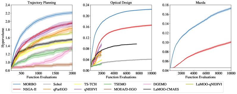
Figure 3: (Left) MORBO outperforms other methods on the trajectory planning problem ($d=60$). (Middle) Illustration of the results on the Optical design problem ($d=146$). NSGA-II performs better than the BO baselines but is not competitive with MORBO. (Right) MORBO shows compelling performance on the Mazda vehicle design problem ($d=222$) with $54$ black-box constraints. For all plots, we show the mean and one standard error of the mean over 20 replications.

5.1 Large-Scale Real-World Problems

Trajectory Planning

We consider a trajectory planning problem similar to the rover trajectory planning problem considered in [Wang et al., 2018]. As in the original problem, the goal is to find a trajectory that maximizes the reward when integrated over the domain. The trajectory is determined by fitting a B-spline to $30$ design points in the 2-objective plane, which yields a $60$-dimensional optimization problem. In this experiment, we constrain the trajectory to begin at the pre-specified starting location, but we do not require it to end at the desired target location. In addition to maximize the reward of the trajectory, we also minimize the distance from the end of the trajectory to the intended target location. Intuitively, these two objectives are expected to be competing because reaching the exact end location may require passing through areas with lower associated reward. The results from $2$,$000$ evaluations using batch size $q=50$ and $200$ initial points are presented in Figure 3, which shows that MORBO performs the best and even state-of-the-art methods such as $q$NEHVI do not out perform NSGA-II.

Optical design problem

We consider the problem of designing an optical system for an augmented reality (AR) see-through display. This optimization task has $146$ parameters describing the geometry and surface morphology of multiple optical elements in the display stack. Several objectives are of interest in this problem, including display efficiency and display quality. Each evaluation of these metrics requires a computationally intensive physics simulation that takes several hours to run. In this benchmark, the task is to explore the Pareto frontier between display efficiency and display quality (both objectives are normalized w.r.t. the reference point). We consider $250$ initial points, batch size $q=50$, and a total of $10$,$000$ evaluations. This is out of reach for the other BO baselines due to runtime considerations, and so we run $q$NEHVI, $q$ParEGO, TS-TCH, TSEMO, MOEA/D-EGO, for $2$,$000$ evaluations and DGEMO for $1$,$000$ evaluations. We were only able to run LaMOO-CMAES for $7,600$ evaluations before it overflowed GPU memory. Figure 3 shows that MORBO achieves substantial improvements in sample efficiency compared to NSGA-II. Furthermore, observe that no other baselines are competitive with NSGA-II except in the very small sample regime (less than $500$ evaluations).

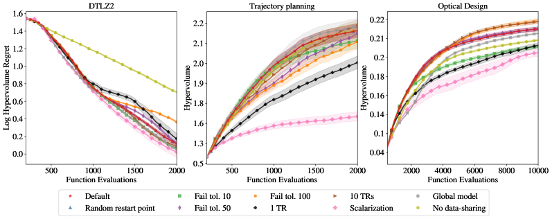
Figure 4: We investigate the sensitivity of MORBO with respect to its hyperparameters. We observe that using multiple TRs performs significantly better than using a single TR and that data-sharing and the use of a hypervolume based acquisition function are important components of MORBO.

Mazda vehicle design problem

We consider the $3$-car Mazda benchmark problem [Kohira et al., 2018]. This challenging MOO problem involves tuning $222$ decision variables that represent the thickness of different structural parts. The goal is to minimize the total vehicle mass of the three vehicles (Mazda CX-$5$, Mazda $6$, and Mazda $3$) as well as maximizing the number of parts shared across vehicles. Additionally, there are $54$ black-box output constraints (evaluated jointly with the two objectives) that enforce that designs meet performance requirements such as collision safety standards. This problem is, to the best our knowledge, the largest MOO problem considered by any BO method and requires fitting $56$ GP models to the objectives and constraints. The original problem underlying the Mazda benchmark was solved on what at the time was the world’s fastest supercomputer and took around $3$,$000$ CPU years to compute [Oyama et al., 2017]. We consider a budget of $10$,$000$ evaluations using batches of size $q=50$ and $300$ initial points.

Figure 3 demonstrates that MORBO clearly outperforms the other methods. A feasible design satisfying the black-box constraints was provided to all methods for all replications as part of the initial $300$ design points. However, in subsequent evaluations Sobol did not find another feasible design, illustrating the challenge of satisfying the $54$ constraints. While NSGA-II made progress from the initial feasible solution, it is not competitive with MORBO. NSGA-II and Sobol are the only applicable baselines because standard multi-objective BO methods are impractically slow with $56$ global GPs and LaMOO does not support black-box constraints.

5.2 Ablation study

Finally, we study the sensitivity of MORBO with respect to the number of TRs ($n_{\text{TR}}$), the failure tolerance ($\tau_{\text{fail}}$), and sharing observations across TRs, local modeling, HVI acquisition function, and the re-initialization strategy. Using several TRs allows MORBO to explore different parts of the search space that potentially contribute to different parts of the Pareto frontier. The failure tolerance controls how quickly each TR shrinks: A large $\tau_{\text{fail}}$ leads to slow shrinkage and potentially too much exploration, while a small $\tau_{\text{fail}}$ may cause each TR to shrink too quickly and not collect enough data. MORBO uses $5$ TRs and $\tau_{\text{fail}}=\max(10,\frac{d}{3})$ by default, similar to what is used by Eriksson et al. [2019].

We consider the DTLZ2 problem ($d=100$, $M=2$), the trajectory planning problem ($d=60$, $M=2$), and the optical design problem ($d=146$, $M=2$). Figure 4 shows that MORBO with the default settings performs well on all three problems. We observe that multiple TRs and the HVI acquisition function are important as neither a single TR nor a Chebyshev scalarization performs well. The performance of MORBO is robust to the choice of failure tolerance except for on the optical design problem where using a value of $10$ is clearly worse than the default and causes the TRs to shrink too quickly. Not sharing data between TRs results in inferior results on the DTLZ2 and optical design problems. While using a global GP model achieves good results on the DTLZ2 and trajectory planning problems, it does not perform as well on the optical design problem. A global GP also comes at a high computational cost. Using a global GP, running MORBO with a budget of $10$,$000$ evaluations on the optical design problem required $30$ hours of computational overhead, whereas MORBO did $10$,$000$ evaluations in less than an hour using local models. Lastly, we find consistently strong performance for both our default HV scalarization-based re-initialization strategy and a strategy that selects a new design at random (denoted as "Random restart points"). The former allows us to bound MORBO’s regret.

6 Discussion

We proposed MORBO, an algorithm for multi-objective BO over high-dimensional search spaces. By using a coordinated, collaborative multi-trust-region approach with scalable local modeling, MORBO scales gracefully to high-dimensional problems and high-throughput settings. In a comprehensive experimental evaluation, we showed that MORBO allows us to effectively tackle important real-world problems that were previously out of reach for existing BO methods. We showed that MORBO achieves substantial improvements in sample efficiency compared to existing state-of-the-art methods such as evolutionary algorithms. Due to the lack of alternatives, NSGA-II has been the method of choice for many practitioners, and we expect MORBO to provide practitioners with significant savings in terms of time and resources across the many disciplines that require solving challenging optimization problems.

However, there are some limitations to our method. Although MORBO can handle a large number of black-box constraints, using hypervolume-based acquisition means the computational complexity scales poorly with the number of objectives. Furthermore, MORBO is optimized for the large-batch high-throughput setting and other methods may be more suitable for and achieve better performance on low-dimensional problems with small evaluation budgets.

Appendix A Details on Batch Selection

As discussed in Section 2, over-exploration can be an issue in high-dimensional BO because there is typically high uncertainty on the boundary of the search space, which often results in over-exploration. This is particularly problematic when using continuous optimization routines to find the maximizer of the acquisition function since the global optimum of the acquisition function will often be on the boundary, see Oh et al. [2018] for a discussion on the “boundary issue” in BO. While the use of trust regions alleviates this issue, this boundary issue can still be problematic, especially when the trust regions are large.

To mitigate this issue of over-exploration, we use a discrete set of candidates by perturbing randomly sampled Pareto optimal points within a trust region by replacing only a small subset of the dimensions with quasi-random values from a scrambled Sobol sequence. This is similar to the approach used by Eriksson and Poloczek [2021] which proved crucial for good performance on high-dimensional problems. In addition, we also decrease the perturbation probability $p_{n}$ as the optimization progresses, which Regis and Shoemaker [2013] found to improve optimization performance. The perturbation probability $p_{n}$ is set according to the following schedule:

$$p_{n}=p_{0}\bigg{[}1-0.5\frac{\log n^{\prime}}{\log b}\bigg{]},$$

where $n_{0}$ is the number of initial points, $n_{f}$ is the total evaluation budget, $p_{0}=\min\{\frac{20}{d},1\}$, $b=n_{f}-n_{0}$, and $n^{\prime}=\min\{\max\{n-n_{0},1\},b\}$.

Given a discrete set of candidates, MORBO draws samples from the joint posterior over the function values for the candidates in this set and the previously selected candidates in the current batch, and selects the candidate with maximum HVI across the joint samples. This procedure is repeated to build the entire batch. Using standard Cholesky-based approaches, exact posterior sampling has complexity that is cubic with respect to the number of test points and therefore is only feasible for relatively small discrete sets.

A.1 RFFs for fast posterior sampling

While asymptotically faster approximations than exact sampling exist; see Pleiss et al. [2020] for a comprehensive review, these methods still limit the candidate set to be of modest size (albeit larger), which may not do an adequate job of covering a the entire input space. Among the alternatives to exact posterior sampling, we consider using Random Fourier Features (RFFs) [Rahimi and Recht, 2007], which provide a deterministic approximation of a GP function sample as a linear combination of Fourier basis functions. This approach has empirically been shown to perform well with Thompson sampling for multi-objective optimization [Bradford et al., 2018]. The RFF samples are cheap to evaluate and which enables using much larger discrete sets of candidates since the joint posterior over the discrete set does not need to be computed. Furthermore, the RFF samples are differentiable with respect to the new candidate $\bm{x}$, and HVI is differentiable with respect to $\bm{x}$ using cached box decompositions [Daulton et al., 2021], so we can use second-order gradient optimization methods to maximize HVI under the RFF samples.

We tried to optimize these RFF samples using a gradient based optimizer, but found that many parameters ended up on the boundary, which led to over-exploration and poor BO performance. In an attempt to address this over-exploration issue, we instead consider continuous optimization over axis-aligned subspaces which is a continuous analogue of the discrete perturbation procedure described in the previous section. Specifically, we generate a discrete set of candidates points by perturbing random subsets of dimensions according to $p_{n}$, as in the exact sampling case. Then, we take the top $5$ initial points with the maximum HVI under the RFF sample. For each of these best initial points we optimize only over the perturbed dimensions using a gradient based optimizer.

Figure 6 shows that the RFF approximation with continuous optimization over axis-aligned subspaces works well on for $D=10$ on the DTLZ2 function, but the performance degrades as the dimensionality increases. Thus, the performance of MORBO can likely be improved on low-dimensional problems by using continuous optimization; we used exact sampling on a discrete set for all experiments in the paper for consistency. We also see that as the dimensionality increases, using RFFs over a discrete set achieves better performance than using continuous optimization. In high-dimensional search spaces, we find that exact posterior sampling over a discrete set achieves better performance than using RFFs, which we hypothesize is due to the quality of the RFF approximations degrading in higher dimensions. Indeed, as shown in Figure 6, optimization performance using RFFs improves if we use more basis functions on higher dimensional problems ($4096$ works better than $1024$).

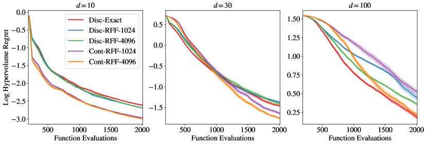
Figure 6: Optimization performance under various Thompson sampling approaches on DTLZ2 test problems with $2$ objectives and various input dimensions $d\in\{10,30,100\}$. Disc-Exact uses exact samples from the joint posterior over a discrete set of $4096$ points. Disc-RFF-$1024$ and Disc-RFF-$4096$ evaluate approximate sample paths (RFFs) over a discrete set of $4096$ points with $1024$ and $4096$ basis functions, respectively. Cont-RFF-$1024$ and Cont-RFF-$4096$ use L-BFGS-B with exact gradients to optimize RFF draws along a subset of the dimensions (see in Appendix A.1 for details) using $1024$ and $4096$ basis functions, respectively.

Appendix B Additional details of constraint handling in MORBO

If there are feasible points, the center is selected as the point with maximum HVC across the feasible Pareto frontier. If there are no feasible points, the center is selected to be the point with minimum total constraint violation (the sum of the constraint violations). A TR’s success counter is incremented if the TR center was feasible and the candidates generated from this TR improved the feasible hypervolume or if the TR center was infeasible and a candidate generated from this TR has lower total constraint violation than the TR center.

Appendix C Proofs

Lemma 4.1.

Let $\bm{f}\in[0,B]^{M}$, and assume that MORBO only considers a newly evaluated sample to be an improvement (for updating the corresponding TR’s success and failure counters) if it increases the HV by at least $\delta\in\mathbb{R}^{+}$ and assume that success counter threshold $\tau_{\text{succ}}=\infty$. Then each TR will only evaluate a finite number of samples.

Proof.

First, note that The hypervolume of the true Pareto frontier $\mathcal{P}^{*}$ is bounded. Without loss of generality, if the reference point $\bm{r}=\bm{0}$, then the $\textsc{HV}(\mathcal{P}^{*})\leq B^{M}.$ Suppose that a trust region evaluates an infinite number of samples. Then, the trust region has not had $1+\log_{2}L_{\text{init}}-\log_{2}L_{\text{min}}$ streaks of $\tau_{\text{fail}}$ consecutive failures. Hence, the trust region has increased the hypervolume of the Pareto frontier over the previously evaluated designs by at least $\delta$ infinitely many times. Hence, the hypervolume over the previously evaluated designs is infinite. This is a contradiction. ∎

Theorem 4.1.

Let $\bm{f}\in[0,B]^{M}$ for $B>0$ and let each component $f^{(m)}$ for $m=1,...,M$ follow a Gaussian distribution with marginal variances $\sigma\leq 1$ and independent observation noise $\epsilon_{m}\sim\mathcal{N}(0,\sigma_{m}^{2})$ such that $\sigma_{m}^{2}\leq\sigma^{2}\leq 1$. Let $\mathcal{P}_{t}$ denote the Pareto frontier over $\bm{f}(X_{t})$, where $X_{t}$ is the set of TR re-initialization points after $t$ TRs have been restarted. Suppose further that the conditions of Lemma 4.1 hold. Then, the cumulative hypervolume regret $R_{T}$ of MORBO after $T$ restarts is bounded by:

$$R_{T}\leq M^{2}(\sqrt{2e\pi}B/2)^{M}\sqrt{d\gamma_{T}T\ln(T)}.$$

Proof.

From Lemma 4.1, we have that each trust region will only evaluate a finite number of samples. Hence, as the number of evaluations goes to infinity, MORBO will terminate and select new initial center points for trust regions an infinite number of times. Our regret bound is in terms of the number of restart points.

Our proof follows that of Zhang and Golovin [2020, Theorem 8], but the final form of our bound holds for arbitrary $B$. Note that lines 13-19 in Algorithm 1 correspond to Paria et al. [2020, Algorithm 1] using Thompson sampling, where the only evaluations are the $t-1$ restart points. From Paria et al. [2020, Theorem 1], the scalarized Bayes regret of Paria et al. [2020, Algorithm 1] using $L$–Lipschitz scalarizations is $O\big{(}LMd^{\frac{1}{2}}[\gamma_{T}T\ln(T)]^{\frac{1}{2}}\big{)}$. Since a hypervolume scalarization $s_{\bm{\lambda}}[\bm{y}]$ is $\mathcal{O}(B^{M}M^{1+M/2})$–Lipschitz [Zhang and Golovin, 2020, Lemma 6], we have that $L\leq B^{M}M^{1+M/2}$. From Zhang and Golovin [2020, Proof of Theorem 8], the hypervolume regret can be expressed by scaling the scalarized Bayes regret by a constant $c_{M}=\frac{\pi^{\frac{M}{2}}}{2^{M}\Gamma(\frac{M}{2}+1)}$ that depends on the number of objectives. Hence, we can bound the hypervolume regret as:

$$R_{T}=\sum_{t=1}^{T}\textsc{HV}(\mathcal{P}^{*})-\textsc{HV}(\mathcal{P}_{t}) \leq c_{M}LMd^{\frac{1}{2}}[\gamma_{T}T\ln(T)]^{\frac{1}{2}}.$$

Note that

$$c_{M}L \leq B^{M}M^{1+M/2}\frac{\pi^{\frac{M}{2}}}{2^{M}\Gamma(\frac{M}{2}+1)}$$

From Li and Chen [2007, Theorem 1], $\Gamma(x)>\frac{x^{x-\gamma}}{e^{x-1}}$, where $\gamma\approx 0.577$ is the Euler-Mascheroni constant. So,

$$\Gamma(M/2+1)>\frac{(M/2+1)^{(M/2+1-\gamma)}}{e^{(M/2)}}>\frac{M^{(M/2)}}{2e^{(M/2)}}.$$

Hence,

$$\frac{1}{\Gamma(\frac{M}{2}+1)}<\frac{(2e)^{(M/2)}}{M^{(M/2)}}.$$

So,

$$c_{M}L \leq B^{M}M^{1+M/2}\frac{\pi^{\frac{M}{2}}}{2^{M}\Gamma(\frac{M}{2}+1)}$$

$$\leq B^{M}M\frac{(2e\pi)^{\frac{M}{2}}}{2^{M}}$$

$$\leq M\big{(}\sqrt{2e\pi}B/2\big{)}^{M}.$$

So the cumulative regret bound is

$$R_{T} \leq c_{M}LMd^{\frac{1}{2}}[\gamma_{T}T\ln(T)]^{\frac{1}{2}}$$

$$\leq M^{2}(\sqrt{2e\pi}B/2)^{M}d^{\frac{1}{2}}[\gamma_{T}T\ln(T)]^{\frac{1}{2}}.$$

∎

Appendix D Details on Experiments

D.1 Algorithmic details

For MORBO, we use $5$ trust regions, which we observed was a robust choice in Figure 4. Following [Eriksson et al., 2019], we set $L_{\text{init}}=0.8$, $L_{\max}=1.6$, and use a minimum length of $L_{\min}=0.01$. We use $4096$ discrete points for optimizing HVI for the vehicle safety and welded beam problems, $2048$ discrete points on the trajectory planning and optical design problems, and $512$ discrete points on the Mazda problem. Note that while the number of discrete points should ideally be chosen as large as possible, it offers a way to control the computational overhead of MORBO; we used a smaller value for the Mazda problem due to the fact that we need to sample from a total of $56$ GP models in each trust region as there are $54$ black-box constraints. We use an independent GP with a a constant mean function and a Matérn-$5/2$ kernel with automatic relevance detection (ARD) and fit the GP hyperparameters by maximizing the marginal log-likelihood (the same model is used for all BO baselines).

When fitting a model for MORBO, we include the data within a hypercube around the trust region center with edgelength $2L$. In the case that there are less than $N_{m}:=\min\{250,2d\}$ points within that region, we include the $N_{m}$ closest points to the trust region center for model fitting. The success streak tolerance is set to be infinity, which prevents the trust region from expanding; we find this leads to good optimization performance when data is shared across trust regions. For $q$NEHVI and $q$ParEGO, we use $128$ quasi-MC samples and for TS-TCH, we optimize RFFs with $500$ Fourier basis functions. All three methods are optimized using L-BFGS-B with $20$ random restarts. For DGEMO, TSEMO, and MOEA/D-EGO, we use the default settings in the open-source implementation at https://github.com/yunshengtian/DGEMO/tree/master. Similarly, we use the default settings for NSGA-II the Platypus package (https://github.com/Project-Platypus/Platypus). We encode the reference point as a black-box constraint to provide this information to NSGA-II.

D.1.1 LaMOO in High-Dimensional Search Spaces

For LaMOO methods, leverage the implementation of LaMOO available at https://drive.google.com/drive/folders/1CMdg5iBdbKe3nkboIjiS998rnBEV09EB?usp=sharing. We set the exploration parameter $C_{p}$ dynamically using the heuristic proposed by Zhao et al. [2021] to be 10% of the hypervolume of the current Pareto frontier over the previously evaluated designs. We follow Zhao et al. [2021] and set the minimum leaf sample size to be $10$.

Zhao et al. [2021] propose to use $q$EHVI with LaMOO, but we opt to use $q$NEHVI instead since it is capable of scaling to the batch size of $q=50$ used in many of our experiments. We refer to this method as LaMOO-$q$NEHVI. We note that $q$NEHVI is mathematically equivalent to $q$EHVI on noiseless problems. The authors propose using rejection sampling to ensure samples come from the “good” region. For high-dimensional search spaces, the acceptance probability is low for uniform random samples from the global design space, and therefore, rejection sampling is prohibitively slow. Rejection sampling is used 1) to select starting points for multi-start L-BFGS-B and within the L-BFGS-B routine to enforce that samples are within the “good” region. We contacted the authors about computational issues with this approach, and the authors recommended to use rejection sampling for selecting starting points, and then to simply run L-BFGS-B from these “good” starting points across the global search space. With this approach, the resulting candidates may not (and often are not) within the “good” region, and LaMOO-qNEHVI is simply an initialization heuristic for optimizing $q$NEHVI, but this approach does speed up candidate generation quite a bit. Nevertheless, even using rejection sampling to generate starting points for L-BFGS-B can be (and is on our problems) prohibitively expensive in high-dimensional search spaces. Hence, we limit the rejection sampling by only considering $120,000$ design points before beginning L-BFGS-B with the most promising designs (whether or not they are in the “good” region). This makes LaMOO-qNEHVI feasible to run our our high-dimensional problems.

For LaMOO-CMA-ES, we use $q=5$ rather than $q=1$ on vehicle safety, as $q=1$ is not supported.

D.2 Synthetic problems

The reference points for all problems are given in Table 1. We multiply the objectives (and reference points) for all synthetic problems by $-1$ and maximize the resulting objectives.

Problem	Reference Point
DTLZ2	[$6$, $6$]
DTLZ3	$[10^{3}]^{M}$
DTLZ5	$[10]^{M}$
DTLZ7	$[15]^{M}$
Vehicle Safety	[$1698.55$, $11.21$, $0.29$]
Welded Beam	[$40$, $0.015$]
MW7	[$1.2$, $1.2$]

Table 1: The reference points for each synthetic benchmark problem.

DTLZ:

We consider the $2$-objective DTLZ2 problem with various input dimensions $d\in\{10,30,100\}$. We also use $2$-objective and $4$-objective variants of DTLZ3, DTLZ5, and DTLZ7 with $d=100$. The DTLZ problems are standard test problems from the multi-objective optimization literature. Mathematical formulas for the objectives in each problem are given in Deb et al. [2002].

MW7:

For a second test problem from the multi-objective optimization literature, we consider a MW7 problem with $2$ objectives, $2$ constraints, and $d=10$ parameters. See Ma and Wang [2019] for details.

Welded Beam:

The welded beam problem [Ray and Liew, 2002] is a structural design problem with $d=4$ input parameters controlling the size of the beam where the goal is to minimize $2$ objectives (cost and end deflection) subject to $4$ constraints. More details are given in Tanabe and Ishibuchi [2020].

Vehicle Safety:

The vehicle safety problem is a $3$-objective problem with $d=5$ parameters controlling the widths of different components of the vehicle’s frame. The goal is to minimize mass (which is correlated with fuel economy), toe-box intrusion (vehicle damage), and acceleration in a full-frontal collision (passenger injury). See Tanabe and Ishibuchi [2020] for additional details.

D.3 Trajectory planning

For the trajectory planning, we consider a trajectory specified by $30$ design points that starts at the pre-specified starting location. Given the $30$ design points, we fit a B-spline with interpolation and integrate over this B-spline to compute the final reward using the same domain as in Wang et al. [2018]. Rather than directly optimizing the locations of the design points, we optimize the difference (step) between two consecutive design points, each one constrained to be in the domain $[0,0.05]\times[0,0.05]$. We use a reference point of [$0$, $0.5$], which means that we want a reward larger than $0$ and a distance that is no more than $0.5$ from the target location [$0.95$, $0.95$]. Since we maximize both objectives, we optimize the distance metric and the corresponding reference point value by $-1$.

D.4 Optical design

In order to obtain precise estimates of the optimization performance at reasonable computational cost, we conduct our evaluation on a neural network surrogate model of the optical system rather than on the actual physics simulator. The surrogate model was constructed from a dataset of $101$,$000$ optical designs and resulting display images to provide an accurate representation of the real problem. The surrogate model is a neural network with a convolutional autoencoder architecture. The model was trained using $80$,$000$ training examples and minimizing MSE (averaged over images, pixels, and RGB color channels) on a validation set of $20$,$000$ examples. A total of $1$,$000$ examples were held-out for final evaluation.

D.5 Mazda vehicle design problem

We follow the suggestions by Kohira et al. [2018] and use the reference point $[1.1,0]$ and optimize the normalized objectives $\tilde{f}_{1}=f_{1}-2$ and $\tilde{f}_{2}=f_{2}/74$ corresponding to the total mass and number of common gauge parts, respectively. Additionally, an initial feasible point is provided with objective values $f_{1}=3.003$ and $f_{2}=35$, corresponding to an initial hypervolume of $\approx 0.046$ for the normalized objectives. This initial solution is given to all algorithms. We limit the number of points used for model fitting to only include the $2$,$000$ points closest to the trust region center in case there are more than $2$,$000$ in the larger hypercube with side length $2L$. Still, for each iteration MORBO using $5$ trust regions fits a total of $56\times 5$ GP models, a scale far out of reach for any other multi-objective BO method.

Appendix E Complexity Improvements from Local Modeling

The differences in model fitting time can be even more profound. To illustrate this, consider a situation in which a total of $N$ data points have been collected by $n_{\text{TR}}$ trust regions. Suppose for simplicity that each TR has the same number of observations (under some abuse of nomenclature we use TR to refer to the modeling domain of a TR in this section). Let $\eta$ denote the average number of trust regions that a data point is part of. Then the number of points in each TR is $\eta N/n_{\text{TR}}$. Assuming cubic time complexity for model fitting (i.e. $O(N^{3})$ if we used a single global model), the total time complexity of fitting all $n_{\text{TR}}$ models in the individual TRs is $O\bigl{(}n_{\text{TR}}(\eta N/n_{\text{TR}})^{3}\bigr{)}=O\bigl{(}\eta^{3}N^{3}/n_{\text{TR}}^{2}\bigr{)}$. This will lead to asymptotic speedups of order $O\bigl{(}n_{\text{TR}}^{2}/\eta^{3}\bigr{)}$ when using local modeling. Typically, as the optimization progresses and the trust regions shrink, $\eta$ becomes quite small (e.g. $\eta<1$). We validate this claim empirically in the lower right subplot in Figure 7, which shows that $\eta$ becomes less than $1$ on the all problems considered as the optimization progresses. In Figure 7 we illustrate some additional information from the trust regions to better understand the role of data-sharing and local modeling in MORBO.

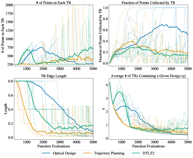
Figure 7: For the optical design, trajectory planning, and DTLZ2 problems. We show the average across replications as a solid line and traces from the first replication as transparent lines. (Upper Left) The number of points in each trust region. Trust regions often usually have a few hundred points on average, which results in computationally efficient local modeling. (Upper Right) The number of points in a trust region that was collected by that trust region. This shows that a large fraction of data within a trust region was actually collected by another trust region. (Lower Left) The trust region length. As the optimization proceeds, the trust regions shrink to focus on specific parts of the search space. (Lower Right) The average number of TRs that contain a given design, $\eta\in[0,N_{\text{TR}}]$. This shows that as the optimization progresses and the TRs shrink, on average less than $1$ TR contains a given design. This is empirical validation of the claim in Appendix E that $\eta$ typically becomes small as the optimization progresses and therefore, the complexity improvements are substantial.

Thus, the speedup relative to fitting a single global model can be multiple orders of magnitude.

E.1 Model fitting times

Empirically, we verify this speedup in Figure 8.

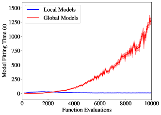
Figure 8: Model fitting time for MORBO with local modeling compared to MORBO with one global model on the $146$-dimensional optical design problem. Fitting a global model takes almost $20$ minutes towards the end of the optimization run compared to $10$ seconds for MORBO.

This can also be seen in the results in Tables 3 and 2. While candidate generation is fast for TSEMO, the model fitting causes a significant overhead with almost an hour being spent on model fitting after collecting $2$,$000$ evaluations on the trajectory planning problem. This is significantly longer than for MORBO, which only requires far less time for the model fitting due to the use of local modeling. This shows that the use of local modeling is a crucial component of MORBO that limits the computational overhead from the model fitting. The model fitting for MORBO on the optical design problem is less than $25$ seconds while methods such as DGEMO and TSEMO that rely on global modeling require far more time for model fitting after only collecting $1$,$200$ points. Additionally, while MORBO needs to fit as many as $56\times 5=280$ GP models on the Mazda problem due to the $54$ black-box constraints and the use of $5$ trust regions, the total time for model fitting still is less than $3$ minutes while this problem is completely out of reach for the other BO methods that rely on global modeling.

Problem DTLZ3 $(M=2)$ DTLZ5 $(M=2)$ DTLZ7 $(M=2)$ DTLZ3 $(M=4)$ DTLZ5 $(M=4)$ DTLZ7 $(M=4)$ MORBO 11.0 (0.6) 9.7 (0.4) 10.6 (0.4) 11.5 (0.9) 10.5 (0.5) 10.6 (0.4) NSGA-II 0.0 (0.0) 0.0 (0.0) 0.0 (0.0) 0.0 (0.0) 0.0 (0.0) 0.0 (0.0) $q$ParEGO 139.5 (24.6) 49.1 (2.2) 26.0 (2.5) 137.2 (15.4) 113.2 (6.6) 49.0 (3.5) TS-TCH 64.5 (3.4) 93.9 (5.8) 89.6 (3.5) 143.3 (5.9) 167.6 (8.8) 141.3 (6.1) $q$NEHVI 133.2 (23.9) 48.9 (4.9) 20.8 (1.7) 25.9 (2.3) 19.8 (1.7) 6.8 (0.4) DGEMO 5425.1 (142.0) 1438.0 (29.0) 180.0 (35.3) N/A N/A N/A TSEMO 4246.3 (91.8) 2481.5 (48.5) 958.4 (49.1) 3767.4 (91.0) 1892.3 (801.5) 402.0 (31.7) MOEAD-EGO 3474.6 (108.6) 1824.0 (40.1) 1130.3 (16.0) 4206.1 (120.5) 2526.3 (77.5) 1048.0 (37.8)

Table 2: Model fitting wall time in seconds. The mean and two standard errors of the mean are reported. All models were fit on 2x Intel(R) Xeon(R) Gold 6138 CPU @ 2.00GHz. For $M=4$, $q$NEHVI exceeded GPU memory during acquisition optimization and therefore has shorter average model fitting times.

Problem	Welded Beam	Vehicle Safety	Rover	Optical Design	Mazda
MORBO	7.81 (0.02)	12.58 (0.26)	9.3 (0.19)	23.57 (0.36)	172.53 (1.89)
$q$ParEGO	0.5 (0.1)	0.1 (0.0)	51.6 (16.4)	46.7 (10.7)	N/A
TS-TCH	0.5 (0.0)	0.2 (0.0)	45.9 (1.8)	40.5 (4.9)	N/A
$q$NEHVI	0.5 (0.0)	0.1 (0.0)	97.8 (16.3)	46.4 (3.2)	N/A
DGEMO	N/A	N/A	809.7 (127.6)	1109.3 (178.7)	N/A
TSEMO	N/A	1.0 (0.1)	305.3 (38.2)	859.4 (131.4)	N/A
MOEA/D-EGO	N/A	0.9 (0.0)	373.2 (51.7)	736.4 (110.4)	N/A

Table 3: Model fitting wall time in seconds. The mean and two standard errors of the mean are reported. All models were fit on 2x Intel(R) Xeon(R) Gold 6138 CPU @ 2.00GHz. For DGEMO, TSEMO and MOEA/D-EGO only $1$,$450$ evaluations were performed on Rover (Trajectory Planning) and only $1$,$250$ evaluations were performed on Optical Design, so the fitting times are shorter than if the full $2$,$000$ evaluations had been performed.

Appendix F Additional Results

F.1 Low-dimensional problems

We consider two low-dimensional problems to allow for a comparison with existing BO baselines. The first problem we consider is a vehicle safety design problem ($d=5$) in which we tune thicknesses of various components of an automobile frame to optimize proxy metrics for maximizing fuel efficiency, minimizing passenger trauma in a full-frontal collision, and maximizing vehicle durability. The second problem is a welded beam design problem ($d=4$), where the goal is to minimize the cost of the beam and the deflection of the beam under the applied load [Deb and Sundar, 2006]. The design variables are the thickness and length of the welds and the height and width of the beam. In addition, there are $4$ black-box constraints that must be satisfied.

Figure 9 presents results for both problems. While MORBO is not designed for such simple, low-dimensional problems, it is still competitive with other baselines such as TS-TCH and $q$ParEGO on the vehicle design problem, though it cannot quite match the performance of $q$NEHVI and TSEMO. The results on the welded beam problem illustrate the efficient constraint handling of MORBO. On both problems, we observe that NSGA-II struggles to keep up, performing barely better (vehicle safety) or even worse (welded beam) than quasi-random Sobol exploration.

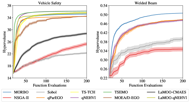
Figure 9: (Left) $q$NEHVI performs the best on the vehicle design problem ($d=5$) with $3$ objectives. (Right) MORBO outperforms the other methods on welded beam problem ($d=4$) with $4$ constraints.

F.2 Candidate Generation Wall Time

Problem	Welded Beam	Vehicle Safety	Rover	Optical Design	Mazda
Batch Size	($q=1$)	($q=1$)	($q=50$)	($q=50$)	($q=50$)
MORBO	1.3 (0.0)	9.6 (0.7)	23.4 (0.4)	9.8 (0.1)	188.16 (1.72)
$q$ParEGO	14.5 (0.3)	1.3 (0.0)	213.4 (11.2)	241.9 (14.9)	N/A
TS-TCH	N/A	0.6 (0.0)	31.3 (1.1)	48.1 (1.2)	N/A
$q$NEHVI	30.4 (0.4)	9.1 (0.1)	997.5 (62.8)	211.27 (6.66)	N/A
NSGA-II	0.0 (0.0)	0.0 (0.0)	0.0 (0.0)	0.0 (0.0)	0.0 (0.0)
DGEMO	N/A	N/A	697.1 (52.5)	2278.7 (199.8)	N/A
TSEMO	N/A	3.4 (0.1)	3.3 (0.0)	4.6 (0.1)	N/A
MOEA/D-EGO	N/A	44.3 (0.3)	71.1 (4.3)	97.5 (6.7)	N/A
LaMOO-CMAES	N/A	0.6 (0.0)	2.6 (0.0)	51.9 (0.3)	N/A
LAMOO-$q$NEHVI	N/A	24.0 (2.3)	292.4 (25.2)	258.8 (1.9)	N/A

Table 4: Batch selection wall time (excluding model fitting) in seconds. The mean and two standard errors of the mean are reported. MORBO, $q$ParEGO, TS-TCH, and $q$NEHVI were run on a Tesla V100 SXM2 GPU (16GB RAM), while DGEMO, TSEMO, MOEA/D-EGO and NSGA-II were run on 2x Intel(R) Xeon(R) Gold 6138 CPU @ 2.00GHz. For Welded Beam and Vehicle Safety, we ran NSGA-II with $q=5$ in order to avoid a singleton population. For DGEMO, TSEMO and MOEA/D-EGO only $1$,$450$ evaluations were performed on Rover (Trajectory Planning) and only $1$,$250$ evaluations were performed on Optical Design, so the generation times are shorter than if the full $2$,$000$ evaluations had been performed.

Problem DTLZ3 $(M=2)$ DTLZ5 $(M=2)$ DTLZ7 $(M=2)$ DTLZ3 $(M=4)$ DTLZ5 $(M=4)$ DTLZ7 $(M=4)$ Batch Size ($q=50$) ($q=50$) ($q=50$) ($q=50$) ($q=50$) ($q=50$) MORBO 26.0 (1.3) 25.1 (0.9) 293.0 (21.9) 976.9 (89.8) 973.0 (91.8) 293.0 (21.9) $q$ParEGO 315.8 (20.2) 299.0 (27.2) 233.0 (21.5) 372.9 (46.6) 373.1 (34.6) 232.4 (22.2) TS-TCH 43.6 (1.4) 49.6 (2.0) 39.5 (1.9) 56.5 (1.8) 69.2 (7.5) 51.4 (3.4) $q$NEHVI 2877.7 (321.3) 1879.6 (285.4) 816.9 (49.1) 4412.9 (600.7) 3778.2 (266.5) 57.6 (4.4) NSGA-II 0.0 (0.0) 0.0 (0.0) 0.0 (0.0) 0.1 (0.0) 0.0 (0.0) 0.0 (0.0) DGEMO N/A N/A N/A N/A N/A N/A TSEMO 6.3 (0.1) 7.2 (0.1) 6.8 (0.1) 2878.1 (162.0) 952.0 (298.1) 22.2 (3.7) MOEAD-EGO 277.8 (1.2) 224.9 (3.2) 245.3 (2.9) 308.7 (2.9) 303.7 (3.1) 292.2 (3.5)

Table 5: Batch selection wall time (excluding model fitting) in seconds on DTLZ problems with 2 and 4 objectives with $d=100$. The mean and two standard errors of the mean are reported.

While candidate generation time is often a secondary concern in classic BO applications, where evaluating the black box function often takes orders of magnitude longer, existing methods using a single global model and standard acquisition function optimization approaches can become the bottleneck in high-throughput asynchronous evaluation settings that are common with high-dimensional problems. Tables 4 and 5 provides a comparison of the wall time for generating a batch of candidates for the different methods on the different benchmark problems. We observe that the candidate generation for MORBO is two orders of magnitudes faster than for other methods such as $q$ParEGO and $q$NEHVI on the trajectory planning problem where all methods ran for the full $2$,$000$ evaluations.

F.3 Pareto Frontiers

We show the Pareto frontiers for the welded beam, trajectory planning, optical design, and Mazda problems in Figure 10. In each column we show the Pareto frontiers corresponding to the worst, median, and best replications according to the final hypervolume. We exclude the vehicle design problem as it has three objectives which makes the final Pareto frontiers challenging to visualize.

Figure 10 shows that even on the low-dimensional $4$D welded beam problem, MORBO is able to achieve much better coverage than the baseline methods. MORBO also explores the trade-offs better than other methods on the trajectory planning problem, where the best run by MORBO found trajectories with high reward that ended up being close to the final target location. In particular, other methods struggle to identify trajectories with large rewards while MORBO consistently find trajectories with rewards close to $5$, which is the maximum possible reward. On both the optical design and Mazda problems, the Pareto frontiers found by MORBO better explore the trade-offs between the objectives compared to NSGA-II and Sobol. We note that MORBO generally achieves good coverage of the Pareto frontier for both problems. For the optical design problem, we exclude the partial results found by running the other baselines for $1$k-$2$k evaluations and only show the methods the ran for the full $10$k evaluations. For the Mazda problem we show the Pareto frontiers of the true objectives and not the normalized objectives that are described in Section 5.1. MORBO is able to significantly decrease the vehicle mass at the cost of using a fewer number of common parts, a trade-off that NSGA-II fails to explore. It is worth noting that the number of common parts objective is integer-valued and that exploiting this additional information may unlock even better optimization performance of MORBO.

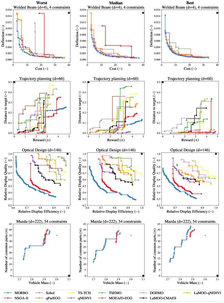
Figure 10: In each column we show the Pareto frontiers for the worst, median, and best replications according to the final hypervolume. We indicate whether an objective is minimized/maximized by $-/+$, respectively. The reference point is illustrated as a black star. The use of multiple trust regions allows MORBO to consistently achieve good coverage of the Pareto frontier, in addition to large hypervolumes.

F.4 Additional Benchmark Problems

To study the performance of MORBO on a broader range of problems, we evaluate MORBO on two-objective and four-objective versions of DTLZ3, DTLZ5, and DTLZ7 problems with $d=100$. As shown in Figure 12, MORBO performs best on the four-objective DTLZ7 and achieve the best final hypervolume on the four-objective DTLZ3 problem. On the two-objective problems, MORBO always ranks in the top 4 methods as shown in Figure 12. To compare the performance in general across the DTLZ3, DTLZ5, and DTLZ7 problems with a given number of objectives, we rank the methods by the average final hypervolume across replications and compute the average rank across the three problems. As shown in Table 6, MORBO achieves the lowest rank across all methods (which is best) on both M=2 and M=4 problems. DGEMO is not evaluated on the 4-objective problems because the open-source implementation (https://github.com/yunshengtian/DGEMO/tree/master) does not support more than two objectives. Although DGEMO, MOEA/D-EGO and $q$NEHVI all perform competitively in the two objective setting, all methods are significantly slower than MORBO.

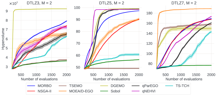
Figure 11: Optimization performance on two-objective DTLZ3, DTLZ5, and DTLZ7 problems with $d=100$ and $q=50$.

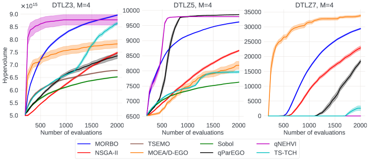
Figure 12: Optimization performance on four-objective DTLZ3, DTLZ5, and DTLZ7 problems with $d=100$ and $q=50$.

	Avg. Rank for M=2	Avg. Rank for M=4
MORBO	3.0	1.67
$q$ParEGO	4.0	3.3
$q$NEHVI	3.0	3.16
TS-TCH	7.3	4.3
NSGA-II	4.3	3.7
DGEMO	3.0	8.2
TSEMO	7.7	8.3
MOEA/D-EGO	4.0	5.5
Sobol	8.7	6.8

Table 6: Mean rank across DTLZ3, DTLZ5, and DTLZ7 problems based on final mean hypervolume with $d=100$ and $q=50$. A lower rank means the method achieves better final performance on average across the DTLZ3, DTLZ5, and DTLZ7 problems with $M$ objectives.

References

- Akhtar and Shoemaker [2015] T. Akhtar and C. Shoemaker. Multi objective optimization of computationally expensive multi-modal functions with rbf surrogates and multi-rule selection. Journal of Global Optimization, 64, 2015.
- Bai et al. [2017] T. Bai, Y.-b. Kan, J.-x. Chang, Q. Huang, and F.-J. Chang. Fusing feasible search space into pso for multi-objective cascade reservoir optimization. Appl. Soft Comput., 51(C), 2017.
- Balandat et al. [2020] M. Balandat, B. Karrer, D. R. Jiang, S. Daulton, B. Letham, A. G. Wilson, and E. Bakshy. BoTorch: A Framework for Efficient Monte-Carlo Bayesian Optimization. In Advances in Neural Information Processing Systems 33, 2020.
- Beume et al. [2007] N. Beume, B. Naujoks, and M. Emmerich. SMS-EMOA: Multiobjective selection based on dominated hypervolume. European Journal of Operational Research, 181(3), 2007.
- Bradford et al. [2018] E. Bradford, A. M. Schweidtmann, and A. Lapkin. Efficient multiobjective optimization employing Gaussian processes, spectral sampling and a genetic algorithm. J. of Global Optimization, 2018.
- Couckuyt et al. [2014] I. Couckuyt, D. Deschrijver, and T. Dhaene. Fast calculation of multiobjective probability of improvement and expected improvement criteria for Pareto optimization. J. of Global Optimization, 60(3), 2014.
- Daulton et al. [2020] S. Daulton, M. Balandat, and E. Bakshy. Differentiable expected hypervolume improvement for parallel multi-objective Bayesian optimization. In Advances in Neural Information Processing Systems 33, 2020.
- Daulton et al. [2021] S. Daulton, M. Balandat, and E. Bakshy. Parallel bayesian optimization of multiple noisy objectives with expected hypervolume improvement. In Advances in Neural Information Processing Systems 34, 2021.
- Daulton et al. [2022] S. Daulton, S. Cakmak, M. Balandat, M. A. Osborne, E. Zhou, and E. Bakshy. Robust multi-objective bayesian optimization under input noise. In Proceedings of the 39th International Conference on Machine Learning, Proceedings of Machine Learning Research, 2022.
- Deb and Sundar [2006] K. Deb and J. Sundar. Reference point based multi-objective optimization using evolutionary algorithms. In Proceedings of the 8th annual conference on Genetic and evolutionary computation, 2006.
- Deb et al. [2002] K. Deb, A. Pratap, S. Agarwal, and T. Meyarivan. A fast and elitist multiobjective genetic algorithm: Nsga-ii. IEEE Transactions on Evolutionary Computation, 6(2), 2002.
- Deb et al. [2002] K. Deb, L. Thiele, M. Laumanns, and E. Zitzler. Scalable multi-objective optimization test problems. volume 1, 2002.
- Dreifuerst et al. [2021] R. M. Dreifuerst, S. Daulton, Y. Qian, P. Varkey, M. Balandat, S. Kasturia, A. Tomar, A. Yazdan, V. Ponnampalam, and R. W. Heath. Optimizing coverage and capacity in cellular networks using machine learning. In ICASSP 2021-2021 IEEE International Conference on Acoustics, Speech and Signal Processing (ICASSP). IEEE, 2021.
- Emmerich et al. [2006] M. T. M. Emmerich, K. C. Giannakoglou, and B. Naujoks. Single- and multiobjective evolutionary optimization assisted by Gaussian random field metamodels. IEEE Transactions on Evolutionary Computation, 10(4), 2006.
- Eriksson and Jankowiak [2021] D. Eriksson and M. Jankowiak. High-dimensional Bayesian optimization with sparse axis-aligned subspaces. In Uncertainty in Artificial Intelligence. PMLR, 2021.
- Eriksson and Poloczek [2021] D. Eriksson and M. Poloczek. Scalable constrained Bayesian optimization. In International Conference on Artificial Intelligence and Statistics. PMLR, 2021.
- Eriksson et al. [2019] D. Eriksson, M. Pearce, J. R. Gardner, R. Turner, and M. Poloczek. Scalable global optimization via local Bayesian optimization. In Advances in Neural Information Processing Systems 32, 2019.
- Eriksson et al. [2021] D. Eriksson, P. I.-J. Chuang, S. Daulton, P. Xia, A. Shrivastava, A. Babu, S. Zhao, A. Aly, G. Venkatesh, and M. Balandat. Latency-aware neural architecture search with multi-objective bayesian optimization, 2021.
- Frazier [2018] P. I. Frazier. A tutorial on Bayesian optimization. arXiv, 2018.
- Gardner et al. [2017] J. R. Gardner, C. Guo, K. Q. Weinberger, R. Garnett, and R. B. Grosse. Discovering and exploiting additive structure for Bayesian optimization. In Proceedings of the 20th International Conference on Artificial Intelligence and Statistics, volume 54, 2017.
- Gopakumar et al. [2018] A. M. Gopakumar, P. V. Balachandran, D. Xue, J. E. Gubernatis, and T. Lookman. Multi-objective optimization for materials discovery via adaptive design. Scientific Reports, 8(1), 2018.
- Hansen [2007] N. Hansen. The CMA Evolution Strategy: A Comparing Review, volume 192. 2007.
- Hernández-Lobato et al. [2015] D. Hernández-Lobato, J. M. Hernández-Lobato, A. Shah, and R. P. Adams. Predictive entropy search for multi-objective Bayesian optimization, 2015.
- Jones et al. [1998] D. R. Jones, M. Schonlau, and W. J. Welch. Efficient global optimization of expensive black-box functions. Journal of Global Optimization, 13, 1998.
- Kandasamy et al. [2015] K. Kandasamy, J. Schneider, and B. P’oczos. High dimensional Bayesian optimisation and bandits via additive models. In Proceedings of the 32nd International Conference on Machine Learning, 2015.
- Knowles [2006] J. Knowles. Parego: a hybrid algorithm with on-line landscape approximation for expensive multiobjective optimization problems. IEEE Transactions on Evolutionary Computation, 10(1), 2006.
- Kohira et al. [2018] T. Kohira, H. Kemmotsu, O. Akira, and T. Tatsukawa. Proposal of benchmark problem based on real-world car structure design optimization. In Proceedings of the Genetic and Evolutionary Computation Conference Companion, 2018.
- Konakovic Lukovic et al. [2020] M. Konakovic Lukovic, Y. Tian, and W. Matusik. Diversity-guided multi-objective Bayesian optimization with batch evaluations. Advances in Neural Information Processing Systems, 33, 2020.
- Letham et al. [2020] B. Letham, R. Calandra, A. Rai, and E. Bakshy. Re-examining linear embeddings for high-dimensional Bayesian optimization. Advances in neural information processing systems, 33, 2020.
- Li and Chen [2007] X. Li and C.-P. Chen. Inequalities for the gamma function. Journal of Inequalities in Pure and Applied Mathematics, 8, 2007.
- Loshchilov et al. [2011] I. Loshchilov, M. Schoenauer, and M. Sebag. Not all parents are equal for mo-cma-es. In Evolutionary Multi-Criterion Optimization, 2011.
- Ma and Wang [2019] Z. Ma and Y. Wang. Evolutionary constrained multiobjective optimization: Test suite construction and performance comparisons. IEEE Transactions on Evolutionary Computation, 23(6), 2019.
- Marler and Arora [2004] R. T. Marler and J. S. Arora. Survey of multi-objective optimization methods for engineering. Structural and multidisciplinary optimization, 26(6), 2004.
- Mathern et al. [2021] A. Mathern, O. Steinholtz, A. Sjöberg, M. Önnheim, K. Ek, R. Rempling, E. Gustavsson, and M. Jirstrand. Multi-objective constrained Bayesian optimization for structural design. Structural and Multidisciplinary Optimization, 63, 2021.
- Munteanu et al. [2019] A. Munteanu, A. Nayebi, and M. Poloczek. A framework for Bayesian optimization in embedded subspaces. In Proceedings of the 36th International Conference on Machine Learning, 2019.
- Oh et al. [2018] C. Oh, E. Gavves, and M. Welling. BOCK: Bayesian optimization with cylindrical kernels. In Proceedings of the 35th International Conference on Machine Learning, volume 80, 2018.
- Owen [2003] A. B. Owen. Quasi-monte carlo sampling. Monte Carlo Ray Tracing: Siggraph, 1, 2003.
- Oyama et al. [2017] A. Oyama, T. Kohira, H. Kemmotsu, T. Tatsukawa, and T. Watanabe. Simultaneous structure design optimization of multiple car models using the k computer. In 2017 IEEE Symposium Series on Computational Intelligence (SSCI), 2017.
- Paria et al. [2020] B. Paria, K. Kandasamy, and B. Póczos. A flexible framework for multi-objective Bayesian optimization using random scalarizations. In Proceedings of The 35th Uncertainty in Artificial Intelligence Conference, volume 115, 2020.
- Pleiss et al. [2020] G. Pleiss, M. Jankowiak, D. Eriksson, A. Damle, and J. Gardner. Fast matrix square roots with applications to Gaussian processes and Bayesian optimization. Advances in Neural Information Processing Systems, 33, 2020.
- Rahimi and Recht [2007] A. Rahimi and B. Recht. Random features for large-scale kernel machines. In Proceedings of the 20th International Conference on Neural Information Processing Systems, 2007.
- Ray and Liew [2002] T. Ray and K. Liew. A swarm metaphor for multiobjective design optimization. Engineering Optimization, 34(2), 2002.
- Regis and Shoemaker [2013] R. G. Regis and C. A. Shoemaker. Combining radial basis function surrogates and dynamic coordinate search in high-dimensional expensive black-box optimization. Engineering Optimization, 45(5), 2013.
- Sener and Koltun [2018] O. Sener and V. Koltun. Multi-task learning as multi-objective optimization. In Advances in Neural Information Processing Systems, volume 31, 2018.
- Srinivas et al. [2010] N. Srinivas, A. Krause, S. Kakade, and M. Seeger. Gaussian process optimization in the bandit setting: No regret and experimental design. In Proceedings of the 27th International Conference on International Conference on Machine Learning, 2010.
- Suzuki et al. [2020] S. Suzuki, S. Takeno, T. Tamura, K. Shitara, and M. Karasuyama. Multi-objective Bayesian optimization using pareto-frontier entropy. In Proceedings of the 37th International Conference on Machine Learning, volume 119, 2020.
- Tanabe and Ishibuchi [2020] R. Tanabe and H. Ishibuchi. An easy-to-use real-world multi-objective optimization problem suite. Applied Soft Computing, 89, 2020.
- Thompson [1933] W. R. Thompson. On the likelihood that one unknown probability exceeds another in view of the evidence of two samples. Biometrika, 25(3/4), 1933.
- Turner et al. [2021] R. Turner, D. Eriksson, M. McCourt, J. Kiili, E. Laaksonen, Z. Xu, and I. Guyon. Bayesian optimization is superior to random search for machine learning hyperparameter tuning: Analysis of the black-box optimization challenge 2020. In NeurIPS 2020 Competition and Demonstration Track, 2021.
- Wan et al. [2021] X. Wan, V. Nguyen, H. Ha, B. Ru, C. Lu, and M. A. Osborne. Think global and act local: Bayesian optimisation over high-dimensional categorical and mixed search spaces, 2021.
- Wang et al. [2016] Z. Wang, F. Hutter, M. Zoghi, D. Matheson, and N. De Freitas. Bayesian optimization in a billion dimensions via random embeddings. J. Artif. Int. Res., 55(1), 2016.
- Wang et al. [2018] Z. Wang, C. Gehring, P. Kohli, and S. Jegelka. Batched large-scale Bayesian optimization in high-dimensional spaces. In International Conference on Artificial Intelligence and Statistics, volume 84, 2018.
- Yang et al. [2019] K. Yang, M. Emmerich, A. Deutz, and T. Bäck. Multi-objective Bayesian global optimization using expected hypervolume improvement gradient. Swarm and Evolutionary Computation, 44, 2019.
- Yuan [1999] Y.-x. Yuan. A review of trust region algorithms for optimization. ICM99: Proceedings of the Fourth International Congress on Industrial and Applied Mathematics, 1999.
- Zhang et al. [2010] Q. Zhang, W. Liu, E. Tsang, and B. Virginas. Expensive multiobjective optimization by MOEA/D with Gaussian process model. IEEE Transactions on Evolutionary Computation, 14(3), 2010.
- Zhang and Golovin [2020] R. Zhang and D. Golovin. Random hypervolume scalarizations for provable multi-objective black box optimization. In International Conference on Machine Learning, 2020.
- Zhao et al. [2021] Y. Zhao, L. Wang, K. Yang, T. Zhang, T. Guo, and Y. Tian. Multi-objective optimization by learning space partitions, 2021.
- Zhou et al. [2012] A. Zhou, Q. Zhang, and G. Zhang. A multiobjective evolutionary algorithm based on decomposition and probability model. In 2012 IEEE Congress on Evolutionary Computation, 2012.
- Zitzler et al. [2003] E. Zitzler, L. Thiele, M. Laumanns, C. M. Fonseca, and V. G. da Fonseca. Performance assessment of multiobjective optimizers: an analysis and review. IEEE Transactions on Evolutionary Computation, 7(2), 2003.