Classification of (2+1)D invertible fermionic topological phases with symmetry

Abstract

We provide a classification of invertible topological phases of interacting fermions with symmetry in two spatial dimensions for general fermionic symmetry groups $G_{f}$ and general values of the chiral central charge $c_{-}$. Here $G_{f}$ is a central extension of a bosonic symmetry group $G_{b}$ by fermion parity, $(-1)^{F}$, specified by a second cohomology class $[\omega_{2}]\in\mathcal{H}^{2}(G_{b},\mathbb{Z}_{2})$. Our approach proceeds by gauging fermion parity and classifying the resulting $G_{b}$ symmetry-enriched topological orders while keeping track of certain additional data and constraints. We perform this analysis through two perspectives, using $G$-crossed braided tensor categories and Spin$(2c_{-})_{1}$ Chern-Simons theory coupled to a background $G$ gauge field. These results give a way to characterize and classify invertible fermionic topological phases in terms of a concrete set of data and consistency equations, which is more physically transparent and computationally simpler than the more abstract methods using cobordism theory and spectral sequences. Our results also generalize and provide a different approach to the recent classification of fermionic symmetry-protected topological phases by Wang and Gu, which have chiral central charge $c_{-}=0$. We show how the 10-fold way classification of topological insulators and superconductors fits into our scheme, along with general non-perturbative constraints due to certain choices of $c_{-}$ and $G_{f}$. Mathematically, our results also suggest an explicit general parameterization of deformation classes of (2+1)D invertible topological quantum field theories with $G_{f}$ symmetry.

I Introduction

The discovery of the integer quantum Hall (IQH) effect and, later, topological insulators and superconductors have revolutionized our understanding of phases of matter [hasan2010, qi2011]. These phases are now understood to be special cases of a general class of phases of matter called invertible topological phases. An invertible topological phase of matter with symmetry group $G$ is an equivalence class of gapped systems that possess a unique $G$-symmetric ground state on any closed spatial manifold[Chen2013, Senthil2015SPT, Kapustin2014, Kapustin:2014dxa, Freed:2016rqq, yonekura2019, gaiotto2017]. Two such systems are defined to be in the same invertible phase if and only if they can be adiabatically connected without closing the bulk energy gap. Importantly, the concept of invertible topological phases of matter applies to systems with arbitrarily strong interactions among the constituent degrees of freedom, and thus is distinct from topological band theory [hasan2010, qi2011, kitaev2009], which is a single-particle concept. Despite nearly 40 years since the discovery of the IQH state [klitzing1980], a systematic and comprehensive understanding of invertible topological phases of matter for general symmetry groups $G$ is still lacking.

An important subset of invertible phases is that of symmetry-protected topological (SPT) phases [Chen2013, Senthil2015SPT]. Such phases can be adiabatically connected to the ‘trivial’ gapped insulating phase without closing the bulk energy gap, but only if the symmetry is broken. The difference between invertible phases and SPT phases is that the former may still be nontrivial even if all symmetries are broken; IQH states, for example, have chiral edge modes, characterized by a chiral central charge, that persist even when charge conservation symmetry is broken. Invertible topological phases have the property that a ground state corresponding to an invertible phase possesses an inverse, such that stacking the state and its inverse gives a state that can be adiabatically connected to a trivial product state. Since invertible topological phases have a unique ground state on any closed spatial manifold, they do not possess topologically nontrivial quasiparticles and therefore a complete classification may be within reach.

Over the past several years, a range of techniques have been developed to characterize and classify SPT or invertible phases. Currently, the most comprehensive approach, which is believed to be applicable to all symmetry types and in general dimensions, is to assume that invertible topological phases of matter are described by deformation classes of invertible topological quantum field theories (TQFTs) [Freed:2016rqq], which are TQFTs whose path integrals have unit magnitude on every closed manifold. Invertible TQFTs, in turn, can be given an abstract classification in terms of bordism theory, although the mathematical results are fully proven only in cases where there is no thermal Hall effect [Kapustin2014, Kapustin:2014dxa, Freed:2016rqq, yonekura2019]. While this approach is believed to be complete, it has two major drawbacks: first, the computations required to carry out the classification for any particular symmetry group $G$ require difficult spectral sequence computations needing significant technical expertise and, as such, have been carried out only in a few cases [Freed:2016rqq, Kapustin:2014dxa, guo2018, guo2020]. Second, this approach is far-removed from the physical properties of the system. This obscures the physical distinction between different invertible phases, and also removes us from the setting of topological phases of matter, which rely on the notion of a gapped Hamiltonian acting on a many-body Hilbert space. A more direct approach to topological phases of matter, in terms of operator algebras, is also under development, although the results are so far less comprehensive than the TQFT approach [kapustin2021, sopenko2021, ogata2021, bourne2021].

Recently, a complete classification of interacting fermion SPTs was proposed in Ref. Wang2020fSPT, using a theory of fixed-point wavefunctions, building on earlier work developing an approach using group supercohomology [Gu2014Supercoh, Wang2017Supercoh]. The properties of these phases were summarized in a set of data $(n_{1},n_{2},\nu_{3})$, which are related to decorating defects of various codimension with lower-dimensional fermionic states. This data is subject to redundancies and consistency equations, which have been explicitly computed. However, a complete formulation of the group multiplication law associated with stacking fermionic SPT phases has not been presented. A similar characterization has not been available for more general invertible phases with nontrivial chiral central charge, partly because it is more difficult to write down analytically tractable microscopic models for chiral topological phases. One of the main results of this work is to obtain a set of data, redundancies, and consistency equations, which is based on the properties of symmetry defects in invertible phases. The data provide a complete characterization of invertible phases of interacting fermions in (2+1) dimensions, thus extending the results of Ref. Wang2020fSPT to more general chiral central charges, and providing an alternate perspective on the results for $c_{-}=0$.

In this paper we carry out our analysis using techniques borrowed from the related field of symmetry-enriched topological phases (SETs). Every fermionic system has a $\mathbb{Z}_{2}^{f}$ symmetry, corresponding to the conservation of fermion parity. The full fermionic symmetry group, $G_{f}$, is the symmetry group that acts nontrivially on fermionic operators, and is a group extension of the bosonic symmetry $G_{b}$ by $\mathbb{Z}_{2}^{f}$, characterized by $[\omega_{2}]\in\mathcal{H}^{2}(G_{b},\mathbb{Z}_{2})$. Upon gauging the fermion parity symmetry, we obtain a bosonic topological phase with nontrivial topological order, corresponding to a state in the 16-fold way [kitaev2006], which is also $G_{b}$ symmetric. Therefore we can classify $G_{f}$-symmetric fermionic invertible phases in terms of $G_{b}$-symmetry enriched bosonic topological phases.

The above program can be carried out using two main theoretical tools, both of which we pursue in this paper. One of these is through the framework of $G$-crossed braided tensor categories [Barkeshli2019, Barkeshli2020Anomaly, Bulmash2020], which is the mathematical theory of SET phases. The other is through $Spin(2c_{-})_{1}$ Chern-Simons theory coupled to a background $G_{b}$ gauge field.

Our analysis contains several new results. The main result, as we summarize in Section II, is that each (2+1)D invertible phase with fermionic symmetry $G_{f}$ can be fully characterized by a set of data $(c_{-},n_{1},n_{2},\nu_{3})$, subject to certain redundancies and consistency conditions. Importantly, these consistency conditions depend nontrivially on the value of $c_{-}$. The data $(c_{-},n_{1},n_{2},\nu_{3})$ encode the braiding and fusion properties of symmetry defects.

A second important result is the explicit derivation of “stacking rules” for invertible phases. Since invertible phases obey an Abelian group structure under stacking, a complete classification theory needs to explain how the $(c_{-},n_{1},n_{2},\nu_{3})$ data of two invertible phases $a$ and $b$ are related to the corresponding data of the phase obtained by stacking $a$ and $b$. In previous works, such stacking rules were only proposed in various special cases [Gu2014Supercoh, Cheng2018fSPT, Chen2019freeinteracting]. The most detailed derivations to date have been given in Ref. Bhardwaj_2017, brumfiel2018pontrjagin; Ref. Bhardwaj_2017 derives stacking rules for the case $c_{-}=0$, $[\omega_{2}]=0$ (i.e. $G_{f}=G_{b}\times\mathbb{Z}_{2}$), and $n_{1}=0$, while Ref. brumfiel2018pontrjagin derives the stacking rule for $c_{-}=0$, $[\omega_{2}]=0$ (i.e. $G_{f}=G_{b}\times\mathbb{Z}_{2}$), and general $n_{1}$. Here we use the framework of anyon condensation [Bischoff_2019, Jiang2017] and Chern-Simons theory to explicitly derive the stacking rules in more generality than previous works have considered, and we conjecture a formula for the complete stacking rules.

Central to both these results is the question of whether a $G_{b}$-crossed BTC (i.e. the SET phase obtained by gauging the fermion parity) can completely and uniquely describe any given invertible phase. In this work we find that different invertible phases may actually correspond to the same $G_{b}$-crossed BTC. In other words, the $G_{b}$-crossed theory for SETs may treat two sets of $(n_{1},n_{2},\nu_{3})$ data as equivalent even though they describe distinct invertible phases. These phases are distinguished by taking the additional step of carefully tracking the $G_{f}$ fluxes in the invertible phases, and seeing how they manifest in the $G_{b}$-crossed theories after the gauging procedure. By adding this extra data about flux labels, our work extends the usual $G$-crossed BTC framework.

Finally, this paper contains several results on specific symmetry groups. We obtain the classification of (2+1)D interacting invertible phases whose symmetries are given by the 10-fold way (Section LABEL:Sec:PdTable) [Altland1997, Ryu_2010]. Thus, for example, we show how the integer quantum Hall states and the $\mathbb{Z}_{2}$ time-reversal invariant topological insulator in Class AII are described within the generalized $G_{b}$-crossed framework. We also study in detail the symmetry groups $G_{f}=\mathbb{Z}_{2}\times\mathbb{Z}_{2}^{f}$ (Section VII.1), reproducing the results of Ref. gu2014, and $G_{f}=U(1)^{f}$ (Section VII.2), providing a complete set of topological invariants along with their physical interpretation and a stacking analysis.

Interestingly, we find that the allowed choices of the symmetry group $G_{f}$ can be constrained by anomalies, depending on the value of $c_{-}$. For example, we show that a system where local fermions carry half-integer isospins under $G_{f}=SU(2)$ symmetry, while bosons carry integer isospins, must have even $c_{-}$ (Section VII.3) : there exists an $\mathcal{H}^{3}$ obstruction which does not permit a symmetric (2+1)-dimensional invertible phase with odd $c_{-}$. While this kind of constraint may be expected from a free fermion band theory perspective, our results give an analysis applicable in the strongly interacting case. This type of anomaly, which can also be understood as a nontrivial manifestation of 2-group symmetry (see e.g. Ref. Benini2018), has been discussed previously in Refs. Kapustin2014anomaly, fidkowski2018surface. It arises here because although a certain type of symmetry fractionalization (e.g. the spin-1/2 property when $G_{b}=SO(3)$) is well-defined for fermions, there may be an obstruction to extending the symmetry fractionalization to the fermion parity fluxes in the $G_{b}$-crossed theory. We also show that this anomaly is absent in certain situations, if the symmetry permutes the fermion parity fluxes in a suitable manner, which may happen for instance if $SO(3)$ is broken down to a discrete group $\mathbb{Z}_{2}\times\mathbb{Z}_{2}$ (Section VII.4).

An interesting mathematical application of this paper is that it suggests an explicit solution to the group of deformation classes of invertible TQFTs in (2+1)D with the appropriate tangential structures, in terms of the data $(c_{-},n_{1},n_{2},\nu_{3})$ and its stacking rules. This extends the result proven mathematically in Ref. brumfiel2018pontrjagin, which applies to the case of spin cobordisms that is applicable for $G_{f}=G_{b}\times\mathbb{Z}_{2}^{f}$ and $c_{-}=0$, to the most general possible symmetry group $G_{f}$ and chiral central charges.

I.1 Organization of paper

The paper is organized as follows. Section II contains an abbreviated summary of our results. Section III contains a derivation of the data and equations describing $G_{b}$ SETs obtained from gauging fermion parity using the framework of $G_{b}$-crossed BTCs. Section IV discusses how the usual $G_{b}$-crossed theory fails to accurately count invertible phases, and provides a resolution involving the specification of $G_{b}$ flux labels. In Section V, we show how to obtain the same results through the Chern-Simons framework. Section VI applies both the $G_{b}$-crossed theory and the Chern-Simons formalism to compute the classification of invertible phases, by deriving explicit stacking rules. Section VII discusses various examples demonstrating the use of our theory to classify and characterize invertible phases. Finally, Section LABEL:Sec:Discussion concludes and discusses future directions.

The more abstract or computationally involved details have been presented in the appendices. In Appendix LABEL:Sec:Gxreview we provide a brief review of $G$-crossed braided tensor categories as applicable to this work. In Appendix LABEL:sec:highercup we summarize some mathematical background for the higher cup product formalism used in this paper. In Appendix LABEL:Sec:RelAnomComps we compute the ’t Hooft anomaly for fermionic invertible phases and use it to derive certain stacking rules. In Appendix LABEL:sec:refstate we discuss a non-anomalous $G_{b}$ symmetry enriched theory which can serve as a non-anomalous reference state and is useful in obtaining the ’t Hooft anomaly in other $G_{b}$ symmetry-enriched theories. In Appendix LABEL:Sec:Psquare we show that the anomaly for the symmetry that does not permute the anyons can be obtained from the anomaly of the one-form symmetry.

II Summary of results

II.1 Preliminaries

First we establish some notation. The fermionic symmetry group $G_{f}$ of an invertible phase always has a $\mathbb{Z}_{2}^{f}$ subgroup corresponding to the conservation of fermion parity. In general, $G_{f}$ is a central extension of a symmetry group $G_{b}$ by $\mathbb{Z}_{2}^{f}$. The group law in $G_{f}$ is specified by a 2-cocycle $\omega_{2}\in Z^{2}(G_{b},\mathbb{Z}_{2})$ (this notation is explained in Appendix LABEL:sec:highercup), as follows. Denote a general element in $G_{f}$ as a pair $({\bf g},a)$, where ${\bf g}\in G_{b}$ and $a\in\mathbb{Z}_{2}^{f}$. Then, the group law in $G_{f}$ is

$$({\bf g}_{1},a_{1})({\bf g}_{2},a_{2})=({\bf g}_{1}{\bf g}_{2},a_{1}+a_{2}+\omega_{2}({\bf g}_{1},{\bf g}_{2}))~{}.$$ (2)

A nontrivial $[\omega_{2}]$ class implies that the local fermion transforms as a projective representation of $G_{b}$, which is still a linear representation of $G_{f}$. The fermion carries fractional $G_{b}$ quantum numbers as specified by the projective representation. We also define the homomorphism $s_{1}:G_{b}\rightarrow\mathbb{Z}_{2}$. If ${\bf g}$ is unitary, $s_{1}({\bf g})=0$; if ${\bf g}$ is antiunitary, $s_{1}({\bf g})=1$. For instance, if the symmetry is the time-reversal symmetry $\mathbf{T}^{2}=(-1)^{F}$ with the local fermion transforming as a Kramer’s doublet, then the bosonic symmetry $\mathbf{T}^{2}=1$ is extended by $\mathbb{Z}_{2}^{f}$ with nontrivial extension class $[\omega_{2}]$ characterized by the nontrivial component $\omega_{2}(\mathbf{T},\mathbf{T})=1$.

We will make repeated use of the cup product of cochains below: these are also reviewed in Appendix LABEL:sec:highercup. Let $f_{p}$ and $g_{q}$ be $p$ (respectively, $q$) variable functions from $G_{b}$ to some abelian group (generally $\mathbb{Z}_{2}$ or $U(1)$). $f_{p}$ and $g_{q}$ are called $p$-and $q$-cochains respectively. Then, we define their cup product $f_{p}\cup g_{q}$ as follows:

$$(f_{p}\cup g_{q})({\bf g}_{1},\dots,{\bf g}_{p+q})=f_{p}({\bf g}_{1},\dots,{\bf g}_{p})g_{q}({\bf g}_{p+1},\dots,{\bf g}_{p+q}).$$ (3)

Similarly we can define objects called higher cup products (see Appendix LABEL:sec:highercup), which are useful in organizing our formulas.

II.2 Defining equations

Each invertible phase is described by a set of data $(c_{-},n_{1},n_{2},\nu_{3})$, where $2c_{-}\in\mathbb{Z}$ sets the chiral central charge, and

$$(n_{1},n_{2},\nu_{3})\in C^{1}(G_{b},\mathbb{Z}_{2})\times C^{2}(G_{b},\mathbb{Z}_{2})\times C^{3}(G_{b},U(1)_{T})~{},$$ (4)

where $C^{k}$ denotes $k$-cochains. For a given value of $c_{-}$ the equations are summarized in Table 1. Three of them constrain $n_{1},n_{2}$ and $\nu_{3}$. The rest are equivalence relations on $n_{2}$ and $\nu_{3}$. To write the equivalence relations, we define $b_{1}\in C^{1}(G_{b},\mathbb{Z}_{2}),b_{2}\in C^{2}(G_{b},\mathbb{Z}_{2})$, and $\chi\in Z^{1}(G_{b},\mathbb{Z}_{2})$. The full set of equivalence relations is obtained by choosing all possible $b_{1},b_{2},\chi$. Throughout this paper we also define

$$\theta=e^{2\pi ic_{-}/8}~{},$$ (5)

which equals the topological twist of the fermion parity fluxes in the 16-fold way UMTC for each $c_{-}$. The data discussed above appeared in special cases in previous works. For $c_{-}=0$, $s_{1}=0$, and $[\omega_{2}]=0$, this data also appeared in Refs. Gaiotto:2015zta, Bhardwaj_2017, Cheng2018fSPT, brumfiel2018pontrjagin. For $c_{-}=0$ and general $s_{1}$, $[\omega_{2}]$, this data appeared in Ref. Wang2020fSPT.

For a fixed $c_{-}$, the data $(n_{1},n_{2},\nu_{3})$ form a torsor over a group extension of the group $\mathcal{H}^{3}(G_{b},U(1)_{T})$ and (sub)groups of $\mathcal{H}^{1}(G_{b},\mathbb{Z}_{2})$, $\mathcal{H}^{2}(G_{b},\mathbb{Z}_{2})$. That is, starting with a given choice of $(c_{-},n_{1},n_{2},\nu_{3})$, other possible invertible phases with the same central charge $c_{-}$ can be obtained by certain actions characterized by some $[\alpha_{1}]\in\mathcal{H}^{1}(G_{b},\mathbb{Z}_{2})$, $[\beta_{2}]\in\mathcal{H}^{2}(G_{b},\mathbb{Z}_{2})$, and $[\gamma_{3}]\in\mathcal{H}^{3}(G_{b},U(1)_{T})$, where $\alpha_{1},\beta_{2},\gamma_{3}$ are cocycle representatives. The detailed actions will be discussed in Sec. II.3.

Invertible topological phases form an abelian group, under an operation called stacking. Physically, stacking two phases can be thought of as taking a double layer system, with each layer consisting of one of the two phases, and viewing the combined system as a single invertible topological phase where the $G_{f}$ symmetry acts on both layers simultaneously. The general group multiplication law, which we also refer to as the stacking rule, is also summarized in Table 1. For trivial $\omega_{2}$, the stacking rule we derive is exact, and reproduces the result in Ref. brumfiel2018pontrjagin. For nontrivial $\omega_{2}$, the stacking rules for $n_{2}$ and $\nu_{3}$ in Table 1 are conjectures that are compatible with our expressions for the ’t Hooft anomaly $\mathcal{O}_{4}$. For nontrivial $s_{1}$, we know the stacking rule for $c_{-}$ and $n_{1}$ exactly, and our stacking rule for $n_{2}$ is again a conjecture; we do not propose a conjecture for the $\nu_{3}$ stacking in this case.

Note that in the previous literature, the stacking rule for $\nu_{3}$ is known only in the case $G_{f}=G_{b}\times\mathbb{Z}_{2}^{f}$, i.e. $\omega_{2}=0$. These stacking rules have previously been derived in the special cases $c_{-}=0$, $n_{1}=0$, and $[\omega_{2}]=0$ in Ref. Bhardwaj_2017, and for $c_{-}=0$, $[\omega_{2}]=0$ (with general $n_{1}$) in Ref. brumfiel2018pontrjagin. They were also guessed but not fully derived for $c_{-}=0$, $n_{1}=0$, $[\omega_{2}]=0$ in Ref. Cheng2018fSPT.

One interesting consequence of our results is that if an invertible fermionic phase corresponding to a particular choice of $(c_{-},n_{1},n_{2},\nu_{3})$ has a nontrivial $[\mathcal{O}_{4}]$, the system cannot exist in (2+1)D. However, the corresponding invertible fermionic phase can exist at the surface of a (3+1)D bosonic SPT characterized by $[\mathcal{O}_{4}]\in\mathcal{H}^{4}(G,U(1))$. This gives an intriguing situation where the surface of a nontrivial (3+1)D bosonic SPT can be symmetry-preserving, gapped, and yet not topologically ordered, at the expense of introducing fermions to the surface. (If fermions are introduced in both the (3+1)D bulk and the (2+1)D surface, we expect that the bosonic SPT becomes a trivial fermionic SPT, and that the (2+1)D system is an example of an anomalous fermionic SPT as described in Ref. wang2019spt).

As we will describe below and in Section IV, there are two equivalent ways of parameterizing the data that classifies invertible phases. The description presented above in terms of $(c_{-},n_{1},n_{2},\nu_{3})$ follows the notation given in Ref. Wang2020fSPT for $c_{-}=0$ i.e. for fSPT phases. There is a second description which is more natural to the $G_{b}$-crossed braided tensor category approach, which consists of a set of data $(c_{-},\tilde{n}_{1},\tilde{n}_{2},\nu_{3},\{L_{\bf g}\})$, and which will be summarized below.

We note that our consistency equations as summarized in Table 1 are mostly equivalent to those of Ref. Wang2020fSPT when $c_{-}=0$, with some differences in the equivalence relations, which are summarized in Section II.4.

Data for invertible fermion phases: $(c_{-},n_{1},n_{2},\nu_{3})\in\frac{1}{2}\mathbb{Z}\times C^{1}(G_{b},\mathbb{Z}_{2})\times C^{2}(G_{b},\mathbb{Z}_{2})\times C^{3}(G_{b},U(1)_{T})$
General equations $\displaystyle dn_{1}$ $\displaystyle=0\quad(\text{mod }2)~{},$ (6) $\displaystyle dn_{2}$ $\displaystyle=n_{1}\cup(\omega_{2}+s_{1}\cup n_{1})+c_{-}\omega_{2}\cup_{1}\omega_{2}\quad(\text{mod }2)~{},$ (7) $\displaystyle d\nu_{3}$ $\displaystyle=\mathcal{O}_{4}[c_{-},n_{1},n_{2}]~{},$ (8) $\displaystyle(n_{2},\nu_{3})$ $\displaystyle\simeq(n_{2},\nu_{3}\times db_{2})\simeq(n_{2}+db_{1},\nu_{3}\times(-1)^{b_{1}\cup\omega_{2}+db_{1}\cup_{1}n_{2}+db_{1}\cup b_{1}})$ $\displaystyle\simeq(n_{2}+{\omega_{2}},\nu_{3}\times(-1)^{{\omega_{2}}\cup_{1}n_{2}})~{},$ (9) $\displaystyle\quad\forall b_{1}\in C^{1}(G_{b},\mathbb{Z}_{2}),\forall b_{2}\in C^{2}(G_{b},U(1)_{T})~{}.$
Formulas for $\mathcal{O}_{4}$ $\displaystyle\mathcal{O}_{4}[c_{-},n_{1}=0,n_{2},s_{1}=0]$ $\displaystyle=(-1)^{n_{2}\cup(n_{2}+\omega_{2})}e^{i\pi\frac{c_{-}}{4}\mathcal{P}(\omega_{2})}~{},$ (10) $\displaystyle\mathcal{O}_{4}[c_{-}=k+1/2,n_{1},n_{2},s_{1}=0]$ $\displaystyle=(-1)^{n_{2}\cup n_{2}}~{},$ (11) $\displaystyle\mathcal{O}_{4}[c_{-}=k,n_{1},n_{2},s_{1}=0]$ $\displaystyle=(-1)^{{\cal P}(n_{2})+n_{2}\cup{\omega_{2}}+\zeta(n_{1},\omega_{2})}i^{n_{1}\cup n_{1}\cup{\omega_{2}}}e^{\frac{i\pi c_{-}}{4}{\cal P}({\omega_{2}})}(-1)^{c_{-}(n_{1}\cup{\omega_{2}})\cup_{2}({\omega_{2}}\cup_{1}{\omega_{2}})}~{},$ (12) $\displaystyle\mathcal{O}_{4}[c_{-}=0,n_{1},n_{2};s_{1}\neq 0]$ $\displaystyle=(-1)^{{\cal P}(n_{2})+n_{2}\cup\omega^{\prime}_{2}+\zeta(n_{1},\omega_{2}^{\prime})}i^{n_{1}\cup n_{1}\cup\omega^{\prime}_{2}}(-1)^{s_{1}\cup n_{1}\cup n_{2}}~{}.$ (13)
Stacking rules (Group multiplication law for invertible phases) $\displaystyle(c_{-}^{\text{tot}},n_{1}^{\text{tot}},n_{2}^{\text{tot}},\nu_{3}^{\text{tot}})=(c_{-}^{a},n_{1}^{a},n_{2}^{a},\nu_{3}^{a})\times(c_{-}^{b},n_{1}^{b},n_{2}^{b},\nu_{3}^{b})$ $\displaystyle c_{-}^{\text{tot}}=c_{-}^{a}+c_{-}^{b}~{},$ (14) $\displaystyle n_{1}^{\text{tot}}=n_{1}^{a}+n_{1}^{b}~{},$ (15) $\displaystyle\text{for }s_{1}=0:\qquad$ $\displaystyle\mkern-17.0mu\begin{cases}n_{2}^{\text{tot}}=&n_{2}^{a}+n_{2}^{b}+n_{1}^{a}\cup n_{1}^{b}~{},\\ \nu_{3}^{\text{tot}}=&\nu_{3}^{a}\nu_{3}^{b}\,(-1)^{(n_{1}^{a}\cup n_{1}^{b})\cup_{1}(n_{2}^{a}+n_{2}^{b})+n_{2}^{a}\cup_{1}n_{2}^{b}+dn_{2}^{a}\cup_{2}n_{2}^{b}+n_{1}^{a}\cup(n_{1}^{a}\cup_{1}n_{1}^{b})\cup n_{1}^{b}+c^{a}({\omega_{2}}\cup_{1}{\omega_{2}})\cup_{3}(n_{1}^{b}\cup{\omega_{2}})}\\ &\cdot~{}i^{(n_{1}^{a}\cup_{1}n_{1}^{b})\cup{\omega_{2}}+n_{1}^{a}\cup n_{1}^{b}\cup n_{1}^{b}}~{},\end{cases}$ (16) $\displaystyle\text{for }s_{1}\neq 0:\qquad$ $\displaystyle n_{2}^{\text{tot}}=n_{2}^{a}+n_{2}^{b}+n_{1}^{a}\cup n_{1}^{b}+n_{1}^{a}\cup(s_{1}\cup_{1}n_{1}^{b})+n_{1}^{b}\cup(s_{1}\cup_{1}n_{1}^{a})+(n_{1}^{a}\cup_{1}n_{1}^{b})\cup s_{1}~{}.$ (17)

Table 1: Data and equivalences for invertible fermion phases for different values of the chiral central charge $c_{-}$ with symmetry $G_{f}$, which is a central extension of $G_{b}$ by $\mathbb{Z}_{2}^{f}$ with the 2-cocycle ${\omega_{2}}\in\mathcal{H}^{2}(G_{b},\mathbb{Z}_{2})$. The parameter $k$ is an integer. In the formulas for ${\cal O}_{4}$, $\zeta=n_{1}\cup[(n_{1}\cup{\omega_{2}})\cup_{2}{\omega_{2}}+n_{1}\cup{\omega_{2}}]$ is the Cartan coboundary [Cartan_coboundary_2020], and $\omega^{\prime}_{2}={\omega_{2}}+s_{1}\cup n_{1}$. Here $\mathcal{P}(X)=X\cup X-X\cup_{1}dX$ is the Pontryagin square of the 2-cochain $X$ [Whitehead1949]. The data $\omega_{2},s_{1}$ are constrained by $c_{-}$: when $c_{-}$ is a half integer, $\omega_{2}=0$, while when $c_{-}\neq 0$, we assume that $s_{1}=0$. (One can in principle also consider $s_{1}\neq 0$ for $c_{-}=4\mod 8$, which could potentially be interpreted as describing an anomalous invertible state, although we do not consider this here.) Our stacking rules for $n_{2}$ and $\nu_{3}$ are derived from Chern-Simons theory in the case where $s_{1}=0$ and $\omega_{2}=0$, and also in the case $G_{f}=U(1)^{f}$. For $\omega_{2}$ or $s_{1}$ non-zero, the general stacking rule for $n_{2}$ is conjectured (an updated version of Ref. [aasen2021characterization] has proven the $n_{2}$ stacking rules in the case $s_{1}=0$); the general stacking rule for $\nu_{3}$ has an additional undetermined $3$-cocycle which we have conjectured to vanish. The transformations of $\nu_{3}$ in the equivalence relations of Eq. (9) in principle may include certain 3-cocycles if the $\nu_{3}$ stacking conjecture is incorrect (see Sec. VI.2 for a detailed discussion).

II.3 Derivation from $G_{b}$-crossed BTCs

Here we will briefly sketch how the classification summarized above arises from the perspective of $G_{b}$-crossed BTCs. We note that Ref. Cheng2018fSPT gave a classification for the case $c_{-}=0$ and $\omega_{2}=0$ using the framework of $G$-crossed BTCs as well. However, there is a crucial conceptual difference between this paper and the approach of Ref. Cheng2018fSPT, which characterized fSPTs as a $G_{f}$-crossed extension of the super-modular category $\{1,\psi\}$. In our approach, we are characterizing invertible phases using a $G_{b}$-crossed extension of the bosonic phase (referred to as the bosonic shadow), described by a UMTC $\mathcal{C}$, obtained by gauging fermion parity. This change in perspective is useful to properly account for a nontrivial $[\omega_{2}]$ and to compute the $\mathcal{O}_{4}$ obstructions; however, the price to pay is that we will need to keep track of certain additional data and equivalences beyond the $G_{b}$-crossed extension.

For simplicity let us assume here that the symmetry is unitary, so $s_{1}=0$. We will include $s_{1}\neq 0$ in the main text.

First, starting with the invertible fermionic phase with $G_{f}$ symmetry, we gauge fermion parity. This gives a bosonic topologically ordered phase with $G_{b}$ symmetry. The intrinsic topological order is characterized by a unitary modular tensor category $\mathcal{C}(c_{-})$. There are 16 distinct possibilities for $\mathcal{C}(c_{-})$, which are referred to as the 16-fold way, depending on the value of $2c_{-}\text{ mod }16$ [kitaev2006]. Mathematically these are the 16 distinct minimal modular extensions of the super-modular category $\{I,\psi\}$ and are summarized in Table 2. If $c_{-}$ is even, the anyons are written as $\{I,e,m,\psi\}$; if $c_{-}$ is odd, they are written as $\{I,v,\psi,\bar{v}\}$; if $c_{-}$ is half-integer, then they are written as $\{I,\sigma,\psi\}$. $m$, $v$, $\bar{v}=\psi\times v$, $e=m\times\psi$, and $\sigma$ all have the physical interpretation of being a fermion parity flux, as a full braid with the fermion $\psi$ gives a sign. By convention, if $c_{-}$ is unspecified, we will denote a fermion parity flux as $m$ and its counterpart as $m\times\psi$.

$c_{-}$	Anyons	$\{d_{a}\}$	Fusion rules
$2k$	$I,\psi,e,m$	$d_{\psi}=d_{e}=d_{m}=1$	$e^{2}=m^{2}=\psi^{2}=I,~{}e\times m=m\times e=\psi$
$2k+1$	$I,\psi,v,\bar{v}$	$d_{\psi}=d_{v}=d_{\bar{v}}=1$	$v^{2}=\psi,~{}v^{3}=\bar{v},~{}v^{4}=I$
$k+1/2$	$I,\psi,\sigma$	$d_{\psi}=1,~{}d_{\sigma}=\sqrt{2}$	$\psi\times\sigma=\sigma\times\psi=\sigma,~{}\sigma\times\sigma=I+\psi$

Table 2: Properties of the UMTC $\mathcal{C}(c_{-})$ described in the ’16 fold way’. These are obtained by gauging the fermion parity of an invertible phase with chiral central charge $c_{-}$, where $k$ are integers. A fermion parity flux always has the topological twist $\theta=e^{i\pi c_{-}/4}$. $d_{a}$ denotes the quantum dimension of the anyon $a$. The complete fusion and braiding properties of the anyons are listed in Table 4.

We note the following constraint between the symmetry $G_{f}$ and the possible chiral central charge $c_{-}$. If $c_{-}=k+1/2$, where $k$ is an integer, then we must have $[\omega_{2}]=0$, i.e. $G_{f}=G_{b}\times\mathbb{Z}_{2}^{f}$. $[\omega_{2}]\neq 0$ means that $\psi$ carries fractional $G_{b}$ quantum numbers, which is inconsistent with the possibility of a fermion parity vortex $\sigma$ that can absorb a fermion: $\sigma\times\psi=\sigma$. Therefore in the equations that follow, if $c_{-}=k+1/2$, we will implicitly assume that $\omega_{2}=0$.

In order to classify fermionic invertible topological phases in terms of $G_{b}$ SETs, we first must specify how the $G_{b}$ symmetries permute the anyons. However, importantly, there is a constraint, which is that the permutation should keep the fermion $\psi$ invariant. Physically, a symmetry in an invertible fermionic phase cannot permute a fermion into a fermion parity flux. Consequently, we see that not all possible $G_{b}$ SETs correspond to valid invertible fermionic phases. The permutation action is therefore specified by a group homomorphism

$$\tilde{n}_{1}:G_{b}\rightarrow\text{Aut}_{\psi}(\mathcal{C}(c_{-}))~{},$$ (18)

where $\text{Aut}_{\psi}(\mathcal{C}(c_{-}))\subset\text{Aut}(\mathcal{C}(c_{-}))$ is the subgroup of braided autoequivalences (also referred to as topological symmetries [Barkeshli2019]) which keep $\psi$ invariant. Note that $\text{Aut}_{\psi}(\mathcal{C}(c_{-}))=\mathbb{Z}_{2}$ if $c_{-}$ is integer and is trivial otherwise.

The choice of $\tilde{n}_{1}$ determines, up to certain gauge transformations, a set of $U(1)$ phases $\{U_{\bf g}(a,b;c)\}$, which determine how each ${\bf g}\in G_{b}$ acts on the fusion and splitting spaces of the anyon theory.

Next, SETs are specified by a set of symmetry fractionalization data [Barkeshli2019]. For the cases of relevance here, this is specified by a set of $U(1)$ phases $\{\eta_{a}({\bf g},{\bf h})\}$, for ${\bf g},{\bf h}\in G_{b}$ which determine the fractional $G_{b}$ quantum numbers carried by the anyons. They are subject to certain consistency equations and gauge transformations. We can always fix $U_{\bf g}$ by fixing a gauge, and fixing a canonical reference state which sets a reference value $\{\eta^{\text{ref}}_{a}({\bf g},{\bf h})\}$. All other symmetry fractionalization classes can then be related to the reference as

$$\eta_{a}({\bf g},{\bf h})=\eta^{\text{ref}}_{a}({\bf g},{\bf h})M_{a,\mathfrak{t}({\bf g},{\bf h})}~{},$$ (19)

where $\mathfrak{t}\in Z^{2}(G_{b},\mathcal{A})$ and where $\mathcal{A}$ is an Abelian group determined by fusion of the Abelian anyons in $\mathcal{C}(c_{-})$. $M_{a,x}$ is the phase obtained by a double braid between $a$ and an Abelian anyon $x$. We define $\mathfrak{t}$ as

$$\mathfrak{t}=\begin{cases}m^{\omega_{2}}\times\psi^{\tilde{n}_{2}}&\text{ for }c_{-}=2k\\ v^{\omega_{2}}\times\psi^{\tilde{n}_{2}}&\text{ for }c_{-}=2k+1\\ \psi^{\tilde{n}_{2}}&\text{ for }c_{-}=k+1/2~{},\end{cases}$$ (20)

where $k$ is an integer and $\tilde{n}_{2}\in C^{2}(G_{b},\mathbb{Z}_{2})$, which we take to be valued in $\tilde{n}_{2}({\bf g},{\bf h})\in\{0,1\}$. We choose our reference $\eta$ symbols as follows:

$$\eta_{a}^{\text{ref}}=\begin{cases}M_{a,\psi^{\tilde{n}_{1}\cup\tilde{n}_{1}}}&\text{ for }c_{-}=4k+3\\ 1&\text{ otherwise }\\ \end{cases}~{}.$$ (21)

These particular reference states are chosen to simplify the formulas for the ’t Hooft anomaly $\mathcal{O}_{4}$ (see Sec. III.3.3). We can show using Chern-Simons theory that these reference states are all non-anomalous (note $G_{b}$ is unitary in the present discussion).

The equations above ensure that

$$\eta_{\psi}({\bf g},{\bf h})=(-1)^{\omega_{2}({\bf g},{\bf h})},$$ (22)

which corresponds to the statement that the fermion $\psi$ carries fractional $G_{b}$ quantum numbers, as specified by $\omega_{2}\in Z^{2}(G_{b},\mathbb{Z}_{2})$.

The requirement that $\mathfrak{t}$ be a $2$-cocycle leads to the equation

$$d\tilde{n}_{2}=\tilde{n}_{1}\cup\omega_{2}+c_{-}\omega_{2}\cup_{1}\omega_{2}~{}.$$ (23)

Since both $m$ and $e=m\times\psi$ are fermion parity fluxes and both $e$ and $m$ are physically on equal footing, we are free to interchange $m$ and $e$ in the above equation; the same holds true for $v$ and $\bar{v}=v\times\psi$. This leads to the redundancy

$$\tilde{n}_{2}\simeq\tilde{n}_{2}+\omega_{2}~{}.$$ (24)

The $G_{b}$-crossed BTC $\mathcal{C}_{G_{b}}^{\times}(c_{-})$ is a $G_{b}$-graded fusion category:

$$\mathcal{C}_{G_{b}}^{\times}(c_{-})=\bigoplus_{{\bf g}\in G_{b}}\mathcal{C}_{\bf g}~{},$$ (25)

where $\mathcal{C}_{\bf 0}=\mathcal{C}(c_{-})$, and the objects of $\mathcal{C}_{\bf g}$ are the topologically distinct ${\bf g}$ defects, $a_{\bf g}\in\mathcal{C}_{\bf g}$. If we write the fusion rules of the defects in the canonical reference state as

$$a_{\bf g}\times b_{\bf h}=\sum_{c_{\bf gh}\in\mathcal{C}_{\bf gh}}N_{a_{\bf g},b_{\bf h}}^{c_{\bf gh}}c_{\bf gh}~{},$$ (26)

then the state in our symmetry fractionalization class of interest has the defect fusion rules

$$a_{\bf g}\times b_{\bf h}=\mathfrak{t}({\bf g},{\bf h})\sum_{c_{\bf gh}\in\mathcal{C}_{\bf gh}}N_{a_{\bf g},b_{\bf h}}^{c_{\bf gh}}c_{\bf gh}~{}.$$ (27)

Thus we can see the physical meaning of $\tilde{n}_{2}$. Changing $\tilde{n}_{2}({\bf g},{\bf h})$ corresponds to changing the fusion outcome of ${\bf g}$ and ${\bf h}$ defects by $\psi$.

The next important ingredient is that the $G_{b}$-crossed BTC by design keeps track of topologically distinct ${\bf g}$ defects $a_{\bf g}$, for ${\bf g}\in G_{b}$. However in the invertible fermionic phase, we physically have $G_{f}$ defects, which we can label as $({\bf g},0),({\bf g},1)\in G_{f}$, for ${\bf g}\in G_{b}$. When we gauge fermion parity, $({\bf g},0)$ gets mapped to some element in $\mathcal{C}_{\bf g}$ and $({\bf g},1)$ gets mapped to another element in $\mathcal{C}_{\bf g}$. Therefore to fully resolve the $G_{f}$ fluxes, we need additional data corresponding to a preferred element $L_{\bf g}\in\mathcal{C}_{\bf g}$ that specifies which ${\bf g}$ defect corresponds to a $({\bf g},0)$ defect. These preferred fluxes satisfy the fusion rules

$$L_{\bf g}\times L_{\bf h}=\begin{cases}m^{{\omega_{2}}({\bf g},{\bf h})}L_{\bf gh}\\ m^{{\omega_{2}}({\bf g},{\bf h})}(L_{\bf gh}+\psi\times L_{\bf gh})~{},\end{cases}$$ (28)

depending on whether $L_{\bf g}$ or $L_{\bf h}$ are Abelian or both non-Abelian. Here $m$ is any fermion parity flux. The factor $m^{{\omega_{2}}({\bf g},{\bf h})}$ ensures that $L_{\bf gh}$ corresponds to a $({\bf gh},0)$ defect if $L_{\bf g}$ and $L_{\bf h}$ correspond to a $({\bf g},0)$ and an $({\bf h},0)$ defect respectively. Here we have another redundancy,

$$L_{\bf g}\simeq L_{\bf g}\times\psi~{},$$ (29)

because fusing with the fermion does not physically change the choice $({\bf g},0)$.

The choice of $\tilde{n}_{1}$ and symmetry fractionalization class, specified by $\omega_{2}$ and $\tilde{n}_{2}$, then specifies the ’t Hooft anomaly of the $G_{b}$ SET. In particular, this specifies an element $[\mathcal{O}_{4}]\in\mathcal{H}^{4}(G_{b},U(1))$, which must vanish for the SET to be a well-defined (2+1)D system. General methods to compute the ’t Hooft anomaly were presented in Ref. Barkeshli2020Anomaly, Bulmash2020. In particular, Ref. Barkeshli2020Anomaly provided simple formulas for the relative anomaly between two SETs whose symmetry fractionalization class differ by an element $[\mathfrak{t}]\in\mathcal{H}^{2}(G_{b},\mathcal{A})$. Therefore, assuming we choose reference states that are non-anomalous, the relative anomaly formulas can be used to give explicit expressions for $\mathcal{O}_{4}$ (see Eq. (10)-(13)). We can show that such a non-anomalous reference state always exists for unitary symmetry; see Appendix LABEL:sec:refstate for an explicit construction.

When the anomaly vanishes, $\mathcal{O}_{4}$ is cohomologically trivial:

$$\mathcal{O}_{4}=d\nu_{3}~{},$$ (30)

for some $\nu_{3}\in C^{3}(G_{b},U(1))$. The data $\nu_{3}({\bf g},{\bf h},{\bf k})$ can be related to certain additional data required to fully specify the $G_{b}$-crossed BTC. More specifically, if we start with some reference theory with $F$ symbols denoted by $\hat{F}$, and change the symmetry fractionalization class by $[\mathfrak{t}]$, then the defect $F$-symbols of the new theory are given by

$$F^{a_{\bf g},b_{\bf h},c_{\bf k}}_{\mathfrak{t}({\bf g},{\bf h})\mathfrak{t}({\bf gh},{\bf k})d_{\bf ghk}}=\tilde{F}^{a_{\bf g},b_{\bf h},c_{\bf k}}_{\mathfrak{t}({\bf g},{\bf h})\mathfrak{t}({\bf gh},{\bf k})d_{\bf ghk}}(\nu_{3})^{-1}({\bf g},{\bf h},{\bf k})~{},$$ (31)

where $\tilde{F}^{a_{\bf g},b_{\bf h},c_{\bf k}}_{\mathfrak{t}({\bf g},{\bf h})\mathfrak{t}({\bf gh},{\bf k})d_{\bf ghk}}$ is obtained by multiplying the $\hat{F}$ symbol in the reference theory with additional $F$ and $R$ symbols of the Abelian anyons [Barkeshli2020Anomaly]. $\nu_{3}$ can be thought of as a kind of local counterterm that corrects $\tilde{F}$, so that $F$ obeys the pentagon equation exactly, and not just up to a 4-coboundary. Applying the pentagon equation gives the constraint

$$d\nu_{3}=\mathcal{O}_{4}$$ (32)

for some 4-cocycle $\mathcal{O}_{4}$ that can be obtained in purely terms of anyon data.

Note that $\tilde{n}_{2},\nu_{3}$ are thus both defined relative to the reference states discussed previously, while $c_{-},\tilde{n}_{1}$ are defined absolutely.

$\tilde{n}_{2}$ and $\nu_{3}$ are subject to three kinds of equivalences. The first equivalence has the form

$$\nu_{3}\simeq\nu_{3}\times db_{2}~{},$$ (33)

where $b_{2}\in C^{2}(G_{b},U(1))$, and describes the change in the defect $F$ symbols under (vertex-basis) gauge transformations of the $G_{b}$-crossed BTC.

The second equivalence is of the form

$$(\tilde{n}_{2},\nu_{3}) \simeq(\tilde{n}_{2}+db_{1},\nu_{3}\times(-1)^{b_{1}\cup{\omega_{2}}+db_{1}\cup_{1}n_{2}+db_{1}\cup b_{1}}\times\alpha_{3}^{\prime})$$ (34)

where $b_{1}\in C^{1}(G_{b},\mathbb{Z}_{2})$. In the $G_{b}$-crossed BTC, this equivalence is obtained by relabeling the defects as $a_{\bf g}\rightarrow a_{\bf g}\times\psi^{b_{1}({\bf g})}$. $\alpha_{3}^{\prime}$ is an undetermined 3-cocycle, see below.

When $b_{1}=\chi$ is a 1-cocycle, the above transformation reduces to

$$\nu_{3}\simeq\nu_{3}\times(-1)^{\chi\cup\omega_{2}}~{}.$$ (35)

Finally, shifting $\tilde{n}_{2}\rightarrow\tilde{n}_{2}+{\omega_{2}}$ also changes $\nu_{3}$; therefore the full equivalence is

$$(\tilde{n}_{2},\nu_{3})\simeq(\tilde{n}_{2}+{\omega_{2}},\nu_{3}\times(-1)^{{\omega_{2}}\cup_{1}\tilde{n}_{2}}\times\alpha_{3}^{\prime\prime})$$ (36)

The 3-cocycles $\alpha_{3}^{\prime},\alpha_{3}^{\prime\prime}$ can be fixed exactly knowing the full stacking rule for $\nu_{3}$ (see Section VI.2); if our conjectured stacking rule is exact, we will have $\alpha_{3}^{\prime}=\alpha_{3}^{\prime\prime}=0$.

We now comment on how to obtain the classification of invertible phases from the above data. We show that the data $(n_{1},n_{2},\nu_{3})$ for a fixed $c_{-}$ form a torsor over a group extension involving subgroups of $\mathcal{H}^{1}(G_{b},\mathbb{Z}_{2})$, $\mathcal{H}^{2}(G_{b},\mathbb{Z}_{2})$, $\mathcal{H}^{3}(G_{b},U(1)_{T})$. First, we notice that $\nu_{3}$ satisfies $d\nu_{3}=\mathcal{O}_{4}$ and therefore if $\nu_{3}$ is a solution, $\nu_{3}\gamma_{3}$ for any $[\gamma_{3}]\in\mathcal{H}^{3}(G_{b},U(1)_{T})$ is also a solution. We define the $\mathcal{H}^{3}$-action by $[\gamma_{3}]\in\mathcal{H}^{3}(G_{b},U(1)_{T})$ on the basic data as follows: ν_3 →ν_3 γ_3, where $\gamma_{3}$ is a cocycle representative. Due to the equivalence relation $\nu_{3}\simeq\nu_{3}(-1)^{\chi\cup\omega_{2}}$ for $\chi\in\mathcal{H}^{1}(G_{b},\mathbb{Z}_{2})$, the $\nu_{3}$ data thus forms a torsor over $\mathcal{H}^{3}(G_{b},U(1)_{T})/\Gamma_{3}$, where $\Gamma_{3}\subseteq\mathcal{H}^{3}(G_{b},U(1)_{T})$ is generated by cocycles of the form $(-1)^{\chi\cup\omega_{2}}$.

Next, given some $[\beta_{2}]\in\mathcal{H}^{2}(G_{b},\mathbb{Z}_{2})$ and $\nu_{3}^{\prime}$ satisfying d ν_3^′= (-1)^β∪(β+ ω_2), we can define an invertible phase with data $(c_{-}^{\prime}=0,n_{1}^{\prime}=0,n_{2}^{\prime}=\beta,\nu_{3}^{\prime})$. Accordingly, the basic data transforms under the following action of $\mathcal{H}^{2}(G_{b},\mathbb{Z}_{2})$: (c_-,n_1, n_2, ν_3) →& (0,0, β, ν_3^′) ×(c_-,n_1, n_2, ν_3)
= (c_-, 0 , n_2 + β, ν_3 ν_3^′×(-1)^β∪_1 n_2). (Since some choices of $\beta$ are trivial, the above action is really by a subgroup of $\mathcal{H}^{2}(G_{b},\mathbb{Z}_{2})$.) $\nu_{3}^{\prime}$ is not uniquely chosen, and can be modified by the $\mathcal{H}^{3}$-action above. Moreover, if the quantity $\beta\cup\beta+\beta\cup\omega_{2}$ is cohomologically trivial for $\beta=B_{2},B_{2}^{\prime}$, it is also trivial for $\beta=B_{2}+B_{2}^{\prime}$. Hence, this $\mathcal{H}^{2}$-action on the data is well-defined and compatible with the $\mathcal{H}^{3}$-action.

Lastly, from $dn_{1}=0$, the allowed choices of $n_{1}$ lie in $\mathcal{H}^{1}(G_{b},\mathbb{Z}_{2})$. Given $[\alpha_{1}^{\prime}]\in\mathcal{H}^{1}(G_{b},\mathbb{Z}_{2})$ and a consistent solution $(c_{-}^{\prime}=0,n_{1}^{\prime}=\alpha_{1}^{\prime},n_{2}^{\prime},\nu_{3}^{\prime})$, we can define an $\mathcal{H}^{1}(G_{b},\mathbb{Z}_{2})$-action on the data $(c_{-},n_{1},n_{2},\nu_{3})$ by (c_-,n_1, n_2, ν_3) →& (0,α_1^′, n_2^′, ν_3^′) ×(c_-,n_1, n_2, ν_3)
= (c_-, n_1 + α_1^′, n_2^tot, ν_3^tot), where $n_{2}^{\text{tot}}$ and $\nu_{3}^{\text{tot}}$ are defined through the stacking rules given in Table 1. The choices of $n_{2}^{\prime}$ and $\nu_{3}^{\prime}$ are not unique since there may be multiple solutions related by the $\mathcal{H}^{2}$ and $\mathcal{H}^{3}$ actions discussed above. The data $(n_{1},n_{2},n_{3})$ for a fixed $c_{-}$ ultimately forms a torsor over some group formed by a sequence of group extensions: $\mathcal{H}^{1}(G_{b},\mathbb{Z}_{2})$ extended by a subgroup of $\mathcal{H}^{2}(G_{b},\mathbb{Z}_{2})$, in turn extended by a subgroup of $\mathcal{H}^{3}(G_{b},U(1)_{T})$.

The equivalence between the data $(\tilde{n}_{1},\tilde{n}_{2},\nu_{3},L_{\bf g})$ that arises in the $G_{b}$-crossed BTC description and the data $(n_{1},n_{2},\nu_{3})$ depends on the value of $c_{-}$ and is discussed in detail in Section IV. Finally, the generalization to the case where $s_{1}\neq 0$ is explained in Section III.

A complementary way of understanding the above results is in terms of the Chern-Simons theory description for the bosonic shadow theory. The $G_{b}$ symmetry enriched bosonic shadow theory can be described using the intrinsic symmetries of the Chern-Simons theory [Benini2018]. We will discuss this approach in detail in Section V, where some of the advantages and shortcomings will also be seen.

II.4 Relation to Wang-Gu fSPT classification

Here we compare our results to those of Ref. [Wang2020fSPT], assuming $c_{-}=0$. We note that our consistency equations as summarized in Table 1 are mostly equivalent to those of Ref. Wang2020fSPT when $c_{-}=0$, with some differences, which are summarized below. Importantly, in Appendix LABEL:sec:_equivalence_of_O4, we show that the obstruction ${\cal O}_{4}$ in Eq. (136) of Ref. Wang2020fSPT is equal to Eq. (12) with $c_{-}=0$ and $s_{1}=0$, up to a coboundary (see Eq. (LABEL:eqn:O4c=4n) in Appendix LABEL:Sec:RelAnomComps for our derivation). The key observation is that the two formulas happen to choose opposite conventions for branching structures; after reversing our convention, the formulas defining $n_{1},n_{2}$ and $\nu_{3}$ all agree. An advantage of our expression is that we can analytically show that $\mathcal{O}_{4}[c_{-},n_{1},n_{2}]$ is closed. There is one key difference in our formulas with respect to those of Ref. [Wang2020fSPT]. Certain equivalence relations were given therein, which change $n_{2}$ but keep the topological phase invariant. Here we show that these equivalences also come with a change in $\nu_{3}$, as summarized in Table 1.

The interacting tenfold way
Cartan	$G_{b}$	$G_{f}$	Free	Interacting
A	$U(1)$	$U(1)^{f}$	$\mathbb{Z}$	$\mathbb{Z}^{2}$
AI	$U(1)\rtimes\mathbb{Z}_{2}^{T}$	$U(1)^{f}\rtimes\mathbb{Z}_{2}^{T}$	$\mathbb{Z}_{1}$	$\mathbb{Z}_{1}$
AII	$U(1)\rtimes\mathbb{Z}_{2}^{T}$	$U(1)^{f}\rtimes\mathbb{Z}_{4}^{Tf}/\mathbb{Z}_{2}$	$\mathbb{Z}_{2}$	$\mathbb{Z}_{2}$
AIII	$U(1)\times\mathbb{Z}_{2}^{T}$	$U(1)^{f}\times\mathbb{Z}_{2}^{T}$	$\mathbb{Z}_{1}$	$\mathbb{Z}_{1}$
D	$\mathbb{Z}_{1}$	$\mathbb{Z}_{2}^{f}$	$\mathbb{Z}$	$\mathbb{Z}$
DIII	$\mathbb{Z}_{2}^{T}$	$\mathbb{Z}_{4}^{Tf}$	$\mathbb{Z}_{2}$	$\mathbb{Z}_{2}$
BDI	$\mathbb{Z}_{2}^{T}$	$\mathbb{Z}_{2}^{T}\times\mathbb{Z}_{2}^{f}$	$\mathbb{Z}_{1}$	$\mathbb{Z}_{1}$
C	$SO(3)$	$SU(2)^{f}$	$2\mathbb{Z}$	$2\mathbb{Z}\times 2\mathbb{Z}$
CI	$SO(3)\times\mathbb{Z}_{2}^{T}$	$SU(2)^{f}\times\mathbb{Z}_{4}^{Tf}/\mathbb{Z}_{2}$	$\mathbb{Z}_{1}$	$\mathbb{Z}_{1}$
CII	$SO(3)\times\mathbb{Z}_{2}^{T}$	$SU(2)^{f}\times\mathbb{Z}_{2}^{T}$	$\mathbb{Z}_{1}$	$\mathbb{Z}_{1}$

Table 3: Classification of invertible (2+1)D fermion phases for the symmetry classes of the ’tenfold way’, with free and interacting fermions.

II.5 Applications

With our general classification in hand, we then proceed to apply the theory to a number of physically relevant situations. One of our main applications (Section LABEL:Sec:PdTable) is to consider the symmetry groups appropriate to the 10-fold way, using our approach to derive an interacting 10-fold way classification of fermionic topological insulators and superconductors. This is summarized in Table 3. As has been noted previously (see e.g. Ref. Morimoto2015), all the free fermion phases in this classification survive in the presence of interactions. Moreover, in class AIII and class C, the interacting classification acquires an extra factor of $\mathbb{Z}$, which comes from the classification of bosonic SPT phases with $G_{b}=U(1)$ and $G_{b}=SO(3)$ respectively. Some entries within the periodic table are discussed in separate examples, as we summarize below.

In Section VII.1, we study the classification and associated invariants for invertible phases with $G_{f}=\mathbb{Z}_{2}\times\mathbb{Z}_{2}^{f}$. We also give an explicit mapping between the free and interacting classifications for this symmetry group. We consider $G_{b}=U(1)^{f}$ in Section VII.2; here we derive the Hall conductivity using the $G_{b}$-crossed theory, and give an alternative discussion on gauging fermion parity using $U(1)$ Chern-Simons theory.

We also discuss the classification of invertible phases with $G_{f}=SU(2)^{f}$ symmetry in a separate example, Section VII.3, as it realizes an $\mathcal{H}^{3}$ obstruction associated with the failure to satisfy the $dn_{2}$ equation. For free fermions, this obstruction is simply the statement that we cannot place isospin-1/2 fermions in a band with odd Chern number. In the interacting case, it follows from the fact that if we gauge fermion parity in a system with odd $c_{-}$ and with the fermion carrying projective representation of half integer isospin under $G_{b}=SO(3)$, the fermion parity flux $v$ would would have to carry isospin “1/4” or “3/4”, which is ill-defined and ruled out by the $\mathcal{H}^{3}$ obstruction mentioned above.

Motivated by this example, in Section VII.4 we consider a $c_{-}=1$ theory with $G_{b}=\mathbb{Z}_{2}\times\mathbb{Z}_{2}$ that has nontrivial $n_{1}$ and ${\omega_{2}}$, so that $G_{f}=\mathbb{D}_{8}$. Unlike $SU(2)^{f}$, this theory admits a solution for $n_{2}$ as well as $\nu_{3}$. We believe it is the simplest example of an invertible phase in which $n_{1},{\omega_{2}}$ are both nontrivial; it is known [Wang2020fSPT] that such examples do not exist when $c_{-}=0$ and $G_{b}$ is a finite abelian group.

$F,R,U,\eta$ symbols of anyons in the 16-fold way
$c_{-}$	$F^{abc}$	$R^{ab}$	$U_{\bf g}(a,b)$	$\eta_{a}({\bf g},{\bf h})$
$4k$	1	$(-1)^{a_{e}b_{m}+\frac{c_{-}}{4}(a_{e}b_{e}+a_{m}b_{m})}$	$\left(\frac{i^{a_{e}a_{m}+b_{e}b_{m}}}{i^{[a_{e}+b_{e}]_{2}[a_{m}+b_{m}]_{2}}}(-1)^{a_{m}b_{e}}\right)^{\tilde{n}_{1}({\bf g})}$	$(-1)^{(a_{e}+a_{m})\tilde{n}_{2}+a_{e}\omega_{2}+a_{e}(1+a_{m})s_{1}\cup\tilde{n}_{1}}$
$4k+2$	$(-1)^{a_{e}b_{e}c_{e}+a_{m}b_{m}c_{m}}$	$\theta^{a_{e}b_{e}+a_{m}b_{m}}$	1	$(-1)^{(a_{e}+a_{m})\tilde{n}_{2}+a_{m}{\omega_{2}}}$
$4k+1$	$\theta^{[a]_{4}([b]_{4}+[c]_{4}-[b+c]_{4})}$	$\theta^{[a]_{4}[b]_{4}}$	$\begin{cases}(-1)^{a\tilde{n}_{1}({\bf g})}&b\neq 0\\ 1&b=0\end{cases}$	$e^{i\pi[a]_{4}\frac{c_{-}}{2}[\omega_{2}]_{2}}\times(-1)^{[a]_{4}\tilde{n}_{2}}$
$4k+3$	$\theta^{[a]_{4}([b]_{4}+[c]_{4}-[b+c]_{4})}$	$\theta^{[a]_{4}[b]_{4}}$	$\begin{cases}(-1)^{a\tilde{n}_{1}({\bf g})}&b\neq 0\\ 1&b=0\end{cases}$	$e^{i\pi[a]_{4}\frac{c_{-}}{2}[\omega_{2}]_{2}}\times(-1)^{[a]_{4}(\tilde{n}_{2}+\tilde{n}_{1}\cup\tilde{n}_{1})}$
$k+1/2$	$F^{\psi\psi\psi}=1$	$R^{\psi\psi}=-1$	1	$\eta_{\psi}=1,\eta_{\sigma}=(-1)^{\tilde{n}_{2}}$

Table 4: $G$-crossed data for the anyons in the SETs obtained by gauging the fermion parity in an invertible fermion phase with symmetry group $G_{f}$. We define $\theta=e^{i2\pi c_{-}/8}$, and $[a]_{m}=a\mod m$; the integer $k$ is a parameter. When $c_{-}$ is not a multiple of 4, we assume that the symmetry group $G_{b}$ has no antiunitary operations, i.e. $s_{1}=0$. We have not written the $F$ and $R$ symbols involving $\sigma$ when $c_{-}=k+1/2$ as they are not required to determine $\tilde{n}_{2}$ or $\nu_{3}$. For a fixed $\tilde{n}_{1}$, the reference states correspond to $\tilde{n}_{2}=0$, $\omega_{2}=0$ in the above equations.

III $G_{b}$-crossed extensions of the 16-fold way

In this section we discuss the $G_{b}$ symmetry enriched bosonic “shadow” theories obtained by gauging the fermion parity symmetry in the fermionic invertible phases, summarized in Section II. The discussion uses the formalism of $G_{b}$-crossed braided tensor category reviewed in Appendix LABEL:Sec:Gxreview. In Section IV we will use the bosonic shadow theories to classify the fermionic invertible phases.

The $G_{b}$ symmetry-enriched bosonic theories are described by $F,R,U,\eta$ symbols that specify the rules between defects and the anyons [Barkeshli:2014cna]. They are summarized in Table 4. The theories can suffer from obstructions that prevent their realization in purely (2+1)D; we compute the obstructions using the relative anomaly formula in Ref. Barkeshli2020Anomaly by choosing a non-anomalous reference state given by $\tilde{n}_{2}=0$ (notation defined in Eq. (50)) and $\omega_{2}=0$.

III.1 Topological order

There are 16 different topological orders obtained by gauging the fermion parity symmetry in invertible fermionic phases with $\mathbb{Z}_{2}^{f}$ symmetry [kitaev2006]. The anyon fusion rules were discussed in Section II and summarized in Table 2. The $F$ and $R$ symbols of the anyons are given in Table 4. Besides the identity particle and the fermion $\psi$, the topological order has either one or two fermion parity fluxes, whose topological twist equals $\theta=e^{i\pi c_{-}/4}$.

We will label the anyons for integer $c_{-}$ as follows. For even $c_{-}$, the anyons obey $\mathbb{Z}_{2}\times\mathbb{Z}_{2}$ fusion algebra, and we will label them by $(a_{e},a_{m})$ with $a_{e},a_{m}=0,1$. we will sometimes use the vector representation $I=(0,0),\psi=(1,1),e=(1,0),m=(0,1)$ for the $\mathbb{Z}_{2}\times\mathbb{Z}_{2}$ anyons. For odd $c_{-}$, the anyons obey $\mathbb{Z}_{4}$ fusion algebra, and we will label the anyons by $a=0,1,2,3$. We will also label them by $I=[0],v=[1],\psi=[2],\bar{v}=[3]$.

When $c_{-}$ is a half-integer, the $\mathbb{Z}_{2}$ abelian anyons are $I,\psi$, and there is also one fermion parity flux $\sigma$ of quantum dimension $\sqrt{2}$. If $c_{-}$ is not specified, we will use the symbol $m$ to refer to a generic fermion parity flux. In that case, the other fermion parity flux (if $c_{-}$ is an integer) will be referred to as $\psi\times m$.

III.2 Symmetry action and structure of defects

III.2.1 integer $c_{-}$

In the usual $G$-crossed theory, we consider all anyon permutations in the group $\text{Aut}(\mathcal{C})$. However, when describing the bosonic shadow of invertible phases, we restrict our analysis to autoequivalences that preserve $\psi$. This is because $\psi$ is a local fermion in the invertible phase, and a global symmetry cannot permute the local fermion and the fermion parity flux. For integer $c_{-}$, these autoequivalences form a group $\mathbb{Z}_{2}$. Therefore we define $\tilde{n}_{1}:G_{b}\rightarrow\mathbb{Z}_{2}$ such that the symmetry $G_{b}$ permutes the fermion parity fluxes if $\tilde{n}_{1}({\bf g})=1$, and does not if $\tilde{n}_{1}({\bf g})=0$. Since the symmetry operations ${\bf g},{\bf h}$ applied separately should permute each anyon in the same way as the operation ${\bf gh}$, we have

$$\tilde{n}_{1}({\bf g})+\tilde{n}_{1}({\bf h}) =\tilde{n}_{1}({\bf gh})\mod 2$$ (37)

$$\implies d\tilde{n}_{1} =0~{}\mod 2.$$ (38)

The choice of $\tilde{n}_{1}$ determines the number of ${\bf g}$-defects as well as their quantum dimension, for each ${\bf g}$ [Cheng2018fSPT]. First we note that the total quantum dimension of $\mathcal{C}_{\bf g}$ equals that of $\mathcal{C}_{\bf 0}$, which is 2. Now if $\tilde{n}_{1}({\bf g})=0$, all 4 anyons are ${\bf g}$-invariant, so from Eq. (LABEL:Eq:numGdefects) we obtain $|\mathcal{C}_{\bf g}|=4$. The only possibility is that all 4 ${\bf g}$-defects are abelian. Denoting one of them as $I_{\bf g}$, we can in fact write the others as $a_{\bf g}:=a\times I_{\bf g}$, where $a\in\mathcal{C}$ (this is proven in Section X of Ref. Barkeshli2019). The fusion of an anyon $b$ with a defect $a_{\bf g}$ is specified by

$$a_{\bf g}\times b=b\times a_{\bf g}=(ab)_{\bf g}~{}.$$ (39)

If $\tilde{n}_{1}({\bf g})=1$, only 2 anyons ($I,\psi$) are ${\bf g}$-invariant, so from Eq. (LABEL:Eq:numGdefects) we obtain $|\mathcal{C}_{\bf g}|=2$. In this case, we can show that the two ${\bf g}$-defects must have the same quantum dimension $\sqrt{2}$, i.e. they correspond to Majorana zero modes. Labelling them as $\sigma^{+}_{\bf g},\sigma^{-}_{\bf g}$, we can further show that

$$\psi\times\sigma_{\bf g}^{\pm}=\sigma_{\bf g}^{\pm}\times\psi =\sigma_{\bf g}^{\pm}$$ (40)

$$m\times\sigma_{\bf g}^{\pm}=\sigma_{\bf g}^{\pm}\times m =\sigma_{\bf g}^{\mp}~{},$$ (41)

where $m$ is a fermion parity flux.

III.2.2 half-integer $c_{-}$

In this case, there are no anyon permutations. As a result, $\mathcal{C}_{\bf g}$ is in bijection with $\mathcal{C}_{\bf 0}$ (see Section X of Ref. Barkeshli2019 for a proof). The ${\bf g}$-defects can therefore be written as $I_{\bf g},\psi_{\bf g}$ and $\sigma_{\bf g}$. The fusion of $\psi$ with $\sigma_{\bf g}$ is $\psi\times\sigma_{\bf g}=\sigma_{\bf g}\times\psi=\sigma_{\bf g}$.

Note that there is no analog of $\tilde{n}_{1}$ in this case. This is the first hint that the usual $G$-crossed theory is missing some information about the invertible phase. We will introduce an analog of $\tilde{n}_{1}$ in this case through additional flux labels in Section IV.

III.3 Symmetry fractionalization

In this section, we will obtain conditions on the symmetry fractionalization classes by solving Eqs. (LABEL:Eq:FR-Uconsistency), (LABEL:kappaU), (LABEL:etaConsistency), (LABEL:etacocycle). This will give us two main results: (i) an explicit form for the $\eta$ and $U$ symbols for the anyons, as summarized in Table 4, and (ii) relatedly, a definition of the data $\tilde{n}_{2}$ as well as a constraint on $\tilde{n}_{2}$, for each value of $c_{-}$. We will also see that the cocycle $\omega_{2}$ determines the fractional quantum numbers of the fermion $\psi$.

III.3.1 $c_{-}=4k$

We will separately deal with the case where $c_{-}$ is a multiple of 4, because the symmetry $G_{b}$ is then allowed to be antiunitary. For all other values of $c_{-}$, we will find that Eq. (LABEL:Eq:FR-Uconsistency) only admits unitary symmetries. Note, however, that for $c_{-}=4\mod 8$ the antiunitary case is anomalous, even though there is no obstruction to solving for the $U$ and $\eta$ symbols of the anyons [barkeshli2019tr]. Therefore our discussion of anti-unitary symmetries will only be physically relevant for purely (2+1)D systems when $c_{-}=0$.

For $c_{-}=4k$ we can choose the anyon $F$ symbols to be trivial, while the $R$ symbols are

$$R^{ab}=(-1)^{a_{e}b_{m}+\frac{c_{-}}{4}(a_{e}b_{e}+a_{m}b_{m})}~{}.$$ (42)

Eq. (LABEL:Eq:FR-Uconsistency) gives the following constraint on $U$:

$$\frac{U_{\bf g}(a,b)}{U_{\bf g}(b,a)}=(-1)^{\tilde{n}_{1}({\bf g})(a_{e}b_{m}+a_{m}b_{e})}.$$ (43)

We can satisfy this constraint by choosing

$$U_{\bf g}(a,b)=\frac{\gamma_{a}({\bf g})\gamma_{b}({\bf g})}{\gamma_{a\times b}({\bf g})}(-1)^{a_{m}b_{e}\tilde{n}_{1}({\bf g})}~{}$$ (44)

for arbitrary functions $\gamma_{a}({\bf g})$. It will be useful to define $\gamma_{a}({\bf g})=i^{\alpha({\bf g})a_{e}a_{m}}$, where $\alpha$ can be an arbitrary homomorphism from $G_{b}\rightarrow\mathbb{Z}_{2}$. Let us take $\alpha=\tilde{n}_{1}$. This is now used to fix the $\eta$ symbols. Substituting into Eq. (LABEL:kappaU), we see that

$$\kappa_{{\bf g},{\bf h}}(a,b)=(-1)^{(s_{1}\cup\tilde{n}_{1})({\bf g},{\bf h})(a_{e}b_{m}+a_{m}b_{e})}~{}.$$ (45)

Here we have defined the cup product $s_{1}\cup\tilde{n}_{1}({\bf g},{\bf h})=s_{1}({\bf g})\tilde{n}_{1}({\bf h})$ (see Appendix LABEL:sec:highercup for the general definition of cup products). Substituting this into Eq. (LABEL:etaConsistency) with $a=e,b=m$ gives

$$\frac{\eta_{e}({\bf g},{\bf h})\eta_{m}({\bf g},{\bf h})}{\eta_{\psi}({\bf g},{\bf h})}=(-1)^{(s_{1}\cup\tilde{n}_{1})({\bf g},{\bf h})}~{}.$$ (46)

We also have $\eta_{a}^{2}=1$ for $a=e,m,\psi$. A general parametrization of the solutions is given by

$$\eta_{a}({\bf g},{\bf h})=(-1)^{a_{e}a_{m}s_{1}({\bf g})\tilde{n}_{1}({\bf h})}M_{a,\mathfrak{t}({\bf g},{\bf h})}~{}.$$ (47)

where $\mathfrak{t}$ is an anyon. Applying Eq. (LABEL:etacocycle) now imposes the following condition on $\mathfrak{t}$:

$$\mathfrak{t}({\bf g},{\bf h})\times\mathfrak{t}({\bf gh},{\bf k})={{}^{\bf g}}\mathfrak{t}({\bf h},{\bf k})\times\mathfrak{t}({\bf g},{\bf hk})~{}.$$ (48)

At this point, we make specific choices for the $\eta$ symbols guided by physical considerations. When $[\omega_{2}]$ is nontrivial, the $\psi$ particle carries fractional quantum numbers under $G_{b}$, as specified by the cocycle $\omega_{2}$. This means that we should set

$$\eta_{\psi}({\bf g},{\bf h})=(-1)^{\omega_{2}({\bf g},{\bf h})}~{}.$$ (49)

Since $M_{\psi,\psi}=1$, this can be done by defining

$$\mathfrak{t}:=m^{\omega_{2}+s_{1}\cup\tilde{n}_{1}}\times\psi^{\tilde{n}_{2}}~{},$$ (50)

for some $\tilde{n}_{2}\in C^{2}(G_{b},\mathbb{Z}_{2})$. Using the condition on $\mathfrak{t}$ we recover the constraint derived in Ref. Wang2020fSPT (up to a 2-coboundary):

$$d\tilde{n}_{2}=\tilde{n}_{1}\cup(\omega_{2}+s_{1}\cup\tilde{n}_{1})\mod 2~{}.$$ (51)

The explicit expressions for $\eta_{m}$ and $\eta_{e}$ are

$$\eta_{m} =(-1)^{\tilde{n}_{2}}$$

$$\eta_{e} =(-1)^{(\tilde{n}_{2}+\omega_{2}+s_{1}\cup\tilde{n}_{1})}~{}.$$ (52)

Note that we made a particular choice of $U$ symbols in the above calculation. Thus there are multiple possible equations for $d\tilde{n}_{2}$ which are physically equivalent, depending on our choice of $\gamma_{a}({\bf g})$.

The $\eta$ symbols can be used to find a simple reference theory and its relation to an arbitrary theory (this will be useful in computing anomalies.) Specifically, by setting $\mathfrak{t}$ trivial, we obtain a reference system with

$$\eta_{e}^{\text{ref}} =\eta_{m}^{\text{ref}}=1;\quad\eta_{\psi}^{\text{ref}}=(-1)^{s_{1}\cup\tilde{n}_{1}}$$ (53)

$$\implies\eta_{a}^{\text{ref}} =(-1)^{a_{e}a_{m}s_{1}\cup\tilde{n}_{1}}~{}.$$ (54)

By our definition of $\omega_{2}$ and $\tilde{n}_{2}$, such a system has

$$\omega_{2}^{\text{ref}}:=s_{1}\cup\tilde{n}_{1},\quad\tilde{n}_{2}^{\text{ref}}=0~{}.$$ (55)

Note that when $G_{b}$ is unitary, we can canonically set $\eta_{a}^{\text{ref}}=1$, so we simply have $\eta_{a}({{\bf g},{\bf h}})=M_{a,\mathfrak{t}({\bf g},{\bf h})}$. We can explicitly check that the $c_{-}=0$ reference is non-anomalous by computing the defect $F$ symbols. For $c_{-}=4k$ and $s_{1}=0$, Appendix LABEL:sec:refstate shows that there is a state with trivial symmetry fractionalization class (i.e. all $\eta=1$) which is non-anomalous.

Finally, we are unable to prove that the reference is non-anomalous when both $s_{1}\neq 0$ and $\tilde{n}_{1}\neq 0$. However, since the reference still has $\eta_{e}=\eta_{m}=1$, we conjecture that this is the case.

In the $G_{b}$-crossed theory, the symmetry fractionalization classes form a torsor over $[\mathfrak{t}]\in\mathcal{H}^{2}_{\tilde{n}_{1}}(G_{b},\mathbb{Z}_{2}\times\mathbb{Z}_{2})$. For future reference, we note that our definition of the $\eta$ symbols can be expressed in a general form as

$$\eta_{a}({\bf g},{\bf h})=(-1)^{(a_{e}\omega_{2}+(a_{e}+a_{m})\tilde{n}_{2}+a_{e}(1+a_{m})s_{1}\cup\tilde{n}_{1})({\bf g},{\bf h})}~{}.$$ (56)

III.3.2 $c_{-}=4k+2$

In this case we have

$$F^{abc} =(-1)^{a_{e}b_{e}c_{e}+a_{m}b_{m}c_{m}}$$ (57)

$$R^{ab} =\theta^{a_{e}b_{e}+a_{m}b_{m}}~{},$$ (58)

with $\theta=e^{i\pi c_{-}/4}$. First we show that $s_{1}$ must be trivial. The physical reason is that the statistics $\theta=\pm i$ of the $e$ and $m$ particles will not remain invariant under an antiunitary symmetry operation. Formally, we can obtain the following condition on $U$ from Eq. (LABEL:Eq:FR-Uconsistency):

$$\frac{U_{\bf g}(b,a)}{U_{\bf g}(a,b)}=(-1)^{s_{1}({\bf g})(a_{e}b_{e}+a_{m}b_{m})}~{}.$$ (59)

Taking $a=b=m$ gives $1=(-1)^{s_{1}({\bf g})}$ for each ${\bf g}$, therefore $s_{1}=0$. We can now satisfy Eq. (LABEL:Eq:FR-Uconsistency) by choosing all $U=1$. This implies that $\eta_{a}\eta_{b}=\eta_{a\times b}$. As in the case $c_{-}=0$, we define

$$\eta_{\psi}({\bf g},{\bf h}) =(-1)^{\omega_{2}({\bf g},{\bf h})}~{}.$$ (60)

Applying Eq. (LABEL:etacocycle) to $\eta_{\psi}$ enforces that $\omega_{2}$ is a cocycle. Applying Eq. (LABEL:etacocycle) to $\eta_{m}$ gives &η_m(g,h)η_m(gh,k)
=  η_m(g,hk)η_m(h,k)( ηe(h,k)ηm(h,k) )^~n_1(g)
⟹ (-1)^d~n_2(g,h,k) = (-1)^(~n_1 ∪ω_2)(g,h,k) . This implies the constraint

$$d\tilde{n}_{2}=\tilde{n}_{1}\cup\omega_{2}\mod 2~{}.$$ (61)

For each $\tilde{n}_{1}$, we take the reference to satisfy all $\eta_{a}^{\text{ref}}=1$. This reference state is non-amonalous, as can be seen from the computations in Appendix LABEL:sec:refstate.

Then, the symmetry fractionalization classes are specified by $\eta_{a}({\bf g},{\bf h})=\eta_{a}^{\text{ref}}({\bf g},{\bf h})M_{a,\mathfrak{t}({\bf g},{\bf h})}$, where we define

$$\mathfrak{t}({\bf g},{\bf h})=m^{\omega_{2}({\bf g},{\bf h})}\times\psi^{\tilde{n}_{2}({\bf g},{\bf h})}~{}.$$ (62)

We note that $M_{\psi,\mathfrak{t}}=(-1)^{\omega_{2}}$, consistent with our definition of $\eta_{\psi}$. This also means that

$$\eta_{m}({\bf g},{\bf h}) =(-1)^{(\tilde{n}_{2}+\omega_{2})({\bf g},{\bf h})}$$ (63)

$$\eta_{e}({\bf g},{\bf h}) =(-1)^{\tilde{n}_{2}({\bf g},{\bf h})}~{}.$$ (64)

III.3.3 $c_{-}=2k+1$

$$F^{abc} =\theta^{[a]_{4}([b]_{4}+[c]_{4}-[b+c]_{4})}$$ (65)

$$R^{ab} =\theta^{[a]_{4}[b]_{4}}~{},$$ (66)

where $[\cdot]_{4}$ denotes reduction mod 4. The $R$ symbols impose the following constraint on $U$:

$$\frac{U_{\bf g}(b,a)}{U_{\bf g}(a,b)}=\frac{K^{s_{1}({\bf g})}R^{ab}K^{s_{1}({\bf g})}}{R^{{{}^{\bf g}}a{{}^{\bf g}}b}}=\frac{\theta^{(1-2s_{1}({\bf g}))[a]_{4}[b]_{4}}}{\theta^{[4-a]_{4}[4-b]_{4}}}~{}.$$ (67)

Setting $a=b=v=[1]$, we see that $1=\theta^{-1-9}=-1$ if $s_{1}({\bf g})=1$. To avoid this contradiction we will assume $s_{1}=0$ in the rest of this subsection. We can solve Eq. (LABEL:Eq:FR-Uconsistency) with

$$U_{\bf g}(a,b)=\begin{cases}(-1)^{a\tilde{n}_{1}({\bf g})}&b\neq 0\\ 1&b=0~{}.\end{cases}$$ (68)

Eq. (LABEL:kappaU) then gives

$$\kappa_{{\bf g},{\bf h}}(a,b)=1~{}.$$ (69)

In turn, Eq. (LABEL:etaConsistency) gives $\eta_{a}\eta_{b}=\eta_{a\times b}$. Now we consider two separate cases. When $c_{-}$ is of the form $4k+1$, we use a reference solution with $\eta^{\text{ref}}\equiv 1$. From Appendix LABEL:sec:refstate, we can see that this reference state is non-anomalous. A general symmetry fractionalization class can now be described by $\eta_{a}({\bf g},{\bf h})=M_{a,\mathfrak{t}({\bf g},{\bf h})}$ for some anyon $\mathfrak{t}({\bf g},{\bf h})$. Since on physical grounds we should have $\eta_{\psi}=(-1)^{\omega_{2}}$, the most general choice of $\mathfrak{t}$ involves $v$ and $\psi$, in the following manner:

$$\mathfrak{t}({\bf g},{\bf h})=v^{\omega_{2}({\bf g},{\bf h})}\times\psi^{\tilde{n}_{2}({\bf g},{\bf h})}=v^{[([\omega_{2}]_{2}+2\tilde{n}_{2})({\bf g},{\bf h})]_{4}}~{}$$ (70)

for some $\tilde{n}_{2}\in C^{2}(G_{b},\mathbb{Z}_{2})$. Here we define $[x]_{k}:=a\mod k$; the last equality was obtained using $\psi=v^{2}$. In general for $c_{-}=4k+1$ we have

$$\eta_{a}({\bf g},{\bf h}) =\theta^{2[a]_{4}[([\omega_{2}]_{2}+2\tilde{n}_{2})({\bf g},{\bf h})]_{4}}$$

$$=e^{i\pi[a]_{4}\frac{c_{-}}{2}[\omega_{2}({\bf g},{\bf h})]_{2}}\times(-1)^{[a]_{4}\tilde{n}_{2}({\bf g},{\bf h})}~{}.$$ (71)

When $c_{-}$ is of the form $4k+3$, we define $\eta^{\text{ref}}$ as follows:

$$\eta^{\text{ref}}_{a}=M_{a,\psi^{\tilde{n}_{1}\cup\tilde{n}_{1}}}~{}.$$ (72)

Indeed, using the stacking rules from Section VI, we can show that this reference state corresponds to a stack of $c_{-}$ copies of the reference state for $c_{-}=1$. This relationship is useful in simplifying our eventual expressions for the anomaly $\mathcal{O}_{4}$. Moreover, Appendix LABEL:sec:refstate shows that for $c_{-}=4k+3$, there is a non-anomalous state with all $\eta=1$. Using the relative anomaly formula, Eq. (LABEL:Eq:RelAnom), we can show that our chosen reference has trivial relative anomaly with this state; therefore our reference is also non-anomalous.

Now a general $\eta$ symbol is of the form $\eta_{a}=\eta_{a}^{\text{ref}}M_{a,\mathfrak{t}}$, where $\mathfrak{t}$ is defined in the same way as for $c_{-}=4k+1$. In this case we have

$$\eta_{a}({\bf g},{\bf h}) =e^{i\pi[a]_{4}\frac{c_{-}}{2}[\omega_{2}({\bf g},{\bf h})]_{2}}\times(-1)^{[a]_{4}(\tilde{n}_{2}+\tilde{n}_{1}\cup\tilde{n}_{1})({\bf g},{\bf h})}~{}.$$ (73)

Finally we constrain $\tilde{n}_{2}$. Applying Eq. (LABEL:etacocycle) to $\eta_{\psi}$ enforces that $\omega_{2}$ is a cocycle. Applying Eq. (LABEL:etacocycle) to $\eta_{v}$ gives

$$\eta_{v}({\bf g},{\bf h})\eta_{v}({\bf gh},{\bf k}) =\eta_{v}({\bf g},{\bf hk})\eta_{v}({\bf h},{\bf k})\left(\frac{\eta_{\bar{v}}({\bf h},{\bf k})}{\eta_{v}({\bf h},{\bf k})}\right)^{\tilde{n}_{1}({\bf g})}$$ (74)

$$\implies(-1)^{(\tilde{n}_{1}\cup\omega_{2})({\bf g},{\bf h},{\bf k})} =e^{i\pi\frac{c_{-}}{2}([\omega_{2}({\bf g},{\bf h})]_{2}+[\omega_{2}({\bf gh},{\bf k})]_{2}-[\omega_{2}({\bf h},{\bf k})]_{2}-[\omega_{2}({\bf g},{\bf hk})]_{2})}\times(-1)^{d\tilde{n}_{2}({\bf g},{\bf h},{\bf k})}~{}.$$ (75)

The first term on the rhs can be simplified. Note that

$$e^{i\pi\frac{c_{-}}{2}([\omega_{2}({\bf g},{\bf h})]_{2}+[\omega_{2}({\bf gh},{\bf k})]_{2}-[\omega_{2}({\bf g},{\bf h})+\omega_{2}({\bf gh},{\bf k})]_{2})}$$ (76)

$$=e^{i\pi\frac{c_{-}}{2}([\omega_{2}({\bf h},{\bf k})]_{2}+[\omega_{2}({\bf g},{\bf hk})]_{2}-[\omega_{2}({\bf h},{\bf k})+\omega_{2}({\bf g},{\bf hk})]_{2})}$$ (77)

$$\quad\cdot(-1)^{\omega_{2}({\bf g},{\bf h})\omega_{2}({\bf gh},{\bf k})}$$ (78)

$$=(-1)^{\omega_{2}({\bf h},{\bf k})\omega_{2}({\bf g},{\bf hk})}~{}.$$ (79)

Upon dividing these equations, and using the cocycle condition on $\omega_{2}$, we see that the term of interest is equal to

$$(-1)^{\omega_{2}({\bf g},{\bf h})\omega_{2}({\bf gh},{\bf k})+\omega_{2}({\bf h},{\bf k})\omega_{2}({\bf g},{\bf hk})}=(-1)^{(\omega_{2}\cup_{1}\omega_{2})({\bf g},{\bf h},{\bf k})}~{}.$$

Here we used the definition of the cup-1 product of two 2-cochains, which was developed in Ref. Steenrod1947. Putting this back in the constraint equation, we obtain

$$d\tilde{n}_{2}=\omega_{2}\cup_{1}\omega_{2}+\tilde{n}_{1}\cup\omega_{2}\mod 2~{}.$$ (80)

Although our definition of $\eta$ was different for $c_{-}=4k+1$ and $c_{-}=4k+3$, the resulting equations for $d\tilde{n}_{2}$ are the same. For a more abstract derivation of the same constraint, see Appendix LABEL:app:Steenrod.

III.3.4 $c_{-}=k+1/2$

A system with $c_{-}=k+1/2$, where $k$ is an integer, must have trivial $[\omega_{2}]$ and $s_{1}$. Physically speaking, $s_{1}$ should be trivial because an antiunitary operation will convert a left-moving edge state into a right-moving edge state, so that $c_{-}\rightarrow-c_{-}$ under such an operation. Furthermore, $[\omega_{2}]$ should be trivial, because if $\psi$ transforms projectively under $G_{b}$, that would mean that inserting $G_{b}$ flux into the system induces a fermion parity flux. However, for SETs with $c_{-}=k+1/2$ this flux is a nonabelian anyon, and therefore cannot be induced through symmetry fractionalization. The same conclusion can be arrived at through different arguments using Chern-Simons theory; this is done in Section V.4.

Formally, we argue as follows. Assume that ${\bf g}\in G_{b}$ is antiunitary, so that $s_{1}({\bf g})=1$. Then the $U$ symbols are constrained by the $R$ symbols as follows (Eq. (LABEL:Eq:FR-Uconsistency)):

$$\frac{U_{\bf g}(\sigma,\sigma;1)}{U_{\bf g}(\sigma,\sigma;1)}=\frac{(R^{\sigma\sigma}_{1})^{*}}{R^{\sigma\sigma}_{1}}~{}.$$ (81)

The lhs of this equation is 1. However, $R^{\sigma\sigma}_{1}=(-i)^{\nu}$, where $\nu=2c_{-}$. Therefore the rhs equals $(-1)^{\nu}=-1$, because $\nu$ is odd. This contradiction implies that there is no consistent solution for $U$ when $s_{1}$ is nontrivial.

We can set all $U=1$. With this we obtain $\kappa_{{\bf g},{\bf h}}=1$, implying $\eta_{a}\eta_{b}=\eta_{a\times b}$. Since $\psi\times\sigma=\sigma$, we find that $\eta_{\psi}=1$, i.e. $\psi$ must transform as a linear representation of $G_{b}$. This forces $[\omega_{2}]=0$. There is still freedom in choosing $\eta_{\sigma}=(-1)^{\tilde{n}_{2}}$ for some $\tilde{n}_{2}\in C^{2}(G_{b},\mathbb{Z}_{2})$. Applying Eq. (LABEL:etacocycle) using this ansatz shows that $d\tilde{n}_{2}=0$.

III.4 Defect obstruction (’t Hooft anomaly)

Let us compute the obstruction ${\cal O}_{4}$, which is the anomaly of the $G_{b}$ symmetry. It is an obstruction to a well-defined $G_{b}$-crossed braided tensor category [ENO2010, Barkeshli2019]. In the case with trivial permutations, the absolute anomaly can be directly computed from Eq. (LABEL:Eq:AbsAnomNoPerm); in Appendix LABEL:Sec:Psquare we show how this formula can be conveniently represented in terms of Pontryagin squares.

When the symmetry permutes the anyons, we will first find a non-anomalous reference bosonic theory $\mathcal{C}_{G,\text{ref}}^{\times}$ that has the same $G_{b}$ symmetry and the same anyon permutation (specified by $\tilde{n}_{1}$). Then we use a relative anomaly formula presented in [Barkeshli2020Anomaly] to compute the anomaly $\mathcal{O}_{4}^{(0)}$ of the given theory relative to $\mathcal{C}_{G,\text{ref}}^{\times}$. Finally we simplify $\mathcal{O}_{4}^{(0)}$ to the final result $\mathcal{O}_{4}=\mathcal{O}_{4}^{(0)}\times dX^{-1}$, by subtracting a suitable 4-coboundary $dX$. Since the reference theory chosen is non-anomalous, this procedure gives the absolute anomaly $[\mathcal{O}_{4}]\in\mathcal{H}^{4}(G_{b},U(1))$.

Let us discuss the reference theory in more detail. The discussion can be separated into $\tilde{n}_{1}=0$ and $\tilde{n}_{1}\neq 0$; in the latter case the $G_{b}$ symmetry permutes the anyons (for integer $c_{-}$). When $\tilde{n}_{1}=0$, there is a reference theory where the symmetry acts trivially, $U=1$ and also $\eta^{\text{ref}}\equiv 1$, and thus the reference theory has trivial anomaly. When $\tilde{n}_{1}\neq 0$, we will focus on the case of unitary symmetry, $s_{1}=0$. For half integer $c_{-}$, the symmetry in our reference theory does not permute the anyons, and we can choose a reference where the symmetry acts trivially, with $U=1$ and $\eta=1$, so this theory is non-anomalous. For each integer $c_{-}$, a non-anomalous theory is given in Appendix LABEL:sec:refstate, which has $\omega_{2}=0$ and corresponds to setting all $\eta=1$ in the $G_{b}$-crossed language. As stated in the previous section, when $c_{-}=3\mod 4$ we use a different reference with $\eta^{\text{ref}}_{a}=M_{a,\psi^{\tilde{n}_{1}\cup\tilde{n}_{1}}}$. We can show that this theory has trivial relative anomaly with the one constructed in Appendix LABEL:sec:refstate.

Upon fixing a non-anomalous reference, we can compute the relative anomaly between $\mathcal{C}_{G,\text{ref}}^{\times}$ and $\mathcal{C}_{G}^{\times}$ by using Eq. (LABEL:Eq:RelAnom). In the next Section, we reparameterize the data $\tilde{n}_{1}$ and $\tilde{n}_{2}$ (along with additional data tracking $G_{b}$ flux labels) in terms of new data $n_{1}$ and $n_{2}$. Combining the results for different $c_{-}$ then leads to the expressions summarized previously in Section II. The details of the computations can be found in Appendix LABEL:Sec:RelAnomComps.

We remark that the results in Table 1 for the anomaly ${\cal O}_{4}$ use a non-anomalous reference theory where the $G_{b}$ symmetry has non-trivial fractionalization (21) for $c_{-}=3$ mod 4 to simplify the formula, instead of the reference theory with trivial symmetry fractionalization. If we instead use the latter reference theory $\eta_{a}=1$ for all values of $c_{-}$, the expressions of ${\cal O}_{4}$ will have extra term $(-1)^{n_{1}\cup n_{1}\cup\omega_{2}}$ for $c_{-}=3$ mod 4. This extra term in ${\cal O}_{4}$ can also be generated by the redefinition $n_{2}\rightarrow n_{2}+n_{1}\cup n_{1}$ in the formula of ${\cal O}_{4}$. As a consistency check, one can perform the time-reversal transformation, which changes $c_{-}\rightarrow-c_{-}$ and complex conjugates ${\cal O}_{4}$. Due to the term $i^{n_{1}\cup n_{1}\cup\omega_{2}}$ in ${\cal O}_{4}$, we find that the anomaly for the theories with chiral central charges $c_{-},-c_{-}$ differ by $(-1)^{n_{1}\cup n_{1}\cup\omega_{2}}$ if the anomaly is evaluated with respect to $\eta_{a}=1$. We remark that one can show both reference theories are non-anomalous, since they have vanishing relative anomaly, and the reference theory with trivial symmetry fractionalization $\eta_{a}=1$ has vanishing anomaly as shown in Appendix LABEL:sec:refstate.

IV Characterizing invertible fermionic phases using the $G_{b}$-crossed theory

Up to this point, we have studied the $G_{b}$-crossed theories as if we were only interested in the SET phases themselves. As we will now see, in order to obtain an accurate counting of invertible fermionic phases, we need to introduce some additional data.

IV.1 The need for flux labels

First we discuss why the data $\tilde{n}_{1},\tilde{n}_{2},\nu_{3}$ in the usual $G_{b}$-crossed BTC theory do not give a complete description of invertible fermion phases. In Section VII.1, we discuss a detailed example which studies the counting and classification of invertible phases with $G_{f}=\mathbb{Z}_{2}\times\mathbb{Z}_{2}^{f}$. The example will concretely illustrate the general points made in this section.

Topological invariants for invertible phases are often interpreted as the symmetry charges associated to $G_{b}$ flux insertion. For example, in the integer quantum Hall states, the Hall conductivity measures the integer $U(1)$ charge transported upon inserting a quantum of $U(1)$ flux, while in the $\mathbb{Z}_{2}$ quantum spin Hall insulator, inserting a $2\pi$ flux of the bosonic $U(1)$ symmetry changes the fermion parity (charge under $\mathbb{Z}_{2}^{f}$) in the ground state. Now, a complete theory of defects in a “$G_{f}$-crossed” theory of topological phases, where the only anyons are the identity and the fermion, has not been fully developed (see Ref. Cheng2018fSPT for a partial theory in the fSPT case). The basic difficulty is that in this case, the anyon category $\mathcal{C}$ is not modular. Nevertheless, we can make several statements about symmetry defects in such theories. In particular, we can define a set of “pure” $G_{b}$ fluxes, represented as $a_{({\bf g},0)}$ (recall that a general element of $G_{f}$ is given by $({\bf g},a)$, where ${\bf g}\in G_{b}$ and $a\in\mathbb{Z}_{2}^{f}$), while the product of a pure $G_{b}$ flux and a fermion parity flux is given by some $a^{\prime}_{({\bf g},1)}$.

In computing topological invariants, we would like to measure the symmetry charge of $a_{({\bf g},0)}$. However, the usual $G_{b}$-crossed theory does not distinguish between $a_{({\bf g},0)}$ and $a^{\prime}_{({\bf g},1)}$. Upon gauging $\mathbb{Z}_{2}^{f}$, the $({\bf g},0)$ and $({\bf g},1)$ defects form a single ${\bf g}$-defect sector. Hence there is an ambiguity in determining topological invariants in this case: the $G_{b}$-crossed theory does not specify which defect to consider. This specification must be included as additional data. For each ${\bf g}\in G_{b}$, we thus define $L_{\bf g}$ as an ${\bf g}$-defect that corresponds to a $({\bf g},0)$ flux in the original $G_{f}$-crossed theory. This lets us physically distinguish between $L_{\bf g}$ and $L_{\bf g}\times m$, where $m$ is a fermion parity flux.

IV.2 Assigning $L_{\bf g}$

We now explain how to assign the label $L_{\bf g}$. For integer $c_{-}$ the assignment proceeds as follows. Suppose $L_{\bf g},L_{\bf h}$ correspond to $({\bf g},0)$ and $({\bf h},0)$ defects in the invertible phase. Then we know that the fusion product of $L_{\bf g}\times L_{\bf h}$ is a $({\bf gh},{\omega_{2}}({\bf g},{\bf h}))$ defect (if $L_{\bf g}$ and $L_{\bf h}$ are both nonabelian, there will be two fusion products). Therefore, the fusion product of $L_{\bf g}\times L_{\bf h}\times m^{{\omega_{2}}({\bf g},{\bf h})}$ must be $({\bf gh},0)$ defect, and we can define $L_{\bf gh}$ through the equation

$$L_{\bf g}\times L_{\bf h}\times m^{{\omega_{2}}({\bf g},{\bf h})}=$$

$$\begin{cases}L_{\bf gh},&\text{$L_{\bf g}$ or $L_{\bf h}$ is abelian}\\ L_{\bf gh}\times(1+\psi),&\text{$L_{\bf g}$ and $L_{\bf h}$ are nonabelian}\end{cases}$$ (82)

This defines $L_{\bf gh}$ up to multiplication by $\psi$. The ambiguity is due to the fact that defects can always be relabelled by fermions without changing the $G_{b}$-crossed theory.

We thus assign $L_{\bf g}$ arbitrarily on a complete set of generators of $G_{b}$; then $L_{\bf g}$ is fully determined by the above equation. Different assignments of $L_{\bf g}$ on the generators in general lead to descriptions of physically distinct invertible phases.

Next we consider the case $c_{-}=k+1/2$. Here the assignment is simple: for each generator of ${\bf g}$, we define $L_{\bf g}$ as either the abelian defect $I_{\bf g}$, or as the nonabelian defect $\sigma_{\bf g}$. This assignment will in fact define a homomorphism $n_{1}:G_{b}\rightarrow\mathbb{Z}_{2}$, as we will see below. Here $L_{\bf gh}$ is simply one of the fusion products of $L_{\bf g}\times L_{\bf h}$.

IV.3 Relation between the representations $(n_{1},n_{2},\nu_{3})$ and $(\tilde{n}_{1},\tilde{n}_{2},\nu_{3},\{L_{\bf g}\})$

From previous sections, we see that an invertible phase is described completely by the data $(\tilde{n}_{1},\tilde{n}_{2},\nu_{3},\{L_{\bf g}\})$. We can relabel the defects so that $L_{\bf g}$ gets redefined into some “canonical” form $L_{\bf g}^{0}$. Then the same information can actually be encoded within a new set of data $(n_{1},n_{2},\nu^{\prime}_{3},L_{\bf g}^{0})$. Since $L_{\bf g}^{0}$ is canonical, we can drop it and simply use the data $(n_{1},n_{2},\nu^{\prime}_{3})$ as introduced in Section II. There are multiple reasons for redefining the data in this way: (i) we can more easily compare our results to those of Ref. Wang2020fSPT when $c_{-}=0$; and (ii) our equations and stacking formulas for different $c_{-}$ can be expressed in a more compact form.

The explicit correspondence is as follows. First let $c_{-}$ be an integer. We define a ‘canonical’ flux labelling $L_{\bf g}^{0}$, say $L_{\bf g}^{0}=I_{\bf g}$ or $\sigma^{+}_{\bf g}$ depending on whether $\tilde{n}_{1}({\bf g})=0$ or $1$. $L_{\bf g}^{0}$ is related to $L_{\bf g}$ by

$$L_{\bf g}^{0}:=\begin{cases}L_{\bf g}\times m^{l_{1}({\bf g})}\times\psi^{b_{1}({\bf g})},&c_{-}=2k\\ L_{\bf g}\times v^{[l_{1}({\bf g})]_{2}}\times\psi^{b_{1}({\bf g})},&c_{-}=2k+1~{}.\end{cases}$$ (83)

Here we define $l_{1},b_{1}\in C^{1}(G_{b},\mathbb{Z}_{2})$; we also use the notation $[a]_{2}=a\mod 2$. Then, by relabelling the defects such that $L_{\bf g}\rightarrow L_{\bf g}^{0}$, we find that

$$n_{1} =\tilde{n}_{1};$$ (84)

$$n_{2} =\begin{cases}\tilde{n}_{2}+n_{1}\cup l_{1},&c_{-}=2k\\ \tilde{n}_{2}+n_{1}\cup l_{1}+l_{1}\cup l_{1},&c_{-}=2k+1~{}.\end{cases}$$ (85)

Thus $n_{2}$ is defined as a specific instance of $\tilde{n}_{2}$, for which the flux labels are canonically defined. From this $n_{1}$ and $n_{2}$, we determine $\nu_{3}$ in the usual manner.

We can prove this as follows. Before the relabelling we have the fusion rule

$$a_{\bf g}\times b_{\bf h}=\mathfrak{t}({\bf g},{\bf h})\times\sum_{c}c_{\bf gh}.$$ (86)

For $c_{-}$ even, if we relabel $a_{\bf g}\rightarrow a_{\bf g}\times m^{l_{1}({\bf g})}\times\psi^{b_{1}({\bf g})}$, we find that

$$\mathfrak{t}\rightarrow\mathfrak{t}\times m^{dl_{1}}\times\psi^{db_{1}+n_{1}\cup l_{1}}~{}.$$ (87)

Up to coboundaries, we see that $\tilde{n}_{2}\rightarrow\tilde{n}_{2}+n_{1}\cup l_{1}$. We can repeat this calculation for the case with odd $c_{-}$; here $\tilde{n}_{2}$ is additionally shifted by a term $l_{1}\cup l_{1}$. This leads to the result quoted above. We note that specifying $L_{\bf g}$ above is equivalent to specifying the relabelling 1-cochain $l_{1}$.

Now consider $c_{-}=k+1/2$. Here we define $L_{\bf g}^{0}=I_{\bf g}$ for each ${\bf g}$. The relation between $L_{\bf g}$ and $L_{\bf g}^{0}$ now defines $n_{1}$:

$$L_{\bf g}:=L_{\bf g}^{0}\times\sigma^{n_{1}({\bf g})}~{}.$$ (88)

We can check that $n_{1}({\bf gh})=n_{1}({\bf g})+n_{1}({\bf h})\mod 2$. This is equivalent to saying that (i) $L_{\bf gh}$ is abelian if $L_{\bf g}$ and $L_{\bf h}$ are both abelian or nonabelian; and (ii)$L_{\bf gh}$ is nonabelian if exactly one of $L_{\bf g}$ and $L_{\bf h}$ is nonabelian. This proves that $n_{1}$ is a homomorphism, in agreement with the definition when $c_{-}=k$. We then define

$$n_{2}:=\tilde{n}_{2}~{},$$ (89)

and determine $\nu_{3}$ as before in terms of $n_{2}$.

This redefinition has the following interesting consequence. In the bosonic shadow theory, the pair $(\omega_{2},\tilde{n}_{2})$ is classified by a torsor over $\mathcal{H}^{2}_{\tilde{n}_{1}}(G_{b},\mathcal{A})$ where $\mathcal{A}$ is the group of abelian anyons in the bosonic shadow; the coboundary equivalences that define $\mathcal{H}^{2}_{\tilde{n}_{1}}(G_{b},\mathcal{A})$ arise because in the bosonic shadow, relabeling symmetry defects by fusing them with Abelian anyons are considered trivial operations. However, once we choose our data so that the flux labels are canonical, we no longer allow relabelings of defects that shift them by a fermion parity flux, because such shifts would change the flux labels away from the canonical choices. Therefore the equivalence on $n_{2}$ is reduced to arise from only those relabelings of symmetry defects corresponding to fusion with the fermion $\psi$. As such, the different choices of $n_{2}$ form a torsor over $\mathcal{H}^{2}(G_{b},\mathbb{Z}_{2})$.

IV.4 Summary and a general counting procedure

We now summarize the details given in previous sections by stating a general procedure to count the number of invertible phases with arbitrary symmetry group $G_{f}$. The steps are as follows, and lead to the results in Table 1:

1. For each choice of $c_{-}$, pick an $n_{1}\in\mathcal{H}^{1}(G_{b},\mathbb{Z}_{2})$. Then compute $\mathcal{H}^{2}_{n_{1}}(G_{b},\mathbb{Z}_{2})$. Find the allowed choices of $n_{2}$ in this case: the distinct classes of $[n_{2}]$ will form a $\mathcal{H}^{2}(G_{b},\mathbb{Z}_{2})$ torsor, if unobstructed.

2. In this representation, we do not need to assign flux labels. If $c_{-}$ is an integer, the use of $n_{1}$ and $n_{2}$ implies that the flux labels are canonically chosen. If $c_{-}$ is a half-integer, $L_{\bf g}$ is fixed by the choice of $n_{1}$.

3. Using the above choice of $n_{2}$, obtain a solution for $\nu_{3}$. The remaining solutions can be obtained by shifting $\nu_{3}$ by cocycle representatives of $\mathcal{H}^{3}(G_{b},U(1)_{T})$.

4. The final step is to count redundancies in $n_{1},n_{2},\nu_{3}$. The various redundancies are discussed below in Section IV.5. To summarize that section, first we show that there is always a redundancy $n_{2}\simeq n_{2}+\omega_{2}$ for integer $c_{-}$, which arises from relabelling the fermion parity fluxes. There are also redundancies in $\nu_{3}$ corresponding to a fixed $n_{2}$. These take the form $\nu_{3}\simeq\nu_{3}\times(-1)^{\chi\cup\omega_{2}}$, where $\chi\in\mathcal{H}^{1}(G_{b},\mathbb{Z}_{2})$. They arise due to the freedom in relabelling defects by fermions. After incorporating these redundancies, we obtain the final count of invertible phases.

IV.5 Equivalences

In this section we will discuss various redundancies in the counting of invertible phases. The redundancies in $n_{2}$ and $\nu_{3}$ were discussed for (2+1)D fSPT phases in Ref. Wang2020fSPT. We will see that similar redundancies hold for all integer values of $c_{-}$ (but not for half-integer $c_{-}$).

The redundancies in $n_{2}$ can be understood in terms of a relabelling of anyons or symmetry defects by $\psi$; this is considered an equivalence because in the invertible theory, $\psi$ is a local fermion that should not change the topological character of the simple objects. The redundancies in $n_{2}$ also transform $\nu_{3}$.

IV.5.1 Equivalence from relabelling fermion parity fluxes

In the analysis below we can use either the representation $(\tilde{n}_{1},\tilde{n}_{2},\nu_{3},\{L_{\bf g}\})$ or the representation $(n_{1},n_{2},\nu_{3})$. Let $c_{-}$ be an integer. The first result, proven below, is that under a relabelling of the fermion parity fluxes we should take $\tilde{n}_{2}\rightarrow\tilde{n}_{2}+{\omega_{2}}$ together with a change in $\nu_{3}$. This result holds for both unitary and antiunitary symmetries. If we switch to the variables $(n_{1},n_{2},\nu_{3})$ the same equivalence takes $n_{2}\rightarrow n_{2}+{\omega_{2}}$.

The relabelling equivalence can be proven in a 2-step process. We start with some $G$-crossed theory with known $F,R,U,\eta$ symbols. In the first step, the fermion parity fluxes are relabelled, thus giving a new theory with data $\tilde{F},\tilde{R},\tilde{U},\tilde{\eta}$. To prove the equivalence between these descriptions, we perform gauge transformations that send $\tilde{F},\tilde{R},\tilde{U}$ back to the original $F,R,U$. In order to send $\tilde{\eta}$ back to $\eta$, we will need to redefine $\tilde{n}_{2}$ as $\tilde{n}_{2}+\omega_{2}$.

First we consider $c_{-}=0$. Here we have the following anyon data for a general $G_{b}$-crossed theory (Table 4):

$$F^{abc} =1$$

$$R^{ab} =(-1)^{a_{e}b_{m}}$$

$$U_{\bf g}(a,b;c) =((-1)^{a_{m}b_{e}}i^{a_{e}a_{m}+b_{e}b_{m}-c_{e}c_{m}})^{\tilde{n}_{1}({\bf g})}$$

$$\eta_{a} =(-1)^{a_{e}(n_{2}+{\omega_{2}}+s_{1}\cup\tilde{n}_{1})+a_{m}\tilde{n}_{2}+a_{e}a_{m}s_{1}\cup\tilde{n}_{1}}~{}.$$ (90)

Step 1: Upon relabelling $e\leftrightarrow m$ we get

$$\tilde{F}^{abc} =1$$

$$\tilde{R}^{ab} =(-1)^{a_{m}b_{e}}$$

$$\tilde{U}_{\bf g}(a,b;c) =((-1)^{a_{e}b_{m}}i^{a_{e}a_{m}+b_{e}b_{m}-c_{e}c_{m}})^{\tilde{n}_{1}({\bf g})}$$

$$\tilde{\eta}_{a} =(-1)^{a_{m}(\tilde{n}_{2}+{\omega_{2}}+s_{1}\cup\tilde{n}_{1})+a_{e}\tilde{n}_{2}+a_{e}a_{m}s_{1}\cup\tilde{n}_{1}}~{}.$$ (91)

Step 2: We perform a vertex basis gauge transformation (see Eq. (LABEL:Eq:VBGT)) given by $\Gamma^{ab}_{a\times b}=i^{a_{m}b_{e}-a_{e}b_{m}}$. This takes ~F^a b c_d &→Γa beΓe cdΓa fdΓb cf~F^a b c = 1 = F^a b c
~R^a b →~R^a b Γb aΓa b= (-1)^a_e b_m = R^a b
~U_g(a,b) →Γga gb(Γa b)1-2s1(g)~U_g(a,b)
= (-1)^(a_m b_e + a_e b_m)(~n_1+s_1)(g) ~U_g(a,b)
=(-1)^(a_m b_e + a_e b_m) s_1(g) U_g(a,b)
~η →~η . These vertex basis gauge transformations do not completely correct $\tilde{U}$ if $s_{1}\neq 0$. The only other gauge transformation that can do so is called a symmetry action gauge transformation; it takes

$$\tilde{U}_{\bf g}(a,b)\rightarrow\frac{\gamma_{a}\gamma_{b}}{\gamma_{a\times b}}({\bf g})\tilde{U}_{\bf g}(a,b).$$ (92)

If we choose $\gamma_{m}=\gamma_{\psi}=1,\gamma_{e}=(-1)^{s_{1}}$, we can check that the $U$ symbols are fully corrected; moreover, the $\eta$ symbols change as follows (Eq. (LABEL:Eq:SAGT)):

$$\tilde{\eta}_{a}\rightarrow(-1)^{(a_{e}+a_{m})s_{1}\cup\tilde{n}_{1}}\tilde{\eta}_{a}.$$ (93)

The original relabelling shifted $\tilde{n}_{2}$ by ${\omega_{2}}+s_{1}\tilde{n}_{1}$. The above gauge transformation $\gamma$ only shifts it back by $\tilde{n}_{1}s_{1}$, which is coboundary equivalent to $s_{1}\tilde{n}_{1}$. This is not sufficient to fully restore the $\eta$ symbols. The only way to do so is to additionally redefine $\tilde{n}_{2}\rightarrow\tilde{n}_{2}+{\omega_{2}}$ by hand. We can see that this corrects the $\eta$ symbols fully. Since we then obtain the same data as in the original theory, we conclude that a relabelling of $e$ and $m$ particles is equivalent to a shift of $\tilde{n}_{2}\rightarrow\tilde{n}_{2}+{\omega_{2}}$, along with suitable gauge transformations.

We have verified in Appendix LABEL:sec:gtappendix that when $s_{1}=0$, additional gauge transformations cannot produce any further equivalences on $n_{2}$. However, when $s_{1}\neq 0$ we do formally obtain another equivalence, namely $\tilde{n}_{2}\rightarrow\tilde{n}_{2}+{\omega_{2}}+s_{1}\tilde{n}_{1}$. The gauge transformations associated to this equivalence all require a particular choice $\Gamma^{\psi\psi}=-1$. On the other hand, in the transformation $\tilde{n}_{2}\rightarrow\tilde{n}_{2}+{\omega_{2}}$ above we used a gauge transformation with $\Gamma^{\psi\psi}=+1$. Ref. [bulmashSymmFrac] noted that allowing $\Gamma^{\psi\psi}=-1$ leads to several inconsistencies in the classification of fermionic SET phases. Following Ref. [bulmashSymmFrac], we thus impose $\Gamma^{\psi\psi}=+1$ on our allowed gauge transformations; as noted there, it is still an open question to find a more physically motivated argument for this condition.

Next we consider $c_{-}\neq 0$. As before, we find that a relabelling of the fermion parity fluxes changes the $G_{b}$-crossed data; moreover the $\eta$ symbols cannot be restored to their original values by gauge transformations. Now the $\eta$ symbols can equivalently be expressed in terms of the cocycle $\mathfrak{t}$:

$$\mathfrak{t}({\bf g},{\bf h})=m^{\omega_{2}({\bf g},{\bf h})}\times\psi^{\tilde{n}_{2}({\bf g},{\bf h})}~{}.$$ (94)

(We denote a fermion parity flux as $m$ or $\psi\times m$ whenever $c_{-}$ is unspecified.) When we shift $\tilde{n}_{2}\rightarrow\tilde{n}_{2}+\omega_{2}$, the cocycle is correspondingly modified as

$$\mathfrak{t}({\bf g},{\bf h}) \rightarrow(\psi m)^{\omega_{2}({\bf g},{\bf h})}\times\psi^{\tilde{n}_{2}({\bf g},{\bf h})}$$ (95)

$$=m^{\omega_{2}({\bf g},{\bf h})}\times\psi^{(\tilde{n}_{2}+\omega_{2})({\bf g},{\bf h})}~{}.$$ (96)

Therefore when $c_{-}$ is an integer, shifting $\tilde{n}_{2}\rightarrow\tilde{n}_{2}+\omega_{2}$ is equivalent to relabelling the fermion parity fluxes. We can check that the $F,R,U$ symbols for the anyons remain invariant up to gauge transformations when such a relabelling is performed. Note that this equivalence does not arise when $c_{-}$ is a half-integer, because $\omega_{2}$ must be trivial in that case.

We note that for any change in $\tilde{n}_{2}$, the expression for $\mathcal{O}_{4}$ changes, and as a result $\nu_{3}$ must also change. For the above equivalence on $\tilde{n}_{2}$, the change in $\mathcal{O}_{4}$ can be computed directly; integrating this gives an expression for the change in $\nu_{3}$, up to a 3-cocycle $\alpha^{\prime\prime}$:

$$(\tilde{n}_{2},\nu_{3})\simeq(\tilde{n}_{2}+{\omega_{2}},\nu_{3}\times(-1)^{{\omega_{2}}\cup_{1}\tilde{n}_{2}}\times\alpha^{\prime\prime})$$ (97)

If our conjectured stacking rules are correct, we will have $\alpha^{\prime\prime}=0$ (see the argument in Section VI.2)

IV.5.2 Equivalences from relabelling symmetry defects

We can obtain additional equivalences as follows: we relabel the symmetry defects with fermions, compute the change in the defect $F,R,U,\eta$ symbols, and then apply gauge transformations which shift the data back to their original form, up to some redefinition of $\nu_{3}$. In this section we use a result from Ref. aasen2021torsorial, which considers general relabellings of defects in a $G$-crossed BTC by anyons. Consider a $G_{b}$-crossed BTC with some $\tilde{n}_{1},\tilde{n}_{2}$ and $\nu_{3}$. Let us relabel each defect as $a_{\bf g}\rightarrow a_{\bf g}\times\psi^{\chi({\bf g})}$, where $\chi\in Z^{1}(G_{b},\mathbb{Z}_{2})$. Then, the results of Ref. aasen2021torsorial, specialized to our case, imply that the defect $F$ symbols transform by a 3-cocycle $\xi\in Z^{3}(G_{b},U(1))$, defined as follows:

$$\xi({\bf g},{\bf h},{\bf k}) :=\eta_{\psi^{\chi({\bf k})}}({\bf g},{\bf h})U_{\bf g}(\psi^{\chi({\bf h})},\psi^{\chi({\bf k})})$$ (98)

$$=(-1)^{\chi({\bf g}){\omega_{2}}({\bf h},{\bf k})}\times 1=(-1)^{(\chi\cup{\omega_{2}})({\bf g},{\bf h},{\bf k})}~{}.$$ (99)

This result is true for all integer values of $c_{-}$, and agrees with the result derived for $c_{-}=0$ in Ref. Wang2020fSPT through a different construction. We note that this idea of relabelling defects using elements of $\mathcal{H}^{1}(G,\mathcal{A})$, where $\mathcal{A}$ is a group of abelian anyons, has also been studied in other recent works (see e.g. Appendix G of Ref. Manjunath2020fqh).

More generally, consider a relabelling of the form

$$a_{\bf g}\rightarrow a_{\bf g}\times\psi^{b_{1}({\bf g})}~{}.$$ (100)

For a general 1-cochain $b_{1}$, this changes the fusion rules. In particular, the symmetry fractionalization cocycle transforms as follows:

$$\mathfrak{t}({\bf g},{\bf h})\rightarrow\mathfrak{t}({\bf g},{\bf h})\times\psi^{db_{1}({\bf g},{\bf h})}~{}.$$ (101)

We can absorb the extra piece into the definition of $\tilde{n}_{2}$ by redefining it as follows:

$$\tilde{n}_{2}\rightarrow\tilde{n}_{2}+db_{1}~{}.$$ (102)

The relabelling also changes $\nu_{3}$: the shift in $\nu_{3}$ can be computed from the formula for $\mathcal{O}_{4}$. We have

$$\frac{\mathcal{O}_{4}^{\text{new}}}{\mathcal{O}_{4}^{\text{old}}}=(-1)^{db_{1}\cup{\omega_{2}}+db_{1}\cup\tilde{n}_{2}+\tilde{n}_{2}\cup db_{1}+db_{1}\cup db_{1}}~{},$$ (103)

and therefore we must have

$$\nu_{3}\rightarrow\nu_{3}\times(-1)^{b_{1}\cup{\omega_{2}}+db_{1}\cup_{1}\tilde{n}_{2}+b_{1}\cup db_{1}}\times\alpha_{3}^{\prime}~{},$$ (104)

where $\alpha_{3}^{\prime}$ is an undetermined 3-cocycle.

In Section VI we discuss the stacking rules for invertible fermionic phases. The stacking rule for $\nu_{3}$ also has an undetermined 3-cocycle which we call $\alpha_{3}$. In Section VI.2 we show that $\alpha_{3}^{\prime}$ can be written exactly in terms of $\alpha_{3}$: in particular, if $\alpha_{3}=0$ then $\alpha_{3}^{\prime}=0$ as well. We conjecture that $\alpha_{3},\alpha_{3}^{\prime}$ indeed vanish.

To summarize, the most general defect relabeling by fermions induces the following transformation on the data (assuming the conjecture $\alpha_{3}^{\prime}=0$):

$$\tilde{n}_{2} \rightarrow\tilde{n}_{2}+db_{1}$$

$$\nu_{3} \rightarrow\nu_{3}\times(-1)^{b_{1}\cup{\omega_{2}}+db_{1}\cup_{1}\tilde{n}_{2}+b_{1}\cup db_{1}}~{}.$$ (105)

The same equivalences apply to the data $(n_{1},n_{2},\nu_{3})$ without tildes, as written in Table 1. This is because the above arguments go through without any changes if we assume that the flux labels are canonically defined.

What do these redundancies physically mean? As pointed out in Ref. Jiang2017, the cocycle $\nu_{3}=(-1)^{\omega_{2}\cup\chi}$ describes a symmetry enriched toric code in which there is no symmetry fractionalization, but the $m$ particles transform as linear representations of $G_{b}$, and have nontrivial integer quantum numbers. Using this, we can heuristically understand the relabelling equivalence as follows. The action of ${\bf g}$ on an $m$ particle in the original system consists of braiding $m$ around a “bare” ${\bf g}$-defect $I_{\bf g}$. If we redefine $I_{\bf g}$ as $I_{\bf g}\times\psi^{\chi({\bf g})}$, then the symmetry action on an $m$ particle in the redefined system consists of braiding the $m$ particle around the bound state of $I_{\bf g}$ and the anyon $\psi^{\chi({\bf g})}$. The extra braiding phase $M_{m,\psi^{\chi({\bf g})}}=(-1)^{\chi({\bf g})}$ indicates that the $m$ particle now carries an additional linear representation under $G_{b}$, as specified by $\chi$, relative to the original system. This shifts $\nu_{3}$ by an SPT 3-cocycle, for the following reason. When we insert $G_{b}$ flux in the relabelled system through the operations ${\bf g},{\bf h}$, we induce the anyon $m^{\omega_{2}({\bf g},{\bf h})}$ (up to a possible fermion). This anyon transforms as a linear representation under a third symmetry operation given by ${\bf k}$. Therefore, a $G_{b}$ flux inserted through ${\bf g},{\bf h}$ has integer $G_{b}$ charge, which is measured by the 3-cocycle

$$M_{\mathfrak{t}({\bf g},{\bf h})\psi^{\chi({\bf k})}}=(-1)^{\omega_{2}({\bf g},{\bf h})\chi({\bf k})}~{}.$$ (106)

Since relabelling defects by fermions is considered a trivial modification, such cocycles should also be modded out of the classification. However, as we have argued previously, relabelling defects in the $G_{b}$-crossed theory by fermion parity fluxes has no physical analog in the fSPT picture, and should not be considered as an equivalence between fSPT phases.

V $\text{Spin}(2c_{-})_{1}$ Chern-Simons theory approach

In this section, we will recover the results of the $G_{b}$-crossed approach using Chern-Simons theory. As in Sections III and IV, we will primarily be interested in constructing “bosonic shadow” theories for $G_{b}$ SET phases. We can also directly construct actions for invertible phases, which are useful in studying the stacking rules: we discuss this in Section VI. Furthermore, there are potential applications of realizing these phases using Chern-Simons theory coupled to matter fields, but we will not discuss them here.

Let us begin with the invertible fermionic phases with only the fermion parity symmetry. The phases are classified by the chiral central charge $c_{-}$, and they can be described by the Chern-Simons theory $SO(L)_{1}$ with $L=2c_{-}$, which depends on the spin structure. The local fermion particle is described by the Wilson line in the vector representation. The theory is invertible [Freed:2004yc], with effective action given by the gravitational Chern-Simons term $-2c_{-}\text{CS}_{\text{grav}}$, with

$$\text{CS}_{\text{grav}}=\frac{1}{192\pi}\text{Tr }\left(\omega d\omega+\frac{2}{3}\omega^{3}\right)~{},$$ (108)

where $\omega$ is the spin connection of the spacetime manifold (not to be confused with the $SO(L)$ gauge field). This effective action generates a $\mathbb{Z}$ classification of the fermionic invertible phases. The fermion parity symmetry can be identified with the magnetic 0-form symmetry of the Chern-Simons theory [Cordova:2017vab], generated by $(-1)^{\oint w_{2}^{SO}}$ where $w_{2}^{SO}$ is the second Stiefel-Whitney class of the $SO(L)$ bundle.

The fermionic invertible phase with symmetry $G_{b}\times\mathbb{Z}_{2}^{f}$ or an extension of $G_{b}$ by $\mathbb{Z}_{2}^{f}$ corresponds to coupling the $SO(L)_{1}$ Chern-Simons theory to background $G_{b}$ gauge field and the spin structure.

V.1 Relation between chiral central charge and symmetry extension

When the symmetry is $G_{b}\times\mathbb{Z}_{2}^{f}$, the gravitational Chern-Simons term is well-defined for any integer coefficient and gives a well-defined fermionic invertible phase (where $G$ acts trivially). Thus we can focus on classifying the phases with $c_{-}=0$: the phases with nonzero $c_{-}$ are obtained by stacking with additional fermionic invertible phase with only fermion parity symmetry (e.g. a $p+ip$ superconductor).

On the other hand, when the symmetry is a nontrivial extension of $G_{b}$ by $\mathbb{Z}_{2}^{f}$ specified by $[\omega_{2}]\in\mathcal{H}^{2}(G_{b},\mathbb{Z}_{2})$, the fermionic invertible phases with only fermion parity symmetry is no longer well-defined: there are $G_{f}$ transformations that are not in $\mathbb{Z}_{2}^{f}$ but can compose into the nontrivial element of $\mathbb{Z}_{2}^{f}$. For example, if the fermion has spin 1/2, a spatial rotation by the angle $2\pi$ is equivalent to multiplication by $(-1)^{F}$ and not $1$. In such cases, it is not consistent for a system to only transform under $\mathbb{Z}_{2}^{f}$ but not other elements of $G_{f}$. In particular, the $p+ip$ topological superconductor does not admit such a symmetry extension.

In fact, we will show later in the section that fermionic invertible phases with $[\omega_{2}]\neq 0$ must have integer chiral central charge, and can never have half integer chiral central charge. The same result is obtained in the $G_{b}$-crossed approach by studying the constraints on symmetry fractionalization when $c_{-}$ is a half integer.

These results can be understood more formally. When the symmetry is a nontrivial extension, the total symmetry group is no longer $Spin_{\text{Lorentz}}\times G_{b}$ but

$${Spin_{\text{Lorentz}}\times G_{f}\over\mathbb{Z}_{2}}~{}.$$ (109)

Now the spin structure is replaced by a “spin-$G_{f}$ structure”, given by a $\mathbb{Z}_{2}$ one-cochain $\rho$ satisfying

$$d\rho=w_{2}(TM)+(A)^{*}\omega_{2}~{}.$$ (110)

Here $A$ is the background gauge field for $G_{b}$ symmetry, and $w_{2}(TM)$ is the second Stiefel-Whitney class of the tangent bundle, and $\omega_{2}\in\mathcal{H}^{2}(G_{b},\mathbb{Z}_{2})$ specifies the extension $G_{f}$. When $\omega_{2}=0$, $\rho$ is independent of the details of $G_{b}$. Since the allowed gravitational CS terms depend only on the definition of $\rho$, they can also be defined independent of the details of $G_{b}$ for each value of $c_{-}$. On the other hand, when $[\omega_{2}]\neq 0$, $\rho$ depends on $\omega_{2}$, and in turn the gravitational Chern-Simons term is only well defined for specific values of $c_{-}$: see the examples below. We remark that since the phases do not depend on the usual spin structure, they are classified by the cobordism group with spin-$G_{f}$ structure instead of the spin cobordism group [Kapustin:2014tfa, Freed:2016rqq, Yonekura:2018ufj].

For example, when $G_{b}=U(1)$ and $G_{f}$ is its double covering, such a symmetry is present in systems that satisfy the spin/charge relation with respect to the global $U(1)$ symmetry: local particles with odd charge are fermion, and with even charge are bosons. The systems require a $spin^{c}$ structure, where $Spin^{c}(d)=\left(Spin(d)_{\text{Lorentz}}\times U(1)\right)/\mathbb{Z}_{2}$. The effective actions for the invertible phases with $spin^{c}$ structure $A$ are fully given by integer linear combinations of the terms (see e.g. Ref. Seiberg:2016rsg, Hsin:2016blu)

$$I[A]=\frac{1}{4\pi}AdA+2\text{CS}_{\text{grav}},$$

$$16\text{CS}_{\text{grav}}~{}.$$ (111)

The latter is the effective action for the bosonic $\overline{(E_{8})_{1}}$ invertible topological order. The above two effective actions have chiral central charge $c_{-}=-1$ and $c_{-}=-8$ respectively, and thus the invertible phases they generate always have integer chiral central charge. For this symmetry, the fermionic invertible phases do not allow half integer chiral central charges.

Another example is the free fermion invertible phase. Consider free massive Majorana fermions transformed under some representation $\mathbf{r}$ of flavor symmetry $G_{f}$, where the center $\mathbb{Z}_{2}^{f}\subset G_{f}$ flips the sign of all fermions. Massive free fermions describe invertible phases [Hastings_2008]. If we turn on background $A$ for $G_{f}$ symmetry, the fermion has action

$${\cal L}=i\bar{\psi}\not{D}_{A}\psi-m\bar{\psi}\psi~{},$$ (112)

where $D_{A}\equiv\partial-iA-\frac{i}{2}\omega$ is the covariant derivative. Integrating out the fermions generates different gravitational Chern-Simons terms for positive and negative mass. The difference is equal to $(\text{dim }\mathbf{r})\text{CS}_{\text{grav}}$, where $\text{dim }\mathbf{r}$ is the dimension of the representation (it is also equal to the number of Majorana fermions in the multiplet). Thus the chiral central charge of the fermionic invertible phase of $G_{f}$ symmetry is given by

$$c_{-}=-\frac{1}{2}\text{dim }\mathbf{r}~{}.$$ (113)

If the group $G_{f}$ is a nontrivial extension of $G_{b}$ by $\mathbb{Z}_{2}$, i.e. $G_{f}$ is a nontrivial double covering of $G_{b}$, then the dimension of the representation that transforms under the $\mathbb{Z}_{2}$ center must be even, $\text{dim }\mathbf{r}\in 2\mathbb{Z}$, and therefore the chiral central charge of the fermionic invertible phase is an integer instead of a half integer. Such a relation between integer $c_{-}$ and nontrivial symmetry extension $[\omega_{2}]$ holds in general for fermionic invertible phases.

V.2 Classifying invertible phases using “bosonic shadow” $Spin(2c_{-})_{1}$ Chern-Simons theory

To obtain the full classification of fermionic invertible phases, and in particular when the symmetry is a nontrivial extension of $G_{b}$ by $\mathbb{Z}_{2}^{f}$, it is easier to work with the bosonic theory obtained by gauging the fermion parity symmetry in the symmetry-enriched $SO(2c_{-})_{1}$ Chern-Simons theory. This theory is called the “bosonic shadow” for the fermionic invertible phase [Bhardwaj_2017]. Since the fermion parity symmetry is the magnetic 0-form symmetry in the $SO(2c_{-})_{1}$ Chern-Simons theory, gauging this symmetry produces the double-covering $Spin(2c_{-})_{1}$ Chern-Simons theory. The latter theory is enriched by the the dual $\mathbb{Z}_{2}$ one-form symmetry corresponding to the fermion $\psi$.

The existence of an additional one-form symmetry means that we couple the Chern-Simons theory to the background gauge field not just for the $G_{b}$ 0-form symmetry, but also a two-form gauge field $B_{2}$ for this one-form symmetry. If we gauge this one-form symmetry, i.e. sum over the background gauge field $B_{2}$, we recover the original fermionic theory. The gauging produces a fermionic theory from a bosonic theory because the one-form symmetry is generated by $\psi$ and hence has a particular anomaly [Gaiotto:2015zta]. In the rest of this section we will discuss the classification of fermionic invertible phases using the bosonic shadow theories.

To relate this to the classification using $G_{b}$-crossed BTCs discussed in previous sections, we note that turning on the background for the 0-form symmetry $G_{b}$ is equivalent to inserting $G_{b}$ symmetry defects. The properties of the anyons and symmetry defects partially specify the invertible phase, but we need to add some extra information in the form of flux labels (see Section IV). Now shifting the definition of flux labels in the $G_{b}$-crossed theory is related to a shift in spin structure in the fermionic invertible phase. We note that the bosonic theory has a “dynamical spin structure” $\rho$ which is summed over in the path integral, whose Wilson line is the fermion line that generates the dual $\mathbb{Z}_{2}$ one-form symmetry. The one-form symmetry has background $B_{2}$ that couples as

$$\pi\int B_{2}\cup\rho~{}.$$ (114)

Thus shifting the spin structure by $A_{b}^{*}n_{1}$ for $n_{1}\in\mathcal{H}^{1}(G_{b},\mathbb{Z}_{2})$, $\rho\rightarrow\rho+A_{b}^{*}n_{1}$, induces the effective action

$$\pi\int_{3d}B_{2}\cup A_{b}^{*}n_{1},\quad n_{1}\in\mathcal{H}^{1}(G_{b},\mathbb{Z}_{2})~{},$$ (115)

which describes a symmetry protected topological phase with $\mathbb{Z}_{2}$ one-form symmetry and $G_{b}$ 0-form symmetry.

Thus, the $G_{b}$-crossed data for anyons and defects, together with flux labels, can be equivalently encoded by coupling the $Spin(2c_{-})_{1}$ theory to background gauge field for 0-form symmetry $G_{b}$ and $\mathbb{Z}_{2}$ one-form symmetry.

We remark that the classification for the fermionic SPT phases with $c_{-}=0$ using this approach (where $Spin(0)_{1}$ is equivalent to the untwisted $\mathbb{Z}_{2}$ gauge theory of the toric code) is discussed in Refs. Bhardwaj_2017, Kapustin:2017jrc.

V.3 Summary of the intrinsic symmetry in $Spin(2c_{-})_{1}$ Chern-Simons theory

Here we summarize some properties of the $Spin(2c_{-})_{1}$ Chern-Simons theory. See e.g. Appendix C of Ref. Seiberg:2016rsg, and Ref. Cordova:2017vab, Benini2018, Hsin:2020nts for a more detailed discussion of the global symmetry and anomaly of the theory. The theory has chiral central charge $c_{-}$, which can be an integer or half integer. These results are also summarized in Tables 1 and 2.

For every $c_{-}$, the theory has a fermion denoted by $\psi$ that generates $\mathbb{Z}_{2}$ one-form symmetry. Gauging the one-form symmetry changes the theory into $SO(2c_{-})_{1}$, which is a fermionic invertible phase with $(-1)^{F}$ symmetry dual to $2c_{-}$ copies of the p+ip topological superconductor. We will construct $Spin(2c_{-})_{1}$ theories enriched with $G_{b}$ symmetry such that gauging the one-form symmetry produces the fermionic theory with $G_{f}$ symmetry.

V.3.1 For $c_{-}$ a half integer

For $c$ a half integer, the theory has three anyons, denoted by $I,\psi,\sigma$ of spin $0,\frac{1}{2},\frac{2c_{-}}{16}$ mod 1. They obey Ising fusion rules (see Table 2) and are Wilson lines in the trivial, vector and spinor representation of $Spin(2c_{-})$. The theory has $\mathbb{Z}_{2}$ one-form symmetry generated by $\psi$, with the anomaly described by an SPT phase in one dimension higher [Gaiotto:2014kfa, Hsin:2018vcg]:

$$\pi\int_{4d}{\cal P}(B_{2})=\pi\int_{4d}Sq^{2}(B_{2})~{},$$ (116)

where $B_{2}$ is the background two-form gauge field for the $\mathbb{Z}_{2}$ one-form symmetry, and it satisfies $dB_{2}=0$. ${\cal P}(B_{2})=B_{2}\cup B_{2}-B_{2}\cup_{1}dB_{2}$ is the Pontryagin square of $B_{2}$ [Whitehead1949],  and for $dB_{2}=0$ mod 2 we have $\pi\int{\cal P}(B_{2})=\pi\int Sq^{2}(B_{2})=\pi\int B_{2}\cup B_{2}$. The background modifies the gauge bundle into $SO(2c_{-})$ bundle with second Stiefel-Whitney class equal to $B_{2}$. That is, the transitions for triple overlapped coordinate patches do not close, up to a sign fixed by $B_{2}$. The Wilson line in the spinor representation (corresponding to $\sigma$), that transforms under the one-form symmetry, is attached with a “Wilson surface” $\int B_{2}$ to be gauge invariant under one-form gauge transformation: this is the generalization of a Wilson line for a 2-form gauge field. The Wilson lines for $I,\psi$ are not attached with a Wilson surface; they are in representations of $SO(2c_{-})$.

We note that there are no anyon-permuting symmetries that act on $Spin(2c_{-})_{1}$ for half integer $c_{-}$.

V.3.2 For $c_{-}$ an even integer

For $c_{-}$ an even integer, the theory has $\mathbb{Z}_{2}\times\mathbb{Z}_{2}$ anyons, $I,e,m,em=\psi$ of spins $0,\frac{2c_{-}}{16},\frac{2c_{-}}{16},\frac{1}{2}$, where $e,m$ are permuted by a $\mathbb{Z}_{2}$ 0-form symmetry. They are Wilson lines in the trivial, spinor, cospinor and vector representation of $Spin(2c_{-})$. The $\mathbb{Z}_{2}$ 0-form symmetry is the electric-magnetic duality symmetry of $Spin(2c_{-})$; it is also referred to as a charge conjugation symmetry. The Chern-Simons theory has $\mathbb{Z}_{2}\times\mathbb{Z}_{2}$ one-form symmetry generated by (say) the $\psi,m$ lines, with the anomaly described by the topological spins of the symmetry lines [Kapustin:2014gua, Gaiotto:2014kfa, Hsin:2018vcg]. Explicitly, the anomaly is described by the SPT phase in 3+1d with effective action

$$\pi\int_{4d}{\cal P}(B_{2}^{(1)})+\pi\int_{4d}B_{2}^{(1)}\cup B_{2}^{(2)}+2\pi\frac{2c_{-}}{16}\int_{4d}{\cal P}(B_{2}^{(2)})~{},$$ (117)

where $B_{2}^{(1)},B_{2}^{(2)}$ are the background two-form gauge fields for the $\mathbb{Z}_{2}\times\mathbb{Z}_{2}$ one-form symmetry. We take $B_{2}^{(1)}$ to be the background for the one-form symmetry generated by $\psi$; it evaluates to the cochain $n_{2}$, while $B_{2}^{(2)}$ is generated by $m$ and evaluates to $\omega_{2}$. ${\cal P}(B_{2}^{(2)})=B_{2}^{(2)}\cup B_{2}^{(2)}-B_{2}^{(2)}\cup_{1}dB_{2}^{(2)}$ is the Pontryagin square of $B_{2}^{(2)}$ and it is a well-defined $\mathbb{Z}_{4}$ class. The background turns the gauge bundle into a $Spin(2c_{-})/(\mathbb{Z}_{2}\times\mathbb{Z}_{2})$ bundle with second Stiefel-Whitney class (valued in $\mathbb{Z}_{2}\times\mathbb{Z}_{2}$) equalling the $\mathbb{Z}_{2}$-valued two-forms $B_{2}^{(1)},B_{2}^{(2)}$.

Charge conjugation 0-form symmetry

If we also turn on a background $B_{1}$ for the $\mathbb{Z}_{2}$ charge conjugation 0-form symmetry, where $dB_{1}=0$, the bundle has first Stiefel-Whitney class given by $B_{1}$, and the $\mathbb{Z}_{4}$ gauge field $B_{2}$ can be expressed as $\mathbb{Z}_{2}\times\mathbb{Z}_{2}$ gauge fields $B_{2}^{(1)},B_{2}^{(2)}$ that satisfies [Hsin:2019fhf, Hsin:2020nts]

$$dB_{2}^{(1)}=B_{1}\cup B_{2}^{(2)},\quad dB_{2}^{(2)}=0~{}.$$ (118)

The gauge fields $B_{1},B_{2}^{(1)},B_{2}^{(2)}$ evaluate to $n_{1},n_{2},\omega_{2}$ respectively on 2-simplices. The backgrounds $(B_{2}^{(1)},B_{2}^{(2)})$ describe a twisted $\mathbb{Z}_{2}\times\mathbb{Z}_{2}$ two-cocycle under the action of the $\mathbb{Z}_{2}$ 0-form symmetry with background $B_{1}$. Moreover, the gauge transformations of this twisted theory encode the various equivalences among the data noted in the $G_{b}$-crossed formalism. For instance, under the 0-form symmetry transformation $B_{1}\rightarrow B_{1}+d\lambda$ by 0-form $\lambda=0,1$, $B_{2}^{(1)}\rightarrow B_{2}^{(1)}+B_{2}^{(2)}\cup\lambda$, and for the global transformation $\lambda=1$ this produces the shift $B_{2}^{(1)}\rightarrow B_{2}^{(1)}+B_{2}^{(2)}$. In the $G_{b}$-crossed language, this gauge transformation implements an $e-m$ relabelling which gives the equivalence $n_{2}\simeq n_{2}+\omega_{2}$.

The charge conjugation symmetry does not have anomaly by itself, and it does not have intrinsic mixed anomaly with the one-form symmetry. The anomaly of the full symmetry (i.e. the $\mathcal{O}_{4}$ obstruction) is given by the Pontryagin square for the twisted cocycle. When the anomaly is expressed in terms of $(B_{2}^{(1)},B_{2}^{(2)},B_{1})$, the expression (117) has the following correction from “Cartan coboundaries”.

$$\pi\int_{4d}{\cal P}(B_{2}^{(1)})+\pi\int_{4d}B_{2}^{(1)}\cup B_{2}^{(2)}+2\pi\frac{2c_{-}}{16}\int_{4d}{\cal P}(B_{2}^{(2)})$$ (119)

$$+\pi\int\zeta(B_{1},B_{2}^{(2)})+c_{-}\pi\int(B_{1}\cup B_{2}^{(2)})\cup_{2}Sq^{1}B_{2}^{(2)}$$ (120)

$$+\frac{\pi}{2}\int\tilde{B}_{1}\cup\tilde{B}_{1}\cup\tilde{B}_{2}^{(2)}~{},$$ (121)

where $\tilde{B}_{1},\tilde{B}_{2}^{(2)}$ are the canonical lift of $B_{1},B_{2}^{(2)}$ to $\mathbb{Z}_{4}$ cochains that take value in $0,1$ (we note $\frac{\pi}{2}\int B_{1}\cup B_{1}\cup\tilde{B}_{2}^{(2)}=\frac{\pi}{2}\int(\tilde{B}_{1}\cup d\tilde{B}_{2}^{(1)}$). In the second line of the above expression, the second term is absent for even $c_{-}$, and the first term $\zeta(B_{1},B_{2}^{(2)})$ satisfies $\zeta(0,B_{2}^{(2)})=0=\zeta(B_{1},0)$ is the Cartan coboundary in the following Cartan formula for Steenrod squares:

$$d\zeta(B_{1},B_{2}^{(2)})=Sq^{2}(B_{1}\cup B_{2}^{(2)})$$

$$-\left(B_{1}\cup Sq^{2}(B_{2}^{(2)})+Sq^{1}(B_{1})\cup Sq^{1}(B_{2}^{(2)})\right)\mod 2~{}.$$ (122)

For an explicit expression, see e.g. Ref. Cartan_coboundary_2020 or Appendix LABEL:Sec:RelAnomComps. A similar Cartan coboundary (for a different Cartan formula) is discussed in Appendix F of Ref. Kapustin:2017jrc. The correction from the last three terms in (119) ensures the action is closed. We note that the equation for $\zeta$ can have two solutions, but they differ only by a coboundary $B_{1}^{2}\cup B_{2}^{(2)}=d(B_{1}\cup B_{2}^{(1)})$, where we used $dB_{2}^{(1)}=B_{1}\cup B_{2}^{(2)}$. Since the coboundary does not change the anomaly, the solution for $\zeta$ is unique. In Appendix LABEL:Sec:RelAnomComps we also derive the above anomaly using the relative anomaly formula in Ref. Barkeshli2020Anomaly.

V.3.3 For $c_{-}$ an odd integer

For $c_{-}$ an odd integer, the theory $Spin(2c_{-})_{1}$ has $\mathbb{Z}_{4}$ anyons $I,v,v^{2},v^{3}=v^{-1}$ with spin $0,\frac{2c_{-}}{16},\frac{1}{2},\frac{2c_{-}}{16}$ mod 1. They are Wilson lines in the trivial, spinor, vector, and cospinor representation of $Spin(2c_{-})$. The anyons $v,v^{-1}$ are permuted by a $\mathbb{Z}_{2}$ 0-form symmetry (the charge conjugation symmetry of $Spin(2c_{-})$). Thus the theory has a $\mathbb{Z}_{4}$ one-form symmetry generated by (say) the $v$ line, with the anomaly described by the SPT phase

$$2\pi\frac{2c_{-}}{16}\int_{4d}{\cal P}(Y_{2})~{},$$ (123)

where $Y_{2}$ is the background two-form gauge field for the $\mathbb{Z}_{4}$ one-form symmetry. (Evaluating $Y_{2}$ on 2-simplices gives the cochain $\omega_{2}+2n_{2}\mod 4$.) The background turns the gauge bundle into a $Spin(2c_{-})/\mathbb{Z}_{4}$ bundle with second Stiefel-Whitney class equal to $Y_{2}$. ${\cal P}(Y_{2})=Y_{2}\cup Y_{2}-Y_{2}\cup_{1}dY_{2}$ is the (generalized) Pontryagin square of $Y_{2}$, and for $\mathbb{Z}_{4}$ valued $Y_{2}$ it is a well-defined $\mathbb{Z}_{8}$ class.

We can also rewrite the anomaly by expressing the $\mathbb{Z}_{4}$ valued background two-from as a pair of $\mathbb{Z}_{2}$ valued two-forms $B_{2}^{(1)},B_{2}^{(2)}$ (which evaluate to $(n_{2},\omega_{2})$) satisfying

$$dB_{2}^{(1)}=B_{2}^{(2)}\cup_{1}B_{2}^{(2)},\quad dB_{2}^{(2)}=0.$$ (124)

The right hand side of the first equation equals $d\tilde{B}_{2}^{(2)}/2$ mod 2, where here and in the following discussion in this section we use tilde to denote the lift from $\mathbb{Z}_{2}$ to $\{0,1\}$ in $\mathbb{Z}_{4}$. It is the image of the Bockstein homomorphism for the short exact sequence $1\rightarrow\mathbb{Z}_{2}\rightarrow\mathbb{Z}_{4}\rightarrow\mathbb{Z}_{2}\rightarrow 1$. The pair $(B_{2}^{(1)},B_{2}^{(2)})$ gives a $\mathbb{Z}_{4}$ cocycle $Y_{2}=2\tilde{B}_{2}^{(1)}+B_{2}^{(2)}$ that satisfies $dY_{2}=0$ mod 4.

In this representation, the anomaly in Eq. (123) equals

$$\pi\int_{4d}{\cal P}(B_{2}^{(1)})+\pi\int_{4d}B_{2}^{(1)}\cup B_{2}^{(2)}+2\pi\frac{2c_{-}}{16}\int_{4d}{\cal P}(B_{2}^{(2)})~{}.$$ (125)

Charge conjugation 0-form symmetry

If we also turn on background $B_{1}$ for the $\mathbb{Z}_{2}$ charge conjugation 0-form symmetry, where $dB_{1}=0$, the bundle has first Stiefel-Whitney class given by $B_{1}$. The $\mathbb{Z}_{4}$ gauge field $Y_{2}$ is now a twisted cocycle due to the action of charge conjugation symmetry. It can be expressed as $\mathbb{Z}_{2}\times\mathbb{Z}_{2}$ gauge fields $B_{2}^{(1)},B_{2}^{(2)}$ that satisfy [Hsin:2019fhf, Hsin:2020nts]

$$dB_{2}^{(1)}=B_{1}\cup B_{2}^{(2)}+B_{2}^{(2)}\cup_{1}B_{2}^{(2)},\quad dB_{2}^{(2)}=0~{}.$$ (126)

The backgrounds $(B_{2}^{(1)},B_{2}^{(2)})$ describe a twisted $\mathbb{Z}_{4}$ two-cocycle under the action of the $\mathbb{Z}_{2}$ 0-form symmetry with background $B_{1}$. The anomaly can be expressed as a Pontryagin square for this twisted cocycle (125). When the anomaly is expressed in terms of $(B_{2}^{(1)},B_{2}^{(2)},B_{1})$, the expression (125) has additional corrections as in (119).

$$\pi\int_{4d}{\cal P}(B_{2}^{(1)})+\pi\int_{4d}B_{2}^{(1)}\cup B_{2}^{(2)}+2\pi\frac{2c_{-}}{16}\int_{4d}{\cal P}(B_{2}^{(2)})$$ (127)

$$+\pi\int\zeta(B_{1},B_{2}^{(2)})+c_{-}\pi\int(B_{1}B_{2}^{(2)})\cup_{2}Sq^{1}B_{2}^{(2)}$$ (128)

$$+\frac{\pi}{2}\int\tilde{B}_{1}\cup\tilde{B}_{1}\cup\tilde{B}_{2}^{(2)}~{}.$$ (129)

One can verify that the bulk action is closed.

By combining the results from the preceding subsections, it is straightforward to obtain the results in Table 1. The rest of this section will show the explicit calculations involved.

V.4 Fermionic invertible phases with half integer $c_{-}$

V.4.1 Bosonic shadow

The theory $Spin(2c_{-})_{1}$ can be enriched by $G_{b}$ symmetry, giving Chern-Simons theory

$${Spin(2c_{-})_{1}\times(\tilde{G})_{\nu}\over\mathbb{Z}_{2}}~{}.$$ (132)

Denote the $G_{b}$ background gauge field by $A_{b}$. It couples to the $Spin(2c_{-})_{1}$ bundle by modifying it into an $SO(2c_{-})$ bundle, characterized by the second Stiefel-Whitney class

$$w_{2}^{SO}=A_{b}^{*}n_{2},\quad n_{2}\in\mathcal{H}^{2}(G_{b},\mathbb{Z}_{2}).$$ (133)

$n_{2}$ also determines the extension

$$1\rightarrow\mathbb{Z}_{2}\rightarrow\tilde{G}\rightarrow G_{b}=\tilde{G}/\mathbb{Z}_{2}\rightarrow 1~{}.$$ (134)

The Wilson line in the spinor representation of $Spin(2c_{-})$ carries projective representation of $G_{b}$ symmetry as specified by $(-1)^{n_{2}}$ [Benini2018].

For instance, we can construct the bosonic shadow as a $Spin(2c_{-})_{1}$ Chern-Simons matter theory with massive scalars $\sigma$, which do not condense and transform in the spinor representation of $Spin(2c_{-})$, and in the projective representation of $G_{b}$ with projective factor $(-1)^{n_{2}}$. The Chern-Simons term at level 1 for $SO(2c_{-})$ bundles is not well-defined and is anomalous (see (116)). This anomaly can be characterized by the bulk term

$$\pi\int_{4d}{\cal P}(w_{2}^{SO})=\pi\int_{4d}A_{b}^{*}{\cal P}(n_{2})~{}.$$ (135)

Thus for the theory to be well-defined, the anomaly can be compensated by demanding the $G_{b}$ gauge field Chern-Simons term $\nu_{3}\in C^{3}(BG_{b},U(1))$ to satisfy

$$d\nu_{3}=(-1)^{{\cal P}(n_{2})}=(-1)^{Sq^{2}(n_{2})}~{}.$$ (136)

In addition, we can turn on a background $B_{2}$ for the $\mathbb{Z}_{2}$ one-form symmetry generated by $\psi$. This is done by shifting $w_{2}^{SO}=B_{2}+A_{b}^{*}n_{2}$ and adding the following SPT phase effective action to the bosonic shadow

$$\pi\int_{3d}B_{2}\cup A_{b}^{*}n_{1},\quad n_{1}\in\mathcal{H}^{1}(BG_{b},\mathbb{Z}_{2})~{}.$$ (137)

V.4.2 Fermionic invertible phase

Suppose we gauge the one-form symmetry by replacing $w_{2}^{SO}$ with $w_{2}^{SO}+B_{2}$ for dynamical $\mathbb{Z}_{2}$ two-form gauge field $B_{2}$ that satisfies $dB_{2}=0$. Then the theory has an anomaly

$$\pi\int_{4d}B_{2}\cup B_{2}=\pi\int_{4d}B_{2}\cup w_{2}(TM)~{},$$ (138)

where $w_{2}(TM)$ is the second Stiefel-Whitney class of the tangent bundle. Here we used the Wu formula [milnor1974characteristic]. The anomaly is cancelled by choosing a spin structure $\rho_{1}$, which couples as $\pi\int_{3d}B_{2}\cup\rho_{1}$, and obeys

$$d\rho_{1}=w_{2}(TM)~{}.$$ (139)

In this case, $\rho$ is independent of $G_{b}$. Thus gauging the one-form symmetry gives a fermionic invertible phase with direct product $G_{b}\times\mathbb{Z}_{2}^{f}$ symmetry: the ‘bosonic” symmetry is not extended by $\mathbb{Z}_{2}^{f}$.

We remark that the mixed one-form/0-form symmetry SPT phase in the bosonic shadow (Eq. (137)) has the following consequence for the fermionic invertible phase. After gauging the one-form symmetry we find the spin structure is given by $\rho_{1}+A_{b}^{*}n_{1}$ instead of just $\rho_{1}$. For instance, when $G_{b}=\mathbb{Z}_{2}$, we have a $\mathbb{Z}_{8}$ classification for fermionic SPT phases. The effective action for the root phase of this classification can be obtained from $SO(2c_{-})_{1}$ with half integer $c_{-}$ by shifting the spin structure as above, and stacking another $SO(2c_{-})_{-1}$ (see e.g. Ref. Cordova:2017vab).

For comparison, in the $G_{b}$-crossed theory, $n_{1}$ determines whether the $G_{b}$ fluxes in the invertible phase are abelian or nonabelian. Thus, a shift in the spin structure determines whether a given $G_{b}$ flux is associated to a Majorana zero mode or not.

V.4.3 Absence of symmetry extension by fermion parity

In Section V.1 we had stated that when $c_{-}$ is a half integer, we must have $[\omega_{2}]$ trivial. The proof is straightforward: $\omega_{2}$ enters the theory through the one-form symmetry with background $B_{2}^{(2)}$. Since $B_{2}^{(2)}$ is absent in the bosonic shadow $Spin(2c_{-})_{1}$ for half integer $c_{-}$, there is no nontrivial $\omega_{2}$ for the corresponding fermionic invertible phases. In other words, the symmetry in the fermionic invertible phase must be a direct product $\mathbb{Z}_{2}^{f}\times G_{b}$.

V.5 Fermionic invertible phases with even integer $c_{-}$ and $n_{1}=0$

V.5.1 Bosonic shadow

For even $c_{-}$ there are two cases: $G_{b}$ symmetry either permutes or does not permute the two anyons $e,m$ in the spinor representation. The permutation is encoded by $n_{1}\in\mathcal{H}^{1}(BG_{b},\mathbb{Z}_{2})$. Let us begin with the case that the symmetry does not permute the anyons.

The $G_{b}$ enriched theory is described by the Chern-Simons theory

$${Spin(2c_{-})_{1}\times(\tilde{G})_{\nu}\over\mathbb{Z}_{2}\times\mathbb{Z}_{2}}~{}.$$ (140)

The $G_{b}$ gauge field $A_{b}$ couples to the theory by modifying the $Spin(2c_{-})$ bundle into a $Spin(2c_{-})/(\mathbb{Z}_{2}\times\mathbb{Z}_{2})$ bundle, with Stiefel-Whitney classes $w_{2}^{(1)},w_{2}^{(2)}$ specified by $A_{b}$ as follows:

$$w_{2}^{(1)}=A_{b}^{*}n_{2},\,w_{2}^{(2)}=A_{b}^{*}\omega_{2},\,$$ (141)

with $n_{2},\omega_{2}\in\mathcal{H}^{2}(BG_{b},\mathbb{Z}_{2})$. The Wilson lines that transforms under the $\mathbb{Z}_{2}\times\mathbb{Z}_{2}$ one-form symmetry carry projective representation of $G_{b}$ symmetry specified by $n_{2},\omega_{2}$ [Benini2018]. For instance, the Wilson lines in the spinor representation of $Spin(2c_{-})$ (corresponding to the $e$ and $m$ anyons) carry a projective representation of $G_{b}$ symmetry as specified by $(-1)^{n_{2}}$.

We can construct the bosonic shadow as $Spin(2c_{-})_{1}$ Chern-Simons matter theory with two types of massive scalars, say $m$ and $em=\psi$ (that do not condense). The scalar $m$ transforms in the spinor (cospinor) representation of $Spin(2c_{-})$ for $c_{-}=0$ mod 4 ($c_{-}=2$ mod 4), and the projective representation of $G_{b}$ with projective factor $(-1)^{n_{2}}$. The scalar $\psi$ transforms in the vector representation of $Spin(2c_{-})$, and the projective representation of $G_{b}$ with projective factor $\omega_{2}$.

The Chern-Simons term at level one for $Spin(2c_{-})/(\mathbb{Z}_{2}\times\mathbb{Z}_{2})$ gauge field is anomalous, due to Eq. (117). The anomaly is characterized by the bulk term

$$\pi\int_{4d}{\cal P}(w_{2}^{(1)})+\pi\int_{4d}w_{2}^{(1)}\cup w_{2}^{(2)}+\frac{2\pi(2c)}{16}\int_{4d}{\cal P}(w_{2}^{(2)}) =\pi\int_{4d}A_{b}^{*}{\cal P}(n_{2})+\pi\int_{4d}A_{b}^{*}n_{2}\cup\omega_{2}+\frac{2\pi(2c_{-})}{16}\int_{4d}A_{b}^{*}{\cal P}(\omega_{2})~{},$$ (142)

where ${\cal P}(x)=x\cup x-x\cup_{1}dx$ is the Pontryagin square of the two-cocycle $x$. The anomaly can be compensated by demanding $\nu_{3}\in C^{3}(BG_{b},U(1))$ to satisfy

$$d\nu_{3}=(-1)^{{\cal P}(n_{2})+n_{2}\cup\omega_{2}}i^{(c/2){\cal P}(\omega_{2})}~{}.$$ (143)

The above equation agrees with that obtained from the $G_{b}$-crossed theory, as computed in Appendix LABEL:Sec:RelAnomComps.

We could consider an additional mixed 1-form/0-form SPT phase with effective action

$$\pi\int_{3d}B_{2}^{(1)}\cup A_{b}^{*}n_{1}^{\prime},\quad n_{1}^{\prime}\in\mathcal{H}^{1}(BG,\mathbb{Z}_{2})~{}.$$ (144)

However, such an SPT phase is redundant, and it can be removed by a global one-form transformation of $B_{2}^{(2)}$ due to the mixed anomaly involving both $B_{2}^{(1)}$ and $B_{2}^{(2)}$. Thus $n_{1}^{\prime}$ does not contribute to additional data in the classification and we will ignore it in the following.

V.5.2 Fermionic invertible phase

Let us gauge the $\mathbb{Z}_{2}$ one-form symmetry generated by $\psi$, by replacing $w_{2}^{(1)}$ with $w_{2}^{(1)}+B_{2}$ for the dynamical $\mathbb{Z}_{2}$ two-form gauge field $B_{2}$. The theory now has anomaly

$$\pi\int_{4d}B_{2}\cup B_{2}+\pi\int_{4d}B_{2}\cup w_{2}^{(2)}$$ (145)

$$=\pi\int_{4d}B_{2}\cup w_{2}(TM)+\pi\int_{4d}B_{2}\cup A_{b}^{*}\omega_{2}~{}.$$ (146)

The anomaly described by the above bulk term can be cancelled by choosing a spin structure $\rho_{1}$ that couples to $B_{2}$ as $\pi\int_{3d}B_{2}\cup\rho_{1}$, with

$$d\rho_{1}=w_{2}(TM)+A_{b}^{*}\omega_{2}~{}.$$ (147)

The resulting fermionic invertible phase has $G_{f}$ symmetry, where $G_{f}$ is the extension of $G_{b}$ by $(-1)^{F}$ specified by $\omega_{2}\in\mathcal{H}^{2}(BG_{b},\mathbb{Z}_{2})$,

$$1\rightarrow\mathbb{Z}_{2}=\mathbb{Z}_{2}^{f}\rightarrow G_{f}\rightarrow G_{b}\rightarrow 1~{}.$$ (148)

To see this, we note that Eq. (147) describes the gauge field for the extension of $SO_{\text{Lorentz}}\times G_{b}$ by $\mathbb{Z}_{2}$ (whose background is $\rho_{1}$), given by

$$1\rightarrow\mathbb{Z}_{2}\rightarrow\frac{Spin_{\text{Lorentz}}\times G_{f}}{\mathbb{Z}_{2}}\rightarrow SO_{\text{Lorentz}}\times G_{b}\rightarrow 1~{}.$$ (149)

Here the $\mathbb{Z}_{2}$ quotient identifies $(-1)^{F}\subset Spin_{\text{Lorentz}}$ with $\mathbb{Z}_{2}\subset G_{f}$, and thus the symmetry in the fermionic invertible phase can be interpreted as $G_{b}$ 0-form symmetry extended by $(-1)^{F}$.

V.6 Fermionic invertible phases with odd integer $c_{-}$ and $n_{1}=0$

V.6.1 Bosonic shadow

Here the $G_{b}$ enriched theory is described by the Chern-Simons theory

$${Spin(2c_{-})_{1}\times(\tilde{G})_{\nu}\over\mathbb{Z}_{4}}~{}.$$ (150)

The $G_{b}$ gauge field $A_{b}$ couples to the theory by modifying the $Spin(2c_{-})$ bundle into a $Spin(2c_{-})/\mathbb{Z}_{4}$ bundle, with Stiefel-Whitney classes $w_{2}^{PSO}$ specified by $A_{b}$ as

$$w_{2}^{PSO}=A_{b}^{*}\eta_{2},\quad\eta_{2}\in\mathcal{H}^{2}(BG_{b},\mathbb{Z}_{4})~{}.$$ (151)

We can describe $\eta_{2}\in\mathcal{H}^{2}(BG_{b},\mathbb{Z}_{4})$ by a pair $n_{2},\omega_{2}$ with $\omega_{2}\in\mathcal{H}^{2}(BG_{b},\mathbb{Z}_{2})$ and

$$dn_{2}=\omega_{2}\cup_{1}\omega_{2}~{}.$$ (152)

Explicitly, $\eta_{2}=2\tilde{n}_{2}-\tilde{\omega}_{2}$ mod 4, where tilde denotes a lift from $\mathbb{Z}_{2}$ to $\mathbb{Z}_{4}$. This corresponds to

$$B_{2}^{(1)}=A_{b}^{*}n_{2},\quad B_{2}^{(2)}=A_{b}^{*}\omega_{2}~{}.$$ (153)

We can construct the bosonic shadow as $Spin(2c_{-})_{1}$ Chern-Simons matter theory with massive scalars $v,\bar{v}$ (that do not condense) transforming in the spinor representation of $Spin(2c_{-})$ and in the projective representation of $G_{b}$ with projective factor $(-1)^{\eta_{2}}$.

The Chern-Simons term at level one for $Spin(2c_{-})/\mathbb{Z}_{4}$ gauge field is anomalous, see (123), as characterized by the bulk term

$${2\pi(2c_{-})\over 16}\int_{4d}{\cal P}(w_{2}^{PSO})=\frac{2\pi(2c_{-})}{16}\int_{4d}A_{b}^{*}{\cal P}(\eta_{2})~{}.$$ (154)

The anomaly described by the above bulk term can be compensated by modifying the $G_{b}$ Chern-Simons term $\nu_{3}\in C^{3}(BG_{b},U(1))$ to satisfy

$$d\nu_{3}=e^{(\pi ic/4){\cal P}(\eta_{2})}~{}.$$ (155)

The above equation agrees with that obtained from the $G_{b}$-crossed theory, as computed in Appendix LABEL:Sec:RelAnomComps.

We could consider stacking an additional mixed 1-form/0-form SPT phase with effective action

$$\pi\int_{3d}Y_{2}\cup A_{b}^{*}n_{1}^{\prime},\quad n_{1}^{\prime}\in\mathcal{H}^{1}(BG,\mathbb{Z}_{2})~{}.$$ (156)

However, such SPT phase is redundant, and it can be removed by a global one-form transformation of $B_{2}^{(2)}$ due to the mixed anomaly involving both $B_{2}^{(1)}$ and $B_{2}^{(2)}$. Thus $n_{1}^{\prime}$ does not contribute to additional data in the classification and we will ignore it in the following.

V.6.2 Fermionic invertible phase

Let us gauge the $\mathbb{Z}_{2}$ one-form symmetry corresponding to $\psi$, by replacing $w_{2}^{PSO}$ with $w_{2}^{PSO}+2B_{2}^{(1)}$. Here $2B_{2}^{(1)}$ is the image of $B_{2}^{(1)}$ under the inclusion map $\mathbb{Z}_{2}\rightarrow\mathbb{Z}_{4}$, for the dynamical $\mathbb{Z}_{2}$ two-form gauge field $B_{2}^{(1)}$. The theory has anomaly described by the bulk term

$$\frac{2\pi(2c_{-})}{16}\int_{4d}{\cal P}(2B_{2}^{(1)}+A_{b}^{*}\eta_{2})-\frac{2\pi(2c)}{16}\int_{4d}{\cal P}(A_{b}^{*}\eta_{2})$$ (157)

$$=\pi\int_{4d}{\cal P}(B_{2}^{(1)})+\pi\int_{4d}B_{2}^{(1)}\cup A_{b}^{*}\eta_{2}$$ (158)

$$=\pi\int_{4d}B_{2}^{(1)}\cup w_{2}(TM)+\pi\int_{4d}B_{2}^{(1)}\cup A_{b}^{*}\eta_{2}~{}.$$ (159)

The anomaly described by the above bulk term can be cancelled by choosing spin structure $\rho_{1}$ that couples to $B_{2}^{(1)}$ as $\pi\int_{3d}B_{2}^{(1)}\cup\rho_{1}$, with

$$d\rho_{1}=w_{2}(TM)+A_{b}^{*}\eta_{2}\text{ mod }2~{}.$$ (160)

As in the case with $c_{-}$ even, we conclude that gauging the one-form symmetry produces a fermionic invertible phase with $G_{f}$ symmetry, where $G_{f}$ is the extension of $G_{b}$ by $(-1)^{F}$ specified by $\omega_{2}$.

V.7 Fermionic invertible phases with even $c_{-}$ and general $n_{1}$

V.7.1 Bosonic shadow

If the symmetry permutes the anyons, then the $G_{b}$ enriched theory can be described by the Chern-Simons theory

$${Pin^{\pm}(2c)_{1}\times(\tilde{G})_{\omega}\over\mathbb{Z}_{2}\times\mathbb{Z}_{2}\times\mathbb{Z}_{2}}~{}.$$ (161)

Let us explain the quotient. One $\mathbb{Z}_{2}$ quotient denotes gauging a $\mathbb{Z}_{2}$ quantum one-form symmetry that identifies the first Stiefel-Whitney class $w_{1}$ of the $Pin^{\pm}$ bundle with $A_{b}^{*}n_{1}$ for $G_{b}$ gauge field $A_{b}$. The other $\mathbb{Z}_{2}\times\mathbb{Z}_{2}$ quotient modifies the $Pin^{\pm}$ gauge field into $Pin^{\pm}/(\mathbb{Z}_{2}\times\mathbb{Z}_{2})$, with Stiefel-Whitney class $w_{2}^{(1)},w_{2}^{(2)}$, which satisfies (118) [Hsin:2019fhf, Hsin:2020nts]:

$$dw_{2}^{(1)}=w_{1}\cup w_{2}^{(2)},$$ (162)

$$w_{2}^{(1)}=A_{b}^{*}n_{2},\,w_{2}^{(2)}=A_{b}^{*}\omega_{2},\quad w_{1}=A_{b}^{*}n_{1}$$ (163)

$$n_{2}\in C^{2}(BG,\mathbb{Z}_{2}),\quad\omega_{2}\in\mathcal{H}^{2}(BG,\mathbb{Z}_{2}),\quad n_{1}\in\mathcal{H}^{1}(BG,\mathbb{Z}_{2})$$ (164)

$$dn_{2}=n_{1}\cup\omega_{2}~{}$$ (165)

for $Pin^{+}/(\mathbb{Z}_{2}\times\mathbb{Z}_{2})$, and similar for $Pin^{-}/(\mathbb{Z}_{2}\times\mathbb{Z}_{2})$ with $w_{2}^{(1)}$ replaced by $w_{2}^{(1)}+w_{1}^{2}$. Without loss of generality we can focus on $Pin^{+}$.

We can construct the bosonic shadow as $Spin(2c_{-})_{1}$ Chern-Simons matter theory with massive scalars $e,m$ (that do not condense). They transform in the spinor (cospinor) representation of $Spin(2c_{-})$ for $c=0$ mod 4 ($c=2$ mod 4). The theory also has a fermion $\psi$ in the vector representation of $Spin(2c_{-})$. $(e,m)$ together also transform in the representation of $\tilde{G}$ which is the twisted projective representation of $G_{b}$ specified by $(n_{2},\omega_{2})$.

The Chern-Simons term for the $Pin^{+}/(\mathbb{Z}_{2}\times\mathbb{Z}_{2})$ bundle at level one is not well-defined and has an anomaly, characterized by the bulk term (119):

$$\pi\int_{4d}{\cal P}(w_{2}^{(1)})+\pi\int_{4d}w_{2}^{(1)}\cup w_{2}^{(2)}+\int\zeta(\tilde{w}_{1}^{Pin},\tilde{w}_{2}^{(2)})+c_{-}\pi\int(w_{1}^{Pin}w_{2}^{(2)})\cup_{2}Sq^{1}w_{2}^{(2)}$$ (166)

$$\quad+{\pi\over 2}\int(w_{1}^{Pin})^{2}\cup w_{2}^{(2)}+2\pi\frac{2c_{-}}{16}\int_{4d}{\cal P}(w_{2}^{(2)})$$ (167)

$$=\pi\int_{4d}A_{b}^{*}({\cal P}(n_{2}))+\pi\int_{4d}A_{b}^{*}n_{2}\cup\omega_{2}+\pi\int A_{b}^{*}\zeta(n_{1},\omega_{2})++c_{-}\pi\int A_{b}^{*}(n_{1}\omega_{2})\cup_{2}Sq^{1}\omega_{2}$$ (168)

$$\quad+{\pi\over 2}\int A_{b}^{*}(\tilde{n}_{1})^{2}\cup\tilde{\omega}_{2}+2\pi\frac{2c_{-}}{16}\int_{4d}A_{b}^{*}{\cal P}(\omega_{2})~{}.$$ (169)

Note that $(n_{1})^{2}\cup\omega_{2}=n_{1}dn_{2}$ mod 2.

The anomaly can be compensated by demanding $\nu_{3}\in C^{3}(BG_{b},U(1))$ to satisfy

$$d\nu_{3}= ~{}(-1)^{{\cal P}(n_{2})+n_{2}\cup\omega_{2}}$$ (170)

$$\cdot(-1)^{\zeta(n_{1},\omega_{2})+c_{-}(n_{1}\omega_{2})\cup_{2}Sq^{1}(\omega_{2})}$$ (171)

$$\cdot i^{\tilde{n}_{1}^{2}\cup\tilde{\omega}_{2}}i^{{c_{-}\over 2}{\cal P}(\omega_{2})}~{}.$$ (172)

The above equation agrees with that obtained from the $G_{b}$-crossed theory, as computed in Appendix LABEL:Sec:RelAnomComps.

V.7.2 Fermionic invertible phase

Let us gauge the $\mathbb{Z}_{2}$ one-form symmetry of $\psi$ by replacing $w_{2}^{(1)}$ with $w_{2}^{(1)}+B_{2}$ for some dynamical $\mathbb{Z}_{2}$ two-form gauge field $B_{2}$ that satisfies $dB_{2}=0$. The theory now has an anomaly described by the bulk term

$$\pi\int_{4d}B_{2}\cup B_{2}+\pi\int_{4d}B_{2}\cup A_{b}^{*}\omega_{2}$$ (173)

$$=\pi\int_{4d}B_{2}\cup w_{2}(TM)+\pi\int_{4d}B_{2}\cup A_{b}^{*}\omega_{2}~{},$$ (174)

which can be compensated by choosing a spin structure $\rho_{1}$ that couples to $B_{2}$ as $\pi\int_{3d}B_{2}\cup\rho_{1}$, with

$$d\rho_{1}=w_{2}(TM)+A_{b}^{*}\omega_{2}~{}.$$ (175)

Thus the resulting theory after gauging the one-form symmetry becomes a fermionic invertible phase with $G_{f}$ symmetry given by the extension of $G_{b}$ by $(-1)^{F}$ as specified by $\omega_{2}\in\mathcal{H}^{2}(BG_{b},\mathbb{Z}_{2})$.

V.8 Fermionic invertible phases with odd $c_{-}$ and general $n_{1}$

V.8.1 Bosonic shadow

If the symmetry permutes the anyons, then the $G_{b}$ symmetry enriched theory can be described by

$${Pin^{\pm}(2c)_{1}\times(\tilde{G})_{\nu}\over\mathbb{Z}_{2}\times\mathbb{Z}_{4}}~{}.$$ (176)

Let us explain the quotient. One $\mathbb{Z}_{2}$ quotient denotes gauging a $\mathbb{Z}_{2}$ quantum one-form symmetry that identifies the first Stiefel-Whitney class $w_{1}$ of the $Pin^{\pm}$ bundle with $A_{b}^{*}n_{1}$ for $G$ gauge field $A_{b}$. The other $\mathbb{Z}_{4}$ quotient modifies the $Pin^{\pm}$ bundle into $Pin^{\pm}/\mathbb{Z}_{4}$ bundle, with the quotient described by two $\mathbb{Z}_{2}$ Stiefel-Whitney class $w_{2}^{(1)},w_{2}^{(2)}$ that satisfy [Hsin:2019fhf, Hsin:2020nts]

$$dw_{2}^{(1)}=w_{1}\cup w_{2}^{(2)}+w_{2}^{(2)}\cup_{1}w_{2}^{(1)},$$

$$w_{2}^{(1)}=A_{b}^{*}n_{2},\quad w_{2}^{(2)}=A_{b}^{*}\omega_{2},\quad w_{1}=A_{b}^{*}n_{1};$$ (177)

$$n_{2}\in C^{2}(BG,\mathbb{Z}_{2}),~{}\omega_{2}\in\mathcal{H}^{2}(BG,\mathbb{Z}_{2}),~{}n_{1}\in\mathcal{H}^{1}(BG,\mathbb{Z}_{2})$$ (178)

$$dn_{2}=n_{1}\cup\omega_{2}+\omega_{2}\cup_{1}\omega_{2}~{}$$ (179)

for $Pin^{+}/\mathbb{Z}_{4}$, and similarly for $Pin^{-}/\mathbb{Z}_{4}$ with $w_{2}^{(1)}$ replaced by $w_{2}^{(1)}+w_{1}^{2}$. Without loss of generality we can focus on $Pin^{+}$. In the above, we used $w_{2}^{(2)}\cup_{1}w_{2}^{(2)}=\text{Bock}(w_{2}^{(2)})$, the Bockstein homomorphism for $1\rightarrow\mathbb{Z}_{2}\rightarrow\mathbb{Z}_{4}\rightarrow\mathbb{Z}_{2}\rightarrow 1$.

The resulting bosonic shadow is a $Spin(2c_{-})_{1}$ Chern-Simons matter theory with massive scalars $(I,v,\psi=v^{2},\bar{v})$ (that do not condense) transforming in the spinor (cospinor) representation of $Spin(2c_{-})$ for $v,\bar{v}$, and vector representation of $Spin(2c_{-})$ for $\psi$. $v,\bar{v}$ also transform under the twisted projective representation of $G_{b}$ specified by $(n_{2},\omega_{2})$.

The Chern-Simons term for the $Pin^{+}/\mathbb{Z}_{4}$ bundle at level one is not well-defined and has an anomaly, characterized by the bulk term (125):

$$\pi\int_{4d}{\cal P}(w_{2}^{(1)})+\pi\int_{4d}w_{2}^{(1)}\cup w_{2}^{(2)}++\pi\int\zeta(w_{1}^{Pin},w_{2}^{(2)})+c_{-}\pi\int(w_{1}^{Pin}w_{2}^{(2)})\cup_{2}Sq^{1}w_{2}^{(2)}$$ (180)

$$\quad+{\pi\over 2}\int(\tilde{w}_{1}^{Pin})^{2}\cup\tilde{w}_{2}^{(2)}+2\pi\frac{2c_{-}}{16}\int_{4d}{\cal P}(w_{2}^{(2)})$$ (181)

$$=\pi\int_{4d}A_{b}^{*}({\cal P}(n_{2}))+\pi\int_{4d}A_{b}^{*}n_{2}\cup\omega_{2}+\pi\int A_{b}^{*}\zeta(n_{1},\omega_{2})+c_{-}\pi\int A_{b}^{*}(n_{1}\omega_{2})\cup_{2}Sq^{1}\omega_{2}$$ (182)

$$\quad+{\pi\over 2}\int A_{b}*(\tilde{n}_{1})^{2}\cup\tilde{\omega}_{2}+2\pi\frac{2c_{-}}{16}\int_{4d}A_{b}^{*}{\cal P}(\omega_{2})~{}.$$ (183)

It can be compensated by demanding $\nu_{3}\in C^{3}(BG_{b},U(1))$ to satisfy

$$d\nu_{3}= (-1)^{{\cal P}(n_{2})+n_{2}\cup\omega_{2}+\zeta(n_{1},\omega_{2})+c_{-}(n_{1}\omega_{2})\cup_{2}Sq^{1}(\omega_{2})}$$ (184)

$$\cdot i^{\tilde{n}_{1}^{2}\cup\tilde{\omega}_{2}}e^{(\pi ic/4){\cal P}(\omega_{2})}~{}.$$ (185)

The above equation agrees with that obtained from the $G_{b}$-crossed theory, as computed in Appendix LABEL:Sec:RelAnomComps.

V.8.2 Fermionic invertible phase

We can gauge the $\mathbb{Z}_{2}$ one-form symmetry of $\psi$ by replacing $w_{2}^{(1)}$ with $w_{2}^{(1)}+B_{2}$ for some dynamical $\mathbb{Z}_{2}$ two-form gauge field $B_{2}$ that satisfies $dB_{2}=0$. The theory now has an anomaly

$$\pi\int_{4d}B_{2}\cup B_{2}+\pi\int_{4d}B_{2}\cup A_{b}^{*}\omega_{2}$$ (186)

$$=\pi\int_{4d}B_{2}\cup w_{2}(TM)+\pi\int_{4d}B_{2}\cup A_{b}^{*}\omega_{2}~{},$$ (187)

which can be compensated by choosing a spin structure $\rho_{1}$ that couples to $B_{2}$ as $\pi\int_{3d}B_{2}\cup\rho_{1}$, with

$$d\rho_{1}=w_{2}(TM)+A_{b}^{*}\omega_{2}~{}.$$ (188)

Thus resulting theory after gauging the one-form symmetry becomes a fermionic invertible phase with $G_{f}$ symmetry given by the extension of $G_{b}$ by $(-1)^{F}$ as specified by $\omega_{2}\in\mathcal{H}^{2}(BG_{b},\mathbb{Z}_{2})$,

$$1\rightarrow\mathbb{Z}_{2}^{f}\rightarrow G_{f}\rightarrow G_{b}\rightarrow 1~{}.$$ (189)

V.9 Equivalence relation from gauge transformation

The equivalence relation discussed in Section IV.5 can be derived using the gauge transformation of the background fields for the intrinsic symmetries. Let us illustrate this using the theories with integer $c_{-}$.

Gauge transformation of $B_{2}^{(1)}$

Consider the background gauge transformation $B_{2}^{(1)}\rightarrow B_{2}^{(1)}+d\lambda$, for $B_{2}^{(1)}=A_{b}^{*}n_{2}$ this is

$$n_{2}\rightarrow n_{2}+d\chi_{1}$$ (190)

for $\mathbb{Z}_{2}$ one-cochain $\chi_{1}$, where $\lambda_{1}=A_{b}^{*}\chi_{1}$. Due to the anomaly between the one-form symmetry for background $B_{2}^{(1)}$ and $G_{b}$ symmetry, one finds $\nu_{3}$ changes as

$$\nu_{3}\rightarrow\nu_{3}(-1)^{\chi_{1}\cup\omega_{2}}(-1)^{d\chi_{1}\cup_{1}n_{2}+d\chi_{1}\cup\chi_{1}}~{}.$$ (191)

If we take $\chi_{1}$ which is closed, $d\chi_{1}=0$, $n_{2}$ does not transform, and thus we find the equivalence relation

$$\nu_{3}\sim\nu_{3}(-1)^{\chi_{1}\cup\omega_{2}},\quad d\chi_{1}=0\text{ mod }2~{}.$$ (192)

Gauge transformation of $B_{2}^{(2)}$

Consider the gauge transformation $B_{2}^{(2)}\rightarrow B_{2}^{(2)}+d\lambda_{1}^{\prime}$, for $B_{2}^{(2)}=A_{b}^{*}\omega_{2}$ this is

$$\omega_{2}\rightarrow\omega_{2}+d\xi_{1}~{}$$ (193)

for $\mathbb{Z}_{2}$ one-cochain $\xi_{1}$, where $\lambda_{1}^{\prime}=A_{b}^{*}\xi_{1}$. Then due to the equation

$$dB_{2}^{(1)}=B_{1}\cup B_{2}^{(2)}+c_{-}Sq^{1}B_{2}^{(2)}~{},$$ (194)

one finds $B_{2}^{(1)}$ also transforms, and $B_{2}^{(1)}=A_{b}^{*}n_{2}$ changes as

$$n_{2}\rightarrow n_{2}+n_{1}\cup\xi_{1}+c_{-}\left(\xi_{1}\cup\xi_{1}+\xi_{1}\cup_{1}d\xi_{1}+\omega_{2}\cup_{2}d\xi_{1}\right)~{}.$$ (195)

For $d\xi=0$ we find

$$n_{2}\sim n_{2}+n_{1}\cup\xi_{1}+c_{-}\xi_{1}\cup\xi_{1}~{}.$$ (196)

On the other hand, this does not lead to an equivalence relation in the fermionic theory after gauging the one-form symmetry by promoting $B_{2}^{(1)}$ to be dynamical. The theory has dual $\mathbb{Z}_{2}^{f}$ symmetry with background $\rho$ that couples as

$$\pi\int B_{2}^{(1)}\cup\rho~{}.$$ (197)

Thus shifting $B_{2}^{(1)}$ due to the background gauge transformation actually changes the effective action by

$$\pi\int A_{b}^{*}\left(n_{2}+n_{1}\cup\xi_{1}+c_{-}\xi_{1}\cup\xi_{1}\right)\cup\rho~{}.$$ (198)

Thus (196) is not an equivalence relation in the fermionic theory; it reproduces the relabelling in (84). On the other hand, the background gauge transformation of $B_{2}^{(1)}$ only changes it by an exact cocycle and it gives an equivalence relation in the fermionic theory.

V.10 Interpretation of the obstructions to the constraint equations

The data that describes the bosonic shadow theory enriched by $G_{b}$ symmetry needs to obey the constraints

$$dn_{2} =n_{1}\cup\omega_{2}+c_{-}Sq^{1}\omega_{2}+n_{1}\cup s_{1}\cup n_{1}\quad(\text{for integer }c_{-})$$ (199)

$$d\nu_{3} ={\cal O}_{4}(n_{1},n_{2},\omega_{2})~{}.$$ (200)

When the first equation cannot be satisfied for integer $c_{-}$, we cannot simply fix the backgrounds for the intrinsic symmetries to be $B_{2}^{(1)}=A_{b}^{*}n_{2},B_{2}^{(2)}=A_{b}^{*}\omega_{2},B_{1}=A_{b}^{*}n_{1}$ for integer $c_{-}$, where $A_{b}$ is the $G_{b}$ background gauge field. Instead, we need to turn on general $B_{2}^{(1)}$ such that

$$dB_{2}^{(1)}=A_{b}^{*}\Theta_{3},\quad\Theta_{3}=n_{1}\cup\omega_{2}+c_{-}Sq^{1}\omega_{2}+n_{1}\cup s_{1}\cup n_{1}~{},$$ (201)

where we cannot express $B_{2}^{(1)}$ as $A_{b}^{*}n_{2}$ for some $n_{2}$. Thus the theory is enriched by the two-group symmetry that extends the $G_{b}$ symmetry by $\mathbb{Z}_{2}$ one-form symmetry generated by the fermion line, where the two-group is specified by the Postnikov class $\Theta$ given in the above equation [kapustin2013, Cordova:2018cvg, Benini2018]. If we gauge the $\mathbb{Z}_{2}$ one-form symmetry in the bosonic shadow theory by summing over the background $B_{2}^{(1)}$, this produces an “anomalous SPT phase” with $G_{f}$ symmetry, which is an almost trivial theory with effective action that depends on the extension of the $G_{f}$ background gauge field to the bulk [Tachikawa:2017gyf, Hsin:2020nts]. After gauging the one-form symmetry in the bosonic shadow theory, the theory has dual $\mathbb{Z}_{2}^{f}$ symmetry, whose background $\rho$ couples as $\pi\int B_{2}^{(1)}\cup\rho$. Then (201) contributes the bulk dependence

$$S_{n_{2}}=\pi\int_{4d}dB_{2}^{(1)}\cup\rho=\pi\int_{4d}(A_{b}^{*}\Theta)\cup\rho$$ (202)

$$=\pi\int_{4d}A_{b}^{*}\left(n_{1}\cup\omega_{2}+c_{-}Sq^{1}\omega_{2}+n_{1}\cup s_{1}\cup n_{1}\right)\cup\rho~{}.$$ (203)

This contribution to the anomaly is only present for integer $c_{-}$, and is absent for half integer $c_{-}$, where the constraint equation is instead $dn_{2}=0$ and it can always be satisfied.

Similarly, if the constraint equation for $\nu_{3}$ cannot be satisfied for any $\nu_{3}$, then the theory after gauging the one-form symmetry generated by the fermion line has additional bulk dependence: $S_{\text{total}}=S_{n_{2}}+S_{\nu_{3}}$ with

$$S_{\nu_{3}}=\int A_{b}^{*}\phi_{4},\quad{\cal O}_{4}\equiv e^{i\phi_{4}}~{}.$$ (205)

Since the bosonic shadow theory becomes an invertible theory with $G_{f}$ symmetry after gauging the one-form symmetry generated by the fermion line, the total anomaly $S_{\text{tot}}$ for the $G_{f}$ symmetry must belong to the trivial class, i.e. it can be expressed as $\int_{4d}d\alpha_{3}$ where $\alpha_{3}$ is a classical action that depends on the $G_{f}$ background gauge field. For instance, when $\omega_{2}=0$, the symmetry is $G_{f}=G_{b}\times\mathbb{Z}_{2}^{f}$, and the anomaly ${\cal O}_{4}=e^{i\phi_{4}}$ can be expressed as a boundary term for the $G_{f}=G_{b}\times\mathbb{Z}_{2}^{f}$ background gauge fields $(A_{b},\rho)$:

$$\int_{4d} A_{b}^{*}\phi_{4}=\pi\int_{4d}A_{b}^{*}n_{2}\cup A_{b}^{*}n_{2}$$ (206)

$$=\pi\int_{4d}A_{b}^{*}n_{2}\cup w_{2}(TM)$$ (207)

$$=\pi\int_{4d}d(A_{b}^{*}n_{2}\cup\rho)]=0\text{ mod }2\pi~{},$$ (208)

where we used the Wu formula, $\rho$ is the spin structure (i.e. the background gauge field for $\mathbb{Z}_{2}^{f}$ symmetry) that satisfies $d\rho=w_{2}(TM)$, and we used $dn_{2}=0$. Another case is when $n_{1}=0$ while $\omega_{2}\neq 0$, where the background for the $G_{f}$ symmetry satisfies $d\rho=A_{b}^{*}\omega_{2}+w_{2}(TM)$ being the trivial class. The anomaly belongs to the trivial class on the bulk manifolds:

$$\int_{4d}A_{b}^{*}\phi_{4}$$ (209)

$$=\pi\int_{4d}A_{b}^{*}{\cal P}(n_{2})+\pi\int_{4d}A_{b}^{*}n_{2}\cup\omega_{2}+\frac{\pi c_{-}}{4}\int{\cal P}(A_{b}^{*}\omega_{2})$$ (210)

$$=\pi\int_{4d}A_{b}^{*}n_{2}\cup w_{2}(TM)+\pi\int_{4d}A_{b}^{*}n_{2}\cup w_{2}(TM)$$ (211)

$$\qquad+{\pi c_{-}\over 4}\int_{4d}\frac{dA^{\prime}}{2\pi}\frac{dA^{\prime}}{2\pi}~{},$$ (212)

where in the first line we used the Wu formula, and we used the property that $w_{2}(TM)$ admits an integral lift $dA^{\prime}/2\pi$ on orientable four-manifolds. Thus the anomaly can be cancelled by a Chern-Simons term on the boundary and belongs to the trivial class on bulk manifolds.

We remark that usually anomaly is defined up to adding local counterterms for the background gauge field. Here, when the obstructions are nontrivial, the anomaly in the theory after gauging the one-form symmetry is nontrivial only in the sense that we cannot cancel the bulk dependence by a local counterterm $A_{b}^{*}\nu_{3}$ on the boundary that only depends on the $G_{b}$ background gauge field, but the anomaly can be cancelled by a local counterterm $\alpha_{3}$ on the boundary that depends on $G_{f}$ background gauge field. Such a boundary theory is an example of an “anomalous” SPT phase with $G_{f}$ symmetry [PhysRevLett.123.207003].

VI Stacking rules and overall classification

The computations in previous sections have given a set of defining equations for invertible fermion phases, as well as a set of equivalence relations among the data. From this we now wish to obtain a general stacking rule for invertible fermion phases. Specifically, given two invertible phases $a$ and $b$ defined by the data $(c_{-}^{i},\tilde{n}_{1}^{i},\tilde{n}_{2}^{i},\nu_{3}^{i},\{L^{i}_{\bf g}\})$ for $i=a,b$, suppose we stack $a$ and $b$ to obtain a phase whose data we will indicate using the symbol ${}^{\prime}\text{tot}^{\prime}$. In a Hamiltonian formulation, the stacking operation is defined by imposing the following relation on the Hilbert spaces $\mathcal{H}_{a},\mathcal{H}_{b},\mathcal{H}_{\text{tot}}$ and the Hamiltonians $H_{a},H_{b},H_{\text{tot}}$ of $a,b$ and ${}^{\prime}{\text{tot}}^{\prime}$:

$$\mathcal{H}_{\text{tot}} =\mathcal{H}_{a}\otimes\mathcal{H}_{b}$$ (213)

$$H_{\text{tot}} =H_{a}\otimes\mathds{1}_{b}+\mathds{1}_{a}\otimes H_{b}~{}.$$ (214)

The goal of this section is to express the data $(c_{-}^{\text{tot}},\tilde{n}_{1}^{\text{tot}},\tilde{n}_{2}^{\text{tot}},\nu_{3}^{\text{tot}},\{L^{\text{tot}}_{\bf g}\})$ in terms of the corresponding data of $a$ and $b$. The results, referred to as “stacking rules”, are summarized in Table 1. When $G_{b}$ is unitary, the stacking rules for $c_{-}$ and $\tilde{n}_{1}$ can be obtained straightforwardly from either the $G_{b}$-crossed theory or from Chern-Simons theory. Using the latter, the complete stacking rules can be derived exactly when $G_{f}=G_{b}\times\mathbb{Z}_{2}^{f}$ and $G_{f}=U(1)^{f}$. For a general unitary $G_{b}$, we make conjectures for the $n_{2}$ and $\nu_{3}$ stacking rules which are compatible with our formulas for $\mathcal{O}_{4}$. To obtain the stacking rule for $\nu_{3}$ we follow the algebraic approach described in Refs. [Gu2014Supercoh, Cheng2018fSPT]: we consider the quantity $\frac{\mathcal{O}_{4}^{\text{tot}}}{O_{4}^{a}O_{4}^{b}}$, and show that it is equal to a coboundary $db_{3}$. Therefore, up to a possible 3-cocycle we can write

$$\nu_{3}^{\text{tot}}=\nu_{3}^{a}\nu_{3}^{b}\times b_{3}~{}.$$ (215)

Although we cannot prove an exact stacking rule for $n_{2}$, this process gives us an answer that reproduces exact results when ${\omega_{2}}=0$. Deriving the exact stacking rules for $n_{2}$ and $\nu_{3}$ within the $G_{b}$-crossed theory requires a more complete theory of anyon condensation in $G$-crossed BTCs, which we do not develop here.

When $s_{1}\neq 0$, we can obtain the stacking rule for $n_{2}$ up to a possible 2-cocycle, by integrating the equation for $dn_{2}$. Since we do not have an exact stacking rule for $n_{2}$, we do not attempt to calculate the stacking rule for $\nu_{3}$ in this case.

VI.1 Stacking rules from $G_{b}$-crossed theory

In this section, we will present stacking rules for $c_{-},n_{1}$ and ${\omega_{2}}$ within the $G_{b}$-crossed theory. We will assume the symmetry is unitary, $s_{1}=0$. The corresponding rules for $n_{2},\nu_{3}$ are not derived exactly, since this requires a complete theory of anyon condensation in $G$-crossed BTCs, which we do not develop here. Note that in this section we will use the representation $n_{1},n_{2},\nu_{3}$, assuming that the flux labels are canonically chosen and denoted as $L_{\bf g}^{0}$.

We first define the notion of stacking two MTCs $\mathcal{C}^{a},\mathcal{C}^{b}$. The anyons in $\mathcal{C}^{a},\mathcal{C}^{b}$ are $\{I^{a},\psi^{a},m^{a},(\psi^{a}m^{a})\}$ and $\{I^{b},\psi^{b},m^{b},(\psi^{b}m^{b})\}$ respectively. (If $c_{-}$ is a half-integer, $m$ and $\psi m$ are identified.) We consider the Deligne product $\mathcal{C}^{a}\boxtimes\mathcal{C}^{b}$, which is defined so that anyons in $\mathcal{C}^{a}$ are assumed to braid trivially with those in $\mathcal{C}^{b}$, and vice versa. Then we condense the bound state $\psi^{a}\psi^{b}$. Upon confining all anyons that braid nontrivially with $\psi^{a}\psi^{b}$, we obtain the “stacked” topological order $\mathcal{C}^{\text{tot}}$. The stacking of two $G_{b}$-crossed theories $\mathcal{C}_{G_{b}}^{\times,a},\mathcal{C}_{G_{b}}^{\times,b}$ is defined similarly: we write

$$\mathcal{C}_{G_{b}}^{\times,{\text{tot}}}:=\frac{\mathcal{C}_{G_{b}}^{\times,a}\boxtimes\mathcal{C}_{G_{b}}^{\times,b}}{\psi^{a}\psi^{b}\sim 1}~{}.$$ (216)

VI.1.1 Stacking rule for $c_{-}$

The chiral central charge follows the rule $c_{-}^{{\text{tot}}}=c_{-}^{a}+c_{-}^{b}\mod 8$. This can be seen by computing the topological spin of a fermion parity flux in $\mathcal{C}^{\text{tot}}$. If $m^{a}$ and $m^{b}$ denote fermion parity fluxes in $\mathcal{C}^{a}$ and $\mathcal{C}^{b}$, then $m^{a}m^{b}$ is a fermion parity flux in $\mathcal{C}^{a}\boxtimes\mathcal{C}^{b}$. It is deconfined, since $\psi^{a}\psi^{b}$ braids trivially with it: $M_{m^{a}m^{b},\psi^{a}\psi^{b}}=M_{m^{a},\psi^{a}}M_{m^{b},\psi^{b}}=(-1)^{2}=1$. Its topological twist moreover remains unchanged after condensing $\psi^{a}\psi^{b}$. Thus we have

$$e^{i\pi c_{-}^{\text{tot}}/4} :=\theta_{m^{\text{tot}}}=\theta_{m^{a}m^{b}}=\theta_{m^{a}}\theta_{m^{b}}M_{m^{a}m^{b}}$$

$$=e^{i\pi(c_{-}^{a}+c_{-}^{b})/4}~{}.$$ (217)

VI.1.2 Stacking rule for $n_{1}$

We next prove the result $n_{1}^{\text{tot}}=n_{1}^{a}+n_{1}^{b}$. Recall that the definition of $n_{1}$ implies two things: 1) if $n_{1}({\bf g})=1$, then $L_{\bf g}^{0}$ is nonabelian; and 2) given a fermion parity flux $m$, the action of ${\bf g}$ takes $m\rightarrow m\times\psi^{n_{1}({\bf g})}$. This is shown diagramatically in Fig. 1, where the symmetry action corresponds to moving $m$ under $L_{\bf g}^{0}$. Note that these two statements hold for any value of $c_{-}$.

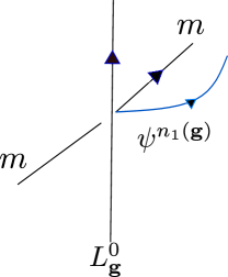
Figure 1: A fermion parity flux $m$ is permuted by ${\bf g}$ action.

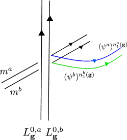
Figure 2: Stacking rule for $n_{1}$. Upon condensing, we identify $\psi^{\text{tot}}\sim\psi^{a}\sim\psi^{b}$.

Upon stacking $a$ and $b$, we have the situation shown in Fig. 2. Prior to the condensation, the defect $L_{\bf g}^{0,\text{tot}}$ can be expressed as a pair $(L_{\bf g}^{0,a},L_{\bf g}^{0,b})$, while the anyon $m^{\text{tot}}$ can be expressed as $m^{a}m^{b}$. The process of passing $m^{\text{tot}}$ under $L_{\bf g}^{0,\text{tot}}$ can be broken up into independent processes occurring in $a$ and $b$. As a result, we see that

$$m^{a}m^{b} \rightarrow(m^{a}\times(\psi^{a})^{n_{1}^{a}({\bf g})})(m^{b}\times(\psi^{b})^{n_{1}^{b}({\bf g})})$$

$$=(m^{a}m^{b})\times((\psi^{a})^{n_{1}^{a}({\bf g})}(\psi^{b})^{n_{1}^{b}({\bf g})})~{}.$$ (218)

After condensation, we have the identity $\psi^{a}\sim\psi^{b}\sim\psi^{\text{tot}}$ and $m^{a}m^{b}\rightarrow m^{\text{tot}}$. The above equation then becomes

$$m^{\text{tot}} \rightarrow m^{\text{tot}}\times(\psi^{\text{tot}})^{(n_{1}^{a}+n_{1}^{b})({\bf g})}~{}.$$ (219)

VI.1.3 Stacking rule for $\omega_{2}$

Below we show that if the stacking of $G_{b}$-crossed theories is to be meaningfully related to the stacking of invertible fermionic phases, then we must have $\omega_{2}^{a}=\omega_{2}^{b}=\omega_{2}$. Although this is intuitively obvious if we consider stacking the original $G_{f}$-crossed theories, it is not so obvious in the $G_{b}$-crossed theory, where the complete set of symmetry fractionalization classes contains different choices of $[\omega_{2}]$. We argue as follows. First we have the definitions $\eta_{\psi^{a}}({\bf g},{\bf h})=\eta_{\psi^{b}}({\bf g},{\bf h})=(-1)^{\omega_{2}({\bf g},{\bf h})}$. Diagramatically, these $\eta$ symbols are calculated by braiding $\psi^{a}$ (respectively, $\psi^{b}$) around a junction formed by the fusion of a ${\bf g}$ and an ${\bf h}$ defect into a ${\bf gh}$ defect (see Fig. 3). The red line can be removed from the junction at the cost of a phase factor $\eta_{\psi}({\bf g},{\bf h})$. When the symmetry is unitary, $\eta_{\psi}({\bf g},{\bf h})$ can be set equal to the braiding phase $M_{\psi,\mathfrak{t}({\bf g},{\bf h})}$ between $\psi$ and an anyon $\mathfrak{t}({\bf g},{\bf h})$, defined as

$$\mathfrak{t}({\bf g},{\bf h})=m^{\omega_{2}({\bf g},{\bf h})}\times\psi^{n_{2}({\bf g},{\bf h})}~{}.$$ (220)

Since $M_{\psi,\psi}=1$, there will be no contribution to $\eta_{\psi}$ from $n_{2}$.

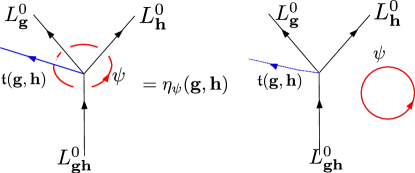
Figure 3: Computation of $\eta_{\psi}$ by performing a full braid of $\psi$ around an $L_{\bf g}^{0},L_{\bf h}^{0},L_{\bf gh}^{0}$ trijunction.

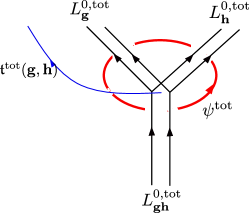
Figure 4: The computation of $\eta_{\psi}$ in the stacked phase splits into independent braiding processes within $a$ and $b$. This is because there are no additional crossings generated by the interaction of $a$ and $b$ lines.

To interpret this stacking of $G_{b}$-crossed theories as a stacking procedure for invertible phases, we need to be able to condense $\psi^{a}\psi^{b}$ without breaking symmetry. For this we must have $\eta_{\psi^{a}\psi^{b}}=1$, i.e. $\psi^{a}\psi^{b}$ should not have any fractional $G_{b}$ quantum numbers [Bischoff_2019]. The symbol $\eta_{\psi^{a}\psi^{b}}$ can be measured by braiding $\psi^{a}\psi^{b}$ around a double junction obtained by stacking $a$ and $b$. Since we are working prior to the $\psi^{a}\psi^{b}$ condensation, the only braiding factors come from the crossing of $\psi^{a}$ with $(m^{a})^{\omega_{2}^{a}}$ and of $\psi^{b}$ with $(m^{b})^{\omega_{2}^{b}}$. These braiding phases are given by $\eta_{\psi^{a}}$ and $\eta_{\psi^{b}}$ respectively. As a result, we can write

$$\eta_{\psi^{a}\psi^{b}}=\eta_{\psi^{a}}\eta_{\psi^{b}}=(-1)^{\omega_{2}^{a}+\omega_{2}^{b}}~{}.$$ (221)

For the lhs to be 1, we must have $\omega_{2}^{a}=\omega_{2}^{b}=\omega_{2}$.

Now let us show that ${\omega_{2}}^{\text{tot}}={\omega_{2}}$ for the stacking of invertible phases. We have $\psi^{\text{tot}}\sim\psi^{a}\sim\psi^{b}$. The value of $\eta_{\psi^{\text{tot}}}$ is measured by braiding $\psi^{\text{tot}}$ around a stacked junction, as depicted in Fig. 4. Here $\psi^{\text{tot}}$ crosses the anyon $\mathfrak{t}^{\text{tot}}$. The statement ${\omega_{2}}^{\text{tot}}={\omega_{2}}$ is equivalent to saying that $\mathfrak{t}^{\text{tot}}({\bf g},{\bf h})$ is a fermion parity flux if and only if $\mathfrak{t}^{a}({\bf g},{\bf h})$ and $\mathfrak{t}^{a}({\bf g},{\bf h})$ are fermion parity fluxes. The ’if’ part is clear: if $\mathfrak{t}^{a}({\bf g},{\bf h})$ and $\mathfrak{t}^{a}({\bf g},{\bf h})$ are fermion parity fluxes, their bound state is also a fermion parity flux, and determines $\mathfrak{t}^{\text{tot}}({\bf g},{\bf h})$ up to a fermion. For the other direction, we argue that if $\mathfrak{t}^{\text{tot}}$ is a fermion parity flux, then both $\mathfrak{t}^{a}({\bf g},{\bf h})$ and $\mathfrak{t}^{a}({\bf g},{\bf h})$ are fermion parity fluxes. Indeed, the only deconfined bound states in the stacked phase are $m^{a}m^{b},(m^{a}\psi^{a})m^{b}$, and $\psi^{a}$ (up to equivalences). The only bound state which gives a fermion parity flux is $m^{a}m^{b}$.

VI.1.4 Conjectured stacking rule for $n_{2}$

In the $G_{b}$-crossed theory, the basic data are given by $\tilde{n}_{1},\tilde{n}_{2},\nu_{3}$ and the flux labels $L_{\bf g}$. For integer $c_{-}$ one passes to $n_{2}$ by relabelling the defects such that $L_{\bf g}\rightarrow L_{\bf g}^{0}$, and then computing the change in $\tilde{n}_{2}$. Thus in order to obtain the stacking rule for $n_{2}$ from the $G_{b}$-crossed theory, we must first obtain the stacking rules for symmetry defects $L_{\bf g}$ and for the symmetry fractionalization parameter $\tilde{n}_{2}$. The former step requires a more complete theory of anyon condensation in $G$-crossed BTCs than is currently available, and so we do not pursue this here.

An exact stacking rule for $n_{2}$ can be independently obtained from Chern-Simons theory when $s_{1}=0$ and $G_{f}=G_{b}\times\mathbb{Z}_{2}^{f}$ (Section VI.4): it has the form

$$n_{2}^{\text{tot}}=n_{2}^{a}+n_{2}^{b}+n_{1}^{a}\cup n_{1}^{b}.$$ (222)

We conjecture that this rule should also hold when ${\omega_{2}}\neq 0$. In support of this conjecture when ${\omega_{2}}\neq 0$, we find that $\frac{\mathcal{O}_{4}[n_{1}^{\text{tot}},n_{2}^{\text{tot}}]}{\mathcal{O}_{4}[n_{1}^{a},n_{2}^{a}]\mathcal{O}_{4}[n_{1}^{a},n_{2}^{a}]}$ is a coboundary even when $[{\omega_{2}}]$ is nontrivial. Thus Eq. (222) gives a meaningful guess for the stacking rule for $\nu_{3}$, as we will discuss below.

VI.2 Stacking rule for $\nu_{3}$ from the $\mathcal{O}_{4}$ anomaly

Here we obtain an explicit expression for the stacking rule for $\nu_{3}$, by integrating the equation for $d\nu_{3}$. We will assume $s_{1}=0$, and also take the $n_{2}$ stacking rule to be given by Eq. (222). This approach determines $\nu_{3}^{\text{tot}}$ up to a 3-cocycle; we conjecture that this 3-cocycle should be trivial, which we verify in the case ${\omega_{2}}=0$ in Section VI.4 using the CS formulation. However we do not have a general direct proof when ${\omega_{2}}\neq 0$.

Note that for half integer $c_{-}$ the symmetry is $G_{b}\times\mathbb{Z}_{2}^{f}$, which is covered by the analysis of Section VI.4. Therefore here we will focus on the case with integer $c_{-}$. The condition satisfied by $\nu_{3}$ is

$$d\nu_{3} =(-1)^{{\cal P}(n_{2})+n_{2}\cup{\omega_{2}}+\zeta(n_{1},{\omega_{2}})+c_{-}(n_{1}\cup{\omega_{2}})\cup_{2}({\omega_{2}}\cup_{1}{\omega_{2}})}$$ (223)

$$\quad\;(-1)^{\frac{c_{-}}{4}{\cal P}({\omega_{2}})}i^{n_{1}\cup n_{1}\cup{\omega_{2}}}~{},$$ (224)

with the Pontryagin square ${\cal P}(X_{2})\equiv X_{2}\cup X_{2}-X_{2}\cup_{1}dX_{2}$ and the Cartan coboundary $\zeta(n_{1},{\omega_{2}})=n_{1}\cup[(n_{1}\cup{\omega_{2}})\cup_{2}{\omega_{2}}+n_{1}\cup{\omega_{2}}]$. We can first verify that the obstruction is closed by expanding out the various terms. To compute the stacking rule for $\nu_{3}$, we use the property that ${\cal O}_{4}(n_{1}^{\text{tot}},n_{2}^{\text{tot}},\omega_{2}^{\text{tot}},c_{-}^{\text{tot}})$ differs from ${\cal O}_{4}(n_{1}^{a},n_{2}^{a},\omega_{2}^{a},c_{-}^{a}){\cal O}_{4}(n_{1}^{b},n_{2}^{b},\omega_{2}^{b},c_{-}^{b})$ by a coboundary. The details of the computation are in Appendix LABEL:sec:stackingnu3. The answer, up to a possible 3-cocycle, is

$$\nu_{3}^{\text{tot}}= \nu_{3}^{a}\nu_{3}^{b}\,i^{\frac{1}{2}n_{1}^{a}\cup n_{1}^{b}\cup n_{1}^{b}+n_{1}^{a}\cup(n_{1}^{a}\cup_{1}n_{1}^{b})\cup n_{1}^{b}}i^{(n_{1}^{a}\cup_{1}n_{1}^{b})\cup{\omega_{2}}}$$ (225)

$$\times(-1)^{(n_{1}^{a}\cup n_{1}^{b})\cup_{1}(n_{2}^{a}+n_{2}^{b})+n_{2}^{a}\cup_{1}n_{2}^{b}+dn_{2}^{a}\cup_{2}n_{2}^{b}}$$ (226)

$$\times(-1)^{c^{a}_{-}(\omega_{2}\cup_{1}\omega_{2})\cup_{3}(n_{1}^{b}\cup\omega_{2})}~{}.$$ (227)

In the special case $\omega_{2}^{a}=\omega_{2}^{b}=\omega_{2}^{\text{tot}}=0$, the stacking rule for $\nu_{3}$ becomes

$$\nu_{3}^{\text{tot}} =\nu_{3}^{a}\nu_{3}^{b}\,i^{n_{1}^{a}\cup n_{1}^{b}\cup n_{1}^{b}+n_{1}^{a}\cup(n_{1}^{a}\cup_{1}n_{1}^{b})\cup n_{1}^{b}}$$ (228)

$$(-1)^{(n_{1}^{a}\cup n_{1}^{b})\cup_{1}(n_{2}^{a}+n_{2}^{b})+n_{2}^{a}\cup_{1}n_{2}^{b}}~{}.$$ (229)

This reproduces the stacking rule of the fermionic invertible phases with $G_{b}\times\mathbb{Z}_{2}^{f}$ symmetry in Ref. brumfiel2018pontrjagin, which is exact, and is derived using the Chern-Simons theory in Section VI.4.

VI.2.1 Application: equivalences on the data

For general ${\omega_{2}}$, the above stacking rule is undetermined up to a possible 3-cocycle $\alpha_{3}({\omega_{2}},D^{a},D^{b})$, where the data $D^{i}=(c^{i},n_{1}^{i},n_{2}^{i},\nu_{3}^{i})$ for $i=a,b$ defines the invertible phase $i$. We conjecture that $\alpha_{3}=0$.

If $\alpha_{3}\neq 0$, the equivalences on $(n_{2},\nu_{3})$ stated in Eq. (9) of Table 1 will also need to be modified. First consider the equivalence (see Eq. (103))

$$(n_{2},\nu_{3})\simeq(n_{2}+db_{1},\nu_{3}\times(-1)^{b_{1}\cup{\omega_{2}}+db_{1}\cup_{1}n_{2}+db_{1}\cup b_{1}}\times\alpha_{3}^{\prime})$$ (230)

where $\alpha_{3}^{\prime}$ is an undetermined 3-cocycle. This equivalence can be thought of as coming from stacking a trivial phase with the data $D^{\prime}_{1}=(0,0,db_{1},(-1)^{db_{1}\cup b_{1}+b_{1}\cup{\omega_{2}}})$ onto an invertible phase with data $D^{\prime}_{2}=(c_{-},n_{1},n_{2},\nu_{3})$. In this case, the $\nu_{3}$ data of the stacked phase equals

$$\nu_{3}^{\text{tot}}=\nu_{3}\times(-1)^{b_{1}\cup{\omega_{2}}+db_{1}\cup_{1}n_{2}+db_{1}\cup b_{1}}\times\alpha_{3}({\omega_{2}},D^{\prime}_{1},D^{\prime}_{2})$$ (231)

and therefore we can express $\alpha^{\prime}_{3}$ in terms of $\alpha_{3}$:

$$\alpha^{\prime}_{3}\equiv\alpha_{3}({\omega_{2}},D^{\prime}_{1},D^{\prime}_{2}).$$ (232)

We can similarly analyze the equivalence (from Eq. (97))

$$(n_{2},\nu_{3})\simeq(n_{2}+{\omega_{2}},\nu_{3}\times(-1)^{{\omega_{2}}\cup_{1}n_{2}}\times\alpha^{\prime\prime}_{3})$$ (233)

and determine $\alpha^{\prime\prime}_{3}$ in terms of $\alpha_{3}$. Here we can interpret the equivalence in terms of stacking two phases with data $D^{\prime\prime}_{1}=(0,0,{\omega_{2}},1)$ and $D^{\prime\prime}_{2}=(c_{-},n_{1},n_{2},\nu_{3})$. Then we find that

$$\alpha^{\prime\prime}_{3}\equiv\alpha_{3}({\omega_{2}},D^{\prime\prime}_{1},D^{\prime\prime}_{2}).$$ (234)

In particular, if $\alpha_{3}=0$ as we conjecture, then we must have $\alpha^{\prime}_{3}=\alpha^{\prime\prime}_{3}=0$.

VI.3 Stacking rules when $s_{1}\neq 0$

We will discuss the stacking rule of $n_{2}$ for $s_{1}\neq 0$ and general $n_{1}$ using the constraint equations for $dn_{2},d\nu_{3}$. For simplicity, we will focus on the stacking rule of $n_{2}$, while leaving the stacking rule of $\nu_{3}$ to future work. The constraint equation for $dn_{2}$ is

$$dn_{2}=n_{1}\cup\omega_{2}+n_{1}\cup s_{1}\cup n_{1}~{}.$$ (235)

This implies that

$$dn_{2}^{\text{tot}}=dn_{2}^{a}+dn_{2}^{b}+n_{1}^{a}\cup s_{1}\cup n_{1}^{b}+n_{1}^{b}\cup s_{1}\cup n_{1}^{a}.$$ (236)

Thus we find

$$n_{2}^{\text{tot}} =n_{2}^{a}+n_{2}^{b}+n_{1}^{a}\cup n_{1}^{b}+(n_{1}^{a}\cup_{1}s_{1})\cup n_{1}^{b}$$ (237)

$$\;\;+(n_{1}^{b}\cup_{1}s_{1})\cup n_{1}^{a}+s_{1}\cup(n_{1}^{a}\cup_{1}n_{1}^{b})+x~{}.$$ (238)

where $x$ is a $\mathbb{Z}_{2}$ two-cocycle that vanishes for $s_{1}=0$. We propose the minimal stacking rule with $x=0$:

$$n_{2}^{\text{tot}} =n_{2}^{a}+n_{2}^{b}+n_{1}^{a}\cup n_{1}^{b}+(n_{1}^{a}\cup_{1}s_{1})\cup n_{1}^{b}$$ (239)

$$\quad+(n_{1}^{b}\cup_{1}s_{1})\cup n_{1}^{a}+s_{1}\cup(n_{1}^{a}\cup_{1}n_{1}^{b})~{}.$$ (240)

VI.4 Stacking rules from Chern-Simons theory when $G_{f}=G_{b}\times\mathbb{Z}_{2}^{f}$

While the bosonic shadow theories are useful for relating the Chern-Simons approach to the $G_{b}$-crossed BTC, we can directly study the invertible fermion phase using Chern-Simons theory. In this section, we assume the symmetry is $G_{b}\times\mathbb{Z}_{2}^{f}$. We can couple the Chern-Simons theory to background $G_{b}$ gauge field $A_{b}$ via the magnetic $\mathbb{Z}_{2}$ 0-form symmetry: we turn on background for the magnetic 0-form symmetry given by the $\mathbb{Z}_{2}$ one-form $A_{b}^{*}n_{1}$, where $n_{1}\in\mathcal{H}^{1}(G_{b},\mathbb{Z}_{2})$. Equivalently, we shift the spin structure by $A_{b}^{*}n_{1}$. We can also add a local action $\int_{3d}A_{b}^{*}\phi_{3}$ for the background $G_{b}$ gauge field, which depends on the bulk extension by

$$\int_{4d}A_{b}^{*}d\phi_{3},\quad\phi_{3}\in C^{3}(BG,\mathbb{R}/2\pi\mathbb{Z})~{}.$$ (241)

In bosonic theory, we require the dependence to be trivial to have a well-defined local action; on spin manifolds, $w_{2}(TM)$ is trivial, and it can instead satisfies

$$A_{b}^{*}d\phi_{3} =\pi w_{2}(TM)\cup A_{b}^{*}n_{2}$$ (242)

$$=\pi A_{b}^{*}Sq^{2}(n_{2}),\quad n_{2}\in\mathcal{H}^{2}(BG,\mathbb{Z}_{2})~{},$$ (243)

where we used the Wu formula $Sq^{2}(n_{2})=n_{2}\cup w_{2}$ mod 2 on orientable four-manifolds [milnor1974characteristic]. For instance, when the symmetry of the fermionic phase is $\mathbb{Z}_{2n}\times\mathbb{Z}_{2}^{f}$, $\phi_{3}$ is given by (possibly spin) Chern-Simons terms of the $\mathbb{Z}_{2n}$ background gauge field, and as demonstrated in Ref. Cordova:2017vab this reproduces the $\mathbb{Z}_{4n}\times\mathbb{Z}_{2}$ classification for even $n$ and $\mathbb{Z}_{8n}$ classification for odd $n$ [PhysRevB.95.195147]. The cochain $\phi_{3}$ can be exponetiated to $\nu_{3}=e^{i\phi_{3}}$.

More explicitly, the effective action for the fermionic invertible phase can be expressed as follows. We would like to understand the effective action for the fermionic invertible phase that is not expressed as $\phi_{3}$. Following Ref. Cordova:2017vab, we denote the effective action produced by shifting the spin structure with $A_{b}^{*}n_{1}$ in $SO(2c_{-})_{1}$ equals $2c_{-}f(A_{b}^{*}n_{1})$, where $f$ is defined by

$$e^{iLf(B_{1})}=\frac{Z_{SO(L)_{1}}[0]}{Z_{SO(L)_{1}}[B_{1}]}~{},$$ (244)

where $Z_{SO(L)_{1}}[B_{1}]$ is the partition function of $SO(L)_{1}$ Chern-Simons theory coupled to background $B_{1}=A_{b}^{*}n_{1}$ by the $\mathbb{Z}_{2}$ magnetic 0-form symmetry. Equivalently, since the magnetic 0-form symmetry in $SO(L)_{1}$ is identified with the fermion parity [Cordova:2017vab], $e^{iLf[B_{1}]}$ is the change of the partition function for $SO(L)_{1}\leftrightarrow-L\text{CS}_{\text{grav}}$ under shifting the spin structure by $B_{1}=A_{b}^{*}n_{1}$, and the exponent is proportional to $L$. The effective action $f(B_{1})$ is the effective action for the fermionic SPT phase with $\mathbb{Z}_{2}\times\mathbb{Z}_{2}^{f}$ unitary symmetry that belongs to the unit class of $\mathbb{Z}_{8}$ classification. We note that $A_{b}^{*}\phi_{3}$ in general cannot be expressed using $f$, since the later is at most $\mathbb{Z}_{8}$ valued. We remark that although $f(A_{b}^{*}n_{1})$ cannot be expressed as a special case of $A_{b}^{*}\phi_{3}$, on the other hand, $2f(A_{b}^{*}n_{1})$ is equivalent to a special case $A_{b}^{*}\phi_{3}$ [Cordova:2017vab]. This is because for $c_{-}=1$, the gravitational Chern-Simons term can be expressed as products of $U(1)_{1}$ Chern-Simons theory, and shifting the spin structure by $\mathbb{Z}_{2}$ gauge field $B_{1}=\pi A_{b}^{*}n_{1}$ (we normalize $n_{1}=0,1$) in $U(1)_{1}$ produces a Chern-Simons term for the background $\mathbb{Z}_{2}$ gauge field $A_{b}^{*}n_{1}$:

$$\frac{1}{4\pi}ada+\frac{1}{2\pi}adB_{1}\leftrightarrow\frac{1}{4\pi}a^{\prime}da^{\prime}-\frac{1}{4\pi}B_{1}dB_{1},\quad a^{\prime}=a+B_{1}~{},$$ (245)

where the Chern-Simons term of $B_{1}=\pi A_{b}^{*}n_{1}$ can be expressed as integral of an auxiliary term in the bulk of the form $Sq^{2}(n_{2})$ with $n_{2}=dn_{1}/2=Sq^{1}(n_{1})$:

$$\frac{1}{4\pi}\int_{3d}dB_{1}dB_{1}=\pi\int_{4d}\frac{dB_{1}}{2\pi}\frac{dB_{1}}{2\pi}$$ (246)

$$=\pi\int Sq^{2}\left(\frac{dB_{1}}{2\pi}\right)=\pi\int A_{b}^{*}Sq^{2}(dn_{1}/2)~{}.$$ (247)

Thus, it is sufficient to parametrize the effective action of the fermionic invertible phase with $G_{b}\times\mathbb{Z}_{2}^{f}$ symmetry by $(n_{1},n_{2},\phi_{3})$ as

$$S(n_{1},n_{2},\phi_{3};A_{b}) =\int A_{b}^{*}\phi_{3}+f(A_{b}^{*}n_{1})-2c_{-}\text{CS}_{\text{grav}},$$ (248)

$$d\phi_{3} =\pi Sq^{2}(n_{2})~{},$$ (249)

where $A_{b}$ is the background $G_{b}$ gauge field. This agrees with the classification in Ref. Bhardwaj_2017, since $f$ is the effective action of the “root” fermionic SPT phase with unitary $\mathbb{Z}_{2}\times\mathbb{Z}_{2}^{f}$ symmetry.

Let us consider the stacking of two fermionic invertible phases with $G_{b}\times\mathbb{Z}_{2}^{f}$ symmetry [brumfiel2018pontrjagin], i.e. how the data $(n_{1},n_{2},\phi_{3})$ composes under addition of the effective action:

$$S(n_{1}^{a},n_{2}^{a},\phi_{3}^{a};A_{b})+S(n_{1}^{b},n_{2}^{b},\phi_{3}^{b};A_{b})$$ (250)

$$\quad=S(n_{1}^{\text{tot}},n_{2}^{\text{tot}},\phi_{3}^{\text{tot}};A_{b})~{}.$$ (251)

From the gravitational Chern-Simons term $-2c_{-}\text{CS}_{\text{grav}}$ we find $c_{-}^{\text{tot}}=c_{-}^{a}+c_{-}^{b}$. We note that

$$f (A_{b}^{*}n_{1}^{a})+f(A_{b}^{*}n_{1}^{b})=f(A_{b}^{*}(n_{1}^{a}+n_{1}^{b}))+A_{b}^{*}\xi(\tilde{n}_{1}^{a},\tilde{n}_{1}^{b}),$$ (252)

$$d\xi =\pi(n_{1}^{a})^{2}\cup(n_{1}^{b})^{2}$$ (253)

$$=Sq^{2}(n_{1}^{a}\cup n_{1}^{b})+d(n_{1}^{a}\cup(n_{1}^{a}\cup_{1}\eta_{b}^{1})\cup n_{1}^{b})~{},$$ (254)

where $\tilde{n}_{1}^{a},\tilde{n}_{1}^{b}$ are the canonical integral one-cochain lifts of $n_{1}^{a},n_{1}^{b}$ that takes value in $0,1$. Explicitly, $\xi=(\pi/2)\tilde{n}_{1}^{a}\cup(\tilde{n}_{1}^{b})^{1}$. We used the identity $(n_{1}^{a}\cup n_{1}^{b}+n_{1}^{b}\cup n_{1}^{a})=d(n_{1}^{a}\cup_{1}n_{1}^{b})$. In Eq. (252), the term $f(A_{b}^{*}(n_{1}^{a}+n_{1}^{b})=f(A_{b}^{*}n_{1}^{\text{tot}})$ gives the stacking rule $n_{1}^{\text{tot}}=n_{1}^{a}+n_{1}^{b}$. In the last line of (252), the first term $Sq^{2}(n_{1}^{a}\cup n_{1}^{b})$ together with $Sq^{2}(n_{2}^{a})+Sq^{2}(n_{2}^{b})$ contribute to $Sq^{2}(n_{2}^{\text{tot}})$. Thus by comparing with (248), we find the stacking rule

$$n_{1}^{\text{tot}}=n_{1}^{a}+n_{1}^{b},\quad n_{2}^{\text{tot}}=n_{2}^{a}+n_{2}^{b}+n_{1}^{a}\cup n_{1}^{b}~{}.$$ (255)

The stacking rule of $\phi_{3}$ is derived by writing the bulk terms other than $Sq^{2}(n_{2}^{\text{tot}})$ as a boundary cochain . In the end we find $\phi_{3}^{\text{tot}}$ is related to $\phi_{3}^{a},\phi_{3}^{b}$ by

$$\phi_{3}^{\text{tot}}= \phi_{3}^{a}+\phi_{3}^{b}+\pi(n_{2}^{a}\cup_{1}n_{2}^{b}+(n_{2}^{a}+n_{2}^{b})\cup_{1}(n_{1}^{a}\cup n_{1}^{b})$$ (259)

$$+n_{1}^{a}\cup(n_{1}^{a}\cup_{1}n_{1}^{b})\cup n_{1}^{b})+\frac{\pi}{2}\tilde{n}_{1}^{a}\cup(\tilde{n}_{1}^{b})^{2}.$$ (260)

Thus we reproduce the stacking rules for $G_{b}\times\mathbb{Z}_{2}^{f}$ symmetry fermionic invertible phases in Ref. brumfiel2018pontrjagin.

VI.5 Stacking rules for $G_{f}=U(1)^{f}$ using CS theory with background $Spin^{c}=(U(1)\times\mathbb{Z}_{2}^{f})/\mathbb{Z}_{2}$ structures

Let us use an example to illustrate the stacking rule when the symmetry of the fermionic invertible phase is an extension of $G_{b}$ by $\mathbb{Z}_{2}^{f}$ (strictly speaking such phases are not fermionic, in the sense that they do not have neutral fermionic particles that are singlet under $G_{b}$). We consider the symmetry to be $Spin^{c}=(U(1)\times\mathbb{Z}_{2}^{f})\mathbb{Z}_{2}$. If we turn on the background gauge field $A$, the fermionic invertible phase has effective action

$$k_{1}\left(\frac{1}{4\pi}AdA+2\text{CS}_{\text{grav}}\right)+16k_{2}\text{CS}_{\text{grav}}~{}$$ (261)

for background $Spin^{c}$ connection $A$, where $(k_{1},k_{2})\in\mathbb{Z}\times\mathbb{Z}$ gives the stacking rule. In particular, although the gravitational part is not well-defined by itself for general $k_{1}$, the stacking rule for the part that depends on $A$ and the gravitational part can be treated separately: when adding the effective action for different classes $(k_{1},k_{2}),(k_{1}^{\prime},k_{2}^{\prime})$, we add the gravitational part and the “non-gravitational” part that depends only on $A$ separately. This behavior of the stacking rule is similar to the case when the symmetry is a direct product $G_{b}\times\mathbb{Z}_{2}^{f}$. As we will argue in the following, this separation of the gravitational and non-gravitational stacking rule continues to hold when the symmetry is a general extension of any $G_{b}$ by $\mathbb{Z}_{2}^{f}$.

We remark that the separation of the stacking rule for gravitational and non-gravitational parts is also related to the absence of topological thermo-electric coupling in unitary theories: there is no topological term that mixes the background gauge field and background gravity. For a recent discussion of absence of topological thermo-electric transport, see Ref. PhysRevB.103.235101.

VII Examples

We now illustrate our classification approach with several examples. To conveniently account for the various equivalences involved, we use the following strategy: (i) find the allowed choices of $n_{1}\in\mathcal{H}^{1}(G_{b},\mathbb{Z}_{2})$. (ii) For each $n_{1}$, find a representative set of allowed choices of $n_{2}$. These form a torsor over $\mathcal{H}^{2}(G_{b},\mathbb{Z}_{2})$ modulo the possible equivalence $n_{2}\simeq n_{2}+{\omega_{2}}$. (iii) With the representative $n_{2}$ fixed, find all possible $\nu_{3}$, accounting for all equivalences that preserve $n_{2}$.

VII.1 $G_{f}=\mathbb{Z}_{2}\times\mathbb{Z}_{2}^{f}$

In this example, we will use the $G_{b}$-crossed theory to classify invertible phases with $G_{f}=\mathbb{Z}_{2}\times\mathbb{Z}_{2}^{f}$. It is well-known from previous work that the classification of fSPTs with this symmetry should be $\mathbb{Z}_{8}$ [Gu2014interaction, Ryu2012interaction, Qi_2013]. From cobordism theory, we also expect that the full classification of invertible phases is $\mathbb{Z}\times\mathbb{Z}_{8}$, with 8 phases for each $c_{-}$ [Kapustin:2014dxa]. Although a naive count of $G_{b}$-crossed theories does not agree with these results, we recover this classification by keeping track of flux labels. Finally, we show how the free and interacting classifications can be explicitly related in this case. We use this correspondence to illuminate the stacking rules.

Free fermion parameter	Interacting fermion parameter	$G_{b}$-crossed data with flux labels	Fully gauged theory
$(\nu^{\uparrow},-\nu^{\downarrow})$	$(n_{1},n_{2},\nu_{3})$	$(\tilde{n}_{1},\tilde{n}_{2},\nu_{3},L_{\bf h})$
$(0,0)$	$(0,0,1)$	$(0,0,1,I_{\bf h})$	$\mathbb{Z}_{2}\text{t.c.}^{\uparrow}\times\mathbb{Z}_{2}\text{t.c.}^{\downarrow}$
$(1,-1)$	$(1,0,1)$	$(1,0,1,\sigma_{\bf h}^{+})$	$\text{Ising}^{\uparrow}\times\overline{\text{Ising}}^{\downarrow}$
$(2,-2)$	$(0,1,-i)$	$(0,1,-i,I_{\bf h})$	$U(1)^{\uparrow}_{4}\times U(1)^{\downarrow}_{-4}$
$(3,-3)$	$(1,1,-i)$	$(1,0,-1,\sigma^{-}_{\bf h})$	$\text{Ising}^{(3),\uparrow}\times\text{Ising}^{(-3),\downarrow}$
$(4,-4)$	$(0,0,-1)$	$(0,0,-1,I_{\bf h})$	$\text{D.S. }(+i)^{\uparrow}\times\text{D.S.}(-i)^{\downarrow}$
$(5,-5)$	$(1,0,-1)$	$(1,0,-1,\sigma^{+}_{\bf h})$	$\text{Ising}^{(5),\uparrow}\times\text{Ising}^{(-5),\downarrow}$
$(6,-6)$	$(0,1,i)$	$(0,1,-i,m_{\bf h})$	$U(1)_{-4}^{\uparrow}\times U(1)_{4}^{\downarrow}$
$(7,-7)$	$(1,1,i)$	$(1,0,1,\sigma_{\bf h}^{-})$	$\text{Ising}^{(7),\uparrow}\times\text{Ising}^{(-7),\downarrow}$

Table 5: Comparison of data for $c_{-}=0$ phases with $G_{f}=\mathbb{Z}_{2}\times\mathbb{Z}_{2}^{f}$ in terms of (1) a free fermion construction, (2) the $(n_{1},n_{2},\nu_{3})$ representation used in Ref. Wang2020fSPT, (3) the $(\tilde{n}_{1},\tilde{n}_{2},\nu_{3},L_{\bf g})$ representation coming from the $G_{b}$-crossed theory, and 4) the theory obtained by fully gauging $G_{f}$. Here “t.c.” means “toric code” while “D.S.$(\pm i)$” means “double semion theory with semion statistics $\pm i$”. All arguments of $n_{1},n_{2},\tilde{n}_{1},\tilde{n}_{2}$, and $\nu_{3}$ are set equal to ${\bf h}$.

VII.1.1 Classification when $c_{-}=0$

Let ${\bf h}$ be the generator of the unitary $\mathbb{Z}_{2}$ symmetry. We begin by naively counting the number of $G_{b}$-crossed extensions of the toric code UMTC. This is done by counting all possible inequivalent triples $(\tilde{n}_{1},\tilde{n}_{2},\nu_{3})$. First consider the case where $\tilde{n}_{1}({\bf h})=1$. After setting $\omega_{2}=0$, we have $[(\omega_{2},\tilde{n}_{2})]\in\mathcal{H}^{2}_{\tilde{n}_{1}}(\mathbb{Z}_{2},\mathbb{Z}_{2}\times\mathbb{Z}_{2})=\mathbb{Z}_{1}$. Although there are 2 choices for the function $\tilde{n}_{2}$, given by $\tilde{n}_{2}({\bf h},{\bf h})=0$ or 1, these choices are coboundary-equivalent. (In particular, these two choices correspond to the symmetry fractionalization cocycles with $\mathfrak{t}({\bf h},{\bf h})=I$ or $\psi$; they are related by the coboundary $d\mathfrak{b}$, where $\mathfrak{b}({\bf h})=m$.) Therefore we will fix $\tilde{n}_{2}=0$. We also have two defect classes, which are inequivalent under relabellings; these correspond to $\nu_{3}({\bf h},{\bf h},{\bf h})=\pm 1$. In total there are two $G_{b}$-crossed theories with $\tilde{n}_{1}\neq 0$.

Next, we look at theories with $\tilde{n}_{1}=0$. In this case there are two symmetry fractionalization classes, with $\tilde{n}_{2}({\bf h},{\bf h})=0,1$; they are classified by the subgroup of $\mathcal{H}^{2}(G_{b},\mathbb{Z}_{2}\times\mathbb{Z}_{2})$ with $\omega_{2}=0$, and are inequivalent. For each symmetry fractionalization class, we have two defect classes (i.e. 2 choices of $\nu_{3}$). However, the two defect classes associated to $\tilde{n}_{2}({\bf h},{\bf h})=1$ (i.e. the ones with $\nu_{3}({\bf h},{\bf h},{\bf h})=\pm i$) are equivalent under a relabelling of defects (this was shown previously in Refs. Lu2016, Barkeshli2019). Therefore we only have 3 SET phases in this case, giving a total of 5 $G_{b}$-crossed theories with $c_{-}=0$. Indeed, by examining the third column of Table 5, we can verify that there are only 5 distinct triples $(\tilde{n}_{1},\tilde{n}_{2},\nu_{3})$.

Below we show that these 5 theories in fact contain a total of 8 topological invariants which take the values $e^{2\pi ik/8}$, for $k=0,1,\dots,7$. Thus the same $G_{b}$-crossed BTC might correspond to two different fSPT phases. In order to fully specify the fSPT, we need to define a flux label $L_{\bf h}$, corresponding to the $({\bf h},0)$ defect in the ungauged $G_{f}$-crossed theory.

Consider the fSPT phases with $\tilde{n}_{1}\neq 0$. Here we can define

$$\tilde{n}_{2}({\bf h},{\bf h}) =0$$ (262)

$$\nu_{3}({\bf h},{\bf h},{\bf h}) =(-1)^{q}~{},$$ (263)

where $q\in\mathbb{Z}_{2}$. In this case, the $G_{b}$-crossed theory has two ${\bf h}$-defects $\sigma^{+}_{\bf h}$ and $\sigma^{-}_{\bf h}$. For each $q$, the $G_{b}$-crossed theory has two invariants, denoted as $\mathcal{I}(\sigma^{+}_{\bf h})$ and $\mathcal{I}(\sigma^{-}_{\bf h})$. The explicit form of the invariants is

$$\mathcal{I}(\sigma^{\pm}_{\bf h}):=\theta_{\sigma^{\pm}_{\bf h}}^{2}\eta_{\sigma^{\pm}_{\bf h}}({\bf h},{\bf h})~{}.$$ (264)

We can solve for the $G$-crossed data in a gauge with all $\eta=1$, and with $\theta_{\sigma^{\pm}_{\bf h}}=i^{\pm[q]_{2}}e^{\pm i\frac{\pi}{8}}$, where $q\in\mathbb{Z}_{2}$ (see Section X.I of Ref. Barkeshli2019). This implies that

$$\mathcal{I}(\sigma^{\pm}_{\bf h}) =(-1)^{q}e^{\pm i\frac{2\pi}{8}}~{}.$$ (265)

By taking $q=0,1$ and $L_{\bf h}=\sigma^{+}_{\bf h},\sigma^{-}_{\bf h}$, we see that the invariants can take 4 values $e^{i\pi/4},e^{i3\pi/4},e^{i5\pi/4},e^{i7\pi/4}$. If we fix $\tilde{n}_{2}$ and $\nu_{3}$, we cannot interchange these invariants by relabelling defects with fermions. This means that the 4 invariants really describe distinct phases.

When $\tilde{n}_{1}=0$, we have 4 abelian ${\bf h}$-defects $I_{\bf h},e_{\bf h},m_{\bf h},\psi_{\bf h}$. The symmetry fractionalization is specified by $\tilde{n}_{2}({\bf h},{\bf h})\in\{0,1\}$. When $\tilde{n}_{2}=0$, we find that

$$\nu_{3}({\bf h},{\bf h},{\bf h}) =(-1)^{q}$$ (266)

$$\mathcal{I}(a_{\bf h}) =(-1)^{q},\quad\forall a_{\bf h}~{}.$$ (267)

We thus have two fSPT invariants taking values $\pm 1$. When $\tilde{n}_{2}({\bf h},{\bf h})=1$, we find that

$$\nu_{3}({\bf h},{\bf h},{\bf h}) =i(-1)^{q}$$ (268)

$$\mathcal{I}(a_{\bf h}) =(-i)(-1)^{q+a_{e}+a_{m}}~{}.$$ (269)

Once again, there are only two invariants, which take the values $\pm i$. The theory with $\nu_{3}=\pm i,L_{\bf h}=I_{\bf h}$ is the same $G_{b}$-crossed theory as the one with $\nu_{3}=\mp i,L_{\bf h}=m_{\bf h}$. Thus if we were just counting SET phases, we would need to treat the two defect classes with $\tilde{n}_{2}({\bf h},{\bf h})=1$ as equivalent. However, relabelling defects by fermion parity fluxes is not a trivial operation in the $G_{b}$-crossed theory, and therefore the two invariants taking the values $\pm i$ correspond to distinct fSPT phases.

Note that we always have $\mathcal{I}(L_{\bf h})=\mathcal{I}(\psi\times L_{\bf h})$. This reflects the fact that it is physically equivalent to choose $I_{\bf h}$ or $\psi_{\bf h}$ as the $\mathbb{Z}_{2}$ flux, since defects can always be relabelled by attaching fermions.

To summarize, we count the number of different values of $\mathcal{I}(L_{\bf h})$ by varying over the distinct choices of $(n_{1},\tilde{n}_{2},\nu_{3},L_{\bf h})$. When $n_{1}=0$, there are 4 values, $\pm 1$ and $\pm i$. Considering the cases $n_{1}=0$ and $n_{1}\neq 0$ together, we obtain 8 different invariants given by $e^{2\pi ik/8}$ for $k=0,1,\dots,7$. Even without considering formal stacking rules, this suggests that the group corresponding to the fSPT classification should be $\mathbb{Z}_{8}$.

VII.1.2 Relating the $G_{b}$-crossed data to the $(n_{1},n_{2},\nu_{3})$ parameterization

We summarize the result of the classification of fSPTs using the $(n_{1},n_{2},\nu_{3})$ parameterization [Wang2020fSPT] for this example in the second column of Table 5. We have $|\mathcal{H}^{1}(G_{b},\mathbb{Z}_{2})|=|\mathcal{H}^{2}(G_{b},\mathbb{Z}_{2})|=|\mathcal{H}^{3}(G_{b},U(1))|=2$. The final classification has 8 fSPTs, obtained by considering all possible values of $n_{1},n_{2}$ and $\nu_{3}$ which satisfy the defining equations. In this case there are no obstructions, so we indeed have 8 phases where each choice of $n_{1}$ gives 4 fSPTs.

We can straightworwardly relate the $G_{b}$-crossed data $(\tilde{n}_{1},\tilde{n}_{2},\nu_{3},L_{\bf g})$ to the $(n_{1},n_{2},\nu_{3})$ parameterization. For $c_{-}=0$ we have $n_{1}:=\tilde{n}_{1}$. Next, we fix a canonical definintion $L_{\bf h}^{0}$ of the flux labels, as follows: if $n_{1}({\bf h})=0,L_{\bf h}^{0}=I_{\bf h}$, while if $n_{1}({\bf h})=1,L_{\bf h}^{0}=\sigma^{+}_{\bf h}$. Then we use the result from Section IV that if $L_{\bf h}=L_{\bf h}^{0}\times m^{l_{1}({\bf h})}$, then

$$n_{2}({\bf h},{\bf h})=\tilde{n}_{2}({\bf h},{\bf h})+l_{1}({\bf h})n_{1}({\bf h})~{}.$$ (270)

The resulting formula for $\nu_{3}$ in terms of $n_{2}$ is

$$\nu_{3}({\bf h},{\bf h},{\bf h}) =(-1)^{q}i^{[n_{2}({\bf h},{\bf h})]_{2}}~{}.$$ (271)

This gives us the desired relations. A similar redefinition is possible for each integer $c_{-}$, although we will not demonstrate it explicitly.

VII.1.3 Classification when $c_{-}\neq 0$

When $c_{-}$ is an arbitrary integer, the analysis is almost identical to the $c_{-}=0$ case. We present only the results. The data of the usual $G_{b}$-crossed theory are given by

$$n_{1}({\bf h}) \in\{0,1\}$$ (272)

$$\tilde{n}_{2}({\bf h},{\bf h}) \in\{0,1\}$$ (273)

$$\nu_{3}({\bf h},{\bf h},{\bf h}) =(-1)^{q}i^{[n_{2}({\bf h},{\bf h})]_{2}}~{}.$$ (274)

For each integer $c_{-}$, we can compute 8 invariants which take the values $e^{2\pi ik/8}$, where $k\in\mathbb{Z}_{8}$. We can go through the steps discussed previously and form a table similar to Table 5 for each $c_{-}$.

The case $c_{-}=k+1/2$ with integer $k$ is slightly different. Here we have 3 ${\bf h}$-defects $I_{\bf h},\psi_{\bf h},\sigma_{\bf h}$, where $\sigma_{\bf h}$ is nonabelian. For each choice of $[\tilde{n}_{2}]$ and $[\nu_{3}]$, we can evaluate $\mathcal{I}(L_{\bf h})$. We get

$$\mathcal{I}(I_{\bf h}) =\mathcal{I}(\psi_{\bf h})=(-1)^{q}i^{-[\tilde{n}_{2}({\bf h},{\bf h})]}$$ (275)

$$\mathcal{I}(\sigma_{\bf h}) =(-1)^{q}i^{[\tilde{n}_{2}({\bf h},{\bf h})]}e^{i2\pi/8}~{}.$$ (276)

Therefore, we have 8 invariants of the form $e^{i2\pi k/8}$, where $k=0,1,\dots,7$. The 4 invariants with $k$ even are obtained by assigning $L_{\bf h}=I_{\bf h}$ or $\psi_{\bf h}$, while the 4 invariants with $k$ odd are obtained by assigning $L_{\bf h}=\sigma_{\bf h}$. In this case we define $n_{1}$ as trivial or nontrivial according as $L_{\bf h}$ is abelian or nonabelian. We then set $n_{2}=\tilde{n}_{2}$ and evaluate $\nu_{3}$ in the usual manner.

VII.1.4 Relation to free fermion constructions

Figure 5: Stacking $p+ip$ superconductors with spin-up and spin-down fermions to obtain an fSPT with $G_{f}=\mathbb{Z}_{2}\times\mathbb{Z}_{2}^{f}$.

In this section we describe a free fermion construction of the $\mathbb{Z}\times\mathbb{Z}_{8}$ classification. Our purpose is twofold: (i) to derive an explicit correspondence between the free and interacting classifications, and (ii) to obtain the stacking rules for the interacting case using the free fermion picture, in which the stacking is particularly simple.

The $\mathbb{Z}_{8}$ classification of fSPT phases was obtained in Ref. Gu2014interaction by gauging the full $\mathbb{Z}_{2}\times\mathbb{Z}_{2}^{f}$ symmetry in a model of free fermions. We now review this argument. Consider spin-up and spin-down fermions which transform under the unitary $\mathbb{Z}_{2}$ symmetry as follows:

$$U_{\bf h}c^{\dagger}_{\uparrow}U_{\bf h}^{\dagger} =-c^{\dagger}_{\uparrow}$$ (277)

$$U_{\bf h}c^{\dagger}_{\downarrow}U_{\bf h}^{\dagger} =+c^{\dagger}_{\downarrow}~{}.$$ (278)

Both types of fermions transform by a minus sign under the $\mathbb{Z}_{2}^{f}$ symmetry operator, denoted as $P^{f}$:

$$P^{f}c^{\dagger}_{\uparrow(\downarrow)}(P^{f})^{\dagger}=-c^{\dagger}_{\uparrow(\downarrow)}~{}.$$ (279)

Now consider placing the $\uparrow$ fermions in a $p+ip$ superconductor state with Chern number $\nu^{\uparrow}$, and the $\downarrow$ fermions in a $p+ip$ superconductor state with Chern number $\nu^{\downarrow}=-\nu^{\uparrow}$. The resulting stack, denoted as $(\nu^{\uparrow},\nu^{\downarrow})$, has zero net chirality, and is a realization of a free fermion SPT phase with $\mathbb{Z}_{2}\times\mathbb{Z}_{2}^{f}$ symmetry (see Fig. 5).

Ref. Gu2014interaction showed that the quantity $\nu^{\uparrow}\mod 8$ remains a topological invariant of the fSPT in the presence of interactions. Following their argument, we first note that the $\mathbb{Z}_{2}$ subgroup of $G_{f}$ generated by ${\bf h}$ acts only on the $\uparrow$ fermions, while the $\mathbb{Z}_{2}$ subgroup generated by ${\bf h}(-1)^{F}$ acts only on the $\downarrow$ fermions. Therefore the full symmetry can be gauged by gauging these subgroups separately in each layer. For example, gauging the $(0,0)$ state results in two copies of the $\mathbb{Z}_{2}$ toric code, while gauging the $(1,-1)$ state gives the topological order $\text{Ising}\times\overline{\text{Ising}}$. The gauged theories for each $\nu^{\uparrow}$ are listed in the third column of Table 5. (In this context, the $G_{b}$-crossed BTC is an intermediate object obtained by gauging just the $\mathbb{Z}_{2}^{f}$ symmetry in both layers.)

The states $(\nu^{\uparrow},-\nu^{\uparrow})$ and $(\nu^{\uparrow}+8,-(\nu^{\uparrow}+8))$ result in the same gauged theory: this can be seen by constructing an explicit isomorphism. On the other hand, the gauged theories corresponding to $(\nu^{\uparrow}+k,-\nu^{\uparrow}-k)$ are all different for $k=0,1,\dots,7$. However, this statement needs some clarification. Upon gauging the $(1,-1)$ state as indicated, we obtain $\text{Ising}\times\overline{\text{Ising}}$. On the other hand, upon gauging the state $(-1,1)\equiv(7,-7)$, we obtain $\overline{\text{Ising}}\times\text{Ising}$, which is the same topological order. Indeed, if we only gauge $\mathbb{Z}_{2}^{f}$, the $G_{b}$-crossed theories for the $(1,-1)$ and $(-1,1)$ states are the same: they are both described by the data $\tilde{n}_{1}\neq 0,[\tilde{n}_{2}]=0$, and $\nu_{3}=1$.

To distinguish between the $(1,-1)$ and $(-1,1)$ states we must keep track of which layer transforms nontrivially under the unitary $\mathbb{Z}_{2}$ symmetry. Thus, the more accurate description of the topological order obtained by gauging the $(1,-1)$ state is $\text{Ising}^{\uparrow}\times\overline{\text{Ising}}^{\downarrow}$. This is different from $\overline{\text{Ising}}^{\uparrow}\times\text{Ising}^{\downarrow}$, which is obtained by gauging the $(-1,1)$ state, because the nonabelian anyon corresponding to the $\uparrow$ layer is different in the two cases. Thus there are indeed 8 different fSPTs with this symmetry group. In a similar way, we can check that the free fermion construction gives 8 different invertible phases associated to each $c_{-}$. The need to keep track of $\uparrow$ and $\downarrow$ fermions is closely related to the requirement of specifying flux labels in the $G_{b}$-crossed theory.

The $G_{b}$-crossed invariants allow us to easily relate the free fermion data $(\nu^{\uparrow},-\nu^{\downarrow})$ to the corresponding $G_{b}$-crossed data $(\tilde{n}_{1},\tilde{n}_{2},\nu_{3},L_{\bf h})$. From the $G_{b}$-crossed theory we find that

$$\mathcal{I}(L_{\bf h})=e^{i2\pi\left(\frac{[n_{1}({\bf h})]_{2}}{8}-\frac{[n_{2}({\bf h},{\bf h})]_{2}}{4}+\frac{q}{2}\right)}~{}.$$ (280)

Now the $\mathbb{Z}_{8}$ topological invariant of the $(\nu^{\uparrow},-\nu^{\downarrow})$ state should measure the $\mathbb{Z}_{2}$ charge of the ${\bf h}$ flux in the $\uparrow$ layer, which transforms nontrivially under ${\bf h}$. This is given by $e^{2\pi i\nu^{\uparrow}/8}$. By setting $\mathcal{I}(L_{\bf h})=e^{2\pi i\nu/8}$, we can straightforwardly obtain the desired relations:

$$c_{-} =\frac{\nu^{\uparrow}+\nu^{\downarrow}}{2}$$ (281)

$$n_{1}({\bf h}) =\nu^{\uparrow}\mod 2$$ (282)

$$n_{2}({\bf h},{\bf h}) =\frac{\nu^{\uparrow}(\nu^{\uparrow}-1)}{2}\mod 2$$ (283)

$$\nu_{3}({\bf h},{\bf h},{\bf h}) =(-i)^{\lfloor\frac{\nu^{\uparrow}}{2}\rfloor\mod 4}~{}.$$ (284)

VII.1.5 Stacking rules

The above results allow us to explicitly verify the stacking rules that were discussed in Section VI. In the free fermion picture, we have a state $a$ with parameters $(\nu^{\uparrow,a},\nu^{\downarrow,a})$ and $(\nu^{\uparrow,b},\nu^{\downarrow,b})$. Stacking them gives a state with

$$(\nu^{\uparrow,\text{tot}},\nu^{\downarrow,\text{tot}})=(\nu^{\uparrow,a}+\nu^{\uparrow,b},\nu^{\downarrow,a}+\nu^{\downarrow,b}).$$ (285)

We can easily verify that the stacking rule for $n_{1}$ is additive, because $n_{1}^{\text{tot}}({\bf h})=\nu^{\uparrow,\text{tot}}$. Moreover, the definition of $n_{2}$ in terms of free fermion parameters implies that

$$n_{2}^{\text{tot}}({\bf h},{\bf h}) =\frac{(\nu^{a}+\nu^{b})(\nu^{a}+\nu^{b}-1)}{2}$$ (286)

$$=\frac{\nu^{a}(\nu^{a}-1)}{2}+\frac{\nu^{b}(\nu^{b}-1)}{2}+\nu^{a}\nu^{b}~{}.$$ (287)

This is consistent with the following stacking rule:

$$n_{2}^{\text{tot}}=n_{2}^{a}+n_{2}^{b}+n_{1}^{a}\cup n_{1}^{b}\mod 2~{}.$$ (288)

We can also check the stacking rule for $\nu_{3}$, but will not perform the calculation here as it is not very illuminating.

VII.2 Invertible fermion phases with $G_{f}=U(1)^{f}$

In this example, we study $G_{b}=U(1)$. Formally we have two possibilities for $G_{f}$: either $G_{f}=U(1)\times\mathbb{Z}_{2}^{f}$ or $G_{f}=U(1)^{f}$. The latter case is more physically relevant as it defines the symmetry of the integer quantum Hall states and many other fermionic systems. We will study this example as it provides insight into the difference between “$G_{b}$ quantum numbers” and “$G_{f}$ quantum numbers”. After working out the mathematical classification using $G$-crossed BTCs data, we will perform the same calculation using $K$-matrix Chern-Simons theory, and explicitly show how to gauge the fermion parity.

VII.2.1 Analysis using $G$-crossed theory

In this case, $G_{f}=U(1)^{f}$ is a central extension of $G_{b}=U(1)$ by $\mathbb{Z}_{2}^{f}$. We represent the group $U(1)$ as $\mathbb{R}/\mathbb{Z}$. A representative cocycle $\omega_{2}$ is

$$\omega_{2}({\bf g},{\bf h})=\begin{cases}1,&{\bf g}+{\bf h}\geq 1\\ 0,&{\bf g}+{\bf h}<1\end{cases}~{}.$$ (289)

Since $\mathcal{H}^{1}(U(1),\mathbb{Z}_{2})=\mathbb{Z}_{1}$, we must have $n_{1}=0$ for each $c_{-}$. Since $\omega_{2}$ is nontrivial, only integer values of $c_{-}$ are allowed. The defining equation for $n_{2}$ becomes

$$dn_{2}=c_{-}\omega_{2}\cup_{1}\omega_{2}\mod 2~{}.$$ (290)

We can show that $\omega_{2}\cup_{1}\omega_{2}$ is in fact the zero function. We have

$$\omega_{2}\cup_{1}\omega_{2}({\bf g},{\bf h},{\bf k}) =\omega_{2}({\bf g},{\bf h})\omega_{2}({\bf gh},{\bf k})+\omega_{2}({\bf g},{\bf hk})\omega_{2}({\bf h},{\bf k})~{}.$$ (291)

The first term is nonzero if and only if

$${\bf g}+{\bf h} \geq 1$$ (292)

$$\text{and}\quad[{\bf g}+{\bf h}]+{\bf k} \geq 1$$ (293)

$$\implies{\bf g}+{\bf h}+{\bf k} \geq 2~{}.$$ (294)

This implies the following relations:

$${\bf g}+[{\bf h}+{\bf k}] \geq 2-1=1$$ (295)

$$\text{and}\quad{\bf h}+{\bf k}\geq 2-{\bf g} >1~{}.$$ (296)

Therefore when the first term in the expression for $\omega_{2}\cup_{1}\omega_{2}$ is 1, the second term is also 1 (and vice versa). We conclude that $\omega_{2}\cup_{1}\omega_{2}\equiv 0$, and therefore $dn_{2}=0$ for each $c$.

Since $\mathcal{H}^{2}(G_{b},\mathbb{Z}_{2})\cong\mathbb{Z}_{2}$, there are two choices for $n_{2}$: we can choose $n_{2}=0$ or $n_{2}=\omega_{2}$. These two choices are equivalent. Therefore we fix $n_{2}=0$, and obtain

$$\mathfrak{t}({\bf g},{\bf h})=m^{\omega_{2}({\bf g},{\bf h})}~{},$$ (297)

where $m$ is a fermion parity flux.

Under the above assumptions, the obstruction equation reads

$$\mathcal{O}_{4}({\bf g},{\bf h},{\bf k},{\bf l})=R^{\mathfrak{t}({\bf g},{\bf h})\mathfrak{t}({\bf k},{\bf l})}=e^{2\pi i\frac{c_{-}}{8}[\omega_{2}]_{2}\cup[\omega_{2}]_{2}({\bf g},{\bf h},{\bf k},{\bf l})}~{}.$$ (298)

(One also needs to evaluate the $F$ symbols in the anomaly expression, Eq. (LABEL:Eq:AbsAnomNoPerm), but that contribution is trivial because its exponent is of the form $\omega_{2}\cup_{1}(\omega_{2}\cup_{1}\omega_{2})$.) This equation can be solved by setting

$$\nu_{3}({\bf g},{\bf h},{\bf k})=e^{2\pi i\left(\frac{c_{-}}{8}+n\right){\bf g}({\bf h}+{\bf k}-[{\bf h}+{\bf k}])}~{}.$$ (299)

where $n\in\mathbb{Z}$ parametrizes the $\mathcal{H}^{3}(U(1),U(1))$ freedom in choosing $\nu_{3}$.

If we consider bosonic integer quantum Hall states, we have a similar equation with $c_{-}=0$. In that case, setting $n=1$ corresponds to $\sigma_{H}=2$ [Manjunath2020fqh]. Therefore naively it would seem that the fermionic $c_{-}=1$ IQH states are described by $\sigma_{H}=2n+1/4$. However, this is incorrect, for the following reason.

The fermion has unit charge under $G_{f}$. Now a $\pi$ flux of $G_{f}$ corresponds to a $2\pi$ flux of $G_{b}$. Also the charge of the fermion under $G_{b}$ is measured by braiding it around a $2\pi$ flux of $G_{b}$, which is the same as a $\pi$ flux of $G_{f}$. Therefore the fermion has charge 1/2 under $G_{b}$.

The Hall conductivity $\sigma_{H}$ is defined as the $G_{f}$ charge of a $2\pi$ flux of $G_{f}$. $\nu_{3}$ is however measuring a different quantity $\sigma_{H}^{b}$, namely the $G_{b}$ charge of a $2\pi$ flux of $G_{b}$. We have $\sigma_{H}^{b}=\frac{1}{4}\sigma_{H}$, because

$$\sigma_{H} =\text{$G_{f}$ charge of a $2\pi$ flux of $G_{f}$}$$

$$=2\times\text{$G_{f}$ charge of a $2\pi$ flux of $G_{b}$}$$

$$=4\times\text{$G_{b}$ charge of a $2\pi$ flux of $G_{b}$}$$

$$=4\sigma_{H}^{b}~{}.$$ (300)

Therefore we really have $\sigma_{H}^{b}=2n+c_{-}/4$, which implies $\sigma_{H}^{f}=c_{-}+8n$.

VII.2.2 Invariants

We now formally compute $\sigma_{H}$ from the $G_{b}$-crossed theory, and address certain mathematical subtleties that arise in the case of $U(1)^{f}$ symmetry. In Ref. Manjunath2020fqh, invariants for bosonic SET phases with $U(1)$ symmetry were obtained as follows. Fix a defect $a_{\bf g}$, where ${\bf g}^{k}={\bf 0}$ for some integer $k$. Then evaluate

$$\mathcal{I}_{k}(a_{\bf g}):=\theta_{a_{\bf g}}^{k}\prod\limits_{j=1}^{k-1}\eta_{a_{\bf g}}({\bf g},{\bf g}^{j})~{}.$$ (301)

This quantity is invariant under gauge transformations, for each $k$ and each $a_{\bf g}$. It is however not clear what values of $k$ and $a_{\bf g}$ to choose.

One resolution is as follows. If we choose a gauge in which $I_{\bf g}$ braids trivially with each anyon for each ${\bf g}$, then we find that $\mathcal{I}_{k}(I_{\bf g})=e^{\frac{2\pi i}{k}\left(\frac{c_{-}}{8}+n\right)}=e^{2\pi i\frac{\sigma_{H}^{b}}{k}}$. This invariant does give the value of $\sigma_{H}^{b}\mod k$. Thus one solution is to simply choose the gauge in which the chosen ${\bf g}$-defect braids trivially with all the anyons, and then evaluate the invariant for diferent values of $k$. Once $k>\sigma_{H}^{b}$, the values of $\sigma_{H}^{b}\mod k$ will stabilize, so this can be taken as the Hall conductivity.

Now we consider what happens if this particular gauge choice is not made. Since there are no anyon permutations, we always have four abelian defects, namely $a_{\bf g}=a\times I_{\bf g}$ for each anyon $a$. In Ref. Manjunath2020fqh, it was also shown that when $a^{k}=I$, we have

$$\frac{\mathcal{I}_{k}(a_{\bf g})}{\mathcal{I}_{k}(I_{\bf g})}=M_{a,m}\theta_{a}^{k}~{}.$$ (302)

If we pick $a=\psi$, we must take $k$ even. The rhs then becomes $M_{\psi,m}\theta_{\psi}^{2}=-1$. Thus, in a gauge where we define $\mathcal{I}_{k}(I_{\bf g})=e^{i2\pi\sigma_{H}^{b}/k}$, we would have $\mathcal{I}_{k}(\psi_{\bf g})=-e^{i2\pi\sigma_{H}^{b}/k}=e^{i2\pi\frac{\sigma_{H}^{b}+k/2}{k}}$. This invariant gives $\sigma_{H}^{b}+k/2\mod k$ and not $\sigma_{H}^{b}\mod k$. Which of the two corresponds to the true Hall conductivity?

We argue that the second case is a pathology and should not be used to define the Hall conductivity. Suppose $k>\sigma_{H}^{b}$. Then, in the usual gauge, the value of $\mathcal{I}_{k}(I_{\bf g})$ will remain fixed at $\sigma_{H}^{b}\mod k$, as $k$ is increased. However, the value of $\mathcal{I}_{k}(\psi_{\bf g})$ will continuously increase with $m$; it is physically impossible for the Hall conductivity to behave in this manner. For the same reason, we do not consider the invariants $\mathcal{I}_{k}(m_{\bf g})$, which are also gauge invariant quantities within the $G$-crossed BTC, but do not give a fixed value of $\sigma_{H}^{b}$ as $k$ is increased.

In general, the requirement that each $I_{\bf g}$ should braid trivially with each anyon $a$ appears to be more restrictive than is needed for our purpose. Since we are interested in what happens at large values of $k$ (or small values of ${\bf g}$), it is sufficient to demand that the braiding data of $I_{\bf g}$ be continuously connected to the identity as ${\bf g}\rightarrow{\bf 0}$ [Manjunath2020fqh]. This will also ensure that the pathological cases mentioned above are ruled out.

VII.2.3 Analysis using $K$-matrix Chern-Simons theory

Here we will use $U(1)$ Chern-Simons theory to corroborate the results from the previous section. To make things clearer, let us consider $G_{b}=\mathbb{Z}_{n}$ with $n$ even, which implies that $G_{f}=\mathbb{Z}_{2n}^{f}$. The calculations are identical for $G_{f}=U(1)^{f}$, but it is easier to see the main idea by taking a discrete group instead. By taking $n\rightarrow\infty$ we can recover the result for $U(1)^{f}$.

If we couple an fSPT to a $G_{f}\cong\mathbb{Z}_{2n}$ gauge field $A$ (which takes values in $\frac{2\pi}{2n}\mathbb{Z}$), we have the following general CS action for the invertible state:

$$\mathcal{L}=-\frac{1}{4\pi}a^{I}\wedge K_{IJ}da^{J}+\frac{t_{I}}{2\pi}a^{I}\wedge dA~{}.$$ (303)

Any element $w\in\mathbb{Z}_{2n}$ can be written as a pair $(w_{1},w_{2})$, where $w_{1}\in\mathbb{Z}_{2}$ and $0\leq w<n$. Specifically, we can write $w_{1}=\lfloor\frac{w}{n}\rfloor$ and $w_{2}=w\mod n$. In the same way, we can split the $\mathbb{Z}_{2n}$ gauge field $A$ into a gauge field for its $\mathbb{Z}_{2}^{f}$ subgroup, given by $\frac{\lfloor 2A\rfloor}{2}$, and the $\mathbb{Z}_{n}$ coset component $\frac{\{2A\}}{2}$. Here $\lfloor x\rfloor$ is the greatest integer less than or equal to the real number $x$, and $\{x\}=x-\lfloor x\rfloor$. The $\mathbb{Z}_{2}^{f}$ gauge field $\frac{\lfloor 2A\rfloor}{2}$ takes values in $\{0,\pi\}$, while $\frac{\{2A\}}{2}$ takes values in $\{0,\pi/n,2\pi/n,\dots,(n-1)\pi/n\}$, and is not an independent $\mathbb{Z}_{n}$ gauge field. However, $\{2A\}$ is a well-defined $\mathbb{Z}_{n}$ gauge field.

For fSPT phases, we have $K=\begin{pmatrix}1&0\\ 0&-1\end{pmatrix}$. The above Lagrangian can then be reexpressed as

$$\mathcal{L} =-\frac{1}{4\pi}(a^{1}\wedge da^{1}-a^{2}\wedge da^{2})$$

$$+\frac{1}{2\pi}(t_{1}a^{1}+t_{2}a^{2})\wedge d\left(\frac{\lfloor 2A\rfloor}{2}+\frac{\{2A\}}{2}\right)~{}.$$ (304)

The $\mathbb{Z}_{2}^{f}$ subgroup is gauged by introducing the additional term

$$\mathcal{L}_{1}=-\frac{1}{\pi}\left(\frac{\lfloor 2A\rfloor}{2}\right)\wedge dB~{}.$$ (305)

Integrating out $\frac{\lfloor 2A\rfloor}{2}$ leads to the constraint $t_{1}a^{1}+t_{2}a^{2}=2B$. Since we want the flux of each $a^{i}$ to have unit charge under $U(1)^{f}$, we set $t_{1}=t_{2}=1$. The constraint is solved by setting $a^{1}=B+C,a^{2}=B-C$. Substituting this into the expression for $\mathcal{L}^{\prime}=\mathcal{L}+\mathcal{L}_{1}$ gives

$$\mathcal{L}^{\prime}=-\frac{1}{2\pi}(B\wedge dC+C\wedge dB)+\frac{1}{2\pi}B\wedge\{2A\}~{},$$ (306)

which corresponds to an SET coupled to a $\mathbb{Z}_{n}$ gauge field $\{2A\}$, with

$$K^{\prime}=\begin{pmatrix}0&2\\ 2&0\end{pmatrix},t^{\prime}=\begin{pmatrix}1\\ 0\end{pmatrix}~{}.$$ (307)

Crucially, the gauged theory couples the topological order to the well-defined $\mathbb{Z}_{n}$ gauge field $\{2A\}$, which is valued in $\frac{2\pi}{n}\mathbb{Z}$. The given value of $t^{\prime}$ corresponds to the symmetry fractionalization class in which $2\pi$ flux insertion induces the anyon $e=(1,0)$. Note that the fermion has a half charge under $\{2A\}$: we have $e^{2\pi iQ_{\psi}^{\{2A\}}}=M_{e,\psi}=-1$, thus $Q_{\psi}^{\{2A\}}=1/2$. The Hall conductivity $\sigma_{H}^{b}$ is constrained to be an even integer, since in such a system $e^{i\pi\sigma^{b}_{H}}=\theta_{e}=1$.

By relabelling $B$ and $C$, we can show that the SET with symmetry fractionalization anyon $m$ is identical to the SET with symmetry fractionalization anyon $e$. Furthermore, we cannot obtain $t^{\prime}=\psi$ by starting from Eq. (VII.2.3). Therefore there is only one SET phase obtained by gauging the fSPT with a nontrivial $[\omega_{2}]$ class. These classification results hold when we replace $G_{b}=\mathbb{Z}_{n}$ by $G_{b}=U(1)$, for example by taking the limit $n\rightarrow\infty$.

Now we generalize this argument to nonzero integers $c_{-}=k$. We again consider $G_{b}=\mathbb{Z}_{n}$, with $\omega_{2}$ nontrivial. We can repeat the above steps starting with $K=\mathbf{1}_{k\times k}$ and $t=(1,1,\dots,1)^{T}$. Upon gauging the fermion parity we obtain the Lagrangian

$$\mathcal{L}^{\prime}=\sum_{I}\left(-\frac{1}{4\pi}a^{I}da^{I}+\frac{1}{2\pi}a^{I}d\frac{\{2A\}}{2}\right)~{},$$ (308)

together with the constraint

$$a^{1}+a^{2}+\dots+a^{k}=2B~{}.$$ (309)

Upon eliminating $a^{1}$ and expressing the result in terms of the vector $(B,a^{2},\dots,a^{k})$, we get

$$K^{\prime}=\begin{pmatrix}4&-2&-2&\dots&-2&-2\\ -2&2&1&\dots&1&1\\ -2&1&2&\dots&\dots&1\\ \vdots&.&.&.&.&\vdots\\ \vdots&.&.&\dots&2&1\\ -2&1&1&1&\dots&2\end{pmatrix},t^{\prime}=\begin{pmatrix}1\\ 0\\ 0\\ \vdots\\ \\ 0\end{pmatrix}~{}.$$ (310)

First consider the case with $c_{-}$ odd. Here we can show that the anyon associated to $t^{\prime}$ is of order 4, thus $t^{\prime}=v$. This means that (i) the fermion has 1/2 charge under $\{2A\}$, and (ii) the Hall conductivity is obtained through the relation $e^{i\pi\sigma_{H}^{b}}=\theta_{v}=e^{i\pi c_{-}/4}$. Thus we obtain $\sigma^{b}_{H}=c_{-}/4$.

Next, consider the case with $c_{-}$ even. Now we have $t^{\prime}=m$. This means that (i) the fermion has 1/2 charge under $\{2A\}$, and (ii) the Hall conductivity is obtained through the relation $e^{i\pi\sigma_{H}^{b}}=\theta_{m}=e^{i\pi c_{-}/4}$. Thus we once again obtain $\sigma_{H}^{b}=c_{-}/4\mod 2$.

VII.3 Obstruction to “halving” a fermion for odd $c_{-}$

In this section we will give examples of a specific $\mathcal{H}^{3}$ obstruction that can be realized in systems with odd $c_{-}$. This obstruction arises entirely from the definition of $\omega_{2}$, i.e. it prohibits the fermion from having certain fractional $G_{b}$ quantum numbers. This example, with $G_{b}=SO(3)$, demonstrates that isospin-1/2 fermions cannot form a symmetric invertible phase with odd $c_{-}$. In Section VII.4, we consider $G_{b}=\mathbb{Z}_{2}\times\mathbb{Z}_{2}$ with nontrivial $[{\omega_{2}}]$ and show how this anomaly may sometimes be cancelled by a suitable definition of $n_{1}$.

VII.3.1 $G_{b}=SO(3)$

Let us now consider isospin-1/2 fermions with the symmetry $G_{b}=SO(3)$, for which we have two possible extensions $G_{f}$, classified by $\mathcal{H}^{2}(SO(3),\mathbb{Z}_{2})\cong\mathbb{Z}_{2}$. The nontrivial extension where $G_{f}=SU(2)^{f}$ corresponds to the fermion having isospin 1/2. When $c_{-}$ is odd, this would imply that a $v$ particle in such a system should have “isospin 1/4” upon gauging the fermion parity. As we now argue, this is mathematically prohibited even for strongly interacting fermions.

For an isospin-1/2 fermion, the single-particle $SO(3)$ rotation operators by an angle $\theta\in[0,2\pi)$ about the axis $\hat{n}$ are given by

$$U(\theta;\hat{n})=e^{i\frac{\theta}{2}\hat{n}\cdot\vec{\sigma}}~{}.$$ (311)

Let the group element corresponding to a $\pi$ rotation about the $x$ axis be denoted $\tilde{X}$; similarly, define $\tilde{Y}$ and $\tilde{Z}$. The group elements $1,\tilde{X},\tilde{Y},\tilde{Z}$ form a $\mathbb{Z}_{2}\times\mathbb{Z}_{2}$ subgroup of $SO(3)$; for our purposes we can work entirely in this subgroup. A spin-1/2 projective representation of these rotations is given by

$$U(\tilde{X})=iX,U(\tilde{Y})=iY,U(\tilde{Z})=iZ~{},$$ (312)

where $X,Y,Z$ are the $2\times 2$ Pauli matrices. For this representation we compute $\omega_{2}(\tilde{X},\tilde{Y})$ through the relation

$$U(\tilde{X})U(\tilde{Y}) =(-1)^{\omega_{2}(\tilde{X},\tilde{Y})}U(\tilde{X}\tilde{Y})$$ (313)

$$\implies(iX)(iY) =(-1)^{\omega_{2}(\tilde{X},\tilde{Y})}(iZ)$$ (314)

$$\implies\omega_{2}(\tilde{X},\tilde{Y}) =1~{}.$$ (315)

We can similarly show that

$$\omega_{2}(\tilde{X},\tilde{X})=\omega_{2}(\tilde{Y},\tilde{Y})=\omega_{2}(\tilde{Z},\tilde{Z}) =1$$

$$\omega_{2}(\tilde{X},\tilde{Y})=\omega_{2}(\tilde{Y},\tilde{Z})=\omega_{2}(\tilde{Z},\tilde{X}) =1$$

$$\omega_{2}(\tilde{Z},\tilde{Y})=\omega_{2}(\tilde{X},\tilde{Z})=\omega_{2}(\tilde{Y},\tilde{X}) =0~{}.$$ (316)

The $\mathbb{Z}_{2}$ invariant in $\{0,1\}$ which characterizes the cohomology class of a 2-cocycle $f_{2}\in Z^{2}(SO(3),\mathbb{Z}_{2})$ is given by

$$I_{2}[f_{2}]=f_{2}(\tilde{X},\tilde{X})+f_{2}(\tilde{Y},\tilde{Y})+f_{2}(\tilde{Z},\tilde{Z})\mod 2~{}.$$ (317)

Taking $f_{2}=\omega_{2}$, we obtain $I_{2}[\omega_{2}]=1$. This confirms that $\omega_{2}$ is a nontrivial cocycle.

Now we also have the result $\mathcal{H}^{3}(SO(3),\mathbb{Z}_{2})\cong\mathbb{Z}_{2}$. Given a cocycle $f_{3}\in Z^{3}(SO(3),\mathbb{Z}_{2})$, the invariant which characterizes $[f_{3}]$ is given by

$$I_{3}[f_{3}]=f_{3}(\tilde{X},\tilde{Y},\tilde{Y})+f_{3}(\tilde{Y},\tilde{X},\tilde{Y})+f_{3}(\tilde{Y},\tilde{Y},\tilde{X})~{}.$$ (318)

(One can replace $\tilde{X},\tilde{Y}$ in this formula by any two distinct elements in the set $\{\tilde{X},\tilde{Y},\tilde{Z}\}$). Now we have

$$(\omega_{2}\cup_{1}\omega_{2})({\bf g},{\bf h},{\bf k})$$

$$=\omega_{2}({\bf g},{\bf h})\omega_{2}({\bf gh},{\bf k})+\omega_{2}({\bf h},{\bf k})\omega_{2}({\bf g},{\bf hk})~{}.$$ (319)

Using this, we can verify that

$$I_{3}[\omega_{2}\cup_{1}\omega_{2}] =(\omega_{2}\cup_{1}\omega_{2})(\tilde{X},\tilde{Y},\tilde{Y})$$

$$+(\omega_{2}\cup_{1}\omega_{2})(\tilde{Y},\tilde{X},\tilde{Y})+(\omega_{2}\cup_{1}\omega_{2})(\tilde{Y},\tilde{Y},\tilde{X})$$

$$=0+1+0=1\mod 2~{}.$$ (320)

Therefore $\omega_{2}\cup_{1}\omega_{2}$ belongs to the nontrivial class of $\mathcal{H}^{3}(SO(3),\mathbb{Z}_{2})$. If $c_{-}$ is odd, this means that the equation for $n_{2}$, which is $dn_{2}=\omega_{2}\cup_{1}\omega_{2}$, has no solution, because the lhs must be cohomologically trivial by definition, while we just showed that the rhs is not. Physically, this obstruction points to the impossibility of putting the $v$ particle in an “isospin $1/4$” representation of $SU(2)^{f}$.

Let us provide another explanation using the effective action of the invertible phase. The effective action is expressed in terms of an $SU(2)$-spin background gauge field for a $(SU(2)\times\text{Lorentz})/\mathbb{Z}_{2}$ bundle. The quotient implies that fermion particles carry half-integer spin under $SU(2)$ symmetry, while boson particles carry integer spin. This is an analogue of the spin/charge relation. The background gauge field can be expressed as an $SO(3)=SU(2)/\mathbb{Z}_{2}$ background gauge field with fixed $\mathbb{Z}_{2}=\pi_{1}(SO(3))$ magnetic flux given by the cocycle representing the second Stiefel Whitney class $w_{2}$. The “root” effective action is generated by the level one Chern-Simons term for the $SU(2)$ background gauge field subject to the $\mathbb{Z}_{2}$ quotient, with an additional correction from a gravitational Chern-Simons term. The $\mathbb{Z}_{2}$ quotient on the $SU(2)_{1}$ Chern-Simons term leads to an anomaly described by the bulk effective action

$$2\pi\frac{1}{4}\int{\cal P}(w_{2})~{},$$ (321)

which can be obtained from the fractional instanton number of $SU(2)/\mathbb{Z}_{2}$ bundle in the bulk, or the property that the generator of the $\mathbb{Z}_{2}$ one-form symmetry in $SU(2)_{1}$ Chern-Simons theory has spin $1/4$ [Hsin:2018vcg]. Using the mathematical identities on orientable manifolds [Wu:1954_3, milnor1974characteristic]

$${\cal P}(w_{2})=p_{1}+2w_{4}\text{ mod }4,\quad w_{4}+w_{2}^{2}=0\text{ mod }2$$ (322)

we find ${\cal P}(w_{2})=-p_{1}$ mod 4, and thus the bulk term (321) can be written as

$$-\frac{1}{48\pi}\int\text{Tr }R\wedge R$$ (323)

which can be cancelled by a boundary gravitational Chern-Simons term that contributes $c_{-}=-2$. Thus the chiral central charge of such invertible phases must be even.

VII.4 Cancellation of the “halving” anomaly with $G_{b}=\mathbb{Z}_{2}\times\mathbb{Z}_{2}$

Above we saw that there is an $\mathcal{H}^{3}$ obstruction due only to ${\omega_{2}}$ with $G_{f}=SU(2)^{f}$. Here we ask if such an obstruction can be cancelled in a separate system that admits $n_{1}\neq 0$. Indeed, we find that when $G_{f}=\mathbb{D}_{8}^{f}$ and $c_{-}$ is odd, the data with $n_{1}=0$ are obstructed as above. However, for a particular choice of $n_{1}\neq 0$, the remaining data $n_{2}$ and $\nu_{3}$ can both be defined consistently.

We will denote the elements of $G_{b}=\mathbb{Z}_{2}\times\mathbb{Z}_{2}$ by ${\bf g_{i}}=(x_{i},y_{i})\in\{(0,0),(0,1),(1,0),(1,1)\}$. Let the generators of $G_{b}$ be given by $\boldsymbol{x}=(1,0),\boldsymbol{y}=(0,1)$. Define $\lambda_{x},\lambda_{y}\in\mathcal{H}^{1}(G_{b},\mathbb{Z}_{2})$ so that $\lambda_{x}({\bf g}_{i})=x_{i},\lambda_{y}({\bf g}_{i})=y_{i}$. We take $\omega_{2}=\lambda_{x}\cup\lambda_{y}$,

$$\omega_{2}({\bf g_{1}},{\bf g_{2}}):=x_{1}y_{2}\mod 2~{}.$$ (324)

Physically, this means that the symmetry operators $U_{\mathbf{a}}$ and $U_{\mathbf{b}}$ do not commute when acting on the fermionic Hilbert space:

$$U_{\mathbf{x}}U_{\mathbf{y}}=U_{\mathbf{y}}U_{\mathbf{x}}(-1)^{F}~{}.$$ (325)

The symmetry $G_{f}$ is isomorphic to the dihedral group of order 8, $\mathbb{D}_{8}$. This group is nonabelian, with $\mathbb{Z}_{2}^{f}$ center that corresponds to an order two rotation.

First assume $n_{1}=0$, so that $n_{2}$ must satisfy

$$dn_{2}=\omega_{2}\cup_{1}\omega_{2}~{}.$$ (326)

With the above choice of $\omega_{2}$, we obtain &(ω_2 ∪_1 ω_2)(g_1, g_2,g_3)
= x_1 y