Joint Estimation and Inference for Multi-Experiment Networks of High-Dimensional Point Processes

Abstract

Modern high-dimensional point process data, especially those from neuroscience experiments, often involve observations from multiple conditions and/or experiments. Networks of interactions corresponding to these conditions are expected to share many edges, but also exhibit unique, condition-specific ones. However, the degree of similarity among the networks from different conditions is generally unknown. Existing approaches for multivariate point processes do not take these structures into account and do not provide inference for jointly estimated networks. To address these needs, we propose a joint estimation procedure for networks of high-dimensional point processes that incorporates easy-to-compute weights in order to data-adaptively encourage similarity between the estimated networks. We also propose a powerful hierarchical multiple testing procedure for edges of all estimated networks, which takes into account the data-driven similarity structure of the multi-experiment networks. Compared to conventional multiple testing procedures, our proposed procedure greatly reduces the number of tests and results in improved power, while tightly controlling the family-wise error rate. Unlike existing procedures, our method is also free of assumptions on dependency between tests, offers flexibility on $p$-values calculated along the hierarchy, and is robust to misspecification of the hierarchical structure. We verify our theoretical results via simulation studies and demonstrate the application of the proposed procedure using neuronal spike train data.

Keyword: Joint estimation; Hawkes process; High-dimensional inference; Multiple testing; Family-wise error rate.

1 Introduction

Multivariate point process data have become prevalent in many application areas, from finance and social networks to biology. Of prominent importance are spike train data, containing spiking times of a collection of neurons [Okatan et al., 2005]. These data, which have become more abundant thanks to the advent of calcium florescent imaging technology, are increasingly used to learn the latent brain connectivity network and glean insight into how neurons respond to external stimuli.

The Hawkes process [Hawkes, 1971] is a popular choice for analyzing multivariate point process data. In this model, the probability of future events for each component can depend on the entire history of events of other components. As such, the Hawkes process offers a flexible and interpretable framework for investigating the latent network of point processes and is widely used in neuroscience applications [Brillinger, 1988, Johnson, 1996, Krumin et al., 2010, Pernice et al., 2011, Reynaud-Bouret et al., 2013, Truccolo, 2016, Lambert et al., 2018].

In modern applications, it is common for the number of measured components, e.g., the number of neurons, to be large compared to the observed period, e.g., the duration of neuroscience experiments. The high-dimensional nature of data in such applications poses challenges to learning the connectivity network of a multivariate Hawkes process. Hansen et al. [2015] and Chen et al. [2019] proposed $\ell_{1}$-regularized estimation procedures to address this challenge. Recently, Wang et al. [2020a] developed a high-dimensional inference procedure to characterize the sampling distribution of these estimators and their uncertainty. However, because of the complex dependence structure of the point process data, even regularized estimation and inference procedures require data collected over a long period to achieve satisfactory performance. Unfortunately, available data routinely consist of short stationary segments that may not satisfy these requirements. This is particularly the case in neuroscience applications, where experiments include multiple stimuli that are examined consecutively in order to investigate and contrast how neurons respond to each stimulus. For instance, Bolding and Franks [2018] apply 10 laser stimuli to a set of neurons at 8 different intensity levels ranging from 0 to 50 $mW/mm^{2}$, resulting in 80 experiments in total.

Neuronal connectivity networks corresponding to different stimuli in a sequence of experiments are expected to share many edges. This shared structure motivates joint estimation of networks from multiple experiments, which could lead to more efficient estimation of common edges. However, the networks from different experiments or conditions are also expected to contain unique edges that are, in fact, of primary scientific interest. For example, distinct neuronal connectivities are found under laser stimulus at different intensity levels [Bolding and Franks, 2018]. Moreover, the degree of (dis)similarity between networks from two experiments depends on the similarity of neuronal responses to the corresponding stimuli, which is generally unknown. These characteristics highlight the need for joint estimation and inference of multiple networks of high-dimensional point processes while accounting for similarities between networks, a task that is not addressed by existing methods.

Joint estimation of multiple graphical models is a powerful tool for differential network analysis [Shojaie, 2021] and has been considered for independent and Gaussian-distributed data [e.g. Chiquet et al., 2011, Guo et al., 2011, Danaher et al., 2014, Yajima et al., 2014, Zhu et al., 2014, Ma and Michailidis, 2016, Cai et al., 2016, Huang et al., 2018, Wang et al., 2020b]. Extensions to time- and/or space-varying networks have also been studied [e.g. Kolar et al., 2010, Qiu et al., 2016, Lin et al., 2017, Hallac et al., 2017, Yang and Peng, 2020]. However, the vast majority of existing approaches are primarily designed for learning two networks or implicitly assume that networks from multiple experiments are equally similar, or that the network similarity is known or implied by the spatial/temporal ordering. On the other hand, the few methods designed for joint estimation of multiple networks [Peterson et al., 2015, Saegusa and Shojaie, 2016] are specific to Gaussian graphical models and either assume the network edges are independent [Peterson et al., 2015], or assume similarities in population means in different conditions reveal similarities among precision matrices [Saegusa and Shojaie, 2016]. Moreover, existing procedures do not provide inference for the estimated networks, which is critically important in many scientific applications.

Given the paucity of methods for joint analysis of point process data from multiple experiments/conditions, in Section 3 we propose a data-adaptive joint estimation procedure for networks of high-dimensional point processes. The proposed approach uses estimates of cross correlations in each condition to obtain a measure of similarities among neuronal connectivity networks. While cross-correlations are widely used by neuroscientists to gain insights into neuronal interaction mechanisms [de Abril et al., 2018], they do not reveal direct interactions between neurons [Tchumatchenko et al., 2011, Reid et al., 2019]. However, they can be easily computed, even in high dimensions. We also show that they provide useful information about the overall similarities among neuronal connectivity networks. In particular, we show that cross-correlations can be used to define data-driven weights for joint estimation of multiple networks. By encouraging similarity among estimated networks, such data-driven weights offer superior finite-sample performance in selecting the edges. Extending previous work under a single experiment [Chen et al., 2019], in Section 4 we establish a unified non-asymptotic convergence rate for edge estimation in multiple networks of generalized Hawkes processes. Unlike previous theoretical analysis, our result implies a faster convergence rate using the joint estimation approach compared with estimating networks separately under each experiment. More specifically, while our method does not assume the correctness of the weights to achieve the estimation convergence, we achieve a lower estimation error when the true weights are known.

To address the need for efficient inference procedures, in Section 5, we develop a hierarchical testing procedure for simultaneous inference on edges of all estimated networks. While statistical inference for a single high-dimensional Hawkes processes has been recently addressed [Wang et al., 2020a], implementing such an approach directly on all estimated networks would amount to a large number of tests. As a result, the testing power can diminish after adjusting for multiple comparisons, especially when the number of experiments is large. This is particularly the case in neuroscience applications, such as that in Bolding and Franks [2018] with 80 experiments. Moreover, the tests associated with network edges under each experiment have complex dependencies. Our proposed inference framework mitigates these challenges by testing hypotheses along the hierarchical structure of network similarities inferred from cross-correlations. By taking advantage of this hierarchical structure, our procedure greatly reduces the number of required tests, which in turn results in increased power while tightly controlling the family-wise error rate (FWER). While motivated by neuroscience applications, the framework is also general and can be applied to testing hypotheses corresponding to joint estimation across multiple conditions.

Unlike existing hierarchical testing procedures that rely on specific assumptions on the dependency between the tests [Yekutieli, 2008, Lynch and Guo, 2016] or particular $p$-value calculation along the hierarchy [Bogomolov et al., 2020], our method is free of such assumptions and can incorporate $p$-values flexibly calculated from any valid test. Moreover, as we show in Section 5, for large and sparse networks, our inference procedure is robust to misspecification of the similarity weights, which had not been previously addressed. The advantages of our estimation and inference procedures are illustrated by analyzing simulated and real data in Sections 6 and 7, respectively.

The implementation of our proposed joint estimation and inference procedure in python is available at https://github.com/stevenwang/NeuroNetLearn.

2 Background: The Hawkes Process

Let $\{t_{k}\}_{k\in\mathbb{Z}}$ be a sequence of real-valued random variables, taking values in $[0,T]$, with $t_{k+1}>t_{k}$ and $t_{1}\geq 0$. Here, time $t=0$ is a reference point in time, e.g., the start of an experiment, and $T$ is the duration of the experiment. A simple point process $N$ on $\mathbb{R}$ is defined as a family $\{N(A)\}_{A\in\mathcal{B}(\mathbb{R})}$, where $\mathcal{B}(\mathbb{R})$ denotes the Borel $\sigma$-field of the real line and $N(A)=\sum_{k}\mathbf{1}_{\{t_{k}\in A\}}$. The process $N$ is essentially a simple counting process with isolated jumps of unit height that occur at $\{t_{k}\}_{k\in\mathbb{Z}}$. We write $N([t,t+dt))$ as $dN(t)$, where $dt$ denotes an arbitrarily small increment of $t$.

Let $\mathbf{N}$ be a $p$-variate counting process $\mathbf{N}\equiv\{N_{i}\}_{i\in\{1,\dots,p\}}$, where, as above, $N_{i}$ satisfies $N_{i}(A)=\sum_{k}\mathbf{1}_{\{t_{ik}\in A\}}$ for $A\in\mathcal{B}(\mathbb{R})$ with $\{t_{i1},t_{i2},\dots\}$ denoting the event times of $N_{i}$. Let $\mathcal{H}_{t}$ be the history of $\mathbf{N}$ prior to time $t$. The intensity process $\{\lambda_{1}(t),\dots,\lambda_{p}(t)\}$ is a $p$-variate $\mathcal{H}_{t}$-predictable process, defined as

$$\lambda_{i}(t)dt =\mathbb{P}(dN_{i}(t)=1\mid\mathcal{H}_{t}).$$ (1)

The intensity function for the Hawkes process [Hawkes, 1971], takes the form

$$\lambda_{i}(t) =g_{i}\left(\mu_{i}+\sum_{j=1}^{p}\left(\omega_{ij}*dN_{j}\right)(t)\right),$$ (2)

where

$$\left(\omega_{ij}*dN_{j}\right)(t)=\int_{0}^{t-}\omega_{ij}(t-s)dN_{j}(s)=\sum_{k:t_{jk}<t}\omega_{ij}(t-t_{jk}).$$ (3)

Here, $\mu_{i}$ is the background intensity of unit $i$ and $\omega_{ij}(\cdot):\mathbb{R}^{+}\mapsto\mathbb{R}$ is the transfer function. In particular, $\omega_{ij}(t-t_{jk})$ represents the influence from the $k$th event of unit $j$ on the intensity of unit $i$ at time $t$. If the link function $g_{i}(\cdot)$ is non-linear, then $\lambda_{i}(\cdot)$ is the intensity of non-linear Hawkes process [Brémaud and Massoulié, 1996]. We refer to the class of Hawkes processes that allows for non-linear link functions and negative transfer functions as the generalized Hawkes process [Chen et al., 2019].

Motivated by applications in neuroscience [Linderman and Adams, 2014, de Abril et al., 2018], we consider a parametric transfer function $\omega_{ij}(\cdot)$ of the form

$$\omega_{ij}(t)=\beta_{ij}\kappa_{j}(t)$$ (4)

with a transition kernel $\kappa_{j}(\cdot):\mathbb{R}^{+}\rightarrow\mathbb{R}$ that captures the decay of the dependence on past events. This leads to $\left(\omega_{ij}*dN_{j}\right)(t)=\beta_{ij}x_{j}(t)$, where the integrated stochastic process

$$x_{j}(t)=\int_{0}^{t-}\kappa_{j}(t-s)dN_{j}(s)$$ (5)

summarizes the entire history of unit $j$ of the multivariate Hawkes processes. A commonly used example is the exponential transition kernel, $\kappa_{j}(t)=e^{-t}$ [Bacry et al., 2015].

In this formulation, the connectivity coefficient of the underlying network, $\beta_{ij}$, represents the strength of the dependence of unit $i$’s intensity on unit $j$’s past events. A positive $\beta_{ij}$, which implies that past events of unit $j$ excite future events of unit $i$, is often considered in the literature [see, e.g., Bacry et al., 2015, Etesami et al., 2016]. We also allow for negative $\beta_{ij}$ values to represent inhibitory effect of one unit’s past events on another [Chen et al., 2019, Costa et al., 2018], expected in neuroscience applications [Babington, 2001].

Denoting $\bm{x}(t)=(x_{1}(t),\dots,x_{p}(t))^{\top}\in\mathbb{R}^{p}$ and $\bm{\beta}_{i}=(\beta_{i1},\dots,\beta_{ip})^{\top}\in\mathbb{R}^{p}$, we can write

$$\lambda_{i}(t) =g_{i}\left(\mu_{i}+\bm{x}^{\top}(t)\bm{\beta}_{i}\right).$$ (6)

3 Networks of Multi-Experiment Hawkes Processes

3.1 Joint Estimation via Regularization

Given point process data from $M$ experiments, let $N_{i}^{(m)}$ be the point process of unit $i$ under experiment $m$ defined on $[0,T_{m}]$, where $m\in\{1,\dots,M\}$. We use experiment-specific notations for the corresponding intensity function $\lambda^{(m)}_{i}(\cdot)$, link function $g_{i}^{(m)}(\cdot)$, background rate $\mu^{(m)}_{i}$, connectivity coefficient $\beta_{ij}^{(m)}$, transfer function $\omega^{(m)}_{ij}(\cdot)$, transition kernel function $\kappa^{(m)}_{j}(\cdot)$, and integrated process $x_{j}^{(m)}(\cdot)$. We also denote the entire model parameter for unit $i$ at experiment $m$ as $\bm{\theta}_{i}^{(m)}=\left(\mu_{i}^{(m)},\big{(}\bm{\beta}^{(m)}_{i}\big{)}^{\top}\right)^{\top}$ , where $\bm{\beta}^{(m)}_{i}=\begin{pmatrix}\beta^{(m)}_{i1}&\dots&\beta^{(m)}_{ip}\end{pmatrix}^{\top}$; and let $\bm{\theta}_{i}=\begin{pmatrix}\big{(}\bm{\theta}_{i}^{(1)}\big{)}^{\top}&\dots&\big{(}\bm{\theta}_{i}^{(M)}\big{)}^{\top}\end{pmatrix}^{\top}$, $\bm{x}^{(m)}(t)=\begin{pmatrix}x_{1}^{(m)}(t)&\dots&x_{p}^{(m)}(t)\end{pmatrix}^{\top}$, and $T=\sum_{m=1}^{M}T_{m}$.

Throughout the paper, we assume that the generalized Hawkes process (6) from each experiment is stationary, meaning that for all units $i\in\{1,\dots,p\}$, the spontaneous rates $\mu^{(m)}_{i}$ and strengths of transition $\bm{\beta}^{(m)}_{i}$ are constant over the time range $[0,T_{m}]$ under each experiment $m\in\{1,\dots,M\}$ [Brémaud and Massoulié, 1996]. This assumption is often satisfied in neuroscience applications, where a “white noise” period is included between consecutive experiments—for instance, Bolding and Franks [2018] turn off the laser for one second between consecutive stimuli.

Let $\ell(\cdot,\cdot):\mathbb{R}\times\mathbb{R}\rightarrow\mathbb{R}^{+}$ be a twice continuously differentiable loss function. To compactly define our penalized estimator, we use (6) to define the expectation of the observed outcome at $[t,t+dt)$ for unit $i$ under experiment $m$ as

$$f_{\bm{\theta}^{(m)}_{i}}\left(\bm{x}^{(m)}(t)\right)\equiv\lambda^{(m)}_{i}(t)dt=g^{(m)}_{i}\left(\mu^{(m)}_{i}+\left(\bm{x}^{(m)}(t)\right)^{\top}\bm{\beta}^{(m)}_{i}\right)dt.$$

Our proposed joint estimation procedure is then characterized by the following optimization problem:

$$\left\{\widehat{\bm{\theta}}_{i}\right\}_{1\leq i\leq p}=\operatorname*{arg\,min}_{\begin{subarray}{c}\bm{\theta}^{(m)}_{i}\in\mathbb{R}^{p+1}\\ 1\leq i\leq p,1\leq m\leq M\end{subarray}}\sum_{i=1}^{p}\left\{\frac{1}{T}\sum_{m=1}^{M}\int_{0}^{T_{m}}\ell\left(dN^{(m)}_{i}(t),f_{\bm{\theta}^{(m)}_{i}}(\bm{x}^{(m)}(t))\right)+\mathcal{P}\left(\left\{\bm{\beta}_{i}^{(m)}\right\}_{m=1}^{M}\right)\right\},$$ (7)

where to achieve both network sparsity and similarity, we consider the penalty

$$\mathcal{P}\left(\left\{\bm{\beta}_{i}^{(m)}\right\}_{m=1}^{M}\right)=\underbrace{\rho_{1}\sum_{m=1}^{M}\left\lVert\bm{\beta}^{(m)}_{i}\right\rVert_{1}}_{\text{sparsity penalty}}+\underbrace{\rho_{2}\sum\limits_{1\leq m<m^{\prime}\leq M}w_{m,m^{\prime}}\sum\limits_{1\leq i\leq p}\left\lVert\bm{\beta}^{(m)}_{i}-\bm{\beta}^{(m^{\prime})}_{i}\right\rVert_{1}}_{\text{fusion penalty}}.$$ (8)

The sparsity penalty encourages a sparse structure of the estimated networks (i.e. few non-zero $\beta^{(m)}_{ij}$, for $1\leq m\leq M$). The fusion penalty [Tibshirani et al., 2005] encourages similarity in the estimated networks. The key feature of our penalty is that the extent of fusion is governed by the data-driven weights $w_{m,m^{\prime}}\in[0,1]$ for $1\leq m,m^{\prime}\leq M$. A larger weight represents more similar networks in two experiments $m$ and $m^{\prime}$.

3.2 Data-Driven Similarity Weights

To construct the similarity weight between networks, $w_{m,m^{\prime}}$, we start by measuring the similarity between two matrices, $A=\left\{a_{ij}\right\},A^{\prime}=\left\{a^{\prime}_{ij}\right\}\in\mathbb{R}^{p\times p}$, by

$$d(A,A^{\prime})\equiv\sum_{1\leq i,j\leq p}\mathbf{1}\left(a_{ij}a^{\prime}_{ij}>0\right).$$ (9)

In the context of network analysis, $d(\cdot,\cdot)$ measures the similarity of two networks according to their connectivity structures. Specifically, consider the $p\times p$ adjacency matrices $\mathsf{B}^{(m)}=\Big{\{}\mathbf{1}_{\beta^{(m)}_{ij}\neq 0}\Big{\}}$ and $\mathsf{B}^{(m^{\prime})}=\Big{\{}\mathbf{1}_{\beta^{(m^{\prime})}_{ij}\neq 0}\Big{\}}$ for networks under condition $m$ and $m^{\prime}$. The network similarity is then given by

$$d^{o}_{m,m^{\prime}}\equiv d\left(\mathsf{B}^{(m)},\mathsf{B}^{(m^{\prime})}\right),$$ (10)

which is well-defined as $p^{2}-d^{o}_{m,m^{\prime}}$ is the Hamming distance between graphs $m$ and $m^{\prime}$, measuring the difference in their connectivity structures. We call $d^{o}_{m,m^{\prime}}$ the oracle network similarity because, in practice, the true connectivity matrices are unknown. As a surrogate, we propose a measure based on cross-covariances [Hawkes, 1971]:

$$d^{c}_{m,m^{\prime}}\equiv d(V^{(m)},V^{(m^{\prime})}),$$ (11)

where $V^{(m)}=\{V^{(m)}_{ij}\}$ and $V^{(m^{\prime})}=\{V^{(m^{\prime})}_{ij}\}$ are cross-covariance matrices for networks under condition $m$ and $m^{\prime}$. While they only represent marginal temporal associations between component processes, cross-covariances can be easily computed, even in high-dimensional settings. Moreover, they tend to capture overall network similarities in different conditions. In fact, for mutually-exciting networks, there exists a one-to-one mapping between the cross-covariance matrix and the connectivity matrix [see Bacry and Muzy, 2016, Theorem 1], and the set of edges represented by the non-zero cross-covariance is a super set of the true edge set [see Chen et al., 2017, Lemma 1]. In practice, we estimate the cross-covariance matrix using its empirical estimate, $\widehat{V}^{(m)}_{ij}=\left\{\widehat{V}^{(m)}_{ij}\right\}$ [Chen et al., 2017]. Given a pre-specified threshold $\kappa>0$, the thresholded sample cross-covariance matrix is given by

$$\widetilde{V}^{(m)}_{ij}=\widehat{V}^{(m)}_{ij}\mathbbm{1}\left(\big{|}\widehat{V}^{(m)}_{ij}\big{|}>\kappa\right).$$

Our proposed empirical network similarity is then defined as

$$d^{e}_{m,m^{\prime}}\equiv d\left(\widetilde{V}^{(m)}_{ij},\widetilde{V}^{(m^{\prime})}_{ij}\right).$$ (12)

By the consistency of the sample cross-covariance estimator [see Chen et al., 2019, Corollary 1], it follows that the empirical network similarity consistently estimates the similarity based on the true cross-covariance if the true cross-covariances are larger in magnitude than the minimum signal strength, $\kappa$. In practice, to put these sample cross-covariances in a comparable range, we transform the covariance values into $z$-scores using Fisher’s transformation and obtain the corresponding $p$-values. We claim an edge in this cross-covariance network if the $p$-value is below a pre-specified threshold, e.g. 0.1. The threshold can also be chosen to achieve a certain level of sparsity in the network [Chen et al., 2017]. The similarity weights used in our algorithm are obtained by normalizing the empirical similarity measure by their total so that the weights are always between 0 and 1; that is,

$$w_{m,m^{\prime}}\equiv\frac{d^{e}_{m,m^{\prime}}}{\sum_{1\leq k^{\prime}\neq k\leq M}d^{e}_{k,k^{\prime}}}\in[0,1],$$ (13)

for $1\leq m\neq m^{\prime}\leq M$.

3.3 Computation and Tuning

Fusion penalty has been used in previous work but with a natural ordering of the conditions defined according to location or network structure [Tang and Song, 2016, Wang et al., 2016]. Given that no ordering necessarily exists between experiments, we adopt a different computation strategy based on the smoothing proximal gradient descent algorithm [Chen et al., 2012] to solve (7). Implementation details are given in Appendix A.

The optimization problem in (7) involves two tuning parameters that are used to control the sparsity and the similarity of the networks between experiments. We use an eBIC-type criterion [Chen and Chen, 2008, Cai et al., 2020] to select these parameters. Let $\widehat{\bm{\Theta}}_{\rho_{1},\rho_{2}}=\left\{\widehat{\bm{\theta}}^{(m)}(\rho_{1},\rho_{2})\right\}_{m=1}^{M}$ be the model parameter estimates using tuning parameters $(\rho_{1},\rho_{2})$. Then,

$$\mathrm{eBIC}\left(\widehat{\bm{\Theta}}_{\rho_{1},\rho_{2}}\right)=\sum_{m=1}^{M}\sum_{i=1}^{p}\left\{2\ell\left(dN^{(m)}_{i}(t),f_{\bm{\theta}^{(m)}_{i}(\rho_{1},\rho_{2})}\left(\bm{x}^{(m)}(t)\right)\right)+s^{(m)}_{i}\log T_{m}+2\gamma\log{p\choose s^{(m)}_{i}}\right\},$$

where $s_{i}^{(m)}=\left\lVert\widehat{\bm{\beta}}^{(m)}_{i}(\rho_{1},\rho_{2})\right\rVert_{0}$ and ${p\choose s^{(m)}_{i}}$ is the binomial coefficient.

For ease of presentation in later sections, let $d_{m,m^{\prime}}=w_{m,m^{\prime}}(\bm{e}^{\top}_{m}-\bm{e}^{\top}_{m^{\prime}})\otimes I_{0}\in\mathbb{R}^{(p+1)\times(p+1)M}$ and denote $D=\left(d_{1,2},\ldots,d_{m,m^{\prime}},\ldots,d_{M-1,M}\right)^{\top}\in\mathbb{R}^{{M\choose 2}(p+1)\times(p+1)M}$, where $\bm{e}_{m}$ is the canonical basis in $\mathbb{R}^{M}$, $I_{0}=\begin{pmatrix}0&0\\ 0&I_{p}\end{pmatrix}\in\mathbb{R}^{(p+1)\times(p+1)}$, and $I_{p}\in\mathbb{R}^{p\times p}$ is the identity matrix. Then, the fusion penalty can be written compactly as

$$\sum_{1\leq m<m^{\prime}\leq M}w_{m,m^{\prime}}\sum_{1\leq i\leq p}\left\lVert\bm{\beta}^{(m)}_{i}-\bm{\beta}^{(m^{\prime})}_{i}\right\rVert_{1}=\left\lVert D\bm{\theta}\right\rVert_{1}.$$ (14)

4 Network Estimation Consistency

In this section we establish consistent parameter estimation and recovery of the latent networks over multiple experiments. Proofs for the results in this section are given in Appendix B.

We start by stating our assumptions. Throughout, we denote the maximum and minimum eigenvalues of a square matrix $A$ as $\Lambda_{\max}(A)$ and $\Lambda_{\min}(A)$, respectively.

Assumption 1.

The link functions, $g^{(m)}_{i}(\cdot)$, are first-order differentiable such that $|\nabla g^{(m)}_{i}(\cdot)|\leq\alpha^{(m)}_{i}$, for $1\leq i\leq p,1\leq m\leq M$. Further, let $\Omega^{(m)}$ be a $p\times p$ matrix whose entries are $\Omega^{(m)}_{ij}=\alpha^{(m)}_{i}\int_{0}^{\infty}|\omega^{(m)}_{ij}(\Delta)|d\Delta$, for $1\leq i,j\leq p,1\leq m\leq M$. Then, there exists a constant $\gamma_{\Omega}$ such that $\Lambda_{\max}((\Omega^{(m)})^{\top}\Omega^{(m)})\leq\gamma^{2}_{\Omega}<1$, for $1\leq m\leq M$.

Assumption 1 is necessary for stationarity of a Hawkes process under each specific experiment [Chen et al., 2019]. The constant $\gamma_{\Omega}$ does not depend on the dimension $p$. For any fixed $p$, Brémaud and Massoulié [1996] show that given this assumption the intensity process of the form (2) is stable in distribution and, thus, a stationary process exists. Since the connectivity coefficients of interest are ill-defined without stationarity, this assumption provides the necessary context for our joint estimation framework.

Assumption 2.

There exists $\lambda_{\max}$ such that $\lambda^{(m)}_{i}(t)\leq\lambda_{\max}<\infty,\quad t\in[0,T_{m}]$ for all $i=1,\dots,p$ and $m=1,\dots,M$.

Assumption 2 requires that intensities are upper bounded. Similar assumptions are commonly considered in the analysis of multivariate Hawkes processes [Hansen et al., 2015, Costa et al., 2018, Chen et al., 2019, Cai et al., 2020].

Assumption 3.

The transition kernel $\kappa^{(m)}_{i}(t)$ is bounded and integrable over $[0,T_{m}]$, for $1\leq i\leq p$ and $1\leq m\leq M$.

Assumption 3 implies that the integrated process $x_{i}^{(m)}(t)$ in (5) is bounded. Together, Assumptions 2 and 3 imply that the model parameters are bounded, which is often required in time-series settings [Safikhani and Shojaie, 2020].

Assumption 4.

There exists constants $\tau_{r}\in(0,1)$ and $0<\tau_{c}<\infty$ such that

$$\max_{1\leq i\leq p}\sum_{j=1}^{p}\Omega^{(m)}_{ij}\leq\tau_{r}\qquad\text{and}\qquad\max_{1\leq j\leq p}\sum_{i=1}^{p}\Omega^{(m)}_{ij}\leq\tau_{c},$$

for $m=1,\dots,M$.

Assumption 4 requires maximum in- and out- intensity flows to be bounded, which helps in bounding the eigenvalues of the cross-covariance of $\bm{x}^{(m)}(t)$ [Wang et al., 2020a]. A similar assumption is also considered by Basu and Michailidis [2015] in the context of VAR models.

Define the set of active indices as $S^{(m)}_{i}=\{j:\beta^{(m)}_{ij}\neq 0,1\leq j\leq p\}$, and let $d^{(m)}_{i}=|S^{(m)}_{i}|$, $d^{*}\equiv\max_{1\leq m\leq M,1\leq i\leq p}d_{i}^{(m)}$, and $S_{i}=\bigcup_{m=1}^{M}S_{i}^{(m)}$. Also denote the set of dissimilar experiment indices as $\widetilde{S}_{i}=\left\{(j,m):\beta_{ij}^{(m)}\neq\beta_{ij}^{(m^{\prime})},\exists\,m^{\prime}\neq m\in\{1,\dots,M\},\text{ for }1\leq j\leq p\right\}$. Define the dissimilarity index $r^{*}\equiv\max_{1\leq i\leq p}|\widetilde{S}_{i}|$, where $r^{*}=0$ for $M=1$. With a slight abuse of notation, we write $m\in\widetilde{S}_{i}$ if $\exists\,j$ such that $(j,m)\in\widetilde{S}_{i}$. In addition, for $\widehat{\bm{\theta}}_{i}^{(m)}$ defined in (7), let $\Delta_{i}^{(m)}=\widehat{\bm{\theta}}_{i}^{(m)}-\bm{\theta}_{i}^{(m)}$ and $\Delta_{i}=\left(\left(\Delta_{i}^{(1)}\right)^{\top},\dots,\left(\Delta_{i}^{(M)}\right)^{\top}\right)^{\top}\in\mathbb{R}^{(p+1)M}$. With these notations, $\Delta_{S_{i}}$ and $\Delta_{\widetilde{S}_{i}}$ are vectors that collect the estimation error on $\beta_{ij}^{(m)}$ that are non-zero, and those varying over the experiments, respectively.

Let

$$\mathcal{C}=\left\{\Delta\in R^{M(p+1)}:\frac{1}{\sqrt{M}}\lVert\Delta_{S_{i}^{c}}\rVert_{1}+2\lVert D_{.,\widetilde{S}_{i}^{c}}\Delta_{\widetilde{S}_{i}^{c}}\rVert_{1}\leq\frac{3}{\sqrt{M}}\lVert\Delta_{S_{i}}\rVert_{1}+2\lVert D_{.,\widetilde{S}_{i}}\Delta_{\widetilde{S}_{i}}\rVert_{1}\right\},$$

where $D$ was defined in (14) and $D_{.,\widetilde{S}_{i}}$, $D_{.,\widetilde{S}^{c}_{i}}$ are columns of $D$ corresponding to index sets $\widetilde{S}_{i}$, $\widetilde{S}^{c}_{i}$, respectively. Next, we introduce two conditions that are required on $\ell(t;\bm{\theta}^{(m)}_{i})\equiv\ell\left(dN_{i}^{(m)}(t),f_{\bm{\theta}_{i}}^{(m)}(\bm{x}^{(m)}(t))\right)$.

Condition 1.

There exist constants $\eta,c,C>0$ such that, for $1\leq i\leq p$,

$$\mathbb{P}\left(\min_{\Delta\in\mathcal{C}}\frac{1}{T}\sum_{m=1}^{M}\Delta_{i}^{\top}\left(\int_{0}^{T_{m}}\nabla^{2}\ell(t;\bm{\theta}_{i}^{(m)})\right)\Delta_{i}\geq\eta\lVert\Delta\rVert^{2}_{2}\right)\geq 1-cp^{2}\sum_{m=1}^{M}T_{m}\exp(-CT_{m}^{1/5}).$$

The first condition is known as the restricted strong convexity (RSC) [Negahban and Wainwright, 2010]. The constraint set, $\mathcal{C}$, is constructed specifically for the penalty in (8), which is geometrically decomposable [Lee et al., 2015]. This construction links the estimation error bound to both the sparsity and dissimilarity of the multi-experiment networks. In Corollary 1, we show that this condition is satisfied for linear Hawkes process or generalized Hawkes process with exponential-link under Assumption 2.

Condition 2.

There exist $c,C>0$ such that, for $1\leq i\leq p$,

$$\mathbb{P}\left(\left\lVert-\frac{1}{T}\sum_{m=1}^{M}\int_{0}^{T_{m}}\nabla\ell(t;\bm{\theta}^{(m)}_{i})\right\rVert_{\infty}\leq CT^{-2/5}\right)\geq 1-cpM\exp(-M^{-1}T^{1/5}).$$

The second condition is a technical condition needed to establish estimation consistency of penalized regression (see Theorem 1). In Corollary 1, we also show that this condition is satisfied for common loss functions such as the least square loss and the negative-likelihood loss. The lower bound in this condition could be potentially improved to $1-cp^{2}T\exp(-CT^{1/5})$. However, this requires examination of the minimum eigenvalues of the Hessian matrix—i.e.,$\frac{1}{T}\int_{0}^{T}\nabla^{2}\ell(t;\bm{\theta}_{i}^{(m)})$— for a non-stationary process over all experiments of duration $T=\sum_{m=1}^{M}T_{m}$ where the process in each experiment is stationary.

Theorem 1.

Assume the $p$-variate Hawkes processes for all $M$ experiments—with each component process has its intensity function defined in (2)—satisfy Assumptions 1– 4. In addition, suppose Conditions 1 and 2 are met and $\log p=o(\min T^{1/5}_{m})$ and $(d^{*}\vee r^{*})^{1/4}=o(T^{1/5})$, where $T=\sum_{m=1}^{M}T_{m}$. Then, taking $\sqrt{M}\lambda_{1}=\lambda_{2}=O(T^{-2/5})$,

$$\lVert\Delta_{i}\rVert_{2}=O_{p}\left(\frac{1}{\eta}T^{-2/5}\left(3\sqrt{d^{*}}+2\phi_{\widetilde{S}_{i}}\sqrt{r^{*}}\right)\right),\quad 1\leq i\leq p,$$ (15)

with probability at least $1-c_{1}p^{2}T\exp(-c_{2}M^{-1}T^{1/5})$, where $\phi_{\widetilde{S}_{i}}=\max\limits_{m\in\widetilde{S}_{i}}\sum\limits_{m^{\prime}\neq m\in\widetilde{S}_{i}}w_{m,m^{\prime}}$, and $c_{1},c_{2}>0$ depend on the model parameters and the transition kernel.

The error bound in Theorem 1 involves the overall network sparsity $d^{*}$ and the dissimilarity index $r^{*}$, suggesting a low prediction error bound for sparse networks that are similar between experiments. The network size, $p$, is allowed to grow much faster than the minimum length of the experiments, as long as $\log p=o(\min T^{1/5}_{m})$. The number of experiments, $M$, is also allowed to grow faster than the length of the experiments, as long as $M=o(T^{1/5})$. This condition is likely met in practice, as the total number of experiment is usually not too large and the lengths of experiments are similar; for instance, Bolding and Franks [2018] conducted $M=80$ experiments with each experiment consisting of data in 30kHz over 10 seconds. The result implies that, compared with methods that separately estimate the network under each experiment, our procedure achieves a faster convergence rate of order $T=\left(\sum_{m=1}^{M}T_{m}\right)^{-2/5}$, instead of $\min_{m=1,\dots,M}T^{-2/5}_{m}$.

Theorem 1 also highlights the effect of using informative weights in the fusion penalty. To see this, first note that with normalized similarity weights,

$$\phi_{\widetilde{S}_{i}}=\max\limits_{m\in\widetilde{S}_{i}}\sum\limits_{m^{\prime}\neq m\in\widetilde{S}_{i}}w_{m,m^{\prime}}\leq\max\limits_{1\leq m\leq M}\sum\limits_{1\leq m^{\prime}\neq m\leq M}w_{m,m^{\prime}}\leq 1.$$

Thus, the estimation error is always bounded by $O_{p}\left(\frac{1}{\eta}T^{-2/5}\left(3\sqrt{d^{*}}+2\sqrt{r^{*}}\right)\right)$, regardless of the choice of weights. However, if the weights are correctly specified—i.e., $w_{m,m^{\prime}}$ are small for pairs of networks that are different—the error bound is improved. Consider, for example, networks corresponding to $M=3$ conditions, where the first two are identical and the third is completely different. Using oracle similarity weights, i.e., $w_{1,2}=1,w_{1,3}=w_{2,3}=0$, we get $\phi_{\widetilde{S}_{i}}=w_{1,3}+w_{2,3}=0$. In contrast, using uninformative weights that treat all networks equally, i.e., $w_{1,2}=w_{1,3}=w_{2,3}=\frac{1}{3}$, we have $\phi_{\widetilde{S}_{i}}=w_{1,3}+w_{2,3}=\frac{2}{3}$.

Corollary 1.

Assume the setting of Theorem 1 and in particular Assumptions 1– 4. Then, the result (15) holds for

1. linear Hawkes processes, with positive background intensities, estimated using the least square loss, $\ell(a,b)=(a-b)^{2}$;

2. non-linear Hawkes processes, with exponential-link function, $g(\cdot)=\exp(\cdot)$, estimated using the negative log likelihood loss, $\ell\left(a,b\right)=-a\log(b)+b$.

To establish the edge selection consistency, we next introduce an additional assumption.

Assumption 5.

There exists $\tau>0$ such that for $1\leq i\leq p$

$$\min_{\beta^{(m)}_{ij}\in\bigcup_{m=1}^{M}S_{i}^{(m)}}\beta^{(m)}_{ij}\geq\beta_{min}>2\tau.$$

Assumption 5 is known as the ‘$\beta$-$\min$ condition’ [Bühlmann and van de Geer, 2011] and requires sufficient signal strength for the true edges in order to distinguish them from $0$. To infer the connectivity patterns, we consider the thresholded connectivity estimator

$$\widetilde{\beta}^{(m)}_{ij}=\widehat{\beta}^{(m)}_{ij}\mathbf{1}\left(\left|\widehat{\beta}^{(m)}_{ij}\right|>\tau\right),\quad 1\leq i,j\leq p.$$

Thresholded estimators are particularly appealing for high-dimensional network estimation [Shojaie et al., 2012], as they offer consistent variable selection under mild assumptions [van de Geer et al., 2011]. Denoting the estimated and true edge set by $\widehat{S}^{(m)}=\left\{(i,j):\widetilde{\beta}^{(m)}_{ij}\neq 0,1\leq i,j\leq p\right\}$ and $S^{(m)}=\left\{(i,j):\beta^{(m)}_{ij}\neq 0,1\leq i,j\leq p\right\}$, respectively, we next establish the consistency of the estimated edge set.

Theorem 2.

Under the same conditions in Theorem 1, suppose Assumption 5 is also satisfied with $\tau=O\left(\frac{1}{\eta}T^{-2/5}\left(3\sqrt{d^{*}}+2\max\limits_{1\leq i\leq p}\phi_{\widetilde{S}_{i}}\sqrt{r^{*}}\right)\right)$. Then,

$$\mathbb{P}\left(\bigcap_{m=1}^{M}\left\{\widehat{S}^{(m)}=S^{(m)}\right\}\right)\geq 1-c_{1}p^{2}T\exp(-c_{2}M^{-1}T^{1/5}),$$

where $\phi_{\widetilde{S}_{i}}=\max\limits_{m\in\widetilde{S}_{i}}\sum\limits_{m^{\prime}\neq m\in\widetilde{S}_{i}}w_{m,m^{\prime}}$, and $c_{1},c_{2}>0$ depending on the model parameters and the transition kernel.

5 Multi-Experiment Inference

In this section, we develop a hierarchical testing procedure for edges of all $M$ networks, using the hierarchy learned from the network similarity weights in Section 3. Taking advantage of the hierarchical structure, our procedure greatly reduces the number of tests, resulting in improved power while controlling the family-wise error rate (FWER). Importantly, the FWER control is achieved under arbitrary hierarchical structure determining dependencies among tests.

In the following, we first discuss how the hierarchy is learned from the similarity weights, and then present our testing procedure. Results from this section are proved in Appendix B.

5.1 Hierarchy for Multi-Experiment Inference

Our hierarchical testing procedure for $M$ experiments utilizes a binary tree, in which the left child node is always a leaf node corresponding to a single hypothesis. This binary tree has $M$ levels, where the level of each node equals one plus the number of connections between the node and the root of the tree. For example, the root is at level $1$ and the two nodes at the bottom of the tree are at level $M$. To build our tree from the network similarity weights, we use a procedure similar to hierarchical clustering with single linkage, but with minor differences to facilitate hierarchical inference.

We build the tree from bottom up. The two nodes at the bottom level (level $M$) correspond to a single experiment each. We assign to the right node the experiment whose network has the fewest edges. Specifically, denoting this experiment as $t$, the right node at bottom is assigned the index set, $\mathcal{L}_{R,M}=\{t\}$. We then assign to the left node the experiment whose network is most similar to that of experiment $t$. In other words, let

$$s=\operatorname*{arg\,max}_{s\in\mathcal{L}_{1}\backslash\mathcal{L}_{R,M}}d(s,t),$$

where $\mathcal{L}_{1}=\{1,\dots,M\}$ and $d(s,t)$ is the similarity between two experiments according to the network similarity weights. The left node at bottom is assigned the index set, $\mathcal{L}_{L,M}=\{s\}$. Next, we merge the index sets of nodes at level $M$ and assign it to the right node at the upper level; that is, $\mathcal{L}_{R,M-1}=\mathcal{L}_{R,M}\bigcup\mathcal{L}_{L,M}=\{s,t\}$. The left node at level $M-1$ will be assigned an individual experiment whose network is the closest to $\mathcal{L}_{R,M-1}$ based on single linkage distance (in case of ties, one experiment is chosen at random). Formally, at each level $l=M-1,\ldots,2$, the single experiment in the left node is given by

$$s=\operatorname*{arg\,max}_{s\in\mathcal{L}_{1}\backslash\mathcal{L}_{R,l}}\max\limits_{t\in\mathcal{L}_{R,l}}d(s,t).$$ (16)

This procedure is repeated until we reach the root of the binary tree, which is assigned the total index set $\mathcal{L}_{1}$.

The above procedure can incorporate different similarity measures, including those discussed in Section 3. Of particular interest is the binary tree built using the empirical network similarity, $d(s,t)=d^{e}_{s,t}$ in (12) which is based on the number of shared edges between networks. We refer to this tree as the empirical tree. An example based on a similarity matrix over 4 conditions is given in Figure 3.

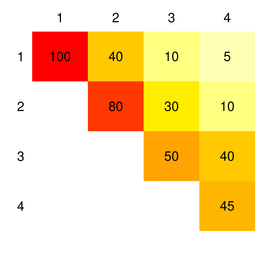
Figure 1: *

Similarity matrix

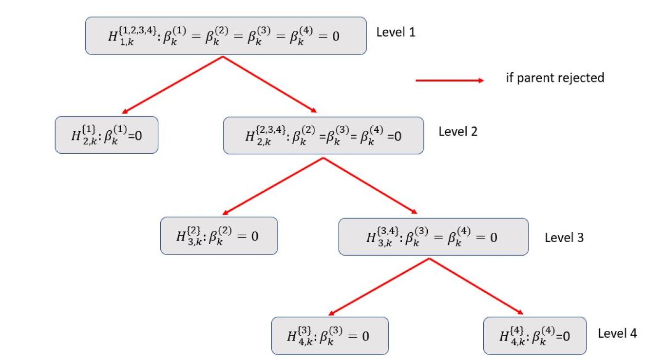
Figure 2: *

Illustration on hierarchical testing procedure

Figure 3: The similarity matrix corresponds to the number of common edges of networks under 4 conditions. Specifically, 40 edges are shared between Conditions 3 and 4, and 4 edges are shared between Conditions 1 and 4. Condition 4 has the fewest edges (45) among all conditions. A $4$-level binary tree (right) is then built according to the network similarity to guide the hierarchical testing procedure.

5.2 Hierarchical Inference

Given the binary tree $\mathcal{D}$ from the previous section, we next describe the hierarchical testing procedure. For ease of notations, we index the $p^{2}$ edge coefficients of a $p$-variate network at condition $m$ as $\beta^{(m)}_{1},\dots,\beta^{(m)}_{p^{2}}$, for $m=1,\dots,M$. Besides the binary tree, $\mathcal{D}$, the algorithm takes in the critical values at each level of the tree, $\{\alpha_{l}\}_{l=1}^{M}$.

Our procedure, summarized in Algorithm 1, is applied separately to each coefficient $\beta_{k},k\in\{1,\dots,p^{2}\}$. At each node of the hierarchy $\mathcal{D}$, we test the global hypothesis that all the edge coefficients corresponding to the experiments indexed by the node are 0; that is, we test $H_{l,k}^{\mathcal{L}}:\beta_{k}^{(m)}=0,m\in\mathcal{L}$ where $\mathcal{L}\in\{\mathcal{L}_{1},\mathcal{L}_{L,l},\mathcal{L}_{R,l}\}$, depending on whether the node is the root of the binary tree, or the left or right child node at level $l$, respectively. Our procedure starts by testing the hypothesis at the root of the tree. If $H_{l,k}^{\mathcal{L}_{1}}$ is rejected, we move down to the next level of the tree and separately test the hypotheses assigned to each of the child nodes. The process continues until we reach a level $m\in\{1,\ldots,M\}$ such that $H_{m,k}^{\mathcal{L}_{R,m}}$ is not rejected.

Consider, for example, testing the edge coefficients for the $M=4$ networks corresponding to the hierarchy defined by the binary tree in Figure 3. Let $Z$ be the $p^{2}\times M$ matrix of rejection indicators. For each edge coefficient $\beta_{k},k\in\{1,\dots,p^{2}\}$, we start from the root of the tree and test $H^{\{1,2,3,4\}}_{1,k}:\beta_{k}^{(1)}=\beta_{k}^{(2)}=\beta_{k}^{(3)}=\beta_{k}^{(4)}=0$. If $H^{\{1,2,3,4\}}_{1,k}$ is rejected, then we move down to the next level and separately test $H^{\{1\}}_{2,k}:\beta_{k}^{(1)}=0$ and $H^{\{2,3,4\}}_{2,k}:\beta_{k}^{(2)}=\beta_{k}^{(3)}=\beta_{k}^{(4)}=0$. If we reject $H^{\{1\}}_{2,k}$ then $Z_{k,1}=1$; otherwise, $Z_{k,1}=0$. We continue this process on the right branch by testing $H^{\{2,3,4\}}_{2,k}$.

Algorithm 1 Hierarchical Testing Procedure for Multi-Experiment Networks

  input: $\mathcal{D}$, $\{\alpha_{l}\}_{l=1}^{M}$;

  initialization: rejection matrix $Z$ ;

  for $k=1,\dots,p^{2}$ do

      root: calculate the $p$-value $P_{k}^{\mathcal{L}_{1}}$ for $H_{1,k}^{\mathcal{L}_{1}}$;

     if $P_{k}^{\mathcal{L}_{1}}\leq\alpha_{1}$ and $M>1$  then

        for $l=2,\dots,M$ do

            left node: calculate the $p$-value $P_{k}^{\mathcal{L}_{L,l}}$ for $H_{l,k}^{\mathcal{L}_{L,l}}$; if $P_{k}^{\mathcal{L}_{L,l}}\leq\alpha_{l}$, set $Z_{k,m}=1$, for $m\in\mathcal{L}_{L,l}$ ;

            right node: calculate the $p$-value $P_{k}^{\mathcal{L}_{R,l}}$ for $H_{m,k}^{\mathcal{L}_{R,l}}$ ; if $P_{k}^{\mathcal{L}_{R,l}}>\alpha_{l}$, stop the loop at level $l$; otherwise, if $l=M$, set $Z_{k,m}=1$ for $m\in\mathcal{L}_{R,l}$;

        end for

     end if

  end for

  return  $Z$

Algorithm 1 can accommodate $p$-values from any valid test of edge coefficients. Here, we use the de-correlated score statistics for testing $\beta^{(m)}_{ij}=0$ [Wang et al., 2020a], defined as

$$S^{(m)}_{ij} =\frac{1}{T_{m}}\int_{0}^{T_{m}}\epsilon^{(m)}_{i}(t)\widetilde{x}_{j}^{(m)}(t)dt,$$

where $\epsilon^{(m)}_{i}(t)=\frac{dN^{(m)}_{i}(t)}{dt}-\lambda^{(m)}_{i}(t)$, and $\widetilde{x}_{j}^{(m)}$ is the de-correlated column, obtained from $x_{j}^{(m)}(t)$ after removing its projection on the other columns, $x^{(m)}_{-j}(t)$. Denoting $\Upsilon^{(m)}_{j}=\frac{1}{T}\int_{0}^{T}\left(\widetilde{x}_{j}^{(m)}(t)\right)^{2}dt$, and $V^{(m)}_{ij}=\sqrt{T}\left(\Upsilon^{(m)}_{j}\right)^{-1/2}S^{(m)}_{ij}$, $V^{(m)}_{ij}\rightarrow_{d}\mathcal{N}(0,1)$. Thus, the global hypothesis at the root, $H_{1,k}^{\mathcal{L}_{1}}$, can be tested using the test statistic

$$U^{\mathrm{total}}_{ij}=\sum\limits_{m\in\mathcal{L}_{1}}\left(V^{(m)}_{ij}\right)^{2}\rightarrow_{d}\chi^{2}_{M},$$

and the corresponding $p$-value is approximately $\mathbb{P}\left(\chi^{2}_{M}\geq U^{\mathrm{total}}_{ij}\right)$. By construction, such a test is powerful when many $\beta_{ij}^{(m)}\neq 0,m\in\mathcal{L}_{1}$. When, on the contrary, a small number of edge coefficients are nonzero, an alternative and more powerful test can be constructed based on the maximum of $\left(V^{(m)}_{ij}\right)^{2}$; that is,

$$U^{\max}_{ij}=\max_{m\in\mathcal{L}_{1}}\left(V^{(m)}_{ij}\right)^{2}.$$

It follows from the asymptotic distribution of $V^{(m)}_{ij}$ [e.g., Embrechts et al., 1997, pp 156] that as $M\rightarrow\infty$,

$$a_{M}(U^{\max}_{ij}-b_{M})\rightarrow_{d}G,$$

where $a_{M}=1/2$, $b_{M}=2(\ln M+(d-1)\ln\ln M-\ln\Gamma(d))$ and $G$ follows Gumble distribution.

We next introduce an ideal binary tree for inference, which we refer to the oracle tree. In addition to being built based on the oracle network similarity distance, the main difference between this tree and the empirical tree introduced earlier is that the oracle tree is edge-specific. Specifically, for each of the $p^{2}$ edge coefficients to be tested, the binary tree is built using the similarity distance $d^{(k)}(s,t)=|\beta^{(s)}_{k}-\beta^{(t)}_{k}|$. Thus, zero coefficients are always places at the bottom right of the oracle tree. Clearly, this information (and the oracle tree) is hardly available in practice, and is primarily used as a theoretical device in the next result to establish the control of the family-wise error rate (FWER) under arbitrary dependencies between tests.

Theorem 3.

The hierarchical testing procedure in Algorithm 1 with the oracle binary tree controls the FWER for testing all $p^{2}M$ hypotheses at level $\alpha$ when using the critical value

$$\alpha_{l}=\frac{\alpha}{p^{2}}\frac{M-l+1}{M},\quad l=1,\dots,M.$$

For a single experiment, the $\alpha_{l}$ in Theorem 3 amounts to the usual Bonferroni correction. However, in multi-experiment settings, our procedure uses a less stringent critical value than that Bonferroni correction, as $\frac{\alpha}{p^{2}}\frac{M-l+1}{M}<\frac{\alpha}{Mp^{2}}$ for $l<M$. This makes the procedure more powerful in practice, particularly for sparse networks when most tests are carried out at shallow levels of the tree. Unlike existing hierarchical testing methods [e.g. Yekutieli, 2008, Lynch and Guo, 2016] that control the error rate all the tests involved, our procedure controls the error among the hypothesis associated with the leaves of the tree—this is exactly the set of hypotheses of interest in our multi-experiment network inference problem. Lastly, the procedure can also be applied to any subset, $\mathcal{J}$, of the $p^{2}$ edges by taking $\alpha_{l}=\frac{\alpha}{|\mathcal{J}|}\frac{M-l+1}{M}$ in Theorem 3.

Theorem 3 assumes an oracle binary tree, which is unavailable in practice. In such cases, the data-driven similarity in Section 3 can be used to create an empirical binary tree. The next result shows that, for large and sparse networks, our procedure is robust to potential misspecification of the binary tree.

Theorem 4.

The testing procedure in Algorithm 1 with a binary tree built based on arbitrary network similarity controls FWER at level $\alpha\left(1+\frac{d^{*}M(M-1)}{2p}\right)$ when using critical values

$$\alpha_{l}=\frac{\alpha}{p^{2}}\frac{M-l+1}{M},\quad l=1,\dots,M.$$

Theorem 4 implies that when $d^{*}M(M-1)=o(p)$, FWER is controlled at $\alpha\left(1+o(1)\right)$ regardless of the hierarchy used in the testing procedure. This condition is met when the underlying network is sparse, i.e, $d^{*}=o(p)$, and the number of experiment is not too large, i.e., $M=o(\sqrt{p})$. Our proof in Appendix B indicates that the unique construction of the binary tree, where the left child node is always a leaf, is critical for achieving this robustness.

6 Simulations

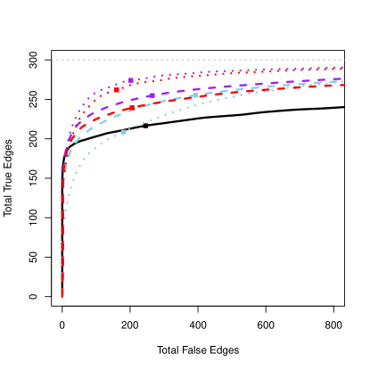
(a)

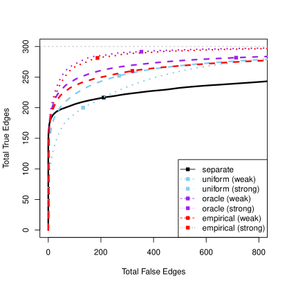
(b)

Figure 4: Edge selection performance of the proposed joint estimation method in a simulation study focused on inferring edges in 3 networks of linear Hawkes processes. The plots show average number of true positive and false positive edges, over 100 simulation runs, for the joint estimation method with different choices of weights, compared to separate estimation of each network. Weight strategies include oracle, empirical and uniform weights. Solid squares ($\blacksquare$) correspond the choice of tuning parameter using eBIC. (a): Network 2 shares 90% edges with Network 1 and 10% with Network 3 as in Figure 11. (b): Network 2 is the same as Network 1.

6.1 Performance of Joint Estimation

We first investigate the edge selection performance of the proposed joint estimation procedure. We consider $M=3$ networks of $p=100$ linear Hawkes processes. The networks are designed such that Networks 1 and 2 are much more similar to each other than Network 3. Specifically, Network 1 and 3 consists of 20 5-node circles and stars, respectively, and Network 2 is a mix of 18 circles and 2 stars (see Figure 11 in Appendix C). The edge coefficients of circles and stars are set to be 0.3 and 0.6, respectively. The background intensity is set to 0.2 for all nodes in all experiments. The transfer kernel function is chosen to be $\exp(-t)$, for all nodes in all experiments. This setting satisfies our assumptions of a stationary Hawkes process under each experiment. The time periods, $T_{m}$, are 200, 500, 300 for $m=1,2,3$, respectively.

We consider three weight choices: informative weights based on the true networks (oracle) and the cross-correlation method of Section 3 (empirical), and uniform weights that treat all networks equally. We consider weak and strong fusion penalties—$\rho_{2}=\rho_{1}$ and $\rho_{2}=10\rho_{1}$—and compare them to separate network estimation.

Simulation results are summarized in Figure 4. It can be seen that our proposed empirical weights perform very similar to the oracle weights and both versions of informative weights greatly improve the edge selection performance compared with the uniform weights. Moreover, while the advantages of the informative weights are clear, even uniform weights can perform better than method that estimates each network separately; however, with uniform weights, the performance of the method is sensitive to the choice of the tuning parameter for the fusion penalty. The benefit of our estimation procedure depends on the similarity between networks. For example, when we alter Network 2 to be the same as Network 1, we observe greater advantages of our method compared to estimating each network separately or using the uniform weights (Figure 4(b)). Additional simulation results in Appendix C (Figure 13) indicate that the performance of our joint estimation procedure improves with increasing number of experiments, if the additional experiments are similar to some of the existed ones.

6.2 Performance of Hierarchical Inference

Next, to evaluate the performance of the hierarchical testing procedure, we consider $M=1,5,10,20,30,50$ experiments where the first $M-1$ networks are the same as Network 1 in the previous subsection and the $M$th network is the same as Network 3. We compare our proposed procedure with Bonferroni correction in terms of power, control of FWER, and false discovery rate (FDR). We run our procedure using the oracle and empirical binary trees. As in Figure 4, we observe similar performances using both types of weights. The results in Figure 5 indicate that our hierarchical inference procedure controls the FWER and offers greatly improved power compared with the non-hierarchical method; this improvement becomes especially noticeable as the number of experiments, $M$, increases. Figure 12 in Appendix C also indicates that our method continues to control the FWER with misspecified networks similarity and gives improved power; however, the improvement is less noticeable when the hierarchy is poorly constructed.

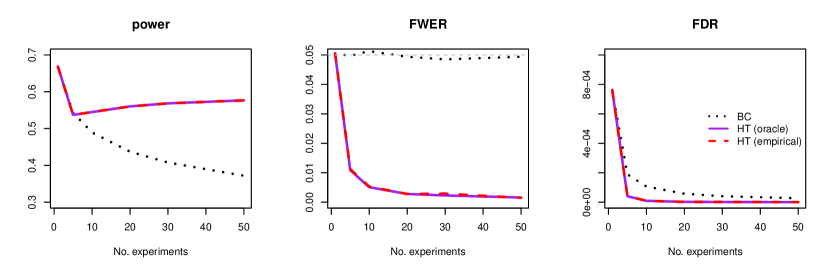
Figure 5: Power, FWER and false discovery rate (FDR) for Bonferroni correction and the proposed hierarchical testing procedure using the oracle and empirical binary trees over 1000 simulation runs. The FWER is controlled at $\alpha=0.05$ (gray dash line).

7 Application

We consider the task of learning the functional connectivity network among a population of neurons, using the spike train data from Bolding and Franks [2018]. In this experiment, spike times are recorded at 30 kHz on a region of the mice olfactory bulb (OB), while a laser pulse is applied directly on the OB cells of the subject mouse. The laser pulse is applied at increasing intensities at 8 levels from 0 to 50 ($mW/mm^{2}$). The laser pulse at each intensity level lasts 10 seconds and is repeated 10 times on the same set of neuron cells of the subject mouse.

While a total of 80 laser stimuli were applied on neurons of multiple mice, for illustration purposes, we consider the spike train data collected at three stimuli at 0, 10 and 20 $mW/mm^{2}$ in a single mouse with the most neurons detected in OB ($p=25$ neurons). Since one laser pulse spans 10 seconds and the spike train data is recorded at 30 kHz, there are 300,000 time points per stimulus. We apply our joint estimation procedure using data under the three stimuli and evaluate the uncertainty of estimates using the hierarchical testing procedure.

Figure 6 illustrates the estimated connectivity coefficients that are specific to each laser condition in a graph representation, where each node represents a neuron and a directed edge indicates a non-zero estimated connectivity coefficient. More edges are observed when laser is applied (32 under 10 $mW/mm^{2}$ and 39 under 20 $mW/mm^{2}$ versus 27 under no laser). Both positive and negative edges are found in all conditions, corroborating the neuroscience hypothesis that both excitatory and inhibitory synapses facilitate maintaining stimulus specificity across odorant concentrations [Bolding and Franks, 2018]. Additionally, we find more common edges in the two laser conditions. Specifically, there are 17 edges (in blue) uniquely shared in the laser conditions compared to 4 edges (in red) shared in all conditions. To assess whether this difference is statistically significant, we generated randomly-connected networks with the same degree distributions at each of the three conditions and compared the observed difference to the distribution of the number of edges uniquely shared in the laser condition. This network permutation test indicates that the observed difference is unlikely under randomly generated networks ($p$-value $<1e-5$). This finding agrees with the observation by neuroscientists that the OB response is sensitive to the intensity level of the external stimuli [Bolding and Franks, 2018].

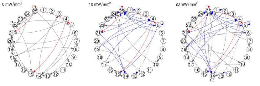
Figure 6: Estimated functional connectivities among neuronal populations using the spike train data from Bolding and Franks [2018]. Common edges across all experiments are in red. Edges shared only under laser conditions are in blue. Statistically significant edges, controlling FWER at $\alpha=0.05$ are shown in dashed lines. Edges that are unique to each condition are in gray.

8 Discussion

In this paper, we developed a joint estimation procedure for networks of high-dimensional Hawkes processes under multiple experiments. The optimization problem corresponding to our proposed estimation procedure is solved using a smoothing proximal gradient descent algorithm [Chen and Chen, 2008]. Although the algorithm works well for linear models, it empirically shows slow and unstable behavior with non-linear Hawkes models. Since non-linear link functions are often used when analyzing spike train data [Paninski et al., 2007, Pillow et al., 2008], developing more computationally-efficient and stable algorithms for the non-linear models would be a potential direction of future research.

Our proposed hierarchical testing procedure improves the testing power by taking advantage of the multi-experiment structure, while controlling the family-wise error rate. Given large-scale networks, a testing procedure that instead controls the FDR [e.g. Benjamini and Hochberg, 1995] may offer additional power. Bogomolov et al. [2020] recently proposed a multiple testing adjustment procedure that controls the FDR by using the tree structure of the tests. While improving the power, the method requires a bottom-up $p$-value calculation, where the upper-level $p$-values needs to be a specific combination of those from the lower levels. Since all the hypotheses on the leaves need to be tested at beginning, such a procedure would be computationally intensive, particularly when the number of tests is large. It is thus desirable to develop a procedure that allows $p$-values flexibly calculated on each node of the tree. For example, a procedure that allows a top-down $p$-value calculation avoids intensive computation in calculating $p$-values over all the leaves, which becomes particularly important in sparse networks, when most leaf-hypotheses are null. Moreover, the existing literature [e.g. Li and Barber, 2019, Bogomolov et al., 2020] that control FDR for structured tests often require the structure to be correctly identified. Given that such structural information is not always available or may not be accurately estimated, developing FDR controlling procedures that are robust to the structure misspecification would be another direction of future research.

Theorem 4 shows that, for large and sparse networks, our proposed hierarchical testing procedure is robust to potential misspecification of the hierarchical structure defined based on the proposed similarity in (11). Nonetheless, consistent estimation of similarities between networks may still be of interest. In particular, such an estimate could, for instance, facilitate the development of hierarchical FDR controlling procedures discussed above. A key requirement for developing consistent estimates of similarities between connectivity networks based on cross-covariances is to develop a measures of similarity that is order-preserving; that is, the order of the similarity based on cross-covariances is the same as that given by the oracle similarity based on the (unknown) connectivity network. One such measure of similarity can be defined based on the connected components of the networks. A connected component is a set of nodes that are connected by paths in an undirected graph. In the setting of our problem, the edges of this undirected graph are given by $\mathcal{E}^{u}=\left\{(i,j):|\beta_{ij}|\neq 0,1\leq i,j\leq p\right\}$. Let $\{\mathcal{C}^{(m)}_{l}\}_{l=1}^{L^{(m)}}$ and $\{\mathcal{C}^{(m^{\prime})}_{l}\}_{l=1}^{L^{(m^{\prime})}}$ denote the connected components of two $p$-variate networks in conditions $m$ and $m^{\prime}$. The connected-component similarity can be defined as

$$d^{cc}\left(\{\mathcal{C}^{(m)}_{l}\}_{l=1}^{L^{(m)}},\{\mathcal{C}^{(m^{\prime})}_{l}\}_{l=1}^{L^{(m^{\prime})}}\right)=\sum_{l,l^{\prime}}r_{l,l^{\prime}}\left\{\log(r_{l,l^{\prime}}/p_{l})+\log(r_{l,l^{\prime}}/q_{l^{\prime}})\right\},$$ (17)

where $p_{l}=\big{\lVert}\mathcal{C}^{(m)}_{l}\big{\rVert}/p$, $q_{l^{\prime}}=\big{\lVert}\mathcal{C}^{(m^{\prime})}_{l}\big{\rVert}/p$ and $r_{l,l^{\prime}}=\big{\lVert}\mathcal{C}^{(m)}_{l}\cap\mathcal{C}^{(m^{\prime})}_{l^{\prime}}\big{\rVert}/p$. This measure, which is also known as variation of information, is often used to compare the similarity between two clusterings [Meila, 2003].

While the true connected components are unknown in practice, they can be consistently estimated. In particular, we can obtain estimates $\{\widehat{\mathcal{C}}^{(m)}_{l}\}_{l=1}^{\hat{L}^{(m)}}$ from undirected graphs corresponding to the nonzero values of thresholded empirical cross-covariances (with thresholding at $\kappa$) as $\widehat{\mathcal{E}}^{u}(\kappa)=\left\{(i,j):\big{|}\widehat{V}_{ij}\big{|}>\kappa,1\leq i,j\leq p\right\}$. Chen [2016] has shown that the connected components of the true network can be consistently identified using the empirical cross-covariances—i.e., $\mathbb{P}\left(\{\mathcal{C}^{(m)}_{l}\}_{l=1}^{L}=\{\widehat{\mathcal{C}}^{(m)}_{l}\}_{l=1}^{\hat{L}^{(m)}}\right)\rightarrow 1$ as $T^{(m)}\rightarrow\infty$ with $\kappa=o\left(\left(T^{(m)}\right)^{-1/5}\right)$. Thus, as a natural estimator of $d^{cc}\left(\{\mathcal{C}^{(m)}_{l}\}_{l=1}^{L^{(m)}},\{\mathcal{C}^{(m^{\prime})}_{l}\}_{l=1}^{L^{(m^{\prime})}}\right)$, $d^{cc}\left(\{\widehat{\mathcal{C}}^{(m)}_{l}\}_{l=1}^{\widehat{L}^{(m)}},\{\widehat{\mathcal{C}}^{(m^{\prime})}_{l}\}_{l=1}^{\widehat{L}^{(m^{\prime})}}\right)$, based on the empirical cross-covariances, consistently represent the similarity in the connected components of the true networks, thus it is order-preserving. However, the effectiveness of a similarity measure based on connected-components depends on the structure of the underlying networks. For instance, while the networks of circles and stars in Figure 11 are quite different, their connected-component structures are identical. As a result, similarity weights and dendrograms defined based on connected component may not be informative in this case. Developing more effective order-preserving network similarity measures is thus an important area of future research.

Appendix A The Smoothing Gradient Descent Algorithm

Our estimator in (7) is solved using the smoothing proximal gradient descent algorithm [Chen et al., 2012]. The algorithm replaces the non-smooth fusion penalty by a smoothing approximation thus makes the original problem easier to solve using the fast iterative shrinkage thresholding algorithm [Beck and Teboulle, 2009]. In the follows, we specify the algorithm to the cases of linear and non-linear Hawkes processes.

Let $I_{0}=\begin{pmatrix}0&0\\ 0&I_{p}\end{pmatrix}\in\mathbb{R}^{(p+1)\times(p+1)}$ and $I_{p}$ is the identity matrix. Then the sparse penalty is written as

$$\lambda_{1}\sum_{m=1}^{M}\lVert\bm{\beta}^{(m)}_{i}\rVert_{1}=\lVert\Lambda\bm{\theta}_{i}\rVert_{1},$$

where $\Lambda=\lambda_{1}I_{M}\otimes I_{0}$ and $I_{M}\in\mathbb{R}^{M\times M}$ is an identity matrix.

Let $d_{m,m^{\prime}}=w_{m,m^{\prime}}(\bm{e}^{\top}_{m}-\bm{e}^{\top}_{m^{\prime}})\otimes I_{0}\in\mathbb{R}^{(p+1)\times(p+1)M}$, where $\bm{e}_{m}$ is canonical basis in $\mathbb{R}^{M}$. Let $D=\begin{pmatrix}d_{1,2}\\ \dots\\ d_{m,m^{\prime}}\\ \dots\\ d_{M-1,M}\end{pmatrix}\in\mathbb{R}^{{M\choose 2}(p+1)\times M(p+1)}$. Define $C=\lambda_{2}D$. Then the fusion penalty becomes

$$\lambda_{2}\sum_{1\leq m<m^{\prime}\leq M}w_{m,m^{\prime}}\left\lVert\bm{\beta}^{(m)}_{i}-\bm{\beta}^{(m^{\prime})}_{i}\right\rVert_{1}=\left\lVert C\bm{\theta}\right\rVert_{1}.$$ (18)

Thus, the penalty in (8) can be written as

$$\mathcal{P}(\bm{\theta}_{i}) =\lVert\Lambda\bm{\theta}_{i}\rVert_{1}+\lVert C\bm{\theta}_{i}\rVert_{1},$$ (19)

where the fusion penalty can be written using its dual norm as

$$\left\lVert C\bm{\theta}_{i}\right\rVert_{1}=\max_{\lVert\bm{\alpha}_{i}\rVert_{\infty}\leq 1}\bm{\alpha}_{i}^{T}C\bm{\theta}_{i}.$$ (20)

Next, let $f_{u}(\bm{\theta}_{i})$ be a smoothing approximation function such that

$$f_{u}(\bm{\theta}_{i})=\left\lVert C\bm{\theta}_{i}\right\rVert_{1}-u\frac{1}{2}\left\lVert\bm{\alpha}_{i}\right\rVert_{2}^{2}=\max_{\lVert\bm{\alpha}_{i}\rVert_{\infty}\leq 1}\bm{\alpha}_{i}^{T}C\bm{\theta}_{i}-u\frac{1}{2}\lVert\bm{\alpha}_{i}\rVert_{2}^{2},$$ (21)

where $u>0$ is a smoothness parameter that controls the level of approximation to the fusion penalty. For example, if we take $u=\frac{4\epsilon}{M(M-1)}$, then the approximation error is up to $\epsilon$. Chen et al. [2012] shows that $f_{u}(\bm{\theta}_{i})$ is convex and continuous differentiable where

$$\nabla f_{u}(\bm{\theta}_{i})=C^{T}\bm{\alpha}_{i}^{*}.$$ (22)

Here $\bm{\alpha}_{i}^{*}=S(\frac{C\bm{\theta}_{i}}{u})$ and $S(\bm{z})$ is a coordinate-wise projection operator that projects each entry of $\bm{z}$ to the $\ell_{\infty}$-ball — i.e.,

$$S(z)=\begin{cases}-1&z<1\\ z&z\in[-1,1]\\ 1&z>1\\ \end{cases}.$$

Substituting the fusion penalty with (21), solving (7) becomes to solve

$$\widehat{\bm{\theta}}_{i} =\arg\min_{\bm{\theta}_{i}\in\mathbb{R}^{(p+1)M}}\left\{h(\bm{\theta}_{i})+\lVert\Lambda_{i}\bm{\theta}_{i}\rVert_{1}\right\}\quad i=1,\dots,p,$$ (23)

where

$$h(\bm{\theta}_{i})=\frac{1}{T}\sum_{m=1}^{M}\int_{0}^{T_{m}}\ell\left(dN^{(m)}_{i}(t),f_{\bm{\theta}^{(m)}_{i}}(\bm{x}^{(m)}(t))\right)+f_{u}(\bm{\theta}_{i}),$$

and $T=\sum_{m=1}^{M}T_{m}$. Problem (23) can be solved using the fast iterative shrinkage thresholding (FISTA) algorithm [Beck and Teboulle, 2009]. The FISTA algorithm is a first-order optimization method [Beck, 2017] that requires evaluating the first derivative of $h(\bm{\theta}_{i})$, and a Lipschitz constant $L$ calculated as a upper bound on the spectral radius of the second derivative of $h(\bm{\theta}_{i})$.

Next, we specify the first derivative of $h(\bm{\theta}_{i})$ and the Lipschitz constant $L$ for the linear Hawkes model with least square loss — i.e., $\ell(a,b)=(a-b)^{2}$.

Let $\gamma^{(m)}_{ij}=\int_{0}^{T_{m}}x^{(m)}_{j}(t)dN^{(m)}_{i}(t)$, $\gamma^{(m)}_{i0}=\int_{0}^{T_{m}}dN^{(m)}_{i}(t)$, and $\bm{\gamma}^{(m)}_{i}=\left(\gamma^{(m)}_{i0},\gamma^{(m)}_{i1},\dots,\gamma^{(m)}_{ip}\right)^{\top}\in\mathbb{R}^{p+1}$. Denote $\textrm{Q}^{(m)}=\int_{0}^{T_{m}}\begin{pmatrix}1\\ \bm{x}^{(m)}(t)\end{pmatrix}\begin{pmatrix}1&\left(\bm{x}^{(m)}(t)\right)^{\top}\end{pmatrix}dt$. Let $\textrm{Q}=\begin{pmatrix}\textrm{Q}^{(1)}&&&\\ &\textrm{Q}^{(2)}&&\\ &&\dots&\\ &&&\textrm{Q}^{(M)}\end{pmatrix},$ and $\bm{\gamma}=\left(\left(\bm{\gamma}^{(1)}\right)^{\top},\dots,\left(\bm{\gamma}^{(m)}\right)^{\top}\right)^{\top}$, where $\textrm{Q}^{(m)}$ and $\bm{\gamma}^{(m)}_{i}$ can be pre-calculated given data and the pre-specified transfer kernel function. With these notations,

$$\ \sum_{m=1}^{M}\int_{0}^{T_{m}}\ell\left(dN^{(m)}_{i}(t),f_{\bm{\theta}^{(m)}_{i}}(\bm{x}^{(m)}(t))\right)=\bm{\theta}_{i}^{\top}\textrm{Q}\bm{\theta}_{i}-2\bm{\theta}_{i}^{\top}\bm{\gamma}_{i}+\sum_{m=1}^{M}\int_{0}^{T_{m}}\left(dN^{(m)}_{i}(t)\right)^{2},$$ (24)

which leads to

$$\nabla h(\bm{\theta}_{i}) =\frac{1}{T}\textrm{Q}\bm{\theta}_{i}-\frac{1}{T}\bm{\gamma}+C^{T}\bm{\alpha}^{*}.$$ (25)

In addition, $\nabla^{2}h(\bm{\theta}_{i})\preccurlyeq\frac{1}{T}\textrm{Q}+\frac{C^{T}C}{u}$, which leads us to choose $L=\Lambda_{\max}\{\frac{1}{T}\textrm{Q}+\frac{C^{T}C}{u}\}$. Notice that both $\nabla h(\bm{\theta}_{i})$ and $L$ can be pre-calculated and stored in memory when implementing the FISTA algorithm. This feature makes the computation scalable to large size data collected over a long time range. The edge selection performance using this algorithm for the linear Hawkes process is illustrated in Figure 4 in Section 6.

Next, we specific $\nabla h(\bm{\theta}_{i})$ and $L$ for non-linear Hawkes model with the exponential-link function, $g_{i}(\cdot)=\exp(\cdot)$ and the negative log likelihood loss — i.e., $\ell\left(a,b\right)=-a\log(b)+b$.

With some algebra,

$$\nabla h(\bm{\theta}_{i}) =\frac{1}{T}\widetilde{Q}_{i}-\frac{1}{T}\bm{\gamma}+C^{T}\bm{\alpha}^{*},$$ (26)

where

$$\widetilde{Q}_{i}=\begin{pmatrix}\widetilde{Q}^{(1)}_{i}&&&\\ &\widetilde{Q}^{(2)}_{i}&&\\ &&\dots&\\ &&&\widetilde{Q}^{(M)}_{i}\end{pmatrix}$$ ,

$$\widetilde{Q}^{(m)}_{i}=\int_{0}^{T_{m}}\bm{x}^{(m)}(t)\exp\left(\begin{pmatrix}1&\left(\bm{x}^{(m)}(t)\right)^{\top}\end{pmatrix}\bm{\theta}^{(m)}_{i}\right)dt ,\quad m\in\{1,\dots,M\}.$$

Unlike the linear model, $\nabla h(\bm{\theta}_{i})$ depends on the unknown value of the parameter. Therefore, we need to evaluate $\nabla h(\bm{\theta})$ at each step in the FISTA algorithm, which slows down the algorithm given observations over long time periods.

Notice that $\nabla^{2}h(\bm{\theta}_{i})\preccurlyeq\max_{1\leq m\leq M}\left\{\exp\left(\begin{pmatrix}1&\left(\bm{x}^{(m)}(t)\right)^{\top}\end{pmatrix}\bm{\theta}^{(m)}_{i}\right)\right\}\frac{1}{T}\textrm{Q}+\frac{C^{T}C}{u}$ , which leads to a choice of $L$. However, we find that this choice of $L$ leads to slow convergence or even divergence when $\frac{C^{T}C}{u}$ is large — e.g., with large $\lambda_{2}$ and small $u$. To mitigate this issue, we use a general convex programming solver as an alternative — e.g., CVXR in R [Fu et al., 2020] —when the algorithm meets convergence problem. The edge selection performance using the algorithm for the non-linear Hawkes process is illustrated in Figure 7.

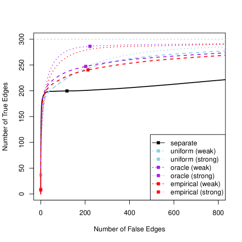
Figure 7: Edge selection performance of the proposed joint estimation method in a simulation study focused on inferring edges in 3 networks of generalized Hawkes processes with exponential link function. The plots show average number of true positive and false positive edges, over 100 simulation runs, for the joint estimation method with different choices of weights, compared to separate estimation of each network. Weight strategies include oracle, empirical and uniform weights. Solid squares ($\blacksquare$) correspond the choice of tuning parameter using eBIC.

We summarize the computational steps described above in Algorithm 2. We note that when the number of experiments, $M$, is large, $u$ becomes very small (proportional to $O(1/M^{2})$), which may lead to very large $L$. In that case, the algorithm may converge slowly, because the step-size, $1/L$, becomes very small.

Algorithm 2 Smoothing Proximal Gradient Descent for Generalized Hawkes Process

  for $i=1,\dots,p$ do

     Input: $\{N^{(m)}_{i}\}_{m=1}^{M}$, $C$, $\Lambda$, $\bm{\theta}_{i}^{0}$, $L$, desired accuracy $\epsilon$

     Initialization: set $u=\frac{4\epsilon}{(M-1)M}$, $\delta^{0}=1$, $\bm{w}^{0}=\bm{\theta}_{i}^{0}$

     repeat

        1: Compute $\nabla h(\bm{w}^{t})$ ;

        2: Solve the proximal operator associated with $\ell_{1}$-norm penalty:

$$\bm{\theta}_{i}^{t+1} =\arg\min_{\bm{\theta}_{i}}\left(h(\bm{w}^{t})+(\bm{\theta}_{i}-\bm{w}^{t})^{\top}\nabla h(\bm{w}^{t})+\frac{L}{2}\lVert\bm{\theta}_{i}-\bm{w}^{t}\rVert_{2}^{2}+\lambda_{1}\lVert\bm{\theta}_{i}\rVert_{1}\right)$$

$$=\arg\min_{\bm{\theta}_{i}}\frac{1}{2}\lVert\bm{\theta}_{i}-\bm{v}\rVert_{2}^{2}+\frac{\lambda_{1}}{2}\lVert\bm{\theta}_{i}\rVert_{1}$$

$$=sign(\bm{v})\max\left(0,|\bm{v}|-\frac{diag(\Lambda)}{L}\right),$$

where $\bm{v}=\bm{w}^{t}-\frac{1}{L}\nabla h(\bm{w}^{t})$.

        3: $\delta^{t+1}=\frac{2}{t+3}$ ;

        4: $\bm{w}^{t+1}=\bm{\theta}_{i}^{t+1}+\frac{1-\delta^{t}}{\delta^{t}}\delta^{t+1}(\bm{\theta}_{i}^{t+1}-\bm{\theta}_{i}^{t})$

     until convergence of $\bm{\theta}_{i}^{t}$ ;

  end for

Appendix B Proofs

For ease of presentation, we stack the data from $M$ experiments and re-label the time index over $[0,T]$ where $T=\sum_{m=1}^{M}T_{m}$. In particular, we denote $N_{i}(t)=N_{i}^{(m)}(t-\sum_{l=0}^{m-1}T_{l})$ if $t\in\big{(}\sum_{l=0}^{m-1}T_{l},\sum_{l=0}^{m}T_{l}\big{]}$ for $1\leq m\leq M$, where $T_{0}=0$. Then, denote

$$\bm{x}(t)=\begin{pmatrix}\mathbf{1}(T_{0}<t\leq T_{1})\\ \bm{x}^{(1)}(t)\mathbf{1}(T_{0}<t\leq T_{1})\\ \dots\\ \mathbf{1}(\sum_{m=0}^{M-1}T_{m}<t\leq T)\\ \bm{x}^{(M)}(t)\mathbf{1}(\sum_{m=0}^{M-1}T_{m}<t\leq T)\end{pmatrix},\quad\bm{\theta}_{i}=\begin{pmatrix}\bm{\theta}_{i}^{(1)}\\ \dots\\ \bm{\theta}_{i}^{(M)}\end{pmatrix},\quad\lambda_{i}(t)=g_{i}(\bm{x}^{\top}(t)\bm{\theta}_{i}).$$

With these notations,

$$\sum_{m=1}^{M}\int_{0}^{T_{m}}\ell\left(dN^{(m)}_{i}(t),f_{\bm{\theta}^{(m)}_{i}}(\bm{x}^{(m)}(t))\right)=\int_{0}^{T}\ell\left(dN_{i}(t),f_{\bm{\theta}_{i}}(\bm{x}(t))\right).$$

In addition, denote $\ell(t;\bm{\theta}_{i})=\ell\left(dN_{i}(t),f_{\bm{\theta}_{i}}(\bm{x}(t))\right)$.

Because optimization problem (7) can be solved separately for each component process, in the following we illustrate the estimation consistency using the estimator (7) for one component process. Moreover, for ease of notation, we drop the subscript $i$; that is, we use $\bm{x}(t)$ for $\bm{x}_{i}(t)$, $\bm{\theta}$ for $\bm{\theta}_{i}$, $dN(t)$ for $dN_{i}(t)$, $g(\cdot)$ for $g_{i}(\cdot)$ and $\lambda(t)$ for $\lambda_{i}(t)$, $S$ for $S_{i}$, $\widetilde{S}$ for $\widetilde{S}_{i}$ and $A$ for $A_{i}$.

Next, we state two lemmas needed for the proofs of Theorems 1 and 2.

Lemma 1 (van de Geer [1995]).

Suppose there exists $\lambda_{\max}$ such that $\lambda(t)\leq\lambda_{\max}$ where $\lambda(t)$ is the intensity function of Hawkes process defined in (1). Let $H(t)$ be a bounded function that is $\mathcal{H}_{t}$-predictable. Then, for any $\epsilon>0$,

$$\frac{1}{T}\int_{0}^{T}H(t)\bigg{\{}\lambda(t)dt-dN(t)\bigg{\}}\leq 4\bigg{\{}\frac{\lambda_{\max}}{2T}\int_{0}^{T}H^{2}(t)dt\bigg{\}}^{1/2}\epsilon^{1/2},$$

with probability at least $1-C\exp(-\epsilon T)$, for some constant $C$.

Lemma 2 (Wang et al. [2020a]).

Suppose the Hawkes process defined in (6) satisfies Assumptions 1– 4. Let $\textrm{Q}=\frac{1}{T}\int_{0}^{T}\begin{pmatrix}1\\ \bm{x}(t)\end{pmatrix}\begin{pmatrix}1&\bm{x}^{\top}(t)\end{pmatrix}dt$, where $\bm{x}(t)$ is defined in (5). Then, there exists $\gamma>0$ such that

$$\Lambda_{\min}\left(\textrm{Q}\right)\geq\gamma>0,$$

with probability at least $1-c_{1}p^{2}T\exp(-c_{2}T^{1/5})$, where constants $c_{1},c_{2}$ depending on the model parameters and the transition kernel.

Proof of Theorem 1:

Let $\Delta=\widehat{\bm{\theta}}-\bm{\theta}$. We linearize $\ell(t;\bm{\theta})$ w.r.t. $\bm{\theta}$ using Taylor expansion:

$$\ell(t;\widehat{\bm{\theta}})-\ell(t;\bm{\theta}) =\left(\nabla\ell(t;\bm{\theta})\right)^{\top}\Delta+\frac{1}{2}\Delta^{\top}\nabla^{2}\ell(t;\bm{\theta})\Delta+o(\lVert\Delta\rVert^{2}_{2}).$$ (27)

Let $R(\bm{\theta})=\left\lVert\Lambda\bm{\theta}\right\rVert_{1}+\left\lVert C\bm{\theta}\right\rVert_{1}$, where $\Lambda$ and $C$ are defined in Appendix A. Taking $\widehat{\bm{\theta}}$ given by (7),

$$\frac{1}{T}\int_{0}^{T}\left\{\ell(t;\widehat{\bm{\theta}})-\ell(t;\bm{\theta})\right\}=\frac{1}{T}\int_{0}^{T}\ell(t;\widehat{\bm{\theta}})-\frac{1}{T}\int_{0}^{T}\ell(t;\bm{\theta})\leq R(\bm{\theta})-R(\widehat{\bm{\theta}}).$$ (28)

Taking (27) in (28),

$$0\leq\Delta^{\top}\left(\frac{1}{2T}\int_{0}^{T}\nabla^{2}\ell(t;\bm{\theta})\right)\Delta\leq-\frac{1}{T}\int_{0}^{T}\left(\nabla\ell(t;\bm{\theta})\right)^{\top}\Delta+R(\bm{\theta})-R(\widehat{\bm{\theta}}).$$ (29)

Let $A=S\cap\widetilde{S}^{c}$. Recalling the definition of $S$ and $\widetilde{S}$ in Section 4, $A$ is the set of indices associated with the coefficients that are nonzero (i.e., in $S$) and have the same values under all conditions (i.e., in $\widetilde{S}^{c}$). Then,

$$R\left(\bm{\theta}\right)-R\left(\widehat{\bm{\theta}}\right) =\rho_{1}\lVert\bm{\theta}\rVert_{1}+\rho_{2}\lVert D\bm{\theta}\rVert_{1}-\rho_{1}\lVert\widehat{\bm{\theta}}\rVert_{1}-\rho_{2}\lVert D\widehat{\bm{\theta}}\rVert_{1}$$

$$=\rho_{1}\lVert\bm{\theta}_{A}\rVert_{1}+\rho_{1}\lVert\bm{\theta}_{S\cap\widetilde{S}}\rVert_{1}-\rho_{1}\lVert\widehat{\bm{\theta}}_{A}\rVert_{1}-\rho_{1}\lVert\widehat{\bm{\theta}}_{S\cap\widetilde{S}}\rVert_{1}-\rho_{1}\lVert\widehat{\bm{\theta}}_{S^{c}}\rVert_{1}$$

$$\quad+\rho_{2}\lVert D\bm{\theta}\rVert_{1}-\rho_{2}\lVert D\widehat{\bm{\theta}}\rVert_{1}$$

$$\leq\rho_{1}\lVert\Delta_{A}\rVert_{1}+\rho_{1}\lVert\Delta_{S\cap\widetilde{S}}\rVert_{1}-\rho_{1}\lVert\Delta_{S^{c}}\rVert_{1}+\rho_{2}\left\lVert D_{.,\widetilde{S}}\Delta_{\widetilde{S}}\right\rVert_{1}-\rho_{2}\left\lVert D_{.,\widetilde{S}^{c}}\Delta_{\widetilde{S}^{c}}\right\rVert_{1}$$

$$=\rho_{1}\lVert\Delta_{S}\rVert_{1}-\rho_{1}\lVert\Delta_{S^{c}}\rVert_{1}+\rho_{2}\left\lVert D_{.,\widetilde{S}}\Delta_{\widetilde{S}}\right\rVert_{1}-\rho_{2}\left\lVert D_{.,\widetilde{S}^{c}}\Delta_{\widetilde{S}^{c}}\right\rVert_{1},$$

where the last equality is because $\lVert\Delta_{S}\rVert_{1}=\lVert\Delta_{A}\rVert_{1}+\lVert\Delta_{S\cap\widetilde{S}}\rVert_{1}$.

In addition,

$$-\frac{1}{T}\int_{0}^{T}\left(\nabla\ell(t;\bm{\theta})\right)^{\top}\Delta\leq\left\lVert-\frac{1}{T}\int_{0}^{T}\nabla\ell(t;\bm{\theta})\right\rVert_{\infty}\lVert\Delta\rVert_{1}.$$

Taking $\rho_{1}=\frac{1}{\sqrt{M}}\rho_{2}=2\left\lVert-\frac{1}{T}\int_{0}^{T}\nabla\ell(t;\bm{\theta})\right\rVert_{\infty}$ , we get

$$\frac{1}{\sqrt{M}}\lVert\Delta_{S^{c}}\rVert_{1}+2\lVert D_{.,\widetilde{S}^{c}}\Delta_{\widetilde{S}^{c}}\rVert_{1}\leq\frac{3}{\sqrt{M}}\lVert\Delta_{S}\rVert_{1}+2\lVert D_{.,\widetilde{S}}\Delta_{\widetilde{S}}\rVert_{1}.$$

Let

$$\mathcal{C}=\left\{\Delta\in R^{M(p+1)}:\frac{1}{\sqrt{M}}\lVert\Delta_{S^{c}}\rVert_{1}+2\lVert D_{.,\widetilde{S}^{c}}\Delta_{\widetilde{S}^{c}}\rVert_{1}\leq\frac{3}{\sqrt{M}}\lVert\Delta_{S}\rVert_{1}+2\lVert D_{.,\widetilde{S}}\Delta_{\widetilde{S}}\rVert_{1}\right\}.$$

By Condition 1, $\forall\Delta\in\mathcal{C}$, there exists $\eta,c,C>0$ such that

$$\min_{\Delta\in\mathcal{C}}\Delta^{\top}\left(\frac{1}{T}\int_{0}^{T}\nabla^{2}\ell(t;\bm{\theta})\right)\Delta\geq\eta\lVert\Delta\rVert^{2}_{2},$$ (30)

with probability at least $1-cp^{2}\sum_{m=1}^{M}T_{m}\exp(-CT_{m}^{1/5})$.

Moreover, letting $\Delta^{(m)}=\widehat{\bm{\theta}}^{(m)}-\bm{\theta}^{(m)}$ and $\Delta^{(m)}_{j}=\widehat{\theta}^{(m)}_{j}-\theta^{(m)}_{j}$,

$$\lVert D_{.,\widetilde{S}}\Delta_{\widetilde{S}}\rVert_{1} =\sum_{\begin{subarray}{c}m\neq m^{\prime}\in\widetilde{S}\end{subarray}}w_{m,m^{\prime}}\left\lVert\Delta_{j}^{(m)}-\Delta_{j}^{(m^{\prime})}\right\rVert_{1}$$

$$\leq\sum_{\begin{subarray}{c}m\neq m^{\prime}\in\widetilde{S}\end{subarray}}w_{m,m^{\prime}}\left(\left\lVert\Delta^{(m)}_{j}\rVert_{1}+\lVert\Delta^{(m^{\prime})}_{j}\right\rVert_{1}\right)$$

$$=\sum_{m\in\widetilde{S}}\sum_{\begin{subarray}{c}m^{\prime}\in\widetilde{S}\\ m^{\prime}\neq m\end{subarray}}w_{m,m^{\prime}}\left\lVert\Delta^{(m)}_{j}\right\rVert_{1}$$

$$\leq\phi_{\widetilde{S}}\left\lVert\Delta_{\widetilde{S}}\right\rVert_{1},$$ (31)

where $\phi_{\widetilde{S}}=\max_{m\in\widetilde{S}}\sum_{m^{\prime}\neq m\in\widetilde{S}}w_{m,m^{\prime}}$. Here, with a little abuse of notation, $m\in\widetilde{S}$ means there exists $j$ such that $(j,m)\in\widetilde{S}$. Because the weights are normalized—i.e., $\sum\limits_{1\leq m\neq m^{\prime}\leq M}w_{m,m^{\prime}}=1$, $\phi_{\widetilde{S}}\leq\max_{1\leq m\leq M}\sum_{1\leq m^{\prime}\neq m\leq M}w_{m,m^{\prime}}\leq 1$.

Next, plugging (30) and (B) into (29),

$$\eta\lVert\Delta\rVert^{2}_{2} \leq 3\frac{\rho_{2}}{\sqrt{M}}\lVert\Delta_{S}\rVert_{1}-\frac{\rho_{2}}{\sqrt{M}}\lVert\Delta_{S^{c}}\rVert_{1}+2\rho_{2}\lVert D_{.,\widetilde{S}}\Delta_{\widetilde{S}}\rVert_{1}-2\rho_{2}\lVert D_{.,\widetilde{S}^{c}}\Delta_{\widetilde{S}^{c}}\rVert_{1}$$

$$\leq 3\frac{\rho_{2}\sqrt{d^{*}M}}{\sqrt{M}}\lVert\Delta_{S}\rVert_{2}+2\rho_{2}\phi_{\widetilde{S}}\sqrt{r^{*}}\lVert\Delta_{\widetilde{S}}\rVert_{2}$$

$$\leq\rho_{2}\left(3\sqrt{d^{*}}+2\phi_{\widetilde{S}}\sqrt{r^{*}}\right)\lVert\Delta\rVert_{2},$$ (32)

where the second inequality follows from $\lVert\Delta_{S}\rVert_{1}\leq\sqrt{|S|}\lVert\Delta_{S}\rVert_{2}$, and $|S|\leq d^{*}M$ , and $\lVert\Delta_{\widetilde{S}}\rVert_{1}\leq\sqrt{|\widetilde{S}|}\lVert\Delta_{\widetilde{S}}\rVert_{2}$ and $|\widetilde{S}|\leq r^{*}$.

Finally, we reach the desired conclusion by plugging $\rho_{2}=2\sqrt{M}\left\lVert-\frac{1}{T}\int_{0}^{T}\nabla\ell(t;\bm{\theta})\right\rVert_{\infty}$ in (32), and by Condition 2, with probability at least $1-c^{\prime}pM\exp(-T^{1/5}M^{-1})$,

$$\left\lVert-\frac{1}{T}\int_{0}^{T}\nabla\ell(t;\bm{\theta})\right\rVert_{\infty}\leq C^{\prime}M^{-1/2}T^{-2/5},$$

where $c^{\prime},C^{\prime}$ are positive constants. ∎

Proof of Corollary 1: We first verify the conditions for the linear Hawkes model with least square loss — i.e., $\ell(a,b)=(a-b)^{2}$. In this case, we have

$$\nabla\ell(t;\bm{\theta}) =2\left(dN(t)-\lambda(t)dt\right)\bm{x}(t).$$

By Lemma 1 and taking the union bound over all entries of $\bm{x}(t)$,

$$\left\lVert\frac{1}{T}\int_{0}^{T}\nabla\ell(t;\bm{\theta})\right\rVert_{\infty}=\left\lVert\frac{1}{T}\int_{0}^{T}2\left(dN(t)-\lambda(t)dt\right)\bm{x}(t)\right\rVert_{\infty}\leq CM^{-1/2}T^{-2/5},$$

with probability at least $1-CpM\exp(-M^{-1}T^{1/5})$. Thus, Condition 2 is satisfied.

In addition,

$$\frac{1}{T}\int_{0}^{T}\nabla^{2}\ell(t;\bm{\theta}) =\frac{1}{T}\int_{0}^{T}\bm{x}(t)\bm{x}^{\top}(t)dt.$$

Thus, Condition 1 is satisfied after applying Lemma 2,

Next, we verify the conditions for the non-linear Hawkes process with the exponential-link function, $g(\cdot)=\exp(\cdot)$ and estimated using the negative log likelihood loss -i.e. $\ell\left(a,b\right)=-a\log(b)+b$. In this case, we have

$$\nabla\ell(t;\bm{\theta}) =\left(dN(t)-\lambda(t)dt\right)\bm{x}(t).$$

Similar to the linear case, Condition 2 is satisfied using Lemma 1.

Under Assumption 2, there exists $\lambda_{\min}$ such that $\lambda^{(m)}(t)\geq\lambda_{\min}>0$

$$\frac{1}{T}\int_{0}^{T}\nabla^{2}\ell(t;\bm{\theta})=\frac{1}{T}\int_{0}^{T}\lambda(t)\bm{x}(t)\bm{x}^{\top}(t)dt\geq\lambda_{\min}\frac{1}{T}\int_{0}^{T}\bm{x}(t)\bm{x}^{\top}(t)dt.$$

Thus, Condition 1 is satisfied following Lemma 2. ∎

Proof of Theorem 2: Recall $S^{(m)}=\{\beta^{(m)}_{ij}:\beta^{(m)}_{ij}\neq 0,1\leq i,j\leq p\}$ and $S^{(m)}_{C}=\{\beta^{(m)}_{ij}:\beta^{(m)}_{ij}=0,1\leq i,j\leq p\}$, $m\in\{1,\dots,M\}$. To establish selection consistency, we need two parts. First, we show that our estimates on the true zero and non-zero coefficients can be separated with high probability; that is, there exists some constant $\Delta>0$ such that for $\beta_{S^{(m)}}\in S^{(m)}$ and $\beta_{S^{(m)}_{C}}\in S^{(m)}_{C}$, $|\widehat{\beta}_{S^{(m)}}-\widehat{\beta}_{S^{(m)}_{C}}|\geq\Delta$ with high probability. By the $\beta$-min condition specified in Assumption 5, we have $\beta^{(m)}_{ij}\in S^{(m)}\geq 2\tau$. Theorem 1 shows that for $m=1,\dots,M$ and $1\leq i,j\leq p$, $|\widehat{\beta}^{(m)}_{ij}-\beta^{(m)}_{ij}|\leq\tau$ with probability at least $1-c_{1}p^{2}M^{2}T\exp(-c_{2}M^{-1}T^{1/5})$. Then, for any $\beta_{S^{(m)}}\in S^{(m)}$ and $\beta_{S^{(m)}_{C}}\in S^{(m)}_{C}$,

$$|\widehat{\beta}_{S^{(m)}}-\widehat{\beta}_{S^{(m)}_{C}}| =|\widehat{\beta}_{S^{(m)}}-\beta_{S^{(m)}}-(\widehat{\beta}_{S^{(m)}_{C}}-\beta_{S^{(m)}_{C}})+\beta_{S^{(m)}}-\beta_{S^{(m)}_{C}}|$$

$$\geq|\beta_{S^{(m)}}-\beta_{S^{(m)}_{C}}|-|\widehat{\beta}_{S^{(m)}}-\beta_{S^{(m)}}|-|\widehat{\beta}_{S^{(m)}_{C}}-\beta_{S^{(m)}_{C}}|$$

$$\geq\beta_{min}-2\tau.$$

This means the estimates on zero and non-zero coefficients can be separated with high probability. Next, we show that the thresholded estimator,

$$\widetilde{\beta}=\widehat{\beta}\mathbf{1}(|\widehat{\beta}|>\tau),$$

correctly identifies $S^{(m)}$ and $S^{(m)}_{C}$.

By Theorem 1, we have $|\widehat{\beta}_{S^{(m)}_{C}}|\leq\tau$, with probability $1-c_{1}p^{2}M^{2}T\exp(-c_{2}T^{1/5})$. Thus,

$$\widetilde{\beta}_{S^{(m)}_{C}}=\widehat{\beta}_{S^{(m)}_{C}}\mathbf{1}(\widehat{\beta}_{S^{(m)}_{C}}>\tau_{S})=0,$$

which means $\widetilde{\beta}$ selects $\beta_{S^{(m)}_{C}}$ into $S^{(m)}_{C}$ with high probability. In addition, since $|\widehat{\beta}_{S^{(m)}}-\beta_{S^{(m)}}|\leq\tau$,

$$|\widehat{\beta}_{S^{(m)}}|\geq|\beta_{S^{(m)}}|-\tau\geq\beta_{min}-\tau>\tau>0.$$

Therefore,

$$\widetilde{\beta}_{S^{(m)}}=\widehat{\beta}_{S^{(m)}}\mathbf{1}(|\widehat{\beta}_{S^{(m)}}|>\tau)=\widehat{\beta}_{S^{(m)}}\neq 0,$$

which means $\widetilde{\beta}_{S^{(m)}}$ selects $\beta_{S^{(m)}}$ into $S^{(m)}$ with high probability.

Combining the two sides, the thresholded estimator $\widetilde{\beta}$ identifies $S^{(m)}$ and $S^{(m)}_{C}$ with high probability, for all $m=1,\dots,M$. ∎

Proof of Theorem 3: We start by introducing the notion of null tree. We call a binary tree or its sub-tree a null tree if the true edge coefficients to be tested on its leaves are all zero. In any binary tree, a given zero coefficient will be associated with either (i) a single leaf associated with that coefficient; or (ii) a multi-leaf null tree, where the coefficient is tested on one of the tree’s leaves. For consistency, we refer to the single leaf in (i) as a single-leaf null tree that has only this coefficient to be tested on its leaf. The level of a null tree, $l$, is the level of its root—i.e., the length of the shortest path between the root of the null tree and the root of the binary tree plus 1. As an illustration, consider a binary tree for testing the coefficients indexed $k$ in $M=4$ experiments—i.e., $\beta_{k}^{(1)},\beta_{k}^{(2)},\beta_{k}^{(3)}$ and $\beta_{k}^{(4)}$. Suppose $\beta_{k}^{(3)}=\beta_{k}^{(4)}=0$. Figure 10 shows two examples of such binary trees. In the tree in Figure 10a, $\beta^{(3)}_{k}$ and $\beta^{(4)}_{k}$ are associated the same two-leaf null tree of level 3, and are also associated with two separate level-4 single-leaf null trees. In the tree in Figure 10b, $\beta^{(3)}_{k}$ is associated with a single-leaf null tree of level 4 and $\beta^{(4)}_{k}$ is associated with a single-leaf null tree of level 3. We call a null tree containing a specific coefficient the largest null tree for that coefficient if it has the highest level. For example, in Figure 10a, the largest null tree for $\beta_{k}^{(4)}$ is the null tree of level 3.

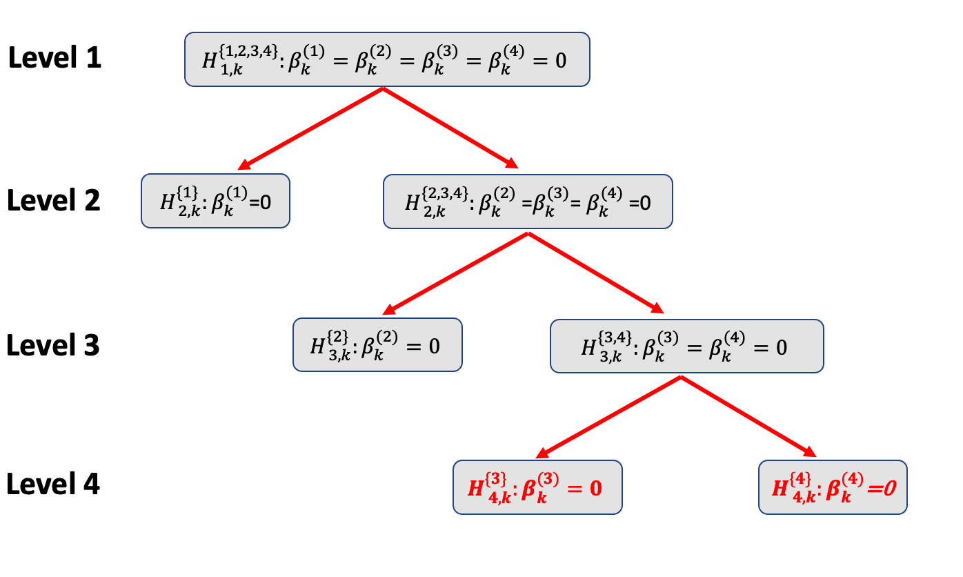
Figure 8: *

a

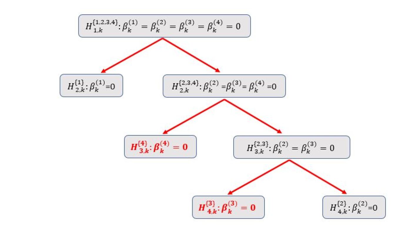
Figure 9: *

b

Figure 10: Two binary trees constructed to test the null hypothesis that $H_{0}:\beta_{k}^{(m)}=0$ for $m=1,2,3,4$, where the true values of $\beta_{k}^{(3)}$ and $\beta_{k}^{(4)}$ are 0; the leaves corresponding to these hypotheses are colored in red. The binary tree in (a) puts both zero coefficients to its bottom right branch; the binary tree in (b) swaps the position of $\beta_{k}^{(2)}$ and $\beta_{k}^{(4)}$.

In the oracle binary tree, there exists a direct relationship between the level of the largest null tree and the total number of zero coefficients to be tested. Consider testing the coefficients indexed $k$—i.e., $\beta^{(m)}_{k},m=1,\dots,M$, and suppose $r$ of these coefficients are 0. Without loss of generality, suppose $\beta^{(m)}_{1}=\dots=\beta^{(m)}_{r}=0$. Now recall that the oracle binary tree puts all zero coefficients to its lower right side. Also, recall that by the construction of the binary tree, there are $M-l+1$ leaves to be tested under a sub-tree of level $l$. Thus, the oracle binary tree puts all $r$ zero coefficients under a sub-tree of level $M-r+1$, meaning that the sub-tree is a level $l=M-r+1$ null tree.

Next, we show that when testing all edge coefficients corresponding to the networks of $p$ nodes in $M$ experiments, our hierarchical testing procedure with the oracle binary tree controls the FWER. Throughout, we refer to the coefficients associated with edges of the networks as ‘nonzero coefficients’ and those associated with non-edges as ‘zero coefficients’.

Recall that we index the connectivity/edge coefficients from $1$ to $p^{2}$. Let $\mathcal{H}_{l,k}$ be the collection of null hypotheses in $H_{k}^{(m)}:\beta^{(m)}_{k}=0$, $m\in\{1,\dots,M\}$, where the level of their corresponding largest null-trees is $l$. Thus, for any binary tree $\mid\mathcal{H}_{l,k}\mid\leq M-l+1$, with the equality holding for the oracle binary tree when there exist at least one zero coefficient. Let $\mathcal{H}_{l}=\left\{\mathcal{H}_{l,k}:\mathcal{H}_{l,k}\neq\emptyset,1\leq k\leq p^{2}\right\}$; that is the collection of non-empty $\mathcal{H}_{l,k}$ sets. Denote $n_{l}=|\mathcal{H}_{l}|$.

Following Step 2 in the hierarchical testing procedure, the root of a level-$l$ sub-tree is rejected with probability not higher than $\alpha_{l}$. In addition, in our hierarchical testing procedure a lower level test is only considered when the test of its parent node is rejected. Therefore,

$$\mathbb{P}\left(\bigcup_{H_{k}^{(m)}\in\mathcal{H}_{l,k}}\text{$H_{k}^{(m)}$ is rejected}\right)\leq\mathbb{P}\big{(}\text{The root of the level-$l$ null tree is rejected}\big{)}\leq\alpha_{l}.$$ (33)

Then, the FWER is controlled as follows.

$$\mathrm{FWER} =\mathbb{P}\left(\bigcup_{l=1}^{M}\bigcup_{\mathcal{H}_{l,k}\in\mathcal{H}_{l}}\bigcup_{H_{k}^{(m)}\in\mathcal{H}_{l,k}}\text{$H_{k}^{(m)}$ is rejected}\right)$$

$$\leq\sum_{l=1}^{M}n_{l}\max\limits_{\mathcal{H}_{l,k}\in\mathcal{H}_{l}}\mathbb{P}\left(\bigcup_{H_{k}^{(m)}\in\mathcal{H}_{l,k}}\text{$H_{k}^{(m)}$ is rejected}\right)$$

$$\leq\sum_{l=1}^{M}n_{l}\alpha_{l},$$

where the first inequality is by Boole’s inequality and the second inequality follows from (33).

Let $\pi_{0}$ be the total number of zero coefficients, which is no greater than the total edges $p^{2}M$. Let $C_{l}$ be the number of leaves under a level $l$ null-tree. Then,

$$\sum_{l=1}^{M}n_{l}C_{l}=\pi_{0}\leq p^{2}M.$$

Now, recall that using an oracle binary tree, $C_{l}=M-l+1$. Thus, taking $\alpha_{l}=\frac{\alpha}{p^{2}}\frac{C_{l}}{M}=\frac{\alpha}{p^{2}}\frac{M-l+1}{M}$,

$$\mathrm{FWER}\leq\sum_{l=1}^{M}n_{l}\frac{\alpha}{p^{2}}\frac{C_{l}}{M}=\frac{\pi_{0}}{p^{2}M}\alpha\leq\alpha.$$

∎

Proof of Theorem 4: Next, we show that given large and sparse networks, the hierarchical testing procedure still controls the FWER for a large number of experiments without the knowledge of the oracle binary tree.

Consider an coefficient indexed $k$ that is not zero in at least 1 experiment. Let $r^{(k)}_{l}$ is the number of level-$l$ null-trees in the binary tree for the coefficient $k$. By the binary tree construction, there is at most one level $l$ null-tree, $r^{(k)}_{l}\leq 1$. (There may be no level-$l$ null tree, in which case, $r^{(k)}_{l}=0$.) Then,

$$\sum_{l=2}^{M}r^{(k)}_{l}(M-l+1)\leq\frac{M(M-1)}{2},$$

The maximum on the right-hand side of the above is achieved when there are $M-1$ zero-coefficients and one non-zero coefficient which is allocated to the bottom right leaf—i.e., the deepest level of the tree.

Let ${n_{1}}/{p^{2}}\leq 1$ indicates the proportion of level-1 null trees — that is, the binary trees on which the coefficients to be tested on all leaves are zero. Taking $\alpha_{l}=\frac{\alpha}{p^{2}}\frac{M-l+1}{M}$,

$$\mathrm{FWER} =n_{1}\alpha_{1}+\sum_{l=2}^{M}n_{l}\alpha_{l}$$

$$=\frac{\alpha}{p^{2}}n_{1}+\frac{\alpha}{p^{2}M}\sum_{l=2}^{M}n_{l}(M-l+1)$$

$$\leq\frac{\alpha}{p^{2}}n_{1}+\frac{\alpha}{p^{2}M}\frac{M(M-1)}{2}(p^{2}-n_{1})$$

Recall that $d^{*}\equiv\max_{1\leq m\leq M,1\leq i\leq p}d_{i}^{(m)}$, where $d^{(m)}_{i}=|S^{(m)}_{i}|$ and $S^{(m)}_{i}=\{j:\beta^{(m)}_{ij}\neq 0,1\leq j\leq p\}$ as defined in Section 4.

Thus, $n_{1}+d^{*}pM\geq p^{2}$, or

$$p^{2}-n_{1}\leq d^{*}pM,$$

which leads to

$$\mathrm{FWER} \leq\frac{\alpha}{p^{2}}n_{1}+\frac{\alpha}{p^{2}}\frac{d^{*}pM(M-1)}{2}.$$

Noting that $n_{1}\leq p^{2}$,

$$\mathrm{FWER} \leq\alpha\left(1+\frac{d^{*}M(M-1)}{2p}\right),$$

as desired. ∎

Appendix C Additional Simulation Results

C.1 Illustration on the simulation setting in Section 6

In Section 6, we consider $M=3$ networks of $p=100$ linear Hawkes processes. The networks are designed such that Networks 1 and 2 are much more similar to each other than Network 3. Specifically, Network 1 and 3 consists of 20 5-node circles and stars, respectively, and Network 2 is a mix of 18 circles and 2 stars (see Figure 11).

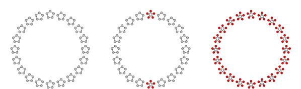
Figure 11: Networks of $p=100$ processes under $M=3$ experiments. Network 1 (left) consists of 20 circles, Network 3 (right) consists of 20 stars, and Network 2 (middle) is a mix of 18 circles and 2 stars.

C.2 Hierarchical testing with incorrect hierarchy

To illustrate how a poorly constructed hierarchy, i.e., binary tree, affects the power of the hierarchical testing procedure, we consider networks of $p=100$ nodes under $M=1,5,10,20,30,50$ experiments. Half of the networks are set to be highly sparse with 0.1% edges. The other half are moderately sparse (referred to as ‘non-sparse’ in the following) with 5% edges. Sparse and non-sparse networks do not share any common edges.

The poorly constructed binary tree we consider assigns the coefficients associated with non-sparse networks to deeper levels of the tree, resulting in nonzero coefficients at the deeper levels of the tree. This is in contrast to the oracle binary tree, which always assigns the zero coefficients to the deeper levels.

As expected, when using a poorly constructed hierarchy, the power of our procedure deteriorates compared with the oracle binary tree. However, the procedure still controls the FWER and is more powerful than Bonferroni correction (see Figure 12).

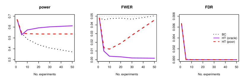
Figure 12: Power, FWER and false discovery rate (FDR) between Bonferroni correction (BC) and the hierarchical testing procedure using the oracle and poorly constructed binary trees (poor). The FWER is controlled at $\alpha=0.05$ (gray dashline).

C.3 Effect of increased number of experiments

In this simulation, we investigate the benefits of the proposed estimation procedure as the number of experiments increases. To this end, we consider networks under four conditions, where the first three conditions are exactly the same as in Figure 11 and the fourth network has the same structure as Network 1. The experiment lengths for the first three condition are the same as those in Section 6.1 and 500 in the fourth condition; that is $T_{m}=200,500,300,500$ for $m=1,2,3,4$, respectively.

The results, summarized in Figure 13, show that the edge selection performance of the proposed methods improves as the number of experiments increases. More specifically, with informative weights (either oracle or empirical), the area under the true positive false positive curves (AUC) improves as the number of experiments increases, whereas the performance deteriorates when noninformative (uniform) weights are used. This finding corroborates our theoretical results, where the error bound becomes tighter when the total experiment length gets larger and more similar conditions are involved.

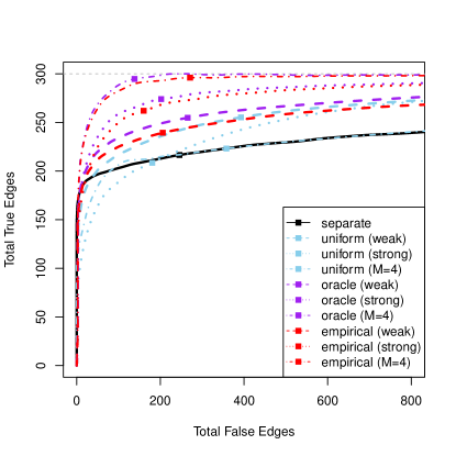
(a)

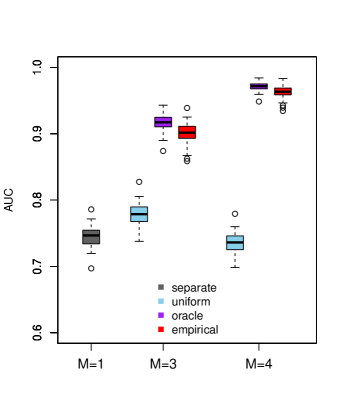
(b)

Figure 13: Edge selection performance of the proposed joint estimation method in a simulation study evaluating the benefit of including extra experiments in the estimation procedure. The main result focused on inferring edges using 3 networks of linear Hawkes processes as in Figure 11. The performance is compared with the result using 4 networks (indicated as $M=4$) with strong fusion penalty where the first three is the same as before and the extra one has the same structure as the first network. The plots in (a) show average number of true positive and false positive edges, over 100 simulation runs, for the joint estimation method with different choices of weights, compared to separate estimation of each network. Weight strategies include oracle, empirical and uniform weights. Solid squares ($\blacksquare$) correspond the choice of tuning parameter using eBIC. The boxplots in (b) show the distribution of the area under the curve (AUC) values corresponding to the edge selection performance in (a) over 100 simulation runs for separate estimation ($M=1$), and the joint estimation with different choices of weights using $M=3$ and $M=4$ experiments. The total numbers of true and false edges are normalized between 0 and 1 when calculating the AUCs.

References

- Babington [2001] P. Babington. Neuroscience (Second ed.). Sunderland, MA: Sinauer Associates, 2 edition, 2001.
- Bacry and Muzy [2016] E. Bacry and J. Muzy. First- and second-order statistics characterization of hawkes processes and non-parametric estimation. IEEE Transactions on Information Theory, 62(4):2184–2202, 2016.
- Bacry et al. [2015] E. Bacry, I. Mastromatteo, and J. Muzy. Hawkes processes in finance. Market Microstructure and Liquidity, 01, 02 2015.
- Basu and Michailidis [2015] S. Basu and G. Michailidis. Regularized estimation in sparse high-dimensional time series models. Ann. Statist., 43(4):1535–1567, 2015.
- Beck [2017] A. Beck. First-Order Methods in Optimization. Society for Industrial and Applied Mathematics, Philadelphia, PA, 2017.
- Beck and Teboulle [2009] A. Beck and M. Teboulle. A fast iterative shrinkage-thresholding algorithm for linear inverse problems. SIAM J. Imaging Sciences, 2:183–202, 2009.
- Benjamini and Hochberg [1995] Y. Benjamini and Y. Hochberg. Controlling the false discovery rate: A practical and powerful approach to multiple testing. Journal of the Royal Statistical Society: Series B (Methodological), 57(1):289–300, 1995.
- Bogomolov et al. [2020] W. Bogomolov, C. B. Peterson, Y. Benjamini, and C. Sabatti. Hypotheses on a tree: new error rates and testing strategies. Biometrika, 10 2020.
- Bolding and Franks [2018] K. A. Bolding and K. M. Franks. Recurrent cortical circuits implement concentration-invariant odor coding. Science, 361(6407), 2018.
- Brémaud and Massoulié [1996] P. Brémaud and L. Massoulié. Stability of nonlinear Hawkes processes. Ann. Probab., 24(3):1563–1588, 1996.
- Brillinger [1988] D. R. Brillinger. Maximum likelihood analysis of spike trains of interacting nerve cells. Biological Cybernetics, 59(3):189–200, Aug 1988.
- Bühlmann and van de Geer [2011] P. Bühlmann and S. van de Geer. Statistics for high-dimensional data: methods, theory and applications. Springer Science & Business Media, 2011.
- Cai et al. [2020] B. Cai, J. Zhang, and Y. Guan. Latent network structure learning from high dimensional multivariate point processes, 2020.
- Cai et al. [2016] T. T. Cai, H. Li, W. Liu, and J. Xie. Joint estimation of multiple high-dimensional precision matrices. Statistica Sinica, 26(2):445–464, 2016.
- Chen and Chen [2008] J. Chen and Z. Chen. Extended Bayesian information criteria for model selection with large model spaces. Biometrika, 95(3):759–771, 09 2008.
- Chen [2016] S. Chen. Flexible modeling and estimation for high-dimensional graphs. PhD thesis, University of Washington, 2016.
- Chen et al. [2017] S. Chen, D. Witten, and A. Shojaie. Nearly assumptionless screening for the mutually-exciting multivariate Hawkes process. Electronic Journal of Statistics, 11(1):1207 – 1234, 2017.
- Chen et al. [2019] S. Chen, A. Shojaie, E. Shea-Brown, and D. Witten. The multivariate hawkes process in high dimensions: Beyond mutual excitation, 2019.
- Chen et al. [2012] X. Chen, Q. Lin, S. Kim, J. G. Carbonell, and E. P. Xing. Smoothing proximal gradient method for general structured sparse regression. The Annals of Applied Statistics, 6(2):719–752, 2012.
- Chiquet et al. [2011] J. Chiquet, Y. Grandvalet, and C. Ambroise. Inferring multiple graphical structures. Statistics and Computing, 21(4):537–553, Oct 2011.
- Costa et al. [2018] M. Costa, C. Graham, L. Marsalle, and V. C. Tran. Renewal in hawkes processes with self-excitation and inhibition, 2018.
- Danaher et al. [2014] P. Danaher, P. Wang, and D. M. Witten. The joint graphical lasso for inverse covariance estimation across multiple classes. Journal of the Royal Statistical Society. Series B (Statistical Methodology), 76(2):373–397, 2014.
- de Abril et al. [2018] I. M. de Abril, J. Yoshimoto, and K. Doya. Connectivity inference from neural recording data: Challenges, mathematical bases and research directions. Neural Networks, 102:120–137, 2018.
- Embrechts et al. [1997] P. Embrechts, C. Klüppelberg, and T. Mikosch. Modelling Extremal Events for Insurance and Finance. Springer-Verlag Berlin Heidelberg, 1 edition, 1997.
- Etesami et al. [2016] J. Etesami, N. Kiyavash, K. Zhang, and K. Singhal. Learning network of multivariate hawkes processes: A time series approach. ArXiv, abs/1603.04319, 2016.
- Fu et al. [2020] A. Fu, B. Narasimhan, and S. Boyd. CVXR: An R package for disciplined convex optimization. Journal of Statistical Software, 94(14):1–34, 2020.
- Guo et al. [2011] J. Guo, E. Levina, G. Michailidis, and J. Zhu. Joint estimation of multiple graphical models. Biometrika, 98(1):1–15, 02 2011.
- Hallac et al. [2017] D. Hallac, Y. Park, S. Boyd, and J. Leskovec. Network inference via the time-varying graphical lasso. In Proceedings of the 23rd ACM SIGKDD International Conference on Knowledge Discovery and Data Mining, KDD ’17, page 205–213, New York, NY, USA, 2017. Association for Computing Machinery. ISBN 9781450348874.
- Hansen et al. [2015] N. R. Hansen, P. Reynaud-Bouret, and V. Rivoirard. Lasso and probabilistic inequalities for multivariate point processes. Bernoulli, 21(1):83–143, 2015.
- Hawkes [1971] A. G. Hawkes. Spectra of some self-exciting and mutually exciting point processes. Biometrika, 58(1):83–90, 1971.
- Huang et al. [2018] F. Huang, S. Chen, and S. Huang. Joint estimation of multiple conditional gaussian graphical models. IEEE Transactions on Neural Networks and Learning Systems, 29(7):3034–3046, 2018.
- Johnson [1996] D. H. Johnson. Point process models of single-neuron discharges. Journal of Computational Neuroscience, 3(4):275–299, Dec 1996.
- Kolar et al. [2010] M. Kolar, L. Song, A. Ahmed, and E. P. Xing. Estimating time-varying networks. Ann. Appl. Stat., 4(1):94–123, 03 2010.
- Krumin et al. [2010] M. Krumin, I. Reutsky, and S. Shoham. Correlation-based analysis and generation of multiple spike trains using hawkes models with an exogenous input. Frontiers in computational neuroscience, 4:147–147, Nov 2010.
- Lambert et al. [2018] R. C. Lambert, C. Tuleau-Malot, T. Bessaih, V. Rivoirard, Y. Bouret, N. Leresche, and P. Reynaud-Bouret. Reconstructing the functional connectivity of multiple spike trains using hawkes models. Journal of Neuroscience Methods, 297:9 – 21, 2018.
- Lee et al. [2015] J. D. Lee, Y. Sun, and J. E. Taylor. On model selection consistency of regularized m-estimators. Electron. J. Statist., 9(1):608–642, 2015.
- Li and Barber [2019] A. Li and R. F. Barber. Multiple testing with the structure-adaptive benjamini–hochberg algorithm. Journal of the Royal Statistical Society: Series B (Statistical Methodology), 81(1):45–74, 2019.
- Lin et al. [2017] Z. Lin, T. Wang, C. Yang, and H. Zhao. On joint estimation of gaussian graphical models for spatial and temporal data. Biometrics, 73(3):769–779, 2017.
- Linderman and Adams [2014] S. W. Linderman and R. P. Adams. Discovering latent network structure in point process data, 2014.
- Lynch and Guo [2016] G. Lynch and W. Guo. On procedures controlling the fdr for testing hierarchically ordered hypotheses, 2016.
- Ma and Michailidis [2016] J. Ma and G. Michailidis. Joint structural estimation of multiple graphical models. Journal of Machine Learning Research, 17(166):1–48, 2016.
- Meila [2003] M. Meila. Comparing Clusterings by the Variation of Information, volume 2777. Lecture Notes in Computer Science, 2003.
- Negahban and Wainwright [2010] S. Negahban and M. Wainwright. Restricted strong convexity and weighted matrix completion: Optimal bounds with noise. Computing Research Repository - CORR, 13, 09 2010.
- Okatan et al. [2005] M. Okatan, M. A. Wilson, and E. N. Brown. Analyzing functional connectivity using a network likelihood model of ensemble neural spiking activity. Neural Computation, 17(9):1927–1961, 2005.
- Paninski et al. [2007] L. Paninski, J. Pillow, and J. Lewi. Statistical models for neural encoding, decoding, and optimal stimulus design. In Computational Neuroscience: Theoretical Insights into Brain Function, volume 165 of Progress in Brain Research, pages 493 – 507. Elsevier, 2007.
- Pernice et al. [2011] V. Pernice, B. Staude, S. Cardanobile, and S. Rotter. How structure determines correlations in neuronal networks. PLoS computational biology, 7(5):e1002059–e1002059, May 2011. ISSN 1553-7358.
- Peterson et al. [2015] C. Peterson, F. C. Stingo, and M. Vannucci. Bayesian inference of multiple gaussian graphical models. Journal of the American Statistical Association, 110(509):159–174, 2015.
- Pillow et al. [2008] J. Pillow, J. Shlens, L. Paninski, A. Sher, A. Litke, E. Chichilnisky, and E. Simoncelli. Spatio-temporal correlations and visual signaling in a complete neuronal population. Nature, 454:995–9, 2008.
- Qiu et al. [2016] H. Qiu, F. Han, H. Liu, and B. Caffo. Joint estimation of multiple graphical models from high dimensional time series. Journal of the Royal Statistical Society. Series B (Statistical Methodology), 78(2):487–504, 2016.
- Reid et al. [2019] A. T. Reid, D. B. Headley, R. D. Mill, R. Sanchez-Romero, L. Q. Uddin, D. Marinazzo, D. J. Lurie, P. A. Valdés-Sosa, S. J. Hanson, B. B. Biswal, V. Calhoun, R. A. Poldrack, and M. W. Cole. Advancing functional connectivity research from association to causation. Nature Neuroscience, 22(11):1751–1760, Nov 2019. ISSN 1546-1726.
- Reynaud-Bouret et al. [2013] P. Reynaud-Bouret, V. Rivoirard, and C. Tuleau-Malot. Inference of functional connectivity in neurosciences via hawkes processes. In 2013 IEEE Global Conference on Signal and Information Processing, pages 317–320, 2013.
- Saegusa and Shojaie [2016] T. Saegusa and A. Shojaie. Joint estimation of precision matrices in heterogeneous populations. Electron. J. Statist., 10(1):1341–1392, 2016.
- Safikhani and Shojaie [2020] A. Safikhani and A. Shojaie. Joint structural break detection and parameter estimation in high-dimensional nonstationary var models. Journal of the American Statistical Association, 0(0):1–14, 2020.
- Shojaie [2021] A. Shojaie. Differential network analysis: A statistical perspective. Wiley Interdisciplinary Reviews: Computational Statistics, 13(2):e1508, 2021.
- Shojaie et al. [2012] A. Shojaie, S. Basu, and G. Michailidis. Adaptive thresholding for reconstructing regulatory networks from time-course gene expression data. Statistics in Biosciences, 4(1):66–83, 2012.
- Tang and Song [2016] L. Tang and P. X. Song. Fused lasso approach in regression coefficients clustering – learning parameter heterogeneity in data integration. Journal of Machine Learning Research, 17(113):1–23, 2016.
- Tchumatchenko et al. [2011] T. Tchumatchenko, T. Geisel, M. Volgushev, and F. Wolf. Spike correlations – what can they tell about synchrony? Frontiers in Neuroscience, 5:68, 2011. ISSN 1662-453X.
- Tibshirani et al. [2005] R. Tibshirani, M. Saunders, S. Rosset, J. Zhu, and K. Knight. Sparsity and smoothness via the fused lasso. Journal of the Royal Statistical Society: Series B (Statistical Methodology), 67(1):91–108, 2005.
- Truccolo [2016] W. Truccolo. From point process observations to collective neural dynamics: Nonlinear hawkes process glms, low-dimensional dynamics and coarse graining. Journal of Physiology-Paris, 110(4, Part A):336 – 347, 2016.
- van de Geer [1995] S. van de Geer. Exponential inequalities for martingales, with application to maximum likelihood estimation for counting processes. Ann. Statist., 23(5):1779–1801, 1995.
- van de Geer et al. [2011] S. van de Geer, P. Bühlmann, and S. Zhou. The adaptive and the thresholded Lasso for potentially misspecified models (and a lower bound for the Lasso). Electronic Journal of Statistics, 5:688 – 749, 2011.
- Wang et al. [2016] F. Wang, L. Wang, and P. Song. Fused lasso with the adaptation of parameter ordering in merging multiple studies with repeated measurements. Biometrics, 72, 02 2016.
- Wang et al. [2020a] X. Wang, M. Kolar, and A. Shojaie. Statistical inference for networks of high-dimensional point processes, 2020a.
- Wang et al. [2020b] Y. Wang, S. Segarra, and C. Uhler. High-dimensional joint estimation of multiple directed Gaussian graphical models. Electronic Journal of Statistics, 14(1):2439 – 2483, 2020b.
- Yajima et al. [2014] M. Yajima, D. Telesca, Y. Ji, and P. Müller. Detecting differential patterns of interaction in molecular pathways. Biostatistics, 16(2):240–251, 12 2014.
- Yang and Peng [2020] J. Yang and J. Peng. Estimating time-varying graphical models. Journal of Computational and Graphical Statistics, 29(1):191–202, 2020.
- Yekutieli [2008] D. Yekutieli. Hierarchical false discovery rate–controlling methodology. Journal of the American Statistical Association, 103(481):309–316, 2008.
- Zhu et al. [2014] Y. Zhu, X. Shen, and W. Pan. Structural pursuit over multiple undirected graphs. Journal of the American Statistical Association, 109(508):1683–1696, 2014.