Transition state dynamics of a driven magnetic free layer

Abstract

Magnetization switching in ferromagnetic structures is an important process for technical applications such as data storage in spintronics, and therefore the determination of the corresponding switching rates becomes essential. We investigate a free-layer system in an oscillating external magnetic field resulting in an additional torque on the spin. The magnetization dynamics including inertial damping can be described by the phenomenological Gilbert equation. The magnetization switching between the two stable orientations on the sphere then requires the crossing of a potential region characterized by a moving rank-1 saddle. We adopt and apply recent extensions of transition state theory for driven systems to compute both the time-dependent and average switching rates of the activated spin system in the saddle region.

1 Introduction

In recent years, the promise of spintronics to emerging technological applications has attracted growing interest leading to extensive research efforts in experimental [1, 2, 3, 4, 5, 6, 7, 8] and theoretical physics [9, 1, 2, 10, 11, 12, 13]. The relative simplicity and accuracy of the single-domain models for ferromagnetic structures has proven to be a popular choice for characterizing such spintronics applications. Specifically, these models describe the macro spin-dynamics underlying the Gilbert equation [14, 15, 16]. The landscape of the corresponding potential includes two minima at the stable spin up and spin down positions which are separated by a rank-1 saddle in certain configurations [17, 18]. The typical goal in spintronics applications is to achieve and control the magnetization switching within a target timescale—viz., a specified rate. This can be achieved, for example, through application of a spin torque [19]. An alternative approach is microwave-assisted magnetic recording—more specifically, microwave-assisted switching [20, 21, 22, 23]—where a microwave field perpendicular to the easy axis is used in conjunction with a static external field along the easy axis in order to facilitate the magnetization switching. Multiple variations of this scheme have been proposed [24, 25, 26, 27], some of which rely solely on rotating AC fields perpendicular to the easy axis [28, 29]. In this paper, we focus on a single AC field along the easy axis without any static external fields.

In chemical reactions, the transition from reactants to products is typically marked by a barrier region with a rank-1 saddle that has exactly one unstable direction called the reaction coordinate, while the remaining orthogonal modes are locally stable and are associated with other bound internal motions. The dynamical crossing of a rank-1 saddle in such chemical systems can be described by transition state theory (TST) [30, 31, 32, 33, 34, 35, 36], which then allows for the calculation of rate constants and the flux. However, TST is not restricted to chemical reactions as it has been applied in many other fields, including, e. g., atomic physics [37], solid state physics [38], cluster formation [39, 40], diffusion dynamics [41, 42], and cosmology [43, 44, 45]. Notably, the theory has also been extended to time-dependent driven systems [46]. Although originally framed using perturbation theory [47, 48, 49, 50], the requisite locally recrossing-free dividing surface (DS) and instantaneous decay rates in TST can now be obtained with more generally-applicable methods [51, 52, 53, 54, 55] as employed here.

Thus, the central result of this paper is the demonstration of the applicability of time-dependent TST to characterize the dynamical crossing of a macrospin across a time-dependent rank-1 saddle using the recent advances cited above. In the language of TST, the spin up and spin down regions can be interpreted as reactants and products, and the magnetization switching corresponds to the “chemical” reaction. An important difference between the previous systems to which TST has so far been applied, and the ferromagnetic systems described by the Gilbert equation lies in the geometry of the phase-space structure. Typically, a Hamiltonian system with $d$ degrees of freedom is described by a $(2d)$-dimensional phase space with $d$ coordinates and $d$ associated velocities or momenta. The Gilbert equation, however, is a first-order differential equation for the dynamics of the magnetic moment on a sphere, i. e., there are no independent velocities or momenta. Therefore, the dynamics is effectively that of a one degree of freedom (DoF) system [56, 57, 14, 58]. Nevertheless, within this domain a DS can be associated with the neighborhood of the rank-1 saddle. In analogy to chemical reactions, we conjecture that the reactive flux across this DS is associated with the decay rate of the spin flip. In this context, the reactive flux is that of all the trajectories that are reactants (viz., spin up) in the infinite past and products (viz., spin down) in the infinite future. In transition state theory, the reactive flux is approximated by the sum of the positive velocities (headed in the direction of the product) over the surface, and it is exact if no trajectory recrosses the DS.

We show that recent extensions of TST for systems with time-dependent moving saddles [51, 52, 53, 54] can indeed be applied to a ferromagnetic single-domain system with a two-dimensional phase space describing the orientation of the magnetic moment on the sphere and the dynamics following the Gilbert equation. The system can even be driven by a time-dependent external magnetic field. The free-layer system and the applied methods are introduced in Sec. 2. The applicability of TST relies on the fact that for any time $t$, the two-dimensional phase space exhibits a stable and unstable manifold, which intersect in a point on the normally hyperbolic invariant manifold (NHIM). A locally recrossing-free DS separating the spin down and spin up regions in phase space can be attached to this point. The time-dependent moving points of the NHIM form the transition state (TS) trajectory, which is a periodic orbit when the free-layer system is driven by an oscillating magnetic field.

The TS trajectories are the starting point for the calculation of rate constants, and the characterization of the magnetization switching. Through application of the ensemble method and the local manifold analysis (LMA) developed in Ref. [54], we obtain the time-dependent instantaneous rates along TS trajectories at various amplitudes and frequencies of the driving external magnetic field. We also find in Sec. 3 that the time-averaged rates along the TS trajectories depend significantly on the external driving.

2 Theory and methods

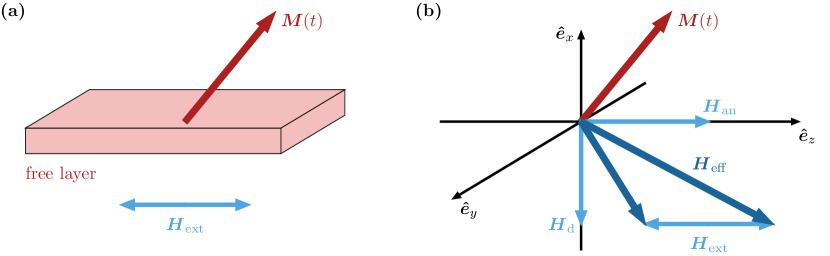
Figure 1: (a) Schematic of a magnetic single-domain layer with variable magnetization $\bm{M}$ (free layer) in an external magnetic field $\bm{H}^{\mathrm{ext}}$. (b) Magnetic field components governing the evolution of the free layer’s magnetization $\bm{M}$. The effective field $\bm{H}$ acting upon $\bm{M}$ consists of the demagnetization field $\bm{H}^{\mathrm{d}}=-M_{\mathrm{S}}m_{x}\hat{{\bf\it e}}_{x}$, the magnetocrystalline anisotropy field $\bm{H}^{\mathrm{an}}=H_{K}m_{z}\hat{{\bf\it e}}_{z}$, and the external driving $\bm{H}^{\mathrm{ext}}=H^{\mathrm{ext}}_{z}\sin(\omega t)\hat{{\bf\it e}}_{z}$. The material’s easy axis is aligned with the $z$-axis.

Here, we briefly discuss our model (cf. Fig. 1) motivated by a free-layer system [17] and present the equations, which describe the spin dynamics of this model including external driving. Then we introduce the basic ideas of TST and the methods, which will be applied for the computation of the instantaneous and average rates of the magnetization switching.

2.1 Spin dynamics in a driven free-layer model

The model addressed here is based on a magnetic single-domain layer with variable magnetization $\bm{M}$, known as a free layer. This layer is modeled in analogy to Stoner and Wohlfarth [59, 60] including a demagnetization field for a thin film (shape anisotropy) [61, 60]. A periodic external magnetic field is added to drive the magnetization. This field is intended as a generic placeholder for some externally applied torque—e. g., certain types of spin torque [62] such as the one stated below—and must not necessarily be realized by a magnetic coil or antenna.

For a classical description of the spin system we start from the Gilbert equation [57, 14]

$$\dot{\bm{M}}=-\gamma\bm{M}\crossproduct\bm{H}+\frac{\alpha}{M_{\mathrm{S}}}\bm{M}\crossproduct\dot{\bm{M}}$$ (1)

to describe the motion of a magnetic moment $\bm{M}=-\gamma\bm{S}$, with $\bm{S}$ the spin, $\gamma$ the gyromagnetic ratio, and $M_{\mathrm{S}}=\absolutevalue{\bm{M}}$ the saturation magnetization [cf. Fig. 1(b)]. The magnetic moment $\bm{M}$ is damped by a strength proportional to the coefficient $\alpha$ and can be driven by the effective magnetic field $\bm{H}$. Because the velocity $\dot{\bm{M}}$ is orthogonal to $\bm{M}$, the length of the magnetic moment is conserved and therefore we can write $\bm{M}=M_{\mathrm{S}}\bm{m}$ with $\absolutevalue{\bm{m}}=1$ and $\bm{m}$ being dimensionless.

The implicit differential equation (1) can be brought to an explicit form. Substituting $\dot{\bm{M}}$ on the right-hand side of Eq. (1) with the equation itself and using the relation $\bm{M}\crossproduct(\bm{M}\crossproduct\dot{\bm{M}})=(\bm{M}\dotproduct\dot{\bm{M}})\bm{M}-\bm{M}^{2}\dot{\bm{M}}=-M_{\mathrm{S}}^{2}\dot{\bm{M}}$ as well as $\bm{M}=M_{\mathrm{S}}\bm{m}$ we obtain the Landau–Lifshitz–Gilbert (LLG) equation [14, 16]

$$\dot{\bm{m}}=-\frac{\gamma}{1+\alpha^{2}}\bm{m}\crossproduct\quantity[\bm{H}+\alpha\quantity(\bm{m}\crossproduct\bm{H})]\,\text{.}$$ (2)

Here, we investigate the motion of a magnetic moment in a free-layer model described by the potential [61]

$$U=\frac{M_{\mathrm{S}}^{2}}{2}m_{x}^{2}-\frac{M_{\mathrm{S}}H_{K}}{2}m_{z}^{2}-M_{\mathrm{S}}H^{\mathrm{ext}}_{z}\sin(\omega t)m_{z}\,\text{,}$$ (3)

where $H_{K}$ is the anisotropy constant of the free layer. A magnetization switching induced by an additional torque modifying the dynamics of Eq. (2), can in principle be achieved by various ways [20, 21, 22, 23, 24, 25, 26, 27, 28, 29]. For the description of spin torque in a pinned-layer system, Slonczewski introduced an additional term to the standard Gilbert equation, depending on the polarization of the pinned layer [19]. In this model, the spin torque is proportional to the applied electron current $I$ flowing trough the pinned layer and, thus, can in principle become oscillating if an AC-source is used [63, 64]. While this specific type of spin torque cannot be represented purely by an additional magnetic field term, others—e. g., Manchon and Zhang [62]—have suggested spin torques that can. Due to the fact that the influence of some spin torques can be reformulated as an additional effective field acting on the spin dynamics [65, 62], we directly add our applied field expression into the effective field, leading to significant simplifications  [16]. The last term in Eq. (3) describes such an oscillating external magnetic field in $z$ direction with amplitude $H^{\mathrm{ext}}_{z}$ and frequency $\omega$. The effective magnetic field then reads

$$\bm{H}=-\frac{1}{M_{\mathrm{S}}}\vnabla_{\!\bm{m}}U=\matrixquantity(-M_{\mathrm{S}}m_{x}\\ 0\\ H_{K}m_{z}+H^{\mathrm{ext}}_{z}\sin(\omega t))\,\text{.}$$ (4)

For the free-layer system with parameters based on Refs. [22, 29, 27] the saturation magnetization and the gyromagnetic ratio read

$$M_{\mathrm{S}}=$1\text{\times}{10}^{6}\text{\,}\mathrm{A}\text{\,}{\mathrm{m}}^{-1}$\mbox{\quad and\quad}\gamma=$2.217\text{\times}{10}^{5}\text{\,}\mathrm{m}\text{\,}{\mathrm{A}}^{-1}\text{\,}{\mathrm{s}}^{-1}$\,\text{,}$$ (5)

respectively. Using these values as units, we can set $M_{\mathrm{S}}=$1$$ and $\gamma=$1$$ for computations with dimensionless parameters. In the following, we choose

$$M_{\mathrm{S}}=$1$,\quad\gamma=$1$,\quad\alpha=$0.01$,\quad H_{K}=$0.5$\,\text{,}$$ (6)

and an external magnetic field with amplitude and frequency

$$H^{\mathrm{ext}}_{z}=$0.15$\mbox{\quad and\quad}\omega=\pi/8$$ (7)

as reference parameters, if not stated otherwise. This corresponds to $H_{K}=$5\text{\times}{10}^{5}\text{\,}\mathrm{A}\text{\,}{\mathrm{m}}^{-1}$$, $H^{\mathrm{ext}}_{z}=$1.5\text{\times}{10}^{5}\text{\,}\mathrm{A}\text{\,}{\mathrm{m}}^{-1}$$, and $\omega/2\pi=$13.86\text{\,}\mathrm{GHz}$$ in the problem defined in Ref. [66] with the standard material parameters of permalloy. This applied field and frequency are well in the range of typical experimental conditions.

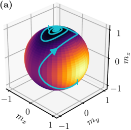
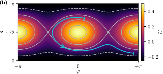
Figure 2: The free-layer potential (3) (a) on the sphere and (b) in the $(\varphi,\theta)$ plane. The saddle points at $\theta=\pi/2$ and $\varphi=\pm\pi/2$ mark the regions of the TS, which must be crossed for the magnetization switching. A typical trajectory with higher friction $\alpha=$0.1$$, propagated without external driving from a spin-down state to a spin-up state, is shown in cyan (or light gray in print) in both panels. Vertical markers highlight the part of the trajectory shown in (b).

To take advantage of the symmetry of the system one can transform the LLG equation (2) in spherical angular coordinates $\theta$ and $\varphi$, i. e.,

$$\dot{\theta}=\frac{\gamma}{1+\alpha^{2}}\quantity(H_{\varphi}+\alpha H_{\theta})\,\text{,}\quad\dot{\varphi}=\frac{\gamma}{1+\alpha^{2}}\frac{1}{\sin\theta}\quantity(-H_{\theta}+\alpha H_{\varphi})\,\text{,}$$ (8)

for $\theta\notin\{0,\pi\}$ and with the projections of the effective field to the basis vectors, $H_{\theta}=\bm{H}\dotproduct\hat{{\bf\it e}}_{\theta}$ and $H_{\varphi}=\bm{H}\dotproduct\hat{{\bf\it e}}_{\varphi}$. The potential (3) on the sphere for the spin system without external driving is illustrated in Fig. 2(a). The reduced equations of motion (8) for the two spherical angular variables describe a two-dimensional problem with the potential $U(\theta,\varphi)$ presented in Fig. 2(b). Two energy minima are located at the poles with $\theta=0$ and $\theta=\pi$, which make the potential (3) a perfect candidate to observe magnetization switching. At the equator $\theta=\pi/2$ there are two local energy maxima for $\varphi=0$ and $\varphi=\pi$ and two rank-1 saddles for $\varphi=-\pi/2$ and $\varphi=+\pi/2$.

A typical trajectory without external driving illustrating the magnetization switching is drawn in both panels (a) and (b) of Fig. 2. It starts on the spin down side of the sphere ($\theta>\pi/2$), crosses the saddle region of the potential near $\theta=\pi/2$, $\varphi=-\pi/2$ and approaches the spin up position ($\theta\approx 0$) on a spiral caused by the damping term in the Gilbert equation (1). We are interested in spin-flip processes crossing the regions close to one of the rank-1 saddles, and investigate in the following, without loss of generality, spin flips crossing the rank-1 saddle near $\varphi=+\pi/2$.

2.2 Transition state theory

The free-layer system, described by the potential (3), features a rank-1 saddle point at $\theta=\varphi=\pi/2$, as shown in Fig. 2(b). This saddle can act as a bottleneck of the spin dynamics, which makes it a candidate for the application of TST models [30, 31, 33, 36]. In typical scenarios for a chemical reaction, a one-dimensional reaction path—e. g., the minimum energy path [67]—characterizes the progress of the reaction. A rank-1 saddle point separates reactants from products along this unstable mode, and can be used to naively characterize the flux and associated reaction rate. In this context, it acts as a TS. In higher dimensions, the other degrees of freedom are stable and are referred to as orthogonal modes. More generally, the TS marks the transition between reactants and products through the location of a DS. Here, we apply TST to a magnetization switching in the free-layer system—e. g., from the “reactant” state spin up to the “product” state spin down—caused by a time-dependent driving of the system via an external magnetic field. To achieve this aim, we resort to recent extensions of TST to time-dependent driven systems [52, 53, 54, 55].

2.2.1 Phase-space structure and TS trajectory

In the free-layer system introduced above, the magnetization switching is related to a change in the $\theta$ coordinate—e. g., from $\theta\gtrsim 0$ to $\theta\lesssim\pi$ in an up to down spin state. In applying TST to resolve the activated dynamics of a spin, it thus appears natural to take the angle $\theta$ as the reaction coordinate and $\varphi$ as an orthogonal mode. However, an important difference between the spin system described by the equations of motion in (8), and systems typically addressed by TST requires some considerations, discussed below, to make the analogy complete.

In a chemical or mechanical system with $d$ degrees of freedom the dynamics is typically described by $d$ second-order differential equations for the coordinates or, in the Hamilton formalism, by $2d$ first-order differential equations for the coordinates and canonical momenta in the $2d$-dimensional phase space. In the spin system, the LLG equation results in the first-order differential equations (8) for the two coordinates $\theta$ and $\varphi$, i. e., there are no canonical momenta $p_{\theta}$ and $p_{\varphi}$, which belong to these coordinates. Nevertheless, TST can be applied to this system. The crucial point is that the two-dimensional phase space of the spin system consisting of the two coordinates $\theta$ and $\varphi$ is treated in formal mathematical analogy to the two-dimensional phase space of a one DoF Hamiltonian system with a reaction coordinate and the corresponding canonical momentum.

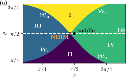
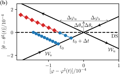
Figure 3: (a) Phase-space structure of the driven free-layer system introduced in Sec. 2.1. The stable and unstable manifolds, $\mathcal{W}_{\mathrm{s}}$ and $\mathcal{W}_{\mathrm{u}}$ separate four different regions marked $(I)$–$(IV)$ (see text). The intersection of the manifold’s closures forms the NHIM. The DS attached to this point separates the spin up and spin down regions in phase space. The external driving causes the NHIM to detach from the saddle point. (b) Schematic of the geometric structure that underlies the rate constant expressions summarized in Sec. 2.2.2. Initially, an equidistant spin ensemble connecting $\mathcal{W}_{\mathrm{s}}$ on the reactant side with the DS parallel to $\mathcal{W}_{\mathrm{u}}$ is generated. Upon time propagation, parts of the ensemble undergo spin flips as they move through the DS. The resulting ensemble is still equidistant, parallel to $\mathcal{W}_{\mathrm{u}}$, and connected to $\mathcal{W}_{\mathrm{s}}$.

The phase-space structure of the driven spin system in the vicinity of the rank-1 saddle at a given time $t$ is illustrated in Fig. 3(a). Note that the reaction coordinate $\theta$ is the ordinate and $\varphi$ the abscissa, which differs from corresponding presentations in Refs. [52, 68, 53, 54, 55], where the reaction coordinate is chosen as the abscissa and the corresponding velocity along the ordinate. The stable and unstable manifolds $\mathcal{W}_{\mathrm{s}}$ and $\mathcal{W}_{\mathrm{u}}$ separate four different regions, where $(I)$ the spin stays down, $(II)$ the spin stays up, $(III)$ the spin switches from up to down, and $(IV)$ the spin switches from down to up, when the system is propagated backwards and forwards in time. One subtlety regarding the time propagation of the spins should be noted: Due to the damping of the magnetic field by the term proportional to $\alpha$ in Eq. (1) the spin without external driving always moves towards a potential minimum, i. e., the spin up or spin down position when propagated forwards in time. However, it moves towards one of the potential maxima located at $\theta=\pi/2$, $\varphi=0$ or $\theta=\pi/2$, $\varphi=\pi$ (see Fig. 2) when propagated backwards. Therefore, appropriate cutoffs for the propagation of trajectories must be introduced to obtain the correct classification to one of the regions $(I)$–$(IV)$ in Fig. 3(a). Failing to do so can lead to visible artifacts, or it can cause the classification algorithm to not terminate. Similar problems in dissipative chemical systems have been discussed in Ref. [69]. In our case, we have found $$0.1$\pi<\varphi<$0.9$\pi$ to yield reliable results.

The intersection of the stable and unstable manifold is a point $(\varphi^{\ddagger},\theta^{\ddagger})$ on the NHIM. Such points do not leave the saddle region when propagated forwards or backwards in time. Therefore, these points describe spins that reside permanently in an unstable intermediate state roughly in $x$ direction that is neither spin up nor spin down. Note that for driven systems the points of the NHIM in general do not coincide with the time-dependent position of the saddle marked by the black point in Fig. 3(a). The line with constant angle $\theta=\theta^{\ddagger}$ represents a recrossing-free DS, which separates the “reactants” and “products” in TST, i. e., a spin with $\theta<\theta^{\ddagger}$ is spin up and a spin with $\theta>\theta^{\ddagger}$ is spin down. In case of periodic driving of the spin system by a time-dependent external magnetic field, the points on the NHIM follow a periodic orbit with the same period as the external driving. This orbit is called the TS trajectory, and is of fundamental importance for the computation of rate constants.

For the numerical construction of the NHIM, we resort to the binary contraction method (BCM) introduced in Ref. [68]. For a given time $t$, the algorithm in the BCM is initialized by defining a quadrangle with each of its corners lying exclusively within one of the four regions in the $(\varphi,\theta)$ plane shown in Fig. 3(a). In each iterative step, we first determine an edge’s midpoint. Then, the adjacent corner corresponding to the same region as that midpoint is moved to the midpoint’s position. By repeating this interleaved bisection procedure in turn for all edges, the quadrangle successively contracts and converges towards the intersection of the stable and unstable manifolds, i. e., a point on the NHIM. This method is numerically very effective and efficient for systems such as the one addressed here.

2.2.2 Decay rates

Three different methods for calculating decay rates in driven systems have recently been introduced and applied in the literature [54, 55]. Here, we adopt these methods with appropriate modifications for the free-layer system. The resulting decay rates are a measure of the instability of specific trajectories near the saddle. They differ significantly from the Kramers rate [70] used in the theory of chemical reactions but nevertheless provide insight about the rate process.

Ensemble method

The conceptually simplest method for calculating decay rates $k_{\mathrm{e}}$ is by means of propagation of an ensemble. In analogy to Ref. [54] we identify a line segment parallel to the unstable manifold that satisfies the property: it lies on the reactant side between the stable manifold and the DS at a distance that is small enough to allow for linear response and large enough to suppress numerical instability. At $t=t_{0}$, a spin ensemble is placed on this line as illustrated by blue dots in Fig. 3(b) and propagated in time to yield a time-dependent spin up population $N_{\uparrow}(t)$. The ensemble at time $t=t_{0}+\Delta t$ is marked in Fig. 3(b) by red and orange dots. Spins, which have crossed the DS (red dots) are spin down and thus cause a decrease of the population $N_{\uparrow}(t)$ (see the orange dots) with increasing time. In principle, one can now obtain a reaction rate constant $k_{\mathrm{e}}$ by fitting an exponential decay $N_{\uparrow}(t)\propto\exp[-k_{\mathrm{e}}(t-t_{0})]$ to the spin up population. This, however, is not possible in all systems because the decay in $N_{\uparrow}(t)$ can be nonexponential. Instead, we use the more general approach described in Ref. [54], which involves examining the instantaneous decays

$$k_{\mathrm{e}}(t)=-\frac{\dot{N}_{\uparrow}(t)}{N_{\uparrow}(t)}\,\text{.}$$ (9)

Local manifold analysis

The ensemble method is computationally expensive because it requires the propagation of a large number of spins for sufficiently long time. An alternative method, called the LMA, can be used to obtain instantaneous spin-flip rates purely from the geometry of the stable and unstable manifolds in phase space. The LMA is based on the observation that the equations of motion (8) can be linearized in the local vicinity of a trajectory $\bm{m}^{\ddagger}(t)$ on the NHIM with the Jacobian

$$\bm{J}(t)=\evaluated{\partialderivative{(\dot{\theta},\dot{\varphi})}{(\theta,\varphi)}}_{\bm{m}^{\ddagger}(t)}\,\text{.}$$ (10)

With the (not necessarily normalized) directions of the stable and unstable manifolds $\mathcal{W}_{\mathrm{s}}$ and $\mathcal{W}_{\mathrm{u}}$ at time $t$ given by $(\Delta\varphi_{\mathrm{s}},\Delta\theta_{\mathrm{s}})$ and $(\Delta\varphi_{\mathrm{u}},\Delta\theta_{\mathrm{u}})$ with $\Delta\theta_{\mathrm{s}}=\Delta\theta_{\mathrm{u}}$, as marked in Fig. 3(b), and using the linearization of the equations of motion (8) with the Jacobian (10) for the propagation of the spin ensemble, we finally obtain an analytical expression for the instantaneous rates of the magnetization switching

$$k_{\mathrm{m}}(t)=-\frac{\dot{N}_{\uparrow}(t)}{N_{\uparrow}(t)}=-\lim_{\Delta t\to 0}\frac{N_{\uparrow}(t+\Delta t)-N_{\uparrow}(t)}{\Delta tN_{\uparrow}(t)}=\evaluated{\partialderivative{\dot{\theta}}{\varphi}}_{\bm{m}^{\ddagger}(t)}\quantity(\frac{\Delta\varphi_{\mathrm{u}}}{\Delta\theta_{\mathrm{u}}}-\frac{\Delta\varphi_{\mathrm{s}}}{\Delta\theta_{\mathrm{s}}})\,\text{.}$$ (11)

These rates can be calculated independently at different times $t$, which allows for computations in parallel. Note that $\Delta\varphi_{\mathrm{s}}/\Delta\theta_{\mathrm{s}}$ and $\Delta\varphi_{\mathrm{u}}/\Delta\theta_{\mathrm{u}}$ are the inverse slopes of the stable and unstable manifolds $\mathcal{W}_{\mathrm{s}}$ and $\mathcal{W}_{\mathrm{u}}$ in Fig. 3(b), and thus the instantaneous rate $k_{\mathrm{m}}(t)$ in Eq. (11) is mainly determined by the difference of these two inverse slopes. This differs from, e. g., Ref. [54], where the instantaneous rate is related to the slopes of the stable and unstable manifolds; the inverse slopes in Eq. (11) occur because the reaction coordinate $\theta$ is not the abscissa but the ordinate in Figs. 3(a) and 3(b). As discussed above, the angles $\theta$ and $\varphi$ are not canonical variables as is typical in applications of TST to systems with Hamiltonian dynamics [54, 55, 45]. This manifests in a nontrivial and time-dependent prefactor $\evaluated*{(\partialderivative*{\dot{\theta}}{\varphi})}_{\bm{m}^{\ddagger}(t)}$ in Eq. (11), which is an element of the Jacobian (10). In the limiting case of a Cartesian reaction coordinate $x$ with canonical momentum $p=m\dot{x}$ (where $m$ is the particle mass), the corresponding element of the Jacobian reduces to a constant $\partialderivative*{\dot{x}}{p}=1/m$ [54].

Floquet method

The average decay rates $k_{\mathrm{F}}$ across time-dependent barriers can also be obtained directly using a Floquet stability analysis [51, 54]. While this method is computationally much cheaper than the ensemble method and the LMA, it cannot yield instantaneous rates.

To obtain the time-independent rate constant $k_{\mathrm{F}}$ for a given TS trajectory on the NHIM, we linearize the equations of motion using the Jacobian (10). By integrating the differential equation

$$\dot{\bm{\sigma}}(t)=\bm{J}(t)\bm{\sigma}(t)\mbox{\quad with\quad}\bm{\sigma}(0)=\bm{1}\,\text{,}$$ (12)

we then obtain the system’s fundamental matrix $\bm{\sigma}(t)$. When considering trajectories with period $T$, $\bm{M}=\bm{\sigma}(T)$ is called the monodromy matrix. Its eigenvalues $m_{\mathrm{u}}$ and $m_{\mathrm{s}}$, termed Floquet multipliers, can be used to determine the Floquet rate constant

$$k_{\mathrm{F}}=\frac{1}{T}\quantity(\ln\absolutevalue{m_{\mathrm{u}}}-\ln\absolutevalue{m_{\mathrm{s}}})\,\text{.}$$ (13)

As shown below, the Floquet rate constant $k_{\mathrm{F}}$ agrees perfectly with the instantaneous rates $k_{\mathrm{e}}(t)$ and $k_{\mathrm{m}}(t)$ when the latter two are averaged over one period $T$ of the TS trajectory.

3 Results and discussion

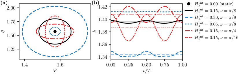
Figure 4: (a) A selection of TS trajectories of the free-layer system with the potential (3) described by the LLG equation (2). The static TS trajectory without external magnetic field ($H^{\mathrm{ext}}_{z}=0$) is marked by a black dot at $\theta=\varphi=\pi/2$. The TS trajectory with the reference parameters given in Eqs. (6) and (7) is shown as solid black line. TS trajectories with driving parameters deviating from Eq. (7) are drawn with colored dash or dash-dotted lines. The elliptical shape and orientation of the TS trajectories depends strongly on the driving by the oscillating external magnetic field. (b) Instantaneous rates (dark lines) and mean rates (pale lines) for some of the periodic TS trajectories shown in (a).

We now present and discuss the TS trajectories and the related instantaneous and averaged decay rates obtained for the free-layer system with and without driving by an oscillating external magnetic field. TS trajectories in the $(\varphi,\theta)$ phase space at various amplitudes $H^{\mathrm{ext}}_{z}$ and frequencies $\omega$ of the driving field relative to the reference system of Eq. (7) are shown in Fig. 4(a). The static TS trajectory without external driving is marked by a black dot at $\theta=\varphi=\pi/2$, which coincides with the position of the static saddle in Fig. 2. When driven by an oscillating external field, the TS trajectories become periodic orbits with the same period as the driving. The elliptical shape and orientation of the orbits strongly depend on the amplitude and frequency of the driving. The black solid line marks the TS trajectory with the reference parameters given in Eqs. (6) and (7). The dashed lines mark TS trajectories, where either the amplitude $H^{\mathrm{ext}}_{z}$ (blue lines) or the frequency $\omega$ (red lines) deviates from these reference parameters. For the chosen sets of parameters investigated here, the driving frequency mostly affects the shape of the orbits, whereas the driving amplitude has a large influence on the orbit size while preserving the shape approximately.

Rate constants, which are related to the TS trajectories in Fig. 4(a), have been computed with the methods introduced in Sec. 2.2.2 and are shown in Fig. 4(b). The (dark lines mark the instantaneous rates obtained by the LMA as functions of $t/T$ where $T=2\pi/\omega$ is the period of the corresponding TS trajectory. As can be seen, the oscillation amplitude of the instantaneous rates at high amplitude $H^{\mathrm{ext}}_{z}=0.3$ of the driving field (dark blue line) is slightly higher than that of the system with $H^{\mathrm{ext}}_{z}=0.15$ ( black line). This trend continues for $H^{\mathrm{ext}}_{z}=0.05$, where the oscillation is almost unnoticeable. The pale lines present the averaged rate constants. Here, the increase of the $H^{\mathrm{ext}}_{z}$ from $0.15$ (light gray line) to $0.3$ (pale blue line) causes a significant decrease in the averaged rate constant. The dark and pale red lines in Fig. 4(b) mark the instantaneous and averaged decay rate of the system at lower frequency $\omega=\pi/16$ and higher frequency $\omega=\pi/4$ of the oscillating magnetic field. The instantaneous rate fluctuates much stronger around the mean value. The alternation in the strength of these fluctuations is strong evidence for a sign change in the modulation amplitude around the reference frequency. As mentioned above, the rate constants obtained as time averages of the instantaneous rates over one period of the TS trajectory agree perfectly with the rate constants computed using the Floquet method.

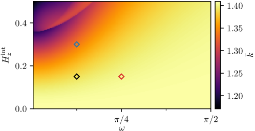
Figure 5: Mean rates $\bar{k}$ as function of the frequency $\omega$ and amplitude $H^{\mathrm{ext}}_{z}$ of the external magnetic field. The diamonds mark the parameters used in Fig. 4(b).

Finally, the dependence of the averaged decay rate $\bar{k}$ on the amplitude $H^{\mathrm{ext}}_{z}$ and frequency $\omega$ of the magnetic field is reported in Fig. 5. The diamonds mark the parameters of the TS trajectories shown in Fig. 4(b). A minimum in the rates lies near the corner with low frequencies $\omega$ and high amplitudes $H^{\mathrm{ext}}_{z}$.

4 Conclusion and outlook

We have investigated magnetization switching in a ferromagnetic free-layer system. The dynamics of the magnetic moment is described by the Gilbert equation (1). We have shown that TST can be applied to its two-dimensional phase space even though the Gilbert equation does not have the expected structure of a Hamiltonian system with coordinates and canonical momenta. We obtained the periodic TS trajectories of the free-layer system driven by an additional oscillating external magnetic field. In turn, these form the basis for the calculation of the instantaneous and averaged decay rates. The rates significantly depend on the time-dependent driving, i. e., the amplitude and frequency of the external magnetic field. The magnetization switching can thus be controlled by the external driving.

In this paper, we have assumed that the time derivative $\dot{\bm{m}}$ of the magnetic moment follows the magnetic field without relaxation, as described by the Gilbert equation (1). In future work, the model for the free-layer system could be extended by taking into account relaxation of the spins [71], which requires one to enlarge the phase space from two to four dimensions. TST will then allow us to study the influence of the relaxation on the decay rates.

Perhaps surprisingly, an increase in the field $H^{\mathrm{ext}}_{z}$ mostly leads to a decrease in the mean rate in Fig. 5. This is perhaps a consequence of the intermediate friction regime wherein the population of activated spins—i. e., those that would go over the barrier—are dampened by the dissipation. Moreover, as the driving frequency increases, the moving trajectory explores a wider oscillation potentially averaging—and suppressing—the difference in the curvatures associated with the stable and unstable directions that contributes to the rate. Resolution of this phenomenon remains a challenge for future work.

In summary, this work suggests that the application of recent advances in locally nonrecrossing TST to magnetization switching could be helpful in future work addressing dynamics in spintronics.

Declaration of competing interest

The authors declare that they have no known competing financial interests or personal relationships that could have appeared to influence the work reported in this paper.

CRediT authorship contribution statement

Johannes Mögerle: Methodology, Software, Formal analysis, Investigation, Writing – Original Draft. Robin Schuldt: Methodology, Formal analysis, Investigation, Writing – Original Draft. Johannes Reiff: Methodology, Software, Validation, Resources, Data Curation, Writing – Review & Editing, Visualization. Jörg Main: Conceptualization, Methodology, Formal analysis, Resources, Writing – Original Draft, Writing – Review & Editing, Supervision, Project administration, Funding acquisition. Rigoberto Hernandez: Conceptualization, Writing – Review & Editing, Project administration, Funding acquisition.

References

- Schneider et al. [2004] C. M. Schneider, B. Zhao, R. Kozhuharova, S. Groudeva-Zotova, T. Mühl, M. Ritschel, I. Mönch, H. Vinzelberg, D. Elefant, A. Graff, et al., Towards molecular spintronics: magnetotransport and magnetism in carbon nanotube-based systems, Diam. Relat. Mater. 13 (2004) 215–220. doi:10.1016/j.diamond.2003.10.009.
- Jiang et al. [2005] X. Jiang, R. Wang, R. M. Shelby, R. M. Macfarlane, S. R. Bank, J. S. Harris, S. S. P. Parkin, Highly spin-polarized room-temperature tunnel injector for semiconductor spintronics using MgO (100), Phys. Rev. Lett. 94 (2005) 056601. doi:10.1103/PhysRevLett.94.056601.
- Cowburn [2007] R. P. Cowburn, Spintronics: Change of direction, Nat. Mater. 6 (2007) 255–256. doi:10.1038/nmat1877.
- Shinjo [2014] T. Shinjo, Overview, in: Nanomagnetism and Spintronics, second edition ed., Elsevier, 2014, pp. 1–14.
- Maekawa et al. [2017] S. Maekawa, S. O. Valenzuela, E. Saitoh, T. Kimura (Eds.), Spin current, volume 22, Oxford University Press, 2017.
- Monakhov et al. [2017] K. Y. Monakhov, M. Moors, P. Kögerler, Chapter nine - perspectives for polyoxometalates in single-molecule electronics and spintronics, in: R. van Eldik, L. Cronin (Eds.), Polyoxometalate Chemistry, volume 69 of Advances in Inorganic Chemistry, Academic Press, 2017, pp. 251–286. doi:10.1016/bs.adioch.2016.12.009.
- Khodadadi et al. [2020] B. Khodadadi, A. Rai, A. Sapkota, A. Srivastava, B. Nepal, Y. Lim, D. A. Smith, C. Mewes, S. Budhathoki, A. J. Hauser, et al., Conductivitylike Gilbert damping due to intraband scattering in epitaxial iron, Phys. Rev. Lett. 124 (2020) 157201. doi:10.1103/physrevlett.124.157201.
- Liu et al. [2020] L. Liu, J. Yu, R. González-Hernández, C. Li, J. Deng, W. Lin, C. Zhou, T. Zhou, J. Zhou, H. Wang, R. Guo, H. Y. Yoong, G. M. Chow, X. Han, B. Dupé, J. Železný, J. Sinova, J. Chen, Electrical switching of perpendicular magnetization in a single ferromagnetic layer, Phys. Rev. B 101 (2020) 220402. doi:10.1103/physrevb.101.220402.
- Wolf et al. [2001] S. A. Wolf, D. D. Awschalom, R. A. Buhrman, J. M. Daughton, S. von Molnár, M. L. Roukes, A. Y. Chtchelkanova, D. M. Treger, Spintronics: A spin-based electronics vision for the future, Science 294 (2001) 1488–1495. doi:10.1126/science.1065389.
- Rocha et al. [2005] A. R. Rocha, V. M. Garcia-Suarez, S. W. Bailey, C. J. Lambert, J. Ferrer, S. Sanvito, Towards molecular spintronics, Nat. Mater. 4 (2005) 335–339. doi:10.1038/nmat1349.
- Adam et al. [2006] S. Adam, M. L. Polianski, P. W. Brouwer, Current-induced transverse spin-wave instability in thin ferromagnets: Beyond linear stability analysis, Phys. Rev. B 73 (2006) 024425. doi:10.1103/PhysRevB.73.024425.
- Chappert et al. [2007] C. Chappert, A. Fert, F. N. van Dau, The emergence of spin electronics in data storage, Nat. Mater. 6 (2007) 813–823. doi:10.1142/9789814287005\_0015.
- Taniguchi et al. [2013] T. Taniguchi, Y. Utsumi, M. Marthaler, D. S. Golubev, H. Imamura, Spin torque switching of an in-plane magnetized system in a thermally activated region, Phys. Rev. B 87 (2013) 054406. doi:10.1103/PhysRevB.87.054406.
- Gilbert [2004] T. L. Gilbert, A phenomenological theory of damping in ferromagnetic materials, IEEE Trans. Magn. 40 (2004) 3443–3449. doi:10.1109/TMAG.2004.836740.
- Apalkov and Visscher [2005] D. M. Apalkov, P. B. Visscher, Spin-torque switching: Fokker-Planck rate calculation, Phys. Rev. B 72 (2005) 180405. doi:10.1103/PhysRevB.72.180405.
- Abert [2019] C. Abert, Micromagnetics and spintronics: models and numerical methods, Eur. Phys. J. B 92 (2019) 120. doi:10.1140/epjb/e2019-90599-6.
- Li and Zhang [2003] Z. Li, S. Zhang, Magnetization dynamics with a spin-transfer torque, Phys. Rev. B 68 (2003) 024404. doi:10.1103/PhysRevB.68.024404.
- Li and Zhang [2004] Z. Li, S. Zhang, Thermally assisted magnetization reversal in the presence of a spin-transfer torque, Phys. Rev. B 69 (2004) 134416. doi:10.1103/PhysRevB.69.134416.
- Slonczewski [1996] J. C. Slonczewski, Current-driven excitation of magnetic multilayers, J. Magn. Magn. Mater. 159 (1996) L1–L7. doi:10.1016/0304-8853(96)00062-5.
- Zhu et al. [2008] J.-G. Zhu, X. Zhu, Y. Tang, Microwave assisted magnetic recording, IEEE Trans. Magn. 44 (2008) 125–131. doi:10.1109/tmag.2007.911031.
- Okamoto et al. [2012] S. Okamoto, N. Kikuchi, M. Furuta, O. Kitakami, T. Shimatsu, Switching behaviors and its dynamics of a Co/Pt nanodot under the assistance of rf fields, Phys. Rev. Lett. 109 (2012). doi:10.1103/physrevlett.109.237209.
- Taniguchi [2014] T. Taniguchi, Magnetization reversal condition for a nanomagnet within a rotating magnetic field, Phys. Rev. B 90 (2014). doi:10.1103/physrevb.90.024424.
- Suto et al. [2015] H. Suto, T. Nagasawa, K. Kudo, K. Mizushima, R. Sato, Microwave-assisted switching of a single perpendicular magnetic tunnel junction nanodot, Appl. Phys. Express 8 (2015) 023001. doi:10.7567/apex.8.023001.
- Barros et al. [2011] N. Barros, M. Rassam, H. Jirari, H. Kachkachi, Optimal switching of a nanomagnet assisted by microwaves, Phys. Rev. B 83 (2011). doi:10.1103/physrevb.83.144418.
- Barros et al. [2013] N. Barros, H. Rassam, H. Kachkachi, Microwave-assisted switching of a nanomagnet: Analytical determination of the optimal microwave field, Phys. Rev. B 88 (2013). doi:10.1103/physrevb.88.014421.
- Klughertz et al. [2015] G. Klughertz, L. Friedland, P.-A. Hervieux, G. Manfredi, Autoresonant switching of the magnetization in single-domain nanoparticles: Two-level theory, Phys. Rev. B 91 (2015). doi:10.1103/physrevb.91.104433.
- Taniguchi et al. [2016] T. Taniguchi, D. Saida, Y. Nakatani, H. Kubota, Magnetization switching by current and microwaves, Phys. Rev. B 93 (2016). doi:10.1103/physrevb.93.014430.
- Rivkin and Ketterson [2006] K. Rivkin, J. B. Ketterson, Magnetization reversal in the anisotropy-dominated regime using time-dependent magnetic fields, Appl. Phys. Lett. 89 (2006) 252507. doi:10.1063/1.2405855.
- Taniguchi [2015] T. Taniguchi, Magnetization switching by microwaves synchronized in the vicinity of precession frequency, Appl. Phys. Express 8 (2015) 083004. doi:10.7567/apex.8.083004.
- Eyring [1935] H. Eyring, The activated complex in chemical reactions, J. Chem. Phys. 3 (1935) 107–115. doi:10.1063/1.1749604.
- Wigner [1937] E. P. Wigner, Calculation of the rate of elementary association reactions, J. Chem. Phys. 5 (1937) 720–725. doi:10.1063/1.1750107.
- Pitzer et al. [1962] K. S. Pitzer, F. T. Smith, H. Eyring, The Transition State, Special Publ., Chemical Society, London, 1962.
- Pechukas [1981] P. Pechukas, Transition state theory, Annu. Rev. Phys. Chem. 32 (1981) 159–177. doi:10.1146/annurev.pc.32.100181.001111.
- Truhlar et al. [1996] D. G. Truhlar, B. C. Garrett, S. J. Klippenstein, Current status of transition-state theory, J. Phys. Chem. 100 (1996) 12771–12800. doi:10.1021/jp953748q.
- Mullen et al. [2014] R. G. Mullen, J.-E. Shea, B. Peters, Communication: An existence test for dividing surfaces without recrossing, J. Chem. Phys. 140 (2014) 041104. doi:10.1063/1.4862504.
- Wiggins [2016] S. Wiggins, The role of normally hyperbolic invariant manifolds (NHIMS) in the context of the phase space setting for chemical reaction dynamics, Regul. Chaotic Dyn. 21 (2016) 621–638. doi:10.1134/S1560354716060034.
- Jaffé et al. [2000] C. Jaffé, D. Farrelly, T. Uzer, Transition state theory without time-reversal symmetry: Chaotic ionization of the hydrogen atom, Phys. Rev. Lett. 84 (2000) 610–613. doi:10.1103/PhysRevLett.84.610.
- Jacucci et al. [1984] G. Jacucci, M. Toller, G. DeLorenzi, C. P. Flynn, Rate Theory, Return Jump Catastrophes, and the Center Manifold, Phys. Rev. Lett. 52 (1984) 295. doi:10.1103/PhysRevLett.52.295.
- Komatsuzaki and Berry [1999] T. Komatsuzaki, R. S. Berry, Regularity in chaotic reaction paths. I. , J. Chem. Phys. 110 (1999) 9160–9173. doi:10.1063/1.478838.
- Komatsuzaki and Berry [2002] T. Komatsuzaki, R. S. Berry, Chemical reaction dynamics: Many-body chaos and regularity, Adv. Chem. Phys. 123 (2002) 79–152. doi:10.1002/0471231509.ch2.
- Toller et al. [1985] M. Toller, G. Jacucci, G. DeLorenzi, C. P. Flynn, Theory of classical diffusion jumps in solids, Phys. Rev. B 32 (1985) 2082. doi:10.1103/PhysRevB.32.2082.
- Voter et al. [2002] A. F. Voter, F. Montalenti, T. C. Germann, Extending the time scale in atomistic simulations of materials, Annu. Rev. Mater. Res. 32 (2002) 321–346. doi:10.1146/annurev.matsci.32.112601.141541.
- de Oliveira et al. [2002] H. P. de Oliveira, A. M. Ozorio de Almeida, I. Damião Soares, E. V. Tonini, Homoclinic chaos in the dynamics of a general Bianchi type-IX model, Phys. Rev. D 65 (2002) 083511/1–9. doi:10.1103/PhysRevD.65.083511.
- Jaffé et al. [2002] C. Jaffé, S. D. Ross, M. W. Lo, J. Marsden, D. Farrelly, T. Uzer, Statistical theory of asteroid escape rates, Phys. Rev. Lett. 89 (2002) 011101. doi:10.1103/PhysRevLett.89.011101.
- Stallings et al. [2020] D. Stallings, S. K. Iyer, R. Hernandez, Removing barriers, in: S. Azad (Ed.), Addressing Gender Bias in Science & Technology, volume 1354 of ACS Symposium Series, American Chemical Society; Oxford University Press, Washington DC, 2020, pp. 91–108. doi:10.1021/bk-2020-1354.ch006.
- Bartsch et al. [2008] T. Bartsch, J. M. Moix, R. Hernandez, S. Kawai, T. Uzer, Time-dependent transition state theory, Adv. Chem. Phys. 140 (2008) 191–238. doi:10.1002/9780470371572.ch4.
- Hernandez and Miller [1993] R. Hernandez, W. H. Miller, Semiclassical transition state theory. A new perspective, Chem. Phys. Lett. 214 (1993) 129–136. doi:10.1016/0009-2614(93)90071-8.
- Uzer et al. [2002] T. Uzer, C. Jaffé, J. Palacián, P. Yanguas, S. Wiggins, The geometry of reaction dynamics, Nonlinearity 15 (2002) 957–992. doi:10.1088/0951-7715/15/4/301.
- Waalkens and Wiggins [2004] H. Waalkens, S. Wiggins, Direct construction of a dividing surface of minimal flux for multi-degree-of-freedom systems that cannot be recrossed, J. Phys. A 37 (2004) L435–L445. doi:10.1088/0305-4470/37/35/L02.
- Çiftçi and Waalkens [2013] U. Çiftçi, H. Waalkens, Reaction dynamics through kinetic transition states, Phys. Rev. Lett. 110 (2013) 233201. doi:10.1103/PhysRevLett.110.233201.
- Craven et al. [2014] G. T. Craven, T. Bartsch, R. Hernandez, Communication: Transition state trajectory stability determines barrier crossing rates in chemical reactions induced by time-dependent oscillating fields, J. Chem. Phys. 141 (2014) 041106. doi:10.1063/1.4891471.
- Feldmaier et al. [2017] M. Feldmaier, A. Junginger, J. Main, G. Wunner, R. Hernandez, Obtaining time-dependent multi-dimensional dividing surfaces using Lagrangian descriptors, Chem. Phys. Lett. 687 (2017) 194. doi:10.1016/j.cplett.2017.09.008.
- Feldmaier et al. [2019a] M. Feldmaier, P. Schraft, R. Bardakcioglu, J. Reiff, M. Lober, M. Tschöpe, A. Junginger, J. Main, T. Bartsch, R. Hernandez, Invariant manifolds and rate constants in driven chemical reactions, J. Phys. Chem. B 123 (2019a) 2070–2086. doi:10.1021/acs.jpcb.8b10541.
- Feldmaier et al. [2019b] M. Feldmaier, R. Bardakcioglu, J. Reiff, J. Main, R. Hernandez, Phase-space resolved rates in driven multidimensional chemical reactions, J. Chem. Phys. 151 (2019b) 244108. doi:10.1063/1.5127539.
- Feldmaier et al. [2020] M. Feldmaier, J. Reiff, R. M. Benito, F. Borondo, J. Main, R. Hernandez, Influence of external driving on decays in the geometry of the LiCN isomerization, J. Chem. Phys. 153 (2020) 084115. doi:10.1063/5.0015509.
- Landau and Lifshitz [1935] L. D. Landau, E. Lifshitz, On the theory of the dispersion of magnetic permeability in ferromagnetic bodies, Phys. Z. Sowjetunion 8 (1935) 101–114.
- Gilbert [1956] T. L. Gilbert, Formulation, Foundations and Applications of the Phenomenological Theory of Ferromagnetism., Ph.D. thesis, Illinois Institute of Technology, 1956.
- Ciornei [2010] M.-C. Ciornei, Role of magnetic inertia in damped macrospin dynamics, Ph.D. thesis, Ecole Polytechnique X, 2010. URL: https://pastel.archives-ouvertes.fr/tel-00460905.
- Stoner and Wohlfarth [1948] E. C. Stoner, E. P. Wohlfarth, A mechanism of magnetic hysteresis in heterogeneous alloys, Philos. Trans. R. Soc. A 240 (1948) 599–642. doi:10.1098/rsta.1948.0007.
- Tannous and Gieraltowski [2008] C. Tannous, J. Gieraltowski, The Stoner–Wohlfarth model of ferromagnetism, Eur. J. Phys. 29 (2008) 475–487. doi:10.1088/0143-0807/29/3/008.
- Zhang and Li [2004] S. Zhang, Z. Li, Roles of nonequilibrium conduction electrons on the magnetization dynamics of ferromagnets, Phys. Rev. Lett. 93 (2004) 127204. doi:10.1103/PhysRevLett.93.127204.
- Manchon and Zhang [2008] A. Manchon, S. Zhang, Theory of nonequilibrium intrinsic spin torque in a single nanomagnet, Phys. Rev. B 78 (2008) 212405. doi:10.1103/PhysRevB.78.212405.
- McMichael et al. [1999] R. D. McMichael, M. J. Donahue, D. G. Porter, J. Eicke, Comparison of magnetostatic field calculation methods on two-dimensional square grids as applied to a micromagnetic standard problem, J. Appl. Phys. 85 (1999) 5816–5818. doi:10.1063/1.369929.
- Zhu and Zhao [2020] D. Zhu, W. Zhao, Threshold current density for perpendicular magnetization switching through spin-orbit torque, Phys. Rev. Appl. 13 (2020) 044078. doi:10.1103/PhysRevApplied.13.044078.
- Apalkov and Visscher [2005] D. M. Apalkov, P. B. Visscher, Slonczewski spin-torque as negative damping: Fokker–Planck computation of energy distribution, J. Magn. Magn. Mater. 286 (2005) 370–374. doi:10.1016/j.jmmm.2004.09.094.
- Najafi et al. [2009] M. Najafi, B. Krüger, S. Bohlens, M. Franchin, H. Fangohr, A. Vanhaverbeke, R. Allenspach, M. Bolte, U. Merkt, D. Pfannkuche, et al., Proposal for a standard problem for micromagnetic simulations including spin-transfer torque, J. Appl. Phys. 105 (2009) 113914. doi:10.1063/1.3126702.
- Glasstone et al. [1941] S. Glasstone, K. J. Laidler, H. Eyring, The Theory of Rate Processes: The Knetics of Chemical Reactions, Viscosity, Diffusion and Electrochemical Phenomena, McGraw-Hill, New York, 1941.
- Bardakcioglu et al. [2018] R. Bardakcioglu, A. Junginger, M. Feldmaier, J. Main, R. Hernandez, Binary contraction method for the construction of time-dependent dividing surfaces in driven chemical reactions, Phys. Rev. E 98 (2018) 032204. doi:10.1103/PhysRevE.98.032204.
- Junginger and Hernandez [2016] A. Junginger, R. Hernandez, Lagrangian descriptors in dissipative systems, Phys. Chem. Chem. Phys. 18 (2016) 30282. doi:10.1039/C6CP02532C.
- Pollak et al. [1989] E. Pollak, H. Grabert, P. Hänggi, Theory of activated rate processes for arbitrary frequency dependent friction: Solution of the turnover problem, J. Chem. Phys. 91 (1989) 4073–4087. doi:10.1063/1.456837.
- Fähnle et al. [2011] M. Fähnle, D. Steiauf, C. Illg, Generalized Gilbert equation including inertial damping: Derivation from an extended breathing Fermi surface model, Phys. Rev. B 84 (2011) 172403. doi:10.1103/PhysRevB.84.172403.