Detecting Central Nodes from Low-rank Excited Graph Signals via Structured Factor Analysis

Abstract

This paper treats a blind detection problem to identify the central nodes in a graph from filtered graph signals. Unlike prior works which impose strong restrictions on the data model, we only require the underlying graph filter to satisfy a low pass property with a generic low-rank excitation model. We treat two cases depending on the low pass graph filter’s strength. When the graph filter is strong low pass, i.e., it has a frequency response that drops sharply at the high frequencies, we show that the principal component analysis (PCA) method detects central nodes with high accuracy. For general low pass graph filter, we show that the graph signals can be described by a structured factor model featuring the product between a low-rank plus sparse factor and an unstructured factor. We propose a two-stage decomposition algorithm to learn the structured factor model via a judicious combination of the non-negative matrix factorization and robust PCA algorithms. We analyze the identifiability conditions for the model which lead to accurate central nodes detection. Numerical experiments on synthetic and real data are provided to support our findings. We demonstrate significant performance gains over prior works.

I Introduction

Recently, the study of network science has proliferated in research fields such as social science, biology, and data science, where it has offered new insights through studying network data from a graph’s perspective. A popular subject is to identify central nodes through the node centrality [2]. Node centrality ranks the relative importance of nodes with respect to the graph topology, and it is useful for identifying influential people in a social network, frequently visited webpages on the Internet, stocks that are important driving forces in the market, etc. [3]. A number of centrality measures such as degree centrality, betweenness centrality, eigen-centrality, etc., have been studied [4]. Among others, the eigen-centrality measure, defined as the top eigenvector of the graph adjacency matrix, is popular as it takes into account the importance of the node’s neighbors as well as the node’s own degree. These appealing features have led to the wide adoption of the eigen-centrality measure, for instance, the PageRank model [5].

Evaluating the eigen-centrality typically requires knowledge of the graph topology. In this paper, we focus on using a data-driven approach to learn the eigen-centrality. Particularly, we develop algorithms that use just graph signals observed on the nodes, e.g., opinions on social networks, or return records in stock market, etc., to detect nodes with high eigen-centrality. We call this task the blind central nodes detection problem. The blind detection problem is related to the fast growing literature in graph learning [6, 7]. In particular, a natural heuristic is to first perform graph learning, and then rank the eigen-centrality using the estimated graph. Such a heuristic is prone to errors since the graph learning algorithms typically require strong assumptions to provide reliable estimates of the graph. For example, they assume precise knowledge of generative models such as graphical Markov random field [8], non-linear dynamical systems [9, 10], etc.. As an alternative, the notion of filtered graph signals which is rooted in graph signal processing (GSP) [11, 12] provides a flexible model through viewing graph signals as generated by filtering the excitation through an unknown graph filter. Based on this model, graph learning algorithms have been proposed which exploit smoothness [13], spectral template [14], graph structure priors [15, 16], etc.. However, further restrictions on the excitation are needed for the above algorithms. For instance, it is assumed in [13, 14, 15, 16] that the excitation is white noise with independent input at each node. The latter assumption which implies full-rank observations may not hold in practice [17].

The approach pursued by the current paper is to detect central nodes directly from filtered graph signals, thereby side-stepping the error-prone graph learning stage. Doing so allows us to relax some restrictions required by previous works on graph learning. Notably, our approach applies to general graph signal models with possibly low-rank excitation. Our key assumption is that the observed graph signals are filtered by a low pass graph filter that has a frequency response which drops at the high frequencies, while the excitation to the graph filter is independent of the graph. This property is commonly found in graph data from applications such as economics, social networks, and power systems, etc. [18]. Depending on the strengths of the low pass graph filter, we treat two cases separately. With a strong low pass graph filter whose frequency response drops sharply at the high frequencies [cf. $\eta\approx 0$ in 1], we show that the principal component analysis (PCA) method detects the central nodes accurately. Note that this case corresponds to graph signals that are smooth with respect to the graph topology. With a general low pass graph filter which may or may not be strong low pass [cf. $\eta<1$ in 1], the blind detection problem becomes more challenging to tackle. As a trade-off, we are motivated by applications in economics and social networks to concentrate on an additional assumption that the excitation graph signals lie in a subspace with the basis given by a sparse and non-negative matrix. Subsequently, the filtered graph signals are treated by a novel structured factor analysis model featuring the product between a ‘low-rank plus sparse’ factor and an unstructured factor. We develop a two-stage decomposition algorithm leveraging a sparse non-negative matrix factorization (NMF) criterion and the robust PCA (RPCA) method. We show that the central nodes of the underlying graph can be detected accurately through analyzing the identifiability of the factor model and a boosting property of the low pass graph filter. To our best knowledge, this is the first application of the NMF and RPCA to detect central nodes from graph signals.

Notice that NMF and RPCA have been separately applied in other domains such as blind source separation, topic modeling, and video surveillance [19, 20, 21]. The theoretical guarantees therein also have different focuses from the current paper. We remark that the approach of side-stepping graph learning is inspired by [22, 23, 24, 25, 26] on the blind community detection problem. In comparison, this paper is the first to handle blind central nodes detection under the challenging case with unknown excitation. Lastly, blind centrality ranking has been treated in [27, 28] using the PCA method. Assuming white noise excitation, these works provided the sample complexity analysis on ranking the eigen-centrality of nodes. In comparison, our work assumes low-rank excitation that yields a strictly more general model.

Contributions. This paper treats the blind detection of central nodes using low-rank excited low pass filtered graph signals. Our contributions are as follows:

• We show that the PCA method accurately identifies the central nodes under the conditions that the graph signals are generated by a strong low pass graph filter [cf. $\eta\approx 0$ in 1] or the excitation is white noise. Our analysis demonstrates an explicit dependence of the detection performance on factors such as the sample size.

• We recognize a structured factor model for the filtered graph signals via an intrinsic decomposition featuring a low-rank plus sparse factor and an unstructured factor under the condition that the graph signals are generated by a general low pass graph filter [cf. $\eta<1$ in 1] which may or may not be strong low pass. Note we have concentrated on a special case where the excitation graph signals lie in a subspace with sparse and non-negative basis, as motivated by applications in economics and social networks.

• We provide the first identifiability analysis on the structured factor model involving filtered graph signals with unknown excitation. We show that the identification performance depends on the low pass ratio of the graph filter and the ratio of the excitation’s rank to the graph’s size. Inspired by the identifiability analysis, we propose to combine a sparse NMF method with the RPCA method to yield a two-stage algorithm for efficient central nodes detection.

• We carry out numerical experiments on real and synthetic data to verify our theoretical results. Compared to existing works, our methods can consistently detect the central nodes with a lower error rate on synthetic data and higher correlation with the global behavior on real data.

Compared to the conference version [1], this paper includes the case with general low pass filter and unknown excitation. We also included an extended set of numerical experiments.

Organization. The rest of this paper is organized as follows. In Section II, we introduce the graph signal model. Two application examples are discussed and their graph signal models are derived. In Section III, we consider strong low pass graph filter and prove that the PCA method can detect central nodes with high accuracy. In Section IV, we consider general low pass graph filter and propose a two-stage algorithm motivated by identifiability conditions with NMF specialized to leverage the graph signal structure. Finally, we discuss the practical implementation issues in Section V, and present numerical experiments to support our findings in Section VI.

Notations. We use boldfaced character (resp. boldfaced capital letter) to denote vector (resp. matrix). For a matrix ${\bm{X}}\in\Re^{m\times n}$, we use $[{\bm{X}}]_{i,j}$ to denote its $(i,j)$th entry. For any vector ${\bm{x}}\in\Re^{n}$, $\|{\bm{x}}\|$, $\|{\bm{x}}\|_{1}$ denote the Euclidean, $\ell_{1}$ norm, respectively; for any matrix ${\bm{X}}\in\Re^{m\times n}$, $\|{\bm{X}}\|$ denotes the spectral norm, $\|{\bm{X}}\|_{\star}$ denotes the nuclear norm, and $\|{\bm{X}}\|_{F}=\sqrt{\sum_{i,j}X_{ij}^{2}}$ denotes the Frobenius norm. For a random vector ${\bm{y}}_{\ell}$, its covariance is denoted as the matrix ${\rm Cov}({\bm{y}}_{\ell})=\mathbb{E}[({\bm{y}}_{\ell}-\mathbb{E}[{\bm{y}}_{\ell}])({\bm{y}}_{\ell}-\mathbb{E}[{\bm{y}}_{\ell}])^{\top}]$.

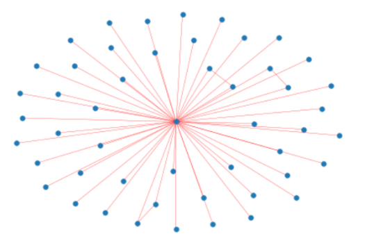
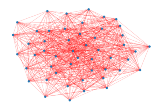
Figure 1: (Left) Graph with a central hub node: ${\lambda_{2}}/{\lambda_{1}}\approx 0.1238$. (Right) an Erdos-Renyi graph that does not have central node(s) with significantly higher degree: ${\lambda_{2}}/{\lambda_{1}}\approx 0.9189$.

II Graph Signal Model

Consider an undirected, connected graph $G=({\mathcal{}V},{\mathcal{}E},{\bm{A}})$ with $n$ nodes given by ${\mathcal{}V}:=\{1,\dots,n\}$ and edge set ${\mathcal{}E}\subseteq{\mathcal{}V}\times{\mathcal{}V}$. The matrix ${\bm{A}}\in\Re_{+}^{n\times n}$ is a weighted adjacency matrix such that $A_{ij}=A_{ji}>0$ if and only if $(i,j)\in E$; otherwise, $A_{ij}=0$. The symmetric matrix ${\bm{A}}$ admits an eigenvalue decomposition as ${\bm{A}}={\bm{V}}\bm{\Lambda}{\bm{V}}^{\top}$, where ${\bm{V}}$ is an orthogonal matrix and $\bm{\Lambda}={\rm Diag}(\bm{\lambda})$ is a diagonal matrix of the eigenvalues. For simplicity, we assume the eigenvalues are ordered as $\lambda_{1}>\lambda_{2}\geq\cdots\geq\lambda_{n}$. To specify the scenario of interest, we focus on graphs with $C$ central nodes of high inter/intra-connectivity, for some $C\ll n$. As studied by [29], such graphs can be characterized by large spectral gap with $\lambda_{1}\gg\lambda_{2}$ [cf. Fig. 1]. Our aim is to detect these central nodes defined via the eigen-centrality vector [2]:

$${\bm{c}}_{\sf eig}:={\sf TopEV}({\bm{A}})={\bm{v}}_{1},\vspace{-.1cm}$$ (1)

where ${\sf TopEV}({\bm{A}})$ denotes the top eigenvector of ${\bm{A}}$. Accordingly, we denote the top-$C$ central nodes as the set of $C$ nodes whose magnitudes $|[{\bm{c}}_{\sf eig}]_{i}|$ are the highest.

We observe a set of vectors $\{{\bm{y}}_{\ell}\}_{\ell=1}^{m}$ generated from a certain process on $G$ treated as filtered graph signals [11]. The graph signal defined on $G$ is an $n$-dimensional vector ${\bm{y}}\in\Re^{n}$ such that $y_{i}$ denotes the signal on node $i$. On the other hand, a graph filter is described as a polynomial of the graph shift operator (GSO):

$${\mathcal{}H}({\bm{A}})=\sum_{t=0}^{T-1}h_{t}{\bm{A}}^{t}={\bm{V}}\left(\sum_{t=0}^{T-1}h_{t}\bm{\Lambda}^{t}\right){\bm{V}}^{\top}\in\Re^{n\times n},$$ (2)

where $\{h_{t}\}_{t=0}^{T-1}$ are the filter coefficients and $T\in\mathbb{Z}_{+}\cup\{\infty\}$ is the filter’s order. In this paper, we took the adjacency matrix ${\bm{A}}$ as the GSO. Accordingly, the graph Fourier transform (GFT) of ${\bm{y}}$ is given by $\tilde{\bm{y}}={\bm{V}}^{\top}{\bm{y}}$ [30]. With this choice of GFT basis, we define the diagonal matrix $h(\bm{\Lambda})=\sum_{t=0}^{T-1}h_{t}\bm{\Lambda}^{t}$, whose diagonal entries are the frequency responses of the graph filter. The $i$th diagonal $h(\lambda_{i})\mathrel{\mathop{:}}=[h(\bm{\Lambda})]_{i,i}$ denotes the frequency response corresponding to the $i$th graph frequency.

Finally, the observations $\{{\bm{y}}_{\ell}\}_{\ell=1}^{m}$ are modeled as the graph filter’s outputs subject to the excitation $\{{\bm{x}}_{\ell}\}_{\ell=1}^{m}$:

$${\bm{y}}_{\ell}={\mathcal{}H}({\bm{A}}){\bm{x}}_{\ell}+{\bm{w}}_{\ell},~{}\ell=1,...,m,$$ (3)

where ${\bm{w}}_{\ell}\sim{\mathcal{}N}({\bm{0}},\sigma^{2}{\bm{I}})$ represents the modeling error and measurement noise. We assume that ${\bm{w}}_{\ell},{\bm{w}}_{\ell^{\prime}}$ are independent if $\ell\neq\ell^{\prime}$. The excitation $\{{\bm{x}}_{\ell}\}_{\ell=1}^{m}$ represent the external stimuli inflicted on $G$ and they are assumed to be independent of the graph, see (5) for further discussion. The main task of this paper is to tackle the blind central nodes detection problem, where we identify the top-$C$ central nodes using just $\{{\bm{y}}_{\ell}\}_{\ell=1}^{m}$.

To identify the central nodes from $\{{\bm{y}}_{\ell}\}_{\ell=1}^{m}$, our key assumption is that the graph filter ${\mathcal{}H}({\bm{A}})$ satisfies a low pass property [18], i.e., its frequency response drops at the high graph frequencies. Particularly, we assume:

Assumption 1

The graph filter ${\mathcal{}H}({\bm{A}})$ is $1$-low pass such that its frequency response satisfies:

$$\eta:={\max_{j=2,...,n}|h(\lambda_{j})|}/{|h(\lambda_{1})|}<1,$$ (4)

where $\eta$ is called the low pass ratio that quantifies the stopband attenuation, see Fig. 2.

Observe that condition (4) describes a (1-)low pass graph filter whose cutoff frequency occurs at $\lambda_{1}$, i.e., the lowest graph frequency. It is imposed on the frequency response function $h(\lambda)$ which requires $|h(\lambda)|$ to be strictly maximized at the lowest graph frequency $\lambda_{1}$ over $\{\lambda_{1},...,\lambda_{n}\}$, justifying its low pass interpretation. For convenience, we will refer to such filter as simply low pass graph filter in the rest of this paper. The low pass assumption is common for modeling practical network data; see the overview in [18]. Examples of low pass graph filter include the $\alpha$-diffusion filter that is inspired by heat diffusion [31], given as ${\mathcal{}H}({\bm{A}})=e^{\alpha{\bm{A}}}$ with $\alpha>0$; the infinite impulse response (IIR) filter given by ${\mathcal{}H}({\bm{A}})=({\bm{I}}-c{\bm{A}})^{-1}$ with $c>0$.

The low pass ratio $\eta<1$ characterizes the amount of stopband attenuation of the low pass graph filter, which we shall use to describe the strength of the low pass graph filter. As a convention, we say that the low pass filter is strong when $\eta\approx 0$; otherwise, the low pass filter is weak when $\eta\approx 1$. For example, the diffusion filter ${\mathcal{}H}({\bm{A}})=e^{\alpha{\bm{A}}}$ is strong low pass for large $\alpha$, particularly, the low pass ratio decreases to zero exponentially with $\alpha$; the IIR filter ${\mathcal{}H}({\bm{A}})=({\bm{I}}-c{\bm{A}})^{-1}$ is weak low-pass for small $c$.

Figure 2: Frequency response $h(\lambda_{i})$ against eigenvalue $\lambda_{i}$ under (Green) weak low pass filter ${\mathcal{}H}_{w}({\bm{A}})=({\bm{I}}-0.01{\bm{A}})^{-1}$ and (Blue) strong low pass filter ${\mathcal{}H}_{s}({\bm{A}})=\frac{1}{7}e^{0.2{\bm{A}}}$ with a core–periphery structure $\lambda_{2}/\lambda_{1}\approx 0.12$. The red shadow area indicates the transition region with cutoff frequency $\lambda_{1}$ while the black shadow area indicates the stopband region. The low pass ratios are $\eta_{\sf w}\approx 0.92$ and $\eta_{\sf s}\approx 0.2$. The lengths of the black arrows show the stopband attenuation. Notice that the $x$-axis is flipped such that $\lambda_{1}>\lambda_{2}\geq\dots\geq\lambda_{n}$.

II-A The Excitation Graph Signals and Applications

As discussed in the Introduction, a majority of prior works on graph learning have imposed various restrictions on the excitation graph signals $\{{\bm{x}}_{\ell}\}_{\ell=1}^{m}$. For example, in [14, 27, 28], it is assumed that the excitation are zero-mean white noise with $\mathbb{E}[{\bm{x}}_{\ell}{\bm{x}}_{\ell}^{\top}]={\bm{I}}$, i.e., the excitation at each node are independent. In practice, there can be correlation between the excitation at different nodes in $G$.

To study a general excitation model, we assume without loss of generality (w.l.o.g.) that ${\bm{x}}_{\ell}$ lies in a $k$-dimensional subspace spanned by $\{{\bm{b}}_{j}\}_{j=1}^{k}$. Here, $1\leq k\leq n$ is the excitation’s rank. We write:

$$\textstyle{\bm{x}}_{\ell}=\sum_{j=1}^{k}{\bm{b}}_{j}z_{\ell,j}={\bm{B}}{\bm{z}}_{\ell},~{}~{}\ell=1,...,m,$$ (5)

such that ${\bm{z}}_{\ell}\in\Re^{k}$ represents the latent parameters of the excitation. The columns of the matrix ${\bm{B}}$ form the basis for the subspace that $\{{\bm{x}}_{\ell}\}_{\ell=1}^{m}$ lie in. When $k=n,{\bm{B}}={\bm{I}}$, $\mathbb{E}[{\bm{z}}_{\ell}({\bm{z}}_{\ell})^{\top}]={\bm{I}}$, we recover the white noise model found in [14, 27, 28]. In general, the $j$th column vector ${\bm{b}}_{j}$ of ${\bm{B}}\in\Re^{n\times k}$ represents the influence profile from an external source $z_{\ell,j}$ to impact on the graph. The excitation ${\bm{x}}_{\ell}$ is a superposition of these influences from external sources. Notice that in general, ${\bm{B}}$ does not depend on $G$ as the excitation models external stimuli, see the examples below.

As we shall demonstrate in the forthcoming sections, the performance of blind central nodes detection is affected by ${\bm{B}}\neq{\bm{I}}$, especially if the graph filter is weak low pass. This motivates us to further investigate the structure of ${\bm{B}}$ in common applications. Specifically, we show that popular economics and social network models can be approximated as filtered graph signals obeying (3), (5). The basis ${\bm{B}}$ in these cases can be modeled as a sparse and non-negative matrix.

Example 1

(Opinions) We consider a social network denoted by $G=({\mathcal{}V},{\mathcal{}E},{\bm{A}})$, where $A_{ij}=A_{ji}\geq 0$ denotes the trust strength between agents $i,j$. As shown in [23, Example 3], with the DeGroot model [32], the steady-state opinions on the $\ell$th topic, ${\bm{y}}_{\ell}$, can be shaped by $k$ stubborn agents ($k\ll n$), denoted as

$${\bm{y}}_{\ell}=({\bm{I}}-{\bm{A}})^{-1}{\bm{B}}{\bm{z}}_{\ell},$$ (6)

where ${\bm{z}}_{\ell}\in\Re_{+}^{k}$ are the opinions held by the stubborn agents and ${\bm{B}}\in\Re_{+}^{n\times k}$ describes the mutual trusts between stubborn and non-stubborn agents. The opinions, which model the probabilities of an action, are non-negative and the stubborn agents are those who influence the non-stubborn agents without being influenced. From (6), it is easy to observe that the steady-state opinion data follows a special case of (3), (5). For sparse social networks with a small number of stubborn agents, the mutual trust matrix ${\bm{B}}$ is non-negative, tall and sparse. $\square$

Example 2

(Stock Returns) We consider an inter-stock influence network described by $G=({\mathcal{}V},{\mathcal{}E},{\bm{A}})$, whose node set consists of $n$ stocks and $(i,j)\in{\mathcal{}E}$ indicates that stocks $i$, $j$ are dependent on each other, e.g., when there are business ties. The graph is endowed with a weighted adjacency matrix ${\bm{A}}$. A popular model from [33] suggests that on day $\ell$, the time series of stock prices, $\{{\bm{s}}_{\ell,t}\}_{t}$, may evolve as

$${\bm{s}}_{\ell,t+1}={\bm{x}}_{\ell}+{\bm{A}}{\bm{s}}_{\ell,t}+{\bm{e}}_{\ell,t},$$ (7)

where ${\bm{e}}_{\ell,t}$ is a zero-mean noise and ${\bm{x}}_{\ell}$ is the mean vector for stock prices on day $\ell$. Notice that (7) describes the evolution of stock prices at a fast timescale. As such, the daily returns of the $n$ stocks ${\bm{y}}_{\ell}$, defined as the ratio between closing and opening prices in a day, are given by ${\bm{s}}_{\ell,T}$ with $T\gg 1$. We observe:

$$\begin{split}{\bm{y}}_{\ell}&\textstyle={\bm{s}}_{\ell,T}={\bm{A}}^{T}{\bm{s}}_{\ell,0}+\sum_{t=0}^{T}{\bm{A}}^{t}\{{\bm{x}}_{\ell}+{\bm{e}}_{\ell,t}\}\\ &\approx({\bm{I}}-{\bm{A}})^{-1}{\bm{x}}_{\ell},\end{split}$$ (8)

where the approximation assumes that $\|{\bm{A}}\|<1$, ${\bm{e}}_{\ell,t}\approx 0$, and the opening stock prices ${\bm{s}}_{\ell,0}$ are normalized to ${\bf 1}$. Thus, the model (8) is a special case of (3). The mean vector ${\bm{x}}_{\ell}$ may describe the state of the businesses on day $\ell$.

As shown in [34], the stock returns are dominated by a few factors implying a low-rank data model. This motivates us to model ${\bm{x}}_{\ell}$ as in (5) with $k\ll n$, where ${\bm{B}}\in\Re^{n\times k}$. Additionally, the latent parameters ${\bm{z}}_{\ell}\in\Re^{k}$ encode the state-of-the-world on day $\ell$. An example is that for some $j\in\{1,...,k\}$, $z_{\ell,j}\geq 0$ is the attention level of the market to ‘oil crisis’, then the stocks in the energy sector will be directly affected by $z_{\ell,j}$. Moreover, ${\bm{b}}_{j}$ is a vector supported only on these stocks. Such sector-specific influence structure suggests us to consider ${\bm{B}}$ as a sparse matrix. Notice that it is reasonable to further assume that ${\bm{B}}\geq{\bm{0}}$ through considering a constant shift to the excitation. $\square$

In the forthcoming sections, we discuss the blind central nodes detection problems when the underlying low pass graph filter is of different strengths. An overview of our strategies for different scenarios is presented in Fig. 3.

Figure 3: Summary of the proposed blind central nodes detection framework. The above shows the studied algorithms and their suitable applications with respect to the low pass graph filter’s strength and data availability. We discuss how to distinguish between strong/general low pass graph filter in Section V.

III Detection with Strong Low Pass Filter

This section discusses the blind central nodes detection problem under a strong low pass graph filter, i.e., when $\eta\approx 0$ in Assumption 1 such that the frequency response decreases sharply over the transition region $[\lambda_{2},\lambda_{1}]$, see Fig. 2. Importantly, our analysis also highlights the role of the low pass ratio $\eta$ in estimating the eigen-centrality vector.

To fix ideas, we concentrate on the covariance matrix of the filtered graph signals and explain the insight behind our central nodes detection method. W.l.o.g., in this section we assume that ${\rm Cov}({\bm{z}}_{\ell})={\bm{I}}$ and observe that

$$\begin{split}{\rm Cov}({\bm{y}}_{\ell})&={\bm{V}}h(\bm{\Lambda}){\bm{V}}^{\top}{\bm{B}}{\bm{B}}^{\top}{\bm{V}}h(\bm{\Lambda}){\bm{V}}^{\top}+\sigma^{2}{\bm{I}}.\end{split}$$ (9)

The top eigenvector of ${\rm Cov}({\bm{y}}_{\ell})$ is different from ${\bm{c}}_{\sf eig}$ in general if ${\bm{B}}\neq{\bm{I}}$. A special case is observed when $\eta\approx 0$, where $h(\bm{\Lambda})=\sum_{t=0}^{T-1}h_{t}\bm{\Lambda}^{t}$ can be approximated by the rank-one matrix $h(\lambda_{1}){\bm{e}}_{1}{\bm{e}}_{1}^{\top}$. Recalling that ${\bm{v}}_{1}={\bm{c}}_{\sf eig}$, we have

$${\rm Cov}({\bm{y}}_{\ell})\approx\|{\bm{B}}^{\top}{\bm{c}}_{\sf eig}\|^{2}|h(\lambda_{1})|^{2}\,{\bm{c}}_{\sf eig}{\bm{c}}_{\sf eig}^{\top}+\sigma^{2}{\bm{I}}.$$ (10)

As a consequence, the top eigenvector of ${\rm Cov}({\bm{y}}_{\ell})$ shall be close to ${\bm{c}}_{\sf eig}$ when the noise is small. The above calculations motivated us to detect central nodes from $\{{\bm{y}}_{\ell}\}_{\ell=1}^{m}$ by taking the top eigenvector of sampled covariance, as follows.

PCA Method. The principal component analysis (PCA) method proceeds by calculating the vector:

$$\textstyle\widehat{\bm{v}}_{1}={\sf TopEV}\big{(}\widehat{\bm{C}}_{y}\big{)}~{}~{}\text{where}~{}~{}\widehat{\bm{C}}_{y}\mathrel{\mathop{:}}=\frac{1}{m}\sum_{\ell=1}^{m}{\bm{y}}_{\ell}{\bm{y}}_{\ell}^{\top}$$ (11)

as a surrogate to ${\bm{c}}_{\sf eig}$. Subsequently, we select $C$ nodes with the highest-$C$ magnitudes from the vector $\widehat{\bm{v}}_{1}$ as the detection output of central nodes.

To analyze the performance of the PCA method, we shall bound the error in estimating the eigen-centrality vector by $\widehat{\bm{v}}_{1}$. We first let $\widehat{\bm{v}}_{1}^{\top}{\bm{c}}_{\sf eig}\geq 0$ w.l.o.g.. We set the noiseless covariance matrix as $\overline{\bm{C}}_{y}:={\bm{V}}h(\bm{\Lambda}){\bm{V}}^{\top}{\bm{B}}{\bm{B}}^{\top}{\bm{V}}h(\bm{\Lambda}){\bm{V}}^{\top}$ and the finite sample error as $\bm{\Delta}:=\widehat{\bm{C}}_{y}-\overline{\bm{C}}_{y}$. Observe:

Lemma 1

Under Assumption 1. Suppose that (i) ${\bm{c}}_{\sf eig}^{\top}{\bm{B}}{\bm{q}}_{1}\neq 0$, where ${\bm{q}}_{1}$ is the top right singular vector of ${\mathcal{}H}({\bm{A}}){\bm{B}}$, and (ii) there exists $\delta>0$ such that

$$\delta:=\lambda_{1}(\overline{\bm{C}}_{y})-\lambda_{2}(\overline{\bm{C}}_{y})-||\bm{\Delta}||>0,$$ (12)

where $\lambda_{i}(\overline{\bm{C}}_{y})$ is the $i$th largest eigenvalue of $\overline{\bm{C}}_{y}$. It holds that

$$\begin{split}&\|{\bm{c}}_{\sf eig}-\widehat{\bm{v}}_{1}\|\leq\sqrt{2}\eta\cdot\frac{\|{\bm{V}}_{n-1}^{\top}{\bm{B}}{\bm{q}}_{1}\|}{|{\bm{v}}_{1}^{\top}{\bm{B}}{\bm{q}}_{1}|}+\frac{||\bm{\Delta}||}{\delta},\end{split}$$ (13)

where ${\bm{V}}_{n-1}$ collects the eigenvectors of ${\bm{A}}$ except for ${\bm{v}}_{1}$.

The proof, which can be found in Appendix A, is based on the Davis-Kahan theorem. Note that condition (ii) requires the finite sample error to be bounded by the spectral gap $\overline{\bm{C}}_{y}$. It is well known that $\|\bm{\Delta}\|={\mathcal{}O}(\sigma^{2}+1/\sqrt{m})$ with high probability [35]. Under 1, it can be shown that $\lambda_{1}(\overline{\bm{C}}_{y})-\lambda_{2}(\overline{\bm{C}}_{y})=\Omega(|h(\lambda_{1})|^{2}(1-c\eta))$ for some $c>0$. As such, (12) holds when $m\gg 1$, $\sigma^{2}\ll 1$, $\eta\approx 0$.

Eq. (13) gives an upper bound on the error in estimating the eigen-centrality via (11). Notice that when $\widehat{\bm{v}}_{1}\approx{\bm{c}}_{\sf eig}$, we can detect the top-$C$ central nodes accurately from $\widehat{\bm{v}}_{1}$. Now, the first term on the right hand side (r.h.s.) of (13) depends on the low pass ratio and the correlation between ${\bm{v}}_{1}$, ${\bm{B}}$. Particularly, this term is small for the strong low pass graph filter with $\eta\approx 0$, corroborating with the insight from (10). The second term in the r.h.s. depends on $\|\bm{\Delta}\|$ which is controlled by the number of samples and the measurement noise. In the special case of ${\bm{B}}={\bm{I}}$, we notice ${\bm{q}}_{1}={\bm{v}}_{1}={\bm{c}}_{\sf eig}$ and the first term in the r.h.s. vanishes. The r.h.s. of (13) is simplified to $\|\bm{\Delta}\|/\delta$ where it only depends on the finite sample error and observation noise variance. Note that as ${\bm{B}}={\bm{I}}$ implies $\mathbb{E}[{\bm{x}}_{\ell}{\bm{x}}_{\ell}^{\top}]={\bm{I}}$, i.e., white noise excitation, we recover the results in [27, 28].

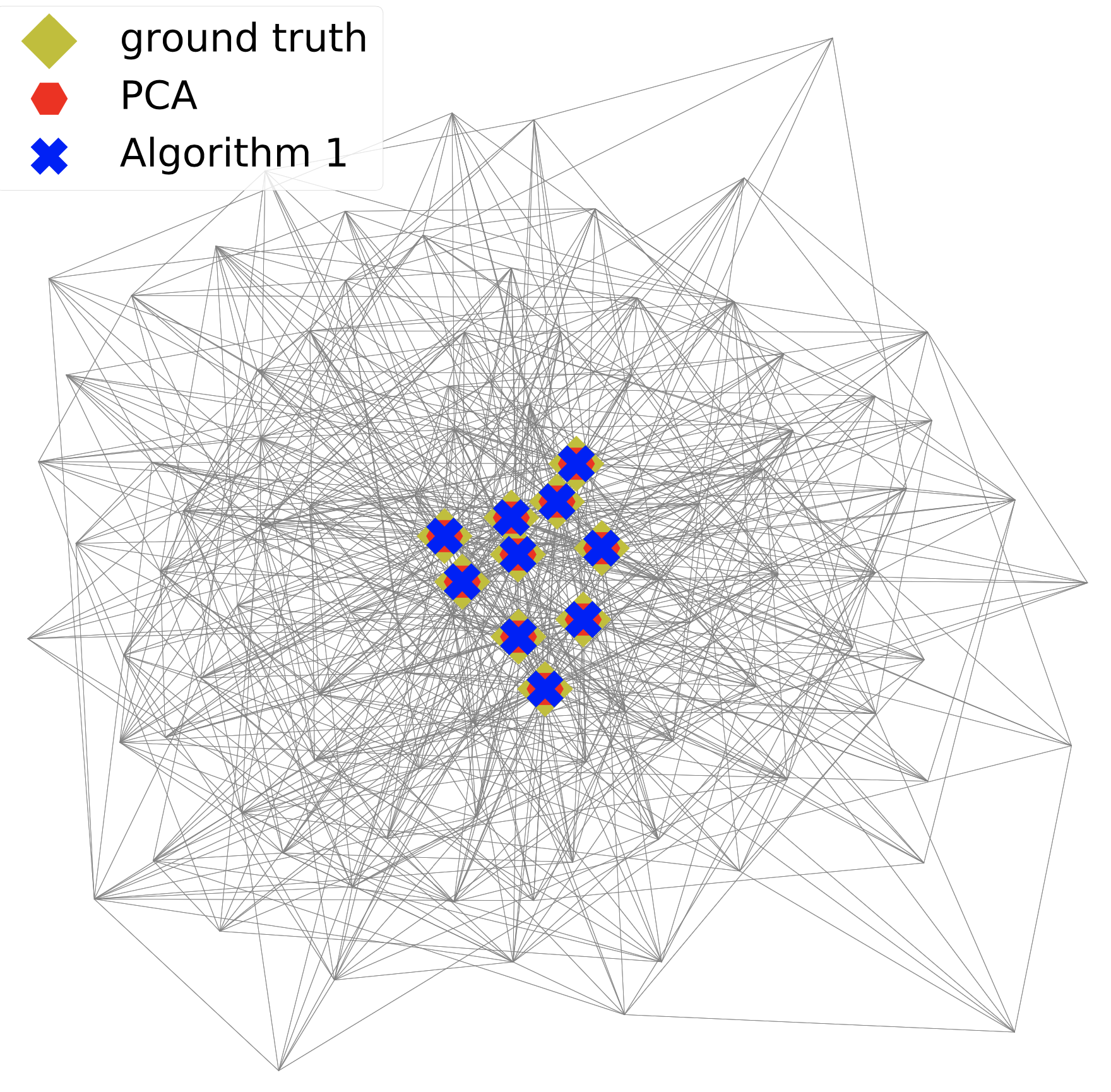
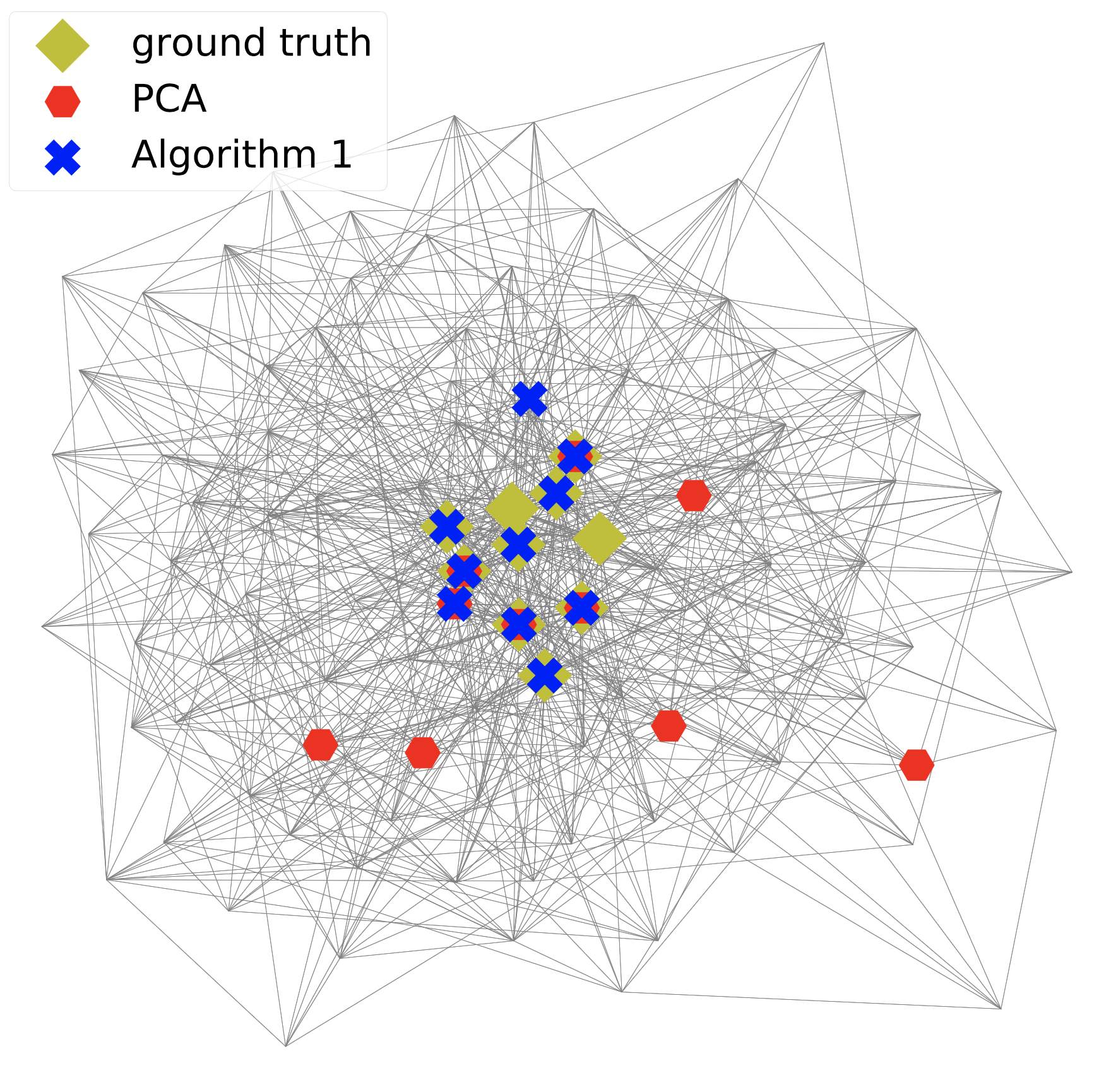
Figure 4: Toy Example illustrating the detection results of the proposed methods on a core periphery graph: (Left) with strong low pass filter ${\mathcal{}H}_{\sf strong}({\bm{A}})=e^{0.1{\bm{A}}}$; (Right) with weak low pass filter ${\mathcal{}H}_{\sf weak}({\bm{A}})=({\bm{I}}-\frac{1}{50}{\bm{A}})^{-1}$.

To summarize, Lemma 1 indicates that for strong low pass graph filter, i.e., $\eta\approx 0$, the PCA method (11) attains high accuracy for central nodes detection with $m\gg 1,\sigma^{2}\ll 1$. However, when dealing with weak low pass graph filter, i.e., $\eta\approx 1$, the method may become unreliable as shown below.

A Toy Example.  We consider detecting central nodes using the PCA method for a simple model. In Fig. 4, we show the detection results for an instance of applying (11) when the observed graph signals are filtered by different low pass filters. The underlying graph topology is a $100$-nodes core-periphery graph generated from a stochastic block model with $C=10$ fully connected central nodes and the excitation is low rank with $k=40$; see Section VI-A for details of the generation model. We observe that the top-10 central nodes are correctly detected by PCA when the underlying graph filter is strong low pass (left panel), yet PCA misidentified a number of nodes when underlying graph filter is weak low pass (right panel).

Before concluding this section, we remark that 1 can be specialized to analyze the top left singular vector of ${\mathcal{}H}({\bm{A}}){\bm{B}}$ for any low pass graph filter ${\mathcal{}H}({\bm{A}})$ and basis matrix ${\bm{B}}$. The result is given by the following corollary:

Corollary 1

Let $\widehat{\bm{v}}_{1},{\bm{q}}_{1}$ be the top left, right singular vector of ${\mathcal{}H}({\bm{A}}){\bm{B}}$, respectively, where ${\mathcal{}H}({\bm{A}})$ is a graph filter satisfying 1. Further, assume that $\widehat{\bm{v}}_{1}^{\top}{\bm{c}}_{\sf eig}\geq 0$ and ${\bm{c}}_{\sf eig}^{\top}{\bm{B}}{\bm{q}}_{1}\neq 0$. It holds

$$\|\widehat{\bm{v}}_{1}-{\bm{c}}_{\sf eig}\|\leq\sqrt{2}\eta\cdot\|{\bm{V}}_{n-1}^{\top}{\bm{B}}{\bm{q}}_{1}\|/|{\bm{v}}_{1}^{\top}{\bm{B}}{\bm{q}}_{1}|={\mathcal{}O}(\eta).\vspace{-.1cm}$$ (14)

The corollary directly relates the estimation error for the eigen-centrality to the low pass ratio. As $\eta\approx 0$, the singular value decomposition of ${\mathcal{}H}({\bm{A}}){\bm{B}}$ generates an accurate estimate of eigen-centrality. We shall exploit this observation next.

IV Detection with General Low Pass Filter

Consider the case of a general low pass graph filter where only $\eta<1$ is needed in 1. This case includes weak $1$-low pass graph filters with $\eta\approx 1$ that are found in some practical models, e.g., the examples in Section II-A have ${\mathcal{}H}({\bm{A}})=({\bm{I}}-c{\bm{A}})^{-1}$ with $\eta\approx 1$. The relaxed condition has made the blind central nodes detection problem significantly more challenging. For instance, simple methods such as PCA may no longer work as observed from (9), where the top eigenvector of ${\rm Cov}({\bm{y}}_{\ell})$ can be different from ${\bm{c}}_{\sf eig}$.

To handle this challenging case, a blind central nodes detection method is developed using two novel observations: (A) We derive an intrinsic decomposition for the graph signal model featuring a boosted graph filter with improved low pass ratio [23]. We then treat $\{{\bm{y}}_{i}\}_{i=1}^{m}$ using a factor analysis model and demonstrate that the desired eigen-centrality vector is embedded with additive and multiplicative perturbations. (B) By concentrating on a special case of the graph signal model with sparse and non-negative basis for the excitation, we treat a sparse non-negative matrix factorization (NMF) problem which can uniquely identify the latent parameter matrix if the unknown matrices satisfy a sufficiently scattered condition, i.e., removing the multiplicative perturbation. Then, a RPCA method is applied to remove the additive perturbation. These observations will be discussed in order.

Structured Factor Analysis Model.   Let $\rho\geq 0$ be a free parameter and assume that ${\bm{w}}_{\ell}={\bm{0}}$ for ease of exposition. Using the matrix notation ${\bm{Y}}=[{\bm{y}}_{1}~{}\cdots~{}{\bm{y}}_{m}]$, ${\bm{Z}}=[{\bm{z}}_{1}~{}\cdots~{}{\bm{z}}_{m}]$, we first observe the following intrinsic decomposition from (3), (5) for the graph signal matrix ${\bm{Y}}$:

$${\bm{Y}}=\big{\{}\tilde{\mathcal{}H}_{\rho}({\bm{A}})+\rho{\bm{I}}\big{\}}{\bm{B}}{\bm{Z}}=\big{\{}\tilde{\mathcal{}H}_{\rho}({\bm{A}}){\bm{B}}+\rho{\bm{B}}\big{\}}{\bm{Z}},$$ (15)

where $\widetilde{\mathcal{}H}_{\rho}({\bm{A}})$ is a boosted graph filter defined as [23]:

$$\widetilde{\mathcal{}H}_{\rho}({\bm{A}})\mathrel{\mathop{:}}={\mathcal{}H}({\bm{A}})-\rho{\bm{I}}.$$ (16)

The filter has a frequency response of $\tilde{h}_{\rho}(\lambda)\mathrel{\mathop{:}}=h(\lambda)-\rho$. A useful result from [23, Observation 1] is that under mild conditions, there exists $\rho>0$ such that $\widetilde{\mathcal{}H}_{\rho}({\bm{A}})$ is a stronger low pass graph filter than ${\mathcal{}H}({\bm{A}})$ with a strictly smaller low pass ratio. For example, consider the IIR graph filter ${\mathcal{}H}({\bm{A}})=({\bm{I}}-c{\bm{A}})^{-1}$. It can be shown that $\tilde{\mathcal{}H}_{\rho}({\bm{A}})$ has an improved low pass ratio, $\tilde{\eta}$, that is bounded by

$$\begin{split}\tilde{\eta}&:=\min_{\rho>0}\frac{\displaystyle\max_{j=2,...,n}|\tilde{h}_{\rho}(\lambda_{j})|}{|\tilde{h}_{\rho}(\lambda_{1})|}\leq\frac{\lambda_{2}}{\lambda_{1}}\frac{(1-c\lambda_{2})^{-1}}{(1-c\lambda_{1})^{-1}}=\frac{\lambda_{2}}{\lambda_{1}}\eta,\end{split}$$ (17)

where the bound is obtained by setting $\rho=1$. Together with the condition that $\lambda_{1}\gg\lambda_{2}$ as the graph $G$ admits a core-periphery structure, we have $\tilde{\eta}\ll\eta<1$. Denote the top left singular vector of $\widetilde{\mathcal{}H}_{\rho}({\bm{A}}){\bm{B}}$ as $\widehat{\bm{v}}_{\sf ideal}$. 1 shows that

$$\|\widehat{\bm{v}}_{\sf ideal}-{\bm{c}}_{\sf eig}\|={\mathcal{}O}(\tilde{\eta}).$$ (18)

In other words, if the matrix $\widetilde{\mathcal{}H}_{\rho}({\bm{A}}){\bm{B}}$ is known, then the eigen-centrality vector can be estimated by computing a singular value decomposition (SVD).

The main question is how to estimate the matrix $\widetilde{\mathcal{}H}_{\rho}({\bm{A}}){\bm{B}}$ from ${\bm{Y}}$? Notice that as $\tilde{\eta}\ll 1$, $\widetilde{\mathcal{}H}_{\rho}({\bm{A}}){\bm{B}}$ is approximately rank-one. From (15), we observe that this low-rank matrix is embedded in ${\bm{Y}}$ with unknown additive ($\rho{\bm{B}}$) and multiplicative perturbations (${\bm{Z}}$), which makes it difficult to estimate. Therefore, retrieving $\widetilde{\mathcal{}H}_{\rho}({\bm{A}}){\bm{B}}$ requires one to leverage additional structures in the graph signals. We are inspired by Examples 1 and 2 to concentrate on a case with:

Assumption 2

The basis matrix ${\bm{B}}$ is sparse and non-negative, and the excitation parameters ${\bm{Z}}$ are non-negative.

Besides Examples 1 and 2, we remark that the above can be satisfied in other applications such as in pricing experiments when the number of controllable agents is small [23]. Finally, we conclude that ${\bm{Y}}$ can be described by a structured factor model consisting of a low-rank plus sparse factor $\tilde{\mathcal{}H}_{\rho}({\bm{A}}){\bm{B}}+\rho{\bm{B}}$, and a non-negative factor ${\bm{Z}}$.

To grasp an idea of how 2 and (15) can contribute to tackling the blind central nodes detection problem, we may take a slight detour by considering the case when ${\bm{Z}}$ is known. Here, a standard algorithm is to apply the robust PCA (RPCA) method [20, 21] which leverages that $\rho{\bm{B}}$ is a sparse matrix. By solving a convex optimization problem [cf. (31)], it is possible to extract the desired low-rank component $\tilde{\mathcal{}H}_{\rho}({\bm{A}}){\bm{B}}$ from ${\bm{Y}}{\bm{Z}}^{\dagger}=\tilde{\mathcal{}H}_{\rho}({\bm{A}}){\bm{B}}+\rho{\bm{B}}$. As our target is to tackle the blind central nodes detection problem, we next focus on the case when ${\bm{Z}}$ is unknown where the property ${\bm{B}},{\bm{Z}}\geq{\bm{0}}$ is exploited by the NMF technique.

IV-A Identifying Factors in (15) using NMF

To fix notations, let us define

$${\bm{H}}_{\star}={\mathcal{}H}({\bm{A}}){\bm{B}}=\tilde{\mathcal{}H}_{\rho}({\bm{A}}){\bm{B}}+\rho{\bm{B}},~{}~{}{\bm{Z}}_{\star}={\bm{Z}}$$ (19)

as the ground truth factors satisfying ${\bm{Y}}={\bm{H}}_{\star}{\bm{Z}}_{\star}$. We concentrate on the special case where ${\bm{H}}_{\star}\geq{\bm{0}},{\bm{Z}}_{\star}\geq{\bm{0}}$. Notice that under 2, ${\bm{B}},{\bm{Z}}$ are non-negative matrices. Further, the condition ${\bm{H}}_{\star}\geq{\bm{0}}$ is satisfied for cases such as ${\mathcal{}H}({\bm{A}})=({\bm{I}}-c{\bm{A}})^{-1}$ with $c<||{\bm{A}}||^{-1}$. With these constraints on (15), the NMF problem finds a pair of matrices $(\widehat{\bm{H}}$, $\widehat{\bm{Z}})\in\Re^{n\times k}\times\Re^{k\times m}$ such that

$${\bm{Y}}={\bm{H}}_{\star}{\bm{Z}}_{\star}=\widehat{\bm{H}}\widehat{\bm{Z}},~{}~{}\widehat{\bm{H}}\geq{\bm{0}},~{}~{}\widehat{\bm{Z}}\geq{\bm{0}}.$$ (20)

We aim to study identifiability conditions which guarantee $\widehat{\bm{Z}}={\bm{Z}}_{\star}$, $\widehat{\bm{H}}={\bm{H}}_{\star}$ so that the low-rank matrix $\tilde{\mathcal{}H}_{\rho}({\bm{A}}){\bm{B}}$ can be derived from the latter, e.g., by applying RPCA. We shall emphasize that the non-negativity constraints are important. Notably, in their absence, for any invertible ${\bm{Q}}\in\Re^{k\times k}$, the pair $({\bm{H}}_{\star}{\bm{Q}},{\bm{Q}}^{-1}{\bm{Z}}_{\star})$ is admissible for the model in (20). Such ambiguity forbids us from estimating $\tilde{\mathcal{}H}_{\rho}({\bm{A}}){\bm{B}}$ with methods like RPCA since the matrix ${\bm{H}}_{\star}{\bm{Q}}=\tilde{\mathcal{}H}_{\rho}({\bm{A}}){\bm{B}}{\bm{Q}}+\rho{\bm{B}}{\bm{Q}}$ does not admit a low-rank plus sparse decomposition. It is unclear if the desired matrix $\tilde{\mathcal{}H}_{\rho}({\bm{A}}){\bm{B}}{\bm{Q}}$ can be extracted.

A major benefit of NMF is that under a relatively mild condition, (20) admits an essentially unique factorization, i.e., the recovered factors are only subjected to diagonal and permutation ambiguities. We observe:

Fact 1

[36, Theorem 4] Suppose that the rows of ${\bm{H}}_{\star}$ and columns of ${\bm{Z}}_{\star}$ are sufficiently scattered, i.e.,

$$\{{\bm{x}}\in\Re^{k}:{\bm{x}}^{\top}{\bf 1}\geq\sqrt{k-1}\|{\bm{x}}\|_{2}\}\subseteq{\rm cone}\{{\bm{H}}_{\star}^{\top}\},$$ (21)

${\rm cone}\{{\bm{H}}_{\star}^{\top}\}\not\subset{\rm cone}\{{\bm{Q}}\}$ for any orthonormal matrix ${\bm{Q}}$ except for the permutation matrix, and the same holds for ${\bm{Z}}_{\star}$. Then, any solution $(\widehat{\bm{H}}$, $\widehat{\bm{Z}})$ satisfying (20) can be written as

$$(\widehat{\bm{H}},\widehat{\bm{Z}})=({\bm{H}}_{\star}{\bm{D}}\bm{\Pi},\bm{\Pi}^{\top}{\bm{D}}^{-1}{\bm{Z}}_{\star}),$$ (22)

where ${\bm{D}}$ is a positive diagonal matrix, and $\bm{\Pi}$ is a permutation matrix.

The sufficiently scattered conditions are satisfied when the ground truth factors are mildly sparse [36]. Our next endeavor is to verify these conditions in terms of the graph signal properties and their impact on the performance of blind central nodes detection. We proceed by discussing two issues in order.

1) Identifiability.  The first issue is whether the identifiability conditions in 1 are satisfied for the filtered graph signals in (19). Unfortunately, at the first glance this appears to be impossible since a necessary condition for 1 to hold is that ${\bm{H}}_{\star}$ contains at least $k-1$ zeros at every row [36, Corollary 2], while ${\bm{H}}_{\star}={\mathcal{}H}({\bm{A}}){\bm{B}}$ is a dense matrix in general.

As a remedy, we consider the approximate model ${\bm{Y}}\approx\rho{\bm{B}}{\bm{Z}}$ and exploit that the basis matrix ${\bm{B}}$ is sparse. Interestingly, the next result recognizes that ${\bm{H}}_{\star}\approx\rho{\bm{B}}$ when the original graph filter’ low pass ratio satisfies $\eta\approx 1$, i.e., the graph filter is weak low pass. To derive this result, we notice the constant $\rho$ is a parameter that can be freely adjusted as it is implicit in the signal model. Specific to the current context, we seek for $\rho>0$ such that the ratio of $\|\widetilde{\mathcal{}H}_{\rho}({\bm{A}}){\bm{B}}\|$ to $\rho\|{\bm{B}}\|$ is minimized. We observe that:

Lemma 2

Under Assumption 1. Suppose that the frequency response $h(\lambda)$ is a convex function and is non-negative over $[\lambda_{n},\lambda_{1}]$. Define $h_{\sf min}:=\min_{i=2,...,n}h(\lambda_{i})$ as the smallest frequency response. It holds

$$\min_{\rho>0}\frac{\|\widetilde{\mathcal{}H}_{\rho}({\bm{A}}){\bm{B}}\|}{\rho\|{\bm{B}}\|}\leq\frac{1-\eta+\frac{\max\{h(\lambda_{2}),h(\lambda_{n})\}-h_{\sf min}}{h(\lambda_{1})}}{1+\eta-\frac{\max\{h(\lambda_{2}),h(\lambda_{n})\}-h_{\sf min}}{h(\lambda_{1})}}.$$ (23)

Furthermore, if $\max\{h(\lambda_{2}),h(\lambda_{n})\}-h_{\sf min}\ll h(\lambda_{1})$, then:

$$\min_{\rho>0}\frac{\|\widetilde{\mathcal{}H}_{\rho}({\bm{A}}){\bm{B}}\|}{\rho\|{\bm{B}}\|}\lesssim\frac{1-\eta}{1+\eta}.\vspace{-.1cm}$$ (24)

The proof can be found in Appendix B and is based on bounding $\rho$ which minimizes the left hand side of (23). In particular, the above shows that the approximation ${\bm{H}}_{\star}\approx\rho{\bm{B}}$ holds if $\eta\approx 1$. Note that the convexity assumption on $h(\cdot)$ is satisfied by the graph filters considered in this work.

Contrary to ${\bm{H}}_{\star}$, the matrix $\rho{\bm{B}}$ is sparse and non-negative. Now consider 1, while the sufficiently scattered condition (21) is NP-complete to check, it is noted “if the latent factors are sparse, it is more likely that the sufficient condition given in 1 is satisfied” [36]. For an NMF model with $\widehat{\bm{Y}}=\rho{\bm{B}}{\bm{Z}}$, a special case where the stated conditions hold is when ${\rm cone}\{{\bm{e}}_{1},...,{\bm{e}}_{k}\}\subseteq{\rm cone}\{{\bm{B}}^{\top}\}$, i.e., ${\bm{B}}$ contains $k$ pure pixel row vectors. When combined with 2, we observe:

Corollary 2

Assume the system parameters $({\bm{B}},{\bm{Z}})$ satisfy 2 and the sufficiently scattered condition in 1, and the assumptions in 2 are satisfied with $\eta\approx 1$. Then solving (20) yields

$$\widehat{\bm{Z}}\approx\bm{\Pi}^{\top}{\bm{D}}^{-1}{\bm{Z}}_{\star},$$ (25)

for some positive diagonal and permutation matrices ${\bm{D}}$, $\bm{\Pi}$.

It has been demonstrated in [36, 19] that the sufficiently scattered conditions hold as long as $({\bm{B}},{\bm{Z}})$ are not fully dense. Concretely, when ${\bm{B}}$ is a random sparse matrix, the NMF model is shown numerically to be identifiable with high probability when the ratio $n/k$ is large.

2) Ambiguities.  Having verified the identifiability conditions for the NMF model, we study the effects on central nodes detection performance caused by diagonal and permutation ambiguities. We find that these ambiguities are typically dismissed in existing applications of NMF such as source separation, topic modeling, and clustering, etc., as they do not directly affect the performances in these applications.

For the blind central nodes detection problem, obtaining $(\widehat{\bm{B}},\widehat{\bm{Z}})$ is not the final goal. Instead, our objective is to estimate the eigen-centrality. As 2 guarantees that $\widehat{\bm{Z}}\approx\bm{\Pi}^{\top}{\bm{D}}^{-1}{\bm{Z}}_{\star}$, we apply the RPCA method to treat ${\bm{Y}}\widehat{\bm{Z}}^{\dagger}\approx{\bm{H}}_{\star}{\bm{D}}\bm{\Pi}$ and recover the low-rank matrix therein as

$$\widehat{\bm{L}}=\tilde{\mathcal{}H}_{\rho}({\bm{A}}){\bm{B}}{\bm{D}}\bm{\Pi}.$$ (26)

Here, ${\bm{D}}$ can be any positive diagonal matrix, the top left singular vector of $\widehat{\bm{L}}$ is a poor estimate of the eigen-centrality.

Our remedy is to estimate the row sum ${\bm{Z}}_{\star}{\bf 1}$ a-priori in order to fix the diagonal ambiguity matrix ${\bm{D}}$. Consider

Assumption 3

For any $\ell,j$, $z_{\ell,j}$ is an independent random variable with $\mathbb{E}[z_{\ell,j}]=\alpha$ and sub-Gaussian parameter $\sigma_{z}$.

The above condition is related to having persistent excitation for the external sources. Together with the approximation analyzed in 2, we study a modified NMF model from (20) with additional constraint as:

$${\bm{Y}}=\rho{\bm{B}}{\bm{Z}}+{\bm{W}}\equiv\widehat{\bm{B}}\widehat{\bm{Z}}+{\bm{W}},~{}\widehat{\bm{B}}\geq{\bm{0}},~{}\widehat{\bm{Z}}\geq{\bm{0}},~{}\widehat{\bm{Z}}{\bf 1}={\bf 1},$$ (27)

where ${\bm{W}}$ is the approximation error from ${\bm{Y}}\approx\rho{\bm{B}}{\bm{Z}}$. We analyze the low-rank matrix recovered using the RPCA method from $\widehat{\bm{Z}}$ satisfying (27) and obtain the lemma below:

Lemma 3

Under Assumptions 1 and 3. Let $\widehat{\bm{L}}$ be defined in (26) using $\widehat{\bm{Z}}$ computed from (27), and its top left (resp. right) singular vector be $\widetilde{\bm{v}}_{1}$ (resp. ${\bm{q}}_{1}$). For any $\delta>0$ and sufficiently large $m$, it holds with probability at least $1-2k\delta$,

$$\|\widetilde{\bm{v}}_{1}-{\bm{c}}_{\sf eig}\|_{2}\leq\sqrt{2}\,\tilde{\eta}\,\frac{\alpha+\frac{2\sigma_{z}^{2}}{m}\log(\delta^{-1})}{\alpha-\frac{2\sigma_{z}^{2}}{m}\log(\delta^{-1})}\frac{\|{\bm{V}}_{n-1}^{\top}{\bm{B}}\bm{\Pi}{\bm{q}}_{1}\|_{2}}{|{\bm{v}}_{1}^{\top}{\bm{B}}\bm{\Pi}{\bm{q}}_{1}|}.\vspace{-.2cm}$$ (28)

The proof, which is based on the Hoeffding’s inequality and 1, can be found in Appendix C. As the number of samples grows $m\rightarrow\infty$, the estimate of the eigen-centrality vector becomes more accurate. We remark that 3 can be relaxed to allow for heterogeneous mean in ${\bm{z}}_{\ell}$, i.e., $\mathbb{E}[z_{\ell,j}]=\alpha_{j}$. In the latter case, the bound (28) will be relaxed to ${\mathcal{}O}(\tilde{\eta}\,\max_{i,j}\frac{\alpha_{i}}{\alpha_{j}})$ when $m\gg 1$.

Algorithm 1 Two-Stage Decomposition Algorithm

1:  INPUT: graph signal matrix ${\bm{Y}}$, regularization parameters $\lambda_{B},\lambda_{S},\lambda_{L}>0$, and the dimension of latent excitation parameters $k$.

2:   Tackle the NMF problem (29) to estimate the latent excitation parameters $\widehat{\bm{Z}}$; see Algorithm 2.

3:  Solve the RPCA problem (31) using $\widehat{\bm{H}}$ from (30).

4:   Compute $\widetilde{\bm{v}}_{1}$ as the top left singular vector of $\widehat{\bm{L}}$.

5:  OUTPUT: select $C$ elements with the highest magnitude in $\widetilde{\bm{v}}_{1}$ as the detected central nodes.

IV-B Two-stage Decomposition Algorithm

The previous discussions established the theoretical foundation of detecting central nodes from graph signals filtered by a general low pass graph filter. Hereafter, we describe how to utilize these observations to develop a practical algorithm.

In light of the structured factor model (15) and our theoretical findings, we split the detection problem into two stages — the first stage estimates the latent excitation parameters $\widehat{\bm{Z}}\approx{\bm{Z}}_{\star}$; the second stage estimates the low-rank matrix $\tilde{\mathcal{}H}_{\rho}({\bm{A}}){\bm{B}}{\bm{D}}\bm{\Pi}$ from ${\bm{Y}}$ based on $\widehat{\bm{Z}}$. Finally, the central nodes are detected through computing and ranking the magnitude of top left singular vector of the estimated $\tilde{\mathcal{}H}_{\rho}({\bm{A}}){\bm{B}}{\bm{D}}\bm{\Pi}$.

The first stage is the most challenging as it relies on identifying the factors from the NMF model (27). In light of Assumptions 2 and 3, we seek for a solution where the ‘left’ factor is a sparse matrix and the row sums of the ‘right’ factor equal to one. Taking into account the noisy observations and the approximation errors, we consider a sparse NMF criterion:

$$\begin{array}[]{rl}\displaystyle\min_{\widehat{\bm{B}}\in\Re^{n\times k},\widehat{\bm{Z}}\in\Re^{k\times m}}&{\textstyle\frac{1}{2}}\|{\bm{Y}}-\widehat{\bm{B}}\widehat{\bm{Z}}\|_{F}^{2}+\lambda_{B}\|{\rm vec}(\widehat{\bm{B}})\|_{1}\\ \text{s.t.}&\widehat{\bm{Z}}{\bf 1}={\bf 1},~{}\widehat{\bm{B}}\geq{\bm{0}},~{}\widehat{\bm{Z}}\geq{\bm{0}},\end{array}$$ (29)

such that $\lambda_{B}>0$ is a regularization parameter promoting sparsity for the solution $\widehat{\bm{B}}$. Notice that while sparse NMF has been applied in empirical studies [37], our criterion is directly motivated by the identifiability conditions in 2 for the graph signals as we aim to recover $\widehat{\bm{B}},\widehat{\bm{Z}}$. The above problem can be efficiently tackled as a customized solver for (29) will be discussed in Section V.

An important observation is when the sufficiently scattered conditions hold for the matrices $({\bm{B}},{\bm{Z}})$, 2 only shows that the solution of (29) satisfies $\widehat{\bm{Z}}\approx\bm{\Pi}^{\top}{\bm{D}}^{-1}{\bm{Z}}_{\star}$. However, our target is to estimate ${\bm{H}}_{\star}$ instead. The latter is achieved by solving the least square problem, e.g.,

$$\textstyle\min_{\widehat{\bm{H}}\in\Re^{n\times k}}~{}\|{\bm{Y}}-\widehat{\bm{H}}\widehat{\bm{Z}}\|_{F}^{2}.$$ (30)

Notice that the solution to (30), i.e., $\widehat{\bm{H}}\approx\tilde{\mathcal{}H}_{\rho}({\bm{A}}){\bm{B}}{\bm{D}}\bm{\Pi}+\rho{\bm{B}}{\bm{D}}\bm{\Pi}$, is composed of a low-rank matrix and a sparse matrix. As such, in the second stage of our algorithm, we solve the RPCA problem:

$$\min_{\widehat{\bm{L}},\widehat{\bm{S}}\in\Re^{n\times k}}~{}\|\widehat{{\bm{H}}}-\widehat{\bm{L}}-\widehat{\bm{S}}\|_{F}^{2}+\lambda_{L}\|\widehat{\bm{L}}\|_{\star}+\lambda_{S}\|{\rm vec}(\widehat{\bm{S}})\|_{1},$$ (31)

where $\lambda_{S},\lambda_{L}>0$ are regularization parameters, to obtain an estimate of $\tilde{\mathcal{}H}_{\rho}({\bm{A}}){\bm{B}}{\bm{D}}\bm{\Pi}$. Similar to [23], this step may also be directly applied when ${\bm{Z}}$ is known [cf. Fig. 3]. With appropriate parameters $\lambda_{S},\lambda_{L}$, the solution to (31) satisfies $\widehat{\bm{L}}\approx\tilde{\mathcal{}H}_{\rho}({\bm{A}}){\bm{B}}{\bm{D}}\bm{\Pi}$. The central nodes can be detected subsequently by computing the top singular vector of the former matrix. We remark that (31) is a convex problem that can be solved efficiently using existing algorithms, e.g., [38].

Finally, our method for blind central nodes detection is summarized in Algorithm 1. Notice that Algorithm 1 requires knowing the excitation’s rank $k$ which can be estimated heuristically from observing the rank of ${\rm Cov}({\bm{y}}_{\ell})$.

Discussion.  We briefly discuss the performance of Algorithm 1. For the first stage, observe that (29) aims at estimating ${\bm{Z}}_{\star}$ by fitting a pair $(\widehat{\bm{B}},\widehat{\bm{Z}})$ to ${\bm{Y}}\approx\rho{\bm{B}}{\bm{Z}}$. To this end, 2 shows that the estimation quality depends on two factors: (i) whether the matrices ${\bm{B}},{\bm{Z}}$ satisfy the sufficiently scattered conditions, and (ii) whether the graph filter is weak low pass [cf. 2].

For the second stage, it is known that if the matrix $\widehat{\bm{H}}$ admits a low-rank plus sparse structure, then solving the RPCA problem (31) decomposes $\widehat{\bm{H}}$ accordingly to the desired low-rank and sparse components. Under these premises, using [20, Corollary 1], it can be shown that the vector $\widetilde{\bm{v}}_{1}$ found in Step 4 of Algorithm 1 is ${\mathcal{}O}(\tilde{\eta})$-close to ${\bm{c}}_{\sf eig}$. With $\tilde{\eta}\ll 1$ due to boosted graph filter, the top-$C$ central nodes can be detected.

The careful readers may notice that when the original graph filter is strong low pass, i.e., $\eta\approx 0$, the approximation ${\mathcal{}H}({\bm{A}}){\bm{B}}\approx\rho{\bm{B}}$ induced by 2 is not guaranteed and the NMF model may become unidentifiable. However, it does not prevent Algorithm 1 from correctly detecting the central nodes. This is because the data matrix ${\bm{Y}}$ as well as the matrix $\widehat{\bm{H}}$ in step 3 of Algorithm 1 are already close to rank-one since $\eta\approx 0$. As such, the obtained estimate $\widetilde{\bm{v}}_{1}$ remains ${\mathcal{}O}(\eta)$-close to ${\bm{c}}_{\sf eig}$ despite erroneous estimation of $\widehat{\bm{Z}}$. We observe from Fig. 4 that Algorithm 1 can successfully detect the central nodes regardless of the low pass filters’ strengths. Therefore, we conclude that Algorithm 1 is suitable for blind central nodes detection with general low pass graph filter.

Remark 1

Notice that Step 3 of Algorithm 1 recovers the low rank matrix as $\widehat{\bm{L}}\approx\tilde{\mathcal{}H}_{\rho}({\bm{A}}){\bm{B}}{\bm{D}}\bm{\Pi}$. The latter can be treated as a set of graph signals filtered by a strong low pass graph filter $\tilde{\mathcal{}H}_{\rho}({\bm{A}})$ with the excitation $[\tilde{\bm{b}}_{1},\ldots,\tilde{\bm{b}}_{K}]\equiv{\bm{B}}{\bm{D}}\bm{\Pi}$. It is an interesting future direction to develop graph learning algorithms for recovering the adjacency matrix ${\bm{A}}$ from $\widehat{\bm{L}}$.

V Practical Issues

We dedicate this section to the practical issues in applying the proposed blind central nodes detection method.

V-A Efficient Implementation of (29)

We provide details of an efficient algorithm for tackling problem (29). Observe that the latter problem is non-convex, we apply an alternating minimization strategy based on projected gradient descent (PGD) similar to [39]. Let us define the following objective function:

$$f(\widehat{\bm{B}},\widehat{\bm{Z}})\mathrel{\mathop{:}}={\textstyle\frac{1}{2}}\|{\bm{Y}}-\widehat{\bm{B}}\widehat{\bm{Z}}\|_{F}^{2}+\lambda_{B}{\textstyle\sum_{i,j}}\widehat{B}_{ij}$$ (32)

and the simplex constraint for $\hat{\bm{Z}}$:

$$\Delta^{K}=\{{\bm{Z}}\in\Re^{k\times m}:{\bm{Z}}\geq{\bm{0}},{\bm{Z}}{\bf 1}={\bf 1}\}.$$

We notice that under the constraint $\widehat{\bm{B}}\geq{\bm{0}}$, minimizing the objective function of (29) is equivalent to minimizing $f(\widehat{\bm{B}},\widehat{\bm{Z}})$ as $\|{\rm vec}(\widehat{\bm{B}})\|_{1}=\sum_{i,j}\widehat{B}_{i,j}$. The benefit of solving (32) is that the latter function is differentiable.

Algorithm 2 Alternating Projected Gradient Descent for (29)

1:  INPUT: graph signals matrix ${\bm{Y}}$, the dimension of latent parameters $k$.

2:  Initialize $\widehat{\bm{B}}^{(0)}\geq{\bm{0}}$ and $\widehat{\bm{Z}}^{(0)}\geq{\bm{0}}$ satisfying $\widehat{\bm{Z}}^{(0)}{\bf 1}={\bf 1}$.

3:  for $t=0,...,T-1$ do

4:     Select step sizes $\alpha_{t},\beta_{t}$ according to (33).

5:     $\widehat{\bm{B}}^{(t+1)}=\big{(}\widehat{\bm{B}}^{(t)}-\alpha_{t}{\nabla}_{\bm{B}}f(\widehat{\bm{B}}^{(t)},\widehat{\bm{Z}}^{(t)})\big{)}_{+}$

6:     $\widehat{\bm{Z}}^{(t+1)}={\mathcal{}P}_{\Delta^{k}}\big{(}\widehat{\bm{Z}}^{(t)}-\beta_{t}{\nabla}_{\bm{Z}}f(\widehat{\bm{B}}^{(t+1)},\widehat{\bm{Z}}^{(t)})\big{)}$

7:  end for

8:  OUTPUT: estimate of latent parameter matrix $\widehat{\bm{Z}}^{(T)}$.

Based on this modification, the alternating PGD algorithm is described in Algorithm 2. The algorithm is initialized by picking random matrices $\widehat{\bm{B}}^{(0)},\widehat{\bm{Z}}^{(0)}$, or using heuristics such as ALS [40]. Notice that in line 5, the operator $(\cdot)_{+}$ denotes the element-wise maximum operator $\max\{\cdot,0\}$; in line 6, the operator ${\mathcal{}P}_{\Delta^{k}}(\cdot)$ denotes the Euclidean projection onto the simplex constraint set. By observing the decomposition $\Delta^{k}=\Delta_{1}\times\cdots\times\Delta_{k}$ where $\Delta_{i}$ is the $m$-dimensional probability simplex constraining the $i$th row vector, the projection can be performed efficiently by running $k$ instances of [41, Algorithm 1] in parallel, each involving a complexity of ${\mathcal{}O}(m\log m)$. Finally, at iteration $t$, we select the step sizes by calculating

$$\begin{split}\alpha_{t}&=\max\Big{\{}\delta_{B},\frac{a}{\|(\widehat{\bm{Z}}^{(t)})^{\top}\widehat{\bm{Z}}^{(t)}\|}\Big{\}},\\ \beta_{t}&=\max\Big{\{}\delta_{Z},\frac{b}{\|(\widehat{\bm{B}}^{(t+1)})^{\top}\widehat{\bm{B}}^{(t+1)}\|}\Big{\}},\end{split}$$ (33)

where $\delta_{B},\delta_{Z}>0$ are small pre-fixed constants to prevent numerical instability, and $a,b\in(0,1]$ are pre-fixed step size parameters. The update steps in line 5, 6 may be repeated for several times to improve convergence.

It is known that Algorithm 2 converges to a stationary solution of (29) and the overall per-iteration complexity is ${\mathcal{}O}(nkm+km\log m)$. To this end, we modify the result proven in [39] for general hybrid BCD algorithm, specialized to our algorithm when both variables are updated via the PGD:

Fact 2

Denote the iterates of Algorithm 2 as ${\bm{x}}^{(t)}=(\widehat{\bm{B}}^{(t)},\widehat{\bm{Z}}^{(t)})$. Then, for any $T\geq 1$, it holds

$$\min_{t=0,...,T-1}\max_{{\bm{y}}\in{\mathcal{}B}^{0}\times\Delta^{k}}\langle{\nabla}f({\bm{x}}^{(t)}),{\bm{x}}^{(t)}-{\bm{y}}\rangle={\mathcal{}O}(1/T),$$ (34)

where ${\mathcal{}B}^{0}=\{{\bm{B}}:{\bm{B}}\geq{\bm{0}},\sum_{ij}B_{ij}\leq\lambda_{S}^{-1}f(\widehat{\bm{B}}^{(0)},\widehat{\bm{Z}}^{(0)})\}$ is a compact subset of $\Re^{n\times k}$.

The above is proven in Appendix D through establishing that the objective value is monotonically decreasing, as such ${\mathcal{}B}^{0}\times\Delta^{k}$ must contain a stationary solution to (27). It follows that (34) implies Algorithm 2 finds an $\epsilon$-stationary solution to (29) in ${\mathcal{}O}(1/\epsilon)$ iterations, which is a standard convergence rate for constrained non-convex optimization.

V-B Distinguishing Strong and General Low Pass Filter

As overviewed in Fig. 3, the PCA method (11) is suitable for detecting central nodes when the graph filter is strong low pass with $\eta\approx 0$; while the NMF-based Algorithm 1 is suitable for general low pass graph filter with $\eta<1$. As illustrated in Section VI, Algorithm 1 demonstrates good performances in all cases. However, to balance between computation complexity and performance, it is desirable to select a suitable algorithm for the given dataset. As it is unknown in general if the underlying graph filter is strong low pass or not, a heuristic is to determine that the graph filter is strong low pass if the the covariance matrix ${\rm Cov}({\bm{y}}_{\ell})$ is approximately rank-one. We leave it as a future work to develop a data-driven algorithm to detect the type of graph filter; see [42, 43].

VI Numerical Experiments

In this section, we present numerical experiments on the proposed centrality nodes detection methods. We validate their efficacy compared to the state-of-the-art algorithms.

VI-A Experiments on Synthetic Data

We evaluate the performances of our algorithms using synthetic graph signals. Two types of random graph models are considered. The first random graph is the core-periphery (CP) graph [29] described by a stochastic block model with $2$ blocks and $n$ nodes. The node set ${\mathcal{}V}=\{1,...,n\}$ is partitioned into ${\mathcal{}V}_{\sf c}=\{1,...,10\}$ and ${\mathcal{}V}_{\sf p}={\mathcal{}V}\setminus{\mathcal{}V}_{\sf c}$. For any $i,j\in{\mathcal{}V}$, an edge is assigned independently with probability $p_{1}$ if $i,j\in{\mathcal{}V}_{\sf c}$; with probability $\min\{p_{1},4p_{2}\}$ if $i\in{\mathcal{}V}_{\sf c},j\in{\mathcal{}V}_{\sf p}$; and with probability $p_{2}$ if $i,j\in{\mathcal{}V}_{\sf p}$. Assume that $p_{1}\gg p_{2}$, the nodes in ${\mathcal{}V}_{\sf c}$ are connected with a higher density of edges than the other nodes. The second random graph is the Barabasi-Albert (BA) model [2]. The model is constructed according to a preferential attachment mechanism: during the graph generation, every new node is connected to $m_{\sf BA}=10$ existing nodes selected randomly proportional to their degrees. Again, the constructed graph exhibits a core-periphery structure as the oldest nodes have high degrees. For the experiments with BA graph, the ground truth top-$C$ central nodes, ${\mathcal{}V}_{\sf c}$, are computed from evaluating the eigen-centrality vector ${\bm{c}}_{\sf eig}$.

We generate the basis matrix ${\bm{B}}\in\Re^{n\times k}$ as a sparse matrix such that $B_{ij}=M_{ij}\widetilde{B}_{ij}$, where $M_{ij},\widetilde{B}_{ij}$ are independent r.v.s, $M_{ij}\in\{0,1\}$ is Bernouli with $\mathbb{E}[M_{ij}]=0.1$, and $\widetilde{B}_{ij}\sim{\mathcal{}U}([0.1,1])$, i.e., $10\%$ of the entries in ${\bm{B}}$ are non-zero. For the latent parameter matrix ${\bm{Z}}\in\Re^{k\times m}$, we have $Z_{ij}=N_{ij}\widetilde{Z}_{ij}$, where $N_{ij},\widetilde{Z}_{ij}$ are independent r.v.s, $N_{ij}\in\{0,1\}$ is Bernouli with $\mathbb{E}[N_{ij}]=0.6$, and $\widetilde{Z}_{ij}\sim{\mathcal{}U}([0.1,1])$, i.e., $60\%$ of the entries in ${\bm{Z}}$ are non-zero.

The observed graph signal is generated as (3), (5) with noise variance $\sigma^{2}=0.01$. We consider two low pass graph filters: (a) ${\mathcal{}H}_{\sf weak}({\bm{A}})=({\bm{I}}-\frac{1}{50}{\bm{A}})^{-1}$, (b) ${\mathcal{}H}_{\sf strong}({\bm{A}})=e^{0.1{\bm{A}}}$. Notice that ${\mathcal{}H}_{\sf weak}({\bm{A}})$ is weak low pass with $\eta\approx 1$, meanwhile ${\mathcal{}H}_{\sf weak}({\bm{A}})$ is strong low pass with $\eta\ll 1$. Fix any $C\in\mathbb{N}$, we focus on the performance of central nodes detection by computing the error rate of detecting the nodes in ${\mathcal{}V}_{\sf c}$ as the top-$C$ central nodes. Specifically, let $\widehat{\mathcal{}V}_{\sf c}$ be the set of central nodes detected by the algorithms. We define the error rate as

$$\textstyle{\sf Error~{}rate}=\mathbb{E}\big{[}\frac{1}{C}|{\mathcal{}V}_{\sf c}\cap\widehat{\mathcal{}V}_{\sf c}|\big{]},$$ (35)

and perform 100 Monte-carlo trials to approximate the above.

Figure 5: Error rate of the central nodes detection methods against the excitation’s rank $k$ on (Left) ${\mathcal{}H}_{\sf weak}({\bm{A}})$ and (Right) ${\mathcal{}H}_{\sf strong}({\bm{A}})$ for CP graph with $p_{1}=0.4,p_{2}=0.05$ and $n=100$ nodes. The RPCA method is plotted with a dashed line to indicate that it requires the extra input ${\bm{Z}}$.

We benchmark the two proposed methods – (i) PCA method (11) and (ii) Algorithm 1. Moreover, we test the RPCA method (31) which assumes ${\bm{Z}}$ is known for benchmarking purpose. For (31), we set the regularization parameters as $\lambda_{L}=0.2$, $\lambda_{S}=0.2+\frac{2}{\sqrt{k}}$ and the convex optimization problem is solved using cvxpy with the built-in solver SCS; while we set $\lambda_{B}=0.001m$ in Algorithm 1. Notice that the RPCA method is ‘semi-blind’ that requires ${\bm{Z}}$; while the PCA method and Algorithm 1 are ‘fully blind’ algorithms which do not require additional inputs other than the observed graph signals $\{{\bm{y}}_{\ell}\}_{\ell=1}^{m}$ and the estimate of $k$. Lastly, in Algorithm 1, we estimate $\widehat{\bm{Z}}$ via Algorithm 2, which is initialized by setting each $\widehat{Z}_{ij}^{(0)}$, $\widehat{B}_{ij}^{(0)}$ to be ${\mathcal{}U}([0,1])$, and is terminated with a fixed number of iteration at $T=10^{4}$ to ensure convergence to optimal solution. For the subroutine Algorithm 2, the stepsize parameters $a,b$ [cf. (33)] are set as: (a) $a=b=0.1$ for ${\mathcal{}H}_{\sf weak}({\bm{A}})$ with CP graph, (b) $a=b=0.01$ for ${\mathcal{}H}_{\sf strong}({\bm{A}})$ with CP graph, (c) $a=b=0.01$ with BA graph. In addition, we compare with the natural heuristics which learns the graph topology from graph signals, and then detect the central nodes using the eigen-centrality vector computed from the estimated adjacency/Laplacian matrix. We benchmark with graph learning methods including GL-SigRep [13], SpecTemp [14], the method by Kalofolias [44], as well as the $k_{\sf NN}$-nearest neighbor (kNN) graph constructed by setting an edge between a node and its $k_{\sf NN}=0.1n$ most correlated neighbors in the observed graph signals.

The first example focuses on the effect of excitation’s rank, $k$, on the detection performance. The number of graph signal samples is $m=200$ and we consider CP graphs with $p_{1}=0.4,p_{2}=0.05$ and $n=100$ nodes. In Fig. 5 (Left), we focus on the case with weak low pass graph filter and compare the error rates in computing the top-10 central nodes of different algorithms against $k$. We observe that the error rate for the proposed methods generally decreases when $k$ increases. The semi-blind RPCA method obtains the best performance, followed by the fully blind Algorithm 1. Importantly, Algorithm 1 delivers a significantly lower error rate compared to the methods which learn the complete graph topology. With a latent dimension of $k=40$, Algorithm 1 detects the central nodes with an error rate of $\sim\!\!0.2$, which is three-fold lower than PCA and the other graph learning methods. Lastly, we observe an increased error rate for Algorithm 1 at $k=50$. This is because as discussed in Section IV, the NMF identifiability condition becomes more difficult to satisfy as the ratio $\frac{n}{k}$ decreases, see Fig. 7 for a further investigation on this phenomena. Furthermore, in Fig. 5 (Right), we consider the strong low pass graph filter. The proposed methods obtain almost zero error rates over the range of $k$ tested.

(a) Top-10 error for CP graph against the core connectivity $p_{1}$.

(b) Top-50 error for BA graph against excitation’s rank $k$.

Figure 6: Error rate comparison for the central nodes detection methods. (Left) Weak low pass filter ${\mathcal{}H}_{\sf weak}({\bm{A}})$. (Right) Strong low pass filter ${\mathcal{}H}_{\sf strong}({\bm{A}})$. Readers are referred to Fig. 5 for legend of the above plots.

The second example considers the effect of the core-periphery structure on the detection performance. Specifically, in Fig. 6 (a), we focus on the CP graph with $n=100$ nodes, $p_{2}=0.05$, and compare the error rates against the connectivity parameter among the core nodes, $p_{1}\in\{0.1,...,1.0\}$. The excitation’s rank is fixed at $k=40$. As observed, the error rates generally decrease as $p_{1}$ increases for both strong and weak low pass graph filters. This is anticipated since the spectral gap in the adjacency matrix $\frac{\lambda_{2}}{\lambda_{1}}$ improves as the graph exhibits a stronger core-periphery structure. Moreover, the proposed Algorithm 1 and RPCA method (31) outperform the benchmark algorithms.

The third example tests the performance of detecting central nodes when the underlying graph is the BA graph with $n=100$ nodes. Notice that we focus on the error rate in detecting the top-$C=50$ central nodes defined by ${\bm{c}}_{\sf eig}$ of the adjacency matrix. We compare the error rate against the excitation’s rank $k$. The result is shown in Fig. 6 (b). As in the first example, for both strong and weak low pass graph filters, we observe that the error rate gradually decreases as $k$ increases, and the proposed Algorithm 1 outperforms the benchmark algorithms. However, we note that the performance gap is not as significant as in the case of CP graphs. A possible reason for this is that the BA graphs have a weaker core-periphery structure than CP graphs; in fact, nodes with similar magnitude in the eigen-centrality vector ${\bm{c}}_{\sf eig}$ may be misidentified.

Figure 7: Error rate of the central nodes detection methods against the size of graph $n$ for (Left) CP and (Right) BA with excitation’s rank $k=50$ on ${\mathcal{}H}_{\sf weak}^{\prime}({\bm{A}})$.

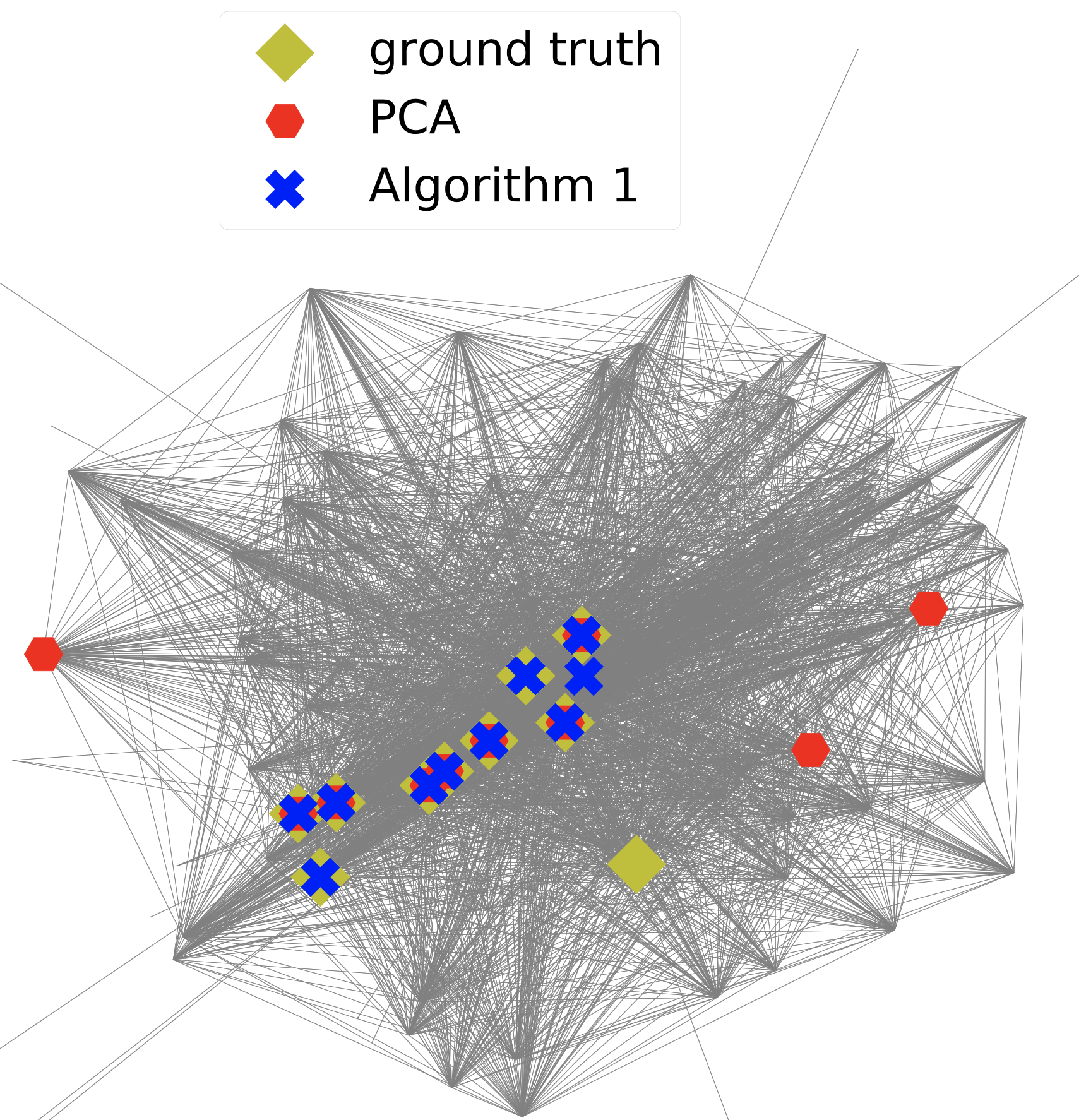
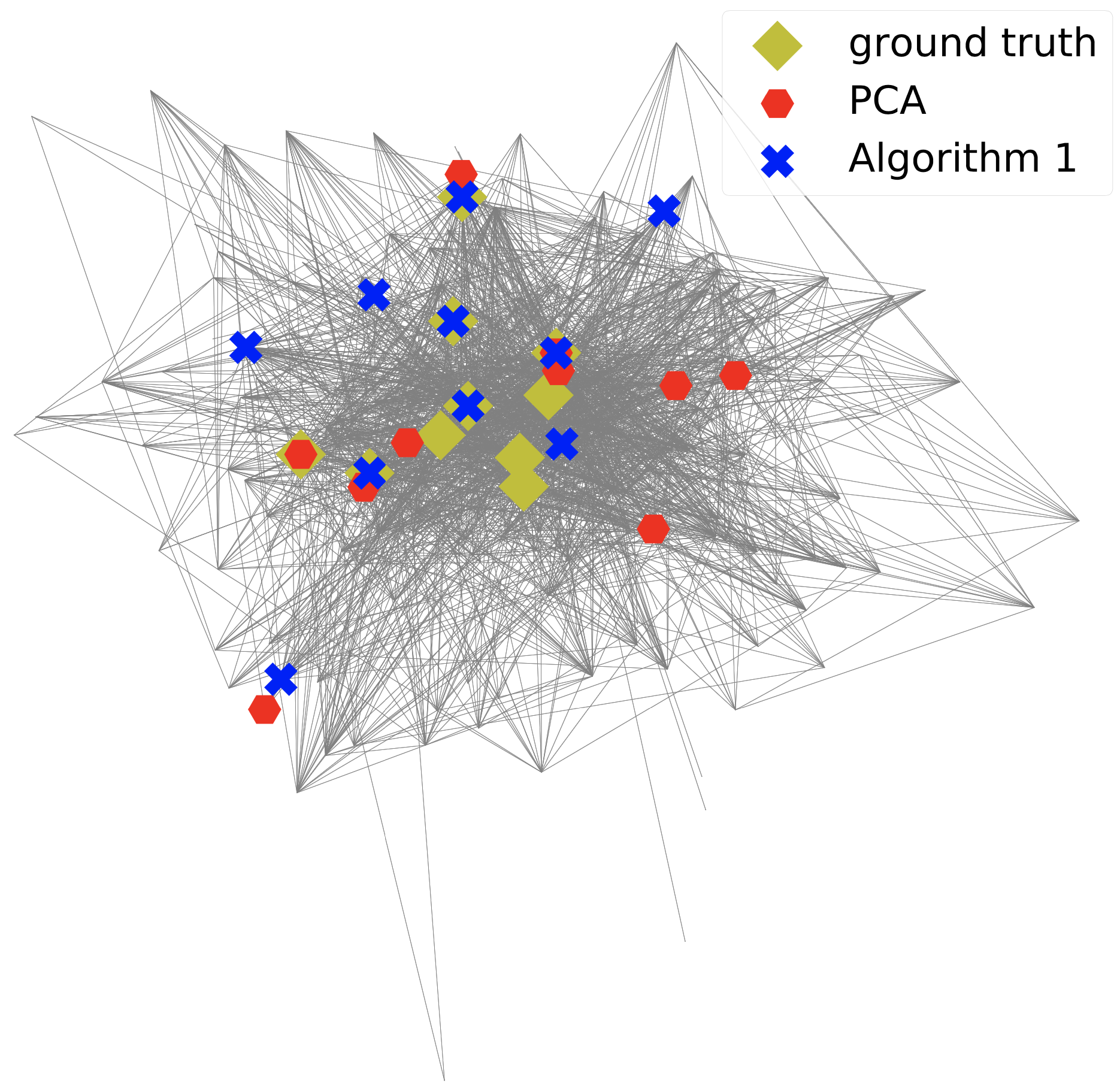
Figure 8: Example illustrating the detection results of the proposed methods: (Left) Email graph and (Right) Neural graph with weak low pass filter ${\mathcal{}H}_{\sf weak}^{\prime\prime}({\bm{A}})$. Step sizes parameters (33) are set as $a=b=0.01$.

The fourth example compares the detection performances with respect to the graph size $n$. We focus on the weak low pass graph filter ${\mathcal{}H}_{\sf weak}^{\prime}({\bm{A}})=({\bm{I}}-\frac{2}{n}{\bm{A}})^{-1}$ and fix the excitation’s rank at $k=50$. The results are shown in Fig. 7 for the CP (with $p_{1}=0.4$) and BA graph models as we evaluate the top-10 and top-$0.5n$ error rates, respectively. Notice that for Algorithm 1, the NMF stage favors models with large $\frac{n}{k}$ as it leads to easier satisfaction of the identifiabiltiy conditions in 1. The figure shows that the error rate of Algorithm 1 approaches that of the RPCA as $n$ increases, as predicted by our analysis. Notice that the performances of all algorithms deteriorate with the graph size $n$ for BA graph as the eigen-centrality vector of BA graphs is less localized.

We also compare the detection results of the proposed methods by simulating graph signals on real graph topologies. We consider the Email and Neural graphs taken from the KONECT project (available: http://konect.cc). The Email graph has $n=167$ nodes and the Neural graph has $n=297$ nodes. We generate the graph signals with a weak low pass graph filter ${\mathcal{}H}_{\sf weak}^{\prime\prime}({\bm{A}})=({\bm{I}}-\frac{1}{100}{\bm{A}})^{-1}$ and the excitation’s rank is fixed at $k=\lceil 0.3n\rceil$. The graphs together with the detection results of our algorithms are presented in Fig. 8. The Email graph has a core-periphery structure where $\frac{\lambda_{2}}{\lambda_{1}}=0.254$, while the Neural graph does not have a set of significantly core nodes as $\frac{\lambda_{2}}{\lambda_{1}}=0.585$. We observe that Algorithm 1 performs well on the Email graph; while the central nodes detection are not as accurate on the Neural graph.

Figure 9: Error rate of central nodes detection implementations with Algorithm 1 the (Left) running time and (Right) iteration number.

As the last example, we examine the efficient implementation of Algorithm 1. In Fig. 9, we fix $n=100,m=200$, $k=40$, $a=b=0.1$, consider the CP graph with $p_{1}=1,p_{2}=0.05$, and the graph filter ${\mathcal{}H}_{\sf weak}({\bm{A}})=({\bm{I}}-\frac{1}{50}{\bm{A}})^{-1}$. We compare the error rates against running time and iteration for Algorithm 2 and the cvxpy-based algorithm. Both algorithms converge to a solution with similar error rates. In particular, the cvxpy-based algorithm converges in less than 60 iterations, while Algorithm 2 requires more than $1000$ iterations to converge. However, in terms of the running time, Algorithm 2 is around 10 fold faster than cvxpy-based algorithm.

Figure 10: Spectrum of the data covariance matrix. (Left) Stock dataset and (Right) Senate dataset. Note that the ratio between the second and first eigenvalue of the covariance matrix is 0.19 for Stock dataset and 0.60 for Senate dataset.

(a) Stock Dataset^†

Method	Top-10 Estimated Central Stocks (sorted left-to-right)
Algorithm 1	ALL	ACN	HON	AXP	IBM	DIS	ORCL	MMM	BRK.B	COST
	0.43	0.56	0.51	0.72	0.50	0.36	0.70	0.33	0.52	0.64
	Average Correlation Score: $0.53\pm 0.133$
PCA (11)	NVDA	NFLX	AMZN	ADBE	PYPL	CAT	MA	GOOG	BA	GOOGL
	0.56	0.60	0.68	0.63	0.65	0.27	0.67	0.63	0.28	0.63
	Average Correlation Score: ${\bf 0.56\pm 0.154}$
GL-SigRep	GOOGL	GOOG	LLY	USB	EMR	DUK	ORCL	GD	VZ	V
[13]	0.63	0.63	0.17	0.43	0.59	0.11	0.70	0.53	0.27	0.71
	Average Correlation Score: $0.48\pm 0.22$
KNN	ACN	HON	ALL	BRK.B	IBM	AXP	EMR	MMM	CSCO	XOM
	0.56	0.51	0.43	0.52	0.50	0.72	0.59	0.33	0.63	0.55
	Average Correlation Score: $0.53\pm 0.107$
SpecTemp	ACN	ORCL	PG	LLY	SUBX	PYPL	MDLZ	FB	PFE	MRK
[14]	0.56	0.70	0.36	0.17	0.58	0.65	0.41	0.61	0.14	0.20
	Average Correlation Score: $0.44\pm 0.211$
Kalofolias	ACN	HON	BRK.B	ALL	AXP	IBM	XOM	KO	USB	COST
[44]	0.56	0.51	0.52	0.43	0.72	0.50	0.55	0.32	0.43	0.64
	Average Correlation Score: $0.52\pm 0.112$
Information Technology/ Communication Services/ Industrials/ Financials/other sectors.

(b) Senate Dataset^†

Method	Top-10 Estimated Central States (sorted left-to-right)
Algorithm 1	MI	MT	KS	RI	TN	MN	NV	ME	MD	IN
	0.79	0.66	0.74	0.67	0.68	0.74	0.43	0.67	0.6	0.62
	Average Correlation Score: ${\bf 0.66\pm 0.099}$
PCA (11)	CA	DE	CO	IL	ND	WV	IA	VA	WY	MA
	0.55	0.46	0.54	0.63	0.72	0.52	0.51	0.56	0.59	0.58
	Average Correlation Score: $0.57\pm 0.072$
GL-SigRep	CA	DE	WV	CO	IL	VA	ND	IA	WY	AZ
[13]	0.55	0.46	0.52	0.54	0.63	0.56	0.72	0.51	0.59	0.31
	Average Correlation Score: $0.54\pm 0.108$
KNN	ND	CA	IL	WV	DE	VA	AZ	CO	WY	IA
	0.72	0.55	0.63	0.52	0.46	0.56	0.31	0.54	0.59	0.51
	Average Correlation Score: $0.54\pm 0.108$
SpecTemp	AL	ND	WV	CA	DE	IL	MO	MA	VA	SD
[14]	0.61	0.72	0.52	0.55	0.46	0.63	0.57	0.58	0.56	0.56
	Average Correlation Score: $0.58\pm 0.069$
Kalofolias	AL	AK	AZ	AR	WV	VA	CA	CO	CT	DE
[44]	0.61	0.63	0.31	0.47	0.52	0.56	0.55	0.54	0.45	0.46
	Average Correlation Score: $0.51\pm 0.093$
Republican/ Democrat/ Mixed.

^†The number below each stock/state shows its normalized correlation score with the S&P100 index and number of ‘Yay’s in the voting result [cf. (36)]. The average correlation scores are taken over the set of central nodes found and the number after ‘$\pm$’ is the standard deviation.

TABLE I: Estimated Central Stocks/States from the Stocks/Senate Datasets.

VI-B Experiments on Real Data

In this subsection, we experiment on detecting the central nodes of the latent graph from two datasets of graph signals. The first dataset (Stock) is the daily return from S&P100 stocks in May 2018 to Aug 2019 with $n=99$ stocks, $m=300$ samples from https://www.alphavantage.co/. The second dataset (Senate) contains $m=657$ votes grouped by $n=50$ states at the US Senate in 2007 to 2009 from https://voteview.com, and consider the combined votes from 2 Senators of the same state by assigning a score of $+2,+1,0$ for a ‘Yay’, ‘Abstention’, ‘Nay’ vote, respectively. The spectrum of the two datasets’ covariance matrices are plotted in Fig. 10. For Stock dataset, the excitation’s rank is estimated at $k=20$; for Senate dataset, the excitation’s rank is estimated at $k=10$. To remove bias from random initialization for Algorithm 1, we run the algorithm for 100 times and record the frequencies in which a node is ranked among the top-$C$ in the estimated centrality ranking. The nodes with the highest $C$ frequencies are denoted as the estimated top-$C$ central nodes.

As the actual central nodes are unknown, we consider testing the quality of selected central nodes as predictors for the network’s overall outcome such as the S&P100 index’s daily return (Stock dataset) or voting results (Senate dataset). To setup the experiment, we take the first $80\%$ of samples as training data and the last 20% as testing data. We apply Algorithm 1, PCA and other benchmark methods to estimate the top-$10$ central nodes from the training data. Then, for each central node, we compute the normalized correlation score between the time series of that node over the testing data and the overall outcome over the matching days/rollcall. For node $i$, we compute

$${\sf corr}_{i}=\|[{\bm{Y}}]_{i,{\sf Test}}\|^{-1}\|{\bm{g}}\|^{-1}\langle[{\bm{Y}}]_{i,{\sf Test}},{\bm{g}}\rangle,$$ (36)

where ${\bm{g}}$ is the S&P100 index’s returns (for Stock dataset), or the number of ‘Yay’ votes, for the days or rollcalls (for Senate dataset) corresponding to testing data. Notice that ${\sf corr}_{i}\in[0,1]$ as the signals are non-negative. A higher ${\sf corr}_{i}$ indicates that node $i$ is a good predictor for the global behavior of all nodes, which may correspond to a more central node.

Table I-(a) shows the estimated top-$C=10$ central nodes for Stock dataset. We observe that PCA identifies the technology firms (e.g., NVDA, NFLX, AMZN); while Algorithm 1 identifies a diverse list of firms, ranging from finance (e.g. ALL), industry (e.g. HON), to technology (e.g. ACN, IBM) firms. Among the benchmarked methods, PCA achieves the highest average correlation scores, and Algorithm 1 has a similar performance. This can be explained by the large gap between the first and second eigenvalues in this dataset (see Fig. 10 (left)), which suggests that the graph signals may have been filtered by a strong low pass filter.

Table I-(b) considers the Senate dataset and highlights the top-$C=10$ states identified. Compared to the other benchmarked methods, we first observe that Algorithm 1 identifies a more ‘balanced’ set of states with sitting Senators from different parties in 2007-2009. Moreover, Algorithm 1 finds a set of states with a significantly higher average correlation score than the other algorithms. Notice that from Fig. 10 (right), this dataset has a small gap between the first and second eigenvalues, suggesting that the underlying low pass graph filter maybe weak. In the latter scenario, Algorithm 1 can reliably detect the central nodes.

Figure 11: Distance in distribution on real datasets against the amount of available data.

Lastly, we examine the consistency of Algorithm 1 on both datasets. We select a subset of samples randomly from the dataset with sizes $0.1m,0.3m,\ldots,0.9m$. For each subset, we record the frequencies in which a node is chosen as one of the top-10 central nodes using 100 trials with random initialization to Algorithm 1, and construct the empirical distribution $\widehat{\bm{\mu}}$ accordingly. We then compare $\widehat{\bm{\mu}}$ to the empirical distributed constructed similarly by applying Algorithm 1 to the full dataset, the latter is denoted as ${\bm{\mu}}_{\sf full}$. Fig. 11 compares the distance in distribution as $\|\widehat{\bm{\mu}}-{\bm{\mu}}_{\sf full}\|_{1}$ averaged over 100 randomly selected subsets. As the amount of available data increases, the distance in distribution decreases as Algorithm 1 produces more consistent estimates of the central nodes. Notice that for Stock dataset, the larger distance in distribution reflects the higher volatility of the stock return data.

VII Conclusions

We have studied the problem of blind central nodes detection under a variety of settings. Our method only relies on a mild condition that the underlying graph filter is low pass, while the excitation can be low-rank in general. For strong low pass graph filter, we show that the PCA method detects the central nodes correctly. For general low pass graph filter, we study a structured factor analysis model and analyse its identifiability through treating a sparse NMF model. The latter motivated us to develop a two-stage decomposition algorithm combining NMF and RPCA. In all settings, we analyze the problem parameters affecting the estimation performance. Future works include incorporating advanced NMF criterion from [19] into Algorithm 1, and analysis for the recoverability of the studied structured factor model with noise.

Appendix A Proof of Lemma 1

Since $||\bar{\bm{v}}_{1}||=1$, $||{\bm{c}}_{\sf eig}||=1$, we have $(\bar{\bm{v}}^{\top}_{1}{\bm{c}}_{\sf eig})^{2}\leq\bar{\bm{v}}^{\top}_{1}{\bm{c}}_{\sf eig}$ and it holds that

$$\begin{split}&||\widehat{\bm{v}}_{1}-{\bm{c}}_{\sf eig}||^{2}=||\widehat{\bm{v}}_{1}||^{2}+||{\bm{c}}_{\sf eig}||^{2}-2\cdot\widehat{\bm{v}}^{\top}_{1}{\bm{c}}_{\sf eig}\\ &\leq||\widehat{\bm{v}}_{1}||^{2}+||{\bm{c}}_{\sf eig}||^{2}-2\cdot(\widehat{\bm{v}}^{\top}_{1}{\bm{c}}_{\sf eig})^{2}=||\widehat{\bm{v}}_{1}\widehat{\bm{v}}_{1}^{\top}-{\bm{c}}_{\sf eig}{\bm{c}}_{\sf eig}^{\top}||^{2}_{F}\\ &\leq 2\cdot||\widehat{\bm{v}}_{1}\widehat{\bm{v}}^{\top}_{1}-{\bm{c}}_{\sf eig}{\bm{c}}_{\sf eig}^{\top}||^{2}.\end{split}$$

This implies $||\widehat{\bm{v}}_{1}-{\bm{c}}_{\sf eig}||\leq\sqrt{2}||\widehat{\bm{v}}_{1}\widehat{\bm{v}}^{\top}_{1}-{\bm{c}}_{\sf eig}{\bm{c}}_{\sf eig}^{\top}||$. Note that the latter is the spectral norm of a rank-2 matrix. Furthermore, the triangular inequality yields:

$$\begin{split}&||\widehat{\bm{v}}_{1}\widehat{\bm{v}}_{1}^{\top}-{\bm{c}}_{\sf eig}{\bm{c}}_{\sf eig}^{\top}||\\ &\leq||\bar{\bm{v}}_{1}\bar{\bm{v}}_{1}^{\top}-{\bm{c}}_{\sf eig}{\bm{c}}_{\sf eig}^{\top}||+||\widehat{\bm{v}}_{1}\widehat{\bm{v}}_{1}^{\top}-\bar{\bm{v}}_{1}\bar{\bm{v}}_{1}^{\top}||.\end{split}$$ (37)

The first term is bounded by [23, Proposition 1] with $K=1$:

$$\|\bar{\bm{v}}_{1}\bar{\bm{v}}_{1}^{\top}-{\bm{c}}_{\sf eig}{\bm{c}}_{\sf eig}^{\top}\|=\sqrt{\gamma^{2}/(1+\gamma^{2})}\leq\gamma,$$ (38)

with $\gamma\leq\eta\frac{\|{\bm{V}}_{N-1}^{\top}{\bm{B}}{\bm{q}}_{1}\|}{|{\bm{v}}_{1}^{\top}{\bm{B}}{\bm{q}}_{1}|}$. The second term is bounded by [23, Proposition 2] with $K=1$:

$$||\widehat{\bm{v}}_{1}\widehat{\bm{v}}_{1}^{\top}-\bar{\bm{v}}_{1}\bar{\bm{v}}_{1}^{\top}||\leq\delta^{-1}{||\bm{\Delta}||}.$$ (39)

Combining the above inequalities yield the desirable results.

Appendix B Proof of Lemma 2

For any $\rho>0$, we observe that

$$\frac{\|\tilde{\mathcal{}H}_{\rho}({\bm{A}}){\bm{B}}\|}{\rho\|{\bm{B}}\|}\leq\frac{\|\tilde{\mathcal{}H}_{\rho}({\bm{A}})\|}{\rho}.$$ (40)

Taking $\min_{\rho>0}$ on both sides yields an upper bound to the ratio in (23) as

$$\min_{\rho>0}\!~{}f(\rho):=\max\{|\rho^{-1}h(\lambda_{1})-1|,...,|\rho^{-1}h(\lambda_{n})-1|\}.$$ (41)

Under Assumption 1, we note that $h_{\sf min}<h(\lambda_{1})$ and there are at least two distinct values in the collection $\{h(\lambda_{1}),...,h(\lambda_{n})\}$. Furthermore, for $0\in\partial f(\rho^{\star})$, we must have $\rho^{\star}$ satisfying

$$|(\rho^{\star})^{-1}h(\lambda_{1})-1|=|(\rho^{\star})^{-1}h_{\sf min}-1|.$$ (42)

Since $h(\lambda_{1})\neq h_{\sf min}$, it holds

$$\rho^{\star}=2^{-1}(h(\lambda_{1})+h_{\sf min}).$$ (43)

Evaluating $f(\rho^{\star})$ and simplifying the expression gives the bound

$$\min_{\rho>0}\frac{\|\tilde{\mathcal{}H}_{\rho}({\bm{A}}){\bm{B}}\|}{\rho\|{\bm{B}}\|}\leq\frac{h(\lambda_{1})-h_{\sf min}}{h(\lambda_{1})+h_{\sf min}}.$$ (44)

As the frequency response $h(\lambda)$ is a convex and non-negative function, it holds that $\eta=\max\{h(\lambda_{2}),h(\lambda_{n})\}/h(\lambda_{1})$. Therefore, dividing the nominator and denominator in the r.h.s. of (44) by $h(\lambda_{1})$ yields the final bound in (23).

Appendix C Proof of Lemma 3

Applying 1 to $\widehat{\bm{L}}$ in (26) yields:

$$\|\widetilde{\bm{v}}_{1}-{\bm{c}}_{\sf eig}\|\leq\widetilde{\eta}\cdot\sqrt{2}\frac{\|{\bm{V}}_{n-1}^{\top}{\bm{B}}{\bm{D}}\bm{\Pi}{\bm{q}}_{1}\|_{2}}{|{\bm{v}}_{1}^{\top}{\bm{B}}{\bm{D}}\bm{\Pi}{\bm{q}}_{1}|}.$$ (45)

Since ${\rm diag}({\bm{D}})>{\bm{0}}$, we observe that

$$\frac{\|{\bm{V}}_{n-1}^{\top}{\bm{B}}{\bm{D}}\bm{\Pi}{\bm{q}}_{1}\|}{|{\bm{v}}_{1}^{\top}{\bm{B}}{\bm{D}}\bm{\Pi}{\bm{q}}_{1}|}\leq\frac{\|{\bm{V}}_{n-1}^{\top}{\bm{B}}\bm{\Pi}{\bm{q}}_{1}\|}{|{\bm{v}}_{1}^{\top}{\bm{B}}\bm{\Pi}{\bm{q}}_{1}|}\frac{\max_{i}D_{i,i}}{\min_{i}D_{i,i}}.$$ (46)

As we have taken $\widehat{\bm{Z}}{\bf 1}={\bm{1}}$, it holds

$${\bf 1}=\widehat{\bm{Z}}{\bf 1}=\bm{\Pi}^{\top}{\bm{D}}^{-1}{\bm{Z}}{\bf 1}\Longleftrightarrow{\rm diag}({\bm{D}})={\bm{Z}}{\bf 1}.$$ (47)

It shows that the diagonal scaling of the obtained solution is controlled by the random vector ${\bm{Z}}{\bf 1}$. Under 3, for any $t>0$, the Hoeffding’s inequality implies that

$$\textstyle\mathbb{P}(\|{\bm{Z}}{\bf 1}/m-\alpha{\bf 1}\|_{\infty}\geq t)\leq 2k\exp(-mt^{2}/(2\sigma_{z}^{2})).$$ (48)

Therefore, with probability at least $1-2k\exp(-mt^{2}/(2\sigma_{z}^{2}))$,

$$\frac{\max_{i}D_{i,i}}{\min_{i}D_{i,i}}=\frac{\max_{i}\sum_{\ell=1}^{m}z_{\ell,i}/m}{\min_{i}\sum_{\ell=1}^{m}z_{\ell,i}/m}\leq\frac{\alpha+t}{\alpha-t}.$$ (49)

Setting $\exp(-mt^{2}/(2\sigma_{z}^{2}))=\delta$ and substituting the above into (46) conclude the proof.

Appendix D Proof of Fact 2

Given an initialization $\hat{\bm{B}}^{(0)},\hat{\bm{Z}}^{(0)}$, define the following compact subset of $\Re^{n\times k}$:

$$\textstyle{\mathcal{}B}^{0}=\{{\bm{B}}:{\bm{B}}\geq{\bm{0}},\sum_{ij}B_{ij}\leq\lambda_{S}^{-1}f(\hat{\bm{B}}^{(0)},\hat{\bm{Z}}^{(0)})\}.$$ (50)

With our choice of step sizes in (33), Algorithm 2 returns iterates which satisfy $\hat{\bm{B}}^{(t)}\geq{\bm{0}}$ and

$$f(\hat{\bm{B}}^{(t+1)},\hat{\bm{Z}}^{(t+1)})\leq f(\hat{\bm{B}}^{(t)},\hat{\bm{Z}}^{(t)}),~{}\forall~{}t\geq 0,$$ (51)

see [39]. As the squared Frobenius norm $\frac{1}{2}\|{\bm{Y}}-{\bm{B}}{\bm{Z}}\|_{F}^{2}$ is non-negative, the above implies that

$$\textstyle\lambda_{S}\sum_{ij}\hat{B}_{ij}^{(t)}\leq f(\hat{\bm{B}}^{(0)},\hat{\bm{Z}}^{(0)}),$$ (52)

and thus $\hat{\bm{B}}^{(t)}\in{\mathcal{}B}^{0}$ for all $t\geq 0$.

We then observe that Algorithm 2 is a special case of the hybrid BCD algorithm applied to:

$$\min_{{\bm{B}},{\bm{Z}}}\widetilde{f}({\bm{B}},{\bm{Z}})\mathrel{\mathop{:}}=f({\bm{B}},{\bm{Z}})+{\mathcal{}I}_{{\mathcal{}B}^{0}}({\bm{B}})+{\mathcal{}I}_{\Delta^{K}}({\bm{Z}}),$$ (53)

where ${\mathcal{}I}_{{\mathcal{}B}^{0}}(\cdot),{\mathcal{}I}_{\Delta^{K}}(\cdot)$ are the $0/\infty$ indicator functions of the sets ${\mathcal{}B}^{0},\Delta^{K}$, respectively, and such that a PGD update step is selected for the individual block updates. Furthermore, the domain of $\widetilde{f}$ is a compact set ${\mathcal{}B}^{0}\times\Delta^{K}$. Consequently, the conclusion in the fact follows by applying [39, Theorem 1].

References

- [1] Y. He and H.-T. Wai, “Estimating centrality blindly from low-pass filtered graph signals,” in ICASSP, 2020, pp. 5330–5334.
- [2] M. Newman, Networks. Oxford university press, 2018.
- [3] S. P. Borgatti, “Centrality and network flow,” Social networks, vol. 27, no. 1, pp. 55–71, 2005.
- [4] F. Bloch, M. O. Jackson, and P. Tebaldi, “Centrality measures in networks,” Available at SSRN 2749124, 2019.
- [5] D. F. Gleich, “Pagerank beyond the web,” Siam Review, vol. 57, no. 3, pp. 321–363, 2015.
- [6] X. Dong, D. Thanou, M. Rabbat, and P. Frossard, “Learning graphs from data: A signal representation perspective,” IEEE Signal Processing Magazine, vol. 36, no. 3, pp. 44–63, 2019.
- [7] G. Mateos, S. Segarra, A. G. Marques, and A. Ribeiro, “Connecting the dots: Identifying network structure via graph signal processing,” IEEE Signal Processing Magazine, vol. 36, no. 3, pp. 16–43, 2019.
- [8] J. Friedman, T. Hastie, and R. Tibshirani, “Sparse inverse covariance estimation with the graphical lasso,” Biostatistics, vol. 9, no. 3, pp. 432–441, 2008.
- [9] V. N. Ioannidis, Y. Shen, and G. B. Giannakis, “Semi-blind inference of topologies and dynamical processes over dynamic graphs,” IEEE Transactions on Signal Processing, vol. 67, no. 9, pp. 2263–2274, 2019.
- [10] H.-T. Wai, A. Scaglione, B. Barzel, and A. Leshem, “Joint network topology and dynamics recovery from perturbed stationary points,” IEEE Transactions on Signal Processing, vol. 67, no. 17, pp. 4582–4596, 2019.
- [11] A. Sandryhaila and J. M. F. Moura, “Discrete signal processing on graphs,” IEEE Transactions on Signal Processing, vol. 61, no. 7, pp. 1644–1656, 2013.
- [12] A. Ortega, P. Frossard, J. Kovačević, J. M. Moura, and P. Vandergheynst, “Graph signal processing: Overview, challenges, and applications,” Proceedings of the IEEE, vol. 106, no. 5, pp. 808–828, 2018.
- [13] X. Dong, D. Thanou, P. Frossard, and P. Vandergheynst, “Learning laplacian matrix in smooth graph signal representations,” IEEE Transactions on Signal Processing, vol. 64, no. 23, pp. 6160–6173, 2016.
- [14] S. Segarra, A. G. Marques, G. Mateos, and A. Ribeiro, “Network topology inference from spectral templates,” IEEE Transactions on Signal and Information Processing over Networks, vol. 3, no. 3, pp. 467–483, 2017.
- [15] H. E. Egilmez, E. Pavez, and A. Ortega, “Graph learning from data under laplacian and structural constraints,” IEEE Journal of Selected Topics in Signal Processing, vol. 11, no. 6, pp. 825–841, 2017.
- [16] Y. Yuan, D. W. Soh, H. H. Yang, and T. Q. S. Quek, “Learning overlapping community-based networks,” IEEE Transactions on Signal and Information Processing over Networks, vol. 5, no. 4, pp. 684–697, 2019.
- [17] M. Udell and A. Townsend, “Why are big data matrices approximately low rank?” SIAM Journal on Mathematics of Data Science, vol. 1, no. 1, pp. 144–160, 2019.
- [18] R. Ramakrishna, H.-T. Wai, and A. Scaglione, “A user guide to low-pass graph signal processing and its applications,” IEEE Signal Processing Magazine, 2020.
- [19] X. Fu, K. Huang, N. D. Sidiropoulos, and W.-K. Ma, “Nonnegative matrix factorization for signal and data analytics: Identifiability, algorithms, and applications.” IEEE Signal Process. Mag., vol. 36, no. 2, pp. 59–80, 2019.
- [20] A. Agarwal, S. Negahban, M. J. Wainwright et al., “Noisy matrix decomposition via convex relaxation: Optimal rates in high dimensions,” The Annals of Statistics, vol. 40, no. 2, pp. 1171–1197, 2012.
- [21] E. J. Candès, X. Li, Y. Ma, and J. Wright, “Robust principal component analysis?” Journal of the ACM (JACM), vol. 58, no. 3, pp. 1–37, 2011.
- [22] M. T. Schaub, S. Segarra, and J. N. Tsitsiklis, “Blind identification of stochastic block models from dynamical observations,” SIAM Journal on Mathematics of Data Science, vol. 2, no. 2, pp. 335–367, Jan 2020.
- [23] H.-T. Wai, S. Segarra, A. E. Ozdaglar, A. Scaglione, and A. Jadbabaie, “Blind community detection from low-rank excitations of a graph filter,” IEEE Transactions on Signal Processing, vol. 68, pp. 436–451, 2019.
- [24] T. Hoffmann, L. Peel, R. Lambiotte, and N. S. Jones, “Community detection in networks without observing edges,” Science Advances, vol. 6, no. 4, p. eaav1478, Jan 2020.
- [25] T. M. Roddenberry, M. T. Schaub, H.-T. Wai, and S. Segarra, “Exact blind community detection from signals on multiple graphs,” IEEE Transaction on Signal Processing, 2020.
- [26] Y. Xing, X. He, H. Fang, and K. H. Johansson, “Community detection for gossip dynamics with stubborn agents,” arXiv preprint arXiv:2003.14028, 2020.
- [27] T. M. Roddenberry and S. Segarra, “Blind inference of eigenvector centrality rankings,” arXiv preprint arXiv:2008.11330, 2020.
- [28] ——, “Blind inference of centrality rankings from graph signals,” in ICASSP. IEEE, 2020, pp. 5335–5339.
- [29] M. Cucuringu, P. Rombach, S. H. Lee, and M. A. Porter, “Detection of core–periphery structure in networks using spectral methods and geodesic paths,” European Journal of Applied Mathematics, vol. 27, no. 6, pp. 846–887, 2016.
- [30] A. Sandryhaila and J. M. Moura, “Discrete signal processing on graphs: Frequency analysis,” IEEE Transactions on Signal Processing, vol. 62, no. 12, pp. 3042–3054, 2014.
- [31] D. Thanou, X. Dong, D. Kressner, and P. Frossard, “Learning heat diffusion graphs,” IEEE Transactions on Signal and Information Processing over Networks, vol. 3, no. 3, pp. 484–499, 2017.
- [32] M. H. DeGroot, “Reaching a consensus,” Journal of the American Statistical Association, vol. 69, no. 345, pp. 118–121, 1974.
- [33] M. Billio, M. Getmansky, A. W. Lo, and L. Pelizzon, “Econometric measures of connectedness and systemic risk in the finance and insurance sectors,” Journal of financial economics, vol. 104, no. 3, pp. 535–559, 2012.
- [34] S. J. Brown, “The number of factors in security returns,” the Journal of Finance, vol. 44, no. 5, pp. 1247–1262, 1989.
- [35] R. Vershynin, High-dimensional probability: An introduction with applications in data science. Cambridge university press, 2018, vol. 47.
- [36] K. Huang, N. D. Sidiropoulos, and A. Swami, “Non-negative matrix factorization revisited: Uniqueness and algorithm for symmetric decomposition,” IEEE Transactions on Signal Processing, vol. 62, no. 1, pp. 211–224, 2013.
- [37] P. O. Hoyer, “Non-negative sparse coding,” in Proceedings of the 12th IEEE Workshop on Neural Networks for Signal Processing. IEEE, 2002, pp. 557–565.
- [38] A. Aravkin, S. Becker, V. Cevher, and P. Olsen, “A variational approach to stable principal component pursuit,” in 30th Conference on Uncertainty in Artificial Intelligence (UAI) 2014, no. CONF, 2014.
- [39] R. Wu, H.-T. Wai, and W.-K. Ma, “Hybrid inexact bcd for coupled structured matrix factorization in hyperspectral super-resolution,” IEEE Transactions on Signal Processing, vol. 68, pp. 1728–1743, 2020.
- [40] A. Cichocki and A.-H. Phan, “Fast local algorithms for large scale nonnegative matrix and tensor factorizations,” IEICE transactions on fundamentals of electronics, communications and computer sciences, vol. 92, no. 3, pp. 708–721, 2009.
- [41] J. Duchi, S. Shalev-Shwartz, Y. Singer, and T. Chandra, “Efficient projections onto the l 1-ball for learning in high dimensions,” in ICML, 2008, pp. 272–279.
- [42] Y. Zhu, F. J. I. Garcia, A. G. Marques, and S. Segarra, “Estimating network processes via blind identification of multiple graph filters,” IEEE Transactions on Signal Processing, vol. 68, pp. 3049–3063, 2020.
- [43] Y. He and H.-T. Wai, “Identifying first-order lowpass graph signals using perron frobenius theorem,” in ICASSP, 2021.
- [44] V. Kalofolias, “How to learn a graph from smooth signals,” in Artificial Intelligence and Statistics, 2016, pp. 920–929.