Abstract

Leptoquarks provide viable solutions to the flavour anomalies, i.e. they can explain the tensions between the measurements and the Standard Model predictions of the anomalous magnetic moment of the muon as well as $b\to s\ell^{+}\ell^{-}$ and $b\to c\tau\nu$ processes. However, LQs also contribute to other flavour observables, such as $\Delta F=2$ processes, at the loop-level. In particular, $B_{s}-\bar{B}_{s}$ mixing provides a crucial bound in setups addressing $b\to c\tau\nu$ data, often excluding a big portion of the parameter space that could otherwise account for it. In this article, we first derive the complete leading order matching, including all five scalar LQ representations, for $D^{0}-\bar{D}^{0}$, $K^{0}-\bar{K}^{0}$ and $B_{s,d}-\bar{B}_{s,d}$ mixing (at the dimension-six level). We then calculate the next-to-leading order $\alpha_{s}$ matching corrections to these $\Delta F=2$ processes in generic scalar leptoquark models. We find that the two-loop corrections increase the effects in $\Delta F=2$ processes by $\sim 5$-$10\%$ and significantly reduce the matching scale uncertainty.

1 Introduction

Leptoquarks (LQs) are hypothetical beyond the Standard Model (BSM) particles, arising originally in the context of Grand Unified Theories [1, 2, 3, 4]. What makes them special, and defines them, are their direct (common) couplings to leptons and quarks (i.e. they convert a quark into a lepton and vice versa). LQs were first systematically classified in Ref. [5], where ten possible LQ representations under the Standard Model (SM) gauge group were found, of which five are scalar fields (spin 0) and five are vector (spin 1) particles.

While LQs have received varying degrees of attention in the past, they have undergone a renaissance in recent years. This can be mainly attributed to the emergence of the flavour anomalies, i.e. the deviations from the SM predictions observed in several flavour observables. In particular, $R(D^{(*)})$ [6, 7, 8, 9, 10, 11], $b\rightarrow s\ell^{+}\ell^{-}$ observables [12, 13, 14, 15, 16, 17, 18] and the muon anomalous magnetic moment $a_{\mu}$ [19, 20] deviate from their SM predictions by more than $3\sigma$ [21, 22, 23, 24, 25], $5\sigma$ [26, 27, 28, 29, 30, 31, 32, 33, 34, 35, 36, 37, 38, 39] and $4.2\sigma$ [40, 41, 42, 43, 44, 45, 46, 47, 48, 49, 50, 51, 52, 53, 54, 55, 56, 57, 58, 59, 60], respectively.

It has been shown LQ models can account for $b\to s\ell^{+}\ell^{-}$ data [61, 62, 63, 64, 65, 66, 67, 68, 69, 70, 71, 72, 73, 74, 75, 76, 77, 78, 79, 80, 81, 82, 83, 84, 85, 86, 87, 88, 89, 90, 91, 92], $R(D^{(*)})$ [62, 63, 82, 65, 66, 67, 68, 69, 95, 72, 73, 96, 74, 83, 97, 84, 76, 77, 98, 99, 100, 101, 102, 103, 81, 104, 105, 106, 107, 108, 109, 110, 111, 112, 113, 114, 115, 116, 117, 118, 119, 120, 121, 122, 123, 124, 125, 126, 86, 87, 127, 88, 128, 129, 89, 90, 93, 94] and/or $a_{\mu}$ [107, 130, 131, 132, 110, 99, 133, 134, 135, 136, 137, 138, 139, 140, 124, 113, 141, 142, 143, 86, 144, 87, 145, 146, 129, 89, 147, 148, 149], making them prime candidates in the search for BSM models. As such, they have been studied in direct searches at the LHC [162, 163, 164, 165, 166, 167, 168, 169, 170, 171, 172, 173, 174, 175, 176, 177, 178, 179, 180], leptonic observables [181] and oblique electroweak parameters, Higgs couplings to gauge bosons [182, 183, 184, 185, 186, 187], a wide range of low energy precision probes [188, 189, 190, 191, 134, 155, 156, 154, 157, 192, 159, 193, 194, 195, 196, 197, 198, 199, 200, 201, 202, 203, 204, 152]. The complete scalar LQ Lagrangian and the corresponding set of Feynman rules has been presented recently in Ref. [205]. The QCD corrections to LQ production and decay at colliders have been known for a long time [206, 162, 163] and have been improved to include NLO parton shower [207] or a large width [208]. Such QCD corrections have also been included in recent analyses correlating the $B$ anomalies to LHC searches [164, 167, 209, 170, 210, 172]. However, the calculation for the analogous $\alpha_{s}$ corrections to flavour observables is still incomplete. So far, only the ${\cal O}(\alpha_{s})$ corrections to semi-leptonic processes [79] and $\ell\to\ell^{\prime}\gamma$ [144] have been calculated, but the analogous two-loop matching for $\Delta F=2$ processes is still missing. Here, specially in models aiming at an explanation of $R(D^{(*)})$, but also in models accounting for $b\to s\ell^{+}\ell^{-}$ (most importantly in models involving couplings to left-handed fermions only [211, 86]), $B_{s}-\bar{B}_{s}$ mixing provides a crucial constraint that limits the possible size of the new physics contribution.

In this article we calculate the next-to-leading order (NLO) QCD matching for $\Delta F=2$ processes in scalar LQ models. However, we will first compute the one-loop matching for $D^{0}-\bar{D}^{0}$, $K^{0}-\bar{K}^{0}$ and $B_{s,d}-\bar{B}_{s,d}$ mixing, taking into account all five scalar LQ representations, which has so far not been presented in the literature. We then compute the two-loop ${\cal O}(\alpha_{s})$ corrections to these $\Delta F=2$ processes, which, together with the (known) two-loop QCD evolution of the corresponding effective operators [212, 213], is needed to reduce significantly the matching-scale uncertainty. This is particularly important in light of the increasingly tighter constraints placed by $\Delta F=2$ processes on NP [214, 215, 216].

2 Scalar Leptoquark models at Low Energies

2.1 Leptoquark interactions with SM fermions

	$SU(3)$	$SU(2)_{L}$	$U(1)_{Y}$
$\Phi_{1}$	3	1	$-{1}/{3}\$
$\tilde{\Phi}_{1}$	3	1	$-{4}/{3}\$
$\Phi_{2}$	3	2	${7}/{6}\$
$\tilde{\Phi}_{2}$	3	2	${1}/{6}\$
$\Phi_{3}$	3	3	$-{1}/{3}\$

Table 1: The five possible scalar leptoquark representations under the SM gauge group.

There are five different representations under the SM gauge group for scalar particles (i.e. scalar LQs) such that a common coupling to quarks and leptons is possible [5], as given in Table 1. The corresponding Lagrangian can be written as

$${\cal L} = \left({\lambda_{fj}^{1R}{\mkern 1.0mu}\bar{u}_{f}^{c}{\ell_{j}}+\lambda_{fj}^{1L}{\mkern 1.0mu}\bar{Q}_{f}^{{\kern 1.0pt}c}i{\tau_{2}}{L_{j}}}\right)\Phi_{1}^{\dagger}+\tilde{\lambda}_{fj}^{1}{\mkern 1.0mu}\bar{d}_{f}^{c}{\ell_{j}}\tilde{\Phi}_{1}^{\dagger}+\lambda_{fj}^{2RL}{\mkern 1.0mu}{{\bar{u}}_{f}}\Phi_{2}^{T}i{\tau_{2}}{L_{j}}$$ (1)

$$+\lambda_{fj}^{2LR}{\mkern 1.0mu}{{\bar{Q}}_{f}}{\ell_{j}}{\Phi_{2}}+\tilde{\lambda}_{fj}^{2}{\mkern 1.0mu}{{\bar{d}}_{f}}\tilde{\Phi}_{2}^{T}i{\tau_{2}}{L_{j}}+\lambda_{fj}^{3}{\mkern 1.0mu}\bar{Q}_{f}^{{\kern 1.0pt}c}i{\tau_{2}}{\left({\tau\cdot{\Phi_{3}}}\right)^{\dagger}}{L_{j}}+{\rm{h}}{\rm{.c}}{\rm{.}}\ .$$

Here $Q$ and $L$ are the quark and lepton $SU(2)_{L}$ doublets while $u$, $d$ and $\ell$ are singlets, $\tau_{2}$ is the second Pauli matrix and the superscript $c$ denotes charge conjugation.

After electroweak (EW) symmetry breaking, the $SU(2)_{L}$ doublets are decomposed into their components with definite electric charge and the quark and lepton fields can be transformed to the physical mass eigenbasis. While the rotations of the lepton and the right-handed quark fields can be absorbed by a redefinition of the couplings $\lambda$, and are thus unphysical, the CKM matrix unavoidably appears in couplings involving left-handed quark fields. Working in the down basis, such that the CKM matrix only enters in couplings to left-handed up-quarks,

$${{\cal L}_{{\rm{EW}}}} = \left({\lambda_{fj}^{1R}\bar{u}_{f}^{c}P_{R}{\ell_{j}}+V_{ff^{\prime}}^{*}\lambda_{f^{\prime}j}^{1L}\bar{u}_{f}^{c}P_{L}{\ell_{j}}-\lambda_{fj}^{1L}{\mkern 1.0mu}\bar{d}_{f}^{c}P_{L}{\nu_{j}}}\right)\Phi_{1}^{-1/3*}+\tilde{\lambda}_{fj}^{1}{\mkern 1.0mu}\bar{d}_{f}^{c}P_{R}{\ell_{j}}\tilde{\Phi}_{1}^{-4/3*}$$ (2)

$$+\lambda_{fj}^{2RL}\left({{\bar{u}}_{f}}P_{L}{\ell_{j}}{\Phi_{2}^{5/3}-{{\bar{u}}_{f}}P_{L}{\nu_{j}}}\Phi_{2}^{2/3}\right)+{{V_{ff^{\prime}}}\lambda_{f^{\prime}j}^{2LR}{\mkern 1.0mu}{{\bar{u}}_{f}}P_{R}{\ell_{j}}\Phi_{2}^{5/3}+\lambda_{fj}^{2LR}{\mkern 1.0mu}{{\bar{d}}_{f}}P_{R}{\ell_{j}}\Phi_{2}^{2/3}}$$

$$+\tilde{\lambda}_{fj}^{2}\left({{\bar{d}}_{f}}P_{L}{\ell_{j}}\tilde{\Phi}_{2}^{2/3}-{{\bar{d}}_{f}}P_{L}{\nu_{j}}\tilde{\Phi}_{2}^{-1/3}\right)+V_{ff^{\prime}}^{*}\lambda_{f^{\prime}j}^{3}\left({\sqrt{2}{{\bar{u}}^{c}}P_{L}\nu\Phi_{3}^{2/3*}-{{\bar{u}}^{c}}{P_{L}}\ell\Phi_{3}^{-1/3*}}\right)$$

$$-\lambda_{fj}^{3}\left({{\bar{d}}^{c}}{P_{L}}{\nu\Phi_{3}^{-1/3*}+\sqrt{2}{{\bar{d}}^{c}}{P_{L}}\ell\Phi_{3}^{-4/3*}}\right)+\text{h.c.}\ ,$$

where the superscripts on the LQ fields indicate the corresponding electric charge.

We can write these interaction terms in a generic manner 

$${\cal L}_{q\ell}^{\text{LQ}}=\sum_{a}\bar{q}\left({{\Gamma^{aL}_{q\ell}}{P_{L}}+{\Gamma^{aR}_{q\ell}}{P_{R}}}\right)\ell\,{\Phi_{a}}+{\rm{h}}{\rm{.c}}{\rm{.}}\ ,$$ (3)

with $a=1,2,\dots$ running over the different LQ fields (several ‘copies’ of LQs belonging to the same representation also allowed). In this notation we would have e.g. for $\Phi_{a}=\tilde{\Phi}_{2}^{2/3}$ the relation

$$\Gamma^{aL}_{q\ell}=\Gamma^{aR}_{q\ell}=\tilde{\lambda}^{2}_{q\ell}\ ,$$ (4)

and similarly for the other LQs. Thus, we will present our results in terms of the generic couplings $\Gamma^{a(L,R)}_{q\ell}$, and one can derive from them the specific cases in terms of the couplings in Eq. (1).

2.2 Leptoquark contributions to $\Delta F=2$ processes at LO

Due to the relatively low energy scale at which neutral meson mixing takes place, its physics can be described by an effective field theory (EFT) where SM EW-scale particles ($W,Z$, higgs and top) as well as the LQs  are not dynamical degrees of freedom but are rather integrated out from the action. Flavour-changing transitions are then mediated by effective operators of dimension six or higher (see, e.g. [217]). The most general set of (physical) dimension six operators for $\Delta F=2$ processes contains eight operators (for a specific flavour transition)

$${\cal L}_{\text{eff}}^{\Delta F=2}=-\sum_{i=1}^{5}C_{i}{\cal O}_{i}-\sum_{i=1}^{3}C^{\prime}_{i}{\cal O}^{\prime}_{i}\ .$$ (5)

In the case of $B_{s}-\bar{B}_{s}$ mixing, the operators in the so-called “SUSY” basis read explicitly

$${{\cal O}_{1}} ={{\bar{s}}_{\alpha}}{\gamma^{\mu}}{P_{L}}{b_{\alpha}}{{\bar{s}}_{\beta}}{\gamma_{\mu}}{P_{L}}{b_{\beta}}\ , {{\cal O}_{5}} ={{\bar{s}}_{\alpha}}{P_{L}}{b_{\beta}}{{\bar{s}}_{\beta}}{P_{R}}{b_{\alpha}}\ ,$$

$${{\cal O}_{2}} ={{\bar{s}}_{\alpha}}{P_{L}}{b_{\alpha}}{{\bar{s}}_{\beta}}{P_{L}}{b_{\beta}}\ , {{\cal O}^{\prime}_{1}} ={{\bar{s}}_{\alpha}}{\gamma^{\mu}}{P_{R}}{b_{\alpha}}{{\bar{s}}_{\beta}}{\gamma_{\mu}}{P_{R}}{b_{\beta}}\ ,$$

$${{\cal O}_{3}} ={{\bar{s}}_{\alpha}}{P_{L}}{b_{\beta}}{{\bar{s}}_{\beta}}{P_{L}}{b_{\alpha}}\ , {{\cal O}^{\prime}_{2}} ={{\bar{s}}_{\alpha}}{P_{R}}{b_{\alpha}}{{\bar{s}}_{\beta}}{P_{R}}{b_{\beta}}\ ,$$ (6)

$${{\cal O}_{4}} ={{\bar{s}}_{\alpha}}{P_{L}}{b_{\alpha}}{{\bar{s}}_{\beta}}{P_{R}}{b_{\beta}}\ , {{\cal O}^{\prime}_{3}} ={{\bar{s}}_{\alpha}}{P_{R}}{b_{\beta}}{{\bar{s}}_{\beta}}{P_{R}}{b_{\alpha}}\ .$$

where $\alpha,\beta$ are colour indices. The corresponding expressions for $K^{0}-\bar{K}^{0}$, $D^{0}-\bar{D}^{0}$ and $B_{d}-\bar{B}_{d}$ mixing follow by a simple exchange of flavours. The associated Wilson coefficients $C_{i}^{(\prime)}$ can be calculated from a given UV-complete theory by performing a matching calculation at the matching scale $\mu_{0}$, which is of the order of the mass of the particles that are integrated out. The matching calculation is done by equating the (expanded) full-theory and the EFT amplitudes at the matching scale, order by order in perturbation theory. We therefore write

$$C_{i}=C_{i}^{(0)}+C_{i}^{(1)}+{\cal O}(\alpha_{s}^{2})\ ,$$ (7)

where the superscript indicates the order in the strong coupling $\alpha_{s}$.

Figure 1: Feynman diagrams depicting leading-order scalar LQ contributions to the Wilson coefficients $C_{i}^{(0)}$.

The leading-order contributions originating from LQ exchange to the LO Wilson coefficients $C_{i}^{(0)}$ arise from the one-loop diagrams shown in Fig. 1. These results, which are similar to the ones in the MSSM [218, 219, 220, 221, 222, 223, 224, 225] or 2HDMs [226] are known [227, 202, 228, 216], and the non-zero Wilson coefficients at the matching scale $\mu_{0}$ are given by

$$C_{1}^{(0)}(\mu_{0}) = \frac{1}{{128{\pi^{2}}{M^{2}}}}\sum_{a,b}\Gamma_{ab}^{R}\Gamma_{ba}^{R}\ \frac{\log(x_{a}/x_{b})}{x_{a}-x_{b}}\ ,$$ (8)

$$C_{1}^{\prime(0)}(\mu_{0}) = \frac{1}{{128{\pi^{2}}{M^{2}}}}\sum_{a,b}\Gamma_{ab}^{L}\Gamma_{ba}^{L}\ \frac{\log(x_{a}/x_{b})}{x_{a}-x_{b}}\ ,$$ (9)

$$C_{4}^{(0)}(\mu_{0}) = -\frac{1}{{32{\pi^{2}}{M^{2}}}}\sum_{a,b}\Gamma_{ab}^{L}\Gamma_{ba}^{R}\ \frac{\log(x_{a}/x_{b})}{x_{a}-x_{b}}\ ,$$ (10)

with

$$x_{a}=\frac{M_{a}^{2}}{M^{2}}\ ,\qquad\Gamma_{ab}^{X}=\sum_{\ell}\Gamma_{s\ell}^{aX}\Gamma_{b\ell}^{bX*}\ .$$ (11)

In these expressions we have introduced a generic mass $M$ setting scale for the Wilson coefficients. In the degenerate case where $M_{a}=M$ (for all $a$)

$$C_{1}^{(0)}(\mu_{0})=\frac{1}{128\pi^{2}M^{2}}\sum_{a}\Gamma_{aa}^{R}\Gamma_{aa}^{R}\ ,\qquad C^{\prime(0)}_{1}=C_{1}\big{|}_{R\to L}\ ,\qquad C_{4}^{(0)}(\mu_{0})=\frac{-1}{32\pi^{2}M^{2}}\sum_{a}\Gamma_{aa}^{L}\Gamma_{aa}^{R}\ .$$ (12)

Note that the leading-order Wilson coefficients $C_{i}^{(0)}$ do not depend explicitly on the matching scale $\mu_{0}$. However they do carry an implicit dependence through the scale dependence of the LQ masses $M_{a}$ and the couplings $\Gamma_{ab}^{X}$. For the numerical analysis it will be reasonable to define the parameters inside $C_{i}^{(0)}(\mu_{0})$ as the renormalized parameters at the scale $\mu_{0}$, i.e. $M_{a}(\mu_{0})$ and $\Gamma_{ab}^{X}(\mu_{0})$. Formally, setting a different scale amounts to an $\alpha_{s}$ correction to $C_{i}^{(0)}$, and thus one could absorb the $\mu_{0}$ dependence into $C_{i}^{(1)}$. However, since the renormalization-scale dependence of $M_{a}$ and $\Gamma_{ab}^{X}$ is known prior to $C_{i}^{(1)}$ (which we are calculating in this article), it is reasonable to include this implicit matching scale dependence in $C_{i}^{(0)}$ already at leading order.

Below the matching scale, the renormalization-scale dependence of the Wilson coefficients is determined by the anomalous dimension matrix (ADM) in the EFT

$$\frac{dC_{i}}{d\log\mu}=\gamma_{ji}\,C_{j}=\Big{(}\hat{\alpha}_{s}\gamma_{ji}^{(0)}+\hat{\alpha}_{s}^{2}\gamma_{ji}^{(1)}+\cdots\Big{)}\,C_{j}\,,$$ (13)

with $\hat{\alpha}_{s}\equiv\alpha_{s}/(4\pi)$. The leading-order ADM $\gamma^{(0)}$ is obtained from the one-loop renormalization of the EFT, and it is scheme-independent :

$$\gamma^{(0)}=\left(\begin{array}[]{ccccc}4&0&0&0&0\\ 0&{\color[rgb]{.5,.5,.5}-28/3}&{\color[rgb]{.5,.5,.5}4/3}&0&0\\ 0&{\color[rgb]{.5,.5,.5}16/3}&{\color[rgb]{.5,.5,.5}32/3}&0&0\\ 0&0&0&-16&0\\ 0&0&0&-6&2\end{array}\right)\ ,$$ (14)

for $C_{1-5}$, with the ADMs for $C^{\prime}_{1-3}$ equal to the ones for the $C_{1-3}$ sector.

The next-to-leading ADM $\gamma^{(1)}$ arises at two-loops [213, 212]. It was derived in Ref. [213] using a different basis for physical operators (the “BMU” basis). The Wilson coefficients at NLO will be scheme-dependent, and it will be important to use the same scheme for $\gamma^{(1)}$ in order to get scheme-independent observables. In our basis and scheme, the ADM $\gamma^{(1)}$ is given by (see App. B for details)

$$\gamma^{(1)}=\left(\begin{array}[]{ccccc}\frac{4f}{9}-7&0&0&0&0\\ 0&{\color[rgb]{.5,.5,.5}\frac{220f}{27}-\frac{476}{3}}&{\color[rgb]{.5,.5,.5}-\frac{4f}{27}-\frac{4}{3}}&0&0\\ 0&{\color[rgb]{.5,.5,.5}73+\frac{110f}{27}}&{\color[rgb]{.5,.5,.5}\frac{359}{3}-\frac{218f}{27}}&0&0\\ 0&0&0&\frac{68f}{9}-\frac{1343}{6}&4f-\frac{225}{2}\\ 0&0&0&\frac{22f}{3}-99&\frac{71}{3}-\frac{22f}{9}\\ \end{array}\right)\ ,$$ (15)

where $f$ is the number of active quark flavours.

2.3 LO matching for $\Delta F=2$ processes including $SU(2)$ invariance

We now calculate the leading-order effect in $\Delta F=2$ processes taking into account explicitly $SU(2)$ invariance for the different LQ representations. For $D^{0}-\bar{D}^{0}$ mixing we find

$$C_{1}^{D(0)}(\mu_{0}) =\frac{{1}}{{128{\pi^{2}}{M^{2}}}}\sum\limits_{i,j}{\left(\begin{array}[]{l}\hat{\lambda}_{1i}^{1L*}{\mkern 1.0mu}\hat{\lambda}_{2i}^{1L}{\mkern 1.0mu}\hat{\lambda}_{1j}^{1L*}{\mkern 1.0mu}\hat{\lambda}_{2j}^{1L}f\left({{x_{1}},{x_{1}}}\right)+\lambda_{1i}^{2LR}\lambda_{2i}^{2LR*}\lambda_{1j}^{2LR}\lambda_{2j}^{2LR*}f\left({{x_{2}},{x_{2}}}\right)\\ +5\hat{\lambda}_{1i}^{3*}\hat{\lambda}_{2i}^{3}\hat{\lambda}_{1j}^{3*}\hat{\lambda}_{2j}^{3}f\left({{x_{3}},{x_{3}}}\right)+2\lambda_{1i}^{1L*}\hat{\lambda}_{2i}^{3}\hat{\lambda}_{1j}^{3*}\lambda_{2j}^{1L}f\left({{x_{1}},{x_{3}}}\right)}{}{\end{array}\right)}\,,$$ (16)

$$C_{4}^{D(0)}(\mu_{0}) =\frac{-1}{{32{\pi^{2}}{M^{2}}}}\sum\limits_{i,j}{\left({\hat{\lambda}_{1i}^{1L*}\hat{\lambda}_{2i}^{1L}\lambda_{1j}^{1R*}\lambda_{2j}^{1R}f\left({{x_{1}},{x_{1}}}\right)+\hat{\lambda}_{1i}^{2LR}\hat{\lambda}_{2i}^{2LR*}\hat{\lambda}_{1j}^{2RL}\hat{\lambda}_{2j}^{2RL*}f\left({{x_{2}},{x_{2}}}\right)}\right)}\,,$$

$$C_{1}^{\prime D(0)}(\mu_{0}) =\frac{{1}}{{128{\pi^{2}}{M^{2}}}}\sum\limits_{i,j}{\left({\lambda_{1i}^{1R*}\lambda_{2i}^{1R}\lambda_{1j}^{1R*}\lambda_{2j}^{1R}f\left({{x_{1}},{x_{1}}}\right)+2\lambda_{1i}^{2RL}\lambda_{2i}^{2RL*}\lambda_{1j}^{2RL}\lambda_{2j}^{2RL*}f\left({{x_{2}},{x_{2}}}\right)}\right)}\,,$$

with

$$f\left({x,y}\right)=\frac{\log(x/y)}{x-y}\,,$$ (17)

and where we have defined

$$\hat{\lambda}_{fj}^{1L}=\sum\limits_{f^{\prime}=1}^{3}{V_{ff^{\prime}}^{*}\lambda_{f^{\prime}j}^{1L}}\ ,\quad\hat{\lambda}_{fj}^{2LR}=\sum\limits_{f^{\prime}=1}^{3}{{V_{ff^{\prime}}}\lambda_{f^{\prime}j}^{2LR}}\ ,\quad\hat{\lambda}_{fj}^{3}=\sum\limits_{f^{\prime}=1}^{3}{V_{ff^{\prime}}^{*}\lambda_{f^{\prime}j}^{3}}\ .$$ (18)

For Kaon mixing we find

$$C_{1}^{K(0)}(\mu_{0}) = \frac{{1}}{{128{\pi^{2}}{M^{2}}}}\sum\limits_{i,j}{\left(\begin{array}[]{l}\lambda_{1i}^{1L*}{\mkern 1.0mu}\lambda_{2i}^{1L}{\mkern 1.0mu}\lambda_{1j}^{1L*}{\mkern 1.0mu}\lambda_{2j}^{1L}f\left({{x_{1}},{x_{1}}}\right)+\lambda_{1i}^{2LR}\lambda_{2i}^{2LR*}\lambda_{1j}^{2LR}\lambda_{2j}^{2LR*}f\left({{x_{2}},{x_{2}}}\right)\\ +5\lambda_{1i}^{3*}\lambda_{2i}^{3}\lambda_{1j}^{3*}\lambda_{2j}^{3}f\left({{x_{3}},{x_{3}}}\right)+2\lambda_{1i}^{1L*}\lambda_{2i}^{3}{\mkern 1.0mu}\lambda_{1j}^{3*}\lambda_{2j}^{1L}f\left({{x_{1}},{x_{3}}}\right)}{\end{array}\right)}\ ,$$ (21)

$$C_{1}^{\prime K(0)}(\mu_{0}) = \frac{{1}}{{128{\pi^{2}}{M^{2}}}}\sum\limits_{i,j}{\left(\begin{array}[]{l}{\mkern 1.0mu}\tilde{\lambda}_{1i}^{1*}{\mkern 1.0mu}\tilde{\lambda}_{2i}^{1}{\mkern 1.0mu}\tilde{\lambda}_{1j}^{1*}{\mkern 1.0mu}\tilde{\lambda}_{2j}^{1}{\mkern 1.0mu}f\left({{x_{\tilde{1}}},{x_{\tilde{1}}}}\right)+2\tilde{\lambda}_{1i}^{2*}{\mkern 1.0mu}\tilde{\lambda}_{2i}^{2}{\mkern 1.0mu}\tilde{\lambda}_{1j}^{2*}{\mkern 1.0mu}\tilde{\lambda}_{2j}^{2}f\left({{x_{\tilde{2}}},{x_{\tilde{2}}}}\right)}{\\ +2\lambda_{1i}^{2LR}\tilde{\lambda}_{2i}^{2*}\tilde{\lambda}_{1j}^{2}\lambda_{2j}^{2LR*}f\left({{x_{2}},{x_{\tilde{2}}}}\right)\end{array}\right)}\ .$$ (24)

From this formula, the matching conditions for $B_{s}-\bar{B}_{s}$ and $B_{d}-\bar{B}_{d}$ mixing can be obtained by a trivial exchange of flavour indices.

Comparing these expressions with Eqs. (8)-(10) we can make the following identification between the couplings $\Gamma$ in the generic Lagrangian of Eq. (4) and the LQ couplings in the $SU(2)$-invariant Lagrangian of Eq. (1). For the case of $D^{0}-\bar{D}^{0}$ mixing we have

$$\begin{array}[]{l}\sum\limits_{a,b}{\Gamma_{ab}^{R}\Gamma_{ba}^{R}f\left({{x_{a}},{x_{b}}}\right)=}\sum\limits_{i,j}{\left(\begin{array}[]{l}\hat{\lambda}_{1i}^{1L*}{\mkern 1.0mu}\hat{\lambda}_{2i}^{1L}{\mkern 1.0mu}\hat{\lambda}_{1j}^{1L*}{\mkern 1.0mu}\hat{\lambda}_{2j}^{1L}f\left({{x_{1}},{x_{1}}}\right)+\lambda_{1i}^{2LR}\lambda_{2i}^{2LR*}\lambda_{1j}^{2LR}\lambda_{2j}^{2LR*}f\left({{x_{2}},{x_{2}}}\right)\\ +5\hat{\lambda}_{1i}^{3*}\hat{\lambda}_{2i}^{3}\hat{\lambda}_{1j}^{3*}\hat{\lambda}_{2j}^{3}f\left({{x_{3}},{x_{3}}}\right)+2\lambda_{1i}^{1L*}\hat{\lambda}_{2i}^{3}\hat{\lambda}_{1j}^{3*}\lambda_{2j}^{1L}f\left({{x_{1}},{x_{3}}}\right)}{}{\end{array}\right)}{\mkern 1.0mu}\,,\\ \sum\limits_{a,b}{\Gamma_{ab}^{L}\Gamma_{ba}^{L}f\left({{x_{a}},{x_{b}}}\right)=\sum\limits_{i,j}{\left({\lambda_{1i}^{1R*}\lambda_{2i}^{1R}\lambda_{1j}^{1R*}\lambda_{2j}^{1R}f\left({{x_{1}},{x_{1}}}\right)+2\lambda_{1i}^{2RL}\lambda_{2i}^{2RL*}\lambda_{1j}^{2RL}\lambda_{2j}^{2RL*}f\left({{x_{2}},{x_{2}}}\right)}\right)}}\,,\\ \sum\limits_{a,b}{\Gamma_{ab}^{L}\Gamma_{ba}^{R}f\left({{x_{a}},{x_{b}}}\right)}=\sum\limits_{i,j}{\left({\hat{\lambda}_{1i}^{1L*}\hat{\lambda}_{2i}^{1L}\lambda_{1j}^{1R*}\lambda_{2j}^{1R}f\left({{x_{1}},{x_{1}}}\right)+\hat{\lambda}_{1i}^{2LR}\hat{\lambda}_{2i}^{2LR*}\hat{\lambda}_{1j}^{2RL}\hat{\lambda}_{2j}^{2RL*}f\left({{x_{2}},{x_{2}}}\right)}\right)}\,,\end{array}$$ (25)

while for $K^{0}-\bar{K}^{0}$ mixing we have

$$\begin{array}[]{l}\sum\limits_{a,b}{\Gamma_{ab}^{R}\Gamma_{ba}^{R}f\left({{x_{a}},{x_{b}}}\right)=}\sum\limits_{i,j}{\left(\begin{array}[]{l}\lambda_{1i}^{1L*}{\mkern 1.0mu}\lambda_{2i}^{1L}{\mkern 1.0mu}\lambda_{1j}^{1L*}{\mkern 1.0mu}\lambda_{2j}^{1L}f\left({{x_{1}},{x_{1}}}\right)+\lambda_{1i}^{2LR}\lambda_{2i}^{2LR*}\lambda_{1j}^{2LR}\lambda_{2j}^{2LR*}f\left({{x_{2}},{x_{2}}}\right)\\ +5\lambda_{1i}^{3*}\lambda_{2i}^{3}\lambda_{1j}^{3*}\lambda_{2j}^{3}f\left({{x_{3}},{x_{3}}}\right)+2\lambda_{1i}^{1L*}\lambda_{2i}^{3}{\mkern 1.0mu}\lambda_{1j}^{3*}\lambda_{2j}^{1L}f\left({{x_{1}},{x_{3}}}\right)}{\end{array}\right)}{\mkern 1.0mu}\,,\\ \sum\limits_{a,b}{\Gamma_{ab}^{L}\Gamma_{ba}^{L}f\left({{x_{a}},{x_{b}}}\right)=\sum\limits_{i,j}{\left(\begin{array}[]{l}{\mkern 1.0mu}\tilde{\lambda}_{1i}^{1*}{\mkern 1.0mu}\tilde{\lambda}_{2i}^{1}{\mkern 1.0mu}\tilde{\lambda}_{1j}^{1*}{\mkern 1.0mu}\tilde{\lambda}_{2j}^{1}{\mkern 1.0mu}f\left({{x_{\tilde{1}}},{x_{\tilde{1}}}}\right)+2\tilde{\lambda}_{1i}^{2*}{\mkern 1.0mu}\tilde{\lambda}_{2i}^{2}{\mkern 1.0mu}\tilde{\lambda}_{1j}^{2*}{\mkern 1.0mu}\tilde{\lambda}_{2j}^{2}f\left({{x_{\tilde{2}}},{x_{\tilde{2}}}}\right)}{\\ +2\lambda_{1i}^{2LR}\tilde{\lambda}_{2i}^{2*}\tilde{\lambda}_{1j}^{2}\lambda_{2j}^{2LR*}f\left({{x_{2}},{x_{\tilde{2}}}}\right)\end{array}\right)}}\,.\end{array}$$ (26)

These expressions can be used to write any Wilson coefficient calculated using the generic Lagrangian of Eq. (4) in terms of the couplings of the $SU(2)$-invariant Lagrangian, also beyond the LO.

3 Next-to-Leading-Order Calculation

3.1 QCD renormalization of the LQ Lagrangian

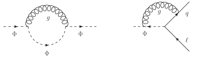
Figure 2: One-loop diagrams leading to the renormalization of the LQ mass and the LQ coupling to quarks and leptons.

In the presence of next-to-leading order (NLO) QCD corrections, the LQ Lagrangian must be renormalized. Thus, the couplings and fields in Eq. (4) are to be understood as bare (divergent) quantities. Using multiplicative renormalization, the Lagrangian reads

$${\cal L}_{\text{LQ}} = -Z_{\Phi}\partial^{\mu}\Phi^{*}\partial_{\mu}\Phi-Z_{M}M^{2}\Phi^{*}\Phi$$ (27)

$$-\frac{Z_{G}}{4}G^{A\mu\nu}G^{A}_{\mu\nu}+iZ_{g_{s}}g_{s}\left[\Phi^{*}_{\alpha}\partial^{\mu}\Phi_{\beta}-(\partial^{\mu}\Phi^{*}_{\alpha})\Phi_{\beta}\right)]G^{A}_{\mu}T^{A}_{\alpha\beta}-Z_{g_{s}}^{2}g_{s}^{2}\Phi^{*}_{\alpha}\Phi_{\beta}G^{A\mu}G^{B}_{\mu}T^{A}_{\alpha\sigma}T^{B}_{\sigma\beta}$$

$$+Z_{q}\bar{q}_{\alpha}(i\not{\partial})q_{\beta}\delta_{\alpha\beta}+Z_{g_{s}}g_{s}\bar{q}_{\alpha}\not{G}^{A}q_{\beta}T_{\alpha\beta}^{A}+\big{[}Z_{\Gamma}\,\bar{q}\left(\Gamma_{q\ell}^{aL}P_{L}+\Gamma_{q\ell}^{aR}P_{R}\right)\ell\,\Phi_{a}^{*}+\text{h.c.}\big{]}\ ,$$

where we have considered massless quarks, only a single LQ as well as only one generation of quark and leptons. However, as QCD is flavour blind, this trivially generalizes to the case of multiple generations of quarks and leptons as well as several LQ components. The renormalization constants $Z_{i}=1+\delta_{i}$ contain the counterterms $\delta_{i}$. At one loop order, these counterterms are fixed by subtracting the $1/\epsilon$ poles originating from the diagrams shown in Fig. 2 (as well as the quark self-energy) within the $\overline{\text{MS}}$ scheme, which we will use throughout this article, resulting in

$$\begin{aligned} \delta_{M}&=-\hat{\alpha}_{s}C_{F}\frac{1}{\epsilon}\ ,\qquad\delta_{\Phi}=\hat{\alpha}_{s}C_{F}\frac{2}{\epsilon}\ ,\\ \delta_{\Gamma}&=-\hat{\alpha}_{s}C_{F}\frac{1}{\epsilon}\ ,\qquad\delta_{q}=-\hat{\alpha}_{s}C_{F}\frac{1}{\epsilon}\ ,\\ \delta_{g_{s}}&=-\hat{\alpha}_{s}\left(-C_{F}-\frac{C_{A}}{2}\right)\frac{1}{\epsilon}\,.\end{aligned}$$ (28)

The renormalized LQ mass and the couplings thus obey a renormalization group (RG) equation which determines their renormalization scale dependence:

$$\frac{dM_{a}}{d\log\mu} = -3C_{F}\hat{\alpha}_{s}M_{a}+{\cal O}(\hat{\alpha}_{s}^{2})\ ,$$

$$\frac{d\Gamma_{q\ell}^{aX}}{d\log\mu} = -3C_{F}\hat{\alpha}_{s}\Gamma_{q\ell}^{aX}+{\cal O}(\hat{\alpha}_{s}^{2})\ ,$$ (29)

$$\frac{d\hat{\alpha}_{s}}{d\log\mu} = {\cal O}(\hat{\alpha}_{s}^{2})\ ,$$

where $\hat{\alpha}_{s}\equiv\alpha_{s}/(4\pi)$ and $C_{F}=4/3$.

3.2 Set-up of the NLO matching calculation

The set-up for the NLO matching calculation is the same as the one described e.g. in Ref. [220]. We match the amplitudes of the full theory onto the ones arising in the EFT at NLO in $\alpha_{s}$ at the matching scale $\mu_{0}$ to determine $C_{i}^{(1)}$. The amplitudes in the EFT are given by

$$\mathcal{A}_{\rm eff}=\sum_{i,j}C_{i}\,\Big{(}\delta_{ij}+\hat{\alpha}_{s}\,r_{ij}+{\cal O}(\alpha_{s}^{2})\Big{)}\langle{\cal O}_{j}\rangle^{(0)}\ ,$$ (30)

where $\langle{\cal O}_{i}\rangle^{(0)}$ are tree-level matrix elements, and $r_{ij}$ is given by [220]

$$r=\left(\begin{array}[]{ccccc}4/3&0&0&0&0\\ 0&{\color[rgb]{.5,.5,.5}44/3}&{\color[rgb]{.5,.5,.5}-4/3}&0&0\\ 0&{\color[rgb]{.5,.5,.5}-16/3}&{\color[rgb]{.5,.5,.5}-16/3}&0&0\\ 0&0&0&64/3&0\\ 0&0&0&6&10/3\end{array}\right)\log(\mu/\lambda)+\left(\begin{array}[]{ccccc}-5&0&0&0&0\\ 0&{\color[rgb]{.5,.5,.5}1/3}&{\color[rgb]{.5,.5,.5}-1}&0&0\\ 0&{\color[rgb]{.5,.5,.5}-15/2}&{\color[rgb]{.5,.5,.5}-25/6}&0&0\\ 0&0&0&19/3&-3\\ 0&0&0&-1/2&-7/6\end{array}\right)\ ,$$ (31)

with the elements in the $3\times 3$ primed sector equal to the ones in the $i=1,2,3$ sector. The parameter $\lambda$, an artificial gluon mass, is an infrared (IR) regulator needed to separate ultraviolet (UV) and IR divergences. The $\lambda$ dependence must cancel in the matching procedure such that the Wilson coefficients do not depend on it. This also provides a cross-check of the calculation. The log-independent term (the second matrix in Eq. (31)) depends on the renormalization scheme. In this case the chosen scheme is the $\overline{\text{MS}}$-NDR scheme with the evanescent operators given in Appendix A of Ref. [213]. It is important to use the same scheme in the calculation of the NLO full-theory amplitude in order to get consistent results.

The amplitudes in the full theory at NLO are the sum of the LO contributions from the diagrams in Fig. 1 and the NLO contributions from the two-loop diagrams shown in Fig. 3. It can be written as

$${\cal A}_{\text{LQ}}=\sum_{i}\Big{(}F_{i}^{(0)}+\hat{\alpha}_{s}\,F_{i}^{(1)}+{\cal O}(\alpha_{s}^{2})\Big{)}\langle{\cal O}_{i}\rangle^{(0)}\ ,$$ (32)

again in terms of tree-level matrix elements. Requiring equality of EFT and full-theory amplitudes at the matching scale $\mu_{0}$ order-by-order in $\alpha_{s}(\mu_{0})$, and writing

$$C_{i}(\mu_{0})=C_{i}^{(0)}(\mu_{0})+C_{i}^{(1)}(\mu_{0})+{\cal O}(\alpha_{s}(\mu_{0})^{2})\ ,$$ (33)

gives

$$C_{i}^{(0)} = F_{i}^{(0)}\ ,$$ (34)

$$C_{i}^{(1)} = \hat{\alpha}_{s}\,F_{i}^{(1)}-\hat{\alpha}_{s}\sum_{j}F_{j}^{(0)}r_{ji}\ .$$ (35)

The coefficients $C_{i}^{(0)}=F_{i}^{(0)}$ have been given in Section 2.2. The only missing pieces are thus the NLO functions $F_{i}^{(1)}$, which are obtained from the evaluation of the genuine two-loop Feynman diagrams and one-loop diagrams with counterterms to be discussed in the next section.

3.3 Calculation of the two-loop contributions

In order to extract the NLO functions $F_{i}^{(1)}$, we compute the ${\cal O}(\alpha_{s})$ part of the (renormalized) amplitude in the full theory ${\cal A}(b_{\alpha}\bar{s}_{\beta}\to s_{\delta}\bar{b}_{\gamma})$, at vanishing external momenta. We express this part of the amplitude as a sum of the two-loop Feynman diagrams (${\cal D}_{x}$) and one-loop Feynman diagrams with counterterms (${\cal C}_{x}$), shown in Fig. 3,

$$i{\cal A}_{\text{LQ}}^{\text{NLO}}=\sum_{x\in\{\text{NLO\ diagrams}\}}\big{(}{\cal D}_{x}+{\cal C}_{x}\big{)}\ .$$ (36)

The counterterm diagrams have the structure of a one-loop box diagram with a $1/\epsilon$ vertex or propagator insertion, and thus the corresponding one-loop integral must be calculated up to and including terms of order $\epsilon$. The pairs $({\cal D}_{x}+{\cal C}_{x})$ are UV-finite, and can be written as

$${\cal D}_{x}+{\cal C}_{x}=\hat{\alpha}_{s}f_{x}(m_{j},\lambda)(\bar{u}_{s\delta}\Gamma_{x}u_{b\alpha})(\bar{v}_{s\beta}\tilde{\Gamma}_{x}v_{b\gamma})+\hat{\alpha}_{s}f^{\prime}_{x}(m_{j},\lambda)(\bar{u}_{s\delta}\Gamma^{\prime}_{x}v_{b\gamma})(\bar{v}_{s\beta}\tilde{\Gamma}^{\prime}_{x}u_{b\alpha})\ .$$ (37)

The parameter $\lambda$ is a gluon mass that we have introduced to regularize IR divergencies in diagrams where the gluon connects the external (massless) quark legs. This is the same IR regulator appearing in Eq. (31).

In order to extract the functions $F_{i}^{(1)}$ we must write the spinor structures in Eq. (37) as a linear combination of tree-level matrix elements $\langle{\cal O}_{i}\rangle^{(0)}$. We do this by applying suitable Dirac projectors $P_{i}=P_{A}^{(i)}S^{(i)}\otimes P_{B}^{(i)}S^{(i)}$ which act on the spinor structures as

$$v_{b\gamma}\bar{u}_{s\delta}\rightarrow P_{A}^{(k)}S^{(k)}_{\delta\gamma}\ ,\quad u_{b\alpha}\bar{v}_{s\beta}\rightarrow P_{B}^{(k)}S^{(k)}_{\alpha\beta}\ .$$ (38)

Here $P^{(k)}$ are Dirac matrices and $S^{(k)}$ colour structures ($\delta$ or $T^{A}$). These projectors are defined such that

$$P_{i}\langle{\cal O}_{j}\rangle^{(0)}=\delta_{ij}+{\cal O}(\epsilon^{2})\ .$$ (39)

Specific details about these projections are given in App. A. In this way, the contribution to the function $F_{i}^{(1)}$ from the pair $({\cal D}_{x}+{\cal C}_{x})$ is given by

$$\alpha_{s}F_{i}^{(1)}\Big{|}_{x}=P_{i}[{\cal D}_{x}+{\cal C}_{x}]\ .$$ (40)

The advantage of this approach is that the projection can be performed before evaluating the loop integrals, transforming the integrands into scalar functions of the loop momenta. The scalar two-loop integrals can now be computed as in Ref. [220]: First, loop momenta in the numerators are reduced by expressing them in the form of the denominators; second, the denominators are decomposed using partial fraction, after which the integral can be expressed as a sum of terms of the form

$$f(M_{i},\lambda)\int\frac{d^{d}q_{1}\,d^{d}q_{2}}{(2\pi)^{2d}}\frac{1}{(q_{1}^{2}-m_{1}^{2})^{n_{1}}(q_{2}^{2}-m_{2}^{2})^{n_{2}}[(q_{1}-q_{2})^{2}-m_{3}^{2}]^{n_{3}}}\ .$$ (41)

The solution of these scalar integrals is known [229].

The contributions from each pair $({\cal D}_{x}+{\cal C}_{x})$ to the the functions $F_{i}^{(1)}$ are separately UV-finite, and this provides a non-trivial check of the two-loop integrals (note that the individual expressions for the scalar integrals in Eq. (41) contain $1/\epsilon$ and $1/\epsilon^{2}$ poles). The results for the functions $F_{i}^{(1)}$ still depend on the IR regulator $\lambda$. This dependence is cancelled in the combination $F_{i}^{(1)}-F_{j}^{(0)}r_{ji}$. This cancellation is also non-trivial and constitutes yet another check of the two-loop calculation.

All types of two-loop diagrams are shown in  Fig. 3. It is useful to classify these diagrams into finite, UV divergent and IR divergent ones. The first two diagrams are finite and thus no renormalization is required. The following two diagrams are UV divergent, and correspond precisely to the one-loop renormalization of the LQ self-energy and vertex correction from  Fig. 2. Their corresponding counterterm diagrams are shown in the last row of Fig. 3. The remaining diagrams, in which the gluon connects external quarks, are IR divergent. Such diagrams will have a $\lambda$ dependence which will contribute to the function $F_{i}^{(1)}$. As mentioned before, this $\lambda$ dependence will cancel with the one from the EFT contained in Eq. (31) when performing the matching.

Figure 3: A sample of two-loop diagrams, and one-loop diagrams with counterterm insertions (indicated by the cross), contributing to the NLO QCD matching for $B_{s}-\bar{B}_{s}$ mixing.

3.4 Matching results for the Wilson coefficients at NLO

The final results for the (non-zero) NLO Wilson Coefficients $C_{i}^{(1)}$ at the matching scale are

$$C_{1}^{\left(1\right)}(\mu_{0}) = \dfrac{{{\alpha_{s}}\Gamma_{ab}^{R}\Gamma_{ba}^{R}}}{{4608{\pi^{3}}{M^{2}}x_{a}^{2}x_{b}^{2}{{\left({{x_{a}}-{x_{b}}}\right)}^{2}}}}$$ (42)

$$\times\left[{x_{a}^{3}x_{b}^{2}\left({30\text{Li}_{2}\left({1-X_{b}^{a}}\right)+\log\left({X_{b}^{a}}\right)\left({54\log\left({X_{b}^{\mu}}\right)+69}\right)-12{{\log}^{2}}\left({X_{b}^{a}}\right)-5{\pi^{2}}+36}\right)}\right.$$

$$-x_{a}^{4}{x_{b}}\left({6\text{Li}_{2}\left({1-X_{b}^{a}}\right)+3{{\log}^{2}}\left({X_{b}^{a}}\right)+36\log\left({X_{b}^{a}}\right)+{\pi^{2}}+36}\right)$$

$$\left.+6x_{a}^{5}\left({6\text{Li}_{2}\left({1-X_{b}^{a}}\right)+3{{\log}^{2}}\left({X_{b}^{a}}\right)+{\pi^{2}}}\right)+a\leftrightarrow b\right]\ ,$$

$$C_{4}^{\left(1\right)}(\mu_{0}) = -\dfrac{{{\alpha_{s}}\Gamma_{ab}^{L}\Gamma_{ba}^{R}}}{{1152{\pi^{3}}{M^{2}}{x_{a}}{x_{b}}{{\left({{x_{a}}-{x_{b}}}\right)}^{2}}}}$$ (43)

$$\times\left[{x_{a}^{2}{x_{b}}\left({12\text{Li}_{2}\left({1-X_{b}^{a}}\right)+6\log\left({X_{b}^{a}}\right)\left({4\log\left({X_{b}^{a}}\right)-3\left({\log\left({X_{a}^{\mu}}\right)+\log\left({X_{b}^{\mu}}\right)}\right)+10}\right)+{\pi^{2}}}\right)}\right.$$

$$\left.{-x_{b}^{3}\left({{\pi^{2}}-6\text{Li}_{2}\left({1-X_{b}^{a}}\right)}\right)+a\leftrightarrow b}\right]\ ,$$

$$C_{5}^{\left(1\right)}(\mu_{0}) = -\dfrac{{{\alpha_{s}}\Gamma_{ab}^{L}\Gamma_{ba}^{R}}}{{384{\pi^{3}}{M^{2}}{x_{a}}{x_{b}}{{\left({{x_{a}}-{x_{b}}}\right)}^{2}}}}$$

$$\times\left[{x_{b}^{3}\left({{\pi^{2}}-6\text{Li}_{2}\left({1-X_{b}^{a}}\right)}\right)+{x_{a}}x_{b}^{2}\left({12\text{Li}_{2}\left({1-X_{b}^{a}}\right)-12\log\left({X_{b}^{a}}\right)-{\pi^{2}}}\right)+a\leftrightarrow b}\right]\ ,$$

with

$$X^{a}_{b}=\dfrac{M_{a}^{2}}{M_{b}^{2}}\ ,\qquad X^{\mu}_{a}=\dfrac{\mu_{0}^{2}}{M_{a}^{2}}\ ,\qquad x_{a}=\dfrac{M_{a}^{2}}{M^{2}}\ .$$ (45)

Note that the dependence on $M$ drops out. In the equal LQ mass limit one has

$$C_{1}^{(1)}(\mu_{0}) = \alpha_{s}\frac{\Gamma^{R}_{aa}\Gamma^{R}_{aa}}{4608\pi^{3}M^{2}}\left(108\log\frac{\mu_{0}}{M}+34\pi^{2}-273\right)\ ,$$ (46)

$$C_{4}^{(1)}(\mu_{0}) = \alpha_{s}\frac{\Gamma^{L}_{aa}\Gamma^{R}_{aa}}{1152\pi^{3}M^{2}}\left(72\log\frac{\mu_{0}}{M}+2\pi^{2}-105\right)\ ,$$ (47)

$$C_{5}^{(1)}(\mu_{0}) = -\alpha_{s}\frac{\Gamma^{L}_{aa}\Gamma^{R}_{aa}}{384\pi^{3}M^{2}}\left(2\pi^{2}+3\right)\ .$$ (48)

The result for $C^{\prime(1)}_{1}(\mu_{0})$ is equal to that of $C^{(1)}_{1}(\mu_{0})$ with the replacement $\Gamma_{ab}^{R}\to\Gamma_{ab}^{L}$.

The results derived here can be easily translated into a matching to the SMEFT above the EW scale. For the necessary formulas we refer to e.g. Ref. [216].

4 Phenomenological analysis

4.1 Numerical Results

Let us now derive simple numerical results from the analytic expressions obtained in the previous section for $K^{0}-\bar{K}^{0}$, $D^{0}-\bar{D}^{0}$ and $B_{s,d}-\bar{B}_{s,d}$ mixing as a function of the couplings $\Gamma$ (for $\mu_{0}=M$).

	$K^{0}-\bar{K}^{0}$	$D^{0}-\bar{D}^{0}$	$B_{d}-\bar{B}_{d}$	$B_{s}-\bar{B}_{s}$
$B^{(1)}_{P}(\mu)$	$0.506(17)$	$0.757(27)$	$0.913(86)$	$0.952(66)$
$B^{(2)}_{P}(\mu)$	$0.46(3)$	$0.65(4)$	$0.761(76)$	$0.806(59)$
$B^{(3)}_{P}(\mu)$	$0.79(5)$	$0.96(8)$	$1.07(22)$	$1.10(16)$
$B^{(4)}_{P}(\mu)$	$0.78(5)$	$0.87(6)$	$1.040(87)$	$1.022(66)$
$B^{(5)}_{P}(\mu)$	$0.47(4)$	$0.68(5)$	$0.96(10)$	$0.943(75)$

Table 2: Bag parameters calculated within lattice QCD, adapted from Refs. [231, 230]. The renormalization scale is $\mu=\{3,3,4.18,4.18\}\,{\rm GeV}$ for $P=\{K^{0},D^{0},B_{d},B_{s}\}$.

The relevant quantity is the matrix element of the $\Delta F=2$ effective Hamiltonian,

$$\langle P^{0}|\mathcal{H}_{\rm eff}^{\Delta F=2}|\bar{P}^{0}\rangle=\sum_{i}C_{i}(\mu)\langle{\cal O}_{i}(\mu)\rangle\ ,$$ (49)

where $\langle{\cal O}_{i}(\mu)\rangle\equiv\langle P^{0}|{\cal O}_{i}(\mu)|\bar{P}^{0}\rangle$ can be expressed in terms of non-perturbative “bag parameters” $B^{(i)}_{P}$ (see e.g. Ref. [230]),

$$\langle{\cal O}_{1}^{(\prime)}(\mu)\rangle = \frac{2}{3}f_{P}^{2}M_{P}^{2}B^{(1)}_{P}(\mu)\ ,$$ (50)

$$\langle{\cal O}_{2}^{(\prime)}(\mu)\rangle = -\frac{5}{12}\bigg{(}\frac{M_{P}}{m_{h}(\mu)+m_{l}(\mu)}\bigg{)}^{2}\ f_{P}^{2}M_{P}^{2}B^{(2)}_{P}(\mu)\ ,$$ (51)

$$\langle{\cal O}_{3}^{(\prime)}(\mu)\rangle = \frac{1}{12}\bigg{(}\frac{M_{P}}{m_{h}(\mu)+m_{l}(\mu)}\bigg{)}^{2}\ f_{P}^{2}M_{P}^{2}B^{(3)}_{P}(\mu)\ ,$$ (52)

$$\langle{\cal O}_{4}(\mu)\rangle = \frac{1}{2}\bigg{[}\bigg{(}\frac{M_{P}}{m_{h}(\mu)+m_{l}(\mu)}\bigg{)}^{2}+\frac{1}{6}\bigg{]}\ f_{P}^{2}M_{P}^{2}B^{(4)}_{P}(\mu)\ ,$$ (53)

$$\langle{\cal O}_{5}(\mu)\rangle = \frac{1}{6}\bigg{[}\bigg{(}\frac{M_{P}}{m_{h}(\mu)+m_{l}(\mu)}\bigg{)}^{2}+\frac{3}{2}\bigg{]}\ f_{P}^{2}M_{P}^{2}B^{(5)}_{P}(\mu)\ ,$$ (54)

where $P=\{K^{0},D^{0},B_{d},B_{s}\}$ and $(m_{h},m_{l})=\{(m_{s},m_{d}),(m_{c},m_{u}),(m_{b},m_{d}),(m_{b},m_{s})\}$ are running $\overline{\text{MS}}$ masses. The numerical values for the bag parameters $B^{(i)}_{P}(\mu)$ are calculated using lattice QCD and can be found in Refs. [231, 230] . For convenience we reproduce these numbers in Table 2 adjusted to the conventions used in Eqs. (50)-(54). The quoted results for the bag parameters are given at the renormalization scales $\mu=\{3,3,4.18,4.18\}\,{\rm GeV}$ for $P=\{K^{0},D^{0},B_{d},B_{s}\}$, and in the renormalization scheme of Ref. [213], which is the same one used here in the calculation of the Wilson coefficients. The numerical values of the various quantities appearing in  Eqs. (50)-(54) are collected in Table 3. The resulting numbers for the matrix elements $\langle{\cal O}_{i}(\mu)\rangle$ at the relevant renormalization scales are collected in Table 4.

$M_{K^{0}}=497.611(13)\,{\rm MeV}$ [234]	$M_{D^{0}}=1.86484(5)\,{\rm GeV}$ [234]
$M_{B_{d}}=5.27965(12)\,{\rm GeV}$ [234]	$M_{B_{s}}=5.36688(14)\,{\rm GeV}$ [234]
$\overline{m}_{u}(3\,{\rm GeV})=2.3(2)\,{\rm MeV}$ ††	$\overline{m}_{d}(3\,{\rm GeV})=4.4(2)\,{\rm MeV}$ ††
$\overline{m}_{s}(3\,{\rm GeV})=84.4(6)\,{\rm MeV}$ ††	$\overline{m}_{c}(3\,{\rm GeV})=0.988(7)\,{\rm GeV}$ [235]
$\overline{m}_{b}(\overline{m}_{b})=4.18(3)\,{\rm GeV}$ [234]
$\overline{m}_{d}(\overline{m}_{b})=4.1(2)\,{\rm MeV}$ ††	$\overline{m}_{s}(\overline{m}_{b})=78.9(6)\,{\rm MeV}$ ††
$f_{K}=155.7(3)\,{\rm MeV}$ [235]	$f_{D}=212.0(7)\,{\rm MeV}$ [235]
$f_{B_{d}}=190.0(1.3)\,{\rm MeV}$ [235]	$f_{B_{s}}=230.3(1.3)\,{\rm MeV}$ [235]

Table 3: Set of inputs used in the numerical analysis. The inputs marked ^†† have been obtained from the values at the scale of $2\,{\rm GeV}$ given in Ref. [235], by running them to $3\,{\rm GeV}$ and $4.18\,{\rm GeV}$ using RunDec [237] at four loops in 4-flavour QCD.

In order to provide numerical formulas for the matrix element in Eq. (49) we also need the matching result $C_{i}(\mu_{0})$ and the evolution matrix $U(\mu,\mu_{0})$, defined by

$$C_{i}(\mu)=U(\mu,\mu_{0})_{ij}C_{j}(\mu_{0})\,.$$ (55)

The evolution matrix is calculated by solving the RGE in Eq. (13) numerically, using the LO and NLO ADMs in Eqs.(14) and (15). For the evolution of the strong coupling $\alpha_{s}(\mu)$ we use the four loop result from RunDec [237]. We find

$$U(4.18\,{\rm GeV},1\,{\rm TeV}) = \left(\begin{array}[]{ccccc}0.794&0&0&0&0\\ 0&{\color[rgb]{.5,.5,.5}1.886}&{\color[rgb]{.5,.5,.5}-0.392}&0&0\\ 0&{\color[rgb]{.5,.5,.5}-0.079}&{\color[rgb]{.5,.5,.5}0.520}&0&0\\ 0&0&0&2.909&0.666\\ 0&0&0&0.114&0.902\end{array}\right)\,,$$ (61)

$$U(3\,{\rm GeV},1\,{\rm TeV}) = \left(\begin{array}[]{ccccc}0.775&0&0&0&0\\ 0&{\color[rgb]{.5,.5,.5}2.034}&{\color[rgb]{.5,.5,.5}-0.445}&0&0\\ 0&{\color[rgb]{.5,.5,.5}-0.089}&{\color[rgb]{.5,.5,.5}0.484}&0&0\\ 0&0&0&3.299&0.798\\ 0&0&0&0.148&0.898\end{array}\right)\,.$$ (67)

Note that the evolution for $C^{\prime}_{1,2,3}$ is the same as the one for $C_{1,2,3}$.

For the LQ contribution to the Wilson coefficients at the matching scale $C_{i}(\mu_{0})=C_{i}(1\,{\rm TeV})$ we use the formulas in Eqs.(12) and (46)-(48) with $M=\mu_{0}=1\,{\rm TeV}$ (the matching scale dependence will be discussed in the following section). We find:

$$C_{1}(1\,{\rm TeV}) = 8.30\cdot 10^{-10}\,\Gamma_{aa}^{R}\Gamma_{aa}^{R}\,\,{\rm GeV}^{-2}\ ,$$ (68)

$$C^{\prime}_{1}(1\,{\rm TeV}) = 8.30\cdot 10^{-10}\,\Gamma_{aa}^{L}\Gamma_{aa}^{L}\,\,{\rm GeV}^{-2}\ ,$$ (69)

$$C_{4}(1\,{\rm TeV}) = -3.38\cdot 10^{-9}\,\Gamma_{aa}^{L}\Gamma_{aa}^{R}\,\,{\rm GeV}^{-2}\ ,$$ (70)

$$C_{5}(1\,{\rm TeV}) = -1.69\cdot 10^{-10}\,\Gamma_{aa}^{L}\Gamma_{aa}^{R}\,\,{\rm GeV}^{-2}\ .$$ (71)

Putting everything together, we have

$$\langle K^{0}|\mathcal{H}_{\rm eff}^{\Delta F=2}|\bar{K}^{0}\rangle = \Big{[}(0.131\pm 0.004)(\Gamma_{aa}^{L}\Gamma_{aa}^{L}+\Gamma_{aa}^{R}\Gamma_{aa}^{R})+(-84.5\pm 5.5)\Gamma_{aa}^{L}\Gamma_{aa}^{R}\Big{]}\cdot 10^{-11}\,{\rm GeV}^{2}\ ,$$

$$\langle D^{0}|\mathcal{H}_{\rm eff}^{\Delta F=2}|\bar{D}^{0}\rangle = \Big{[}(0.051\pm 0.002)(\Gamma_{aa}^{L}\Gamma_{aa}^{L}+\Gamma_{aa}^{R}\Gamma_{aa}^{R})+(-2.91\pm 0.20)\Gamma_{aa}^{L}\Gamma_{aa}^{R}\Big{]}\cdot 10^{-9}\,{\rm GeV}^{2}\ ,$$

$$\langle B_{d}|\mathcal{H}_{\rm eff}^{\Delta F=2}|\bar{B}_{d}\rangle = \Big{[}(0.41\pm 0.38)(\Gamma_{aa}^{L}\Gamma_{aa}^{L}+\Gamma_{aa}^{R}\Gamma_{aa}^{R})+(-9.41\pm 0.81)\Gamma_{aa}^{L}\Gamma_{aa}^{R}\Big{]}\cdot 10^{-9}\,{\rm GeV}^{2}\ ,$$

$$\langle B_{s}|\mathcal{H}_{\rm eff}^{\Delta F=2}|\bar{B}_{s}\rangle = \Big{[}(0.64\pm 0.04)(\Gamma_{aa}^{L}\Gamma_{aa}^{L}+\Gamma_{aa}^{R}\Gamma_{aa}^{R})+(-13.98\pm 0.94)\Gamma_{aa}^{L}\Gamma_{aa}^{R}\Big{]}\cdot 10^{-9}\,{\rm GeV}^{2}\ .$$

In a first approximation (neglecting logarithmic effects) these matrix elements scale like $1\,{\rm TeV}^{2}/M^{2}$. Thus after inserting the explicit expressions for the couplings $\Gamma$, they can be easily applied to set bounds on LQ models.

	$K^{0}-\bar{K}^{0}$	$D^{0}-\bar{D}^{0}$	$B_{d}-\bar{B}_{d}$	$B_{s}-\bar{B}_{s}$
$\langle{\cal O}^{(\prime)}_{1}(\mu)\rangle$	$0.00202(0.00007)$	$0.079(0.003)$	$0.611(0.058)$	$0.967(0.068)$
$\langle{\cal O}^{(\prime)}_{2}(\mu)\rangle$	$-0.0361(0.0024)$	$-0.150(0.010)$	$-0.508(0.051)$	$-0.813(0.061)$
$\langle{\cal O}^{(\prime)}_{3}(\mu)\rangle$	$0.0124(0.0008)$	$0.044(0.004)$	$0.142(0.030)$	$0.222(0.033)$
$\langle{\cal O}_{4}(\mu)\rangle$	$0.0739(0.0048)$	$0.252(0.018)$	$0.921(0.079)$	$1.367(0.092)$
$\langle{\cal O}_{5}(\mu)\rangle$	$0.0154(0.0013)$	$0.089(0.007)$	$0.498(0.052)$	$0.739(0.059)$

Table 4: Values for the matrix elements of $\Delta F=2$ operators, in units of $\,{\rm GeV}^{4}$. The renormalization scale is $\mu=\{3,3,4.18,4.18\}\,{\rm GeV}$ for $P=\{K,D,B_{d},B_{s}\}$.

4.2 Matching scale dependence and importance of NLO corrections

The renormalization-scale dependence of the Wilson coefficients is given by the Renormalization Group Equation (RGE)

$$\Bigg{[}\frac{\partial}{\partial\log\mu}+\frac{d\alpha_{s}}{d\log\mu}\frac{\partial}{\partial\alpha_{s}}+\frac{dM_{a}}{d\log\mu}\frac{\partial}{\partial M_{a}}+\frac{d\Gamma_{q\ell}^{aX}}{d\log\mu}\frac{\partial}{\partial\Gamma_{q\ell}^{aX}}-\gamma^{T}\bigg{]}\,\vec{C}(\mu)=0\ ,$$ (73)

where a sum over the indices $a,q,\ell$ and $X=L,R$ is understood. It is easy to check that the matching conditions given in Eqs. (8)-(10) and (42)-(3.4) satisfy this RGE up to higher order ${\cal O}(\alpha_{s}^{2})$ terms. More explicitly, using the beta functions in Eq. (29),

$$\frac{\partial C_{i}^{(1)}}{\partial\log\mu}=\hat{\alpha}_{s}\bigg{[}3C_{F}M_{a}\frac{\partial C_{i}^{(0)}}{\partial M_{a}}+3C_{F}\Gamma_{q\ell}^{aX}\frac{\partial C_{i}^{(0)}}{\partial\Gamma_{q\ell}^{aX}}+\gamma^{(0)}_{ji}C_{j}^{(0)}\bigg{]}\ .$$ (74)

As discussed already in the previous section, even though the LO Wilson coefficients $C_{i}^{(0)}$ do not depend explicitly on the matching scale $\mu_{0}$, they do depend on it implicitly through the running masses and couplings. This means we treat $M(\mu_{0})$ and $\Gamma_{ij}^{X}(\mu_{0})$ as functions of the matching scale $\mu_{0}$. Then, one can calculate the matrix element for the $\Delta F=2$ process in question, taking into account that $\mu_{0}$ is at the same time the initial scale for the renormalization-group evolution of the Wilson coefficients down to the hadronic scale. The running of the masses and couplings cancels the matching-scale dependence of physical observables order-by-order in $\alpha_{s}(\mu_{0})$. For the evolution down to the hadronic scale we will use the NLO anomalous dimensions also for the LO estimate (even though this is higher order $\alpha_{s}$) since these results were known previously to our calculation.

In order to illustrate both the relative size of the NLO matching corrections and the reduction of the matching-scale dependence of physical observables, we focus on the case of $\bar{B}_{s}-B_{s}$ mixing and consider the quantity

$${\cal R}(\mu_{0})=\frac{C_{i}(\mu_{b})\langle{\cal O}_{i}(\mu_{b})\rangle}{C^{(0)}_{i}(\mu_{b})\langle{\cal O}_{i}(\mu_{b})\rangle|_{\mu_{0}=1\,{\rm TeV}}}\ .$$ (75)

The numerator in ${\cal R}$ depends on the matching scale $\mu_{0}$ via the starting scale of the RGE, the LQ mass $M(\mu_{0})$, the LQ couplings to fermions $\Gamma^{L,R}(\mu_{0})$ and the explicit $\mu_{0}$ dependence of $C_{i}^{(1)}$, which contains a logarithm of the matching scale. In the denominator the matching scale is fixed to the reference value $\mu_{0}=1\,{\rm TeV}$.

In Fig. 4 we plot separately the contributions to ${\cal R}$ proportional to $\Gamma^{R}\Gamma^{R}$ and $\Gamma^{R}\Gamma^{L}$, which are called ${\cal R}_{1}$ and ${\cal R}_{4,5}$, respectively, as they are related to the corresponding Wilson coefficients. We also show separately the LO and NLO contributions to ${\cal R}$. The LO effect is obtained by setting $C_{i}=C_{i}^{(0)}$ in the numerator of Eq. (75), understanding $M$ and $\Gamma^{L,R}$ in the expression for $C_{i}^{(0)}$ as running parameters at the scale $\mu_{0}$ derived from their reference values $M(1\,{\rm TeV})=1\,{\rm TeV}$ and $\Gamma^{L,R}(1\,{\rm TeV})$. We see that the LO result has a sizable matching scale dependence, both in the $C_{1}$ contribution (or equivalently $C^{\prime}_{1}$) and in the $C_{4,5}$ contribution. This scale dependence is, as expected and required, significantly reduced once the NLO matching effects are included. One can also see from Fig. 4 that the NLO corrections lead to a constructive effect of the order of 5% (8%) for the case of $C_{1}$ ($C_{4,5}$).

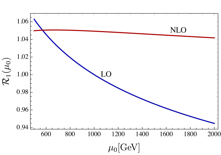
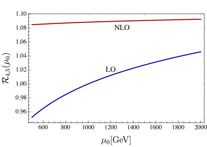
Figure 4: Matching-scale dependence of the ratios ${\cal R}_{1}$ and ${\cal R}_{4,5}$ for $M(1\,{\rm TeV})=1\,{\rm TeV}$. The upper plot shows the case in which $C_{1}$ is generated (the $\Gamma^{R}\Gamma^{R}$ contribution to the mass difference), while the lower plot shows the case in which $C_{4}$ and $C_{5}$ are generated (the $\Gamma^{L}\Gamma^{R}$ contribution to the mass difference).

5 Conclusions

Leptoquarks are prime candidates for an explanation of the flavour anomalies, in particular of the hints for NP in $b\to s\ell^{+}\ell^{-}$ and $b\to c\tau\nu$ transitions. While contributing to these processes, other flavour observables, such as $\Delta F=2$ processes, are unavoidably also modified. Thus, viable explanations of the flavour anomalies must also satisfy these experimental bounds.

In this article we have studied the $\Delta F=2$ processes $D^{0}-\bar{D}^{0}$, $K^{0}-\bar{K}^{0}$ and $B_{s,d}-\bar{B}_{s,d}$ mixing in models with scalar LQs. We have first obtained the complete LO matching for all five representations of scalar LQs under the SM gauge group (including mixed contributions). Then we have calculated the NLO $\alpha_{s}$ corrections to the matching. This allows for a consistent use of the existing two-loop anomalous dimensions in the EFT and significantly reduces the matching scale uncertainty in the calculation of physical observables. We find that the NLO matching corrections lead to a constructive effect of the order of 5% (8%) for the case of $C_{1}$ ($C_{4}$, $C_{5}$). We have also provided easy-to-use semi-numerical formulas for the neutral meson mixing amplitudes (at the meson level).

Appendix A Projections

We describe the method used in the evaluation of both the EFT and full theory amplitudes in our calculation. As explained in Sec. 3.3 we construct projectors $P_{i},i=1,...,8$ defined as

$$P_{i}\langle{\cal O}_{j}\rangle^{(0)}=\delta_{ij}+{\cal O}(\epsilon^{2})\,,$$ (76)

for a consistent method up to order $\mathcal{O(\epsilon)}$ as this is the order of the divergences (see Sec. 3.1). In order to illustrate the approach, we first consider the full theory amplitude. A generic two-loop amplitude can be expressed as

$$D=\int\frac{d^{n}k}{(2\pi)^{n}}\int\frac{d^{n}q}{(2\pi)^{n}}\frac{\bar{u}_{s\delta}\Gamma_{A}(k,q,\mu,\nu)u_{b\alpha}\otimes\bar{v}_{s\beta}\Gamma_{B}(k,q,\mu,\nu)v_{b\gamma}}{(k^{2}-m_{1}^{2})^{n_{1}}(q^{2}-m_{2}^{2})^{n_{2}}((k-q)^{2}-m_{3}^{2})^{n_{3}}}\,,$$ (77)

where Greek letters are colour indices and the $s(b)$ index indicates the $s(b)$ quark. The objects $\Gamma_{A,B}$ represent strings of gamma matrices and loop momenta with saturated Lorentz indices . Once the integration is performed (following Ref. [229]) the amplitude is expressed in terms of strings of gamma matrices with structures $\overline{\Lambda}^{(i)}_{A}\otimes\overline{\Lambda}^{(i)}_{B}$ together with coefficients $a_{i}(m)$ which only depend on masses (generically denoted by $m$)

$$D=\sum_{i}a_{i}(m)\left[\bar{u}_{s\delta}\overline{\Lambda}^{(i)}_{A}u_{b\alpha}\otimes\bar{v}_{s\beta}\overline{\Lambda}^{(i)}_{B}v_{b\gamma}\right].$$ (78)

The coefficients $a_{i}(m)$ are UV finite because the full theory has been renormalized. The Dirac structure $\bar{u}_{s\delta}\overline{\Lambda}^{(i)}_{A}u_{b\alpha}\otimes\bar{v}_{s\beta}\overline{\Lambda}^{(i)}_{B}v_{b\gamma}$ corresponds to the tree-level matrix element of a physical operator $\langle\mathcal{O}_{i}\rangle^{(0)}$, which is always possible after some four-dimensional Dirac algebra.

Therefore, the projectors are constructed such that the coefficients $a_{i}(m)$ are projected out whenever $P_{i}$ is applied to the amplitude in Eq. (78). For $P_{i}=P^{(i)}_{A}\otimes P^{(i)}_{B}$, we require

$$\text{Tr}\left[\overline{\Lambda}^{(i)}_{A}P_{A}^{(j)}\overline{\Lambda}^{(i)}_{B}P_{B}^{(j)}\right]=\delta_{ij}\ ,$$ (79)

and the projection on the amplitude is defined by the following replacement:

$$u_{b\alpha}\bar{v}_{s\beta}\rightarrow P_{B}^{(i)}\delta_{\alpha\beta},\quad v_{b\gamma}\bar{u}_{s\delta}\rightarrow P_{A}^{(i)}\delta_{\delta\gamma}\ .$$ (80)

Using  Eq. (79) we find the projectors

$$P_{1} =-\frac{i}{384}p_{1}\,, P_{2} =-\frac{i}{64}p_{2}+\frac{i}{2304}p_{5}\,, P_{3} =\frac{i}{192}p_{2}+\frac{5i}{2304}p_{5}\,,$$

$$P_{4} =-\frac{i}{192}p_{3}-\frac{i}{32}p_{4}\,, P_{5} =\frac{i}{64}p_{3}+\frac{i}{96}p_{4}\,,$$ (81)

which are given as linear combinations of the following more basic ones,

$$p_{1} =\gamma_{\mu}P_{R}\otimes\gamma^{\mu}P_{R}\,, p_{2} =P_{L}\otimes P_{L}\,, p_{3} =\gamma_{\mu}P_{L}\otimes\gamma^{\mu}P_{R}\,,$$

$$p_{4} =P_{L}\otimes P_{R}\,, p_{5} =\sigma_{\mu\nu}P_{L}\otimes\sigma^{\mu\nu}P_{L}\,.$$ (82)

The projectors $P^{\prime}_{1,2,3}$ projecting onto $C^{\prime}_{1,2,3}$ are equal to $P_{1,2,3}$ with the replacement $P_{R}\leftrightarrow P_{L}$. One can verify that the projectors of Eq. (82) fulfill the condition in Eq. (76), and so when one applies $P_{i}$ to an amplitude it projects out the coefficient of the $\langle{\cal O}_{i}\rangle^{(0)}$ term.

In the EFT, the Dirac algebra cannot be carried out in four dimensions because the presence of $1/\epsilon$ poles in the loop integrals requires keeping $\epsilon$ terms in the Dirac Algebra (see e.g. Ref. [213]). Thus, when reducing the spinor structures in the EFT amplitudes to tree-level matrix elements one is forced to introduce Evanescent operators $E=E_{A}\otimes E_{B}$. For the basis of Evanescent operators relevant for $\Delta F=2$ processes we use the ones given in App. A of Ref. [213]. In this case we require the projectors to project out these terms:

$$\text{Tr}\left[E^{(i)}_{A}P_{A}^{(j)}E^{(i)}_{B}P_{B}^{(j)}\right]=\mathcal{O}(\epsilon^{2})\quad\forall\quad i,j\,,$$ (83)

This implies that for the EFT the projectors must be calculated to order ${\cal O}(\epsilon)$ explicitly, and as a consequence the list of projectors $p_{i}$ includes further Dirac structures and colour structures. Now, the replacement is

$$u_{b\alpha}\bar{v}_{s\beta}\rightarrow P_{B}^{(k)}S_{\alpha\beta}\,,\quad v_{b\gamma}\bar{u}_{s\delta}\rightarrow P_{A}^{(k)}S_{\delta\gamma}\,,$$ (84)

where $S_{\alpha\beta(\delta\gamma)}$ is the colour structure which can either be $\delta_{\alpha\beta(\delta\gamma)}$ or $T_{\alpha\beta(\delta\gamma)}^{A}$. Using the corresponding conditions for the projectors, we find

$$P_{1} = -\frac{455i}{2304}p_{1}-\frac{193i}{384}p_{9}+\frac{i}{1152}p_{8}+\frac{323i}{12288}p_{13}+\epsilon\frac{149i}{256}p_{1}\,,$$ (85)

$$P_{2} = -\frac{2520983i}{273888}p_{2}+\frac{1489i}{45648}p_{7}-\frac{655699i}{45648}p_{10}+\frac{10229i}{365184}p_{15}+\frac{7i}{4608}p_{16}\,$$ (87)

$$-\frac{105617i}{1095552}p_{5}+\epsilon\left(\frac{31272625i}{1643328}p_{2}+\frac{4117901i}{136944}p_{10}\right)\,,$$

$$P_{3} = -\frac{1257571i}{136944}p_{2}+\frac{373i}{11412}p_{7}-\frac{655645i}{45648}p_{10}+\frac{10157i}{365184}p_{15}+\frac{7i}{4608}p_{16}$$ (89)

$$-\frac{51817i}{547776}p_{5}+\epsilon\left(\frac{15625897i}{821664}p_{2}+\frac{2056349i}{68472}p_{10}\right)\,,$$

$$P_{4} = -\frac{i}{16}p_{11}+\frac{i}{144}p_{6}+\frac{i}{16}p_{12}-\frac{i}{192}p_{14}-\frac{i}{12}p_{4}-\epsilon\left(\frac{3i}{16}p_{12}+\frac{i}{24}p_{3}\right)\,,$$ (90)

$$P_{5} = -\frac{3i}{16}p_{12}+\frac{i}{48}p_{11}-\frac{i}{36}p_{3}+\frac{i}{64}p_{14}+\frac{i\epsilon}{16}p_{12}\,,$$ (91)

with the following list of projectors $p_{i}$: For $S_{\alpha\beta(\delta\gamma)}=\delta_{\alpha\beta(\delta\gamma)}$,

$$p_{6} = \gamma_{\mu}\gamma_{\nu}\gamma_{\rho}P_{R}\otimes\gamma^{\mu}\gamma^{\nu}\gamma^{\rho}P_{R}\,,$$

$$p_{7} = \sigma_{\mu\nu}P_{L}\otimes\sigma^{\mu\nu}P_{R}\,,$$ (92)

$$p_{8} = \gamma_{\mu}\gamma_{\nu}\gamma_{\rho}\gamma_{\sigma}\gamma_{\lambda}P_{R}\otimes\gamma^{\mu}\gamma^{\nu}\gamma^{\rho}\gamma^{\sigma}\gamma^{\lambda}P_{R}\,,$$

and for $S_{\alpha\beta(\delta\gamma)}=T_{\alpha\beta(\delta\gamma)}^{A}$,

$$p_{9} =\gamma_{\mu}P_{R}\otimes\gamma^{\mu}P_{R}\,, p_{13} =\gamma_{\mu}\gamma_{\nu}\gamma_{\rho}P_{R}\otimes\gamma^{\mu}\gamma^{\nu}\gamma^{\rho}P_{R}\,,$$

$$p_{10} =P_{L}\otimes P_{L}\,, p_{14} =\gamma_{\mu}\gamma_{\nu}\gamma_{\rho}P_{L}\otimes\gamma^{\mu}\gamma^{\nu}\gamma^{\rho}P_{R}\,,$$

$$p_{11} =\gamma_{\mu}P_{L}\otimes\gamma^{\mu}P_{R}\,, p_{15} =\sigma_{\mu\nu}P_{L}\otimes\sigma^{\mu\nu}P_{R}\,,$$ (93)

$$p_{12} =P_{L}\otimes P_{R}\,, p_{16} =\gamma_{\mu}\gamma_{\nu}\gamma_{\rho}\gamma_{\sigma}\gamma_{\lambda}\gamma_{\delta}P_{L}\otimes\gamma^{\mu}\gamma^{\nu}\gamma^{\rho}\gamma^{\sigma}\gamma^{\lambda}\gamma^{\delta}P_{L}\,.$$

Appendix B Two-loop ADM in the SUSY basis

Our NLO matching calculation has been performed in the SUSY basis. A byproduct of this calculation is the LO ADM $\gamma^{(0)}$ (which is scheme-independent). However, in order to perform NLL resummation, the NLO ADM $\gamma^{(1)}$ is needed, which arises from the renormalization of the EFT at two-loop order. This calculation has been performed in Ref. [213], in a different basis (the “BMU” basis) for physical operators,

$$Q=\left(Q_{1}^{\text{VLL}},Q_{1}^{\text{SLL}},Q_{2}^{\text{SLL}},Q_{1}^{\text{LR}},Q_{2}^{\text{LR}},Q_{1}^{\text{VRR}},Q_{1}^{\text{SRR}},Q_{2}^{\text{SRR}}\right)^{T}\ .$$ (94)

Therefore, we must rotate the result in Ref. [213] to our basis. The SUSY (${\cal O}$) and BMU ($Q$) bases are related in the following way

$$\vec{{\cal O}}=R\,\left(\vec{Q}+W\vec{E}\right)\ ,$$ (95)

where the Fierz-evanescent operators $\vec{E}^{T}=\left(\star,E_{1}^{\text{SLL}},\star,E_{1}^{\text{LR}},\star\right)$ are defined in Ref. [213] and

$$R=\left(\begin{array}[]{ccccc}1&0&0&0&0\\ 0&1&0&0&0\\ 0&-1/2&1/8&0&0\\ 0&0&0&0&1\\ 0&0&0&-1/2&0\end{array}\right),\quad W=\left(\begin{array}[]{rrrrr}0&\quad 0&\quad 0&\quad 0&\quad 0\\ 0&0&0&0&0\\ 0&8&0&0&0\\ 0&0&0&-2&0\\ 0&0&0&0&0\end{array}\right).$$ (96)

(The corresponding results for the sector ${\cal O}^{\prime}_{1-3}$ vs VRR/SRR are the same as the 1-3 sector above.) Due to the presence of evanescent operators ($\vec{E}$) and their mixing with the physical operators, the transformation for $\gamma^{(1)}$ from the BMU basis to the SUSY basis corresponds to a rotation plus a change of scheme, given by (e.g.[239, 240])

$$\gamma^{(1)}_{\mathcal{O}}=R\left(\gamma^{(1)}_{Q}-\left[r_{Q},\gamma^{(0)}_{Q}\right]-2\beta_{0}r_{Q}\right)R^{-1}+\left[r_{\mathcal{O}},\gamma^{(0)}_{\mathcal{O}}\right]+2\beta_{0}r_{\mathcal{O}},$$ (97)

where the matrices $r_{\cal O}$ and $r_{Q}$ are defined in Eq. (30) in their corresponding bases. The LO ADM $\gamma^{(0)}$ is scheme-independent and thus it holds that $\gamma^{(0)}_{\cal O}=R\gamma^{(0)}_{Q}R^{-1}$.

We compute $r_{Q}$ from scratch directly in the BMU basis (along the lines of Section 3.2), and obtain

$$r_{Q}=\left(\begin{array}[]{ccccc}4/3&0&0&0&0\\ 0&{\color[rgb]{.5,.5,.5}46/3}&{\color[rgb]{.5,.5,.5}-1/6}&0&0\\ 0&{\color[rgb]{.5,.5,.5}40}&{\color[rgb]{.5,.5,.5}-6}&0&0\\ 0&0&0&10/3&-12\\ 0&0&0&0&64/3\end{array}\right)\log(\mu/\lambda)+\left(\begin{array}[]{ccccc}-5&0&0&0&0\\ 0&{\color[rgb]{.5,.5,.5}5/6}&{\color[rgb]{.5,.5,.5}-1/8}&0&0\\ 0&{\color[rgb]{.5,.5,.5}-46/3}&{\color[rgb]{.5,.5,.5}1/6}&0&0\\ 0&0&0&-7/6&1\\ 0&0&0&3/2&19/3\end{array}\right)\ .$$ (98)

where again we have indicated in gray the sector that does not impact our $SU(2)$-invariant model. Using Eq. (97) and taking $\gamma^{(1)}_{Q}$ from Ref. [213], we find

$$\gamma^{(1)}_{\mathcal{O}}=\left(\begin{array}[]{ccccc}\frac{4f}{9}-7&0&0&0&0\\ 0&{\color[rgb]{.5,.5,.5}\frac{220f}{27}-\frac{476}{3}}&{\color[rgb]{.5,.5,.5}-\frac{4f}{27}-\frac{4}{3}}&0&0\\ 0&{\color[rgb]{.5,.5,.5}73+\frac{110f}{27}}&{\color[rgb]{.5,.5,.5}\frac{359}{3}-\frac{218f}{27}}&0&0\\ 0&0&0&\frac{68f}{9}-\frac{1343}{6}&4f-\frac{225}{2}\\ 0&0&0&\frac{22f}{3}-99&\frac{71}{3}-\frac{22f}{9}\\ \end{array}\right)\ ,$$ (99)

in accordance with Eq. (15).

The SLL/SRR sector (in gray) can be reproduced using the formulas given in Section C.1 of Ref. [238], leading to a result in agreement with Eq. (99).

References

• [1] J. C. Pati and A. Salam, “Lepton Number as the Fourth Color,” Phys. Rev. D 10, 275-289 (1974) [erratum: Phys. Rev. D 11, 703-703 (1975)]
• [2] H. Georgi and S. L. Glashow, “Unity of All Elementary Particle Forces,” Phys. Rev. Lett. 32, 438-441 (1974)
• [3] H. Georgi, H. R. Quinn and S. Weinberg, “Hierarchy of Interactions in Unified Gauge Theories,” Phys. Rev. Lett. 33, 451-454 (1974)
• [4] H. Fritzsch and P. Minkowski, “Unified Interactions of Leptons and Hadrons,” Annals Phys. 93, 193-266 (1975)
• [5] W. Buchmuller, R. Ruckl and D. Wyler, “Leptoquarks in Lepton - Quark Collisions,” Phys. Lett. B 191, 442-448 (1987) [erratum: Phys. Lett. B 448, 320-320 (1999)]
• [6] J. P. Lees et al. [BaBar], “Evidence for an excess of $\bar{B}\to D^{(*)}\tau^{-}\bar{\nu}_{\tau}$ decays,” Phys. Rev. Lett. 109, 101802 (2012) [arXiv:1205.5442 [hep-ex]].
• [7] J. P. Lees et al. [BaBar], “Measurement of an Excess of $\bar{B}\to D^{(*)}\tau^{-}\bar{\nu}_{\tau}$ Decays and Implications for Charged Higgs Bosons,” Phys. Rev. D 88, no.7, 072012 (2013) [arXiv:1303.0571 [hep-ex]].
• [8] R. Aaij et al. [LHCb], “Measurement of the ratio of branching fractions $\mathcal{B}(\bar{B}^{0}\to D^{*+}\tau^{-}\bar{\nu}_{\tau})/\mathcal{B}(\bar{B}^{0}\to D^{*+}\mu^{-}\bar{\nu}_{\mu})$,” Phys. Rev. Lett. 115, no.11, 111803 (2015) [erratum: Phys. Rev. Lett. 115, no.15, 159901 (2015)] [arXiv:1506.08614 [hep-ex]].
• [9] R. Aaij et al. [LHCb], “Test of Lepton Flavor Universality by the measurement of the $B^{0}\to D^{*-}\tau^{+}\nu_{\tau}$ branching fraction using three-prong $\tau$ decays,” Phys. Rev. D 97, no.7, 072013 (2018) [arXiv:1711.02505 [hep-ex]].
• [10] R. Aaij et al. [LHCb], “Measurement of the ratio of the $B^{0}\to D^{*-}\tau^{+}\nu_{\tau}$ and $B^{0}\to D^{*-}\mu^{+}\nu_{\mu}$ branching fractions using three-prong $\tau$-lepton decays,” Phys. Rev. Lett. 120, no.17, 171802 (2018) [arXiv:1708.08856 [hep-ex]].
• [11] A. Abdesselam et al. [Belle], “Measurement of $\mathcal{R}(D)$ and $\mathcal{R}(D^{\ast})$ with a semileptonic tagging method,” [arXiv:1904.08794 [hep-ex]].
• [12] V. Khachatryan et al. [CMS and LHCb], “Observation of the rare $B^{0}_{s}\to\mu^{+}\mu^{-}$ decay from the combined analysis of CMS and LHCb data,” Nature 522, 68-72 (2015) [arXiv:1411.4413 [hep-ex]].
• [13] R. Aaij et al. [LHCb], “Angular analysis of the $B^{0}\to K^{*0}\mu^{+}\mu^{-}$ decay using 3 fb-1 of integrated luminosity,” JHEP 02, 104 (2016) [arXiv:1512.04442 [hep-ex]].
• [14] A. Abdesselam et al. [Belle], “Angular analysis of $B^{0}\to K^{\ast}(892)^{0}\ell^{+}\ell^{-}$,” [arXiv:1604.04042 [hep-ex]].
• [15] R. Aaij et al. [LHCb], “Test of lepton universality with $B^{0}\rightarrow K^{*0}\ell^{+}\ell^{-}$ decays,” JHEP 08, 055 (2017) [arXiv:1705.05802 [hep-ex]].
• [16] R. Aaij et al. [LHCb], “Search for lepton-universality violation in $B^{+}\to K^{+}\ell^{+}\ell^{-}$ decays,” Phys. Rev. Lett. 122, no.19, 191801 (2019) [arXiv:1903.09252 [hep-ex]].
• [17] R. Aaij et al. [LHCb], “Measurement of $CP$-Averaged Observables in the $B^{0}\rightarrow K^{*0}\mu^{+}\mu^{-}$ Decay,” Phys. Rev. Lett. 125, no.1, 011802 (2020) [arXiv:2003.04831 [hep-ex]].
• [18] R. Aaij et al. [LHCb], “Test of lepton universality in beauty-quark decays,” [arXiv:2103.11769 [hep-ex]].
• [19] G. W. Bennett et al. [Muon g-2], “Final Report of the Muon E821 Anomalous Magnetic Moment Measurement at BNL,” Phys. Rev. D 73, 072003 (2006) [arXiv:hep-ex/0602035 [hep-ex]].
• [20] B. Abi et al. [Muon g-2], “Measurement of the Positive Muon Anomalous Magnetic Moment to 0.46 ppm,” Phys. Rev. Lett. 126, no.14, 141801 (2021) [arXiv:2104.03281 [hep-ex]].
• [21] Y. Amhis et al. [HFLAV], “Averages of $b$-hadron, $c$-hadron, and $\tau$-lepton properties as of summer 2016,” Eur. Phys. J. C 77, no.12, 895 (2017) [arXiv:1612.07233 [hep-ex]].
• [22] C. Murgui, A. Peñuelas, M. Jung and A. Pich, “Global fit to $b\to c\tau\nu$ transitions,” JHEP 09, 103 (2019) [arXiv:1904.09311 [hep-ph]].
• [23] R. X. Shi, L. S. Geng, B. Grinstein, S. Jäger and J. Martin Camalich, “Revisiting the new-physics interpretation of the $b\to c\tau\nu$ data,” JHEP 12, 065 (2019) [arXiv:1905.08498 [hep-ph]].
• [24] M. Blanke, A. Crivellin, T. Kitahara, M. Moscati, U. Nierste and I. Nišandžić, “Addendum to “Impact of polarization observables and $B_{c}\to\tau\nu$ on new physics explanations of the $b\to c\tau\nu$ anomaly”,” [arXiv:1905.08253 [hep-ph]].
• [25] S. Kumbhakar, A. K. Alok, D. Kumar and S. U. Sankar, “A global fit to $b\rightarrow c\tau\bar{\nu}$ anomalies after Moriond 2019,” PoS EPS-HEP2019, 272 (2020) [arXiv:1909.02840 [hep-ph]].
• [26] S. Descotes-Genon, L. Hofer, J. Matias and J. Virto, “Global analysis of $b\to s\ell\ell$ anomalies,” JHEP 06, 092 (2016) [arXiv:1510.04239 [hep-ph]].
• [27] B. Capdevila, A. Crivellin, S. Descotes-Genon, J. Matias and J. Virto, “Patterns of New Physics in $b\to s\ell^{+}\ell^{-}$ transitions in the light of recent data,” JHEP 01, 093 (2018) [arXiv:1704.05340 [hep-ph]].
• [28] W. Altmannshofer, P. Stangl and D. M. Straub, “Interpreting Hints for Lepton Flavor Universality Violation,” Phys. Rev. D 96, no.5, 055008 (2017) [arXiv:1704.05435 [hep-ph]].
• [29] M. Algueró, B. Capdevila, A. Crivellin, S. Descotes-Genon, P. Masjuan, J. Matias, M. Novoa Brunet and J. Virto, “Emerging patterns of New Physics with and without Lepton Flavour Universal contributions,” Eur. Phys. J. C 79, no.8, 714 (2019) [arXiv:1903.09578 [hep-ph]].
• [30] A. K. Alok, A. Dighe, S. Gangal and D. Kumar, “Continuing search for new physics in $b\to s\mu\mu$ decays: two operators at a time,” JHEP 06, 089 (2019) [arXiv:1903.09617 [hep-ph]].
• [31] M. Ciuchini, A. M. Coutinho, M. Fedele, E. Franco, A. Paul, L. Silvestrini and M. Valli, “New Physics in $b\to s\ell^{+}\ell^{-}$ confronts new data on Lepton Universality,” Eur. Phys. J. C 79, no.8, 719 (2019) [arXiv:1903.09632 [hep-ph]].
• [32] J. Aebischer, W. Altmannshofer, D. Guadagnoli, M. Reboud, P. Stangl and D. M. Straub, “$B$-decay discrepancies after Moriond 2019,” Eur. Phys. J. C 80, no.3, 252 (2020) [arXiv:1903.10434 [hep-ph]].
• [33] A. Arbey, T. Hurth, F. Mahmoudi, D. M. Santos and S. Neshatpour, “Update on the $b\to s$ anomalies,” Phys. Rev. D 100, no.1, 015045 (2019) [arXiv:1904.08399 [hep-ph]].
• [34] D. Kumar, K. Kowalska and E. M. Sessolo, “Global Bayesian Analysis of new physics in $b\to s\mu\mu$ transitions after Moriond-2019,” [arXiv:1906.08596 [hep-ph]].
• [35] M. Algueró, B. Capdevila, S. Descotes-Genon, J. Matias and M. Novoa-Brunet, “$\boldsymbol{b\to s\ell\ell}$ global fits after Moriond 2021 results,” [arXiv:2104.08921 [hep-ph]].
• [36] W. Altmannshofer and P. Stangl, “New Physics in Rare B Decays after Moriond 2021,” [arXiv:2103.13370 [hep-ph]].
• [37] A. K. Alok, S. Kumbhakar and S. Uma Sankar, “A unique discrimination between new physics scenarios in $b\rightarrow s\mu^{+}\mu^{-}$ anomalies,” [arXiv:2001.04395 [hep-ph]].
• [38] T. Hurth, F. Mahmoudi and S. Neshatpour, “Model independent analysis of the angular observables in $B^{0}\to K^{*0}\mu^{+}\mu^{-}$ and $B^{+}\to K^{*+}\mu^{+}\mu^{-}$,” Phys. Rev. D 103, 095020 (2021) [arXiv:2012.12207 [hep-ph]].
• [39] M. Ciuchini, M. Fedele, E. Franco, A. Paul, L. Silvestrini and M. Valli, “Lessons from the $B^{0,+}\to K^{*0,+}\mu^{+}\mu^{-}$ angular analyses,” Phys. Rev. D 103, no.1, 015030 (2021) [arXiv:2011.01212 [hep-ph]].
• [40] T. Aoyama, N. Asmussen, M. Benayoun, J. Bijnens, T. Blum, M. Bruno, I. Caprini, C. M. Carloni Calame, M. Cè and G. Colangelo, et al. “The anomalous magnetic moment of the muon in the Standard Model,” Phys. Rept. 887, 1-166 (2020) [arXiv:2006.04822 [hep-ph]].
• [41] T. Aoyama, M. Hayakawa, T. Kinoshita and M. Nio, “Complete Tenth-Order QED Contribution to the Muon $g-2$,” Phys. Rev. Lett. 109, 111808 (2012) [arXiv:1205.5370 [hep-ph]].
• [42] T. Aoyama, T. Kinoshita and M. Nio, “Theory of the Anomalous Magnetic Moment of the Electron,” Atoms 7, no.1, 28 (2019)
• [43] A. Czarnecki, W. J. Marciano and A. Vainshtein, “Refinements in electroweak contributions to the muon anomalous magnetic moment,” Phys. Rev. D 67, 073006 (2003) [erratum: Phys. Rev. D 73, 119901 (2006)] [arXiv:hep-ph/0212229 [hep-ph]].
• [44] C. Gnendiger, D. Stöckinger and H. Stöckinger-Kim, “The electroweak contributions to $(g-2)_{\mu}$ after the Higgs boson mass measurement,” Phys. Rev. D 88, 053005 (2013) [arXiv:1306.5546 [hep-ph]].
• [45] M. Davier, A. Hoecker, B. Malaescu and Z. Zhang, “Reevaluation of the hadronic vacuum polarisation contributions to the Standard Model predictions of the muon $g-2$ and ${\alpha(m_{Z}^{2})}$ using newest hadronic cross-section data,” Eur. Phys. J. C 77, no.12, 827 (2017) [arXiv:1706.09436 [hep-ph]].
• [46] A. Keshavarzi, D. Nomura and T. Teubner, “Muon $g-2$ and $\alpha(M_{Z}^{2})$: a new data-based analysis,” Phys. Rev. D 97, no.11, 114025 (2018) [arXiv:1802.02995 [hep-ph]].
• [47] G. Colangelo, M. Hoferichter and P. Stoffer, “Two-pion contribution to hadronic vacuum polarization,” JHEP 02, 006 (2019) [arXiv:1810.00007 [hep-ph]].
• [48] M. Hoferichter, B. L. Hoid and B. Kubis, “Three-pion contribution to hadronic vacuum polarization,” JHEP 08, 137 (2019) [arXiv:1907.01556 [hep-ph]].
• [49] M. Davier, A. Hoecker, B. Malaescu and Z. Zhang, “A new evaluation of the hadronic vacuum polarisation contributions to the muon anomalous magnetic moment and to $\mathbf{\boldsymbol{\alpha}(m_{Z}^{2})}$,” Eur. Phys. J. C 80, no.3, 241 (2020) [erratum: Eur. Phys. J. C 80, no.5, 410 (2020)] [arXiv:1908.00921 [hep-ph]].
• [50] A. Keshavarzi, D. Nomura and T. Teubner, “$g-2$ of charged leptons, $\alpha(M^{2}_{Z})$ , and the hyperfine splitting of muonium,” Phys. Rev. D 101, no.1, 014029 (2020) [arXiv:1911.00367 [hep-ph]].
• [51] A. Kurz, T. Liu, P. Marquard and M. Steinhauser, “Hadronic contribution to the muon anomalous magnetic moment to next-to-next-to-leading order,” Phys. Lett. B 734, 144-147 (2014) [arXiv:1403.6400 [hep-ph]].
• [52] K. Melnikov and A. Vainshtein, “Hadronic light-by-light scattering contribution to the muon anomalous magnetic moment revisited,” Phys. Rev. D 70, 113006 (2004) [arXiv:hep-ph/0312226 [hep-ph]].
• [53] P. Masjuan and P. Sanchez-Puertas, “Pseudoscalar-pole contribution to the $(g_{\mu}-2)$: a rational approach,” Phys. Rev. D 95, no.5, 054026 (2017) [arXiv:1701.05829 [hep-ph]].
• [54] G. Colangelo, M. Hoferichter, M. Procura and P. Stoffer, “Dispersion relation for hadronic light-by-light scattering: two-pion contributions,” JHEP 04, 161 (2017) [arXiv:1702.07347 [hep-ph]].
• [55] M. Hoferichter, B. L. Hoid, B. Kubis, S. Leupold and S. P. Schneider, “Dispersion relation for hadronic light-by-light scattering: pion pole,” JHEP 10, 141 (2018) [arXiv:1808.04823 [hep-ph]].
• [56] A. Gérardin, H. B. Meyer and A. Nyffeler, “Lattice calculation of the pion transition form factor with $N_{f}=2+1$ Wilson quarks,” Phys. Rev. D 100, no.3, 034520 (2019) [arXiv:1903.09471 [hep-lat]].
• [57] J. Bijnens, N. Hermansson-Truedsson and A. Rodríguez-Sánchez, “Short-distance constraints for the HLbL contribution to the muon anomalous magnetic moment,” Phys. Lett. B 798, 134994 (2019) [arXiv:1908.03331 [hep-ph]].
• [58] G. Colangelo, F. Hagelstein, M. Hoferichter, L. Laub and P. Stoffer, “Longitudinal short-distance constraints for the hadronic light-by-light contribution to $(g-2)_{\mu}$ with large-$N_{c}$ Regge models,” JHEP 03, 101 (2020) [arXiv:1910.13432 [hep-ph]].
• [59] T. Blum, N. Christ, M. Hayakawa, T. Izubuchi, L. Jin, C. Jung and C. Lehner, “Hadronic Light-by-Light Scattering Contribution to the Muon Anomalous Magnetic Moment from Lattice QCD,” Phys. Rev. Lett. 124, no.13, 132002 (2020) [arXiv:1911.08123 [hep-lat]].
• [60] G. Colangelo, M. Hoferichter, A. Nyffeler, M. Passera and P. Stoffer, “Remarks on higher-order hadronic corrections to the muon g$-$2,” Phys. Lett. B 735, 90-91 (2014) [arXiv:1403.7512 [hep-ph]].
• [61] B. Gripaios, M. Nardecchia and S. A. Renner, “Composite leptoquarks and anomalies in $B$-meson decays,” JHEP 05, 006 (2015) [arXiv:1412.1791 [hep-ph]].
• [62] R. Alonso, B. Grinstein and J. Martin Camalich, “Lepton universality violation and lepton flavor conservation in $B$-meson decays,” JHEP 10, 184 (2015) [arXiv:1505.05164 [hep-ph]].
• [63] L. Calibbi, A. Crivellin and T. Ota, “Effective Field Theory Approach to $b\to s\ell\ell^{(^{\prime})}$, $B\to K^{(*)}\nu\overline{\nu}$ and $B\to D^{(*)}\tau\nu$ with Third Generation Couplings,” Phys. Rev. Lett. 115, 181801 (2015) [arXiv:1506.02661 [hep-ph]].
• [64] G. Hiller, D. Loose and K. Schönwald, “Leptoquark Flavor Patterns & B Decay Anomalies,” JHEP 12, 027 (2016) [arXiv:1609.08895 [hep-ph]].
• [65] B. Bhattacharya, A. Datta, J. P. Guévin, D. London and R. Watanabe, “Simultaneous Explanation of the $R_{K}$ and $R_{D^{(*)}}$ Puzzles: a Model Analysis,” JHEP 01, 015 (2017) [arXiv:1609.09078 [hep-ph]].
• [66] D. Buttazzo, A. Greljo, G. Isidori and D. Marzocca, “B-physics anomalies: a guide to combined explanations,” JHEP 11, 044 (2017) [arXiv:1706.07808 [hep-ph]].
• [67] R. Barbieri, G. Isidori, A. Pattori and F. Senia, “Anomalies in $B$-decays and $U(2)$ flavour symmetry,” Eur. Phys. J. C 76, no.2, 67 (2016) [arXiv:1512.01560 [hep-ph]].
• [68] R. Barbieri, C. W. Murphy and F. Senia, “B-decay Anomalies in a Composite Leptoquark Model,” Eur. Phys. J. C 77, no.1, 8 (2017) [arXiv:1611.04930 [hep-ph]].
• [69] L. Calibbi, A. Crivellin and T. Li, “Model of vector leptoquarks in view of the $B$-physics anomalies,” Phys. Rev. D 98, no.11, 115002 (2018) [arXiv:1709.00692 [hep-ph]].
• [70] A. Crivellin, D. Müller, A. Signer and Y. Ulrich, “Correlating lepton flavor universality violation in $B$ decays with $\mu\to e\gamma$ using leptoquarks,” Phys. Rev. D 97, no.1, 015019 (2018) [arXiv:1706.08511 [hep-ph]].
• [71] L. Di Luzio, A. Greljo and M. Nardecchia, “Gauge leptoquark as the origin of $B$-physics anomalies,” Phys. Rev. D 96, no.11, 115011 (2017) [arXiv:1708.08450 [hep-ph]].
• [72] M. Bordone, C. Cornella, J. Fuentes-Martín and G. Isidori, “Low-energy signatures of the $\mathrm{PS}^{3}$ model: from $B$-physics anomalies to LFV,” JHEP 10, 148 (2018) [arXiv:1805.09328 [hep-ph]].
• [73] J. Kumar, D. London and R. Watanabe, “Combined Explanations of the $b\to s\mu^{+}\mu^{-}$ and $b\to c\tau^{-}{\bar{\nu}}$ Anomalies: a General Model Analysis,” Phys. Rev. D 99, no.1, 015007 (2019) [arXiv:1806.07403 [hep-ph]].
• [74] A. Crivellin, C. Greub, D. Müller and F. Saturnino, “Importance of Loop Effects in Explaining the Accumulated Evidence for New Physics in B Decays with a Vector Leptoquark,” Phys. Rev. Lett. 122, no.1, 011805 (2019) [arXiv:1807.02068 [hep-ph]].
• [75] A. Crivellin and F. Saturnino, “Explaining the Flavor Anomalies with a Vector Leptoquark (Moriond 2019 update),” PoS DIS2019, 163 (2019) [arXiv:1906.01222 [hep-ph]].
• [76] C. Cornella, J. Fuentes-Martin and G. Isidori, “Revisiting the vector leptoquark explanation of the B-physics anomalies,” JHEP 07, 168 (2019) [arXiv:1903.11517 [hep-ph]].
• [77] M. Bordone, O. Catà and T. Feldmann, “Effective Theory Approach to New Physics with Flavour: General Framework and a Leptoquark Example,” JHEP 01, 067 (2020) [arXiv:1910.02641 [hep-ph]].
• [78] J. Bernigaud, I. de Medeiros Varzielas and J. Talbert, “Finite Family Groups for Fermionic and Leptoquark Mixing Patterns,” JHEP 01, 194 (2020) [arXiv:1906.11270 [hep-ph]].
• [79] J. Aebischer, A. Crivellin and C. Greub, “QCD improved matching for semileptonic B decays with leptoquarks,” Phys. Rev. D 99, no.5, 055002 (2019) [arXiv:1811.08907 [hep-ph]].
• [80] J. Fuentes-Martín, G. Isidori, M. König and N. Selimović, “Vector Leptoquarks Beyond Tree Level,” Phys. Rev. D 101, no.3, 035024 (2020) [arXiv:1910.13474 [hep-ph]].
• [81] O. Popov, M. A. Schmidt and G. White, “$R_{2}$ as a single leptoquark solution to $R_{D^{(*)}}$ and $R_{K^{(*)}}$,” Phys. Rev. D 100, no.3, 035028 (2019) [arXiv:1905.06339 [hep-ph]].
• [82] S. Fajfer and N. Košnik, “Vector leptoquark resolution of $R_{K}$ and $R_{D^{(*)}}$ puzzles,” Phys. Lett. B 755, 270-274 (2016) [arXiv:1511.06024 [hep-ph]].
• [83] M. Blanke and A. Crivellin, “$B$ Meson Anomalies in a Pati-Salam Model within the Randall-Sundrum Background,” Phys. Rev. Lett. 121, no.1, 011801 (2018) [arXiv:1801.07256 [hep-ph]].
• [84] I. de Medeiros Varzielas and J. Talbert, “Simplified Models of Flavourful Leptoquarks,” Eur. Phys. J. C 79, no.6, 536 (2019) [arXiv:1901.10484 [hep-ph]].
• [85] I. de Medeiros Varzielas and G. Hiller, “Clues for flavor from rare lepton and quark decays,” JHEP 06, 072 (2015) [arXiv:1503.01084 [hep-ph]].
• [86] A. Crivellin, D. Müller and F. Saturnino, “Flavor Phenomenology of the Leptoquark Singlet-Triplet Model,” JHEP 06, 020 (2020) [arXiv:1912.04224 [hep-ph]].
• [87] S. Saad, “Combined explanations of $(g-2)_{\mu}$, $R_{D^{(*)}}$, $R_{K^{(*)}}$ anomalies in a two-loop radiative neutrino mass model,” Phys. Rev. D 102, no.1, 015019 (2020) [arXiv:2005.04352 [hep-ph]].
• [88] S. Saad and A. Thapa, “Common origin of neutrino masses and $R_{D^{(\ast)}}$, $R_{K^{(\ast)}}$ anomalies,” Phys. Rev. D 102, no.1, 015014 (2020) [arXiv:2004.07880 [hep-ph]].
• [89] V. Gherardi, D. Marzocca and E. Venturini, “Low-energy phenomenology of scalar leptoquarks at one-loop accuracy,” JHEP 01, 138 (2021) [arXiv:2008.09548 [hep-ph]].
• [90] L. Da Rold and F. Lamagna, “Model for the singlet-triplet leptoquarks,” Phys. Rev. D 103, no.11, 115007 (2021) [arXiv:2011.10061 [hep-ph]].
• [91] J. Davighi, M. Kirk and M. Nardecchia, “Anomalies and accidental symmetries: charging the scalar leptoquark under $L_{\mu}-L_{\tau}$,” JHEP 12, 111 (2020) [arXiv:2007.15016 [hep-ph]].
• [92] S. Iguro, J. Kawamura, S. Okawa and Y. Omura, “TeV-scale vector leptoquark from Pati-Salam unification with vectorlike families,” [arXiv:2103.11889 [hep-ph]].
• [93] S. Iguro and R. Watanabe, “Bayesian fit analysis to full distribution data of $\bar{B}\to{D}^{(*)}\ell\bar{\nu}$: $|{V}_{cb}|$ determination and new physics constraints,” JHEP 08, no.08, 006 (2020) [arXiv:2004.10208 [hep-ph]].
• [94] S. Iguro, T. Kitahara, Y. Omura, R. Watanabe and K. Yamamoto, “D polarization vs. ${R}_{D^{\left(\ast\right)}}$ anomalies in the leptoquark models,” JHEP 02, 194 (2019) [arXiv:1811.08899 [hep-ph]].
• [95] M. Bordone, C. Cornella, J. Fuentes-Martin and G. Isidori, “A three-site gauge model for flavor hierarchies and flavor anomalies,” Phys. Lett. B 779, 317-323 (2018) [arXiv:1712.01368 [hep-ph]].
• [96] A. Biswas, D. Kumar Ghosh, N. Ghosh, A. Shaw and A. K. Swain, “Collider signature of $U_{1}$ Leptoquark and constraints from $b\to c$ observables,” J. Phys. G 47, no.4, 045005 (2020) [arXiv:1808.04169 [hep-ph]].
• [97] J. Heeck and D. Teresi, “Pati-Salam explanations of the B-meson anomalies,” JHEP 12, 103 (2018) [arXiv:1808.07492 [hep-ph]].
• [98] S. Sahoo and R. Mohanta, “Scalar leptoquarks and the rare $B$ meson decays,” Phys. Rev. D 91, no.9, 094019 (2015) [arXiv:1501.05193 [hep-ph]].
• [99] C. H. Chen, T. Nomura and H. Okada, “Explanation of $B\to K^{(*)}\ell^{+}\ell^{-}$ and muon $g-2$, and implications at the LHC,” Phys. Rev. D 94, no.11, 115005 (2016) [arXiv:1607.04857 [hep-ph]].
• [100] U. K. Dey, D. Kar, M. Mitra, M. Spannowsky and A. C. Vincent, “Searching for Leptoquarks at IceCube and the LHC,” Phys. Rev. D 98, no.3, 035014 (2018) [arXiv:1709.02009 [hep-ph]].
• [101] D. Bečirević and O. Sumensari, “A leptoquark model to accommodate $R_{K}^{\mathrm{exp}}<R_{K}^{\mathrm{SM}}$ and $R_{K^{\ast}}^{\mathrm{exp}}<R_{K^{\ast}}^{\mathrm{SM}}$,” JHEP 08, 104 (2017) [arXiv:1704.05835 [hep-ph]].
• [102] B. Chauhan, B. Kindra and A. Narang, “Discrepancies in simultaneous explanation of flavor anomalies and IceCube PeV events using leptoquarks,” Phys. Rev. D 97, no.9, 095007 (2018) [arXiv:1706.04598 [hep-ph]].
• [103] D. Bečirević, I. Doršner, S. Fajfer, N. Košnik, D. A. Faroughy and O. Sumensari, “Scalar leptoquarks from grand unified theories to accommodate the $B$-physics anomalies,” Phys. Rev. D 98, no.5, 055003 (2018) [arXiv:1806.05689 [hep-ph]].
• [104] S. Fajfer, J. F. Kamenik, I. Nisandzic and J. Zupan, “Implications of Lepton Flavor Universality Violations in B Decays,” Phys. Rev. Lett. 109, 161801 (2012) [arXiv:1206.1872 [hep-ph]].
• [105] N. G. Deshpande and A. Menon, “Hints of R-parity violation in B decays into $\tau\nu$,” JHEP 01, 025 (2013) [arXiv:1208.4134 [hep-ph]].
• [106] M. Freytsis, Z. Ligeti and J. T. Ruderman, “Flavor models for $\bar{B}\to D^{(*)}\tau\bar{\nu}$,” Phys. Rev. D 92, no.5, 054018 (2015) [arXiv:1506.08896 [hep-ph]].
• [107] M. Bauer and M. Neubert, “Minimal Leptoquark Explanation for the $R_{D^{(*)}}$ , $R_{K}$ , and $(g-2)_{\mu}$ Anomalies,” Phys. Rev. Lett. 116, no.14, 141802 (2016) [arXiv:1511.01900 [hep-ph]].
• [108] X. Q. Li, Y. D. Yang and X. Zhang, “Revisiting the one leptoquark solution to the R(D(∗)) anomalies and its phenomenological implications,” JHEP 08, 054 (2016) [arXiv:1605.09308 [hep-ph]].
• [109] J. Zhu, H. M. Gan, R. M. Wang, Y. Y. Fan, Q. Chang and Y. G. Xu, “Probing the R-parity violating supersymmetric effects in the exclusive $b\to c\ell^{-}\bar{\nu}_{\ell}$ decays,” Phys. Rev. D 93, no.9, 094023 (2016) [arXiv:1602.06491 [hep-ph]].
• [110] O. Popov and G. A. White, “One Leptoquark to unify them? Neutrino masses and unification in the light of $(g-2)_{\mu}$, $R_{D^{(\star)}}$ and $R_{K}$ anomalies,” Nucl. Phys. B 923, 324-338 (2017) [arXiv:1611.04566 [hep-ph]].
• [111] N. G. Deshpande and X. G. He, “Consequences of R-parity violating interactions for anomalies in $\bar{B}\to D^{(*)}\tau\bar{\nu}$ and $b\to s\mu^{+}\mu^{-}$,” Eur. Phys. J. C 77, no.2, 134 (2017) [arXiv:1608.04817 [hep-ph]].
• [112] D. Bečirević, N. Košnik, O. Sumensari and R. Zukanovich Funchal, “Palatable Leptoquark Scenarios for Lepton Flavor Violation in Exclusive $b\to s\ell_{1}\ell_{2}$ modes,” JHEP 11, 035 (2016) [arXiv:1608.07583 [hep-ph]].
• [113] Y. Cai, J. Gargalionis, M. A. Schmidt and R. R. Volkas, “Reconsidering the One Leptoquark solution: flavor anomalies and neutrino mass,” JHEP 10, 047 (2017) [arXiv:1704.05849 [hep-ph]].
• [114] W. Altmannshofer, P. S. Bhupal Dev and A. Soni, “$R_{D^{(*)}}$ anomaly: A possible hint for natural supersymmetry with $R$-parity violation,” Phys. Rev. D 96, no.9, 095010 (2017) [arXiv:1704.06659 [hep-ph]].
• [115] S. Kamali, A. Rashed and A. Datta, “New physics in inclusive $B\to X_{c}\ell\bar{\nu}$ decay in light of $R(D^{(*)})$ measurements,” Phys. Rev. D 97, no.9, 095034 (2018) [arXiv:1801.08259 [hep-ph]].
• [116] T. Mandal, S. Mitra and S. Raz, “$R_{D^{(*)}}$ motivated $\mathcal{S}_{1}$ leptoquark scenarios: Impact of interference on the exclusion limits from LHC data,” Phys. Rev. D 99, no.5, 055028 (2019) [arXiv:1811.03561 [hep-ph]].
• [117] A. Azatov, D. Bardhan, D. Ghosh, F. Sgarlata and E. Venturini, “Anatomy of $b\to c\tau\nu$ anomalies,” JHEP 11, 187 (2018) [arXiv:1805.03209 [hep-ph]].
• [118] J. Zhu, B. Wei, J. H. Sheng, R. M. Wang, Y. Gao and G. R. Lu, “Probing the R-parity violating supersymmetric effects in $B_{c}\to J/\psi\ell^{-}\bar{\nu}_{\ell},\eta_{c}\ell^{-}\bar{\nu}_{\ell}$ and $\Lambda_{b}\to\Lambda_{c}\ell^{-}\bar{\nu}_{\ell}$ decays,” Nucl. Phys. B 934, 380-395 (2018) [arXiv:1801.00917 [hep-ph]].
• [119] A. Angelescu, D. Bečirević, D. A. Faroughy and O. Sumensari, “Closing the window on single leptoquark solutions to the $B$-physics anomalies,” JHEP 10, 183 (2018) [arXiv:1808.08179 [hep-ph]].
• [120] T. J. Kim, P. Ko, J. Li, J. Park and P. Wu, “Correlation between ${R}_{D^{\left(\ast\right)}}$ and top quark FCNC decays in leptoquark models,” JHEP 07, 025 (2019) [arXiv:1812.08484 [hep-ph]].
• [121] U. Aydemir, T. Mandal and S. Mitra, “Addressing the ${\mathbf{R}_{D^{(*)}}}$ anomalies with an ${\mathbf{S}_{1}}$ leptoquark from $\mathbf{SO(10)}$ grand unification,” Phys. Rev. D 101, no.1, 015011 (2020) [arXiv:1902.08108 [hep-ph]].
• [122] A. Crivellin and F. Saturnino, “Correlating tauonic $B$ decays with the neutron electric dipole moment via a scalar leptoquark,” Phys. Rev. D 100, no.11, 115014 (2019) [arXiv:1905.08257 [hep-ph]].
• [123] H. Yan, Y. D. Yang and X. B. Yuan, “Phenomenology of $b\to c\tau\bar{\nu}$ decays in a scalar leptoquark model,” Chin. Phys. C 43, no.8, 083105 (2019) [arXiv:1905.01795 [hep-ph]].
• [124] A. Crivellin, D. Müller and T. Ota, “Simultaneous explanation of R(D(∗)) and $b\to s\mu^{+}\mu^{-}$: the last scalar leptoquarks standing,” JHEP 09, 040 (2017) [arXiv:1703.09226 [hep-ph]].
• [125] D. Marzocca, “Addressing the B-physics anomalies in a fundamental Composite Higgs Model,” JHEP 07, 121 (2018) [arXiv:1803.10972 [hep-ph]].
• [126] I. Bigaran, J. Gargalionis and R. R. Volkas, “A near-minimal leptoquark model for reconciling flavour anomalies and generating radiative neutrino masses,” JHEP 10, 106 (2019) [arXiv:1906.01870 [hep-ph]].
• [127] P. S. Bhupal Dev, R. Mohanta, S. Patra and S. Sahoo, “Unified explanation of flavor anomalies, radiative neutrino masses, and ANITA anomalous events in a vector leptoquark model,” Phys. Rev. D 102, no.9, 095012 (2020) [arXiv:2004.09464 [hep-ph]].
• [128] W. Altmannshofer, P. S. B. Dev, A. Soni and Y. Sui, “Addressing R${}_{D^{(*)}}$, R${}_{K^{(*)}}$, muon $g-2$ and ANITA anomalies in a minimal $R$-parity violating supersymmetric framework,” Phys. Rev. D 102, no.1, 015031 (2020) [arXiv:2002.12910 [hep-ph]].
• [129] J. Fuentes-Martín and P. Stangl, “Third-family quark-lepton unification with a fundamental composite Higgs,” Phys. Lett. B 811, 135953 (2020) [arXiv:2004.11376 [hep-ph]].
• [130] A. Djouadi, T. Kohler, M. Spira and J. Tutas, “$(eb)$, $(et)$ type leptoquarks at $e$-$p$ colliders,” Z. Phys. C 46, 679-686 (1990)
• [131] D. Chakraverty, D. Choudhury and A. Datta, “A Nonsupersymmetric resolution of the anomalous muon magnetic moment,” Phys. Lett. B 506, 103-108 (2001) [arXiv:hep-ph/0102180 [hep-ph]].
• [132] K. m. Cheung, “Muon anomalous magnetic moment and leptoquark solutions,” Phys. Rev. D 64, 033001 (2001) [arXiv:hep-ph/0102238 [hep-ph]].
• [133] C. Biggio, M. Bordone, L. Di Luzio and G. Ridolfi, “Massive vectors and loop observables: the $g-2$ case,” JHEP 10, 002 (2016) [arXiv:1607.07621 [hep-ph]].
• [134] S. Davidson, D. C. Bailey and B. A. Campbell, “Model independent constraints on leptoquarks from rare processes,” Z. Phys. C 61, 613-644 (1994) [arXiv:hep-ph/9309310 [hep-ph]].
• [135] G. Couture and H. Konig, “Bounds on second generation scalar leptoquarks from the anomalous magnetic moment of the muon,” Phys. Rev. D 53, 555-557 (1996) [arXiv:hep-ph/9507263 [hep-ph]].
• [136] U. Mahanta, “Implications of BNL measurement of delta a(mu) on a class of scalar leptoquark interactions,” Eur. Phys. J. C 21, 171-173 (2001) [arXiv:hep-ph/0102176 [hep-ph]].
• [137] F. S. Queiroz, K. Sinha and A. Strumia, “Leptoquarks, Dark Matter, and Anomalous LHC Events,” Phys. Rev. D 91, no.3, 035006 (2015) [arXiv:1409.6301 [hep-ph]].
• [138] E. Coluccio Leskow, G. D’Ambrosio, A. Crivellin and D. Müller, “$(g-2)\mu$, lepton flavor violation, and $Z$ decays with leptoquarks: Correlations and future prospects,” Phys. Rev. D 95, no.5, 055018 (2017) [arXiv:1612.06858 [hep-ph]].
• [139] C. H. Chen, T. Nomura and H. Okada, “Excesses of muon $g-2$, $R_{D^{(\ast)}}$, and $R_{K}$ in a leptoquark model,” Phys. Lett. B 774, 456-464 (2017) [arXiv:1703.03251 [hep-ph]].
• [140] D. Das, C. Hati, G. Kumar and N. Mahajan, “Towards a unified explanation of $R_{D^{(\ast)}}$, $R_{K}$ and $(g-2)_{\mu}$ anomalies in a left-right model with leptoquarks,” Phys. Rev. D 94, 055034 (2016) [arXiv:1605.06313 [hep-ph]].
• [141] A. Crivellin, M. Hoferichter and P. Schmidt-Wellenburg, “Combined explanations of $(g-2)_{\mu,e}$ and implications for a large muon EDM,” Phys. Rev. D 98, no.11, 113002 (2018) [arXiv:1807.11484 [hep-ph]].
• [142] K. Kowalska, E. M. Sessolo and Y. Yamamoto, “Constraints on charmphilic solutions to the muon g-2 with leptoquarks,” Phys. Rev. D 99, no.5, 055007 (2019) [arXiv:1812.06851 [hep-ph]].
• [143] I. Doršner, S. Fajfer and O. Sumensari, “Muon $g-2$ and scalar leptoquark mixing,” JHEP 06, 089 (2020) [arXiv:1910.03877 [hep-ph]].
• [144] L. Delle Rose, C. Marzo and L. Marzola, “Simplified leptoquark models for precision $\ell_{i}\to\ell_{f}\gamma$ experiments: two-loop structure of $O(\alpha_{s}Y^{2})$ corrections,” Phys. Rev. D 102, no.11, 115020 (2020) [arXiv:2005.12389 [hep-ph]].
• [145] I. Bigaran and R. R. Volkas, “Getting chirality right: Single scalar leptoquark solutions to the $(g-2)_{e,\mu}$ puzzle,” Phys. Rev. D 102, no.7, 075037 (2020) [arXiv:2002.12544 [hep-ph]].
• [146] I. Doršner, S. Fajfer and S. Saad, “$\mu\to e\gamma$ selecting scalar leptoquark solutions for the $(g-2)_{e,\mu}$ puzzles,” Phys. Rev. D 102, no.7, 075007 (2020) [arXiv:2006.11624 [hep-ph]].
• [147] K. S. Babu, P. S. B. Dev, S. Jana and A. Thapa, “Unified framework for $B$-anomalies, muon $g-2$ and neutrino masses,” JHEP 03, 179 (2021) [arXiv:2009.01771 [hep-ph]].
• [148] A. Crivellin, D. Mueller and F. Saturnino, “Correlating $h\to\mu^{+}\mu^{-}$ to the Anomalous Magnetic Moment of the Muon via Leptoquarks,” Phys. Rev. Lett. 127, no.2, 021801 (2021) [arXiv:2008.02643 [hep-ph]].
• [149] L. Di Luzio, J. Fuentes-Martin, A. Greljo, M. Nardecchia and S. Renner, “Maximal Flavour Violation: a Cabibbo mechanism for leptoquarks,” JHEP 11, 081 (2018) [arXiv:1808.00942 [hep-ph]].
• [150] A. M. Sirunyan et al. [CMS], “Search for resonant and nonresonant new phenomena in high-mass dilepton final states at $\sqrt{s}$ = 13 TeV,” JHEP 07, 208 (2021) [arXiv:2103.02708 [hep-ex]].
• [151] A. Crivellin, C. A. Manzari and M. Montull, “Correlating Non-Resonant Di-Electron Searches at the LHC to the Cabibbo-Angle Anomaly and Lepton Flavour Universality Violation,” [arXiv:2103.12003 [hep-ph]].
• [152] A. Crivellin, D. Müller and L. Schnell, “Combined constraints on first generation leptoquarks,” Phys. Rev. D 103, no.11, 115023 (2021) [arXiv:2104.06417 [hep-ph]].
• [153] A. Crivellin, M. Hoferichter, M. Kirk, C. A. Manzari and L. Schnell, “First-Generation New Physics in Simplified Models: From Low-Energy Parity Violation to the LHC,” [arXiv:2107.13569 [hep-ph]].
• [154] B. Belfatto, R. Beradze and Z. Berezhiani, “The CKM unitarity problem: A trace of new physics at the TeV scale?,” Eur. Phys. J. C 80, no.2, 149 (2020) [arXiv:1906.02714 [hep-ph]].
• [155] Y. Grossman, E. Passemar and S. Schacht, “On the Statistical Treatment of the Cabibbo Angle Anomaly,” JHEP 07, 068 (2020) [arXiv:1911.07821 [hep-ph]].
• [156] C. Y. Seng, X. Feng, M. Gorchtein and L. C. Jin, “Joint lattice QCD–dispersion theory analysis confirms the quark-mixing top-row unitarity deficit,” Phys. Rev. D 101, no.11, 111301 (2020) [arXiv:2003.11264 [hep-ph]].
• [157] A. M. Coutinho, A. Crivellin and C. A. Manzari, “Global Fit to Modified Neutrino Couplings and the Cabibbo-Angle Anomaly,” Phys. Rev. Lett. 125, no.7, 071802 (2020) [arXiv:1912.08823 [hep-ph]].
• [158] C. A. Manzari, A. M. Coutinho and A. Crivellin, “Modified lepton couplings and the Cabibbo-angle anomaly,” PoS LHCP2020, 242 (2021) [arXiv:2009.03877 [hep-ph]].
• [159] A. Crivellin and M. Hoferichter, “$\beta$ Decays as Sensitive Probes of Lepton Flavor Universality,” Phys. Rev. Lett. 125, no.11, 111801 (2020) [arXiv:2002.07184 [hep-ph]].
• [160] A. Carvunis, A. Crivellin, D. Guadagnoli and S. Gangal, “The Forward-Backward Asymmetry in $B\to D^{*}\ell\nu$: One more hint for Scalar Leptoquarks?,” [arXiv:2106.09610 [hep-ph]].
• [161] C. Bobeth, D. van Dyk, M. Bordone, M. Jung and N. Gubernari, “Lepton-flavour non-universality of $\bar{B}\to D^{*}\ell\bar{\nu}$ angular distributions in and beyond the Standard Model,” [arXiv:2104.02094 [hep-ph]].
• [162] M. Kramer, T. Plehn, M. Spira and P. M. Zerwas, “Pair production of scalar leptoquarks at the Tevatron,” Phys. Rev. Lett. 79, 341-344 (1997) [arXiv:hep-ph/9704322 [hep-ph]].
• [163] M. Kramer, T. Plehn, M. Spira and P. M. Zerwas, “Pair production of scalar leptoquarks at the CERN LHC,” Phys. Rev. D 71, 057503 (2005) [arXiv:hep-ph/0411038 [hep-ph]].
• [164] D. A. Faroughy, A. Greljo and J. F. Kamenik, “Confronting lepton flavor universality violation in B decays with high-$p_{T}$ tau lepton searches at LHC,” Phys. Lett. B 764, 126-134 (2017) [arXiv:1609.07138 [hep-ph]].
• [165] A. Greljo and D. Marzocca, “High-$p_{T}$ dilepton tails and flavor physics,” Eur. Phys. J. C 77, no.8, 548 (2017) [arXiv:1704.09015 [hep-ph]].
• [166] J. Blumlein, E. Boos and A. Kryukov, “Leptoquark pair production in hadronic interactions,” Z. Phys. C 76, 137-153 (1997) [arXiv:hep-ph/9610408 [hep-ph]].
• [167] I. Doršner, S. Fajfer, D. A. Faroughy and N. Košnik, “The role of the $S_{3}$ GUT leptoquark in flavor universality and collider searches,” JHEP 10, 188 (2017) [arXiv:1706.07779 [hep-ph]].
• [168] A. Cerri, V. V. Gligorov, S. Malvezzi, J. Martin Camalich, J. Zupan, S. Akar, J. Alimena, B. C. Allanach, W. Altmannshofer and L. Anderlini, et al. “Report from Working Group 4: Opportunities in Flavour Physics at the HL-LHC and HE-LHC,” CERN Yellow Rep. Monogr. 7, 867-1158 (2019) [arXiv:1812.07638 [hep-ph]].
• [169] P. Bandyopadhyay and R. Mandal, “Revisiting scalar leptoquark at the LHC,” Eur. Phys. J. C 78, 491 (2018) [arXiv:1801.04253 [hep-ph]].
• [170] G. Hiller, D. Loose and I. Nišandžić, “Flavorful leptoquarks at hadron colliders,” Phys. Rev. D 97, no.7, 075004 (2018) [arXiv:1801.09399 [hep-ph]].
• [171] T. Faber, M. Hudec, H. Kolešová, Y. Liu, M. Malinský, W. Porod and F. Staub, “Collider phenomenology of a unified leptoquark model,” Phys. Rev. D 101, no.9, 095024 (2020) [arXiv:1812.07592 [hep-ph]].
• [172] M. Schmaltz and Y. M. Zhong, “The leptoquark Hunter’s guide: large coupling,” JHEP 01, 132 (2019) [arXiv:1810.10017 [hep-ph]].
• [173] K. Chandak, T. Mandal and S. Mitra, “Hunting for scalar leptoquarks with boosted tops and light leptons,” Phys. Rev. D 100, no.7, 075019 (2019) [arXiv:1907.11194 [hep-ph]].
• [174] B. C. Allanach, T. Corbett and M. Madigan, “Sensitivity of Future Hadron Colliders to Leptoquark Pair Production in the Di-Muon Di-Jets Channel,” Eur. Phys. J. C 80, no.2, 170 (2020) [arXiv:1911.04455 [hep-ph]].
• [175] L. Buonocore, U. Haisch, P. Nason, F. Tramontano and G. Zanderighi, “Lepton-Quark Collisions at the Large Hadron Collider,” Phys. Rev. Lett. 125, no.23, 231804 (2020) [arXiv:2005.06475 [hep-ph]].
• [176] U. Haisch and G. Polesello, “Resonant third-generation leptoquark signatures at the Large Hadron Collider,” JHEP 05, 057 (2021) [arXiv:2012.11474 [hep-ph]].
• [177] C. Borschensky, B. Fuks, A. Kulesza and D. Schwartländer, “Scalar leptoquark pair production at hadron colliders,” Phys. Rev. D 101, no.11, 115017 (2020) [arXiv:2002.08971 [hep-ph]].
• [178] S. Iguro, M. Takeuchi and R. Watanabe, “Testing leptoquark/EFT in ${\bar{B}}\rightarrow{D^{(*)}}l{\bar{\nu}}$ at the LHC,” Eur. Phys. J. C 81, no.5, 406 (2021) [arXiv:2011.02486 [hep-ph]].
• [179] P. Bandyopadhyay, A. Karan and R. Mandal, “Distinguishing signatures of scalar leptoquarks at hadron and muon colliders,” [arXiv:2108.06506 [hep-ph]].
• [180] P. Bandyopadhyay, S. Dutta, M. Jakkapu and A. Karan, “Distinguishing Leptoquarks at the LHC/FCC,” Nucl. Phys. B 971, 115524 (2021) [arXiv:2007.12997 [hep-ph]].
• [181] A. Crivellin, C. Greub, D. Müller and F. Saturnino, “Scalar Leptoquarks in Leptonic Processes,” JHEP 02, 182 (2021) [arXiv:2010.06593 [hep-ph]].
• [182] E. Keith and E. Ma, “S, T, and leptoquarks at HERA,” Phys. Rev. Lett. 79, 4318-4320 (1997) [arXiv:hep-ph/9707214 [hep-ph]].
• [183] I. Doršner, S. Fajfer, A. Greljo, J. F. Kamenik and N. Košnik, “Physics of leptoquarks in precision experiments and at particle colliders,” Phys. Rept. 641, 1-68 (2016) [arXiv:1603.04993 [hep-ph]].
• [184] A. Bhaskar, D. Das, B. De and S. Mitra, “Enhancing scalar productions with leptoquarks at the LHC,” Phys. Rev. D 102, no.3, 035002 (2020) [arXiv:2002.12571 [hep-ph]].
• [185] J. Zhang, C. X. Yue, C. H. Li and S. Yang, “Constraints on scalar and vector leptoquarks from the LHC Higgs data,” [arXiv:1905.04074 [hep-ph]].
• [186] V. Gherardi, D. Marzocca and E. Venturini, “Matching scalar leptoquarks to the SMEFT at one loop,” JHEP 07, 225 (2020) [erratum: JHEP 01, 006 (2021)] [arXiv:2003.12525 [hep-ph]].
• [187] A. Crivellin, D. Müller and F. Saturnino, “Leptoquarks in oblique corrections and Higgs signal strength: status and prospects,” JHEP 11, 094 (2020) [arXiv:2006.10758 [hep-ph]].
• [188] O. U. Shanker, “Flavor Violation, Scalar Particles and Leptoquarks,” Nucl. Phys. B 206, 253-272 (1982)
• [189] O. U. Shanker, “$\pi_{\ell 2}$, $K_{\ell 3}$ and $K^{0}-\bar{K}$0 Constraints on Leptoquarks and Supersymmetric Particles,” Nucl. Phys. B 204, 375-386 (1982)
• [190] M. Leurer, “A Comprehensive study of leptoquark bounds,” Phys. Rev. D 49, 333-342 (1994) [arXiv:hep-ph/9309266 [hep-ph]].
• [191] M. Leurer, “Bounds on vector leptoquarks,” Phys. Rev. D 50, 536-541 (1994) [arXiv:hep-ph/9312341 [hep-ph]].
• [192] P. Arnan, D. Becirevic, F. Mescia and O. Sumensari, “Probing low energy scalar leptoquarks by the leptonic $W$ and $Z$ couplings,” JHEP 02, 109 (2019) [arXiv:1901.06315 [hep-ph]].
• [193] B. Capdevila, A. Crivellin, C. A. Manzari and M. Montull, “Explaining $b\to s\ell^{+}\ell^{-}$ and the Cabibbo angle anomaly with a vector triplet,” Phys. Rev. D 103, no.1, 015032 (2021) [arXiv:2005.13542 [hep-ph]].
• [194] A. Crivellin, F. Kirk, C. A. Manzari and M. Montull, “Global Electroweak Fit and Vector-Like Leptons in Light of the Cabibbo Angle Anomaly,” JHEP 12, 166 (2020) [arXiv:2008.01113 [hep-ph]].
• [195] M. Kirk, “Cabibbo anomaly versus electroweak precision tests: An exploration of extensions of the Standard Model,” Phys. Rev. D 103, no.3, 035004 (2021) [arXiv:2008.03261 [hep-ph]].
• [196] A. K. Alok, A. Dighe, S. Gangal and J. Kumar, “The role of non-universal Z couplings in explaining the Vus anomaly,” Nucl. Phys. B 971, 115538 (2021) [arXiv:2010.12009 [hep-ph]].
• [197] A. Crivellin, C. A. Manzari, M. Alguero and J. Matias, “Combined Explanation of the Z→bb¯ Forward-Backward Asymmetry, the Cabibbo Angle Anomaly, and $\tau$ $\mu$ $\nu$ $\nu$ and b→s$\ell$+$\ell$- Data,” Phys. Rev. Lett. 127, no.1, 011801 (2021) [arXiv:2010.14504 [hep-ph]].
• [198] A. Crivellin, F. Kirk, C. A. Manzari and L. Panizzi, “Searching for lepton flavor universality violation and collider signals from a singly charged scalar singlet,” Phys. Rev. D 103, no.7, 073002 (2021) [arXiv:2012.09845 [hep-ph]].
• [199] A. Crivellin, M. Hoferichter and C. A. Manzari, “Fermi Constant from Muon Decay Versus Electroweak Fits and Cabibbo-Kobayashi-Maskawa Unitarity,” Phys. Rev. Lett. 127, no.7, 071801 (2021) [arXiv:2102.02825 [hep-ph]].
• [200] B. Belfatto and Z. Berezhiani, “Are the CKM anomalies induced by vector-like quarks? Limits from flavor changing and Standard Model precision tests,” [arXiv:2103.05549 [hep-ph]].
• [201] G. C. Branco, J. T. Penedo, P. M. F. Pereira, M. N. Rebelo and J. I. Silva-Marcos, “Addressing the CKM unitarity problem with a vector-like up quark,” JHEP 07, 099 (2021) [arXiv:2103.13409 [hep-ph]].
• [202] C. Bobeth and A. J. Buras, “Leptoquarks meet $\varepsilon^{\prime}/\varepsilon$ and rare Kaon processes,” JHEP 02, 101 (2018) [arXiv:1712.01295 [hep-ph]].
• [203] I. Doršner, S. Fajfer and M. Patra, “A comparative study of the $S_{1}$ and $U_{1}$ leptoquark effects in the light quark regime,” Eur. Phys. J. C 80, no.3, 204 (2020) [arXiv:1906.05660 [hep-ph]].
• [204] R. Mandal and A. Pich, “Constraints on scalar leptoquarks from lepton and kaon physics,” JHEP 12, 089 (2019) [arXiv:1908.11155 [hep-ph]].
• [205] A. Crivellin and L. Schnell, “Complete Set of Feynman Rules for Scalar Leptoquarks,” [arXiv:2105.04844 [hep-ph]].
• [206] T. Plehn, H. Spiesberger, M. Spira and P. M. Zerwas, “Formation and decay of scalar leptoquarks / squarks in e p collisions,” Z. Phys. C 74, 611-614 (1997) [arXiv:hep-ph/9703433 [hep-ph]].
• [207] T. Mandal, S. Mitra and S. Seth, “Pair Production of Scalar Leptoquarks at the LHC to NLO Parton Shower Accuracy,” Phys. Rev. D 93, no.3, 035018 (2016) [arXiv:1506.07369 [hep-ph]].
• [208] J. B. Hammett and D. A. Ross, “NLO Leptoquark Production and Decay: The Narrow-Width Approximation and Beyond,” JHEP 07, 148 (2015) [arXiv:1501.06719 [hep-ph]].
• [209] I. Doršner and A. Greljo, “Leptoquark toolbox for precision collider studies,” JHEP 05, 126 (2018) [arXiv:1801.07641 [hep-ph]].
• [210] A. Monteux and A. Rajaraman, “B Anomalies and Leptoquarks at the LHC: Beyond the Lepton-Quark Final State,” Phys. Rev. D 98, no.11, 115032 (2018) [arXiv:1803.05962 [hep-ph]].
• [211] L. Di Luzio, M. Kirk and A. Lenz, “Updated $B_{s}$-mixing constraints on new physics models for $b\to s\ell^{+}\ell^{-}$ anomalies,” Phys. Rev. D 97, no.9, 095035 (2018) [arXiv:1712.06572 [hep-ph]].
• [212] M. Ciuchini, E. Franco, V. Lubicz, G. Martinelli, I. Scimemi and L. Silvestrini, “Next-to-leading order QCD corrections to Delta F = 2 effective Hamiltonians,” Nucl. Phys. B 523, 501-525 (1998) [arXiv:hep-ph/9711402 [hep-ph]].
• [213] A. J. Buras, M. Misiak and J. Urban, “Two loop QCD anomalous dimensions of flavor changing four quark operators within and beyond the standard model,” Nucl. Phys. B 586, 397-426 (2000) [arXiv:hep-ph/0005183 [hep-ph]].
• [214] M. Bona et al. [UTfit], “Model-independent constraints on $\Delta F=2$ operators and the scale of new physics,” JHEP 03, 049 (2008) [arXiv:0707.0636 [hep-ph]].
• [215] L. Di Luzio, M. Kirk, A. Lenz and T. Rauh, “$\Delta M_{s}$ theory precision confronts flavour anomalies,” JHEP 12, 009 (2019) [arXiv:1909.11087 [hep-ph]].
• [216] J. Aebischer, C. Bobeth, A. J. Buras and J. Kumar, “SMEFT ATLAS of $\Delta$F = 2 transitions,” JHEP 12, 187 (2020) [arXiv:2009.07276 [hep-ph]].
• [217] J. Aebischer, M. Fael, C. Greub and J. Virto, “B physics Beyond the Standard Model at One Loop: Complete Renormalization Group Evolution below the Electroweak Scale,” JHEP 09, 158 (2017) [arXiv:1704.06639 [hep-ph]].
• [218] M. Ciuchini, V. Lubicz, L. Conti, A. Vladikas, A. Donini, E. Franco, G. Martinelli, I. Scimemi, V. Gimenez and L. Giusti, et al. “Delta M(K) and epsilon(K) in SUSY at the next-to-leading order,” JHEP 10, 008 (1998) [arXiv:hep-ph/9808328 [hep-ph]].
• [219] M. Ciuchini, E. Franco, D. Guadagnoli, V. Lubicz, M. Pierini, V. Porretti and L. Silvestrini, “$D$ - $\bar{D}$ mixing and new physics: General considerations and constraints on the MSSM,” Phys. Lett. B 655, 162-166 (2007) [arXiv:hep-ph/0703204 [hep-ph]].
• [220] J. Virto, “Exact NLO strong interaction corrections to the $\Delta F=2$ effective Hamiltonian in the MSSM,” JHEP 11, 055 (2009) [arXiv:0907.5376 [hep-ph]].
• [221] W. Altmannshofer, A. J. Buras, S. Gori, P. Paradisi and D. M. Straub, “Anatomy and Phenomenology of FCNC and CPV Effects in SUSY Theories,” Nucl. Phys. B 830, 17-94 (2010) [arXiv:0909.1333 [hep-ph]].
• [222] A. Crivellin and U. Nierste, “Chirally enhanced corrections to FCNC processes in the generic MSSM,” Phys. Rev. D 81, 095007 (2010) [arXiv:0908.4404 [hep-ph]].
• [223] A. Crivellin and M. Davidkov, “Do squarks have to be degenerate? Constraining the mass splitting with Kaon and D mixing,” Phys. Rev. D 81, 095004 (2010) [arXiv:1002.2653 [hep-ph]].
• [224] J. Virto, “Top mass dependent ${\cal O}(\alpha_{s}^{3})$ corrections to $B$-meson mixing in the MSSM,” JHEP 01, 120 (2012) [arXiv:1111.0940 [hep-ph]].
• [225] F. Mescia and J. Virto, “Natural SUSY and Kaon Mixing in view of recent results from Lattice QCD,” Phys. Rev. D 86, 095004 (2012) [arXiv:1208.0534 [hep-ph]].
• [226] A. Crivellin, A. Kokulu and C. Greub, “Flavor-phenomenology of two-Higgs-doublet models with generic Yukawa structure,” Phys. Rev. D 87, no.9, 094031 (2013) [arXiv:1303.5877 [hep-ph]].
• [227] P. Arnan, L. Hofer, F. Mescia and A. Crivellin, “Loop effects of heavy new scalars and fermions in $b\to s\mu^{+}\mu^{-}$,” JHEP 04, 043 (2017) [arXiv:1608.07832 [hep-ph]].
• [228] P. Arnan, A. Crivellin, M. Fedele and F. Mescia, “Generic Loop Effects of New Scalars and Fermions in $b\to s\ell^{+}\ell^{-}$, $(g-2)_{\mu}$ and a Vector-like $4^{\rm th}$ Generation,” JHEP 06, 118 (2019) [arXiv:1904.05890 [hep-ph]].
• [229] A. I. Davydychev and J. B. Tausk, “Two loop selfenergy diagrams with different masses and the momentum expansion,” Nucl. Phys. B 397, 123-142 (1993)
• [230] A. Bazavov et al. [Fermilab Lattice and MILC], “$B^{0}_{(s)}$-mixing matrix elements from lattice QCD for the Standard Model and beyond,” Phys. Rev. D 93, no.11, 113016 (2016) [arXiv:1602.03560 [hep-lat]].
• [231] N. Carrasco et al. [ETM], “$\Delta$S=2 and $\Delta$C=2 bag parameters in the standard model and beyond from Nf=2+1+1 twisted-mass lattice QCD,” Phys. Rev. D 92, no.3, 034516 (2015) [arXiv:1505.06639 [hep-lat]].
• [232] A. Bazavov, C. Bernard, C. M. Bouchard, C. C. Chang, C. DeTar, D. Du, A. X. El-Khadra, E. D. Freeland, E. Gámiz and S. Gottlieb, et al. “Short-distance matrix elements for $D^{0}$-meson mixing for $N_{f}=2+1$ lattice QCD,” Phys. Rev. D 97, no.3, 034513 (2018) [arXiv:1706.04622 [hep-lat]].
• [233] R. J. Dowdall, C. T. H. Davies, R. R. Horgan, G. P. Lepage, C. J. Monahan, J. Shigemitsu and M. Wingate, “Neutral B-meson mixing from full lattice QCD at the physical point,” Phys. Rev. D 100, no.9, 094508 (2019) [arXiv:1907.01025 [hep-lat]].
• [234] P. A. Zyla et al. [Particle Data Group], “Review of Particle Physics,” PTEP 2020, no.8, 083C01 (2020), and 2021 update.
• [235] S. Aoki et al. [Flavour Lattice Averaging Group], “FLAG Review 2019: Flavour Lattice Averaging Group (FLAG),” Eur. Phys. J. C 80, no.2, 113 (2020) [arXiv:1902.08191 [hep-lat]].
• [236] A. J. Buras, S. Jager and J. Urban, “Master formulae for $\Delta F=2$ NLO QCD factors in the standard model and beyond,” Nucl. Phys. B 605, 600-624 (2001) [arXiv:hep-ph/0102316 [hep-ph]].
• [237] K. G. Chetyrkin, J. H. Kuhn and M. Steinhauser, “RunDec: A Mathematica package for running and decoupling of the strong coupling and quark masses,” Comput. Phys. Commun. 133, 43-65 (2000) [arXiv:hep-ph/0004189 [hep-ph]].
• [238] M. Gorbahn, S. Jager, U. Nierste and S. Trine, “The supersymmetric Higgs sector and $B-\bar{B}$ mixing for large tan $\beta$,” Phys. Rev. D 84 (2011), 034030 [arXiv:0901.2065 [hep-ph]].
• [239] K. G. Chetyrkin, M. Misiak and M. Munz, “$|\Delta F|=1$ nonleptonic effective Hamiltonian in a simpler scheme,” Nucl. Phys. B 520 (1998), 279-297 [arXiv:hep-ph/9711280 [hep-ph]].
• [240] M. Gorbahn and U. Haisch, “Effective Hamiltonian for non-leptonic $|\Delta F|=1$ decays at NNLO in QCD,” Nucl. Phys. B 713 (2005), 291-332 [arXiv:hep-ph/0411071 [hep-ph]].
• [241] E. E. Jenkins, A. V. Manohar and P. Stoffer, “Low-Energy Effective Field Theory below the Electroweak Scale: Operators and Matching,” JHEP 03, 016 (2018) [arXiv:1709.04486 [hep-ph]].