Abstract: We propose a reproducing kernel Hilbert space approach to estimate the slope in a function-on-function linear regression via penalised least squares, regularized by the thin-plate spline smoothness penalty. In contrast to most of the work on functional linear regression, our main focus is on statistical inference with respect to the sup-norm. This point of view is motivated by the fact that slope (surfaces) with rather different shapes may still be identified as similar when the difference is measured by an $L^{2}$-type norm. However, in applications it is often desirable to use metrics reflecting the visualization of the objects in the statistical analysis.

We prove the weak convergence of the slope surface estimator as a process in the space of all continuous functions. This allows us the construction of simultaneous confidence regions for the slope surface and simultaneous prediction bands. As a further consequence, we derive new tests for the hypothesis that the maximum deviation between the “true” slope surface and a given surface is less or equal than a given threshold. In other words: we are not trying to test for exact equality (because in many applications this hypothesis is hard to justify), but rather for pre-specified deviations under the null hypothesis. To ensure practicability, non-standard bootstrap procedures are developed addressing particular features that arise in these testing problems.

As a by-product, we also derive several new results and statistical inference tools for the function-on-function linear regression model, such as minimax optimal convergence rates and likelihood-ratio tests. We also demonstrate that the new methods have good finite sample properties by means of a simulation study and illustrate their practicability by analyzing a data example.

Keywords: function-on-function linear regression, minimax optimality, simultaneous confidence regions, relevant hypotheses, bootstrap, reproducing kernel Hilbert space, maximum deviation

AMS Subject Classification: 62R10, 62F03, 62F25, 46E22

1 Introduction

Over the past decades, new measurement technologies provide enormous amounts of data with complex structure. A popular and extremely successful approach to model high-dimensional data on a dense grid exhibiting a certain degree of smoothness is functional data analysis (FDA), which considers the observations as discretized functions. Meanwhile, numerous practical and theoretical aspects in FDA have been discussed (see, for example, the monographs Bosq, 2000; Ramsay and Silverman,, 2005; Ferraty and Vieu, 2010; Horváth and Kokoszka,, 2012; Hsing and Eubank, 2015, among others). A large portion of the literature uses dimension reduction techniques such as (functional) principal components. On the other hand, as argued in Aue et al., (2018), there are numerous applications, where it is reasonable to assume that the functions are at least continuous, and in such cases dimension reduction techniques can incur a loss of information and fully functional methods can prove advantageous.

Because of its simplicity and good interpretability, the scalar-on-function regression model

$$Y_{i}=\alpha_{0}+\int_{0}^{1}\beta_{0}(s)\,X_{i}(s)\,ds+\varepsilon_{i}\,,\quad 1\leq i\leq n\,.$$ (1.1)

has found considerable attention (see, for exemple, James,, 2002; Cardot et al., 2003; Müller and Stadtmüller,, 2005; Yao et al.,, 2005; Hall and Horowitz,, 2007; Yuan and Cai,, 2010, among manny others). Here, the $Y_{i}$ and the (centred) errors $\varepsilon_{i}$ are scalar variables, the predictors $X_{i}$ are functions (typically of time or location) defined on the interval $[0,1]$, and the scalar $\alpha_{0}$ and the function $\beta_{0}$ are the unknown parameters to be estimated. On the other hand, there also exist many applications, where both, the predictor and the response, are functions, and in recent years the function-on-function regression model

$$Y_{i}(t)=\alpha_{0}(t)+\int_{0}^{1}\beta_{0}(s,t)\,X_{i}(s)\,ds+\varepsilon_{i}(t)\,,\quad t\in[0,1]\,,\ 1\leq i\leq n\,,$$ (1.2)

has gained increasing attention (see Lian,, 2007, 2015; Scheipl and Greven,, 2016; Benatia et al.,, 2017; Luo and Qi,, 2017; Sun et al.,, 2018). Here $\alpha_{0}$, $Y_{i}$, $X_{i},$ $\varepsilon_{i}$ are functions defined on the interval $[0,1]$ and the slope parameter $\beta_{0}$ is a function defined on the square $[0,1]^{2}$, which we call slope surface throughout this paper in order to distinguish it from the slope function in model (1.1).

The slope $\beta_{0}$ quantifies the strength of the dependence between the predictor and the response, and is the main object of statistical inference in this context. Many methods, such as estimation, testing, confidence regions, have been developed in the last decades for the scalar-on-function linear regression model (1.1), which are often based on the $L^{2}$ metric (see, for example, Hall and Horowitz,, 2007; Horváth and Kokoszka,, 2012, among many others). A popular estimation tool is functional principle component (FPC) analysis, which provides a series representation of the function $\beta_{0}$ in the corresponding $L^{2}$ space (see, for example, Yao et al.,, 2005). Other authors proposed reproducing kernel Hilbert space (RKHS) approaches to estimate the slope parameter in a functional linear regression model. For example, Yuan and Cai, (2010) used the RKHS framework to construct a minimax optimal estimate in the scalar-on-function linear regression, and Cai and Yuan, (2012) discussed minimax properties of their RKHS estimator in terms of prediction accuracy. We also refer to the work of Meister, (2011) who showed the asymptotic equivalence of the scalar-on-function linear regression and the Gaussian white noise model in the Le Cam’s sense. Besides estimation, the problem of testing the hypotheses

$$H_{0}:\beta_{0}=\beta_{*}\ \mbox{~{}~{}~{}versus ~{}~{}}H_{1}:\beta_{0}\not=\beta_{*}~{},$$ (1.3)

for a prespecified function $\beta_{*}$ in the scalar-functional linear regression model has been discussed intensively (see Cardot et al., 2003; Cardot et al., 2004; Hilgert et al., 2013; Lei,, 2014; Kong et al., 2016; Qu and Wang,, 2017, among others). There also exist several proposals to construct $L^{2}$-based confidence regions (see Müller and Stadtmüller,, 2005; Imaizumi and Kato,, 2019, among others).

Non-linear and semiparametric scalar-on-function regression models, such as generalized linear models and the Cox model, have been studied by Shang and Cheng, (2015), Li and Zhu, (2020) and Hao et al., (2021). For the function-on-function model (1.2), the literature is more scarce. Lian, (2015) studied the minimax prediction rate in an RKHS, where regularization of the estimator is only performed in one argument, while Scheipl and Greven, (2016) investigated a penalized B-spline approach. Benatia et al., (2017) used Tikhonov regularization, Luo and Qi, (2017) proposed a so-called signal compression approach and Sun et al., (2018) considered a tensor product RKHS approach to estimate the slope surface and the achieved the minimax prediction risk.

This list of references is by no means complete, but a common feature of most of the work in this context consists in the fact that statistical methodology is developed in a Hilbert space framework (often the space or a subspace of the square-integrable functions on an interval), which means that the statistical properties of estimators, tests and confidence regions for the slope parameter are usually described in terms of a norm corresponding to a Hilbert space. While this is convenient from a theoretical point of view and also reflects the mathematical structure of the (integral) operator of the functional linear model, it has some drawbacks from a practical perspective. In applications, using a metric that reflects the visualization of the curve/surface is usually more desirable, since functions/surfaces with a small difference with respect to an $L^{2}$-type distance can differ significantly in terms of maximum deviation. For example, a confidence region of the slope function/surface based on an $L^{2}$-type distance is often hard to visualize and does not give much information about the shape of the curve or surface.

The choice of the metric also matters if one takes a more careful look at the formulation of the hypotheses in (1.3). We argue that, in many regression problems, it is very unlikely that the unknown slope $\beta_{0}$ coincides with a pre-specified function/surface $\beta_{*}$ on its complete domain, and as a consequence, testing the null hypothesis in (1.3) might be questionable in such cases. Usually, hypotheses of the form (1.3) are formulated with the intention to investigate the question whether the effect of the predictor on the response can be approximately described by the function/surface $\beta_{*}$, such that the difference $\beta_{0}-\beta_{*}$ is in some sense “small”. This question can be better answered by testing the hypotheses of a relevant difference

$$H_{0}:\|\beta_{0}-\beta_{*}\|\leq\Delta~{}~{}\mbox{ versus ~{}~{}}H_{1}:\|\beta_{0}-\beta_{*}\|>\Delta\,,$$ (1.4)

where $\|\cdot\|$ denotes a norm and $\Delta>0$ defines a threshold. Hypotheses of this type have recently found some interest in functional data analysis (see, for example, Fogarty and Small,, 2014; Dette et al.,, 2020), and here the choice of the norm matters, as different norms define different hypotheses. One may also view the choice of the threshold $\Delta$ as a particular perspective of a bias-variance trade-off, which depends sensitively on the specific application, and, of course, also on the metric under consideration. In particular, we argue that the specification of the threshold in (1.4) is more accessible for a norm which reflects the visualization, such as the sup-norm.

In the present paper, we address these issues and provide new statistical methodology for the function-on-function linear regression model (1.2) if inference is based on the maximum deviation. We propose an estimator for the slope surface $\beta_{0}$ minimizing an integrated squared error loss with a thin-plate spline smoothness penalty functional, and prove its minimax optimality using an RKHS framework. Based on a Bahadur representation, we establish the weak convergence of this estimator as a process in the Banach space $C([0,1]^{2})$ with a Gaussian limiting process. As the covariance structure of this process is not easily accessible, we develop a multiplier bootstrap to obtain quantiles for the distribution of functionals of the limiting process. In contrast to the $L^{2}$-metric based methods, this enables us to construct simultaneous asymptotic $(1-\alpha)$-confidence regions for the slope surface $\beta_{0}$ in model (1.2). Moreover, we also provide an efficient solution to the problem of testing for a relevant deviation from a given function $\beta_{*}$ with respect to the sup-norm. Here, we combine the developed bootstrap methodology with estimates of the extremal set of the function $\beta_{0}-\beta_{*}$, and develop an asymptotic level $\alpha$-test for the relevant hypotheses in (1.4), where the norm is given by the sup-norm. Although we mainly concentrate on the model (1.2), it is worth mentioning that, as a special case, our approach provides also new methods for the scalar-on-function linear regression model (1.1), which allows inference with respect to the sup-norm.

The rest of this article is organized as follows. In Section 2, we propose our RKHS methodology of function-on-function linear regression and study the asymptotic properties of our estimator in Section 3. Section 4 discusses several statistical applications of our results and the finite sample properties of the proposed methodology are illustrated in Section 5. Finally, the technical details and proofs of our theoretical results are given in the online supplementary material.

2 Function-on-function linear regression

Suppose that $(X_{1},Y_{1}),\ldots,(X_{n},Y_{n})$ are independent identically distributed random variables defined by the function-on-function regression model in (1.2), where $\varepsilon_{i}$ is the centred random noise, and the slope surface $\beta_{0}$ is defined on $[0,1]^{2}$. For the sake of brevity, throughout this article, we assume that the observed curves, i.e., $X_{i}$ and $Y_{i}$ in (1.2), are centred, that is, ${\rm E}\{X(s)\}={\rm E}\{Y(t)\}=0$, for any $(s,t)\in[0,1]^{2}$, so that we may ignore the intercept function $\alpha_{0}$, since $\alpha_{0}(t)={\rm E}\{Y(t)\}-\int_{0}^{1}\beta_{0}(s,t)\,{\rm E}\{X(s)\}ds$. In this case, the function-on-function linear regression model in (1.2) becomes

$$Y_{i}(t)=\int_{0}^{1}\beta_{0}(s,t)\,X_{i}(s)\,ds+\varepsilon_{i}(t)\,,\quad 1\leq i\leq n\,,$$ (2.1)

and a similar relation can be derived for the model (1.1).

In the sequel, we use $L^{2}([0,1])$ and $L^{2}([0,1]^{2})$ to denote the space of square-integrable functions on $[0,1]$ and $[0,1]^{2}$, respectively, and the corresponding inner product is denoted by $\langle\cdot,\cdot\rangle_{L^{2}}$. By $C([0,1]^{2})$ we denote the Banach space of continuous functions on $[0,1]^{2}$ equipped with the supremum norm $\|\cdot\|_{\infty}$, by “$\rightsquigarrow$” we denote weak convergence in $C([0,1])$ and $C([0,1]^{2})$, and “$\overset{d}{\longrightarrow}$” stays for convergence in distribution in $\mathbb{R}^{k}$ (for some positive integer $k$).

We start by proposing a RKHS approach for estimating the slope surface $\beta_{0}$ in model (2.1), and define by

$$\mathcal{H}=\Big{\{}\beta:[0,1]^{2}\to\mathbb{R}\,\big{|}\, \tfrac{\partial^{\theta_{1}+\theta_{2}}\beta}{\partial s^{\theta_{1}}\partial t^{\theta_{2}}}\text{ is absolutely continuous, for }0\leq\theta_{1}+\theta_{2}\leq m-1\,;$$

$$\tfrac{\partial^{\theta_{1}+\theta_{2}}\beta}{\partial s^{\theta_{1}}\partial t^{\theta_{2}}}\in L^{2}([0,1]^{2}),\text{ for }\theta_{1}+\theta_{2}=m\Big{\}}$$ (2.2)

the Sobolev space of order $m>1$ on $[0,1]^{2}$. It is known (see, for example, Wahba,, 1990) that $\mathcal{H}$ in (2) is a Hilbert space equipped with the Sobolev norm defined by

$$\|\beta\|_{\mathcal{H}}^{2}=\sum_{0\leq\theta_{1}+\theta_{2}\leq m-1}{\theta_{1}+\theta_{2}\choose\theta_{1}}\left(\int\frac{\partial^{\theta_{1}+\theta_{2}}\beta}{\partial s^{\theta_{1}}\partial t^{\theta_{2}}}\right)^{2}+\sum_{\theta_{1}+\theta_{2}=m}{m\choose\theta_{1}}\int\left(\frac{\partial^{m}\beta}{\partial s^{\theta_{1}}\partial t^{\theta_{2}}}\right)^{2}\,.$$ (2.3)

We propose to estimate $\beta_{0}$ in model (2.1) by

$$\widehat{\beta}_{n} =\underset{\beta\in\mathcal{H}}{\arg\min}\ \big{\{}L_{n}(\beta)+(\lambda/2)J(\beta,\beta)\big{\}}\,,$$ (2.4)

where

$$L_{n}(\beta)=\frac{1}{2n}\sum_{i=1}^{n}\int_{0}^{1}\left\{Y_{i}(t)-\int_{0}^{1}\beta(s,t)X_{i}(s)\,ds\right\}^{2}dt\,$$ (2.5)

is the integrated squared loss functional, $\lambda>0$ is a regularization parameter, and for $m>1$,

$$J(\beta_{1},\beta_{2})=\sum_{\theta=0}^{m}{m\choose\theta}\int_{0}^{1}\int_{0}^{1}\frac{\partial^{m}\beta_{1}}{\partial s^{\theta}\,\partial t^{m-\theta}}\times\frac{\partial^{m}\beta_{2}}{\partial s^{\theta}\,\partial t^{m-\theta}}\,ds\,dt\,$$ (2.6)

is the thin-plate spline smoothness penalty functional (see, for example, Wood,, 2003).

In (2.4), for notational brevity, we suppress the dependence of $\widehat{\beta}_{n}$ on $\lambda$, and denote by

$$L_{n,\lambda}(\beta)=L_{n}(\beta)+(\lambda/2)J(\beta,\beta)$$ (2.7)

the objective function in (2.4). For $\beta_{1},\beta_{2}\in\mathcal{H}$, we consider the following map $\langle\cdot,\cdot\rangle_{K}:\mathcal{H}\times\mathcal{H}\to\mathbb{R}$ defined by

$$\langle\beta_{1},\beta_{2}\rangle_{K}=V(\beta_{1},\beta_{2})+\lambda J(\beta_{1},\beta_{2})\,,$$ (2.8)

where

$$V(\beta_{1},\beta_{2})=\int_{[0,1]^{3}}C_{X}(s_{1},s_{2})\,\beta_{1}(s_{1},t)\,\beta_{2}(s_{2},t)\,ds_{1}\,ds_{2}\,dt\,$$ (2.9)

and

$$C_{X}(s_{1},s_{2})={\rm cov}\{X(s_{1}),X(s_{2})\}$$ (2.10)

denotes the the covariance function of the predictor. We first make the following mild assumption on $C_{X}$.

Assumption A1.

$C_{X}$ is continuous on $[0,1]^{2}$. For any $\gamma\in L^{2}([0,1])$, $\int_{0}^{1}C_{X}(s,s^{\prime})\gamma(s)ds=0$ implies that $\gamma\equiv 0$.

Our first result, which is proved in Section A.1, shows that the relation $\langle\cdot,\cdot\rangle_{K}$ in (2.8) defines an inner product on the space $\mathcal{H}$ in (2), and its corresponding norm is equivalent to the Sobolev norm $\|\cdot\|_{\mathcal{H}}$ given in (2.3).

Proposition 2.1.

If Assumption A1 holds, then $\langle\cdot,\cdot\rangle_{K}$ in (2.8) is a well-defined inner product on $\mathcal{H}$. If $\|\cdot\|_{K}$ denotes its corresponding norm, then $\|\cdot\|_{K}$ and $\|\cdot\|_{\mathcal{H}}$ in (2.3) are equivalent. Moreover, $\mathcal{H}$ is a reproducing kernel Hilbert space equipped with the inner product $\langle\cdot,\cdot\rangle_{K}$.

In the sequel, for $s_{1},s_{2},t_{1},t_{2}\in[0,1]$, let $K\{(s_{1},t_{1}),(s_{2},t_{2})\}$ denote the reproducing kernel of the reproducing kernel Hilbert space $\mathcal{H}$ equipped with inner product $\langle\cdot,\cdot\rangle_{K}$. For functions $x,y$ on $[0,1]$, let $x\otimes y$ denote the function defined by $x\otimes y(s,t)=x(s)y(t)$. We use $\sum_{k,\ell}$ to denote the sum $\sum_{k=1}^{\infty}\sum_{\ell=1}^{\infty}$ for abbreviation. Let $\mathcal{C}_{X}$ denote the covariance operator of $X$ defined by

$$\mathcal{C}_{X}(x)=\int_{0}^{1}C_{X}(s,\cdot)\,x(s)\,ds\,,$$ (2.11)

for $x\in L^{2}([0,1]).$ We assume that there exists a sequence of functions in $\mathcal{H}$ that diagonalizes operators $V$ in (2.9) and $J$ in (2.6) simultaneously. A concrete example that satisfies the following assumption will be provided in Section B.2 of the online supplement.

Assumption A2 (Simultaneous diagonalization).

There exists a sequence of functions $\varphi_{k\ell}=x_{k\ell}\otimes\eta_{\ell}\in\mathcal{H}$, such that $\|\varphi_{k\ell}\|_{\infty}\leq c(k\ell)^{a}$ for any $k,\ell\geq 1$, and

$$V(\varphi_{k\ell},\varphi_{k^{\prime}\ell^{\prime}})=\delta_{kk^{\prime}}\,\delta_{\ell\ell^{\prime}}\,,\qquad J(\varphi_{k\ell},\varphi_{k^{\prime}\ell^{\prime}})=\rho_{k\ell}\,\delta_{kk^{\prime}}\,\delta_{\ell\ell^{\prime}}\,,$$ (2.12)

where $a\geq 0$, $c>0$ are constants, $\delta_{kk^{\prime}}$ is the Kronecker delta and $\rho_{k\ell}$ are constants, such that $\rho_{k\ell}\asymp(k\ell)^{2D}$ for some constant $D>a+1/2$. Furthermore, any $\beta\in\mathcal{H}$ admits the expansion

$$\beta=\sum_{k,\ell}V(\beta,\varphi_{k\ell})\varphi_{k\ell}$$

with convergence in $\mathcal{H}$ with respect to the norm $\|\cdot\|_{K}$.

Note that a similar diagonalization assumption has been made in Shang and Cheng, (2015) in the context of generalized scalar-on-function model. For the inner product $\langle\cdot,\cdot\rangle_{K}$ in (2.8) it follows from Assumption A2 that

$$\langle\varphi_{k\ell},\varphi_{k^{\prime}\ell^{\prime}}\rangle_{K}=V(\varphi_{k\ell},\varphi_{k^{\prime}\ell^{\prime}})+\lambda J(\varphi_{k\ell},\varphi_{k^{\prime}\ell^{\prime}})=(1+\lambda\rho_{k\ell})\,\delta_{kk^{\prime}}\,\delta_{\ell\ell^{\prime}}~{}~{}(k,k^{\prime},\ell,\ell^{\prime}\geq 1).$$

Therefore, it follows $\langle\beta,\varphi_{k^{\prime}\ell^{\prime}}\rangle_{K}=\sum_{k,\ell}V(\beta,\varphi_{k\ell})\langle\varphi_{k\ell},\varphi_{k^{\prime}\ell^{\prime}}\rangle_{K}=(1+\lambda\rho_{k\ell})V(\beta,\varphi_{k\ell})$ for any $\beta\in\mathcal{H}$, so that

$$\beta(s,t)=\sum_{k,\ell}V(\beta,\varphi_{k\ell})\varphi_{k\ell}(s,t)=\sum_{k,\ell}\frac{\langle\beta,\varphi_{k\ell}\rangle_{K}}{1+\lambda\rho_{k\ell}}\varphi_{k\ell}(s,t)\,.$$ (2.13)

Recall that $K$ is the reproducing kernel and using the notation $K_{(s,t)}=K\{(s,t),\cdot\}$ we have $\varphi_{k\ell}(s,t)=\langle K_{(s,t)},\varphi_{k\ell}\rangle_{K}$, so that by (2.13),

$$K_{(s,t)}=\sum_{k,\ell}\frac{\varphi_{k\ell}(s,t)}{1+\lambda\rho_{k\ell}}\varphi_{k\ell}\,;\qquad K\{(s_{1},t_{1}),(s_{2},t_{2})\}=\sum_{k,\ell}\frac{\varphi_{k\ell}(s_{1},t_{1})\varphi_{k\ell}(s_{2},t_{2})}{1+\lambda\rho_{k\ell}}\,.$$ (2.14)

For $\beta_{1},\beta_{2}\in\mathcal{H}$, let $W_{\lambda}$ denote a linear self-adjoint operator such that $\langle W_{\lambda}\beta_{1},\beta_{2}\rangle_{K}=\lambda J(\beta_{1},\beta_{2})$. By definition, for the $\{\varphi_{k\ell}\}_{k,\ell\geq 1}$ in Assumption A2, we have $\langle W_{\lambda}\varphi_{k\ell},\varphi_{k^{\prime}\ell^{\prime}}\rangle_{K}=\lambda J(\varphi_{k\ell},\varphi_{k^{\prime}\ell^{\prime}})=\lambda\rho_{k\ell}\,\delta_{kk^{\prime}}\,\delta_{\ell\ell^{\prime}}$, so that in view of (2.13),

$$W_{\lambda}\varphi_{k\ell}=\sum_{k^{\prime},\ell^{\prime}}\frac{\langle W_{\lambda}\varphi_{k\ell},\varphi_{k^{\prime}\ell^{\prime}}\rangle_{K}}{1+\lambda\rho_{k^{\prime}\ell^{\prime}}}\varphi_{k^{\prime}\ell^{\prime}}=\frac{\lambda\,\rho_{k\ell}\,\varphi_{k\ell}}{1+\lambda\rho_{k\ell}}\,.$$ (2.15)

For any $z\in L^{2}([0,1]^{2})$ and $\beta\in\mathcal{H}$, $\mathfrak{S}_{z}(\beta)=\int_{0}^{1}\int_{0}^{1}\beta(s,t)z(s,t)dsdt$ is a bounded linear functional. By the Riesz representation theorem, there exists a unique element $\tau(z)\in\mathcal{H}$ such that

$$\langle\tau(z),\beta\rangle_{K}=\mathfrak{S}_{z}(\beta)=\int_{0}^{1}\int_{0}^{1}\beta(s,t)\,z(s,t)\,ds\,dt\,.$$ (2.16)

In particular, $\langle\tau(z),\varphi_{k\ell}\rangle_{K}=\langle z,\varphi_{k\ell}\rangle_{L^{2}}$, so that

$$\tau(z)=\sum_{k,\ell}\frac{\langle z,\varphi_{k\ell}\rangle_{L^{2}}}{1+\lambda\rho_{k\ell}}\varphi_{k\ell}\,.$$ (2.17)

3 Asymptotic properties

In order to develop statistical methodology for inference on the slope surface in the function-on-function linear regression model (1.2), we study in this section the asymptotic properties of the estimator $\widehat{\beta}_{n}$ defined by (2.4). We first present a Bahadur representation, which is used to prove weak convergence of the estimator (point-wise and as process in $C([0,1]^{2})$). Several statistical applications of the following results will be given in Section 4 below.

We begin introducing several useful quantities. Recalling the notation of $W_{\lambda}$ and $\tau$ defined in (2.15) and (2.17), respectively, we obtain by direct calculations the first and second order Fréchet derivatives of the integrated squared error $L_{n}$ in (2.5)

$$\mathcal{D}L_{n}(\beta)\beta_{1} =-\frac{1}{n}\sum_{i=1}^{n}\int_{0}^{1}\int_{0}^{1}\bigg{\{}Y_{i}(t)-\int_{0}^{1}\beta(s_{1},t)\,X_{i}(s_{1})ds_{1}\bigg{\}}\,X_{i}(s_{2})\,\beta_{1}(s_{2},t)\,ds_{2}\,dt$$

$$=-\frac{1}{n}\sum_{i=1}^{n}\Bigg{\langle}\tau\bigg{[}X_{i}\otimes\bigg{\{}Y_{i}-\int_{0}^{1}\beta(s,\cdot)\,X_{i}(s)\,ds\bigg{\}}\bigg{]},\,\beta_{1}\Bigg{\rangle}_{K}\,;$$

$$\mathcal{D}^{2}L_{n}(\beta)\beta_{1}\beta_{2} =\frac{1}{n}\sum_{i=1}^{n}\int_{0}^{1}\int_{0}^{1}\left\{\int_{0}^{1}\beta_{1}(s_{1},t)\,X_{i}(s_{1})\,ds_{1}\right\}X_{i}(s_{2})\,\beta_{2}(s_{2},t)\,ds_{2}\,dt$$

$$=\frac{1}{n}\sum_{i=1}^{n}\Bigg{\langle}\tau\bigg{[}X_{i}\otimes\bigg{\{}\int_{0}^{1}\beta_{1}(s,\cdot)\,X_{i}(s)\,ds\bigg{\}}\bigg{]},\,\beta_{2}\Bigg{\rangle}_{K}\,.$$ (3.1)

Therefore, it follows for the function $L_{n,\lambda}$ in (2.7) that

$$\mathcal{D}L_{n,\lambda}(\beta)\beta_{1} =\langle S_{n,\lambda}(\beta),\beta_{1}\rangle_{K}~{},$$

$$\mathcal{D}^{2}L_{n,\lambda}(\beta)\beta_{1}\beta_{2} =\langle\mathcal{D}S_{n,\lambda}(\beta)\beta_{1},\beta_{2}\rangle_{K}~{},$$

where we use the notations

$$\begin{split}S_{n,\lambda}(\beta)&=-\frac{1}{n}\sum_{i=1}^{n}\tau\bigg{[}X_{i}\otimes\bigg{\{}Y_{i}-\int_{0}^{1}\beta(s,\cdot)\,X_{i}(s)\,ds\bigg{\}}\bigg{]}+W_{\lambda}(\beta)\,,\\ \mathcal{D}S_{n,\lambda}(\beta)\beta_{1}&=\frac{1}{n}\sum_{i=1}^{n}\tau\bigg{[}X_{i}\otimes\bigg{\{}\int_{0}^{1}\beta_{1}(s,\cdot)\,X_{i}(s)\,ds\bigg{\}}\bigg{]}+W_{\lambda}(\beta_{1})\,.\end{split}$$ (3.2)

In addition, we have, in view of (2.8),

$${\rm E}\{\mathcal{D}^{2}L_{n,\lambda}(\beta)\beta_{1}\beta_{2}\}=V(\beta_{1},\beta_{2})+\lambda J(\beta_{1},\beta_{2})=\langle\beta_{1},\beta_{2}\rangle_{K}.$$

Remark 3.1.

In the unregularized case, where $\lambda=0$, one can show that setting ${\rm E}\{S_{n,0}(\beta)\}=0$ yields the common FPC expansion

$$\beta=\sum_{k,\ell}\frac{{\rm E}(\langle X,u_{k}\rangle_{L^{2}}\langle Y,v_{\ell}\rangle_{L^{2}})}{{\rm E}(\langle X,u_{k}\rangle_{L^{2}}^{2})}\,u_{k}\otimes v_{\ell}\,,$$ (3.3)

where the $u_{k}$’s and the $v_{\ell}$’s are eigenfunctions of the covariance functions of $X$ and $Y$, respectively (see, for example, Yao et al.,, 2005). To see this, in view of the definition of $\tau$ in (2.16), note that $\tau(0)=0$ and that $\tau(z)=0$ implies $z=0$. Hence, ${\rm E}\{S_{n,0}(\beta)\}={\rm E}\big{(}\tau\big{[}X\otimes\big{\{}Y-\int_{0}^{1}\beta(s,\cdot)X(s)ds\big{\}}\big{]}\big{)}=0$ implies that ${\rm E}(X\otimes Y)={\rm E}\big{[}X\otimes\big{\{}\int_{0}^{1}\beta(s,\cdot)X(s)ds\big{\}}\big{]}$, so that ${\rm cov}\{X(s),Y(t)\}=\int_{0}^{1}\beta(s^{\prime},t)C_{X}(s,s^{\prime})ds^{\prime}$. Then, (3.3) can be obtained via the expansion of this equation on both sides with respect to the eigenfunctions.

We now state several assumptions required for the asymptotic theory developed in this section.

Assumption A3.

For any $t_{1},t_{2}\in[0,1]$, ${\rm E}\{\varepsilon(t_{1})|X\}=0$ and ${\rm E}\{\varepsilon(t_{1})\varepsilon(t_{2})|X\}=C_{\varepsilon}(t_{1},t_{2})$ almost surely. Assume further that $C_{\varepsilon}(t_{1},t_{2})=\sigma_{\varepsilon}^{2}\,\delta(t_{1},t_{2})$, for some $\sigma_{\varepsilon}^{2}>0$, where $\delta$ is the Dirac-delta function.

Assumption A4.

There exist constants $c_{X},c_{\varepsilon}>0$ such that ${\rm E}\{\exp(c_{X}\|X\|_{L^{2}})\}<\infty$ and ${\rm E}\{\exp(c_{\varepsilon}\|\varepsilon\|_{L^{2}})|X\}<\infty$ almost surely. There exists a constant $c^{\prime}>0$ such that, for any $\omega\in L^{2}([0,1])$,

$${\rm E}\bigg{\{}\int_{0}^{1}X(s)\,\omega(s)ds\bigg{\}}^{4}\leq c^{\prime}\,\bigg{[}{\rm E}\bigg{\{}\int_{0}^{1}X(s)\,\omega(s)ds\bigg{\}}^{2}\,\bigg{]}^{2}\,.$$ (3.4)

Moreover, ${\rm E}\{\varepsilon(\cdot)\varepsilon(\cdot)\varepsilon(\cdot)\varepsilon(\cdot)|X\}\in L^{2}([0,1]^{4})$ almost surely.

Assumption A5.

The regularization parameter $\lambda$ in (2.8) satisfies $\lambda=o(1)$, $n^{-1}\lambda^{-1/(2D)}=o(1)$ and $n^{-1/2}\lambda^{-\varsigma}\,(\log\log n)^{1/2}=o(1)$ as $n\to\infty$, where $\varsigma=(2D-2a-1)/(4Dm)+(a+1)/(2D)>0$, for the constants $a$ and $D$ in Assumption A2.

Remark 3.2.

The reason for postulating a white-noise error covariance in Assumption A3 is that the commonly used $L^{2}$ loss function defined in (2.5) corresponds to the likelihood function in the case of the Gaussian white noise error process; see, for example, Wellner,, 2003. It is also notable, that for the scalar-on-function model in (1.1), this assumption is in fact not necessary (as there is no error function in this model) and Assumption A3 reduces to ${\rm E}(\varepsilon|X)=0$ and ${\rm E}(\varepsilon^{2}|X)=\sigma_{\varepsilon}^{2}$ almost surely.

Assumption A4 requires that $\|X\|_{L^{2}}$, and $\|\varepsilon\|_{L^{2}}$ conditional on $X$, have finite exponential moments. Moreover, condition (3.4) is a common moment assumption in the context of scalar-on function regression, used, for example, in Cai and Yuan, (2012) and Shang and Cheng, (2015). Assumption A5 specifies the condition on the rate in which $\lambda$ tends to zero as $n\to\infty$.

The first result of this section establishes a Bahadur representation for the estimator (2.4) in the function-on-function linear regression model (2.1). It is essential for deriving weak convergence of the estimator $\widehat{\beta}_{n}$, which serves as the foundation of our statistical analysis in Section 4. The proof of Theorem 3.1 is given in Section A.2.

Theorem 3.1 (Bahadur representation).

Suppose Assumptions A1–A5 are satisfied. Then, we have

$$\|\widehat{\beta}_{n}-\beta_{0}+S_{n,\lambda}(\beta_{0})\|_{K}=O_{p}(v_{n}),$$

where $S_{n,\lambda}$ is defined in (3.2), $\varsigma>0$ is the constant in Assumption A5 and

$$v_{n}=n^{-1/2}\lambda^{-\varsigma}(\lambda^{1/2}+n^{-1/2}\lambda^{-1/(4D)})(\log\log n)^{1/2}\,.$$ (3.5)

Due to the reproducing property of the kernel $K$, we have, for $(s,t)\in[0,1]^{2}$ fixed,

$$\widehat{\beta}_{n}(s,t)-\beta_{0}(s,t)=\langle\widehat{\beta}_{n}-\beta_{0},K_{(s,t)}\rangle_{K}\,,$$

and, by Theorem 3.1, this expression can be linearized to establish point-wise asymptotic normality of $\widehat{\beta}_{n}(s,t)$. The following theorem gives a rigorous formulation of these heuristic arguments and is proved in Section A.3.

Theorem 3.2.

Suppose that Assumptions A1–A5 hold. Assume $n\lambda^{(2a+1)/(2D)}\{\log(\lambda^{-1})\}^{-4}\to\infty$, $\sqrt{n}v_{n}=o(1)$, $n\lambda^{2}=o(1)$, $\sum_{k,\ell}(1+\lambda\rho_{k\ell})^{-2}\varphi_{k\ell}^{2}(s,t)\asymp\lambda^{-(2a+1)/(2D)}$, as $n\to\infty$; $\sum_{k,\ell}\rho_{k\ell}^{2}\,V^{2}(\beta_{0},\varphi_{k\ell})<\infty$. Then,

$$\frac{\sqrt{n}\{\widehat{\beta}_{n}(s,t)-\beta_{0}(s,t)\}}{\sqrt{\sum_{k,\ell}(1+\lambda\rho_{k\ell})^{-2}\varphi_{k\ell}^{2}(s,t)}}\overset{d.}{\longrightarrow}N(0,1)\,.$$

The final result of this section establishes the weak convergence of the process $\widehat{\beta}_{n}$ in the space $C([0,1]^{2})$, which enables us to construct simultaneous confidence regions for the slope surface $\beta_{0}$ (see Section 4.2 below). The proof is given in Section A.4.

Theorem 3.3.

Suppose that Assumptions A1–A5 hold and that $n\lambda^{2}=o(1)$, $\sqrt{n}v_{n}=o(1)$, $\lambda=o(n^{-\nu_{1}})$, $n^{1-\nu_{2}}\lambda^{(2a+1)/(2D)}\to\infty$ for some constants $\nu_{1},\nu_{2}>0$ as $n\to\infty$. Assume that $\sum_{k,\ell}\rho_{k\ell}^{2}\,V^{2}(\beta_{0},\varphi_{k\ell})<\infty$, that the limit

$$C_{Z}\{(s_{1},t_{1}),(s_{2},t_{2})\}=\lim_{n\to\infty}\lambda^{(2a+1)/(2D)}\sum_{k,\ell}\frac{\varphi_{k\ell}(s_{1},t_{1})\varphi_{k\ell}(s_{2},t_{2})}{(1+\lambda\rho_{k\ell})^{2}}$$ (3.6)

exists, and that there exist nonnegative constants $c_{0},b,\vartheta$ such that

$$\limsup_{\lambda\to 0}\,\lambda^{(2b+1)/(2D)}\sum_{k,\ell}\frac{|\varphi_{k\ell}(s_{1},t_{1})-\varphi_{k\ell}(s_{2},t_{2})|^{2}}{(1+\lambda\rho_{k\ell})^{2}}\leq c_{0}\max\{|s_{1}-s_{2}|^{2\vartheta},|t_{1}-t_{2}|^{2\vartheta}\}\,.$$ (3.7)

If the constant $a$ in Assumption A2 either satisfies the condition (i) $b<a$, $\vartheta\geq 0$ or the condition (ii) $b=a$, $\vartheta>1$, then

$$\{\mathbb{G}_{n}(s,t)\}_{s,t\in[0,1]}=\sqrt{n}\lambda^{(2a+1)/(4D)}\{\widehat{\beta}_{n}(s,t)-\beta_{0}(s,t)\}_{s,t\in[0,1]}\rightsquigarrow\{Z(s,t)\}_{s,t\in[0,1]}$$ (3.8)

in $C([0,1]^{2})$, where ${Z}$ is a mean-zero Gaussian process with covariance kernel $C_{Z}$ in (3.6).

4 Statistical consequences

In this section, we study several statistical inference problems regarding the model in (2.1). We first show in Section 4.1 that the estimator $\widehat{\beta}_{n}$ in (2.4) achieves the minimax convergence rate. In Section 4.2, we propose point-wise and simultaneous confidence regions for the slope surface $\beta_{0}$. In Section 4.3, we develop a new test for the the classical hypotheses (1.3) based on the sup-norm using the duality between confidence regions and hypotheses testing. Moreover, we also extend the penalized likelihood-ratio test for scalar-on-function linear regression proposed in Shang and Cheng, (2015) to the function-on-function linear regression model (a numerical comparison of both tests can be found in Section 5.2 and shows some superiority of the confidence region approach.) In Section 4.4, we study a test for a relevant deviation of the “true” slope function and a given function $\beta_{*}$. Finally, a simultaneous prediction band for the conditional mean curve ${\rm E}\{Y(t)|X=x_{0}\}$ is proposed in Section 4.5. The methodology requires knowledge of the constants $a$ and $D$ in Assumption A2, and a data driven rule for this choice will be given in Section 5.1.

We also emphasize that, although we are mainly concentrating on the function-on-function linear regression model, all results presented so far also hold for the scalar-on-function linear model (under even weaker assumptions). As a consequence, we also obtain new powerful methodology for the scalar-on-function linear regression model (1.1) as well, and we briefly illustrate this fact for the problem of testing relevant hypotheses in Section 4.6.

4.1 Optimality

Under Assumption A1, the operator $V$ in (2.9) defines a norm, say $\|\beta\|_{V}^{2}=V(\beta,\beta)$, on $\mathcal{H}$. As a by-product of the Bahadur representation in Theorem 3.1, we are able to show the upper bound for the convergence rate of the estimator $\widehat{\beta}_{n}$ in (2.4) with respect to the $\|\cdot\|_{V}$-norm. Moreover, we also prove that this rate is of the same order as the lower bound for estimating $\beta_{0}$, which shows that $\widehat{\beta}_{n}$ is minimax optimal. To be precise, let $\mathcal{G}$ denote the collection of all estimators from the data $(X_{1},Y_{1}),\ldots,(X_{n},Y_{n})$, and let $\mathcal{F}$ denote the collection of the joint distribution $F$ of the $X$ and $Y$ that satisfies Assumptions A1–A4, according to the linear model in (2.1). The following theorem is proved in Section A.5.

Theorem 4.1 (Optimal convergence rate).

Suppose Assumptions A1–A5 hold.
(i) By taking $\lambda\asymp n^{-2D/(2D+1)}$, we have

$$\lim_{c\to\infty}\,\limsup_{n\to\infty}\,\sup_{\begin{subarray}{c}\beta_{0}\in\mathcal{\mathcal{H}}\\ F\in\mathcal{F}\end{subarray}}\,{\rm P}\big{(}\|\widehat{\beta}_{n}-\beta_{0}\|_{V}^{2}\geq c\,n^{-2D/(2D+1)}\big{)}=0\,.$$

(ii) There exists a constant $c_{0}>0$ such that

$$\liminf_{n\to\infty}\,\inf_{\widetilde{\beta}\in\mathcal{G}}\,\sup_{\begin{subarray}{c}\beta_{0}\in\mathcal{\mathcal{H}}\\ F\in\mathcal{F}\end{subarray}}\,{\rm P}\big{(}\|\widetilde{\beta}-\beta_{0}\|_{V}^{2}\geq c_{0}\,n^{-2D/(2D+1)}\big{)}>0\,.$$

Theorem 4.1 shows that the estimator $\widehat{\beta}_{n}$ in (2.4) achieves the minimax optimal convergence rate $n^{-2D/(2D+1)}$ with respect to the $\|\cdot\|_{V}$-norm. It is of interest to compare this result with the minimax prediction rate obtained in Sun et al., (2018). First, we consider the estimation of the slope surface $\beta_{0}$ in the Sobolev space $\mathcal{H}$ on the square $[0,1]^{2}$ defined in (2), whereas Sun et al., (2018) considered a tensor product RKHS on $[0,1]^{2}$. Second, Sun et al., (2018) showed their minimax properties in terms of excess prediction rate (hereinafter denoted by EPR), defined by

$${\rm EPR}(\widetilde{\beta}_{n}) =\int_{0}^{1}{\rm E}_{n+1}\bigg{\{}\left|Y_{n+1}-\int_{0}^{1}\widetilde{\beta}_{n}(s,t)X_{n+1}(s)ds\right|^{2}-\left|Y_{n+1}-\int_{0}^{1}\beta_{0}(s,t)X_{n+1}(s)ds\right|^{2}\bigg{\}}dt$$

$$=\int_{0}^{1}{\rm E}_{n+1}\left|\int_{0}^{1}\big{\{}\widetilde{\beta}_{n}(s,t)-\beta_{0}(s,t)\big{\}}X_{n+1}(s)ds\right|^{2}dt\,.$$ (4.1)

Here $\widetilde{\beta}_{n}$ is an estimator from the data $\{(X_{i},Y_{i})\}_{i=1}^{n}$, $(X_{n+1},Y_{n+1})$ is an independent future observation and ${\rm E}_{n+1}$ is the conditional expectation with respect to $(X_{1},Y_{1}),\ldots,(X_{n},Y_{n})$ (which means that the expectation is taken with respect to $(X_{n+1},Y_{n+1})$). In fact, we have

$${\rm EPR}(\widetilde{\beta}_{n}) =\int_{0}^{1}\bigg{[}\int_{0}^{1}\int_{0}^{1}C_{X}(s_{1},s_{2})\{\widetilde{\beta}_{n}(s_{1},t)-\beta_{0}(s_{1},t)\}\{\widetilde{\beta}_{n}(s_{2},t)-\beta_{0}(s_{2},t)\}ds_{1}ds_{2}\bigg{]}dt$$

$$=V(\widetilde{\beta}_{n}-\beta_{0},\widetilde{\beta}_{n}-\beta_{0})=\|\widetilde{\beta}_{n}-\beta_{0}\|_{V}^{2}\,,$$

which shows that the difference between $\widetilde{\beta}_{n}$ and the true $\beta_{0}$ in squared $\|\cdot\|_{V}$-norm is equivalent to ${\rm EPR}(\widetilde{\beta}_{n})$. Therefore, it follows from Theorem 4.1 that for the estimator $\widehat{\beta}_{n}$ in (2.4), ${\rm EPR}(\widehat{\beta}_{n})$ achieves the minimax rate $n^{-2D/(2D+1)}$, which is determined by the constant $D>0$ that specifies the growing rate of $J(\varphi_{k\ell},\varphi_{k\ell})$ in Assumption A2. In comparison, Sun et al., (2018) showed that the EPR of their estimator achieves the minimax rate $n^{-2\breve{D}/(2\breve{D}+1)}$, where the constant $\breve{D}>0$ characterises the decay rate of eigenvalues of the kernel

$$\Pi\{(s_{1},t_{1}),(s_{2},t_{2})\}=\int_{[0,1]^{3}}C_{X}(s,t)\widetilde{K}^{1/2}\{(s_{1},t_{1}),(s,t)\}\widetilde{K}^{1/2}\{(s_{2},t_{2}),(s,u)\}\,ds\,dt\,du\,,$$

where $\widetilde{K}$ is the reproducing kernel of their tensor product RKHS.

4.2 Confidence regions

The asymptotic normality of the estimator $\widehat{\beta}_{n}(s,t)$ in Theorem 3.2 enables us to construct a point-wise $(1-\alpha)$-confidence interval of $\beta_{0}(s,t)$, for fixed $(s,t)\in[0,1]^{2}$, since

$$\lim_{n\to\infty}{\rm P}\Big{\{}\beta_{0}(s,t)\in\big{[}\widehat{\beta}_{n}(s,t)-\mathcal{Q}_{1-\alpha/2}\,\sigma_{\tau}(s,t)\,,\widehat{\beta}_{n}(s,t)+\mathcal{Q}_{1-\alpha/2}\,\sigma_{\tau}(s,t)\big{]}\Big{\}}=1-\alpha\,,$$

where $\sigma_{\tau}(s,t)=\big{\{}\sum_{k,\ell}(1+\lambda\rho_{k\ell})^{-2}\varphi_{k\ell}^{2}(s,t)\big{\}}^{1/2}$ and $\mathcal{Q}_{1-\alpha/2}$ is the $(1-\alpha/2)$-quantile of the standard normal distribution.

On the other hand, the construction of simultaneous confidence regions based on the sup-norm for the slope surface $\beta_{0}$ is more complicated. In principle, this is possible using Theorem 3.3 and the continuous mapping theorem, which give

$$\sqrt{n}\lambda^{(2a+1)/(4D)}\sup_{(s,t)\in[0,1]^{2}}|\widehat{\beta}_{n}(s,t)-\beta_{0}(s,t)|\overset{d}{\longrightarrow}T=\max_{(s,t)\in[0,1]^{2}}|Z(s,t)|\,,$$ (4.2)

where $Z$ is the mean-zero Gaussian process defined in (3.8). Thus, if $\mathcal{Q}_{1-\alpha}(T)$ denotes the $(1-\alpha)$-quantile of the distribution of $T$ and

$$\widehat{\beta}_{n}^{\pm}(s,t)=\widehat{\beta}_{n}(s,t)\pm\frac{\mathcal{Q}_{1-\alpha}(T)}{\sqrt{n}\lambda^{(2a+1)/(4D)}}\,,$$

then the set $\mathfrak{C}_{n}(\alpha)=\big{\{}\beta:\widehat{\beta}_{n}^{-}(s,t)\leq\beta(s,t)\leq\widehat{\beta}_{n}^{+}(s,t)\big{\}}$ defines a simultaneous asymptotic $(1-\alpha)$-confidence region for $\beta_{0}$, i.e.,

$$\lim_{n\to\infty}{\rm P}\{\beta_{0}\in\mathfrak{C}_{n}(\alpha)\}=1-\alpha.$$

However, the quantiles of the distribution of $T$ depend on the covariance function $C_{Z}$ in (3.6) of the Gaussian process $Z$, and is rarely available in practice. In order to circumvent this difficulty, we propose the following bootstrap procedure to approximate $\mathcal{Q}_{1-\alpha}(T)$.

Algorithm 4.1 (Bootstrap simultaneous confidence region for the slope surface $\beta_{0}$).

1. Generate i.i.d. bootstrap weights $\{M_{i,q}\}_{1\leq i\leq n,1\leq q\leq Q}$ independent of the data $\{(X_{i},Y_{i})\}_{i=1}^{n}$ from a two-point distribution: taking $1-1/\sqrt{2}$ with probability $2/3$ and taking $1+\sqrt{2}$ with probability $1/3$, such that ${\rm E}(M_{i,q})={\rm var}(M_{i,q})=1$.

2. Compute $\widehat{\beta}_{n}$ in (2.4); for each $1\leq q\leq Q$, compute the bootstrap estimator

   $$\widehat{\beta}_{n,q}^{*} =\underset{\beta\in\mathcal{H}}{\arg\min}\bigg{[}\frac{1}{2n}\sum_{i=1}^{n}M_{i,q}\int_{0}^{1}\bigg{\{}Y_{i}(t)-\int_{0}^{1}\beta(s,t)X_{i}(s)ds\bigg{\}}^{2}dt+\frac{\lambda}{2}\,J(\beta,\beta)\bigg{]}\,.$$ (4.3)

3. For $1\leq q\leq Q$, let

   $$\mathbb{G}_{n,q}^{*}(s,t) =\sqrt{n}\lambda^{(2a+1)/(4D)}\{\widehat{\beta}_{n,q}^{*}(s,t)-\widehat{\beta}_{n}(s,t)\}\,;$$

   $$\widehat{T}_{n,q}^{*} =\sup_{(s,t)\in[0,1]^{2}}|\mathbb{G}_{n,q}^{*}(s,t)|\,.$$ (4.4)

   Compute the empirical $(1-\alpha)$-quantile of the sample $\{\widehat{T}_{n,q}^{*}\}_{q=1}^{Q}$, denoted by $\mathcal{Q}_{1-\alpha}(\widehat{T}_{n,Q}^{*})$.

4. Let $\widehat{\beta}_{n,Q}^{*^{\pm}}(s,t)=\widehat{\beta}_{n}(s,t)\pm\mathcal{Q}_{1-\alpha}(\widehat{T}^{*}_{n,Q})/\{\sqrt{n}\lambda^{(2a+1)/(4D)}\}$. Define the set

   $$\mathfrak{C}_{n,Q}^{*}(\alpha)=\big{\{}\beta:[0,1]^{2}\to\mathbb{R}:~{}\widehat{\beta}_{n,Q}^{*^{-}}(s,t)\leq\beta(s,t)\leq\widehat{\beta}_{n,Q}^{*^{+}}(s,t)\big{\}}$$ (4.5)

   as the simultaneous $(1-\alpha)$ confidence region for the slope surface $\beta_{0}$ in model (2.1).

The following theorem, which is proved in Section A.6, provides a theoretical justification of the above bootstrap procedure and establishes the consistency of the simultaneous confidence region in Algorithm 4.1.

Theorem 4.2.

Under the conditions of Theorem 3.3 we have

$$\{\mathbb{G}^{*}_{n,q}(s,t)\}_{s,t\in[0,1]}\rightsquigarrow\{Z(s,t)\}_{s,t\in[0,1]}\text{ ~{}~{}in }C([0,1]^{2})$$ (4.6)

conditionally on the data $\{(X_{i},Y_{i})\}_{i=1}^{n}$, where $Z$ is the Gaussian process in Theorem 3.3.
In particular, the set $\mathfrak{C}_{n}^{*}(\alpha)$ in Algorithm 4.1 defines a simultaneous asymptotic $(1-\alpha)$ confidence region for the slope surface $\beta_{0}$ in model (2.1), that is

$$\lim_{Q\to\infty}\lim_{n\to\infty}{\rm P}\{\beta_{0}\in\mathfrak{C}^{*}_{n,Q}(\alpha)\}=1-\alpha\,.$$ (4.7)

4.3 Classical hypotheses

For a given surface $\beta_{*}$ on $[0,1]^{2}$, consider the “classical” hypotheses

$$H_{0}:\,\beta_{0}=\beta_{*}\qquad \text{versus}\qquad H_{1}:\,\beta_{0}\neq\beta_{*}\,.$$ (4.8)

In the special case where $\beta_{*}\equiv 0$, (4.8) becomes $H_{0}:\beta_{0}=0$ versus $H_{1}:\beta_{0}\neq 0$, which is the conventional hypothesis for linear effect; we refer to Tekbudak et al., (2019) for a review in the scalar-on-function regression context.

In order to construct a test for (4.8), we may utilize the duality between hypotheses thesing and confidence regions (see, for example, Aitchison, 1964). Specifically, recall from Section 4.2 that we are able to construct a simultaneous confidence region $\mathfrak{C}_{n,Q}^{*}(\alpha)$ for $\beta_{0}$ using Algorithm 4.1, such that ${\rm P}\{\beta_{0}\in\mathfrak{C}^{*}_{n,Q}(\alpha)\}\to 1-\alpha$ as $n,Q\to\infty$. Then, the decision rule, which rejects the null hypothesis, whenever

$$\beta_{*}\notin\mathfrak{C}_{n,Q}^{*}(\alpha)\,,$$ (4.9)

defines an asymptotic level $\alpha$ test for the classical hypotheses in (4.8).

An alternative approach to construct a test for these classical hypotheses is to extend the penalized likelihood ratio test (hereinafter denoted by PLRT), proposed in Shang and Cheng, (2015) for the scalar-on-function regression context, to the functional response context. Specifically, for the objective function $L_{n,\lambda}$ in (2.7), consider the penalized likelihood ratio test statistic defined by

$$\mathfrak{L}_{n}(\beta_{*})=L_{n,\lambda}(\beta_{*})-L_{n,\lambda}(\widehat{\beta}_{n})\,.$$ (4.10)

In order to find the asymptotic distribution of $\mathfrak{L}_{n}(\beta_{*})$ under the null hypothesis, we define the sequences

$$u_{n}=\frac{\big{\{}\sum_{k,\ell}(1+\lambda\rho_{k\ell})^{-1}\big{\}}^{2}}{\sum_{k,\ell}(1+\lambda\rho_{k\ell})^{-2}}\,,\qquad\sigma_{n}^{2}=\frac{\sum_{k,\ell}(1+\lambda\rho_{k\ell})^{-1}}{\sum_{k,\ell}(1+\lambda\rho_{k\ell})^{-2}}\,,$$ (4.11)

and obtain the following result, which is proved in Section A.7.

Theorem 4.3.

Let Assumptions A1–A5 be satisfied. Assume that as $n\to\infty$, $n\lambda^{(2D+1)/(2D)}=o(1)$, $nv_{n}^{2}=o(1)$ and $nv_{n}\lambda^{(D+1)/(2D)}=o(1)$, where $v_{n}$ is defined in (3.5). Then, under the null hypothesis in (4.8),

$$\frac{1}{\sqrt{2u_{n}}}\{2n\sigma_{n}^{2}\,\mathfrak{L}_{n}(\beta_{*})-u_{n}\}\overset{d}{\longrightarrow}N(0,1)\,,$$

where $u_{n}$ and $\sigma_{n}^{2}$ are given in (4.11).

Then, the PLRT at nominal level $\alpha$ rejects the null hypothesis in (4.8), whenever

$$2n\sigma_{n}^{2}\,\mathfrak{L}_{n}(\beta_{*})-u_{n}\geq\sqrt{2u_{n}}\,\mathcal{Q}_{1-\alpha}\,,$$ (4.12)

where $\mathcal{Q}_{1-\alpha}$ is the $(1-\alpha)$-quantile of the standard normal distribution. We compare the test (4.9) and PLRT (4.12) for the classical hypotheses (4.8) through simulated data in Section 5.2.

4.4 Relevant hypotheses

It turns out that the construction of an asymptotic level $\alpha$ test for relevant hypotheses as formulated in (1.4) is substantially more difficult. Recall that we are interested in testing whether the maximum deviation between a given surface $\beta_{*}$ and the unknown “true” slope surface $\beta_{0}$ exceeds a given value $\Delta\geq 0$, and note that with the notation $d_{\infty}=\sup_{(s,t)\in[0,1]^{2}}|\beta_{0}(s,t)-\beta_{*}(s,t)|$ the relevant hypothesis in (1.4) can be rewritten as

$$H_{0}:\,d_{\infty}\leq\Delta\quad \text{versus}\quad H_{1}:\,d_{\infty}>\Delta~{}.$$ (4.13)

Therefore, a reasonable decision rule is to reject the null hypothesis for large values of the statistic

$$\widehat{d}_{\infty}=\sup_{(s,t)\in[0,1]^{2}}|\widehat{\beta}_{n}(s,t)-\beta_{*}(s,t)|~{}.$$ (4.14)

When $\Delta=0$, the above relevant hypothesis reduces to the classical hypotheses in (4.8). In this case, under the null hypothesis $H_{0}:\beta_{0}=\beta_{*}$, there exists only one function-on-function linear model, which simplifies the asymptotic analysis of the corresponding test statistics substantially, because basically the asymptotic distribution can be obtained from Theorem 3.3 via continuous mapping (see also the discussion in Section 4.3). On the other hand, if $\Delta>0$, there appear additional nuisance parameters in the asymptotic distribution of the difference $\widehat{d}_{\infty}-d_{\infty}$, which makes the analysis of a decision rule more intricate.

For a precise description of the asymptotic distribution of $\widehat{d}_{\infty}$ in the case $\Delta>0$, let

$$\mathcal{E}^{\pm}=\{(s,t)\in[0,1]^{2}:\beta_{0}(s,t)-\beta_{*}(s,t)=\pm d_{\infty}\}\,,$$ (4.15)

denote the set of points, where the surface $\beta_{0}-\beta_{*}$ attains it sup-norm (the set $\mathcal{E}^{+}$) or its negative sup-norm (the set $\mathcal{E}^{-}$). Here we take the convention that $\mathcal{E}^{+}=\mathcal{E}^{-}=[0,1]^{2}$ if $d_{\infty}=0$ and denote by $\mathcal{E}=\mathcal{E}^{+}\cup\mathcal{E}^{-}$ the set of extremal points of the difference $\beta_{0}-\beta_{*}$. The following result describes the asymptotic properties of $\widehat{d}_{\infty}$ and is crucial for constructing a test for the relevant hypothesis. It is proved in Section A.8.

Corollary 4.1.

If the assumptions of Theorem 3.3 are satisfied, then

$$\sqrt{n}\lambda^{(2a+1)/(4D)}(\widehat{d}_{\infty}-d_{\infty})\overset{d}{\longrightarrow}T_{\mathcal{E}}=\max\Big{\{}\sup_{(s,t)\in\mathcal{E}^{+}}Z(s,t),\sup_{(s,t)\in\mathcal{E}^{-}}\{-Z(s,t)\}\Big{\}}\,,$$ (4.16)

where $Z$ is the mean-zero Gaussian process defined in (3.8).

Note that the distribution of $T_{\mathcal{E}}$ depends on the covariance structure of the limiting process $Z$ in (3.8) and implicitly through the sets of extremal points $\mathcal{E}^{+}$ and $\mathcal{E}^{-}$ on the “true” (unknown) difference $\beta_{0}-\beta_{*}$. In order to motivate the final test, assume for the moment the quantile, say $\mathcal{Q}_{1-\alpha}(T_{\mathcal{E}})$, of this distribution would be available (we will soon provide an estimate for it), then we will show in Section A.8 that

$$\lim_{n\to\infty}{\rm P}\bigg{\{}\widehat{d}_{\infty}>\Delta+\frac{\mathcal{Q}_{1-\alpha}(T_{\mathcal{E}})}{\sqrt{n}\lambda^{(2a+1)/(4D)}}\bigg{\}}=\left\{\begin{array}[]{ll}\vspace{-0.5em}0&\quad\text{if}\ d_{\infty}<\Delta\\ \vspace{-0.5em}\alpha&\quad\text{if}\ d_{\infty}=\Delta\\ 1&\quad\text{if}\ d_{\infty}>\Delta\end{array}\right.~{}.$$ (4.20)

Here the first two lines correspond to the null hypothesis $d_{\infty}\leq\Delta$ and the third line to the alternative in (4.13).

This yields, in principle, a consistent asymptotic level $\alpha$ test for the relevant hypotheses (4.13). To implement such a test we need to approximate the quantiles of the random variable $T_{\mathcal{E}}$ in (4.16). While the covariance structure of the process $Z$ can be again estimated by the multiplier bootstrap (see the discussion below), the estimation of the extremal sets is a little more tricky. For this purpose we propose to estimate the sets $\mathcal{E}^{+}$ and $\mathcal{E}^{-}$ by

$$\widehat{\mathcal{E}}^{+}=\Big{\{}(s,t)\in[0,1]^{2}:\widehat{\beta}_{n}(s,t)-\beta_{*}(s,t)\geq\widehat{d}_{\infty}-c\,\frac{\log n}{\sqrt{n}}\Big{\}}\,,$$

$$\widehat{\mathcal{E}}^{-}=\Big{\{}(s,t)\in[0,1]^{2}:\widehat{\beta}_{n}(s,t)-\beta_{*}(s,t)\leq-\widehat{d}_{\infty}+c\,\frac{\log n}{\sqrt{n}}\Big{\}}\,,$$ (4.21)

respectively, where we use a term $c\log n/\sqrt{n}$ in the cut-off values, for some tuning parameter $c>0$. Then, the random variable $T_{\mathcal{E}}$ in (4.16) can be approximated by

$$\widehat{T}_{\mathcal{E}}=\max\bigg{\{}\sup_{(s,t)\in\widehat{\mathcal{E}}^{+}}Z(s,t)\,,\sup_{(s,t)\in\widehat{\mathcal{E}}^{-}}\{-Z(s,t)\}\bigg{\}}\,.$$ (4.22)

In view of (4.20), the null hypothesis should be rejected at nominal level $\alpha\in(0,1)$, if

$$\widehat{d}_{\infty}=\sup_{(s,t)\in[0,1]^{2}}|\widehat{\beta}_{n}(s,t)-\beta_{*}(s,t)|>\Delta+\frac{\mathcal{Q}_{1-\alpha}(\widehat{T}_{\mathcal{E}})}{\sqrt{n}\lambda^{(2a+1)/(4D)}}\,,$$ (4.23)

where $\mathcal{Q}_{1-\alpha}(\widehat{T}_{\mathcal{E}})$ denotes the $(1-\alpha)$-quantile of $\widehat{T}_{\mathcal{E}}$. Now, we still need to approximate the quantile $\mathcal{Q}_{1-\alpha}(\widehat{T}_{\mathcal{E}})$ of $\widehat{T}_{\mathcal{E}}$. Since the asymptotic distribution of $\widehat{T}_{\mathcal{E}}$ depends on the unknown covariance function $C_{Z}$ in (3.6), we propose to combine a multiplier bootstrap similar to the ones introduced in Section 4.2 with the estimation of the extremal sets. Specifically, for $1\leq q\leq Q$ and the process $\mathbb{G}_{n,q}^{*}(s,t)$ defined in (3), let

$$\widehat{T}_{\mathcal{E},n,q}^{*}=\max\bigg{\{}\sup_{(s,t)\in\widehat{\mathcal{E}}^{+}}\mathbb{G}_{n,q}^{*}(s,t)\,,\sup_{(s,t)\in\widehat{\mathcal{E}}^{-}}\{-\mathbb{G}_{n,q}^{*}(s,t)\}\bigg{\}}\,,$$ (4.24)

where $\widehat{\mathcal{E}}^{\pm}$ are the estimated extremal sets defined in (4.4). Then, the quantile of $\widehat{T}_{\mathcal{E}}$ can be approximated by the quantiles of the bootstrap extremal value estimates $\{\widehat{T}_{\mathcal{E},n,q}^{*}\}_{q=1}^{Q}$. We summarize the bootstrap procedures for the relevant hypothesis in (4.13) at nominal level $\alpha$ in the following algorithm.

Algorithm 4.2 (Bootstrap for relevant hypotheses).

1. Generate i.i.d. bootstrap weights $\{M_{i,q}\}_{1\leq i\leq n,1\leq q\leq Q}$ and compute the bootstrap process $\mathbb{G}_{n,q}^{*}(s,t)$ in (3).

2. Compute the extremal sets $\widehat{\mathcal{E}}^{\pm}$ in (4.4). For $1\leq q\leq Q$, compute $\widehat{T}_{\mathcal{E},n,q}^{*}$ in (4.24) and obtain the empirical $(1-\alpha)$-quantile of the sample $\{\widehat{T}_{\mathcal{E},n,q}^{*}\}_{q=1}^{Q}$, denoted by $\mathcal{Q}_{1-\alpha}(\widehat{T}_{\mathcal{E},n,Q}^{*})$.

3. Reject the null hypothesis in (4.13) at nominal level $\alpha$, if

   $$\widehat{d}_{\infty}=\sup_{(s,t)\in[0,1]^{2}}|\widehat{\beta}_{n}(s,t)-\beta_{*}(s,t)|>\Delta+\frac{\mathcal{Q}_{1-\alpha}(\widehat{T}_{\mathcal{E},n,Q}^{*})}{\sqrt{n}\lambda^{(2a+1)/(4D)}}\,.$$ (4.25)

The following theorem, which is proved in Section A.9, provides a theoretical justification of the test (4.25).

Theorem 4.4.

Suppose the conditions of Theorem 3.3 hold. Then, the decision rule (4.25) defines a consistent and asymptotic level $\alpha$ test for the hypotheses (4.13), that is

$$\lim_{Q\to\infty}\lim_{n\to\infty}{\rm P}\bigg{\{}\widehat{d}_{\infty}>\Delta+\frac{\mathcal{Q}_{1-\alpha}(\widehat{T}_{\mathcal{E},n,Q}^{*})}{\sqrt{n}\lambda^{(2a+1)/(4D)}}\bigg{\}}=\left\{\begin{array}[]{ll}\vspace{-0.5em}0&\quad\text{if}\ d_{\infty}<\Delta\\ \vspace{-0.5em}\alpha&\quad\text{if}\ d_{\infty}=\Delta\\ 1&\quad\text{if}\ d_{\infty}>\Delta\end{array}\right.~{}.$$ (4.29)

4.5 Simultaneous prediction bands

Based on the estimator $\widehat{\beta}_{n}$ in (2.4), we can construct a simultaneous confidence region of the conditional mean $\mu_{x_{0}}(t)={\rm E}\{Y(t)|X=x_{0}\}=\int_{0}^{1}\beta_{0}(s,t)x_{0}(s)ds$, using the consistent estimator

$$\widehat{\mu}_{x_{0}}(t)=\int_{0}^{1}\widehat{\beta}_{n}(s,t)x_{0}(s)ds.$$ (4.30)

The following theorem establishes the weak convergence of the process $\widehat{\mu}_{x_{0}}$ in the space $C([0,1])$, which enables us to construct simultaneous confidence regions for the function $\mu_{x_{0}}$. The proof is given in Section A.10.

Theorem 4.5 (Simultaneous prediction band).

Suppose that the conditions of Theorem 3.3 are satisfied. Then,

$$\sqrt{n}\lambda^{(2a+1)/(4D)}\big{\{}\widehat{\mu}_{x_{0}}(t)-\mu_{x_{0}}(t)\big{\}}_{t\in[0,1]}\rightsquigarrow\big{\{}Z_{x_{0}}(t)\big{\}}_{t\in[0,1]}~{}~{}~{}~{}\text{in }C([0,1])\,,$$

where $Z_{x_{0}}$ is a mean zero Gaussian process with covariance function

$$C_{Z,{x_{0}}}(t_{1},t_{2})=\int_{0}^{1}\int_{0}^{1}C_{Z}\{(s_{1},t_{1}),(s_{2},t_{2})\}\,x_{0}(s_{1})\,x_{0}(s_{2})\,ds_{1}\,ds_{2}\,$$ (4.31)

and $C_{Z}$ is defined in (3.6), Moreover,

$$\sqrt{n}\lambda^{(2a+1)/(4D)}\sup_{t\in[0,1]}|\widehat{\mu}_{x_{0}}(t)-\mu_{x_{0}}(t)|\overset{d}{\longrightarrow}R_{x_{0}}=\max_{t\in[0,1]}|Z_{x_{0}}(t)|\,.$$

As the quantiles of the distribution of $R_{x_{0}}$ depend in a complicate way on the covariance structure of the process $Z_{x_{0}}$, we propose the following bootstrap procedure for a simultaneous asymptotic $(1-\alpha)$ prediction band for the finction $t\to\mu_{x_{0}}(t)={\rm E}\{Y(t)|X=x_{0}\}$.

Algorithm 4.3 (Bootstrap simultaneous prediction band).

1. Generate i.i.d. weights $\{M_{i,q}\}_{1\leq i\leq n,1\leq q\leq Q}$ and compute the bootstrap estimators $\{\widehat{\beta}_{n,q}^{*}\}_{q=1}^{Q}$ in (4.3). Compute $\widehat{\beta}_{n}$ in (2.4) and $\widehat{\mu}_{x_{0}}(t)$ in (4.30).

2. For $1\leq q\leq Q$, compute $\mathbb{L}_{x_{0},q}^{*}(t)=\sqrt{n}\lambda^{(2a+1)/(4D)}\int_{0}^{1}\{\widehat{\beta}_{n,q}^{*}(s,t)-\widehat{\beta}_{n}(s,t)\}x_{0}(s)ds$ and define $\widehat{R}_{x_{0},q}^{*}=\sup_{t\in[0,1]}|\mathbb{L}_{x_{0},q}^{*}(t)|$. Compute the empirical $(1-\alpha)$-quantile of the bootstrap sample $\{\widehat{R}_{x_{0},q}^{*}\}_{q=1}^{Q}$, denoted by $\mathcal{Q}_{1-\alpha}(\widehat{R}_{x_{0},Q}^{*})$.

3. Let $\widehat{\mu}_{x_{0},Q}^{*^{\pm}}(t)=\widehat{\mu}_{x_{0}}(t)\pm\mathcal{Q}_{1-\alpha}(\widehat{R}_{x_{0},Q}^{*})/\{\sqrt{n}\lambda^{(2a+1)/(4D)}\}$. Define the set

   $$\mathfrak{B}_{n,Q}^{*}(\alpha)=\big{\{}\mu:\widehat{\mu}_{x_{0},Q}^{*^{-}}(t)\leq\mu(t)\leq\widehat{\mu}_{x_{0},Q}^{*^{+}}(t)\big{\}}$$ (4.32)

   as simultaneous $(1-\alpha)$ prediction band for the function $\mu_{x_{0}}$.

The following theorem provides a formal justification of the bootstrap procedure in Algorithm 4.3, the proof uses similar arguments as given in the proof of Theorem 4.2 and is therefore omitted.

Theorem 4.6 (Bootstrap simultaneous prediction band).

Suppose the assumptions in Theorem 3.3 are satisfied. Then, the set $\mathfrak{B}_{n,Q}^{*}(\alpha)$ in (4.32) defines a simultaneous asymptotic $(1-\alpha)$ prediction band for the function $\mu_{x_{0}}$, that is

$$\lim_{Q\to\infty}\lim_{n\to\infty}{\rm P}\{\mu_{x_{0}}\in\mathfrak{B}^{*}_{n,Q}(\alpha)\}=1-\alpha\,.$$

4.6 Scalar response

The results presented so far provide also new inference tools for the scalar-on-function linear model

$$Y_{i}=\int_{0}^{1}\beta_{0}(s)\,X_{i}(s)\,ds+\varepsilon_{i}\,,\quad 1\leq i\leq n\,,$$ (4.33)

which can be considered as a special case of model (1.2), where the response $Y$ is a scalar variable. In this setting, the estimator defined in (2.4) becomes

$$\widehat{\beta}_{n} =\underset{\beta\in\mathcal{H}_{\rm s}}{\arg\min}\bigg{[}\frac{1}{2n}\sum_{i=1}^{n}\left\{Y_{i}-\int_{0}^{1}\beta(s)X_{i}(s)\,ds\right\}^{2}+\frac{\lambda}{2}\,J_{\rm s}(\beta,\beta)\bigg{]}\,,$$

where $\mathcal{H}_{\rm s}=\big{\{}\beta:[0,1]\to\mathbb{R}\,|\,\beta,\beta^{\prime},\ldots,\beta^{(m-1)}\text{ are absolutely continuous};\,\beta^{(m)}\in L^{2}([0,1])\big{\}}$ is the Sobolev space on $[0,1]$ of order $m$, and $J_{\rm s}(\beta,\beta)=\int_{0}^{1}\{\beta^{(m)}(s)\}^{2}ds$. A direct consequence of Theorem 3.3 in the function-response setting is the weak convergence

$$\{\mathbb{G}_{n}(s)\}_{s\in[0,1]}=\sqrt{n}\lambda^{(2a+1)/(4D)}\big{\{}\widehat{\beta}_{n}(s)-\beta_{0}(s)\big{\}}_{s\in[0,1]}\rightsquigarrow\{Z(s)\}_{s\in[0,1]}$$ (4.34)

in $C([0,1]),$ where $Z$ is a mean-zero Gaussian process. Hence, the methodology proposed in Section 4, namely the bootstrap procedures for simultaneous confidence regions, relevant hypothesis tests and simultaneous prediction bands, carries over naturally to the scalar response case.

Exemplary, we consider (for a given constant $\Delta\geq 0$) the problem of constructing a test for the relevant hypotheses

$$H_{0}:\,\sup_{s\in[0,1]}|\beta_{0}(s)-\beta_{*}(s)|\leq\Delta\quad \text{versus}\quad H_{1}:\,\sup_{s\in[0,1]}|\beta_{0}(s)-\beta_{*}(s)|>\Delta\,,$$ (4.35)

in model (4.33), which is more challenging in nature to tackle. A consistent estimator of the maximum deviation $d_{\infty}=\sup_{s\in[0,1]}|\beta_{0}(s)-\beta_{*}(s)|$ is $\widehat{d}_{\infty}=\sup_{s\in[0,1]}|\widehat{\beta}_{n}(s)-\beta_{*}(s)|$, so that the null hypothesis in (4.35) should be rejected for large values of $\widehat{d}_{\infty}$. As analog of Algorithm 4.2, we obtain the following bootstrap test for the relevant hypotheses in (4.35).

Algorithm 4.4 (Bootstrap test for relevant hypotheses in the scalar-on-function mdoel).

1. Generate i.i.d. bootstrap weights $\{M_{i,q}\}_{1\leq i\leq n,1\leq q\leq Q}$ as in Algorithm 4.1 and for each $1\leq q\leq Q$, compute the bootstrap estimator

   $$\widehat{\beta}_{n,q}^{*}=\underset{\beta\in\mathcal{H}_{\rm s}}{\arg\min}\bigg{[}\frac{1}{2n}\sum_{i=1}^{n}M_{i,q}\bigg{\{}Y_{i}-\int_{0}^{1}\beta(s)\,X_{i}(s)\,ds\bigg{\}}^{2}+\frac{\lambda}{2}\,J_{\rm s}(\beta,\beta)\bigg{]}$$

   and $\mathbb{G}_{n,q}^{*}(s)=\sqrt{n}\lambda^{(2a+1)/(4D)}\{\widehat{\beta}_{n,q}^{*}(s)-\widehat{\beta}_{n}(s)\}$.

2. Compute the extremal sets

   $$\widehat{\mathcal{E}}^{\pm}=\Big{\{}s\in[0,1]:\pm\{\widehat{\beta}_{n}(s)-\beta_{*}(s)\}\geq\widehat{d}_{\infty}-c\,\frac{\log n}{\sqrt{n}}\Big{\}}\,.$$

3. For $1\leq q\leq Q$, compute

   $$\widehat{T}_{\mathcal{E},n,q}^{*}=\max\bigg{\{}\sup_{s\in\widehat{\mathcal{E}}^{+}}\mathbb{G}_{n,q}^{*}(s)\,,\sup_{s\in\widehat{\mathcal{E}}^{-}}\{-\mathbb{G}_{n,q}^{*}(s)\}\bigg{\}}\,,$$

   and obtain the empirical $(1-\alpha)$-quantile of the bootstrap sample $\{\widehat{T}_{\mathcal{E},n,q}^{*}\}_{q=1}^{Q}$, denoted by $\mathcal{Q}_{1-\alpha}(\widehat{T}_{\mathcal{E},n,Q}^{*})$.

4. Reject the null hypothesis in (4.35) at nominal level $\alpha$, if

   $$\sup_{s\in[0,1]}|\widehat{\beta}_{n}(s)-\beta_{*}(s)|>\Delta+\frac{\mathcal{Q}_{1-\alpha}(\widehat{T}_{\mathcal{E},n,Q}^{*})}{\sqrt{n}\lambda^{(2a+1)/(4D)}}\,.$$ (4.36)

It can be shown by similar arguments as given in the proof of Theorem 4.4 that the test (4.36) is a consistent and asymptotic level $\alpha$ test. The details are omitted for the sake of brevity.

5 Finite sample properties

5.1 Implementation

Because the estimators $\widehat{\beta}_{n}$ in (2.4) and its bootstrap analog $\widehat{\beta}_{n,q}^{*}$ in (4.3) are defined as the solution of a (penalized) minimization problem on an infinite dimensional function space, exact solution are inaccessible. In this section, we introduce finite-sample methods to circumvent this difficulty, and propose a method to choose the regularization parameter $\lambda$. We shall only present our approach for computing the bootstrap estimator $\widehat{\beta}_{n,q}^{*}$ in (4.3), since the estimator (2.4) can be viewed as a special case of (4.3) by taking $M_{i,q}=1$ for any $1\leq i\leq n$ and $1\leq q\leq Q$.

We start by deducing from Assumption A2 that $J(x_{k\ell}\otimes\eta_{\ell},x_{k^{\prime}\ell^{\prime}}\otimes\eta_{\ell^{\prime}})=\rho_{k\ell}\,\delta_{kk^{\prime}}\,\delta_{\ell\ell^{\prime}}$, so that for $\beta(s,t)=\sum_{k,\ell}b_{k\ell}\,\varphi_{k\ell}(s,t)\in\mathcal{H}$ and for $b_{k\ell}\in\mathbb{R}$, we have $J(\beta,\beta)=\sum_{k,\ell}b_{k\ell}^{2}\,\rho_{k\ell}$. We consider the Sobolev space on $[0,1]^{2}$ of order $m=2$. In this case, the penalty functional in (2.4) is $J(\beta,\beta)=\int_{0}^{1}\int_{0}^{1}(\beta_{ss}^{2}+2\beta_{st}^{2}+\beta_{tt}^{2})\,ds\,dt$, where $\beta_{st}=\frac{\partial^{2}\beta}{\partial s\partial t}$. For the choice of the basis, we use Proposition B.1 in Section B.2 of the online supplement. More precisely, $\eta_{1}(t)\equiv 1$, $\eta_{\ell}(t)=\sqrt{2}\cos\{(\ell-1)\pi t\}$ ($\ell=2,3,\ldots$) and for $\ell\geq 1$ the functions $\{\widetilde{x}_{k\ell}\}_{k\geq 1}$ are the eigenfunctions of integro-differential equation

$$\left\{\begin{array}[]{ll}\displaystyle\rho_{\ell}\int_{0}^{1}C_{X}(s_{1},s_{2})\,\widetilde{x}(s_{2})\,ds_{2}=\widetilde{x}^{(4)}(s_{1})-2(\ell-1)^{2}\pi^{2}\widetilde{x}^{(2)}(s_{1})+(\ell-1)^{4}\pi^{4}\\ \widetilde{x}^{(\theta)}(0)=\widetilde{x}^{(\theta)}(1)=0\,,\qquad\text{ for }\theta=3\text{ and }4\end{array}\right.$$ (5.3)

with corresponding eigenvalues $\{\rho_{k\ell}\}_{k\geq 1}$. In order to find the eigenvalue and the eigenfunction of (5.3), we use Chebfun, an efficient open-source Matlab add-on package, available at https://www.chebfun.org/. We substitute the covariance function $C_{X}$ in (5.3) by its empirical version $\widehat{C}_{X}$, and find the eigenvalues $\widehat{\rho}_{k\ell}$ and the normalized eigenfunctions $\widehat{x}_{k\ell}$. Observing that the functions $\{\eta_{\ell}\}_{\ell\geq 1}$ are given by the cosine basis, we take the empirical eigenfunctions $\widehat{\varphi}_{k\ell}=\widehat{x}_{k\ell}\otimes\eta_{\ell}$. Now, we approximate the space $\mathcal{H}$ by a finite dimensional subspace spanned by $\{\widehat{\varphi}_{k\ell}\}_{1\leq k,\ell\leq v}$, defined by $\widetilde{\mathcal{H}}=\big{\{}\sum_{1\leq k,\ell\leq v}b_{k\ell}\,\widehat{\varphi}_{k\ell}\big{\}}$, where $v$ is a truncation parameter that depends on the sample size $n$.

For $1\leq q\leq Q$, for the $q$-th bootstrap estimator $\widehat{\beta}_{n,q}^{*}$ and for the bootstrap weights $\{M_{i,q}\}_{i=1}^{n}$ in Algorithms 4.1–4.3, let $\widetilde{M}_{q}={\rm diag}(M_{1,q},\ldots,M_{n,q})$ denote an $n\times n$ diagonal matrix. For $1\leq i\leq n$ and $1\leq k,\ell\leq v$, let $\omega_{ik\ell}=\int_{0}^{1}X_{i}(s)\widehat{x}_{k\ell}(s)ds$ and let $\Omega_{\ell}=(\omega_{ik\ell})$ denote a $n\times v$ matrix; let $\widehat{\Lambda}_{\ell}={\rm diag}\big{\{}\widehat{\rho}_{1\ell},\ldots,\widehat{\rho}_{v\ell}\big{\}}$ denote a $v\times v$ diagonal matrix; let $\widetilde{Y}_{i\ell}=\langle Y_{i},\eta_{\ell}\rangle_{L^{2}}$ and let $\widetilde{Y}_{\ell}=(\widetilde{Y}_{1\ell},\ldots,\widetilde{Y}_{n\ell})^{\rm T}\in\mathbb{R}^{v}$. If we write $\widetilde{\beta}_{n,q}=\sum_{k=1}^{v}\sum_{\ell=1}^{v}\widetilde{b}_{k\ell}^{(q)}\,\widehat{\varphi}_{k\ell}\in\widetilde{\mathcal{H}}$, then, in order to approximate $\widehat{\beta}_{n,q}^{*}$ in (4.3), we find the $\widetilde{b}_{k\ell}^{(q)}$’s by solving the following optimization problem

$$\{\widetilde{b}_{k\ell}^{(q)}\} =\underset{\{b_{k\ell}^{(q)}\}}{\arg\min}\left\{\frac{1}{2n}\sum_{i=1}^{n}M_{i,q}\int_{0}^{1}\bigg{|}Y_{i}(t)-\sum_{k,\ell=1}^{v}b_{k\ell}^{(q)}\,\eta_{\ell}(t)\int_{0}^{1}X_{i}(s)\widehat{x}_{k\ell}(s)ds\bigg{|}^{2}dt+\frac{\lambda_{q}}{2}\sum_{k,\ell=1}^{v}b_{k\ell}^{(q)^{2}}\,\widehat{\rho}_{k\ell}\right\}$$

$$=\underset{\{b_{k\ell}^{(q)}\}}{\arg\min}\left\{\frac{1}{2n}\sum_{i=1}^{n}\sum_{\ell=1}^{v}M_{i,q}\bigg{|}\widetilde{Y}_{i\ell}-\sum_{k=1}^{v}b_{k\ell}^{(q)}\int_{0}^{1}X_{i}(s)\widehat{x}_{k\ell}(s)ds\bigg{|}^{2}+\frac{\lambda_{q}}{2}\sum_{k,\ell=1}^{v}b_{k\ell}^{(q)^{2}}\,\widehat{\rho}_{k\ell}\right\}$$

$$=\underset{\{b_{\ell}^{(q)}\}}{\arg\min}\Bigg{\{}\frac{1}{2n}\sum_{\ell=1}^{v}\big{(}\widetilde{Y}_{\ell}-\Omega_{\ell}\,b_{\ell}^{(q)}\big{)}^{\rm T}\,\widetilde{M}_{q}\,\big{(}\widetilde{Y}_{\ell}-\Omega_{\ell}\,b_{\ell}^{(q)}\big{)}+\frac{\lambda_{q}}{2}\sum_{\ell=1}^{v}b_{\ell}^{(q)^{\rm T}}\,\widehat{\Lambda}_{\ell}\,b_{\ell}^{(q)}\,\Bigg{\}}\,,$$ (5.4)

where we write $b_{\ell}^{(q)}=(b_{1\ell}^{(q)},\ldots,b_{v\ell}^{(q)})^{\rm T}\in\mathbb{R}^{v}$. By direct calculations, for $1\leq\ell\leq v$, we have

$$\widehat{b}_{\ell}^{(q)}=(\Omega_{\ell}^{\rm T}\,\widetilde{M}_{q}\,\Omega_{\ell}+n\lambda_{q}\widehat{\Lambda}_{\ell})^{-1}\Omega_{\ell}^{\rm T}\,\widetilde{M}_{q}\,\widetilde{Y}_{\ell}\,,$$ (5.5)

so that we can approximate $\widehat{\beta}_{n,q}^{*}$ in (4.3) by

$$\widetilde{\beta}_{n,q}^{*}=\sum_{\ell=1}^{v}(\widehat{b}_{\ell}^{(q)^{\rm T}}\,\widehat{x}_{\ell})\otimes\eta_{\ell}\,,$$

if we let $\widehat{x}_{\ell}=(\widehat{x}_{1\ell},\ldots,\widehat{x}_{v\ell})^{\rm T}$ denote a function-valued $v$-dimensional vector. We propose to use generalized cross-validation (GCV, see, for example, Wahba,, 1990) to choose the smoothing parameter $\lambda_{q}$ in (5.1). For the $q$-th bootstrap estimator $\widetilde{\beta}_{n,q}^{*}$, we choose $\lambda_{q}$ that minimizes the GCV score

$$\text{GCV}(\lambda_{q})=\frac{n^{-1}\sum_{\ell=1}^{v}\|\widehat{Y}_{\ell,q}-\widetilde{Y}_{\ell}\|_{2}^{2}}{\{1-{\rm{tr}}(H_{q})/n\}^{2}}\,,$$

where $\widehat{Y}_{\ell,q}=\Omega_{\ell}(\Omega_{\ell}^{\rm T}\,\widetilde{M}_{q}\,\Omega_{\ell}+n\lambda_{q}\widehat{\Lambda}_{\ell})^{-1}\Omega_{\ell}^{\rm T}\,\widetilde{M}_{q}\,\widetilde{Y}_{\ell}$ and $H_{q}$ is the so-called hat matrix with ${\rm tr}(H_{q})=\sum_{\ell=1}^{v}{\rm tr}\{\Omega_{\ell}(\Omega_{\ell}^{\rm T}\,\widetilde{M}_{q}\,\Omega_{\ell}+n\lambda_{q}\,\widehat{\Lambda}_{\ell})^{-1}\,\Omega_{\ell}^{\rm T}\,\widetilde{M}_{q}\}$.

The statistical inference methods in Section 4 rely on the parameters $a$ and $D$, and we propose to estimate these two parameters from the data. To achieve this, we make use of the growing rate of the eigenvalues of the integro-differential equation (5.3). As indicated by Proposition B.1 in Section B.2 of the inline supplement, the $\rho_{k\ell}$’s diverge at a rate of $(k\ell)^{2D}$, so that we exploit the linear relationship between $\log(\rho_{k\ell})$ and $\log(k\ell)$. Specifically, for the empirical eigenvalues $\{\widehat{\rho}_{k\ell}\}$ of equation (5.3), we fit a line through the points $\{(\log(k\ell),\log(\widehat{\rho}_{k\ell}))\}_{1\leq k,\ell\leq 2v}$, and take $\widetilde{D}$ to be the value of the slope of this line divided by 2, where we use a total number of $4v^{2}$ eigenvalues. In the case of $m=2$, by Proposition B.1, $D\geq 3$ and $a=D-2$, so that we take

$$\widehat{D}=\max\{\widetilde{D},3\}\text{~{}~{} and ~{}~{}}\widehat{a}=\widehat{D}-2\,.$$

5.2 Simulated data

For evaluating the functions $X$ and $Y$ on their domain $[0,1]$ we take $100$ equally spaced time points. For the data generating process (DGP), we used the following three settings:

1. Let $f_{1}(s)\equiv 1$, $f_{j+1}(s)=\sqrt{2}\cos(j\pi s)$, for $j\geq 1$, and define

   $$\beta_{0}(s,t)=f_{1}(s)f_{1}(t)+4\sum_{j=2}^{50}(-1)^{j+1}j^{-2}f_{j}(s)f_{j}(t)\,.$$

   Let $X_{i}=\sum_{j=1}^{50}j^{-1}Z_{ij}\,f_{j}$, where $Z_{ij}\overset{\small{\text{iid}}}{\sim}\text{unif}(-\sqrt{3},\sqrt{3})$, for $1\leq i\leq n,1\leq j\leq 50$.

2. Let $\beta_{0}(s,t)=e^{-(s+t)}$; the $X_{i}$’s are the same as DGP 1.

3. Let $f_{1}(s)\equiv 1$, $f_{j+1}(s)=\sqrt{2}\cos(j\pi s)$ and $g_{j+1}(s)=\sqrt{2}\{1+\cos(j\pi s)\}$, for $j\geq 1$ and define

   $$\beta_{0}(s,t)=f_{1}(s)f_{1}(t)+4\sum_{j=2}^{50}(-1)^{j+1}j^{-2}g_{j}(s)f_{j}(t)\,;$$

   the $X_{i}$’s are the same as DGP 1.

The first setting is similar to the ones used in Yuan and Cai, (2010) and Sun et al., (2018); the second setting is exactly the same as Scenario 1 in Sun et al., (2018); the third setting is a non-standard setting that involves an asymmetric slope surface $\beta_{0}$. We took $\varepsilon$ to be the Gaussian process with the following three covariance settings:

• For $t_{1},t_{2}\in[0,1]$, $C_{\varepsilon}(t_{1},t_{2})=\sigma_{1}^{2}\delta(t_{1},t_{2})$, where $\sigma_{1}^{2}=0.1\times\int{\rm var}\{\widetilde{Y}(t)\}dt$ and $\widetilde{Y}(t)=\int_{0}^{1}\beta_{0}(s,t)X(s)ds$, for $t\in[0,1]$.

• For $t_{1},t_{2}\in[0,1]$, $C_{\varepsilon}(t_{1},t_{2})=\sigma_{2}^{2}(t)\delta(t_{1},t_{2})$, where $\sigma_{2}^{2}(t)=0.1\times{\rm var}\{Y(t)\}$, for $t\in[0,1]$.

• For $t_{1},t_{2}\in[0,1]$, $C_{\varepsilon}(t_{1},t_{2})=2\sigma_{1}^{2}\delta(t_{1},t_{2})$, where $\sigma_{1}^{2}$ is as in (i).

For each above setting, we simulated $1000$ Monte Carlo samples, each of size $n=30$ or 60, and we took the bootstrap sample size $Q=300$. We compared our method (hereinafter referred to as RK) with the tensor product reproducing kernel Hilbert space method proposed in Sun et al., (2018) (hereinafter referred to as TP). For our method, we took the number of components $v=\lceil n^{2/5}\rceil$ in Section 5.1. To evaluate the performance of different estimators, we considered the following three criteria. The first criterion is the integrated squared error of $\widehat{\beta}$, defined by

$$\textrm{ISE}(\widehat{\beta})=\int_{0}^{1}\int_{0}^{1}|\widehat{\beta}(s,t)-\beta_{0}(s,t)|^{2}dsdt.$$

The second criterion is the excess prediction risk ${\rm EPR}(\widehat{\beta})$ defined in (4.1). The third criterion is the maximum deviation, defined by

$${\rm MD}(\widehat{\beta})=\sup_{(s,t)\in[0,1]^{2}}|\widehat{\beta}(s,t)-\beta_{0}(s,t)|\,.$$

In Table 1, we report the three quartiles of ${\rm ISE}$, ${\rm EPR}$ and ${\rm MD}$ of the estimators computed from the $1000$ Monte Carlo samples under the data generating process 1–3 with error processes (i)–(iii), using our method (RK) and Sun et al., (2018)’s method (TP). Figure 1 displays the plots of the true slope surface $\beta_{0}$ and their corresponding estimators using RK and TP, under the data generating processes 1–3 with error (i) and sample size $n=60$.

The results in Table 1 indicate that, for DGPs 1 and 3, our method (RK) produces higher estimation accuracy in terms of ISE, EPR and MD compared to Sun et al., (2018)’s method (TP), whereas Sun et al., (2018)’s produces slightly better estimators in DGP 2. These results are in accordance with the fact that, in contrast to DGPs 1 and 3, the true $\beta_{0}$ in DGP 2 is multiplicatively separable and the approach of Sun et al., (2018) is based on this assumption. However, it is notable that the loss of the RK-method, which does not require this condition, is not substantial. From Table 1, we also notice that, in some cases, both methods perform better in error setting (ii) than in error setting (i). An explanation for this observation is that, the point-wise signal-to-noise ratio is $10$ in error setting (i), whereas this value is smaller than 10 for some $t\in[0,1]$ in setting (ii). As for computation, Sun et al., (2018)’s method involves computing the inverse or the Cholesky decomposition of matrices, whose size are larger than $n^{2}$-by-$n^{2}$, which means their method could be time consuming for sample size $n$ larger than, say, $100$.

We also evaluated the performance of the simultaneous confidence region $\mathfrak{C}^{*}_{n,Q}$ defined in Algorithm 4.1, using the uniform covering probability

$${\rm UCP}(\mathfrak{C}^{*}_{n,Q})={\rm P}\big{\{}\beta_{0}(s,t)\in\mathfrak{C}^{*}_{n,Q},\text{ for all }(s,t)\in[0,1]^{2}\big{\}}.$$

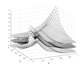
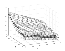
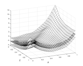
Figure 2: Simultaneous $0.95$ confidence regions for the slope surface $\beta_{0}$ under DGPs 1–3 with error (i) and sample size $n=60$.

In Table 2 we report the empirical empirical UCP from $1000$ simulation runs for data generating processes 1–3 with all error setting (i) and nominal level $\alpha=0.10$ and 0.05. We observe a reasonable approximation of the confidence level in all cases under consideration. The simultaneous confidence regions for the slope function for the DGPs 1–3 and the error process (i) are displayed in Figure 2.

For the finite sample properties of classical hypothesis tests proposed in Section 4.3, we consider the following hypothesis:

$$H_{0}:\,\beta_{0}=0\qquad \text{versus}\qquad H_{1}:\,\beta_{0}\neq 0\,,$$ (5.6)

that is, we put $\beta_{*}\equiv 0$ in (4.8). We compared the decision rule based on the bootstrap confidence regions defined in (4.9) (denoted by BT) and the penalized likelihood ratio test (PLRT) at (4.12). Here, for the PLRT, in view of (5.1) and (5.5), substituting $\widetilde{M}_{q}$ by $I_{n}$ and observing that $\Omega_{\ell}^{\rm T}\,\Omega_{\ell}=nI_{v}$, the statistic $\mathfrak{L}_{n}(0)=L_{n,\lambda}(0)-L_{n,\lambda}(\widehat{\beta}_{n})$ (defined in equation (4.10)) can be estimated by

$$\widetilde{\mathfrak{L}}_{n}(0)=\frac{1}{2n}\sum_{\ell=1}^{v}\widetilde{Y}_{\ell}^{\rm T}\Omega_{\ell}\,(nI_{v}+n\lambda\widehat{\Lambda}_{\ell})^{-1}\Omega_{\ell}^{\rm T}\,\widetilde{Y}_{\ell}\,.$$

We took $n=30$ and $60$, and chose the nominal level $\alpha=0.05$ and used DGPs 1–3 with error settings (i)–(iii). For DGPs 1 and 3, the empirical rejection probabilities are all 1.0 for both methods for all settings. Table 3 displays the empirical rejection probabilities under DGP 2 with error settings (i)–(iii), together with the empirical sizes under $H_{0}$ (that is, $\beta_{0}=0$), of both BT and PLRT for the classical hypothesis (5.6) out of 1000 simulation runs. From the results we observe reasonable approximation of both BT and PLRT of the nominal level 0.05 under $H_{0}$; BT outperforms PLRT in terms of empirical power, and as expected, the empirical powers increases for larger sample sizes.

Next, we study the finite sample properties of the test (4.25) for the relevant hypotheses

$$H_{0}:\sup_{(s,t)\in[0,1]^{2}}|\beta_{0}(s,t)|\leq\Delta\quad\text{ versus }\quad H_{1}:\sup_{(s,t)\in[0,1]^{2}}|\beta_{0}(s,t)|>\Delta\,,$$ (5.7)

(we put $\beta_{*}\equiv 0$ in (4.13)), where the nominal level is chosen as $\alpha=0.05$. We used the data generating processes 1–3 with error setting (i), where the true $\|\beta_{0}\|_{\infty}=6.0$, $1.0$ and $11.0$ for the three DGPs, respectively. We took the cut-off parameter $c=\|\widehat{\beta}_{n}\|_{\infty}/4$ in (4.4), which scales according to the magnitude of $\widehat{\beta}_{n}$. In Figure 3, we display the empirical rejection probabilities of test (4.13) based on $1000$ simulation runs, for the three data generating processes, for different values of $\Delta$ in (4.13). The results shown in Figure 3 indicate that, when $\Delta\leq d_{\infty}$, the empirical rejection probabilities are smaller than $\alpha=0.05$, and when $\Delta>d_{\infty}$, the rejection probabilities increases towards 1 as $\Delta$ increases, which is consistent with our theory.

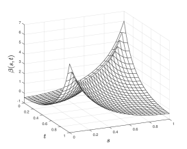
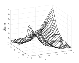
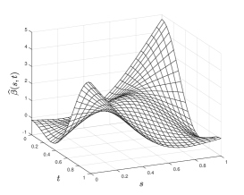
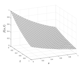
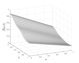
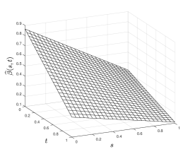
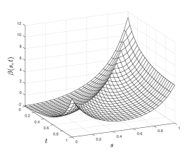
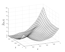
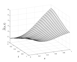
[5pt]True [5pt]RK [5pt]TP

Figure 1: Plots of the “true” slope surface $\beta_{0}$ in model (2.1) and the corresponding estimators using our method (RK) and Sun et al., (2018)’s method (TP), under DGP 1–3 (rows 1–3) with error (i) with sample size $n=60$.

DGP	Error	Method	${\rm ISE}\ (\times 10^{-3})$		${\rm EPR}\ (\times 10^{-4})$		${\rm MD}\ (\times 10^{-1})$
			$n=30$	$n=60$	$n=30$	$n=60$	$n=30$	$n=60$
1	(i)	RK	17.6 [16.4, 20.1]	13.4 [11.6, 16.2]	31.7 [28.0, 35.6]	27.3 [23.7, 31.3]	11.0 [9.32, 12.2]	7.21 [6.23, 8.50]
		TP	73.8 [73.1, 74.6]	53.1 [52.4, 54.3]	87.8 [81.9, 95.2]	61.7 [56.5, 68.8]	13.2 [12.2, 14.3]	11.4 [10.3, 12.5]
	(ii)	RK	17.0 [16.1, 18.5]	12.6 [10.6, 15.1]	28.3 [24.7, 33.0]	25.3 [21.9, 29.6]	10.5 [9.27, 12.0]	6.58 [5.83, 7.59]
		TP	68.7 [68.1, 69.6]	33.0 [32.4, 33.7]	85.9 [80.9, 91.5]	38.0 [34.9, 45.3]	13.0 [12.0, 13.9]	10.4 [9.13, 11.7]
	(iii)	RK	23.2 [19.7, 28.6]	21.1 [17.5, 26.0]	44.7 [38.6, 53.9]	39.0 [34.2, 44.3]	11.7 [9.23, 14.2]	7.51 [6.57, 9.01]
		TP	79.3 [78.0, 80.6]	34.0 [32.8, 37.6]	96.1 [88.9, 112]	57.3 [47.9, 68.4]	18.9 [15.5, 22.2]	11.8 [10.4, 13.5]
2	(i)	RK	1.14 [0.75, 1.74]	0.65 [0.46, 0.88]	7.45 [5.37, 9.76]	4.62 [3.36, 5.61]	0.86 [0.67, 1.13]	0.65 [0.54, 0.85]
		TP	0.87 [0.67, 1.23]	0.38 [0.41, 0.48]	5.67 [4.59, 7.56]	3.96 [3.19, 4.20]	0.45 [0.32, 0.49]	0.34 [0.29, 0.39]
	(ii)	RK	0.32 [0.23, 0.40]	0.23 [0.17, 0.29]	2.29 [1.83, 2.96]	1.97 [1.68, 2.37]	0.53 [0.46, 0.59]	0.51 [0.45, 0.55]
		TP	0.22 [0.18, 0.28]	0.18 [0.11, 0.25]	2.18 [2.09, 2.51]	1.05 [1.96, 2.14]	0.33 [0.32, 0.35]	0.33 [0.32, 0.35]
	(iii)	RK	2.39 [1.49, 3.47]	1.08 [0.75, 1.57]	13.1 [9.38, 17.4]	6.96 [5.09, 8.96]	1.28 [0.95, 1.65]	0.80 [0.65, 1.14]
		TP	1.50 [0.99, 1.95]	0.70 [0.40, 0.86]	7.77 [5.71, 9.87]	5.52 [4.44, 7.52]	0.47 [0.37, 0.68]	0.42 [0.35, 0.51]
3	(i)	RK	28.6 [26.7, 31.6]	15.0 [12.9, 18.6]	37.7 [33.0, 43.6]	31.5 [27.2, 36.2]	12.8 [11.0, 15.6]	8.97 [7.88, 10.2]
		TP	146 [142, 150]	83.8 [81.8, 86.9]	138 [129, 149]	77.7 [71.7, 73.3]	14.5 [11.8, 17.5]	11.3 [9.31, 13.5]
	(ii)	RK	29.1 [27.1, 32.4]	17.7 [14.0, 22.2]	39.7 [33.4, 46.7]	34.6 [29.8, 39.4]	11.9 [10.2, 14.6]	8.81 [7.27, 10.0]
		TP	150 [147, 153]	84.4 [82.6, 88.6]	141 [129, 156]	81.8 [72.4, 92.9]	15.8 [13.1, 19.7]	11.9 [10.0, 14.6]
	(iii)	RK	32.5 [29.2, 39.0]	22.5 [18.4, 26.9]	54.3 [44.3, 62.4]	41.0 [36.3, 48.1]	15.5 [12.9, 18.1]	9.79 [8.27, 11.6]
		TP	170 [166, 174]	86.6 [83.3, 92.5]	148 [134, 163]	94.8 [84.4, 105.1]	23.5 [22.2, 24.9]	13.8 [11.6, 16.7]

Table 1: The three quartiles $(2^{\rm nd}\,[1^{\rm st},\,3^{\rm rd}])$ of integrated squared error $({\rm ISE})$, excess prediction rate $({\rm EPR})$ and maximum deviation $({\rm MD})$ of estimators computed from 1000 simulation runs under the data generating processes 1–3 with error processes (i)–(iii), using our method (RK) and Sun et al., (2018)’s method (TP).

DGP	1		2		3
$\alpha$	0.10	0.05	0.10	0.05	0.10	0.05
$n=30$	0.863	0.932	0.882	0.963	0.858	0.915
$n=60$	0.881	0.944	0.913	0.960	0.870	0.939

Table 2: Empirical covering probabilities of the simultaneous confidence region (4.5) for the slope surface $\beta_{0}$ under DGPs 1–3 with error setting (i).

	(i)		(ii)		(iii)
	$n=30$	$n=60$	$n=30$	$n=60$	$n=30$	$n=60$
BT	0.536	0.693	0.328	0.494	0.478	0.546
	(0.061)	(0.037)	(0.012)	(0.028)	(0.063)	(0.042)
PLRT	0.367	0.562	0.304	0.418	0.330	0.513
	(0.059)	(0.020)	(0.074)	(0.057)	(0.027)	(0.060)

Table 3: Empirical rejection probabilities under DGP 2, together with empirical sizes (in brackets) of the decision rule based on the bootstrap confidence region $({\rm BT})$ in (4.9) and the penalized likelihood ratio test $({\rm PLRT})$ in (4.12) for the classical hypothesis (5.6) with error settings (i)–(iii) at nominal level $\alpha=0.05$.

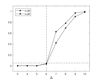
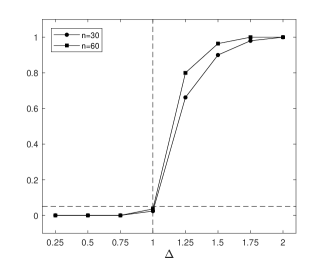
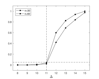
Figure 3: Empirical rejection probabilities of test (4.25) for the relevant hypothesis in (5.7) at nominal level $\alpha=0.05$, under DGPs 1–3 with error setting (i) and sample size $n=30,60$, for different values of $\Delta$ in (4.13). The horizontal dashed line is the nominal level 0.05; the vertical dashed line is $\Delta=d_{\infty}$.

5.3 Real data example

We applied the new methodology to the Canadian weather data in Ramsay and Silverman, (2005), which consists of daily temperature and precipitation at $n=35$ locations in Canada averaged over 1960 to 1994. In this case, for $1\leq i\leq 35$, $X_{i}$ is the average daily temperature for each day of the year at the $i$-th location, and $Y_{i}$ is the base 10 logarithm of the corresponding average precipitation; see Ramsay and Silverman, (2005), p. 248. We took the domain of $X$ and $Y$ to be $[0,1]$ with $365$ equality spaced time points. The size of the bootstrap sample is $Q=300$ and the truncation parameter is chosen as $v=\lceil n^{2/5}\rceil=4$. In Figure 4, we display the estimated slope function $\beta_{0}$ and the 0.95 confidence region, using our method RK. In order to evaluate the prediction accuracy, for both our method RK and Sun et al., (2018)’s method TP, we computed the integrated squared prediction error (ISPE) and maximum prediction deviation (MPD), for each observation ($1\leq i\leq n$), defined by

$$\begin{split}&{\rm ISPE}_{i}=\int_{0}^{1}\bigg{|}Y_{i}(t)-\int_{0}^{1}X_{i}(s)\,\widehat{\beta}_{-i}(s)\,ds\bigg{|}^{2}\,dt\,;\\ &{\rm MPD}_{i}=\sup_{t\in[0,1]}\bigg{|}Y_{i}(t)-\int_{0}^{1}X_{i}(s)\,\widehat{\beta}_{-i}(s)\,ds\bigg{|}\,,\end{split}$$ (5.8)

where $\widehat{\beta}_{-i}$ is the estimator of the slope function based on the data with the $i$-th observation removed. In Figure 5, we display the boxplot of $\{\sqrt{\rm ISPE}_{i}\}_{i=1}^{n}$ and $\{{\rm MPD}_{i}\}_{i=1}^{n}$, for both methods RK and TP. The results in Figure 5 show that, in general, our method performs better in terms of prediction accuracy and robustness, which is indicated by a smaller median, smaller interquartile range in terms of $\sqrt{\rm ISPE}$ and ${\rm MPD}$, and fewer outliers of $\sqrt{\rm ISPE}$. In contrast, Sun et al., (2018)’s method achieves a smaller minimum value of both $\sqrt{\rm ISPE}$ and ${\rm MPD}$.

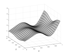
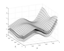
Figure 4: Estimated slope surface in model (2.1) (left panel) and its 0.95 simultaneous band (right panel), using the Canadian weather data.

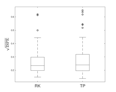
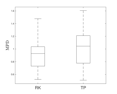
Figure 5: Boxplot of the square root of the integrated squared prediction error $\sqrt{\rm ISPE}$ (left penal), and the maximum prediction deviation $({\rm MPD})$ (right penal) defined in (5.8) using our method RK and Sun et al., (2018)’s method TP.

Acknowledgements

This work has been supported in part by the Collaborative Research Center “Statistical modeling of nonlinear dynamic processes” (SFB 823, Teilprojekt A1,C1) of the German Research Foundation (DFG). The authors would like to thank Martina Stein, who typed parts of this paper with considerable expertise. The Canadian weather data are available in Ramsay et al., (2014)’s fda R package.

In this supplementary material we provide technical details of our theoretical results. In Section A we provide the proofs of our theorems in our main article. In Section B.1 we provide supporting lemmas that are used in the proofs in Section A. Section B.2 provides a concrete example that satisfies Assumption A2. In the sequel, we use $c$ to denote a generic positive constant that might differ from line to line.

Appendix A Proofs of main results

A.1 Proof of Proposition 2.1

To begin with, by Mercer’s theorem and Assumption A1, there exists a series of positive real values $\{v_{j}\}_{j=1}^{\infty}$ and orthogonal basis functions $\{\gamma_{j}(s)\}_{j=1}^{\infty}$ of $L^{2}([0,1])$ such that

$$C_{X}(s_{1},s_{2})=\sum_{j=1}^{\infty}v_{j}\gamma_{j}(s_{1})\gamma_{j}(s_{2})\,,$$ (A.1)

where $v_{j}\geq v_{j+1}>0$, for $j\geq 1$. For any $\beta\in\mathcal{H}$ such that $\|\beta\|_{K}^{2}=0$, for the $\gamma_{j}$ in (A.1) and for $t\in[0,1]$, let $c_{\beta,j}(t)=\int_{0}^{1}\beta(s,t)\gamma_{j}(s)ds$, so that $\beta(s,t)=\sum_{j=1}^{\infty}\gamma_{j}(s)c_{\beta,j}(t)$. Since $\{\gamma_{j}\}_{j=1}^{\infty}$ is the orthogonal basis of $L^{2}([0,1])$, we have

$$\|\beta\|_{L^{2}}^{2}=\left\|\sum_{j=1}^{\infty}\gamma_{j}(s)c_{\beta,j}(t)\right\|_{L^{2}}^{2}=\sum_{j=1}^{\infty}\|\gamma_{j}\|_{L^{2}}^{2}\|c_{\beta,j}\|_{L^{2}}^{2}=\sum_{j=1}^{\infty}\|c_{\beta,j}\|_{L^{2}}^{2}\,.$$ (A.2)

Moreover,

$$V(\beta,\beta) =\int_{0}^{1}\int_{0}^{1}\int_{0}^{1}C_{X}(s_{1},s_{2})\bigg{\{}\sum_{j=1}^{\infty}\gamma_{j}(s_{1})c_{\beta,j}(t)\bigg{\}}\bigg{\{}\sum_{j=1}^{\infty}\gamma_{j}(s_{2})c_{\beta,j}(t)\bigg{\}}ds_{1}ds_{2}dt$$

$$=\sum_{j=1}^{\infty}v_{j}\,\|c_{\beta,j}\|_{L^{2}}^{2}\,.$$ (A.3)

By the fact that $v_{j}>0$ and Assumption A1, $\|\beta\|_{K}^{2}=0$ implies that, for any $j\geq 1$, $v_{j}\int_{0}^{1}c^{2}_{\beta,j}(t)dt=V(\beta,\beta)\leq\|\beta\|_{K}^{2}=0$, so that $c_{\beta,j}(t)=0$, and by (A.2) we have $\|\beta\|_{L^{2}}^{2}=\sum_{j=1}^{\infty}\|c_{\beta,j}\|_{L^{2}}^{2}=0$, which shows that $\|\beta\|_{K}^{2}=0$ implies $\beta=0$. Also, both $V$ and $J$ in (2.8) are symmetric bilinear operators. Therefore, $\langle\cdot,\cdot\rangle_{K}$ is an well-defined inner product.

Next, we show the equivalence of $\|\cdot\|_{K}$ and $\|\cdot\|_{\mathcal{H}}$. First, for any $\beta\in\mathcal{H}$, by (A.2) and (A.1),

$$V(\beta,\beta) =\sum_{j=1}^{\infty}v_{j}\|c_{\beta,j}\|_{L^{2}}^{2}\leq v_{1}\sum_{j=1}^{\infty}\|c_{\beta,j}\|_{L^{2}}^{2}=v_{1}\|\beta\|_{L^{2}}^{2}\leq cv_{1}\|\beta\|_{\mathcal{H}}^{2}\,,$$ (A.4)

for some $c>0$. Hence,

$$\|\beta\|_{K}^{2}=V(\beta,\beta)+\lambda J(\beta,\beta)\leq(cv_{1}+\lambda)\|\beta\|_{\mathcal{H}}^{2}\,.$$ (A.5)

We proceed to show that there exists a constant $c_{0}>0$ such that $\|\beta\|_{\mathcal{H}}^{2}\leq c_{0}\|\beta\|_{K}^{2}$. To achieve this, recall the definition of $J$ in (2.6) and note that $J(\beta,\beta)$ is a semi-norm on $\mathcal{H}$. Let $\mathcal{H}_{0}=\{\beta\in\mathcal{H}:J(\beta,\beta)=0\}$ denote the null space of $J(\beta,\beta)$. It is known that $\mathcal{H}_{0}$ is a finite-dimensional subspace of $\mathcal{H}$ spanned by the polynomials of total degree $\leq m-1$, and $m_{0}:={\rm dim}\{\mathcal{H}_{0}\}=(m+1)m/2$; see Wahba, (1990). Let $\{\xi_{1},\ldots,\xi_{m_{0}}\}$ denote an orthonormal basis of $\mathcal{H}_{0}$. Let $\mathcal{H}_{1}=\{\gamma_{1}\in\mathcal{H}:\langle\gamma_{1},\gamma_{0}\rangle_{\mathcal{H}}=0,\,\forall\gamma_{0}\in\mathcal{H}_{0}\}$ denote the orthogonal complement of $\mathcal{H}_{0}$ in $\mathcal{H}$, such that $\mathcal{H}=\mathcal{H}_{0}\oplus\mathcal{H}_{1}$, where “$\oplus$” stands for the direct sum. That is, for any $\beta\in\mathcal{H}$, there are unique vectors $\beta_{0},\beta_{1}$ such that

$$\beta=\beta_{0}+\beta_{1}\,,\quad\beta_{0}\in\mathcal{H}_{0}\,,\ \beta_{1}\in\mathcal{H}_{1}\,,$$ (A.6)

Here, in view of (2.3), $\langle\cdot,\cdot\rangle_{\mathcal{H}}$ is the inner product corresponding to $\|\cdot\|_{\mathcal{H}}$ defined by

$$\langle\gamma_{1},\gamma_{2}\rangle_{\mathcal{H}} =\sum_{0\leq\theta_{1}+\theta_{2}\leq m-1}{\theta_{1}+\theta_{2}\choose\theta_{1}}\int_{[0,1]^{2}}\frac{\partial^{\theta_{1}+\theta_{2}}\gamma_{1}}{\partial s^{\theta_{1}}\partial t^{\theta_{2}}}dsdt\times\int_{[0,1]^{2}}\frac{\partial^{\theta_{1}+\theta_{2}}\gamma_{2}}{\partial s^{\theta_{1}}\partial t^{\theta_{2}}}dsdt$$

$$\qquad+\sum_{\theta_{1}+\theta_{2}=m}{m\choose\theta_{1}}\int_{[0,1]^{2}}\frac{\partial^{m}\gamma_{1}}{\partial s^{\theta_{1}}\partial t^{\theta_{2}}}\times\frac{\partial^{m}\gamma_{2}}{\partial s^{\theta_{1}}\partial t^{\theta_{2}}}dsdt\,,\qquad\text{for }\gamma_{1},\gamma_{2}\in\mathcal{H}\,.$$

Due to the fact that $\xi_{k}\in\mathcal{H}_{0}$, for $1\leq k\leq m_{0}$, we have

$$0=\langle\xi_{k},\beta_{1}\rangle_{\mathcal{H}}=\sum_{0\leq\theta_{1}+\theta_{2}\leq m-1}{\theta_{1}+\theta_{2}\choose\theta_{1}}\int_{[0,1]^{2}}\frac{\partial^{\theta_{1}+\theta_{2}}\xi_{k}}{\partial s^{\theta_{1}}\partial t^{\theta_{2}}}dsdt\times\int_{[0,1]^{2}}\frac{\partial^{\theta_{1}+\theta_{2}}\beta_{1}}{\partial s^{\theta_{1}}\partial t^{\theta_{2}}}dsdt\,,$$

for $1\leq k\leq m_{0}$. We deduce from the above result that $\int_{[0,1]^{2}}\frac{\partial^{\theta_{1}+\theta_{2}}\beta_{1}}{\partial s^{\theta_{1}}\partial t^{\theta_{2}}}dsdt=0$, for $0\leq\theta_{1}+\theta_{2}\leq m-1$. In fact, the above argument shows that

$$\mathcal{H}_{1}=\left\{\gamma\in\mathcal{H}:\int_{[0,1]^{2}}\frac{\partial^{\theta_{1}+\theta_{2}}\beta_{1}}{\partial s^{\theta_{1}}\partial t^{\theta_{2}}}dsdt=0,\,0\leq\theta_{1}+\theta_{2}\leq m-1\right\}\,.$$

Therefore,

$$\|\beta_{1}\|_{\mathcal{H}}^{2}=J(\beta_{1},\beta_{1})\leq\lambda^{-1}V(\beta,\beta)+J(\beta_{1},\beta_{1})=\lambda^{-1}\|\beta\|_{K}^{2}\,.$$ (A.7)

It then suffice to show that $\|\beta_{0}\|_{\mathcal{H}}^{2}\leq c_{0}\|\beta\|_{K}^{2}$ for some $c_{0}>0$. Since $\beta_{0}\in\mathcal{H}_{0}$, we have $J(\beta_{0},\beta_{0})=J(\beta_{0},\beta_{1})=0$, so that in view of (A.7),

$$\|\beta\|_{K}^{2} =V(\beta_{0}+\beta_{1},\beta_{0}+\beta_{1})+\lambda J(\beta_{1},\beta_{1})$$

$$=V(\beta_{0},\beta_{0})+2V(\beta_{0},\beta_{1})+V(\beta_{1},\beta_{1})+\lambda\|\beta_{1}\|_{\mathcal{H}}^{2}\,.$$ (A.8)

Since $V(\cdot,\cdot)$ is an inner product, by the Cauchy-Schwarz inequality,

$$|V(\beta_{0},\beta_{1})|\leq\{V(\beta_{0},\beta_{0})\}^{1/2}\{V(\beta_{1},\beta_{1})\}^{1/2}$$ (A.9)

Next, we examine the connection between $\|\beta_{1}\|_{\mathcal{H}}^{2}$ and $V(\beta_{1},\beta_{1})$. It is known that both $\mathcal{H}_{0}$ and $\mathcal{H}_{1}$ are reproducing kernel Hilbert spaces with inner product $\langle\cdot,\cdot\rangle_{\mathcal{H}}$ restricted to $\mathcal{H}_{0}$ and $\mathcal{H}_{1}$, respectively. Let $C_{1}\{(s_{1},t_{1}),(s_{2},t_{2})\}$ denote the reproducing kernel of $\mathcal{H}_{1}$. It is known that $C_{1}$ is continuous and square-integrable on $[0,1]^{2}\times[0,1]^{2}$; see, for example, Section 2.4 in Wahba, (1990) and Section 4.3.2 in Gu, (2013). Hence, by Mercer’s theorem, $C_{1}$ admits the following eigen-decomposition:

$$C_{1}\{(s_{1},t_{1}),(s_{2},t_{2})\}=\sum_{j=1}^{\infty}\zeta_{j}\,\chi_{j}(s_{1},t_{1})\chi_{j}(s_{2},t_{2})\,,$$

where $\zeta_{j}\geq\zeta_{j+1}\geq 0$, for $j\geq 1$, $\{\chi_{j}\}_{j\geq 1}$ forms an orthonormal basis of $L^{2}([0,1]^{2})$, and $s_{1},s_{2},t_{1},t_{2}\in[0,1]$. Note that

$$\langle\chi_{j},\chi_{\ell}\rangle_{L^{2}}=\delta_{j\ell}\,,\qquad\langle\chi_{j},\chi_{\ell}\rangle_{\mathcal{H}}=\zeta_{j}^{-1}\delta_{j\ell}\,,$$

where $\delta_{j\ell}$ is the Kronecker delta; see, for example, Cucker and Smale, (2001) and Yuan and Cai, (2010). For $\beta_{1}$ in (A.6), we have $\beta_{1}(s,t)=\sum_{j=1}^{\infty}\langle\beta_{1},\chi_{j}\rangle_{L^{2}}\chi_{j}(s,t)$, so that

$$\|\beta_{1}\|_{\mathcal{H}}^{2} =\sum_{j=1}^{\infty}\langle\beta_{1},\chi_{j}\rangle_{L^{2}}^{2}\|\chi_{j}\|_{\mathcal{H}}^{2}=\sum_{j=1}^{\infty}\zeta_{j}^{-1}\langle\beta_{1},\chi_{j}\rangle_{L^{2}}^{2}$$

$$\geq\zeta_{1}^{-1}\sum_{j=1}^{\infty}\langle\beta_{1},\chi_{j}\rangle_{L^{2}}^{2}=\zeta_{1}^{-1}\|\beta_{1}\|_{L^{2}}^{2}\,.$$ (A.10)

In view of (A.2) and (A.1),

$$V(\beta_{1},\beta_{1}) =\sum_{j=1}^{\infty}v_{j}\|c_{\beta_{1},j}\|_{L^{2}}^{2}\leq v_{1}\sum_{j=1}^{\infty}\|c_{\beta_{1},j}\|_{L^{2}}^{2}=v_{1}\,\|\beta_{1}\|_{L^{2}}^{2}\,.$$

Combining the above equation with (A.1) yields that

$$\|\beta_{1}\|_{\mathcal{H}}^{2}\geq\zeta_{1}^{-1}v_{1}^{-1}V(\beta_{1},\beta_{1})\,.$$

Therefore, combining the above equation with (A.1) and (A.9), we find that

$$\|\beta\|_{K}^{2} \geq V(\beta_{0},\beta_{0})-2|V(\beta_{0},\beta_{1})|+V(\beta_{1},\beta_{1})+\lambda\|\beta_{1}\|_{\mathcal{H}}^{2}$$

$$\geq V(\beta_{0},\beta_{0})-2\{V(\beta_{0},\beta_{0})\}^{1/2}\{V(\beta_{1},\beta_{1})\}^{1/2}+\left(1+\frac{\lambda}{v_{1}\zeta_{1}}\right)V(\beta_{1},\beta_{1})$$

$$=\frac{\lambda}{v_{1}\zeta_{1}+\lambda}V(\beta_{0},\beta_{0})+\left[\sqrt{\frac{v_{1}\zeta_{1}}{v_{1}\zeta_{1}+\lambda}}\{V(\beta_{0},\beta_{0})\}^{1/2}-\sqrt{\frac{v_{1}\zeta_{1}+\lambda}{v_{1}\zeta_{1}}}\{V(\beta_{1},\beta_{1})\}^{1/2}\right]^{2}$$

$$\geq\frac{\lambda}{v_{1}\zeta_{1}+\lambda}V(\beta_{0},\beta_{0})\,.$$ (A.11)

Next, we examine the connection between $V(\beta_{0},\beta_{0})$ and $\|\beta_{0}\|_{\mathcal{H}}^{2}$. Since $\beta_{0}\in\mathcal{H}_{0}$ and $\{\xi_{j}\}_{j=1}^{m_{0}}$ is an orthonormal basis of $\mathcal{H}_{0}$ under the inner product $\langle\cdot,\cdot\rangle_{\mathcal{H}}$, we have $\beta_{0}(s,t)=\sum_{j=1}^{m_{0}}\langle\beta_{0},\xi_{j}\rangle_{\mathcal{H}}\,\xi_{j}(s,t)$ and $\|\beta_{0}\|_{\mathcal{H}}^{2}=\sum_{j=1}^{m_{0}}\langle\beta_{0},\xi_{j}\rangle_{\mathcal{H}}^{2}$. Note that

$$V(\beta_{0},\beta_{0})=\sum_{j=1}^{m_{0}}\sum_{\ell=1}^{m_{0}}\langle\beta_{0},\xi_{j}\rangle_{\mathcal{H}}\,\langle\beta_{0},\xi_{\ell}\rangle_{\mathcal{H}}\,V(\xi_{j},\xi_{\ell})\,.$$

Let $b$ denote an $m_{0}\times 1$ vector whose $j$-th entry is $\langle\beta_{0},\xi_{j}\rangle_{\mathcal{H}}$, and let $V_{*}$ denote an $m_{0}\times m_{0}$ matrix, whose $(j,\ell)$-th entry is

$$V(\xi_{j},\xi_{\ell})=\int_{[0,1]^{3}}C_{X}(s_{1},s_{2})\xi_{j}(s_{1},t)\xi_{\ell}(s_{2},t)\,ds_{1}ds_{2}dt\,.$$

Now, we have $V(\beta_{0},\beta_{0})=b^{\rm T}V_{*}b$ and $\|\beta_{0}\|_{\mathcal{H}}^{2}=\|b\|_{2}^{2}$. Due to Assumption A1, the matrix $V_{*}$ is a positive definite matrix, and therefore admits a singular value decomposition $V_{*}=U^{\rm T}DU$, where $U$ is an orthogonal matrix and $W={\rm diag}(d_{1},\ldots,d_{m_{0}})$ is a diagonal matrix with $d_{1}\geq\ldots\geq d_{m_{0}}>0$. Therefore,

$$V(\beta_{0},\beta_{0})=b^{\rm T}U^{\rm T}WUb\geq d_{m_{0}}\|Ub\|_{2}^{2}=d_{m_{0}}\|b\|_{2}^{2}=d_{m_{0}}\|\beta_{0}\|_{\mathcal{H}}^{2}\,.$$

Therefore, combining the above result with (A.1), we find

$$\|\beta_{0}\|_{\mathcal{H}}^{2}\leq d_{m_{0}}^{-1}V(\beta_{0},\beta_{0})\leq\frac{v_{1}\zeta_{1}+\lambda}{d_{m_{0}}\lambda}\|\beta\|_{K}^{2}\,.$$

Combining the above equation with (A.7) yields that

$$\|\beta\|_{\mathcal{H}}^{2}=\|\beta_{0}\|_{\mathcal{H}}^{2}+\|\beta_{1}\|_{\mathcal{H}}^{2}\leq\frac{v_{1}\zeta_{1}+\lambda+d_{m_{0}}}{d_{m_{0}}\lambda}\|\beta\|_{K}^{2}\,.$$ (A.12)

This together with (A.5) completes the proof of the equivalence between $\|\cdot\|_{\mathcal{H}}$ and $\|\cdot\|_{K}$. Since $\mathcal{H}$ is a reproducing kernel Hilbert space equipped with $\|\cdot\|_{\mathcal{H}}$, we therefore deduce that $\mathcal{H}$ equipped with $\|\cdot\|_{K}$ is a reproducing kernel Hilbert space.

A.2 Proof of Theorem 3.1

We first prove the following lemma, which is useful for proving Theorem 3.1. In this section, without loss of generality, we assume that $\sigma_{\varepsilon}^{2}=1$ in Assumption A3.

Lemma A.1.

For any $\beta\in\mathcal{H}$, let

$$g(X_{i},\beta)=\tau\bigg{[}X_{i}\otimes\bigg{\{}\int_{0}^{1}\beta(s,\cdot)X_{i}(s)ds\bigg{\}}\bigg{]}\,,$$ (A.13)

$$H_{n}(\beta)=\frac{1}{\sqrt{n}}\sum_{i=1}^{n}\big{[}g(X_{i},\beta)-{\rm E}\{g(X,\beta)\}\big{]}\,.$$ (A.14)

For $p_{n}\geq 1$, let

$$\mathcal{F}_{p_{n}}=\{\beta\in\mathcal{H}:\|\beta\|_{L^{2}}\leq 1,J(\beta,\beta)\leq p_{n}\}.$$ (A.15)

Then, under Assumptions A1–A4, as $n\to\infty$,

$$\sup_{\beta\in\mathcal{F}_{p_{n}}}\,\frac{\|H_{n}(\beta)\|_{K}}{p_{n}^{1/(2m)}\|\beta\|_{L^{2}}^{(m-1)/m}+n^{-1/2}}=O_{p}\big{(}\lambda^{-1/(2D)}\log\log n\big{)}^{1/2}\,.$$ (A.16)

Proof.

We follow the proof of Lemma 3.4 in Shang and Cheng, (2015). For the $\{x_{k\ell}\}_{k,\ell\geq 1}$ and $\{\eta_{\ell}\}_{\ell\geq 1}$ in Assumption A2, and for $1\leq i\leq n$, let

$$w(X_{i})=\|X_{i}\|_{L^{2}}\bigg{(}\sum_{k,\ell}\frac{1}{1+\lambda\rho_{k\ell}}\,\langle X_{i},x_{k\ell}\rangle_{L^{2}}^{2}\,\|\eta_{\ell}\|^{2}_{L^{2}}\bigg{)}^{1/2}\,,$$ (A.17)

and let $\mathcal{X}_{n}=\{w(X_{i})\}_{i=1}^{n}$. By Lemma B.5 in Section B,

$$\frac{1}{\sqrt{n}}\,\Big{\|}\big{[}g(X_{i},\beta_{1})-{\rm E}\{g(X_{i},\beta_{1})\}\big{]}-\big{[}g(X_{i},\beta_{2})-{\rm E}\{g(X_{i},\beta_{2})\}\big{]}\Big{\|}_{K}$$

$$\leq\frac{1}{\sqrt{n}}\,\bigg{\|}\tau\bigg{(}X_{i}\otimes\bigg{[}\int_{0}^{1}\{\beta_{1}(s,\cdot)-\beta_{2}(s,\cdot)\}X_{i}(s)ds\bigg{]}\bigg{)}\bigg{\|}_{K}$$

$$\qquad+\frac{1}{\sqrt{n}}\,{\rm E}\,\bigg{\|}\tau\bigg{(}X_{i}\otimes\bigg{[}\int_{0}^{1}\{\beta_{1}(s,\cdot)-\beta_{2}(s,\cdot)\}X_{i}(s)ds\bigg{]}\bigg{)}\bigg{\|}_{K}$$

$$\leq\frac{1}{\sqrt{n}}\,\|\beta_{1}-\beta_{2}\|_{L^{2}}\times\big{[}w(X_{i})+{\rm E}\{w(X_{i})\}\big{]}\,.$$

By Theorem 3.5 in Pinelis, (1994),

$${\rm P}\left\{\|H_{n}(\beta_{1})-H_{n}(\beta_{2})\|_{K}\geq x\,\big{|}\mathcal{X}_{n}\right\}\leq 2\exp\left(-\frac{x^{2}}{2\,W_{n}^{2}\,\|\beta_{1}-\beta_{2}\|_{L^{2}}^{2}}\right)\,,$$

where

$$W_{n}=\frac{1}{\sqrt{n}}\bigg{(}\sum_{i=1}^{n}\big{[}w(X_{i})+{\rm E}\{w(X_{i})\}\big{]}^{2}\bigg{)}^{1/2}\,.$$ (A.18)

By Lemma B.6 in Section B, ${\rm E}(W_{n}^{2})\leq 4{\rm E}|w(X)|^{2}\leq c\,\lambda^{-1/(2D)}$. Let

$$\|Z\|_{\Psi}=\inf\big{\{}c>0:{\rm E}\{\Psi(|Z|/c)|\mathcal{X}_{n}\}\leq 1\big{\}}$$

denote the Orlicz norm of a random variable $Z$ conditional on $\mathcal{X}_{n}$, with $\Psi(x)=\exp(x^{2})-1$, then, by Lemma 8.1 in Kosorok, (2007),

$$\Big{\|}\|H_{n}(\beta_{1})-H_{n}(\beta_{2})\|_{K}\Big{\|}_{\Psi}\leq\sqrt{6}\,W_{n}\,\|\beta_{1}-\beta_{2}\|_{L^{2}}\,.$$

Let $N(\delta,\mathcal{F}_{p_{n}},\|\cdot\|_{L^{2}})$ denote $\delta$-covering number of the class $\mathcal{F}_{p_{n}}$ in (A.15) w.r.t. the $L^{2}([0,1]^{2})$-norm. Since $p_{n}\geq 1$ for $n$ large enough and $J(p_{n}^{1/2}\beta,p_{n}^{1/2}\beta)=p_{n}J(\beta,\beta)$, we have $\mathcal{F}_{p_{n}}\subset p_{n}^{1/2}\mathcal{F}_{1}$. Hence,

$$\log N(\delta,\mathcal{F}_{p_{n}},\|\cdot\|_{L^{2}}) \leq\log N(\delta,p_{n}^{1/2}\mathcal{F}_{1},\|\cdot\|_{L^{2}})$$

$$\leq\log N(p_{n}^{-1/2}\delta,\mathcal{F}_{1},\|\cdot\|_{L^{2}})\leq c\,(p_{n}^{-1/2}\delta)^{-2/m}\,,$$

where in the last step we used the result in Birman and Solomjak, (1967). By Lemma 8.2 and Theorem 8.4 in Kosorok, (2007), we have

$$\left\|\sup_{\beta_{1},\beta_{2}\in\mathcal{F}_{p_{n}},\,\|\beta_{1}-\beta_{2}\|_{L^{2}}\leq\delta}\|H_{n}(\beta_{1})-H_{n}(\beta_{2})\|_{K}\right\|_{\psi}$$

$$\leq c\,W_{n}\bigg{[}\int_{0}^{\delta}\sqrt{\log\{1+N(\eta,\mathcal{F}_{p_{n}},\|\cdot\|_{L^{2}})\}}\,d\eta+\delta\sqrt{\log\{1+N^{2}(\delta,\mathcal{F}_{p_{n}},\|\cdot\|_{L^{2}})\}}\,\bigg{]}$$

$$\leq c_{1}W_{n}\,p_{n}^{1/(2m)}\delta^{1-1/m}\,,$$

for some absolute constant $c_{1}>0$. Since $H_{n}(0)=0$, by Lemma 8.1 in Kosorok, (2007),

$${\rm P}\left\{\sup_{\beta\in\mathcal{F}_{p_{n}},\,\|\beta\|_{L^{2}}\leq\delta}\|H_{n}(\beta)\|_{K}\geq x\,\big{|}\mathcal{X}_{n}\right\}\leq 2\exp\big{(}-c_{1}^{-2}W_{n}^{-2}p_{n}^{-1/m}\delta^{-2+2/m}x^{2}\big{)}\,.$$

Taking $\gamma=1-1/m$, $b_{n}=\sqrt{n}\,p_{n}^{1/(2m)}$, $\theta_{n}=b_{n}^{-1}$, $Q_{n}=\lceil-\log_{2}\theta_{n}+\gamma-1\rceil$ and $T_{n}=c_{2}(\lambda^{-1/(2D)}\log\log n)^{1/2}$, for some constant $c_{2}>0$ to be specified below, yields that

$${\rm P}\left\{\sup_{\beta\in\mathcal{F}_{p_{n}},\,\|\beta\|_{L^{2}}\leq 2}\,\frac{\sqrt{n}\|H_{n}(\beta)\|_{K}}{b_{n}\|\beta\|_{L^{2}}^{\gamma}+1}\geq T_{n}\,\big{|}\mathcal{X}_{n}\right\}$$

$$\leq{\rm P}\left\{\sup_{\beta\in\mathcal{F}_{p_{n}},\,\|\beta\|_{L^{2}}\leq\theta_{n}^{1/\gamma}}\sqrt{n}\|H_{n}(\beta)\|_{K}\geq T_{n}\,\big{|}\mathcal{X}_{n}\right\}$$

$$\hskip 28.45274pt+\sum_{j=0}^{Q_{n}}{\rm P}\left\{\sup_{\beta\in\mathcal{F}_{p_{n}},\,(\theta_{n}2^{j})^{1/\gamma}\leq\|\beta\|_{L^{2}}\leq(\theta_{n}2^{j+1})^{1/\gamma}}\,\frac{\sqrt{n}\|H_{n}(\beta)\|_{K}}{b_{n}\|\beta\|_{L^{2}}^{\gamma}+1}\geq T_{n}\,\big{|}\mathcal{X}_{n}\right\}$$

$$\leq{\rm P}\left\{\sup_{\beta\in\mathcal{F}_{p_{n}},\,\|\beta\|_{L^{2}}\leq\theta_{n}^{1/\gamma}}\sqrt{n}\|H_{n}(\beta)\|_{K}\geq T_{n}\,\big{|}\mathcal{X}_{n}\right\}$$

$$\hskip 28.45274pt+\sum_{j=0}^{Q_{n}}{\rm P}\left\{\sup_{\beta\in\mathcal{F}_{p_{n}},\,\|\beta\|_{L^{2}}\leq(\theta_{n}2^{j+1})^{1/\gamma}}\,\sqrt{n}\|H_{n}(\beta)\|_{K}\geq(b_{n}\theta_{n}2^{j}+1)T_{n}\,\big{|}\mathcal{X}_{n}\right\}$$

$$\leq 2\exp\big{(}-c_{1}^{-2}W_{n}^{-2}p_{n}^{-1/m}\theta_{n}^{(-2+2/m)/\gamma}n^{-1}T_{n}^{2}\big{)}$$

$$\hskip 28.45274pt+2\sum_{j=0}^{Q_{n}}\exp\Big{\{}-c_{1}^{-2}W_{n}^{-2}p_{n}^{-1/m}(\theta_{n}2^{j+1})^{(-2+2/m)/\gamma}(b_{n}\theta_{n}2^{j}+1)^{2}n^{-1}T_{n}^{2}\Big{\}}$$

$$\leq 2\exp\big{(}-c_{1}^{-2}W_{n}^{-2}T_{n}^{2}\big{)}+2(Q_{n}+1)\exp\big{(}-c_{1}^{-2}W_{n}^{-2}T_{n}^{2}/4\big{)}$$

$$\leq 2(Q_{n}+2)\exp\big{(}-c_{1}^{-2}W_{n}^{-2}T_{n}^{2}/4\big{)}\,.$$ (A.19)

For the $W_{n}^{2}$ in (A.18), denote the event $\mathcal{A}_{n}=\{W_{n}^{2}\leq c_{3}\lambda^{-1/(2D)}\}$ for some constant $c_{3}>0$. Since ${\rm E}(W_{n}^{2})\leq c\lambda^{-1/(2D)}$, we have that, for $c_{3}$ large enough, ${\rm P}(\mathcal{A}_{n})$ tends to one. On the event $\mathcal{A}_{n}$, by taking $c_{2}>2c_{1}c_{3}^{-1/2}$, as $n\to\infty$,

$$2(Q_{n}+2)\exp\big{(}-c_{1}^{-2}W_{n}^{-2}T_{n}^{2}/4\big{)}\leq 2(Q_{n}+2)\exp\big{(}-c_{1}^{-2}c_{2}^{2}c_{3}\log\log n/4\big{)}=o(1)\,,$$

which together with (A.55) completes the proof of Lemma A.1.

∎

Next, we prove the following lemma regarding the convergence rate of $\widehat{\beta}_{n}$, which is useful to prove Theorem 3.1.

Lemma A.2.

Under Assumptions A1–A5, for any $\beta_{0}\in\mathcal{H}$, we have

$$\|\widehat{\beta}_{n}-\beta_{0}\|_{K}=O_{p}(\lambda^{1/2}+n^{-1/2}\lambda^{-1/(4D)}).$$

Proof.

For $L_{n}$ and $S_{n,\lambda}$ defined in (2.5) and (3.2), let

$$S_{n}(\beta)=\mathcal{D}L_{n}(\beta)\,;\quad S(\beta)={\rm E}\{\mathcal{D}L_{n}(\beta)\}\,;\quad S_{\lambda}(\beta)={\rm E}\{S_{n,\lambda}(\beta)\}\,.$$ (A.20)

In view of (3.2), $S_{\lambda}(\beta)=S(\beta)+W_{\lambda}(\beta)$. We first show that there exists a unique element $\beta_{\lambda}\in\mathcal{H}$ such that $S_{\lambda}(\beta_{\lambda})=0$, and then we prove the upper bound for $\|\beta_{\lambda}-\beta_{0}\|_{K}$. Since

$$\mathcal{D}^{2}L_{\lambda}(\beta_{0})\beta_{1}\beta_{2}=\langle\mathcal{D}S_{\lambda}(\beta_{0})\beta_{1},\beta_{2}\rangle_{K}=\langle\beta_{1},\beta_{2}\rangle_{K},$$

we have $\mathcal{D}S_{\lambda}(\beta_{0})=id$, where $id$ is the identity operator. Since $\mathcal{D}^{2}S_{\lambda}$ vanishes, we deduce that $\mathcal{D}S_{\lambda}(\beta)=id$ for any $\beta\in\mathcal{H}$. Hence, by the mean value theorem, for any $\beta\in\mathcal{H}$, $S_{\lambda}(\beta)=\beta+S_{\lambda}(\beta_{0})-\beta_{0}$. Therefore, letting $\beta_{\lambda}=\beta_{0}-S_{\lambda}(\beta_{0})$, we find $S_{\lambda}(\beta_{\lambda})=0$, and $\beta_{\lambda}$ is the unique solution to the estimating equation $S_{\lambda}(\beta)=0$. Moreover, since $S(\beta_{0})=0$, we have $S_{\lambda}(\beta_{0})=S(\beta_{0})+W_{\lambda}(\beta_{0})=W_{\lambda}(\beta_{0})$. By the Cauchy-Schwarz inequality, for $J$ in (2.6),

$$\|\beta_{\lambda}-\beta_{0}\|_{K}=\|W_{\lambda}(\beta_{0})\|_{K}=\sup_{\|\gamma\|_{K}=1}|\langle W_{\lambda}(\beta_{0}),\gamma\rangle_{K}|=\sup_{\|\gamma\|_{K}=1}\lambda|J(\beta_{0},\gamma)|$$

$$\leq\sup_{\|\gamma\|_{K}=1}\big{\{}\sqrt{\lambda J(\beta_{0},\beta_{0})}\sqrt{\lambda J(\gamma,\gamma)}\big{\}}\leq\sup_{\|\gamma\|_{K}=1}\big{\{}\sqrt{\lambda J(\beta_{0},\beta_{0})}\,\|\gamma\|_{K}\big{\}}=\sqrt{\lambda J(\beta_{0},\beta_{0})}\,.$$ (A.21)

Since $\|\widehat{\beta}_{n}-\beta_{0}\|_{K}\leq\|\beta_{\lambda}-\beta_{0}\|_{K}+\|\widehat{\beta}_{n}-\beta_{\lambda}\|_{K}$, we then proceed to show the rate of $\|\widehat{\beta}_{n}-\beta_{\lambda}\|_{K}$. Let $F_{n}(\beta)=\beta-S_{n,\lambda}(\beta_{\lambda}+\beta)$. Recall that $\mathcal{D}S_{\lambda}(\beta_{\lambda})\beta=\beta$, so that, for $\mathcal{D}S_{n,\lambda}$ in (3.2),

$$F_{n}(\beta)=I_{1,n}(\beta)+I_{2,n}(\beta)-S_{n,\lambda}(\beta_{\lambda})\,,$$ (A.22)

where

$$I_{1,n}(\beta)=-\{S_{n,\lambda}(\beta_{\lambda}+\beta)-S_{n,\lambda}(\beta_{\lambda})-\mathcal{D}S_{n,\lambda}(\beta_{\lambda})\beta\}\,,$$

$$I_{2,n}(\beta)=-\{\mathcal{D}S_{n,\lambda}(\beta_{\lambda})\beta-\mathcal{D}S_{\lambda}(\beta_{\lambda})\beta\}\,.$$ (A.23)

First, for $I_{1,n}(\beta)$ in (A.23), in view of $S_{n,\lambda}$ and $\mathcal{D}S_{n,\lambda}$ defined in (3.2),

$$I_{1,n}(\beta) =\frac{1}{n}\sum_{i=1}^{n}\tau\bigg{(}X_{i}\otimes\bigg{[}Y_{i}-\int_{0}^{1}\{\beta_{\lambda}(s,\cdot)+\beta(s,\cdot)\}X_{i}(s)ds\bigg{]}\bigg{)}$$

$$\quad-\frac{1}{n}\sum_{i=1}^{n}\tau\bigg{[}X_{i}\otimes\bigg{\{}Y_{i}-\int_{0}^{1}\beta(s,\cdot)X_{i}(s)ds\bigg{\}}\bigg{]}$$

$$\quad+\frac{1}{n}\sum_{i=1}^{n}\tau\bigg{[}X_{i}\otimes\bigg{\{}\int_{0}^{1}\beta_{\lambda}(s,\cdot)X_{i}(s)ds\bigg{\}}\bigg{]}=0\,.$$ (A.24)

For $I_{2,n}(\beta)$ in (A.23), in view of (3.2),

$$\|I_{2,n}(\beta)\|_{K} =\big{\|}\mathcal{D}S_{n,\lambda}(\beta_{\lambda})\beta-\mathcal{D}S_{\lambda}(\beta_{\lambda})\beta\big{\|}_{K}$$

$$=\big{\|}\mathcal{D}S_{n}(\beta_{\lambda})\beta-\mathcal{D}S(\beta_{\lambda})\beta\big{\|}_{K}=\frac{1}{\sqrt{n}}\|H_{n}(\beta)\|_{K}\,,$$ (A.25)

where $H_{n}(\beta)$ is defined in (A.14) in Lemma A.1. For $a,D$ in Assumption A2 and $c_{K}$ in Lemma B.3, let $p_{n}=c_{K}^{-2}\lambda^{(2a+1)/(2D)-1}$. In order to apply Lemma A.1, we shall rescale $\beta$ such that the $L^{2}$-norm of its rescaled version is bounded by $1$. For the constant $c_{K}$ in Lemma B.3, let

$$\widetilde{\beta}=\left\{\begin{array}[]{ll}\big{(}c_{K}\lambda^{-(2a+1)/(4D)}\|\beta\|_{K}\big{)}^{-1}\beta&\text{ if }\beta\neq 0\,,\\ 0&\text{ if }\beta=0\,.\end{array}\right.$$ (A.28)

We have $\|\widetilde{\beta}\|_{L^{2}}\leq c_{K}\lambda^{-(2a+1)/(4D)}\|\widetilde{\beta}\|_{K}\leq 1$, since $\|\widetilde{\beta}\|_{K}\leq(c_{K}\lambda^{-(2a+1)/(4D)})^{-1}$ by Lemma B.3. In addition, in view of (2.8), $J(\widetilde{\beta},\widetilde{\beta})\leq\lambda^{-1}\|\widetilde{\beta}\|_{K}^{2}\leq c_{K}^{-2}\lambda^{(2a+1)/(2D)-1}=p_{n}$, which implies $\widetilde{\beta}\in\mathcal{F}_{p_{n}}$. By Lemma A.1, since $n^{-1/2}=o(p_{n}^{1/(2m)})$ by Assumption A5, we find that, for some constant $c>0$ large enough, with probability tending to one,

$$\|H_{n}(\widetilde{\beta})\|_{K}\leq c\big{(}p_{n}^{1/(2m)}+n^{-1/2}\big{)}\big{(}\lambda^{-1/(2D)}\log\log n\big{)}^{1/2}\leq c\,p_{n}^{1/(2m)}\lambda^{-1/(4D)}(\log\log n)^{1/2}\,.$$

Therefore, in view of (A.28), we deduce from the above inequality that, for some constant $c>0$ large enough, with probability tending to one,

$$\|H_{n}(\beta)\|_{K} \leq\big{(}c_{K}\lambda^{-(2a+1)/(4D)}\|\beta\|_{K}\big{)}\|H_{n}(\widetilde{\beta})\|_{K}\leq c\,p_{n}^{1/(2m)}\lambda^{-(a+1)/(2D)}(\log\log n)^{1/2}\|\beta\|_{K}\,.$$

Recall that $p_{n}=O(\lambda^{(2a+1)/(2D)-1})$. Therefore, for $I_{2,n}(\beta)$ in (A.23), in view of (A.2), we deduce from the equation result that, for some constant $c>0$ large enough, with probability tending to one,

$$\|I_{2,n}(\beta)\|_{K}\leq n^{-1/2}\|H_{n}(\beta)\|_{K} \leq c\,n^{-1/2}p_{n}^{1/(2m)}\lambda^{-(a+1)/(2D)}(\log\log n)^{1/2}\|\beta\|_{K}$$

$$\leq c\,n^{-1/2}\lambda^{-\varsigma}(\log\log n)^{1/2}\,\|\beta\|_{K}=o(1)\,\|\beta\|_{K}\,,$$ (A.29)

where we used Assumption A5 in the last step.

For estimating the remaining term $-S_{n,\lambda}(\beta_{\lambda})$ in (A.22), we recall the definition of $\tau$ in (2.17) and define $O_{i}=\tau\big{[}X_{i}\otimes\big{\{}Y_{i}-\int_{0}^{1}\beta_{\lambda}(s,\cdot)X_{i}(s)ds\big{\}}\big{]}$, for $1\leq i\leq n$. Since $S_{\lambda}(\beta_{\lambda})=0$, we obtain observing (3) that

$$-S_{n,\lambda}(\beta_{\lambda})=-\{S_{n,\lambda}(\beta_{\lambda})-S_{\lambda}(\beta_{\lambda})\}=n^{-1}\sum_{i=1}^{n}\{O_{i}-{\rm E}(O_{i})\}.$$

Let $\Delta_{\lambda}\beta=\beta_{0}-\beta_{\lambda}$, so that from (A.2) we obtain $\|\Delta_{\lambda}\beta\|_{K}^{2}\leq c\lambda$ for some constant $c>0$. We notice that

$${\rm E}\|S_{n,\lambda}(\beta_{\lambda})\|_{K}^{2}=n^{-1}{\rm E}\|O_{i}-{\rm E}(O_{i})\|_{K}^{2}\leq n^{-1}{\rm E}\|O_{i}\|_{K}^{2}$$

$$=n^{-1}{\rm E}\bigg{\|}\tau\bigg{[}X_{i}\otimes\bigg{\{}Y_{i}-\int_{0}^{1}\beta_{\lambda}(s,\cdot)X_{i}(s)ds\bigg{\}}\bigg{]}\bigg{\|}_{K}^{2}$$

$$=n^{-1}{\rm E}\bigg{\|}\tau(X_{i}\otimes\varepsilon_{i})+\tau\bigg{[}X_{i}\otimes\bigg{\{}\int_{0}^{1}\Delta_{\lambda}\beta(s,\cdot)X_{i}(s)ds\bigg{\}}\bigg{]}\bigg{\|}_{K}^{2}$$

$$\leq 2n^{-1}{\rm E}\big{\|}\tau(X_{i}\otimes\varepsilon_{i})\big{\|}_{K}^{2}+2n^{-1}{\rm E}\bigg{\|}\tau\bigg{[}X_{i}\otimes\bigg{\{}\int_{0}^{1}\Delta_{\lambda}\beta(s,\cdot)X_{i}(s)ds\bigg{\}}\bigg{]}\bigg{\|}_{K}^{2}\,.$$ (A.30)

By Lemma B.4 in Section B, we have

$${\rm E}\bigg{\|}\tau\bigg{[}X_{i}\otimes\bigg{\{}\int_{0}^{1}\Delta_{\lambda}\beta(s,\cdot)X_{i}(s)ds\bigg{\}}\bigg{]}\bigg{\|}_{K}^{2}\leq c\,\lambda^{-1/D}\,\|\Delta_{\lambda}\beta\|_{K}^{2}\,,$$ (A.31)

and Lemmas B.2, B.7 and Assumption A2 give for the first term in (A.2)

$${\rm E}\big{\|}\tau(X_{i}\otimes\varepsilon_{i})\big{\|}_{K}^{2}=\sum_{k,\ell}\frac{1}{1+\lambda\rho_{k\ell}}\leq c\sum_{k,\ell}\frac{1}{1+\lambda({k\ell})^{2D}}\leq c\,\lambda^{-1/(2D)}\,.$$

Combining this equality with (A.2), (A.2), (A.31) and Lemma B.7 yields

$${\rm E}\|S_{n,\lambda}(\beta_{\lambda})\|_{K}^{2} \leq c\,n^{-1}{\rm E}\big{\|}\tau(X_{i}\otimes\varepsilon_{i})\big{\|}_{K}^{2}+c\,n^{-1}\lambda^{-1/D}\,\|\Delta_{\lambda}\beta\|_{K}^{2}$$

$$\leq c\,n^{-1}\lambda^{-1/(2D)}+c\,n^{-1}\lambda^{1-1/D}\leq c\,n^{-1}\lambda^{-1/(2D)}\,.$$ (A.32)

Let $q_{n}=2c_{0}n^{-1/2}\lambda^{-1/(4D)}$ and denote by $\mathcal{B}(r)=\{\gamma\in\mathcal{H},\,\|\gamma\|_{K}\leq r\}$ the $\|\cdot\|_{K}$-ball with radius $r>0$ in $\mathcal{H}$. In view of (A.2), for any $\beta\in\mathcal{B}(q_{n})$, with probability tending to one, $\|I_{2,n}(\beta)\|_{K}\leq\|\beta\|_{K}/2\leq q_{n}/2$. Therefore, observing (A.22) and (A.2), we obtain for the term $F_{n}(\beta)$ in (A.22), with probability tending to one, for any $\beta\in\mathcal{B}(q_{n})$,

$$\|F_{n}(\beta)\|_{K}\leq\|I_{2,n}(\beta)\|_{K}+\|S_{n,\lambda}(\beta_{\lambda})\|_{K}\leq c_{0}\,n^{-1/2}\lambda^{-1/(4D)}+q_{n}/2\leq q_{n}\,,$$

which implies that $F_{n}\{\mathcal{B}(q_{n})\}\subset\mathcal{B}_{n}(q_{n})$ with probability converging to one. Note that for any $\beta_{1},\beta_{2}\in\mathcal{B}(q_{n})$, $F_{n}(\beta_{1})-F_{n}(\beta_{2})=I_{2,n}(\beta_{1})-I_{2,n}(\beta_{2})$. Due to (A.2), with probability tending to one,

$$\|F_{n}(\beta_{1})-F_{n}(\beta_{2})\|=\|I_{2,n}(\beta_{1})-I_{2,n}(\beta_{2})\|_{K}\leq\|\beta_{1}-\beta_{2}\|_{K}/2\,,$$

which indicates that $F_{n}$ is a contraction mapping on $\mathcal{B}(q_{n})$. By the Banach contraction mapping theorem with probability converging to one, there exists a unique element $\beta^{*}\in\mathcal{B}_{n}$ such that $\beta^{*}=F_{n}(\beta^{*})=\beta^{*}-S_{n,\lambda}(\beta_{\lambda}+\beta^{*})$. Letting $\widehat{\beta}_{n}=\beta_{\lambda}+\beta^{*}$, we have $S_{n,\lambda}(\widehat{\beta}_{n})=0$, which indicates that $\widehat{\beta}_{n}$ is the estimator defined by (2.4). In view of (A.2),

$$\|\widehat{\beta}_{n}-\beta_{0}\|_{K} \leq\|\beta_{\lambda}-\beta_{0}\|_{K}+\|\widehat{\beta}_{n}-\beta_{\lambda}\|_{K}=O_{p}(\lambda^{1/2}+q_{n})=O_{p}\big{(}\lambda^{1/2}+n^{-1/2}\lambda^{-1/(4D)}\big{)}\,.$$

∎

Finally, we conclude the proof of Theorem 3.1 using Lemmas A.1 and A.2.

Proof of Theorem 3.1.

Let $\beta_{\Delta}=\widehat{\beta}_{n}-\beta_{0}$. Since $\mathcal{D}^{2}S_{\lambda}$ vanishes and $\mathcal{D}S_{\lambda}(\beta_{0})=id$, we have $S_{\lambda}(\widehat{\beta}_{n})-S_{\lambda}(\beta_{0})=\mathcal{D}S_{\lambda}(\beta_{0})\beta_{\Delta}=\beta_{\Delta}$. For $S_{n}$ and $S$ defined in (A.20), since $S_{n,\lambda}(\widehat{\beta}_{n})=0$,

$$\widehat{\beta}_{n}-\beta_{0}+S_{n,\lambda}(\beta_{0}) =\beta_{\Delta}+S_{n,\lambda}(\beta_{0})=-S_{n,\lambda}(\widehat{\beta}_{n})+S_{n,\lambda}(\beta_{0})+S_{\lambda}(\widehat{\beta}_{n})-S_{\lambda}(\beta_{0})$$

$$=-S_{n}(\widehat{\beta}_{n})+S_{n}(\beta_{0})+S(\widehat{\beta}_{n})-S(\beta_{0})\,.$$ (A.33)

Let $r_{n}=\lambda^{1/2}+n^{-1/2}\lambda^{-1/(4D)}$. For $c_{1}>0$, denote the event $\mathcal{M}_{n}=\big{\{}\|\beta_{\Delta}\|_{K}\leq c_{1}r_{n}\big{\}}$. From Lemma A.2, we obtain that ${\rm P}(\mathcal{M}_{n})$ is arbitrarily close to one except for a finite number of $n$ if $c_{1}>0$ is large enough. For the constant $c_{K}>0$ in Lemma B.3, let $q_{n}=c_{1}c_{K}\lambda^{-(2a+1)/(4D)}r_{n}$ and let $p_{n}=c_{1}^{2}q_{n}^{-2}\lambda^{-1}r_{n}^{2}=c_{K}^{-2}\lambda^{(-2D+2a+1)/(2D)}$. We have $p_{n}\geq 1$ for $n$ large enough since $D>a+1/2$ by Assumption A2. In order to apply Lemma A.1, we shall rescale $\beta_{\Delta}$ such that the $L^{2}$-norm of its rescaled version is bounded by $1$. Let $\widetilde{\beta}_{\Delta}=q_{n}^{-1}\beta_{\Delta}$. By Lemma B.3, we have that, on the event $\mathcal{M}_{n}$,

$$\|\widetilde{\beta}_{\Delta}\|_{L^{2}}\leq c_{K}\lambda^{-(2a+1)/(4D)}\|\widetilde{\beta}_{\Delta}\|_{K}\leq c_{K}q_{n}^{-1}\lambda^{-(2a+1)/(4D)}\|\beta_{\Delta}\|_{K}\leq c_{1}c_{K}q_{n}^{-1}\lambda^{-(2a+1)/(4D)}r_{n}\leq 1\,.$$

In addition, since $J(\beta_{\Delta},\beta_{\Delta})\leq\lambda^{-1}\|\beta_{\Delta}\|_{K}^{2}$, we have

$$J(\widetilde{\beta}_{\Delta},\widetilde{\beta}_{\Delta})\leq q_{n}^{-2}J(\beta_{\Delta},\beta_{\Delta})\leq q_{n}^{-2}\lambda^{-1}\|\beta_{\Delta}\|_{K}^{2}\leq c_{1}^{2}\,q_{n}^{-2}\lambda^{-1}r_{n}^{2}=p_{n}\,.$$

Hence, we have shown that $\widetilde{\beta}_{\Delta}\in\mathcal{F}_{p_{n}}$, where the set $\mathcal{F}_{p_{n}}$ is defined in (A.15).

Recalling the notations (3.2), (A.14) and the identity (A.2), we have

$$\big{\|}\widehat{\beta}_{n}-\beta_{0}+S_{n,\lambda}(\beta_{0})\big{\|}_{K} =\big{\|}-S_{n}(\widehat{\beta}_{n})+S_{n}(\beta_{0})+S(\widehat{\beta}_{n})-S(\beta_{0})\big{\|}_{K}$$

$$=n^{-1/2}\|H_{n}(\beta_{\Delta})\|_{K}\,.$$ (A.34)

Since $\widetilde{\beta}_{\Delta}\in\mathcal{F}_{p_{n}}$, by Lemma A.1,

$$\|H_{n}(\widetilde{\beta}_{\Delta})\|_{K} =O_{p}\big{\{}\big{(}p_{n}^{1/(2m)}+n^{-1/2}\big{)}\big{(}\lambda^{-1/(2D)}\log\log n\big{)}^{1/2}\big{\}}$$

$$=O_{p}\big{\{}p_{n}^{1/(2m)}\lambda^{-1/(4D)}(\log\log n)^{1/2}\big{\}}\,.$$

since $n^{-1/2}=o(p_{n}^{1/(2m)})$ by Assumption A5. Therefore, we deduce from the above equation that, for some constant $c>0$ large enough, with probability tending to one,

$$n^{-1/2}\|H_{n}(\beta_{\Delta})\|_{K} \leq n^{-1/2}q_{n}\,\|H_{n}(\widetilde{\beta}_{\Delta})\|_{K}\leq c\,n^{-1/2}q_{n}\,p_{n}^{1/(2m)}\lambda^{-1/(4D)}(\log\log n)^{1/2}$$

$$\leq c\,n^{-1/2}(\lambda^{-(2a+1)/(4D)}\,r_{n})\,\lambda^{(-2D+2a+1)/(4Dm)}\,\lambda^{-1/(4D)}(\log\log n)^{1/2}$$

$$=c\,n^{-1/2}\lambda^{-\varsigma}(\lambda^{1/2}+n^{-1/2}\lambda^{-1/(4D)})(\log\log n)^{1/2}\,,$$ (A.35)

where $\varsigma>0$ is the constant in Assumption A5. Combining the above result with (A.2) yields that

$$\big{\|}\widehat{\beta}_{n}-\beta_{0}+S_{n,\lambda}(\beta_{0})\big{\|}_{K} =O_{p}\big{\{}n^{-1/2}\lambda^{-\varsigma}(\lambda^{1/2}+n^{-1/2}\lambda^{-1/(4D)})(\log\log n)^{1/2}\big{\}}\,,$$

which completes the proof of Theorem 3.1.

∎

A.3 Proof of Theorem 3.2

Recall that

$$v_{n}=n^{-1/2}\lambda^{-\varsigma}(\lambda^{1/2}+n^{-1/2}\lambda^{-1/(4D)})(\log\log n)^{1/2}\,,$$ (A.36)

where $\varsigma>0$ is the constant in Assumption A5, so that by Theorem 3.1, $\|\widehat{\beta}_{n}-\beta_{0}+S_{n,\lambda}(\beta_{0})\|_{K}=O_{p}(v_{n})$. In view of (3.2), $S_{n,\lambda}(\beta_{0})=-n^{-1}\sum_{i=1}^{n}\tau(X_{i}\otimes\varepsilon_{i})+W_{\lambda}(\beta_{0})$, so that

$$\widehat{\beta}_{n}-\beta_{0}=(\widehat{\beta}_{n}-\beta_{0}+S_{n,\lambda}\beta_{0})-W_{\lambda}(\beta_{0})+\frac{1}{n}\sum_{i=1}^{n}\tau(X_{i}\otimes\varepsilon_{i})\,.$$ (A.37)

We first denote

$$\sigma_{\tau}(s,t)=\bigg{\{}\sum_{k,\ell}(1+\lambda\rho_{k\ell})^{-2}\varphi_{k\ell}^{2}(s,t)\bigg{\}}^{1/2}\,,$$ (A.38)

so that

$$\frac{\sqrt{n}}{\sigma_{\tau}(s,t)}\{\widehat{\beta}_{n}(s,t)-\beta_{0}(s,t)\}=I_{1,n}(s,t)+I_{2,n}(s,t)+I_{3,n}(s,t)\,,$$

where

$$I_{1,n}(s,t)=\frac{\sqrt{n}}{\sigma_{\tau}(s,t)}\big{\langle}\widehat{\beta}_{n}-\beta_{0}+S_{n,\lambda}\beta_{0},K_{(s,t)}\rangle_{K}\,,$$

$$I_{2,n}(s,t)=-\frac{\sqrt{n}}{\sigma_{\tau}(s,t)}W_{\lambda}\beta_{0}(s,t)\,,$$

$$I_{3,n}(s,t)=\frac{1}{\sqrt{n}\,\sigma_{\tau}(s,t)}\sum_{i=1}^{n}\tau(X_{i}\otimes\varepsilon_{i})(s,t)\,.$$

By Theorem 3.1, (B.2) and Cauchy-Schwarz inequality,

$$|I_{1,n}(s,t)| =\frac{\sqrt{n}}{\sigma_{\tau}(s,t)}\big{|}\big{\langle}\widehat{\beta}_{n}-\beta_{0}+S_{n,\lambda}\beta_{0},K_{(s,t)}\big{\rangle}_{K}\big{|}$$

$$\leq\frac{\sqrt{n}}{\sigma_{\tau}(s,t)}\|K_{(s,t)}\|_{K}\times\|\widehat{\beta}_{n}-\beta_{0}+S_{n,\lambda}(\beta_{0})\|_{K}$$

$$\leq\frac{\sqrt{n}}{\sigma_{\tau}(s,t)}\bigg{\{}\sum_{k,\ell}\frac{\varphi_{k\ell}^{2}(s,t)}{1+\lambda\rho_{k\ell}}\bigg{\}}^{1/2}\times\|\widehat{\beta}_{n}-\beta_{0}+S_{n,\lambda}(\beta_{0})\|_{K}$$

$$\leq O(\sqrt{n}\lambda^{(2a+1)/(4D)})\times O_{p}(v_{n})\times\bigg{\{}\sum_{k,\ell}\frac{\|\varphi_{k\ell}\|^{2}_{\infty}}{1+\lambda\rho_{k\ell}}\bigg{\}}^{1/2}=O_{p}(\sqrt{n}v_{n})\,,$$ (A.39)

where we used Assumption A2 and Lemma B.2, which imply $\sigma_{\tau}(s,t)\asymp\lambda^{-(2a+1)/(4D)}$.

For the term $I_{2,n}$, in view of (2.15), by the assumption that $\sum_{k,\ell}\rho_{k\ell}^{2}V^{2}(\beta_{0},\varphi_{k\ell})<\infty$, Assumption A2 and Lemma B.2,

$$|I_{2,n}(s,t)|=\frac{\sqrt{n}}{\sigma_{\tau}(s,t)}|W_{\lambda}\beta_{0}(s,t)|=\frac{\sqrt{n}\lambda}{\sigma_{\tau}(s,t)}\bigg{|}\sum_{k,\ell}\frac{\rho_{k\ell}\,V(\beta_{0},\varphi_{k\ell})}{1+\lambda\rho_{k\ell}}\,\varphi_{k\ell}(s,t)\bigg{|}$$

$$\leq\frac{\sqrt{n}\,\lambda}{\sigma_{\tau}(s,t)}\bigg{\{}\sum_{k,\ell}\rho_{k\ell}^{2}\,V^{2}(\beta_{0},\varphi_{k\ell})\bigg{\}}^{1/2}\bigg{\{}\sum_{k,\ell}\frac{\|\varphi_{k\ell}\|_{\infty}^{2}}{(1+\lambda\rho_{k\ell})^{2}}\bigg{\}}^{1/2}\leq c\sqrt{n}\,\lambda=o(1)\,.$$ (A.40)

Finally, the term $I_{3,n}$ can be estimated as follows. For $1\leq i\leq n$, let

$$\mathfrak{U}_{i}=\frac{\tau(X_{i}\otimes\varepsilon_{i})(s,t)}{\sqrt{n}\,\sigma_{\tau}(s,t)}=\frac{\tau(X_{i}\otimes\varepsilon_{i})(s,t)}{\sqrt{n\sum_{k,\ell}(1+\lambda\rho_{k\ell})^{-2}\varphi_{k\ell}^{2}(s,t)}}\,,$$

so that $I_{3,n}=\sum_{i=1}^{n}\mathfrak{U}_{i}$. We start by noticing that, Assumption A3 indicates that

$${\rm E}\Big{\{}\big{\langle}\tau(X\otimes\varepsilon),\varphi_{k\ell}\big{\rangle}_{L^{2}}\Big{\}}={\rm E}\bigg{[}\int_{[0,1]^{2}}{\rm E}\{\varepsilon(t)|X\}\varphi_{k\ell}(s,t)X_{i}(s)dsdt\bigg{]}=0\,,$$

so that in view of (2.17), ${\rm E}\{\tau(X\otimes\varepsilon)(s,t)\}=\sum_{k,\ell}{\rm E}\big{(}\langle X\otimes\varepsilon,\varphi_{k\ell}\rangle_{L^{2}}\big{)}(1+\lambda\rho_{k\ell})^{-1}\varphi_{k\ell}(s,t)=0$, so that ${\rm E}(\mathfrak{U}_{i})=0$. In view of (B.7) in the proof of Lemma B.7 in Section B,

$${\rm E}|\tau(X\otimes\varepsilon)(s,t)|^{2}={\rm E}\left(\sum_{k,\ell}\frac{\langle X\otimes\varepsilon,\varphi_{k\ell}\rangle_{L^{2}}}{1+\lambda\rho_{k\ell}}\varphi_{k\ell}(s,t)\right)^{2}$$

$$=\sum_{k,k^{\prime},\ell,\ell^{\prime}}\frac{\varphi_{k\ell}(s,t)\,\varphi_{k^{\prime}\ell^{\prime}}(s,t)}{(1+\lambda\rho_{k\ell})(1+\lambda\rho_{k^{\prime}\ell^{\prime}})}{\rm E}\Big{\{}\langle X\otimes\varepsilon,\varphi_{k\ell}\rangle_{L^{2}}\,\langle X\otimes\varepsilon,\varphi_{k^{\prime}\ell^{\prime}}\rangle_{L^{2}}\Big{\}}=\sigma_{\tau}^{2}(s,t)\,,$$

where $\sigma_{\tau}$ is defined in (A.38) and we used $\sigma_{\tau}^{2}(s,t)$ (B.1) in the last step. By the assumption that $\sigma_{\tau}^{2}(s,t)\asymp\lambda^{-(2a+1)/(2D)}$, we deduce that ${\rm E}|\tau(X\otimes\varepsilon)(s,t)|^{2}=\sigma_{\tau}^{2}(s,t)\geq c_{0}^{2}\lambda^{-(2a+1)/(2D)}$ for some constant $c_{0}>0$.

To conclude the proof, we shall check that the triangular array of random variables $\{\mathfrak{U}_{i}\}_{i=1}^{n}=\{n^{-1/2}\sigma^{-1}_{\tau}(s,t)\tau(X_{i}\otimes\varepsilon_{i})(s,t)\}_{i=1}^{n}$ satisfies the Lindeberg’s condition. By the Cauchy-Schwarz inequality, for any $e>0$,

$$\sum_{i=1}^{n}{\rm E}\big{[}|\mathfrak{U_{i}}|^{2}\times\mathbbm{1}\{|\mathfrak{U}_{i}|>e\}\big{]}$$

$$=\frac{1}{\sigma^{2}_{\tau}(s,t)}\,{\rm E}\Big{[}|\tau(X\otimes\varepsilon)(s,t)|^{2}\times\mathbbm{1}\Big{\{}|\tau(X\otimes\varepsilon)(s,t)|\geq e\sqrt{n}\,\sigma_{\tau}(s,t)\Big{\}}\Big{]}$$

$$\leq\frac{1}{\sigma^{2}_{\tau}(s,t)}\,\Big{\{}{\rm E}|\tau(X\otimes\varepsilon)(s,t)|^{4}\Big{\}}^{1/2}\times\Big{[}{\rm P}\Big{\{}|\tau(X\otimes\varepsilon)(s,t)|\geq e\sqrt{n}\,\sigma_{\tau}(s,t)\Big{\}}\Big{]}^{1/2}\,.$$ (A.41)

We shall deal with the above moment term and the tail probability separately. In order to find the order of ${\rm E}|\tau(X\otimes\varepsilon)(s,t)|^{4}$, in view of (B.2) and Lemma B.2, by Assumption A2,

$$\sup_{(s,t)\in[0,1]^{2}}\|K_{(s,t)}\|_{K}^{2}=\sum_{k,\ell}\frac{\|\varphi_{k\ell}\|_{\infty}^{2}}{1+\lambda\rho_{k\ell}}\leq c\lambda^{-(2a+1)/(2D)}\,.$$ (A.42)

Therefore, by Lemma B.7, we find

$$\sup_{(s,t)\in[0,1]^{2}}{\rm E}\big{|}\tau(X\otimes\varepsilon)(s,t)\big{|}^{4}\leq\sup_{(s,t)\in[0,1]^{2}}\|K_{(s,t)}\|_{K}^{4}\times{\rm E}\|\tau(X\otimes\varepsilon)\|_{K}^{4}\leq c\lambda^{-(2a+2)/D}\,.$$ (A.43)

In order to find the order of the tail probability ${\rm P}\big{\{}|\tau(X\otimes\varepsilon)(s,t)|\geq e\sqrt{n}\sigma_{\tau}(s,t)\big{\}}$, we first show an upper bound of $|\tau(X\otimes\varepsilon)(s,t)|$. To achieve this, in view of (B.7) in the proof of Lemma B.7 in Section B, by Lemma B.3,

$$\|\tau(X\otimes\varepsilon)\|_{K}=\sup_{\|\gamma\|_{K}=1}|\langle\tau(X\otimes\varepsilon),\gamma\rangle_{K}|=\sup_{\|\gamma\|_{K}=1}|\langle X\otimes\varepsilon,\gamma\rangle_{L^{2}}|$$

$$\leq\sup_{\|\gamma\|_{K}=1}\|\gamma\|_{L^{2}}\times\|X\otimes\varepsilon\|_{L^{2}}\leq c_{K}\lambda^{-(2a+1)/(4D)}\|X\|_{L^{2}}\|\varepsilon\|_{L^{2}}\,.$$

By (A.42) and the Cauchy-Schwarz inequality, we deduce from the above equation that

$$\sup_{(s,t)\in[0,1]^{2}}|\tau(X\otimes\varepsilon)(s,t)| =\sup_{(s,t)\in[0,1]^{2}}|\langle K_{(s,t)},\tau(X\otimes\varepsilon)\rangle_{K}|\leq\sup_{(s,t)\in[0,1]^{2}}\|K_{(s,t)}\|_{K}\times\|\tau(X\otimes\varepsilon)\|_{K}$$

$$\leq c\lambda^{-(2a+1)/(2D)}\|X\|_{L^{2}}\|\varepsilon\|_{L^{2}}\,.$$ (A.44)

Now, by assumption, $\sigma_{\tau}(s,t)\geq c_{0}\lambda^{-(2a+1)/(4D)}$ for some $c_{0}>0$, hence for any $e>0$, we can choose $c_{1}>(c_{\varepsilon}D)^{-1}$, for $c_{\varepsilon}>0$ in Assumption A4, so that

$${\rm P}\Big{\{}|\tau(X\otimes\varepsilon)(s,t)|\geq e\sqrt{n}\,\sigma_{\tau}(s,t)\Big{\}}$$

$$\leq{\rm P}\Big{(}c\lambda^{-(2a+1)/(2D)}\|X\|_{L^{2}}\|\varepsilon\|_{L^{2}}\geq ec_{0}\sqrt{n}\lambda^{-(2a+1)/(4D)}\Big{)}$$

$$={\rm P}\Big{(}\|X\|_{L^{2}}\|\varepsilon\|_{L^{2}}\geq ec^{-1}c_{0}\sqrt{n}\lambda^{(2a+1)/(4D)}\Big{)}$$

$$\leq{\rm P}\Big{\{}\|X\|_{L^{2}}\geq ec_{1}^{-1}c^{-1}c_{0}\sqrt{n}\lambda^{(2a+1)/(4D)}/{\log(\lambda^{-1})}\Big{\}}+{\rm P}\Big{\{}\|\varepsilon\|_{L^{2}}\geq c_{1}{\log(\lambda^{-1})}\Big{\}}$$

$$\leq\exp\{-c_{X}ec_{1}^{-1}c^{-1}c_{0}\sqrt{n}\lambda^{(2a+1)/(4D)}/\log(\lambda^{-1})\}{\rm E}\{\exp(c_{X}\|X\|_{L^{2}})\}$$

$$\qquad+\lambda^{c_{1}c_{\varepsilon}}{\rm E}\{\exp(c_{\varepsilon}\|\varepsilon\|_{L^{2}})\}$$

$$=O\big{(}\lambda^{c_{X}ec_{1}^{-1}c^{-1}c_{0}\{\sqrt{n}\lambda^{(2a+1)/(4D)}/\log^{2}(\lambda^{-1})\}}\big{)}+O(\lambda^{c_{1}c_{\varepsilon}})=o(\lambda^{1/D})\,,$$ (A.45)

where we used the assumption that $\sqrt{n}\lambda^{(2a+1)/(4D)}/\log^{2}(\lambda^{-1})\to\infty$ in the last step. Since, by assumption, $\sigma^{2}_{\tau}(s,t)\asymp\lambda^{-(2a+1)/(2D)}$, combining the above equation with (A.3) and (A.43) yields that, for any $e>0$,

$$\sum_{i=1}^{n}{\rm E}\big{[}|\mathfrak{U_{i}}|^{2}\times\mathbbm{1}\{|\mathfrak{U}_{i}|>e\}\big{]}\leq\frac{c}{\sigma^{2}_{\tau}(s,t)}\times O(\lambda^{-(a+1)/D})\times o(\lambda^{1/(2D)})=o(1)\,.$$

Therefore, by Lindeberg’s CLT,

$$\frac{1}{\sqrt{n}\,\sigma_{\tau}(s,t)}\sum_{i=1}^{n}\tau(X_{i}\otimes\varepsilon_{i})(s,t)\overset{d.}{\longrightarrow}N(0,1)\,.$$

Combining the above result with (A.37)–(A.3), we deduce that

$$\frac{\sqrt{n}}{\sigma_{\tau}(s,t)}\big{\{}\widehat{\beta}_{n}(s,t)-\beta_{0}(s,t)\big{\}}=\frac{1}{\sqrt{n}\,\sigma_{\tau}(s,t)}\sum_{i=1}^{n}\tau(X_{i}\otimes\varepsilon_{i})(s,t)+o_{p}(1)\overset{d.}{\longrightarrow}N(0,1)\,,$$

which completes the proof.

A.4 Proof of Theorem 3.3

Recall the definition of the process $\mathbb{G}_{n}$ in (3.8) and note that in view of (A.37),

$$\mathbb{G}_{n}(s,t)=I_{1,n}(s,t)+I_{2,n}(s,t)+I_{3,n}(s,t)\,,$$ (A.46)

where

$$I_{1,n}(s,t)=\sqrt{n}\lambda^{(2a+1)/(4D)}\{\widehat{\beta}_{n}(s,t)-\beta_{0}(s,t)+S_{n,\lambda}\beta_{0}(s,t)\}$$

$$I_{2,n}(s,t)=-\sqrt{n}\lambda^{(2a+1)/(4D)}W_{\lambda}\beta_{0}(s,t)\,,$$

$$I_{3,n}(s,t)=n^{-1/2}\lambda^{(2a+1)/(4D)}\sum_{i=1}^{n}\tau(X_{i}\otimes\varepsilon_{i})(s,t)\,.$$ (A.47)

In view of (A.3) and Theorem 3.1, for $v_{n}$ in (A.36),

$$\sup_{(s,t)\in[0,1]^{2}}|I_{1,n}(s,t)| \leq\sqrt{n}\lambda^{(2a+1)/(4D)}\bigg{\{}\sum_{k,\ell}\frac{\|\varphi_{k\ell}\|_{\infty}^{2}}{1+\lambda\rho_{k\ell}}\bigg{\}}^{1/2}\|\widehat{\beta}_{n}-\beta_{0}+S_{n,\lambda}(\beta_{0})\|_{K}$$

$$=O_{p}(\sqrt{n}v_{n})=o_{p}(1)\,,$$ (A.48)

$$\sup_{(s,t)\in[0,1]^{2}}|I_{2,n}(s,t)| =\sqrt{n}\lambda^{1+(2a+1)/(4D)}\sup_{(s,t)\in[0,1]^{2}}\bigg{|}\sum_{k,\ell}\frac{\rho_{k\ell}\,V(\beta_{0},\varphi_{k\ell})}{1+\lambda\rho_{k\ell}}\,\varphi_{k\ell}(s,t)\bigg{|}$$

$$\leq\sqrt{n}\lambda^{1+(2a+1)/(4D)}\bigg{\{}\sum_{k,\ell}\rho_{k\ell}^{2}\,V^{2}(\beta_{0},\varphi_{k\ell})\bigg{\}}^{1/2}\bigg{\{}\sum_{k,\ell}\frac{\|\varphi_{k\ell}\|_{\infty}^{2}}{(1+\lambda\rho_{k\ell})^{2}}\bigg{\}}^{1/2}$$

$$=O(\sqrt{n}\lambda)=o(1)\,.$$ (A.49)

For the term $I_{3,n}$ we use ${\rm E}\big{\{}\tau(X\otimes\varepsilon)(s,t)\big{\}}=0$ and (B.1) to obtain as $n\to\infty$

$${\rm cov}\big{\{}I_{3,n}(s_{1},t_{1}),I_{3,n}(s_{2},t_{2})\big{\}}$$

$$=\lambda^{(2a+1)/(2D)}{\rm cov}\big{\{}\tau(X\otimes\varepsilon)(s_{1},t_{1}),\tau(X\otimes\varepsilon)(s_{2},t_{2})\big{\}}$$

$$=\lambda^{(2a+1)/(2D)}\,{\rm E}\Bigg{[}\bigg{\{}\sum_{k,\ell}\frac{\langle X\otimes\varepsilon,\varphi_{k\ell}\rangle_{L^{2}}}{1+\lambda\rho_{k\ell}}\varphi_{k\ell}(s_{1},t_{1})\bigg{\}}\bigg{\{}\sum_{k^{\prime},\ell^{\prime}}\frac{\langle X\otimes\varepsilon,\varphi_{k^{\prime}\ell^{\prime}}\rangle_{L^{2}}}{1+\lambda\rho_{k^{\prime}\ell^{\prime}}}\varphi_{k^{\prime}\ell^{\prime}}(s_{2},t_{2})\bigg{\}}\Bigg{]}$$

$$=\lambda^{(2a+1)/(2D)}\sum_{k,\ell}\frac{\varphi_{k\ell}(s_{1},t_{1})\varphi_{k\ell}(s_{2},t_{2})}{(1+\lambda\rho_{k\ell})^{2}}=C_{Z}\{(s_{1},t_{1}),(s_{2},t_{2})\}+o(1)\,.$$ (A.50)

Note that the results in Section 1.5 in van der Vaart and Wellner, (1996) are valid if the $\ell^{\infty}([0,1]^{2})$ space is replaced by $C([0,1]^{2})$. We shall prove the weak convergence in $C([0,1]^{2})$ through the following two steps.

Step 1. Weak convergence of the finite-dimensional marginals of $\mathbb{G}_{n}$

In order to prove the weak convergence of the finite-dimensional marginal distributions of $\mathbb{G}_{n}$, by the Cramér-Wold device, we shall show that, for any $q\in\mathbb{N}$, $(c_{1},\ldots,c_{q})^{\rm T}\in\mathbb{R}^{q}$ and $(s_{1},t_{1}),\ldots,(s_{q},t_{q})\in[0,1]^{2}$,

$$\sum_{j=1}^{q}c_{j}\mathbb{G}_{n}(s_{j},t_{j})\overset{d.}{\longrightarrow}\sum_{j=1}^{q}c_{j}Z(s_{j},t_{j})\,.$$ (A.51)

For $1\leq i\leq n$, let $\mathfrak{U}_{i,q}=n^{-1/2}\lambda^{(2a+1)/(4D)}\sum_{j=1}^{q}c_{j}\tau(X_{i}\otimes\varepsilon_{i})(s_{j},t_{j})$. In view of (A.4) and (A.4), we deduce that

$$\sum_{j=1}^{q}c_{j}\mathbb{G}_{n}(s_{j},t_{j}) =\sum_{j=1}^{q}c_{j}I_{3,n}(s_{j},t_{j})+\sum_{j=1}^{q}c_{j}\{I_{1,n}(s_{j},t_{j})+I_{2,n}(s_{j},t_{j})\}=\sum_{i=1}^{n}\mathfrak{U}_{i,q}+o_{p}(1)\,.$$

By (A.4) and assumption, we find, as $n\to\infty$,

$${\rm var}(\mathfrak{U}_{i,q}) =n^{-1}\sum_{j_{1},j_{2}=1}^{q}c_{j_{1}}c_{j_{2}}\,{\rm cov}\big{\{}\tau(X_{i}\otimes\varepsilon_{i})(s_{j_{1}},t_{j_{1}}),\tau(X_{i}\otimes\varepsilon_{i})(s_{j_{2}},t_{j_{2}})\big{\}}$$

$$=n^{-1}\sum_{j_{1},j_{2}=1}^{q}c_{j_{1}}c_{j_{2}}C_{Z}\{(s_{j_{1}},t_{j_{1}}),(s_{j_{2}},t_{j_{2}})\}+o(n^{-1})\,.$$

When $\sum_{j_{1},j_{2}=1}^{q}c_{j_{1}}c_{j_{2}}C_{Z}\{(s_{j_{1}},t_{j_{1}}),(s_{j_{2}},t_{j_{2}})\}=0$, we have that $\sum_{j=1}^{q}c_{j}Z(s_{j},t_{j})$ has a degenerate distribution with a point mass at zero, so that (A.51) is followed by the Markov’s inequality. When $\sum_{j_{1},j_{2}=1}^{q}c_{j_{1}}c_{j_{2}}C_{Z}\{(s_{j_{1}},t_{j_{1}}),(s_{j_{2}},t_{j_{2}})\}\neq 0$, to prove (A.51), we shall check that the triangular array of random variables $\{\mathfrak{U}_{i,q}\}_{i=1}^{n}$ satisfies Lindeberg’s condition. By the Cauchy-Schwarz inequality, we find, for any $e>0$,

$$\sum_{i=1}^{n}{\rm E}\big{\{}\mathfrak{U}_{i,q}^{2}\,\mathbbm{1}(|\mathfrak{U}_{i,q}|>e)\big{\}}$$

$$={\rm E}\bigg{[}\lambda^{(2a+1)/(2D)}\bigg{|}\sum_{j=1}^{q}c_{j}\tau(X\otimes\varepsilon)(s_{j},t_{j})\bigg{|}^{2}\times\mathbbm{1}\bigg{\{}\lambda^{(2a+1)/(4D)}\bigg{|}\sum_{j=1}^{q}c_{j}\tau(X\otimes\varepsilon)(s_{j},t_{j})\bigg{|}\geq e\sqrt{n}\bigg{\}}\bigg{]}$$

$$\leq\lambda^{(2a+1)/(2D)}\bigg{\{}{\rm E}\bigg{|}\sum_{j=1}^{q}c_{j}\tau(X\otimes\varepsilon)(s_{j},t_{j})\bigg{|}^{4}\bigg{\}}^{\frac{1}{2}}\,{\rm P}\bigg{\{}\lambda^{(2a+1)/(4D)}\bigg{|}\sum_{j=1}^{q}c_{j}\tau(X\otimes\varepsilon)(s_{j},t_{j})\bigg{|}\geq e\sqrt{n}\bigg{\}}^{\frac{1}{2}}\,.$$

In view of (A.43),

$$\bigg{\{}{\rm E}\bigg{|}\sum_{j=1}^{q}c_{j}\tau(X\otimes\varepsilon)(s_{j},t_{j})\bigg{|}^{4}\bigg{\}}^{\frac{1}{2}}\leq c\,\bigg{\{}\sup_{(s,t)\in[0,1]^{2}}{\rm E}|\tau(X\otimes\varepsilon)(s,t)|^{4}\bigg{\}}^{\frac{1}{2}}\leq c\lambda^{-(a+1)/D}\,.$$

Let $\mathfrak{s}_{q}=\sum_{j=1}^{q}|c_{j}|$. We have $\mathfrak{s}_{q}>0$, since $\sum_{j_{1},j_{2}=1}^{q}c_{j_{1}}c_{j_{2}}C_{Z}\{(s_{j_{1}},t_{j_{1}}),(s_{j_{2}},t_{j_{2}})\}\not=0$. In view of (A.3), by arguments similar to the ones used in (A.3), we find, by taking $c_{1}>(c_{\varepsilon}D)^{-1}$, for $c_{\varepsilon}>0$ in Assumption A4,

$${\rm P}\bigg{\{}\lambda^{(2a+1)/(4D)}\bigg{|}\sum_{j=1}^{q}c_{j}\tau(X\otimes\varepsilon)(s_{j},t_{j})\bigg{|}\geq e\sqrt{n}\bigg{\}}$$

$$\leq{\rm P}\bigg{\{}\mathfrak{s}_{q}\lambda^{(2a+1)/(4D)}\sup_{(s,t)\in[0,1]^{2}}\big{|}\tau(X\otimes\varepsilon)(s,t)\big{|}\geq e\sqrt{n}\bigg{\}}$$

$$\leq{\rm P}\Big{(}\|X\|_{L^{2}}\|\varepsilon\|_{L^{2}}\geq ec^{-1}\mathfrak{s}_{q}^{-1}\sqrt{n}\lambda^{(2a+1)/(4D)}\Big{)}$$

$$\leq{\rm P}\Big{\{}\|X\|_{L^{2}}\geq ec_{1}^{-1}c^{-1}\mathfrak{s}_{q}^{-1}\sqrt{n}\lambda^{(2a+1)/(4D)}/{\log(\lambda^{-1})}\Big{\}}+{\rm P}\Big{\{}\|\varepsilon\|_{L^{2}}\geq c_{1}{\log(\lambda^{-1})}\Big{\}}$$

$$\leq\exp\{-c_{X}ec_{1}^{-1}c^{-1}\mathfrak{s}_{q}^{-1}\sqrt{n}\lambda^{(2a+1)/(4D)}/\log(\lambda^{-1})\}{\rm E}\{\exp(c_{X}\|X\|_{L^{2}})\}$$

$$\qquad+\lambda^{c_{1}c_{\varepsilon}}{\rm E}\{\exp(c_{\varepsilon}\|\varepsilon\|_{L^{2}})\}$$

$$=O\big{(}\lambda^{c_{X}ec_{1}^{-1}c^{-1}\mathfrak{s}_{q}^{-1}\{\sqrt{n}\lambda^{(2a+1)/(4D)}/\log^{2}(\lambda^{-1})\}}\big{)}+O(\lambda^{c_{1}c_{\varepsilon}})=o(\lambda^{1/D})\,,$$

Therefore, for any $e>0$,

$$\sum_{i=1}^{n}{\rm E}\big{\{}\mathfrak{U}_{i,q}^{2}\,\mathbbm{1}(|\mathfrak{U}_{i,q}|>e)\big{\}}\leq c\lambda^{(2a+1)/(2D)}\times\lambda^{-(a+1)/D}\times o(\lambda^{1/(2D)})=o(1)\,.$$

By Lindeberg’s CLT,

$$\sum_{j=1}^{q}c_{j}\mathbb{G}_{n}(s_{j},t_{j}) =\sum_{i=1}^{n}\mathfrak{U}_{i,q}+o_{p}(1)$$

$$\overset{d}{\longrightarrow}\sum_{j=1}^{q}c_{j}Z(s_{j},t_{j})\sim{\cal N}\Big{(}0,\sum_{j_{1},j_{2}=1}^{q}c_{j_{1}}c_{j_{2}}C_{Z}\{(s_{j_{1}},t_{j_{1}}),(s_{j_{2}},t_{j_{2}})\}\Big{)}\,.$$

Step 2. Asymptotic tightness of $\mathbb{G}_{n}$

Next, we show the equicontinuity of the process $\mathbb{G}_{n}$ in (3.8). We first focus on the leading term $I_{3,n}$ in (A.4), and recall that

$$I_{3,n}(s,t)=\sum_{i=1}^{n}\mathfrak{U}_{i}(s,t)=n^{-1/2}\lambda^{(2a+1)/(4D)}\sum_{i=1}^{n}\tau(X_{i}\otimes\varepsilon_{i})(s,t)\,.$$ (A.52)

Let $\Psi(x)=x^{2}$ and let $\|U\|_{\Psi}=\inf\{c>0:{\rm E}\{\Psi(|U|/c)\}\leq 1\}$ denote the Orlicz norm for a real-valued random variable $U$. For some metric $d$ on $[0,1]^{2}$, let $\mathfrak{D}(w,d)$ denote the $w$-packing number of the metric space $([0,1]^{2},d)$, where $d$ is an appropriate metric specified below. Since ${\rm E}\{\tau(X\otimes\varepsilon)(s,t)\}=0$ for any $(s,t)\in[0,1]^{2}$ and ${\rm E}\{\langle X\otimes\varepsilon,\varphi_{k\ell}\rangle_{L^{2}}\langle X\otimes\varepsilon,\varphi_{k^{\prime}\ell^{\prime}}\rangle_{L^{2}}\}=\delta_{kk^{\prime}}\delta_{\ell\ell^{\prime}}$, for $k,k^{\prime},\ell,\ell^{\prime}\geq 1$, by (3.7), for any $(s_{1},t_{1}),(s_{2},t_{2})\in[0,1]^{2}$,

$${\rm E}|I_{3,n}(s_{1},t_{1})-I_{3,n}(s_{2},t_{2})|^{2}$$

$$=\lambda^{(2a+1)/(2D)}\,{\rm E}\big{|}\tau(X\otimes\varepsilon)(s_{1},t_{1})-\tau(X\otimes\varepsilon)(s_{2},t_{2})\big{|}^{2}$$

$$=\lambda^{(2a+1)/(2D)}\,{\rm E}\bigg{|}\sum_{k,\ell}\frac{\langle X\otimes\varepsilon,\varphi_{k\ell}\rangle_{L^{2}}}{1+\lambda\rho_{k\ell}}\big{\{}\varphi_{k\ell}(s_{1},t_{1})-\varphi_{k\ell}(s_{2},t_{2})\big{\}}\bigg{|}^{2}$$

$$=\lambda^{(2a+1)/(2D)}\,\sum_{k,\ell}\frac{1}{(1+\lambda\rho_{k\ell})^{2}}\big{|}\varphi_{k\ell}(s_{1},t_{1})-\varphi_{k\ell}(s_{2},t_{2})\big{|}^{2}$$

$$\leq c\,\lambda^{(a-b)/D}\,\max\{|s_{1}-s_{2}|^{2\vartheta},|t_{1}-t_{2}|^{2\vartheta}\}\,.$$ (A.53)

We therefore deduce from (A.4) that

$$\|I_{3,n}(s_{1},t_{1})-I_{3,n}(s_{2},t_{2})\|_{\Psi}\leq c\,\lambda^{(a-b)/(2D)}\,\max\{|s_{1}-s_{2}|^{\vartheta},|t_{1}-t_{2}|^{\vartheta}\}\,.$$ (A.54)

Next, we shall show that, there exists a metric $d$ on $[0,1]^{2}$ such that, for any $e>0$,

$$\lim_{\delta\downarrow 0}\,\limsup_{n\to\infty}\,{\rm P}\bigg{\{}\sup_{d\{(s_{1},t_{1}),(s_{2},t_{2})\}\leq\delta}|I_{3,n}(s_{1},t_{1})-I_{3,n}(s_{2},t_{2})|>e\bigg{\}}=0\,,$$ (A.55)

where we distinguish the cases: $\vartheta>1$ and $0\leq\vartheta\leq 1$.

Case (i): $\vartheta>1$

Recall that in the case of $\vartheta>1$, we have assumed $b=a$, and let $d_{1}\{(s_{1},t_{1}),(s_{2},t_{2})\}=\max\{|s_{1}-s_{2}|^{\vartheta},|t_{1}-t_{2}|^{\vartheta}\}$. In view of (A.4), we have $\|I_{3,n}(s_{1},t_{1})-I_{3,n}(s_{2},t_{2})\|_{\Psi}\leq c\,d_{1}\{(s_{1},t_{1}),(s_{2},t_{2})\}$. Note that the packing number of $[0,1]^{2}$ with respect to the metric $d_{1}$ satisfies $\mathfrak{D}(\zeta,d_{1})\lesssim\zeta^{-2/\vartheta}$. By Theorem 2.2.4 in van der Vaart and Wellner, (1996), for any $e,\eta>0$,

$${\rm P}\bigg{\{}\sup_{d_{1}\{(s_{1},t_{1}),(s_{2},t_{2})\}\leq\delta}|I_{3,n}(s_{1},t_{1})-I_{3,n}(s_{2},t_{2})|>e\bigg{\}}$$

$$\leq c\,\bigg{\|}\sup_{d_{1}\{(s_{1},t_{1}),(s_{2},t_{2})\}\leq\delta}|I_{3,n}(s_{1},t_{1})-I_{3,n}(s_{2},t_{2})\bigg{\|}_{\Psi}\leq c\int_{0}^{\eta}\sqrt{\mathfrak{D}(\zeta,d_{1})}d\zeta+\delta\,\mathfrak{D}(\eta,d_{1})$$

$$\leq c\int_{0}^{\eta}\zeta^{-1/\vartheta}d\zeta+\delta\,w^{-2/\vartheta}=c\,\eta^{(\vartheta-1)/\vartheta}+\delta\,\eta^{-2/\vartheta}\,.$$

Using $\eta=\sqrt{\delta}$ and $\vartheta>1$, it follows that (A.55) holds by taking the metric $d=d_{1}$.

Case (ii): $0\leq\vartheta\leq 1$

In this case, in order to show (A.55), we shall use Lemma B.8 in Section B.1, which is a modified version of Lemma A.1 in Kley et al., (2016). Let

$$d_{2}\{(s_{1},t_{1}),(s_{2},t_{2})\}=\max\{|s_{1}-s_{2}|^{2},|t_{1}-t_{2}|^{2}\}$$

and let $\overline{\eta}=\lambda^{(a-b)/(2D-\vartheta D)}$. In view of (A.54), we have, when $d_{2}\{(s_{1},t_{1}),(s_{2},t_{2})\}\geq\overline{\eta}/2>0$,

$$\|I_{3,n}(s_{1},t_{1})-I_{3,n}(s_{2},t_{2})\|_{\Psi}\leq c\,\lambda^{(a-b)/(2D)}\big{[}d_{2}\{(s_{1},t_{1}),(s_{2},t_{2})\}\big{]}^{\vartheta/2}\leq c\,d_{2}\{(s_{1},t_{1}),(s_{2},t_{2})\}\,.$$

By Assumption A4 and Markov’s inequality, by taking $c>c_{X}^{-1}$, for $c_{X}$ in Assumption A4, $\sum_{n=1}^{\infty}{\rm P}\big{(}\|X\|_{L^{2}}\geq c\log n\big{)}\leq{\rm E}\{\exp(c_{X}\|X\|_{L^{2}})\}\sum_{n=1}^{\infty}n^{-cc_{X}}<\infty$. By the Borel-Cantelli lemma and applying the same argument to $\|\varepsilon\|_{L^{2}}$ yields that $\|X\otimes\varepsilon\|_{L^{2}}=\|X\|_{L^{2}}\times\|\varepsilon\|_{L^{2}}\leq(c\log n)^{2}$ holds for $n$ large enough almost surely. Hence, by Assumption A2 and Lemma B.2, for $n$ large enough,

$$\sup_{(s,t)\in[0,1]^{2}}|\mathfrak{U}_{i}(s,t)|\leq \sup_{(s,t)\in[0,1]^{2}}n^{-1/2}\lambda^{(2a+1)/(4D)}\sum_{k,\ell}\frac{1}{1+\lambda\rho_{k\ell}}|\langle X_{i}\otimes\varepsilon_{i},\varphi_{k\ell}\rangle_{L^{2}}|\times\|\varphi_{k\ell}\|_{\infty}$$

$$\leq n^{-1/2}\lambda^{(2a+1)/(4D)}\sum_{k,\ell}\frac{1}{1+\lambda\rho_{k\ell}}\|X_{i}\otimes\varepsilon_{i}\|_{L^{2}}\times\|\varphi_{k\ell}\|_{L^{2}}\times\|\varphi_{k\ell}\|_{\infty}$$

$$\leq c\,n^{-1/2}\lambda^{(2a+1)/(4D)}(\log n)^{2}\sum_{k,\ell}\frac{(k\ell)^{2a}}{1+\lambda(k\ell)^{2D}}$$

$$\leq c\,n^{-1/2}\lambda^{-(2a+1)/(4D)}(\log n)^{2}$$ (A.56)

almost surely. In addition, by (A.4),

$$\sup_{(s_{1},t_{1}),(s_{2},t_{2})\in[0,1]^{2}}{\rm E}|I_{3,n}(s_{1},t_{1})-I_{3,n}(s_{2},t_{2})|^{2}\leq c\,\lambda^{(a-b)/D}.$$

By Bernstein’s inequality, combining the above equation with (A.4), we deduce that, for $n$ large enough, for any $(s_{1},t_{1}),(s_{2},t_{2})\in[0,1]^{2}$ and for any $e>0$,

$${\rm P}\Big{\{}|I_{3,n}(s_{1},t_{1})-I_{3,n}(s_{2},t_{2})|>e/4\Big{\}}$$

$$\leq 2\exp\bigg{\{}-\frac{e^{2}/16}{2\lambda^{(a-b)/D}+en^{-1/2}\lambda^{-(2a+1)/(4D)}(\log n)^{2}/6}\bigg{\}}\,.$$ (A.57)

Now, note that $\mathfrak{D}(\zeta,d_{2})\leq c\,\zeta^{-1}$ and recall that in the case of $0\leq\vartheta\leq 1$ we have assumed $b<a$. By Lemma B.8 and (A.4), there exists a set $\widetilde{[}0,1]^{2}\subset[0,1]^{2}$ that contains at most $\mathfrak{D}(\zeta,d_{2})$ points, such that, for any $\delta,e>0$ and $\eta>\overline{\eta}$, as $n\to\infty$,

$${\rm P}\bigg{\{}\sup_{d_{2}\{(s_{1},t_{1}),(s_{2},t_{2})\}\leq\delta}|I_{3,n}(s_{1},t_{1})-I_{3,n}(s_{2},t_{2})|>e\bigg{\}}$$

$$\leq c\,\bigg{\{}\int_{\overline{\eta}/2}^{\eta}\sqrt{\mathfrak{D}(\zeta,d_{2})}d\zeta+(\delta+2\overline{\eta})\,\mathfrak{D}(\eta,d_{2})\Bigg{\}}^{2}$$

$$\qquad+{\rm P}\Bigg{\{}\sup_{\begin{subarray}{c}d_{2}\{(s_{1},t_{1}),(s_{2},t_{2})\}\leq\overline{\eta}\\ (s_{1},t_{1})\in\widetilde{[}0,1]^{2}\end{subarray}}|I_{3,n}(s_{1},t_{1})-I_{3,n}(s_{2},t_{2})|>e/4\Bigg{\}}$$

$$\leq c\,\bigg{\{}\int_{\overline{\eta}/2}^{\eta}\zeta^{-1/2}d\zeta+(\delta+2\lambda^{(a-b)/(2D-\vartheta D)})\eta^{-1}\bigg{\}}^{2}$$

$$\qquad+\mathfrak{D}(\overline{\eta},d_{2})\times\sup_{(s_{1},t_{1}),(s_{2},t_{2})\in\widetilde{[}0,1]^{2}}{\rm P}\Big{\{}|I_{3,n}(s_{1},t_{1})-I_{3,n}(s_{2},t_{2})|>e/4\Big{\}}$$

$$\leq c\,(\eta+\delta^{2}\eta^{-2})+c\,\lambda^{-(a-b)/(2D-\vartheta D)}\exp\bigg{\{}-\frac{e^{2}/16}{2\lambda^{(a-b)/D}+en^{-1/2}\lambda^{-(2a+1)/(4D)}(\log n)^{2}/6}\bigg{\}}$$

$$\leq c\,(\eta+\delta^{2}\eta^{-2})+o(1)\,,$$

where in the last step we used $\lambda^{-1}\lesssim n^{2D}$ by Assumption A5, and the assumption that $\lambda^{(a-b)/D}=o(n^{-(a-b)\nu_{1}/D})$ and $n^{-1/2}\lambda^{-(2a+1)/(4D)}=o(n^{-\nu_{2}})$, for $\nu_{1},\nu_{2}>0$. Therefore, by taking $\eta>0$ small enough, we deduce from the above equation that, when $0\leq\vartheta\leq 1$, for any $e>0$, (A.55) holds by taking the metric $d=d_{2}$.

As for the remaining processes $I_{1,n}$ and $I_{2,n}$ in (A.46), in view of (A.4), for any $e>0$ and for the metric $d$,

$$\lim_{\delta\downarrow 0}\,\limsup_{n\to\infty}\,{\rm P}\bigg{\{}\sup_{d\{(s_{1},t_{1}),(s_{2},t_{2})\}\leq\delta}|I_{1,n}(s_{1},t_{1})+I_{2,n}(s_{1},t_{1})-I_{1,n}(s_{2},t_{2})-I_{2,n}(s_{2},t_{2})|>e\bigg{\}}$$

$$\leq\limsup_{n\to\infty}\,{\rm P}\bigg{\{}\sup_{(s,t)\in[0,1]^{2}}|I_{1,n}(s,t)|+\sup_{(s,t)\in[0,1]^{2}}|I_{2,n}(s,t)|>e/2\bigg{\}}=0\,,$$

Combining this result with (A.55) proves that the process $\mathbb{G}_{n}$ is asymptotic uniformly equicontinuous w.r.t. the metric $d$ in (A.55) (that is, $d=d_{1}$ when $\vartheta>1$, and $d=d_{2}$ when $0\leq\vartheta\leq 1$), which entails the asymptotic tightness of $\mathbb{G}_{n}$.

The assertion of the theorem therefore follows from Theorems 1.5.4 and 1.5.7 in van der Vaart and Wellner, (1996).

A.5 Proof of Theorem 4.1

By taking $\lambda\asymp n^{-2D/(2D+1)}$, the upper bound in (i) follows from Lemma A.2 and the fact that $\|\beta\|_{V}^{2}\leq\|\beta\|_{K}^{2}$ for any $\beta\in\mathcal{H}$.

For (ii), we prove the lower bound in the particular case where $\varepsilon$ is a mean zero Gaussian white noise process independent of $X$ with ${\rm E}\{\varepsilon^{2}(t)\}\equiv\sigma_{\varepsilon}^{2}>0$. By Theorem 2.5 in Tsybakov, (2008), in order to show the lower bound, we need to show that, for $M\geq 2$, $\mathcal{H}$ contains elements $\beta_{0},\ldots,\beta_{M}$ that satisfy the following two conditions:

1. $\|\beta_{j}-\beta_{k}\|_{V}^{2}\geq 2c_{0}n^{-2D/(2D+1)}$, for $0\leq j<k\leq M$;

2. $M^{-1}\sum_{j=1}^{M}\mathcal{K}(P_{j},P_{0})\leq\alpha\log M$, where $0<\alpha<1/8$, $\mathcal{K}$ is the Kullback-Leibler divergence, and $P_{j}$ denotes joint distribution of $(X_{1,j},Y_{1,j}),\ldots,(X_{n,j},Y_{n,j})$, where $Y_{i,j}(t)=\int\beta_{j}(s,t)X_{i,j}(s)ds+\varepsilon_{i,j}(t)$, for $1\leq i\leq n$.

For the constant $D$ in Assumption A2, define $\nu_{n}=\lfloor n^{1/(4D+2)}\rfloor$. For any $\omega=(\omega_{(\nu_{n}+1,\nu_{n}+1)},\ldots,\omega_{(2\nu_{n},2\nu_{n})})\in\{0,1\}^{\nu_{n}^{2}}$, let

$$\beta_{\omega}=c_{1}n^{-1/2}\sum_{k=\nu_{n}+1}^{2\nu_{n}}\,\sum_{\ell=\nu_{n}+1}^{2\nu_{n}}\omega_{(k,\ell)}\,\varphi_{k\ell}\,,$$ (A.58)

where $c_{1}>0$ is a constant independent of $n$ to be specified later. We first verify that the $\beta_{\omega}$’s are elements in $\mathcal{H}$. Since, by Assumption A2, $\{\varphi_{k\ell}\}_{k,\ell\geq 1}$ diagonalizes the operator $J$ defined in (2.6), we have

$$\|\beta_{\omega}\|_{K}^{2} =c_{1}^{2}\,n^{-1}\Bigg{\langle}\sum_{k=\nu_{n}+1}^{2\nu_{n}}\,\sum_{\ell=\nu_{n}+1}^{2\nu_{n}}\omega_{(k,\ell)}\,\varphi_{k\ell}\,,\sum_{k^{\prime}=\nu_{n}+1}^{2\nu_{n}}\,\sum_{\ell^{\prime}=\nu_{n}+1}^{2\nu_{n}}\omega_{(k^{\prime},\ell^{\prime})}\,\varphi_{k^{\prime}\ell^{\prime}}\Bigg{\rangle}_{K}$$

$$=c_{1}^{2}\,n^{-1}\sum_{k=\nu_{n}+1}^{2\nu_{n}}\,\sum_{\ell=\nu_{n}+1}^{2\nu_{n}}\omega_{(k,\ell)}^{2}\,\|\varphi_{k\ell}\|_{K}^{2}=c_{1}^{2}\,n^{-1}\sum_{k=\nu_{n}+1}^{2\nu_{n}}\,\sum_{\ell=\nu_{n}+1}^{2\nu_{n}}\omega_{(k,\ell)}^{2}\,(1+\lambda\rho_{k\ell})$$

$$\leq c\,n^{-1}\sum_{k=\nu_{n}+1}^{2\nu_{n}}\,\sum_{\ell=\nu_{n}+1}^{2\nu_{n}}\{1+\lambda(k\ell)^{2D}\}\,.$$

Note that this inequality and the inequality in (A.12) in the proof of Proposition 2.1 holds for any $\lambda>0$. Therefore, for $\|\cdot\|_{\mathcal{H}}$ defined in (2.3), combining these two equations, we may take $\lambda=1$ and find that

$$\|\beta_{\omega}\|_{\mathcal{H}}^{2}\leq c\,\|\beta_{\omega}\|_{K}^{2}\leq c\,n^{-1}\sum_{k=\nu_{n}+1}^{2\nu_{n}}\,\sum_{\ell=\nu_{n}+1}^{2\nu_{n}}(k\ell)^{2D}\leq c\,n^{-1}\nu_{n}^{2+4D}\leq c\,,$$

which shows that, for any $\omega\in\{0,1\}^{\nu_{n}^{2}}$, $\beta_{\omega}$ defined in (A.58) is an element of $\mathcal{H}$.

By the Varshamov-Gilbert bound (Lemma 2.9 in Tsybakov,, 2008), for $\nu_{n}^{2}\geq 8$, there exists a subset $\Omega=\{\omega^{(0)},\ldots,\omega^{(M)}\}\in\{0,1\}^{\nu_{n}^{2}}$ with $M\geq 2^{\nu_{n}^{2}/8}$ such that, $\omega^{(0)}=(0,\ldots,0)$ and for any $0\leq j<j^{\prime}\leq M$,

$${\rm H}\big{(}\omega^{(j_{1})},\omega^{(j_{2})}\big{)}\geq\frac{\nu_{n}^{2}}{8}\,,$$

where ${\rm H}(\cdot,\cdot)$ is the Hamming distance. For $0\leq j\leq M$, let $\omega^{(j)}=(\omega^{(j)}_{(\nu_{n}+1,\nu_{n}+1)},\ldots,\omega^{(j)}_{(2\nu_{n},2\nu_{n})})$. Let $\beta_{0},\ldots,\beta_{M}$ denote the functions defined as in (A.58) that corresponds to $\omega^{(0)},\ldots,\omega^{(M)}\in\Omega$. For $0\leq j<j^{\prime}\leq M$, in view of (A.58),

$$\beta_{j}-\beta_{j^{\prime}}=c_{1}\,n^{-1/2}\sum_{k=\nu_{n}+1}^{2\nu_{n}}\,\sum_{\ell=\nu_{n}+1}^{2\nu_{n}}\big{(}\omega^{(j)}_{(k,\ell)}-\omega^{(j^{\prime})}_{(k,\ell)}\big{)}\,\varphi_{k\ell}\,.$$ (A.59)

By Assumption A2, since $\{\varphi_{k\ell}\}_{k,\ell\geq 1}$ diagonalizes the operator $V$ defined in (2.9), we deduce from (A.59) that

$$\|\beta_{j}-\beta_{j^{\prime}}\|_{V}^{2} =c_{1}^{2}\,n^{-1}\sum_{k=\nu_{n}+1}^{2\nu_{n}}\,\sum_{\ell=\nu_{n}+1}^{2\nu_{n}}\big{(}\omega^{(j)}_{(k,\ell)}-\omega^{(j^{\prime})}_{(k,\ell)}\big{)}^{2}\,V(\varphi_{k\ell},\varphi_{k\ell})$$

$$=c_{1}^{2}\,n^{-1}\sum_{k=\nu_{n}+1}^{2\nu_{n}}\,\sum_{\ell=\nu_{n}+1}^{2\nu_{n}}\mathbbm{1}\big{\{}\omega^{(j)}_{(k,\ell)}\neq\omega^{(j^{\prime})}_{(k,\ell)}\big{\}}$$

$$=c_{1}^{2}\,n^{-1}{\rm H}\big{(}\omega^{(j)},\omega^{(j^{\prime})}\big{)}\geq c_{1}^{2}\,8^{-1}n^{-1}\nu_{n}^{2}\geq c_{1}^{2}\,8^{-1}n^{-2D/(2D+1)}\,.$$

By taking $c_{0}=c_{1}^{2}/16$, the above equation indicates that Condition (C1) is valid.

For any $0\leq j<j^{\prime}\leq M$, in view of (A.59),

$$\mathcal{K}(P_{j},P_{j^{\prime}}) =\frac{n}{2\sigma_{\varepsilon}^{2}}\,{\rm E}\int_{0}^{1}\bigg{[}\int_{0}^{1}\{\beta_{j}(s,t)-\beta_{j^{\prime}}(s,t)\}X(s)ds\bigg{]}^{2}dt=\frac{n}{2\sigma_{\varepsilon}^{2}}\|\beta_{j}-\beta_{j^{\prime}}\|_{V}^{2}$$

$$=c_{1}^{2}\,\sigma_{\varepsilon}^{-2}\,\sum_{k=\nu_{n}+1}^{2\nu_{n}}\sum_{\ell=\nu_{n}+1}^{2\nu_{n}}\big{(}\omega^{(j)}_{(k,\ell)}-\omega^{(j^{\prime})}_{(k,\ell)}\big{)}^{2}\leq c_{1}^{2}\,\sigma_{\varepsilon}^{-2}\nu_{n}^{2}\,.$$

Therefore, for any $0<\alpha<1/8$, by taking $0<c_{1}<\sigma_{\varepsilon}\sqrt{\alpha\log 2/8}$ in (A.58), we have

$$\frac{1}{M}\sum_{j=1}^{M}\mathcal{K}(P_{j},P_{0})\leq c_{1}^{2}\,\sigma_{\varepsilon}^{-2}\nu_{n}^{2}\leq\frac{\alpha\nu_{n}^{2}\log 2}{8}\leq\alpha\log M\,,$$

which verifies Condition (C2) and completes the proof.

A.6 Proof of Theorem 4.2

Let ${\rm BL}_{1}\{C([0,1]^{2})\}$ denote the collection of all functionals $h:C([0,1]^{2})\to[-1,1]$ such that $h$ is uniformly Lipschitz: for any $g_{1},g_{2}\in C([0,1]^{2})$, $|h(g_{1})-h(g_{2})|\leq\|g_{1}-g_{2}\|_{\infty}=\sup_{(s,t)\in[0,1]^{2}}|g_{1}(s,t)-g_{2}(s,t)|$. We shall show that conditionally on the data $\{(X_{i},Y_{i})\}_{i=1}^{n}$, the bootstrap process $\mathbb{G}_{n,q}^{*}$ converges to the same limit as $\mathbb{G}_{n}$ in (3.8). To achieve this, we shall prove that, for $Z$ in (3.8), as $n\to\infty$,

$$\sup_{h\in{\rm BL}_{1}\{C([0,1]^{2})\}}|{\rm E}_{M}\{h(\mathbb{G}_{n,1}^{*})\}-{\rm E}\{h(Z)\}|=o_{p}(1)\,,$$

where ${\rm E}_{M}$ denote the conditional expectation given the data $\{(X_{i},Y_{i})\}_{i=1}^{n}$; see Theorem 23.7 in Van der Vaart, (1998). Note that the results in Lemma 3.1 in Bücher and Kojadinovic, (2019) hold if their $\ell^{\infty}(T)$ space is replaced by $C(T)$, and therefore, in our case, we shall show that, for any fixed $Q\geq 2$, as $n\to\infty$,

$$(\mathbb{G}_{n},\mathbb{G}_{n,1}^{*},\ldots,\mathbb{G}_{n,Q}^{*})\rightsquigarrow(Z,Z_{1},\ldots,Z_{Q})\quad\text{ in }\{C([0,1]^{2})\}^{Q+1}\,,$$ (A.60)

where $Z_{1},\ldots,Z_{Q}$ are i.i.d. copies of the process $Z$ in (3.8).

For $1\leq q\leq Q$, define the bootstrap version of $S_{n,\lambda}$ in (3.2) by

$$S_{n,q}^{*}(\beta) =-\frac{1}{n}\sum_{i=1}^{n}M_{i,q}\,\tau\bigg{[}X_{i}\otimes\bigg{\{}Y_{i}-\int_{0}^{1}\beta(s,\cdot)X_{i}(s)ds\bigg{\}}\bigg{]}+W_{\lambda}(\beta)\,,$$

and let $L_{n,\lambda}^{*}(\beta)$ denote the bootstrap objective function in (4.3). Direct calculations yields that $L_{n,\lambda}^{*}(\beta)\beta_{1}=\langle S_{n,q}^{*}(\beta),\beta_{1}\rangle_{K}$, ${\rm E}\{\mathcal{D}^{2}L_{n,\lambda}^{*}(\beta)\beta_{1}\beta_{2}\}=\langle\beta_{1},\beta_{2}\rangle_{K}$ and $S_{n,q}^{*}(\beta_{0})=-n^{-1}\sum_{i=1}^{n}M_{i,q}\,\tau(X_{i}\otimes\varepsilon_{i})$. Recalling the notation of $I_{n,2}(s,t)$ in (A.4), we have

$$\mathbb{G}_{n,q}^{*}(s,t)=\sqrt{n}\lambda^{(2a+1)/(4D)}\{\widehat{\beta}^{*}_{n,q}(s,t)-\widehat{\beta}_{n}(s,t)\}=\mathfrak{J}_{n,q}^{*}(s,t)+H_{n,q}^{*}(s,t)-I_{n,2}(s,t)\,,$$

where

$$\mathfrak{J}_{n,q}^{*}(s,t) =\sqrt{n}\lambda^{(2a+1)/(4D)}\{\widehat{\beta}^{*}_{n,q}(s,t)-\beta_{0}(s,t)+S_{n,\lambda}^{*}\beta_{0}(s,t)\}\,,$$

$$H_{n,q}^{*}(s,t) =\sqrt{n}\lambda^{(2a+1)/(4D)}\{S_{n,\lambda}\beta_{0}(s,t)-S^{*}_{n,q}\beta_{0}(s,t)\}$$

$$=n^{-1/2}\lambda^{(2a+1)/(4D)}\sum_{i=1}^{n}(1-M_{i,q})\,\tau(X_{i}\otimes\varepsilon_{i})(s,t)\,.$$

By exactly the same arguments used in the proof of Theorem 3.3, it follows that $\sup_{(s,t)\in[0,1]^{2}}|\mathfrak{J}_{n,q}^{*}(s,t)|=o_{p}(1)$ as $n\to\infty$. Furthermore, recall from (A.4) that $\sup_{(s,t)\in[0,1]^{2}}|I_{n,2}(s,t)|=o_{p}(1)$. Since in the proof of Theorem 3.3 we have shown that $H_{n}\rightsquigarrow Z$ in $C([0,1]^{2})$, therefore, in order to show (A.60), we shall show that $(H_{n,1}^{*},\ldots,H_{n,Q}^{*})\rightsquigarrow(Z_{1},\ldots,Z_{Q})$ in $C([0,1]^{2})$. The proof of (A.60) therefore relies on the finite dimensional convergence of $(H_{n,1}^{*},\ldots,H_{n,Q}^{*})$ and the asymptotic tightness of the process $H_{n,q}^{*}$.

We first show convergence of the finite dimensional distributions and introduce the notations $\mathbb{H}_{n}^{*}=(H_{n,1}^{*},\ldots,H_{n,Q}^{*})^{\top}$ and $\mathbf{Z}=(Z_{1},\ldots,Z_{Q})^{\top}$. For arbitrary $L\in\mathbb{N}$, $b_{1},\ldots,b_{L}\in\mathbb{R}$ and $\mathbf{c}_{1},\ldots,\mathbf{c}_{L}\in\mathbb{R}^{Q}$, we need to prove that

$$\sum_{\ell=1}^{L}\mathbf{c}_{\ell}^{\top}\mathbb{H}^{*}_{n}(s_{\ell},t_{\ell})\overset{d}{\longrightarrow}\sum_{\ell=1}^{L}\mathbf{c}_{\ell}^{\top}\mathbf{Z}(s_{\ell},t_{\ell})\,.$$ (A.61)

For $1\leq i\leq n$, let $\mathfrak{H}_{i}^{*}=n^{-1/2}\lambda^{(2a+1)/(4D)}\sum_{\ell=1}^{L}\sum_{q=1}^{Q}c_{\ell,q}(M_{i,q}-1)\,\tau(X_{i}\otimes\varepsilon_{i})(s_{\ell},t_{\ell})$, and note that the $\mathfrak{H}_{i}^{*}$’s are i.i.d. and $\sum_{\ell=1}^{L}\mathbf{c}_{\ell}^{\top}\mathbb{H}^{*}_{n}(s_{\ell},t_{\ell})=\sum_{i=1}^{n}\mathfrak{H}_{i}^{*}$. Since the $M_{i,q}$’s are i.i.d., ${\rm E}(M_{i,q})=1$ and ${\rm E}|M_{i,q}-1|^{2}=1$, direct calculations yield that

$${\rm var}\bigg{\{}\sum_{\ell=1}^{L}\mathbf{c}_{\ell}^{\top}\mathbb{H}^{*}_{n}(s_{\ell},t_{\ell})\bigg{\}}={\rm var}(\mathfrak{H}_{1}^{*})=\lambda^{(2a+1)/(2D)}{\rm var}\bigg{\{}\sum_{\ell=1}^{L}\sum_{q=1}^{Q}c_{\ell,q}(M_{1,q}-1)\,\tau(X_{1}\otimes\varepsilon_{1})(s_{\ell},t_{\ell})\bigg{\}}$$

$$=\lambda^{(2a+1)/(2D)}\sum_{\ell,\ell^{\prime}=1}^{L}\sum_{q,q^{\prime}=1}^{Q}c_{\ell,q}c_{\ell^{\prime},q^{\prime}}{\rm E}\{(M_{1,q}-1)(M_{1,q^{\prime}}-1)\}{\rm E}\big{\{}\tau(X_{1}\otimes\varepsilon_{1})(s_{\ell},t_{\ell})\tau(X_{1}\otimes\varepsilon_{1})(s_{\ell^{\prime}},t_{\ell^{\prime}})\big{\}}$$

$$=\lambda^{(2a+1)/(2D)}\sum_{\ell,\ell^{\prime}=1}^{L}\sum_{q=1}^{Q}c_{\ell,q}c_{\ell^{\prime},q}{\rm E}\{(M_{1,q}-1)^{2}\}{\rm E}\bigg{\{}\tau(X_{1}\otimes\varepsilon_{1})(s_{\ell},t_{\ell})\tau(X_{1}\otimes\varepsilon_{1})(s_{\ell^{\prime}},t_{\ell^{\prime}})\bigg{\}}$$

$$=\lambda^{(2a+1)/(2D)}\sum_{\ell,\ell^{\prime}=1}^{L}\sum_{q=1}^{Q}c_{\ell,q}c_{\ell^{\prime},q}\sum_{k,j}\frac{\varphi_{kj}(s_{\ell},t_{\ell})\varphi_{kj}(s_{\ell^{\prime}},t_{\ell^{\prime}})}{(1+\lambda\rho_{kj})^{2}}$$

$$=\sum_{q=1}^{Q}\sum_{\ell,\ell^{\prime}=1}^{L}c_{\ell,q}c_{\ell^{\prime},q}\,C_{Z}\{(s_{\ell},t_{\ell}),(s_{\ell^{\prime}},t_{\ell^{\prime}})\}+o(1)\,,$$

as $n\to\infty$. Note that ${\rm var}\big{\{}\sum_{\ell=1}^{L}\mathbf{c}_{\ell}^{\top}\mathbf{Z}(s_{\ell},t_{\ell})\big{\}}=\sum_{q=1}^{Q}\sum_{\ell,\ell^{\prime}=1}^{L}c_{\ell,q}c_{\ell^{\prime},q}\,C_{Z}\{(s_{\ell},t_{\ell}),(s_{\ell^{\prime}},t_{\ell^{\prime}})\}$. When $\sum_{q=1}^{Q}\sum_{\ell,\ell^{\prime}=1}^{L}c_{\ell,q}c_{\ell^{\prime},q}\,C_{Z}\{(s_{\ell},t_{\ell}),(s_{\ell^{\prime}},t_{\ell^{\prime}})\}=0$, $\sum_{\ell=1}^{L}\mathbf{c}_{\ell}^{\top}\mathbf{Z}(s_{\ell},t_{\ell})$ has a degenerate distribution with a point mass at zero, and $\sum_{\ell=1}^{L}\mathbf{c}_{\ell}^{\top}\mathbb{H}^{*}_{n}(s_{\ell},t_{\ell})=o_{p}(1)$, so that (A.61) is valid. When $\sum_{q=1}^{Q}\sum_{\ell,\ell^{\prime}=1}^{L}c_{\ell,q}c_{\ell^{\prime},q}\,C_{Z}\{(s_{\ell},t_{\ell}),(s_{\ell^{\prime}},t_{\ell^{\prime}})\}\neq 0$, using arguments similar to the ones used in the proof of Theorem 3.3, we can show that Lindeberg’s condition is satisfied, so that (A.61) is valid.

For the asymptotic tightness of the $H_{n,q}^{*}$, note that $|1-M_{i,q}|\leq\sqrt{2}$ almost surely. Therefore, the asymptotic tightness of $H_{n}$ in (A.52), proved in Section A.4, implies the asymptotic tightness of $H_{n,q}^{*}$. By Theorem 1.5.4 in van der Vaart and Wellner, (1996), together with the weak convergence $H_{n}\rightsquigarrow Z$ proved in Section A.4, we have that, for any $Q\geq 2$, as $n\to\infty$,

$$(H_{n},H_{n,1}^{*},\ldots,H_{n,Q}^{*})\rightsquigarrow(Z,Z_{1},\ldots,Z_{Q})\quad\text{ in }\{C([0,1]^{2})\}^{Q+1}\,,$$

which validates (A.60) and completes the proof.

A.7 Proof of Theorem 4.3

Defining $\widehat{\beta}_{\Delta}=\widehat{\beta}_{n}-\beta_{*}$ and observing (3), (3.2) and (A.20), it follows that

$$\mathfrak{L}_{n}(\beta_{*}) =L_{n,\lambda}(\beta_{*})-L_{n,\lambda}(\beta_{*}+\widehat{\beta}_{\Delta})=-\mathcal{D}L_{n,\lambda}(\beta_{*})\widehat{\beta}_{\Delta}-\frac{1}{2}\mathcal{D}^{2}L_{n,\lambda}(\beta_{*})\widehat{\beta}_{\Delta}\widehat{\beta}_{\Delta}$$

$$=-\big{\langle}S_{n,\lambda}(\beta_{*}),\widehat{\beta}_{\Delta}\big{\rangle}_{K}-\frac{1}{2}\big{\langle}\mathcal{D}S_{n,\lambda}(\beta_{*})\widehat{\beta}_{\Delta},\widehat{\beta}_{\Delta}\big{\rangle}_{K}$$

$$=-\big{\langle}S_{n,\lambda}(\beta_{*}),\widehat{\beta}_{\Delta}\big{\rangle}_{K}-\frac{1}{2}\Big{\langle}\mathcal{D}S_{n,\lambda}(\beta_{*})\widehat{\beta}_{\Delta}-\mathcal{D}S_{\lambda}(\beta_{*})\widehat{\beta}_{\Delta},\widehat{\beta}_{\Delta}\Big{\rangle}_{K}-\frac{1}{2}\|\widehat{\beta}_{\Delta}\|_{K}^{2}$$

$$=\frac{1}{2}\|\widehat{\beta}_{\Delta}\|_{K}^{2}-\big{\langle}\widehat{\beta}_{\Delta}+S_{n,\lambda}(\beta_{*}),\widehat{\beta}_{\Delta}\big{\rangle}_{K}-\frac{1}{2}\Big{\langle}\mathcal{D}S_{n,\lambda}(\beta_{*})\widehat{\beta}_{\Delta}-\mathcal{D}S_{\lambda}(\beta_{*})\widehat{\beta}_{\Delta},\widehat{\beta}_{\Delta}\Big{\rangle}_{K}\,,$$

where we use the fact that $\mathcal{D}S_{\lambda}(\beta_{*})=id$. Note that

$$\|\widehat{\beta}_{\Delta}\|_{K}^{2} =\big{\|}\{\widehat{\beta}_{\Delta}+S_{n,\lambda}(\beta_{*})\}-S_{n,\lambda}(\beta_{*})\big{\|}_{K}^{2}$$

$$=\|S_{n,\lambda}(\beta_{*})\|_{K}^{2}-2\langle S_{n,\lambda}(\beta_{*}),\widehat{\beta}_{\Delta}+S_{n,\lambda}(\beta_{*})\rangle_{K}+\|\widehat{\beta}_{\Delta}+S_{n,\lambda}(\beta_{*})\|_{K}^{2}\,.$$

Therefore, we deduce that

$$2n\,\mathfrak{L}_{n}(\beta_{*}) =I_{1,n}+I_{2,n}+I_{3,n}+I_{4,n}\,,$$

where we use the notations that

$$\begin{split}&I_{1,n}=n\|S_{n,\lambda}(\beta_{*})\|_{K}^{2}\,,\\ &I_{2,n}=-2n\big{\langle}\widehat{\beta}_{\Delta}+S_{n,\lambda}(\beta_{*}),\widehat{\beta}_{\Delta}\big{\rangle}_{K}\,,\\ &I_{3,n}=-n\big{\langle}\mathcal{D}S_{n,\lambda}(\beta_{*})\widehat{\beta}_{\Delta}-\mathcal{D}S_{\lambda}(\beta_{*})\widehat{\beta}_{\Delta},\widehat{\beta}_{\Delta}\big{\rangle}_{K}\,\\ &I_{4,n}=-2n\big{\langle}S_{n,\lambda}(\beta_{*}),\widehat{\beta}_{\Delta}+S_{n,\lambda}(\beta_{*})\big{\rangle}_{K}+n\|\widehat{\beta}_{\Delta}+S_{n,\lambda}(\beta_{*})\|_{K}^{2}\,.\end{split}$$ (A.62)

We now discuss the term $I_{\ell,n}$ separately, starting with $I_{1,n}$. In view of (3.2), we have

$$n\|S_{n,\lambda}(\beta_{*})\|_{K}^{2}=n\,\bigg{\|}-\frac{1}{n}\sum_{i=1}^{n}\tau(X_{i}\otimes\varepsilon_{i})+W_{\lambda}(\beta_{*})\bigg{\|}_{K}^{2}=I_{1,1,n}+I_{1,2,n}+I_{1,3,n}\,,$$ (A.63)

where

$$\begin{split}&I_{1,1,n}=\frac{1}{n}\,\bigg{\|}\sum_{i=1}^{n}\tau(X_{i}\otimes\varepsilon_{i})\bigg{\|}_{K}^{2}\,\\ &I_{1,2,n}=-2\sum_{i=1}^{n}\big{\langle}\tau(X_{i}\otimes\varepsilon_{i}),W_{\lambda}(\beta_{*})\big{\rangle}_{K}\,\\ &I_{1,3,n}=n\,\|W_{\lambda}(\beta_{*})\|_{K}^{2}\,.\end{split}$$ (A.64)

Observing (2.13), we have

$$\|\beta\|_{K}^{2}=\sum_{k,\ell,k^{\prime},\ell^{\prime}}\frac{\langle\beta,\varphi_{k\ell}\rangle_{K}\,\langle\beta,\varphi_{k^{\prime}\ell^{\prime}}\rangle_{K}}{(1+\lambda\rho_{k\ell})(1+\lambda\rho_{k^{\prime}\ell^{\prime}})}\langle\varphi_{k\ell},\varphi_{k^{\prime}\ell^{\prime}}\rangle_{K}=\sum_{k,\ell}\frac{\langle\beta,\varphi_{k\ell}\rangle_{K}^{2}}{1+\lambda\rho_{k\ell}}\,,\quad\forall\beta\in\mathcal{H}\,,$$ (A.65)

which gives

$$I_{1,1,n} =\frac{1}{n}\bigg{\|}\sum_{i=1}^{n}\tau(X_{i}\otimes\varepsilon_{i})\bigg{\|}_{K}^{2}=\frac{1}{n}\sum_{k,\ell}\frac{1}{1+\lambda\rho_{k\ell}}\bigg{\langle}\sum_{i=1}^{n}\tau(X_{i}\otimes\varepsilon_{i}),\varphi_{k\ell}\bigg{\rangle}_{K}^{2}$$

$$=\frac{1}{n}\sum_{k,\ell}\frac{1}{1+\lambda\rho_{k\ell}}\bigg{\{}\sum_{i=1}^{n}\big{\langle}\tau(X_{i}\otimes\varepsilon_{i}),\varphi_{k\ell}\big{\rangle}_{K}\bigg{\}}^{2}=\frac{W_{n}}{n}+\frac{1}{n}\sum_{i=1}^{n}W_{0,i}\,,$$ (A.66)

where $W_{n}=\sum_{i_{1}<i_{2}}W_{i_{1}i_{2}}$ and

$$W_{i_{1}i_{2}}=2\sum_{k,\ell}\frac{1}{1+\lambda\rho_{k\ell}}\big{\langle}\tau(X_{i_{1}}\otimes\varepsilon_{i_{1}}),\varphi_{k\ell}\big{\rangle}_{K}\big{\langle}\tau(X_{i_{2}}\otimes\varepsilon_{i_{2}}),\varphi_{k\ell}\big{\rangle}_{K}\,,$$

$$W_{0,i}=\sum_{k,\ell}\frac{1}{1+\lambda\rho_{k\ell}}\big{\langle}\tau(X_{i}\otimes\varepsilon_{i}),\varphi_{k\ell}\big{\rangle}_{K}^{2}\,.$$ (A.67)

For $W_{n}$ in (A.7), we have

$$\sigma_{W_{n}}^{2} :={\rm E}(W_{n}^{2})=\sum_{i_{1}<i_{2}}{\rm E}(W_{i_{1}i_{2}}^{2})$$

$$=4\sum_{i_{1}<i_{2}}{\rm E}\Bigg{[}\bigg{\{}\sum_{k,\ell}\frac{1}{1+\lambda\rho_{k\ell}}\big{\langle}\tau(X_{i_{1}}\otimes\varepsilon_{i_{1}}),\varphi_{k\ell}\big{\rangle}_{K}\big{\langle}\tau(X_{i_{2}}\otimes\varepsilon_{i_{2}}),\varphi_{k\ell}\big{\rangle}_{K}\bigg{\}}$$

$$\qquad\times\bigg{\{}\sum_{k^{\prime},\ell^{\prime}}\frac{1}{1+\lambda\rho_{k^{\prime}\ell^{\prime}}}\big{\langle}\tau(X_{i_{1}}\otimes\varepsilon_{i_{1}}),\varphi_{k^{\prime}\ell^{\prime}}\big{\rangle}_{K}\big{\langle}\tau(X_{i_{2}}\otimes\varepsilon_{i_{2}}),\varphi_{k^{\prime}\ell^{\prime}}\big{\rangle}_{K}\bigg{\}}\Bigg{]}$$

$$=4\sum_{i_{1}<i_{2}}\sum_{k,k^{\prime},\ell,\ell^{\prime}}\bigg{[}\frac{1}{(1+\lambda\rho_{k\ell})(1+\lambda\rho_{k^{\prime}\ell^{\prime}})}{\rm E}\Big{\{}\big{\langle}\tau(X_{i_{1}}\otimes\varepsilon_{i_{1}}),\varphi_{k\ell}\big{\rangle}_{K}\big{\langle}\tau(X_{i_{1}}\otimes\varepsilon_{i_{1}}),\varphi_{k^{\prime}\ell^{\prime}}\big{\rangle}_{K}\Big{\}}$$

$$\qquad\times{\rm E}\Big{\{}\big{\langle}\tau(X_{i_{2}}\otimes\varepsilon_{i_{2}}),\varphi_{k\ell}\big{\rangle}_{K}\big{\langle}\tau(X_{i_{2}}\otimes\varepsilon_{i_{2}}),\varphi_{k^{\prime}\ell^{\prime}}\big{\rangle}_{K}\Big{\}}\bigg{]}$$

$$=2n(n-1)\sum_{k,\ell}\frac{1}{(1+\lambda\rho_{k\ell})^{2}}=O(n^{2}\lambda^{-1/(2D)})\,,$$

by Assumption A2.

In order to show the asymptotic normality of $W_{n}$, we use Proposition 3.2 in de Jong, (1987) and show that

$$H_{1}=\sum_{i_{1}<i_{2}}{\rm E}(W_{i_{1}i_{2}}^{4})$$

$$H_{2}=\sum_{i_{1}<i_{2}<i_{3}}\big{\{}{\rm E}(W_{i_{1}i_{2}}^{2}W_{i_{2}i_{3}}^{2})+{\rm E}(W_{i_{2}i_{1}}^{2}W_{i_{2}i_{3}}^{2})+{\rm E}(W_{i_{3}i_{1}}^{2}W_{i_{3}i_{2}}^{2})\big{\}}\,,$$

$$H_{3}=\sum_{i_{1}<i_{2}<i_{3}<i_{4}}\big{\{}{\rm E}(W_{i_{1}i_{2}}W_{i_{1}i_{3}}W_{i_{4}i_{2}}W_{i_{4}i_{3}})+{\rm E}(W_{i_{1}i_{2}}W_{i_{1}i_{4}}W_{i_{3}i_{2}}W_{i_{3}i_{4}})+{\rm E}(W_{i_{1}i_{3}}W_{i_{1}i_{4}}W_{i_{2}i_{3}}W_{i_{2}i_{4}})\big{\}}\,.$$

are of order $o(\sigma_{W_{n}}^{4})$ as $n\to\infty$. Since ${\rm E}\{\langle\tau(X_{i_{1}}\otimes\varepsilon_{i_{1}}),\varphi_{k\ell}\rangle_{K}\}=0$ due to Assumption A3, we have ${\rm E}(W_{i_{1}i_{2}}|\varepsilon_{i_{1}},X_{i_{1}})=0$ for $i_{1}\neq i_{2}$. From (B.1), we obtain ${\rm E}\{\langle\tau(X_{i}\otimes\varepsilon_{i}),\varphi_{k\ell}\rangle_{K}^{4}\}\leq c$, which implies that

$$H_{1}=\sum_{i_{1}<i_{2}}{\rm E}(W_{i_{1}i_{2}}^{4}) =16\sum_{i_{1}<i_{2}}{\rm E}\Bigg{[}\bigg{\{}\sum_{k,\ell}\frac{1}{1+\lambda\rho_{k\ell}}\big{\langle}\tau(X_{i_{1}}\otimes\varepsilon_{i_{1}}),\varphi_{k\ell}\big{\rangle}_{K}\big{\langle}\tau(X_{i_{2}}\otimes\varepsilon_{i_{2}}),\varphi_{k\ell}\big{\rangle}_{K}\bigg{\}}^{4}\Bigg{]}$$

$$\leq c\,n^{2}\bigg{(}\sum_{k,\ell}\frac{1}{1+\lambda\rho_{k\ell}}\bigg{)}^{4}\leq c\,n^{2}\lambda^{-2/D}\,.$$

Since ${\rm E}(W_{i_{1}i_{2}}^{2}W_{i_{1}i_{3}}^{2})\leq{\rm E}(W_{i_{1}i_{2}}^{4})$, we have $H_{2}\leq cn^{3}\lambda^{-2/D}$. Finally, for the term $H_{3}$, we use (B.1) and obtain,

$${\rm E}(W_{i_{1}i_{2}}W_{i_{1}i_{3}}W_{i_{4}i_{2}}W_{i_{4}i_{3}})$$

$$=16\,{\rm E}\Bigg{[}\bigg{\{}\sum_{k_{1},\ell_{1}}\frac{1}{1+\lambda\rho_{k_{1}\ell_{1}}}\big{\langle}\tau(X_{i_{1}}\otimes\varepsilon_{i_{1}}),\varphi_{k_{1}\ell_{1}}\big{\rangle}_{K}\big{\langle}\tau(X_{i_{2}}\otimes\varepsilon_{i_{2}}),\varphi_{k_{1}\ell_{1}}\big{\rangle}_{K}\bigg{\}}$$

$$\quad\times\bigg{\{}\sum_{k_{2},\ell_{2}}\frac{1}{1+\lambda\rho_{k_{2}\ell_{2}}}\big{\langle}\tau(X_{i_{1}}\otimes\varepsilon_{i_{1}}),\varphi_{k_{2}\ell_{2}}\big{\rangle}_{K}\big{\langle}\tau(X_{i_{3}}\otimes\varepsilon_{i_{3}}),\varphi_{k_{2}\ell_{2}}\big{\rangle}_{K}\bigg{\}}$$

$$\quad\times\bigg{\{}\sum_{k_{3},\ell_{3}}\frac{1}{1+\lambda\rho_{k_{3}\ell_{3}}}\big{\langle}\tau(X_{i_{4}}\otimes\varepsilon_{i_{4}}),\varphi_{k_{3}\ell_{3}}\big{\rangle}_{K}\big{\langle}\tau(X_{i_{2}}\otimes\varepsilon_{i_{2}}),\varphi_{k_{3}\ell_{3}}\big{\rangle}_{K}\bigg{\}}$$

$$\quad\times\bigg{\{}\sum_{k_{4},\ell_{4}}\frac{1}{1+\lambda\rho_{k_{4}\ell_{4}}}\big{\langle}\tau(X_{i_{4}}\otimes\varepsilon_{i_{4}}),\varphi_{k_{4}\ell_{4}}\big{\rangle}_{K}\big{\langle}\tau(X_{i_{3}}\otimes\varepsilon_{i_{3}}),\varphi_{k_{4}\ell_{4}}\big{\rangle}_{K}\bigg{\}}\Bigg{]}$$

$$=16\,\sum_{k_{1},k_{2},k_{3},k_{4},\ell_{1},\ell_{2},\ell_{3},\ell_{4}}\delta_{k_{1}k_{2}}\,\delta_{k_{1}k_{3}}\,\delta_{k_{2}k_{4}}\,\delta_{k_{3}k_{4}}\,\delta_{\ell_{1}\ell_{2}}\,\delta_{\ell_{1}\ell_{3}}\,\delta_{\ell_{2}\ell_{4}}\,\delta_{\ell_{3}\ell_{4}}\,\prod_{j=1}^{4}\frac{1}{1+\lambda\rho_{k_{j}\ell_{j}}}$$

$$=16\,\sum_{k,\ell}\frac{1}{(1+\lambda\rho_{k\ell})^{4}}\,.$$

We therefore deduce that $H_{3}\leq cn^{4}\lambda^{-1/(2D)}$, which yields

$$H_{1}+H_{2}+H_{3}=O(n^{3}\lambda^{-2/D}+n^{4}\lambda^{-1/(2D)})=o(\sigma_{W_{n}}^{4})$$

since $n\lambda^{1/D}\to\infty$. By Proposition 3.2 in de Jong, (1987), it follows that

$$\bigg{\{}2\sum_{k,\ell}\frac{1}{(1+\lambda\rho_{k\ell})^{2}}\bigg{\}}^{-1/2}\,\frac{W_{n}}{n}\overset{d}{\longrightarrow}N(0,1)\,.$$ (A.68)

Next, we examine the second term $n^{-1}\sum_{i=1}^{n}W_{0,i}$ in (A.7). Note that the $W_{0,i}$’s in (A.7) are i.i.d. and satisfy

$${\rm E}(W_{0,i})=\sum_{k,\ell}\frac{1}{1+\lambda\rho_{k\ell}}{\rm E}\Big{\{}\big{\langle}\tau(X_{i}\otimes\varepsilon_{i}),\varphi_{k\ell}\big{\rangle}_{K}^{2}\Big{\}}=\sum_{k,\ell}\frac{1}{1+\lambda\rho_{k\ell}}\,,$$ (A.69)

where we used (B.1) in the last step. For the variance, by (B.1), ${\rm E}\{\langle\tau(X_{i}\otimes\varepsilon_{i}),\varphi_{k\ell}\rangle_{K}^{4}\}\leq c$, so that by Assumption A2,

$${\rm var}\Big{(}n^{-1}\sum_{i=1}^{n}W_{0,i}\Big{)} =n^{-1}\,{\rm var}(W_{0,i})\leq n^{-1}\,{\rm E}(W_{0,i}^{2})=n^{-1}\,{\rm E}\,\bigg{|}\sum_{k,\ell}\frac{1}{1+\lambda\rho_{k\ell}}\big{\langle}\tau(X_{i}\otimes\varepsilon_{i}),\varphi_{k\ell}\big{\rangle}_{K}^{2}\bigg{|}^{2}$$

$$\leq c\,n^{-1}\,\bigg{\{}\sum_{k,\ell}\frac{1}{1+\lambda\rho_{k\ell}}\bigg{\}}^{2}=O(n^{-1}\lambda^{-1/D})\,.$$ (A.70)

Therefore, the above equation and (A.69) yields that

$$\frac{1}{n}\sum_{i=1}^{n}W_{0,i}=\sum_{k,\ell}\frac{1}{1+\lambda\rho_{k\ell}}+O_{p}(n^{-1/2}\lambda^{-1/(2D)})=O_{p}(\lambda^{-1/(2D)}+n^{-1/2}\lambda^{-1/(2D)})=O_{p}(\lambda^{-1/(2D)})\,,$$

where we use Assumption A2, which yields ${\rm E}(W_{0,i})\leq c\,\lambda^{-1/{2D}}$. In view of (A.7), since we have shown $W_{n}/n=O_{p}(\lambda^{-1/(4D)})$, we therefore deduce from the above equation that

$$I_{1,1,n}=\frac{1}{n}\,\bigg{\|}\sum_{i=1}^{n}\tau(X_{i}\otimes\varepsilon_{i})\bigg{\|}_{K}^{2}=O_{p}(\lambda^{-1/(2D)})\,.$$ (A.71)

Moreover, since by Assumption A2, $\sum_{k,\ell}(1+\lambda\rho_{k\ell})^{-2}=O(\lambda^{-1/(2D)})$, and in view of (A.7), ${\rm var}\big{(}n^{-1}\sum_{i=1}^{n}W_{0,i}\big{)}=O(n^{-1}\lambda^{-1/D})=o(\lambda^{-1/(2D)})$ due to the assumption that $n^{-1}\lambda^{-1/(2D)}=o(1)$ in Assumption A5, combining (A.7), (A.68) and (A.69),

$$\bigg{\{}2\sum_{k,\ell}\frac{1}{(1+\lambda\rho_{k\ell})^{2}}\bigg{\}}^{-1/2}\big{\{}I_{1,1,n}-{\rm E}(I_{1,1,n})\big{\}}$$

$$=\bigg{\{}2\sum_{k,\ell}\frac{1}{(1+\lambda\rho_{k\ell})^{2}}\bigg{\}}^{-1/2}\bigg{(}\frac{W_{n}}{n}+\frac{1}{n}\sum_{i=1}^{n}W_{0,i}-\sum_{k,\ell}\frac{1}{1+\lambda\rho_{k\ell}}\bigg{)}\overset{d}{\longrightarrow}N(0,1)\,.$$ (A.72)

We now consider the term $I_{1,2,n}$ in (A.64). By Assumption A2, we obtain

$$W_{\lambda}(\beta_{*})=\sum_{k,\ell}V(\beta_{*},\varphi_{k\ell})W_{\lambda}(\varphi_{k\ell})=\lambda\sum_{k,\ell}\frac{V(\beta_{*},\varphi_{k\ell})\,\rho_{k\ell}\,\varphi_{k\ell}}{1+\lambda\rho_{k\ell}}\,.$$ (A.73)

Since $J(\beta_{*},\beta_{*})=\sum_{k,\ell}\rho_{k\ell}V^{2}(\beta_{*},\varphi_{k\ell})<\infty$, we have $\lambda\sum_{k,\ell}\rho_{k\ell}^{2}\,V^{2}(\beta_{*},\varphi_{k\ell})/(1+\lambda\rho_{k\ell})^{2}=o(1)$ by the dominated convergence theorem. Since ${\rm E}\{\langle\tau(X_{i}\otimes\varepsilon_{i}),W_{\lambda}(\beta_{*})\rangle_{K}\}=0$, it follows from (2.17) and Assumption A2 that

$${\rm E}(I_{1,2,n}^{2}) =n\,{\rm E}\Big{\{}\langle\tau(X_{i}\otimes\varepsilon_{i}),W_{\lambda}(\beta_{*})\rangle_{K}\Big{\}}^{2}=n\,{\rm E}\Big{\{}\big{\langle}X\otimes\varepsilon,W_{\lambda}(\beta_{*})\big{\rangle}_{L^{2}}^{2}\Big{\}}$$

$$=n\,V\{W_{\lambda}(\beta_{*}),W_{\lambda}(\beta_{*})\}=n\lambda^{2}V\bigg{\{}\sum_{k,\ell}\frac{\rho_{k\ell}V(\beta_{*},\varphi_{k\ell})}{1+\lambda\rho_{k\ell}}\varphi_{k\ell},\sum_{k,\ell}\frac{\rho_{k\ell}V(\beta_{*},\varphi_{k\ell})}{1+\lambda\rho_{k\ell}}\varphi_{k\ell}\bigg{\}}$$

$$=n\lambda^{2}\sum_{k,\ell}\frac{\rho^{2}_{k\ell}\,V^{2}(\beta_{*},\varphi_{k\ell})}{(1+\lambda\rho_{k\ell})^{2}}=o(n\lambda)\,.$$ (A.74)

For the term $I_{1,3,n}=n\|W_{\lambda}(\beta_{*})\|_{K}^{2}$ in (A.64), we use (A.73), the dominated convergence theorem and the fact that $\sum_{k,\ell}\rho_{k\ell}V^{2}(\beta_{*},\varphi_{k\ell})<\infty$, and obtain

$$n\|W_{\lambda}(\beta_{*})\|_{K}^{2}=n\bigg{\|}\sum_{k,\ell}\frac{\rho_{k\ell}V(\beta_{*},\varphi_{k\ell})}{1+\lambda\rho_{k\ell}}\varphi_{k\ell}\bigg{\|}_{K}^{2}=n\lambda^{2}\sum_{k,\ell}\frac{\rho_{k\ell}^{2}\,V^{2}(\beta_{*},\varphi_{k\ell})}{1+\lambda\rho_{k\ell}}=o(n\lambda)\,.$$ (A.75)

Therefore, combining (A.63), (A.71), (A.7) and (A.76), we find

$$n\|S_{n,\lambda}(\beta_{*})\|_{K}^{2} =O_{p}(\lambda^{-1/(2D)})+o(n\lambda)+o_{p}(n^{1/2}\lambda^{1/2})=O_{p}(\lambda^{-1/(2D)})\,.$$ (A.76)

For the term $I_{2,n}$ in (A.62), by Lemma A.2 and Theorem 3.1, we find

$$|I_{2,n}| \leq 2n\,\|\widehat{\beta}_{\Delta}+S_{n,\lambda}(\beta_{*})\|_{K}\times\|\widehat{\beta}_{\Delta}\|_{K}=O_{p}(nv_{n})\times O_{p}\big{(}\lambda^{1/2}+n^{-1/2}\lambda^{-1/(4D)}\big{)}\,,$$

where $v_{n}$ is defined in (A.36). For the term $I_{3,n}$ in (A.62), note that, in view of (3.2), for $H_{n}(\cdot)$ defined in (A.14),

$$\|\mathcal{D}S_{n,\lambda}(\beta_{*})\widehat{\beta}_{\Delta}-\mathcal{D}S_{\lambda}(\beta_{*})\widehat{\beta}_{\Delta}\|_{K}=n^{-1/2}\|H_{n}(\widehat{\beta}_{\Delta})\|_{K}=O_{p}(v_{n})\,,$$

where we used (A.2). Therefore, by Lemma A.2,

$$|I_{3,n}|\leq n\,\|\mathcal{D}S_{n,\lambda}(\beta_{*})\widehat{\beta}_{\Delta}-\mathcal{D}S_{\lambda}(\beta_{*})\widehat{\beta}_{\Delta}\|_{K}\times\|\widehat{\beta}_{\Delta}\|_{K}=O_{p}(nv_{n})\times O_{p}\big{(}\lambda^{1/2}+n^{-1/2}\lambda^{-1/(4D)}\big{)}\,.$$

For the term $I_{4,n}$ in (A.62), by (A.76) and Theorem 3.1,

$$|I_{4,n}|\leq 2n\|S_{n,\lambda}(\beta_{*})\|_{K}\times\|\widehat{\beta}_{\Delta}+S_{n,\lambda}(\beta_{*})\|_{K}+n\|\widehat{\beta}_{\Delta}+S_{n,\lambda}(\beta_{*})\|_{K}^{2}\leq O_{p}(\lambda^{-1/(2D)}v_{n}+nv_{n}^{2})\,.$$

Combining (A.71), (A.7), (A.75) and the above convergence rates of $I_{2,n},I_{3,n},I_{4,n}$, it follows that $I_{1,2,n}+I_{1,3,n}+I_{2,n}+I_{3,n}+I_{4,n}=o_{p}(\lambda^{-1/(2D)})$. In addition, we use Assumption A2 and Lemma B.2 to obtain that $\sum_{k,\ell}(1+\lambda\rho_{k\ell})^{-1}\asymp\lambda^{-1/(2D)}$ and $\sum_{k,\ell}(1+\lambda\rho_{k\ell})^{-2}\asymp\lambda^{-1/(2D)}$. Therefore, in view of (A.71), (A.7),

$$\bigg{\{}\sum_{k,\ell}\frac{2}{(1+\lambda\rho_{k\ell})^{2}}\bigg{\}}^{-1/2}\bigg{(}2n\,\mathfrak{L}_{n}(\beta_{*})-\sum_{k,\ell}\frac{1}{1+\lambda\rho_{k\ell}}\bigg{)}\overset{d}{\longrightarrow}N(0,1)\,.$$

Since for $u_{n}$ and $\sigma_{n}^{2}$ in (4.11),

$$\sqrt{u_{n}}=\frac{\sum_{k,\ell}(1+\lambda\rho_{k\ell})^{-1}}{\{\sum_{k,\ell}(1+\lambda\rho_{k\ell})^{-2}\}^{1/2}}\,;\quad\frac{\sigma_{n}^{2}}{\sqrt{u_{n}}}=\frac{\big{\{}\sum_{k,\ell}(1+\lambda\rho_{k\ell})^{-2}\big{\}}^{1/2}}{\sum_{k,\ell}(1+\lambda\rho_{k\ell})^{-2}}=\bigg{\{}\sum_{k,\ell}\frac{1}{(1+\lambda\rho_{k\ell})^{2}}\bigg{\}}^{-1/2}\,,$$

the proof is therefore complete.

A.8 Proof of Corollary 4.1 and (4.20)

By assumption, we have $n^{-1/2}\lambda^{-(2a+1)/(4D)}\log(n\lambda^{(2a+1)/(2D)})=o(1)$. Therefore, Corollary 4.1 is a consequence of Theorem B.1 in Dette and Kokot, 2021a and Theorem 3.3. For a proof of (4.20), note that $d_{\infty}<\Delta$,

$$\lim_{n\to\infty}{\rm P}\bigg{\{}\widehat{d}_{\infty}>\Delta+\frac{\mathcal{Q}_{1-\alpha}(T_{\mathcal{E}})}{\sqrt{n}\lambda^{(2a+1)/(4D)}}\bigg{\}}$$

$$=\lim_{n\to\infty}{\rm P}\Big{\{}\sqrt{n}\lambda^{(2a+1)/(4D)}(\widehat{d}_{\infty}-d_{\infty})>\sqrt{n}\lambda^{(2a+1)/(4D)}(\Delta-d_{\infty})+\mathcal{Q}_{1-\alpha}(T_{\mathcal{E}})\Big{\}}=0\,,$$

since $\sqrt{n}\lambda^{(2a+1)/(4D)}\to\infty$ as $n\to\infty$, where $T_{\mathcal{E}}$ is defined in (4.16). If $d_{\infty}=\Delta$,

$$\lim_{n\to\infty}{\rm P}\bigg{\{}\widehat{d}_{\infty}>\Delta+\frac{\mathcal{Q}_{1-\alpha}(T_{\mathcal{E}})}{\sqrt{n}\lambda^{(2a+1)/(4D)}}\bigg{\}}=\lim_{n\to\infty}{\rm P}\Big{\{}\sqrt{n}\lambda^{(2a+1)/(4D)}(\widehat{d}_{\infty}-d_{\infty})>\mathcal{Q}_{1-\alpha}(T_{\mathcal{E}})\Big{\}}=\alpha\,.$$

Under the alternative hypothesis $H_{1}$ in (4.13), i.e., $d_{\infty}>\Delta$,

$$\lim_{n\to\infty}{\rm P}\bigg{\{}\widehat{d}_{\infty}>\Delta+\frac{\mathcal{Q}_{1-\alpha}(T_{\mathcal{E}})}{\sqrt{n}\lambda^{(2a+1)/(4D)}}\bigg{\}}$$

$$=\lim_{n\to\infty}{\rm P}\Big{\{}\sqrt{n}\lambda^{(2a+1)/(4D)}(\widehat{d}_{\infty}-d_{\infty})>\sqrt{n}\lambda^{(2a+1)/(4D)}(\Delta-d_{\infty})+\mathcal{Q}_{1-\alpha}(T_{\mathcal{E}})\Big{\}}=1\,.$$

A.9 Proof of Theorem 4.4

We notice that, by the continuous mapping theorem, Theorem 3.3 and Lemma B.3 in Dette et al., (2020), conditional on the data, the bootstrap statistic $\widehat{T}_{\mathcal{E},n,q}^{*}$ in (4.24) converges to $T_{\mathcal{E}}$ in (4.16), the same limit as $\sqrt{n}\lambda^{(2a+1)/(4D)}(\widehat{d}_{\infty}-d_{\infty})$. Hence, the assertion in Theorem 4.4 follows from arguments similar to the ones in the proof of (4.20) in Section A.8.

A.10 Proof of Theorem 4.5

By (3.6), we obtain, for the kernel $C_{Z,x_{0}}$ in (4.31),

$$C_{Z,{x_{0}}}(t_{1},t_{2}) =\lambda^{(2a+1)/(2D)}\sum_{k,\ell}\frac{1}{(1+\lambda\rho_{k\ell})^{2}}\int_{0}^{1}\varphi_{k\ell}(s_{1},t_{1})x_{0}(s_{1})ds_{1}$$

$$\hskip 56.9055pt\times\int_{0}^{1}\varphi_{k\ell}(s_{2},t_{2})x_{0}(s_{2})ds_{2}+o(1)\,,$$ (A.77)

since it follows from the dominated convergence theorem and the Cauchy-Schwarz inequality, uniformly in $n\geq 1$,

$$\lambda^{(2a+1)/(2D)}\bigg{|}\sum_{k,\ell}\frac{1}{(1+\lambda\rho_{k\ell})^{2}}\int_{0}^{1}\varphi_{k\ell}(s_{1},t_{1})x_{0}(s_{1})ds_{1}\int_{0}^{1}\varphi_{k\ell}(s_{2},t_{2})x_{0}(s_{2})ds_{2}\bigg{|}$$

$$\leq\lambda^{(2a+1)/(2D)}\|x_{0}\|_{L^{2}}^{2}\sum_{k,\ell}\frac{\|\varphi_{k\ell}\|_{\infty}^{2}}{(1+\lambda\rho_{k\ell})^{2}}\leq c\lambda^{(2a+1)/(2D)}\|x_{0}\|_{L^{2}}^{2}\sum_{k,\ell}\frac{(k\ell)^{2a}}{\{1+\lambda(k\ell)^{2D}\}^{2}}\leq c\,.$$

By the definition of $\tau$ in (2.17),

$$\widehat{\mu}_{x_{0}}(t)-\mu_{x_{0}}(t) =\int_{0}^{1}\{\widehat{\beta}_{n}(s,t)-\beta_{0}(s,t)\}x_{0}(s)ds=\big{\langle}\widehat{\beta}_{n}-\beta_{0},\tau(x_{0}\otimes\delta_{t})\big{\rangle}_{K}\,,$$

where $\delta_{t}$ is the delta function at $t\in[0,1]$. We have,

$$\sqrt{n}\lambda^{(2a+1)/(4D)}\{\widehat{\mu}_{x_{0}}(t)-\mu_{x_{0}}(t)\}=I_{1,n}(t)+I_{2,n}(t)+I_{3,n}(t)\,,$$

where

$$I_{1,n}(t)=\sqrt{n}\lambda^{(2a+1)/(4D)}\big{\langle}\widehat{\beta}_{n}-\beta_{0}+S_{n,\lambda}\beta_{0},\tau(x_{0}\otimes\delta_{t})\big{\rangle}_{K}\,,$$

$$I_{2,n}(t)=\sqrt{n}\lambda^{(2a+1)/(4D)}\big{\langle}W_{\lambda}\beta_{0},\tau(x_{0}\otimes\delta_{t})\big{\rangle}_{K}\,,$$

$$I_{3,n}(t)=n^{-1/2}\lambda^{(2a+1)/(4D)}\sum_{i=1}^{n}\big{\langle}\tau(X_{i}\otimes\varepsilon_{i}),\tau(x_{0}\otimes\delta_{t})\big{\rangle}_{K}\,.$$

Observing (2.17), Assumption A2 and Lemma B.2, and the Cauchy-Schwarz inequality, it follows

$$\sup_{t\in[0,1]}\|\tau(x_{0}\otimes\delta_{t})\|_{K}^{2} =\sup_{t\in[0,1]}\sum_{k,\ell}\frac{\langle x_{0}\otimes\delta_{t},\varphi_{k\ell}\rangle_{L^{2}(T)}^{2}}{1+\lambda\rho_{k\ell}}\leq\sup_{t\in[0,1]}\|x_{0}\otimes\delta_{t}\|_{L^{2}}^{2}\times\sum_{k,\ell}\frac{\|\varphi_{k\ell}\|_{\infty}^{2}}{1+\lambda\rho_{k\ell}}$$

$$\leq c\sum_{k,\ell}\frac{(k\ell)^{2a}}{1+\lambda(k\ell)^{2D}}\leq c\,\lambda^{-(2a+1)/(2D)}\,.$$ (A.78)

Hence, by Theorem 3.1 and the Cauchy-Schwarz inequality,

$$\sup_{t\in[0,1]}|I_{1,n}(t)| \leq\sqrt{n}\lambda^{(2a+1)/(4D)}\|\widehat{\beta}_{n}-\beta_{0}+S_{n,\lambda}\beta_{0}\|_{K}\times\sup_{t\in[0,1]}\|\tau(x_{0}\otimes\delta_{t})\|_{K}$$

$$=O_{p}(\sqrt{n}v_{n})=o_{p}(1)\,.$$ (A.79)

where $v_{n}$ is defined in (A.36).

In addition, since by assumption, $\sum_{k,\ell}\rho_{k\ell}^{2}V^{2}(\beta_{0},\varphi_{k\ell})<\infty$, we have

$$\|W_{\lambda}\beta_{0}\|_{K}^{2}=\lambda^{2}\,\bigg{\|}\sum_{k,\ell}\frac{\rho_{k\ell}\,V(\beta_{0},\varphi_{k\ell})}{1+\lambda\rho_{k\ell}}\,\varphi_{k\ell}\bigg{\|}_{K}^{2}=\lambda^{2}\sum_{k,\ell}\frac{\rho_{k\ell}^{2}V^{2}(\beta_{0},\varphi_{k\ell})}{1+\lambda\rho_{k\ell}}\leq c\lambda^{2}\,.$$

Therefore, we obtain, for the term $I_{2,n}$,

$$\sup_{t\in[0,1]}|I_{2,n}(t)| \leq\sqrt{n}\lambda^{(2a+1)/(4D)}\|W_{\lambda}\beta_{0}\|_{K}\times\sup_{t\in[0,1]}\|\tau(x_{0}\otimes\delta_{t})\|_{K}$$

$$\leq c\sqrt{n}\|W_{\lambda}\beta_{0}\|_{K}=O(\sqrt{n}\lambda)=o(1)\,.$$ (A.80)

Finally, using the representation $\tau(X\otimes\varepsilon)=\sum_{k,\ell}(1+\lambda\rho_{k\ell})^{-1}\langle X\otimes\varepsilon,\varphi_{k\ell}\rangle_{L^{2}}\varphi_{k\ell}$ (see equation (B.7) in the proof of Lemma B.7 in Section B), we obtain

$$I_{3,n}(t) =n^{-1/2}\lambda^{(2a+1)/(4D)}\sum_{i=1}^{n}\big{\langle}\tau(X_{i}\otimes\varepsilon_{i}),\tau(x_{0}\otimes\delta_{t})\big{\rangle}_{K}$$

$$=n^{-1/2}\lambda^{(2a+1)/(4D)}\sum_{i=1}^{n}\sum_{k,\ell}\frac{1}{1+\lambda\rho_{k\ell}}\langle X_{i}\otimes\varepsilon_{i},\varphi_{k\ell}\rangle_{L^{2}}\langle\varphi_{k\ell},\tau(x_{0}\otimes\delta_{t})\rangle_{K}$$

$$=n^{-1/2}\lambda^{(2a+1)/(4D)}\sum_{i=1}^{n}\sum_{k,\ell}\frac{1}{1+\lambda\rho_{k\ell}}\langle X_{i}\otimes\varepsilon_{i},\varphi_{k\ell}\rangle_{L^{2}}\langle\varphi_{k\ell},x_{0}\otimes\delta_{t}\rangle_{L^{2}}$$

$$=n^{-1/2}\lambda^{(2a+1)/(4D)}\sum_{i=1}^{n}\sum_{k,\ell}\frac{\langle X_{i}\otimes\varepsilon_{i},\varphi_{k\ell}\rangle_{L^{2}}}{1+\lambda\rho_{k\ell}}\int_{0}^{1}\varphi_{k\ell}(s,t)x_{0}(s)ds\,.$$ (A.81)

For $1\leq i\leq n$, let

$$\mathfrak{U}_{i}(t) =n^{-1/2}\lambda^{(2a+1)/(4D)}\big{\langle}\tau(X_{i}\otimes\varepsilon_{i}),\tau(x_{0}\otimes\delta_{t})\big{\rangle}_{K}$$

$$=n^{-1/2}\lambda^{(2a+1)/(4D)}\sum_{k,\ell}\frac{\langle X_{i}\otimes\varepsilon_{i},\varphi_{k\ell}\rangle_{L^{2}}}{1+\lambda\rho_{k\ell}}\int_{0}^{1}\varphi_{k\ell}(s,t)x_{0}(s)ds\,,$$

so that $I_{3,n}(t)=\sum_{i=1}^{n}\mathfrak{U}_{i}(t)$. Since ${\rm E}\{\langle X_{i}\otimes\varepsilon_{i},\varphi_{k\ell}\rangle_{L^{2}}\}=0$ for $k,\ell\geq 1$, we have ${\rm E}\{\mathfrak{U}_{i}(t)\}=0$, and observing (B.1), it follows that

$${\rm cov}\{\mathfrak{U}_{i}(t_{1}),\mathfrak{U}_{i}(t_{2})\}$$

$$=\lambda^{(2a+1)/(2D)}\sum_{k,\ell,k^{\prime},\ell^{\prime}}\frac{1}{(1+\lambda\rho_{k\ell})(1+\lambda\rho_{k^{\prime}\ell^{\prime}})}{\rm E}\Big{\{}\langle X\otimes\varepsilon,\varphi_{k\ell}\rangle_{L^{2}}\,\langle X\otimes\varepsilon,\varphi_{k^{\prime}\ell^{\prime}}\rangle_{L^{2}}\Big{\}}$$

$$\qquad\times\int\varphi_{k\ell}(s_{1},t_{1})x_{0}(s_{1})ds_{1}\times\int\varphi_{k\ell}(s_{2},t_{2})x_{0}(s_{2})ds_{2}$$

$$=\lambda^{(2a+1)/(2D)}\sum_{k,\ell}\frac{1}{(1+\lambda\rho_{k\ell})^{2}}\int\varphi_{k\ell}(s_{1},t_{1})x_{0}(s_{1})ds_{1}\times\int\varphi_{k\ell}(s_{2},t_{2})x_{0}(s_{2})ds_{2}$$

$$=C_{Z,x_{0}}(t_{1},t_{2})+o(1)\,,\qquad\text{as }n\to\infty\,,$$ (A.82)

where we used (A.10) in the last step.

In order to prove the weak convergence of the finite-dimensional marginal distributions of $\widehat{\mu}_{x_{0}}$, by the Cramér-Wold device, we shall show that, for any $q\in\mathbb{N}$, $(c_{1},\ldots,c_{q})^{\rm T}\in\mathbb{R}^{q}$ and $t_{1},\ldots,t_{q}\in[0,1]$,

$$\sum_{j=1}^{q}c_{j}\widehat{\mu}_{x_{0}}(t_{j})\overset{d.}{\longrightarrow}\sum_{j=1}^{q}c_{j}Z_{x_{0}}(t_{j})\,.$$ (A.83)

In view of (A.10) and (A.10), we deduce that

$$\sum_{j=1}^{q}c_{j}\widehat{\mu}_{x_{0}}(t_{j}) =\sum_{j=1}^{q}c_{j}I_{3,n}(t_{j})+\sum_{j=1}^{q}c_{j}\{I_{n,1}(t_{j})+I_{n,2}(t_{j})\}=\sum_{i=1}^{n}\sum_{j=1}^{q}c_{j}\mathfrak{U}_{i}(t_{j})+o_{p}(1)\,.$$

Observing (A.10), we have

$${\rm var}\bigg{\{}\sum_{i=1}^{n}\sum_{j=1}^{q}c_{j}\mathfrak{U}_{i}(t_{j})\bigg{\}}=\sum_{j_{1},j_{2}=1}^{q}c_{j_{1}}c_{j_{2}}C_{Z,x_{0}}(t_{j_{1}},t_{j_{2}})+o(1)$$

as $n\to\infty$. If $\sum_{j_{1},j_{2}=1}^{q}c_{j_{1}}c_{j_{2}}C_{Z,x_{0}}(t_{j_{1}},t_{j_{2}})=0$, $\sum_{j=1}^{q}c_{j}Z_{x_{0}}(t_{j})$ has a degenerate distribution with a point mass at zero, so that (A.83) is a consequence of the Markov’s inequality. If $\sum_{j_{1},j_{2}=1}^{q}c_{j_{1}}c_{j_{2}}C_{Z,x_{0}}(t_{j_{1}},t_{j_{2}})\neq 0$, we have ${\rm var}\big{\{}\sum_{i=1}^{n}\sum_{j=1}^{q}c_{j}\mathfrak{U}_{i}(t_{j})\big{\}}=\sum_{j_{1},j_{2}=1}^{q}c_{j_{1}}c_{j_{2}}C_{Z,x_{0}}(t_{j_{1}},t_{j_{2}})+o(1)={\rm var}\big{\{}\sum_{j=1}^{q}c_{j}Z_{x_{0}}(t_{j})\big{\}}+o(1)$. To prove (A.83), we shall check that the triangular array of random variables $\{\sum_{j=1}^{q}c_{j}\mathfrak{U}_{i}(t_{j})\}_{i=1}^{n}$ satisfies Lindeberg’s condition. Let $\Sigma_{q}=\sum_{j=1}^{q}|c_{j}|$. We have $\Sigma_{q}>0$ since $\Sigma_{q}=0$ indicates $\sum_{j_{1},j_{2}=1}^{q}c_{j_{1}}c_{j_{2}}C_{Z,x_{0}}(t_{j_{1}},t_{j_{2}})=0$. For any $e>0$, by the Cauchy-Schwarz inequality,

$$\sum_{i=1}^{n}{\rm E}\bigg{[}\bigg{|}\sum_{j=1}^{q}c_{j}\mathfrak{U}_{i}(t_{j})\bigg{|}^{2}\times\mathbbm{1}\bigg{\{}\bigg{|}\sum_{j=1}^{q}c_{j}\mathfrak{U}_{i}(t_{j})\bigg{|}>e\bigg{\}}\bigg{]}$$

$$=\lambda^{(2a+1)/(2D)}\,{\rm E}\bigg{[}\bigg{|}\sum_{j=1}^{q}c_{j}\big{\langle}\tau(X_{i}\otimes\varepsilon_{i}),\tau(x_{0}\otimes\delta_{t_{j}})\big{\rangle}_{K}\bigg{|}^{2}\times\mathbbm{1}\bigg{\{}\bigg{|}\sum_{j=1}^{q}c_{j}\mathfrak{U}_{i}(t_{j})\bigg{|}>e\bigg{\}}\bigg{]}$$

$$\leq c\,\lambda^{(2a+1)/(2D)}\,\sup_{t\in[0,1]}{\rm E}\Big{\{}\big{|}\big{\langle}\tau(X_{i}\otimes\varepsilon_{i}),\tau(x_{0}\otimes\delta_{t})\big{\rangle}_{K}\big{|}^{4}\Big{\}}^{\frac{1}{2}}\times{\rm P}\bigg{\{}\bigg{|}\sum_{j=1}^{q}c_{j}\mathfrak{U}_{i}(t_{j})\bigg{|}>e\bigg{\}}^{\frac{1}{2}}\,.$$ (A.84)

Using (A.10) and Lemma B.7 in Section B.1, it follows that

$$\sup_{t\in[0,1]}{\rm E}\big{|}\big{\langle}\tau(X_{i}\otimes\varepsilon_{i}),\tau(x_{0}\otimes\delta_{t})\big{\rangle}_{K}\big{|}^{4}$$

$$\leq{\rm E}\|\tau(X_{i}\otimes\varepsilon_{i})\|_{K}^{4}\times\sup_{t\in[0,1]}\|\tau(x_{0}\otimes\delta_{t})\|_{K}^{4}\leq c\,\lambda^{-(2a+2)/D}\,.$$ (A.85)

In addition, for some $c_{0}>0$,

$$\sup_{t\in[0,1]}\bigg{|}\sum_{k,\ell}\frac{\langle X\otimes\varepsilon,\varphi_{k\ell}\rangle_{L^{2}}}{1+\lambda\rho_{k\ell}}\int_{0}^{1}\varphi_{k\ell}(s,t)x_{0}(s)ds\bigg{|}$$

$$\leq\|x_{0}\|_{L^{2}}\times\|X\otimes\varepsilon\|_{L^{2}}\times\sum_{k,\ell}\frac{\|\varphi_{k\ell}\|_{\infty}^{2}}{1+\lambda\rho_{k\ell}}\leq c_{0}\lambda^{-(2a+1)/(2D)}\|X\|_{L^{2}}\,\|\varepsilon\|_{L^{2}}\,.$$

Hence, by arguments similar to the ones used in (A.3), by taking $c_{1}>a(c_{\varepsilon}D)^{-1}$, for $c_{\varepsilon}>0$ in Assumption A4, we find

$${\rm P}\bigg{\{}\bigg{|}\sum_{j=1}^{q}c_{j}\mathfrak{U}_{i}(t_{j})\bigg{|}>e\bigg{\}}$$

$$={\rm P}\bigg{\{}\sup_{t\in[0,1]}\bigg{|}\sum_{k,\ell}\frac{\langle X\otimes\varepsilon,\varphi_{k\ell}\rangle_{L^{2}}}{1+\lambda\rho_{k\ell}}\int_{0}^{1}\varphi_{k\ell}(s,t)x_{0}(s)ds\bigg{|}>e\Sigma_{q}^{-1}\sqrt{n}\lambda^{-(2a+1)/(4D)}\bigg{\}}$$

$$\leq{\rm P}\Big{\{}\|X\|_{L^{2}}\,\|\varepsilon\|_{L^{2}}>ec_{0}^{-1}\Sigma_{q}^{-1}\sqrt{n}\lambda^{(2a+1)/(4D)}\Big{\}}$$

$$\leq{\rm P}\Big{\{}\|X\|_{L^{2}}\geq ec_{1}^{-1}c_{0}^{-1}\Sigma_{q}^{-1}\sqrt{n}\lambda^{(2a+1)/(4D)}/{\log(\lambda^{-1})}\Big{\}}+{\rm P}\Big{\{}\|\varepsilon\|_{L^{2}}\geq c_{1}{\log(\lambda^{-1})}\Big{\}}$$

$$\leq\exp\big{\{}-c_{X}ec_{1}^{-1}c_{0}^{-1}\Sigma_{q}^{-1}\sqrt{n}\lambda^{(2a+1)/(4D)}/\log(\lambda^{-1})\big{\}}{\rm E}\{\exp(c_{X}\|X\|_{L^{2}})\}$$

$$\qquad+\lambda^{c_{1}c_{\varepsilon}}{\rm E}\{\exp(c_{\varepsilon}\|\varepsilon\|_{L^{2}})\}$$

$$=O\big{(}\lambda^{c_{X}ec_{1}^{-1}c_{0}^{-1}\Sigma_{q}^{-1}\{\sqrt{n}\lambda^{(2a+1)/(4D)}/\log^{2}(\lambda^{-1})\}}\big{)}+O(\lambda^{c_{1}c_{\varepsilon}})=o(\lambda^{1/D})\,,$$

where we used the assumption $\sqrt{n}\lambda^{(2a+1)/(4D)}/\log^{2}(\lambda^{-1})\to\infty$ in the last step. Therefore, combining the above result with (A.10) and (A.10) yields

$$\sum_{i=1}^{n}{\rm E}\bigg{[}\bigg{|}\sum_{j=1}^{q}c_{j}\mathfrak{U}_{i}(t_{j})\bigg{|}^{2}\times\mathbbm{1}\bigg{\{}\bigg{|}\sum_{j=1}^{q}c_{j}\mathfrak{U}_{i}(t_{j})\bigg{|}>e\bigg{\}}\bigg{]}\leq c\,\lambda^{(2a+1)/(2D)}\,\lambda^{-(a+1)/D}\,o(\lambda^{1/(2D)})=o(1)\,.$$

By Lindeberg’s CLT,

$$\sum_{j=1}^{q}c_{j}\widehat{\mu}_{x_{0}}(t_{j})=\sum_{i=1}^{n}\sum_{j=1}^{q}c_{j}\mathfrak{U}_{i}(t_{j})+o_{p}(1)\overset{d}{\longrightarrow}N\bigg{(}0,\sum_{j_{1},j_{2}=1}^{q}c_{j_{1}}c_{j_{2}}C_{Z,x_{0}}(t_{j_{1}},t_{j_{2}})\bigg{)}\overset{d.}{=}\sum_{j=1}^{q}c_{j}Z_{x_{0}}(t_{j})\,.$$

Next, we prove the asymptotic tightness of $\widehat{\mu}_{x_{0}}$. For any $t_{1},t_{2}\in[0,1]$, since ${\rm E}\{I_{3,n}(t_{1})-I_{3,n}(t_{2})\}=0$, by (B.1) and the Cauchy-Schwarz inequality, we find

$${\rm E}|I_{3,n}(t_{1})-I_{3,n}(t_{2})|^{2}=n\,{\rm E}|\mathfrak{U}_{i}(t_{1})-\mathfrak{U}_{i}(t_{2})|^{2}$$

$$=\lambda^{(2a+1)/(2D)}{\rm E}\bigg{|}\sum_{k,\ell}\frac{\langle X_{i}\otimes\varepsilon_{i},\varphi_{k\ell}\rangle_{L^{2}}}{1+\lambda\rho_{k\ell}}\int_{0}^{1}\{\varphi_{k\ell}(s,t_{1})-\varphi_{k\ell}(s,t_{2})\}x_{0}(s)ds\bigg{|}^{2}$$

$$=\lambda^{(2a+1)/(2D)}\sum_{k,\ell}\frac{1}{(1+\lambda\rho_{k\ell})^{2}}\bigg{|}\int_{0}^{1}\{\varphi_{k\ell}(s,t_{1})-\varphi_{k\ell}(s,t_{2})\}x_{0}(s)ds\bigg{|}^{2}$$

$$\leq\lambda^{(2a+1)/(2D)}\|x_{0}\|_{L^{2}}^{2}\sum_{k,\ell}\frac{1}{(1+\lambda\rho_{k\ell})^{2}}\int_{0}^{1}|\varphi_{k\ell}(s,t_{1})-\varphi_{k\ell}(s,t_{2})|^{2}ds\,.$$

By the assumption in (3.7), we have, for constants $c_{0}$, $\vartheta$ and $b$ specified in Theorem 3.3,

$${\rm E}|I_{3,n}(t_{1})-I_{3,n}(t_{2})|^{2}\leq c_{0}\lambda^{(a-b)/D}\|x_{0}\|_{L^{2}}^{2}|t_{1}-t_{2}|^{2\vartheta}\leq c\,\lambda^{(a-b)/D}|t_{1}-t_{2}|^{2\vartheta}\,.$$

Moreover, in view of (A.10), by the Cauchy-Schwarz inequality, Assumption A2, we deduce that

$$\sup_{t\in[0,1]}|\mathfrak{U}_{i}(t)|$$

$$\leq n^{-1/2}\lambda^{(2a+1)/(4D)}\sum_{k,\ell}\frac{|\langle X_{i}\otimes\varepsilon_{i},\varphi_{k\ell}\rangle_{L^{2}}|}{1+\lambda\rho_{k\ell}}\times\sup_{t\in[0,1]}\bigg{|}\int_{0}^{1}\varphi_{k\ell}(s,t)x_{0}(s)ds\bigg{|}$$

$$\leq n^{-1/2}\lambda^{(2a+1)/(4D)}\|X_{i}\otimes\varepsilon_{i}\|_{L^{2}}\|x_{0}\|_{L^{2}}\sum_{k,\ell}\frac{\|\varphi_{k\ell}\|_{L^{2}}}{1+\lambda\rho_{k\ell}}\times\sup_{t\in[0,1]}\bigg{\{}\int_{0}^{1}|\varphi_{k\ell}(s,t)|^{2}ds\bigg{\}}^{1/2}$$

$$\leq c\,n^{-1/2}\lambda^{(2a+1)/(4D)}(\log n)^{2}\sum_{k,\ell}\frac{\|\varphi_{k\ell}\|_{\infty}^{2}}{1+\lambda\rho_{k\ell}}$$

$$\leq c\,n^{-1/2}\lambda^{(2a+1)/(4D)}(\log n)^{2}\sum_{k,\ell}\frac{(k\ell)^{2a}}{1+\lambda(k\ell)^{2D}}$$

$$\leq c\,n^{-1/2}\lambda^{-(2a+1)/(4D)}(\log n)^{2}\,,$$

almost surely, where we used Lemma B.2 and the fact that $\|X\otimes\varepsilon\|_{L^{2}}\leq c(\log n)^{2}$ almost surely from Section A.4. Therefore, by arguments similar to the ones used in the proof of Theorem 3.3, we find that, there exists a semi-metric $d$ on $[0,1]^{2}$ such that, for any $e>0$,

$$\lim_{\delta\downarrow 0}\,\limsup_{n\to\infty}\,{\rm P}\bigg{\{}\sup_{d\{(s_{1},t_{1}),(s_{2},t_{2})\}\leq\delta}|I_{3,n}(t_{1})-I_{3,n}(t_{2})|>e\bigg{\}}=0\,.$$

Combining the above result with (A.10) and (A.10),

$$\lim_{\delta\downarrow 0}\,\limsup_{n\to\infty}\,{\rm P}\bigg{\{}\sup_{d\{(s_{1},t_{1}),(s_{2},t_{2})\}\leq\delta}|\widehat{\mu}_{x_{0}}(t_{1})-\widehat{\mu}_{x_{0}}(t_{2})|>e\bigg{\}}=0\,.$$

Therefore, by applying Theorems 1.5.4 and 1.5.7 in van der Vaart and Wellner, (1996), we have shown that $\sqrt{n}\lambda^{(2a+1)/(4D)}\{\widehat{\mu}_{x_{0}}-\mu_{x_{0}}\}\rightsquigarrow Z_{x_{0}}$ in $C([0,1]^{2})$. By the continuous mapping theorem, $\sqrt{n}\lambda^{(2a+1)/(4D)}\sup_{t\in[0,1]}|\widehat{\mu}_{x_{0}}(t)-\mu_{x_{0}}(t)|\overset{d}{\longrightarrow}\max_{t\in[0,1]}|Z_{x_{0}}(t)|$.

Appendix B Auxiliary lemmas and technical details

B.1 Auxiliary lemmas for the proofs in Section A

Lemma B.1.

For any $\beta_{1},\beta_{2}\in\mathcal{H}$ and $x\in L^{2}([0,1])$, for $\tau$ defined in (2.16),

$$\left\langle\tau\bigg{[}x\otimes\bigg{\{}\int_{0}^{1}\beta_{1}(s,\cdot)x(s)ds\bigg{\}}\bigg{]},\beta_{2}\right\rangle_{K} =\left\langle\tau\bigg{[}x\otimes\bigg{\{}\int_{0}^{1}\beta_{2}(s,\cdot)x(s)ds\bigg{\}}\bigg{]},\beta_{1}\right\rangle_{K}$$

$$=\int_{[0,1]^{3}}\beta_{1}(s_{1},t)\,\beta_{2}(s_{2},t)\,x(s_{1})\,x(s_{2})\,ds_{1}\,ds_{2}\,dt\,.$$

Proof.

By Fubini’s theorem and (2.17), direct calculation yields

$$\left\langle\tau\bigg{[}x\otimes\bigg{\{}\int_{0}^{1}\beta_{1}(s,\cdot)x(s)ds\bigg{\}}\bigg{]},\beta_{2}\right\rangle_{K}$$

$$=\int_{0}^{1}\int_{0}^{1}x(s_{2})\bigg{\{}\int_{0}^{1}\beta_{1}(s_{1},t)\,x(s_{1})\,ds_{1}\bigg{\}}\beta_{2}(s_{2},t)\,ds_{2}\,dt$$

$$=\int_{[0,1]^{3}}\beta_{1}(s_{1},t)\,\beta_{2}(s_{2},t)\,x(s_{1})\,x(s_{2})\,ds_{1}\,ds_{2}\,dt$$

$$=\int_{0}^{1}\int_{0}^{1}x(s_{1})\bigg{\{}\int_{0}^{1}\beta_{2}(s_{2},t)\,x(s_{2})\,ds_{2}\bigg{\}}\beta_{1}(s_{1},t)\,ds_{1}\,dt$$

$$=\left\langle\tau\bigg{[}x\otimes\bigg{\{}\int_{0}^{1}\beta_{2}(s,\cdot)\,x(s)\,ds\bigg{\}}\bigg{]},\beta_{1}\right\rangle_{K}\,.$$

∎

Lemma B.2.

For $D$ in Assumption A2, for any $0\leq\nu<D-1/2$, for $0<\lambda<1$ and for either $r=1$ or $2$, there exist constants $c_{1},c_{2}>0$ independent of $\lambda$ such that

$$c_{1}\,\lambda^{-(2\nu+1)/(2D)}\leq\sum_{k,\ell\geq 1}\frac{(k\ell)^{2\nu}}{\{1+\lambda(k\ell)^{2D}\}^{r}}\leq c_{2}\,\lambda^{-(2\nu+1)/(2D)}\,.$$ (B.1)

Proof.

Using change of variables, we first notice that

$$\int_{0}^{\infty}\int_{0}^{\infty}\frac{x^{2\nu}y^{2\nu}}{(1+\lambda\,x^{2D}y^{2D})^{r}}\,dx\,dy=\lambda^{-(2\nu+1)/(2D)}\int_{0}^{\infty}\int_{0}^{\infty}\frac{x^{2\nu}y^{2\nu}}{(1+x^{2D}y^{2D})^{r}}\,dx\,dy\,.$$

Since $2D-2\nu>1$, we have $\int_{0}^{\infty}\int_{0}^{\infty}x^{2\nu}y^{2\nu}(1+x^{2D}y^{2D})^{-r}dxdy<\infty$.

Let $\mathfrak{m}_{\lambda}=\lambda^{-1/(2D)}\{\nu/(rD-\nu)\}^{1/(2D)}$. Note that the function $x^{2\nu}/(1+\lambda x^{2D})$ is increasing on $(0,\mathfrak{m}_{\lambda})$, and is decreasing on $(\mathfrak{m}_{\lambda},\infty)$. For any real value $x\in\mathbb{R}$, let $\lceil x\rceil$ denote the smallest integer greater than or equal to $x$, and let $\lfloor x\rfloor$ denote the largest integer smaller than or equal to $x$. Let $\mathbbm{1}\{\cdot\}$ denote the indicator function. For the left-hand side of the inequality in (B.1), note that

$$\sum_{k,\ell\geq 1}\frac{(k\ell)^{2\nu}}{\{1+\lambda(k\ell)^{2D}\}^{r}}$$

$$=\sum_{k,\ell\geq 1}\frac{(k\ell)^{2\nu}}{\{1+\lambda(k\ell)^{2D}\}^{r}}\big{[}\mathbbm{1}\{k\ell<\lfloor\mathfrak{m}_{\lambda}\rfloor\}+\mathbbm{1}\{k\ell>\lceil\mathfrak{m}_{\lambda}\rceil\}\big{]}$$

$$\qquad+\sum_{k,\ell\geq 1}\frac{(k\ell)^{2\nu}}{\{1+\lambda(k\ell)^{2D}\}^{r}}\mathbbm{1}\{\lfloor\mathfrak{m}_{\lambda}\rfloor\leq k\ell\leq\lceil\mathfrak{m}_{\lambda}\rceil\}$$

$$\leq\int_{0}^{\infty}\int_{0}^{\infty}\frac{(xy)^{2\nu}}{\{1+\lambda(xy)^{2D}\}^{r}}dxdy+\sum_{k,\ell\geq 1}\frac{(k\ell)^{2\nu}}{\{1+\lambda(k\ell)^{2D}\}^{r}}\mathbbm{1}\{\lfloor\mathfrak{m}_{\lambda}\rfloor\leq k\ell\leq\lceil\mathfrak{m}_{\lambda}\rceil\}$$

$$\leq\int_{0}^{\infty}\int_{0}^{\infty}\frac{(xy)^{2\nu}}{\{1+\lambda(xy)^{2D}\}^{r}}dxdy+\frac{\lceil\mathfrak{m}_{\lambda}\rceil^{2\nu}}{(1+\lambda\lfloor\mathfrak{m}_{\lambda}\rfloor^{2D})^{r}}\sum_{k,\ell\geq 1}\mathbbm{1}\{\lfloor\mathfrak{m}_{\lambda}\rfloor\leq k\ell\leq\lceil\mathfrak{m}_{\lambda}\rceil\}$$

$$\leq\int_{0}^{\infty}\int_{0}^{\infty}\frac{(xy)^{2\nu}}{\{1+\lambda(xy)^{2D}\}^{r}}dxdy+\frac{2\lceil\mathfrak{m}_{\lambda}\rceil^{2\nu+1}}{(1+\lambda\lfloor\mathfrak{m}_{\lambda}\rfloor^{2D})^{r}}$$

$$\leq\int_{0}^{\infty}\int_{0}^{\infty}\frac{(xy)^{2\nu}}{\{1+\lambda(xy)^{2D}\}^{r}}dxdy+c\,\lambda^{-(2\nu+1)/(2D)}\,,$$

for some $c>0$ that does not depend on $\lambda$, where we used the fact that $\sum_{k,\ell\geq 1}\mathbbm{1}\{\lfloor\mathfrak{m}_{\lambda}\rfloor\leq k\ell\leq\lceil\mathfrak{m}_{\lambda}\rceil\}\leq 2\lceil\mathfrak{m}_{\lambda}\rceil$. This proves the right-hand side of (B.1).

For the left-hand side of the inequality in (B.1), by change of variables, we find

$$\sum_{k,\ell\geq 1}\frac{(k\ell)^{2\nu}}{\{1+\lambda(k\ell)^{2D}\}^{r}}$$

$$=\sum_{k,\ell\geq 1}\frac{(k\ell)^{2\nu}}{\{1+\lambda(k\ell)^{2D}\}^{r}}\mathbbm{1}\{k\ell\leq\lfloor\mathfrak{m}_{\lambda}\rfloor\}+\sum_{k,\ell\geq 1}\frac{(k\ell)^{2\nu}}{\{1+\lambda(k\ell)^{2D}\}^{r}}\mathbbm{1}\{k\ell\geq\lceil\mathfrak{m}_{\lambda}\rceil\}$$

$$\geq\int_{0}^{\infty}\int_{0}^{\infty}\frac{(xy)^{2\nu}}{\{1+\lambda(xy)^{2D}\}^{r}}\big{[}\mathbbm{1}\{xy\leq\lfloor\mathfrak{m}_{\lambda}\rfloor\}+\mathbbm{1}\{xy\geq\lceil\mathfrak{m}_{\lambda}\rceil\}\big{]}dxdy$$

$$=\lambda^{-(2\nu+1)/(2D)}\int_{0}^{\infty}\int_{0}^{\infty}\frac{(xy)^{2\nu}}{\{1+(xy)^{2D}\}^{r}}\big{[}\mathbbm{1}\{xy\leq\lambda^{1/(2D)}\lfloor\mathfrak{m}_{\lambda}\rfloor\}+\mathbbm{1}\{xy\geq\lambda^{1/(2D)}\lceil\mathfrak{m}_{\lambda}\rceil\}\big{]}dxdy\,.$$

Note that there exists constants $0<\widetilde{c}_{1}<\widetilde{c}_{2}$ independent of $\lambda$ such that $0<\widetilde{c}_{1}\leq\lambda^{1/(2D)}\lfloor\mathfrak{m}_{\lambda}\rfloor$ and $\lambda^{1/(2D)}\lceil\mathfrak{m}_{\lambda}\rceil\leq\widetilde{c}_{2}<\infty$. We therefore deduce from the above equation that

$$\sum_{k,\ell\geq 1}\frac{(k\ell)^{2\nu}}{\{1+\lambda(k\ell)^{2D}\}^{r}}\geq\lambda^{-(2\nu+1)/(2D)}\int_{0}^{\infty}\int_{0}^{\infty}\frac{(xy)^{2\nu}}{\{1+(xy)^{2D}\}^{r}}\big{[}\mathbbm{1}\{xy>\widetilde{c}_{2}\}+\mathbbm{1}\{xy\leq\widetilde{c}_{1}\}\big{]}dxdy\,,$$

which completes the proof of (B.1).

∎

Lemma B.3.

Under Assumptions A1–A4, for $\beta\in\mathcal{H}$, we have, for some constant $c_{K}>0$,

$$\|\beta\|_{L^{2}}\leq c_{K}\lambda^{-(2a+1)/(4D)}\,\|\beta\|_{K}\,.$$

Proof.

For any $\beta\in\mathcal{H}$ and the reproducing kernel $K$ in (2.14), we have $\beta(s,t)=\langle\beta,K_{(s,t)}\rangle_{K}$, from which we deduce that $|\beta(s,t)|\leq\|\beta\|_{K}\,\|K_{(s,t)}\|_{K}$, so that

$$\|\beta\|_{L^{2}}^{2}\leq\|\beta\|_{K}^{2}\int_{0}^{1}\int_{0}^{1}\|K_{(s,t)}\|_{K}^{2}\,ds\,dt\,,$$

which yields

$$\|K_{(s,t)}\|_{K}^{2}=\sum_{k,\ell}\frac{\langle K_{(s,t)},\varphi_{k\ell}\rangle_{K}^{2}}{1+\lambda\rho_{k\ell}}=\sum_{k,\ell}\frac{\varphi_{k\ell}^{2}(s,t)}{1+\lambda\rho_{k\ell}}\,.$$ (B.2)

Therefore, we find

$$\int_{0}^{1}\int_{0}^{1}\|K_{(s,t)}\|_{K}^{2}\,ds\,dt =\sum_{k,\ell}\frac{1}{1+\lambda\rho_{k\ell}}\|\varphi_{k\ell}\|^{2}_{L^{2}}\leq c\sum_{k,\ell}\frac{k^{2a}\ell^{2a}}{1+\lambda\,k^{2D}\ell^{2D}}\leq c\lambda^{-(2a+1)/(2D)}\,,$$

where we used the assumption that $D>a+1/2$ in Assumption A2 and Lemma B.2 in the last step.

∎

Lemma B.4.

Under Assumptions A1–A4, for any $\beta\in\mathcal{H}$,

$$\bigg{\|}\tau\bigg{[}x\otimes\bigg{\{}\int_{0}^{1}\beta(s,\cdot)x(s)ds\bigg{\}}\bigg{]}\bigg{\|}_{K}\leq c_{1}\,\lambda^{-(2a+1)/(2D)}\,\|\beta\|_{K}\times\|x\|_{L^{2}}^{2}\,,$$ (B.3)

$${\rm E}\bigg{\|}\tau\bigg{[}X_{i}\otimes\bigg{\{}\int_{0}^{1}\beta(s,\cdot)X_{i}(s)ds\bigg{\}}\bigg{]}\bigg{\|}_{K}^{2}\leq c_{2}\,\lambda^{-1/D}\,\|\beta\|_{K}^{2}\,.$$ (B.4)

Here, $c_{1},c_{2}>0$ are absolute constants.

Proof.

By the Cauchy-Schwarz inequality,

$$\bigg{\|}\tau\bigg{[}x\otimes\bigg{\{}\int_{0}^{1}\beta(s,\cdot)x(s)ds\bigg{\}}\bigg{]}\bigg{\|}_{K}$$

$$=\sup_{\|\gamma\|_{K}=1}\bigg{|}\left\langle\tau\bigg{[}x\otimes\bigg{\{}\int_{0}^{1}\beta(s,\cdot)x(s)ds\bigg{\}}\bigg{]},\gamma\right\rangle_{K}\bigg{|}$$

$$=\sup_{\|\gamma\|_{K}=1}\bigg{|}\int_{[0,1]^{3}}\beta(s_{1},t)\,\gamma(s_{2},t)\,x(s_{1})\,x(s_{2})\,ds_{1}\,ds_{2}\,dt\bigg{|}$$

$$\leq\sup_{\|\gamma\|_{K}=1}\bigg{\{}\int_{[0,1]^{3}}\gamma^{2}(s_{1},t)\,x^{2}(s_{2})\,ds_{1}\,ds_{2}\,dt\bigg{\}}^{1/2}\times\bigg{\{}\int_{[0,1]^{3}}\beta^{2}(s_{2},t)\,x^{2}(s_{1})\,ds_{1}\,ds_{2}\,dt\bigg{\}}^{1/2}$$

$$=\sup_{\|\gamma\|_{K}=1}\|\gamma\|_{L^{2}}\times\|\beta\|_{L^{2}}\times\|x\|_{L^{2}}^{2}$$

$$\leq c_{K}\,\lambda^{(2a+1)/(4D)}\,\|\beta\|_{L^{2}}\times\|x\|_{L^{2}}^{2}$$

$$\leq c_{K}^{2}\,\lambda^{(2a+1)/(2D)}\,\|\beta\|_{K}\times\|x\|_{L^{2}}^{2}\,,$$

where we used Lemma B.3. This proves (B.3).

In order to prove (B.4), by Lemma B.1, we find

$${\rm E}\Bigg{(}\bigg{\langle}\tau\bigg{[}X_{i}\otimes\bigg{\{}\int_{0}^{1}\varphi_{k\ell}(s,\cdot)X_{i}(s)ds\bigg{\}}\bigg{]},\varphi_{k^{\prime}\ell^{\prime}}\bigg{\rangle}_{K}^{2}\Bigg{)}$$

$$={\rm E}\bigg{\{}\int_{[0,1]^{3}}X_{i}(s_{1})X_{i}(s_{2})\varphi_{k\ell}(s_{1},t)\varphi_{k^{\prime}\ell^{\prime}}(s_{2},t)ds_{1}ds_{2}dt\bigg{\}}^{2}$$

$$={\rm E}\bigg{\{}\int_{[0,1]^{3}}X_{i}(s_{1})X_{i}(s_{2})x_{k\ell}(s_{1})x_{k^{\prime}\ell^{\prime}}(s_{1})ds_{1}ds_{2}\bigg{\}}^{2}\times\bigg{\{}\int_{0}^{1}\eta_{\ell}(t)\eta_{\ell^{\prime}}(t)dt\bigg{\}}^{2}$$

$$={\rm E}\Bigg{[}\bigg{\{}\int_{0}^{1}X_{i}(s_{1})x_{k\ell}(s_{1})ds_{1}\bigg{\}}^{2}\times\bigg{\{}\int_{0}^{1}X_{i}(s_{2})x_{k^{\prime}\ell^{\prime}}(s_{2})ds_{2}\bigg{\}}^{2}\Bigg{]}\times\bigg{\{}\int_{0}^{1}\eta_{\ell}(t)\eta_{\ell^{\prime}}(t)dt\bigg{\}}^{2}\,.$$

Using the Cauchy-Schwarz inequality, by Assumptions A2 and A4, we deduce from the above equation that, for the constant $c_{0}>0$ in (3.4),

$${\rm E}\Bigg{(}\bigg{\langle}\tau\bigg{[}X_{i}\otimes\bigg{\{}\int_{0}^{1}\varphi_{k\ell}(s,\cdot)X_{i}(s)ds\bigg{\}}\bigg{]},\varphi_{k^{\prime}\ell^{\prime}}\bigg{\rangle}_{K}^{2}\Bigg{)}$$

$$\leq\Bigg{[}{\rm E}\bigg{\{}\int_{0}^{1}X_{i}(s_{1})x_{k\ell}(s_{1})ds_{1}\bigg{\}}^{4}\Bigg{]}^{\frac{1}{2}}\Bigg{[}{\rm E}\bigg{\{}\int_{0}^{1}X_{i}(s_{2})x_{k^{\prime}\ell^{\prime}}(s_{2})ds_{2}\bigg{\}}^{4}\Bigg{]}^{\frac{1}{2}}\times\|\eta_{\ell}\|_{L^{2}}^{2}\times\|\eta_{\ell^{\prime}}\|_{L^{2}}^{2}$$

$$\leq c_{0}\,{\rm E}\bigg{\{}\int_{0}^{1}X_{i}(s_{1})x_{k\ell}(s_{1})ds_{1}\bigg{\}}^{2}\times{\rm E}\bigg{\{}\int_{0}^{1}X_{i}(s_{2})x_{k^{\prime}\ell^{\prime}}(s_{2})ds_{2}\bigg{\}}^{2}\times\|\eta_{\ell}\|_{L^{2}}^{2}\times\|\eta_{\ell^{\prime}}\|_{L^{2}}^{2}$$

$$=c_{0}\,\bigg{\{}\int_{[0,1]^{2}}C_{X}(s_{1},s_{2})x_{k\ell}(s_{1})x_{k\ell}(s_{2})ds_{1}ds_{2}\bigg{\}}$$

$$\qquad\times\bigg{\{}\int_{[0,1]^{2}}C_{X}(s_{1},s_{2})x_{k^{\prime}\ell^{\prime}}(s_{1})x_{k^{\prime}\ell^{\prime}}(s_{2})ds_{1}ds_{2}\bigg{\}}\times\|\eta_{\ell}\|_{L^{2}}^{2}\times\|\eta_{\ell^{\prime}}\|_{L^{2}}^{2}$$

$$=c_{0}\,\langle\mathcal{C}_{X}(x_{k\ell}),x_{k\ell}\rangle_{L^{2}}\,\langle\mathcal{C}_{X}(x_{k^{\prime}\ell^{\prime}}),x_{k^{\prime}\ell^{\prime}}\rangle_{L^{2}}\,\|\eta_{\ell}\|_{L^{2}}^{2}\,\|\eta_{\ell^{\prime}}\|_{L^{2}}^{2}$$

$$=c_{0}\,V(x_{k\ell}\otimes\eta_{\ell},x_{k\ell}\otimes\eta_{\ell})\,V(x_{k^{\prime}\ell^{\prime}}\otimes\eta_{\ell^{\prime}},x_{k^{\prime}\ell^{\prime}}\otimes\eta_{\ell^{\prime}})$$

$$=c_{0}\,V(\varphi_{k\ell},\varphi_{k\ell})\,V(\varphi_{k^{\prime}\ell^{\prime}},\varphi_{k^{\prime}\ell^{\prime}})=c_{0}\,.$$

In view of (A.65), the above equation implies that

$${\rm E}\,\bigg{\|}\tau\bigg{[}X_{i}\otimes\bigg{\{}\int_{0}^{1}\varphi_{k\ell}(s,\cdot)X_{i}(s)ds\bigg{\}}\bigg{]}\bigg{\|}_{K}^{2}$$

$$=\sum_{k^{\prime},\ell^{\prime}}\frac{1}{1+\lambda\rho_{k^{\prime}\ell^{\prime}}}\,{\rm E}\Bigg{(}\bigg{\langle}\tau\bigg{[}X_{i}\otimes\bigg{\{}\int_{0}^{1}\varphi_{k\ell}(s,\cdot)X_{i}(s)ds\bigg{\}}\bigg{]},\varphi_{k^{\prime}\ell^{\prime}}\bigg{\rangle}_{K}^{2}\Bigg{)}$$

$$\leq c_{0}\,\sum_{k^{\prime},\ell^{\prime}}\frac{1}{1+\lambda\rho_{k^{\prime}\ell^{\prime}}}\,.$$ (B.5)

Now, using (A.65) once again, by Lemma B.1 and Cauchy-Schwarz inequality,

$${\rm E}\Bigg{\|}\tau\bigg{[}X_{i}\otimes\bigg{\{}\int_{0}^{1}\beta(s,\cdot)X_{i}(s)ds\bigg{\}}\bigg{]}\Bigg{\|}_{K}^{2}$$

$$=\sum_{k,\ell}\frac{1}{1+\lambda\rho_{k\ell}}\,{\rm E}\Bigg{(}\bigg{\langle}\tau\bigg{[}X_{i}\otimes\bigg{\{}\int_{0}^{1}\beta(s,\cdot)X_{i}(s)ds\bigg{\}}\bigg{]},\varphi_{k\ell}\bigg{\rangle}_{K}^{2}\Bigg{)}$$

$$=\sum_{k,\ell}\frac{1}{1+\lambda\rho_{k\ell}}\,{\rm E}\Bigg{(}\bigg{\langle}\tau\bigg{[}X_{i}\otimes\bigg{\{}\int_{0}^{1}\varphi_{k\ell}(s,\cdot)X_{i}(s)ds\bigg{\}}\bigg{]},\beta\bigg{\rangle}_{K}^{2}\Bigg{)}$$

$$\leq\|\beta\|_{K}^{2}\times\sum_{k,\ell}\frac{1}{1+\lambda\rho_{k\ell}}\,{\rm E}\,\bigg{\|}\tau\bigg{[}X_{i}\otimes\bigg{\{}\int_{0}^{1}\varphi_{k\ell}(s,\cdot)X_{i}(s)ds\bigg{\}}\bigg{]}\bigg{\|}_{K}^{2}\,.$$

Combining the above result and (B.1), by Assumption A2 and Lemma B.2, we find

$${\rm E}\Bigg{\|}\tau\bigg{[}X_{i}\otimes\bigg{\{}\int_{0}^{1}\beta(s,\cdot)X_{i}(s)ds\bigg{\}}\bigg{]}\Bigg{\|}_{K}^{2}\leq c_{0}\,\|\beta\|_{K}^{2}\times\sum_{k,\ell}\frac{1}{1+\lambda\rho_{k\ell}}\times\sum_{k^{\prime},\ell^{\prime}}\frac{1}{1+\lambda\rho_{k^{\prime}\ell^{\prime}}}$$

$$\leq c\,\|\beta\|_{K}^{2}\times\bigg{\{}\sum_{k,\ell}\frac{1}{1+\lambda({k\ell})^{2D}}\bigg{\}}^{2}\leq c\,\lambda^{-1/D}\,\|\beta\|_{K}^{2}\,,$$

which proves (B.4).

∎

Lemma B.5.

Under Assumptions A1–A4, for the $x_{k\ell}$’s in Assumption A2, for any $\beta\in\mathcal{H}$ and $\breve{x}\in L^{2}([0,1])$,

$$\bigg{\|}\tau\bigg{[}\breve{x}\otimes\bigg{\{}\int_{0}^{1}\beta(s,\cdot)\breve{x}(s)ds\bigg{\}}\bigg{]}\bigg{\|}_{K}^{2}\leq\|\breve{x}\|_{L^{2}}^{2}\,\|\beta\|_{L^{2}}^{2}\sum_{k,\ell}\frac{1}{1+\lambda\rho_{k\ell}}\,\langle\breve{x},x_{k\ell}\rangle_{L^{2}}^{2}\,\|\eta_{\ell}\|^{2}_{L^{2}}\,.$$ (B.6)

Proof.

By Assumption A2, the representation $\beta(s,t)=\sum_{k,\ell}V(\beta,\varphi_{k\ell})\varphi_{k\ell}(s,t)=\sum_{k,\ell}V(\beta,x_{k\ell}\otimes\eta_{\ell})x_{k\ell}(s)\eta_{\ell}(t)$ holds for any $\beta\in\mathcal{H}$, and the Cauchy-Schwarz inequality and Lemma B.1 yield

$$\bigg{\langle}\tau\bigg{[}\breve{x}\otimes\bigg{\{}\int_{0}^{1}\beta(s,\cdot)\breve{x}(s)ds\bigg{\}}\bigg{]},\varphi_{k\ell}\bigg{\rangle}_{K}^{2}$$

$$=\bigg{|}\int_{[0,1]^{3}}\varphi_{k\ell}(s_{1},t)\,\beta(s_{2},t)\,\breve{x}(s_{1})\,\breve{x}(s_{2})\,ds_{1}\,ds_{2}\,dt\bigg{|}^{2}$$

$$=\bigg{|}\sum_{k^{\prime},\ell^{\prime}}V(\beta,x_{k^{\prime}\ell^{\prime}}\otimes\eta_{\ell^{\prime}})\int_{[0,1]^{3}}x_{k\ell}(s_{1})\,x_{k^{\prime}\ell^{\prime}}(s_{2})\,\breve{x}(s_{1})\,\breve{x}(s_{2})\,\eta_{\ell}(t)\,\eta_{\ell^{\prime}}(t)ds_{1}\,ds_{2}\,dt\bigg{|}^{2}$$

$$=\bigg{|}\int_{0}^{1}\breve{x}(s_{1})\,x_{k\ell}(s_{1})\,ds_{1}\bigg{|}^{2}\times\bigg{|}\sum_{k^{\prime},\ell^{\prime}}V(\beta,x_{k^{\prime}\ell^{\prime}}\otimes\eta_{\ell^{\prime}})\int_{0}^{1}\breve{x}(s_{2})\,x_{k^{\prime}\ell^{\prime}}(s_{2})\,ds_{2}\int_{0}^{1}\eta_{\ell}(t)\,\eta_{\ell^{\prime}}(t)\,dt\bigg{|}^{2}$$

$$=\bigg{|}\int_{0}^{1}\breve{x}(s_{1})\,x_{k\ell}(s_{1})\,ds_{1}\bigg{|}^{2}\times\bigg{|}\int_{[0,1]^{2}}\beta(s_{2},t)\,\breve{x}(s_{2})\,\eta_{\ell}(t)\,ds_{2}\,dt\bigg{|}^{2}$$

$$\leq\|\beta\|_{L^{2}}^{2}\,\|\breve{x}\|_{L^{2}}^{2}\,\|\eta_{\ell}\|_{L^{2}}^{2}\bigg{\{}\int_{0}^{1}\breve{x}(s)\,x_{k\ell}(s)\,ds\bigg{\}}^{2}$$

$$=\|\beta\|_{L^{2}}^{2}\,\|\breve{x}\|_{L^{2}}^{2}\,\langle\breve{x},x_{k\ell}\rangle_{L^{2}}^{2}\,\|\eta_{\ell}\|^{2}_{L^{2}}\,.$$

Therefore, in view of (A.65), we deduce from the above result that

$$\bigg{\|}\tau\bigg{[}\breve{x}\otimes\bigg{\{}\int_{0}^{1}\beta(s,\cdot)\breve{x}(s)ds\bigg{\}}\bigg{]}\bigg{\|}_{K}^{2} =\sum_{k,\ell}\frac{1}{1+\lambda\rho_{k\ell}}\,\bigg{\langle}\tau\bigg{[}\breve{x}\otimes\bigg{\{}\int_{0}^{1}\beta(s,\cdot)\breve{x}(s)ds\bigg{\}}\bigg{]},\varphi_{k\ell}\bigg{\rangle}_{K}^{2}$$

$$\leq\|\beta\|_{L^{2}}^{2}\,\|\breve{x}\|_{L^{2}}^{2}\sum_{k,\ell}\frac{1}{1+\lambda\rho_{k\ell}}\,\langle\breve{x},x_{k\ell}\rangle_{L^{2}}^{2}\,\|\eta_{\ell}\|^{2}_{L^{2}}\,,$$

which proves (B.6).

∎

Recall from (A.17) that, for the $\{x_{k\ell}\}_{k,\ell\geq 1}$ and $\{\eta_{\ell}\}_{\ell\geq 1}$ in Assumption A2,

$$w^{2}(X_{i})=\|X_{i}\|_{L^{2}}^{2}\sum_{k,\ell}\frac{1}{1+\lambda\rho_{k\ell}}\,\langle X_{i},x_{k\ell}\rangle_{L^{2}}^{2}\,\|\eta_{\ell}\|^{2}_{L^{2}}\,,\quad 1\leq i\leq n\,.$$

We have the following lemma regarding the second moment of $w(X)$.

Lemma B.6.

Under Assumptions A1–A4, we have ${\rm E}\{w^{2}(X_{i})\}\leq c\,\lambda^{-1/(2D)}$, where $w(X_{i})$ is defined in (A.17) and $c>0$ is an absolute constant.

Proof.

By Assumption A2, for $k,\ell\geq 1$,

$$V(\varphi_{k\ell},\varphi_{k\ell})=\|\eta_{\ell}\|_{L^{2}}^{2}\int C_{X}(s_{1},s_{2})x_{k\ell}(s_{1})x_{k\ell}(s_{2})ds_{1}ds_{2}=1\,.$$

Using the Cauchy-Schwarz inequality and Assumption A4,

$${\rm E}\{w^{2}(X_{i})\} =\sum_{k,\ell}\frac{1}{1+\lambda\rho_{k\ell}}\,\|\eta_{\ell}\|_{L^{2}}^{2}{\rm E}\Bigg{[}\|X_{i}\|_{L^{2}}^{2}\,\bigg{\{}\int_{0}^{1}X_{i}(s)\,x_{k\ell}(s)\,ds\bigg{\}}^{2}\Bigg{]}$$

$$\leq\Big{(}{\rm E}\|X_{i}\|_{L^{2}}^{4}\Big{)}^{1/2}\sum_{k,\ell}\frac{1}{1+\lambda\rho_{k\ell}}\,\|\eta_{\ell}\|_{L^{2}}^{2}\Bigg{[}{\rm E}\bigg{\{}\int_{0}^{1}X_{i}(s)\,x_{k\ell}(s)\,ds\bigg{\}}^{4}\Bigg{]}^{1/2}$$

$$\leq c\Big{(}{\rm E}\|X_{i}\|_{L^{2}}^{4}\Big{)}^{1/2}\sum_{k,\ell}\frac{1}{1+\lambda\rho_{k\ell}}\,\|\eta_{\ell}\|_{L^{2}}^{2}\,{\rm E}\bigg{\{}\int_{0}^{1}X_{i}(s)\,x_{k\ell}(s)\,ds\bigg{\}}^{2}$$

$$=c\Big{(}{\rm E}\|X_{i}\|_{L^{2}}^{4}\Big{)}^{1/2}\sum_{k,\ell}\frac{1}{1+\lambda\rho_{k\ell}}\,\|\eta_{\ell}\|_{L^{2}}^{2}\int C_{X}(s_{1},s_{2})\,x_{k\ell}(s_{1})\,x_{k\ell}(s_{2})\,ds_{1}\,ds_{2}$$

$$=c\Big{(}{\rm E}\|X_{i}\|_{L^{2}}^{4}\Big{)}^{1/2}\sum_{k,\ell}\frac{1}{1+\lambda\rho_{k\ell}}\,V(\varphi_{k\ell},\varphi_{k\ell})$$

$$=c\Big{(}{\rm E}\|X_{i}\|_{L^{2}}^{4}\Big{)}^{1/2}\sum_{k,\ell}\frac{1}{1+\lambda\rho_{k\ell}}\,.$$

Since ${\rm E}\|X_{i}\|_{L^{2}}^{4}$ is finite by Assumption A4, by Assumption A2 and Lemma B.2, we deduce from the above equation that

$${\rm E}\{w^{2}(X_{i})\}\leq c\,\sum_{k,\ell}\frac{1}{1+\lambda(k\ell)^{2D}}\leq c\,\lambda^{-1/(2D)}\,.$$

∎

Lemma B.7.

Under Assumptions A1–A4,

$${\rm E}\|\tau(X\otimes\varepsilon)\|_{K}^{2}=\sum_{k,\ell}\frac{1}{1+\lambda\rho_{k\ell}}\,,$$

$${\rm E}\|\tau(X\otimes\varepsilon)\|_{K}^{4}\leq c\,\lambda^{-1/D}\,,$$

where $c>0$ is an absolute constant.

Proof.

In view of (2.13) and (A.65), we have

$$\begin{split}&\tau(X\otimes\varepsilon)=\sum_{k,\ell}\frac{\langle\tau(X\otimes\varepsilon),\varphi_{k\ell}\rangle_{K}}{1+\lambda\rho_{k\ell}}\,\varphi_{k\ell}=\sum_{k,\ell}\frac{\langle X\otimes\varepsilon,\varphi_{k\ell}\rangle_{L^{2}}}{1+\lambda\rho_{k\ell}}\,\varphi_{k\ell}\,,\\ &\|\tau(X\otimes\varepsilon)\|_{K}^{2}=\sum_{k,\ell}\frac{\langle\tau(X\otimes\varepsilon),\varphi_{k\ell}\rangle_{K}^{2}}{1+\lambda\rho_{k\ell}}=\sum_{k,\ell}\frac{\langle X\otimes\varepsilon,\varphi_{k\ell}\rangle_{L^{2}}^{2}}{1+\lambda\rho_{k\ell}}\,.\end{split}$$ (B.7)

Recall from Assumption A3 that $C_{\varepsilon}(s_{1},s_{2})={\rm E}\{\varepsilon(s_{1})\varepsilon(s_{2})|X\}=\delta(s_{1},s_{2})$ (we have assumed $\sigma_{\varepsilon}^{2}=1$ without loss of generality; see the beginning of Section A.5). Observing the definition of $V$ in (2.9) and $\tau$ in (2.17), we find, for $k,k^{\prime},\ell,\ell^{\prime}\geq 1$,

$${\rm E}\Big{\{}\big{\langle}\tau(X\otimes\varepsilon),\varphi_{k\ell}\big{\rangle}_{K}\,\big{\langle}\tau(X\otimes\varepsilon),\varphi_{k^{\prime}\ell^{\prime}}\big{\rangle}_{K}\Big{\}}$$

$$={\rm E}\Big{\{}\big{\langle}X\otimes\varepsilon,\varphi_{k\ell}\big{\rangle}_{L^{2}}\,\big{\langle}X\otimes\varepsilon,\varphi_{k^{\prime}\ell^{\prime}}\big{\rangle}_{L^{2}}\Big{\}}$$

$$={\rm E}\Bigg{[}\bigg{\{}\int_{[0,1]^{2}}X(s)\varepsilon(t)\varphi_{k\ell}(s,t)\,ds\,dt\bigg{\}}\times\bigg{\{}\int_{[0,1]^{2}}X(s^{\prime})\varepsilon(t^{\prime})\varphi_{k^{\prime}\ell^{\prime}}(s^{\prime},t^{\prime})\,ds^{\prime}\,dt^{\prime}\bigg{\}}\Bigg{]}$$

$$={\rm E}\bigg{[}\int_{[0,1]^{4}}{\rm E}\{\varepsilon(t)\varepsilon(t^{\prime})|X\}\,X(s)X(s^{\prime})\,\varphi_{k\ell}(s,t)\,\varphi_{k^{\prime}\ell^{\prime}}(s^{\prime},t^{\prime})\,ds\,ds^{\prime}\,dt\,dt^{\prime}\bigg{]}$$

$$=\int_{[0,1]^{4}}C_{\varepsilon}(t,t^{\prime})\,C_{X}(s,s^{\prime})\,\varphi_{k\ell}(s,t)\,\varphi_{k^{\prime}\ell^{\prime}}(s^{\prime},t^{\prime})\,ds\,ds^{\prime}\,dt\,dt^{\prime}$$

$$=\int_{[0,1]^{3}}C_{X}(s,s^{\prime})\,\varphi_{k\ell}(s,t)\,\varphi_{k^{\prime}\ell^{\prime}}(s^{\prime},t)\,ds\,ds^{\prime}\,dt$$

$$=V(\varphi_{k\ell},\varphi_{k^{\prime}\ell^{\prime}})=\delta_{kk^{\prime}}\,\delta_{\ell\ell^{\prime}}\,,$$ (B.8)

where we used Assumption A2 in the last step. From the above equation we have obtained

$${\rm E}\Big{(}\big{\langle}X\otimes\varepsilon,\varphi_{k\ell}\big{\rangle}_{L^{2}}^{2}\Big{)} =1\,.$$

In view of (B.7),

$${\rm E}\|\tau(X\otimes\varepsilon)\|_{K}^{2}=\sum_{k,\ell}\frac{{\rm E}\big{(}\langle X\otimes\varepsilon,\varphi_{k\ell}\rangle_{L^{2}}^{2}\big{)}}{1+\lambda\rho_{k\ell}}=\sum_{k,\ell}\frac{1}{1+\lambda\rho_{k\ell}}\,.$$

To show the order of ${\rm E}\|\tau(X\otimes\varepsilon)\|_{K}^{4}$ we use Assumptions A2 and A4 to obtain

$${\rm E}\big{(}\langle X\otimes\varepsilon,\varphi_{k\ell}\rangle_{L^{2}}^{4}\big{)}={\rm E}\bigg{\{}\int_{0}^{1}\int_{0}^{1}X(s)\varepsilon(t)\varphi_{k\ell}(s,t)\,ds\,dt\bigg{\}}^{4}$$

$$={\rm E}\Bigg{[}\bigg{\{}\int_{0}^{1}X(s)x_{k\ell}(s)ds\bigg{\}}^{4}\int_{[0,1]^{4}}{\rm E}\{\varepsilon(t_{1})\varepsilon(t_{2})\varepsilon(t_{3})\varepsilon(t_{4})|X\}\eta_{\ell}(t_{1})\eta_{\ell}(t_{2})\eta_{\ell}(t_{3})\eta_{\ell}(t_{4})dt_{1}dt_{2}dt_{3}dt_{4}\Bigg{]}$$

$$\leq\bigg{(}\int_{[0,1]^{4}}\Big{[}{\rm E}\{\varepsilon(t_{1})\varepsilon(t_{2})\varepsilon(t_{3})\varepsilon(t_{4})|X\}\Big{]}^{2}dt_{1}dt_{2}dt_{3}dt_{4}\bigg{)}^{1/2}\times\|\eta_{\ell}\|_{L^{2}}^{4}\times\Bigg{[}{\rm E}\bigg{\{}\int_{0}^{1}X(s)x_{k\ell}(s)ds\bigg{\}}^{2}\Bigg{]}^{2}$$

$$=c\,\Bigg{[}{\rm E}\bigg{\{}\int_{0}^{1}\int_{0}^{1}C_{X}(s_{1},s_{2})x_{k\ell}(s_{1})x_{k\ell}(s_{2})ds_{1}ds_{2}\bigg{\}}^{2}\Bigg{]}^{2}=c\,\{V(x_{k\ell},x_{k\ell})\}^{2}=c\,.$$ (B.9)

Therefore, we deduce that

$${\rm E}\|\tau(X\otimes\varepsilon)\|_{K}^{4} =\sum_{k_{1},\ell_{1},k_{2},\ell_{2}}\frac{1}{(1+\lambda\rho_{k_{1}\ell_{1}})(1+\lambda\rho_{k_{2}\ell_{2}})}{\rm E}\Big{(}\langle X\otimes\varepsilon,\varphi_{k_{1}\ell_{1}}\rangle_{L^{2}}^{2}\langle X\otimes\varepsilon,\varphi_{k_{2}\ell_{2}}\rangle_{L^{2}}^{2}\Big{)}$$

$$\leq\Bigg{[}\sum_{k,\ell}\frac{1}{1+\lambda\rho_{k\ell}}\Big{\{}{\rm E}\big{(}\langle X\otimes\varepsilon,\varphi_{k\ell}\rangle_{L^{2}}^{4}\big{)}\Big{\}}^{1/2}\Bigg{]}^{2}\leq c\,\bigg{\{}\sum_{k,\ell}\frac{1}{1+\lambda\rho_{k\ell}}\bigg{\}}^{2}\leq c\lambda^{-1/D}\,.$$

∎

The following lemma is a modified version of Lemma A.1 in Kley et al., (2016), which we use to prove Theorem 3.3.

Lemma B.8.

For any non-decreasing, convex function $\Psi:\mathbb{R}^{+}\to\mathbb{R}^{+}$ with $\Psi(0)=0$ and for any real-valued random variable $Z$, let $\|Z\|_{\Psi}=\inf\{c>0:{\rm E}\{\Psi(|Z|/c)\}\leq 1\}$ denote the Orlicz norm. Let $\{H(s,t):(s,t)\in[0,1]^{2}\}$ be a separable stochastic process with $\|H(s_{1},t_{1})-H(s_{2},t_{2})\|_{\Psi}\leq c\,d\{(s_{1},t_{1}),(s_{2},t_{2})\}$ for any $(s_{1},t_{1}),(s_{2},t_{2})\in[0,1]^{2}$ with $d\{(s_{1},t_{1}),(s_{2},t_{2})\}\geq\overline{\eta}/2\geq 0$ and for some constant $c>0$. Let $\mathfrak{D}(w,d)$ denote the packing number of the metric space $([0,1]^{2},d)$. Then, for any $\delta>0$, $\eta>\overline{\eta}$, there exists a random variable $S$ and a constant $K>0$ such that

$$\sup_{d\{(s_{1},t_{1}),(s_{2},t_{2})\}\leq\delta}|H(s_{1},t_{1})-H(s_{2},t_{2})|\leq S+2\sup_{\begin{subarray}{c}d\{(s_{1},t_{1}),(s_{2},t_{2})\}\leq\overline{\eta}\\ (s_{1},t_{1})\in[0,1]^{2}\end{subarray}}|H(s_{1},t_{1})-H(s_{2},t_{2})|$$

and

$$\|S\|_{\Psi}\leq K\bigg{[}\int_{\overline{\eta}/2}^{\eta}\Psi^{(-1)}\{\mathfrak{D}(\varepsilon,d)\}d\varepsilon+(\delta+2\overline{\eta})\,\Psi^{(-1)}\{\mathfrak{D}^{2}(\eta,d)\}\bigg{]}\,,$$

where $\Psi^{(-1)}$ is the inverse function of $\Psi$, and the set $[0,1]^{2}$ contains at most $\mathfrak{D}(\overline{\eta},d)$ points.

B.2 An example for Assumption A2

In this section we provide a concrete example that satisfies Assumption A2. We use the cosine basis of $L^{2}([0,1])$ defined by

$$\eta_{1}(t)\equiv 1~{},~{}~{}\eta_{\ell}(t)=\sqrt{2}\cos\{(\ell-1)\pi t\}~{}~{}~{}\ell=2,3,\ldots$$ (B.10)

Now, the derivatives of these functions are orthogonal with respect to the $L^{2}$-inner product $\langle\cdot,\cdot\rangle_{L^{2}}$, that is, for any integer $\theta\geq 0$ and $\ell,\ell^{\prime}\geq 2$, $\langle\eta_{\ell}^{(\theta)},\eta_{\ell^{\prime}}^{(\theta)}\rangle_{L^{2}}=\delta_{\ell\ell^{\prime}}\,\|\eta_{\ell}^{(\theta)}\|_{L^{2}}^{2}=\delta_{\ell\ell^{\prime}}(\ell-1)^{2\theta}\pi^{2\theta}$; for any $\theta\geq 0$ and $\ell\geq 2$, $\langle\eta_{1}^{(\theta)},\eta_{\ell}^{(\theta)}\rangle_{L^{2}}=0$. Given $\{\eta_{\ell}\}_{\ell\geq 1}$, the functions $x_{k\ell}$ are defined as the solution of a series of integral-differential equations whose parameters depend on $\|\eta_{\ell}^{(\theta)}\|_{L^{2}}^{2}$, such that (2.12) is satisfied. In particular, we have the following proposition, which provides an example of an eigen-system that satisfies Assumption A2 and is proved in Section B.3 using the theory of integro-differential equations.

Proposition B.1.

For each $\ell\geq 1$, let $\{(\rho_{k\ell},\widetilde{x}_{k\ell})\}_{k\geq 1}$ denote the eigenvalue-eigenfunction pairs of the following integro-differential equations with boundary conditions:

$$\left\{\begin{aligned} &\displaystyle\rho_{\ell}\int_{0}^{1}C_{X}(s,s^{\prime})\widetilde{x}(s^{\prime})ds^{\prime}=(-1)^{m}\widetilde{x}^{(2m)}(s)+\sum_{\theta=0}^{m-1}{m\choose\theta}(-1)^{\theta}\{(\ell-1)\pi\}^{2m-2\theta}\widetilde{x}^{(2\theta)}(s)\,,\\ &\widetilde{x}^{(\theta)}(0)=\widetilde{x}^{(\theta)}(1)=0\,,\qquad\text{ for }m\leq\theta\leq 2m-1\,.\end{aligned}\right.$$ (B.11)

For the functions $\eta_{\ell}$ defined in (B.10), let $x_{k\ell}=\langle\mathcal{C}_{X}(\widetilde{x}_{k\ell}),\widetilde{x}_{k\ell}\rangle^{-1/2}_{L^{2}}\,\widetilde{x}_{k\ell}$ and $\varphi_{k\ell}=x_{k\ell}\otimes\eta_{\ell}$, where the operator $\mathcal{C}_{X}$ is defined by (2.11). Suppose Condition B($r$) below is satisfied for some constant $r\geq 0$. Then, the pairs $(\rho_{k\ell},\varphi_{k\ell})_{k,\ell}$ satisfy Assumption A2 with $D=m+r+1$ and $a=r+1$.

For a constant $r\geq 0$, we now state as follows Condition B($r$) for Proposition B.1, which was proposed in Shang and Cheng, (2015). Let $\Omega_{+}=\{(s,t)\in[0,1]:s>t\}$, $\Omega_{-}=\{(s,t)\in[0,1]:s<t\}$ and let ${\rm cl}(A)$ denote the closure of $A\subset[0,1]^{2}$. Recall that $C_{X}$ defined in (2.10) is the covariance function of $X$.

Condition B($r$).

Suppose that there exists a constant $r\geq 0$ such that one of the following two assumptions is satisfied: (i) $r=0$; (ii) $r\geq 1$, and for any $j=0,1,\ldots,r-1$, $C_{X}^{(j,0)}(0,t)=0$, for any $0\leq t\leq 1$. Assume $C_{X}$ satisfies the following pseudo SY conditions of order $r$:

1. $L(s_{1},s_{2}):=C_{X}^{(r,r)}(s_{1},s_{2})$ is continuous on $[0,1]^{2}$. All the partial derivatives of $L(s_{1},s_{2})$ up to order $2m+2r+2$ are continuous on $\Omega_{+}\cup\Omega_{-}$, and continuously extendable to ${\rm cl}(\Omega_{+})$ and ${\rm cl}(\Omega_{+})$.

2. $a(s):=L_{-}^{(1,0)}(s,s)-L_{+}^{(1,0)}(s,s)$ has a positive lower bound for any $s\in[0,1]$, where $L_{-}^{(1,0)}$ and $L_{+}^{(1,0)}$ are two different extensions of $L^{(1,0)}$ to $[0,1]^{2}$ that are continuous on ${\rm cl}(\Omega_{-})$ and ${\rm cl}(\Omega_{+})$, respectively.

3. $L^{(2,0)}_{+}(s_{1},s_{2})$ is bounded over $[0,1]^{2}$, where $L_{+}^{(2,0)}$ is the extension of $L^{(2,0)}$ to $[0,1]^{2}$ that is continuous on ${\rm cl}(\Omega_{+})$.

In addition, assume that the integro-differential equations with the boundary conditions in Proposition B.1 are regular in the the sense of Birkhoff, 1908b (see Definition B.1 below).

Definition B.1 (Regular boundary conditions of even order; Birkhoff, 1908b, ).

Consider the linear differential equation of order $2k$ in $\varphi$: $\varphi^{(2k)}(x)+\sum_{\ell=0}^{2k-2}p_{\ell}(x)\varphi^{(\ell)}(x)+\gamma\varphi(x)=0$ on an interval $[\mathfrak{a},\mathfrak{b}]$ with $2k$ linear homogeneous boundary conditions $W_{i}(\varphi)=0$ in $\varphi(\mathfrak{a}),\varphi^{\prime}(\mathfrak{a}),\varphi^{(k-1)}(\mathfrak{a}),\ldots,\varphi(\mathfrak{b}),\varphi^{\prime}(\mathfrak{b}),\varphi^{(k-1)}(\mathfrak{b})$, for $1\leq i\leq 2k$. Applying the linear transformation on the $W_{i}$’s to obtain the normalized boundary conditions in the form $W_{i}(\varphi)=W_{i\mathfrak{a}}(\varphi)+W_{i\mathfrak{b}}(\varphi)=0$, where $W_{i\mathfrak{a}}(\varphi)=a_{i}\varphi^{(j_{i})}(\mathfrak{a})+\sum_{\ell=0}^{j_{i}-1}a_{i\ell}\varphi^{(\ell)}(\mathfrak{a})$, $W_{i\mathfrak{b}}(\varphi)=b_{i}\varphi^{(j_{i})}(\mathfrak{b})+\sum_{\ell=0}^{j_{i}-1}b_{i\ell}\varphi^{(\ell)}(\mathfrak{b})$, and where $j_{1}\geq\ldots\geq j_{n}$ are such that no successive three of them are equal. Define $\zeta_{0},\zeta_{1},\zeta_{2}\in\mathbb{C}$ through the identity

$$\zeta_{0}+\zeta_{1}s+\frac{\zeta_{2}}{s}\equiv\left|\begin{matrix}a_{1}w_{1}^{j_{1}}&\cdots&a_{1}w_{k-1}^{j_{1}}&(a_{1}+b_{1}s)w_{k}^{j_{1}}&(a_{1}+\frac{b_{1}}{s})w_{k+1}^{j_{1}}&b_{1}w_{k+2}^{j_{1}}&\cdots&b_{1}w_{n}^{j_{1}}\\ a_{2}w_{1}^{j_{2}}&\cdots&a_{2}w_{k-1}^{j_{2}}&(a_{2}+b_{2}s)w_{k}^{j_{2}}&(a_{2}+\frac{b_{2}}{s})w_{k+1}^{j_{2}}&b_{2}w_{k+2}^{j_{2}}&\cdots&b_{2}w_{n}^{j_{2}}\\ \cdots&\cdots&\cdots&\cdots&\cdots&\cdots&\cdots&\cdots\\ a_{n}w_{1}^{j_{n}}&\cdots&a_{n}w_{k-1}^{j_{n}}&(a_{n}+b_{n}s)w_{k}^{j_{n}}&(a_{n}+\frac{b_{n}}{s})w_{k+1}^{j_{2}}&b_{n}w_{k+2}^{j_{n}}&\cdots&b_{n}w_{n}^{j_{n}}\\ \end{matrix}\right|\,,$$

where the $w_{i}$’s are the $2k$-th root of unity ordered according to ${\rm Re}(\rho w_{1})<{\rm Re}(\rho w_{2})<\cdots<{\rm Re}(\rho w_{n})$ and $\rho=\gamma^{1/(2k)}$. Then, the boundary conditions $W_{1}(\varphi),\ldots,W_{2k}(\varphi)$ are regular if $\zeta_{1}\neq 0$ and $\zeta_{2}\neq 0$.

B.3 Proof of Proposition B.1

We follow the proof of Proposition 2.2 in Shang and Cheng, (2015) and we assume that $a(\cdot)$ in Condition B($r$) satisfies $a\equiv 1$ without loss of generality. For the integro-differential equation (B.11), taking $\ell=1$ yields

$$\begin{cases}\displaystyle\rho_{1}\int_{0}^{1}C_{X}(s_{1},s_{2})\,x(s_{2})\,ds_{2}=(-1)^{m}\,\widetilde{x}^{(2\theta)}(s_{1})\,,\\ \widetilde{x}^{(\theta)}(0)=\widetilde{x}^{(\theta)}(1)=0\,,\hskip 28.45274pt\text{ for }m\leq\theta\leq 2m-1\,.\end{cases}$$

This case was proved by Shang and Cheng, (2015). We therefore focus on the case where $\ell\geq 2$ in equation (B.11), which is equivalent to, for $\ell\geq 2$,

$$\begin{cases}\displaystyle\rho_{\ell}\int_{0}^{1}C_{X}(s_{1},s_{2})\,x(s_{2})\,ds_{2}=\sum_{\theta=0}^{m}{m\choose\theta}(-1)^{\theta}\{(\ell-1)\pi\}^{2m-2\theta}\,\widetilde{x}^{(2\theta)}(s_{1})\,,\\ \widetilde{x}^{(\theta)}(0)=\widetilde{x}^{(\theta)}(1)=0\,,\hskip 28.45274pt\text{ for }m\leq\theta\leq 2m-1\,.\end{cases}$$ (B.12)

By virtue of simple presentation, without loss of generality, we change the subscript of $\rho_{\ell}$ to $\ell-1$ in (B.12) to write, for $\ell\geq 1$,

$$\begin{cases}\displaystyle\rho_{\ell}\int_{0}^{1}C_{X}(s_{1},s_{2})\,x(s_{2})\,ds_{2}=\sum_{\theta=0}^{m}{m\choose\theta}(-1)^{\theta}(\ell\pi)^{2m-2\theta}\,\widetilde{x}^{(2\theta)}(s_{1})\,,\\ \widetilde{x}^{(\theta)}(0)=\widetilde{x}^{(\theta)}(1)=0\,,\hskip 28.45274pt\text{ for }m\leq\theta\leq 2m-1\,.\end{cases}$$ (B.13)

In the sequel we show the results in Proposition B.1 based on (B.13). Let $N(s_{1},s_{2})=L_{+}^{(2,0)}(s_{1},s_{2})$ for $L_{+}$ in Section B.2 and let $M(s_{1},s_{2})$ denote its reciprocal kernel such that the following reciprocal property (Tamarkin,, 1927) is satisfied

$$M(s_{1},s_{2})+N(s_{1},s_{2})=\int_{0}^{1}M(s_{1},\xi)N(\xi,s_{2})d\xi=\int_{0}^{1}N(s_{1},\xi)M(\xi,s_{2})d\xi\,.$$ (B.14)

For $0\leq\theta\leq m$, let $c_{\theta}={m\choose\theta}(-1)^{\theta}\pi^{2m-2\theta}$. For $r$ in Condition B($r$), we have (B.13) is equivalent to the following equation

$$\begin{cases}&\displaystyle\sum_{\theta=0}^{m}c_{\theta}\,\ell^{2m-2\theta}\psi^{(2\theta+r)}(s_{1})=\rho_{\ell}\int_{0}^{1}C_{X}(s_{1},s_{2})\,\psi^{(r)}(s_{2})\,ds_{2}\,,\\ &\psi^{(\upsilon)}(0)=\psi^{(\upsilon)}(1)=0\,,\text{ for }m+r\leq\upsilon\leq 2m+r-1\,,\\ &\psi^{(\upsilon)}(1)=0\,,\text{ for }0\leq\upsilon\leq r-1\,.\end{cases}$$ (B.15)

That is, $\widetilde{x}=\psi^{(r)}$ being the solution to (B.13) is equivalent to $\psi$ being the solution to (B.15). From the first equation in (B.15), by integration by parts we find

$$\sum_{\theta=0}^{m}c_{\theta}\,\ell^{2m-2\theta}\psi^{(2\theta+r)}(s_{1})=(-1)^{r}\rho_{\ell}\int_{0}^{1}C_{X}^{(0,r)}(s_{1},s_{2})\,\psi(s_{2})\,ds_{2}\,,$$

due to the assumption that $C_{X}^{(0,\upsilon)}(s,0)=1$ for $0\leq\upsilon\leq r-1$, and that $\psi^{(\upsilon)}(1)=0$, for $0\leq\upsilon\leq r-1$ in (B.15). Taking partial derivatives of the above equation yields that, for $0\leq\upsilon\leq r$,

$$\sum_{\theta=0}^{m}c_{\theta}\,\ell^{2m-2\theta}\psi^{(2\theta+r+\upsilon)}(s_{1})=(-1)^{r}\rho_{\ell}\int_{0}^{1}C_{X}^{(\upsilon,r)}(s_{1},s_{2})\,\psi(s_{2})\,ds_{2}\,,$$

$$\sum_{\theta=0}^{m}c_{\theta}\,\ell^{2m-2\theta}\psi^{(2\theta+2r+1)}(s_{1})=(-1)^{r}\rho_{\ell}\int_{0}^{1}L^{(1,0)}(s_{1},s_{2})\,\psi(s_{2})\,ds_{2}\,,$$

$$\sum_{\theta=0}^{m}c_{\theta}\,\ell^{2m-2\theta}\psi^{(2\theta+2r+2)}(s_{1})=(-1)^{r+1}\rho_{\ell}\,\psi(s_{1})+(-1)^{r}\rho_{\ell}\int_{0}^{1}L_{+}^{(2,0)}(s_{1},s_{2})\,\psi(s_{2})\,ds_{2}\,,$$

due to the fact that $a(s)=1$ and $\int_{0}^{1}L^{(1,0)}(s_{1},s_{2})\psi(s_{2})\,ds_{2}=\int_{s_{1}}^{1}L_{-}^{(1,0)}(s_{1},s_{2})\psi(s_{2})ds_{2}+\int_{0}^{s_{1}}L_{+}^{(1,0)}(s_{1},s_{2})\psi(s_{2})ds_{2}$. Hence we find that (B.15) is equivalent to the following boundary value problem

$$\begin{cases}&\displaystyle\sum_{\theta=0}^{m}c_{\theta}\,\ell^{2m-2\theta}\psi^{(2\theta+2r+2)}(s_{1})+(-1)^{r}\rho_{\ell}\bigg{\{}\psi(s_{1})-\int_{0}^{1}L_{+}^{(2,0)}(s_{1},s_{2})\psi(s_{2})ds_{2}\bigg{\}}=0\,,\\ &\psi^{(\upsilon)}(0)=\psi^{(\upsilon)}(1)=0\,,\qquad\text{ for }m+r\leq\upsilon\leq 2m+r-1\,,\\ &\psi^{(\upsilon)}(1)=0\,,\qquad\qquad\qquad\ \text{ for }0\leq\upsilon\leq r-1\,,\\ &\displaystyle\sum_{\theta=0}^{m}c_{\theta}\,\ell^{2m-2\theta}\psi^{(2\theta+r+\upsilon)}(0)=(-1)^{r}\rho_{\ell}\int_{0}^{1}C_{X}^{(\upsilon,r)}(0,s)\psi(s)ds\,,\ \ 0\leq\upsilon\leq r+1\,.\end{cases}$$ (B.16)

Recall from the paragraph above (B.14) that $N(s_{1},s_{2})=L_{+}^{(2,0)}(s_{1},s_{2})$. For the first equation in (B.16), using the reciprocal property in (B.14),

$$(-1)^{r+1}\sum_{\theta=0}^{m}c_{\theta}\,\ell^{2m-2\theta}\int_{0}^{1}M(\xi,s)\,\psi^{(2\theta+2r+2)}(s)ds$$

$$=\rho_{\ell}\bigg{\{}\int_{0}^{1}M(\xi,s)\psi(s)ds-\int_{0}^{1}\int_{0}^{1}M(\xi,s_{1})N(s_{1},s_{2})\psi(s_{2})ds_{1}ds_{2}\bigg{\}}$$

$$=\rho_{\ell}\bigg{[}\int_{0}^{1}M(\xi,s)\psi(s)ds-\int_{0}^{1}\{M(\xi,s)+N(\xi,s)\}\psi(s)ds\bigg{]}$$

$$=-\rho_{\ell}\breve{\int}_{0}^{1}N(\xi,s)\psi(s)ds=-\rho_{\ell}\int_{0}^{1}L_{+}^{(2,0)}(\xi,s)\psi(s)\,ds\,.$$

Combining the above equation with the first equation of (B.16) yields

$$\rho_{\ell}\psi(s_{1}) =(-1)^{r+1}\sum_{\theta=0}^{m}c_{\theta}\,\ell^{2m-2\theta}\left\{\psi^{(2\theta+2r+2)}(s_{1})-\int_{0}^{1}M(s_{1},s_{2})\,\psi^{(2\theta+2r+2)}(s_{2})ds_{2}\right\}\,.$$ (B.17)

Combining (B.17) with the first equation of (B.16) and using the reciprocal property in (B.14), we find

$$(-1)^{r+1}\sum_{\theta=0}^{m}c_{\theta}\,\ell^{2m-2\theta}\psi^{(2\theta+2r+2)}(s_{1})$$

$$=\rho_{\ell}\psi(s_{1})-\int_{0}^{1}N(s_{1},s_{2})$$

$$\quad\times\left[(-1)^{r+1}\sum_{\theta=0}^{m}c_{\theta}\,\ell^{2m-2\theta}\left\{\psi^{(2\theta+2r+2)}(s_{2})-\int_{0}^{1}M(s_{2},\xi)\,\psi^{(2\theta+2r+2)}(\xi)d\xi\right\}\right]ds_{2}$$

$$=\rho_{\ell}\psi(s_{1})-(-1)^{r+1}\sum_{\theta_{1}=0}^{m}c_{\theta}\,\ell^{2m-2\theta}\int_{0}^{1}N(s_{1},s_{2})\psi^{(2\theta+2r+2)}(s_{2})ds_{2}$$

$$\quad+(-1)^{r+1}\sum_{\theta=0}^{m}c_{\theta}\,\ell^{2m-2\theta}\int_{0}^{1}\int_{0}^{1}N(s_{1},s_{2})M(s_{2},\xi)\psi^{(2\theta+2r+2)}(\xi)d\xi ds_{2}$$

$$=\rho_{\ell}\psi(s_{1})-(-1)^{r+1}\sum_{\theta=0}^{m}c_{\theta}\,\ell^{2m-2\theta}\int_{0}^{1}N(s_{1},s_{2})\psi^{(2\theta+2r+2)}(s_{2})ds_{2}$$

$$\quad+(-1)^{r+1}\sum_{\theta=0}^{m}c_{\theta}\,\ell^{2m-2\theta}\int_{0}^{1}N(s_{1},\xi)\psi^{(2\theta+2r+2)}(\xi)d\xi$$

$$\quad+(-1)^{r+1}\sum_{\theta=0}^{m}c_{\theta}\,\ell^{2m-2\theta}\int_{0}^{1}M(s_{1},\xi)\psi^{(2\theta+2r+2)}(\xi)d\xi$$

$$=\rho_{\ell}\psi(s_{1})+(-1)^{r+1}\sum_{\theta=0}^{m}c_{\theta}\,\ell^{2m-2\theta}\int_{0}^{1}M(s_{1},s_{2})\psi^{(2\theta+2r+2)}(s_{2})ds_{2}\,.$$

Using integration by parts, we deduce from the above equation that

$$(-1)^{r+1}\sum_{\theta=0}^{m}c_{\theta}\,\ell^{2m-2\theta}\psi^{(2\theta+2r+2)}(s_{1})$$

$$=\rho_{\ell}\psi(s_{1})+(-1)^{r+1}\sum_{\theta=0}^{m}c_{\theta}\,\ell^{2m-2\theta}\int_{0}^{1}M^{(0,2\theta+2r+2)}(s_{1},s_{2})\,\psi(s_{2})ds_{2}$$

$$+\sum_{\theta=0}^{m}\sum_{j=1}^{2\theta+2r+2}(-1)^{r+j}c_{\theta}\,\ell^{2m-2\theta}\Big{\{}M^{(0,j-1)}(s_{1},1)\psi^{(2\theta+2r+2-j)}(1)-M^{(0,j-1)}(s_{1},0)\psi^{(2\theta+2r+2-j)}(0)\Big{\}}$$

$$=\rho_{\ell}\psi(s_{1})+L_{\ell}\psi(s_{1})\,,$$ (B.18)

if we define

$$L_{\ell}\psi(s_{1}) =(-1)^{r+1}\sum_{\theta=0}^{m}c_{\theta}\,\ell^{2m-2\theta}\int_{0}^{1}M^{(0,2\theta+2r+2)}(s_{1},s_{2})\,\psi(s_{2})ds_{2}+\sum_{\theta=0}^{m}\sum_{j=1}^{2\theta+2r+2}(-1)^{r+j}c_{\theta}\,\ell^{2m-2\theta}$$

$$\quad\times\Big{\{}M^{(0,j-1)}(s_{1},1)\,\psi^{(2\theta+2r+2-j)}(1)-M^{(0,j-1)}(s_{1},0)\,\psi^{(2\theta+2r+2-j)}(0)\Big{\}}\,.$$ (B.19)

For the last boundary value condition in (B.16), by (B.17) and integration by parts, we find that, for $0\leq\upsilon\leq r+1$,

$$(-1)^{r}\sum_{\theta=0}^{m}c_{\theta}\,\ell^{2m-2\theta}\psi^{(2\theta+r+\upsilon)}(0)$$

$$=\int_{0}^{1}C_{X}^{(r,\upsilon)}(s_{1},0)\Bigg{[}(-1)^{r+1}\sum_{\theta=0}^{m}c_{\theta}\,\ell^{2m-2\theta}\bigg{\{}\psi^{(2\theta+2r+2)}(s_{1})-\int_{0}^{1}M(s_{1},s_{2})\,\psi^{(2\theta+2r+2)}(s_{2})ds_{2}\bigg{\}}\Bigg{]}ds_{1}$$

$$=(-1)^{r+1}\sum_{\theta=0}^{m}c_{\theta}\,\ell^{2m-2\theta}\bigg{\{}\int_{0}^{1}C_{X}^{(r,\upsilon)}(s_{1},0)\,\psi^{(2\theta+2r+2)}(s_{1})ds_{1}$$

$$\qquad-\int_{0}^{1}\int_{0}^{1}C_{X}^{(r,\upsilon)}(s_{1},0)M(s_{1},s_{2})\,\psi^{(2\theta+2r+2)}(s_{2})ds_{2}ds_{1}\bigg{\}}$$

$$=(-1)^{r+1}\sum_{\theta=0}^{m}c_{\theta}\,\ell^{2m-2\theta}\Bigg{[}\int_{0}^{1}C_{X}^{(2\theta+3r+2,\upsilon)}(s_{1},0)\,\psi(s_{1})ds_{1}$$

$$\qquad-\int_{0}^{1}\int_{0}^{1}C_{X}^{(r,\upsilon)}(s_{1},0)M^{(0,2\theta+2r+2)}(s_{1},s_{2})\,\psi(s_{2})ds_{2}ds_{1}$$

$$\qquad+\sum_{j=1}^{2\theta+2r+2}(-1)^{j-1}\bigg{\{}C_{X}^{(r+j-1,\upsilon)}(1,0)\,\psi^{(2\theta+2r+2-j)}(1)-C_{X}^{(r+j-1,\upsilon)}(0,0)\,\psi^{(2\theta+2r+2-j)}(0)$$

$$\qquad-\psi^{(2\theta+2r+2-j)}(1)\int_{0}^{1}C_{X}^{(r,\upsilon)}(s_{1},0)M^{(0,j-1)}(s_{1},1)ds_{1}$$

$$\qquad+\psi^{(2\theta+2r+2-j)}(0)\int_{0}^{1}C_{X}^{(r,\upsilon)}(s_{1},0)M^{(0,j-1)}(s_{1},0)ds_{1}\,\bigg{\}}\Bigg{]}\,.$$

For $0\leq\upsilon\leq r+1$ and $1\leq j\leq 2m+2r+2$, if we denote

$$A_{\ell,\upsilon}(s)=\sum_{\theta=0}^{m}c_{\theta}\,\ell^{2m-2\theta}\left\{C_{X}^{(2\theta+3r+2,\upsilon)}(s,0)-\int_{0}^{1}C_{X}^{(r,\upsilon)}(\xi,0)M^{(0,2\theta+2r+2)}(\xi,s)d\xi\right\}\,;$$

$$a_{j,\upsilon}=(-1)^{j}\bigg{\{}C_{X}^{(r+j-1,\upsilon)}(0,0)-\int_{0}^{1}C_{X}^{(r,\upsilon)}(s,0)M^{(0,j-1)}(s,0)ds\bigg{\}}\,;$$

$$b_{j,\upsilon}=(-1)^{j+1}\bigg{\{}C_{X}^{(r+j-1,\upsilon)}(1,0)-\int_{0}^{1}C_{X}^{(r,\upsilon)}(s,0)M^{(0,j-1)}(s,1)ds\bigg{\}}\,,$$ (B.20)

we have that for $0\leq\upsilon\leq r+1$,

$$\sum_{\theta=0}^{m}\sum_{j=1}^{2\theta+2r+2}c_{\theta}\,\ell^{2m-2\theta}\Big{\{}a_{j,\upsilon}\,\psi^{(2\theta+2r+2-j)}(0)+b_{j,\upsilon}\,\psi^{(2\theta+2r+2-j)}(1)\Big{\}}$$

$$\hskip 85.35826pt+\sum_{\theta=0}^{m}c_{\theta}\,\ell^{2m-2\theta}\,\psi^{(2\theta+r+\upsilon)}(0)+\int A_{\ell,\upsilon}(s)\psi(s)ds=0\,.$$

By assumption, we have $C_{X}^{(j,0)}(0,s)\equiv 0$ for $0\leq j\leq r-1$, so that $C_{X}^{(q,\upsilon)}(s,0)=C_{X}^{(\upsilon,q)}(0,s)\equiv 0$ for $0\leq\upsilon\leq r-1$ and $1\leq q\leq 2m+3r+2$. Hence $a_{j,\upsilon}=b_{j,\upsilon}=0$ and $A_{\ell,\upsilon}(s)\equiv 0$, for $0\leq j\leq r-1$ and $1\leq\upsilon\leq 2\theta+2r+2$. Therefore, in view of (B.3), from the above calculations, if we let $D=m+r+1$, we find that (B.13), (B.15) and (B.16) are equivalent, and are equivalent to the following boundary value problem

$$\left\{\begin{array}[]{l}\displaystyle\psi^{(2D)}(s)+(-1)^{m}\sum_{\theta=0}^{m-1}c_{\theta}\,\ell^{2m-2\theta}\psi^{(2D-2\theta)}(s)+(-1)^{m+r}\rho_{\ell}\psi(s)+L_{\ell}\psi(s)=0\,,\\ \psi^{(\upsilon)}(0)=0\,,\qquad\text{ for }m+r\leq\upsilon\leq 2m+r-1\,,\\ \psi^{(\upsilon)}(1)=0\,,\qquad\text{ for }0\leq\upsilon\leq r-1\text{ and }m+r\leq\upsilon\leq 2m+r-1\,,\\ \displaystyle\sum_{\theta=0}^{m}\sum_{j=1}^{2\theta+2r+2}c_{\theta}\,\ell^{2m-2\theta}\Big{\{}a_{j,\upsilon}\,\psi^{(2\theta+2r+2-j)}(0)+b_{j,\upsilon}\,\psi^{(2\theta+2r+2-j)}(1)\Big{\}}\\ \displaystyle\qquad+\sum_{\theta=0}^{m}c_{\theta}\,\ell^{2m-2\theta}\psi^{(2\theta+r+\upsilon)}(0)+\int A_{\ell,\upsilon}(s)\psi(s)ds=0\,,\quad\text{ for }\upsilon=r,r+1\,.\end{array}\right.$$ (B.26)

The auxiliary problem (cf. Tamarkin and Langer,, 1928, p. 459) of (B.26) is

$$\begin{cases}&\displaystyle\psi^{(2D)}(s)+(-1)^{m}\sum_{\theta=0}^{m-1}c_{\theta}\,\ell^{2m-2\theta}\psi^{(2D-2\theta)}(s)+(-1)^{m+r}\breve{\rho}_{\ell}\psi(s)=0\,,\\ &\psi^{(\upsilon)}(0)=0\,,\qquad\text{ for }m+r\leq\upsilon\leq 2m+r-1\,,\\ &\psi^{(\upsilon)}(1)=0\,,\qquad\text{ for }0\leq\upsilon\leq r-1\text{ and }m+r\leq\upsilon\leq 2m+r-1\,,\\ &\displaystyle\sum_{\theta=0}^{m}\sum_{j=1}^{2\theta+2r+2}c_{\theta}\,\ell^{2m-2\theta}\Big{\{}a_{j,\upsilon}\,\psi^{(2\theta+2r+2-j)}(0)+b_{j,\upsilon}\,\psi^{(2\theta+2r+2-j)}(1)\Big{\}}\\ &\displaystyle\qquad+\sum_{\theta=0}^{m}c_{\theta}\,\ell^{2m-2\theta}\psi^{(2\theta+r+\upsilon)}(0)=0\,,\quad\text{ for }\upsilon=r,r+1\,.\end{cases}$$ (B.27)

The above boundary value problem in (B.27) is a linear differential equation of the order of $2m+2r+2=2D$ in $\psi$, with $2D$ linear homogeneous conditions on the $\psi^{(j)}(0)$ and $\psi^{(j)}(1)$, for $0\leq j\leq 2m+2r+1$; furthermore, the coefficients of the odd-order derivatives of $\psi$ in the first equation of (B.27) are all zero. The characteristic value (see Birkhoff, 1908b, ) of (B.27) is $(-1)^{m+r}\breve{\rho}_{\ell}$. Letting $\breve{\rho}_{\ell}=(-1)^{D+1}\ell^{\,2D}\breve{\varrho}^{2D}$, we have the first equation in (B.27) is

$$\psi^{(2D)}(s)+\sum_{\theta=1}^{m}c_{m-\theta}\,\ell^{2\theta}\psi^{(2D-2\theta)}(s)+\ell^{\,2D}\breve{\varrho}^{2D}\,\psi(s)=0\,,$$ (B.28)

Let $\widetilde{\psi}(s)=\psi(s/\ell)$, so that $\widetilde{\psi}^{(\upsilon)}(s)=\ell^{-\upsilon}\psi^{(\upsilon)}(s/\ell)$, for $0\leq\upsilon\leq 2D$. The key of this proof is that $\psi(s)$ being the solution to (B.28) is equivalent to $\widetilde{\psi}(s)$ being the solution to the following ordinary differential equation corresponding to the characteristic value $\varrho^{2D}$ that is independent of $\ell$:

$$\widetilde{\psi}^{(2D)}(s)+\sum_{\theta=1}^{m}c_{m-\theta}\,\widetilde{\psi}^{(2D-2\theta)}(s)+\breve{\varrho}^{2D}\,\widetilde{\psi}(s)=0\,.$$ (B.29)

In view of (B.27), together with the boundary conditions, $\widetilde{\psi}$ is the solution of the following boundary value problem.

$$\begin{cases}&\displaystyle\widetilde{\psi}^{(2D)}(s)+\sum_{\theta=1}^{m}c_{m-\theta}\,\widetilde{\psi}^{(2D-2\theta)}(s)+\breve{\varrho}^{2D}\,\widetilde{\psi}(s)=0\,,\\ &\widetilde{\psi}^{(\upsilon)}(0)=0\,,\qquad\text{ for }m+r\leq\upsilon\leq 2m+r-1\,,\\ &\widetilde{\psi}^{(\upsilon)}(\ell)=0\,,\qquad\text{ for }0\leq\upsilon\leq r-1\text{ and }m+r\leq\upsilon\leq 2m+r-1\,,\\ &\displaystyle\sum_{\theta=0}^{m}\sum_{j=1}^{2\theta+2r+2}c_{\theta}\,\ell^{2D-j}\Big{\{}a_{j,\upsilon}\,\widetilde{\psi}^{(2\theta+2r+2-j)}(0)+b_{j,\upsilon}\,\widetilde{\psi}^{(2\theta+2r+2-j)}(\ell)\Big{\}}\\ &\displaystyle\qquad+\ell^{2m+r+\upsilon}\sum_{\theta=0}^{m}c_{\theta}\widetilde{\psi}^{(2\theta+r+\upsilon)}(0)=0\,,\qquad\text{ for }\upsilon=r,r+1\,.\end{cases}$$ (B.30)

Rearranging the last two boundary conditions in (B.30) yields that, for $\upsilon=r+1,r$ and for $a_{j,\upsilon},b_{j,\upsilon}$ in (B.3),

$$\sum_{\theta=0}^{m}\sum_{j=0}^{2\theta+2r+1}c_{\theta}\ell^{2m-2\theta+j}\Big{\{}a_{2\theta+2r+2-j,\upsilon}\widetilde{\psi}^{(j)}(0)+b_{2\theta+2r+2-j,\upsilon}\widetilde{\psi}^{(j)}(\ell)\Big{\}}+\ell^{2m+r+\upsilon}\sum_{\theta=0}^{m}c_{\theta}\widetilde{\psi}^{(2\theta+r+\upsilon)}(0)$$

$$=\ell^{2D-1}\Bigg{[}\sum_{j=0}^{2m+2r+1}\Big{\{}\widetilde{a}_{j,\upsilon,\ell}\,\widetilde{\psi}^{(j)}(0)+\widetilde{b}_{j,\upsilon,\ell}\,\widetilde{\psi}^{(j)}(\ell)\Big{\}}+\ell^{\upsilon-r-1}\sum_{\theta=0}^{m}c_{\theta}\,\widetilde{\psi}^{(2\theta+r+\upsilon)}(0)\Bigg{]}=0\,.$$

For convenience of presentation, let $a_{j,\upsilon}=0$, for $-2m+1\leq j\leq 0$. For $\upsilon=r,r+1$ and $0\leq j\leq 2m+2r+1$, denote

$$\widetilde{a}_{j,\upsilon,\ell}=\sum_{\theta=0}^{m}\ell^{j-2\theta-2r-1}c_{\theta}\,a_{2\theta+2r+2-j,\upsilon}\,,\qquad\widetilde{b}_{j,\upsilon,\ell}=\sum_{\theta=0}^{m}\ell^{j-2\theta-2r-1}c_{\theta}\,b_{2\theta+2r+2-j,\upsilon}\,.$$ (B.31)

Let

$$\widetilde{W}_{1}(\widetilde{\psi})=\sum_{j=0}^{2m+2r+1}\Big{\{}\widetilde{a}_{j,r+1,\ell}\,\widetilde{\psi}^{(j)}(0)+\widetilde{b}_{j,r+1,\ell}\,\widetilde{\psi}^{(j)}(\ell)\Big{\}}+\sum_{\theta=0}^{m}c_{\theta}\widetilde{\psi}^{(2\theta+2r+1)}(0)$$

$$\widetilde{W}_{2}(\widetilde{\psi})=\sum_{j=0}^{2m+2r+1}\Big{\{}\widetilde{a}_{j,r,\ell}\,\widetilde{\psi}^{(j)}(0)+\widetilde{b}_{j,r,\ell}\,\widetilde{\psi}^{(j)}(\ell)\Big{\}}+\ell^{-1}\sum_{\theta=0}^{m}c_{\theta}\widetilde{\psi}^{(2\theta+2r)}(0)$$

In view of (B.27), for the $\widetilde{a}_{j,\upsilon,\ell}$’s and $\widetilde{b}_{j,\upsilon,\ell}$’s in (B.31), $\widetilde{\psi}$ satisfies the following differential equation with normalized boundary conditions (Birkhoff, 1908b, , p. 382) is

$$\begin{cases}&\displaystyle\widetilde{\psi}^{(2D)}(s)+\sum_{\theta=1}^{m}c_{\theta}\,\widetilde{\psi}^{(2D-2\theta)}(s)+\breve{\varrho}^{2D}\,\widetilde{\psi}(s)=0\\ &\displaystyle\widetilde{W}_{1}(\widetilde{\psi})=\sum_{j=0}^{2m+2r+1}\Big{\{}\widetilde{a}_{j,r+1,\ell}\,\widetilde{\psi}^{(j)}(0)+\widetilde{b}_{j,r+1,\ell}\,\widetilde{\psi}^{(j)}(\ell)\Big{\}}+\sum_{\theta=0}^{m}c_{\theta}\widetilde{\psi}^{(2\theta+2r+1)}(0)=0\,,\\ &\displaystyle\widetilde{W}_{2}(\widetilde{\psi})=\sum_{j=0}^{2m+2r+1}\Big{\{}\widetilde{a}_{j,r,\ell}\,\widetilde{\psi}^{(j)}(0)+\widetilde{b}_{j,r,\ell}\,\widetilde{\psi}^{(j)}(\ell)\Big{\}}+\ell^{-1}\sum_{\theta=0}^{m}c_{\theta}\widetilde{\psi}^{(2\theta+2r)}(0)=0\,,\\ &\widetilde{\psi}^{(\upsilon)}(0)=0\,,\quad\widetilde{\psi}^{(\upsilon)}(\ell)=0\,,\quad\text{ for }m+r\leq\upsilon\leq 2m+r-1\,,\\ &\widetilde{\psi}^{(\upsilon)}(\ell)=0\,,\quad\text{ for }0\leq\upsilon\leq r-1\,.\end{cases}$$ (B.32)

Let $\widetilde{W}_{3}(\widetilde{\psi}),\ldots,\widetilde{W}_{2D}(\widetilde{\psi})$ denote left hand side of the boundary conditions in the rest of the last two lines of the above equations. Now, $\psi$ being the solution to (B.27) is equivalent to $\widetilde{\psi}$ being the solution to (B.32).

Next, we draw the conclusion of the growing rate of the characteristic value $\breve{\varrho}^{2D}$ in (B.32). For $\breve{\varrho}\in\mathbb{C}$, let $\widetilde{w}_{1},\ldots,\widetilde{w}_{2D}$ denote the roots of $w^{2D}+1=0$, whose subscript is ordered according to

$${\rm Re}(\breve{\varrho}\,\widetilde{w}_{1})\leq{\rm Re}(\breve{\varrho}\,\widetilde{w}_{2})\leq\cdots\leq{\rm Re}(\breve{\varrho}\,\widetilde{w}_{2D})\,.$$

By Birkhoff, 1908a and Theorem III’ in Stone, (1926), for any $\varrho\in\mathbb{C}$, (B.29) has $2D$ linear independent analytic solutions $\breve{\psi}_{\ell,1},\ldots,\breve{\psi}_{\ell,2D}$ in the form of

$$\breve{\psi}^{(\upsilon)}_{\ell,j}(s)=(\breve{\varrho}\widetilde{w}_{j})^{\upsilon}\exp(\breve{\varrho}\widetilde{w}_{j}s)\bigg{\{}1+\sum_{q=1}^{M-1}\frac{B_{q,\upsilon,\ell}(s)}{(\breve{\varrho}\widetilde{w}_{j})^{q}}+\frac{E_{j,\upsilon,\ell}(s,\breve{\varrho})}{\breve{\varrho}^{M}}\bigg{\}}\,,$$ (B.33)

for some uniformly bounded functions $B_{q,\upsilon,\ell}$ and $E_{j,\upsilon,\ell}$. The condition that $\varrho^{2D}$ is the characteristic value of (B.32) is that

$$\widetilde{\Delta}\equiv\left|\begin{matrix}\widetilde{W}_{1}(\breve{\psi}_{\ell,1})&\widetilde{W}_{1}(\breve{\psi}_{\ell,2})&\cdots&\widetilde{W}_{1}(\breve{\psi}_{\ell,2D})\\ \widetilde{W}_{2}(\breve{\psi}_{\ell,1})&\widetilde{W}_{2}(\breve{\psi}_{\ell,2})&\cdots&\widetilde{W}_{2}(\breve{\psi}_{\ell,2D})\\ \cdots&\cdots&\cdots&\cdots\\ \widetilde{W}_{2D}(\breve{\psi}_{\ell,1})&\widetilde{W}_{2D}(\breve{\psi}_{\ell,2})&\cdots&\widetilde{W}_{2D}(\breve{\psi}_{\ell,2D})\end{matrix}\right|=0\,.$$ (B.34)

In order to analyse the condition in (B.34), Birkhoff, 1908b introduced the definition of regular boundary conditions; see Birkhoff, 1908b , p. 382 and Definition B.1 in Section B.2. For the $\widetilde{a}_{j,\upsilon,\ell}$’s and $\widetilde{b}_{j,\upsilon,\ell}$’s in (B.31), the boundary conditions in (B.32) is regular if $\zeta_{0,\ell},\zeta_{1,\ell},\zeta_{2,\ell}$ defined through the following equation according to the boundary conditions in (B.32) is such that $\zeta_{1,\ell}\,\zeta_{2,\ell}\neq 0$ for any $\ell\geq 1$:

$$\zeta_{0,\ell}+\zeta_{1,\ell}s+\frac{\zeta_{2,\ell}}{s}\equiv$$

$${\rm det}\scalebox{0.59}{$\begin{bmatrix}(\widetilde{a}_{j,r+1,\ell}+c_{0})\widetilde{w}_{1}^{2D-1}&\cdots&(\widetilde{a}_{j,r+1,\ell}+c_{0})\widetilde{w}_{D-1}^{2D-1}\,&\,\{(\widetilde{a}_{j,r+1,\ell}+c_{0})+\widetilde{b}_{j,r+1,\ell}s\}\widetilde{w}_{D}^{2D-1}\,&\,\{(\widetilde{a}_{j,r+1,\ell}+c_{0})+\frac{\widetilde{b}_{j,r+1,\ell}}{s}\}\widetilde{w}_{D+1}^{2D-1}\ &\ \widetilde{b}_{j,r+1,\ell}\widetilde{w}_{D+2}^{2D-1}&\cdots&\widetilde{b}_{j,r+1,\ell}\widetilde{w}_{2D}^{2D-1}\\ \widetilde{a}_{j,r,\ell}\widetilde{w}_{1}^{2D}&\cdots&\widetilde{a}_{j,r,\ell}\widetilde{w}_{D-1}^{2D}&(\widetilde{a}_{j,r,\ell}+\widetilde{b}_{j,r,\ell}s)\widetilde{w}_{D}^{2D}&(\widetilde{a}_{j,r,\ell}+\frac{\widetilde{b}_{j,r,\ell}}{s})\widetilde{w}_{D+1}^{2D}&\widetilde{b}_{j,r,\ell}\widetilde{w}_{D+2}^{2D}&\cdots&\widetilde{b}_{j,r,\ell}\widetilde{w}_{2D}^{2D}\\ \widetilde{w}_{1}^{2m+r-1}&\cdots&\widetilde{w}_{D-1}^{2m+r-1}&\widetilde{w}_{D}^{2m+r-1}&\widetilde{w}_{D+1}^{2m+r-1}&0&\cdots&0\\ 0&\cdots&0&s\widetilde{w}_{D}^{2m+r-1}&\frac{1}{s}\widetilde{w}_{D}^{2m+r-1}&\widetilde{w}_{D+2}^{2m+r-1}&\cdots&\widetilde{w}_{2D}^{2m+r-1}\\ \widetilde{w}_{1}^{2m+r-2}&\cdots&\widetilde{w}_{D-1}^{2m+r-2}&\widetilde{w}_{D}^{2m+r-2}&\widetilde{w}_{D+1}^{2m+r-2}&0&\cdots&0\\ 0&\cdots&0&s\widetilde{w}_{D}^{2m+r-2}&\frac{1}{s}\widetilde{w}_{D}^{2m+r-2}&\widetilde{w}_{D+2}^{2m+r-2}&\cdots&\widetilde{w}_{2D}^{2m+r-2}\\ \cdots&\cdots&\cdots&\cdots&\cdots&\cdots&\cdots&\cdots\\ \widetilde{w}_{1}^{m+r}&\cdots&\widetilde{w}_{D-1}^{m+r}&\widetilde{w}_{D}^{m+r}&\widetilde{w}_{D+1}^{m+r}&0&\cdots&0\\ 0&\cdots&0&s\widetilde{w}_{D}^{m+r}&\frac{1}{s}\widetilde{w}_{D+1}^{m+r}&\widetilde{w}_{D+2}^{m+r}&\cdots&\widetilde{w}_{2D}^{m+r}\\ 0&\cdots&0&s\widetilde{w}_{D}^{r-1}&\frac{1}{s}\widetilde{w}_{D+1}^{r-1}&\widetilde{w}_{D+2}^{r-1}&\cdots&b_{n}\widetilde{w}_{2D}^{r-1}\\ \cdots&\cdots&\cdots&\cdots&\cdots&\cdots&\cdots&\cdots\\ 0&\cdots&0&s\widetilde{w}_{D}^{0}&\frac{1}{s}\widetilde{w}_{D+1}^{0}&\widetilde{w}_{D+2}^{0}&\cdots&b_{n}\widetilde{w}_{2D}^{0}\end{bmatrix}$}\,.$$

Then, letting ${\rm i}=\sqrt{-1}$, by the theorem in Birkhoff, 1908b , p. 383, we find that the eigenvalue $\varrho_{k}$ in (B.32) is of the following form:

$$\breve{\varrho}_{k}=\pm\frac{2k\pi{\rm i}}{\widetilde{w}_{D}}+\frac{1}{\widetilde{w}_{D}}\log\bigg{(}-\frac{\zeta_{1,\ell}}{\zeta_{2,\ell}}\bigg{)}+\sum_{j=1}^{M_{0}-1}\frac{e_{j,\ell}}{\breve{\varrho}^{j}}+\frac{E_{\ell}(\breve{\varrho})}{\breve{\varrho}^{M_{0}}}\,,$$

where $e_{j,\ell}(s)$ and $E_{2,\ell}$ are the coefficients of the equal or higher order terms of $\breve{\varrho}^{-1}$ from the determinant $\widetilde{\Delta}$ in (B.34), and $|e_{j,\ell}|\leq c_{1}$ and $|E_{\ell}|\leq c_{2}$ uniformly in $k,\ell\geq 1$ and $\breve{\varrho}$. Moreover, $c_{1}\leq|\zeta_{1,\ell}/\zeta_{2,\ell}|\leq c_{2}$ for some $c_{1},c_{2}>0$. Therefore, $(-1)^{D+1}\breve{\varrho}_{k}^{2D}\asymp k^{2D}$. In conclusion, the eigenvalue of (B.27) is $\breve{\rho}_{k\ell}=(-1)^{D+1}\ell^{\,2D}\breve{\varrho}_{k}^{2D}\asymp(k\ell)^{2D}$.

Suppose $\varrho^{2D}$ is a characteristic value of (B.26) and suppose $\psi(s)=\widetilde{\psi}(\ell s)$ is the solution to the problem (B.26) corresponding to $\varrho^{2D}$. We rewrite the first equation in (B.26) that $\widetilde{\psi}$ satisfies. For the $L_{\ell}$ in (B.26) defined in (B.3), substituting $\psi(s)$ by $\widetilde{\psi}(\ell s)$ yields

$$L_{\ell}\psi(s_{1})=\sum_{\theta=0}^{m}\ell^{-2\theta-2r-2}c_{\theta}\int_{0}^{1}M^{(0,2\theta+2r+2)}(s_{1},s_{2})\,\widetilde{\psi}(\ell s_{2})ds_{2}+\sum_{\theta=0}^{m}\sum_{j=1}^{2\theta+2r+2}(-1)^{m+r+j}\ell^{-j}c_{\theta}$$

$$\hskip 56.9055pt\times\Big{\{}M^{(0,j-1)}(s_{1},1)\,\widetilde{\psi}^{(2\theta+2r+2-j)}(\ell)-M^{(0,j-1)}(s_{1},0)\,\widetilde{\psi}^{(2\theta+2r+2-j)}(0)\Big{\}}$$

$$=\int_{0}^{1}\mathfrak{H}_{\ell}(s,\xi)\,\widetilde{\psi}(\ell\xi)d\xi+\sum_{\theta=0}^{m}\sum_{j=1}^{2\theta+2r+2}\Big{\{}\mathfrak{A}_{j,\theta,\ell}(s)\widetilde{\psi}^{(2\theta+2r+2-j)}(\ell)-\mathfrak{B}_{j,\theta,\ell}(s)\widetilde{\psi}^{(2\theta+2r+2-j)}(0)\Big{\}}\,,$$

where, for $0\leq\theta\leq m$ and $1\leq j\leq 2\theta+2r+2$,

$$\mathfrak{H}_{\ell}(s_{1},s_{2})=\sum_{\theta=0}^{m}\ell^{-2\theta-2r-2}c_{\theta}M^{(0,2\theta+2r+2)}(s_{1},s_{2})\,,$$

$$\mathfrak{A}_{j,\theta,\ell}(s)=(-1)^{m+r+j}\ell^{-j}c_{\theta}\,M^{(0,j-1)}(s,1)\,,$$

$$\mathfrak{B}_{j,\theta,\ell}(s)=(-1)^{m+r+j}\ell^{-j}c_{\theta}\,M^{(0,j-1)}(s,0)\,.$$

We have $|\mathfrak{H}_{\ell}(s_{1},s_{2})|\leq c\ell^{-2r-2}$ uniformly in $s_{1},s_{2}\in[0,1]$; $|\mathfrak{A}_{j,\theta,\ell}(s)|,|\mathfrak{B}_{j,\theta,\ell}(s)|\leq c\ell^{-1}$ uniformly in $s\in[0,1]$, for $0\leq\theta\leq m$ and $1\leq j\leq 2\theta+2r+2$. Therefore, for $A_{\ell,\upsilon}$ is as in (B.3), we have that $\widetilde{\psi}(s)$ is the solution to the following equations

$$\begin{cases}&\displaystyle\widetilde{\psi}^{(2D)}(s)+\sum_{\theta=1}^{m}c_{\theta}\widetilde{\psi}^{(2D-2\theta)}(s)+\varrho^{2D}\,\widetilde{\psi}(s)+\int_{0}^{1}\mathfrak{H}_{\ell}(s,\xi)\,\widetilde{\psi}(\ell\xi)d\xi\\ &\hskip 28.45274pt\displaystyle+\sum_{\theta=0}^{m}\sum_{j=1}^{2\theta+2r+2}\Big{\{}\mathfrak{A}_{j,\theta,\ell}(s)\widetilde{\psi}^{(2\theta+2r+2-j)}(\ell)-\mathfrak{B}_{j,\theta,\ell}(s)\widetilde{\psi}^{(2\theta+2r+2-j)}(0)\Big{\}}=0\,,\\ &\widetilde{\psi}^{(\upsilon)}(0)=0\,,\qquad\text{ for }m+r\leq\upsilon\leq 2m+r-1\,,\\ &\widetilde{\psi}^{(\upsilon)}(\ell)=0\,,\qquad\text{ for }0\leq\upsilon\leq r-1\text{ and }m+r\leq\upsilon\leq 2m+r-1\,,\\ &\displaystyle\sum_{\theta=0}^{m}\sum_{j=1}^{2\theta+2r+2}\ell^{2D-j}c_{\theta}\Big{\{}a_{j,\upsilon}\,\widetilde{\psi}^{(2\theta+2r+2-j)}(0)+b_{j,\upsilon}\,\widetilde{\psi}^{(2\theta+2r+2-j)}(\ell)\Big{\}}\\ &\displaystyle\qquad+\sum_{\theta=0}^{m}\ell^{2m+r+\upsilon}c_{\theta}\,\widetilde{\psi}^{(2\theta+r+\upsilon)}(0)+\int A_{\ell,\upsilon}(s)\widetilde{\psi}(s)ds=0\,,\quad\text{ for }\upsilon=r,r+1\,.\end{cases}$$ (B.35)

Following the proof of Theorem 7 in Tamarkin, (1927), the characteristic value $\varrho_{k}$ of (B.35) and the characteristic value $\breve{\varrho}_{k}$ of (B.32) have the same growing rate uniformly in $\ell$, so that $\rho_{k\ell}\asymp(k\ell)^{2D}$.

For the order of $\|x_{k\ell}\|_{\infty}$, Let $\widetilde{\gamma}_{k\ell}=\rho_{k\ell}^{1/(2D)}\in\mathbb{R}$ and $\gamma_{k\ell}={\rm i}\widetilde{\gamma}_{k\ell}\exp\{\pi{\rm i}/(2D)\}$. We therefore have $\gamma_{k\ell}^{2k}=(-1)^{m+r}\rho_{k\ell}$, and ${\rm Re}(\gamma_{k\ell})=-\widetilde{\gamma}_{k\ell}\sin\{\pi/(2D)\}$, and ${\rm Im}(\gamma_{k\ell})=\widetilde{\gamma}_{k\ell}\cos\{\pi/(2D)\}$. Let $w_{k\ell,1},\ldots,w_{k\ell,2D}\in\big{\{}\exp\{(2\nu-1)\pi{\rm i}/(2D)\}\big{\}}_{1\leq\nu\leq 2D}$ denote the solution of $w^{2D}+1=0$, of which the subscripts are assigned according to the order

$${\rm Re}(\ell\gamma_{k\ell}\,w_{k\ell,1})\leq{\rm Re}(\ell\gamma_{k\ell}\,w_{k\ell,2})\leq\cdots\leq{\rm Re}(\ell\gamma_{k\ell}\,w_{k\ell,2D})\,,$$

so that ${\rm Re}(\gamma_{k\ell}\,w_{k\ell,j})<0$ when $1\leq j\leq D$, and ${\rm Re}(\gamma_{k\ell}\,w_{k\ell,j})\geq 0$ when $D+1\leq\nu\leq 2D$. Following Tamarkin and Langer, (1928), pp. 467–469, the solution $\psi(s)$ corresponding to the eigenvalue $\rho_{k\ell}$ in (B.26) is such that, for $0\leq\upsilon\leq 2D-1$,

$$\psi_{k\ell}^{(\upsilon)}(s) =\gamma_{k\ell}^{\upsilon}\bigg{[}\sum_{j=1}^{D}\exp(\gamma_{k\ell}\,w_{k\ell,j}s)[Q_{\ell,j}w_{k\ell,j}^{\upsilon}]+\sum_{j=D+1}^{2D}\exp\{\gamma_{k\ell}\,w_{k\ell,j}(s-1)\}[Q_{\ell,j}w_{k\ell,j}^{\upsilon}]\bigg{]}\,,$$ (B.36)

where for $z\in\mathbb{C}$, $[z]$ is such that $|[z]-z|=O(k^{-1}+\ell^{-1})$, and $Q_{\ell,1},\ldots,Q_{\ell,2D}$ are real-valued constants that does not depend on $k$ and are bounded, and at least one of these $2D$ constants is non-zero. Without loss of generality we may assume that ${\rm Im}(w_{k\ell,D})<0$ and ${\rm Im}(w_{k\ell,D+1})>0$, so that $\gamma_{k\ell}\,w_{k\ell,D}=-{\rm i}\widetilde{\gamma}_{k\ell}$ and $\gamma_{k\ell}\,w_{k\ell,D+1}={\rm i}\widetilde{\gamma}_{k\ell}$; when $j\neq D$ and $2D$, $|{\rm Re}(\gamma_{k\ell}\,w_{k\ell,j})|\geq\widetilde{\gamma}_{k\ell}\sin(\pi/D)$. Now, since $s\in[0,1]$, when $1\leq\nu\leq D-1$, $|\exp(\gamma_{k\ell}\,w_{k\ell,j}s)|=\exp\{{\rm Re}(\gamma_{k\ell}\,w_{k\ell,j})s\}\leq 1$; when $D+2\leq\nu\leq 2D$, $|\exp\{\gamma_{k\ell}\,w_{k\ell,j}(s-1)\}|=\exp\{{\rm Re}(\gamma_{k\ell}\,w_{k\ell,j})(s-1)\}\leq 1$; $|\exp(\gamma_{k\ell}\,w_{k\ell,D}s)|=|\exp\{\gamma_{k\ell}\,w_{k\ell,D+1}(s-1)\}|=1$. Therefore, from (B.36), we find that, for $0\leq\theta\leq m$,

$$\sup_{s\in[0,1]}\big{|}\psi_{k\ell}^{(r+\theta)}(s)\big{|}$$

$$\leq|\gamma_{k\ell}|^{r+\theta}\sup_{s\in[0,1]}\bigg{[}\sum_{j=1}^{D}|\exp(\gamma_{k\ell}\,w_{k\ell,j}s)|\,|Q_{\ell,j}|+\sum_{j=D+1}^{2D}|\exp\{\gamma_{k\ell}\,w_{k\ell,j}(s-1)\}|\,|Q_{\ell,j}|+O(k^{-1})\bigg{]}$$

$$\leq|\gamma_{k\ell}|^{r+\theta}\bigg{\{}\sup_{\ell\geq 1}\sum_{j=1}^{2D}|Q_{\ell,j}|+O(k^{-1})\bigg{\}}\asymp(\ell k)^{r+\theta}\,.$$ (B.37)

Let

$$Z_{k\ell,\theta,j}(s)=\begin{cases}\exp(\gamma_{k\ell}\,w_{k\ell,j}s)[Q_{\ell,j}w_{k\ell,j}^{r+\theta}]\,,\hskip 56.9055pt\text{for }1\leq j\leq D\,,\\ \exp\{\gamma_{k\ell}\,w_{k\ell,j}(s-1)\}[Q_{\ell,j}w_{k\ell,j}^{r+\theta}]\,,\hskip 24.18501pt\text{for }D+1\leq j\leq 2D\,,\\ \end{cases}$$

so that $\psi_{k\ell}^{(r+\theta)}(s)=\gamma_{k\ell}^{r+\theta}\sum_{j=1}^{2D}Z_{k\ell,\theta,j}(s)$. Note that for $1\leq j_{1}\leq D-1$ and for $1\leq j_{2}\leq 2D$,

$$\big{|}Z_{k\ell,\theta,j_{1}}(s)\,\overline{Z_{k\ell,\theta,j_{2}}(s)}\big{|} \leq\big{|}\exp(\gamma_{k\ell}\,w_{k\ell,j_{1}}s)\big{|}\times|[Q_{\ell,j_{1}}]|\times|[Q_{\ell,j_{2}}]|+O(k^{-1})$$

$$=\exp\{{\rm Re}(\gamma_{k\ell}\,w_{k\ell,j_{1}})s\}\times|Q_{\ell,j_{1}}Q_{\ell,j_{2}}|+O(k^{-1})$$

$$\leq\exp\{-\widetilde{\gamma}_{k\ell}\sin(\pi/D)s\}\times|Q_{\ell,j_{1}}Q_{\ell,j_{2}}|+O(k^{-1})$$

$$\leq c_{\ell}\exp(-c_{\ell}^{\prime}ks)\,,$$ (B.38)

for $c_{\ell},c_{\ell}^{\prime}>0$. Hence, we deduce from the above equation that $\int_{0}^{1}\big{|}Z_{k\ell,\theta,j_{1}}(s)\,\overline{Z_{k\ell,\theta,j_{2}}(s)}\big{|}ds\lesssim k^{-1}$. Likewise, for $D+2\leq j_{1}\leq 2D$ and for any $1\leq j_{2}\leq 2D$,

$$\big{|}Z_{k\ell,\theta,j_{1}}(s)\,\overline{Z_{k\ell,\theta,j_{2}}(s)}\big{|} \leq\big{|}\exp\{\gamma_{k\ell}\,w_{k\ell,j_{1}}(s-1)\}\big{|}\times|[Q_{\ell,j_{1}}]|\times|[Q_{\ell,j_{2}}]|+O(k^{-1})$$

$$=\exp\{{\rm Re}(\gamma_{k\ell}\,w_{k\ell,j_{1}})(s-1)\}\times|Q_{\ell,j_{1}}Q_{\ell,j_{2}}|+O(k^{-1})$$

$$\leq\exp\{\widetilde{\gamma}_{k\ell}\sin(\pi/D)(s-1)\}\times|Q_{\ell,j_{1}}Q_{\ell,j_{2}}|+O(k^{-1})$$

$$\leq c_{\ell}\exp\{-c_{\ell}^{\prime}k(s-1)\}\,,$$ (B.39)

for $c_{\ell},c_{\ell}^{\prime}>0$. Hence, we find that $\int_{0}^{1}\big{|}Z_{k\ell,\theta,j_{1}}(s)\,\overline{Z_{k\ell,\theta,j_{2}}(s)}\big{|}ds\lesssim k^{-1}$. Recall that $\gamma_{k\ell}\,w_{k\ell,D}=-{\rm i}\widetilde{\gamma}_{k\ell}$ and $\gamma_{k\ell}\,w_{k\ell,D+1}={\rm i}\widetilde{\gamma}_{k\ell}$. We have

$$\big{|}Z_{k\ell,\theta,D}(s)\big{|}^{2}=\exp\{2{\rm Re}(\gamma_{k\ell}\,w_{k\ell,D})s\}\times|Q_{\ell,D}|^{2}+O(k^{-1})=|Q_{\ell,D}|^{2}+O(k^{-1})\,.$$

$$\big{|}Z_{k\ell,\theta,D+1}(s)\big{|}^{2}=\exp\{2{\rm Re}(\gamma_{k\ell}\,w_{k\ell,D+1})(s-1)\}\times|Q_{\ell,D+1}|^{2}+O(k^{-1})=|Q_{\ell,D+1}|^{2}+O(k^{-1})\,.$$

Therefore,

$$\|\psi_{k\ell}^{(r+\theta)}\|_{L^{2}}^{2} =|\gamma_{k\ell}|^{2r+2\theta}\sum_{j_{1}=1}^{2D}\sum_{j_{2}=1}^{2D}\int Z_{k\ell,\theta,j_{1}}(s)\,\overline{Z_{k\ell,\theta,j_{2}}(s)}ds$$

$$=|\gamma_{k\ell}|^{2r+2\theta}\bigg{\{}\int\big{|}Z_{k\ell,\theta,D}(s)\big{|}^{2}ds+\int\big{|}{Z_{k\ell,\theta,D+1}(s)}\big{|}^{2}ds+O(k^{-1})\bigg{\}}$$

$$=|\gamma_{k\ell}|^{2r+2\theta}\Big{\{}|Q_{\ell,D}|^{2}+|Q_{\ell,D+1}|^{2}+O(k^{-1})\Big{\}}\,.$$

Now we show that in the above equation $|Q_{\ell,D}|^{2}+|Q_{\ell,D+1}|^{2}\neq 0$, which can be proved by contradiction. Suppose $Q_{\ell,D}=Q_{\ell,D+1}=0$. Then, in view of the boundary condition in (B.27), for $m+r\leq\upsilon_{1}\leq 2m+r-1$, and for $\upsilon_{2}$ such that $0\leq\upsilon_{2}\leq r-1$ or $m+r\leq\upsilon_{2}\leq 2m+r-1$,

$$0=\psi_{k\ell}^{(\upsilon_{1})}(0)=\gamma_{k\ell}^{\upsilon_{1}}\bigg{\{}\sum_{j=1}^{D-1}[Q_{\ell,j}w_{k\ell,j}^{\upsilon_{1}}]+\sum_{j=D+2}^{2D}\exp(-\gamma_{k\ell}\,w_{k\ell,j})[Q_{\ell,j}w_{k\ell,j}^{\upsilon_{1}}]+O(k^{-1})\bigg{\}}\,,$$

$$0=\psi_{k\ell}^{(\upsilon_{2})}(1)=\gamma_{k\ell}^{\upsilon_{2}}\bigg{\{}\sum_{j=1}^{D-1}\exp(\gamma_{k\ell}\,w_{k\ell,j})[Q_{\ell,j}w_{k\ell,j}^{\upsilon_{2}}]+\sum_{j=D+2}^{2D}[Q_{\ell,j}w_{k\ell,j}^{\upsilon_{2}}]+O(k^{-1})\bigg{\}}\,.$$

Following the arguments in Shang and Cheng, 2015b , pp. 7–9, letting $k\to\infty$ yields $Q_{\ell,j}=0$ for all $1\leq j\leq 2D$, which contradicts with the fact that at least one of these $2D$ constants is nonzero. Therefore, we deduce that $|Q_{\ell,D}|^{2}+|Q_{\ell,D+1}|^{2}\neq 0$, so that $\|\psi_{k\ell}^{(r+\theta)}\|_{L^{2}}^{2}\asymp|\gamma_{k\ell}|^{2r+2\theta}\asymp(\ell k)^{2r+2\theta}$, for $0\leq\theta\leq m$. From this we deduce that

$$\big{\langle}\mathcal{C}_{X}\psi_{k\ell}^{(r)},\psi_{k\ell}^{(r)}\big{\rangle}_{L^{2}}=\rho_{k\ell}^{-1}\sum_{\theta=0}^{m}{m\choose\theta}\|\eta_{\ell}^{(m-\theta)}\|_{L^{2}}^{2}\big{\|}\psi_{k\ell}^{(r+\theta)}\big{\|}_{L^{2}}^{2}\asymp(k\ell)^{-2}\,.$$

Recall that $x_{k\ell}=\langle\mathcal{C}_{X}(\psi_{k\ell}^{(r)}),\psi_{k\ell}^{(r)}\rangle^{-1/2}_{L^{2}}\,\psi_{k\ell}^{(r)}$. Hence, from the above equation and (B.3) we conclude that $\|x_{k\ell}\|_{\infty}=\langle\mathcal{C}_{X}(\psi_{k\ell}^{(r)}),\psi_{k\ell}^{(r)}\rangle^{-1/2}_{L^{2}}\,\|\psi_{k\ell}^{(r)}\|_{\infty}\lesssim(k\ell)^{r+1}$.

Since the cosine series $\{\eta_{\ell}\}_{\ell\geq 1}$ is a complete basis of $L^{2}([0,1])$ (Theorem 2.4.18 in Hsing and Eubank,, 2015), by the argument similar to the ones in Shang and Cheng, 2015b p. 7, we have $\{\varphi_{k\ell}\}_{k,\ell\geq 1}$ is complete in $\mathcal{H}$, and any $\beta\in\mathcal{H}$ admits the Fourier expansion $\beta=\sum_{k,\ell}V(\beta,\varphi_{k\ell})\varphi_{k\ell}$.

In order to show (2.12), due to Assumption A1, $V_{X}(x_{1},x_{2})\equiv\langle\mathcal{C}_{X}x_{1},x_{2}\rangle_{L^{2}}$ defines an inner product, for $x_{1},x_{2}\in L^{2}([0,1])$. For each $\ell\geq 1$, we may orthonormalize the $\breve{x}_{k\ell}$’s, $k\geq 1$, w.r.t. $V_{X}$ to obtain the $x_{k\ell}$’s. That is, $V_{X}(x_{k\ell},x_{k^{\prime}\ell})=\delta_{kk^{\prime}}$, for $k,k^{\prime}\geq 1$. Recall that $\varphi_{k\ell}(s,t)=x_{k\ell}(s)\eta_{\ell}(t)$, $k,\ell\geq 1$. For $V$ in (2.9),

$$V(\varphi_{k\ell},\varphi_{k^{\prime}\ell^{\prime}}) =\int_{s_{1},s_{2}\in[0,1];\,t\in[0,1]}C_{X}(s_{1},s_{2})\big{\{}x_{k\ell}(s_{1})\eta_{\ell}(t)\big{\}}\big{\{}x_{k^{\prime}\ell^{\prime}}(s_{2})\eta_{\ell^{\prime}}(t)\big{\}}\,ds_{1}ds_{2}dt$$

$$=\int_{[0,1]^{2}}C_{X}(s_{1},s_{2})x_{j\ell}(s_{1})x_{k\ell^{\prime}}(s_{2})ds_{1}ds_{2}\times\int_{0}^{1}\eta_{\ell}(t)\eta_{\ell^{\prime}}(t)\,dt$$

$$=\big{\langle}\mathcal{C}_{X}(x_{k\ell}),x_{k\ell^{\prime}}\big{\rangle}_{L^{2}}\times\langle\eta_{\ell},\eta_{\ell^{\prime}}\rangle_{L^{2}}=V_{X}(x_{k\ell},x_{k^{\prime}\ell})\,\delta_{\ell\ell^{\prime}}=\delta_{kk^{\prime}}\,\delta_{\ell\ell^{\prime}}\,.$$

For $J$ in (2.6) and the $\eta_{\ell}$ in (B.10), we have $\langle\eta_{\ell}^{(\theta)},\eta_{\ell^{\prime}}^{(\theta)}\rangle_{L^{2}}=0$ for $0\leq\theta\leq m$ and $\ell\geq 1$, so that

$$J(\varphi_{k\ell},\varphi_{k^{\prime}\ell^{\prime}}) =J(x_{k\ell}\otimes\eta_{\ell},x_{k^{\prime}\ell^{\prime}}\otimes\eta_{\ell^{\prime}})=\sum_{\theta=0}^{m}{m\choose\theta}\big{\langle}x_{k\ell}^{(\theta)},x_{k^{\prime}\ell^{\prime}}^{(\theta)}\big{\rangle}_{L^{2}}\big{\langle}\eta_{\ell}^{(m-\theta)},\eta_{\ell^{\prime}}^{(m-\theta)}\big{\rangle}_{L^{2}}$$

$$=\sum_{\theta=0}^{m}{m\choose\theta}\big{\langle}x_{k\ell}^{(\theta)},x_{k^{\prime}\ell^{\prime}}^{(\theta)}\big{\rangle}_{L^{2}}\big{\langle}\eta_{\ell}^{(m-\theta)},\eta_{\ell^{\prime}}^{(m-\theta)}\big{\rangle}_{L^{2}}$$

$$=\delta_{\ell\ell^{\prime}}\sum_{\theta=0}^{m}{m\choose\theta}\big{\langle}x_{k\ell}^{(\theta)},x_{k^{\prime}\ell^{\prime}}^{(\theta)}\big{\rangle}_{L^{2}}\|\eta_{\ell}^{(m-\theta)}\|_{L^{2}}^{2}\,.$$

Using integration by parts and the boundary conditions, in view of (B.13), we deduce from the above equation that

$$J(\varphi_{k\ell},\varphi_{k^{\prime}\ell^{\prime}}) =\delta_{\ell\ell^{\prime}}\sum_{\theta=0}^{m}{m\choose\theta}(-1)^{\theta}\,\big{\langle}x_{k\ell}^{(2\theta)},x_{k^{\prime}\ell^{\prime}}\big{\rangle}_{L^{2}}\,\|\eta_{\ell}^{(m-\theta)}\|_{L^{2}}^{2}$$

$$=\delta_{\ell\ell^{\prime}}\left\langle\sum_{\theta=0}^{m}{m\choose\theta}(-1)^{\theta}\,\|\eta_{\ell}^{(m-\theta)}\|_{L^{2}}^{2}\,x_{k^{\prime}\ell^{\prime}}^{(2\theta)}\,,x_{k^{\prime}\ell^{\prime}}\right\rangle_{L^{2}}$$

$$=\delta_{\ell\ell^{\prime}}\left\langle\rho_{k\ell}\int_{0}^{1}C_{X}(s_{1},s_{2})\,x_{k\ell^{\prime}}(s_{2})\,ds_{2}\,,x_{k^{\prime}\ell^{\prime}}\right\rangle_{L^{2}}$$

$$=\delta_{\ell\ell^{\prime}}\,\rho_{k\ell}\,V_{X}(x_{j\ell},x_{k\ell^{\prime}})=\rho_{k\ell}\,\delta_{kk^{\prime}}\,\delta_{\ell\ell^{\prime}}\,,$$

which completes the proof.

References

- Aitchison (1964) Aitchison, J. (1964). Confidence-region tests. J. R. Stat. Soc. Ser. B, 26, 462–476.
- Aue et al., (2018) Aue, A., Rice, G. and Sönmez, O. (2018). Detecting and dating structural breaks in functional data without dimension reduction. J. R. Stat. Soc. Ser. B, 80, 509–529.
- Benatia et al., (2017) Benatia, D., Carrasco, M. and Florens, J. P. (2017). Functional linear regression with functional response. J. Econometrics, 201, 269–291.
- Bosq (2000) Bosq, D. (2000). Linear Processes in Function Spaces: Theory and Applications. Lecture Notes in Statistics. Springer New York.
- Cai and Yuan, (2012) Cai, T. T. and Yuan, M. (2012). Minimax and adaptive prediction for functional linear regression. J. Amer. Statist. Assoc., 107, 1201–1216.
- Cardot et al. (2003) Cardot, H., Ferraty, F. and Sarda, P. (2003). Spline estimators for the functional linear model. Statist. Sinica, 13, 571–591.
- Cardot et al. (2003) Cardot, H., Ferraty, F., Mas, A., and Sarda, P. (2003). Testing hypotheses in the functional linear model. Scand. J. Stat., 30, 241–255.
- Cardot et al. (2004) Cardot, H., Goia, A. and Sarda, P. (2004). Testing for no effect in functional linear regression models, some computational approaches. Comm. Statist. Simulation Comput., 33, 179–199.
- Cucker and Smale, (2001) Cucker, F. and Smale, S. (2001). On the mathematical foundations of learning. Bull. Amer. Math. Soc., 39, 1–49.
- (10) Dette, H. and Kokot, K. (2021a). Bio-equivalence tests in functional data by maximum deviation. Biometrika, to appear.
- (11) Dette, H. and Kokot, K. (2021b). Detecting relevant differences in the covariance operators of functional time series–a sup-norm approach. Ann. Inst. Statist. Math., to appear.
- Dette et al., (2020) Dette, H., Kokot, K. and Aue, A. (2020). Functional data analysis in the Banach space of continuous functions. Ann. Stat., 48, 1168–1192.
- Fan et al., (2001) Fan, J., Zhang, C. and Zhang, J. (2001). Generalized likelihood ratio statistics and Wilks phenomenon. Ann. Stat., 29, 153–193.
- Ferraty and Vieu (2010) Ferraty, F. and P. Vieu (2010). Nonparametric Functional Data Analysis. Springer-Verlag, New York.
- Fogarty and Small, (2014) Fogarty, C. B. and Small, D. S. (2014). Equivalence testing for functional data with an application to comparing pulmonary function devices. Ann. Appl. Stat., 8, 2002–2026.
- Gu, (2013) Gu, C. (2013). Smoothing Spline ANOVA Models. Springer Science & Business Media.
- Hall and Horowitz, (2007) Hall, P. and Horowitz, J. L. (2007). Methodology and convergence rates for functional linear regression. Ann. Stat., 35, 70–91.
- Hao et al., (2021) Hao, M., Liu, K. Y., Xu, W. and Zhao, X. (2021). Semiparametric inference for the functional Cox model. J. Amer. Statist. Assoc., to appear.
- Hilgert et al. (2013) Hilgert, N., Mas, A. and Verzelen, N. (2013). Minimax adaptive tests for the functional linear model. Ann. Stat., 41, 838–869.
- Horváth and Kokoszka, (2012) Horváth, L. and Kokoszka, P. (2012). Inference for functional data with applications. Springer Science & Business Media.
- Hsing and Eubank (2015) Hsing, T. and Eubank, R. (2015). Theoretical Foundations of Functional Data Analysis, with an Introduction to linear Operators. New York: Wiley.
- Imaizumi and Kato, (2019) Imaizumi, M. and Kato, K. (2019). A simple method to construct confidence bands in functional linear regression. Statist. Sinica, 29, 2055–2081.
- James, (2002) James, G. M. (2002). Generalized linear models with functional predictors. J. R. Stat. Soc. Ser. B, 64, 411–432.
- Kong et al. (2016) Kong, D., Staicu, A. M. and Maity, A (2016). Classical testing in functional linear models. J. Nonparametr. Stat., 28, 813–838.
- Le Cam, (1964) Le Cam, L. (1964). Sufficiency and approximate sufficiency. Ann. Math. Statist., 35, 1419–1455.
- Le Cam and Yang, (2012) Le Cam, L. and Yang, G. L. (1990). Asymptotics in Statistics: Some Basic Concepts. Springer Science & Business Media.
- Lei, (2014) Lei, J. (2014). Adaptive global testing for functional linear models. J. Amer. Statist. Assoc., 109, 624–634.
- Li and Zhu, (2020) Li, T. and Zhu, Z. (2020). Inference for generalized partial functional linear regression. Statist. Sinica, 30, 1379–1397.
- Lian, (2007) Lian, H. (2007). Nonlinear functional models for functional responses in reproducing kernel Hilbert spaces. Can. J. Stat., 35, 597–606.
- Lian, (2015) Lian, H. (2015). Minimax prediction for functional linear regression with functional responses in reproducing kernel Hilbert spaces. J. Multivar. Anal., 140, 395–402.
- Luo and Qi, (2017) Luo, R. and Qi, X. (2017). Function-on-function linear regression by signal compression. J. Amer. Statist. Assoc., 112, 690–705.
- Meister, (2011) Meister, A. (2011). Asymptotic equivalence of functional linear regression and a white noise inverse problem. Ann. Stat., 39, 1471–1495.
- Meister, (2016) Meister, A. (2016). Optimal classification and nonparametric regression for functional data. Bernoulli, 22, 1729–1744.
- Müller and Stadtmüller, (2005) Müller, H. G. and Stadtmüller, U. (2005). Generalized functional linear models. Ann. Stat., 33, 774–805.
- Pearce and Wand, (2006) Pearce, N. D. and Wand, M. P. (2006). Penalized splines and reproducing kernel methods. Amer. Statist., 60, 233–240.
- Qu and Wang, (2017) Qu, S. and Wang, X. (2017). Optimal global test for functional regression. arXiv preprint arXiv:1710.02269.
- Ramsay and Silverman, (2005) Ramsay, J. O. and Silverman, B. W. (2005). Functional data analysis. New York: Springer-Verlag.
- Ramsay et al., (2014) Ramsay, J. O. Wickham, H., Graves, S. and Hooker, G. (2014). fda: Functional data analysis. R package version 2.4.3. http://CRAN.R-project.org/package=fda.
- Shang and Cheng, (2015) Shang, Z. and Cheng, G. (2015). Nonparametric inference in generalized functional linear models. Ann. Stat., 43, 1742–1773.
- Scheipl and Greven, (2016) Scheipl, F. and Greven, S. (2016). Identifiability in penalized function-on-function regression models. Electron. J. Stat., 10, 495–526.
- Sun et al., (2018) Sun, X., Du, P., Wang, X. and Ma, P. (2018). Optimal penalized function-on-function regression under a reproducing kernel Hilbert space framework. J. Amer. Statist. Assoc., 113, 1601–1611.
- Tekbudak et al., (2019) Tekbudak, M. Y., Alfaro-Córdoba, M., Maity, A. and Staicu, A. M. (2019). A comparison of testing methods in scalar-on-function regression. AStA Adv. Stat. Anal., 103, 411–436.
- van der Vaart and Wellner, (1996) Van der Vaart, A. W. and Wellner, J. A. (1996). Weak Convergence and Empirical Processes. Springer, New York.
- Wahba, (1990) Wahba, G. (1990). Spline Models for Observational Data. Society for industrial and applied mathematics.
- Wellner, (2003) Wellner, J. A. (2003). Gaussian white noise models: some results for monotone functions. Institute of Mathematical Statistics Lecture Notes–Monograph Series, 87–104.
- Wood, (2003) Wood, S. N. (2003). Thin plate regression splines. J. R. Stat. Soc. Ser. B, 65, 95–114.
- Yao et al., (2005) Yao, F., Müller, H. G. and Wang, J. L. (2005). Functional linear regression analysis for longitudinal data. Ann. Stat., 33, 2873–2903.
- Yuan and Cai, (2010) Yuan, M. and Cai, T. T. (2010). A reproducing kernel Hilbert space approach to functional linear regression. Ann. Stat., 38, 3412–3444.
Supplementary material for “Statistical inference for function-on-function linear regression”
Holger Dette, Jiajun Tang
Fakultät für Mathematik, Ruhr-Universität Bochum, Bochum, Germany

References

- (1) Birkhoff, G. D. (1908a). On the asymptotic character of the solutions of certain linear differential equations containing a parameter. Trans. Amer. Math. Soc., 9, 219–231.
- (2) Birkhoff, G. D. (1908b). Boundary value and expansion problems of ordinary linear differential equations. Trans. Amer. Math. Soc., 9, 373–395.
- Birman and Solomjak, (1967) Birman, M. Š. and Solomjak, M. Z. (1967). Piecewise-polynomial approximations of functions of the classes. Mathematics of the USSR-Sbornik, 2, 295–317.
- Bücher and Kojadinovic, (2019) Bücher, A. and Kojadinovic, I. (2019). A note on conditional versus joint unconditional weak convergence in bootstrap consistency results. J. Theor. Probab., 32, 1145–1165.
- Hsing and Eubank, (2015) Hsing, T. and Eubank, R. (2015). Theoretical Foundations of Functional Data Analysis, with an Introduction to Linear Operators. John Wiley & Sons.
- de Jong, (1987) de Jong, P. (1987). A central limit theorem for generalized quadratic forms. Probab. Theory Related Fields, 75, 261–277.
- Kley et al., (2016) Kley, T., Volgushev, S., Dette, H. and Hallin, M. (2016). Quantile spectral processes: Asymptotic analysis and inference. Bernoulli, 22, 1770–1807.
- Kosorok, (2007) Kosorok, M. R. (2007). Introduction to empirical processes and semiparametric inference. Springer Science & Business Media.
- Pinelis, (1994) Pinelis, I. (1994). Optimum bounds for the distributions of martingales in Banach spaces. Ann. Probab., 22, 1679–1706.
- Ritter et al., (1995) Ritter, K., Wasilkowski, G. W. and Wozniakowski, H. (1995). Multivariate integration and approximation for random fields satisfying Sacks-Ylvisaker conditions. Ann. Appl. Probab., 5, 518–540.
- (11) Shang, Z. and Cheng, G. (2015b) Supplement to “Nonparametric inference in generalized functional linear models”. DOI:10.1214/15-AOS1322SUPP.
- Stone, (1926) Stone, M. H. (1926). A comparison of the series of Fourier and Birkhoff. Trans. Amer. Math. Soc., 28, 695–761.
- Tamarkin, (1927) Tamarkin, J. D. (1927). The notion of the Green’s function in the theory of integro-differential equations. Trans. Amer. Math. Soc., 29, 755–800.
- Tamarkin, (1930) Tamarkin, J. D. (1930). The Notion of the Green’s Function in the Theory of Integro-Differential Equations, II. Trans. Amer. Math. Soc., 32, 860–868.
- Tamarkin and Langer, (1928) Tamarkin, J. D. and Langer, R. E. (1928). On integral equations with discontinuous kernels. Trans. Amer. Math. Soc., 30, 453–471.
- Tsybakov, (2008) Tsybakov, A. B. (2008). Introduction to nonparametric estimation. Springer Science & Business Media.
- Van der Vaart, (1998) Van der Vaart, A. W. (1998). Asymptotic Statistics. Cambridge university press.