Bayesian neural network unit priors  
and generalized Weibull-tail property

Abstract

The connection between Bayesian neural networks and Gaussian processes gained a lot of attention in the last few years. Hidden units are proven to follow a Gaussian process limit when the layer width tends to infinity. Recent work has suggested that finite Bayesian neural networks may outperform their infinite counterparts because they adapt their internal representations flexibly. To establish solid ground for future research on finite-width neural networks, our goal is to study the prior induced on hidden units. Our main result is an accurate description of hidden units tails which shows that unit priors become heavier-tailed going deeper, thanks to the introduced notion of generalized Weibull-tail. This finding sheds light on the behavior of hidden units of finite Bayesian neural networks.

1 Introduction

Theoretical insights and the development of a comprehensive theory are often the driving force underlying the development of new and improved methods. Neural networks are powerful models, but they still lack comprehensive theoretical support. The Bayesian approach applied to neural networks is considered one of the best-suited frameworks to obtain theoretical explanations and improve the models.

Infinite-width Bayesian neural networks are well-studied. Induced priors in Bayesian neural networks with Gaussian weights are Gaussian processes when the number of hidden units per layer tends to infinity (Neal, 1996; Matthews et al., 2018; Lee et al., 2018; Garriga-Alonso et al., 2019). Stable distributions also lead to stable processes, which are generalizations of Gaussian ones (Favaro et al., 2020).

Since in some cases finite models perform better (Lee et al., 2018; Garriga-Alonso et al., 2019; Lee et al., 2020), there is a need for theoretical justifications. One of the ways is to study induced priors. By analyzing the priors over representations, Aitchison (2020) suggests that finite Bayesian neural networks may generalize better than their infinite counterparts because of their ability to learn representations. Another idea is to find the induced priors in the functional space (Wilson and Izmailov, 2020).

By bounding moments of distributions induced on units, Vladimirova et al. (2019) proved that hidden units have heavier-tailed upper bounds and follow sub-Weibull distributions with an increasing tail parameter depending on the layer depth. Those bounds are optimal as they are achieved for shallow Bayesian neural networks; however, they are not accurate.

Recently, Zavatone-Veth and Pehlevan (2021); Noci et al. (2021) showed that there exists a precise description of induced unit priors through Meijer G-functions. These are full descriptions of priors at the unit level. The results are in accordance with the heavy-tailed nature and asymptotic expansions in a wide regime, but it has restrictions. First, the setting is simplified: linear or ReLU activation functions and Gaussian priors on weights. While Wilson and Izmailov (2020) argue that vague Gaussian priors in the parameter space induce useful function-space priors, in some cases, heavier-tailed priors can perform better (Fortuin et al., 2021). Second, it is hard to work with Meijer G-functions due to their complexity. Our goal is to obtain more general characterizations for hidden units.

We introduce a new concept for describing distributional properties of tails by extending the existing Weibull-tail characterization. A random variable $X$ is called Weibull-tail (Gardes et al., 2011) with tail parameter $\beta>0$, which is denoted by $X\sim\text{WT}_{\mathbb{R}_{+}}(\beta)$, if its cumulative distribution function $F_{X}$ satisfies

$$\overline{F}_{X}(x)=1-F_{X}(x)=\mathrm{e}^{-x^{\beta}l(x)},\,\,\,\text{for }x>0,$$ (1)

where $l(x)$ is a slowly-varying function, i.e. it is a positive function such that for all $t>0$ $\lim_{x\to\infty}\frac{l(tx)}{l(x)}=1$. We note that the Weibull-tail property only considers the right tail of distributions. Here we adapt the Weibull-tail characterization to the whole space $\mathbb{R}$ by taking into consideration the left tail as well. Additionally, we introduce generalized Weibull-tail random variables with tail parameter $\beta>0$ which have Weibull-tail upper and lower bounds for both tails (Definition 2.1). Such a characterization is easily interpretable and stable under basic operations, even for dependent random variables. The family of generalized Weibull-tail distributions covers a large variety of fundamental distributions such as Gaussian ($\beta=2$), gamma ($\beta=1$), Weibull ($\beta>0$), to name a few, and turns out to be a key tool to describe distributional tails.

Contributions. We make the following contributions:

• We introduce a new notion of tail characteristics called generalized Weibull-tail, a version of Weibull-tail characteristics on $\mathbb{R}_{+}$ extended to variables on $\mathbb{R}$ (Section 2). The additional advantage of this notion is stability under basic operations such as multiplication by a constant and summation.

• With the results on generalized Weibull-tail characterization and dependence, we obtain an accurate characterization of the heavy-tailed nature of hidden units in Bayesian neural networks (Section 3). We establish these results under possibly heavy-tailed priors and relatively mild assumptions on the non-linearity. The conclusions of Vladimirova et al. (2019); Zavatone-Veth and Pehlevan (2021); Noci et al. (2021) which consider only Gaussian priors, mostly follow as corollaries of the obtained characterization. The comparison of different characterizations and related works are deferred to Sections 4 and 5.

2 Generalized Weibull-tail random variables

The study of the distributional tail behavior arises in many applied probability models of different areas, such as hydrology (Strupczewski et al., 2011), finance (Rachev, 2003) and insurance risk theory (McNeil et al., 2015). Since exact distributions are not available in most cases, deriving asymptotic relationships for their tail probabilities becomes essential. In this context, an important role is played by so-called Weibull-tail distributions satisfying Equation (1) (Gardes et al., 2011; Gardes and Girard, 2016).

A majority of works focuses on right tails of distributions and develops a theory only applicable to right tails, while it is essential to study both right and left tails of distributions. We extend the notion of Weibull-tail on $\mathbb{R}_{+}$ to $\mathbb{R}$ and introduce generalized Weibull-tail random variables on $\mathbb{R}$ in the following definition. They are stable (under basic operations) extensions of Weibull-tail random variables on $\mathbb{R}$ (Appendix B).

Definition 2.1 (Generalized Weibull-tail on $\mathbb{R}$).

A random variable $X$ is generalized Weibull-tail on $\mathbb{R}$ with tail parameter $\beta>0$ if both its right and left tails are upper and lower bounded by some Weibull-tail functions with tail parameter $\beta$:

$$\mathrm{e}^{-x^{\beta}l_{1}^{r}(x)}\leq \overline{F}_{X}(x)\leq\mathrm{e}^{-x^{\beta}l_{2}^{r}(x)},\quad\ \ \ \text{for }x>0\text{ and $x$ large enough},$$

$$\mathrm{e}^{-|x|^{\beta}l_{1}^{l}(|x|)}\leq F_{X}(x)\leq\mathrm{e}^{-|x|^{\beta}l_{2}^{l}(|x|)},\quad\text{for }x<0\text{ and $-x$ large enough},$$

where $l_{1}^{r}$, $l_{2}^{r}$, $l_{1}^{l}$ and $l_{2}^{l}$ are slowly-varying functions. We note $X\sim\mathrm{GWT}_{\mathbb{R}}(\beta)$.

This family includes widely used distributions such as Gaussian ($\beta=2$), Laplace ($\beta=1$) and generalized Gaussian distributions. These distributions are also symmetric (around 0), so their left and right tails are equal. Thus, it naturally leads to obtain tail characteristics for symmetric distributions by considering random variables whose absolute value is Weibull-tail on $\mathbb{R}_{+}$. See Appendix B for details. While Weibull-tail random variables are also generalized Weibull-tail, the opposite is not always true. Consider slowly-varying functions $l_{1}\equiv 1$ and $l_{2}\equiv 2$. Then function $l(\cdot)=1+\cos^{2}(\ln(\cdot))$ satisfies $l_{1}\leq l\leq l_{2}$ but is not slowly varying. However, for any $\beta\geq 2$, function $\overline{F}_{X}(x)=\mathrm{e}^{-x^{\beta}l(x)}$ is the survival function (it is decreasing) of some random variable $X$ and it satisfies $\mathrm{e}^{-x^{\beta}l_{2}(x)}\leq\overline{F}_{X}(x)\leq\mathrm{e}^{-x^{\beta}l_{1}(x)}$. Therefore, $X$ is $\text{GWT}(\beta)$ but not $\text{WT}(\beta)$.

Next, we aim to obtain a tail characterization for the sum of generalized Weibull-tail variables on $\mathbb{R}$, where we allow random variables to be dependent. Further, we show that under the following assumption of positive dependence, the sum has a tail parameter equal to the minimum among the considered ones (Theorem 2).

Definition 2.2 (Positive dependence condition).

Random variables $X_{1},\dots,X_{N}$ satisfy the positive dependence (PD) condition if the following inequalities hold for all $z\in\mathbb{R}$ and some constant $C>0$:

$$\mathbb{P}\left(X_{1}\geq 0,\ldots,X_{N-1}\geq 0|X_{N}\geq z\right)\geq C,\quad\mathbb{P}\left(X_{1}\leq 0,\ldots,X_{N-1}\leq 0|X_{N}\leq z\right)\geq C.$$

Remark 1.

The choice of zeros and $z$ in the PD condition is arbitrary: one can choose any $z_{1},\dots,z_{N}$ instead such that $z_{1}+\cdots+z_{N}=z$. The choice of the $N$-th variable within $X_{1},\dots,X_{N}$ is also arbitrary. Besides, if random variables $X_{1},\dots,X_{N}$ are independent with non-zero right and left tails, then they satisfy the PD condition and the constant $C$ is equal to the minimum between $\mathbb{P}(X_{1}\leq 0)\ldots\mathbb{P}(X_{N-1}\leq 0)$ and $\mathbb{P}(X_{1}\geq 0)\ldots\mathbb{P}(X_{N-1}\geq 0)$.

There is a great variety of dependent distributions that obey this dependence property including pre-activations in Bayesian neural networks (see Lemma 3.1 for details). Note that the positive orthant dependence condition (POD, see Nelsen, 2007) implies the PD condition.

Theorem 2 (Sum of GWT_R variables).

Let $X_{1},\dots,X_{N}\in\mathrm{GWT}_{\mathbb{R}}$ with tail parameters $\beta_{1},\dots,\beta_{N}$. If $X_{1},\dots,X_{N}$ satisfy the PD condition of Definition 2.2, then, $X_{1}+\dots+X_{N}\in\mathrm{GWT}_{\mathbb{R}}(\beta)$ with $\beta=\min\{\beta_{1},\dots,\beta_{N}\}$.

All proofs are deferred in Appendix. The intuition of the PD condition is to prevent the tail of a sum from becoming lighter due to a negative connection. The simplest example of such negative dependence comes with counter-monotonicity where $(X,Y)$ is such that $Y=-X$. Another less trivial example is $Y=X\mathbb{I}(|X|\leq m)-X\mathbb{I}(|X|>m)$ for some $m>0$: the sum $X+Y=2X\mathbb{I}(|X|\leq m)$ is a version of $X$ truncated to the compact set $[-m,m]$. In both cases, it is easy to see that the PD condition does not hold. We conclude this section with a result on the product of independent generalized Weibull-tail random variables.

Theorem 3 (Product of $\text{GWT}_{\mathbb{R}}$ variables).

Let $X_{1},\dots,X_{N}\in\mathrm{GWT}_{\mathbb{R}}$ be independent symmetric with tail parameters $\beta_{1},\dots,\beta_{N}$. Then, the product $X_{1}\ldots X_{N}\in\mathrm{GWT}_{\mathbb{R}}(\beta)$ with $\beta$ such that $\frac{1}{\beta}=\frac{1}{\beta_{1}}+\cdots+\frac{1}{\beta_{N}}$.

Now the obtained results can be applied to Bayesian neural networks, showing that hidden units are generalized Weibull-tail on $\mathbb{R}$.

3 Bayesian neural networks induced priors

Neural networks are hierarchical models made of layers: an input, several hidden layers, and an output. Each layer following the input layer consists of units which are linear combinations of previous layer units transformed by a nonlinear function, often referred to as the nonlinearity or activation function denoted by $\phi$. Given an input $\mathbf{x}\in\mathbb{R}^{H_{0}}$, the $\ell$-th hidden layer consists of a vector whose size is called the width of the layer, denoted by $H_{\ell}$. The coefficients of linear combinations are called weights, denoted by $w_{ij}^{(\ell)}$ for $i=1,\dots,H_{\ell-1},j=1,\dots,H_{\ell}$. In Bayesian neural networks, weights are assigned some prior distribution (Neal, 1996). The pre-activations and post-activations of layer $\ell$ are respectively defined as

$$g_{j}^{(\ell)}=\sum_{i=1}^{H_{\ell-1}}w_{ij}^{(\ell)}h_{i}^{(\ell-1)},\quad h_{j}^{(\ell)}=\phi(g_{j}^{(\ell)})$$ (2)

where $h_{i}^{(0)}$ are elements of input vector $\mathbf{x}$, so $h_{i}^{(0)}$ are deterministic numerical object features.

The main ingredient for Theorem 2 is the positive dependence condition of Definition 2.2. The product of hidden units and weights satisfies the positive dependence condition:

Lemma 3.1

Let $X_{1},\dots,X_{N}$ be some possibly dependent random variables and $W_{1},\dots,W_{N}$ be symmetric, mutually independent and independent from $X_{1},\dots,X_{N}$, then random variables $X_{1}W_{1},\dots,X_{N}W_{N}$ satisfy the PD condition.

Along with Theorem 2, the previous lemma implies that neural network hidden units are generalized Weibull-tail with tail parameter depending on those of the weights.

Theorem 1 (Hidden units are GWT).

Consider a Bayesian neural network as described in Equation (2) with ReLU activation function. Let $\ell$-th layer weights be independent symmetric generalized Weibull-tail on $\mathbb{R}$ with tail parameter $\beta^{(\ell)}_{w}$. Then, $\ell$-th layer pre-activations are generalized Weibull-tail on $\mathbb{R}$ with tail parameter $\beta^{(\ell)}$ such that $\frac{1}{\beta^{(\ell)}}=\frac{1}{\beta^{(1)}_{w}}+\dots+\frac{1}{\beta^{(\ell)}_{w}}$.

Note that the most popular case of weight prior, iid Gaussian (Neal, 1996), corresponds to $\text{GWT}_{\mathbb{R}}(2)$ weights. This leads to units of layer $\ell$ which are $\text{GWT}_{\mathbb{R}}(\frac{2}{\ell})$.

To illustrate this theorem, we have built neural networks of 4 hidden layers, with 4 hidden units on each layer. We used a fixed input $\mathbf{x}$ of size $10^{4}$, which can be thought of as an image of dimension $100\times 100$. This input was sampled once for all with standard Gaussian entries. In order to obtain samples from the prior distribution of the neural network units, we have sampled the weights from independent centered Gaussians from which units were obtained by forward evaluation with the ReLU non-linearity. This process was iterated $n=10^{6}$ times. Note that for a $\mathrm{GWT}_{\mathbb{R}}$ random variable, $\mathbb{P}(X\geq x)=\mathrm{e}^{-x^{\beta}l(x)}$ so the tail parameter can be expressed as:

$$\beta=\frac{\log(-\log\mathbb{P}(X\geq x))}{\log x}-\frac{\log l(x)}{\log x}.$$ (3)

In Figure 1, we plot $\log(-\log\mathbb{P}(X\geq x))$ as a function of $\log x$. We see that the obtained tail parameters approximations are increasing for the increasing layer number and visually correspond to the theoretical tail parameter.

[capbesideposition=left,top,capbesidewidth=.45]figure[]

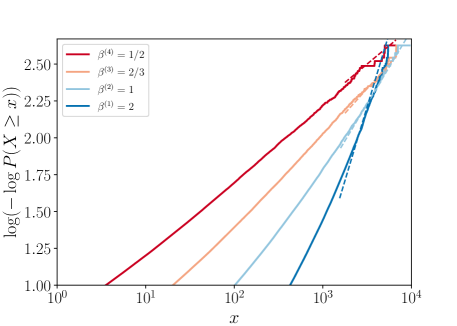
Figure 1: Solid lines: approximations of tail parameters $\beta^{(\ell)}$ based on Equation (3) where $X$ are hidden units of layers $\ell=1,2,3,4$ corresponding theoretically to generalized Weibull-tail with tail parameters $\beta^{(\ell)}=2,1,\nicefrac{{2}}{{3}},\nicefrac{{1}}{{2}}$, under the independent Gaussian weights assumption. Dashed lines: linear regressions with coefficients equal to the theoretical tail parameters $\beta^{(\ell)}=\nicefrac{{2}}{{\ell}}$ and manually selected biases to approach the solid lines for visual comparison.

4 Comparison of different characterizations

4.1 Generalized Weibull-tail vs sub-Weibull

Some of the commonly used techniques to study the tail behavior is to consider probability tail bounds such as sub-Gaussian, sub-exponential, or their generalization to sub-Weibull distributions (Vladimirova et al., 2020; Kuchibhotla and Chakrabortty, 2018). A non-negative random variable $X$ is called sub-Weibull with tail parameter $\theta>0$ if its survival function is upper-bounded by that of a Weibull distribution:

$$\overline{F}_{X}(x)\leq a\mathrm{e}^{-bx^{1/\theta}},\,\,\,\text{for }x>0\,\,\,\text{and some }a,b>0.$$ (4)

This property ensures the existence of the moment generating function as well as bounds on moments. In contrast, the Weibull-tail property characterizes the survival or density functions without a hand on moments. While tail parameters in Equation (1) and (4) of generalized Weibull-tail and sub-Weibull properties respectively are different, there exist connections. Notice that for any constants $a,b,\beta>0$, function $l(x)=b-\frac{\log a}{x^{\beta}}\geq 0$ is slowly-varying for $x$ large enough and $a\mathrm{e}^{-bx^{\beta}}=\mathrm{e}^{-x^{\beta}l(x)}$. It means that if a random variable $X$ is sub-Weibull with parameter $\theta=1/\beta>0$, satisfying Equation (4), then the survival function of $X$ is upper-bounded by a Weibull-tail function with tail parameter $\beta$ and slowly-varying function $l(x)=1$, satisfying Equation (1). If random variable $X$ is generalized Weibull-tail with tail parameter $\beta$, then from the last item of Proposition 1, for $a_{1},a_{2}>0$ we have

$$a_{1}\mathrm{e}^{-x^{\beta_{1}}}\leq\overline{F}_{X}(x)=\mathrm{e}^{-x^{\beta}l(x)}\leq a_{2}\mathrm{e}^{-x^{\beta_{2}}},$$

or $\text{GWT}_{\mathbb{R}_{+}}(\beta)\subset\text{SubW}(1/\beta_{2})$ and $\text{GWT}_{\mathbb{R}_{+}}(\beta)\not\subset\text{SubW}(1/\beta_{1})$ for $x$ large enough and $\forall(\beta_{1},\beta_{2})$ such that $0<\beta_{2}<\beta<\beta_{1}$, as illustrated on Figure 2.

Figure 2: Relation between sub-Weibull and generalized Weibull-tail characteristics.

It was recently shown in Vladimirova et al. (2019) that hidden units of Bayesian neural networks with iid Gaussian priors are sub-Weibull with tail parameter proportional to the hidden layer number, that is $\theta=\frac{\ell}{2}$. It means that the unit distributions of hidden layer $\ell$ can be upper-bounded by some Weibull distributions $a\mathrm{e}^{-x^{2/\ell}}$ for all $\ell$. For larger tail parameter $\theta$, Weibull distribution $a\mathrm{e}^{-x^{1/\theta}}$ is heavier-tailed but being sub-Weibull does not guarantee the heaviness of the tails. However, this upper bound is optimal in the sense that it is achieved for neural networks with one hidden unit per layer.

From Theorem 1, for neural networks with independent Gaussian weights, hidden units of $\ell$-th layer are generalized Weibull-tail with tail parameter $\beta=1/\theta=2/\ell$ so they have upper and lower bounds of the form $\mathrm{e}^{-x^{2/\ell}l(x)}$ up to a constant where $l$ is some slowly-varying function. Therefore, it proves that hidden units are heavier-tailed as going deeper for any finite numbers of hidden units per layer.

4.2 Meijer G-functions description

In Springer and Thompson (1970) it was shown that the probability density function of the product of independent normal variables could be expressed through a Meijer G-function. It resulted in an accurate description of induced unit priors given Gaussian priors on weights and linear or ReLU activation function  (Zavatone-Veth and Pehlevan, 2021; Noci et al., 2021). It is a full description of function-space priors but under strong assumptions, requiring Gaussian priors on weights and linear or ReLU activation functions, and with convoluted expressions. In contrast, we provide results for many distributions, including heavy-tailed ones, and our results can be extended to smooth activation functions, such as PReLU, ELU, Softplus.

5 Future applications

Cold posterior effect and priors.

It was recently empirically found that Gaussian priors led to the cold posterior effect in which a tempered “cold” posterior, obtained by exponentiating the posterior to some power largely greater than one, performs better than an untempered one (Wenzel et al., 2020). The performed Bayesian inference is considered sub-optimal due to the need for cold posteriors, and the model is deemed misspecified. From that angle, Wenzel et al. (2020) suggested that Gaussian priors might not be a good choice for Bayesian neural networks. In some works, data augmentation is argued to be the main reason for this effect (Izmailov et al., 2021; Nabarro et al., 2021) as the increased amount of observed data naturally leads to higher posterior contraction (Izmailov et al., 2021). At the same time, even considering the data augmentation for some models, the cold posterior effect is still present. In addition, Aitchison (2021) demonstrates that the problem might originate in the wrong likelihood of the models and that modifying only the likelihood based on data curation mitigates the cold posterior effect. Nabarro et al. (2021) hypothesize that using an appropriate prior incorporating knowledge of data augmentation might provide a solution. Moreover, heavy-tailed priors have been shown to mitigate the cold posterior effect (Fortuin et al., 2021). According to Theorem 1, heavier-tailed priors lead to even heavier-tailed induced priors in function-space. Thus, the heavy-tail property of distributions in function-space might be a highly beneficial feature. Fortuin et al. (2021) also proposed correlated priors for convolutional neural networks since trained weights are empirically strongly correlated. Correlated priors improve overall performance but do not alleviate the cold posterior effect. Our theory can be extended to correlated weight priors. This direction is promising for further uncovering the effect of weight prior on function-space prior.

Edge of Chaos.

An active line of research studies the propagation of deterministic inputs in neural networks (Poole et al., 2016; Schoenholz et al., 2017; Hayou et al., 2019). The main idea is to explore the covariance between pre-activations for two given different data points. Poole et al. (2016) and Schoenholz et al. (2017) obtained recurrence relations under the assumption of Gaussian initialization and Gaussian pre-activations. They conclude that there is a critical line, so-called Edge of Chaos, separating signal propagation into two regions. The first one is an ordered phase in which all inputs end up asymptotically correlated. The second is a chaotic phase in which all inputs end up asymptotically independent. To propagate the information deeper in a neural network, one should choose Gaussian prior variances corresponding to the separating line. Hayou et al. (2019) show that the smoothness of the activation function also plays an important role. Since this line of works considers Gaussian priors not only on the weights but also on the pre-activations, it is closely related to a wide regime where the number of hidden units per layer tends to infinity. Given that hidden units are heavier-tailed with depth, we speculate that future research will focus on finding better approximations of the pre-activation functions in recurrence relations obtained for finite-width neural networks.

6 Conclusion

We extend the theory on induced distributions in Bayesian neural networks and establish an accurate and easily interpretable characterization of hidden units tails. The obtained results confirm the heavy-tailed nature of hidden units for different weight priors.

Appendix A Slowly and regularly-varying functions theory

The set of regular-varying functions with index $\rho\in\mathbb{R}$ is denoted by $\mathcal{RV}_{\rho}$. Note that for $\rho=0$, the set $\mathcal{RV}_{0}$ boils down to the set of slowly-varying functions. In particular, any function $r\in\mathcal{RV}_{\rho}$ can be written $r(x)=x^{\rho}l(x)$, where $l$ is slowly-varying.

Definition A.1 (Regularly-varying function).

Let $r$ be a positive function. Then $r\in\mathcal{RV}_{\rho}$ if for all $t>0$ $\lim_{x\to\infty}\frac{r(tx)}{r(x)}=t^{\rho}$.

Proposition 1.

(Bingham et al., 1989, Proposition 1.3.6) Let $l,l_{1},\ldots,l_{k}$ be slowly-varying functions. Then:

1. $(\log l(x))/\log x\to 0$ as $x\to\infty$.

2. $l^{\alpha}$ varies slowly for every $\alpha\in\mathbb{R}$.

3. $l_{1}l_{2}$, $l_{1}+l_{2}$, and (if $l_{2}(x)\to\infty$ as $x\to\infty$) $l_{1}\circ l_{2}$ vary slowly.

4. If $f(x_{1},\dots,x_{k})$ is a rational function with positive coefficients, $f(l_{1},\dots,l_{k})$ varies slowly.

5. For any $\alpha>0$, $x^{\alpha}l(x)\to\infty,\ x^{-\alpha}l(x)\to 0\ (x\to\infty)$.

Lemma A.1

If $l_{1}(x)$ is slowly-varying, then $l_{2}(x)=l_{1}(x^{a})$ is slowly-varying for $a>0$.

Lemma A.2

If $l_{1},l_{2}$ vary slowly, so does $\max\{l_{1},l_{2}\}$ and $\min\{l_{1},l_{2}\}$.

Lemma A.3

Let $r_{1}$ and $r_{2}$ be regularly-varying functions with parameters $\beta_{1}>0$ and $\beta_{2}>0$. Then, the function $r$ such that $\mathrm{e}^{-r}=\mathrm{e}^{-r_{1}}+\mathrm{e}^{-r_{2}}$, is regularly-varying with parameter $\beta=\min\{\beta_{1},\beta_{2}\}$.

Proof A.2.

Let us express function $r$ from the statement: $r(x)=-\log\varphi(x)=-\log\left(\mathrm{e}^{-r_{1}(x)}+\mathrm{e}^{-r_{2}(x)}\right)$. If $\beta_{1}\not=\beta_{2}$, without loss of generality, let us assume that $\beta_{1}<\beta_{2}$, then

$$\varphi(x)=\mathrm{e}^{-r_{1}(x)}\left(1+\mathrm{e}^{-r_{2}(x)+r_{1}(x)}\right)=\mathrm{e}^{-r_{1}(x)}\left(1+\mathrm{e}^{r_{2}(x)\left(-1+\frac{r_{1}(x)}{r_{2}(x)}\right)}\right).$$

Notice that $\frac{r_{1}}{r_{2}}\in\mathcal{RV}_{\beta_{1}-\beta_{2}}$. For $\beta_{1}<\beta_{2}$, $\frac{r_{1}(x)}{r_{2}(x)}\to 0$ when $x\to\infty$. The expression in the exponent $r_{2}(x)\left(-1+\frac{r_{1}(x)}{r_{2}(x)}\right)\simeq-r_{2}(x)\to-\infty$, so the exponent $\mathrm{e}^{r_{2}(x)\left(-1+\frac{r_{1}(x)}{r_{2}(x)}\right)}\to 0$. Then $\varphi(x)\simeq\mathrm{e}^{-r_{1}(x)}$ and $r(x)=-\log\varphi(x)\simeq r_{1}(x)$. It means that for the case $\beta_{1}<\beta_{2}$, $r\in\mathcal{RV}_{\beta_{1}}$.

Let us consider the case with equal parameters $\beta_{1}=\beta_{2}=\beta$, then $r_{1}(x)=x^{\beta}l_{1}(x)$, $r_{2}(x)=x^{\beta}l_{2}(x)$ with slowly-varying $l_{1}$ and $l_{2}$. With $l=\min\{l_{1},l_{2}\}$, we can write

$$\varphi(x)=\mathrm{e}^{-x^{\beta}l(x)}\left(1+\mathrm{e}^{-x^{\beta}|l_{2}(x)-l_{1}(x)|}\right).$$

Consider the logarithm of the latter expression

$$-\log\varphi(x)=x^{\beta}\left(l(x)+x^{-\beta}\log\left(1+\mathrm{e}^{-x^{\beta}|l_{2}(x)-l_{1}(x)|}\right)\right).$$

Since the function $l$ is slowly-varying by Lemma A.2 and $0\leq\mathrm{e}^{-x^{\beta}|l_{2}(x)-l_{1}(x)|}\leq 1$, then $r(x)=-\log\varphi(x)\simeq x^{\beta}l(x)\in\mathcal{RV}_{\beta}$.

Appendix B Weibull-tail properties on $\mathbb{R}$

Let us firstly introduce a notion of generalized Weibull-tail random variable which has an additional property of stability:

Definition B.1 (Generalized Weibull-tail on $\mathbb{R}_{+}$).

A random variable $X$ is called generalized Weibull-tail with tail parameter $\beta>0$ if its survival function $\overline{F}_{X}$ is bounded by Weibull-tail functions of tail parameter $\beta$ with possibly different slowly-varying functions $l_{1}$ and $l_{2}$:

$$\mathrm{e}^{-x^{\beta}l_{1}(x)}\leq\overline{F}_{X}(x)\leq\mathrm{e}^{-x^{\beta}l_{2}(x)},\,\,\,\text{for }x>0.$$ (5)

We note $X\sim\text{GWT}_{\mathbb{R}_{+}}(\beta)$.

Now we define a random variable whose both right and left tails are Weibull-tail on $\mathbb{R}_{+}$.

Definition B.2 (Weibull-tail on $\mathbb{R}$).

A random variable $X$ on $\mathbb{R}$ is Weibull-tail on $\mathbb{R}$ with tail parameter $\beta>0$ if both its right and left tails are Weibull-tail with tail parameter $\beta$:

$$\overline{F}_{X}(x)=1-F_{X}(x)=\mathrm{e}^{-x^{\beta}l_{1}(x)},\quad x>0$$

$$F_{X}(x)=\mathrm{e}^{-|x|^{\beta}l_{2}(|x|)},\quad x<0,$$

where $l_{1}$ and $l_{2}$ are slowly-varying functions. We note $X\sim\text{WT}_{\mathbb{R}}(\beta)$.

Lemma B.1

1. If random variable $X$ on $\mathbb{R}$ is $\text{WT}_{\mathbb{R}}(\beta)$, then $|X|$ is $\text{WT}_{\mathbb{R}_{+}}(\beta)$.

2. If $X$ is asymmetric but both tails are Weibull-tail and $|X|$ is $\text{WT}_{\mathbb{R}_{+}}(\beta)$, then one of the tails (right or left) is $\text{WT}_{\mathbb{R}_{+}}(\beta)$ and the other one is $\text{WT}_{\mathbb{R}_{+}}(\beta^{\prime})$ where $\beta^{\prime}\geq\beta$.

3. For symmetric distributions, $X$ is $\text{WT}_{\mathbb{R}}(\beta)$ if and only if $|X|$ is $\text{WT}_{\mathbb{R}_{+}}(\beta)$.

Proof B.3.

1. For $x>0$, the cumulative distribution function of $|X|$ is the following

   $$F_{|X|}(x)=F_{X}(x)-F_{X}(-x).$$

   Then, $\overline{F}_{|X|}(x)$ can be expressed as a sum of the right and left tails:

   $$\overline{F}_{|X|}(x)=\overline{F}_{X}(x)+F_{X}(-x).$$

   If $X$ is $\text{WT}_{\mathbb{R}}(\beta)$, then $|X|$ is $\text{WT}_{\mathbb{R}_{+}}(\beta)$ as a consequence of Definition B.2 and Lemma A.3.

2. Let $|X|$ be $\text{WT}_{\mathbb{R}_{+}}(\beta)$ and $X$ has Weibull left and right tails with different tail parameters. Without loss of generality, assume that ${F}_{X}(-x)$ is Weibull-tail with tail parameter $\beta^{\prime}<\beta$. According to Lemma A.3, the sum survival function $\overline{F}_{|X|}(x)$ will be Weibull-tail with tail parameter $\beta^{\prime}=\min\{\beta^{\prime},\beta\}$. We obtained a contradiction and ${F}_{X}(-x)$ must have tail parameter greater or equal $\beta$. If both tail parameters are greater than $\beta$, then the tails sum have the tail parameter equal to the minimum tail parameter among them which is greater than $\beta$. It means that at least one tail must have tail parameter $\beta$.

3. For symmetric distributions $\overline{F}_{X}(x)={F}_{X}(-x)$ for any $x$, then $\frac{1}{2}\overline{F}_{|X|}(x)=\overline{F}_{X}(x)={F}_{X}(-x)$ and we have the equality.

Lemma B.2

1. If a random variable $X$ is $\text{GWT}_{\mathbb{R}}(\beta)$, then $|X|$ is $\text{GWT}_{\mathbb{R}_{+}}(\beta)$.

2. For symmetric distributions, $X$ is $\text{GWT}_{\mathbb{R}}(\beta)$ if and only if $|X|$ is $\text{GWT}_{\mathbb{R}_{+}}(\beta)$.

Proof B.4.

Similarly as in Lemma B.1, we obtain $\overline{F}_{|X|}(x)=\overline{F}_{X}(x)+F_{X}(-x)$ for $x\geq 0$.

1. If $X$ is $\text{GWT}_{\mathbb{R}}(\beta)$, then right and left tails are upper and lower-bounded by some Weibull-tail functions. Then, the sum of the right and left tails is upper and lower-bounded by these Weibull-tail functions and $|X|\sim\text{GWT}_{\mathbb{R}_{+}}(\beta)$.

2. For symmetric distributions we have $\overline{F}_{X}(x)={F}_{X}(-x)$ for all $x$, then $\frac{1}{2}\overline{F}_{|X|}(x)=\overline{F}_{X}(x)={F}_{X}(-x)$ and we have the equality.

Lemma B.3 (Power and multiplication by a constant)

If $X\sim\text{GWT}_{\mathbb{R}}(\beta)$ and the distribution of $X$ is symmetric, then $a|X|^{b}\sim\text{GWT}_{\mathbb{R}_{+}}\left(\frac{\beta}{b}\right)$ for $a,b>0$.

Proof B.5.

According to Lemma B.1, $|X|\sim\text{GWT}_{\mathbb{R}_{+}}(\beta)$. For $a,b>0$, the tail of $Y=a|X|^{b}$ is

$$\mathbb{P}\Bigl{(}a|X|^{b}\geq y\Bigr{)}=\mathbb{P}\left(|X|^{b}\geq\frac{y}{a}\right)=\mathbb{P}\Bigl{(}|X|\geq\left(\frac{y}{a}\right)^{1/b}\Bigr{)}.$$

Since $|X|$ is generalized Weibull-tail on $\mathbb{R}_{+}$ with tail parameter $\beta$, $\mathrm{e}^{-x^{\beta}l_{1}(x)}\leq\mathbb{P}\left(|X|\geq x\right)\leq\mathrm{e}^{-x^{\beta}l_{2}(x)}$, where $l_{1}$ and $l_{2}$ are slowly-varying functions, it implies

$$\mathrm{e}^{-y^{\beta/b}\tilde{l}_{1}(y)}\leq\mathbb{P}\Bigl{(}a|X|^{b}\geq y\Bigr{)}\leq\mathrm{e}^{-y^{\beta/b}\tilde{l}_{2}(y)},$$

where $\tilde{l}_{i}(y)=\frac{l_{i}((y/a)^{1/b})}{a^{\beta/b}}$, $i=1,2$ are slowly-varying functions by Lemma A.1. It leads to the statement of the lemma.

Theorem 2 (Sum of GWT_R variables)

Let $X_{1},\dots,X_{N}\in\mathrm{GWT}_{\mathbb{R}}$ with tail parameters $\beta_{1},\dots,\beta_{N}$. If $X_{1},\dots,X_{N}$ satisfy the PD condition of Definition 2.2, then, $X_{1}+\dots+X_{N}\in\mathrm{GWT}_{\mathbb{R}}(\beta)$ with $\beta=\min\{\beta_{1},\dots,\beta_{N}\}$.

Proof B.6.

Let us start with $N=2$. For any random variables $X$ and $Y$, the following upper bound holds:

$$\mathbb{P}(X+Y\geq z)\leq\mathbb{P}(X\geq\nicefrac{{z}}{{2}})+\mathbb{P}(Y\geq\nicefrac{{z}}{{2}})\leq 2\max\{\mathbb{P}(X\geq\nicefrac{{z}}{{2}}),\mathbb{P}(Y\geq\nicefrac{{z}}{{2}})\}.$$

The PD condition leads to a lower bound for the sum:

$$\mathbb{P}(X+Y\geq z)\geq\mathbb{P}(X\geq 0,Y\geq z)=\mathbb{P}(X\geq 0|Y\geq z)\mathbb{P}(Y\geq z)\geq C\,\mathbb{P}(Y\geq z),$$

where constant $C>0$. Thus, the sum survival function $\overline{F}_{Z}(z)=\mathbb{P}(X+Y\geq z)$ has the following bounds for the right tail:

$$C\,\overline{F}_{Y}(z)\leq\overline{F}_{Z}(z)\leq 2\max\{\overline{F}_{X}(\nicefrac{{z}}{{2}}),\overline{F}_{Y}(\nicefrac{{z}}{{2}})\},$$

where $\overline{F}_{X}$ and $\overline{F}_{Y}$ are the survival functions of $X$ and $Y$.

Let $X$ and $Y$ be generalized Weibull-tail on $\mathbb{R}$ of parameters $\beta_{x}$ and $\beta_{y}$, then for $z>0$ large enough

$$C\,\mathrm{e}^{-z^{\beta_{y}}l_{1}^{r}(z)}\leq\overline{F}_{Z}(z)\leq 2\mathrm{e}^{-z^{\min\{\beta_{x},\beta_{y}\}}l_{2}^{r}(z)},$$

where $l_{1}^{r}=l_{1}^{y}$ is the slowly-varying function appearing in the right tail lower bound of generalized Weibull-tail $Y$ and $l_{2}^{r}(z)=\min\{\frac{1}{2^{\beta_{x}}}l_{2}^{x}(\nicefrac{{z}}{{2}}),\frac{1}{2^{\beta_{y}}}l_{2}^{y}(\nicefrac{{z}}{{2}})\}$ is the minimum among slowly-varying functions, where $l_{2}^{x}$ and $l_{2}^{y}$ are slowly-varying functions in the right tails upper bounds of $X$ and $Y$. According to Lemma A.2, $l_{2}^{r}(z)$ is also slowly-varying. Similarly, we can get bounds for the left tail. Therefore, $X+Y$ is generalized Weibull-tail on $\mathbb{R}$ with tail parameter $\beta=\min\{\beta_{x},\beta_{y}\}$.

Similarly as above when $N=2$, bounds for the right tail of the sum $Z=X_{1}+\dots+X_{N}$ with survival function $\overline{F}_{Z}=\mathbb{P}(Z\geq z)$ are:

$$C\overline{F}_{N}(z)\leq\overline{F}_{Z}(z)\leq N\max\{\overline{F}_{1}(\nicefrac{{z}}{{N}}),\dots,\overline{F}_{N}(\nicefrac{{z}}{{N}})\},$$

where $\overline{F}_{i}$ is the survival functions of $X_{i}$ and constant $C>0$. The rest of the proof is identical to the one of the case $N=2$.

The case when distributions have only right tails (or only left tails), can be considered as a particular case of the last theorem: a sum of non-negative generalized Weibull-tail random variables is non-negative generalized Weibull-tail with tail parameter equal to the minimum among those of the terms.

Theorem 3 (Product of independent $\text{GWT}_{\mathbb{R}}$ variables)

Let $X_{1},\dots,X_{N}\in\mathrm{GWT}_{\mathbb{R}}$ be independent symmetric with tail parameters $\beta_{1},\dots,\beta_{N}$. Then, the product $X_{1}\ldots X_{N}\in\mathrm{GWT}_{\mathbb{R}}(\beta)$ with $\beta$ such that $\frac{1}{\beta}=\frac{1}{\beta_{1}}+\cdots+\frac{1}{\beta_{N}}$.

Proof B.7.

Consider two independent symmetric generalized Weibull-tail random variables with tail parameters $\beta_{x}=\frac{1}{\theta_{x}}$ and $\beta_{y}=\frac{1}{\theta_{y}}$, $X\sim\text{GWT}_{\mathbb{R}}\left(\frac{1}{\theta_{x}}\right)$ and $Y\sim\text{GWT}_{\mathbb{R}}\left(\frac{1}{\theta_{y}}\right)$. From Lemma B.1 and since random variables $X$ and $Y$ are symmetric, it is equivalent to $|X|\sim\text{GWT}_{\mathbb{R}_{+}}\left(\frac{1}{\theta_{x}}\right)$ and $|Y|\sim\text{GWT}_{\mathbb{R}_{+}}\left(\frac{1}{\theta_{y}}\right)$.

The product of independent symmetric distributions is symmetric since $Z=XY=^{d}(-X)Y=^{d}-Z$. From Lemma B.1, $Z\sim\text{GWT}_{\mathbb{R}}(\beta)$ if and only if $|Z|\sim\text{GWT}_{\mathbb{R}_{+}}(\beta)$.

Our goal is to show that for some slowly-varying functions $l_{1}$ and $l_{2}$, there exist upper and lower bounds for the survival function of $|Z|$ and $z$ large enough as follows:

$$\mathrm{e}^{-z^{\frac{1}{\theta_{x}+\theta_{y}}}l_{1}(z)}\leq\overline{F}_{|Z|}(z)=\mathbb{P}(|XY|\geq z)\leq\mathrm{e}^{-z^{\frac{1}{\theta_{x}+\theta_{y}}}l_{2}(z)}.$$ (6)

1. Upper bound. First, notice that from the concavity of the logarithm, we have $\ln(pu+(1-p)v)\geq p\ln u+(1-p)\ln v$ for any $u,v>0$ and $p\in(0,1)$. Then $pu+(1-p)v\geq u^{p}v^{1-p}$. The change of variables $x=u^{p}$, $y=v^{1-p}$ implies $px^{\nicefrac{{1}}{{p}}}+(1-p)y^{\nicefrac{{1}}{{(1-p)}}}\geq xy$. From the latter equation, an upper bound of the product tail is

   $$\mathbb{P}(|XY|\geq z)\leq\mathbb{P}\left(p|X|^{\nicefrac{{1}}{{p}}}+(1-p)|Y|^{\nicefrac{{1}}{{(1-p)}}}\geq z\right).$$ (7)

   Lemma B.3 implies that $p|X|^{\nicefrac{{1}}{{p}}}\sim\text{GWT}_{\mathbb{R}_{+}}\left(\frac{p}{\theta_{x}}\right)$ and $(1-p)|Y|^{\nicefrac{{1}}{{1-p}}}\sim\text{GWT}_{\mathbb{R}_{+}}\left(\frac{1-p}{\theta_{y}}\right)$. Taking $p=\frac{\theta_{x}}{\theta_{x}+\theta_{y}}$ and $1-p=\frac{\theta_{y}}{\theta_{x}+\theta_{y}}$, yields a sum of two independent non-negative generalized Weibull-tail random variables with tail parameter $\frac{1}{\theta_{x}+\theta_{y}}$ on the right-hand side of Equation (7). By Theorem 2, this sum is generalized Weibull-tail with the same tail parameter $\frac{1}{\theta_{x}+\theta_{y}}$. It means that there exists a slowly-varying function $l_{2}$ such that the tail of product absolute value $|XY|$ is upper-bounded by

   $$\mathbb{P}(|XY|\geq z)\leq\mathrm{e}^{-z^{\frac{1}{\theta_{x}+\theta_{y}}}l_{2}(z)}.$$ (8)

2. Lower bound. By independence of $|X|$ and $|Y|$ we have

   $$\mathbb{P}(|XY|\geq z)\geq\mathbb{P}\left(|X|\geq z^{\frac{\theta_{x}}{\theta_{x}+\theta_{y}}}\right)\mathbb{P}\left(|Y|\geq z^{\frac{\theta_{y}}{\theta_{x}+\theta_{y}}}\right).$$

   Since $|X|$ and $|Y|$ are generalized Weibull-tail on $\mathbb{R}_{+}$, we can define function $l_{1}(z)=l_{1}^{x}(z^{\theta_{x}/{(\theta_{x}+\theta_{y})}})+l_{1}^{y}(z^{\theta_{y}/{(\theta_{x}+\theta_{y})}})$ with $l_{1}^{x}$ and $l_{1}^{y}$ being slowly-varying functions in the lower bounds of generalized Weibull-tail $|X|$ and $|Y|$. Then, $l_{1}$ is slowly-varying by Lemma A.1 and we have

   $$\mathbb{P}(|XY|\geq z)\geq\mathrm{e}^{-z^{\frac{1}{\theta_{x}+\theta_{y}}}l_{1}(z)}.$$ (9)

Combining together Equations (8) and (9) and Definition B.1 with Lemma B.1 implies the statement of the theorem.

Appendix C Bayesian neural network properties

Proofs of Section 3.

Lemma 3.1

Let $X_{1},\dots,X_{N}$ be some possibly dependent random variables and $W_{1},\dots,W_{N}$ be symmetric, mutually independent and independent from $X_{1},\dots,X_{N}$, then random variables $X_{1}W_{1},\dots,X_{N}W_{N}$ satisfy the PD condition.

Proof C.1.

The joint probability for the right tail $\mathbb{P}\left(\bigcap_{i=1}^{N}W_{i}X_{i}\geq z_{i}\right)$ can be expressed as

$$\int_{-\infty}^{\infty}\dots\int_{-\infty}^{\infty}\mathbb{P}\left(\bigcap_{i=1}^{N}W_{i}x_{i}\geq z_{i}\Bigl{.}\Bigr{|}\bigcap_{j=1}^{N}X_{j}=x_{j}\right)f(x_{1},\dots,x_{N})\,\mathrm{d}x_{1}\dots\mathrm{d}x_{N}.$$ (10)

Independence between $W_{i}$ and $X_{j}$ yields

$$\mathbb{P}\left(\bigcap_{i=1}^{N}W_{i}x_{i}\geq z_{i}\Bigl{.}\Bigr{|}\bigcap_{j=1}^{N}X_{j}=x_{j}\right)=\mathbb{P}\left(\bigcap_{i=1}^{N}W_{i}x_{i}\geq z_{i}\right)=\prod_{i=1}^{N}\mathbb{P}\left(W_{i}x_{i}\geq z_{i}\right),$$

where the last equality is due to the mutual independence of weights $W_{1},\dots,W_{N}$. Let $z_{1}=\dots=z_{N-1}=0$ and $z_{N}=z$. If $x_{i}=0$, the probability $\mathbb{P}\left(W_{i}x_{i}\geq 0\right)=1$. If $x_{i}\not=0$, then, due to the symmetry of $W_{i}$, the probability $\mathbb{P}\left(W_{i}x_{i}\geq 0\right)=\frac{1}{2}$. Thus, the following lower bound holds:

$$\mathbb{P}\left(W_{i}x_{i}\geq 0\right)\geq\frac{1}{2}\quad\text{for all }i\in\{1,\dots,N-1\}.$$

Notice that

$$\int_{-\infty}^{\infty}\dots\int_{-\infty}^{\infty}\mathbb{P}\left(W_{N}x_{N}\geq z\right)f(x_{1},\dots,x_{N})\,\mathrm{d}x_{1}\dots\mathrm{d}x_{N}=\mathbb{P}\left(W_{N}X_{N}\geq z\right).$$

Substituting the latter equations into Equation (10) leads to the lower bound:

$$\mathbb{P}\left(\bigcap_{i=1}^{N-1}W_{i}X_{i}\geq 0,W_{N}X_{N}\geq z\right)\geq\frac{1}{2^{N-1}}\mathbb{P}\left(W_{N}X_{N}\geq z\right).$$

By the conditional probability definition, we have

$$\mathbb{P}\left(\bigcap_{i=1}^{N-1}W_{i}X_{i}\geq 0\Bigl{.}\Bigr{|}W_{N}X_{N}\geq z\right)=\frac{\mathbb{P}\left(\bigcap_{i=1}^{N}W_{i}X_{i}\geq 0\right)}{\mathbb{P}\left(W_{N}X_{N}\geq z\right)}\geq\frac{1}{2^{N-1}}.$$

The proof for the left tail is identical.

Theorem 1

Consider a Bayesian neural network as described in Equation (2) with ReLU activation function. Let $\ell$-th layer weights be independent symmetric generalized Weibull-tail on $\mathbb{R}$ with tail parameter $\beta^{(\ell)}_{w}$. Then, $\ell$-th layer pre-activations are generalized Weibull-tail on $\mathbb{R}$ with tail parameter $\beta^{(\ell)}$ such that $\frac{1}{\beta^{(\ell)}}=\frac{1}{\beta^{(1)}_{w}}+\dots+\frac{1}{\beta^{(\ell)}_{w}}$.

Proof C.2.

The goal is to show that $h_{j}^{(\ell)}\sim\text{GWT}_{\mathbb{R}_{+}}\left(\beta^{(\ell)}\right)$ where $\frac{1}{\beta^{(\ell)}}=\frac{1}{\beta^{(1)}_{w}}+\dots+\frac{1}{\beta^{(\ell)}_{w}}$. We proceed by induction on the layer depth $\ell$.

1. First hidden layer

   For $\ell=1$, by Lemma 3.1, products $w_{ij}^{(1)}h_{i}^{(0)}$ for $i=1,\dots,H_{1}$ satisfy the positive dependence condition of Definition 2.2, thus the sum $g_{j}^{(1)}=\sum_{i}w_{ij}^{(1)}h_{i}^{(0)}$ is generalized Weibull-tail on $\mathbb{R}$ with tail parameter $\beta^{(1)}=\beta^{(1)}_{w}$. Since ReLU function does not change the right tail and post-activations lie completely on $\mathbb{R}_{+}$, we have $h_{j}^{(1)}\sim\text{GWT}_{\mathbb{R}_{+}}(\beta^{(1)})$.

2. Step of induction

   Let $h_{j}^{(\ell-1)}\sim\text{GWT}_{\mathbb{R}_{+}}\left(\beta^{(\ell-1)}\right)$ where $\frac{1}{\beta^{(\ell-1)}}=\frac{1}{\beta^{(1)}_{w}}+\dots+\frac{1}{\beta^{(\ell-1)}_{w}}$. Since $h_{j}^{(\ell-1)}$ is non-negative and $w_{ij}^{(\ell)}$ are symmetric, their product is symmetric by symmetry of the weights: $h_{j}^{(\ell-1)}w_{ij}^{(\ell)}$ has the same distribution as $h_{j}^{(\ell-1)}\left(-w_{ij}^{(\ell)}\right)=-h_{j}^{(\ell-1)}w_{ij}^{(\ell)}$. By Theorem 3 and independence of random variables $h_{j}^{(\ell-1)}$ and $w_{ij}^{(\ell)}$, we obtain that $h_{j}^{(\ell-1)}w_{ij}^{(\ell)}\sim\text{GWT}_{\mathbb{R}}(\beta^{(\ell)})$ where $\frac{1}{\beta^{(\ell)}}=\frac{1}{\beta^{(\ell-1)}}+\frac{1}{\beta^{(\ell)}_{w}}=\frac{1}{\beta^{(1)}_{w}}+\dots+\frac{1}{\beta^{(\ell-1)}_{w}}+\frac{1}{\beta^{(\ell)}_{w}}$.

   According to Lemma 3.1, $w_{ij}^{(\ell)}h_{i}^{(\ell-1)}$, $i=1,\dots,H_{\ell}$ satisfy the dependence condition of Definition 2.2. Thus, the sum $g_{j}^{(\ell)}=\sum_{i=1}^{H_{\ell}}w_{ij}^{(\ell)}h_{i}^{(\ell-1)}$ is symmetric generalized Weibull-tail with the same tail parameter. The ReLU activation does not impact the right tail, therefore, $h_{j}^{(\ell)}\sim\text{GWT}_{\mathbb{R}_{+}}(\beta^{(\ell)})$.

References

- Aitchison (2020) Laurence Aitchison. Why bigger is not always better: on finite and infinite neural networks. In International Conference on Machine Learning, 2020.
- Aitchison (2021) Laurence Aitchison. A statistical theory of cold posteriors in deep neural networks. In International Conference on Learning Representations, 2021.
- Bingham et al. (1989) Nicholas H Bingham, Charles M Goldie, and Jef L Teugels. Regular variation. Number 27. Cambridge university press, 1989.
- Favaro et al. (2020) Stefano Favaro, Sandra Fortini, and Peluchetti Stefano. Stable behaviour of infinitely wide deep neural networks. In International Conference on Artificial Intelligence and Statistics, 2020.
- Fortuin et al. (2021) Vincent Fortuin, Adrià Garriga-Alonso, Florian Wenzel, Gunnar Rätsch, Richard Turner, Mark van der Wilk, and Laurence Aitchison. Bayesian neural network priors revisited. arXiv preprint arXiv:2102.06571, 2021.
- Gardes and Girard (2016) Laurent Gardes and Stéphane Girard. On the estimation of the functional Weibull tail-coefficient. Journal of Multivariate Analysis, 146:29–45, 2016.
- Gardes et al. (2011) Laurent Gardes, Stéphane Girard, and Armelle Guillou. Weibull tail-distributions revisited: a new look at some tail estimators. Journal of Statistical Planning and Inference, 141(1):429–444, 2011.
- Garriga-Alonso et al. (2019) Adrià Garriga-Alonso, Carl Edward Rasmussen, and Laurence Aitchison. Deep convolutional networks as shallow Gaussian processes. In International Conference on Learning Representations, 2019.
- Hayou et al. (2019) Soufiane Hayou, Arnaud Doucet, and Judith Rousseau. On the impact of the activation function on deep neural networks training. In International Conference on Machine Learning, 2019.
- Izmailov et al. (2021) Pavel Izmailov, Sharad Vikram, Matthew D Hoffman, and Andrew Gordon Wilson. What are Bayesian neural network posteriors really like? In International Conference on Machine Learning, 2021.
- Kuchibhotla and Chakrabortty (2018) Arun Kumar Kuchibhotla and Abhishek Chakrabortty. Moving beyond sub-Gaussianity in high-dimensional statistics: Applications in covariance estimation and linear regression. arXiv preprint arXiv:1804.02605, 2018.
- Lee et al. (2018) Jaehoon Lee, Jascha Sohl-Dickstein, Jeffrey Pennington, Roman Novak, Sam Schoenholz, and Yasaman Bahri. Deep neural networks as Gaussian processes. In International Conference on Learning Representations, 2018.
- Lee et al. (2020) Jaehoon Lee, Samuel Schoenholz, Jeffrey Pennington, Ben Adlam, Lechao Xiao, Roman Novak, and Jascha Sohl-Dickstein. Finite versus infinite neural networks: an empirical study. In International Conference on Neural Information Processing Systems, 2020.
- Matthews et al. (2018) Alexander G de G Matthews, Mark Rowland, Jiri Hron, Richard E Turner, and Zoubin Ghahramani. Gaussian process behaviour in wide deep neural networks. In International Conference on Learning Representations, 2018.
- McNeil et al. (2015) Alexander J McNeil, Rüdiger Frey, and Paul Embrechts. Quantitative risk management: concepts, techniques and tools. Princeton university press, 2015.
- Nabarro et al. (2021) Seth Nabarro, Stoil Ganev, Adrià Garriga-Alonso, Vincent Fortuin, Mark van der Wilk, and Laurence Aitchison. Data augmentation in Bayesian neural networks and the cold posterior effect. arXiv preprint arXiv:2106.05586, 2021.
- Neal (1996) Radford M Neal. Bayesian learning for neural networks. Springer Science & Business Media, 1996.
- Nelsen (2007) Roger B Nelsen. An introduction to copulas. Springer Science & Business Media, 2007.
- Noci et al. (2021) Lorenzo Noci, Gregor Bachmann, Kevin Roth, Sebastian Nowozin, and Thomas Hofmann. Precise characterization of the prior predictive distribution of deep ReLU networks. arXiv preprint arXiv:2106.06615, 2021.
- Poole et al. (2016) Ben Poole, Subhaneil Lahiri, Maithra Raghu, Jascha Sohl-Dickstein, and Surya Ganguli. Exponential expressivity in deep neural networks through transient chaos. In International Conference on Neural Information Processing Systems, 2016.
- Rachev (2003) Svetlozar Todorov Rachev. Handbook of Heavy Tailed Distributions in Finance: Handbooks in Finance, Book 1. Elsevier, 2003.
- Schoenholz et al. (2017) Samuel S Schoenholz, Justin Gilmer, Surya Ganguli, and Jascha Sohl-Dickstein. Deep information propagation. In International Conference on Learning Representations, 2017.
- Springer and Thompson (1970) Melvin Dale Springer and William E. Thompson. The distribution of products of beta, gamma and Gaussian random variables. SIAM Journal on Applied Mathematics, 18(4):721–737, 1970.
- Strupczewski et al. (2011) Witold G Strupczewski, Krzysztof Kochanek, Iwona Markiewicz, Ewa Bogdanowicz, Stanislaw Weglarczyk, and Vijay P Singh. On the tails of distributions of annual peak flow. Hydrology Research, 42(2-3):171–192, 2011.
- Vladimirova et al. (2019) Mariia Vladimirova, Jakob Verbeek, Pablo Mesejo, and Julyan Arbel. Understanding priors in Bayesian neural networks at the unit level. In International Conference on Machine Learning, 2019.
- Vladimirova et al. (2020) Mariia Vladimirova, Stéphane Girard, Hien Nguyen, and Julyan Arbel. Sub-Weibull distributions: Generalizing sub-Gaussian and sub-exponential properties to heavier tailed distributions. Stat, 9(1):e318, 2020.
- Wenzel et al. (2020) Florian Wenzel, Kevin Roth, Bastiaan Veeling, Jakub Swiatkowski, Linh Tran, Stephan Mandt, Jasper Snoek, Tim Salimans, Rodolphe Jenatton, and Sebastian Nowozin. How good is the Bayes posterior in deep neural networks really? In International Conference on Machine Learning, 2020.
- Wilson and Izmailov (2020) Andrew Gordon Wilson and Pavel Izmailov. Bayesian deep learning and a probabilistic perspective of generalization. International Conference on Neural Information Processing Systems, 2020.
- Zavatone-Veth and Pehlevan (2021) Jacob A Zavatone-Veth and Cengiz Pehlevan. Exact priors of finite neural networks. arXiv preprint arXiv:2104.11734, 2021.