Asymptotic expansion of the Wright function for large variable and parameter

Abstract

We consider the asymptotic expansion of the Wright function

$$W_{\lambda,\mu}(z)=\sum_{n=0}^{\infty}\frac{z^{n}}{n!\Gamma(\lambda n+\mu)}\qquad(\lambda>-1)$$

for large (positive and negative) variable and large parameter $\mu$. The analysis is based on use of the method of steepest descents applied to a suitable integral representation and, in part, complements the recent work of Ansari and Askari. Numerical results are presented to illustrate the accuracy of the different expansions obtained.

Mathematics subject classification (2020): 33C10, 34E05, 41A30, 41A60

Keywords: Asymptotic expansion, method of steepest descents, Wright function

  

1. Introduction

The Wright function under consideration (also known as a generalised Bessel function) is defined by

$$W_{\lambda,\mu}(z)=\sum_{n=0}^{\infty}\frac{z^{n}}{n!\Gamma(\lambda n+\mu)},$$ (1.1)

where $\lambda$ is supposed real and $\mu$ is, in general, an arbitrary complex parameter. The series converges for all finite $z$ provided $\lambda>-1$ and, when $\lambda=1$, it reduces to the modified Bessel function $z^{(1-\mu)/2}I_{\mu-1}(2\sqrt{z})$. This function has found recent application in the theory of fractional calculus [2, 3]. The case corresponding to $\lambda=-\sigma$, $0<\sigma<1$ arises in the analysis of time-fractional diffusion and diffusion-wave equations [4]; see also [6]. The case $\mu=0$ in (1.1) also finds application in probability theory and is discussed extensively in [7], where it is denoted by $\phi(\lambda,0;z)=W_{\lambda,0}(z)$ and referred to therein as a ‘reduced’ Wright function.

The asymptotics of this function were first studied by Wright [8, 9] using the method of steepest descents applied to the integral representation

$$W_{\lambda,\mu}(z)=\frac{1}{2\pi i}\int_{-\infty}^{(0+)}t^{-\mu}\exp\,[t+zt^{-\lambda}]\,dt\qquad(\lambda>-1,\ \mu\in{\bf C});$$ (1.2)

see also the summaries in [5, 6] using a different approach. A recent paper by Ansari and Askari [1] has investigated the asymptotic expansion of (1.1) when the argument $z<0$ and the parameter $\mu>0$ are both large. More specifically, these authors considered the Wright function

$${\cal W}^{-}_{\lambda,\nu}(x):=(\mbox{${\textstyle\frac{1}{2}}$}x)^{\nu}W_{\lambda,\nu+1}(-(\mbox{${\textstyle\frac{1}{2}}$}x)^{\lambda+1})=(\mbox{${\textstyle\frac{1}{2}}$}x)^{\nu}\sum_{n=0}^{\infty}\frac{(-)^{n}(x/2)^{(\lambda+1)n}}{n!\Gamma(\lambda n+\nu+1)}$$ (1.3)

for $x\to+\infty$ when $\nu=ax$, where $a>0$ is fixed, by employing the method of steepest descents applied to a suitable Laplace-type integral representation. Here we consider the same problem in more detail using the same approach. In a certain domain of the integration variable it is found that there are two relevant saddle points, which can either be real or a complex conjugate pair. We also discuss a special case when the parameters $a$ and $\lambda$ are connected in a specific manner that corresponds to the formation of a double saddle point.

The function of positive argument

$${\cal W}^{+}_{\lambda,\nu}(x):=(\mbox{${\textstyle\frac{1}{2}}$}x)^{\nu}W_{\lambda,\nu+1}((\mbox{${\textstyle\frac{1}{2}}$}x)^{\lambda+1})=(\mbox{${\textstyle\frac{1}{2}}$}x)^{\nu}\sum_{n=0}^{\infty}\frac{(x/2)^{(\lambda+1)n}}{n!\Gamma(\lambda n+\nu+1)}$$ (1.4)

is also considered for $x\to+\infty$ when $\nu=ax$, where $a>0$ is fixed. This function is described by a similar Laplace-type integral which, in contrast to that defining ${\cal W}^{-}_{\lambda,\nu}(x)$, can involve a more elaborate saddle-point structure. There is always a single real saddle but, dependent on the values of $a$ and $\lambda$, there can be several contributory complex saddles. In addition, it is possible to encounter a Stokes phenomenon as the parameters $a$ and $\lambda$ are varied (with $x>0$). However, the additional complex saddle points yield contributions that are subdominant relative to that from the real saddle; these contributions may be neglected in certain applications.

2. The integral representation of ${\cal W}^{-}_{\lambda,\nu}(x)$

From (1.2), we find the integral representation

$${\cal W}^{-}_{\lambda,\nu}(x) = \frac{(\mbox{${\textstyle\frac{1}{2}}$}x)^{\nu}}{2\pi i}\int_{-\infty}^{(0+)}t^{-\nu-1}\exp\,[t-(x/2)^{\lambda+1}t^{-\lambda}]\,dt$$

$$= \frac{1}{2\pi i}\int_{-\infty}^{(0+)}\tau^{-\nu-1}\exp\,[(x/2)(\tau-\tau^{-\lambda})]\,d\tau,$$

where $t=\mbox{${\textstyle\frac{1}{2}}$}x\tau$. If we make the further change of variable $\tau=e^{u}$ and put $\nu=ax$, we obtain

$${\cal W}^{-}_{\lambda,\nu}(x)=\frac{1}{2\pi i}\int_{C}e^{xh(u)}du,\qquad h(u):=\mbox{${\textstyle\frac{1}{2}}$}(e^{u}-e^{-\lambda u})-au.$$ (2.1)

This last transformation causes all the Riemann sheets in the $\tau$-plane to appear as horizontal strips of width $2\pi$ in the $u$-plane. The loop in the $\tau$-plane can be taken to be a circle of radius $\rho$ about the origin together with straight line segments on the upper and lower sides of the branch cut on the negative real axis. The map $C$ of this path in the $u$-plane then consists of the three sides of the rectangle with vertices at $\infty-\pi i$, $\log\,\rho-\pi i$, $\log\,\rho+\pi i$ and $\infty+\pi i$; see Fig. 1. An equivalent version of (2.1) was given in [1].

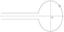
($a$)     ($b$)

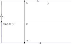
Figure 1: ($a$) The loop in the $\tau$-plane with a circular path round the origin of radius $\rho$; ($b$) the contour $C$ in the $u$-plane shown with $\rho<1$.

Saddle points of the integrand in (2.1) occur at $h^{\prime}(u)=0$; that is, at the point $u=u_{0}$ of the equation

$$e^{u_{0}}+\lambda e^{-\lambda u_{0}}=2a.$$ (2.2)

It is sufficient to confine our attention to the strip $-\pi\leq\Im(u)\leq\pi$ when considering the location of the saddle points. By inspection of the above equation, it is easily seen that when $-1<\lambda<0$ there is only one real saddle in this strip and when $\lambda>0$, there are two saddles, either both real or a complex conjugate pair. The saddles coincide to form a double saddle point when $h^{\prime}(u)=h^{\prime\prime}(u)=0$ at

$$u_{0}=\frac{2\log\,\lambda}{1+\lambda}.$$ (2.3)

From (2.2), this requires the relation between the parameters $a$ and $\lambda$ given by

$$a=\frac{(1+\lambda)}{2}\,\lambda^{\gamma},\qquad\gamma:=\frac{1-\lambda}{1+\lambda}.$$ (2.4)

A plot of this curve is shown in Fig. 2. Above this curve the saddles are real and below they are a complex conjugate pair; on the curve there is a double saddle. Routine calculations show that the maximum of the curve occurs at $a\doteq 1.19123$ when $\lambda\doteq 2.09350$.

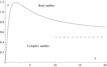
Figure 2: Plot of the curve in (2.4) corresponding to the formation of a double saddle on the real $u$-axis when $\lambda>0$. Above this curve the two saddles are real and below they form a complex conjugate pair. The dashed line $a=\frac{1}{2}$ represents the asymptotic limit of the curve.

Typical paths of steepest descent through the relevant saddles in the strip $|\Im(u)|\leq\pi$ are shown in Fig. 3. In each case the paths that pass through the contributory saddle(s) pass to infinity in the right half-plane with $\Im(u)=\pm\pi$. When $\lambda>0$ and $(a,\lambda)$ is situated above the curve in Fig. 2 only the larger real saddle contributes to the expansion of ${\cal W}^{-}_{\lambda,\nu}(x)$; the path through the smaller saddle is a path of steepest ascent. The integration path $C$ can, in each case, be deformed to pass over the steepest descent paths passing through the contributory saddle(s); in the case of complex saddles this can be achieved by letting $\rho\to 0$.

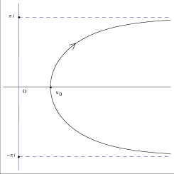
($a$)     ($b$) 

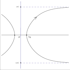
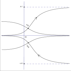
($c$)     ($d$) 

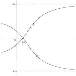
Figure 3: Steepest descent paths ($a$) when $-1<\lambda<0$, ($b$) real saddle case when $\lambda>0$; ($c$) complex saddles case and ($d$) double saddle case. The arrows denote the direction of integration.

In this section we consider the asymptotic expansions of ${\cal W}^{-}_{\lambda,\nu}(x)$ in the three cases that can arise, namely a real contributory saddle, a complex conjugate pair of saddles and a real double saddle.

3.1  Real saddle point

When $-1<\lambda<0$ and $\lambda>0$ with $(a,\lambda)$ situated above the curve in Fig. 2, the contributory saddle is real; see Fig. 3(a, b). We have from (2.1)

$${\cal W}^{-}_{\lambda,\nu}(x)=\frac{e^{xh(u_{0})}}{2\pi i}\int_{-\infty}^{\infty}e^{-xw^{2}/2}\,\frac{du}{dw}\,dw,$$

where we have introduced the new variable $w$ by

$$-\frac{1}{2}w^{2}=h(u)-h(u_{0})=\frac{h_{0}^{\prime\prime}}{2!}(u-u_{0})^{2}+\frac{h_{0}^{\prime\prime\prime}}{3!}(u-u_{0})^{3}+\cdots$$

and for brevity we denote the derivatives of $h(u)$ evaluated at $u=u_{0}$ by $h_{0}^{(n)}\equiv h^{(n)}(u_{0})$. Inversion of this expansion using the InverseSeries command in Mathematica (essentially Lagrange inversion) yields

$$u-u_{0}=\frac{w}{\sqrt{-h_{0}^{\prime\prime}}}+\frac{h_{0}^{\prime\prime\prime}w^{2}}{6h_{0}^{\prime\prime 2}}-\frac{(5h_{0}^{\prime\prime\prime 2}-3h_{0}^{\prime\prime}h_{0}^{iv})}{72h_{0}^{\prime\prime 3}\sqrt{-h_{0}^{\prime\prime}}}\,w^{3}+\cdots\ .$$ (3.1)

Upon differentiation this yields

$$\frac{du}{dw}\stackrel{{\scriptstyle e}}{{=}}\frac{1}{\sqrt{-h_{0}^{\prime\prime}}}\sum_{k\geq 0}(-)^{k}A_{k}w^{2k},$$

where $\stackrel{{\scriptstyle e}}{{=}}$ denotes the inclusion of only the even powers of $w$, since odd powers will not enter into this calculation. We have

$$h_{0}^{\prime\prime}=\mbox{${\textstyle\frac{1}{2}}$}(e^{u_{0}}-\lambda^{2}e^{-\lambda u_{0}})=\mbox{${\textstyle\frac{1}{2}}$}(1+\lambda)e^{u_{0}}-a\lambda$$ (3.2)

and note that $0<h_{0}^{\prime\prime}<a$. The first few coefficients $A_{k}$ are:

$$A_{0} = 1,\qquad A_{1}=\frac{1}{24h_{0}^{\prime\prime}}(5{\bf h}_{3}^{2}-3{\bf h}_{4}),$$

$$A_{2} = \frac{1}{3456h_{0}^{\prime\prime 2}}(385{\bf h}_{3}^{4}-620{\bf h}_{3}^{2}{\bf h}_{4}+105{\bf h}_{4}^{2}+168{\bf h}_{3}{\bf h}_{5}-24{\bf h}_{6})$$ (3.3)

$$A_{3} = \frac{1}{6220800h_{0}^{\prime\prime 3}}(425425{\bf h}_{3}^{6}-1126125{\bf h}_{3}^{4}{\bf h}_{4}+675675{\bf h}_{3}^{2}{\bf h}_{4}^{2}-51975{\bf h}_{4}^{3}+360360{\bf h}_{3}^{3}{\bf h}_{5}$$

$$-249480{\bf h}_{3}{\bf h}_{4}{\bf h}_{5}+13608{\bf h}_{5}^{2}-83160{\bf h}_{3}^{2}{\bf h}_{6}+22680{\bf h}_{4}{\bf h}_{6}+12960{\bf h}_{3}{\bf h}_{7}-1080{\bf h}_{8}),$$

where we have defined

$${\bf h}_{n}:=\frac{h_{0}^{(n)}}{h_{0}^{\prime\prime}},\qquad h_{0}^{(n)}=\mbox{${\textstyle\frac{1}{2}}$}(1-(-\lambda)^{n-1})e^{u_{0}}+a(-\lambda)^{n-1}\qquad(n\geq 3).$$

Then

$${\cal W}^{-}_{\lambda,\nu}(x)\sim\frac{e^{xh(u_{0})}}{\pi\sqrt{2xh_{0}^{\prime\prime}}}\sum_{k\geq 0}\frac{(-)^{k}A_{k}}{(x/2)^{k}}\int_{0}^{\infty}e^{-s}s^{k-1/2}ds$$

$$=\frac{e^{xh(u_{0})}}{\sqrt{2\pi xh_{0}^{\prime\prime}}}\sum_{k\geq 0}\frac{(-)^{k}(\mbox{${\textstyle\frac{1}{2}}$})_{k}A_{k}}{(x/2)^{k}}\hskip 8.5359pt$$ (3.4)

as $x\to+\infty$ with $\nu=ax$, where $(a)_{n}=a(a+1)\ldots(a+n-1)$ is the Pochhammer symbol. An expansion equivalent to this is given in Theorem 2.2 in [1].

3.2  Complex saddle points

When $\lambda>0$ and $(a,\lambda)$ is situated below the curve in Fig. 2 the contributory saddles are complex as illustrated in Fig. 3(c). The contribution to ${\cal W}^{-}_{\lambda,\nu}(x)$ from the upper steepest descent path is given by (compare (3.4))

$$\frac{e^{xh(u_{0})}}{i\sqrt{2\pi xh_{0}^{\prime\prime}}}\sum_{k\geq 0}\frac{(-)^{k}(\mbox{${\textstyle\frac{1}{2}}$})_{k}A_{k}}{(x/2)^{k}},$$

where in this case $h_{0}^{\prime\prime}$ given in (3.2) is complex-valued. Since the contribution from the lower path yields the conjugate expression, we therefore obtain

$${\cal W}^{-}_{\lambda,\nu}(x)\sim\sqrt{\frac{2}{\pi x}}\,\Re\biggl{\{}\frac{e^{xh(u_{0})}}{\sqrt{h_{0}^{\prime\prime}}}\sum_{k\geq 0}\frac{(-)^{k}(\mbox{${\textstyle\frac{1}{2}}$})_{k}A_{k}}{(x/2)^{k}}\biggr{\}}$$ (3.5)

as $x\to+\infty$ with $\nu=ax$. The leading term of this expansion is given in an equivalent form in Theorem 3.1 in [1].

It is worth remarking that in §§3.1, 3.2 the exact location of the saddle $u_{0}$ is not available in closed form. This necessitates the numerical solution of (2.2) to obtain $u_{0}$ when the parameters $a$ and $\lambda$ have specific values. It is apparent that the presentation of higher coefficients $A_{k}$ becomes prohibitive on account of their rapidly increasing complexity. This point is discussed further in Section 5 where it is indicated how more coefficients $A_{k}$ can be generated by numerical reversion in specific cases.

3.3  Double saddle point

In the case of the double saddle point we are in the fortunate position of having an exact expression for the location of this saddle given in (2.3) combined with the condition (2.4). The contribution from the upper half of the steepest descent path illustrated in Fig. 3(d) is

$$I=\int_{u_{0}}^{\infty+\pi i}e^{xh(u)}du=e^{xh(u_{0})}\int_{0}^{\infty}e^{-xw^{3}/3}\frac{du}{dw}\,dw,$$

where we have introduced the new variable $w$ by

$$-\frac{w^{3}}{3}=h(u)-h(u_{0})=\frac{h_{0}^{\prime\prime\prime}}{3!}(u-u_{0})^{3}+\frac{h_{0}^{(4)}}{4!}(u-u_{0})^{4}+\cdots\ .$$

Inversion of this expansion (using Mathematica) yields for the upper half of the integration path

$$u-u_{0}=\frac{2^{2/3}e^{\pi i/3}}{H^{1/3}}\,w+\frac{(\lambda-1)e^{2\pi i/3}}{2^{2/3}\cdot 3H^{2/3}}\,w^{2}-\frac{(1-6\lambda+\lambda^{2})}{60H}\,w^{3}+\cdots\ ,$$

where $H:=2h_{0}^{\prime\prime\prime}$. Upon differentiation, we then obtain

$$\frac{du}{dw}=\frac{2^{2/3}}{H^{1/3}}\sum_{k\geq 0}\frac{e^{\frac{1}{3}\pi i(k+1)}B_{k}}{H^{k/3}}\,w^{k},$$

where

$$B_{0} = 1,\quad B_{1}=\frac{\lambda-1}{2^{1/3}\cdot 3},\quad B_{2}=\frac{1-6\lambda+\lambda^{2}}{2^{2/3}\cdot 20},\quad B_{3}=\frac{1}{1620}(5+93\lambda-93\lambda^{2}-5\lambda^{3}),$$

$$B_{4} = -\frac{1}{2^{1/3}\cdot 136080}(277+826\lambda-6114\lambda^{2}+826\lambda^{3}+277\lambda^{4}),$$

$$B_{5} = \frac{1}{2^{2/3}\cdot 16800}(1-61\lambda-254\lambda^{2}+254\lambda^{3}+61\lambda^{4}-\lambda^{5}),$$

$$B_{6} = \frac{1}{10497600}(959+7098\lambda-2031\lambda^{2}-58708\lambda^{3}-2031\lambda^{4}+7098\lambda^{5}+959\lambda^{6}).$$

The contribution from the upper half of the steepest descent path then becomes

$$I\sim\frac{2^{2/3}e^{xh(u_{0})}}{3(Hx/3)^{1/3}}\sum_{k\geq 0}\frac{e^{\frac{1}{3}\pi i(k+1)}B_{k}}{(Hx/3)^{k/3}}\int_{0}^{\infty}e^{-s}s^{k/2-2/3}\,ds$$

$$=\frac{2^{2/3}e^{xh(u_{0})}}{3(Hx/3)^{1/3}}\sum_{k\geq 0}\frac{e^{\frac{1}{3}\pi i(k+1)}B_{k}}{(Hx/3)^{k/3}}\,\Gamma\biggl{(}\frac{k+1}{3}\biggr{)}.$$

The contribution from the lower half of the integration path is given by the conjugate expansion. Hence, when $\nu=ax$, $\lambda>0$ and the parameter $a$ satisfies the condition (2.4), we obtain the expansion

$${\cal W}^{-}_{\lambda,\nu}(x)\!\! \sim \!\!\frac{1}{2\pi i}(I-{\overline{I}})$$ (3.6)

$$= \!\!\frac{2^{2/3}e^{xh(u_{0})}}{3\pi(Hx/3)^{1/3}}\sum_{k\geq 0}\frac{B_{k}}{(Hx/3)^{k/3}}\,\Gamma\biggl{(}\frac{k+1}{3}\biggr{)}\sin\frac{\pi}{3}(k+1)$$

as $x\to+\infty$, where

$$H=\lambda^{2/(1+\lambda)}(1+\lambda),\qquad h(u_{0})=\frac{(\lambda^{2}-1)}{2\lambda^{2}}e^{u_{0}}-\lambda^{\gamma}\log\,\lambda,$$

with $u_{0}$ and $\gamma$ given in (2.3) and (2.4). We observe that the terms corresponding to $k=2,5,8,\ldots$ make no contribution to the expansion (3.6).

4. The expansion of ${\cal W}^{+}_{\lambda,\nu}(x)$

We consider the function ${\cal W}^{+}_{\lambda,\nu}(x)$ defined in (1.4), which has the integral representation

$${\cal W}^{+}_{\lambda,\nu}(x)=\frac{1}{2\pi i}\int_{C}e^{x{\tilde{h}}(u)}du,\qquad{\tilde{h}}(u):=\mbox{${\textstyle\frac{1}{2}}$}(e^{u}+e^{-\lambda u})-au,$$ (4.1)

where $C$ is the same path as in (2.1). Paths of steepest descent (resp. ascent) as $\Re(u)\to-\infty$ asymptote to $\Im(u)=\pi n/\lambda$ for odd (resp. even) $n$. Saddle points are given by

$$e^{u_{0}}-\lambda e^{-\lambda u_{0}}=2a;$$

when $-1<\lambda<0$, there is just one real saddle $u_{0}$ in the principal strip $-\pi\leq\Im(u)\leq\pi$. When $\lambda>0$, there is the real saddle $u_{0}$ together with an infinite string of complex saddles $u_{k}=X_{k}\pm iY_{k}$, $k=1,2,\ldots$ approximately parallel to the imaginary axis with $X_{k}>0$. The saddle $u_{1}$ has $\pi/\lambda<Y_{1}<3\pi/\lambda$ while it is found that $Y_{k}\simeq(2k-1)\pi/\lambda$ as $k$ increases. As $\lambda$ increases, more of these complex saddles enter the principal strip, some of which may, dependent on the values of $a$ and $\lambda$, interact with the steepest descent path through $u_{0}$. We define the second derivative ${\tilde{h}}_{k}^{\prime\prime}$ by

$${\tilde{h}}_{k}^{\prime\prime}:=\mbox{${\textstyle\frac{1}{2}}$}(e^{u_{k}}+\lambda^{2}e^{-\lambda u_{k}})=\mbox{${\textstyle\frac{1}{2}}$}(1+\lambda)e^{u_{k}}-a\lambda\qquad(k=0,1,2\ldots).$$

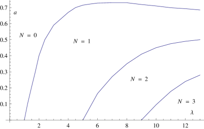
Figure 4: Curves in the $a,\lambda$-plane on which an additional pair of complex saddles appears (via a Stokes phenomenon).

For $a$ and $\lambda$ in a certain domain (labelled $N=0$ in Fig. 4), and also for $-1<\lambda<0$, the steepest descent path passes through only the saddle $u_{0}$ on the real axis, as shown in Fig. 5(a). In this case the expansion of ${\cal W}^{+}_{\lambda,\nu}(x)$ is given by

$${\cal W}^{+}_{\lambda,\nu}(x)\sim I_{0}(a,\lambda;x):=\frac{e^{x{\tilde{h}}(u_{0})}}{\sqrt{2\pi x{\tilde{h}}_{0}^{\prime\prime}}}\sum_{k=0}^{\infty}\frac{(-)^{k}(\mbox{${\textstyle\frac{1}{2}}$})_{k}B_{k}^{(0)}}{(x/2)^{k}}\qquad(x\to+\infty),$$

where the coefficients $B_{k}^{(0)}$ are obtained in the same manner as the $A_{k}$ described in Section 3, with $h(u)$ replaced by ${\tilde{h}}(u)$. As $\lambda$ ($>1$) increases in the domain labelled $N=1$ in Fig. 4, the steepest descent path through $u_{0}$ either passes to $\infty\pm\pi i$ (as shown in Fig. 5(a)) or to $-\infty$ along the directions $\Im(u)=\pm\pi/\lambda$ and thence over the saddles $u_{1}$, ${\overline{u}}_{1}$ to the endpoints $\infty\pm\pi i$; see Fig. 5(c). The intermediate case shown in Fig. 5(b) shows the steepest descent path through $u_{0}$ connecting with the adjacent saddles $u_{1}$ and ${\overline{u}}_{1}$ to produce a Stokes phenomenon. As $\lambda$ increases further in a certain domain of the $a,\lambda$-plane, the saddles $u_{2}$, ${\overline{u}}_{2}$ become connected; see Fig. 5(d). In each case, the integration path $C$ can be deformed to coincide with these different steepest descent paths. It is worth noting that the appearance of each new pair of complex saddles results in a Stokes phenomenon. We do not consider the details of this transition here.

($a$)     ($b$) 

($c$)     ($d$) 

Figure 5: Steepest descent paths ($a$) when $\lambda=1,a=0.50$ ($N=0$), ($b$) $\lambda=2,a=0.4075$ (on the boundary between $N=0$ and $N=1$ in Fig. 4); ($c$) $\lambda=2,a=0.60$ ($N=1$) and ($d$) $\lambda=6,a=0.10$ ($N=2$). For clarity the paths in ($d$) are shown only in the upper-half plane; a symmetrical distribution is present in the lower-half plane. The arrows indicate the direction of integration.

Table 1: Values of the coefficients $A_{k}$ and the absolute relative error in ${\cal W}^{-}_{\lambda,\nu}(x)$ resulting from the expansion (3.4) for different truncation index $k$ when $x=40$. The value of the real saddle $u_{0}$ is indicated.

	$\lambda=-0.25,\ a=1$		$\lambda=1,\ a=1.20$		$\lambda=0.50,\ a=0.80$
	$u_{0}=0.83644438$		$u_{0}=0.62236250$		$u_{0}=0.12181472$
$k$	$A_{k}$	Error	$A_{k}$	Error	$A_{k}$	Error
0	1.000000	$2.019(-3)$	1.000000	$1.839(-2)$	1.000000	$1.331(-2)$
1	$+8.087175(-2)$	$3.189(-6)$	0.839435	$2.655(-3)$	0.571373	$9.888(-4)$
2	$+1.681574(-3)$	$2.995(-8)$	1.770726	$7.334(-4)$	0.598231	$1.490(-4)$
3	$-1.284463(-4)$	$2.168(-10)$	4.345560	$3.037(-4)$	0.768780	$3.359(-5)$
4	$-5.177287(-6)$	$4.055(-12)$	11.283213	$1.678(-4)$	1.050527	$1.008(-5)$
5	$+4.453244(-7)$	$6.262(-14)$	30.237515	$1.164(-4)$	1.483045	$3.788(-6)$

The contribution from the pair of complex saddles $u_{j}$ and ${\overline{u}}_{j}$ is

$$I_{j}(a,\lambda;x):=\sqrt{\frac{2}{\pi x}}\,\Re\biggl{\{}\frac{e^{x{\tilde{h}}(u_{j})}}{\sqrt{{\tilde{h}}_{j}^{\prime\prime}}}\sum_{k\geq 0}\frac{(-)^{k}(\mbox{${\textstyle\frac{1}{2}}$})_{k}B^{(j)}_{k}}{(x/2)^{k}}\biggr{\}}\qquad(x\to+\infty),$$

where the coefficients $B_{k}^{(j)}$ are computed as in (3.5). Hence the expansion of ${\cal W}^{+}_{\lambda,\nu}(x)$ takes the form

$${\cal W}^{+}_{\lambda,\nu}(x)\sim\sum_{j=0}^{N}I_{j}(a,\lambda;x)\qquad(x\to+\infty),$$ (4.2)

where $N$ denotes the number of contributory pairs of complex saddles. The different values of $N$ in the $a,\lambda$-plane are shown in Fig. 4, where each curve represents the appearance (via a Stokes phenomenon) of the pair of contributory complex saddles $u_{N}$ and ${\overline{u}}_{N}$. The dominant contribution results from $I_{0}(a,\lambda;x)$ with the series $I_{j}(a,\lambda;x)$ being progressively less dominant as $j$ increases. It is found numerically that the final series $I_{N}(a,\lambda;x)$ can be either exponentially large or small as $x\to+\infty$ according to the location of the parameters in the $a,\lambda$-plane.

5. Numerical verification

In this section we present some numerical results that confirm the accuracy of the different expansions obtained for ${\cal W}^{\pm}_{\lambda,\nu}(x)$. We first present results for ${\cal W}^{-}_{\lambda,\nu}(x)$. In Table 1 we show the absolute relative error in the computation of ${\cal W}^{-}_{\lambda,\nu}(x)$ using the expansion in (3.4) for different values of the parameters $a$ and $\lambda$ as a function of the truncation index $k$. The value of the real saddle point $u_{0}$ is given together with the first six coefficients $A_{k}$. The coefficients with $k\leq 3$ can be obtained from (3.4), but it is more direct, with specific values of $a$ and $\lambda$, to compute these coefficients using the InverseSeries command in Mathematica to generate the numerical equivalent of (3.1).

Table 2: Values of the coefficients $A_{k}$ and the absolute relative error in ${\cal W}^{-}_{\lambda,\nu}(x)$ resulting from the expansion (3.4) for different truncation index $k$ when $x=40$, $\lambda=1.50$, $a=0.50$.

$k$	$A_{k}$	Error
0	1.000000	$6.233(-3)$
1	$+0.00929936+0.19815193i$	$1.157(-4)$
2	$-0.08194718+0.01105633i$	$1.416(-5)$
3	$-0.00729013-0.04233881i$	$5.787(-7)$
4	$+0.02361754-0.00432441i$	$1.840(-7)$
5	$+0.00253174+0.01363033i$	$1.014(-8)$

Table 2 shows the errors involved in using the expansion (3.5) when the contributory saddles are a conjugate pair located at $u_{0}=0.24834557\pm 0.90919096i$. The coefficients $A_{k}$ in the case are complex valued. The special case when $a$ and $\lambda$ are linked via (2.4) corresponding to a double saddle point is shown in Table 3 for different $\lambda$. All cases presented correspond to sub-optimal truncation as the relative error is seen to steadily decrease with increasing truncation index $k$.

Table 3: Values of the absolute relative error in ${\cal W}^{-}_{\lambda,\nu}(x)$ in the double saddle case resulting from the expansion (3.6) for different $\lambda$ and truncation index $k$ when $x=40$.

$k$	$\lambda=0.50$	$\lambda=1$	$\lambda=2$
0	$3.433(-2)$	$9.869(-5)$	$3.414(-2)$
1	$8.333(-4)$	$9.869(-5)$	$6.041(-4)$
3	$9.241(-5)$	$9.869(-5)$	$8.876(-5)$
4	$1.218(-7)$	$2.279(-6)$	$2.582(-6)$
6	$2.125(-8)$	$4.987(-7)$	$4.842(-7)$

In Table 4 we present the absolute relative error in the computation of ${\cal W}^{+}_{\lambda,\nu}(x)$ using (4.2). The examples shown correspond to situations with $N=0,1$ and 2. In the cases $N=1$ and 2 the value of $\Re h(u_{N})<0$, so that $I_{N}(a,\lambda;x)$ is exponentially small and is neglected. The contributory series $I_{j}(a,\lambda;x)$ were calculated at optimal truncation, that is truncation at or near the term of least magnitude; this required the calculation of up to 30 coefficients $A_{k}$ and $B_{k}^{(1)}$.

Finally, to confirm the presence of the series $I_{1}(a,\lambda;x)$ in the $N=1$ case, we show in the upper half of Table 5 the values of $\Delta{\cal W}\equiv{\cal W}^{+}_{\lambda,\nu}(x)-I_{0}(a,\lambda;x)$ for three values of $x$ compared with $I_{1}(a,\lambda;x)$, both series being optimally truncated. The first case $\lambda=3$, $a=0.20$ corresponds to $\Re h(u_{1})<0$ whereas the second case $\lambda=4$, $a=0.20$ corresponds to $\Re h(u_{1})>0$. In the lower half of the table we present similar calculations when $\lambda=6$, $a=0.20$ corresponding to $N=2$. In this case it is found that $\Re h(u_{2})<0$ and so the exponentially small series $I_{2}(a,\lambda;x)$ is neglected.

Table 4: Values of the absolute relative error in ${\cal W}^{+}_{\lambda,\nu}(x)$ resulting from the expansion (4.2) for different truncation index $k$ when $x=20$.

$k$	$\lambda=1,\ a=0.50$	$\lambda=3,\ a=0.20$	$\lambda=6,\ a=0.20$
	$N=0$	$N=1$	$N=2$
0	$3.730(-3)$	$3.787(-3)$	$1.550(-2)$
1	$3.020(-6)$	$2.432(-4)$	$3.381(-3)$
2	$3.898(-6)$	$6.006(-5)$	$2.963(-4)$
3	$3.919(-7)$	$1.100(-5)$	$1.256(-4)$
4	$2.813(-8)$	$1.774(-6)$	$8.332(-4)$
5	$\,\,7.909(-10)$	$1.786(-7)$	$1.419(-5)$

Table 5: Values of $\Delta{\cal W}(x)\equiv{\cal W}^{+}_{\lambda,\nu}(x)-I_{0}(a,\lambda;x)$ compared with $I_{1}(a,\lambda;x)$ when $N=1$ and $N=2$ for different values of $x$.

	$\lambda=3,\ a=0.20\ \ (N=1)$
$x$	$\Delta{\cal W}(x)$	$I_{1}(a,\lambda;x)$	${\cal W}^{+}_{\lambda,\nu}(x)$
20	$-1.58935(-2)$	$-1.57281(-2)$	$+7.070661(+5)$
30	$-1.48072(-2)$	$-1.48186(-2)$	$+1.986142(+9)$
40	$-8.74902(-3)$	$-8.74792(-3)$	$+5.920851(+12)$
	$\lambda=4,\ a=0.20\ \ (N=1)$
20	$-4.21656$	$-4.20876$	$+2.277758(+5)$
30	$-3.00021(+1)$	$-3.00057(+1)$	$+3.823713(+8)$
40	$-7.95934$(+2)	$-7.95905(+2)$	$+6.805185(+11)$
	$\lambda=6,\ a=0.20\ \ (N=2)$
20	$+4.36797(+1)$	$+4.31217(+1)$	$+5.336787(+4)$
30	$+1.45878(+4)$	$+1.45867(+4)$	$+4.687193(+7)$
40	$-1.01722(+6)$	$-1.01707(+6)$	$+4.352648(+10)$

References

[1]
A. Ansari and H. Askari, Asymptotic analysis of the Wright function with a large parameter. J. Math. Anal. Appl. 507 (2022) 125731.
[2]
R. Gorenflo, Yu. Luchko and F. Mainardi, Analytical properties and appliucations of the Wright function, Frac. calc. Appl. Anal. 2 (1999) 383–414.
[3]
Y. Luchko The Wright function and its applications. In: Handbook of Fractional Calculus with Applications, (A. Kochubei, Yu. Luchko, J. Teneiro Machado (eds.) (2019) 241–268.
[4]
F. Mainardi and A. Consiglio,
The Wright function of the second kind in
mathematical physics,
SI on Special Functions with Applications
in Mathematical Physics,
Mathematics8 No 6
(2020) 884.
[5]
R.B. Paris, Asymptotics of the special functions of fractional calculus. In: Handbook of Fractional Calculus with Applications, (A. Kochubei, Yu. Luchko, J. Teneiro Machado (eds.) (2019) 297–325.
[6]
R.B. Paris, A. Consiglio and F. Mainardi, On the asymptotics of the Wright function of the second kind, Frac. Calc. Appl. Anal. 24 (2021) 54–72.
[7] R.B. Paris and V. Vinogradov,
Asymptotic and structural properties
of the Wright function arising in probability
theory,
Lithuanian Math. J.56 (2016) 377–409.
[8] E.M. Wright,
The asymptotic expansion of
the generalized Bessel function,
Proc. Lond. Math. Soc. (Ser. 2)
38 (1934) 286–293.
[9] E.M. Wright,
The generalized Bessel function
of order greater than one,
Qu. J. Math.11 (1940) 36–48.
()
()
()
()
()
()
()
()
()
()