Bayesian logistic regression for online recalibration and revision of risk prediction models with guarantees

See pages - of word.pdf

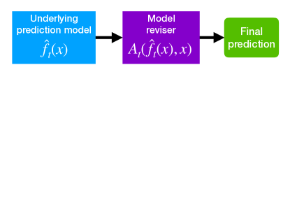
Figure 1: Given a patient with variables $x$, the model reviser $\hat{A}_{t}$ wraps around an underlying ML model $\hat{f}_{t}$ to predict the true probability of having or developing a disease (or outcome). The focus of this work is the design of an online model reviser.

(a) Bayesian logistic revision (BLR) estimates the model revision parameters $\theta_{t}$ for the underlying prediction model $\hat{f}_{t}$ with the simplifying assumption that the data $(X_{t},Y_{t})$ are independently and identically distributed for a constant set of model revision parameters over all time points $t=1,...,T$.

(b) MarBLR defines a prior over revision parameter sequences that change over time. It assumes that the revision parameters change with probability $\alpha$ at each time $t$, as modeled by a binary random variable $W_{t}$. It supposes that changes in the model revision parameters follow a Gaussian prior centered at zero.

Figure 2: BLR and its Markov variant MarBLR update the deployed model revision at each time point per the evolving Bayesian posterior. Theoretical guarantees for BLR and MarBLR hold under misspecification of the logistic model and/or priors.

(a) Univariate recalibration. Calibration measured with respect to the general population.

(b) Subgroup-aware recalibration. Calibration measured with respect to subgroups A (top) and B (bottom).

Figure 3: Results from online model recalibration of a fixed underlying prediction model in a patient population with patient subgroups A and B with prevalence 20% and 80% (Scenario 1). Left: Estimated calibration index (ECI) at each time point. Right: Calibration curves for the original model and the revised versions from BLR and MarBLR. The ideal calibration curve is the identity function, which has an ECI of zero.

Figure 4: Results from online logistic revision of a fixed underlying model with respect to the forecasted score and ten patient variables (Scenario 2), in terms of the estimated calibration index (ECI, left) and AUC (right). Data is simulated to be stationary over time after an initial shift (Initial Shift, top), shift in a cyclical fashion (Cyclical, middle), and shift such that the original model decays in performance over time (Decay, bottom). All online logistic revision methods outperformed locking the original model in terms of the average ECI and AUC, with BLR and MarBLR performing the best. Note that the revised models were worse than the original model briefly in the Decay setting.

(a) Initial Shift, All-Refit

(b) Decay, All-Refit

(c) Initial Shift, Subset-Refit

(d) Decay, Subset-Refit

Figure 5: Model calibration and discrimination (left and right panels, respectively) from online ensembling of the original model with an underlying prediction model that is continually refitted over time (Scenario 3). Data is simulated to be stationary over time after an initial shift (Initial Shift) and nonstationary such that the original model decays in performance over time (Decay). Underlying prediction model is updated by continually refitting on all previous data (All-Refit) or refit on the most recent subset of data (Subset-Refit). Note that Subset-Refit simulates a sudden drop in performance for the continually refitted model at time $t=100$ and, consequently, across all online ensembling procedures. BLR and MarBLR recover from this sudden performance decay and achieve better performance than locking the original model in terms of the average ECI and AUC.

(a) Online recalibration of a fixed prediction model

(b) Online logistic revision with respect to a fixed prediction model and patient variables

(c) Online ensembling of the original and continually-refitted prediction models

Figure 6: Results from online logistic recalibration and revision for a fixed COPD risk prediction model (a and b, respectively) and online reweighting for fixed and continually-refitted (evolving) COPD risk prediction models (c) using BLR and MarBLR. Calibration curves are estimated across four time periods that divide the full dataset into equal lengths. The receiver operating characteristic (ROC) curve is shown for the online ensembling approach because the ROC curves did not change significantly for (a) or (b).

Appendix for “Bayesian logistic regression for online recalibration and revision of clinical prediction models with guarantees”

Notation	Description
General terms
$T$	Time horizon
$d$	Number of variables
$(x_{t},y_{t})$	Observed variables and outcome at time $t$
$\hat{f}_{t}:\mathcal{X}\mapsto\mathbb{R}$	Underlying prediction model at time $t$
$\hat{A}_{t}:\mathbb{R}\times\mathcal{X}\mapsto[0,1]$	Model revision deployed at time $t$: A function that maps predictions from the underlying prediction model at time $t$ and patient variables to a probability
$\hat{\theta}_{t}$	Parameters for logistic model revision at time $t$
$\tau=(\tau_{1},\tau_{2},\cdots,\tau_{s})$	Update times for a given sequence of model revisions
Regret
$\bigg{(}\frac{1}{T}\sum_{t=1}^{T}\bigg{[}-\log p\left(y_{t},\hat{A}_{t}(\hat{f}_{t}(x_{t}),x_{t})\right)+\log p\left(y_{t},\hat{A}_{1}(\hat{f}_{1}(x_{t}),x_{t})\right)\bigg{]}\bigg{)}_{+}$	Type I Regret: The average increase in the negative log likelihood when using the online reviser instead of locking the original model
$\bigg{(}\frac{1}{T}\sum_{t=1}^{T}\bigg{[}-\log p\left(y_{t},\hat{A}_{t}(\hat{f}_{t}(x_{t}),x_{t})\right)+\log p\left(y_{t},{A}^{*}_{\tau,t}(\hat{f}_{t}(x_{t}),x_{t})\right)\bigg{]}\bigg{)}_{+}$	Type II $\tau$-Regret: The average increase in the negative log likelihood when using the online reviser versus the oracle model reviser $\{{A}^{*}_{\tau,t}:t=1,...,T\}$ with update times $\tau$
BLR and MarBLR parameters
$N(\theta_{\mathrm{init}},\Sigma_{\mathrm{init}})$	Gaussian prior in BLR and MarBLR for the logistic revision parameter at time $t=1$
$\alpha$	Prior probability in MarBLR that the model revision shifts at time $t$
$\delta^{2}$	Factor controlling the variance of the MarBLR prior over shifts in the model revision parameters

Table A.1: Terminology and notation

Appendix A Practical Implementation of BLR and MarBLR

In this manuscript, we implement MarBLR using a Laplace approximation of the logistic posterior and perform Kalman filtering with collapsing (Gordon and Smith, 1990; West and Harrison, 1997). Because BLR corresponds to MarBLR with $\alpha=0$ and $\delta^{2}=0$, we use this same procedure to perform approximate Bayesian inference. The Kalman filtering approach is simple and computationally efficient; We describe the steps below. We note that for the special case of BLR, one can also perform posterior inference by sampling Polya-Gamma latent variables (Polson et al., 2013). This would allow one to perform full Bayesian inference but is significantly more costly in terms of computation time.

We make predictions and update the posterior using the following recursive procedure. The process is initialized with the Gaussian prior for $\theta_{1}$ with mean $\theta_{\mathrm{init}}$ and posterior covariance $\Sigma_{\mathrm{init}}$. Let $D^{(t)}$ denote the observations up to and including time $t$.

Prediction step. At time $t$, let the approximation for $\theta_{t-1}|W_{t-1}=w_{t-1},D^{(t-1)}$ be the Gaussian distribution with mean $\hat{\theta}_{t-1,w_{t-1}}$ and covariance $\hat{\Sigma}_{t-1,w_{t-1}}$. We also assume $\Pr(W_{t-1}=w_{t-1}|D^{(t-1)})$ is known. We generate predictions at time $t$ using the posterior distribution $\theta_{t}|D^{(t-1)}$, which is a mixture of the distributions

$$\theta_{t}|W_{t}=w_{t},W_{t-1}=w_{t-1},D^{(t-1)}\sim N\left(\hat{\theta}_{t-1,w_{t-1}},(1+\delta^{2}w_{t})\hat{\Sigma}_{t-1,w_{t-1}}\right)$$ (1)

for $w_{t},w_{t=1}\in\{0,1\}$ with weights by $\Pr(W_{t}=w_{t}|W_{t-1}=w_{t-1})\Pr(W_{t-1}=w_{t-1}|D^{(t-1)})$. Recall that $\Pr(W_{t}=1|W_{t-1}=w_{t-1})=\alpha$ in the MarBLR prior. We predict that $Y=1$ for a subject $x$ using the posterior mean of $\Pr(Y=1|X=x)$.

Update step. Next, we observe a new batch of labeled observations and update the posterior. That is, we must perform inference for $\theta_{t}|D^{(t)}$, which is a mixture of the distributions $\theta_{t}|W_{t}=w_{t},W_{t-1}=w_{t-1},D^{(t)}$ with probability weights $\Pr(W_{t}=w_{t},W_{t-1}=w_{t-1}|D^{(t)})$ for $w_{t},w_{t-1}\in\{0,1\}$. Let $\tilde{\ell}_{t}(\theta,w)=\sum_{i=1}^{n}\log p\left(y_{t,i}|z_{t,i},\theta\right)+\log p(\theta\mid w,D^{(t-1)})$. We approximate the distribution $\theta_{t}|W_{t}=w_{t},W_{t-1}=w_{t-1},D^{(t)}$ using a Gaussian distribution with its mean computed using a Newton update

$$\hat{\theta}_{t,w_{t},w_{t-1}}=\hat{\theta}_{t-1,w_{t-1}}-\left[\nabla_{\theta}^{2}\tilde{\ell}_{t}\left(\hat{\theta}_{t-1,w_{t-1}},w_{t-1}\right)\right]^{-1}\nabla_{\theta}\tilde{\ell}_{t}\left(\hat{\theta}_{t-1,w_{t-1}},w_{t-1}\right)$$ (2)

and its covariance as

$$\hat{\Sigma}_{t,w_{t},w_{t-1}}=\left[\nabla_{\theta}^{2}\tilde{\ell}_{t}(\hat{\theta}_{t-1,w_{t-1}},w_{t-1})\right]^{-1}.$$

The probability $\Pr(W_{t}=w_{t},W_{t-1}=w_{t-1}\mid D^{(t)})$, which is proportional to

$$\left[\int_{\theta_{t}}p\left(y_{t,\cdot}\mid z_{t,\cdot},\theta_{t}\right)p\left(\theta_{t}\mid w_{t},w_{t-1},D^{(t-1)}\right)d\theta_{t}\right]\Pr(W_{t}|W_{t-1})\Pr(W_{t-1}|D^{(t-1)}),$$ (3)

is approximated using a Laplace approximation for the integral in (3), i.e.

$$2\pi^{d/2}\left|\left\{\nabla^{2}_{\theta}\tilde{\ell}(\hat{\theta}_{t,w_{t},w_{t-1}})\right\}^{-1}\right|^{1/2}p\left(y_{t,\cdot}\mid z_{t,\cdot},\hat{\theta}_{t,w_{t},w_{t-1}}\right)p\left(\hat{\theta}_{t,w_{t},w_{t-1}}\mid D^{(t-1)}\right).$$ (4)

Let $\hat{q}_{w_{t},w_{t-1}}$ denote the estimated probability. Finally, we approximate the posterior distribution $\theta_{t}|W_{t}=w_{t},D^{(t)}$ using a single Gaussian distribution by moment-matching (West and Harrison, 1997; Orguner and Demırekler, 2007) with mean and covariance

$$\hat{\theta}_{t,w_{t}}=\frac{1}{\hat{q}_{w_{t},0}+\hat{q}_{w_{t},1}}\left(\hat{q}_{w_{t},0}\hat{\theta}_{t,w_{t},0}+\hat{q}_{w_{t},1}\hat{\theta}_{t,w_{t},1}\right)$$ (5)

$$\hat{\Sigma}_{t,w_{t}}=\frac{1}{\hat{q}_{w_{t},0}+\hat{q}_{w_{t},1}}\left(\hat{q}_{w_{t},0}\hat{\Sigma}_{t,w_{t},0}+\hat{q}_{w_{t},1}\hat{\Sigma}_{t,w_{t},1}\right).$$ (6)

Appendix B Online model revision for batched data

In certain settings, it is more convenient and practical for the data stream to be observed in batches of size $n>1$. Here we discuss the necessary modifications to our framework for analyzing the performance on an online model reviser for batched data. We denote a batch of observations as $\{(x_{t,i},y_{t,i}):i=1,....,n\}$ and use the notation $a_{t,\cdot}$ to denote the sequence $(a_{t,1},...,a_{t,n})$.

We extend the online model reviser to output a probability distribution over all possible outcomes for a batch of observations, i.e. $\hat{A}_{t}:\mathbb{R}^{n}\times\mathcal{X}^{n}\mapsto\Delta_{2^{n}}$ where $\Delta_{2^{n}}$ is the probability simplex over all possible outcomes $(y_{t,1},...,y_{t,n})$. The loss of the online model reviser over the entire time period is then defined as the average negative log likelihood

$$-\frac{1}{nT}\sum_{t=1}^{T}\log p\left(y_{t,\cdot},\hat{A}_{t}\left(\hat{f}_{t}(x_{t,\cdot}),x_{t,\cdot}\right)\right).$$ (7)

This theoretical framework allows predictions from the online model reviser to depend on all unlabeled observations $\{x_{t,i}:i=1,...,n\}$. By defining regret with respect to (7), we are able to derive Type I and II regret bounds for the batched setting. This is necessary for analyzing BLR and MarBLR because outcomes are not independent given the observations up to time $t$ in the Bayesian framework. In particular, the outcomes are correlated because of the shared (latent) revision parameter $\theta_{t}$.

Table A.2: Descriptive statistics of variables included in the COPD risk prediction model. Continuous variables are summarized by Mean (SD). Binary/ordinal variables are summarized by number of nonzero entries (%).

Variable
Diagnosed with COPD	2756 (2.55)
Age at encounter	60.31 (18.60)
Medical history
Asthma	741 (0.69)
Bronchitis	5855 (5.42)
COPD	14950 (13.84)
Smoking	42651 (39.49)
Pulmonary Function Test	2844 (2.63)
Intubation	2420 (2.24)
Spirometry	1091 (1.01)
Bilevel positive airway pressure	710 (0.66)
Acute coronary syndrome	11008 (10.19)
Pneumonia	15386 (14.25)
Steroids	23249 (21.53)
Antihypertensives	7740 (7.17)
Short-acting bronchodilator	13088 (12.12)
Antihistiminic	17768 (16.45)
Respiratory Clearance	2791 (2.58)
Upper Respiratory Infection	1242 (1.15)
Antiarrythmic order	7650 (7.08)
Inhaled bronchodilators	122 (0.11)
Inhaled corticosteroid	78 (0.07)
Long-acting bronchodilator	91 (0.08)
Combination of inhaled bronchodilators	8 (0.001)
History of current emergency department visit
Pneumonia	3503 (3.24)
Short-acting bronchodilator	5982 (5.54)
Steroids	4518 (4.18)
Antihypertensives	694 (0.64)
Acute coronary syndrome	2386 (2.21)
Antiarrthymic	1665 (1.54)
Antihistaminic	2624 (2.43)
Inhaled corticosteroid	146 (0.14)
Inhaled bronchodilators	304 (0.28)
Long-acting bronchodilator	420 (0.39)
Asthma	142 (0.13)
Upper Respiratory Infection	238 (0.22)
Respiratory Clearance	131 (0.12)
Combination of inhaled bronchodilators	3 (0.003)

Appendix C Type I and II Regret bounds

C.1 Notation and assumptions

We suppose there are $n$ observations at time points $t=1,...,T$ for some $T\geq 2$. Consider any sequence of revision parameters $\boldsymbol{\theta}=\{\theta_{1},\theta_{2},\ldots,\theta_{T}\}$, where $\theta_{t}\in\mathbb{R}^{d}$ for all $t=1,2,\ldots,T$, with unique values at times $\boldsymbol{\tau}=\{\tau_{1},\tau_{2},...,\tau_{s}\}$, where $\tau_{1}=1<\tau_{2}<\ldots<\tau_{s}\leq T$. In other words, $\{\theta_{\tau_{1}},\theta_{\tau_{2}},\ldots,\theta_{\tau_{s}}\}$ denotes the sequence of values that the sequence $\boldsymbol{\theta}$ shifted over. Henceforth, we use $|\boldsymbol{\tau}|$ (rather than $s$) to indicate the number of times in $\boldsymbol{\tau}$. For ease of notation, we use the convention $\tau_{|\tau|+1}:=T+1$. Note that the variable $\tau_{|\tau|+1}$ is not part of the sequence $\boldsymbol{\tau}$ and is used purely to simplify the notation. We use $\boldsymbol{\tau}_{\mathrm{locked}}:=\{\tau_{1}\}=\{1\}$ to denote the shift times in the edge case of “locked” sequences $\boldsymbol{\theta}$ that do not shift over time. Let $D^{(t)}$ denote all the data observed up to time $t$.

The cumulative negative log-likelihood when using Bayesian inference at each time point is

$$L_{\mathrm{BF}}=-\sum_{t=1}^{T}\log p\left(y_{t,\cdot}\mid z_{t,\cdot},D^{(t-1)}\right),$$

where $p\left(y_{t,\cdot}\mid z_{t,\cdot},D^{(t-1)}\right)$ is the posterior distribution at time $t$. The cumulative negative log-likelihoods for MarBLR and BLR are denoted by $L_{\mathrm{MarBLR}}$ and $L_{\mathrm{BLR}}$, respectively, and are special cases of $L_{\mathrm{BF}}$ for their specific choice of priors. The MarBLR prior $p_{0}$ over $\boldsymbol{\theta}$ is defined using a Gaussian random walk with a homogeneous transition matrix as follows. Given $\theta_{\mathrm{init}}\in\mathbb{R}^{d}$, $\Sigma_{\mathrm{init}}\in\mathbb{R}^{d\times d}$, and some shift probability $\alpha\in[0,1]$, let

$$\theta_{1}\sim N(\theta_{\mathrm{init}},\Sigma_{\mathrm{init}}),\quad W_{1}=1,$$ (8)

and for $t=2,3,\ldots,T$ let

$$\theta_{t} =\theta_{t-1}+\beta_{t}W_{t}$$ (9)

$$W_{t} \sim\operatorname{Bernoulli}(\alpha)$$

$$\beta_{t} \sim N(0,\delta^{2}\Sigma_{\mathrm{init}}).$$

Note that $\boldsymbol{\tau}=\left\{\tau_{1},\tau_{2},\ldots,\tau_{|\boldsymbol{\tau}|}\right\}$ can be regarded as the indices at which the sequence $\left\{W_{1},W_{2},\dots,W_{T}\right\}$ is $1$-valued. In particular, having $\boldsymbol{\tau}=\boldsymbol{\tau}_{\mathrm{locked}}$ implies that $W_{1}=1$ and $W_{t}=0$ for all $t>1$. The BLR prior is a special case where $\delta^{2}=\alpha=0$.

Type I regret compares BLR and MarBLR to locking the original revision parameters at its initial value $\theta_{\mathrm{init}}$, i.e. $\theta_{t}=\theta_{\mathrm{init}}$ for all $t\in\left\{1,2,\ldots,T\right\}$. The cumulative negative log-likelihood of the locked initial model is given by

$$L_{\mathrm{locked}}=-\sum_{t=1}^{T}\log p\left(y_{t,\cdot}\mid z_{t,\cdot};\theta_{\mathrm{init}}\right).$$

Type II $\boldsymbol{\tau}$-regret compares BLR and MarBLR to the best sequence of parameters in retrospect for update times $\boldsymbol{\tau}$, denoted $\tilde{\theta}_{\tau_{j}}$ for $j=1,...,|\tau|$. Its cumulative negative log-likelihood is defined as

$$L_{\mathrm{Dyn},\boldsymbol{\tau}}=-\sum_{t=1}^{T}\log p\left(y_{t,\cdot}\mid z_{t,\cdot};\tilde{\theta}_{t}\right)$$

where $\tilde{\theta}_{\tau_{j}}$ for $j=1,...,|\tau|$ satisfy

$$\left.\nabla\sum_{t=\tau_{j}}^{\tau_{j+1}-1}\log p\left(y_{t,\cdot}\mid z_{t,\cdot};\theta\right)\right|_{\theta=\tilde{\theta}_{\tau_{j}}}=0,\quad\forall j=1,\ldots,|\boldsymbol{\tau}|.$$ (10)

In addition, we introduce the notion of a distribution over the sequences $\boldsymbol{\theta}$. For such a distribution $Q$, its expected negative log-likelihood is given by

$$L_{Q}=E_{Q}\left[-\sum_{t=1}^{T}\log p\left(y_{t,\cdot}\mid z_{t,\cdot};\theta_{t}\right)\right].$$

Given mean and variance parameters $\boldsymbol{\mu}=(\mu_{t})_{t\in\boldsymbol{\tau}}$ and $\boldsymbol{\Sigma}=(\Sigma_{t})_{t\in\boldsymbol{\tau}}$, we define $Q_{\boldsymbol{\tau},\boldsymbol{\mu},\Sigma}$ to be the distribution over $\boldsymbol{\theta}$ with shift times $\boldsymbol{\tau}$ where $\theta_{\tau_{j}}$ for $j=1,...,|\boldsymbol{\tau}|$ are jointly independent and normally distributed per

$$\theta_{\tau_{j}}\sim N\left(\mu_{\tau_{j}},\Sigma_{j}\right).$$ (11)

Some results in the following sections rely on the assumption that there exists a constant $c>0$ such that

$$\left|\frac{\partial^{2}}{\partial w^{2}}\log p\left(y|z^{\top}\theta=w\right)\right|\leq c,$$ (12)

for all $y$ and $w$. This always holds for logistic regression with $c\leq 1$.

C.2 Useful Results

Consider the prior distribution $p_{0}(\boldsymbol{\theta})$ over sequences $\boldsymbol{\theta}$. Let $p_{0}(\boldsymbol{\tau})$ be its marginal distribution over shift times $\boldsymbol{\tau}$ and $p_{0}\left(\boldsymbol{\theta}\mid\boldsymbol{\tau}\right)$ be the conditional distribution over sequences $\boldsymbol{\theta}$ with shift times $\boldsymbol{\tau}$.

Lemma 1 (Variational bound).

Consider any prior distribution $p_{0}$ over sequences $\boldsymbol{\theta}$. Given any $\boldsymbol{\tau}$ and any distribution $Q$, it holds that

$$L_{\mathrm{BF}}-L_{Q}\leq\operatorname{E}_{\boldsymbol{\tau}\sim Q}\left[\operatorname{KL}\left(Q(\boldsymbol{\theta}|\boldsymbol{\tau})\mid\mid p_{0}\left(\boldsymbol{\theta}\mid\boldsymbol{\tau}\right)\right)\right]+\operatorname{KL}\left(Q(\boldsymbol{\tau})\mid\mid p_{0}\left(\boldsymbol{\tau}\right)\right).$$

Proof.

First, we can reexpress the cumulative negative log-likelihood of the Bayesian dynamical model by chaining the conditional probabilities as follows:

$$L_{\mathrm{BF}} =-\sum_{t=1}^{T}\log p\left(y_{t,\cdot}\mid z_{t,\cdot},D^{(t-1)}\right)$$

$$=-\log p\left((y_{t,\cdot})_{t=1,...,T}\mid(z_{t,\cdot})_{t=1,...,T}\right).$$

Similarly, the cumulative negative log-likelihood of any sequence of calibration parameters can be written as

$$-\sum_{t=1}^{T}\log p\left(y_{t,\cdot}\mid z_{t,\cdot};\theta_{t}\right)=-\log p\left((y_{t,\cdot})_{t=1,...,T}\mid(z_{t,\cdot})_{t=1,...,T};\boldsymbol{\theta}\right).$$

Thus, the difference in the cumulative negative log-likelihood between the Bayesian dynamical model and any sequence of parameters is given by

$$L_{\mathrm{BF}}-L_{Q} =\operatorname{E}_{Q}\left[\log\frac{p\left((y_{t,\cdot})_{t=1,...,T}\mid(z_{t,\cdot})_{t=1,...,T};\boldsymbol{\theta}\right)}{p\left((y_{t,\cdot})_{t=1,...,T}\mid(z_{t,\cdot})_{t=1,...,T}\right)}\right].$$

By Bayes’ Rule, the posterior distribution $p_{T}$ over $\boldsymbol{\theta}$ with respect to the Bayesian dynamical model satisfies

$$p_{T}\left(\boldsymbol{\theta}\right)=\frac{p\left((y_{t,\cdot})_{t=1,...,T}\mid(z_{t,\cdot})_{t=1,...,T};\boldsymbol{\theta}\right)p_{0}\left(\boldsymbol{\theta}\right)}{p\left((y_{t,\cdot})_{t=1,...,T}\mid(z_{t,\cdot})_{t=1,...,T}\right)}.$$

Thus, we have that

$$L_{\mathrm{BF}}-L_{Q} =\operatorname{E}_{Q}\left[\log\frac{p_{T}\left(\boldsymbol{\theta}\right)}{p_{0}\left(\boldsymbol{\theta}\right)}\right]$$ (13)

$$=\operatorname{E}_{\boldsymbol{\tau}\sim Q}\left[\operatorname{E}_{\boldsymbol{\theta}\sim Q(\cdot|\boldsymbol{\tau})}\left[\log\frac{p_{T}\left(\boldsymbol{\theta}\mid\boldsymbol{\tau}\right)}{p_{0}\left(\boldsymbol{\theta}\mid\boldsymbol{\tau}\right)}\right]\right]+\operatorname{E}_{\boldsymbol{\tau}\sim Q}\left[\log\frac{p_{T}(\boldsymbol{\tau})}{p_{0}(\boldsymbol{\tau})}\right].$$

Moreover, because the KL divergence is always positive, it holds that

$$\operatorname{E}_{\boldsymbol{\theta}\sim Q(\cdot|\boldsymbol{\tau})}\left[\log\frac{p_{T}\left(\boldsymbol{\theta}\mid\boldsymbol{\tau}\right)}{p_{0}\left(\boldsymbol{\theta}\mid\boldsymbol{\tau}\right)}\right] =\operatorname{KL}\left(Q(\cdot|\boldsymbol{\tau})\mid\mid p_{0}\left(\boldsymbol{\theta}\mid\boldsymbol{\tau}\right)\right)-\operatorname{KL}\left(Q(\cdot|\boldsymbol{\tau})\mid\mid p_{T}\left(\boldsymbol{\theta}\mid\boldsymbol{\tau}\right)\right)$$ (14)

$$\leq\operatorname{KL}\left(Q(\cdot|\boldsymbol{\tau})\mid\mid p_{0}\left(\boldsymbol{\theta}\mid\boldsymbol{\tau}\right)\right).$$

Likewise,

$$E_{\boldsymbol{\tau}\sim Q}\left[\log\frac{p_{T}(\boldsymbol{\tau})}{p_{0}(\boldsymbol{\tau})}\right]\leq\operatorname{KL}\left(Q(\boldsymbol{\tau})\mid\mid p_{0}(\boldsymbol{\tau})\right).$$ (15)

Finally, by combining equations (13) and (14) we arrive at the conclusion of this theorem. ∎

C.3 Type I regret results for MarBLR

Let the distribution $p_{0}$ be the MarBLR prior as defined per (8) and (9). For a given $\boldsymbol{\tau}$, let $Q_{\boldsymbol{\tau},\boldsymbol{\beta},\nu}^{(W)}$ be a Gaussian random walk with expected shifts $\beta_{j}$ at known shift times $\tau_{j}$ for $j=1,...,|\tau|$. That is,

$$\theta_{\tau_{j}}-\theta_{\tau_{j-1}}\sim N\left(\beta_{j},\nu^{2}\Sigma_{\mathrm{init}}\right).$$ (16)

and

$$\theta_{\tau_{1}}\sim N\left(\mu_{1},\epsilon_{1}^{2}\Sigma_{\mathrm{init}}\right).$$ (17)

We begin with simplifying the KL divergence term in Lemma 1.

Lemma 2.

For any $\boldsymbol{\tau}$, consider the Gaussian random walk $Q_{\boldsymbol{\tau},\boldsymbol{\beta},\nu}^{(W)}$. We have that

$$\begin{split}\operatorname{KL}\left(Q_{\boldsymbol{\tau},\boldsymbol{\beta},\nu}^{(W)}\mid\mid p_{0}\left(\boldsymbol{\theta}\mid\boldsymbol{\tau}\right)\right)=&\frac{1}{2}\epsilon_{1}^{2}d+\frac{1}{2}\left(\mu_{1}-\theta_{\mathrm{init}}\right)^{\top}\Sigma_{\mathrm{init}}^{-1}\left(\mu_{1}-\theta_{\mathrm{init}}\right)-\frac{d|\tau|}{2}\\ &+d(|\tau|-1)\log\frac{\delta}{\nu}-d\log\epsilon_{1}\\ &+\frac{d\nu^{2}(|\tau|-1)}{2\delta^{2}}+\frac{1}{2\delta^{2}}\sum_{j=2}^{|\tau|}\beta_{j}^{\top}\Sigma_{\mathrm{init}}^{-1}\beta_{j}.\end{split}$$ (18)

Proof.

For ease of notation, let $\Theta_{J}$ be the space over sequences $\left(\theta_{1},...,\theta_{J}\right)$. Given the known times $\boldsymbol{\tau}$, there is a one-to-one mapping from sequences in $\Theta_{|\boldsymbol{\tau}|}$ to sequences in $\Theta_{T}$ with unique values at times $\boldsymbol{\tau}$. Let $Q^{\mathrm{sub}}$ be the probability distribution over $\Theta_{|\boldsymbol{\tau}|}$ as defined by $Q_{\boldsymbol{\tau},\boldsymbol{\beta},\nu}^{(W)}$. Likewise, let $p_{0}^{\mathrm{sub}}$ be the PDF over $\Theta_{|\boldsymbol{\tau}|}$ as defined by the conditional prior distribution $p_{0}\left(\cdot\mid\boldsymbol{\tau}\right)$.

We have that

$$\operatorname{KL}\left(Q_{\boldsymbol{\tau},\boldsymbol{\beta},\nu}^{(W)}\mid\mid p_{0}\left(\boldsymbol{\theta}\mid\boldsymbol{\tau}\right)\right)$$

$$= \int\cdots\int Q^{\mathrm{sub}}(\boldsymbol{\theta})\log\frac{Q^{\mathrm{sub}}(\boldsymbol{\theta})}{p_{0}^{\mathrm{sub}}(\boldsymbol{\theta})}\mathrm{d}\boldsymbol{\theta}$$

$$\begin{split}=&\int Q^{\mathrm{sub}}({\theta}_{1})\log\frac{Q^{\mathrm{sub}}({\theta}_{1})}{p_{0}^{\mathrm{sub}}({\theta}_{1})}\mathrm{d}{\theta}_{1}+\sum_{j=1}^{|\tau|-1}\int\int Q^{\mathrm{sub}}({\theta}_{j},{\theta}_{j+1})\log\frac{Q^{\mathrm{sub}}({\theta}_{j+1}\mid{\theta}_{j})}{p_{0}^{\mathrm{sub}}({\theta}_{j+1}\mid{\theta}_{j})}\mathrm{d}{\theta}_{j+1}\mathrm{d}{\theta}_{j}\end{split}$$ (19)

The first term in (19) is the KL divergence of two multivariate Normal distributions, $N(\mu_{1},\epsilon_{1}^{2}\Sigma_{\mathrm{init}})$ and $N(\theta_{\mathrm{init}},\Sigma_{\mathrm{init}})$, and can be shown to be equal to

$$\frac{1}{2}\epsilon_{1}^{2}d+\frac{1}{2}\left(\mu_{1}-\theta_{\mathrm{init}}\right)^{\top}\Sigma_{\mathrm{init}}^{-1}\left(\mu_{1}-\theta_{\mathrm{init}}\right)-d\log\epsilon_{1}-\frac{d}{2}.$$ (20)

Also, for $j=1,...,|\tau|-1$, we have that each summand in the second term in (19) is equal to

$$\int\int Q^{\mathrm{sub}}({\theta}_{j},{\theta}_{j+1})\log\frac{Q^{\mathrm{sub}}({\theta}_{j+1}\mid{\theta}_{j})}{p_{0}^{\mathrm{sub}}({\theta}_{j+1}\mid{\theta}_{j})}\mathrm{d}{\theta}_{j+1}\mathrm{d}{\theta}_{j}$$

$$= d\log\frac{\delta}{\nu}+\frac{1}{2\delta^{2}}\int\int Q^{\mathrm{sub}}({\theta}_{j},{\theta}_{j+1})\left({\theta}_{j+1}-{\theta}_{j}\right)^{\top}\Sigma_{\mathrm{init}}^{-1}\left({\theta}_{j+1}-{\theta}_{j}\right)\mathrm{d}{\theta}_{j+1}\mathrm{d}{\theta}_{j}-\frac{d}{2}.$$ (21)

By the definition of $Q_{\boldsymbol{\tau},\boldsymbol{\beta},\nu}^{(W)}$, we have that $\Delta_{j+1}=\theta_{\tau_{j+1}}-\theta_{\tau_{j}}\sim N\left(\beta_{j+1},\nu^{2}\Sigma_{\mathrm{init}}\right)$. Thus,

$$\int Q^{\mathrm{sub}}({\theta}_{j},{\theta}_{j+1})\left({\theta}_{j+1}-{\theta}_{j}\right)^{\top}\Sigma_{\mathrm{init}}^{-1}\left({\theta}_{j+1}-{\theta}_{j}\right)\mathrm{d}{\theta}_{j+1}\mathrm{d}{\theta}_{j}= d\nu^{2}+\beta_{j+1}^{\top}\Sigma_{\mathrm{init}}^{-1}\beta_{j+1}.$$

Plugging in the above result into (21), we have that

$$\int\int Q^{\mathrm{sub}}({\theta}_{j},{\theta}_{j+1})\log\frac{Q^{\mathrm{sub}}({\theta}_{j+1}\mid{\theta}_{j})}{p_{0}^{\mathrm{sub}}({\theta}_{j+1}\mid{\theta}_{j})}\mathrm{d}{\theta}_{j+1}\mathrm{d}{\theta}_{j}= d\log\frac{\delta}{\nu}+\frac{1}{2\delta^{2}}\left(d\nu^{2}+\beta_{j+1}^{\top}\Sigma_{\mathrm{init}}^{-1}\beta_{j+1}\right)-\frac{d}{2}.$$ (22)

Combining the results (19), (20) and (22), we attain the desired conclusion. ∎

To bound the Type I regret for MarBLR, we compare the regret via the intermediary $Q$ with marginal distribution over $\boldsymbol{\tau}$ the same as $p_{0}$ and the conditional distribution given $\tau$ to be $Q_{\boldsymbol{\tau},\boldsymbol{\beta},\nu}^{(W)}$ with $\boldsymbol{\beta}_{j}=0$ for all $j=2,...,|\tau|$. That is, the regret is decomposed into

$$(L_{\mathrm{BF}}-L_{Q})+(L_{Q}-L_{\mathrm{locked}}).$$ (23)

We bound $L_{\mathrm{BF}}-L_{Q}$ by marginalizing Lemma 2 over $\boldsymbol{\tau}$ as follows.

Lemma 3.

Let the distribution $p_{0}$ be defined as above. Let distribution $Q$ over $\boldsymbol{\theta}$ have the same distribution over $\boldsymbol{\tau}$ as $p_{0}$, with $\theta_{1}$ distributed $N(\theta_{\mathrm{init}},\epsilon_{1}^{2}\Sigma_{\mathrm{init}})$, and $Q(\cdot|\boldsymbol{\tau})$ be a zero-centered Gaussian random walk $\boldsymbol{\beta}_{j}=0$ for all $j=2,...,|\tau|$. Let $\xi=\operatorname{E}_{p_{0}}|\boldsymbol{\tau}|$. We have that

$$L_{\mathrm{BF}}-L_{Q}\leq \frac{1}{2}\epsilon_{1}^{2}d-\frac{d\xi}{2}+d(\xi-1)\log\frac{\delta}{\nu}-d\log\epsilon_{1}+\frac{d\nu^{2}(\xi-1)}{2\delta^{2}}.$$ (24)

Proof.

Taking the expectation of (18) from Lemma 2 with respect to $\boldsymbol{\tau}$ under the additional assumptions of this Lemma, and plugging the result into Lemma 1 yields the desired conclusion. ∎

Next we bound $L_{Q}-L_{\mathrm{locked}}$.

Lemma 4.

Assume that there is a $c>0$ that bounds the second derivative as in (12). Assume that there is an $R$ such that $\frac{1}{n(\tau_{j+1}-\tau_{j})}\sum_{t=\tau_{j}}^{\tau_{j+1}-1}\sum_{i=1}^{n}z_{t,i}z_{t,i}^{\top}\preceq R^{2}I$ for all $j\in\{1,2,\ldots,|\boldsymbol{\tau}|\}$. Let $Q_{\boldsymbol{\tau},\boldsymbol{\beta},\nu}^{(W)}$ be the zero-centered Gaussian random walk with $\mu_{1}=\theta_{\mathrm{init}}$. Then it holds that

$$L_{Q_{\boldsymbol{\tau},\boldsymbol{\beta},\nu}^{(W)}}-L_{\mathrm{locked}}\leq\frac{cnR^{2}}{2}\operatorname{Tr}(\Sigma_{\mathrm{init}})\left(T\epsilon_{1}^{2}+\nu^{2}\sum_{j=2}^{|\tau|}(\tau_{j+1}-\tau_{j})(j-1)\right).$$

Proof.

We use a Taylor expansion. For $j=1,...,|\tau|$, there is some $\theta_{mid}$ such that

$$\begin{split}-\sum_{t=\tau_{j}}^{\tau_{j+1}-1}\sum_{i=1}^{n}\log p\left(y_{t,i}\mid z_{t,i};\theta_{\tau_{j}}\right)=&-\sum_{t=\tau_{j}}^{\tau_{j+1}-1}\sum_{i=1}^{n}\log p\left(y_{t,i}\mid z_{t,i};\theta_{\mathrm{init}}\right)-\left.\nabla_{\theta}\sum_{t=\tau_{j}}^{\tau_{j+1}-1}\sum_{i=1}^{n}\log p\left(y_{t,i}\mid z_{t,i};\theta\right)\right|_{\theta=\theta_{\mathrm{init}}}^{\top}\left(\theta_{\tau_{j}}-\theta_{\mathrm{init}}\right)\\ &\ -\frac{1}{2}\left(\theta_{\tau_{j}}-\theta_{\mathrm{init}}\right)^{\top}\left.\nabla_{\theta}^{2}\sum_{t=\tau_{j}}^{\tau_{j+1}-1}\sum_{i=1}^{n}\log p\left(y_{t,i}\mid z_{t,i};\theta\right)\right|_{\theta=\theta_{mid}}\left(\theta_{\tau_{j}}-\theta_{\mathrm{init}}\right).\end{split}$$ (25)

Note that

$$\left(\theta_{\tau_{j}}-\theta_{\mathrm{init}}\right)^{\top}\nabla_{\theta}^{2}\log p\left(y\mid z;\theta\right)\left(\theta_{\tau_{j}}-\theta_{\mathrm{init}}\right)=\frac{\partial^{2}}{\partial w^{2}}\log p\left(y|w\right)\left(z^{\top}\left(\theta_{\tau_{j}}-\theta_{\mathrm{init}}\right)\right)^{2},$$

where $w=z^{\top}\theta$ is the predicted logit. Using equation (12) it follows that

$$\left|\frac{1}{2}\left(\theta_{\tau_{j}}-\theta_{\mathrm{init}}\right)^{\top}\left.\nabla_{\theta}^{2}\sum_{t=\tau_{j}}^{\tau_{j+1}-1}\sum_{i=1}^{n}\log p\left(y_{t,i}\mid z_{t,i};\theta\right)\right|_{\theta=\theta_{mid}}\left(\theta_{\tau_{j}}-\theta_{\mathrm{init}}\right)\right|$$ (26)

$$\leq \frac{c}{2}\sum_{t=\tau_{j}}^{\tau_{j+1}-1}\sum_{i=1}^{n}\left(z_{t,i}^{\top}\left(\theta_{\tau_{j}}-\theta_{\mathrm{init}}\right)\right)^{2}$$ (27)

$$= \frac{c}{2}\left(\theta_{\tau_{j}}-\theta_{\mathrm{init}}\right)^{\top}\left(\sum_{t=\tau_{j}}^{\tau_{j+1}-1}\sum_{i=1}^{n}z_{t,i}z_{t,i}^{\top}\right)\left(\theta_{\tau_{j}}-\theta_{\mathrm{init}}\right).$$ (28)

Because the expected value of $\theta$ with respect to $Q$ is $\theta_{\mathrm{init}}$, we have the following after taking the expectation of equation (25) combined with equation (26):

$$L_{Q} =\operatorname{E}_{Q}\left[-\sum_{t=1}^{T}\sum_{i=1}^{n}\log p\left(y_{t,i}\mid z_{t,i};\theta_{t}\right)\right]$$

$$\leq L_{\mathrm{locked}}+\sum_{j=1}^{|\tau|}\frac{c}{2}\operatorname{E}_{Q}\left[\left(\theta_{\tau_{j}}-\theta_{\mathrm{init}}\right)^{\top}\left(\sum_{t=\tau_{j}}^{\tau_{j+1}-1}\sum_{i=1}^{n}z_{t,i}z_{t,i}^{\top}\right)\left(\theta_{\tau_{j}}-\theta_{\mathrm{init}}\right)\right].$$

Assuming there exists some $R^{2}$ that satisfies the lemma assumptions, the following holds after taking the expectation with respect to $Q$:

$$\operatorname{E}_{Q}\left[\left(\theta_{\tau_{j}}-\theta_{\mathrm{init}}\right)^{\top}\left(\sum_{t=\tau_{j}}^{\tau_{j+1}-1}\sum_{i=1}^{n}z_{t,i}z_{t,i}^{\top}\right)\left(\theta_{\tau_{j}}-\theta_{\mathrm{init}}\right)\right] \leq(\tau_{j+1}-\tau_{j})nR^{2}\operatorname{E}_{Q}\|\theta_{\tau_{j}}-\theta_{\mathrm{init}}\|^{2}$$

$$=(\tau_{j+1}-\tau_{j})nR^{2}\left(\epsilon_{1}^{2}+(j-1)\nu^{2}\right)\operatorname{Tr}(\Sigma_{\mathrm{init}}).$$

After summing over $j=1,...,|\tau|$, we reach our desired result. ∎

We combine the two prior lemmas to obtain the following bound on the Type I error for MarBLR.

Theorem 5 (Type I regret for MarBLR).

Let $\xi=\operatorname{E}_{p_{0}}|\boldsymbol{\tau}|$ denote the expected number of shift times be denoted. The Type I regret for MarBLR is bounded as follows:

$$L_{\mathrm{MarBLR}}-L_{\mathrm{locked}} \leq\frac{d}{2}\log\left(1+\frac{cnR^{2}T\operatorname{Tr}(\Sigma_{\mathrm{init}})}{d}\right)$$

$$\quad\quad+\frac{d\alpha(T-1)}{2}\log\left(1+\frac{\delta^{2}cnR^{2}T\operatorname{Tr}(\Sigma_{\mathrm{init}})}{2d}\right).$$

Proof.

First, note that under the MarBLR prior $p_{0}$ over shift times $\boldsymbol{\tau}$ as defined previously, we have that

$$\operatorname{E}_{p_{0}}\left[\sum_{j=2}^{|\tau|}(\tau_{j+1}-\tau_{j})(j-1)\right]=\operatorname{E}_{p_{0}}\left[\sum_{t=2}^{T}W_{t}(T+1-t)\right]=\frac{\alpha}{2}T(T-1),$$

and $\xi=\operatorname{E}_{p_{0}}|\boldsymbol{\tau}|=\alpha(T-1)+1$.

Thus, summing the upper bounds from Lemmas 3 and 4 and taking expectations with respect to $\boldsymbol{\tau}\sim p_{0}$, we have that

$$L_{\mathrm{BF}}-L_{\mathrm{locked}} \leq\frac{1}{2}\epsilon_{1}^{2}d-\frac{d\alpha(T-1)}{2}-\frac{d}{2}+d\alpha(T-1)\log\frac{\delta}{\nu}-d\log\epsilon_{1}+\frac{d\alpha(T-1)}{2\delta^{2}}\nu^{2}$$ (29)

$$+\frac{cnR^{2}T}{2}\operatorname{Tr}(\Sigma_{\mathrm{init}})\left(\epsilon_{1}^{2}+\frac{\alpha}{2}(T-1)\nu^{2}\right).$$ (30)

We minimize the upper bound by selecting

$$\epsilon_{1}^{2}=\frac{d}{d+cnR^{2}T\operatorname{Tr}(\Sigma_{\mathrm{init}})}$$

and

$$\nu^{2}=\frac{d}{\frac{d}{\delta^{2}}+\frac{c}{2}nR^{2}T\operatorname{Tr}(\Sigma_{\mathrm{init}})}$$

to obtain the upper bound

$$\frac{d}{2}\log\left(1+\frac{cnR^{2}T\operatorname{Tr}(\Sigma_{\mathrm{init}})}{d}\right)+\frac{d\alpha(T-1)}{2}\log\left(1+\frac{\delta^{2}cnR^{2}T\operatorname{Tr}(\Sigma_{\mathrm{init}})}{2d}\right).$$

∎

C.4 Type II $\boldsymbol{\tau}$-regret results for BLR

Let $\tilde{\theta}_{\tau_{\mathrm{locked}}}$ be the minimizer of the cumulative log-likelihood of the locked model, i.e., $\tilde{\theta}_{\tau_{\mathrm{locked}}}$ satisfies that

$$\left.\nabla\sum_{t=1}^{T}\sum_{i=1}^{n}\log p\left(y_{t,i}\mid z_{t,i};\theta\right)\right|_{\theta=\tilde{\theta}_{\tau_{\mathrm{locked}}}}=0.$$

Let $\tilde{Q}$ denote the distribution $Q_{\boldsymbol{\tau}_{\mathrm{locked}},\tilde{\theta}_{\tau_{\mathrm{locked}}},\epsilon^{2}\Sigma_{\mathrm{init}}}$ (defined according to section C.1 and equation (11) with the parameters specified here). That is, we have that

$$\tilde{Q}(\theta_{1})=Q_{\boldsymbol{\tau}_{\mathrm{locked}},\tilde{\theta}_{\tau_{\mathrm{locked}}},\epsilon^{2}\Sigma_{\mathrm{init}}}(\theta_{1})=N\left(\tilde{\theta}_{\tau_{locked}},\epsilon^{2}\Sigma_{\mathrm{init}}\right),$$

and $\theta_{t}=\theta_{1}$ for all $t\in\left\{2,3,\ldots,T\right\}$.

We bound the difference in the cumulative negative log-likelihood, $L_{\mathrm{BLR}}-L_{\mathrm{Dyn},\boldsymbol{\tau}}$, by breaking it into two summands

$$L_{\mathrm{BLR}}-L_{\mathrm{Dyn},\boldsymbol{\tau}}=\left(L_{\mathrm{BLR}}-L_{\tilde{Q}}\right)+\left(L_{\tilde{Q}}-L_{\mathrm{Dyn},\boldsymbol{\tau}}\right).$$ (31)

We have already bounded the first summand by Lemmas 1 and 2. We just need to bound the second summand.

Lemma 6.

Assume that the second derivative is bounded by a constant $c$ as shown in equation (12), and that there are $R_{\tau_{1}},R_{\tau_{2}},\ldots,R_{\tau_{|\boldsymbol{\tau}|}}$ such that

$$\frac{1}{n(\tau_{j+1}-\tau_{j})}\sum_{t=\tau_{j}}^{\tau_{j+1}-1}\sum_{i=1}^{n}z_{t,i}z_{t,i}^{\top}\preceq R_{j}^{2}I.$$

It holds that

$$L_{\tilde{Q}}-L_{\mathrm{Dyn},\boldsymbol{\tau}} \leq\frac{cn\sum_{j=1}^{|\boldsymbol{\tau}|}R_{j}^{2}\left(\tau_{j+1}-\tau_{j}\right)}{2}\epsilon^{2}\operatorname{Tr}(\Sigma_{\mathrm{init}})+\frac{cn}{2}\sum_{j=1}^{|\boldsymbol{\tau}|}R_{j}^{2}\left(\tau_{j+1}-\tau_{j}\right)\left\|\tilde{\theta}_{\tau_{locked}}-\tilde{\theta}_{\tau_{j}}\right\|^{2}.$$

Proof.

Because $\tilde{\theta}_{\tau_{j}}$ is the minimizer of $\nabla_{\theta}\sum_{t=\tau_{j}}^{\tau_{j+1}-1}\sum_{i=1}^{n}\log p\left(y_{t,i}\mid z_{t,i};\theta\right)$, per Taylor’s expansion there is some $\theta_{\mathrm{mid}}$ such that

$$-\sum_{t=\tau_{j}}^{\tau_{j+1}-1}\sum_{i=1}^{n}\log p\left(y_{t,i}\mid z_{t,i};\theta\right)=-\sum_{t=\tau_{j}}^{\tau_{j+1}-1}\sum_{i=1}^{n}\log p\left(y_{t,i}\mid z_{t,i};\tilde{\theta}_{\tau_{j}}\right)\\ -\frac{1}{2}\left(\theta-\tilde{\theta}_{\tau_{j}}\right)^{\top}\left.\nabla_{\theta}^{2}\sum_{t=\tau_{j}}^{\tau_{j+1}-1}\sum_{i=1}^{n}\log p\left(y_{t,i}\mid z_{t,i};\theta\right)\right|_{\theta=\theta_{\mathrm{mid}}}\left(\theta-\tilde{\theta}_{\tau_{j}}\right).$$

Following the same arguments as in the proof of Lemma 4, we have that

$$\operatorname{E}_{\tilde{Q}}\left[-\sum_{t=\tau_{j}}^{\tau_{j+1}-1}\sum_{i=1}^{n}\log p\left(y_{t,i}\mid z_{t,i};\theta\right)\right]\leq-\sum_{t=\tau_{j}}^{\tau_{j+1}-1}\sum_{i=1}^{n}\log p\left(y_{t,i}\mid z_{t,i};\tilde{\theta}_{\tau_{j}}\right)\\ +\frac{c}{2}\operatorname{E}_{\tilde{Q}}\left[\left(\theta_{1}-\tilde{\theta}_{\tau_{j}}\right)^{\top}\left(\sum_{t=\tau_{j}}^{\tau_{j+1}-1}\sum_{i=1}^{n}z_{t,i}z_{t,i}^{\top}\right)\left(\theta_{1}-\tilde{\theta}_{\tau_{j}}\right)\right].$$

Taking expectation with respect to $\tilde{Q}$, we note that

$$\operatorname{E}_{\tilde{Q}}\left[\left(\theta_{1}-\tilde{\theta}_{\tau_{j}}\right)^{\top}\left(\sum_{t=\tau_{j}}^{\tau_{j+1}-1}\sum_{i=1}^{n}z_{t,i}z_{t,i}^{\top}\right)\left(\theta_{1}-\tilde{\theta}_{\tau_{j}}\right)\right]$$

$$=\operatorname{E}_{\tilde{Q}}\left[\left(\theta_{1}-\tilde{\theta}_{\tau_{\mathrm{locked}}}\right)^{\top}\left(\sum_{t=\tau_{j}}^{\tau_{j+1}-1}\sum_{i=1}^{n}z_{t,i}z_{t,i}^{\top}\right)\left(\theta_{1}-\tilde{\theta}_{\tau_{\mathrm{locked}}}\right)\right]+\left(\tilde{\theta}_{\tau_{\mathrm{locked}}}-\tilde{\theta}_{\tau_{j}}\right)^{\top}\left(\sum_{t=\tau_{j}}^{\tau_{j+1}-1}\sum_{i=1}^{n}z_{t,i}z_{t,i}^{\top}\right)\left(\tilde{\theta}_{\tau_{\mathrm{locked}}}-\tilde{\theta}_{\tau_{j}}\right)$$

$$\leq\left(\tau_{j+1}-\tau_{j}\right)nR_{j}^{2}\epsilon^{2}\operatorname{Tr}\left(\Sigma_{\mathrm{init}}\right)+\left(\tau_{j+1}-\tau_{j}\right)nR_{j}^{2}\left\|\tilde{\theta}_{\tau_{\mathrm{locked}}}-\tilde{\theta}_{\tau_{j}}\right\|^{2}.$$

We arrive at our results after summing over all $j=1,...,|\tau|$. ∎

Theorem 7 (Type II regret for BLR).

Assume that there is an $R$ such that $\frac{1}{n(\tau_{j+1}-\tau_{j})}\sum_{t=\tau_{j}}^{\tau_{j+1}-1}\sum_{i=1}^{n}z_{t,i}z_{t,i}^{\top}\preceq R^{2}I$ for all $j\in\{1,2,\ldots,|\boldsymbol{\tau}|\}$. It holds that

$$L_{\mathrm{BLR}}-L_{\mathrm{Dyn},\boldsymbol{\tau}} \leq\frac{1}{2}\left(\tilde{\theta}_{\tau_{\mathrm{locked}}}-\theta_{\mathrm{init}}\right)^{\top}\Sigma_{\mathrm{init}}^{-1}\left(\tilde{\theta}_{\tau_{\mathrm{locked}}}-\theta_{\mathrm{init}}\right)+\frac{d}{2}\log\left(\frac{d+cnTR^{2}\operatorname{Tr}(\Sigma_{\mathrm{init}})}{d}\right)$$

$$\quad\quad+\frac{cnR^{2}}{2}\sum_{j=1}^{|\tau|}\left(\tau_{j+1}-\tau_{j}\right)\left\|\tilde{\theta}_{\tau_{\mathrm{locked}}}-\tilde{\theta}_{\tau_{j}}\right\|^{2}.$$

Proof.

To bound the first summand of decomposition (31), we use Lemmas 1 and 2 and the fact that $p_{0}(\boldsymbol{\tau}_{\mathrm{locked}})=1$ under BLR. We use Lemma 6 to bound the second summand of decomposition (31). Thus, we obtain

$$L_{\mathrm{BLR}}-L_{\mathrm{locked}}\leq\frac{1}{2}\epsilon^{2}d +\frac{1}{2}\left(\tilde{\theta}_{\tau_{locked}}-\theta_{\mathrm{init}}\right)^{\top}\Sigma^{-1}\left(\tilde{\theta}_{\tau_{locked}}-\theta_{\mathrm{init}}\right)+\frac{d}{2}-d\log(\epsilon)+\frac{cnTR^{2}}{2}\epsilon^{2}\operatorname{Tr}(\Sigma_{\mathrm{init}})$$

$$+\frac{cnR}{2}\sum_{j=1}^{|\tau|}\left(\tau_{j+1}-\tau_{j}\right)\left\|\tilde{\theta}_{\tau_{locked}}-\tilde{\theta}_{\tau,j}\right\|^{2}.$$

Choosing $\epsilon^{2}=\frac{d}{d+cnTR^{2}\operatorname{Tr}(\Sigma_{\mathrm{init}})}$ will minimize this expression, which yields the desired conclusion. ∎

C.5 Type II $\boldsymbol{\tau}$-regret results for MarBLR

As before, we bound the difference in the cumulative negative log-likelihood, $L_{\mathrm{BF}}-L_{\mathrm{Dyn},\boldsymbol{\tau}}$, by breaking it into two summands

$$L_{\mathrm{BF}}-L_{\mathrm{Dyn},\boldsymbol{\tau}}=\left(L_{\mathrm{BF}}-L_{Q_{\boldsymbol{\tau}^{\prime},\tilde{\boldsymbol{\theta}}^{\prime},\boldsymbol{\epsilon}^{2}\Sigma_{\mathrm{init}}}}\right)+\left(L_{Q_{\boldsymbol{\tau}^{\prime},\tilde{\boldsymbol{\theta}}^{\prime},\boldsymbol{\epsilon}^{2}\Sigma_{\mathrm{init}}}}-L_{\mathrm{Dyn},\boldsymbol{\tau}}\right).$$ (32)

Thus the proof proceeds by comparing against an intermediary distribution $Q_{\boldsymbol{\tau}^{\prime},\tilde{\boldsymbol{\theta}}^{\prime},\boldsymbol{\epsilon}^{2}\Sigma_{\mathrm{init}}}$ defined per (11), where $\boldsymbol{\tau}^{\prime}$ be any subsequence of $\boldsymbol{\tau}$ with $\tau^{\prime}_{1}=1$, $\tilde{\boldsymbol{\theta}}^{\prime}:=(\tilde{\theta}_{t})_{t\in\boldsymbol{\tau}^{\prime}}$, and $\boldsymbol{\epsilon}^{2}=\left(\epsilon_{1}^{2},\epsilon_{2}^{2},\ldots,\epsilon_{|\boldsymbol{\tau}^{\prime}|}^{2}\right)$. This intermediary distribution is centered around a dynamic oracle that may evolve slower than than the specified update times $\boldsymbol{\tau}$. The final Type II regret bound will depend on $\boldsymbol{\tau}^{\prime}$. Optimizing our choice of $\boldsymbol{\tau}^{\prime}$ can lead to tighter Type Ii regret bounds, particularly when $\alpha$ in the MarBLR prior is small and $|\tau|$ is large.

We use the following lemma to bound the first summand of (32).

Lemma 8.

Consider the distribution $Q_{\boldsymbol{\tau},\boldsymbol{\mu},\boldsymbol{\epsilon}^{2}\Sigma_{\mathrm{init}}}$ as defined above, and the MarBLR prior $p_{0}$ as defined per (8) and (9). For any $\boldsymbol{\tau}$, $\boldsymbol{\mu}$ and $\boldsymbol{\epsilon}^{2}$, we have that

$$KL\left(Q_{\boldsymbol{\tau},\boldsymbol{\mu},\boldsymbol{\epsilon}^{2}\Sigma_{\mathrm{init}}}\mid\mid p_{0}\left(\boldsymbol{\theta}\mid\tau\right)\right)$$

$$=\frac{d}{2}\epsilon_{1}^{2}+\frac{1}{2}\left(\mu_{1}-\theta_{\mathrm{init}}\right)^{\top}\Sigma_{\mathrm{init}}^{-1}\left(\mu_{1}-\theta_{\mathrm{init}}\right)-d\log\epsilon_{1}-\frac{d}{2}|\boldsymbol{\tau}|+(|\boldsymbol{\tau}|-1)d\log\delta$$

$$+\sum_{t=2}^{|\boldsymbol{\tau}|}\left[\frac{1}{2\delta^{2}}\left(d\left(\epsilon_{t-1}^{2}+\epsilon_{t}^{2}\right)+\left(\mu_{t}-\mu_{t-1}\right)^{\top}\Sigma_{\mathrm{init}}^{-1}\left(\mu_{t}-\mu_{t-1}\right)\right)-d\log\epsilon_{t}\right].$$

Proof.

We define $\Theta_{J}$ and $p_{0}^{\mathrm{sub}}$ as in Lemma 2. We define $Q^{\mathrm{sub}}$ as the distribution over $\Theta_{J}$ as defined by $Q_{\boldsymbol{\tau},\boldsymbol{\mu},\boldsymbol{\epsilon}^{2}\Sigma_{\mathrm{init}}}$. We have that

$$KL\left(Q_{\tau,(\mu_{t})_{t\in\tau}}\mid\mid p_{0}\left(\boldsymbol{\theta}\mid\tau\right)\right) =KL\left(Q^{\mathrm{sub}}\mid\mid p_{0}^{\mathrm{sub}}\right)$$

$$=\int\cdots\int Q^{\mathrm{sub}}(\boldsymbol{\theta})\sum_{t=1}^{|\boldsymbol{\tau}|}\log\frac{Q^{\mathrm{sub}}\left(\theta_{t}\right)}{p_{0}^{\mathrm{sub}}\left(\theta_{t}\mid\theta_{t-1}\right)}d\theta_{|\boldsymbol{\tau}|}\cdots d\theta_{1},$$ (33)

because $\theta_{t}$ in $Q^{\mathrm{sub}}$ are jointly independent and $\theta_{t}$ in $p_{0}^{\mathrm{sub}}$ only depend on $\theta_{t-1}$. As such,

$$KL\left(Q^{\mathrm{sub}}\mid\mid p_{0}^{\mathrm{sub}}\right) =\int Q^{\mathrm{sub}}\left(\theta_{1}\right)\log\frac{Q^{\mathrm{sub}}\left(\theta_{1}\right)}{p_{0}^{\mathrm{sub}}\left(\theta_{1}\right)}d\theta_{1}$$ (34)

$$\quad+\sum_{t=2}^{|\boldsymbol{\tau}|}\int\int Q^{\mathrm{sub}}\left(\theta_{t-1},\theta_{t}\right)\log\frac{Q^{\mathrm{sub}}\left(\theta_{t}\right)}{p_{0}^{\mathrm{sub}}\left(\theta_{t}\mid\theta_{t-1}\right)}d\theta_{t}d\theta_{t-1}.$$ (35)

The first term (34) is the KL divergence of two multivariate Normal distributions, $N(\mu_{1},\epsilon_{1}^{2}\Sigma_{\mathrm{init}})$ and $N(\theta_{\mathrm{init}},\Sigma_{\mathrm{init}})$, and can be shown to be equal to

$$\int Q^{\mathrm{sub}}\left(\theta_{1}\right)\log\frac{Q^{\mathrm{sub}}\left(\theta_{1}\right)}{p_{0}^{\mathrm{sub}}\left(\theta_{1}\right)}d\theta_{1}=\frac{1}{2}\epsilon_{1}^{2}d+\frac{1}{2}\left(\mu_{1}-\theta_{\mathrm{init}}\right)^{\top}\Sigma_{\mathrm{init}}^{-1}\left(\mu_{1}-\theta_{\mathrm{init}}\right)-d\log\epsilon_{1}-\frac{d}{2}.$$ (36)

Next each term in the summation of (35) is equal to

$$\int\int Q^{\mathrm{sub}}({\theta}_{t-1},{\theta}_{t})\log\frac{Q^{\mathrm{sub}}({\theta}_{t})}{p_{0}^{\mathrm{sub}}({\theta}_{t}\mid{\theta}_{t-1})}\mathrm{d}{\theta}_{t}\mathrm{d}{\theta}_{t-1}$$

$$= d\log\frac{\delta}{\epsilon_{t}}+\frac{1}{2\delta^{2}}\int\int Q^{\mathrm{sub}}({\theta}_{t-1},{\theta}_{t})\left({\theta}_{t}-{\theta}_{t-1}\right)^{\top}\Sigma_{\mathrm{init}}^{-1}\left({\theta}_{t}-{\theta}_{t-1}\right)\mathrm{d}{\theta}_{t}\mathrm{d}{\theta}_{t-1}-\frac{d}{2}.$$ (37)

We note that under $Q^{\mathrm{sub}}$ it holds that

$$(\theta_{t}-\theta_{t-1})\sim N\left(\mu_{t}-\mu_{t-1},(\epsilon_{t-1}^{2}+\epsilon_{t}^{2})\Sigma_{\mathrm{init}}\right).$$

Therefore, (37) simplifies to

$$\int\int Q^{\mathrm{sub}}({\theta}_{t-1},{\theta}_{t})\log\frac{Q^{\mathrm{sub}}({\theta}_{t})}{p_{0}^{\mathrm{sub}}({\theta}_{t}\mid{\theta}_{t-1})}\mathrm{d}{\theta}_{t}\mathrm{d}{\theta}_{t-1}$$

$$= d\log\frac{\delta}{\epsilon_{t}}+\frac{1}{2\delta^{2}}\left(d\left(\epsilon_{t-1}^{2}+\epsilon_{t}^{2}\right)+(\mu_{t}-\mu_{t-1})^{\top}\Sigma_{\mathrm{init}}^{-1}(\mu_{t}-\mu_{t-1})\right)-\frac{d}{2}.$$ (38)

Plugging (36) and (38) into (34) and (35) gives us the desired result. ∎

Next we need to bound the second summand of (32).

Lemma 9.

Suppose there is a constant $c$ that bounds the second derivative as in (12). Assume that there is an $R$ such that $\frac{1}{n(\tau_{j+1}-\tau_{j})}\sum_{t=\tau_{j}}^{\tau_{j+1}-1}\sum_{i=1}^{n}z_{t,i}z_{t,i}^{\top}\preceq R^{2}I$ for all $j\in\{1,2,\ldots,|\boldsymbol{\tau}|\}$. Then it holds that

$$L_{Q_{\boldsymbol{\tau}^{\prime},\tilde{\boldsymbol{\theta}}^{\prime},\boldsymbol{\epsilon}^{2}\Sigma_{\mathrm{init}}}}-L_{\mathrm{Dyn},\boldsymbol{\tau}} \leq\frac{1}{2}cnR^{2}\sum_{j=1}^{|\boldsymbol{\tau}|}(\tau_{j+1}-\tau_{j})\left(\epsilon_{k(j)}^{2}\operatorname{Tr}(\Sigma_{\mathrm{init}})+\left\|\tilde{\theta}_{\tau^{\prime}_{k(j)}}-\tilde{\theta}_{\tau_{j}}\right\|^{2}\right)$$

where $k(j):=\max\{k:\tau^{\prime}_{k}\leq\tau_{j}\}$.

Proof.

For the ease of notation denote $\tilde{Q}:=Q_{\boldsymbol{\tau}^{\prime},\tilde{\boldsymbol{\theta}}^{\prime},\boldsymbol{\epsilon}^{2}\Sigma_{\mathrm{init}}}$. It holds that

$$L_{\tilde{Q}}-L_{\mathrm{Dyn},\boldsymbol{\tau}}$$

$$=\sum_{j=1}^{|\boldsymbol{\tau}|}\left(E_{\tilde{Q}}\left[\sum_{t=\tau_{j}}^{\tau_{j+1}-1}\sum_{i=1}^{n}-\log p\left(y_{t,i}\mid z_{t,i};\theta_{t}\right)+\log p\left(y_{t,i}\mid z_{t,i};\tilde{\theta}_{\tau_{j}}\right)\right]\right)$$

Recall that for any sequence $\boldsymbol{\theta}$ drawn from $\tilde{Q}$, for any $j=1,\ldots,|\boldsymbol{\tau}|$, the parameters $\theta_{t}$ are constant over $t=\tau^{\prime}_{j},\ldots,\tau^{\prime}_{j+1}-1$. Taking a Taylor expansion, there exists some $\theta_{mid}$ such that

$$\begin{split}-\sum_{t=\tau_{j}}^{\tau_{j+1}-1}\sum_{i=1}^{n}\log p\left(y_{t,i}\middle|z_{t,i};\theta\right)&=-\sum_{t=\tau_{j}}^{\tau_{j+1}-1}\sum_{i=1}^{n}\log p\left(y_{t,i}\middle|z_{t,i};\tilde{\theta}_{\tau_{j}}\right)\\ &\quad\quad-\left.\nabla_{\theta}\sum_{t=\tau_{j}}^{\tau_{j+1}-1}\sum_{i=1}^{n}\log p\left(y_{t,i}\middle|z_{t,i};\theta\right)\right|_{\theta=\tilde{\theta}_{\tau_{j}}}^{\top}\left(\theta-\tilde{\theta}_{\tau_{j}}\right)\\ &\quad\quad-\frac{1}{2}\left(\theta-\tilde{\theta}_{\tau_{j}}\right)^{\top}\left.\nabla_{\theta}^{2}\sum_{t=\tau_{j}}^{\tau_{j+1}-1}\sum_{i=1}^{n}\log p\left(y_{t,i}\middle|z_{t,i};\theta\right)\right|_{\theta=\theta_{mid}}\left(\theta-\tilde{\theta}_{\tau_{j}}\right).\end{split}$$ (39)

Since $\boldsymbol{\tau}^{\prime}$ is a subsequence of $\boldsymbol{\tau}$, for $\boldsymbol{\theta}\sim\tilde{Q}$ we have that $\theta_{t}=\theta_{\tau^{\prime}_{k(j)}}$ for all $t=\tau_{j},....,\tau_{j+1}-1$, where $k(j):=\max\{k:\tau^{\prime}_{k}\leq\tau_{j}\}$. Thus, we can use the above decomposition to evaluate (39) with $\theta_{t}=\theta_{\tau^{\prime}_{k_{j}}}$ in place of $\theta$.

By the definition of $\tilde{\theta}_{\tau_{j}}$, the gradient in the expression above is zero, so the second term is equal to zero. Because we assumed the second derivative was bounded by $c$ as in (12), the expression simplifies to the bound

$$-\sum_{t=\tau_{j}}^{\tau_{j+1}-1}\sum_{i=1}^{n}\log p\left(y_{t,i}\mid z_{t,i};\theta_{t}\right) \leq-\sum_{t=\tau_{j}}^{\tau_{j+1}-1}\sum_{i=1}^{n}\log p\left(y_{t,i}\mid z_{t,i};\tilde{\theta}_{\tau_{j}}\right)$$

$$\quad+\frac{c}{2}\left(\theta_{\tau^{\prime}_{k(j)}}-\tilde{\theta}_{\tau_{j}}\right)^{\top}\left(\sum_{t=\tau_{j}}^{\tau_{j+1}-1}\sum_{i=1}^{n}z_{t,i}z_{t,i}^{\top}\right)\left(\theta_{\tau^{\prime}_{k(j)}}-\tilde{\theta}_{\tau_{j}}\right).$$

Assuming there exists some $R^{2}$ that satisfies the lemma assumptions, it follows that

$$\operatorname{E}_{\tilde{Q}}\left[\left(\theta_{\tau^{\prime}_{k(j)}}-\tilde{\theta}_{\tau_{j}}\right)^{\top}\left(\sum_{t=\tau_{j}}^{\tau_{j+1}-1}\sum_{i=1}^{n}z_{t,i}z_{t,i}^{\top}\right)\left(\theta_{\tau^{\prime}_{k(j)}}-\tilde{\theta}_{\tau_{j}}\right)\right]$$

$$\leq(\tau_{j+1}-\tau_{j})nR^{2}\operatorname{E}_{\tilde{Q}}\left\|\theta_{\tau^{\prime}_{k(j)}}-\tilde{\theta}_{\tau_{j}}\right\|^{2}$$

$$=(\tau_{j+1}-\tau_{j})nR^{2}\left(\epsilon_{k(j)}^{2}\operatorname{Tr}(\Sigma_{\mathrm{init}})+\left\|\tilde{\theta}_{\tau^{\prime}_{k(j)}}-\tilde{\theta}_{\tau_{j}}\right\|^{2}\right).$$

We finish the proof by summing over $j$. ∎

We combine the results to get the following bound.

Theorem 10 (Type II regret for MarBLR).

Suppose there is a constant $c$ that bounds the second derivative as in (12). Assume that there is an $R$ such that $\frac{1}{n(\tau_{j+1}-\tau_{j})}\sum_{t=\tau_{j}}^{\tau_{j+1}-1}\sum_{i=1}^{n}z_{t,i}z_{t,i}^{\top}\preceq R^{2}I$ for all $j\in\{1,2,\ldots,|\boldsymbol{\tau}|\}$. Let $\boldsymbol{\tau}^{\prime}$ be any subsequence of the sequence of shift times $\boldsymbol{\tau}$. Then it holds that

$$L_{\mathrm{MarBLR}}-L_{\mathrm{Dyn},\boldsymbol{\tau}}$$

$$\leq\frac{1}{2}\left(\tilde{\theta}_{1}-\theta_{\mathrm{init}}\right)^{\top}\Sigma_{\mathrm{init}}^{-1}\left(\tilde{\theta}_{1}-\theta_{\mathrm{init}}\right)+\frac{d}{2}\log\left(1+\frac{1}{\delta^{2}}+\frac{cnR^{2}\operatorname{Tr}(\Sigma_{\mathrm{init}})\left(\tau^{\prime}_{2}-\tau^{\prime}_{1}\right)}{d}\right)$$

$$+\frac{1}{2}\sum_{t=2}^{|\boldsymbol{\tau}^{\prime}|}\left[\frac{1}{\delta^{2}}\left(\tilde{\theta}_{\tau^{\prime}_{t}}-\tilde{\theta}_{\tau^{\prime}_{t-1}}\right)^{\top}\Sigma_{\mathrm{init}}^{-1}\left(\tilde{\theta}_{\tau^{\prime}_{t}}-\tilde{\theta}_{\tau^{\prime}_{t-1}}\right)+d\log\left(\frac{2}{\delta^{2}}+\frac{cnR^{2}\operatorname{Tr}(\Sigma_{\mathrm{init}})\left(\tau^{\prime}_{j+1}-\tau^{\prime}_{j}\right)}{d}\right)\right]$$

$$-\log p_{0}(\boldsymbol{\tau}^{\prime})+(|\boldsymbol{\tau}^{\prime}|-1)d\log\delta+\frac{1}{2}cnR^{2}\sum_{j=1}^{|\boldsymbol{\tau}|}(\tau_{j+1}-\tau_{j})\left\|\tilde{\theta}_{\tau^{\prime}_{k(j)}}-\tilde{\theta}_{\tau_{j}}\right\|^{2}.$$

Proof.

By combining Lemmas 1, 8 and 9 we obtain the following upper bound

$$L_{\mathrm{BF}}-L_{\mathrm{Dyn},\boldsymbol{\tau}} \leq\frac{d}{2}\epsilon_{1}^{2}+\frac{1}{2}\left(\tilde{\theta}_{1}-\theta_{\mathrm{init}}\right)^{\top}\Sigma_{\mathrm{init}}^{-1}\left(\tilde{\theta}_{1}-\theta_{\mathrm{init}}\right)-d\log\epsilon_{1}-\frac{d}{2}|\boldsymbol{\tau}^{\prime}|+(|\boldsymbol{\tau}^{\prime}|-1)d\log\delta$$ (40)

$$+\sum_{t=2}^{|\boldsymbol{\tau}^{\prime}|}\left[\frac{1}{2\delta^{2}}\left(d\left(\epsilon_{t-1}^{2}+\epsilon_{t}^{2}\right)+\left(\tilde{\theta}_{\tau^{\prime}_{t}}-\tilde{\theta}_{\tau^{\prime}_{t-1}}\right)^{\top}\Sigma_{\mathrm{init}}^{-1}\left(\tilde{\theta}_{\tau^{\prime}_{t}}-\tilde{\theta}_{\tau^{\prime}_{t-1}}\right)\right)-d\log\epsilon_{t}\right]$$

$$-\log p_{0}(\boldsymbol{\tau}^{\prime})+\frac{1}{2}cnR^{2}\sum_{j=1}^{|\boldsymbol{\tau}|}(\tau_{j+1}-\tau_{j})\left(\epsilon_{k(j)}^{2}\operatorname{Tr}(\Sigma_{\mathrm{init}})+\left\|\tilde{\theta}_{\tau^{\prime}_{k(j)}}-\tilde{\theta}_{\tau_{j}}\right\|^{2}\right).$$

We minimize the upper bound with respect to $\left(\epsilon_{j}\right)_{j=1,2,\ldots,|\boldsymbol{\tau}^{\prime}|}$.

For $j=1$, $\epsilon_{1}$ only contributes to the above bound through the terms

$$\frac{1}{2}\left(d+\frac{d}{\delta^{2}}+cnR^{2}\operatorname{Tr}(\Sigma_{\mathrm{init}})\left(\tau^{\prime}_{2}-\tau^{\prime}_{1}\right)\right)\epsilon_{1}^{2}-d\log\epsilon_{1}.$$ (41)

For $j=2,...,|\tau^{\prime}|-1$, $\epsilon_{j}$ only contributes to the bound through the terms

$$\frac{1}{2}\left[\frac{2d}{\delta^{2}}+cnR^{2}\operatorname{Tr}(\Sigma_{\mathrm{init}})\left(\tau^{\prime}_{j+1}-\tau^{\prime}_{j}\right)\right]\epsilon_{j}^{2}-d\log\epsilon_{j}.$$ (42)

For $j=|\boldsymbol{\tau}^{\prime}|$, $\epsilon_{|\boldsymbol{\tau}^{\prime}|}$ only contributes to the bound through the terms

$$\frac{1}{2}\left[\frac{d}{\delta^{2}}+cnR^{2}\operatorname{Tr}(\Sigma_{\mathrm{init}})\left(\tau^{\prime}_{|\boldsymbol{\tau}^{\prime}|+1}-\tau^{\prime}_{|\boldsymbol{\tau}^{\prime}|}\right)\right]\epsilon_{|\boldsymbol{\tau}^{\prime}|}^{2}-d\log\epsilon_{|\boldsymbol{\tau}^{\prime}|}.$$ (43)

It follows that the upper bound is minimized for

$$\epsilon_{1}^{2} =\frac{d}{d+\frac{d}{\delta^{2}}+cnR^{2}\operatorname{Tr}(\Sigma_{\mathrm{init}})\left(\tau^{\prime}_{2}-\tau^{\prime}_{1}\right)},$$ (44)

$$\epsilon_{j}^{2} =\frac{d}{\frac{2d}{\delta^{2}}+cnR^{2}\operatorname{Tr}(\Sigma_{\mathrm{init}})\left(\tau^{\prime}_{j+1}-\tau^{\prime}_{j}\right)},\quad\forall j\in\left\{2,3,\ldots,|\boldsymbol{\tau}^{\prime}|-1\right\},$$ (45)

$$\epsilon_{|\boldsymbol{\tau}^{\prime}|} =\frac{d}{\frac{d}{\delta^{2}}+cnR^{2}\operatorname{Tr}(\Sigma_{\mathrm{init}})\left(\tau^{\prime}_{|\boldsymbol{\tau}^{\prime}|+1}-\tau^{\prime}_{|\boldsymbol{\tau}^{\prime}|}\right)}.$$ (46)

Note that the upper bound (40) is a sum of the terms (41), (42) repeated once for each $j\in\left\{2,3,\ldots,|\boldsymbol{\tau}^{\prime}|-1\right\}$, (43), and the following remaining terms

$$\frac{1}{2}\left(\tilde{\theta}_{1}-\theta_{\mathrm{init}}\right)^{\top}\Sigma_{\mathrm{init}}^{-1}\left(\tilde{\theta}_{1}-\theta_{\mathrm{init}}\right)-\frac{d}{2}|\boldsymbol{\tau}^{\prime}|+(|\boldsymbol{\tau}^{\prime}|-1)d\log\delta-\log p_{0}(\boldsymbol{\tau}^{\prime})$$

$$+\sum_{t=2}^{|\boldsymbol{\tau}^{\prime}|}\frac{1}{2\delta^{2}}\left(\tilde{\theta}_{\tau^{\prime}_{t}}-\tilde{\theta}_{\tau^{\prime}_{t-1}}\right)^{\top}\Sigma_{\mathrm{init}}^{-1}\left(\tilde{\theta}_{\tau^{\prime}_{t}}-\tilde{\theta}_{\tau^{\prime}_{t-1}}\right)+\frac{1}{2}cnR^{2}\sum_{j=1}^{|\boldsymbol{\tau}|}(\tau_{j+1}-\tau_{j})\left\|\tilde{\theta}_{\tau^{\prime}_{k(j)}}-\tilde{\theta}_{\tau_{j}}\right\|^{2}.$$

Plugging in (44), (45) and (46), we get the desired bound. ∎

(a) Initial Shift, All-Refit

(b) Decay, All-Refit

(c) Initial Shift, Subset-Refit

(d) Decay, Subset-Refit

Figure A.7: Evolution of the estimated intercepts and coefficients by BLR and MarBLR when combining the original model with an evolving prediction model (Scenario 3). Data is simulated to be stationary over time after an initial shift (Initial Shift) and nonstationary such that the original model decays in performance over time (Decay). Underlying prediction model is updated by continually refitting on all previous data (All-Refit) or refit on the most recent subset of data (Subset-Refit).

(a) Online recalibration of a fixed prediction model

(b) Online logistic revision with respect to a fixed prediction model and patient variables

(c) Online ensembling of the original and continually-refitted prediction models

Figure A.8: Evolution of the estimated intercepts and coefficients for online recalibration and revision of a fixed COPD risk prediction model (a and b, respectively) and online reweighting for fixed and continually-refitted (evolving) COPD risk prediction models using BLR and MarBLR.

References

- Gordon and Smith [1990] K Gordon and A F M Smith. Modeling and monitoring biomedical time series. J. Am. Stat. Assoc., 85(410):328–337, June 1990. URL https://doi.org/10.1080/01621459.1990.10476205.
- Orguner and Demırekler [2007] U Orguner and M Demırekler. Analysis of single gaussian approximation of gaussian mixtures in bayesian filtering applied to mixed multiple-model estimation. Int. J. Control, 80(6):952–967, June 2007. URL https://doi.org/10.1080/00207170701261952.
- Polson et al. [2013] Nicholas G Polson, James G Scott, and Jesse Windle. Bayesian inference for logistic models using Pólya–Gamma latent variables. J. Am. Stat. Assoc., 108(504):1339–1349, December 2013. URL https://doi.org/10.1080/01621459.2013.829001.
- West and Harrison [1997] Mike West and Jeff Harrison. Bayesian Forecasting and Dynamic Models. Springer, New York, NY, 1997. URL https://link.springer.com/book/10.1007%2Fb98971.