Determination of varying speed of light from Black hole

Abstract

Recently, a viable varying speed of light (VSL) model has been proposed to solve various late-time cosmological problems. This model has one free parameter, $b$, to characterize the time variation of the speed of light as a function of a scale factor, $c=c_{0}a^{b/4}$. Time variation of various physical constants and quantities are also given by different powers of scale factor as a function of $b$. Both the sign and the magnitude of this parameter are generally arbitrary. One can constrain the value of this free parameter, $b$ from cosmological observation. However, we might be able to theoretically determine the sign of this parameter by using the general second law of thermodynamics of the black hole. Any value of $b$ satisfies the generalized second thermodynamics laws of the black hole except the astrophysical black holes. The positive values of $b$ are required when the pair-production charge of the black hole contributes to entropy changes.

I Introduction

The $\Lambda$CDM model is frequently referred to as the standard model of Big Bang cosmology because it is the simplest model that can explain the most well-known modern cosmological observations such as BBN, CMB, LSS, SNe Ia, etc. Buchert:2015wwr . Despite its successes with its standard parameter values, there exists a broad range of observations with significant disagreement Perivolaropoulos:2021jda . Thus, we might need to suspect the validity of the standard cosmological model. The success of the standard model of cosmology is based on its possibility of explaining several observations under two main assumptions: Petit:1995ass ; Petit:2008arX ; Lee:2020zts

• Local physics laws including electromagnetism and thermodynamics are the same on the synchronous reference frame, (i.e., the hypersurface of a given cosmic time).

• Gravity is governed by Einstein’s general relativity (GR).

The dynamics of cosmic expansion of a four-dimensional spacetime are determined by its energy-momentum tensor. In an expanding universe, all observers are moving away from one another with clocks running at different their own local times but one can still assign a unique time (i.e., cosmic time) applicable to all of them. The spacetime of spatially homogeneous and isotropic, expanding universe is so regular that one can define spatial constant-time hypersurface whose length scale evolves with a scale factor, $a(t)$. In a homogeneous Universe, the proportionality constant of tensor must only depends on time, $T^{\mu\nu}(t)=f[t]g^{\mu\nu}$.

These features are obtained from local observations and expreiments satisfying a certain set of physics equations. From this set of equations, we can build measuring instruments containing physical quantities and constants like $m$ (rest mass), $e$ (elementary charge), $T$ (temperature), $\lambda$ (wavelength), $\nu$ (frequency), $G$ (gravitational constant), $c$ (speed of light), $\epsilon$ (permittivity), $\mu$ (permeability), $\hbar$ (reduced Planck constant), $k_{\text{B}}$ (Boltzmann constant), etc.

As the universe expands, both the temperature and the chemical potential change in such a way that the energy continuity equation is satisfied and conserved quantum numbers remain constant. Thus, an expanding universe is not in equilibrium in principle. However, the expansion is so slow that the particle soup usually has time to settle close to the local thermal equilibrium. And since the universe is homogeneous, the local values of thermodynamic quantities are also global.

Among various fundamental generalizations of the standard model, assumptions of fundamental physical constants to be dynamical variables of cosmological redshift is one of the possible ways of modifying the standard model without increasing the number of six independent cosmological parameters. One can freely choose $c=1$ locally because it corresponds to a rescaling of the units of length. Thus, when one considers the time-varying speed of light to solve problematic observations in the Universe, one should investigate the simultaneous variations of other physical constants in order to avoid the trivial rescaling of units.

Sometimes, it is argued that the time variation of dimensional constants is meaningless because their values differ from one choice of units to the next. And it is claimed that it is only meaningful to consider the possibility of time variation of dimensionless constant. However, constructions of dimensionless constants are based on dimensional analysis and these processes might include physics beyond known physics laws. For example, $qQ/(4\pi\epsilon GmM)$ is a dimensionless quantity however we do not have a unification theory of gravity and electromagnetic forces and we do not know why it should be a globally universal value.

The possibility of time variations of dimensional constants is still under debate. It is claimed that it is meaningless to consider the time variations of dimensional constants because they are merely human-constructed values that differ from one choice of units to another Duff:2002vp ; Duff:2014mva . However, when one argues about the possibility of the cosmic time evolutions of dimensional constants, one should consider the principle of locality of the given theory. We should emphasize that Einstein’s general relativity (GR) is a local theory. A solution of Einstein’s field equations is local if the underlying equations are co-variant: i.e., if all (non-gravitational) laws make the same predictions for identical experiments taking place at the same time in two different inertial (that is, non-accelerating) frames; such that the variations from the resting state are the same (i.e. vary equally) for each frame. Thus, one can write all classical physics laws by using dimensional constants at one given cosmic time, $t_{1}$. One can also rewrite the same physics laws by using the same dimensional constants at another cosmic time, $t_{0}$. If we admit the cosmic evolutions of these dimensional constants, then it is possible to obtain the time evolutions of dimensionless quantities related to the ratio of dimensional constants. In other words, if $G(t_{1})$ and $G(t_{0})$ are the gravitational constants at different cosmic times $t_{1}$ and $t_{0}$, respectively, then the principle of locality allows

$$\frac{G_{0}}{G_{1}}=\left(\frac{a_{0}}{a_{1}}\right)^{n}\,.$$ (1)

One can extend this process for other dimensional constants as long as one can establish physics laws based on the principle of locality. With this principle, we recently proposed the so-called minimally extended varying speed of light (meVSL) model Lee:2020zts . The cosmic evolutions of both physical constants and quantities are summarized in the table. 1. With these relations, we can establish thermodynamics, electromagnetism, and special relativity which are consistent with those obtained from general relativity. The cosmological evolutions of physical quantities are determined by the value of $b$. And one can constrain the value of $b$ from cosmological observations.

local physics laws	Special Relativity	Electromagnetism	Thermodynamics
quantities	$\tilde{m}=\tilde{m}_{0}a^{-b/2}$	$\tilde{e}=\tilde{e}_{0}a^{-b/4}\,,\tilde{\lambda}=\tilde{\lambda}_{0}a\,,\tilde{\nu}=\tilde{\nu}_{0}a^{-1+b/4}$	$\tilde{T}=\tilde{T}_{0}a^{-1}$
constants	$\tilde{c}=\tilde{c}_{0}a^{b/4}\,,\tilde{G}=\tilde{G}_{0}a^{b}$	$\tilde{\epsilon}=\tilde{\epsilon}_{0}a^{-b/4}\,,\tilde{\mu}=\tilde{\mu}_{0}a^{-b/4}\,,\tilde{c}=\tilde{c}_{0}a^{b/4}$	$\tilde{k}_{\text{B}0}\,,\tilde{\hbar}=\tilde{\hbar}_{0}a^{-b/4}\,,\tilde{c}=\tilde{c}_{0}a^{b/4}$
energies	$\tilde{m}\tilde{c}^{2}=\tilde{m}_{0}\tilde{c}_{0}^{2}$	$\tilde{h}\tilde{\nu}=\tilde{h}_{0}\tilde{\nu}_{0}$	$\tilde{k}_{\text{B}}\tilde{T}=\tilde{k}_{\text{B}0}\tilde{T}_{0}a^{-1}$

Table 1: Summary for cosmological evolutions of physical constants and quantities of meVSL model. These relations satisfy all known local physics laws including special relativity, thermodynamics, and electromagnetic force.

In this manuscript, we want to adapt the generalized thermodynamics of the black hole (BH) to put the theoretical constraint on the value of $b$. We briefly review the basics of BHs in the next section. In Sec. III, we investigate the generalized thermodynamics of BH for various cases of BHs. We distinguish the different entropy flows between two systems and analyze those cases. We conclude in Sec IV.

II Basics of BH

The Reissner–Nordström (RN) metric is the unique static solution to the Einstein-Maxwell field equations corresponding to the gravitational field of a non-rotating spherically symmetric charged object of mass $M$

$$ds^{2}=-\frac{c^{2}}{g_{rr}}dt^{2}+g_{rr}dr^{2}+r^{2}dr^{2}+r^{2}\sin^{2}\theta d\phi^{2}\quad,\quad\text{where}$$ (2)

$$g_{rr}=\left(1-\frac{\tilde{r}_{s}}{r}+\frac{\tilde{r}_{Q}^{2}}{r^{2}}\right)^{-1}\quad,\quad\tilde{r}_{s}=\frac{2\tilde{G}\tilde{M}}{\tilde{c}^{2}}=\frac{2\tilde{G}_{0}\tilde{M}_{0}}{\tilde{c}_{0}^{2}}\quad,\quad\tilde{r}_{Q}^{2}=\frac{\tilde{Q}^{2}\tilde{G}}{4\pi\tilde{\epsilon}\tilde{c}^{4}}=\frac{\tilde{Q}_{0}^{2}\tilde{G}_{0}}{4\pi\tilde{\epsilon}_{0}\tilde{c}_{0}^{4}}a^{-b/4}\,,$$ (3)

$$\tilde{r}_{\text{BH}}\equiv\frac{\tilde{r}_{s}}{2}\left(1+\sqrt{1-\left(2\tilde{r}_{Q}/\tilde{r}_{s}\right)^{2}}\,\right)\equiv\frac{\tilde{G}_{0}\tilde{M}_{0}}{\tilde{c}_{0}^{2}}\left(1+\sqrt{1-B(a)}\,\right)\,,\quad\text{where}$$

$$B(a)=\frac{\tilde{Q}_{0}^{2}}{4\pi\tilde{\epsilon}_{0}\tilde{G}_{0}\tilde{M}_{0}^{2}}a^{-b/4}\equiv B_{0}a^{-b/4}\,,\quad B_{0}=3.41\times 10^{-41}\left(\frac{\text{M}_{\odot}}{\tilde{M}_{0}}\right)^{2}\left(\frac{\tilde{Q}_{0}}{\text{C}}\right)^{2}\,,$$

where we use SI units and $M_{\odot}\,(C)$ denotes the solar mass (the coulomb). Also, $B(a)$ is a dimensionless quantity evolving as a function of a scale factor, $a$. We regard time evolutions of both physical quantities (mass and charge) and physical constants (the vacuum permittivity and the Gravitational constant) of meVSL model as Lee:2020zts

$$\tilde{M}=\tilde{M}_{0}a^{-b/2}\quad,\quad\tilde{Q}=\tilde{Q}_{0}a^{-b/4}\quad,\quad\tilde{\epsilon}=\tilde{\epsilon}_{0}a^{-b/4}\quad,\quad\tilde{G}=\tilde{G}_{0}a^{b}\,,$$ (5)

where a subscript $0$ on each quantity implies its value at the present epoch. Thus, the Schwarzschild radius of meVSL model, $\tilde{r}_{s}$, is the same as that of GR. However, the characteristic length scale, $\tilde{r}_{Q}$, evolves as a function of scale factor, $a$. There exists the condition between them, $2r_{Q}\leq r_{s}$, in order to have the physical event horizon as shown in Eq. (II). Objects with $2r_{Q}>r_{s}$ can exist but they are not able to collapse down to form a BH. Thus, the maximum charge of a BH is given by

$$\tilde{Q}_{\text{Max}}=\sqrt{4\pi\tilde{\epsilon}_{0}\tilde{G}_{0}}\tilde{M}_{0}a^{b/8}=1.71\times 10^{20}\left(\frac{\tilde{M}_{0}}{M_{\odot}}\right)a^{b/8}[C]\,.$$ (6)

However, it has been shown that large BHs should neither acquire significant charge nor approach $\tilde{Q}_{\text{Max}}$ Gibbons:1975cmp . Also, one expects that the density distributions of electrons and protons are comparable due to the quasineutrality of BH Bally:1978apj ; Zajacek:2019kla . This leads to the equality of potential of electrons and protons and makes us obtain a value of the equilibrium charge

$$\tilde{Q}_{\text{eq}}=\frac{2\pi\tilde{\epsilon}\tilde{G}\left(\tilde{m}_{p}-\tilde{m}_{e}\right)}{\tilde{e}}\tilde{M}=\frac{2\pi\tilde{\epsilon}_{0}\tilde{G}_{0}\left(\tilde{m}_{p0}-\tilde{m}_{e0}\right)}{\tilde{e}_{0}}\tilde{M}_{0}=0.77\times 10^{2}\left(\frac{\tilde{M}_{0}}{M_{\odot}}\right)[C]\,,$$ (7)

There exists another characteristic charge scale, $Q_{\text{pp}}$, above which the BH quickly discharges by the superradiant Schwinger-type $e^{+}e^{-}$ pair-production in the electrostatic field surrounding the BH

$$\tilde{Q}_{\text{pp}} =4\pi\tilde{\epsilon}\frac{\tilde{G}^{2}\tilde{m}_{e}^{2}\tilde{M}^{2}}{\tilde{\hbar}\tilde{c}\tilde{e}}=4\pi\tilde{\epsilon}_{0}\frac{\tilde{G}_{0}^{2}\tilde{m}_{e0}^{2}\tilde{M}_{0}^{2}}{\tilde{\hbar}_{0}\tilde{c}_{0}\tilde{e}_{0}}=3.23\times 10^{14}\left(\frac{\tilde{M}_{0}}{M_{\odot}}\right)^{2}\left[C\right]\,.$$ (8)

Another interesting charge scale, $Q_{\text{bp}}$, above which it is energetically favorable to form pairs

$$\tilde{Q}_{\text{bp}} =4\pi\tilde{\epsilon}\frac{\tilde{G}\tilde{m}_{e}\tilde{M}}{\tilde{e}}=4\pi\tilde{\epsilon}_{0}\frac{\tilde{G}_{0}\tilde{m}_{e0}\tilde{M}_{0}}{\tilde{e}_{0}}=8.40\times 10^{-2}\left(\frac{\tilde{M}_{0}}{M_{\odot}}\right)\left[C\right]\,.$$ (10)

The mass dependences on the different definitions of charges of BH are shown in the figure. 1. The behaviors of $Q_{\text{Max}}\,,Q_{e}\,,Q_{\text{bp}}$  , and $Q_{\text{pp}}$ are represented as the solid, dotted, dashed, and dot-dashed lines, respectively. In the left panel of Fig. 1, one can find that $Q_{\text{bp}}$ can be greater than $Q_{\text{pp}}$ for the small mass of BHs. $Q_{\text{Max}}$ should be greater than other definitions of charges. This condition cannot be satisfied for SMBHs as shown in the right panel of Fig. 1.

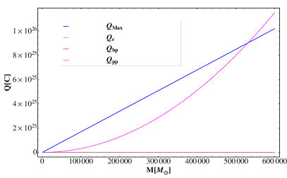
Figure 1: The behaviors of different definitions of BH charges as a function of BH mass. The solid, dotted, dashed, and dot-dashed lines represent $Q_{\text{Max}}\,,Q_{e}\,,Q_{\text{bp}}$  , and $Q_{\text{pp}}$, respectively. a) The behaviors of them for the mass range up to $4\times 10^{-16}M_{\odot}$. b) Their behaviors for the mass range to $6\times 10^{5}M_{\odot}$.

Hawking has shown that a BH is continuously emitting quasi-thermal radiations with a temperature

$$\tilde{T}_{\text{BH}} =\frac{2\tilde{\hbar}\tilde{G}\tilde{M}}{\tilde{k}_{\text{B}}\tilde{c}\tilde{A}_{\text{BH}}}\sqrt{1-\frac{\tilde{Q}^{2}}{4\pi\tilde{\epsilon}\tilde{G}\tilde{M}^{2}}}=\frac{2\tilde{\hbar}_{0}\tilde{G}_{0}\tilde{M}_{0}}{\tilde{k}_{\text{B}0}\tilde{c}_{0}\tilde{A}_{\text{BH}}}\sqrt{1-B(a)}=\frac{\tilde{\hbar}_{0}\tilde{c}_{0}^{3}}{2\pi\tilde{k}_{\text{B}0}\tilde{G}_{0}\tilde{M}_{0}}\frac{\sqrt{1-B(a)}}{\left(1+\sqrt{1-B(a)}\right)^{2}}\,.$$ (11)

As expected, the temperature of RN BH recovers the Schwarzschild one when $Q=0$. The Hawking luminosity $\tilde{L}_{\text{BH}}$ of the BH is given by the usual Stefan-Boltzmann blackbody formula

$$\tilde{L}_{\text{BH}}=\tilde{A}_{\text{BH}}\tilde{\sigma}_{\text{SB}}\tilde{T}_{\text{BH}}^{4}=\frac{\tilde{\hbar}_{0}\tilde{c}_{0}^{6}}{\tilde{G}_{0}^{2}\tilde{M}_{0}^{2}}a^{b/4}\frac{\left(1-B(a)\right)^{2}}{240\pi\left(1+\sqrt{1-B(a)}\right)^{6}}\,,$$ (12)

where we use the Stefan-Boltzmann constant

$$\tilde{\sigma}_{\text{SB}}\equiv\frac{\pi^{2}}{60}\frac{\tilde{k}_{\text{B}}^{4}}{\tilde{c}^{2}\tilde{\hbar}^{3}}=\frac{\pi^{2}}{60}\frac{\tilde{k}_{\text{B}0}^{4}}{\tilde{c}_{0}^{2}\tilde{\hbar}_{0}^{3}}a^{b/4}\equiv\tilde{\sigma}_{\text{SB}0}a^{b/4}\,.$$ (13)

If the Hawking temperature exceeds the rest mass energy of a particle, then the BH radiates particles and antiparticles in addition to photons. Luminosity, $\tilde{L}_{\text{BH}}$, given in Eq. (12), actually means the energy output and thus

$$\frac{d\tilde{E}_{\text{BH}}}{dt}\equiv-\tilde{L}_{\text{BH}}=-\frac{\tilde{\hbar}_{0}\tilde{c}_{0}^{6}}{\tilde{G}_{0}^{2}\tilde{M}_{0}^{2}}a^{b/4}\frac{\left(1-B(a)\right)^{2}}{240\pi\left(1+\sqrt{1-B(a)}\right)^{6}}\,.$$ (14)

From the above equation (14), one can obtain the mass loss due to Hawking radiation as

$$\frac{dM_{\text{H}}}{dt} \equiv\frac{1}{\tilde{c}^{2}}\frac{d\tilde{E}_{\text{BH}}}{dt}\approx-\frac{\tilde{\hbar}_{0}\tilde{c}_{0}^{4}}{\tilde{G}_{0}^{2}\tilde{M}_{0}^{2}}a^{-b/4}\frac{\left(1-B(a)\right)^{2}}{240\pi\left(1+\sqrt{1-B(a)}\right)^{6}}\equiv-\frac{\tilde{\hbar}_{0}\tilde{c}_{0}^{4}}{\tilde{G}_{0}^{2}\tilde{M}_{0}^{2}}\beta(a)\quad,\quad\text{where}$$ (15)

$$\frac{\tilde{\hbar}_{0}\tilde{c}_{0}^{4}}{\tilde{G}_{0}^{2}\tilde{M}_{0}^{2}} =2.430\times 10^{-71}\left(\frac{M_{\odot}}{\tilde{M}_{0}}\right)^{2}\left[\frac{\text{M}_{\odot}}{\text{s}}\right]\quad\text{and}\quad\beta(a)=a^{-b/4}\frac{\left(1-B(a)\right)^{2}}{240\pi\left(1+\sqrt{1-B(a)}\right)^{6}}\,.$$

$\beta(a_{0})$, the present value of $\beta$ without a charge, gives the standard value $1/(15360\pi)\approx 2.1\times 10^{-5}$. This mass loss rate applies only if the charge of BH is much smaller than the maximal possible charge on a BH, $\tilde{Q}_{\text{MAX}}=\sqrt{\tilde{G}_{0}\tilde{M}_{0}^{2}/(4\pi\tilde{\epsilon}_{0})}a^{b/8}$. Strictly, the mass loss rate in Eq. (15) applies only if $\tilde{Q}\ll\tilde{Q}_{\text{Max}}$ and this is satisfied in this case because high $\tilde{Q}$ is quickly discharged if $\tilde{M}\leq\tilde{\hbar}\tilde{c}\tilde{e}/(\tilde{G}^{3/2}\tilde{m}_{e}^{2}\sqrt{4\pi\tilde{\epsilon}})\approx 5\times 10^{5}a^{-9b/8}\left[M_{\odot}\right]$.

We compare the values of these charges for different (mass) types of BHs in table 2. The MBH denotes the micro BH which has the Planck mass, $M\sim 10^{-38}M_{\odot}$. We define YBH as the youngest BH which has the minimum mass ($M\sim 10^{-19}M_{\odot}$) to exist at present. Also, we define the BH with an electron mass as the specific BH. SMBH denotes the super massive BH. We also show both temperatures ($T_{\text{BH}}$) and the evaporation times ($t_{\text{eva}}$) for the different BHs in this table. Values of $Q_{\text{pp}}$ of SMBHs are larger than those of $Q_{\text{Max}}$ and thus it is impossible to obtain $Q_{\text{pp}}$ for SMBHs. Usually, $Q_{\text{pp}}\gg Q_{\text{bp}}$ for astrophysical BHs but this relation is opposite for the smaller BHs (i.e., $\text{M}<10^{-17}M_{\odot}$) as shown in table 2.

	MBH	YBH	specific BH	stellar mass BH	intermediate BH	SMBH
M [$M_{\odot}$]	$10^{-38}$	$10^{-19}$	$10^{-17}$	$4\sim 10^{2}$	$10^{2}\sim 10^{5}$	$10^{5}\sim 10^{10}$
$Q_{\text{Max}}^{0}$ [$C$]	$10^{-18}$	$10$	$10^{3}$	$10^{20}\sim 10^{22}$	$10^{22}\sim 10^{25}$	$10^{25}\sim 10^{30}$
$Q_{\text{pp}}$ [$C$]	$10^{-62}$	$10^{-24}$	$10^{-20}$	$10^{14}\sim 10^{18}$	$10^{18}\sim 10^{24}$	$10^{24}\sim 10^{34}$
$Q_{\text{eq}}$ [$C$]	$10^{-36}$	$10^{-17}$	$10^{-15}$	$10^{2}\sim 10^{4}$	$10^{4}\sim 10^{7}$	$10^{7}\sim 10^{12}$
$Q_{\text{bp}}$ [$C$]	$10^{-40}$	$10^{-21}$	$10^{-19}$	$10^{-2}\sim 10^{0}$	$10^{0}\sim 10^{3}$	$10^{3}\sim 10^{8}$
$t_{\text{eva}}$ [yrs]	$10^{-47}$	$10^{10}$	$10^{16}$	$10^{68}\sim 10^{73}$	$10^{73}\sim 10^{82}$	$10^{82}\sim 10^{97}$
$T_{\text{BH}}$ [$K$]	$10^{30}$	$10^{11}$	$10^{9}$	$10^{-8}\sim 10^{-10}$	$10^{-10}\sim 10^{-13}$	$10^{-13}\sim 10^{-18}$
$k_{\text{B}}T_{\text{BH}}$ [$eV$]	$10^{26}$	$10^{7}$	$10^{5}$	$10^{-12}\sim 10^{-14}$	$10^{-14}\sim 10^{-17}$	$10^{-17}\sim 10^{-22}$

Table 2: The different definitions of charges, the evaporation times, and the temperatures for different BHs. MBH denotes micro BH and YBH means the youngest BH which has the evaporation time equal to the age of the Universe. The specific BH means that its thermal energy is the same as the rest mass energy of the electron. SMBH denotes a supermassive black hole. Also, yrs means years.

III Entropy of BH system

The entropy of a BH is given by Hawking:1974nat ; Hawking:1975CMP

$$S_{\text{BH}}=\frac{\tilde{k}_{\text{B}}\tilde{c}^{3}}{\tilde{\hbar}\tilde{G}}\frac{\tilde{A}_{\text{BH}}}{4}=\frac{k_{\text{B}0}\tilde{c}_{0}^{3}}{\tilde{\hbar}_{0}\tilde{G}_{0}}\frac{\tilde{A}_{\text{BH}}}{4}\quad,\quad\tilde{A}_{\text{BH}}=4\pi\tilde{r}_{\text{BH}}^{2}\,,$$ (16)

where we rewrite it for the meVSL model and $\tilde{A}_{\text{BH}}$ is the area of a BH’s event horizon of the meVSL model. Time evolutions of quantities as functions of a scale factor, $a$, are given by Lee:2020zts

$$\tilde{k}_{\text{B}}=\tilde{k}_{\text{B}0}\quad,\quad\tilde{c}=\tilde{c}_{0}a^{b/4}\quad,\quad\tilde{\hbar}=\tilde{\hbar}_{0}a^{-b/4}\,,$$ (17)

where $k_{\text{B}}$ is the Boltzmann constant, $c$ is the speed of light, and $\hbar$ is the reduced Planck constant. Thus, the prefactor of the BH entropy of meVSL model, $\tilde{k}_{B}\tilde{c}^{3}/(\tilde{\hbar}\tilde{G})$ is the same as that of GR even though the physical constants are functions of a scale factor as shown in Eq. (16). The generalized second law of thermodynamics of the black hole (BH) system states that the net entropy of the system cannot decrease with time Bekenstein:1973prd . From this fact, we might be able to constrain time variations of physical constants MacGibbon:2007qh . The increase of the net generalized entropy of the system over a time interval $\Delta t$ is given by

$$\Delta S\equiv\Delta S_{\text{BH}}+\Delta S_{\text{env}}\geq 0\,,$$ (18)

where $\Delta S_{\text{BH}}$ and $\Delta S_{\text{env}}$ denote the changes in the entropy of the BH and of the environment (the ambient radiation and/or matter), respectively. From its definition given in Eq. (16), the change in BH entropy over time should include the contribution from the Hawking flux as well as partial change induced by time evolutions of physical constants

$$\frac{\Delta S_{\text{BH}}^{\text{eff}}}{\Delta t} \approx\frac{dS_{\text{BH}}}{dt}=\frac{k_{\text{B}0}\tilde{c}_{0}^{3}}{4\tilde{\hbar}_{0}\tilde{G}_{0}}\frac{d\tilde{A}_{\text{BH}}}{dt}\quad,\quad\text{where}$$

$$\frac{d\tilde{A}_{\text{BH}}}{dt} =\frac{8\pi\tilde{G}_{0}^{2}\tilde{M}_{0}^{2}}{\tilde{c}_{0}^{4}}\frac{1+\sqrt{1-B(a)}}{\sqrt{1-B(a)}}\left[\left(1+\sqrt{1-B(a)}\right)\frac{1}{M}\frac{dM_{\text{H}}}{dt}-B(a)\frac{1}{Q}\frac{dQ_{\text{H}}}{dt}+\frac{b}{8}HB(a)\right]\,.$$ (19)

$$\frac{dS_{\text{BH}}}{dt} =\frac{2\pi k_{\text{B}0}\tilde{G}_{0}\tilde{M}_{0}^{2}}{\tilde{\hbar}_{0}\tilde{c}_{0}}\frac{1+\sqrt{1-B(a)}}{\sqrt{1-B(a)}}\left[\left(1+\sqrt{1-B(a)}\right)\frac{1}{M}\frac{dM_{\text{H}}}{dt}-B(a)\frac{1}{Q}\frac{dQ_{\text{H}}}{dt}+\frac{b}{8}HB(a)\right]$$ (20)

$$\equiv\frac{dS_{\text{BH}}}{dt}\Bigl{|}_{\mathrm{I}}+\frac{dS_{\text{BH}}}{dt}\Bigl{|}_{\mathrm{II}}+\frac{dS_{\text{BH}}}{dt}\Bigl{|}_{\mathrm{III}}\,,$$

where both $M$ and $Q$ change as the BH radiates and this effect is described by the subscript H. Also, the effect of meVSL on the entropy change is shown in the last term of Eq. (20). This term is further simplified for the late time $\Lambda$CDM cosmology as

$$\frac{dS_{\text{BH}}}{dt}\Bigl{|}_{\mathrm{III}} =\frac{\tilde{k}_{\text{B}0}Q^{2}H_{0}^{(\text{GR})}}{16\tilde{\epsilon}_{0}\tilde{\hbar}_{0}\tilde{c}_{0}}b\frac{1+\sqrt{1-B}}{\sqrt{1-B}}E(a)a^{-b/4}\approx 2.01\times 10^{-5}\left(\frac{Q}{C}\right)^{2}h\cdot b\cdot E(a)a^{-b/4}\left[\frac{\text{J}}{\text{K}\cdot\text{s}}\right]\,,$$

$$\text{where}\quad E(a)=\sqrt{\Omega_{m0}a^{-3}+\Omega_{\Lambda}}\,,$$ (21)

where $h$ comes from the Hubble parameter ($H_{0}=100h\,\text{km/s/Mpc}$). Thus, this effect increases (decreases) the entropy change in addition to the BH entropy change due to Hawking radiation if the sign of $b$ is positive (negative). This term is significant to probe the thermodynamics of BH and thus we need to investigate it in detail. In the above Eq. (21), we use the following relation

$$HB(a) =H_{0}^{(\text{GR})}B_{0}E(a)=1.10\times 10^{-58}\frac{\text{M}_{\odot}^{2}}{\text{C}^{2}}\left(\frac{\tilde{Q}_{0}}{\tilde{M}_{0}}\right)^{2}h\cdot E(a)\left[\text{s}^{-1}\right]\,.$$ (22)

In the following subsections, we compare the magnitude of each term in Eq. (20) for different cases.

For the emission of $n_{s}$ species of two-polarization massless particles of spin $s=1/2,1,$ and $2$ from a Schwarzschild BH into empty space, numerical calculations have been obtained Page:1976prd ; Page:1976prd14 ; Page:1983prl

$$\frac{dS_{\text{rad}}}{dt} =2.8\times 10^{-21}\left(3.3710n_{1/2}+1.2684n_{1}+0.1300n_{2}\right)\left(\frac{M_{\odot}}{M}\right)\left[\frac{J}{K\cdot s}\right]\,,$$ (23)

$$\frac{dS_{\text{BH}}}{dt} =-2.8\times 10^{-21}\left(2.0566n_{1/2}+0.8454n_{1}+0.0964n_{2}\right)\left(\frac{M_{\odot}}{M}\right)\left[\frac{J}{K\cdot s}\right]\,.$$ (24)

Now we investigate two cases by comparing the temperature of BH with that of its environment.

III.1 $\tilde{T}_{\text{BH}}>T_{\text{env}}$

When the temperature of the BH is greater than that of its surroundings, there is a net radiation loss from the BH into its environment. This case also can be divided into whether the charge of the BH, $Q$, is affected by the Hawking radiation or not.

III.1.1 $dQ_{\text{H}}/dt=0$ (i.e., $k_{\text{B}}T_{\text{BH}}\leq m_{e}c^{2}$)

This is the case when the thermal energy of the BH with its temperature given in Eq. (11) is below the rest mass energy of the electron (i.e., $0.511$ MeV). This corresponds to

$$\tilde{M}_{\text{BH}}\geq 4.15\times 10^{-17}\frac{\sqrt{1-B(a)}}{\left(1+\sqrt{1-B(a)}\right)^{2}}\left[M_{\odot}\right]\,.$$ (25)

Thus, one can simplify the equation (20) as

$$\frac{dS_{\text{BH}}}{dt}=\frac{dS_{\text{BH}}}{dt}\Bigl{|}_{\mathrm{I}}+\frac{dS_{\text{BH}}}{dt}\Bigl{|}_{\mathrm{III}}\,,$$ (26)

One needs to adopt the mass loss due to the Hawking radiation given in the equation (15). As mentioned before, this mass loss rate in Eq. (15) applies only if $Q\ll Q_{\text{Max}}$ and this is satisfied in this case because high $Q$ is quickly discharged if $M\leq\hbar ce/(G^{3/2}m_{e}^{2}\sqrt{4\pi\epsilon_{0}})\approx 5\times 10^{5}M_{\odot}$. This case is limited below the mass of SMBHs. Thus, the first term in Eq. (26) is rewritten as

$$\frac{dS_{\text{BH}}}{dt}\Bigl{|}_{\mathrm{I}} =-2.34\times 10^{-20}\left(\frac{M_{\odot}}{\tilde{M}_{0}}\right)\frac{\left(1-B\right)^{3/2}}{\left(1+\sqrt{1-B}\right)^{4}}a^{b/4}\left[\frac{J}{K\cdot s}\right]\,.$$ (27)

We can also estimate the second term in Eq. (26)

$$\frac{dS_{\text{BH}}}{dt}\Bigl{|}_{\mathrm{III}} =2.01\times 10^{-5}h\cdot b\left(\frac{\tilde{Q}_{0}}{C}\right)^{2}E(a)\,.$$ (28)

If the charge is greater than $Q_{\text{pp}}$, then the BH is quickly discharged by superradiant pair production in the electrostatic field surrounding the BH. The discharge rate for $M\geq 10^{-17}M_{\odot}$ BH with $Q>Q_{\text{pp}}$ is given by

$$\frac{dQ_{\text{pp}}}{dt} \approx-\frac{e^{4}Q^{3}}{\left(4\pi\epsilon\right)^{3}\hbar^{3}c^{2}r_{\text{BH}}}\exp\left[-\frac{\pi m_{e}^{2}c^{3}\left(4\pi\epsilon\right)r_{\text{BH}}^{2}}{\hbar Qe}\right]$$

$$=-\frac{\tilde{e}_{0}^{4}\tilde{Q}_{0}^{3}}{\left(4\pi\tilde{\epsilon}_{0}\right)^{3}\hbar_{0}^{3}\tilde{G}_{0}\tilde{M}_{0}}\exp\left[-\frac{\pi\tilde{m}_{e0}^{2}\left(4\pi\tilde{\epsilon}_{0}\right)\tilde{G}_{0}^{2}\tilde{M}_{0}^{2}}{\tilde{\hbar}_{0}\tilde{c}_{0}\tilde{Q}_{0}\tilde{e}_{0}}a^{b/4}\left(1+\sqrt{1-B}\right)^{2}\right]\frac{a^{-3b/4}}{\left(1+\sqrt{1-B}\right)}\,.$$ (29)

Thus, from this charge contribution, we have a new term $(dS_{\text{BH}}/dt)_{\mathrm{II}}$ in this case

$$\frac{dS_{\text{BH}}}{dt}\Bigl{|}_{\mathrm{II}}^{(\text{pp})} =\frac{2\pi\tilde{k}_{\text{B}0}\tilde{e}_{0}^{4}\tilde{Q}_{0}^{4}}{\left(4\pi\tilde{\epsilon}_{0}\right)^{4}\tilde{\hbar}_{0}^{4}\tilde{G}_{0}\tilde{M}_{0}\tilde{c}_{0}}\exp\left[-\frac{\pi\tilde{m}_{e0}^{2}\left(4\pi\tilde{\epsilon}_{0}\right)\tilde{G}_{0}^{2}\tilde{M}_{0}^{2}}{\tilde{\hbar}_{0}\tilde{c}_{0}\tilde{Q}_{0}\tilde{e}_{0}}a^{b/4}\left(1+\sqrt{1-B}\right)^{2}\right]\frac{a^{-3b/4}}{\sqrt{1-B}}$$

$$=7.68\times 10^{49}\left(\frac{\tilde{Q}_{0}}{C}\right)^{4}\left(\frac{M_{\odot}}{\tilde{M}_{0}}\right)\exp\left[-1.01\times 10^{15}\left(\frac{C}{\tilde{Q}_{0}}\right)\left(\frac{\tilde{M}_{0}}{M_{\odot}}\right)^{2}\right]\left[\frac{J}{K\cdot s}\right]\,.$$ (30)

As shown in Eqs. (23) and (24), the increase of the entropy of the environment due to the Hawking radiation is $1.62$ times bigger than the decrease of the entropy of BH due to Hawking emission ($dS_{\text{env}}/dt=1.62dS_{\text{BH}}/dt|_{\mathrm{I}}$). Thus, the total entropy of the system can be divided into two cases for different values of charge

$$\frac{dS_{\text{tot}}}{dt}=\frac{dS_{\text{env}}}{dt}+\frac{dS_{\text{BH}}}{dt} =\begin{cases}1.62\frac{dS_{\text{BH}}}{dt}\Bigl{|}_{\mathrm{I}}-\frac{dS_{\text{BH}}}{dt}\Bigl{|}_{\mathrm{I}}+\frac{dS_{\text{BH}}}{dt}\Bigl{|}_{\mathrm{II}}^{(\text{pp})}+\frac{dS_{\text{BH}}}{dt}\Bigl{|}_{\mathrm{III}}^{(\text{pp})}\equiv\frac{dS_{\text{tot}}^{(\text{pp})}}{dt}&\,,Q_{\text{pp}}<Q\\ 1.62\frac{dS_{\text{BH}}}{dt}\Bigl{|}_{\mathrm{I}}-\frac{dS_{\text{BH}}}{dt}\Bigl{|}_{\mathrm{I}}+\frac{dS_{\text{BH}}}{dt}\Bigl{|}_{\mathrm{III}}^{(\text{eq})}\equiv\frac{dS_{\text{tot}}^{(\text{eq})}}{dt}&\,,Q_{\text{eq}}<Q<Q_{\text{pp}}\end{cases}\,,$$ (31)

One can estimate each term of the above Eq. (31) for the effective mass range of BHs. We show this in Table 3.

	specific	stellar mass BH	intermediate BH
M [$M_{\odot}$]	$10^{-17}$	$10^{0}\sim 10^{2}$	$10^{2}\sim 10^{5}$
$Q_{\text{pp}}$ [$C$]	$10^{-20}$	$10^{14}\sim 10^{18}$	$10^{18}\sim 10^{24}$
$Q_{\text{eq}}$ [$C$]	$10^{-15}$	$10^{2}\sim 10^{4}$	$10^{4}\sim 10^{7}$
$dS_{\text{BH}}/dt|_{\mathrm{I}}$ [$J/(K\cdot s)$]	$10^{-4}$	$10^{-21}\sim 10^{-23}$	$10^{-23}\sim 10^{-26}$
$dS_{\text{BH}}/dt|_{\mathrm{II}}^{(\text{pp})}$ [$J/(K\cdot s)$]	$10^{-14}$	$10^{105}\sim 10^{120}$	$10^{120}\sim 10^{140}$
$dS_{\text{BH}}/dt|_{\mathrm{III}}^{(\text{pp})}$ [$J/(K\cdot s)$]	$10^{-45}(h\cdot b)$	$10^{23}(h\cdot b)\sim 10^{31}(h\cdot b)$	$10^{31}(h\cdot b)\sim 10^{43}(h\cdot b)$
$dS_{\text{BH}}/dt|_{\mathrm{III}}^{(\text{eq})}$ [$J/(K\cdot s)$]	$10^{-35}(h\cdot b)$	$10^{-1}(h\cdot b)\sim 10^{3}(h\cdot b)$	$10^{3}(h\cdot b)\sim 10^{9}(h\cdot b)$
$dS_{\text{tot}}^{(\text{pp})}/dt$ [$J/(K\cdot s)$]	$10^{-4}$	$10^{105}\sim 10^{120}$	$10^{120}\sim 10^{140}$
$dS_{\text{tot}}^{(\text{eq})}/dt$ [$J/(K\cdot s)$]	$10^{-4}$	$10^{-1}(h\cdot b)\sim 10^{3}(h\cdot b)$	$10^{3}(h\cdot b)\sim 10^{9}(h\cdot b)$

Table 3: Comparisons of entropy changes from different contributions for the different BHs.

As shown in this table, $dS_{\text{BH}}/dt|_{\mathrm{I}}$-term dominates when $\tilde{M}_{0}=10^{-17}M_{\odot}$ independent of the magnitude of the charge of BH. Thus, the total entropy increases irrelevant to the sign of $b$. But the $dS_{\text{BH}}/dt_{\mathrm{II}}^{(\text{pp})}$-term dominates other terms for BHs mass from $1$ to $10^{5}$ solar mass. Again, the total entropy increases for any sign of $b$. However, if the charge of BH is $Q_{\text{eq}}$, then the total entropy is dominated by $dS_{\text{BH}}/dt_{\mathrm{III}}^{(\text{eq})}$-term and in this case, only the positive values of $b$ are allowed to increase the total entropy of the system.

III.1.2 $dQ_{\text{H}}/dt\neq 0$ (i.e., $k_{\text{B}}T_{\text{BH}}\geq m_{e}c^{2}$)

As the subcase of $T_{\text{BH}}>T_{\text{env}}$, we consider the Hawking radiation which the BH is emitting charged particles (i.e., $dQ_{H}/dt\neq 0$). This happens when $M_{\text{BH}}\leq 10^{-17}M_{\odot}$. In this case, the entropy change of a BH given in Eq. (20) becomes

$$\frac{dS_{\text{BH}}}{dt}=\frac{2\pi k_{\text{B}0}\tilde{G}_{0}\tilde{M}_{0}^{2}}{\tilde{\hbar}_{0}\tilde{c}_{0}}\frac{1+\sqrt{1-B(a)}}{\sqrt{1-B(a)}}\left[\left(1+\sqrt{1-B(a)}\right)\frac{1}{M}\frac{dM_{\text{H}}}{dt}-B(a)\frac{1}{Q}\frac{dQ_{\text{H}}}{dt}+\frac{b}{8}HB(a)\right]\,,$$ (32)

It is natural that a charged BH preferentially emits charged particles of the same sign as its own charge at a rate that depends on $Q$

$$\frac{dQ_{H}}{dt}=-\left(\frac{e|Q|}{Q}\right)\frac{dN_{H}}{dt}\,,$$ (33)

where $e=-1.6\times 10^{-19}C$ is the electron charge and $edN_{H}/dt$ is the net emission rate of charge. Then the total emission rate of all particles from the BH is given by

$$\frac{dN_{\text{Tot}}}{dt}=-\frac{\tilde{c}_{0}^{2}}{E_{\text{av}0}}\frac{dM_{H}}{dt}\geq\frac{dN_{H}}{dt}\,,$$ (34)

where $E_{\text{av}0}\approx 5k_{\text{B}}T_{\text{BH}0}=5\tilde{\hbar}_{0}\tilde{c}_{0}^{3}/(2\pi\tilde{G}_{0}\tilde{M}_{0})$ is the average energy of particles emitted by the BH Page:1976prd . By combining Eqs. (33) and (34), one obtains

$$\left|\frac{B}{Q}\frac{dQ_{H}}{dt}\right|\leq\frac{\tilde{c}_{0}^{2}}{E_{\text{av}}}\left|\frac{eB}{Q}\frac{dM_{H}}{dt}\right|\approx\frac{\left|\tilde{e}_{0}\tilde{Q}_{0}\right|}{10\tilde{\epsilon}_{0}\tilde{\hbar}_{0}\tilde{c}_{0}\tilde{M}_{0}}\frac{\left(1+\sqrt{1-B}\right)^{2}}{\sqrt{1-B}}\frac{dM_{H}}{dt}\,.$$ (35)

Thus, the second term of the entropy change given in Eq. (32) lies in the range

$$0\leq\frac{dS_{\text{BH}}}{dt}\Bigl{|}_{\mathrm{II}}\leq-\frac{2\pi k_{\text{B}0}\tilde{G}_{0}\tilde{M}_{0}\left|\tilde{e}_{0}\tilde{Q}_{0}\right|}{5\tilde{\epsilon}_{0}\left(\tilde{\hbar}_{0}\tilde{c}_{0}\right)^{2}}\frac{\left(1+\sqrt{1-B}\right)^{3}}{1-B}\frac{dM_{H}}{dt}\equiv\frac{dS_{\text{BH}}}{dt}\Bigl{|}_{\mathrm{II}}^{(\text{up})}\,.$$ (36)

If we adopt the mass loss due to the Hawking radiation in Eq. (15) into the above equation, then we can estimate the upper limit of this entropy change as

$$\frac{dS_{\text{BH}}}{dt}\Bigl{|}_{\mathrm{II}}^{(\text{up})}=\frac{2\pi\tilde{k}_{\text{B}0}\tilde{c}_{0}^{2}|\tilde{e}_{0}\tilde{Q}_{0}|}{5\tilde{\epsilon}_{0}\tilde{\hbar}_{0}\tilde{G}_{0}\tilde{M}_{0}}\frac{\left(1-B\right)a^{-b/4}}{240\pi\left(1+\sqrt{1-B}\right)^{3}}=2.02\left(\frac{M_{\odot}}{\tilde{M}_{0}}\right)\left(\frac{\tilde{Q}_{0}}{C}\right)\frac{\left(1-B\right)a^{-b/4}}{240\pi\left(1+\sqrt{1-B}\right)^{3}}\left[\frac{J}{K\cdot s}\right]\,.$$ (37)

Now we can compare the magnitudes of all three contributions of the BH entropy and these are shown in Table 4. The first contribution of the BH entropy change ($10^{17}$) is dominant for the MBH. The second contributions of the change of the BH entropy ($10^{-2}$) are dominant for both YBH and the specific BH. Thus, the sign of $b$ is irrelevant to satisfy the generalized second law of the BH thermodynamics.

	MBH	YBH	specific BH
M [$M_{\odot}$]	$10^{-38}$	$10^{-19}$	$10^{-17}$
$Q_{\text{eq}}$ [$C$]	$10^{-36}$	$10^{-17}$	$10^{-15}$
$dS_{\text{BH}}/dt|_{\mathrm{I}}$ [$J/(K\cdot s)$]	$10^{17}$	$10^{-2}$	$10^{-4}$
$dS_{\text{BH}}/dt|_{\mathrm{II}}^{(\text{eq})}$ [$J/(K\cdot s)$]	$10^{-2}$	$10^{-2}$	$10^{-2}$
$dS_{\text{BH}}/dt|_{\mathrm{III}}^{(\text{eq})}$ [$J/(K\cdot s)$]	$10^{-72}(h\cdot b)$	$10^{-48}(h\cdot b)$	$10^{-40}(h\cdot b)$
$dS_{\text{tot}}^{(\text{eq})}/dt$ [$J/(K\cdot s)$]	$10^{17}$	$10^{-2}$	$10^{-2}$

Table 4: The contributions of the change of BH entropy for the different BHs. The superscript (eq) denotes when one adopts the equal charge of BH in the calculation.

III.2 $\tilde{T}_{\text{BH}}\leq T_{\text{env}}$

If the temperature of BH is equal to or less than the temperature of its environment, then the BH accretes from its surroundings faster than it Hawking radiates. This accretion increases the mass of the BH $M$, further lowering its temperature, $T_{\text{BH}}$. During accretion, the amount of the increase of the BH mass-energy ($Mc^{2}$) should be equal to that of the decrease of the energy of the environment, $E_{\text{env}}$. The thermodynamical definitions of the temperature of an object is related to its entropy as

$$\beta_{i}\equiv\left(k_{\text{B}}T_{i}\right)^{-1}\equiv\frac{\partial S_{i}}{\partial E_{i}}=\frac{1}{c^{2}}\frac{\partial S_{i}}{\partial M_{i}}\Bigl{|}_{Q_{i}}\,.$$ (38)

Thus, if the temperature of the environment is greater than that of the BH, $\tilde{T}_{\text{BH}}\leq T_{\text{env}}$, then the increase in BH entropy due to accretion, $S_{\text{BH}}$, must be greater than the decrease in the entropy of its environment, $S_{\text{env}}$ as shown in Eq. (38). We can also consider both the increase and the decrease of BH entropies due to accretion and Hawking radiation. For this consideration, we regard a cold large BH in a warm thermal bath which absorbs energy and emits radiations at a rate

$$\frac{dE}{dt}\Bigl{|}_{\text{abs}}=\frac{\pi^{2}\sigma_{\text{S}}}{60\hbar^{3}\tilde{c}^{2}}\left(\tilde{k}_{\text{B}}T_{\text{env}}\right)^{4}\quad,\quad\frac{dE}{dt}\Bigl{|}_{\text{emt}}=\frac{\pi^{2}\sigma_{\text{S}}}{60\hbar^{3}\tilde{c}^{2}}\left(\tilde{k}_{\text{B}}T_{\text{BH}}\right)^{4}\,,\text{where}\quad\sigma_{\text{S}}=\frac{27\pi\tilde{G}_{0}^{2}\tilde{M}_{0}^{2}}{\tilde{c}_{0}^{4}}\,.$$ (39)

The increase in $S_{\text{BH}}$ due to accretion ($dE/dt|_{\text{abs}}$) is greater than the decrease in $S_{\text{BH}}$ due to Hawking radiation ($dE/dt|_{\text{emt}}$). Thus, the generalized entropy of the system is increased $\Delta S\geq 0$ in this case irrelevant to the sign of $b$.

IV Conclusions

We have applied the generalized second law of thermodynamics by including the entropy of the black hole to extract the sign of meVSL parameter, $b$. We limit our consideration to the classical general relativity to be consistent with classical thermodynamics when we define the temperature and entropy of the black hole.

We consider two cases by comparing the temperatures between the black hole and its surrounding. Firstly, the temperature of the black hole is greater than that of its environment. Secondly, the black hole temperature is lesser than its surrounding temperature.

The first case can be also divided into two sub-cases. One is for the temperature is lower than the rest mass energy of the electron in order not to have any charge creation due to Hawking radiation. This case corresponds to massive black holes with mass greater than $10^{-17}\,M_{\odot}$. The second sub-case of the first case is the mass of temperature is below $10^{-17}\,M_{\odot}$. If the pair production charge is contributed, then the entropy changes are dominated by the terms of charge pair productions of BHs. In this case, the generalized black hole thermodynamic is satisfied irrelevant to the sign of $b$. However, if the charge of the black hole is below that of the pair production charge and the above equality charge, then the dominant contribution comes from the term that is related to the parameter $b$ and in this case, $b$ should be positive to satisfy the generalized second law of black hole thermodynamics.

The black hole accretes from its environment in the second case. And from the definition of temperatures of the black holes and their environments, the generalized second law of thermodynamics is guaranteed from their definitions of temperatures no matter what is the value of $b$.

Thus, we might conclude that the generalized second thermodynamics laws of the black hole are satisfied for most of the black hole system. Only when there exists a pair production charge of a black hole for astrophysical black holes, then the positive values of $b$ are required to satisfy the generalized second thermodynamics laws of the black hole.

References

• (1) T.ย Buchert, A.ย A.ย Coley, H.ย Kleinert, B.ย F.ย Roukema and D.ย L.ย Wiltshire, Int. J. Mod. Phys. D 25, no.03, 1630007 (2016) doi:10.1142/S021827181630007X [arXiv:1512.03313 [astro-ph.CO]].
• (2) L.ย Perivolaropoulos and F.ย Skara, [arXiv:2105.05208 [astro-ph.CO]].
• (3) J.ย P.ย Petit, Astrophys. Sp. Science 226, 273 (1995) doi:10.1007/bf00627375.
• (4) J.ย P.ย Petit and G.ย dโ€™Agostini, [arXiv:0803.1362 [math-ph]].
• (5) S.ย Lee, โ€œThe minimally extended Varying Speed of Light (meVSL),โ€ JCAP 08, (2021) [arXiv:2011.09274 [astro-ph.CO]].
• (6) M.ย J.ย Duff, [arXiv:hep-th/0208093 [hep-th]].
• (7) M.ย J.ย Duff, Contemp. Phys. 56, no.1, 35-47 (2015) doi:10.1080/00107514.2014.980093 [arXiv:1412.2040 [hep-th]].
• (8) G.ย W.ย Gibbons, โ€œVacuum polarization and the spontaneous loss of charge by black holesโ€, Commun.ย Math.ย Phys 44, 245 (1975) doi:10.1007/BF01609829.
• (9) J.ย Bally and E.ย R.ย Harrison, Astrophys. I. 220, 743 (1978) doi: 10.1086/155961
• (10) M.ย Zajaฤek and A.ย Tursunov, [arXiv:1904.04654 [astro-ph.GA]].
• (11) S.ย W.ย Hawking, โ€œBlack hole explosions ?โ€, Nature 248, 30 (1974) doi.org:10.1038/248030a0
• (12) S.ย W.ย Hawking, โ€œParticle creation by black holesโ€, Commun. Math. Phys. 43, 199 (1975) doi.org:10.1007/BF02345020
• (13) J. D. Bekenstein, โ€œBlack Holes and Entropyโ€, Phys. Rev. D 7, 2333 (1973) doi:/10.1103/PhysRevD.7.2333.
• (14) J.ย H.ย MacGibbon, โ€œBlack Hole Constraints on Varying Fundamental Constants,โ€ Phys. Rev. Lett. 99, 061301 (2007) doi:10.1103/PhysRevLett.99.061301 [arXiv:0706.2188 [astro-ph]].
• (15) D. N. Page, โ€œParticle emission rates from a black hole: Massless particles from an uncharged, nonrotating holeโ€, Phys. Rev. D 13, 198 (1976) doi:10.1103/PhysRevD.13.198.
• (16) D. N. Page, โ€œParticle emission rates from a black hole. II. Massless particles from a rotating holeโ€, Phys. Rev. D 14, 3260 (1976) doi:10.1103/PhysRevD.14.3260.
• (17) D. N. Page, โ€œComment on โ€Entropy Evaporated by a Black Holeโ€โ€, Phys. Rev. Lett 50, 1013 (1983) doi:10.1103/PhysRevLett.50.1013.