Contrastive Learning of Visual-Semantic Embeddings

Abstract

Contrastive learning is a powerful technique to learn representations that are semantically distinctive and geometrically invariant. While most of the earlier approaches have demonstrated its effectiveness on single-modality learning tasks such as image classification, recently there have been a few attempts towards extending this idea to multi-modal data. In this paper, we propose two loss functions based on normalized cross-entropy to perform the task of learning joint visual-semantic embedding using batch contrastive training. In a batch, for a given anchor point from one modality, we consider its negatives only from another modality, and define our first contrastive loss based on expected violations incurred by all the negatives. Next, we update this loss and define the second contrastive loss based on the violation incurred only by the hardest negative. We compare our results with existing visual-semantic embedding methods on cross-modal image-to-text and text-to-image retrieval tasks using the MS-COCO and Flickr30K datasets, where we outperform the state-of-the-art on the MS-COCO dataset and achieve comparable results on the Flickr30K dataset.

I Introduction and Background

Joint embedding learning is a well-studied problem, where the objective is to learn a common embedding space for two (or more) diverse domains/modalities (e.g. images and text) that represents their underlying structure and semantics. Such embeddings entail mapping of semantically similar samples from diverse modalities to similar locations, thus facilitating direct matching of samples from different modalities using simple vector operations such as dot product. As a result, these can enable a wide range of visual and language understanding tasks such as image/video tagging [1, 2], captioning [3, 4] and retrieval [5, 6], visual question answering [7], fine-grained recognition [8], zero-shot learning [2], bilingual word embeddings [9], etc.

In this paper, we focus on learnig visual-semantic embeddings for cross-modal image-text retrieval; i.e., the retrieval of semantically relevant images given a caption, or of semantically relevant captions given a query image. Since it is not possible to match samples from diverse modalities represented in heterogeneous feature spaces directly, many of the existing approaches have addressed this problem by learning an embedding function that projects these features into a common subspace where these can be directly matched. Among the non-deep learning based techniques, one popular paradigm is to learn a common subspace such that the correlations among semantically similar samples are maximized [10, 11, 12, 13, 14, 15, 16]. The deep learning based techniques approach this problem by learning non-linear projections for individual modalities that are subsequently fused to lead to a common subspace where heterogeneous samples can be directly matched [17, 18, 19, 20]. These non-linear projections are mostly learned jointly by imposing a (dis)similarity constraints on image and text features using cross-modal triplet constraints [20, 6, 21, 5, 22]. These ranking-based constraints capture semantic correlations between modalities by optimizing the similarity between positive pairs to be more than that between negative pairs by a margin. While the primary objective of such constraint functions is to minimize semantic gap based on similarity between cross-modal paired samples, their ability to learn a good projection gets hindered due to heterogeneity gap that is introduced by incompatible feature distributions in diverse modalities.

To address this, in this paper, we propose to learn joint embedding space by integrating triplet ranking loss with contrastive representation learning [23, 24, 25, 26]. Contrastive representation learning has been found to be an effective approach in reducing the heterogeneity gap between semantically similar samples. The underlying idea in these techniques is that given an anchor point, maximize its similarity with a “positive” sample and minimize its expected similarity with many “negative” samples in a mini-batch. Among these, the SimCLR [23] approach, which is also a representative state-of-the-art in contrastive representation learning for unimodal data, does this using the normalized temperature-scaled cross entropy (or NCE) loss. Because of its simplicity, SimCLR has been adapted for a variety of visual understanding tasks [27, 28, 29]. Recently, [29] proposed an NCE-based loss to learn generalized similarity-preserving multi-modal representations using expected similarity between all negative multi-modal pairs; i.e., for an anchor point from one modality, they consider negatives from all the modalities including those from the anchor’s modality. However, in our preliminary experiments, we used this loss to learn a joint visual-semantic embedding using image-caption pairs, and found this to give not-so-good results on the cross-modal retrieval task. This is because in cross-modal retrieval tasks, we are interested in reducing the similarity between negative pairs across different modalities instead of negative pairs within the same modality. To incorporate this idea, our first contribution is a new NCE-based contrastive loss for learning joint embeddings that considers negatives from other modalities excluding the anchor’s modality. We would like to emphasize that while this update may appear to be trivial, it provides a significant boost in empirical results as we will discuss later (c.f. Table III).

Next, it was noted by [20] that a triplet loss function that considers expected similarity with all the negatives may be biased and create problematic local minima, particularly in those problems where we have a structured output space such as learning joint visual-semantic embeddings, and advocated the use of only hard negatives. As our second contribution, we integrate this idea in the contrastive learning set-up, and propose second NCE-based contrastive loss for joint embedding learning. Specifically, we update our previous loss function by considering only the hardest negative from other modalities excluding the anchor’s modality. We will show later that this update further improves the empirical results. As per our knowledge, this is the first attempt of incorporating the idea of using only the hardest negatives in NCE-based deep contrastive learning.

To validate the effectiveness of our proposals, we extensively compare them with existing joint embedding learning approaches on cross-modal image-text retrieval tasks using the MS-COCO and Flickr30K datasets, where we outperform the state-of-the-art on the MS-COCO dataset and achieve comparable results on the Flickr30K dataset.

The paper is organized as follows. In Section II, we discuss the preliminaries on learning visual-semantic embeddings using hinge-based triplet ranking loss. Section III describes the proposed approach. In Section IV, we present the experimental analyses, and finally Section V presents the conclusions and directions for future research.

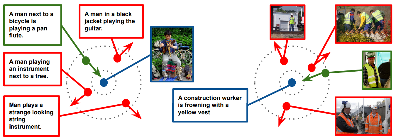
(a)

(b)

Figure 1: A visual illustration of the proposed loss functions: (a) the sum-of-negatives loss $l_{CSN}$ (Eq. 6), and (b) the max-of-negatives loss $l_{CMN}$ (Eq. 12). Data points marked in blue, green and red denote the anchor point, the positive (target) point and the negative points respectively (see text for details).

II Preliminaries

To learn a visual-semantic embedding, our training set $\mathcal{D}=\{(I_{i},C_{i})\}$ consists of pairs of images and corresponding captions. We consider $(I_{i},C_{i})$ to denote a positive pair and $(I_{i},C_{j})$ ($j\neq i$) to denote a negative pair; i.e., for image $I_{i}$, $C_{i}$ is the most relevant caption and $C_{j}$ is a caption corresponding to some other image, and vice-versa. Initially, we use image and text encoders to compute the representations of an image and a caption respectively, and project them into a joint embedding space. For a given image $I$ and a caption $C$, we denote the embeddings in the joint embedding space as $z_{I},z_{C}\in\mathbb{R}^{d}$ respectively. To compute the similarity between the embeddings of an image $I$ and a caption $C$ in this joint embedding space, we use normalized correlation (or, the cosine similarity), which is given by

$$s(I,C)=\frac{z_{I}^{T}z_{C}}{\|z_{I}\|\|z_{C}\|}$$ (1)

II-A Base Joint Embedding

Many approaches that learn joint visual-semantic embeddings have used hinge-based triplet ranking loss in a cross-modal set-up [6, 21, 5, 22]. To learn the base embedding network, a deep CNN (e.g., ResNet152 [30]) is used as an image encoder and a GRU is used as a caption encoder. Given an image-caption pair $(I,C)$, the triplet loss uses all negative captions $\hat{C}$ given $I$, and all negative images $\hat{I}$ given $C$, and is given as:

$$l_{SH}(I,C)=\sum_{\hat{C}}[\alpha+s(I,\hat{C})-s(I,C)]_{+}$$

$$+\sum_{\hat{I}}[\alpha+s(\hat{I},C)-s(I,C)]_{+}\;,$$ (2)

where $[x]_{+}=max(x,0)$, and $\alpha\geq 0$ denotes margin. The joint embedding learnt using the above sum-of-hinges loss $l_{SH}$ has been popularly termed as baseline visual-semantic embedding, or simply VSE. Later, [20] showed that the accuracy of cross-modal retrieval can be significantly improved by considering only the hardest negative pairs in the above loss. For a given anchor point, the hardest negative is the negative sample which has the maximum similarity with the anchor point. Given an image-caption pair $(I,C)$, let $I^{*}$ denote the hardest negative image for $C$ and let $C^{*}$ denote the hardest negative caption for $I$ in a mini-batch, and are computed as below:

$$I^{*}=\arg\max_{I^{\prime}\neq I}\;s(z_{I^{\prime}},z_{C}),$$ (3)

$$C^{*}=\arg\max_{C^{\prime}\neq C}\;s(z_{I},z_{C^{\prime}})$$ (4)

Using these, the new triplet ranking loss is given by:

$$l_{MH}(I,C)=[\alpha+s(I,C^{*})-s(I,C)]_{+}$$

$$+[\alpha+s(I^{*},C)-s(I,C)]_{+}\;,$$ (5)

The joint embedding learnt using the above max-of-hinges loss $l_{MH}$ was termed as visual-semantic embedding with hard negatives, or VSE++. Due to the empirical advantages of VSE++ over VSE, several subsequent approaches [31, 32, 33, 34, 35] have used VSE++ in their proposals, thus making this a de facto baseline for visual-semantic embbedings. Following these, we also use VSE++ as our base joint embedding.

III Our Approach

As we discussed earlier, the ability of triplet ranking loss (as in VSE++) to minimize the semantic gap can be strengthened by reducing the heterogeneity gap between incompatible feature distributions in diverse modalities, and this can be achieved by integrating it with contrastive learning. Building upon this hypothesis, below we describe our NCE-based loss functions for contrastive learning of visual-semantic embeddings. In a mini-batch, the first loss considers total similarity with all the samples from another modality, while the second loss considers similarity with only the hardest negative from another modality. Figure 1 gives an overview of both the loss functions. As both of our loss functions build upon the SimCLR [23] approach, first we briefly describe it below.

III-A An overview of SimCLR

In SimCLR, a minibatch of $N$ samples is iteratively picked from the training dataset and two corresponding views are generated for each sample. Out of these, one is the original sample, and second is obtained by applying some transformation(s) to it (e.g., channel distortion, random cropping, etc.), thus giving $2N$ samples. For each sample, a positive pair is formed by considering it along with its transformed view, and the remaining $2\times(N-1)$ samples are used to make negative pairs. Finally, the similarity (agreement) between the samples in the positive pair is maximized and the expected similarity between the negative pairs is minimized using the NCE loss function.

III-B Contrastive Visual-Semantic Embedding

Analogous to the unimodal setting of SimCLR, we have $2N$ samples in a minibatch from $N$ (image,caption) pairs. If we directly adapt the SimCLR approach for cross-modal data, for each image (caption) we get one positive pair and $2\times(N-1)$ negative pairs; i.e., by pairing a given image/caption with the remaining $N-1$ images and $N-1$ captions, thus giving $2\times(N-1)$ negative pairs for each sample. This will give us the multi-modal NCE loss that was introduced by [29] to train a multi-modal versatile network (or MVN), which can also be adopted for cross-modal matching and retrieval tasks. However, as we discussed earlier, in cross-modal retrieval tasks, we are interested in reducing the similarity between negative pairs across different modalities instead of negative pairs within the same modality. Hence, for a given image $I$, we propose to make the positive pair by associating it with its true caption $C$, and $N-1$ negative pairs by associating it with the remaining $N-1$ captions. Similarly, for a given caption $C$, we make the positive pair by associating it with its true image $I$, and $N-1$ negative pairs by associating it with the remaining $N-1$ images in the mini-batch. Based on this, we define our first contrastive triplet loss for an image-caption pair $(I,C)$ as:

$$l_{CSN}(I,C)=l_{CSN}^{I}(I,C)+l_{CSN}^{C}(I,C),$$ (6)

$$l_{CSN}^{I}(I,C)=-\text{log}\left(\frac{\text{exp}(s(z_{I},z_{C})/\tau)}{\Sigma_{k=1}^{N}\text{exp}(s(z_{I},z_{C_{k}})/\tau)}\right),$$ (7)

$$l_{CSN}^{C}(I,C)=-\text{log}\left(\frac{\text{exp}(s(z_{I},z_{C})/\tau)}{\Sigma_{k=1}^{N}\text{exp}(s(z_{I_{k}},z_{C})/\tau)}\right),$$ (8)

where $\tau$ denotes the temperature parameter used for scaling the similarity score. We call the joint embedding learnt using the above sum-of-negatives loss $l_{CSN}$ as contrastive visual-semantic embedding, or ConVSE. As we can observe, the above loss function consists of two terms: caption retrieval loss and image retrieval loss, with both being given equal importance. In Figure 1(a), the left and right portions illustrate the terms corresponding to caption and image retrieval losses respectively. The blue dot denotes the anchor point, green dot denotes the positive point and red dots denote negative points. In the $l_{CSN}$ loss, we aim at pulling the positive (target) point closer to the anchor point and push all the negatives away from the outer circle in a combined manner. This is performed irrespective of whether the negative points are near to the anchor point compared to target or not. Considering a case when all the negative points are near the outer circle and the target is near the center, it is still possible that we get a small positive value for the $l_{CSN}$ loss and update the network, which may not be desirable. To address this, we next update the $l_{CSN}$ loss by considering the influence of only the hardest negatives.

III-C Contrastive Visual-Semantic Embedding with Hard Negatives

The success of cross-modal retrieval tasks as measured by Recall@1 (i.e., the first retrieved sample) primarily depends on the hard negatives. In other words, this would mean that for correct retrieval, we want the similarity of the positive pair to be the maximum. If the similarity of the query (anchor) point with the hardest negative is less than the similarity with the target, we can call it a successful retrieval. Motivated by the empirical gains achieved by the usage of hard negatives in VSE++ as discussed in the previous section, we extend this idea to our contrastive $l_{CSN}$ loss and update it by considering the similarity of only the hardest negative pair as below:

$$l_{\widetilde{CMN}}(I,C)=l_{\widetilde{CMN}}^{I}(I,C)+l_{\widetilde{CMN}}^{C}(I,C),$$ (9)

$$l_{\widetilde{CMN}}^{I}(I,C)=-\text{log}\left(\frac{\text{exp}(s(z_{I},z_{C})/\tau)}{\text{exp}(s(z_{I},z_{C^{*}})/\tau)}\right),$$ (10)

$$l_{\widetilde{CMN}}^{C}(I,C)=-\text{log}\left(\frac{\text{exp}(s(z_{I},z_{C})/\tau)}{\text{exp}(s(z_{I^{*}},z_{C})/\tau)}\right),$$ (11)

where, $I^{*}$ (Eq. 3) and $C^{*}$ (Eq. 4) denote the hardest negative image and caption for the anchors $C$ and $I$ respectively.

Now, let us consider the first term (i.e., the caption retrieval loss term) of Eq. 9. Here, we can observe that for a positive pair $(I,C)$, if the similarity of the image $I$ (anchor) with the target caption $C$ is more than the similarity with the hardest negative caption $C^{*}$, the loss value would be negative. This would subsequently lead to updating the weights of the network even though the retrieval is correct, which is undesirable. A similar issue will occur when we get a negative value for the second term (i.e., the image retrieval loss term). To address this, we update the loss in Eq. 9 by first taking a max of each term in the loss function with $0$ analogous to the conventional hinge-loss, ensuring that we do not update the network weights in case of correct retrieval. Next, we also add a positive margin term $\alpha$ to the similarity score of the anchor point with the hardest negative before scaling to ensure that the hardest negative is less similar than the target by a margin. These two changes in $l_{\widetilde{CMN}}$ give us our second contrastive triplet loss as:

$$l_{CMN}(I,C)=l_{CMN}^{I}(I,C)+l_{CMN}^{C}(I,C),$$ (12)

$$l_{CMN}^{I}(I,C)=\left[-\text{log}\left(\frac{\text{exp}(s(z_{I},z_{C})/\tau)}{\text{exp}((s(z_{I},z_{C^{*}})+\alpha)/\tau)}\right)\right]_{+},$$ (13)

$$l_{CMN}^{C}(I,C)=\left[-\text{log}\left(\frac{\text{exp}(s(z_{I},z_{C})/\tau)}{\text{exp}((s(z_{I^{*}},z_{C})+\alpha)/\tau)}\right)\right]_{+},$$ (14)

We call the joint embedding learnt using the above max-of-negatives with margin loss $l_{CMN}$ as contrastive visual-semantic embedding with hard negatives, or ConVSE++. In Figure 1(b), we illustrate the working of $l_{CMN}$. The inner circle represents the maximum desired distance (or, the minimum desired similarity) of the target sample from the anchor point, and the distance between the inner and outer circle denotes the margin $\alpha$. The hardest negative sample (denoted by a continuous red border) that lies within the margin is used to compute the loss, and the remaining negative samples (marked in dashed red border) do not contribute in the loss. From the figure, we can observe that even when all the negatives are within the margin, the $l_{CMN}$ loss considers only the hardest negative, and all the other negatives indirectly get pushed away by pushing the hardest negative, thus satisfying the requirement of cross-modal retrieval tasks where it is crucial to obtain correct retrievals among the top few retrieved samples. Algorithm 1 summarizes the ConVSE++ method.

1:  for sampled minibatch $\{(I_{i},C_{i})\}_{i=1}^{i=N}$ do

2:     for all $i\in\{1,\dots,N\}$ do

3:        $h_{I_{i}}=ImgEnc(I_{i})$ # image representation

4:        $h_{C_{i}}=TextEnc(C_{i})$ # text representation

5:        $z_{I_{i}}=g_{I}(h_{I_{i}})$ # projection

6:        $z_{C_{i}}=g_{C}(h_{C_{i}})$ # projection

7:     end for

8:     for all $i\in\{1,\dots,N\}$ and $j\in\{1,\dots,N\}$ do

9:        $s(I_{i},C_{j})=\frac{z_{I_{i}}^{T}z_{C_{j}}}{\|z_{I_{i}}\|\|z_{C_{j}}\|}$ # pairwise similarity

10:     end for

11:     for all $i\in\{1,\dots,N\}$ do

12:        $I_{i}^{*}=\arg\max_{j\neq i}\;s(z_{I_{j}},z_{C_{i}})$

13:        $C_{i}^{*}=\arg\max_{k\neq i}\;s(z_{I_{i}},z_{C_{k}})$

14:        Compute $l_{CMN}(I_{i},C_{i})$ using Eq. 12.

15:     end for

16:     $\mathcal{L}=\frac{1}{N}\Sigma_{k=1}^{k=N}l_{CMN}(I_{k},C_{k})$

17:     Update networks to minimize $\mathcal{L}$

18:  end for

Algorithm 1 ConVSE++’s learning algorithm

IV Experiments

For experimental analysis, we consider the downstream task of cross-modal image-to-text (I2T) and text-to-image (T2I) retrieval, and evaluate and compare the proposed approaches with several existing visual-embedding learning methods.

IV-A Experimental Procedure

IV-A1 Datasets and Evaluation metrics

We use two datasets in our experiments: (1) Flickr30K [36] dataset which consists of 31000 images, with each image being described using five captions. Out of these, we consider 29000, 1000 and 1000 images and corresponding captions for training, validation and testing respectively following the split from [5]. (2) MS-COCO [37] dataset which consists of 113287, 5000 and 5000 images for training, validation and testing respectively, with each image being described using five captions. We use the publicly available splits, and report the results after averaging over 5 folds of 1k testing images following earlier papers.

To evaluate cross-modal retrieval performance, we use the metrics used by earlier approaches. Precisely, we use recall at rank-K (R@K) and report R@1, R@5, and R@10 for both I2T and T2I. Recall@K measures the percentage of queries for which the positive (target) sample from another modality is retrieved in the top-K retrieved samples. Additionally, we also report “R@sum”, which denotes the summation of all the R@K values.

IV-A2 Network architecture

Our image and text encoders are similar to those used in [20]. Specifically, we use ResNet-152 [30] pretrained on ImageNet as the image encoder. Each image is resized to 256 $\times$ 256, and a random crop of size 224 $\times$ 224 is given as an input to the encoder. This gives a 2048-dimensional feature representation using the output of the penultimate fully connected layer. On top of this, we employ a 1024-dimensional fully connected layer. In the text representation pipeline, we use GRU as the caption encoder. To the GRU, we feed 300-dimensional word2vec word embeddings which produces a 1024-dimensional caption embedding as the output. We use this architecture as the base embedding network to learn a joint embedding space using the $l_{MH}$ loss (Eq. 5).

For the proposed (ConVSE and ConVSE++) joint embedding models, we add a non-linear projection head using two MLP layers, on both the image and the text processing pipelines of the above base embedding network. Both these MLPs consist of two fully connected layers with 2048 and 1024 hidden units respectively, and finally we get 1024-dimensional embeddings for each modality. This network is trained using the proposed loss functions given in Eq. 6 and Eq. 12 to obtain ConVSE and ConVSE++ respectively. We use the same network architecture for both the datasets.

TABLE I: Cross-modal retrieval results of ConVSE and ConVSE++ for five runs on the MS-COCO and Flickr30K datasets, along with mean and standard deviation across all the runs

		MS-COCO							Flickr30K
Method	Run	Image-to-Text (I2T)			Text-to-Image (T2I)				Image-to-Text (I2T)			Text-to-Image (T2I)
		R@1	R@5	R@10	R@1	R@5	R@10	R@sum	R@1	R@5	R@10	R@1	R@5	R@10	R@sum
ConVSE	1	63.2	89.2	95.2	50.3	83.5	92.2	473.6	54.2	79.6	88.1	39.6	70.3	80.4	412.2
	2	63.4	89.2	95.2	50.4	83.5	92.2	473.9	54.9	79.3	88.6	39.4	70.1	80.4	412.7
	3	63.9	89.3	95.3	50.5	83.3	92.3	474.6	55.6	81.0	88.8	39.0	69.3	79.4	413.1
	4	63.6	89.3	95.4	50.7	83.4	92.3	474.7	56.4	80.0	87.9	39.8	70.3	80.2	414.6
	5	63.8	89.5	95.4	50.7	83.7	92.2	475.3	56.1	80.4	88.2	39.4	70.7	80.1	414.9
	mean	63.6	89.3	95.3	50.5	83.5	92.2	474.4	55.4	80.1	88.3	39.4	70.1	80.1	413.5
	(std)	(0.29)	(0.12)	(0.10)	(0.18)	(0.15)	(0.05)	(0.68)	(0.90)	(0.67)	(0.37)	(0.30)	(0.52)	(0.41)	(1.19)
ConVSE++	1	66.7	91.1	96.7	53.0	84.1	91.7	483.3	58.2	82.3	89.8	41.4	70.5	79.5	421.7
	2	66.6	91.4	96.8	53.0	84.1	91.4	483.3	57.8	83.6	89.6	41.0	70.5	79.8	422.3
	3	66.6	91.3	96.7	53.0	84.1	91.8	483.5	57.8	84.3	88.9	41.0	71.1	80.0	423.1
	4	66.7	91.5	96.6	53.1	84.1	91.6	483.6	57.9	83.5	90.6	41.3	70.6	79.4	423.3
	5	66.7	91.5	96.7	53.1	84.1	91.5	483.6	58.9	83.3	89.8	41.8	71.1	79.7	424.6
	mean	66.7	91.4	96.7	53.0	84.1	91.6	483.5	58.1	83.4	89.7	41.3	70.8	79.7	423.0
	(std)	(0.05)	(0.17)	(0.07)	(0.05)	(0.00)	(0.16)	(0.15)	(0.47)	(0.72)	(0.61)	(0.33)	(0.31)	(0.24)	(1.10)

TABLE II: Cross-modal retrieval results of ConVSE++ for different values of temperature ($\tau$) and projection output dimensionality ($d$) on the MS-COCO dataset

Hyp.	Val.	Image-to-Text (I2T)			Text-to-Image (T2I)
		R@1	R@5	R@10	R@1	R@5	R@10	R@sum
$\tau$	0.05	66.0	91.2	96.3	52.9	84.0	91.5	481.9
	0.1	66.6	91.3	96.7	53.0	84.1	91.8	483.5
	0.5	66.5	90.8	96.8	52.9	84.2	91.5	482.7
	1.0	66.3	90.9	96.6	52.8	84.0	91.4	482.0
$d$	64	64.5	90.1	96.0	51.3	82.8	90.7	475.4
	128	65.8	90.7	96.2	52.4	83.9	91.2	480.2
	256	66.2	91.1	96.6	52.7	83.9	91.5	482.0
	512	66.1	91.1	96.6	52.6	84.0	91.5	481.9
	1024	66.6	91.3	96.7	53.0	84.1	91.8	483.5
	2048	66.5	91.2	96.8	52.8	84.0	91.5	482.8

IV-A3 Training details

We train the base embedding network by keeping the image encoder fixed for 30 epochs with a learning rate of 0.0002 for the first 15 epochs and then update the learning rate to 0.00002 for the subsequent epochs. After this, we fine-tune the base embedding network, including the image encoder, with a learning rate of 0.00002 for 15 epochs. The minibatch size is set to 128 during the initial training and fine-tuning of the base embedding network. For the training of our ConVSE and ConVSE++ joint embedding networks, we initialize the network weights with the previously trained base embedding network, and then train the whole network for 30 epochs by keeping a fixed learning rate of 0.00002. The weights of the image encoder remain freezed during this training. We conducted multiple experiments for training the ConVSE and ConVSE++ embedding networks by setting the batch size to 256, and varying size of the common embedding space in {64, 128, 256, 512, 1024, 2048}, and the temperature parameter ($\tau$) in {0.05, 0.1, 0.5, 1.0}, and found the optimal values of the common embedding and temperature to be 1024 and 0.1 respectively. In all the experiments, we fixed the margin value to $\alpha=0.2$, used Adam [38] for optimization. For both the datasets, we use the same training set-up. Our implementation and pretrained models can be downloaded from this link.

TABLE III: Cross-modal retrieval comparisons of the proposed joint embedding ConVSE based on sum-of-negatives contrastive loss (Eq. 6) and ConVSE++ based on max-of-negatives contrastive loss (Eq. 12), with three baseline joint embedding methods: an adaptation of the multi-modal contrastive loss of the MVN [29] approach for visual-semantic embedding, VSE that uses sum-of-hinges triplet ranking loss (Eq. 2), and VSE++ that uses max-of-hinges triplet ranking loss (Eq. 5)

		MS-COCO							Flickr30K
Method	Backbone	Image-to-Text (I2T)			Text-to-Image (T2I)				Image-to-Text (I2T)			Text-to-Image (T2I)
	Network	R@1	R@5	R@10	R@1	R@5	R@10	R@sum	R@1	R@5	R@10	R@1	R@5	R@10	R@sum
MVN [29]	ResNet-152	54.1	83.8	92.1	44.9	80.5	90.5	445.9	42.8	72.9	83.1	34.1	64.7	75.6	373.2
VSE	ResNet-152	56.0	85.8	93.5	43.7	79.4	89.7	448.1	42.1	73.2	84.0	31.8	62.6	74.1	367.8
VSE++	ResNet-152	64.6	90.0	95.7	52.0	84.3	92.0	478.6	52.9	80.5	87.2	39.6	70.1	79.5	409.8
ConVSE (Ours)	ResNet-152	63.9	89.3	95.3	50.5	83.3	92.3	474.6	55.6	81.0	88.8	39.0	69.3	79.4	413.1
ConVSE++ (Ours)	ResNet-152	66.7	91.5	96.6	53.1	84.1	91.6	483.6	57.8	84.3	88.9	41.0	71.1	80.0	423.1

TABLE IV: Cross-modal retrieval results using the proposed approaches and state-of-the-art methods on the MS-COCO and Flickr30K datasets. The best results in both are highlighted in bold

		MS-COCO							Flickr30K
Method	Backbone	Image-to-Text (I2T)			Text-to-Image (T2I)				Image-to-Text (I2T)			Text-to-Image (T2I)
	Network	R@1	R@5	R@10	R@1	R@5	R@10	R@sum	R@1	R@5	R@10	R@1	R@5	R@10	R@sum
UVS [6]	AlexNet	23.0	50.7	62.9	16.8	42.0	56.5	251.9	23.0	50.7	62.9	16.8	42.0	56.5	251.9
m-RNN [17]	VGG	43.4	75.7	85.8	31.0	66.7	79.9	382.5	35.4	63.8	73.7	22.8	50.7	63.1	309.5
DSPE+FV [39]	VGG	50.1	79.7	89.2	39.6	75.2	86.9	420.7	40.3	68.9	79.9	29.7	60.1	72.1	351.0
sm-LSTM [40]	VGG	53.2	83.1	91.5	40.7	75.8	87.4	431.7	42.5	71.9	81.5	30.2	60.4	72.3	358.8
RRF-Net [41]	ResNet-152	56.4	85.3	91.5	43.9	78.1	88.6	443.8	47.6	77.4	87.1	35.4	68.3	79.9	395.7
DAN [42]	ResNet-152	-	-	-	-	-	-	-	55.0	81.8	89.0	39.4	69.2	79.1	413.5
Embedding Net [18]	VGG	50.4	79.3	69.4	39.8	75.3	86.6	400.8	40.7	69.7	79.2	29.2	59.6	71.7	350.1
CMPM+CMPC [43]	MobileNet	52.9	83.8	92.1	41.3	74.6	85.9	430.6	40.3	66.9	76.7	30.4	58.2	68.5	341.0
CMPM+CMPC [43]	ResNet-152	-	-	-	-	-	-	-	49.6	76.8	86.1	37.3	65.7	75.5	391.0
Joint Learning [19]	ResNet-152	55.3	82.7	90.2	41.7	75.0	87.4	432.3	48.6	73.6	83.6	32.3	62.5	74.0	374.6
TIMAM [44]	ResNet-152	-	-	-	-	-	-	-	53.1	78.8	87.6	42.6	71.6	81.9	415.6
Dual-path I [45]	ResNet-152	52.2	80.4	88.7	37.2	69.5	80.6	408.6	44.2	70.2	79.7	30.7	59.2	70.8	354.8
Dual-path II [45]	ResNet-152	65.6	89.8	95.5	47.1	79.9	90.0	467.9	55.6	81.9	89.5	39.1	69.2	80.9	416.2
ITMeetsAL [46]	MobileNet	54.7	84.3	91.1	41.0	76.7	88.1	435.9	46.6	73.5	82.5	34.4	63.3	74.2	374.5
ITMeetsAL [46]	ResNet-152	58.5	85.3	92.1	48.3	82.0	90.6	456.8	56.5	82.2	89.6	43.5	71.8	80.2	423.8
ConVSE (Ours)	ResNet-152	63.9	89.3	95.3	50.5	83.3	92.3	474.6	55.6	81.0	88.8	39.0	69.3	79.4	413.1
ConVSE++ (Ours)	ResNet-152	66.7	91.5	96.6	53.1	84.1	91.6	483.6	57.8	84.3	88.9	41.0	71.1	80.0	423.1

IV-B Ablation studies

In Table I, we show the results of the proposed ConVSE and ConVSE++ approaches for five runs on the MS-COCO dataset. Here, we can observe that their performance is quite stable, with standard deviation below $0.50\%$ in almost all the cases. For comparisons with existing methods, we use the median results with respect to R@sum. In Table II, we show the performance of ConVSE++ for different values of the hyperparameters temperature ($\tau$) and projection output dimensionality, keeping other hyperparameters as fixed. Here, we can observe that the performance is quite stable with respect to temperature. In case of projection output dimensionality, initially the performance is somewhat low for smaller dimensionality values, however it increases quickly and then becomes stable. It is worth noting that similar trend is observed with respect to these two hyperparameters in SimCLR [23] as well, though for unimodal data.

In general, the above analyses show that the performance of our proposed approaches are quite stable with respect to multiple runs and variations in the values of different hyperparameters, thus making them easily reproducible.

IV-C Results and Discussion

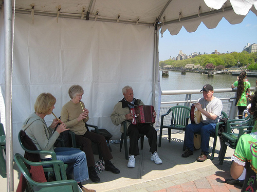
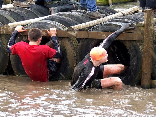
(1) A man holding a dog sitting on a bench overlooking a lake.                (2) A man and his dog watch the sunset from a bench.                       (3) A man and a dog sit on a bench near a body of water.	(1) Four elderly people sitting under a white tent playing musical instruments.                            (2) Four people playing instruments underneath a white tent.                                       (3) A group of people sit outside under a white shade tent, sitting in green lawn chairs, playing instruments with a view of a body of water behind them.	(1) One man in the hole of a tire in water, and another man getting up from the water next to him.                                     (2) Two men are playing with tires in muddy water.                                       (3) Two men climb onto tires while sitting in the muddy water.
(1) A young girl is running across the beach to get to the water.                                       (2) A little girl wearing pink is running along a beach towards the water.                                              (3) A girl at the shore of a beach with a mountain in the distance.	(1) Four people relaxing on a grassy hill overlooking a rocky valley.                                              (2) An African group of men, women, and babies pose in a field with large hills in the background.                                              (3) A group of people rest on a cliff overlooking a scenic view.	(1) A black dog springs up into a pool.                                              (2) A small black dog jumping over gates.                                              (3) A black dog sprints near the blue fence.

Figure 2: Examples of image-to-text (I2T) retrieval on the Flickr30K dataset using the using the proposed ConVSE++ approach. For each query image, we show the top-3 retrieved captions. The captions in green denote correct retrievals, and those in red denote incorrect retrievals. Top: success cases; bottom: failure cases.

IV-C1 Comparison with baselines

In Table III, we compare the proposed joint embedding ConVSE and ConVSE++ with with the baseline joint embedding methods VSE, VSE++ and an adaptation of the multi-modal contrastive loss of [29] for learning a joint image-caption embedding space. We can make following observations from these results: (a) In general, our best method ConVSE++ achieves best results. Specifically, it achieves absolute improvements of 5.0 and 10.0 respectively in R@sum on the MS-COCO and Flickr30K datasets respectively compared to the second best method. (b) The results obtained using MVN are comparable to VSE and consistently inferior to ConVSE, thus confirming the advantage of excluding the modality of the anchor point while defining negative pairs. (c) ConVSE always outperforms VSE, and ConVSE++ always outperforms VSE++. These results validate our initial hypothesis that the ability of triplet ranking loss functions in learning joint embedding spaces can be strengthened by integrating them with contrastive training, as it helps in reducing the heterogeneity gap between incompatible feature distributions of diverse modalities. (d) In general, ConVSE++ outperforms ConVSE, and VSE++ outperforms VSE. The improvements are particularly significant w.r.t. R@1 and R@5 in comparison to R@10 for both I2T and T2I and on both the datasets. These results validate that using only the hardest negative instead of all can be particularly useful in learning visual-semantic embeddings for cross-modal retrieval tasks, where it is desirable to have high accuracy among the top few retrievals.

IV-C2 Comparison with benchmark methods

In Table IV, we compare the results of cross-modal retrieval using the proposed approaches with the state-of-the-art visual-semantic embedding methods on the MS-COCO and Flickr30K datasets respectively. Note that in almost all the recent approaches, the backbone vision network is the same (i.e., ResNet-152). For both I2T and T2I tasks on the MS-COCO dataset, both ConVSE and ConVSE++ outperform all the compared methods, achieving absolute improvements of 6.7 and 15.7 respectively in R@sum. Similarly, on the Flickr30K dataset, our ConVSE++ approach outperforms all the compared approaches except the recent ITMeetsAL [46] approach where it achieves comparable results. These results demonstrate the empirical promise of using ConVSE and ConVSE++ for cross-modal retrieval compared to the existing approaches.

IV-C3 Qualitative Analyses

In Figure 2 and 3, we show some examples of image-to-text (I2T) and text-to-image (T2I) retrieval respectively. For both these tasks, we show examples of both success and failure cases. Particularly in case of incorrect retrievals, we can observe that they are semantically quite related to the corresponding query. In general, both the success as well as failure cases validate the capability of our approach in learning complex visual-semantic relationships.

Query: Chinese male on his cellphone walking through the alley.
Query: Three brown dogs are jumping up at the woman wearing blue.
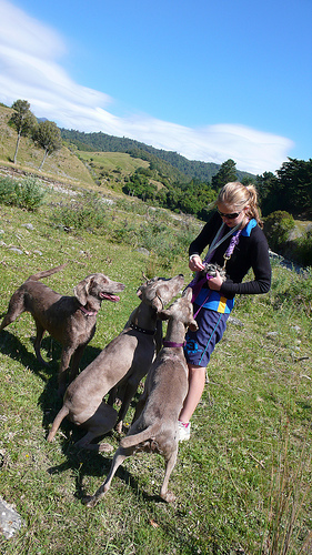
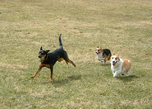
Query: A child is splashing in the water.
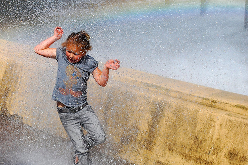
Query: A woman with a black shirt and tan apron is standing behind a counter in a restaurant.

Figure 3: Examples of text-to-image (T2I) retrieval on the Flickr30K dataset using the using the proposed ConVSE++ approach. For each query caption, we show the top-3 retrieved images (from left to right). The images with green border denote correct retrievals, and those with red border denote incorrect retrievals. The top two rows denote examples of success cases where the correct image is retrieved at rank-1, and the bottom two rows denote examples of failure cases where the correct image is not retrieved at rank-1.

V Conclusion

Triplet loss and contrastive training are two powerful paradigms for learning joint visual-semantic embeddings. In this paper, we have proposed two new formulations that integrate them in a principled way, and subsequently achieve results either better than or comparable to the state-of-the-art methods on the downstream task of cross-modal image-text retrieval. Looking at the generality of our formulations and their performance trends, we believe they can also be adopted for other cross-modal learning and matching tasks.

References

- [1] J. Weston, S. Bengio, and N. Usunier, “WSABIE: Scaling up to large vocabulary image annotation.” in IJCAI, 2011.
- [2] A. Frome, G. S. Corrado, J. Shlens, S. Bengio, J. Dean, M. A. Ranzato, and T. Mikolov, “DeViSE: A deep visual-semantic embedding model,” in Advances in Neural Information Processing Systems, 2013.
- [3] V. Ordonez, G. Kulkarni, and T. L. Berg, “Im2Text: Describing images using 1 million captioned photographs.” in NIPS, 2011.
- [4] X. Wang, Y.-F. Wang, and W. Y. Wang, “Watch, Listen, and Describe: Globally and locally aligned cross-modal attentions for video captioning.” in NAACL-HLT, 2018.
- [5] A. Karpathy and F. F. Li, “Deep visual-semantic alignments for generating image descriptions,” in IEEE Conference on Computer Vision and Pattern Recognition (CVPR), 2015.
- [6] R. Kiros, R. Salakhutdinov, and R. Zemel, “Unifying visual-semantic embeddings with multimodal neural language models,” in International Conference on Machine Learning, 2014.
- [7] M. Malinowski, M. Rohrbach, and M. Fritz, “Ask your neurons: A neural-based approach to answering questions about images.” in ICCV, 2015.
- [8] S. E. Reed, Z. Akata, H. Lee, and B. Schiele, “Learning deep representations of fine-grained visual descriptions.” in CVPR, 2016.
- [9] W. Y. Zou, R. Socher, D. M. Cer, and C. D. Manning, “Bilingual word embeddings for phrase-based machine translation.” in EMNLP, 2013, pp. 1393–1398.
- [10] D. R. Hardoon, S. Szedmak, and J. Shawe-Taylor, “Canonical correlation analysis: An overview with application to learning methods.” Neural Comput., vol. 16, no. 12, pp. 2639–2664, 2004.
- [11] N. Rasiwasia, J. C. Pereira, E. Coviello, G. Doyle, G. R. G. Lanckriet, R. Levy, and N. Vasconcelos, “A new approach to cross-modal multimedia retrieval.” in ACM MM, 2010.
- [12] A. Sharma, A. Kumar, H. D. III, and D. W. Jacobs, “Generalized multiview analysis: A discriminative latent space.” in CVPR, 2012.
- [13] N. Rasiwasia, D. Mahajan, V. Mahadevan, and G. Aggarwal, “Cluster canonical correlation analysis.” in AISTATS, 2014.
- [14] Y. Gong, Q. Ke, M. Isard, and S. Lazebnik, “A multi-view embedding space for modeling internet images, tags, and their semantics.” IJCV, vol. 106, no. 2, pp. 210–233, 2013.
- [15] V. Ranjan, N. Rasiwasia, and C. V. Jawahar, “Multi-label cross-modal retrieval.” in ICCV, 2015.
- [16] X. Shu and G. Zhao, “Scalable multi-label canonical correlation analysis for cross-modal retrieval,” Pattern Recognit., vol. 115, p. 107905, 2021.
- [17] J. Mao, W. Xu, Y. Yang, J. Wang, Z. Huang, and A. Yuille, “Deep captioning with multimodal recurrent neural networks (m-rnn),” in ICLR, 2015.
- [18] L. Wang, Y. Li, and S. Lazebnik, “Learning two-branch neural networks for image-text matching tasks,” IEEE Transactions on Pattern Analysis and Machine Intelligence, 2017.
- [19] S. Wang, D. Guo, X. Xu, L. Zhuo, and M. Wang, “Cross-modality retrieval by joint correlation learning.” ACM Trans. Multim. Comput. Commun. Appl., vol. 15, no. 2s, pp. 56:1–56:16, 2019.
- [20] F. Faghri, D. J. Fleet, J. Kiros, and S. Fidler, “VSE++: Improving visual-semantic embeddings with hard negatives,” in BMVC, 2018.
- [21] R. Socher, A. Karpathy, Q. Le, C. Manning, and A. Ng, “Grounded compositional semantics for finding and describing images with sentences,” Transactions of the Association for Computational Linguistics, vol. 2, pp. 207–218, 2014.
- [22] Y. Zhu, R. Kiros, R. Zemel, R. Salakhutdinov, R. Urtasun, A. Torralba, and S. Fidler, “Aligning books and movies: Towards story-like visual explanations by watching movies and reading books,” in IEEE International Conference on Computer Vision (ICCV), 2015.
- [23] T. Chen, S. Kornblith, M. Norouzi, and G. Hinton, “A simple framework for contrastive learning of visual representations,” in International Conference on Machine Learning, 2020.
- [24] R. D. Hjelm, A. Fedorov, S. Lavoie-Marchildon, K. Grewal, P. Bachman, A. Trischler, and Y. Bengio, “Learning deep representations by mutual information estimation and maximization,” in International Conference on Learning Representations, 2019.
- [25] O. J. Hénaff, “Data-efficient image recognition with contrastive predictive coding,” in International Conference on Machine Learning, 2020.
- [26] P. Khosla, P. Teterwak, C. Wang, A. Sarna, Y. Tian, P. Isola, A. Maschinot, C. Liu, and D. Krishnan, “Supervised contrastive learning,” in NeurIPS 2020, 2020.
- [27] T. Park, A. A. Efros, R. Zhang, and J. Zhu, “Contrastive learning for unpaired image-to-image translation,” in ECCV, 2020.
- [28] I. Misra and L. van der Maaten, “Self-supervised learning of pretext-invariant representations,” in IEEE/CVF Conference on Computer Vision and Pattern Recognition, 2020.
- [29] J. Alayrac, A. Recasens, R. Schneider, R. Arandjelovic, J. Ramapuram, J. D. Fauw, L. Smaira, S. Dieleman, and A. Zisserman, “Self-supervised multimodal versatile networks,” in NeurIPS 2020, 2020.
- [30] K. He, X. Zhang, S. Ren, and J. Sun, “Deep residual learning for image recognition,” in CVPR, 2016.
- [31] M. Engilberge, L. Chevallier, P. Pérez, and M. Cord, “Finding beans in burgers: Deep semantic-visual embedding with localization,” in IEEE/CVF Conference on Computer Vision and Pattern Recognition, 2018, pp. 3984–3993.
- [32] P.-Y. Huang, G. Kang, W. Liu, X. Chang, and A. Hauptmann, “Annotation efficient cross-modal retrieval with adversarial attentive alignment,” in Proceedings of the 27th ACM International Conference on Multimedia, 2019.
- [33] M. Bastan, A. Ramisa, and M. Tek, “T-vse: Transformer-based visual semantic embedding,” ArXiv, vol. abs/2005.08399, 2020.
- [34] Y. Chen and L. Bazzani, “Learning joint visual semantic matching embeddings for language-guided retrieval,” in ECCV, 2020.
- [35] T. Matsubara, “Target-oriented deformation of visual-semantic embedding space,” IEICE Trans. Inf. Syst., vol. 104-D, pp. 24–33, 2021.
- [36] P. Young, A. Lai, M. Hodosh, and J. Hockenmaier, “From image descriptions to visual denotations: New similarity metrics for semantic inference over event descriptions,” Transactions of the Association for Computational Linguistics, vol. 2, pp. 67–78, 2014.
- [37] T.-Y. Lin, M. Maire, S. Belongie, J. Hays, P. Perona, D. Ramanan, P. Dollár, and C. Zitnick, “Microsoft coco: Common objects in context,” in ECCV, 2014.
- [38] D. P. Kingma and J. Ba, “Adam: A method for stochastic optimization,” CoRR, vol. abs/1412.6980, 2015.
- [39] L. Wang, Y. Li, and S. Lazebnik, “Learning deep structure-preserving image-text embeddings,” in IEEE Conference on Computer Vision and Pattern Recognition (CVPR), 2016.
- [40] Y. Huang, W. Wang, and L. Wang, “Instance-aware image and sentence matching with selective multimodal lstm,” in IEEE Conference on Computer Vision and Pattern Recognition (CVPR), 2017.
- [41] Y. Liu, Y. Guo, E. M. Bakker, and M. S. Lew, “Learning a recurrent residual fusion network for multimodal matching,” in IEEE International Conference on Computer Vision (ICCV), 2017.
- [42] H. Nam, J.-W. Ha, and J. Kim, “Dual attention networks for multimodal reasoning and matching,” in IEEE Conference on Computer Vision and Pattern Recognition (CVPR), 2017.
- [43] Y. Zhang and H. Lu, “Deep cross-modal projection learning for image-text matching,” in Proceedings of the European Conference on Computer Vision (ECCV), 2018.
- [44] N. Sarafianos, X. Xu, and I. Kakadiaris, “Adversarial representation learning for text-to-image matching,” in IEEE/CVF International Conference on Computer Vision (ICCV), 2019.
- [45] Z. Zheng, L. Zheng, M. Garrett, Y. Yang, M. Xu, and Y.-D. Shen, “Dual-path convolutional image-text embeddings with instance loss,” ACM Trans. Multim. Comput. Commun. Appl., vol. 16, no. 2, pp. 1–23, 2020.
- [46] W. Chen, Y. Liu, E. M. Bakker, and M. S. Lew, “Integrating information theory and adversarial learning for cross-modal retrieval,” Pattern Recognition, vol. 117, p. 107983, 2021.