Fractality in Cosmic Topology Models with Spectral Action Gravity

Abstract.

We consider cosmological models based on the spectral action formulation of (modified) gravity. We analyze the coupled effects, in this model, of the presence of nontrivial cosmic topology and of fractality in the large scale structure of spacetime. We show that the topology constrains the possible fractal structures, and in turn the correction terms to the spectral action due to fractality distinguish the various cosmic topology candidates, with effects detectable in a slow-roll inflation scenario, through the power spectra of the scalar and tensor fluctuations. We also discuss explicit effects of the presence of fractal structures on the gravitational waves equations.

1. Introduction

The paper is organized in the following way. In this introductory section we review the (modified) gravity model based on the spectral action functional, and we introduce the question of cosmic topology and the question of the possible presence of fractality in the large scale structure of the universe. These two problems have so far been investigated as separate questions in theoretical cosmology, while our goal here is to focus on the combined effects of the presence of both cosmic topology and fractality.

In Section 2 we present Sierpinski constructions that are suitable for describing fractality within each of the possible spherical and flat cosmic topology candidate. These Sierpinski constructions are based on the polyhedral fundamental domains (in the $3$-sphere or in the $3$-torus) for these cosmic topology candidates. For each of these cases, we then compute the spectral action expansion, first in a simplified static model and then in the actual Robertson–Walker model. We identify the correction terms to the spectral action that arise due to the presence of fractality and we show the resulting effect on an associated slow-roll potential arising as a scalar perturbation of the Dirac operator in the spectral action. We show that the presence of fractality determines detectable effects that suffice to distinguish between all the possible cosmic topology candidates. We also discuss other, Koch-type, forms of fractal growth and we state a general question regarding the construction of fractal structures on manifolds, to which we hope to return in future work.

In Section 3 we discuss the original type of fractal arrangement of the Packed Swiss Cheese Cosmology model, in the case of the sphere topology, which is modelled on Apollonian sphere packings. We discuss here in particular some arithmetic cases of packings with integer curvatures, for which the zeta function is computable explicitly. We show that, in these cases, an interesting connection emerges between the form of the asymptotic expansion of the spectral action and series of number theoretic interest, involving the derivative of the Riemann zeta function at the non-trivial zeros. We also discuss how the fractality models based on sphere packings are not stable under small random perturbations of the geometry, which would lead to intersecting spheres, while we propose that fractal models based on “cratering” (removal of a random collection of spheres creating a fractal residual set) can provide a version of these fractal arrangements of sphere that is stable under the introduction of some randomness factor.

In Section 4 we investigate effects of the presence of fractality on the gravitational wave equations. In this first section on this topic, we consider the usual GR equations, without additional modified gravity terms from the spectral action, and we look at the kind of model of sphere arrangements that we proposed in the previous section, where some of the spheres are intersecting. We show that, in such a model, there is transmission of gravitational waves between the different spheres across their intersection, creating oscillations inside the sphere of intersection. Thus, multiple gravitational wave sources near the intersection would induce a $3$-ball of interfering gravity wave modes on the boundary hypersurface.

In Section 5 we continue investigating effects of fractality on the gravitational waves. In this section we focus more specifically on the gravitational waves equation arising from the spectral action, and we consider the fractal structures investigated in Section 2 for Robertson-Walker spacetimes associated to the various cosmic topology candidates. We focus on the effect on the gravitational waves equation of the correction terms to the spectral action due to fractality, with particular attention to the contribution of the first term of the series coming from the poles of the fractal zeta function, the one associated to the pole $s_{0}$ given by the self-similarity dimension. We show that the variation of the metric determines a tensor given by the corresponding variation of the value at $s_{0}$ of the zeta function of the Dirac operator on the Robertson-Walker geometry. This tensor plays the role of an energy-momentum tensor in the equations, so that the presence of fractality emulates the presence of a type of matter than only interacts gravitationally but is otherwise dark.

1.1. Spectral Action model of gravity

The spectral action functional as a model of gravity originates in noncommutative geometry [7], where it provides a setting for the construction of geometric models of gravity coupled to matter, [8] (see also [60] and Chapter 1 of [14] for an overview).

The main underlying geometric setting is given by spectral triples, [13], which provide a generalization of Riemannian spin geometry to the noncommutative setting.

A spectral triple $(A,H,D)$ consists of an involutive algebra $A$, with a representation $\pi:A\to B(H)$ as bounded operators on a complex Hilbert space $H$, and a self-adjoint operator $D$ on a dense domain in $H$, with compact resolvent. The compatibility condition between the algebra and the Dirac operator is expressed as the property that the commutators $[D,\pi(a)]$ are bounded operators for all $a\in A$. The spectral action functional of a spectral triple is defined as

(1.1) $${\mathcal{S}}_{\Lambda}(D):={\rm Tr}(f(\frac{D}{\Lambda})).$$

Here the Dirac operator is the dynamical variable of the spectral action functional, with $\Lambda>0$ an energy scale that makes the integral unitless and $f$ is an even smooth function of rapid decay.

The test function $f$ is a smooth approximation to a cutoff function that regularizes the (otherwise divergent) trace of the Dirac operator. For example, it is convenient to take the test function to be of the form

(1.2) $$f(x)=\int_{0}^{\infty}e^{-tx^{2}}\,dm(t)$$

where $dm(t)$ is some measure on ${\mathbb{R}}_{+}$.

The properties of a spectral triple recalled above include the requirements that $D$ is self-adjoint and with compact resolvent, which imply the discreteness of the spectrum ${\rm Spec}(D)\subset{\mathbb{R}}_{+}$, so that the definition (1.1) makes sense. The main idea here is that gravity is encoded geometrically through the Dirac operator, rather than in the metric tensor, as in the usual formutation of general relativity. The usual Einstein-Hilbert action functional of general relativity is recovered from the spectral action through its asymptotic expansion for large $\Lambda\to\infty$, as we recall in more detail below, along with other higher derivatives terms that make the spectral action into an interesting modified gravity model.

As a prototype (commutative) example of a spectral triple, one should think of $A={\mathcal{C}}^{\infty}(X)$ as the algebra of smooth functions on a compact Riemannian spin manifold $X$, with $H=L^{2}(X,{\mathbb{S}})$ the Hilbert space of square-integrable spinors, and $D=\not{D}_{X}$ the Dirac operator. This example immediately illustrates two delicate points in the use of the spectral triples formalism in relation to cosmological model: compactness and Euclidean signature. Indeed, taken in itself, the spectral action model of gravity that we will summarize in the rest of this section is a model of Euclidean gravity, which moreover requires a compactness hypothesis. This seems ill suited for modeling realistic spacetimes. However, as we discuss below, the asymptotic expansion of the spectral action provides local gravity terms that still make sense when Wick rotated to Lorentzian signature, and in more general geometries (for example with suitable boundary terms as discussed in [27]).

Thus, one should view spectral geometry models of gravity in the following way: one uses Wick rotation to Euclidean signature and compactification as a computational device to achieve the desired analytic properties of the Dirac operator that are required for the definition and main features of the spectral action functional. The terms then obtained from the expansion of the spectral action can be interpreted in the original geometry, so that conclusions about cosmological models can be derived. In this paper we will work with explicit examples constructed using Riemannian metrics and compactified spacetimes, which will be sufficient to illustrate the main phenomena we are interested in, through the computation of the spectral action expansion.

The asymptotic expansion of the spectral action is closely related to the associated heat kernel expansion for the square $D^{2}$ of the Dirac operator. Assuming that the operator $D^{2}$ has a small time heat kernel expansion

(1.3) $${\rm Tr}(e^{-tD^{2}})\sim_{t\to 0}\sum_{\alpha}a_{\alpha}(D)t^{\alpha},$$

using a test function of the form (1.2) gives a corresponding expansion of the spectral action as

(1.4) $${\rm Tr}(f(\frac{D}{\Lambda}))\sim_{\Lambda\to\infty}a_{0}f(0)+\sum_{\alpha}{\mathfrak{f}}_{\alpha}c_{\alpha}\Lambda^{-\alpha},$$

with

$${\mathfrak{f}}_{\alpha}=\left\{\begin{array}[]{ll}\int_{0}^{\infty}f(v)v^{-\alpha-1}dv&\alpha<0\\ (-1)^{\alpha}f^{(\alpha)}(0)&\alpha>0\,.\end{array}\right.$$

We refer the reader to [7], [60] for details.

There is a well known Mellin transform relation between the heat kernel and the zeta function of the Dirac operator,

(1.5) $$|D|^{-s}=\frac{1}{\Gamma(s/2)}\int_{0}^{\infty}e^{-tD^{2}}t^{s/2-1}dt$$

so that

$$\zeta_{D}(s)={\rm Tr}(|D|^{-s})\sim\sum_{\alpha}\frac{a_{\alpha}}{\Gamma(s/2)}\int_{0}^{\infty}t^{\alpha+s/2-1}dt\,.$$

For $\alpha<0$, the values $s=-2\alpha$ correspond to poles of $\zeta_{D}(s)$ with

$${\rm Res}_{s=-2\alpha}\zeta_{D}(s)=\frac{2a_{\alpha}}{\Gamma(-\alpha)}.$$

Thus, one can express the coefficients of the leading terms (the case $\alpha<0$) in the spectral action expansion in terms of residues of the Dirac zeta function. At each of these residues one has an associated notion of integration, defined as

$$\fint a|D|^{-\beta}:={\rm Res}_{s=\beta}\zeta_{a,D}(s)={\rm Res}_{s=\beta}{\rm Tr}(\pi(a)|D|^{-s}),$$

and the set of points $\beta$ where the zeta functions $\zeta_{a,D}(s)$ have poles is refereed to as the dimension spectrum of the spectral triple. In the case of the commutative or almost-commutative geometries used in models of gravity and matter, these integrals at the points of the dimension spectrum correspond to local terms given by integration of certain curvature forms on the underlying manifold, which recover the classical form of various physical action functionals.

In the case of the spectral triple $({\mathcal{C}}^{\infty}(X),L^{2}(X,{\mathbb{S}}),\not{D}_{X})$ for a smooth compact Riemannian spin manifold of dimension $\dim X=4$ the leading terms in the asymptotic expansion of the spectral action are of the forrm

$$Tr(f(\not{D}_{X}/\Lambda))\sim{\mathfrak{f}}_{2}\Lambda^{2}\fint|D|^{-2}+{\mathfrak{f}}_{4}\Lambda^{4}\fint|D|^{-4}+f(0)\zeta_{D}(0)+o(1),$$

with

$${\mathfrak{f}}_{2}\Lambda^{2}\fint|D|^{-2}=\frac{96{\mathfrak{f}}_{2}\Lambda^{2}}{24\pi^{2}}\int_{X}R\,\,dvol(g),$$

$${\mathfrak{f}}_{4}\Lambda^{4}\fint|D|^{-4}=\frac{48{\mathfrak{f}}_{4}\Lambda^{4}}{\pi^{2}}\int_{X}\,dvol(g),$$

$$f(0)\zeta_{D}(0)=(\frac{{\mathfrak{f}}_{0}}{10\pi^{2}}\int_{X}\frac{11}{6}R^{*}R^{*}-3C_{abcd}C^{abcd})\,dvol(g),$$

where $C_{abcd}$ is the Weyl curvature tensor and $R^{*}R^{*}$ is the Gauss-Bonnet term. Thus, in this case one obtains as leading terms the Einstein-Hilbert action with cosmological term, with an additional modified gravity term, involving conformal and Gauss–Bonnet gravity. The effect of these modified gravity terms on the gravitational waves equations was analyzed in [44].

Cosmological and gravitational models based on the spectral action functional were considered, for instance, in [2], [4], [5], [10], [16], [17], [18], [19], [37], [38], [39], [40], [41], [42], [45], [46], [59], though this is certainly not an exhaustive list of references on the subject. The main goal of the present paper is to continue this investigation by combining the analysis of cosmic topology effects considered in [5], [41], [42], with the analysis of the effect of multifractal structures considered in [2] and [18].

1.2. Cosmic Topology

The problem of cosmic topology in theoretical cosmology aims at identifying possible signatures of the presence of non-trivial topology on the spatial hypersurfaces of the spacetime manifold modeling our universe. The main focus of investigation is possible signatures that may be detectable in the cosmic microwave background (CMB). Observational constraints favor a spatial geometry that is either flat or slightly positively curved, while the negatively curved case of hyperbolic $3$-manifolds is observationally disfavoured. Thus, under the assumption of (large scale) homogeneity, the possible candidate cosmic topologies are either spherical space forms, namely quotients $Y=S^{3}/\Gamma$ of the round constant positive curvature $3$-sphere by a finite group of isometries, or (under the compactness assumption we work with in our spectral gravity model) the Bieberbach manifolds that are quotients $Y=T^{3}/\Gamma$ of the flat $3$-torus by a group of isometries.

For a general overview of the problem of cosmic topology, we refer the reader to [34], and also [1], [35], [36], [51]. The cosmic topology question was studied within the framework of spectral action models of gravity in [5], [37], [38], [41], [42], [59].

The main way in which the presence of nontrivial cosmic topology may be detectable, in the case of a model of gravity based on the spectral action functional, is through a slow-roll potential for cosmic inflation that arises in the model as a scalar perturbation of the Dirac operator.

In a slow-roll inflation model, the power spectra ${\mathcal{P}}_{s}$ and ${\mathcal{P}}_{t}$ of the scalar and tensor perturbations of the metric have a dependence on the shape of the slow-roll potential $V$. More precisely, the fluctuations, as a function of the Fourier modes, obey a power law

$${\mathcal{P}}_{s}(k)\sim{\mathcal{P}}_{s}(k_{0})(k/k_{0})^{1-n_{s}+\frac{\alpha_{s}}{2}\log(k/k_{0})}\ \ \ \text{ and }\ \ \ {\mathcal{P}}_{t}(k)\sim{\mathcal{P}}_{t}(k_{0})(k/k_{0})^{1-n_{t}+\frac{\alpha_{t}}{2}\log(k/k_{0})}\,,$$

where the exponents $n_{s},n_{t},\alpha_{s},\alpha_{t}$ are linear functions of the slow-roll parameters $\epsilon,\eta,\xi$, whose dependence on the potential $V$ is as follows, up to a numerical factor that depends on a power of the Planck mass,

$$\epsilon\sim\left(\frac{V^{\prime}}{V}\right)^{2},\ \ \ \eta\sim\frac{V^{\prime\prime}}{V},\ \ \ \xi\sim\frac{V^{\prime}V^{\prime\prime\prime}}{V^{2}}\,.$$

On the other hand, the amplitudes also depend on the shape of the potential as

$${\mathcal{P}}_{s}\sim\frac{V^{3}}{(V^{\prime})^{2}}\ \ \ \text{ and }\ \ \ {\mathcal{P}}_{t}\sim V\,,$$

again up to a constant factor given by a power of the Planck mass, see [56] and also the discussion in Section 1 of [42].

It is shown in [42] that a scalar perturbation ${\mathcal{D}}^{2}\mapsto{\mathcal{D}}^{2}+\phi^{2}$ of the Dirac operator in the spectral action determines a slow-roll potential $V(\phi)$, which exhibits the typical flat plateau of slow-roll inflation models. The potential is computed explicitly for the candidate cosmic topologies in both the spherical and the flat case. The result is that the resulting slow-roll parameters $\epsilon,\eta,\xi$ are the same within each curvature class, namely the same for all the spherical space form and the same for all the Bieberbach manifolds, but different for the two classes, hence they distinguish whether the geometry is flat or positively curved. Within each class, the amplitudes differ by a factor, which is the order of the group in the spherical case and a numerical factor depending on the group and the shape of the fundamental domain in the Bieberbach case. These further amplitude values do not distinguish all cases. For example, in the spherical case some lens spaces can have, by concidence, the same order of the group as one of the other non-isomorphism spherical space forms.

In this paper, we refine this model by assuming that the universe can exhibit, at the same time, non-trivial cosmic topology and a fractal structure, where the self-similarity of the fractal structure now necessarily depends on the topology, through the shape of the fundamental domain of the candidate topology. We discuss fractality in the following subsection. We show in this paper that this combination of cosmic topology and fractality resolves the ambiguities and the slow-roll potential generated by the spectral action now completely distinguished all the possible cosmic topologies.

1.3. Multifractal cosmological models

The standard cosmological paradigm, or Cosmological Principle, postulates that (at sufficiently large scales) the universe should be homogeneous and isotropic. A homogeneous spacetime $(X,g)$ is one that can be foliated by a one-parameter family of spatial hypersurfaces, with the property that any two points in each hypersurface can be transported to the other along an isometry of the metric. In other words, this is the assumption that there is no “special place” in the universe. The other assumption, isotropy, requires that at any point $p\in X$, given two vectors $v_{1},v_{2}$ orthogonal to a timelike curve passing through $p$, we can find an isometry rotating $v_{1}$ into $v_{2}$. This corresponds to the idea that there is no “special direction” in the universe.

A first possible clue that the homogeneity hypothesis may fail even at very large scales came from the distribution of galaxy clusters. Statistical analysis in [58] showed fractal correlations up to the observational limits. Similarly, in [22] it is shown that all clustering observed have scaling and fractal properties, which cannot be properly described by small-amplitude fluctuations theory. However, as emphasized in [58], [22], the presence of fractality in large scale spacetime is still an undetermined question in cosmology. A new generation of cosmology probes may be able to give us an answer in larger scales.

A theoretical model of spacetime exhibiting multifractal structures is provided by the Packed Swiss Cheese Cosmology models, see [43]. This model originates from an idea of Rees and Sciama, [50], that generated inhomogeneities by altering a standard Robertson–Walker cosmology through the removal of a configuration of balls. In the Packed Swiss Cheese Cosmology model this is done so that the resulting spacetime is described by the geometry of an Apollonian packing of spheres.

In [2] and [18] the Packed Swiss Cheese Cosmology models are analyzed from the point of view of spectral action gravity and it is shown that the presence of fractality is detectable in the form of additional terms in the spectral action, coming from poles of the zeta function off the real line and from the non-integer Hausdorff dimension, as well as in a modification to the effective gravitational and cosmological constants of the terms of the action coming from the underlying Robertson–Walker cosmology. This analysis is done in [2] in the case of a static model, and in [18] in the more general case of a Robertson–Walker cosmology with a nontrivial expansion/contraction factor.

One of the mathematical difficulties in describing a model of gravity with fractality lies in the fact that one cannot directly describe such spaces in terms of ordinary differential geometry, because of their fractal nature. One needs a generalization of Riemannian geometry that applies to non-manifold structures like fractals. Even though fractals are ordinary commutative spaces, the fact that they are not smooth manifolds makes them amenable to the tools of noncommutative geometry: although these methods were originally designed to apply to noncommutative spaces, they also apply to commutative but non-smooth spaces like fractals. In particular, fractals such as Apollonian packings of spheres, various Sierpinski-type constructions, Koch curves and their higher-dimensional analogs, and other such geometries, are well described by the formalism of spectral triples, hence they have a well defined gravity action functional given by the spectral action. This shows that the spectral action model of gravity is the most directly suitable for the description of gravity in the presence of fractality and of cosmology in fractal spacetimes.

The main question we focus on in this paper is how the effects of fractality (multifractal cosmologies) and of nontrivial topology (cosmic topology) combine in the spectral action model of gravity. We will consider various relevant examples of fractal geometries, including the Apollonian packings of spheres and fractal arrangements obtained from various kinds of solids representing fundamental domains of cosmic topology models, and we will show how the effects of fractality vary in different topological background and, conversely, how the effect of nontrivial topology of the spacelike hypersurfaces are affected by the presence of fractality.

2. Fractality and Topology in static models and in Robertson-Walker models

In this section we consider different candidate cosmic topology models, first in the spherical and then in the flat case, with two models of spacetime: a simplified static model based on a product $Y\times S^{1}$ with circle compactification, and then a more realistic Robertson–Walker model on a cylinder $Y\times{\mathbb{R}}$ with an expansion/contraction factor $a(t)$. We compute the asymptotic expansion of the spectral action in all of these cases, along the lines of [2] for the static model and of [18] for the Robertson–Walker case. For every cosmic topology candidate we identify a corresponding possible fractal structure, based on a Sierpinski construction associated to the fundamental domain in the $3$-sphere (or the $3$-torus, respectively). We compute how the presence of fractality affects the spectral action expansion in each of these cases. We show that these correction terms coming from fractality suffice for the spectral action (and the associated slow-roll potential) to distinguish all the possible cosmic topology candidates. The main mathematical tools in these calculations are the Poisson summation formula and the Feynman–Kac formula.

At the end of this section we also analyze other models of fractal growth based on polyhedral domains, modelled on the case of the Koch snowflake. We discuss Koch-type constructions based on tetrahedra and octahedra and compute the associated zeta functions. We discuss the related problem of constructing fractal structures on more general manifolds that are not quotients with polyhedral fundamental domains.

2.1. Static model

The first case we analyze is the static model considered in [2], where the spacetime (Euclidean and compactified) is taken to be of the form $S^{1}_{\beta}\times{\mathcal{P}}$, where $\beta>0$ is the radius of the circle-compactification and the spacelike hypersurfaces are given by a fractal arrangement ${\mathcal{P}}$. The main case discussed in [2] was with ${\mathcal{P}}$ an Apollonian packing of $3$-spheres, but Section 5 of [2] also discusses an exactly-self-similar model where ${\mathcal{P}}$ is a fractal arrangement of dodecahedra, giving rise to a dodecahedral-space cosmic topology model with fractality. Our goal in this subsection is to extend the analysis of Section 5 of [2] by comparing fractal arrangements based on different candidate cosmic topology models and describe how the different topology affects the contribution of fractality to the spectral action functional. From the purely mathematical perspective, the results of this subsection rely essentially on a combination of earlier results proved in [2], [5], [41], [42]. We also correct here an inaccuracy in Proposition 5.2 of [2] and we provide a more detailed discussion of the (weak) convergence of the series of the log-periodic terms.

2.1.1. The fractal arrangements

The general setting here is the following. Consider a spherical $3$-manifold of the form $Y=S^{3}/\Gamma$, where $\Gamma$ is a finite group of isometries of $S^{3}$, which can be identified with the symmetry group of a platonic solid ${\mathbb{P}}_{\Gamma}$. These manifolds cover the main significant candidate for positively curved cosmic topologies (with the exclusion of lens spaces, which we will discuss separately). For each of these candidate models, we then construct a Sierpinski fractal, $\mathcal{P}_{\Gamma}$, using the appropriate construction rules associated with the underlying platonic solid ${\mathbb{P}}_{\Gamma}$ with symmetry group $\Gamma$. Each Sierpinski construction yields a scaling factor and a replication factor, which we will denote by $\frac{1}{f_{\sigma}}$ and $f_{\rho}$, respectively. We can identify ${\mathbb{P}}_{\Gamma}$ with a fundamental domain of the action of $\Gamma$ on $S^{3}$ and, with the closed $3$-manifold $Y$ obtained by gluing together the faces of this solid according to the action of $\Gamma$. In this way the fractal arrangement ${\mathcal{P}}_{\Gamma}$ of polyhedra ${\mathbb{P}}_{\Gamma}$ gives rise to a fractal arrangement ${\mathcal{P}}_{Y}$ of copies of $Y$.

2.1.2. The Sierpinski construction

We recall here the main examples of Sierpinski constructions, [28]. Our goal is to compare the effects on the spectral action functional and the associated slow-roll potentials of the different fractal arrangements associated to different candidate cosmic topologies. We compare the candidate topologies given by spherical forms $Y=S^{3}/\Gamma$. These are quotients by a finite subgroup $\Gamma\subset SU(2)$. According to the classification of such subgroups, [64], there are two infinite families, cyclic groups $Z_{n}$ and binary dihedral groups $D^{*}_{n}$, and three additional cases, the binary tetrahedral group $T$, binary octahedral group $O$, and binary icosahedral group ${\mathcal{I}}$. In the case of cyclic groups $Z_{n}$ one obtains a lens space $Y=L(n,1)$, with fundamental domain a lens-shaped spherical solid (see Figure 1). The sphere $S^{3}$ is tiled by $n$ copies of this fundamental domain. In the case of the binary dihedral group $D_{n}^{*}$, the quotient $Y$ is a prism manifold, where the fundamental domain is a prism with $2n$ sides, $4n$ of which tile the sphere (see Figure 1). In the three last cases, the fundamental domain is given, respectively, by a (spherical) octahedron, a truncated cube (cuboctahedron), and a spherical dodecahedron. The sphere $S^{3}$ is tiled by $24$ copies of the octahedron, by $48$ copies of the truncated cube, and by $120$ copies of the dodecahedron. We describe fractal Sierpinski constructions for various such spaces. We first discuss the case of the two regular solids, octahedron and dodecahedron, then the Archimedean case (the cuboctahedron), and then the case of lenses and prisms. General Sierpinski constructions for polyhedra, and in particular for regular solids, are described in [28], [31], [30], [32], [33].

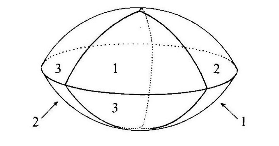
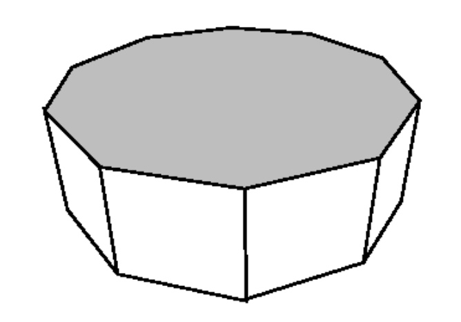
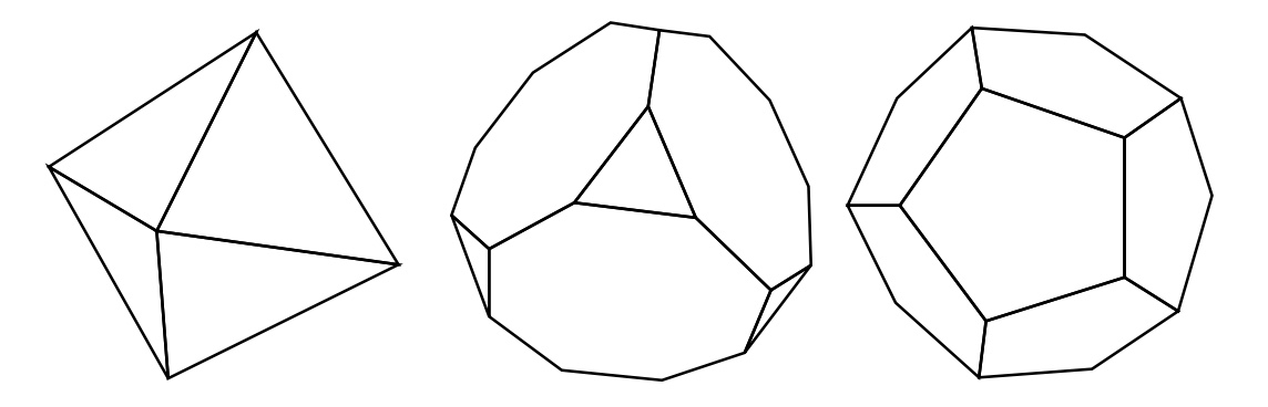
Figure 1. Fundamental domain for the lens space $L(3,1)$ with face identifications; fundamental domain of the prism manifold of the binary dihedral group $D_{5}^{*}$ of order $20$; fundamental domains for the binary tetrahedral, binary octahedral, and binary icosahedral group.

Figure 2. The first step of the Sierpinski construction for octahedron and dodecahedron, and for the cuboctahedron.

The binary tetrahedral group $T\subset SU(2)$, with $|T|=24$, can be identified with the group of units in the ring of Hurwitz integers

$$T=\{\pm 1,\pm i,\pm j,\pm k,{\tfrac{1}{2}}(\pm 1\pm i\pm j\pm k)\}.$$

Its action on $S^{3}$ has fundamental domain given by a spherical octahedron. A fractal arrangement for this case can therefore be obtained by considering a Sierpinski construction of octahedra, as illustrated in Figure 2. Each step of this Sierpinski construction replaces each octahedron of the previous step with $6$ identical copies scaled by a scaling factor of $1/2$. Thus, in this case we have $f_{\rho}=6$ and $f_{\sigma}=2$ and the self-similarity dimension, which for these regular constructions equals the Hausdorff dimension, is

$$\dim_{H}{\mathbb{P}}_{T}=\frac{\log f_{\rho}}{\log f_{\sigma}}=\frac{\log 6}{\log 2}\,.$$

The resulting fractal arrangement ${\mathcal{P}}_{T}$ is the fractal obtained as fixed point of the iteration of this construction, and the arrangement ${\mathcal{P}}_{Y}$ is then obtained by closing up all the octahedra in ${\mathcal{P}}_{T}$ according to the action of $T$ on its fundamental domain, to give copies of $Y$.

The other regular solid is the dodecahedron, which is the fundamental domain for the binary icosahedral group ${\mathcal{I}}$. The first step of a Sierpinski construction of dodecahedra is illustrated in Figure 2. Here at each step the dodecahedra of the previous step are replaced with $20$ identical copies scaled by a factor of $(2+\phi)^{-1}$ where $\phi=\frac{1+\sqrt{5}}{2}$ is the golden ratio. This is the same Sierpinski construction considered in §5 of [2]. One has $f_{\rho}=20$ and $f_{\sigma}=2+\phi$ and

$$\dim_{H}{\mathbb{P}}_{\mathcal{I}}=\frac{\log f_{\rho}}{\log f_{\sigma}}=\frac{\log 20}{\log(2+\phi)}\,.$$

A similar Sierpinski construction can be done for Archimedean solids, [31]. In the case of the cuboctahedron, which is the fundamental domain of the the binary octahedral group $O$, with $|O|=48$, the first step of the Sierpinski construction is also illustrated in Figure 2. In this case one replaces a cuboctahedron with $12$ identical copies with a scaling factor of $1/3$, so that $f_{\rho}=12$ and $f_{\sigma}=3$ and

$$\dim_{H}{\mathbb{P}}_{O}=\frac{\log f_{\rho}}{\log f_{\sigma}}=\frac{\log 12}{\log 3}\,.$$

Figure 3. Second step of the Sierpinski construction of an hexaflake.

A Sierpinski construction suitable for handling the case of cyclic groups (lens spaces) and of binary dihedral groups (prism manifolds) can be obtained by considering planar Sierpinski constructions for the underlying polygons and obtain from those an associated Sierpinski construction for the respective lenses/prisms. In a Sierpinski $n$-polygon (also known as an $n$-polyflake), see [15], a regular $n$-polygon is replaced by $f_{\rho}(n)=n$ copies scaled by a factor $1/f_{\sigma}$ with

$$f_{\sigma}(n)=2\left(1+\sum_{k=1}^{\lfloor n/4\rfloor}\cos(\frac{2\pi k}{n})\right).$$

For example, the second step of the Sierpinski construction of the hexaflake is illustrated in Figure 3. For the hexaflake $f_{\rho}(6)=6$ and $f_{\sigma}(6)=3$.

Given a Sierpinski $n$-polygon (respectively, $2n$-polygon), we can obtain a fractal arrangement ${\mathbb{P}}_{Z_{n}}$ (respectively, ${\mathbb{P}}_{D_{n}^{*}}$) of lenses/prisms, by building either a lens (double cone) or a prism (product with an interval) over each polygon in the construction and a corresponding fractal arrangement of lens spaces or prism manifolds ${\mathcal{P}}_{Y}$, by closing up each lens/prims in the construction according to the face identifications specified by the group action. So we have

$$\dim_{H}{\mathcal{P}}_{Z_{n}}=\frac{\log n}{\log(f_{\sigma}(n))}\ \ \ \text{ and }\ \ \ \dim_{H}{\mathcal{P}}_{D_{n}^{*}}=\frac{\log(2n)}{\log(f_{\sigma}(2n))}.$$

2.1.3. The spectral triple

We then construct spectral triples associated to these arrangements ${\mathcal{P}}_{Y}$, as done in [2], modelled on the spectral triples of Sierpinski gaskets constructed in [11], [12]. Namely, to a fractal arrangement ${\mathcal{P}}_{Y}$ where the building blocks are manifolds $Y_{a_{n}}$ scaled by a sequence of scaling factors (radii) $a_{n}$, we assign a spectral triple of the form

$$(\mathcal{A}_{\mathcal{P}_{Y}},\mathcal{H}_{\mathcal{P}_{Y}},\mathcal{D}_{\mathcal{P}_{Y}})=(\mathcal{A}_{\mathcal{P}_{Y}},\oplus_{n}\mathcal{H}_{Y_{a_{n}}},\oplus_{n}\mathcal{D}_{Y_{a_{n}}})$$

Where $Y_{a_{n}}=S^{3}_{a_{n}}/\Gamma$, with $S^{3}_{a_{n}}$ a sphere with radius $a_{n}$, with the sequence $\{a_{n}\}$ of radii determined by the Sierpinski construction. The algebra $\mathcal{A}_{\mathcal{P}_{Y}}\subset\oplus_{n}C(Y_{a_{n}})$ is given by collections of functions in $C(Y_{a_{n}})$ that agree on all the points of contact between different $Y_{a_{n}}$ in the packing ${\mathcal{P}}_{Y}$, and each component Hilbert space is $\mathcal{H}_{Y_{a_{n}}}=L^{2}(Y_{a_{n}},\mathbb{S})$.

2.1.4. The zeta function

As discussed in [2], the zeta function of the Dirac operator ${\mathcal{D}}_{{\mathcal{P}}_{Y}}=\oplus_{n}\mathcal{D}_{Y_{a_{n}}}$ factorizes as a product of the zeta function $\zeta_{{\mathcal{D}}_{Y}}(s)$ of the quotient $Y=S^{3}/\Gamma$ of the sphere of radius one, and the zeta function of the fractal string ${\mathcal{L}}_{\Gamma}=\{a_{n}\}$ given by the sequence of the radii of the packing ${\mathcal{P}}_{\Gamma}$,

(2.1) $$\zeta_{{\mathcal{D}}_{{\mathcal{P}}_{Y}}}(s)=\zeta_{{\mathcal{L}}_{\Gamma}}(s)\cdot\zeta_{{\mathcal{D}}_{Y}}(s),$$

where

(2.2) $$\zeta_{{\mathcal{L}}_{\Gamma}}(s):=\sum_{n}a_{n}^{s}.$$

Indeed, we have

$$\zeta_{{\mathcal{D}}_{{\mathcal{P}}_{Y}}}(s)={\rm Tr}(|\mathcal{D}_{\mathcal{P}_{Y}}|^{-s})=\sum_{n}{\rm Tr}(|{\mathcal{D}}_{Y_{a_{n}}}|^{-s})=\sum_{n}a_{n}^{s}\,\,\zeta_{\mathcal{D}_{Y}}(s),$$

where the last identity follows from the fact that, if the length scales by a factor of $a>0$, the Dirac eigenvalues scale by a factor of $a^{-1}$.

2.1.5. The fractal string zeta function

Thus, in the specific case of the Sierpinski constructions ${\mathcal{P}}_{\Gamma}$ associated to the polyhedra ${\mathbb{P}}_{Y}$, the sequence of radii of the packing can be described as a set

$${\mathcal{L}}_{\Gamma}=\{a_{n,k}\,|\,n\in{\mathbb{N}},\,\,k\in\{1,2,...,f_{\rho}^{n}\}\},$$

with $f_{\rho}$ the replication factor of the Sierpinski construction. Moreover, because these are exact self-similar constructions, where the scaling is uniform across any $n$, we have, at level $n$,

$$a_{n,k}=a\cdot f_{\sigma}^{-n}$$

for some $a>0$ and for all $k=1,\ldots,f_{\rho}^{n}$, so that we obtain the very simple expression

(2.3) $$\zeta_{{\mathcal{L}}_{\Gamma}}(s)=\sum_{n,k}a_{n,k}^{s}=a^{s}\sum_{n=1}^{\infty}f_{\rho}^{n}f_{\sigma}^{-sn}=\frac{a^{s}}{1-f_{\rho}f_{\sigma}^{-s}}.$$

2.1.6. The manifold zeta function and the spectral action

First consider the zeta function $\zeta_{\mathcal{D}_{Y}}(s)$ for the Dirac operator on the $3$-manifold $Y=S^{3}/\Gamma$. Note that, while on $S^{3}$ there is a unique (trivial) spin structure, the manifold $Y$ has different choices of spin structures, each with its own Dirac operator, and the Dirac spectrum is dependent on the choice of the spin structure. However, as shown in [59], there are cancellations that happen when summing over the spectrum that make the resulting spectral action independent of the spin structure, so that the spectral action simply satisfies, as $\Lambda\to\infty$

(2.4) $${\mathcal{S}}_{\Lambda}({\mathcal{D}}_{Y})\sim\frac{1}{|\Gamma|}\,{\mathcal{S}}_{\Lambda}({\mathcal{D}}_{S^{3}}).$$

In fact, in [5] it is shown that this identity for the spectral action follows from the relation between the heat kernel of ${\mathcal{D}}_{Y}^{2}$ and the heat kernel for ${\mathcal{D}}_{S^{3}}^{2}$, which is of the form (Lemma 3.9 of [5])

(2.5) $${\rm Tr}(e^{-t{\mathcal{D}}_{Y}^{2}})=\frac{1}{|\Gamma|}{\rm Tr}(e^{-t\\ cD_{S^{3}}^{2}})+\frac{1}{|\Gamma|}\sum_{\gamma\in\Gamma\smallsetminus\{e\}}\int_{S^{3}}{\rm tr}(\rho(\gamma)(x\gamma^{-1})K_{S^{3}}(t,x\gamma^{-1},x)dvol_{S^{3}}(x).$$

Note that the Mellin transform relation between heat kernel and zeta function implies that the zeta functions $\zeta_{\mathcal{D}_{Y}}(s)$ and $\frac{1}{|\Gamma|}\,\zeta_{\mathcal{D}_{S^{3}}}(s)$ similarly differ by a term determined by the Mellin transform of the last term in the heat kernel relation. As shown in [5] (Proof of Theorem 3.6), these terms decay faster than any power of $\Lambda$ when integrated against a rapidly decaying test function $\phi\in{\mathcal{S}}(0,\infty)$

$$\int_{0}^{\infty}\left(\int_{S^{3}}{\rm tr}(\rho(\gamma)(x\gamma^{-1})K_{S^{3}}(\frac{s}{\Lambda^{2}},x\gamma^{-1},x)dvol_{S^{3}}(x)\right)\phi(s)ds=O(\Lambda^{-\infty}),$$

which implies the identity (2.4) of the spectral actions for a test function $f(x)={\mathcal{L}}(\phi)(x^{2})$, written as Laplace transform of a rapidly decaying $\phi$,

$${\rm Tr}(f(\frac{D}{\Lambda}))=\int_{0}^{\infty}{\rm Tr}(e^{-sD^{2}/\Lambda^{2}})\phi(s)ds.$$

We then consider the relation between the leading terms in the expansion of the spectral actions ${\mathcal{S}}_{\Lambda}({\mathcal{D}}_{Y})$ and ${\mathcal{S}}_{\Lambda}({\mathcal{D}}_{S^{3}})$ and the poles and residues of the respective zeta functions $\zeta_{\mathcal{D}_{Y}}(s)$ and $\zeta_{\mathcal{D}_{S^{3}}}(s)$, namely

(2.6) $$\begin{array}[]{ll}\displaystyle{{\mathcal{S}}_{\Lambda}({\mathcal{D}}_{Y})\sim}&\displaystyle{\sum\frac{{\mathfrak{f}}_{\alpha}\Lambda^{\alpha}}{2}{\rm Res}_{s=\alpha}\zeta_{\mathcal{D}_{Y}}+f(0)\zeta_{\mathcal{D}_{Y}}(0)}\\[8.53581pt] \displaystyle{{\mathcal{S}}_{\Lambda}({\mathcal{D}}_{S^{3}})\sim}&\displaystyle{\sum\frac{{\mathfrak{f}}_{\alpha}\Lambda^{\alpha}}{2}{\rm Res}_{s=\alpha}\zeta_{\mathcal{D}_{S^{3}}}+f(0)\zeta_{\mathcal{D}_{S^{3}}}(0)\,,}\end{array}$$

where the sums are over poles with $\alpha>0$ of the respective zeta functions. Direct comparison between (2.6) and (2.4) gives

$${\mathcal{S}}_{\Lambda}({\mathcal{D}}_{Y})\sim\sum\frac{{\mathfrak{f}}_{\alpha}\Lambda^{\alpha}}{2|\Gamma|}{\rm Res}_{s=\alpha}\zeta_{\mathcal{D}_{S^{3}}}+\frac{f(0)}{|\Gamma|}\zeta_{\mathcal{D}_{S^{3}}}(0)=\Lambda^{3}\frac{{\mathfrak{f}}_{3}}{|\Gamma|}-\Lambda\frac{{\mathfrak{f}}_{1}}{4|\Gamma|},$$

with the two terms corresponding to the poles $\alpha=3$ and $\alpha=1$ of

(2.7) $$\zeta_{\mathcal{D}_{S^{3}}}(s)=2\zeta(s-2,\frac{3}{2})-\frac{1}{2}\zeta(s,\frac{3}{2}),$$

where $\zeta(s,q)$ is the Hurwitz zeta function. The remaining term is $\zeta_{\mathcal{D}_{S^{3}}}(0)=0$, since it is equal to $-\frac{2}{3}B_{3}(3/2)-\frac{1}{2}\zeta(0,\frac{3}{2})=0$, with $B_{3}(x)$ the third Bernoulli polynomial.

Similarly, we obtain for the spectral action expansion for the Dirac operator of the fractal packing ${\mathcal{D}}_{{\mathcal{P}}_{Y}}$

(2.8) $${\mathcal{S}}_{\Lambda}({\mathcal{D}}_{{\mathcal{P}}_{Y}})\sim\sum_{\alpha}\frac{{\mathfrak{f}}_{\alpha}\Lambda^{\alpha}\,\zeta_{{\mathcal{L}}_{\Gamma}}(\alpha)}{2|\Gamma|}{\rm Res}_{s=\alpha}\zeta_{\mathcal{D}_{S^{3}}}+\sum_{\beta}\frac{{\mathfrak{f}}_{\beta}\Lambda^{\beta}\,\zeta_{\mathcal{D}_{S^{3}}}(\beta)}{2|\Gamma|}{\rm Res}_{s=\beta}\zeta_{{\mathcal{L}}_{\Gamma}}$$

where we used the identity (2.1) of the zeta functions. Here the first sum ranges over the poles $\alpha>0$ of the zeta function $\zeta_{\mathcal{D}_{S^{3}}}$ and the second sum ranges over the poles with $\Re(\beta)>0$ of the zeta function $\zeta_{{\mathcal{L}}_{\Gamma}}$, where again we do not have the zero-order term as $\zeta_{\mathcal{D}_{S^{3}}}(0)=0$. This gives

(2.9) $${\mathcal{S}}_{\Lambda}({\mathcal{D}}_{{\mathcal{P}}_{Y}})\sim\Lambda^{3}\frac{{\mathfrak{f}}_{3}\,\zeta_{{\mathcal{L}}_{\Gamma}}(3)}{|\Gamma|}-\Lambda\frac{{\mathfrak{f}}_{1}\,\zeta_{{\mathcal{L}}_{\Gamma}}(1)}{4|\Gamma|}+\sum_{\beta}\frac{{\mathfrak{f}}_{\beta}\Lambda^{\beta}\,\zeta_{\mathcal{D}_{S^{3}}}(\beta)}{2|\Gamma|}{\rm Res}_{s=\beta}\zeta_{{\mathcal{L}}_{\Gamma}}\,,$$

where the terms in the last sum depend on the Sierpinski construction.

Using the explicit form of the fractal string zeta function from (2.3) we see that the zeta function $\zeta_{{\mathcal{L}}_{\Gamma}}$ as poles where

$$f_{\rho}f_{\sigma}^{-s}=1\Leftrightarrow e^{-s\log f_{\sigma}+\log f_{\rho}}=e^{2\pi in},\ \ \ n\in{\mathbb{Z}},$$

which gives the set of poles

(2.10) $$\Sigma_{{\mathcal{L}}_{\Gamma}}=\left\{s_{n}:=\frac{\log f_{\rho}}{\log f_{\sigma}}+\frac{2\pi in}{\log f_{\sigma}}\,\bigg{|}\,n\in{\mathbb{Z}}\right\}.$$

The pole on the real line is also the value of the Hausdorff dimension (self-similarity dimension) of the fractal string

$$s_{0}=\frac{\log f_{\rho}}{\log f_{\sigma}}=\dim_{H}{\mathcal{L}}_{\Gamma}.$$

The residues are given by

(2.11) $${\rm Res}_{s=s_{n}}\zeta_{{\mathcal{L}}_{\Gamma}}={\rm Res}_{s=s_{n}}\frac{a^{s}}{(s-s_{n})\log f_{\sigma}}=\frac{a^{s_{n}}}{\log f_{\sigma}}.$$

Thus, we obtain an overall expression for the spectral action expansion of the form

(2.12) $${\mathcal{S}}_{\Lambda}({\mathcal{D}}_{{\mathcal{P}}_{Y}})\sim\Lambda^{3}\frac{{\mathfrak{f}}_{3}\,\zeta_{{\mathcal{L}}_{\Gamma}}(3)}{|\Gamma|}-\Lambda\frac{{\mathfrak{f}}_{1}\,\zeta_{{\mathcal{L}}_{\Gamma}}(1)}{4|\Gamma|}+\sum_{n\in{\mathbb{Z}}}\Lambda^{s_{n}}\,\frac{{\mathfrak{f}}_{s_{n}}\,a^{s_{n}}\,\zeta_{\mathcal{D}_{S^{3}}}(s_{n})}{2|\Gamma|\,\log f_{\sigma}}$$

$$\sim\frac{\Lambda^{3}\,a^{3}\,{\mathfrak{f}}_{3}}{|\Gamma|(1-f_{\rho}f_{\sigma}^{-3})}-\frac{\Lambda\,a\,{\mathfrak{f}}_{1}}{4|\Gamma|(1-f_{\rho}f_{\sigma}^{-1})}+\sum_{n\in{\mathbb{Z}}}\frac{\Lambda^{s_{n}}\,{\mathfrak{f}}_{s_{n}}\,a^{s_{n}}\,\zeta_{\mathcal{D}_{S^{3}}}(s_{n})}{2|\Gamma|\,\log f_{\sigma}}\,.$$

2.1.7. Weak convergence

Note that in general asymptotic series are not convergent series and one relies on truncations to get approximations (see Section 4 of [2] for a discussion of truncations). Nonetheless, we can analyze more closely the behavior of the series on $n\in{\mathbb{Z}}$ in (2.12). We can equivalently write the series in the form

$$\frac{(\Lambda a)^{s_{0}}}{2|\Gamma|\,\log f_{\sigma}}\,\,\sum_{n\in{\mathbb{Z}}}{\mathfrak{f}}_{s_{n}}\,\zeta_{\mathcal{D}_{S^{3}}}(s_{n})\,\exp\left(2\pi in\frac{\log(\Lambda a)}{\log f_{\sigma}}\right)\,.$$

We can assume the momenta ${\mathfrak{f}}_{s_{n}}$ of the test function are uniformly bounded. Thus, by (2.7), the behavior of this series depends on the behavior of the Hurwitz zeta function $\zeta(s,3/2)$ along the vertical lines

$$L=\{s=s_{0}+it\,|\,t\in{\mathbb{R}}\}\ \ \text{ and }\ \ L^{\prime}=\{s=s_{0}-2+it\,|\,t\in{\mathbb{R}}\}.$$

The asymptotic behavior of the Hurwitz zeta function along vertical lines satisfies (see Lemma 2 of [29])

(2.13) $$\mu_{s_{0},q}=\limsup_{t\to\pm\infty}\frac{|\zeta(s_{0}+it,q)|}{\log|t|}\leq\left\{\begin{array}[]{ll}\frac{1}{2}-s_{0}&s_{0}<0\\[5.69054pt] \frac{1}{2}(1-s_{0})&0\leq s_{0}\leq 1\\[5.69054pt] 0&s_{0}\geq 1.\end{array}\right.$$

In particular, the sequences $\zeta(s_{n},3/2)$ and $\zeta(s_{n}-2,3/2)$ are bounded when the self-similarity dimension is in the range $s_{0}\geq 3$. In all cases, because of the estimate (2.13) the coefficients of the series satisfy, for sufficiently large $|n|$,

$$|\zeta_{\mathcal{D}_{S^{3}}}(s_{n})|\leq 2\bigg{|}\zeta(s_{0}-2+i\frac{2\pi}{\log f_{\sigma}}n,\frac{3}{2})\bigg{|}+\frac{1}{2}\bigg{|}\zeta(s_{0}+i\frac{2\pi}{\log f_{\sigma}}n,\frac{3}{2})\bigg{|}$$

$$\leq\frac{5}{2}\left(\frac{2\pi}{\log f_{\sigma}}|n|\right)^{\mu}\leq C|n|^{N}$$

with $\mu=\max\{\mu_{s_{0},3/2},\mu_{s_{0}-2,3/2}\}$ and $N\geq\lceil\mu\rceil$.

We can interpret the series

$$\sum_{n\in{\mathbb{Z}}}\zeta_{\mathcal{D}_{S^{3}}}(s_{n})\,\exp\left(2\pi in\frac{\log(\Lambda a)}{\log f_{\sigma}}\right)$$

as a Fourier series $\sum_{n\in{\mathbb{Z}}}c_{n}e^{inx}$ with $x=\frac{2\pi\log(\Lambda a)}{\log f_{\sigma}}$. The condition

$$|c_{n}|\leq C\,|n|^{N}$$

for some $C>0$ and some $N\in{\mathbb{N}}$ ensures the weak convergence of the Fourier series to a periodic distribution (see Theorem 9.6 of [20]). For example, the periodic delta distribution is the weak limit of the Fourier series

$$\delta_{per}(x):=\sum_{n\in{\mathbb{Z}}}\delta(x-2\pi n)\stackrel{{\scriptstyle\text{weak lim}}}{{=}}\frac{1}{2\pi}\sum_{n\in{\mathbb{Z}}}e^{inx}.$$

Thus, we can write

(2.14) $${\mathcal{S}}_{\Lambda}({\mathcal{D}}_{{\mathcal{P}}_{Y}})\sim\Lambda^{3}\frac{{\mathfrak{f}}_{3}\,\zeta_{{\mathcal{L}}_{\Gamma}}(3)}{|\Gamma|}-\Lambda\frac{{\mathfrak{f}}_{1}\,\zeta_{{\mathcal{L}}_{\Gamma}}(1)}{4|\Gamma|}+\frac{(\Lambda a)^{s_{0}}}{2|\Gamma|\,\log f_{\sigma}}\,\,\Theta_{{\mathcal{P}}_{\Gamma}}(\frac{\log(\Lambda a)}{\log f_{\sigma}})\,,$$

where we write

(2.15) $$\Theta_{{\mathcal{P}}_{\Gamma}}(\frac{\log(\Lambda a)}{\log f_{\sigma}})\stackrel{{\scriptstyle\text{weak lim}}}{{=}}\sum_{n\in{\mathbb{Z}}}\zeta_{\mathcal{D}_{S^{3}}}(s_{n})\,\exp\left(2\pi in\frac{\log(\Lambda a)}{\log f_{\sigma}}\right)$$

for the log-periodic distribution defined by the weak limit of the Fourier series.

2.1.8. The static spacetime action

We consider a product geometry of the form $S^{1}_{\beta}\times{\mathcal{P}}_{Y}$, with $Y=S^{3}/\Gamma$ and ${\mathcal{P}}_{Y}$ the fractal arrangement resulting from the Sierpinski construction for the polyhedra ${\mathbb{P}}_{Y}$, as discussed above, and with $S^{1}_{\beta}$ a circle of some (large) compactification radius $\beta>0$. The Dirac operator on this product geometry is of the form

(2.16) $$\mathcal{D}_{S^{1}_{\beta}\times{\mathcal{P}}_{Y}}=\begin{pmatrix}0&\mathcal{D}_{{\mathcal{P}}_{Y}}\otimes 1+i\otimes\mathcal{D}_{S^{1}_{\beta}}\\ \mathcal{D}_{{\mathcal{P}}_{Y}}\otimes 1-i\otimes\mathcal{D}_{S^{1}_{\beta}}&0\end{pmatrix}\,.$$

The spectral action for this product geometry can be computed with the same method used in [9], given the previous computation of the spectral action for ${\mathcal{P}}_{Y}$. The heat kernel of the operator $\mathcal{D}^{2}_{S^{1}_{\beta}\times{\mathcal{P}}_{Y}}$ of (2.16) satisfies

(2.17) $${\rm Tr}(e^{-s\mathcal{D}^{2}_{S^{1}_{\beta}\times{\mathcal{P}}_{Y}}/\Lambda^{2}})=2\,{\rm Tr}(e^{-s\mathcal{D}^{2}_{S^{1}_{\beta}}/\Lambda^{2}})\,\,{\rm Tr}(e^{-s\mathcal{D}^{2}_{{\mathcal{P}}_{Y}}/\Lambda^{2}})\,.$$

The spectrum of $\mathcal{D}_{S^{1}_{\beta}}$ is $\beta^{-1}({\mathbb{Z}}+1/2)$, and the leading part of the heat kernel expansion is given by, for all $k>0$

$${\rm Tr}(e^{-s\mathcal{D}^{2}_{S^{1}_{\beta}}/\Lambda^{2}})\sim\sqrt{\frac{\pi}{s}}\beta\Lambda+O(\Lambda^{-k})\,.$$

Thus, we have, for all $k>0$

$${\rm Tr}(e^{-s\mathcal{D}^{2}_{S^{1}_{\beta}\times{\mathcal{P}}_{Y}}/\Lambda^{2}})=2\beta\Lambda\,{\rm Tr}(\sqrt{\pi/s}\,\,e^{-s\mathcal{D}^{2}_{{\mathcal{P}}_{Y}}/\Lambda^{2}})+O(\Lambda^{-k+3})\,.$$

Thus, we obtain

(2.18) $${\rm Tr}(h(\frac{\mathcal{D}_{S^{1}_{\beta}\times{\mathcal{P}}_{Y}}^{2}}{\Lambda^{2}}))\sim 2\beta\Lambda{\rm Tr}(\kappa(\frac{\mathcal{D}_{{\mathcal{P}}_{Y}}^{2}}{\Lambda^{2}}))\,,$$

for test functions $h(x)=e^{-sx}$ and $k(x)=\sqrt{\pi/s}\,\,e^{-sx}$ and more generally for a test function $h(x)$ and $k(x)=\int_{0}^{\infty}v^{-1/2}h(x+v)dv$, see Lemma 2 of [9].

Thus, we obtain, as in Proposition 3.6 of [2], an expansion of the spectral action of $\mathcal{D}_{S^{1}_{\beta}\times{\mathcal{P}}_{Y}}$ of the form

(2.19) $${\mathcal{S}}_{\Lambda}(\mathcal{D}_{S^{1}_{\beta}\times{\mathcal{P}}_{Y}})\sim\frac{\beta}{|\Gamma|}\left(\Lambda^{4}\,2\,\zeta_{{\mathcal{L}}_{\Gamma}}(3)\,{\mathfrak{h}}_{3}-\frac{\Lambda^{2}}{2}\zeta_{{\mathcal{L}}_{\Gamma}}(1)\,{\mathfrak{h}}_{1}+\sum_{n\in{\mathbb{Z}}}\frac{\Lambda^{s_{n}+1}\,a^{s_{n}}\,\zeta_{{\mathcal{D}}_{S^{3}}}(s_{n})}{\log f_{\sigma}}\,{\mathfrak{h}}_{s_{n}}\right)$$

$$\sim\frac{\beta}{|\Gamma|}\left(\,\frac{2\Lambda^{4}\,a^{3}}{(1-f_{\rho}f_{\sigma}^{-3})}\,\,{\mathfrak{h}}_{3}-\frac{\Lambda^{2}\,a}{2(1-f_{\rho}f_{\sigma}^{-1})}\,{\mathfrak{h}}_{1}+\sum_{n\in{\mathbb{Z}}}\frac{\Lambda^{s_{n}+1}\,a^{s_{n}}\,\zeta_{{\mathcal{D}}_{S^{3}}}(s_{n})}{\log f_{\sigma}}\,{\mathfrak{h}}_{s_{n}}\right)\,,$$

where

$${\mathfrak{h}}_{3}:=\pi\int_{0}^{\infty}h(\rho^{2})\rho^{3}\,d\rho,\ \ \ \ {\mathfrak{h}}_{1}:=2\pi\int_{0}^{\infty}h(\rho^{2})\rho\,d\rho,\ \ \ \ {\mathfrak{h}}_{s_{n}}=2\int_{0}^{\infty}h(\rho^{2})\rho^{s_{n}}d\rho.$$

2.1.9. Slow roll potentials

Correspondingly, if we consider a scalar perturbation of the Dirac operator, of the form

$${\mathcal{D}}^{2}\mapsto{\mathcal{D}}^{2}+\phi^{2},$$

the spectral action computed above and the one for this modified Dirac operator differ by a Lagrangian density for the scalar field $\phi$, which in the case of these static models only contains a potential term of the form

(2.20) $${\mathcal{L}}(\phi)=A\,\,\Lambda^{4}\,\,{\mathcal{V}}(\phi^{2}/\Lambda^{2})+B\,\,\Lambda^{2}\,{\mathcal{W}}(\phi^{2}/\Lambda^{2})+\sum_{n\in{\mathbb{Z}}}C_{n}\,\,\Lambda^{s_{n}+1}\,\,{\mathcal{U}}_{n}(\phi^{2}/\Lambda^{2}),$$

where

(2.21) $$A=\frac{\pi\beta\,a^{3}}{|\Gamma|(1-f_{\rho}f_{\sigma}^{-3})},\ \ \ \ B=-\frac{\pi\beta\,a}{2|\Gamma|(1-f_{\rho}f_{\sigma}^{-1})},\ \ \ \ C_{n}=\frac{2\beta\,a^{s_{n}}\,\zeta_{{\mathcal{D}}_{S^{3}}}(s_{n})}{|\Gamma|\log f_{\sigma}}$$

and

(2.22) $${\mathcal{V}}(x):=\int_{0}^{\infty}u(h(x+u)-h(u))du,\ \ \ \ {\mathcal{W}}(x):=\int_{0}^{x}h(u)du,$$

(2.23) $${\mathcal{U}}_{n}(x)=\int_{0}^{\infty}u^{(s_{n}-1)/2}(h(x+u)-h(u))du,$$

see [2], and also [5], [9], [41], [42].

One can see the behavior of the potentials ${\mathcal{V}}(\phi^{2}/\Lambda^{2})$, ${\mathcal{W}}(\phi^{2}/\Lambda^{2})$, ${\mathcal{U}}_{n}(\phi^{2}/\Lambda^{2})$, and of the resulting Lagrangian ${\mathcal{L}}(\phi)$, in the regime where $\phi/\Lambda$ is small, in the following way.

Consider the potential ${\mathcal{U}}_{n}(x)$ as in (2.23). A variable substitution yields

$$\int_{0}^{\infty}(v-x)^{(s_{n}-1)/2}h(v)dv-\int^{x}_{0}(v-x)^{(s_{n}-1)/2}h(v)dv-\int_{0}^{\infty}u^{(s_{n}-1)/2}h(u)du\,.$$

If we assume we have a function that is approximately constant on the interval $[0,x]$, such as a smooth approximation to a cutoff function in the range where $x$ is sufficiently small, the middle term simplifies to

$$\frac{2h(0)e^{i\pi(s_{n}+1)/2}}{s_{n}+1}x^{(s_{n}+1)/2}\,.$$

Additionally, using the binomial expansion for complex coefficients, the first and third terms can be written as

$$\sum_{j=1}^{\infty}{(s_{n}-1)/2\choose j}(-1)^{j}\,{\mathcal{F}}_{j}\,x^{j}\,,$$

$${\mathcal{F}}_{j}=\int_{0}^{\infty}v^{(s_{n}-1)/2-j}\,h(v)\,dv\,.$$

The factor of $\Lambda^{s_{n}+1}$ implies that, in the limit $\Lambda\rightarrow\infty$, we may write

$${\mathcal{U}}_{n}(\phi^{2}/\Lambda^{2})\sim\sum_{j=1}^{\left\lfloor{(s_{n}+1)/2}\right\rfloor}{(s_{n}-1)/2\choose j}{\mathcal{F}}_{j}\cdot(-1)^{j}(\phi/\Lambda)^{2j}+\frac{2h(0)e^{i\pi(s_{n}+1)/2}}{s_{n}+1}(\phi/\Lambda)^{(s_{n}+1)}\,.$$

The contribution of the real pole $s_{0}$ of the fractal string zeta function then becomes

$$\frac{2\beta a^{s_{0}}\zeta_{\mathcal{D}_{S^{3}}}(s_{0})\Lambda^{s_{0}+1}}{|\Gamma|\cdot logf_{\sigma}}\mathcal{U}_{0}(\phi^{2}/\Lambda^{2})\sim\sum_{j=1}^{\left\lfloor{(s_{0}+1)/2}\right\rfloor}\mathfrak{a}_{j}\Lambda^{s_{0}+1-2j}\phi^{2j}+\mathfrak{b}_{0}\phi^{s_{0}+1}\,,$$

$$\mathfrak{a}_{j}=C_{0}{(s_{0}-1)/2\choose j}(-1)^{j}\mathcal{F}_{j},\ \ \ \ \ \mathfrak{b}_{0}=C_{0}\frac{2h(0)e^{i\pi(s_{0}+1)/2}}{s_{0}+1}\,,$$

with $C_{0}$ as in (2.21). Under the same assumptions, denoting $\int^{\infty}_{0}h(v)dv=|h|$, we also have

$${\mathcal{V}}(\phi^{2}/\Lambda^{2})=-|h|\frac{\phi^{2}}{\Lambda^{2}}-\frac{h(0)}{2\Lambda^{4}}\phi^{4}$$

$${\mathcal{W}}(\phi^{2}/\Lambda^{2})=h(0)\frac{\phi^{2}}{\Lambda^{2}}\,,$$

in the range where $\phi/\Lambda$ is sufficiently small.

Thus, in this range the Lagrangian can be written in the form

$${\mathcal{L}}(\phi)\sim(B-A|h|)\Lambda^{2}\phi^{2}-\frac{h(0)}{2}\phi^{4}+\mathfrak{b}_{0}\phi^{s_{0}+1}+\sum_{j=1}^{\left\lfloor{(s_{0}+1)/2}\right\rfloor}\mathfrak{a}_{j}\Lambda^{s_{0}+1-2j}\phi^{2j}+\mathcal{O}(\Lambda,\phi)\,,$$

where $\mathcal{O}(\Lambda,\phi)$ is the contribution to the complex poles of fractal zeta function, which as discussed in §2.1.7 converges in a weak sense,

$$\mathcal{O}(\Lambda,\phi)=\sum_{n\in\mathbb{Z}-\{0\}}C_{n}\Lambda^{s_{n}+1}\mathcal{U}_{n}(\phi^{2}/\Lambda^{2})\,.$$

The behavior of the Lagrangian in the small $\phi/\Lambda$ allows us to compute the effective mass term of the field $\phi$, by comparing the quadratic term in our Lagrangian to the mass term $-\frac{1}{2}m\phi^{2}$ and taking the cut-off function to be normalized (namely, $|h|=1$). We obtain an effective mass of the form

$$m_{{\rm eff}}=\frac{\pi\beta}{|\Gamma|}(\frac{2a^{3}}{1-f_{\rho}f_{\sigma}^{-3}}+\frac{a}{1-f_{\rho}f_{\sigma}^{-1}})\,.$$

In the range where $\phi^{2}/\Lambda^{2}$ is large, the approximations considered above no longer apply, and the potentials ${\mathcal{V}}$, ${\mathcal{W}}$, and ${\mathcal{U}}_{n}$ flatten out to an asymptotic plateau (see the corresponding discussion in [9] and in §3.2 of [42]). It is this plateau behavior for large $\phi^{2}/\Lambda^{2}$ that makes the resulting ${\mathcal{L}}(\phi)$ suitable for describing a slow-roll inflation model in cosmology.

2.1.10. Fractality and cosmic topology in static spherical models

In [41] it was shown that the different candidates for spherical cosmic topology are distinguished, in a spectral action model of gravity, only through the different scaling factors $|\Gamma|$ in the spectral action, which in turn gives a different scaling factor in the amplitude of the power spectra determined by the slow-roll potential. However, there are some ambiguities that cannot be resolved by this simple dependence on the scaling factors $|\Gamma|$. For example, the lens space $L(24,1)$, the prism manifold of the binary dihedral group $D^{*}_{6}$, and the spherical manifold of the binary tetrahedral group will all have the same scaling factor $1/|\Gamma|=1/24$. So the action functional with slow-roll potential given by the spectral action will not distinguish between these cases, and other similar situations. However, in the presence of both cosmic topology and fractality, the dependence on the topology of the spectral action model of gravity is more subtle, as the type of Sierpinski fractal arrangement itself depends on the topology, so that the contributions of fractality to the spectral action and the slow-roll potential will themselves depend explicitly on the topology.

To see the effect explicitly, it suffices to consider the contribution of the real pole $s_{0}$ of the zeta function $\zeta_{{\mathcal{L}}_{\Gamma}}$ to the spectral action and the slow-roll potential. These are, respectively, given by the expressions

(2.24) $$\frac{\Lambda^{s_{0}}\zeta_{{\mathcal{D}}_{S^{3}}}(s_{0})}{2|\Gamma|\log f_{\sigma}}\ \ \ \text{ and }\ \ \ \frac{2\beta\Lambda^{s_{0}+1}\zeta_{{\mathcal{D}}_{S^{3}}}(s_{0})}{|\Gamma|\log f_{\sigma}}\int_{0}^{\infty}u^{(s_{0}-1)/2}(h(\frac{\phi^{2}}{\Lambda^{2}}+u)-h(u))du$$

The following table of values shows that in this case, even for cases where $|\Gamma$ has the same value, other terms are different, so that the terms above distinguish the different spherical topologies. Notice moreover, that the shape of the potential ${\mathcal{U}}_{0}(\phi^{2}/\Lambda^{2})$ given by the integral above, also depends explicitly on the value of $s_{0}$. This means that not only the amplitude of the power spectra determined by the slow-roll potential has a dependence on the topology, but also the slow-roll parameters will now depend on the topology, due to the presence of fractality.

$\Gamma$	$|\Gamma|$	$s_{0}$	$\zeta_{{\mathcal{D}}_{S^{3}}}(s_{0})$	$\log f_{\sigma}$
$Z_{n}$	$n$	$\frac{\log n}{\log f_{\sigma}(n)}$	$2\zeta(\frac{\log n}{\log f_{\sigma}(n)}-2,\frac{3}{2})-\frac{1}{2}\zeta(\frac{\log n}{\log f_{\sigma}(n)},\frac{3}{2})$	$\log(f_{\sigma}(n))$
$D_{n}^{*}$	$4n$	$\frac{\log n}{\log f_{\sigma}(2n)}$	$2\zeta(\frac{\log n}{\log f_{\sigma}(2n)}-2,\frac{3}{2})-\frac{1}{2}\zeta(\frac{\log n}{\log f_{\sigma}(2n)},\frac{3}{2})$	$\log(f_{\sigma}(2n))$
$T$	$24$	$\frac{\log 6}{\log 2}\sim 2.5849$	$\zeta_{{\mathcal{D}}_{S^{3}}}(\frac{\log 6}{\log 2})\sim-5.1396$	$\log(2)\sim 0.6931$
$O$	$48$	$\frac{\log(12)}{\log 3}\sim 2.2618$	$\zeta_{{\mathcal{D}}_{S^{3}}}(\frac{\log(12)}{\log 3})\sim-3.0905$	$\log(3)\sim 1.0986$
${\mathcal{I}}$	$120$	$\frac{\log(20)}{\log(2+\phi)}\sim 2.3296$	$\zeta_{{\mathcal{D}}_{S^{3}}}(\frac{\log(20)}{\log(2+\phi)})\sim-3.3486$	$\log(2+\phi)\sim 1.2859$

2.2. Robertson-Walker model

We consider here a more realistic Robertson–Walker model of multifractal cosmology, where the individual manifolds in the fractal configuration are copies of $4$-dimensional Robertson–Walker spacetimes. This is the same type of model considered, in the case of Apollonian packings of spheres, in [18].

A (Euclidean) Robertson–Walker metric on a spacetime $X={\mathbb{R}}\times S^{3}$ is of the form

$$ds^{2}_{RW}=dt^{2}+a(t)^{2}d\sigma^{2}$$

with $d\sigma^{2}$ is the metric on the unit sphere $S^{3}$. The scale factor $a(t)$ describes the expansion/contraction of the spatial sections of the $4$-dimensional spacetime. In [18] the full asymptotic expansion of the spectral action functional was computed for a Robertson–Walker spacetime $(X={\mathbb{R}}\times S^{3},ds^{2}_{RW})$ and for a multifractal cosmology given by a product ${\mathbb{R}}\times{\mathcal{P}}$, with ${\mathcal{P}}$ an Apollonian packing of $3$-spheres, with a metric that is of the form

(2.25) $$ds^{2}_{n,k}=a^{2}_{n,k}(dt^{2}+a(t)^{2}d\sigma^{2})$$

on each sub-cylinder ${\mathbb{R}}\times S^{3}_{n,k}$ of the packing ${\mathbb{R}}\times{\mathcal{P}}$. The case of a metric of the form $dt^{2}+a(t)^{2}a^{2}_{n,k}d\sigma^{2}$ is also discussed in [18], but for simplicity we will focus here on the analog of (2.25) for other fractal geometries.

The explicit computation of the spectral action expansion for the Robertson–Walker metric is obtained in [18] using a technique originally introduced in [10], based on representing the heat kernel in terms of the Feynman–Kac formula and Brownian bridge integrals (see [55]).

We summarize here briefly the main steps of the calculation of [18] that we will extend to our fractal geometries. The Dirac operator ${\mathcal{D}}_{S^{3}}$ has eigenvalues ${\rm Spec}({\mathcal{D}}_{S^{3}})=\{(\ell+\frac{3}{2})\}_{\ell\in{\mathbb{Z}}}$ with multiplicities $\mu(\ell+\frac{3}{2})=4(\ell+1)(\ell+2)$. On a basis of eigenspinors $\{\psi_{\ell,j}\,|\,\ell\in{\mathbb{Z}},\,j=1,\ldots,4(\ell+1)(\ell+2)\}$, with ${\mathcal{V}}_{\ell}\subset L^{2}(S^{3},{\mathbb{S}})$ the eigenspaces ${\mathcal{V}}_{\ell}={\rm span}\{\psi_{\ell,j}\,|\,j=1,\ldots,4(\ell+1)(\ell+2)\}$, we decompose the operator as

$${\mathcal{D}}^{2}_{S^{3}}|_{{\mathcal{V}}_{\ell}}=(\ell+\frac{3}{2})^{2}\,.$$

Similarly, as shown in [10], we can decompose the operator

$${\mathcal{D}}^{2}_{{\mathbb{R}}\times S^{3}}=\oplus_{\ell}H_{\ell}$$

$$H_{\ell}=-\frac{d^{2}}{dt^{2}}+V_{\ell}(t)$$

$$V_{\ell}(t)=\frac{(\ell+\frac{3}{2})}{a(t)^{2}}\left(((\ell+\frac{3}{2})-a^{\prime}(t)\right)\,,$$

so that the heat kernel can be written in the form

$$\sum_{\ell}\mu(\ell+\frac{3}{2})\,{\rm Tr}(e^{-sH_{\ell}})\,.$$

This can be evaluated using the Feynman–Kac formula, which gives

$$e^{-sH_{\ell}}(t,t)=\frac{1}{2\sqrt{\pi s}}\int e^{-s\int_{0}^{1}V_{\ell}(t+\sqrt{2s}\,\alpha(u))du}\,D[\alpha]$$

where $D[\alpha]$ denotes the Brownian bridge integral. In [18], after the change of variables

(2.26) $$U=s\int_{0}^{1}B(t+\sqrt{2s}\alpha(u))du,\ \ \ \ \ V=s\int_{0}^{1}A^{\prime}(t+\sqrt{2s}\alpha(u))du\,,$$

with $A(t)=a(t)^{-1}$ and $B(t)=A(t)^{2}$, and $x=\ell+\frac{3}{2}$, which gives

(2.27) $$-s\int_{0}^{1}V_{\ell}(t+\sqrt{2s}\alpha)dv=-x^{2}U-xV\,,$$

the Poisson summation formula is applied to the function

$$f_{s}(x)=(x^{2}-\frac{1}{4})\,e^{-x^{2}U-xV}\,$$

over the lattice $L=\{\ell+3/2\,|\,\ell\in{\mathbb{Z}}\}$. The summation of the Fourier dual $\hat{f}_{s}$ localizes at the origin and gives

$$\sum_{x\in L}f_{s}(\ell)=\sum_{y\in\hat{L}}\hat{f}_{s}(y)\sim\int_{\mathbb{R}}f_{s}(x)\,dx$$

$$\int_{\mathbb{R}}f_{s}(x)\,dx=\frac{\sqrt{\pi}e^{\frac{V^{2}}{4U}}(-U^{2}+2U+V^{2})}{4U^{5/2}}\,$$

so that one obtains the generating function for the spectral action expansion as

$$e^{sH_{\ell}}(t,t)=\frac{1}{2\sqrt{\pi s}}\int(\sum_{x=\ell+3/2,\,\ell\in\mathbb{Z}}\mu(x)e^{-x^{2}U-xV})D[\alpha]=\frac{1}{2\sqrt{\pi s}}\int(\sum_{w\in\mathbb{Z}}\hat{f_{s}}(w))D[\alpha]$$

$$\sim\frac{1}{\sqrt{s}}\int\frac{e^{\frac{V^{2}}{4U}}(-U^{2}+2U+V^{2})}{4U^{5/2}}\,D[\alpha]\,.$$

By further expanding $U$ and $V$ in powers of $\tau=\sqrt{s}$, it is shown in [18] that one has an expansion

(2.28) $$e^{\frac{V^{2}}{4U}}U^{r}V^{m}=\tau^{2(r+m)}\sum_{M=0}^{\infty}C^{(r,m)}_{M}\tau^{M}$$

where the coefficients $C^{(r,m)}_{M}$ have an explicit expression in terms Bell polynomials. Thus, one can write the heat kernel expansion as

$${\rm Tr}(e^{-\tau^{2}\,{\mathcal{D}}_{{\mathbb{R}}\times S^{3}}^{2}})\sim\sum_{M=0}^{\infty}\tau^{2M-4}\int\bigg{(}\int\big{(}\frac{1}{2}C^{-3/2,0}_{2M}+\frac{1}{4}(C^{-5/2,2}_{2M-2}-C^{-1/2,0}_{2M-2})\big{)}\,D[\alpha]\bigg{)}dt\,.$$

For a further discussion of how to evaluate the Brownian bridge integrals, see §4, especially Lemma 4.14 and and Theorem 4.15, of [18].

We need a simple modification of the computation above that takes into account replacing the $3$-sphere $S^{3}$ with a spherical form $Y=S^{3}/\Gamma$ and forming a fractal arrangement ${\mathcal{P}}_{\Gamma}$ of scaled copied of $Y$ with scaling factors

(2.29) $${\mathcal{L}}_{\Gamma}=\{a_{n,k}=f_{\sigma}^{-n}\,|\,n\in{\mathbb{N}},\,k=1,\ldots,f_{\rho}^{n}\}$$

for the same Sierpinski constructions considered in the previous section.

The replacement of $S^{3}$ with $Y=S^{3}/\Gamma$ in the argument above affects the multiplicities of the spectrum and the corresponding Poisson summation formula argument. This is the same argument used in [41] and [59] to compute the spectral action on $Y$. It was shown in [59] that, for each $3$-dimensional spherical space form $Y=S^{3}/\Gamma$, the spectrum of the Dirac operator ${\mathcal{D}}_{Y}$ admits a decomposition into a union of arithmetic progressions

$${\rm Spec}({\mathcal{D}}_{Y})=\bigcup_{i}L_{i}$$

where the multiplicities are polynomial functions

$$\mu(\lambda)=P_{i}(\lambda),\ \ \ \text{ for }\lambda\in L_{i}\,.$$

These polynomials satisfy

(2.30) $$\sum_{i}P_{i}(x)=\frac{1}{R}\left(x^{2}-\frac{1}{4}\right)\,,$$

for some $R\in{\mathbb{N}}$, while the corresponding arithmetic progressions are of the form

(2.31) $$L_{i}=\{b_{i}+Nm\,|\,m\in{\mathbb{Z}}\}\subset\{\frac{3}{2}+\ell\,|\,\ell\in{\mathbb{Z}}\}$$

for some $b_{i}\in{\mathbb{Q}}$, where the integers $N$ and $R$ are related by

(2.32) $$N\cdot R=|\Gamma|.$$

While the specific form of the $L_{i}$ and $P_{i}$ and the values of $N,R$ depend on which $\Gamma$ one is considering, in all cases one obtains the following identity for the Poisson summation. Let $P_{i}(x)=\sum_{j}c_{j}x^{j}$, and $g_{i}(x)=P_{i}(x)f_{s}(x)$ with $h_{i}(x)=g_{i}(b_{i}+Nx)=P_{i}(b_{i}+Nx)f_{s}(b_{i}+Nx)$. We also set $P(x)=(x^{2}-1/4)$ and $g(x)=P(x)f_{s}(x)$. The Poisson summation formula gives

$$\sum_{i}\sum_{\lambda\in L_{i}}P_{i}(\lambda)f_{s}(\lambda)=\sum_{i}\sum_{m\in{\mathbb{Z}}}P_{i}(b_{i}+Nm)f_{s}(b_{i}+mN)$$

$$=\sum_{i}\sum_{k\in{\mathbb{Z}}}\frac{1}{N}e^{2\pi b_{i}k/N}\widehat{g_{i}}(k/N),$$

since

(2.33) $$\widehat{h_{i}}(y)=\int h_{i}(x)e^{-2\pi ixy}dx=\int P_{i}(b_{i}+Nx)f_{s}(b_{i}+Nx)e^{-2\pi ixy}dx$$

$$=\frac{1}{N}e^{2\pi ib_{i}y/N}\widehat{g_{i}}(y/N).$$

Thus, if we retain only the contribution at the origin of the Fourier dual summation we have

$$\sum_{i}\sum_{\lambda\in L_{i}}P_{i}(\lambda)f_{s}(\lambda)\sim\sum_{i}\frac{1}{N}\sum_{j}c_{j}\hat{f}_{s}^{(j)}(0)\,.$$

Using then (2.30) and (2.32) we can write the above equivalently as

(2.34) $$\sum_{i}\sum_{\lambda\in L_{i}}P_{i}(\lambda)f_{s}(\lambda)\sim\frac{1}{|\Gamma|}\hat{g}(0)$$

since

$$\frac{1}{|\Gamma|}\hat{g}(0)=\frac{1}{R\cdot N}\widehat{P\cdot f_{s}}=\frac{1}{N}\sum_{i}\widehat{P_{i}\cdot f_{s}}=\sum_{i}\frac{1}{N}\sum_{j}c_{j}\hat{f}_{s}^{(j)}(0).$$

Thus, we consider the decomposition ${\mathcal{D}}_{{\mathbb{R}}\times Y}^{2}$ along eigenspaces ${\mathcal{V}}_{\ell}$ of ${\mathcal{D}}_{Y}$,

$${\mathcal{D}}_{{\mathbb{R}}\times Y}^{2}=\oplus_{i,\ell}H_{i,\ell}$$

$$H_{i,\ell}=-\frac{d^{2}}{dt^{2}}+V_{i,\ell}(t)$$

$$V_{i,\ell}(t)=\frac{(b_{i}+N\ell)}{a(t)^{2}}\left((b_{i}+N\ell)-a^{\prime}(t)\right)\,,$$

with the heat kernel

$${\rm Tr}(e^{-s{\mathcal{D}}_{{\mathbb{R}}\times Y}^{2}})=\sum_{i,\ell}P_{i}(b_{i}+N\ell){\rm Tr}(e^{-sH_{i,\ell}})\,.$$

The Poisson summation argument above then provides an overall factor of $1/|\Gamma|$ in the expansions

$$e^{sH_{i,\ell}}(t,t)\sim\frac{1}{|\Gamma|}\frac{1}{\sqrt{s}}\int\frac{e^{\frac{V^{2}}{4U}}(-U^{2}+2U+V^{2})}{4U^{5/2}}\,D[\alpha]\,,$$

and consequently in the expansion

(2.35) $${\rm Tr}(e^{-s{\mathcal{D}}_{{\mathbb{R}}\times Y}^{2}})\sim\frac{1}{|\Gamma|}\sum_{M=0}^{\infty}\tau^{2M-4}\int\bigg{(}\int\big{(}\frac{1}{2}C^{-3/2,0}_{2M}+\frac{1}{4}(C^{-5/2,2}_{2M-2}-C^{-1/2,0}_{2M-2})\big{)}\,D[\alpha]\bigg{)}dt\,,$$

where the coefficients $C^{(r,m)}_{M}$ on the right-hand-side of this expansion are those computed for the case of the heat kernel of the operator ${\mathcal{D}}_{{\mathbb{R}}\times S^{3}}^{2}$.

Note that the presence of this overall factor $1/|\Gamma|$ can also be deduced directly from the heat kernel argument of [5] that we recalled in the previous section, applying (2.5) and showing as in [5] that it is only the first term on the right-hand-side of (2.5) that contributes to the spectral action expansion, as the other terms give rise to contributions smaller than any power of $\Lambda$.

The fractal arrangement of scaled copies of $Y$ into the corresponding Sierpinski construction can be accounted for in the calculation of the spectral action expansion by the same method used in [18] for the packing of spheres. As above let ${\mathcal{L}}_{\Gamma}=\{a_{n,k}\}$ be the list of radii of the Sierpinski construction for $Y=S^{3}/\Gamma$, as in (2.29). As in [18], we use the following general result of complex analysis. Let $h(\tau)$ be a function with a small $\tau$ asymptotic expansion

$$h(\tau)\sim_{\tau\to 0^{+}}\sum_{N}c_{N}\,\tau^{N}$$

and let ${\mathcal{M}}(h)(z)$ be the (non-normalized) Mellin transform,

$${\mathcal{M}}(h)(z)=\int_{0}^{\infty}h(\tau)\tau^{z-1}d\tau\,.$$

Let $g_{\Gamma}(\tau)$ be the series

$$g_{\Gamma}(\tau):=\sum_{n,k}h(a_{n,k}\,\tau),\ \ \ \text{ with }{\mathcal{L}}_{\Gamma}=\{a_{n,k}\}\,.$$

This has Mellin transform ${\mathcal{M}}(g_{\Gamma})(z)=\zeta_{{\mathcal{L}}_{\Gamma}}(z)\cdot{\mathcal{M}}(h)(z)$. Then, from the relation small-time between asymptotic expansion of a function and singular expansion of its Mellin transform $g_{\Gamma}(\tau)$ has a small-time asymptotic expansion

$$g_{\Gamma}(\tau)\sim_{\tau\to 0^{+}}\sum_{N}c_{N}\,\zeta_{{\mathcal{L}}_{\Gamma}}(-N)\,\tau^{N}+\sum_{\alpha}\,\,{\rm Res}_{z=\alpha}\zeta_{{\mathcal{L}}_{\Gamma}}\,\cdot\,{\mathcal{M}}(h)(\alpha)\,\cdot\,\tau^{-\alpha}\,$$

where $\alpha$ ranges over the poles of $\zeta_{{\mathcal{L}}_{\Gamma}}(z)$.

We apply this directly to $h(\tau)={\rm Tr}(e^{-\tau^{2}\,{\mathcal{D}}_{{\mathbb{R}}\times Y}^{2}})$ with the asymptotic expansion (2.35). Under the scaling $ds^{2}_{n,k}=a_{n,k}^{2}(dt^{2}+a(t)^{2}d\sigma^{2})$ of the Robertson–Walker metric on ${\mathbb{R}}\times Y$, the spectrum of the Dirac operator ${\mathcal{D}}_{({\mathbb{R}}\times Y)_{n,k}}^{2}$ scales by $a_{n,k}^{-2}$, so that we can identify ${\rm Tr}(e^{-\tau{\mathcal{D}}_{{\mathbb{R}}\times{\mathcal{P}}_{\Gamma}}})$ obtained with these scaled metrics with

$$g_{\Gamma}(\tau)=\sum_{n,k}{\rm Tr}(e^{-\tau^{2}\,{\mathcal{D}}_{({\mathbb{R}}\times Y)_{n,k}}^{2}})=\sum_{n,k}f(a_{n,k}\tau)\,,$$

with corresponding asymptotic expansion

$${\rm Tr}(e^{-\tau{\mathcal{D}}_{{\mathbb{R}}\times{\mathcal{P}}_{\Gamma}}})\sim\frac{1}{|\Gamma|}\sum_{M=0}^{\infty}\tau^{2M-4}\,\zeta_{{\mathcal{L}}_{\Gamma}}(-2M+4)\,\int\bigg{(}\int\big{(}\frac{1}{2}C^{-3/2,0}_{2M}+\frac{1}{4}(C^{-5/2,2}_{2M-2}-C^{-1/2,0}_{2M-2})\big{)}\,D[\alpha]\bigg{)}dt$$

$$+\sum_{n\in{\mathbb{Z}}}{\rm Res}_{s=s_{n}}\zeta_{{\mathcal{L}}_{\Gamma}}\,\,{\mathcal{M}}(h)(s_{n})\,\tau^{-s_{n}},$$

where $\Sigma_{\Gamma}=\{s_{n}\,|\,n\in{\mathbb{Z}}\}$ is the set of poles of $\zeta_{{\mathcal{L}}_{\Gamma}}$. We now use what we explicitly know about $\zeta_{{\mathcal{L}}_{\Gamma}}$ and ${\mathcal{M}}(h)$. Using the Mellin transform relation (1.5) and ${\mathcal{M}}(h)(s)=\frac{1}{2}{\mathcal{M}}(f)(s/2)$ for $h(\tau)=f(\tau^{2})$, we obtain

$${\mathcal{M}}(h)(s)=\frac{1}{2}\,\Gamma(s/2)\,\zeta_{{\mathcal{D}}_{{\mathbb{R}}\times Y}}(s)\,.$$

Thus, using (2.10) and (2.11) for the poles and residues of $\zeta_{{\mathcal{L}}_{\Gamma}}$ we obtain

$${\rm Tr}(e^{-\tau{\mathcal{D}}_{{\mathbb{R}}\times{\mathcal{P}}_{\Gamma}}})\sim\frac{1}{|\Gamma|}\sum_{M=0}^{\infty}\tau^{2M-4}\,\zeta_{{\mathcal{L}}_{\Gamma}}(-2M+4)\,\int\bigg{(}\int\big{(}\frac{1}{2}C^{-3/2,0}_{2M}+\frac{1}{4}(C^{-5/2,2}_{2M-2}-C^{-1/2,0}_{2M-2})\big{)}\,D[\alpha]\bigg{)}dt$$

$$+\frac{1}{2|\Gamma|\log f_{\sigma}}\sum_{n\in{\mathbb{Z}}}\,\Gamma(s_{n}/2)\,\zeta_{{\mathcal{D}}_{{\mathbb{R}}\times Y}}(s_{n})\,\tau^{-s_{n}}\,.$$

Correspondingly, the spectral action expansion is of the form

(2.36) $$\begin{array}[]{l}{\rm Tr}(f({\mathcal{D}}_{{\mathbb{R}}\times{\mathcal{P}}_{\Gamma}}/\Lambda))\sim\\[11.38109pt] \displaystyle{\frac{1}{|\Gamma|}\sum_{M=0}^{\infty}}\displaystyle{\frac{\Lambda^{4-2M}\,{\mathfrak{f}}_{4-2M}}{(1-f_{\rho}f_{\sigma}^{2M-4})}\cdot}\displaystyle{\int\bigg{(}\int\big{(}\frac{1}{2}C^{-3/2,0}_{2M}+\frac{1}{4}(C^{-5/2,2}_{2M-2}-C^{-1/2,0}_{2M-2})\big{)}\,D[\alpha]\bigg{)}dt}\\[14.22636pt] \displaystyle{+\frac{1}{2|\Gamma|\log f_{\sigma}}\sum_{n\in{\mathbb{Z}}}}{\mathfrak{f}}_{s_{n}}\,\Gamma(s_{n}/2)\,\zeta_{{\mathcal{D}}_{{\mathbb{R}}\times Y}}(s_{n})\Lambda^{s_{n}}\,.\end{array}$$

Again we see, as in the discussion of the static model in the previous section, that the different Sierpinski constructions for the different topologies $Y=S^{3}/\Gamma$ give rise to different correction terms to the spectral action, through the different values of $f_{\sigma}$, $s_{0}$, and the values $\zeta_{\mathcal{L}}(4-2M)$, $M\in{\mathbb{N}}$, and $\zeta_{{\mathcal{D}}_{{\mathbb{R}}\times Y}}(s_{n})$. Different candidate spherical cosmic topologies are fully detectable by the spectral action model of gravity in the presence of fractality, in the form of the corresponding Sierpinski constructions.

2.3. Fractality in flat cosmic topologies

In this section we have focused primarily on the spherical space forms as candidate cosmic topologies, and we have shown that the possible presence of fractality and the explicit form of the contributions of fractality to the spectral action functional depend on the choice of spherical space form for the underlying cosmic topology. It is natural to ask whether the same effect persists in the case of the flat cosmic topologies, given by the Bieberbach manifolds, obtained as quotients $Y=T^{3}/\Gamma$ of a torus by a finite group of isometries. The spectral action for Bieberbach manifolds was computed in [42], [47].

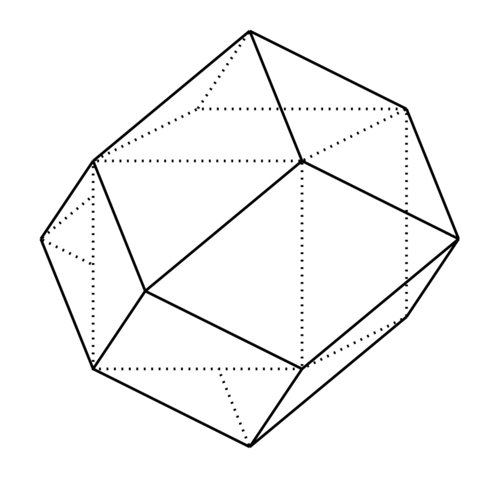
Figure 4. The fundamental domains of Bieberbach manifolds correspond to tilings of ${\mathbb{R}}^{3}$ by parallelepipeds ($G_{1}$, $G_{2}$, $G_{4}$) or hexagonal prisms ($G_{3}$, $G_{5}$), while the Hantzsche–Wendt manifold $G_{6}$ has a fundamental domain given by a rhombic dodecahedron.

There are six affine equivalence classes of (compact and orientable) Bieberbach manifolds, usually labelled $G_{1},\ldots,G_{6}$, with $G_{1}=T^{3}$. The other classes are, respectively known as half-turn space $G_{2}$, third-turn space $G_{3}$, quarter-turn space $G_{4}$, sixth-turn space $G_{5}$, and Hantzsche–Wendt space $G_{6}$, which corresponds to a half-turn along each coordinate axis. The corresponding groups, which we denote by $\Gamma_{G_{i}}$, are of the form (with $t_{i}$ implementing the translation by the vector $a_{i}$):

• with $a_{1}=(0,0,H)$, $a_{2}=(L,0,0)$, and $a_{3}=(T,S,0)$, $H,L,S\in{\mathbb{R}}^{*}_{+}$ and $T\in{\mathbb{R}}$

  $$\Gamma_{G_{2}}=\langle\alpha,t_{1},t_{2},t_{3}\,|\,\alpha^{2}=t_{1},\,\alpha t_{2}\alpha^{-1}=t_{2}^{-1},\,\alpha t_{3}\alpha^{-1}=t_{3}^{-1}\rangle\,,$$

• with $a_{1}=(0,0,H)$, $a_{2}=(L,0,0)$ and $a_{3}=(-\frac{1}{2}L,\frac{\sqrt{3}}{2}L,0)$, for $H$ and $L$ in ${\mathbb{R}}^{*}_{+}$

  $$\Gamma_{G_{3}}=\langle\alpha,t_{1},t_{2},t_{3}\,|\,\alpha^{3}=t_{1},\,\alpha t_{2}\alpha^{-1}=t_{3},\,\alpha t_{3}\alpha^{-1}=t_{2}^{-1}t_{3}^{-1}\rangle$$

• with $a_{1}=(0,0,H)$, $a_{2}=(L,0,0)$, and $a_{3}=(0,L,0)$, with $H,L>0$

  $$\Gamma_{G_{4}}=\langle\alpha,t_{1},t_{2},t_{3}\,|\,\alpha^{4}=t_{1},\,\alpha t_{2}\alpha^{-1}=t_{3},\,\alpha t_{3}\alpha^{-1}=t_{2}^{-1}\rangle$$

• with $a_{1}=(0,0,H)$, $a_{2}=(L,0,0)$ and $a_{3}=(\frac{1}{2}L,\frac{\sqrt{3}}{2}L,0)$, $H,L>0$

  $$\Gamma_{G_{5}}=\langle\alpha,t_{1},t_{2},t_{3}\,|\,\alpha^{6}=t_{1},\,\alpha t_{2}\alpha^{-1}=t_{3},\,\alpha t_{3}\alpha^{-1}=t_{2}^{-1}t_{3}\rangle$$

• with $a_{1}=(0,0,H)$, $a_{2}=(L,0,0)$, and $a_{3}=(0,S,0)$, with $H,L,S>0$

  $$\Gamma_{G_{6}}=\langle\alpha,\beta,\gamma,t_{1},t_{2},t_{3}\,|\,$$

  $$\begin{array}[]{ccc}\alpha^{2}=t_{1},&\alpha t_{2}\alpha^{-1}=t_{2}^{-1},&\alpha t_{3}\alpha^{-1}=t_{3}^{-1},\\ \beta^{2}=t_{2},&\beta t_{1}\beta^{-1}=t_{1}^{-1},&\beta t_{3}\beta^{-1}=t_{3}^{-1},\\ \gamma^{2}=t_{3},&\gamma t_{1}\gamma^{-1}=t_{1}^{-1},&\gamma t_{2}\gamma^{-1}=t_{2}^{-1},\\ &\gamma\beta\alpha=t_{1}t_{3}\rangle&\end{array}$$

.

The fundamental domains for the Bieberbach manifolds are parallelepipeds (for $G_{1}$, $G_{2}$, $G_{4}$) or hexagonal prisms (for $G_{3}$, $G_{5}$), see Figure 4. The Hantzsche–Wendt manifold has a more interesting structure (for its role in Cosmic Topology see [1]) and a fundamental domain given by a rhombic dodecahedron, see Figure 4. For a general discussion of these manifolds in the context of the Cosmic Topology problem see [35], [36], [51]).

Figure 5. The first step of the Sierpinski construction for the rhombic dodecahedron, [30].

Thus, the presence of fractality would, in this case, require a Sierpinski construction based on these parallelepipeds and hexagonal prisms. The case of parallelepipeds, as in the cube case, leads to Menger-sponge type fractals, while the hexagonal prisms have a Sierpinski construction based on the hexaflake, see Figure 3. In the case of the Hantzsche–Wendt manifold, we need to use a Sierpinski construction for the rhombic dodecahedron. We have already analyzed the Sierpinski construction for a prism based on the hexaflake fractal in the previous section, so we focus here on the case of a parallelepiped (for which it suffices to consider the case of a cube) and of a rhombic dodecahedron. For the latter, Sierpinski constructions for Catalan solids have been developed in [30]. In the case of the rhombic dodecahedron, the first step of the Sierpinski construction is shown in Figure 5.

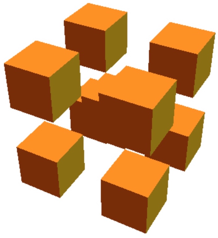
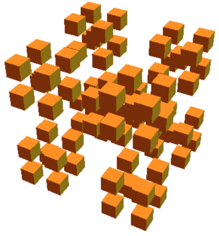
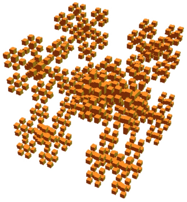
Figure 6. The first steps of the Sierpinski construction for the Sierpinski-Menger snowflake.

The case of a cube (or parallelepiped) is slightly more subtle than it seems at first. If one applies the same type of Sierpinski construction that we have used for the regular, Archimedean, and Catalan solids, [31], [30], [32], then one does not obtain a fractal, as eight copies of a cube scaled by $1/2$ just fill an identical copy of the same cube, so this Sierpinski construction just replicated the cube itself without introducing fractality. One can instead construct Menger-sponge type fractals based on cubes, where a cube is subdivided into scaled copies of itself and only some of these copies are retained. However, not all such Menger constructions are suitable for our purpose, since we need each cube in the construction to be a fundamental domain of a Bieberbach manifold, which means that the faces of the cube should be free to be glued to other faces according to the group action, and not attached to faces of other cubes in the Menger solid. This means that cubes need to be removed so that the remaining ones are only adjacent along edges or vertices, but not along faces. All the Sierpinski constructions we considered so far have this property. A Menger construction that satisfies this property is given by the Sierpinski-Menger snowflake (Figure 6).

In the Sierpinski-Menger snowflake construction of Figure 6, at every step each of the previous cubes is replaced by eight corner cubes and one central cube of $1/3$ the size. Thus, for this Sierpinski construction the replication factor is $f_{\rho}=9$ and the scaling factor is $f_{\sigma}=3$, with

$$\dim_{H}{\mathbb{P}}_{G_{a}}=\frac{\log f_{\rho}}{\log f_{\sigma}}=\frac{\log 9}{\log 3}=2\,,\ \ \ \text{ for }\ a\in\{1,2,4\}\,.$$

It is worth pointing out that, among the Sierpinski constructions associated to the candidate cosmic topologies in both positive and flat curvature this is the only case where the self-similarity dimension agrees with the value observed from the large scale distribution of galaxy clusters, [22], [58].

In the case of the hexaflex prism, we have, as discussed in the previous section,

$$\dim_{H}{\mathbb{P}}_{G_{a}}=\frac{\log 6}{\log 3}\sim 1.63093\,,\ \ \ \text{ for }\ a\in\{3,5\}\,,$$

while in the case of the rhombic dodecahedron, at each step of the Sierpinski construction each rhombic dodecahedron is replaced by $14$ identical copies scaled by a factor of $1/3$ so that $f_{\rho}=14$ and $f_{\sigma}=3$ and

$$\dim_{H}{\mathbb{P}}_{G_{6}}=\frac{\log(14)}{\log 3}\sim 2.40217\,.$$

2.4. Static model in the flat case

The computation of the spectral action, for both the static and the Robertson–Walker model, follow the same pattern that we discussed in the previous section, but with $S^{3}$ replaced with the flat torus $T^{3}$. As shown in [41], [42], the spectral actions of the torus and the Bieberbach manifolds are related by a scalar factor

$${\rm Tr}(f({\mathcal{D}}_{G_{a}}/\Lambda))\sim\lambda_{G_{a}}\cdot{\rm Tr}(f({\mathcal{D}}_{T^{3}}/\Lambda))=\frac{\lambda_{G_{a}}\,\Lambda^{3}}{4\pi^{3}}\int_{{\mathbb{R}}^{3}}f(u^{2}+v^{2}+w^{2})\,du\,dv\,dw$$

up to $O(\Lambda^{-\infty})$ terms. In this case, the factor $\lambda_{G_{a}}$ also depends on the continuous parameters $H,L,S,T$ in the generators of the groups $\Gamma_{G_{a}}$ (see the explicit presentations recalled above), so they are not just a rational number $1/|\Gamma|$ as in the spherical case. Nonetheless, the argument is otherwise very similar. On the product $S^{1}_{\beta}\times T^{3}$ the spectral action is of the form (see [41])

$${\rm Tr}(h({\mathcal{D}}_{S^{1}_{\beta}\times T^{3}}/\Lambda))=\frac{\Lambda^{4}\beta}{4\pi}\int_{0}^{\infty}uh(u)du+O(\Lambda^{-\infty})\,.$$

Also, as shown in [41], in the flat torus case, the corresponding slow-roll potential is only given by the term

$${\mathcal{V}}(\phi^{2}/\Lambda^{2})=\int_{0}^{\infty}u(h(u+\phi^{2}/\Lambda^{2})-h(u))\,du$$

without the part ${\mathcal{W}}(\phi^{2}/\Lambda^{2})$ of the spherical case (2.22). For the fractal arrangement ${\mathcal{P}}_{G_{a}}$ we will again obtain

$${\mathcal{S}}_{\Lambda}({\mathcal{D}}_{{\mathcal{P}}_{G_{a}}})\sim\sum_{\alpha}\frac{{\mathfrak{f}}_{\alpha}\Lambda^{\alpha}\,\lambda_{G_{a}}\,\zeta_{{\mathcal{L}}_{\Gamma}}(\alpha)}{2}{\rm Res}_{s=\alpha}\zeta_{\mathcal{D}_{T^{3}}}+\sum_{\beta}\frac{{\mathfrak{f}}_{\beta}\Lambda^{\beta}\,\lambda_{G_{a}}\,\zeta_{\mathcal{D}_{T^{3}}}(\beta)}{2}{\rm Res}_{s=\beta}\zeta_{{\mathcal{L}}_{\Gamma}}$$

and the same argument based on (2.17), (2.18) gives then

(2.37) $${\mathcal{S}}_{\Lambda}(\mathcal{D}_{S^{1}_{\beta}\times{\mathcal{P}}_{G_{a}}})\sim\beta\,\lambda_{G_{a}}\,\left(\Lambda^{4}\,2\,\zeta_{{\mathcal{L}}_{\Gamma}}(3)\,{\mathfrak{h}}_{3}+\sum_{n\in{\mathbb{Z}}}\frac{\Lambda^{s_{n}+1}\,a^{s_{n}}\,\zeta_{{\mathcal{D}}_{T^{3}}}(s_{n})}{\log f_{\sigma}}\,{\mathfrak{h}}_{s_{n}}\right)$$

$$\sim\beta\,\lambda_{G_{a}}\,\left(\frac{\Lambda^{4}\,2}{(1-f_{\rho}f_{\sigma}^{-3})}\,\,{\mathfrak{h}}_{3}+\sum_{n\in{\mathbb{Z}}}\frac{\Lambda^{s_{n}+1}\,a^{s_{n}}\,\zeta_{{\mathcal{D}}_{T^{3}}}(s_{n})}{\log f_{\sigma}}\,{\mathfrak{h}}_{s_{n}}\right)\,,$$

where

$${\mathfrak{h}}_{3}:=\pi\int_{0}^{\infty}h(\rho^{2})\rho^{3}\,d\rho\ \ \text{ and }\ \ {\mathfrak{h}}_{s_{n}}=2\int_{0}^{\infty}h(\rho^{2})\rho^{s_{n}}d\rho.$$

The slow-roll potential is of the form

(2.38) $${\mathcal{L}}(\phi)=A\,\,\Lambda^{4}\,\,{\mathcal{V}}(\phi^{2}/\Lambda^{2})+\sum_{n\in{\mathbb{Z}}}C_{n}\,\,\Lambda^{s_{n}+1}\,\,{\mathcal{U}}_{n}(\phi^{2}/\Lambda^{2}),$$

$$\text{ with }\ \ \ A=\frac{\pi\beta\,\lambda_{G_{a}}}{(1-f_{\rho}f_{\sigma}^{-3})}\,,\ \ \ \text{ and }\ \ \ C_{n}=\frac{2\beta\,\lambda_{G_{a}}\,a^{s_{n}}\,\zeta_{{\mathcal{D}}_{T^{3}}}(s_{n})}{\log f_{\sigma}}\,,$$

and with ${\mathcal{V}}(\phi^{2}/\Lambda^{2})$ as above and ${\mathcal{U}}_{n}(\phi^{2}/\Lambda^{2})$ as in (2.23).

2.5. Robertson–Walker model in the flat case

We sketch here the argument for the Robertson–Walker model $({\mathbb{R}}\times T^{3},dt^{2}+a(t)^{2}ds_{T^{3}})$ and the corresponding fractal arrangements $({\mathbb{R}}\times{\mathcal{P}}_{G_{a}},a_{n,k}^{2}(dt^{2}+a(t)^{2}ds_{T^{3}}))$. We will not provide a full computation in this paper.

We start by considering the Dirac operator ${\mathcal{D}}_{T^{3}}$ on the flat $3$-torus $T^{3}={\mathbb{R}}^{3}/{\mathbb{Z}}^{3}$. We take the standard torus for simplicity, but one can also consider more generally tori ${\mathbb{R}}^{3}/L$, for other lattices $L\subset{\mathbb{R}}^{3}$. The spectrum of ${\mathcal{D}}_{T^{3}}^{2}$ consists of

$$\lambda^{2}_{(n,m,k)}=4\pi\|(n,m,k)+(n_{0},m_{0},k_{0})\|^{2},\ \ \ \text{ for }\ (n,m,k)\in{\mathbb{Z}}^{3}\,,$$

where each $(n,m,k)\in{\mathbb{Z}}^{3}$ contributes with an additional multiplicity $2$, and where the vector $(n_{0},m_{0},k_{0})$ depends on the choice of one of the $8$ possible spin structures. Since the spectral action itself is independent of the choice of spin structure (see [41]), we can fix any of the eight choices of $v_{0}=(n_{0},m_{0},k_{0})$. The eigenspinor spaces decompose as

$${\mathcal{V}}_{\lambda}=\bigoplus_{v\in{\mathbb{Z}}^{3}\,:\,\pm 2\sqrt{\pi}\|v+v_{0}\|=\lambda}{\mathcal{V}}_{v,\pm}\,.$$

We then decompose the operator ${\mathcal{D}}^{2}_{{\mathbb{R}}\times T^{3}}$ with the Robertson–Walker metric $dt^{2}+a(t)^{2}ds_{T^{3}}$ on ${\mathbb{R}}\times T^{3}$ as

$${\mathcal{D}}^{2}_{{\mathbb{R}}\times T^{3}}=\oplus_{v\in{\mathbb{Z}}^{3}}\,H_{v,\pm}$$

$$H_{v,\pm}=-\frac{d^{2}}{dt^{2}}+V_{v}(t)$$

$$V_{v}(t)=\frac{\lambda_{v}}{a(t)^{2}}\left(\lambda_{v}-a^{\prime}(t)\right)\,,\ \ \ \text{ with }\ \ \lambda_{v}=\pm 2\sqrt{\pi}\|v+v_{0}\|\,,$$

so that the trace of the heat kernel is written as

$$\sum_{v\in{\mathbb{Z}}^{3}}{\rm Tr}(e^{-sH_{v,\pm}})\,.$$

We again then use the Feynman–Kac formula to express the heat kernel as

$$e^{-sH_{v,\pm}}(t,t)=\frac{1}{2\sqrt{\pi s}}\int e^{-s\int_{0}^{1}V_{v,\pm}(t+\sqrt{2s}\,\alpha(u))\,du}\,D[\alpha]\,.$$

We use the same variables $U$ and $V$ of (2.26) as in the sphere case, so that we have the same expression (2.27) with $x$ replaced by $\lambda_{v}=\pm 2\sqrt{\pi}\,\|v+v_{0}\|$. Thus, we now apply the Poisson summation to the functions

$$f_{s,\pm}(v)=e^{-\lambda_{v}^{2}\,U\pm|\lambda_{v}|\,V}\,,$$

and again we select the term at $w=(0,0,0)$, which is the main term contributing to the spectral action expansion. We obtain

$$\sum_{v\in{\mathbb{Z}}^{3}}(f_{s,+}+f_{s,-})(v)=\sum_{w\in{\mathbb{Z}}^{3}}(\hat{f}_{s,+}+\hat{f}_{s,-})(w)\sim\int_{{\mathbb{R}}^{3}}(f_{s,+}+f_{s,-})(x,y,z)dx\,dy\,dz\,$$

$$={\rm Vol}(S^{2})\,\left(\int_{0}^{\infty}e^{-4\pi r^{2}\,U-2\sqrt{\pi}\,r\,V}\,r^{2}\,dr+\int_{0}^{\infty}e^{-4\pi r^{2}\,U+2\sqrt{\pi}\,r\,V}\,r^{2}\,dr\right)$$

$$=\frac{1}{\sqrt{\pi}}\int_{\mathbb{R}}e^{-x^{2}\,U-x\,V}\,x^{2}\,dx=\frac{e^{\frac{V^{2}}{4U}}(2U+V)}{4U^{5/2}}\,.$$

Note that this expression differs from the case of the sphere only in the absence of the term $-U^{2}$ in the numerator, and in the normalization factor of $\sqrt{\pi}$.

Thus, we then have a very similar argument to [18] for the full expansion of the spectral action for the Robertson–Walker metric on ${\mathbb{R}}\times T^{3}$. Using the same expansion (2.28) in powers of $\tau=s^{2}$ we obtain

$$\frac{1}{\sqrt{\pi}\tau}\frac{e^{\frac{V^{2}}{4U}}(2U+V^{2})}{4U^{5/2}}=\frac{1}{4}\sum_{M=0}^{\infty}C^{(-5/2,2)}_{M}\tau^{M-2}+\frac{1}{2}\sum_{M=0}^{\infty}C^{(-3/2,0)}_{M}\tau^{M-4},$$

which differs from the case of $S^{3}$ of [18] in the absence of the $C^{(-1/2,0)}_{M}$ terms. Thus, we obtain the heat kernel expansion

$${\rm Tr}(e^{-\tau^{2}\,{\mathcal{D}}_{{\mathbb{R}}\times T^{3}}^{2}})\sim\sum_{M=0}^{\infty}\tau^{2M-4}\int\bigg{(}\int\big{(}\frac{1}{2}C^{-3/2,0}_{2M}+\frac{1}{4}C^{-5/2,2}_{2M-2}\big{)}\,D[\alpha]\bigg{)}dt\,.$$

The evaluation of the Brownian bridge integrals can then be done as in the sphere case, and we refer the reader to [18] for a detailed discussion.

Passing from the expansion for the heat kernel of ${\mathcal{D}}_{{\mathbb{R}}\times T^{3}}^{2}$ to the expansion for ${\mathcal{D}}_{{\mathbb{R}}\times G_{a}}^{2}$ for the Bieberbach manifolds $G_{a}$ can be handled in the same way as we did in the previous section for the spherical space forms, using a decomposition of the spectrum of ${\mathcal{D}}_{G_{a}}$ into subregions of the lattice ${\mathbb{Z}}^{3}$, with appropriate multiplicity functions, as shown in [42], and applying this decomposition to the Poisson summation formula in the argument above. The spin structure $v_{0}$ on $T^{3}$ needs to be chosen in a subset of those that descend to the quotient $G_{a}$. The resulting spectral action is still be independent of this choice.

We summarize the results of [42] and [47] on the Bieberbach manifolds. According to the Dirac spectrum computation of [48], the spectrum of ${\mathcal{D}}_{G_{a}}$ decomposes into a symmetric and an asymmetric component. The asymmetric component is only present for certain spin structures and it’s not present at all in the case of $G_{6}$. The symmetric part of the spectrum is parameterized by a finite collection of regions ${\mathcal{I}}_{i}\subset{\mathbb{Z}}^{3}$ in the lattice, with the corresponding eigenvalues given by a function $\lambda_{i}(v)$, $v\in{\mathcal{I}}_{i}$ with multiplicity a constant multiple of the number of $v\in{\mathcal{I}}_{i}$ realizing the same value $\lambda=\lambda_{i}(v)$. The asymmetric component is an arithmetic progression of the form ${\mathcal{B}}=\{2\pi H^{-1}(k\ell+c)\,|\,\ell\in{\mathbb{Z}}\}$ where $c$ depends on the spin structure, and $k$ is $2$ for $G_{2}$, $3$ for $G_{3}$, $4$ for $G_{4}$, and $6$ for $G_{5}$. Arguing as in [42] and [47], the Poisson summation formula for the $T^{3}$ case,

$$\sum_{v\in{\mathbb{Z}}^{3}}(f_{s,+}+f_{s,-})(v)=\frac{1}{\sqrt{\pi}}\int_{\mathbb{R}}e^{-x^{2}\,U-x\,V}\,x^{2}\,dx$$

is replaced by the summation

$$\sum_{i}\sum_{v\in{\mathcal{I}}_{i}}f_{s,i}(v)+\sum_{\ell\in{\mathbb{Z}}}f_{s}(\frac{2\pi c}{H}+\frac{2\pi k}{H}\ell)\,,$$

where $f_{s}(x)=e^{-x^{2}U-xV}$ and $f_{s,i}(v)=e^{-\lambda_{i}(v)^{2}U-\lambda_{i}(v)V}$. As in (2.33), the second summation gives

$$\sum_{\ell\in{\mathbb{Z}}^{3}}\frac{H}{2\pi k}e^{2\pi ic\ell/k}\hat{f}_{s}(\frac{H\ell}{2\pi k})\sim\frac{H}{2\pi k}\int_{\mathbb{R}}f_{s}(x)\,dx\,,$$

while the first term in the Poisson summation, coming from the symmetric component of the spectrum can be dealt with as in the individual cases discussed in [42] and [47], which we do not recall explicitly here. In all cases the Fourier transformed sides of the Poisson summation add up so that the zero-term of the combined summation is simply a multiple of the same term in the torus case,

$$\sum_{i}\sum_{v\in{\mathcal{I}}_{i}}f_{s,i}(v)+\sum_{\ell\in{\mathbb{Z}}}f_{s}(\frac{2\pi c}{H}+\frac{2\pi k}{H}\ell)\sim\lambda_{G_{a}}\,\int_{{\mathbb{R}}^{3}}(f_{s,+}+f_{s,-})(x,y,z)dx\,dy\,dz\,$$

$$=\lambda_{G_{a}}\,\,\frac{e^{\frac{V^{2}}{4U}}(2U+V)}{4U^{5/2}}\,,$$

where, as mentioned above, the factor $\lambda_{G_{a}}$ depends on the continuous parameters $H,L,S,T$ in the groups $\Gamma_{G_{a}}$ but not on the spin structure.

Thus, we obtain the same expansion for the expression above and a corresponding heat kernel expansion of the form

(2.39) $${\rm Tr}(e^{-\tau^{2}\,{\mathcal{D}}_{{\mathbb{R}}\times G_{a}}^{2}})\sim\lambda_{G_{a}}\,\,\sum_{M=0}^{\infty}\tau^{2M-4}\int\bigg{(}\int\big{(}\frac{1}{2}C^{-3/2,0}_{2M}+\frac{1}{4}C^{-5/2,2}_{2M-2}\big{)}\,D[\alpha]\bigg{)}dt\,.$$

We can then apply the same method as in the spherical cases to pass to the heat kernel expansion for the fractal arrangement, and we obtain

$${\rm Tr}(e^{-\tau{\mathcal{D}}_{{\mathbb{R}}\times{\mathcal{P}}_{G_{a}}}})\sim\lambda_{G_{a}}\,\,\sum_{M=0}^{\infty}\tau^{2M-4}\,\zeta_{{\mathcal{L}}_{\Gamma}}(-2M+4)\,\int\bigg{(}\int\big{(}\frac{1}{2}C^{-3/2,0}_{2M}+\frac{1}{4}C^{-5/2,2}_{2M-2}\big{)}\,D[\alpha]\bigg{)}dt$$

$$+\frac{\lambda_{G_{a}}}{2\log f_{\sigma}}\sum_{n\in{\mathbb{Z}}}\,\Gamma(s_{n}/2)\,\zeta_{{\mathcal{D}}_{{\mathbb{R}}\times G_{a}}}(s_{n})\,\tau^{-s_{n}}\,.$$

The spectral action is correspondingly of the form

(2.40) $$\begin{array}[]{rl}{\rm Tr}(f({\mathcal{D}}_{{\mathbb{R}}\times{\mathcal{P}}_{G_{a}}}/\Lambda))&\sim\\ &\displaystyle{\lambda_{G_{a}}\,\sum_{M=0}^{\infty}}\displaystyle{\Lambda^{4-2M}\,{\mathfrak{f}}_{4-2M}\,\zeta_{{\mathcal{L}}_{\Gamma}}(4-2M)\cdot}\\ &\displaystyle{\int\bigg{(}\int\big{(}\frac{1}{2}C^{-3/2,0}_{2M}+\frac{1}{4}C^{-5/2,2}_{2M-2}\big{)}\,D[\alpha]\bigg{)}dt}\\ &\displaystyle{+\frac{\lambda_{G_{a}}}{2\log f_{\sigma}}\sum_{n\in{\mathbb{Z}}}}\,{\mathfrak{f}}_{s_{n}}\,\Gamma(s_{n}/2)\,\zeta_{{\mathcal{D}}_{{\mathbb{R}}\times G_{a}}}(s_{n})\Lambda^{s_{n}}\end{array}$$

$$\sim\lambda_{G_{a}}\,\sum_{M=0}^{\infty}\frac{\Lambda^{4-2M}\,{\mathfrak{f}}_{4-2M}}{(1-f_{\rho}f_{\sigma}^{2M-4})}\int\bigg{(}\int\big{(}\frac{1}{2}C^{-3/2,0}_{2M}+\frac{1}{4}C^{-5/2,2}_{2M-2}\big{)}\,D[\alpha]\bigg{)}dt$$

$$+\frac{\lambda_{G_{a}}}{2\log f_{\sigma}}\sum_{n\in{\mathbb{Z}}}\,{\mathfrak{f}}_{s_{n}}\,\Gamma(s_{n}/2)\,\zeta_{{\mathcal{D}}_{{\mathbb{R}}\times G_{a}}}(s_{n})\Lambda^{s_{n}}\,.$$

2.6. Fractal structures on manifolds

In our analysis in the previous sections of the possible fractal structures associated to the different cosmic topologies, we have used the fact that these are all homogeneous manifolds obtained as quotients by group actions, which admit a nice polyhedral fundamental domain (either spherical or flat Euclidean). This allowed us to use Sierpinski constructions based on the model polyhedron, and apply them to build a fractal arrangement of copies of the same manifold.

More generally, one can ask a broad question about fractal constructions based on manifolds with decompositions into polyhedra. These more general manifolds will not provide standard candidate cosmic topologies as they fail to have the desired homogeneity property. However, this appears to be a question of independent interest, both for the spectral action model of gravity we are considering and for more general physical models.

We will return to this question in a separate paper, where we develop the necessary mathematical background to address it in the required generality. However, in this section we outline briefly some aspects of this problem and some relevant examples.

2.6.1. Fractality from triangulations

The easiest form of decomposition of a manifold into polyhedral structures is a triangulation, namely a decomposition into simplices (tetrahedra in a $3$-manifold case, triangles in a surface case), glued together along lower dimensional faces. The algebraic topology of simplicial sets describes the general topological objects (not always smooth manifolds) obtained by such arrangements of simplices. Not all topological manifolds admit a triangulation, but all smooth manifolds do.

Thus, a first possible idea of how to obtain fractal arrangements of manifolds would be to consider fractal constructions associated to tetrahedra (and higher dimensional simplices) and apply them to every tetrahedron (simplex) in the triangulation, by compatibly performing all the gluing that describe the triangulation at each level of the fractal construction. A similar idea was used, for instance, in [6].

Figure 7. The first two stages of the tetrahedral Sierpinski construction, [28].

In the case of a $3$-dimensional manifold $M$ with a triangulation $T$, this can be done, for instance, by considering the Sierpinski construction for the tetrahedron, as illustrated in Figure 7. For this tetrahedral Sierpinski construction we have $f_{\rho}=4$ and $f_{\sigma}=2$, so that the self-similarity dimension is

$$\dim_{H}{\mathbb{P}}_{T}=\frac{\log f_{\rho}}{\log f_{\sigma}}=2,$$

where ${\mathbb{P}}_{T}$ is the resulting fractal arrangement of tetrahedra arising from a given triangulation $T$. The corresponding fractal string zeta function is of the form

$$\zeta_{{\mathcal{L}}}(s)=\frac{1}{1-2^{2-s}}\,,$$

with poles $s_{n}=2+\frac{2\pi in}{\log 2}$, for $n\in{\mathbb{Z}}$. Note that in all these cases, the self-similarity dimension is $2$ (as expected for cosmological reasons, [22], [58], though $M$ will in general not satisfy the requirement of a candidate cosmological model).

In order to be able to perform the gluing of the tetrahedra, as prescribed by the triangulation, at each level of the fractal construction, we again need to use the fact that the tetrahedra in each subdivision of a previous level are only adjacent along vertices and not along faces. The resulting fractal arrangement of copies of $M$ will be denoted by ${\mathcal{P}}_{M}$. For a higher dimensional simplex $\Delta_{n}$ generalizations of the Sierpinski construction have been considered, for instance, in [65].

If the spectral action ${\mathcal{S}}_{\Lambda}({\mathcal{D}}_{M})$ for the $3$-manifold $M$ is given by

$${\mathcal{S}}_{\Lambda}({\mathcal{D}}_{M})=\sim\sum\frac{{\mathfrak{f}}_{\alpha}\Lambda^{\alpha}}{2}{\rm Res}_{s=\alpha}\zeta_{\mathcal{D}_{M}}+f(0)\zeta_{\mathcal{D}_{M}}(0)\,,$$

then the spectral action of the fractal arrangement ${\mathcal{P}}_{M}$ is

$$\begin{array}[]{rl}{\mathcal{S}}_{\Lambda}({\mathcal{D}}_{{\mathcal{P}}_{M}})\sim&\displaystyle{\sum\frac{{\mathfrak{f}}_{\alpha}\Lambda^{\alpha}\,\zeta_{{\mathcal{L}}}(\alpha)}{2}{\rm Res}_{s=\alpha}\zeta_{\mathcal{D}_{M}}}+f(0)\zeta_{\mathcal{D}_{M}}(0)\zeta_{{\mathcal{L}}}(0)\\[8.53581pt] +&\displaystyle{\sum_{n\in{\mathbb{Z}}}\frac{{\mathfrak{f}}_{s_{n}}\Lambda^{s_{n}}\zeta_{{\mathcal{D}}_{M}}(s_{n})}{2\log 2}}\end{array}$$

$$\begin{array}[]{rl}\sim&\displaystyle{\sum\frac{{\mathfrak{f}}_{\alpha}\Lambda^{\alpha}}{2(1-2^{2-\alpha})}{\rm Res}_{s=\alpha}\zeta_{\mathcal{D}_{M}}}-\frac{f(0)\zeta_{\mathcal{D}_{M}}(0)}{3}\\[8.53581pt] +&\displaystyle{\sum_{n\in{\mathbb{Z}}}\frac{{\mathfrak{f}}_{s_{n}}\Lambda^{s_{n}}\zeta_{{\mathcal{D}}_{M}}(s_{n})}{2\log 2}}\,.\end{array}$$

The asymptotic expansion for the spectral action on a static model $S^{1}_{\beta}\times M$ can then be obtained from this along the same lines as in the cases discussed in the previous section. We don’t have in this case a direct analog of the argument for the Robertson–Walker models, unless something more explicit is known about the spectrum and eigenspaces of ${\mathcal{D}}_{M}$, which is usually the case only for homogeneous spaces like those we considered before.

2.6.2. Koch-type fractal growth

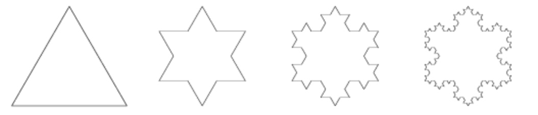
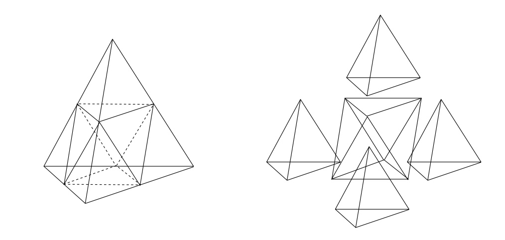
Figure 8. The first three steps in the Koch construction for a triangle (Koch snowflake, [62]) and for a tetrahedron, [52], and the tetrahedron decomposition into tetrahedra and an octahedron.

There are other natural fractal constructions associated to tetrahedra (and to higher dimensional simplices) to which we cannot directly apply the argument described in the previous subsection for the Sierpinski construction. The simplest such example is the Koch construction. In the case of triangles, the Koch construction produces the well known Koch snowflake as the boundary curve. At each step of the Koch curve construction, one replaces each segment with $4$ segments of length $1/3$ so the self-similarity dimension is $\log(4)/\log(3)$. Note that this is a fractal construction based on the boundary curve. If we consider $2$-dimensional triangles, then at the first step of the construction the initial triangle is replaced by $12$ triangles with scaling factor $1/3$, as all the triangles filling the triangle of the previous step are also retained. So at each next step the number $T_{n}$ of triangles is $T_{n}=9\cdot T_{n-1}+S_{n-1}$ where $S_{n-1}$ is the number of boundary sides $S_{n}=3\cdot 4^{n-1}$.

In the case of a tetrahedron, the first steps of the Koch construction are illustrated in Figure 8. At each step of the Koch construction one attaches a new tetrahedron, scaled by $1/2$, in the center of each of the triangular faces of the previous step. As in the case of the Koch snowflake, we can view this as a fractal construction for the boundary triangles, or for the interior solids. The boundary has exact self-similarity in the sense that $6$ new triangles of size $1/2$ replace each triangular face with $\dim_{H}=\log(6)/\log(2)$ and the zeta function is then just given by $\zeta_{{\mathcal{L}}}(s)=(1-6\cdot 2^{-s})^{-1}$. However, the interior solid does not have exact self-similarity, since the interior region of the first tetrahedron is replaced in the first step of the Koch construction by a union of an octahedron and $8$ tetrahedra, but the octahedron does not further decompose into other regular tetrahedra.

Figure 9. The first steps of a Koch octahedron construction, on one of the faces of the original solid, and the decomposition of an octahedron into six octahedra with $1/2$ scale factor and four tetrahedra.

We can consider a similar case by constructing a Koch-like fractal from an octahedron. Starting with an octahedron, in each of its faces we place another octahedron scaled by $\frac{1}{2}$, see Figure 9. Again the situation is the same as in the tetrahedron case. The fractal construction seen on the $2$-dimensional surface has exact self-similarity with each triangle being first subdivided into four subtriangles of size $1/2$, of which three are retained and $7$ new ones are added in place of the fourth one. Due to the geometry of the octahedron, in the second step of the construction, three of the scaled copies placed on each face are tangent to faces both in the original face (red) and in the octahedron from the previous iteration (blue). Thus, if $T_{0}$ is the number of triangles in the original copy, namely $T_{0}=8$, at the first step we have $T_{1}=10\,T_{0}=80$ (three subtriangles in each original one plus $7$ new ones in place of the fourth one), while at the second step we have $T_{2}=10\,T_{1}-3T_{0}$, where the $3T_{0}$ accounts for those new faces that end up matching subtriangles of the original faces. We can repeat this process for each of the next iterations: at the $n$-th step the number of triangles is $T_{n+1}=10\,T_{n}-3\,T_{n-1}$. The solution of this recursion with $T_{-1}=0$ and $T_{0}=8$ is

$$T_{n}=(\frac{10}{11}\sqrt{22}+4)\,(5+\sqrt{22})^{n}+(-\frac{10}{11}\sqrt{22}+4)\,(5-\sqrt{22})^{n}\,,$$

with the first few terms equal to $T_{1}=80$, $T_{2}=776$, $T_{3}=7520$, $T_{4}=72872$, $T_{5}=706160$, etc. This example is slightly different from the cases of self-similarity we analyzed so far, because instead of having a single replication factor $f_{\rho}$ and a similarity factor $f_{\sigma}$, in this case we have a weighted combination of two different replication factors $f_{\rho,\pm}=5\pm\sqrt{22}$. (Note that here $f_{\rho,\pm}$ are not integers but their weighted combinations $T_{n}=a_{+}f^{n}_{\rho,+}+a_{-}f^{n}_{\rho,-}$, with $a_{\pm}=4\pm\frac{10}{11}\sqrt{22}$ are integers. Thus, in this case we have

$${\mathcal{L}}=\{a_{n,k}=2^{-n}\,|\,k=1,\ldots,T_{n}\}$$

so that the zeta function is

$$\zeta_{{\mathcal{L}}}(s)=\sum_{n\geq 0}\,T_{n}\,\,2^{-ns}=$$

$$=(\frac{10}{11}\sqrt{22}+4)\,\sum_{n}(5+\sqrt{22})^{n}2^{-ns}+(-\frac{10}{11}\sqrt{22}+4)\,\sum_{n}(5-\sqrt{22})^{n}2^{-ns}$$

$$=\frac{(\frac{10}{11}\sqrt{22}+4)}{1-(5+\sqrt{22})2^{-s}}+\frac{(-\frac{10}{11}\sqrt{22}+4)}{1-(5-\sqrt{22})2^{-s}}\,.$$

The $3$-dimensional solid octahedra in this construction do not have exact self-similarity. Indeed, as in the case of the tetrahedron, an octahedron does not decompose exactly into octahedra of $1/2$ the size, but requires additionally four tetrahedra (see Figure 9).

Moreover, in the tetrahedral case we cannot directly proceed as in the Sierpinski case to glue the tetrahedra of each step of the construction into a manifold triangulation, as some faces of the tetrahedra are already glued to parts of faces of tetrahedra of the previous step. Similarly for the octahedral construction.

However, one still expects that interesting fractal versions of simplicial objects should be obtainable from this type of fractal growth model as well. To this purpose, one needs to analyze more in depth the usual notion of simplicial sets, and the analogous notion of cubical sets, in algebraic topology and enrich it with a notion of fractality implemented by scaling maps. We will discuss the mathematical structure necessary for this construction, and some of its applications, in a forthcoming paper.

3. Arithmetic structures in fractal packings

In this section we consider again the Packed Swiss Cheese Cosmology models considered in [2], [18], based on Apollonian packings of spheres, as in [43]. As observed in other settings, [16], [17], [19], cosmological models based on the spectral action often reveal interesting arithmetic structures. Thus, we focus here on a class of Apollonian packing that have nice arithmetic properties and we investigate how the associated spectral action function reflects the presence of an arithmetic structure.

3.1. Integral Apollonian packings

We consider the integral Apollonian packings as in [23], [25], based on $3$-spheres. These are packings where the curvatures of all spheres are integers. Note that the term “curvature” in this setting denotes the oriented curvature, $a_{i}=\frac{1}{r_{i}}$. We recall the general structure of Apollonian packings from [25]. Explicit examples of constructions of sphere packings of $3$-spheres and $4$-spheres are given in [57].

Apollonian packings of $(n-1)$-spheres in $\mathbb{R}^{n}$ are characterized by $n+2$ tangent spheres obeying the Descartes relation for $n$ dimensions

$$\sum_{i=1}^{n+2}a_{i}^{2}=\frac{1}{n}(\sum_{i=1}^{n+2}a_{i})^{2}\,,$$

where $a_{i}=\frac{1}{r_{i}}$ is the curvature of each sphere. Following [25] we consider

$$Q_{D,n}:=\textbf{I}_{n+2}-\frac{1}{n}1_{n+2}1_{n+2}^{T}\,,$$

where $\textbf{I}_{n+2}$ is the identity and $(1_{n+2})_{j}=1,\forall j\in\{1,2,...,n+2\}$ with $\textbf{I}_{n+2}\in M_{n+2}(\mathbb{R})$ and $1_{n+2}\in\mathbb{R}^{n+2}$. The Descartes relation for $(n-1)$-spheres can then be written equivalently as

$$a^{T}Q_{D,n}a=0\,.$$

Consider a Lorentz quadratic form:

$$a^{T}Q_{L,n}a=-a_{1}^{2}+a_{2}^{2}+...+a_{n+2}^{2}=0\,.$$

Descartes forms and Lorentz forms are real-equivalent in all dimensions, as discussed in [25]. This leads to a bijection $\{a^{\mathcal{D}}_{n+2}\}\simeq\{a^{\mathcal{L}}_{n+2}\}$, which means Descartes forms can be counted using the Lorentz forms. We also need to recall the notion of dual Apollonian packing from [25]. The packing is described by the dual Apollonian group

$$\mathcal{A}^{\bot}_{n}=\{S_{1}^{\bot},S_{2}^{\bot},...,S_{n+2}^{\bot}\}\,,$$

where $S_{i}^{\bot}=\textbf{I}_{n+2}+2\cdot 1_{n+2}e_{i}^{T}-4\cdot e_{i}e_{i}^{T}$, with $1_{n+2}$ as before and $e_{i}$ the standard Cartesian basis in $\mathbb{R}^{n+2}$. Let $\textbf{W}_{\mathcal{D}}$ denote the curvature-center coordinate matrix of the original Descartes form. The dual Apollonian group acts on it by $S_{i}^{\bot}\textbf{W}_{\mathcal{D}}$.

Here, we will work with the dual Apollonian configuration of sphere packings, since it has been shown to not intersect, when taking higher dimensional spheres in the packing, whereas the usual Apollonian construction leads to intersections under the same circumstances. Additionally, Theorem 4.1 of [25] suggests that Apollonian packings in higher dimensions do not necessarily remain integral. However, dual Apollonian packings do retain integral curvature for $n>1$. Altogether, Apollonian configurations in higher dimensions are not always an appropriate choice for sphere packings, but dual Apollonian configurations retain all the usual qualities associated with circle packings for higher dimensions.

In the construction of the dual Apollonian packing, if the initial configuration of spheres has integer curvatures, then all the curvatures will remain integer in the whole packing. The packing zeta function can then be described as

$$\zeta_{\mathcal{L}}(s)=\sum_{n,k}r_{n,k}^{s}=\sum_{n\in\mathbb{N}}\frac{r^{*}_{5}(a_{n}^{2})}{a_{n}^{s}}\,,$$

where $r^{*}_{5}(k)$ denotes the number of primitive integer representations of $k$ as a sum of $5$ square integers. As shown in [26], this is given by

$$\sum_{n\in\mathbb{N}}\frac{r^{*}_{5}(a_{n}^{2})}{a_{n}^{s}}=\frac{1}{\zeta(s)}\sum_{n\in\mathbb{N}}\frac{r_{5}(a_{n}^{2})}{a_{n}^{s}}\,,$$

with $r_{5}(k)$ the number of general integer representations of $k$. It is shown in [53] that this sum simplifies to

$$\sum_{n\in\mathbb{N}}\frac{r_{5}(a_{n}^{2})}{a_{n}^{s}}=\frac{10\,\,\zeta(s)\zeta(s-3)}{\zeta(s-1)(1-2^{1-s})}\,,$$

so that we obtain

(3.1) $$\zeta_{\mathcal{L}}(s)=\frac{10\,\,\zeta(s-3)}{\zeta(s-1)(1-2^{1-s})}\,.$$

The set of poles of the zeta function (3.1) is the union of the following sets

1. The point $s=4$, which is a pole of $\zeta(s-3)$ with residue

   $${\rm Res}_{s=4}\zeta_{\mathcal{L}}=\frac{80}{7\,\zeta(3)}\,.$$

2. The points $s_{n}=1+\frac{2\pi in}{\log 2}$, with $n\in{\mathbb{Z}}$, which are poles of $(1-2^{1-s})^{-1}$, with residue

   $${\rm Res}_{s=s_{n}}\zeta_{\mathcal{L}}=\frac{10\,\,\zeta(\frac{2\pi in}{\log 2}-2)}{\zeta(\frac{2\pi in}{\log 2})\,\log 2}\,.$$

3. The nontrivial zeros of the zeta function $\zeta(s-1)$, given by the set $\{s_{\rho}=1+\rho\,|\,\rho\in{\mathcal{Z}}(\zeta)\}$, with ${\mathcal{Z}}(\zeta)$ the set of non-trivial zeros of the Riemann zeta function, with residues

   $${\rm Res}_{s=s_{\rho}}\zeta_{\mathcal{L}}=\frac{10\,\,\zeta(\rho-2)}{(1-2^{-\rho})\,\zeta^{\prime}(\rho)}\,.$$

Note that the trivial zeros of $\zeta(s-1)$, at the points $s_{k}=1-2k$ with $k\in{\mathbb{N}}$, do not contribute poles because also $\zeta(-2(k+1))=0$ in the numerator of (3.1).

We see that, in the case of a Packed Swiss Cheese Cosmology model based on an integral Apollonian packing of $3$-spheres, the spectral action expansion will contain a series over the non-trivial zeros of the Riemann zeta function, of the form

$$\sum_{\rho}\frac{5\,{\mathfrak{f}}_{s_{\rho}}\,\zeta_{{\mathcal{D}}_{S^{3}}}(1+\rho)\,\zeta(\rho-2)}{(1-2^{-\rho})\,\zeta^{\prime}(\rho)}\,\Lambda^{1+\rho}\,.$$

The behavior of this series depends on delicate number theoretic properties of the Riemann zeta function and on whether the Riemann hypothesis holds. For example, estimates on the behavior of the derivative $\zeta^{\prime}(\rho)$ of the Riemann zeta function at non-trivial zeros are derived in [24] and [21]. In particular, series of the form

$$\sum_{\rho}\zeta^{\prime}(\rho)\Lambda^{\rho}\ \ \ \text{ and }\ \ \ \sum_{\rho_{n}}\zeta^{\prime}(\rho_{n})e^{2\pi inx}$$

have been studied in [24] and [21]. The series above, which arises naturally in our physical model, appears to be of independent interest, though we will not pursue its analysis further in the present paper.

3.2. Perturbation of sphere tangencies

The Packed Swiss Cheese Cosmology model, as described in [43], uses Apollonian packings of $3$-sphere as a convenient mathematical model for achieving a fractal arrangement that can be seen as an iterative construction based on the original idea of Rees and Sciama [50] on how to introduce inhomogeneities in a Robertson–Walker spacetime. There are however some limitations to the Apollonian packing model. For example, the condition of tangency is geometrically not an open condition, in the sense that small random perturbations of the data will break this condition and will yield intersecting spheres. The latter is a generic condition that is stable under small perturbations. Moreover, in a realistic physical model one would not be working with exact self-similar fractals, but with random fractals as the latter provide more realistic physical models. Thus, one should think of a physical or cosmological process that generates fractality as a random process where bubbles randomly open up in the fabric of Robertson–Walker spacetime, in such a way that what remains acquires a fractal geometry. However, if the subtraction of bubbles of spacetime is achieved through a random process, the resulting geometry will not look like a configuration of tangent spheres like an Apollonian packing, which is a deterministic fractal, but rather like a configuration of intersecting spheres with a sequence ${\mathcal{L}}=\{a_{n,k}\}$ of radii. Thus, we can imagine a model where one starts with an Apollonian packing and maintains the same sequence of radii but introduces a random perturbation of the positions of the centers of the spheres, which causes some of the spheres to overlap with intersection along a hypersphere rather than only at a tangent point.

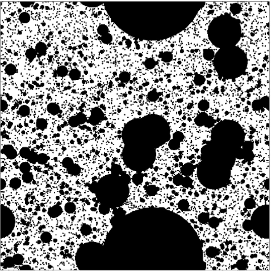
Figure 10. Example of a random fractal created by cratering (removal of discs/balls). In the example illustrated here the sequence of radii is simply taken as $a_{n,k}=3^{-n}$ (from a geophysical model of [63]).

We can also obtain simple models with intersecting spheres by considering Apollonian packings in lower dimensions as the intersection with an equatorial hyperplane of a configuration of spheres in higher dimension. While for some special choices of the lower dimensional packing the higher dimensional spheres will also intersect only at the tangent points, in general the higher dimensional spheres have a larger intersection. Such constructions where an Apollonian packing of circles is used to construct a fractal arrangement of higher dimensional spheres was considered already in [18] in the case of the Ford circles, which also have a nice arithmetic structure.

We consider here another variant of this model, again by considering configurations of $3$-spheres obtained starting from an Apollonian packing of circles, where we consider packings with integer curvatures. We then take each circle and make it the equator of a $2$-sphere, and repeat the process one more time by taking each $2$-sphere and making it the equator of a $3$-sphere. The resulting configuration of $3$-spheres is in general no longer an Apollonian packing, as the $3$-spheres now can have intersections and not only tangency points. The fractal string for this configuration is the same as the $S^{1}$ case for integer curvature, which gives

$$\zeta_{\mathcal{L}}(s)=\sum_{n,k}a_{n,k}^{s}=\sum_{n}\frac{r_{3}^{*}(a^{2}_{n})}{a_{n}^{s}}\,.$$

The evaluation of this series is similar to the case of integral packings of $3$-spheres discussed above.

Let $\eta(s)$ be the Dirichlet $\eta$-function

$$\eta(s)=\sum_{n\geq 1}\frac{(-1)^{n-1}}{n^{s}}=(1-2^{1-s})\zeta(s)\,.$$

Consider then the series

$$\tilde{\eta}(s)=\sum_{n\geq 1}\frac{(-1)^{n-1}}{(2n-1)^{s}}=\sum_{n\geq 1}\left(\frac{(-1)^{n-1}}{n^{s}}-\frac{(-1)^{n-1}}{(2n)^{s}}\right)=(1-2^{-s})\eta(s)\,.$$

We obtain, as in [26], [53],

$$\zeta_{\mathcal{L}}(s)=6\frac{\zeta(s-1)(1-2^{1-s})}{\tilde{\eta}(s)}$$

$$=6\frac{\zeta(s-1)(1-2^{1-s})}{(1-2^{-s})\eta(s)}=6\frac{\zeta(s-1)}{(1-2^{-s})\zeta(s)}\,.$$

Note that [53] uses the notation $\eta(s)$ for our $\tilde{\eta}(s)$. In this case again we have poles at $s_{n}=\frac{2\pi in}{\log 2}$, at $s=2$, and at the zeros (in this case both the trivial and the nontrivial zeros) of the Riemann zeta function. Again this means that the spectral action expansion for this configuration of $3$-spheres will contain a series with a sum over the nontrivial zeros of the same general form we discussed above,

$$\sum_{\rho}\frac{3\,{\mathfrak{f}}_{s_{\rho}}\,\zeta_{{\mathcal{D}}_{S^{3}}}(\rho)\zeta(\rho-1)}{(1-2^{-\rho})\zeta^{\prime}(\rho)}\Lambda^{\rho}\,.$$

4. Gravitational waves in fractal models with intersecting spheres

In this section we discuss some aspects of the gravitational waves behavior in fractal cosmological models. We focus on the case discussed at the end of the previous section, where instead of packings of spheres that only touch at tangent points, we allow for perturbations of the geometry that introduce intersections between some of the $3$-spheres along some $2$-spheres.

4.1. Transmission between spheres in perturbed packings

In this section, we discuss some consequences of being an observer in one of the positively curved spaces in a fractal configuration of $3$-spheres obtained as a perturbation of a sphere packing configuration. Specifically, we consider the intersections of the spheres as a transmission site for gravitational waves going from one $3$-sphere to another and derive an approximate form of the metric describing the gravitational wave in the receiving sphere. As we will see, this calculation implies there exist directly observable phenomena that come from having positively curved universes intersect each other.

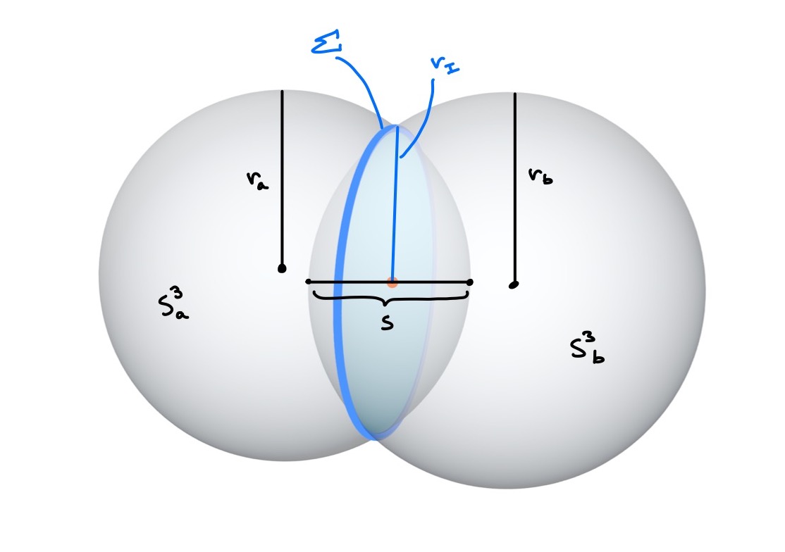
Figure 11. Two 3-spheres $S^{3}_{a}$ and $S^{3}_{b}$ with radii $r_{a}$ and $r_{b}$, intersecting at a 2-sphere, $\Sigma$, with separation distance $s$.

We begin by considering the intersection of two 3-spheres, $S^{3}_{a}$ and $S^{3}_{b}$ along a $2$-sphere $\Sigma\equiv S^{3}_{a}\bigcap S^{3}_{b}=S^{2}_{I}$. We write $s$ for the distance between the poles of the two smaller spherical caps subtended by the $2$-sphere of intersection, see Figure 11. We refer to $s$ as the “separation distance” of $S^{3}_{a}$ and $S^{3}_{b}$. An quick calculation yields the relation between the radii,

$$r_{I}^{2}=\frac{(2r_{b}-s)(2r_{a}-s)(2r_{a}+2r_{b}-s)s}{4(r_{a}+r_{b}-s)^{2}}\,.$$

In the case of a Robertson-Walker cosmology, each $3$-sphere would be undergoing inflation, which would affect this calculation. For simplicity, we will consider only the static model, where there is no time evolution in the shape of each sphere, so both the radii $r_{a},r_{b}$ and the relative position of the two $3$-spheres are constant. Thus, an observer in each sphere follows the same spatial hypersurface-orthogonal timelike vector $\eta^{\mu}=(1,0,0,0)$.

Also, for the purpose of the computations presented in this section, we work directly with Lorentzian signature, unlike for the previous spectral action calculations, where we had to Wick rotate to Euclidean signature.

Another assumption for this section is that $r_{b}>>r_{a}$. This makes it reasonable to assume that the region surrounding $\Sigma$ in $S^{3}_{b}$ can be approximated by Minkowski space $\mathbb{R}^{3,1}$, which we can use to significantly simplify the solution of the metric tensor under linearized General Relativity (GR) conditions.

We discuss briefly the boundary conditions in GR. Following [49], if $x^{\mu}$ and $x^{\prime\mu}$ are local coordinates on the spheres $S^{3}_{a}$ and $S^{3}_{b}$, respectively, and $y^{a}$ are the coordinates on $\Sigma$, then the tangent curves and induced metric on $\Sigma$ are given by

$$e^{\mu}_{a}=\frac{\partial x^{\mu}}{\partial y^{a}}\,,$$

$$h_{ab}=g_{\mu\nu}e^{\mu}_{a}e^{\nu}_{b}\,.$$

The extrinsic curvature tensor is given by

$$K_{ab}:=\nabla_{\nu}\eta_{\mu}e^{\mu}_{a}e^{\nu}_{b}\,,$$

where $\eta_{\mu}$ is the orthogonal vector to $\Sigma$ in either $S^{3}_{a}$ or $S^{3}_{b}$.

As above, let $s$ be the separation distance of the two hypersurfaces and let $\ell$ be a coordinate in $[-s/2,s/2]$. Let $\Theta(\ell)$ be the Heaviside function. We consider a stress energy-momentum tensor of the form

$$T_{\mu\nu}=T^{a}_{\mu\nu}\,\Theta(-\ell)+S_{\mu\nu}\,\delta(\ell)+T^{b}_{\mu\nu}\,\Theta(\ell)\,,$$

where $S_{\mu\nu}$ is the surface energy-momentum tensor (see [49]) given by

$$S_{ab}=-\frac{\eta_{\mu}\eta^{\mu}}{8\pi}([K_{ab}]-[K]h_{ab})\,.$$

Here the jump of a quantity across $\Sigma$ is given by

$$[A^{\mu_{1}\mu_{2}...\mu_{n}}_{\nu_{1}\nu_{2}...\nu_{k}}]=A^{\mu_{1}\mu_{2}...\mu_{n}}_{\nu_{1}\nu_{2}...\nu_{k}}|_{\Sigma^{+}}-A^{\mu_{1}\mu_{2}...\mu_{n}}_{\nu_{1}\nu_{2}...\nu_{k}}|_{\Sigma^{-}}\,,$$

with $+,-$ for the two hypersurfaces $\Sigma^{\pm}$ (here given by the spheres $S^{3}_{a}$ and $S^{3}_{b}$).

The respective unperturbed metrics on $S^{3}_{a}$, $S^{3}_{b}$ and $\Sigma$ are given by

$$ds_{a}^{2}=-dt^{2}+r_{a}^{2}(d\psi_{a}^{2}+\sin^{2}\psi_{a}\,(d\theta_{a}^{2}+\sin^{2}\theta_{a}\,d\phi_{a}^{2}))\,,$$

$$ds_{b}^{2}=-dt^{2}+r_{b}^{2}(d\psi_{b}^{2}+\sin^{2}\psi_{b}\,(d\theta_{b}^{2}+\sin^{2}\theta_{b}\,d\phi_{b}^{2}))\,,$$

$$ds_{\Sigma}^{2}=-dt^{2}+r_{I}^{2}(d\theta_{I}^{2}+\sin^{2}\theta_{I}\,d\phi_{I}^{2})\,.$$

We orient each shere so that the $2$-sphere $\Sigma$ is located at a constant value of the angle coordinate $\phi$ for each $3$-sphere. The variation of the other two coordinates in each system of local coordinates on a $3$-sphere maps out a $2$-sphere. With the correct choice of

$$\phi_{a}=\phi^{a}_{o}\equiv{\rm arcsin}(\frac{r_{I}}{r_{a}})\ \ \text{ and }\ \ \phi_{b}=\phi^{b}_{o}\equiv{\rm arcsin}(\frac{r_{I}}{r_{b}}),$$

this gives the coordinate description of $\Sigma$ in the respective coordinate systems. This implies the vectors orthogonal to $\Sigma$ are $\eta^{\mu}=(0,0,0,1)$ in both spaces and the tangent curves are, respectively, given by

$$e^{a}_{\mu}=\begin{pmatrix}1&0&0\\ 0&\frac{r_{I}}{r_{a}}&0\\ 0&0&\frac{r_{I}\sin\theta_{I}}{r_{a}\sin\psi_{a}}\\ 0&0&0\end{pmatrix}\,,$$

$$e^{b}_{\mu}=\begin{pmatrix}1&0&0\\ 0&\frac{r_{I}}{r_{b}}&0\\ 0&0&\frac{r_{I}\sin\theta_{I}}{r_{b}\sin\psi_{b}}\\ 0&0&0\end{pmatrix}\,.$$

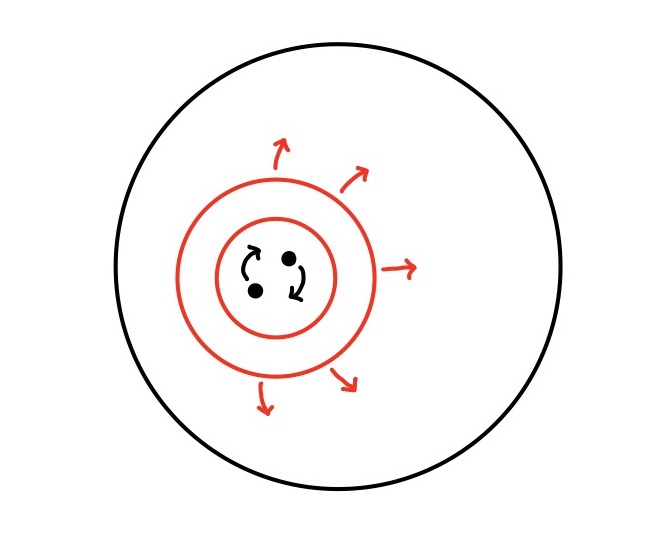
Figure 12. Gravitational waves production on a $2$-sphere.

Note that in a $2$-sphere, plane waves due to the spiralling of two objects in spacetime would be produced by distorting the $\theta$-component of the metric while moving in the $\phi$-direction, see Figure 12. So, the wave perturbation to the metric looks like

$$\Psi_{\mu\nu}={\rm diag}(0,A\sin(k(\phi-t)),0)\,.$$

Thus, we can consider a perturbation to $S^{3}_{a}$ of the form

$$g^{a}_{\mu\nu}\rightarrow g^{a}_{\mu\nu}+\epsilon\Psi_{\mu\nu},\ \ \ \text{ with }|\epsilon|<<1\,,$$

with $\Psi_{\mu\nu}={\rm diag}(0,A_{\psi}\cos(k(\phi_{a}-t)),0,0)$.

We then obtain the surface energy-momentum tensor induced by this perturbation, of the form

$$S_{ab}=\begin{pmatrix}-\frac{A_{\psi}k\epsilon\sin(k(\phi_{o}-t))}{16\pi(r_{a}^{2}+A_{\psi}k\epsilon\cos(k(\phi_{o}-t)))}&0&0\\ 0&0&0\\ 0&0&\frac{A_{\psi}r_{I}^{2}\sin^{2}\theta_{I}k\epsilon\sin(k(\phi_{o}-t))}{16\pi(r_{a}^{2}+A_{\psi}k\epsilon\cos(k(\phi_{o}-t)))}\end{pmatrix}\,.$$

We use the assumption that $r_{b}>>r_{a}$ to approximate the space surrounding $\Sigma$ in $S^{3}_{b}$ with a flat space. Specifically, we can imagine sending the metric inside some open $3$-ball $U\subset S^{3}_{b}$ to the limit

$$ds^{2}_{b}|_{U}\rightarrow-dt^{2}+dr^{2}+r^{2}(d\theta^{2}+\sin^{2}\theta d\phi^{2}).$$

In this limit, the metric component of the azimuth angle $\phi_{b}$ that we fixed becomes associated with the $r$-component for $\mathbb{R}^{3,1}_{b}$, while the components for the other two angles stay the same, since they still map out the same $2$-sphere in $\mathbb{R}^{3,1}_{b}$, see Figure 13.

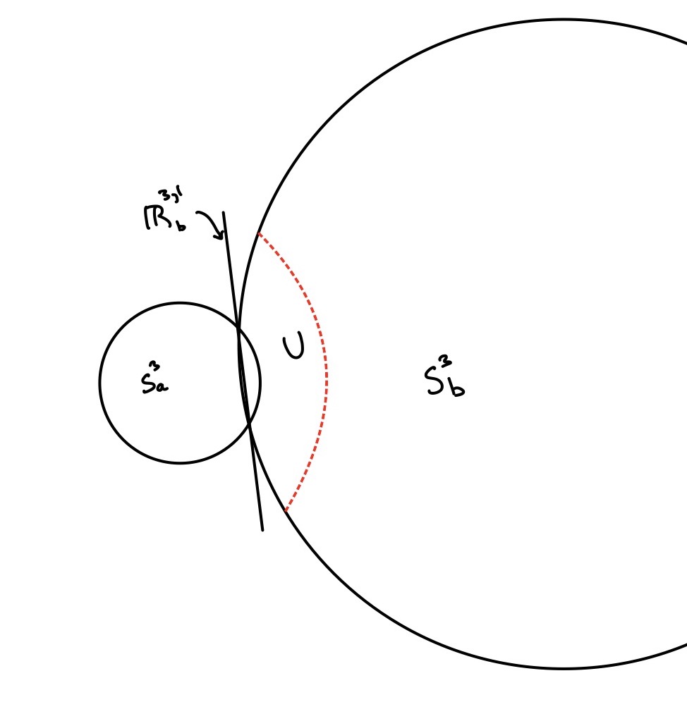
Figure 13. As $r_{b}\rightarrow\infty$, an open $3$-ball $U$ on $S^{3}_{b}$ with $\Sigma\subset U$ can be approximated by some $U^{\prime}\subset\mathbb{R}^{3}$.

Then the induced energy-momentum tensor on $U$, described in spherical coordinates, is approximated by

$$T_{\mu\nu}\approx\begin{pmatrix}-\frac{A_{\psi}k\epsilon\sin(k(\phi^{a}_{o}-t))}{16\pi(r_{a}^{2}+A_{\psi}k\epsilon\cos(k(\phi^{a}_{o}-t)))}\delta(r-r_{I})&0&0&0\\ 0&0&0&0\\ 0&0&0&0\\ 0&0&0&\frac{A_{\psi}r_{I}^{2}sin^{2}\theta k\epsilon\sin(k(\phi^{a}_{o}-t))}{16\pi(r_{a}^{2}+A_{\psi}k\epsilon\cos(k(\phi_{o}^{a}-t)))}\delta(r-r_{I})\end{pmatrix}\,.$$

Recall that, for a tensor $\gamma_{\mu\nu}$, we have $\gamma=\gamma^{\mu}_{\,\mu}=\eta_{\mu\nu}\gamma_{\mu\nu}$, with the flat Minkowski metric $\eta_{\mu\nu}$, and the trace-reverse of $\gamma_{\mu\nu}$ is given by $\bar{\gamma}_{\mu\nu}=\gamma_{\mu\nu}-\frac{1}{2}\eta_{\mu\nu}\gamma$. The equation for the trace-reversed pertubation to the metric tensor, $\bar{\Psi}_{\mu\nu}$, in linearized gravity for the Lorenz gauge condition is then given by

$$\Box\bar{\Psi}_{\mu\nu}=-16\pi GT_{\mu\nu}\,.$$

Using the known Green function for Minkowski space,

$$G(x^{\mu}-x^{\prime\mu})=-\frac{1}{4\pi|\mathbf{x-x^{\prime}}|}\delta(\mathbf{|x-x^{\prime}|}-(x^{0}-x^{\prime 0}))\Theta(x^{0}-x^{\prime 0})\,,$$

we can write our solution in the form

$$\bar{\Psi}_{\mu\nu}=4G\int d^{3}x^{\prime}\frac{1}{|\mathbf{x-x^{\prime}}|}T_{\mu\nu}(t-|\mathbf{x-x^{\prime}}|,\mathbf{x^{\prime}})\,.$$

This integral is non-trivial for either $\bar{\Psi}_{\phi\phi}$ or $\bar{\Psi}_{tt}$. Since this calculation is meant to give us an overall idea of what happens at this boundary, we have opted to approximate the result in two cases:

1. the solution for the metric inside $\Sigma$ in $U$;

2. the solution for the metric outside and far away from $\Sigma$.

4.1.1. First case: internal solution

We begin with the solution in the first case listed above. In this case, to linear order in $\epsilon$, $T_{\phi\phi}$ we have

$$T_{\phi\phi}=\frac{A_{\Psi}kr_{I}^{2}}{16\pi r_{a}^{2}}\sin^{2}\theta\sin(k(\phi_{o}^{a}-t))\delta(r-r_{I})\epsilon+O(\epsilon^{2})\,.$$

Thus, we obtain a solution for $\bar{\Psi}_{\phi\phi}$ given by the integral

$$\frac{4GA_{\Psi}kr_{I}^{2}\epsilon}{16\pi r_{a}^{2}}\int_{\mathbb{S}^{2}}d\Omega^{\prime}\,\sin^{2}\theta^{\prime}\,\,\frac{\sin(k(|\mathbf{x-x^{\prime}}|-t))}{|\mathbf{x-x^{\prime}}|}\,,$$

where we have suppressed the term $\phi^{a}_{o}$, since it is simply a phase factor. The Euclidean distance is given by

$$|\mathbf{x-x^{\prime}}|=\sqrt{r^{2}+r_{I}^{2}-2rr_{I}\mathbf{u\cdot u^{\prime}}}\,,$$

where $\mathbf{u}$ and $\mathbf{u^{\prime}}$ are the respective unit vectors on a sphere $S^{2}$.

This integral can be solved exactly using the Funk-Hecke formula of harmonic analysis (see for instance [54])

$$\int f(x\cdot y)Y_{k}(x)\sigma_{\mathbb{S}^{n-1}}(dx)=\lambda_{k}Y_{k}(y)\,,$$

for any bounded measurable function $f:S^{n-1}\to{\mathbb{R}}$, and any $y\in S^{n-1}$, where $Y_{k}$ are the spherical harmonics on $S^{n-1}$ of degree $k\geq 0$ and the constant $\lambda_{k}$ is given by

$$\lambda_{k}=\frac{\Gamma(n/2)}{\sqrt{\pi}\,\Gamma((n-1)/2)}\int_{-1}^{1}f(t)P_{k}(t)(1-t^{2})^{(\frac{n-3}{2})}\,,$$

with $P_{k}$ the $k$-th Gegenbauer polynomial.

Note that polynomials of sinusoids can be written in the basis of spherical harmonics on a sphere, so we may write

$$\sin^{2}\theta^{\prime}=-\frac{1}{3}(4\sqrt{\frac{\pi}{5}}Y_{2}^{0}(\theta^{\prime},\phi^{\prime})-2)\,,$$

where

$$Y_{2}^{0}(\theta^{\prime},\phi^{\prime})=\frac{1}{4}\sqrt{\frac{5}{\pi}}(3\cos^{2}\theta-1)\,.$$

We then define

$$f(x):=\frac{e^{ik\sqrt{\gamma-\beta x}}}{\sqrt{\gamma-\beta x}}\,,$$

where $\gamma=r^{2}+r_{I}^{2}$ and $\beta=2rr_{I}$. The integral can then be solved as

$$\bar{\Psi}_{\phi\phi}=Ae^{-ikt}\bigg{(}-\frac{4}{3}\sqrt{\frac{\pi}{5}}\int d\Omega_{S^{2}}^{\prime}Y^{0}_{2}(\theta^{\prime},\phi^{\prime})f(\mathbf{u\cdot u^{\prime}})+\frac{2}{3}\int d\Omega_{S^{2}}^{\prime}f(\mathbf{u\cdot u^{\prime}})\bigg{)}$$

$$=Ae^{-ikt}\bigg{(}\sqrt{\frac{\pi}{5}}\frac{8\Lambda_{2}(\gamma,\beta)}{\beta^{3}k^{4}}Y_{2}^{0}(\theta,\phi)+\frac{2i}{3\beta}(e^{ik\sqrt{\gamma-\beta}}-e^{ik\sqrt{\gamma+\beta}})\bigg{)}\,,$$

where $A=\frac{4GA_{\Psi}r_{I}^{2}\epsilon}{16\pi r_{a}^{2}}$ and $\Lambda_{2}(\gamma,\beta)$ is given by

$$\Lambda_{2}=e^{ik\sqrt{\gamma+\beta}}\,\mathbb{P}^{+}+e^{ik\sqrt{\gamma-\beta}}\,\mathbb{P}^{-}\,,$$

with the $\mathbb{P}^{\pm}$ given by

$$\mathbb{P}^{+}=-(k^{3}\beta-6k)\sqrt{\gamma+\beta}-i((2\gamma+3\beta)k^{2}-\frac{\beta^{2}k^{4}}{6}-6)\,,$$

$$\mathbb{P}^{-}=-(k^{3}\beta+6k)\sqrt{\gamma-\beta}+i((2\gamma-3\beta)k^{2}-\frac{\beta^{2}k^{4}}{6}-6)\,.$$

Getting the imaginary part of this expression for the metric is then trivial. This solution is quite unwieldy without any approximations and one could easily take different limits to analyze the consequences. Instead, here we opt to numerically graph the solutions. The results are plotted in Figure 14 for different planes of the sphere intersection.

We choose an arbitrary system for numerical plotting, with

$$k=5.0,\ \ \ r_{I}=1,\ \ \ A_{\Psi}=\bigg{(}\frac{4Gkr_{I}^{4}\epsilon}{16\pi r_{a}^{2}}\bigg{)}^{-1}\,,$$

where $k=5.0$ is chosen to highlight the presence of oscillations in the solution. The solution to our theory has the property that the perturbation of the trace reversed metric tensor is mainly located in the $z=0$ plane, which can be somewhat expected of a plane wave centered at $\theta=\pi/2$, as our energy tensor indicates. It is clear the energy tensor induced by the transmission of gravitational waves between two positively curved spaces produces perturbations inside of the intersection sphere that can directly influence the trajectory of particles passing through it. Specifically, it is clear through the plots that the boundary itself sends waves inwards into the $3$-ball region, as well as outwards.

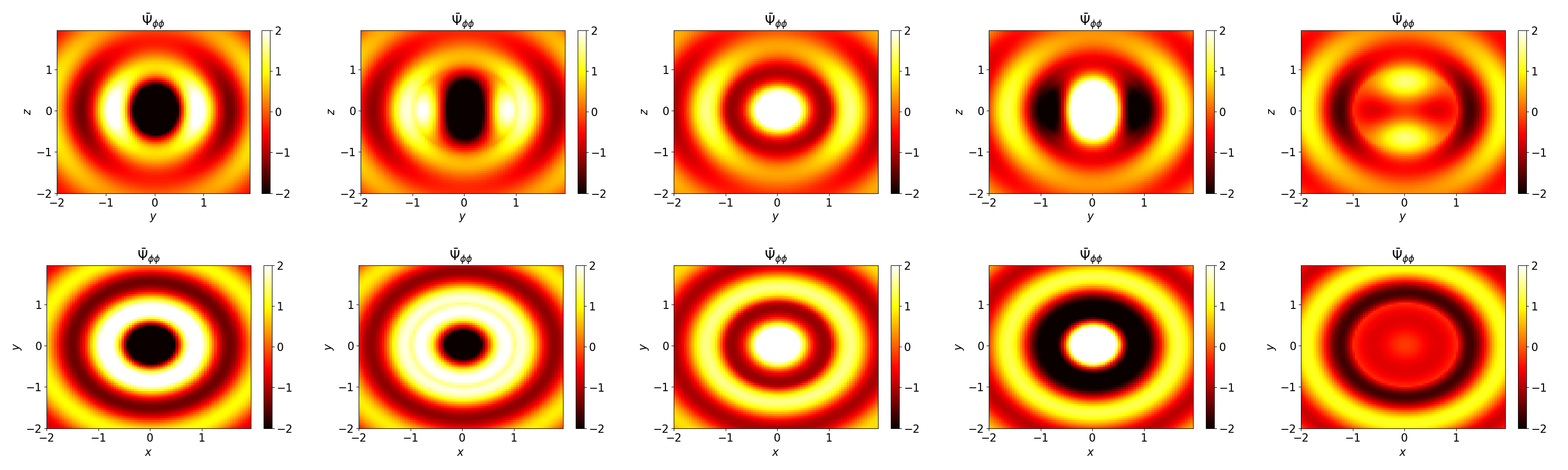
Figure 14. The numerical solution to $\bar{\Psi}_{\phi\phi}$, plotted in the emission plane (2nd row) and the perpendicular plane (1st row) at times $t=(\frac{i\cdot 2\pi}{5k})_{i=0,1,2,3,4}$ for the parameters described. The most obvious consequence is the inward and outward radial emissions in the $\theta=\pi/2$ plane (as $T_{\mu\nu}$ would suggest). The azimuthal symmetry in the solution is also characteristic of plane waves.

4.1.2. Second case: external distant solution

Now, we discuss the second case listed above, namely the far away case ($r>>r_{I}$). We can use the quadrupole formula

$$\bar{\Psi}_{ij}\approx\frac{2G}{r}\frac{d^{2}I_{ij}}{dt^{2}}(t_{r})\,,$$

and one can easily check that the resulting trace-reversed metric in Cartesian coordinates is then given by

$$\bar{\Psi}_{\mu\nu}\approx\frac{A_{\Psi}G\epsilon\pi k^{3}r_{I}^{2}}{8r_{a}^{2}}\frac{\sin(k(r-t))}{r}\begin{pmatrix}0&0&0&0\\ 0&1/2&0&0\\ 0&0&1/2&0\\ 0&0&0&1\end{pmatrix}\,.$$

4.1.3. Summary of behavior

To summarize, we have considered the intersection of two positively curved spaces as a possible boundary for the transmission of gravitational waves. We derived an expression for the stress-energy tensor on the receiving universe induced by the gravitational waves from the emitting universe. We then considered a scenario where radius of the receiving space is much larger than the one of the emitting space ($r_{b}>>r_{a}$) and we considered what the solution to the linearized gravity field equations would look like under such stresses on the $2$-sphere boundary. We found that plane waves can be transmitted at this boundary and create oscillations inside the sphere of intersection as well apparent emission far way from the boundary using the quadruple formula.

The former result has significant theoretical value, as it predicts the creation of observable universe intersections. That is, if one considers the case where we have multiple gravitational wave sources near the intersection on the emitting sphere, our results indicate this configuration would induce a $3$-ball of interfering gravity wave modes on the boundary between the two universes. This $3$-ball will then cause the gravitational lensing of photons if they began their path on a geodesic passing through the intersection and should thus be directly observable.

Our approximations and idealized circumstances should caution one to the exactness of our results, but our result is an indication that this system would follow a behavior similar to that of our solutions, and should still create modes inside the intersection as well as likely-not-observable modes outside of it, falling at $1/r$ as they travel away from the intersection.

4.2. Green functions for the non-flat case

If we were looking for a solution in the non-flat case, we would have to use the Green function for a $3$-sphere crossed with $\mathbb{R}$ (which gives a manifold locally homeomorphic to Minkowski space). To do this, we can use a result derived from [3]. Using $\hat{\phi}(||\mathbf{x}-\mathbf{x^{\prime}}||)=G(\mathbf{x},\mathbf{x^{\prime}})$, where $||\mathbf{x}-\mathbf{x^{\prime}}||$ is the Euclidean distance on $S^{n}$, we can write the Green function for an $S^{n}$ sphere as

$$\hat{\phi}(x)=\frac{2}{n\,{\rm Vol}(S^{n})}\int_{x^{2}/4}^{1}{}_{2}F_{1}(1,n,\frac{n}{2}+1,1-s)ds+C\,,$$

where ${}_{2}F_{1}$ is the Gauss hypergeometric function. This directly implies that, for a $3$-sphere $S_{b}^{3}$ with radius $r_{b}$ we have

$$\hat{\phi}(x)=\frac{1}{4\pi^{2}r_{b}^{3}}\bigg{(}1-\frac{2(x^{2}-2){\rm arcsin}(\sqrt{1-(x/2)^{2}})}{\sqrt{x^{2}(x^{2}-4)}}\bigg{)}+C$$

$$=-\frac{1}{4\pi^{2}r_{b}^{3}}\frac{2(x^{2}-2){\rm arcsin}(\sqrt{1-(x/2)^{2}})}{\sqrt{x^{2}(x^{2}-4)}}+O(1)\,.$$

5. Gravitational waves and the spectral action with fractality

It was shown in [44] that, when considering the expansion of the spectral action functional on a $4$-dimensional spacetime manifold, the Euler-Lagrange equations take the form (for trivial cosmological constant)

$$\frac{-1}{2\kappa}(R^{\mu\nu}-\frac{1}{2}g^{\mu\nu}R)+2\alpha(2\nabla_{\lambda}\nabla_{\kappa}C^{\mu\kappa\nu\lambda}+C^{\mu\kappa\nu\lambda}R_{\kappa\lambda}),$$

with $C^{\mu\kappa\nu\lambda}$ the Weyl curvature tensor. Thus, the variational equations with respect to a perturbation of the metric $g_{\mu\nu}=\eta_{\mu\nu}+\gamma_{\mu\nu}$, to first order in $\gamma_{\mu\nu}$ are of the form

$$\frac{-1}{2}\partial_{\kappa}\partial^{\kappa}\bar{\gamma}^{\mu\nu}+\frac{1}{2\beta^{2}}\partial_{\kappa}\partial^{\kappa}(\partial_{\lambda}\partial^{\lambda}\bar{\gamma}^{\mu\nu}+\frac{1}{3}(\eta^{\mu\nu}\partial_{\lambda}\partial^{\lambda}-\partial^{\mu}\partial^{\nu})\gamma)\,,$$

where $\bar{\gamma}_{\mu\nu}$ is the trace-reversed perturbation as in the previous section and $\beta^{2}=-1/(32\pi G\alpha)$. We refer the reader to [44] for a further discussion of the gauge fixing conditions.

In this derivation of the Euler-Lagrange equations of [44], one considers only the usual the leading terms of the spectral action expansion on a $4$-manifold, which correspond to the order $0$, order $2$, and order $4$ terms of the heat kernel expansion of the squared Dirac operator. As classical action functionals these terme recover the usual Einstein–Hilbert action (with cosmological term) plus the Weyl curvature term and the non-dynamical topological Gauss–Bonnet term, hence one obtains the variational equations of the form recalled above.

Here we consider the effect on these equations of the presence of fractality. We have seen that there are two main effects of fractality on the spectral action. One effect corrects the coefficients of these cosmological, Einstein–Hilbert, and Weyl curvature terms by special values of the fractal packing zeta function $\zeta_{\mathcal{L}}(s)$ at $s=4$, $s=2$, and $s=0$, respectively, for the cosmological, the Einstein–Hilbert, and the Weyl term. This effect can be seen as altering the effecting gravitational and effective cosmological constants, and the coupling constant $\alpha$ of the model. In the variational equations above, this change will affect the value of the $\beta^{2}$ coefficient. The second, more interesting effect, is the presence of the series of log-periodic terms coming from the poles of the fractal packing zeta function $\zeta_{\mathcal{L}}(s)$. We focus here on this second effect and we show that one can interpret these terms as contributing an effecting energy-momentum tensor to the equations of motion. Thus, through this second effect on the spectral action, the presence of fractality is perceived in the gravitational equations as a presence of a type of matter that only interacts gravitationally and is otherwise dark.

5.1. Fractality as an effective energy-momentum tensor

Consider the spectral action expansion for the fractal packings arising from the Robertson–Walker spacetimes for spherical forms or Bieberbach manifolds, as discussed in §2. We focus on the leading terms in the spectral action expansion including the first term (at $s=s_{0}$ of the log-periodic series). These terms suffice to see the effect of fractality on the gravitational waves equation. In the spherical case these terms are of the form

$${\mathcal{S}}_{\Lambda}({\mathcal{D}}_{{\mathcal{P}}_{\Gamma}\times{\mathbb{R}}})\sim\frac{1}{|\Gamma|}\sum_{M=0}^{4}\frac{\Lambda^{4-2M}\,{\mathfrak{f}}_{4-2M}\,A_{M}}{(1-f_{\rho}f_{\sigma}^{2M-4})}+\frac{\Lambda^{s_{0}}\,{\mathfrak{f}}_{s_{0}}\,\Gamma(s_{0}/2)}{2|\Gamma|\log f_{\sigma}}\zeta_{{\mathcal{D}}_{Y\times{\mathbb{R}}}}(s_{0})$$

where $s_{0}=\frac{\log f_{\rho}}{\log f_{\sigma}}=\dim_{H}{\mathcal{L}}_{\Gamma}$, and

$$A_{M}:=\int\bigg{(}\int\big{(}\frac{1}{2}C^{-3/2,0}_{2M}+\frac{1}{4}(C^{-5/2,2}_{2M-2}-C^{-1/2,0}_{2M-2})\big{)}\,D[\alpha]\bigg{)}dt\,.$$

In the flat case they are of the form

$${\mathcal{S}}_{\Lambda}({\mathcal{D}}_{{\mathcal{P}}_{G_{a}}\times{\mathbb{R}}})\sim\lambda_{G_{a}}\sum_{M=0}^{4}\frac{\Lambda^{4-2M}\,{\mathfrak{f}}_{4-2M}\,B_{M}}{(1-f_{\rho}f_{\sigma}^{2M-4})}+\frac{\Lambda^{s_{0}}\,{\mathfrak{f}}_{s_{0}}\,\Gamma(s_{0}/2)\,\lambda_{G_{a}}}{2\log f_{\sigma}}\zeta_{{\mathcal{D}}_{Y_{a}}\times{\mathbb{R}}}(s_{0})\,,$$

with

$$B_{M}:=\int\bigg{(}\int\big{(}\frac{1}{2}C^{-3/2,0}_{2M}+\frac{1}{4}(C^{-5/2,2}_{2M-2})\big{)}\,D[\alpha]\bigg{)}dt\,.$$

As shown in [18], the terms $A_{M}$, $B_{M}$, for $M=0,2,4$ give the cosmological, Einstein–Hilbert, and Weyl term. Thus, we see that, when we consider a variation of the metric and the resulting Euler–Lagrange equations, the first three terms, for $M=0,2,4$, contribute the same variational equations as in [44] (including the cosmological term), with coefficients scaled by the $(1-f_{\rho}f_{\sigma}^{2M-4})^{-1}$ factors that are an effect of the presence of fractality. On the other hand, the last term contributes a variation of the form

$$K\cdot\,\,\frac{\delta\,\zeta_{{\mathcal{D}}_{Y\times{\mathbb{R}}}}(s_{0})}{\delta\gamma_{\mu\nu}}\,,$$

where the factor $K$ is either

$$K=\frac{\Lambda^{s_{0}}\,{\mathfrak{f}}_{s_{0}}\,\Gamma(s_{0}/2)}{2|\Gamma|\log f_{\sigma}}\ \ \ \text{ or }\ \ \ K=\frac{\Lambda^{s_{0}}\,{\mathfrak{f}}_{s_{0}}\,\Gamma(s_{0}/2)\,\lambda_{G_{a}}}{2\log f_{\sigma}}\,,$$

for the spherical and flat case, respectively.

To analyze the variation

(5.1) $$T_{\mu\nu}:=\frac{\delta\,\zeta_{{\mathcal{D}}_{Y\times{\mathbb{R}}}}(s_{0})}{\delta\gamma_{\mu\nu}}$$

we use the following general fact about the zeta function of the Dirac operator. Let ${\mathcal{D}}={\mathcal{D}}_{X,g}$ be the Dirac operator on a $4$-manifold $(X,g)$, which for us will be a Robertson–Walker spacetime $Y\times{\mathbb{R}}$ with a candidate cosmic topology $Y$. We consider a smooth variation of the metric $g_{\mu\nu}(u)=g_{\mu\nu}+u\gamma_{\mu\nu}$, in a one-parameter family with parameter $u\geq 0$. We write the corresponding Dirac operator as ${\mathcal{D}}_{u}={\mathcal{D}}_{Y\times{\mathbb{R}},g_{\mu\nu}(u)}$. We assume that, under this variation of the metric, the eigenvalues $\lambda_{u}$ of ${\mathcal{D}}_{u}$ depend smoothly on the parameter $u$. We also assume for simplicity that ${\rm Ker}({\mathcal{D}}_{u})=0$ for all $u\geq 0$. Consider the zeta function

$$\zeta_{{\mathcal{D}}_{u}}(s)={\rm Tr}(|{\mathcal{D}}_{u}|^{-s})=\sum_{\lambda_{u}\in{\rm Spec}({\mathcal{D}}_{u})}|\lambda_{u}|^{-s}\,.$$

We assume that this series converges for $\Re(s)>R$ for some sufficiently large constant $R>0$, for all $u\geq 0$. With the notation $Q_{u}=|{\mathcal{D}}_{u}|$ and $\dot{Q}_{u}=\frac{d}{du}Q_{u}$, we then have

$$\frac{d}{du}\zeta_{{\mathcal{D}}_{u}}(s)=-s\sum_{\lambda_{u}\in{\rm Spec}(Q_{u})}\dot{\lambda}_{u}\lambda_{u}^{-(s-1)}=-s{\rm Tr}(\dot{Q}_{u}\,Q_{u}^{-(s-1)})\,.$$

We can then write the variation (5.1) as

$$T_{\mu\nu}=-s_{0}\,{\rm Tr}\left(\frac{\delta Q}{\delta\gamma_{\mu\nu}}\,\,Q^{-(s_{0}-1)}\right)\,.$$

We can interpret the variations (5.1) of the zeta value as playing the role of an energy-momentum tensor in the variational equations for the spectral action gravity functional.

Acknowledgment

This work was supported by NSF grants DMS-1707882 and DMS-2104330. The first author acknowledges support from the Caltech WAVE program for undergraduate research.

References

• [1] R. Aurich, S. Lustig, The Hantzsche–Wendt manifold in cosmic topology, Class. Quantum Grav. 31 (2014) 165009 (19pp)
• [2] A. Ball, M. Marcolli, Spectral action models of gravity on packed swiss cheese cosmology, Class. Quantum Gravity 33 (2016) N.11, 115018, [39 pages]
• [3] C. Beltran, N. Corral, J. Criado Del Rey, Discrete and continuous Green energy on compact manifolds, Journal of Approximation Theory, Vol. 237 (2019), 160–185.
• [4] M. Buck, M. Fairbairn, M. Sakellariadou, Inflation in models with Conformally Coupled Scalar fields: An application to the Noncommutative Spectral Action, Phys. Rev. D 82 (2010) 043509 [14 pages]
• [5] B. Cacic, M. Marcolli, K. Teh, Coupling of gravity to matter, spectral action and cosmic topology, J. Noncommut. Geom. 8 (2014), no. 2, 473–504.
• [6] C. Cattani, E. Laserra, I. Bochicchio, Simplicial approach to fractal structures, Mathematical Problems in Engineering, (2012), Article ID 958101 [21 pages]
• [7] A.H.Chamseddine, A.Connes, The spectral action principle, Comm. Math. Phys. 186 (1997), no. 3, 731–750.
• [8] A.H.Chamseddine, A.Connes, Universal formula for noncommutative geometry actions: unification of gravity and the standard model, Phys. Rev. Lett. 77 (1996), no. 24, 4868–4871
• [9] A.H. Chamseddine, A. Connes, The uncanny precision of the spectral action, Communications in Mathematical Physics, 293 (2010) N.3, 867–897.
• [10] A.H. Chamseddine, A. Connes, Spectral action for Robertson-Walker metrics. J. High Energy Phys. 2012, no. 10, 101, front matter + 29 pp.
• [11] E. Christensen, C. Ivan, M.L. Lapidus, Dirac operators and spectral triples for some fractal sets built on curves, Adv. Math. 217 (2008), no. 1, 42–78.
• [12] E. Christensen, C. Ivan, E. Schrohe, Spectral triples and the geometry of fractals, J. Noncommut. Geom. 6 (2012), N.2, 249–274.
• [13] A. Connes, Geometry from the spectral point of view. Lett. Math. Phys. 34 (1995), no. 3, 203–238.
• [14] A. Connes, M. Marcolli, Noncommutative Geometry, Quantum Fields and Motives, Colloquium Publ. Vol.55, American Mathematical Society, 2008.
• [15] K. Dennis, S. Schlicker, Sierpinski $n$-gons,
https://faculty.gvsu.edu/schlicks/SNGONS4.pdf
• [16] W. Fan, F. Fathizadeh, M. Marcolli, Motives and periods in Bianchi IX gravity models, Lett. Math. Phys. 108 (2018) N.12, 2729–2747.
• [17] W. Fan, F. Fathizadeh, M. Marcolli, Modular forms in the spectral action of Bianchi IX gravitational instantons, J. High Energy Phys. 01 (2019), 234
• [18] F. Fathizadeh, Y. Kafkoulis, M. Marcolli, Bell Polynomials and Brownian Bridge in Spectral Gravity Models on Multifractal Robertson–Walker Cosmologies, Ann. Henri Poincaré, 21 (2020), no. 4, 1329–1382.
• [19] F. Fathizadeh, M. Marcolli, Periods and motives in the spectral action of Robertson–Walker spacetimes, Commun. Math. Phys. 356 (2017) N.2, 641–671.
• [20] G.B. Folland, Fourier Analysis and Its Applications, American Mathematical Society, 1992.
• [21] A. Fujii, On the distribution of values of the derivative of the Riemann zeta function at its zeros. I, Proc. Steklov Inst. Math. 276 (2012), no. 1, 51–76.
• [22] A. Gabrielli, F. Sylos Labini, M. Joyce, L. Pietronero, Statistical Physics for Cosmic Structures, Springer, 2005.
• [23] R.L. Graham, J.C. Lagarias, C.L. Mallows, A.R. Wilks, C.H. Yan, Apollonian circle packings: number theory. J. Number Theory 100 (2003), 1–45.
• [24] G.A. Hiary, A.M. Odlyzko, Numerical study of the derivative of the Riemann zeta function at zeros, Comment. Math. Univ. St. Pauli, Vol. 60 (2011), no. 1-2, 47–60.
• [25] R.L. Graham, J.C. Lagarias, C.L. Mallows, A.R. Wilks, C.H. Yan, Apollonian Circle Packings: Geometry and Group Theory III. Higher Dimensions, Discrete Comput Geom 35 (2006), 37–72.
• [26] Ronald L. Graham, Jeffrey C. Lagarias, Colin L. Mallows, Allan R. Wilks, Catherine H. Yan, Apollonian circle packings: number theory, Journal of Number Theory, Volume 100, Issue 1, 2003, Pages 1-45.
• [27] B. Iochum, C. Levy, Spectral triples and manifolds with boundary, J. Funct. Anal. 260 (2011), N.1, 117–134.
• [28] H. Jones, A. Campa, Fractals Based on Regular Polygons and Polyhedra, in N.M. Patrikalakis (Ed.) “Scientific Visualization of Physical Phenomena”, pp. 299–313, Springer, 1991.
• [29] M. Katsurada, On an asymptotic formula of Ramanujan for a certain theta-type series, Acta Arithmetica, 97 No. 2 (2001), 157–172.
• [30] A. Katunin, Construction of fractals based on Catalan solids, Int. J. Mathematical Sciences and Computing, 4 (2017), 1–7.
• [31] A. Katunin, Deterministic fractals based on Archimedean solids, Scientific Research of the Institute of Mathematics and Computer Science, Vol.1 (2011), N.10, 93–100.
• [32] A. Katunin, D. Kurzyk, General rules of fractals construction from polyhedra, Journal for Geometry and Graphics, Vol. 16 (2012), No. 2, 129–137.
• [33] A. Kunnen, S. Schlicker, Regular Sierpinski polyhedra, Pi Mu Epsilon J. 10 (1998), 607–619.
• [34] M. Lachièze-Rey, J.P. Luminet, Cosmic topology, Phys. Rep. 254 (1995), 135–214.
• [35] J. Levin, Topology and the cosmic microwave background, Physics Reports 365 (2002) 251–333.
• [36] J.P. Luminet, B.F. Roukema, Topology of the Universe: Theory and Observation, in “Theoretical and Observational Cosmology” pp. 117–156, NATO Science Series (Series C: Mathematical and Physical Sciences), vol 541. Springer, 1999.
• [37] M. Marcolli, Noncommutative Cosmology, World Scientific, 2017.
• [38] M. Marcolli, Spectral action gravity and cosmological models, Comptes Rendus Physique, Vol. 18 (2017) N. 3–4, 226–234.
• [39] M. Marcolli, Building cosmological models via noncommutative geometry, Int. J. Geom. Meth. Mod. Phys., Vol.8, N.5 (2011) 1131–1168.
• [40] M. Marcolli, E. Pierpaoli, Early universe models from noncommutative geometry, Adv. Theor. Math. Phys. 14 (2010), no. 5, 1373–1432.
• [41] M. Marcolli, E. Pierpaoli, K. Teh, The spectral action and cosmic topology, Commun. Math. Phys. 304 (2011), 125–174.
• [42] M. Marcolli, E. Pierpaoli, K. Teh, The coupling of topology and inflation in noncommutative cosmology, Commun. Math. Phys. 309 (2012) N.2, 341–369.
• [43] J.R. Mureika, C.C. Dyer, Multifractal analysis of packed swiss cheese cosmologies, Gen. Rel. Gravit. 36 (2004) N.1, 151–184.
• [44] W. Nelson, J. Ochoa, M. Sakellariadou, Gravitational waves in the spectral action of noncommutative geometry, Phys. Rev. D 82 (2010), 085021 [14 pages]
• [45] W. Nelson, J. Ochoa, M. Sakellariadou, Constraining the noncommutative spectral action via astrophysical observations, Phys. Rev. Lett.105 (2010) 101602
• [46] W. Nelson, M. Sakellariadou, Natural inflation mechanism in asymptotic noncommutative geometry, Phys. Lett. B 680 (2009) 263–266.
• [47] P. Olczykowski, A. Sitarz, On spectral action over Bieberbach manifolds, Acta Phys. Polon. B 42 (2011) N.6, 1189–1198.
• [48] F. Pfäffle, The Dirac spectrum of Bieberbach manifolds, J. Geom. Phys. 35 (2000), 367–385.
• [49] E. Poisson, A Relativist’s Toolkit, Cambridge University Press, 2004.
• [50] M.J. Rees, D.W. Sciama, Large-scale density inhomogeneities in the universe, Nature 217 (1968), 511–516.
• [51] A. Riazuelo, J. Weeks, J.P. Uzan, R. Lehoucq, J.P. Luminet, Cosmic microwave background anisotropies in multiconnected flat spaces, Phys. Rev. D 69 (2004), 103518 [25 pages]
• [52] M. Ruman, Topological and Hausdorff dimension of Koch tetrahedron fractal, URL (version: 2018-01-11)
https://math.stackexchange.com/users/520540/marko-ruman
• [53] H.F. Sandham, A square as the sum of $7$ squares, The Quarterly Journal of Mathematics, Vol. 4 (1953), N.1, 230–236.
• [54] R.T. Seeley, Spherical harmonics, The American Mathematical Monthly, Vol. 73 (1966), No. 4, 115–121.
• [55] B. Simon, Functional Integration and Quantum Physics, Pure and Applied Mathematics, vol. 86. Academic Press, 1979.
• [56] T.L. Smith, M. Kamionkowski, A. Cooray, Direct detection of the inflationary gravitational wave background, Phys. Rev. D 73 (2006), N.2, 023504 [14 pages].
• [57] D.V. Stäger, H.J. Herrmann, Self-similar space-filling sphere packings in three and four dimensions, arXiv:1607.08391.
• [58] F. Sylos Labini, M. Montuori, L. Pietronero, Scale-invariance of galaxy clustering, Physics Reports. 293 (1998), 61–226.
• [59] K. Teh, Nonperturbative spectral action of round coset spaces of $SU(2)$, J. Noncommut. Geom. 7 (2013), 677–708.
• [60] W.D. van Suijlekom, Noncommutative geometry and particle physics, Mathematical Physics Studies. Springer, 2015.
• [61] Vassilevich, D. V.: Noncommutative Heat Kernel. Letters in Mathematical Physics. 67, 185–194 (2004)
• [62] E.W. Weisstein, Koch Snowflake, MathWorld–A Wolfram Web Resource.
https://mathworld.wolfram.com/KochSnowflake.html
• [63] D.K. Wilson, C.L. Pettit, S.N. Vecherin, Wavelet-based cascade model for intermittent structure in terrestrial environments, arXiv:1312.5649.
• [64] J.A. Wolf, Spaces of constant curvature, AMS Chelsea Publishing, 2011.
• [65] Y. Yang, Y. Feng, Y. Yu, The generalization of Sierpinski carpet and Sierpinski triangle in $n$-dimensional space, Fractals, Vol. 25 (2017), N.5, 1750040.