Neural-adaptive Stochastic Attitude Filter on SO(3)

Abstract

Successful control of a rigid-body rotating in three dimensional space requires accurate estimation of its attitude. The attitude dynamics are highly nonlinear and are posed on the Special Orthogonal Group $SO(3)$. In addition, measurements supplied by low-cost sensing units pose a challenge for the estimation process. This paper proposes a novel stochastic nonlinear neural-adaptive-based filter on $SO(3)$ for the attitude estimation problem. The proposed filter produces good results given measurements extracted from low-cost sensing units (e.g., IMU or MARG sensor modules). The filter is guaranteed to be almost semi-globally uniformly ultimately bounded in the mean square. In addition to Lie Group formulation, quaternion representation of the proposed filter is provided. The effectiveness of the proposed neural-adaptive filter is tested and evaluated in its discrete form under the conditions of large initialization error and high measurement uncertainties.

I Introduction

Robotics and control applications are heavily reliant on robust filtering solutions to guarantee feasibility of accurate rigid-body orientation (attitude) estimation [1, 2, 3, 4]. The attitude can be reconstructed algebraically given known observations in the inertial-frame and the associated measurements in the body-frame. Examples include QUEST algorithm [5] and singular value decomposition (SVD) [1]. However, body-frame measurements might be attached with uncertainties, in particular if they were supplied by low-cost inertial measurement units (IMUs) or magnetic, angular rate, and gravity (MARG) sensor. Hence, accounting for measurement imperfections requires substituting algebraic attitude reconstruction with estimation filters.

The problem of attitude estimation is traditionally tackled by the active control and robotics research community using Gaussian filters, such as, Kalman filter (KF) [6], extended Kalman filter (EKF) [7], multiplicative extended Kalman filter (MEKF) [2], unscented Kalman filter (UKF) [3], and invariant extended Kalman filter (IEKF) [8]. The unit-quaternion structure of the majority of Gaussian filters offers the benefit of nonsingular attitude representation [9, 10]. However, on the other hand, unit-quaternion formulation is subject to nonuniqueness [11, 12]. This motivated the researchers to explore posing the attitude on the Special Orthogonal Group $\mathbb{SO}(3)$. Unlike unit-quaternion, $\mathbb{SO}(3)$ offers unique and global representation of the rotational matrix [4, 13, 14, 15, 9, 10]. Therefore, over the last decade multiple nonlinear attitude filters on $\mathbb{SO}(3)$ have been proposed, such as nonlinear deterministic filters [4, 13, 14, 15] and nonlinear stochastic filters [9, 10]. The nonlinear filter design on $\mathbb{SO}(3)$ has proven to 1) have a simpler structure, 2) be computationally cheap, and 3) have better tracking performance in contrast to Gaussian filters [4, 13, 14, 15, 9, 10].

It is widely known that neural networks (NNs) have capability to learn complex nonlinear relationships [16, 17, 18, 19]. In the recent years, adaptive artificial neural networks (ANNs) learning, known as neural-adaptive learning, has been found effective for approximating unknown nonlinear dynamics online in several control applications. Examples include two-degrees-of-freedom arm robots [16], multi-agent systems [17], unknown multi-input multi-output systems [18] and fault-tolerant control [19]. Accurate NN approximation of unknown nonlinear dynamics allows for successful control process [16, 17, 18, 19]. In this work, the attitude dynamics are modelled on the Lie Group of $\mathbb{SO}(3)$. The uncertainties inherent to attitude dynamics and gyroscope measurements, are addressed using Brownian motion process. The contributions of this paper are as follows: 1) a neural-adaptive nonlinear stochastic attitude filter on $\mathbb{SO}(3)$ is proposed, 2) the measurement uncertainties are corrected using neural-adaptive adaptation mechanisms extracted by adopting Lyapunov stability, and 3) the closed loop signals are guaranteed to be almost semi-globally uniformly ultimately bounded (SGUUB). While the filter is proposed in a continuous form, its discrete form obtained using exact integration methods is also presented. The filter is tested at a low sampling rate to reflect real-life applications. To the best of the authors knowledge, the attitude estimation problem has not been addressed using a neural-adaptive stochastic filter on $\mathbb{SO}(3)$.

The paper is structured to include six Sections. Section II presents preliminaries of the attitude problem. Section III defines the problem, contains the available measurements, error criteria, and neural network approximation. Section IV presents a novel neural-adaptive stochastic attitude filter. Section V shows and discusses the obtained results. Lastly, Section VI concludes the paper.

II Preliminaries

In this work, $\mathbb{R}$ represents the set of real numbers, $\mathbb{R}_{+}$ denotes the set of nonnegative real numbers, and $\mathbb{R}^{n\times m}$ stands for a real $n$-by-$m$ dimensional space. $\mathbf{I}_{n}$ and $0_{n\times m}$ denote an $n$-by-$n$ identity matrix and an $n$-by-$m$ dimensional matrix of zeros, respectively. For $a\in\mathbb{R}^{n}$ and $A\in\mathbb{R}^{n\times m}$, $||a||=\sqrt{a^{\top}a}$ stands for Euclidean norm of $x$ and $||A||_{F}=\sqrt{{\rm Tr}\{AA^{*}\}}$ describes the Frobenius norm of $A$ where $*$ denotes a conjugate transpose. For $A\in\mathbb{R}^{n\times n}$, define a set of eigenvalues as $\lambda(A)=\{\lambda_{1},\lambda_{2},\ldots,\lambda_{n}\}$ where $\overline{\lambda}_{A}=\overline{\lambda}(A)$ denotes the maximum value, while $\underline{\lambda}_{A}=\underline{\lambda}(A)$ describes the minimum value of $\lambda(A)$. $\left\{\mathcal{I}\right\}$ defines a fixed inertial-frame and $\left\{\mathcal{B}\right\}$ describes a fixed body-frame. Rigid-body’s orientation in three-dimensional space, commonly known as attitude, is expressed as $R\in\mathbb{SO}(3)$ with

$$\mathbb{SO}(3)=\{R\in\mathbb{R}^{3\times 3}|R^{\top}R=\mathbf{I}_{3}\text{, }{\rm det}(R)=+1\}$$

where ${\rm det}(\cdot)$ denotes a determinant. The Lie algebra associated with $\mathbb{SO}(3)$ is termed $\mathfrak{so}(3)$ and can be described as

$$\mathfrak{so}(3) =\{[a]_{\times}\in\mathbb{R}^{3\times 3}|[a]_{\times}^{\top}=-[a]_{\times},a\in\mathbb{R}^{3}\}$$

$$\left[a\right]_{\times} =\left[\begin{array}[]{ccc}0&-a_{3}&a_{2}\\ a_{3}&0&-a_{1}\\ -a_{2}&a_{1}&0\end{array}\right]\in\mathfrak{so}\left(3\right),\hskip 10.00002pta=\left[\begin{array}[]{c}a_{1}\\ a_{2}\\ a_{3}\end{array}\right]$$

The operator $\mathbf{vex}$ stands for the inverse mapping of $[\cdot]_{\times}$ with the map $\mathbf{vex}:\mathfrak{so}(3)\rightarrow\mathbb{R}^{3}$ where $\mathbf{vex}([a]_{\times})=a,\forall a\in\mathbb{R}^{3}$. The anti-symmetric projection has the map $\boldsymbol{\mathcal{P}}_{a}:\mathbb{R}^{3\times 3}\rightarrow\mathfrak{so}(3)$ where

$$\boldsymbol{\mathcal{P}}_{a}(M)=\frac{1}{2}(M-M^{\top})\in\mathfrak{so}\left(3\right),\forall M\in\mathbb{R}^{3\times 3}$$

For $M=[m_{i,j}]_{i,j=1,2,3}\in\mathbb{R}^{3\times 3}$, let us define

$$\boldsymbol{\Upsilon}(M)=\mathbf{vex}(\boldsymbol{\mathcal{P}}_{a}(M))=\frac{1}{2}\left[\begin{array}[]{c}m_{32}-m_{23}\\ m_{13}-m_{31}\\ m_{21}-m_{12}\end{array}\right]\in\mathbb{R}^{3}$$ (1)

For $R\in\mathbb{SO}\left(3\right)$, define the Euclidean distance of $R$ as follows:

$$||R||_{{\rm I}}=\frac{1}{4}{\rm Tr}\{\mathbf{I}_{3}-R\}\in\left[0,1\right]$$ (2)

with ${\rm Tr}\{\cdot\}$ standing for a trace of a matrix. For $A\in\mathbb{R}^{3\times 3}$ and $\alpha\in\mathbb{R}^{3}$, considering the composition mapping in (1), let us introduce the following identity:

$${\rm Tr}\{A[\alpha]_{\times}\}={\rm Tr}\{\boldsymbol{\mathcal{P}}_{a}(A)[\alpha]_{\times}\}=-2\boldsymbol{\Upsilon}(A)^{\top}\alpha$$ (3)

III Problem Formulation

III-A Measurements and Dynamics

Let $R\in\mathbb{SO}(3)$ be the attitude of a rigid-body in three-dimensional space defined with respect to $\left\{\mathcal{B}\right\}$. The true attitude dynamics:

$$\dot{R}=R\left[\Omega\right]_{\times}$$ (4)

where $\Omega\in\mathbb{R}^{3}$ represents angular velocity of the rigid-body defined with respect to $\left\{\mathcal{B}\right\}$. The attitude of a rigid-body can be obtained given a group of measurements in $\left\{\mathcal{B}\right\}$ and a group of observations in $\left\{\mathcal{I}\right\}$. Let $r_{i}\in\mathbb{R}^{3}$ denote an observation in $\left\{\mathcal{I}\right\}$. As such, the measurement of $r_{i}$ with respect to $\left\{\mathcal{B}\right\}$ is given by

$$y_{i} =R^{\top}r_{i}+n_{i}\in\mathbb{R}^{3},\hskip 10.00002pt\forall i=1,2,\ldots,N$$ (5)

where $n_{i}$ denotes unknown noise. The attitude can be obtained given two or more non-collinear inertial observations ($N\geq 2$) and the respective body-frame measurements. If $N=2$, the third observation and the associated measurement can be defined by $r_{3}=r_{2}\times r_{1}$ and $y_{3}=y_{2}\times y_{1}$ where $\times$ denotes a cross product. The set of observations and measurements can be normalized as follows:

$${\bf r}_{i}=\frac{r_{i}}{||r_{i}||},\hskip 10.00002pt{\bf y}_{i}=\frac{y_{i}}{||y_{i}||}$$ (6)

Low-cost IMU or MARG sensors can be utilized for attitude determination or estimation, see [4, 13, 14, 15, 9, 10]. Gyroscope (angular rate or angular velocity) measurements can be defined as follows:

$$\Omega_{m}=\Omega+n\in\mathbb{R}^{3}$$ (7)

with $\Omega$ being the true angular velocity defined in (4), and $n$ being unknown noise corrupting $\Omega_{m}$. The noise vector $n$ is bounded and Gaussian with a zero mean $\mathbb{E}[n]=0$ where $\mathbb{E}[\cdot]$ denotes expected value of a component. Derivative of a Gaussian process results in a Gaussian process [20, 21]. As such, $n$ can be formulated as a Brownian motion process

$$n=\mathcal{Q}\frac{d\beta}{dt}$$ (8)

where $\beta\in\mathbb{R}^{3}$ and $\mathcal{Q}\in\mathbb{R}^{3\times 3}$ is an unknown time-variant symmetric matrix with $\mathcal{Q}^{2}=\mathcal{Q}\mathcal{Q}^{\top}$ being the noise covariance. It is worth noting that $\mathbb{P}\{\beta(0)=0\}=1$ and $\mathbb{E}[\beta]=0$ where $\mathbb{P}\{\cdot\}$ denotes probability of a component. Therefore, from (4), (7), and (8), the true attitude dynamics can be defined in a stochastic sense as follows:

$$dR=R[\Omega_{m}]_{\times}dt-R[\mathcal{Q}d\beta]_{\times}$$ (9)

In view of (1)-(3), one obtains the normalized Euclidean distance of $R$ in (9) as follows:

$$d||R||_{{\rm I}}=2\boldsymbol{\Upsilon}(R)^{\top}\Omega_{m}dt-2\boldsymbol{\Upsilon}(R)^{\top}\mathcal{Q}d\beta$$ (10)

Lemma 1.

[10] Let $R\in\mathbb{SO}(3)$, $\boldsymbol{\Upsilon}(R)=\mathbf{vex}(\boldsymbol{\mathcal{P}}_{a}(R))$ as in (1), and $||R||_{{\rm I}}=\frac{1}{4}{\rm Tr}\{\mathbf{I}_{3}-R\}$ as (2). Hence, the following equality holds:

$$||\boldsymbol{\Upsilon}(R)||^{2}=4(1-||R||_{{\rm I}})||R||_{{\rm I}}$$

Definition 1.

[10, 22] Consider the stochastic attitude dynamics in (10) and let $t_{0}$ be the initial time. $||R||_{{\rm I}}=||R(t)||_{{\rm I}}$ is said to be almost SGUUB if for a given set $\pi\in\mathbb{R}$ and $||R(t_{0})||_{{\rm I}}$ a constant $\alpha>0$ exists and a time constant $T_{\alpha}=T_{\alpha}(\kappa,||R(t_{0})||_{{\rm I}})$ such that $\mathbb{E}[||R(t_{0})||_{{\rm I}}]<\alpha,\forall t>t_{0}+\alpha$.

Lemma 2.

[23] Recall the stochastic attitude dynamics in (10) and assume that $V(||R||_{{\rm I}})$ be a twice differentiable potential function such that

$$\mathcal{L}V(||R||_{{\rm I}})=V_{1}^{\top}f+\frac{1}{2}{\rm Tr}\{g\mathcal{Q}^{2}g^{\top}V_{2}\}$$ (11)

with $f=2\boldsymbol{\Upsilon}(R)^{\top}\Omega_{m}\in\mathbb{R}$, $g=-2\boldsymbol{\Upsilon}(R)^{\top}\in\mathbb{R}^{1\times 3}$, $\mathcal{L}V(||R||_{{\rm I}})$ being a differential operator, $V_{1}=\partial V/\partial||R||_{{\rm I}}$, and $V_{2}=\partial^{2}V/\partial||R||_{{\rm I}}^{2}$. Let $\underline{\alpha}_{1}(\cdot)$ and $\overline{\alpha}_{2}(\cdot)$ be class $\mathcal{K}_{\infty}$ functions, and assume that the constants $\beta>0$ and $\eta\geq 0$ such that

$$\hskip 10.00002pt\underline{\alpha}_{1}(||R||_{{\rm I}})\leq V(||R||_{{\rm I}})\leq\overline{\alpha}_{2}(||R||_{{\rm I}})$$ (12)

$$\mathcal{L}V(||R||_{{\rm I}}) =V_{1}^{\top}f+\frac{1}{2}{\rm Tr}\{g\mathcal{Q}^{2}g^{\top}V_{2}\}$$

$$\leq-\beta V(||R||_{{\rm I}})+\eta$$ (13)

Hence, the stochastic attitude dynamics in (10) have an almost unique strong solution on $[0,\infty)$. Moreover, the solution $||R||_{{\rm I}}$ is upper bounded in probability with

$$\mathbb{E}[V(||R||_{{\rm I}})]\leq V(||R(0)||_{{\rm I}}){\rm exp}(-\beta t)+\eta/\beta$$ (14)

Also, (14) implies that $||R||_{{\rm I}}$ is SGUUBin the mean square.

Define $\hat{R}$ as the estimate of $R$. Define the error in estimation by

$$\tilde{R}=R^{\top}\hat{R}$$ (15)

III-B Filter Structure and Error Dynamics

Define the filter dynamics as follows:

$$\dot{\hat{R}}=\hat{R}[\Omega_{m}-C]_{\times}$$ (16)

with $C\in\mathbb{R}^{3\times 1}$ being a neural-adaptive-based correction matrix to be designed in the subsequent Section. From (4) and (16), the error dynamics are as follows:

$$d\tilde{R} =R^{\top}d\hat{R}+dR^{\top}\hat{R}$$

$$=(\tilde{R}[\Omega-C]_{\times}+[\Omega]_{\times}^{\top}\tilde{R})dt+\tilde{R}[\mathcal{Q}d\beta]_{\times}$$

$$=\tilde{R}[\Omega]_{\times}-[\Omega]_{\times}\tilde{R}-\tilde{R}[C]_{\times}dt+\tilde{R}[\mathcal{Q}d\beta]_{\times}$$ (17)

In view of (3) and (17), one obtains the Euclidean distance of (17) as below:

$$d||\tilde{R}||_{{\rm I}}=d\frac{1}{4}{\rm Tr}\{\mathbf{I}_{3}-\tilde{R}\}=-\frac{1}{4}{\rm Tr}\{d\tilde{R}\}$$

$$\hskip 20.00003pt=\frac{1}{4}{\rm Tr}\{\tilde{R}[Cdt-\mathcal{Q}d\beta]_{\times}\}-\frac{1}{4}{\rm Tr}\{\tilde{R}[\Omega]_{\times}-[\Omega]_{\times}\tilde{R}\}$$

$$\hskip 20.00003pt=\frac{1}{4}{\rm Tr}\{\mathcal{P}_{a}(\tilde{R})[Cdt-\mathcal{Q}d\beta]_{\times}\}$$

$$\hskip 20.00003pt=-\frac{1}{2}\boldsymbol{\Upsilon}(\tilde{R})^{\top}Cdt+\frac{1}{2}\boldsymbol{\Upsilon}(\tilde{R})^{\top}\mathcal{Q}d\beta$$ (18)

where ${\rm Tr}\{\tilde{R}[\Omega]_{\times}-[\Omega]_{\times}\tilde{R}\}=0$.

III-C Neural Network Structure

In this work, NNs with a linear in parameter structure will be employed. For $x\in\mathbb{R}^{n}$ and a function $f(x)\in\mathbb{R}^{m}$, one has

$$f(x)=W^{\top}\varphi(x)+\alpha_{f}$$

where $W\in\mathbb{R}^{q\times m}$ denotes a $q$-by-$m$-dimensional matrix of synaptic weights, $\varphi(x)\in\mathbb{R}^{q}$ denotes an activation function, $q$ denotes number of neurons, and $\alpha_{f}\in\mathbb{R}^{m}$ denotes an approximated error vector. The activation function may contain high order connections, for instance, Gaussian functions [24], radial basis functions (RBFs) [25], sigmoid functions [26]. Our objectives are to achieve accurate estimation of the attitude matrix, estimate the nonlinear attitude dynamics, and compensate for the uncertainties. NNs have been proven to be successful in estimating high-order nonlinear dynamics [16, 17, 18, 19]. Recall the nonlinear dynamics in (18)

$$d||\tilde{R}||_{{\rm I}}=-\frac{1}{2}\boldsymbol{\Upsilon}(\tilde{R})^{\top}Cdt+\frac{1}{2}\boldsymbol{\Upsilon}(\tilde{R})^{\top}\mathcal{Q}d\beta$$

Define $\varphi(\boldsymbol{\Upsilon}(\tilde{R}))$ as an activation function, and let us approximate

$$C^{\top}\boldsymbol{\Upsilon}(\tilde{R}) =C^{\top}\Gamma_{c}^{\top}\varphi(\boldsymbol{\Upsilon}(\tilde{R}))+\alpha_{b}$$

$$\mathcal{Q}\boldsymbol{\Upsilon}(\tilde{R}) =W_{\sigma}^{\top}\varphi(\boldsymbol{\Upsilon}(\tilde{R}))+\alpha_{\sigma}$$

where $\varphi(\boldsymbol{\Upsilon}(\tilde{R}))\in\mathbb{R}^{q\times 1}$ is an activation function, $\Gamma_{c}\in\mathbb{R}^{q\times 3}$ is a known weighted matrix, $C\in\mathbb{R}^{3\times 1}$ is a correction weights vector to be adaptively tuned, $W_{\sigma}\in\mathbb{R}^{q\times 3}$ are the unknown NN weights to be adaptively tuned, $q>0$ is an integer that denotes the number of neurons, and $\alpha_{b}\in\mathbb{R}$ and $\alpha_{\sigma}\in\mathbb{R}^{3}$ are the approximated error components. Note that $\alpha_{b},||\alpha_{\sigma}||\rightarrow 0$ as $q\rightarrow\infty$. Therefore, the error dynamics of the Euclidean distance in (18) can be reformulated as below:

$$d||\tilde{R}||_{{\rm I}}=\tilde{f}dt+\tilde{g}\mathcal{Q}d\beta= -\frac{1}{2}(C^{\top}\Gamma_{c}^{\top}\varphi(\boldsymbol{\Upsilon}(\tilde{R}))+\alpha_{b})dt$$

$$+\frac{1}{2}(\varphi(\boldsymbol{\Upsilon}(\tilde{R}))^{\top}W_{\sigma}+\alpha_{\sigma}^{\top})d\beta$$ (19)

Define $W_{\sigma}$ as an unknown symmetric constant matrix of NN weights where $\overline{W}_{\sigma}=W_{\sigma}W_{\sigma}^{\top}\in\mathbb{R}^{q\times q}$. Let $\hat{W}_{\sigma}\in\mathbb{R}^{q\times q}$ be the estimate of $\overline{W}_{\sigma}$, and the error in NN weights be

$$\tilde{W}_{\sigma}=\overline{W}_{\sigma}-\hat{W}_{\sigma}\in\mathbb{R}^{q\times q}$$ (20)

IV Neural-adaptive-based Stochastic Filter Design

In this Section, our objective is to develop a nonlinear stochastic filter based on neural-adaptive techniques for the attitude estimation problem. Consider the following neural-adaptive-based nonlinear stochastic filter design:

$$\begin{cases}\dot{\hat{R}}&=\hat{R}[\Omega_{m}-C]_{\times}\\ \dot{\hat{W}}_{\sigma}&=\frac{\psi_{2}}{2}\Gamma_{\sigma}\varphi(\boldsymbol{\Upsilon}(\tilde{R}))\varphi(\boldsymbol{\Upsilon}(\tilde{R}))^{\top}-k_{\sigma}\Gamma_{\sigma}\hat{W}_{\sigma}\\ C&=\left(\Gamma_{c}^{\top}+\frac{\psi_{2}}{2\psi_{1}}(\Gamma_{c}^{\top}\Gamma_{c})^{-1}\Gamma_{c}^{\top}\hat{W}_{\sigma}\right)\varphi(\boldsymbol{\Upsilon}(\tilde{R}))\end{cases}$$ (21)

where $k_{\sigma}\in\mathbb{R}$ and $k_{c}\in\mathbb{R}$ are positive constants, $\Gamma_{\sigma}\in\mathbb{R}^{q\times q}$ is a positive diagonal matrix, $\Gamma_{c}\in\mathbb{R}^{q\times 3}$ with $\Gamma_{c}^{\top}\Gamma_{c}$ being positive definite, $q$ denotes the number of neurons, $\hat{W}_{\sigma}\in\mathbb{R}^{q\times q}$ is the estimate of $\overline{W}_{\sigma}$, and $\tilde{R}=R_{y}^{\top}\hat{R}$ with $R_{y}$ being the reconstructed attitude, see QUEST [5] or SVD [1]. $\boldsymbol{\Upsilon}(\tilde{R})=\mathbf{vex}(\boldsymbol{\mathcal{P}}_{a}(\tilde{R}))$, $||\tilde{R}||_{{\rm I}}=\frac{1}{4}{\rm Tr}\{\mathbf{I}_{3}-\tilde{R}\}$, $\psi_{1}=\frac{1}{2}(1+||\tilde{R}||_{{\rm I}})\exp(||\tilde{R}||_{{\rm I}})$, and $\psi_{2}=\frac{1}{2}(2+||\tilde{R}||_{{\rm I}})\exp(||\tilde{R}||_{{\rm I}})$. It is becomes apparent that $\hat{W}_{\sigma}$ is symmetric for $\hat{W}_{\sigma}(0)=\hat{W}_{\sigma}(0)^{\top}$. It is worth noting that $\Gamma_{c}$ defines the convergence rate of $||\tilde{R}||_{{\rm I}}$ to the neighbourhood of the origin, while $\Gamma_{\sigma}$ defines the convergence rate of $\hat{W}_{\sigma}$ to $\overline{W}_{\sigma}$.

Theorem 1.

Recall the stochastic attitude dynamics in (9). Assume the availability of at least two observations and their respective measurements in (5) at each time instant. Consider the nonlinear neural-adaptive stochastic filter in (21) supplied with measurements in (7) $\Omega_{m}=\Omega+n$ and (5) $y_{i}=R^{\top}r_{i}$ for all $\forall i=1,2,\ldots,N$. Hence, for $||\tilde{R}(0)||_{{\rm I}}\neq+1$ (unstable equilibria), all the closed-loop errors are SGUUB in the mean square.

Proof.

Let $V=V(||\tilde{R}||_{{\rm I}},\tilde{W}_{\sigma})$ be a Lyapunov function candidate defined as

$$V=2||\tilde{R}||_{{\rm I}}\exp(||\tilde{R}||_{{\rm I}})+\frac{1}{2}{\rm Tr}\{\tilde{W}_{\sigma}^{\top}\Gamma_{\sigma}^{-1}\tilde{W}_{\sigma}\}$$ (22)

with the map $V:\mathbb{SO}\left(3\right)\times\mathbb{R}^{q\times q}\rightarrow\mathbb{R}_{+}$. Since $\exp(||\tilde{R}||_{{\rm I}})\leq\exp(1)<3$, one obtains

$$e^{\top}\underbrace{\left[\begin{array}[]{cc}1&0\\ 0&\frac{1}{2}\underline{\lambda}(\Gamma_{\sigma}^{-1})\end{array}\right]}_{H_{1}}e\leq V\leq e^{\top}\underbrace{\left[\begin{array}[]{cc}3&0\\ 0&\frac{1}{2}\overline{\lambda}(\Gamma_{\sigma}^{-1})\end{array}\right]}_{H_{2}}e$$

such that

$$\underline{\lambda}(H_{1})||e||^{2}\leq V\leq\overline{\lambda}(H_{2})||e||^{2}$$

where $e=[\sqrt{||\tilde{R}||_{{\rm I}}},||\tilde{W}_{\sigma}||_{F}]^{\top}$ and $\underline{\lambda}(\Gamma_{\sigma}^{-1})$ and $\overline{\lambda}(\Gamma_{\sigma}^{-1})$ stand for the minimum and the maximum eigenvalues of $\Gamma_{\sigma}^{-1}$, respectively. Since both $\underline{\lambda}(\Gamma_{\sigma}^{-1})>0$ and $\overline{\lambda}(\Gamma_{\sigma}^{-1})>0$, $\underline{\lambda}(H_{1})$ and $\overline{\lambda}(H_{2})$ are positive and $V(||\tilde{R}||_{{\rm I}},\tilde{W}_{\sigma})>0$ for all $e\in\mathbb{R}^{2}\backslash\{0\}$. Consequently, on has

$$\begin{cases}\frac{\partial V}{\partial||\tilde{R}||_{{\rm I}}}=&2\psi_{1}=2(1+||\tilde{R}||_{{\rm I}})\exp(||\tilde{R}||_{{\rm I}})\\ \frac{\partial^{2}V}{\partial||\tilde{R}||_{{\rm I}}^{2}}=&2\psi_{2}=2(2+||\tilde{R}||_{{\rm I}})\exp(||\tilde{R}||_{{\rm I}})\end{cases}$$ (23)

In view of (22), (23), and Lemma 2, the following differential operator is obtained:

$$\mathcal{L}V=\psi_{1}\tilde{f}+\frac{1}{2}{\rm Tr}\left\{\tilde{g}\tilde{g}^{\top}\psi_{2}\right\}-{\rm Tr}\{\tilde{W}_{\sigma}^{\top}\Gamma_{\sigma}^{-1}\dot{\hat{W}}_{\sigma}\}$$ (24)

From (21)

$$\mathcal{L}V=-\psi_{1}{\rm Tr}\{C\varphi(\boldsymbol{\Upsilon}(\tilde{R}))^{\top}\Gamma_{c}\}+\psi_{1}\alpha_{b}+$$ (25)

$$\frac{\psi_{2}}{4}{\rm Tr}\{(W_{\sigma}^{\top}\varphi(\boldsymbol{\Upsilon}(\tilde{R}))+\alpha_{\sigma})(W_{\sigma}^{\top}\varphi(\boldsymbol{\Upsilon}(\tilde{R}))+\alpha_{\sigma})^{\top}\}$$

$$-{\rm Tr}\{\tilde{W}_{\sigma}^{\top}\Gamma_{\sigma}^{-1}\dot{\hat{W}}_{\sigma}\}$$

According to Young’s inequality, $\alpha_{\sigma}^{\top}W_{\sigma}^{\top}\varphi(\boldsymbol{\Upsilon}(\tilde{R}))\leq\frac{1}{2}\varphi(\boldsymbol{\Upsilon}(\tilde{R}))^{\top}\overline{W}_{\sigma}\varphi(\boldsymbol{\Upsilon}(\tilde{R}))+\frac{1}{2}||\alpha_{\sigma}||$. Therefore, one obtains

$$\mathcal{L}V\leq-\psi_{1}{\rm Tr}\{C\varphi(\boldsymbol{\Upsilon}(\tilde{R}))^{\top}\Gamma_{c}\}-{\rm Tr}\{\tilde{W}_{\sigma}^{\top}\Gamma_{\sigma}^{-1}\dot{\hat{W}}_{\sigma}\}$$

$$\hskip 10.00002pt+\frac{\psi_{2}}{2}\varphi(\boldsymbol{\Upsilon}(\tilde{R}))\varphi(\boldsymbol{\Upsilon}(\tilde{R}))^{\top}\overline{W}_{\sigma}+\psi_{1}\alpha_{b}+\frac{\psi_{2}}{2}||\alpha_{\sigma}||^{2}$$ (26)

Note that $\psi_{1}\leq\exp(||\tilde{R}||_{{\rm I}})<3$ and $\psi_{2}\leq 3\exp(||\tilde{R}||_{{\rm I}})<9$. In view of (20), let us replace $\overline{W}_{\sigma}$ in (21) by $\overline{W}_{\sigma}=\tilde{W}_{\sigma}+\hat{W}_{\sigma}$. Thus, using $\dot{\hat{W}}_{\sigma}$ and $C$ in (21), the expression (26) can be reformulated in an inequality form as follows:

$$\mathcal{L}V\leq -\psi_{1}||\Gamma_{c}^{\top}\varphi(\boldsymbol{\Upsilon}(\tilde{R}))||^{2}-k_{\sigma}||\tilde{W}_{\sigma}||_{F}^{2}$$

$$+k_{\sigma}||\tilde{W}_{\sigma}||_{F}||\overline{W}_{\sigma}||_{F}+3\alpha_{b}+\frac{9}{2}||\alpha_{\sigma}||^{2}$$ (27)

Based on Young’s inequality, $k_{\sigma}||\tilde{W}_{\sigma}||_{F}||\overline{W}_{\sigma}||_{F}\leq\frac{k_{\sigma}}{2}||\tilde{W}_{\sigma}||_{F}^{2}+\frac{k_{\sigma}}{2}||\overline{W}_{\sigma}||_{F}^{2}$. Consider a hyperbolic tangent activation function $\varphi(a)=\frac{\exp(a)-\exp(-a)}{\exp(a)+\exp(-a)}$ where $a\in\mathbb{R}$. One finds that $4||\Gamma_{c}^{\top}\varphi(\boldsymbol{\Upsilon}(\tilde{R}))||^{2}\geq k_{c}||\boldsymbol{\Upsilon}(\tilde{R})||^{2}$ where $k_{c}=\underline{\lambda}(\Gamma_{c}^{\top}\Gamma_{c})$. Hence, for a hyperbolic tangent activation function one has

$$\mathcal{L}V\leq -\frac{k_{c}}{4}||\boldsymbol{\Upsilon}(\tilde{R})||^{2}-\frac{k_{b}}{2}||\tilde{W}_{\sigma}||_{F}^{2}+\eta$$ (28)

where $\eta=\sup_{t\geq 0}\frac{k_{b}}{2}||\overline{W}_{\sigma}||_{F}^{2}+3\alpha_{b}+\frac{9}{2}||\alpha_{\sigma}||^{2}$. This shows that $\mathcal{L}V$ is ultimately bounded. Let $\underline{\delta}\geq 1-||\tilde{R}(0)||_{{\rm I}}$ and recall Lemma 1. Accordingly, one shows

$$\mathcal{L}V\leq -e^{\top}\underbrace{\left[\begin{array}[]{cc}\underline{\delta}\,k_{c}&0\\ 0&k_{\sigma}\end{array}\right]}_{H_{3}}e+\eta$$ (31)

$$\leq -\underline{\lambda}(H_{3})||e||^{2}+\eta$$ (32)

where $e=[\sqrt{||\tilde{R}||_{{\rm I}}},||\tilde{W}_{\sigma}||_{F}]^{\top}$. Since $k_{\sigma}>0$ and $k_{c}>0$ and given that $||\tilde{R}(0)||_{{\rm I}}$ does not belong to the unstable equilibria, it becomes apparent that $\underline{\lambda}(H_{3})>0$. Hence, $\mathcal{L}V<0$ if

$$||e||^{2}>\frac{\eta}{\underline{\lambda}(H_{3})}$$

Consequently, one finds

$$\frac{d\mathbb{E}[V]}{dt}=\mathbb{E}[\mathcal{L}V]\leq-\frac{\underline{\lambda}(H_{3})}{\overline{\lambda}(H_{2})}\mathbb{E}[V]+\eta$$ (33)

Let us define $\beta=\frac{\underline{\lambda}(H_{3})}{\overline{\lambda}(H_{2})}$. Therefore, one obtains

$$0\leq V(t) \leq V(0)\exp(-\beta t)+\frac{\eta}{\beta}(1-\exp(-\beta t))$$ (34)

As such, it becomes apparent that $e$ is almost SGUUB which completes the proof.∎

The comprehensive steps of the neural-adaptive stochastic attitude filter implementation in its discrete form are listed in Algorithm 1 with $\Delta t$ being a small sampling time. Singular value decomposition [1] has been utilized a method of attitude reconstruction. In Algorithm 1, $s_{i}$ denotes $i$th sensor measurement confidence level with $\sum_{i=1}^{N}s_{i}=1$.

Algorithm 1 Neural-adaptive stochastic attitude estimator

Initialization:

1. Set $\hat{R}[0]=\hat{R}_{0}\in\mathbb{SO}\left(3\right)$, $\hat{W}_{\sigma}[0]=\hat{W}_{\sigma|0}=0_{q\times q}$, $q>0$, $s_{i}\geq 0$ for all $i\geq 2$, select $\Gamma_{\sigma},k_{\sigma}>0$, $\underline{\lambda}(\Gamma_{c}^{\top}\Gamma_{c})>0$, and set $k=0$.

while

1. /* Attitude reconstruction using Singular Value Decomposition */

2. $\begin{cases}{\bf r}_{i}&=\frac{r_{i}}{||r_{i}||},\hskip 10.00002pt{\bf y}_{i}=\frac{y_{i}}{||y_{i}||},\hskip 10.00002pti=1,2,\ldots,N\\ B&=\sum_{i=1}^{n}s_{i}{\bf y}_{i}{\bf r}_{i}^{\top}=USV^{\top}\\ U_{+}&=U\cdot diag(1,1,\det(U))\\ V_{+}&=V\cdot diag(1,1,\det(V))\\ R_{y}&=V_{+}U_{+}^{\top}\end{cases}$

3. $\tilde{R}_{k}=R_{y}^{\top}\hat{R}_{k}$ and $\boldsymbol{\Upsilon}=\boldsymbol{\Upsilon}(\tilde{R}_{k})=\mathbf{vex}(\boldsymbol{\mathcal{P}}_{a}(\tilde{R}))$

4. $\varphi(\boldsymbol{\Upsilon})=\frac{\exp(\boldsymbol{\Upsilon})-\exp(-\boldsymbol{\Upsilon})}{\exp(\boldsymbol{\Upsilon})+\exp(-\boldsymbol{\Upsilon})}$ /* hyperbolic tangent activation function */

5. $\hat{W}_{\sigma|k}=\hat{W}_{\sigma|k-1}+\Delta t\Gamma_{\sigma}(\psi_{2}\varphi(\boldsymbol{\Upsilon})\varphi(\boldsymbol{\Upsilon})^{\top}-k_{\sigma}\hat{W}_{\sigma|k-1})$

6. $C=\left(\Gamma_{c}^{\top}+\frac{\psi_{2}}{2\psi_{1}}(\Gamma_{c}^{\top}\Gamma_{c})^{-1}\Gamma_{c}^{\top}\hat{W}_{\sigma|k}\right)\varphi(\boldsymbol{\Upsilon})$

7. /* angle-axis parameterization */

8. $\begin{cases}\varrho&=(\Omega_{m|k}-C)\Delta t\\ \mu&=||\varrho||,\hskip 10.00002ptx=\varrho/||\varrho||\\ \mathcal{R}_{exp}&=\mathbf{I}_{3}+\sin(\mu)[x]_{\times}+(1-\cos(\mu))[x]_{\times}^{2}\end{cases}$

9. $\hat{R}_{k+1}=\hat{R}_{k}\mathcal{R}_{exp}$

10. $k+1\rightarrow k$

end while

V Simulation Results

This section illustrates the functionality of the proposed neural-adaptive stochastic filter on the Lie group of $\mathbb{SO}\left(3\right)$. The discrete filter presented in Algorithm 1 has been tested at a sampling rate of $\Delta t=0.01$ seconds. Assume that the initial value of $R$ is $R(0)=\mathbf{I}_{3}\in\mathbb{SO}\left(3\right)$ and the true angular velocity be as below:

$$\Omega=0.6\left[\sin(0.4t),\sin(0.7t+\frac{\pi}{4}),0.4\cos(0.3t)\right]^{\top},\,\text{(rad/sec)}$$

Let the true angular velocity be attached with unknown normally distributed random noise $n=\mathcal{N}(0,0.11)$ (rad/sec) (zero mean and standard deviation of $0.11$), see (7). Define two observations in $\{\mathcal{I}\}$: $r_{1}=[1,-1,1]^{\top}$ and $r_{2}=[0,0,1]^{\top}$. Let $\{\mathcal{B}\}$ measurements be corrupted with unknown normally distributed random noise $n_{1}=n_{2}=\mathcal{N}(0,0.1)$, see (5). Let us consider three neurons ($q=3$). Consider selecting the design parameters as follows: $\Gamma_{c}=2\mathbf{I}_{3}$, $\Gamma_{\sigma}=2\mathbf{I}_{3}$, and $k_{\sigma}=1$. Let the initial estimate of neural network weights be set to $\hat{W}(0)=0_{3\times 3}$ and the initial estimate of the attitude be

$$\hat{R}(0)=\left[\begin{array}[]{ccc}-0.9214&-0.0103&0.3884\\ 0.2753&-0.7227&0.634\\ 0.2742&0.6911&0.6687\end{array}\right]\in\mathbb{SO}\left(3\right)$$

where $||\tilde{R}(0)||_{{\rm I}}=\frac{1}{4}{\rm Tr}\{\mathbf{I}_{3}-R_{0}^{\top}\hat{R}_{0}\}\approx 0.994$ approaching the unstable equilibrium $+1$. As to activation function, we selected a hyperbolic tangent activation function:

$$\varphi(\alpha)=\frac{\exp(\alpha)-\exp(-\alpha)}{\exp(\alpha)+\exp(-\alpha)},\hskip 10.00002pt\alpha\in\mathbb{R}$$

Fig. 1 illustrates the high level of noise corrupting the angular velocity measurements in comparison to the true data. In Fig. 2, the estimated Euler angles (roll ($\hat{\phi}$), pitch ($\hat{\theta}$), and yaw ($\hat{\psi}$)) are plotted against the true Euler angles ($\phi$, $\theta$, $\psi$). Fig. 2 demonstrates fast and strong tracking capability of the proposed approach. The effectiveness and robustness of the neural-adaptive approach are illustrated in Fig. 3 where the error initiates at a large value and rapidly reaches close neighborhood of the origin. Table I shows statistical analysis of mean and standard deviation (std) of the steady-state error values between 5 to 29 seconds with respect to the number of neurons. As illustrated by Table I, greater number of neurons results in improved steady-state error convergence. Finally, Fig. 4 depicts the boundedness of the neural-adaptive estimates as they converge close to zero as $||\tilde{R}||_{{\rm I}}\rightarrow 0$.

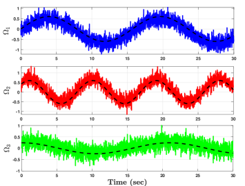
Figure 1: Rate gyro: True (black center-line) and measurements (colored)

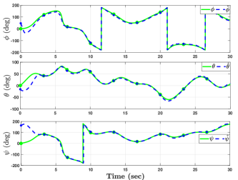
Figure 2: Euler angles: True (green solid-line) and estimated (blue dash-line) using 3 neurons

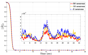
Figure 3: Normalized Euclidean error $||\tilde{R}||_{{\rm I}}=\frac{1}{4}{\rm Tr}\{\mathbf{I}_{3}-R_{k}^{\top}\hat{R}_{k}\}$.

TABLE I: Statistical analysis of the steady-state error with respect to the number of neurons.

Output data of $||\tilde{R}||_{{\rm I}}=\frac{1}{4}{\rm Tr}\{\mathbf{I}_{3}-R_{k}^{\top}\hat{R}_{k}\}$ over the period (5-29 sec)
Neurons number	3	10	50
Mean	$2.3\times 10^{-3}$	$2\times 10^{-3}$	$1.4\times 10^{-3}$
STD	$1.9\times 10^{-3}$	$1.4\times 10^{-3}$	$9\times 10^{-4}$

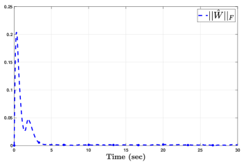
Figure 4: Frobenius norm of neural-adaptive estimates (3 neurons).

VI Conclusion

Accurate attitude estimation is a fundamental component of successful robotic applications. The estimation can be achieved using a group of observations and measurements. Accurate estimation become challenging when low-cost measurement units are utilized. This work addressed the attitude estimation problem using a neural-adaptive stochastic filter on the Special Orthogonal Group $\mathbb{SO}(3)$. The novel filter accounts for the noise present in the gyroscope measurements. The proposed filter is ensured to be almost SGUUB in the mean square. The numerical simulation illustrates robustness and rapid adaptability of the proposed neural-adaptive approach.

References

• [1] F. L. Markley, “Attitude determination using vector observations and the singular value decomposition,” Journal of the Astronautical Sciences, vol. 36, no. 3, pp. 245–258, 1988.
• [2] ——, “Attitude error representations for kalman filtering,” Journal of guidance, control, and dynamics, vol. 26, no. 2, pp. 311–317, 2003.
• [3] J. L. Crassidis and F. L. Markley, “Unscented filtering for spacecraft attitude estimation,” Journal of guidance, control, and dynamics, vol. 26, no. 4, pp. 536–542, 2003.
• [4] D. E. Zlotnik and J. R. Forbes, “Exponential convergence of a nonlinear attitude estimator,” Automatica, vol. 72, pp. 11–18, 2016.
• [5] M. D. Shuster and S. D. Oh, “Three-axis attitude determination from vector observations,” Journal of Guidance, Control, and Dynamics, vol. 4, pp. 70–77, 1981.
• [6] D. Choukroun, I. Y. Bar-Itzhack, and Y. Oshman, “Novel quaternion kalman filter,” IEEE Transactions on Aerospace and Electronic Systems, vol. 42, no. 1, pp. 174–190, 2006.
• [7] V. Madyastha, V. Ravindra, S. Mallikarjunan, and A. Goyal, “Extended kalman filter vs. error state kalman filter for aircraft attitude estimation,” in AIAA Guidance, Navigation, and Control Conference, 2011, p. 6615.
• [8] S. Bonnabel, “Left-invariant extended kalman filter and attitude estimation,” in Decision and Control, 2007 46th IEEE Conference on.   IEEE, 2007, pp. 1027–1032.
• [9] H. A. Hashim, L. J. Brown, and K. McIsaac, “Nonlinear stochastic attitude filters on the special orthogonal group 3: Ito and stratonovich,” IEEE Transactions on Systems, Man, and Cybernetics: Systems, vol. 49, no. 9, pp. 1853–1865, 2019.
• [10] H. A. Hashim, “Systematic convergence of nonlinear stochastic estimators on the special orthogonal group SO(3),” International Journal of Robust and Nonlinear Control, vol. 30, no. 10, pp. 3848–3870, 2020.
• [11] M. D. Shuster, “A survey of attitude representations,” Navigation, vol. 8, no. 9, pp. 439–517, 1993.
• [12] H. A. Hashim, “Special orthogonal group SO(3), euler angles, angle-axis, rodriguez vector and unit-quaternion: Overview, mapping and challenges,” arXiv preprint arXiv:1909.06669, 2019.
• [13] H. A. Hashim, L. J. Brown, and K. McIsaac, “Guaranteed performance of nonlinear attitude filters on the special orthogonal group SO(3),” IEEE Access, vol. 7, no. 1, pp. 3731–3745, 2019.
• [14] R. Mahony, T. Hamel, and J.-M. Pflimlin, “Nonlinear complementary filters on the special orthogonal group,” IEEE Transactions on Automatic Control, vol. 53, no. 5, pp. 1203–1218, 2008.
• [15] T. Lee, “Bayesian attitude estimation with approximate matrix fisher distributions on so (3),” in 2018 IEEE Conference on Decision and Control (CDC).   IEEE, 2018, pp. 5319–5325.
• [16] K. Zhao and Y. Song, “Neuroadaptive robotic control under time-varying asymmetric motion constraints: A feasibility-condition-free approach,” IEEE transactions on cybernetics, vol. 50, no. 1, pp. 15–24, 2018.
• [17] Y. Wang and Y. Song, “Fraction dynamic-surface-based neuroadaptive finite-time containment control of multiagent systems in nonaffine pure-feedback form,” IEEE transactions on neural networks and learning systems, vol. 28, no. 3, pp. 678–689, 2016.
• [18] Y. Song, B. Zhang, and K. Zhao, “Indirect neuroadaptive control of unknown mimo systems tracking uncertain target under sensor failures,” Automatica, vol. 77, pp. 103–111, 2017.
• [19] Y. Song, L. He, D. Zhang, J. Qian, and J. Fu, “Neuroadaptive fault-tolerant control of quadrotor uavs: a more affordable solution,” IEEE transactions on neural networks and learning systems, vol. 30, no. 7, pp. 1975–1983, 2018.
• [20] H. A. Hashim, “A geometric nonlinear stochastic filter for simultaneous localization and mapping,” Aerospace Science and Technology, vol. 111, p. 106569, 2021.
• [21] R. Khasminskii, Stochastic stability of differential equations.   Rockville, MD: S & N International, 1980.
• [22] H.-B. Ji and H.-S. Xi, “Adaptive output-feedback tracking of stochastic nonlinear systems,” IEEE Transactions on Automatic Control, vol. 51, no. 2, pp. 355–360, 2006.
• [23] H. Deng, M. Krstic, and R. J. Williams, “Stabilization of stochastic nonlinear systems driven by noise of unknown covariance,” IEEE Transactions on Automatic Control, vol. 46, no. 8, pp. 1237–1253, 2001.
• [24] O. Gundogdu, E. Egrioglu, C. H. Aladag, and U. Yolcu, “Multiplicative neuron model artificial neural network based on gaussian activation function,” Neural Computing and Applications, vol. 27, no. 4, pp. 927–935, 2016.
• [25] C. She, Z. Wang, F. Sun, P. Liu, and L. Zhang, “Battery aging assessment for real-world electric buses based on incremental capacity analysis and radial basis function neural network,” IEEE Transactions on Industrial Informatics, vol. 16, no. 5, pp. 3345–3354, 2019.
• [26] S. Elfwing, E. Uchibe, and K. Doya, “Sigmoid-weighted linear units for neural network function approximation in reinforcement learning,” Neural Networks, vol. 107, pp. 3–11, 2018.