Optimal control using flux potentials: A way to construct bound-preserving finite element schemes for conservation laws

Abstract

To ensure preservation of local or global bounds for numerical solutions of conservation laws, we constrain a baseline finite element discretization using optimization-based (OB) flux correction. The main novelty of the proposed methodology lies in the use of flux potentials as control variables and targets of inequality-constrained optimization problems for numerical fluxes. In contrast to optimal control via general source terms, the discrete conservation property of flux-corrected finite element approximations is guaranteed without the need to impose additional equality constraints. Since the number of flux potentials is less than the number of fluxes in the multidimensional case, the potential-based version of optimal flux control involves fewer unknowns than direct calculation of optimal fluxes. We show that the feasible set of a potential-state potential-target (PP) optimization problem is nonempty and choose a primal-dual Newton method for calculating the optimal flux potentials. The results of numerical studies for linear advection and anisotropic diffusion problems in 2D demonstrate the superiority of the new OB-PP algorithms to closed-form flux limiting under worst-case assumptions.

1 Introduction

In many applications of practical interest, it is essential to guarantee that numerical approximations to a scalar conserved quantity $u$ attain values in a range $[u^{\min},u^{\max}]$ of physically admissible states. For example, concentrations and volume fractions must stay between $u^{\min}=0$ and $u^{\max}=1$. Because of modeling errors, even exact solutions of the governing equations can sometimes violate such constraints. A physics-compatible numerical method should ensure preservation of global bounds and the discrete conservation property, while keeping consistency errors as small as possible. Moreover, numerical solutions may be required to satisfy local maximum principles and stay free of spurious oscillations.

A very general framework for enforcing inequality constraints in numerical schemes for conservation laws is based on the concept of algebraic flux correction (AFC) [1, 12, 13]. Given a high-order baseline discretization, an AFC scheme modifies it using numerical fluxes associated with a graph Laplacian operator. The validity of relevant maximum principles is enforced using flux limiters. A typical limiting technique is derived by formulating an inequality-constrained optimization problem and making worst-case assumptions to obtain a closed-form formula for limited fluxes or correction factors. Many limiters of this kind are based on ideas introduced in the work of Boris and Book [6], Van Leer [26, 27], Zalesak [28], and Harten [10, 11]. If necessary, the accuracy of flux-corrected approximations can be improved by using iterative or optimization-based limiting procedures. For example, iterative methods for calculating physics-aware flux approximations were proposed in [7, 14].

The development of optimization-based (OB) finite element methods for conservation laws was greatly advanced by the recent work of Bochev et al. [3, 4, 5] who used different kinds of optimal control to ensure preservation of local bounds. Their flux-state flux-target (FF) optimization method [3] has the structure of an AFC scheme. The equivalence to a flux-corrected transport (FCT) algorithm was shown in [3] for a simplified quadratic programming problem with box constraints. This interesting relationship means that flux limiters can be interpreted as approximate solvers for optimization problems. In particular, the existence of a bound-preserving AFC approximation implies that the feasible set is nonempty and provides a good initial guess for iterative optimization.

If fluxes are used as optimization variables, as in the OB-FF method, the size of the problem depends on the number of edges in the sparsity graph of the finite element matrix. To reduce the number of unknowns and choose a more intuitive target for AFC, we formulate inequality-constrained optimization problems using flux potentials in the present paper. The new optimization variables can be interpreted as approximations to nodal time derivatives, and the size of the resulting potential-state potential-target (PP) optimization problem is proportional to the number of nodes (rather than edges). The optimal fluxes, defined in terms of the potentials, can be applied after the discretization in space and time or at the level of spatial semi-discretization. The latter option makes it possible to construct OB-PP counterparts of the monolithic AFC schemes developed in [13, 16, 17].

In the next two sections, we discretize a generic conservation law using the continuous Galerkin method and review the basics of algebraic flux correction. In Section 4, we discuss closed-form flux limiting and its connection to optimal control of OB-FF type. The new OB-PP approach is introduced in Section 5, where we define the flux potentials, formulate the inequality constraints, and show that the feasible set is nonempty. A primal-dual Newton’s method for solving OB-PP optimization problems is outlined in Section 6. The numerical examples of Section 7 demonstrate the potential benefits of optimal control for numerical approximations to linear advection and anisotropic diffusion problems. We conclude this paper with a discussion of the main results and open problems in Section 8.

2 Baseline discretization

Let $u(\mathbf{x},t)$ be a scalar conserved quantity depending on the space location $\mathbf{x}\in\mathbb{R}^{d},\ d\in\{1,2,3\}$ and time instant $t\geq 0$. Restricting our attention to a bounded domain $\Omega\subset\mathbb{R}^{d}$ with Lipschitz boundary $\Gamma=\partial\Omega$, we consider a general initial-boundary value problem of the form

$$\frac{\partial u}{\partial t}+\nabla\cdot\mathbf{f}(u) =\nabla\cdot(\mathcal{D}\nabla u) \qquad\mbox{in}\ \Omega\times\mathbb{R}_{+},$$ (1a)

$$u =u_{D} \qquad\mbox{on}\ \Gamma_{D}\times\mathbb{R}_{+},$$ (1b)

$$u =u_{0} \qquad\mbox{on}\ \Omega\times\{0\},$$ (1c)

where $\mathbf{f}(u)\in\mathbb{R}^{d}$ is an inviscid flux and $\mathcal{D}\in\mathbb{R}^{d\times d}$ is a symmetric positive semidefinite tensor. The Dirichlet boundary data $u_{D}$ is prescribed on $\Gamma_{D}=\Gamma$ in the case $\mathcal{D}\neq 0$. For hyperbolic problems, $\Gamma_{D}=\{\mathbf{x}\in\Gamma\,:\,\mathbf{f}^{\prime}(u)\cdot\mathbf{n}(\mathbf{x})<0\}$, where $\mathbf{n}$ is the unit outward normal. We are also interested in steady-state solutions of problem (1), i.e., in solutions of the boundary value problem

$$\nabla\cdot\mathbf{f}(u) =\nabla\cdot(\mathcal{D}\nabla u) \qquad\mbox{in}\ \Omega,$$ (2a)

$$u =u_{D} \qquad\mbox{on}\ \Gamma_{D}.$$ (2b)

We discretize (1a) in space using a numerical scheme that yields an algebraic system of the form

$$M_{C}\frac{\mathrm{d}u}{\mathrm{d}t}=r(u).$$ (3)

By abuse of notation, $u=(u_{1},\ldots,u_{N_{h}})^{T}$ denotes the vector of $N_{h}$ discrete unknowns in formulas involving matrices rather than differential operators. The subscript $C$ is used for consistent mass matrices of (differential-)algebraic systems corresponding to a baseline scheme, such as the continuous Galerkin discretization with linear ($\mathbb{P}_{1}$) or multilinear ($\mathbb{Q}_{1}$) finite elements. For this particular method, a weak form of (1a), (1b) yields $M_{C}=(m_{ij})_{i,j=1}^{N_{h}}$ and $r(u)=(r_{i})_{i=1}^{N_{h}}$ with entries

$$m_{ij}=\sum_{e=1}^{E_{h}}\int_{K_{e}}\varphi_{i}\varphi_{j}\,{\rm d}{\mathbf{x}},$$

$$\qquad r_{i}=\sum_{e=1}^{E_{h}}\left[\lambda\int_{K_{e}\cap\Gamma_{D}}\varphi_{i}(u_{D}-u_{h})\,{\rm d}{\mathrm{s}}-\int_{K_{e}}\varphi_{i}\nabla\cdot\mathbf{f}(u_{h})\,{\rm d}{\mathbf{x}}-\int_{K_{e}}\nabla\varphi_{i}\cdot(\mathcal{D}\nabla u_{h})\,{\rm d}{\mathbf{x}}\right],$$ (4)

where $\lambda>0$ is a sufficiently large penalty parameter, $K_{1},\ldots,K_{E_{h}}$ are elements of a computational mesh and $\varphi_{1},\ldots,\varphi_{N_{h}}$ are the basis functions of the Lagrange finite element approximation

$$u_{h}(\mathbf{x},t)=\sum_{j=1}^{N_{h}}u_{j}(t)\varphi_{j}(\mathbf{x}).$$

The flux function $\mathbf{f}(u_{h})$ is sometimes approximated by the group finite element interpolant [2, 12]

$$\mathbf{f}_{h}(\mathbf{x},t)=\sum_{j=1}^{N_{h}}\mathbf{f}(u_{j}(t))\varphi_{j}(\mathbf{x})$$

and its contribution to $r(u)$ is stabilized using additional terms. In the numerical experiments of Section 7, we use Taylor-Galerkin stabilization [21, 23] for linear advection problems.

To discuss the modifications that are needed to satisfy maximum principles for general discretizations and conservation laws, we abstain from giving further details of our baseline method so far.

3 Algebraic flux correction

To enforce the validity of relevant inequality constraints using the algebraic flux correction (AFC) methodology [12], we replace (3) by the system of ordinary differential equations

$$M_{L}\frac{\mathrm{d}u}{\mathrm{d}t}=r(u)+g(u),$$ (5)

where $M_{L}=\mathrm{diag}(\delta_{ij}m_{i})$ is the lumped mass matrix with positive diagonal entries

$$m_{i}=\sum_{j=1}^{N_{h}}m_{ij}>0.$$

The vector $g(u)=(g_{i})_{i=1}^{N_{h}}$ defines a particular semi-discrete scheme and can be interpreted as source term control for inequality-constrained optimization. Note that systems (3) and (5) are equivalent for $g(u)=(M_{L}-M_{C})\dot{u}$, where $\dot{u}$ is the solution of the linear system $M_{C}\dot{u}=r(u)$.

To preserve the discrete conservation property, the control term $g(u)$ must satisfy $\sum_{i=1}^{N_{h}}g_{i}=0.$ This zero sum condition implies existence of numerical fluxes $g_{ij}=-g_{ji}$ such that

$$g_{i}=\sum_{j\in\mathcal{N}_{i}\backslash\{i\}}g_{ij},$$

where $\mathcal{N}_{i}$ is the stencil of node $i$. For our finite element scheme $\mathcal{N}_{i}=\{j\in\{1,\ldots N_{h}\}\,:\,m_{ij}>0\}$ is the integer set containing the index $i$ and the indices of nearest neighbors of node $i$.

The fluxes corresponding to the high-order target $g^{H}(u)=(M_{L}-M_{C})\dot{u}$ are given by [12, 13]

$$g_{ij}^{H}=m_{ij}(\dot{u}_{i}-\dot{u}_{j}),\qquad\dot{u}=M_{C}^{-1}r(u).$$ (6)

Indeed, the $i$th component of $g^{H}(u)$ admits the following decomposition:

$$g_{i}^{H}=m_{i}\dot{u}_{i}-\sum_{j\in\mathcal{N}_{i}}m_{ij}\dot{u}_{j}=\sum_{j\in\mathcal{N}_{i}}m_{ij}\dot{u}_{i}-\sum_{j\in\mathcal{N}_{i}}m_{ij}\dot{u}_{j}=\sum_{j\in\mathcal{N}_{i}\backslash\{i\}}m_{ij}(\dot{u}_{i}-\dot{u}_{j}).$$

Let us discretize the AFC system (5) in time using an explicit or implicit method that yields

$$M_{L}u^{n+1}=M_{L}u^{n}+\Delta t(r+g),$$ (7)

where $\Delta t>0$ is a constant time step and $u^{n}\approx u(t^{n})$ for $t^{n}=n\Delta t$. The number of intermediate stages (if any) and the way to compute $r+g$ depend on the particular space-time discretization.

A numerical scheme is called bound preserving (BP) if discrete maximum principles of the form

$$u^{\min}\leq u_{i}^{\min}(t)\leq u_{i}(t)\leq u_{i}^{\max}(t)\leq u^{\max}$$ (8)

hold for each node and time level. As shown in [17], the BP property of (7) is guaranteed for any strong stability preserving (SSP) Runge-Kutta time integrator if (5) can be written as

$$m_{i}\frac{\mathrm{d}u_{i}}{\mathrm{d}t}=c_{i}(u_{i}^{*}-u_{i}),\qquad i=1,\ldots,N_{h},$$ (9)

where $c_{i}>0$ is bounded and $u_{i}^{*}$ is an intermediate state such that

$$u_{j}\in[u_{i}^{\min},u_{i}^{\max}]\quad\forall j\in\mathcal{N}_{i}\quad\Rightarrow\quad u_{i}^{*}\in[u_{i}^{\min},u_{i}^{\max}].$$ (10)

Remark 1.

For an explicit SSP-RK method with forward Euler stages of the form

$$u_{i}^{\rm SSP}=u_{i}+\frac{\Delta t}{m_{i}}c_{i}(u_{i}^{*}-u_{i})$$

and a time step satisfying $\Delta tc_{i}\leq m_{i}$, the result $u_{i}^{\rm SSP}=(1-\Delta tc_{i}/m_{i})u_{i}+\Delta tc_{i}/m_{i})u_{i}^{*}$ is a convex combination of the states $u_{i}$ and $u_{i}^{*}$. It follows that $u_{i}^{\rm SSP}\in[u_{i}^{\min},u_{i}^{\max}]$.

The objective of algebraic flux correction is to enforce the inequality constraints for $u_{i}^{*}$ or $u_{i}^{n}$ using sufficiently accurate approximations $g_{ij}^{*}$ to the fluxes $g_{ij}$ of the target discretization.

4 Flux limiting and optimization

Many generalizations of classical flux-corrected transport (FCT) algorithms [6, 28] and total variation diminishing (TVD) methods [10, 11], combine (3) with a low-order BP semi-discretization

$$M_{L}\frac{\mathrm{d}u}{\mathrm{d}t}=r(u)+Du,$$

where $D=(d_{ij})_{i,j=1}^{N_{h}}$ is an artificial diffusion operator such that $d_{ij}\geq 0$ for $j\neq i$. If $D$ is a graph Laplacian (i.e., a symmetric matrix with zero row and column sums), the corresponding low-order AFC control $g^{L}(u)=Du$ admits a conservative decomposition into the diffusive fluxes [12]

$$g_{ij}^{L}=d_{ij}(u_{j}-u_{i}).$$ (11)

Such fluxes are used to enforce the BP property in the vicinity of discontinuities and steep gradients. In smooth regions, the Galerkin approximation to a hyperbolic or advection-dominated conservation law may be stabilized using a high-order dissipative flux $g_{ij}^{S}$. The use of high-order stabilization in numerical fluxes of AFC approximations makes it possible to avoid spurious ripples, achieve optimal convergence behavior, and ensure entropy stability for nonlinear problems [8, 13, 16].

In nonlinear high-resolution schemes, a convex combination of $g_{ij}^{L}$ and $g_{ij}=g_{ij}^{H}+g_{ij}^{S}$ is defined by

$$g_{ij}^{*}=g_{ij}^{L}+\alpha_{ij}f_{ij}=\alpha_{ij}g_{ij}+(1-\alpha_{ij})d_{ij}(u_{j}-u_{i}),$$ (12)

where $\alpha_{ij}\in[0,1]$ is a correction factor satisfying the symmetry condition $\alpha_{ji}=\alpha_{ij}$ and

$$f_{ij}=m_{ij}(\dot{u}_{i}-\dot{u}_{j})+d_{ij}(u_{i}-u_{j})+g_{ij}^{S}$$ (13)

is a raw antidiffusive flux such that $f_{ji}=-f_{ij}$. An algorithm for calculating $\alpha_{ij}$ is called a flux limiter.

Since the solution $u^{n+1}$ of the fully discrete problem (7) and the auxiliary states $u_{i}^{*}$ of the space discretization (9) depend on the sum of limited antidiffusive fluxes $f_{ij}^{*}=\alpha_{ij}f_{ij}$, the BP property (8) of an AFC scheme can typically be shown under flux constraints of the form [12, 13, 28]

$$f_{i}^{\min}\leq\sum_{j\in\mathcal{N}_{i}\backslash\{i\}}\alpha_{ij}f_{ij}\leq f_{i}^{\max}$$

and CFL-like time step restrictions. To avoid solution of a global inequality-constrained optimization problem and derive a closed-form expression for $\alpha_{ij}$, flux limiting is usually performed under worst-case assumptions. Examples of AFC schemes equipped with closed-form flux limiters include a family of multidimensional FCT algorithms [8, 12, 28] and the monolithic convex limiting (MCL) strategy proposed in [13]. We use FCT and MCL in some numerical experiments of Section 7.

As shown by Bochev et al. [3, 4, 5] in the context of remap and transport algorithms, closed-form flux limiters approximate the exact solution of an inequality-constrained optimization problem for $\alpha_{ij}$ by the exact solution of a simplified optimization problem with box constraints. The lack of optimality can be cured by using iterative flux correction [7, 12, 14] or optimization-based (OB) limiting [3, 4]. The flux-state flux-target (FF) algorithm presented in [3] is an AFC scheme that determines the optimal antidiffusive fluxes $f_{ij}^{*}=\alpha_{ij}f_{ij}$ by solving the quadratic programming (QP) problem

$$\mbox{minimize}\ \sum_{i=1}^{N_{h}}\sum_{j\in\mathcal{N}_{i}\backslash\{i\}}(f_{ij}^{*}-f_{ij})^{2}\qquad\mbox{subject to}$$ (14)

$$f_{ji}^{*}=-f_{ij}^{*},\qquad f_{i}^{\min}\leq\sum_{j\in\mathcal{N}_{i}\backslash\{i\}}f_{ij}^{*}\leq f_{i}^{\max}.$$ (15)

If $f_{i}^{\min}\leq 0$ and $f_{i}^{\max}\geq 0$ for $i=1,\ldots,N_{h}$, then the feasible set of the QP problem is nonempty because the fluxes $f_{ij}^{*}=0$ satisfy conditions (15). By default, the target flux $f_{ij}$ is defined by (13). An initial guess for an iterative optimization procedure can be calculated using an AFC scheme with a closed-form limiter of FCT or MCL type. In many cases, further iterations bring about just marginal improvements. However, the need for iterative limiting arises, e.g., in situations when calculation of (nearly) optimal fluxes / correction factors is required to minimize consistency errors [7, 14].

5 Optimal control and flux potentials

The OB-FF algorithm formulated in Section 4 is a PDE-constrained optimization method of discretize-then-optimize type with the state equation (7) and flux variables $f_{ij}^{*}$. To avoid formal dependence of the flux target $f_{ij}$ on the artificial diffusion coefficient $d_{ij}$, the FF optimization problem can be formulated in terms of the flux variables $g_{ij}^{*}$ and target fluxes $g_{ij}=g_{ij}^{H}+g_{ij}^{S}$ as follows:

$$\mbox{minimize}\ \sum_{i=1}^{N_{h}}\sum_{j\in\mathcal{N}_{i}\backslash\{i\}}(g_{ij}^{*}-g_{ij})^{2}\qquad\mbox{subject to}$$ (16)

$$g_{ji}^{*}=-g_{ij}^{*},\qquad u_{i}^{\min}\leq u_{i}^{*}=u_{i}^{n}+\frac{\Delta t}{m_{i}}\left(r_{i}+\sum_{j\in\mathcal{N}_{i}\backslash\{i\}}g_{ij}^{*}\right)\leq u_{i}^{\max}.$$ (17)

To reduce the number of control variables, we introduce a new kind of optimal flux control in this section. Mimicking the definition (6) of $g_{ij}^{H}=m_{ij}(\dot{u}_{i}-\dot{u}_{j})$, we express the flux variables $g_{ij}^{*}$ in terms of optimal flux potentials $\dot{u}_{i}^{*}$ that can be interpreted as modified time derivatives. Using this representation, we seek the best approximation $\dot{u}_{i}^{*}$ to a given potential target $\dot{u}_{i}$ such that the inequality constraints (8) hold for (7) with $g$ assembled from $g_{ij}^{*}=m_{ij}(\dot{u}_{i}^{*}-\dot{u}_{j}^{*})$. The resulting OB method can be classified as a potential-state potential-target (PP) optimization algorithm.

Let the baseline space-time discretization of (1a) be given by an algebraic system of the form

$$M_{C}u^{T}=M_{C}u^{n}+\Delta tr\quad\Leftrightarrow\quad M_{L}u^{T}=M_{L}u^{n}+\Delta tr-(M_{C}-M_{L})(u^{T}-u^{n}),$$ (18)

where $r$ may include optional high-order stabilization. Choosing the target potential

$$\dot{u}^{T}=\frac{u^{T}-u^{n}}{\Delta t}=M_{C}^{-1}r,$$

we calculate the optimal flux potentials $\dot{u}_{i}^{*}$ by solving the PP optimization problem

$$\mbox{minimize}\ \frac{1}{2}(\dot{u}^{*}-\dot{u}^{T})^{\top}M_{C}(\dot{u}^{*}-\dot{u}^{T})+\frac{\mu}{2}(\dot{u}^{*})^{\top}(M_{L}-M_{C})\dot{u}^{*}\qquad\mbox{subject to}$$ (19)

$$\frac{m_{i}}{\Delta t}(u_{i}^{\min}-\tilde{u}_{i}^{T})\leq\sum_{j\in\mathcal{N}_{i}\backslash\{i\}}m_{ij}(\dot{u}_{i}^{*}-\dot{u}_{j}^{*})\leq\frac{m_{i}}{\Delta t}(u_{i}^{\max}-\tilde{u}_{i}^{T}),$$ (20)

where $\tilde{u}_{i}^{T}=u_{i}^{n}+\Delta tr_{i}/m_{i}$ is a lumped-mass approximation to $u_{i}^{T}$ defined by the solution of (18). The first term in the definition (19) of the objective function is $\frac{1}{2}\|\dot{u}_{h}^{*}-\dot{u}_{h}^{T}\|_{L^{2}(\Omega)}^{2}$. The second one is introduced for stabilization purposes and can be controlled using the parameter $\mu\geq 0$. The so-defined optimization problem has the same structure as optimal control approaches with elliptic operators and pointwise constraints [22]. Indeed, the matrix of our algebraic stabilization term $g=(M_{L}-M_{C})\dot{u}^{*}$ has the properties of a discrete Laplacian operator that fits into the framework developed in [22].

Remark 2.

Note that conditions (20) imply the validity of the discrete maximum principle

$$u_{i}^{\min}\leq u_{i}^{*}=\tilde{u}_{i}^{T}+\frac{\Delta t}{m_{i}}\sum_{j\in\mathcal{N}_{i}\backslash\{i\}}m_{ij}(\dot{u}_{i}^{*}-\dot{u}_{j}^{*})\leq u_{i}^{\max}$$ (21)

and $u_{i}^{*}=u_{i}^{T}$ is obtained if the PP algorithm produces $\dot{u}_{j}^{*}=\dot{u}_{j}^{T}$ for all $j\in\mathcal{N}_{i}$. Indeed, we have

$$\tilde{u}_{i}^{T}+\sum_{j\in\mathcal{N}_{i}\backslash\{i\}}m_{ij}(\dot{u}_{i}^{T}-\dot{u}_{j}^{T})=u_{i}^{n}+\frac{1}{m_{i}}\left(\Delta tr_{i}+\sum_{j\in\mathcal{N}_{i}\backslash\{i\}}m_{ij}[(u_{i}^{T}-u_{j}^{T})-(u_{i}^{n}-u_{j}^{n})]\right)=u_{i}^{T}.$$

Remark 3.

The linear system corresponding to an explicit baseline discretization of the form (18) can be solved efficiently using a few iterations of the deferred correction method

$$M_{L}u^{(m)}=M_{L}u^{n}+\Delta tr-(M_{C}-M_{L})(u^{(m-1)}-u^{n}),\qquad m=1,\ldots,M$$

with the initial guess $u^{(0)}=\tilde{u}^{T}=u^{n}+\Delta tM_{L}^{-1}r$ and the final result $u^{T}:=u^{(M)}$. This approach corresponds to approximation of $M_{C}^{-1}$ by a truncated Neumann series; see [8, 21] for details.

Let us now show that the feasible set of the PP optimization problem (19),(20) is nonempty, i.e., that there exists a vector $\dot{u}^{B}$ of backup potentials such that conditions (20) and the equivalent inequality constraints (21) hold for $\dot{u}^{*}=\dot{u}^{B}$. To that end, we define $u^{B}$ as an auxiliary solution corresponding to a BP space discretization of the form (9) with the right-hand side $r_{i}^{B}(u)$ such that

$$\sum_{i=1}^{N_{h}}(r_{i}^{B}-r_{i})=0.$$ (22)

The validity of this zero sum condition implies that a solution $\dot{u}^{B}$ of the linear system

$$(M_{L}-M_{C})\dot{u}^{B}=r^{B}-r$$

with the symmetric positive semidefinite graph Laplacian $M_{L}-M_{C}$ exists and is unique up to a constant. The corresponding flux variables $g_{ij}^{B}=m_{ij}(\dot{u}_{i}^{B}-\dot{u}_{j}^{B})$ are defined uniquely. The use of $\dot{u}^{*}=\dot{u}^{B}$ in (21) yields $u_{i}^{*}=\tilde{u}_{i}^{T}+\Delta t(r_{i}^{B}-r_{i})/m_{i}=u_{i}^{n}+\Delta tr_{i}^{B}/m_{i}=u_{i}^{B}$.

It remains to construct $r^{B}(u)$ such that condition (22) holds and $u_{i}^{B}\in[u_{i}^{\min},u_{i}^{\max}]$, perhaps under time step restrictions. Using the residual distribution procedure proposed in [9], we define

$$r_{i}^{B}=\frac{\omega_{i}\rho}{\sum_{j=1}^{N_{h}}\omega_{j}},\quad\qquad\rho=\sum_{i=1}^{N_{h}}r_{i},\qquad\omega_{i}=\begin{cases}u_{i}^{\max}-u_{i}^{n}&\quad\mbox{if}\ \rho>0,\\ 0&\quad\mbox{if}\ \rho=0,\\ u_{i}^{\min}-u_{i}^{n}&\quad\mbox{if}\ \rho<0.\end{cases}$$

Note that the residual components $r_{i}^{B}$ satisfy (22) and $r_{i}^{B}=c^{B}(u_{i}^{*}-u_{i}^{n})$, where

$$c^{B}=\frac{\rho}{\sum_{j=1}^{N_{h}}\omega_{j}}\geq 0,\qquad u_{i}^{*}\in\{u_{i}^{\min},u_{i}^{\max}\}.$$

Hence, the BP property of the feasible approximation $u_{i}^{B}=u_{i}^{n}+\Delta tr_{i}^{B}/m_{i}$ is guaranteed by (10), at least for time steps satisfying the a posteriori CFL-like condition $\Delta tc^{B}\leq m_{i}$; cf. [9].

For $r_{i}$ defined by (4), we have $\rho=\sum_{e=1}^{E_{h}}\left[\lambda\int_{K_{e}\cap\Gamma_{D}}(u_{D}-u_{h})\,{\rm d}{\mathrm{s}}-\int_{K_{e}\cap\Gamma}\mathbf{f}(u_{h})\cdot\mathbf{n}\,{\rm d}{\mathrm{s}}\right]$. The addition of optional high-order stabilization terms does not change the value of $\rho$. Hence, the coefficient $c^{B}\geq 0$ of the “CFL” constraint is independent of these terms and of the physical diffusion tensor $\mathcal{D}$.

Remark 4.

Implicit schemes with closed-form limiters may ensure the BP property under milder time step restrictions or unconditionally. If such a scheme exists for the given problem, the corresponding flux potential $\dot{u}^{\rm AFC}$ belongs to the admissible set of the PP optimization problem.

Remark 5.

In contrast to flux correction based on limiting, the OB-PP approach does not rely on the availability of a consistent low-order BP discretization for the given conservation law. For example, even the positivity-preserving exact solution of $\eqref{ibvp-pde}$ with $\mathbf{f}(u)=\mathbf{v}u$ may violate the upper bound $u^{\max}=1$ for a concentration field $u$ if the given velocity field $\mathbf{v}=\mathbf{v}(\mathbf{x})$ is not exactly divergence-free [14]. The PP algorithm can easily be configured to produce the best physics-compatible approximations using optimal flux control to preserve the global bounds and the conservation property.

Similarly to limiter-based monolithic AFC schemes, optimal flux control can also be applied at the level of the spatial semi-discretization (5). Since the BP criterion (10) is satisfied for a family of closed-form limiters [17], the feasible set of the semi-discrete optimization problem

$$\mbox{minimize}\ \frac{1}{2}(\dot{u}^{*}-\dot{u}^{T})^{\top}M_{C}(\dot{u}^{*}-\dot{u}^{T})+\frac{\mu}{2}(\dot{u}^{*})^{\top}(M_{L}-M_{C})\dot{u}^{*}\qquad\mbox{subject to}$$ (23)

$$c_{i}(u_{i}^{\min}-u_{i})\leq r_{i}(u)+\sum_{j\in\mathcal{N}_{i}\backslash\{i\}}m_{ij}(\dot{u}_{i}^{*}-\dot{u}_{j}^{*})\leq c_{i}(u_{i}^{\max}-u_{i})$$ (24)

is nonempty, and an OB-PP algorithm can be used to fine-tune the fluxes at individual RK stages. The potential advantages of flux correction at the semi-discrete level include flexibility in the choice of the time discretization and better convergence behavior at steady state [13, 17].

Remark 6.

For numerical schemes with diagonal mass matrices, PP optimization should be performed using the coefficients $s_{ij}$ of another discrete Laplacian operator to define $g_{ij}^{*}=s_{ij}(\dot{u}_{i}^{*}-\dot{u}_{j}^{*})$.

6 Solution of optimization problems

The PP optimization problem can be solved using a barrier method, which guarantees that intermediate solutions stay in the feasible set defined by (20). Specifically, we choose the primal-dual Newton method presented in [24, Section 6.6.2]. The problem at hand can be written as

$$\min_{\dot{u}\in\mathbb{R}^{n}}f(\dot{u})\qquad\text{s.t.}\quad A\dot{u}\leq b,$$

where $n=N_{h}$ is the number of optimization variables. The inequality constraints are defined using

$$A=\begin{pmatrix}M_{L}-M_{C}\\ M_{C}-M_{L}\end{pmatrix}\in\mathbb{R}^{2n\times n}\quad\text{and}\quad b=\begin{bmatrix}\frac{M_{L}}{\Delta t}(u^{\max}-u^{n})-r\\ \frac{M_{L}}{\Delta t}(u^{n}-u^{\min})+r\end{bmatrix}\in\mathbb{R}^{2n}.$$

The gradient and Hessian of the convex objective function

$$f_{\mu}(\dot{u})=\frac{1}{2}(\dot{u}-\dot{u}^{T})^{\top}M_{C}(\dot{u}-\dot{u}^{T})+\frac{\mu}{2}\dot{u}^{\top}(M_{L}-M_{C})\dot{u}$$

are given by

$$\nabla f_{\mu}=M_{C}(\dot{u}-\dot{u}^{T})+\mu(M_{L}-M_{C})\dot{u}\quad\text{and}\quad H_{f_{\mu}}=M_{C}+\mu(M_{L}-M_{C}).$$ (25)

Introducing a vector $s\in\mathbb{R}^{2n}$ of slack variables, we reformulate the inequality constraints as follows:

$$\min_{\dot{u}\in\mathbb{R}^{n}}f_{\mu}(\dot{u})\qquad\text{s.t.}\quad A\dot{u}+s=b,\qquad s\geq 0.$$

The corresponding system of optimality conditions reads

$$\nabla f_{\mu}(\dot{u})+A^{\top}\lambda =0,$$

$$A\dot{u}+s =b,$$

$$s_{i}\lambda_{i} =\sigma,\quad i=1,\ldots,2n,$$

where $\lambda\in\mathbb{R}^{2n}$ is the vector of Lagrange multipliers and $\sigma\geq 0$ is a parameter which is gradually decreased in the process of solving a sequence of auxiliary problems.

The initial guess $\dot{u}^{(0)}$ for the iterative optimization procedure should belong to the feasible set and be a usable approximation to the optimization target $\dot{u}^{T}$. Such an approximation can be defined using an AFC scheme. Given the artificial diffusion operator $D$ and the antidiffusive fluxes $f_{ij}^{*}$ produced by a closed-form limiter, we compute $\dot{u}^{(0)}$ by solving the linear system

$$(M_{L}-M_{C})\dot{u}^{(0)}=Du^{n}+f^{*}_{ij}$$ (26)

subject to the equality constraint $\sum_{i=1}^{N_{h}}\dot{u}_{i}^{(0)}=0$ which ensures uniqueness of the solution to the discrete Neumann problem with the singular graph Laplacian $M_{L}-M_{C}$. Unless mentioned otherwise, we calculate the fluxes $f^{*}_{ij}$ for (26) using Zalesak’s FCT algorithm [28].

We use Newton’s method to update the solution $(\dot{u},\lambda,s)$. At an intermediate step $j+1$, the search directions $\delta\dot{u}^{j+1}$ and $\delta\lambda^{j+1}$ are determined by solving a linear system of the form

$$\begin{pmatrix}H_{f}&A^{T}\\ A&G^{j}\end{pmatrix}\begin{bmatrix}\delta\dot{u}^{j+1}\\ \delta\lambda^{j+1}\end{bmatrix}=\begin{bmatrix}-\nabla f_{\mu}(\dot{u}^{j})-A^{T}\lambda^{j}\\ b-A\dot{u}^{j}-\sigma/\lambda^{j}\end{bmatrix}.$$

The block $G^{j}\in\mathbb{R}^{2n\times 2n}$ is a diagonal matrix with entries $g^{j}_{ii}=-s^{j}_{i}/\lambda^{j}_{i}$; see [24, Section 6.6.2].

The search directions $\delta s^{j+1}_{i}$ for individual slack variables $s_{i}$ are defined by

$$\delta s_{i}^{j+1}=(\sigma-s^{j}_{i}\lambda^{j}_{i}-s^{j}_{i}\delta\lambda_{i}^{j+1})/\lambda^{j}_{i},\qquad i=1,\ldots,2n.$$

Using the above search directions, the employed barrier method updates the solution as follows:

$$s^{j+1} =s^{j}+\alpha\delta s^{j+1}>0,\qquad\alpha\in\left[0,1\right],$$

$$\dot{u}^{j+1} =\dot{u}^{j}+\alpha\delta\dot{u}^{j+1},$$

$$\lambda^{j+1} =\lambda^{j}+\beta\delta\lambda^{j+1}>0,\qquad\beta\in\left[0,1\right].$$

To achieve fast convergence, it is essential to adjust the value of $\sigma$ adaptively. If the initial value of $\sigma$ is chosen too small, the method may converge slowly or fail to converge. Hence, a sufficiently large value of $\sigma$ should be used at the beginning. If $\sigma$ turns out to be so large that the current Newton step would increase the value of $f_{\mu}$, this step should be repeated with a smaller value of $\sigma$.

In our implementation, we iterate using a fixed value of $\sigma$ until the improvement factor

$$\frac{f_{\mu}(\dot{u}^{j+1})}{f_{\mu}(\dot{u}^{j})}$$

becomes close to or greater than $1$. Then we decrease $\sigma$ and restart the Newton iteration using the current solution as an initial guess. This process is repeated until a threshold value $\sigma^{\min}$ is reached. The final result is an approximate solution of the PP optimization problem (19),(20).

We use the direct solver UMFPACK from the SuiteSparse library [25] to solve linear systems. Since $G^{j}$ depends on $s^{j}$ and $\lambda^{j}$, the LU decomposition needs to be updated in every Newton iteration.

7 Case studies and numerical examples

In this section, we apply the OB-PP algorithm to linear advection problems and to an anisotropic diffusion equation. Stationary problems of the form (2) are solved using time marching. For comparison purposes, we present numerical results obtained with AFC schemes based on Zalesak’s FCT algorithm [12, 28] and the monolithic convex limiting (MCL) strategy [13, 16]. All methods under investigation are implemented in the open-source C++ finite element library MFEM [20]. The target discretization for PP optimal control and closed-form flux limiting is chosen individually in each experiment. The objective function for all optimization problems is defined using $\mu=0.01$.

7.1 Solid body rotation

We begin with a popular solid body rotation test [12, 19]. The unsteady linear advection equation

$$\frac{\partial u}{\partial t}+\nabla\cdot(\mathbf{v}u)=0$$

is solved in $\Omega=(0,1)^{2}$ using the solenoidal velocity field ${\bf v}(x,y)=(0.5-y,x-0.5)^{T}$. The initial condition, as defined by LeVeque [19], is given by

$$u_{0}(x,y)=\begin{cases}u_{0}^{\rm hump}(x,y)&\text{if}\ \sqrt{(x-0.25)^{2}+(y-0.5)^{2}}\leq 0.15,\\ u_{0}^{\rm cone}(x,y)&\text{if}\ \sqrt{(x-0.5)^{2}+(y-0.25)^{2}}\leq 0.15,\\ 1&\text{if}\ \begin{cases}\left(\sqrt{(x-0.5)^{2}+(y-0.75)^{2}}\leq 0.15\right)\wedge\\ \left(|x-0.5|\geq 0.025\vee\ y\geq 0.85\right),\end{cases}\\ 0&\text{otherwise},\end{cases}$$

where

$$u_{0}^{\rm hump}(x,y) =\frac{1}{4}+\frac{1}{4}\cos\left(\frac{\pi\sqrt{(x-0.25)^{2}+(y-0.5)^{2}}}{0.15}\right),$$

$$u_{0}^{\rm cone}(x,y) =1-\frac{\sqrt{(x-0.5)^{2}+(y-0.25)^{2}}}{0.15}.$$

On the inflow boundary $\Gamma_{D}$ of $\Omega$, we prescribe the homogeneous Dirichlet boundary condition

$$u(x,y)=0\qquad\mbox{for}\ (x,y)\in\Gamma_{D}.$$

As a target discretization, we use the fourth-order Taylor-Galerkin (TTG-4A) method [21, 23]

$$M_{C}u^{n+1/3} =M_{C}u^{n}+\frac{\Delta t}{3}[Ku^{n}+b^{n}]+\frac{(\Delta t)^{2}}{12}Su^{n},$$

$$M_{C}u^{T} =M_{C}u^{n}+\Delta t[Ku^{n}+b^{n}]+\frac{(\Delta t)^{2}}{2}Su^{n+1/3},$$

where $K=(k_{ij})_{i,j=1}^{N_{h}}$ and $S=(s_{ij})_{i,j=1}^{N_{h}}$ are sparse matrices with entries

$$k_{ij}=-\sum_{e=1}^{E_{h}}\int_{K_{e}}\varphi_{i}\nabla\cdot(\mathbf{v}\varphi_{j})\,{\rm d}{\mathbf{x}},\qquad s_{ij}=-\sum_{e=1}^{E_{h}}\int_{K_{e}}(\mathbf{v}\cdot\nabla\varphi_{i})(\mathbf{v}\cdot\nabla\varphi_{j})\,{\rm d}{\mathbf{x}}.$$

The Dirichlet boundary conditions are taken into account using the vector $b=(b_{i})_{i}^{N_{h}}$ of surface integrals

$$\qquad b_{i}=\sum_{e=1}^{E_{h}}\int_{K_{e}\cap\Gamma_{D}}\varphi_{i}(u_{D}-u_{h})|\mathbf{v}\cdot\mathbf{n}|\,{\rm d}{\mathrm{s}}=\tilde{b}_{i}+\sum_{j\in\mathcal{N}_{i}\backslash\{i\}}f_{ij}^{b},$$

$$\tilde{b}_{i}=\sum_{e=1}^{E_{h}}\int_{K_{e}\cap\Gamma_{D}}\varphi_{i}(u_{D}-u_{i})|\mathbf{v}\cdot\mathbf{n}|\,{\rm d}{\mathrm{s}},\qquad f_{ij}^{b}=(u_{i}-u_{j})\sum_{e=1}^{E_{h}}\int_{K_{e}\cap\Gamma_{D}}\varphi_{i}\varphi_{j}|\mathbf{v}\cdot\mathbf{n}|\,{\rm d}{\mathrm{s}}.$$

Flux correction of FCT and MCL type is performed at the second step using the target fluxes

$$f_{ij}=m_{ij}(\dot{u}_{i}^{T}-\dot{u}_{j}^{T})+d_{ij}(u_{i}^{n}-u_{j}^{n})-\frac{\Delta t}{2}s_{ij}\Big{(}u_{i}^{n+1/3}-u_{j}^{n+1/3}\Big{)}+f_{ij}^{b},$$

$$d_{ij}=\max\{-k_{ij},0,-k_{ji}\}$$

such that

$$M_{L}u^{T}=M_{L}u^{n}+\Delta t[(K+D)u^{n}+\tilde{b}^{n}]+f,\qquad f_{i}=\sum_{j\in\mathcal{N}_{i}\backslash\{i\}}f_{ij}.$$

The potentials $\dot{u}_{i}^{T}$ for calculation of $f_{ij}$ and definition of the OB-PP objective function are given by

$$\dot{u}^{T}=M_{C}^{-1}\left[Ku^{n}+b^{n}+\frac{\Delta t}{2}Su^{n+1/3}\right].$$

All methods under investigation lead to nonlinear flux-corrected approximations of the form

$$M_{L}u^{n+1}=M_{L}u^{n}+\Delta t\left[Ku^{n}+b^{n}+\frac{\Delta t}{2}Su^{n+1/3}+g^{*}\right],\qquad g_{i}^{*}=\sum_{j\in\mathcal{N}_{i}\backslash\{i\}}g_{ij}^{*}.$$

The FCT and MCL schemes differ in the way to compute the limited antidiffusive components $f_{ij}^{*}$ of

$$g_{ij}^{*}=f_{ij}^{*}+d_{ij}(u_{j}^{n}-u_{i}^{n})-\frac{\Delta t}{2}s_{ij}\Big{(}u_{j}^{n+1/3}-u_{i}^{n+1/3}\Big{)}-f_{ij}^{b}.$$

Zalesak’s FCT limiter is designed to enforce the maximum principle (8) for the solution of the fully discrete problem, while MCL constrains the spatial semi-discretization (5) to satisfy (9),(10) with

$$c_{i}=\sum_{j\in\mathcal{N}_{i}\backslash\{i\}}d_{ij}.$$

The fully discrete OB-PP algorithm yields the optimal fluxes $g_{ij}^{*}=m_{ij}(u_{i}^{*}-u_{j}^{*})$ corresponding to the solution of (19),(20). We do not consider the semi-discrete version (23),(24) in this example because the selected target scheme corresponds to a specific space-time discretization (TTG-4A).

In our numerical experiments for this benchmark, we run simulations up to the final time $T=2\pi$ using the mesh size $h=1/128$ and time step $\Delta t=10^{-3}$. The interpolant $u_{h}(\cdot,0)$ of the initial data is depicted in Fig. 1a. The analytical solution $u_{h}(\cdot,2\pi)$ after one full rotation reproduces it exactly. The numerical solutions shown in Figs 1b and 1c were obtained using closed-form flux limiters of MCL and FCT type, respectively. The MCL result exhibits significant levels of numerical diffusion on the narrow back side of the slotted cylinder and at the two peaks. The FCT solution is less diffusive but not as accurate as the OB–PP result that we show in Fig. 1d. Since the optimization-based approach does not rely on worst-case assumptions, the resulting approximations preserve the shape of the initial data better their flux-limited counterparts. In particular, the peak clipping effects are less pronounced, and the global maximum of the OB-PP solution is closer to the analytical value $u^{\max}=1$.

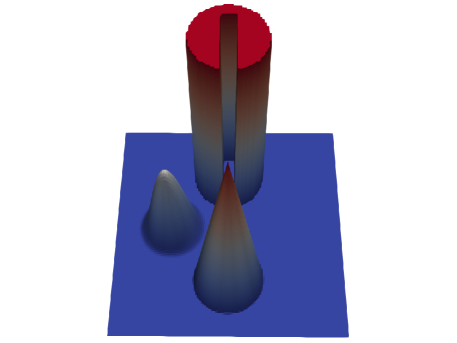
(a) initial data, $u_{h}\in\begin{bmatrix}0,1\end{bmatrix}$

(b) MCL, $u_{h}\in\begin{bmatrix}0,0.98\end{bmatrix}$

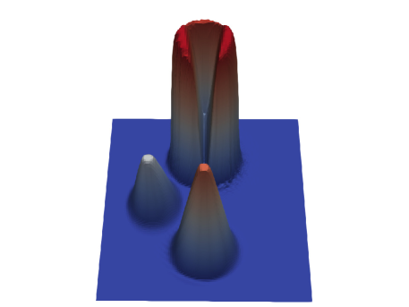
(c) FCT, $u_{h}\in\begin{bmatrix}0,0.988\end{bmatrix}$

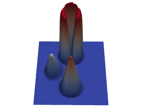
(d) OB-PP, $u_{h}\in\begin{bmatrix}3.14\cdot 10^{-9},1-10^{-7}\end{bmatrix}$

Figure 1: Solutions to the solid body rotation problem at $T=2\pi$.

7.2 Steady circular advection

In the second standard test for AFC schemes, we solve the stationary linear advection equation

$$\nabla\cdot(\mathbf{v}u)=0$$

in $\Omega=(0,1)^{2}$ using the divergence-free velocity field $\mathbf{v}(x,y)=(y,-x)$ unless mentioned otherwise. The inflow boundary condition and the exact solution at any point in $\bar{\Omega}$ are given by

$$u(x,y)=\left\{\begin{array}[]{ll}1&\quad\mbox{if}\ \ 0.15\leq\sqrt{x^{2}+y^{2}}\leq 0.45,\\ \cos^{2}\left(10\pi\frac{\sqrt{x^{2}+y^{2}}-0.7}{3}\right)&\quad\mbox{if}\ \ 0.55\leq\sqrt{x^{2}+y^{2}}\leq 0.85,\\ 0,&\quad\mbox{otherwise}.\end{array}\right.$$

We march numerical solutions to the steady state using the lumped-mass finite element version

$$M_{L}u^{n+1}=M_{L}u^{n}+\Delta t[Ku^{n}+b(u^{n})]+\frac{(\Delta t)^{2}}{2}Su^{n}$$

of the classical Lax-Wendroff (LW) method as target discretization for FCT, MCL, and OB-PP corrections. The amount of stabilizing streamline diffusion is determined by the pseudo-time step

$$\Delta t=\frac{\nu h}{\|\mathbf{v}\|_{L^{\infty}(\Omega)}},$$

where $h$ is the mesh size and $\nu$ is a user-defined Courant number. The target potential corresponding to the steady-state residual $r(u)=\left[K+\frac{\Delta t}{2}S\right]u+b(u)$ is given by $\dot{u}^{T}=0$. In our numerical study, we use $h=1/64$ and $\Delta t=10^{-3}$. For $\|\mathbf{v}\|_{L^{\infty}(\Omega)}=1.413$, this choice of $\Delta t$ corresponds to the Courant number $\nu=0.09.$ Computations are terminated at $T=9.5$, when the $L^{2}$ norm of the pseudo-time derivative becomes smaller than $10^{-12}$ for MCL and as small as $7\cdot 10^{-9}$ for OB-PP. The same output time is used for Zalesak’s FCT algorithm which belongs to the family of predictor-corrector methods and, therefore, cannot be expected to produce a fully converged steady state solution.

Figure 2b shows the unlimited Galerkin solution which violates the discrete maximum principle and exhibits spurious oscillations even in regions where the exact solution is smooth. All other solutions shown in Fig. 2 are globally bound preserving and nonoscillatory. As in the unsteady advection test, the most diffusive approximation is produced by MCL (see Fig. 2c), followed by FCT (cf. Fig. 2d). The OB-PP result $u_{h}^{\rm OB}$ is virtually indistinguishable from the interpolant $u_{h}^{\rm ex}$ of the exact solution (compare Figs 2a and 2e). To examine the distribution of pointwise errors, we plot $u_{h}^{\rm OB}-u_{h}^{\rm ex}$ in Fig. 2f. As expected, the largest errors are generated around the streamlines along which the exact solution has a discontinuity, a peak, or a nonsmooth transition in the crosswind direction. In this example, we used OB-PP based on formulation (19),(20). The algorithm based on the semi-discrete version (23),(24) produces very similar results. The difference between the solutions obtained with the two OB-PP approaches is so small that we scale it by a factor of 50 in Fig. 3 for better visibility.

In Table 1, we list the values of the objective function (25) calculated using the initial guess $\dot{u}^{(0)}$ (as defined by (26) with FCT fluxes $f_{ij}^{*}$) and the final solution $\dot{u}^{*}$ of the OB-PP optimization problem. It can be seen that the values of $f_{\mu}(\dot{u}^{*})$ are indeed significantly smaller than those of $f_{\mu}(\dot{u}^{(0)})$.

pseudo-time	$f_{\mu}(\dot{u}^{(0)})$	$f_{\mu}(\dot{u}^{*})$
0.1	0.595	3.642e-02
0.5	1.969	6.018e-02
1.0	1.527	4.349e-02

Table 1: Values of the objective function $f_{\mu}$ for the initial guess (Zalesak’s FCT) and the OB-PP flux potential.

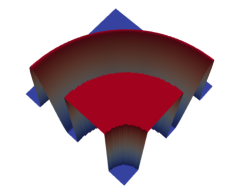
(a) exact, $u_{h}\in\begin{bmatrix}0,1\end{bmatrix}$

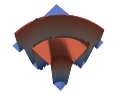
(b) unlimited, $u_{h}\in\begin{bmatrix}-0.24,1.23\end{bmatrix}$

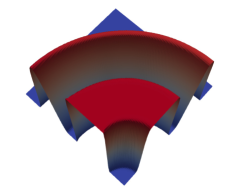
(c) MCL, $u_{h}\in\begin{bmatrix}0,1\end{bmatrix}$

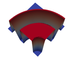
(d) FCT, $u_{h}\in\begin{bmatrix}0,1\end{bmatrix}$

(e) OB-PP, $u_{h}\in\begin{bmatrix}1.7\cdot 10^{-11},1.0\end{bmatrix}$

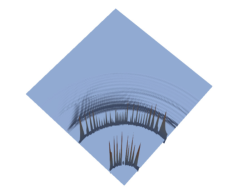
(f) $u_{h}^{\rm OB}-u_{h}^{\rm ex}\in\begin{bmatrix}-0.448,0.975\end{bmatrix}$

Figure 2: Solutions to the steady advection problem at the pseudo-time $T=9.5$.

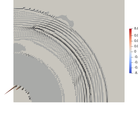
Figure 3: Difference between the OB-PP results obtained using formulations (19),(20) and (23),(24) of the optimization problem (multiplied by a scaling factor of 50 for better visibility).

7.3 Anisotropic diffusion

In the last example, we use the OB-PP algorithm to solve the steady anisotropic diffusion equation

$$-\nabla\cdot({\cal D}\nabla u)=0$$

with [12, 18]

$$\mathcal{D}=R(-\theta)\left(\begin{array}[]{cc}100&0\\ 0&1\end{array}\right){\cal R}(\theta),\qquad{\cal R}(\theta)=\left(\begin{array}[]{rr}\cos\theta&\sin\theta\\ -\sin\theta&\cos\theta\\ \end{array}\right),\qquad\theta=\frac{\pi}{6}$$

in the domain $\Omega=(0,1)^{2}\backslash[4/9,5/9]^{2}$. The outer and inner boundary of $\Omega$ are denoted by $\Gamma_{0}$ and $\Gamma_{1}$, respectively. The Dirichlet boundary condition for this test is given by

$$u(x,y)=\left\{\begin{array}[]{rl}-1&\ \mbox{ if }(x,y)\in\Gamma_{0},\\ 1&\ \mbox{ if }(x,y)\in\Gamma_{1}.\end{array}\right.$$

The standard Galerkin discretization yields the stiffness matrix $K=(k_{ij})_{i,j=1}^{N_{h}}$ with entries

$$\qquad k_{ij}=-\sum_{e=1}^{E_{h}}\int_{K_{e}}\nabla\varphi_{i}\cdot(\mathcal{D}\nabla\varphi_{j})\,{\rm d}{\mathbf{x}}.$$

Although the unconstrained Galerkin solution is known to possess the best approximation property w.r.t. the energy norm, it may violate the global bounds $u^{\min}=-1$ and $u^{\max}=1$ if the mesh is nonuniform and/or the diffusion tensor $\mathcal{D}$ is highly anisotropic [12, 18].

The design of BP flux limiters for elliptic problems is more difficult than for hyperbolic conservation laws because of the additional requirement that the limiting procedure be linearity preserving [18]. The FCT and MCL schemes that we used in the first two examples are tailored for hyperbolic problems and do not ensure linearity preservation. Therefore, we constrain the Galerkin discretization of the anisotropic diffusion equation using the OB-PP algorithm. In this example, we use the target potential $\dot{u}^{T}=0$ and impose the Dirichlet boundary condition strongly (as an equality constraint).

We run steady-state simulations using $h=1/18$ and $\Delta t=10^{-6}$ up to the pseudo-time $T=2\cdot 10^{-2}$. In addition to the standard Galerkin method, we test the OB-PP algorithms based on (19),(20) and (23),(24). The local bounds for the latter version of optimal control are defined using

$$c_{i}=\sum_{j\in\mathcal{N}_{i}\backslash\{i\}}|k_{ij}|.$$

The difference between the OB-PP solutions is shown in Fig. 4a. The maximum pointwise discrepancy is as small as $1.1\cdot 10^{-5}$. Hence, the fully discrete and semi-discrete versions of OB-PP perform similarly again. In Fig. 5 we show the unlimited Galerkin solution and the result of fully discrete OB-PP optimization. The two diagrams look alike but the Galerkin approximation violates the global lower bound $u^{\min}=-1$, while the OB-PP result is free of undershoots and overshoots.

The results of grid convergence studies for the anisotropic diffusion problem are reported in Table 2. On the coarsest mesh, OB-PP is more accurate than the unlimited Galerkin method. On the next refinement level, the $L^{1}$ errors of the two approximations are almost the same, which explains the difference in the convergence rates of the two algorithms. On finer meshes, the $L^{1}$ error of the OB-PP discretization stays as small and goes to zero as fast as that of the underlying Galerkin scheme. However, the overhead cost of optimization-based flux correction is high since the discrete problem becomes nonlinear and many fixed-point iterations (pseudo-time steps) are needed to solve it.

$\frac{1}{h}$	unlimited	$p$	OB-PP	$p$
18	6.4831e-02		5.7464e-02
36	3.2154e-02	1.0117	3.2269e-02	0.8325
72	1.4789e-02	1.1205	1.4790e-02	1.1256
144	6.3533e-03	1.2189	-	-

Table 2: $L^{1}$ errors and convergence rates for the anisotropic diffusion test.

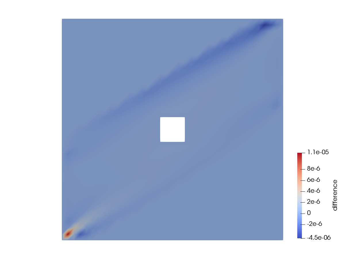
(a)

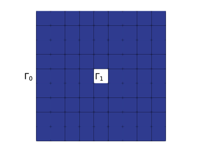
(b)

Figure 4: Anisotropic diffusion test. (a) difference between the OB-PP solutions, (b) coarsest mesh.

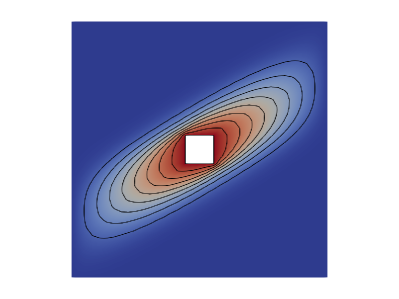
(a) unlimited solution $u_{h}\in\begin{bmatrix}-1.004,1\end{bmatrix}$

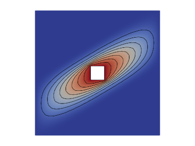
(b) OB-PP $u_{h}\in\begin{bmatrix}-1,1\end{bmatrix}$

Figure 5: Solutions to the anisotropic diffusion problem at the pseudo-time $T=2\cdot 10^{-2}$.

8 Conclusions

The research presented in this paper indicates that optimal control based on the use of flux potentials provides a versatile tool for enforcing discrete maximum principles in a locally conservative manner. As demonstrated in our numerical studies, the new OB-PP algorithm yields more accurate approximations than closed-form flux limiters and is better suited for preserving the range of physically admissible states in the presence of modeling errors. Moreover, the number of flux potentials is less than the number of fluxes that are used as control variables in the OB-FF version. While the cost of solving inequality-constrained optimization problems is considerable, it may be comparable to or even lower than that of iterative flux limiting in monolithic AFC schemes for stationary problems. We envisage that entropy stability conditions (cf. [15, 16]) and/or additional problem-dependent constraints can be included in the formulation of the PP optimization problem. Another promising avenue for further research is the design of new monolithic flux control algorithms for spatial semi-discretizations of the form (5) using criterion (9),(10) to formulate the inequality constraints. It is hoped that further development and analysis of flux-based optimal control approaches will make them an attractive alternative to more traditional PDE-constrained optimization methods for conservation laws.

Acknowledgments

The second author would like to thank Dr. Pavel Bochev and Dr. Denis Ridzal (Sandia National Laboratories) for very helpful discussions of the potential-state potential-target flux optimization method (named so by Dr. Bochev) at early stages of this work.

References

• [1] G. Barrenechea, V. John, and P. Knobloch, Analysis of algebraic flux correction schemes. SIAM J. Numer. Anal. 54 (2016) 2427–2451.
• [2] G. Barrenechea and P. Knobloch, Analysis of a group finite element formulation. Applied Numerical Mathematics 118 (2017) 238–248.
• [3] P. Bochev, D. Ridzal, M. D’Elia, M. Perego, and K. Peterson, Optimization-based, property-preserving finite element methods for scalar advection equations and their connection to Algebraic Flux Correction. Computer Methods Appl. Mech. Engrg. 367 (2020) 112982.
• [4] P. Bochev, D. Ridzal, and K. Peterson, Optimization-based remap and transport: A divide and conquer strategy for feature-preserving discretizations. J. Comput. Phys. 257 (2014) 1113–1139.
• [5] P. Bochev, D. Ridzal, G. Scovazzi, and M. Shashkov, Constrained-optimization based data transfer: A new perspective on flux correction. In: D. Kuzmin, R. LΓΆhner, S. Turek (eds), Flux-Corrected Transport: Principles, Algorithms, and Applications. Springer, 2nd edition: 2012, pp. 345–398.
• [6] J.P.Β Boris and D.L.Β Book, Flux-Corrected Transport: I. SHASTA, a fluid transport algorithm that works. J. Comput. Phys. 11 (1973) 38–69.
• [7] F. Frank, A. Rupp, and D. Kuzmin, Bound-preserving flux limiting schemes for DG discretizations of conservation laws with applications to the Cahn-Hilliard equation. Computer Methods Appl. Mech. Engrg. 359 (2019) 112665.
• [8] J.-L. Guermond, M. Nazarov, B. Popov, and Y. Yang, A second-order maximum principle preserving Lagrange finite element technique for nonlinear scalar conservation equations. SIAM J. Numer. Anal. 52 (2014) 2163–2182.
• [9] H. Hajduk, D. Kuzmin, Tz. Kolev, and R. Abgrall, Matrix-free subcell residual distribution for Bernstein finite element discretizations of linear advection equations. Computer Methods Appl. Mech. Engrg. 359 (2020) 112658.
• [10] A.Β Harten, High resolution schemes for hyperbolic conservation laws. J. Comput. Phys. 49 (1983) 357–393.
• [11] A.Β Harten, On a class of high resolution total-variation-stable finite-difference-schemes. SIAM J. Numer. Anal. 21 (1984) 1-23.
• [12] D. Kuzmin, Algebraic flux correction I. Scalar conservation laws. In: D. Kuzmin, R. LΓΆhner and S. Turek (eds.) Flux-Corrected Transport: Principles, Algorithms, and Applications. Springer, 2nd edition: 145–192 (2012).
• [13] D. Kuzmin, Monolithic convex limiting for continuous finite element discretizations of hyperbolic conservation laws. Comput. Methods Appl. Mech. Engrg. 361 (2020) 112804.
• [14] D. Kuzmin and Y. Gorb, A flux-corrected transport algorithm for handling the close-packing limit in dense suspensions. J. Comput. Appl. Math. 236 (2012) 4944–4951.
• [15] D. Kuzmin and M. Quezada de Luna, Algebraic entropy fixes and convex limiting for continuous finite element discretizations of scalar hyperbolic conservation laws. Computer Methods Appl. Mech. Engrg. 372 (2020) 113370.
• [16] D. Kuzmin and M. Quezada de Luna, Entropy conservation property and entropy stabilization of high-order continuous Galerkin approximations to scalar conservation laws. Computers and Fluids 213 (2020) 104742.
• [17] D. Kuzmin, M. QuezadaΒ de Luna, D. Ketcheson, and J. GrΓΌll, Bound-preserving convex limiting for high-order Runge-Kutta time discretizations of hyperbolic conservation laws. Preprint http://arxiv.org/abs/2009.01133
• [18] D. Kuzmin, M.J. Shashkov, and D. Svyatskiy, A constrained finite element method satisfying the discrete maximum principle for anisotropic diffusion problems. J. Comput. Phys. 228 (2009) 3448-3463.
• [19] R.J. LeVeque, High-resolution conservative algorithms for advection in incompressible flow. SIAM Journal on Numerical Analysis 33, (1996) 627–665.
• [20] MFEM: Modular finite element methods library. https://mfem.org
• [21] L.Β Quartapelle, Numerical Solution of the Incompressible Navier-Stokes Equations. BirkΓ€user, Basel, 1993.
• [22] C. Meyer and A. RΓΆsch, Superconvergence properties of optimal control problems. SIAM J. Control Optim. 43 (2004) 970–985.
• [23] V.Β Selmin and L.Β Quartapelle, A unified approach to build artificial dissipation operators for finite element and finite volume discretisations. In: K.Β Morgan et al. (eds), Finite Elements in Fluids, CIMNE / Pineridge Press, 1993, 1329–1341.
• [24] A.Β Ruszczynski, Nonlinear Optimization. Princeton University Press, 2011.
• [25] SuiteSparse: A suite of sparse matrix software. https://people.engr.tamu.edu/davis/suitesparse.html
• [26] B. Van Leer, Towards the ultimate conservative difference scheme. II. Monotonicity and conservation combined in a second-order scheme. J. Comput. Phys. 14 (1974) 361–370.
• [27] B. Van Leer, Towards the ultimate conservative difference scheme. III. Upstream-centered finite-difference schemes for ideal compressible flow. J. Comput. Phys. 23 (1977) 263–275.
• [28] S.T.Β Zalesak, Fully multidimensional flux-corrected transport algorithms for fluids. J. Comput. Phys. 31 (1979) 335–362.