Minimal Multi-Layer Modifications of
Deep Neural Networks

Abstract

Deep neural networks (DNNs) have become increasingly popular in recent years. However, despite their many successes, DNNs may also err and produce incorrect and potentially fatal outputs in safety-critical settings, such as autonomous driving, medical diagnosis, and airborne collision avoidance systems. Much work has been put into detecting such erroneous behavior in DNNs, e.g., via testing or verification, but removing these errors after their detection has received lesser attention. We present here a new tool, called 3M-DNN, for repairing a given DNN, which is known to err on some set of inputs. The novel repair procedure implemented in 3M-DNN computes a modification to the network’s weights that corrects its behavior, and attempts to minimize this change via a sequence of calls to a backend, black-box DNN verification engine. To the best of our knowledge, our method is the first one that allows repairing the network by simultaneously modifying multiple layers. This is achieved by splitting the network into sub-networks, and applying a single-layer repairing technique to each component. We evaluated 3M-DNN tool on an extensive set of benchmarks, obtaining promising results.

1 Introduction

The popularity of deep neural networks (DNNs) [19] has increased significantly over the past few years. DNNs are machine-learned artifacts, trained using a finite training set of examples; and they are capable of correctly handling previously-unseen inputs. DNNs have shown great success in many application domains, such as image recognition [36, 8], audio transcription [46], language translation [48], and even in safety-critical domains such as medical diagnosis [35], autonomous driving [4], and airborne collision avoidance [25].

Despite their evident success, DNNs can sometimes contain bugs. This has been demonstrated repeatedly: in one famous example, Goodfellow et al. [20] showed that slight perturbations to a DNN’s input could lead to misclassification — a phenomenon now known as susceptibility to adversarial perturbations. In another case, Liu et al. [41] showed how DNNs are vulnerable to Trojan attacks. These issues, and others, combined with the increasing integration of DNNs into safety-critical systems, have created a surge of interest in establishing their correctness. A great deal of effort has been put into developing methods for testing DNNs [52], and, more recently, also into verifying them [31, 55, 12]. These verification methods could play a significant role in the future certification of DNN-based systems.

Here, we deal with the case where we already know that a given DNN is malfunctioning; specifically, we assume we have a finite set of concrete inputs which are handled erroneously (discovered by testing, verification, or any other method). In this situation, we would like to modify the network, so that it produces correct predictions for these inputs. A naïve approach for accomplishing this is to add these faulty inputs to the training set used to create the DNN, and then retrain it, but this is often too computationally expensive [22]. Also, retraining may change the network significantly, potentially introducing new bugs on inputs that were previously correctly handled. Finally, retraining might be impossible when the original training set is inaccessible, e.g., due to its privacy or sensitivity [25].

Instead, we advocate an approach that requires no retraining, and which has recently gained some attention [9, 54, 40, 57]: we present a new tool, called 3M-DNN (Minimal, Multi-layer Modifications for DNNs), which can directly find a modification to the network and correct the erroneous behavior. In this context, a modification means changing the networks weights — the set of real values that determine the DNN’s output, and which are initially selected during training. Further, because we assume the original network is mostly correct, we seek to find a modification which is also minimal. The motivation is that such a change would maintain as much as possible of the network’s behavior on other inputs. In other words, our goal is to improve the DNN’s overall accuracy — the percentage of correctly handled inputs, which is normally measured with respect to a test set of examples — by improving its handling of problematic inputs, and without harming its handling of other inputs.

A DNN is, by definition, a layered artifact; and to the best of our knowledge, all previous work on finding minimal modifications to a DNN’s weights focused on changing the weights of a single layer [18, 9, 54]. Intuitively, and as we later demonstrate, this significant restriction could prevent one from finding potentially smaller (and thus preferable) changes to the network. In 3M-DNN, we seek to lift this restriction by proposing and implementing a novel method for the multi-layer modification of a DNN, with the goal of finding smaller modifications than could be otherwise possible. The key idea of our approach is to split the network into multiple sub-networks along certain layers, which we refer to as separation layers; and then attempt to find a minimal change for each of these sub-networks separately, in a way that brings about the desired overall change to the network.

More concretely, 3M-DNN is comprised of two logical levels. In the top, search level, the tool conducts a heuristic search through possible changes to the values computed by the separation layers. Each possible change to these values that we consider, translates into a possible fix to the DNN; it naturally gives rise to a sequence of problems on the bottom, single-layer modification level, each involving a single sub-network. Solving these single-layer modification problems can be performed using existing techniques; and the changes discovered to the sub-networks modify the values of the separation layers as selected by the top level. Thus, the process as a whole allows 3M-DNN to reduce the problem of multi-layer changes into a sequence of single-layer change problems, which can be dispatched using existing DNN modification tools as backends.

In its search for a minimal change, 3M-DNN alternates between the two levels: each time the top-level examines a potential change to the separation layers, and invokes the lower level in order to compute the overall cost of using that change (by combining the costs of changing each individual sub-network). The top-level always maintains the minimal change it has encountered so far, and uses search heuristics in order to find new, better options. The search space is infinite, and so our tool is anytime — it is designed to be run with a timeout, and whenever it is stopped, it returns the best (smallest) change discovered so far.

The search heuristic used by the top-level can have a crucial impact on performance. The approach implemented in 3M-DNN is general, in the sense that any search heuristic can be plugged in; and here, we consider and implement three such heuristics. The first is a random search, in which the top level randomly explores possible changes; this heuristic serves as a baseline. The second is a greedy search heuristic, in which the search always progresses in the direction that produces the most immediate gain. The third heuristic is a Monte Carlo Tree Search (MCTS) approach [5], which attempts to balance between exploration of the search space and the explorations of regions already known to produce good solutions.

The 3M-DNN tool will be made publicly available with the final version of this paper. It is designed in a modular fashion, so that additional search heuristics can be plugged in; it currently uses the Marabou DNN verification tool [31, 56] as a backend, although other tools could be used as well. We used 3M-DNN to compare the different aforementioned heuristic strategies, and to compare our method to a single-layer modification method, with respect to the accuracy and minimal change size found. In our experiments, 3M-DNN achieved favorable results when compared to single-layer modification techniques. The greedy and MCTS heuristics both performed better than the random one; and while the greedy approach generally outperformed MCTS, there were cases where the latter proved superior. Finally, we also used 3M-DNN to find three-layers modification to a network, as a proof-of-concept that demonstrates its ability to modify any number of layers simultaneously.

The rest of this paper is organized as follows. In Section 2 we provide the necessary background on DNNs and repairing DNNs with minimal modifications. In Section 3 we describe 3M-DNN’s algorithm for multi-layer modification in greater detail, and explain its different strategies for the heuristic search. Then, in Section 4 we provide additional technical details on our implementation of 3M-DNN. We describe our experiments and results in Section 5. In Section 6 we review relevant related work, and finally in Section 7 we conclude and describe our plans for future work.

2 Background

2.0.1 Deep Neural Networks.

A deep neural network (a model) $N$ is comprised of $n$ layers, $L_{1},\ldots,L_{n}$. Each layer $L_{i}$ is comprised of $s_{i}$ nodes, also called neurons. The first layer, $L_{1}$, is the input layer, and is used to provide the network with an input vector $v_{1}\in\mathbb{R}^{s_{1}}$. The network is then evaluated by iteratively computing the assignment $v_{i}$ of layer $L_{i}$ for $i=2,\ldots,n$, each time using the assignment $v_{i-1}$ as part of the computation. Finally, the DNN computes the assignment $v_{n}$ of layer $L_{n}$, which is the output layer. $v_{n}$ serves as the output of the entire neural network. Layers $L_{2},\ldots,L_{n-1}$ are referred to as hidden layers.

Each assignment $v_{i}$ for $2\leq i\leq n$ is computed by multiplying $v_{i-1}$ by a real-valued weight vector $\theta_{i}$, and applying a non-linear activation function (except for the final output layer, where no activation function is applied). We use $\theta$ to denote the set of all weights $\theta=[\theta_{2},\ldots,\theta_{n}]$, and use $N_{\theta}$ to refer to the function $N_{\theta}:\mathbb{R}^{s_{1}}\rightarrow\mathbb{R}^{s_{n}}$ computed by $N$. The weight vectors $\theta_{i}$ are key, and they are selected during the network’s training phase, which is beyond our scope here (see, e.g., [19] for details). Modern DNNs use various activation functions [44]; for simplicity, we restrict our attention here to the popular rectified linear unit (ReLU) function, defined as

$$\text{ReLU}{}{(x)}=\max\left(0,x\right),$$

although our approach could be used with other functions as well. When ReLUs are used, the values $v_{i}$ of layer $L_{i}$ are computed as $v_{i}=\text{ReLU}{}{}(\theta_{i}\cdot v_{i-1})$, where the ReLUs are applied element-wise. We use the term network architecture to refer to the number of layers in $N$, the size of each layer $s_{i}$, and the activation functions in use. Note that the network’s weights are not considered part of the network’s architecture.

For a given point $x\in\mathbb{R}^{s_{1}}$, we refer to the assignment of the output layer $N_{\theta}(x)$ as the network’s prediction on $x$. A common class of DNNs are designed for the purpose of classification, where the maximal entry of the prediction $N_{\theta}(x)$ indicates the label to which $x$ is classified. In other words, the classification of $x\in\mathbb{R}^{s_{1}}$ as determined by $N_{\theta}$ is defined as $\arg\max N_{\theta}(x)$. Classification DNNs are useful, for example, for image recognition [47], and are highly popular. When dealing with classification networks, we say that $N_{\theta}$ produces an erroneous output for $x$ if it classifies it differently than some given, ground-truth label $l$:

$$\arg\max N_{\theta}(x)\neq l$$

A small, running example is depicted in Fig. 1. This toy DNN is comprised of five layers — an input layer with a single node, three hidden layers with two nodes each, and an output layer with two nodes. The weight of each edge appears in the figure (a missing edge indicates a weight of $0$). All activation functions in this example are ReLUs. When the network is evaluated on input $v_{1}=[1]$, the assignment of the first hidden layer is $v_{2}=[1,1]$; the second hidden layer evaluates to $v_{3}=[0.01,100]$; the third hidden layer evaluates to $v_{4}=[10,1]$; and finally, the output layer evaluates to $v_{5}=[11,-11]$. If we treat this DNN as a classification model, the classification of $x=1$ is $1$, as $11=v_{5}^{1}>v_{5}^{2}=-11$.

Figure 1: A toy DNN.

2.0.2 Repairing DNNs with Minimal Modification.

For a given DNN $N_{\theta}:\mathbb{R}^{s_{1}}\rightarrow\mathbb{R}^{s_{n}}$ with $n$ layers, and a finite set of points $S\subset\mathbb{R}^{s_{1}}$ for which we know $N_{\theta}$ produces a wrong prediction, our goal is to change the network’s weights $\theta$, so that its classification of $S$ becomes correct.

We begin by formally defining the minimal modification problem for classification networks (later, we extend this definition to other networks as well). Let $N_{\theta}$ be a classification DNN, let $S$ be a set of inputs, and let $F$ be an oracle function $F:\mathbb{R}^{s_{1}}\rightarrow\{1,\ldots,s_{n}\}$ which indicates the correct classification for each point $x\in S$. Our goal is to produce a modification to $\theta$, which we denote $\delta$, and obtain a new set of weights $\theta^{\prime}=\theta+\delta$, such that:

$$\forall x\in S.\quad\arg\max N_{\theta^{\prime}}(x)=F(x)$$ (1)

Observe that the architecture of $N$ is unchanged. Our goal is to find a $\delta$ that is minimal, with the goal of preserving $N$’s behavior on points outside $S$. The magnitude of $\delta$ can be measured using any metric, such as the $L_{1}$ or $L_{\infty}$ norms.

Using these definitions, the minimal modification problem for classification DNNs is defined as follows:

Definition 1

The Minimal Modification Problem for Classification Models. Let $N_{\theta}:\mathbb{R}^{s_{1}}\rightarrow\mathbb{R}^{s_{n}}$ be a classification model with $n$ layers, and let $S\subset\mathbb{R}^{s_{1}}$ be a set of points. Let $F:S\rightarrow\{1,\ldots,s_{n}\}$ be an oracle function, which indicates the correct classification for each $x\in S$. Let $\left\lVert.\right\rVert$ be some norm function. The Minimal Modification Problem is:

$$\begin{array}[]{ll@{}ll}\text{minimize}&\left\lVert\delta\right\rVert&\\ \text{subject to}&\arg\max N_{\theta^{\prime}}(x)=F(x)&\quad\forall x\in S\\ &\theta^{\prime}=\theta+\delta\end{array}$$

We continue with our running example from Fig. 1. Recall that for input $x=1$, we get $v_{5}^{1}=11$ and $v_{5}^{2}=-11$. Now assume that $S=\{1\}$, and that the desired classification for $x=1$ is actually $F(1)=2$. Thus, we need the network to satisfy that $v_{5}^{1}<v_{5}^{2}$ when evaluated on $x=1$. We make an even stronger requirement, that $v_{5}^{1}+\mu\leq v_{5}^{2}$, for some small $\mu>0$; this guarantees a small gap in the scores assigned to $v_{5}^{1}$ and $v_{5}^{2}$, and avoids draws. For this example, we set $\mu=0.1$. Using the $L_{1}$ norm, the minimal single-layer modification that achieves the desired changes has size $2.21$, as depicted in Fig. 2. With this change to the network, we get that $v_{5}^{1}=-11.1<-11=v_{5}^{2}$. However, if we allow changing two layers, we can actually achieve a smaller minimal modification of size $2.11$, which is preferable because it has a smaller impact on the DNN’s behavior. We will later return to this example in Section 3.

Figure 2: Minimal single-layer modification for the toy example of Fig. 1. The only changed layer is the output layer, where the weight of the edge $v_{4}^{1}\rightarrow v_{5}^{1}$ was changed from $1$ to $-1.21$. The size of the change (using the $L_{1}$ norm) is $2.21$.

Definition 1 is typically sufficient for classification DNNs, but it can be generalized to support arbitrary constraints on the DNN’s outputs. Let $N_{\theta}$ be a general DNN (not necessarily a classification DNN). For each point $x\in S$, we consider a matrix $A_{x}\in\mathbb{R}^{k_{x}\times s_{n}}$ and a vector $b_{x}\in\mathbb{R}^{k_{x}}$, where $k_{x}$ is the number of linear constraints on the output of the netowrk on $x$. The aim is to produce a modification to $\theta$, which we denote again with $\delta$, and get new weights $\theta^{\prime}=\theta+\delta$, which satisfies:

$$A_{x}N_{\theta^{\prime}}(x)\leq b_{x}$$ (2)

Under this formulation we can express constraints such as “the first output of $N_{\theta^{\prime}}$ on $x$ should satisfy $3\leq N_{\theta^{\prime}}(x)\leq 5$”, which could not be expressed using the previous formulation. This formulation subsumes the classification case. Again notice that we keep the architecture of $N$ the same, and we only make modifications to $\theta$. More formally, the minimal modification problem for the general case is defined as follows:

Definition 2

The Minimal Modification Problem. Let $N_{\theta}:\mathbb{R}^{s_{1}}\rightarrow\mathbb{R}^{s_{n}}$ be a DNN model with $n$ layers, and let $S\subset\mathbb{R}^{s_{1}}$ be a set of points. For each point $x\in S$, let $A_{x}\in\mathbb{R}^{k_{x}\times s_{n}}$, $b_{x}\in\mathbb{R}^{k_{x}}$ be the output consraints of $N_{\theta}$ on $x$. Let $\left\lVert.\right\rVert$ be some norm function. The Minimal Modification Problem is:

$$\begin{array}[]{ll@{}ll}\text{minimize}&\left\lVert\delta\right\rVert&\\ \text{subject to}&A_{x}N_{\theta^{\prime}}(x)\leq b_{x}&\quad\forall x\in S\\ &\theta^{\prime}=\theta+\delta\end{array}$$

To the best of our knowledge, all previous approaches for solving the problems stated in Definitions 1 and 2 focused on finding a minimal modification for only a single layer of $N$. In contrast, in 3M-DNN we seek to solve the problem while allowing multiple layers of $N$ to be modified, as we discuss next.

3 3M-DNN: Finding Multi-Layer DNN Changes

The key idea incorporated into 3M-DNN is to reduce the multi-layer modification problem into a sequence of single-layer modification problems. Specifically, given a DNN $N$ with $n$ layers $L_{1},\ldots,L_{n}$ and a list of $k$ separation layer indices $1<i_{1}<\ldots<i_{k}<n$, we wish to partition the layers of $N$ into $k+1$ sub-networks $N^{0},N^{1},\ldots,N^{k}$. Each sub-network is comprised of a subset of the original network’s layers $L_{1},\ldots,L_{n}$, as follows: sub-network $N^{0}$ is comprised of layers $L_{1},\ldots,L_{i_{1}}$; sub-network $N^{k}$ is comprised of layers $L_{i_{k}},\ldots L_{n}$; and for each $1\leq j\leq k-1$, sub-network $N^{j}$ is comprised of layers $L_{i_{j}},\ldots,L_{i_{j+1}}$. Note that each pair of consecutive sub-networks $N^{j}$ and $N^{j+1}$ both contain layer $L_{i_{j+1}}$, which functions once as $N^{j}$’s output layer, and once as $N^{j+1}$’s input layer. We refer to the shared layers $L_{i_{1}},\ldots,L_{i_{k}}$ as the separation layers.

We apply this partitioning to our running example, as depicted in Fig. 3. There, we split the DNN into two sub-networks $N^{0}$ and $N^{1}$, with the original $L_{3}$ layer serving as the only separation layer. Observe that the input layer of $N^{0}$ is the input layer of the original network, and that the output layer of $N^{1}$ is the output layer of the original network. Indeed, if we were to evaluate $N^{0}$ on some input $x$, and then feed its output as the input to $N^{1}$, then $N^{1}$’s output would match the output of the original network when evaluated on $x$.

Figure 3: Splitting a network along a separation layer.

Next, we wish to modify $N^{0}$ and $N^{1}$, and then combine these modifications into a modification of the original network. Let $S=\{1\}$, i.e. $x=1$ is our only misclassified input, and let us require that $x$ be classified as class $2$. In other words, we wish $N(1)$ to produce output values for which $v_{5}^{1}+\mu\leq v_{5}^{2}$ for some small $\mu>0$. 3M-DNN begins by deciding on a change of values for the neurons of the separation layer, $v^{1}_{3}$ and $v^{2}_{3}$. In the original evaluation of the network on $x=1$, we got $v_{3}^{1}=0.01$ and $v_{3}^{2}=100$. Let us require that $v_{3}^{1}$’s value be changed to $0$, and that $v_{3}^{2}$’s value remains unchanged. This requirement translates into two single-layer modification queries: for $N^{0}$, 3M-DNN will require that on input $x=1$, the outputs be $[0,100]$; and for $N^{1}$, 3M-DNN will require that on input $[0,100]$, the network’s outputs satisfy $v_{5}^{1}+\mu\leq v_{5}^{2}$. Both these single-layer modification queries can be solved using a black-box modification procedure; for example, here, if we assume again that $\mu=0.1$, a possible modification is to change the weight of edge $v_{2}^{1}\rightarrow v_{3}^{1}$ to $0$ in $N^{0}$, and to change the weight of edge $v_{4}^{2}\rightarrow v_{5}^{2}$ to $1.1$ in $N^{1}$. Applying both of these changes to the original network produces a modification of size $2.11$ (using the $L_{1}$-norm), which results in the desired behavior for $x=1$; indeed, after applying this change, we get that $1=v_{5}^{1}<v_{5}^{2}=1.1$. The modified network is depicted in Fig. 4. Observe that this change is minimal for our particular selection of a separation layer index and the ensuing selection of changes to the separation layer’s assignment; but it is not necessarily globally minimal, as a different choice of separation index or assignment could result in smaller changes.

Figure 4: The two-layer modification found using 3M-DNN.

The example described above is generalized into 3M-DNN’s full algorithm, which appears as Algorithm 1. For simplicity of presentation, Algorithm 1 handles the classification model case from Definition 1; 3M-DNN actually supports the more general case from Definition 2, and the implemented algorithm is very similar to the one given here. Algorithm 1 takes as input the DNN $N$ in question, the set of misclassified points $S$ and the oracle function $F$ that describes these points desired classification; the separation indices $I=\{i_{1},\ldots,i_{k}\}$ indicating how the network is to be broken down into sub-networks, in which only a single layer will be changed; and a timeout value $T$. The algorithm then begins its heuristic search for a minimal change to the network that brings about the desired changes.

Algorithm 1 The 3M-DNN Algorithm (For Classification Networks)

Input: DNN $N$, set of input points $S=\{x_{1},\ldots,x_{n}\}$, oracle function $F$, separation indices $I=\{i_{1},\ldots,i_{k}\}$, timeout $T$
      Output: A repaired DNN $N^{\prime}$ with the same architecture as $N$

1:for $j=1\ldots n$ do

2:     $v^{j}_{i_{1}},\ldots,v^{j}_{i_{k}}\leftarrow N(x_{j})$ COMMENT$\triangleright$ Compute the separation layers’ assignments

3:end for

4:$N^{0},\ldots,N^{k}\leftarrow\textsc{Split}(N,I)$

5:$\text{bestChange}{}{}\leftarrow\bot,\text{bestCost}{}{}\leftarrow\infty$

6:while timeout $T$ not exceeded do

7:     for $l=1\ldots k$ do

8:         $c_{l}\leftarrow\textsc{ProposeChange}($)

9:         for $j=1\ldots n$ do

10:              $v^{\prime j}_{i_{l}}\leftarrow v^{j}_{i_{l}}+c_{l}$ COMMENT$\triangleright$ Select new assignments for the separation layers

11:         end for

12:     end for

13:     $N^{\prime 0},cost_{0}\leftarrow\textsc{SingleLayerModification}(N^{0},\langle x_{1},v^{\prime 1}_{i_{1}}\rangle,\ldots,\langle x_{n},v^{\prime n}_{i_{1}}\rangle)$

14:     for $l=1\ldots k-1$ do

15:         $N^{l},cost_{l}\leftarrow\textsc{SingleLayerModification}(N^{\prime l},\langle v^{\prime 1}_{i_{l}},v^{\prime 1}_{i_{l+1}}\rangle,\ldots,\langle v^{\prime n}_{i_{l}},v^{\prime n}_{i_{l+1}}\rangle)$

16:     end for

17:     $N^{\prime k},cost_{k}\leftarrow\textsc{SingleLayerModification}(N^{k},\langle v^{\prime 1}_{i_{k}},F(x_{1})\rangle,\ldots,\langle v^{\prime n}_{i_{k}},F(x_{n})\rangle)$

18:     $\text{cost}{}{}\leftarrow\textsc{TotalCost}(\text{cost}{}{}_{0},\ldots,\text{cost}{}{}_{k})$

19:     if $\text{cost}{}{}<\text{bestCost}{}{}$ then

20:         $\text{bestCost}{}{}\leftarrow\text{cost}{}{}$

21:         $\text{bestChange}{}\leftarrow\langle N^{\prime 0},\ldots,N^{\prime k}\rangle$

22:     end if

23:end while

24:return $\langle\text{bestCost}{},\textsc{Combine}(\text{bestChange}{})\rangle$

First, in Lines 1–3, the algorithm evaluates the assignments of the separation layers, for each input point in $S$. Then, in Line 4, the algorithm constructs the sub-networks $N^{0},\ldots,N^{k}$, according to the separation indices. Recall that our algorithm is anytime, i.e., always maintains the best modification discovered so far; this modification, and its cost (i.e., its distance from the original network according to the distance metric in use) is stored in the variables initialized in Line 5. The algorithm then begins running in a loop until exhausting its timeout value.

In every iteration of its main loop, the algorithm begins (Lines 8–11) by selecting a modified assignment for each separation layer $L_{i_{l}}$ for $1\leq l\leq k$. This modification is selected by the place-holder function ProposeChange(); this function is where the heuristic search used in the search level of 3M-DNN comes into play. We discuss these heuristics in detail in Section 3.1. Then, in Lines 13–17, the algorithm computes for each of the sub-networks $N^{0},\ldots,N^{k}$ the minimal, single-layer changes required to bring about the global changes selected by the search level. These changes are computed by repeated invocations of the SingleLayerModification() function, which is again a place-holder function that represents the single-layer modification level of 3M-DNN; we describe it in more depth in Section 3.2. This function takes as input a DNN, and a list of pairs of input points and their desired outputs; and returns the modified DNN, and the modification’s cost. In Line 13, we use SingleLayerModification() to modify $N^{0}$: we required that the original input points $x_{1},\ldots,x_{n}$ produce outputs that match the selected modified assignments $v^{\prime 1}_{i_{1}},\ldots,v^{\prime n}_{i_{1}}$ of $L_{1}$. In Line 15, SingleLayerModification() is used to modify each of the $N^{1},\ldots,N^{k-1}$ sub-networks, so that each sub-network produces as output the input selected for its successor. Finally, in Line 17, the last sub-network $N^{k}$ is modified, so that it produces outputs that match the oracle’s predictions on the original input points.

The single-layer modification procedures invoked for $N^{0},\ldots,N^{k}$ each return the modified sub-networks $N^{\prime 0},\ldots,N^{\prime k}$, and the respective costs of the modifications $cost_{0},\ldots,cost_{k}$. The total modification cost for the complete network is then computed by the TotalCost() function in Line 18, whose implementation depends on the norm used for measuring distance; for example, in the case of $L_{1}$ norm, it returns the sum of its inputs; for $L_{\infty}$, it returns the maximal input; etc. The modified sub-networks with the lowest total cost found so far, along with the cost itself, are saved in Lines 19–22.

The algorithm halts when the provided timeout is exhausted, and it then returns the complete modified network with the best modifications found so far, and the cost of that modification. The re-assembling of the complete modified network is performed by the function Combine(), whose implementation is omitted for brevity.

3.0.1 Soundness and Completeness.

Assuming that the SingleLayerModification() is sound — for example, if it is implemented using a sound DNN verifier [18] — any modification returned by our tool will indeed correct the global DNN behavior on the input set $S$. In that sense, 3M-DNN is sound. It is, however, generally incomplete; there are infinitely many modifications that can be attempted for the separation layers, and it is infeasible to try them all. This is our motivation for introducing the timeout mechanism and making the algorithm anytime; and indeed, the algorithm is not guaranteed to return the smallest change possible. It does, however, attempt to minimize the change based on search heuristics that we discuss next.

3.1 The Search Level

Algorithm 1 considers an infinite space of possible changes to the values of the separation layers, each time selecting a single possible change and computing its cost (Line 8 of the Algorithm). For a single separation layer with $n$ neurons, the search space is $\mathbb{R}^{n}$ in its entirety, and the problem is compounded when multiple separation layers are involved. To exacerbate matters even further, the computed cost function for possible changes need not be convex; see Fig. 5 for an illustration.

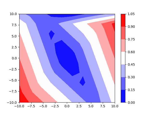
Figure 5: The cost function for a small DNN, with a single separation layer with 2 neurons. The X and Y axes represents the change for each neuron, and the color represents the size of the minimal modification achieved. The function is not convex.

To circumvent this difficulty, we first define the following grid, parameterized by a step size $\epsilon$:

$$\mathcal{G}_{\epsilon}=\{v=\langle\alpha_{1}\cdot\epsilon,\alpha_{2}\cdot\epsilon,\ldots,\alpha_{n}\cdot\epsilon\rangle\ |\ \alpha_{i}\in\mathbb{Z}\}$$

Each point in the grid represents a single, possible change for a separation layer, and the discretization allows us to better handle the search space. Naturally, this comes at the cost of possibly overlooking better changes that do not coincide with the grid, but this can be mitigated by making the grid dense (picking a smaller $\epsilon$). The grid’s origin, i.e., point $0^{n}\in\mathbb{R}^{n}$, corresponds to no change at all to the separation layer; and points that are very far away from the origin are likely to represent significant changes to the DNN.

Despite the discretization, the grid is still infinite and multi-dimensional, and so 3M-DNN implements three search heuristics: random search, greedy search and Monte-Carlo Tree Search (MCTS). Each of these heuristics can be regarded as a possible implementation of the ProposeChange() method from Algorithm 1. We next elaborate on each of them.

3.1.1 Random Search.

This heuristic performs a uniform random search over $\mathcal{G}_{\epsilon}$. Specifically, it samples a grid point uniformly at random, and that point constitutes the proposed change to the separation layer. We treat this simple heuristic as a baseline, to which the more sophisticated heuristics are compared.

3.1.2 Greedy Search.

The motivation for this heuristic is that the optimal grid point is likely not far away from the origin (as far away points likely correspond to significant changes to the network). Thus, we start from the grid’s origin as our current change, and at each iteration, consider the grid points that are immediate neighbors of our current points — that is, points obtained by adding or subtracting $\epsilon$ from one of the coordinates of the current point. We then compute the costs associated with each of these points, and pick the cheapest one as our new current point.

More formally, if $g_{0}\in\mathcal{G}_{\epsilon}$ is our current search point, we observe all points $g\in\mathcal{G}_{\epsilon}$ such that $\lVert g_{0}-g\rVert_{L_{1}}=\epsilon$, invoke the SingleLayerModification() with appropriate paremeters to compute the cost of each $g$, and update $g_{0}$ to be the $g$ that obtained the lowest cost.

3.1.3 Monte Carlo Tree Search.

The aforementioned greedy approach can be regarded as an attempt to optimize exploitation: whenever a good “direction” on the grid is discovered, we follow that direction. A natural concern is that such an approach might lead to local minima, and fail to detect cheaper changes that can only be reached via grid points with higher costs (recall that the cost function is not necessarily convex). To balance the greedy approach’s exploitation with exploration for detecting possibly better changes, we employ a Monte Carlo Tree Search (MCTS) heuristic [5]. We give here a short overview of this approach; see [5] for a more in-depth review.

MCTS is a heuristic search algorithm over a discrete set of actions, with the goal of selecting the most promising move based on simulations. It has recently been shown quite successful in multiple application domains, most notably in board games such as Go [15]. The search is conducted on a search tree, where each node represents a state. The root node of the search tree represents the initial state, and a child of a node represents another state that can be reached by performing a single action. Initially, the entire search tree is yet unexplored; and the algorithm iteratively explores additional parts thereof, one node in every iteration. In our setting, each node of the search tree is a grid point; and the possible moves include moving to one of the adjacent grid points (similarly to the greedy approach).

In each iteration, MCTS performs simulations in order to decide which unexplored node to visit next. Specifically, these simulations allow MCTS to compute a cost for each of the candidate nodes, and then pick the candidate with the lowest cost as the next node to visit.

More concretely, each MCTS iteration consists of 4 steps:

1. Selection: one of the nodes at each level in the explored portion of tree is selected, according to some policy, until reaching a leaf node. A common policy, also used in 3M-DNN, is the upper confidence bound (UCB) policy. The policy’s details are beyond our scope here; see [5] for additional details.

2. Expansion: one of the unexplored children of the leaf node from Step 1 is selected randomly.

3. Simulation: one or more simulations are carried out for the node selected in Step 2. Each simulation explores deeper into the search sub-tree rooted at the new node until reaching a predefined tree depth, by picking a child randomly in each level of the sub-tree. When the simulation arrives at the last node, it computes a cost value that takes into account all the steps that led from the node picked at Step 2 to the final node that was reached.

4. Backpropagation: the cost computed in each simulation is back-propagated through all the nodes in the path leading back up to the root. Each node aggregates the costs of simulations of paths containing it, and the aggregated cost is used for Step 1 in the next iteration of MCTS.

After reaching a predefined number of iterations, the unexplored node that has obtained the lowest cost so far is chosen as the next move.

In our implementation of the MCTS search heuristic, every invocation of ProposeChange() for a given separation layer $L_{j}$ runs the MCTS algorithm, which in turn performs a predefined number of sub-iterations. The root of the search tree represents the current change to the assignment of $L_{j}$, and a move to a child node represents a single step along the grid. Consequently, for each tree node of the search tree in the MCTS algorithm, there are $2s_{j}+1$ child nodes (including the option to not take a step at all). The simulation step of MCTS includes, in our case, dispatching single-layer modification queries.

3.2 The Single-Layer Modification level

As part of its operation, our algorithm needs to dispatch numerous queries of single-layer modifications in DNN (the SingleLayerModification() calls in Algorithm 1). In each of these queries, the sub-network in question has specific inputs, for which certain output constraints need to hold — either the outputs need to classify the inputs as a certain label (for the last sub-network), or they need to take on exact, predetermined values (for all other sub-networks). Solving such queries has been studied before, and as part of our solution, we propose to use existing techniques and tools as a backend. In our implementation (described in greater detail later), we used the approach proposed by Goldberger et. al [18].

4 Implementation

We implemented Algorithm 1 and the aforementioned search heuristics in the new 3M-DNN tool. 3M-DNN is implemented as a Python $3.7.3$ module, and uses TensorFlow-Keras $2.3$ as a backend for representing DNNs. We attempted to design 3M-DNN in a modular fashion, in order to easily allow the future addition of new search heuristics in the search level, as well as additional backend engines for dispatching single-layer modification queries.

The main class of 3M-DNN is the abstract NetworkCorrectionMethod class. It defines the interfaces and methods that a subclass must implement in order to fit the mold defined by Algorithm 1. Specifically, the class defines the following methods:

4.0.1 __init__(DNN $N$, $[x_{1},\ldots,x_{n}]$, $[o_{1},\ldots,o_{n}]$):

a constructor for the inheriting class. It takes as input a TensorFlow-Keras DNN, a list of input points as NumPy arrays, and a list of output constraints for each point. Each output constraint is a list of 2 items: a NumPy array $A$ and a NumPy vector $b$, and the output $y$ of the corresponding point should satisfy $Ay\leq b$ (per Definition 2).

4.0.2 correct_network()

the main entry point for the inheriting class, responsible for running the correction procedure for the DNN and constraints provided through the constructor. Its implementation depends on the heuristic search method and the single-layer modification method chosen. Returns True if a modification to the network was found, or False otherwise.

4.0.3 get_corrected_network():

this method is invoked after correct_network(), and returns the corrected network as a tensorflow-keras model.

4.0.4 get_minimal_change():

a method called after correct_network(), which returns the list of the changes found during the modification process, for each changed layer.

4.0.5 get_changed_layers():

a method called after correct_network(), which returns a list of layer indices of the layers changed during the modification process.

Our implementation of 3M-DNN includes multiple instantiations of the NetworkCorrectionMethod class that implement the heuristics defined in Section 3. Specifically, class NetworkCorrectionTwoLayersUniform implements the random search heuristic; the core of the implementation appears in the correct_network() method. Similarly, class NetworkCorrectionTwoLayersGreedy implements the greedy search approach; and its core is again in method correct_network(). Finally, the MCTS approach is implemented in classes NetworkCorrectionTwoLayersTreeSearch and MCTS. Class MCTS controls the various configurable parameters of the search, such as the step size, the number of simulations per iteration, and the maximal depth of the search tree. All three grid search heuristics are currently linked to the Marabou DNN verification as the single-layer change backend; this connection is implemented in class MarabouRunner.

Exp. #	Search Strategy	Number of input points	Average Change	Minimal Change	Maximal Change	Average Accuracy	Minimal Accuracy	Maximal Accuracy
1	Random	1	0.1520	0.0615	0.4922	0.6865	0.1916	0.9308
	Greedy		0.0133	0.001	0.0566	0.943	0.7971	0.9576
	MCTS		0.0139	0.001	0.0566	0.943	0.7971	0.9576
	Random	2	0.197	0.0791	0.4775	0.6302	0.2563	0.9161
	Greedy		0.0463	0.0058	0.1435	0.9245	0.7417	0.9598
	MCTS		0.0478	0.0058	0.1484	0.9261	0.7398	0.9594
2	Greedy	1	0.0305	0.0029	0.1699	0.9397	0.9565	0.5856
	1-Layer		0.0307	0.0029	0.1875	0.9394	0.585	0.9562
	Greedy	2	0.0459	0.0039	0.2041	0.9178	0.3124	0.9576
	1-Layer		0.0464	0.0039	0.208	0.9163	0.3124	0.9576
3	Greedy-3	1	0.25097	0.25097	0.25097	0.886	0.886	0.886

Table 1: Results of experiments. The 1-Layer search strategy stands for a single-layer modification process. Greedy-3 stands for three-layer-modification using the greedy heuristic search.

5 Evaluation

5.0.1 Setup.

We used 3M-DNN to evaluate the usefulness of our modification approach. Specifically, we experimented with a DNN trained on the MNIST dataset for digit recognition [39]. The dataset contains 70,000 handwritten digit images with $28\times 28$ pixels, split into a training set of 60,000 images, and a test set of 10,000 images. We trained a network $N$ comprised of 8 layers: an input layer of size 784 neurons, six hidden layers, each of size 20 neurons, and an output layer with ten neurons. The hidden layers all used the ReLU activation function. We then used network $N$ to conduct three kinds of experiment (all conducted with the $L_{\infty}$-norm): (i) comparing search heuristics: an experiment where we used 3M-DNN to find two-layer modifications for $N$, using each of the three heuristic search strategies discussed in Section 3; (ii) comparing multi-layer and single-layer modifications: here, we used 3M-DNN to search for repairs for $N$ that modified either a single layer or two layers, in order to evaluate the necessity of modifying multiple layers; and (iii) three-layer repairs: we attempted to repair $N$ by modifying three layers, to demonstrate 3M-DNN ability to repair the network by changing any number of layers. Below we provide additional information on each of the experiments, and their results are summarized in Table 1.

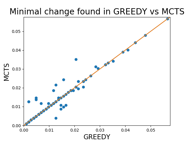
Figure 6: Minimal modification size achieved by the Greedy and MCTS heuristic strategies in Experiment 1.

5.0.2 Experiment 1: comparing search heuristics.

We used 3M-DNN in each of the three search method configurations, to solve: (i) 100 benchmarks where $N$ was modified to repair its output on 1 input point; and (ii) another 100 benchmarks with repair on 2 input points. In all experiments, we split $N$ into two sub-networks along its fourth hidden layer, with $\epsilon=0.5$ as the grid parameter; and the timeout value was set to 1000 seconds. In experiments involving two input points, we expedited the process by restricting changes solely to the final layer of each sub-network. The results are summarized in Table 1. Both the Greedy and MCTS strategies significantly outperform the uniform random search heuristic, achieving higher accuracy and smaller change size. The Greedy and MCTS heuristics are relatively equal in their performance, with each strategy outperforming the other in some cases.

5.0.3 Experiment 2: comparing multi- and single-layer modifications.

Here, we configured 3M-DNN to use the greedy search heuristic, and used it to solve: (i) 2000 minimal modification queries where where a single input point had to be corrected; and (ii) another 2000 minimal modification queries with repair on 2 input points. We ran each query once, looking for a one-layer minimal modification, and once searching for a two-layer modification. As before, we set $\epsilon=0.5$ and a timeout value of 1000 seconds (for both methods). To expedite the experiments, we allowed the single-layer method to modify only the final layer of the network [18], and the two-layers greedy method to modify the last layer of each of the two sub-networks. Table. 1 shows the superior performance of the two-layers greedy method over the single-layer method; although the single-layer modification method was usually able to find its minimal modification within a minute, while the two-layers greedy method took longer. This is not surprising, as the single-layer modification problem is significantly easier computationally [18].

5.0.4 Experiment 3: three-layer repairs.

In the final experiment, serving as a proof-of-concept, we used 3M-DNN to find a three-layer modification for $N$. We ran this experiment once, with 3M-DNN configured to use the greedy search heuristic on a single input point. We used a step size of $\epsilon=0.5$. The timeout value was set to 3600 seconds, and Table 1 depicts the results. The search space when changing three layers is significantly more complex than in the previous experiments, and so it is not surprising that 3M-DNN was only able to discover changes that were larger than before. As we continue to improve our search heuristics, and as the underlying verification engines continue to improve, the scalability of 3M-DNN will also improve.

6 Related Work

The need to modify existing DNNs in order to correct them naturally arises as part of the DNN life cycle, and has been a topic of interest in the wider machine learning community. Most existing approaches are heuristic in nature: for example, one approach is to iteratively apply Max-SMT solvers in search for changes to the DNN [49]; another is to use reachability analysis to enrich the training data [57]; and yet another approach is to heuristically identify “problematic” neurons and modify them [9]. A common property of most of these approaches is that, in contrast to verification-based approaches, they provide no formal guarantees about the minimality of the fixes that they produce.

Another approach for modifying the behavior of an existing DNN is to augment it with additional, non-DNN components that can override its output in certain cases. This has been attempted using, e.g., decision trees [32, 33] and scenario objects [26, 30]. A different technique is to transform the DNN into another object, which is simpler to repair: for example, a pair of DNNs, in which one determines the weights and another the activation functions [50]; or a DNN with a self-repairing output layer [40]. Our technique is separated from these approaches by the fact that the repaired artifact that it produces is a standard DNN, and is thus directly compatible with existing tools and infrastructure.

The approach that we take here, namely the application of DNN verification technology in order to find minimal modifications, has already received some attention. The approach that most closely resembles our own is the one proposed by Goldberger et al. [18]; and a related approach has also been proposed by Usman et al. [54]. However, these approaches are limited to modifying a single layer of the DNN in question, whereas the novelty of our approach is in enabling the simultaneous modification of multiple layers.

The technique proposed here uses a DNN verification engine as a black-box. DNN verification is an active research field, with many available tools and techniques. These include SMT-based approaches [23, 27, 31, 29], LP- and MILP-solver based approaches [6, 12, 53], symbolic interval propagation [55], abstraction and abstract-interpretation based techniques [13, 16, 3], techniques for tackling recurrent networks [58, 24] and binarized networks [2, 43], and many others (e.g., [11, 42, 45]); and these techniques have been applied to multiple ends, such as verifying adversarial robustness properties [16, 53, 21, 37, 7, 28], verifying hybrid systems with DNN controllers [10, 51], verifying DNNs that serve as controllers for congestion control systems [34, 1, 14], and DNN simplification [17, 38]. As DNN verification engines continue to improve, so will the speed and scalability of our approach. Further, our line of work continues to demonstrate that DNN repair is an attractive application domain for verification.

7 Conclusion and Future Work

Due to the recent surge in DNN popularity, it is becoming increasingly important to provide tools and methodologies for facilitating tasks that naturally arise as part of DNN usage — such as modifying existing DNNs. Verification-based modification techniques offer significant advantages, and in this work, we have taken a step towards improving their applicability. Specifically, we were able to move beyond the single-layer change barrier that existed in prior work, and propose an approach that can simultaneously modify multiple layers of the DNN. Consequently, our approach can find modifications that are superior to those that would have been discovered by existing techniques.

Moving forward, we plan to extend our approach along several axes. First, we intend to explore additional strategies for conducting the grid search, as the strategy in use has a significant effect on overall performance. Specifically, we intend to train a DNN controller to manage the search strategy. Second, we observe that the grid search naturally lends itself to parallelization, and so we intend to explore parallelization techniques; and third, we intend to further demonstrate the usefulness of our technique by applying it to additional DNNs and case studies.

7.0.1 Acknowledgements.

This work was partially supported by the Israel Science Foundation (grant number 683/18) and the HUJI Federmann Cyber Security Center.

References

- [1] G. Amir, M. Schapira, and G. Katz. Towards Scalable Verification of Deep Reinforcement Learning. In Proc. 21st Int. Conf. on Formal Methods in Computer-Aided Design (FMCAD), 2021.
- [2] G. Amir, H. Wu, C. Barrett, and G. Katz. An SMT-Based Approach for Verifying Binarized Neural Networks. In Proc. 27th Int. Conf. on Tools and Algorithms for the Construction and Analysis of Systems (TACAS), pages 203–222, 2021.
- [3] P. Ashok, V. Hashemi, J. Kretinsky, and S. Mohr. DeepAbstract: Neural Network Abstraction for Accelerating Verification. In Proc. 18th Int. Symp. on Automated Technology for Verification and Analysis (ATVA), pages 92–107, 2020.
- [4] M. Bojarski, D. Del Testa, D. Dworakowski, B. Firner, B. Flepp, P. Goyal, L. Jackel, M. Monfort, U. Muller, J. Zhang, X. Zhang, J. Zhao, and K. Zieba. End to End Learning for Self-Driving Cars, 2016. Technical Report. http://arxiv.org/abs/1604.07316.
- [5] C. Browne, E. Powley, D. Whitehouse, S. Lucas, P. Cowling, P. Rohlfshagen, S. Tavener, D. Perez, S. Samothrakis, and S. Colton. A Survey of Monte Carlo Tree Search Methods. IEEE Transactions on Computational Intelligence and AI in Games, 4(1):1–43, 2012.
- [6] R. Bunel, I. Turkaslan, P. Torr, P. Kohli, and P. Mudigonda. A Unified View of Piecewise Linear Neural Network Verification. In Proc. 32nd Conf. on Neural Information Processing Systems (NeurIPS), pages 4795–4804, 2018.
- [7] N. Carlini, G. Katz, C. Barrett, and D. Dill. Provably Minimally-Distorted Adversarial Examples, 2017. Technical Report. https://arxiv.org/abs/1709.10207.
- [8] D. Ciregan, U. Meier, and J. Schmidhuber. Multi-Column Deep Neural Networks for Image Classification. In Proc. IEEE Conf. on Computer Vision and Pattern Recognition (CVPR), pages 3642–3649, 2012.
- [9] G. Dong, J. Sun, J. Wang, X. Wang, and T. Dai. Towards Repairing Neural Networks Correctly, 2020. Technical Report. http://arxiv.org/abs/2012.01872.
- [10] S. Dutta, X. Chen, and S. Sankaranarayanan. Reachability Analysis for Neural Feedback Systems using Regressive Polynomial Rule Inference. In Proc. 22nd ACM Int. Conf. on Hybrid Systems: Computation and Control (HSCC), 2019.
- [11] S. Dutta, S. Jha, S. Sanakaranarayanan, and A. Tiwari. Output Range Analysis for Deep Neural Networks. In Proc. 10th NASA Formal Methods Symposium (NFM), pages 121–138, 2018.
- [12] R. Ehlers. Formal Verification of Piece-Wise Linear Feed-Forward Neural Networks. In Proc. 15th Int. Symp. on Automated Technology for Verification and Analysis (ATVA), pages 269–286, 2017.
- [13] Y. Elboher, J. Gottschlich, and G. Katz. An Abstraction-Based Framework for Neural Network Verification. In Proc. 32nd Int. Conf. on Computer Aided Verification (CAV), pages 43–65, 2020.
- [14] T. Eliyahu, Y. Kazak, G. Katz, and M. Schapira. Verifying Learning-Augmented Systems. In Proc. Conf. of the ACM Special Interest Group on Data Communication on the Applications, Technologies, Architectures, and Protocols for Computer Communication (SIGCOMM), pages 305–318, 2021.
- [15] M. Fu. AlphaGo and Monte Carlo Tree Search: the Simulation Optimization Perspective. In Proc. Winter Simulation Conference (WSC), pages 659–670, 2016.
- [16] T. Gehr, M. Mirman, D. Drachsler-Cohen, E. Tsankov, S. Chaudhuri, and M. Vechev. AI2: Safety and Robustness Certification of Neural Networks with Abstract Interpretation. In Proc. 39th IEEE Symposium on Security and Privacy (S&P), 2018.
- [17] S. Gokulanathan, A. Feldsher, A. Malca, C. Barrett, and G. Katz. Simplifying Neural Networks using Formal Verification. In Proc. 12th NASA Formal Methods Symposium (NFM), pages 85–93, 2020.
- [18] B. Goldberger, Y. Adi, J. Keshet, and G. Katz. Minimal Modifications of Deep Neural Networks using Verification. In Proc. 23rd Int. Conf. on Logic for Programming, Artificial Intelligence and Reasoning (LPAR), pages 260–278, 2020.
- [19] I. Goodfellow, Y. Bengio, A. Courville, and Y. Bengio. Deep Learning. MIT press Cambridge, 2016.
- [20] I. Goodfellow, J. Shlens, and C. Szegedy. Explaining and Harnessing Adversarial Examples, 2014. Technical Report. http://arxiv.org/abs/1412.6572.
- [21] D. Gopinath, G. Katz, C. Pǎsǎreanu, and C. Barrett. DeepSafe: A Data-driven Approach for Checking Adversarial Robustness in Neural Networks. In Proc. 16th. Int. Symp. on on Automated Technology for Verification and Analysis (ATVA), pages 3–19, 2018.
- [22] K. Hao. Training a Single AI Model can Emit as much Carbon as Five Cars In Their Lifetimes. MIT Technology Review, 2019.
- [23] X. Huang, M. Kwiatkowska, S. Wang, and M. Wu. Safety Verification of Deep Neural Networks. In Proc. 29th Int. Conf. on Computer Aided Verification (CAV), pages 3–29, 2017.
- [24] Y. Jacoby, C. Barrett, and G. Katz. Verifying Recurrent Neural Networks using Invariant Inference. In Proc. 18th Int. Symposium on Automated Technology for Verification and Analysis (ATVA), pages 57–74, 2020.
- [25] K. Julian, J. Lopez, J. Brush, M. Owen, and M. Kochenderfer. Policy Compression for Aircraft Collision Avoidance Systems. In Proc. 35th Digital Avionics Systems Conf. (DASC), pages 1–10, 2016.
- [26] G. Katz. Guarded Deep Learning using Scenario-Based Modeling. In Proc. 8th Int. Conf. on Model-Driven Engineering and Software Development (MODELSWARD), pages 126–136, 2020.
- [27] G. Katz, C. Barrett, D. Dill, K. Julian, and M. Kochenderfer. Reluplex: An Efficient SMT Solver for Verifying Deep Neural Networks. In Proc. 29th Int. Conf. on Computer Aided Verification (CAV), pages 97–117, 2017.
- [28] G. Katz, C. Barrett, D. Dill, K. Julian, and M. Kochenderfer. Towards Proving the Adversarial Robustness of Deep Neural Networks. In Proc. 1st Workshop on Formal Verification of Autonomous Vehicles (FVAV), pages 19–26, 2017.
- [29] G. Katz, C. Barrett, D. Dill, K. Julian, and M. Kochenderfer. Reluplex: a Calculus for Reasoning about Deep Neural Networks. Formal Methods in System Design (FMSD), 2021.
- [30] G. Katz and A. Elyasaf. Towards Combining Deep Learning, Verification, and Scenario-Based Programming. In Proc. 1st Workshop on Verification of Autonomous and Robotic Systems (VARS), pages 1–3, 2021.
- [31] G. Katz, D. Huang, D. Ibeling, K. Julian, C. Lazarus, R. Lim, P. Shah, S. Thakoor, H. Wu, A. Zeljić, D. Dill, M. Kochenderfer, and C. Barrett. The Marabou Framework for Verification and Analysis of Deep Neural Networks. In Proc. 31st Int. Conf. on Computer Aided Verification (CAV), pages 443–452, 2019.
- [32] D. Kauschke, S. Lehmann. Towards Neural Network Patching: Evaluating Engagement-Layers and Patch-Architectures , 2018. Technical Report. http://arxiv.org/abs/1812.03468.
- [33] S. Kauschke and J. Furnkranz. Batchwise Patching of Classifiers. In Proc. 32nd AAAI Conf. on Artifical Alliance, 2018.
- [34] Y. Kazak, C. Barrett, G. Katz, and M. Schapira. Verifying Deep-RL-Driven Systems. In Proc. 1st ACM SIGCOMM Workshop on Network Meets AI & ML (NetAI), pages 83–89, 2019.
- [35] D. Kermany, M. Goldbaum, W. Cai, C. Valentim, H. Liang, S. Baxter, A. McKeown, G. Yang, X. Wu, F. Yan, et al. Identifying Medical Diagnoses and Treatable Diseases by Image-Based Deep Learning. Cell, 172(5):1122–1131, 2018.
- [36] A. Krizhevsky, I. Sutskever, and G. Hinton. Imagenet Classification with Deep Convolutional Neural Networks. In Proc. 26th Conf. on Neural Information Processing Systems (NIPS), pages 1097–1105, 2012.
- [37] L. Kuper, G. Katz, J. Gottschlich, K. Julian, C. Barrett, and M. Kochenderfer. Toward Scalable Verification for Safety-Critical Deep Networks, 2018. Technical Report. https://arxiv.org/abs/1801.05950.
- [38] O. Lahav and G. Katz. Pruning and Slicing Neural Networks using Formal Verification. In Proc. 21st Int. Conf. on Formal Methods in Computer-Aided Design (FMCAD), 2021.
- [39] Y. LeCun. The MNIST database of handwritten digits, 1998. http://yann.lecun.com/exdb/mnist/.
- [40] K. Leino, A. Fromherz, R. Mangal, M. Fredrikson, B. Parno, and C. Păsăreanu. Self-Repairing Neural Networks: Provable Safety for Deep Networks via Dynamic Repair, 2021. Technical Report. https://arxiv.org/abs/2107.11445.
- [41] Y. Liu, S. Ma, Y. Aafer, W.-C. Lee, J. Zhai, W. Wang, and X. Zhang. Trojaning Attack on Neural Networks, 2017.
- [42] A. Lomuscio and L. Maganti. An Approach to Reachability Analysis for Feed-Forward ReLU Neural Networks, 2017. Technical Report. http://arxiv.org/abs/1706.07351.
- [43] N. Narodytska, S. Kasiviswanathan, L. Ryzhyk, M. Sagiv, and T. Walsh. Verifying Properties of Binarized Deep Neural Networks, 2017. Technical Report. http://arxiv.org/abs/1709.06662.
- [44] C. Nwankpa, W. Ijomah, A. Gachagan, and S. Marshall. Activation Functions: Comparison of Trends in Practice and Research for Deep Learning, 2018. Technical Report. http://arxiv.org/abs/1811.03378.
- [45] W. Ruan, X. Huang, and M. Kwiatkowska. Reachability Analysis of Deep Neural Networks with Provable Guarantees. In Proc. 27th Int. Joint Conf. on Artificial Intelligence (IJCAI), 2018.
- [46] F. Seide, G. Li, and D. Yu. Conversational Speech Transcription using Context-Dependent Deep Neural Networks. In Proc. 12th Conf. of the International Speech Communication Association (Interspeech), pages 437–440, 2011.
- [47] K. Simonyan and A. Zisserman. Very Deep Convolutional Networks for Large-Scale Image Recognition, 2014. Technical Report. http://arxiv.org/abs/1409.1556.
- [48] S. Singh, A. Kumar, H. Darbari, L. Singh, A. Rastogi, and S. Jain. Machine Translation using Deep Learning: an Overview. In Proc. Int. Conf. on Computer, Communications and Electronics (Comptelix), pages 162–167, 2017.
- [49] M. Sotoudeh and A. Thakur. Correcting Deep Neural Networks with Small, Generalizing Patches. In Workshop on Safety and Robustness in Decision Making, 2019.
- [50] M. Sotoudeh and A. Thakur. Provable Repair of Deep Neural Networks. In Proc. 42nd ACM SIGPLAN Int. Conf. on Programming Language Design and Implementation (PLDI), pages 588–603, 2021.
- [51] X. Sun, H. Khedr, and Y. Shoukry. Formal Verification of Neural Network Controlled Autonomous Systems. In Proc. 22nd ACM Int. Conf. on Hybrid Systems: Computation and Control (HSCC), 2019.
- [52] Y. Sun, X. Huang, D. Kroening, J. Sharp, M. Hill, and R. Ashmore. Testing Deep Neural Networks, 2018. Technical Report. http://arxiv.org/abs/1803.04792.
- [53] V. Tjeng, K. Xiao, and R. Tedrake. Evaluating Robustness of Neural Networks with Mixed Integer Programming. In Proc. 7th Int. Conf. on Learning Representations (ICLR), 2019.
- [54] M. Usman, D. Gopinath, Y. Sun, Y. Noller, and C. Pǎsǎreanu. NNrepair: Constraint-based Repair of Neural Network Classifiers, 2021. Technical Report. http://arxiv.org/abs/2103.12535.
- [55] S. Wang, K. Pei, J. Whitehouse, J. Yang, and S. Jana. Formal Security Analysis of Neural Networks using Symbolic Intervals. In Proc. 27th USENIX Security Symposium, pages 1599–1614, 2018.
- [56] H. Wu, A. Ozdemir, A. Zeljić, A. Irfan, K. Julian, D. Gopinath, S. Fouladi, G. Katz, C. Păsăreanu, and C. Barrett. Parallelization Techniques for Verifying Neural Networks. In Proc. 20th Int. Conf. on Formal Methods in Computer-Aided Design (FMCAD), pages 128–137, 2020.
- [57] X. Yang, T. Yamaguchi, H.-D. Tran, B. Hoxha, T. Johnson, and D. Prokhorov. Neural Network Repair with Reachability Analysis, 2021. Technical Report. https://arxiv.org/abs/2108.04214.
- [58] H. Zhang, M. Shinn, A. Gupta, A. Gurfinkel, N. Le, and N. Narodytska. Verification of Recurrent Neural Networks for Cognitive Tasks via Reachability Analysis. In Proc. 24th Conf. of European Conference on Artificial Intelligence (ECAI), 2020.