Large-scale dynamics of event-chain Monte Carlo

Abstract

Event-chain Monte Carlo (ECMC) accelerates the sampling of hard-sphere systems, and has been generalized to the potentials used in classical molecular simulation. Rather than imposing detailed balance on transition probabilities, the method enforces a weaker global-balance condition in order to guarantee convergence to equilibrium. In this paper we generalize the factor-field variant of ECMC to higher space dimensions. In the two-dimensional fluid phase, factor-field ECMC saturates the lower bound $z=0$ for the dynamical scaling exponent for local dynamics, whereas molecular dynamics is characterized by $z=1$ and local Metropolis Monte Carlo by $z=2$. In the presence of hexatic order, factor fields are not found to speed up the convergence. We indicate applications to the physics of glasses, and note that generalizations of factor fields could couple to orientational order.

I Introduction

Event-chain Monte Carlo (ECMC) has led to important advances in the simulation of $N$-particle systems [1, 2, 3, 4, 5, 6, 7, 8, 9, 10]. The efficiency gains that it brings have led to an improved understanding of phase transitions in two spatial dimensions (2D) [11]. As a non-reversible Markov-chain Monte Carlo (MCMC) algorithm [12, 13, 14], ECMC exactly samples the equilibrium Boltzmann distribution. However, it is itself out of equilibrium, because it replaces the diffusive dynamics of reversible MCMC (based on the detailed-balance condition) by ballistic dynamics (rooted in the more general global-balance condition). Non-reversible MCMC can approach the steady state, often the equilibrium Boltzmann distribution, on shorter time scales than reversible formulations [15, 16]. At large MCMC times, steady-state autocorrelation functions are exponential both for reversible and generally also for non-reversible Markov chains. The slowest mode generally relaxes on a time scale $\tau$ which depends on the system size $L$ as $\tau\sim L^{z}$. For $N$-particle systems in one spatial dimension (1D), ECMC can be analyzed in great detail [17, 18] and compared to molecular dynamics and to the reversible local Metropolis algorithm. The autocorrelation functions of density fluctuations in ECMC, as in molecular dynamics, are characterized by a dynamic exponent $z=1$, where the unit of time corresponds to a sweep of $N$ moves or events. This is asymptotically faster than for the reversible local Metropolis algorithm, for which $z=2$ so that the autocorrelation time, in $d$ dimensions, corresponds to $\sim L^{z}N\sim N^{1+z/d}$ moves. For 1D systems, a powerful variant of ECMC [18] adds a factor potential to the Hamiltonian. The factor potential leaves thermodynamic properties rigorously invariant, yet takes the system to zero pressure, $P$ by replacing the external forces by an attraction between particles. Factor-field ECMC lowers the 1D dynamic exponents to $z=1/2$, the theoretical minimum for a local MCMC algorithm. This acceleration is accompanied by super-diffusive dynamics of the instantaneous active particle [18, 19].

In the present paper, we formulate factor fields for higher-dimensional particle models and implement them for hard spheres in a 2D box. In fluid phases, hydrodynamic fluctuations that are coupled to local conservation laws constitute the long-lived modes for stochastic dynamics of the types realized in local MCMC algorithms [20, 21, 22]. We demonstrate through extensive numerical simulations for the implemented 2D hard-sphere model that factor fields can again lower the dynamical scaling exponents for such modes to their theoretical minimum, below those reached by molecular dynamics and by reversible local Monte Carlo. The reduction in dynamical scaling exponents translates into shorter correlation times for density fluctuations and, more generally, shorter overall correlation times.

The 2D factor fields introduced in this paper do not seem to couple to orientational degrees of freedom. In the hexatic phase, orientational order is itself (quasi)-long-ranged, and the dynamical scaling exponent of the hexatic field are thought to be diffusive for Hamiltonian dynamics, with $z\sim 2$ (see [23]). We expect this scaling to hold for reversible MCMC and for ECMC, but also for molecular dynamics. The computation of dynamical scaling exponents in the ordered phases beyond initial explorations [24] remains an unsolved problem, which is much more difficult than establishing the phase diagrams. Devising ECMC with modified factor fields with reduced scaling exponents for ordered phases appears as an outstanding challenge. We point to possible applications of the present formalism, for example in the study of glasses, where current simulation methods [25] use a non-local MCMC algorithm to relax structural degrees of freedom, but molecular dynamics to relax density modes. ECMC with factor fields may well decrease dynamical scaling exponents in these higher-dimensional polydisperse-particle models, and thus open the way for simulations of larger glassy systems than currently possible.

The ECMC algorithm evolves in continuous MCMC time $t$. Its event-driven implementation eliminates all discretization errors [1, 2, 3]. In the straight variant of ECMC, a unique active particle moves at unit speed in the chain direction, along one of the coordinate axes, in 2D between $\hat{\mathbf{e}}_{x}$ and $\hat{\mathbf{e}}_{y}$. At a lifting event, the motion transfers from the active sphere to the target sphere, preserving the chain direction. For hard spheres, such lifting events correspond to pair collisions. The algorithm is organized into event chains of chain time $\tau_{\text{chain}}$, an intrinsic parameter of straight ECMC that influences its efficiency. At the end of a chain a new active particle is randomly sampled and the chain direction may alternate between $\hat{\mathbf{e}}_{x}$ and $\hat{\mathbf{e}}_{y}$. The active sphere changes identity at each lifting move. It advances at an average speed which is proportional to the pressure, $P$. More precisely, the total displacement $\Delta_{\text{chain}}$ of the chain—the difference of the final position of the last chain sphere and of the initial position of the initial chain sphere—depends on the continuous MCMC time $\tau_{\text{chain}}$ of the chain as [3]

$$\beta P=\frac{N}{V}\ \left\langle\frac{\Delta_{\text{chain}}}{\tau_{\text{chain}}}\right\rangle,$$ (1)

where $\left\langle.\right\rangle$ is the ensemble mean and $\beta$ the inverse temperature, which is set to $\beta=1$ throughout. Eq. (1) holds for general pair potentials and it allows for the presence of factor potentials.

In this paper, we focus on the two-dimensional system of $N$ hard spheres of radius $\sigma$ in a square box of sides $L$ with periodic boundary condition. The position of each sphere is given by the coordinates of its center. The density is $\eta=N\pi\sigma^{2}/L^{2}$. For large $N$, the system is fluid for densities $0<\eta<0.7$. It is in fluid–hexatic coexistence for $0.7<\eta<0.716$ as a consequence of an underlying first-order phase transition, and it is hexatic at $0.716<\eta\lesssim 0.72$, above which it is solid [1, 26]. The hard-sphere factor-field algorithm can be generalized to smooth potentials, where we expect our conclusions to carry over.

II Factor fields in 1D and 2D

We first consider $N$ spheres on a continuous 1D interval of length $L$. The hard-sphere pair interaction,

$$V_{\text{hs}}=\sum_{i=1}^{N}v_{\text{hs}}(x_{i+1}-x_{i}),$$ (2)

between successive spheres (with $v_{\text{hs}}$ either zero or infinity) is understood with periodic boundary conditions in positions ($x+L\equiv x$) and indices ($i+N\equiv i$). The 1D factor potential [18] consists in a sum of linear potentials

$$V_{\text{{f}{f}}}=-h_{\text{{f}{f}}}\sum_{i}(x_{i+1}-x_{i})=-h_{\text{{f}{f}}}L,$$ (3)

that is constant for any factor field $h_{\text{{f}{f}}}$, because of the periodic boundary conditions. The factor potential $V_{\text{{f}{f}}}$ can be added to the inter-particle potential without changing correlation functions, as the constant, $-h_{\text{{f}{f}}}L$, cancels between the statistical weight and the partition function. Furthermore, force-based time evolutions such as molecular dynamics and energy-based Monte Carlo trajectories (Metropolis, heatbath, etc.) have indistinguishable dynamics for all $h_{\text{{f}{f}}}$. In contrast, in ECMC, the acceptance of a move depends on independent decisions made by pairs of spheres (see [9] for a detailed discussion of the general case), and the ECMC dynamics is strongly altered through $V_{\text{{f}{f}}}$. A factor field $h_{\text{{f}{f}}}=P$, with $P$ throughout this paper the pressure in the absence of factor fields, implies that the factor-field system, with potential $V_{\text{hs}}+V_{\text{{f}{f}}}$, has zero pressure, so that the average chain displacement $\left\langle\Delta_{\text{chain}}\right\rangle$ vanishes (see eq. (1)). The lifting move between an active and a target sphere can be a hard-sphere collision, that always goes forward in the chain direction, or else a factor-field lifting move that always goes backward. In the absence of drift, at $h_{\text{{f}{f}}}=P$, the position of the instantaneous active sphere (that changes identity at each lifting move) is characterized by hyperdiffusive motion with long-term memory. In the steady state, this lowers the 1D dynamical exponent from $z=1$ to $z=\frac{1}{2}$ and it also accelerates mixing.

Figure 1: Spheres in a 2D box, with a grating of lanes derived from a 2D cell system. Hard-sphere lifting moves correspond to collisions (for example of the active sphere $B$ with $C$). Factor-field lifting moves always concern same-lane spheres (for example $A$, for the active sphere $B$).

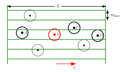
To adapt factor fields to 2D hard spheres, we construct for each chain a grating of lanes of width $w_{\text{lane}}\lesssim 2\sigma$ that is compatible with $L$ and that is oriented parallel to the chain direction (see Fig. 1). There, spheres are quasi-one-dimensional, and the factor potential of eq. (3) can again be added between spheres in the same lane. Spheres in nearby lanes only interact through the hard-sphere potential (see Fig. 1 for examples). The factor potential is now a sum over all lanes of an expression analogous to the 1D factor potential of eq. (3), each of which is a constant. Again, the factor field leaves thermodynamic properties rigorously invariant. As we will show, at least in the fluid phase, it also lowers the dynamical scaling exponent to its theoretical minimum.

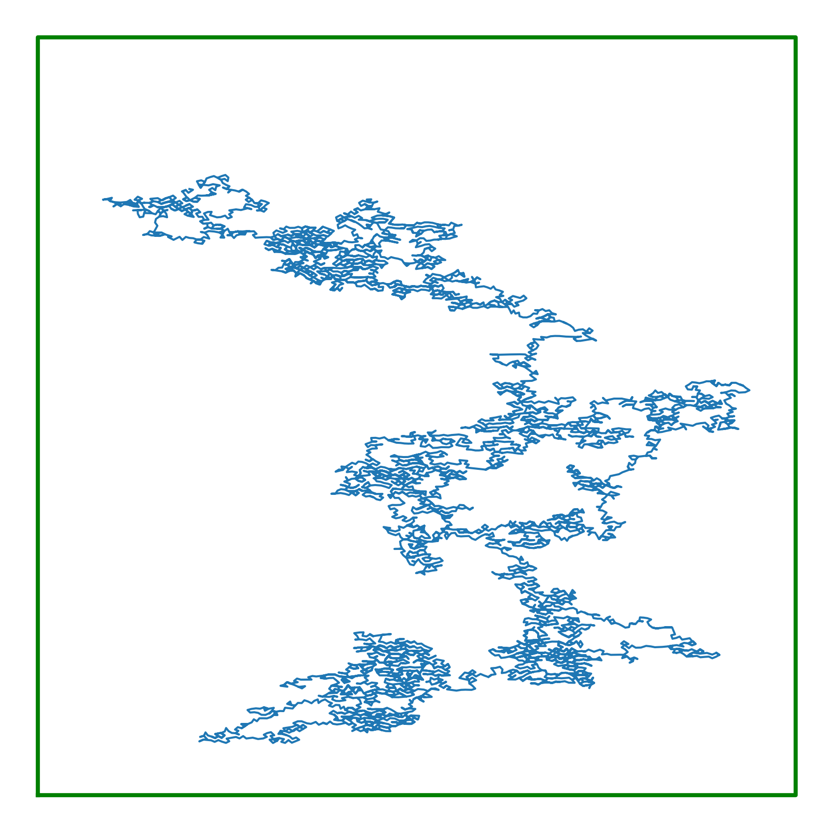
A hard-sphere lifting move can concern an active and a target sphere in different lanes so that the active sphere effectively moves in 2D. A factor-field lifting move, in contrast, always remains within a given lane. The optimal factor field is now $h_{\text{{f}{f}}}=Pw_{\text{lane}}$. At this value, the active sphere undergoes disordered 2D motion (see Fig. 3). The degree of anisotropy depends on the lane width $w_{\text{lane}}$.

Practically, the grating is derived from the 2D local cell system which is used to scan for possible hard-sphere collisions (see Fig. 1). The underlying Poisson process for the factor-field events does not require the advance knowledge of the position or identity of the target sphere (as the lifting move $B$ to $A$ in Fig. 1). A factor-field event simply requires walking back through the cells of the active-sphere lane to find the target sphere. Narrow lanes ($w_{\text{lane}}<2\sigma$) simplify the implementation of this algorithm, which however generalizes in a straightforward way to larger lanes, to arbitrary pair potentials and to more than two dimensions. In 2D, two different chain directions, as $\hat{\mathbf{e}}_{x}$ and $\hat{\mathbf{e}}_{y}$, are needed for the irreducibility of the ECMC algorithm (see [27] for a detailed discussion of irreducibility in 2D hard-sphere systems).

Figure 2: Maximum distance of the empirical cumulated distribution function of $rg(r)$ for $2\sigma<r<4\sigma$, with and without factor field for $n_{c}$ recordings (i.e. $n_{c}$ $N$-sphere samples). The $\sim 1/\sqrt{n_{c}}$ scaling of this Kolmogorov–Smirnov-like statistic indicates that $rg(r)$ (shown in the inset) is independent of $h_{\text{{f}{f}}}$ ($N=64^{2}$, $\eta=0.67$).

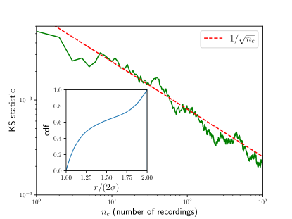
In 2D, the $P$ can be estimated through independent simulations in small physical systems. It need not be known to high precision to obtain efficient acceleration of the simulation. The correctness of the factor-field algorithm can be checked by comparing the pair-distribution function $rg(r)$ near contact using a Kolmogorov–Smirnov-like statistic [28]. The invariance of this key structural observable as a function of the factor field $h_{\text{{f}{f}}}=0$ or $h_{\text{{f}{f}}}=P$ holds to high precision (see Fig. 2).

Figure 3: Active-sphere trajectory featuring anisotropic 2D diffusion of a single event chain with direction $\hat{\mathbf{e}}_{x}$ for the 2D hard-sphere system at $\eta=0.67$. The optimal $h_{\text{{f}{f}}}=Pw_{\text{lane}}$ is used ($N=192^{2}$).

III Unidirectional displacements: Eigenmodes and dynamics

We now consider the restricted ECMC dynamics for a chain direction $\hat{\mathbf{e}}_{x}$ and for moves from a specific equilibrated 2D hard-sphere configuration $\mathbf{x}(t=0)$. The Markov chain then evolves for $t\to\infty$ towards a restricted Boltzmann equilibrium among samples that can be reached from $\mathbf{x}(t=0)$. We write $\mathbf{x}(t)=\{\mathbf{x}_{1}(t),\ldots,\mathbf{x}_{N}(t)\}$, where $\mathbf{x}_{i}(t)=\{x_{i}(t),y_{i}(t)\}$ describes the 2D position of sphere $i$, with periodic boundary conditions understood, and with all $y_{i}$ independent of $t$. (See Section IV for the full dynamics, with chain directions $\hat{\mathbf{e}}_{x}$ and $\hat{\mathbf{e}}_{y}$.) As discussed, spheres inside a narrow lane cannot re-order. The same applies to pairs $i,j$ of spheres in different lanes, with $|y_{i}-y_{j}|<2\sigma$. Each resulting constraint between $x_{i}$ and $x_{j}$ can be expressed as an inequality, and the sample space accessible from $\mathbf{x}(t=0)$ forms a convex polytope [29]. The ECMC dynamics of this restricted problem will allow us to better understand the full dynamics of the 2D fluid.

Figure 4: Eigenmodes $v^{(k)}$ with dominant eigenvalues $\lambda^{(k)}$ of the steady-state equal-time correlation matrix of eq. (5) (moves in $\hat{\mathbf{e}}_{x}$ from a given initial configuration $\mathbf{x}(t=0)$). Red and blue denote positive and negative displacements of $x_{i}$ around its mean. Simple shears ((a), (b)) coexist with higher-order shear ((c)), compression ((d)) and mixed modes ($N=256^{2}$, $\eta=0.67$).

We first extract the eigenmodes of fluctuations from a given initial configuration $\mathbf{x}$ (moving only along $\hat{\mathbf{e}}_{x}$). Subtracting the center-of-mass motion, allows one to define average positions,

$$\overline{x}_{i}=\frac{1}{m}\sum_{t=1}^{m}x_{i}(t),$$ (4)

and the equal-time correlation matrix $D=(D_{jl})$ with

$$D_{jl}=\frac{1}{m}\sum_{t=1}^{m}(x_{j}(t)-\overline{x}_{j})(x_{l}(t)-\overline{x}_{l}).$$ (5)

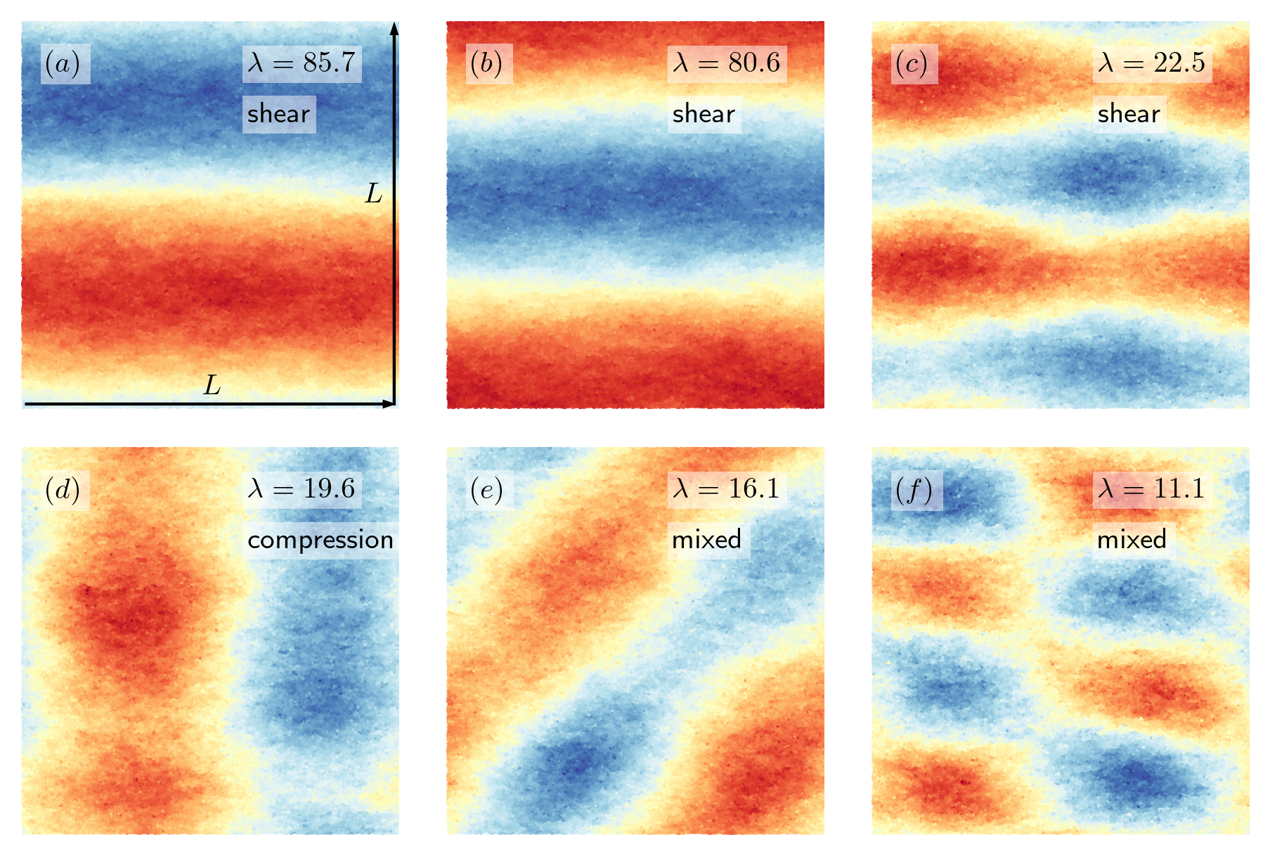
Lanczos’ algorithm yields the largest eigenvalues $\lambda^{(k)}$ and eigenmodes $v^{(k)}$ of the symmetric $N\times N$ matrix $D$ (see Fig. 4 for examples). The matrix $D$, and therefore the precise eigenmodes, depend on the initial configuration $\mathbf{x}(t=0)$, and degeneracies of the associated eigenvalues, for example of the two simple shear modes, are lifted for this reason.

In a Markov chain started from the same initial configuration $\mathbf{x}(t=0)$ that was used to compute the correlation matrix $D$, the configurations $\mathbf{x}(t)$ (with all the $y_{i}$ kept fixed) may now be decomposed onto the eigenmodes $v^{(k)}$. The time averages of autocorrelations of the eigenmode-amplitudes $a^{(k)}$

$$R_{k}(\tau)=\left\langle a^{(k)}(t)\,a^{(k)}(t+\tau)\right\rangle$$ (6)

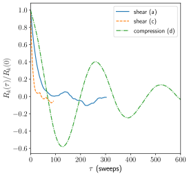
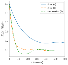
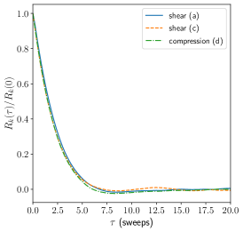
characterize the decay of correlations. In straight ECMC, the chain time $\tau_{\text{chain}}$ is an intrinsic parameter which through eq. (1) is connected to the chain length $\Delta_{\text{chain}}$, its overall extension. Shortest autocorrelation times are obtained for a chain length $\Delta_{\text{chain}}\sim\sqrt{N}\sim L$ (see [1]). For large chain times (chain length $\Delta_{\text{chain}}\gg L$), compression eigenmodes relax more slowly than shear eigenmodes and show long-time oscillations, while for short chains ($\Delta_{\text{chain}}\ll L$), the opposite is true, and shears can relax more slowly (see Fig. 5a and Fig. 5b). A factor field $h_{\text{{f}{f}}}=Pw_{\text{lane}}$ leads to the coordinated decay of autocorrelation functions for all eigenmodes on a time scale that is much shorter than for $h_{\text{{f}{f}}}=0$ (see Fig. 5c). The sampling of the polytope is thus greatly accelerated by the factor fields.

(a)

(b)

(c)

Figure 5: Autocorrelation of the static eigenmodes from eq. (6) (legends refer to Fig. 4, displacements in $\hat{\mathbf{e}}_{x}$ from a given initial configuration $\mathbf{x}(t=0)$, center-of-mass motion subtracted). (a): Factor field $h_{\text{{f}{f}}}=0$, large chain times $\tau_{\text{chain}}$ (corresponding to $\Delta_{\text{chain}}=3.1L$): Compression eigenmodes relax more slowly that shear eigenmodes and are oscillatory. (b): Factor field $h_{\text{{f}{f}}}=0$, small $\tau_{\text{chain}}$ (corresponding to $\Delta_{\text{chain}}=0.54L$): Shear eigenmodes may relax more slowly than compression eigenmodes. (c): Factor fields $h_{\text{{f}{f}}}=Pw_{\text{lane}}$, all eigenmodes decay rapidly, on similar time scales ($N=256^{2}$, $\eta=0.67$).

In order to extract the integrated autocorrelation time of the dominant eigenmode for large system sizes $N$ (where the equal time correlation matrix $D$ of eq. (5) can not be easily stored in main memory), we model the eigenmode in Fig. 4a, that is the displacement $x_{i}=\overline{x}_{i}+v_{i}^{(1)}$ as a constant in $\hat{\mathbf{e}}_{x}$ multiplied by a sine wave in $\hat{\mathbf{e}}_{y}$ (see Fig. 4b):

$$\mathbf{v}^{\text{approx}}=\{v_{1},\ldots,v_{N}\}\quad\text{with}\ v_{i}=\sin\left(2\pi y_{i}/L\right).$$ (7)

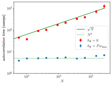
We then compute a projection coefficient as the scalar product of the displacement $\{(x_{1}(t)-\overline{x}_{1}),\ldots,(x_{N}(t)-\overline{x}_{N})\}$ with $\mathbf{v}^{\text{approx}}$. The timeseries of the projection coefficients yields an autocorrelation function, and an autocorrelation time. For $h_{\text{{f}{f}}}=0$, the optimal choice of the intrinsic parameter $\tau_{\text{chain}}$ is adopted from Fig. 4b. The autocorrelation time increases proportionally to $L$. For this restricted MCMC with fixed chain direction, this is consistent with a dynamical scaling exponent $z=1$ (see Fig. 6). For the optimal factor field $h_{\text{{f}{f}}}=Pw_{\text{lane}}$, the autocorrelation time of the approximate eigenmode of eq. (7) is consistent with $z=0$. For our largest system with $N=512^{2}$, factor fields accelerate the decorrelation by more than two orders of magnitude. It thus appears that factor-field ECMC realizes the optimal $z$.

Figure 6: Integrated ECMC autocorrelation time for the eigenmodes of Fig. 4a and Fig. 4b in the approximation of eq. (7). (Chain direction $\hat{\mathbf{e}}_{x}$, moves from given initial configurations $\mathbf{x}(t=0)$.) The scaling exponent for $h_{\text{{f}{f}}}=Pw_{\text{lane}}$ appears to saturate the lower bound $z=0$ (density $\eta=0.67$).

IV ECMC Dynamics in the fluid phase

In the fluid phase, hydrodynamic modes are long-lived due to the presence of local conservation laws [20, 21, 22]. Basic thermodynamics stipulates that fluctuations of extensive quantities, as the volume, grow as their square root. If a volume $V$ corresponds to a length scale $L^{d}$, then $V+\sqrt{V}$ corresponds to a length $L+L^{-d/2+1}$. In 1D, a test volume $\sim L$ may thus expand by its square root, leading to a lower limit $z=1/2$ for local algorithms with moves on a scale $\mathcal{O}(1)$ This, as discussed, is realized by factor-field ECMC. In 2D, the test volume expands only by a constant length, corresponding to a minimum of a single $\mathcal{O}(1)$ move per sphere, which corresponds to $z=0$. We will now present evidence showing that this value of $z=0$ (which may contain a logarithm so that the correlation time is of order $\mathcal{O}(\log N)$) is actually realized by factor-field ECMC, implying that a local algorithm may well reach the same scaling as the non-local MCMC algorithms, which have a proven mixing rate of $\mathcal{O}\left(N\log\!\,N\right)$ at small but finite densities [30], in the fluid phase [31].

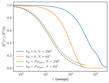
To trace the ECMC evolution of density fluctuations at the largest available length scales, we consider the Fourier coefficient $\rho(\mathbf{q})$ of the number density $\rho(\mathbf{x})=\sum_{i}\delta(\mathbf{x}-\mathbf{x}_{i})$,

$$\rho(\mathbf{q})=\sum_{j}\exp\left(i\mathbf{q}\cdot\mathbf{x}_{j}\right),$$ (8)

at the longest wavelength $\mathbf{q}=(2\pi/L)(1,0)$. We studied the autocorrelation function of $\rho(\mathbf{q})$ or relatedly, the autocorrelation of the corresponding structure factor $S_{\mathbf{q}}=|\rho(\mathbf{q})|^{2}$,

$$R^{S}(\tau)=\left\langle S_{\mathbf{q}}(t)S_{\mathbf{q}}(t+\tau)\right\rangle.$$ (9)

For $h_{\text{{f}{f}}}=0$, the optimal chain time $\tau_{\text{chain}}$ again corresponds to $\Delta_{\text{chain}}\sim L$, and long chains ($\Delta_{\text{chain}}\gg L$) again oscillate slowly (compare with Fig. 5). Without factor fields, long-wavelength excitations are much slower to decorrelate (see Fig. 7). The factor field again appears to lower the dynamical scaling exponent of density fluctuations, and by the same token, of overall correlations.

Figure 7: Autocorrelation $R^{S}(\tau)$ of the structure factor $S_{\mathbf{q}}$ for full ECMC in the fluid phase (density $\eta=0.67$). With factor fields, the autocorrelations seem to decay on a time scale that is independent of $N$, indicating $z=0$.

V ECMC dynamics in the coexisting-phase regime

At density $\eta=0.708$, the 2D hard-sphere system presents coexisting fluid and hexatic phases of different densities. In the two-phase region, the lower limit for the dynamical scaling exponent of a local MCMC algorithm is $z=1$ because switching from one of the coexisting to the other in an extensive test volume requires mass transport of $\mathcal{O}(N)$ spheres by a distance $\mathcal{O}(L)$. One of the coexisting phases, the hexatic, has quasi-long-range order, for which one expects $z\sim 2$ for Hamiltonian dynamics [23] and possibly also for ECMC. The hydrodynamic modes discussed in Section IV are no longer the only slow ones. The correlation times of local MCMC algorithms have however not been firmly established in the coexisting-phase region and in the hexatic phase. Our preliminary computations in this section present evidence that in the coexisting-phase regime factor fields certainly do not greatly speed up the convergence. It is thus likely that the factor fields, as presently formulated, do not couple to the orientational order.

We evaluate the global orientational order parameter

$$\psi=\frac{1}{N}\sum_{j=1}^{N}\frac{1}{n(j)}\sum_{\text{neig:}p}e^{6i\theta_{jp}},$$ (10)

where $n(j)$ denotes the number of neighbors $p$ of sphere $j$, and $\theta_{jp}$ is the angle between spheres $j$ and $p$. Rather than the Voronoi classification of neighbors we simply determine neighborhood through a cut-off based on the cell system. This does not change qualitative features. We study the autocorrelation of the norm of this complex field, Fig. 8, which is sensitive to fluctuations in the amplitude of the hexatic field.

$$R^{\psi}(\tau)=\left\langle|\psi|^{2}(t)\,\,|\psi|^{2}(t+\tau)\right\rangle$$ (11)

Figure 8: Autocorrelation $R^{\psi}(\tau)$ of the squared amplitude $|\psi|^{2}$ of the global orientational order parameter in the two-phase region ($\eta=0.708$). The autocorrelations decay on a time scale that increases with $N$ both for $h_{\text{{f}{f}}}=0$ and for $h_{\text{{f}{f}}}=Pw_{\text{lane}}$, where the simulation is slightly slowed down.

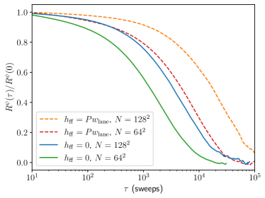
We perform simulation for $h_{\text{{f}{f}}}=0$ and for $h_{\text{{f}{f}}}=Pw_{\text{lane}}$ (see Fig. 8). Unlike the case of the density fluctuations in the fluid phase we find that the factor field slows the dynamics of the orientational order parameter $\psi$ by a small numerical factor. Even though long-wavelength density fluctuations are sampled efficiently by factor-field ECMC, this efficiency does not seem to feed into the dynamics of the global orientational order parameter.

VI Conclusions

In this paper, we have generalized factor-field ECMC from the previously introduced 1D case, where it appears natural, to higher-dimensional particle systems. As an example, we have implemented it for 2D hard spheres, although the new algorithm is trivial to extend to smooth interactions, as for example Lennard-Jones or soft-sphere potentials in any spatial dimension. Factor-field ECMC is found to sample density fluctuations very quickly, with a dynamical scaling exponent at the theoretical minimum $z=0$ (in the 2D fluid phase), while reversible local Markov chains feature $z=2$ and molecular dynamics with coupling to a thermostat $z=1$. The autocorrelation times is reached once each sphere has moved a number of times that at most grows with the logarithm of the system size.

We have further discussed the factor-field algorithm at densities where 2D hard spheres present two coexisting phases of different densities, namely the fluid and the hexatic and demonstrated that local MCMC algorithms must have a dynamical scaling exponent $z\geq 1$, simply because the density differences require important mass transfers between any two independent equilibrium configurations. Moreover, as one of the coexistent phases has quasi-long-range orientational order, we expect local algorithms to satisfy $z=2$. Simulation timescales involved in studying 2D hard spheres in the hexatic phase are still today extremely time-consuming, and the dynamical scaling exponents have not yet been computed. Our preliminary studies however do not allow us to conclude to any speed increases of factor-field ECMC in the presence of a hexatic phase. We conjecture that the factor field does not couple to orientational degrees of freedom, because it is aligned with the chain direction. Modified non-reversible Markov chains that couple to hexatic order can be set up, possibly with factor fields that point in a direction different from the chain direction.

Besides its theoretical interest, we imagine applications of factor-field ECMC (already in its present formulation) in the physics of glasses, as well as in studies of the melting transition for soft spheres, in 2D and higher. Most importantly, factor-field ECMC outperforms molecular dynamics, and it has superior dynamical scaling. This fact was already proven in 1D (see [18]) and is now firmly established in higher-dimensional systems. It should motivate further studies in non-reversible Markov chains.

References

- Bernard et al. [2009] E. P. Bernard, W. Krauth, and D. B. Wilson, Event-chain Monte Carlo algorithms for hard-sphere systems, Phys. Rev. E 80, 056704 (2009).
- Peters and de With [2012] E. A. J. F. Peters and G. de With, Rejection-free Monte Carlo sampling for general potentials, Phys. Rev. E 85, 026703 (2012).
- Michel et al. [2014] M. Michel, S. C. Kapfer, and W. Krauth, Generalized event-chain Monte Carlo: Constructing rejection-free global-balance algorithms from infinitesimal steps, J. Chem. Phys. 140, 054116 (2014), arXiv:1309.7748 [cond-mat.stat-mech] .
- Kampmann et al. [2015] T. A. Kampmann, H.-H. Boltz, and J. Kierfeld, Parallelized event chain algorithm for dense hard sphere and polymer systems, Journal of Computational Physics 281, 864 (2015).
- Harland et al. [2017] J. Harland, M. Michel, T. A. Kampmann, and J. Kierfeld, Event-chain Monte Carlo algorithms for three- and many-particle interactions, EPL (Europhysics Letters) 117, 30001 (2017).
- Hu and Charbonneau [2018] Y. Hu and P. Charbonneau, Clustering and assembly dynamics of a one-dimensional microphase former, Soft Matter 14, 4101 (2018).
- Klement and Engel [2019] M. Klement and M. Engel, Efficient equilibration of hard spheres with Newtonian event chains, The Journal of Chemical Physics 150, 174108 (2019).
- Michel et al. [2020] M. Michel, A. Durmus, and S. Sénécal, Forward Event-Chain Monte Carlo: Fast Sampling by Randomness Control in Irreversible Markov Chains, Journal of Computational and Graphical Statistics 29, 689 (2020).
- Krauth [2021] W. Krauth, Event-Chain Monte Carlo: Foundations, Applications, and Prospects, Frontiers in Physics 9, 229 (2021).
- Kampmann et al. [2021] T. A. Kampmann, D. Müller, L. P. Weise, C. F. Vorsmann, and J. Kierfeld, Event-Chain Monte-Carlo Simulations of Dense Soft Matter Systems, Frontiers in Physics 9, 10.3389/fphy.2021.635886 (2021).
- Bernard and Krauth [2011] E. P. Bernard and W. Krauth, Two-Step Melting in Two Dimensions: First-Order Liquid-Hexatic Transition, Phys. Rev. Lett. 107, 155704 (2011).
- Suwa and Todo [2010] H. Suwa and S. Todo, Markov Chain Monte Carlo Method without Detailed Balance, Phys. Rev. Lett. 105, 120603 (2010).
- Turitsyn et al. [2011] K. S. Turitsyn, M. Chertkov, and M. Vucelja, Irreversible Monte Carlo algorithms for efficient sampling, Physica D: Nonlinear Phenomena 240, 410 (2011).
- Bierkens et al. [2018] J. Bierkens, A. Bouchard-Côté, A. Doucet, A. B. Duncan, P. Fearnhead, T. Lienart, G. Roberts, and S. J. Vollmer, Piecewise Deterministic Markov Processes for Scalable Monte Carlo on Restricted Domains, Statistics and Probability Letters 136, 148–154 (2018).
- Diaconis et al. [2000] P. Diaconis, S. Holmes, and R. M. Neal, Analysis of a nonreversible Markov chain sampler, Ann. Appl. Probab. 10, 726 (2000).
- Chen et al. [1999] F. Chen, L. Lovász, and I. Pak, Lifting Markov Chains to Speed up Mixing, Proceedings of the 17th Annual ACM Symposium on Theory of Computing , 275 (1999).
- Kapfer and Krauth [2017] S. C. Kapfer and W. Krauth, Irreversible Local Markov Chains with Rapid Convergence towards Equilibrium, Phys. Rev. Lett. 119, 240603 (2017).
- Lei et al. [2019] Z. Lei, W. Krauth, and A. C. Maggs, Event-chain Monte Carlo with factor fields, Physical Review E 99, 10.1103/physreve.99.043301 (2019).
- Kimura and Higuchi [2017] K. Kimura and S. Higuchi, Anomalous diffusion analysis of the lifting events in the event-chain Monte Carlo for the classical XY models, EPL 120, 30003 (2017).
- Martin et al. [1972] P. C. Martin, O. Parodi, and P. S. Pershan, Unified Hydrodynamic Theory for Crystals, Liquid Crystals, and Normal Fluids, Phys. Rev. A 6, 2401 (1972).
- Forster [1975] D. Forster, Hydrodynamic fluctuations, broken symmetry, and correlation functions, Frontiers in Physics, Vol. 47 (W. A. Benjamin, Reading, Massachusetts, 1975).
- Hohenberg and Halperin [1977] P. C. Hohenberg and B. I. Halperin, Theory of dynamic critical phenomena, Rev. Mod. Phys. 49, 435 (1977).
- Zippelius et al. [1980] A. Zippelius, B. I. Halperin, and D. R. Nelson, Dynamics of two-dimensional melting, Physical Review B 22, 2514 (1980).
- Weigel [2018] R. F. B. Weigel, Equilibration of orientational order in hard disks via arcuate event-chain Monte Carlo (2018), Master thesis, Friedrich-Alexander-Universität Erlangen-Nürnberg.
- Ninarello et al. [2017] A. Ninarello, L. Berthier, and D. Coslovich, Models and Algorithms for the Next Generation of Glass Transition Studies, Phys. Rev. X 7, 021039 (2017).
- Thorneywork et al. [2017] A. L. Thorneywork, J. L. Abbott, D. G. A. L. Aarts, and R. P. A. Dullens, Two-Dimensional Melting of Colloidal Hard Spheres, Physical Review Letters 118, 10.1103/PhysRevLett.118.158001 (2017).
- Hoellmer et al. [2021] P. Hoellmer, N. Noirault, B. Li, A. C. Maggs, and W. Krauth, Sparse hard-disk packings and local Markov chains (2021), arXiv:2109.13343 [cond-mat.stat-mech] .
- Feller [1948] W. Feller, On the Kolmogorov-Smirnov Limit Theorems for Empirical Distributions, The Annals of Mathematical Statistics 19, 177 (1948).
- Kapfer and Krauth [2013] S. C. Kapfer and W. Krauth, Sampling from a polytope and hard-disk Monte Carlo, Journal of Physics: Conference Series 454, 012031 (2013).
- Kannan et al. [2003] R. Kannan, M. W. Mahoney, and R. Montenegro, Rapid mixing of several Markov chains for a hard-core model, in Proc. 14th annual ISAAC, Lecture Notes in Computer Science (Springer, Berlin, Heidelberg, 2003) pp. 663–675.
- Helmuth et al. [2020] T. Helmuth, W. Perkins, and S. Petti, Correlation decay for hard spheres via Markov chains (2020), arXiv:2001.05323 [math.PR] .