Additive Density-on-Scalar Regression in Bayes Hilbert Spaces with an Application to Gender Economics

Abstract

abstract Motivated by research on gender identity norms and the distribution of the woman’s share in a couple’s total labor income, we consider functional additive regression models for probability density functions as responses with scalar covariates. To preserve nonnegativity and integration to one under summation and scalar multiplication, we formulate the model for densities in a Bayes Hilbert space with respect to an arbitrary finite measure. This enables us to not only consider continuous densities, but also, e.g., discrete or mixed densities. Mixed densities occur in our application, as the woman’s income share is a continuous variable having discrete point masses at zero and one for single-earner couples. We discuss interpretation of effect functions in our model via odds-ratios. Estimation is based on a gradient boosting algorithm, allowing for potentially numerous flexible covariate effects. We show how to handle the challenging estimation for mixed densities within our framework using an orthogonal decomposition. Applying this approach to data from the German Socio-Economic Panel Study (SOEP) shows a more symmetric distribution in East German than in West German couples after reunification and a smaller child penalty comparing couples with and without minor children. These West-East differences become smaller, but are persistent over time.

Keywords: Density Regression; Functional Additive Model; Gradient Boosting; Mixed Densities.

abstract Motivated by research on gender identity norms and the distribution of the woman’s share in a couple’s total labor income, we consider functional additive regression models for probability density functions as responses with scalar covariates. To preserve nonnegativity and integration to one under summation and scalar multiplication, we formulate the model for densities in a Bayes Hilbert space with respect to an arbitrary finite measure. This enables us to not only consider continuous densities, but also, e.g., discrete or mixed densities. Mixed densities occur in our application, as the woman’s income share is a continuous variable having discrete point masses at zero and one for single-earner couples. We discuss interpretation of effect functions in our model via odds-ratios. Estimation is based on a gradient boosting algorithm, allowing for potentially numerous flexible covariate effects. We show how to handle the challenging estimation for mixed densities within our framework using an orthogonal decomposition. Applying this approach to data from the German Socio-Economic Panel Study (SOEP) shows a more symmetric distribution in East German than in West German couples after reunification and a smaller child penalty comparing couples with and without minor children. These West-East differences become smaller, but are persistent over time.

Keywords: Density Regression; Functional Additive Model; Gradient Boosting; Mixed Densities.

1 Introduction

Analyzing the distribution of the female income share for couples in the U.S., [44] show that the fraction of couples with a share below 0.5 is much higher than the fraction of those with a share above 0.5 and that there is a discontinuous drop in the density at 0.5. This drop is attributed to gender identity norms with men being averse to a situation with their female partners making more money than themselves. Subsequent studies, however, showed mixed results (e.g., [36, 25]). Most of the literature does not consider how the share distribution changes depending on covariates, but this in itself is of great interest. Social norms change over time towards higher employment of females, with part-time employment becoming more prevalent, especially in the presence of children. And the employment and earnings of female partners show a strong childhood penalty [23, 17].
From a methodological perspective, the focus on a univariate analysis of the share distribution reflects the lack of an interpretable multivariate analysis of its determinants. Filling this gap, we introduce a regression approach for outcomes that are probability density functions with scalar covariates and we use this new approach to analyze how the female income share distribution in Germany varies by place of residence (e.g., between West and East Germany), the presence of children, and over time.
For the continuous density case, our approach could be viewed as a special case of functional regression, which is part of the vast field of functional data analysis (e.g., [33]). One usually distinguishes three types of functional regression models (e.g., [48]): scalar-on-function, where the response is scalar while the covariates are functions, function-on-scalar with functional response and scalar covariates and function-on-function, where both, response and covariates, are functions. Analogously, we refer to our regression setting as density-on-scalar. Existing function-on-scalar methods are not applicable in this case, as multiplying a density with a negative scalar or adding two densities in the classical sense immediately violates the nonnegativity and integrate-to-one constraints of densities. An appropriate alternative normed vector space structure for densities is provided by Bayes Hilbert spaces, motivated by Aitchison’s work about compositional data [1]. [50] first introduced Bayes Hilbert spaces for densities with respect to the Lebesgue measure on a finite interval. This was extended by [46] to Bayes Hilbert spaces on finite measure spaces. [40] use Bayes Hilbert spaces for linear density-on-scalar regression, considering only densities defined on a finite interval and Lebesgue integrals. For estimation, the model is mapped into a subspace of the $L^{2}$ of square integrable functions applying the centered log-ratio (clr) transformation. We extend their framework to additive density-on-scalar regression models for densities on arbitrary finite measure spaces. This enables us to handle not only densities with respect to the Lebesgue measure on a finite interval (continuous case) or to the weighted sum of Dirac measures on a finite set (discrete case) but also mixtures of both (mixed case) in a unified framework. We introduce a gradient boosting algorithm based on the approach of [21], enabling estimation directly in the Bayes Hilbert space. Furthermore, we develop a method to interpret the estimated effects analogously to odds ratios. In our motivating application, we analyze the distribution of the woman’s share in a couple’s total labor income in Germany – an example of the mixed case: The corresponding densities defined on $[0,1]$ have positive point mass at the boundary values $0$ and $1$, corresponding to single-earner couples. This leads to a mixed (Dirac/Lebesgue) reference measure.
Apart from the Bayes Hilbert space approach, different ideas for density regression have been proposed. [30] discuss density-on-density regression without any positivity constraints, performing linear regression directly on the deviations from the mean density. [32] present linear regression for densities based on the Wasserstein metric, which constitutes a popular approach to statistical analysis of distributional data ([29]). However, with this approach the densities are considered in a nonlinear space, which makes modeling and interpretation more difficult. [18] introduce additive functional regression models for the density-on-scalar case as well. They transform the densities to the $L^{2}$, in particular proposing the log hazard and the log quantile density transformations. [19] show that for both, numerical instabilities may occur and finally prefer the clr transformation to both. In contrast to [18], which only considers the transformed densities for modeling, our Bayes Hilbert space approach provides an entire conceptual framework that allows to embed the densities and specify the model in a vector space structure. The clr transformation, an isometric isomorphism, allows an equivalent formulation in the $L^{2}$, which enables appealing odds-ratio-type interpretations on the original density-level.
Density regression is related to several other areas of research. For the discrete case, also known as compositional data [31, i.e., a multivariate vector of non-negative fractions summing to one, e.g.,], regression has also been studied, with [7] for instance considering Bayesian regression with compositional response. In general, there are also approaches not modeling densities but equivalent functions. E.g., [42] present a Bayesian approach to model quantile functions as response in a functional linear regression by introducing their quantlet basis representation. In contrast, modeling the density function has the distinct advantage that shifts of probability masses and special characteristics of the distribution such as bimodality can be identified straightforwardly. All methods mentioned so far share the assumption that a sample of densities (or, e.g., quantile functions) has been observed (or estimated). In contrast, there are also individual-level approaches, which model the conditional density or equivalent functions given covariates based on a sample of individual scalar data. Parametric approaches such as generalized additive models for location, scale and shape (GAMLSS, also known as distributional regression; e.g., [34]) require a known distribution family and only enable interpretation on the level of their parameters, not the distribution, which can be restrictive. In quantile regression (e.g., [24]) no specific distribution family is assumed, but for each quantile of interest one model has to be estimated, which is potentially computationally demanding. Furthermore, the estimated quantiles may cross, which can be avoided, e.g., by monotonization or rearrangement (e.g., [13]). Conditional transformation models (CTMs, e.g., [21]) model a monotone transformation function, which transforms the conditional distribution function (cdf) of the response to an a priori specified reference distribution function, in terms of covariates. In distribution regression (e.g., [14]), the cdf is estimated pointwise, similarly as in quantile regression. It requires the choice of a link function between the conditional distribution and the parametric covariate effects. Moreover, there are Bayesian (e.g., [28]), kernel estimation (e.g., [39]), and machine learning approaches [26, e.g.,] for modeling conditional response densities, suffering from two limitations: They work with a relatively large number of hyper-parameter(-distribution)s which influence the outcome; related to this is their lack of interpretability, in particular in terms of the covariate effects.
We aim to bridge this gap in the literature by directly modeling the response density on the one hand, while borrowing interpretable yet flexible additive models from functional data analysis on the other hand. To the best of the authors’ knowledge, our approach is the first to cover continuous, discrete and mixed cases in a unified framework.
In the following, Section 2 summarizes the construction of Bayes Hilbert spaces. Section 3 introduces our density-on-scalar regression approach, where models are formulated in Bayes Hilbert spaces and estimated using a boosting algorithm. In the mixed case, we derive an orthogonal decomposition of the Bayes Hilbert space to facilitate (separate continuous/discrete) estimation. We develop an interpretation method of the estimated effects using odds-ratios. Section 4 involves a comprehensive application for the mixed case in analyzing the distribution of the woman’s share in a couple’s total labor income in Germany. Section 5 provides a small simulation study based on our application setting to validate our approach. We conclude with a discussion and an outlook in Section 6.

2 The Bayes Hilbert space

We briefly introduce Bayes spaces and summarize their basic vector space properties for a $\sigma$-finite reference measure as described in [45]. Refining these to Bayes Hilbert spaces [46], we have to restrict ourselves to finite reference measures. We provide proofs for all theorems in appendix LABEL:appendix_proofs_BHS since we take a slightly different point of view compared to [45, 46].

Let $(\mathcal{T},\mathcal{A})$ be a measurable space and $\mu$ a $\sigma$-finite measure on it, the so-called reference measure. Consider the set $\mathcal{M}(\mathcal{T},\mathcal{A},\mu)$, or short $\mathcal{M}(\mu)$, of $\sigma$-finite measures with the same null sets as $\mu$. Such measures are mutually absolutely continuous to each other, i.e., by Radon-Nikodyms’ theorem, the $\mu$-density of $\nu$ or Radon-Nikodym derivative of $\nu$ with respect to $\mu$, $f_{\nu}:=\mathrm{d}\nu/\mathrm{d}\mu:\mathcal{T}\rightarrow\mathbb{R}$, exists for every $\nu\in\mathcal{M}(\mu)$. It is $\mu$-almost everywhere ($\mu$-a.e.) positive and unique. We write $f_{\nu}\cong\nu$ for a measure $\nu\in\mathcal{M}(\mu)$ and its corresponding $\mu$-density $f_{\nu}$. For measures $\nu_{1},\nu_{2}\in\mathcal{M}(\mu)$, let the equivalence relation $=_{\mathcal{B}}$ be given by $\nu_{1}=_{\mathcal{B}}\nu_{2}$, iff there is a $c>0$ such that $\nu_{1}(A)=c\,\nu_{2}(A)$ for every $A\in\mathcal{A}$, where $c\,(+\infty)=+\infty$. Respectively, we define $f_{\nu_{1}}=_{\mathcal{B}}f_{\nu_{2}}$, iff $f_{\nu_{1}}=c\,f_{\nu_{2}}$ for some $c>0$. Here and in the following, pointwise identities have to be understood $\mu$-a.e. Both definitions of $=_{\mathcal{B}}$ are compatible with the Radon-Nikodym identification $f_{\nu}\cong\nu$. The set of $(=_{\mathcal{B}})$-equivalence classes is called the Bayes space (with reference measure $\mu$), denoted by $\mathcal{B}(\mu)=\mathcal{B}(\mathcal{T},\mathcal{A},\mu)$. For equivalence classes containing finite measures, we choose the respective probability measure as representative in practice. Then, the corresponding $\mu$-density is a probability density. However, mathematically it is more convenient to use a non-normalized representative. For better readability, we omit the index $\mathcal{B}$ in $=_{\mathcal{B}}$ and the square brackets denoting equivalence classes in the following. For $f_{\nu_{1}}\cong\nu_{1},f_{\nu_{2}}\cong\nu_{2}\in\mathcal{B}(\mu)$, the addition or perturbation is given by the equivalent definitions

$$(\nu_{1}\oplus\nu_{2})(A) :=\int_{A}\frac{\mathrm{d}\nu_{1}}{\mathrm{d}\mu}\,\frac{\mathrm{d}\nu_{2}}{\mathrm{d}\mu}\,\mathrm{d}\mu, f_{\nu_{1}}\oplus f_{\nu_{2}}:=f_{\nu_{1}}\,f_{\nu_{2}}.$$

For $f_{\nu}\cong\nu\in\mathcal{B}(\mu)$ and $\alpha\in\mathbb{R}$, the scalar multiplication or powering is defined by

$$(\alpha\odot\nu)(A) :=\int_{A}\left(\frac{\mathrm{d}\nu}{\mathrm{d}\mu}\right)^{\alpha}\,\mathrm{d}\mu, \alpha\odot f_{\nu}:=(f_{\nu})^{\alpha}.$$

Theorem 2.1 ([45]).

The Bayes space $\mathcal{B}(\mu)$ with perturbation $\oplus$ and powering $\odot$ is a real vector space with additive neutral element $0:=\mu\cong 1$, additive inverse element $\ominus\nu:=\int_{A}\mathrm{d}\mu/\mathrm{d}\nu\,\mathrm{d}\mu\cong 1/f_{\nu}$ for $\nu\in\mathcal{B}(\mu)$, and multiplicative neutral element $1\in\mathbb{R}$.

For subtraction, we write $\nu_{1}\ominus\nu_{2}:=\nu_{1}\oplus(\ominus\nu_{2})$ and $f_{\nu_{1}}\ominus f_{\nu_{2}}:=f_{\nu_{1}}\oplus(\ominus f_{\nu_{2}})$.

From now on, we restrict the reference measure $\mu$ to be finite, progressing to Bayes Hilbert spaces. This is similar to [46] with some details different. In the style of the well-known $L^{p}$ spaces, $B^{p}$ spaces for $1\leq p<\infty$ are defined as

$$B^{p}(\mu)=B^{p}(\mathcal{T},\mathcal{A},\mu):=\Bigl{\{}\nu\in\mathcal{B}(\mu)\leavevmode\nobreak\ \Big{|}\leavevmode\nobreak\ \int_{\mathcal{T}}\bigl{|}\log\frac{\mathrm{d}\nu}{\mathrm{d}\mu}\bigr{|}^{p}\,\mathrm{d}\mu<\infty\Bigr{\}}.$$

We also say $f_{\nu}\in B^{p}(\mu)$ for $f_{\nu}\cong\nu\in B^{p}(\mu)$. This is equivalent to $\log f_{\nu}\in L^{p}(\mu)$, which gives us $B^{q}(\mu)\subset B^{p}(\mu)$ for $p,q\in\mathbb{R}$ with $1\leq p<q$. Note that for every $p\in\mathbb{R}$ with $1\leq p<\infty$, the space $B^{p}(\mu)$ is a vector subspace of $\mathcal{B}(\mu)$, see [46]. For $f_{\nu}\cong\nu\in B^{p}(\mu)$, the centered log-ratio (clr) transformation of $\nu$ is given by

$$\operatorname{clr}_{B^{p}(\mathcal{T},\mathcal{A},\mu)}[\nu]=\operatorname{clr}_{B^{p}(\mathcal{T},\mathcal{A},\mu)}[f_{\nu}]:=\log f_{\nu}-\mathcal{S}_{B^{p}(\mathcal{T},\mathcal{A},\mu)}(f_{\nu}),$$ (2.1)

with $\mathcal{S}_{B^{p}(\mathcal{T},\mathcal{A},\mu)}(f_{\nu}):=1/\mu(\mathcal{T})\,\int_{\mathcal{T}}\log f_{\nu}\,\mathrm{d}\mu$ the mean logarithmic integral. We omit the indices $B^{p}(\mathcal{T},\mathcal{A},\mu)$ or shorten them to $\mu$ or $\mathcal{T}$, if the underlying space is clear from context.

Proposition 2.2 (For $p=1$ shown in [46]).

For $1\leq p<\infty$, the clr transformation $\operatorname{clr}:B^{p}(\mu)\rightarrow L^{p}_{0}(\mu):=\{\tilde{f}\in L^{p}(\mu)\leavevmode\nobreak\ |\leavevmode\nobreak\ \int_{\mathcal{T}}\tilde{f}\,\mathrm{d}\mu=0\}$ is an isomorphism with inverse transformation $\operatorname{clr}^{-1}[\tilde{f}]=\exp\tilde{f}$.

Note that $L^{p}_{0}(\mu)$ is a closed subspace of $L^{p}(\mu)$. The space $B^{2}(\mu)$ is called the Bayes Hilbert space (with reference measure $\mu$). For $f_{\nu_{1}}\cong\nu_{1},f_{\nu_{2}}\cong\nu_{2}\in B^{2}(\mu)$, consider

$$\langle\nu_{1},\nu_{2}\rangle_{B^{2}(\mu)}:=\langle f_{\nu_{1}},f_{\nu_{2}}\rangle_{B^{2}(\mu)}:=\int_{\mathcal{T}}\operatorname{clr}[f_{\nu_{1}}]\,\operatorname{clr}[f_{\nu_{2}}]\,\mathrm{d}\mu,$$

which is an inner product on $B^{2}(\mu)$, see Proposition LABEL:inner_product_thm in appendix LABEL:appendix_proofs_BHS. It induces a norm on $B^{2}(\mu)$ by $\|\nu\|_{B^{2}(\mu)}:=\|f_{\nu}\|_{B^{2}(\mu)}:=\sqrt{\langle f_{\nu},f_{\nu}\rangle_{B^{2}(\mu)}}$ for $f_{\nu}\cong\nu\in B^{2}(\mu)$. By definition, we have $\langle f_{\nu_{1}},f_{\nu_{2}}\rangle_{B^{2}(\mu)}=\langle\operatorname{clr}[f_{\nu_{1}}],\operatorname{clr}[f_{\nu_{2}}]\rangle_{L^{2}(\mu)},$ which immediately implies that $\operatorname{clr}:B^{2}(\mu)\rightarrow L^{2}_{0}(\mu)$ is isometric. We now formulate the main statement of this section:

Theorem 2.3 ([46]).

The Bayes Hilbert space $B^{2}(\mu)$ is a Hilbert space.

Note that in Proposition LABEL:thm_subcompositional_coherence in appendix LABEL:appendix_proofs_BHS, we introduce a notion of canonical embedding, which enables us to identify the Bayes Hilbert space $B^{2}(\mathcal{T}_{0},\mathcal{A}\cap\mathcal{T}_{0},\mu)$ with a closed subspace of $B^{2}(\mathcal{T},\mathcal{A},\mu)$ for any $\mathcal{T}_{0}\in\mathcal{A}$. Furthermore, we explicitly compute the orthogonal projection onto $B^{2}(\mathcal{T}_{0},\mathcal{A}\cap\mathcal{T}_{0},\mu)$. This construction is new to the best of the authors’ knowledge. An important consequence of the properties of the orthogonal projection is that we may restrict linear problems (like regression models) onto subsets of $\mathcal{T}$ consistently with the geometry of the Bayes Hilbert spaces. For compositional data, the correspondence of subcompositions in $\mathcal{T}_{0}\subset\mathcal{T}$ to subspaces of the Bayes Hilbert space is referred to as subcompositional coherence [31].

3 Density-on-scalar regression

We consider regression models with a density as response and scalar covariates. More precisely, the response has to be an element of a Bayes Hilbert space $B^{2}(\mu)=B^{2}(\mathcal{T},\mathcal{A},\mu)$. This requires $\mu$ to be finite on $(\mathcal{T},\mathcal{A})$, excluding, e.g., densities on the whole real line using the Lebesgue measure as reference or densities which are exactly zero in parts of $\mathcal{T}$. To consider $\mathcal{T}=\mathbb{R}$ with the Borel $\sigma$-algebra $\mathfrak{B}_{\mathbb{R}}$, a possible reference is the probability measure corresponding to the standard normal distribution [46]. If a density is not directly observed but estimated from an observed sample, density values of zero can be avoided by choosing a density estimation method that yields a positive density. For discrete sets $\mathcal{T}$, one option is to replace observed density values of zero with small values (e.g., [31]). The framework allows for a variety of different applications. Usually, we consider $\mathcal{T}\subset\mathbb{R}$ with three common cases: In the continuous case, we consider a nontrivial interval $\mathcal{T}=I$ with $\mathcal{A}=\mathfrak{B}$ the Borel $\sigma$-algebra restricted to $I$ and $\mu=\lambda$ the Lebesgue measure. The discrete case refers to a discrete set $\mathcal{T}=\{t_{1},\ldots,t_{D}\}$ with $\mathcal{A}=\mathcal{P}(\mathcal{T})$ the power set of $\mathcal{T}$ and $\mu=\sum_{d=1}^{D}w_{d}\,\delta_{t_{d}}$ a weighted sum of Dirac measures, where $w_{d}>0$. The mixed case is a mixture of both: As in the continuous case, we have $\mathcal{T}=I$ and $\mathcal{A}=\mathfrak{B}$, but some points $\mathcal{D}=\{t_{1},\ldots,t_{D}\}\subset I$ have positive probability mass. The corresponding reference measure is a mixture of weighted Dirac measures and the Lebesgue measure, i.e., $\mu=\sum_{d=1}^{D}w_{d}\,\delta_{t_{d}}+\lambda$. Note that the special case $\mathcal{D}=\emptyset$ yields the continuous case. Our application in Section 4 gives an example for the mixed case.

3.1 Regression model

Density-on-scalar regression is motivated by function-on-scalar regression. Both regression types are closely related (at least in the continuous case), as density-on-scalar models can be transformed to function-on-scalar models in $L^{2}_{0}(\mu)$ via the clr transformation. We formulate our model analogously to structured additive function-on-scalar regression models [48], considering densities in a Bayes Hilbert space $B^{2}(\mu)$ instead of functions in $L^{2}(I,\mathfrak{B},\lambda)$ and using the corresponding operations. For data pairs $(y_{i},\mathbf{x}_{i})\in B^{2}(\mu)\times\mathbb{R}^{K},\leavevmode\nobreak\ K\in\mathbb{N},\leavevmode\nobreak\ i=1,\ldots,N,\leavevmode\nobreak\ N\in\mathbb{N}$, this yields the structured additive density-on-scalar regression model

$$y_{i}=h(\mathbf{x}_{i})\oplus\varepsilon_{i}=\bigoplus_{j=1}^{J}h_{j}(\mathbf{x}_{i})\oplus\varepsilon_{i},$$ (3.1)

where $\varepsilon_{i}\in B^{2}(\mu)$ are functional error terms with $\mathbb{E}(\varepsilon_{i})=0\in B^{2}(\mu)$ and $h_{j}(\mathbf{x}_{i})\in B^{2}(\mu)$ are partial effects, $J\in\mathbb{N}$. The expectations of the $B^{2}(\mu)$-valued random elements $\varepsilon_{i}$ are defined using the Bochner integral (e.g., [22]). Each partial effect $h_{j}(\mathbf{x}_{i})\in B^{2}(\mu)$ in (3.1) models an effect of none, one or more covariates in $\mathbf{x}_{i}$.

Covariate(s)	Type of effect	$h_{j}(\mathbf{x})$
None	Intercept	$\beta_{0}$
One scalar covariate $x$	Linear effect	$x\odot\beta$
	Flexible effect	$g(x)$
Two scalar covariates $x_{1},x_{2}$	Linear interaction	$x_{1}\odot(x_{2}\odot\beta)$
	Functional varying coefficient	$x_{1}\odot g(x_{2})$
	Flexible interaction	$g(x_{1},x_{2})$
Grouping variable $k$	Group-specific intercepts	$\beta_{k}$
Grouping variable $k$ and scalar $x$	Group-specific linear effects	$x\odot\beta_{k}$
	Group-specific flexible effects	$g_{k}(x)$

Table 3.1: Partial effects for density-on-scalar regression.

Table 3.1 gives an overview of possible partial effects, inspired by Table 1 in [48]. The upper part shows effects for up to two different scalar covariates. In the lower part, group-specific effects for categorical variables are presented. Interactions of the given effects are possible as well. Scalar covariates are denoted by $x$, densities in $B^{2}(\mu)$ by $\beta$ and $g(\,)$. Note that constraints are necessary to obtain identifiable models. For a model with an intercept $\beta_{0}$, this is obtained by centering the partial effects:

$$\frac{1}{N}\odot\bigoplus_{i=1}^{N}h_{j}(\mathbf{x}_{i})=0.$$ (3.2)

More details about how to include this constraint in a functional linear array model for function-on-scalar regression can be found in appendix A of [48]. A similar procedure can be used to obtain a centering of interaction effects around the main effects, see appendix A of [38]. Both approaches are based on [59, Section 1.8.1 ] and can be transferred straightforwardly to density-on-scalar regression.

3.2 Estimation by Gradient Boosting

To estimate the function $h(\mathbf{x}_{i})\in B^{2}(\mu)$ in Equation (3.1), the sum of squared errors

$$\mathrm{SSE}(h):=\sum_{i=1}^{N}\|\varepsilon_{i}\|_{B^{2}(\mu)}^{2}=\sum_{i=1}^{N}\|y_{i}\ominus h(\mathbf{x}_{i})\|_{B^{2}(\mu)}^{2}=\sum_{i=1}^{N}\rho_{y_{i}}\left(h(\mathbf{x}_{i})\right)$$ (3.3)

is minimized. Here, $\rho_{y_{i}}:B^{2}(\mu)\rightarrow\mathbb{R},\,f_{\nu}\mapsto\|y_{i}\ominus f_{\nu}\|_{B^{2}(\mu)}^{2}$ is the quadratic loss functional. To simplify the minimization problem and to determine the type of an effect, compare Table 3.1, we consider a basis representation for each partial effect:

$$h_{j}(\mathbf{x}_{i})=\left(\mathbf{b}_{j}(\mathbf{x}_{i})^{\top}\begin{picture}(3.0,2.0)\put(1.5,0.6){\circle{2.0}}\put(1.5,0.6){\makebox(0.0,0.0)[]{$\otimes$}} \end{picture}\mathbf{b}_{Y}^{\top}\right)\boldsymbol{\theta}_{j}=\bigoplus_{n=1}^{K_{j}}\bigoplus_{m=1}^{K_{Y}}b_{j,n}(\mathbf{x}_{i})\odot b_{Y,m}\odot\theta_{j,n,m},$$ (3.4)

where $\mathbf{b}_{j}=(b_{j,1},\ldots,b_{j,K_{j}}):\mathbb{R}^{K}\rightarrow\mathbb{R}^{K_{j}}$ is a vector of basis functions in direction of the covariates and $\mathbf{b}_{Y}=(b_{Y,1},\ldots,b_{Y,K_{Y}})\in B^{2}(\mu)^{K_{Y}}$ is a vector of basis functions over $\mathcal{T}$. With , we denote the Kronecker product of a real-valued with a $B^{2}(\mu)$-valued matrix. It is defined like the Kronecker product of two real-valued matrices, using $\odot$ instead of the usual multiplication. Similarly, matrix multiplication of a real-valued with a $B^{2}(\mu)$-valued matrix is defined by replacing sums with $\oplus$ and products with $\odot$ in the usual matrix multiplication. Our goal is to estimate the coefficient vector $\boldsymbol{\theta}_{j}=(\theta_{j,1,1},\ldots,\theta_{j,K_{j},K_{Y}})\in\mathbb{R}^{K_{j}\,K_{Y}}$. To allow sufficient flexibility for $h_{j}$, the product $K_{j}\,K_{Y}$ can be chosen to be large. The necessary regularization can then be accomplished with a Ridge-type penalty term $\boldsymbol{\theta}_{j}^{\top}\mathbf{P}_{j,Y}\boldsymbol{\theta}_{j}$. For a basis representation as in equation (3.4), an anisotropic penalty matrix $\mathbf{P}_{j,Y}=\lambda_{j}(\mathbf{P}_{j}\otimes\mathbf{I}_{K_{Y}})+\lambda_{Y}(\mathbf{I}_{K_{j}}\otimes\mathbf{P}_{Y})$ can be used. Here, $\mathbf{P}_{j}\in\mathbb{R}^{K_{j}\times K_{j}}$ and $\mathbf{P}_{Y}\in\mathbb{R}^{K_{Y}\times K_{Y}}$ are suitable penalty matrices for $\mathbf{b}_{j}$ and $\mathbf{b}_{Y}$, respectively, and $\lambda_{j},\lambda_{Y}\geq 0$ are smoothing parameters in the respective directions. Alternatively, a simplified isotropic penalty matrix $\mathbf{P}_{j,Y}=\lambda_{j}((\mathbf{P}_{j}\otimes\mathbf{I}_{K_{Y}})+(\mathbf{I}_{K_{j}}\otimes\mathbf{P}_{Y}))$ with only one smoothing parameter is possible [9]. The basis representation framework might seem restrictive at first, but it indeed allows for very flexible modeling of the effects, as discussed below.

We fit model (3.1) using a component-wise gradient boosting algorithm, where the expected loss is minimized step-wise along the steepest gradient descent. It is an adaption of the algorithm presented in [48], which was modified from [21]. Advantages of this approach are that it can deal with a large number of covariates, it performs variable selection, and includes regularization. [11] discuss theoretical properties of gradient boosting w.r.t. sum of squares errors, which is typically referred to as $L_{2}$-Boosting, for scalar responses. They show – simplifying to a single learner – that bias decays exponentially fast while estimator variance increases in exponentially small steps over the boosting iterations, which supports the general practice of stopping the algorithm early before it eventually reaches the standard (penalized) least squares estimate. [27] show consistency of component-wise $L_{2}$-Boosting for linear regression with both high-dimensional multivariate response and predictors. Similar to these predecessors, our $L_{2}$-Boosting algorithm for Bayes Hilbert spaces simplifies to repeated re-fitting of residuals – which, however, present densities in our case.

Algorithm: Bayes space $L_{2}$-Boosting for density-on-scalar models

1. Select vectors of basis functions $\mathbf{b}_{Y},\mathbf{b}_{j}$, the starting coefficient vector $\boldsymbol{\theta}_{j}^{[0]}\in\mathbb{R}^{K_{j}\,K_{Y}}$, and penalty matrices $\mathbf{P}_{j,Y},j=1,\ldots,J$. Choose the step-length $\kappa\in(0,1)$ and the stopping iteration $m_{\text{stop}}$ and set the iteration number $m$ to zero. We comment on a suitable selection of these quantities below.

2. Calculate the negative gradient of the empirical risk with respect to the Fréchet differential (see appendix LABEL:appendix_proofs_regression for the proof of this equation)

   $$U_{i}:=\ominus\nabla\rho_{y_{i}}(f_{\nu})\big{|}_{{f_{\nu}=\hat{h}^{[m]}(\mathbf{x}_{i})}}=2\odot\left(y_{i}\ominus\hat{h}^{[m]}(\mathbf{x}_{i})\right),$$ (3.5)

   where $\hat{h}^{[m]}(\mathbf{x}_{i})=\bigoplus_{j=1}^{J}\left(\mathbf{b}_{j}(\mathbf{x}_{i})^{\top}\begin{picture}(3.0,2.0)\put(1.5,0.6){\circle{2.0}}\put(1.5,0.6){\makebox(0.0,0.0)[]{$\otimes$}} \end{picture}\mathbf{b}_{Y}^{\top}\right)\boldsymbol{\theta}_{j}^{[m]}$. Fit the base-learners

   $$\hat{\boldsymbol{\gamma}}_{j} =\operatorname*{argmin}_{\boldsymbol{\gamma}\in\mathbb{R}^{K_{j}\,K_{Y}}}\sum_{i=1}^{N}\bigl{\|}U_{i}\ominus\left(\mathbf{b}_{j}(\mathbf{x}_{i})^{\top}\begin{picture}(3.0,2.0)\put(1.5,0.6){\circle{2.0}}\put(1.5,0.6){\makebox(0.0,0.0)[]{$\otimes$}} \end{picture}\mathbf{b}_{Y}^{\top}\right)\boldsymbol{\gamma}\bigr{\|}_{B^{2}(\mu)}^{2}+\boldsymbol{\gamma}^{\top}\mathbf{P}_{jY}\boldsymbol{\gamma}$$ (3.6)

   for $j=1,\ldots,J$ and select the best base-learner

   $$j^{\ast}=\operatorname*{argmin}_{j=1,\ldots,J}\sum_{i=1}^{N}\bigl{\|}U_{i}\ominus\left(\mathbf{b}_{j}(\mathbf{x}_{i})^{\top}\begin{picture}(3.0,2.0)\put(1.5,0.6){\circle{2.0}}\put(1.5,0.6){\makebox(0.0,0.0)[]{$\otimes$}} \end{picture}\mathbf{b}_{Y}^{\top}\right)\hat{\boldsymbol{\gamma}}_{j}\bigr{\|}_{B^{2}(\mu)}^{2}.$$ (3.7)

3. The coefficient vector corresponding to the best base-learner is updated, the others stay the same: $\boldsymbol{\theta}_{j^{\ast}}^{[m+1]}:=\boldsymbol{\theta}_{j^{\ast}}^{[m]}+\kappa\,\hat{\boldsymbol{\gamma}}_{j^{\ast}},\leavevmode\nobreak\ \boldsymbol{\theta}_{j}^{[m+1]}:=\boldsymbol{\theta}_{j}^{[m]}\quad\text{for}\leavevmode\nobreak\ j\neq j^{\ast}$.

4. While $m<m_{\text{stop}}$, increase $m$ by one and go back to step 2. Stop otherwise.

The resulting estimator of model (3.1) is $\hat{y}_{i}=\hat{\mathbb{E}}(y_{i}\leavevmode\nobreak\ |\leavevmode\nobreak\ \mathbf{X}=\mathbf{x}_{i})=\bigoplus_{j=1}^{J}\hat{h}_{j}^{[m_{\text{stop}}]}(\mathbf{x}_{i}),$ with $\hat{h}_{j}^{[m_{\text{stop}}]}(\mathbf{x}_{i})=(\mathbf{b}_{j}(\mathbf{x}_{i})^{\top}\begin{picture}(3.0,2.0)\put(1.5,0.6){\circle{2.0}}\put(1.5,0.6){\makebox(0.0,0.0)[]{$\otimes$}} \end{picture}\mathbf{b}_{Y}^{\top})\boldsymbol{\theta}_{j}^{[m_{\text{stop}}]}$. In the following, we discuss the selection of parameters in step 1, see also [48, 9].

The choice of vectors of basis functions $\mathbf{b}_{Y}$ and $\mathbf{b}_{j}$ and their corresponding penalty matrices $\mathbf{P}_{j}$ and $\mathbf{P}_{Y}$ depends on the desired partial effect $h_{j}(\mathbf{x})$. Regarding the basis functions $\mathbf{b}_{j}$ in direction of the covariates, suitable selections for flexible effects are B-splines with a difference penalty. For a linear effect of one covariate, the vector of basis functions is chosen as $\mathbf{b}_{j}=(1,\operatorname{id}):\mathbb{R}\rightarrow\mathbb{R}^{2},\leavevmode\nobreak\ x\mapsto(1,x)$, resulting in the design matrix of a simple linear model. Here, a reasonable penalty matrix is $\mathbf{P}_{j}=\mathbf{I}_{2}$ corresponding to the Ridge penalty. A basis $\mathbf{b}_{Y}\in B^{2}(\mu)^{K_{Y}}$ can be obtained from a suitable basis $\bar{\mathbf{b}}_{Y}\in L^{2}(\mu)^{K_{Y}+1}$ as follows. Transforming $\bar{\mathbf{b}}_{Y}$ to $L^{2}_{0}(\mu)^{K_{Y}}$ yields a basis $\tilde{\mathbf{b}}_{Y}\in L^{2}_{0}(\mu)^{K_{Y}}$. The respective transformation matrix is constructed in appendix LABEL:appendix_constraint. Applying the inverse clr transformation on each component of $\tilde{\mathbf{b}}_{Y}$ gives the desired basis $\mathbf{b}_{Y}$. For the continuous case, a reasonable choice for $\bar{\mathbf{b}}_{Y}\in L^{2}(\lambda)^{K_{Y}+1}$ is a B-spline basis with a difference penalty, allowing for flexible modeling of the response densities. For the discrete case, a suitable selection is $\bar{\mathbf{b}}_{Y}=(\mathbbm{1}_{\{t_{1}\}},\ldots,\mathbbm{1}_{\{t_{D}\}})\in L^{2}(\sum_{d=1}^{D}w_{d}\,\delta_{t_{d}})^{D}$, where $\mathbbm{1}_{A}$ denotes the indicator function of $A\in\mathcal{A}$. Again, a difference penalty can be used to control the volatility of the estimates. The mixed case is not as straightforward. We show in Section 3.3 that it can be decomposed into a continuous and a discrete component. Thus, it is not necessary to explicitly select basis functions $\mathbf{b}_{Y}\in B^{2}(\mu)^{K_{Y}}$ for the mixed case. However, they can be obtained by concatenating the basis functions of the continuous and the discrete components.

Selecting the smoothing parameters is also important for regularization. They are specified such that the degrees of freedom are equal for all base-learners, to ensure a fair base-learner selection in each iteration of the algorithm. Otherwise, selection of more flexible base-learners is more likely than that of less flexible ones, see [20]. However, the effective degrees of freedom of an effect after $m_{\text{stop}}$ iterations will in general differ from those preselected for the base learners in each single iteration. They are successively adapted to the data. The starting coefficient vectors $\boldsymbol{\theta}_{j}^{[0]}$ are usually all set to zero, enabling variable selection as an effect that is never selected stays at zero. Like in functional regression, a suitable offset can be used for the intercept to improve the convergence rate of the algorithm, e.g., the mean density of the responses in $B^{2}(\mu)$. Note that a scalar offset, which is another common choice in functional regression, equals zero in the Bayes Hilbert space and thus corresponds to no offset. The optimal number of boosting iterations $m_{\text{stop}}$ can be found with cross-validation, sub-sampling or bootstrapping, with samples generated on the level of elements of $B^{2}(\mu)$. The early-stopping avoids overfitting. Finally, the value $\kappa=0.1$ for the step-length is suitable in most applications for a quadratic loss function [9]. A smaller step-length usually requires a larger value for $m_{\text{stop}}$.
Note that the estimation problem can also be solved in $L^{2}_{0}(\mu)$ based on the clr transformed model, with the estimates in $B^{2}(\mu)$ obtained applying the inverse clr transformation, as proposed by [40] for functional linear models on closed intervals. For our functional additive models, gradient boosting can be performed in $L^{2}_{0}(\mu)$ analogously to the algorithm described above. The results of both algorithms are equivalent via the clr transformation, which we show in appendix LABEL:appendix_boosting_equivalence. In the continuous case, this yields the functional boosting algorithm of [48] with the modification that the basis functions $\mathbf{b}_{Y}$ are constrained to be elements of $L^{2}_{0}(\lambda)$ instead of $L^{2}(\lambda)$.

3.3 Estimation in the mixed case

Recall the mixed case, i.e., $B^{2}(\mu)=B^{2}\left(I,\mathfrak{B},\mu\right)$ with $\mu=\delta+\lambda$, where $\delta=\sum_{d=1}^{D}w_{d}\,\delta_{t_{d}}$ for $\{t_{1},\ldots,t_{D}\}=\mathcal{D}\subset I$ and $w_{d}>0$. Due to the mixed reference measure, the specification of suitable basis functions $\mathbf{b}_{Y}\in B^{2}(\mu)^{K_{Y}}$ is not straightforward. We simplify this by tracing the estimation problem back to two separate estimation problems – one continuous and one discrete. For the continuous one, consider the Bayes Hilbert space $B^{2}(\lambda)=B^{2}\left(\mathcal{C},\mathfrak{B}\cap\mathcal{C},\lambda\right)$, where $\mathcal{C}:=I\setminus\mathcal{D}\in\mathfrak{B}$. Remarkably, its orthogonal complement in $B^{2}(\mu)$ is not the Bayes Hilbert space $B^{2}\left(\mathcal{D},\mathfrak{B}\cap\mathcal{D},\delta\right)$. Instead, an additional arbitrary discrete value $t_{D+1}\in\mathbb{R}\setminus\mathcal{D}$ is required, which can be considered the discrete equivalent of $\mathcal{C}$. Thus, an intuitive choice is $t_{D+1}\in\mathcal{C}$. Then, the orthogonal complement of $B^{2}(\lambda)$ in $B^{2}(\mu)$ is the Bayes Hilbert space $B^{2}(\delta^{\bullet})=B^{2}\left(\mathcal{D}^{\bullet},\mathcal{P}\left(\mathcal{D}^{\bullet}\right),\delta^{\bullet}\right)$, where $\mathcal{D}^{\bullet}:=\mathcal{D}\cup\{t_{D+1}\}$ and $\delta^{\bullet}:=\sum_{d=1}^{D+1}w_{d}\,\delta_{t_{d}}$ with $w_{D+1}:=\lambda(I)$. The embeddings to consider $B^{2}(\lambda)$ and $B^{2}(\delta^{\bullet})$ as subspaces of $B^{2}(\mu)$ are $\iota_{\mathrm{c}}:B^{2}(\lambda)\hookrightarrow B^{2}(\mu)$ and $\iota_{\mathrm{d}}:B^{2}(\delta^{\bullet})\hookrightarrow B^{2}(\mu)$, which are defined as $\iota_{\mathrm{c}}(f_{c})=f_{c}$ and $\iota_{\mathrm{d}}(f_{\mathrm{d}})=f_{\mathrm{d}}\left(t_{D+1}\right)$ on $\mathcal{C}$, respectively, and $\iota_{\mathrm{c}}(f_{c})=\exp\mathcal{S}_{\lambda}(f_{\mathrm{c}})$ and $\iota_{\mathrm{d}}(f_{\mathrm{d}})=f_{\mathrm{d}}$ on $\mathcal{D}$. Here, $\mathcal{S}_{\lambda}(f_{\mathrm{c}})$ is the mean logarithmic integral as defined in (2.1). Note that $\exp\mathcal{S}_{\lambda}(f_{\mathrm{c}})$ corresponds to the geometric mean of $f_{\mathrm{c}}$ using the natural generalization of the usual definition of the geometric mean of a discrete set $\{g(s_{1}),\ldots,g(s_{L})\}$, since $(\prod_{l=1}^{L}g(s_{l}))^{1/L}=\exp\mathcal{S}_{B^{2}(\mathcal{T},\mathcal{P}(\mathcal{T}),\sum_{l=1}^{L}\delta_{s_{l}})}(g)$ for $\mathcal{T}=\{s_{1},\ldots,s_{L}\}$. For $f\in B^{2}(\mu)$, the unique functions $f_{\mathrm{c}}\in B^{2}(\lambda),f_{\mathrm{d}}\in B^{2}(\delta^{\bullet})$ such that $f=\iota_{\mathrm{c}}(f_{\mathrm{c}})\oplus\iota_{\mathrm{d}}(f_{\mathrm{d}})$ are given by

$$f_{\mathrm{c}}:\mathcal{C}\rightarrow\mathbb{R},\quad t\mapsto f(t), f_{\mathrm{d}}:\mathcal{D}^{\bullet}\rightarrow\mathbb{R},\quad t\mapsto\begin{cases}1,&t=t_{D+1}\\ \frac{f(t)}{\exp\mathcal{S}_{\lambda}(f)},&t\in\mathcal{D}.\end{cases}$$ (3.8)

See Proposition LABEL:thm_decomposition_bayes in appendix LABEL:appendix_proofs_regression for the proof that the orthogonal complement of $B^{2}(\lambda)$ in $B^{2}(\mu)$ is $B^{2}(\delta^{\bullet})$, including (3.8). Then, we obtain $\|f\|_{B^{2}(\mu)}^{2}=\|f_{\mathrm{c}}\|_{B^{2}(\lambda)}^{2}+\|f_{\mathrm{d}}\|_{B^{2}(\delta^{\bullet})}^{2}$ implying that minimizing the sum of squared errors (3.3) is equivalent to minimizing its discrete and continuous components separately and then combining the solutions $\hat{f}_{\mathrm{c}}$ and $\hat{f}_{\mathrm{d}}$ in the overall solution $\hat{f}=\iota_{\mathrm{c}}(\hat{f}_{\mathrm{c}})\oplus\iota_{\mathrm{d}}(\hat{f}_{\mathrm{d}})$.

Equivalently, we can decompose the Hilbert space $L^{2}_{0}\left(I,\mathfrak{B},\mu\right)$ such that embeddings and clr transformations commute. See Proposition LABEL:thm_decomposition_L2 in appendix LABEL:appendix_proofs_regression for details and proof.

3.4 Interpretation

The interpretation of the estimated effects $\hat{h}_{j}:=\hat{h}_{j}^{[m_{\text{stop}}]}(\mathbf{x}_{i})\in B^{2}(\mu),\leavevmode\nobreak\ j=1,\ldots,J$, has to respect the special structure of Bayes Hilbert spaces. In particular, it should be independent of the selected representative of an equivalence class in $B^{2}(\mu)$. Naturally, interpretation in a Bayes Hilbert space is relative. Accordingly, the shape of clr transformed effects can be interpreted using differences, resulting in an interpretation analogous to the well-known odds ratios. For two effects $\hat{h}_{j}$ and $\hat{h}_{k}$ for $j\neq k\in\{1,\ldots,J\}$ and $s,t\in\mathcal{T}$, we have

$$\exp\left(\operatorname{clr}[\hat{h}_{j}](t)-\operatorname{clr}[\hat{h}_{j}](s)-\left(\operatorname{clr}[\hat{h}_{k}](t)-\operatorname{clr}[\hat{h}_{k}](s)\right)\right)=\frac{\hat{h}_{j}(t)\,/\,\hat{h}_{j}(s)}{\hat{h}_{k}(t)\,/\,\hat{h}_{k}(s)}.$$ (3.9)

The compound fraction on the right is called odds ratio of $\hat{h}_{j}$ and $\hat{h}_{k}$ for $t$ compared to $s$, its numerator is called odds of $\hat{h}_{j}$ for $t$ compared to $s$. Thus, the log odds ratio corresponds to the difference of the differences of the clr transformed effects evaluated at $t$ and $s$. In a reference coding setting, this reduces to a simple difference as the clr transformed effect for the reference category is $0$. Considering additional effects $\hat{h}_{\mathcal{J}}=\bigoplus_{l\in\mathcal{J}}\hat{h}_{l}$ with $\mathcal{J}\subset\{1,\ldots,J\}\setminus\{j,k\}$, the odds ratio of $\hat{h}_{\mathcal{J}}\oplus\hat{h}_{j}$ and $\hat{h}_{\mathcal{J}}\oplus\hat{h}_{k}$ for $t$ compared to $s$ is equal to the odds ratio of $\hat{h}_{j}$ and $\hat{h}_{k}$ for $t$ compared to $s$, enabling a ceteris paribus interpretation.

The odds ratio (3.9) is a ratio of density values, which depending on the case (discrete, continuous, mixed) is identical to or approximates a usual ratio of probabilities: Let $\mathbb{P}_{j}\cong\hat{h}_{j}$ and $\mathbb{P}_{k}\cong\hat{h}_{k}$ be the corresponding probability measures in $B^{2}(\mu)$ of the estimated effects. In the discrete case, i.e., $\mathcal{T}=\{t_{1},\ldots,t_{D}\}$ and $\mu=\sum_{d=1}^{D}w_{d}\,\delta_{t_{d}}$, we have $\mathbb{P}_{j}(\{t_{d}\})/\mu(\{t_{d}\})=[w_{d}\,\hat{h}_{j}(t_{d})]/w_{d}=\hat{h}_{j}(t_{d})$ for every $t_{d}\in\mathcal{T}$. Then, the odds ratio of $\hat{h}_{j}$ and $\hat{h}_{k}$ for $t_{d_{1}}\in\mathcal{T}$ compared to $t_{d_{2}}\in\mathcal{T}$ equals $[\mathbb{P}_{j}(\{t_{d_{1}}\})/\mathbb{P}_{j}(\{t_{d_{2}}\})]\,/\,[\mathbb{P}_{k}(\{t_{d_{1}}\})/\mathbb{P}_{k}(\{t_{d_{2}}\})]$, i.e., the odds ratio of $\mathbb{P}_{j}$ and $\mathbb{P}_{k}$ for $\{t_{d_{1}}\}$ compared to $\{t_{d_{2}}\}$. In the continuous and mixed cases, i.e., $\mathcal{T}=I\subset\mathbb{R}$ and $\mu=\sum_{d=1}^{D}w_{d}\,\delta_{t_{d}}+\lambda$ for $\mathcal{D}=\{t_{1},\ldots,t_{D}\}\subset I$ (continuous case: $\mathcal{D}=\emptyset$), the relation holds approximately: For $s,t\in I$, let $A_{n},B_{n}\subseteq I$ be two nested sequences of intervals centered at $s$ and $t$ for all $n\in\mathbb{N}$, whose intersection is $\{s\}$ and $\{t\}$, respectively. Then,

$$\frac{\hat{h}_{j}(t)}{\hat{h}_{j}(s)}=\lim_{n\rightarrow\infty}\frac{\mathbb{P}_{j}(B_{n})\,/\,\mu(B_{n})}{\mathbb{P}_{j}(A_{n})\,/\,\mu(A_{n})} \frac{\hat{h}_{j}(t)\,/\,\hat{h}_{j}(s)}{\hat{h}_{k}(t)\,/\,\hat{h}_{k}(s)}=\lim_{n\rightarrow\infty}\frac{\mathbb{P}_{j}(B_{n})\,/\,\mathbb{P}_{j}(A_{n})}{\mathbb{P}_{k}(B_{n})\,/\,\mathbb{P}_{k}(A_{n})},$$ and thus (3.10)

i.e., the odds ratio of density values approximates the odds ratio of probabilities for small neighborhoods of $s$ and $t$. We prove (3.10) in appendix LABEL:appendix_proofs_regression, where we also show that if there exist $I_{t},I_{s}\subset I$ with $\hat{h}_{j}(t)/\hat{h}_{j}(s)<\hat{h}_{k}(t)/\hat{h}_{k}(s)$ for all $t\in I_{t},s\in I_{s}$, then, $\mathbb{P}_{j}(I_{t})/\mathbb{P}_{j}(I_{s})<\mathbb{P}_{k}(I_{t})/\mathbb{P}_{k}(I_{s})$. Further ideas of interpreting effects are developed in appendix LABEL:appendix_interpretation.

4 Application

With our modeling approach, we analyze the distribution of the female share in a couple’s total labor income in Germany. Note that for simplicity we use the terms East/West Germany also after reunification. Although we refer to [44], we do not focus on the question of whether there is actually a decline in density at 0.5.

4.1 Background and hypotheses

There is a larger share fraction in Germany below 0.5 (as in [44]) reflecting the gender pay gap, but there is no consensus in the literature regarding a discontinuous drop at 0.5 [36, 25]. The employment and earnings of female partners show a strong childhood penalty [23, 17]. The social norm in West Germany used to be that mothers should stay at home with their children. Institutionalized child care was scarce and there are strong financial incentives for part-time work for the second earner. Together, this results in part-time employment increasing strongly for women after having their first child. Thus, we expect that the income share of the woman is lower in the presence of children reflecting a childhood penalty.

Due to changing social norms, the female employment increases strongly over time. However, occupational segregation by gender is persistent [15] with men being more likely to work in better paying occupations. Still, occupations with a higher share of women seem to benefit from technological change [4]. Thus, the income share of female partners without children is predicted to grow over time.

Ex ante reasoning suggests an ambiguous effect on the childhood penalty. On the one hand, the incentives for part-time work especially for female partners with young children may prevent an increase in the income share. Thus, the childhood penalty in the income share may even grow over time. On the other hand, growing female employment may actually increase the female income share, especially among female partners with older children.

Turning to the comparison between East and West Germany, the literature emphasizes that social norms are likely to differ between the two parts of the country [2]. Before reunification, it was basically mandatory for women to work in East Germany and comprehensive institutionalized child care was available. This suggests that the female income share in East Germany is higher than in West Germany.

After reunification, social norms have been converging between the East and the West. In East Germany, female employment may have fallen more strongly than for males due to the strong economic transformation and the lower mobility of female partners after job loss. Part-time employment is likely to become more prevalent in East Germany, and over time mothers more often drop out of the labor force. While we expect the childhood penalty to be lower in East Germany than in West Germany, it is ex ante ambiguous whether the East-West gap in the childhood penalty decreases over time, a question of interest.

4.2 Data and descriptive evidence on response densities

Our data set derived from the German Socio-Economic Panel (see appendix LABEL:appendix_soep for details) contains $154,924$ observations of couples of opposite sex living together in a household, where at least one partner reports positive labor income. We include cohabitating couples in addition to married ones as there is a strong tax incentive to get married in case of unequal incomes, leading to a bias. The women’s share in the couple’s total gross labor income together with the household’s sample weight yields the response densities. Four variables serve as covariates. First, the binary covariate West_East specifies whether the couple lives in West Germany or in East Germany (including Berlin). A second finer disaggregation distinguishes six regions (two in East and four in West Germany, see appendix LABEL:appendix_soep_regions). The third covariate c_age is a categorical variable for the age range (in years) of the couple’s youngest child living in the household: 0-6, 7-18, and other (i.e., couples without minor children). Finally, year ranges from 1984 (West Germany)/1991 (East Germany) to 2016.

A response density $f_{\text{\emph{region, c\_age, year}}}:[0,1]\rightarrow\mathbb{R}^{+},s\mapsto f_{\emph{\text{region, c\_age, year}}}(s)$ is estimated for each combination of covariate values (note that region determines West_East), with $s$ denoting the woman’s income share. In total, this yields 552 response densities. Often, we just write $f$ and omit the indices. Before elaborating on the estimation, we determine a suitable underlying Bayes Hilbert space $B^{2}(\mu)=B^{2}(\mathcal{T},\mathcal{A},\mu)$. Since $s$ denotes a share, we consider $\mathcal{T}=[0,1]$ with $\mathcal{A}=\mathfrak{B}$. The Lebesgue measure is no appropriate reference, as the boundary values $0$ and $1$ correspond to single-earner households and thus have positive probability mass (see appendix LABEL:appendix_soep_barplots for exemplary barplots). A suitable reference measure respecting this structure is $\mu:=\delta_{0}+\lambda+\delta_{1}$, i.e., the mixed case with $D=2,\leavevmode\nobreak\ t_{1}=0,\leavevmode\nobreak\ t_{2}=1$, and $w_{1}=1=w_{2}$, see Section 3. The values $f(0)$ and $f(1)$ are the (weighted) relative frequencies for shares of $0$ and $1$, denoted by $p_{0}$ and $p_{1}$, respectively. To estimate $f$ on $(0,1)$, we compute continuous densities based on dual-earner households, and multiply them by $p_{(0,1)}=1-p_{0}-p_{1}$. For this purpose, weighted kernel density estimation with beta-kernels [49] is used to preserve the support $(0,1)$, see appendix LABEL:appendix_kernel_density_estmation for details.
The response densities are very similar in the different regions within West and East Germany, respectively. Thus, we restrict visualization in Figure 4.1 to the exemplary regions west (North Rhine-Westphalia) for West Germany and east (Saxony-Anhalt, Thuringia, Saxony) for East Germany. See Figure LABEL:figure_densities in appendix LABEL:appendix_soep_sensitivity_check for the corresponding figure for all six regions, with additional illustration of the respective relative frequencies $p_{0},\,p_{(0,1)},\,p_{1}$ over time. Figure 4.1 depicts the response densities for all years by the c_age groups, for the regions west and east, with a color gradient and different line types distinguishing the year. The density values $f(0)$ and $f(1)$ are represented as dashes, shifted slightly outwards for better visibility. Consider the continuous parts ($s\in(0,1)$): In west (first row), the densities differ between couples with (0-6 and 7-18) and without minor children (other), with the latter lying more to the right reflecting lower female shares in the presence of children. In east, the shapes are more egalitarian and vary much less with the age of the youngest child. In all cases, the fraction of couples with a share less than 0.5 exceeds the fraction with a share larger than 0.5. Over time, the probability mass for a small share increases and the share of non-working women declines, reflecting the increase in female part-time employment. These findings show the importance of considering the mixed densities. The shares of dual-earner households and non-working women evolve in opposite direction over time, while the share of single-earner women remains small.

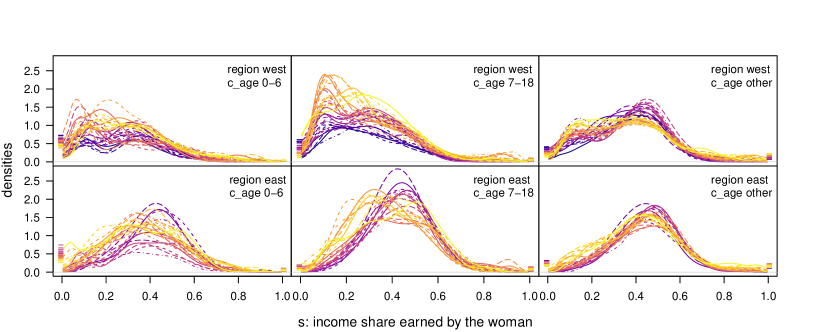
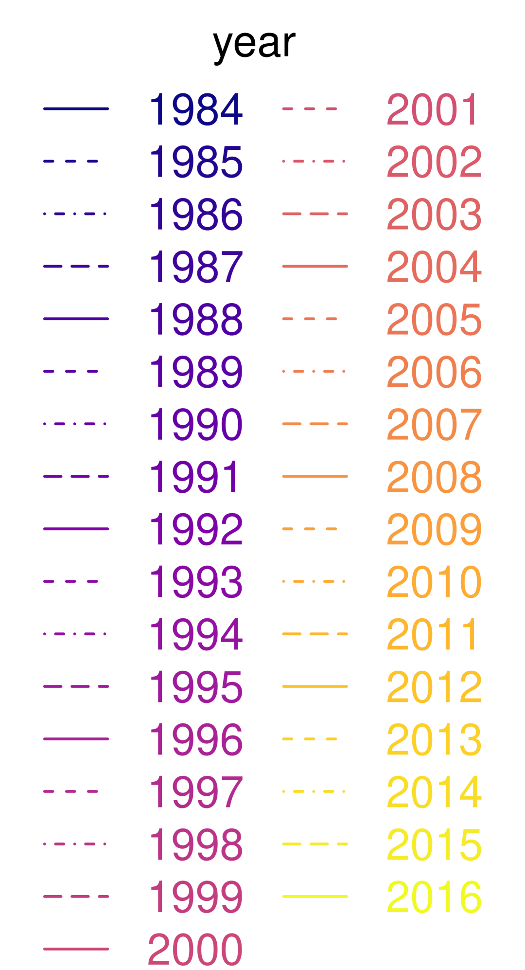
Figure 4.1: Response densities for regions west and east [rows] for all three values of c_age [columns].

4.3 Model specification

Based on the empirical response densities $f_{\text{\emph{region, c\_age, year}}}$, we estimate the model

$$f_{\text{\emph{region, c\_age, year}}} =\beta_{0}\oplus\beta_{\text{\emph{West\_East}}}\oplus\beta_{region}\oplus\beta_{c\_age}\oplus\beta_{\text{\emph{c\_age, West\_East}}}$$

$$\hskip 12.80365pt\oplus g(year)\oplus g_{\text{\emph{West\_East}}}(year)\oplus g_{c\_age}(year)$$

$$\hskip 12.80365pt\oplus g_{\text{\emph{c\_age, West\_East}}}(year)\oplus\varepsilon_{\text{\emph{region, c\_age, year}}}.$$ (4.1)

All summands are densities of the share $s\in[0,1]$ and elements of the Bayes Hilbert space $B^{2}(\mu)$. The model is reference coded with reference categories $West\_East=West,\,c\_age=other$, and $year=1991$. The corresponding effect for the reference is given by the intercept $\beta_{0}$. The effect for the six regions $\beta_{region}$ is centered around the respective $\beta_{\text{\emph{West\_East}}}$. The smooth year effect $g(year)$ describes the deviation for each year from the reference 1991 (for West Germany and c_age other). Finally, several interaction terms are included with a group-specific intercept $\beta_{\text{\emph{c\_age, West\_East}}}$ as well as group-specific flexible terms $g_{West\_East}(year)$, $g_{c\_age}(year)$, and $g_{\text{\emph{c\_age, West\_East}}}(year)$. They are constrained to be orthogonal to the respective main effects using a similar constraint as (3.2) to ensure identifiability. Due to reference coding, all partial effects for the reference categories are zero.

As described in Section 3.3, we decompose the Bayes Hilbert space $B^{2}(\mu)$ into two orthogonal subspaces $B^{2}(\lambda)=B^{2}((0,1),\mathfrak{B}\cap(0,1),\lambda)$ and $B^{2}(\delta^{\bullet})=B^{2}(\mathcal{D}^{\bullet},\mathcal{P}(\mathcal{D}^{\bullet}),\delta^{\bullet})$, where $\mathcal{D}^{\bullet}=\{t_{1},t_{2},t_{3}\}$ and $\delta^{\bullet}=\sum_{d=1}^{3}\delta_{t_{d}}$. We choose $t_{3}=1/2$ to represent the continuous component in between the boundary values $t_{1}=0$ and $t_{2}=1$. For every $f$ we generate the unique functions $f_{\mathrm{c}}\in B^{2}(\lambda)$ and $f_{\mathrm{d}}\in B^{2}(\delta^{\bullet})$ as in (3.8). As proposed in Section 3.2, we choose transformed cubic B-splines as basis functions $\mathbf{b}_{Y}$ for the continuous component and a transformed basis of indicator functions for the discrete component. The remaining specification is identical in both models. We use an anisotropic penalty without penalizing in direction of the share, i.e., $\lambda_{Y}=0$, to ensure the necessary flexibility towards the boundaries. For the flexible nonlinear effects, the selected basis functions are cubic B-splines with penalization of second order differences. We set the degrees of freedom to 2 for all effects but $\beta_{0}$ and $\beta_{\text{\emph{West\_East}}}$, as these only allow for a maximum value of 1. Regarding base-learner selection, $\beta_{\text{\emph{West\_East}}}$ thus is at a slight disadvantage compared to other main effects. However, in a sensitivity check imposing equal degrees of freedom for all base-learners by adjusting $\lambda_{Y}$ to $1$ for all effects, we do not observe large deviations in the selection frequencies while the fit to the data is better with unequal degrees of freedom, see appendix LABEL:appendix_soep_sensitivity_check. Note that the intercept as well as the interaction effects are separated from the main effects due to the orthogonalizing constraints, ensuring a fair selection for the remaining base-learners. The starting coefficients are set to zero in every component and we set the step-length $\kappa$ to $0.1$. We obtain a stopping iteration value of $262$ for the continuous model and $731$ for the discrete model based on $25$ bootstrap samples, respectively.

4.4 Regression Results

All effects in our regression model (4.1) are selected by the algorithm (see appendix LABEL:appendix_estimated_effects). The predictions in Figure LABEL:figure_predictions in appendix LABEL:appendix_soep_sensitivity_check mostly show a good fit. In the following, we discuss the key findings.

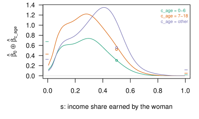
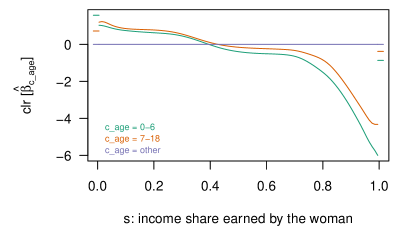
Figure 4.2: Expected densities for couples living in West Germany in 1991 for all three values of c_age [left] and clr transformed estimated effects of c_age [right].

The left part of Figure 4.2 shows the perturbation of the intercept by the c_age effect, i.e., the expected densities for couples without minor children (c_age other), for couples with children aged 0-6, and for couples with children aged 7-18 living in West Germany in 1991. The circles at $0.5$ represent the expected relative frequency of dual-earner households. Our main finding is that the expected density on $(0,1)$ for c_age other is unimodal with a maximum above 0.4, while the densities for c_age 0-6 and 7-18 are bimodal with both maxima to the left of 0.4. The latter show a similar shape, but are scaled differently. The relative frequencies of dual-earner households (circles at $0.5$) and the two types of single-earner households (dashes at $0$, $1$) are similar for couples with children aged 7-18 years and couples without minor children, respectively. In contrast, the relative frequency of non-working women is much higher and the relative frequency of dual-earner households is much lower for couples with children aged 0-6. The right part of the figure shows the clr transformed effect for interpretation via (log) odds ratios, see Section 3.4. As c_age=other is the reference category, we have $\operatorname{clr}[\hat{\beta}_{other}]=0$. The clr transformed effects of c_age 0-6 and 7-18 again show similar shapes on $(0,1)$, but shifted vertically. As the log odds ratio of $\hat{\beta}_{k}$ and $\hat{\beta}_{other}$ for $s$ compared to $t$ corresponds to vertical differences within $\operatorname{clr}[\hat{\beta}_{k}],\leavevmode\nobreak\ k\in\{\emph{0-6},\emph{7-18}\}$, the log odds ratio of $\hat{\beta}_{\emph{0-6}}$ and $\hat{\beta}_{other}$ is similar to the one of $\hat{\beta}_{\emph{7-18}}$ and $\hat{\beta}_{other}$. This implies they have similar impact on the shape of a density. Both log odds ratios are always negative for $s<t\in(0,1)$, i.e., the odds for a larger versus a smaller income share are always smaller for couples with minor children than for couples without minor children, reflecting the strong childhood penalty in West Germany in 1991. See Appendix LABEL:appendix_estimated_effects for quantitative examples of concrete odds ratios.

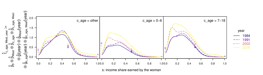
Figure 4.3: Expected densities in the years 1984, 1991, 2003, and 2016 for West Germany for all three values of c_age: other [left], 0-6 [middle], 7-18 [right].

Figure 4.3 shows the expected densities for four selected years, separately for couples with and without minor children (see Figure LABEL:appendix_estimated_year_old_new_cgroup in appendix LABEL:appendix_estimated_effects for all years). For other, the frequency of non-working women ($s=0$) falls continuously over time and the density becomes more dispersed with a lower maximum around 0.4 in 2016 than in 1993 and 2003 (however, it was even lower in 1984). In fact, by 2016 the expected density tends to have a second maximum further left and a heavier tail on the right, most likely due to the strong growth of part-time employment even among women without minor children. Furthermore, the frequency of single-earner women ($s=1$) increases to a level similar to the frequency of non-working women. For 0-6 and 7-18, we also observe a fall in the frequency of non-working women and a stronger concentration around the larger mode until 1991. However, up to 2016 the distributions show more probability mass for small shares, reflecting the even larger growth of part-time employment among women with minor children.

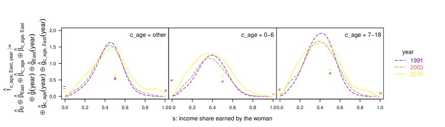
Figure 4.4: Expected densities in the years 1991, 2003, and 2016 for East Germany for all three values of c_age: other [left], 0-6 [middle], 7-18 [right].

Figure 4.4 shows the expected densities in East Germany for selected years (see Figure LABEL:appendix_estimated_year_old_new_cgroup in appendix LABEL:appendix_estimated_effects for all years). In all three cases, the share distribution has a unique mode at or above 0.4. The distribution becomes more dispersed over time, with more probability mass moving to the left and a growing right tail. The frequency of non-working women is falling over time. While showing a similar trend as in West Germany, there remain persistent differences. In East Germany, the frequency of non-working women for couples with minor children remains much lower and the shape of the distribution shows no trend towards a second maximum at a low share. Hence, there remains a considerable West-East gap in the childhood penalty.

To address this issue explicitly, the West-East gap in the childhood penalty is calculated by the difference-in-differences (DiD) effect for $year\in\{1991,2016\}$ and $\text{\emph{c\_age}}\in\{\text{\emph{0-6}},\text{\emph{7-18}}\}$:

$$DiD_{\text{\emph{c\_age, year}}}=(\hat{f}_{\text{\emph{c\_age, West, year}}}\ominus\hat{f}_{\text{\emph{other, West, year}}})\ominus(\hat{f}_{\text{\emph{c\_age, East, year}}}\ominus\hat{f}_{\text{\emph{other, East, year}}}).$$

Figure 4.5 shows the log odds

$$LO_{\text{\emph{c\_age, year}}}(t,s):=\log\left([DiD_{\text{\emph{c\_age, year}}}](t)/[DiD_{\text{\emph{c\_age, year}}}](s)\right)$$

of $DiD_{\text{\emph{c\_age, year}}}$ for $t$ compared to $s$ for pairs $(t,s)\in[0,1]^{2}$, see Section 3.4, as heat maps. We omit the index c_age, year in the following. The inner quadrant shows the respective heat map for $t,s\in(0,1)$. The log odds involving the two mass points $0$ and $1$ are given by the band around the inner quadrants. The top-left corner concerns the log odds for $t=0$ (non-working woman) compared to $s=1$ (single-earner woman). The inner bands around the inner quadrant correspond to the log odds between a mass point $0,1$ and a share in $(0,1)$. The outer bands show the constant log odds between one of the mass points and the event dual-earner household $(0<s,t<1)$. A positive (negative) value implies that the log odds for shares $t$ versus $s$ are higher (lower) in the West than in the East. Thus, $LO(t,s)>0$ for $t<s$ implies that the child penalty (lower share $t$ is more likely relative to $s$ in the presence of children) is more pronounced (stronger) in the West than in the East. For 1991, the vertical band for $t=0$ to the left of the heatmap is quite red ($LO(0,s)>0$), implying that it is much more likely that women in the West compared to the East stop working in the presence of a child, relative to all other shares. This holds both for c_age 0-6 (top panel) and c_age 7-18 (bottom panel). However, the entire heatmap shows positive (negative) values above (below) the 45-degree-line implying that the shift to lower shares compared to higher shares in the presence of children is stronger in the West than in the East, with the West-East gap in the child penalty being even larger for c_age 7-18.

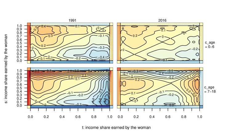
Figure 4.5: Log Odds $LO_{\text{\emph{c\_age, year}}}(t,s)$ of the West-East gap in the childhood penalty (DiD effects) for c_age 0-6 [top] and 7-18 [bottom] for the years 1991 [left] and 2016 [right].

The comparison between the two years is informative about the change in the West-East gap in the childhood penalty over time. In 2016, the childhood penalty remains larger in the West compared to the East over almost the entire share distribution – only for c_age 7-18 is there a reversal for very large shares compared to medium share levels. However, since the absolute log odds have become much smaller, especially for non-working women, the West-East gap in the childhood penalty has decreased considerably over time.

Summarizing our main findings, the frequency of non-working women and women with a lower income share is higher in West Germany than in East Germany and these differences are larger for couples with children. Over time, the share of non-working women decreased. Among dual-earner households the dispersion of the share distribution increased over time with both a growing lower and higher tail. Despite persistent East-West differences in the share distributions and the child penalty until the end of the observation period, the West-East gap in the childhood penalty fell considerably over time.

5 Simulation study

The gradient boosting approach has already been tested extensively in several simulation studies for scalar and functional data (e.g., [48] and references therein). For completeness and to validate our modified approach for density-on-scalar models, we present a small simulation study for this case. It is based on the results of our analysis in Section 4. The predictions obtained there serve as true mean response densities for the simulation and are denoted by $F_{i}\in B^{2}(\mu),\leavevmode\nobreak\ i=1,\ldots,552$, where each $i$ corresponds to one combination of values for the covariates region, c_age, and year and $B^{2}(\mu)$ is the Bayes Hilbert space from Section 4. To simulate data, we perform a functional principal component (PC) analysis [33, e.g.] on the clr transformed functional residuals $\operatorname{clr}[\hat{\varepsilon}_{i}]=\operatorname{clr}[f_{i}\ominus F_{i}]=\operatorname{clr}[f_{i}]-\operatorname{clr}[F_{i}]$, with $f_{i}\in B^{2}(\mu)$ the response densities from the application. Let $\psi_{m}$ denote the PC functions corresponding to the descending ordered eigenvalues $\xi_{m}$ and let $\rho_{im}$ denote the PC scores for $i=1,\ldots,552$ and $m\in\mathbb{N}$. Then, the truncated Karhunen-Loève expansion for $M\in\mathbb{N}$ yields an approximation of the functional residuals: $\operatorname{clr}[\hat{\varepsilon}_{i}]\approx\sum_{m=1}^{M}{\rho}_{im}\psi_{m}$. The PC scores can be viewed as realizations of uncorrelated random variables $\rho_{m}$ with zero-mean and covariance $\mathrm{Cov}(\rho_{m},\rho_{n})=\xi_{m}\delta_{mn}$, where $\delta_{mn}$ denotes the Kronecker delta and $m,n=1,\ldots,M$. We simulate residuals $\tilde{\varepsilon}_{i}$ by drawing uncorrelated random $\tilde{\rho}_{im}$ from mean zero normal distributions with variance $\xi_{m}$ and applying the inverse clr transformation to the truncated Karhunen-Loève expansion, $\tilde{\varepsilon}_{i}=\operatorname{clr}^{-1}[\,\sum_{m=1}^{M}\tilde{\rho}_{im}\psi_{m}\,]=\bigoplus_{m=1}^{M}\tilde{\rho}_{im}\odot\operatorname{clr}^{-1}\left[\psi_{m}\right].$ Adding these to the mean response densities yields the simulated data: $\tilde{f}_{i}=F_{i}\oplus\tilde{\varepsilon}_{i},\leavevmode\nobreak\ i=1,\ldots,552$. Using these as observed response densities, we then estimate model (4.1) and denote the resulting predictions with $\hat{f}_{i}\in B^{2}(\mu),\leavevmode\nobreak\ i=1,\ldots,552$. We replicate this approach 200 times with $M=102$, which is the maximal possible value due to the number of available grid points per density.

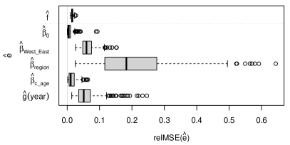
Figure 5.1: RelMSE for predictions [top] and main effects [bottom].

To evaluate the goodness of the estimation results, we use the relative mean squared error (relMSE; defined in appendix LABEL:appendix_simulation_relmse_def) motivated by [48], standardizing the mean squared error with respect to the global variability of the true density. Figure 5.1 shows the boxplots of the relMSEs (200 each) of the predictions and the main effects. All effects are illustrated in appendix LABEL:appendix_simulation_relmse. The distribution of $\mathrm{relMSE}(\hat{f})$ over the 200 simulation runs shows good estimation quality, with a median of $1.55\%$. Regarding the main effects, the relMSEs are the smallest for $\hat{\beta}_{0}$ and $\hat{\beta}_{\text{\emph{c\_age}}}$ with medians of $0.48\%$ and $1.1\%$, respectively. For $\hat{\beta}_{\text{\emph{West\_East}}}$ and $\hat{g}(year)$, the values tend to be slightly larger (medians: $5.96\%$ and $5.12\%$) while they are clearly larger for $\hat{\beta}_{region}$ (median: $18.28\%$). However, the larger relative values, especially for $\hat{\beta}_{region}$, arise from the variability of the true effects being small, not from the mean squared errors being large. This is also the case for the interaction effects, see appendix LABEL:appendix_simulation_relmse. Regarding model selection, the main effects are all selected in each simulation run, while the smaller interaction effects are not, see appendix LABEL:appendix_simulation_selected_effects for details. Overall, the estimates capture the true means $F_{i}$ and all effects that are pronounced very well. Small effects in the model are estimated well in absolute, but badly in relative terms.

6 Conclusion

We presented a flexible framework for density-on-scalar regression models by formulating them in a Bayes Hilbert space $B^{2}(\mu)$, which respects the nature of probability densities and allows for a unified treatment of arbitrary finite measure spaces. This covers in particular the common discrete, continuous, and mixed cases. To estimate the covariate effects in $B^{2}(\mu)$, we introduced a gradient boosting algorithm. We used our approach to analyze the distribution of the woman’s share in a couple’s total labor income, an example of the challenging mixed case, for which we developed a decomposition into a continuous and a discrete estimation problem. We observe strong differences between West and East Germany and between couples with and without children. Among dual-earner households the dispersion of the share distribution increased over time. Despite persistent East-West differences in the share distributions and the child penalty until the end of the observation period, the West-East gap in the childhood penalty fell considerably over time. Finally, we performed a small simulation study justifying our approach in a setting motivated by our application.

Density regression has particular advantages in terms of interpretation compared to approaches considering equivalent functions like quantile functions (e.g., [42, 24]) or distribution functions (CTMs, e.g., [21]; distribution regression, e.g., [14]), as shifts in probability masses or bimodality are easily visible in densities. Odds-ratio-type interpretations of effect functions further add to the interpretability of our model. A crucial part in our approach is played by the clr transformation, which simplifies among other things estimation, as gradient boosting can be performed equivalently on the clr transformed densities in $L_{0}^{2}(\mu)$. This allows taking advantage of and extending existing implementations for function-on-scalar regression like the R add-on package FDboost [47], see the github repository FDboost for our enhanced version of the package and in particular our vignette “density-on-scalar_birth”. The idea to transform the densities to (a subspace of) the well-known $L^{2}$ space with its metric is also used by other approaches. Besides the clr transformation, the square root velocity transformation [37] as well as the log hazard and log quantile density transformations (e.g., [18]) are popular choices. The approach of [32] does not use a transformation, but also computes the applied Wasserstein metric via the $L^{2}$ metric. What is special about the clr transformation based Bayes Hilbert space approach, is the embedding of the untransformed densities in a Hilbert space structure. It is the extension of the well-established Aitchison geometry [1], which provides a reasonable framework for compositional data – the discrete equivalent of densities – fulfilling appealing properties like subcompositional coherence. The clr transformation helps to conveniently interpret covariate effects via ratios of density values (odds-ratios), which approximate or are equal to ratios of probabilities in three common cases (discrete, continuous, mixed). Modeling those three cases in a unified framework is a novelty to the best of the authors’ knowledge, and a contribution of our approach to the literature on density regression.

Due to the gradient boosting algorithm used for estimation, our method includes variable selection and regularization, while it can deal with numerous covariates. However, like all gradient boosting approaches, it is limited by not naturally yielding inference – unlike some existing approaches (e.g., [32]). This might be developed using a bootstrap-based approach or selective inference [35] in the future. Alternatively, other estimation methods allowing for formal inference could be derived.

The (current) definition of Bayes Hilbert spaces, which only allows finite reference measures, does not cover the interesting case of the measurable space $(\mathbb{R},\mathfrak{B}_{\mathbb{R}})$ with Lebesgue measure $\lambda$. Though $(\mathbb{R},\mathfrak{B}_{\mathbb{R}})$ can still be considered using, e.g., the probability measure corresponding to the standard normal distribution [46] as reference, it would be desirable to extend Bayes Hilbert spaces to $\sigma$-finite reference measures, allowing for $B^{2}(\mathbb{R},\mathfrak{B}_{\mathbb{R}},\lambda)$. Moreover, Bayes Hilbert spaces include only ($\mu$-a.e.) positive densities. While in the continuous case, values of zero can in many cases be avoided using a suitable density estimation method, they are often replaced with small values in the discrete case (see [31]). In contrast, the square root velocity transformation [37] allows density values of zero and may be an alternative in such cases, at the price of loosing the Hilbert space structure for the untransformed densities.

Finally, while in practice densities are sometimes directly reported, one often does not observe the response densities directly, but has to first estimate them from individual data to enable the use of density-on-scalar regression. This causes two problems. First, when treating estimated densities as observed, like also in other approaches such as [32, 18], estimation uncertainty is not accounted for in the analysis. Second, the number of individual observations for each covariate value combination which is available for density estimation can limit the number of covariates that can be included in the model. In the future, we thus aim to extend our approach to also model conditional densities for individual observations, still allowing flexibility in the covariate effects, but without restrictive assumptions such as a particular distribution family as in GAMLSS [34].

APPENDIX

7_appendix.tex

References

- [1] J. Aitchison “The Statistical Analysis of Compositional Data” London, UK, UK: Chapman & Hall, Ltd., 1986
- [2] Miriam Beblo and Luise Görges “On the nature of nurture. The malleability of gender differences in work preferences” In Journal of Economic Behavior & Organization 151 Elsevier, 2018, pp. 19–41
- [3] Marianne Bertrand, Emir Kamenica and Jessica Pan “Gender Identity and Relative Income within Households” In The Quarterly Journal of Economics 130.2, 2015, pp. 571–614 DOI: 10.1093/qje/qjv001
- [4] Sandra E Black and Alexandra Spitz-Oener “Explaining women’s success: technological change and the skill content of women’s work” In The Review of Economics and Statistics 92.1 The MIT Press, 2010, pp. 187–194
- [5] Karl Gerald Boogaart, Juan José Egozcue and Vera Pawlowsky-Glahn “Bayes linear spaces” In SORT: statistics and operations research transactions 34.4 Institut d´ Estadı́stica de Catalunya (Idescat), 2010, pp. 201–222
- [6] Karl Gerald Boogaart, Juan José Egozcue and Vera Pawlowsky-Glahn “Bayes Hilbert Spaces” In Australian & New Zealand Journal of Statistics 56.2, 2014, pp. 171–194 DOI: 10.1111/anzs.12074
- [7] Karl Gerald Boogaart, Raimon Tolosana-Delgado and Matthias Templ “Regression with compositional response having unobserved components or below detection limit values” In Statistical Modelling 15.2 Sage Publications Sage India: New Delhi, India, 2015, pp. 191–213
- [8] Sarah Brockhaus and David Rügamer “FDboost: Boosting Functional Regression Models” R package version 0.3-2, 2018
- [9] Sarah Brockhaus, David Rügamer and Sonja Greven “Boosting Functional Regression Models with FDboost” In Journal of Statistical Software 94.1, 2020, pp. 1–50
- [10] Sarah Brockhaus, Fabian Scheipl, Torsten Hothorn and Sonja Greven “The functional linear array model” In Statistical Modelling 15.3, 2015, pp. 279–300 DOI: 10.1177/1471082X14566913
- [11] Peter Bühlmann and Bin Yu “Boosting with the L2 loss: regression and classification” In Journal of the American Statistical Association 98.462 Taylor & Francis, 2003, pp. 324–339
- [12] Song X. Chen “Beta kernel estimators for density functions” In Computational Statistics & Data Analysis 31.2, 1999, pp. 131–145 URL: https://EconPapers.repec.org/RePEc:eee:csdana:v:31:y:1999:i:2:p:131-145
- [13] Victor Chernozhukov, Iván Fernández-Val and Alfred Galichon “Quantile and probability curves without crossing” In Econometrica 78.3 Wiley Online Library, 2010, pp. 1093–1125
- [14] Victor Chernozhukov, Iván Fernández-Val and Blaise Melly “Inference on counterfactual distributions” In Econometrica 81.6 Wiley Online Library, 2013, pp. 2205–2268
- [15] Patricia Cortes and Jessica Pan “Occupation and gender” In The Oxford handbook of women and the economy Oxford University Press New York, NY, 2018, pp. 425–452
- [16] J.. Egozcue, J.. Díaz-Barrero and V. Pawlowsky-Glahn “Hilbert Space of Probability Density Functions Based on Aitchison Geometry” In Acta Mathematica Sinica 22.4, 2006, pp. 1175–1182 DOI: 10.1007/s10114-005-0678-2
- [17] Bernd Fitzenberger, Katrin Sommerfeld and Susanne Steffes “Causal effects on employment after first birth—A dynamic treatment approach” In Labour Economics 25 Elsevier, 2013, pp. 49–62
- [18] Kyunghee Han, Hans-Georg Müller and Byeong U Park “Additive functional regression for densities as responses” In Journal of the American Statistical Association 115.530 Taylor & Francis, 2020, pp. 997–1010
- [19] Clara Happ, Fabian Scheipl, Alice Gabriel and Sonja Greven “A general framework for multivariate functional principal component analysis of amplitude and phase variation” In Stat 8.1, 2019, pp. e220 DOI: 10.1002/sta4.220
- [20] Benjamin Hofner, Torsten Hothorn, Thomas Kneib and Matthias Schmid “A framework for unbiased model selection based on boosting” In Journal of Computational and Graphical Statistics 20.4 Taylor & Francis, 2011, pp. 956–971
- [21] Torsten Hothorn, Thomas Kneib and Peter Bühlmann “Conditional transformation models” In Journal of the Royal Statistical Society: Series B (Statistical Methodology) 76.1 Wiley Online Library, 2014, pp. 3–27
- [22] T. Hsing and R. Eubank “Theoretical Foundations of Functional Data Analysis, with an Introduction to Linear Operators”, Wiley Series in Probability and Statistics Chichester: John Wiley & Sons, Ltd, 2015 URL: https://books.google.de/books?id=YjsbAAAACAAJ
- [23] Henrik Kleven, Camille Landais, Johanna Posch, Andreas Steinhauer and Josef Zweimüller “Child penalties across countries: Evidence and explanations” In AEA Papers and Proceedings 109, 2019, pp. 122–26
- [24] R. Koenker “Quantile Regression”, Econometric Society Monographs Cambridge University Press, 2005 URL: https://books.google.de/books?id=hdkt7V4NXsgC
- [25] Daniel Kuehnle, Michael Oberfichtner and Kerstin Ostermann “Revisiting Gender Identity and Relative Income within Households: A Cautionary Tale on the Potential Pitfalls of Density Estimators” In Journal of Applied Econometrics, 2021, pp. to appear
- [26] Rui Li, Brian J Reich and Howard D Bondell “Deep distribution regression” In Computational Statistics & Data Analysis 159 Elsevier, 2021, pp. 107203
- [27] Roman Werner Lutz and Peter Bühlmann “Boosting for high-multivariate responses in high-dimensional linear regression” In Statistica Sinica JSTOR, 2006, pp. 471–494
- [28] Steven N. MacEachern “Dependent nonparametric processes” In ASA proceedings of the section on Bayesian statistical science 1, 1999, pp. 50–55 Alexandria, Virginia. Virginia: American Statistical Association; 1999
- [29] Yann Ollivier, Hervé Pajot and Cédric Villani “Optimal Transport: Theory and Applications” Cambridge University Press, 2014
- [30] Joon Y. Park and Junhui Qian “Functional regression of continuous state distributions” In Journal of Econometrics 167.2 Elsevier, 2012, pp. 397–412
- [31] Vera Pawlowsky-Glahn, Juan José Egozcue and Raimon Tolosana-Delgado “Modeling and analysis of compositional data” John Wiley & Sons, 2015
- [32] Alexander Petersen and Hans-Georg Müller “Fréchet regression for random objects with Euclidean predictors” In The Annals of Statistics 47.2 Institute of Mathematical Statistics, 2019, pp. 691–719
- [33] James Ramsay and B.. Silverman “Functional Data Analysis” Springer-Verlag New York, 2005
- [34] Robert A. Rigby and D. Stasinopoulos “Generalized additive models for location, scale and shape” In Journal of the Royal Statistical Society: Series C (Applied Statistics) 54.3 Wiley Online Library, 2005, pp. 507–554
- [35] David Rügamer and Sonja Greven “Inference for L2-Boosting” In Statistics and Computing 30.2 Springer, 2020, pp. 279–289
- [36] Maximilian Sprengholz, Anna Wieber and Elke Holst “Gender identity and wives’ labor market outcomes in West and East Germany between 1983 and 2016” In Socio-Economic Review, 2020, pp. to appear
- [37] A. Srivastava, I. Jermyn and S. Joshi “Riemannian Analysis of Probability Density Functions with Applications in Vision” In 2007 IEEE Conference on Computer Vision and Pattern Recognition, 2007, pp. 1–8 DOI: 10.1109/CVPR.2007.383188
- [38] Almond Stöcker, Sarah Brockhaus, Sophia Schaffer, Benedikt Bronk, Madeleine Opitz and Sonja Greven “Boosting Functional Response Models for Location, Scale and Shape with an Application to Bacterial Competition” In Statistical Modelling, 2021, pp. to appear
- [39] Ichiro Takeuchi, Quoc V. Le, Timothy D. Sears and Alexander J. Smola “Nonparametric quantile estimation” In Journal of machine learning research 7.Jul, 2006, pp. 1231–1264
- [40] R. Talská, A. Menafoglio, J. Machalová, K. Hron and E. Fišerová “Compositional regression with functional response” In Computational Statistics & Data Analysis 123.C, 2018, pp. 66–85 URL: https://EconPapers.repec.org/RePEc:eee:csdana:v:123:y:2018:i:c:p:66-85
- [41] S.. Wood “Generalized Additive Models: An Introduction with R” Boca Raton: ChapmanHall/CRC, 2017
- [42] Hojin Yang, Veerabhadran Baladandayuthapani, Arvind U.. Rao and Jeffrey S. Morris “Regression Analyses of Distributions using Quantile Functional Regression” In arXiv preprint arXiv:1810.03496, 2018
- [43] Marino Badiale and Enrico Serra “Semilinear Elliptic Equations for Beginners: Existence Results via the Variational Approach” Springer Science & Business Media, 2011
- [44] Marianne Bertrand, Emir Kamenica and Jessica Pan “Gender Identity and Relative Income within Households” In The Quarterly Journal of Economics 130.2, 2015, pp. 571–614 DOI: 10.1093/qje/qjv001
- [45] Karl Gerald Boogaart, Juan José Egozcue and Vera Pawlowsky-Glahn “Bayes linear spaces” In SORT: statistics and operations research transactions 34.4 Institut d´ Estadı́stica de Catalunya (Idescat), 2010, pp. 201–222
- [46] Karl Gerald Boogaart, Juan José Egozcue and Vera Pawlowsky-Glahn “Bayes Hilbert Spaces” In Australian & New Zealand Journal of Statistics 56.2, 2014, pp. 171–194 DOI: 10.1111/anzs.12074
- [47] Sarah Brockhaus and David Rügamer “FDboost: Boosting Functional Regression Models” R package version 0.3-2, 2018
- [48] Sarah Brockhaus, Fabian Scheipl, Torsten Hothorn and Sonja Greven “The functional linear array model” In Statistical Modelling 15.3, 2015, pp. 279–300 DOI: 10.1177/1471082X14566913
- [49] Song X. Chen “Beta kernel estimators for density functions” In Computational Statistics & Data Analysis 31.2, 1999, pp. 131–145 URL: https://EconPapers.repec.org/RePEc:eee:csdana:v:31:y:1999:i:2:p:131-145
- [50] J.. Egozcue, J.. Díaz-Barrero and V. Pawlowsky-Glahn “Hilbert Space of Probability Density Functions Based on Aitchison Geometry” In Acta Mathematica Sinica 22.4, 2006, pp. 1175–1182 DOI: 10.1007/s10114-005-0678-2
- [51] J. Elstrodt “Maß- und Integrationstheorie”, Springer-Lehrbuch Springer Berlin Heidelberg, 2011 URL: https://books.google.de/books?id=5ugfBAAAQBAJ
- [52] Jan Goebel, Markus M Grabka, Stefan Liebig, Martin Kroh, David Richter, Carsten Schröder and Jürgen Schupp “The German socio-economic panel (SOEP)” In Jahrbücher für Nationalökonomie und Statistik 239.2 De Gruyter, 2019, pp. 345–360
- [53] Torsten Hothorn, Peter Buehlmann, Thomas Kneib, Matthias Schmid and Benjamin Hofner “mboost: Model-Based Boosting” R package version 2.9-1, 2018 URL: https://CRAN.R-project.org/package=mboost
- [54] M.. Jones and D.. Henderson “Miscellanea Kernel-Type Density Estimation on the Unit Interval” In Biometrika 94.4, 2007, pp. 977–984 DOI: 10.1093/biomet/asm068
- [55] Jonas Moss and Martin Tveten “kdensity: Kernel Density Estimation with Parametric Starts and Asymmetric Kernels” R package version 1.0.0, 2018 URL: https://CRAN.R-project.org/package=kdensity
- [56] Alexander Petersen and Hans-Georg Müller “Functional data analysis for density functions by transformation to a Hilbert space” In The Annals of Statistics 44.1 Institute of Mathematical Statistics, 2016, pp. 183–218
- [57] David W. Scott “Multivariate Density Estimation: Theory, Practice, and Visualization” Hoboken, New Jersey: John Wiley & Sons, Inc., 2015
- [58] Richard L. Wheeden and Antoni Zygmund “Measure and Integral: An Introduction to Real Analysis” CRC press, 2015
- [59] S.. Wood “Generalized Additive Models: An Introduction with R” Boca Raton: ChapmanHall/CRC, 2017