From scalar fields on quantum spaces to blobbed topological recursion

Abstract.

We review the construction of the $\lambda\phi^{4}$-model on noncommutative geometries via exact solutions of Dyson-Schwinger equations and explain how this construction relates via (blobbed) topological recursion to problems in algebraic and enumerative geometry.

1. Introduction

Quantum field theories on noncommutative spaces appeared at the end of the last century [GM92, DFR95, Fil96, GKP96]. These investigations and compactifications of M-theory on the noncommutative torus [CDS98] motivated the perturbative renormalisation programme of QFT on noncommutative geometries. Whereas renormalisable at one-loop order [MSR99, KW00], a new class of problems (UV/IR-mixing [MVRS00, CR00]) was found at higher loop order.

Two of us (HG+RW) found a way to avoid the UV/IR-mixing problem for scalar fields by understanding that it signals the generation of another marginal coupling [GW05a, GW05c]. This coupling corresponds to a harmonic oscillator potential and implements a particular duality under Fourier transform [LS02]. The duality-covariant scalar model (with oscillator potential) is perturbatively renormalisable [GW05b, GW05a]. Moreover, the $\beta$-function of the coupling constant vanishes at the self-duality point [GW04, DR07]. The proof [DGMR07] led to a new solution strategy first formulated by two of us (HG+RW) in [GW09] and then extended in [GW14]. All these developments and results have been reviewed previously in great detail [Sza03, Wul06, Riv07, Wul19].

This paper provides the first review of the enormous progress made during the last three years. It started with the exact solution by one of us (RW) with E. Panzer [PW20] of the non-linear Dyson-Schwinger equation found in [GW09] for the case of 2-dimensional Moyal space. A renewed interest in higher planar correlation functions [dJHW22] established a link to the Hermitian 2-matrix model [EO05] which has a non-mixed sector that follows topological recursion [Eyn16]. This observation identified the key to generalise [PW20] to a solution of all quartic matrix models [GHW19] by three of us (AH+HG+RW). After initial investigations of the algebraic-geometrical structure in [SW19], three of us (JB+AH+RW) identified in [BHW20] the objects which obey (conjecturally; proved in the planar case [HW21]) blobbed topological recursion [BS17], a systematic extension of topological recursion [EO07]. Several properties of these objects have already been investigated [BHW21].

Contents

1. 1 Introduction
2. 2 What are quantum fields on quantum spaces?
3. 3 Algebraic geometrical structures
4. 4 Solving the Model
5. 5 Scalar QFT on Moyal space
6. 6 Cross-checks: perturbative expansions
7. 7 Summary and outlook

2. What are quantum fields on quantum spaces?

2.1. The free scalar field

Quantum Physics was developed (by Planck, Heisenberg, Schrödinger and others) between 1900 and 1926, special relativity by Einstein in 1905. Attempts to combine both led to the Klein-Gordon and the Dirac equations. These equations, coupled to electromagnetic potentials, describe energy levels of the electron and other particles. Certain energy levels predicted to be degenerate are split in nature (Lamb-shift). These tiny corrections are explained by quantum electrodynamics (QED) and other quantum field theories.

A standard treatment in quantum field theory consists in expanding it around a linear, exactly solvable, model. A favourite example is the free scalar field in $D$ dimensions which arises by canonical quantisation of the Klein-Gordon equation. The two-point function of the free scalar field has an analytic continuation in time to a two-point function on Euclidean space:

$$G(t,\vec{x})=\int\frac{d^{D-1}\vec{p}}{(2\pi)^{D-1}\cdot 2\omega_{p}}e^{-\omega_{p}|t|+\mathrm{i}\vec{p}\vec{x}},\qquad\omega_{p}=\sqrt{M^{2}+\vec{p}^{2}}\;.$$ (2.1)

According to Minlos’ theorem there exists a measure on the space $X$ of tempered distributions such that $G(t,\vec{x})=\int_{X}d\mu(\phi)\;\phi(t,\vec{x})\phi(0,\vec{0})$, where $\phi(t,\vec{x})$ is a stochastic field. Moments of $d\mu(\phi)$ are understood as Euclidean correlation functions. They fulfil the Osterwalder-Schrader (OS) axioms [OS75] of smoothness, Euclidean covariance, OS positivity and symmetry.

2.2. Interacting fields and renormalisation

The Minlos measure associated with (2.1) is the starting point for attempts to construct interacting models (in the Euclidean picture). They are formally obtained by a deformation

$$d\mu(\phi)\mapsto d\mu_{\mathrm{int}}(\phi)=\frac{d\mu(\phi)\;e^{-S_{\mathrm{int}}(\phi)}}{\int_{X}d\mu(\phi)\;e^{-S_{\mathrm{int}}(\phi)}},$$ (2.2)

where the derivative of the functional $S_{\mathrm{int}}$ is non-linear in $\phi$.

As a matter of fact, in all cases of interest this deformation is problematic because there exist (many) moments $\int_{X}d\mu_{\mathrm{int}}(\phi)\;\phi(t_{1},\vec{x}_{1})\cdots\phi(t_{n},\vec{x}_{n})$ which diverge. To produce meaningful quantities a procedure known as renormalisation theory is necessary. Its first step is regularisation, which amounts to understand the space $X$ of all $\phi$ as limit of a sequence (or net) of finite-dimensional spaces $X_{\alpha}$. Then every finite-dimensional space is endowed with its own functional $S^{\alpha}_{\mathrm{int}}(\phi)$ which is carefully adjusted so that certain moments $\int_{X_{\alpha}}d\mu_{\mathrm{int}}^{\alpha}(\phi)\;\phi(x_{1})\cdots\phi(x_{n})$ stay constant when increasing $\alpha$. Hence, they at least have a limit when approaching $X$. The challenge is to make sure that an adjustment of finitely many moments suffices to render all moments meaningful; the theory is then called renormalisable. In realistic particle physics models, this was only achieved in infinitesimal neighbourhoods of the free theory, which by far miss the required physical parameter values. Much harder are models which require adjustment of infinitely many moments to render infinitely many other moments meaningful; Einstein gravity could be of this type.

2.3. Scalar fields on quantum spaces

This article reviews a framework of quantum field theory where the renormalisation programme sketched in sec. 2.2 can be fully implemented for truly interacting fields. Our fields do not live on familiar space-time; they live on a quantum space (a quantised space whose points follow non-trivial commutation relations – the main example in this work will be the noncommutative Moyal space). It is conceivable that such quantum spaces could be a good description of our world when gravity and quantum physics are simultaneously relevant [DFR95]. It is probably difficult to give a picture of a quantum space, but it is fairly easy to describe scalar fields on it.

For that we let our finite-dimensional spaces $X_{\alpha}$ of sec. 2.2 be the spaces $H_{N}$ of Hermitean $N\times N$-matrices. Given a sequence $(E_{1},E_{2},\dots)$ of positive real numbers, the energies, we construct the Minlos measure $d\mu(\phi)$ of a free scalar field on quantum space by the requirement

$$\int_{H_{N}}d\mu(\phi)\;\phi_{kl}=0,\qquad\int_{H_{N}}d\mu(\phi)\;\phi_{kl}\phi_{k^{\prime}l^{\prime}}=\frac{\delta_{kl^{\prime}}\delta_{lk^{\prime}}}{N(E_{k}+E_{l})},$$ (2.3)

and factorisation of higher $n$-point functions. Here, the $(\phi_{kl})$ are the matrix elements of $\phi\in H_{N}$. The $E_{k}$ should be viewed as eigenvalues of the Laplacian on our quantum space. Their asymptotic behaviour (for $N\to\infty$) defines a dimension of the quantum space as the smallest number $D$ such that $\sum_{k=1}^{\infty}E_{k}^{-D/2-\epsilon}$ converges for all $\epsilon>0$.

We deform the Minlos measure (2.3) as in (2.2) via a quartic functional,

$$d\mu_{\mathrm{int}}(\phi)=\frac{d\mu(\phi)\;e^{-\frac{\lambda N}{4}\mathrm{Tr}(\phi^{4})}}{\int_{H_{N}}d\mu(\phi)\;e^{-\frac{\lambda N}{4}\mathrm{Tr}(\phi^{4})}},\qquad d\mu\text{ as in }(\ref{minlos-q}).$$ (2.4)

The deformation (2.4) is a quartic analogue of the Kontsevich model [Kon92] in which a cubic potential $\frac{\mathrm{i}N}{6}\mathrm{Tr}(\phi^{3})$ is used to deform (2.3). The Kontsevich model gives deep insight into the moduli space $\overline{\mathcal{M}}_{g,n}$ of complex curves and provides a rigorous formulation of quantum gravity in two dimensions [Wit91]. For obvious reasons we call the model which studies (2.4) and its moments the quartic Kontsevich model.

In dimension $D\geq 2$ (encoded in the $E_{k}$), moments of (2.4) show the same divergences as discussed in sec. 2.2 on ordinary space-time. Between 2002 and 2004 we treated them in a formal power series in (infinitesimal) $\lambda$. It turned out that an affine rescaling $E_{k}\mapsto ZE_{k}+c$ was enough, where $Z=Z(\lambda,N)$ and $c=c(\lambda,N)$ depend only on $\lambda$ and the size $N$ of the matrices, but not on $k$. We actually considered a more general Minlos measure where two further renormalisation parameters $\Omega(\lambda,N)$ and $\tilde{\lambda}(\lambda,N)$ were necessary [GW05a]; in lowest $\lambda$-order we found [GW04] that $\frac{\Omega^{2}}{\tilde{\lambda}}$ is independent of $N$. This was a remarkable symmetry which indicated that the Landau ghost problem [LAK54] could be absent in this model.

This perspective influenced V. Rivasseau who, with M. Disertori, R. Gurau and J. Magnen, proved in [DGMR07] that the model with quartic interaction functional (2.4) tolerates the same $\lambda$ for all matrix sizes $N$, at least for infinitesimal $\lambda$. We understood immediately that their method can potentially provide relations between moments of $d\mu_{\mathrm{int}}(\phi)$.

This turned out to be true, with amazing consequences: The model was revealed to be solvable. This solution has two aspects: First, the planar 2-point function of the measure (2.4) satisfies a closed non-linear equation [GW09, GW14]. A solution theory for this equation was developed in [PW20, GHW19]; it suggested a particular change of variables. In a second step it was found in [BHW20] that special combinations of the correlation functions possess after complexification and the mentioned change-of-variables a beautiful and universal algebraic-geometrical structure: (blobbed) topological recursion. The next section gives a short introduction. We return to the model under consideration in section 4.

3. Algebraic geometrical structures

3.1. Topological recursion

Topological recursion (TR) is a universal structure which is common to surprisingly many different topics in algebraic geometry, enumerative geometry, noncommutative geometry, random matrix theory, string theory, knot theory and more. It covers e.g. Witten’s conjecture [Wit91] about intersection numbers on the moduli space of stable complex curves (proved by Kontsevich [Kon92]), Mirzakhani’s recursion [Mir06] for Weil-Petersson volumes of bordered Riemann surfaces and generating functions of Hurwitz numbers [BMn08] with the same universal structure (see eq. (3.1) below)! The common structure was formulated by B. Eynard and N. Orantin [EO07] after insight into the Hermitean 2-matrix model [CEO06]. Since then it became an active field of research. We refer to [Bor18] for an overview covering more than 100 papers.

Topological recursion constructs a family $\omega_{g,n}$ of symmetric meromorphic differentials on products of Riemann surfaces $\Sigma$. These $\omega_{g,n}$ are labeled by the genus $g$ and the number $n$ of marked points of a compact complex curve, they occur as invariants of algebraic curves $P(x,y)=0$ (understood in parametric representation $x(z)$ and $y(z)$).

From initial data consisting of a ramified covering $x:\Sigma\to\Sigma_{0}$ of Riemann surfaces, a differential 1-form $\omega_{0,1}(z)=y(z)dx(z)$ and the Bergman kernel $\omega_{0,2}(z,u)=B(z,u)=\frac{dzdu}{(z-u)^{2}}$ (here assuming a genus-0 spectral curve), TR constructs the meromorphic differentials $\omega_{g,n+1}(z_{1},...,z_{n},z)$ with $2g+n\geq 2$ via the following universal formula (in which we abbreviate $I=\{z_{1},...,z_{n}\}$):

$$\omega_{g,n+1}(I,z)$$ (3.1)

$$=\sum_{\beta_{i}}\operatorname{Res}\displaylimits_{q\to\beta_{i}}K_{i}(z,q)\bigg{(}\omega_{g-1,n+2}(I,q,\sigma_{i}(q))+\sum_{\begin{subarray}{c}g_{1}+g_{2}=g\\ I_{1}\uplus I_{2}=I\\ (g_{1},I_{1})\neq(0,\emptyset)\neq(g_{2},I_{2})\end{subarray}}\omega_{g_{1},|I_{1}|+1}(I_{1},q)\omega_{g_{2},|I_{2}|+1}(I_{2},\sigma_{i}(q))\!\bigg{)}\;.$$

This construction proceeds recursively in the negative Euler characteristic $-\chi=2g+n-2$. Here we need to define:

• A sum over the ramification points $\beta_{i}$ of the ramified covering $x:\Sigma\to\Sigma_{0}$, defined via $dx(\beta_{i})=0$.
  Example: $x(z)=z^{2}$ for a Riemann surface $\Sigma=\hat{\mathbb{C}}:=\mathbb{C}\cup\{\infty\}$ with $\beta=0$. The two sheets merge at $z=\beta=0$, but also at $z=\infty$ which is exceptional.

• the local Galois involution $\sigma_{i}\neq\mathrm{id}$ defined via $x(q)=x(\sigma_{i}(q))$ near $\beta_{i}$ having the fixed point $\beta_{i}$ itself.
  Example: $x(z)=z^{2}$ gives $\sigma(z)=-z$;

• the recursion kernel $K_{i}(z,q)=\frac{\frac{1}{2}\int^{q^{\prime}=q}_{q^{\prime}=\sigma_{i}(q)}B(z,q^{\prime})}{\omega_{0,1}(q)-\omega_{0,1}(\sigma_{i}(q))}$ constructed from the initial data.

To orientate oneself within this jungle of definitions, we turn the master formula into a picture (Fig. 1). The recursion becomes a successive gluing of objects at their boundaries, starting with the recursion kernel and two cylinders and then becoming more and more complicated.

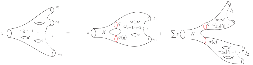
Figure 1. There are two different ways to obtain the left hand side $\omega_{g,n}$ by gluing the initial data (recursion kernel with three boundaries) with something of lower topology: Either one glues one object with one genus less and one boundary more $(g-1,n+2)$ with two boundaries of the kernel creating the missing genus, or one glues two objects with the kernel (causing no genus change): Then one has to account any $(g_{1},n_{1}),(g_{2},n_{2})$ conform with the left hand side – the sum over all possible partitions in the master formula (3.1) arises.

We conclude this subsection by giving the rather simple initial data of the three previously listed prime examples ($\omega_{0,2}=B$ and $\Sigma=\hat{\mathbb{C}}=\Sigma_{0}$ in all cases):

• Witten’s conjecture: $x(z)=z^{2}$, $\omega_{0,1}(z)=2z^{2}dz$;

• Weil-Petersson volumes: $x(z)=z^{2}$, $\omega_{0,1}(z)=\frac{4z}{\pi}\sin(\pi z)dz$;

• Simple Hurwitz numbers: $x(z)=-z+\log(z)$, $\omega_{0,1}(z)=(1-z)dz$.

3.2. Blobbed topological recursion

We emphasised that topological recursion covers a large spectrum of examples in enumerative geometry, mathematical physics, etc. The model under consideration fits perfectly into an extension of TR developed in 2015 by G. Borot and S. Shadrin [BS17]: Blobbed topological recursion (BTR).

Its philosophy is quite analogous to that of TR, however the recursion is equipped with an infinite stack of further initial data, successively contributing to each recursion step. More precisely, the meromorphic differentials

$$\omega_{g,n}(...,z)=\mathcal{P}_{z}\omega_{g,n}(...,z)+\mathcal{H}_{z}\omega_{g,n}(...,z)$$

decompose into a polar part $\mathcal{P}_{z}\omega_{g,n}$ (with poles in a selected variable $z$ at ramification points) and a holomorphic part $\mathcal{H}_{z}\omega_{g,n}$ with poles somewhere else. The polar part follows exactly the usual TR [EO07], whereas the holomorphic part is not given via a universal structure.

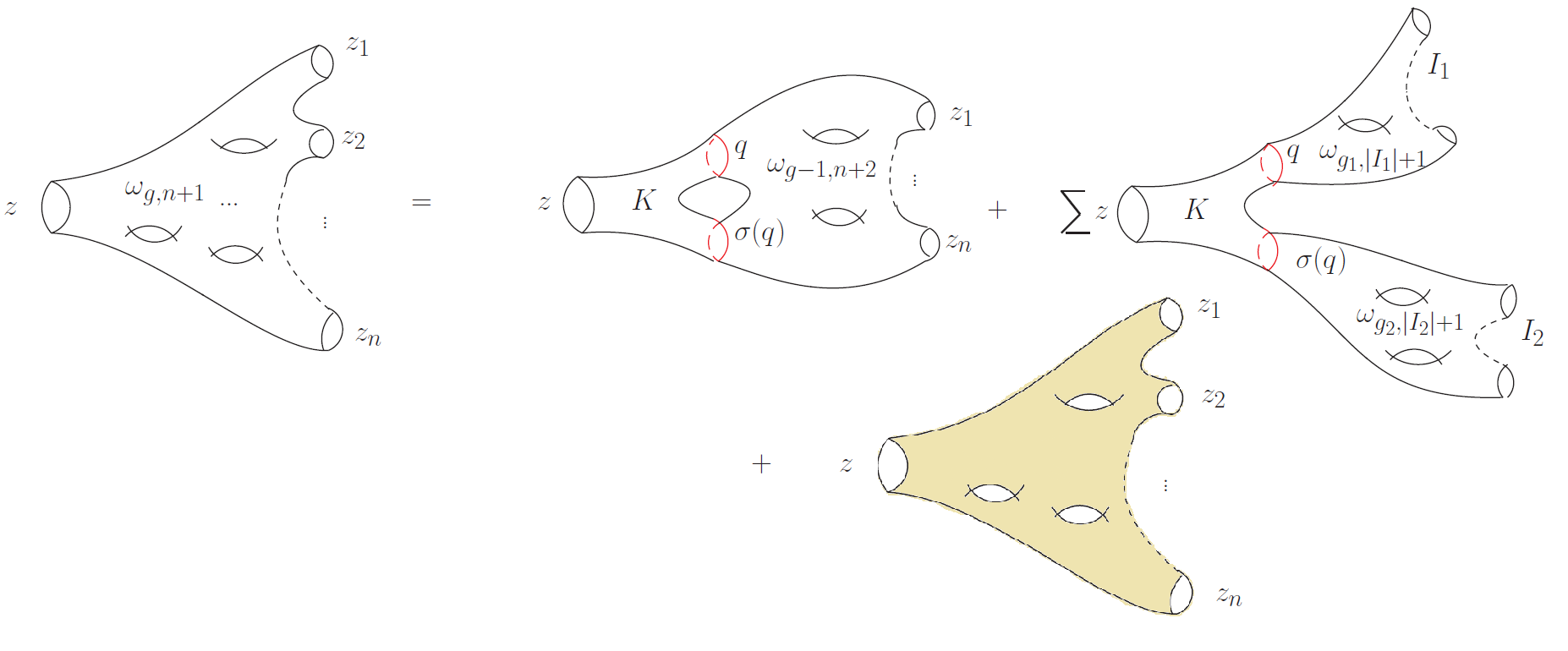
Figure 2. Graphical interpretation of blobbed topological recursion: The usual recursion formula is enriched by a holomorphic (at ramification points) add-on $\mathcal{H}_{z}\omega_{g,n+1}$ (coloured) that appears as a surplus structure in the solution of the loop equations. It has to be seen as additional data that has to be taken into account at each further recursion step.

This extended theory was baptised blobbed due to the occurring purely holomorphic parts (for $2g+m-2>0$) $\phi_{g,m}(z_{1},...,z_{m-1},z)=\mathcal{H}_{z_{1}}...\mathcal{H}_{z_{m-1}}\mathcal{H}_{z}\omega_{g,m}(z_{1}...,z_{m-1},z)$, called the blob. A family $\omega_{g,m}$ obeys BTR iff it fulfils abstract loop equations [BEO15]:

1. $\omega_{g,m}$ fulfils the so-called linear loop equation if

   $$\omega_{g,m+1}(u_{1},...,u_{m},z)+\omega_{g,m+1}(u_{1},...,u_{m},\sigma_{i}(z))=\mathcal{O}(z-\beta_{i})dz$$ (3.2)

   is a holomorphic linear form for $z\to\beta_{i}$ with (at least) a simple zero at $\beta_{i}$.

2. $\omega_{g,m}$ fulfils the quadratic loop equation if

   $$Q^{i}_{g,m+1} :=\omega_{g-1,m+2}(u_{1},...,u_{m},z,\sigma_{i}(z))+\sum_{\begin{subarray}{c}g_{1}+g_{2}=g\\ I_{1}\uplus I_{2}=\{u_{1},...,u_{m}\}\end{subarray}}\omega_{g_{1},|I_{1}|+1}(I_{1},z)\omega_{g_{2},|I_{2}|+1}(I_{2},\sigma_{i}(z))$$

   $$=\mathcal{O}((z-\beta_{i})^{2})(dz)^{2}$$ (3.3)

   is a holomorphic quadratic form with at least a double zero at $z\to\beta_{i}$.

Although these formulae seem simple, a proof that the actual $\omega_{g,m}$ of a certain model fulfil the abstract loop equations may demand some sophisticated techniques. We list three models governed by BTR that were investigated within the last years:

• Stuffed maps [Bor14]: The investigation of stuffed maps arising from the multi-trace Hermitian one-matrix model – not perfectly following the established theory of TR – gave the motivation to formulate BTR in its full generality (two years later, [BS17]).

• Tensor models [BD20]: Tensor models are the natural generalisation of matrix models and are now known to be covered by BTR at least in the case of quartic melonic interactions for arbitrary tensor models.

• Orlov–Scherbin partition functions [BDBKS20]: Using $n$-point differentials corresponding to Kadomtsev-Petviashvili tau functions of hypergeometric type (Orlov–Scherbin partition functions) that follow BTR, the authors were able to reprove previous results and also to establish new enumerative problems in the realm of Hurwitz numbers.

A fourth example is the quartic interacting quantum field theory defined by the measure (2.4).

4. Solving the Model

4.1. The setup

Moments of the measure $d\mu_{\mathrm{int}}(\phi)$ defined in (2.4) come with an intricate substructure. They first decompose into connected functions (or cumulants)

$$\int_{H_{N}}d\mu_{\mathrm{int}}(\phi)\;\phi_{k_{1}l_{1}}\cdots\phi_{k_{n}l_{n}}=\sum_{\begin{subarray}{c}\text{partitions }\\ \mathcal{P}\text{ of }\{1,\dots,n\}\end{subarray}}\prod_{\text{blocks }\mathcal{B}\in\mathcal{P}}\Big{\langle}\prod_{i\in\mathcal{B}}\phi_{k_{i}l_{i}}\Big{\rangle}_{c}.$$ (4.1)

Because of the invariance of (2.4) under $\phi\mapsto-\phi$, the only contributions come from $n$ and all $|\mathcal{B}|$ even. Take all $k_{1},...,k_{n}$ pairwise different. Then it follows from (2.3) that contributions to cumulants $\big{\langle}\phi_{k_{1}l_{1}}\cdots\phi_{k_{n}l_{n}}\big{\rangle}_{c}$ vanish unless the $l_{i}$ are a permutation of the $k_{j}$. Any permutation is a product of cycles, and after renaming matrix indices, only cumulants of the form

$$N^{2-b}G_{|k_{1}^{1}\dots k_{n_{1}}^{1}|\dots|k_{1}^{b}\dots k_{n_{b}}^{b}|}:=N^{n}\Big{\langle}\prod_{j=1}^{b}\prod_{i=1}^{n_{j}}\phi_{k_{i}^{j}k_{i+1}^{j}}\Big{\rangle}_{c}$$ (4.2)

arise, where $k_{n_{j}+1}^{j}=k_{1}^{j}$ is cyclic. Finally, the $G_{\dots}$ come with a grading, which is called genus because it relates to the genus of Riemann surfaces:

$$G_{|k_{1}^{1}\dots k_{n_{1}}^{1}|\dots|k_{1}^{b}\dots k_{n_{b}}^{b}|}=\sum_{g=0}^{\infty}N^{-2g}G^{(g)}_{|k_{1}^{1}\dots k_{n_{1}}^{1}|\dots|k_{1}^{b}\dots k_{n_{b}}^{b}|}.$$ (4.3)

These $G^{(g)}_{\dots}$ are not independent. They are related by quantum equations of motions, called Dyson-Schwinger equations. Moreover, symmetries of the model give rise to a Ward-Takahashi identity [DGMR07]

$$0=\sum_{p=1}^{N}\Big{(}(E_{k}-E_{l})\frac{\partial^{2}}{\partial J_{kp}\partial J_{pl}}-J_{lp}\frac{\partial}{\partial J_{kp}}+J_{pk}\frac{\partial}{\partial J_{pl}}\Big{)}\int_{H_{N}}d\mu_{\mathrm{int}}(\phi)\;e^{\mathrm{i}\mathrm{Tr}(\phi J)}.$$ (4.4)

It breaks down to further relations between the $G^{(g)}_{\dots}$. All these relations together imply a remarkable pattern [GW14]: The functions $G^{(g)}_{\dots}$ come with a partial order, i.e. either two (different) functions are independent, or precisely one is strictly smaller than the other. The relations respect this partial order: A function of interest depends only on finitely many smaller functions. The smallest function is the planar two-point function $G^{(0)}_{|ab|}$ which satisfies a closed non-linear equation [GW09]. The non-linearity makes this equation hard to solve. The solution eventually succeeded with techniques from complex geometry. First, the equation extends to an equation for a holomorphic function $G^{(0)}(\zeta,\eta)$. Let $(e_{1},...,e_{d})$ be the pairwise different values in $E_{1},...,E_{N}$, which arise with multiplicities $(r_{1},...,r_{d})$. To deal with the renormalisation problem in the limit $N,d\to\infty$, we have to rescale and shift these values to $e_{k}\mapsto Z(e_{k}+\frac{\mu_{bare}^{2}}{2})$. Then $G^{(0)}_{|ab|}=G^{(0)}(e_{a},e_{b})$ where $G^{(0)}(\zeta,\eta)$ satisfies the non-linear closed equation

$$(\zeta+\eta+\mu^{2}_{bare})ZG^{(0)}(\zeta,\eta)$$ (4.5)

$$=1-\frac{\lambda}{N}\sum_{k=1}^{d}r_{k}\Big{(}ZG^{(0)}(\zeta,\eta)\;ZG^{(0)}(\zeta,e_{k})-\frac{ZG^{(0)}(e_{k},\eta)-ZG^{(0)}(\zeta,\eta)}{e_{k}-\zeta}\Big{)}.$$

For finite $d$ one can safely set $\mu_{bare}^{2}=0=Z-1$. We already included $\mu_{bare}^{2},Z$ in (4.5) to prepare the limit $N,d\to\infty$ in which, depending on the growth rate of $r_{k}$, this equation will suffer from a divergence problem. One has to carefully adjust $Z(N,\lambda)$ and $\mu^{2}_{bare}(N,\lambda)$ to make $\lim_{N\to\infty}G^{(0)}(\zeta,\eta)$ well-defined.

The key step to solve (4.5) is a transform of variables $\zeta\mapsto z=R^{-1}(\zeta)$ implemented by a biholomorphic mapping $R^{-1}$ depicted in Figure 3.

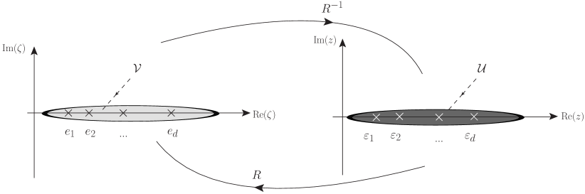
Figure 3. Illustration of the change of variables: The biholomorphic map $R:\mathcal{U}\to\mathcal{V}$ with $R(\varepsilon_{k})=e_{k}$ will later be enlarged to a ramified cover $R:\hat{\mathbb{C}}\to\hat{\mathbb{C}}$. Functions on $\mathcal{U}$ will meromorphically continue to the Riemann sphere $\hat{\mathbb{C}}=\mathbb{C}\cup\{\infty\}$.

For appropriately chosen preimages $R(\varepsilon_{k})=e_{k}$ we introduce another holomorphic function $\mathcal{G}^{(0)}$ by $\mathcal{G}^{(0)}(z,w)=G^{(0)}(R(z),R(w))$. We require that $R$ and $\mathcal{G}^{(0)}$ relate by

$$R(z)+\mu^{2}_{bare}+\frac{\lambda}{N}\sum_{k=1}^{d}r_{k}Z\mathcal{G}^{(0)}(z,\varepsilon_{k})+\frac{\lambda}{N}\sum_{k=1}^{d}\frac{r_{k}}{R(\varepsilon_{k})-R(z)}=-R(-z).$$ (4.6)

These steps turn (4.5) into

$$(R(w)-R(-z))Z\mathcal{G}^{(0)}(z,w)=1+\frac{\lambda}{N}\sum_{k=1}^{d}r_{k}\frac{Z\mathcal{G}^{(0)}(\varepsilon_{k},w)}{R(\varepsilon_{k})-R(z)},$$ (4.7)

which is a linear equation for which a solution theory exists. It expresses $\mathcal{G}^{(0)}$ in terms of the not yet known function $R$. Inserting it into (4.6) yields a complicated equation for $R$. The miracle is that relatively mild assumptions on $R$ allow to solve this problem:

Theorem 4.1 ([SW19], building on [GHW19]).

Let $\lambda,e_{k}>0$ and $\mu^{2}_{bare}=0=Z-1$ (absent renormalisation). Assume that there is a rational function $R:\hat{\mathbb{C}}\to\hat{\mathbb{C}}$ with

1. $R$ has degree $d+1$, is normalised to $R(\infty)=\infty$ and biholomorphically maps a domain $\mathcal{U}\subset\mathbb{C}$ to a neighbourhood $\mathcal{V}$ of a real interval that contains $e_{1},\dots,e_{d}$.

2. $R$ satisfies (4.6) with $\mathcal{G}^{(0)}$ the solution of (4.7), where $z,w,\varepsilon_{k}\in\mathcal{U}$.

Then the functions $R$ and $\mathcal{G}^{(0)}$ are uniquely identified as

$$R(z) =z-\frac{\lambda}{N}\sum_{k=1}^{d}\frac{\varrho_{k}}{\varepsilon_{k}+z}\;,\qquad R(\varepsilon_{k})=e_{k}\;,\quad\varrho_{k}R^{\prime}(\varepsilon_{k})=r_{k}\;,$$ (4.8)

$$\mathcal{G}^{(0)}(z,w) =\frac{\displaystyle 1-\frac{\lambda}{N}\sum_{k=1}^{d}\frac{r_{k}}{(R(z)-R(\varepsilon_{k}))(R(\varepsilon_{k})-R({-}w))}\prod_{j=1}^{d}\frac{R(w){-}R({-}\widehat{\varepsilon_{k}}^{j})}{R(w)-R(\varepsilon_{j})}}{R(w)-R(-z)}\;.$$ (4.9)

Here, the solutions of $R(v)=R(z)$ are denoted by $v\in\{z,\hat{z}^{1},\dots,\hat{z}^{d}\}$ with $z\in\mathcal{U}$ when considering $R:\hat{\mathbb{C}}\to\hat{\mathbb{C}}$. The symmetry $\mathcal{G}^{(0)}(z,w)=\mathcal{G}^{(0)}(w,z)$ is automatic.

We discuss later the renormalisation problem $\mu_{bare}^{2}(N,\lambda)\neq 0\neq Z(N,\lambda)-1$ in the limit $N\to\infty$.

The change of variables (4.8) identified in the solution (4.9) of the two-point function is the starting point for everything else. However, although the equations for all other $G_{..}$ are affine, they cannot be solved directly. It was understood in [BHW20] that one has first to introduce two further families of functions, as we will explain in the next subsection.

4.2. BTR of the Quartic Kontsevich Model

To give an impression how blobbed topological recursion is related to our model, we first introduce the aforementioned three families of functions whose importance became clear during an attempt of solving the $2{+}2$-point function:

• the cumulants $G^{(g)}_{|k_{1}^{1}\dots k_{n_{1}}^{1}|\dots|k_{1}^{b}\dots k_{n_{b}}^{b}|}$ defined in (4.2), (4.1) and (4.3), called $(n_{1}{+}...{+}n_{b})$-point functions of genus $g$;

• the generalised correlation functions defined as derivatives (here we need $E_{k}=e_{k}$ and $r_{k}=1$; this restriction is later relaxed)

  $$T^{(g)}_{q_{1},q_{2},...,q_{m}\|k_{1}^{1}...k_{n_{1}}^{1}|k_{1}^{2}...k_{n_{2}}^{2}|...|k_{1}^{b}...k_{n_{b}}^{b}|}:=\frac{(-N)^{m}\partial^{m}}{\partial e_{q_{1}}\partial e_{q_{2}}...\partial e_{q_{m}}}G^{(g)}_{|k_{1}^{1}...k_{n_{1}}^{1}|k_{1}^{2}...k_{n_{2}}^{2}|...|k_{1}^{b}...k_{n_{b}}^{b}|}\;;$$ (4.10)

• functions $\Omega_{q_{1},...,q_{m}}$ recursively defined by

  $$\Omega^{(g)}_{q_{1},...,q_{m}} :=\frac{(-N)^{m-1}\partial^{m-1}\Omega^{(g)}_{q_{1}}}{\partial e_{q_{2}}...\partial e_{q_{m}}}+\frac{\delta_{m,2}\delta_{g,0}}{(e_{q_{1}}-e_{q_{2}})^{2}}\qquad\text{for }m\geq 2$$ (4.11)

  and $\Omega^{(g)}_{q}:=\frac{1}{N}\sum_{k=1}^{N}G^{(g)}_{|qk|}+\frac{1}{N^{2}}G^{(g)}_{|q|q|}$. They are symmetric in their indices and will soon be related to meromorphic differentials which satisfy BTR.

A straightforward extension gave birth to (generalised) Dyson-Schwinger equations between these functions. They first extend to equations for holomorphic functions on several copies of $\mathcal{V}$ and then via the change of variables $R,R^{-1}$ to equations between meromorphic functions

$$\mathcal{G}^{(g)}(z_{1}^{1},\dots,z_{n_{1}}^{1}|\dots|z_{1}^{b},\dots z_{n_{b}}^{b})\;,\quad\mathcal{T}^{(g)}(u_{1},...,u_{m}\|z_{1}^{1},\dots,z_{n_{1}}^{1}|\dots|z_{1}^{b},\dots z_{n_{b}}^{b}|)\;,$$

$$\Omega^{(g)}_{m}(u_{1},...,u_{m})$$ (4.12)

on several copies of $\hat{\mathbb{C}}$. It was shown in [BHW20] that these equations can be recursively solved in a triangular pattern of interwoven loop equations connecting these three families $(\mathcal{G}^{(g)},\mathcal{T}^{(g)},\Omega^{(g)}_{m})$ of (4.12), see Figure 4.

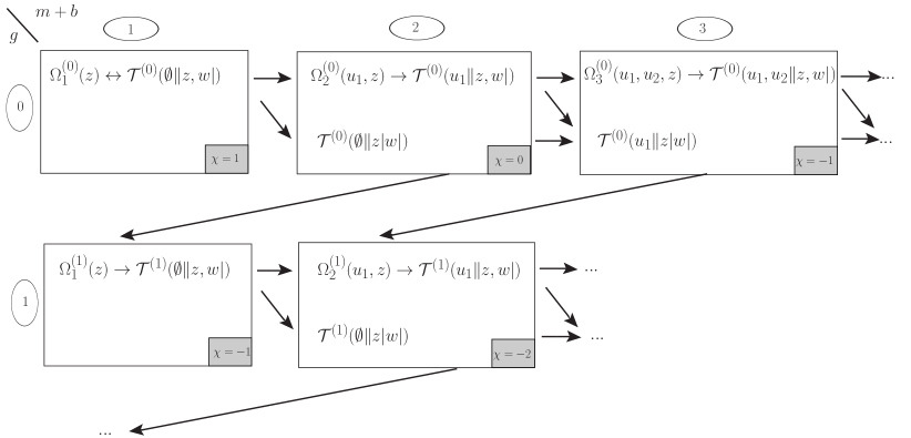
Figure 4. Illustration of the interwoven solution procedure, ordered by $-\chi$. Theorem 4.1 which simultaneously gives $\Omega^{(0)}_{1}(z)=\frac{1}{N}\sum_{k}r_{k}\mathcal{G}^{(0)}(\varepsilon_{k},z)$ and the two-point function $\mathcal{T}^{(0)}(\emptyset\|z,w)=\mathcal{G}^{(0)}(z,w)$ is the starting point. A generic box at position $(g,m+b)$ contains $\Omega_{m}^{(g)}(u_{1},...,u_{m-1},z)\to\mathcal{T}^{(g)}(u_{1},...,u_{m-1}\|z,w|)$ and $\mathcal{T}^{(g)}(u_{1},...,u_{m-2}\|z|w|)$.

The arrows represent very different difficulties. It is easy to express every next $\mathcal{T}^{(g)}$ in terms of previous $\Omega^{(g^{\prime})}_{m}$, but the result is an extremely lengthy and complicated equation for the next $\Omega^{(g)}_{m}$ in terms of the previous $\Omega^{(g^{\prime})}_{m^{\prime}}$. Obtaining a $(n_{1}{+}...{+}n_{b})$-point function of genus $g$ from $\mathcal{T}^{(g^{\prime})},\Omega^{(g^{\prime})}_{m^{\prime}}$ in all boxes with $g^{\prime}\leq g$ and $m^{\prime}+b^{\prime}\leq b$ is also easy (unless one wants to make the symmetries manifest).

To our enormous surprise, the solution of the first of these very difficult equations for $\Omega^{(g)}_{m}$ with $2g+m-2\geq 0$ turned out to be ravishingly simple and structured. After the solution of $\Omega_{m}^{(g)}$ for $(g,m)\in\{(0,2),(0,3),(0,4),(1,1)\}$ in [BHW20] via the interwoven equations, it became nearly obvious that the meromorphic differentials $\omega_{g,n}$ defined by

$$\omega_{g,n}(z_{1},...,z_{n}):=\lambda^{2-2g-n}\Omega^{(g)}_{n}(z_{1},...,z_{n})dR(z_{1})\cdots dR(z_{n})$$ (4.13)

obey BTR. In this process the variable transform $R$ is again of central importance. It provides the spectral curve $(x:\hat{\mathbb{C}}\to\hat{\mathbb{C}},\omega_{0,1}=ydx,\omega_{0,2})$ discussed in Sec. 3 with

$$x(z)=R(z)\;,\quad y(z)=-R(-z)\;,\quad\omega_{0,2}(u,z)=\frac{du\,dz}{(u-z)^{2}}+\frac{du\,dz}{(u+z)^{2}}\;.$$ (4.14)

We underline the appearance of some additional initial data in $\omega_{0,2}$, namely $\frac{du\,dz}{(u+z)^{2}}=-B(u,-z)$ (Bergman kernel with one changed sign).

The next steps will consist in identifying structures and equations directly for the family $\omega_{g,n}$, avoiding the $\mathcal{T}^{(g)}$. This task was accomplished for the planar sector $\omega_{0,n}$ in [HW21]. The symmetry of the spectral curve, $y(z)=-x(-z)$ and $\omega_{0,2}(u,z)=B(u,z)-B(u,-z)$ played a key rôle. This symmetry extends to a deep involution identity

$$\omega_{0,|I|+1}(I,q)+\omega_{0,|I|+1}(I,-q)$$ (4.15)

$$=-\sum_{s=2}^{|I|}\sum_{I_{1}\uplus...\uplus I_{s}=I}\frac{1}{s}\operatorname{Res}\displaylimits_{z\to q}\Big{(}\frac{dR(-q)dR(z)}{(R(-z)-R(-q))^{s}}\prod_{j=1}^{s}\frac{\omega_{0,|I_{j}|+1}(I_{j},z)}{dR(z)}\Big{)}\;.$$

With considerable combinatorial effort it was possible to prove that this involution identity completely determines the moromorphic differentials $\omega_{0,n+1}$ to the following structure astonishingly similar to usual TR:

Theorem 4.2 ([HW21]).

Assume that $z\mapsto\omega_{0,n+1}(u_{m},...,u_{m},z)$ is for $m\geq 2$ holomorphic at $z=-\beta_{i}$ and $z=u_{k}$ and has poles at most in points where the rhs of (4.15) has poles. Then equation (4.15) is for $I=\{u_{1},...,u_{m}\}$ with $m\geq 2$ uniquely solved by

$$\omega_{0,|I|+1}(I,z) =\sum_{i=1}^{r}\operatorname{Res}\displaylimits_{q\to\beta_{i}}K_{i}(z,q)\sum_{I_{1}\uplus I_{2}=I}\omega_{0,|I_{1}|+1}(I_{1},q)\omega_{0,|I_{2}|+1}(I_{2},\sigma_{i}(q))$$ (4.16)

$$-\sum_{k=1}^{m}d_{u_{k}}\Big{[}\operatorname{Res}\displaylimits_{q\to-u_{k}}\sum_{I_{1}\uplus I_{2}=I}\tilde{K}(z,q,u_{k})d_{u_{k}}^{-1}\big{(}\omega_{0,|I_{1}|+1}(I_{1},q)\omega_{0,|I_{2}|+1}(I_{2},q)\big{)}\Big{]}\,.$$

Here $\beta_{1},...,\beta_{r}$ are the ramification points of the ramified covering $R:\hat{\mathbb{C}}\to\hat{\mathbb{C}}$ given in (4.8) and $\sigma_{i}\neq\mathrm{id}$ denotes the local Galois involution in the vicinity of $\beta_{i}$, i.e. $R(\sigma_{i}(z))=R(z)$, $\lim_{z\to\beta_{i}}\sigma_{i}(z)=\beta_{i}$. By $d_{u_{k}}$ we denote the exterior differential in $u_{k}$, which on 1-forms has a right inverse $d^{-1}_{u}\omega(u)=\int_{u^{\prime}=\infty}^{u^{\prime}=u}\omega(u^{\prime})$. The recursion kernels are given by

$$K_{i}(z,q) :=\frac{\frac{1}{2}(\frac{dz}{z-q}-\frac{dz}{z-\sigma_{i}(q)})}{dR(\sigma_{i}(q))(R(-\sigma_{i}(q))-R(-q))}\;,\qquad$$

$$\tilde{K}(z,q,u) :=\frac{\frac{1}{2}\big{(}\frac{dz}{z-q}-\frac{dz}{z+u}\big{)}}{dR(q)(R(u)-R(-q))}\;.$$ (4.17)

The solution (4.16)$+$(4.17) coincides with the solution of the interwoven loop equations depicted in Fig. 4. The linear and quadratic loop equations (3.2) and (3.3) hold. The symmetry of the rhs of (4.15) under $q\mapsto-q$ is automatic.

To give an explicit formula for the holomorphic part as well, using the structure of topological recursion itself, is to the best of our knowledge exceptional. Higher genera $g$ are under current investigation and require again an arduous solution of the interwoven loop equations by hand. These non-planar symmetric meromorphic differentials have an additional pole of higher order at the fixed point $q=0$ of the involution $q\to-q$.

Figure 5 represents similarities between the quartic Kontsevich model, the original Kontsevich model [Kon92], the Hermitian one- and two matrix models [Eyn16, Eyn03, CEO06]).

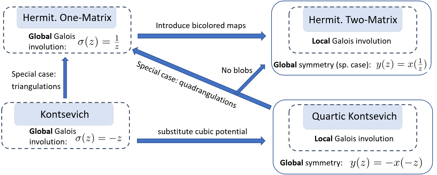
Figure 5. Despite completely different mathematical structures behind the models, we can reach the limit both of the Hermitian one- and two-matrix model. Moreover, we stress that the global Galois involution of the one-matrix model and the Kontsevich model turn into the global symmetry of the spectral curve belonging to their more intricate siblings.

Although the modifications to go from one model to the other seem mild, the mathematics of the four models differs drastically. But they all fit into some flavour of topological recursion so that there is a fruitful exchange of methods.

4.3. Solution strategy of all quartic models

In the two previous subsections we assumed finite matrices, in particular a truncated energy spectrum at finite $E_{N}$. The relations to ordinary QFTs appear in a limit $N\to\infty$ and depend on the (spectral) dimension encoded in the $E_{k}$. In this subsection we describe this limit process. Note that the limit $N\to\infty$ turns rational functions into transcendental functions so that most algebraic structures get lost. Future research projects will address the questions whether parts of (B)TR survive and whether these surviving algebraic structures are compatible with renormalisation. This subsection addresses the simplest topological sector $(g,n)=(0,1)$.

Introducing the measure $\varrho_{0}(t):=\frac{1}{N}\sum_{k=1}^{d}r_{k}\delta(t-e_{k})$ we can turn the non-linear equation (4.5) into the integral equation

$$\bigg{[}\zeta+\eta+\mu^{2}_{bare}+\lambda\mathchoice{{\vbox{\hbox{$\textstyle-$}}\kern-4.86108pt}}{{\vbox{\hbox{$\scriptstyle-$}}\kern-3.25pt}}{{\vbox{\hbox{$\scriptscriptstyle-$}}\kern-2.29166pt}}{{\vbox{\hbox{$\scriptscriptstyle-$}}\kern-1.875pt}}\!\int_{0}^{\Lambda^{2}}dt\,\varrho_{0}(t)\bigg{(}ZG^{(0)}(\zeta,t)+\frac{1}{t-\zeta}\bigg{)}\bigg{]}ZG^{(0)}(\zeta,\eta)$$ (4.18)

$$=1+\lambda\mathchoice{{\vbox{\hbox{$\textstyle-$}}\kern-4.86108pt}}{{\vbox{\hbox{$\scriptstyle-$}}\kern-3.25pt}}{{\vbox{\hbox{$\scriptscriptstyle-$}}\kern-2.29166pt}}{{\vbox{\hbox{$\scriptscriptstyle-$}}\kern-1.875pt}}\!\int_{0}^{\Lambda^{2}}dt\,\varrho_{0}(t)\Big{(}\frac{ZG^{(0)}(t,\eta)}{t-\zeta}\Big{)},$$

where $\mathchoice{{\vbox{\hbox{$\textstyle-$}}\kern-4.86108pt}}{{\vbox{\hbox{$\scriptstyle-$}}\kern-3.25pt}}{{\vbox{\hbox{$\scriptscriptstyle-$}}\kern-2.29166pt}}{{\vbox{\hbox{$\scriptscriptstyle-$}}\kern-1.875pt}}\!\int$ is the Cauchy principle value and $\Lambda^{2}=\mathrm{max}_{k}(e_{k})$. The limit $N\to\infty$ will be achieved in two steps. In the first step we interpret the measure $\varrho_{0}$ as a Hölder-continuous function. The renormalisation constants $Z,\mu^{2}_{bare}$ obtain a dependence on $\Lambda^{2}$ which in the second step is sent to $\infty$. Furthermore, the spectral dimension $D$ is also provided by an integral representation depending on the asymptotics of $\varrho_{0}(t)$ for $\Lambda^{2}\to\infty$, being the smallest $D$ such that the integral

$$\sum_{k=1}^{\infty}E_{k}^{-D/2-\epsilon}=\lim_{\Lambda^{2}\to\infty}\int_{0}^{\Lambda^{2}}dt\,\frac{\varrho_{0}(t)}{(1+t)^{D/2+\epsilon}}.$$ (4.19)

converges for all $\epsilon>0$.

Example 4.3.

• For an asymptotically constant measure $\varrho_{0}(t)\sim const$, the spectral dimension becomes $D=2$. The integral on the lhs of (4.18) diverges logarithmically in $\Lambda^{2}$, which can be absorbed by $\mu^{2}_{bare}(\Lambda^{2})$. The field renormalisation is set to $Z=1$.

• For an asymptotically linear measure $\varrho_{0}(t)\sim t$, the spectral dimension becomes $D=4$. The renormalisation constants $\mu^{2}_{bare}(\Lambda^{2})$ and $Z(\Lambda^{2})$ have to be adapted carefully such that $\lim_{\Lambda^{2}\to\infty}G^{(0)}(\zeta,\eta)$ converges.

• For a measure with asymptotic behaviour $\varrho_{0}(t)\sim t^{a}$ and $a\geq 2$, the spectral dimension becomes $D\geq 6$. In this case, the model is not renormalisable anymore.

Assuming that the expression in the square brackets in (4.18) is known, then the powerful solution theory of singular integral equations [Tri85] provides the explicit expression [GW14]

$$ZG^{(0)}(a,b)=\frac{e^{\mathcal{H}^{\Lambda}_{a}[\tau_{b}(\bullet)]\sin\tau_{b}(a)}}{\lambda\pi\varrho_{0}(a)}\qquad a,b\in[0,\Lambda^{2}],$$

where $\mathcal{H}^{\Lambda}_{a}[f(\bullet)]:=\frac{1}{\pi}\mathchoice{{\vbox{\hbox{$\textstyle-$}}\kern-4.86108pt}}{{\vbox{\hbox{$\scriptstyle-$}}\kern-3.25pt}}{{\vbox{\hbox{$\scriptscriptstyle-$}}\kern-2.29166pt}}{{\vbox{\hbox{$\scriptscriptstyle-$}}\kern-1.875pt}}\!\int_{0}^{\Lambda^{2}}\frac{dt\,f(t)}{t-a}$ is the finite Hilbert transform. Inserting this ansatz into (4.18) gives a consistency equation [PW20, GHW19] for the angle function $\tau_{a}:(0,\Lambda^{2})\to[0,\pi]$ for $\lambda>0$ and $\tau_{a}:(0,\Lambda^{2})\to[-\pi,0]$ for $\lambda<0$:

$$\frac{\cot\tau_{a}(p)}{\lambda\pi\varrho_{0}(p)}=a+p+\mu^{2}_{bare}(\Lambda^{2})+\lambda\pi\mathcal{H}_{p}^{\Lambda}[\varrho_{0}(\bullet)]+\frac{1}{\pi}\int_{0}^{\Lambda^{2}}dt\,\tau_{p}(t).$$ (4.20)

The solution of the angle function was first found in [PW20] for the special case $\varrho_{0}(t)=1$ and generalised for any Hölder-continuous measure with spectral dimension $D<6$ in [GHW19]. First, we need the following implicitly defined construction:

Definition 4.4.

Let $D\in\{0,2,4\}$ (otherwise take $2\lfloor\frac{D}{2}\rfloor$) and $\mu^{2}>0$. Define implicitly the complex function $R_{D}(z)$ and the deformed measure $\varrho_{\lambda}(t)$ by the system of equations

$$R_{D}(z)=z-\lambda(-z)^{\frac{D}{2}}\int_{\nu_{D}}^{\Lambda_{D}^{2}}\frac{dt\,\varrho_{\lambda}(t)}{(t+\mu^{2})^{\frac{D}{2}}(t+\mu^{2}+z)}\qquad\text{and}\qquad\varrho_{\lambda}(t)=\varrho_{0}(R_{D}(t)),$$

where $R_{D}(\Lambda^{2}_{D})=\Lambda^{2}$ and $R_{D}(\nu_{D})=0$. The limit $\Lambda^{2}\to\infty$ converges.

This implicitly defined system of equations is for general $\varrho_{0}$ not exactly solvable. We will give in Sec. 5 two examples corresponding to the 2- and 4-dimensional Moyal space, where $R_{D}$ and $\varrho_{\lambda}$ can be found explicitly.

Nevertheless, a formal expansion in $\lambda$ of $R_{D}$ and $\varrho_{\lambda}$ can be achieved recursively already in the general case, starting with

$$\varrho_{\lambda}(t) =\varrho_{0}(t)+\mathcal{O}(\lambda),\quad$$

$$R_{D}(z) =z-\lambda(-z)^{\frac{D}{2}}\int_{0}^{\Lambda^{2}}\frac{dt\,\varrho_{0}(t)}{(t+\overline{\mu}^{2})^{\frac{D}{2}}(t+\overline{\mu}^{2}+z)}+\mathcal{O}(\lambda^{2}),$$ (4.21)

where $\mu^{2}=\overline{\mu}^{2}+\mathcal{O}(\lambda)$. The expression is convergent for $\Lambda^{2}\to\infty$.

One can prove that the complex function $R_{D}(z)$ is biholomorphic from the right half plane $\{z\in\mathbb{C}:\mathrm{Re}(z)>-\frac{\mu^{2}}{2}\}$ onto a domain $U_{D}\subset\mathbb{C}$ containing $[0,\infty)$ for real $\lambda$ [GHW19]. We define on this domain $U_{D}$ the inverse $R^{-1}_{D}$ (which is not globally defined on $\mathbb{C}$). Then, the solution of the angle function is obtained by

Theorem 4.5 ([GHW19]).

Let $I_{D}:U_{D}\setminus[0,\Lambda^{2}]\ni w\mapsto I_{D}(w)\in\mathbb{C}$ be defined by

$$I_{D}(w):=-R_{D}(-\mu^{2}-R^{-1}_{D}(w)).$$

The consistency relation (4.20) is solved by

$$\tau_{a}(p)=\lim_{\epsilon\to 0}\mathrm{Im}\big{(}\log(a+I_{D}(p+\mathrm{i}\epsilon))\big{)},$$

where $\mu^{2}_{bare}(\Lambda^{2})$ is related to $\mu^{2}$ by

$$D=0: \mu^{2}_{bare}(\Lambda^{2})=\mu^{2}\;,$$

$$D=2: \mu^{2}_{bare}(\Lambda^{2})=\mu^{2}-2\lambda\int_{R_{D}^{-1}(0)}^{R_{D}^{-1}(\Lambda^{2})}\frac{dt\,\varrho_{\lambda}(t)}{t+\mu^{2}}\;,$$

$$D=4: \mu^{2}_{bare}(\Lambda^{2})=\mu^{2}-\lambda\mu^{2}\int_{R_{D}^{-1}(0)}^{R_{D}^{-1}(\Lambda^{2})}\frac{dt\,\varrho_{\lambda}(t)}{(t+\mu^{2})^{2}}-2\lambda\int_{R_{D}^{-1}(0)}^{R_{D}^{-1}(\Lambda^{2})}\frac{dt\,\varrho_{\lambda}(t)}{t+\mu^{2}}\;.$$

The angle function $\tau_{a}(p)$ converges in the limit $\Lambda^{2}\to\infty$.

Equivalently to Theorem 4.5 is the statement that the expression in the square brackets of (4.18) is equal to $I_{D}$, that is

$$\zeta+\mu^{2}_{bare}+\lambda\int_{0}^{\Lambda^{2}}dt\,\varrho_{0}(t)\bigg{(}ZG^{(0)}(\zeta,t)+\frac{1}{t-\zeta}\bigg{)}=I_{D}(\zeta)=-R_{D}(-\mu^{2}-R^{-1}_{D}(\zeta)),$$

for $\zeta\in U_{D}\setminus[0,\Lambda^{2}]$. The proof of the theorem is essentially achieved by inserting the solution of $\tau_{a}(p)$ into rhs of the consistency relation (4.20), using the system of implicitly defined functions from Definition 4.4 and applying the Lagrange-Bürmann inversion theorem, a generalisation of Lagrange inversion theorem. We refer to [GHW19] for details.

In conclusion, Theorem 4.5 together with Definition 4.4 provide the solution of the initial topology $(g,n)=(0,1)$, generalising the first part of Theorem 4.1 to higher dimensions. The second part of Theorem 4.1, i.e. the explicit expression for the 2-point correlation function, extends as follows to $N\to\infty$:

Theorem 4.6 ([GHW19]).

The renormalised 2-point function of the $\lambda\phi^{4}$ matricial QFT-model in $D$ dimensions is given by

$$G(a,b):=\frac{\mu^{2\delta_{4,D}}\exp(N_{D}(a,b))}{\mu^{2}+a+b}$$

where

$$N_{D}(a,b)=\frac{1}{2\pi\mathrm{i}}\int_{-\infty}^{\infty} dt\bigg{\{}\log\big{(}a-R_{D}(-\tfrac{\mu^{2}}{2}-\mathrm{i}t)\big{)}\frac{d}{dt}\log\big{(}b-R_{D}(-\tfrac{\mu^{2}}{2}+\mathrm{i}t)\big{)}$$

$$-\log\big{(}a-(-\tfrac{\mu^{2}}{2}-\mathrm{i}t)\big{)}\frac{d}{dt}\log\big{(}b-(-\tfrac{\mu^{2}}{2}+\mathrm{i}t)\big{)}$$

$$-\delta_{4,D}\log\big{(}-R_{D}(-\tfrac{\mu^{2}}{2}-\mathrm{i}t)\big{)}\frac{d}{dt}\log\big{(}-R_{D}(-\tfrac{\mu^{2}}{2}+\mathrm{i}t)\big{)}$$

$$+\delta_{4,D}\log\big{(}-(-\tfrac{\mu^{2}}{2}-\mathrm{i}t)\big{)}\frac{d}{dt}\log\big{(}-(-\tfrac{\mu^{2}}{2}+\mathrm{i}t)\big{)}\bigg{\}}$$

and $R_{D}$ built by Definition 4.4. For $D\in\{0,2\}$ and for some restricted cases in $D=4$ (including the $D=4$ Moyal space), there is an alternative representation

$$G(a,b)$$ (4.22)

$$=\frac{(\mu^{2}{+}a{+}b)\exp\Bigg{\{}\mbox{\small$\displaystyle\frac{1}{2\pi\mathrm{i}}\int_{-\infty}^{\infty}dt\log\bigg{(}\frac{a-R_{D}(-\frac{\mu^{2}}{2}{-}\mathrm{i}t)}{a-(-\frac{\mu^{2}}{2}{-}\mathrm{i}t)}\bigg{)}\frac{d}{dt}\log\bigg{(}\frac{b-R_{D}(-\frac{\mu^{2}}{2}{+}\mathrm{i}t)}{b-(-\frac{\mu^{2}}{2}{+}\mathrm{i}t)}\bigg{)}$}\Bigg{\}}}{(\mu^{2}+b+R_{D}^{-1}(a))(\mu^{2}+a+R_{D}^{-1}(b))}.$$

We emphasise that $G(a,b)$, as a 2-point function, is by definition symmetric under $a\leftrightarrow b$. This symmetry is revealed by integration by parts within the exponential in (4.22).

Theorem 4.6 provides an exact formula for the 2-point function for an open neighbourhood around $\lambda=0$ such that a convergent expansion exists. The following example will give the first order contribution:

Example 4.7.

Let $\mu^{2}=1$ for convenience. The first order expansion of $\varrho_{\lambda}$ and $R_{D}$ was already given in (4.21). Equivalently, we get for the inverse

$$R^{-1}(a)=a+\lambda(-a)^{\frac{D}{2}}\int_{0}^{\Lambda^{2}}\frac{dt\,\varrho_{0}(t)}{(t+1)^{\frac{D}{2}}(t+1+a)}+\mathcal{O}(\lambda^{2}).$$

Expanding (4.22) of Theorem 4.6, where the exponential does not contribute at the first order since each logarithm starts at order $\lambda$, yields the convergent first order expression

$$G(a,b)=\frac{1}{1+a+b}-\frac{\lambda}{(1+a+b)^{2}}\bigg{(} (-a)^{\frac{D}{2}}\int_{0}^{\infty}\frac{dt\,\varrho_{0}(t)}{(t+1)^{\frac{D}{2}}(t+1+a)}$$

$$+(-b)^{\frac{D}{2}}\int_{0}^{\infty}\frac{dt\,\varrho_{0}(t)}{(t+1)^{\frac{D}{2}}(t+1+b)}\bigg{)}+\mathcal{O}(\lambda^{2}).$$

The reader may also compute the second order contribution in $\lambda$, where an iterated integral occurs with the canonical measure $dt\,\varrho_{0}(t)$. For the exponential, the contour of the integral should be deformed, and the integrand expands similar to the computation carried out in [PW20, Sec. 7].

The structure of the solution is still very abstract. The next section will convey more insight into the implicit definitions of $\varrho_{\lambda}$ and $R_{D}$ and their structure. This implicit system of equations will be solved for two examples, the 2- and 4-dimensional Moyal space.

5. Scalar QFT on Moyal space

Given a real skew-symmetric $D\times D$-matrix $\Theta$, the associative but noncommutative Moyal product between Schwartz functions $f,g\in\mathcal{S}(\mathbb{R}^{D})$ is defined by

$$(f\star g)(x)=\int_{\mathbb{R}^{D}\times\mathbb{R}^{D}}\frac{dy\,dk}{(2\pi)^{D}}\;f(x+\tfrac{1}{2}\Theta k)g(x+y)e^{\mathrm{i}\langle k,y\rangle}.$$ (5.1)

It was understood in [GW05b, GW05a] that the scalar QFT on Moyal space which arises from the action functional

$$S(\phi) :=\int_{\mathbb{R}^{D}}\frac{dx}{(8\pi)^{D/2}}\Big{(}\frac{1}{2}\phi\star(-\Delta+4\Omega^{2}\|\Theta^{-1}x\|^{2}+\mu^{2})\phi+\frac{\lambda}{4}\phi\star\phi\star\phi\star\phi\Big{)}(x)$$ (5.2)

is perturbatively renormalisable in dimensions $D=2$ and $D=4$. It was also noticed [GW04] that the renormalisation group (RG) flow of the effective coupling constant (in $D=4$, lowest $\lambda$-order) is bounded and that $\Omega=1$ is a RG fixed point. Further investigations therefore focused to $\Omega=1$ [DR07] for which the RG-flow of the coupling constant in $D=4$ was proved to be bounded at any order in perturbation theory [DGMR07].

Methods developed in the proofs of these results were decisive in the derivation [GW09, GW14] of non-linear equation (4.5) we started with.

5.1. $D=2$

In two dimensions we have $\Theta=\left(\begin{smallmatrix}0&\theta\\ -\theta&0\end{smallmatrix}\right)$. We introduce a family $(f_{kl})_{k,l\in\mathbb{N}}$ of Schwartz functions by

$$f_{kl}(x_{1},x_{2})=2(-1)^{k}\sqrt{\frac{k!}{l!}}(x_{1}+\mathrm{i}x_{2})^{l-k}L^{l-k}_{k}\Big{(}\frac{2x_{1}^{2}+2x_{2}^{2}}{\theta}\Big{)}e^{-\frac{x_{1}^{2}+x_{2}^{2}}{\theta}},$$ (5.3)

where $L^{\alpha}_{k}$ are associated Laguerre polynomials. It is straightforward to prove

$$\overline{f_{kl}} =f_{lk}\;,\qquad f_{kl}\star f_{mn}=\delta_{lm}f_{kn}\;,\qquad\int_{\mathbb{R}^{2}}dx\;f_{kl}(x)=2\pi\theta\delta_{kl}\;,$$

$$(-\partial_{x_{1}}^{2}-\partial_{x_{2}}^{2}+\frac{4}{\theta^{2}}(x_{1}^{2}+x_{2}^{2}))f_{kl}(x_{1},x_{2})=\frac{4}{\theta}(k+l+1)f_{kl}(x_{1},x_{2}).$$ (5.4)

Therefore, expanding $\phi(x)=\sum_{k,l=0}^{\infty}\phi_{kl}f_{kl}(x)$, we turn (5.2) for $D=2$ into $S(\phi)=\lim_{N\to\infty}S_{N}(\phi)$ with

$$S_{N}(\phi)=\frac{\theta}{4}\Big{(}\sum_{k,l=0}^{N-1}\Big{(}\frac{4}{\theta}k+\frac{\mu^{2}}{2}+\frac{2}{\theta}\Big{)}\phi_{kl}\phi_{lk}+\frac{\lambda}{4}\sum_{k,l,m,n=0}^{N-1}\phi_{kl}\phi_{lm}\phi_{mn}\phi_{nk}\Big{)}.$$ (5.5)

Setting here $\frac{\theta}{4}=\frac{N}{\Lambda^{2}}$ and $E_{k}=\Lambda^{2}\frac{k}{N}+\frac{\mu^{2}}{2}+\frac{\Lambda^{2}}{2N}$ we recover the Minlos measure (2.4) as

$$d\mu_{int}(\phi)=\frac{1}{\mathcal{Z}}\exp(-\Lambda^{2}S_{N}(\phi))\prod_{k=0}^{N-1}d\phi_{kk}\prod_{k=1}^{N-1}\prod_{l=0}^{k}d\mathrm{Re}\phi_{kl}\,d\mathrm{Im}\phi_{kl}\;.$$ (5.6)

After some shift by the lowest spectral value $E_{0}$ which is absorbed in the bare mass we identifty $e_{k}=\Lambda^{2}\frac{k}{N}$ and $r_{k}=1$ in the spectral measure $\varrho_{0}(t)=\frac{1}{N}\sum_{k=0}^{N-1}\delta(t-e_{k})$. For $N\to\infty$ this converges, in the sense of Riemann sums, to the characteristic function on $[0,\Lambda^{2}]$. Compared with Definition 4.4 we recover $D=2$ and obtain for the function $R_{2}$ in the limit $\Lambda^{2}\to\infty$

$$R_{2}(z)=z+\lambda z\int_{0}^{\infty}\frac{dt}{(t+\mu^{2})(t+\mu^{2}+z)}=z+\lambda\log\Big{(}1+\frac{z}{\mu^{2}}\Big{)}.$$ (5.7)

The function $R_{2}$ is holomorphic on $\mathbb{C}\setminus]-\infty,-\mu^{2}]$. It can be inverted there in terms of the Lambert-$W$ function defined by $W(z)e^{W(z)}=z$ to

$$R^{-1}_{2}(z)=\lambda W\Big{(}\frac{\mu^{2}}{\lambda}e^{\frac{z+\mu^{2}}{\lambda}}\Big{)}-\mu^{2}.$$

Similar to the logarithm, the Lambert-$W$ function has infinitely many branches $W_{k}$ labelled by $k\in\mathbb{Z}$, where the inverse $R^{-1}$ is obtained by the principal branch $W_{0}$. Following [PW20], this inverse admits a convergent expansion

$$R^{-1}_{2}(z)=\sum_{n=1}^{\infty}\frac{(-\lambda)^{n}}{n!}\frac{d^{n-1}}{dz^{n-1}}\log\Big{(}1+\frac{z}{\mu^{2}}\Big{)}^{n}$$

consisting only of powers of the logarithm.

Carrying out higher order computations on the $D=2$ Moyal plane shows that further transcendental functions occur which are not representable via powers of logarithms. These functions are generated by the integral inside the exponential of (4.22), they are essentially in the class of Nielsen polylogarithms (see [PW20] for more detials).

Applying the construction of Sec. 4.2, a completely different structure of the spectral curve is revealed, which is built of

$$x(z)=z+\lambda\log\Big{(}1+\frac{z}{\mu^{2}}\Big{)},\qquad y(z)=-x(-z-\mu^{2})=z+\mu^{2}-\lambda\log\Big{(}-\frac{z}{\mu^{2}}\Big{)}.$$

This curve is no longer of algebraic nature. The continuum limit from an algebraic curve (as in (4.14)) to a transcendental spectral curve is still rather mysterious. The number of branches of $R^{-1}$ tends in the limit to infinity, where the number of ramification points increases as well. However, these ramification points accumulate in the continuum to a single ramification point $\beta$ at

$$x^{\prime}(\beta)=R^{\prime}_{2}(\beta)=1+\frac{\lambda}{\mu^{2}+\beta}=0\quad\Rightarrow\quad\beta=-\mu^{2}-\lambda.$$

In the limit $\lambda\to 0$, the ramification point $\beta$ approaches the singularity of the logarithm, where the full construction becomes meaningless.

However for positive $\lambda$, we may ask whether the model is still governed by the universal structure of Theorem 4.2. This would imply rationality for all $\Omega^{(0)}_{n}(z_{1},...,z_{n})$ in $z_{i}$. Inserting $z_{i}=R_{2}^{-1}(x_{i})$, we could verify that the $\Omega^{(0)}_{n}$ are expanded only into powers of logarithms, and therefore remain in a simple class of functions. Whereas, correlation functions in general are generated by generalisations of polylogarithms, like Nielsen polylogarithms.

The local Galois involution becomes fairly easy to handle:

Lemma 5.1.

Let $\mathcal{V}:=\{z\in\mathbb{C}\;|\leavevmode\nobreak\ |z-\beta|<\lambda\}$ and $\tilde{z}(z)=\frac{\exp[(1+z)/\lambda](1+z)}{\lambda}$ with $\tilde{z}(\beta)=-1/e$, the threefold branch point. Then the local Galois involution $\sigma_{2}(z)$ with $R_{2}(z)=R_{2}(\sigma_{2}(z))$ and fixed point $\sigma_{2}(\beta)=\beta$ is piecewise defined within three branches of the Lambert W-function as

$$\sigma_{2}(z)=-1+\lambda W_{k}(\tilde{z})$$

$$\text{with }\begin{cases}k=-1&\text{if $\{\mathrm{Re}(\tilde{z})\geq-1/e,|\mathrm{Im}(\tilde{z})|\cot[|\mathrm{Im}(\tilde{z})|]\leq\mathrm{Re}(\tilde{z})\}$}\\ k=1&\text{c.c. of $k=-1$ sector }\\ k=0&\text{else}\end{cases}$$

Figure 6 gives a picture of this local Galois involution.

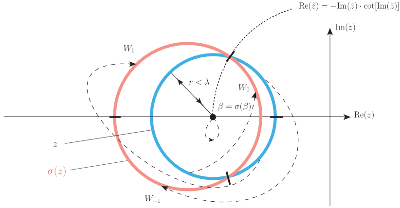
Figure 6. Symbolical interpretation of the local Galois involution $\sigma(z)$ (red) which can be defined piecewise using the three branches of the Lambert $W$-function $W_{0,\pm 1}$. The definition as Galois involution holds for $|z-\beta|<\lambda$ giving a concrete meaning to the term local involution.

5.2. $D=4$

By transform of variables one can achieve $\Theta=\left(\begin{smallmatrix}0&\theta\\ -\theta&0\end{smallmatrix}\right)\otimes\mathbb{I}_{2\times 2}$. We expand $\phi(x_{1},x_{2},x_{3},x_{4})=\phi_{\begin{subarray}{c}k_{1}l_{1}\\ k_{2}l_{2}\end{subarray}}f_{k_{1}l_{1}}(x_{1},x_{2})f_{k_{2}l_{2}}(x_{3},x_{4})$. Using the Cantor bijection $P\binom{k_{1}}{k_{2}}:=k_{2}+\frac{1}{2}(k_{1}+k_{2})(k_{1}+k_{2}+1)$ between $\mathbb{N}^{2}$ and $\mathbb{N}$ we can map $\phi_{\begin{subarray}{c}k_{1}l_{1}\\ k_{2}l_{2}\end{subarray}}$ to standard matrix elements $\phi_{kl}$. Setting $|k|:=k_{1}+k_{2}$ if $P\binom{k_{1}}{k_{2}}=k$, the action functional (5.2) takes for $D=4$ the form $S(\phi)=\lim_{N\to\infty}S_{N}(\phi)$ with

$$S_{N}(\phi)=\Big{(}\frac{\theta}{4}\Big{)}^{2}\Bigg{(} \sum_{\begin{subarray}{c}k,l=0\\ |k|,|l|<\sqrt{N}\end{subarray}}^{\infty}\frac{4}{\theta}|k|+\frac{\mu^{2}}{2}+\frac{4}{\theta}\Big{)}\phi_{kl}\phi_{lk}+\frac{\lambda}{4}\sum_{\begin{subarray}{c}k,l,m,n=0\\ |k|,|l|,|m|,|n|<\sqrt{N}\end{subarray}}^{\infty}\phi_{kl}\phi_{lm}\phi_{mn}\phi_{nk}\Big{)}\Bigg{)}.$$

There are $n+1$ natural numbers $k$ with $|k|=n$ and $\frac{(n+1)(n+2)}{2}$ natural numbers $k$ with $|k|\leq n$. Setting $\frac{\theta}{4}=\frac{\sqrt{N}}{\Lambda^{2}}$ and $e_{n}=\Lambda^{2}\frac{n}{\sqrt{N}}+\frac{\mu^{2}}{2}+\frac{\Lambda^{2}}{\sqrt{N}}$ we recover the Minlos measure (2.4) as

$$d\mu_{int}(\phi)=\frac{1}{\mathcal{Z}}\exp(-\Lambda^{4}S_{N}(\phi))d\phi$$ (5.8)

where the spectral values $e_{n}$ have multiplicity $r_{n}=n+1$. After some shift by the lowest spectral value $e_{0}$, which is absorbed in the bare mass, the spectral measure $\varrho_{0}(t)=\frac{1}{N}\sum_{n=0}^{\sqrt{N}-1}r_{n}\delta(t-e_{n})$ converges for $N\to\infty$, in the sense of Riemann sums, to $t\chi_{[0,\Lambda^{2}]}(t)$, where $\chi_{[0,\Lambda^{2}]}$ is the characteristic function of $[0,\Lambda^{2}]$. Compared with Definition 4.4 we recover $D=4$ and obtain the function $R_{4}$ in the limit $\Lambda^{2}\to\infty$ as

$$R_{4}(z)=z-\lambda z^{2}\int_{0}^{\infty}\frac{dt\,R_{4}(t)}{(t+\mu^{2})^{2}(t+\mu^{2}+z)}.$$ (5.9)

The leading order expansion is easily computed

$$R_{4}(z)=z+\lambda\bigg{(}z-\mu^{2}\Big{(}1+\frac{z}{\mu^{2}}\Big{)}\log\Big{(}1+\frac{z}{\mu^{2}}\Big{)}\bigg{)}+\mathcal{O}(\lambda^{2}).$$

From the expansion, one would expect that $R_{4}(z)$ has linear asymptotics for $z$ tending to infinity. However, this is not the case: The asymptotic behaviour is only visible by the resummation of all orders in $\lambda$, which is given in terms of a Gaußian hypergeometric function:

Theorem 5.2 ([GHW20]).

The linear integral equation (5.9) is solved by

$$R(z)=z\;_{2}F_{1}\Big{(}\genfrac{}{}{0.0pt}{}{\alpha_{\lambda},\;1-\alpha_{\lambda}}{2}\Big{|}-\frac{z}{\mu^{2}}\Big{)},\quad\text{where }\leavevmode\nobreak\ \alpha_{\lambda}:=\begin{cases}\frac{\arcsin(\lambda\pi)}{\pi}&\text{for }|\lambda|\leq\frac{1}{\pi}\;,\\ \frac{1}{2}+\mathrm{i}\frac{\mathrm{arcosh}(\lambda\pi)}{\pi}&\text{for }\lambda\geq\frac{1}{\pi}\;.\end{cases}$$ (5.10)

The proof is obtained by inserting the result into the linear integral equation and using identities of the Gaussian hypergeometric function.

The important fact is that the linear dependence of $\lambda$ within the integral equation (5.9) is packed into a highly nonlinear dependence given by the $\arcsin$-function into the coefficients of the hypergeometric function. Making use of that, a different asymptotic behaviour between $\varrho_{\lambda}$ and $\varrho_{0}$ is observed. It is well-known that the hypergeometric function behaves like

$$\,{}_{2}F_{1}\Big{(}\genfrac{}{}{0.0pt}{}{a,\;1-a}{2}\Big{|}-x\Big{)}\stackrel{{\scriptstyle x\to\infty}}{{\sim}}\frac{1}{x^{a}}\quad\text{for }|a|<\frac{1}{2}.$$

Together with the definition of the spectral dimension (4.19), we conclude:

Corollary 5.3 ([GHW20]).

For $|\lambda|<\frac{1}{\pi}$, the deformed measure $\varrho_{\lambda}=R_{4}$ of four-dimensional Moyal space has the spectral dimension $D=4-2\frac{\arcsin(\lambda\pi)}{\pi}$.

The theory admits on the four-dimensional Moyal space a dimensional drop to an effective spectral dimension related to an effective spectral measure. This is revealed by knowledge of the exact solutions.

From a quantum field theoretical perspective, this dimension drop is the most important result. It means that the $\lambda\phi^{*4}$-QFT model on 4D Moyal space is non-trivial, i.e. consistent over any (energy) scale $\Lambda^{2}\to\infty$. If we had $R_{4}(z)\propto z$ as expected from a perturbative expansion then the integral in (5.9) had to be restricted to $[0,\Lambda^{2}]$ (otherwise $R^{-1}$ would be not defined on $\mathbb{R}_{+}$). We recall that the Landau ghost problem [LAK54], or triviality, is a severe threat to quantum field theory. It almost killed renormalisation theory in the 1960s, rescued then by discovery of asymptotic freedom rescued non-Abelian Yang-Mills theories. But these theories are complicated; they require a non-perturbative treatment to deal with confinement. A simple 4D QFT-model without triviality problem was not known so far. For the $\lambda\phi^{4}$-model, triviality was proved in $D=4+\epsilon$ dimensions [Aiz81, Frö82] in the 1980s. (Non-)triviality in $D=4$ dimensions remained an open problem for almost 40 years; only recently Aizenman and Duminil-Copin achieved the proof [ADC21] of (marginal) triviality. Therefore, the construction of a simple, solvable and non-trivial QFT-model in four dimensions (albeit on a noncommutative space) is a major achievement for renormalisation theory.

In the next step one aims to apply the construction of (B)TR as explained in Sec. 4.2. But here we are faced with a problem: Defining $x(z)=R_{4}(z)$, the derivative $x^{\prime}(z)$ is no longer in the class of rational functions, which was a fundamental assumption in (B)TR. In other words, the full construction of (B)TR based on algebraic, not transcendental, ramification points fails directly from the beginning. It remains to investigate in a long-term project whether an adapted formulation of (B)TR can extend the previous results to four dimensions.

6. Cross-checks: perturbative expansions

In nowadays particle physics, one is often dependent on approximative methods like expansions of correlation functions into series of Feynman graphs. A main advantage of investigating the present toy model is undoubtedly the fact that we only use the Feynman graph expansion to perform a cross-check of our exact solutions. Due to its nature as a matrix model, the expansion of the cumulants creates ribbon graphs (also fat Feynman graphs). By their duality to maps on surfaces, we also have points of contact with enumerative geometry and combinatorics.

6.1. Ribbon graphs

In order to obtain a perturbative series of the cumulants (4.1), one expands the exponential $\exp(-\frac{\lambda N}{4}\mathrm{Tr}(\phi^{4}))$ inside the measure (2.4) into a (formal) power series in the coupling constant $\lambda$. As result we obtain products of matrix elements $\phi_{kl}$ from the expansion $(\mathrm{Tr}(\phi^{4}))^{v}$ of the exponential and from the products present in (4.1), integrated against the Gauß measure (2.3). The resulting sum over pairings can be interpreted as ribbon graphs. A ribbon has two strands, which carry a labelling. Two strands connected by a four-valent vertex are identified. We denote by $\mathfrak{G}^{v,\pi}_{k_{1},...,k_{n}}$ the set of labelled connected ribbon graphs with $v$ four-valent vertices and $n$ one-valent vertices, where the strands connected to the one-valent vertices (from the $n$ factors in (4.1)) are labelled by $(k_{1},k_{\pi(1)})$, …, $(k_{n},k_{\pi(n)})$. It is assumed here that the $k_{i}$ in (4.1) are pairwise different so that $l_{i}=\pi(k_{i})$ for a permutation $\pi in\mathcal{S}_{n}$. Let a graph $\Gamma$ have $r=2v+n/2$ ribbons and $s(\Gamma)$ loops (closed strands). We associate a weight $\varpi(\Gamma)$ to $\Gamma$ by applying the following Feynman rules:

• every 4-valent ribbon-vertex carries a factor $-\lambda$

• every ribbon with strands labelled by $p,q$ carries a factor $\frac{1}{e_{p}+e_{q}}$ (propagator)

• multiply all factors and apply the summation operator $\frac{1}{N^{s}}\sum_{l_{1},..,l_{s}=1}^{N}r_{l_{1}}...r_{l_{s}}$ over the $s=s(\Gamma)$ loops (closed strands) labelled by $l_{1},...,l_{s}$.

Then the cumulants expand for pairwise different $k_{1},...,k_{n}$ and $n$ even into the following series:

$$\sum_{v=0}^{\infty}\sum_{\Gamma\in\mathfrak{G}^{v,\pi}_{k_{1},...,k_{n}}}N^{v-r+n+s(\Gamma)}\varpi(\Gamma).$$ (6.1)

The cyclic order of the ribbon vertex gives an orientation of the full ribbon graph such that we achieve a natural embedding of the graph into a Riemann surface. The exponent of $N^{v-r+n+s(\Gamma)}$ represents the Euler characteristic $\chi=2g-2+b$ of the Riemann surface with $b$ the number of boundary components and $g$ the genus. Furthermore, the permutation $\pi$ splits $(k_{1},k_{\pi(1)})$, …, $(k_{n},k_{\pi(n)})$ into blocks with cyclic symmetry, see (4.2). This suggests the notation $G_{|k_{1}^{1}\dots k_{n_{1}}^{1}|\dots|k_{1}^{b}\dots k_{n_{b}}^{b}|}$ where the blocks are seperated by the vertical lines and each block is cyclically symmetric (see [BHW21] for more details). We will denote the set of these ribbon graphs by $\mathfrak{G}^{v}_{|k_{1}^{1}...k_{n_{1}}^{1}|...|k_{1}^{b}...k_{n_{b}}^{b}|}=\bigcup_{g=0}^{\infty}\mathfrak{G}^{g,v}_{|k_{1}^{1}...k_{n_{1}}^{1}|...|k_{1}^{b}...k_{n_{b}}^{b}|}$, so that finally the expansion reads:

$$G^{(g)}_{|k_{1}^{1}...k_{n_{1}}^{1}|...|k_{1}^{b}...k_{n_{b}}^{b}|}=\sum_{v=0}^{\infty}\sum_{\Gamma\in\mathfrak{G}^{g,v}_{|k_{1}^{1}...k_{n_{1}}^{1}|...|k_{1}^{b}...k_{n_{b}}^{b}|}}\varpi(\Gamma)\;.$$ (6.2)

6.2. Perturbative renormalisation of ribbon graphs

As mentioned before, a QFT is achieved in a continuum limit $N\to\infty$. In sec. 5 we have implemented this limit in two steps. We first passed to continuous spectral measure $\varrho_{0}$ on a finite interval $[0,\Lambda^{2}]$ and then arrived at a QFT in the limit $\Lambda^{2}\to\infty$. This procedure gives rise to slightly different Feynman rules. The summations converge to integrals, which are not necessarily convergent (by themselves) after removing the cut-off $\Lambda^{2}$. The perturbative renormalisation to avoid divergencies is well understood and of similar structure as renormalisation in local QFT. The overlapping divergencies are controlled by Zimmermann’s forest formula (see e.g. [Hoc20]). In the work [Thü21b] even more is proved. It is known that certain graphs (so-called 2-graphs, where ribbon graphs are a special case) have a Hopf-algebraic structure. The application of the antipode of the Hopf algebra proves Zimmermann’s forest formula for the 2-graphs in general [Thü21a]. This is analogous to the techniques of Connes and Kreimer [CK00].

We refer to these works and references therein for more details, but want to present a rather trivial example, where the forest consists only of the empty forest.

Example 6.1.

The two graphs of the 2-point function of order $\lambda$ are given in Fig. 7.

Figure 7. All graphs contributing to the 2-point function $G^{(0)}_{|ab|}$ up to order $\lambda^{2}$, where the upper strand is labelled by $a$ and the lower by $b$ for each graph. Topologically, some graphs are the same but different elements of $\mathfrak{G}^{0,v}_{|ab|}$ due to different labellings.

The forest formula is trivial and realised by a Taylor subtraction depending on the dimension of the theory given by the spectral measure $\varrho_{0}(t)dt$. In $D$ dimensions this measure behaves asymptotically as $\varrho_{0}(t)dt\sim t^{\frac{D}{2}-1}dt$. For the first graph of order $\lambda$ with external labelling $a,b$, we get (put $\mu^{2}=1$ for convenience)

$$\frac{-\lambda}{(1+a+b)^{2}}\int_{0}^{\infty}\varrho(t)dt\bigg{(}\frac{1}{1+a+t}-T^{D/2-1}_{a}\Big{(}\frac{1}{1+a+t}\Big{)}\bigg{)}$$

$$= \frac{-\lambda}{(1+a+b)^{2}}\int_{0}^{\infty}\varrho(t)dt\bigg{(}\frac{1}{1+a+t}-\frac{1}{1+t}...-\frac{a^{\frac{D}{2}-1}}{(\frac{D}{2}-1)!}\frac{d^{\frac{D}{2}-1}}{dw^{\frac{D}{2}-1}}\frac{1}{1+t+w}|_{w=0}\bigg{)}$$

$$= \frac{-\lambda}{(1+a+b)^{2}}\int_{0}^{\infty}\varrho(t)dt\frac{(-a)^{\frac{D}{2}}}{(1+a+t)(1+t)^{\frac{D}{2}}}.$$

Taking the second graph of Fig. 7 into account, we have to interchange $a$ with $b$ only. Adding both expressions, we confirm the result of Example 4.7 for any $D$, which was the expansion of the explicit result.

We refer to [Hoc20] for further explicit examples. Already the second order of the 2-point function involves tricky computations, since the full beauty of Zimmermann’s forest formula is required for the sunrise graph at $D=4$. An interested reader could try this computation and compare it with the expansion of the exact solution of Theorem 4.6, where a contour integral around the branch cut of a sectionally holomorphic function has to be evaluated.

6.3. Boundary creation

In this subsection we will focus on the perturbative interpretation of the objects constructed in Sec. 4.2. The objects $\Omega_{g,n}$ form the fundamental building blocks of the theory. We will forget about the continuum limit and work in the discrete setting again, since their construction in $D=4$ is not yet understood.

It was shown in [BHW21] that the $\Omega^{(g)}_{q_{1},...,q_{m}}$ are special polynomials of the cumulants $G^{(g)}_{\dots}$. For $m=1$ this is the definition $\Omega^{(g)}_{q}:=\frac{1}{N}\sum_{k=1}^{N}G^{(g)}_{|qk|}+\frac{1}{N^{2}}G^{(g)}_{|q|q|}$ given after (4.11). For $m=2$ we have:

Proposition 6.2 ([BHW21]).

For $q_{1}\neq q_{2}$ one has

$$\Omega^{(g)}_{q_{1},q_{2}} =\frac{\delta_{g,0}}{(e_{q_{1}}-e_{q_{2}})^{2}}+\sum_{g_{1}+g_{2}=g}G^{(g_{1})}_{|q_{1}q_{2}|}G^{(g_{2})}_{|q_{1}q_{2}|}$$

$$+\frac{1}{N^{2}}\sum_{k,l=1}^{N}G^{(g)}_{|q_{1}k|q_{2}l|}+\frac{1}{N}\sum_{k=1}^{N}\Big{(}G^{(g)}_{|q_{1}kq_{1}q_{2}|}+G^{(g)}_{|q_{2}kq_{2}q_{1}|}+G^{(g)}_{|q_{1}kq_{2}k|}\Big{)}$$

$$+\frac{1}{N}\sum_{k=1}^{N}\Big{(}G^{(g-1)}_{|q_{1}k|q_{2}|q_{2}|}+G^{(g-1)}_{|q_{2}k|q_{1}|q_{1}|}\Big{)}+G^{(g-1)}_{|q_{1}q_{2}q_{2}|q_{2}|}+G^{(g-1)}_{|q_{2}q_{1}q_{1}|q_{1}|}$$

$$+\sum_{g_{1}+g_{2}=g-1}G^{(g_{1})}_{|q_{1}|q_{2}|}G^{(g_{2})}_{|q_{1}|q_{2}|}+G^{(g-2)}_{|q_{1}|q_{1}|q_{2}|q_{2}|}\;.$$ (6.3)

Inserting the ribbon graph expansions of the cumulants $G^{(g)}$ one obtains in this way a ribbon graph expansion of the $\Omega^{(g)}_{q_{1},...,q_{m}}$.

There is an alternative way to produce these ribbon graph expansions. We recall from (4.11) that the $\Omega^{(g)}_{q_{1},...,q_{m}}$ are defined as derivatives of $\Omega_{q_{1}}^{(g)}$ with respect to the spectral values $e_{q_{i}}$. We declare this derivative as a boundary creation operator $\hat{T}_{q}:=-N\frac{\partial}{\partial e_{q}}$ (looking at its action, its name is self-explanatory). One can go one step further and think about a primitive of $\Omega^{(g)}_{q}$ under the creation operator, $\Omega_{q}^{(g)}=:\hat{T}_{q}\mathcal{F}^{(g)}$. The free energies $\mathcal{F}^{(g)}$ defined in this way agree with the genus expansion of the logarithm of the partition function itself:

$$\log\mathcal{Z}=\sum_{g=0}^{\infty}\sum_{v=0}^{\infty}\sum_{\Gamma_{0}\in\mathfrak{G}^{g,v}_{\emptyset}}\frac{N^{2-g}\varpi(\Gamma_{0})}{|\mathrm{Aut}(\Gamma_{0})|}\;,$$ (6.4)

where $\varpi(\Gamma_{0})$ is given by the same Feynman rules as before. This expansion creates closed ribbon graphs without any boundary (in physics vocabulary: vacuum graphs). In contrast to the previously considered open graphs, closed graphs have a non-trivial automorphism group.

Let us focus on the planar sector to illustrate the structures. We start with $\mathcal{F}^{(0)}$ and describe geometrically how the operator $\hat{T}_{q}$ produces $\Omega^{(0)}_{q}$ with one boundary more. In the Quartic Kontsevich model the $g=0$ free energy has an expression as a residue at the poles $a$ of $\omega_{0,1}(z)$:

$$\mathcal{F}^{(0)}=\frac{1}{2}\sum_{a}\biggl{[}\operatorname{Res}\displaylimits_{q\to a}\omega_{0,1}(q)V_{a}(q)+t_{a}\mu_{a}\biggl{]}-\frac{\lambda}{2N}\sum_{k}r_{k}e_{k}^{2}+\frac{\lambda^{2}}{2N^{2}}\sum_{k,i,k\neq i}r_{i}r_{k}\log(e_{i}-e_{k})$$

$$\quad\mu_{a}:=\lim_{q\to a}\big{(}V_{a}(q)-t_{a}\log[\xi_{a}(q)]-\int\omega_{0,1}\big{)}\;.$$

(see [BHW21] for the definition of the potential $V_{a}$, the temperatures $t_{a}$ and the local variables $\xi_{a}(q)$). We give in Fig. 8 the elements of $\mathfrak{G}^{0,v}_{\emptyset}$ up to $v=2$.

Figure 8. The graph at order $\lambda^{0}$ is added as the empty ribbon graph. All these graphs contribute to the free energy of genus 0 up to order $\lambda^{2}$. These graphs are elements of $\mathfrak{G}^{0,v}_{\emptyset}$. The melon graph $\Gamma_{M}$ (in the second row) has $|\mathrm{Aut}(\Gamma_{M})|=8$ and the other four graphs $|\mathrm{Aut}(\Gamma)|=2$.

Let us pick the order $\lambda^{1}$ to visualise the perturbative action of the boundary creation operator. The creation operator cuts all strands of the ribbon graph giving rise to two different graphs (two equal by symmetry, explaining the order 2 of the automorphism group) with one boundary and one loop:

Figure 9. The action of the boundary creation operator for the genus zero free energy at $\mathcal{O}(\lambda^{1})$: there are four ways to cut the ribbons, however only two are distinct – explaining pictorially the order 2 of the automorphism group of this graph. One obtains the $\mathcal{O}(\lambda^{1})$-contribution to the planar $2$-point function.

One can perform exactly the same technique at $\mathcal{O}(\lambda^{2})$ giving the graphs in Fig. 7.

We see that the initial data $\Omega^{(0)}_{q_{1}}(z)$ have to be identified with the partially summed $2$-point function. Repetitive application of the creation operator gives the ribbon graph expansion of the higher $\Omega^{(g)}_{q_{1},...,q_{m}}$.

6.4. Enumeration of graphs

A natural question might be the following: Could one give a closed form for the numbers of graphs contributing to the cumulants and $\Omega^{(g)}_{q_{1},...,q_{m}}$ at a certain order? In this subsection we give a partial answer by exploiting the duality (interchanging the rôle of vertices and faces) between ribbon graphs and maps on surfaces with marked faces.

Observing that the Hermitian 1-matrix model is governed by topological recursion caused an enormous progress in the enumeration of maps with $k$-angulations and $m$ marked faces of any lengths (explained in a very readable way in [Eyn16]). Only allowing for a quartic potential, a connection to the correlation functions of the Quartic Kontsevich Model seems natural. However, despite having the same partition function if one sets $d=1$ (an $N$-fold degenerate eigenvalue $e_{1}=e$, giving the same weight to every strand in the ribbon graph), one has to look carefully at the definition of the objects studied in the original works, namely cumulants like $\langle\prod_{i=1}^{b}\mathrm{Tr}\,\phi^{L_{i}}\rangle_{c}$ for a sequence $(L_{i})_{i=1}^{b}$ of natural numbers. Luckily, a very recent investigation [BCGF21] showed that when exchanging the role of $x$ and $y$ as the ingredients of the spectral curve of the topological recursion in the 1-matrix model one counts the so-called fully simple maps. These are equivalent to our correlation functions $G^{(g)}_{|k_{1}^{1}...k_{n_{1}}^{1}|...|k_{1}^{b}...k_{n_{b}}^{b}|}$ when replacing the traces (summed over all indices, possibly equal) by a set of $b$ pairwise disjoint cycles $\gamma_{i}=(k^{i}_{1},...,k_{n_{i}}^{i})$ of length $l(\gamma_{i})=n_{i}$. This formulation takes pairwise different indices into account.

Therefore, only a subset of the ordinary graphs/maps from the former investigation of the 1MM can be generated. These fully simple maps can be concretely characterised by allowing only boundaries where no more than two edges belonging to the boundary are incident to a vertex. The enumeration of this kind of maps was investigated for quadrangulations by Bernardi and Fusy [BF18]. Building on their results, we can relate (the $\lambda$-expansion of) our correlation functions $G^{(0)}_{|k_{1}^{1}...k_{n_{1}}^{1}|...|k_{1}^{b}...k_{n_{b}}^{b}|}$ ($n_{i}$ even) for $d=1$ to the number of (planar) fully simple maps/ribbon graphs:

$$G^{(0)}_{|k_{1}^{1}...k_{n_{1}}^{1}|...|k_{1}^{b}...k_{n_{b}}^{b}|}\Big{|}_{d=1}=\sum_{n=0}^{\infty}\frac{3^{b+n-2}(\#n_{e}-1)!}{n!(3l_{h}+b+n-2)!}\prod_{i=1}^{b}n_{i}\binom{\frac{3n_{i}}{2}}{\frac{n_{i}}{2}}\cdot\frac{(-\lambda)^{n+l_{h}+b-2}}{(2e)^{2(n+l_{h}+b-1)}}\;.$$

Here $l_{h}:=\frac{1}{2}\sum_{i}n_{i}$ is the half boundary length and $\#n_{e}:=3l_{h}+2b+2n-4$ the number of edges. For $b=1$, $n_{1}=2$ and thus $l_{h}=1$, one recovers the famous result of Tutte for the number of rooted planar quadrangulations $\frac{2\cdot 3^{n}(2n)!}{n!(n+2)!}$, obtained as coefficient of $\frac{(-\lambda)^{n}}{(2e)^{2n+2}}$ in the 2-point function. Compare the first terms of this sequence $(1,2,9,54,...)$ with Fig. 7. Once again, we can apply the creation operator to the $d=1$ result of $\mathcal{F}^{(0)}$ being

$$\mathcal{F}^{(0)}=\sum_{n=1}^{\infty}3^{n}\frac{(2n-1)!}{n!(n+2)!}\frac{(-\lambda)^{n}}{(2e)^{2n}}=\frac{-\lambda}{2(2e)^{2}}+\frac{9(-\lambda)^{2}}{8(2e)^{4}}+\frac{9(-\lambda)^{3}}{2(2e)^{6}}+\frac{189(-\lambda)^{4}}{8(2e)^{8}}+...$$

For example, the orders $2,2,8$ of the automorphism groups the graphs contributing to $\mathcal{O}(\lambda^{2})$ in Fig. 8 produce the coefficient $\frac{1}{2}+\frac{1}{2}+\frac{1}{8}=\frac{9}{8}$ in front of $\frac{(-\lambda)^{2}}{(2e)^{4}}$. Acting with $-\frac{\partial}{\partial e}$ on $\mathcal{F}^{(0)}$ gives the aforementioned numbers $\frac{2\cdot 3^{n}(2n)!}{n!(n+2)!}$, providing again evidence for the correctness of the creation operator.

We give a very brief outlook on the transition from $G^{(g)}_{|k_{1}^{1}...k_{n_{1}}^{1}|...|k_{1}^{b}...k_{n_{b}}^{b}|}$ (fully simple quadrangulations) to $\Omega_{q_{1},...,q_{n}}^{(g)}$. Currently, we know that $\Omega_{q}^{(g)}$ generate the number of ordinary quadrangulations as in the Hermitian one-matrix model. The basic relation $\Omega^{(g)}_{q}:=\frac{1}{N}\sum_{k=1}^{N}G^{(g)}_{|qk|}+\frac{1}{N^{2}}G^{(g)}_{|q|q|}$ extends the relation for $g=1$ found in [BGF20] to any genus $g$. Moreover, we remark that the pure TR constituents of $\Omega_{q}^{(g)}$ seem to be a generating function of only the bipartite rooted quadrangulations (so far known for $g=0,1,2$).

An interpretation of all $\Omega_{q_{1},...,q_{n}}^{(g)}$, $n>1$, with and without blobs, especially in a closed or recursive form, is under current investigation.

7. Summary and outlook

In this article we reviewed the accomplishments of the last two decades towards the exact solution of a scalar quantum field theory on noncommutative geometries of various dimensions. We highlighted how the recursive structure in the solution theory fits into a larger picture in complex algebraic geometry. After having introduced our understanding of quantum fields on a noncommutative space as well as the powerful machinery of (blobbed) topological recursion, we mainly focused on results of the previous three years: With the discovery of meromorphic differentials in our model which are governed by blobbed topological recursion, the long-term project of its exact solution seems to gradually come to an end. We are convinced of having found the most suitable structures that lead us to the path of a complete understanding of the underlying recursive patterns in the quantum field theory.

We interpret this plethora of fascinating algebraic structures as the main reason for the exact solvability of this class of QFT-models. This is highly exceptional. We started with the most concrete results in the finite-matrix (zero-dimensional) case, the quartic Kontsevich model, and explained how it relates to structures in algebraic geometry such as ramified coverings of Riemann surfaces, meromorphic differential forms and the moduli space of complex curves. Then we explained how at in the simplest topological sector one can achieve the limit to a quantum field theory models on 2- and 4-dimensional Moyal space. The most remarkable result here is the absence of any triviality problem. We concluded with a glimpse into perturbation theory, which we not only see as a useful cross-check of our exact results, but also as an active area of research with interesting connections to enumerative geometry and number theory.

The mind-blowing algebro-geometric tool of topological recursion shall lead us one day to the long awaited property of integrability of a quantum field theory. To reach this goal at the horizon and also to explore further structures and phenomena, many questions are still on the agenda. We finally list an excerpt:

• Does a generic structure of the holomorphic part of $\omega_{g,n}$ also exist in the non-planar sector? How does it look like (also taking the free energies into consideration)?

• The recursion formula of the holomorphic add-ons shares many characteristics with usual topological recursion. Can we achieve these results also with pure TR by changing the spectral curve (e.g. of genus 1)?

• How can we formulate BTR in 4 dimensions, where no algebraic ramification point is given anymore?

• Does the particular combination of Feynman graphs contributing to $\omega_{g,n}$ have a particular meaning in quantum field theory?

• Which property of the moduli space of stable complex curves is captured by the intersection numbers generated by the quartic Kontsevich model?

• Is there an integrable hierarchy behind our quantum field theory?

We are looking forward to many interesting insights in the not-too-distant future and invite the reader to follow our progress towards blobbed topological recursion of a noncommutative quantum field theory!

References

- [ADC21] M. Aizenman and H. Duminil-Copin. Marginal triviality of the scaling limits of critical 4D Ising and models. Ann. Math, 194:163–235, 2021, 1912.07973. doi:10.4007/annals.2021.194.1.3.
- [Aiz81] M. Aizenman. Proof of the triviality of field theory and some mean field features of Ising models for . Phys. Rev. Lett., 47:1–4, 1981. doi:10.1103/PhysRevLett.47.1.
- [BCGF21] G. Borot, S. Charbonnier, and E. Garcia-Failde. Topological recursion for fully simple maps from ciliated maps. 2021, 2106.09002.
- [BD20] V. Bonzom and N. Dub. Blobbed topological recursion for correlation functions in tensor models. 2020, 2011.09399.
- [BDBKS20] B. Bychkov, P. Dunin-Barkowski, M. Kazarian, and S. Shadrin. Topological recursion for Kadomtsev-Petviashvili tau functions of hypergeometric type. 2020, 2012.14723.
- [BEO15] G. Borot, B. Eynard, and N. Orantin. Abstract loop equations, topological recursion and new applications. Commun. Num. Theor. Phys., 09:51–187, 2015, 1303.5808. doi:10.4310/CNTP.2015.v9.n1.a2.
- [BF18] O. Bernardi and E. Fusy. Bijections for planar maps with boundaries. J. Combin. Theory Ser. A, 158:176–227, 2018, 1510.05194. doi:10.1016/j.jcta.2018.03.001.
- [BGF20] G. Borot and E. Garcia-Failde. Simple maps, Hurwitz numbers, and Topological Recursion. Commun. Math. Phys., 380(2):581–654, 2020, 1710.07851. doi:10.1007/s00220-020-03867-1.
- [BHW20] J. Branahl, A. Hock, and R. Wulkenhaar. Blobbed topological recursion of the quartic Kontsevich model I: Loop equations and conjectures. 2020, 2008.12201.
- [BHW21] J. Branahl, A. Hock, and R. Wulkenhaar. Perturbative and geometric analysis of the quartic Kontsevich Model. SIGMA, 17:085, 2021, 2012.02622. doi:10.3842/SIGMA.2021.085.
- [BMn08] V. Bouchard and M. Mariño. Hurwitz numbers, matrix models and enumerative geometry. In From Hodge theory to integrability and TQFT: tt*-geometry, volume 78 of Proc. Symp. Pure Math., pages 263–283. Amer. Math. Soc., Providence, RI, 2008, 0709.1458. doi:10.1090/pspum/078/2483754.
- [Bor14] G. Borot. Formal multidimensional integrals, stuffed maps, and topological recursion. Ann. Inst. H. Poincaré D, 1:225–264, 2014, 1307.4957. doi:10.4171/AIHPD/7.
- [Bor18] G. Borot. Summary of Results in Topological Recursion. notes on Gaëtan Borot’s personal homepage, 2018. URL https://www.mathematik.hu-berlin.de/de/forschung/forschungsgebiete/mathematische-physik/borot-mp-homepage/trsummary2.pdf.
- [BS17] G. Borot and S. Shadrin. Blobbed topological recursion: properties and applications. Math. Proc. Cambridge Phil. Soc., 162(1):39–87, 2017, 1502.00981. doi:10.1017/S0305004116000323.
- [CDS98] A. Connes, M. R. Douglas, and A. S. Schwarz. Noncommutative geometry and matrix theory: Compactification on tori. JHEP, 02:003, 1998, hep-th/9711162. doi:10.1088/1126-6708/1998/02/003.
- [CEO06] L. Chekhov, B. Eynard, and N. Orantin. Free energy topological expansion for the 2-matrix model. JHEP, 12:053, 2006, math-ph/0603003. doi:10.1088/1126-6708/2006/12/053.
- [CK00] A. Connes and D. Kreimer. Renormalization in quantum field theory and the Riemann-Hilbert problem. 1. The Hopf algebra structure of graphs and the main theorem. Commun. Math. Phys., 210:249–273, 2000, hep-th/9912092. doi:10.1007/s002200050779.
- [CR00] I. Chepelev and R. Roiban. Renormalization of quantum field theories on noncommutative . 1. Scalars. JHEP, 05:037, 2000, hep-th/9911098. doi:10.1088/1126-6708/2000/05/037.
- [DFR95] S. Doplicher, K. Fredenhagen, and J. E. Roberts. The quantum structure of space-time at the Planck scale and quantum fields. Commun. Math. Phys., 172:187–220, 1995, hep-th/0303037. doi:10.1007/BF02104515.
- [DGMR07] M. Disertori, R. Gurau, J. Magnen, and V. Rivasseau. Vanishing of beta function of non-commutative theory to all orders. Phys. Lett., B649:95–102, 2007, hep-th/0612251. doi:10.1016/j.physletb.2007.04.007.
- [dJHW22] J. de Jong, A. Hock, and R. Wulkenhaar. Nested Catalan tables and a recurrence relation in noncommutative quantum field theory. Annales H. Poincaré, to appear, 2022, 1904.11231.
- [DR07] M. Disertori and V. Rivasseau. Two- and three-loops beta function of non-commutative theory. Eur. Phys. J., C50:661–671, 2007, hep-th/0610224. doi:10.1140/epjc/s10052-007-0211-0.
- [EO05] B. Eynard and N. Orantin. Mixed correlation functions in the 2-matrix model, and the Bethe ansatz. JHEP, 08:028, 2005, hep-th/0504029. doi:10.1088/1126-6708/2005/08/028.
- [EO07] B. Eynard and N. Orantin. Invariants of algebraic curves and topological expansion. Commun. Num. Theor. Phys., 1:347–452, 2007, math-ph/0702045. doi:10.4310/CNTP.2007.v1.n2.a4.
- [Eyn03] B. Eynard. Large N expansion of the 2 matrix model. JHEP, 01:051, 2003, hep-th/0210047. doi:10.1088/1126-6708/2003/01/051.
- [Eyn16] B. Eynard. Counting Surfaces, volume 70 of Prog. Math. Phys. Birkhäuser/ Springer, 2016. doi:10.1007/978-3-7643-8797-6.
- [Fil96] T. Filk. Divergencies in a field theory on quantum space. Phys. Lett., B376:53–58, 1996. doi:10.1016/0370-2693(96)00024-X.
- [Frö82] J. Fröhlich. On the triviality of theories and the approach to the critical point in dimensions. Nucl. Phys., B200:281–296, 1982. doi:10.1016/0550-3213(82)90088-8.
- [GHW19] H. Grosse, A. Hock, and R. Wulkenhaar. Solution of all quartic matrix models. arXiv:1906.04600 [math-ph], 2019, 1906.04600.
- [GHW20] H. Grosse, A. Hock, and R. Wulkenhaar. Solution of the self-dual QFT-model on four-dimensional Moyal space. JHEP, 01:081, 2020, 1908.04543. doi:10.1007/JHEP01(2020)081.
- [GKP96] H. Grosse, C. Klimčík, and P. Prešnajder. Towards finite quantum field theory in noncommutative geometry. Int. J. Theor. Phys., 35:231–244, 1996, hep-th/9505175. doi:10.1007/BF02083810.
- [GM92] H. Grosse and J. Madore. A noncommutative version of the Schwinger model. Phys. Lett., B283:218–222, 1992. doi:10.1016/0370-2693(92)90011-R.
- [GW04] H. Grosse and R. Wulkenhaar. The -function in duality covariant noncommutative -theory. Eur. Phys. J., C35:277–282, 2004, hep-th/0402093. doi:10.1140/epjc/s2004-01853-x.
- [GW05a] H. Grosse and R. Wulkenhaar. Renormalisation of -theory on noncommutative in the matrix base. Commun. Math. Phys., 256:305–374, 2005, hep-th/0401128. doi:10.1007/s00220-004-1285-2.
- [GW05b] H. Grosse and R. Wulkenhaar. Power-counting theorem for non-local matrix models and renormalisation. Commun. Math. Phys., 254:91–127, 2005, hep-th/0305066. doi:10.1007/s00220-004-1238-9.
- [GW05c] H. Grosse and R. Wulkenhaar. Renormalisation of -theory on noncommutative to all orders. Lett. Math. Phys., 71:13–26, 2005, hep-th/0403232. doi:10.1007/s11005-004-5116-3.
- [GW09] H. Grosse and R. Wulkenhaar. Progress in solving a noncommutative quantum field theory in four dimensions. 2009, 0909.1389.
- [GW14] H. Grosse and R. Wulkenhaar. Self-dual noncommutative -theory in four dimensions is a non-perturbatively solvable and non-trivial quantum field theory. Commun. Math. Phys., 329:1069–1130, 2014, 1205.0465. doi:10.1007/s00220-014-1906-3.
- [Hoc20] A. Hock. Matrix Field Theory. PhD thesis, 2020, 2005.07525.
- [HW21] A. Hock and R. Wulkenhaar. Blobbed topological recursion of the quartic Kontsevich model II: Genus=0. 2021, 2103.13271.
- [Kon92] M. Kontsevich. Intersection theory on the moduli space of curves and the matrix Airy function. Commun. Math. Phys., 147:1–23, 1992. doi:10.1007/BF02099526.
- [KW00] T. Krajewski and R. Wulkenhaar. Perturbative quantum gauge fields on the noncommutative torus. Int. J. Mod. Phys., A15:1011–1030, 2000, hep-th/9903187. doi:10.1142/S0217751X00000495.
- [LAK54] L. D. Landau, A. A. Abrikosov, and I. M. Khalatnikov. On the removal of infinities in quantum electrodynamics (in russ.). Dokl. Akad. Nauk SSSR, 95:497–500, 1954.
- [LS02] E. Langmann and R. J. Szabo. Duality in scalar field theory on noncommutative phase spaces. Phys. Lett., B533:168–177, 2002, hep-th/0202039. doi:10.1016/S0370-2693(02)01650-7.
- [Mir06] M. Mirzakhani. Simple geodesics and Weil-Petersson volumes of moduli spaces of bordered Riemann surfaces. Invent. Math., 167(1):179–222, 2006. doi:10.1007/s00222-006-0013-2.
- [MSR99] C. P. Martín and D. Sánchez-Ruiz. The one loop UV divergent structure of U(1) Yang-Mills theory on noncommutative . Phys. Rev. Lett., 83:476–479, 1999, hep-th/9903077. doi:10.1103/PhysRevLett.83.476.
- [MVRS00] S. Minwalla, M. Van Raamsdonk, and N. Seiberg. Noncommutative perturbative dynamics. JHEP, 02:020, 2000, hep-th/9912072. doi:10.1088/1126-6708/2000/02/020.
- [OS75] K. Osterwalder and R. Schrader. Axioms for Euclidean Green’s functions. 2. Commun. Math. Phys., 42:281–305, 1975. doi:10.1007/BF01608978.
- [PW20] E. Panzer and R. Wulkenhaar. Lambert-W solves the noncommutative -model. Commun. Math. Phys., 374:1935–1961, 2020, 1807.02945. doi:10.1007/s00220-019-03592-4.
- [Riv07] V. Rivasseau. Non-commutative renormalization. In Quantum Spaces, volume 53 of Progress in Mathematical Physics, pages 19–107. Birkhäuser, Basel, 2007, 0705.0705. doi:10.1007/978-3-7643-8522-4_2.
- [SW19] J. Schürmann and R. Wulkenhaar. An algebraic approach to a quartic analogue of the Kontsevich model. 2019, 1912.03979.
- [Sza03] R. J. Szabo. Quantum field theory on noncommutative spaces. Phys. Rept., 378:207–299, 2003, hep-th/0109162. doi:10.1016/S0370-1573(03)00059-0.
- [Thü21a] J. Thürigen. Renormalization in combinatorially non-local field theories: the BPHZ momentum scheme. 2021, 2103.01136.
- [Thü21b] J. Thürigen. Renormalization in combinatorially non-local field theories: the Hopf algebra of 2-graphs. Math. Phys. Anal. Geom., 24(2):19, 2021, 2102.12453. doi:10.1007/s11040-021-09390-6.
- [Tri85] F. Tricomi. Integral Equations. Dover Publications, 1985.
- [Wit91] E. Witten. Two-dimensional gravity and intersection theory on moduli space. In Surveys in differential geometry (Cambridge, MA, 1990), pages 243–310. Lehigh Univ., Bethlehem, PA, 1991. doi:10.4310/SDG.1990.v1.n1.a5.
- [Wul06] R. Wulkenhaar. Field theories on deformed spaces. J. Geom. Phys., 56:108–141, 2006. doi:10.1016/j.geomphys.2005.04.019.
- [Wul19] R. Wulkenhaar. Quantum field theory on noncommutative spaces. In A. Chamseddine, C. Consani, N. Higson, M. Khalkhali, H. Moscovici, and G. Yu, editors, Advances in Noncommutative Geometry, pages 607–690. Springer International Publishing, 2019. doi:10.1007/978-3-030-29597-4_11.