GeneDisco: A Benchmark for Experimental Design in Drug Discovery

Abstract

In vitro cellular experimentation with genetic interventions, using for example CRISPR technologies, is an essential step in early-stage drug discovery and target validation that serves to assess initial hypotheses about causal associations between biological mechanisms and disease pathologies. With billions of potential hypotheses to test, the experimental design space for in vitro genetic experiments is extremely vast, and the available experimental capacity - even at the largest research institutions in the world - pales in relation to the size of this biological hypothesis space. Machine learning methods, such as active and reinforcement learning, could aid in optimally exploring the vast biological space by integrating prior knowledge from various information sources as well as extrapolating to yet unexplored areas of the experimental design space based on available data. However, there exist no standardised benchmarks and data sets for this challenging task and little research has been conducted in this area to date. Here, we introduce GeneDisco, a benchmark suite for evaluating active learning algorithms for experimental design in drug discovery. GeneDisco contains a curated set of multiple publicly available experimental data sets as well as open-source implementations of state-of-the-art active learning policies for experimental design and exploration.

1 Introduction

The discovery and development of new therapeutics is one of the most challenging human endeavours with success rates of around 5% (Hay et al., 2014; Wong et al., 2019), timelines that span on average over a decade (Dickson & Gagnon, 2009; 2004), and monetary costs exceeding two billion United States (US) dollars (DiMasi et al., 2016; Berdigaliyev & Aljofan, 2020). The successful discovery of drugs at an accelerated pace is critical to satisfy current unmet medical needs (Rawlins, 2004; Ringel et al., 2020), and, with thousands of potential treatments currently in development (informa PLC, 2018), increasing the probability of success of new medicines by establishing causal links between drug targets and diseases (Nelson et al., 2015) could introduce an additional hundreds of new and potentially life-changing therapeutic options for patients every year.

However, given the current estimate of around 20 000 protein-coding genes (Pertea et al., 2018), a continuum of potentially thousands of cell types and states under a multitude of environmental conditions (Trapnell, 2015; MacLean et al., 2018; Worzfeld et al., 2017), and tens of thousands of cellular measurements that could be taken (Hasin et al., 2017; Chappell et al., 2018), the combinatorial space of biological exploration spans hundreds of billions of potential experimental configurations, and vastly exceeds the experimental capacity of even the world’s largest research institutes. Machine learning methods, such as active and reinforcement learning, could potentially aid in optimally exploring the space of genetic interventions by prioritising experiments that are more likely to yield mechanistic insights of therapeutic relevance (Figure 1), but, given the lack of openly accessible curated experimental benchmarks, there does not yet exist to date a concerted effort to leverage the machine learning community for advancing research in this important domain.

To bridge the gap between machine learning researchers versed in causal inference and the challenging task of biological exploration, we introduce GeneDisco, an open benchmark suite for evaluating batch active learning algorithms for experimental design in drug discovery. GeneDisco consists of several curated datasets, tasks and associated performance metrics, open implementations of state-of-the-art active learning algorithms for experimental design, and an accessible open-source code base for evaluating and comparing new batch active learning methods for biological discovery.

Concretely, the contributions presented in this work are as follows:

• We introduce GeneDisco, an open benchmark suite for batch active learning for drug discovery that provides curated datasets, tasks, performance evaluation and open source implementations of state-of-the-art algorithms for experimental exploration.

• We perform an extensive experimental baseline evaluation that establishes the relative performance of existing state-of-the-art methods on all the developed benchmark settings using a total of more than 20 000 central processing unit (CPU) hours of compute time.

• We survey and analyse the current state-of-the-art of active learning for biological exploration in the context of the generated experimental results, and present avenues of heightened potential for future research based on the developed benchmark.

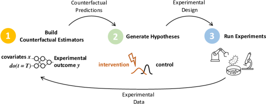
Figure 1: In the setting considered in this work, counterfactual estimators of experimental outcomes (step 1, left) are used to propose experimental hypotheses (step 2, center) for validation in in vitro experiments with genetic interventions (step 3, right), such as CRISPR knockouts, in order to discover potential causal associations between biological entities that could be relevant for the development of novel therapeutics. The trained counterfactual estimators can be used to direct the experimental search towards the space of biological interest, and thus more efficiently explore the vast space of genetic interventions. After every cycle, experimental data are generated that could lead to mechanistic scientific discoveries forming the basis for new therapeutics development, and guide subsequent experiment cycles with enhanced counterfactual estimators.

2 Related Work

Background. Drug discovery is a challenging endeavour with (i) historically low probabilities of successful development into clinical-stage therapeutics (Hay et al., 2014; Wong et al., 2019), and, for many decades until recently (Ringel et al., 2020), (ii) declining industry productivity commonly referred to as “Eroom’s law” (Scannell et al., 2012). Seminal studies by Nelson et al. (2015) and King et al. (2019) respectively first reported and later independently confirmed that the probability of clinical success of novel therapeutics increases up to three-fold if a medicine’s molecular target is substantiated by high-confidence causal evidence from genome-wide association studies (GWAS) Visscher et al. (2017). With the advent of molecular technologies for genetic perturbation, such as Clustered Regularly Interspaced Short Palindromic Repeats (CRISPR) (Jehuda et al., 2018), there now exist molecular tools for establishing causal evidence supporting the putative mechanism of a potential therapeutic hypothesis by means of in vitro experimentation beyond GWAS early on during the target identification and target validation stages of drug discovery (Rubin et al., 2019; Itokawa et al., 2016; Harrer et al., 2019; Vamathevan et al., 2019). Among other applications (Chen et al., 2018; Ekins et al., 2019; Mak & Pichika, 2019), machine learning methods, such as active and reinforcement learning, could potentially aid in discovering the molecular targets with the highest therapeutic potential faster.

Machine Learning for Drug Discovery. There exist a number of studies that proposed, advanced or evaluated the use of machine learning algorithms for drug discovery: Costa et al. (2010) used decision tree meta-classifier to identify genes associated with morbidity using protein-protein, metabolic, transcriptional, and sub-cellular interactions as input. Jeon et al. (2014) used a support vector machine (SVM) on protein expressions to predict target or non-target for breast pancreatic or ovarian cancers, and Ament et al. (2018) used least absolute shrinkage and selection operator (LASSO) regularised linear regression on transcription factor binding sites and transcriptome profiling to predict transcriptional changes associated with Huntington’s disease. In the domain of human muscle ageing, Mamoshina et al. (2018) used a SVM on deep features extracted from gene expression signatures in tissue samples from young and old subjects to discover molecular targets with putative involvement in muscle ageing. More recently, Stokes et al. (2020) utilised deep learning to discover Halicin as a repurposed molecule with antibiotic activity in mice.

Reinforcement and Active Learning. The use of deep reinforcement learning for de novo molecular design has been extensively studied (Olivecrona et al., 2017; Popova et al., 2018; Putin et al., 2018; Lim et al., 2018; Blaschke et al., 2020; Gottipati et al., 2020; Horwood & Noutahi, 2020). Active learning for de novo molecular design has seen less attention (Dixit et al., 2016; Green et al., 2020), however, active learning for causal inference has seen increasing application toward causal-effect estimation (Deng et al., 2011; Schwab et al., 2018; Sundin et al., 2019; Schwab et al., 2020; Bhattacharyya et al., 2020; Parbhoo et al., 2021; Qin et al., 2021; Jesson et al., 2021; Chau et al., 2021), and causal graph discovery (Ke et al., 2019; Tong & Koller, 2001; Murphy, 2001; Hauser & Bühlmann, 2014; Ghassami et al., 2018; Ness et al., 2017; Agrawal et al., 2019; Lorch et al., 2021; Annadani et al., 2021; Scherrer et al., 2021).

Benchmarks. Benchmark datasets play an important role in developing machine learning methodologies. Examples include ImageNet (Deng et al., 2009) or MSCOCO (Lin et al., 2014) for computer vision, as well as cart-pole (Barto et al., 1983) or reinforcement learning (Ahmed et al., 2020). Validation of active learning for causal inference methods depends largely on synthetic data experiments due to the difficulty or impossibility of obtaining real world counterfactual outcomes. For causal-effect active learning, real world data with synthetic outcomes such as IHDP (Hill, 2011) or ACIC2016 Dorie et al. (2019) are used. For active causal discovery, in silico data such as DREAM4 (Prill et al., 2011) or the gene regulatory networks proposed by Marbach et al. (2009) are used. Non synthetic data has been limited to protein signalling networks (Sachs et al., 2005) thus far. Most similar to our work is the benchmark for de novo molecular design of Brown et al. (2019).

In contrast to existing works, we develop an open benchmark to evaluate the use of machine learning for efficient experimental exploration in an iterative batch active learning setting. To the best of our knowledge, this is the first study (i) to introduce a curated open benchmark for the challenging task of biological discovery, and (ii) to comprehensively survey and evaluate state-of-the-art active learning algorithms in this setting.

3 Methodology

Problem Setting. We consider the setting in which we are given a dataset consisting of covariates $X\in\mathbb{R}^{p}$ with input feature dimensionality $p\in\mathbb{N}$ and treatment descriptors $T\in\mathbb{R}^{q}$ with treatment descriptor dimensionality $q\in\mathbb{N}^{+}$ that indicate similarity between interventions. Our aim is to estimate the expectation of the conditional distribution of an unseen counterfactual outcome $Y_{t}\in\mathbb{R}$ given observed covariates $X=x$ and intervention $do(T=t)$, $\hat{y}_{t}=\widehat{g}(X=x,do(T=t))\approx\mathbb{E}[Y\mid X=x,do(T=t)]$. This setting corresponds to the Rubin-Neyman potential outcomes framework (Rubin, 2005) adapted to the context of genetic interventions with a larger number of parametric interventions. In the context of a biological experiment with genetic interventions, $y_{t}$ is the experimental outcome relative to a non-interventional control (e.g., change in pro-inflammatory effect) that is measured upon perturbation of the cellular system with intervention $t$, $x$ is a descriptor of the properties of the model system and/or cell donor (e.g., the immuno-phenotype of the cell donor), and $t$ is a descriptor of the genetic intervention (e.g., a CRISPR knockout on gene STAT1) that indicates similarity to other genetic interventions that could potentially be applied. In general, certain ranges of $y_{t}$ may be preferable for further pursuit of an intervention $T=t$ that inhibits a given molecular target - often, but not necessarily always, larger absolute values that move the experimental result more are of higher mechanistic interest. We note that the use of an empty covariate vector $X=x_{0}$ with $p=0$ is permissible if all experiments are performed in the same model system with the same donor properties. In in vitro experimentation, the set of all possible genetic interventions $\mathcal{D}_{\textrm{pool}}=\{t_{i}\}_{i=1}^{n_{\textrm{pool}}}$ is typically known a-priori and of finite size (e.g., knockout interventions on all 20 000 protein-coding genes).

Batch Active Learning. In the considered setting, reading out additional values for yet unexplored interventions $t$ requires a lab experiment and can be costly and time-consuming. Lab experiments are typically conducted in parallelised manner, for example by performing a batch of multiple interventions at once in an experimental plate. Our overall aim is to leverage the counterfactual estimator $\widehat{g}$ trained on the available dataset to simulate future experiments with the aim of maximising an objective function $\mathcal{L}$ in the next iteration with as few interventions as possible. For the purpose of this benchmark, we consider the counterfactual mean squared error (MSE) of $\widehat{g}$ in predicting experimentally observed true outcomes $y_{t}$ from predicted outcomes $\hat{y}_{t}$ as the optimisation objective $\mathcal{L}_{\text{MSE}}=\text{MSE}(y_{t},\hat{y}_{t})$. Depending on context, other objective functions, such as for example maximising the number of discovered molecular targets with certain properties of interest (e.g., druggability (Keller et al., 2006)) may also be sensible in the context of biological exploration. At every time point, a new counterfactual estimator $\widehat{g}$ is trained with the entire available experimental dataset, and used to propose the batch of $b$ interventions to be explored in the next iteration with the batch size $b\in\mathbb{N}^{+}$. When using $\mathcal{L}_{\text{MSE}}$, this setting corresponds to batch active learning with the optimisation objective of maximally improving the counterfactual estimator $\widehat{g}$.

Acquisition Function. An acquisition function $\mathcal{D}^{k}=\alpha(g(t),\mathcal{D}^{k}_{\textrm{avail}})$ takes the model and the set of all available interventions $\mathcal{D}^{k}_{\textrm{avail}}$ in cycle $k$ as input and outputs the set of interventions $\mathcal{D}^{k}$ that are most informative after the $k$th experimental cycle with cycle index $k\in[K]=[0\mathrel{{.}\,{.}}\nobreak K]$ where $K\in\mathbb{N}^{+}$ is the maximum number of cycles that can be run. Formally speaking, the acquisition function $\alpha:\mathcal{P}({\mathcal{D}_{\textrm{avail}}})\times\mathcal{G}\to\mathcal{P}({\mathcal{D}_{\textrm{avail}}})$ takes a subset of all possible interventions that have not been tried so far ($\mathcal{D}_{\textrm{avail}}$), together with the trained model ($\widehat{g}$) derived from the cumulative data collected over the previous cycles, and outputs a subset of the available interventions $\mathcal{D}^{k}$ that are likely to be most useful under $\mathcal{L}$ to obtain $\widehat{g}\in\mathcal{G}$ as a better estimate of $\mathbb{E}[Y\mid X=x,do(T=t)]$ with $\mathcal{G}$ being the space of the models which can be, e.g. the space of models and (hyper-)parameters.

4 Datasets, Metrics & Baselines

The GeneDisco benchmark curates and standardizes two types of datasets: three standardized feature sets describing interventions $t$ (inputs to counterfactual estimators; Section 4.1), and four different in vitro genome-wide CRISPR experimental assays (predicted counterfactual outcomes; Section 4.2), each measuring a specific outcome $y_{t}$ following possible interventions $T$. We perform an extensive evaluation across these datasets, leveraging two different model types (Section 4.3) and nine different acquisition functions (Section 4.4). Since all curated assay datasets contained only outcomes for only one model system, we used the empty covariate set $X=x_{0}$ for all evaluated benchmark configurations. The metrics used to evaluate the various experimental conditions (acquisition functions and model types) include model performance (Figure 2) and the ratio of discovered interesting hits (Figure 3) as a function of number of samples queried.

4.1 Treatment Descriptors

The treatment descriptors $T$ characterize a genetic intervention and generally should correspond to data sources that are informative as to a genes’ functional similarity - i.e. defining which genes if acted upon, would potentially respond similarly to perturbation. Any dataset considered for use as a treatment descriptor must be available for all potentially available interventions $\mathcal{D}_{\textrm{pool}}$ in the considered experimental setting. In GeneDisco, we provide three standardised gene descriptor sets for genetic interventions, and furthermore enable users to provide custom treatment descriptors via a standardised programming interface:

Achilles. The Achilles project generated dependency scores across cancer cell lines by assaying 808 cell lines covering a broad range of tissue types and cancer types (Dempster et al., 2019). The genetic intervention effects are based on interventional CRISPR screens performed across the included cell lines. When using the Achilles treatment descriptors, each genetic intervention is summarized using a gene representation $T$ with $q=808$ corresponding to the dependency scores measured in each cell line. In Achilles, after processing and normalisation (see Dempster et al. (2019)), the final dependency scores provided are such that the median negative control (non-essential) gene effect for each cell line is 0, and the median positive control (essential) gene effect for each cell line is -1. The rationale for using treatment descriptors based on the Achilles dataset is that genetic effects measured across the various tissues and cancer types in the 808 cell line assays included in (Dempster et al., 2019) could serve as a similarity vector in functional space that may extrapolate to other biological contexts due to its breadth.

Search Tool for the Retrieval of Interacting Genes/Proteins (STRING) Network Embeddings. The STRING (Szklarczyk et al., 2021) database collates known and predicted protein-protein interactions (PPIs) for both physical as well as for functional associations. In order to derive a vector representation suitable to serve as a genetic intervention descriptor $T$, we utilised the network embeddings of the PPIs contained in STRING as provided by Cho et al. (2016; 2015) with dimensionality $q=799$. PPI network embeddings could be an informative descriptor of functional gene similarity since proteins that functionally interact with the same network partners may serve similar biological functions (Vazquez et al., 2003; Saha et al., 2014).

Cancer Cell Line Encyclopedia (CCLE). The CCLE (Nusinow et al., 2020) project collected quantitative proteomics data from thousands of proteins by mass spectrometry across 375 diverse cancer cell lines. The generated protein quantification profiles with dimensionality $q=420$ could indicate similarity of genetic interventions since similar expression profiles across a broad range of biological contexts may indicate functional similarity.

Custom Treatment Descriptors. Additional, user-defined treatment descriptors can be evaluated in GeneDisco by implementing the standardised dataset interface provided within.

4.2 Assays

As ground-truth interventional outcome datasets, we leverage various genome-wide CRISPR screens, primarily from the domain of immunology, that evaluated the causal effect of intervening on a large number of genes in cellular model systems in order to identify the genetic perturbations that induce a desired phenotype of interest.

4.2.1 Regulation of Human T cells proliferation

Experimental setting.

This assay is based on Shifrut et al. (2018). After isolating CD8${}^{+}$ T cells from human donors, Shifrut et al. (2018) performed a genome-wide loss-of-function screen to identify genes that impact the proliferation of T cells following stimulation with T cell receptors.

Measurement.

The measured outcome is the proliferation of T cells in response to T cell receptor stimulation. Cells were labeled before stimulation with CFSE (a fluorescent cell staining dye). Proliferation of cells is measured 4 days following stimulation by FACS sorting (a flow cytometry technique to sort cells based on their fluorescence).

Importance.

Human T cells play a central role in immunity and cancer immunotherapies. The identification of genes driving T cell proliferation could serve as the basis for new preclinical drug candidates or adoptive T cell therapies that help eliminate cancerous tumors.

4.2.2 Interleukin-2 production in primary human T cells

Experimental setting.

This dataset is based on a genome-wide CRISPR interference (CRISPRi) screen in primary human T cells to uncover the genes regulating the production of Interleukin-2 (IL-2). CRISPRi screens test for loss-of-function genes by reducing their expression levels. IL-2 is a cytokine produced by CD4${}^{+}$ T cells and is a major driver of T cell expansion during adaptive immune responses. Assays were performed on primary T cells from 2 different donors. The detailed experimental protocol is described in Schmidt et al. (2021).

Measurement.

Log fold change (high/low sorting bins) in IL-2 normalized read counts (averaged across the two donors). Sorting was done via flow cytometry after intracellular cytokine staining.

Importance.

IL-2 is central to several immunotherapies against cancer and autoimmunity.

4.2.3 Interferon-$\gamma$ production in primary human T cells

Experimental setting.

This data is also based on Schmidt et al. (2021), except that this experiment was performed to understand genes driving production of Interferon-$\gamma$ (IFN-$\gamma$). IFN-$\gamma$ is a cytokine produced by CD4${}^{+}$ and CD8${}^{+}$ T cells that induces additional T cells.

Measurement.

Log fold change (high/low sorting bins) in IFN-$\gamma$ normalized read counts (averaged across the two donors).

Importance.

IFN-$\gamma$ is critical to cancerous tumor killing and resistance to IFN-$\gamma$ is one escape mechanism for malignant cells.

4.2.4 Vulnerability of Leukemia cells to NK cells

Experimental setting.

This genome-wide CRISPR screen was performed in the K562 cell line to identify genes regulating the sensitivity of leukemia cells to cytotoxic activity of primary human NK cells. Detailed protocol is described in Zhuang et al. (2019).

Measurement.

Log fold counts of gRNAs in surviving K562 cells (after exposition to NK cells) compared to control (no exposition to NK cells). Gene scores are normalized fold changes for all gRNAs targeting this gene.

Importance.

Better understanding and control over the genes that drive the vulnerability of leukemia cells to NK cells will help improve anti-cancer treatment efficacy for leukemia patients, for example by preventing relapse during hematopoeitic stem cell transplantation.

4.3 Models

Parametric or non-parametric models can be used to model the conditional expected outcomes, $\mathbb{E}[Y\mid X=x,do(T=t)]$. Parametric models assume that the outcome $Y$ has density $f(y\mid t,\omega)$ conditioned on the intervention $t$ and the parameters of the model $\omega$ (we drop $x_{0}$ for compactness). A common assumption for continuous outcomes is a Gaussian distribution with density $f(y\mid t,\omega)=\mathcal{N}(y\mid\widehat{g}(t;\omega),\sigma^{2})$, which assumes that $y$ is a deterministic function of $\widehat{g}(t;\omega)$ with additive Gaussian noise scaled by $\sigma^{2}$. Bayesian methods treat the model parameters $\omega$ as instances of the random variable $\Omega\in\mathcal{W}$ and aim to model the posterior density of the parameters given the data, $f(\omega\mid\mathcal{D})$. For high-dimensional, large-sample data, such as we explore here, a variational approximation to the posterior is often used, $q(\omega\mid\mathcal{D})$ (MacKay, 1992; Hinton & Van Camp, 1993; Barber & Bishop, 1998; Gal & Ghahramani, 2016). In this work we use Bayesian Neural Networks (BNNs) to approximate the posterior over model parameters. A BNN gives $\widehat{g}^{k-1}(t)=\frac{1}{m}\sum_{j=1}^{m}\widehat{g}(t;\omega_{j}^{k-1})$, where $\widehat{g}(t;\omega_{j}^{k-1})$ is a unique functional estimator of $\mathbb{E}[Y\mid X=x,do(T=t)]$ induced by $\omega_{j}^{k-1}\sim q(\omega\mid\mathcal{D}^{k-1}_{\textrm{cum}})$: a sample from the approximate posterior over parameters given the cumulative data at acquisition step $k-1$. We also use non-parametric, non-Bayesian, Random Forest Regression (Breiman, 2001). A Random Forest gives $\widehat{g}^{k-1}(t)=\frac{1}{m}\sum_{j=1}^{m}\widehat{g}_{j}^{k-1}(t)$, where $\widehat{g}_{j}^{k-1}(t)$ is a unique functional estimator of $\mathbb{E}[Y\mid X=x,do(T=t)]$ indexed by the $j$th sample in the ensemble of $m$ trees trained on $\mathcal{D}^{k-1}_{\textrm{cum}})$. In the following, we will define our acquisition functions in terms of parametric models, but the definitions are easily adapted for non-parametric models as well.

4.4 Acquisition Functions

Random. As a baseline we look at random acquisition. Random acquisition at cycle $k$ can be seen as uniformly sampling data from $\mathcal{D}^{k}_{\textrm{avail}}$:

$$\alpha_{\textrm{Random}}(\widehat{g}^{k-1}(t),\mathcal{D}^{k}_{\textrm{avail}})=\{t_{1},\dots t_{b}\}\sim\left\{t_{i};\frac{1}{n_{\textrm{avail}}}\right\}_{i=1}^{n_{\textrm{avail}}}.$$ (1)

Here, the acquisition function samples $b$ elements without replacement from the set of $n_{\textrm{avail}}$ elements. The set element ($t_{i}$) is on the left of the semicolon, and the probability of the element being acquired ($\frac{1}{n_{\textrm{avail}}}$) is on the right of the semicolon. This convention will be used again below.

BADGE. BADGE looks to maximize the diversity of acquired samples, but, in contrast to Coreset, it additionally takes the uncertainty of the prediction into account (Ash et al., 2019). If the true label $y$ were observed, BADGE would proceed by maximizing the diversity of samples based on the gradient of the loss function $l$ with respect to the weights of the final layer of the most recently trained model $\tilde{w}^{k-1}$: $\frac{\partial}{\partial\tilde{\omega}^{k-1}}l(y,\widehat{g}(t;\omega))$. Intuitively, it asks how much would our parameters change if we observed the labeled outcome for this example? However, the true label $y$ is not yet observed. Ash et al. (2019) explore BADGE in the classification setting. For a two class problem, where $f(y\mid t,\omega)=\textrm{Bernoulli}(y\mid\widehat{g}(t;\omega))$, they propose using the class with the highest predicted probability, $\widehat{y}=\mathop{\mathrm{argmax}}_{y\in{0,1}}{f(y\mid t,\omega)}$, to approximate the gradient as $\frac{\partial}{\partial\tilde{\omega}^{k-1}}l(\widehat{y},\widehat{g}(t;\omega))$. This does not directly translate to the regression setting, as under our modelling assumptions the $y$ with the highest predicted likelihood corresponds exactly to $\widehat{g}(t;\omega)$, which would lead to a loss of zero, and gradients of zero. As a starting point, we instead take $\widehat{y}$ as a random sample from $f(y\mid t,\omega)=\mathcal{N}(y\mid\widehat{g}(t;\omega),\sigma^{2})$. We then use the same $k$-means++ algorithm as Ash et al. (2019) to approximate:

$$\begin{split}\alpha&{}_{\textrm{BADGE}}(\widehat{g}^{k-1}(t),\mathcal{D}^{k}_{\textrm{avail}})\\ &=\mathop{\mathrm{argmin}}_{\{t_{1},\dots t_{b}\}\in\mathcal{D}^{k}_{\textrm{avail}}}\mathop{\mathrm{argmax}}_{t_{i}\in\mathcal{D}^{k}_{\textrm{avail}}}\mathop{\mathrm{argmin}}_{t_{j}\in\mathcal{D}^{k}_{\textrm{avail}}\cup\mathcal{D}^{k-1}_{\textrm{cum}}}\Delta\left(\frac{\partial l(\widehat{y},\widehat{g}(t_{i};\omega^{k-1}))}{\partial\tilde{\omega}^{k-1}},\frac{\partial l(\widehat{y},\widehat{g}(t_{j};\omega^{k-1}))}{\partial\tilde{\omega}^{k-1}}\right)\end{split}$$ (2)

where $\Delta$ is again the Euclidean distance.

Bayesian Active Learning by Disagreement (BALD). Given an uncertainty aware model, such as a BNN or Random Forest we can now take an information theoretic approach to selecting interventions from the pool data. Houlsby et al. (2011) frame active learning as looking to maximize the information gain about the model parameters if we observe the outcome $Y=y$ given model inputs. Formally, the information gain is given by the mutual information between the random variables $Y$ and $\Omega$ given the intervention $t$ and acquired training data $\mathcal{D}^{k-1}_{\textrm{cum}}$ up until acquisition step $k$:

$$\begin{split}\mathcal{I}(Y;\Omega\mid t,\mathcal{D}^{k-1}_{\textrm{cum}})&=H(Y\mid t,\mathcal{D}^{k-1}_{\textrm{cum}})-H(Y\mid\Omega,t,\mathcal{D}^{k-1}_{\textrm{cum}})\\ &=H(Y\mid t,\mathcal{D}^{k-1}_{\textrm{cum}})-\mathbb{E}_{f(\omega\mid\mathcal{D}^{k-1}_{\textrm{cum}})}H(Y\mid\omega,t).\end{split}$$ (3)

Under the assumed model we have

$$\begin{split}\mathcal{I}(Y;\Omega\mid t,\mathcal{D}^{k-1}_{\textrm{cum}})&=\frac{1}{2}\log{\left(\frac{\sigma^{2}+\mathbb{E}_{f(\omega\mid\mathcal{D}^{k-1}_{\textrm{cum}})}\left[\widehat{g}(t;\omega)^{2}\right]-\mathbb{E}_{f(\omega\mid\mathcal{D}^{k-1}_{\textrm{cum}})}\left[\widehat{g}(t;\omega)\right]^{2}}{\sigma^{2}}\right)},\end{split}$$ (4)

which leads to the following estimator setting $\sigma^{2}=1$

$$\widehat{\mathcal{I}}(Y;\Omega\mid t,\mathcal{D}^{k-1}_{\textrm{cum}})=\frac{1}{2}\log{\left(1+\frac{1}{m}\sum_{j=1}^{m}\left(\widehat{g}(t;\omega_{j}^{k-1})-\frac{1}{m}\sum_{j=1}^{m}\widehat{g}(t;\omega_{j}^{k-1})\right)^{2}\right)}.$$ (5)

We look at two acquisition functions for BALD. First, we consider the naive batch acquisition $\alpha_{\textrm{BALD}}$ proposed by Gal et al. (2017) which acquires the the top $b$ examples from $\mathcal{D}^{k}_{\textrm{avail}}$:

$$\alpha_{\textrm{BALD}}(\widehat{g}^{k-1}(t),\mathcal{D}^{k}_{\textrm{avail}})=\mathop{\mathrm{argmax}}_{\{t_{1},\dots t_{b}\}\in\mathcal{D}^{k}_{\textrm{avail}}}\sum_{i=1}^{b}\widehat{\mathcal{I}}(Y;\Omega\mid t_{i},\mathcal{D}^{k-1}_{\textrm{cum}}).$$ (6)

This method will be referred to as topuncertain in the plots later. And second, we consider $\alpha_{\textrm{SoftBALD}}$ which randomly samples $b$ interventions from $\mathcal{D}^{k}_{\textrm{avail}}$ weighted by a tempered softmax function (Kirsch et al., 2021):

$$\alpha_{\textrm{SoftBALD}}(\widehat{g}^{k-1}(t),\mathcal{D}^{k}_{\textrm{avail}})=\{t_{1},\dots t_{b}\}\sim\left\{t_{i};\frac{\exp{\left(\frac{1}{\textrm{Temp}}\widehat{\mathcal{I}}(Y;\Omega\mid t_{i},\mathcal{D}^{k-1}_{\textrm{cum}})\right)}}{\sum_{l=1}^{n_{\textrm{avail}}}\exp{\left(\frac{1}{\textrm{Temp}}\widehat{\mathcal{I}}(Y;\Omega\mid t_{l},\mathcal{D}^{k-1}_{\textrm{cum}})\right)}}\right\}_{i=1}^{n_{\textrm{avail}}},$$ (7)

where $\textrm{Temp}>0$ is a user defined constant. This method will be referred to as softuncertain in the plots. As $\textrm{Temp}\to\infty$, $\alpha_{\textrm{SoftBALD}}$ will behave more like $\alpha_{\textrm{Random}}$. And as $\textrm{Temp}\to 0$, $\alpha_{\textrm{SoftBALD}}$ will behave more like $\alpha_{\textrm{BALD}}$. The remaining acquisition functions (Coreset, Margin Sample (Margin), Adversarial Basic Iteractive Method (AdvBIM), $k$-means Sampling (kmeansdata and kmeansembed)) included in the benchmark are described in detail in Appendix B.

5 Experimental Evaluation

Figure 2: The evaluation of the model trained with STRING treatment descriptors at each active learning cycle for 4 datasets and 3 acquisition batch sizes. In each plot, the x-axis is the active learning cycles multiplied by the acquisition bath size that gives the total number of data points collected so far. The y-axis is the test MSE error evaluated on the test data.

Figure 3: The hit ratio of different acquisition for BNN model, different target datasets, and different acquisition batch sizes. We use STRING treatment descriptors here. The x-axis shows the number of data points collected so far during the active learning cycles. The y-axis shows the ratio of the set of interesting genes that have been found by the acquisition function up until each cycle.

Setup. In order to assess current state-of-the-art methods on the GeneDisco benchmark, we perform an extensive baseline evaluation of 9 acquisition functions, 6 acquisition batch sizes and 4 experimental assays using in excess of 20 000 CPU hours of compute time. Due to the space limit, we include the results for 3 batch sizes in the main text and present the results for all batch sizes in the appendix. The employed counterfactual estimator $\hat{g}$ is a multi-layer perceptron (MLP) that has one hidden layer with ReLU activation and a linear output layer. The size of the hidden layer is determined at each active learning cycle by k-fold cross validation against $20\%$ of the acquired batch. At each cycle, the model is trained for at most 100 epochs but early stopping may interrupt training earlier if the validation error does not decrease. Each experiment is repeated with 5 random seeds to assess experimental variance. To choose the number of active learning cycles, we use the following strategy: the number of cycles are bounded to 40 for the acquisition batches of sizes 16, 32 and 64 due to the computational limits. For larger batch sizes, the number of cycles are reduced proportionally so that the same total number of data points are acquired throughout the cycles. At each cycle, the model is trained from scratch using the data collected up to that cycle, i.e. a trained model is not transferred to the future cycles. The test data is a random $20\%$ subset of the whole data that is left aside before the active learning process initiates, and is kept fixed across all experimental settings (i.e., for different datasets and different batch sizes) to enable a consistent comparison of the various acquisition functions, counterfactual estimator and treatment descriptor configurations.

Results. The model performance based on the STRING treatment descriptors for different acquisition functions, acquisition batch sizes and datasets are presented in Figure 2. The same metrics in the Achilles and CCLE treatment descriptors are provided in Appendix C. To showcase the effect of the model class, we additionally repeat the experiments using a random forest model as an uncertainty aware ensemble model with a reduced set of acquisition functions that are compatible with non-differentiable models (Appendix C). To investigate the types of genes chosen by different acquisition functions, we defined a subset of potentially interesting genes as the top $5\%$ with the largest absolute target value. These are the genes that could potentially be of therapeutic value due to their outsized causal influence on the phenotype of interest. The hit ratio out of the set of interesting genes chosen by different acquisition functions are presented in Figure 3 for the STRING treatment descriptors, and in Appendix C for Achilles and CCLE. Benchmark results of interest include that model-independent acquisition methods using diversity heuristics (random, kmeansdata) perform relatively better in terms of model improvement than acquisition functions based on model uncertainty (e.g., topuncertain, softuncertain) when using lower batch acquisition sizes than in regimes with larger batch acquisition sizes potentially due to diversity being inherently higher in larger batch acquisition regimes due to the larger set of included interventions in an intervention space with a limited amount of similar interventions. Notably, while diversity-focused, model-independent acquisition functions, such as random and kmeansdata, perform well in terms of model performance, they underperform in terms of interesting hits discovered as a function of acquired interventional samples (Figure 3). Based on these results, there appears to be a trade-off between model improvement and hit discovery in experimental exploration with counterfactual estimators that may warrant research into approaches to manage this trade-off to maximize long-term discovery rates.

6 Discussion and Conclusion

The ranking of acquisition functions in GeneDisco depends on several confounding factors, such as the choice of evaluation metric to compare different approaches, the characteristics of the dataset of interest, and the choice of the model class and its hyperparameters. An extrapolation of results obtained in GeneDisco to new settings may not be possible under significantly different experimental conditions. There is a subtle interplay between the predictive strength of the model and the acquisition function used to select the next set of interventions, as certain acquisition functions are more sensitive to the ability to the model to estimate its own epistemic uncertainty. From a practical standpoint, GeneDisco assumes the availability of a labeled set that is sufficiently representative to train and validate the different models required by the successive active learning cycles. However, model validation might be challenging when this set is small (e.g., during the early active learning cycles) or when the labelling process is noisy. Label noise is unfortunately common in interventional biological experiments, such as the ones considered in GeneDisco. Experimental noise introduces additional trade-offs for consideration in experimental design not considered in GeneDisco, such as choosing the optimal budget allocation between performing experiment replicates (technical and biological) to mitigate label noise or collecting more data points via additional active learning cycles.

GeneDisco addresses the current lack of standardised benchmarks for developing batch active learning methods for experimental design in drug discovery. GeneDisco consists of several curated datasets for experimental outcomes and genetic interventions, provides open source implementations of state-of-the-art acquisition functions for batch active learning, and includes a thorough assessment of these methods across a wide range of hyperparameter settings. We aim to attract the broader active learning community with an interest in causal inference by providing a robust and user-friendly benchmark that diversifies the benchmark repertoire over standard vision datasets. New models and acquisition functions for batch active learning in experimental design are of critical importance to realise the potential of machine learning for improving drug discovery. As future research, we aim to expand GeneDisco to enable multi-modal learning and support simultaneous optimization across multiple output phenotypes of interest.

Reproducibility Statement

This work introduces a new curated and standardized benchmark, GeneDisco, for batch active learning for drug discovery. The benchmark includes four publicly available datasets, which have previously been published in a peer review process. Using a total of more than 20,000 central processing unit (CPU) hours of compute time, we perform an extensive evaluation of state-of-the-art acquisition functions for batch active learning on the GeneDisco benchmark, across a wide range of hyperparameters. To the best of our knowledge, this is the first comprehensive survey and evaluation of active learning algorithms on real-world interventional genetic experiment data. Similar to developments in other fields e.g. for the learning of disentangled representations (Locatello et al., 2019) or generative adversarial networks (Lucic et al., 2017), we hope that our large scale experiments across a diverse set of real-world datasets provide an evidence basis to better understand the settings in which different active learning approaches work or do not work for drug discovery applications.

All used models and acquisition functions are described in detail and referenced in Section 4.4 and Section 4.3. For all introduced datasets, we include a detailed description and the details on the train, test and validation splits at the beginning of Section 5.

For all experimental results we report the range of hyper-parameters considered and the methods of selecting hyper-parameters as well as the exact number of training and evaluation runs (Appendix C). We additionally provide error bars over multiple random seeds and the code was executed on a cloud cluster with Intel CPUs. We provide detailed results for all investigated settings in the appendix (C).

Appendix A Notations

Here is the list of notations used in this manuscript.

• $\mathcal{D}_{\textrm{pool}}$: The pool of unlabeled data.

• $\mathcal{D}_{\textrm{acq}}^{k}$: Acquired data at $k$-th AL cycle.

• $\mathcal{D}_{\textrm{train}}^{k}$: Cumulative training data after $k$-th cycle of AL.

• $\mathcal{D}_{\textrm{val}}$: Validation data.

• $\mathcal{D}_{\textrm{test}}$: Held-out test data.

• $b$: Acquisition batch size.

• $K$: Total number of AL cycles.

• $k=[1,2,\ldots,K]$: Index of the AL cycle.

• $[K]=[1,2,\ldots,K]$.

• $e\in\mathcal{E}$: Inherent noise (aleatoric uncertainty).

• $T\in{\mathcal{T}}$: Treatment variable.

• $\mathbb{E}[Y\mid X=x,do(T=t)]$: The conditional expected outcomes.

• $\hat{g}(t;\omega)$: The model parameterised by $\omega\in\Omega$ to estimate $\mathbb{E}[Y\mid X=x,do(T=t)]$.

• $X$: random variable $X$ with distribution $X\sim F(X)$ and density $f(x)$.

Appendix B Acquisition Functions cont.

Coreset.

Coreset acquisition looks to maximize the diversity of acquired samples. This is done by finding the data points in $\mathcal{D}^{k}_{\textrm{avail}}$ that are furthest from the labelled data points in $\mathcal{D}^{k-1}_{\textrm{cum}}$. The robust K-centers algorithm of Sener & Savarese (2017) approximates a solution to:

$$\alpha_{\textrm{CORESET}}(\widehat{g}^{k-1}(t),\mathcal{D}^{k}_{\textrm{avail}})=\mathop{\mathrm{argmin}}_{\{t_{1},\dots t_{b}\}\in\mathcal{D}^{k}_{\textrm{avail}}}\mathop{\mathrm{argmax}}_{t_{i}\in\mathcal{D}^{k}_{\textrm{avail}}}\mathop{\mathrm{argmin}}_{t_{j}\in\mathcal{D}^{k}_{\textrm{avail}}\cup\mathcal{D}^{k-1}_{\textrm{cum}}}\Delta(t_{i},t_{j}).$$ (8)

Euclidean distances, $\Delta(t_{i},t_{j})$, are calculated between the output of the penultimate layer of $\widehat{g}(t;\omega)$.

Margin Sample.

Margin sampling is designed for classifiers where selection is based on the distance of a sample from the classifiers decision boundary (Roth & Small, 2006). As a proxy, the difference between the predicted probability of the most and second most probable classes is used. The distance between the most probable and the second most probable classes for a multi-class classification problem can be seen as how confident the model is about the label of that class. However, The concept of a decision boundary is ill-defined for regression tasks. One option to approximate margin sampling could be to model the aleatoric uncertainty of the model by predicting the conditional variance of the outcome $\sigma^{2}(t;\omega)$ and select data based on the magnitude of this value. Here, we instead look at the difference in the maximum and minimum values of the predicted outcome as a measure of the model’s confidence and select data based on the magnitude of this value. Formally, we have

$$\widehat{\mathcal{M}}(Y;\Omega\mid t_{i},\mathcal{D}^{k-1}_{\textrm{cum}})=\max_{j\in\{1,\dots m\}}(\widehat{g}(t;\omega_{j}^{k-1}))-\min_{j\in\{1,\dots m\}}(\widehat{g}(t;\omega_{j}^{k-1})),$$ (9)

and the acquisition function:

$$\alpha_{\textrm{Margin}}(\widehat{g}^{k-1}(t),\mathcal{D}^{k}_{\textrm{avail}})=\mathop{\mathrm{argmax}}_{\{t_{1},\dots t_{b}\}\in\mathcal{D}^{k}_{\textrm{avail}}}\sum_{i=1}^{b}\widehat{\mathcal{M}}(Y;\Omega\mid t_{i},\mathcal{D}^{k-1}_{\textrm{cum}}).$$ (10)

Note that this approximation is similar to BALD under the assumption of a uniformly distributed outcome: $f(y\mid t,\omega)=\mathcal{U}(y\mid\widehat{g}(t;\omega))$.

Adversarial Basic Iteractive Method (AdvBIM).

Some of the adversarial algorithms can act as active learning acquisition functions by nominating the adversarial samples. Here, we extended the famous Adversarial BIM method for our regression task as an example. BIM was introduced by (Kurakin et al., 2016) to iteratively perturb adversarial samples to maximize the cost function $J$ subject to an $l_{p}$ norm constraint as

$$\hat{t}^{(0)}=t,\hat{t}^{(i)}=\text{clip}_{t,e}(\hat{t}^{(i-1)}+\text{sign}(\nabla_{\hat{t}^{(i-1)}}J(\theta,\hat{t}^{(i-1)},y)))$$ (11)

(intermediate results are clipped to stay in $e$-neighbourhood of the primary data point $t$). This technique bypasses the intractable problem of finding the distance from the decision boundary by iteratively perturbing the features until crossing the boundary (Tramèr et al., 2017). In our regression task, we perturb the features in the gradients’ direction to increase the conditional variance of the outcome, i.e.,

$$\hat{t}^{(0)}=t,\hat{t}^{(i)}=\text{clip}_{t,e}(\hat{t}^{(i-1)}+\text{sign}(\nabla_{\hat{t}^{(i-1)}}\textrm{Var}_{\omega}(\hat{g}(t,\omega))))\text{ for $i=\{1,\dots,m\}$},$$ (12)

where $||\hat{t}_{i}-t||_{2}<\gamma*||t||_{2}$ with the hyperparameter $\gamma$. After creating adversarial samples for each data point in $D_{\textrm{avail}}^{k}$, $\alpha_{\textrm{AdversarialBIM}}$ acquires the samples by

$$\alpha_{\textrm{AdversarialBIM}}(\widehat{g}^{k-1}(t),\mathcal{D}^{k}_{\textrm{avail}})=\bigcup_{t_{i}\in\mathcal{D}^{k}_{\textrm{avail}}}\mathop{\mathrm{argmin}}_{t_{j}\in\mathcal{D}^{k}_{\textrm{avail}}}\Delta(\hat{t}^{(m)}_{i},t_{j}),$$ (13)

where $\Delta$ is the euclidean distance.

$k$-means Sampling.

This method nominates samples by returning the closest sample to each center of the unlabeled data clusters. In order to do so, one may run Kmeans++ clustering algorithm with the number of clusters equal to $b$ over either the unlabeled data points $D_{\textrm{avail}}^{k}$ or the output of the penultimate layer of $\widehat{g}(t;\omega)$. We refer to the former as kmeansdata and to the latter as kmeansembed in the experiments. Assuming $\{\mu_{1},\dots,\mu_{b}\}$ are the centers of the clustering, we have

$$\alpha_{\textrm{Kmeans}}(\widehat{g}^{k-1}(t),\mathcal{D}^{k}_{\textrm{avail}})=\bigcup_{i=1}^{b}\mathop{\mathrm{argmin}}_{t_{j}\in\mathcal{D}^{k}_{\textrm{avail}}}\Delta(\mu_{i},t_{j}),$$ (14)

where $\Delta$ is euclidean distance over the data points or the penultimate layer of $\widehat{g}(t;\omega)$.

Appendix C Detailed experimental results

C.1 Bayesian Neural Network (BNN) Model

We provide here detailed experimental results across all hyperparameter settings. The result of fig. 2 that was presented for 3 batch sizes are provided for 6 batch sizes in fig. 4. Similarly, the results of fig. 3 are provided for additional batch sizes in LABEL:fig:hitratio_bnn_feat_string_alldatasets_allbathcsizes. In addition, both fig. 2 and fig. 3 report the results for the STRING treatment descriptors. All experiments are repeated for two other sets of input treatment descriptors (Achilles and CCLE) whose results are provided in figs. 5, LABEL:fig:bnn_feat_ccle_alldatasets_allbathcsizes, LABEL:fig:hitratio_bnn_feat_achilles_alldatasets_allbathcsizes and LABEL:fig:hitratio_bnn_feat_ccle_alldatasets_allbathcsizes.

C.2 Random Forest Model

In addition to the BNN model, we carried out thorough analyses for a different model class. The experiments are repeated for the random forest as an uncertainty aware ensemble model. The uncertainty in random forests, similar to other ensemble methods, is originated from the prediction made by each model instance in the ensemble. We use the random forest implementation in the Scikit-learn package (Pedregosa et al., 2011) with 100 trees and set the option max_depth=None so that the depth of the trees are determined automatically. The performance of the model trained over the active learning cycles can be seen in LABEL:fig:rf_feat_string_alldatasets_allbathcsizes for different acquisition functions, different batch sizes, different target datasets, and the STRING treatment descriptors. Similarly, the hit ratio of the interesting genes for a random forest model is reported in LABEL:fig:hitratio_rf_feat_string_alldatasets_allbathcsizes. The same experiment was repeated for CCLE treatment descriptors whose results are provided in LABEL:fig:rf_feat_ccle_alldatasets_allbathcsizes and LABEL:fig:hitratio_rf_feat_ccle_alldatasets_allbathcsizes. Notice that random forest experiments are done with a reduced set of acquisition functions that could be adjusted to the random forest model.

C.3 In-depth Description of the Hit Ratio Experiment

Here we elaborate more on the purpose and the message of the hit ratio experiment whose results are reported in LABEL:fig:hitratio_bnn_feat_string_alldatasets_allbathcsizes, LABEL:fig:hitratio_bnn_feat_achilles_alldatasets_allbathcsizes, LABEL:fig:hitratio_bnn_feat_ccle_alldatasets_allbathcsizes, LABEL:fig:hitratio_rf_feat_string_alldatasets_allbathcsizes and LABEL:fig:hitratio_rf_feat_ccle_alldatasets_allbathcsizes for various settings. The purpose of these experiments is to compare the performance of different acquisition functions in different settings of batch sizes and input/output datasets to hit the gene targets that are known to be interesting by genomics experts. To choose the set of interesting genes, we sort them based on their absolute target values. Then we choose the top $5\%$ of this list that corresponds to both extremes of positive and negative values (both extremes are considered to be good targets by experts.) The experiments are repeated for 5 different random seeds to obtain the error bars.

Figure 4: The evaluation of the model trained with STRING treatment descriptors at each active learning cycle for 4 datasets and 6 acquisition batch sizes. In each plot, the x-axis is the active learning cycles multiplied by the acquisition bath size that gives the total number of data points collected so far. The y-axis is the test MSE error evaluated on the test data.

Figure 5: The evaluation of the model trained with Achilles treatment descriptors at each active learning cycle for 4 datasets and 6 acquisition batch sizes. In each plot, the x-axis is the active learning cycles multiplied by the acquisition bath size that gives the total number of data points collected so far. The y-axis is the test MSE error evaluated on the test data.

References

- Agrawal et al. (2019) Raj Agrawal, Chandler Squires, Karren Yang, Karthikeyan Shanmugam, and Caroline Uhler. Abcd-strategy: Budgeted experimental design for targeted causal structure discovery. In The 22nd International Conference on Artificial Intelligence and Statistics, pp. 3400–3409. PMLR, 2019.
- Ahmed et al. (2020) Ossama Ahmed, Frederik Träuble, Anirudh Goyal, Alexander Neitz, Yoshua Bengio, Bernhard Schölkopf, Manuel Wüthrich, and Stefan Bauer. Causalworld: A robotic manipulation benchmark for causal structure and transfer learning. arXiv preprint arXiv:2010.04296, 2020.
- Ament et al. (2018) Seth A Ament, Jocelynn R Pearl, Jeffrey P Cantle, Robert M Bragg, Peter J Skene, Sydney R Coffey, Dani E Bergey, Vanessa C Wheeler, Marcy E MacDonald, Nitin S Baliga, et al. Transcriptional regulatory networks underlying gene expression changes in huntington’s disease. Molecular Systems Biology, 14(3):e7435, 2018.
- Annadani et al. (2021) Yashas Annadani, Jonas Rothfuss, Alexandre Lacoste, Nino Scherrer, Anirudh Goyal, Yoshua Bengio, and Stefan Bauer. Variational causal networks: Approximate bayesian inference over causal structures. arXiv preprint arXiv:2106.07635, 2021.
- Ash et al. (2019) Jordan T Ash, Chicheng Zhang, Akshay Krishnamurthy, John Langford, and Alekh Agarwal. Deep batch active learning by diverse, uncertain gradient lower bounds. arXiv preprint arXiv:1906.03671, 2019.
- Barber & Bishop (1998) David Barber and Christopher M Bishop. Ensemble learning in bayesian neural networks. Nato ASI Series F Computer and Systems Sciences, 168:215–238, 1998.
- Barto et al. (1983) Andrew G Barto, Richard S Sutton, and Charles W Anderson. Neuronlike adaptive elements that can solve difficult learning control problems. IEEE Transactions on Systems, Man, and Cybernetics, (5):834–846, 1983.
- Berdigaliyev & Aljofan (2020) Nurken Berdigaliyev and Mohamad Aljofan. An overview of drug discovery and development. Future Medicinal Chemistry, 12(10):939–947, 2020.
- Bhattacharyya et al. (2020) Arnab Bhattacharyya, Sutanu Gayen, Saravanan Kandasamy, Ashwin Maran, and Vinodchandran N Variyam. Learning and sampling of atomic interventions from observations. In International Conference on Machine Learning, pp. 842–853. PMLR, 2020.
- Blaschke et al. (2020) Thomas Blaschke, Ola Engkvist, Jürgen Bajorath, and Hongming Chen. Memory-assisted reinforcement learning for diverse molecular de novo design. Journal of Cheminformatics, 12(1):1–17, 2020.
- Breiman (2001) Leo Breiman. Random forests. Machine Learning, 45(1):5–32, 2001.
- Brown et al. (2019) Nathan Brown, Marco Fiscato, Marwin HS Segler, and Alain C Vaucher. Guacamol: benchmarking models for de novo molecular design. Journal of chemical information and modeling, 59(3):1096–1108, 2019.
- Chappell et al. (2018) Lia Chappell, Andrew JC Russell, and Thierry Voet. Single-cell (multi) omics technologies. Annual Review of Genomics and Human Genetics, 19:15–41, 2018.
- Chau et al. (2021) Siu Lun Chau, Jean-François Ton, Javier González, Yee Whye Teh, and Dino Sejdinovic. Bayesimp: Uncertainty quantification for causal data fusion. arXiv preprint arXiv:2106.03477, 2021.
- Chen et al. (2018) Hongming Chen, Ola Engkvist, Yinhai Wang, Marcus Olivecrona, and Thomas Blaschke. The rise of deep learning in drug discovery. Drug Discovery Today, 23(6):1241–1250, 2018.
- Cho et al. (2015) Hyunghoon Cho, Bonnie Berger, and Jian Peng. Diffusion component analysis: unraveling functional topology in biological networks. In International Conference on Research in Computational Molecular Biology, pp. 62–64. Springer, 2015.
- Cho et al. (2016) Hyunghoon Cho, Bonnie Berger, and Jian Peng. Compact integration of multi-network topology for functional analysis of genes. Cell Systems, 3(6):540–548, 2016.
- Costa et al. (2010) Pedro R Costa, Marcio L Acencio, and Ney Lemke. A machine learning approach for genome-wide prediction of morbid and druggable human genes based on systems-level data. In BMC Genomics, volume 11, pp. 1–15. Springer, 2010.
- Dempster et al. (2019) Joshua M. Dempster, Jordan Rossen, Mariya Kazachkova, Joshua Pan, Guillaume Kugener, David E. Root, and Aviad Tsherniak. Extracting biological insights from the project achilles genome-scale crispr screens in cancer cell lines. bioRxiv, 2019. doi: 10.1101/720243. URL https://www.biorxiv.org/content/early/2019/07/31/720243.
- Deng et al. (2009) Jia Deng, Wei Dong, Richard Socher, Li-Jia Li, Kai Li, and Li Fei-Fei. Imagenet: A large-scale hierarchical image database. In IEEE Conference on Computer Vision and Pattern Recognition, pp. 248–255. Ieee, 2009.
- Deng et al. (2011) Kun Deng, Joelle Pineau, and Susan Murphy. Active learning for personalizing treatment. In 2011 IEEE Symposium on Adaptive Dynamic Programming and Reinforcement Learning (ADPRL), pp. 32–39. IEEE, 2011.
- Dickson & Gagnon (2004) Michael Dickson and Jean Paul Gagnon. Key factors in the rising cost of new drug discovery and development. Nature Reviews Drug Discovery, 3(5):417–429, 2004.
- Dickson & Gagnon (2009) Michael Dickson and Jean Paul Gagnon. The cost of new drug discovery and development. Discovery Medicine, 4(22):172–179, 2009.
- DiMasi et al. (2016) Joseph A DiMasi, Henry G Grabowski, and Ronald W Hansen. Innovation in the pharmaceutical industry: new estimates of r&d costs. Journal of Health Economics, 47:20–33, 2016.
- Dixit et al. (2016) Atray Dixit, Oren Parnas, Biyu Li, Jenny Chen, Charles P Fulco, Livnat Jerby-Arnon, Nemanja D Marjanovic, Danielle Dionne, Tyler Burks, Raktima Raychowdhury, et al. Perturb-seq: dissecting molecular circuits with scalable single-cell rna profiling of pooled genetic screens. Cell, 167(7):1853–1866, 2016.
- Dorie et al. (2019) Vincent Dorie, Jennifer Hill, Uri Shalit, Marc Scott, and Dan Cervone. Automated versus do-it-yourself methods for causal inference: Lessons learned from a data analysis competition. Statistical Science, 34(1):43–68, 2019.
- Ekins et al. (2019) Sean Ekins, Ana C Puhl, Kimberley M Zorn, Thomas R Lane, Daniel P Russo, Jennifer J Klein, Anthony J Hickey, and Alex M Clark. Exploiting machine learning for end-to-end drug discovery and development. Nature Materials, 18(5):435–441, 2019.
- Gal & Ghahramani (2016) Yarin Gal and Zoubin Ghahramani. Dropout as a bayesian approximation: Representing model uncertainty in deep learning. In International Conference on Machine Learning, pp. 1050–1059, 2016.
- Gal et al. (2017) Yarin Gal, Riashat Islam, and Zoubin Ghahramani. Deep bayesian active learning with image data. In International Conference on Machine Learning, pp. 1183–1192. PMLR, 2017.
- Ghassami et al. (2018) AmirEmad Ghassami, Saber Salehkaleybar, Negar Kiyavash, and Elias Bareinboim. Budgeted experiment design for causal structure learning. In International Conference on Machine Learning, pp. 1724–1733. PMLR, 2018.
- Gottipati et al. (2020) Sai Krishna Gottipati, Boris Sattarov, Sufeng Niu, Yashaswi Pathak, Haoran Wei, Shengchao Liu, Simon Blackburn, Karam Thomas, Connor Coley, Jian Tang, et al. Learning to navigate the synthetically accessible chemical space using reinforcement learning. In International Conference on Machine Learning, pp. 3668–3679. PMLR, 2020.
- Green et al. (2020) Darren VS Green, Stephen Pickett, Chris Luscombe, Stefan Senger, David Marcus, Jamel Meslamani, David Brett, Adam Powell, and Jonathan Masson. Bradshaw: a system for automated molecular design. Journal of Computer-aided Molecular Design, 34(7):747–765, 2020.
- Harrer et al. (2019) Stefan Harrer, Pratik Shah, Bhavna Antony, and Jianying Hu. Artificial intelligence for clinical trial design. Trends in Pharmacological Sciences, 40(8):577–591, 2019.
- Hasin et al. (2017) Yehudit Hasin, Marcus Seldin, and Aldons Lusis. Multi-omics approaches to disease. Genome Biology, 18(1):1–15, 2017.
- Hauser & Bühlmann (2014) Alain Hauser and Peter Bühlmann. Two optimal strategies for active learning of causal models from interventional data. International Journal of Approximate Reasoning, 55(4):926–939, 2014.
- Hay et al. (2014) Michael Hay, David W Thomas, John L Craighead, Celia Economides, and Jesse Rosenthal. Clinical development success rates for investigational drugs. Nature Biotechnology, 32(1):40–51, 2014.
- Hill (2011) Jennifer L Hill. Bayesian nonparametric modeling for causal inference. Journal of Computational and Graphical Statistics, 20(1):217–240, 2011.
- Hinton & Van Camp (1993) Geoffrey E Hinton and Drew Van Camp. Keeping the neural networks simple by minimizing the description length of the weights. In Proceedings of the Sixth Annual Conference on Computational Learning Theory, pp. 5–13, 1993.
- Horwood & Noutahi (2020) Julien Horwood and Emmanuel Noutahi. Molecular design in synthetically accessible chemical space via deep reinforcement learning. ACS omega, 5(51):32984–32994, 2020.
- Houlsby et al. (2011) Neil Houlsby, Ferenc Huszár, Zoubin Ghahramani, and Máté Lengyel. Bayesian active learning for classification and preference learning. arXiv preprint arXiv:1112.5745, 2011.
- informa PLC (2018) informa PLC. Pharma R&D Annual Review 2018. 2018. Accessed: 2021-10-03.
- Itokawa et al. (2016) Kentaro Itokawa, Osamu Komagata, Shinji Kasai, Kohei Ogawa, and Takashi Tomita. Testing the causality between cyp9m10 and pyrethroid resistance using the talen and crispr/cas9 technologies. Scientific Reports, 6(1):1–10, 2016.
- Jehuda et al. (2018) Ronen Ben Jehuda, Yuval Shemer, and Ofer Binah. Genome editing in induced pluripotent stem cells using crispr/cas9. Stem Cell Reviews and Reports, 14(3):323–336, 2018.
- Jeon et al. (2014) Jouhyun Jeon, Satra Nim, Joan Teyra, Alessandro Datti, Jeffrey L Wrana, Sachdev S Sidhu, Jason Moffat, and Philip M Kim. A systematic approach to identify novel cancer drug targets using machine learning, inhibitor design and high-throughput screening. Genome Medicine, 6(7):1–18, 2014.
- Jesson et al. (2021) Andrew Jesson, Panagiotis Tigas, Joost van Amersfoort, Andreas Kirsch, Uri Shalit, and Yarin Gal. Causal-bald: Deep bayesian active learning of outcomes to infer treatment-effects from observational data. Advances in Neural Information Processing Systems, 34, 2021.
- Ke et al. (2019) Nan Rosemary Ke, Olexa Bilaniuk, Anirudh Goyal, Stefan Bauer, Hugo Larochelle, Bernhard Schölkopf, Michael C Mozer, Chris Pal, and Yoshua Bengio. Learning neural causal models from unknown interventions. arXiv preprint arXiv:1910.01075, 2019.
- Keller et al. (2006) Thomas H Keller, Arkadius Pichota, and Zheng Yin. A practical view of ‘druggability’. Current Opinion in Chemical Biology, 10(4):357–361, 2006.
- King et al. (2019) Emily A King, J Wade Davis, and Jacob F Degner. Are drug targets with genetic support twice as likely to be approved? revised estimates of the impact of genetic support for drug mechanisms on the probability of drug approval. PLoS Genetics, 15(12):e1008489, 2019.
- Kirsch et al. (2021) Andreas Kirsch, Sebastian Farquhar, and Yarin Gal. A simple baseline for batch active learning with stochastic acquisition functions, 2021.
- Kurakin et al. (2016) Alexey Kurakin, Ian Goodfellow, Samy Bengio, et al. Adversarial examples in the physical world, 2016.
- Lim et al. (2018) Jaechang Lim, Seongok Ryu, Jin Woo Kim, and Woo Youn Kim. Molecular generative model based on conditional variational autoencoder for de novo molecular design. Journal of Cheminformatics, 10(1):1–9, 2018.
- Lin et al. (2014) Tsung-Yi Lin, Michael Maire, Serge Belongie, James Hays, Pietro Perona, Deva Ramanan, Piotr Dollár, and C Lawrence Zitnick. Microsoft coco: Common objects in context. In European Conference on Computer Vision, pp. 740–755. Springer, 2014.
- Locatello et al. (2019) Francesco Locatello, Stefan Bauer, Mario Lucic, Gunnar Raetsch, Sylvain Gelly, Bernhard Schölkopf, and Olivier Bachem. Challenging common assumptions in the unsupervised learning of disentangled representations. In international conference on machine learning, pp. 4114–4124. PMLR, 2019.
- Lorch et al. (2021) Lars Lorch, Jonas Rothfuss, Bernhard Schölkopf, and Andreas Krause. Dibs: Differentiable bayesian structure learning. arXiv preprint arXiv:2105.11839, 2021.
- Lucic et al. (2017) Mario Lucic, Karol Kurach, Marcin Michalski, Sylvain Gelly, and Olivier Bousquet. Are gans created equal? a large-scale study. arXiv preprint arXiv:1711.10337, 2017.
- MacKay (1992) David JC MacKay. A practical bayesian framework for backpropagation networks. Neural Computation, 4(3):448–472, 1992.
- MacLean et al. (2018) Adam L. MacLean, Tian Hong, and Qing Nie. Exploring intermediate cell states through the lens of single cells. Current Opinion in Systems Biology, 9:32–41, 2018. ISSN 2452-3100. doi: https://doi.org/10.1016/j.coisb.2018.02.009. URL https://www.sciencedirect.com/science/article/pii/S2452310017302238. Mathematic Modelling.
- Mak & Pichika (2019) Kit-Kay Mak and Mallikarjuna Rao Pichika. Artificial intelligence in drug development: present status and future prospects. Drug Discovery Today, 24(3):773–780, 2019.
- Mamoshina et al. (2018) Polina Mamoshina, Marina Volosnikova, Ivan V Ozerov, Evgeny Putin, Ekaterina Skibina, Franco Cortese, and Alex Zhavoronkov. Machine learning on human muscle transcriptomic data for biomarker discovery and tissue-specific drug target identification. Frontiers in Genetics, 9:242, 2018.
- Marbach et al. (2009) Daniel Marbach, Thomas Schaffter, Claudio Mattiussi, and Dario Floreano. Generating realistic in silico gene networks for performance assessment of reverse engineering methods. Journal of Computational Biology, 16(2):229–239, 2009.
- Murphy (2001) Kevin P Murphy. Active learning of causal bayes net structure. 2001.
- Nelson et al. (2015) Matthew R Nelson, Hannah Tipney, Jeffery L Painter, Judong Shen, Paola Nicoletti, Yufeng Shen, Aris Floratos, Pak Chung Sham, Mulin Jun Li, Junwen Wang, et al. The support of human genetic evidence for approved drug indications. Nature Genetics, 47(8):856–860, 2015.
- Ness et al. (2017) Robert Osazuwa Ness, Karen Sachs, Parag Mallick, and Olga Vitek. A bayesian active learning experimental design for inferring signaling networks. In International Conference on Research in Computational Molecular Biology, pp. 134–156. Springer, 2017.
- Nusinow et al. (2020) David P Nusinow, John Szpyt, Mahmoud Ghandi, Christopher M Rose, E Robert McDonald III, Marian Kalocsay, Judit Jané-Valbuena, Ellen Gelfand, Devin K Schweppe, Mark Jedrychowski, et al. Quantitative proteomics of the cancer cell line encyclopedia. Cell, 180(2):387–402, 2020.
- Olivecrona et al. (2017) Marcus Olivecrona, Thomas Blaschke, Ola Engkvist, and Hongming Chen. Molecular de-novo design through deep reinforcement learning. Journal of Cheminformatics, 9(1):1–14, 2017.
- Parbhoo et al. (2021) Sonali Parbhoo, Stefan Bauer, and Patrick Schwab. NCoRE: Neural Counterfactual Representation Learning for Combinations of Treatments. arXiv preprint arXiv:2103.11175, 2021.
- Pedregosa et al. (2011) F. Pedregosa, G. Varoquaux, A. Gramfort, V. Michel, B. Thirion, O. Grisel, M. Blondel, P. Prettenhofer, R. Weiss, V. Dubourg, J. Vanderplas, A. Passos, D. Cournapeau, M. Brucher, M. Perrot, and E. Duchesnay. Scikit-learn: Machine learning in Python. Journal of Machine Learning Research, 12:2825–2830, 2011.
- Pertea et al. (2018) Mihaela Pertea, Alaina Shumate, Geo Pertea, Ales Varabyou, Florian P Breitwieser, Yu-Chi Chang, Anil K Madugundu, Akhilesh Pandey, and Steven L Salzberg. Chess: a new human gene catalog curated from thousands of large-scale rna sequencing experiments reveals extensive transcriptional noise. Genome Biology, 19(1):1–14, 2018.
- Popova et al. (2018) Mariya Popova, Olexandr Isayev, and Alexander Tropsha. Deep reinforcement learning for de novo drug design. Science Advances, 4(7):eaap7885, 2018.
- Prill et al. (2011) Robert Prill, Julio Saez-Rodriguez, Leonidas Alexopoulos, Peter Sorger, and Gustavo Stolovitzky. Crowdsourcing network inference: The dream predictive signaling network challenge. Science Signaling, 4:mr7, 09 2011. doi: 10.1126/scisignal.2002212.
- Putin et al. (2018) Evgeny Putin, Arip Asadulaev, Yan Ivanenkov, Vladimir Aladinskiy, Benjamin Sanchez-Lengeling, Alán Aspuru-Guzik, and Alex Zhavoronkov. Reinforced adversarial neural computer for de novo molecular design. Journal of Chemical Information and Modeling, 58(6):1194–1204, 2018.
- Qin et al. (2021) Tian Qin, Tian-Zuo Wang, and Zhi-Hua Zhou. Budgeted heterogeneous treatment effect estimation. In Marina Meila and Tong Zhang (eds.), Proceedings of the 38th International Conference on Machine Learning, volume 139 of Proceedings of Machine Learning Research, pp. 8693–8702. PMLR, 18–24 Jul 2021. URL https://proceedings.mlr.press/v139/qin21b.html.
- Rawlins (2004) Michael D Rawlins. Cutting the cost of drug development? Nature Reviews Drug Discovery, 3(4):360–364, 2004.
- Ringel et al. (2020) Michael S Ringel, Jack W Scannell, Mathias Baedeker, and Ulrik Schulze. Breaking eroom’s law. Nature Reviews Drug Discovery, 2020.
- Roth & Small (2006) Dan Roth and Kevin Small. Margin-based active learning for structured output spaces. In European Conference on Machine Learning, pp. 413–424. Springer, 2006.
- Rubin et al. (2019) Adam J Rubin, Kevin R Parker, Ansuman T Satpathy, Yanyan Qi, Beijing Wu, Alvin J Ong, Maxwell R Mumbach, Andrew L Ji, Daniel S Kim, Seung Woo Cho, et al. Coupled single-cell crispr screening and epigenomic profiling reveals causal gene regulatory networks. Cell, 176(1-2):361–376, 2019.
- Rubin (2005) Donald B Rubin. Causal inference using potential outcomes: Design, modeling, decisions. Journal of the American Statistical Association, 100(469):322–331, 2005.
- Sachs et al. (2005) Karen Sachs, Omar Perez, Dana Pe’er, Douglas A Lauffenburger, and Garry P Nolan. Causal protein-signaling networks derived from multiparameter single-cell data. Science, 308(5721):523–529, 2005.
- Saha et al. (2014) Sovan Saha, Piyali Chatterjee, Subhadip Basu, Mahantapas Kundu, and Mita Nasipuri. Funpred-1: Protein function prediction from a protein interaction network using neighborhood analysis. Cellular and Molecular Biology Letters, 19(4):675–691, 2014.
- Scannell et al. (2012) Jack W Scannell, Alex Blanckley, Helen Boldon, and Brian Warrington. Diagnosing the decline in pharmaceutical r&d efficiency. Nature Reviews Drug Discovery, 11(3):191–200, 2012.
- Scherrer et al. (2021) Nino Scherrer, Olexa Bilaniuk, Yashas Annadani, Anirudh Goyal, Patrick Schwab, Bernhard Schölkopf, Michael C Mozer, Yoshua Bengio, Stefan Bauer, and Nan Rosemary Ke. Learning neural causal models with active interventions. arXiv preprint arXiv:2109.02429, 2021.
- Schmidt et al. (2021) Ralf Schmidt, Zachary Steinhart, Madeline Layeghi, Jacob W. Freimer, Vinh Q. Nguyen, Franziska Blaeschke, and Alexander Marson. Crispr activation and interference screens in primary human t cells decode cytokine regulation. bioRxiv, 2021. doi: 10.1101/2021.05.11.443701. URL https://www.biorxiv.org/content/early/2021/05/12/2021.05.11.443701.
- Schwab et al. (2018) Patrick Schwab, Lorenz Linhardt, and Walter Karlen. Perfect Match: A Simple Method for Learning Representations For Counterfactual Inference With Neural Networks. arXiv preprint arXiv:1810.00656, 2018.
- Schwab et al. (2020) Patrick Schwab, Lorenz Linhardt, Stefan Bauer, Joachim M Buhmann, and Walter Karlen. Learning Counterfactual Representations for Estimating Individual Dose-Response Curves. In AAAI Conference on Artificial Intelligence, 2020.
- Sener & Savarese (2017) Ozan Sener and Silvio Savarese. Active learning for convolutional neural networks: A core-set approach. arXiv preprint arXiv:1708.00489, 2017.
- Shifrut et al. (2018) Eric Shifrut, Julia Carnevale, Victoria Tobin, Theodore L. Roth, Jonathan M. Woo, Christina T. Bui, P. Jonathan Li, Morgan E. Diolaiti, Alan Ashworth, and Alexander Marson. Genome-wide crispr screens in primary human t cells reveal key regulators of immune function. Cell, 175(7):1958–1971.e15, 2018. ISSN 0092-8674. doi: https://doi.org/10.1016/j.cell.2018.10.024. URL https://www.sciencedirect.com/science/article/pii/S0092867418313333.
- Stokes et al. (2020) Jonathan M Stokes, Kevin Yang, Kyle Swanson, Wengong Jin, Andres Cubillos-Ruiz, Nina M Donghia, Craig R MacNair, Shawn French, Lindsey A Carfrae, Zohar Bloom-Ackermann, et al. A deep learning approach to antibiotic discovery. Cell, 180(4):688–702, 2020.
- Sundin et al. (2019) Iiris Sundin, Peter Schulam, Eero Siivola, Aki Vehtari, Suchi Saria, and Samuel Kaski. Active learning for decision-making from imbalanced observational data. In International Conference on Machine Learning, pp. 6046–6055. PMLR, 2019.
- Szklarczyk et al. (2021) Damian Szklarczyk, Annika L Gable, Katerina C Nastou, David Lyon, Rebecca Kirsch, Sampo Pyysalo, Nadezhda T Doncheva, Marc Legeay, Tao Fang, Peer Bork, et al. The string database in 2021: customizable protein–protein networks, and functional characterization of user-uploaded gene/measurement sets. Nucleic Acids Research, 49(D1):D605–D612, 2021.
- Tong & Koller (2001) Simon Tong and Daphne Koller. Active learning for structure in bayesian networks. In International Joint Conference on Artificial Intelligence, volume 17, pp. 863–869. Citeseer, 2001.
- Tramèr et al. (2017) Florian Tramèr, Alexey Kurakin, Nicolas Papernot, Ian Goodfellow, Dan Boneh, and Patrick McDaniel. Ensemble adversarial training: Attacks and defenses. arXiv preprint arXiv:1705.07204, 2017.
- Trapnell (2015) Cole Trapnell. Defining cell types and states with single-cell genomics. Genome Research, 25(10):1491–1498, 2015.
- Vamathevan et al. (2019) Jessica Vamathevan, Dominic Clark, Paul Czodrowski, Ian Dunham, Edgardo Ferran, George Lee, Bin Li, Anant Madabhushi, Parantu Shah, Michaela Spitzer, et al. Applications of machine learning in drug discovery and development. Nature Reviews Drug Discovery, 18(6):463–477, 2019.
- Vazquez et al. (2003) Alexei Vazquez, Alessandro Flammini, Amos Maritan, and Alessandro Vespignani. Global protein function prediction from protein-protein interaction networks. Nature biotechnology, 21(6):697–700, 2003.
- Visscher et al. (2017) Peter M Visscher, Naomi R Wray, Qian Zhang, Pamela Sklar, Mark I McCarthy, Matthew A Brown, and Jian Yang. 10 years of GWAS discovery: biology, function, and translation. The American Journal of Human Genetics, 101(1):5–22, 2017.
- Wong et al. (2019) Chi Heem Wong, Kien Wei Siah, and Andrew W Lo. Estimation of clinical trial success rates and related parameters. Biostatistics, 20(2):273–286, 2019.
- Worzfeld et al. (2017) Thomas Worzfeld, Elke Pogge von Strandmann, Magdalena Huber, Till Adhikary, Uwe Wagner, Silke Reinartz, and Rolf Müller. The unique molecular and cellular microenvironment of ovarian cancer. Frontiers in Oncology, 7:24, 2017.
- Zhuang et al. (2019) Xiaoxuan Zhuang, Daniel P. Veltri, and Eric O. Long. Genome-wide crispr screen reveals cancer cell resistance to nk cells induced by nk-derived ifn-. Frontiers in Immunology, 10:2879, 2019. ISSN 1664-3224. doi: 10.3389/fimmu.2019.02879. URL https://www.frontiersin.org/article/10.3389/fimmu.2019.02879.