The Diversity of Core–Halo Structure in the Fuzzy Dark Matter Model

Abstract

In the fuzzy dark matter (FDM) model, gravitationally collapsed objects always consist of a solitonic core located within a virialised halo. Although various numerical simulations have confirmed that the collapsed structure can be described by a cored NFW-like density profile, there is still disagreement about the relation between the core mass and the halo mass. To fully understand this relation, we have assembled a large sample of cored haloes based on both idealised soliton mergers and cosmological simulations with various box sizes. We find that there exists a sizeable dispersion in the core–halo mass relation that increases with halo mass, indicating that the FDM model allows cores and haloes to coexist in diverse configurations. We provide a new empirical equation for a core–halo mass relation with uncertainties that can encompass all previously-found relations in the dispersion, and emphasise that any observational constraints on the particle mass $m$ using a tight one-to-one core–halo mass relation should suffer from an additional uncertainty on the order of 50 % for halo masses $\gtrsim 10^{9}\,(8\times 10^{-23}\,\mathrm{eV}/(mc^{2}))^{3/2}\,\mathrm{M}_{\odot}$. We suggest that tidal stripping may be one of the effects contributing to the scatter in the relation.

1 Introduction

The CDM model is one of the essential components of the standard cosmological paradigm. In this model, DM is described as a cold, pressureless, non-interacting fluid that dominates the matter content of the universe. The CDM model is extremely successful in explaining the observed large-scale structure of our universe (Aghanim et al., 2020; Alam et al., 2017; Pillepich et al., 2018). However, on small scales, the behaviour of DM is still weakly constrained and its properties are less understood. A prominent manifestation of this is a series of possible incompatibilities found between predictions from CDM-only simulations and observations (Bullock & Boylan-Kolchin, 2017).

The FDM model is proposed to be a promising alternative to CDM (for reviews see e. g. Hui et al., 2017; Niemeyer, 2020; Ferreira, 2020; Hui, 2021). In this model, DM is composed of ultra-light particles. With a particle mass as light as ${10}^{-22}\text{\,}\mathrm{eV}\text{\,}{\mathrm{\text{$c$}}}^{-2}$, this candidate has a de Broglie wavelength of $\sim$1\text{\,}\mathrm{kpc}$$, behaving as a wave on astrophysical scales, while on large scales it behaves like CDM, as required by observations. This wave behaviour on small scales leads to a series of phenomenological consequences, like the suppression of structure formation on those scales, and the formation of a core in the interior of each galaxy halo, where the field is in its ground state (soliton). With these features, the FDM model not only presents many predictions that can be tested using observations, but depending on its mass, it might reconcile some of the small-scale incompatibilities, like the cusp–core problem.

The dynamics of structure formation in the FDM model are governed by the non-relativistic Schrödinger–Poisson system of equations. Although the computational cost of solving the coupled system in a cosmological box is known to be much more expensive than for CDM simulations (May & Springel, 2021), Schive et al. (2014a) were able to perform cosmological FDM simulation on an adaptive refined mesh to gain detailed insights into the non-linear structure formation. Their self-gravitating virialised FDM haloes are well-resolved to confirm the existence of a solitonic core at the centre of each halo, for which the density structure is approximated by the so-called soliton profile with an outer NFW-like profile. In addition, simulations have confirmed that FDM indeed mimics the non-linear power spectrum of CDM on large scales, but suppresses structure on small scales depending on the particle mass (Widrow & Kaiser, 1993; Schive et al., 2014a; Mocz et al., 2018).

Regardless of the different numerical approaches and initial setup, several independent simulations have been performed to confirm the core–halo structure of a FDM halo, but there is still disagreement on the relation between the core mass and the halo mass, expressed as $M_{\mathrm{c}}\propto M_{\mathrm{h}}^{\alpha}$ (Schive et al., 2014b; Schwabe et al., 2016; Mocz et al., 2017; Nori & Baldi, 2021). The relation depends on the mechanism of interaction between the core and the NFW region, which is not well understood yet. It might also depend on the formation and merger history of the haloes, as shown in Du et al. (2017). Recent literature pointed out that the soliton is in a perturbed ground state interacting with the NFW region, i. e. the excited states, by means of wave interference (Li et al., 2021). The resulting oscillation of the soliton further complicates the analytical understanding of the relation.

The disagreement on the core–halo mass relation is of particular observational importance because many previous constraints on the particle mass of FDM are made by dynamic modeling of dark matter-dominated galaxies, which relies on the soliton profile and core–halo mass relation predicted by simulations. For instance, analyses of dwarf spheroidal galaxies that have often found a particle mass of $mc^{2}\sim${10}^{-22}\text{\,}\mathrm{eV}$$ or smaller (Chen et al., 2017; González-Morales et al., 2017; Safarzadeh & Spergel, 2020) are in tension with measurements like the Lyman-$\alpha$ forest measurement $mc^{2}\geq${10}^{-20}\text{\,}\mathrm{eV}$$ (Rogers & Peiris, 2021), which constrains the FDM mass by probing a different prediction, the suppression of structures. For UFD galaxies that have even smaller stellar-to-total mass ratios, some studies predicted similar particle masses as found for dwarf spheroidals (Calabrese & Spergel, 2016), while others (Safarzadeh & Spergel, 2020) have found that the particle mass should be heavier, with the strongest bound coming from Hayashi et al. (2021) with a particle mass as heavy as $mc^{2}=1.1^{+8.3}_{-0.7}\times${10}^{-19}\text{\,}\mathrm{eV}$$ from Segue I. Constraints from ultra-diffuse galaxies also suggest a FDM mass of $mc^{2}\sim${10}^{-22}\text{\,}\mathrm{eV}$$ (Broadhurst et al., 2020). Except for the Lyman-$\alpha$ bounds, the constraints cited above depend on the assumed core–halo mass relation. Although the origin of such incompatibilities might also be due the influence of baryons in these systems, the core–halo relation is another important aspect, and any change or uncertainty in this relation will influence the bounds on the FDM mass cited above.

In this work, we perform new FDM halo simulations, and use the largest cosmological FDM simulations with full wave dynamics to date (May & Springel, 2021), to obtain a large sample of collapsed objects. We revisit the core–halo mass relation, and find a scatter that can encompass all previously-found relations (i. e. Schive et al., 2014b; Mocz et al., 2017; Mina et al., 2020; Nori & Baldi, 2021).

The paper is organized as follows: Section 2 reviews the equations of motion of the FDM model in the form of the coupled Schrödinger–Poisson equations. Section 3 outlines the adopted numerical scheme and initial setup to perform the simulations. Section 4 presents the measured density profiles, scaling relations and their observational consequences. Section 5 summarises the results and suggests a ‘to-do list’ for future high-resolution simulations.

2 Theory

2.1 The fuzzy dark matter model

The FDM model proposes that DM is made of bosonic particles that are ultra-light, with a mass of $mc^{2}\sim${10}^{-22}\text{\,}\mathrm{eV}{10}^{-19}\text{\,}\mathrm{eV}$$ when all or most of the dark matter consists of FDM. Within this mass range, the de Broglie wavelength of this particle, given by $\lambda_{\mathrm{db}}\sim 1/mv$, is of the order of $\mathrm{k}\mathrm{p}\mathrm{c}$, or slightly smaller. This means that inside galaxies, these particles are going to behave as classical waves. This model only has one free parameter, the particle mass $m$. For heavier particle masses, the de Broglie wavelength (and thus the wave behaviour) would be relegated to smaller and smaller scales, so that the particles would eventually behave very closely to CDM (Widrow & Kaiser, 1993; Mocz et al., 2018; Garny et al., 2020).

As we are interested in the dynamics of this model on small scales, FDM can be described as a non-relativistic scalar field that obeys the SP equations. This can be written, in comoving coordinates, as:

$$\mathrm{i}\hbar\frac{\partial\psi}{\partial t} =-\frac{\hbar^{2}}{2ma^{2}}\nabla^{2}\psi+\frac{m\Phi}{a}\psi\,,$$ (1)

$$\nabla^{2}\Phi =4\pi Gm(|\psi|^{2}-\langle|\psi|^{2}\rangle),$$ (2)

where $a=1/(1+z)$ is the cosmological scale factor and $\Phi$ is the gravitational potential. Note that the SP equations follow a scaling symmetry

$$\{x,t,\rho,m,\psi\}=\{\alpha x,\beta t,\beta^{-2}\rho,\alpha\beta^{-2}m,\beta^{-1}\psi\}\,.$$ (3)

Therefore, this symmetry can be used to re-scale the resulting structure of a simulation to another particle mass.

The complex scalar field can be written in polar coordinates,

$$\psi=\sqrt{\frac{\rho}{m}}\mathrm{e}^{\mathrm{i}\theta}\,,$$ (4)

where the amplitude and phase are related to the fluid comoving density and velocity

$$\rho=m|\psi|^{2},\qquad\mathbf{v}=\frac{\hbar}{am}\nabla\theta\,.$$ (5)

The above relation is called the Madelung transformation (Madelung, 1927). This allows us to rewrite the system of eqs. 1 and 2 for FDM in a hydrodynamical form:

$$\dot{\rho}+3H\rho+\frac{1}{a}\mathbf{\nabla}\cdot\left(\rho\mathbf{v}\right)=0\,,$$ (6)

$$\dot{\mathbf{v}}+H\mathbf{v}+\frac{1}{a}\left(\mathbf{v}\cdot\mathbf{\nabla}\right)\mathbf{v}=-\frac{1}{a}\mathbf{\nabla}\Phi+\frac{1}{2a^{3}m^{2}}\mathbf{\nabla}\left(\frac{\nabla^{2}\sqrt{\rho}}{\sqrt{\rho}}\right)\,,$$ (7)

with the Hubble parameter $H=\dot{a}/a$. These equations are the Madelung equations.

The last term of eq. 7, the modified Euler equation, is often called ‘quantum pressure’, which has an effect of counteracting gravity. This term is not present in CDM and only appears in this type of models. From the competition between these two components, hydrostatic equilibrium is reached at a defined length scale, the Jeans wavelength, below which structures will not form. Therefore, this model predicts a suppression of structure formation on small scales.

2.2 Non-linear structure of the fuzzy dark matter model

A consequence of the finite Jeans length and corresponding suppression of small-scale structure formation can be seen in the suppression of small-scale power in the power spectrum of these models, and consequently the suppression of the formation of smaller haloes. The effect of this suppression can also be seen inside haloes, where there is a highly non-linear evolution. The interior of each halo forms a core, where there is no further structure formation and the FDM field is in its ground state. A gravitationally bound object thus consists of two components in the FDM model: The inner part – where quantum pressure dominates – is called the core, while in the outer part, gravity dominates and structure formation can happen. The density profile of the entire halo structure can be modeled by a cored NFW profile

$$\rho(r)=\begin{cases}\rho_{\mathrm{c}}\left[1+0.091\left(\frac{r}{r_{\mathrm{c}}}\right)^{2}\right]^{-8}&\text{, for $r<r_{\mathrm{t}}$}\\ \rho_{\mathrm{s}}\left[\frac{r}{r_{\mathrm{s}}}\right]^{-1}\left[1+\left(\frac{r}{r_{\mathrm{s}}}\right)\right]^{-2}&\text{, for $r\geq r_{\mathrm{t}}$}\end{cases}$$ (8)

with the core density

$$\rho_{\mathrm{c}}=$1.9\text{\times}{10}^{9}$\,a^{-1}\left(\frac{${10}^{-23}\text{\,}\mathrm{eV}$}{mc^{2}}\right)^{2}\left(\frac{$\mathrm{kpc}$}{r_{\mathrm{c}}}\right)^{4}\,.$$ (9)

The core density is a numerical fit to the FDM simulations from Schive et al. (2014b). The scale density $\rho_{\mathrm{s}}$ can be obtained from the continuity condition for the density

$$\frac{\rho_{\mathrm{s}}}{\rho_{\mathrm{c}}}=\left[1+0.091\left(\frac{r_{\mathrm{t}}}{r_{\mathrm{c}}}\right)^{2}\right]^{-8}\left[\frac{r_{\mathrm{t}}}{r_{\mathrm{s}}}\right]\left[1+\left(\frac{r_{\mathrm{t}}}{r_{\mathrm{s}}}\right)\right]^{2}\,.$$ (10)

Thus, the cored NFW profile depends on three parameters $r_{\mathrm{c}}$, $r_{\mathrm{t}}$ and $r_{\mathrm{s}}$, which denote the core, transition, and scale radius, respectively. Previous simulations show that the core structure is well fitted by the core profile with maximum error $2\text{\,}\mathrm{\char 37\relax}$ up to the transition radius $r_{\mathrm{t}}\geq 3r_{\mathrm{c}}$ (Schive et al., 2014b). For the outer region $r>r_{\mathrm{t}}$, the profile follows the NFW profile.

This model, imposing only continuity of the densities, does not guarantee a smooth transition. To do so, an extra continuity condition in the first derivative of the density must be imposed in addition to eq. 10 for the model to be both continuous and smooth. However, the resulting transition radius for a smooth transition is $r_{\mathrm{t}}<3r_{\mathrm{c}}$, as was shown analytically in (Bernal et al., 2018), which is in disagreement with previous results from simulations (Schive et al., 2014b; Mocz et al., 2017). In this work, we will only apply the continuity eq. 10, and allow $r_{\mathrm{t}}$ to vary.

In Schive et al. (2014b), a fitting function for the core–halo mass relation was obtained:

$$M_{\mathrm{c}}=\frac{1}{4\sqrt{a}}\left[\left(\frac{\zeta(z)}{\zeta(0)}\right)^{1/2}\frac{M_{\mathrm{h}}}{M_{\text{min,0}}}\right]^{1/3}M_{\text{min,0}}\,,$$ (11)

where $M_{\mathrm{c}}$ and $M_{\mathrm{h}}$ are again the core and halo masses, and $M_{\text{min,0}}\sim$4.4\text{\times}{10}^{7}$\big{(}mc^{2}/(${10}^{-22}\text{\,}\mathrm{eV}$)\big{)}^{-3/2}\mathrm{M}_{\odot}$, and the outer exponent $\alpha=1/3$ represents the (logarithmic) slope of the relation $M_{\mathrm{c}}\propto M_{\mathrm{h}}^{\alpha}$. In order to compare with Schive et al. (2014b), we follow their definition of halo mass $M_{\mathrm{h}}=(4\pi r_{\mathrm{h}}^{3}/3)\zeta(z)\rho_{\mathrm{m0}}$, where $r_{\mathrm{h}}$ is the halo’s virial radius, $\rho_{\mathrm{m0}}$ is the background matter density and $\zeta\sim 180$ ($350$) for $z=0$ ($\geq 1$).

Previous studies were able to confirm the empirical density profile eqs. 8 and 9 using different simulations. However, they disagree about the form of the core–halo mass relation, calling the validity of eq. 11 obtained by Schive et al. (2014b) into question. Schwabe et al. (2016) performed idealised soliton merger simulations and were unable to reproduce eq. 11. Mocz et al. (2017) used a larger halo sample with simulations of a similar setup and obtained a slope of $\alpha=5/9$, disagreeing with eq. 11. Mina et al. (2020) found the same slope of $5/9$ using cosmological simulations with a box size of $2.5\text{\,}\mathrm{Mpc}\text{\,}{\mathrm{\text{$h$}}}^{-1}$. Finally, Nori & Baldi (2021) performed zoom-in simulations by including an external quantum pressure term in an $N$-body code, and obtained a relation with yet another value of the slope, $\alpha=0.6$. Such disagreement between different studies indicates that there is still a fundamental lack of understanding of the core–halo structure in the FDM model, and also generates uncertainty in any constraints on the FDM mass which were obtained using eq. 11 or similar relations. Therefore, the main motivation of this work is to revisit and clarify the core–halo mass relation. We will further discuss the existing discrepancies in the literature and their possible origins together with our own results in section 4.2.

3 Numerical method

Previous core–halo relations are obtained from different types of simulations. The most general way is to perform a cosmological simulation, but these simulations are often restricted to end before redshift $z=0$ and the number of well-resolved cores is limited due to computational difficulties. A cheaper approach is to perform non-cosmological simulations of soliton mergers. This approach allows more control of the resolution and the final halo mass, but is at risk of simulating unrealistic haloes due to the idealised, non-cosmological initial conditions. In this work, we analyse properties of haloes from three different sets of simulations: 1) soliton merger simulations, 2) cosmological simulations in a small box, and 3) a high-resolution large-scale cosmological simulation. The first two sets of simulations are performed in this work, and the last was performed by May & Springel (2021). All of them used the same numerical scheme, but different initial conditions.

3.1 Numerical scheme

The time-dependent SP given in eqs. 1 and 2 are discretised on a uniform spatial grid and evolved from timestep $n$ to the next timestep using the pseudo-spectral method

$$\psi_{n+1}\approx\mathrm{e}^{K\Delta t}\mathcal{F}^{-1}\left[\mathrm{e}^{D\Delta t}\,\mathcal{F}\left[\mathrm{e}^{K\Delta t}\psi_{n}\right]\right]\,,$$ (12)

where $K=-\mathrm{i}m\Phi/(2\hbar a)$, $D=-\mathrm{i}\hbar k^{2}/(2ma^{2})$, and $\mathcal{F}$ denotes the Fourier transform operator (see e. g. Woo & Chiueh, 2009). This scheme is second-order accurate in time and exponentially accurate in space. Each full time integration is divided into three steps, which is similar to the symplectic leapfrog, ‘kick-drift-kick’, integrator. Before applying the ‘kick’ operator $\mathrm{e}^{K\Delta t}$, the potential $\Phi$ must be updated by solving the Poisson equation shown in eq. 2.

Since the numerical method is explicit, the choice of time step must follow a CFL-like condition. In this case, the phases of the exponential operators must be smaller than $2\pi$:

$$\Delta t<\operatorname{min}\left\{\frac{4}{3\pi}\frac{m}{\hbar}\Delta x^{2}a^{2},\;2\pi a\frac{\hbar}{m\,|\Phi_{\text{max}}|}\right\}\,,$$ (13)

where $|\Phi_{\text{max}}|$ is the maximum value of the potential. The scale factor for the next time step is approximated by $a_{\text{next}}\approx a+Ha\Delta t$, which is later used to calculate the time steps for the ‘kick’ and ‘drift’ operators.

At early times, the CFL condition is determined by the ‘drift’ operator. As the gravitational potential becomes deeper at later times, the ‘kick’ term begins to control the choice of time step. For example, $\sim$90\text{\,}\mathrm{\char 37\relax}$$ of the computational time is controlled by the ‘drift’ term in our simulations. The scheme restricts this work to simulations of less massive haloes, because the core radius–halo mass relation $r_{\mathrm{s}}\propto M_{\mathrm{h}}^{-\alpha}$ implies that a higher spatial resolution is required to resolve the small core radius of a massive halo, leading to smaller time steps based on the CFL condition $\Delta t\propto\Delta x^{2}$.

3.2 Initial setup

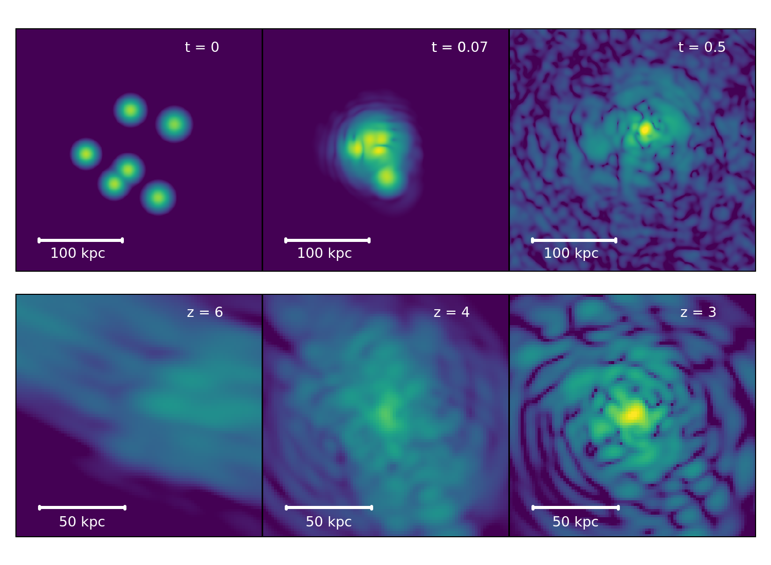
Figure 1: Time evolution of core and halo. The top row shows an example of a soliton merger simulation at $z=3$ in a box of size $300\text{\,}\mathrm{kpc}$ with particle mass $mc^{2}=${10}^{-22}\text{\,}\mathrm{eV}$$. The bottom row shows a selected halo formation from the large-scale structure simulations by May & Springel (2021). A stable core–halo structure can always be found at the end of all simulations. For illustrative purposes, the first two columns show the projected density (obtained by integrating density slices along the $z$-axis), but the last column is a single slice (i. e. one grid cell in thickness) of the snapshot through the $z$-coordinate of the halo center.

3.2.1 Soliton merger simulations

The soliton merger simulations are performed with a particle mass $mc^{2}=${10}^{-22}\text{\,}\mathrm{eV}$$, a box size $L=$300\text{\,}\mathrm{kpc}$$ and at $z=3$ on a grid with $N^{3}=512^{3}$ cells. The simulations are started with six randomly-placed solitons with mergers mostly occurring at $t\sim 0.1\,t_{\mathrm{H}}$, where $t_{\mathrm{H}}$ is the Hubble time. Since the simulations at $z=3$ take 16 times longer than those at $z=0$ due to the dependence of time step on the scale factor as shown in eq. 13, we stop the simulations at $0.5\,t_{\mathrm{H}}$. We have checked that haloes at $t\sim 0.5\,t_{\mathrm{H}}$ are relaxed, since they meet the virialisation criterion $|2(K+Q)/W|\approx 1$ (Hui et al., 2017; Mocz et al., 2017) (where $K$, $Q$ and $W$, are the kinetic, quantum and potential energies, respectively). However, we also included unrelaxed haloes in between $0.1\,t_{\mathrm{H}}<t<0.5\,t_{\mathrm{H}}$ in our results. Alternative initial settings were tested, such as increasing the number of solitons with a larger range of masses, but the results do not change the main conclusion of this work.

3.2.2 Small-volume cosmological simulations

A series of cosmological simulations are performed using the same resolution, particle mass and box size. They all begin from $z=50$ and stop at $z=0$. The initial conditions are generated using MUSIC (Hahn & Abel, 2011) with the CDM transfer function from Eisenstein & Hu (1998, 1999), and the following cosmological parameters: $\Omega_{m}=0.276$, $\Omega_{\Lambda}=0.724$, $h=0.677$ and $\sigma_{8}=0.8$. Due to the difficulty of simultaneously resolving the large-scale structure and the inner non-linear evolution of haloes on a grid size of $512^{3}$, we use initial conditions that correspond to ‘zoom-in’ regions with $L=$300\text{\,}\mathrm{kpc}$$ of a larger $1\text{\,}\mathrm{Mpc}$ box generated by MUSIC with different random seeds.

3.2.3 Large-volume cosmological simulation

A large-volume high-resolution cosmological simulation was performed by May & Springel (2021) with similar cosmological parameters, but larger box size $L=$10\text{\,}\mathrm{Mpc}\text{\,}{\mathrm{\text{$h$}}}^{-1}$$ and grid size $N^{3}=8640^{3}$, and slightly lighter particle mass $mc^{2}=$7\text{\times}{10}^{-23}\text{\,}\mathrm{eV}$$. With such a box size and spatial resolution, this simulation contains a population of haloes with diverse formation histories, including tidally stripped, isolated, and merged haloes. Therefore, it provided us with a more realistic measurement of the core–halo mass relation in a FDM universe. Figure 1 visually shows the time evolution of the density distribution in different simulations. It is clear that, whether a halo is formed through soliton mergers or gravitational collapse of large-scale structure, there always exists a stable core structure enveloped by interference fluctuations within its host halo, but we will see later that different box sizes can lead to different types of core–halo structure.

3.2.4 Initial power spectrum

As noted above, in this work (as well as May & Springel, 2021), we did not use the initial power spectrum of the FDM model, which presents a suppression of power on small scales, because the inner structure of haloes should be insensitive to the initial conditions (Schive et al., 2014b). Although different merger histories may lead to different core–halo structure, the extent of this impact is still to be determined. We assume here that the increased amount of small-scale structure, as well as the number of system interactions, will have negligible effects on the statistics of core–halo structure. Simulated haloes with comparable size of the soliton are rare if a more realistic power spectrum is applied, but should still exist and therefore be included in the resulting core–halo mass relation.

3.3 Spatial resolution

Our soliton merger simulations have a smaller box size, but the same number of grid cells ($512^{3}$) as our cosmological simulations, so the resolution $\Delta x=$0.644\text{\,}\mathrm{kpc}$$ is better than previous studies (Schwabe et al., 2016; Mocz et al., 2017). This allows us to resolve smaller cores, but the haloes may experience stripping effects from their own gravitational pull. On the other hand, although the large simulation is performed in high resolution, the (re-scaled) grid resolution $\Delta x=$1.547\text{\,}\mathrm{kpc}$$ is still twice as large as that of the soliton merger simulations. The importance of resolving the core with fine enough grids is reflected in the core mass–radius relation. Figure 2 shows that simulated haloes have cores following a tight relation:

$$a^{1/2}M_{\mathrm{c}}=\frac{$5.5\text{\times}{10}^{9}$}{(mc^{2}/${10}^{-23}\text{\,}\mathrm{eV}$)^{2}(a^{1/2}r_{\mathrm{c}}/$\mathrm{kpc}$)}\mathrm{M}_{\odot}\,.$$ (14)

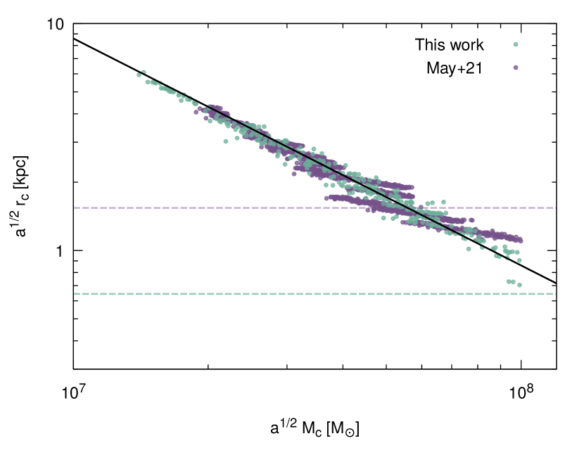
Figure 2: Core mass–radius relation scaled to $mc^{2}=$8\text{\times}{10}^{-23}\text{\,}\mathrm{eV}$$ via eq. 3. The black line is a fitting relation (14) from Schive et al. (2014a). The dashed lines show $2\Delta x$ as a reference of the resolution limit for the simulations of this work and May & Springel (2021).

As the core becomes more massive, the core size decreases further. When the core size is resolved by less than two grid cell lengths, the relation becomes more dispersed and discretised.

4 Results

4.1 Density profiles

The centres of the haloes from the simulations performed in this work are found by the minimum gravitational potential, and those from the cosmological simulation in May & Springel (2021) are determined by selecting the densest cells of haloes found by a grid-based friends-of-friends-like halo finder. We measured the spherically averaged density profile and performed fitting to eq. 8 to extract $r_{\mathrm{c}}$, $r_{\mathrm{t}}$ and $r_{\mathrm{s}}$ for all haloes. As shown in Figure 3, a flat cored structure is identified towards the center in all profiles. They are well fitted by the core density profile eq. 8 with a maximum error of $10\text{\,}\mathrm{\char 37\relax}$ up to the core radius $r_{\mathrm{c}}$. After the transition radius $r_{\mathrm{t}}$, the profiles follow the NFW profile. We also see that for some haloes, we have a direct transition from the core to the NFW profile, while others show a longer transition with an intermediate behaviour linking the two regimes.

One interesting feature we observe is oscillations in these profiles in their outer regions that can only be modelled on average by the smooth NFW profile. A possible reason for the fluctuations is that they are caused by the interference granules in the NFW region. If this is true, it is possible that halo density profiles can be used to measure this unique interference pattern present in models like FDM. More tests are needed to confirm this hypothesis.

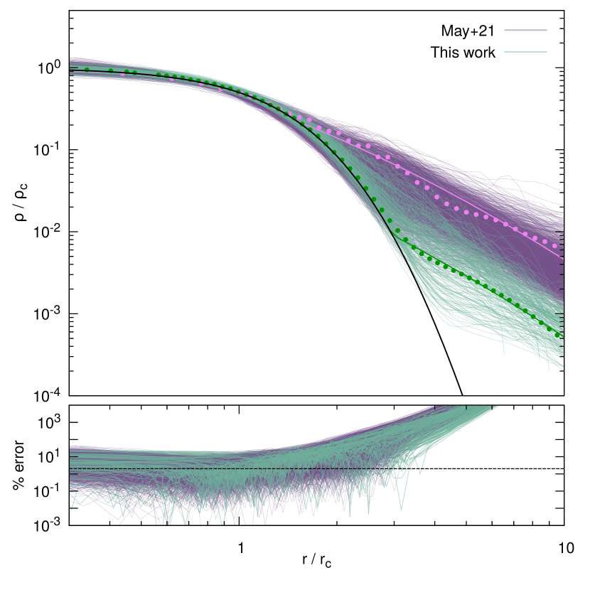
Figure 3: Scaled density profile of haloes obtained from simulations of this work and May & Springel (2021). The scaled core profile is shown as black line. We highlight two haloes with pink and dark green and their best-fit cored NFW profile. They have similar core mass, but an order of magnitude difference in the halo mass. Bottom sub-panel shows the percentage error between data and core profile. The dashed line denotes an error of $2\text{\,}\mathrm{\char 37\relax}$.

In previous simulations (Schive et al., 2014b; Mocz et al., 2017), the transition radius was found to be $r_{\mathrm{t}}\geq 3r_{\mathrm{c}}$, where the residual error between the data and the core profile is less than $2\text{\,}\mathrm{\char 37\relax}$ for $r<r_{\mathrm{t}}$. However, our measured $r_{\mathrm{t}}$, purely from fitting to the cored NFW profile eq. 8, disagrees with these previous results. The error at $3r_{\mathrm{c}}$ is greater than at least $10\text{\,}\mathrm{\char 37\relax}$, as shown in the bottom panel of Figure 3, meaning the actual $r_{\mathrm{t}}$ should be located at a radius smaller than $3r_{\mathrm{c}}$. The range of values for the measured $r_{\mathrm{t}}$ in Figure 4 shows that most haloes do have $r_{\mathrm{t}}\leq 3r_{\mathrm{c}}$. Other recent work, such as Yavetz et al. (2021), also shows smaller transition radii, e. g. $r_{\mathrm{t}}\approx 2r_{\mathrm{c}}$. As mentioned before, from theory, to guarantee a continuous and smooth transition from the solitonic core to the NFW profile, continuity of both the density and of its first derivative would be necessary, which translates to the requirement $r_{\mathrm{t}}\leq 3r_{\mathrm{c}}$, which, therefore, agrees with our result. This implies that all the haloes in the simulations presented here have a continuous and smooth transition from the core to the NFW profile, with or without a transition period, and thus do not suffer from the apparent inconsistency present in previous simulations.

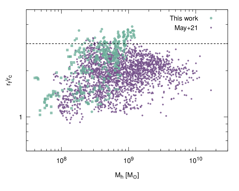
Figure 4: Range of transition radius as a function of halo mass. The dashed line shows the typical transition $r_{\mathrm{t}}=3r_{\mathrm{c}}$ obtained from Schive et al. (2014b).

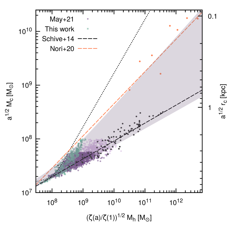
Figure 5: Core–halo relation scaled to $mc^{2}=$8\text{\times}{10}^{-23}\text{\,}\mathrm{eV}$$ via eq. 3. Green dots are haloes simulated in this work with cores resolved by at least $3\Delta x$. Purple and and faint purple dots are haloes from the large-box cosmological simulation (May & Springel, 2021) with cores resolved by at least 2$\Delta x$ and $\Delta x$ respectively. The pink shaded region is enclosed by the empirical fits to the purple and green dots, with the maximum and minimum values of the parameters in eq. 11. The solid dotted line corresponds to the soliton-only relation obtained from a pure core profile. The black and orange dashed lines are fitting relations corresponding to the black and orange dots obtained from Schive et al. (2014b) and Nori & Baldi (2021)respectively.

4.2 The core–halo mass relation

Footnote 3 shows the core–halo mass relation obtained from the soliton merger and cosmological simulations. All data are scaled to $mc^{2}=$8\text{\times}{10}^{-23}\text{\,}\mathrm{eV}$$ using eq. 3 in order to enable a direct comparison with the data and fitting relation from Schive et al. (2014b). For reference, we also show the ‘core–halo’ mass relation of a soliton-only profile, i. e. a pure core profile with $r_{\mathrm{t}}\to\infty$ in eq. 8, represented by the solid black line. This curve indicates the minimum halo mass for a certain core mass, and any haloes located to the right of the soliton-only core–halo relation must have the usual cored NFW structure. For haloes in the soliton merger simulations with mass $\gtrsim${10}^{8}\text{\,}\mathrm{\text{$\mathrm{M}_{\odot}$}}$$, the relation has a steeper slope than $\alpha=1/3$, confirming the results from Mocz et al. (2017). However, haloes from the large-scale cosmological simulation predict a core–halo relation with a large enough dispersion that can cover a range of data produced by both the soliton merger simulations and Schive et al. (2014b). The range of the dispersion can span as large as one order of magnitude in halo mass for $M_{\mathrm{c}}\sim$5\text{\times}{10}^{7}\text{\,}\mathrm{\text{$\mathrm{M}_{\odot}$}}$$. This dispersion, which fills in the space in between the soliton-only line and the relation from Schive et al. (2014b), indicates the diversity of the cored NFW structure in the FDM simulations. For example, Figure 3 highlights two profiles of haloes with similar core mass $M_{\mathrm{c}}\sim$5\text{\times}{10}^{7}\text{\,}\mathrm{\text{$\mathrm{M}_{\odot}$}}$$, but different halo mass. The tight ‘one-to-one’ core–halo relations found by different groups, with different slopes, therefore only describe a part, but not all populations of haloes in the FDM model.

We suggest an empirical equation that has the following form: $M_{\mathrm{c}}=\beta+\left(M_{h}/\gamma\right)^{\alpha}$. The parameter $\beta$ takes the limit of the relation for small halo masses into account, although low-mass haloes are rare in a FDM universe due to the suppression in the initial power spectrum. $\alpha$ is the slope that can be compared to previous works. After including the scaling symmetry in eq. 3 and the redshift dependence according to Schive et al. (2014b), we have

$$\begin{split}a^{1/2}M_{\mathrm{c}}&=\beta\left(\frac{mc^{2}}{$8\text{\times}{10}^{-23}\text{\,}\mathrm{eV}$}\right)^{-3/2}\\ &+\left(\sqrt{\frac{\zeta(z)}{\zeta(0)}}\frac{M_{\mathrm{h}}}{\gamma}\right)^{\alpha}\left(\frac{mc^{2}}{$8\text{\times}{10}^{-23}\text{\,}\mathrm{eV}$}\right)^{3(\alpha-1)/2}\mathrm{M}_{\odot}\,.\end{split}$$ (15)

The best-fit parameters for the haloes from the large-box cosmological simulation give $\beta=8.00^{+0.52}_{-6.00}\times 10^{6}\,{\mathrm{M}_{\odot}},\log_{10}(\gamma/{\mathrm{M}_{\odot}})=-5.73^{+2.38}_{-8.38}\,$ and $\alpha=0.515^{+0.130}_{-0.189}$, which is shown as a pink shaded region in footnote 3.

The effect of the large dispersion is encompassed in the uncertainty of the model parameters. This uncertainty is not the statistical uncertainty of the fit, but an ‘overestimation’ of the uncertainty in the parameters that can reflect the large dispersion of the data. Indeed, the statistical uncertainty would be the incorrect quantity to consider in this case, since we do not assume that there is an underlying ‘true’ set of values for the parameters with statistical fluctuations, but rather propose that different halo populations could systematically follow different relations depending on their histories and properties (see section 4.2.1). To obtain a more appropriate description of the core–halo diversity, we employed KDE, estimating the probability distribution function of the core masses with respect to the central value of the corresponding binned halo mass. Each of these distributions reveals the dispersion of core masses for each halo mass. We then obtain the minimum and maximum curves $M_{\mathrm{c}}(M_{\mathrm{h}})$ that fit all of these distributions, and extract the minimum and maximum vales for the parameters $b$, $\gamma$ and $\alpha$ from these curves. The difference to the global fit is our uncertainty in the parameters.

Nori & Baldi (2021); Mocz et al. (2017); Schive et al. (2014b) determined slopes $\alpha$ of $0.60.5560.333$, respectively. Given the large dispersion seen in our data, all of these slopes are compatible when taking into account the uncertainty we assigned to the fitting parameters. So when considering the fitting function we propose, all of the other cases in the literature are covered as well. We emphasise that our results show that a general halo population is not well-described by any single one-to-one core–halo mass relation. Further investigation is required to determine which halo populations follow which relations (if any), and under what conditions – cf. section 4.2.1.

This large spread and uncertainty in the fitting function can affect the constraints on the FDM mass obtained from these relations. Here, we provide a rough estimate of the error. For the same halo mass $M_{\mathrm{h}}=${10}^{9}\text{\,}\mathrm{\text{$\mathrm{M}_{\odot}$}}$$ in footnote 3, we can have the least massive core mass as $M_{\mathrm{c}}=$3\text{\times}{10}^{7}\text{\,}\mathrm{\text{$\mathrm{M}_{\odot}$}}$$ and the most massive as $M_{\mathrm{c}}=${10}^{8}\text{\,}\mathrm{\text{$\mathrm{M}_{\odot}$}}$$. Applying these values to the core density in eq. 8 gives a $50\text{\,}\mathrm{\char 37\relax}$ difference in particle mass $m$. Therefore, any observational constraints made using the relation eq. 11 should include an additional uncertainty on the order of $50\text{\,}\mathrm{\char 37\relax}$ in the results, unless the halo mass is smaller than $10^{9}($8\text{\times}{10}^{-23}\text{\,}\mathrm{eV}$/(mc^{2}))^{3/2}\,\mathrm{M}_{\odot}$. Therefore, when obtaining the FDM mass using the core–halo relation, one needs to take into account the dispersion of these values, shown in the uncertainty in the fitting parameters, which will translate to a higher uncertainty in the FDM mass.

We now scrutinize whether the scatter of the core–halo relation has an influence on the FDM mass constraints through a dynamical analysis for dwarf galaxies, as has been performed in the literature when fitting the presence of a core in such galaxies. To this end, we apply the spherical Jeans analysis to the kinematic data of the Fornax dwarf spheroidal galaxy, which has the largest data set among the Galactic dwarf satellites. We perform the Jeans analysis using two different core–halo relations, which are suggested by Schive et al. (2014b) and this work, and then we map the posterior probability distributions of the FDM mass through the MCMC technique based on Bayesian statistics. Comparing the posteriors, there is no clear difference in the shape of those distributions, including that of FDM mass, but this is due to the fact that there exists a degeneracy between halo mass and FDM mass.Therefore, this degeneracy makes it hard to see the impact that the core–halo relation has in the Jeans analysis.

Due to limited spatial resolution, we could only observe the dispersion to increase with halo mass until $M_{\mathrm{c}}\sim$6\text{\times}{10}^{7}\text{\,}\mathrm{\text{$\mathrm{M}_{\odot}$}}$$. It would be important for potential future higher-resolution simulations to examine if the dispersion keeps increasing along the soliton-only relation or not. Again, the increasing dispersion is of importance to observational studies since it will also lead to an increasing uncertainty in the core–halo relation.

4.2.1 The origin of the dispersion

Different core–halo structures have been found in different simulations:

• As mentioned before, Schive et al. (2014b) and Mocz et al. (2017) find different results for the slope $\alpha$ ($1/3$ vs. $5/9$), even for similar simulation setups (soliton mergers).

• Mina et al. (2020) claim to confirm a slope of $\alpha=5/9$, as found in the soliton merger simulations of Mocz et al. (2017), but using a cosmological simulation, contradicting the result of $\alpha=1/3$ from Schive et al. (2014b). However, the number of haloes in their sample is very small.

• Schwabe et al. (2016) performed soliton merger simulations similar to Schive et al. (2014b) (and later Mocz et al., 2017) and could not reproduce the previously-found value of the slope $\alpha$, or indeed any universal relation.

• Nori & Baldi (2021) studied the dynamics of eight simulated haloes and concluded with a similar comment: Schive et al. (2014b) and Mocz et al. (2017) only captured a partial representation of the core–halo relation in a realistic cosmological sample.

• Yavetz et al. (2021) used the Schwarzschild method to construct self-consistent FDM halos and found that a stable core–halo structure can exist even when the adopted core–halo mass relation deviates from Schive et al. (2014b).

These examples illustrate that the diversity of the possible core–halo slopes found in different works seems originate from the type of simulations performed, which results in halos and cores that have different properties. The diversity of core–halo structure found in these simulations is exhibited in our work, where we can clearly see the difference between the core–halo mass relation from halos formed in soliton merger simulations (green points in footnote 3) and in cosmological simulations (pink points in footnote 3).

We can think of a few possible explanations for this diversity of halos: merger history (Du et al., 2017; Yavetz et al., 2021), tidal stripping effects, and the relaxation state of the halo (Nori & Baldi, 2021). Formation and merger history is an explanation that seems very plausible to be a relevant factor. Larger cosmological simulations, like the one from May & Springel (2021), present halos that could have very different merger histories, and a large dispersion is expected. This is different from the soliton merger simulations, where we do not expect a complicated merger history. We leave for future work to try to identify the different merger histories and try to clarify how this relates to the different incarnations of the core–halo mass relation.

Another possible factor that can also contribute to the dispersion found is stripping. Here, we will attempt to provide an argument to support tidal stripping as one element responsible for the dispersion, based on the setups of various simulations. By comparing the box sizes and the resulting slopes $\alpha$ between the small-volume cosmological simulations of this work with Mocz et al. (2017) and Schive et al. (2014b), which are $335\text{\,}\mathrm{kpc}1765\text{\,}\mathrm{kpc}\geq 2000\text{\,}\mathrm{kpc}$ (box sizes) after re-scaling via eq. 3, and $\sim 0.90.5560.333$ (slopes) respectively, we find that smaller simulation box sizes are correlated with a steeper slope in the core–halo relation. This can be explained by the stripping effect on the halo by its own gravity due to the periodic boundary conditions: the self-stripping effect becomes more effective at removing mass from the NFW region as the box size decreases. This skews the core–halo structure towards smaller halo masses, steepening the core–halo relation. A more rigorous test to prove the above argument requires simulations with increased spatial resolution and box sizes up to at least $2\text{\,}\mathrm{Mpc}$, which current numerical schemes are unable to feasibly achieve.

The self-stripping effect is a numerical artifact, but there is no doubt that a stable core–halo structure can exist within such environments. In more realistic cosmological simulations, dwarf satellites also experience a similar effect from their host haloes in the form of tidal stripping. Therefore, we suggest that stripping effects by tidal forces are one of the contributing factors causing the dispersion obtained from the large-box simulation in May & Springel (2021). One subtlety is that the tidal effect is an interaction between host haloes and sub-haloes with at least two orders of magnitude difference in mass, but the halo finder used in May & Springel (2021) does not identify sub-haloes. However, it is known that sub-haloes in CDM simulations can temporarily move outside of the virial radius of the host halo after the first pericentric passage (van den Bosch, 2017). We assume that ejected sub-haloes should also exist in a FDM cosmology, and therefore identified by the halo finder. An in-depth analysis of the tidal effect on the core–halo relation, or FDM sub-haloes in general, would require building merger trees, which is still not yet studied in any FDM cosmological simulations. We leave this investigation to future work.

4.3 Other relations

4.3.1 Inner dark matter slope–halo mass relation

Observational constraints obtained through Jeans analysis require adopting the cored NFW density profile and core–halo mass relation. The scatter in the core–halo mass relation plays a part in the analysis simply as an uncertainty in the relation. To study the observational consequences of the diversity, we suggest showing the inner slope–halo mass relation and core radius–halo mass relation for our FDM haloes, which can be compared to previous observational results.

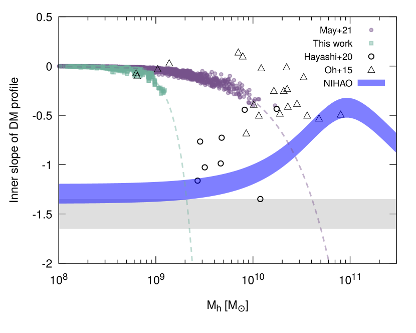
Figure 6: Inner dark matter slope as a function of halo mass. The inner slope is defined as the logarithmic gradient density at $$0.015$r_{\mathrm{h}}$. Green and purple dots represent haloes from simulations of this work and May & Springel (2021), where halo mass is rescaled to $mc^{2}=$8\text{\times}{10}^{-23}\text{\,}\mathrm{eV}$$ and $z=0$ via eq. 3. Open triangles are the observed relation from dwarf galaxies based on Jeans analysis (Hayashi et al., 2020), whereas open circles are predicted from the rotation curves of dwarf galaxies (Oh et al., 2015). The blue band is a fitting function with an uncertainty of $\pm 0.1$ predicted by NIHAO, a CDM simulation with baryonic feedback physics (Tollet et al., 2016). The grey band shows the prediction by CDM-only simulations.

We define the inner slope as the logarithmic gradient dark matter density $\Delta\log\rho/\Delta\log r$ at an inner radius of $1.5\text{\,}\mathrm{\char 37\relax}$ of the halo’s virial radius $r_{\mathrm{h}}$: $r_{\text{inner}}=$0.015$r_{\mathrm{h}}$. The definition is frequently used to study the impact of feedback physics on the inner dark matter structure (Tollet et al., 2016). As shown in Figure 6, the inner slope of FDM haloes is expected to be cored (i. e. 0) for less massive haloes with mass $\lesssim${10}^{9}\text{\,}\mathrm{\text{$\mathrm{M}_{\odot}$}}$$. In contrast, haloes in CDM simulations with baryonic feedback physics show a cuspy inner slope $\sim-1.5$ within this mass range, due to the inefficient core formation process by feedback (Tollet et al., 2016). It is therefore important to observe the inner slope of ultra-faint dwarf galaxies, which can help to distinguish between feedback-induced and quantum pressure-induced cores. As the relation moves to more massive FDM haloes, the inner radius begins to shift outside of the cored region because of the inverse proportionality between core radius and halo mass. As a result, the inner slope steepens. Note that the steepening occurs at different halo mass ranges for different sets of FDM halo samples, because haloes in simulations of smaller box size tend to be stripped, so the steepening occurs earlier.

The inferred observational relation from the stellar kinematics of eight dwarf galaxies (Hayashi et al., 2020), and rotation curves of 26 dwarf galaxies (Oh et al., 2015) shows a large scatter of inner slope for a certain halo masses, which is a result of diverse dark matter density profiles. If we consider an extrapolation of the inner slope–halo mass relation (dashed lines in Figure 6), including both small and large box size simulations, the FDM model with $mc^{2}\approx$8\text{\times}{10}^{-23}\text{\,}\mathrm{eV}$$ may be able to explain the scatter presented by the observations.

We caution that the definition of halo mass and inner slope vary across the literature. Moreover, populating the region in between the extrapolated relations would require sub-halo data, which we did not investigate in this work. We therefore emphasise that the particle mass $mc^{2}\approx$8\text{\times}{10}^{-23}\text{\,}\mathrm{eV}$$ only represents a loose constraint, and the main motivation of Figure 6 is to demonstrate the possibility of explaining the observed diversity of inner slopes by stripped, or more realistically, tidally stripped sub-haloes, which is closely related to the diversity of the core–halo structure.

4.3.2 Core radius–halo mass relation

As suggested by Burkert (2020), the FDM model may fail to explain the observed trend of the core radius–halo mass relation measured from dwarf galaxies. We follow Mina et al. (2020) and present the core radius–halo mass relation measured from our FDM halo samples. As shown in Figure 7, the scatter is still observed, but the decreasing trend, which is a fundamental property of quantum pressure-induced cores, is in disagreement with the positive scaling predicted by LSB galaxies (Salucci et al., 2007; Di Paolo et al., 2019).

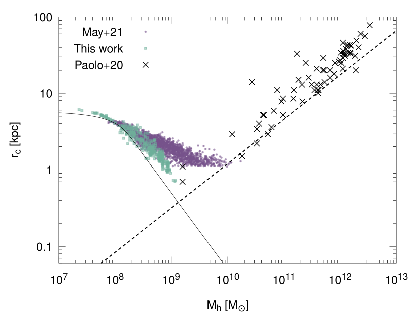
Figure 7: Core radius vs. halo mass. Green and purple points are properties of haloes from simulations of this work and May & Springel (2021). The black line shows the relation predicted by a soliton-only density profile. The dashed line is an empirical function predicted by LSB galaxies (Salucci et al., 2007). Black crosses are from Di Paolo et al. (2019).

The disagreement is expected because the negative scaling, where less massive galaxies are cored, allows the FDM model to solve the core–cusp problem, but the relation from LSB galaxies has the opposite behaviour, where massive galaxies have larger cores. In addition, LSB galaxies are predicted in CDM simulations to have experienced tidal heating and supernova feedback (Martin et al., 2019). Therefore, the relation between core radius and halo mass poses a challenge to the FDM model, but more importantly, it motivates future FDM simulations to include baryonic physics to verify if LSB-like galaxies can be formed or not.

5 Conclusion

Solitonic cores are found to be formed in simulations of the FDM model as a consequence of gravity and the uncertainty principle, but there is still no consensus on a single universal scaling relation that describes the relationship between a halo’s mass and that of its core, or that one even exists. In this work, we performed new soliton merger simulations and used data from a large-scale cosmological FDM simulation. All simulations are evolved by solving the Schrödinger–Poisson equations through the pseudo-spectral method, which can capture wave phenomena completely. Here is a summary of our findings.

We found an agreement between the measured density profiles and a cored NFW profile, but the transition radii of most of haloes are located at $\leq 3r_{\mathrm{c}}$. This is in disagreement with previous simulations (Schive et al., 2014b; Mocz et al., 2017), but more consistent with the analytical requirement where the transition between the inner core and the outer NFW profile must be continuous and smooth.

The resulting core–halo mass relation, obtained from both soliton merger and cosmological simulations, shows an increasing dispersion with halo mass. The spread extends all the way from the limit of a pure soliton profile to that of Schive et al. (2014b), signifying the diversity in core–halo structure. We suggest that, for small cosmological simulations, ‘artificial’ stripping effects due to periodic boundary conditions could partially be responsible for the variety of slopes in the relation predicted by different simulations. However, ‘natural’ tidal stripping effects of various severity also exist in larger simulations, which therefore exhibit a greater spread in the relation. Further, the exact impact of variations between individual haloes on the relation, such as merger history or relaxation state, remains to be uncovered.

We provided a new empirical equation that considers the non-linearity in the low-mass end, but we emphasise that any core–halo relation must suffer from an uncertainty produced by the diversity demonstrated in this work. Therefore, observational analyses that adopted a core–halo relation must take into account this uncertainty in the fitting parameters, including the particle mass of the FDM model.

Due to the limited spatial resolution imposed by the time step criteria, our samples still do not represent the full population of core–halo structure. To obtain this, simulations using a more flexible numerical scheme, such as adaptive mesh refinement (Schive et al., 2014a; Mina et al., 2020), and sub-halo catalogues from merger trees would be needed. Such future work would provide verification of whether the dispersion keeps growing beyond halo masses of $10^{9}($8\text{\times}{10}^{-23}\text{\,}\mathrm{eV}$/(mc^{2}))^{3/2}\,\mathrm{M}_{\odot}$, or whether the tidally stripped sub-haloes can explain the observed diversity in the inner slope–halo mass relation. We also plan in the future to understand the merger history of the halos we have in the cosmological simulation, using the same techniques as for CDM, in order to try to understand how halos with different merger histories influence the core–halo mass relation.

Lastly, including baryonic physics will further complicate the core–halo structure because the core can now not only be induced by quantum pressure, but also by stellar feedback physics, not to mention the question of how these processes would interact. However, only baryonic physics have a chance of matching the core radius–halo mass relation of LSB galaxies with FDM.

Data availability statement

The data underlying this article will be shared on request to the corresponding authors.

Appendix A Code comparison

Since there is no analytical solution to the general time-dependent Schrödinger–Poisson equations, we can only ensure reliability of the code in the general case (beyond toy examples and limiting cases) through comparison with other groups. Thus, we compared the dark matter density fluctuations at $z=0$ with May & Springel (2021) in a test simulation. Our codes are independently developed, but adopted the same pseudo-spectral splitting method in second order.

We ran a cosmological fuzzy dark matter simulation separately with identical initial conditions generated by MUSIC with box size $L=$10\text{\,}\mathrm{Mpc}\text{\,}{\mathrm{\text{$h$}}}^{-1}$$, particle mass $mc^{2}=$2.5\text{\times}{10}^{-24}\text{\,}\mathrm{eV}$$, and number of grid cells $N^{3}=1024^{3}$. The cosmological simulations are evolved until $z=0$, and the density fluctuations are measured as the power spectrum shown in Figure 8.

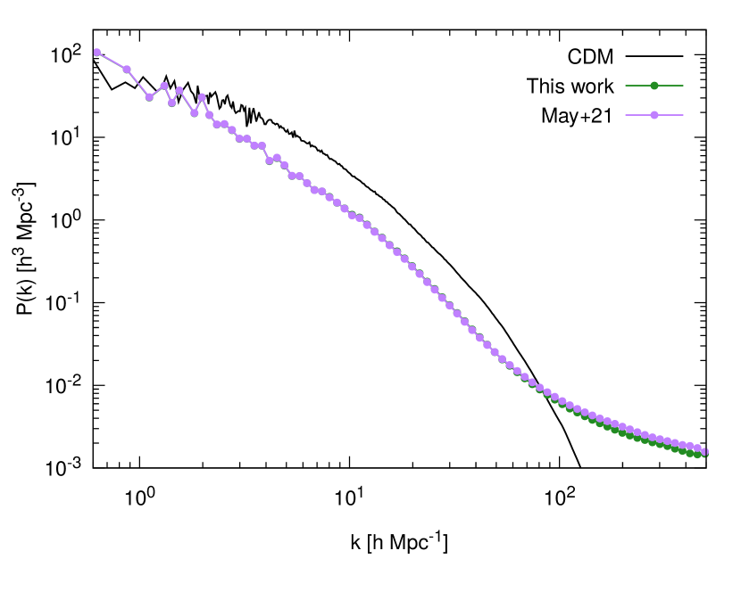
Figure 8: Comparison of the power spectrum at $z=0$ between the code used in this work and that of May & Springel (2021) for a cosmological test simulation.

REFERENCES

- Aghanim et al. (2020) Aghanim N., et al., 2020, Astron. Astrophys., 641, A6
- Alam et al. (2017) Alam S., et al., 2017, Mon. Not. Roy. Astron. Soc., 470, 2617
- Bernal et al. (2018) Bernal T., Fernández-Hernández L. M., Matos T., Rodríguez-Meza M. A., 2018, MNRAS, 475, 1447
- Broadhurst et al. (2020) Broadhurst T., De Martino I., Luu H. N., Smoot G. F., Tye S. H. H., 2020, Phys. Rev. D, 101, 083012
- Bullock & Boylan-Kolchin (2017) Bullock J. S., Boylan-Kolchin M., 2017, Annu. Rev. Astron. Astrophys., 55, 343
- Burkert (2020) Burkert A., 2020, ApJ, 904, 161
- Calabrese & Spergel (2016) Calabrese E., Spergel D. N., 2016, MNRAS, 460, 4397
- Chen et al. (2017) Chen S.-R., Schive H.-Y., Chiueh T., 2017, Mon. Not. Roy. Astron. Soc., 468, 1338
- Di Paolo et al. (2019) Di Paolo C., Salucci P., Erkurt A., 2019, MNRAS, 490, 5451
- Du et al. (2017) Du X., Behrens C., Niemeyer J. C., Schwabe B., 2017, Phys. Rev. D, 95, 043519
- Eisenstein & Hu (1998) Eisenstein D. J., Hu W., 1998, ApJ, 496, 605
- Eisenstein & Hu (1999) Eisenstein D. J., Hu W., 1999, ApJ, 511, 5
- Ferreira (2020) Ferreira E. G. M., 2020, Ultra-Light Dark Matter (arXiv:2005.03254)
- Garny et al. (2020) Garny M., Konstandin T., Rubira H., 2020, J. Cosmology Astropart. Phys., 2020, 003
- González-Morales et al. (2017) González-Morales A. X., Marsh D. J. E., Peñarrubia J., Ureña López L. A., 2017, Mon. Not. Roy. Astron. Soc., 472, 1346
- Hahn & Abel (2011) Hahn O., Abel T., 2011, MNRAS, 415, 2101
- Hayashi et al. (2020) Hayashi K., Chiba M., Ishiyama T., 2020, ApJ, 904, 45
- Hayashi et al. (2021) Hayashi K., Ferreira E. G. M., Chan H. Y. J., 2021, ApJ, 912, L3
- Hui (2021) Hui L., 2021, Wave Dark Matter (arXiv:2101.11735)
- Hui et al. (2017) Hui L., Ostriker J. P., Tremaine S., Witten E., 2017, Phys. Rev. D, 95, 043541
- Li et al. (2021) Li X., Hui L., Yavetz T. D., 2021, Phys. Rev. D, 103, 023508
- Madelung (1927) Madelung E., 1927, Zeitschrift für Physik, 40, 322
- Martin et al. (2019) Martin G., et al., 2019, MNRAS, 485, 796
- May & Springel (2021) May S., Springel V., 2021, MNRAS, 506, 2603
- Mina et al. (2020) Mina M., Mota D. F., Winther H. A., 2020, Solitons in the dark: non-linear structure formation with fuzzy dark matter (arXiv:2007.04119)
- Mocz et al. (2017) Mocz P., Vogelsberger M., Robles V. H., Zavala J., Boylan-Kolchin M., Fialkov A., Hernquist L., 2017, MNRAS, 471, 4559
- Mocz et al. (2018) Mocz P., Lancaster L., Fialkov A., Becerra F., Chavanis P.-H., 2018, Phys. Rev. D, 97, 083519
- Niemeyer (2020) Niemeyer J. C., 2020, Progress in Particle and Nuclear Physics, 113, 103787
- Nori & Baldi (2021) Nori M., Baldi M., 2021, MNRAS, 501, 1539
- Oh et al. (2015) Oh S.-H., et al., 2015, Astron. J., 149, 180
- Pillepich et al. (2018) Pillepich A., et al., 2018, Mon. Not. Roy. Astron. Soc., 473, 4077
- Rogers & Peiris (2021) Rogers K. K., Peiris H. V., 2021, Phys. Rev. Lett., 126, 071302
- Safarzadeh & Spergel (2020) Safarzadeh M., Spergel D. N., 2020, ApJ, 893, 21
- Salucci et al. (2007) Salucci P., Lapi A., Tonini C., Gentile G., Yegorova I., Klein U., 2007, MNRAS, 378, 41
- Schive et al. (2014a) Schive H.-Y., Chiueh T., Broadhurst T., 2014a, Nature Phys., 10, 496
- Schive et al. (2014b) Schive H.-Y., Liao M.-H., Woo T.-P., Wong S.-K., Chiueh T., Broadhurst T., Hwang W. Y. P., 2014b, Phys. Rev. Lett., 113, 261302
- Schwabe et al. (2016) Schwabe B., Niemeyer J. C., Engels J. F., 2016, Phys. Rev. D, 94, 043513
- Tollet et al. (2016) Tollet E., et al., 2016, MNRAS, 456, 3542
- Widrow & Kaiser (1993) Widrow L. M., Kaiser N., 1993, ApJ, 416, L71
- Woo & Chiueh (2009) Woo T.-P., Chiueh T., 2009, ApJ, 697, 850
- Yavetz et al. (2021) Yavetz T. D., Li X., Hui L., 2021, Construction of Wave Dark Matter Halos: Numerical Algorithm and Analytical Constraints (arXiv:2109.06125)
- van den Bosch (2017) van den Bosch F. C., 2017, MNRAS, 468, 885