A novel fourth-order WENO interpolation technique

Abstract

Context. Several numerical problems require the interpolation of discrete data that present at the same time (i) complex smooth structures and (ii) various types of discontinuities. The radiative transfer in solar and stellar atmospheres is a typical example of such a problem. This calls for high-order well-behaved techniques that are able to interpolate both smooth and discontinuous data.

Aims. This article expands on different nonlinear interpolation techniques capable of guaranteeing high-order accuracy and handling discontinuities in an accurate and non-oscillatory fashion. The final aim is to propose new techniques which could be suitable for applications in the context of numerical radiative transfer.

Methods. We have proposed and tested two different techniques. Essentially non-oscillatory (ENO) techniques generate several candidate interpolations based on different substencils. The smoothest candidate interpolation is determined from a measure for the local smoothness, thereby enabling the essential non-oscillatory property. Weighted ENO (WENO) techniques use a convex combination of all candidate substencils to obtain high-order accuracy in smooth regions while keeping the essentially non-oscillatory property. In particular, we have outlined and tested a novel well-performing fourth-order WENO interpolation technique for both uniform and nonuniform grids.

Results. Numerical tests prove that the fourth-order WENO interpolation guarantees fourth-order accuracy in smooth regions of the interpolated functions. In the presence of discontinuities, the fourth-order WENO interpolation enables the non-oscillatory property, avoiding oscillations. Unlike Bézier and monotonic high-order Hermite interpolations, it does not degenerate to a linear interpolation near smooth extrema of the interpolated function.

Conclusions. The novel fourth-order WENO interpolation guarantees high accuracy in smooth regions, while effectively handling discontinuities. This interpolation technique might be particularly suitable for several problems, including a number of radiative transfer applications such as multidimensional problems, multigrid methods, and formal solutions.

1 Introduction

In astrophysics, it is common practice to solve the radiative transfer equation in solar and stellar atmospheres by means of numerical methods. It is also known that realistic atmospheric models can be highly inhomogeneous and dynamic and often present discontinuities or sharp gradients. Interpolations are ubiquitous in such problems: for instance, they are a fundamental ingredient of multidimensional radiative transfer, of multigrid methods, and of many formal solvers. For such problems, which contain both sharp discontinuities and complex smooth features, one seeks interpolation techniques able to handle singularities in an accurate and non-oscillatory fashion and at the same time to perform with uniform high-order accuracy in smooth regions.

It is a well known fact that standard high-order interpolations tend to misrepresent the nonsmooth regions of a problem, introducing spurious oscillations near discontinuities (e.g., Richards 1991; Zhang & Martin 1997; Shu 1998). However, monotonicity-preserving strategies such as Bézier and monotonic high-order Hermite interpolations, usually sacrifice accuracy to obtain monotonicity (Aràndiga et al. 2013). In fact, near smooth extrema of the interpolated function, they degenerate to a linear interpolation, dropping to second-order accuracy (Shu 1998). By contrast, essentially non-oscillatory (ENO) and weighted ENO (WENO) techniques accomplish the feat of approximating a function with high-order accuracy in smooth parts, while avoiding “Gibbs-like” oscillations near the discontinuities (Fjordholm 2016).

Section 2 presents the ENO approximation technique and it exposes the third-order ENO interpolation. Section 3 presents the WENO approximation technique, with a special focus on a novel fourth-order WENO interpolation. Section 4 exposes numerical tests for different interpolations. Section 5 describes different radiative transfer problems that require high-order robust interpolation techniques. Finally, Section 6 provides remarks and conclusions.

2 ENO approximation

The term stencil indicates the arrangement of grid points and corresponding function values (or coefficients) that is considered for a particular interpolation or reconstruction. Fixed stencil interpolations of second or higher order of accuracy are necessarily oscillatory near a discontinuity and such oscillations do not decay in magnitude when the computational grid is refined; an explicit example will be given in Section 4. Such issues are well recognized and considerable efforts have been already exercised to resolve them. In a seminal paper, van Leer (1979) proposed a hybrid technique that switches from a linear polynomial (second-order accurate) to a piecewise constant approximation (first-order accurate) near discontinuities. Similarly, one can also make use of a quadratic polynomial interpolation and limit the polynomial degree near discontinuities. Alternatively, monotonic Hermite interpolants suppress over- and undershoots by controlling the first-order derivatives (Fritsch & Carlson 1980), whereas Bézier interpolants make use of the so-called control points to shape the curve and suppress spurious extrema, preserving monotonicity in the interpolation. These limiting strategies are very robust, produce smooth solutions, and are widely used for problems containing shocks and other discontinuities. However, such monotonicity-preserving strategies sacrifice accuracy in order to obtain monotonicity (Aràndiga et al. 2013). Their main weakness is that they necessarily degenerate to a linear interpolation near smooth extrema of the interpolated function (Shu 1998). A local extremum is any point at which the value of a function is larger (a maximum) or smaller (a minimum) than all the adjacent function values. In this context, a smooth extremum is a local extremum of the function which is at least of class $C^{2}$, that is, twice continuously differentiable.

By contrast, ENO techniques are high-order approximations that handle discontinuities and maintain high-order accuracy near smooth extrema. The key point of the ENO strategy is to adaptively choose the stencil in the direction of smoothness. In practice, ENO schemes generate several candidate interpolations, measure the local smoothness and choose the smoothest candidate interpolation to work with, discarding the rest. This strategy enables the essential non-oscillatory property. There is broad and well-cited body of literature attesting to the importance and the success of this strategy: from the pioneering works by Harten et al. (1986, 1987) and Shu & Osher (1988, 1989) to the recent survey by Zhang & Shu (2016).

Most of the literature about ENO (and WENO) techniques is dedicated to reconstruction schemes and not to interpolations. However, the reconstruction of cell averages of a function is equivalent to the interpolation of the point values of its primitive. Therefore, ENO (and WENO) algorithms can be formulated as an interpolation technique (Fjordholm et al. 2013).

2.1 Divided differences

Given a set of function values $\{y_{k}\}\coloneqq\{y(x_{k})\}$ at positions $\{x_{k}\}$, the zeroth degree divided differences are defined as

$$y[x_{k}]\coloneqq y_{k}\,.$$

while the first degree divided differences read

$$y[x_{k},x_{k+1}]=\frac{y_{k+1}-y_{k}}{x_{k+1}-x_{k}}\,.$$

In general, the $j$-th degree forward divided differences, for $j>1$, are inductively defined by

$$y[x_{k},\dots,x_{k+j}]\coloneqq\frac{y[x_{k+1},\dots,x_{k+j}]-y[x_{k},\dots,x_{k+j-1}]}{x_{k+j}-x_{k}}\,.$$

As long as the function $y(x)$ is smooth inside $[x_{k},x_{k+j}]$, the standard approximation theory affirms that (e.g., Fjordholm 2016)

$$y[x_{k},\dots,x_{k+j}]=\frac{y^{(j)}(\xi)}{j!}\,,\text{ for some }\xi\in[x_{k},x_{k+j}]\,.$$

By contrast, if the function $y(x)$ is discontinuous at some point inside $[x_{k},x_{k+j}]$, then

$$y[x_{k},\dots,x_{k+j}]=\mathcal{O}\left(\frac{1}{\Delta x^{j}}\right)\,,$$

which diverges for $\Delta x\rightarrow 0$. Thus, divided differences are a good measure of the smoothness of the function $y(x)$ inside the stencil. This property plays an essential role in the adaptive choice of the stencil in ENO schemes.

2.2 ENO interpolation

Consider a function $y(x)$ and a set of function values $\{y_{i}\}$ at positions $\{x_{i}\}$ with $i\in\{1,\dots,N\}$. The general $p$-th order ENO interpolation $E(x)$ in the interval $[x_{1},x_{N}]$ reads

$$E(x)=\sum_{i=1}^{N-1}p_{i}(x){I_{i}(x)}\,,$$ (1)

with

$$I_{i}(x)=\begin{cases}1&\text{ if }x\in[x_{i},x_{i+1}]\,,\\ 0&\text{ if }x\notin[x_{i},x_{i+1}]\,,\end{cases}$$ (2)

and $p_{i}(x)$ denotes the interpolating polynomial acting on the interval $[x_{i},x_{i+1}]$. This polynomial must satisfy the accuracy requirement

$$p_{i}(x)=y(x)+\mathcal{O}(\Delta x^{p})\,,\text{ for }x\in[x_{i},x_{i+1}].$$

The choice of ENO stencil for constructing $p_{i}(x)$ is based on the divided differences presented in Section 2.1. The stencil is adaptively chosen so that, starting from $x_{i}$, it extends in the direction where $y(x)$ is smoothest, that is, where the divided differences are smallest.

A general $p$-point stencil containing $x_{i}$ is given by

$$S_{p}^{q}=\{x_{i-p+q},\dots,x_{i+q-1}\}\,,$$ (3)

with $q\in\{1,\dots,p\}$. For notational simplicity, the explicit dependence of the stencil $S_{p}^{q}$ on index $i$ is not indicated. This stencil can be expanded in two ways: by adding either the left neighbor $x_{i-p+q-1}$ or the right neighbor $x_{i+q}$. One decides upon which point to add by comparing the two relevant divided differences and picking the one with a smaller absolute value. Thus, if

$$|y[x_{i-p+q-1},\dots,x_{i+q-1}]|\leq|y[x_{i-p+q},\dots,x_{i+q}]|\,,$$

one adds $x_{i-p+q-1}$ to the stencil, otherwise, $x_{i+q}$.

In order to build $p_{i}(x)$, one starts with the one-point stencil

$$S_{1}^{1}=\{x_{i}\}\,,$$

and adaptively adds points with the procedure described above, ending up with a $p$-point stencil

$$S_{p}^{q}=\{x_{i-p+q},\dots,x_{i+q-1}\}\,,\text{ for some }q\in\{1,\dots,p\}\,.$$

We note that each substencil $S_{p}^{q}$ is a substencil of the large stencil

$$S_{2p-1}^{p}=\{x_{i-p+1},\dots,x_{i+p-1}\}\,,$$

and always contains the considered $x_{i}$ (but not necessarily $x_{i+1}$).

Numerical analysis asserts that there is a unique polynomial $q_{q}(x)$ of degree at most $p-1$, that goes through all the data points of the substencil $S_{p}^{q}$. Its Lagrangian expression reads

$$q_{q}(x)=\sum_{x_{k}\in S_{p}^{q}}y(x_{k})\ell_{k}(x)\,,$$ (4)

where the Lagrange basis polynomials $\ell_{k}$ are defined as

$$\ell_{k}(x)=\prod_{\begin{subarray}{c}x_{j}\in S_{p}^{q}\\ j\neq k\end{subarray}}\frac{x-x_{j}}{x_{k}-x_{j}}\,.$$

Hence, once the optimal candidate substencil $S_{p}^{q}$ is determined, the $p$-order accurate polynomial $p_{i}(x)$ in Equation (1) is simply chosen as

$$p_{i}(x)=q_{q}(x)\,,$$

with $q_{q}(x)$ given by Equation (4).

Even though there are very few theoretical results about the stability of ENO schemes (e.g., Fjordholm et al. 2012, 2013), these schemes are very robust and stable in practice. In fact, the ENO interpolant $E(x)$ is essentially non-oscillatory in the sense of recovering $y(x)$ to order $\mathcal{O}(\Delta x^{p})$ near (but not at) the location of a discontinuity. We note that ENO schemes allow for minimal over- or undershoots near discontinuities. As an explicit example of this technique, the third-order accurate ENO interpolation is presented in the following.

2.3 Third-order ENO interpolation

In order to build a third-order accurate $p_{i}(x)$, one needs a three-point stencil. Thus, starting from the one-point stencil

$$S_{1}^{1}=\{x_{i}\}\,,$$

one adds either the left neighbor $x_{i-1}$ or the right neighbor $x_{i+1}$. One takes the decision by comparing the absolute values of the two relevant divided differences

$$y[x_{i-1},x_{i}]=\frac{y_{i}-y_{i-1}}{x_{i}-x_{i-1}}\,,$$

$$y[x_{i},x_{i+1}]=\frac{y_{i+1}-y_{i}}{x_{i+1}-x_{i}}\,.$$

The smaller one implies that the function is smoother in that stencil. Therefore, if

$$|y[x_{i-1},x_{i}]|<|y[x_{i},x_{i+1}]|\,,$$

the two-point stencil is taken as

$$S^{1}_{2}=\{x_{i-1},x_{i}\}\,,$$

otherwise,

$$S^{2}_{2}=\{x_{i},x_{i+1}\}\,.$$

Suppose that the two-point stencil $S^{2}_{2}=\{x_{i},x_{i+1}\}$ has been chosen. In this case, one can add either the left neighbor $x_{i-1}$ or the right neighbor $x_{i+2}$. One takes the decision by comparing the absolute values of the two relevant divided differences

$$y[x_{i-1},x_{i},x_{i+1}]=\frac{y[x_{i},x_{i+1}]-y[x_{i-1},x_{i}]}{x_{i+1}-x_{i-1}}\,,$$

$$y[x_{i},x_{i+1},x_{i+2}]=\frac{y[x_{i+1},x_{i+2}]-y[x_{i},x_{i+1}]}{x_{i+2}-x_{i}}\,.$$

Once again, if

$$|y[x_{i-1},x_{i},x_{i+1}]|<|y[x_{i},x_{i+1},x_{i+2}]|\,,$$

the three-point stencil is taken as

$$S^{2}_{3}=\{x_{i-1},x_{i},x_{i+1}\}\,,$$

otherwise,

$$S^{3}_{3}=\{x_{i},x_{i+1},x_{i+2}\}\,.$$

Then, one proceeds with the Lagrange interpolation given by Equation (4) on the selected substencil, yielding the third-order accurate quadratic polynomial $p_{i}(x)$.

We note that the choice of the two-point stencil $S^{1}_{2}=\{x_{i-1},x_{i}\}$ at the previous step may lead to the three-point stencil

$$S^{1}_{3}=\{x_{i-2},x_{i-1},x_{i}\}\,.$$

In order to build $p_{i}(x)$, the third-order ENO interpolation thus considers the large stencil

$$S_{5}^{3}=\{x_{i-2},x_{i-1},x_{i},x_{i+1},x_{i+2}\}\,.$$

All the substencils $S^{1}_{3}$, $S^{2}_{3}$, and $S^{3}_{3}$ usually work well for globally smooth problems, while the ENO technique adaptively avoids including possible discontinuities in the selected substencil.

3 WENO approximation

WENO approximations are inspired by the ENO strategy, offering with additional advantages. Instead of using the smoothest candidate substencil to form the interpolation, WENO schemes use a convex combination of all candidate substencils to obtain high-order accuracy in smooth regions while keeping the essentially non-oscillatory property. Additionally, the WENO strategy yields smoother interpolations and avoids the use of conditional “if$\dots$else” statements, which burden the algorithm.

Liu et al. (1994) proposed this strategy, constructing the first WENO schemes. Jiang & Shu (1996) constructed arbitrary-order accurate WENO approximations for finite difference schemes and most applications use their fifth-order WENO version. General information is found in the recent surveys by Shu (2009) and Zhang & Shu (2016). Many papers about WENO approximations consider their implementation to uniform grids. However, the WENO strategy extends naturally to nonuniform grids, although it becomes quite complicated, depending on the complexity of the grid structure and on the interpolation degree (Črnjarić-Žic et al. 2007).

3.1 WENO interpolation

Consider a function $y(x)$ and a set of function values $\{y_{i}\}$ at positions $\{x_{i}\}$ with $i\in\{1,\dots,N\}$. The general $p$-th order WENO interpolation $W(x)$ in the interval $[x_{1},x_{N}]$ reads

$$W(x)=\sum_{i=1}^{N-1}p_{i}(x){I_{i}(x)}\,,$$ (5)

where $I_{i}(x)$ is defined in Equation (2). Consider the $p$-point stencil $S_{p}^{q}$ given by Equation (3) to be the large stencil. The unique $p$-th-order accurate Lagrange polynomial $p(x)$ interpolating $S_{p}^{q}$ can be recovered as a linear combination of $\ell$-th-order accurate Lagrange polynomials $q_{m}(x)$ defined on a set of $\ell$-point substencils $S_{\ell}^{m}$ with $\ell\in\{1,\dots,p\}$ and $m\in\{-p+q+\ell,\dots,q\}$, i.e.,

$$p(x)=\sum_{m=-p+q+\ell}^{q}\gamma_{m}(x)q_{m}(x)\,,$$ (6)

where $\gamma_{m}(x)$ are the so-called linear (or optimal) weights, which are always positive and univocally defined. Because of consistency one has

$$\sum_{m=-p+q+\ell}^{q}\gamma_{m}(x)=1\,.$$

The key idea of the WENO strategy is to build the polynomial $p_{i}(x)$ in Equation (5) as a weighted combination based on Equation (6), namely,

$$p_{i}(x)=\sum_{m=-p+q+\ell}^{q}\omega_{m}(x)q_{m}(x)\,,$$

where the weights coefficients $\omega_{m}(x)$ must satisfy the requirements:

• $\omega_{m}(x)\geq 0\;\forall\;m$ for stability;

• $\sum_{m=-p+q+\ell}^{q}\omega_{m}(x)=1$ for consistency;

• $\omega_{m}(x)\approx\gamma_{m}(x)\;\forall\;m$ if $y(x)$ is smooth in the large stencil $S_{p}^{q}$;

• $\omega_{m}(x)\approx 0$ if $y(x)$ has a discontinuity in the stencil $S_{\ell}^{m}$.

These (nonlinear) weights are usually defined as

$$\omega_{m}(x)=\frac{\alpha_{m}(x)}{\sum_{k=-p+q+\ell}^{q}\alpha_{k}(x)}\,,$$

where the unnormalized weights are given by

$$\alpha_{m}(x)=\frac{\gamma_{m}(x)}{(\epsilon+\beta_{m})^{a}}\,,$$

and $\epsilon$ is a small positive constant used to avoid vanishing denominators; typically $\epsilon=10^{-6}$ (Zhang & Shu 2016). A larger power $a$ makes the weight assigned to a nonsmooth substencil approach to zero faster, resulting in more dissipative WENO interpolations (Liu et al. 2018). The exponent $a$ is a free parameter. In this work, one has either $a=1$ or $a=3/2$.

The nonlinear weights $\omega_{m}(x)$ rely on the smoothness indicators $\beta_{m}$, which measure the relative smoothness of the function $y(x)$ inside the stencils $S_{\ell}^{m}$. A larger $\beta_{m}$ indicates a lack of smoothness of $y(x)$ in the stencil $S_{\ell}^{m}$ and produces a smaller nonlinear weight $\omega_{m}(x)$. The choice of the smoothness indicators plays an essential role in the performance of WENO approximations. Within the literature, the version of Jiang & Shu (1996)

$$\beta_{m}=\sum_{j=1}^{\ell-1}\Delta x^{2j-1}\int_{i}^{i+1}\left(\frac{{\rm d}^{j}}{{\rm d}x^{j}}q_{m}(x)\right)^{2}{\rm d}x\,,$$ (7)

is well established. Unfortunately, indicators (7) consider uniform grids alone and are particularly dissipative (i.e., they smear sharp gradients) for low-order WENO interpolations. In the following, a third-order and a novel fourth-order accurate WENO interpolations are presented.

3.2 Third-order WENO interpolation

Compared with higher-order versions, the third-order WENO interpolation is more robust for the treatment of discontinuous problems, it uses fewer grid points, and it provides a suitable compromise between computational cost and accuracy (Liu et al. 2018).

The unique quadratic Lagrange polynomial $p(x)$ interpolating the three-point large stencil

$$S_{3}^{2}=\{x_{i-1},x_{i},x_{i+1}\}\,,$$

can be written as

$$p(x)=\gamma_{1}(x)q_{1}(x)+\gamma_{2}(x)q_{2}(x)\,,$$

in other words, as a linear combination of the linear Lagrange interpolations

$$q_{1}(x) =\frac{-y_{i-1}(x-x_{i})+y_{i}(x-x_{i-1})}{x_{i}-x_{i-1}}\,,$$

$$q_{2}(x) =\frac{-y_{i}(x-x_{i+1})+y_{i+1}(x-x_{i})}{x_{i+1}-x_{i}}\,,$$

based, respectively, on the two two-point substencils

$$S_{2}^{1}=\{x_{i-1},x_{i}\}\,,\;\text{ and }\;S_{2}^{2}=\{x_{i},x_{i+1}\}\,.$$

The linear weights are given by

$$\gamma_{1}(x)=-\frac{x-x_{i+1}}{x_{i+1}-x_{i-1}}\,,\;\text{ and }\;\gamma_{2}(x)=\frac{x-x_{i-1}}{x_{i+1}-x_{i-1}}\,,$$

and satisfy $\gamma_{1}(x)+\gamma_{2}(x)=1$. The linear weights depend just on the grid geometry and not on the function values. The third-order WENO interpolation in the interval $[x_{i},x_{i+1}]$ reads

$$p_{i}(x)=\omega_{1}(x)q_{1}(x)+\omega_{2}(x)q_{2}(x)\,,$$

where the nonlinear weights are defined as

$$\omega_{1}(x)=\frac{\alpha_{1}(x)}{\alpha_{1}(x)+\alpha_{2}(x)}\,,\;\text{ and }\;\omega_{2}(x)=\frac{\alpha_{2}(x)}{\alpha_{1}(x)+\alpha_{2}(x)}\,,$$

with

$$\alpha_{1}(x)=\frac{\gamma_{1}(x)}{(\epsilon+\beta_{1})^{\frac{3}{2}}}\,,\;\text{ and }\;\alpha_{2}(x)=\frac{\gamma_{2}(x)}{(\epsilon+\beta_{2})^{\frac{3}{2}}}\,,$$

and $\epsilon=10^{-6}$.

3.2.1 Smoothness indicators for uniform grids

In uniform grids, the conventional choice for the smoothness indicators (7) yields

$$\beta_{1}=(y_{i}-y_{i-1})^{2}\,,\;\text{ and }\;\beta_{2}=(y_{i+1}-y_{i})^{2}\,.$$

Unfortunately, this version renders the third-order WENO interpolation too dissipative.

Alternatively, the mapping function of the WENO-M scheme (Henrick et al. 2005) and the global stencil indicator of the WENO-Z scheme (Borges et al. 2008) effectively improve the accuracy of high-order WENO schemes, but they are not satisfactory for the third-order one. More recently, Wu et al. (2015) proposed the global smoothness indicators for the less dissipative third-order WENO-N3 and WENO-NP3 schemes. Similarly, Gande et al. (2017) proposed the global smoothness indicator of the WENO-F3 scheme. However, such methods are usually not satisfactory in terms of accuracy or generate apparent oscillatory interpolations.

For these reasons, Liu et al. (2018) proposed smoothness indicators that make use of all the three points of the $S_{3}^{2}$ stencil, namely,

$$\beta_{1} =\frac{1}{4}(|y_{i+1}-y_{i-1}|-|4y_{i}-3y_{i-1}-y_{i+1}|)^{2}\,,$$ (8)

$$\beta_{2} =\frac{1}{4}(|y_{i+1}-y_{i-1}|-|4y_{i}-y_{i-1}-3y_{i+1}|)^{2}\,.$$

Numerical tests demonstrate that these new indicators provide less dissipation and better resolution than the standard ones.

3.2.2 Smoothness indicators for nonuniform grids

Liu et al. (2018) defined the smoothness indicators (8) for uniform grids only. The generalization to the nonuniform case is presented in the following. For notational convenience

$$d_{i}=\frac{y_{i+1}-y_{i}}{h_{i}}\,,\;\text{ with }\;h_{i}=x_{i+1}-x_{i}\,.$$

The first-order three-point numerical derivatives of $y(x)$ at nodes $x_{i-1}$, $x_{i}$ and $x_{i+1}$ for nonuniform grids are approximated by (e.g., Singh & Bhadauria 2009)

$$y^{\prime}_{i-1} =\frac{2h_{i-1}+h_{i}}{h_{i-1}+h_{i}}\cdot d_{i-1}-\frac{h_{i-1}}{h_{i-1}+h_{i}}\cdot d_{i}\,,$$ (9)

$$y^{\prime}_{i} =\frac{h_{i}}{h_{i-1}+h_{i}}\cdot d_{i-1}+\frac{h_{i-1}}{h_{i-1}+h_{i}}\cdot d_{i}\,,$$

$$y^{\prime}_{i+1} =\frac{-h_{i}}{h_{i-1}+h_{i}}\cdot d_{i-1}+\frac{h_{i-1}+2h_{i}}{h_{i-1}+h_{i}}\cdot d_{i}\,.$$

Following the underlying idea of Liu et al. (2018), the new indicators are constructed as follows

$$\beta_{1} =h_{i}^{2}\left(|y^{\prime}_{i}|-|y^{\prime}_{i-1}|\right)^{2}\,,$$ (10)

$$\beta_{2} =h_{i-1}^{2}\left(|y^{\prime}_{i+1}|-|y^{\prime}_{i}|\right)^{2}\,.$$

If $h_{i-1}=h_{i}$, the indicators (10) reduce to the uniform case indicators (8).

In monotonic smooth regions, the numerical derivatives (9) have the same sign, meaning that $\operatorname{sign}y^{\prime}_{i-1}=\operatorname{sign}y^{\prime}_{i}=\operatorname{sign}y^{\prime}_{i+1}$, and the indicators (10) reduce to

$$\beta_{1}=\beta_{2}=\left(2\frac{h_{i-1}h_{i}}{h_{i-1}+h_{i}}\right)^{2}\left(d_{i}-d_{i-1}\right)^{2}\,.$$

and, consequently,

$$\omega_{1}(x)=\gamma_{1}(x)\,,\;\text{ and }\;\omega_{2}(x)=\gamma_{2}(x)\,.$$

In monotonic smooth regions, the nonlinear weights are exactly equal to the optimal weights, reducing numerical dissipation for the WENO interpolation.

Assume now that $y(x)$ has a discontinuity in the interval $[x_{i-1},x_{i}]$ and is smooth in the interval $[x_{i},x_{i+1}]$. In this case one has

$$\left|d_{i-1}\right|\gg\left|d_{i}\right|\,.$$

Consequently, $\operatorname{sign}y^{\prime}_{i-1}=\operatorname{sign}y^{\prime}_{i}\neq\operatorname{sign}y^{\prime}_{i+1}$ and

$$\beta_{1} =\left(2\frac{h_{i-1}h_{i}}{h_{i-1}+h_{i}}\right)^{2}\left(d_{i}-d_{i-1}\right)^{2}=\mathcal{O}\left(d_{i-1}^{2}\right)\,,$$

$$\beta_{2} =(2h_{i-1}d_{i})^{2}=\mathcal{O}\left(d_{i}^{2}\right)\,,$$

resulting in $\beta_{1}\gg\beta_{2}$. Analogously, if $y(x)$ is smooth in $[x_{i-1},x_{i}]$ and has a discontinuity inside $[x_{i},x_{i+1}]$, one obtains

$$\beta_{1} =\mathcal{O}\left(d_{i-1}^{2}\right)\,,$$

$$\beta_{2} =\mathcal{O}\left(d_{i}^{2}\right)\,,$$

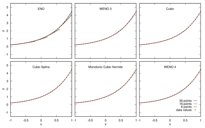
Figure 1: Exponential function (16), is approximated in the interval $x\in[-1,1]$ with third-order ENO, third-order WENO, cubic Lagrange, cubic Spline, monotonic cubic Hermite, and fourth-order WENO interpolations, with different homogeneously spaced grid points densities. Black dots represent the data values on the 36-point grid.

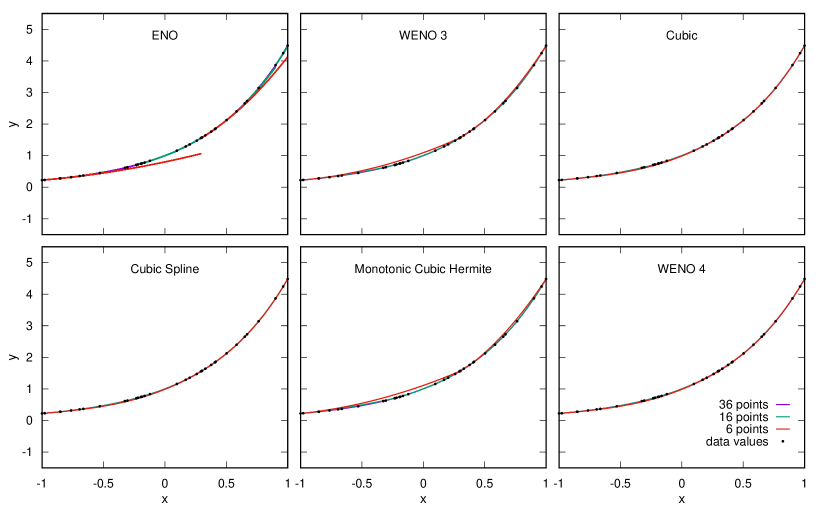
Figure 2: Same as Figure 1, but for inhomogeneous samplings.

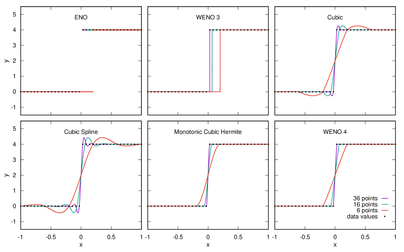
Figure 3: Same as Figure 1, but for the modified Heaviside function given by Equation (17).

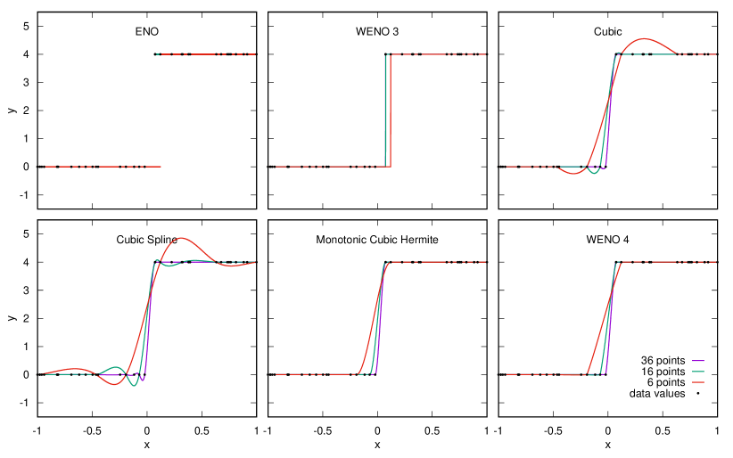
Figure 4: Same as Figure 3, but for inhomogeneous samplings.

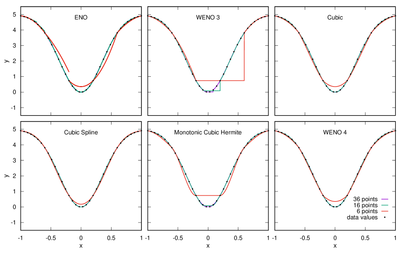
Figure 5: Same as Figure 1, but for the modified Gaussian function given by Equation (18).

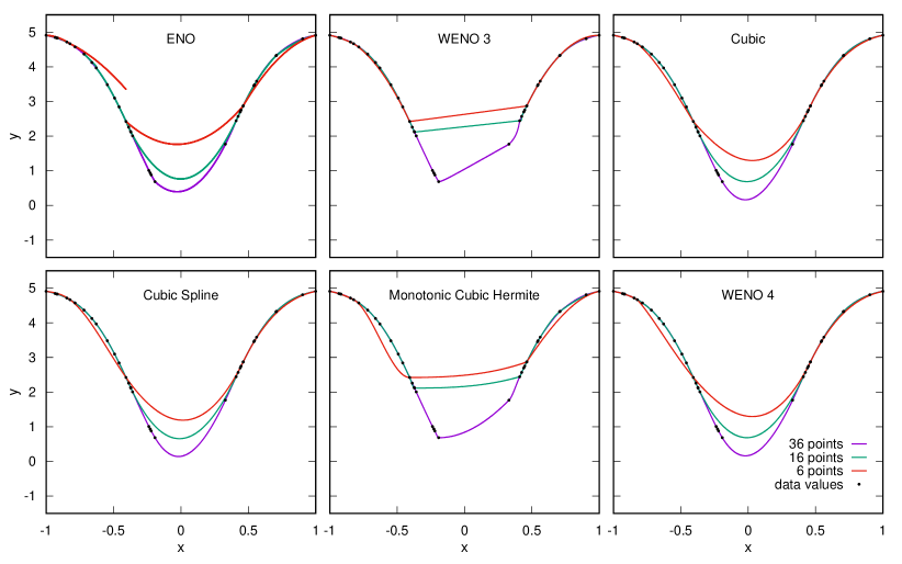
Figure 6: Same as Figure 5, but for inhomogeneous samplings.

resulting in $\beta_{1}\ll\beta_{2}$. This guarantees that the smoothness indicators (10) effectively detect discontinuities in nonuniform grids and ensure the non-oscillatory property in the interpolation. The indicators (8) and (10) do not distinguish between discontinuities and smooth extrema. For this reason, they do not guarantee accuracy near such critical points. Some numerical evidence for the third-order WENO interpolation with smoothness indicators (10) is shown in Figures 1-6.

3.3 Fourth-order WENO interpolation

The WENO interpolation and the relative smoothness indicators outlined in the following are completely original. This novel fourth-order WENO interpolation uses a four-point stencil, is symmetric around the considered interval $[x_{i},x_{i+1}]$, and provides a suitable compromise of the computation cost and the accuracy.

The unique cubic Lagrange polynomial $p(x)$ interpolating the four-point large stencil

$$S_{4}^{3}=\{x_{i-1},x_{i},x_{i+1},x_{i+2}\}\,,$$

can be written as

$$p(x)=\gamma_{2}(x)q_{2}(x)+\gamma_{3}(x)q_{3}(x)\,,$$

that is, as a linear combination of the quadratic Lagrange interpolations

$$q_{2}(x) =y_{i-1}\frac{(x\!-\!x_{i})(x\!-\!x_{i+1})}{h_{i-1}(h_{i-1}+h_{i})}\!-\!y_{i}\frac{(x\!-\!x_{i-1})(x\!-\!x_{i+1})}{h_{i-1}h_{i}}\!+\!y_{i+1}\frac{(x\!-\!x_{i-1})(x\!-\!x_{i})}{(h_{i-1}+h_{i})h_{i}},$$

$$q_{3}(x) =y_{i}\frac{(x\!-\!x_{i+1})(x\!-\!x_{i+2})}{h_{i}(h_{i}+h_{i+1})}\!-\!y_{i+1}\frac{(x\!-\!x_{i})(x\!-\!x_{i+2})}{h_{i}h_{i+1}}\!+\!y_{i+2}\frac{(x\!-\!x_{i})(x\!-\!x_{i+1})}{(h_{i}+h_{i+1})h_{i+1}},$$

based, respectively, on the two three-point substencils

$$S_{3}^{2}=\{x_{i-1},x_{i},x_{i+1}\}\,,\;\text{ and }\;S_{3}^{3}=\{x_{i},x_{i+1},x_{i+2}\}\,.$$

The linear weights are given by

$$\gamma_{2}(x)=-\frac{x-x_{i+2}}{x_{i+2}-x_{i-1}}\,,\;\text{ and }\;\gamma_{3}(x)=\frac{x-x_{i-1}}{x_{i+2}-x_{i-1}}\,,$$

and satisfy $\gamma_{2}(x)+\gamma_{3}(x)=1$. The linear weights depend just on the grid geometry and not on the values of the function. The fourth-order WENO interpolation in the interval $[x_{i},x_{i+1}]$ reads

$$p_{i}(x)=\omega_{2}(x)q_{2}(x)+\omega_{3}(x)q_{3}(x)\,,$$

where the nonlinear weights are defined as

$$\omega_{2}(x)=\frac{\alpha_{2}(x)}{\alpha_{2}(x)+\alpha_{3}(x)}\,,\;\text{ and }\;\omega_{3}(x)=\frac{\alpha_{3}(x)}{\alpha_{2}(x)+\alpha_{3}(x)}\,,$$

with

$$\alpha_{2}(x)=\frac{\gamma_{2}(x)}{\epsilon+\beta_{2}}\,,\;\text{ and }\;\alpha_{3}(x)=\frac{\gamma_{3}(x)}{\epsilon+\beta_{3}}\,,$$

and $\epsilon=10^{-6}$.

3.3.1 Smoothness indicators for uniform grids

The first-order 4-point numerical derivatives of $y(x)$ at nodes $x_{i-1}$, $x_{i}$, $x_{i+1}$ and $x_{i+2}$ for uniform grids read (e.g., Singh & Bhadauria 2009)

$$\begin{bmatrix}y^{\prime}_{i-1}\\ y^{\prime}_{i}\\ y^{\prime}_{i+1}\\ y^{\prime}_{i+2}\end{bmatrix}=\frac{1}{6h}\begin{bmatrix}-11&18&-9&2\\ -2&-3&6&-1\\ 1&-6&3&2\\ -2&9&-18&11\end{bmatrix}\begin{bmatrix}y_{i-1}\\ y_{i}\\ y_{i+1}\\ y_{i+2}\end{bmatrix}\,,$$ (11)

or, alternatively,

$$\begin{bmatrix}y^{\prime}_{i-1}\\ y^{\prime}_{i}\\ y^{\prime}_{i+1}\\ y^{\prime}_{i+2}\end{bmatrix}=\frac{1}{6}\begin{bmatrix}11&-7&2\\ 2&5&-1\\ -1&5&2\\ 2&-7&11\end{bmatrix}\begin{bmatrix}d_{i-1}\\ d_{i}\\ d_{i+1}\end{bmatrix}\,.$$

Using these, the new indicators are constructed as follows

$$\beta_{2} =4\left(|y^{\prime}_{i+1}-y^{\prime}_{i}|-|y^{\prime}_{i}-y^{\prime}_{i-1}|\right)^{2}\,,$$ (12)

$$\beta_{3} =4\left(|y^{\prime}_{i+2}-y^{\prime}_{i+1}|-|y^{\prime}_{i+1}-y^{\prime}_{i}|\right)^{2}\,,$$

with

$$\begin{bmatrix}y^{\prime}_{i}-y^{\prime}_{i-1}\\ y^{\prime}_{i+1}-y^{\prime}_{i}\\ y^{\prime}_{i+2}-y^{\prime}_{i+1}\end{bmatrix}=\frac{1}{6}\begin{bmatrix}-9&12&-3\\ -3&0&3\\ 3&-12&9\end{bmatrix}\begin{bmatrix}d_{i-1}\\ d_{i}\\ d_{i+1}\end{bmatrix}\,.$$ (13)

In smooth regions where the second derivative has a constant sign, the differences of the numerical derivatives (13) have the same sign, that is,

$$\operatorname{sign}\left(y^{\prime}_{i}-y^{\prime}_{i-1}\right)=\operatorname{sign}\left(y^{\prime}_{i+1}-y^{\prime}_{i}\right)=\operatorname{sign}\left(y^{\prime}_{i+2}-y^{\prime}_{i+1}\right)\,.$$

Consequently, the indicators (12) reduce to

$$\beta_{2}=\beta_{3}=4\left(-y_{i-1}+3y_{i}-3y_{i+1}+y_{i+2}\right)^{2}\,,$$

and one gets

$$\omega_{2}(x)=\gamma_{2}(x)\,,\;\text{ and }\;\omega_{3}(x)=\gamma_{3}(x)\,.$$

Hence, in smooth regions where the second derivative has a constant sign, the nonlinear weights correspond to the linear weights, reducing the numerical dissipation of the fourth-order WENO interpolation. We note that the indicators (12) allow for over- or undershoots around smooth extrema, yielding a higher accuracy near such critical points with respect to monotonic interpolations. However, this feature may have the adverse effect of producing negative interpolated values in strictly positive functions. Moreover, the indicators (12) do not guarantee accuracy near inflection points.

For the discontinuous case, assume that $y(x)$ has a discontinuity in the interval $[x_{i-1},x_{i}]$ and is smooth in the interval $[x_{i},x_{i+2}]$. In this case one has

$$\left|d_{i-1}\right|\gg\left|d_{i}\right|,\left|d_{i+1}\right|\,,$$

and from Equation (13), one has

$$\operatorname{sign}\left(y^{\prime}_{i}-y^{\prime}_{i-1}\right)=\operatorname{sign}\left(y^{\prime}_{i+1}-y^{\prime}_{i}\right)\neq\operatorname{sign}\left(y^{\prime}_{i+2}-y^{\prime}_{i+1}\right)\,.$$

Consequently,

$$\beta_{2} =4\left(d_{i-1}-2d_{i}+d_{i+1}\right)^{2}=\mathcal{O}\left(d_{i-1}^{2}\right)\,,$$

$$\beta_{3} =4\left(2d_{i}-2d_{i+1}\right)^{2}=\mathcal{O}\left((d_{i}-d_{i+1})^{2}\right)\,,$$

resulting in $\beta_{2}\gg\beta_{3}$. Analogously, if the function $y(x)$ is smooth in $[x_{i-1},x_{i+1}]$ and has a discontinuity inside $[x_{i+1},x_{i+2}]$, one obtains

$$\beta_{2} =\mathcal{O}\left((d_{i}-d_{i-1})^{2}\right)\,,$$

$$\beta_{3} =\mathcal{O}\left(d_{i+1}^{2}\right)\,,$$

resulting in $\beta_{2}\ll\beta_{3}$. If the discontinuity point is located in the interval $[x_{i},x_{i+1}]$, both substencils $S_{3}^{2}$ and $S_{3}^{3}$ contain the discontinuity. This seemingly difficult case is actually not problematic, because both polynomials $q_{2}(x)$ and $q_{3}(x)$ are essentially monotone inside $[x_{i},x_{i+1}]$, because the over- or undershoots appear in the cells adjacent to the discontinuity (Shu 1998, 2009).

3.3.2 Smoothness indicators for nonuniform grids

The first-order four-point derivatives of $y(x)$ at nodes $x_{i-1}$, $x_{i}$, $x_{i+1}$ and $x_{i+2}$ for nonuniform grids are approximated by (e.g., Singh & Bhadauria 2009)

$$y^{\prime}_{i-1} =-\frac{(2h_{i-1}+h_{i})H+h_{i-1}(h_{i-1}+h_{i})}{h_{i-1}(h_{i-1}+h_{i})H}y_{i-1}+\frac{(h_{i-1}+h_{i})H}{h_{i-1}h_{i}(h_{i}+h_{i+1})}y_{i}$$ (14)

$$-\frac{h_{i-1}H}{(h_{i-1}+h_{i})h_{i}h_{i+1}}y_{i+1}+\frac{h_{i-1}(h_{i-1}+h_{i})}{(h_{i}+h_{i+1})h_{i+1}H}y_{i+2}\,,$$

$$y^{\prime}_{i} =-\frac{h_{i}(h_{i}+h_{i+1})}{h_{i-1}(h_{i-1}+h_{i})H}y_{i-1}+\frac{h_{i}(h_{i}+h_{i+1})-h_{i-1}(2h_{i}+h_{i+1})}{h_{i-1}h_{i}(h_{i}+h_{i+1})}y_{i}$$

$$+\frac{h_{i-1}(h_{i}+h_{i+1})}{(h_{i-1}+h_{i})h_{i}h_{i+1}}y_{i+1}-\frac{h_{i-1}h_{i}}{(h_{i}+h_{i+1})h_{i+1}H}y_{i+2}\,,$$

$$y^{\prime}_{i+1} =\frac{h_{i}h_{i+1}}{h_{i-1}(h_{i-1}+h_{i})H}y_{i-1}-\frac{h_{i+1}(h_{i-1}+h_{i})}{h_{i-1}h_{i}(h_{i}+h_{i+1})}y_{i}$$

$$+\frac{(h_{i-1}+2h_{i})h_{i+1}-(h_{i-1}+h_{i})h_{i}}{(h_{i-1}+h_{i})h_{i}h_{i+1}}y_{i+1}+\frac{(h_{i-1}+h_{i})h_{i}}{(h_{i}+h_{i+1})h_{i+1}H}y_{i+2}\,,$$

$$y^{\prime}_{i+2} =-\frac{(h_{i}+h_{i+1})h_{i+1}}{h_{i-1}(h_{i-1}+h_{i})H}y_{i-1}+\frac{h_{i+1}H}{h_{i-1}h_{i}(h_{i}+h_{i+1})}y_{i}$$

$$-\frac{(h_{i}+h_{i+1})H}{(h_{i-1}+h_{i})h_{i}h_{i+1}}y_{i+1}+\frac{(2h_{i+1}+h_{i})H+h_{i+1}(h_{i}+h_{i+1})}{(h_{i}+h_{i+1})h_{i+1}H}y_{i+2}\,,$$

where $H=h_{i-1}+h_{i}+h_{i+1}$. The novel smoothness indicators are constructed as follows

$$\beta_{2} =(h_{i}+h_{i+1})^{2}\left(\frac{|y^{\prime}_{i+1}-y^{\prime}_{i}|}{h_{i}}-\frac{|y^{\prime}_{i}-y^{\prime}_{i-1}|}{h_{i-1}}\right)^{2}\,,$$ (15)

$$\beta_{3} =(h_{i-1}+h_{i})^{2}\left(\frac{|y^{\prime}_{i+2}-y^{\prime}_{i+1}|}{h_{i+1}}-\frac{|y^{\prime}_{i+1}-y^{\prime}_{i}|}{h_{i}}\right)^{2}\,.$$

For $h_{i-1}=h_{i}=h_{i+1}=h$, the finite difference formulae (14) and (15) reduce to uniform grids formulae (11) and (12), respectively.

In smooth regions where the second derivative has a constant sign, the differences of two consecutive numerical derivatives given by Equation (14) have the same sign, that is,

$$\operatorname{sign}\left(y^{\prime}_{i}-y^{\prime}_{i-1}\right)=\operatorname{sign}\left(y^{\prime}_{i+1}-y^{\prime}_{i}\right)=\operatorname{sign}\left(y^{\prime}_{i+2}-y^{\prime}_{i+1}\right)\,.$$

In this case, one shows with some tedious algebra that the indicators (15) satisfy $\beta_{2}=\beta_{3}$ and, consequently,

$$\omega_{2}(x)=\gamma_{2}(x)\,,\;\text{ and }\;\omega_{3}(x)=\gamma_{3}(x)\,.$$

Hence, in smooth regions where the second derivative has a constant sign, the nonlinear weights correspond to the optimal weights, reducing numerical dissipation. As above, indicators (15) allow for over- or undershoots around smooth extrema, yielding a higher accuracy near such critical points with respect to monotonic interpolations. As for the uniform case, this feature may have the adverse effect of producing negative interpolated values in strictly positive function.

The capability of the smoothness indicators (15) to detect discontinuities in the interpolation is already demonstrated for the uniform case in Section 3.3.1. The generalization of the proof to nonuniform grids is particularly cumbersome, but leads to the same conclusion. However, the indicators (15) do not guarantee accuracy near inflection points.

In conclusion, the smoothness indicators (12) and (15) effectively detect discontinuities and ensure the non-oscillatory property in the interpolation. Some numerical evidence for the fourth-order WENO interpolations with smoothness indicators (12) and (15) is displayed in Figures 1-6. Moreover, an alternative fourth-order WENO interpolation is presented in Appendix A.

4 Numerical tests

For the sake of comparison, the third-order ENO, the third-order WENO (version Liu et al. 2018), the cubic Lagrange, the cubic Spline, the local monotonic piecewise cubic Hermite (Fritsch & Butland 1984; Ibgui et al. 2013), and the novel fourth-order WENO interpolations are tested. Four different functions are interpolated on both uniform and nonuniform grids with different numbers of grid points. The nonuniform grids are randomly generated. The experimental orders of convergence on uniform grids are summarized in Table 1. We note that the monotonic cubic Hermite interpolation is third-order accurate only. This is due to the derivatives provided by Fritsch & Butland (1984), which are second-order accurate on uniform grids. In order to verify the accuracy for smooth cases, in Figures 1 and 2 we analyze the interpolation of the exponential function

$$y(x)=e^{\frac{3}{2}x}\,,\;\text{ with }x\in[-1,1]\,.$$ (16)

No essential difference between the various interpolations is visible for the homogeneous samplings, apart from the ENO technique that shows a slightly fragmented interpolation. Major differences appear for the inhomogeneous samplings, where fourth-order interpolations perform definitely better and the ENO technique shows a fragmented interpolation. Moreover, the monotonic cubic Hermite interpolation proves to be less accurate for inhomogeneous samplings. This is due to the derivatives provided by Fritsch & Butland (1984), which drop to first-order accuracy on non-uniform grids.

In order to understand the behaviors around discontinuities, Figures 3 and 4 show the interpolation of the scaled Heaviside function, that is,

$$y(x)=4H(x)=\begin{cases}0&\text{ if }x<0\,,\\ 4&\text{ if }x\geq 0\,,\end{cases}\;\text{ with }x\in[-1,1]\,.$$ (17)

The cubic Lagrange and the cubic Spline interpolations reveal Gibbs-like oscillations for homogeneous and inhomogeneous samplings. For the homogeneous sampling, such oscillations do not decay in magnitude when the computational grid is refined. By contrast, monotonic cubic Hermite, ENO and WENO interpolations approximate the discontinuity more sharply and without oscillations. In this example, the WENO interpolation algorithm successfully capitalizes on its main idea, that is, placing much heavier weights on the candidate substencils in which the discontinuity is absent.

In order to better understand the different behaviors around smooth critical points (smooth extrema), Figures 5 and 6 analyze the interpolation of the function

$$y(x)=5(1-e^{-4x^{2}})\,,\;\text{ with }x\in[-1,1]\,.$$ (18)

With 16 or more uniformly distributed grid points, third-order ENO, the cubic Lagrange, the cubic Spline interpolations, and WENO 4 accurately represent the minimum. All these methods require 36 points to accurately represent the extremum for inhomogeneous samplings. By contrast, the accuracy of WENO 3 and of the monotonic cubic Hermite interpolations locally decreases near the smooth extremum of the interpolated function. We note that the WENO 4 method allows for over- or undershoots around the smooth extrema, yielding a higher accuracy with respect to monotonic interpolants near such critical points.

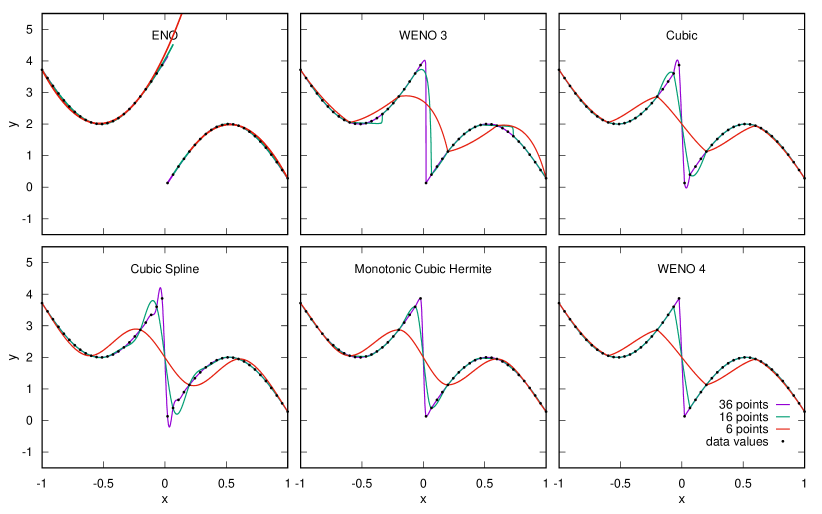
Figure 7: Same as Figure 1, but for the discontinuous sine function given by Equation (19).

Figures 7 and 8 show the interpolation of the function

$$y(x)=\begin{cases}2\sin(3x)+4&\text{ if }x<0\,,\\ 2\sin(3x)&\text{ if }x\geq 0\,,\end{cases}\;\text{ with }x\in[-1,1]\,,$$ (19)

which contains both a high-order smooth structure and a discontinuity. Standard interpolations present oscillations for homogeneous and inhomogeneous samplings. The ENO interpolation is robust and resolves the complex discontinuous function quite well, albeit with small overshoots. WENO 3 and the monotonic cubic Hermite interpolation do not present oscillations, but struggle with accurately reproducing the smooth extrema in the function. By contrast, WENO 4 shows no oscillations, nor does it produce the spread of the extrema.

Table 1: Order of accuracy

Interpolation method	Exponential	Heaviside	Discontinuous sine	Gaussian
ENO	3.017	1.072	1.073	3.033
WENO 3	3.026	1.072	1.072	3.046
Cubic Spline	4.043	1.024	1.025	4.046
Cubic	4.043	1.029	1.029	4.044
Monotonic Hermite	3.033	1.045	1.059	2.922
WENO 4	4.043	1.035	1.036	4.371

5 Application to radiative transfer

High accuracy is required in many radiative transfer problems (Socas-Navarro et al. 2000; Trujillo Bueno 2003). In particular, the upcoming American Daniel K. Inouye Solar Telescope (DKIST) (Elmore et al. 2014; Tritschler et al. 2016) and the planned European Solar Telescope (EST) (Matthews et al. 2016; Matthews & Collados 2017) have a diffraction limit near to or surpassing the resolution of the best current 3D radiative-magnetohydrodynamic (R-MHD) simulations of the solar surface (Peck et al. 2017), making high accuracy critical for comparisons with observations. Such 3D R-MHD atmospheric models can be highly inhomogeneous and dynamic and present discontinuities. However, common radiative transfer calculations usually assume smooth variations in the radiation field and in the atmospheric physical parameters, and the incidence of discontinuities is often neglected (Steiner et al. 2016; Janett 2019). In fact, standard numerical schemes and high-order interpolations tend to misrepresent the nonsmooth regions of a problem, introducing spurious oscillations near discontinuities (e.g., Richards 1991; Zhang & Martin 1997; Shu 1998). Moreover, many radiative transfer codes require grid refinements, that is, the process of resolving the input data on a finer grid.

The fourth-order WENO interpolation technique presented in Sections 3.3 is particularly suitable for scenarios that involve both complex smooth structures and discontinuities in the physical parameters. Moreover, it uses the same four-point stencil as the cubic Lagrange and monotonic cubic interpolations. Therefore, it is fairly straightforward to implement them on already existing codes.

5.1 2D and 3D problems

The only difference between 1D and multidimensional radiative transfer lies in the mapping of the relevant quantities along the path of the photons (Carlsson 2008), typically through interpolation. At least for the Cartesian type grids, multidimensional interpolations can be obtained from 1D procedures. In 2D problems, the usual strategy is to discretize the ray by taking its intersections with the segments connecting the grid points, dealing then with 1D interpolations to recover off-grid points quantities (Auer 2003). In 3D problems, an efficient approach is to discretize the ray by taking its intersections with the individual planes defined by the grid points, dealing then with 2D interpolations.

Many radiative transfer codes have the option to use linear or bi-linear interpolations from the values of the nearest grid points: for example, RH by Uitenbroek (2001), MULTI3D by Leenaarts & Carlsson (2009), and PORTA by Štěpán & Trujillo Bueno (2013). In multiple dimensions, the commonly used short-characteristic method suffers large numerical diffusion if the upwind intensity is successively linearly interpolated in the direction of propagation. Consequently, the solution lacks high-order accuracy (Fabiani Bendicho 2003; Ibgui et al. 2013; Peck et al. 2017). Such diffusion errors decrease with increasing order of accuracy of the interpolation and a natural choice would be to use bi-quadratic or bi-cubic interpolations (Kunasz & Auer 1988; Dullemond 2013). However, if the behavior of the quantities to be interpolated is discontinuous or particularly intermittent, high-order interpolants introduce spurious extrema that could lead to nonphysical results (e.g., negative values of the source function or of the intensity). To avoid this, one can opt for monotonic interpolation schemes (e.g., Steffen 1990; Auer & Paletou 1994; Hayek et al. 2010; Ibgui et al. 2013), which however degenerate to a linear interpolation near smooth extrema, dropping to second-order accuracy. This calls for high-order interpolations that are able to handle discontinuities and the WENO interpolation presented in Section 3.3 can be easily generalized to 2D and 3D Cartesian grids with a direct application dimension by dimension (Zhang & Shu 2016).

5.2 Multigrid methods

Steiner (1991) first implemented a linear multigrid method for radiative transfer problems. Later on, Fabiani Bendicho et al. (1997) applied the nonlinear multigrid method to the multi-level NLTE radiative transfer problem. Recently, Štěpán & Trujillo Bueno (2013) generalized the method to the polarized case and Bjørgen & Leenaarts (2017) applied a nonlinear multigrid method to realistic 3D R-MHD atmospheric models, which are highly inhomogeneous and dynamic.

The Jacobi and Gauss-Seidel iterative schemes for 3D NLTE radiative transfer problems quickly smooth out the high-spatial-frequency error, whereas they slowly decrease the low-frequency error. To accelerate the global smoothing of errors, multigrid methods transfer the problem to a coarser grid, where such low-frequency errors become high-frequency errors and iterations on the coarse grid quickly decrease these errors. The coarser grid correction is mapped to the finer grid with an interpolation operator. In this step, cubic interpolations appear to give higher convergence rates (Štěpán & Trujillo Bueno 2013). However, when abrupt changes of atmospheric physical quantities are present (e.g., in 3D R-MHD atmospheric models), such interpolations introduce spurious oscillations, which negatively affect the convergence rate of multigrid methods and even induce numerical instabilities, leading to unphysical negative values of strictly positive physical parameters. In such situations, it is safer to use monotonic interpolation, such as the monotonic cubic Hermite interpolation used in MULTI3D (Bjørgen & Leenaarts 2017). The interpolation operation is thus a crucial ingredient of any multigrid method and the fourth-order WENO interpolation might be an improvement over currently used interpolations.

5.3 Conversion to optical depth

The steady-state version of the radiative transfer equation consists in the linear first-order inhomogeneous ODE given by (e.g., Mihalas 1978)

$$\frac{\rm d}{{\rm d}s}I_{\nu}(s)=-\chi_{\nu}(s)I_{\nu}(s)+\epsilon_{\nu}(s)\,,$$ (20)

where the spatial coordinate $s$ denotes the position along the ray under consideration, $\nu$ is the frequency, $I_{\nu}$ is the specific intensity, and $\chi_{\nu}$ and $\epsilon_{\nu}$ are the absorption and the emission coefficients, respectively. In non-local thermodynamic equilibrium (NLTE) conditions, the absorption and the emission coefficients depend in a complicated manner on the intensity $I_{\nu}$, so that Equation (20) is nonlinear and must be supplemented by additional statistical equilibrium equations and/or by suitable redistribution matrices for scattering processes.

The change of coordinates defined by

$${\rm d}\tau_{\nu}=-\chi_{\nu}(s){\rm d}s\,,$$ (21)

transplants Equation (20) to the optical depth scale, namely,

$$\frac{\rm d}{{\rm d}\tau_{\nu}}I_{\nu}(\tau_{\nu})=I_{\nu}(\tau_{\nu})-S_{\nu}(\tau_{\nu})\,,$$ (22)

where $S_{\nu}=\epsilon_{\nu}/\chi_{\nu}$ is the source function. From Equation (21), one has

$$\tau_{\nu}=\tau_{\nu,0}-\int_{s_{0}}^{s}\chi_{\nu}(x)\,{\rm d}x\,,$$

and numerical approximations of $\tau_{\nu}(s)$ can be obtained by replacing the integral with a numerical quadrature. Janett et al. (2017a) explain that high-order formal solvers require a corresponding high-order quadrature of the integral above.

A $n$-point weighted quadrature rule is usually stated as

$$\int_{a}^{b}f(x){\rm d}x=\sum_{i=1}^{n}\omega_{i}f(x_{i})\,,$$

and is based on a suitable choice of the nodes $\{x_{i}\}$ and the weights $\{\omega_{i}\}$. In high-order quadratures, one must recover the values of $f(x)$ at off-grid points, which typically requires high-order interpolations.

As a practical example, the fourth-order accurate Simpson’s formula

$$\int_{a}^{b}f(x){\rm d}x=\frac{b-a}{6}\left[f(a)+4f(\tfrac{a+b}{2})+f(b)\right]\,,$$

considers the node points $\{a,\tfrac{a+b}{2},b\}\,,$ and their corresponding function values. The midpoint function value $f(\tfrac{a+b}{2})$ must be recovered through a high-order interpolation, for example, the fourth-order WENO interpolation.

5.4 High-order formal solvers

When applied to Equation (20) or Equation (22), certain high-order formal solvers, such as the RK4 method proposed by Landi Degl’Innocenti (1976) and and the third-order pragmatic method by Janett et al. (2018), require the absorption $\chi_{\nu}$ and emission $\epsilon_{\nu}$ coefficients at off-grid points. In order to maintain high-order accuracy, such quantities must be obtained through high-order interpolations (e.g., Janett et al. 2017b, for the polarized problem), which are notoriously oscillatory in the presence of abrupt changes or discontinuities in the atmospheric physical quantities. In such formal solvers, spurious oscillations in the interpolation of $\chi_{\nu}$ and $\epsilon_{\nu}$ can negatively affect their order of accuracy. The fourth-order WENO interpolation might be befitting in such situations.

5.5 Redistribution matrix formalism

The redistribution matrix formalism is often used for calculating the emissivity in NLTE conditions, especially when partial frequency redistribution effects are important. The emissivity is evaluated by integrating the incident radiation field, multiplied by the redistribution matrix, over frequency and direction. However, performing the frequency integration is often nontrivial because of the sharp frequency dependence of the redistribution matrix. The quadrature of such integral requires describing the frequency dependence of the radiation field between the specific frequency points where its values are known. Interpolation techniques such as cardinal natural cubic splines have already been used (see Adams et al. 1971; Belluzzi & Trujillo Bueno 2014; Alsina Ballester et al. 2017). However, such a choice is problematic if the radiation field is not sufficiently smooth in the considered frequency interval. This calls for high-order interpolations capable of dealing with such sharp variations, such as the fourth-order WENO interpolation.

6 Conclusions

This paper discusses different ENO and WENO interpolation techniques. These interpolations are particularly suitable to problems containing both sharp discontinuities and complex smooth structures, where high-order Lagrange or spline interpolations are prone to over- and undershoots.

Special attention is paid to the possible applications of a novel fourth-order WENO interpolation, which is outlined, analyzed, and tested for both the uniform and nonuniform cases. This method for computing non-oscillatory fourth-order interpolants is simple, symmetrical, and completely local. Unlike Bézier and monotonic Hermite interpolations, it does not degenerate to second-order accuracy near smooth extrema of the interpolated function and it avoids the use of conditional “if$\dots$else” statements in the algorithm. Moreover, it uses the same four-point stencil as the cubic Lagrange interpolation. The implementation on already existing codes is, therefore, fairly straightforward. Numerical analysis and numerical experiments indicate that the smoothness indicators given by Equations (12) and (15) guarantee fourth-order accuracy in smooth regions, while effectively detecting discontinuities and enabling the non-oscillatory property. These novel local smoothness indicators yield less dissipation and better resolution than the canonical ones. Such indicators allow for minimal over- or undershoots around smooth extrema, yielding a higher accuracy near such critical points. However, we note that this feature may have the adverse effect of producing negative interpolated values in strictly positive function. Moreover, this WENO interpolation is not differentiable at the grid points (i.e., it has kinks). Even though the fourth-order WENO interpolation may require more CPU time than the cubic Lagrange interpolation (depending on the specific algorithm components and computer implementation), it may still be computationally advantageous for many problems because of its high accuracy. Moreover, the method can be extended to the interpolation of 2D or 3D data.

This interpolation technique might be particularly suitable in the context of the numerical radiative transfer, which must be performed with ever increasing spatial and spectral resolution and consequently requires high accuracy in calculations. However, the fourth-order WENO interpolation is a general approximation procedure, which can also be used in many other applications beyond radiative transfer, such as computer vision and image processing. Alternative approximation techniques are available, such as the so-called HWENO approximations - WENO schemes based on Hermite polynomials (Qiu & Shu 2004; Zhu & Qiu 2009).

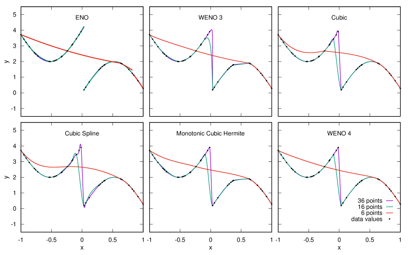
Figure 8: Same as Figure 7, but for inhomogeneous samplings.

Appendix A An alternative version of the fourth-order WENO interpolation

In this appendix, an alternative to the fourth-order WENO interpolation presented in Section 3.3 is outlined. The unique cubic Lagrange polynomial $p(x)$ interpolating the four-point large stencil

$$S_{4}^{3}=\{x_{i-1},x_{i},x_{i+1},x_{i+2}\}\,,$$

can be written as

$$p(x)=\gamma_{2}(x)q_{2}(x)+\gamma_{3}(x)q_{3}(x)+\gamma_{4}(x)q_{4}(x)\,,$$

in other words, as a linear combination of the linear Lagrange interpolations

$$q_{2}(x) =\frac{-y_{i-1}(x-x_{i})+y_{i}(x-x_{i-1})}{x_{i}-x_{i-1}}\,,$$

$$q_{3}(x) =\frac{-y_{i}(x-x_{i+1})+y_{i+1}(x-x_{i})}{x_{i+1}-x_{i}}\,,$$

$$q_{4}(x) =\frac{-y_{i+1}(x-x_{i+2})+y_{i+2}(x-x_{i+1})}{x_{i+2}-x_{i+1}}\,,$$

based, respectively, on the three two-point substencils

$$S_{3}^{2}=\{x_{i-1},x_{i}\}\,,\;S_{3}^{3}=\{x_{i},x_{i+1}\}\,,\;S_{3}^{4}=\{x_{i+1},x_{i+2}\}\,.$$

The linear weights are given by

$$\gamma_{2}(x) =\frac{(x-x_{i+1})(x-x_{i+2})}{(x_{i+1}-x_{i-1})(x_{i+2}-x_{i-1})}\,,$$

$$\gamma_{3}(x) =-\frac{(x-x_{i-1})(x-x_{i+2})}{x_{i+2}-x_{i-1}}\left[\frac{1}{x_{i+1}-x_{i-1}}+\frac{1}{x_{i+2}-x_{i}}\right]\,,$$

$$\gamma_{4}(x) =\frac{(x-x_{i-1})(x-x_{i})}{(x_{i+2}-x_{i-1})(x_{i+2}-x_{i})}\,,$$

and satisfy $\gamma_{2}(x)+\gamma_{3}(x)+\gamma_{4}(x)=1$. The linear weights depend just on the grid geometry and not on the function values. The fourth-order WENO interpolation in the interval $[x_{i},x_{i+1}]$ reads

$$p_{i}(x)=\omega_{2}(x)q_{2}(x)+\omega_{3}(x)q_{3}(x)+\omega_{4}(x)q_{4}(x)\,,$$

where the nonlinear weights are defined as

$$\omega_{2}(x) =\frac{\alpha_{2}(x)}{\alpha_{2}(x)+\alpha_{3}(x)+\alpha_{4}(x)}\,,$$

$$\omega_{3}(x) =\frac{\alpha_{3}(x)}{\alpha_{2}(x)+\alpha_{3}(x)+\alpha_{4}(x)}\,,$$

$$\omega_{4}(x) =\frac{\alpha_{4}(x)}{\alpha_{2}(x)+\alpha_{3}(x)+\alpha_{4}(x)}\,,$$

with

$$\alpha_{2}(x)=\frac{\gamma_{2}(x)}{\epsilon+\beta_{2}}\,,\;\alpha_{3}(x)=\frac{\gamma_{3}(x)}{\epsilon+\beta_{3}}\,,\;\alpha_{4}(x)=\frac{\gamma_{4}(x)}{\epsilon+\beta_{4}}\,,$$

and $\epsilon=10^{-6}$.

A.1 Smoothness indicators for uniform grids

In case of uniform grids, a possible choice for the smoothness indicators is

$$\beta_{2} =\left(y^{\prime}_{i}-y^{\prime}_{i-1}\right)^{2}\,,$$

$$\beta_{3} =\left(y^{\prime}_{i+1}-y^{\prime}_{i}\right)^{2}\,,$$

$$\beta_{4} =\left(y^{\prime}_{i+2}-y^{\prime}_{i+1}\right)^{2}\,,$$

where the differences of the numerical derivatives are given by Equation (13). Unfortunately, this version makes the fourth-order WENO interpolation too dissipative and generates apparent oscillations. The search of smoothness indicators that yield less dissipation and better resolution is not over.

A.2 Smoothness indicators for nonuniform grids

In case of nonuniform grids, a possible choice for the smoothness indicators is

$$\beta_{2} =\left(\frac{y^{\prime}_{i}-y^{\prime}_{i-1}}{h_{i-1}}\right)^{2}\,,$$

$$\beta_{3} =\left(\frac{y^{\prime}_{i+1}-y^{\prime}_{i}}{h_{i}}\right)^{2}\,,$$

$$\beta_{4} =\left(\frac{y^{\prime}_{i+2}-y^{\prime}_{i+1}}{h_{i+1}}\right)^{2}\,,$$

where the numerical derivatives are given by Equation (14). As for the uniform case, this version makes the fourth-order WENO interpolation too dissipative and generates apparent oscillations. The search of smoothness indicators that yield less dissipation and better resolution is not over.

References

- Adams et al. (1971) Adams, T. F., Hummer, D. G., & Rybicki, G. B. 1971, J. Quant. Spec. Radiat. Transf., 11, 1365
- Alsina Ballester et al. (2017) Alsina Ballester, E., Belluzzi, L., & Trujillo Bueno, J. 2017, ApJ, 836, 6
- Aràndiga et al. (2013) Aràndiga, F., Baeza, A., & Yáñez, D. F. 2013, Advances in Computational Mathematics, 39, 289
- Auer (2003) Auer, L. 2003, in Astronomical Society of the Pacific Conference Series, Vol. 288, Stellar Atmosphere Modeling, ed. I. Hubeny, D. Mihalas, & K. Werner, 3
- Auer & Paletou (1994) Auer, L. H. & Paletou, F. 1994, A&A, 285, 675
- Belluzzi & Trujillo Bueno (2014) Belluzzi, L. & Trujillo Bueno, J. 2014, A&A, 564, A16
- Bjørgen & Leenaarts (2017) Bjørgen, J. P. & Leenaarts, J. 2017, A&A, 599, A118
- Borges et al. (2008) Borges, R., Carmona, M., Costa, B., & Don, W. S. 2008, Journal of Computational Physics, 227, 3191
- Carlsson (2008) Carlsson, M. 2008, Physica Scripta Volume T, 133, 014012
- Črnjarić-Žic et al. (2007) Črnjarić-Žic, N., Maćešić, S., & Crnković, B. 2007, Annali dell’Università di Ferrara, 53, 199
- Dullemond (2013) Dullemond, C. P. 2013, Radiative Transfer in Astrophysics. Theory, Numerical Methods and Applications, Tech. rep., University of Heidelberg
- Elmore et al. (2014) Elmore, D. F., Rimmele, T., Casini, R., et al. 2014, in Proc. SPIE, Vol. 9147, Ground-based and Airborne Instrumentation for Astronomy V, 914707
- Fabiani Bendicho (2003) Fabiani Bendicho, P. 2003, in Astronomical Society of the Pacific Conference Series, Vol. 288, Stellar Atmosphere Modeling, ed. I. Hubeny, D. Mihalas, & K. Werner, 419
- Fabiani Bendicho et al. (1997) Fabiani Bendicho, P., Trujillo Bueno, J., & Auer, L. 1997, A&A, 324, 161
- Fjordholm et al. (2012) Fjordholm, U., Mishra, S., & Tadmor, E. 2012, SIAM Journal on Numerical Analysis, 50, 544
- Fjordholm (2016) Fjordholm, U. S. 2016, in Handbook of Numerical Analysis, Vol. 17, Handbook of Numerical Methods for Hyperbolic Problems: Basic and Fundamental Issues (Elsevier), 123–145
- Fjordholm et al. (2013) Fjordholm, U. S., Mishra, S., & Tadmor, E. 2013, Found. Comput. Math., 13, 139
- Fritsch & Butland (1984) Fritsch, F. N. & Butland, J. 1984, SIAM Journal on Scientific and Statistical Computing, 5, 300
- Fritsch & Carlson (1980) Fritsch, F. N. & Carlson, R. E. 1980, SIAM Journal on Numerical Analysis, 17, 238
- Gande et al. (2017) Gande, N. R., Rathod, Y., & Rathan, S. 2017, International Journal for Numerical Methods in Fluids, 85, 90
- Harten et al. (1987) Harten, A., Engquist, B., Osher, S., & Chakravarthy, S. R. 1987, J. Comput. Phys., 71, 231
- Harten et al. (1986) Harten, A., Osher, S., Engquist, B., & Chakravarthy, S. R. 1986, Applied Numerical Mathematics, 2, 347 , special Issue in Honor of Milt Rose’s Sixtieth Birthday
- Hayek et al. (2010) Hayek, W., Asplund, M., Carlsson, M., et al. 2010, A&A, 517, A49
- Henrick et al. (2005) Henrick, A. K., Aslam, T. D., & Powers, J. M. 2005, Journal of Computational Physics, 207, 542
- Ibgui et al. (2013) Ibgui, L., Hubeny, I., Lanz, T., & Stehlé, C. 2013, A&A, 549, A126
- Janett (2019) Janett, G. 2019, A&A, 622, A162
- Janett et al. (2017a) Janett, G., Carlin, E. S., Steiner, O., & Belluzzi, L. 2017a, ApJ, 840, 107
- Janett et al. (2017b) Janett, G., Steiner, O., & Belluzzi, L. 2017b, The Astrophysical Journal, 845, 104
- Janett et al. (2018) Janett, G., Steiner, O., & Belluzzi, L. 2018, The Astrophysical Journal, 865, 16
- Jiang & Shu (1996) Jiang, G.-S. & Shu, C.-W. 1996, Journal of Computational Physics, 126, 202
- Kunasz & Auer (1988) Kunasz, P. & Auer, L. H. 1988, J. Quant. Spec. Radiat. Transf., 39, 67
- Landi Degl’Innocenti (1976) Landi Degl’Innocenti, E. 1976, A&A, 25, 379
- Leenaarts & Carlsson (2009) Leenaarts, J. & Carlsson, M. 2009, in Astronomical Society of the Pacific Conference Series, Vol. 415, The Second Hinode Science Meeting: Beyond Discovery-Toward Understanding, ed. B. Lites, M. Cheung, T. Magara, J. Mariska, & K. Reeves, 87
- Liu et al. (2018) Liu, S., Shen, Y., Chen, B., & Zeng, F. 2018, International Journal for Numerical Methods in Fluids, 87, 51
- Liu et al. (1994) Liu, X.-D., Osher, S., & Chan, T. 1994, J. Comput. Phys., 115, 200
- Matthews & Collados (2017) Matthews, S. A. & Collados, M. 2017, in SOLARNET IV: The Physics of the Sun from the Interior to the Outer Atmosphere, 78
- Matthews et al. (2016) Matthews, S. A., Collados, M., Mathioudakis, M., & Erdelyi, R. 2016, in Proc. SPIE, Vol. 9908, Ground-based and Airborne Instrumentation for Astronomy VI, 990809
- Mihalas (1978) Mihalas, D. 1978, Stellar Atmospheres, 2nd edn. (San Francisco: W.H. Freeman and Company)
- Peck et al. (2017) Peck, C. L., Criscuoli, S., & Rast, M. P. 2017, The Astrophysical Journal, 850, 9
- Qiu & Shu (2004) Qiu, J. & Shu, C.-W. 2004, Journal of Computational Physics, 193, 115
- Richards (1991) Richards, F. 1991, Journal of Approximation Theory, 66, 334
- Shu (1998) Shu, C.-W. 1998, Essentially non-oscillatory and weighted essentially non-oscillatory schemes for hyperbolic conservation laws (Springer), 325–432
- Shu (2009) Shu, C.-W. 2009, SIAM Review, 51, 82
- Shu & Osher (1988) Shu, C.-W. & Osher, S. 1988, Journal of Computational Physics, 77, 439
- Shu & Osher (1989) Shu, C.-W. & Osher, S. 1989, Journal of Computational Physics, 83, 32
- Singh & Bhadauria (2009) Singh, A. K. & Bhadauria, B. S. 2009, International Journal of Mathematical Analysis, 3, 815
- Socas-Navarro et al. (2000) Socas-Navarro, H., Bueno, J. T., & Cobo, B. R. 2000, The Astrophysical Journal, 530, 977
- Steffen (1990) Steffen, M. 1990, A&A, 239, 443
- Steiner (1991) Steiner, O. 1991, A&A, 242, 290
- Steiner et al. (2016) Steiner, O., Züger, F., & Belluzzi, L. 2016, A&A, 586, A42
- Tritschler et al. (2016) Tritschler, A., Rimmele, T. R., Berukoff, S., et al. 2016, Astronomische Nachrichten, 337, 1064
- Trujillo Bueno (2003) Trujillo Bueno, J. 2003, in Astronomical Society of the Pacific Conference Series, Vol. 288, Stellar Atmosphere Modeling, ed. I. Hubeny, D. Mihalas, & K. Werner, 551
- Uitenbroek (2001) Uitenbroek, H. 2001, ApJ, 557, 389
- Štěpán & Trujillo Bueno (2013) Štěpán, J. & Trujillo Bueno, J. 2013, A&A, 557, A143
- van Leer (1979) van Leer, B. 1979, Journal of Computational Physics, 32, 101
- Wu et al. (2015) Wu, X., Liang, J., & Zhao, Y. 2015, International Journal for Numerical Methods in Fluids, 81, n/a
- Zhang & Shu (2016) Zhang, Y.-T. & Shu, C.-W. 2016, in Handbook of Numerical Analysis, Vol. 17, Handbook of Numerical Methods for Hyperbolic Problems, ed. R. Abgrall & C.-W. Shu (Elsevier), 103 – 122
- Zhang & Martin (1997) Zhang, Z. & Martin, C. F. 1997, Journal of Computational and Applied Mathematics, 87, 359
- Zhu & Qiu (2009) Zhu, J. & Qiu, J. 2009, Journal of Scientific Computing, 39, 293