TOD: GPU-accelerated Outlier Detection via Tensor Operations

Abstract.

Outlier detection (OD) is a key learning task for finding rare and deviant data samples, with many time-critical applications such as fraud detection and intrusion detection. In this work, we propose TOD, the first tensor-based system for efficient and scalable outlier detection on distributed multi-GPU machines. A key idea behind TOD is decomposing complex OD applications into a small collection of basic tensor algebra operators. This decomposition enables TOD to accelerate OD computations by leveraging recent advances in deep learning infrastructure in both hardware and software. Moreover, to deploy memory-intensive OD applications on modern GPUs with limited on-device memory, we introduce two key techniques. First, provable quantization speeds up OD computations and reduces its memory footprint by automatically performing specific floating-point operations in lower precision while provably guaranteeing no accuracy loss. Second, to exploit the aggregated compute resources and memory capacity of multiple GPUs, we introduce automatic batching, which decomposes OD computations into small batches for both sequential execution on a single GPU and parallel execution on multiple GPUs.

TOD supports a diverse set of OD algorithms. Extensive evaluation on 11 real and 3 synthetic OD datasets shows that TOD is on average 10.9$\times$ faster than the leading CPU-based OD system PyOD (with a maximum speedup of 38.9$\times$), and can handle much larger datasets than existing GPU-based OD systems. In addition, TOD allows easy integration of new OD operators, enabling fast prototyping of emerging and yet-to-discovered OD algorithms.

PVLDB Reference Format:
PVLDB, 16(1): XXX-XXX, 2022.
doi:XX.XX/XXX.XX

PVLDB Artifact Availability:
The source code, data, and other artifacts have been made available at https://github.com/yzhao062/pytod.

1. Introduction

Outlier detection (OD) is a crucial machine learning task for identifying data points deviating from a general distribution (Aggarwal, 2013; Yu et al., 2016; Liu et al., 2021a). OD has numerous real-world applications, including anti-money laundering (Lee et al., 2020), rare disease detection (Pang et al., 2021), rumor detection (Tam et al., 2019), and network intrusion detection (Lazarevic et al., 2003). OD algorithms have been serving a critical role in large cloud services for monitoring server abnormality at Microsoft (Ren et al., 2019) and Amazon (Ayed et al., 2020), as well as for fraud detection at eBay (Abdulaal et al., 2021) and Alibaba (Liu et al., 2021b).

Scalability challenges of OD  . Numerous OD algorithms have been proposed recently to detect outliers for different types of data (e.g., tabular data (Aggarwal, 2013; Kingsbury and Alvaro, 2020; Li et al., 2022; Zhao et al., 2019b), time series (Boniol and Palpanas, 2020; Lai et al., 2021; Boniol et al., 2021; Cao et al., 2019), graphs (Aggarwal et al., 2011; Boniol et al., 2020)). Although there is no shortage of detection algorithms, OD applications face challenges in scaling to large datasets, both in terms of execution time and memory consumption, which prevents OD algorithms from being deployed in data-intensive or time-critical tasks such as real-time credit card fraud detection. To address these challenges, recent work focuses on both developing distributed OD algorithms on CPUs (Lozano and Acuña, 2005; Otey et al., 2006; Angiulli et al., 2010; Bhaduri et al., 2011; Oku et al., 2014; Yan et al., 2017; Toliopoulos et al., 2020; Zhao et al., 2021; Zhang et al., 2022) and accelerating certain OD algorithms on GPUs (Angiulli et al., 2016; Leal and Gruenwald, 2018). However, existing GPU-based OD solutions only target specific (families of) OD algorithms and cannot support generic OD computations. For instance, Angiulli et al. (Angiulli et al., 2016) showcases an example of using GPUs for distance-based algorithms, while how to handle linear and probabilistic OD algorithms remains unclear under the proposed solution.

Advances in deep neural networks  . On the other hand, deep neural networks (DNNs) have revolutionized computer vision, natural language processing, and various other fields (LeCun et al., 2015; Goodfellow et al., 2016; Yang et al., 2022) over the last decade. This success is largely due to the recent development of DNN systems (e.g., TensorFlow (Abadi et al., 2016) and PyTorch (Paszke et al., 2019)). These systems achieve fast tensor algebra computations (e.g., matrix multiplication, convolution, etc.) on modern hardware accelerators (e.g., GPUs and TPUs) and use efficient parallelization strategies (e.g., data, model, and pipeline parallelism (Abadi et al., 2016; Jia et al., 2019; Narayanan et al., 2019)) to aggregate the compute resources across multiple accelerators, enabling efficient and scalable DNN computations.

This paper explores a new approach to building GPU-accelerated OD systems. Instead of following the methodology used in existing GPU-based OD frameworks (i.e., providing efficient GPU implementations tailored to specific OD applications), we ask: can we leverage the compilation and optimization techniques in DNN systems to minimize the time and memory consumption of a wide range of common OD computations?

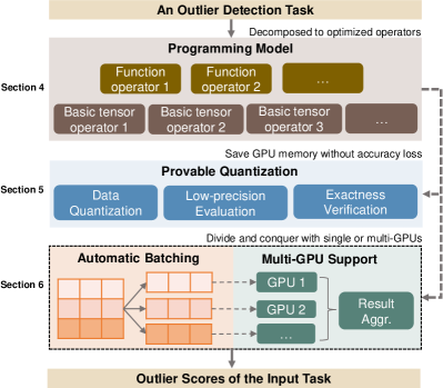
Figure 1. System overview. TOD abstracts OD algorithms into small building blocks via the programming model for deep optimization, with a set of techniques including provable quantization, automatic batching, and multi-GPU support.

1.1. Our Approach

In this paper, we present TOD, a tensor-based outlier detection system that abstracts OD applications into tensor operations for efficient GPU acceleration. TOD leverages both the software and hardware optimizations in modern deep learning frameworks to enable efficient and scalable OD computations on distributed multi-GPU clusters. To the best of our knowledge, TOD is the first GPU-based system for generic OD applications. Fig. 1 shows an overview of TOD. Building a tensor-based OD system requires addressing three major obstacles.

Representing OD computations using tensor operations.   Unlike DNN models, which are represented as a pipeline of tensor algebra operators (e.g., matrix multiplication), many OD applications involve a diverse collection of operators that have traditionally not been implemented in terms of tensor operations, such as proximity-based algorithms, statistical approaches, and linear methods (see an overview of OD applications in §2.1). Implementing OD applications one at a time and accounting for software and hardware optimizations is labor-intensive. To address this obstacle, TOD introduces a new programming model for OD that decomposes a broad set of OD applications into a small collection of basic tensor operators and functional operators, which significantly reduces the implementation and optimization effort and opens the possibility of easily supporting new OD algorithms.

Quantizing OD computations.   Quantization is commonly used in existing DNN frameworks to reduce time and memory consumption of DNN computations by executing intermediate operations of DNN models in a low-precision floating-point representation. Quantization in general does not preserve the end-to-end equivalence of a DNN model and may introduce potential accuracy losses. To apply quantization, the current practice is fine-tuning a quantized DNN model on the training dataset in a supervised fashion and assessing the accuracy loss; however, this approach is not directly applicable to OD, since most OD algorithms are unsupervised and thus lack a direct way for measuring accuracy. To address this challenge, TOD introduces a novel quantization technique called provable quantization, which leverages the numerical insensitivity of some OD algorithms (e.g., $k$-nearest-neighbors may return identical results for some samples when computing with different floating-point precisions) and automatically performs specific OD operators in lower precision. In contrast to prior quantization techniques that also use lower precision calculations at the expense of accuracy, our proposed provable quantization technique provably guarantees no accuracy loss.

Enabling scalable OD computations.   Existing deep learning frameworks cannot directly support large-scale OD applications, since modern deep learning systems are designed to iteratively process a small batch of training samples even though the entire training dataset can be large. For example, to train ResNet-50 (He et al., 2016) on the ImageNet dataset (Deng et al., 2009), the DNN systems only handle small mini-batches (e.g., 256 samples) in each training iteration, while the dataset contains more than 14 million samples. However, many OD applications involve operating on all samples, such as computing distances between all sample pairs. Executing such an application on a single GPU would typically run out of memory because GPUs nowadays have limited memory capacities (e.g., compared to those of CPU RAM). To overcome the difficulty of executing OD applications in iterations and the resource limits of a single GPU, TOD uses an automatic batching mechanism to execute memory-intensive OD operators in small batches, which are distributed across multiple GPUs in parallel in a pipeline fashion. The automatic batching and multi-GPU support allow TOD to scale to datasets as large as those commonly encountered in deep learning.

We compare TOD against existing CPU- and GPU-based OD systems on both real-world and synthetic datasets. TOD is on average 10.9 times faster than PyOD, a state-of-the-art comprehensive CPU-based OD system (Zhao et al., 2019a), and can process a million samples within an hour while PyOD cannot. Compared to existing GPU-based OD systems, TOD can handle much larger datasets, while the GPU baselines run out of GPU memory. Our evaluation further shows that provable quantization, automatic batching, and multi-GPU support are all critical for efficient and scalable OD computations.

In summary, this paper makes the following contributions:

• We propose TOD, the first tensor-based system for generic outlier detection, enabling efficient and scalable OD computations on distributed multi-GPU clusters.

• TOD uses a new programming model that abstracts complex OD applications into a small collection of basic tensor operators for efficient GPU acceleration.

• We introduce provable quantization that accelerates unsupervised OD computations by performing specific floating-point operators in lower precision while provably guaranteeing no accuracy loss.

Extensibility and integration.   TOD is open-sourced (see Appx. §D for API demonstration), which enables easy development of new OD algorithms by leveraging highly optimized tensor operators or including new operators (see examples in §7.1). This extensibility of TOD yields a large number of yet-to-be-discovered OD methods. Thus, we believe that TOD also provides a platform that enables rapid research and development of novel OD methods.

2. Background and Related Work

We provide background on existing OD algorithms for tabular data and which ones are accelerated by TOD (§2.1), on the DNN infrastructure that TOD builds off of to do acceleration (§2.2), and on existing comprehensive OD systems (§2.3), including the current state-of-the-art PyOD (Zhao et al., 2019a). In §2.4, we review additional systems, algorithms, and applications for other data formats in addition to tabular data (e.g., time series and graphs). Note that TOD primarily focuses on OD in tabular data due to its popularity (Aggarwal, 2013); TOD can be extended to support OD in other data types with modifications.

Table 1. Key OD algorithms for tabular data and their time and space complexity with a brute-force implementation (additional optimization is possible but not considered here), where $n$ is the number of samples, and $d$ is the number of dimensions. Note that ensemble-based methods’ complexities depend on the underlying base estimators. Algorithms that can be accelerated in TOD are marked with ✓.

Category	Algorithm	Time Compl.	Space Compl.	Optimized in TOD
Proximity	$k$NNOD	$O(n^{2})$	$O(n^{2})$	✓
Proximity	COF	$O(n^{3})$	$O(n^{2})$	✓
Proximity	LOF	$O(n^{2})$	$O(n^{2})$	✓
Proximity	LOCI	$O(n^{2})$	$O(n^{2})$	✓
Statistical	KDE	$O(n^{3})$	$O(n^{2})$	✗
Statistical	HBOS	$O(nd)$	$O(nd)$	✓
Statistical	COPOD	$O(nd)$	$O(nd)$	✓
Statistical	ECOD	$O(nd)$	$O(nd)$	✓
Ensemble	LODA	N/A	N/A	✓
Ensemble	FB	N/A	N/A	✓
Ensemble	iForest	N/A	N/A	✗
Ensemble	LSCP	N/A	N/A	✓
Linear	PCA	$O(nd)$	$O(n)$	✓
Linear	OCSVM	$O(n^{3})$	$O(n^{2})$	✗

2.1. Existing OD Algorithms and Scalability

Outlier detection (also called anomaly detection) is a key machine learning task that aims to find data points that deviate from a general distribution (Aggarwal, 2013; Yu et al., 2016; Liu et al., 2021a). As shown in Table 1, non-deep-learning OD algorithms may be grouped into four categories (see the book (Aggarwal, 2013) by Aggarwal for more details on algorithms): (i) proximity-based algorithms that rely on measuring sample similarity including $k$NN (Angiulli and Pizzuti, 2002), ABOD (Kriegel et al., 2008), COF (Tang et al., 2002), LOF (Breunig et al., 2000), and LOCI (Papadimitriou et al., 2003); (ii) statistical approaches including KDE (Schubert et al., 2014), HBOS (Goldstein and Dengel, 2012), COPOD (Li et al., 2020), and ECOD (Li et al., 2022); (iii) ensemble-based methods that build a collection of detectors for aggregation like iForest (Liu et al., 2008), LODA (Pevný, 2016), and LCSP (Zhao et al., 2019b); and (iv) linear models such as PCA (Shyu et al., 2003).

Importantly, many OD algorithms suffer from scalability issues (Orair et al., 2010; Zhao et al., 2021). For example, Table 1 shows that various proximity-based OD algorithms have at least $O(n^{2})$ time and space complexities—they all require estimating and storing pairwise distances among all $n$ samples. The high time complexities of many OD algorithms limit their applicability in real-world applications that require either real-time responses (e.g., fraud detection (Liu et al., 2020)) or the concurrent processing of millions of samples (Zhong et al., 2020). As shown in the table, TOD supports nearly all the OD algorithms mentioned.

2.2. DNN Infrastructure and Acceleration

Deep neural networks have dramatically improved the accuracy of artificial intelligence systems across numerous fields (Goodfellow et al., 2016; Fu et al., 2021; Pang et al., 2021). Its success is fueled by recent advances in both hardware and software (LeCun, 2019). Specifically, DNN systems depend on tensor operations that can often be parallelized and executed in small batches. These operations are well-suited for GPUs, especially as a single GPU nowadays often has many more cores than a single CPU; while GPU cores are not as general purpose as CPU cores, they suffice in executing the tensor operations of deep learning. Moreover, the maturity of DNN programming interfaces such as PyTorch (Paszke et al., 2019) and TensorFlow (Abadi et al., 2016) makes developing machine learning models easy with a wide range of GPUs. Multiple works attempt to leverage DNN systems for accelerating training data science and ML tasks, including Hummingbird (Nakandala et al., 2020), Tensors (Koutsoukos et al., 2021), and AC-DBSCAN (Ji and Wang, 2021).

Differently, TOD for the first time, extends the acceleration usage of DNN systems to OD algorithms. We build TOD using the DNN ecosystem, taking advantage of its established hardware acceleration and software accessibility. This design choice also opens the opportunity for unifying classical OD algorithms (see §2.1) and DNN-based OD algorithms on the same platform—this emerging direction has gained increasing attention in OD research (Ruff et al., 2020).

2.3. Outlier Detection Systems

CPU-based systems  . Over the years, comprehensive OD systems on CPUs that cover a diverse group of algorithms have been developed in different programming languages, including ELKI Data Mining (Achtert et al., 2010) and RapidMiner (Ristoski et al., 2015) in Java, and PyOD (Zhao et al., 2019a) in Python. Among these, PyOD is the state-of-the-art (SOTA) with deep optimization including just-in-time compilation and parallelization. It is widely used in both academia and industry, with hundreds of citations (Zhao, 2021) and millions of downloads per year (Sincraian, 2021). Recently, the PyOD team proposed an acceleration system called SUOD to further speed up the training and prediction in PyOD with a large collection of heterogeneous OD models (Zhao et al., 2021). Specifically, SUOD uses algorithmic approximation and efficient parallelization to reduce the computational cost and therefore runtime. There are other distributed/parallel systems designed for specific (family of) OD algorithms with non-GPU nodes (e.g., CPUs): (i) Parallel Bay, Parallel LOF, DLOF for local OD algorithms (Lozano and Acuña, 2005; Oku et al., 2014; Yan et al., 2017), (ii) DOoR for distance-based OD (Bhaduri et al., 2011), (iii) distributed OD for mixed-attributed data (Otey et al., 2006) (iv) PROUD for stream data (Toliopoulos et al., 2020) and (v) Sparx for Apache Spark (Zhang et al., 2022). These distributed non-GPU systems do not constitute as baselines as TOD is a comprehensive system covering different types OD algorithms, while the specialized systems only cover specific algorithms. Thus, we consider the SOTA comprehensive system, PyOD, as the primary baseline (see exp. results in §7.3).

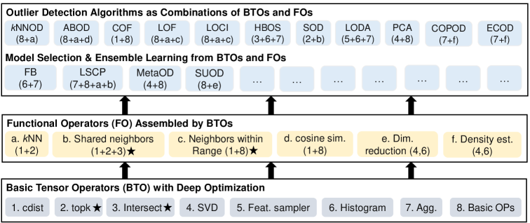
Figure 2. With algorithmic abstraction, more than 20 OD algorithms (denoted by  ) are abstracted into eight basic tensor operators (in  ) and six functional operators (in  ). This abstraction reduces the implementation and optimization effort, and opens the possibility of including new algorithms. All operators are executed on GPUs using automatic batching (see §6), and operators marked with $\bigstar$ are further accelerated using provable quantization (see §5).

GPU-based systems  . There are efforts to use GPUs for fast OD calculations for LOF (Alshawabkeh et al., 2010), distance-based methods (Angiulli et al., 2016), KDE (Azmandian et al., 2012), and data stream (Leal and Gruenwald, 2018). These approaches rely on exploring the characteristics of a specific OD algorithm for GPU acceleration. This limits their generalization to a wide collection of OD algorithms. Furthermore, none has direct multi-GPU support, leading to limited scalability. To the best of our knowledge, there is no existing comprehensive GPU-based OD system that covers a diverse group of algorithms. Thus, we use direct GPU implementations of OD algorithms and selected works above as GPU baselines when appropriate (see details in §7.2 and Table 3).

2.4. Systems for Other Data Types and Scenarios

Over the years, various algorithms and systems have been developed for OD with different types of data other than tabular, including time-series/sequence (TOP (Cao et al., 2019), NETS (Yoon et al., 2019), GraphAn (Boniol et al., 2020), CPOD (Tran et al., 2020), Series2graph (Boniol and Palpanas, 2020), SAND (Boniol et al., 2021), etc.), and graph (e.g., Elle (Kingsbury and Alvaro, 2020), PyGOD (Liu et al., 2022b, a), etc.). Also, different input data are also assumed in streaming and feature-evolving fashions (e.g., xStream (Manzoor et al., 2018), etc.). Meanwhile, emphasis has also been given to building systems for explaining outliers (VSOutlier (Cao et al., 2014) and Exathlon (Jacob et al., 2021), etc.) and outlier repairing (IMR (Zhang et al., 2017), etc.), other than detecting them. In this paper, we focus on the detection task in the most prevalent setting (i.e., static tabular data) (Aggarwal, 2013), while future works may extend to other data types and scenarios.

3. Overview

3.1. Definition and Problem Formulation

A comprehensive OD system implements a collection of OD models $\mathcal{M}=\{M_{1},...,M_{m}\}$ such that given a user-specified OD model $M\in\mathcal{M}$ and input data $\mathbf{X}\in\mathbbm{R}^{n\times d}$ without ground truth labels (rows of $\mathbf{X}$ index data points, while columns index features), the system outputs outlier scores $\mathbf{O}:=M(\mathbf{X})\in\mathbbm{R}^{n}$, which should be roughly deterministic and irrespective of the underlying system (higher values in $\mathbf{O}$ correspond to data points more likely to be identified as outliers; threshold on outlier scores can be used to determine which points are outliers). Given a hardware configuration $\mathcal{C}$, e.g., CPU, RAM, and GPU (if available), the system performance can be measured in efficiency (both runtime and memory consumption).

3.2. System Overview

As a reminder from Section 1, TOD is a comprehensive (i.e., covering a diverse group of methods) OD system as outlined in Fig. 1 and Table 1. For an outlier detection task, TOD decomposes it into a combination of predefined tensor operators via the proposed programming model for direct GPU acceleration (§4). Notably, TOD opportunistically performs provable quantization on tensor operators to enable faster computation and reduce memory requirements, while provably maintaining model accuracy (§5). To overcome the resource limitation of a single GPU, we further introduce automatic batching and multi-GPU support in TOD (§6).

4. Programming Model

Motivation.   As a comprehensive system, TOD aims to include a diverse collection of OD algorithms, including proximity-based methods, statistical methods, and more (see §2.1). However, not all algorithms can be directly converted into tensor operations for GPU acceleration. A key design goal of our programming model is to allow for many OD algorithms to be implemented by piecing together some basic commonly recurring building blocks. In particular, rather than manually implementing many OD algorithms separately, which is a labor-intensive process, we instead define OD algorithms in terms of basic building blocks that each just needs to be implemented once. Moreover, the building blocks can be optimized independently.

4.1. Algorithmic Abstraction

The key idea of our programming model is to decompose existing OD algorithms into a set of low-level basic tensor operators (BTOs), which can directly benefit from GPU acceleration. On top of these BTOs, we introduce higher-level OD operators called functional operators (FOs) with richer semantics. Consequently, OD algorithms can be constructed as combinations of BTOs and FOs.

Fig. 2 shows the hierarchy of TOD’s programming abstraction in a bottom-up way, with increasing dependency: 8 BTOs are first constructed as the foundation of TOD (shown at the bottom in gray), while 6 FOs are then created on top of them (shown in the middle). Finally, OD algorithms and key functions on the top of the figure can be assembled by BTOs and FOs. In other words, TOD uses a tree-structured dependency graph, where the BTOs (as leaves of the tree) are fully independent for deep optimization, and all the algorithms depending on these BTOs can be collectively optimized. Clearly, this abstraction process reduces the repetitive implementation and optimization effort, and improves system efficiency and generalization. Additionally, it also facilities fast prototyping and experimentation with new algorithms.

4.2. Building Complete Algorithms

It is easy to build an end-to-end OD application by constructing its computation graph using FOs and BTOs. For instance, angle-based outlier detection (ABOD) is a classical OD algorithm (Kriegel et al., 2008), where each sample’s outlier score is calculated as the average cosine similarity of its neighbors. Fig. 3(a) highlights an implementation of ABOD that uses an FO called $k$NN to obtain a list of neighbors for each sample and then applies another FO called cosine sim. for calculating cosine similarity. Note that the FOs are also built as combinations of BTOs. For example, $k$NN is implemented as calculating pairwise sample distance using cdist and then identifying the $k$ “neighbor” with smallest distances using topk. Additionally, Fig. 3(b) shows the abstraction graph of copula-based outlier detection (COPOD) (Li et al., 2020). Other OD algorithms follow the same abstraction protocol as a combination of BTOs and FOs.

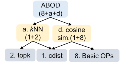
(a)

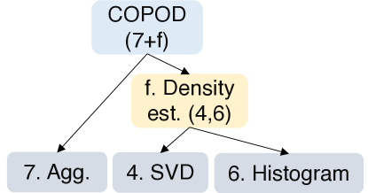
(b)

Figure 3. Examples of building complex OD algorithms with FO and BTO conveniently.

5. Provable Quantization

Motivation.   OD operators mainly depend on floating-point operations, namely $\{+,-,\times,/\}$. For these operations, the main source of the imprecision is rounding (Lee et al., 2018). Of course, rounding errors increase when storing numbers using fewer bits, e.g., 16-bit precision leads to more inaccuracy than 64-bit precision. Many machine learning algorithms therefore use high-precision floating-points when possible to minimize the impact of the rounding errors. However, working with high-precision floating-point numbers can increase computation time and storage costs. This is especially critical for GPU systems with limited memory.

To reduce memory usage and runtime, quantization has been applied to many machine learning algorithms (Blalock and Guttag, 2017) and data-driven applications (André et al., 2016; Wang and Deng, 2020; Wang and Ferhatosmanoglu, 2020). Simply put, it refers to executing an operator (function) with lower-precision floating representations. If we denote the original function by $r(x)$ and its quantization by $r_{q}(x)$, the rounding error $\text{Err}(\cdot)$ of quantization is defined as the output difference between $r(x)$ and $r_{q}(x)$, namely $\text{Err}(r_{q}(x))=r(x)-r_{q}(x)$. Intuitively, quantization can save memory at the cost of accuracy. How to balance the tradeoff between the memory cost and algorithm accuracy is a key challenge for quantizing in machine learning (Dai et al., 2021). In supervised ML, one may measure the inaccuracy caused by quantization via using ground truth labels to evaluate the performance. However, this is infeasible under unsupervised OD settings, where no ground truth labels is available for evaluation as described in §3. Thus, existing quantization techniques for supervised ML do not suit the need of unsupervised OD.

In TOD, we design a correctness-preserving quantization for (unsupervised) OD applications, termed provable quantization. The key idea we use is that depending on the operator used, it is possible to apply quantization to save memory consumption with no loss in accuracy. As a motivating example, consider the sign function $r(x)$ that returns “$+$” if $x>0$ and returns “$-$” otherwise. Clearly, even if we quantize $x$ to have a single bit (that precisely indicates the sign of $x$), we can achieve an exact answer for $r(x)$ that is the same as if instead $x$ had more bits. Similarly, the ranking between two floating-point numbers often only depends on the most significant digits. Building on this simple intuition, we introduce provable quantization for a collection of OD operators, where the output and accuracy of the operators remain provably unchanged before and after quantization.

5.1. $(1+\epsilon)$-property for Rounding Errors

Provable quantization relies on a standard analysis technique for floating-point numbers called the “$(1+\epsilon)$-property” (e.g., (Lee et al., 2018)). Let $\mathbb{F}$ denote the set of 64-bit floating-point numbers. For $x,y\in\mathbb{F}$, we define the floating-point operation “$\circledast$” as $x\circledast y\triangleq\text{fl}(x*y)$, where $*\in\{+,-,\times,/\}$ and $\text{fl}(\cdot)$ refers to the IEEE 754 standard for rounding a real number to a 64-bit floating-point number (Kahan, 1996). For example, $\oplus$ is floating-point addition and $\otimes$ is floating-point multiplication. The standard technique for calculating the rounding errors in floating-point operations is the $(1+\epsilon)$-property (Lee et al., 2018), which is formally defined as follows.

Theorem 1 (Theorem 3.2 of Lee et al. 2018).

Let $x,y\in\mathbb{F}$, and $*\in\{+,-,\times,/\}$. Suppose that $|x*y|\leq\max\mathbb{F}$. Then when we compute $x*y$ in floating-point, there exist multiplicative and additive error terms $\delta\in\mathbb{R}$ and $\delta^{\prime}\in\mathbb{R}$ respectively such that

(1) $$x\circledast y=(x*y)(1+\delta)+\delta^{\prime},\quad\text{where }|\delta|\leq\epsilon,|\delta^{\prime}|\leq\epsilon^{\prime}.$$

In the above equation, $\epsilon$ and $\epsilon^{\prime}$ are constants that do not depend on $x$ or $y$. For instance, when working with 64-bit floating-point numbers, $\epsilon=2^{-53}$ and $\epsilon^{\prime}=2^{-1075}$.

As discussed by Lee et al. (2018, Section 5), this property can be further simplified when the exact result of the floating operation is not in the so-called “subnormal” range: the addictive error term $\delta^{\prime}$ can be soundly removed, leading to a simplified $(1+\epsilon)$-property:

(2) $$x\circledast y=(x*y)(1+\delta),\quad\text{where }|\delta|\leq\epsilon.$$

5.2. Provable Quantization in TOD

TOD applies provable quantization for an applicable operator $r(\cdot)$ with input $x$ in three steps: (i) input quantization, (ii) low-precision evaluation, and (iii) exactness verification and, if needed, recalculation. In a nutshell, the input is first quantized into lower precision, and then the operator is evaluated in the lower precision, where $r(\cdot)$ is evaluated as $r_{q}(x)$. To verify the exactness of the quantization, we calculate the rounding error $\text{Err}(r_{q}(x))$ by the simplified $(1+\epsilon)$-property in eq. (2) and then check whether the result of $r(\cdot)$ may change with the rounding error. If it passes the verification, then we output $\text{Err}(r_{q}(x))$ as the final result; otherwise, we use the original precision of $x$ to recalculate $r(x)$. Note that we apply this technique to the entire input data $\mathbf{X}\in\mathbbm{R}^{n\times d}$, and only need to recalculate on the subset of $\mathbf{X}$ where the verification fails. Note that provable quantization does not apply to all operators, and we elaborate on the criteria in §5.4.

5.3. Case Study: Neighbors Within Range

We show the usage of provable quantization in TOD on neighbors within range (NWR, one of the FOs of our programming model), a common step in many OD algorithms, e.g., LOF (Breunig et al., 2000) and LOCI (Papadimitriou et al., 2003). NWR identifies nearest neighbors within a preset distance threshold (usually a small number), which may be considered as a variant of $k$ nearest neighbors. More formally, given an input tensor $\mathbf{X}:=[X_{1},X_{2},...,X_{n}]\in\mathbb{R}^{n\times d}$ ($n$ samples and $d$ dimensions) and the distance threshold $\phi$, NWR first calculates the pairwise distance among each sample via the cdist operator, yielding a distance matrix $\mathbf{D}\in\mathbb{R}^{n\times n}$, where $\mathbf{D}_{i,j}$ is the pairwise distance between $X_{i}$ and $X_{j}$. Then, each pairwise distance in $\mathbf{D}$ is compared with $\phi$, and NWR outputs the indices of samples where $\mathbf{D}_{i,j}\leq\phi$. As the pairwise distance calculation in NWR requires $O(n^{2})$ space, provable quantization can provide significant GPU memory savings.

NWR meets the criterion we outline in §5.2, where eq. (2) can be applied to estimate the rounding errors. Recall that the pairwise Euclidean distance between two samples is

(3) $$\mathbf{D}_{ij}=\left\lVert X_{i}-X_{j}\right\rVert^{2}_{2}=\left\lVert X_{i}\right\rVert_{2}^{2}+\left\lVert X_{j}\right\rVert_{2}^{2}-2X_{i}^{T}X_{j}.$$

We shall compute this in floating-point. Importantly, in our analysis to follow, the ordering of floating-point operations matters in determining rounding errors. To this end, we calculate distance using the right-most expression in eq. (3) (note that we do not first compute the difference $X_{i}-X_{j}$ and then compute its squared Euclidean norm). When calculating the first term in the RHS of eq. (3) via floating-point operations, we get

$$\text{fl}(\left\lVert X_{i}\right\rVert_{2}^{2}) \!=\!(X_{i,1}\otimes X_{i,1})\oplus(X_{i,2}\otimes X_{i,2})\oplus\cdots\oplus(X_{i,d}\otimes X_{i,d})$$

$$\!=\!(X_{i,1}^{2}(1\!+\!\delta_{1}))\oplus(X_{i,2}^{2}(1\!+\!\delta_{2}))\oplus\cdots\oplus(X_{i,d}^{2}(1\!+\!\delta_{d})),$$

where the second equality uses eq. (2) and we note that the errors $\delta_{1},\dots,\delta_{d}$ across the floating-point multiplications (for squaring) need not be the same (in fact, these need not be the same across samples $i=1,2,\dots,n$ but we omit this indexing to keep the equation from getting cluttered).

Next, by defining $x_{\max}\triangleq\max_{i\in\{1,\dots,n\},k\in\{1,\dots,d\}}|X_{i,k}|$ and recalling from Theorem 1 that each of $\delta_{1},\delta_{2},\dots,\delta_{d}$ above is at most $\epsilon$, we get

$$\text{fl}(\left\lVert X_{i}\right\rVert_{2}^{2}) \!=\!(X_{i,1}^{2}(1\!+\!\delta_{1}))\oplus(X_{i,2}^{2}(1\!+\!\delta_{2}))\oplus\cdots\oplus(X_{i,d}^{2}(1\!+\!\delta_{d}))$$

$$\!\leq\!\underbrace{[x_{\max}^{2}(1+\epsilon)]\oplus[x_{\max}^{2}(1+\epsilon)]\oplus\cdots\oplus[x_{\max}^{2}(1+\epsilon)]}_{d\text{ terms added via floating-point addition}}$$

$$\!\leq\!d\cdot x_{\max}^{2}(1+\epsilon)^{1+\lceil\log_{2}d\rceil},$$

where for the last step, $\log_{2}d$ shows up since summation of $d$ elements in lower-level programming languages is implemented in a divide-and-conquer manner that reduces to $\lceil\log_{2}d\rceil$ operations (there is still a “$1+$” term in the exponent for the floating-point multiplication/squaring). The rounding error is bounded as follows:

$$\text{Err}(\|X_{i}\|_{2}^{2}) =\|X_{i}\|_{2}^{2}-\text{fl}(\|X_{i}\|_{2}^{2})$$

$$\leq d\cdot x_{\max}^{2}-\text{fl}(\|X_{i}\|_{2}^{2})$$

$$\leq\big{|}d\cdot x_{\max}^{2}-\text{fl}(\|X_{i}\|_{2}^{2})\big{|}$$

$$\leq d\cdot x_{\max}^{2}[(1+\epsilon)^{1+\lceil\log_{2}d\rceil}-1].$$

This same analysis can be used to bound the floating-point errors of the other terms in eq. (3). Overall, we get

(4) $$\text{Err}(\mathbf{D}_{ij})\leq 4d\cdot x_{\text{max}}^{2}[(1+\epsilon)^{1+\lceil\log_{2}d\rceil+2}-1],$$

where the “$+2$” shows up in the exponent due to the addition and subtraction in the RHS of (3) that we compute in floating-point.

Inequality (4) provides a numerical way for checking whether a single entry $\mathbf{D}_{ij}$ is within the range of $\phi$ as $|\mathbf{D}_{ij}-\phi|>\text{Err}(\mathbf{D}_{ij})$. More conveniently, we could scale the input $\mathbf{X}$ into the range of $[0,1]$ before the distance calculation (Raschka, 2015), so that $x_{\text{max}}\leq 1$ and the implementation complexity can be further reduced. With this treatment, a large amount of GPU memory can be saved in NWR operations (see §7.5 for results).

5.4. Applicability and Opportunities of Provable Quantization

Not all operators can benefit from provable quantization. To benefit from provable quantization, an operator needs to satisfy two criteria. First, the operator’s output values cannot require a floating-point representation in the original precision, otherwise the exactness verification would require executing the operator in the original precision, resulting in no memory or time savings. For example, provable quantization is not applicable to cdist since its outputs are raw floating-point pairwise distances, and verifying its exactness requires calculating cdist in the original precision. Second, the performance gain in low-precision evaluation of the operator needs to be larger than the overhead of verification. Based on these two criteria, we mark the operators generally applicable for provable quantization by $\bigstar$ in Fig. 2. Also see §7.5 for experimental results on this. Although the design of provable quantization is motivated by unsupervised OD algorithms with extensive ranking and selecting operations, other ML algorithms can also benefit if they meet the above criteria. For OD algorithms in which provable quantization does not apply, they could still benefit from TOD’s other optimizations such as automatic batching (§6).

6. Automatic Batching and Multi-GPU Support

Motivation.   Unlike CPU nodes with up to terabytes of DRAM, today’s GPU nodes face much more stringent memory limitations (Min et al., 2020; Gera et al., 2020; Min et al., 2021; Lee et al., 2021)—modern GPUs are mostly equipped with 4-40 GB of on-device memory (Meng et al., 2017; Svedin et al., 2021). Out-of-memory (OOM) errors have thus become common in GPU-based systems for machine learning tasks (Gao et al., 2020). To overcome this challenge, we design an automatic batching mechanism to decompose memory-intensive BTOs into multiple batches, which are executed on GPUs in a pipeline fashion. Automatic batching also allows TOD to equally distribute OD computation across multiple GPUs. TOD applies different mechanisms to decompose an operator into batches based on its data dependency. Specifically, an operator has inter-sample dependency if the computation of each sample requires accessing other samples, such as cdist. On the other hand, an operator has inter-feature dependency if the computation of each feature depends on other features, such as Feat. sampler. Fig. 4 summarizes TOD batching mechanisms for operators with and without these dependencies.

Direct batching.   TOD automatically decomposes an operator into small batches if the operator is: (i) sample-independent: the estimation of each sample is independent, or (ii) feature-independent: the contribution of each feature is independent. When either condition holds, TOD directly partitions the operator into multiple batches by splitting along the sample or feature dimension, computes these batches in a pipeline fashion, and aggregates individual batches to produce the final output, as shown in Fig. 5. For instance, topk is a sample-independent operator. For an input tensor $\mathbf{X}\in\mathbb{R}^{n\times d}$, topk outputs the indices of the largest $k$ values for each sample (i.e., row), resulting in an output tensor $\mathbf{I}_{\mathbf{X}}:=\texttt{topk}(\mathbf{X},k)\in\mathbb{R}^{n\times k}$. Therefore, we could split $\mathbf{X}$ into batches with full features, each with $b$ samples (i.e.,, $\{\mathbf{X}_{1},\mathbf{X}_{2},...\}\in\mathbb{R}^{b\times d}$). As another example, Histogram outputs the frequencies of each feature’s values, which is feature-independent. Thus, we could partition $\mathbf{X}$ into blocks of $b$ features, e.g., $\{\mathbf{X}_{1},\mathbf{X}_{2},...\}\in\mathbb{R}^{n\times b}$.

Customized batching.   For operators with both inter-sample and inter-feature dependencies, the computation of each data point involves all samples and features, and therefore cannot be directly decomposed into batches along the same or feature dimension. TOD provides customized batching strategies for these operators. For example, to automatically batch cdist, TOD uses the approach introduced in Neeb and Kurrus (2016), which splits an input dataset across samples and calculates the pairwise distance of each pair of split in batches.

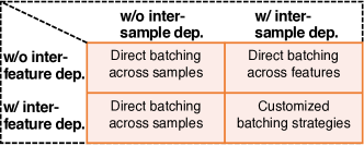
Figure 4. TOD applies automatic batching to operators without inter-sample or inter-feature dependency, and uses customized batching strategies for operators with both data dependencies.

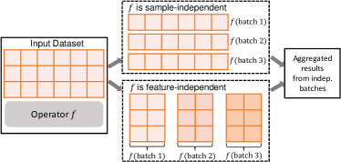
Figure 5. Direct batching with independence assumption creates batches along the sample or feature index.

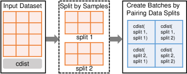
Figure 6. Customized batching solution for cdist in TOD.

6.1. Sequential Batching and Operator Fusion

Simple concatenation.   Since BTOs are independent from each other, executing a sequence of BTOs in batches is straightforward, i.e., simply feed the output of a batch operator as an input to another one. For example, $k$NN (see Fig. 2) finds the $k$ nearest neighbors by first calculating pairwise distances of input samples via the cdist BTO and then returns the index of $k$ items with the smallest distance via the topk BTO. Thus, $k$NN batching is achieved by running cdist and topk sequentially, where each uses automatic batching and the output of the former is the input of the latter. Note that simple concatenation applies to all BTOs and FOs as the default choice.

Operator fusion.   Although the simple concatenation discussed above is straightforward, a closer look unlocks deeper optimization opportunities in automatic batching with a sequence of operators. Notably, the output of $k$NN is the indices of the $k$ nearest neighbors of an input dataset, where the pairwise distance generated by cdist is only used in an intermediate step but not returned. If we could prevent moving this large distance matrix between operators (i.e., cdist and topk), space efficiency can be improved. In deep learning systems, operator fusion is a common optimization technique to fuse multiple operators into a single one in a computational graph (Neubig et al., 2017; Looks et al., 2017; Wang et al., 2021b; Boehm et al., 2018; Menon et al., 2017). Fig. 7 compares simple concatenation (subfigure a) and operator fusion (subfigure b) on $k$NN. Specifically, the latter executes the topk BTO on the cdist BTO’s individual batches separately rather than running topk on the full distance matrix outputted by cdist. Note that the global $k$ nearest neighbors (of the full dataset) can be identified from the $k$ local neighbor candidates from batches in the final aggregation, so the result is still exact. This prevents moving the entire $n\times n$ distance matrix between operators, which often causes OOM. TOD uses a rule-based approach to opportunistically fusing operators to reduce the kernel launch overhead and data transfers between CPUs and GPUs. TOD provides an interface that allows users to add fusion rules for new OD operators. Appx. C.3 provides a case study on the effectiveness of operator fusion.

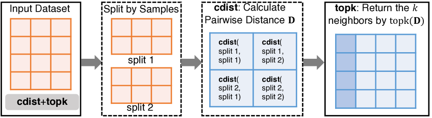
(a)

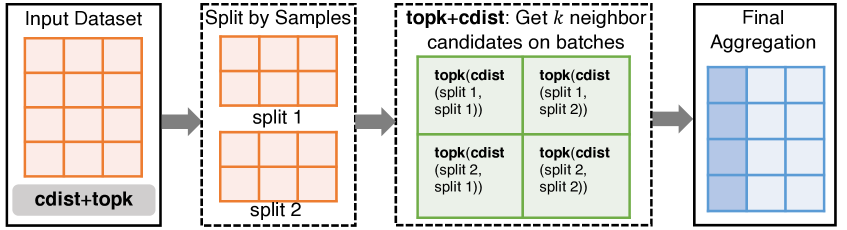
(b)

Figure 7. The comparison of automatic batching for $k$NN between simple concatenation and operator fusion. The latter has better scalability by not creating and moving large distance matrix $\mathbf{D}$.

6.2. Multi-GPU Support

To further reduce the execution time of OD algorithms on GPUs, TOD also supports multi-GPU execution, which is important for time-critical OD applications and has been widely used for other data-intensive applications such as graph neural networks (Jia et al., 2020). Intuitively, if there is only one GPU, TOD iterates across multiple batches sequentially and aggregates the results. When multiple GPUs are available, we could achieve better performance by executing OD computations concurrently on multiple homogeneous GPUs. Specifically, TOD first applies automatic batching to an underlying task—multiple subtasks are created and assigned to available GPUs. TOD creates a subprocess for each available GPU to execute the assigned subtasks and a shared global container to store the results returned from each GPU. Since we equally distribute subtasks across GPUs, we deem the runtime of each GPU is close. Once all the subtasks are complete, the final output is generated by aggregating the results in the global container. For example, automatically batching cdist in Fig. 6 leads to 4 subtasks, each of which calculates the pairwise distances for a pair of splits (denoted as blue blocks in the figure). Each of the four available GPUs executes an assigned subtask and sends the cdist results to the global container. Finally, the full cdist result is obtained by aggregating the intermediate results in the global container. Note that the multi-GPU execution is at the operator level (e.g., cdist). §7.7 evaluates TOD’s scalability across multiple GPUs..

7. Experimental Evaluation

Our experiments answer the following questions:

1. Is TOD more efficient (in time and space) than SOTA CPU-based OD system (i.e., PyOD) and selected GPU baselines? (§7.3)

2. How scalable is TOD while handling more and more data? (§7.4)

3. How effective are provable quantization and automatic batching), in comparison to PyTorch implementation? (§7.5 & 7.6)

4. How much performance gain can TOD achieve on the multiple GPUs? (§7.7)

7.1. Implementation and Environment

TOD is implemented on top of PyTorch (Paszke et al., 2019). We extend PyTorch in the following aspects to support efficient OD. First, we implement a set of BTOs and FOs (see Fig. 2) for fast tensor operations in OD. Second, for operators that support provable quantization (see §5) and batching (see §6), we create corresponding versions of them to improve scalability. Additionally, we enable specialized multi-GPU support in TOD by leveraging PyTorch’s multiprocessing. The usage and APIs of the open-sourced system can be found in §D.

Adding new operators  . In addition to the BTOs and FOs listed in Fig. 2, users can add new operators in TOD by defining the operator’s interface (i.e., the input and output tensors of the operator) and providing an implementation of the operator in PyTorch. This implementation will be used by TOD to decompose the operator into PyTorch’s tensor algebra primitives and execute these primitives in parallel on multiple GPUs. For operators that do not have inter-sample or inter-feature dependency (see §6), TOD automatically decomposes the operator’s computation into multiple batches. For operators that involve both inter-sample and inter-feature dependencies, TOD require users to provide a customized strategy to decompose the operator into batches.

Implementing new OD algorithms  . One notable characteristic of OD is that most algorithms involve only straightforward computation, which can be decomposed into 2-3 BTOs and FOs. Therefore, we expect that implementing new OD algorithms in TOD should only involve low cognitive complexity. Appx. A demonstrates an implementation of a recent ECOD (Li et al., 2022) detection algorithm in TOD in less than ten lines of code.

Experimental setup.   All the experiments were performed on an Amazon EC2 cluster with an Intel Xeon E5-2686 v4 CPU, 61GB DRAM, and an NVIDIA Tesla V100 GPU. For the multi-GPU support evaluation, we extend it to multiple NVIDIA Tesla V100 GPUs with the same CPU node.

7.2. Datasets, Baselines, and Evaluation Metrics

Datasets.   Table 2 shows the 11 real-world benchmark datasets used in this study, which are widely evaluated in OD research (Campos et al., 2016; Zhao et al., 2019b; Ruff et al., 2020; Li et al., 2020) and available in the latest ADBench (Han et al., 2022). Given the limited size of real-world OD datasets, we also build data generation function in TOD to create larger synthetic datasets (up to 1.5 million samples) to evaluate the scalability of TOD (see §7.4 for details).

OD algorithms and operators.   Throughout the experiments, we compare the performance of five representative but diverse OD algorithms across different systems (see §2.1): proximity-based algorithms including LOF (Breunig et al., 2000), ABOD (Kriegel et al., 2008), and $k$NN (Angiulli and Pizzuti, 2002); statistical method HBOS (Goldstein and Dengel, 2012), and linear model PCA (Shyu et al., 2003). We also provide an operator-level analysis on selected BTOs and FOs to demonstrate the effectiveness of certain techniques.

Evaluation metrics.   Since TOD and the baselines do not involve any approximation, the output results are exact and consistent across systems. Therefore, we omit the accuracy evaluation, and compare the wall-clock time and GPU memory consumption as measures of time and space efficiency.

Baselines.   As discussed in Section 2, there is no existing GPU system that covers a diverse group of OD algorithms (not even the above five algorithms) for a fair comparison. Therefore, we use the SOTA comprehensive system PyOD (Zhao et al., 2019a) as a CPU baseline in §7.3 and 7.4, which is deeply optimized with JIT compilation and parallelization. Regarding GPU baselines, we compare two representative OD algorithms (i.e., $k$NN-CUDA (Angiulli et al., 2016) and LOF-CUDA (Alshawabkeh et al., 2010)) that have GPU support in §7.3, and direct implementation of operators in PyTorch in §7.5, 7.6, and 7.7. Note that the implementation of $k$NN-CUDA and LOF-CUDA are not open-sourced, so we follow the original papers to implement.

Table 2. Real-world OD datasets used in the experiments. To demonstrate the results on larger datasets, we also create and use synthetic datasets throughout the experiments.

Dataset	Pts (n)	Dim (d)	% Outlier
musk	3,062	166	3.17
speech	3,686	400	1.65
mnist	7,603	100	9.21
mammography	11,183	6	2.32
ALOI	49,534	27	3.04
fashion-mnist	60,000	784	10
cifar-10	60,000	3072	10
celeba	202,599	39	2.24
fraud	284,807	29	0.17
census	299,285	500	6.20
donors	619,326	10	5.93

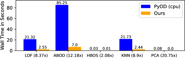
(a)

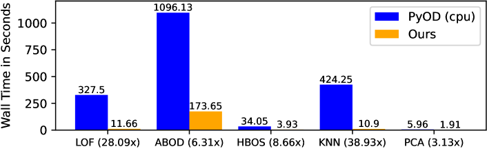
(b)

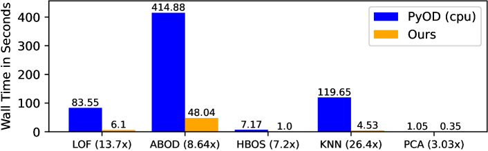
(c)

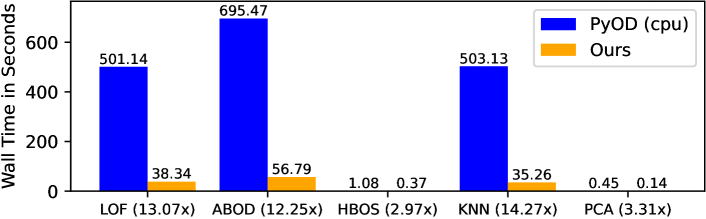
(d)

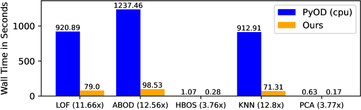
(e)

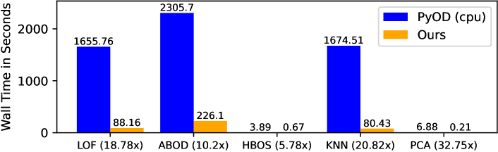
(f)

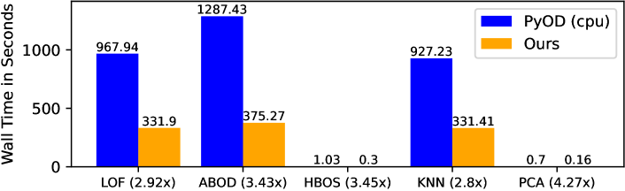
(g)

Figure 8. Runtime comparison between PyOD and TOD in seconds on both real-world and synthetic datasets (see Appx. Fig C3 for synthetic data results). TOD significantly outperforms PyOD in all w/ much smaller runtime, where the speedup factor is shown in parenthesis by each algorithm. On avg., TOD is 10.9$\times$ faster than PyOD (up to 38.9$\times$).

7.3. End-to-end Evaluation

TOD is significantly faster than the leading CPU-based system. We first present the runtime comparison between TOD and PyOD in Fig. 8 using seven real datasets (ALOI, fashion-mnist, and cifar-10) and Appx. Fig. C3 with three synthetic datasets (where Synthetic 1 contains 100,000 samples, Synthetic 2 contains 200,000 samples, and Synthetic 3 contains 400,000 samples (all are with 200 features). The results show that TOD is on average 10.9$\times$ faster than PyOD on the five benchmark algorithms (13.0$\times$, 15.9$\times$, 9.3$\times$, 7.2$\times$, and 8.9$\times$ speed-up on LOF, $k$NN, ABOD, HBOS, and PCA, respectively). For proximity-based algorithms, a larger speed-up is observed for datasets with a higher number of dimensions: LOF and $k$NN are 28.1$\times$ and 38.9$\times$ faster on cifar-10 with 3,072 features. This is expected as GPUs are well-suited for dense tensor multiplication, which is essential in proximity-based methods. Separately, a larger improvement can be achieved for HBOS and PCA on datasets with larger sample sizes. For instance, HBOS is 11.83$\times$ faster on Synthetic 1 (100,000 samples), while the speedup is 17.16$\times$ on Synthetic 2 (200,000 samples). This is expected as HBOS treats each feature independently for density estimation on GPUs, so a large number of samples with a small number of features should yield a significant speed-up. In summary, all the OD algorithms tested are significantly faster in TOD than in the SOTA PyOD system, with the precise amount of speed improvement varying across algorithms. Appx. C.2 shows that GPU computation takes most of the run time for various OD algorithms, explaining the significant time reduction by TOD. We also provide ablation studies to evaluate provable quantization and automatic batching in Appx. C.4.

TOD can handle larger datasets than the GPU baselines. Due to the absence of GPU systems that support all five OD algorithms, we specifically compare the performance of TOD to specialized GPU algorithms $k$NN-CUDA (Angiulli et al., 2016) and LOF-CUDA (Alshawabkeh et al., 2010). Table 3 shows that TOD with 8-GPUs outperforms in all three datasets due to the multi-GPU support, which enables it to handle data more efficient than the baselines and TOD with a single GPU. By focusing on the use of a single GPU, we find that TOD is faster or on par with both baselines due to provable quantization (e.g., 33.13% speedup to LOF-CUDA). Also note that the GPU baselines face the out-of-memory issue (OOM) on large datasets (e.g., the last row of the table with 2,000,000 samples), while TOD can still handle it due to automatic batching. In comparison to these specialized GPU baselines, TOD does not only provide more coverage of diverse algorithms, but also yields better efficiency and scalability.

Table 3. Runtime comparison among selected GPU baselines ($k$NN-CUDA (Angiulli et al., 2016) and LOF-CUDA (Alshawabkeh et al., 2010); neither supports multi-GPU directly), and TOD (single GPU) and TOD-8 (8 GPUs). The first column shows three synthetic datasets with an increasing number of samples (100 dimensions), and the most efficient result is highlighted in bold for each setting. TOD-8 outperforms in all cases due to multi-GPU support, while TOD with a single GPU is faster or on par with the baselines. Note that the GPU baselines run out-of-memory (OOM) on large datasets (e.g., the last row), while TOD does not.

Dataset	$k$NN-CUDA	TOD	TOD-8	LOF-CUDA	TOD	TOD-8
500,000	205.33	208.84	28.59	312.55	209	28.64
1,000,000	850.12	827	112.35	OOM	819	113.72
2,000,000	OOM	3173.39	430.29	OOM	3174.05	434.18

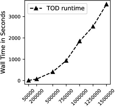
(a)

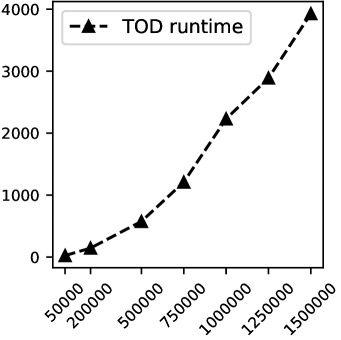
(b)

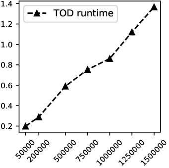
(c)

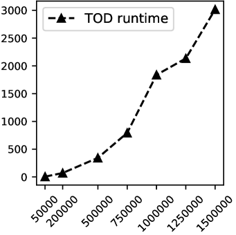
(d)

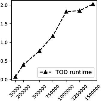
(e)

Figure 9. Scalability plot of selected algorithms in TOD, where it scales well with an increasing number of samples.

7.4. Scalability of TOD

We now gauge the scalability of TOD on datasets of varying sizes, including ones larger than fashion-mnist and cifar-10. In Fig. 9, we plot TOD’s runtime with five OD algorithms on the synthetic datasets with sample sizes ranging from 50,000 to 1,500,000 (all with 200 features). To the best of our knowledge, none of the existing comprehensive OD systems can handle datasets with more than a million samples within a reasonable amount of time (Aggarwal, 2013; Zhao et al., 2021), as most of the OD algorithms are associated with quadratic time complexity. Fig. 9 shows that TOD can process million-sample OD datasets within an hour, providing a scalable approach to deploying OD algorithms in many real-world tasks.

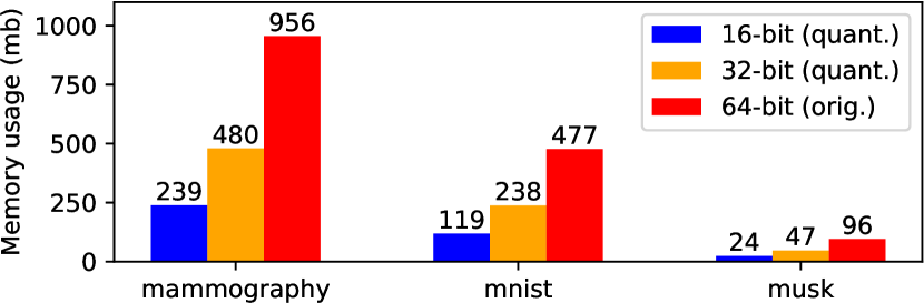
(a)

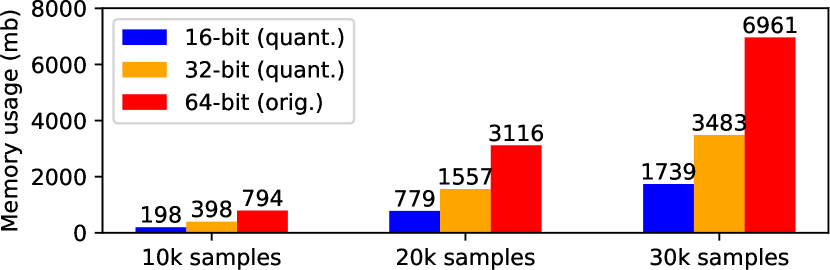
(b)

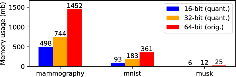
(c)

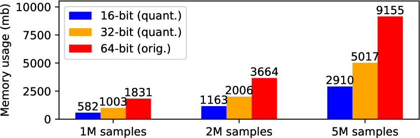
(d)

Figure 10. GPU memory consumption comparison between using provable quantization (16-bit and 32-bit) and the full precision (64-bit). Clearly, provable quantization leads to significant memory consumption saving on nwr and topk.

Table 4. Comparison of operator runtime (in seconds) with provable quantization (i.e., 16-bit and 32-bit) and without quantization (i.e., 64-bit) for nwr and topk. The best model is highlighted in bold (per column), where provable quantization in 16-bit outperforms the rest in most cases.

Prec.	mammog.	mnist	musk	10k	20k	30k
16-bit	2.66	0.54	0.06	0.87	3.02	6.56
32-bit	2.92	1.51	0.09	2.57	10.09	22.51
64-bit	3.31	1.53	0.09	3.49	12.7	27.32

(a) For nwr, 16-bit provable quantization outperforms in all

Prec.	cifar-10	f-mnist	speech	1M	2M	5M
16-bit	0.31	0.09	0.0054	0.58	1.16	2.90
32-bit	0.32	0.1	0.0048	0.70	1.40	3.52
64-bit	0.34	0.07	0.0038	0.71	1.73	3.88

(b) For topk, 16-bit provable quantization wins for large data

7.5. Provable Quantization

Provable quantization (§5) in TOD can optimize the operator memory usage while provably preserving correctness (i.e., no accuracy degradation). To demonstrate its effectiveness, we compare the GPU memory consumption of two applicable operators, nwr and topk, with and without provable quantization using the GPU baseline. Multiple real-world and synthetic datasets are used in the comparison (see Table 2), where synthetic datasets’ names, such as “10k” and “1M”, denote their sample sizes. We deem the 64-bit floating point as the ground truth, and evaluate the provable quantization results in 32- and 16-bit floating-point.

The results demonstrate that provable quantization always leads to memory savings. Specifically, Fig. 10 (a-b) shows nwr with provable quantization on average saves 71.27% (with 16-bit precision) and 47.59% (with 32-bit precision) of the full 64-bit precision GPU memory. Similarly, Fig. 10 (c-d) shows that topk with provable quantization saves 73.49% (with 16-bit precision) and 49.58% (with 32-bit precision) of the full precision memory. Regarding the runtime comparison, operating in lower precision may also lead to an edge. Table 4 shows the operator runtime comparison between using provable quantization (in 16-bit and 32-bit precision) and using the full 64-bit precision. It shows that provable quantization in 16-bit precision is faster than the computations in full precision in most cases, especially for large datasets (e.g., the last three columns of Table 4). This empirical finding can be attributed to lower-precision operations typically being faster, and this speed improvement outweighs the overhead of post verification (see §5.4). For small datasets (the first three columns of Table 4), provable quantization does not necessarily improve the run time due to the additional verification and data movement, both of which finish in 0.1 seconds.

Table 5. Runtime breakdown of using provable quantization on nwr operator with a 30,000 sample synthetic dataset. Column 1 shows the runtime for low-precision evaluation, where column 2 and 3 show the runtime for correctness verification and recalculation, respectively. It shows the primary speed-up comes from low-precision evaluation, while the overhead of verification and recalculation is marginal.

Prec.	Low Prec.	Verification	Recalculation	Total
16-bit	5.91	0.05	0.61	6.56
32-bit	22	0.05	0.47	22.51
64-bit	N/A	N/A	N/A	27.32

Case study on runtime breakdown  . In addition to comparing the total runtime of an operator with or without provable quantization (§7.5), it is interesting to see the time breakdown of each phase of provable quantization. Specifically, the runtime of provable quantization can be divided into (i) operator evaluation in lower precision, (ii) result verification and (iii) recalculation in the original precision for the ones that fail in the verification. Taking nwr on 30k samples as an example (the last column of Table 4(a)), we show the time breakdown of (i) low-precision evaluation (ii) correctness verification and (iii) recalculation in higher precision in Table 5. In this case, the performance improvement of provable quantization comes from the reduced evaluation time in lower precision, which outweighs the cost of verification and recalculation. To further demonstrate the necessity of post-verification, we also measure the accuracy variation (e.g., ROC-AUC (Aggarwal, 2013)) by simply running $k$NN detector on fraud, census, and donors datasets in 16-bit precision without post-verification, which leads to $-3.48\%$, $+1.05\%$, $-4.27\%$ accuracy variation. These results show the merit of provable quantization over direct quantization.

7.6. Automatic Batching

To evaluate the effectiveness of automatic batching, we compare the runtime of multiple BOs and FOs under (i) an Numpy implementation on a CPU (Harris et al., 2020), (ii) a direct PyTorch GPU implementation without batching (Paszke et al., 2019), and (iii) TOD’s automatic batching.

Table 6 compares the three implementations of key operators in OD systems. Clearly, TOD with automatic batching achieves the best balance of efficiency and scalability, leading to 7.22$\times$, 17.46$\times$, and 11.49$\times$ speedups compared to a highly optimized NumPy implementation on CPUs. TOD can also handle more than 10$\times$ larger datasets where the direct PyTorch implementation faces out of memory (OOM) errors. TOD is only marginally slower than PyTorch when the input dataset is small (see the first row of each operator). In this case, batching is not needed, and TOD is equivalent to PyTorch; TOD is slightly slower due to the overhead of TOD deciding whether or not to enable automatic batching.

Table 6. Operator runtime comparison among implementations in NumPy (no batching), PyTorch (no batching) and TOD (with automatic batching); the most efficient result is highlighted in bold per row. Automatic batching in TOD prevents out-of-memory (OOM) errors yet shows great efficiency, especially on large datasets.

Operator	Size	NumPy	PyTorch	TOD
topk	10,000,000	7.88	1.08	1.09
topk	20,000,000	15.77	OOM	2.44
topk	100,000,000	OOM	OOM	10.83
intersect	20,000,000	1.99	0.12	0.14
intersect	100,000,000	11	0.63	0.63
intersect	200,000,000	21.65	OOM	2.11
$k$NN	50,000	20.15	0.27	0.28
$k$NN	200,000	194.43	OOM	19.65
$k$NN	400,000	818.32	OOM	71.22

(a)

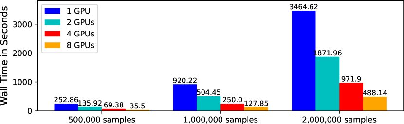
(b)

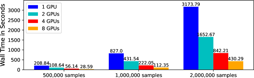
(c)

Figure 11. Runtime comparison of using different numbers of GPUs (top: LOF; middle: ABOD; bottom: $k$NN). TOD can efficiently leverage multiple GPUs for faster OD.

7.7. Multi-GPU Results

We now evaluate the scalability of TOD on multiple GPUs on a single compute node. Specifically, we compare the run time of three compute-intensive OD algorithms (i.e., LOF, ABOD, and $k$NN) with 1,2,4, and 8 NVIDIA Tesla V100 GPUs.

Fig. 11 shows that for three OD algorithms tested, TOD can achieve nearly linear speed-up with more GPUs—the GPU efficiency is mostly above 90%. For instance, the $k$NN result shows that using 2, 4, and 8 GPUs are $1.91\times$, $3.73\times$, and $7.34\times$ faster than the single-GPU performance. As a comparison, using 2, 4, and 8 GPUs with ABOD and LOF are $1.85\times$, $3.63\times$, $7.14\times$ faster and $1.91\times$, $3.70\times$, $7.27\times$ faster, respectively. First, there is inevitably a small overhead in multi-processing, causing the speed-up to not exactly be linear. Second, the minor efficiency difference between $k$NN and ABOD is due to most OD operations in the former being executed on multiple GPUs, while the latter involves several sequential steps that have to be run on CPUs. To sum up, TOD can leverage multiple GPUs efficiently to process large datasets.

8. Limitations and Future Directions

Tree-based OD algorithms.   One limitation of TOD is that it does not support tree-based OD algorithms such as isolation forests (Liu et al., 2008). Tree-based operations involve random data access (Lefohn et al., 2006), which is not friendly for GPUs designed for batch operations. Future work can consider converting trees to tensor operations (Nakandala et al., 2020) for acceleration.

Approximate solutions.   Our focus in this paper has been on exact efficient, scalable implementations of OD algorithms. In particular, we have not considered implementations that intentionally are meant to be approximate, where for instance, one could trade off between accuracy, computation time, and memory usage. Note that even with our provable quantization technique, we ask for the lower-precision computation to yield the correct (exact) output. A future research direction is to extend TOD to support approximate solutions for even better scalability and efficiency when reduced accuracy is acceptable. For instance, exact nearest neighbor search in can be switched to approximate nearest neighbor search (Fu et al., 2019; Wang et al., 2021a).

Heterogeneous GPUs.   Thus far, we have not studied the use of TOD with heterogeneous GPUs. In this setting, incorporating a cost model could be helpful in balancing the workload between the different GPUs, accounting for their different characteristics such as varying memory capacities.

Gradient-based operators.   Currently, TOD does not support operators that involve solving an optimization problem via gradient descent. Future work may consider incorporating optimization-based operators to support (a small group of) optimization-based OD algorithms, e.g., OCSVM (Schölkopf et al., 2001).

Extension to classification.   It is possible to use TOD to build classification models, as the operators in TOD are generic and may serve the tasks beyond OD. We provide an example of using TOD to construct $k$ nearest neighbor classifier in Appx. B, which also exhibits a significant performance improvement over the CPU implementation in scikit-learn (Pedregosa et al., 2011). Note that classification tasks often involve optimization (e.g., via gradient descent), which we already pointed out that TOD does not yet support. Thus, only calculation-based classifiers can be implemented by TOD for now.

9. Conclusion

In this paper, we propose the first comprehensive GPU-based outlier detection system called TOD, which is on average 10.9 times faster than the leading system PyOD and is capable of handling larger datasets than existing GPU baselines. The key idea is to decompose complex outlier detection algorithms into a combination of tensor operations for effective GPU acceleration. Our system enables many large-scale real-world outlier detection applications that could have stringent time constraints. With ease of extensibility, TOD can prototype and implement new detection algorithms.

Supplementary Material for TOD

Details on system design and experiments.

Appendix A Demo on Using TOD to Implement New OD Algorithms from Scratch

Overview of implementing new OD algorithms with TOD  . As shown in §4, TOD takes a modular approach to implement an OD algorithm. Thus, using TOD to implement a new OD algorithm requires conceptualizing the algorithm as a combination of operators (BTOs and FOs) in TOD (see Fig. 2). Thanks to the nature of OD applications that do not involve complex optimization, most OD algorithms can be decomposed as a combination of 2 to 3 operators.

Overview of ECOD  . We provide an example of using TOD to implement the latest OD algorithm with empirical cumulative distribution functions (ECOD) (Li et al., 2022), which is just published in early 2022. In a nutshell, ECOD estimates the empirical distribution of each feature (i.e., density estimation), where it considers that outliers locate in low-density regions. After that, ECOD aggregates all density estimation results per feature into final outlier scores.

Turning ECOD into abstraction.   ECOD mainly involves two operators: (i) it estimates the density (“f. Density est.”) of each features by “8. Basic OPs (ECDF)” and (ii) then aggregates density results across all features via “7. Agg.”. By having the process in mind, we could sketch the abstraction of ECOD in Fig. A1.

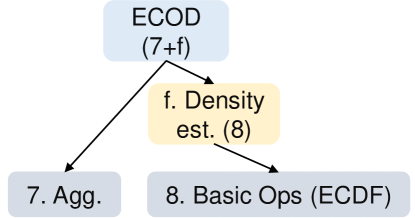
Figure A1. Examples of building latest OD algorithm ECOD with FOs and BTOs conveniently.

Turning abstraction into code  . We provide the code breakdown to show how to use TOD to implement ECOD, and the full implementation is available for further reference. The code snippet (i) shows that we use the basic operator ECDF for density estimation and (ii) shows the aggregation step of density estimation as outlier scores. Putting these core parts together with some skeleton code, we could conveniently include ECOD in TOD. It is noted that we still need to glue the operators together, while the use of predefined TOD operators helps us to achieve acceleration.

⬇

from .basic_operators import ecdf_multiple

# density estimation via ECDF

self.U_l = ecdf_multiple(X, device=self.device)

self.U_r = ecdf_multiple(-X, device=self.device)

(i) code of density estimation in ECOD

⬇

# take the negative log

self.U_l = -1 * torch.log(self.U_l)

self.U_r = -1 * torch.log(self.U_r)

# aggregate and generate outlier scores

self.O = torch.maximum(self.U_l, self.U_r)

self.decision_scores_ = torch.sum(self.O, dim=1).cpu().numpy() * -1

(ii) code of density aggregation in ECOD

Appendix B Example of Using TOD to Build Classification Algorithms

As discussed in §8, TOD may be used to construct algorithms beyond OD, e.g., classification and regression. In this section, we demonstrate the use of TOD to build a popular classifier called $k$ nearest neighbor classifiers ($k$NN_CLF)(Fix and Hodges, 1989).

In short, $k$NN_CLF is a lazy classifier and does not involve a training stage. For a test sample $\mathbf{X}_{\text{test}}$, it calculates the pairwise distance between the test sample with each “training” data. It then uses the aggregation (e.g., majority vote or avg.) to decide the predicted classes of each test sample. Thus, it can be decomposed as the combination of (i) calculating pairwise distance by cdist (ii) identifying the top $k$ neighbors by topk and (iii) predicting the class labels by aggregating the labels from the neighbors (i.e., Basic OPs).

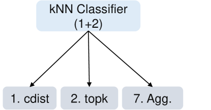
Figure B2. Examples of building $k$NN classifier with TOD

Table B1 provides a detailed comparison between CPU-based implementation of $k$NN_CLF in scikit-learn (sklearn) (Pedregosa et al., 2011) and TOD’s implementation. On average, TOD’s $k$NN_CLF is 10.1 times faster than that of sklearn due to the GPU acceleration.

Table B1. Runtime (in seconds) comparison of $k$NN classifier using CPU-based scikit-learn (sklearn) (Pedregosa et al., 2011) vs. GPU-enabled TOD. On average, TOD’s implementation is 10.1 times faster than that of sklearn.

Train Size	Test Size	Number of Features	$k$NN-sklearn	$k$NN-TOD
50,000	50,000	100	41.35	4.76
50,000	50,000	200	52.26	4.83
100,000	50,000	100	84.84	8.09
100,000	50,000	200	88.13	8.36

Appendix C Additional Experiment Results

C.1. End-to-end Results on Synthetic Datasets

Consistent with the results presented in §7.3, TOD is significantly faster than the leading CPU-based system on large synthetic datasets. Fig. C3 shows the results on three synthetic datasets (where Synthetic 1 contains 100,000 samples, Synthetic 2 contains 200,000 samples, and Synthetic 3 contains 400,000 samples (all are with 200 features). The results show that TOD is on average 10.9$\times$ faster than PyOD on the five benchmark algorithms (13.0$\times$, 15.9$\times$, 9.3$\times$, 7.2$\times$, and 8.9$\times$ speed-up on LOF, $k$NN, ABOD, HBOS, and PCA, respectively).

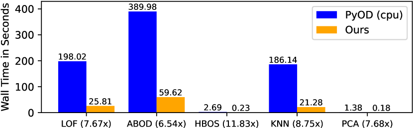
(a)

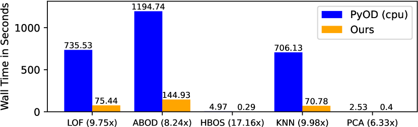
(b)

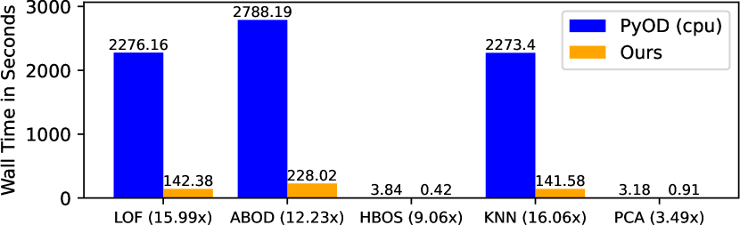
(c)

Figure C3. Runtime comparison between PyOD and TOD in seconds on synthetic datasets (see §7.3 Fig. 8 for results on real-world datasets). TOD significantly outperforms PyOD in all w/ much smaller runtime, where the speedup factor is shown in parenthesis by each algorithm. On avg., TOD is 10.9$\times$ faster than PyOD (up to 38.9$\times$).

C.2. Further Time Analysis

Fig. C4 shows the comparison between GPU time and the total runtime, where GPU time consists of a large portion of the total runtime, and verifies that the acceleration of TOD mainly comes from the use of GPU(s). Moreover, we also notice that the GPU efficiency increases for larger datasets with higher percentages. This also explains why we observe more acceleration of TOD on large datasets in Fig. 8 and Appx. Fig. C3.

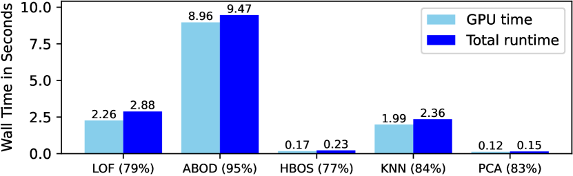
(a)

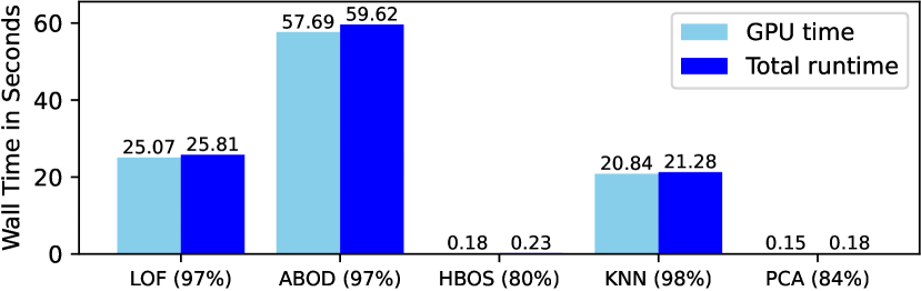
(b)

Figure C4. GPU time and total runtime of TOD in seconds on synthetic datasets (where the percentage is shown in parenthesis). TOD achieves significant efficiency improvement with high GPU usages (e.g., mostly $>80\%$).

C.3. Case Study on Operator Fusion

Although automatic batching applies to all BTOs and FOs, we introduce an additional technique called operator fusion in §6.1 to further optimize the execution of selected operators in sequence. For instance, $k$NN batching is achieved by running cdist and topk sequentially, where each uses automatic batching and the output of the former is the input of the latter.

Differently, we could further optimize this simple concatenation execution by fusing cdist and topk together for better efficiency. Fig. 7 compares simple concatenation (subfigure a) and operator fusion (subfigure b) on $k$NN. Specifically, the latter executes the topk BTO on the cdist BTO’s individual batches separately rather than running topk on the full distance matrix outputted by cdist. This prevents moving the entire $n\times n$ distance matrix between operators, which often causes OOM.

In Table C2, we compare the performance of simple concatenation (i.e., cdist and then topk) and operator fusion regarding both GPU memory and time consumption, where operator fusion shows great performance improvement.

Table C2. GPU memory consumption (in Mb) and runtime (in seconds) comparison of simple concatenation (SC) and operator fusion (OF) for $k$NN. Operator fusion brings huge savings in both GPU memory consumption and runtime.

Sample Size	GPU-SC	GPU-OF	Runtime-SC	Runtime-OF
50,000	5280	3060	8.47	2.80
100,000	9010	3060	33.48	9.12

C.4. Ablation Studies on Provable Quantization and Automatic Batching

In addition to the end-to-end analysis in §7.3, we also provide further ablations on provable quantization (PQ) and automatic batching (AB) in this section. We demonstrate this experiment with $k$-NN OD algorithm where both techniques apply. Table C3 shows that automatic batching addresses the issue of out-of-memory on large datasets, while provable quantization reduces GPU memory consumption and runtime. The ablations show that using both techniques leads to the best performance.

Table C3. Ablations on provable quantization (PQ) and automatic batching (AB) for $k$NN. We set batch size equal to 40,000, and thus AB does not apply to the first row of the table. The best performing combination is highlighted in bold, where using both techniques achieves the best performance.

# Samples	PQ&AB	AB only	PQ only	None
40,000	5.34	N/A	5.34	10.88
80,000	15.12	20.91	17.56	OOM
160,000	45.37	67.22	OOM	OOM

(a) Runtime in seconds

# Samples	PQ&AB	AB only	PQ only	None
40,000	3,040	N/A	3040	12,170
80,000	3,040	12,050	12,020	OOM
160,000	3,040	12,050	OOM	OOM

(b) GPU memory consumption in Mb

Appendix D Open-source System and API Demonstration

Accessibility  . To facilitate accessibility of TOD, we release it under the open BSD 2 license, which can be easily installed via Python Package Index (PyPI) with name pytod.

API design and demonstration  . Follow by the mature API design of scikit-learn (Buitinck et al., 2013) and PyOD (Zhao et al., 2019a), all the supported OD algorithms have a unified API design: (i) fit processes the input data and calculates necessary statistics for prediction, where the outlier scores are also calculated on the input data (ii) decision_function returns the raw outlier scores of newcoming samples based on the fitted outlier detector in the inductive setting and (iii) predict returns the binary labels of newcoming samples based on the fitted outlier detector. We demonstrate these APIs in TOD with $k$NN detector below, and other supported OD algorithms have the same APIs.

⬇

from pytod.utils.data import generate_data

from pytod.utils.data import evaluate_print

from pytod.models.knn import KNN

# Generate sample data

X_train, y_train, X_test, y_test = \

generate_data(n_train=50000, n_test=10000)

device = validate_device(0) # get the GPU 0

# initialize a kNN model in TOD with k=10 and batch=10000

clf = KNN(n_neighbors=k, batch_size=10000, device=device)

# fit the kNN model

clf.fit(X_train)

# get the train labels and outlier scores

y_train_scores = clf.decision_scores_ # raw outlier scores

y_train_pred = clf.labels_ # binary labels

# evaluate and print the results

evaluate_print(clf_name, y_train, y_train_scores)

# get the prediction labels and outlier scores on test

y_test_scores = clf.decision_function(X_test) # raw scores

API demo of invoking $k$NN in TOD; other OD algorithms follow the same API design

Utility functions.   To facilitate system comparison and evaluation, we also create a set of helper functions including (i) generate_data that can creates synthetic OD datasets by modeling normal samples by Gaussian distribution and outliers by uniform distribution and (ii) evaluate_print to provide OD specific evaluations by the metrics described in §7.2.

References

- (1)
- Abadi et al. (2016) Martín Abadi, Paul Barham, Jianmin Chen, Zhifeng Chen, Andy Davis, Jeffrey Dean, Matthieu Devin, Sanjay Ghemawat, Geoffrey Irving, Michael Isard, Manjunath Kudlur, Josh Levenberg, Rajat Monga, Sherry Moore, Derek Gordon Murray, Benoit Steiner, Paul A. Tucker, Vijay Vasudevan, Pete Warden, Martin Wicke, Yuan Yu, and Xiaoqiang Zheng. 2016. TensorFlow: A System for Large-Scale Machine Learning. In 12th USENIX Symposium on Operating Systems Design and Implementation, OSDI 2016, Savannah, GA, USA, November 2-4, 2016, Kimberly Keeton and Timothy Roscoe (Eds.). USENIX Association, 265–283. https://www.usenix.org/conference/osdi16/technical-sessions/presentation/abadi
- Abdulaal et al. (2021) Ahmed Abdulaal, Zhuanghua Liu, and Tomer Lancewicki. 2021. Practical approach to asynchronous multivariate time series anomaly detection and localization. In Proceedings of the 27th ACM SIGKDD Conference on Knowledge Discovery & Data Mining. ACM, 2485–2494.
- Achtert et al. (2010) Elke Achtert, Hans-Peter Kriegel, Lisa Reichert, Erich Schubert, Remigius Wojdanowski, and Arthur Zimek. 2010. Visual Evaluation of Outlier Detection Models. In Database Systems for Advanced Applications, 15th International Conference, DASFAA 2010, Tsukuba, Japan, April 1-4, 2010, Proceedings, Part II (Lecture Notes in Computer Science), Hiroyuki Kitagawa, Yoshiharu Ishikawa, Qing Li, and Chiemi Watanabe (Eds.), Vol. 5982. Springer, 396–399. https://doi.org/10.1007/978-3-642-12098-5_34
- Aggarwal (2013) Charu C. Aggarwal. 2013. Outlier Analysis. Springer.
- Aggarwal et al. (2011) Charu C Aggarwal, Yuchen Zhao, and S Yu Philip. 2011. Outlier detection in graph streams. In 2011 IEEE 27th international conference on data engineering. IEEE, IEEE, 399–409.
- Alshawabkeh et al. (2010) Malak Alshawabkeh, Byunghyun Jang, and David R. Kaeli. 2010. Accelerating the local outlier factor algorithm on a GPU for intrusion detection systems. In Proceedings of 3rd Workshop on General Purpose Processing on Graphics Processing Units, GPGPU 2010, Pittsburgh, Pennsylvania, USA, March 14, 2010 (ACM International Conference Proceeding Series), David R. Kaeli and Miriam Leeser (Eds.), Vol. 425. ACM, 104–110. https://doi.org/10.1145/1735688.1735707
- André et al. (2016) Fabien André, Anne-Marie Kermarrec, and Nicolas Le Scouarnec. 2016. Cache locality is not enough: High-performance nearest neighbor search with product quantization fast scan. In VLDB, Vol. 9. VLDB Endowment, 12.
- Angiulli et al. (2010) Fabrizio Angiulli, Stefano Basta, Stefano Lodi, and Claudio Sartori. 2010. A Distributed Approach to Detect Outliers in Very Large Data Sets. In Euro-Par 2010 - Parallel Processing. Springer Berlin Heidelberg, Berlin, Heidelberg, 329–340.
- Angiulli et al. (2016) Fabrizio Angiulli, Stefano Basta, Stefano Lodi, and Claudio Sartori. 2016. GPU Strategies for Distance-Based Outlier Detection. IEEE Trans. Parallel Distributed Syst. 27, 11 (2016), 3256–3268.
- Angiulli and Pizzuti (2002) Fabrizio Angiulli and Clara Pizzuti. 2002. Fast Outlier Detection in High Dimensional Spaces. In Principles of Data Mining and Knowledge Discovery, 6th European Conference, PKDD 2002, Helsinki, Finland, August 19-23, 2002, Proceedings (Lecture Notes in Computer Science), Tapio Elomaa, Heikki Mannila, and Hannu Toivonen (Eds.), Vol. 2431. Springer, 15–26. https://doi.org/10.1007/3-540-45681-3_2
- Ayed et al. (2020) Fadhel Ayed, Lorenzo Stella, Tim Januschowski, and Jan Gasthaus. 2020. Anomaly detection at scale: The case for deep distributional time series models. In International Conference on Service-Oriented Computing. Springer, 97–109.
- Azmandian et al. (2012) Fatemeh Azmandian, Ayse Yilmazer, Jennifer G. Dy, Javed A. Aslam, and David R. Kaeli. 2012. GPU-Accelerated Feature Selection for Outlier Detection Using the Local Kernel Density Ratio. In 12th IEEE International Conference on Data Mining, ICDM 2012, Brussels, Belgium, December 10-13, 2012, Mohammed Javeed Zaki, Arno Siebes, Jeffrey Xu Yu, Bart Goethals, Geoffrey I. Webb, and Xindong Wu (Eds.). IEEE Computer Society, 51–60. https://doi.org/10.1109/ICDM.2012.51
- Bhaduri et al. (2011) Kanishka Bhaduri, Bryan L Matthews, and Chris R Giannella. 2011. Algorithms for speeding up distance-based outlier detection. In KDD. ACM, 859–867.
- Blalock and Guttag (2017) Davis W Blalock and John V Guttag. 2017. Bolt: Accelerated data mining with fast vector compression. In KDD. ACM, 727–735.
- Boehm et al. (2018) Matthias Boehm, Berthold Reinwald, Dylan Hutchison, Prithviraj Sen, Alexandre V. Evfimievski, and Niketan Pansare. 2018. On Optimizing Operator Fusion Plans for Large-Scale Machine Learning in SystemML. Proc. VLDB Endow. 11, 12 (2018), 1755–1768. https://doi.org/10.14778/3229863.3229865
- Boniol and Palpanas (2020) Paul Boniol and Themis Palpanas. 2020. Series2graph: Graph-based subsequence anomaly detection for time series. VLDB 13, 12 (2020), 1821–1834.
- Boniol et al. (2020) Paul Boniol, Themis Palpanas, Mohammed Meftah, and Emmanuel Remy. 2020. GraphAn: Graph-based subsequence anomaly detection. VLDB 13, 12 (2020), 2941–2944.
- Boniol et al. (2021) Paul Boniol, John Paparrizos, Themis Palpanas, and Michael J Franklin. 2021. SAND: streaming subsequence anomaly detection. VLDB 14, 10 (2021), 1717–1729.
- Breunig et al. (2000) Markus M. Breunig, Hans-Peter Kriegel, Raymond T. Ng, and Jörg Sander. 2000. LOF: Identifying Density-Based Local Outliers.. In SIGMOD. ACM, 93–104.
- Buitinck et al. (2013) Lars Buitinck, Gilles Louppe, Mathieu Blondel, Fabian Pedregosa, Andreas Mueller, Olivier Grisel, Vlad Niculae, Peter Prettenhofer, Alexandre Gramfort, Jaques Grobler, Robert Layton, Jake VanderPlas, Arnaud Joly, Brian Holt, and Gaël Varoquaux. 2013. API design for machine learning software: experiences from the scikit-learn project. In Proceedings of ECML PKDD Workshop: Languages for Data Mining and Machine Learning. ECML, 108–122.
- Campos et al. (2016) Guilherme O Campos, Arthur Zimek, Jörg Sander, Ricardo JGB Campello, Barbora Micenková, Erich Schubert, Ira Assent, and Michael E Houle. 2016. On the evaluation of unsupervised outlier detection: measures, datasets, and an empirical study. Data mining and knowledge discovery 30, 4 (2016), 891–927.
- Cao et al. (2014) Lei Cao, Qingyang Wang, and Elke A Rundensteiner. 2014. Interactive outlier exploration in big data streams. VLDB 7, 13 (2014), 1621–1624.
- Cao et al. (2019) Lei Cao, Yizhou Yan, Samuel Madden, Elke A Rundensteiner, and Mathan Gopalsamy. 2019. Efficient discovery of sequence outlier patterns. VLDB 12, 8 (2019), 920–932.
- Dai et al. (2021) Steve Dai, Rangharajan Venkatesan, Haoxing Ren, Brian Zimmer, William J. Dally, and Brucek Khailany. 2021. VS-Quant: Per-vector Scaled Quantization for Accurate Low-Precision Neural Network Inference. CoRR (2021). arXiv:2102.04503
- Deng et al. (2009) Jia Deng, Wei Dong, Richard Socher, Li-Jia Li, Kai Li, and Li Fei-Fei. 2009. Imagenet: A large-scale hierarchical image database. In 2009 IEEE conference on computer vision and pattern recognition. IEEE, 248–255.
- Fix and Hodges (1989) Evelyn Fix and Joseph Lawson Hodges. 1989. Discriminatory analysis. Nonparametric discrimination: Consistency properties. International Statistical Review/Revue Internationale de Statistique 57, 3 (1989), 238–247.
- Fu et al. (2019) Cong Fu, Chao Xiang, Changxu Wang, and Deng Cai. 2019. Fast approximate nearest neighbor search with the navigating spreading-out graph. VLDB 12, 5 (2019), 461–474.
- Fu et al. (2021) Tianfan Fu, Cao Xiao, Cheng Qian, Lucas M Glass, and Jimeng Sun. 2021. Probabilistic and Dynamic Molecule-Disease Interaction Modeling for Drug Discovery. In KDD. ACM, 404–414.
- Gao et al. (2020) Yanjie Gao, Yu Liu, Hongyu Zhang, Zhengxian Li, Yonghao Zhu, Haoxiang Lin, and Mao Yang. 2020. Estimating GPU memory consumption of deep learning models. In ESEC/FSE. ACM, 1342–1352.
- Gera et al. (2020) Prasun Gera, Hyojong Kim, Piyush Sao, Hyesoon Kim, and David Bader. 2020. Traversing large graphs on GPUs with unified memory. VLDB 13, 7 (2020), 1119–1133.
- Goldstein and Dengel (2012) Markus Goldstein and Andreas Dengel. 2012. Histogram-based outlier score (hbos): A fast unsupervised anomaly detection algorithm. KI (2012), 59–63.
- Goodfellow et al. (2016) Ian Goodfellow, Yoshua Bengio, and Aaron Courville. 2016. Deep learning. MIT.
- Han et al. (2022) Songqiao Han, Xiyang Hu, Hailiang Huang, Mingqi Jiang, and Yue Zhao. 2022. ADBench: Anomaly Detection Benchmark. arXiv preprint arXiv:2206.09426 (2022).
- Harris et al. (2020) Charles R Harris, K Jarrod Millman, Stéfan J van der Walt, Ralf Gommers, Pauli Virtanen, David Cournapeau, Eric Wieser, Julian Taylor, Sebastian Berg, Nathaniel J Smith, et al. 2020. Array programming with NumPy. Nature (2020).
- He et al. (2016) Kaiming He, Xiangyu Zhang, Shaoqing Ren, and Jian Sun. 2016. Deep residual learning for image recognition. In Proceedings of the IEEE conference on computer vision and pattern recognition. IEEE, 770–778.
- Jacob et al. (2021) Vincent Jacob, Fei Song, Arnaud Stiegler, Bijan Rad, Yanlei Diao, and Nesime Tatbul. 2021. A demonstration of the exathlon benchmarking platform for explainable anomaly detection. VLDB (PVLDB) (2021).
- Ji and Wang (2021) Zhuoran Ji and Cho-Li Wang. 2021. Accelerating DBSCAN Algorithm with AI Chips for Large Datasets. In ICPP 2021: 50th International Conference on Parallel Processing, Lemont, IL, USA, August 9 - 12, 2021, Xian-He Sun, Sameer Shende, Laxmikant V. Kalé, and Yong Chen (Eds.). ACM, 51:1–51:11. https://doi.org/10.1145/3472456.3473518
- Jia et al. (2020) Zhihao Jia, Sina Lin, Mingyu Gao, Matei Zaharia, and Alex Aiken. 2020. Improving the Accuracy, Scalability, and Performance of Graph Neural Networks with Roc. In MLSys. mlsys.org.
- Jia et al. (2019) Zhihao Jia, Matei Zaharia, and Alex Aiken. 2019. Beyond Data and Model Parallelism for Deep Neural Networks. In Proceedings of Machine Learning and Systems 2019, MLSys 2019, Stanford, CA, USA, March 31 - April 2, 2019, Ameet Talwalkar, Virginia Smith, and Matei Zaharia (Eds.). mlsys.org. https://proceedings.mlsys.org/book/265.pdf
- Kahan (1996) William Kahan. 1996. IEEE standard 754 for binary floating-point arithmetic. Lecture Notes on the Status of IEEE 754, 94720-1776 (1996), 11.
- Kingsbury and Alvaro (2020) Kyle Kingsbury and Peter Alvaro. 2020. Elle: inferring isolation anomalies from experimental observations. VLDB 14, 3 (2020), 268–280.
- Koutsoukos et al. (2021) Dimitrios Koutsoukos, Supun Nakandala, Konstantinos Karanasos, Karla Saur, Gustavo Alonso, and Matteo Interlandi. 2021. Tensors: An abstraction for general data processing. VLDB 14, 10 (2021), 1797–1804.
- Kriegel et al. (2008) Hans-Peter Kriegel, Matthias Schubert, and Arthur Zimek. 2008. Angle-based outlier detection in high-dimensional data.. In KDD. ACM, 444–452.
- Lai et al. (2021) Kwei-Herng Lai, Daochen Zha, Junjie Xu, Yue Zhao, Guanchu Wang, and Xia Hu. 2021. Revisiting Time Series Outlier Detection: Definitions and Benchmarks. In Proceedings of the Neural Information Processing Systems Track on Datasets and Benchmarks 1, NeurIPS Datasets and Benchmarks 2021, December 2021, virtual. Joaquin Vanschoren and Sai-Kit Yeung. https://datasets-benchmarks-proceedings.neurips.cc/paper/2021/hash/ec5decca5ed3d6b8079e2e7e7bacc9f2-Abstract-round1.html
- Lazarevic et al. (2003) Aleksandar Lazarevic, Levent Ertöz, Vipin Kumar, Aysel Ozgur, and Jaideep Srivastava. 2003. A Comparative Study of Anomaly Detection Schemes in Network Intrusion Detection. In SDM. SIAM, 25–36.
- Leal and Gruenwald (2018) Eleazar Leal and Le Gruenwald. 2018. Research Issues of Outlier Detection in Trajectory Streams Using GPUs. SIGKDD Explor. 20, 2 (2018), 13–20.
- LeCun (2019) Yann LeCun. 2019. 1.1 deep learning hardware: past, present, and future. In 2019 IEEE International Solid-State Circuits Conference-(ISSCC). IEEE, 12–19.
- LeCun et al. (2015) Yann LeCun, Yoshua Bengio, and Geoffrey Hinton. 2015. Deep learning. nature 521, 7553 (2015), 436–444.
- Lee et al. (2020) Meng-Chieh Lee, Yue Zhao, Aluna Wang, Pierre Jinghong Liang, Leman Akoglu, Vincent S. Tseng, and Christos Faloutsos. 2020. AutoAudit: Mining Accounting and Time-Evolving Graphs. In Big Data. IEEE, 950–956.
- Lee et al. (2021) Rubao Lee, Minghong Zhou, Chi Li, Shenggang Hu, Jianping Teng, Dongyang Li, and Xiaodong Zhang. 2021. The art of balance: a RateupDB™ experience of building a CPU/GPU hybrid database product. VLDB 14, 12 (2021), 2999–3013.
- Lee et al. (2018) Wonyeol Lee, Rahul Sharma, and Alex Aiken. 2018. On automatically proving the correctness of math.h implementations. Proc. ACM Program. Lang. 2, POPL (2018), 47:1–47:32. https://doi.org/10.1145/3158135
- Lefohn et al. (2006) Aaron E Lefohn, Shubhabrata Sengupta, Joe Kniss, Robert Strzodka, and John D Owens. 2006. Glift: Generic, efficient, random-access GPU data structures. ACM Transactions on Graphics (TOG) 25, 1 (2006), 60–99.
- Li et al. (2020) Zheng Li, Yue Zhao, Nicola Botta, Cezar Ionescu, and Xiyang Hu. 2020. COPOD: Copula-Based Outlier Detection. In ICDM. IEEE, 1118–1123.
- Li et al. (2022) Zheng Li, Yue Zhao, Xiyang Hu, Nicola Botta, Cezar Ionescu, and George Chen. 2022. ECOD: Unsupervised Outlier Detection Using Empirical Cumulative Distribution Functions. IEEE Transactions on Knowledge and Data Engineering (2022), 1–1. https://doi.org/10.1109/TKDE.2022.3159580
- Liu et al. (2021b) Can Liu, Li Sun, Xiang Ao, Jinghua Feng, Qing He, and Hao Yang. 2021b. Intention-aware heterogeneous graph attention networks for fraud transactions detection. In Proceedings of the 27th ACM SIGKDD Conference on Knowledge Discovery & Data Mining. 3280–3288.
- Liu et al. (2008) Fei Tony Liu, Kai Ming Ting, and Zhi-Hua Zhou. 2008. Isolation Forest. In ICDM. IEEE Computer Society, 413–422.
- Liu et al. (2021a) Haoyu Liu, Fenglong Ma, Shibo He, Jiming Chen, and Jing Gao. 2021a. Fairness-aware Outlier Ensemble. arXiv preprint arXiv:2103.09419 (2021).
- Liu et al. (2022a) Kay Liu, Yingtong Dou, Yue Zhao, Xueying Ding, Xiyang Hu, Ruitong Zhang, Kaize Ding, Canyu Chen, Hao Peng, Kai Shu, et al. 2022a. Benchmarking Node Outlier Detection on Graphs. arXiv preprint arXiv:2206.10071 (2022).
- Liu et al. (2022b) Kay Liu, Yingtong Dou, Yue Zhao, Xueying Ding, Xiyang Hu, Ruitong Zhang, Kaize Ding, Canyu Chen, Hao Peng, Kai Shu, et al. 2022b. PyGOD: A Python Library for Graph Outlier Detection. arXiv preprint arXiv:2204.12095 (2022).
- Liu et al. (2020) Zhiwei Liu, Yingtong Dou, Philip S. Yu, Yutong Deng, and Hao Peng. 2020. Alleviating the Inconsistency Problem of Applying Graph Neural Network to Fraud Detection. In Proceedings of the 43rd International ACM SIGIR conference on research and development in Information Retrieval, SIGIR 2020, Virtual Event, China, July 25-30, 2020, Jimmy Huang, Yi Chang, Xueqi Cheng, Jaap Kamps, Vanessa Murdock, Ji-Rong Wen, and Yiqun Liu (Eds.). ACM, 1569–1572. https://doi.org/10.1145/3397271.3401253
- Looks et al. (2017) Moshe Looks, Marcello Herreshoff, DeLesley Hutchins, and Peter Norvig. 2017. Deep Learning with Dynamic Computation Graphs. In ICLR. OpenReview.net.
- Lozano and Acuña (2005) Elio Lozano and Edgar Acuña. 2005. Parallel Algorithms for Distance-Based and Density-Based Outliers. In ICDM. IEEE Computer Society, 729–732.
- Manzoor et al. (2018) Emaad Manzoor, Hemank Lamba, and Leman Akoglu. 2018. xstream: Outlier detection in feature-evolving data streams. In KDD. ACM, 1963–1972.
- Meng et al. (2017) Chen Meng, Minmin Sun, Jun Yang, Minghui Qiu, and Yang Gu. 2017. Training deeper models by GPU memory optimization on TensorFlow. In Proc. of ML Systems Workshop in NIPS. NIPS.
- Menon et al. (2017) Prashanth Menon, Todd C Mowry, and Andrew Pavlo. 2017. Relaxed operator fusion for in-memory databases: Making compilation, vectorization, and prefetching work together at last. VLDB 11, 1 (2017), 1–13.
- Min et al. (2020) Seung Won Min, Vikram Sharma Mailthody, Zaid Qureshi, Jinjun Xiong, Eiman Ebrahimi, and Wen-mei Hwu. 2020. EMOGI: efficient memory-access for out-of-memory graph-traversal in GPUs. VLDB 14, 2 (2020), 114–127.
- Min et al. (2021) Seung Won Min, Kun Wu, Sitao Huang, Mert Hidayetoğlu, Jinjun Xiong, Eiman Ebrahimi, Deming Chen, and Wen Mei Hwu. 2021. Large graph convolutional network training with GPU-oriented data communication architecture. VLDB 14, 11 (2021), 2087–2100.
- Nakandala et al. (2020) Supun Nakandala, Karla Saur, Gyeong-In Yu, Konstantinos Karanasos, Carlo Curino, Markus Weimer, and Matteo Interlandi. 2020. A Tensor Compiler for Unified Machine Learning Prediction Serving. In OSDI. OSDI, 899–917.
- Narayanan et al. (2019) Deepak Narayanan, Aaron Harlap, Amar Phanishayee, Vivek Seshadri, Nikhil R. Devanur, Gregory R. Ganger, Phillip B. Gibbons, and Matei Zaharia. 2019. PipeDream: Generalized Pipeline Parallelism for DNN Training. In Proceedings of the 27th ACM Symposium on Operating Systems Principles (Huntsville, Ontario, Canada) (SOSP ’19). Association for Computing Machinery, New York, NY, USA, 1–15. https://doi.org/10.1145/3341301.3359646
- Neeb and Kurrus (2016) Henry Neeb and Christopher Kurrus. 2016. Distributed k-nearest neighbors.
- Neubig et al. (2017) Graham Neubig, Yoav Goldberg, and Chris Dyer. 2017. On-the-fly Operation Batching in Dynamic Computation Graphs. In NeurIPS. 3971–3981.
- Oku et al. (2014) Junki Oku, Keiichi Tamura, and Hajime Kitakami. 2014. Parallel processing for distance-based outlier detection on a multi-core CPU. In IEEE International Workshop on Computational Intelligence and Applications (IWCIA). IEEE, 65–70.
- Orair et al. (2010) Gustavo H Orair, Carlos HC Teixeira, Wagner Meira Jr, Ye Wang, and Srinivasan Parthasarathy. 2010. Distance-based outlier detection: consolidation and renewed bearing. VLDB 3, 1-2 (2010), 1469–1480.
- Otey et al. (2006) Matthew Eric Otey, Amol Ghoting, and Srinivasan Parthasarathy. 2006. Fast Distributed Outlier Detection in Mixed-Attribute Data Sets. Data Min. Knowl. Discov. 12, 2-3 (2006), 203–228. https://doi.org/10.1007/s10618-005-0014-6
- Pang et al. (2021) Guansong Pang, Chunhua Shen, Longbing Cao, and Anton Van Den Hengel. 2021. Deep learning for anomaly detection: A review. CSUR 54, 2 (2021), 1–38.
- Papadimitriou et al. (2003) Spiros Papadimitriou, Hiroyuki Kitagawa, Phillip B. Gibbons, and Christos Faloutsos. 2003. LOCI: Fast Outlier Detection Using the Local Correlation Integral. In ICDE. IEEE Computer Society, 315–326.
- Paszke et al. (2019) Adam Paszke, Sam Gross, Francisco Massa, Adam Lerer, James Bradbury, Gregory Chanan, Trevor Killeen, Zeming Lin, Natalia Gimelshein, Luca Antiga, et al. 2019. Pytorch: An imperative style, high-performance deep learning library. NeuIPS 32 (2019), 8026–8037.
- Pedregosa et al. (2011) Fabian Pedregosa, Gaël Varoquaux, Alexandre Gramfort, Vincent Michel, Bertrand Thirion, Olivier Grisel, Mathieu Blondel, Peter Prettenhofer, Ron Weiss, Vincent Dubourg, et al. 2011. Scikit-learn: Machine learning in Python. the Journal of machine Learning research 12 (2011), 2825–2830.
- Pevný (2016) Tomás Pevný. 2016. Loda: Lightweight on-line detector of anomalies. Mach. Learn. 102, 2 (2016), 275–304.
- Raschka (2015) Sebastian Raschka. 2015. Python machine learning. Packt publishing ltd.
- Ren et al. (2019) Hansheng Ren, Bixiong Xu, Yujing Wang, Chao Yi, Congrui Huang, Xiaoyu Kou, Tony Xing, Mao Yang, Jie Tong, and Qi Zhang. 2019. Time-series anomaly detection service at microsoft. In Proceedings of the 25th ACM SIGKDD international conference on knowledge discovery & data mining. ACM, 3009–3017.
- Ristoski et al. (2015) Petar Ristoski, Christian Bizer, and Heiko Paulheim. 2015. Mining the Web of Linked Data with RapidMiner. J. Web Semant. 35 (2015), 142–151. https://doi.org/10.1016/j.websem.2015.06.004
- Ruff et al. (2020) Lukas Ruff, Robert A. Vandermeulen, Nico Görnitz, Alexander Binder, Emmanuel Müller, Klaus-Robert Müller, and Marius Kloft. 2020. Deep Semi-Supervised Anomaly Detection. In 8th International Conference on Learning Representations, ICLR 2020, Addis Ababa, Ethiopia, April 26-30, 2020. OpenReview.net. https://openreview.net/forum?id=HkgH0TEYwH
- Schölkopf et al. (2001) Bernhard Schölkopf, John C. Platt, John Shawe-Taylor, Alexander J. Smola, and Robert C. Williamson. 2001. Estimating the Support of a High-Dimensional Distribution. Neural Comput. 13, 7 (2001), 1443–1471.
- Schubert et al. (2014) Erich Schubert, Arthur Zimek, and Hans-Peter Kriegel. 2014. Generalized Outlier Detection with Flexible Kernel Density Estimates. In SDM. SIAM, 542–550.
- Shyu et al. (2003) Mei-Ling Shyu, Shu-Ching Chen, Kanoksri Sarinnapakorn, and LiWu Chang. 2003. A novel anomaly detection scheme based on principal component classifier. Technical Report.
- Sincraian (2021) Petru Sincraian. 2021. PyOD Download Statistics. https://pepy.tech/project/pyod. Accessed: 2021-09-09.
- Svedin et al. (2021) Martin Svedin, Steven Wei Der Chien, Gibson Chikafa, Niclas Jansson, and Artur Podobas. 2021. Benchmarking the Nvidia GPU Lineage: From Early K80 to Modern A100 with Asynchronous Memory Transfers. In HEART ’21. ACM, 9:1–9:6.
- Tam et al. (2019) Nguyen Thanh Tam, Matthias Weidlich, Bolong Zheng, Hongzhi Yin, Nguyen Quoc Viet Hung, and Bela Stantic. 2019. From anomaly detection to rumour detection using data streams of social platforms. VLDB 12, 9 (2019), 1016–1029.
- Tang et al. (2002) Jian Tang, Zhixiang Chen, Ada Wai-Chee Fu, and David Wai-Lok Cheung. 2002. Enhancing Effectiveness of Outlier Detections for Low Density Patterns. In PAKDD (Lecture Notes in Computer Science), Vol. 2336. Springer, 535–548.
- Toliopoulos et al. (2020) Theodoros Toliopoulos, Christos Bellas, Anastasios Gounaris, and Apostolos Papadopoulos. 2020. PROUD: PaRallel OUtlier Detection for Streams. In Proceedings of the 2020 International Conference on Management of Data, SIGMOD Conference 2020, online conference [Portland, OR, USA], June 14-19, 2020, David Maier, Rachel Pottinger, AnHai Doan, Wang-Chiew Tan, Abdussalam Alawini, and Hung Q. Ngo (Eds.). ACM, 2717–2720. https://doi.org/10.1145/3318464.3384688
- Tran et al. (2020) Luan Tran, Min Y Mun, and Cyrus Shahabi. 2020. Real-time distance-based outlier detection in data streams. VLDB 14, 2 (2020), 141–153.
- Wang et al. (2021b) Haojie Wang, Jidong Zhai, Mingyu Gao, Zixuan Ma, Shizhi Tang, Liyan Zheng, Yuanzhi Li, Kaiyuan Rong, Yuanyong Chen, and Zhihao Jia. 2021b. PET: Optimizing Tensor Programs with Partially Equivalent Transformations and Automated Corrections. In OSDI. OSDI, 37–54.
- Wang et al. (2021a) Mengzhao Wang, Xiaoliang Xu, Qiang Yue, and Yuxiang Wang. 2021a. A Comprehensive Survey and Experimental Comparison of Graph-Based Approximate Nearest Neighbor Search. Proc. VLDB Endow. 14, 11 (2021), 1964–1978. https://doi.org/10.14778/3476249.3476255
- Wang and Deng (2020) Runhui Wang and Dong Deng. 2020. DeltaPQ: lossless product quantization code compression for high dimensional similarity search. VLDB 13, 13 (2020), 3603–3616.
- Wang and Ferhatosmanoglu (2020) Shuang Wang and Hakan Ferhatosmanoglu. 2020. PPQ-trajectory: spatio-temporal quantization for querying in large trajectory repositories. VLDB 14, 2 (2020), 215–227.
- Yan et al. (2017) Yizhou Yan, Lei Cao, Caitlin Kulhman, and Elke Rundensteiner. 2017. Distributed local outlier detection in big data. In KDD. ACM, 1225–1234.
- Yang et al. (2022) Ling Yang, Zhilong Zhang, Shenda Hong, Runsheng Xu, Yue Zhao, Yingxia Shao, Wentao Zhang, Ming-Hsuan Yang, and Bin Cui. 2022. Diffusion Models: A Comprehensive Survey of Methods and Applications. arXiv preprint arXiv:2209.00796 (2022).
- Yoon et al. (2019) Susik Yoon, Jae-Gil Lee, and Byung Suk Lee. 2019. NETS: extremely fast outlier detection from a data stream via set-based processing. VLDB 12, 11 (2019), 1303–1315.
- Yu et al. (2016) Rose Yu, Huida Qiu, Zhen Wen, ChingYung Lin, and Yan Liu. 2016. A survey on social media anomaly detection. SIGKDD Explorations 18 (2016), 1–14.
- Zhang et al. (2017) Aoqian Zhang, Shaoxu Song, Jianmin Wang, and Philip S Yu. 2017. Time series data cleaning: From anomaly detection to anomaly repairing. VLDB 10, 10 (2017), 1046–1057.
- Zhang et al. (2022) Sean Zhang, Varun Ursekar, and Leman Akoglu. 2022. Sparx: Distributed Outlier Detection at Scale. arXiv preprint arXiv:2206.01281 (2022).
- Zhao (2021) Yue Zhao. 2021. PyOD Citation Statistics. https://scholar.google.ca/scholar?cites=3726241381117726876&as_sdt=5,39&sciodt=0,39&hl=en. Accessed: 2021-09-09.
- Zhao et al. (2021) Yue Zhao, Xiyang Hu, Cheng Cheng, Cong Wang, Changlin Wan, Wen Wang, Jianing Yang, Haoping Bai, Zheng Li, Cao Xiao, Yunlong Wang, Zhi Qiao, Jimeng Sun, and Leman Akoglu. 2021. SUOD: Accelerating Large-Scale Unsupervised Heterogeneous Outlier Detection. In Proceedings of Machine Learning and Systems 2021, MLSys 2021, virtual, April 5-9, 2021, Alex Smola, Alex Dimakis, and Ion Stoica (Eds.). mlsys.org. https://proceedings.mlsys.org/paper/2021/hash/98dce83da57b0395e163467c9dae521b-Abstract.html
- Zhao et al. (2019b) Yue Zhao, Zain Nasrullah, Maciej K. Hryniewicki, and Zheng Li. 2019b. LSCP: Locally Selective Combination in Parallel Outlier Ensembles. In Proceedings of the 2019 SIAM International Conference on Data Mining, SDM 2019, Calgary, Alberta, Canada, May 2-4, 2019, Tanya Y. Berger-Wolf and Nitesh V. Chawla (Eds.). SIAM, 585–593. https://doi.org/10.1137/1.9781611975673.66
- Zhao et al. (2019a) Yue Zhao, Zain Nasrullah, and Zheng Li. 2019a. PyOD: A Python Toolbox for Scalable Outlier Detection. JMLR 20 (2019), 96:1–96:7.
- Zhong et al. (2020) Qiwei Zhong, Yang Liu, Xiang Ao, Binbin Hu, Jinghua Feng, Jiayu Tang, and Qing He. 2020. Financial defaulter detection on online credit payment via multi-view attributed heterogeneous information network. In WWW. ACM, 785–795.