MisConv: Convolutional Neural Networks for Missing Data

Abstract

Processing of missing data by modern neural networks, such as CNNs, remains a fundamental, yet unsolved challenge, which naturally arises in many practical applications, like image inpainting or autonomous vehicles and robots. While imputation-based techniques are still one of the most popular solutions, they frequently introduce unreliable information to the data and do not take into account the uncertainty of estimation, which may be destructive for a machine learning model. In this paper, we present MisConv, a general mechanism, for adapting various CNN architectures to process incomplete images. By modeling the distribution of missing values by the Mixture of Factor Analyzers, we cover the spectrum of possible replacements and find an analytical formula for the expected value of convolution operator applied to the incomplete image. The whole framework is realized by matrix operations, which makes MisConv extremely efficient in practice. Experiments performed on various image processing tasks demonstrate that MisConv achieves superior or comparable performance to the state-of-the-art methods.

1 Introduction

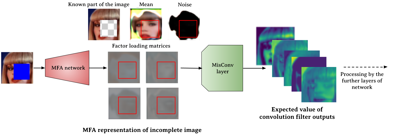
Figure 1: MisConv redefines the first convolutional layer of existing CNN to process incomplete images. First, it estimates a distribution of possible replacements for an incomplete image using a Mixture of Factor Analyzers. Next, the convolutional layer computes the expected value of the convolutional operator taken over the MFA distribution. This mechanism takes the uncertainty of imputation into account and can be implemented efficiently using matrix operations.

Convolutional neural networks (CNNs) present state-of-the-art performance on various image processing tasks, such as classification, segmentation, object detection [27, 24, 7]. Nevertheless, standard CNNs cannot directly process images, which contain missing regions. Since missing data are very common in medical diagnosis, self-driving vehicles or robots, and other computer vision applications, generalizing CNNs to this case is of great importance.

The typical strategy for using neural networks with incomplete images relies on replacing absent pixels with the most probable candidates in the initial stage [6, 28]. While imputation-based techniques can be combined with various machine learning models, they do not take into account the uncertainty of estimation. In particular, more than one replacement usually conforms to a given image, but only a single one is selected in the imputation stage. The use of such a hard decision may be destructive because important information about data distribution is lost during this process.

To overcome the aforementioned problems, many classical machine learning models, such as logistic regression or SVM, were adapted to learn from missing data directly [5, 9, 15]. They either ignore missing values or integrate the probability distribution of missing data to make a final prediction. Although these approaches do not substitute missing values with a single point estimate, the works on adapting neural networks, including CNNs, to the case of incomplete images are limited [48, 32].

In this paper, we propose a general mechanism, MisConv, for adapting CNN architectures to incomplete images. MisConv does not rely on a single imputation, but takes the uncertainty contained in missing pixels into account. Our idea is to model the probability distribution of missing values and calculate the expected value of the convolution operator taken over all possible replacements – see Figure 1 for the illustration. Making use of the modified Mixture of Factor Analyzers (MFA) [43, 40], we model the distribution of missing pixels with sufficient accuracy as well as we are able to find an analytical formula for the expected value of convolution. Although related approaches have been considered before for shallow models, such as logistic regression [55] and kernel methods [47], or fully connected neural networks [48], there are no works on applying similar ideas to CNNs.

MisConv can be applied to various CNN architectures and requires only a modification of the first convolutional layer. The whole framework is realized by matrix operations and classical convolutions. In consequence, the complexity of MisConv is comparable to typical CNNs operating on complete images. The proposed approach is experimentally verified on various image processing tasks, including image classification, reconstruction, and generation. We demonstrate that MisConv compares favorably with state-of-the-art techniques used for processing incomplete images, which confirms its practical usefulness.

Our contributions can be summarized as follows:

• We introduce a general mechanism for adapting CNNs to the case of incomplete data, which takes into account the uncertainty contained in missing values.

• We show that MisConv can be easily implemented using typical matrix operations, which makes it extremely efficient in practice.

• Experimental results demonstrate that MisConv can be successfully applied to various tasks and CNN architectures, achieving state-of-the-art performance.

2 Related work

Imputation-based techniques

One of the most common approaches for applying machine learning models to the case of missing data relies on completing absent attributes and next using a given model on complete inputs. Missing attributes may be replaced using simple statistical techniques, such as mean value or k-nn imputation [6], or by applying more advanced machine learning methods [45, 50]. Although iterative regression approaches [4, 1] are frequently used for small data, they are computationally too demanding for large high dimensional data such as images. The authors of [17] used denoising autoencoders for multiple imputations. It was shown that zero imputation can also obtain competitive results if only the rate of missingness is carefully taken into account. There are also many works that apply deep learning methods for image inpainting [30, 38, 58, 46], but they require complete data for training, which is in contradiction with many real data sets (such as medical ones).

Adaptation of shallow models

Replacing or deleting missing values is not always necessary when the task is to perform a prediction, e.g. classification, regression, etc. [23]. Given a rough estimation of missing data density by GMM (Gaussian mixture model) [13, 52], one can adapt logistic regression [55] or kernel methods [49, 54, 47, 34] to operate on incomplete data directly. The authors of [10, 31] estimated the parameters of the probability model and the classifier jointly. Decision function can also be learned based on the visible inputs alone [9, 15], see [5, 56] for SVM and random forest. The authors of [20] designed an algorithm for kernel classification under the low-rank assumption, while Goldberg et. al. [16] used matrix completion strategy to solve the missing data problem. Pelckmans et. al. [39] modeled the expected risk under the uncertainty of the predicted outputs. Khosravi et al. embedded logistic regression classifier by computing the expected prediction on a given feature distribution [25].

Adaptation of deep learning models

Partial convolution is a general technique that redefines convolutional layers in CNNs and deals with arbitrary missing patterns in images [32]. Danel et al. generalized GCNs (graph convolutional networks) to operate on incomplete images and show that this method works well on small images [8]. The authors of [14], proposed a trainable embedding of incomplete inputs, which can be used as an input layer to a given neural network. Mesquita et al. adapted neural networks with random weights to the case of incomplete data by estimating the weights of the output layer as a function of the uncertainty of the missing data [35]. The paper [2] used recurrent neural networks with feedback into the input units, which fills absent attributes for the sole purpose of minimizing a learning criterion. By applying the rough set theory, the authors of [36] presented a feedforward neural network that gives an imprecise answer as the result of input data imperfection. Goodfellow et. al. [18] introduced the multi-prediction deep Boltzmann machine, which is capable of solving different inference problems, including classification with missing inputs.

Many recent works focus on imputation strategies. Yoon et al. adapted conditional GANs to fill missing values [57]. In this approach, discriminator is trained to classify which components were observed and which have been imputed. Mattei and Frellsen introduced MIWAE technique, which allows for training autoencoders on missing data by approximating the maximum likelihood of only the observed portion of the data [33]. The authors of [29] proposed a flow-based model (ACFlow), which gives an explicit formula for a conditional density function of missing values.

Śmieja et al. defined a generalized neuron’s response, which computes the expected activation for missing data points, and applied this mechanism for fully connected networks [48]. However, this work ignores the case of CNNs and does not show how to compute the expected activation in this situation. Moreover, modeling high dimensional data, such as images, using Gaussian mixture models (GMMs) requires special attention. On the one hand, the number of parameters of Gaussian distribution with full covariance matrix grows quadratically with data dimension, while on the other hand, restricting to diagonal covariance is insufficient for modeling images [43]. In this paper, we show how to efficiently apply a similar probabilistic approach for CNNs and image data.

3 Convolutional layer for missing data

Model overview

We consider the problem of processing missing data by convolutional neural networks (CNNs). Typical CNNs can only process complete images, in which values of all pixels are known. For incomplete images, the convolutional operation is not defined and there appears a question of how to harness the power of CNNs in this case.

We tackle this problem using a probabilistic approach, where missing data is represented by probability distributions. Such a representation takes into account the uncertainty of missing data estimation, which is more reliable than using a single or multiple imputation. As a probabilistic model, we use a Gaussian density represented in the form of the Mixture of Factor Analyzers (MFA), which was successfully used to model image distributions [43]. Moreover, its Gaussian form allows for performing an analytical calculation on this random vector.

To process the probabilistic representation of missing data, we adapt the convolution operator. Here, we introduce a convolution that is a generalization of typical convolution, which computes the mean activation (expected value) taken over all possible replacements. Formally, if $\mathbf{Z}$ is a random vector representing incomplete image $\mathbf{x}$, $\mathbf{M}$ is linear convolution and $f$ is the activity function, our convolutional layer computes:

$$f(\mathbf{M}\mathbf{x}):=\mathbb{E}[f(\mathbf{M}\mathbf{Z})].$$

Since the expected value transforms random variables to numeric values, our convolution has to be applied only in the first layer. As a benefit, the rest of the architecture can be left unchanged, which is very important in practice, because typical neural networks can be directly reused in our framework.

Probabilistic representation of incomplete images

A missing data point is denoted by $\mathbf{x}=(\mathbf{x}_{o},\mathbf{x}_{m})\in\mathbb{R}^{n}$, where $\mathbf{x}_{o}\in\mathbb{R}^{d}$ represents pixels with known values, while $\mathbf{x}_{m}\in\mathbb{R}^{n-d}$ denotes absent pixels. The set of indices (pixels) with missing values at sample $\mathbf{x}$ is denoted $\mathcal{J}\subset\{1,\ldots,n\}$. Formally $\mathcal{J}=\mathcal{J}_{\mathbf{x}}$, which means that the missing pattern can be different for every instance $\mathbf{x}$, but we drop the subscript $\mathbf{x}$ to simplify notation.

To account for uncertainty contained in missing pixels, we employ a conditional probability distribution $p_{\mathbf{x}_{m}|\mathbf{x}_{o}}$. Making use of conditional density, we can cover a wider spectrum of possible replacements than using point estimates. While the conditional density $p_{\mathbf{x}_{m}|\mathbf{x}_{o}}$ is defined on $(n-d)$-th dimensional space, we make its natural extension to the whole $\mathbb{R}^{n}$ space, by putting

$$P_{\mathbf{x}_{m}|\mathbf{x}_{o}}(\mathbf{t})=\left\{\begin{array}[]{ll}p_{\mathbf{x}_{m}|\mathbf{x}_{o}}(\mathbf{t}_{\mathcal{J}^{\prime}}),&\text{ if }\mathbf{t}_{\mathcal{J}^{\prime}}=\mathbf{x}_{o},\\ 0,&\text{ otherwise},\end{array}\right.$$

where $\mathbf{t}_{\mathcal{J}^{\prime}}$ denotes the restriction of $\mathbf{t}\in\mathbb{R}^{n}$ to the observed pixels $\mathcal{J}^{\prime}=\{1,\ldots,n\}\setminus\mathcal{J}$.

As a parametric model of conditional density $p_{\mathbf{x}_{m}|\mathbf{x}_{o}}$, we select the Mixture of Factor Analyzers (MFA), a type of Gaussian mixture model (GMM) [12]. Let us recall that a single component of MFA, called Factor Analyzer (FA), has a Gaussian distribution with a covariance matrix spanned on a low dimensional space, which drastically reduces the number of model parameters. In particular, the memory and complexity of estimating MFA grow linearly with data dimension (not quadratically as in the standard GMM). Moreover, the Gaussian form of MFA allows us to perform analytical calculations on the conditional density. In the case of deep generative models, such as GANs [19], VAEs [26] or INFs [11], analytical calculation is difficult or even impossible and sampling remains as the only possible strategy. Finally, it was recently shown that MFA is competitive to simple versions of GANs in estimating a density of high dimensional data such as images [43]. Since we do not need sharp, realistic replacements, but only a rough estimation of possible values, MFA suits our needs perfectly.

Formally, a single Factor Analyzer (FA) defined in $\mathbb{R}^{n}$ is described by the mean vector $\bm{\mu}\in\mathbb{R}^{n}$ and the covariance matrix $\mathbf{\Sigma}=\mathbf{A}\mathbf{A}^{T}+\mathbf{D}$, where $\mathbf{A}_{n\times l}$ is a low rank factor loading matrix composed of $l$ vectors $\mathbf{a}_{1},\ldots,\mathbf{a}_{l}\in\mathbb{R}^{n}$, such that $l\ll n$, and $\mathbf{D}=\mathbf{D}_{n\times n}=\mathrm{diag}(\mathbf{d})$ is a diagonal matrix representing noise defined by $\mathbf{d}\in\mathbb{R}^{n}$. Formally, FA is modeled as a random vector defined by:

$$\mathbf{Z}=\bm{\mu}+\sqrt{\mathbf{d}}\odot\mathbf{X}+\sum_{j=1}^{l}Y_{j}\cdot\mathbf{a}_{j},$$ (1)

where $\mathbf{X}\sim N(0,\mathbf{I})$, $Y_{j}\sim N(0,1)$ are independent, $\sqrt{\mathbf{d}}$ denotes element-wise square root of vector $\mathbf{d}$, and $\mathbf{a}\odot\mathbf{b}$ stands for element-wise multiplication of vectors $\mathbf{a}$ and $\mathbf{b}$.

Linear transformation of missing data

We consider a random vector $\mathbf{Z}$ with MFA distribution $P_{\mathbf{Z}}$ representing a missing data point $\mathbf{x}=(\mathbf{x}_{o},\mathbf{x}_{m})$. The introduced convolutional layer allows us to transform a probabilistic MFA representation $\mathbf{Z}$ into a numeric output vector. Our idea is to calculate the expected value of the convolution applied to $\mathbf{Z}$. Below, we present an analytical formula for this transformation.

Let $\mathbf{M}$ be a linear convolution operator (without applying nonlinear activity function), which produces a random vector $\mathbf{M}\mathbf{Z}$ when applied to $\mathbf{Z}$. First, we show that if $\mathbf{Z}$ is a Factor Analyzer then $\mathbf{M}\mathbf{Z}$ is also a Factor Analyzer.

Theorem 3.1.

Let $\mathbf{Z}$ be a random vector with FA distribution defined by $\mathbf{Z}=\bm{\mu}+\sqrt{\mathbf{d}}\odot\mathbf{X}+\sum_{j=1}^{l}Y_{j}\cdot\mathbf{a}_{j}$. Then the random vector $\mathbf{M}\mathbf{Z}$ has Factor Analyzer distribution with mean and variance given by

$$\begin{array}[]{l}\mathbb{E}[\mathbf{M}\mathbf{Z}]=\mathbf{M}\bm{\mu}\\[3.44444pt] \mathbb{V}[\mathbf{M}\mathbf{Z}]=\mathrm{diag}(\mathbf{M}\mathbf{d})+\sum_{j=1}^{l}(\mathbf{M}\mathbf{a}_{j})\cdot(\mathbf{M}\mathbf{a}_{j})^{T}\end{array}$$ (2)

Proof.

Observe that $\mathbf{M}\mathbf{Z}$ produces Gaussian distribution, because $\mathbf{M}$ is a linear operator. Its parameters can be calculated as follows:

$$\begin{array}[]{ll}\mathbb{E}[\mathbf{M}\mathbf{Z}]&=\mathbf{M}\mathbb{E}[\mathbf{Z}]=\mathbf{M}\bm{\mu},\\[3.44444pt] \mathbb{V}[\mathbf{M}\mathbf{Z}]&=\mathbb{V}[\mathbf{M}(\sqrt{\mathbf{d}}.\mathbf{X})]+\sum_{j=1}^{l}\mathbb{V}[\mathbf{M}(Y_{j}\cdot\mathbf{a}_{j})]\\ &=\mathrm{diag}(\mathbf{M}\mathbf{d})+\sum_{j=1}^{l}\mathbb{V}[Y_{i}\cdot\mathbf{M}\mathbf{a}_{j}]\\[3.44444pt] &=\mathrm{diag}(\mathbf{M}\mathbf{d})+\sum_{j=1}^{l}(\mathbf{M}\mathbf{a}_{j})\cdot(\mathbf{M}\mathbf{a}_{j})^{T}.\end{array}$$

∎

If $\mathbf{Z}$ is the MFA then we need to apply the convolution operator to every component according to Theorem 3.1 (the mixture proportions remains the same).

Expected activation

The next step is the application of the activation function to every coordinate of the feature map produced by $\mathbf{M}\mathbf{Z}$. Thus, we ignore the correlations between coordinates and take into account only the elements on the diagonal of the covariance matrix. The diagonal of $\mathbf{M}\mathbf{Z}$ from Theorem 3.1 is given by:

$$\mathbf{M}\mathbf{d}+\sum_{j=1}^{l}(\mathbf{M}\mathbf{a}_{j})\odot(\mathbf{M}\mathbf{a}_{j}).$$ (3)

Due to the above marginalization, it is sufficient to consider 1-dimensional MFA representing the distribution of $\mathbf{M}\mathbf{Z}$ on each coordinate of the feature map. Since we deal with random vectors, we calculate the expected value of the activation function. We restrict our attention to ReLU activation because it is commonly used in CNNs.

Theorem 3.2.

Let $P=\sum_{i=1}^{k}p_{i}N(m_{i},\sigma_{i}^{2})$ be 1-dimensional Gaussian density. The expected value of ReLU applied to random variable with density $P$ equals:

$$\mathbb{E}[\mathrm{ReLU}(P)]=\\ \frac{1}{2}\sum_{i=1}^{k}p_{i}\left(m_{i}+\frac{\sigma_{i}}{2\sqrt{2\pi}}\exp(-\frac{m_{i}^{2}}{2\sigma_{i}^{2}})+m_{i}\cdot\mathrm{erf}(\frac{m_{i}}{\sigma_{i}\sqrt{2}})\right),$$ (4)

where $\mathrm{erf}(z)=\frac{2}{\sqrt{\pi}}\int_{0}^{z}\exp(-t^{2})dt$ is the error function.

Proof.

First, observe that:

$$\mathbb{E}[\mathrm{ReLU}(P)]=\int_{\mathbb{R}}\mathrm{ReLU}(x)\sum_{i}N(m_{i},\sigma_{i}^{2})(x)dx$$

$$=\sum_{i}p_{i}\int_{0}^{\infty}xN(m_{i},\sigma_{i}^{2})(x)dx.$$

Finally, the last integral can be calculated as follows:

$$\int_{0}^{\infty}xN(m,\sigma^{2})(x)dx=\\ \frac{1}{2}\left(m+\frac{\sigma}{2\sqrt{2\pi}}\exp(-\frac{m^{2}}{2\sigma^{2}})+m\cdot\mathrm{erf}(\frac{m}{\sigma\sqrt{2}})\right).$$

∎

Practical realization

MisConv allows us to efficiently adapt typical CNNs to the case of incomplete data by redefining the first hidden layer. The whole procedure is summarized in Algorithm 1.

Algorithm 1:  

1:  INPUT:

2:     $\mathbf{x}=(\mathbf{x}_{o},\mathbf{x}_{m})$ – incomplete image

3:  OUTPUT:

4:     $\mathrm{ReLU}(\mathbf{M}\mathbf{x}))$ – transformation of $\mathbf{x}$ by the 1st hidden layer

5:  1st HIDDEN LAYER

6:     Compute a density $F_{\mathbf{Z}}=\sum_{i=1}^{k}p_{i}N(\bm{\mu}_{i},\mathbf{A}_{i}^{T}\mathbf{A}_{i}+\mathrm{diag}(\mathbf{d}_{i}))$ of MFA representation $\mathbf{Z}$ of $\mathbf{x}$.

7:     Compute a distribution $F_{\mathbf{M}\mathbf{Z}}=\sum_{i=1}^{k}p_{i}N(\mathbf{m}_{i},\mathrm{diag}(\bm{\sigma}_{i}))$ of $\mathbf{M}\mathbf{Z}$ on every pixel where:

8:         $\mathbf{m}_{i}=(m_{i}^{1},\ldots,m_{i}^{n})=\mathbf{M}\bm{\mu}_{i}$

9:         $\bm{\sigma}_{i}=(\sigma_{i}^{1},\ldots,\sigma_{i}^{n})=\mathbf{M}\mathbf{d}+\sum_{j=1}^{l}(\mathbf{M}\mathbf{a}_{j})\odot(\mathbf{M}\mathbf{a}_{j})$

10:     Compute the expected ReLU activation of $\sum_{i=1}^{k}p_{i}N(m_{i}^{j},(\sigma_{i}^{j})^{2})$ on every pixel $j$ using (4)

 

As can be seen, MisConv can be implemented with the use of typical matrix operations and classical convolutions. The first layer applies a convolution operator $\mathbf{M}$ to the mean vector $\bm{\mu}$ of every FA as well as to each column of matrix $\mathbf{A}$ and noise vector $\mathbf{d}$ defining the covariance matrix. Since MisConv involves only the modification in the first layer, the remaining part of the CNN architecture can be left unchanged. We experimentally verify that the computational overhead introduced by this modification is small and has little effect on the overall network performance, see the supplementary materials.

Incomplete image $\mathbf{x}$ can be represented by MFA in two ways. One way is to estimate MFA from an incomplete data set and compute conditional MFA for every image $\mathbf{x}$ [43]. An alternative option relies on direct estimation of conditional MFA using density network [40, 3]. In the latter case, we construct a neural network that takes incomplete image $\mathbf{x}$ and returns the parameters of a conditional MFA. Such an inpainting network is trained using log-likelihood loss. Experimental evaluation, presented in the following section, demonstrates that this approach leads to better results, see Section 5.

4 Experiments

We evaluate MisConv on three machine learning problems: classification, image generation and image reconstruction.

Experimental setting

If not stated otherwise, every model is trained and tested on missing data. To generate missing regions, we remove a square patch covering 1/4 area of the image. The location of the patch is uniformly sampled for each example. In the supplementary materials, we also consider more challenging tasks, where larger portions of images are missing.

MisConv is parametrized by MFA, which builds a probabilistic representation of incomplete images. For this purpose, we use DMFA (Deep Mixture of Factor Analyzers) [41, 40] – a variant of density network [3], which returns the parameters of conditional FA for the incomplete image. It should be emphasized that in contrast to [40], our DMFA is also trained on missing data, see supplementary material for details.

As our main baseline, we consider Partial Convolution (PC) [32], where the convolution is masked and renormalized to be conditioned on only the valid pixels. To the best of our knowledge, it is the only publicly available method for adapting CNNs to the case of missing data. Additionally, we consider various imputation strategies, which modify input images, but leave CNN architecture unchanged:

• ACFlow: missing features are replaced with imputations produced by Arbitrary Conditional Flow [29]. This is a recent generative model, which allows for sampling from conditional distribution of missing values. In coherence with the authors of this method, we utilize ACFlow models trained on complete data (other models considered here, including MisConv, are trained only on incomplete data).

• zero: missing values are replaced with zeros.

• mask: the results of zero imputation is concatenated with a mask vector indicating missing pixels.

• k-NN: missing pixels are replaced with mean values of those pixels computed from the $k$ nearest training samples (we use $k=5$). Because of the computational complexity of k-NN, we use a random subset of 5000 training samples for finding neighbors.

We also report the performance of CNN trained and tested on complete datasets (no missing values), which is denoted by GT (ground-truth). For a comparison, we only considered methods with publicly available codebases suitable for processing of images and thus many methods described in the related work section [57, 33] have not been taken into account.

Image classification

For the classification task, we consider three popular datasets: MNIST, SVHN, and CIFAR-10. We use a classifier built from blocks of Convolution-ReLU-Batch-Normalization-Dropout layers [22], followed by two fully-connected layers with a ReLU nonlinearity between them. Detailed parameters of classifiers used for each dataset can be found in the supplemental material.

Classification accuracies reported in Table 1 clearly indicate that MisConv obtains better results than competitive methods. While the advantage of MisConv over second-best mask imputation on MNIST is small, the disproportion on SVHN is large. It is evident that recent methods, such as ACFlow and PC, are unstable and frequently give lower scores than MisConv and a simple zero imputation strategy.

In Table 2 we also report the accuracies achieved by testing the above classifiers on complete images (without missing values). Although most results are fairly similar on the simplest case of MNIST, experiments on more challenging SVHN and CIFAR10 datasets show that the classifier equipped with MisConv shows the strongest ability to adapt to the complete data.

Table 1: Classification accuracy when training and testing on incomplete images.

	MNIST	SVHN	CIFAR10
zero	0.910	0.679	0.709
mask	0.925	0.493	0.563
k-NN	0.875	0.523	0.660
PC	0.920	0.376	0.522
ACFlow	0.908	0.666	0.671
MisConv	0.931	0.757	0.722
GT	0.990	0.889	0.811

Table 2: Classification accuracy when training on incomplete images and testing on complete images.

	MNIST	SVHN	CIFAR10
zero	0.984	0.843	0.761
mask	0.986	0.827	0.752
k-NN	0.957	0.805	0.742
PC	0.987	0.759	0.731
ACFlow	0.983	0.845	0.746
MisConv	0.986	0.860	0.769
GT	0.990	0.889	0.811

Table 3: Frechet Inception Distance (FID) between true images and images generated by WAE (lower is better).

	MNIST	SVHN	CelebA
zero	9.72	21.97	56.62
mask	10.96	24.36	59.45
k-NN	9.46	19.90	61.48
PC	9.75	22.61	64.92
ACFlow	9.08	21.49	59.04
MisConv	9.60	19.53	56.60
GT	6.45	19.65	51.75

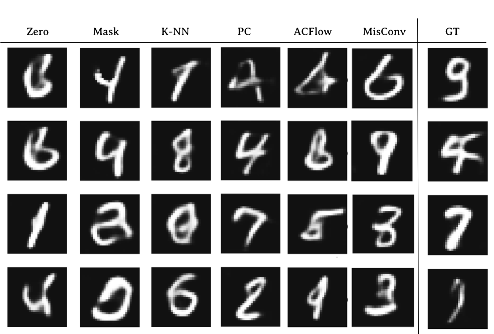
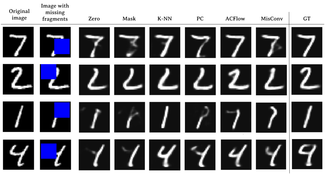
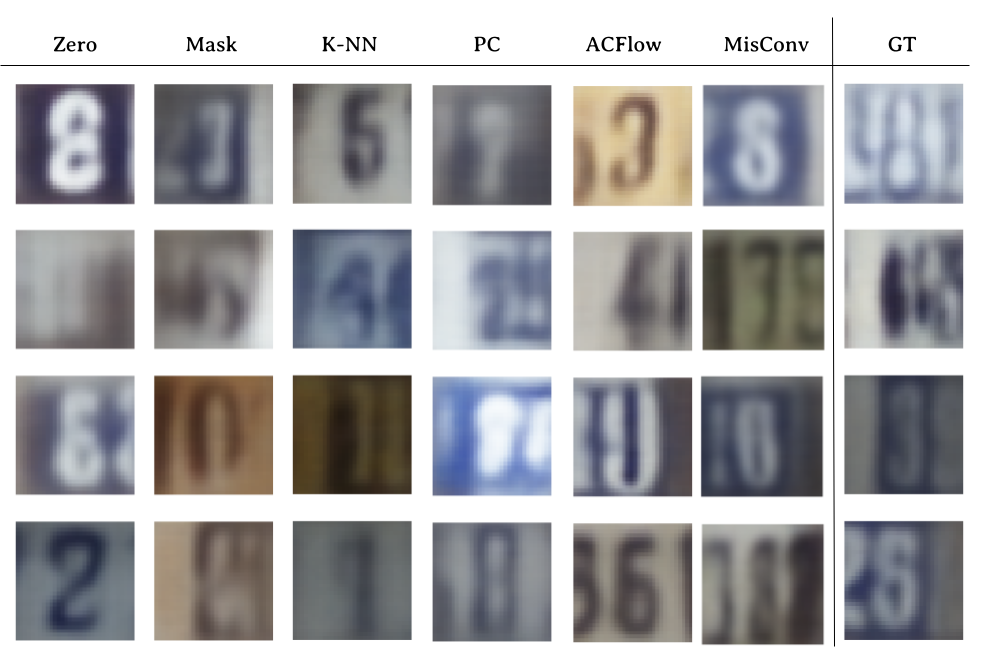
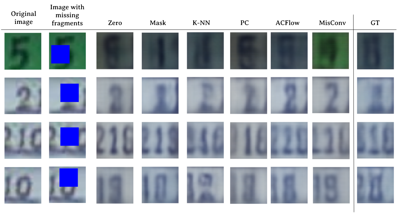
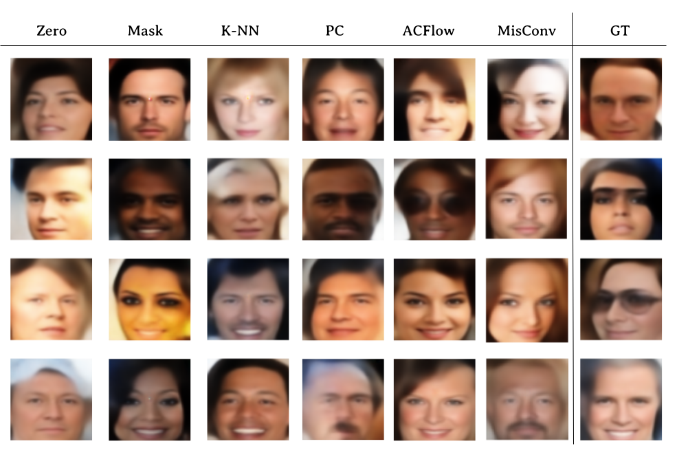
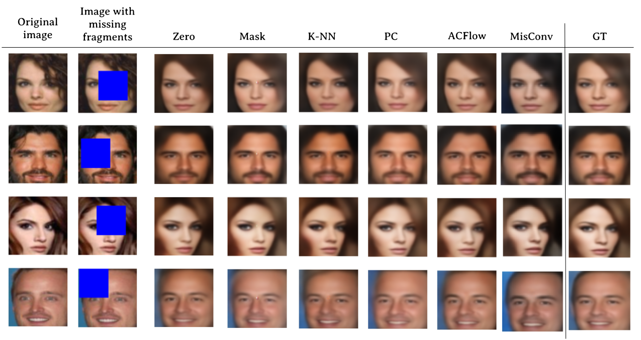
Figure 2: Samples (right) and reconstructions (left) produced by WAE models.

Table 4: Structural similarities (SSIM) between true and reconstructed images (higher is better).

	MNIST	SVHN	CelebA
zero	0.696	0.777	0.795
mask	0.658	0.775	0.802
k-NN	0.770	0.771	0.798
PC	0.662	0.774	0.786
ACFlow	0.628	0.787	0.805
MisConv	0.803	0.792	0.812
GT	0.944	0.811	0.832

Table 5: Peak signal-noise ratio (PSNR) between true and reconstructed images (higher is better).

	MNIST	SVHN	CelebA
zero	15.05	23.81	22.74
mask	14.26	23.64	22.94
k-NN	16.01	23.62	22.74
PC	14.15	23.74	22.64
ACFlow	14.91	24.09	23.14
MisConv	16.27	24.25	23.40
GT	21.48	24.70	24.02

Image generation

In the second experiment, we use Wasserstein Auto-Encoder (WAE) [51] for the image generation task. During training, the WAE reconstruction loss function is evaluated only on the observed pixels. We consider three datasets: MNIST, SVHN, and CelebA. In the case of CelebA dataset, we employ a common preprocessing step – cropping out the background part of the image and resizing the remaining part to the size of $64\times 64$. The models were assessed using Frechet Inception Distance (FID) [21, 44] calculated between the set of ground-truth images and images sampled from WAE models. Due to the large volatility of FID scores, we decided to report the best (lowest) value across the whole training process.

The architecture of the WAE decoder and encoder is based on the DCGAN network [42] – namely, the encoder and decoder are built from repeated blocks of Convolution-ReLU-Batch-Normalization layers, which gradually downsample and then upsample the feature maps. We use fully connected layers to map the encoded feature maps into the latent dimension and a fully connected network to discriminate between random samples and features of real images in the latent space. Details of the architectures can be found in the supplemental material.

As shown in Table 3, MisConv outperforms competitive methods on two more challenging datasets, SVHN and CelebA. In the case of SVHN, the FID score obtained by MisConv is even slightly better than the one of the original model trained on complete images. It means that MisConv is capable of producing images of similar quality to standard WAE. While ACFlow performs very well on MNIST, its performance drops significantly on other datasets. PC, our main baseline, again gives unsatisfactory results. For the illustration, we present sample images generated by WAE models, see Figure 2 (left).

Image reconstruction

To complement the previous experiment, we also benchmark MisConv in the task of image reconstruction. For this purpose, we use the same architecture and datasets as before and report structural similarity (SSIM) and peak signal-noise ratio (PSNR) between the ground-truth and reconstructed images [53].

As can be seen in Tables 4 and 5, MisConv obtained the best scores on all datasets in terms of both metrics. It is difficult to identify the second-best method because their performances vary across datasets. While k-NN performs quite well on MNIST, it is worse than ACFlow on SVHN and CelebA. In Figure 2 (right), we show sample reconstructions.

Table 6: Classification accuracy of MisConv using SMFA and DMFA.

	SMFA	DMFA
MNIST	0.922	0.931
SVHN	0.554	0.757
CIFAR-10	0.640	0.722

Table 7: Quality of SMFA and DMFA on SVHN dataset.

	NLL	MSE	PSNR	SSIM
SMFA	-1127.71	5.81	26.90	0.86
DMFA	-1584.08	5.34	30.14	0.94

5 Analysis of MisConv

In this section, we experimentally analyze MisConv. First, we examine the influence of MFA representation on the performance of MisConv. Next, we show that calculating the expected value of the convolution layer applied to MFA is essentially better strategy than using imputation taken from analogical MFA model. We restrict our attention to the classification problem.

MFA representation

MisConv relies on applying the expected value of the convolution operator applied to the MFA representation of the incomplete image. To investigate the influence of MFA parametrization, we consider its two variants. In the first one, the MFA is estimated from the whole dataset, and next its conditional distribution is calculated for each incomplete image. This classical approach, termed here SMFA (shallow MFA), was recently explored in [43]. In the second variant, conditional MFA is directly estimated for each incomplete image using density network [40]. The latter option, called DMFA (deep MFA), was used in the previous experiments.

As can be seen in Table 6, MisConv with DMFA is consistently better than with SMFA. To find the reason behind this behavior, we inspect both models regardless on MisConv (we restrict our attention to the SVHN dataset). Table 7 presents the Negative Log-Likelihood (NLL) and mean squared error (MSE) of the most probable imputation inferred by the DMFA and SMFA, as well as SSIM and PSNR between the original image and the image with missing pixels replaced by the imputation. Higher quality of DMFA results in a better description of missing values, which impacts the performance of MisConv.

Comparison with MFA imputation

There is a question whether taking the expected value in MisConv is a better strategy than using a single imputation from an analogical MFA model. To verify this aspect, we compare MisConv with typical CNN applied to the imputation produced by the MFA. It is evident from Table 8 that taking the whole distribution of missing values is more profitable than using only a point estimate.

We additionally compare the outputs of the initial classifier layer produced by those two variants, see Figure 3. It can be seen that MisConv is able to differentiate between the observed and missing pixels. This leads us to hypothesize that MisConv allows for processing the signal from the observed and missing regions with varying levels of trust, treating the latter with lower confidence.

Table 8: Comparing MisConv with MFA imputation in terms of classification accuracy.

	MFA imputation	MisConv
MNIST	0.923	0.931
SVHN	0.720	0.757
CIFAR-10	0.716	0.722

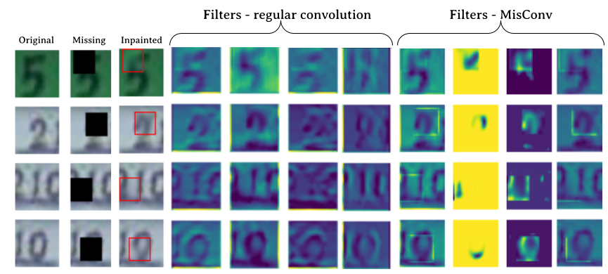
Figure 3: Outputs of the first convolutional layer for MFA imputaton and MisConv.

6 Conclusion

We have presented MisConv – a generalization of CNNs, capable of processing incomplete images. By taking the expected value over all possible replacements after the first convolutional layer, MisConv allows for exploring the uncertainty contained in missing pixels. Making use of MFA as the missing data representation, we were able to efficiently implement the whole framework using matrix operations without the need of sampling. Experimental results confirm that MisConv obtains better results across various tasks and datasets than the recent adaptation of CNNs to the case of missing data as well as typical imputation strategies.

Appendix A Experimental details

In this section, we describe in detail the architectures and hyperparameters of all models used in our experiments. We use the following notation:

• $conv_{n}$ - a convolution-ReLU-BatchNorm sequence with $n$ convolution filters

• $lin_{n}$ - a fully connected layer with $n$ output features followed by ReLU

• $down$ / $up$ - downsampling / upsampling convolution (with stride of 2), respectively:

• $drop_{p}$ - dropout layer with probability $p$

For simplicity, we omit the reshaping operations which take place between convolutions and fully connected layers.

A.1 Mixture of Factor Analyzers

In this section, we describe the implementation of Deep Mixture of Factor Analyzers (DMFA) and outline the architecture and hyperparameters used for each dataset. For additional information, we refer the reader to [41, 40].

MNIST

Following [40], we use DMFA which uses a small convolutional feature extractor and single fully-connected layers to make final predictions of each MFA parameter $(\mu,A,D)$. The extractor is a sequence of four convolution layers with ReLU activations, with 16, 32, 64 and 32 filters, respectively. The number of predicted factor analyzers is $l=4$. The DMFA is trained for 20 epochs, with a learning rate of $4*10^{-5}$ and a batch size of 48.

SVHN and CIFAR-10

Due to the increased dimentionality of those datasets, we use a fully convolutional variant of DMFA, which consists of a fully convolutional feature extractor composed of Convolution-ReLU-BatchNorm blocks [40], followed by a downsampling / upsampling convolution with a stride of 2. The network returns three heads that predict $(\mu,A,D)$. Thus the extractor consists of the following layers:

$$[conv_{32}]\times 2,down,[conv_{64}]\times 2,down,\\ [conv_{128}]\times 4,up,[conv_{64}]\times 2,up,[conv_{32}]\times 2$$

and parameter predictor heads consist of two convolutional layers with 16 filters with a ReLU nonlinearity and a BatchNorm layer between them.

The number of predicted factor analyzers is $l=4$. We train the DMFA for 100 epochs, with a batch size of 64 and a learning rate of $4*10^{-5}$ for the first 10 epochs and $1*10^{-5}$ afterwards. Similarly to [40] we note that a fully-convolutional DMFA trained by minimizing only the NLL loss finds it difficult to find a good mean vector $\mu$ of the returned density. We mitigate this by supplying the NLL loss with MSE for the first 10 epochs of training.

CelebA

For this dataset we use the same setup as in the case of SVHN / CIFAR-10 images, with two differences: a shorter training time - 50 epochs in total, as well as the size of the feature extractor, which is approximately two times bigger:

$$[conv_{32}]\times 4,down,[conv_{64}]\times 3,down,\\ [conv_{128}]\times 8,up,[conv_{64}]\times 4,up,[conv_{32}]\times 4$$

Training of DMFA on incomplete data

In general, the DMFA model is trained by hiding a portion $x_{m}$ of a sample $x$ from the model and minimizing the Negative Log-Likelihood of imputation of $x_{m}$ produced by the model. Since we work with incomplete images, we cannot evaluate the NLL on $x_{m}$, because we do not have access to complete ground-truth data. Thus we simulate incompleteness of the data by hiding the other part $x_{u}$ of each data sample $x$. Although the model produces imputations for both $x_{u}$ and $x_{m}$, only the NLL of imputation of $x_{u}\setminus x_{m}$ is minimized, because this is an artificially created missing region.

A.2 Image classifier

For image classification we use a model composed of similar Convolution-ReLU-BatchNorm sequences and downsampling convolutions as in the fully convolutional DMFA, followed by two fully connected layers with a ReLU nonlinearity between them.

MNIST and SVHN

We use an architecture of: $[conv_{32},down,[conv_{64}]\times 2,lin_{20},lin_{10}]$ and train the model with a batch size of 24 and a learning rate of $10^{-3}$ for 10 epochs in case of MNIST dataset and 25 epochs in case of SVHN dataset.

CIFAR-10

We use an architecture of: $[conv_{32},drop_{0.3}]\times 2,down,[conv_{64},drop_{0.3}]\times 3,lin_{128},drop_{0.3},lin_{10}]$ and train the model with a batch size of 64 and a learning rate of $10^{-4}$ for 35 epochs.

A.3 Wasserstein Autoencoder (WAE)

In accordance with [51], encoder and decoder sections of the WAE are fully convolutional, with a fully connected layer at the end of the encoder and the beginning of the encoder for transformation into and from the latent space, whereas the discriminator part of the network consists solely of fully connected layers with ReLU between them and a sigmoid layer at the end.

MNIST

Architecture:

• encoder: $conv_{32},conv_{40},down,conv_{80},down,lin_{20}$

• decoder: $lin_{3920},up,conv_{80},up,[conv_{40}]\times 2,conv_{1}$

• discriminator: $[lin_{64}]\times 4,lin_{1}$

We train the WAE for 20 epochs with a batch size of 128 and learning rate of $4*10^{-4}$ for encoder and decoder, and $4*10^{-6}$ for the discriminator.

SVHN

Architecture:

• encoder: $conv_{32},[conv_{96}]\times 2,down$,
  $[conv_{192}]\times 2,down,lin_{20}$

• decoder: $lin_{12288},up,[conv_{192}]\times 2,up$,
  $[conv_{96}]\times 3,conv_{3}$

• discriminator: $[lin_{64}]\times 4,lin_{1}$

We train the WAE for 50 epochs with a batch size of 64 and a learning rate of $4*10^{-4}$ for encoder and decoder, and $4*10^{-6}$ for the discriminator.

CelebA

Architecture:

• encoder: $conv_{32},[conv_{64}]\times 4$,
  $[conv_{128}]\times 4,[conv_{256}]\times 4,[conv{512}]\times 4,lin_{64}$

• decoder: $lin_{8192},[conv_{512}]\times 4$,
  $[conv_{256}]\times 4,[conv_{128}]\times 4,[conv_{64}]\times 5,conv_{3}$

• discriminator: $[lin_{512}]\times 4,lin_{1}$

We train the WAE for 50 epochs with a batch size of 16 and a learning rate of $10^{-4}$ for encoder and decoder, and $2.5*10^{-6}$ for the discriminator.

A.4 Implementation details

The models and experiments have been implemented using the PyTorch framework [37] and run on GeForce GTX 1080 and RTX 2080 NVIDIA GPUs. Every experiment described in this work is runnable on a single GPU.

The code implementing our technique is available publicly at https://github.com/mprzewie/dmfa_inpainting. The instructions on how to run the code are written in the README file included with the code.

In addition to our code, in this work we have used the following open-source implementations of baseline imputations: Partial Convolutions, SMFA, ACFlow and KNN.

Appendix B Other missing data tasks

Throughout the experiments, we used square missing regions which encompass 1/4 of their area. To benchmark the performance of MisConv on more diverse and difficult tasks, we also consider images where half of the image area was occluded with a trapezoid shape (trapezoid), as well as images with 3/4 of pixels randomly removed (noise) – see Figure 4. Although the missing regions have different shape, we consequently trained the DMFA by simulating additional missing parts with square shape.

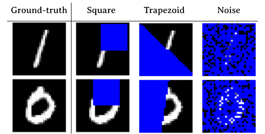
Figure 4: Examples of MNIST images with missing data simulated with square, trapezoid and noise techniques.

Table 9: Classification accuracy when testing on various kinds of incomplete MNIST datasets.

	square	trapezoid	noise
zero	0.91	0.891	0.946
mask	0.926	0.905	0.703
k-NN	0.874	0.854	0.912
PC	0.920	0.674	0.804
ACFlow	0.908	0.799	0.788
MisConv	0.931	0.918	0.966
GT	0.992	0.992	0.992

As shown in Table 9, MisConv achieves the best accuracy on all variants of missing data. The above results show promise that MisConv can be leveraged to handle various kinds of missing data problems, even when the percentage of missing data is large.

Appendix C Computational overhead introduced by using MisConv

When computing the expected activation of the convolution based on the MFA representation of the missing data ($\mathbf{\mu,A,d}$), $\mathbf{M}$ must also be applied to $\mathbf{x}$, $\mathbf{\mu}$, $\mathbf{d}$, as well as each of the $l$ vectors $\mathbf{a_{1},...,a_{l}}$ of which $\mathbf{A}$ is composed. In consequence, there the total of $3+l$ vectors are processed by $\mathbf{M}$, which introduces a computational overhead compared with classical convolutions. Since in practice $l$ is usually small, the effective increase in processing time is insignificant.

We demonstrate this by measuring the time it takes to perform a forward pass of missing data through a classical convolutional layer and through MisConv. As in all the above experiments, we select $l=4$, which should lead to approximately quadrupled time of a forward pass. We check the time of a forward pass for images of sizes $28\times 28$ (as in the MNIST dataset), $32\times 32$ (as in the SVHN and CIFAR-10 datasets) and $64\times 64$ (as in the CelebA dataset), with batch sizes of 16, 32 and 64. For each such setting, we make 5000 measurements of the time of a forward pass of a batch and report the results in Table 10 and Figure 5. It can be seen that in all cases, the overhead introduced by MisConv indeed increases the processing time approximately by a factor of 4. However, the order of magnitude of this increase is milliseconds. It should also be stressed that this overhead affects only the initial convolutional layer in the entire target neural network, which often consists of tens or even hundreds of layers. MisConv is therefore very efficient in practice, because it introduces a small computational overhead only in the initial layer of the entire neural network.

				Layer type
Datasets	I	M	B	Classic convolution	MisConv
MNIST	28	14	16	0.00016 ± 0.00006	0.00092 ± 0.00030
			32	0.00017 ± 0.00006	0.00097 ± 0.00041
			64	0.00020 ± 0.00008	0.00138 ± 0.00061
SVHN, CIFAR-10	32	16	16	0.00022 ± 0.00012	0.00109 ± 0.00039
			32	0.00037 ± 0.00020	0.00111 ± 0.00046
			64	0.00034 ± 0.00016	0.00121 ± 0.00047
CelebA	64	32	16	0.00034 ± 0.00017	0.00091 ± 0.00025
			32	0.00031 ± 0.00012	0.00115 ± 0.00037
			64	0.00029 ± 0.00008	0.00109 ± 0.00029

Table 10: Time of a forward-pass through a classical convolutional layer and MisConv layer, measured for different image sizes (denoted in the I column) with their respective sizes of missing data squares (denoted in the M column) and different batch sizes (denoted in the B column).

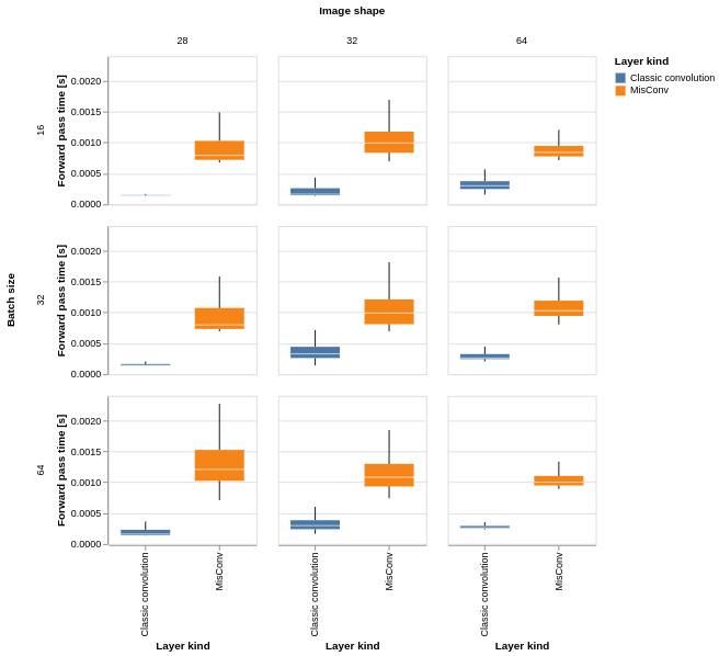
Figure 5: Time of a forward-pass through a classical convolutional layer and MisConv layer, measured for different image sizes in a form of boxplots.

References

- [1] Melissa J Azur, Elizabeth A Stuart, Constantine Frangakis, and Philip J Leaf. Multiple imputation by chained equations: what is it and how does it work? International journal of methods in psychiatric research, 20(1):40–49, 2011.
- [2] Yoshua Bengio and Francois Gingras. Recurrent neural networks for missing or asynchronous data. In Advances in neural information processing systems, pages 395–401, 1996.
- [3] Christopher M Bishop. Mixture density networks. 1994.
- [4] Stef Buuren and Karin Groothuis-Oudshoorn. mice: Multivariate imputation by chained equations in r. Journal of statistical software, 45(3), 2011.
- [5] Gal Chechik, Geremy Heitz, Gal Elidan, Pieter Abbeel, and Daphne Koller. Max-margin classification of data with absent features. Journal of Machine Learning Research, 9:1–21, 2008.
- [6] Ching-Hsue Cheng, Chia-Pang Chan, and Yu-Jheng Sheu. A novel purity-based k nearest neighbors imputation method and its application in financial distress prediction. Engineering Applications of Artificial Intelligence, 81:283–299, 2019.
- [7] Dan Claudiu Ciresan, Ueli Meier, Jonathan Masci, Luca Maria Gambardella, and Jürgen Schmidhuber. Flexible, high performance convolutional neural networks for image classification. In Twenty-Second International Joint Conference on Artificial Intelligence, 2011.
- [8] Tomasz Danel, Marek Śmieja, Łukasz Struski, Przemysław Spurek, and Łukasz Maziarka. Processing of incomplete images by (graph) convolutional neural networks. In International Conference on Neural Information Processing, pages 512–523. Springer, 2020.
- [9] Ofer Dekel, Ohad Shamir, and Lin Xiao. Learning to classify with missing and corrupted features. Machine Learning, 81(2):149–178, 2010.
- [10] Uwe Dick, Peter Haider, and Tobias Scheffer. Learning from incomplete data with infinite imputations. In Proceedings of the International Conference on Machine Learning, pages 232–239. ACM, 2008.
- [11] Laurent Dinh, David Krueger, and Yoshua Bengio. Nice: Non-linear independent components estimation. arXiv preprint arXiv:1410.8516, 2014.
- [12] Zoubin Ghahramani, Geoffrey E Hinton, et al. The em algorithm for mixtures of factor analyzers. Technical report, Technical Report CRG-TR-96-1, University of Toronto, 1996.
- [13] Zoubin Ghahramani and Michael I Jordan. Supervised learning from incomplete data via an EM approach. In Advances in Neural Information Processing Systems, pages 120–127. Citeseer, 1994.
- [14] Amirata Ghorbani and James Y Zou. Embedding for informative missingness: Deep learning with incomplete data. In 2018 56th Annual Allerton Conference on Communication, Control, and Computing (Allerton), pages 437–445. IEEE, 2018.
- [15] Amir Globerson and Sam Roweis. Nightmare at test time: robust learning by feature deletion. In Proceedings of the International Conference on Machine Learning, pages 353–360. ACM, 2006.
- [16] Andrew Goldberg, Ben Recht, Junming Xu, Robert Nowak, and Xiaojin Zhu. Transduction with matrix completion: Three birds with one stone. In Advances in neural information processing systems, pages 757–765, 2010.
- [17] Lovedeep Gondara and Ke Wang. Multiple imputation using deep denoising autoencoders. arXiv preprint arXiv:1705.02737, 2017.
- [18] Ian Goodfellow, Mehdi Mirza, Aaron Courville, and Yoshua Bengio. Multi-prediction deep boltzmann machines. In Advances in Neural Information Processing Systems, pages 548–556, 2013.
- [19] I. Goodfellow, J. Pouget-Abadie, M. Mirza, B. Xu, D. Warde-Farley, S. Ozair, A. Courville, , and Y. Bengio. Generative adversarial nets. In Advances in Neural Information Processing Systems, pages 2672–2680, 2014.
- [20] Elad Hazan, Roi Livni, and Yishay Mansour. Classification with low rank and missing data. In Proceedings of The 32nd International Conference on Machine Learning, pages 257–266, 2015.
- [21] Martin Heusel, Hubert Ramsauer, Thomas Unterthiner, Bernhard Nessler, Günter Klambauer, and Sepp Hochreiter. Gans trained by a two time-scale update rule converge to a nash equilibrium. CoRR, abs/1706.08500, 2017.
- [22] Sergey Ioffe and Christian Szegedy. Batch normalization: Accelerating deep network training by reducing internal covariate shift. In Proceedings of the 32nd International Conference on International Conference on Machine Learning - Volume 37, ICML’15, page 448–456. JMLR.org, 2015.
- [23] Niels Ipsen, Pierre-Alexandre Mattei, and Jes Frellsen. How to deal with missing data in supervised deep learning? In ICML Workshop on the Art of Learning with Missing Values (Artemiss), 2020.
- [24] Andrej Karpathy, George Toderici, Sanketh Shetty, Thomas Leung, Rahul Sukthankar, and Li Fei-Fei. Large-scale video classification with convolutional neural networks. In Proceedings of the IEEE conference on Computer Vision and Pattern Recognition, pages 1725–1732, 2014.
- [25] Pasha Khosravi, Yitao Liang, YooJung Choi, and Guy Van den Broeck. What to expect of classifiers? reasoning about logistic regression with missing features. arXiv preprint arXiv:1903.01620, 2019.
- [26] D. Kingma and M. Welling. Auto-encoding variational Bayes. In International Conference on Learning Representations, 2014.
- [27] Alex Krizhevsky, Ilya Sutskever, and Geoffrey E Hinton. Imagenet classification with deep convolutional neural networks. In Advances in neural information processing systems, pages 1097–1105, 2012.
- [28] Steven Cheng-Xian Li, Bo Jiang, and Benjamin Marlin. Misgan: Learning from incomplete data with generative adversarial networks. arXiv preprint arXiv:1902.09599, 2019.
- [29] Yang Li, Shoaib Akbar, and Junier B. Oliva. Flow models for arbitrary conditional likelihoods. CoRR, abs/1909.06319, 2019.
- [30] Yijun Li, Sifei Liu, Jimei Yang, and Ming-Hsuan Yang. Generative face completion. In Proceedings of the IEEE Conference on Computer Vision and Pattern Recognition, pages 3911–3919, 2017.
- [31] Xuejun Liao, Hui Li, and Lawrence Carin. Quadratically gated mixture of experts for incomplete data classification. In Proceedings of the International Conference on Machine Learning, pages 553–560. ACM, 2007.
- [32] Guilin Liu, Fitsum A. Reda, Kevin J. Shih, Ting-Chun Wang, Andrew Tao, and Bryan Catanzaro. Image inpainting for irregular holes using partial convolutions. In The European Conference on Computer Vision (ECCV), 2018.
- [33] Pierre-Alexandre Mattei and Jes Frellsen. Miwae: Deep generative modelling and imputation of incomplete data sets. In International Conference on Machine Learning, pages 4413–4423, 2019.
- [34] Diego PP Mesquita, João PP Gomes, Francesco Corona, Amauri H Souza Junior, and Juvêncio S Nobre. Gaussian kernels for incomplete data. Applied Soft Computing, 77:356–365, 2019.
- [35] Diego PP Mesquita, João Paulo P Gomes, and Leonardo R Rodrigues. Artificial neural networks with random weights for incomplete datasets. Neural Processing Letters, pages 1–28, 2019.
- [36] Robert K Nowicki, Rafal Scherer, and Leszek Rutkowski. Novel rough neural network for classification with missing data. In Methods and Models in Automation and Robotics (MMAR), 2016 21st International Conference on, pages 820–825. IEEE, 2016.
- [37] Adam Paszke, Sam Gross, Francisco Massa, Adam Lerer, James Bradbury, Gregory Chanan, Trevor Killeen, Zeming Lin, Natalia Gimelshein, Luca Antiga, Alban Desmaison, Andreas Kopf, Edward Yang, Zachary DeVito, Martin Raison, Alykhan Tejani, Sasank Chilamkurthy, Benoit Steiner, Lu Fang, Junjie Bai, and Soumith Chintala. Pytorch: An imperative style, high-performance deep learning library. In H. Wallach, H. Larochelle, A. Beygelzimer, F. d'Alché-Buc, E. Fox, and R. Garnett, editors, Advances in Neural Information Processing Systems 32, pages 8024–8035. Curran Associates, Inc., 2019.
- [38] Deepak Pathak, Philipp Krahenbuhl, Jeff Donahue, Trevor Darrell, and Alexei A Efros. Context encoders: Feature learning by inpainting. In Proceedings of the IEEE Conference on Computer Vision and Pattern Recognition, pages 2536–2544, 2016.
- [39] Kristiaan Pelckmans, Jos De Brabanter, Johan AK Suykens, and Bart De Moor. Handling missing values in support vector machine classifiers. Neural Networks, 18(5):684–692, 2005.
- [40] Marcin Przewięźlikowski, Marek Śmieja, and Łukasz Struski. Estimating conditional density of missing values using deep gaussian mixture model. In Haiqin Yang, Kitsuchart Pasupa, Andrew Chi-Sing Leung, James T. Kwok, Jonathan H. Chan, and Irwin King, editors, Neural Information Processing, pages 220–231, Cham, 2020. Springer International Publishing.
- [41] Marcin Przewięźlikowski, Marek Śmieja, and Łukasz Struski. Estimating conditional density of missing values using deep gaussian mixture model. In ICML Workshop on The Art of Learning with Missing Values (Artemiss), page 7, 2020.
- [42] Alec Radford, Luke Metz, and Soumith Chintala. Unsupervised representation learning with deep convolutional generative adversarial networks. arXiv preprint arXiv:1511.06434, 2015.
- [43] Eitan Richardson and Yair Weiss. On gans and gmms. In Advances in Neural Information Processing Systems, pages 5847–5858, 2018.
- [44] Maximilian Seitzer. pytorch-fid: FID Score for PyTorch. https://github.com/mseitzer/pytorch-fid, August 2020. Version 0.1.1.
- [45] Peter K Sharpe and RJ Solly. Dealing with missing values in neural network-based diagnostic systems. Neural Computing & Applications, 3(2):73–77, 1995.
- [46] Marek Śmieja, Maciej Kołomycki, Łukasz Struski, Mateusz Juda, and Mário AT Figueiredo. Iterative imputation of missing data using auto-encoder dynamics. In International Conference on Neural Information Processing, pages 258–269. Springer, 2020.
- [47] Marek Śmieja, Łukasz Struski, Jacek Tabor, and Mateusz Marzec. Generalized rbf kernel for incomplete data. Knowledge-Based Systems, 2019.
- [48] Marek Śmieja, Łukasz Struski, Jacek Tabor, Bartosz Zieliński, and Przemysław Spurek. Processing of missing data by neural networks. In Advances in Neural Information Processing Systems, pages 2719–2729, 2018.
- [49] Alexander J Smola, SVN Vishwanathan, and Thomas Hofmann. Kernel methods for missing variables. In Proceedings of the International Conference on Artificial Intelligence and Statistics. Citeseer, 2005.
- [50] Dušan Sovilj, Emil Eirola, Yoan Miche, Kaj-Mikael Björk, Rui Nian, Anton Akusok, and Amaury Lendasse. Extreme learning machine for missing data using multiple imputations. Neurocomputing, 174:220–231, 2016.
- [51] I. Tolstikhin, O. Bousquet, S. Gelly, and B. Schölkopf. Wasserstein auto-encoders. arXiv:1711.01558, 2017.
- [52] Volker Tresp, Subutai Ahmad, and Ralph Neuneier. Training neural networks with deficient data. In Advances in neural information processing systems, pages 128–135, 1994.
- [53] Zhou Wang, A.C. Bovik, H.R. Sheikh, and E.P. Simoncelli. Image quality assessment: from error visibility to structural similarity. IEEE Transactions on Image Processing, 13(4):600–612, 2004.
- [54] David Williams and Lawrence Carin. Analytical kernel matrix completion with incomplete multi-view data. In Proceedings of the ICML Workshop on Learning With Multiple Views, 2005.
- [55] David Williams, Xuejun Liao, Ya Xue, and Lawrence Carin. Incomplete-data classification using logistic regression. In Proceedings of the International Conference on Machine Learning, pages 972–979. ACM, 2005.
- [56] Jing Xia, Shengyu Zhang, Guolong Cai, Li Li, Qing Pan, Jing Yan, and Gangmin Ning. Adjusted weight voting algorithm for random forests in handling missing values. Pattern Recognition, 69:52–60, 2017.
- [57] Jinsung Yoon, James Jordon, and Mihaela van der Schaar. Gain: Missing data imputation using generative adversarial nets. pages 5689–5698, 2018.
- [58] Jiahui Yu, Zhe Lin, Jimei Yang, Xiaohui Shen, Xin Lu, and Thomas S Huang. Generative image inpainting with contextual attention. In IEEE Conference on Computer Vision and Pattern Recognition, pages 5505–5514, 2018.