Using the Climate App to learn about
Planetary Habitability and Climate Change

Abstract

Simple climate models have been around for more than a century but have recently come back into fashion: they are useful for explaining global warming and the habitability of extrasolar planets. The Climate App (www.climateapp.ca) is an interactive web-based application that describes the radiative transfer governing planetary climate. The App is currently available in French and English and is suitable for teaching high-school through college students, or public outreach. The beginner version can be used to explore the greenhouse effect and planetary albedo, sufficient for explaining anthropogenic climate change, the Faint Young Sun Paradox, the habitability of TRAPPIST planets and other simple scenarios. There is also an advanced option with more atmospheric layers and incorporating the absorption and scattering of shortwave radiation for students and educators wishing a deeper dive into atmospheric radiative transfer. A number of pedagogical activities are being beta tested and rolled out.

1 Introduction

Global warming has become a matter of increasing concern in recent decades [1, 2]. In parallel, astronomers have discovered thousands of exoplanets with varied atmospheres, some of which could harbour life. Despite tremendous public and academic interest in both topics, it is not widely appreciated that the same 19^th century atmospheric physics governing anthropogenic climate change also governs planetary habitability [3, 4].

A visually intuitive and interactive way to convey the concepts of albedo and the greenhouse effect can be useful for students, educators and the public, e.g., [5, 6]. This motivated the web-based Climate App, which serves as a tool to explore the roles that atmospheric absorption and emission play in planetary climate. We introduce each component of the Climate App in Section 2 and explain the underlying physical concepts and mathematical model in Section 3.

2 The User Interface

The Climate App is a single-page web application written in HTML5, javascript and CSS using React.js v16.5.1 so it works on a computer, tablet or smartphone. The app is currently available in French and English. You can change between the beginner and advanced version using the switch below the title. The two versions differ in the complexity of their underlying atmospheric models, and consequently have different number of adjustable parameters (sliders). As shown in Figure 1, the user interface consists of a control panel and a graphical panel that changes in real time as the parameters are adjusted.

2.1 The Trenberth Diagram

The graphical panel of the Climate App is a visual representation of the energy flows controlling the planet’s climate. The pale blue swath above the planet’s surface represents the atmosphere. The yellow arrows show shortwave radiation from the star, roughly corresponding to visible light for the Sun. The red arrows represent longwave thermal emission, typically infrared, from the planetary surface and atmosphere. The width of each arrow is proportional to the importance of that energy flow as compared to the amount of starlight that reaches the planet. This sort of schematic showing energy flows in a planet’s atmosphere is sometimes called a Trenberth Diagram and are commonplace in climate studies of Earth and other worlds [7, 8, 9].

Moving the sliders in the control panel changes the planetary parameters and hence the way that energy flows in and out of the atmosphere, which is ultimately what governs the surface temperature. Temperatures are reported in Celsius for the beginner version and Kelvin for the advanced version. The beginner version of the app also reports the magnitude of the greenhouse effect in degrees Celsius; this is the difference between the surface temperature and the value it would take if the infrared opacity of the atmosphere were zero. The default values of the sliders when you open the Climate App, both the beginner and advanced versions, are approximately the average values for modern-day Earth.

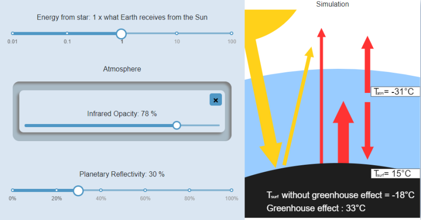
Figure 1: Screenshot of the Beginner version of the Climate App.

2.2 The Sliders

The control panel on the left lets you vary the planet’s properties and hence its climate with the corresponding sliders. Three properties are common to both versions while two extra properties are present exclusively in the Advanced version.

Energy from Star (Stellar Radiation in Advanced App)
Also known as “instellation”, this slider controls the amount of starlight that reaches the top of the planet’s atmosphere. For planets in the Solar System, the star in question is none other than the Sun! Incident starlight is the most important factor determining a planet’s climate. For convenience, the Climate App expresses the instellation in terms of the solar constant, the average flux that the Earth receives from the Sun (341 W/m²). For example, a value of 10 on this slider would mean that the planet receives ten times the amount of stellar radiation that we receive on Earth. The slider is a logarithmic scale, which allows for values a hundred times smaller or greater than the solar constant.

Planetary Reflectivity (Surface Albedo in Advanced App)
This slider controls the surface reflectivity of the planet. A value of 0 means the planet is perfectly black and absorbs all incoming stellar radiation; there are many planets close to this limit. No planet, on the other hand, reflects all incoming radiation, so the Climate App restricts the albedo to values less than 99%.

Albedo and instellation determine how much energy the planet absorbs every second and hence how much energy it must radiate away every second in order to remain in radiative equilibrium. Although this energy balance is only approximate from one second to another, it must be maintained on timescales of years.

In the advanced app, starlight can also be reflected back to space by the atmospheric layer(s) so the top-of-atmosphere effective albedo is reported in the Trenberth diagram. The effective albedo can be greater than or less than the underlying surface albedo, depending on the shortwave properties of the atmosphere.

The default value for the planetary reflectivity in the beginner app is 30%, while in the advanced app the surface albedo is 18% and the effective albedo—accounting for scattering by the atmosphere—is 30%. The Earth’s albedo is approximately 30%, largely due to clouds. When this slider is moved, the planet in the simulation canvas change shade.

Atmosphere (Atmospheric Layers in Advanced App)
This box contains properties that are specific to the planetary atmosphere. In the beginner version, the atmosphere is treated as a single layer (Figure 1). You may remove the atmosphere by clicking the $\times$ and add it back by clicking on a + box that only appears when your planet does not have an atmosphere.

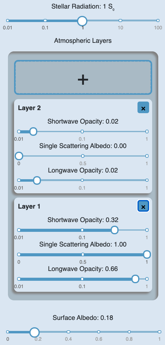
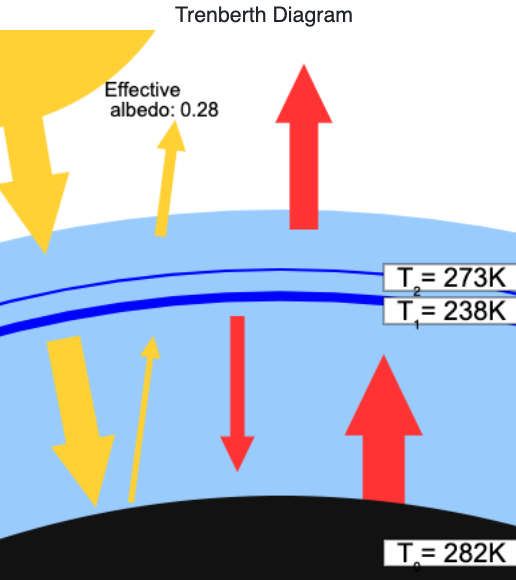
Figure 2: Screenshot of the Advanced version of the Climate App, as it appears on a smartphone.

For the advanced version (Figure 2), a maximum of three atmospheric layers are allowed and each can be assigned different properties. This simulates vertical changes in atmospheric properties, e.g., Earth’s atmosphere has more water vapour in the lower, warmer layers compared to the higher and colder layers. In this case, it is more realistic to assign greater infrared opacity to lower layers instead of setting one single value representing the whole atmosphere. You can click on the + box to add a new layer, and the $\times$ on a layer to remove it.

Infrared Opacity (Longwave Emissivity in Adv. App)
Each atmospheric layer has an adjustable longwave emissivity, its effectiveness in absorbing and emitting thermal radiation. A value of 1 absorbs all infrared radiation that hits it and re-radiates that energy equally up and down. This value depends on the greenhouse gases (GHG) in the atmosphere: for small levels of GHG the infrared opacity increases linearly with gas abundance, but once absorption lines are saturated—as they are on Earth—opacity increases more slowly.

Shortwave Opacity (only in Advanced app)
As shortwave radiation encounters an atmospheric layer, the photons may pass through without interaction, be absorbed, or be scattered by molecules and aerosols in the atmosphere. This slider determines the fraction of shortwave radiation interacting with the corresponding layer (absorbed or scattered). A value of 1 means that all of the shortwave photons are either absorbed or scattered by that atmospheric layer.

Single Scattering Albedo (only in Advanced app)
Single scattering albedo refers to the fraction of interacting shortwave photons that are scattered rather than absorbed. For example, a value of 0.1 indicates that out of all the shortwave photons having interacted with the atmosphere, 10% are scattered, while the remaining 90% are absorbed. The Climate App assumes isotropic scattering, so half of the scattered photons keep going in their original direction of travel, while the other half are back-scattered from whence they came.

3 The Underlying Physics

3.1 Key Concepts

The Climate App is built upon atmospheric physics that have been known since the late 19^th century[4]. The following key concepts are essential for users or students who wish to dive deeper into the model derivation.

3.1.1 Shortwave and Longwave Radiation

All objects emit radiation, whether you can see it or not. The colour-dependence of this so-called blackbody radiation is quantitatively described by Planck’s Law. Hot objects like the Sun emit most of their light at visible wavelengths (the range of light that human eye can see, not coincidentally). Somewhat cooler objects like planets and people tend to emit most of their radiation at longer infrared wavelengths (beyond the red end of the rainbow). Since visible and thermal light interact with the planetary surface and atmosphere in qualitatively different ways, it is customary in climate science to distinguish between the shortwave radiation received from a star and longwave radiation emitted by the planet (among experts, this is known as the two band approximation). In the Climate App visualizations, shortwave light is denoted by yellow arrows, while thermal radiation is denoted by red arrows.

3.1.2 The Stefan-Boltzmann Law

The Stefan-Boltzmann law quantifies the relation between the temperature and total emitted flux (at all wavelengths) for a perfectly absorbing and emitting object, a so-called blackbody: $F_{\rm bb}=\sigma T^{4}$, where $F_{\rm bb}$ is the emitted flux (units of W/m²), $T$ is the temperature of the object in Kelvin, and $\sigma$ is the Stefan-Boltzmann constant: $\sigma=5.67\times 10^{-8}$ W m^-2 K^-4.

Real materials are not perfect blackbodies: they do not perfectly absorb and radiate. Since the surface and atmosphere of a planet emit at longer, thermal wavelengths, we quantify the ability of an object to radiate by its longwave emissivity, $\epsilon_{\rm LW}$. The flux emitted by an element of the climate system is therefore given by $F=\epsilon_{\rm LW}\sigma T^{4}$. The surface emits this amount of radiation upwards, while an atmospheric layer emits this amount of radiation upwards and the same amount downwards.

3.1.3 Kirchhoff’s Law of Thermal Radiation

Kirchhoff’s law of thermal radiation dictates that a material’s ability to emit radiation at some wavelength is equal to its ability to absorb radiation at that same wavelength. For example, gases that readily absorb infrared light—so-called greenhouse gases—must also emit well at those same wavelengths.

Solid and liquid surfaces clearly do not absorb all of the light that hits them (otherwise they would appear perfectly black!). Indeed, the surface reflectance (or albedo) slider in the Climate App controls the fraction of visible light that the planetary surface reflects. These same materials, however, are very close to being perfect blackbodies in the thermal infrared. They all have $\epsilon_{\rm LW}\approx 1$. To very good approximation, we therefore adopt $\epsilon_{\rm LW}\equiv 1$ for the planetary surface in the Climate App.

A planet’s atmosphere, on the other hand, can have an infrared emissivity anywhere between zero to one ($0\leq\epsilon_{\rm LW}\leq 1$), depending on the presence of greenhouse gases; this is precisely what the Longwave Opacity slider controls (Infrared Opacity in the beginner version). In the beginner version the atmosphere cannot absorb shortwave radiation, so if the longwave emissivity is set to zero then the atmosphere simply cannot absorb any energy and its temperature is ill-defined and we remove the atmospheric temperature label.

In the beginner version of the app we assume that shortwave radiation does not interact with the atmosphere ($\epsilon_{\rm SW}\equiv 0$). This is approximately correct for planets like Earth and Mars, where most Sunlight indeed makes it down to the surface of the planet, but is utterly inadequate for Venus or Titan. Such thick atmospheres require the Advanced Climate App, which allows for the absorption or scattering of shortwave radiation ($0<\epsilon_{\rm SW}\leq 1$).

3.1.4 Radiative Equilibrium

A planet must radiate as much energy to space as it absorbs from its star, at least on average. Moreover, if radiation is the only way to move energy around in a climate system, then the total absorbed and emitted flux must be equal for each component of the climate system (atmospheric layer or planetary surface). To understand why this equilibrium arises, imagine a patch of ground that absorbs more energy than it emits: it will warm up and hence radiate away more heat following the Stefan-Boltzmann Law, finding a new, warmer, equilibrium. Conversely, a region that radiates more energy than it absorbs will cool down.

Radiation is not the only way to move energy around. Heat conduction is rarely important for planetary climate so we completely neglect it in the Climate App. Convection, on the other hand, operates in many planetary atmosphere, including the Earth’s. Since convection is just another means of moving heat from the planetary surface up to the atmosphere, it can roughly be thought of as contributing to the red arrow pointing from the surface up to the atmosphere.

The concept of radiative equilibrium is illustrated in the right panel of the Climate App: the total width of all arrows from the planetary surface equal the total width of all arrows reaching the surface. The same situation applies for each atmospheric layer, and indeed even at the top of the atmosphere: the same amount of energy enters the atmosphere from above as exits to space.

3.1.5 The Two Stream Approximation

Photons can go in any direction, but it is expedient for one-dimensional climate calculations such as these to assume that light is either travelling straight up or straight down (this simplification is known to aficionados as the two stream approximation). Conceptually, it is easy to see how the messy reality of multi-directional photons might boil down to the two-stream approximation: any ray of light must be travelling somewhat towards or away from the planet, but typical rays must pass through a bit more atmosphere because they are not entering or exiting the atmosphere perfectly vertically.

3.2 Beginner App: Single-Layer Model

In the Beginner version we consider the simplest greenhouse model, where the incoming solar radiation passes through the atmosphere without incident. The flow of energy under this simple model is illustrated in Figure 3. Incoming solar radiation (1) is partially reflected back into space (2). The absorbed power heats up the surface, which radiates away energy as longwave radiation (red arrows). Some of this energy makes it to space (3) while some is absorbed by the atmosphere (4). The atmosphere radiates away the energy it absorbs to remain in radiative equilibrium. Unlike the surface, the atmosphere radiates both upwards (5) and downwards (6).

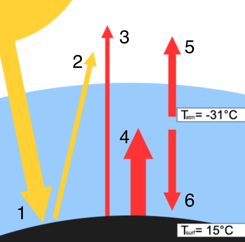
Figure 3: Schematic showing radiative fluxes in the beginner version of the Climate App.

Since the temperatures of the surface and the atmosphere are interdependent, we can establish a system of equations to solve for both temperatures. In fact, a more complex model with three or more layers follows the same principle, but the system of equations becomes more involved, as shown below.

The guiding principle is radiative equilibrium: each component of the climate system must emit as much flux as it absorbs. There are two unknowns: the surface temperature, $T_{\rm surf}$, and the atmospheric temperature, $T_{\rm atm}$. We therefore need two equations in order to solve the problem. In each case we put the absorbed power on the left hand side and the emitted power on the right. The atmospheric balance is

$$\epsilon_{\rm LW}\sigma T_{\rm surf}^{4}=2\epsilon_{\rm LW}\sigma T_{\rm atm}^{4},$$ (1)

where $\epsilon_{\rm LW}$ is the longwave emissivity (infrared opacity in the Beginner version). The left hand side is the flux emitted by the surface that is absorbed by the atmosphere (arrow 4) and the right hand side is the sum of the upward and downward fluxes emitted by the atmosphere (arrows 5 and 6). Inspection of Equation 1 reveals many of the same symbols on both sides of the equality, which begs for simplification, yielding $T_{\rm surf}^{4}=2T_{\rm atm}^{4}$.

The flux balance at the surface is

$$F_{*}-AF_{*}+\epsilon_{\rm LW}\sigma T_{\rm atm}^{4}=\sigma T_{\rm surf}^{4},$$ (2)

where $F_{*}$ is the stellar flux reaching the planet and $A$ is the planetary albedo (planetary reflectivity in the Beginner App). The first term on the left hand side is the incident stellar flux (arrow 1), the second term is the reflected light (arrow 2) and the third term is the downward atmospheric emission (arrow 6); on the right hand side there is the emission from the planetary surface (arrow 4)—recall that we assume perfect surface emissivity, an excellent approximation.

Substituting our expression for atmospheric radiative equilibrium, $T_{\rm surf}^{4}=2T_{\rm atm}^{4}$, into Equation 1, we obtain

$$(1-A)F_{*}+\epsilon_{\rm LW}\sigma T_{\rm atm}^{4}=\sigma(2T_{\rm atm}^{4}),$$ (3)

which can be solved for the atmospheric temperature:

$$T_{\rm atm}=\left(\frac{F_{*}}{\sigma}\right)^{1/4}\left(\frac{1-A}{2-\epsilon_{\rm LW}}\right)^{1/4}$$ (4)

and from thence the surface temperature:

$$T_{\rm surf}=\left(\frac{F_{*}}{\sigma}\right)^{1/4}\left(\frac{1-A}{1-\epsilon_{\rm LW}/2}\right)^{1/4}.$$ (5)

For the Climate App’s default values of $A=0.30$ and $\epsilon_{\rm LW}=0.78$, we obtain $T_{\rm atm}=242$ K $=-31^{\circ}$C and $T_{\rm surf}=288$ K $=15^{\circ}$C, as shown in Fig. 1 and in good agreement with average values on Earth today.

Lastly, the Beginner version of the Climate App reports the magnitude of the greenhouse effect. This is calculated by comparing the surface temperature with what it would have been in the absence of the greenhouse effect, i.e., $\epsilon_{\rm LW}=0$. For the default parameters, the magnitude of the greenhouse effect is 33^∘C, again in good agreement with modern-day Earth.

3.3 Advanced App: Three-Layer Model

Using the same reasoning as the simple greenhouse model, we can derive the system of equations to solve for the temperatures of the planetary surface and three atmospheric layers. However, the model used in the advanced version is more complicated. In addition to the extra atmospheric layers, the advanced Climate App includes two new parameters for each atmospheric layer to control how they interact with shortwave radiation. These parameters are the shortwave opacity, $\epsilon_{\rm SW}$, and the single-scattering albedo, $\alpha$.

3.3.1 Shortwave Radiation

When shortwave radiation arrives at an atmospheric layer, it can do three things: transmission with a factor of $1-\epsilon_{\rm SW}$, scattering with a factor of $\epsilon_{\rm SW}\alpha$, and absorption with a factor of $\epsilon_{\rm SW}(1-\alpha)$. We use $F_{3}$, $F_{2}$, $F_{1}$ and $F_{0}$ to denote the shortwave flux absorbed at layer 3, layer 2, layer 1 of the atmosphere and at the surface, respectively.

The values of the shortwave flux terms $F_{3}$, $F_{2}$, $F_{1}$ and $F_{0}$ are determined as follows. In the one-dimensional scattering model used in the Climate App, we assume an asymmetry factor of 0 at each atmospheric layer, i.e., isotropic scattering. This means that half of the photons scattered at a given layer are scattered back in the direction they came from, while the other half are scattered forward. Since we use a 1-D model, we treat the forward scattering case as equivalent to transmission. With the isotropic scattering assumption, we can solve the following system of equations to obtain the shortwave terms:

$$F_{3} =(I+u_{2})\epsilon_{\rm SW3}(1-\alpha_{3})$$

$$F_{2} =(d_{3}+u_{1})\epsilon_{\rm SW2}(1-\alpha_{2})$$

$$F_{1} =(d_{2}+u_{0})\epsilon_{\rm SW1}(1-\alpha_{1})$$

$$F_{0} =d_{1}(1-A)$$

$$u_{0} =d_{1}A$$

$$d_{1} =0.5u_{0}\epsilon_{\rm SW1}\alpha_{1}+d_{2}(1-\epsilon_{\rm SW1})+0.5d_{2}\epsilon_{\rm SW1}\alpha_{1}$$

$$u_{1} =u_{0}(1-\epsilon_{\rm SW1})+0.5d_{2}\epsilon_{\rm SW1}\alpha_{1}+0.5u_{0}\epsilon_{\rm SW1}\alpha_{1}$$

$$d_{2} =0.5u_{1}\epsilon_{\rm SW2}\alpha_{2}+d_{3}(1-\epsilon_{\rm SW2})+0.5d_{3}\epsilon_{\rm SW2}\alpha_{2}$$

$$u_{2} =0.5d_{3}\epsilon_{\rm SW2}\alpha_{2}+u_{1}(1-\epsilon_{\rm SW2})+0.5u_{1}\epsilon_{\rm SW2}\alpha_{2}$$

$$d_{3} =0.5u_{2}\epsilon_{\rm SW3}\alpha_{3}+I(1-\epsilon_{\rm SW3})+0.5I\epsilon_{\rm SW3}\alpha_{3}$$

$$u_{3} =u_{2}(1-\epsilon_{\rm SW3})+0.5I\epsilon_{\rm SW3}\alpha_{3}+0.5u_{2}\epsilon_{\rm SW3}\alpha_{3},$$

where $I$ is the incident stellar flux, $u_{i}$ and $d_{i}$ are the total shortwave radiation heading upward and downward from the $i^{\rm th}$ layer, $\epsilon_{\rm SW1}$, $\epsilon_{\rm SW2}$ and $\epsilon_{\rm SW3}$ are the shortwave opacities of each atmospheric layer, $\alpha_{1}$, $\alpha_{2}$ and $\alpha_{3}$ are their single scattering albedo, and $A$ is the surface albedo.

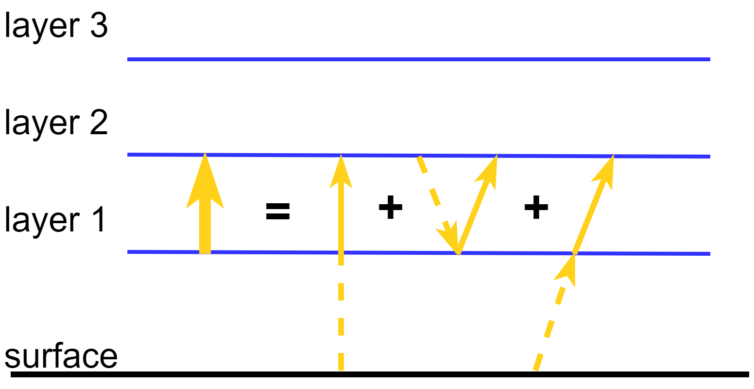
Figure 4: Diagram showing how the expression of $u_{1}$ (the leftmost thick arrow) was obtained.

As an example, Figure 4 shows the shortwave radiation transmitted upward from layer 1, $u_{1}$. It is the sum of three components indicated by three thinner arrows (from left to right): a fraction of shortwave radiation reflected upward from the surface that goes through layer 1 without any interaction, $u_{0}(1-\epsilon_{\rm SW1})$, a fraction of radiation transmitted downward from layer 2 that back-scatters off of layer 1, $\frac{1}{2}d_{2}\epsilon_{\rm SW1}\alpha_{1}$, and another fraction of radiation reflected upward from the surface that forward scatters off layer 1, $\frac{1}{2}u_{0}\epsilon_{\rm SW1}\alpha_{1}$. The factors of $\frac{1}{2}$ comes from the assumption of isotropic scattering.

3.3.2 Longwave Radiation

Following the logic that led us to Equation 1, we focus on layer 2 (with absorbed shortwave flux $F_{2}$, temperature $T_{2}$ and longwave emissivity $\epsilon_{\rm LW2}$) as an example to the derivation of the full system of equations shown in Appendix A. The emission from layer 2 is $2\epsilon_{\rm LW2}\sigma T_{2}^{4}$, identical to the right hand side of Equation 1 since layer 2 also emits both upwards and downwards. As for the absorption, we have shortwave radiation $F_{2}$, thermal radiation from layer 3 and layer 1, and attenuated thermal radiation from the surface. The equation of radiative equilibrium is therefore:

$$2\epsilon_{\rm LW2}\sigma T_{2}^{4}= F_{2}+\sigma T_{0}^{4}\epsilon_{\rm LW2}(1-\epsilon_{\rm LW1})$$

$$+\sigma T_{1}^{4}\epsilon_{\rm LW1}\epsilon_{\rm LW2}+\sigma T_{3}^{4}\epsilon_{\rm LW2}\epsilon_{\rm LW3}.$$ (6)

The full system of equations and its analytic solutions are listed in Appendix A.

Appendix B explains how the shortwave flux terms ($F_{3}$, $F_{2}$, $F_{1}$ and $F_{0}$) are determined; they also result in analytic expressions that only depend on user-input parameters. Near-immediate feedback while using the application is therefore allowed.

4 Summary

The Climate App incorporates simple climate models based on radiative equilibrium. It offers an intuitive and user-friendly way to explain various climate concepts to students in high school and college. Example modules at various stages of development and beta testing include: the Faint Young Sun Paradox, Snowball Earth, Global Warming, and the habitability of the TRAPPIST-1 planets. If you would like to test activities or have questions about the Climate App then please contact Nick Cowan.

Acknowledgements: The authors thank Dorian Abbot and Tim Merlis for constructive feedback.

Appendix A Three-Layer Radiative Equilibrium

The system of equations that ensure radiative equilibrium at each atmospheric layer and at the surface is:

$$2\epsilon_{\rm LW3}\sigma T_{3}^{4} =F_{3}+\epsilon_{\rm LW3}\Big{(}\sigma T_{0}^{4}(1-\epsilon_{\rm LW1})(1-\epsilon_{\rm LW2})+\sigma T_{1}^{4}\epsilon_{\rm LW1}(1-\epsilon_{\rm LW2})+\sigma T_{2}^{4}\epsilon_{\rm LW2}\Big{)}$$

$$2\epsilon_{\rm LW2}\sigma T_{2}^{4} =F_{2}+\epsilon_{\rm LW2}\Big{(}\sigma T_{0}^{4}(1-\epsilon_{\rm LW1})+\sigma T_{1}^{4}\epsilon_{\rm LW1}+\sigma T_{3}^{4}\epsilon_{\rm LW3}\Big{)}$$

$$2\epsilon_{\rm LW1}\sigma T_{1}^{4} =F_{1}+\epsilon_{\rm LW1}\Big{(}\sigma T_{0}^{4}+\sigma T_{2}^{4}\epsilon_{\rm LW2}+\sigma T_{3}^{4}\epsilon_{\rm LW3}(1-\epsilon_{\rm LW2})\Big{)}$$

$$\sigma T_{0}^{4} =F_{0}+\Big{(}\sigma T_{1}^{4}\epsilon_{\rm LW1}+\sigma T_{2}^{4}\epsilon_{\rm LW2}(1-\epsilon_{\rm LW1})+\sigma T_{3}^{4}\epsilon_{\rm LW3}(1-\epsilon_{\rm LW2})(1-\epsilon_{\rm LW1})\Big{)},$$

where $\epsilon_{\rm LW1}$, $\epsilon_{\rm LW2}$ and $\epsilon_{\rm LW3}$ are the longwave emissivity of the three atmopsheric layers (recall that we assume the surface has a longwave emissivity of 1). Solving this system of equation gives:

$$T_{3}^{4}= \frac{\epsilon_{\rm LW3}F_{1}+\epsilon_{\rm LW3}F_{2}+\epsilon_{\rm LW3}F_{0}+F_{3}}{\sigma\epsilon_{\rm LW3}(2-\epsilon_{\rm LW3})}$$

$$T_{2}^{4}=$$

$$T_{1}^{4}= \frac{\raisebox{-25.0pt}{\bBigg@{7.5}(}\displaystyle\begin{multlined}-2\epsilon_{\rm LW1}2\epsilon_{\rm LW2}\epsilon_{\rm LW3}F_{1}-\epsilon_{\rm LW1}2\epsilon_{\rm LW2}\epsilon_{\rm LW3}l_{2}-2\epsilon_{\rm LW1}2\epsilon_{\rm LW2}\epsilon_{\rm LW3}F_{0}\\ \displaystyle\begin{multlined}+2\epsilon_{\rm LW1}2\epsilon_{\rm LW2}F_{1}-\epsilon_{\rm LW1}2\epsilon_{\rm LW2}F_{3}+2\epsilon_{\rm LW1}2\epsilon_{\rm LW2}F_{0}+2\epsilon_{\rm LW1}2\epsilon_{\rm LW3}F_{1}\\ \displaystyle\begin{multlined}+\epsilon_{\rm LW1}2\epsilon_{\rm LW3}F_{2}+2\epsilon_{\rm LW1}2\epsilon_{\rm LW3}F_{0}+2\epsilon_{\rm LW1}2F_{2}+2\epsilon_{\rm LW1}2F_{3}\\ \displaystyle\begin{multlined}+4\epsilon_{\rm LW1}\epsilon_{\rm LW2}\epsilon_{\rm LW3}F_{1}+2\epsilon_{\rm LW1}\epsilon_{\rm LW2}\epsilon_{\rm LW3}F_{2}+3\epsilon_{\rm LW1}\epsilon_{\rm LW2}\epsilon_{\rm LW3}F_{0}\\ \displaystyle\begin{multlined}-4\epsilon_{\rm LW1}\epsilon_{\rm LW2}F_{1}+2\epsilon_{\rm LW1}\epsilon_{\rm LW2}F_{3}-2\epsilon_{\rm LW1}\epsilon_{\rm LW2}F_{0}-4\epsilon_{\rm LW1}\epsilon_{\rm LW3}F_{1}\\ \displaystyle\begin{multlined}-2\epsilon_{\rm LW1}\epsilon_{\rm LW3}F_{2}-2\epsilon_{\rm LW1}\epsilon_{\rm LW3}F_{0}-4\epsilon_{\rm LW1}F_{2}-4\epsilon_{\rm LW1}F_{3}\\ -4\epsilon_{\rm LW1}F_{0}-\epsilon_{\rm LW2}\epsilon_{\rm LW3}F_{1}+2\epsilon_{\rm LW2}F_{1}+2\epsilon_{\rm LW3}F_{1}-4F_{1}\end{multlined}-2\epsilon_{\rm LW1}\epsilon_{\rm LW3}F_{2}-2\epsilon_{\rm LW1}\epsilon_{\rm LW3}F_{0}-4\epsilon_{\rm LW1}F_{2}-4\epsilon_{\rm LW1}F_{3}\\ -4\epsilon_{\rm LW1}F_{0}-\epsilon_{\rm LW2}\epsilon_{\rm LW3}F_{1}+2\epsilon_{\rm LW2}F_{1}+2\epsilon_{\rm LW3}F_{1}-4F_{1}\end{multlined}-4\epsilon_{\rm LW1}\epsilon_{\rm LW2}F_{1}+2\epsilon_{\rm LW1}\epsilon_{\rm LW2}F_{3}-2\epsilon_{\rm LW1}\epsilon_{\rm LW2}F_{0}-4\epsilon_{\rm LW1}\epsilon_{\rm LW3}F_{1}\\ \displaystyle\begin{multlined}-2\epsilon_{\rm LW1}\epsilon_{\rm LW3}F_{2}-2\epsilon_{\rm LW1}\epsilon_{\rm LW3}F_{0}-4\epsilon_{\rm LW1}F_{2}-4\epsilon_{\rm LW1}F_{3}\\ -4\epsilon_{\rm LW1}F_{0}-\epsilon_{\rm LW2}\epsilon_{\rm LW3}F_{1}+2\epsilon_{\rm LW2}F_{1}+2\epsilon_{\rm LW3}F_{1}-4F_{1}\end{multlined}-2\epsilon_{\rm LW1}\epsilon_{\rm LW3}F_{2}-2\epsilon_{\rm LW1}\epsilon_{\rm LW3}F_{0}-4\epsilon_{\rm LW1}F_{2}-4\epsilon_{\rm LW1}F_{3}\\ -4\epsilon_{\rm LW1}F_{0}-\epsilon_{\rm LW2}\epsilon_{\rm LW3}F_{1}+2\epsilon_{\rm LW2}F_{1}+2\epsilon_{\rm LW3}F_{1}-4F_{1}\end{multlined}+4\epsilon_{\rm LW1}\epsilon_{\rm LW2}\epsilon_{\rm LW3}F_{1}+2\epsilon_{\rm LW1}\epsilon_{\rm LW2}\epsilon_{\rm LW3}F_{2}+3\epsilon_{\rm LW1}\epsilon_{\rm LW2}\epsilon_{\rm LW3}F_{0}\\ \displaystyle\begin{multlined}-4\epsilon_{\rm LW1}\epsilon_{\rm LW2}F_{1}+2\epsilon_{\rm LW1}\epsilon_{\rm LW2}F_{3}-2\epsilon_{\rm LW1}\epsilon_{\rm LW2}F_{0}-4\epsilon_{\rm LW1}\epsilon_{\rm LW3}F_{1}\\ \displaystyle\begin{multlined}-2\epsilon_{\rm LW1}\epsilon_{\rm LW3}F_{2}-2\epsilon_{\rm LW1}\epsilon_{\rm LW3}F_{0}-4\epsilon_{\rm LW1}F_{2}-4\epsilon_{\rm LW1}F_{3}\\ -4\epsilon_{\rm LW1}F_{0}-\epsilon_{\rm LW2}\epsilon_{\rm LW3}F_{1}+2\epsilon_{\rm LW2}F_{1}+2\epsilon_{\rm LW3}F_{1}-4F_{1}\end{multlined}-2\epsilon_{\rm LW1}\epsilon_{\rm LW3}F_{2}-2\epsilon_{\rm LW1}\epsilon_{\rm LW3}F_{0}-4\epsilon_{\rm LW1}F_{2}-4\epsilon_{\rm LW1}F_{3}\\ -4\epsilon_{\rm LW1}F_{0}-\epsilon_{\rm LW2}\epsilon_{\rm LW3}F_{1}+2\epsilon_{\rm LW2}F_{1}+2\epsilon_{\rm LW3}F_{1}-4F_{1}\end{multlined}-4\epsilon_{\rm LW1}\epsilon_{\rm LW2}F_{1}+2\epsilon_{\rm LW1}\epsilon_{\rm LW2}F_{3}-2\epsilon_{\rm LW1}\epsilon_{\rm LW2}F_{0}-4\epsilon_{\rm LW1}\epsilon_{\rm LW3}F_{1}\\ \displaystyle\begin{multlined}-2\epsilon_{\rm LW1}\epsilon_{\rm LW3}F_{2}-2\epsilon_{\rm LW1}\epsilon_{\rm LW3}F_{0}-4\epsilon_{\rm LW1}F_{2}-4\epsilon_{\rm LW1}F_{3}\\ -4\epsilon_{\rm LW1}F_{0}-\epsilon_{\rm LW2}\epsilon_{\rm LW3}F_{1}+2\epsilon_{\rm LW2}F_{1}+2\epsilon_{\rm LW3}F_{1}-4F_{1}\end{multlined}-2\epsilon_{\rm LW1}\epsilon_{\rm LW3}F_{2}-2\epsilon_{\rm LW1}\epsilon_{\rm LW3}F_{0}-4\epsilon_{\rm LW1}F_{2}-4\epsilon_{\rm LW1}F_{3}\\ -4\epsilon_{\rm LW1}F_{0}-\epsilon_{\rm LW2}\epsilon_{\rm LW3}F_{1}+2\epsilon_{\rm LW2}F_{1}+2\epsilon_{\rm LW3}F_{1}-4F_{1}\end{multlined}+\epsilon_{\rm LW1}2\epsilon_{\rm LW3}F_{2}+2\epsilon_{\rm LW1}2\epsilon_{\rm LW3}F_{0}+2\epsilon_{\rm LW1}2F_{2}+2\epsilon_{\rm LW1}2F_{3}\\ \displaystyle\begin{multlined}+4\epsilon_{\rm LW1}\epsilon_{\rm LW2}\epsilon_{\rm LW3}F_{1}+2\epsilon_{\rm LW1}\epsilon_{\rm LW2}\epsilon_{\rm LW3}F_{2}+3\epsilon_{\rm LW1}\epsilon_{\rm LW2}\epsilon_{\rm LW3}F_{0}\\ \displaystyle\begin{multlined}-4\epsilon_{\rm LW1}\epsilon_{\rm LW2}F_{1}+2\epsilon_{\rm LW1}\epsilon_{\rm LW2}F_{3}-2\epsilon_{\rm LW1}\epsilon_{\rm LW2}F_{0}-4\epsilon_{\rm LW1}\epsilon_{\rm LW3}F_{1}\\ \displaystyle\begin{multlined}-2\epsilon_{\rm LW1}\epsilon_{\rm LW3}F_{2}-2\epsilon_{\rm LW1}\epsilon_{\rm LW3}F_{0}-4\epsilon_{\rm LW1}F_{2}-4\epsilon_{\rm LW1}F_{3}\\ -4\epsilon_{\rm LW1}F_{0}-\epsilon_{\rm LW2}\epsilon_{\rm LW3}F_{1}+2\epsilon_{\rm LW2}F_{1}+2\epsilon_{\rm LW3}F_{1}-4F_{1}\end{multlined}-2\epsilon_{\rm LW1}\epsilon_{\rm LW3}F_{2}-2\epsilon_{\rm LW1}\epsilon_{\rm LW3}F_{0}-4\epsilon_{\rm LW1}F_{2}-4\epsilon_{\rm LW1}F_{3}\\ -4\epsilon_{\rm LW1}F_{0}-\epsilon_{\rm LW2}\epsilon_{\rm LW3}F_{1}+2\epsilon_{\rm LW2}F_{1}+2\epsilon_{\rm LW3}F_{1}-4F_{1}\end{multlined}-4\epsilon_{\rm LW1}\epsilon_{\rm LW2}F_{1}+2\epsilon_{\rm LW1}\epsilon_{\rm LW2}F_{3}-2\epsilon_{\rm LW1}\epsilon_{\rm LW2}F_{0}-4\epsilon_{\rm LW1}\epsilon_{\rm LW3}F_{1}\\ \displaystyle\begin{multlined}-2\epsilon_{\rm LW1}\epsilon_{\rm LW3}F_{2}-2\epsilon_{\rm LW1}\epsilon_{\rm LW3}F_{0}-4\epsilon_{\rm LW1}F_{2}-4\epsilon_{\rm LW1}F_{3}\\ -4\epsilon_{\rm LW1}F_{0}-\epsilon_{\rm LW2}\epsilon_{\rm LW3}F_{1}+2\epsilon_{\rm LW2}F_{1}+2\epsilon_{\rm LW3}F_{1}-4F_{1}\end{multlined}-2\epsilon_{\rm LW1}\epsilon_{\rm LW3}F_{2}-2\epsilon_{\rm LW1}\epsilon_{\rm LW3}F_{0}-4\epsilon_{\rm LW1}F_{2}-4\epsilon_{\rm LW1}F_{3}\\ -4\epsilon_{\rm LW1}F_{0}-\epsilon_{\rm LW2}\epsilon_{\rm LW3}F_{1}+2\epsilon_{\rm LW2}F_{1}+2\epsilon_{\rm LW3}F_{1}-4F_{1}\end{multlined}+4\epsilon_{\rm LW1}\epsilon_{\rm LW2}\epsilon_{\rm LW3}F_{1}+2\epsilon_{\rm LW1}\epsilon_{\rm LW2}\epsilon_{\rm LW3}F_{2}+3\epsilon_{\rm LW1}\epsilon_{\rm LW2}\epsilon_{\rm LW3}F_{0}\\ \displaystyle\begin{multlined}-4\epsilon_{\rm LW1}\epsilon_{\rm LW2}F_{1}+2\epsilon_{\rm LW1}\epsilon_{\rm LW2}F_{3}-2\epsilon_{\rm LW1}\epsilon_{\rm LW2}F_{0}-4\epsilon_{\rm LW1}\epsilon_{\rm LW3}F_{1}\\ \displaystyle\begin{multlined}-2\epsilon_{\rm LW1}\epsilon_{\rm LW3}F_{2}-2\epsilon_{\rm LW1}\epsilon_{\rm LW3}F_{0}-4\epsilon_{\rm LW1}F_{2}-4\epsilon_{\rm LW1}F_{3}\\ -4\epsilon_{\rm LW1}F_{0}-\epsilon_{\rm LW2}\epsilon_{\rm LW3}F_{1}+2\epsilon_{\rm LW2}F_{1}+2\epsilon_{\rm LW3}F_{1}-4F_{1}\end{multlined}-2\epsilon_{\rm LW1}\epsilon_{\rm LW3}F_{2}-2\epsilon_{\rm LW1}\epsilon_{\rm LW3}F_{0}-4\epsilon_{\rm LW1}F_{2}-4\epsilon_{\rm LW1}F_{3}\\ -4\epsilon_{\rm LW1}F_{0}-\epsilon_{\rm LW2}\epsilon_{\rm LW3}F_{1}+2\epsilon_{\rm LW2}F_{1}+2\epsilon_{\rm LW3}F_{1}-4F_{1}\end{multlined}-4\epsilon_{\rm LW1}\epsilon_{\rm LW2}F_{1}+2\epsilon_{\rm LW1}\epsilon_{\rm LW2}F_{3}-2\epsilon_{\rm LW1}\epsilon_{\rm LW2}F_{0}-4\epsilon_{\rm LW1}\epsilon_{\rm LW3}F_{1}\\ \displaystyle\begin{multlined}-2\epsilon_{\rm LW1}\epsilon_{\rm LW3}F_{2}-2\epsilon_{\rm LW1}\epsilon_{\rm LW3}F_{0}-4\epsilon_{\rm LW1}F_{2}-4\epsilon_{\rm LW1}F_{3}\\ -4\epsilon_{\rm LW1}F_{0}-\epsilon_{\rm LW2}\epsilon_{\rm LW3}F_{1}+2\epsilon_{\rm LW2}F_{1}+2\epsilon_{\rm LW3}F_{1}-4F_{1}\end{multlined}-2\epsilon_{\rm LW1}\epsilon_{\rm LW3}F_{2}-2\epsilon_{\rm LW1}\epsilon_{\rm LW3}F_{0}-4\epsilon_{\rm LW1}F_{2}-4\epsilon_{\rm LW1}F_{3}\\ -4\epsilon_{\rm LW1}F_{0}-\epsilon_{\rm LW2}\epsilon_{\rm LW3}F_{1}+2\epsilon_{\rm LW2}F_{1}+2\epsilon_{\rm LW3}F_{1}-4F_{1}\end{multlined}+2\epsilon_{\rm LW1}2\epsilon_{\rm LW2}F_{1}-\epsilon_{\rm LW1}2\epsilon_{\rm LW2}F_{3}+2\epsilon_{\rm LW1}2\epsilon_{\rm LW2}F_{0}+2\epsilon_{\rm LW1}2\epsilon_{\rm LW3}F_{1}\\ \displaystyle\begin{multlined}+\epsilon_{\rm LW1}2\epsilon_{\rm LW3}F_{2}+2\epsilon_{\rm LW1}2\epsilon_{\rm LW3}F_{0}+2\epsilon_{\rm LW1}2F_{2}+2\epsilon_{\rm LW1}2F_{3}\\ \displaystyle\begin{multlined}+4\epsilon_{\rm LW1}\epsilon_{\rm LW2}\epsilon_{\rm LW3}F_{1}+2\epsilon_{\rm LW1}\epsilon_{\rm LW2}\epsilon_{\rm LW3}F_{2}+3\epsilon_{\rm LW1}\epsilon_{\rm LW2}\epsilon_{\rm LW3}F_{0}\\ \displaystyle\begin{multlined}-4\epsilon_{\rm LW1}\epsilon_{\rm LW2}F_{1}+2\epsilon_{\rm LW1}\epsilon_{\rm LW2}F_{3}-2\epsilon_{\rm LW1}\epsilon_{\rm LW2}F_{0}-4\epsilon_{\rm LW1}\epsilon_{\rm LW3}F_{1}\\ \displaystyle\begin{multlined}-2\epsilon_{\rm LW1}\epsilon_{\rm LW3}F_{2}-2\epsilon_{\rm LW1}\epsilon_{\rm LW3}F_{0}-4\epsilon_{\rm LW1}F_{2}-4\epsilon_{\rm LW1}F_{3}\\ -4\epsilon_{\rm LW1}F_{0}-\epsilon_{\rm LW2}\epsilon_{\rm LW3}F_{1}+2\epsilon_{\rm LW2}F_{1}+2\epsilon_{\rm LW3}F_{1}-4F_{1}\end{multlined}-2\epsilon_{\rm LW1}\epsilon_{\rm LW3}F_{2}-2\epsilon_{\rm LW1}\epsilon_{\rm LW3}F_{0}-4\epsilon_{\rm LW1}F_{2}-4\epsilon_{\rm LW1}F_{3}\\ -4\epsilon_{\rm LW1}F_{0}-\epsilon_{\rm LW2}\epsilon_{\rm LW3}F_{1}+2\epsilon_{\rm LW2}F_{1}+2\epsilon_{\rm LW3}F_{1}-4F_{1}\end{multlined}-4\epsilon_{\rm LW1}\epsilon_{\rm LW2}F_{1}+2\epsilon_{\rm LW1}\epsilon_{\rm LW2}F_{3}-2\epsilon_{\rm LW1}\epsilon_{\rm LW2}F_{0}-4\epsilon_{\rm LW1}\epsilon_{\rm LW3}F_{1}\\ \displaystyle\begin{multlined}-2\epsilon_{\rm LW1}\epsilon_{\rm LW3}F_{2}-2\epsilon_{\rm LW1}\epsilon_{\rm LW3}F_{0}-4\epsilon_{\rm LW1}F_{2}-4\epsilon_{\rm LW1}F_{3}\\ -4\epsilon_{\rm LW1}F_{0}-\epsilon_{\rm LW2}\epsilon_{\rm LW3}F_{1}+2\epsilon_{\rm LW2}F_{1}+2\epsilon_{\rm LW3}F_{1}-4F_{1}\end{multlined}-2\epsilon_{\rm LW1}\epsilon_{\rm LW3}F_{2}-2\epsilon_{\rm LW1}\epsilon_{\rm LW3}F_{0}-4\epsilon_{\rm LW1}F_{2}-4\epsilon_{\rm LW1}F_{3}\\ -4\epsilon_{\rm LW1}F_{0}-\epsilon_{\rm LW2}\epsilon_{\rm LW3}F_{1}+2\epsilon_{\rm LW2}F_{1}+2\epsilon_{\rm LW3}F_{1}-4F_{1}\end{multlined}+4\epsilon_{\rm LW1}\epsilon_{\rm LW2}\epsilon_{\rm LW3}F_{1}+2\epsilon_{\rm LW1}\epsilon_{\rm LW2}\epsilon_{\rm LW3}F_{2}+3\epsilon_{\rm LW1}\epsilon_{\rm LW2}\epsilon_{\rm LW3}F_{0}\\ \displaystyle\begin{multlined}-4\epsilon_{\rm LW1}\epsilon_{\rm LW2}F_{1}+2\epsilon_{\rm LW1}\epsilon_{\rm LW2}F_{3}-2\epsilon_{\rm LW1}\epsilon_{\rm LW2}F_{0}-4\epsilon_{\rm LW1}\epsilon_{\rm LW3}F_{1}\\ \displaystyle\begin{multlined}-2\epsilon_{\rm LW1}\epsilon_{\rm LW3}F_{2}-2\epsilon_{\rm LW1}\epsilon_{\rm LW3}F_{0}-4\epsilon_{\rm LW1}F_{2}-4\epsilon_{\rm LW1}F_{3}\\ -4\epsilon_{\rm LW1}F_{0}-\epsilon_{\rm LW2}\epsilon_{\rm LW3}F_{1}+2\epsilon_{\rm LW2}F_{1}+2\epsilon_{\rm LW3}F_{1}-4F_{1}\end{multlined}-2\epsilon_{\rm LW1}\epsilon_{\rm LW3}F_{2}-2\epsilon_{\rm LW1}\epsilon_{\rm LW3}F_{0}-4\epsilon_{\rm LW1}F_{2}-4\epsilon_{\rm LW1}F_{3}\\ -4\epsilon_{\rm LW1}F_{0}-\epsilon_{\rm LW2}\epsilon_{\rm LW3}F_{1}+2\epsilon_{\rm LW2}F_{1}+2\epsilon_{\rm LW3}F_{1}-4F_{1}\end{multlined}-4\epsilon_{\rm LW1}\epsilon_{\rm LW2}F_{1}+2\epsilon_{\rm LW1}\epsilon_{\rm LW2}F_{3}-2\epsilon_{\rm LW1}\epsilon_{\rm LW2}F_{0}-4\epsilon_{\rm LW1}\epsilon_{\rm LW3}F_{1}\\ \displaystyle\begin{multlined}-2\epsilon_{\rm LW1}\epsilon_{\rm LW3}F_{2}-2\epsilon_{\rm LW1}\epsilon_{\rm LW3}F_{0}-4\epsilon_{\rm LW1}F_{2}-4\epsilon_{\rm LW1}F_{3}\\ -4\epsilon_{\rm LW1}F_{0}-\epsilon_{\rm LW2}\epsilon_{\rm LW3}F_{1}+2\epsilon_{\rm LW2}F_{1}+2\epsilon_{\rm LW3}F_{1}-4F_{1}\end{multlined}-2\epsilon_{\rm LW1}\epsilon_{\rm LW3}F_{2}-2\epsilon_{\rm LW1}\epsilon_{\rm LW3}F_{0}-4\epsilon_{\rm LW1}F_{2}-4\epsilon_{\rm LW1}F_{3}\\ -4\epsilon_{\rm LW1}F_{0}-\epsilon_{\rm LW2}\epsilon_{\rm LW3}F_{1}+2\epsilon_{\rm LW2}F_{1}+2\epsilon_{\rm LW3}F_{1}-4F_{1}\end{multlined}+\epsilon_{\rm LW1}2\epsilon_{\rm LW3}F_{2}+2\epsilon_{\rm LW1}2\epsilon_{\rm LW3}F_{0}+2\epsilon_{\rm LW1}2F_{2}+2\epsilon_{\rm LW1}2F_{3}\\ \displaystyle\begin{multlined}+4\epsilon_{\rm LW1}\epsilon_{\rm LW2}\epsilon_{\rm LW3}F_{1}+2\epsilon_{\rm LW1}\epsilon_{\rm LW2}\epsilon_{\rm LW3}F_{2}+3\epsilon_{\rm LW1}\epsilon_{\rm LW2}\epsilon_{\rm LW3}F_{0}\\ \displaystyle\begin{multlined}-4\epsilon_{\rm LW1}\epsilon_{\rm LW2}F_{1}+2\epsilon_{\rm LW1}\epsilon_{\rm LW2}F_{3}-2\epsilon_{\rm LW1}\epsilon_{\rm LW2}F_{0}-4\epsilon_{\rm LW1}\epsilon_{\rm LW3}F_{1}\\ \displaystyle\begin{multlined}-2\epsilon_{\rm LW1}\epsilon_{\rm LW3}F_{2}-2\epsilon_{\rm LW1}\epsilon_{\rm LW3}F_{0}-4\epsilon_{\rm LW1}F_{2}-4\epsilon_{\rm LW1}F_{3}\\ -4\epsilon_{\rm LW1}F_{0}-\epsilon_{\rm LW2}\epsilon_{\rm LW3}F_{1}+2\epsilon_{\rm LW2}F_{1}+2\epsilon_{\rm LW3}F_{1}-4F_{1}\end{multlined}-2\epsilon_{\rm LW1}\epsilon_{\rm LW3}F_{2}-2\epsilon_{\rm LW1}\epsilon_{\rm LW3}F_{0}-4\epsilon_{\rm LW1}F_{2}-4\epsilon_{\rm LW1}F_{3}\\ -4\epsilon_{\rm LW1}F_{0}-\epsilon_{\rm LW2}\epsilon_{\rm LW3}F_{1}+2\epsilon_{\rm LW2}F_{1}+2\epsilon_{\rm LW3}F_{1}-4F_{1}\end{multlined}-4\epsilon_{\rm LW1}\epsilon_{\rm LW2}F_{1}+2\epsilon_{\rm LW1}\epsilon_{\rm LW2}F_{3}-2\epsilon_{\rm LW1}\epsilon_{\rm LW2}F_{0}-4\epsilon_{\rm LW1}\epsilon_{\rm LW3}F_{1}\\ \displaystyle\begin{multlined}-2\epsilon_{\rm LW1}\epsilon_{\rm LW3}F_{2}-2\epsilon_{\rm LW1}\epsilon_{\rm LW3}F_{0}-4\epsilon_{\rm LW1}F_{2}-4\epsilon_{\rm LW1}F_{3}\\ -4\epsilon_{\rm LW1}F_{0}-\epsilon_{\rm LW2}\epsilon_{\rm LW3}F_{1}+2\epsilon_{\rm LW2}F_{1}+2\epsilon_{\rm LW3}F_{1}-4F_{1}\end{multlined}-2\epsilon_{\rm LW1}\epsilon_{\rm LW3}F_{2}-2\epsilon_{\rm LW1}\epsilon_{\rm LW3}F_{0}-4\epsilon_{\rm LW1}F_{2}-4\epsilon_{\rm LW1}F_{3}\\ -4\epsilon_{\rm LW1}F_{0}-\epsilon_{\rm LW2}\epsilon_{\rm LW3}F_{1}+2\epsilon_{\rm LW2}F_{1}+2\epsilon_{\rm LW3}F_{1}-4F_{1}\end{multlined}+4\epsilon_{\rm LW1}\epsilon_{\rm LW2}\epsilon_{\rm LW3}F_{1}+2\epsilon_{\rm LW1}\epsilon_{\rm LW2}\epsilon_{\rm LW3}F_{2}+3\epsilon_{\rm LW1}\epsilon_{\rm LW2}\epsilon_{\rm LW3}F_{0}\\ \displaystyle\begin{multlined}-4\epsilon_{\rm LW1}\epsilon_{\rm LW2}F_{1}+2\epsilon_{\rm LW1}\epsilon_{\rm LW2}F_{3}-2\epsilon_{\rm LW1}\epsilon_{\rm LW2}F_{0}-4\epsilon_{\rm LW1}\epsilon_{\rm LW3}F_{1}\\ \displaystyle\begin{multlined}-2\epsilon_{\rm LW1}\epsilon_{\rm LW3}F_{2}-2\epsilon_{\rm LW1}\epsilon_{\rm LW3}F_{0}-4\epsilon_{\rm LW1}F_{2}-4\epsilon_{\rm LW1}F_{3}\\ -4\epsilon_{\rm LW1}F_{0}-\epsilon_{\rm LW2}\epsilon_{\rm LW3}F_{1}+2\epsilon_{\rm LW2}F_{1}+2\epsilon_{\rm LW3}F_{1}-4F_{1}\end{multlined}-2\epsilon_{\rm LW1}\epsilon_{\rm LW3}F_{2}-2\epsilon_{\rm LW1}\epsilon_{\rm LW3}F_{0}-4\epsilon_{\rm LW1}F_{2}-4\epsilon_{\rm LW1}F_{3}\\ -4\epsilon_{\rm LW1}F_{0}-\epsilon_{\rm LW2}\epsilon_{\rm LW3}F_{1}+2\epsilon_{\rm LW2}F_{1}+2\epsilon_{\rm LW3}F_{1}-4F_{1}\end{multlined}-4\epsilon_{\rm LW1}\epsilon_{\rm LW2}F_{1}+2\epsilon_{\rm LW1}\epsilon_{\rm LW2}F_{3}-2\epsilon_{\rm LW1}\epsilon_{\rm LW2}F_{0}-4\epsilon_{\rm LW1}\epsilon_{\rm LW3}F_{1}\\ \displaystyle\begin{multlined}-2\epsilon_{\rm LW1}\epsilon_{\rm LW3}F_{2}-2\epsilon_{\rm LW1}\epsilon_{\rm LW3}F_{0}-4\epsilon_{\rm LW1}F_{2}-4\epsilon_{\rm LW1}F_{3}\\ -4\epsilon_{\rm LW1}F_{0}-\epsilon_{\rm LW2}\epsilon_{\rm LW3}F_{1}+2\epsilon_{\rm LW2}F_{1}+2\epsilon_{\rm LW3}F_{1}-4F_{1}\end{multlined}-2\epsilon_{\rm LW1}\epsilon_{\rm LW3}F_{2}-2\epsilon_{\rm LW1}\epsilon_{\rm LW3}F_{0}-4\epsilon_{\rm LW1}F_{2}-4\epsilon_{\rm LW1}F_{3}\\ -4\epsilon_{\rm LW1}F_{0}-\epsilon_{\rm LW2}\epsilon_{\rm LW3}F_{1}+2\epsilon_{\rm LW2}F_{1}+2\epsilon_{\rm LW3}F_{1}-4F_{1}\end{multlined}-2\epsilon_{\rm LW1}2\epsilon_{\rm LW2}\epsilon_{\rm LW3}F_{1}-\epsilon_{\rm LW1}2\epsilon_{\rm LW2}\epsilon_{\rm LW3}l_{2}-2\epsilon_{\rm LW1}2\epsilon_{\rm LW2}\epsilon_{\rm LW3}F_{0}\\ \displaystyle\begin{multlined}+2\epsilon_{\rm LW1}2\epsilon_{\rm LW2}F_{1}-\epsilon_{\rm LW1}2\epsilon_{\rm LW2}F_{3}+2\epsilon_{\rm LW1}2\epsilon_{\rm LW2}F_{0}+2\epsilon_{\rm LW1}2\epsilon_{\rm LW3}F_{1}\\ \displaystyle\begin{multlined}+\epsilon_{\rm LW1}2\epsilon_{\rm LW3}F_{2}+2\epsilon_{\rm LW1}2\epsilon_{\rm LW3}F_{0}+2\epsilon_{\rm LW1}2F_{2}+2\epsilon_{\rm LW1}2F_{3}\\ \displaystyle\begin{multlined}+4\epsilon_{\rm LW1}\epsilon_{\rm LW2}\epsilon_{\rm LW3}F_{1}+2\epsilon_{\rm LW1}\epsilon_{\rm LW2}\epsilon_{\rm LW3}F_{2}+3\epsilon_{\rm LW1}\epsilon_{\rm LW2}\epsilon_{\rm LW3}F_{0}\\ \displaystyle\begin{multlined}-4\epsilon_{\rm LW1}\epsilon_{\rm LW2}F_{1}+2\epsilon_{\rm LW1}\epsilon_{\rm LW2}F_{3}-2\epsilon_{\rm LW1}\epsilon_{\rm LW2}F_{0}-4\epsilon_{\rm LW1}\epsilon_{\rm LW3}F_{1}\\ \displaystyle\begin{multlined}-2\epsilon_{\rm LW1}\epsilon_{\rm LW3}F_{2}-2\epsilon_{\rm LW1}\epsilon_{\rm LW3}F_{0}-4\epsilon_{\rm LW1}F_{2}-4\epsilon_{\rm LW1}F_{3}\\ -4\epsilon_{\rm LW1}F_{0}-\epsilon_{\rm LW2}\epsilon_{\rm LW3}F_{1}+2\epsilon_{\rm LW2}F_{1}+2\epsilon_{\rm LW3}F_{1}-4F_{1}\end{multlined}-2\epsilon_{\rm LW1}\epsilon_{\rm LW3}F_{2}-2\epsilon_{\rm LW1}\epsilon_{\rm LW3}F_{0}-4\epsilon_{\rm LW1}F_{2}-4\epsilon_{\rm LW1}F_{3}\\ -4\epsilon_{\rm LW1}F_{0}-\epsilon_{\rm LW2}\epsilon_{\rm LW3}F_{1}+2\epsilon_{\rm LW2}F_{1}+2\epsilon_{\rm LW3}F_{1}-4F_{1}\end{multlined}-4\epsilon_{\rm LW1}\epsilon_{\rm LW2}F_{1}+2\epsilon_{\rm LW1}\epsilon_{\rm LW2}F_{3}-2\epsilon_{\rm LW1}\epsilon_{\rm LW2}F_{0}-4\epsilon_{\rm LW1}\epsilon_{\rm LW3}F_{1}\\ \displaystyle\begin{multlined}-2\epsilon_{\rm LW1}\epsilon_{\rm LW3}F_{2}-2\epsilon_{\rm LW1}\epsilon_{\rm LW3}F_{0}-4\epsilon_{\rm LW1}F_{2}-4\epsilon_{\rm LW1}F_{3}\\ -4\epsilon_{\rm LW1}F_{0}-\epsilon_{\rm LW2}\epsilon_{\rm LW3}F_{1}+2\epsilon_{\rm LW2}F_{1}+2\epsilon_{\rm LW3}F_{1}-4F_{1}\end{multlined}-2\epsilon_{\rm LW1}\epsilon_{\rm LW3}F_{2}-2\epsilon_{\rm LW1}\epsilon_{\rm LW3}F_{0}-4\epsilon_{\rm LW1}F_{2}-4\epsilon_{\rm LW1}F_{3}\\ -4\epsilon_{\rm LW1}F_{0}-\epsilon_{\rm LW2}\epsilon_{\rm LW3}F_{1}+2\epsilon_{\rm LW2}F_{1}+2\epsilon_{\rm LW3}F_{1}-4F_{1}\end{multlined}+4\epsilon_{\rm LW1}\epsilon_{\rm LW2}\epsilon_{\rm LW3}F_{1}+2\epsilon_{\rm LW1}\epsilon_{\rm LW2}\epsilon_{\rm LW3}F_{2}+3\epsilon_{\rm LW1}\epsilon_{\rm LW2}\epsilon_{\rm LW3}F_{0}\\ \displaystyle\begin{multlined}-4\epsilon_{\rm LW1}\epsilon_{\rm LW2}F_{1}+2\epsilon_{\rm LW1}\epsilon_{\rm LW2}F_{3}-2\epsilon_{\rm LW1}\epsilon_{\rm LW2}F_{0}-4\epsilon_{\rm LW1}\epsilon_{\rm LW3}F_{1}\\ \displaystyle\begin{multlined}-2\epsilon_{\rm LW1}\epsilon_{\rm LW3}F_{2}-2\epsilon_{\rm LW1}\epsilon_{\rm LW3}F_{0}-4\epsilon_{\rm LW1}F_{2}-4\epsilon_{\rm LW1}F_{3}\\ -4\epsilon_{\rm LW1}F_{0}-\epsilon_{\rm LW2}\epsilon_{\rm LW3}F_{1}+2\epsilon_{\rm LW2}F_{1}+2\epsilon_{\rm LW3}F_{1}-4F_{1}\end{multlined}-2\epsilon_{\rm LW1}\epsilon_{\rm LW3}F_{2}-2\epsilon_{\rm LW1}\epsilon_{\rm LW3}F_{0}-4\epsilon_{\rm LW1}F_{2}-4\epsilon_{\rm LW1}F_{3}\\ -4\epsilon_{\rm LW1}F_{0}-\epsilon_{\rm LW2}\epsilon_{\rm LW3}F_{1}+2\epsilon_{\rm LW2}F_{1}+2\epsilon_{\rm LW3}F_{1}-4F_{1}\end{multlined}-4\epsilon_{\rm LW1}\epsilon_{\rm LW2}F_{1}+2\epsilon_{\rm LW1}\epsilon_{\rm LW2}F_{3}-2\epsilon_{\rm LW1}\epsilon_{\rm LW2}F_{0}-4\epsilon_{\rm LW1}\epsilon_{\rm LW3}F_{1}\\ \displaystyle\begin{multlined}-2\epsilon_{\rm LW1}\epsilon_{\rm LW3}F_{2}-2\epsilon_{\rm LW1}\epsilon_{\rm LW3}F_{0}-4\epsilon_{\rm LW1}F_{2}-4\epsilon_{\rm LW1}F_{3}\\ -4\epsilon_{\rm LW1}F_{0}-\epsilon_{\rm LW2}\epsilon_{\rm LW3}F_{1}+2\epsilon_{\rm LW2}F_{1}+2\epsilon_{\rm LW3}F_{1}-4F_{1}\end{multlined}-2\epsilon_{\rm LW1}\epsilon_{\rm LW3}F_{2}-2\epsilon_{\rm LW1}\epsilon_{\rm LW3}F_{0}-4\epsilon_{\rm LW1}F_{2}-4\epsilon_{\rm LW1}F_{3}\\ -4\epsilon_{\rm LW1}F_{0}-\epsilon_{\rm LW2}\epsilon_{\rm LW3}F_{1}+2\epsilon_{\rm LW2}F_{1}+2\epsilon_{\rm LW3}F_{1}-4F_{1}\end{multlined}+\epsilon_{\rm LW1}2\epsilon_{\rm LW3}F_{2}+2\epsilon_{\rm LW1}2\epsilon_{\rm LW3}F_{0}+2\epsilon_{\rm LW1}2F_{2}+2\epsilon_{\rm LW1}2F_{3}\\ \displaystyle\begin{multlined}+4\epsilon_{\rm LW1}\epsilon_{\rm LW2}\epsilon_{\rm LW3}F_{1}+2\epsilon_{\rm LW1}\epsilon_{\rm LW2}\epsilon_{\rm LW3}F_{2}+3\epsilon_{\rm LW1}\epsilon_{\rm LW2}\epsilon_{\rm LW3}F_{0}\\ \displaystyle\begin{multlined}-4\epsilon_{\rm LW1}\epsilon_{\rm LW2}F_{1}+2\epsilon_{\rm LW1}\epsilon_{\rm LW2}F_{3}-2\epsilon_{\rm LW1}\epsilon_{\rm LW2}F_{0}-4\epsilon_{\rm LW1}\epsilon_{\rm LW3}F_{1}\\ \displaystyle\begin{multlined}-2\epsilon_{\rm LW1}\epsilon_{\rm LW3}F_{2}-2\epsilon_{\rm LW1}\epsilon_{\rm LW3}F_{0}-4\epsilon_{\rm LW1}F_{2}-4\epsilon_{\rm LW1}F_{3}\\ -4\epsilon_{\rm LW1}F_{0}-\epsilon_{\rm LW2}\epsilon_{\rm LW3}F_{1}+2\epsilon_{\rm LW2}F_{1}+2\epsilon_{\rm LW3}F_{1}-4F_{1}\end{multlined}-2\epsilon_{\rm LW1}\epsilon_{\rm LW3}F_{2}-2\epsilon_{\rm LW1}\epsilon_{\rm LW3}F_{0}-4\epsilon_{\rm LW1}F_{2}-4\epsilon_{\rm LW1}F_{3}\\ -4\epsilon_{\rm LW1}F_{0}-\epsilon_{\rm LW2}\epsilon_{\rm LW3}F_{1}+2\epsilon_{\rm LW2}F_{1}+2\epsilon_{\rm LW3}F_{1}-4F_{1}\end{multlined}-4\epsilon_{\rm LW1}\epsilon_{\rm LW2}F_{1}+2\epsilon_{\rm LW1}\epsilon_{\rm LW2}F_{3}-2\epsilon_{\rm LW1}\epsilon_{\rm LW2}F_{0}-4\epsilon_{\rm LW1}\epsilon_{\rm LW3}F_{1}\\ \displaystyle\begin{multlined}-2\epsilon_{\rm LW1}\epsilon_{\rm LW3}F_{2}-2\epsilon_{\rm LW1}\epsilon_{\rm LW3}F_{0}-4\epsilon_{\rm LW1}F_{2}-4\epsilon_{\rm LW1}F_{3}\\ -4\epsilon_{\rm LW1}F_{0}-\epsilon_{\rm LW2}\epsilon_{\rm LW3}F_{1}+2\epsilon_{\rm LW2}F_{1}+2\epsilon_{\rm LW3}F_{1}-4F_{1}\end{multlined}-2\epsilon_{\rm LW1}\epsilon_{\rm LW3}F_{2}-2\epsilon_{\rm LW1}\epsilon_{\rm LW3}F_{0}-4\epsilon_{\rm LW1}F_{2}-4\epsilon_{\rm LW1}F_{3}\\ -4\epsilon_{\rm LW1}F_{0}-\epsilon_{\rm LW2}\epsilon_{\rm LW3}F_{1}+2\epsilon_{\rm LW2}F_{1}+2\epsilon_{\rm LW3}F_{1}-4F_{1}\end{multlined}+4\epsilon_{\rm LW1}\epsilon_{\rm LW2}\epsilon_{\rm LW3}F_{1}+2\epsilon_{\rm LW1}\epsilon_{\rm LW2}\epsilon_{\rm LW3}F_{2}+3\epsilon_{\rm LW1}\epsilon_{\rm LW2}\epsilon_{\rm LW3}F_{0}\\ \displaystyle\begin{multlined}-4\epsilon_{\rm LW1}\epsilon_{\rm LW2}F_{1}+2\epsilon_{\rm LW1}\epsilon_{\rm LW2}F_{3}-2\epsilon_{\rm LW1}\epsilon_{\rm LW2}F_{0}-4\epsilon_{\rm LW1}\epsilon_{\rm LW3}F_{1}\\ \displaystyle\begin{multlined}-2\epsilon_{\rm LW1}\epsilon_{\rm LW3}F_{2}-2\epsilon_{\rm LW1}\epsilon_{\rm LW3}F_{0}-4\epsilon_{\rm LW1}F_{2}-4\epsilon_{\rm LW1}F_{3}\\ -4\epsilon_{\rm LW1}F_{0}-\epsilon_{\rm LW2}\epsilon_{\rm LW3}F_{1}+2\epsilon_{\rm LW2}F_{1}+2\epsilon_{\rm LW3}F_{1}-4F_{1}\end{multlined}-2\epsilon_{\rm LW1}\epsilon_{\rm LW3}F_{2}-2\epsilon_{\rm LW1}\epsilon_{\rm LW3}F_{0}-4\epsilon_{\rm LW1}F_{2}-4\epsilon_{\rm LW1}F_{3}\\ -4\epsilon_{\rm LW1}F_{0}-\epsilon_{\rm LW2}\epsilon_{\rm LW3}F_{1}+2\epsilon_{\rm LW2}F_{1}+2\epsilon_{\rm LW3}F_{1}-4F_{1}\end{multlined}-4\epsilon_{\rm LW1}\epsilon_{\rm LW2}F_{1}+2\epsilon_{\rm LW1}\epsilon_{\rm LW2}F_{3}-2\epsilon_{\rm LW1}\epsilon_{\rm LW2}F_{0}-4\epsilon_{\rm LW1}\epsilon_{\rm LW3}F_{1}\\ \displaystyle\begin{multlined}-2\epsilon_{\rm LW1}\epsilon_{\rm LW3}F_{2}-2\epsilon_{\rm LW1}\epsilon_{\rm LW3}F_{0}-4\epsilon_{\rm LW1}F_{2}-4\epsilon_{\rm LW1}F_{3}\\ -4\epsilon_{\rm LW1}F_{0}-\epsilon_{\rm LW2}\epsilon_{\rm LW3}F_{1}+2\epsilon_{\rm LW2}F_{1}+2\epsilon_{\rm LW3}F_{1}-4F_{1}\end{multlined}-2\epsilon_{\rm LW1}\epsilon_{\rm LW3}F_{2}-2\epsilon_{\rm LW1}\epsilon_{\rm LW3}F_{0}-4\epsilon_{\rm LW1}F_{2}-4\epsilon_{\rm LW1}F_{3}\\ -4\epsilon_{\rm LW1}F_{0}-\epsilon_{\rm LW2}\epsilon_{\rm LW3}F_{1}+2\epsilon_{\rm LW2}F_{1}+2\epsilon_{\rm LW3}F_{1}-4F_{1}\end{multlined}+2\epsilon_{\rm LW1}2\epsilon_{\rm LW2}F_{1}-\epsilon_{\rm LW1}2\epsilon_{\rm LW2}F_{3}+2\epsilon_{\rm LW1}2\epsilon_{\rm LW2}F_{0}+2\epsilon_{\rm LW1}2\epsilon_{\rm LW3}F_{1}\\ \displaystyle\begin{multlined}+\epsilon_{\rm LW1}2\epsilon_{\rm LW3}F_{2}+2\epsilon_{\rm LW1}2\epsilon_{\rm LW3}F_{0}+2\epsilon_{\rm LW1}2F_{2}+2\epsilon_{\rm LW1}2F_{3}\\ \displaystyle\begin{multlined}+4\epsilon_{\rm LW1}\epsilon_{\rm LW2}\epsilon_{\rm LW3}F_{1}+2\epsilon_{\rm LW1}\epsilon_{\rm LW2}\epsilon_{\rm LW3}F_{2}+3\epsilon_{\rm LW1}\epsilon_{\rm LW2}\epsilon_{\rm LW3}F_{0}\\ \displaystyle\begin{multlined}-4\epsilon_{\rm LW1}\epsilon_{\rm LW2}F_{1}+2\epsilon_{\rm LW1}\epsilon_{\rm LW2}F_{3}-2\epsilon_{\rm LW1}\epsilon_{\rm LW2}F_{0}-4\epsilon_{\rm LW1}\epsilon_{\rm LW3}F_{1}\\ \displaystyle\begin{multlined}-2\epsilon_{\rm LW1}\epsilon_{\rm LW3}F_{2}-2\epsilon_{\rm LW1}\epsilon_{\rm LW3}F_{0}-4\epsilon_{\rm LW1}F_{2}-4\epsilon_{\rm LW1}F_{3}\\ -4\epsilon_{\rm LW1}F_{0}-\epsilon_{\rm LW2}\epsilon_{\rm LW3}F_{1}+2\epsilon_{\rm LW2}F_{1}+2\epsilon_{\rm LW3}F_{1}-4F_{1}\end{multlined}-2\epsilon_{\rm LW1}\epsilon_{\rm LW3}F_{2}-2\epsilon_{\rm LW1}\epsilon_{\rm LW3}F_{0}-4\epsilon_{\rm LW1}F_{2}-4\epsilon_{\rm LW1}F_{3}\\ -4\epsilon_{\rm LW1}F_{0}-\epsilon_{\rm LW2}\epsilon_{\rm LW3}F_{1}+2\epsilon_{\rm LW2}F_{1}+2\epsilon_{\rm LW3}F_{1}-4F_{1}\end{multlined}-4\epsilon_{\rm LW1}\epsilon_{\rm LW2}F_{1}+2\epsilon_{\rm LW1}\epsilon_{\rm LW2}F_{3}-2\epsilon_{\rm LW1}\epsilon_{\rm LW2}F_{0}-4\epsilon_{\rm LW1}\epsilon_{\rm LW3}F_{1}\\ \displaystyle\begin{multlined}-2\epsilon_{\rm LW1}\epsilon_{\rm LW3}F_{2}-2\epsilon_{\rm LW1}\epsilon_{\rm LW3}F_{0}-4\epsilon_{\rm LW1}F_{2}-4\epsilon_{\rm LW1}F_{3}\\ -4\epsilon_{\rm LW1}F_{0}-\epsilon_{\rm LW2}\epsilon_{\rm LW3}F_{1}+2\epsilon_{\rm LW2}F_{1}+2\epsilon_{\rm LW3}F_{1}-4F_{1}\end{multlined}-2\epsilon_{\rm LW1}\epsilon_{\rm LW3}F_{2}-2\epsilon_{\rm LW1}\epsilon_{\rm LW3}F_{0}-4\epsilon_{\rm LW1}F_{2}-4\epsilon_{\rm LW1}F_{3}\\ -4\epsilon_{\rm LW1}F_{0}-\epsilon_{\rm LW2}\epsilon_{\rm LW3}F_{1}+2\epsilon_{\rm LW2}F_{1}+2\epsilon_{\rm LW3}F_{1}-4F_{1}\end{multlined}+4\epsilon_{\rm LW1}\epsilon_{\rm LW2}\epsilon_{\rm LW3}F_{1}+2\epsilon_{\rm LW1}\epsilon_{\rm LW2}\epsilon_{\rm LW3}F_{2}+3\epsilon_{\rm LW1}\epsilon_{\rm LW2}\epsilon_{\rm LW3}F_{0}\\ \displaystyle\begin{multlined}-4\epsilon_{\rm LW1}\epsilon_{\rm LW2}F_{1}+2\epsilon_{\rm LW1}\epsilon_{\rm LW2}F_{3}-2\epsilon_{\rm LW1}\epsilon_{\rm LW2}F_{0}-4\epsilon_{\rm LW1}\epsilon_{\rm LW3}F_{1}\\ \displaystyle\begin{multlined}-2\epsilon_{\rm LW1}\epsilon_{\rm LW3}F_{2}-2\epsilon_{\rm LW1}\epsilon_{\rm LW3}F_{0}-4\epsilon_{\rm LW1}F_{2}-4\epsilon_{\rm LW1}F_{3}\\ -4\epsilon_{\rm LW1}F_{0}-\epsilon_{\rm LW2}\epsilon_{\rm LW3}F_{1}+2\epsilon_{\rm LW2}F_{1}+2\epsilon_{\rm LW3}F_{1}-4F_{1}\end{multlined}-2\epsilon_{\rm LW1}\epsilon_{\rm LW3}F_{2}-2\epsilon_{\rm LW1}\epsilon_{\rm LW3}F_{0}-4\epsilon_{\rm LW1}F_{2}-4\epsilon_{\rm LW1}F_{3}\\ -4\epsilon_{\rm LW1}F_{0}-\epsilon_{\rm LW2}\epsilon_{\rm LW3}F_{1}+2\epsilon_{\rm LW2}F_{1}+2\epsilon_{\rm LW3}F_{1}-4F_{1}\end{multlined}-4\epsilon_{\rm LW1}\epsilon_{\rm LW2}F_{1}+2\epsilon_{\rm LW1}\epsilon_{\rm LW2}F_{3}-2\epsilon_{\rm LW1}\epsilon_{\rm LW2}F_{0}-4\epsilon_{\rm LW1}\epsilon_{\rm LW3}F_{1}\\ \displaystyle\begin{multlined}-2\epsilon_{\rm LW1}\epsilon_{\rm LW3}F_{2}-2\epsilon_{\rm LW1}\epsilon_{\rm LW3}F_{0}-4\epsilon_{\rm LW1}F_{2}-4\epsilon_{\rm LW1}F_{3}\\ -4\epsilon_{\rm LW1}F_{0}-\epsilon_{\rm LW2}\epsilon_{\rm LW3}F_{1}+2\epsilon_{\rm LW2}F_{1}+2\epsilon_{\rm LW3}F_{1}-4F_{1}\end{multlined}-2\epsilon_{\rm LW1}\epsilon_{\rm LW3}F_{2}-2\epsilon_{\rm LW1}\epsilon_{\rm LW3}F_{0}-4\epsilon_{\rm LW1}F_{2}-4\epsilon_{\rm LW1}F_{3}\\ -4\epsilon_{\rm LW1}F_{0}-\epsilon_{\rm LW2}\epsilon_{\rm LW3}F_{1}+2\epsilon_{\rm LW2}F_{1}+2\epsilon_{\rm LW3}F_{1}-4F_{1}\end{multlined}+\epsilon_{\rm LW1}2\epsilon_{\rm LW3}F_{2}+2\epsilon_{\rm LW1}2\epsilon_{\rm LW3}F_{0}+2\epsilon_{\rm LW1}2F_{2}+2\epsilon_{\rm LW1}2F_{3}\\ \displaystyle\begin{multlined}+4\epsilon_{\rm LW1}\epsilon_{\rm LW2}\epsilon_{\rm LW3}F_{1}+2\epsilon_{\rm LW1}\epsilon_{\rm LW2}\epsilon_{\rm LW3}F_{2}+3\epsilon_{\rm LW1}\epsilon_{\rm LW2}\epsilon_{\rm LW3}F_{0}\\ \displaystyle\begin{multlined}-4\epsilon_{\rm LW1}\epsilon_{\rm LW2}F_{1}+2\epsilon_{\rm LW1}\epsilon_{\rm LW2}F_{3}-2\epsilon_{\rm LW1}\epsilon_{\rm LW2}F_{0}-4\epsilon_{\rm LW1}\epsilon_{\rm LW3}F_{1}\\ \displaystyle\begin{multlined}-2\epsilon_{\rm LW1}\epsilon_{\rm LW3}F_{2}-2\epsilon_{\rm LW1}\epsilon_{\rm LW3}F_{0}-4\epsilon_{\rm LW1}F_{2}-4\epsilon_{\rm LW1}F_{3}\\ -4\epsilon_{\rm LW1}F_{0}-\epsilon_{\rm LW2}\epsilon_{\rm LW3}F_{1}+2\epsilon_{\rm LW2}F_{1}+2\epsilon_{\rm LW3}F_{1}-4F_{1}\end{multlined}-2\epsilon_{\rm LW1}\epsilon_{\rm LW3}F_{2}-2\epsilon_{\rm LW1}\epsilon_{\rm LW3}F_{0}-4\epsilon_{\rm LW1}F_{2}-4\epsilon_{\rm LW1}F_{3}\\ -4\epsilon_{\rm LW1}F_{0}-\epsilon_{\rm LW2}\epsilon_{\rm LW3}F_{1}+2\epsilon_{\rm LW2}F_{1}+2\epsilon_{\rm LW3}F_{1}-4F_{1}\end{multlined}-4\epsilon_{\rm LW1}\epsilon_{\rm LW2}F_{1}+2\epsilon_{\rm LW1}\epsilon_{\rm LW2}F_{3}-2\epsilon_{\rm LW1}\epsilon_{\rm LW2}F_{0}-4\epsilon_{\rm LW1}\epsilon_{\rm LW3}F_{1}\\ \displaystyle\begin{multlined}-2\epsilon_{\rm LW1}\epsilon_{\rm LW3}F_{2}-2\epsilon_{\rm LW1}\epsilon_{\rm LW3}F_{0}-4\epsilon_{\rm LW1}F_{2}-4\epsilon_{\rm LW1}F_{3}\\ -4\epsilon_{\rm LW1}F_{0}-\epsilon_{\rm LW2}\epsilon_{\rm LW3}F_{1}+2\epsilon_{\rm LW2}F_{1}+2\epsilon_{\rm LW3}F_{1}-4F_{1}\end{multlined}-2\epsilon_{\rm LW1}\epsilon_{\rm LW3}F_{2}-2\epsilon_{\rm LW1}\epsilon_{\rm LW3}F_{0}-4\epsilon_{\rm LW1}F_{2}-4\epsilon_{\rm LW1}F_{3}\\ -4\epsilon_{\rm LW1}F_{0}-\epsilon_{\rm LW2}\epsilon_{\rm LW3}F_{1}+2\epsilon_{\rm LW2}F_{1}+2\epsilon_{\rm LW3}F_{1}-4F_{1}\end{multlined}+4\epsilon_{\rm LW1}\epsilon_{\rm LW2}\epsilon_{\rm LW3}F_{1}+2\epsilon_{\rm LW1}\epsilon_{\rm LW2}\epsilon_{\rm LW3}F_{2}+3\epsilon_{\rm LW1}\epsilon_{\rm LW2}\epsilon_{\rm LW3}F_{0}\\ \displaystyle\begin{multlined}-4\epsilon_{\rm LW1}\epsilon_{\rm LW2}F_{1}+2\epsilon_{\rm LW1}\epsilon_{\rm LW2}F_{3}-2\epsilon_{\rm LW1}\epsilon_{\rm LW2}F_{0}-4\epsilon_{\rm LW1}\epsilon_{\rm LW3}F_{1}\\ \displaystyle\begin{multlined}-2\epsilon_{\rm LW1}\epsilon_{\rm LW3}F_{2}-2\epsilon_{\rm LW1}\epsilon_{\rm LW3}F_{0}-4\epsilon_{\rm LW1}F_{2}-4\epsilon_{\rm LW1}F_{3}\\ -4\epsilon_{\rm LW1}F_{0}-\epsilon_{\rm LW2}\epsilon_{\rm LW3}F_{1}+2\epsilon_{\rm LW2}F_{1}+2\epsilon_{\rm LW3}F_{1}-4F_{1}\end{multlined}-2\epsilon_{\rm LW1}\epsilon_{\rm LW3}F_{2}-2\epsilon_{\rm LW1}\epsilon_{\rm LW3}F_{0}-4\epsilon_{\rm LW1}F_{2}-4\epsilon_{\rm LW1}F_{3}\\ -4\epsilon_{\rm LW1}F_{0}-\epsilon_{\rm LW2}\epsilon_{\rm LW3}F_{1}+2\epsilon_{\rm LW2}F_{1}+2\epsilon_{\rm LW3}F_{1}-4F_{1}\end{multlined}-4\epsilon_{\rm LW1}\epsilon_{\rm LW2}F_{1}+2\epsilon_{\rm LW1}\epsilon_{\rm LW2}F_{3}-2\epsilon_{\rm LW1}\epsilon_{\rm LW2}F_{0}-4\epsilon_{\rm LW1}\epsilon_{\rm LW3}F_{1}\\ \displaystyle\begin{multlined}-2\epsilon_{\rm LW1}\epsilon_{\rm LW3}F_{2}-2\epsilon_{\rm LW1}\epsilon_{\rm LW3}F_{0}-4\epsilon_{\rm LW1}F_{2}-4\epsilon_{\rm LW1}F_{3}\\ -4\epsilon_{\rm LW1}F_{0}-\epsilon_{\rm LW2}\epsilon_{\rm LW3}F_{1}+2\epsilon_{\rm LW2}F_{1}+2\epsilon_{\rm LW3}F_{1}-4F_{1}\end{multlined}-2\epsilon_{\rm LW1}\epsilon_{\rm LW3}F_{2}-2\epsilon_{\rm LW1}\epsilon_{\rm LW3}F_{0}-4\epsilon_{\rm LW1}F_{2}-4\epsilon_{\rm LW1}F_{3}\\ -4\epsilon_{\rm LW1}F_{0}-\epsilon_{\rm LW2}\epsilon_{\rm LW3}F_{1}+2\epsilon_{\rm LW2}F_{1}+2\epsilon_{\rm LW3}F_{1}-4F_{1}\raisebox{-25.0pt}{\bBigg@{7.5})}}{\sigma\epsilon_{\rm LW1}(\epsilon_{\rm LW1}\epsilon_{\rm LW2}\epsilon_{\rm LW3}-2\epsilon_{\rm LW1}\epsilon_{\rm LW2}-2\epsilon_{\rm LW1}\epsilon_{\rm LW3}+4\epsilon_{\rm LW1}-2\epsilon_{\rm LW2}\epsilon_{\rm LW3}+4\epsilon_{\rm LW2}+4\epsilon_{\rm LW3}-8)}$$

$$T_{0}^{4}= \frac{\raisebox{-9.0pt}{\bBigg@{4.5}(}\displaystyle\begin{multlined}-2\epsilon_{\rm LW1}\epsilon_{\rm LW2}\epsilon_{\rm LW3}F_{1}-\epsilon_{\rm LW1}\epsilon_{\rm LW2}\epsilon_{\rm LW3}F_{2}-2\epsilon_{\rm LW1}\epsilon_{\rm LW2}\epsilon_{\rm LW3}F_{0}+2\epsilon_{\rm LW1}\epsilon_{\rm LW2}F_{1}\\ \displaystyle\begin{multlined}-\epsilon_{\rm LW1}\epsilon_{\rm LW2}F_{3}+2\epsilon_{\rm LW1}\epsilon_{\rm LW2}F_{0}+2\epsilon_{\rm LW1}\epsilon_{\rm LW3}F_{1}+\epsilon_{\rm LW1}\epsilon_{\rm LW3}F_{2}+2\epsilon_{\rm LW1}\epsilon_{\rm LW3}F_{0}\\ \displaystyle\begin{multlined}+2\epsilon_{\rm LW1}F_{2}+2\epsilon_{\rm LW1}F_{3}+3\epsilon_{\rm LW2}\epsilon_{\rm LW3}F_{1}+2\epsilon_{\rm LW2}\epsilon_{\rm LW3}F_{2}+2\epsilon_{\rm LW2}\epsilon_{\rm LW3}F_{0}-2\epsilon_{\rm LW2}F_{1}\\ +2\epsilon_{\rm LW2}F_{3}-2\epsilon_{\rm LW3}F_{1}-2\epsilon_{\rm LW3}F_{2}-4F_{1}-4F_{2}-4F_{3}-8F_{0}\end{multlined}+2\epsilon_{\rm LW1}F_{2}+2\epsilon_{\rm LW1}F_{3}+3\epsilon_{\rm LW2}\epsilon_{\rm LW3}F_{1}+2\epsilon_{\rm LW2}\epsilon_{\rm LW3}F_{2}+2\epsilon_{\rm LW2}\epsilon_{\rm LW3}F_{0}-2\epsilon_{\rm LW2}F_{1}\\ +2\epsilon_{\rm LW2}F_{3}-2\epsilon_{\rm LW3}F_{1}-2\epsilon_{\rm LW3}F_{2}-4F_{1}-4F_{2}-4F_{3}-8F_{0}\end{multlined}-\epsilon_{\rm LW1}\epsilon_{\rm LW2}F_{3}+2\epsilon_{\rm LW1}\epsilon_{\rm LW2}F_{0}+2\epsilon_{\rm LW1}\epsilon_{\rm LW3}F_{1}+\epsilon_{\rm LW1}\epsilon_{\rm LW3}F_{2}+2\epsilon_{\rm LW1}\epsilon_{\rm LW3}F_{0}\\ \displaystyle\begin{multlined}+2\epsilon_{\rm LW1}F_{2}+2\epsilon_{\rm LW1}F_{3}+3\epsilon_{\rm LW2}\epsilon_{\rm LW3}F_{1}+2\epsilon_{\rm LW2}\epsilon_{\rm LW3}F_{2}+2\epsilon_{\rm LW2}\epsilon_{\rm LW3}F_{0}-2\epsilon_{\rm LW2}F_{1}\\ +2\epsilon_{\rm LW2}F_{3}-2\epsilon_{\rm LW3}F_{1}-2\epsilon_{\rm LW3}F_{2}-4F_{1}-4F_{2}-4F_{3}-8F_{0}\end{multlined}+2\epsilon_{\rm LW1}F_{2}+2\epsilon_{\rm LW1}F_{3}+3\epsilon_{\rm LW2}\epsilon_{\rm LW3}F_{1}+2\epsilon_{\rm LW2}\epsilon_{\rm LW3}F_{2}+2\epsilon_{\rm LW2}\epsilon_{\rm LW3}F_{0}-2\epsilon_{\rm LW2}F_{1}\\ +2\epsilon_{\rm LW2}F_{3}-2\epsilon_{\rm LW3}F_{1}-2\epsilon_{\rm LW3}F_{2}-4F_{1}-4F_{2}-4F_{3}-8F_{0}\end{multlined}-2\epsilon_{\rm LW1}\epsilon_{\rm LW2}\epsilon_{\rm LW3}F_{1}-\epsilon_{\rm LW1}\epsilon_{\rm LW2}\epsilon_{\rm LW3}F_{2}-2\epsilon_{\rm LW1}\epsilon_{\rm LW2}\epsilon_{\rm LW3}F_{0}+2\epsilon_{\rm LW1}\epsilon_{\rm LW2}F_{1}\\ \displaystyle\begin{multlined}-\epsilon_{\rm LW1}\epsilon_{\rm LW2}F_{3}+2\epsilon_{\rm LW1}\epsilon_{\rm LW2}F_{0}+2\epsilon_{\rm LW1}\epsilon_{\rm LW3}F_{1}+\epsilon_{\rm LW1}\epsilon_{\rm LW3}F_{2}+2\epsilon_{\rm LW1}\epsilon_{\rm LW3}F_{0}\\ \displaystyle\begin{multlined}+2\epsilon_{\rm LW1}F_{2}+2\epsilon_{\rm LW1}F_{3}+3\epsilon_{\rm LW2}\epsilon_{\rm LW3}F_{1}+2\epsilon_{\rm LW2}\epsilon_{\rm LW3}F_{2}+2\epsilon_{\rm LW2}\epsilon_{\rm LW3}F_{0}-2\epsilon_{\rm LW2}F_{1}\\ +2\epsilon_{\rm LW2}F_{3}-2\epsilon_{\rm LW3}F_{1}-2\epsilon_{\rm LW3}F_{2}-4F_{1}-4F_{2}-4F_{3}-8F_{0}\end{multlined}+2\epsilon_{\rm LW1}F_{2}+2\epsilon_{\rm LW1}F_{3}+3\epsilon_{\rm LW2}\epsilon_{\rm LW3}F_{1}+2\epsilon_{\rm LW2}\epsilon_{\rm LW3}F_{2}+2\epsilon_{\rm LW2}\epsilon_{\rm LW3}F_{0}-2\epsilon_{\rm LW2}F_{1}\\ +2\epsilon_{\rm LW2}F_{3}-2\epsilon_{\rm LW3}F_{1}-2\epsilon_{\rm LW3}F_{2}-4F_{1}-4F_{2}-4F_{3}-8F_{0}\end{multlined}-\epsilon_{\rm LW1}\epsilon_{\rm LW2}F_{3}+2\epsilon_{\rm LW1}\epsilon_{\rm LW2}F_{0}+2\epsilon_{\rm LW1}\epsilon_{\rm LW3}F_{1}+\epsilon_{\rm LW1}\epsilon_{\rm LW3}F_{2}+2\epsilon_{\rm LW1}\epsilon_{\rm LW3}F_{0}\\ \displaystyle\begin{multlined}+2\epsilon_{\rm LW1}F_{2}+2\epsilon_{\rm LW1}F_{3}+3\epsilon_{\rm LW2}\epsilon_{\rm LW3}F_{1}+2\epsilon_{\rm LW2}\epsilon_{\rm LW3}F_{2}+2\epsilon_{\rm LW2}\epsilon_{\rm LW3}F_{0}-2\epsilon_{\rm LW2}F_{1}\\ +2\epsilon_{\rm LW2}F_{3}-2\epsilon_{\rm LW3}F_{1}-2\epsilon_{\rm LW3}F_{2}-4F_{1}-4F_{2}-4F_{3}-8F_{0}\end{multlined}+2\epsilon_{\rm LW1}F_{2}+2\epsilon_{\rm LW1}F_{3}+3\epsilon_{\rm LW2}\epsilon_{\rm LW3}F_{1}+2\epsilon_{\rm LW2}\epsilon_{\rm LW3}F_{2}+2\epsilon_{\rm LW2}\epsilon_{\rm LW3}F_{0}-2\epsilon_{\rm LW2}F_{1}\\ +2\epsilon_{\rm LW2}F_{3}-2\epsilon_{\rm LW3}F_{1}-2\epsilon_{\rm LW3}F_{2}-4F_{1}-4F_{2}-4F_{3}-8F_{0}\raisebox{-9.0pt}{\bBigg@{4.5})}}{\sigma(\epsilon_{\rm LW1}\epsilon_{\rm LW2}\epsilon_{\rm LW3}-2\epsilon_{\rm LW1}\epsilon_{\rm LW2}-2\epsilon_{\rm LW1}\epsilon_{\rm LW3}+4\epsilon_{\rm LW1}-2\epsilon_{\rm LW2}\epsilon_{\rm LW3}+4\epsilon_{\rm LW2}+4\epsilon_{\rm LW3}-8)}.$$

Appendix B Shortwave Flux Absorption Terms

Substituting the expressions for $d_{i}$ and $u_{i}$ into the equations for $F_{i}$ yields

$$F_{3}=\frac{\raisebox{-73.0pt}{\bBigg@{17}(}\displaystyle\begin{multlined}I\cdot\epsilon_{\mathrm{SW3}}\cdot(1-\alpha_{3})\Big{(}\big{(}A\alpha_{1}^{2}\alpha_{2}^{2}\alpha_{3}\epsilon_{\mathrm{SW1}}^{2}\epsilon_{\mathrm{SW2}}^{2}\epsilon_{\mathrm{SW3}}-4A\alpha_{1}^{2}\alpha_{2}\epsilon_{\mathrm{SW1}}^{2}\epsilon_{\mathrm{SW2}}\\ \displaystyle\begin{multlined}-A\alpha_{1}^{2}\alpha_{3}\epsilon_{\mathrm{SW1}}^{2}\epsilon_{\mathrm{SW3}}(\alpha_{2}\epsilon_{\mathrm{SW2}}-2\epsilon_{\mathrm{SW2}}+2)^{2}-4A\alpha_{1}\alpha_{2}\alpha_{3}\epsilon_{\mathrm{SW1}}\epsilon_{\mathrm{SW2}}\epsilon_{\mathrm{SW3}}+16A\alpha_{1}\epsilon_{\mathrm{SW1}}\\ \displaystyle\begin{multlined}-A\alpha_{2}^{2}\alpha_{3}\epsilon_{\mathrm{SW2}}^{2}\epsilon_{\mathrm{SW3}}(\alpha_{1}\epsilon_{\mathrm{SW1}}-2\epsilon_{\mathrm{SW1}}+2)^{2}+4A\alpha_{2}\epsilon_{\mathrm{SW2}}(\alpha_{1}\epsilon_{\mathrm{SW1}}-2\epsilon_{\mathrm{SW1}}+2)^{2}\\ \displaystyle\begin{multlined}+A\alpha_{3}\epsilon_{\mathrm{SW3}}(\alpha_{1}\epsilon_{\mathrm{SW1}}-2\epsilon_{\mathrm{SW1}}+2)^{2}(\alpha_{2}\epsilon_{\mathrm{SW2}}-2\epsilon_{\mathrm{SW2}}+2)^{2}-2\alpha_{1}\alpha_{2}^{2}\alpha_{3}\epsilon_{\mathrm{SW1}}\epsilon_{\mathrm{SW2}}^{2}\epsilon_{\mathrm{SW3}}\\ \displaystyle\begin{multlined}+8\alpha_{1}\alpha_{2}\epsilon_{\mathrm{SW1}}\epsilon_{\mathrm{SW2}}+2\alpha_{1}\alpha_{3}\epsilon_{\mathrm{SW1}}\epsilon_{\mathrm{SW3}}(\alpha_{2}\epsilon_{\mathrm{SW2}}-2\epsilon_{\mathrm{SW2}}+2)^{2}+8\alpha_{2}\alpha_{3}\epsilon_{\mathrm{SW2}}\epsilon_{\mathrm{SW3}}-32\big{)}\\ \displaystyle\begin{multlined}-(\alpha_{3}\epsilon_{\mathrm{SW3}}-2\epsilon_{\mathrm{SW3}}+2)\big{(}A\alpha_{1}^{2}\alpha_{2}^{2}\epsilon_{\mathrm{SW1}}^{2}\epsilon_{\mathrm{SW2}}^{2}-A\alpha_{1}^{2}\alpha_{2}\epsilon_{\mathrm{SW1}}^{2}\epsilon_{\mathrm{SW2}}(\alpha_{2}\epsilon_{\mathrm{SW2}}-2\epsilon_{\mathrm{SW2}}+2)\\ \displaystyle\begin{multlined}-2A\alpha_{1}^{2}\alpha_{2}\epsilon_{\mathrm{SW1}}^{2}\epsilon_{\mathrm{SW2}}+2A\alpha_{1}^{2}\epsilon_{\mathrm{SW1}}^{2}\epsilon_{\mathrm{SW2}}(\alpha_{2}\epsilon_{\mathrm{SW2}}-2\epsilon_{\mathrm{SW2}}+2)+4A\alpha_{1}^{2}\epsilon_{\mathrm{SW1}}^{2}\epsilon_{\mathrm{SW2}}\\ \displaystyle\begin{multlined}-4A\alpha_{1}^{2}\epsilon_{\mathrm{SW1}}^{2}-4A\alpha_{1}\alpha_{2}\epsilon_{\mathrm{SW1}}\epsilon_{\mathrm{SW2}}+4A\alpha_{1}\epsilon_{\mathrm{SW1}}(\alpha_{1}\epsilon_{\mathrm{SW1}}-2\epsilon_{\mathrm{SW1}}+2)+8A\alpha_{1}\epsilon_{\mathrm{SW1}}\\ \displaystyle\begin{multlined}-A\alpha_{2}^{2}\epsilon_{\mathrm{SW2}}^{2}(\alpha_{1}\epsilon_{\mathrm{SW1}}-2\epsilon_{\mathrm{SW1}}+2)^{2}+A\alpha_{2}\epsilon_{\mathrm{SW2}}(\alpha_{1}\epsilon_{\mathrm{SW1}}-2\epsilon_{\mathrm{SW1}}+2)^{2}(\alpha_{2}\epsilon_{\mathrm{SW2}}-2\epsilon_{\mathrm{SW2}}+2)\\ \displaystyle\begin{multlined}+2A\alpha_{2}\epsilon_{\mathrm{SW2}}(\alpha_{1}\epsilon_{\mathrm{SW1}}-2\epsilon_{\mathrm{SW1}}+2)^{2}-8A\epsilon_{\mathrm{SW1}}(\alpha_{1}\epsilon_{\mathrm{SW1}}-2\epsilon_{\mathrm{SW1}}+2)-16A\epsilon_{\mathrm{SW1}}\\ \displaystyle\begin{multlined}-2A\epsilon_{\mathrm{SW2}}(\alpha_{1}\epsilon_{\mathrm{SW1}}-2\epsilon_{\mathrm{SW1}}+2)^{2}(\alpha_{2}\epsilon_{\mathrm{SW2}}-2\epsilon_{\mathrm{SW2}}+2)-4A\epsilon_{\mathrm{SW2}}(\alpha_{1}\epsilon_{\mathrm{SW1}}-2\epsilon_{\mathrm{SW1}}+2)^{2}\\ \displaystyle\begin{multlined}+16A-2\alpha_{1}\alpha_{2}^{2}\epsilon_{\mathrm{SW1}}\epsilon_{\mathrm{SW2}}^{2}+2\alpha_{1}\alpha_{2}\epsilon_{\mathrm{SW1}}\epsilon_{\mathrm{SW2}}(\alpha_{2}\epsilon_{\mathrm{SW2}}-2\epsilon_{\mathrm{SW2}}+2)\\ \displaystyle\begin{multlined}+4\alpha_{1}\alpha_{2}\epsilon_{\mathrm{SW1}}\epsilon_{\mathrm{SW2}}-4\alpha_{1}\epsilon_{\mathrm{SW1}}\epsilon_{\mathrm{SW2}}(\alpha_{2}\epsilon_{\mathrm{SW2}}-2\epsilon_{\mathrm{SW2}}+2)\\ -8\alpha_{1}\epsilon_{\mathrm{SW1}}\epsilon_{\mathrm{SW2}}+8\alpha_{1}\epsilon_{\mathrm{SW1}}+8\alpha_{2}\epsilon_{\mathrm{SW2}}\big{)}\Big{)}\end{multlined}+4\alpha_{1}\alpha_{2}\epsilon_{\mathrm{SW1}}\epsilon_{\mathrm{SW2}}-4\alpha_{1}\epsilon_{\mathrm{SW1}}\epsilon_{\mathrm{SW2}}(\alpha_{2}\epsilon_{\mathrm{SW2}}-2\epsilon_{\mathrm{SW2}}+2)\\ -8\alpha_{1}\epsilon_{\mathrm{SW1}}\epsilon_{\mathrm{SW2}}+8\alpha_{1}\epsilon_{\mathrm{SW1}}+8\alpha_{2}\epsilon_{\mathrm{SW2}}\big{)}\Big{)}\end{multlined}+16A-2\alpha_{1}\alpha_{2}^{2}\epsilon_{\mathrm{SW1}}\epsilon_{\mathrm{SW2}}^{2}+2\alpha_{1}\alpha_{2}\epsilon_{\mathrm{SW1}}\epsilon_{\mathrm{SW2}}(\alpha_{2}\epsilon_{\mathrm{SW2}}-2\epsilon_{\mathrm{SW2}}+2)\\ \displaystyle\begin{multlined}+4\alpha_{1}\alpha_{2}\epsilon_{\mathrm{SW1}}\epsilon_{\mathrm{SW2}}-4\alpha_{1}\epsilon_{\mathrm{SW1}}\epsilon_{\mathrm{SW2}}(\alpha_{2}\epsilon_{\mathrm{SW2}}-2\epsilon_{\mathrm{SW2}}+2)\\ -8\alpha_{1}\epsilon_{\mathrm{SW1}}\epsilon_{\mathrm{SW2}}+8\alpha_{1}\epsilon_{\mathrm{SW1}}+8\alpha_{2}\epsilon_{\mathrm{SW2}}\big{)}\Big{)}\end{multlined}+4\alpha_{1}\alpha_{2}\epsilon_{\mathrm{SW1}}\epsilon_{\mathrm{SW2}}-4\alpha_{1}\epsilon_{\mathrm{SW1}}\epsilon_{\mathrm{SW2}}(\alpha_{2}\epsilon_{\mathrm{SW2}}-2\epsilon_{\mathrm{SW2}}+2)\\ -8\alpha_{1}\epsilon_{\mathrm{SW1}}\epsilon_{\mathrm{SW2}}+8\alpha_{1}\epsilon_{\mathrm{SW1}}+8\alpha_{2}\epsilon_{\mathrm{SW2}}\big{)}\Big{)}\end{multlined}-2A\epsilon_{\mathrm{SW2}}(\alpha_{1}\epsilon_{\mathrm{SW1}}-2\epsilon_{\mathrm{SW1}}+2)^{2}(\alpha_{2}\epsilon_{\mathrm{SW2}}-2\epsilon_{\mathrm{SW2}}+2)-4A\epsilon_{\mathrm{SW2}}(\alpha_{1}\epsilon_{\mathrm{SW1}}-2\epsilon_{\mathrm{SW1}}+2)^{2}\\ \displaystyle\begin{multlined}+16A-2\alpha_{1}\alpha_{2}^{2}\epsilon_{\mathrm{SW1}}\epsilon_{\mathrm{SW2}}^{2}+2\alpha_{1}\alpha_{2}\epsilon_{\mathrm{SW1}}\epsilon_{\mathrm{SW2}}(\alpha_{2}\epsilon_{\mathrm{SW2}}-2\epsilon_{\mathrm{SW2}}+2)\\ \displaystyle\begin{multlined}+4\alpha_{1}\alpha_{2}\epsilon_{\mathrm{SW1}}\epsilon_{\mathrm{SW2}}-4\alpha_{1}\epsilon_{\mathrm{SW1}}\epsilon_{\mathrm{SW2}}(\alpha_{2}\epsilon_{\mathrm{SW2}}-2\epsilon_{\mathrm{SW2}}+2)\\ -8\alpha_{1}\epsilon_{\mathrm{SW1}}\epsilon_{\mathrm{SW2}}+8\alpha_{1}\epsilon_{\mathrm{SW1}}+8\alpha_{2}\epsilon_{\mathrm{SW2}}\big{)}\Big{)}\end{multlined}+4\alpha_{1}\alpha_{2}\epsilon_{\mathrm{SW1}}\epsilon_{\mathrm{SW2}}-4\alpha_{1}\epsilon_{\mathrm{SW1}}\epsilon_{\mathrm{SW2}}(\alpha_{2}\epsilon_{\mathrm{SW2}}-2\epsilon_{\mathrm{SW2}}+2)\\ -8\alpha_{1}\epsilon_{\mathrm{SW1}}\epsilon_{\mathrm{SW2}}+8\alpha_{1}\epsilon_{\mathrm{SW1}}+8\alpha_{2}\epsilon_{\mathrm{SW2}}\big{)}\Big{)}\end{multlined}+16A-2\alpha_{1}\alpha_{2}^{2}\epsilon_{\mathrm{SW1}}\epsilon_{\mathrm{SW2}}^{2}+2\alpha_{1}\alpha_{2}\epsilon_{\mathrm{SW1}}\epsilon_{\mathrm{SW2}}(\alpha_{2}\epsilon_{\mathrm{SW2}}-2\epsilon_{\mathrm{SW2}}+2)\\ \displaystyle\begin{multlined}+4\alpha_{1}\alpha_{2}\epsilon_{\mathrm{SW1}}\epsilon_{\mathrm{SW2}}-4\alpha_{1}\epsilon_{\mathrm{SW1}}\epsilon_{\mathrm{SW2}}(\alpha_{2}\epsilon_{\mathrm{SW2}}-2\epsilon_{\mathrm{SW2}}+2)\\ -8\alpha_{1}\epsilon_{\mathrm{SW1}}\epsilon_{\mathrm{SW2}}+8\alpha_{1}\epsilon_{\mathrm{SW1}}+8\alpha_{2}\epsilon_{\mathrm{SW2}}\big{)}\Big{)}\end{multlined}+4\alpha_{1}\alpha_{2}\epsilon_{\mathrm{SW1}}\epsilon_{\mathrm{SW2}}-4\alpha_{1}\epsilon_{\mathrm{SW1}}\epsilon_{\mathrm{SW2}}(\alpha_{2}\epsilon_{\mathrm{SW2}}-2\epsilon_{\mathrm{SW2}}+2)\\ -8\alpha_{1}\epsilon_{\mathrm{SW1}}\epsilon_{\mathrm{SW2}}+8\alpha_{1}\epsilon_{\mathrm{SW1}}+8\alpha_{2}\epsilon_{\mathrm{SW2}}\big{)}\Big{)}\end{multlined}+2A\alpha_{2}\epsilon_{\mathrm{SW2}}(\alpha_{1}\epsilon_{\mathrm{SW1}}-2\epsilon_{\mathrm{SW1}}+2)^{2}-8A\epsilon_{\mathrm{SW1}}(\alpha_{1}\epsilon_{\mathrm{SW1}}-2\epsilon_{\mathrm{SW1}}+2)-16A\epsilon_{\mathrm{SW1}}\\ \displaystyle\begin{multlined}-2A\epsilon_{\mathrm{SW2}}(\alpha_{1}\epsilon_{\mathrm{SW1}}-2\epsilon_{\mathrm{SW1}}+2)^{2}(\alpha_{2}\epsilon_{\mathrm{SW2}}-2\epsilon_{\mathrm{SW2}}+2)-4A\epsilon_{\mathrm{SW2}}(\alpha_{1}\epsilon_{\mathrm{SW1}}-2\epsilon_{\mathrm{SW1}}+2)^{2}\\ \displaystyle\begin{multlined}+16A-2\alpha_{1}\alpha_{2}^{2}\epsilon_{\mathrm{SW1}}\epsilon_{\mathrm{SW2}}^{2}+2\alpha_{1}\alpha_{2}\epsilon_{\mathrm{SW1}}\epsilon_{\mathrm{SW2}}(\alpha_{2}\epsilon_{\mathrm{SW2}}-2\epsilon_{\mathrm{SW2}}+2)\\ \displaystyle\begin{multlined}+4\alpha_{1}\alpha_{2}\epsilon_{\mathrm{SW1}}\epsilon_{\mathrm{SW2}}-4\alpha_{1}\epsilon_{\mathrm{SW1}}\epsilon_{\mathrm{SW2}}(\alpha_{2}\epsilon_{\mathrm{SW2}}-2\epsilon_{\mathrm{SW2}}+2)\\ -8\alpha_{1}\epsilon_{\mathrm{SW1}}\epsilon_{\mathrm{SW2}}+8\alpha_{1}\epsilon_{\mathrm{SW1}}+8\alpha_{2}\epsilon_{\mathrm{SW2}}\big{)}\Big{)}\end{multlined}+4\alpha_{1}\alpha_{2}\epsilon_{\mathrm{SW1}}\epsilon_{\mathrm{SW2}}-4\alpha_{1}\epsilon_{\mathrm{SW1}}\epsilon_{\mathrm{SW2}}(\alpha_{2}\epsilon_{\mathrm{SW2}}-2\epsilon_{\mathrm{SW2}}+2)\\ -8\alpha_{1}\epsilon_{\mathrm{SW1}}\epsilon_{\mathrm{SW2}}+8\alpha_{1}\epsilon_{\mathrm{SW1}}+8\alpha_{2}\epsilon_{\mathrm{SW2}}\big{)}\Big{)}\end{multlined}+16A-2\alpha_{1}\alpha_{2}^{2}\epsilon_{\mathrm{SW1}}\epsilon_{\mathrm{SW2}}^{2}+2\alpha_{1}\alpha_{2}\epsilon_{\mathrm{SW1}}\epsilon_{\mathrm{SW2}}(\alpha_{2}\epsilon_{\mathrm{SW2}}-2\epsilon_{\mathrm{SW2}}+2)\\ \displaystyle\begin{multlined}+4\alpha_{1}\alpha_{2}\epsilon_{\mathrm{SW1}}\epsilon_{\mathrm{SW2}}-4\alpha_{1}\epsilon_{\mathrm{SW1}}\epsilon_{\mathrm{SW2}}(\alpha_{2}\epsilon_{\mathrm{SW2}}-2\epsilon_{\mathrm{SW2}}+2)\\ -8\alpha_{1}\epsilon_{\mathrm{SW1}}\epsilon_{\mathrm{SW2}}+8\alpha_{1}\epsilon_{\mathrm{SW1}}+8\alpha_{2}\epsilon_{\mathrm{SW2}}\big{)}\Big{)}\end{multlined}+4\alpha_{1}\alpha_{2}\epsilon_{\mathrm{SW1}}\epsilon_{\mathrm{SW2}}-4\alpha_{1}\epsilon_{\mathrm{SW1}}\epsilon_{\mathrm{SW2}}(\alpha_{2}\epsilon_{\mathrm{SW2}}-2\epsilon_{\mathrm{SW2}}+2)\\ -8\alpha_{1}\epsilon_{\mathrm{SW1}}\epsilon_{\mathrm{SW2}}+8\alpha_{1}\epsilon_{\mathrm{SW1}}+8\alpha_{2}\epsilon_{\mathrm{SW2}}\big{)}\Big{)}\end{multlined}-2A\epsilon_{\mathrm{SW2}}(\alpha_{1}\epsilon_{\mathrm{SW1}}-2\epsilon_{\mathrm{SW1}}+2)^{2}(\alpha_{2}\epsilon_{\mathrm{SW2}}-2\epsilon_{\mathrm{SW2}}+2)-4A\epsilon_{\mathrm{SW2}}(\alpha_{1}\epsilon_{\mathrm{SW1}}-2\epsilon_{\mathrm{SW1}}+2)^{2}\\ \displaystyle\begin{multlined}+16A-2\alpha_{1}\alpha_{2}^{2}\epsilon_{\mathrm{SW1}}\epsilon_{\mathrm{SW2}}^{2}+2\alpha_{1}\alpha_{2}\epsilon_{\mathrm{SW1}}\epsilon_{\mathrm{SW2}}(\alpha_{2}\epsilon_{\mathrm{SW2}}-2\epsilon_{\mathrm{SW2}}+2)\\ \displaystyle\begin{multlined}+4\alpha_{1}\alpha_{2}\epsilon_{\mathrm{SW1}}\epsilon_{\mathrm{SW2}}-4\alpha_{1}\epsilon_{\mathrm{SW1}}\epsilon_{\mathrm{SW2}}(\alpha_{2}\epsilon_{\mathrm{SW2}}-2\epsilon_{\mathrm{SW2}}+2)\\ -8\alpha_{1}\epsilon_{\mathrm{SW1}}\epsilon_{\mathrm{SW2}}+8\alpha_{1}\epsilon_{\mathrm{SW1}}+8\alpha_{2}\epsilon_{\mathrm{SW2}}\big{)}\Big{)}\end{multlined}+4\alpha_{1}\alpha_{2}\epsilon_{\mathrm{SW1}}\epsilon_{\mathrm{SW2}}-4\alpha_{1}\epsilon_{\mathrm{SW1}}\epsilon_{\mathrm{SW2}}(\alpha_{2}\epsilon_{\mathrm{SW2}}-2\epsilon_{\mathrm{SW2}}+2)\\ -8\alpha_{1}\epsilon_{\mathrm{SW1}}\epsilon_{\mathrm{SW2}}+8\alpha_{1}\epsilon_{\mathrm{SW1}}+8\alpha_{2}\epsilon_{\mathrm{SW2}}\big{)}\Big{)}\end{multlined}+16A-2\alpha_{1}\alpha_{2}^{2}\epsilon_{\mathrm{SW1}}\epsilon_{\mathrm{SW2}}^{2}+2\alpha_{1}\alpha_{2}\epsilon_{\mathrm{SW1}}\epsilon_{\mathrm{SW2}}(\alpha_{2}\epsilon_{\mathrm{SW2}}-2\epsilon_{\mathrm{SW2}}+2)\\ \displaystyle\begin{multlined}+4\alpha_{1}\alpha_{2}\epsilon_{\mathrm{SW1}}\epsilon_{\mathrm{SW2}}-4\alpha_{1}\epsilon_{\mathrm{SW1}}\epsilon_{\mathrm{SW2}}(\alpha_{2}\epsilon_{\mathrm{SW2}}-2\epsilon_{\mathrm{SW2}}+2)\\ -8\alpha_{1}\epsilon_{\mathrm{SW1}}\epsilon_{\mathrm{SW2}}+8\alpha_{1}\epsilon_{\mathrm{SW1}}+8\alpha_{2}\epsilon_{\mathrm{SW2}}\big{)}\Big{)}\end{multlined}+4\alpha_{1}\alpha_{2}\epsilon_{\mathrm{SW1}}\epsilon_{\mathrm{SW2}}-4\alpha_{1}\epsilon_{\mathrm{SW1}}\epsilon_{\mathrm{SW2}}(\alpha_{2}\epsilon_{\mathrm{SW2}}-2\epsilon_{\mathrm{SW2}}+2)\\ -8\alpha_{1}\epsilon_{\mathrm{SW1}}\epsilon_{\mathrm{SW2}}+8\alpha_{1}\epsilon_{\mathrm{SW1}}+8\alpha_{2}\epsilon_{\mathrm{SW2}}\big{)}\Big{)}\end{multlined}-A\alpha_{2}^{2}\epsilon_{\mathrm{SW2}}^{2}(\alpha_{1}\epsilon_{\mathrm{SW1}}-2\epsilon_{\mathrm{SW1}}+2)^{2}+A\alpha_{2}\epsilon_{\mathrm{SW2}}(\alpha_{1}\epsilon_{\mathrm{SW1}}-2\epsilon_{\mathrm{SW1}}+2)^{2}(\alpha_{2}\epsilon_{\mathrm{SW2}}-2\epsilon_{\mathrm{SW2}}+2)\\ \displaystyle\begin{multlined}+2A\alpha_{2}\epsilon_{\mathrm{SW2}}(\alpha_{1}\epsilon_{\mathrm{SW1}}-2\epsilon_{\mathrm{SW1}}+2)^{2}-8A\epsilon_{\mathrm{SW1}}(\alpha_{1}\epsilon_{\mathrm{SW1}}-2\epsilon_{\mathrm{SW1}}+2)-16A\epsilon_{\mathrm{SW1}}\\ \displaystyle\begin{multlined}-2A\epsilon_{\mathrm{SW2}}(\alpha_{1}\epsilon_{\mathrm{SW1}}-2\epsilon_{\mathrm{SW1}}+2)^{2}(\alpha_{2}\epsilon_{\mathrm{SW2}}-2\epsilon_{\mathrm{SW2}}+2)-4A\epsilon_{\mathrm{SW2}}(\alpha_{1}\epsilon_{\mathrm{SW1}}-2\epsilon_{\mathrm{SW1}}+2)^{2}\\ \displaystyle\begin{multlined}+16A-2\alpha_{1}\alpha_{2}^{2}\epsilon_{\mathrm{SW1}}\epsilon_{\mathrm{SW2}}^{2}+2\alpha_{1}\alpha_{2}\epsilon_{\mathrm{SW1}}\epsilon_{\mathrm{SW2}}(\alpha_{2}\epsilon_{\mathrm{SW2}}-2\epsilon_{\mathrm{SW2}}+2)\\ \displaystyle\begin{multlined}+4\alpha_{1}\alpha_{2}\epsilon_{\mathrm{SW1}}\epsilon_{\mathrm{SW2}}-4\alpha_{1}\epsilon_{\mathrm{SW1}}\epsilon_{\mathrm{SW2}}(\alpha_{2}\epsilon_{\mathrm{SW2}}-2\epsilon_{\mathrm{SW2}}+2)\\ -8\alpha_{1}\epsilon_{\mathrm{SW1}}\epsilon_{\mathrm{SW2}}+8\alpha_{1}\epsilon_{\mathrm{SW1}}+8\alpha_{2}\epsilon_{\mathrm{SW2}}\big{)}\Big{)}\end{multlined}+4\alpha_{1}\alpha_{2}\epsilon_{\mathrm{SW1}}\epsilon_{\mathrm{SW2}}-4\alpha_{1}\epsilon_{\mathrm{SW1}}\epsilon_{\mathrm{SW2}}(\alpha_{2}\epsilon_{\mathrm{SW2}}-2\epsilon_{\mathrm{SW2}}+2)\\ -8\alpha_{1}\epsilon_{\mathrm{SW1}}\epsilon_{\mathrm{SW2}}+8\alpha_{1}\epsilon_{\mathrm{SW1}}+8\alpha_{2}\epsilon_{\mathrm{SW2}}\big{)}\Big{)}\end{multlined}+16A-2\alpha_{1}\alpha_{2}^{2}\epsilon_{\mathrm{SW1}}\epsilon_{\mathrm{SW2}}^{2}+2\alpha_{1}\alpha_{2}\epsilon_{\mathrm{SW1}}\epsilon_{\mathrm{SW2}}(\alpha_{2}\epsilon_{\mathrm{SW2}}-2\epsilon_{\mathrm{SW2}}+2)\\ \displaystyle\begin{multlined}+4\alpha_{1}\alpha_{2}\epsilon_{\mathrm{SW1}}\epsilon_{\mathrm{SW2}}-4\alpha_{1}\epsilon_{\mathrm{SW1}}\epsilon_{\mathrm{SW2}}(\alpha_{2}\epsilon_{\mathrm{SW2}}-2\epsilon_{\mathrm{SW2}}+2)\\ -8\alpha_{1}\epsilon_{\mathrm{SW1}}\epsilon_{\mathrm{SW2}}+8\alpha_{1}\epsilon_{\mathrm{SW1}}+8\alpha_{2}\epsilon_{\mathrm{SW2}}\big{)}\Big{)}\end{multlined}+4\alpha_{1}\alpha_{2}\epsilon_{\mathrm{SW1}}\epsilon_{\mathrm{SW2}}-4\alpha_{1}\epsilon_{\mathrm{SW1}}\epsilon_{\mathrm{SW2}}(\alpha_{2}\epsilon_{\mathrm{SW2}}-2\epsilon_{\mathrm{SW2}}+2)\\ -8\alpha_{1}\epsilon_{\mathrm{SW1}}\epsilon_{\mathrm{SW2}}+8\alpha_{1}\epsilon_{\mathrm{SW1}}+8\alpha_{2}\epsilon_{\mathrm{SW2}}\big{)}\Big{)}\end{multlined}-2A\epsilon_{\mathrm{SW2}}(\alpha_{1}\epsilon_{\mathrm{SW1}}-2\epsilon_{\mathrm{SW1}}+2)^{2}(\alpha_{2}\epsilon_{\mathrm{SW2}}-2\epsilon_{\mathrm{SW2}}+2)-4A\epsilon_{\mathrm{SW2}}(\alpha_{1}\epsilon_{\mathrm{SW1}}-2\epsilon_{\mathrm{SW1}}+2)^{2}\\ \displaystyle\begin{multlined}+16A-2\alpha_{1}\alpha_{2}^{2}\epsilon_{\mathrm{SW1}}\epsilon_{\mathrm{SW2}}^{2}+2\alpha_{1}\alpha_{2}\epsilon_{\mathrm{SW1}}\epsilon_{\mathrm{SW2}}(\alpha_{2}\epsilon_{\mathrm{SW2}}-2\epsilon_{\mathrm{SW2}}+2)\\ \displaystyle\begin{multlined}+4\alpha_{1}\alpha_{2}\epsilon_{\mathrm{SW1}}\epsilon_{\mathrm{SW2}}-4\alpha_{1}\epsilon_{\mathrm{SW1}}\epsilon_{\mathrm{SW2}}(\alpha_{2}\epsilon_{\mathrm{SW2}}-2\epsilon_{\mathrm{SW2}}+2)\\ -8\alpha_{1}\epsilon_{\mathrm{SW1}}\epsilon_{\mathrm{SW2}}+8\alpha_{1}\epsilon_{\mathrm{SW1}}+8\alpha_{2}\epsilon_{\mathrm{SW2}}\big{)}\Big{)}\end{multlined}+4\alpha_{1}\alpha_{2}\epsilon_{\mathrm{SW1}}\epsilon_{\mathrm{SW2}}-4\alpha_{1}\epsilon_{\mathrm{SW1}}\epsilon_{\mathrm{SW2}}(\alpha_{2}\epsilon_{\mathrm{SW2}}-2\epsilon_{\mathrm{SW2}}+2)\\ -8\alpha_{1}\epsilon_{\mathrm{SW1}}\epsilon_{\mathrm{SW2}}+8\alpha_{1}\epsilon_{\mathrm{SW1}}+8\alpha_{2}\epsilon_{\mathrm{SW2}}\big{)}\Big{)}\end{multlined}+16A-2\alpha_{1}\alpha_{2}^{2}\epsilon_{\mathrm{SW1}}\epsilon_{\mathrm{SW2}}^{2}+2\alpha_{1}\alpha_{2}\epsilon_{\mathrm{SW1}}\epsilon_{\mathrm{SW2}}(\alpha_{2}\epsilon_{\mathrm{SW2}}-2\epsilon_{\mathrm{SW2}}+2)\\ \displaystyle\begin{multlined}+4\alpha_{1}\alpha_{2}\epsilon_{\mathrm{SW1}}\epsilon_{\mathrm{SW2}}-4\alpha_{1}\epsilon_{\mathrm{SW1}}\epsilon_{\mathrm{SW2}}(\alpha_{2}\epsilon_{\mathrm{SW2}}-2\epsilon_{\mathrm{SW2}}+2)\\ -8\alpha_{1}\epsilon_{\mathrm{SW1}}\epsilon_{\mathrm{SW2}}+8\alpha_{1}\epsilon_{\mathrm{SW1}}+8\alpha_{2}\epsilon_{\mathrm{SW2}}\big{)}\Big{)}\end{multlined}+4\alpha_{1}\alpha_{2}\epsilon_{\mathrm{SW1}}\epsilon_{\mathrm{SW2}}-4\alpha_{1}\epsilon_{\mathrm{SW1}}\epsilon_{\mathrm{SW2}}(\alpha_{2}\epsilon_{\mathrm{SW2}}-2\epsilon_{\mathrm{SW2}}+2)\\ -8\alpha_{1}\epsilon_{\mathrm{SW1}}\epsilon_{\mathrm{SW2}}+8\alpha_{1}\epsilon_{\mathrm{SW1}}+8\alpha_{2}\epsilon_{\mathrm{SW2}}\big{)}\Big{)}\end{multlined}+2A\alpha_{2}\epsilon_{\mathrm{SW2}}(\alpha_{1}\epsilon_{\mathrm{SW1}}-2\epsilon_{\mathrm{SW1}}+2)^{2}-8A\epsilon_{\mathrm{SW1}}(\alpha_{1}\epsilon_{\mathrm{SW1}}-2\epsilon_{\mathrm{SW1}}+2)-16A\epsilon_{\mathrm{SW1}}\\ \displaystyle\begin{multlined}-2A\epsilon_{\mathrm{SW2}}(\alpha_{1}\epsilon_{\mathrm{SW1}}-2\epsilon_{\mathrm{SW1}}+2)^{2}(\alpha_{2}\epsilon_{\mathrm{SW2}}-2\epsilon_{\mathrm{SW2}}+2)-4A\epsilon_{\mathrm{SW2}}(\alpha_{1}\epsilon_{\mathrm{SW1}}-2\epsilon_{\mathrm{SW1}}+2)^{2}\\ \displaystyle\begin{multlined}+16A-2\alpha_{1}\alpha_{2}^{2}\epsilon_{\mathrm{SW1}}\epsilon_{\mathrm{SW2}}^{2}+2\alpha_{1}\alpha_{2}\epsilon_{\mathrm{SW1}}\epsilon_{\mathrm{SW2}}(\alpha_{2}\epsilon_{\mathrm{SW2}}-2\epsilon_{\mathrm{SW2}}+2)\\ \displaystyle\begin{multlined}+4\alpha_{1}\alpha_{2}\epsilon_{\mathrm{SW1}}\epsilon_{\mathrm{SW2}}-4\alpha_{1}\epsilon_{\mathrm{SW1}}\epsilon_{\mathrm{SW2}}(\alpha_{2}\epsilon_{\mathrm{SW2}}-2\epsilon_{\mathrm{SW2}}+2)\\ -8\alpha_{1}\epsilon_{\mathrm{SW1}}\epsilon_{\mathrm{SW2}}+8\alpha_{1}\epsilon_{\mathrm{SW1}}+8\alpha_{2}\epsilon_{\mathrm{SW2}}\big{)}\Big{)}\end{multlined}+4\alpha_{1}\alpha_{2}\epsilon_{\mathrm{SW1}}\epsilon_{\mathrm{SW2}}-4\alpha_{1}\epsilon_{\mathrm{SW1}}\epsilon_{\mathrm{SW2}}(\alpha_{2}\epsilon_{\mathrm{SW2}}-2\epsilon_{\mathrm{SW2}}+2)\\ -8\alpha_{1}\epsilon_{\mathrm{SW1}}\epsilon_{\mathrm{SW2}}+8\alpha_{1}\epsilon_{\mathrm{SW1}}+8\alpha_{2}\epsilon_{\mathrm{SW2}}\big{)}\Big{)}\end{multlined}+16A-2\alpha_{1}\alpha_{2}^{2}\epsilon_{\mathrm{SW1}}\epsilon_{\mathrm{SW2}}^{2}+2\alpha_{1}\alpha_{2}\epsilon_{\mathrm{SW1}}\epsilon_{\mathrm{SW2}}(\alpha_{2}\epsilon_{\mathrm{SW2}}-2\epsilon_{\mathrm{SW2}}+2)\\ \displaystyle\begin{multlined}+4\alpha_{1}\alpha_{2}\epsilon_{\mathrm{SW1}}\epsilon_{\mathrm{SW2}}-4\alpha_{1}\epsilon_{\mathrm{SW1}}\epsilon_{\mathrm{SW2}}(\alpha_{2}\epsilon_{\mathrm{SW2}}-2\epsilon_{\mathrm{SW2}}+2)\\ -8\alpha_{1}\epsilon_{\mathrm{SW1}}\epsilon_{\mathrm{SW2}}+8\alpha_{1}\epsilon_{\mathrm{SW1}}+8\alpha_{2}\epsilon_{\mathrm{SW2}}\big{)}\Big{)}\end{multlined}+4\alpha_{1}\alpha_{2}\epsilon_{\mathrm{SW1}}\epsilon_{\mathrm{SW2}}-4\alpha_{1}\epsilon_{\mathrm{SW1}}\epsilon_{\mathrm{SW2}}(\alpha_{2}\epsilon_{\mathrm{SW2}}-2\epsilon_{\mathrm{SW2}}+2)\\ -8\alpha_{1}\epsilon_{\mathrm{SW1}}\epsilon_{\mathrm{SW2}}+8\alpha_{1}\epsilon_{\mathrm{SW1}}+8\alpha_{2}\epsilon_{\mathrm{SW2}}\big{)}\Big{)}\end{multlined}-2A\epsilon_{\mathrm{SW2}}(\alpha_{1}\epsilon_{\mathrm{SW1}}-2\epsilon_{\mathrm{SW1}}+2)^{2}(\alpha_{2}\epsilon_{\mathrm{SW2}}-2\epsilon_{\mathrm{SW2}}+2)-4A\epsilon_{\mathrm{SW2}}(\alpha_{1}\epsilon_{\mathrm{SW1}}-2\epsilon_{\mathrm{SW1}}+2)^{2}\\ \displaystyle\begin{multlined}+16A-2\alpha_{1}\alpha_{2}^{2}\epsilon_{\mathrm{SW1}}\epsilon_{\mathrm{SW2}}^{2}+2\alpha_{1}\alpha_{2}\epsilon_{\mathrm{SW1}}\epsilon_{\mathrm{SW2}}(\alpha_{2}\epsilon_{\mathrm{SW2}}-2\epsilon_{\mathrm{SW2}}+2)\\ \displaystyle\begin{multlined}+4\alpha_{1}\alpha_{2}\epsilon_{\mathrm{SW1}}\epsilon_{\mathrm{SW2}}-4\alpha_{1}\epsilon_{\mathrm{SW1}}\epsilon_{\mathrm{SW2}}(\alpha_{2}\epsilon_{\mathrm{SW2}}-2\epsilon_{\mathrm{SW2}}+2)\\ -8\alpha_{1}\epsilon_{\mathrm{SW1}}\epsilon_{\mathrm{SW2}}+8\alpha_{1}\epsilon_{\mathrm{SW1}}+8\alpha_{2}\epsilon_{\mathrm{SW2}}\big{)}\Big{)}\end{multlined}+4\alpha_{1}\alpha_{2}\epsilon_{\mathrm{SW1}}\epsilon_{\mathrm{SW2}}-4\alpha_{1}\epsilon_{\mathrm{SW1}}\epsilon_{\mathrm{SW2}}(\alpha_{2}\epsilon_{\mathrm{SW2}}-2\epsilon_{\mathrm{SW2}}+2)\\ -8\alpha_{1}\epsilon_{\mathrm{SW1}}\epsilon_{\mathrm{SW2}}+8\alpha_{1}\epsilon_{\mathrm{SW1}}+8\alpha_{2}\epsilon_{\mathrm{SW2}}\big{)}\Big{)}\end{multlined}+16A-2\alpha_{1}\alpha_{2}^{2}\epsilon_{\mathrm{SW1}}\epsilon_{\mathrm{SW2}}^{2}+2\alpha_{1}\alpha_{2}\epsilon_{\mathrm{SW1}}\epsilon_{\mathrm{SW2}}(\alpha_{2}\epsilon_{\mathrm{SW2}}-2\epsilon_{\mathrm{SW2}}+2)\\ \displaystyle\begin{multlined}+4\alpha_{1}\alpha_{2}\epsilon_{\mathrm{SW1}}\epsilon_{\mathrm{SW2}}-4\alpha_{1}\epsilon_{\mathrm{SW1}}\epsilon_{\mathrm{SW2}}(\alpha_{2}\epsilon_{\mathrm{SW2}}-2\epsilon_{\mathrm{SW2}}+2)\\ -8\alpha_{1}\epsilon_{\mathrm{SW1}}\epsilon_{\mathrm{SW2}}+8\alpha_{1}\epsilon_{\mathrm{SW1}}+8\alpha_{2}\epsilon_{\mathrm{SW2}}\big{)}\Big{)}\end{multlined}+4\alpha_{1}\alpha_{2}\epsilon_{\mathrm{SW1}}\epsilon_{\mathrm{SW2}}-4\alpha_{1}\epsilon_{\mathrm{SW1}}\epsilon_{\mathrm{SW2}}(\alpha_{2}\epsilon_{\mathrm{SW2}}-2\epsilon_{\mathrm{SW2}}+2)\\ -8\alpha_{1}\epsilon_{\mathrm{SW1}}\epsilon_{\mathrm{SW2}}+8\alpha_{1}\epsilon_{\mathrm{SW1}}+8\alpha_{2}\epsilon_{\mathrm{SW2}}\big{)}\Big{)}\end{multlined}-4A\alpha_{1}^{2}\epsilon_{\mathrm{SW1}}^{2}-4A\alpha_{1}\alpha_{2}\epsilon_{\mathrm{SW1}}\epsilon_{\mathrm{SW2}}+4A\alpha_{1}\epsilon_{\mathrm{SW1}}(\alpha_{1}\epsilon_{\mathrm{SW1}}-2\epsilon_{\mathrm{SW1}}+2)+8A\alpha_{1}\epsilon_{\mathrm{SW1}}\\ \displaystyle\begin{multlined}-A\alpha_{2}^{2}\epsilon_{\mathrm{SW2}}^{2}(\alpha_{1}\epsilon_{\mathrm{SW1}}-2\epsilon_{\mathrm{SW1}}+2)^{2}+A\alpha_{2}\epsilon_{\mathrm{SW2}}(\alpha_{1}\epsilon_{\mathrm{SW1}}-2\epsilon_{\mathrm{SW1}}+2)^{2}(\alpha_{2}\epsilon_{\mathrm{SW2}}-2\epsilon_{\mathrm{SW2}}+2)\\ \displaystyle\begin{multlined}+2A\alpha_{2}\epsilon_{\mathrm{SW2}}(\alpha_{1}\epsilon_{\mathrm{SW1}}-2\epsilon_{\mathrm{SW1}}+2)^{2}-8A\epsilon_{\mathrm{SW1}}(\alpha_{1}\epsilon_{\mathrm{SW1}}-2\epsilon_{\mathrm{SW1}}+2)-16A\epsilon_{\mathrm{SW1}}\\ \displaystyle\begin{multlined}-2A\epsilon_{\mathrm{SW2}}(\alpha_{1}\epsilon_{\mathrm{SW1}}-2\epsilon_{\mathrm{SW1}}+2)^{2}(\alpha_{2}\epsilon_{\mathrm{SW2}}-2\epsilon_{\mathrm{SW2}}+2)-4A\epsilon_{\mathrm{SW2}}(\alpha_{1}\epsilon_{\mathrm{SW1}}-2\epsilon_{\mathrm{SW1}}+2)^{2}\\ \displaystyle\begin{multlined}+16A-2\alpha_{1}\alpha_{2}^{2}\epsilon_{\mathrm{SW1}}\epsilon_{\mathrm{SW2}}^{2}+2\alpha_{1}\alpha_{2}\epsilon_{\mathrm{SW1}}\epsilon_{\mathrm{SW2}}(\alpha_{2}\epsilon_{\mathrm{SW2}}-2\epsilon_{\mathrm{SW2}}+2)\\ \displaystyle\begin{multlined}+4\alpha_{1}\alpha_{2}\epsilon_{\mathrm{SW1}}\epsilon_{\mathrm{SW2}}-4\alpha_{1}\epsilon_{\mathrm{SW1}}\epsilon_{\mathrm{SW2}}(\alpha_{2}\epsilon_{\mathrm{SW2}}-2\epsilon_{\mathrm{SW2}}+2)\\ -8\alpha_{1}\epsilon_{\mathrm{SW1}}\epsilon_{\mathrm{SW2}}+8\alpha_{1}\epsilon_{\mathrm{SW1}}+8\alpha_{2}\epsilon_{\mathrm{SW2}}\big{)}\Big{)}\end{multlined}+4\alpha_{1}\alpha_{2}\epsilon_{\mathrm{SW1}}\epsilon_{\mathrm{SW2}}-4\alpha_{1}\epsilon_{\mathrm{SW1}}\epsilon_{\mathrm{SW2}}(\alpha_{2}\epsilon_{\mathrm{SW2}}-2\epsilon_{\mathrm{SW2}}+2)\\ -8\alpha_{1}\epsilon_{\mathrm{SW1}}\epsilon_{\mathrm{SW2}}+8\alpha_{1}\epsilon_{\mathrm{SW1}}+8\alpha_{2}\epsilon_{\mathrm{SW2}}\big{)}\Big{)}\end{multlined}+16A-2\alpha_{1}\alpha_{2}^{2}\epsilon_{\mathrm{SW1}}\epsilon_{\mathrm{SW2}}^{2}+2\alpha_{1}\alpha_{2}\epsilon_{\mathrm{SW1}}\epsilon_{\mathrm{SW2}}(\alpha_{2}\epsilon_{\mathrm{SW2}}-2\epsilon_{\mathrm{SW2}}+2)\\ \displaystyle\begin{multlined}+4\alpha_{1}\alpha_{2}\epsilon_{\mathrm{SW1}}\epsilon_{\mathrm{SW2}}-4\alpha_{1}\epsilon_{\mathrm{SW1}}\epsilon_{\mathrm{SW2}}(\alpha_{2}\epsilon_{\mathrm{SW2}}-2\epsilon_{\mathrm{SW2}}+2)\\ -8\alpha_{1}\epsilon_{\mathrm{SW1}}\epsilon_{\mathrm{SW2}}+8\alpha_{1}\epsilon_{\mathrm{SW1}}+8\alpha_{2}\epsilon_{\mathrm{SW2}}\big{)}\Big{)}\end{multlined}+4\alpha_{1}\alpha_{2}\epsilon_{\mathrm{SW1}}\epsilon_{\mathrm{SW2}}-4\alpha_{1}\epsilon_{\mathrm{SW1}}\epsilon_{\mathrm{SW2}}(\alpha_{2}\epsilon_{\mathrm{SW2}}-2\epsilon_{\mathrm{SW2}}+2)\\ -8\alpha_{1}\epsilon_{\mathrm{SW1}}\epsilon_{\mathrm{SW2}}+8\alpha_{1}\epsilon_{\mathrm{SW1}}+8\alpha_{2}\epsilon_{\mathrm{SW2}}\big{)}\Big{)}\end{multlined}-2A\epsilon_{\mathrm{SW2}}(\alpha_{1}\epsilon_{\mathrm{SW1}}-2\epsilon_{\mathrm{SW1}}+2)^{2}(\alpha_{2}\epsilon_{\mathrm{SW2}}-2\epsilon_{\mathrm{SW2}}+2)-4A\epsilon_{\mathrm{SW2}}(\alpha_{1}\epsilon_{\mathrm{SW1}}-2\epsilon_{\mathrm{SW1}}+2)^{2}\\ \displaystyle\begin{multlined}+16A-2\alpha_{1}\alpha_{2}^{2}\epsilon_{\mathrm{SW1}}\epsilon_{\mathrm{SW2}}^{2}+2\alpha_{1}\alpha_{2}\epsilon_{\mathrm{SW1}}\epsilon_{\mathrm{SW2}}(\alpha_{2}\epsilon_{\mathrm{SW2}}-2\epsilon_{\mathrm{SW2}}+2)\\ \displaystyle\begin{multlined}+4\alpha_{1}\alpha_{2}\epsilon_{\mathrm{SW1}}\epsilon_{\mathrm{SW2}}-4\alpha_{1}\epsilon_{\mathrm{SW1}}\epsilon_{\mathrm{SW2}}(\alpha_{2}\epsilon_{\mathrm{SW2}}-2\epsilon_{\mathrm{SW2}}+2)\\ -8\alpha_{1}\epsilon_{\mathrm{SW1}}\epsilon_{\mathrm{SW2}}+8\alpha_{1}\epsilon_{\mathrm{SW1}}+8\alpha_{2}\epsilon_{\mathrm{SW2}}\big{)}\Big{)}\end{multlined}+4\alpha_{1}\alpha_{2}\epsilon_{\mathrm{SW1}}\epsilon_{\mathrm{SW2}}-4\alpha_{1}\epsilon_{\mathrm{SW1}}\epsilon_{\mathrm{SW2}}(\alpha_{2}\epsilon_{\mathrm{SW2}}-2\epsilon_{\mathrm{SW2}}+2)\\ -8\alpha_{1}\epsilon_{\mathrm{SW1}}\epsilon_{\mathrm{SW2}}+8\alpha_{1}\epsilon_{\mathrm{SW1}}+8\alpha_{2}\epsilon_{\mathrm{SW2}}\big{)}\Big{)}\end{multlined}+16A-2\alpha_{1}\alpha_{2}^{2}\epsilon_{\mathrm{SW1}}\epsilon_{\mathrm{SW2}}^{2}+2\alpha_{1}\alpha_{2}\epsilon_{\mathrm{SW1}}\epsilon_{\mathrm{SW2}}(\alpha_{2}\epsilon_{\mathrm{SW2}}-2\epsilon_{\mathrm{SW2}}+2)\\ \displaystyle\begin{multlined}+4\alpha_{1}\alpha_{2}\epsilon_{\mathrm{SW1}}\epsilon_{\mathrm{SW2}}-4\alpha_{1}\epsilon_{\mathrm{SW1}}\epsilon_{\mathrm{SW2}}(\alpha_{2}\epsilon_{\mathrm{SW2}}-2\epsilon_{\mathrm{SW2}}+2)\\ -8\alpha_{1}\epsilon_{\mathrm{SW1}}\epsilon_{\mathrm{SW2}}+8\alpha_{1}\epsilon_{\mathrm{SW1}}+8\alpha_{2}\epsilon_{\mathrm{SW2}}\big{)}\Big{)}\end{multlined}+4\alpha_{1}\alpha_{2}\epsilon_{\mathrm{SW1}}\epsilon_{\mathrm{SW2}}-4\alpha_{1}\epsilon_{\mathrm{SW1}}\epsilon_{\mathrm{SW2}}(\alpha_{2}\epsilon_{\mathrm{SW2}}-2\epsilon_{\mathrm{SW2}}+2)\\ -8\alpha_{1}\epsilon_{\mathrm{SW1}}\epsilon_{\mathrm{SW2}}+8\alpha_{1}\epsilon_{\mathrm{SW1}}+8\alpha_{2}\epsilon_{\mathrm{SW2}}\big{)}\Big{)}\end{multlined}+2A\alpha_{2}\epsilon_{\mathrm{SW2}}(\alpha_{1}\epsilon_{\mathrm{SW1}}-2\epsilon_{\mathrm{SW1}}+2)^{2}-8A\epsilon_{\mathrm{SW1}}(\alpha_{1}\epsilon_{\mathrm{SW1}}-2\epsilon_{\mathrm{SW1}}+2)-16A\epsilon_{\mathrm{SW1}}\\ \displaystyle\begin{multlined}-2A\epsilon_{\mathrm{SW2}}(\alpha_{1}\epsilon_{\mathrm{SW1}}-2\epsilon_{\mathrm{SW1}}+2)^{2}(\alpha_{2}\epsilon_{\mathrm{SW2}}-2\epsilon_{\mathrm{SW2}}+2)-4A\epsilon_{\mathrm{SW2}}(\alpha_{1}\epsilon_{\mathrm{SW1}}-2\epsilon_{\mathrm{SW1}}+2)^{2}\\ \displaystyle\begin{multlined}+16A-2\alpha_{1}\alpha_{2}^{2}\epsilon_{\mathrm{SW1}}\epsilon_{\mathrm{SW2}}^{2}+2\alpha_{1}\alpha_{2}\epsilon_{\mathrm{SW1}}\epsilon_{\mathrm{SW2}}(\alpha_{2}\epsilon_{\mathrm{SW2}}-2\epsilon_{\mathrm{SW2}}+2)\\ \displaystyle\begin{multlined}+4\alpha_{1}\alpha_{2}\epsilon_{\mathrm{SW1}}\epsilon_{\mathrm{SW2}}-4\alpha_{1}\epsilon_{\mathrm{SW1}}\epsilon_{\mathrm{SW2}}(\alpha_{2}\epsilon_{\mathrm{SW2}}-2\epsilon_{\mathrm{SW2}}+2)\\ -8\alpha_{1}\epsilon_{\mathrm{SW1}}\epsilon_{\mathrm{SW2}}+8\alpha_{1}\epsilon_{\mathrm{SW1}}+8\alpha_{2}\epsilon_{\mathrm{SW2}}\big{)}\Big{)}\end{multlined}+4\alpha_{1}\alpha_{2}\epsilon_{\mathrm{SW1}}\epsilon_{\mathrm{SW2}}-4\alpha_{1}\epsilon_{\mathrm{SW1}}\epsilon_{\mathrm{SW2}}(\alpha_{2}\epsilon_{\mathrm{SW2}}-2\epsilon_{\mathrm{SW2}}+2)\\ -8\alpha_{1}\epsilon_{\mathrm{SW1}}\epsilon_{\mathrm{SW2}}+8\alpha_{1}\epsilon_{\mathrm{SW1}}+8\alpha_{2}\epsilon_{\mathrm{SW2}}\big{)}\Big{)}\end{multlined}+16A-2\alpha_{1}\alpha_{2}^{2}\epsilon_{\mathrm{SW1}}\epsilon_{\mathrm{SW2}}^{2}+2\alpha_{1}\alpha_{2}\epsilon_{\mathrm{SW1}}\epsilon_{\mathrm{SW2}}(\alpha_{2}\epsilon_{\mathrm{SW2}}-2\epsilon_{\mathrm{SW2}}+2)\\ \displaystyle\begin{multlined}+4\alpha_{1}\alpha_{2}\epsilon_{\mathrm{SW1}}\epsilon_{\mathrm{SW2}}-4\alpha_{1}\epsilon_{\mathrm{SW1}}\epsilon_{\mathrm{SW2}}(\alpha_{2}\epsilon_{\mathrm{SW2}}-2\epsilon_{\mathrm{SW2}}+2)\\ -8\alpha_{1}\epsilon_{\mathrm{SW1}}\epsilon_{\mathrm{SW2}}+8\alpha_{1}\epsilon_{\mathrm{SW1}}+8\alpha_{2}\epsilon_{\mathrm{SW2}}\big{)}\Big{)}\end{multlined}+4\alpha_{1}\alpha_{2}\epsilon_{\mathrm{SW1}}\epsilon_{\mathrm{SW2}}-4\alpha_{1}\epsilon_{\mathrm{SW1}}\epsilon_{\mathrm{SW2}}(\alpha_{2}\epsilon_{\mathrm{SW2}}-2\epsilon_{\mathrm{SW2}}+2)\\ -8\alpha_{1}\epsilon_{\mathrm{SW1}}\epsilon_{\mathrm{SW2}}+8\alpha_{1}\epsilon_{\mathrm{SW1}}+8\alpha_{2}\epsilon_{\mathrm{SW2}}\big{)}\Big{)}\end{multlined}-2A\epsilon_{\mathrm{SW2}}(\alpha_{1}\epsilon_{\mathrm{SW1}}-2\epsilon_{\mathrm{SW1}}+2)^{2}(\alpha_{2}\epsilon_{\mathrm{SW2}}-2\epsilon_{\mathrm{SW2}}+2)-4A\epsilon_{\mathrm{SW2}}(\alpha_{1}\epsilon_{\mathrm{SW1}}-2\epsilon_{\mathrm{SW1}}+2)^{2}\\ \displaystyle\begin{multlined}+16A-2\alpha_{1}\alpha_{2}^{2}\epsilon_{\mathrm{SW1}}\epsilon_{\mathrm{SW2}}^{2}+2\alpha_{1}\alpha_{2}\epsilon_{\mathrm{SW1}}\epsilon_{\mathrm{SW2}}(\alpha_{2}\epsilon_{\mathrm{SW2}}-2\epsilon_{\mathrm{SW2}}+2)\\ \displaystyle\begin{multlined}+4\alpha_{1}\alpha_{2}\epsilon_{\mathrm{SW1}}\epsilon_{\mathrm{SW2}}-4\alpha_{1}\epsilon_{\mathrm{SW1}}\epsilon_{\mathrm{SW2}}(\alpha_{2}\epsilon_{\mathrm{SW2}}-2\epsilon_{\mathrm{SW2}}+2)\\ -8\alpha_{1}\epsilon_{\mathrm{SW1}}\epsilon_{\mathrm{SW2}}+8\alpha_{1}\epsilon_{\mathrm{SW1}}+8\alpha_{2}\epsilon_{\mathrm{SW2}}\big{)}\Big{)}\end{multlined}+4\alpha_{1}\alpha_{2}\epsilon_{\mathrm{SW1}}\epsilon_{\mathrm{SW2}}-4\alpha_{1}\epsilon_{\mathrm{SW1}}\epsilon_{\mathrm{SW2}}(\alpha_{2}\epsilon_{\mathrm{SW2}}-2\epsilon_{\mathrm{SW2}}+2)\\ -8\alpha_{1}\epsilon_{\mathrm{SW1}}\epsilon_{\mathrm{SW2}}+8\alpha_{1}\epsilon_{\mathrm{SW1}}+8\alpha_{2}\epsilon_{\mathrm{SW2}}\big{)}\Big{)}\end{multlined}+16A-2\alpha_{1}\alpha_{2}^{2}\epsilon_{\mathrm{SW1}}\epsilon_{\mathrm{SW2}}^{2}+2\alpha_{1}\alpha_{2}\epsilon_{\mathrm{SW1}}\epsilon_{\mathrm{SW2}}(\alpha_{2}\epsilon_{\mathrm{SW2}}-2\epsilon_{\mathrm{SW2}}+2)\\ \displaystyle\begin{multlined}+4\alpha_{1}\alpha_{2}\epsilon_{\mathrm{SW1}}\epsilon_{\mathrm{SW2}}-4\alpha_{1}\epsilon_{\mathrm{SW1}}\epsilon_{\mathrm{SW2}}(\alpha_{2}\epsilon_{\mathrm{SW2}}-2\epsilon_{\mathrm{SW2}}+2)\\ -8\alpha_{1}\epsilon_{\mathrm{SW1}}\epsilon_{\mathrm{SW2}}+8\alpha_{1}\epsilon_{\mathrm{SW1}}+8\alpha_{2}\epsilon_{\mathrm{SW2}}\big{)}\Big{)}\end{multlined}+4\alpha_{1}\alpha_{2}\epsilon_{\mathrm{SW1}}\epsilon_{\mathrm{SW2}}-4\alpha_{1}\epsilon_{\mathrm{SW1}}\epsilon_{\mathrm{SW2}}(\alpha_{2}\epsilon_{\mathrm{SW2}}-2\epsilon_{\mathrm{SW2}}+2)\\ -8\alpha_{1}\epsilon_{\mathrm{SW1}}\epsilon_{\mathrm{SW2}}+8\alpha_{1}\epsilon_{\mathrm{SW1}}+8\alpha_{2}\epsilon_{\mathrm{SW2}}\big{)}\Big{)}\end{multlined}-A\alpha_{2}^{2}\epsilon_{\mathrm{SW2}}^{2}(\alpha_{1}\epsilon_{\mathrm{SW1}}-2\epsilon_{\mathrm{SW1}}+2)^{2}+A\alpha_{2}\epsilon_{\mathrm{SW2}}(\alpha_{1}\epsilon_{\mathrm{SW1}}-2\epsilon_{\mathrm{SW1}}+2)^{2}(\alpha_{2}\epsilon_{\mathrm{SW2}}-2\epsilon_{\mathrm{SW2}}+2)\\ \displaystyle\begin{multlined}+2A\alpha_{2}\epsilon_{\mathrm{SW2}}(\alpha_{1}\epsilon_{\mathrm{SW1}}-2\epsilon_{\mathrm{SW1}}+2)^{2}-8A\epsilon_{\mathrm{SW1}}(\alpha_{1}\epsilon_{\mathrm{SW1}}-2\epsilon_{\mathrm{SW1}}+2)-16A\epsilon_{\mathrm{SW1}}\\ \displaystyle\begin{multlined}-2A\epsilon_{\mathrm{SW2}}(\alpha_{1}\epsilon_{\mathrm{SW1}}-2\epsilon_{\mathrm{SW1}}+2)^{2}(\alpha_{2}\epsilon_{\mathrm{SW2}}-2\epsilon_{\mathrm{SW2}}+2)-4A\epsilon_{\mathrm{SW2}}(\alpha_{1}\epsilon_{\mathrm{SW1}}-2\epsilon_{\mathrm{SW1}}+2)^{2}\\ \displaystyle\begin{multlined}+16A-2\alpha_{1}\alpha_{2}^{2}\epsilon_{\mathrm{SW1}}\epsilon_{\mathrm{SW2}}^{2}+2\alpha_{1}\alpha_{2}\epsilon_{\mathrm{SW1}}\epsilon_{\mathrm{SW2}}(\alpha_{2}\epsilon_{\mathrm{SW2}}-2\epsilon_{\mathrm{SW2}}+2)\\ \displaystyle\begin{multlined}+4\alpha_{1}\alpha_{2}\epsilon_{\mathrm{SW1}}\epsilon_{\mathrm{SW2}}-4\alpha_{1}\epsilon_{\mathrm{SW1}}\epsilon_{\mathrm{SW2}}(\alpha_{2}\epsilon_{\mathrm{SW2}}-2\epsilon_{\mathrm{SW2}}+2)\\ -8\alpha_{1}\epsilon_{\mathrm{SW1}}\epsilon_{\mathrm{SW2}}+8\alpha_{1}\epsilon_{\mathrm{SW1}}+8\alpha_{2}\epsilon_{\mathrm{SW2}}\big{)}\Big{)}\end{multlined}+4\alpha_{1}\alpha_{2}\epsilon_{\mathrm{SW1}}\epsilon_{\mathrm{SW2}}-4\alpha_{1}\epsilon_{\mathrm{SW1}}\epsilon_{\mathrm{SW2}}(\alpha_{2}\epsilon_{\mathrm{SW2}}-2\epsilon_{\mathrm{SW2}}+2)\\ -8\alpha_{1}\epsilon_{\mathrm{SW1}}\epsilon_{\mathrm{SW2}}+8\alpha_{1}\epsilon_{\mathrm{SW1}}+8\alpha_{2}\epsilon_{\mathrm{SW2}}\big{)}\Big{)}\end{multlined}+16A-2\alpha_{1}\alpha_{2}^{2}\epsilon_{\mathrm{SW1}}\epsilon_{\mathrm{SW2}}^{2}+2\alpha_{1}\alpha_{2}\epsilon_{\mathrm{SW1}}\epsilon_{\mathrm{SW2}}(\alpha_{2}\epsilon_{\mathrm{SW2}}-2\epsilon_{\mathrm{SW2}}+2)\\ \displaystyle\begin{multlined}+4\alpha_{1}\alpha_{2}\epsilon_{\mathrm{SW1}}\epsilon_{\mathrm{SW2}}-4\alpha_{1}\epsilon_{\mathrm{SW1}}\epsilon_{\mathrm{SW2}}(\alpha_{2}\epsilon_{\mathrm{SW2}}-2\epsilon_{\mathrm{SW2}}+2)\\ -8\alpha_{1}\epsilon_{\mathrm{SW1}}\epsilon_{\mathrm{SW2}}+8\alpha_{1}\epsilon_{\mathrm{SW1}}+8\alpha_{2}\epsilon_{\mathrm{SW2}}\big{)}\Big{)}\end{multlined}+4\alpha_{1}\alpha_{2}\epsilon_{\mathrm{SW1}}\epsilon_{\mathrm{SW2}}-4\alpha_{1}\epsilon_{\mathrm{SW1}}\epsilon_{\mathrm{SW2}}(\alpha_{2}\epsilon_{\mathrm{SW2}}-2\epsilon_{\mathrm{SW2}}+2)\\ -8\alpha_{1}\epsilon_{\mathrm{SW1}}\epsilon_{\mathrm{SW2}}+8\alpha_{1}\epsilon_{\mathrm{SW1}}+8\alpha_{2}\epsilon_{\mathrm{SW2}}\big{)}\Big{)}\end{multlined}-2A\epsilon_{\mathrm{SW2}}(\alpha_{1}\epsilon_{\mathrm{SW1}}-2\epsilon_{\mathrm{SW1}}+2)^{2}(\alpha_{2}\epsilon_{\mathrm{SW2}}-2\epsilon_{\mathrm{SW2}}+2)-4A\epsilon_{\mathrm{SW2}}(\alpha_{1}\epsilon_{\mathrm{SW1}}-2\epsilon_{\mathrm{SW1}}+2)^{2}\\ \displaystyle\begin{multlined}+16A-2\alpha_{1}\alpha_{2}^{2}\epsilon_{\mathrm{SW1}}\epsilon_{\mathrm{SW2}}^{2}+2\alpha_{1}\alpha_{2}\epsilon_{\mathrm{SW1}}\epsilon_{\mathrm{SW2}}(\alpha_{2}\epsilon_{\mathrm{SW2}}-2\epsilon_{\mathrm{SW2}}+2)\\ \displaystyle\begin{multlined}+4\alpha_{1}\alpha_{2}\epsilon_{\mathrm{SW1}}\epsilon_{\mathrm{SW2}}-4\alpha_{1}\epsilon_{\mathrm{SW1}}\epsilon_{\mathrm{SW2}}(\alpha_{2}\epsilon_{\mathrm{SW2}}-2\epsilon_{\mathrm{SW2}}+2)\\ -8\alpha_{1}\epsilon_{\mathrm{SW1}}\epsilon_{\mathrm{SW2}}+8\alpha_{1}\epsilon_{\mathrm{SW1}}+8\alpha_{2}\epsilon_{\mathrm{SW2}}\big{)}\Big{)}\end{multlined}+4\alpha_{1}\alpha_{2}\epsilon_{\mathrm{SW1}}\epsilon_{\mathrm{SW2}}-4\alpha_{1}\epsilon_{\mathrm{SW1}}\epsilon_{\mathrm{SW2}}(\alpha_{2}\epsilon_{\mathrm{SW2}}-2\epsilon_{\mathrm{SW2}}+2)\\ -8\alpha_{1}\epsilon_{\mathrm{SW1}}\epsilon_{\mathrm{SW2}}+8\alpha_{1}\epsilon_{\mathrm{SW1}}+8\alpha_{2}\epsilon_{\mathrm{SW2}}\big{)}\Big{)}\end{multlined}+16A-2\alpha_{1}\alpha_{2}^{2}\epsilon_{\mathrm{SW1}}\epsilon_{\mathrm{SW2}}^{2}+2\alpha_{1}\alpha_{2}\epsilon_{\mathrm{SW1}}\epsilon_{\mathrm{SW2}}(\alpha_{2}\epsilon_{\mathrm{SW2}}-2\epsilon_{\mathrm{SW2}}+2)\\ \displaystyle\begin{multlined}+4\alpha_{1}\alpha_{2}\epsilon_{\mathrm{SW1}}\epsilon_{\mathrm{SW2}}-4\alpha_{1}\epsilon_{\mathrm{SW1}}\epsilon_{\mathrm{SW2}}(\alpha_{2}\epsilon_{\mathrm{SW2}}-2\epsilon_{\mathrm{SW2}}+2)\\ -8\alpha_{1}\epsilon_{\mathrm{SW1}}\epsilon_{\mathrm{SW2}}+8\alpha_{1}\epsilon_{\mathrm{SW1}}+8\alpha_{2}\epsilon_{\mathrm{SW2}}\big{)}\Big{)}\end{multlined}+4\alpha_{1}\alpha_{2}\epsilon_{\mathrm{SW1}}\epsilon_{\mathrm{SW2}}-4\alpha_{1}\epsilon_{\mathrm{SW1}}\epsilon_{\mathrm{SW2}}(\alpha_{2}\epsilon_{\mathrm{SW2}}-2\epsilon_{\mathrm{SW2}}+2)\\ -8\alpha_{1}\epsilon_{\mathrm{SW1}}\epsilon_{\mathrm{SW2}}+8\alpha_{1}\epsilon_{\mathrm{SW1}}+8\alpha_{2}\epsilon_{\mathrm{SW2}}\big{)}\Big{)}\end{multlined}+2A\alpha_{2}\epsilon_{\mathrm{SW2}}(\alpha_{1}\epsilon_{\mathrm{SW1}}-2\epsilon_{\mathrm{SW1}}+2)^{2}-8A\epsilon_{\mathrm{SW1}}(\alpha_{1}\epsilon_{\mathrm{SW1}}-2\epsilon_{\mathrm{SW1}}+2)-16A\epsilon_{\mathrm{SW1}}\\ \displaystyle\begin{multlined}-2A\epsilon_{\mathrm{SW2}}(\alpha_{1}\epsilon_{\mathrm{SW1}}-2\epsilon_{\mathrm{SW1}}+2)^{2}(\alpha_{2}\epsilon_{\mathrm{SW2}}-2\epsilon_{\mathrm{SW2}}+2)-4A\epsilon_{\mathrm{SW2}}(\alpha_{1}\epsilon_{\mathrm{SW1}}-2\epsilon_{\mathrm{SW1}}+2)^{2}\\ \displaystyle\begin{multlined}+16A-2\alpha_{1}\alpha_{2}^{2}\epsilon_{\mathrm{SW1}}\epsilon_{\mathrm{SW2}}^{2}+2\alpha_{1}\alpha_{2}\epsilon_{\mathrm{SW1}}\epsilon_{\mathrm{SW2}}(\alpha_{2}\epsilon_{\mathrm{SW2}}-2\epsilon_{\mathrm{SW2}}+2)\\ \displaystyle\begin{multlined}+4\alpha_{1}\alpha_{2}\epsilon_{\mathrm{SW1}}\epsilon_{\mathrm{SW2}}-4\alpha_{1}\epsilon_{\mathrm{SW1}}\epsilon_{\mathrm{SW2}}(\alpha_{2}\epsilon_{\mathrm{SW2}}-2\epsilon_{\mathrm{SW2}}+2)\\ -8\alpha_{1}\epsilon_{\mathrm{SW1}}\epsilon_{\mathrm{SW2}}+8\alpha_{1}\epsilon_{\mathrm{SW1}}+8\alpha_{2}\epsilon_{\mathrm{SW2}}\big{)}\Big{)}\end{multlined}+4\alpha_{1}\alpha_{2}\epsilon_{\mathrm{SW1}}\epsilon_{\mathrm{SW2}}-4\alpha_{1}\epsilon_{\mathrm{SW1}}\epsilon_{\mathrm{SW2}}(\alpha_{2}\epsilon_{\mathrm{SW2}}-2\epsilon_{\mathrm{SW2}}+2)\\ -8\alpha_{1}\epsilon_{\mathrm{SW1}}\epsilon_{\mathrm{SW2}}+8\alpha_{1}\epsilon_{\mathrm{SW1}}+8\alpha_{2}\epsilon_{\mathrm{SW2}}\big{)}\Big{)}\end{multlined}+16A-2\alpha_{1}\alpha_{2}^{2}\epsilon_{\mathrm{SW1}}\epsilon_{\mathrm{SW2}}^{2}+2\alpha_{1}\alpha_{2}\epsilon_{\mathrm{SW1}}\epsilon_{\mathrm{SW2}}(\alpha_{2}\epsilon_{\mathrm{SW2}}-2\epsilon_{\mathrm{SW2}}+2)\\ \displaystyle\begin{multlined}+4\alpha_{1}\alpha_{2}\epsilon_{\mathrm{SW1}}\epsilon_{\mathrm{SW2}}-4\alpha_{1}\epsilon_{\mathrm{SW1}}\epsilon_{\mathrm{SW2}}(\alpha_{2}\epsilon_{\mathrm{SW2}}-2\epsilon_{\mathrm{SW2}}+2)\\ -8\alpha_{1}\epsilon_{\mathrm{SW1}}\epsilon_{\mathrm{SW2}}+8\alpha_{1}\epsilon_{\mathrm{SW1}}+8\alpha_{2}\epsilon_{\mathrm{SW2}}\big{)}\Big{)}\end{multlined}+4\alpha_{1}\alpha_{2}\epsilon_{\mathrm{SW1}}\epsilon_{\mathrm{SW2}}-4\alpha_{1}\epsilon_{\mathrm{SW1}}\epsilon_{\mathrm{SW2}}(\alpha_{2}\epsilon_{\mathrm{SW2}}-2\epsilon_{\mathrm{SW2}}+2)\\ -8\alpha_{1}\epsilon_{\mathrm{SW1}}\epsilon_{\mathrm{SW2}}+8\alpha_{1}\epsilon_{\mathrm{SW1}}+8\alpha_{2}\epsilon_{\mathrm{SW2}}\big{)}\Big{)}\end{multlined}-2A\epsilon_{\mathrm{SW2}}(\alpha_{1}\epsilon_{\mathrm{SW1}}-2\epsilon_{\mathrm{SW1}}+2)^{2}(\alpha_{2}\epsilon_{\mathrm{SW2}}-2\epsilon_{\mathrm{SW2}}+2)-4A\epsilon_{\mathrm{SW2}}(\alpha_{1}\epsilon_{\mathrm{SW1}}-2\epsilon_{\mathrm{SW1}}+2)^{2}\\ \displaystyle\begin{multlined}+16A-2\alpha_{1}\alpha_{2}^{2}\epsilon_{\mathrm{SW1}}\epsilon_{\mathrm{SW2}}^{2}+2\alpha_{1}\alpha_{2}\epsilon_{\mathrm{SW1}}\epsilon_{\mathrm{SW2}}(\alpha_{2}\epsilon_{\mathrm{SW2}}-2\epsilon_{\mathrm{SW2}}+2)\\ \displaystyle\begin{multlined}+4\alpha_{1}\alpha_{2}\epsilon_{\mathrm{SW1}}\epsilon_{\mathrm{SW2}}-4\alpha_{1}\epsilon_{\mathrm{SW1}}\epsilon_{\mathrm{SW2}}(\alpha_{2}\epsilon_{\mathrm{SW2}}-2\epsilon_{\mathrm{SW2}}+2)\\ -8\alpha_{1}\epsilon_{\mathrm{SW1}}\epsilon_{\mathrm{SW2}}+8\alpha_{1}\epsilon_{\mathrm{SW1}}+8\alpha_{2}\epsilon_{\mathrm{SW2}}\big{)}\Big{)}\end{multlined}+4\alpha_{1}\alpha_{2}\epsilon_{\mathrm{SW1}}\epsilon_{\mathrm{SW2}}-4\alpha_{1}\epsilon_{\mathrm{SW1}}\epsilon_{\mathrm{SW2}}(\alpha_{2}\epsilon_{\mathrm{SW2}}-2\epsilon_{\mathrm{SW2}}+2)\\ -8\alpha_{1}\epsilon_{\mathrm{SW1}}\epsilon_{\mathrm{SW2}}+8\alpha_{1}\epsilon_{\mathrm{SW1}}+8\alpha_{2}\epsilon_{\mathrm{SW2}}\big{)}\Big{)}\end{multlined}+16A-2\alpha_{1}\alpha_{2}^{2}\epsilon_{\mathrm{SW1}}\epsilon_{\mathrm{SW2}}^{2}+2\alpha_{1}\alpha_{2}\epsilon_{\mathrm{SW1}}\epsilon_{\mathrm{SW2}}(\alpha_{2}\epsilon_{\mathrm{SW2}}-2\epsilon_{\mathrm{SW2}}+2)\\ \displaystyle\begin{multlined}+4\alpha_{1}\alpha_{2}\epsilon_{\mathrm{SW1}}\epsilon_{\mathrm{SW2}}-4\alpha_{1}\epsilon_{\mathrm{SW1}}\epsilon_{\mathrm{SW2}}(\alpha_{2}\epsilon_{\mathrm{SW2}}-2\epsilon_{\mathrm{SW2}}+2)\\ -8\alpha_{1}\epsilon_{\mathrm{SW1}}\epsilon_{\mathrm{SW2}}+8\alpha_{1}\epsilon_{\mathrm{SW1}}+8\alpha_{2}\epsilon_{\mathrm{SW2}}\big{)}\Big{)}\end{multlined}+4\alpha_{1}\alpha_{2}\epsilon_{\mathrm{SW1}}\epsilon_{\mathrm{SW2}}-4\alpha_{1}\epsilon_{\mathrm{SW1}}\epsilon_{\mathrm{SW2}}(\alpha_{2}\epsilon_{\mathrm{SW2}}-2\epsilon_{\mathrm{SW2}}+2)\\ -8\alpha_{1}\epsilon_{\mathrm{SW1}}\epsilon_{\mathrm{SW2}}+8\alpha_{1}\epsilon_{\mathrm{SW1}}+8\alpha_{2}\epsilon_{\mathrm{SW2}}\big{)}\Big{)}\end{multlined}-2A\alpha_{1}^{2}\alpha_{2}\epsilon_{\mathrm{SW1}}^{2}\epsilon_{\mathrm{SW2}}+2A\alpha_{1}^{2}\epsilon_{\mathrm{SW1}}^{2}\epsilon_{\mathrm{SW2}}(\alpha_{2}\epsilon_{\mathrm{SW2}}-2\epsilon_{\mathrm{SW2}}+2)+4A\alpha_{1}^{2}\epsilon_{\mathrm{SW1}}^{2}\epsilon_{\mathrm{SW2}}\\ \displaystyle\begin{multlined}-4A\alpha_{1}^{2}\epsilon_{\mathrm{SW1}}^{2}-4A\alpha_{1}\alpha_{2}\epsilon_{\mathrm{SW1}}\epsilon_{\mathrm{SW2}}+4A\alpha_{1}\epsilon_{\mathrm{SW1}}(\alpha_{1}\epsilon_{\mathrm{SW1}}-2\epsilon_{\mathrm{SW1}}+2)+8A\alpha_{1}\epsilon_{\mathrm{SW1}}\\ \displaystyle\begin{multlined}-A\alpha_{2}^{2}\epsilon_{\mathrm{SW2}}^{2}(\alpha_{1}\epsilon_{\mathrm{SW1}}-2\epsilon_{\mathrm{SW1}}+2)^{2}+A\alpha_{2}\epsilon_{\mathrm{SW2}}(\alpha_{1}\epsilon_{\mathrm{SW1}}-2\epsilon_{\mathrm{SW1}}+2)^{2}(\alpha_{2}\epsilon_{\mathrm{SW2}}-2\epsilon_{\mathrm{SW2}}+2)\\ \displaystyle\begin{multlined}+2A\alpha_{2}\epsilon_{\mathrm{SW2}}(\alpha_{1}\epsilon_{\mathrm{SW1}}-2\epsilon_{\mathrm{SW1}}+2)^{2}-8A\epsilon_{\mathrm{SW1}}(\alpha_{1}\epsilon_{\mathrm{SW1}}-2\epsilon_{\mathrm{SW1}}+2)-16A\epsilon_{\mathrm{SW1}}\\ \displaystyle\begin{multlined}-2A\epsilon_{\mathrm{SW2}}(\alpha_{1}\epsilon_{\mathrm{SW1}}-2\epsilon_{\mathrm{SW1}}+2)^{2}(\alpha_{2}\epsilon_{\mathrm{SW2}}-2\epsilon_{\mathrm{SW2}}+2)-4A\epsilon_{\mathrm{SW2}}(\alpha_{1}\epsilon_{\mathrm{SW1}}-2\epsilon_{\mathrm{SW1}}+2)^{2}\\ \displaystyle\begin{multlined}+16A-2\alpha_{1}\alpha_{2}^{2}\epsilon_{\mathrm{SW1}}\epsilon_{\mathrm{SW2}}^{2}+2\alpha_{1}\alpha_{2}\epsilon_{\mathrm{SW1}}\epsilon_{\mathrm{SW2}}(\alpha_{2}\epsilon_{\mathrm{SW2}}-2\epsilon_{\mathrm{SW2}}+2)\\ \displaystyle\begin{multlined}+4\alpha_{1}\alpha_{2}\epsilon_{\mathrm{SW1}}\epsilon_{\mathrm{SW2}}-4\alpha_{1}\epsilon_{\mathrm{SW1}}\epsilon_{\mathrm{SW2}}(\alpha_{2}\epsilon_{\mathrm{SW2}}-2\epsilon_{\mathrm{SW2}}+2)\\ -8\alpha_{1}\epsilon_{\mathrm{SW1}}\epsilon_{\mathrm{SW2}}+8\alpha_{1}\epsilon_{\mathrm{SW1}}+8\alpha_{2}\epsilon_{\mathrm{SW2}}\big{)}\Big{)}\end{multlined}+4\alpha_{1}\alpha_{2}\epsilon_{\mathrm{SW1}}\epsilon_{\mathrm{SW2}}-4\alpha_{1}\epsilon_{\mathrm{SW1}}\epsilon_{\mathrm{SW2}}(\alpha_{2}\epsilon_{\mathrm{SW2}}-2\epsilon_{\mathrm{SW2}}+2)\\ -8\alpha_{1}\epsilon_{\mathrm{SW1}}\epsilon_{\mathrm{SW2}}+8\alpha_{1}\epsilon_{\mathrm{SW1}}+8\alpha_{2}\epsilon_{\mathrm{SW2}}\big{)}\Big{)}\end{multlined}+16A-2\alpha_{1}\alpha_{2}^{2}\epsilon_{\mathrm{SW1}}\epsilon_{\mathrm{SW2}}^{2}+2\alpha_{1}\alpha_{2}\epsilon_{\mathrm{SW1}}\epsilon_{\mathrm{SW2}}(\alpha_{2}\epsilon_{\mathrm{SW2}}-2\epsilon_{\mathrm{SW2}}+2)\\ \displaystyle\begin{multlined}+4\alpha_{1}\alpha_{2}\epsilon_{\mathrm{SW1}}\epsilon_{\mathrm{SW2}}-4\alpha_{1}\epsilon_{\mathrm{SW1}}\epsilon_{\mathrm{SW2}}(\alpha_{2}\epsilon_{\mathrm{SW2}}-2\epsilon_{\mathrm{SW2}}+2)\\ -8\alpha_{1}\epsilon_{\mathrm{SW1}}\epsilon_{\mathrm{SW2}}+8\alpha_{1}\epsilon_{\mathrm{SW1}}+8\alpha_{2}\epsilon_{\mathrm{SW2}}\big{)}\Big{)}\end{multlined}+4\alpha_{1}\alpha_{2}\epsilon_{\mathrm{SW1}}\epsilon_{\mathrm{SW2}}-4\alpha_{1}\epsilon_{\mathrm{SW1}}\epsilon_{\mathrm{SW2}}(\alpha_{2}\epsilon_{\mathrm{SW2}}-2\epsilon_{\mathrm{SW2}}+2)\\ -8\alpha_{1}\epsilon_{\mathrm{SW1}}\epsilon_{\mathrm{SW2}}+8\alpha_{1}\epsilon_{\mathrm{SW1}}+8\alpha_{2}\epsilon_{\mathrm{SW2}}\big{)}\Big{)}\end{multlined}-2A\epsilon_{\mathrm{SW2}}(\alpha_{1}\epsilon_{\mathrm{SW1}}-2\epsilon_{\mathrm{SW1}}+2)^{2}(\alpha_{2}\epsilon_{\mathrm{SW2}}-2\epsilon_{\mathrm{SW2}}+2)-4A\epsilon_{\mathrm{SW2}}(\alpha_{1}\epsilon_{\mathrm{SW1}}-2\epsilon_{\mathrm{SW1}}+2)^{2}\\ \displaystyle\begin{multlined}+16A-2\alpha_{1}\alpha_{2}^{2}\epsilon_{\mathrm{SW1}}\epsilon_{\mathrm{SW2}}^{2}+2\alpha_{1}\alpha_{2}\epsilon_{\mathrm{SW1}}\epsilon_{\mathrm{SW2}}(\alpha_{2}\epsilon_{\mathrm{SW2}}-2\epsilon_{\mathrm{SW2}}+2)\\ \displaystyle\begin{multlined}+4\alpha_{1}\alpha_{2}\epsilon_{\mathrm{SW1}}\epsilon_{\mathrm{SW2}}-4\alpha_{1}\epsilon_{\mathrm{SW1}}\epsilon_{\mathrm{SW2}}(\alpha_{2}\epsilon_{\mathrm{SW2}}-2\epsilon_{\mathrm{SW2}}+2)\\ -8\alpha_{1}\epsilon_{\mathrm{SW1}}\epsilon_{\mathrm{SW2}}+8\alpha_{1}\epsilon_{\mathrm{SW1}}+8\alpha_{2}\epsilon_{\mathrm{SW2}}\big{)}\Big{)}\end{multlined}+4\alpha_{1}\alpha_{2}\epsilon_{\mathrm{SW1}}\epsilon_{\mathrm{SW2}}-4\alpha_{1}\epsilon_{\mathrm{SW1}}\epsilon_{\mathrm{SW2}}(\alpha_{2}\epsilon_{\mathrm{SW2}}-2\epsilon_{\mathrm{SW2}}+2)\\ -8\alpha_{1}\epsilon_{\mathrm{SW1}}\epsilon_{\mathrm{SW2}}+8\alpha_{1}\epsilon_{\mathrm{SW1}}+8\alpha_{2}\epsilon_{\mathrm{SW2}}\big{)}\Big{)}\end{multlined}+16A-2\alpha_{1}\alpha_{2}^{2}\epsilon_{\mathrm{SW1}}\epsilon_{\mathrm{SW2}}^{2}+2\alpha_{1}\alpha_{2}\epsilon_{\mathrm{SW1}}\epsilon_{\mathrm{SW2}}(\alpha_{2}\epsilon_{\mathrm{SW2}}-2\epsilon_{\mathrm{SW2}}+2)\\ \displaystyle\begin{multlined}+4\alpha_{1}\alpha_{2}\epsilon_{\mathrm{SW1}}\epsilon_{\mathrm{SW2}}-4\alpha_{1}\epsilon_{\mathrm{SW1}}\epsilon_{\mathrm{SW2}}(\alpha_{2}\epsilon_{\mathrm{SW2}}-2\epsilon_{\mathrm{SW2}}+2)\\ -8\alpha_{1}\epsilon_{\mathrm{SW1}}\epsilon_{\mathrm{SW2}}+8\alpha_{1}\epsilon_{\mathrm{SW1}}+8\alpha_{2}\epsilon_{\mathrm{SW2}}\big{)}\Big{)}\end{multlined}+4\alpha_{1}\alpha_{2}\epsilon_{\mathrm{SW1}}\epsilon_{\mathrm{SW2}}-4\alpha_{1}\epsilon_{\mathrm{SW1}}\epsilon_{\mathrm{SW2}}(\alpha_{2}\epsilon_{\mathrm{SW2}}-2\epsilon_{\mathrm{SW2}}+2)\\ -8\alpha_{1}\epsilon_{\mathrm{SW1}}\epsilon_{\mathrm{SW2}}+8\alpha_{1}\epsilon_{\mathrm{SW1}}+8\alpha_{2}\epsilon_{\mathrm{SW2}}\big{)}\Big{)}\end{multlined}+2A\alpha_{2}\epsilon_{\mathrm{SW2}}(\alpha_{1}\epsilon_{\mathrm{SW1}}-2\epsilon_{\mathrm{SW1}}+2)^{2}-8A\epsilon_{\mathrm{SW1}}(\alpha_{1}\epsilon_{\mathrm{SW1}}-2\epsilon_{\mathrm{SW1}}+2)-16A\epsilon_{\mathrm{SW1}}\\ \displaystyle\begin{multlined}-2A\epsilon_{\mathrm{SW2}}(\alpha_{1}\epsilon_{\mathrm{SW1}}-2\epsilon_{\mathrm{SW1}}+2)^{2}(\alpha_{2}\epsilon_{\mathrm{SW2}}-2\epsilon_{\mathrm{SW2}}+2)-4A\epsilon_{\mathrm{SW2}}(\alpha_{1}\epsilon_{\mathrm{SW1}}-2\epsilon_{\mathrm{SW1}}+2)^{2}\\ \displaystyle\begin{multlined}+16A-2\alpha_{1}\alpha_{2}^{2}\epsilon_{\mathrm{SW1}}\epsilon_{\mathrm{SW2}}^{2}+2\alpha_{1}\alpha_{2}\epsilon_{\mathrm{SW1}}\epsilon_{\mathrm{SW2}}(\alpha_{2}\epsilon_{\mathrm{SW2}}-2\epsilon_{\mathrm{SW2}}+2)\\ \displaystyle\begin{multlined}+4\alpha_{1}\alpha_{2}\epsilon_{\mathrm{SW1}}\epsilon_{\mathrm{SW2}}-4\alpha_{1}\epsilon_{\mathrm{SW1}}\epsilon_{\mathrm{SW2}}(\alpha_{2}\epsilon_{\mathrm{SW2}}-2\epsilon_{\mathrm{SW2}}+2)\\ -8\alpha_{1}\epsilon_{\mathrm{SW1}}\epsilon_{\mathrm{SW2}}+8\alpha_{1}\epsilon_{\mathrm{SW1}}+8\alpha_{2}\epsilon_{\mathrm{SW2}}\big{)}\Big{)}\end{multlined}+4\alpha_{1}\alpha_{2}\epsilon_{\mathrm{SW1}}\epsilon_{\mathrm{SW2}}-4\alpha_{1}\epsilon_{\mathrm{SW1}}\epsilon_{\mathrm{SW2}}(\alpha_{2}\epsilon_{\mathrm{SW2}}-2\epsilon_{\mathrm{SW2}}+2)\\ -8\alpha_{1}\epsilon_{\mathrm{SW1}}\epsilon_{\mathrm{SW2}}+8\alpha_{1}\epsilon_{\mathrm{SW1}}+8\alpha_{2}\epsilon_{\mathrm{SW2}}\big{)}\Big{)}\end{multlined}+16A-2\alpha_{1}\alpha_{2}^{2}\epsilon_{\mathrm{SW1}}\epsilon_{\mathrm{SW2}}^{2}+2\alpha_{1}\alpha_{2}\epsilon_{\mathrm{SW1}}\epsilon_{\mathrm{SW2}}(\alpha_{2}\epsilon_{\mathrm{SW2}}-2\epsilon_{\mathrm{SW2}}+2)\\ \displaystyle\begin{multlined}+4\alpha_{1}\alpha_{2}\epsilon_{\mathrm{SW1}}\epsilon_{\mathrm{SW2}}-4\alpha_{1}\epsilon_{\mathrm{SW1}}\epsilon_{\mathrm{SW2}}(\alpha_{2}\epsilon_{\mathrm{SW2}}-2\epsilon_{\mathrm{SW2}}+2)\\ -8\alpha_{1}\epsilon_{\mathrm{SW1}}\epsilon_{\mathrm{SW2}}+8\alpha_{1}\epsilon_{\mathrm{SW1}}+8\alpha_{2}\epsilon_{\mathrm{SW2}}\big{)}\Big{)}\end{multlined}+4\alpha_{1}\alpha_{2}\epsilon_{\mathrm{SW1}}\epsilon_{\mathrm{SW2}}-4\alpha_{1}\epsilon_{\mathrm{SW1}}\epsilon_{\mathrm{SW2}}(\alpha_{2}\epsilon_{\mathrm{SW2}}-2\epsilon_{\mathrm{SW2}}+2)\\ -8\alpha_{1}\epsilon_{\mathrm{SW1}}\epsilon_{\mathrm{SW2}}+8\alpha_{1}\epsilon_{\mathrm{SW1}}+8\alpha_{2}\epsilon_{\mathrm{SW2}}\big{)}\Big{)}\end{multlined}-2A\epsilon_{\mathrm{SW2}}(\alpha_{1}\epsilon_{\mathrm{SW1}}-2\epsilon_{\mathrm{SW1}}+2)^{2}(\alpha_{2}\epsilon_{\mathrm{SW2}}-2\epsilon_{\mathrm{SW2}}+2)-4A\epsilon_{\mathrm{SW2}}(\alpha_{1}\epsilon_{\mathrm{SW1}}-2\epsilon_{\mathrm{SW1}}+2)^{2}\\ \displaystyle\begin{multlined}+16A-2\alpha_{1}\alpha_{2}^{2}\epsilon_{\mathrm{SW1}}\epsilon_{\mathrm{SW2}}^{2}+2\alpha_{1}\alpha_{2}\epsilon_{\mathrm{SW1}}\epsilon_{\mathrm{SW2}}(\alpha_{2}\epsilon_{\mathrm{SW2}}-2\epsilon_{\mathrm{SW2}}+2)\\ \displaystyle\begin{multlined}+4\alpha_{1}\alpha_{2}\epsilon_{\mathrm{SW1}}\epsilon_{\mathrm{SW2}}-4\alpha_{1}\epsilon_{\mathrm{SW1}}\epsilon_{\mathrm{SW2}}(\alpha_{2}\epsilon_{\mathrm{SW2}}-2\epsilon_{\mathrm{SW2}}+2)\\ -8\alpha_{1}\epsilon_{\mathrm{SW1}}\epsilon_{\mathrm{SW2}}+8\alpha_{1}\epsilon_{\mathrm{SW1}}+8\alpha_{2}\epsilon_{\mathrm{SW2}}\big{)}\Big{)}\end{multlined}+4\alpha_{1}\alpha_{2}\epsilon_{\mathrm{SW1}}\epsilon_{\mathrm{SW2}}-4\alpha_{1}\epsilon_{\mathrm{SW1}}\epsilon_{\mathrm{SW2}}(\alpha_{2}\epsilon_{\mathrm{SW2}}-2\epsilon_{\mathrm{SW2}}+2)\\ -8\alpha_{1}\epsilon_{\mathrm{SW1}}\epsilon_{\mathrm{SW2}}+8\alpha_{1}\epsilon_{\mathrm{SW1}}+8\alpha_{2}\epsilon_{\mathrm{SW2}}\big{)}\Big{)}\end{multlined}+16A-2\alpha_{1}\alpha_{2}^{2}\epsilon_{\mathrm{SW1}}\epsilon_{\mathrm{SW2}}^{2}+2\alpha_{1}\alpha_{2}\epsilon_{\mathrm{SW1}}\epsilon_{\mathrm{SW2}}(\alpha_{2}\epsilon_{\mathrm{SW2}}-2\epsilon_{\mathrm{SW2}}+2)\\ \displaystyle\begin{multlined}+4\alpha_{1}\alpha_{2}\epsilon_{\mathrm{SW1}}\epsilon_{\mathrm{SW2}}-4\alpha_{1}\epsilon_{\mathrm{SW1}}\epsilon_{\mathrm{SW2}}(\alpha_{2}\epsilon_{\mathrm{SW2}}-2\epsilon_{\mathrm{SW2}}+2)\\ -8\alpha_{1}\epsilon_{\mathrm{SW1}}\epsilon_{\mathrm{SW2}}+8\alpha_{1}\epsilon_{\mathrm{SW1}}+8\alpha_{2}\epsilon_{\mathrm{SW2}}\big{)}\Big{)}\end{multlined}+4\alpha_{1}\alpha_{2}\epsilon_{\mathrm{SW1}}\epsilon_{\mathrm{SW2}}-4\alpha_{1}\epsilon_{\mathrm{SW1}}\epsilon_{\mathrm{SW2}}(\alpha_{2}\epsilon_{\mathrm{SW2}}-2\epsilon_{\mathrm{SW2}}+2)\\ -8\alpha_{1}\epsilon_{\mathrm{SW1}}\epsilon_{\mathrm{SW2}}+8\alpha_{1}\epsilon_{\mathrm{SW1}}+8\alpha_{2}\epsilon_{\mathrm{SW2}}\big{)}\Big{)}\end{multlined}-A\alpha_{2}^{2}\epsilon_{\mathrm{SW2}}^{2}(\alpha_{1}\epsilon_{\mathrm{SW1}}-2\epsilon_{\mathrm{SW1}}+2)^{2}+A\alpha_{2}\epsilon_{\mathrm{SW2}}(\alpha_{1}\epsilon_{\mathrm{SW1}}-2\epsilon_{\mathrm{SW1}}+2)^{2}(\alpha_{2}\epsilon_{\mathrm{SW2}}-2\epsilon_{\mathrm{SW2}}+2)\\ \displaystyle\begin{multlined}+2A\alpha_{2}\epsilon_{\mathrm{SW2}}(\alpha_{1}\epsilon_{\mathrm{SW1}}-2\epsilon_{\mathrm{SW1}}+2)^{2}-8A\epsilon_{\mathrm{SW1}}(\alpha_{1}\epsilon_{\mathrm{SW1}}-2\epsilon_{\mathrm{SW1}}+2)-16A\epsilon_{\mathrm{SW1}}\\ \displaystyle\begin{multlined}-2A\epsilon_{\mathrm{SW2}}(\alpha_{1}\epsilon_{\mathrm{SW1}}-2\epsilon_{\mathrm{SW1}}+2)^{2}(\alpha_{2}\epsilon_{\mathrm{SW2}}-2\epsilon_{\mathrm{SW2}}+2)-4A\epsilon_{\mathrm{SW2}}(\alpha_{1}\epsilon_{\mathrm{SW1}}-2\epsilon_{\mathrm{SW1}}+2)^{2}\\ \displaystyle\begin{multlined}+16A-2\alpha_{1}\alpha_{2}^{2}\epsilon_{\mathrm{SW1}}\epsilon_{\mathrm{SW2}}^{2}+2\alpha_{1}\alpha_{2}\epsilon_{\mathrm{SW1}}\epsilon_{\mathrm{SW2}}(\alpha_{2}\epsilon_{\mathrm{SW2}}-2\epsilon_{\mathrm{SW2}}+2)\\ \displaystyle\begin{multlined}+4\alpha_{1}\alpha_{2}\epsilon_{\mathrm{SW1}}\epsilon_{\mathrm{SW2}}-4\alpha_{1}\epsilon_{\mathrm{SW1}}\epsilon_{\mathrm{SW2}}(\alpha_{2}\epsilon_{\mathrm{SW2}}-2\epsilon_{\mathrm{SW2}}+2)\\ -8\alpha_{1}\epsilon_{\mathrm{SW1}}\epsilon_{\mathrm{SW2}}+8\alpha_{1}\epsilon_{\mathrm{SW1}}+8\alpha_{2}\epsilon_{\mathrm{SW2}}\big{)}\Big{)}\end{multlined}+4\alpha_{1}\alpha_{2}\epsilon_{\mathrm{SW1}}\epsilon_{\mathrm{SW2}}-4\alpha_{1}\epsilon_{\mathrm{SW1}}\epsilon_{\mathrm{SW2}}(\alpha_{2}\epsilon_{\mathrm{SW2}}-2\epsilon_{\mathrm{SW2}}+2)\\ -8\alpha_{1}\epsilon_{\mathrm{SW1}}\epsilon_{\mathrm{SW2}}+8\alpha_{1}\epsilon_{\mathrm{SW1}}+8\alpha_{2}\epsilon_{\mathrm{SW2}}\big{)}\Big{)}\end{multlined}+16A-2\alpha_{1}\alpha_{2}^{2}\epsilon_{\mathrm{SW1}}\epsilon_{\mathrm{SW2}}^{2}+2\alpha_{1}\alpha_{2}\epsilon_{\mathrm{SW1}}\epsilon_{\mathrm{SW2}}(\alpha_{2}\epsilon_{\mathrm{SW2}}-2\epsilon_{\mathrm{SW2}}+2)\\ \displaystyle\begin{multlined}+4\alpha_{1}\alpha_{2}\epsilon_{\mathrm{SW1}}\epsilon_{\mathrm{SW2}}-4\alpha_{1}\epsilon_{\mathrm{SW1}}\epsilon_{\mathrm{SW2}}(\alpha_{2}\epsilon_{\mathrm{SW2}}-2\epsilon_{\mathrm{SW2}}+2)\\ -8\alpha_{1}\epsilon_{\mathrm{SW1}}\epsilon_{\mathrm{SW2}}+8\alpha_{1}\epsilon_{\mathrm{SW1}}+8\alpha_{2}\epsilon_{\mathrm{SW2}}\big{)}\Big{)}\end{multlined}+4\alpha_{1}\alpha_{2}\epsilon_{\mathrm{SW1}}\epsilon_{\mathrm{SW2}}-4\alpha_{1}\epsilon_{\mathrm{SW1}}\epsilon_{\mathrm{SW2}}(\alpha_{2}\epsilon_{\mathrm{SW2}}-2\epsilon_{\mathrm{SW2}}+2)\\ -8\alpha_{1}\epsilon_{\mathrm{SW1}}\epsilon_{\mathrm{SW2}}+8\alpha_{1}\epsilon_{\mathrm{SW1}}+8\alpha_{2}\epsilon_{\mathrm{SW2}}\big{)}\Big{)}\end{multlined}-2A\epsilon_{\mathrm{SW2}}(\alpha_{1}\epsilon_{\mathrm{SW1}}-2\epsilon_{\mathrm{SW1}}+2)^{2}(\alpha_{2}\epsilon_{\mathrm{SW2}}-2\epsilon_{\mathrm{SW2}}+2)-4A\epsilon_{\mathrm{SW2}}(\alpha_{1}\epsilon_{\mathrm{SW1}}-2\epsilon_{\mathrm{SW1}}+2)^{2}\\ \displaystyle\begin{multlined}+16A-2\alpha_{1}\alpha_{2}^{2}\epsilon_{\mathrm{SW1}}\epsilon_{\mathrm{SW2}}^{2}+2\alpha_{1}\alpha_{2}\epsilon_{\mathrm{SW1}}\epsilon_{\mathrm{SW2}}(\alpha_{2}\epsilon_{\mathrm{SW2}}-2\epsilon_{\mathrm{SW2}}+2)\\ \displaystyle\begin{multlined}+4\alpha_{1}\alpha_{2}\epsilon_{\mathrm{SW1}}\epsilon_{\mathrm{SW2}}-4\alpha_{1}\epsilon_{\mathrm{SW1}}\epsilon_{\mathrm{SW2}}(\alpha_{2}\epsilon_{\mathrm{SW2}}-2\epsilon_{\mathrm{SW2}}+2)\\ -8\alpha_{1}\epsilon_{\mathrm{SW1}}\epsilon_{\mathrm{SW2}}+8\alpha_{1}\epsilon_{\mathrm{SW1}}+8\alpha_{2}\epsilon_{\mathrm{SW2}}\big{)}\Big{)}\end{multlined}+4\alpha_{1}\alpha_{2}\epsilon_{\mathrm{SW1}}\epsilon_{\mathrm{SW2}}-4\alpha_{1}\epsilon_{\mathrm{SW1}}\epsilon_{\mathrm{SW2}}(\alpha_{2}\epsilon_{\mathrm{SW2}}-2\epsilon_{\mathrm{SW2}}+2)\\ -8\alpha_{1}\epsilon_{\mathrm{SW1}}\epsilon_{\mathrm{SW2}}+8\alpha_{1}\epsilon_{\mathrm{SW1}}+8\alpha_{2}\epsilon_{\mathrm{SW2}}\big{)}\Big{)}\end{multlined}+16A-2\alpha_{1}\alpha_{2}^{2}\epsilon_{\mathrm{SW1}}\epsilon_{\mathrm{SW2}}^{2}+2\alpha_{1}\alpha_{2}\epsilon_{\mathrm{SW1}}\epsilon_{\mathrm{SW2}}(\alpha_{2}\epsilon_{\mathrm{SW2}}-2\epsilon_{\mathrm{SW2}}+2)\\ \displaystyle\begin{multlined}+4\alpha_{1}\alpha_{2}\epsilon_{\mathrm{SW1}}\epsilon_{\mathrm{SW2}}-4\alpha_{1}\epsilon_{\mathrm{SW1}}\epsilon_{\mathrm{SW2}}(\alpha_{2}\epsilon_{\mathrm{SW2}}-2\epsilon_{\mathrm{SW2}}+2)\\ -8\alpha_{1}\epsilon_{\mathrm{SW1}}\epsilon_{\mathrm{SW2}}+8\alpha_{1}\epsilon_{\mathrm{SW1}}+8\alpha_{2}\epsilon_{\mathrm{SW2}}\big{)}\Big{)}\end{multlined}+4\alpha_{1}\alpha_{2}\epsilon_{\mathrm{SW1}}\epsilon_{\mathrm{SW2}}-4\alpha_{1}\epsilon_{\mathrm{SW1}}\epsilon_{\mathrm{SW2}}(\alpha_{2}\epsilon_{\mathrm{SW2}}-2\epsilon_{\mathrm{SW2}}+2)\\ -8\alpha_{1}\epsilon_{\mathrm{SW1}}\epsilon_{\mathrm{SW2}}+8\alpha_{1}\epsilon_{\mathrm{SW1}}+8\alpha_{2}\epsilon_{\mathrm{SW2}}\big{)}\Big{)}\end{multlined}+2A\alpha_{2}\epsilon_{\mathrm{SW2}}(\alpha_{1}\epsilon_{\mathrm{SW1}}-2\epsilon_{\mathrm{SW1}}+2)^{2}-8A\epsilon_{\mathrm{SW1}}(\alpha_{1}\epsilon_{\mathrm{SW1}}-2\epsilon_{\mathrm{SW1}}+2)-16A\epsilon_{\mathrm{SW1}}\\ \displaystyle\begin{multlined}-2A\epsilon_{\mathrm{SW2}}(\alpha_{1}\epsilon_{\mathrm{SW1}}-2\epsilon_{\mathrm{SW1}}+2)^{2}(\alpha_{2}\epsilon_{\mathrm{SW2}}-2\epsilon_{\mathrm{SW2}}+2)-4A\epsilon_{\mathrm{SW2}}(\alpha_{1}\epsilon_{\mathrm{SW1}}-2\epsilon_{\mathrm{SW1}}+2)^{2}\\ \displaystyle\begin{multlined}+16A-2\alpha_{1}\alpha_{2}^{2}\epsilon_{\mathrm{SW1}}\epsilon_{\mathrm{SW2}}^{2}+2\alpha_{1}\alpha_{2}\epsilon_{\mathrm{SW1}}\epsilon_{\mathrm{SW2}}(\alpha_{2}\epsilon_{\mathrm{SW2}}-2\epsilon_{\mathrm{SW2}}+2)\\ \displaystyle\begin{multlined}+4\alpha_{1}\alpha_{2}\epsilon_{\mathrm{SW1}}\epsilon_{\mathrm{SW2}}-4\alpha_{1}\epsilon_{\mathrm{SW1}}\epsilon_{\mathrm{SW2}}(\alpha_{2}\epsilon_{\mathrm{SW2}}-2\epsilon_{\mathrm{SW2}}+2)\\ -8\alpha_{1}\epsilon_{\mathrm{SW1}}\epsilon_{\mathrm{SW2}}+8\alpha_{1}\epsilon_{\mathrm{SW1}}+8\alpha_{2}\epsilon_{\mathrm{SW2}}\big{)}\Big{)}\end{multlined}+4\alpha_{1}\alpha_{2}\epsilon_{\mathrm{SW1}}\epsilon_{\mathrm{SW2}}-4\alpha_{1}\epsilon_{\mathrm{SW1}}\epsilon_{\mathrm{SW2}}(\alpha_{2}\epsilon_{\mathrm{SW2}}-2\epsilon_{\mathrm{SW2}}+2)\\ -8\alpha_{1}\epsilon_{\mathrm{SW1}}\epsilon_{\mathrm{SW2}}+8\alpha_{1}\epsilon_{\mathrm{SW1}}+8\alpha_{2}\epsilon_{\mathrm{SW2}}\big{)}\Big{)}\end{multlined}+16A-2\alpha_{1}\alpha_{2}^{2}\epsilon_{\mathrm{SW1}}\epsilon_{\mathrm{SW2}}^{2}+2\alpha_{1}\alpha_{2}\epsilon_{\mathrm{SW1}}\epsilon_{\mathrm{SW2}}(\alpha_{2}\epsilon_{\mathrm{SW2}}-2\epsilon_{\mathrm{SW2}}+2)\\ \displaystyle\begin{multlined}+4\alpha_{1}\alpha_{2}\epsilon_{\mathrm{SW1}}\epsilon_{\mathrm{SW2}}-4\alpha_{1}\epsilon_{\mathrm{SW1}}\epsilon_{\mathrm{SW2}}(\alpha_{2}\epsilon_{\mathrm{SW2}}-2\epsilon_{\mathrm{SW2}}+2)\\ -8\alpha_{1}\epsilon_{\mathrm{SW1}}\epsilon_{\mathrm{SW2}}+8\alpha_{1}\epsilon_{\mathrm{SW1}}+8\alpha_{2}\epsilon_{\mathrm{SW2}}\big{)}\Big{)}\end{multlined}+4\alpha_{1}\alpha_{2}\epsilon_{\mathrm{SW1}}\epsilon_{\mathrm{SW2}}-4\alpha_{1}\epsilon_{\mathrm{SW1}}\epsilon_{\mathrm{SW2}}(\alpha_{2}\epsilon_{\mathrm{SW2}}-2\epsilon_{\mathrm{SW2}}+2)\\ -8\alpha_{1}\epsilon_{\mathrm{SW1}}\epsilon_{\mathrm{SW2}}+8\alpha_{1}\epsilon_{\mathrm{SW1}}+8\alpha_{2}\epsilon_{\mathrm{SW2}}\big{)}\Big{)}\end{multlined}-2A\epsilon_{\mathrm{SW2}}(\alpha_{1}\epsilon_{\mathrm{SW1}}-2\epsilon_{\mathrm{SW1}}+2)^{2}(\alpha_{2}\epsilon_{\mathrm{SW2}}-2\epsilon_{\mathrm{SW2}}+2)-4A\epsilon_{\mathrm{SW2}}(\alpha_{1}\epsilon_{\mathrm{SW1}}-2\epsilon_{\mathrm{SW1}}+2)^{2}\\ \displaystyle\begin{multlined}+16A-2\alpha_{1}\alpha_{2}^{2}\epsilon_{\mathrm{SW1}}\epsilon_{\mathrm{SW2}}^{2}+2\alpha_{1}\alpha_{2}\epsilon_{\mathrm{SW1}}\epsilon_{\mathrm{SW2}}(\alpha_{2}\epsilon_{\mathrm{SW2}}-2\epsilon_{\mathrm{SW2}}+2)\\ \displaystyle\begin{multlined}+4\alpha_{1}\alpha_{2}\epsilon_{\mathrm{SW1}}\epsilon_{\mathrm{SW2}}-4\alpha_{1}\epsilon_{\mathrm{SW1}}\epsilon_{\mathrm{SW2}}(\alpha_{2}\epsilon_{\mathrm{SW2}}-2\epsilon_{\mathrm{SW2}}+2)\\ -8\alpha_{1}\epsilon_{\mathrm{SW1}}\epsilon_{\mathrm{SW2}}+8\alpha_{1}\epsilon_{\mathrm{SW1}}+8\alpha_{2}\epsilon_{\mathrm{SW2}}\big{)}\Big{)}\end{multlined}+4\alpha_{1}\alpha_{2}\epsilon_{\mathrm{SW1}}\epsilon_{\mathrm{SW2}}-4\alpha_{1}\epsilon_{\mathrm{SW1}}\epsilon_{\mathrm{SW2}}(\alpha_{2}\epsilon_{\mathrm{SW2}}-2\epsilon_{\mathrm{SW2}}+2)\\ -8\alpha_{1}\epsilon_{\mathrm{SW1}}\epsilon_{\mathrm{SW2}}+8\alpha_{1}\epsilon_{\mathrm{SW1}}+8\alpha_{2}\epsilon_{\mathrm{SW2}}\big{)}\Big{)}\end{multlined}+16A-2\alpha_{1}\alpha_{2}^{2}\epsilon_{\mathrm{SW1}}\epsilon_{\mathrm{SW2}}^{2}+2\alpha_{1}\alpha_{2}\epsilon_{\mathrm{SW1}}\epsilon_{\mathrm{SW2}}(\alpha_{2}\epsilon_{\mathrm{SW2}}-2\epsilon_{\mathrm{SW2}}+2)\\ \displaystyle\begin{multlined}+4\alpha_{1}\alpha_{2}\epsilon_{\mathrm{SW1}}\epsilon_{\mathrm{SW2}}-4\alpha_{1}\epsilon_{\mathrm{SW1}}\epsilon_{\mathrm{SW2}}(\alpha_{2}\epsilon_{\mathrm{SW2}}-2\epsilon_{\mathrm{SW2}}+2)\\ -8\alpha_{1}\epsilon_{\mathrm{SW1}}\epsilon_{\mathrm{SW2}}+8\alpha_{1}\epsilon_{\mathrm{SW1}}+8\alpha_{2}\epsilon_{\mathrm{SW2}}\big{)}\Big{)}\end{multlined}+4\alpha_{1}\alpha_{2}\epsilon_{\mathrm{SW1}}\epsilon_{\mathrm{SW2}}-4\alpha_{1}\epsilon_{\mathrm{SW1}}\epsilon_{\mathrm{SW2}}(\alpha_{2}\epsilon_{\mathrm{SW2}}-2\epsilon_{\mathrm{SW2}}+2)\\ -8\alpha_{1}\epsilon_{\mathrm{SW1}}\epsilon_{\mathrm{SW2}}+8\alpha_{1}\epsilon_{\mathrm{SW1}}+8\alpha_{2}\epsilon_{\mathrm{SW2}}\big{)}\Big{)}\end{multlined}-4A\alpha_{1}^{2}\epsilon_{\mathrm{SW1}}^{2}-4A\alpha_{1}\alpha_{2}\epsilon_{\mathrm{SW1}}\epsilon_{\mathrm{SW2}}+4A\alpha_{1}\epsilon_{\mathrm{SW1}}(\alpha_{1}\epsilon_{\mathrm{SW1}}-2\epsilon_{\mathrm{SW1}}+2)+8A\alpha_{1}\epsilon_{\mathrm{SW1}}\\ \displaystyle\begin{multlined}-A\alpha_{2}^{2}\epsilon_{\mathrm{SW2}}^{2}(\alpha_{1}\epsilon_{\mathrm{SW1}}-2\epsilon_{\mathrm{SW1}}+2)^{2}+A\alpha_{2}\epsilon_{\mathrm{SW2}}(\alpha_{1}\epsilon_{\mathrm{SW1}}-2\epsilon_{\mathrm{SW1}}+2)^{2}(\alpha_{2}\epsilon_{\mathrm{SW2}}-2\epsilon_{\mathrm{SW2}}+2)\\ \displaystyle\begin{multlined}+2A\alpha_{2}\epsilon_{\mathrm{SW2}}(\alpha_{1}\epsilon_{\mathrm{SW1}}-2\epsilon_{\mathrm{SW1}}+2)^{2}-8A\epsilon_{\mathrm{SW1}}(\alpha_{1}\epsilon_{\mathrm{SW1}}-2\epsilon_{\mathrm{SW1}}+2)-16A\epsilon_{\mathrm{SW1}}\\ \displaystyle\begin{multlined}-2A\epsilon_{\mathrm{SW2}}(\alpha_{1}\epsilon_{\mathrm{SW1}}-2\epsilon_{\mathrm{SW1}}+2)^{2}(\alpha_{2}\epsilon_{\mathrm{SW2}}-2\epsilon_{\mathrm{SW2}}+2)-4A\epsilon_{\mathrm{SW2}}(\alpha_{1}\epsilon_{\mathrm{SW1}}-2\epsilon_{\mathrm{SW1}}+2)^{2}\\ \displaystyle\begin{multlined}+16A-2\alpha_{1}\alpha_{2}^{2}\epsilon_{\mathrm{SW1}}\epsilon_{\mathrm{SW2}}^{2}+2\alpha_{1}\alpha_{2}\epsilon_{\mathrm{SW1}}\epsilon_{\mathrm{SW2}}(\alpha_{2}\epsilon_{\mathrm{SW2}}-2\epsilon_{\mathrm{SW2}}+2)\\ \displaystyle\begin{multlined}+4\alpha_{1}\alpha_{2}\epsilon_{\mathrm{SW1}}\epsilon_{\mathrm{SW2}}-4\alpha_{1}\epsilon_{\mathrm{SW1}}\epsilon_{\mathrm{SW2}}(\alpha_{2}\epsilon_{\mathrm{SW2}}-2\epsilon_{\mathrm{SW2}}+2)\\ -8\alpha_{1}\epsilon_{\mathrm{SW1}}\epsilon_{\mathrm{SW2}}+8\alpha_{1}\epsilon_{\mathrm{SW1}}+8\alpha_{2}\epsilon_{\mathrm{SW2}}\big{)}\Big{)}\end{multlined}+4\alpha_{1}\alpha_{2}\epsilon_{\mathrm{SW1}}\epsilon_{\mathrm{SW2}}-4\alpha_{1}\epsilon_{\mathrm{SW1}}\epsilon_{\mathrm{SW2}}(\alpha_{2}\epsilon_{\mathrm{SW2}}-2\epsilon_{\mathrm{SW2}}+2)\\ -8\alpha_{1}\epsilon_{\mathrm{SW1}}\epsilon_{\mathrm{SW2}}+8\alpha_{1}\epsilon_{\mathrm{SW1}}+8\alpha_{2}\epsilon_{\mathrm{SW2}}\big{)}\Big{)}\end{multlined}+16A-2\alpha_{1}\alpha_{2}^{2}\epsilon_{\mathrm{SW1}}\epsilon_{\mathrm{SW2}}^{2}+2\alpha_{1}\alpha_{2}\epsilon_{\mathrm{SW1}}\epsilon_{\mathrm{SW2}}(\alpha_{2}\epsilon_{\mathrm{SW2}}-2\epsilon_{\mathrm{SW2}}+2)\\ \displaystyle\begin{multlined}+4\alpha_{1}\alpha_{2}\epsilon_{\mathrm{SW1}}\epsilon_{\mathrm{SW2}}-4\alpha_{1}\epsilon_{\mathrm{SW1}}\epsilon_{\mathrm{SW2}}(\alpha_{2}\epsilon_{\mathrm{SW2}}-2\epsilon_{\mathrm{SW2}}+2)\\ -8\alpha_{1}\epsilon_{\mathrm{SW1}}\epsilon_{\mathrm{SW2}}+8\alpha_{1}\epsilon_{\mathrm{SW1}}+8\alpha_{2}\epsilon_{\mathrm{SW2}}\big{)}\Big{)}\end{multlined}+4\alpha_{1}\alpha_{2}\epsilon_{\mathrm{SW1}}\epsilon_{\mathrm{SW2}}-4\alpha_{1}\epsilon_{\mathrm{SW1}}\epsilon_{\mathrm{SW2}}(\alpha_{2}\epsilon_{\mathrm{SW2}}-2\epsilon_{\mathrm{SW2}}+2)\\ -8\alpha_{1}\epsilon_{\mathrm{SW1}}\epsilon_{\mathrm{SW2}}+8\alpha_{1}\epsilon_{\mathrm{SW1}}+8\alpha_{2}\epsilon_{\mathrm{SW2}}\big{)}\Big{)}\end{multlined}-2A\epsilon_{\mathrm{SW2}}(\alpha_{1}\epsilon_{\mathrm{SW1}}-2\epsilon_{\mathrm{SW1}}+2)^{2}(\alpha_{2}\epsilon_{\mathrm{SW2}}-2\epsilon_{\mathrm{SW2}}+2)-4A\epsilon_{\mathrm{SW2}}(\alpha_{1}\epsilon_{\mathrm{SW1}}-2\epsilon_{\mathrm{SW1}}+2)^{2}\\ \displaystyle\begin{multlined}+16A-2\alpha_{1}\alpha_{2}^{2}\epsilon_{\mathrm{SW1}}\epsilon_{\mathrm{SW2}}^{2}+2\alpha_{1}\alpha_{2}\epsilon_{\mathrm{SW1}}\epsilon_{\mathrm{SW2}}(\alpha_{2}\epsilon_{\mathrm{SW2}}-2\epsilon_{\mathrm{SW2}}+2)\\ \displaystyle\begin{multlined}+4\alpha_{1}\alpha_{2}\epsilon_{\mathrm{SW1}}\epsilon_{\mathrm{SW2}}-4\alpha_{1}\epsilon_{\mathrm{SW1}}\epsilon_{\mathrm{SW2}}(\alpha_{2}\epsilon_{\mathrm{SW2}}-2\epsilon_{\mathrm{SW2}}+2)\\ -8\alpha_{1}\epsilon_{\mathrm{SW1}}\epsilon_{\mathrm{SW2}}+8\alpha_{1}\epsilon_{\mathrm{SW1}}+8\alpha_{2}\epsilon_{\mathrm{SW2}}\big{)}\Big{)}\end{multlined}+4\alpha_{1}\alpha_{2}\epsilon_{\mathrm{SW1}}\epsilon_{\mathrm{SW2}}-4\alpha_{1}\epsilon_{\mathrm{SW1}}\epsilon_{\mathrm{SW2}}(\alpha_{2}\epsilon_{\mathrm{SW2}}-2\epsilon_{\mathrm{SW2}}+2)\\ -8\alpha_{1}\epsilon_{\mathrm{SW1}}\epsilon_{\mathrm{SW2}}+8\alpha_{1}\epsilon_{\mathrm{SW1}}+8\alpha_{2}\epsilon_{\mathrm{SW2}}\big{)}\Big{)}\end{multlined}+16A-2\alpha_{1}\alpha_{2}^{2}\epsilon_{\mathrm{SW1}}\epsilon_{\mathrm{SW2}}^{2}+2\alpha_{1}\alpha_{2}\epsilon_{\mathrm{SW1}}\epsilon_{\mathrm{SW2}}(\alpha_{2}\epsilon_{\mathrm{SW2}}-2\epsilon_{\mathrm{SW2}}+2)\\ \displaystyle\begin{multlined}+4\alpha_{1}\alpha_{2}\epsilon_{\mathrm{SW1}}\epsilon_{\mathrm{SW2}}-4\alpha_{1}\epsilon_{\mathrm{SW1}}\epsilon_{\mathrm{SW2}}(\alpha_{2}\epsilon_{\mathrm{SW2}}-2\epsilon_{\mathrm{SW2}}+2)\\ -8\alpha_{1}\epsilon_{\mathrm{SW1}}\epsilon_{\mathrm{SW2}}+8\alpha_{1}\epsilon_{\mathrm{SW1}}+8\alpha_{2}\epsilon_{\mathrm{SW2}}\big{)}\Big{)}\end{multlined}+4\alpha_{1}\alpha_{2}\epsilon_{\mathrm{SW1}}\epsilon_{\mathrm{SW2}}-4\alpha_{1}\epsilon_{\mathrm{SW1}}\epsilon_{\mathrm{SW2}}(\alpha_{2}\epsilon_{\mathrm{SW2}}-2\epsilon_{\mathrm{SW2}}+2)\\ -8\alpha_{1}\epsilon_{\mathrm{SW1}}\epsilon_{\mathrm{SW2}}+8\alpha_{1}\epsilon_{\mathrm{SW1}}+8\alpha_{2}\epsilon_{\mathrm{SW2}}\big{)}\Big{)}\end{multlined}+2A\alpha_{2}\epsilon_{\mathrm{SW2}}(\alpha_{1}\epsilon_{\mathrm{SW1}}-2\epsilon_{\mathrm{SW1}}+2)^{2}-8A\epsilon_{\mathrm{SW1}}(\alpha_{1}\epsilon_{\mathrm{SW1}}-2\epsilon_{\mathrm{SW1}}+2)-16A\epsilon_{\mathrm{SW1}}\\ \displaystyle\begin{multlined}-2A\epsilon_{\mathrm{SW2}}(\alpha_{1}\epsilon_{\mathrm{SW1}}-2\epsilon_{\mathrm{SW1}}+2)^{2}(\alpha_{2}\epsilon_{\mathrm{SW2}}-2\epsilon_{\mathrm{SW2}}+2)-4A\epsilon_{\mathrm{SW2}}(\alpha_{1}\epsilon_{\mathrm{SW1}}-2\epsilon_{\mathrm{SW1}}+2)^{2}\\ \displaystyle\begin{multlined}+16A-2\alpha_{1}\alpha_{2}^{2}\epsilon_{\mathrm{SW1}}\epsilon_{\mathrm{SW2}}^{2}+2\alpha_{1}\alpha_{2}\epsilon_{\mathrm{SW1}}\epsilon_{\mathrm{SW2}}(\alpha_{2}\epsilon_{\mathrm{SW2}}-2\epsilon_{\mathrm{SW2}}+2)\\ \displaystyle\begin{multlined}+4\alpha_{1}\alpha_{2}\epsilon_{\mathrm{SW1}}\epsilon_{\mathrm{SW2}}-4\alpha_{1}\epsilon_{\mathrm{SW1}}\epsilon_{\mathrm{SW2}}(\alpha_{2}\epsilon_{\mathrm{SW2}}-2\epsilon_{\mathrm{SW2}}+2)\\ -8\alpha_{1}\epsilon_{\mathrm{SW1}}\epsilon_{\mathrm{SW2}}+8\alpha_{1}\epsilon_{\mathrm{SW1}}+8\alpha_{2}\epsilon_{\mathrm{SW2}}\big{)}\Big{)}\end{multlined}+4\alpha_{1}\alpha_{2}\epsilon_{\mathrm{SW1}}\epsilon_{\mathrm{SW2}}-4\alpha_{1}\epsilon_{\mathrm{SW1}}\epsilon_{\mathrm{SW2}}(\alpha_{2}\epsilon_{\mathrm{SW2}}-2\epsilon_{\mathrm{SW2}}+2)\\ -8\alpha_{1}\epsilon_{\mathrm{SW1}}\epsilon_{\mathrm{SW2}}+8\alpha_{1}\epsilon_{\mathrm{SW1}}+8\alpha_{2}\epsilon_{\mathrm{SW2}}\big{)}\Big{)}\end{multlined}+16A-2\alpha_{1}\alpha_{2}^{2}\epsilon_{\mathrm{SW1}}\epsilon_{\mathrm{SW2}}^{2}+2\alpha_{1}\alpha_{2}\epsilon_{\mathrm{SW1}}\epsilon_{\mathrm{SW2}}(\alpha_{2}\epsilon_{\mathrm{SW2}}-2\epsilon_{\mathrm{SW2}}+2)\\ \displaystyle\begin{multlined}+4\alpha_{1}\alpha_{2}\epsilon_{\mathrm{SW1}}\epsilon_{\mathrm{SW2}}-4\alpha_{1}\epsilon_{\mathrm{SW1}}\epsilon_{\mathrm{SW2}}(\alpha_{2}\epsilon_{\mathrm{SW2}}-2\epsilon_{\mathrm{SW2}}+2)\\ -8\alpha_{1}\epsilon_{\mathrm{SW1}}\epsilon_{\mathrm{SW2}}+8\alpha_{1}\epsilon_{\mathrm{SW1}}+8\alpha_{2}\epsilon_{\mathrm{SW2}}\big{)}\Big{)}\end{multlined}+4\alpha_{1}\alpha_{2}\epsilon_{\mathrm{SW1}}\epsilon_{\mathrm{SW2}}-4\alpha_{1}\epsilon_{\mathrm{SW1}}\epsilon_{\mathrm{SW2}}(\alpha_{2}\epsilon_{\mathrm{SW2}}-2\epsilon_{\mathrm{SW2}}+2)\\ -8\alpha_{1}\epsilon_{\mathrm{SW1}}\epsilon_{\mathrm{SW2}}+8\alpha_{1}\epsilon_{\mathrm{SW1}}+8\alpha_{2}\epsilon_{\mathrm{SW2}}\big{)}\Big{)}\end{multlined}-2A\epsilon_{\mathrm{SW2}}(\alpha_{1}\epsilon_{\mathrm{SW1}}-2\epsilon_{\mathrm{SW1}}+2)^{2}(\alpha_{2}\epsilon_{\mathrm{SW2}}-2\epsilon_{\mathrm{SW2}}+2)-4A\epsilon_{\mathrm{SW2}}(\alpha_{1}\epsilon_{\mathrm{SW1}}-2\epsilon_{\mathrm{SW1}}+2)^{2}\\ \displaystyle\begin{multlined}+16A-2\alpha_{1}\alpha_{2}^{2}\epsilon_{\mathrm{SW1}}\epsilon_{\mathrm{SW2}}^{2}+2\alpha_{1}\alpha_{2}\epsilon_{\mathrm{SW1}}\epsilon_{\mathrm{SW2}}(\alpha_{2}\epsilon_{\mathrm{SW2}}-2\epsilon_{\mathrm{SW2}}+2)\\ \displaystyle\begin{multlined}+4\alpha_{1}\alpha_{2}\epsilon_{\mathrm{SW1}}\epsilon_{\mathrm{SW2}}-4\alpha_{1}\epsilon_{\mathrm{SW1}}\epsilon_{\mathrm{SW2}}(\alpha_{2}\epsilon_{\mathrm{SW2}}-2\epsilon_{\mathrm{SW2}}+2)\\ -8\alpha_{1}\epsilon_{\mathrm{SW1}}\epsilon_{\mathrm{SW2}}+8\alpha_{1}\epsilon_{\mathrm{SW1}}+8\alpha_{2}\epsilon_{\mathrm{SW2}}\big{)}\Big{)}\end{multlined}+4\alpha_{1}\alpha_{2}\epsilon_{\mathrm{SW1}}\epsilon_{\mathrm{SW2}}-4\alpha_{1}\epsilon_{\mathrm{SW1}}\epsilon_{\mathrm{SW2}}(\alpha_{2}\epsilon_{\mathrm{SW2}}-2\epsilon_{\mathrm{SW2}}+2)\\ -8\alpha_{1}\epsilon_{\mathrm{SW1}}\epsilon_{\mathrm{SW2}}+8\alpha_{1}\epsilon_{\mathrm{SW1}}+8\alpha_{2}\epsilon_{\mathrm{SW2}}\big{)}\Big{)}\end{multlined}+16A-2\alpha_{1}\alpha_{2}^{2}\epsilon_{\mathrm{SW1}}\epsilon_{\mathrm{SW2}}^{2}+2\alpha_{1}\alpha_{2}\epsilon_{\mathrm{SW1}}\epsilon_{\mathrm{SW2}}(\alpha_{2}\epsilon_{\mathrm{SW2}}-2\epsilon_{\mathrm{SW2}}+2)\\ \displaystyle\begin{multlined}+4\alpha_{1}\alpha_{2}\epsilon_{\mathrm{SW1}}\epsilon_{\mathrm{SW2}}-4\alpha_{1}\epsilon_{\mathrm{SW1}}\epsilon_{\mathrm{SW2}}(\alpha_{2}\epsilon_{\mathrm{SW2}}-2\epsilon_{\mathrm{SW2}}+2)\\ -8\alpha_{1}\epsilon_{\mathrm{SW1}}\epsilon_{\mathrm{SW2}}+8\alpha_{1}\epsilon_{\mathrm{SW1}}+8\alpha_{2}\epsilon_{\mathrm{SW2}}\big{)}\Big{)}\end{multlined}+4\alpha_{1}\alpha_{2}\epsilon_{\mathrm{SW1}}\epsilon_{\mathrm{SW2}}-4\alpha_{1}\epsilon_{\mathrm{SW1}}\epsilon_{\mathrm{SW2}}(\alpha_{2}\epsilon_{\mathrm{SW2}}-2\epsilon_{\mathrm{SW2}}+2)\\ -8\alpha_{1}\epsilon_{\mathrm{SW1}}\epsilon_{\mathrm{SW2}}+8\alpha_{1}\epsilon_{\mathrm{SW1}}+8\alpha_{2}\epsilon_{\mathrm{SW2}}\big{)}\Big{)}\end{multlined}-A\alpha_{2}^{2}\epsilon_{\mathrm{SW2}}^{2}(\alpha_{1}\epsilon_{\mathrm{SW1}}-2\epsilon_{\mathrm{SW1}}+2)^{2}+A\alpha_{2}\epsilon_{\mathrm{SW2}}(\alpha_{1}\epsilon_{\mathrm{SW1}}-2\epsilon_{\mathrm{SW1}}+2)^{2}(\alpha_{2}\epsilon_{\mathrm{SW2}}-2\epsilon_{\mathrm{SW2}}+2)\\ \displaystyle\begin{multlined}+2A\alpha_{2}\epsilon_{\mathrm{SW2}}(\alpha_{1}\epsilon_{\mathrm{SW1}}-2\epsilon_{\mathrm{SW1}}+2)^{2}-8A\epsilon_{\mathrm{SW1}}(\alpha_{1}\epsilon_{\mathrm{SW1}}-2\epsilon_{\mathrm{SW1}}+2)-16A\epsilon_{\mathrm{SW1}}\\ \displaystyle\begin{multlined}-2A\epsilon_{\mathrm{SW2}}(\alpha_{1}\epsilon_{\mathrm{SW1}}-2\epsilon_{\mathrm{SW1}}+2)^{2}(\alpha_{2}\epsilon_{\mathrm{SW2}}-2\epsilon_{\mathrm{SW2}}+2)-4A\epsilon_{\mathrm{SW2}}(\alpha_{1}\epsilon_{\mathrm{SW1}}-2\epsilon_{\mathrm{SW1}}+2)^{2}\\ \displaystyle\begin{multlined}+16A-2\alpha_{1}\alpha_{2}^{2}\epsilon_{\mathrm{SW1}}\epsilon_{\mathrm{SW2}}^{2}+2\alpha_{1}\alpha_{2}\epsilon_{\mathrm{SW1}}\epsilon_{\mathrm{SW2}}(\alpha_{2}\epsilon_{\mathrm{SW2}}-2\epsilon_{\mathrm{SW2}}+2)\\ \displaystyle\begin{multlined}+4\alpha_{1}\alpha_{2}\epsilon_{\mathrm{SW1}}\epsilon_{\mathrm{SW2}}-4\alpha_{1}\epsilon_{\mathrm{SW1}}\epsilon_{\mathrm{SW2}}(\alpha_{2}\epsilon_{\mathrm{SW2}}-2\epsilon_{\mathrm{SW2}}+2)\\ -8\alpha_{1}\epsilon_{\mathrm{SW1}}\epsilon_{\mathrm{SW2}}+8\alpha_{1}\epsilon_{\mathrm{SW1}}+8\alpha_{2}\epsilon_{\mathrm{SW2}}\big{)}\Big{)}\end{multlined}+4\alpha_{1}\alpha_{2}\epsilon_{\mathrm{SW1}}\epsilon_{\mathrm{SW2}}-4\alpha_{1}\epsilon_{\mathrm{SW1}}\epsilon_{\mathrm{SW2}}(\alpha_{2}\epsilon_{\mathrm{SW2}}-2\epsilon_{\mathrm{SW2}}+2)\\ -8\alpha_{1}\epsilon_{\mathrm{SW1}}\epsilon_{\mathrm{SW2}}+8\alpha_{1}\epsilon_{\mathrm{SW1}}+8\alpha_{2}\epsilon_{\mathrm{SW2}}\big{)}\Big{)}\end{multlined}+16A-2\alpha_{1}\alpha_{2}^{2}\epsilon_{\mathrm{SW1}}\epsilon_{\mathrm{SW2}}^{2}+2\alpha_{1}\alpha_{2}\epsilon_{\mathrm{SW1}}\epsilon_{\mathrm{SW2}}(\alpha_{2}\epsilon_{\mathrm{SW2}}-2\epsilon_{\mathrm{SW2}}+2)\\ \displaystyle\begin{multlined}+4\alpha_{1}\alpha_{2}\epsilon_{\mathrm{SW1}}\epsilon_{\mathrm{SW2}}-4\alpha_{1}\epsilon_{\mathrm{SW1}}\epsilon_{\mathrm{SW2}}(\alpha_{2}\epsilon_{\mathrm{SW2}}-2\epsilon_{\mathrm{SW2}}+2)\\ -8\alpha_{1}\epsilon_{\mathrm{SW1}}\epsilon_{\mathrm{SW2}}+8\alpha_{1}\epsilon_{\mathrm{SW1}}+8\alpha_{2}\epsilon_{\mathrm{SW2}}\big{)}\Big{)}\end{multlined}+4\alpha_{1}\alpha_{2}\epsilon_{\mathrm{SW1}}\epsilon_{\mathrm{SW2}}-4\alpha_{1}\epsilon_{\mathrm{SW1}}\epsilon_{\mathrm{SW2}}(\alpha_{2}\epsilon_{\mathrm{SW2}}-2\epsilon_{\mathrm{SW2}}+2)\\ -8\alpha_{1}\epsilon_{\mathrm{SW1}}\epsilon_{\mathrm{SW2}}+8\alpha_{1}\epsilon_{\mathrm{SW1}}+8\alpha_{2}\epsilon_{\mathrm{SW2}}\big{)}\Big{)}\end{multlined}-2A\epsilon_{\mathrm{SW2}}(\alpha_{1}\epsilon_{\mathrm{SW1}}-2\epsilon_{\mathrm{SW1}}+2)^{2}(\alpha_{2}\epsilon_{\mathrm{SW2}}-2\epsilon_{\mathrm{SW2}}+2)-4A\epsilon_{\mathrm{SW2}}(\alpha_{1}\epsilon_{\mathrm{SW1}}-2\epsilon_{\mathrm{SW1}}+2)^{2}\\ \displaystyle\begin{multlined}+16A-2\alpha_{1}\alpha_{2}^{2}\epsilon_{\mathrm{SW1}}\epsilon_{\mathrm{SW2}}^{2}+2\alpha_{1}\alpha_{2}\epsilon_{\mathrm{SW1}}\epsilon_{\mathrm{SW2}}(\alpha_{2}\epsilon_{\mathrm{SW2}}-2\epsilon_{\mathrm{SW2}}+2)\\ \displaystyle\begin{multlined}+4\alpha_{1}\alpha_{2}\epsilon_{\mathrm{SW1}}\epsilon_{\mathrm{SW2}}-4\alpha_{1}\epsilon_{\mathrm{SW1}}\epsilon_{\mathrm{SW2}}(\alpha_{2}\epsilon_{\mathrm{SW2}}-2\epsilon_{\mathrm{SW2}}+2)\\ -8\alpha_{1}\epsilon_{\mathrm{SW1}}\epsilon_{\mathrm{SW2}}+8\alpha_{1}\epsilon_{\mathrm{SW1}}+8\alpha_{2}\epsilon_{\mathrm{SW2}}\big{)}\Big{)}\end{multlined}+4\alpha_{1}\alpha_{2}\epsilon_{\mathrm{SW1}}\epsilon_{\mathrm{SW2}}-4\alpha_{1}\epsilon_{\mathrm{SW1}}\epsilon_{\mathrm{SW2}}(\alpha_{2}\epsilon_{\mathrm{SW2}}-2\epsilon_{\mathrm{SW2}}+2)\\ -8\alpha_{1}\epsilon_{\mathrm{SW1}}\epsilon_{\mathrm{SW2}}+8\alpha_{1}\epsilon_{\mathrm{SW1}}+8\alpha_{2}\epsilon_{\mathrm{SW2}}\big{)}\Big{)}\end{multlined}+16A-2\alpha_{1}\alpha_{2}^{2}\epsilon_{\mathrm{SW1}}\epsilon_{\mathrm{SW2}}^{2}+2\alpha_{1}\alpha_{2}\epsilon_{\mathrm{SW1}}\epsilon_{\mathrm{SW2}}(\alpha_{2}\epsilon_{\mathrm{SW2}}-2\epsilon_{\mathrm{SW2}}+2)\\ \displaystyle\begin{multlined}+4\alpha_{1}\alpha_{2}\epsilon_{\mathrm{SW1}}\epsilon_{\mathrm{SW2}}-4\alpha_{1}\epsilon_{\mathrm{SW1}}\epsilon_{\mathrm{SW2}}(\alpha_{2}\epsilon_{\mathrm{SW2}}-2\epsilon_{\mathrm{SW2}}+2)\\ -8\alpha_{1}\epsilon_{\mathrm{SW1}}\epsilon_{\mathrm{SW2}}+8\alpha_{1}\epsilon_{\mathrm{SW1}}+8\alpha_{2}\epsilon_{\mathrm{SW2}}\big{)}\Big{)}\end{multlined}+4\alpha_{1}\alpha_{2}\epsilon_{\mathrm{SW1}}\epsilon_{\mathrm{SW2}}-4\alpha_{1}\epsilon_{\mathrm{SW1}}\epsilon_{\mathrm{SW2}}(\alpha_{2}\epsilon_{\mathrm{SW2}}-2\epsilon_{\mathrm{SW2}}+2)\\ -8\alpha_{1}\epsilon_{\mathrm{SW1}}\epsilon_{\mathrm{SW2}}+8\alpha_{1}\epsilon_{\mathrm{SW1}}+8\alpha_{2}\epsilon_{\mathrm{SW2}}\big{)}\Big{)}\end{multlined}+2A\alpha_{2}\epsilon_{\mathrm{SW2}}(\alpha_{1}\epsilon_{\mathrm{SW1}}-2\epsilon_{\mathrm{SW1}}+2)^{2}-8A\epsilon_{\mathrm{SW1}}(\alpha_{1}\epsilon_{\mathrm{SW1}}-2\epsilon_{\mathrm{SW1}}+2)-16A\epsilon_{\mathrm{SW1}}\\ \displaystyle\begin{multlined}-2A\epsilon_{\mathrm{SW2}}(\alpha_{1}\epsilon_{\mathrm{SW1}}-2\epsilon_{\mathrm{SW1}}+2)^{2}(\alpha_{2}\epsilon_{\mathrm{SW2}}-2\epsilon_{\mathrm{SW2}}+2)-4A\epsilon_{\mathrm{SW2}}(\alpha_{1}\epsilon_{\mathrm{SW1}}-2\epsilon_{\mathrm{SW1}}+2)^{2}\\ \displaystyle\begin{multlined}+16A-2\alpha_{1}\alpha_{2}^{2}\epsilon_{\mathrm{SW1}}\epsilon_{\mathrm{SW2}}^{2}+2\alpha_{1}\alpha_{2}\epsilon_{\mathrm{SW1}}\epsilon_{\mathrm{SW2}}(\alpha_{2}\epsilon_{\mathrm{SW2}}-2\epsilon_{\mathrm{SW2}}+2)\\ \displaystyle\begin{multlined}+4\alpha_{1}\alpha_{2}\epsilon_{\mathrm{SW1}}\epsilon_{\mathrm{SW2}}-4\alpha_{1}\epsilon_{\mathrm{SW1}}\epsilon_{\mathrm{SW2}}(\alpha_{2}\epsilon_{\mathrm{SW2}}-2\epsilon_{\mathrm{SW2}}+2)\\ -8\alpha_{1}\epsilon_{\mathrm{SW1}}\epsilon_{\mathrm{SW2}}+8\alpha_{1}\epsilon_{\mathrm{SW1}}+8\alpha_{2}\epsilon_{\mathrm{SW2}}\big{)}\Big{)}\end{multlined}+4\alpha_{1}\alpha_{2}\epsilon_{\mathrm{SW1}}\epsilon_{\mathrm{SW2}}-4\alpha_{1}\epsilon_{\mathrm{SW1}}\epsilon_{\mathrm{SW2}}(\alpha_{2}\epsilon_{\mathrm{SW2}}-2\epsilon_{\mathrm{SW2}}+2)\\ -8\alpha_{1}\epsilon_{\mathrm{SW1}}\epsilon_{\mathrm{SW2}}+8\alpha_{1}\epsilon_{\mathrm{SW1}}+8\alpha_{2}\epsilon_{\mathrm{SW2}}\big{)}\Big{)}\end{multlined}+16A-2\alpha_{1}\alpha_{2}^{2}\epsilon_{\mathrm{SW1}}\epsilon_{\mathrm{SW2}}^{2}+2\alpha_{1}\alpha_{2}\epsilon_{\mathrm{SW1}}\epsilon_{\mathrm{SW2}}(\alpha_{2}\epsilon_{\mathrm{SW2}}-2\epsilon_{\mathrm{SW2}}+2)\\ \displaystyle\begin{multlined}+4\alpha_{1}\alpha_{2}\epsilon_{\mathrm{SW1}}\epsilon_{\mathrm{SW2}}-4\alpha_{1}\epsilon_{\mathrm{SW1}}\epsilon_{\mathrm{SW2}}(\alpha_{2}\epsilon_{\mathrm{SW2}}-2\epsilon_{\mathrm{SW2}}+2)\\ -8\alpha_{1}\epsilon_{\mathrm{SW1}}\epsilon_{\mathrm{SW2}}+8\alpha_{1}\epsilon_{\mathrm{SW1}}+8\alpha_{2}\epsilon_{\mathrm{SW2}}\big{)}\Big{)}\end{multlined}+4\alpha_{1}\alpha_{2}\epsilon_{\mathrm{SW1}}\epsilon_{\mathrm{SW2}}-4\alpha_{1}\epsilon_{\mathrm{SW1}}\epsilon_{\mathrm{SW2}}(\alpha_{2}\epsilon_{\mathrm{SW2}}-2\epsilon_{\mathrm{SW2}}+2)\\ -8\alpha_{1}\epsilon_{\mathrm{SW1}}\epsilon_{\mathrm{SW2}}+8\alpha_{1}\epsilon_{\mathrm{SW1}}+8\alpha_{2}\epsilon_{\mathrm{SW2}}\big{)}\Big{)}\end{multlined}-2A\epsilon_{\mathrm{SW2}}(\alpha_{1}\epsilon_{\mathrm{SW1}}-2\epsilon_{\mathrm{SW1}}+2)^{2}(\alpha_{2}\epsilon_{\mathrm{SW2}}-2\epsilon_{\mathrm{SW2}}+2)-4A\epsilon_{\mathrm{SW2}}(\alpha_{1}\epsilon_{\mathrm{SW1}}-2\epsilon_{\mathrm{SW1}}+2)^{2}\\ \displaystyle\begin{multlined}+16A-2\alpha_{1}\alpha_{2}^{2}\epsilon_{\mathrm{SW1}}\epsilon_{\mathrm{SW2}}^{2}+2\alpha_{1}\alpha_{2}\epsilon_{\mathrm{SW1}}\epsilon_{\mathrm{SW2}}(\alpha_{2}\epsilon_{\mathrm{SW2}}-2\epsilon_{\mathrm{SW2}}+2)\\ \displaystyle\begin{multlined}+4\alpha_{1}\alpha_{2}\epsilon_{\mathrm{SW1}}\epsilon_{\mathrm{SW2}}-4\alpha_{1}\epsilon_{\mathrm{SW1}}\epsilon_{\mathrm{SW2}}(\alpha_{2}\epsilon_{\mathrm{SW2}}-2\epsilon_{\mathrm{SW2}}+2)\\ -8\alpha_{1}\epsilon_{\mathrm{SW1}}\epsilon_{\mathrm{SW2}}+8\alpha_{1}\epsilon_{\mathrm{SW1}}+8\alpha_{2}\epsilon_{\mathrm{SW2}}\big{)}\Big{)}\end{multlined}+4\alpha_{1}\alpha_{2}\epsilon_{\mathrm{SW1}}\epsilon_{\mathrm{SW2}}-4\alpha_{1}\epsilon_{\mathrm{SW1}}\epsilon_{\mathrm{SW2}}(\alpha_{2}\epsilon_{\mathrm{SW2}}-2\epsilon_{\mathrm{SW2}}+2)\\ -8\alpha_{1}\epsilon_{\mathrm{SW1}}\epsilon_{\mathrm{SW2}}+8\alpha_{1}\epsilon_{\mathrm{SW1}}+8\alpha_{2}\epsilon_{\mathrm{SW2}}\big{)}\Big{)}\end{multlined}+16A-2\alpha_{1}\alpha_{2}^{2}\epsilon_{\mathrm{SW1}}\epsilon_{\mathrm{SW2}}^{2}+2\alpha_{1}\alpha_{2}\epsilon_{\mathrm{SW1}}\epsilon_{\mathrm{SW2}}(\alpha_{2}\epsilon_{\mathrm{SW2}}-2\epsilon_{\mathrm{SW2}}+2)\\ \displaystyle\begin{multlined}+4\alpha_{1}\alpha_{2}\epsilon_{\mathrm{SW1}}\epsilon_{\mathrm{SW2}}-4\alpha_{1}\epsilon_{\mathrm{SW1}}\epsilon_{\mathrm{SW2}}(\alpha_{2}\epsilon_{\mathrm{SW2}}-2\epsilon_{\mathrm{SW2}}+2)\\ -8\alpha_{1}\epsilon_{\mathrm{SW1}}\epsilon_{\mathrm{SW2}}+8\alpha_{1}\epsilon_{\mathrm{SW1}}+8\alpha_{2}\epsilon_{\mathrm{SW2}}\big{)}\Big{)}\end{multlined}+4\alpha_{1}\alpha_{2}\epsilon_{\mathrm{SW1}}\epsilon_{\mathrm{SW2}}-4\alpha_{1}\epsilon_{\mathrm{SW1}}\epsilon_{\mathrm{SW2}}(\alpha_{2}\epsilon_{\mathrm{SW2}}-2\epsilon_{\mathrm{SW2}}+2)\\ -8\alpha_{1}\epsilon_{\mathrm{SW1}}\epsilon_{\mathrm{SW2}}+8\alpha_{1}\epsilon_{\mathrm{SW1}}+8\alpha_{2}\epsilon_{\mathrm{SW2}}\big{)}\Big{)}\end{multlined}-(\alpha_{3}\epsilon_{\mathrm{SW3}}-2\epsilon_{\mathrm{SW3}}+2)\big{(}A\alpha_{1}^{2}\alpha_{2}^{2}\epsilon_{\mathrm{SW1}}^{2}\epsilon_{\mathrm{SW2}}^{2}-A\alpha_{1}^{2}\alpha_{2}\epsilon_{\mathrm{SW1}}^{2}\epsilon_{\mathrm{SW2}}(\alpha_{2}\epsilon_{\mathrm{SW2}}-2\epsilon_{\mathrm{SW2}}+2)\\ \displaystyle\begin{multlined}-2A\alpha_{1}^{2}\alpha_{2}\epsilon_{\mathrm{SW1}}^{2}\epsilon_{\mathrm{SW2}}+2A\alpha_{1}^{2}\epsilon_{\mathrm{SW1}}^{2}\epsilon_{\mathrm{SW2}}(\alpha_{2}\epsilon_{\mathrm{SW2}}-2\epsilon_{\mathrm{SW2}}+2)+4A\alpha_{1}^{2}\epsilon_{\mathrm{SW1}}^{2}\epsilon_{\mathrm{SW2}}\\ \displaystyle\begin{multlined}-4A\alpha_{1}^{2}\epsilon_{\mathrm{SW1}}^{2}-4A\alpha_{1}\alpha_{2}\epsilon_{\mathrm{SW1}}\epsilon_{\mathrm{SW2}}+4A\alpha_{1}\epsilon_{\mathrm{SW1}}(\alpha_{1}\epsilon_{\mathrm{SW1}}-2\epsilon_{\mathrm{SW1}}+2)+8A\alpha_{1}\epsilon_{\mathrm{SW1}}\\ \displaystyle\begin{multlined}-A\alpha_{2}^{2}\epsilon_{\mathrm{SW2}}^{2}(\alpha_{1}\epsilon_{\mathrm{SW1}}-2\epsilon_{\mathrm{SW1}}+2)^{2}+A\alpha_{2}\epsilon_{\mathrm{SW2}}(\alpha_{1}\epsilon_{\mathrm{SW1}}-2\epsilon_{\mathrm{SW1}}+2)^{2}(\alpha_{2}\epsilon_{\mathrm{SW2}}-2\epsilon_{\mathrm{SW2}}+2)\\ \displaystyle\begin{multlined}+2A\alpha_{2}\epsilon_{\mathrm{SW2}}(\alpha_{1}\epsilon_{\mathrm{SW1}}-2\epsilon_{\mathrm{SW1}}+2)^{2}-8A\epsilon_{\mathrm{SW1}}(\alpha_{1}\epsilon_{\mathrm{SW1}}-2\epsilon_{\mathrm{SW1}}+2)-16A\epsilon_{\mathrm{SW1}}\\ \displaystyle\begin{multlined}-2A\epsilon_{\mathrm{SW2}}(\alpha_{1}\epsilon_{\mathrm{SW1}}-2\epsilon_{\mathrm{SW1}}+2)^{2}(\alpha_{2}\epsilon_{\mathrm{SW2}}-2\epsilon_{\mathrm{SW2}}+2)-4A\epsilon_{\mathrm{SW2}}(\alpha_{1}\epsilon_{\mathrm{SW1}}-2\epsilon_{\mathrm{SW1}}+2)^{2}\\ \displaystyle\begin{multlined}+16A-2\alpha_{1}\alpha_{2}^{2}\epsilon_{\mathrm{SW1}}\epsilon_{\mathrm{SW2}}^{2}+2\alpha_{1}\alpha_{2}\epsilon_{\mathrm{SW1}}\epsilon_{\mathrm{SW2}}(\alpha_{2}\epsilon_{\mathrm{SW2}}-2\epsilon_{\mathrm{SW2}}+2)\\ \displaystyle\begin{multlined}+4\alpha_{1}\alpha_{2}\epsilon_{\mathrm{SW1}}\epsilon_{\mathrm{SW2}}-4\alpha_{1}\epsilon_{\mathrm{SW1}}\epsilon_{\mathrm{SW2}}(\alpha_{2}\epsilon_{\mathrm{SW2}}-2\epsilon_{\mathrm{SW2}}+2)\\ -8\alpha_{1}\epsilon_{\mathrm{SW1}}\epsilon_{\mathrm{SW2}}+8\alpha_{1}\epsilon_{\mathrm{SW1}}+8\alpha_{2}\epsilon_{\mathrm{SW2}}\big{)}\Big{)}\end{multlined}+4\alpha_{1}\alpha_{2}\epsilon_{\mathrm{SW1}}\epsilon_{\mathrm{SW2}}-4\alpha_{1}\epsilon_{\mathrm{SW1}}\epsilon_{\mathrm{SW2}}(\alpha_{2}\epsilon_{\mathrm{SW2}}-2\epsilon_{\mathrm{SW2}}+2)\\ -8\alpha_{1}\epsilon_{\mathrm{SW1}}\epsilon_{\mathrm{SW2}}+8\alpha_{1}\epsilon_{\mathrm{SW1}}+8\alpha_{2}\epsilon_{\mathrm{SW2}}\big{)}\Big{)}\end{multlined}+16A-2\alpha_{1}\alpha_{2}^{2}\epsilon_{\mathrm{SW1}}\epsilon_{\mathrm{SW2}}^{2}+2\alpha_{1}\alpha_{2}\epsilon_{\mathrm{SW1}}\epsilon_{\mathrm{SW2}}(\alpha_{2}\epsilon_{\mathrm{SW2}}-2\epsilon_{\mathrm{SW2}}+2)\\ \displaystyle\begin{multlined}+4\alpha_{1}\alpha_{2}\epsilon_{\mathrm{SW1}}\epsilon_{\mathrm{SW2}}-4\alpha_{1}\epsilon_{\mathrm{SW1}}\epsilon_{\mathrm{SW2}}(\alpha_{2}\epsilon_{\mathrm{SW2}}-2\epsilon_{\mathrm{SW2}}+2)\\ -8\alpha_{1}\epsilon_{\mathrm{SW1}}\epsilon_{\mathrm{SW2}}+8\alpha_{1}\epsilon_{\mathrm{SW1}}+8\alpha_{2}\epsilon_{\mathrm{SW2}}\big{)}\Big{)}\end{multlined}+4\alpha_{1}\alpha_{2}\epsilon_{\mathrm{SW1}}\epsilon_{\mathrm{SW2}}-4\alpha_{1}\epsilon_{\mathrm{SW1}}\epsilon_{\mathrm{SW2}}(\alpha_{2}\epsilon_{\mathrm{SW2}}-2\epsilon_{\mathrm{SW2}}+2)\\ -8\alpha_{1}\epsilon_{\mathrm{SW1}}\epsilon_{\mathrm{SW2}}+8\alpha_{1}\epsilon_{\mathrm{SW1}}+8\alpha_{2}\epsilon_{\mathrm{SW2}}\big{)}\Big{)}\end{multlined}-2A\epsilon_{\mathrm{SW2}}(\alpha_{1}\epsilon_{\mathrm{SW1}}-2\epsilon_{\mathrm{SW1}}+2)^{2}(\alpha_{2}\epsilon_{\mathrm{SW2}}-2\epsilon_{\mathrm{SW2}}+2)-4A\epsilon_{\mathrm{SW2}}(\alpha_{1}\epsilon_{\mathrm{SW1}}-2\epsilon_{\mathrm{SW1}}+2)^{2}\\ \displaystyle\begin{multlined}+16A-2\alpha_{1}\alpha_{2}^{2}\epsilon_{\mathrm{SW1}}\epsilon_{\mathrm{SW2}}^{2}+2\alpha_{1}\alpha_{2}\epsilon_{\mathrm{SW1}}\epsilon_{\mathrm{SW2}}(\alpha_{2}\epsilon_{\mathrm{SW2}}-2\epsilon_{\mathrm{SW2}}+2)\\ \displaystyle\begin{multlined}+4\alpha_{1}\alpha_{2}\epsilon_{\mathrm{SW1}}\epsilon_{\mathrm{SW2}}-4\alpha_{1}\epsilon_{\mathrm{SW1}}\epsilon_{\mathrm{SW2}}(\alpha_{2}\epsilon_{\mathrm{SW2}}-2\epsilon_{\mathrm{SW2}}+2)\\ -8\alpha_{1}\epsilon_{\mathrm{SW1}}\epsilon_{\mathrm{SW2}}+8\alpha_{1}\epsilon_{\mathrm{SW1}}+8\alpha_{2}\epsilon_{\mathrm{SW2}}\big{)}\Big{)}\end{multlined}+4\alpha_{1}\alpha_{2}\epsilon_{\mathrm{SW1}}\epsilon_{\mathrm{SW2}}-4\alpha_{1}\epsilon_{\mathrm{SW1}}\epsilon_{\mathrm{SW2}}(\alpha_{2}\epsilon_{\mathrm{SW2}}-2\epsilon_{\mathrm{SW2}}+2)\\ -8\alpha_{1}\epsilon_{\mathrm{SW1}}\epsilon_{\mathrm{SW2}}+8\alpha_{1}\epsilon_{\mathrm{SW1}}+8\alpha_{2}\epsilon_{\mathrm{SW2}}\big{)}\Big{)}\end{multlined}+16A-2\alpha_{1}\alpha_{2}^{2}\epsilon_{\mathrm{SW1}}\epsilon_{\mathrm{SW2}}^{2}+2\alpha_{1}\alpha_{2}\epsilon_{\mathrm{SW1}}\epsilon_{\mathrm{SW2}}(\alpha_{2}\epsilon_{\mathrm{SW2}}-2\epsilon_{\mathrm{SW2}}+2)\\ \displaystyle\begin{multlined}+4\alpha_{1}\alpha_{2}\epsilon_{\mathrm{SW1}}\epsilon_{\mathrm{SW2}}-4\alpha_{1}\epsilon_{\mathrm{SW1}}\epsilon_{\mathrm{SW2}}(\alpha_{2}\epsilon_{\mathrm{SW2}}-2\epsilon_{\mathrm{SW2}}+2)\\ -8\alpha_{1}\epsilon_{\mathrm{SW1}}\epsilon_{\mathrm{SW2}}+8\alpha_{1}\epsilon_{\mathrm{SW1}}+8\alpha_{2}\epsilon_{\mathrm{SW2}}\big{)}\Big{)}\end{multlined}+4\alpha_{1}\alpha_{2}\epsilon_{\mathrm{SW1}}\epsilon_{\mathrm{SW2}}-4\alpha_{1}\epsilon_{\mathrm{SW1}}\epsilon_{\mathrm{SW2}}(\alpha_{2}\epsilon_{\mathrm{SW2}}-2\epsilon_{\mathrm{SW2}}+2)\\ -8\alpha_{1}\epsilon_{\mathrm{SW1}}\epsilon_{\mathrm{SW2}}+8\alpha_{1}\epsilon_{\mathrm{SW1}}+8\alpha_{2}\epsilon_{\mathrm{SW2}}\big{)}\Big{)}\end{multlined}+2A\alpha_{2}\epsilon_{\mathrm{SW2}}(\alpha_{1}\epsilon_{\mathrm{SW1}}-2\epsilon_{\mathrm{SW1}}+2)^{2}-8A\epsilon_{\mathrm{SW1}}(\alpha_{1}\epsilon_{\mathrm{SW1}}-2\epsilon_{\mathrm{SW1}}+2)-16A\epsilon_{\mathrm{SW1}}\\ \displaystyle\begin{multlined}-2A\epsilon_{\mathrm{SW2}}(\alpha_{1}\epsilon_{\mathrm{SW1}}-2\epsilon_{\mathrm{SW1}}+2)^{2}(\alpha_{2}\epsilon_{\mathrm{SW2}}-2\epsilon_{\mathrm{SW2}}+2)-4A\epsilon_{\mathrm{SW2}}(\alpha_{1}\epsilon_{\mathrm{SW1}}-2\epsilon_{\mathrm{SW1}}+2)^{2}\\ \displaystyle\begin{multlined}+16A-2\alpha_{1}\alpha_{2}^{2}\epsilon_{\mathrm{SW1}}\epsilon_{\mathrm{SW2}}^{2}+2\alpha_{1}\alpha_{2}\epsilon_{\mathrm{SW1}}\epsilon_{\mathrm{SW2}}(\alpha_{2}\epsilon_{\mathrm{SW2}}-2\epsilon_{\mathrm{SW2}}+2)\\ \displaystyle\begin{multlined}+4\alpha_{1}\alpha_{2}\epsilon_{\mathrm{SW1}}\epsilon_{\mathrm{SW2}}-4\alpha_{1}\epsilon_{\mathrm{SW1}}\epsilon_{\mathrm{SW2}}(\alpha_{2}\epsilon_{\mathrm{SW2}}-2\epsilon_{\mathrm{SW2}}+2)\\ -8\alpha_{1}\epsilon_{\mathrm{SW1}}\epsilon_{\mathrm{SW2}}+8\alpha_{1}\epsilon_{\mathrm{SW1}}+8\alpha_{2}\epsilon_{\mathrm{SW2}}\big{)}\Big{)}\end{multlined}+4\alpha_{1}\alpha_{2}\epsilon_{\mathrm{SW1}}\epsilon_{\mathrm{SW2}}-4\alpha_{1}\epsilon_{\mathrm{SW1}}\epsilon_{\mathrm{SW2}}(\alpha_{2}\epsilon_{\mathrm{SW2}}-2\epsilon_{\mathrm{SW2}}+2)\\ -8\alpha_{1}\epsilon_{\mathrm{SW1}}\epsilon_{\mathrm{SW2}}+8\alpha_{1}\epsilon_{\mathrm{SW1}}+8\alpha_{2}\epsilon_{\mathrm{SW2}}\big{)}\Big{)}\end{multlined}+16A-2\alpha_{1}\alpha_{2}^{2}\epsilon_{\mathrm{SW1}}\epsilon_{\mathrm{SW2}}^{2}+2\alpha_{1}\alpha_{2}\epsilon_{\mathrm{SW1}}\epsilon_{\mathrm{SW2}}(\alpha_{2}\epsilon_{\mathrm{SW2}}-2\epsilon_{\mathrm{SW2}}+2)\\ \displaystyle\begin{multlined}+4\alpha_{1}\alpha_{2}\epsilon_{\mathrm{SW1}}\epsilon_{\mathrm{SW2}}-4\alpha_{1}\epsilon_{\mathrm{SW1}}\epsilon_{\mathrm{SW2}}(\alpha_{2}\epsilon_{\mathrm{SW2}}-2\epsilon_{\mathrm{SW2}}+2)\\ -8\alpha_{1}\epsilon_{\mathrm{SW1}}\epsilon_{\mathrm{SW2}}+8\alpha_{1}\epsilon_{\mathrm{SW1}}+8\alpha_{2}\epsilon_{\mathrm{SW2}}\big{)}\Big{)}\end{multlined}+4\alpha_{1}\alpha_{2}\epsilon_{\mathrm{SW1}}\epsilon_{\mathrm{SW2}}-4\alpha_{1}\epsilon_{\mathrm{SW1}}\epsilon_{\mathrm{SW2}}(\alpha_{2}\epsilon_{\mathrm{SW2}}-2\epsilon_{\mathrm{SW2}}+2)\\ -8\alpha_{1}\epsilon_{\mathrm{SW1}}\epsilon_{\mathrm{SW2}}+8\alpha_{1}\epsilon_{\mathrm{SW1}}+8\alpha_{2}\epsilon_{\mathrm{SW2}}\big{)}\Big{)}\end{multlined}-2A\epsilon_{\mathrm{SW2}}(\alpha_{1}\epsilon_{\mathrm{SW1}}-2\epsilon_{\mathrm{SW1}}+2)^{2}(\alpha_{2}\epsilon_{\mathrm{SW2}}-2\epsilon_{\mathrm{SW2}}+2)-4A\epsilon_{\mathrm{SW2}}(\alpha_{1}\epsilon_{\mathrm{SW1}}-2\epsilon_{\mathrm{SW1}}+2)^{2}\\ \displaystyle\begin{multlined}+16A-2\alpha_{1}\alpha_{2}^{2}\epsilon_{\mathrm{SW1}}\epsilon_{\mathrm{SW2}}^{2}+2\alpha_{1}\alpha_{2}\epsilon_{\mathrm{SW1}}\epsilon_{\mathrm{SW2}}(\alpha_{2}\epsilon_{\mathrm{SW2}}-2\epsilon_{\mathrm{SW2}}+2)\\ \displaystyle\begin{multlined}+4\alpha_{1}\alpha_{2}\epsilon_{\mathrm{SW1}}\epsilon_{\mathrm{SW2}}-4\alpha_{1}\epsilon_{\mathrm{SW1}}\epsilon_{\mathrm{SW2}}(\alpha_{2}\epsilon_{\mathrm{SW2}}-2\epsilon_{\mathrm{SW2}}+2)\\ -8\alpha_{1}\epsilon_{\mathrm{SW1}}\epsilon_{\mathrm{SW2}}+8\alpha_{1}\epsilon_{\mathrm{SW1}}+8\alpha_{2}\epsilon_{\mathrm{SW2}}\big{)}\Big{)}\end{multlined}+4\alpha_{1}\alpha_{2}\epsilon_{\mathrm{SW1}}\epsilon_{\mathrm{SW2}}-4\alpha_{1}\epsilon_{\mathrm{SW1}}\epsilon_{\mathrm{SW2}}(\alpha_{2}\epsilon_{\mathrm{SW2}}-2\epsilon_{\mathrm{SW2}}+2)\\ -8\alpha_{1}\epsilon_{\mathrm{SW1}}\epsilon_{\mathrm{SW2}}+8\alpha_{1}\epsilon_{\mathrm{SW1}}+8\alpha_{2}\epsilon_{\mathrm{SW2}}\big{)}\Big{)}\end{multlined}+16A-2\alpha_{1}\alpha_{2}^{2}\epsilon_{\mathrm{SW1}}\epsilon_{\mathrm{SW2}}^{2}+2\alpha_{1}\alpha_{2}\epsilon_{\mathrm{SW1}}\epsilon_{\mathrm{SW2}}(\alpha_{2}\epsilon_{\mathrm{SW2}}-2\epsilon_{\mathrm{SW2}}+2)\\ \displaystyle\begin{multlined}+4\alpha_{1}\alpha_{2}\epsilon_{\mathrm{SW1}}\epsilon_{\mathrm{SW2}}-4\alpha_{1}\epsilon_{\mathrm{SW1}}\epsilon_{\mathrm{SW2}}(\alpha_{2}\epsilon_{\mathrm{SW2}}-2\epsilon_{\mathrm{SW2}}+2)\\ -8\alpha_{1}\epsilon_{\mathrm{SW1}}\epsilon_{\mathrm{SW2}}+8\alpha_{1}\epsilon_{\mathrm{SW1}}+8\alpha_{2}\epsilon_{\mathrm{SW2}}\big{)}\Big{)}\end{multlined}+4\alpha_{1}\alpha_{2}\epsilon_{\mathrm{SW1}}\epsilon_{\mathrm{SW2}}-4\alpha_{1}\epsilon_{\mathrm{SW1}}\epsilon_{\mathrm{SW2}}(\alpha_{2}\epsilon_{\mathrm{SW2}}-2\epsilon_{\mathrm{SW2}}+2)\\ -8\alpha_{1}\epsilon_{\mathrm{SW1}}\epsilon_{\mathrm{SW2}}+8\alpha_{1}\epsilon_{\mathrm{SW1}}+8\alpha_{2}\epsilon_{\mathrm{SW2}}\big{)}\Big{)}\end{multlined}-A\alpha_{2}^{2}\epsilon_{\mathrm{SW2}}^{2}(\alpha_{1}\epsilon_{\mathrm{SW1}}-2\epsilon_{\mathrm{SW1}}+2)^{2}+A\alpha_{2}\epsilon_{\mathrm{SW2}}(\alpha_{1}\epsilon_{\mathrm{SW1}}-2\epsilon_{\mathrm{SW1}}+2)^{2}(\alpha_{2}\epsilon_{\mathrm{SW2}}-2\epsilon_{\mathrm{SW2}}+2)\\ \displaystyle\begin{multlined}+2A\alpha_{2}\epsilon_{\mathrm{SW2}}(\alpha_{1}\epsilon_{\mathrm{SW1}}-2\epsilon_{\mathrm{SW1}}+2)^{2}-8A\epsilon_{\mathrm{SW1}}(\alpha_{1}\epsilon_{\mathrm{SW1}}-2\epsilon_{\mathrm{SW1}}+2)-16A\epsilon_{\mathrm{SW1}}\\ \displaystyle\begin{multlined}-2A\epsilon_{\mathrm{SW2}}(\alpha_{1}\epsilon_{\mathrm{SW1}}-2\epsilon_{\mathrm{SW1}}+2)^{2}(\alpha_{2}\epsilon_{\mathrm{SW2}}-2\epsilon_{\mathrm{SW2}}+2)-4A\epsilon_{\mathrm{SW2}}(\alpha_{1}\epsilon_{\mathrm{SW1}}-2\epsilon_{\mathrm{SW1}}+2)^{2}\\ \displaystyle\begin{multlined}+16A-2\alpha_{1}\alpha_{2}^{2}\epsilon_{\mathrm{SW1}}\epsilon_{\mathrm{SW2}}^{2}+2\alpha_{1}\alpha_{2}\epsilon_{\mathrm{SW1}}\epsilon_{\mathrm{SW2}}(\alpha_{2}\epsilon_{\mathrm{SW2}}-2\epsilon_{\mathrm{SW2}}+2)\\ \displaystyle\begin{multlined}+4\alpha_{1}\alpha_{2}\epsilon_{\mathrm{SW1}}\epsilon_{\mathrm{SW2}}-4\alpha_{1}\epsilon_{\mathrm{SW1}}\epsilon_{\mathrm{SW2}}(\alpha_{2}\epsilon_{\mathrm{SW2}}-2\epsilon_{\mathrm{SW2}}+2)\\ -8\alpha_{1}\epsilon_{\mathrm{SW1}}\epsilon_{\mathrm{SW2}}+8\alpha_{1}\epsilon_{\mathrm{SW1}}+8\alpha_{2}\epsilon_{\mathrm{SW2}}\big{)}\Big{)}\end{multlined}+4\alpha_{1}\alpha_{2}\epsilon_{\mathrm{SW1}}\epsilon_{\mathrm{SW2}}-4\alpha_{1}\epsilon_{\mathrm{SW1}}\epsilon_{\mathrm{SW2}}(\alpha_{2}\epsilon_{\mathrm{SW2}}-2\epsilon_{\mathrm{SW2}}+2)\\ -8\alpha_{1}\epsilon_{\mathrm{SW1}}\epsilon_{\mathrm{SW2}}+8\alpha_{1}\epsilon_{\mathrm{SW1}}+8\alpha_{2}\epsilon_{\mathrm{SW2}}\big{)}\Big{)}\end{multlined}+16A-2\alpha_{1}\alpha_{2}^{2}\epsilon_{\mathrm{SW1}}\epsilon_{\mathrm{SW2}}^{2}+2\alpha_{1}\alpha_{2}\epsilon_{\mathrm{SW1}}\epsilon_{\mathrm{SW2}}(\alpha_{2}\epsilon_{\mathrm{SW2}}-2\epsilon_{\mathrm{SW2}}+2)\\ \displaystyle\begin{multlined}+4\alpha_{1}\alpha_{2}\epsilon_{\mathrm{SW1}}\epsilon_{\mathrm{SW2}}-4\alpha_{1}\epsilon_{\mathrm{SW1}}\epsilon_{\mathrm{SW2}}(\alpha_{2}\epsilon_{\mathrm{SW2}}-2\epsilon_{\mathrm{SW2}}+2)\\ -8\alpha_{1}\epsilon_{\mathrm{SW1}}\epsilon_{\mathrm{SW2}}+8\alpha_{1}\epsilon_{\mathrm{SW1}}+8\alpha_{2}\epsilon_{\mathrm{SW2}}\big{)}\Big{)}\end{multlined}+4\alpha_{1}\alpha_{2}\epsilon_{\mathrm{SW1}}\epsilon_{\mathrm{SW2}}-4\alpha_{1}\epsilon_{\mathrm{SW1}}\epsilon_{\mathrm{SW2}}(\alpha_{2}\epsilon_{\mathrm{SW2}}-2\epsilon_{\mathrm{SW2}}+2)\\ -8\alpha_{1}\epsilon_{\mathrm{SW1}}\epsilon_{\mathrm{SW2}}+8\alpha_{1}\epsilon_{\mathrm{SW1}}+8\alpha_{2}\epsilon_{\mathrm{SW2}}\big{)}\Big{)}\end{multlined}-2A\epsilon_{\mathrm{SW2}}(\alpha_{1}\epsilon_{\mathrm{SW1}}-2\epsilon_{\mathrm{SW1}}+2)^{2}(\alpha_{2}\epsilon_{\mathrm{SW2}}-2\epsilon_{\mathrm{SW2}}+2)-4A\epsilon_{\mathrm{SW2}}(\alpha_{1}\epsilon_{\mathrm{SW1}}-2\epsilon_{\mathrm{SW1}}+2)^{2}\\ \displaystyle\begin{multlined}+16A-2\alpha_{1}\alpha_{2}^{2}\epsilon_{\mathrm{SW1}}\epsilon_{\mathrm{SW2}}^{2}+2\alpha_{1}\alpha_{2}\epsilon_{\mathrm{SW1}}\epsilon_{\mathrm{SW2}}(\alpha_{2}\epsilon_{\mathrm{SW2}}-2\epsilon_{\mathrm{SW2}}+2)\\ \displaystyle\begin{multlined}+4\alpha_{1}\alpha_{2}\epsilon_{\mathrm{SW1}}\epsilon_{\mathrm{SW2}}-4\alpha_{1}\epsilon_{\mathrm{SW1}}\epsilon_{\mathrm{SW2}}(\alpha_{2}\epsilon_{\mathrm{SW2}}-2\epsilon_{\mathrm{SW2}}+2)\\ -8\alpha_{1}\epsilon_{\mathrm{SW1}}\epsilon_{\mathrm{SW2}}+8\alpha_{1}\epsilon_{\mathrm{SW1}}+8\alpha_{2}\epsilon_{\mathrm{SW2}}\big{)}\Big{)}\end{multlined}+4\alpha_{1}\alpha_{2}\epsilon_{\mathrm{SW1}}\epsilon_{\mathrm{SW2}}-4\alpha_{1}\epsilon_{\mathrm{SW1}}\epsilon_{\mathrm{SW2}}(\alpha_{2}\epsilon_{\mathrm{SW2}}-2\epsilon_{\mathrm{SW2}}+2)\\ -8\alpha_{1}\epsilon_{\mathrm{SW1}}\epsilon_{\mathrm{SW2}}+8\alpha_{1}\epsilon_{\mathrm{SW1}}+8\alpha_{2}\epsilon_{\mathrm{SW2}}\big{)}\Big{)}\end{multlined}+16A-2\alpha_{1}\alpha_{2}^{2}\epsilon_{\mathrm{SW1}}\epsilon_{\mathrm{SW2}}^{2}+2\alpha_{1}\alpha_{2}\epsilon_{\mathrm{SW1}}\epsilon_{\mathrm{SW2}}(\alpha_{2}\epsilon_{\mathrm{SW2}}-2\epsilon_{\mathrm{SW2}}+2)\\ \displaystyle\begin{multlined}+4\alpha_{1}\alpha_{2}\epsilon_{\mathrm{SW1}}\epsilon_{\mathrm{SW2}}-4\alpha_{1}\epsilon_{\mathrm{SW1}}\epsilon_{\mathrm{SW2}}(\alpha_{2}\epsilon_{\mathrm{SW2}}-2\epsilon_{\mathrm{SW2}}+2)\\ -8\alpha_{1}\epsilon_{\mathrm{SW1}}\epsilon_{\mathrm{SW2}}+8\alpha_{1}\epsilon_{\mathrm{SW1}}+8\alpha_{2}\epsilon_{\mathrm{SW2}}\big{)}\Big{)}\end{multlined}+4\alpha_{1}\alpha_{2}\epsilon_{\mathrm{SW1}}\epsilon_{\mathrm{SW2}}-4\alpha_{1}\epsilon_{\mathrm{SW1}}\epsilon_{\mathrm{SW2}}(\alpha_{2}\epsilon_{\mathrm{SW2}}-2\epsilon_{\mathrm{SW2}}+2)\\ -8\alpha_{1}\epsilon_{\mathrm{SW1}}\epsilon_{\mathrm{SW2}}+8\alpha_{1}\epsilon_{\mathrm{SW1}}+8\alpha_{2}\epsilon_{\mathrm{SW2}}\big{)}\Big{)}\end{multlined}+2A\alpha_{2}\epsilon_{\mathrm{SW2}}(\alpha_{1}\epsilon_{\mathrm{SW1}}-2\epsilon_{\mathrm{SW1}}+2)^{2}-8A\epsilon_{\mathrm{SW1}}(\alpha_{1}\epsilon_{\mathrm{SW1}}-2\epsilon_{\mathrm{SW1}}+2)-16A\epsilon_{\mathrm{SW1}}\\ \displaystyle\begin{multlined}-2A\epsilon_{\mathrm{SW2}}(\alpha_{1}\epsilon_{\mathrm{SW1}}-2\epsilon_{\mathrm{SW1}}+2)^{2}(\alpha_{2}\epsilon_{\mathrm{SW2}}-2\epsilon_{\mathrm{SW2}}+2)-4A\epsilon_{\mathrm{SW2}}(\alpha_{1}\epsilon_{\mathrm{SW1}}-2\epsilon_{\mathrm{SW1}}+2)^{2}\\ \displaystyle\begin{multlined}+16A-2\alpha_{1}\alpha_{2}^{2}\epsilon_{\mathrm{SW1}}\epsilon_{\mathrm{SW2}}^{2}+2\alpha_{1}\alpha_{2}\epsilon_{\mathrm{SW1}}\epsilon_{\mathrm{SW2}}(\alpha_{2}\epsilon_{\mathrm{SW2}}-2\epsilon_{\mathrm{SW2}}+2)\\ \displaystyle\begin{multlined}+4\alpha_{1}\alpha_{2}\epsilon_{\mathrm{SW1}}\epsilon_{\mathrm{SW2}}-4\alpha_{1}\epsilon_{\mathrm{SW1}}\epsilon_{\mathrm{SW2}}(\alpha_{2}\epsilon_{\mathrm{SW2}}-2\epsilon_{\mathrm{SW2}}+2)\\ -8\alpha_{1}\epsilon_{\mathrm{SW1}}\epsilon_{\mathrm{SW2}}+8\alpha_{1}\epsilon_{\mathrm{SW1}}+8\alpha_{2}\epsilon_{\mathrm{SW2}}\big{)}\Big{)}\end{multlined}+4\alpha_{1}\alpha_{2}\epsilon_{\mathrm{SW1}}\epsilon_{\mathrm{SW2}}-4\alpha_{1}\epsilon_{\mathrm{SW1}}\epsilon_{\mathrm{SW2}}(\alpha_{2}\epsilon_{\mathrm{SW2}}-2\epsilon_{\mathrm{SW2}}+2)\\ -8\alpha_{1}\epsilon_{\mathrm{SW1}}\epsilon_{\mathrm{SW2}}+8\alpha_{1}\epsilon_{\mathrm{SW1}}+8\alpha_{2}\epsilon_{\mathrm{SW2}}\big{)}\Big{)}\end{multlined}+16A-2\alpha_{1}\alpha_{2}^{2}\epsilon_{\mathrm{SW1}}\epsilon_{\mathrm{SW2}}^{2}+2\alpha_{1}\alpha_{2}\epsilon_{\mathrm{SW1}}\epsilon_{\mathrm{SW2}}(\alpha_{2}\epsilon_{\mathrm{SW2}}-2\epsilon_{\mathrm{SW2}}+2)\\ \displaystyle\begin{multlined}+4\alpha_{1}\alpha_{2}\epsilon_{\mathrm{SW1}}\epsilon_{\mathrm{SW2}}-4\alpha_{1}\epsilon_{\mathrm{SW1}}\epsilon_{\mathrm{SW2}}(\alpha_{2}\epsilon_{\mathrm{SW2}}-2\epsilon_{\mathrm{SW2}}+2)\\ -8\alpha_{1}\epsilon_{\mathrm{SW1}}\epsilon_{\mathrm{SW2}}+8\alpha_{1}\epsilon_{\mathrm{SW1}}+8\alpha_{2}\epsilon_{\mathrm{SW2}}\big{)}\Big{)}\end{multlined}+4\alpha_{1}\alpha_{2}\epsilon_{\mathrm{SW1}}\epsilon_{\mathrm{SW2}}-4\alpha_{1}\epsilon_{\mathrm{SW1}}\epsilon_{\mathrm{SW2}}(\alpha_{2}\epsilon_{\mathrm{SW2}}-2\epsilon_{\mathrm{SW2}}+2)\\ -8\alpha_{1}\epsilon_{\mathrm{SW1}}\epsilon_{\mathrm{SW2}}+8\alpha_{1}\epsilon_{\mathrm{SW1}}+8\alpha_{2}\epsilon_{\mathrm{SW2}}\big{)}\Big{)}\end{multlined}-2A\epsilon_{\mathrm{SW2}}(\alpha_{1}\epsilon_{\mathrm{SW1}}-2\epsilon_{\mathrm{SW1}}+2)^{2}(\alpha_{2}\epsilon_{\mathrm{SW2}}-2\epsilon_{\mathrm{SW2}}+2)-4A\epsilon_{\mathrm{SW2}}(\alpha_{1}\epsilon_{\mathrm{SW1}}-2\epsilon_{\mathrm{SW1}}+2)^{2}\\ \displaystyle\begin{multlined}+16A-2\alpha_{1}\alpha_{2}^{2}\epsilon_{\mathrm{SW1}}\epsilon_{\mathrm{SW2}}^{2}+2\alpha_{1}\alpha_{2}\epsilon_{\mathrm{SW1}}\epsilon_{\mathrm{SW2}}(\alpha_{2}\epsilon_{\mathrm{SW2}}-2\epsilon_{\mathrm{SW2}}+2)\\ \displaystyle\begin{multlined}+4\alpha_{1}\alpha_{2}\epsilon_{\mathrm{SW1}}\epsilon_{\mathrm{SW2}}-4\alpha_{1}\epsilon_{\mathrm{SW1}}\epsilon_{\mathrm{SW2}}(\alpha_{2}\epsilon_{\mathrm{SW2}}-2\epsilon_{\mathrm{SW2}}+2)\\ -8\alpha_{1}\epsilon_{\mathrm{SW1}}\epsilon_{\mathrm{SW2}}+8\alpha_{1}\epsilon_{\mathrm{SW1}}+8\alpha_{2}\epsilon_{\mathrm{SW2}}\big{)}\Big{)}\end{multlined}+4\alpha_{1}\alpha_{2}\epsilon_{\mathrm{SW1}}\epsilon_{\mathrm{SW2}}-4\alpha_{1}\epsilon_{\mathrm{SW1}}\epsilon_{\mathrm{SW2}}(\alpha_{2}\epsilon_{\mathrm{SW2}}-2\epsilon_{\mathrm{SW2}}+2)\\ -8\alpha_{1}\epsilon_{\mathrm{SW1}}\epsilon_{\mathrm{SW2}}+8\alpha_{1}\epsilon_{\mathrm{SW1}}+8\alpha_{2}\epsilon_{\mathrm{SW2}}\big{)}\Big{)}\end{multlined}+16A-2\alpha_{1}\alpha_{2}^{2}\epsilon_{\mathrm{SW1}}\epsilon_{\mathrm{SW2}}^{2}+2\alpha_{1}\alpha_{2}\epsilon_{\mathrm{SW1}}\epsilon_{\mathrm{SW2}}(\alpha_{2}\epsilon_{\mathrm{SW2}}-2\epsilon_{\mathrm{SW2}}+2)\\ \displaystyle\begin{multlined}+4\alpha_{1}\alpha_{2}\epsilon_{\mathrm{SW1}}\epsilon_{\mathrm{SW2}}-4\alpha_{1}\epsilon_{\mathrm{SW1}}\epsilon_{\mathrm{SW2}}(\alpha_{2}\epsilon_{\mathrm{SW2}}-2\epsilon_{\mathrm{SW2}}+2)\\ -8\alpha_{1}\epsilon_{\mathrm{SW1}}\epsilon_{\mathrm{SW2}}+8\alpha_{1}\epsilon_{\mathrm{SW1}}+8\alpha_{2}\epsilon_{\mathrm{SW2}}\big{)}\Big{)}\end{multlined}+4\alpha_{1}\alpha_{2}\epsilon_{\mathrm{SW1}}\epsilon_{\mathrm{SW2}}-4\alpha_{1}\epsilon_{\mathrm{SW1}}\epsilon_{\mathrm{SW2}}(\alpha_{2}\epsilon_{\mathrm{SW2}}-2\epsilon_{\mathrm{SW2}}+2)\\ -8\alpha_{1}\epsilon_{\mathrm{SW1}}\epsilon_{\mathrm{SW2}}+8\alpha_{1}\epsilon_{\mathrm{SW1}}+8\alpha_{2}\epsilon_{\mathrm{SW2}}\big{)}\Big{)}\end{multlined}-4A\alpha_{1}^{2}\epsilon_{\mathrm{SW1}}^{2}-4A\alpha_{1}\alpha_{2}\epsilon_{\mathrm{SW1}}\epsilon_{\mathrm{SW2}}+4A\alpha_{1}\epsilon_{\mathrm{SW1}}(\alpha_{1}\epsilon_{\mathrm{SW1}}-2\epsilon_{\mathrm{SW1}}+2)+8A\alpha_{1}\epsilon_{\mathrm{SW1}}\\ \displaystyle\begin{multlined}-A\alpha_{2}^{2}\epsilon_{\mathrm{SW2}}^{2}(\alpha_{1}\epsilon_{\mathrm{SW1}}-2\epsilon_{\mathrm{SW1}}+2)^{2}+A\alpha_{2}\epsilon_{\mathrm{SW2}}(\alpha_{1}\epsilon_{\mathrm{SW1}}-2\epsilon_{\mathrm{SW1}}+2)^{2}(\alpha_{2}\epsilon_{\mathrm{SW2}}-2\epsilon_{\mathrm{SW2}}+2)\\ \displaystyle\begin{multlined}+2A\alpha_{2}\epsilon_{\mathrm{SW2}}(\alpha_{1}\epsilon_{\mathrm{SW1}}-2\epsilon_{\mathrm{SW1}}+2)^{2}-8A\epsilon_{\mathrm{SW1}}(\alpha_{1}\epsilon_{\mathrm{SW1}}-2\epsilon_{\mathrm{SW1}}+2)-16A\epsilon_{\mathrm{SW1}}\\ \displaystyle\begin{multlined}-2A\epsilon_{\mathrm{SW2}}(\alpha_{1}\epsilon_{\mathrm{SW1}}-2\epsilon_{\mathrm{SW1}}+2)^{2}(\alpha_{2}\epsilon_{\mathrm{SW2}}-2\epsilon_{\mathrm{SW2}}+2)-4A\epsilon_{\mathrm{SW2}}(\alpha_{1}\epsilon_{\mathrm{SW1}}-2\epsilon_{\mathrm{SW1}}+2)^{2}\\ \displaystyle\begin{multlined}+16A-2\alpha_{1}\alpha_{2}^{2}\epsilon_{\mathrm{SW1}}\epsilon_{\mathrm{SW2}}^{2}+2\alpha_{1}\alpha_{2}\epsilon_{\mathrm{SW1}}\epsilon_{\mathrm{SW2}}(\alpha_{2}\epsilon_{\mathrm{SW2}}-2\epsilon_{\mathrm{SW2}}+2)\\ \displaystyle\begin{multlined}+4\alpha_{1}\alpha_{2}\epsilon_{\mathrm{SW1}}\epsilon_{\mathrm{SW2}}-4\alpha_{1}\epsilon_{\mathrm{SW1}}\epsilon_{\mathrm{SW2}}(\alpha_{2}\epsilon_{\mathrm{SW2}}-2\epsilon_{\mathrm{SW2}}+2)\\ -8\alpha_{1}\epsilon_{\mathrm{SW1}}\epsilon_{\mathrm{SW2}}+8\alpha_{1}\epsilon_{\mathrm{SW1}}+8\alpha_{2}\epsilon_{\mathrm{SW2}}\big{)}\Big{)}\end{multlined}+4\alpha_{1}\alpha_{2}\epsilon_{\mathrm{SW1}}\epsilon_{\mathrm{SW2}}-4\alpha_{1}\epsilon_{\mathrm{SW1}}\epsilon_{\mathrm{SW2}}(\alpha_{2}\epsilon_{\mathrm{SW2}}-2\epsilon_{\mathrm{SW2}}+2)\\ -8\alpha_{1}\epsilon_{\mathrm{SW1}}\epsilon_{\mathrm{SW2}}+8\alpha_{1}\epsilon_{\mathrm{SW1}}+8\alpha_{2}\epsilon_{\mathrm{SW2}}\big{)}\Big{)}\end{multlined}+16A-2\alpha_{1}\alpha_{2}^{2}\epsilon_{\mathrm{SW1}}\epsilon_{\mathrm{SW2}}^{2}+2\alpha_{1}\alpha_{2}\epsilon_{\mathrm{SW1}}\epsilon_{\mathrm{SW2}}(\alpha_{2}\epsilon_{\mathrm{SW2}}-2\epsilon_{\mathrm{SW2}}+2)\\ \displaystyle\begin{multlined}+4\alpha_{1}\alpha_{2}\epsilon_{\mathrm{SW1}}\epsilon_{\mathrm{SW2}}-4\alpha_{1}\epsilon_{\mathrm{SW1}}\epsilon_{\mathrm{SW2}}(\alpha_{2}\epsilon_{\mathrm{SW2}}-2\epsilon_{\mathrm{SW2}}+2)\\ -8\alpha_{1}\epsilon_{\mathrm{SW1}}\epsilon_{\mathrm{SW2}}+8\alpha_{1}\epsilon_{\mathrm{SW1}}+8\alpha_{2}\epsilon_{\mathrm{SW2}}\big{)}\Big{)}\end{multlined}+4\alpha_{1}\alpha_{2}\epsilon_{\mathrm{SW1}}\epsilon_{\mathrm{SW2}}-4\alpha_{1}\epsilon_{\mathrm{SW1}}\epsilon_{\mathrm{SW2}}(\alpha_{2}\epsilon_{\mathrm{SW2}}-2\epsilon_{\mathrm{SW2}}+2)\\ -8\alpha_{1}\epsilon_{\mathrm{SW1}}\epsilon_{\mathrm{SW2}}+8\alpha_{1}\epsilon_{\mathrm{SW1}}+8\alpha_{2}\epsilon_{\mathrm{SW2}}\big{)}\Big{)}\end{multlined}-2A\epsilon_{\mathrm{SW2}}(\alpha_{1}\epsilon_{\mathrm{SW1}}-2\epsilon_{\mathrm{SW1}}+2)^{2}(\alpha_{2}\epsilon_{\mathrm{SW2}}-2\epsilon_{\mathrm{SW2}}+2)-4A\epsilon_{\mathrm{SW2}}(\alpha_{1}\epsilon_{\mathrm{SW1}}-2\epsilon_{\mathrm{SW1}}+2)^{2}\\ \displaystyle\begin{multlined}+16A-2\alpha_{1}\alpha_{2}^{2}\epsilon_{\mathrm{SW1}}\epsilon_{\mathrm{SW2}}^{2}+2\alpha_{1}\alpha_{2}\epsilon_{\mathrm{SW1}}\epsilon_{\mathrm{SW2}}(\alpha_{2}\epsilon_{\mathrm{SW2}}-2\epsilon_{\mathrm{SW2}}+2)\\ \displaystyle\begin{multlined}+4\alpha_{1}\alpha_{2}\epsilon_{\mathrm{SW1}}\epsilon_{\mathrm{SW2}}-4\alpha_{1}\epsilon_{\mathrm{SW1}}\epsilon_{\mathrm{SW2}}(\alpha_{2}\epsilon_{\mathrm{SW2}}-2\epsilon_{\mathrm{SW2}}+2)\\ -8\alpha_{1}\epsilon_{\mathrm{SW1}}\epsilon_{\mathrm{SW2}}+8\alpha_{1}\epsilon_{\mathrm{SW1}}+8\alpha_{2}\epsilon_{\mathrm{SW2}}\big{)}\Big{)}\end{multlined}+4\alpha_{1}\alpha_{2}\epsilon_{\mathrm{SW1}}\epsilon_{\mathrm{SW2}}-4\alpha_{1}\epsilon_{\mathrm{SW1}}\epsilon_{\mathrm{SW2}}(\alpha_{2}\epsilon_{\mathrm{SW2}}-2\epsilon_{\mathrm{SW2}}+2)\\ -8\alpha_{1}\epsilon_{\mathrm{SW1}}\epsilon_{\mathrm{SW2}}+8\alpha_{1}\epsilon_{\mathrm{SW1}}+8\alpha_{2}\epsilon_{\mathrm{SW2}}\big{)}\Big{)}\end{multlined}+16A-2\alpha_{1}\alpha_{2}^{2}\epsilon_{\mathrm{SW1}}\epsilon_{\mathrm{SW2}}^{2}+2\alpha_{1}\alpha_{2}\epsilon_{\mathrm{SW1}}\epsilon_{\mathrm{SW2}}(\alpha_{2}\epsilon_{\mathrm{SW2}}-2\epsilon_{\mathrm{SW2}}+2)\\ \displaystyle\begin{multlined}+4\alpha_{1}\alpha_{2}\epsilon_{\mathrm{SW1}}\epsilon_{\mathrm{SW2}}-4\alpha_{1}\epsilon_{\mathrm{SW1}}\epsilon_{\mathrm{SW2}}(\alpha_{2}\epsilon_{\mathrm{SW2}}-2\epsilon_{\mathrm{SW2}}+2)\\ -8\alpha_{1}\epsilon_{\mathrm{SW1}}\epsilon_{\mathrm{SW2}}+8\alpha_{1}\epsilon_{\mathrm{SW1}}+8\alpha_{2}\epsilon_{\mathrm{SW2}}\big{)}\Big{)}\end{multlined}+4\alpha_{1}\alpha_{2}\epsilon_{\mathrm{SW1}}\epsilon_{\mathrm{SW2}}-4\alpha_{1}\epsilon_{\mathrm{SW1}}\epsilon_{\mathrm{SW2}}(\alpha_{2}\epsilon_{\mathrm{SW2}}-2\epsilon_{\mathrm{SW2}}+2)\\ -8\alpha_{1}\epsilon_{\mathrm{SW1}}\epsilon_{\mathrm{SW2}}+8\alpha_{1}\epsilon_{\mathrm{SW1}}+8\alpha_{2}\epsilon_{\mathrm{SW2}}\big{)}\Big{)}\end{multlined}+2A\alpha_{2}\epsilon_{\mathrm{SW2}}(\alpha_{1}\epsilon_{\mathrm{SW1}}-2\epsilon_{\mathrm{SW1}}+2)^{2}-8A\epsilon_{\mathrm{SW1}}(\alpha_{1}\epsilon_{\mathrm{SW1}}-2\epsilon_{\mathrm{SW1}}+2)-16A\epsilon_{\mathrm{SW1}}\\ \displaystyle\begin{multlined}-2A\epsilon_{\mathrm{SW2}}(\alpha_{1}\epsilon_{\mathrm{SW1}}-2\epsilon_{\mathrm{SW1}}+2)^{2}(\alpha_{2}\epsilon_{\mathrm{SW2}}-2\epsilon_{\mathrm{SW2}}+2)-4A\epsilon_{\mathrm{SW2}}(\alpha_{1}\epsilon_{\mathrm{SW1}}-2\epsilon_{\mathrm{SW1}}+2)^{2}\\ \displaystyle\begin{multlined}+16A-2\alpha_{1}\alpha_{2}^{2}\epsilon_{\mathrm{SW1}}\epsilon_{\mathrm{SW2}}^{2}+2\alpha_{1}\alpha_{2}\epsilon_{\mathrm{SW1}}\epsilon_{\mathrm{SW2}}(\alpha_{2}\epsilon_{\mathrm{SW2}}-2\epsilon_{\mathrm{SW2}}+2)\\ \displaystyle\begin{multlined}+4\alpha_{1}\alpha_{2}\epsilon_{\mathrm{SW1}}\epsilon_{\mathrm{SW2}}-4\alpha_{1}\epsilon_{\mathrm{SW1}}\epsilon_{\mathrm{SW2}}(\alpha_{2}\epsilon_{\mathrm{SW2}}-2\epsilon_{\mathrm{SW2}}+2)\\ -8\alpha_{1}\epsilon_{\mathrm{SW1}}\epsilon_{\mathrm{SW2}}+8\alpha_{1}\epsilon_{\mathrm{SW1}}+8\alpha_{2}\epsilon_{\mathrm{SW2}}\big{)}\Big{)}\end{multlined}+4\alpha_{1}\alpha_{2}\epsilon_{\mathrm{SW1}}\epsilon_{\mathrm{SW2}}-4\alpha_{1}\epsilon_{\mathrm{SW1}}\epsilon_{\mathrm{SW2}}(\alpha_{2}\epsilon_{\mathrm{SW2}}-2\epsilon_{\mathrm{SW2}}+2)\\ -8\alpha_{1}\epsilon_{\mathrm{SW1}}\epsilon_{\mathrm{SW2}}+8\alpha_{1}\epsilon_{\mathrm{SW1}}+8\alpha_{2}\epsilon_{\mathrm{SW2}}\big{)}\Big{)}\end{multlined}+16A-2\alpha_{1}\alpha_{2}^{2}\epsilon_{\mathrm{SW1}}\epsilon_{\mathrm{SW2}}^{2}+2\alpha_{1}\alpha_{2}\epsilon_{\mathrm{SW1}}\epsilon_{\mathrm{SW2}}(\alpha_{2}\epsilon_{\mathrm{SW2}}-2\epsilon_{\mathrm{SW2}}+2)\\ \displaystyle\begin{multlined}+4\alpha_{1}\alpha_{2}\epsilon_{\mathrm{SW1}}\epsilon_{\mathrm{SW2}}-4\alpha_{1}\epsilon_{\mathrm{SW1}}\epsilon_{\mathrm{SW2}}(\alpha_{2}\epsilon_{\mathrm{SW2}}-2\epsilon_{\mathrm{SW2}}+2)\\ -8\alpha_{1}\epsilon_{\mathrm{SW1}}\epsilon_{\mathrm{SW2}}+8\alpha_{1}\epsilon_{\mathrm{SW1}}+8\alpha_{2}\epsilon_{\mathrm{SW2}}\big{)}\Big{)}\end{multlined}+4\alpha_{1}\alpha_{2}\epsilon_{\mathrm{SW1}}\epsilon_{\mathrm{SW2}}-4\alpha_{1}\epsilon_{\mathrm{SW1}}\epsilon_{\mathrm{SW2}}(\alpha_{2}\epsilon_{\mathrm{SW2}}-2\epsilon_{\mathrm{SW2}}+2)\\ -8\alpha_{1}\epsilon_{\mathrm{SW1}}\epsilon_{\mathrm{SW2}}+8\alpha_{1}\epsilon_{\mathrm{SW1}}+8\alpha_{2}\epsilon_{\mathrm{SW2}}\big{)}\Big{)}\end{multlined}-2A\epsilon_{\mathrm{SW2}}(\alpha_{1}\epsilon_{\mathrm{SW1}}-2\epsilon_{\mathrm{SW1}}+2)^{2}(\alpha_{2}\epsilon_{\mathrm{SW2}}-2\epsilon_{\mathrm{SW2}}+2)-4A\epsilon_{\mathrm{SW2}}(\alpha_{1}\epsilon_{\mathrm{SW1}}-2\epsilon_{\mathrm{SW1}}+2)^{2}\\ \displaystyle\begin{multlined}+16A-2\alpha_{1}\alpha_{2}^{2}\epsilon_{\mathrm{SW1}}\epsilon_{\mathrm{SW2}}^{2}+2\alpha_{1}\alpha_{2}\epsilon_{\mathrm{SW1}}\epsilon_{\mathrm{SW2}}(\alpha_{2}\epsilon_{\mathrm{SW2}}-2\epsilon_{\mathrm{SW2}}+2)\\ \displaystyle\begin{multlined}+4\alpha_{1}\alpha_{2}\epsilon_{\mathrm{SW1}}\epsilon_{\mathrm{SW2}}-4\alpha_{1}\epsilon_{\mathrm{SW1}}\epsilon_{\mathrm{SW2}}(\alpha_{2}\epsilon_{\mathrm{SW2}}-2\epsilon_{\mathrm{SW2}}+2)\\ -8\alpha_{1}\epsilon_{\mathrm{SW1}}\epsilon_{\mathrm{SW2}}+8\alpha_{1}\epsilon_{\mathrm{SW1}}+8\alpha_{2}\epsilon_{\mathrm{SW2}}\big{)}\Big{)}\end{multlined}+4\alpha_{1}\alpha_{2}\epsilon_{\mathrm{SW1}}\epsilon_{\mathrm{SW2}}-4\alpha_{1}\epsilon_{\mathrm{SW1}}\epsilon_{\mathrm{SW2}}(\alpha_{2}\epsilon_{\mathrm{SW2}}-2\epsilon_{\mathrm{SW2}}+2)\\ -8\alpha_{1}\epsilon_{\mathrm{SW1}}\epsilon_{\mathrm{SW2}}+8\alpha_{1}\epsilon_{\mathrm{SW1}}+8\alpha_{2}\epsilon_{\mathrm{SW2}}\big{)}\Big{)}\end{multlined}+16A-2\alpha_{1}\alpha_{2}^{2}\epsilon_{\mathrm{SW1}}\epsilon_{\mathrm{SW2}}^{2}+2\alpha_{1}\alpha_{2}\epsilon_{\mathrm{SW1}}\epsilon_{\mathrm{SW2}}(\alpha_{2}\epsilon_{\mathrm{SW2}}-2\epsilon_{\mathrm{SW2}}+2)\\ \displaystyle\begin{multlined}+4\alpha_{1}\alpha_{2}\epsilon_{\mathrm{SW1}}\epsilon_{\mathrm{SW2}}-4\alpha_{1}\epsilon_{\mathrm{SW1}}\epsilon_{\mathrm{SW2}}(\alpha_{2}\epsilon_{\mathrm{SW2}}-2\epsilon_{\mathrm{SW2}}+2)\\ -8\alpha_{1}\epsilon_{\mathrm{SW1}}\epsilon_{\mathrm{SW2}}+8\alpha_{1}\epsilon_{\mathrm{SW1}}+8\alpha_{2}\epsilon_{\mathrm{SW2}}\big{)}\Big{)}\end{multlined}+4\alpha_{1}\alpha_{2}\epsilon_{\mathrm{SW1}}\epsilon_{\mathrm{SW2}}-4\alpha_{1}\epsilon_{\mathrm{SW1}}\epsilon_{\mathrm{SW2}}(\alpha_{2}\epsilon_{\mathrm{SW2}}-2\epsilon_{\mathrm{SW2}}+2)\\ -8\alpha_{1}\epsilon_{\mathrm{SW1}}\epsilon_{\mathrm{SW2}}+8\alpha_{1}\epsilon_{\mathrm{SW1}}+8\alpha_{2}\epsilon_{\mathrm{SW2}}\big{)}\Big{)}\end{multlined}-A\alpha_{2}^{2}\epsilon_{\mathrm{SW2}}^{2}(\alpha_{1}\epsilon_{\mathrm{SW1}}-2\epsilon_{\mathrm{SW1}}+2)^{2}+A\alpha_{2}\epsilon_{\mathrm{SW2}}(\alpha_{1}\epsilon_{\mathrm{SW1}}-2\epsilon_{\mathrm{SW1}}+2)^{2}(\alpha_{2}\epsilon_{\mathrm{SW2}}-2\epsilon_{\mathrm{SW2}}+2)\\ \displaystyle\begin{multlined}+2A\alpha_{2}\epsilon_{\mathrm{SW2}}(\alpha_{1}\epsilon_{\mathrm{SW1}}-2\epsilon_{\mathrm{SW1}}+2)^{2}-8A\epsilon_{\mathrm{SW1}}(\alpha_{1}\epsilon_{\mathrm{SW1}}-2\epsilon_{\mathrm{SW1}}+2)-16A\epsilon_{\mathrm{SW1}}\\ \displaystyle\begin{multlined}-2A\epsilon_{\mathrm{SW2}}(\alpha_{1}\epsilon_{\mathrm{SW1}}-2\epsilon_{\mathrm{SW1}}+2)^{2}(\alpha_{2}\epsilon_{\mathrm{SW2}}-2\epsilon_{\mathrm{SW2}}+2)-4A\epsilon_{\mathrm{SW2}}(\alpha_{1}\epsilon_{\mathrm{SW1}}-2\epsilon_{\mathrm{SW1}}+2)^{2}\\ \displaystyle\begin{multlined}+16A-2\alpha_{1}\alpha_{2}^{2}\epsilon_{\mathrm{SW1}}\epsilon_{\mathrm{SW2}}^{2}+2\alpha_{1}\alpha_{2}\epsilon_{\mathrm{SW1}}\epsilon_{\mathrm{SW2}}(\alpha_{2}\epsilon_{\mathrm{SW2}}-2\epsilon_{\mathrm{SW2}}+2)\\ \displaystyle\begin{multlined}+4\alpha_{1}\alpha_{2}\epsilon_{\mathrm{SW1}}\epsilon_{\mathrm{SW2}}-4\alpha_{1}\epsilon_{\mathrm{SW1}}\epsilon_{\mathrm{SW2}}(\alpha_{2}\epsilon_{\mathrm{SW2}}-2\epsilon_{\mathrm{SW2}}+2)\\ -8\alpha_{1}\epsilon_{\mathrm{SW1}}\epsilon_{\mathrm{SW2}}+8\alpha_{1}\epsilon_{\mathrm{SW1}}+8\alpha_{2}\epsilon_{\mathrm{SW2}}\big{)}\Big{)}\end{multlined}+4\alpha_{1}\alpha_{2}\epsilon_{\mathrm{SW1}}\epsilon_{\mathrm{SW2}}-4\alpha_{1}\epsilon_{\mathrm{SW1}}\epsilon_{\mathrm{SW2}}(\alpha_{2}\epsilon_{\mathrm{SW2}}-2\epsilon_{\mathrm{SW2}}+2)\\ -8\alpha_{1}\epsilon_{\mathrm{SW1}}\epsilon_{\mathrm{SW2}}+8\alpha_{1}\epsilon_{\mathrm{SW1}}+8\alpha_{2}\epsilon_{\mathrm{SW2}}\big{)}\Big{)}\end{multlined}+16A-2\alpha_{1}\alpha_{2}^{2}\epsilon_{\mathrm{SW1}}\epsilon_{\mathrm{SW2}}^{2}+2\alpha_{1}\alpha_{2}\epsilon_{\mathrm{SW1}}\epsilon_{\mathrm{SW2}}(\alpha_{2}\epsilon_{\mathrm{SW2}}-2\epsilon_{\mathrm{SW2}}+2)\\ \displaystyle\begin{multlined}+4\alpha_{1}\alpha_{2}\epsilon_{\mathrm{SW1}}\epsilon_{\mathrm{SW2}}-4\alpha_{1}\epsilon_{\mathrm{SW1}}\epsilon_{\mathrm{SW2}}(\alpha_{2}\epsilon_{\mathrm{SW2}}-2\epsilon_{\mathrm{SW2}}+2)\\ -8\alpha_{1}\epsilon_{\mathrm{SW1}}\epsilon_{\mathrm{SW2}}+8\alpha_{1}\epsilon_{\mathrm{SW1}}+8\alpha_{2}\epsilon_{\mathrm{SW2}}\big{)}\Big{)}\end{multlined}+4\alpha_{1}\alpha_{2}\epsilon_{\mathrm{SW1}}\epsilon_{\mathrm{SW2}}-4\alpha_{1}\epsilon_{\mathrm{SW1}}\epsilon_{\mathrm{SW2}}(\alpha_{2}\epsilon_{\mathrm{SW2}}-2\epsilon_{\mathrm{SW2}}+2)\\ -8\alpha_{1}\epsilon_{\mathrm{SW1}}\epsilon_{\mathrm{SW2}}+8\alpha_{1}\epsilon_{\mathrm{SW1}}+8\alpha_{2}\epsilon_{\mathrm{SW2}}\big{)}\Big{)}\end{multlined}-2A\epsilon_{\mathrm{SW2}}(\alpha_{1}\epsilon_{\mathrm{SW1}}-2\epsilon_{\mathrm{SW1}}+2)^{2}(\alpha_{2}\epsilon_{\mathrm{SW2}}-2\epsilon_{\mathrm{SW2}}+2)-4A\epsilon_{\mathrm{SW2}}(\alpha_{1}\epsilon_{\mathrm{SW1}}-2\epsilon_{\mathrm{SW1}}+2)^{2}\\ \displaystyle\begin{multlined}+16A-2\alpha_{1}\alpha_{2}^{2}\epsilon_{\mathrm{SW1}}\epsilon_{\mathrm{SW2}}^{2}+2\alpha_{1}\alpha_{2}\epsilon_{\mathrm{SW1}}\epsilon_{\mathrm{SW2}}(\alpha_{2}\epsilon_{\mathrm{SW2}}-2\epsilon_{\mathrm{SW2}}+2)\\ \displaystyle\begin{multlined}+4\alpha_{1}\alpha_{2}\epsilon_{\mathrm{SW1}}\epsilon_{\mathrm{SW2}}-4\alpha_{1}\epsilon_{\mathrm{SW1}}\epsilon_{\mathrm{SW2}}(\alpha_{2}\epsilon_{\mathrm{SW2}}-2\epsilon_{\mathrm{SW2}}+2)\\ -8\alpha_{1}\epsilon_{\mathrm{SW1}}\epsilon_{\mathrm{SW2}}+8\alpha_{1}\epsilon_{\mathrm{SW1}}+8\alpha_{2}\epsilon_{\mathrm{SW2}}\big{)}\Big{)}\end{multlined}+4\alpha_{1}\alpha_{2}\epsilon_{\mathrm{SW1}}\epsilon_{\mathrm{SW2}}-4\alpha_{1}\epsilon_{\mathrm{SW1}}\epsilon_{\mathrm{SW2}}(\alpha_{2}\epsilon_{\mathrm{SW2}}-2\epsilon_{\mathrm{SW2}}+2)\\ -8\alpha_{1}\epsilon_{\mathrm{SW1}}\epsilon_{\mathrm{SW2}}+8\alpha_{1}\epsilon_{\mathrm{SW1}}+8\alpha_{2}\epsilon_{\mathrm{SW2}}\big{)}\Big{)}\end{multlined}+16A-2\alpha_{1}\alpha_{2}^{2}\epsilon_{\mathrm{SW1}}\epsilon_{\mathrm{SW2}}^{2}+2\alpha_{1}\alpha_{2}\epsilon_{\mathrm{SW1}}\epsilon_{\mathrm{SW2}}(\alpha_{2}\epsilon_{\mathrm{SW2}}-2\epsilon_{\mathrm{SW2}}+2)\\ \displaystyle\begin{multlined}+4\alpha_{1}\alpha_{2}\epsilon_{\mathrm{SW1}}\epsilon_{\mathrm{SW2}}-4\alpha_{1}\epsilon_{\mathrm{SW1}}\epsilon_{\mathrm{SW2}}(\alpha_{2}\epsilon_{\mathrm{SW2}}-2\epsilon_{\mathrm{SW2}}+2)\\ -8\alpha_{1}\epsilon_{\mathrm{SW1}}\epsilon_{\mathrm{SW2}}+8\alpha_{1}\epsilon_{\mathrm{SW1}}+8\alpha_{2}\epsilon_{\mathrm{SW2}}\big{)}\Big{)}\end{multlined}+4\alpha_{1}\alpha_{2}\epsilon_{\mathrm{SW1}}\epsilon_{\mathrm{SW2}}-4\alpha_{1}\epsilon_{\mathrm{SW1}}\epsilon_{\mathrm{SW2}}(\alpha_{2}\epsilon_{\mathrm{SW2}}-2\epsilon_{\mathrm{SW2}}+2)\\ -8\alpha_{1}\epsilon_{\mathrm{SW1}}\epsilon_{\mathrm{SW2}}+8\alpha_{1}\epsilon_{\mathrm{SW1}}+8\alpha_{2}\epsilon_{\mathrm{SW2}}\big{)}\Big{)}\end{multlined}+2A\alpha_{2}\epsilon_{\mathrm{SW2}}(\alpha_{1}\epsilon_{\mathrm{SW1}}-2\epsilon_{\mathrm{SW1}}+2)^{2}-8A\epsilon_{\mathrm{SW1}}(\alpha_{1}\epsilon_{\mathrm{SW1}}-2\epsilon_{\mathrm{SW1}}+2)-16A\epsilon_{\mathrm{SW1}}\\ \displaystyle\begin{multlined}-2A\epsilon_{\mathrm{SW2}}(\alpha_{1}\epsilon_{\mathrm{SW1}}-2\epsilon_{\mathrm{SW1}}+2)^{2}(\alpha_{2}\epsilon_{\mathrm{SW2}}-2\epsilon_{\mathrm{SW2}}+2)-4A\epsilon_{\mathrm{SW2}}(\alpha_{1}\epsilon_{\mathrm{SW1}}-2\epsilon_{\mathrm{SW1}}+2)^{2}\\ \displaystyle\begin{multlined}+16A-2\alpha_{1}\alpha_{2}^{2}\epsilon_{\mathrm{SW1}}\epsilon_{\mathrm{SW2}}^{2}+2\alpha_{1}\alpha_{2}\epsilon_{\mathrm{SW1}}\epsilon_{\mathrm{SW2}}(\alpha_{2}\epsilon_{\mathrm{SW2}}-2\epsilon_{\mathrm{SW2}}+2)\\ \displaystyle\begin{multlined}+4\alpha_{1}\alpha_{2}\epsilon_{\mathrm{SW1}}\epsilon_{\mathrm{SW2}}-4\alpha_{1}\epsilon_{\mathrm{SW1}}\epsilon_{\mathrm{SW2}}(\alpha_{2}\epsilon_{\mathrm{SW2}}-2\epsilon_{\mathrm{SW2}}+2)\\ -8\alpha_{1}\epsilon_{\mathrm{SW1}}\epsilon_{\mathrm{SW2}}+8\alpha_{1}\epsilon_{\mathrm{SW1}}+8\alpha_{2}\epsilon_{\mathrm{SW2}}\big{)}\Big{)}\end{multlined}+4\alpha_{1}\alpha_{2}\epsilon_{\mathrm{SW1}}\epsilon_{\mathrm{SW2}}-4\alpha_{1}\epsilon_{\mathrm{SW1}}\epsilon_{\mathrm{SW2}}(\alpha_{2}\epsilon_{\mathrm{SW2}}-2\epsilon_{\mathrm{SW2}}+2)\\ -8\alpha_{1}\epsilon_{\mathrm{SW1}}\epsilon_{\mathrm{SW2}}+8\alpha_{1}\epsilon_{\mathrm{SW1}}+8\alpha_{2}\epsilon_{\mathrm{SW2}}\big{)}\Big{)}\end{multlined}+16A-2\alpha_{1}\alpha_{2}^{2}\epsilon_{\mathrm{SW1}}\epsilon_{\mathrm{SW2}}^{2}+2\alpha_{1}\alpha_{2}\epsilon_{\mathrm{SW1}}\epsilon_{\mathrm{SW2}}(\alpha_{2}\epsilon_{\mathrm{SW2}}-2\epsilon_{\mathrm{SW2}}+2)\\ \displaystyle\begin{multlined}+4\alpha_{1}\alpha_{2}\epsilon_{\mathrm{SW1}}\epsilon_{\mathrm{SW2}}-4\alpha_{1}\epsilon_{\mathrm{SW1}}\epsilon_{\mathrm{SW2}}(\alpha_{2}\epsilon_{\mathrm{SW2}}-2\epsilon_{\mathrm{SW2}}+2)\\ -8\alpha_{1}\epsilon_{\mathrm{SW1}}\epsilon_{\mathrm{SW2}}+8\alpha_{1}\epsilon_{\mathrm{SW1}}+8\alpha_{2}\epsilon_{\mathrm{SW2}}\big{)}\Big{)}\end{multlined}+4\alpha_{1}\alpha_{2}\epsilon_{\mathrm{SW1}}\epsilon_{\mathrm{SW2}}-4\alpha_{1}\epsilon_{\mathrm{SW1}}\epsilon_{\mathrm{SW2}}(\alpha_{2}\epsilon_{\mathrm{SW2}}-2\epsilon_{\mathrm{SW2}}+2)\\ -8\alpha_{1}\epsilon_{\mathrm{SW1}}\epsilon_{\mathrm{SW2}}+8\alpha_{1}\epsilon_{\mathrm{SW1}}+8\alpha_{2}\epsilon_{\mathrm{SW2}}\big{)}\Big{)}\end{multlined}-2A\epsilon_{\mathrm{SW2}}(\alpha_{1}\epsilon_{\mathrm{SW1}}-2\epsilon_{\mathrm{SW1}}+2)^{2}(\alpha_{2}\epsilon_{\mathrm{SW2}}-2\epsilon_{\mathrm{SW2}}+2)-4A\epsilon_{\mathrm{SW2}}(\alpha_{1}\epsilon_{\mathrm{SW1}}-2\epsilon_{\mathrm{SW1}}+2)^{2}\\ \displaystyle\begin{multlined}+16A-2\alpha_{1}\alpha_{2}^{2}\epsilon_{\mathrm{SW1}}\epsilon_{\mathrm{SW2}}^{2}+2\alpha_{1}\alpha_{2}\epsilon_{\mathrm{SW1}}\epsilon_{\mathrm{SW2}}(\alpha_{2}\epsilon_{\mathrm{SW2}}-2\epsilon_{\mathrm{SW2}}+2)\\ \displaystyle\begin{multlined}+4\alpha_{1}\alpha_{2}\epsilon_{\mathrm{SW1}}\epsilon_{\mathrm{SW2}}-4\alpha_{1}\epsilon_{\mathrm{SW1}}\epsilon_{\mathrm{SW2}}(\alpha_{2}\epsilon_{\mathrm{SW2}}-2\epsilon_{\mathrm{SW2}}+2)\\ -8\alpha_{1}\epsilon_{\mathrm{SW1}}\epsilon_{\mathrm{SW2}}+8\alpha_{1}\epsilon_{\mathrm{SW1}}+8\alpha_{2}\epsilon_{\mathrm{SW2}}\big{)}\Big{)}\end{multlined}+4\alpha_{1}\alpha_{2}\epsilon_{\mathrm{SW1}}\epsilon_{\mathrm{SW2}}-4\alpha_{1}\epsilon_{\mathrm{SW1}}\epsilon_{\mathrm{SW2}}(\alpha_{2}\epsilon_{\mathrm{SW2}}-2\epsilon_{\mathrm{SW2}}+2)\\ -8\alpha_{1}\epsilon_{\mathrm{SW1}}\epsilon_{\mathrm{SW2}}+8\alpha_{1}\epsilon_{\mathrm{SW1}}+8\alpha_{2}\epsilon_{\mathrm{SW2}}\big{)}\Big{)}\end{multlined}+16A-2\alpha_{1}\alpha_{2}^{2}\epsilon_{\mathrm{SW1}}\epsilon_{\mathrm{SW2}}^{2}+2\alpha_{1}\alpha_{2}\epsilon_{\mathrm{SW1}}\epsilon_{\mathrm{SW2}}(\alpha_{2}\epsilon_{\mathrm{SW2}}-2\epsilon_{\mathrm{SW2}}+2)\\ \displaystyle\begin{multlined}+4\alpha_{1}\alpha_{2}\epsilon_{\mathrm{SW1}}\epsilon_{\mathrm{SW2}}-4\alpha_{1}\epsilon_{\mathrm{SW1}}\epsilon_{\mathrm{SW2}}(\alpha_{2}\epsilon_{\mathrm{SW2}}-2\epsilon_{\mathrm{SW2}}+2)\\ -8\alpha_{1}\epsilon_{\mathrm{SW1}}\epsilon_{\mathrm{SW2}}+8\alpha_{1}\epsilon_{\mathrm{SW1}}+8\alpha_{2}\epsilon_{\mathrm{SW2}}\big{)}\Big{)}\end{multlined}+4\alpha_{1}\alpha_{2}\epsilon_{\mathrm{SW1}}\epsilon_{\mathrm{SW2}}-4\alpha_{1}\epsilon_{\mathrm{SW1}}\epsilon_{\mathrm{SW2}}(\alpha_{2}\epsilon_{\mathrm{SW2}}-2\epsilon_{\mathrm{SW2}}+2)\\ -8\alpha_{1}\epsilon_{\mathrm{SW1}}\epsilon_{\mathrm{SW2}}+8\alpha_{1}\epsilon_{\mathrm{SW1}}+8\alpha_{2}\epsilon_{\mathrm{SW2}}\big{)}\Big{)}\end{multlined}-2A\alpha_{1}^{2}\alpha_{2}\epsilon_{\mathrm{SW1}}^{2}\epsilon_{\mathrm{SW2}}+2A\alpha_{1}^{2}\epsilon_{\mathrm{SW1}}^{2}\epsilon_{\mathrm{SW2}}(\alpha_{2}\epsilon_{\mathrm{SW2}}-2\epsilon_{\mathrm{SW2}}+2)+4A\alpha_{1}^{2}\epsilon_{\mathrm{SW1}}^{2}\epsilon_{\mathrm{SW2}}\\ \displaystyle\begin{multlined}-4A\alpha_{1}^{2}\epsilon_{\mathrm{SW1}}^{2}-4A\alpha_{1}\alpha_{2}\epsilon_{\mathrm{SW1}}\epsilon_{\mathrm{SW2}}+4A\alpha_{1}\epsilon_{\mathrm{SW1}}(\alpha_{1}\epsilon_{\mathrm{SW1}}-2\epsilon_{\mathrm{SW1}}+2)+8A\alpha_{1}\epsilon_{\mathrm{SW1}}\\ \displaystyle\begin{multlined}-A\alpha_{2}^{2}\epsilon_{\mathrm{SW2}}^{2}(\alpha_{1}\epsilon_{\mathrm{SW1}}-2\epsilon_{\mathrm{SW1}}+2)^{2}+A\alpha_{2}\epsilon_{\mathrm{SW2}}(\alpha_{1}\epsilon_{\mathrm{SW1}}-2\epsilon_{\mathrm{SW1}}+2)^{2}(\alpha_{2}\epsilon_{\mathrm{SW2}}-2\epsilon_{\mathrm{SW2}}+2)\\ \displaystyle\begin{multlined}+2A\alpha_{2}\epsilon_{\mathrm{SW2}}(\alpha_{1}\epsilon_{\mathrm{SW1}}-2\epsilon_{\mathrm{SW1}}+2)^{2}-8A\epsilon_{\mathrm{SW1}}(\alpha_{1}\epsilon_{\mathrm{SW1}}-2\epsilon_{\mathrm{SW1}}+2)-16A\epsilon_{\mathrm{SW1}}\\ \displaystyle\begin{multlined}-2A\epsilon_{\mathrm{SW2}}(\alpha_{1}\epsilon_{\mathrm{SW1}}-2\epsilon_{\mathrm{SW1}}+2)^{2}(\alpha_{2}\epsilon_{\mathrm{SW2}}-2\epsilon_{\mathrm{SW2}}+2)-4A\epsilon_{\mathrm{SW2}}(\alpha_{1}\epsilon_{\mathrm{SW1}}-2\epsilon_{\mathrm{SW1}}+2)^{2}\\ \displaystyle\begin{multlined}+16A-2\alpha_{1}\alpha_{2}^{2}\epsilon_{\mathrm{SW1}}\epsilon_{\mathrm{SW2}}^{2}+2\alpha_{1}\alpha_{2}\epsilon_{\mathrm{SW1}}\epsilon_{\mathrm{SW2}}(\alpha_{2}\epsilon_{\mathrm{SW2}}-2\epsilon_{\mathrm{SW2}}+2)\\ \displaystyle\begin{multlined}+4\alpha_{1}\alpha_{2}\epsilon_{\mathrm{SW1}}\epsilon_{\mathrm{SW2}}-4\alpha_{1}\epsilon_{\mathrm{SW1}}\epsilon_{\mathrm{SW2}}(\alpha_{2}\epsilon_{\mathrm{SW2}}-2\epsilon_{\mathrm{SW2}}+2)\\ -8\alpha_{1}\epsilon_{\mathrm{SW1}}\epsilon_{\mathrm{SW2}}+8\alpha_{1}\epsilon_{\mathrm{SW1}}+8\alpha_{2}\epsilon_{\mathrm{SW2}}\big{)}\Big{)}\end{multlined}+4\alpha_{1}\alpha_{2}\epsilon_{\mathrm{SW1}}\epsilon_{\mathrm{SW2}}-4\alpha_{1}\epsilon_{\mathrm{SW1}}\epsilon_{\mathrm{SW2}}(\alpha_{2}\epsilon_{\mathrm{SW2}}-2\epsilon_{\mathrm{SW2}}+2)\\ -8\alpha_{1}\epsilon_{\mathrm{SW1}}\epsilon_{\mathrm{SW2}}+8\alpha_{1}\epsilon_{\mathrm{SW1}}+8\alpha_{2}\epsilon_{\mathrm{SW2}}\big{)}\Big{)}\end{multlined}+16A-2\alpha_{1}\alpha_{2}^{2}\epsilon_{\mathrm{SW1}}\epsilon_{\mathrm{SW2}}^{2}+2\alpha_{1}\alpha_{2}\epsilon_{\mathrm{SW1}}\epsilon_{\mathrm{SW2}}(\alpha_{2}\epsilon_{\mathrm{SW2}}-2\epsilon_{\mathrm{SW2}}+2)\\ \displaystyle\begin{multlined}+4\alpha_{1}\alpha_{2}\epsilon_{\mathrm{SW1}}\epsilon_{\mathrm{SW2}}-4\alpha_{1}\epsilon_{\mathrm{SW1}}\epsilon_{\mathrm{SW2}}(\alpha_{2}\epsilon_{\mathrm{SW2}}-2\epsilon_{\mathrm{SW2}}+2)\\ -8\alpha_{1}\epsilon_{\mathrm{SW1}}\epsilon_{\mathrm{SW2}}+8\alpha_{1}\epsilon_{\mathrm{SW1}}+8\alpha_{2}\epsilon_{\mathrm{SW2}}\big{)}\Big{)}\end{multlined}+4\alpha_{1}\alpha_{2}\epsilon_{\mathrm{SW1}}\epsilon_{\mathrm{SW2}}-4\alpha_{1}\epsilon_{\mathrm{SW1}}\epsilon_{\mathrm{SW2}}(\alpha_{2}\epsilon_{\mathrm{SW2}}-2\epsilon_{\mathrm{SW2}}+2)\\ -8\alpha_{1}\epsilon_{\mathrm{SW1}}\epsilon_{\mathrm{SW2}}+8\alpha_{1}\epsilon_{\mathrm{SW1}}+8\alpha_{2}\epsilon_{\mathrm{SW2}}\big{)}\Big{)}\end{multlined}-2A\epsilon_{\mathrm{SW2}}(\alpha_{1}\epsilon_{\mathrm{SW1}}-2\epsilon_{\mathrm{SW1}}+2)^{2}(\alpha_{2}\epsilon_{\mathrm{SW2}}-2\epsilon_{\mathrm{SW2}}+2)-4A\epsilon_{\mathrm{SW2}}(\alpha_{1}\epsilon_{\mathrm{SW1}}-2\epsilon_{\mathrm{SW1}}+2)^{2}\\ \displaystyle\begin{multlined}+16A-2\alpha_{1}\alpha_{2}^{2}\epsilon_{\mathrm{SW1}}\epsilon_{\mathrm{SW2}}^{2}+2\alpha_{1}\alpha_{2}\epsilon_{\mathrm{SW1}}\epsilon_{\mathrm{SW2}}(\alpha_{2}\epsilon_{\mathrm{SW2}}-2\epsilon_{\mathrm{SW2}}+2)\\ \displaystyle\begin{multlined}+4\alpha_{1}\alpha_{2}\epsilon_{\mathrm{SW1}}\epsilon_{\mathrm{SW2}}-4\alpha_{1}\epsilon_{\mathrm{SW1}}\epsilon_{\mathrm{SW2}}(\alpha_{2}\epsilon_{\mathrm{SW2}}-2\epsilon_{\mathrm{SW2}}+2)\\ -8\alpha_{1}\epsilon_{\mathrm{SW1}}\epsilon_{\mathrm{SW2}}+8\alpha_{1}\epsilon_{\mathrm{SW1}}+8\alpha_{2}\epsilon_{\mathrm{SW2}}\big{)}\Big{)}\end{multlined}+4\alpha_{1}\alpha_{2}\epsilon_{\mathrm{SW1}}\epsilon_{\mathrm{SW2}}-4\alpha_{1}\epsilon_{\mathrm{SW1}}\epsilon_{\mathrm{SW2}}(\alpha_{2}\epsilon_{\mathrm{SW2}}-2\epsilon_{\mathrm{SW2}}+2)\\ -8\alpha_{1}\epsilon_{\mathrm{SW1}}\epsilon_{\mathrm{SW2}}+8\alpha_{1}\epsilon_{\mathrm{SW1}}+8\alpha_{2}\epsilon_{\mathrm{SW2}}\big{)}\Big{)}\end{multlined}+16A-2\alpha_{1}\alpha_{2}^{2}\epsilon_{\mathrm{SW1}}\epsilon_{\mathrm{SW2}}^{2}+2\alpha_{1}\alpha_{2}\epsilon_{\mathrm{SW1}}\epsilon_{\mathrm{SW2}}(\alpha_{2}\epsilon_{\mathrm{SW2}}-2\epsilon_{\mathrm{SW2}}+2)\\ \displaystyle\begin{multlined}+4\alpha_{1}\alpha_{2}\epsilon_{\mathrm{SW1}}\epsilon_{\mathrm{SW2}}-4\alpha_{1}\epsilon_{\mathrm{SW1}}\epsilon_{\mathrm{SW2}}(\alpha_{2}\epsilon_{\mathrm{SW2}}-2\epsilon_{\mathrm{SW2}}+2)\\ -8\alpha_{1}\epsilon_{\mathrm{SW1}}\epsilon_{\mathrm{SW2}}+8\alpha_{1}\epsilon_{\mathrm{SW1}}+8\alpha_{2}\epsilon_{\mathrm{SW2}}\big{)}\Big{)}\end{multlined}+4\alpha_{1}\alpha_{2}\epsilon_{\mathrm{SW1}}\epsilon_{\mathrm{SW2}}-4\alpha_{1}\epsilon_{\mathrm{SW1}}\epsilon_{\mathrm{SW2}}(\alpha_{2}\epsilon_{\mathrm{SW2}}-2\epsilon_{\mathrm{SW2}}+2)\\ -8\alpha_{1}\epsilon_{\mathrm{SW1}}\epsilon_{\mathrm{SW2}}+8\alpha_{1}\epsilon_{\mathrm{SW1}}+8\alpha_{2}\epsilon_{\mathrm{SW2}}\big{)}\Big{)}\end{multlined}+2A\alpha_{2}\epsilon_{\mathrm{SW2}}(\alpha_{1}\epsilon_{\mathrm{SW1}}-2\epsilon_{\mathrm{SW1}}+2)^{2}-8A\epsilon_{\mathrm{SW1}}(\alpha_{1}\epsilon_{\mathrm{SW1}}-2\epsilon_{\mathrm{SW1}}+2)-16A\epsilon_{\mathrm{SW1}}\\ \displaystyle\begin{multlined}-2A\epsilon_{\mathrm{SW2}}(\alpha_{1}\epsilon_{\mathrm{SW1}}-2\epsilon_{\mathrm{SW1}}+2)^{2}(\alpha_{2}\epsilon_{\mathrm{SW2}}-2\epsilon_{\mathrm{SW2}}+2)-4A\epsilon_{\mathrm{SW2}}(\alpha_{1}\epsilon_{\mathrm{SW1}}-2\epsilon_{\mathrm{SW1}}+2)^{2}\\ \displaystyle\begin{multlined}+16A-2\alpha_{1}\alpha_{2}^{2}\epsilon_{\mathrm{SW1}}\epsilon_{\mathrm{SW2}}^{2}+2\alpha_{1}\alpha_{2}\epsilon_{\mathrm{SW1}}\epsilon_{\mathrm{SW2}}(\alpha_{2}\epsilon_{\mathrm{SW2}}-2\epsilon_{\mathrm{SW2}}+2)\\ \displaystyle\begin{multlined}+4\alpha_{1}\alpha_{2}\epsilon_{\mathrm{SW1}}\epsilon_{\mathrm{SW2}}-4\alpha_{1}\epsilon_{\mathrm{SW1}}\epsilon_{\mathrm{SW2}}(\alpha_{2}\epsilon_{\mathrm{SW2}}-2\epsilon_{\mathrm{SW2}}+2)\\ -8\alpha_{1}\epsilon_{\mathrm{SW1}}\epsilon_{\mathrm{SW2}}+8\alpha_{1}\epsilon_{\mathrm{SW1}}+8\alpha_{2}\epsilon_{\mathrm{SW2}}\big{)}\Big{)}\end{multlined}+4\alpha_{1}\alpha_{2}\epsilon_{\mathrm{SW1}}\epsilon_{\mathrm{SW2}}-4\alpha_{1}\epsilon_{\mathrm{SW1}}\epsilon_{\mathrm{SW2}}(\alpha_{2}\epsilon_{\mathrm{SW2}}-2\epsilon_{\mathrm{SW2}}+2)\\ -8\alpha_{1}\epsilon_{\mathrm{SW1}}\epsilon_{\mathrm{SW2}}+8\alpha_{1}\epsilon_{\mathrm{SW1}}+8\alpha_{2}\epsilon_{\mathrm{SW2}}\big{)}\Big{)}\end{multlined}+16A-2\alpha_{1}\alpha_{2}^{2}\epsilon_{\mathrm{SW1}}\epsilon_{\mathrm{SW2}}^{2}+2\alpha_{1}\alpha_{2}\epsilon_{\mathrm{SW1}}\epsilon_{\mathrm{SW2}}(\alpha_{2}\epsilon_{\mathrm{SW2}}-2\epsilon_{\mathrm{SW2}}+2)\\ \displaystyle\begin{multlined}+4\alpha_{1}\alpha_{2}\epsilon_{\mathrm{SW1}}\epsilon_{\mathrm{SW2}}-4\alpha_{1}\epsilon_{\mathrm{SW1}}\epsilon_{\mathrm{SW2}}(\alpha_{2}\epsilon_{\mathrm{SW2}}-2\epsilon_{\mathrm{SW2}}+2)\\ -8\alpha_{1}\epsilon_{\mathrm{SW1}}\epsilon_{\mathrm{SW2}}+8\alpha_{1}\epsilon_{\mathrm{SW1}}+8\alpha_{2}\epsilon_{\mathrm{SW2}}\big{)}\Big{)}\end{multlined}+4\alpha_{1}\alpha_{2}\epsilon_{\mathrm{SW1}}\epsilon_{\mathrm{SW2}}-4\alpha_{1}\epsilon_{\mathrm{SW1}}\epsilon_{\mathrm{SW2}}(\alpha_{2}\epsilon_{\mathrm{SW2}}-2\epsilon_{\mathrm{SW2}}+2)\\ -8\alpha_{1}\epsilon_{\mathrm{SW1}}\epsilon_{\mathrm{SW2}}+8\alpha_{1}\epsilon_{\mathrm{SW1}}+8\alpha_{2}\epsilon_{\mathrm{SW2}}\big{)}\Big{)}\end{multlined}-2A\epsilon_{\mathrm{SW2}}(\alpha_{1}\epsilon_{\mathrm{SW1}}-2\epsilon_{\mathrm{SW1}}+2)^{2}(\alpha_{2}\epsilon_{\mathrm{SW2}}-2\epsilon_{\mathrm{SW2}}+2)-4A\epsilon_{\mathrm{SW2}}(\alpha_{1}\epsilon_{\mathrm{SW1}}-2\epsilon_{\mathrm{SW1}}+2)^{2}\\ \displaystyle\begin{multlined}+16A-2\alpha_{1}\alpha_{2}^{2}\epsilon_{\mathrm{SW1}}\epsilon_{\mathrm{SW2}}^{2}+2\alpha_{1}\alpha_{2}\epsilon_{\mathrm{SW1}}\epsilon_{\mathrm{SW2}}(\alpha_{2}\epsilon_{\mathrm{SW2}}-2\epsilon_{\mathrm{SW2}}+2)\\ \displaystyle\begin{multlined}+4\alpha_{1}\alpha_{2}\epsilon_{\mathrm{SW1}}\epsilon_{\mathrm{SW2}}-4\alpha_{1}\epsilon_{\mathrm{SW1}}\epsilon_{\mathrm{SW2}}(\alpha_{2}\epsilon_{\mathrm{SW2}}-2\epsilon_{\mathrm{SW2}}+2)\\ -8\alpha_{1}\epsilon_{\mathrm{SW1}}\epsilon_{\mathrm{SW2}}+8\alpha_{1}\epsilon_{\mathrm{SW1}}+8\alpha_{2}\epsilon_{\mathrm{SW2}}\big{)}\Big{)}\end{multlined}+4\alpha_{1}\alpha_{2}\epsilon_{\mathrm{SW1}}\epsilon_{\mathrm{SW2}}-4\alpha_{1}\epsilon_{\mathrm{SW1}}\epsilon_{\mathrm{SW2}}(\alpha_{2}\epsilon_{\mathrm{SW2}}-2\epsilon_{\mathrm{SW2}}+2)\\ -8\alpha_{1}\epsilon_{\mathrm{SW1}}\epsilon_{\mathrm{SW2}}+8\alpha_{1}\epsilon_{\mathrm{SW1}}+8\alpha_{2}\epsilon_{\mathrm{SW2}}\big{)}\Big{)}\end{multlined}+16A-2\alpha_{1}\alpha_{2}^{2}\epsilon_{\mathrm{SW1}}\epsilon_{\mathrm{SW2}}^{2}+2\alpha_{1}\alpha_{2}\epsilon_{\mathrm{SW1}}\epsilon_{\mathrm{SW2}}(\alpha_{2}\epsilon_{\mathrm{SW2}}-2\epsilon_{\mathrm{SW2}}+2)\\ \displaystyle\begin{multlined}+4\alpha_{1}\alpha_{2}\epsilon_{\mathrm{SW1}}\epsilon_{\mathrm{SW2}}-4\alpha_{1}\epsilon_{\mathrm{SW1}}\epsilon_{\mathrm{SW2}}(\alpha_{2}\epsilon_{\mathrm{SW2}}-2\epsilon_{\mathrm{SW2}}+2)\\ -8\alpha_{1}\epsilon_{\mathrm{SW1}}\epsilon_{\mathrm{SW2}}+8\alpha_{1}\epsilon_{\mathrm{SW1}}+8\alpha_{2}\epsilon_{\mathrm{SW2}}\big{)}\Big{)}\end{multlined}+4\alpha_{1}\alpha_{2}\epsilon_{\mathrm{SW1}}\epsilon_{\mathrm{SW2}}-4\alpha_{1}\epsilon_{\mathrm{SW1}}\epsilon_{\mathrm{SW2}}(\alpha_{2}\epsilon_{\mathrm{SW2}}-2\epsilon_{\mathrm{SW2}}+2)\\ -8\alpha_{1}\epsilon_{\mathrm{SW1}}\epsilon_{\mathrm{SW2}}+8\alpha_{1}\epsilon_{\mathrm{SW1}}+8\alpha_{2}\epsilon_{\mathrm{SW2}}\big{)}\Big{)}\end{multlined}-A\alpha_{2}^{2}\epsilon_{\mathrm{SW2}}^{2}(\alpha_{1}\epsilon_{\mathrm{SW1}}-2\epsilon_{\mathrm{SW1}}+2)^{2}+A\alpha_{2}\epsilon_{\mathrm{SW2}}(\alpha_{1}\epsilon_{\mathrm{SW1}}-2\epsilon_{\mathrm{SW1}}+2)^{2}(\alpha_{2}\epsilon_{\mathrm{SW2}}-2\epsilon_{\mathrm{SW2}}+2)\\ \displaystyle\begin{multlined}+2A\alpha_{2}\epsilon_{\mathrm{SW2}}(\alpha_{1}\epsilon_{\mathrm{SW1}}-2\epsilon_{\mathrm{SW1}}+2)^{2}-8A\epsilon_{\mathrm{SW1}}(\alpha_{1}\epsilon_{\mathrm{SW1}}-2\epsilon_{\mathrm{SW1}}+2)-16A\epsilon_{\mathrm{SW1}}\\ \displaystyle\begin{multlined}-2A\epsilon_{\mathrm{SW2}}(\alpha_{1}\epsilon_{\mathrm{SW1}}-2\epsilon_{\mathrm{SW1}}+2)^{2}(\alpha_{2}\epsilon_{\mathrm{SW2}}-2\epsilon_{\mathrm{SW2}}+2)-4A\epsilon_{\mathrm{SW2}}(\alpha_{1}\epsilon_{\mathrm{SW1}}-2\epsilon_{\mathrm{SW1}}+2)^{2}\\ \displaystyle\begin{multlined}+16A-2\alpha_{1}\alpha_{2}^{2}\epsilon_{\mathrm{SW1}}\epsilon_{\mathrm{SW2}}^{2}+2\alpha_{1}\alpha_{2}\epsilon_{\mathrm{SW1}}\epsilon_{\mathrm{SW2}}(\alpha_{2}\epsilon_{\mathrm{SW2}}-2\epsilon_{\mathrm{SW2}}+2)\\ \displaystyle\begin{multlined}+4\alpha_{1}\alpha_{2}\epsilon_{\mathrm{SW1}}\epsilon_{\mathrm{SW2}}-4\alpha_{1}\epsilon_{\mathrm{SW1}}\epsilon_{\mathrm{SW2}}(\alpha_{2}\epsilon_{\mathrm{SW2}}-2\epsilon_{\mathrm{SW2}}+2)\\ -8\alpha_{1}\epsilon_{\mathrm{SW1}}\epsilon_{\mathrm{SW2}}+8\alpha_{1}\epsilon_{\mathrm{SW1}}+8\alpha_{2}\epsilon_{\mathrm{SW2}}\big{)}\Big{)}\end{multlined}+4\alpha_{1}\alpha_{2}\epsilon_{\mathrm{SW1}}\epsilon_{\mathrm{SW2}}-4\alpha_{1}\epsilon_{\mathrm{SW1}}\epsilon_{\mathrm{SW2}}(\alpha_{2}\epsilon_{\mathrm{SW2}}-2\epsilon_{\mathrm{SW2}}+2)\\ -8\alpha_{1}\epsilon_{\mathrm{SW1}}\epsilon_{\mathrm{SW2}}+8\alpha_{1}\epsilon_{\mathrm{SW1}}+8\alpha_{2}\epsilon_{\mathrm{SW2}}\big{)}\Big{)}\end{multlined}+16A-2\alpha_{1}\alpha_{2}^{2}\epsilon_{\mathrm{SW1}}\epsilon_{\mathrm{SW2}}^{2}+2\alpha_{1}\alpha_{2}\epsilon_{\mathrm{SW1}}\epsilon_{\mathrm{SW2}}(\alpha_{2}\epsilon_{\mathrm{SW2}}-2\epsilon_{\mathrm{SW2}}+2)\\ \displaystyle\begin{multlined}+4\alpha_{1}\alpha_{2}\epsilon_{\mathrm{SW1}}\epsilon_{\mathrm{SW2}}-4\alpha_{1}\epsilon_{\mathrm{SW1}}\epsilon_{\mathrm{SW2}}(\alpha_{2}\epsilon_{\mathrm{SW2}}-2\epsilon_{\mathrm{SW2}}+2)\\ -8\alpha_{1}\epsilon_{\mathrm{SW1}}\epsilon_{\mathrm{SW2}}+8\alpha_{1}\epsilon_{\mathrm{SW1}}+8\alpha_{2}\epsilon_{\mathrm{SW2}}\big{)}\Big{)}\end{multlined}+4\alpha_{1}\alpha_{2}\epsilon_{\mathrm{SW1}}\epsilon_{\mathrm{SW2}}-4\alpha_{1}\epsilon_{\mathrm{SW1}}\epsilon_{\mathrm{SW2}}(\alpha_{2}\epsilon_{\mathrm{SW2}}-2\epsilon_{\mathrm{SW2}}+2)\\ -8\alpha_{1}\epsilon_{\mathrm{SW1}}\epsilon_{\mathrm{SW2}}+8\alpha_{1}\epsilon_{\mathrm{SW1}}+8\alpha_{2}\epsilon_{\mathrm{SW2}}\big{)}\Big{)}\end{multlined}-2A\epsilon_{\mathrm{SW2}}(\alpha_{1}\epsilon_{\mathrm{SW1}}-2\epsilon_{\mathrm{SW1}}+2)^{2}(\alpha_{2}\epsilon_{\mathrm{SW2}}-2\epsilon_{\mathrm{SW2}}+2)-4A\epsilon_{\mathrm{SW2}}(\alpha_{1}\epsilon_{\mathrm{SW1}}-2\epsilon_{\mathrm{SW1}}+2)^{2}\\ \displaystyle\begin{multlined}+16A-2\alpha_{1}\alpha_{2}^{2}\epsilon_{\mathrm{SW1}}\epsilon_{\mathrm{SW2}}^{2}+2\alpha_{1}\alpha_{2}\epsilon_{\mathrm{SW1}}\epsilon_{\mathrm{SW2}}(\alpha_{2}\epsilon_{\mathrm{SW2}}-2\epsilon_{\mathrm{SW2}}+2)\\ \displaystyle\begin{multlined}+4\alpha_{1}\alpha_{2}\epsilon_{\mathrm{SW1}}\epsilon_{\mathrm{SW2}}-4\alpha_{1}\epsilon_{\mathrm{SW1}}\epsilon_{\mathrm{SW2}}(\alpha_{2}\epsilon_{\mathrm{SW2}}-2\epsilon_{\mathrm{SW2}}+2)\\ -8\alpha_{1}\epsilon_{\mathrm{SW1}}\epsilon_{\mathrm{SW2}}+8\alpha_{1}\epsilon_{\mathrm{SW1}}+8\alpha_{2}\epsilon_{\mathrm{SW2}}\big{)}\Big{)}\end{multlined}+4\alpha_{1}\alpha_{2}\epsilon_{\mathrm{SW1}}\epsilon_{\mathrm{SW2}}-4\alpha_{1}\epsilon_{\mathrm{SW1}}\epsilon_{\mathrm{SW2}}(\alpha_{2}\epsilon_{\mathrm{SW2}}-2\epsilon_{\mathrm{SW2}}+2)\\ -8\alpha_{1}\epsilon_{\mathrm{SW1}}\epsilon_{\mathrm{SW2}}+8\alpha_{1}\epsilon_{\mathrm{SW1}}+8\alpha_{2}\epsilon_{\mathrm{SW2}}\big{)}\Big{)}\end{multlined}+16A-2\alpha_{1}\alpha_{2}^{2}\epsilon_{\mathrm{SW1}}\epsilon_{\mathrm{SW2}}^{2}+2\alpha_{1}\alpha_{2}\epsilon_{\mathrm{SW1}}\epsilon_{\mathrm{SW2}}(\alpha_{2}\epsilon_{\mathrm{SW2}}-2\epsilon_{\mathrm{SW2}}+2)\\ \displaystyle\begin{multlined}+4\alpha_{1}\alpha_{2}\epsilon_{\mathrm{SW1}}\epsilon_{\mathrm{SW2}}-4\alpha_{1}\epsilon_{\mathrm{SW1}}\epsilon_{\mathrm{SW2}}(\alpha_{2}\epsilon_{\mathrm{SW2}}-2\epsilon_{\mathrm{SW2}}+2)\\ -8\alpha_{1}\epsilon_{\mathrm{SW1}}\epsilon_{\mathrm{SW2}}+8\alpha_{1}\epsilon_{\mathrm{SW1}}+8\alpha_{2}\epsilon_{\mathrm{SW2}}\big{)}\Big{)}\end{multlined}+4\alpha_{1}\alpha_{2}\epsilon_{\mathrm{SW1}}\epsilon_{\mathrm{SW2}}-4\alpha_{1}\epsilon_{\mathrm{SW1}}\epsilon_{\mathrm{SW2}}(\alpha_{2}\epsilon_{\mathrm{SW2}}-2\epsilon_{\mathrm{SW2}}+2)\\ -8\alpha_{1}\epsilon_{\mathrm{SW1}}\epsilon_{\mathrm{SW2}}+8\alpha_{1}\epsilon_{\mathrm{SW1}}+8\alpha_{2}\epsilon_{\mathrm{SW2}}\big{)}\Big{)}\end{multlined}+2A\alpha_{2}\epsilon_{\mathrm{SW2}}(\alpha_{1}\epsilon_{\mathrm{SW1}}-2\epsilon_{\mathrm{SW1}}+2)^{2}-8A\epsilon_{\mathrm{SW1}}(\alpha_{1}\epsilon_{\mathrm{SW1}}-2\epsilon_{\mathrm{SW1}}+2)-16A\epsilon_{\mathrm{SW1}}\\ \displaystyle\begin{multlined}-2A\epsilon_{\mathrm{SW2}}(\alpha_{1}\epsilon_{\mathrm{SW1}}-2\epsilon_{\mathrm{SW1}}+2)^{2}(\alpha_{2}\epsilon_{\mathrm{SW2}}-2\epsilon_{\mathrm{SW2}}+2)-4A\epsilon_{\mathrm{SW2}}(\alpha_{1}\epsilon_{\mathrm{SW1}}-2\epsilon_{\mathrm{SW1}}+2)^{2}\\ \displaystyle\begin{multlined}+16A-2\alpha_{1}\alpha_{2}^{2}\epsilon_{\mathrm{SW1}}\epsilon_{\mathrm{SW2}}^{2}+2\alpha_{1}\alpha_{2}\epsilon_{\mathrm{SW1}}\epsilon_{\mathrm{SW2}}(\alpha_{2}\epsilon_{\mathrm{SW2}}-2\epsilon_{\mathrm{SW2}}+2)\\ \displaystyle\begin{multlined}+4\alpha_{1}\alpha_{2}\epsilon_{\mathrm{SW1}}\epsilon_{\mathrm{SW2}}-4\alpha_{1}\epsilon_{\mathrm{SW1}}\epsilon_{\mathrm{SW2}}(\alpha_{2}\epsilon_{\mathrm{SW2}}-2\epsilon_{\mathrm{SW2}}+2)\\ -8\alpha_{1}\epsilon_{\mathrm{SW1}}\epsilon_{\mathrm{SW2}}+8\alpha_{1}\epsilon_{\mathrm{SW1}}+8\alpha_{2}\epsilon_{\mathrm{SW2}}\big{)}\Big{)}\end{multlined}+4\alpha_{1}\alpha_{2}\epsilon_{\mathrm{SW1}}\epsilon_{\mathrm{SW2}}-4\alpha_{1}\epsilon_{\mathrm{SW1}}\epsilon_{\mathrm{SW2}}(\alpha_{2}\epsilon_{\mathrm{SW2}}-2\epsilon_{\mathrm{SW2}}+2)\\ -8\alpha_{1}\epsilon_{\mathrm{SW1}}\epsilon_{\mathrm{SW2}}+8\alpha_{1}\epsilon_{\mathrm{SW1}}+8\alpha_{2}\epsilon_{\mathrm{SW2}}\big{)}\Big{)}\end{multlined}+16A-2\alpha_{1}\alpha_{2}^{2}\epsilon_{\mathrm{SW1}}\epsilon_{\mathrm{SW2}}^{2}+2\alpha_{1}\alpha_{2}\epsilon_{\mathrm{SW1}}\epsilon_{\mathrm{SW2}}(\alpha_{2}\epsilon_{\mathrm{SW2}}-2\epsilon_{\mathrm{SW2}}+2)\\ \displaystyle\begin{multlined}+4\alpha_{1}\alpha_{2}\epsilon_{\mathrm{SW1}}\epsilon_{\mathrm{SW2}}-4\alpha_{1}\epsilon_{\mathrm{SW1}}\epsilon_{\mathrm{SW2}}(\alpha_{2}\epsilon_{\mathrm{SW2}}-2\epsilon_{\mathrm{SW2}}+2)\\ -8\alpha_{1}\epsilon_{\mathrm{SW1}}\epsilon_{\mathrm{SW2}}+8\alpha_{1}\epsilon_{\mathrm{SW1}}+8\alpha_{2}\epsilon_{\mathrm{SW2}}\big{)}\Big{)}\end{multlined}+4\alpha_{1}\alpha_{2}\epsilon_{\mathrm{SW1}}\epsilon_{\mathrm{SW2}}-4\alpha_{1}\epsilon_{\mathrm{SW1}}\epsilon_{\mathrm{SW2}}(\alpha_{2}\epsilon_{\mathrm{SW2}}-2\epsilon_{\mathrm{SW2}}+2)\\ -8\alpha_{1}\epsilon_{\mathrm{SW1}}\epsilon_{\mathrm{SW2}}+8\alpha_{1}\epsilon_{\mathrm{SW1}}+8\alpha_{2}\epsilon_{\mathrm{SW2}}\big{)}\Big{)}\end{multlined}-2A\epsilon_{\mathrm{SW2}}(\alpha_{1}\epsilon_{\mathrm{SW1}}-2\epsilon_{\mathrm{SW1}}+2)^{2}(\alpha_{2}\epsilon_{\mathrm{SW2}}-2\epsilon_{\mathrm{SW2}}+2)-4A\epsilon_{\mathrm{SW2}}(\alpha_{1}\epsilon_{\mathrm{SW1}}-2\epsilon_{\mathrm{SW1}}+2)^{2}\\ \displaystyle\begin{multlined}+16A-2\alpha_{1}\alpha_{2}^{2}\epsilon_{\mathrm{SW1}}\epsilon_{\mathrm{SW2}}^{2}+2\alpha_{1}\alpha_{2}\epsilon_{\mathrm{SW1}}\epsilon_{\mathrm{SW2}}(\alpha_{2}\epsilon_{\mathrm{SW2}}-2\epsilon_{\mathrm{SW2}}+2)\\ \displaystyle\begin{multlined}+4\alpha_{1}\alpha_{2}\epsilon_{\mathrm{SW1}}\epsilon_{\mathrm{SW2}}-4\alpha_{1}\epsilon_{\mathrm{SW1}}\epsilon_{\mathrm{SW2}}(\alpha_{2}\epsilon_{\mathrm{SW2}}-2\epsilon_{\mathrm{SW2}}+2)\\ -8\alpha_{1}\epsilon_{\mathrm{SW1}}\epsilon_{\mathrm{SW2}}+8\alpha_{1}\epsilon_{\mathrm{SW1}}+8\alpha_{2}\epsilon_{\mathrm{SW2}}\big{)}\Big{)}\end{multlined}+4\alpha_{1}\alpha_{2}\epsilon_{\mathrm{SW1}}\epsilon_{\mathrm{SW2}}-4\alpha_{1}\epsilon_{\mathrm{SW1}}\epsilon_{\mathrm{SW2}}(\alpha_{2}\epsilon_{\mathrm{SW2}}-2\epsilon_{\mathrm{SW2}}+2)\\ -8\alpha_{1}\epsilon_{\mathrm{SW1}}\epsilon_{\mathrm{SW2}}+8\alpha_{1}\epsilon_{\mathrm{SW1}}+8\alpha_{2}\epsilon_{\mathrm{SW2}}\big{)}\Big{)}\end{multlined}+16A-2\alpha_{1}\alpha_{2}^{2}\epsilon_{\mathrm{SW1}}\epsilon_{\mathrm{SW2}}^{2}+2\alpha_{1}\alpha_{2}\epsilon_{\mathrm{SW1}}\epsilon_{\mathrm{SW2}}(\alpha_{2}\epsilon_{\mathrm{SW2}}-2\epsilon_{\mathrm{SW2}}+2)\\ \displaystyle\begin{multlined}+4\alpha_{1}\alpha_{2}\epsilon_{\mathrm{SW1}}\epsilon_{\mathrm{SW2}}-4\alpha_{1}\epsilon_{\mathrm{SW1}}\epsilon_{\mathrm{SW2}}(\alpha_{2}\epsilon_{\mathrm{SW2}}-2\epsilon_{\mathrm{SW2}}+2)\\ -8\alpha_{1}\epsilon_{\mathrm{SW1}}\epsilon_{\mathrm{SW2}}+8\alpha_{1}\epsilon_{\mathrm{SW1}}+8\alpha_{2}\epsilon_{\mathrm{SW2}}\big{)}\Big{)}\end{multlined}+4\alpha_{1}\alpha_{2}\epsilon_{\mathrm{SW1}}\epsilon_{\mathrm{SW2}}-4\alpha_{1}\epsilon_{\mathrm{SW1}}\epsilon_{\mathrm{SW2}}(\alpha_{2}\epsilon_{\mathrm{SW2}}-2\epsilon_{\mathrm{SW2}}+2)\\ -8\alpha_{1}\epsilon_{\mathrm{SW1}}\epsilon_{\mathrm{SW2}}+8\alpha_{1}\epsilon_{\mathrm{SW1}}+8\alpha_{2}\epsilon_{\mathrm{SW2}}\big{)}\Big{)}\end{multlined}-4A\alpha_{1}^{2}\epsilon_{\mathrm{SW1}}^{2}-4A\alpha_{1}\alpha_{2}\epsilon_{\mathrm{SW1}}\epsilon_{\mathrm{SW2}}+4A\alpha_{1}\epsilon_{\mathrm{SW1}}(\alpha_{1}\epsilon_{\mathrm{SW1}}-2\epsilon_{\mathrm{SW1}}+2)+8A\alpha_{1}\epsilon_{\mathrm{SW1}}\\ \displaystyle\begin{multlined}-A\alpha_{2}^{2}\epsilon_{\mathrm{SW2}}^{2}(\alpha_{1}\epsilon_{\mathrm{SW1}}-2\epsilon_{\mathrm{SW1}}+2)^{2}+A\alpha_{2}\epsilon_{\mathrm{SW2}}(\alpha_{1}\epsilon_{\mathrm{SW1}}-2\epsilon_{\mathrm{SW1}}+2)^{2}(\alpha_{2}\epsilon_{\mathrm{SW2}}-2\epsilon_{\mathrm{SW2}}+2)\\ \displaystyle\begin{multlined}+2A\alpha_{2}\epsilon_{\mathrm{SW2}}(\alpha_{1}\epsilon_{\mathrm{SW1}}-2\epsilon_{\mathrm{SW1}}+2)^{2}-8A\epsilon_{\mathrm{SW1}}(\alpha_{1}\epsilon_{\mathrm{SW1}}-2\epsilon_{\mathrm{SW1}}+2)-16A\epsilon_{\mathrm{SW1}}\\ \displaystyle\begin{multlined}-2A\epsilon_{\mathrm{SW2}}(\alpha_{1}\epsilon_{\mathrm{SW1}}-2\epsilon_{\mathrm{SW1}}+2)^{2}(\alpha_{2}\epsilon_{\mathrm{SW2}}-2\epsilon_{\mathrm{SW2}}+2)-4A\epsilon_{\mathrm{SW2}}(\alpha_{1}\epsilon_{\mathrm{SW1}}-2\epsilon_{\mathrm{SW1}}+2)^{2}\\ \displaystyle\begin{multlined}+16A-2\alpha_{1}\alpha_{2}^{2}\epsilon_{\mathrm{SW1}}\epsilon_{\mathrm{SW2}}^{2}+2\alpha_{1}\alpha_{2}\epsilon_{\mathrm{SW1}}\epsilon_{\mathrm{SW2}}(\alpha_{2}\epsilon_{\mathrm{SW2}}-2\epsilon_{\mathrm{SW2}}+2)\\ \displaystyle\begin{multlined}+4\alpha_{1}\alpha_{2}\epsilon_{\mathrm{SW1}}\epsilon_{\mathrm{SW2}}-4\alpha_{1}\epsilon_{\mathrm{SW1}}\epsilon_{\mathrm{SW2}}(\alpha_{2}\epsilon_{\mathrm{SW2}}-2\epsilon_{\mathrm{SW2}}+2)\\ -8\alpha_{1}\epsilon_{\mathrm{SW1}}\epsilon_{\mathrm{SW2}}+8\alpha_{1}\epsilon_{\mathrm{SW1}}+8\alpha_{2}\epsilon_{\mathrm{SW2}}\big{)}\Big{)}\end{multlined}+4\alpha_{1}\alpha_{2}\epsilon_{\mathrm{SW1}}\epsilon_{\mathrm{SW2}}-4\alpha_{1}\epsilon_{\mathrm{SW1}}\epsilon_{\mathrm{SW2}}(\alpha_{2}\epsilon_{\mathrm{SW2}}-2\epsilon_{\mathrm{SW2}}+2)\\ -8\alpha_{1}\epsilon_{\mathrm{SW1}}\epsilon_{\mathrm{SW2}}+8\alpha_{1}\epsilon_{\mathrm{SW1}}+8\alpha_{2}\epsilon_{\mathrm{SW2}}\big{)}\Big{)}\end{multlined}+16A-2\alpha_{1}\alpha_{2}^{2}\epsilon_{\mathrm{SW1}}\epsilon_{\mathrm{SW2}}^{2}+2\alpha_{1}\alpha_{2}\epsilon_{\mathrm{SW1}}\epsilon_{\mathrm{SW2}}(\alpha_{2}\epsilon_{\mathrm{SW2}}-2\epsilon_{\mathrm{SW2}}+2)\\ \displaystyle\begin{multlined}+4\alpha_{1}\alpha_{2}\epsilon_{\mathrm{SW1}}\epsilon_{\mathrm{SW2}}-4\alpha_{1}\epsilon_{\mathrm{SW1}}\epsilon_{\mathrm{SW2}}(\alpha_{2}\epsilon_{\mathrm{SW2}}-2\epsilon_{\mathrm{SW2}}+2)\\ -8\alpha_{1}\epsilon_{\mathrm{SW1}}\epsilon_{\mathrm{SW2}}+8\alpha_{1}\epsilon_{\mathrm{SW1}}+8\alpha_{2}\epsilon_{\mathrm{SW2}}\big{)}\Big{)}\end{multlined}+4\alpha_{1}\alpha_{2}\epsilon_{\mathrm{SW1}}\epsilon_{\mathrm{SW2}}-4\alpha_{1}\epsilon_{\mathrm{SW1}}\epsilon_{\mathrm{SW2}}(\alpha_{2}\epsilon_{\mathrm{SW2}}-2\epsilon_{\mathrm{SW2}}+2)\\ -8\alpha_{1}\epsilon_{\mathrm{SW1}}\epsilon_{\mathrm{SW2}}+8\alpha_{1}\epsilon_{\mathrm{SW1}}+8\alpha_{2}\epsilon_{\mathrm{SW2}}\big{)}\Big{)}\end{multlined}-2A\epsilon_{\mathrm{SW2}}(\alpha_{1}\epsilon_{\mathrm{SW1}}-2\epsilon_{\mathrm{SW1}}+2)^{2}(\alpha_{2}\epsilon_{\mathrm{SW2}}-2\epsilon_{\mathrm{SW2}}+2)-4A\epsilon_{\mathrm{SW2}}(\alpha_{1}\epsilon_{\mathrm{SW1}}-2\epsilon_{\mathrm{SW1}}+2)^{2}\\ \displaystyle\begin{multlined}+16A-2\alpha_{1}\alpha_{2}^{2}\epsilon_{\mathrm{SW1}}\epsilon_{\mathrm{SW2}}^{2}+2\alpha_{1}\alpha_{2}\epsilon_{\mathrm{SW1}}\epsilon_{\mathrm{SW2}}(\alpha_{2}\epsilon_{\mathrm{SW2}}-2\epsilon_{\mathrm{SW2}}+2)\\ \displaystyle\begin{multlined}+4\alpha_{1}\alpha_{2}\epsilon_{\mathrm{SW1}}\epsilon_{\mathrm{SW2}}-4\alpha_{1}\epsilon_{\mathrm{SW1}}\epsilon_{\mathrm{SW2}}(\alpha_{2}\epsilon_{\mathrm{SW2}}-2\epsilon_{\mathrm{SW2}}+2)\\ -8\alpha_{1}\epsilon_{\mathrm{SW1}}\epsilon_{\mathrm{SW2}}+8\alpha_{1}\epsilon_{\mathrm{SW1}}+8\alpha_{2}\epsilon_{\mathrm{SW2}}\big{)}\Big{)}\end{multlined}+4\alpha_{1}\alpha_{2}\epsilon_{\mathrm{SW1}}\epsilon_{\mathrm{SW2}}-4\alpha_{1}\epsilon_{\mathrm{SW1}}\epsilon_{\mathrm{SW2}}(\alpha_{2}\epsilon_{\mathrm{SW2}}-2\epsilon_{\mathrm{SW2}}+2)\\ -8\alpha_{1}\epsilon_{\mathrm{SW1}}\epsilon_{\mathrm{SW2}}+8\alpha_{1}\epsilon_{\mathrm{SW1}}+8\alpha_{2}\epsilon_{\mathrm{SW2}}\big{)}\Big{)}\end{multlined}+16A-2\alpha_{1}\alpha_{2}^{2}\epsilon_{\mathrm{SW1}}\epsilon_{\mathrm{SW2}}^{2}+2\alpha_{1}\alpha_{2}\epsilon_{\mathrm{SW1}}\epsilon_{\mathrm{SW2}}(\alpha_{2}\epsilon_{\mathrm{SW2}}-2\epsilon_{\mathrm{SW2}}+2)\\ \displaystyle\begin{multlined}+4\alpha_{1}\alpha_{2}\epsilon_{\mathrm{SW1}}\epsilon_{\mathrm{SW2}}-4\alpha_{1}\epsilon_{\mathrm{SW1}}\epsilon_{\mathrm{SW2}}(\alpha_{2}\epsilon_{\mathrm{SW2}}-2\epsilon_{\mathrm{SW2}}+2)\\ -8\alpha_{1}\epsilon_{\mathrm{SW1}}\epsilon_{\mathrm{SW2}}+8\alpha_{1}\epsilon_{\mathrm{SW1}}+8\alpha_{2}\epsilon_{\mathrm{SW2}}\big{)}\Big{)}\end{multlined}+4\alpha_{1}\alpha_{2}\epsilon_{\mathrm{SW1}}\epsilon_{\mathrm{SW2}}-4\alpha_{1}\epsilon_{\mathrm{SW1}}\epsilon_{\mathrm{SW2}}(\alpha_{2}\epsilon_{\mathrm{SW2}}-2\epsilon_{\mathrm{SW2}}+2)\\ -8\alpha_{1}\epsilon_{\mathrm{SW1}}\epsilon_{\mathrm{SW2}}+8\alpha_{1}\epsilon_{\mathrm{SW1}}+8\alpha_{2}\epsilon_{\mathrm{SW2}}\big{)}\Big{)}\end{multlined}+2A\alpha_{2}\epsilon_{\mathrm{SW2}}(\alpha_{1}\epsilon_{\mathrm{SW1}}-2\epsilon_{\mathrm{SW1}}+2)^{2}-8A\epsilon_{\mathrm{SW1}}(\alpha_{1}\epsilon_{\mathrm{SW1}}-2\epsilon_{\mathrm{SW1}}+2)-16A\epsilon_{\mathrm{SW1}}\\ \displaystyle\begin{multlined}-2A\epsilon_{\mathrm{SW2}}(\alpha_{1}\epsilon_{\mathrm{SW1}}-2\epsilon_{\mathrm{SW1}}+2)^{2}(\alpha_{2}\epsilon_{\mathrm{SW2}}-2\epsilon_{\mathrm{SW2}}+2)-4A\epsilon_{\mathrm{SW2}}(\alpha_{1}\epsilon_{\mathrm{SW1}}-2\epsilon_{\mathrm{SW1}}+2)^{2}\\ \displaystyle\begin{multlined}+16A-2\alpha_{1}\alpha_{2}^{2}\epsilon_{\mathrm{SW1}}\epsilon_{\mathrm{SW2}}^{2}+2\alpha_{1}\alpha_{2}\epsilon_{\mathrm{SW1}}\epsilon_{\mathrm{SW2}}(\alpha_{2}\epsilon_{\mathrm{SW2}}-2\epsilon_{\mathrm{SW2}}+2)\\ \displaystyle\begin{multlined}+4\alpha_{1}\alpha_{2}\epsilon_{\mathrm{SW1}}\epsilon_{\mathrm{SW2}}-4\alpha_{1}\epsilon_{\mathrm{SW1}}\epsilon_{\mathrm{SW2}}(\alpha_{2}\epsilon_{\mathrm{SW2}}-2\epsilon_{\mathrm{SW2}}+2)\\ -8\alpha_{1}\epsilon_{\mathrm{SW1}}\epsilon_{\mathrm{SW2}}+8\alpha_{1}\epsilon_{\mathrm{SW1}}+8\alpha_{2}\epsilon_{\mathrm{SW2}}\big{)}\Big{)}\end{multlined}+4\alpha_{1}\alpha_{2}\epsilon_{\mathrm{SW1}}\epsilon_{\mathrm{SW2}}-4\alpha_{1}\epsilon_{\mathrm{SW1}}\epsilon_{\mathrm{SW2}}(\alpha_{2}\epsilon_{\mathrm{SW2}}-2\epsilon_{\mathrm{SW2}}+2)\\ -8\alpha_{1}\epsilon_{\mathrm{SW1}}\epsilon_{\mathrm{SW2}}+8\alpha_{1}\epsilon_{\mathrm{SW1}}+8\alpha_{2}\epsilon_{\mathrm{SW2}}\big{)}\Big{)}\end{multlined}+16A-2\alpha_{1}\alpha_{2}^{2}\epsilon_{\mathrm{SW1}}\epsilon_{\mathrm{SW2}}^{2}+2\alpha_{1}\alpha_{2}\epsilon_{\mathrm{SW1}}\epsilon_{\mathrm{SW2}}(\alpha_{2}\epsilon_{\mathrm{SW2}}-2\epsilon_{\mathrm{SW2}}+2)\\ \displaystyle\begin{multlined}+4\alpha_{1}\alpha_{2}\epsilon_{\mathrm{SW1}}\epsilon_{\mathrm{SW2}}-4\alpha_{1}\epsilon_{\mathrm{SW1}}\epsilon_{\mathrm{SW2}}(\alpha_{2}\epsilon_{\mathrm{SW2}}-2\epsilon_{\mathrm{SW2}}+2)\\ -8\alpha_{1}\epsilon_{\mathrm{SW1}}\epsilon_{\mathrm{SW2}}+8\alpha_{1}\epsilon_{\mathrm{SW1}}+8\alpha_{2}\epsilon_{\mathrm{SW2}}\big{)}\Big{)}\end{multlined}+4\alpha_{1}\alpha_{2}\epsilon_{\mathrm{SW1}}\epsilon_{\mathrm{SW2}}-4\alpha_{1}\epsilon_{\mathrm{SW1}}\epsilon_{\mathrm{SW2}}(\alpha_{2}\epsilon_{\mathrm{SW2}}-2\epsilon_{\mathrm{SW2}}+2)\\ -8\alpha_{1}\epsilon_{\mathrm{SW1}}\epsilon_{\mathrm{SW2}}+8\alpha_{1}\epsilon_{\mathrm{SW1}}+8\alpha_{2}\epsilon_{\mathrm{SW2}}\big{)}\Big{)}\end{multlined}-2A\epsilon_{\mathrm{SW2}}(\alpha_{1}\epsilon_{\mathrm{SW1}}-2\epsilon_{\mathrm{SW1}}+2)^{2}(\alpha_{2}\epsilon_{\mathrm{SW2}}-2\epsilon_{\mathrm{SW2}}+2)-4A\epsilon_{\mathrm{SW2}}(\alpha_{1}\epsilon_{\mathrm{SW1}}-2\epsilon_{\mathrm{SW1}}+2)^{2}\\ \displaystyle\begin{multlined}+16A-2\alpha_{1}\alpha_{2}^{2}\epsilon_{\mathrm{SW1}}\epsilon_{\mathrm{SW2}}^{2}+2\alpha_{1}\alpha_{2}\epsilon_{\mathrm{SW1}}\epsilon_{\mathrm{SW2}}(\alpha_{2}\epsilon_{\mathrm{SW2}}-2\epsilon_{\mathrm{SW2}}+2)\\ \displaystyle\begin{multlined}+4\alpha_{1}\alpha_{2}\epsilon_{\mathrm{SW1}}\epsilon_{\mathrm{SW2}}-4\alpha_{1}\epsilon_{\mathrm{SW1}}\epsilon_{\mathrm{SW2}}(\alpha_{2}\epsilon_{\mathrm{SW2}}-2\epsilon_{\mathrm{SW2}}+2)\\ -8\alpha_{1}\epsilon_{\mathrm{SW1}}\epsilon_{\mathrm{SW2}}+8\alpha_{1}\epsilon_{\mathrm{SW1}}+8\alpha_{2}\epsilon_{\mathrm{SW2}}\big{)}\Big{)}\end{multlined}+4\alpha_{1}\alpha_{2}\epsilon_{\mathrm{SW1}}\epsilon_{\mathrm{SW2}}-4\alpha_{1}\epsilon_{\mathrm{SW1}}\epsilon_{\mathrm{SW2}}(\alpha_{2}\epsilon_{\mathrm{SW2}}-2\epsilon_{\mathrm{SW2}}+2)\\ -8\alpha_{1}\epsilon_{\mathrm{SW1}}\epsilon_{\mathrm{SW2}}+8\alpha_{1}\epsilon_{\mathrm{SW1}}+8\alpha_{2}\epsilon_{\mathrm{SW2}}\big{)}\Big{)}\end{multlined}+16A-2\alpha_{1}\alpha_{2}^{2}\epsilon_{\mathrm{SW1}}\epsilon_{\mathrm{SW2}}^{2}+2\alpha_{1}\alpha_{2}\epsilon_{\mathrm{SW1}}\epsilon_{\mathrm{SW2}}(\alpha_{2}\epsilon_{\mathrm{SW2}}-2\epsilon_{\mathrm{SW2}}+2)\\ \displaystyle\begin{multlined}+4\alpha_{1}\alpha_{2}\epsilon_{\mathrm{SW1}}\epsilon_{\mathrm{SW2}}-4\alpha_{1}\epsilon_{\mathrm{SW1}}\epsilon_{\mathrm{SW2}}(\alpha_{2}\epsilon_{\mathrm{SW2}}-2\epsilon_{\mathrm{SW2}}+2)\\ -8\alpha_{1}\epsilon_{\mathrm{SW1}}\epsilon_{\mathrm{SW2}}+8\alpha_{1}\epsilon_{\mathrm{SW1}}+8\alpha_{2}\epsilon_{\mathrm{SW2}}\big{)}\Big{)}\end{multlined}+4\alpha_{1}\alpha_{2}\epsilon_{\mathrm{SW1}}\epsilon_{\mathrm{SW2}}-4\alpha_{1}\epsilon_{\mathrm{SW1}}\epsilon_{\mathrm{SW2}}(\alpha_{2}\epsilon_{\mathrm{SW2}}-2\epsilon_{\mathrm{SW2}}+2)\\ -8\alpha_{1}\epsilon_{\mathrm{SW1}}\epsilon_{\mathrm{SW2}}+8\alpha_{1}\epsilon_{\mathrm{SW1}}+8\alpha_{2}\epsilon_{\mathrm{SW2}}\big{)}\Big{)}\end{multlined}-A\alpha_{2}^{2}\epsilon_{\mathrm{SW2}}^{2}(\alpha_{1}\epsilon_{\mathrm{SW1}}-2\epsilon_{\mathrm{SW1}}+2)^{2}+A\alpha_{2}\epsilon_{\mathrm{SW2}}(\alpha_{1}\epsilon_{\mathrm{SW1}}-2\epsilon_{\mathrm{SW1}}+2)^{2}(\alpha_{2}\epsilon_{\mathrm{SW2}}-2\epsilon_{\mathrm{SW2}}+2)\\ \displaystyle\begin{multlined}+2A\alpha_{2}\epsilon_{\mathrm{SW2}}(\alpha_{1}\epsilon_{\mathrm{SW1}}-2\epsilon_{\mathrm{SW1}}+2)^{2}-8A\epsilon_{\mathrm{SW1}}(\alpha_{1}\epsilon_{\mathrm{SW1}}-2\epsilon_{\mathrm{SW1}}+2)-16A\epsilon_{\mathrm{SW1}}\\ \displaystyle\begin{multlined}-2A\epsilon_{\mathrm{SW2}}(\alpha_{1}\epsilon_{\mathrm{SW1}}-2\epsilon_{\mathrm{SW1}}+2)^{2}(\alpha_{2}\epsilon_{\mathrm{SW2}}-2\epsilon_{\mathrm{SW2}}+2)-4A\epsilon_{\mathrm{SW2}}(\alpha_{1}\epsilon_{\mathrm{SW1}}-2\epsilon_{\mathrm{SW1}}+2)^{2}\\ \displaystyle\begin{multlined}+16A-2\alpha_{1}\alpha_{2}^{2}\epsilon_{\mathrm{SW1}}\epsilon_{\mathrm{SW2}}^{2}+2\alpha_{1}\alpha_{2}\epsilon_{\mathrm{SW1}}\epsilon_{\mathrm{SW2}}(\alpha_{2}\epsilon_{\mathrm{SW2}}-2\epsilon_{\mathrm{SW2}}+2)\\ \displaystyle\begin{multlined}+4\alpha_{1}\alpha_{2}\epsilon_{\mathrm{SW1}}\epsilon_{\mathrm{SW2}}-4\alpha_{1}\epsilon_{\mathrm{SW1}}\epsilon_{\mathrm{SW2}}(\alpha_{2}\epsilon_{\mathrm{SW2}}-2\epsilon_{\mathrm{SW2}}+2)\\ -8\alpha_{1}\epsilon_{\mathrm{SW1}}\epsilon_{\mathrm{SW2}}+8\alpha_{1}\epsilon_{\mathrm{SW1}}+8\alpha_{2}\epsilon_{\mathrm{SW2}}\big{)}\Big{)}\end{multlined}+4\alpha_{1}\alpha_{2}\epsilon_{\mathrm{SW1}}\epsilon_{\mathrm{SW2}}-4\alpha_{1}\epsilon_{\mathrm{SW1}}\epsilon_{\mathrm{SW2}}(\alpha_{2}\epsilon_{\mathrm{SW2}}-2\epsilon_{\mathrm{SW2}}+2)\\ -8\alpha_{1}\epsilon_{\mathrm{SW1}}\epsilon_{\mathrm{SW2}}+8\alpha_{1}\epsilon_{\mathrm{SW1}}+8\alpha_{2}\epsilon_{\mathrm{SW2}}\big{)}\Big{)}\end{multlined}+16A-2\alpha_{1}\alpha_{2}^{2}\epsilon_{\mathrm{SW1}}\epsilon_{\mathrm{SW2}}^{2}+2\alpha_{1}\alpha_{2}\epsilon_{\mathrm{SW1}}\epsilon_{\mathrm{SW2}}(\alpha_{2}\epsilon_{\mathrm{SW2}}-2\epsilon_{\mathrm{SW2}}+2)\\ \displaystyle\begin{multlined}+4\alpha_{1}\alpha_{2}\epsilon_{\mathrm{SW1}}\epsilon_{\mathrm{SW2}}-4\alpha_{1}\epsilon_{\mathrm{SW1}}\epsilon_{\mathrm{SW2}}(\alpha_{2}\epsilon_{\mathrm{SW2}}-2\epsilon_{\mathrm{SW2}}+2)\\ -8\alpha_{1}\epsilon_{\mathrm{SW1}}\epsilon_{\mathrm{SW2}}+8\alpha_{1}\epsilon_{\mathrm{SW1}}+8\alpha_{2}\epsilon_{\mathrm{SW2}}\big{)}\Big{)}\end{multlined}+4\alpha_{1}\alpha_{2}\epsilon_{\mathrm{SW1}}\epsilon_{\mathrm{SW2}}-4\alpha_{1}\epsilon_{\mathrm{SW1}}\epsilon_{\mathrm{SW2}}(\alpha_{2}\epsilon_{\mathrm{SW2}}-2\epsilon_{\mathrm{SW2}}+2)\\ -8\alpha_{1}\epsilon_{\mathrm{SW1}}\epsilon_{\mathrm{SW2}}+8\alpha_{1}\epsilon_{\mathrm{SW1}}+8\alpha_{2}\epsilon_{\mathrm{SW2}}\big{)}\Big{)}\end{multlined}-2A\epsilon_{\mathrm{SW2}}(\alpha_{1}\epsilon_{\mathrm{SW1}}-2\epsilon_{\mathrm{SW1}}+2)^{2}(\alpha_{2}\epsilon_{\mathrm{SW2}}-2\epsilon_{\mathrm{SW2}}+2)-4A\epsilon_{\mathrm{SW2}}(\alpha_{1}\epsilon_{\mathrm{SW1}}-2\epsilon_{\mathrm{SW1}}+2)^{2}\\ \displaystyle\begin{multlined}+16A-2\alpha_{1}\alpha_{2}^{2}\epsilon_{\mathrm{SW1}}\epsilon_{\mathrm{SW2}}^{2}+2\alpha_{1}\alpha_{2}\epsilon_{\mathrm{SW1}}\epsilon_{\mathrm{SW2}}(\alpha_{2}\epsilon_{\mathrm{SW2}}-2\epsilon_{\mathrm{SW2}}+2)\\ \displaystyle\begin{multlined}+4\alpha_{1}\alpha_{2}\epsilon_{\mathrm{SW1}}\epsilon_{\mathrm{SW2}}-4\alpha_{1}\epsilon_{\mathrm{SW1}}\epsilon_{\mathrm{SW2}}(\alpha_{2}\epsilon_{\mathrm{SW2}}-2\epsilon_{\mathrm{SW2}}+2)\\ -8\alpha_{1}\epsilon_{\mathrm{SW1}}\epsilon_{\mathrm{SW2}}+8\alpha_{1}\epsilon_{\mathrm{SW1}}+8\alpha_{2}\epsilon_{\mathrm{SW2}}\big{)}\Big{)}\end{multlined}+4\alpha_{1}\alpha_{2}\epsilon_{\mathrm{SW1}}\epsilon_{\mathrm{SW2}}-4\alpha_{1}\epsilon_{\mathrm{SW1}}\epsilon_{\mathrm{SW2}}(\alpha_{2}\epsilon_{\mathrm{SW2}}-2\epsilon_{\mathrm{SW2}}+2)\\ -8\alpha_{1}\epsilon_{\mathrm{SW1}}\epsilon_{\mathrm{SW2}}+8\alpha_{1}\epsilon_{\mathrm{SW1}}+8\alpha_{2}\epsilon_{\mathrm{SW2}}\big{)}\Big{)}\end{multlined}+16A-2\alpha_{1}\alpha_{2}^{2}\epsilon_{\mathrm{SW1}}\epsilon_{\mathrm{SW2}}^{2}+2\alpha_{1}\alpha_{2}\epsilon_{\mathrm{SW1}}\epsilon_{\mathrm{SW2}}(\alpha_{2}\epsilon_{\mathrm{SW2}}-2\epsilon_{\mathrm{SW2}}+2)\\ \displaystyle\begin{multlined}+4\alpha_{1}\alpha_{2}\epsilon_{\mathrm{SW1}}\epsilon_{\mathrm{SW2}}-4\alpha_{1}\epsilon_{\mathrm{SW1}}\epsilon_{\mathrm{SW2}}(\alpha_{2}\epsilon_{\mathrm{SW2}}-2\epsilon_{\mathrm{SW2}}+2)\\ -8\alpha_{1}\epsilon_{\mathrm{SW1}}\epsilon_{\mathrm{SW2}}+8\alpha_{1}\epsilon_{\mathrm{SW1}}+8\alpha_{2}\epsilon_{\mathrm{SW2}}\big{)}\Big{)}\end{multlined}+4\alpha_{1}\alpha_{2}\epsilon_{\mathrm{SW1}}\epsilon_{\mathrm{SW2}}-4\alpha_{1}\epsilon_{\mathrm{SW1}}\epsilon_{\mathrm{SW2}}(\alpha_{2}\epsilon_{\mathrm{SW2}}-2\epsilon_{\mathrm{SW2}}+2)\\ -8\alpha_{1}\epsilon_{\mathrm{SW1}}\epsilon_{\mathrm{SW2}}+8\alpha_{1}\epsilon_{\mathrm{SW1}}+8\alpha_{2}\epsilon_{\mathrm{SW2}}\big{)}\Big{)}\end{multlined}+2A\alpha_{2}\epsilon_{\mathrm{SW2}}(\alpha_{1}\epsilon_{\mathrm{SW1}}-2\epsilon_{\mathrm{SW1}}+2)^{2}-8A\epsilon_{\mathrm{SW1}}(\alpha_{1}\epsilon_{\mathrm{SW1}}-2\epsilon_{\mathrm{SW1}}+2)-16A\epsilon_{\mathrm{SW1}}\\ \displaystyle\begin{multlined}-2A\epsilon_{\mathrm{SW2}}(\alpha_{1}\epsilon_{\mathrm{SW1}}-2\epsilon_{\mathrm{SW1}}+2)^{2}(\alpha_{2}\epsilon_{\mathrm{SW2}}-2\epsilon_{\mathrm{SW2}}+2)-4A\epsilon_{\mathrm{SW2}}(\alpha_{1}\epsilon_{\mathrm{SW1}}-2\epsilon_{\mathrm{SW1}}+2)^{2}\\ \displaystyle\begin{multlined}+16A-2\alpha_{1}\alpha_{2}^{2}\epsilon_{\mathrm{SW1}}\epsilon_{\mathrm{SW2}}^{2}+2\alpha_{1}\alpha_{2}\epsilon_{\mathrm{SW1}}\epsilon_{\mathrm{SW2}}(\alpha_{2}\epsilon_{\mathrm{SW2}}-2\epsilon_{\mathrm{SW2}}+2)\\ \displaystyle\begin{multlined}+4\alpha_{1}\alpha_{2}\epsilon_{\mathrm{SW1}}\epsilon_{\mathrm{SW2}}-4\alpha_{1}\epsilon_{\mathrm{SW1}}\epsilon_{\mathrm{SW2}}(\alpha_{2}\epsilon_{\mathrm{SW2}}-2\epsilon_{\mathrm{SW2}}+2)\\ -8\alpha_{1}\epsilon_{\mathrm{SW1}}\epsilon_{\mathrm{SW2}}+8\alpha_{1}\epsilon_{\mathrm{SW1}}+8\alpha_{2}\epsilon_{\mathrm{SW2}}\big{)}\Big{)}\end{multlined}+4\alpha_{1}\alpha_{2}\epsilon_{\mathrm{SW1}}\epsilon_{\mathrm{SW2}}-4\alpha_{1}\epsilon_{\mathrm{SW1}}\epsilon_{\mathrm{SW2}}(\alpha_{2}\epsilon_{\mathrm{SW2}}-2\epsilon_{\mathrm{SW2}}+2)\\ -8\alpha_{1}\epsilon_{\mathrm{SW1}}\epsilon_{\mathrm{SW2}}+8\alpha_{1}\epsilon_{\mathrm{SW1}}+8\alpha_{2}\epsilon_{\mathrm{SW2}}\big{)}\Big{)}\end{multlined}+16A-2\alpha_{1}\alpha_{2}^{2}\epsilon_{\mathrm{SW1}}\epsilon_{\mathrm{SW2}}^{2}+2\alpha_{1}\alpha_{2}\epsilon_{\mathrm{SW1}}\epsilon_{\mathrm{SW2}}(\alpha_{2}\epsilon_{\mathrm{SW2}}-2\epsilon_{\mathrm{SW2}}+2)\\ \displaystyle\begin{multlined}+4\alpha_{1}\alpha_{2}\epsilon_{\mathrm{SW1}}\epsilon_{\mathrm{SW2}}-4\alpha_{1}\epsilon_{\mathrm{SW1}}\epsilon_{\mathrm{SW2}}(\alpha_{2}\epsilon_{\mathrm{SW2}}-2\epsilon_{\mathrm{SW2}}+2)\\ -8\alpha_{1}\epsilon_{\mathrm{SW1}}\epsilon_{\mathrm{SW2}}+8\alpha_{1}\epsilon_{\mathrm{SW1}}+8\alpha_{2}\epsilon_{\mathrm{SW2}}\big{)}\Big{)}\end{multlined}+4\alpha_{1}\alpha_{2}\epsilon_{\mathrm{SW1}}\epsilon_{\mathrm{SW2}}-4\alpha_{1}\epsilon_{\mathrm{SW1}}\epsilon_{\mathrm{SW2}}(\alpha_{2}\epsilon_{\mathrm{SW2}}-2\epsilon_{\mathrm{SW2}}+2)\\ -8\alpha_{1}\epsilon_{\mathrm{SW1}}\epsilon_{\mathrm{SW2}}+8\alpha_{1}\epsilon_{\mathrm{SW1}}+8\alpha_{2}\epsilon_{\mathrm{SW2}}\big{)}\Big{)}\end{multlined}-2A\epsilon_{\mathrm{SW2}}(\alpha_{1}\epsilon_{\mathrm{SW1}}-2\epsilon_{\mathrm{SW1}}+2)^{2}(\alpha_{2}\epsilon_{\mathrm{SW2}}-2\epsilon_{\mathrm{SW2}}+2)-4A\epsilon_{\mathrm{SW2}}(\alpha_{1}\epsilon_{\mathrm{SW1}}-2\epsilon_{\mathrm{SW1}}+2)^{2}\\ \displaystyle\begin{multlined}+16A-2\alpha_{1}\alpha_{2}^{2}\epsilon_{\mathrm{SW1}}\epsilon_{\mathrm{SW2}}^{2}+2\alpha_{1}\alpha_{2}\epsilon_{\mathrm{SW1}}\epsilon_{\mathrm{SW2}}(\alpha_{2}\epsilon_{\mathrm{SW2}}-2\epsilon_{\mathrm{SW2}}+2)\\ \displaystyle\begin{multlined}+4\alpha_{1}\alpha_{2}\epsilon_{\mathrm{SW1}}\epsilon_{\mathrm{SW2}}-4\alpha_{1}\epsilon_{\mathrm{SW1}}\epsilon_{\mathrm{SW2}}(\alpha_{2}\epsilon_{\mathrm{SW2}}-2\epsilon_{\mathrm{SW2}}+2)\\ -8\alpha_{1}\epsilon_{\mathrm{SW1}}\epsilon_{\mathrm{SW2}}+8\alpha_{1}\epsilon_{\mathrm{SW1}}+8\alpha_{2}\epsilon_{\mathrm{SW2}}\big{)}\Big{)}\end{multlined}+4\alpha_{1}\alpha_{2}\epsilon_{\mathrm{SW1}}\epsilon_{\mathrm{SW2}}-4\alpha_{1}\epsilon_{\mathrm{SW1}}\epsilon_{\mathrm{SW2}}(\alpha_{2}\epsilon_{\mathrm{SW2}}-2\epsilon_{\mathrm{SW2}}+2)\\ -8\alpha_{1}\epsilon_{\mathrm{SW1}}\epsilon_{\mathrm{SW2}}+8\alpha_{1}\epsilon_{\mathrm{SW1}}+8\alpha_{2}\epsilon_{\mathrm{SW2}}\big{)}\Big{)}\end{multlined}+16A-2\alpha_{1}\alpha_{2}^{2}\epsilon_{\mathrm{SW1}}\epsilon_{\mathrm{SW2}}^{2}+2\alpha_{1}\alpha_{2}\epsilon_{\mathrm{SW1}}\epsilon_{\mathrm{SW2}}(\alpha_{2}\epsilon_{\mathrm{SW2}}-2\epsilon_{\mathrm{SW2}}+2)\\ \displaystyle\begin{multlined}+4\alpha_{1}\alpha_{2}\epsilon_{\mathrm{SW1}}\epsilon_{\mathrm{SW2}}-4\alpha_{1}\epsilon_{\mathrm{SW1}}\epsilon_{\mathrm{SW2}}(\alpha_{2}\epsilon_{\mathrm{SW2}}-2\epsilon_{\mathrm{SW2}}+2)\\ -8\alpha_{1}\epsilon_{\mathrm{SW1}}\epsilon_{\mathrm{SW2}}+8\alpha_{1}\epsilon_{\mathrm{SW1}}+8\alpha_{2}\epsilon_{\mathrm{SW2}}\big{)}\Big{)}\end{multlined}+4\alpha_{1}\alpha_{2}\epsilon_{\mathrm{SW1}}\epsilon_{\mathrm{SW2}}-4\alpha_{1}\epsilon_{\mathrm{SW1}}\epsilon_{\mathrm{SW2}}(\alpha_{2}\epsilon_{\mathrm{SW2}}-2\epsilon_{\mathrm{SW2}}+2)\\ -8\alpha_{1}\epsilon_{\mathrm{SW1}}\epsilon_{\mathrm{SW2}}+8\alpha_{1}\epsilon_{\mathrm{SW1}}+8\alpha_{2}\epsilon_{\mathrm{SW2}}\big{)}\Big{)}\end{multlined}+8\alpha_{1}\alpha_{2}\epsilon_{\mathrm{SW1}}\epsilon_{\mathrm{SW2}}+2\alpha_{1}\alpha_{3}\epsilon_{\mathrm{SW1}}\epsilon_{\mathrm{SW3}}(\alpha_{2}\epsilon_{\mathrm{SW2}}-2\epsilon_{\mathrm{SW2}}+2)^{2}+8\alpha_{2}\alpha_{3}\epsilon_{\mathrm{SW2}}\epsilon_{\mathrm{SW3}}-32\big{)}\\ \displaystyle\begin{multlined}-(\alpha_{3}\epsilon_{\mathrm{SW3}}-2\epsilon_{\mathrm{SW3}}+2)\big{(}A\alpha_{1}^{2}\alpha_{2}^{2}\epsilon_{\mathrm{SW1}}^{2}\epsilon_{\mathrm{SW2}}^{2}-A\alpha_{1}^{2}\alpha_{2}\epsilon_{\mathrm{SW1}}^{2}\epsilon_{\mathrm{SW2}}(\alpha_{2}\epsilon_{\mathrm{SW2}}-2\epsilon_{\mathrm{SW2}}+2)\\ \displaystyle\begin{multlined}-2A\alpha_{1}^{2}\alpha_{2}\epsilon_{\mathrm{SW1}}^{2}\epsilon_{\mathrm{SW2}}+2A\alpha_{1}^{2}\epsilon_{\mathrm{SW1}}^{2}\epsilon_{\mathrm{SW2}}(\alpha_{2}\epsilon_{\mathrm{SW2}}-2\epsilon_{\mathrm{SW2}}+2)+4A\alpha_{1}^{2}\epsilon_{\mathrm{SW1}}^{2}\epsilon_{\mathrm{SW2}}\\ \displaystyle\begin{multlined}-4A\alpha_{1}^{2}\epsilon_{\mathrm{SW1}}^{2}-4A\alpha_{1}\alpha_{2}\epsilon_{\mathrm{SW1}}\epsilon_{\mathrm{SW2}}+4A\alpha_{1}\epsilon_{\mathrm{SW1}}(\alpha_{1}\epsilon_{\mathrm{SW1}}-2\epsilon_{\mathrm{SW1}}+2)+8A\alpha_{1}\epsilon_{\mathrm{SW1}}\\ \displaystyle\begin{multlined}-A\alpha_{2}^{2}\epsilon_{\mathrm{SW2}}^{2}(\alpha_{1}\epsilon_{\mathrm{SW1}}-2\epsilon_{\mathrm{SW1}}+2)^{2}+A\alpha_{2}\epsilon_{\mathrm{SW2}}(\alpha_{1}\epsilon_{\mathrm{SW1}}-2\epsilon_{\mathrm{SW1}}+2)^{2}(\alpha_{2}\epsilon_{\mathrm{SW2}}-2\epsilon_{\mathrm{SW2}}+2)\\ \displaystyle\begin{multlined}+2A\alpha_{2}\epsilon_{\mathrm{SW2}}(\alpha_{1}\epsilon_{\mathrm{SW1}}-2\epsilon_{\mathrm{SW1}}+2)^{2}-8A\epsilon_{\mathrm{SW1}}(\alpha_{1}\epsilon_{\mathrm{SW1}}-2\epsilon_{\mathrm{SW1}}+2)-16A\epsilon_{\mathrm{SW1}}\\ \displaystyle\begin{multlined}-2A\epsilon_{\mathrm{SW2}}(\alpha_{1}\epsilon_{\mathrm{SW1}}-2\epsilon_{\mathrm{SW1}}+2)^{2}(\alpha_{2}\epsilon_{\mathrm{SW2}}-2\epsilon_{\mathrm{SW2}}+2)-4A\epsilon_{\mathrm{SW2}}(\alpha_{1}\epsilon_{\mathrm{SW1}}-2\epsilon_{\mathrm{SW1}}+2)^{2}\\ \displaystyle\begin{multlined}+16A-2\alpha_{1}\alpha_{2}^{2}\epsilon_{\mathrm{SW1}}\epsilon_{\mathrm{SW2}}^{2}+2\alpha_{1}\alpha_{2}\epsilon_{\mathrm{SW1}}\epsilon_{\mathrm{SW2}}(\alpha_{2}\epsilon_{\mathrm{SW2}}-2\epsilon_{\mathrm{SW2}}+2)\\ \displaystyle\begin{multlined}+4\alpha_{1}\alpha_{2}\epsilon_{\mathrm{SW1}}\epsilon_{\mathrm{SW2}}-4\alpha_{1}\epsilon_{\mathrm{SW1}}\epsilon_{\mathrm{SW2}}(\alpha_{2}\epsilon_{\mathrm{SW2}}-2\epsilon_{\mathrm{SW2}}+2)\\ -8\alpha_{1}\epsilon_{\mathrm{SW1}}\epsilon_{\mathrm{SW2}}+8\alpha_{1}\epsilon_{\mathrm{SW1}}+8\alpha_{2}\epsilon_{\mathrm{SW2}}\big{)}\Big{)}\end{multlined}+4\alpha_{1}\alpha_{2}\epsilon_{\mathrm{SW1}}\epsilon_{\mathrm{SW2}}-4\alpha_{1}\epsilon_{\mathrm{SW1}}\epsilon_{\mathrm{SW2}}(\alpha_{2}\epsilon_{\mathrm{SW2}}-2\epsilon_{\mathrm{SW2}}+2)\\ -8\alpha_{1}\epsilon_{\mathrm{SW1}}\epsilon_{\mathrm{SW2}}+8\alpha_{1}\epsilon_{\mathrm{SW1}}+8\alpha_{2}\epsilon_{\mathrm{SW2}}\big{)}\Big{)}\end{multlined}+16A-2\alpha_{1}\alpha_{2}^{2}\epsilon_{\mathrm{SW1}}\epsilon_{\mathrm{SW2}}^{2}+2\alpha_{1}\alpha_{2}\epsilon_{\mathrm{SW1}}\epsilon_{\mathrm{SW2}}(\alpha_{2}\epsilon_{\mathrm{SW2}}-2\epsilon_{\mathrm{SW2}}+2)\\ \displaystyle\begin{multlined}+4\alpha_{1}\alpha_{2}\epsilon_{\mathrm{SW1}}\epsilon_{\mathrm{SW2}}-4\alpha_{1}\epsilon_{\mathrm{SW1}}\epsilon_{\mathrm{SW2}}(\alpha_{2}\epsilon_{\mathrm{SW2}}-2\epsilon_{\mathrm{SW2}}+2)\\ -8\alpha_{1}\epsilon_{\mathrm{SW1}}\epsilon_{\mathrm{SW2}}+8\alpha_{1}\epsilon_{\mathrm{SW1}}+8\alpha_{2}\epsilon_{\mathrm{SW2}}\big{)}\Big{)}\end{multlined}+4\alpha_{1}\alpha_{2}\epsilon_{\mathrm{SW1}}\epsilon_{\mathrm{SW2}}-4\alpha_{1}\epsilon_{\mathrm{SW1}}\epsilon_{\mathrm{SW2}}(\alpha_{2}\epsilon_{\mathrm{SW2}}-2\epsilon_{\mathrm{SW2}}+2)\\ -8\alpha_{1}\epsilon_{\mathrm{SW1}}\epsilon_{\mathrm{SW2}}+8\alpha_{1}\epsilon_{\mathrm{SW1}}+8\alpha_{2}\epsilon_{\mathrm{SW2}}\big{)}\Big{)}\end{multlined}-2A\epsilon_{\mathrm{SW2}}(\alpha_{1}\epsilon_{\mathrm{SW1}}-2\epsilon_{\mathrm{SW1}}+2)^{2}(\alpha_{2}\epsilon_{\mathrm{SW2}}-2\epsilon_{\mathrm{SW2}}+2)-4A\epsilon_{\mathrm{SW2}}(\alpha_{1}\epsilon_{\mathrm{SW1}}-2\epsilon_{\mathrm{SW1}}+2)^{2}\\ \displaystyle\begin{multlined}+16A-2\alpha_{1}\alpha_{2}^{2}\epsilon_{\mathrm{SW1}}\epsilon_{\mathrm{SW2}}^{2}+2\alpha_{1}\alpha_{2}\epsilon_{\mathrm{SW1}}\epsilon_{\mathrm{SW2}}(\alpha_{2}\epsilon_{\mathrm{SW2}}-2\epsilon_{\mathrm{SW2}}+2)\\ \displaystyle\begin{multlined}+4\alpha_{1}\alpha_{2}\epsilon_{\mathrm{SW1}}\epsilon_{\mathrm{SW2}}-4\alpha_{1}\epsilon_{\mathrm{SW1}}\epsilon_{\mathrm{SW2}}(\alpha_{2}\epsilon_{\mathrm{SW2}}-2\epsilon_{\mathrm{SW2}}+2)\\ -8\alpha_{1}\epsilon_{\mathrm{SW1}}\epsilon_{\mathrm{SW2}}+8\alpha_{1}\epsilon_{\mathrm{SW1}}+8\alpha_{2}\epsilon_{\mathrm{SW2}}\big{)}\Big{)}\end{multlined}+4\alpha_{1}\alpha_{2}\epsilon_{\mathrm{SW1}}\epsilon_{\mathrm{SW2}}-4\alpha_{1}\epsilon_{\mathrm{SW1}}\epsilon_{\mathrm{SW2}}(\alpha_{2}\epsilon_{\mathrm{SW2}}-2\epsilon_{\mathrm{SW2}}+2)\\ -8\alpha_{1}\epsilon_{\mathrm{SW1}}\epsilon_{\mathrm{SW2}}+8\alpha_{1}\epsilon_{\mathrm{SW1}}+8\alpha_{2}\epsilon_{\mathrm{SW2}}\big{)}\Big{)}\end{multlined}+16A-2\alpha_{1}\alpha_{2}^{2}\epsilon_{\mathrm{SW1}}\epsilon_{\mathrm{SW2}}^{2}+2\alpha_{1}\alpha_{2}\epsilon_{\mathrm{SW1}}\epsilon_{\mathrm{SW2}}(\alpha_{2}\epsilon_{\mathrm{SW2}}-2\epsilon_{\mathrm{SW2}}+2)\\ \displaystyle\begin{multlined}+4\alpha_{1}\alpha_{2}\epsilon_{\mathrm{SW1}}\epsilon_{\mathrm{SW2}}-4\alpha_{1}\epsilon_{\mathrm{SW1}}\epsilon_{\mathrm{SW2}}(\alpha_{2}\epsilon_{\mathrm{SW2}}-2\epsilon_{\mathrm{SW2}}+2)\\ -8\alpha_{1}\epsilon_{\mathrm{SW1}}\epsilon_{\mathrm{SW2}}+8\alpha_{1}\epsilon_{\mathrm{SW1}}+8\alpha_{2}\epsilon_{\mathrm{SW2}}\big{)}\Big{)}\end{multlined}+4\alpha_{1}\alpha_{2}\epsilon_{\mathrm{SW1}}\epsilon_{\mathrm{SW2}}-4\alpha_{1}\epsilon_{\mathrm{SW1}}\epsilon_{\mathrm{SW2}}(\alpha_{2}\epsilon_{\mathrm{SW2}}-2\epsilon_{\mathrm{SW2}}+2)\\ -8\alpha_{1}\epsilon_{\mathrm{SW1}}\epsilon_{\mathrm{SW2}}+8\alpha_{1}\epsilon_{\mathrm{SW1}}+8\alpha_{2}\epsilon_{\mathrm{SW2}}\big{)}\Big{)}\end{multlined}+2A\alpha_{2}\epsilon_{\mathrm{SW2}}(\alpha_{1}\epsilon_{\mathrm{SW1}}-2\epsilon_{\mathrm{SW1}}+2)^{2}-8A\epsilon_{\mathrm{SW1}}(\alpha_{1}\epsilon_{\mathrm{SW1}}-2\epsilon_{\mathrm{SW1}}+2)-16A\epsilon_{\mathrm{SW1}}\\ \displaystyle\begin{multlined}-2A\epsilon_{\mathrm{SW2}}(\alpha_{1}\epsilon_{\mathrm{SW1}}-2\epsilon_{\mathrm{SW1}}+2)^{2}(\alpha_{2}\epsilon_{\mathrm{SW2}}-2\epsilon_{\mathrm{SW2}}+2)-4A\epsilon_{\mathrm{SW2}}(\alpha_{1}\epsilon_{\mathrm{SW1}}-2\epsilon_{\mathrm{SW1}}+2)^{2}\\ \displaystyle\begin{multlined}+16A-2\alpha_{1}\alpha_{2}^{2}\epsilon_{\mathrm{SW1}}\epsilon_{\mathrm{SW2}}^{2}+2\alpha_{1}\alpha_{2}\epsilon_{\mathrm{SW1}}\epsilon_{\mathrm{SW2}}(\alpha_{2}\epsilon_{\mathrm{SW2}}-2\epsilon_{\mathrm{SW2}}+2)\\ \displaystyle\begin{multlined}+4\alpha_{1}\alpha_{2}\epsilon_{\mathrm{SW1}}\epsilon_{\mathrm{SW2}}-4\alpha_{1}\epsilon_{\mathrm{SW1}}\epsilon_{\mathrm{SW2}}(\alpha_{2}\epsilon_{\mathrm{SW2}}-2\epsilon_{\mathrm{SW2}}+2)\\ -8\alpha_{1}\epsilon_{\mathrm{SW1}}\epsilon_{\mathrm{SW2}}+8\alpha_{1}\epsilon_{\mathrm{SW1}}+8\alpha_{2}\epsilon_{\mathrm{SW2}}\big{)}\Big{)}\end{multlined}+4\alpha_{1}\alpha_{2}\epsilon_{\mathrm{SW1}}\epsilon_{\mathrm{SW2}}-4\alpha_{1}\epsilon_{\mathrm{SW1}}\epsilon_{\mathrm{SW2}}(\alpha_{2}\epsilon_{\mathrm{SW2}}-2\epsilon_{\mathrm{SW2}}+2)\\ -8\alpha_{1}\epsilon_{\mathrm{SW1}}\epsilon_{\mathrm{SW2}}+8\alpha_{1}\epsilon_{\mathrm{SW1}}+8\alpha_{2}\epsilon_{\mathrm{SW2}}\big{)}\Big{)}\end{multlined}+16A-2\alpha_{1}\alpha_{2}^{2}\epsilon_{\mathrm{SW1}}\epsilon_{\mathrm{SW2}}^{2}+2\alpha_{1}\alpha_{2}\epsilon_{\mathrm{SW1}}\epsilon_{\mathrm{SW2}}(\alpha_{2}\epsilon_{\mathrm{SW2}}-2\epsilon_{\mathrm{SW2}}+2)\\ \displaystyle\begin{multlined}+4\alpha_{1}\alpha_{2}\epsilon_{\mathrm{SW1}}\epsilon_{\mathrm{SW2}}-4\alpha_{1}\epsilon_{\mathrm{SW1}}\epsilon_{\mathrm{SW2}}(\alpha_{2}\epsilon_{\mathrm{SW2}}-2\epsilon_{\mathrm{SW2}}+2)\\ -8\alpha_{1}\epsilon_{\mathrm{SW1}}\epsilon_{\mathrm{SW2}}+8\alpha_{1}\epsilon_{\mathrm{SW1}}+8\alpha_{2}\epsilon_{\mathrm{SW2}}\big{)}\Big{)}\end{multlined}+4\alpha_{1}\alpha_{2}\epsilon_{\mathrm{SW1}}\epsilon_{\mathrm{SW2}}-4\alpha_{1}\epsilon_{\mathrm{SW1}}\epsilon_{\mathrm{SW2}}(\alpha_{2}\epsilon_{\mathrm{SW2}}-2\epsilon_{\mathrm{SW2}}+2)\\ -8\alpha_{1}\epsilon_{\mathrm{SW1}}\epsilon_{\mathrm{SW2}}+8\alpha_{1}\epsilon_{\mathrm{SW1}}+8\alpha_{2}\epsilon_{\mathrm{SW2}}\big{)}\Big{)}\end{multlined}-2A\epsilon_{\mathrm{SW2}}(\alpha_{1}\epsilon_{\mathrm{SW1}}-2\epsilon_{\mathrm{SW1}}+2)^{2}(\alpha_{2}\epsilon_{\mathrm{SW2}}-2\epsilon_{\mathrm{SW2}}+2)-4A\epsilon_{\mathrm{SW2}}(\alpha_{1}\epsilon_{\mathrm{SW1}}-2\epsilon_{\mathrm{SW1}}+2)^{2}\\ \displaystyle\begin{multlined}+16A-2\alpha_{1}\alpha_{2}^{2}\epsilon_{\mathrm{SW1}}\epsilon_{\mathrm{SW2}}^{2}+2\alpha_{1}\alpha_{2}\epsilon_{\mathrm{SW1}}\epsilon_{\mathrm{SW2}}(\alpha_{2}\epsilon_{\mathrm{SW2}}-2\epsilon_{\mathrm{SW2}}+2)\\ \displaystyle\begin{multlined}+4\alpha_{1}\alpha_{2}\epsilon_{\mathrm{SW1}}\epsilon_{\mathrm{SW2}}-4\alpha_{1}\epsilon_{\mathrm{SW1}}\epsilon_{\mathrm{SW2}}(\alpha_{2}\epsilon_{\mathrm{SW2}}-2\epsilon_{\mathrm{SW2}}+2)\\ -8\alpha_{1}\epsilon_{\mathrm{SW1}}\epsilon_{\mathrm{SW2}}+8\alpha_{1}\epsilon_{\mathrm{SW1}}+8\alpha_{2}\epsilon_{\mathrm{SW2}}\big{)}\Big{)}\end{multlined}+4\alpha_{1}\alpha_{2}\epsilon_{\mathrm{SW1}}\epsilon_{\mathrm{SW2}}-4\alpha_{1}\epsilon_{\mathrm{SW1}}\epsilon_{\mathrm{SW2}}(\alpha_{2}\epsilon_{\mathrm{SW2}}-2\epsilon_{\mathrm{SW2}}+2)\\ -8\alpha_{1}\epsilon_{\mathrm{SW1}}\epsilon_{\mathrm{SW2}}+8\alpha_{1}\epsilon_{\mathrm{SW1}}+8\alpha_{2}\epsilon_{\mathrm{SW2}}\big{)}\Big{)}\end{multlined}+16A-2\alpha_{1}\alpha_{2}^{2}\epsilon_{\mathrm{SW1}}\epsilon_{\mathrm{SW2}}^{2}+2\alpha_{1}\alpha_{2}\epsilon_{\mathrm{SW1}}\epsilon_{\mathrm{SW2}}(\alpha_{2}\epsilon_{\mathrm{SW2}}-2\epsilon_{\mathrm{SW2}}+2)\\ \displaystyle\begin{multlined}+4\alpha_{1}\alpha_{2}\epsilon_{\mathrm{SW1}}\epsilon_{\mathrm{SW2}}-4\alpha_{1}\epsilon_{\mathrm{SW1}}\epsilon_{\mathrm{SW2}}(\alpha_{2}\epsilon_{\mathrm{SW2}}-2\epsilon_{\mathrm{SW2}}+2)\\ -8\alpha_{1}\epsilon_{\mathrm{SW1}}\epsilon_{\mathrm{SW2}}+8\alpha_{1}\epsilon_{\mathrm{SW1}}+8\alpha_{2}\epsilon_{\mathrm{SW2}}\big{)}\Big{)}\end{multlined}+4\alpha_{1}\alpha_{2}\epsilon_{\mathrm{SW1}}\epsilon_{\mathrm{SW2}}-4\alpha_{1}\epsilon_{\mathrm{SW1}}\epsilon_{\mathrm{SW2}}(\alpha_{2}\epsilon_{\mathrm{SW2}}-2\epsilon_{\mathrm{SW2}}+2)\\ -8\alpha_{1}\epsilon_{\mathrm{SW1}}\epsilon_{\mathrm{SW2}}+8\alpha_{1}\epsilon_{\mathrm{SW1}}+8\alpha_{2}\epsilon_{\mathrm{SW2}}\big{)}\Big{)}\end{multlined}-A\alpha_{2}^{2}\epsilon_{\mathrm{SW2}}^{2}(\alpha_{1}\epsilon_{\mathrm{SW1}}-2\epsilon_{\mathrm{SW1}}+2)^{2}+A\alpha_{2}\epsilon_{\mathrm{SW2}}(\alpha_{1}\epsilon_{\mathrm{SW1}}-2\epsilon_{\mathrm{SW1}}+2)^{2}(\alpha_{2}\epsilon_{\mathrm{SW2}}-2\epsilon_{\mathrm{SW2}}+2)\\ \displaystyle\begin{multlined}+2A\alpha_{2}\epsilon_{\mathrm{SW2}}(\alpha_{1}\epsilon_{\mathrm{SW1}}-2\epsilon_{\mathrm{SW1}}+2)^{2}-8A\epsilon_{\mathrm{SW1}}(\alpha_{1}\epsilon_{\mathrm{SW1}}-2\epsilon_{\mathrm{SW1}}+2)-16A\epsilon_{\mathrm{SW1}}\\ \displaystyle\begin{multlined}-2A\epsilon_{\mathrm{SW2}}(\alpha_{1}\epsilon_{\mathrm{SW1}}-2\epsilon_{\mathrm{SW1}}+2)^{2}(\alpha_{2}\epsilon_{\mathrm{SW2}}-2\epsilon_{\mathrm{SW2}}+2)-4A\epsilon_{\mathrm{SW2}}(\alpha_{1}\epsilon_{\mathrm{SW1}}-2\epsilon_{\mathrm{SW1}}+2)^{2}\\ \displaystyle\begin{multlined}+16A-2\alpha_{1}\alpha_{2}^{2}\epsilon_{\mathrm{SW1}}\epsilon_{\mathrm{SW2}}^{2}+2\alpha_{1}\alpha_{2}\epsilon_{\mathrm{SW1}}\epsilon_{\mathrm{SW2}}(\alpha_{2}\epsilon_{\mathrm{SW2}}-2\epsilon_{\mathrm{SW2}}+2)\\ \displaystyle\begin{multlined}+4\alpha_{1}\alpha_{2}\epsilon_{\mathrm{SW1}}\epsilon_{\mathrm{SW2}}-4\alpha_{1}\epsilon_{\mathrm{SW1}}\epsilon_{\mathrm{SW2}}(\alpha_{2}\epsilon_{\mathrm{SW2}}-2\epsilon_{\mathrm{SW2}}+2)\\ -8\alpha_{1}\epsilon_{\mathrm{SW1}}\epsilon_{\mathrm{SW2}}+8\alpha_{1}\epsilon_{\mathrm{SW1}}+8\alpha_{2}\epsilon_{\mathrm{SW2}}\big{)}\Big{)}\end{multlined}+4\alpha_{1}\alpha_{2}\epsilon_{\mathrm{SW1}}\epsilon_{\mathrm{SW2}}-4\alpha_{1}\epsilon_{\mathrm{SW1}}\epsilon_{\mathrm{SW2}}(\alpha_{2}\epsilon_{\mathrm{SW2}}-2\epsilon_{\mathrm{SW2}}+2)\\ -8\alpha_{1}\epsilon_{\mathrm{SW1}}\epsilon_{\mathrm{SW2}}+8\alpha_{1}\epsilon_{\mathrm{SW1}}+8\alpha_{2}\epsilon_{\mathrm{SW2}}\big{)}\Big{)}\end{multlined}+16A-2\alpha_{1}\alpha_{2}^{2}\epsilon_{\mathrm{SW1}}\epsilon_{\mathrm{SW2}}^{2}+2\alpha_{1}\alpha_{2}\epsilon_{\mathrm{SW1}}\epsilon_{\mathrm{SW2}}(\alpha_{2}\epsilon_{\mathrm{SW2}}-2\epsilon_{\mathrm{SW2}}+2)\\ \displaystyle\begin{multlined}+4\alpha_{1}\alpha_{2}\epsilon_{\mathrm{SW1}}\epsilon_{\mathrm{SW2}}-4\alpha_{1}\epsilon_{\mathrm{SW1}}\epsilon_{\mathrm{SW2}}(\alpha_{2}\epsilon_{\mathrm{SW2}}-2\epsilon_{\mathrm{SW2}}+2)\\ -8\alpha_{1}\epsilon_{\mathrm{SW1}}\epsilon_{\mathrm{SW2}}+8\alpha_{1}\epsilon_{\mathrm{SW1}}+8\alpha_{2}\epsilon_{\mathrm{SW2}}\big{)}\Big{)}\end{multlined}+4\alpha_{1}\alpha_{2}\epsilon_{\mathrm{SW1}}\epsilon_{\mathrm{SW2}}-4\alpha_{1}\epsilon_{\mathrm{SW1}}\epsilon_{\mathrm{SW2}}(\alpha_{2}\epsilon_{\mathrm{SW2}}-2\epsilon_{\mathrm{SW2}}+2)\\ -8\alpha_{1}\epsilon_{\mathrm{SW1}}\epsilon_{\mathrm{SW2}}+8\alpha_{1}\epsilon_{\mathrm{SW1}}+8\alpha_{2}\epsilon_{\mathrm{SW2}}\big{)}\Big{)}\end{multlined}-2A\epsilon_{\mathrm{SW2}}(\alpha_{1}\epsilon_{\mathrm{SW1}}-2\epsilon_{\mathrm{SW1}}+2)^{2}(\alpha_{2}\epsilon_{\mathrm{SW2}}-2\epsilon_{\mathrm{SW2}}+2)-4A\epsilon_{\mathrm{SW2}}(\alpha_{1}\epsilon_{\mathrm{SW1}}-2\epsilon_{\mathrm{SW1}}+2)^{2}\\ \displaystyle\begin{multlined}+16A-2\alpha_{1}\alpha_{2}^{2}\epsilon_{\mathrm{SW1}}\epsilon_{\mathrm{SW2}}^{2}+2\alpha_{1}\alpha_{2}\epsilon_{\mathrm{SW1}}\epsilon_{\mathrm{SW2}}(\alpha_{2}\epsilon_{\mathrm{SW2}}-2\epsilon_{\mathrm{SW2}}+2)\\ \displaystyle\begin{multlined}+4\alpha_{1}\alpha_{2}\epsilon_{\mathrm{SW1}}\epsilon_{\mathrm{SW2}}-4\alpha_{1}\epsilon_{\mathrm{SW1}}\epsilon_{\mathrm{SW2}}(\alpha_{2}\epsilon_{\mathrm{SW2}}-2\epsilon_{\mathrm{SW2}}+2)\\ -8\alpha_{1}\epsilon_{\mathrm{SW1}}\epsilon_{\mathrm{SW2}}+8\alpha_{1}\epsilon_{\mathrm{SW1}}+8\alpha_{2}\epsilon_{\mathrm{SW2}}\big{)}\Big{)}\end{multlined}+4\alpha_{1}\alpha_{2}\epsilon_{\mathrm{SW1}}\epsilon_{\mathrm{SW2}}-4\alpha_{1}\epsilon_{\mathrm{SW1}}\epsilon_{\mathrm{SW2}}(\alpha_{2}\epsilon_{\mathrm{SW2}}-2\epsilon_{\mathrm{SW2}}+2)\\ -8\alpha_{1}\epsilon_{\mathrm{SW1}}\epsilon_{\mathrm{SW2}}+8\alpha_{1}\epsilon_{\mathrm{SW1}}+8\alpha_{2}\epsilon_{\mathrm{SW2}}\big{)}\Big{)}\end{multlined}+16A-2\alpha_{1}\alpha_{2}^{2}\epsilon_{\mathrm{SW1}}\epsilon_{\mathrm{SW2}}^{2}+2\alpha_{1}\alpha_{2}\epsilon_{\mathrm{SW1}}\epsilon_{\mathrm{SW2}}(\alpha_{2}\epsilon_{\mathrm{SW2}}-2\epsilon_{\mathrm{SW2}}+2)\\ \displaystyle\begin{multlined}+4\alpha_{1}\alpha_{2}\epsilon_{\mathrm{SW1}}\epsilon_{\mathrm{SW2}}-4\alpha_{1}\epsilon_{\mathrm{SW1}}\epsilon_{\mathrm{SW2}}(\alpha_{2}\epsilon_{\mathrm{SW2}}-2\epsilon_{\mathrm{SW2}}+2)\\ -8\alpha_{1}\epsilon_{\mathrm{SW1}}\epsilon_{\mathrm{SW2}}+8\alpha_{1}\epsilon_{\mathrm{SW1}}+8\alpha_{2}\epsilon_{\mathrm{SW2}}\big{)}\Big{)}\end{multlined}+4\alpha_{1}\alpha_{2}\epsilon_{\mathrm{SW1}}\epsilon_{\mathrm{SW2}}-4\alpha_{1}\epsilon_{\mathrm{SW1}}\epsilon_{\mathrm{SW2}}(\alpha_{2}\epsilon_{\mathrm{SW2}}-2\epsilon_{\mathrm{SW2}}+2)\\ -8\alpha_{1}\epsilon_{\mathrm{SW1}}\epsilon_{\mathrm{SW2}}+8\alpha_{1}\epsilon_{\mathrm{SW1}}+8\alpha_{2}\epsilon_{\mathrm{SW2}}\big{)}\Big{)}\end{multlined}+2A\alpha_{2}\epsilon_{\mathrm{SW2}}(\alpha_{1}\epsilon_{\mathrm{SW1}}-2\epsilon_{\mathrm{SW1}}+2)^{2}-8A\epsilon_{\mathrm{SW1}}(\alpha_{1}\epsilon_{\mathrm{SW1}}-2\epsilon_{\mathrm{SW1}}+2)-16A\epsilon_{\mathrm{SW1}}\\ \displaystyle\begin{multlined}-2A\epsilon_{\mathrm{SW2}}(\alpha_{1}\epsilon_{\mathrm{SW1}}-2\epsilon_{\mathrm{SW1}}+2)^{2}(\alpha_{2}\epsilon_{\mathrm{SW2}}-2\epsilon_{\mathrm{SW2}}+2)-4A\epsilon_{\mathrm{SW2}}(\alpha_{1}\epsilon_{\mathrm{SW1}}-2\epsilon_{\mathrm{SW1}}+2)^{2}\\ \displaystyle\begin{multlined}+16A-2\alpha_{1}\alpha_{2}^{2}\epsilon_{\mathrm{SW1}}\epsilon_{\mathrm{SW2}}^{2}+2\alpha_{1}\alpha_{2}\epsilon_{\mathrm{SW1}}\epsilon_{\mathrm{SW2}}(\alpha_{2}\epsilon_{\mathrm{SW2}}-2\epsilon_{\mathrm{SW2}}+2)\\ \displaystyle\begin{multlined}+4\alpha_{1}\alpha_{2}\epsilon_{\mathrm{SW1}}\epsilon_{\mathrm{SW2}}-4\alpha_{1}\epsilon_{\mathrm{SW1}}\epsilon_{\mathrm{SW2}}(\alpha_{2}\epsilon_{\mathrm{SW2}}-2\epsilon_{\mathrm{SW2}}+2)\\ -8\alpha_{1}\epsilon_{\mathrm{SW1}}\epsilon_{\mathrm{SW2}}+8\alpha_{1}\epsilon_{\mathrm{SW1}}+8\alpha_{2}\epsilon_{\mathrm{SW2}}\big{)}\Big{)}\end{multlined}+4\alpha_{1}\alpha_{2}\epsilon_{\mathrm{SW1}}\epsilon_{\mathrm{SW2}}-4\alpha_{1}\epsilon_{\mathrm{SW1}}\epsilon_{\mathrm{SW2}}(\alpha_{2}\epsilon_{\mathrm{SW2}}-2\epsilon_{\mathrm{SW2}}+2)\\ -8\alpha_{1}\epsilon_{\mathrm{SW1}}\epsilon_{\mathrm{SW2}}+8\alpha_{1}\epsilon_{\mathrm{SW1}}+8\alpha_{2}\epsilon_{\mathrm{SW2}}\big{)}\Big{)}\end{multlined}+16A-2\alpha_{1}\alpha_{2}^{2}\epsilon_{\mathrm{SW1}}\epsilon_{\mathrm{SW2}}^{2}+2\alpha_{1}\alpha_{2}\epsilon_{\mathrm{SW1}}\epsilon_{\mathrm{SW2}}(\alpha_{2}\epsilon_{\mathrm{SW2}}-2\epsilon_{\mathrm{SW2}}+2)\\ \displaystyle\begin{multlined}+4\alpha_{1}\alpha_{2}\epsilon_{\mathrm{SW1}}\epsilon_{\mathrm{SW2}}-4\alpha_{1}\epsilon_{\mathrm{SW1}}\epsilon_{\mathrm{SW2}}(\alpha_{2}\epsilon_{\mathrm{SW2}}-2\epsilon_{\mathrm{SW2}}+2)\\ -8\alpha_{1}\epsilon_{\mathrm{SW1}}\epsilon_{\mathrm{SW2}}+8\alpha_{1}\epsilon_{\mathrm{SW1}}+8\alpha_{2}\epsilon_{\mathrm{SW2}}\big{)}\Big{)}\end{multlined}+4\alpha_{1}\alpha_{2}\epsilon_{\mathrm{SW1}}\epsilon_{\mathrm{SW2}}-4\alpha_{1}\epsilon_{\mathrm{SW1}}\epsilon_{\mathrm{SW2}}(\alpha_{2}\epsilon_{\mathrm{SW2}}-2\epsilon_{\mathrm{SW2}}+2)\\ -8\alpha_{1}\epsilon_{\mathrm{SW1}}\epsilon_{\mathrm{SW2}}+8\alpha_{1}\epsilon_{\mathrm{SW1}}+8\alpha_{2}\epsilon_{\mathrm{SW2}}\big{)}\Big{)}\end{multlined}-2A\epsilon_{\mathrm{SW2}}(\alpha_{1}\epsilon_{\mathrm{SW1}}-2\epsilon_{\mathrm{SW1}}+2)^{2}(\alpha_{2}\epsilon_{\mathrm{SW2}}-2\epsilon_{\mathrm{SW2}}+2)-4A\epsilon_{\mathrm{SW2}}(\alpha_{1}\epsilon_{\mathrm{SW1}}-2\epsilon_{\mathrm{SW1}}+2)^{2}\\ \displaystyle\begin{multlined}+16A-2\alpha_{1}\alpha_{2}^{2}\epsilon_{\mathrm{SW1}}\epsilon_{\mathrm{SW2}}^{2}+2\alpha_{1}\alpha_{2}\epsilon_{\mathrm{SW1}}\epsilon_{\mathrm{SW2}}(\alpha_{2}\epsilon_{\mathrm{SW2}}-2\epsilon_{\mathrm{SW2}}+2)\\ \displaystyle\begin{multlined}+4\alpha_{1}\alpha_{2}\epsilon_{\mathrm{SW1}}\epsilon_{\mathrm{SW2}}-4\alpha_{1}\epsilon_{\mathrm{SW1}}\epsilon_{\mathrm{SW2}}(\alpha_{2}\epsilon_{\mathrm{SW2}}-2\epsilon_{\mathrm{SW2}}+2)\\ -8\alpha_{1}\epsilon_{\mathrm{SW1}}\epsilon_{\mathrm{SW2}}+8\alpha_{1}\epsilon_{\mathrm{SW1}}+8\alpha_{2}\epsilon_{\mathrm{SW2}}\big{)}\Big{)}\end{multlined}+4\alpha_{1}\alpha_{2}\epsilon_{\mathrm{SW1}}\epsilon_{\mathrm{SW2}}-4\alpha_{1}\epsilon_{\mathrm{SW1}}\epsilon_{\mathrm{SW2}}(\alpha_{2}\epsilon_{\mathrm{SW2}}-2\epsilon_{\mathrm{SW2}}+2)\\ -8\alpha_{1}\epsilon_{\mathrm{SW1}}\epsilon_{\mathrm{SW2}}+8\alpha_{1}\epsilon_{\mathrm{SW1}}+8\alpha_{2}\epsilon_{\mathrm{SW2}}\big{)}\Big{)}\end{multlined}+16A-2\alpha_{1}\alpha_{2}^{2}\epsilon_{\mathrm{SW1}}\epsilon_{\mathrm{SW2}}^{2}+2\alpha_{1}\alpha_{2}\epsilon_{\mathrm{SW1}}\epsilon_{\mathrm{SW2}}(\alpha_{2}\epsilon_{\mathrm{SW2}}-2\epsilon_{\mathrm{SW2}}+2)\\ \displaystyle\begin{multlined}+4\alpha_{1}\alpha_{2}\epsilon_{\mathrm{SW1}}\epsilon_{\mathrm{SW2}}-4\alpha_{1}\epsilon_{\mathrm{SW1}}\epsilon_{\mathrm{SW2}}(\alpha_{2}\epsilon_{\mathrm{SW2}}-2\epsilon_{\mathrm{SW2}}+2)\\ -8\alpha_{1}\epsilon_{\mathrm{SW1}}\epsilon_{\mathrm{SW2}}+8\alpha_{1}\epsilon_{\mathrm{SW1}}+8\alpha_{2}\epsilon_{\mathrm{SW2}}\big{)}\Big{)}\end{multlined}+4\alpha_{1}\alpha_{2}\epsilon_{\mathrm{SW1}}\epsilon_{\mathrm{SW2}}-4\alpha_{1}\epsilon_{\mathrm{SW1}}\epsilon_{\mathrm{SW2}}(\alpha_{2}\epsilon_{\mathrm{SW2}}-2\epsilon_{\mathrm{SW2}}+2)\\ -8\alpha_{1}\epsilon_{\mathrm{SW1}}\epsilon_{\mathrm{SW2}}+8\alpha_{1}\epsilon_{\mathrm{SW1}}+8\alpha_{2}\epsilon_{\mathrm{SW2}}\big{)}\Big{)}\end{multlined}-4A\alpha_{1}^{2}\epsilon_{\mathrm{SW1}}^{2}-4A\alpha_{1}\alpha_{2}\epsilon_{\mathrm{SW1}}\epsilon_{\mathrm{SW2}}+4A\alpha_{1}\epsilon_{\mathrm{SW1}}(\alpha_{1}\epsilon_{\mathrm{SW1}}-2\epsilon_{\mathrm{SW1}}+2)+8A\alpha_{1}\epsilon_{\mathrm{SW1}}\\ \displaystyle\begin{multlined}-A\alpha_{2}^{2}\epsilon_{\mathrm{SW2}}^{2}(\alpha_{1}\epsilon_{\mathrm{SW1}}-2\epsilon_{\mathrm{SW1}}+2)^{2}+A\alpha_{2}\epsilon_{\mathrm{SW2}}(\alpha_{1}\epsilon_{\mathrm{SW1}}-2\epsilon_{\mathrm{SW1}}+2)^{2}(\alpha_{2}\epsilon_{\mathrm{SW2}}-2\epsilon_{\mathrm{SW2}}+2)\\ \displaystyle\begin{multlined}+2A\alpha_{2}\epsilon_{\mathrm{SW2}}(\alpha_{1}\epsilon_{\mathrm{SW1}}-2\epsilon_{\mathrm{SW1}}+2)^{2}-8A\epsilon_{\mathrm{SW1}}(\alpha_{1}\epsilon_{\mathrm{SW1}}-2\epsilon_{\mathrm{SW1}}+2)-16A\epsilon_{\mathrm{SW1}}\\ \displaystyle\begin{multlined}-2A\epsilon_{\mathrm{SW2}}(\alpha_{1}\epsilon_{\mathrm{SW1}}-2\epsilon_{\mathrm{SW1}}+2)^{2}(\alpha_{2}\epsilon_{\mathrm{SW2}}-2\epsilon_{\mathrm{SW2}}+2)-4A\epsilon_{\mathrm{SW2}}(\alpha_{1}\epsilon_{\mathrm{SW1}}-2\epsilon_{\mathrm{SW1}}+2)^{2}\\ \displaystyle\begin{multlined}+16A-2\alpha_{1}\alpha_{2}^{2}\epsilon_{\mathrm{SW1}}\epsilon_{\mathrm{SW2}}^{2}+2\alpha_{1}\alpha_{2}\epsilon_{\mathrm{SW1}}\epsilon_{\mathrm{SW2}}(\alpha_{2}\epsilon_{\mathrm{SW2}}-2\epsilon_{\mathrm{SW2}}+2)\\ \displaystyle\begin{multlined}+4\alpha_{1}\alpha_{2}\epsilon_{\mathrm{SW1}}\epsilon_{\mathrm{SW2}}-4\alpha_{1}\epsilon_{\mathrm{SW1}}\epsilon_{\mathrm{SW2}}(\alpha_{2}\epsilon_{\mathrm{SW2}}-2\epsilon_{\mathrm{SW2}}+2)\\ -8\alpha_{1}\epsilon_{\mathrm{SW1}}\epsilon_{\mathrm{SW2}}+8\alpha_{1}\epsilon_{\mathrm{SW1}}+8\alpha_{2}\epsilon_{\mathrm{SW2}}\big{)}\Big{)}\end{multlined}+4\alpha_{1}\alpha_{2}\epsilon_{\mathrm{SW1}}\epsilon_{\mathrm{SW2}}-4\alpha_{1}\epsilon_{\mathrm{SW1}}\epsilon_{\mathrm{SW2}}(\alpha_{2}\epsilon_{\mathrm{SW2}}-2\epsilon_{\mathrm{SW2}}+2)\\ -8\alpha_{1}\epsilon_{\mathrm{SW1}}\epsilon_{\mathrm{SW2}}+8\alpha_{1}\epsilon_{\mathrm{SW1}}+8\alpha_{2}\epsilon_{\mathrm{SW2}}\big{)}\Big{)}\end{multlined}+16A-2\alpha_{1}\alpha_{2}^{2}\epsilon_{\mathrm{SW1}}\epsilon_{\mathrm{SW2}}^{2}+2\alpha_{1}\alpha_{2}\epsilon_{\mathrm{SW1}}\epsilon_{\mathrm{SW2}}(\alpha_{2}\epsilon_{\mathrm{SW2}}-2\epsilon_{\mathrm{SW2}}+2)\\ \displaystyle\begin{multlined}+4\alpha_{1}\alpha_{2}\epsilon_{\mathrm{SW1}}\epsilon_{\mathrm{SW2}}-4\alpha_{1}\epsilon_{\mathrm{SW1}}\epsilon_{\mathrm{SW2}}(\alpha_{2}\epsilon_{\mathrm{SW2}}-2\epsilon_{\mathrm{SW2}}+2)\\ -8\alpha_{1}\epsilon_{\mathrm{SW1}}\epsilon_{\mathrm{SW2}}+8\alpha_{1}\epsilon_{\mathrm{SW1}}+8\alpha_{2}\epsilon_{\mathrm{SW2}}\big{)}\Big{)}\end{multlined}+4\alpha_{1}\alpha_{2}\epsilon_{\mathrm{SW1}}\epsilon_{\mathrm{SW2}}-4\alpha_{1}\epsilon_{\mathrm{SW1}}\epsilon_{\mathrm{SW2}}(\alpha_{2}\epsilon_{\mathrm{SW2}}-2\epsilon_{\mathrm{SW2}}+2)\\ -8\alpha_{1}\epsilon_{\mathrm{SW1}}\epsilon_{\mathrm{SW2}}+8\alpha_{1}\epsilon_{\mathrm{SW1}}+8\alpha_{2}\epsilon_{\mathrm{SW2}}\big{)}\Big{)}\end{multlined}-2A\epsilon_{\mathrm{SW2}}(\alpha_{1}\epsilon_{\mathrm{SW1}}-2\epsilon_{\mathrm{SW1}}+2)^{2}(\alpha_{2}\epsilon_{\mathrm{SW2}}-2\epsilon_{\mathrm{SW2}}+2)-4A\epsilon_{\mathrm{SW2}}(\alpha_{1}\epsilon_{\mathrm{SW1}}-2\epsilon_{\mathrm{SW1}}+2)^{2}\\ \displaystyle\begin{multlined}+16A-2\alpha_{1}\alpha_{2}^{2}\epsilon_{\mathrm{SW1}}\epsilon_{\mathrm{SW2}}^{2}+2\alpha_{1}\alpha_{2}\epsilon_{\mathrm{SW1}}\epsilon_{\mathrm{SW2}}(\alpha_{2}\epsilon_{\mathrm{SW2}}-2\epsilon_{\mathrm{SW2}}+2)\\ \displaystyle\begin{multlined}+4\alpha_{1}\alpha_{2}\epsilon_{\mathrm{SW1}}\epsilon_{\mathrm{SW2}}-4\alpha_{1}\epsilon_{\mathrm{SW1}}\epsilon_{\mathrm{SW2}}(\alpha_{2}\epsilon_{\mathrm{SW2}}-2\epsilon_{\mathrm{SW2}}+2)\\ -8\alpha_{1}\epsilon_{\mathrm{SW1}}\epsilon_{\mathrm{SW2}}+8\alpha_{1}\epsilon_{\mathrm{SW1}}+8\alpha_{2}\epsilon_{\mathrm{SW2}}\big{)}\Big{)}\end{multlined}+4\alpha_{1}\alpha_{2}\epsilon_{\mathrm{SW1}}\epsilon_{\mathrm{SW2}}-4\alpha_{1}\epsilon_{\mathrm{SW1}}\epsilon_{\mathrm{SW2}}(\alpha_{2}\epsilon_{\mathrm{SW2}}-2\epsilon_{\mathrm{SW2}}+2)\\ -8\alpha_{1}\epsilon_{\mathrm{SW1}}\epsilon_{\mathrm{SW2}}+8\alpha_{1}\epsilon_{\mathrm{SW1}}+8\alpha_{2}\epsilon_{\mathrm{SW2}}\big{)}\Big{)}\end{multlined}+16A-2\alpha_{1}\alpha_{2}^{2}\epsilon_{\mathrm{SW1}}\epsilon_{\mathrm{SW2}}^{2}+2\alpha_{1}\alpha_{2}\epsilon_{\mathrm{SW1}}\epsilon_{\mathrm{SW2}}(\alpha_{2}\epsilon_{\mathrm{SW2}}-2\epsilon_{\mathrm{SW2}}+2)\\ \displaystyle\begin{multlined}+4\alpha_{1}\alpha_{2}\epsilon_{\mathrm{SW1}}\epsilon_{\mathrm{SW2}}-4\alpha_{1}\epsilon_{\mathrm{SW1}}\epsilon_{\mathrm{SW2}}(\alpha_{2}\epsilon_{\mathrm{SW2}}-2\epsilon_{\mathrm{SW2}}+2)\\ -8\alpha_{1}\epsilon_{\mathrm{SW1}}\epsilon_{\mathrm{SW2}}+8\alpha_{1}\epsilon_{\mathrm{SW1}}+8\alpha_{2}\epsilon_{\mathrm{SW2}}\big{)}\Big{)}\end{multlined}+4\alpha_{1}\alpha_{2}\epsilon_{\mathrm{SW1}}\epsilon_{\mathrm{SW2}}-4\alpha_{1}\epsilon_{\mathrm{SW1}}\epsilon_{\mathrm{SW2}}(\alpha_{2}\epsilon_{\mathrm{SW2}}-2\epsilon_{\mathrm{SW2}}+2)\\ -8\alpha_{1}\epsilon_{\mathrm{SW1}}\epsilon_{\mathrm{SW2}}+8\alpha_{1}\epsilon_{\mathrm{SW1}}+8\alpha_{2}\epsilon_{\mathrm{SW2}}\big{)}\Big{)}\end{multlined}+2A\alpha_{2}\epsilon_{\mathrm{SW2}}(\alpha_{1}\epsilon_{\mathrm{SW1}}-2\epsilon_{\mathrm{SW1}}+2)^{2}-8A\epsilon_{\mathrm{SW1}}(\alpha_{1}\epsilon_{\mathrm{SW1}}-2\epsilon_{\mathrm{SW1}}+2)-16A\epsilon_{\mathrm{SW1}}\\ \displaystyle\begin{multlined}-2A\epsilon_{\mathrm{SW2}}(\alpha_{1}\epsilon_{\mathrm{SW1}}-2\epsilon_{\mathrm{SW1}}+2)^{2}(\alpha_{2}\epsilon_{\mathrm{SW2}}-2\epsilon_{\mathrm{SW2}}+2)-4A\epsilon_{\mathrm{SW2}}(\alpha_{1}\epsilon_{\mathrm{SW1}}-2\epsilon_{\mathrm{SW1}}+2)^{2}\\ \displaystyle\begin{multlined}+16A-2\alpha_{1}\alpha_{2}^{2}\epsilon_{\mathrm{SW1}}\epsilon_{\mathrm{SW2}}^{2}+2\alpha_{1}\alpha_{2}\epsilon_{\mathrm{SW1}}\epsilon_{\mathrm{SW2}}(\alpha_{2}\epsilon_{\mathrm{SW2}}-2\epsilon_{\mathrm{SW2}}+2)\\ \displaystyle\begin{multlined}+4\alpha_{1}\alpha_{2}\epsilon_{\mathrm{SW1}}\epsilon_{\mathrm{SW2}}-4\alpha_{1}\epsilon_{\mathrm{SW1}}\epsilon_{\mathrm{SW2}}(\alpha_{2}\epsilon_{\mathrm{SW2}}-2\epsilon_{\mathrm{SW2}}+2)\\ -8\alpha_{1}\epsilon_{\mathrm{SW1}}\epsilon_{\mathrm{SW2}}+8\alpha_{1}\epsilon_{\mathrm{SW1}}+8\alpha_{2}\epsilon_{\mathrm{SW2}}\big{)}\Big{)}\end{multlined}+4\alpha_{1}\alpha_{2}\epsilon_{\mathrm{SW1}}\epsilon_{\mathrm{SW2}}-4\alpha_{1}\epsilon_{\mathrm{SW1}}\epsilon_{\mathrm{SW2}}(\alpha_{2}\epsilon_{\mathrm{SW2}}-2\epsilon_{\mathrm{SW2}}+2)\\ -8\alpha_{1}\epsilon_{\mathrm{SW1}}\epsilon_{\mathrm{SW2}}+8\alpha_{1}\epsilon_{\mathrm{SW1}}+8\alpha_{2}\epsilon_{\mathrm{SW2}}\big{)}\Big{)}\end{multlined}+16A-2\alpha_{1}\alpha_{2}^{2}\epsilon_{\mathrm{SW1}}\epsilon_{\mathrm{SW2}}^{2}+2\alpha_{1}\alpha_{2}\epsilon_{\mathrm{SW1}}\epsilon_{\mathrm{SW2}}(\alpha_{2}\epsilon_{\mathrm{SW2}}-2\epsilon_{\mathrm{SW2}}+2)\\ \displaystyle\begin{multlined}+4\alpha_{1}\alpha_{2}\epsilon_{\mathrm{SW1}}\epsilon_{\mathrm{SW2}}-4\alpha_{1}\epsilon_{\mathrm{SW1}}\epsilon_{\mathrm{SW2}}(\alpha_{2}\epsilon_{\mathrm{SW2}}-2\epsilon_{\mathrm{SW2}}+2)\\ -8\alpha_{1}\epsilon_{\mathrm{SW1}}\epsilon_{\mathrm{SW2}}+8\alpha_{1}\epsilon_{\mathrm{SW1}}+8\alpha_{2}\epsilon_{\mathrm{SW2}}\big{)}\Big{)}\end{multlined}+4\alpha_{1}\alpha_{2}\epsilon_{\mathrm{SW1}}\epsilon_{\mathrm{SW2}}-4\alpha_{1}\epsilon_{\mathrm{SW1}}\epsilon_{\mathrm{SW2}}(\alpha_{2}\epsilon_{\mathrm{SW2}}-2\epsilon_{\mathrm{SW2}}+2)\\ -8\alpha_{1}\epsilon_{\mathrm{SW1}}\epsilon_{\mathrm{SW2}}+8\alpha_{1}\epsilon_{\mathrm{SW1}}+8\alpha_{2}\epsilon_{\mathrm{SW2}}\big{)}\Big{)}\end{multlined}-2A\epsilon_{\mathrm{SW2}}(\alpha_{1}\epsilon_{\mathrm{SW1}}-2\epsilon_{\mathrm{SW1}}+2)^{2}(\alpha_{2}\epsilon_{\mathrm{SW2}}-2\epsilon_{\mathrm{SW2}}+2)-4A\epsilon_{\mathrm{SW2}}(\alpha_{1}\epsilon_{\mathrm{SW1}}-2\epsilon_{\mathrm{SW1}}+2)^{2}\\ \displaystyle\begin{multlined}+16A-2\alpha_{1}\alpha_{2}^{2}\epsilon_{\mathrm{SW1}}\epsilon_{\mathrm{SW2}}^{2}+2\alpha_{1}\alpha_{2}\epsilon_{\mathrm{SW1}}\epsilon_{\mathrm{SW2}}(\alpha_{2}\epsilon_{\mathrm{SW2}}-2\epsilon_{\mathrm{SW2}}+2)\\ \displaystyle\begin{multlined}+4\alpha_{1}\alpha_{2}\epsilon_{\mathrm{SW1}}\epsilon_{\mathrm{SW2}}-4\alpha_{1}\epsilon_{\mathrm{SW1}}\epsilon_{\mathrm{SW2}}(\alpha_{2}\epsilon_{\mathrm{SW2}}-2\epsilon_{\mathrm{SW2}}+2)\\ -8\alpha_{1}\epsilon_{\mathrm{SW1}}\epsilon_{\mathrm{SW2}}+8\alpha_{1}\epsilon_{\mathrm{SW1}}+8\alpha_{2}\epsilon_{\mathrm{SW2}}\big{)}\Big{)}\end{multlined}+4\alpha_{1}\alpha_{2}\epsilon_{\mathrm{SW1}}\epsilon_{\mathrm{SW2}}-4\alpha_{1}\epsilon_{\mathrm{SW1}}\epsilon_{\mathrm{SW2}}(\alpha_{2}\epsilon_{\mathrm{SW2}}-2\epsilon_{\mathrm{SW2}}+2)\\ -8\alpha_{1}\epsilon_{\mathrm{SW1}}\epsilon_{\mathrm{SW2}}+8\alpha_{1}\epsilon_{\mathrm{SW1}}+8\alpha_{2}\epsilon_{\mathrm{SW2}}\big{)}\Big{)}\end{multlined}+16A-2\alpha_{1}\alpha_{2}^{2}\epsilon_{\mathrm{SW1}}\epsilon_{\mathrm{SW2}}^{2}+2\alpha_{1}\alpha_{2}\epsilon_{\mathrm{SW1}}\epsilon_{\mathrm{SW2}}(\alpha_{2}\epsilon_{\mathrm{SW2}}-2\epsilon_{\mathrm{SW2}}+2)\\ \displaystyle\begin{multlined}+4\alpha_{1}\alpha_{2}\epsilon_{\mathrm{SW1}}\epsilon_{\mathrm{SW2}}-4\alpha_{1}\epsilon_{\mathrm{SW1}}\epsilon_{\mathrm{SW2}}(\alpha_{2}\epsilon_{\mathrm{SW2}}-2\epsilon_{\mathrm{SW2}}+2)\\ -8\alpha_{1}\epsilon_{\mathrm{SW1}}\epsilon_{\mathrm{SW2}}+8\alpha_{1}\epsilon_{\mathrm{SW1}}+8\alpha_{2}\epsilon_{\mathrm{SW2}}\big{)}\Big{)}\end{multlined}+4\alpha_{1}\alpha_{2}\epsilon_{\mathrm{SW1}}\epsilon_{\mathrm{SW2}}-4\alpha_{1}\epsilon_{\mathrm{SW1}}\epsilon_{\mathrm{SW2}}(\alpha_{2}\epsilon_{\mathrm{SW2}}-2\epsilon_{\mathrm{SW2}}+2)\\ -8\alpha_{1}\epsilon_{\mathrm{SW1}}\epsilon_{\mathrm{SW2}}+8\alpha_{1}\epsilon_{\mathrm{SW1}}+8\alpha_{2}\epsilon_{\mathrm{SW2}}\big{)}\Big{)}\end{multlined}-A\alpha_{2}^{2}\epsilon_{\mathrm{SW2}}^{2}(\alpha_{1}\epsilon_{\mathrm{SW1}}-2\epsilon_{\mathrm{SW1}}+2)^{2}+A\alpha_{2}\epsilon_{\mathrm{SW2}}(\alpha_{1}\epsilon_{\mathrm{SW1}}-2\epsilon_{\mathrm{SW1}}+2)^{2}(\alpha_{2}\epsilon_{\mathrm{SW2}}-2\epsilon_{\mathrm{SW2}}+2)\\ \displaystyle\begin{multlined}+2A\alpha_{2}\epsilon_{\mathrm{SW2}}(\alpha_{1}\epsilon_{\mathrm{SW1}}-2\epsilon_{\mathrm{SW1}}+2)^{2}-8A\epsilon_{\mathrm{SW1}}(\alpha_{1}\epsilon_{\mathrm{SW1}}-2\epsilon_{\mathrm{SW1}}+2)-16A\epsilon_{\mathrm{SW1}}\\ \displaystyle\begin{multlined}-2A\epsilon_{\mathrm{SW2}}(\alpha_{1}\epsilon_{\mathrm{SW1}}-2\epsilon_{\mathrm{SW1}}+2)^{2}(\alpha_{2}\epsilon_{\mathrm{SW2}}-2\epsilon_{\mathrm{SW2}}+2)-4A\epsilon_{\mathrm{SW2}}(\alpha_{1}\epsilon_{\mathrm{SW1}}-2\epsilon_{\mathrm{SW1}}+2)^{2}\\ \displaystyle\begin{multlined}+16A-2\alpha_{1}\alpha_{2}^{2}\epsilon_{\mathrm{SW1}}\epsilon_{\mathrm{SW2}}^{2}+2\alpha_{1}\alpha_{2}\epsilon_{\mathrm{SW1}}\epsilon_{\mathrm{SW2}}(\alpha_{2}\epsilon_{\mathrm{SW2}}-2\epsilon_{\mathrm{SW2}}+2)\\ \displaystyle\begin{multlined}+4\alpha_{1}\alpha_{2}\epsilon_{\mathrm{SW1}}\epsilon_{\mathrm{SW2}}-4\alpha_{1}\epsilon_{\mathrm{SW1}}\epsilon_{\mathrm{SW2}}(\alpha_{2}\epsilon_{\mathrm{SW2}}-2\epsilon_{\mathrm{SW2}}+2)\\ -8\alpha_{1}\epsilon_{\mathrm{SW1}}\epsilon_{\mathrm{SW2}}+8\alpha_{1}\epsilon_{\mathrm{SW1}}+8\alpha_{2}\epsilon_{\mathrm{SW2}}\big{)}\Big{)}\end{multlined}+4\alpha_{1}\alpha_{2}\epsilon_{\mathrm{SW1}}\epsilon_{\mathrm{SW2}}-4\alpha_{1}\epsilon_{\mathrm{SW1}}\epsilon_{\mathrm{SW2}}(\alpha_{2}\epsilon_{\mathrm{SW2}}-2\epsilon_{\mathrm{SW2}}+2)\\ -8\alpha_{1}\epsilon_{\mathrm{SW1}}\epsilon_{\mathrm{SW2}}+8\alpha_{1}\epsilon_{\mathrm{SW1}}+8\alpha_{2}\epsilon_{\mathrm{SW2}}\big{)}\Big{)}\end{multlined}+16A-2\alpha_{1}\alpha_{2}^{2}\epsilon_{\mathrm{SW1}}\epsilon_{\mathrm{SW2}}^{2}+2\alpha_{1}\alpha_{2}\epsilon_{\mathrm{SW1}}\epsilon_{\mathrm{SW2}}(\alpha_{2}\epsilon_{\mathrm{SW2}}-2\epsilon_{\mathrm{SW2}}+2)\\ \displaystyle\begin{multlined}+4\alpha_{1}\alpha_{2}\epsilon_{\mathrm{SW1}}\epsilon_{\mathrm{SW2}}-4\alpha_{1}\epsilon_{\mathrm{SW1}}\epsilon_{\mathrm{SW2}}(\alpha_{2}\epsilon_{\mathrm{SW2}}-2\epsilon_{\mathrm{SW2}}+2)\\ -8\alpha_{1}\epsilon_{\mathrm{SW1}}\epsilon_{\mathrm{SW2}}+8\alpha_{1}\epsilon_{\mathrm{SW1}}+8\alpha_{2}\epsilon_{\mathrm{SW2}}\big{)}\Big{)}\end{multlined}+4\alpha_{1}\alpha_{2}\epsilon_{\mathrm{SW1}}\epsilon_{\mathrm{SW2}}-4\alpha_{1}\epsilon_{\mathrm{SW1}}\epsilon_{\mathrm{SW2}}(\alpha_{2}\epsilon_{\mathrm{SW2}}-2\epsilon_{\mathrm{SW2}}+2)\\ -8\alpha_{1}\epsilon_{\mathrm{SW1}}\epsilon_{\mathrm{SW2}}+8\alpha_{1}\epsilon_{\mathrm{SW1}}+8\alpha_{2}\epsilon_{\mathrm{SW2}}\big{)}\Big{)}\end{multlined}-2A\epsilon_{\mathrm{SW2}}(\alpha_{1}\epsilon_{\mathrm{SW1}}-2\epsilon_{\mathrm{SW1}}+2)^{2}(\alpha_{2}\epsilon_{\mathrm{SW2}}-2\epsilon_{\mathrm{SW2}}+2)-4A\epsilon_{\mathrm{SW2}}(\alpha_{1}\epsilon_{\mathrm{SW1}}-2\epsilon_{\mathrm{SW1}}+2)^{2}\\ \displaystyle\begin{multlined}+16A-2\alpha_{1}\alpha_{2}^{2}\epsilon_{\mathrm{SW1}}\epsilon_{\mathrm{SW2}}^{2}+2\alpha_{1}\alpha_{2}\epsilon_{\mathrm{SW1}}\epsilon_{\mathrm{SW2}}(\alpha_{2}\epsilon_{\mathrm{SW2}}-2\epsilon_{\mathrm{SW2}}+2)\\ \displaystyle\begin{multlined}+4\alpha_{1}\alpha_{2}\epsilon_{\mathrm{SW1}}\epsilon_{\mathrm{SW2}}-4\alpha_{1}\epsilon_{\mathrm{SW1}}\epsilon_{\mathrm{SW2}}(\alpha_{2}\epsilon_{\mathrm{SW2}}-2\epsilon_{\mathrm{SW2}}+2)\\ -8\alpha_{1}\epsilon_{\mathrm{SW1}}\epsilon_{\mathrm{SW2}}+8\alpha_{1}\epsilon_{\mathrm{SW1}}+8\alpha_{2}\epsilon_{\mathrm{SW2}}\big{)}\Big{)}\end{multlined}+4\alpha_{1}\alpha_{2}\epsilon_{\mathrm{SW1}}\epsilon_{\mathrm{SW2}}-4\alpha_{1}\epsilon_{\mathrm{SW1}}\epsilon_{\mathrm{SW2}}(\alpha_{2}\epsilon_{\mathrm{SW2}}-2\epsilon_{\mathrm{SW2}}+2)\\ -8\alpha_{1}\epsilon_{\mathrm{SW1}}\epsilon_{\mathrm{SW2}}+8\alpha_{1}\epsilon_{\mathrm{SW1}}+8\alpha_{2}\epsilon_{\mathrm{SW2}}\big{)}\Big{)}\end{multlined}+16A-2\alpha_{1}\alpha_{2}^{2}\epsilon_{\mathrm{SW1}}\epsilon_{\mathrm{SW2}}^{2}+2\alpha_{1}\alpha_{2}\epsilon_{\mathrm{SW1}}\epsilon_{\mathrm{SW2}}(\alpha_{2}\epsilon_{\mathrm{SW2}}-2\epsilon_{\mathrm{SW2}}+2)\\ \displaystyle\begin{multlined}+4\alpha_{1}\alpha_{2}\epsilon_{\mathrm{SW1}}\epsilon_{\mathrm{SW2}}-4\alpha_{1}\epsilon_{\mathrm{SW1}}\epsilon_{\mathrm{SW2}}(\alpha_{2}\epsilon_{\mathrm{SW2}}-2\epsilon_{\mathrm{SW2}}+2)\\ -8\alpha_{1}\epsilon_{\mathrm{SW1}}\epsilon_{\mathrm{SW2}}+8\alpha_{1}\epsilon_{\mathrm{SW1}}+8\alpha_{2}\epsilon_{\mathrm{SW2}}\big{)}\Big{)}\end{multlined}+4\alpha_{1}\alpha_{2}\epsilon_{\mathrm{SW1}}\epsilon_{\mathrm{SW2}}-4\alpha_{1}\epsilon_{\mathrm{SW1}}\epsilon_{\mathrm{SW2}}(\alpha_{2}\epsilon_{\mathrm{SW2}}-2\epsilon_{\mathrm{SW2}}+2)\\ -8\alpha_{1}\epsilon_{\mathrm{SW1}}\epsilon_{\mathrm{SW2}}+8\alpha_{1}\epsilon_{\mathrm{SW1}}+8\alpha_{2}\epsilon_{\mathrm{SW2}}\big{)}\Big{)}\end{multlined}+2A\alpha_{2}\epsilon_{\mathrm{SW2}}(\alpha_{1}\epsilon_{\mathrm{SW1}}-2\epsilon_{\mathrm{SW1}}+2)^{2}-8A\epsilon_{\mathrm{SW1}}(\alpha_{1}\epsilon_{\mathrm{SW1}}-2\epsilon_{\mathrm{SW1}}+2)-16A\epsilon_{\mathrm{SW1}}\\ \displaystyle\begin{multlined}-2A\epsilon_{\mathrm{SW2}}(\alpha_{1}\epsilon_{\mathrm{SW1}}-2\epsilon_{\mathrm{SW1}}+2)^{2}(\alpha_{2}\epsilon_{\mathrm{SW2}}-2\epsilon_{\mathrm{SW2}}+2)-4A\epsilon_{\mathrm{SW2}}(\alpha_{1}\epsilon_{\mathrm{SW1}}-2\epsilon_{\mathrm{SW1}}+2)^{2}\\ \displaystyle\begin{multlined}+16A-2\alpha_{1}\alpha_{2}^{2}\epsilon_{\mathrm{SW1}}\epsilon_{\mathrm{SW2}}^{2}+2\alpha_{1}\alpha_{2}\epsilon_{\mathrm{SW1}}\epsilon_{\mathrm{SW2}}(\alpha_{2}\epsilon_{\mathrm{SW2}}-2\epsilon_{\mathrm{SW2}}+2)\\ \displaystyle\begin{multlined}+4\alpha_{1}\alpha_{2}\epsilon_{\mathrm{SW1}}\epsilon_{\mathrm{SW2}}-4\alpha_{1}\epsilon_{\mathrm{SW1}}\epsilon_{\mathrm{SW2}}(\alpha_{2}\epsilon_{\mathrm{SW2}}-2\epsilon_{\mathrm{SW2}}+2)\\ -8\alpha_{1}\epsilon_{\mathrm{SW1}}\epsilon_{\mathrm{SW2}}+8\alpha_{1}\epsilon_{\mathrm{SW1}}+8\alpha_{2}\epsilon_{\mathrm{SW2}}\big{)}\Big{)}\end{multlined}+4\alpha_{1}\alpha_{2}\epsilon_{\mathrm{SW1}}\epsilon_{\mathrm{SW2}}-4\alpha_{1}\epsilon_{\mathrm{SW1}}\epsilon_{\mathrm{SW2}}(\alpha_{2}\epsilon_{\mathrm{SW2}}-2\epsilon_{\mathrm{SW2}}+2)\\ -8\alpha_{1}\epsilon_{\mathrm{SW1}}\epsilon_{\mathrm{SW2}}+8\alpha_{1}\epsilon_{\mathrm{SW1}}+8\alpha_{2}\epsilon_{\mathrm{SW2}}\big{)}\Big{)}\end{multlined}+16A-2\alpha_{1}\alpha_{2}^{2}\epsilon_{\mathrm{SW1}}\epsilon_{\mathrm{SW2}}^{2}+2\alpha_{1}\alpha_{2}\epsilon_{\mathrm{SW1}}\epsilon_{\mathrm{SW2}}(\alpha_{2}\epsilon_{\mathrm{SW2}}-2\epsilon_{\mathrm{SW2}}+2)\\ \displaystyle\begin{multlined}+4\alpha_{1}\alpha_{2}\epsilon_{\mathrm{SW1}}\epsilon_{\mathrm{SW2}}-4\alpha_{1}\epsilon_{\mathrm{SW1}}\epsilon_{\mathrm{SW2}}(\alpha_{2}\epsilon_{\mathrm{SW2}}-2\epsilon_{\mathrm{SW2}}+2)\\ -8\alpha_{1}\epsilon_{\mathrm{SW1}}\epsilon_{\mathrm{SW2}}+8\alpha_{1}\epsilon_{\mathrm{SW1}}+8\alpha_{2}\epsilon_{\mathrm{SW2}}\big{)}\Big{)}\end{multlined}+4\alpha_{1}\alpha_{2}\epsilon_{\mathrm{SW1}}\epsilon_{\mathrm{SW2}}-4\alpha_{1}\epsilon_{\mathrm{SW1}}\epsilon_{\mathrm{SW2}}(\alpha_{2}\epsilon_{\mathrm{SW2}}-2\epsilon_{\mathrm{SW2}}+2)\\ -8\alpha_{1}\epsilon_{\mathrm{SW1}}\epsilon_{\mathrm{SW2}}+8\alpha_{1}\epsilon_{\mathrm{SW1}}+8\alpha_{2}\epsilon_{\mathrm{SW2}}\big{)}\Big{)}\end{multlined}-2A\epsilon_{\mathrm{SW2}}(\alpha_{1}\epsilon_{\mathrm{SW1}}-2\epsilon_{\mathrm{SW1}}+2)^{2}(\alpha_{2}\epsilon_{\mathrm{SW2}}-2\epsilon_{\mathrm{SW2}}+2)-4A\epsilon_{\mathrm{SW2}}(\alpha_{1}\epsilon_{\mathrm{SW1}}-2\epsilon_{\mathrm{SW1}}+2)^{2}\\ \displaystyle\begin{multlined}+16A-2\alpha_{1}\alpha_{2}^{2}\epsilon_{\mathrm{SW1}}\epsilon_{\mathrm{SW2}}^{2}+2\alpha_{1}\alpha_{2}\epsilon_{\mathrm{SW1}}\epsilon_{\mathrm{SW2}}(\alpha_{2}\epsilon_{\mathrm{SW2}}-2\epsilon_{\mathrm{SW2}}+2)\\ \displaystyle\begin{multlined}+4\alpha_{1}\alpha_{2}\epsilon_{\mathrm{SW1}}\epsilon_{\mathrm{SW2}}-4\alpha_{1}\epsilon_{\mathrm{SW1}}\epsilon_{\mathrm{SW2}}(\alpha_{2}\epsilon_{\mathrm{SW2}}-2\epsilon_{\mathrm{SW2}}+2)\\ -8\alpha_{1}\epsilon_{\mathrm{SW1}}\epsilon_{\mathrm{SW2}}+8\alpha_{1}\epsilon_{\mathrm{SW1}}+8\alpha_{2}\epsilon_{\mathrm{SW2}}\big{)}\Big{)}\end{multlined}+4\alpha_{1}\alpha_{2}\epsilon_{\mathrm{SW1}}\epsilon_{\mathrm{SW2}}-4\alpha_{1}\epsilon_{\mathrm{SW1}}\epsilon_{\mathrm{SW2}}(\alpha_{2}\epsilon_{\mathrm{SW2}}-2\epsilon_{\mathrm{SW2}}+2)\\ -8\alpha_{1}\epsilon_{\mathrm{SW1}}\epsilon_{\mathrm{SW2}}+8\alpha_{1}\epsilon_{\mathrm{SW1}}+8\alpha_{2}\epsilon_{\mathrm{SW2}}\big{)}\Big{)}\end{multlined}+16A-2\alpha_{1}\alpha_{2}^{2}\epsilon_{\mathrm{SW1}}\epsilon_{\mathrm{SW2}}^{2}+2\alpha_{1}\alpha_{2}\epsilon_{\mathrm{SW1}}\epsilon_{\mathrm{SW2}}(\alpha_{2}\epsilon_{\mathrm{SW2}}-2\epsilon_{\mathrm{SW2}}+2)\\ \displaystyle\begin{multlined}+4\alpha_{1}\alpha_{2}\epsilon_{\mathrm{SW1}}\epsilon_{\mathrm{SW2}}-4\alpha_{1}\epsilon_{\mathrm{SW1}}\epsilon_{\mathrm{SW2}}(\alpha_{2}\epsilon_{\mathrm{SW2}}-2\epsilon_{\mathrm{SW2}}+2)\\ -8\alpha_{1}\epsilon_{\mathrm{SW1}}\epsilon_{\mathrm{SW2}}+8\alpha_{1}\epsilon_{\mathrm{SW1}}+8\alpha_{2}\epsilon_{\mathrm{SW2}}\big{)}\Big{)}\end{multlined}+4\alpha_{1}\alpha_{2}\epsilon_{\mathrm{SW1}}\epsilon_{\mathrm{SW2}}-4\alpha_{1}\epsilon_{\mathrm{SW1}}\epsilon_{\mathrm{SW2}}(\alpha_{2}\epsilon_{\mathrm{SW2}}-2\epsilon_{\mathrm{SW2}}+2)\\ -8\alpha_{1}\epsilon_{\mathrm{SW1}}\epsilon_{\mathrm{SW2}}+8\alpha_{1}\epsilon_{\mathrm{SW1}}+8\alpha_{2}\epsilon_{\mathrm{SW2}}\big{)}\Big{)}\end{multlined}-2A\alpha_{1}^{2}\alpha_{2}\epsilon_{\mathrm{SW1}}^{2}\epsilon_{\mathrm{SW2}}+2A\alpha_{1}^{2}\epsilon_{\mathrm{SW1}}^{2}\epsilon_{\mathrm{SW2}}(\alpha_{2}\epsilon_{\mathrm{SW2}}-2\epsilon_{\mathrm{SW2}}+2)+4A\alpha_{1}^{2}\epsilon_{\mathrm{SW1}}^{2}\epsilon_{\mathrm{SW2}}\\ \displaystyle\begin{multlined}-4A\alpha_{1}^{2}\epsilon_{\mathrm{SW1}}^{2}-4A\alpha_{1}\alpha_{2}\epsilon_{\mathrm{SW1}}\epsilon_{\mathrm{SW2}}+4A\alpha_{1}\epsilon_{\mathrm{SW1}}(\alpha_{1}\epsilon_{\mathrm{SW1}}-2\epsilon_{\mathrm{SW1}}+2)+8A\alpha_{1}\epsilon_{\mathrm{SW1}}\\ \displaystyle\begin{multlined}-A\alpha_{2}^{2}\epsilon_{\mathrm{SW2}}^{2}(\alpha_{1}\epsilon_{\mathrm{SW1}}-2\epsilon_{\mathrm{SW1}}+2)^{2}+A\alpha_{2}\epsilon_{\mathrm{SW2}}(\alpha_{1}\epsilon_{\mathrm{SW1}}-2\epsilon_{\mathrm{SW1}}+2)^{2}(\alpha_{2}\epsilon_{\mathrm{SW2}}-2\epsilon_{\mathrm{SW2}}+2)\\ \displaystyle\begin{multlined}+2A\alpha_{2}\epsilon_{\mathrm{SW2}}(\alpha_{1}\epsilon_{\mathrm{SW1}}-2\epsilon_{\mathrm{SW1}}+2)^{2}-8A\epsilon_{\mathrm{SW1}}(\alpha_{1}\epsilon_{\mathrm{SW1}}-2\epsilon_{\mathrm{SW1}}+2)-16A\epsilon_{\mathrm{SW1}}\\ \displaystyle\begin{multlined}-2A\epsilon_{\mathrm{SW2}}(\alpha_{1}\epsilon_{\mathrm{SW1}}-2\epsilon_{\mathrm{SW1}}+2)^{2}(\alpha_{2}\epsilon_{\mathrm{SW2}}-2\epsilon_{\mathrm{SW2}}+2)-4A\epsilon_{\mathrm{SW2}}(\alpha_{1}\epsilon_{\mathrm{SW1}}-2\epsilon_{\mathrm{SW1}}+2)^{2}\\ \displaystyle\begin{multlined}+16A-2\alpha_{1}\alpha_{2}^{2}\epsilon_{\mathrm{SW1}}\epsilon_{\mathrm{SW2}}^{2}+2\alpha_{1}\alpha_{2}\epsilon_{\mathrm{SW1}}\epsilon_{\mathrm{SW2}}(\alpha_{2}\epsilon_{\mathrm{SW2}}-2\epsilon_{\mathrm{SW2}}+2)\\ \displaystyle\begin{multlined}+4\alpha_{1}\alpha_{2}\epsilon_{\mathrm{SW1}}\epsilon_{\mathrm{SW2}}-4\alpha_{1}\epsilon_{\mathrm{SW1}}\epsilon_{\mathrm{SW2}}(\alpha_{2}\epsilon_{\mathrm{SW2}}-2\epsilon_{\mathrm{SW2}}+2)\\ -8\alpha_{1}\epsilon_{\mathrm{SW1}}\epsilon_{\mathrm{SW2}}+8\alpha_{1}\epsilon_{\mathrm{SW1}}+8\alpha_{2}\epsilon_{\mathrm{SW2}}\big{)}\Big{)}\end{multlined}+4\alpha_{1}\alpha_{2}\epsilon_{\mathrm{SW1}}\epsilon_{\mathrm{SW2}}-4\alpha_{1}\epsilon_{\mathrm{SW1}}\epsilon_{\mathrm{SW2}}(\alpha_{2}\epsilon_{\mathrm{SW2}}-2\epsilon_{\mathrm{SW2}}+2)\\ -8\alpha_{1}\epsilon_{\mathrm{SW1}}\epsilon_{\mathrm{SW2}}+8\alpha_{1}\epsilon_{\mathrm{SW1}}+8\alpha_{2}\epsilon_{\mathrm{SW2}}\big{)}\Big{)}\end{multlined}+16A-2\alpha_{1}\alpha_{2}^{2}\epsilon_{\mathrm{SW1}}\epsilon_{\mathrm{SW2}}^{2}+2\alpha_{1}\alpha_{2}\epsilon_{\mathrm{SW1}}\epsilon_{\mathrm{SW2}}(\alpha_{2}\epsilon_{\mathrm{SW2}}-2\epsilon_{\mathrm{SW2}}+2)\\ \displaystyle\begin{multlined}+4\alpha_{1}\alpha_{2}\epsilon_{\mathrm{SW1}}\epsilon_{\mathrm{SW2}}-4\alpha_{1}\epsilon_{\mathrm{SW1}}\epsilon_{\mathrm{SW2}}(\alpha_{2}\epsilon_{\mathrm{SW2}}-2\epsilon_{\mathrm{SW2}}+2)\\ -8\alpha_{1}\epsilon_{\mathrm{SW1}}\epsilon_{\mathrm{SW2}}+8\alpha_{1}\epsilon_{\mathrm{SW1}}+8\alpha_{2}\epsilon_{\mathrm{SW2}}\big{)}\Big{)}\end{multlined}+4\alpha_{1}\alpha_{2}\epsilon_{\mathrm{SW1}}\epsilon_{\mathrm{SW2}}-4\alpha_{1}\epsilon_{\mathrm{SW1}}\epsilon_{\mathrm{SW2}}(\alpha_{2}\epsilon_{\mathrm{SW2}}-2\epsilon_{\mathrm{SW2}}+2)\\ -8\alpha_{1}\epsilon_{\mathrm{SW1}}\epsilon_{\mathrm{SW2}}+8\alpha_{1}\epsilon_{\mathrm{SW1}}+8\alpha_{2}\epsilon_{\mathrm{SW2}}\big{)}\Big{)}\end{multlined}-2A\epsilon_{\mathrm{SW2}}(\alpha_{1}\epsilon_{\mathrm{SW1}}-2\epsilon_{\mathrm{SW1}}+2)^{2}(\alpha_{2}\epsilon_{\mathrm{SW2}}-2\epsilon_{\mathrm{SW2}}+2)-4A\epsilon_{\mathrm{SW2}}(\alpha_{1}\epsilon_{\mathrm{SW1}}-2\epsilon_{\mathrm{SW1}}+2)^{2}\\ \displaystyle\begin{multlined}+16A-2\alpha_{1}\alpha_{2}^{2}\epsilon_{\mathrm{SW1}}\epsilon_{\mathrm{SW2}}^{2}+2\alpha_{1}\alpha_{2}\epsilon_{\mathrm{SW1}}\epsilon_{\mathrm{SW2}}(\alpha_{2}\epsilon_{\mathrm{SW2}}-2\epsilon_{\mathrm{SW2}}+2)\\ \displaystyle\begin{multlined}+4\alpha_{1}\alpha_{2}\epsilon_{\mathrm{SW1}}\epsilon_{\mathrm{SW2}}-4\alpha_{1}\epsilon_{\mathrm{SW1}}\epsilon_{\mathrm{SW2}}(\alpha_{2}\epsilon_{\mathrm{SW2}}-2\epsilon_{\mathrm{SW2}}+2)\\ -8\alpha_{1}\epsilon_{\mathrm{SW1}}\epsilon_{\mathrm{SW2}}+8\alpha_{1}\epsilon_{\mathrm{SW1}}+8\alpha_{2}\epsilon_{\mathrm{SW2}}\big{)}\Big{)}\end{multlined}+4\alpha_{1}\alpha_{2}\epsilon_{\mathrm{SW1}}\epsilon_{\mathrm{SW2}}-4\alpha_{1}\epsilon_{\mathrm{SW1}}\epsilon_{\mathrm{SW2}}(\alpha_{2}\epsilon_{\mathrm{SW2}}-2\epsilon_{\mathrm{SW2}}+2)\\ -8\alpha_{1}\epsilon_{\mathrm{SW1}}\epsilon_{\mathrm{SW2}}+8\alpha_{1}\epsilon_{\mathrm{SW1}}+8\alpha_{2}\epsilon_{\mathrm{SW2}}\big{)}\Big{)}\end{multlined}+16A-2\alpha_{1}\alpha_{2}^{2}\epsilon_{\mathrm{SW1}}\epsilon_{\mathrm{SW2}}^{2}+2\alpha_{1}\alpha_{2}\epsilon_{\mathrm{SW1}}\epsilon_{\mathrm{SW2}}(\alpha_{2}\epsilon_{\mathrm{SW2}}-2\epsilon_{\mathrm{SW2}}+2)\\ \displaystyle\begin{multlined}+4\alpha_{1}\alpha_{2}\epsilon_{\mathrm{SW1}}\epsilon_{\mathrm{SW2}}-4\alpha_{1}\epsilon_{\mathrm{SW1}}\epsilon_{\mathrm{SW2}}(\alpha_{2}\epsilon_{\mathrm{SW2}}-2\epsilon_{\mathrm{SW2}}+2)\\ -8\alpha_{1}\epsilon_{\mathrm{SW1}}\epsilon_{\mathrm{SW2}}+8\alpha_{1}\epsilon_{\mathrm{SW1}}+8\alpha_{2}\epsilon_{\mathrm{SW2}}\big{)}\Big{)}\end{multlined}+4\alpha_{1}\alpha_{2}\epsilon_{\mathrm{SW1}}\epsilon_{\mathrm{SW2}}-4\alpha_{1}\epsilon_{\mathrm{SW1}}\epsilon_{\mathrm{SW2}}(\alpha_{2}\epsilon_{\mathrm{SW2}}-2\epsilon_{\mathrm{SW2}}+2)\\ -8\alpha_{1}\epsilon_{\mathrm{SW1}}\epsilon_{\mathrm{SW2}}+8\alpha_{1}\epsilon_{\mathrm{SW1}}+8\alpha_{2}\epsilon_{\mathrm{SW2}}\big{)}\Big{)}\end{multlined}+2A\alpha_{2}\epsilon_{\mathrm{SW2}}(\alpha_{1}\epsilon_{\mathrm{SW1}}-2\epsilon_{\mathrm{SW1}}+2)^{2}-8A\epsilon_{\mathrm{SW1}}(\alpha_{1}\epsilon_{\mathrm{SW1}}-2\epsilon_{\mathrm{SW1}}+2)-16A\epsilon_{\mathrm{SW1}}\\ \displaystyle\begin{multlined}-2A\epsilon_{\mathrm{SW2}}(\alpha_{1}\epsilon_{\mathrm{SW1}}-2\epsilon_{\mathrm{SW1}}+2)^{2}(\alpha_{2}\epsilon_{\mathrm{SW2}}-2\epsilon_{\mathrm{SW2}}+2)-4A\epsilon_{\mathrm{SW2}}(\alpha_{1}\epsilon_{\mathrm{SW1}}-2\epsilon_{\mathrm{SW1}}+2)^{2}\\ \displaystyle\begin{multlined}+16A-2\alpha_{1}\alpha_{2}^{2}\epsilon_{\mathrm{SW1}}\epsilon_{\mathrm{SW2}}^{2}+2\alpha_{1}\alpha_{2}\epsilon_{\mathrm{SW1}}\epsilon_{\mathrm{SW2}}(\alpha_{2}\epsilon_{\mathrm{SW2}}-2\epsilon_{\mathrm{SW2}}+2)\\ \displaystyle\begin{multlined}+4\alpha_{1}\alpha_{2}\epsilon_{\mathrm{SW1}}\epsilon_{\mathrm{SW2}}-4\alpha_{1}\epsilon_{\mathrm{SW1}}\epsilon_{\mathrm{SW2}}(\alpha_{2}\epsilon_{\mathrm{SW2}}-2\epsilon_{\mathrm{SW2}}+2)\\ -8\alpha_{1}\epsilon_{\mathrm{SW1}}\epsilon_{\mathrm{SW2}}+8\alpha_{1}\epsilon_{\mathrm{SW1}}+8\alpha_{2}\epsilon_{\mathrm{SW2}}\big{)}\Big{)}\end{multlined}+4\alpha_{1}\alpha_{2}\epsilon_{\mathrm{SW1}}\epsilon_{\mathrm{SW2}}-4\alpha_{1}\epsilon_{\mathrm{SW1}}\epsilon_{\mathrm{SW2}}(\alpha_{2}\epsilon_{\mathrm{SW2}}-2\epsilon_{\mathrm{SW2}}+2)\\ -8\alpha_{1}\epsilon_{\mathrm{SW1}}\epsilon_{\mathrm{SW2}}+8\alpha_{1}\epsilon_{\mathrm{SW1}}+8\alpha_{2}\epsilon_{\mathrm{SW2}}\big{)}\Big{)}\end{multlined}+16A-2\alpha_{1}\alpha_{2}^{2}\epsilon_{\mathrm{SW1}}\epsilon_{\mathrm{SW2}}^{2}+2\alpha_{1}\alpha_{2}\epsilon_{\mathrm{SW1}}\epsilon_{\mathrm{SW2}}(\alpha_{2}\epsilon_{\mathrm{SW2}}-2\epsilon_{\mathrm{SW2}}+2)\\ \displaystyle\begin{multlined}+4\alpha_{1}\alpha_{2}\epsilon_{\mathrm{SW1}}\epsilon_{\mathrm{SW2}}-4\alpha_{1}\epsilon_{\mathrm{SW1}}\epsilon_{\mathrm{SW2}}(\alpha_{2}\epsilon_{\mathrm{SW2}}-2\epsilon_{\mathrm{SW2}}+2)\\ -8\alpha_{1}\epsilon_{\mathrm{SW1}}\epsilon_{\mathrm{SW2}}+8\alpha_{1}\epsilon_{\mathrm{SW1}}+8\alpha_{2}\epsilon_{\mathrm{SW2}}\big{)}\Big{)}\end{multlined}+4\alpha_{1}\alpha_{2}\epsilon_{\mathrm{SW1}}\epsilon_{\mathrm{SW2}}-4\alpha_{1}\epsilon_{\mathrm{SW1}}\epsilon_{\mathrm{SW2}}(\alpha_{2}\epsilon_{\mathrm{SW2}}-2\epsilon_{\mathrm{SW2}}+2)\\ -8\alpha_{1}\epsilon_{\mathrm{SW1}}\epsilon_{\mathrm{SW2}}+8\alpha_{1}\epsilon_{\mathrm{SW1}}+8\alpha_{2}\epsilon_{\mathrm{SW2}}\big{)}\Big{)}\end{multlined}-2A\epsilon_{\mathrm{SW2}}(\alpha_{1}\epsilon_{\mathrm{SW1}}-2\epsilon_{\mathrm{SW1}}+2)^{2}(\alpha_{2}\epsilon_{\mathrm{SW2}}-2\epsilon_{\mathrm{SW2}}+2)-4A\epsilon_{\mathrm{SW2}}(\alpha_{1}\epsilon_{\mathrm{SW1}}-2\epsilon_{\mathrm{SW1}}+2)^{2}\\ \displaystyle\begin{multlined}+16A-2\alpha_{1}\alpha_{2}^{2}\epsilon_{\mathrm{SW1}}\epsilon_{\mathrm{SW2}}^{2}+2\alpha_{1}\alpha_{2}\epsilon_{\mathrm{SW1}}\epsilon_{\mathrm{SW2}}(\alpha_{2}\epsilon_{\mathrm{SW2}}-2\epsilon_{\mathrm{SW2}}+2)\\ \displaystyle\begin{multlined}+4\alpha_{1}\alpha_{2}\epsilon_{\mathrm{SW1}}\epsilon_{\mathrm{SW2}}-4\alpha_{1}\epsilon_{\mathrm{SW1}}\epsilon_{\mathrm{SW2}}(\alpha_{2}\epsilon_{\mathrm{SW2}}-2\epsilon_{\mathrm{SW2}}+2)\\ -8\alpha_{1}\epsilon_{\mathrm{SW1}}\epsilon_{\mathrm{SW2}}+8\alpha_{1}\epsilon_{\mathrm{SW1}}+8\alpha_{2}\epsilon_{\mathrm{SW2}}\big{)}\Big{)}\end{multlined}+4\alpha_{1}\alpha_{2}\epsilon_{\mathrm{SW1}}\epsilon_{\mathrm{SW2}}-4\alpha_{1}\epsilon_{\mathrm{SW1}}\epsilon_{\mathrm{SW2}}(\alpha_{2}\epsilon_{\mathrm{SW2}}-2\epsilon_{\mathrm{SW2}}+2)\\ -8\alpha_{1}\epsilon_{\mathrm{SW1}}\epsilon_{\mathrm{SW2}}+8\alpha_{1}\epsilon_{\mathrm{SW1}}+8\alpha_{2}\epsilon_{\mathrm{SW2}}\big{)}\Big{)}\end{multlined}+16A-2\alpha_{1}\alpha_{2}^{2}\epsilon_{\mathrm{SW1}}\epsilon_{\mathrm{SW2}}^{2}+2\alpha_{1}\alpha_{2}\epsilon_{\mathrm{SW1}}\epsilon_{\mathrm{SW2}}(\alpha_{2}\epsilon_{\mathrm{SW2}}-2\epsilon_{\mathrm{SW2}}+2)\\ \displaystyle\begin{multlined}+4\alpha_{1}\alpha_{2}\epsilon_{\mathrm{SW1}}\epsilon_{\mathrm{SW2}}-4\alpha_{1}\epsilon_{\mathrm{SW1}}\epsilon_{\mathrm{SW2}}(\alpha_{2}\epsilon_{\mathrm{SW2}}-2\epsilon_{\mathrm{SW2}}+2)\\ -8\alpha_{1}\epsilon_{\mathrm{SW1}}\epsilon_{\mathrm{SW2}}+8\alpha_{1}\epsilon_{\mathrm{SW1}}+8\alpha_{2}\epsilon_{\mathrm{SW2}}\big{)}\Big{)}\end{multlined}+4\alpha_{1}\alpha_{2}\epsilon_{\mathrm{SW1}}\epsilon_{\mathrm{SW2}}-4\alpha_{1}\epsilon_{\mathrm{SW1}}\epsilon_{\mathrm{SW2}}(\alpha_{2}\epsilon_{\mathrm{SW2}}-2\epsilon_{\mathrm{SW2}}+2)\\ -8\alpha_{1}\epsilon_{\mathrm{SW1}}\epsilon_{\mathrm{SW2}}+8\alpha_{1}\epsilon_{\mathrm{SW1}}+8\alpha_{2}\epsilon_{\mathrm{SW2}}\big{)}\Big{)}\end{multlined}-A\alpha_{2}^{2}\epsilon_{\mathrm{SW2}}^{2}(\alpha_{1}\epsilon_{\mathrm{SW1}}-2\epsilon_{\mathrm{SW1}}+2)^{2}+A\alpha_{2}\epsilon_{\mathrm{SW2}}(\alpha_{1}\epsilon_{\mathrm{SW1}}-2\epsilon_{\mathrm{SW1}}+2)^{2}(\alpha_{2}\epsilon_{\mathrm{SW2}}-2\epsilon_{\mathrm{SW2}}+2)\\ \displaystyle\begin{multlined}+2A\alpha_{2}\epsilon_{\mathrm{SW2}}(\alpha_{1}\epsilon_{\mathrm{SW1}}-2\epsilon_{\mathrm{SW1}}+2)^{2}-8A\epsilon_{\mathrm{SW1}}(\alpha_{1}\epsilon_{\mathrm{SW1}}-2\epsilon_{\mathrm{SW1}}+2)-16A\epsilon_{\mathrm{SW1}}\\ \displaystyle\begin{multlined}-2A\epsilon_{\mathrm{SW2}}(\alpha_{1}\epsilon_{\mathrm{SW1}}-2\epsilon_{\mathrm{SW1}}+2)^{2}(\alpha_{2}\epsilon_{\mathrm{SW2}}-2\epsilon_{\mathrm{SW2}}+2)-4A\epsilon_{\mathrm{SW2}}(\alpha_{1}\epsilon_{\mathrm{SW1}}-2\epsilon_{\mathrm{SW1}}+2)^{2}\\ \displaystyle\begin{multlined}+16A-2\alpha_{1}\alpha_{2}^{2}\epsilon_{\mathrm{SW1}}\epsilon_{\mathrm{SW2}}^{2}+2\alpha_{1}\alpha_{2}\epsilon_{\mathrm{SW1}}\epsilon_{\mathrm{SW2}}(\alpha_{2}\epsilon_{\mathrm{SW2}}-2\epsilon_{\mathrm{SW2}}+2)\\ \displaystyle\begin{multlined}+4\alpha_{1}\alpha_{2}\epsilon_{\mathrm{SW1}}\epsilon_{\mathrm{SW2}}-4\alpha_{1}\epsilon_{\mathrm{SW1}}\epsilon_{\mathrm{SW2}}(\alpha_{2}\epsilon_{\mathrm{SW2}}-2\epsilon_{\mathrm{SW2}}+2)\\ -8\alpha_{1}\epsilon_{\mathrm{SW1}}\epsilon_{\mathrm{SW2}}+8\alpha_{1}\epsilon_{\mathrm{SW1}}+8\alpha_{2}\epsilon_{\mathrm{SW2}}\big{)}\Big{)}\end{multlined}+4\alpha_{1}\alpha_{2}\epsilon_{\mathrm{SW1}}\epsilon_{\mathrm{SW2}}-4\alpha_{1}\epsilon_{\mathrm{SW1}}\epsilon_{\mathrm{SW2}}(\alpha_{2}\epsilon_{\mathrm{SW2}}-2\epsilon_{\mathrm{SW2}}+2)\\ -8\alpha_{1}\epsilon_{\mathrm{SW1}}\epsilon_{\mathrm{SW2}}+8\alpha_{1}\epsilon_{\mathrm{SW1}}+8\alpha_{2}\epsilon_{\mathrm{SW2}}\big{)}\Big{)}\end{multlined}+16A-2\alpha_{1}\alpha_{2}^{2}\epsilon_{\mathrm{SW1}}\epsilon_{\mathrm{SW2}}^{2}+2\alpha_{1}\alpha_{2}\epsilon_{\mathrm{SW1}}\epsilon_{\mathrm{SW2}}(\alpha_{2}\epsilon_{\mathrm{SW2}}-2\epsilon_{\mathrm{SW2}}+2)\\ \displaystyle\begin{multlined}+4\alpha_{1}\alpha_{2}\epsilon_{\mathrm{SW1}}\epsilon_{\mathrm{SW2}}-4\alpha_{1}\epsilon_{\mathrm{SW1}}\epsilon_{\mathrm{SW2}}(\alpha_{2}\epsilon_{\mathrm{SW2}}-2\epsilon_{\mathrm{SW2}}+2)\\ -8\alpha_{1}\epsilon_{\mathrm{SW1}}\epsilon_{\mathrm{SW2}}+8\alpha_{1}\epsilon_{\mathrm{SW1}}+8\alpha_{2}\epsilon_{\mathrm{SW2}}\big{)}\Big{)}\end{multlined}+4\alpha_{1}\alpha_{2}\epsilon_{\mathrm{SW1}}\epsilon_{\mathrm{SW2}}-4\alpha_{1}\epsilon_{\mathrm{SW1}}\epsilon_{\mathrm{SW2}}(\alpha_{2}\epsilon_{\mathrm{SW2}}-2\epsilon_{\mathrm{SW2}}+2)\\ -8\alpha_{1}\epsilon_{\mathrm{SW1}}\epsilon_{\mathrm{SW2}}+8\alpha_{1}\epsilon_{\mathrm{SW1}}+8\alpha_{2}\epsilon_{\mathrm{SW2}}\big{)}\Big{)}\end{multlined}-2A\epsilon_{\mathrm{SW2}}(\alpha_{1}\epsilon_{\mathrm{SW1}}-2\epsilon_{\mathrm{SW1}}+2)^{2}(\alpha_{2}\epsilon_{\mathrm{SW2}}-2\epsilon_{\mathrm{SW2}}+2)-4A\epsilon_{\mathrm{SW2}}(\alpha_{1}\epsilon_{\mathrm{SW1}}-2\epsilon_{\mathrm{SW1}}+2)^{2}\\ \displaystyle\begin{multlined}+16A-2\alpha_{1}\alpha_{2}^{2}\epsilon_{\mathrm{SW1}}\epsilon_{\mathrm{SW2}}^{2}+2\alpha_{1}\alpha_{2}\epsilon_{\mathrm{SW1}}\epsilon_{\mathrm{SW2}}(\alpha_{2}\epsilon_{\mathrm{SW2}}-2\epsilon_{\mathrm{SW2}}+2)\\ \displaystyle\begin{multlined}+4\alpha_{1}\alpha_{2}\epsilon_{\mathrm{SW1}}\epsilon_{\mathrm{SW2}}-4\alpha_{1}\epsilon_{\mathrm{SW1}}\epsilon_{\mathrm{SW2}}(\alpha_{2}\epsilon_{\mathrm{SW2}}-2\epsilon_{\mathrm{SW2}}+2)\\ -8\alpha_{1}\epsilon_{\mathrm{SW1}}\epsilon_{\mathrm{SW2}}+8\alpha_{1}\epsilon_{\mathrm{SW1}}+8\alpha_{2}\epsilon_{\mathrm{SW2}}\big{)}\Big{)}\end{multlined}+4\alpha_{1}\alpha_{2}\epsilon_{\mathrm{SW1}}\epsilon_{\mathrm{SW2}}-4\alpha_{1}\epsilon_{\mathrm{SW1}}\epsilon_{\mathrm{SW2}}(\alpha_{2}\epsilon_{\mathrm{SW2}}-2\epsilon_{\mathrm{SW2}}+2)\\ -8\alpha_{1}\epsilon_{\mathrm{SW1}}\epsilon_{\mathrm{SW2}}+8\alpha_{1}\epsilon_{\mathrm{SW1}}+8\alpha_{2}\epsilon_{\mathrm{SW2}}\big{)}\Big{)}\end{multlined}+16A-2\alpha_{1}\alpha_{2}^{2}\epsilon_{\mathrm{SW1}}\epsilon_{\mathrm{SW2}}^{2}+2\alpha_{1}\alpha_{2}\epsilon_{\mathrm{SW1}}\epsilon_{\mathrm{SW2}}(\alpha_{2}\epsilon_{\mathrm{SW2}}-2\epsilon_{\mathrm{SW2}}+2)\\ \displaystyle\begin{multlined}+4\alpha_{1}\alpha_{2}\epsilon_{\mathrm{SW1}}\epsilon_{\mathrm{SW2}}-4\alpha_{1}\epsilon_{\mathrm{SW1}}\epsilon_{\mathrm{SW2}}(\alpha_{2}\epsilon_{\mathrm{SW2}}-2\epsilon_{\mathrm{SW2}}+2)\\ -8\alpha_{1}\epsilon_{\mathrm{SW1}}\epsilon_{\mathrm{SW2}}+8\alpha_{1}\epsilon_{\mathrm{SW1}}+8\alpha_{2}\epsilon_{\mathrm{SW2}}\big{)}\Big{)}\end{multlined}+4\alpha_{1}\alpha_{2}\epsilon_{\mathrm{SW1}}\epsilon_{\mathrm{SW2}}-4\alpha_{1}\epsilon_{\mathrm{SW1}}\epsilon_{\mathrm{SW2}}(\alpha_{2}\epsilon_{\mathrm{SW2}}-2\epsilon_{\mathrm{SW2}}+2)\\ -8\alpha_{1}\epsilon_{\mathrm{SW1}}\epsilon_{\mathrm{SW2}}+8\alpha_{1}\epsilon_{\mathrm{SW1}}+8\alpha_{2}\epsilon_{\mathrm{SW2}}\big{)}\Big{)}\end{multlined}+2A\alpha_{2}\epsilon_{\mathrm{SW2}}(\alpha_{1}\epsilon_{\mathrm{SW1}}-2\epsilon_{\mathrm{SW1}}+2)^{2}-8A\epsilon_{\mathrm{SW1}}(\alpha_{1}\epsilon_{\mathrm{SW1}}-2\epsilon_{\mathrm{SW1}}+2)-16A\epsilon_{\mathrm{SW1}}\\ \displaystyle\begin{multlined}-2A\epsilon_{\mathrm{SW2}}(\alpha_{1}\epsilon_{\mathrm{SW1}}-2\epsilon_{\mathrm{SW1}}+2)^{2}(\alpha_{2}\epsilon_{\mathrm{SW2}}-2\epsilon_{\mathrm{SW2}}+2)-4A\epsilon_{\mathrm{SW2}}(\alpha_{1}\epsilon_{\mathrm{SW1}}-2\epsilon_{\mathrm{SW1}}+2)^{2}\\ \displaystyle\begin{multlined}+16A-2\alpha_{1}\alpha_{2}^{2}\epsilon_{\mathrm{SW1}}\epsilon_{\mathrm{SW2}}^{2}+2\alpha_{1}\alpha_{2}\epsilon_{\mathrm{SW1}}\epsilon_{\mathrm{SW2}}(\alpha_{2}\epsilon_{\mathrm{SW2}}-2\epsilon_{\mathrm{SW2}}+2)\\ \displaystyle\begin{multlined}+4\alpha_{1}\alpha_{2}\epsilon_{\mathrm{SW1}}\epsilon_{\mathrm{SW2}}-4\alpha_{1}\epsilon_{\mathrm{SW1}}\epsilon_{\mathrm{SW2}}(\alpha_{2}\epsilon_{\mathrm{SW2}}-2\epsilon_{\mathrm{SW2}}+2)\\ -8\alpha_{1}\epsilon_{\mathrm{SW1}}\epsilon_{\mathrm{SW2}}+8\alpha_{1}\epsilon_{\mathrm{SW1}}+8\alpha_{2}\epsilon_{\mathrm{SW2}}\big{)}\Big{)}\end{multlined}+4\alpha_{1}\alpha_{2}\epsilon_{\mathrm{SW1}}\epsilon_{\mathrm{SW2}}-4\alpha_{1}\epsilon_{\mathrm{SW1}}\epsilon_{\mathrm{SW2}}(\alpha_{2}\epsilon_{\mathrm{SW2}}-2\epsilon_{\mathrm{SW2}}+2)\\ -8\alpha_{1}\epsilon_{\mathrm{SW1}}\epsilon_{\mathrm{SW2}}+8\alpha_{1}\epsilon_{\mathrm{SW1}}+8\alpha_{2}\epsilon_{\mathrm{SW2}}\big{)}\Big{)}\end{multlined}+16A-2\alpha_{1}\alpha_{2}^{2}\epsilon_{\mathrm{SW1}}\epsilon_{\mathrm{SW2}}^{2}+2\alpha_{1}\alpha_{2}\epsilon_{\mathrm{SW1}}\epsilon_{\mathrm{SW2}}(\alpha_{2}\epsilon_{\mathrm{SW2}}-2\epsilon_{\mathrm{SW2}}+2)\\ \displaystyle\begin{multlined}+4\alpha_{1}\alpha_{2}\epsilon_{\mathrm{SW1}}\epsilon_{\mathrm{SW2}}-4\alpha_{1}\epsilon_{\mathrm{SW1}}\epsilon_{\mathrm{SW2}}(\alpha_{2}\epsilon_{\mathrm{SW2}}-2\epsilon_{\mathrm{SW2}}+2)\\ -8\alpha_{1}\epsilon_{\mathrm{SW1}}\epsilon_{\mathrm{SW2}}+8\alpha_{1}\epsilon_{\mathrm{SW1}}+8\alpha_{2}\epsilon_{\mathrm{SW2}}\big{)}\Big{)}\end{multlined}+4\alpha_{1}\alpha_{2}\epsilon_{\mathrm{SW1}}\epsilon_{\mathrm{SW2}}-4\alpha_{1}\epsilon_{\mathrm{SW1}}\epsilon_{\mathrm{SW2}}(\alpha_{2}\epsilon_{\mathrm{SW2}}-2\epsilon_{\mathrm{SW2}}+2)\\ -8\alpha_{1}\epsilon_{\mathrm{SW1}}\epsilon_{\mathrm{SW2}}+8\alpha_{1}\epsilon_{\mathrm{SW1}}+8\alpha_{2}\epsilon_{\mathrm{SW2}}\big{)}\Big{)}\end{multlined}-2A\epsilon_{\mathrm{SW2}}(\alpha_{1}\epsilon_{\mathrm{SW1}}-2\epsilon_{\mathrm{SW1}}+2)^{2}(\alpha_{2}\epsilon_{\mathrm{SW2}}-2\epsilon_{\mathrm{SW2}}+2)-4A\epsilon_{\mathrm{SW2}}(\alpha_{1}\epsilon_{\mathrm{SW1}}-2\epsilon_{\mathrm{SW1}}+2)^{2}\\ \displaystyle\begin{multlined}+16A-2\alpha_{1}\alpha_{2}^{2}\epsilon_{\mathrm{SW1}}\epsilon_{\mathrm{SW2}}^{2}+2\alpha_{1}\alpha_{2}\epsilon_{\mathrm{SW1}}\epsilon_{\mathrm{SW2}}(\alpha_{2}\epsilon_{\mathrm{SW2}}-2\epsilon_{\mathrm{SW2}}+2)\\ \displaystyle\begin{multlined}+4\alpha_{1}\alpha_{2}\epsilon_{\mathrm{SW1}}\epsilon_{\mathrm{SW2}}-4\alpha_{1}\epsilon_{\mathrm{SW1}}\epsilon_{\mathrm{SW2}}(\alpha_{2}\epsilon_{\mathrm{SW2}}-2\epsilon_{\mathrm{SW2}}+2)\\ -8\alpha_{1}\epsilon_{\mathrm{SW1}}\epsilon_{\mathrm{SW2}}+8\alpha_{1}\epsilon_{\mathrm{SW1}}+8\alpha_{2}\epsilon_{\mathrm{SW2}}\big{)}\Big{)}\end{multlined}+4\alpha_{1}\alpha_{2}\epsilon_{\mathrm{SW1}}\epsilon_{\mathrm{SW2}}-4\alpha_{1}\epsilon_{\mathrm{SW1}}\epsilon_{\mathrm{SW2}}(\alpha_{2}\epsilon_{\mathrm{SW2}}-2\epsilon_{\mathrm{SW2}}+2)\\ -8\alpha_{1}\epsilon_{\mathrm{SW1}}\epsilon_{\mathrm{SW2}}+8\alpha_{1}\epsilon_{\mathrm{SW1}}+8\alpha_{2}\epsilon_{\mathrm{SW2}}\big{)}\Big{)}\end{multlined}+16A-2\alpha_{1}\alpha_{2}^{2}\epsilon_{\mathrm{SW1}}\epsilon_{\mathrm{SW2}}^{2}+2\alpha_{1}\alpha_{2}\epsilon_{\mathrm{SW1}}\epsilon_{\mathrm{SW2}}(\alpha_{2}\epsilon_{\mathrm{SW2}}-2\epsilon_{\mathrm{SW2}}+2)\\ \displaystyle\begin{multlined}+4\alpha_{1}\alpha_{2}\epsilon_{\mathrm{SW1}}\epsilon_{\mathrm{SW2}}-4\alpha_{1}\epsilon_{\mathrm{SW1}}\epsilon_{\mathrm{SW2}}(\alpha_{2}\epsilon_{\mathrm{SW2}}-2\epsilon_{\mathrm{SW2}}+2)\\ -8\alpha_{1}\epsilon_{\mathrm{SW1}}\epsilon_{\mathrm{SW2}}+8\alpha_{1}\epsilon_{\mathrm{SW1}}+8\alpha_{2}\epsilon_{\mathrm{SW2}}\big{)}\Big{)}\end{multlined}+4\alpha_{1}\alpha_{2}\epsilon_{\mathrm{SW1}}\epsilon_{\mathrm{SW2}}-4\alpha_{1}\epsilon_{\mathrm{SW1}}\epsilon_{\mathrm{SW2}}(\alpha_{2}\epsilon_{\mathrm{SW2}}-2\epsilon_{\mathrm{SW2}}+2)\\ -8\alpha_{1}\epsilon_{\mathrm{SW1}}\epsilon_{\mathrm{SW2}}+8\alpha_{1}\epsilon_{\mathrm{SW1}}+8\alpha_{2}\epsilon_{\mathrm{SW2}}\big{)}\Big{)}\end{multlined}-4A\alpha_{1}^{2}\epsilon_{\mathrm{SW1}}^{2}-4A\alpha_{1}\alpha_{2}\epsilon_{\mathrm{SW1}}\epsilon_{\mathrm{SW2}}+4A\alpha_{1}\epsilon_{\mathrm{SW1}}(\alpha_{1}\epsilon_{\mathrm{SW1}}-2\epsilon_{\mathrm{SW1}}+2)+8A\alpha_{1}\epsilon_{\mathrm{SW1}}\\ \displaystyle\begin{multlined}-A\alpha_{2}^{2}\epsilon_{\mathrm{SW2}}^{2}(\alpha_{1}\epsilon_{\mathrm{SW1}}-2\epsilon_{\mathrm{SW1}}+2)^{2}+A\alpha_{2}\epsilon_{\mathrm{SW2}}(\alpha_{1}\epsilon_{\mathrm{SW1}}-2\epsilon_{\mathrm{SW1}}+2)^{2}(\alpha_{2}\epsilon_{\mathrm{SW2}}-2\epsilon_{\mathrm{SW2}}+2)\\ \displaystyle\begin{multlined}+2A\alpha_{2}\epsilon_{\mathrm{SW2}}(\alpha_{1}\epsilon_{\mathrm{SW1}}-2\epsilon_{\mathrm{SW1}}+2)^{2}-8A\epsilon_{\mathrm{SW1}}(\alpha_{1}\epsilon_{\mathrm{SW1}}-2\epsilon_{\mathrm{SW1}}+2)-16A\epsilon_{\mathrm{SW1}}\\ \displaystyle\begin{multlined}-2A\epsilon_{\mathrm{SW2}}(\alpha_{1}\epsilon_{\mathrm{SW1}}-2\epsilon_{\mathrm{SW1}}+2)^{2}(\alpha_{2}\epsilon_{\mathrm{SW2}}-2\epsilon_{\mathrm{SW2}}+2)-4A\epsilon_{\mathrm{SW2}}(\alpha_{1}\epsilon_{\mathrm{SW1}}-2\epsilon_{\mathrm{SW1}}+2)^{2}\\ \displaystyle\begin{multlined}+16A-2\alpha_{1}\alpha_{2}^{2}\epsilon_{\mathrm{SW1}}\epsilon_{\mathrm{SW2}}^{2}+2\alpha_{1}\alpha_{2}\epsilon_{\mathrm{SW1}}\epsilon_{\mathrm{SW2}}(\alpha_{2}\epsilon_{\mathrm{SW2}}-2\epsilon_{\mathrm{SW2}}+2)\\ \displaystyle\begin{multlined}+4\alpha_{1}\alpha_{2}\epsilon_{\mathrm{SW1}}\epsilon_{\mathrm{SW2}}-4\alpha_{1}\epsilon_{\mathrm{SW1}}\epsilon_{\mathrm{SW2}}(\alpha_{2}\epsilon_{\mathrm{SW2}}-2\epsilon_{\mathrm{SW2}}+2)\\ -8\alpha_{1}\epsilon_{\mathrm{SW1}}\epsilon_{\mathrm{SW2}}+8\alpha_{1}\epsilon_{\mathrm{SW1}}+8\alpha_{2}\epsilon_{\mathrm{SW2}}\big{)}\Big{)}\end{multlined}+4\alpha_{1}\alpha_{2}\epsilon_{\mathrm{SW1}}\epsilon_{\mathrm{SW2}}-4\alpha_{1}\epsilon_{\mathrm{SW1}}\epsilon_{\mathrm{SW2}}(\alpha_{2}\epsilon_{\mathrm{SW2}}-2\epsilon_{\mathrm{SW2}}+2)\\ -8\alpha_{1}\epsilon_{\mathrm{SW1}}\epsilon_{\mathrm{SW2}}+8\alpha_{1}\epsilon_{\mathrm{SW1}}+8\alpha_{2}\epsilon_{\mathrm{SW2}}\big{)}\Big{)}\end{multlined}+16A-2\alpha_{1}\alpha_{2}^{2}\epsilon_{\mathrm{SW1}}\epsilon_{\mathrm{SW2}}^{2}+2\alpha_{1}\alpha_{2}\epsilon_{\mathrm{SW1}}\epsilon_{\mathrm{SW2}}(\alpha_{2}\epsilon_{\mathrm{SW2}}-2\epsilon_{\mathrm{SW2}}+2)\\ \displaystyle\begin{multlined}+4\alpha_{1}\alpha_{2}\epsilon_{\mathrm{SW1}}\epsilon_{\mathrm{SW2}}-4\alpha_{1}\epsilon_{\mathrm{SW1}}\epsilon_{\mathrm{SW2}}(\alpha_{2}\epsilon_{\mathrm{SW2}}-2\epsilon_{\mathrm{SW2}}+2)\\ -8\alpha_{1}\epsilon_{\mathrm{SW1}}\epsilon_{\mathrm{SW2}}+8\alpha_{1}\epsilon_{\mathrm{SW1}}+8\alpha_{2}\epsilon_{\mathrm{SW2}}\big{)}\Big{)}\end{multlined}+4\alpha_{1}\alpha_{2}\epsilon_{\mathrm{SW1}}\epsilon_{\mathrm{SW2}}-4\alpha_{1}\epsilon_{\mathrm{SW1}}\epsilon_{\mathrm{SW2}}(\alpha_{2}\epsilon_{\mathrm{SW2}}-2\epsilon_{\mathrm{SW2}}+2)\\ -8\alpha_{1}\epsilon_{\mathrm{SW1}}\epsilon_{\mathrm{SW2}}+8\alpha_{1}\epsilon_{\mathrm{SW1}}+8\alpha_{2}\epsilon_{\mathrm{SW2}}\big{)}\Big{)}\end{multlined}-2A\epsilon_{\mathrm{SW2}}(\alpha_{1}\epsilon_{\mathrm{SW1}}-2\epsilon_{\mathrm{SW1}}+2)^{2}(\alpha_{2}\epsilon_{\mathrm{SW2}}-2\epsilon_{\mathrm{SW2}}+2)-4A\epsilon_{\mathrm{SW2}}(\alpha_{1}\epsilon_{\mathrm{SW1}}-2\epsilon_{\mathrm{SW1}}+2)^{2}\\ \displaystyle\begin{multlined}+16A-2\alpha_{1}\alpha_{2}^{2}\epsilon_{\mathrm{SW1}}\epsilon_{\mathrm{SW2}}^{2}+2\alpha_{1}\alpha_{2}\epsilon_{\mathrm{SW1}}\epsilon_{\mathrm{SW2}}(\alpha_{2}\epsilon_{\mathrm{SW2}}-2\epsilon_{\mathrm{SW2}}+2)\\ \displaystyle\begin{multlined}+4\alpha_{1}\alpha_{2}\epsilon_{\mathrm{SW1}}\epsilon_{\mathrm{SW2}}-4\alpha_{1}\epsilon_{\mathrm{SW1}}\epsilon_{\mathrm{SW2}}(\alpha_{2}\epsilon_{\mathrm{SW2}}-2\epsilon_{\mathrm{SW2}}+2)\\ -8\alpha_{1}\epsilon_{\mathrm{SW1}}\epsilon_{\mathrm{SW2}}+8\alpha_{1}\epsilon_{\mathrm{SW1}}+8\alpha_{2}\epsilon_{\mathrm{SW2}}\big{)}\Big{)}\end{multlined}+4\alpha_{1}\alpha_{2}\epsilon_{\mathrm{SW1}}\epsilon_{\mathrm{SW2}}-4\alpha_{1}\epsilon_{\mathrm{SW1}}\epsilon_{\mathrm{SW2}}(\alpha_{2}\epsilon_{\mathrm{SW2}}-2\epsilon_{\mathrm{SW2}}+2)\\ -8\alpha_{1}\epsilon_{\mathrm{SW1}}\epsilon_{\mathrm{SW2}}+8\alpha_{1}\epsilon_{\mathrm{SW1}}+8\alpha_{2}\epsilon_{\mathrm{SW2}}\big{)}\Big{)}\end{multlined}+16A-2\alpha_{1}\alpha_{2}^{2}\epsilon_{\mathrm{SW1}}\epsilon_{\mathrm{SW2}}^{2}+2\alpha_{1}\alpha_{2}\epsilon_{\mathrm{SW1}}\epsilon_{\mathrm{SW2}}(\alpha_{2}\epsilon_{\mathrm{SW2}}-2\epsilon_{\mathrm{SW2}}+2)\\ \displaystyle\begin{multlined}+4\alpha_{1}\alpha_{2}\epsilon_{\mathrm{SW1}}\epsilon_{\mathrm{SW2}}-4\alpha_{1}\epsilon_{\mathrm{SW1}}\epsilon_{\mathrm{SW2}}(\alpha_{2}\epsilon_{\mathrm{SW2}}-2\epsilon_{\mathrm{SW2}}+2)\\ -8\alpha_{1}\epsilon_{\mathrm{SW1}}\epsilon_{\mathrm{SW2}}+8\alpha_{1}\epsilon_{\mathrm{SW1}}+8\alpha_{2}\epsilon_{\mathrm{SW2}}\big{)}\Big{)}\end{multlined}+4\alpha_{1}\alpha_{2}\epsilon_{\mathrm{SW1}}\epsilon_{\mathrm{SW2}}-4\alpha_{1}\epsilon_{\mathrm{SW1}}\epsilon_{\mathrm{SW2}}(\alpha_{2}\epsilon_{\mathrm{SW2}}-2\epsilon_{\mathrm{SW2}}+2)\\ -8\alpha_{1}\epsilon_{\mathrm{SW1}}\epsilon_{\mathrm{SW2}}+8\alpha_{1}\epsilon_{\mathrm{SW1}}+8\alpha_{2}\epsilon_{\mathrm{SW2}}\big{)}\Big{)}\end{multlined}+2A\alpha_{2}\epsilon_{\mathrm{SW2}}(\alpha_{1}\epsilon_{\mathrm{SW1}}-2\epsilon_{\mathrm{SW1}}+2)^{2}-8A\epsilon_{\mathrm{SW1}}(\alpha_{1}\epsilon_{\mathrm{SW1}}-2\epsilon_{\mathrm{SW1}}+2)-16A\epsilon_{\mathrm{SW1}}\\ \displaystyle\begin{multlined}-2A\epsilon_{\mathrm{SW2}}(\alpha_{1}\epsilon_{\mathrm{SW1}}-2\epsilon_{\mathrm{SW1}}+2)^{2}(\alpha_{2}\epsilon_{\mathrm{SW2}}-2\epsilon_{\mathrm{SW2}}+2)-4A\epsilon_{\mathrm{SW2}}(\alpha_{1}\epsilon_{\mathrm{SW1}}-2\epsilon_{\mathrm{SW1}}+2)^{2}\\ \displaystyle\begin{multlined}+16A-2\alpha_{1}\alpha_{2}^{2}\epsilon_{\mathrm{SW1}}\epsilon_{\mathrm{SW2}}^{2}+2\alpha_{1}\alpha_{2}\epsilon_{\mathrm{SW1}}\epsilon_{\mathrm{SW2}}(\alpha_{2}\epsilon_{\mathrm{SW2}}-2\epsilon_{\mathrm{SW2}}+2)\\ \displaystyle\begin{multlined}+4\alpha_{1}\alpha_{2}\epsilon_{\mathrm{SW1}}\epsilon_{\mathrm{SW2}}-4\alpha_{1}\epsilon_{\mathrm{SW1}}\epsilon_{\mathrm{SW2}}(\alpha_{2}\epsilon_{\mathrm{SW2}}-2\epsilon_{\mathrm{SW2}}+2)\\ -8\alpha_{1}\epsilon_{\mathrm{SW1}}\epsilon_{\mathrm{SW2}}+8\alpha_{1}\epsilon_{\mathrm{SW1}}+8\alpha_{2}\epsilon_{\mathrm{SW2}}\big{)}\Big{)}\end{multlined}+4\alpha_{1}\alpha_{2}\epsilon_{\mathrm{SW1}}\epsilon_{\mathrm{SW2}}-4\alpha_{1}\epsilon_{\mathrm{SW1}}\epsilon_{\mathrm{SW2}}(\alpha_{2}\epsilon_{\mathrm{SW2}}-2\epsilon_{\mathrm{SW2}}+2)\\ -8\alpha_{1}\epsilon_{\mathrm{SW1}}\epsilon_{\mathrm{SW2}}+8\alpha_{1}\epsilon_{\mathrm{SW1}}+8\alpha_{2}\epsilon_{\mathrm{SW2}}\big{)}\Big{)}\end{multlined}+16A-2\alpha_{1}\alpha_{2}^{2}\epsilon_{\mathrm{SW1}}\epsilon_{\mathrm{SW2}}^{2}+2\alpha_{1}\alpha_{2}\epsilon_{\mathrm{SW1}}\epsilon_{\mathrm{SW2}}(\alpha_{2}\epsilon_{\mathrm{SW2}}-2\epsilon_{\mathrm{SW2}}+2)\\ \displaystyle\begin{multlined}+4\alpha_{1}\alpha_{2}\epsilon_{\mathrm{SW1}}\epsilon_{\mathrm{SW2}}-4\alpha_{1}\epsilon_{\mathrm{SW1}}\epsilon_{\mathrm{SW2}}(\alpha_{2}\epsilon_{\mathrm{SW2}}-2\epsilon_{\mathrm{SW2}}+2)\\ -8\alpha_{1}\epsilon_{\mathrm{SW1}}\epsilon_{\mathrm{SW2}}+8\alpha_{1}\epsilon_{\mathrm{SW1}}+8\alpha_{2}\epsilon_{\mathrm{SW2}}\big{)}\Big{)}\end{multlined}+4\alpha_{1}\alpha_{2}\epsilon_{\mathrm{SW1}}\epsilon_{\mathrm{SW2}}-4\alpha_{1}\epsilon_{\mathrm{SW1}}\epsilon_{\mathrm{SW2}}(\alpha_{2}\epsilon_{\mathrm{SW2}}-2\epsilon_{\mathrm{SW2}}+2)\\ -8\alpha_{1}\epsilon_{\mathrm{SW1}}\epsilon_{\mathrm{SW2}}+8\alpha_{1}\epsilon_{\mathrm{SW1}}+8\alpha_{2}\epsilon_{\mathrm{SW2}}\big{)}\Big{)}\end{multlined}-2A\epsilon_{\mathrm{SW2}}(\alpha_{1}\epsilon_{\mathrm{SW1}}-2\epsilon_{\mathrm{SW1}}+2)^{2}(\alpha_{2}\epsilon_{\mathrm{SW2}}-2\epsilon_{\mathrm{SW2}}+2)-4A\epsilon_{\mathrm{SW2}}(\alpha_{1}\epsilon_{\mathrm{SW1}}-2\epsilon_{\mathrm{SW1}}+2)^{2}\\ \displaystyle\begin{multlined}+16A-2\alpha_{1}\alpha_{2}^{2}\epsilon_{\mathrm{SW1}}\epsilon_{\mathrm{SW2}}^{2}+2\alpha_{1}\alpha_{2}\epsilon_{\mathrm{SW1}}\epsilon_{\mathrm{SW2}}(\alpha_{2}\epsilon_{\mathrm{SW2}}-2\epsilon_{\mathrm{SW2}}+2)\\ \displaystyle\begin{multlined}+4\alpha_{1}\alpha_{2}\epsilon_{\mathrm{SW1}}\epsilon_{\mathrm{SW2}}-4\alpha_{1}\epsilon_{\mathrm{SW1}}\epsilon_{\mathrm{SW2}}(\alpha_{2}\epsilon_{\mathrm{SW2}}-2\epsilon_{\mathrm{SW2}}+2)\\ -8\alpha_{1}\epsilon_{\mathrm{SW1}}\epsilon_{\mathrm{SW2}}+8\alpha_{1}\epsilon_{\mathrm{SW1}}+8\alpha_{2}\epsilon_{\mathrm{SW2}}\big{)}\Big{)}\end{multlined}+4\alpha_{1}\alpha_{2}\epsilon_{\mathrm{SW1}}\epsilon_{\mathrm{SW2}}-4\alpha_{1}\epsilon_{\mathrm{SW1}}\epsilon_{\mathrm{SW2}}(\alpha_{2}\epsilon_{\mathrm{SW2}}-2\epsilon_{\mathrm{SW2}}+2)\\ -8\alpha_{1}\epsilon_{\mathrm{SW1}}\epsilon_{\mathrm{SW2}}+8\alpha_{1}\epsilon_{\mathrm{SW1}}+8\alpha_{2}\epsilon_{\mathrm{SW2}}\big{)}\Big{)}\end{multlined}+16A-2\alpha_{1}\alpha_{2}^{2}\epsilon_{\mathrm{SW1}}\epsilon_{\mathrm{SW2}}^{2}+2\alpha_{1}\alpha_{2}\epsilon_{\mathrm{SW1}}\epsilon_{\mathrm{SW2}}(\alpha_{2}\epsilon_{\mathrm{SW2}}-2\epsilon_{\mathrm{SW2}}+2)\\ \displaystyle\begin{multlined}+4\alpha_{1}\alpha_{2}\epsilon_{\mathrm{SW1}}\epsilon_{\mathrm{SW2}}-4\alpha_{1}\epsilon_{\mathrm{SW1}}\epsilon_{\mathrm{SW2}}(\alpha_{2}\epsilon_{\mathrm{SW2}}-2\epsilon_{\mathrm{SW2}}+2)\\ -8\alpha_{1}\epsilon_{\mathrm{SW1}}\epsilon_{\mathrm{SW2}}+8\alpha_{1}\epsilon_{\mathrm{SW1}}+8\alpha_{2}\epsilon_{\mathrm{SW2}}\big{)}\Big{)}\end{multlined}+4\alpha_{1}\alpha_{2}\epsilon_{\mathrm{SW1}}\epsilon_{\mathrm{SW2}}-4\alpha_{1}\epsilon_{\mathrm{SW1}}\epsilon_{\mathrm{SW2}}(\alpha_{2}\epsilon_{\mathrm{SW2}}-2\epsilon_{\mathrm{SW2}}+2)\\ -8\alpha_{1}\epsilon_{\mathrm{SW1}}\epsilon_{\mathrm{SW2}}+8\alpha_{1}\epsilon_{\mathrm{SW1}}+8\alpha_{2}\epsilon_{\mathrm{SW2}}\big{)}\Big{)}\end{multlined}-A\alpha_{2}^{2}\epsilon_{\mathrm{SW2}}^{2}(\alpha_{1}\epsilon_{\mathrm{SW1}}-2\epsilon_{\mathrm{SW1}}+2)^{2}+A\alpha_{2}\epsilon_{\mathrm{SW2}}(\alpha_{1}\epsilon_{\mathrm{SW1}}-2\epsilon_{\mathrm{SW1}}+2)^{2}(\alpha_{2}\epsilon_{\mathrm{SW2}}-2\epsilon_{\mathrm{SW2}}+2)\\ \displaystyle\begin{multlined}+2A\alpha_{2}\epsilon_{\mathrm{SW2}}(\alpha_{1}\epsilon_{\mathrm{SW1}}-2\epsilon_{\mathrm{SW1}}+2)^{2}-8A\epsilon_{\mathrm{SW1}}(\alpha_{1}\epsilon_{\mathrm{SW1}}-2\epsilon_{\mathrm{SW1}}+2)-16A\epsilon_{\mathrm{SW1}}\\ \displaystyle\begin{multlined}-2A\epsilon_{\mathrm{SW2}}(\alpha_{1}\epsilon_{\mathrm{SW1}}-2\epsilon_{\mathrm{SW1}}+2)^{2}(\alpha_{2}\epsilon_{\mathrm{SW2}}-2\epsilon_{\mathrm{SW2}}+2)-4A\epsilon_{\mathrm{SW2}}(\alpha_{1}\epsilon_{\mathrm{SW1}}-2\epsilon_{\mathrm{SW1}}+2)^{2}\\ \displaystyle\begin{multlined}+16A-2\alpha_{1}\alpha_{2}^{2}\epsilon_{\mathrm{SW1}}\epsilon_{\mathrm{SW2}}^{2}+2\alpha_{1}\alpha_{2}\epsilon_{\mathrm{SW1}}\epsilon_{\mathrm{SW2}}(\alpha_{2}\epsilon_{\mathrm{SW2}}-2\epsilon_{\mathrm{SW2}}+2)\\ \displaystyle\begin{multlined}+4\alpha_{1}\alpha_{2}\epsilon_{\mathrm{SW1}}\epsilon_{\mathrm{SW2}}-4\alpha_{1}\epsilon_{\mathrm{SW1}}\epsilon_{\mathrm{SW2}}(\alpha_{2}\epsilon_{\mathrm{SW2}}-2\epsilon_{\mathrm{SW2}}+2)\\ -8\alpha_{1}\epsilon_{\mathrm{SW1}}\epsilon_{\mathrm{SW2}}+8\alpha_{1}\epsilon_{\mathrm{SW1}}+8\alpha_{2}\epsilon_{\mathrm{SW2}}\big{)}\Big{)}\end{multlined}+4\alpha_{1}\alpha_{2}\epsilon_{\mathrm{SW1}}\epsilon_{\mathrm{SW2}}-4\alpha_{1}\epsilon_{\mathrm{SW1}}\epsilon_{\mathrm{SW2}}(\alpha_{2}\epsilon_{\mathrm{SW2}}-2\epsilon_{\mathrm{SW2}}+2)\\ -8\alpha_{1}\epsilon_{\mathrm{SW1}}\epsilon_{\mathrm{SW2}}+8\alpha_{1}\epsilon_{\mathrm{SW1}}+8\alpha_{2}\epsilon_{\mathrm{SW2}}\big{)}\Big{)}\end{multlined}+16A-2\alpha_{1}\alpha_{2}^{2}\epsilon_{\mathrm{SW1}}\epsilon_{\mathrm{SW2}}^{2}+2\alpha_{1}\alpha_{2}\epsilon_{\mathrm{SW1}}\epsilon_{\mathrm{SW2}}(\alpha_{2}\epsilon_{\mathrm{SW2}}-2\epsilon_{\mathrm{SW2}}+2)\\ \displaystyle\begin{multlined}+4\alpha_{1}\alpha_{2}\epsilon_{\mathrm{SW1}}\epsilon_{\mathrm{SW2}}-4\alpha_{1}\epsilon_{\mathrm{SW1}}\epsilon_{\mathrm{SW2}}(\alpha_{2}\epsilon_{\mathrm{SW2}}-2\epsilon_{\mathrm{SW2}}+2)\\ -8\alpha_{1}\epsilon_{\mathrm{SW1}}\epsilon_{\mathrm{SW2}}+8\alpha_{1}\epsilon_{\mathrm{SW1}}+8\alpha_{2}\epsilon_{\mathrm{SW2}}\big{)}\Big{)}\end{multlined}+4\alpha_{1}\alpha_{2}\epsilon_{\mathrm{SW1}}\epsilon_{\mathrm{SW2}}-4\alpha_{1}\epsilon_{\mathrm{SW1}}\epsilon_{\mathrm{SW2}}(\alpha_{2}\epsilon_{\mathrm{SW2}}-2\epsilon_{\mathrm{SW2}}+2)\\ -8\alpha_{1}\epsilon_{\mathrm{SW1}}\epsilon_{\mathrm{SW2}}+8\alpha_{1}\epsilon_{\mathrm{SW1}}+8\alpha_{2}\epsilon_{\mathrm{SW2}}\big{)}\Big{)}\end{multlined}-2A\epsilon_{\mathrm{SW2}}(\alpha_{1}\epsilon_{\mathrm{SW1}}-2\epsilon_{\mathrm{SW1}}+2)^{2}(\alpha_{2}\epsilon_{\mathrm{SW2}}-2\epsilon_{\mathrm{SW2}}+2)-4A\epsilon_{\mathrm{SW2}}(\alpha_{1}\epsilon_{\mathrm{SW1}}-2\epsilon_{\mathrm{SW1}}+2)^{2}\\ \displaystyle\begin{multlined}+16A-2\alpha_{1}\alpha_{2}^{2}\epsilon_{\mathrm{SW1}}\epsilon_{\mathrm{SW2}}^{2}+2\alpha_{1}\alpha_{2}\epsilon_{\mathrm{SW1}}\epsilon_{\mathrm{SW2}}(\alpha_{2}\epsilon_{\mathrm{SW2}}-2\epsilon_{\mathrm{SW2}}+2)\\ \displaystyle\begin{multlined}+4\alpha_{1}\alpha_{2}\epsilon_{\mathrm{SW1}}\epsilon_{\mathrm{SW2}}-4\alpha_{1}\epsilon_{\mathrm{SW1}}\epsilon_{\mathrm{SW2}}(\alpha_{2}\epsilon_{\mathrm{SW2}}-2\epsilon_{\mathrm{SW2}}+2)\\ -8\alpha_{1}\epsilon_{\mathrm{SW1}}\epsilon_{\mathrm{SW2}}+8\alpha_{1}\epsilon_{\mathrm{SW1}}+8\alpha_{2}\epsilon_{\mathrm{SW2}}\big{)}\Big{)}\end{multlined}+4\alpha_{1}\alpha_{2}\epsilon_{\mathrm{SW1}}\epsilon_{\mathrm{SW2}}-4\alpha_{1}\epsilon_{\mathrm{SW1}}\epsilon_{\mathrm{SW2}}(\alpha_{2}\epsilon_{\mathrm{SW2}}-2\epsilon_{\mathrm{SW2}}+2)\\ -8\alpha_{1}\epsilon_{\mathrm{SW1}}\epsilon_{\mathrm{SW2}}+8\alpha_{1}\epsilon_{\mathrm{SW1}}+8\alpha_{2}\epsilon_{\mathrm{SW2}}\big{)}\Big{)}\end{multlined}+16A-2\alpha_{1}\alpha_{2}^{2}\epsilon_{\mathrm{SW1}}\epsilon_{\mathrm{SW2}}^{2}+2\alpha_{1}\alpha_{2}\epsilon_{\mathrm{SW1}}\epsilon_{\mathrm{SW2}}(\alpha_{2}\epsilon_{\mathrm{SW2}}-2\epsilon_{\mathrm{SW2}}+2)\\ \displaystyle\begin{multlined}+4\alpha_{1}\alpha_{2}\epsilon_{\mathrm{SW1}}\epsilon_{\mathrm{SW2}}-4\alpha_{1}\epsilon_{\mathrm{SW1}}\epsilon_{\mathrm{SW2}}(\alpha_{2}\epsilon_{\mathrm{SW2}}-2\epsilon_{\mathrm{SW2}}+2)\\ -8\alpha_{1}\epsilon_{\mathrm{SW1}}\epsilon_{\mathrm{SW2}}+8\alpha_{1}\epsilon_{\mathrm{SW1}}+8\alpha_{2}\epsilon_{\mathrm{SW2}}\big{)}\Big{)}\end{multlined}+4\alpha_{1}\alpha_{2}\epsilon_{\mathrm{SW1}}\epsilon_{\mathrm{SW2}}-4\alpha_{1}\epsilon_{\mathrm{SW1}}\epsilon_{\mathrm{SW2}}(\alpha_{2}\epsilon_{\mathrm{SW2}}-2\epsilon_{\mathrm{SW2}}+2)\\ -8\alpha_{1}\epsilon_{\mathrm{SW1}}\epsilon_{\mathrm{SW2}}+8\alpha_{1}\epsilon_{\mathrm{SW1}}+8\alpha_{2}\epsilon_{\mathrm{SW2}}\big{)}\Big{)}\end{multlined}+2A\alpha_{2}\epsilon_{\mathrm{SW2}}(\alpha_{1}\epsilon_{\mathrm{SW1}}-2\epsilon_{\mathrm{SW1}}+2)^{2}-8A\epsilon_{\mathrm{SW1}}(\alpha_{1}\epsilon_{\mathrm{SW1}}-2\epsilon_{\mathrm{SW1}}+2)-16A\epsilon_{\mathrm{SW1}}\\ \displaystyle\begin{multlined}-2A\epsilon_{\mathrm{SW2}}(\alpha_{1}\epsilon_{\mathrm{SW1}}-2\epsilon_{\mathrm{SW1}}+2)^{2}(\alpha_{2}\epsilon_{\mathrm{SW2}}-2\epsilon_{\mathrm{SW2}}+2)-4A\epsilon_{\mathrm{SW2}}(\alpha_{1}\epsilon_{\mathrm{SW1}}-2\epsilon_{\mathrm{SW1}}+2)^{2}\\ \displaystyle\begin{multlined}+16A-2\alpha_{1}\alpha_{2}^{2}\epsilon_{\mathrm{SW1}}\epsilon_{\mathrm{SW2}}^{2}+2\alpha_{1}\alpha_{2}\epsilon_{\mathrm{SW1}}\epsilon_{\mathrm{SW2}}(\alpha_{2}\epsilon_{\mathrm{SW2}}-2\epsilon_{\mathrm{SW2}}+2)\\ \displaystyle\begin{multlined}+4\alpha_{1}\alpha_{2}\epsilon_{\mathrm{SW1}}\epsilon_{\mathrm{SW2}}-4\alpha_{1}\epsilon_{\mathrm{SW1}}\epsilon_{\mathrm{SW2}}(\alpha_{2}\epsilon_{\mathrm{SW2}}-2\epsilon_{\mathrm{SW2}}+2)\\ -8\alpha_{1}\epsilon_{\mathrm{SW1}}\epsilon_{\mathrm{SW2}}+8\alpha_{1}\epsilon_{\mathrm{SW1}}+8\alpha_{2}\epsilon_{\mathrm{SW2}}\big{)}\Big{)}\end{multlined}+4\alpha_{1}\alpha_{2}\epsilon_{\mathrm{SW1}}\epsilon_{\mathrm{SW2}}-4\alpha_{1}\epsilon_{\mathrm{SW1}}\epsilon_{\mathrm{SW2}}(\alpha_{2}\epsilon_{\mathrm{SW2}}-2\epsilon_{\mathrm{SW2}}+2)\\ -8\alpha_{1}\epsilon_{\mathrm{SW1}}\epsilon_{\mathrm{SW2}}+8\alpha_{1}\epsilon_{\mathrm{SW1}}+8\alpha_{2}\epsilon_{\mathrm{SW2}}\big{)}\Big{)}\end{multlined}+16A-2\alpha_{1}\alpha_{2}^{2}\epsilon_{\mathrm{SW1}}\epsilon_{\mathrm{SW2}}^{2}+2\alpha_{1}\alpha_{2}\epsilon_{\mathrm{SW1}}\epsilon_{\mathrm{SW2}}(\alpha_{2}\epsilon_{\mathrm{SW2}}-2\epsilon_{\mathrm{SW2}}+2)\\ \displaystyle\begin{multlined}+4\alpha_{1}\alpha_{2}\epsilon_{\mathrm{SW1}}\epsilon_{\mathrm{SW2}}-4\alpha_{1}\epsilon_{\mathrm{SW1}}\epsilon_{\mathrm{SW2}}(\alpha_{2}\epsilon_{\mathrm{SW2}}-2\epsilon_{\mathrm{SW2}}+2)\\ -8\alpha_{1}\epsilon_{\mathrm{SW1}}\epsilon_{\mathrm{SW2}}+8\alpha_{1}\epsilon_{\mathrm{SW1}}+8\alpha_{2}\epsilon_{\mathrm{SW2}}\big{)}\Big{)}\end{multlined}+4\alpha_{1}\alpha_{2}\epsilon_{\mathrm{SW1}}\epsilon_{\mathrm{SW2}}-4\alpha_{1}\epsilon_{\mathrm{SW1}}\epsilon_{\mathrm{SW2}}(\alpha_{2}\epsilon_{\mathrm{SW2}}-2\epsilon_{\mathrm{SW2}}+2)\\ -8\alpha_{1}\epsilon_{\mathrm{SW1}}\epsilon_{\mathrm{SW2}}+8\alpha_{1}\epsilon_{\mathrm{SW1}}+8\alpha_{2}\epsilon_{\mathrm{SW2}}\big{)}\Big{)}\end{multlined}-2A\epsilon_{\mathrm{SW2}}(\alpha_{1}\epsilon_{\mathrm{SW1}}-2\epsilon_{\mathrm{SW1}}+2)^{2}(\alpha_{2}\epsilon_{\mathrm{SW2}}-2\epsilon_{\mathrm{SW2}}+2)-4A\epsilon_{\mathrm{SW2}}(\alpha_{1}\epsilon_{\mathrm{SW1}}-2\epsilon_{\mathrm{SW1}}+2)^{2}\\ \displaystyle\begin{multlined}+16A-2\alpha_{1}\alpha_{2}^{2}\epsilon_{\mathrm{SW1}}\epsilon_{\mathrm{SW2}}^{2}+2\alpha_{1}\alpha_{2}\epsilon_{\mathrm{SW1}}\epsilon_{\mathrm{SW2}}(\alpha_{2}\epsilon_{\mathrm{SW2}}-2\epsilon_{\mathrm{SW2}}+2)\\ \displaystyle\begin{multlined}+4\alpha_{1}\alpha_{2}\epsilon_{\mathrm{SW1}}\epsilon_{\mathrm{SW2}}-4\alpha_{1}\epsilon_{\mathrm{SW1}}\epsilon_{\mathrm{SW2}}(\alpha_{2}\epsilon_{\mathrm{SW2}}-2\epsilon_{\mathrm{SW2}}+2)\\ -8\alpha_{1}\epsilon_{\mathrm{SW1}}\epsilon_{\mathrm{SW2}}+8\alpha_{1}\epsilon_{\mathrm{SW1}}+8\alpha_{2}\epsilon_{\mathrm{SW2}}\big{)}\Big{)}\end{multlined}+4\alpha_{1}\alpha_{2}\epsilon_{\mathrm{SW1}}\epsilon_{\mathrm{SW2}}-4\alpha_{1}\epsilon_{\mathrm{SW1}}\epsilon_{\mathrm{SW2}}(\alpha_{2}\epsilon_{\mathrm{SW2}}-2\epsilon_{\mathrm{SW2}}+2)\\ -8\alpha_{1}\epsilon_{\mathrm{SW1}}\epsilon_{\mathrm{SW2}}+8\alpha_{1}\epsilon_{\mathrm{SW1}}+8\alpha_{2}\epsilon_{\mathrm{SW2}}\big{)}\Big{)}\end{multlined}+16A-2\alpha_{1}\alpha_{2}^{2}\epsilon_{\mathrm{SW1}}\epsilon_{\mathrm{SW2}}^{2}+2\alpha_{1}\alpha_{2}\epsilon_{\mathrm{SW1}}\epsilon_{\mathrm{SW2}}(\alpha_{2}\epsilon_{\mathrm{SW2}}-2\epsilon_{\mathrm{SW2}}+2)\\ \displaystyle\begin{multlined}+4\alpha_{1}\alpha_{2}\epsilon_{\mathrm{SW1}}\epsilon_{\mathrm{SW2}}-4\alpha_{1}\epsilon_{\mathrm{SW1}}\epsilon_{\mathrm{SW2}}(\alpha_{2}\epsilon_{\mathrm{SW2}}-2\epsilon_{\mathrm{SW2}}+2)\\ -8\alpha_{1}\epsilon_{\mathrm{SW1}}\epsilon_{\mathrm{SW2}}+8\alpha_{1}\epsilon_{\mathrm{SW1}}+8\alpha_{2}\epsilon_{\mathrm{SW2}}\big{)}\Big{)}\end{multlined}+4\alpha_{1}\alpha_{2}\epsilon_{\mathrm{SW1}}\epsilon_{\mathrm{SW2}}-4\alpha_{1}\epsilon_{\mathrm{SW1}}\epsilon_{\mathrm{SW2}}(\alpha_{2}\epsilon_{\mathrm{SW2}}-2\epsilon_{\mathrm{SW2}}+2)\\ -8\alpha_{1}\epsilon_{\mathrm{SW1}}\epsilon_{\mathrm{SW2}}+8\alpha_{1}\epsilon_{\mathrm{SW1}}+8\alpha_{2}\epsilon_{\mathrm{SW2}}\big{)}\Big{)}\end{multlined}-(\alpha_{3}\epsilon_{\mathrm{SW3}}-2\epsilon_{\mathrm{SW3}}+2)\big{(}A\alpha_{1}^{2}\alpha_{2}^{2}\epsilon_{\mathrm{SW1}}^{2}\epsilon_{\mathrm{SW2}}^{2}-A\alpha_{1}^{2}\alpha_{2}\epsilon_{\mathrm{SW1}}^{2}\epsilon_{\mathrm{SW2}}(\alpha_{2}\epsilon_{\mathrm{SW2}}-2\epsilon_{\mathrm{SW2}}+2)\\ \displaystyle\begin{multlined}-2A\alpha_{1}^{2}\alpha_{2}\epsilon_{\mathrm{SW1}}^{2}\epsilon_{\mathrm{SW2}}+2A\alpha_{1}^{2}\epsilon_{\mathrm{SW1}}^{2}\epsilon_{\mathrm{SW2}}(\alpha_{2}\epsilon_{\mathrm{SW2}}-2\epsilon_{\mathrm{SW2}}+2)+4A\alpha_{1}^{2}\epsilon_{\mathrm{SW1}}^{2}\epsilon_{\mathrm{SW2}}\\ \displaystyle\begin{multlined}-4A\alpha_{1}^{2}\epsilon_{\mathrm{SW1}}^{2}-4A\alpha_{1}\alpha_{2}\epsilon_{\mathrm{SW1}}\epsilon_{\mathrm{SW2}}+4A\alpha_{1}\epsilon_{\mathrm{SW1}}(\alpha_{1}\epsilon_{\mathrm{SW1}}-2\epsilon_{\mathrm{SW1}}+2)+8A\alpha_{1}\epsilon_{\mathrm{SW1}}\\ \displaystyle\begin{multlined}-A\alpha_{2}^{2}\epsilon_{\mathrm{SW2}}^{2}(\alpha_{1}\epsilon_{\mathrm{SW1}}-2\epsilon_{\mathrm{SW1}}+2)^{2}+A\alpha_{2}\epsilon_{\mathrm{SW2}}(\alpha_{1}\epsilon_{\mathrm{SW1}}-2\epsilon_{\mathrm{SW1}}+2)^{2}(\alpha_{2}\epsilon_{\mathrm{SW2}}-2\epsilon_{\mathrm{SW2}}+2)\\ \displaystyle\begin{multlined}+2A\alpha_{2}\epsilon_{\mathrm{SW2}}(\alpha_{1}\epsilon_{\mathrm{SW1}}-2\epsilon_{\mathrm{SW1}}+2)^{2}-8A\epsilon_{\mathrm{SW1}}(\alpha_{1}\epsilon_{\mathrm{SW1}}-2\epsilon_{\mathrm{SW1}}+2)-16A\epsilon_{\mathrm{SW1}}\\ \displaystyle\begin{multlined}-2A\epsilon_{\mathrm{SW2}}(\alpha_{1}\epsilon_{\mathrm{SW1}}-2\epsilon_{\mathrm{SW1}}+2)^{2}(\alpha_{2}\epsilon_{\mathrm{SW2}}-2\epsilon_{\mathrm{SW2}}+2)-4A\epsilon_{\mathrm{SW2}}(\alpha_{1}\epsilon_{\mathrm{SW1}}-2\epsilon_{\mathrm{SW1}}+2)^{2}\\ \displaystyle\begin{multlined}+16A-2\alpha_{1}\alpha_{2}^{2}\epsilon_{\mathrm{SW1}}\epsilon_{\mathrm{SW2}}^{2}+2\alpha_{1}\alpha_{2}\epsilon_{\mathrm{SW1}}\epsilon_{\mathrm{SW2}}(\alpha_{2}\epsilon_{\mathrm{SW2}}-2\epsilon_{\mathrm{SW2}}+2)\\ \displaystyle\begin{multlined}+4\alpha_{1}\alpha_{2}\epsilon_{\mathrm{SW1}}\epsilon_{\mathrm{SW2}}-4\alpha_{1}\epsilon_{\mathrm{SW1}}\epsilon_{\mathrm{SW2}}(\alpha_{2}\epsilon_{\mathrm{SW2}}-2\epsilon_{\mathrm{SW2}}+2)\\ -8\alpha_{1}\epsilon_{\mathrm{SW1}}\epsilon_{\mathrm{SW2}}+8\alpha_{1}\epsilon_{\mathrm{SW1}}+8\alpha_{2}\epsilon_{\mathrm{SW2}}\big{)}\Big{)}\end{multlined}+4\alpha_{1}\alpha_{2}\epsilon_{\mathrm{SW1}}\epsilon_{\mathrm{SW2}}-4\alpha_{1}\epsilon_{\mathrm{SW1}}\epsilon_{\mathrm{SW2}}(\alpha_{2}\epsilon_{\mathrm{SW2}}-2\epsilon_{\mathrm{SW2}}+2)\\ -8\alpha_{1}\epsilon_{\mathrm{SW1}}\epsilon_{\mathrm{SW2}}+8\alpha_{1}\epsilon_{\mathrm{SW1}}+8\alpha_{2}\epsilon_{\mathrm{SW2}}\big{)}\Big{)}\end{multlined}+16A-2\alpha_{1}\alpha_{2}^{2}\epsilon_{\mathrm{SW1}}\epsilon_{\mathrm{SW2}}^{2}+2\alpha_{1}\alpha_{2}\epsilon_{\mathrm{SW1}}\epsilon_{\mathrm{SW2}}(\alpha_{2}\epsilon_{\mathrm{SW2}}-2\epsilon_{\mathrm{SW2}}+2)\\ \displaystyle\begin{multlined}+4\alpha_{1}\alpha_{2}\epsilon_{\mathrm{SW1}}\epsilon_{\mathrm{SW2}}-4\alpha_{1}\epsilon_{\mathrm{SW1}}\epsilon_{\mathrm{SW2}}(\alpha_{2}\epsilon_{\mathrm{SW2}}-2\epsilon_{\mathrm{SW2}}+2)\\ -8\alpha_{1}\epsilon_{\mathrm{SW1}}\epsilon_{\mathrm{SW2}}+8\alpha_{1}\epsilon_{\mathrm{SW1}}+8\alpha_{2}\epsilon_{\mathrm{SW2}}\big{)}\Big{)}\end{multlined}+4\alpha_{1}\alpha_{2}\epsilon_{\mathrm{SW1}}\epsilon_{\mathrm{SW2}}-4\alpha_{1}\epsilon_{\mathrm{SW1}}\epsilon_{\mathrm{SW2}}(\alpha_{2}\epsilon_{\mathrm{SW2}}-2\epsilon_{\mathrm{SW2}}+2)\\ -8\alpha_{1}\epsilon_{\mathrm{SW1}}\epsilon_{\mathrm{SW2}}+8\alpha_{1}\epsilon_{\mathrm{SW1}}+8\alpha_{2}\epsilon_{\mathrm{SW2}}\big{)}\Big{)}\end{multlined}-2A\epsilon_{\mathrm{SW2}}(\alpha_{1}\epsilon_{\mathrm{SW1}}-2\epsilon_{\mathrm{SW1}}+2)^{2}(\alpha_{2}\epsilon_{\mathrm{SW2}}-2\epsilon_{\mathrm{SW2}}+2)-4A\epsilon_{\mathrm{SW2}}(\alpha_{1}\epsilon_{\mathrm{SW1}}-2\epsilon_{\mathrm{SW1}}+2)^{2}\\ \displaystyle\begin{multlined}+16A-2\alpha_{1}\alpha_{2}^{2}\epsilon_{\mathrm{SW1}}\epsilon_{\mathrm{SW2}}^{2}+2\alpha_{1}\alpha_{2}\epsilon_{\mathrm{SW1}}\epsilon_{\mathrm{SW2}}(\alpha_{2}\epsilon_{\mathrm{SW2}}-2\epsilon_{\mathrm{SW2}}+2)\\ \displaystyle\begin{multlined}+4\alpha_{1}\alpha_{2}\epsilon_{\mathrm{SW1}}\epsilon_{\mathrm{SW2}}-4\alpha_{1}\epsilon_{\mathrm{SW1}}\epsilon_{\mathrm{SW2}}(\alpha_{2}\epsilon_{\mathrm{SW2}}-2\epsilon_{\mathrm{SW2}}+2)\\ -8\alpha_{1}\epsilon_{\mathrm{SW1}}\epsilon_{\mathrm{SW2}}+8\alpha_{1}\epsilon_{\mathrm{SW1}}+8\alpha_{2}\epsilon_{\mathrm{SW2}}\big{)}\Big{)}\end{multlined}+4\alpha_{1}\alpha_{2}\epsilon_{\mathrm{SW1}}\epsilon_{\mathrm{SW2}}-4\alpha_{1}\epsilon_{\mathrm{SW1}}\epsilon_{\mathrm{SW2}}(\alpha_{2}\epsilon_{\mathrm{SW2}}-2\epsilon_{\mathrm{SW2}}+2)\\ -8\alpha_{1}\epsilon_{\mathrm{SW1}}\epsilon_{\mathrm{SW2}}+8\alpha_{1}\epsilon_{\mathrm{SW1}}+8\alpha_{2}\epsilon_{\mathrm{SW2}}\big{)}\Big{)}\end{multlined}+16A-2\alpha_{1}\alpha_{2}^{2}\epsilon_{\mathrm{SW1}}\epsilon_{\mathrm{SW2}}^{2}+2\alpha_{1}\alpha_{2}\epsilon_{\mathrm{SW1}}\epsilon_{\mathrm{SW2}}(\alpha_{2}\epsilon_{\mathrm{SW2}}-2\epsilon_{\mathrm{SW2}}+2)\\ \displaystyle\begin{multlined}+4\alpha_{1}\alpha_{2}\epsilon_{\mathrm{SW1}}\epsilon_{\mathrm{SW2}}-4\alpha_{1}\epsilon_{\mathrm{SW1}}\epsilon_{\mathrm{SW2}}(\alpha_{2}\epsilon_{\mathrm{SW2}}-2\epsilon_{\mathrm{SW2}}+2)\\ -8\alpha_{1}\epsilon_{\mathrm{SW1}}\epsilon_{\mathrm{SW2}}+8\alpha_{1}\epsilon_{\mathrm{SW1}}+8\alpha_{2}\epsilon_{\mathrm{SW2}}\big{)}\Big{)}\end{multlined}+4\alpha_{1}\alpha_{2}\epsilon_{\mathrm{SW1}}\epsilon_{\mathrm{SW2}}-4\alpha_{1}\epsilon_{\mathrm{SW1}}\epsilon_{\mathrm{SW2}}(\alpha_{2}\epsilon_{\mathrm{SW2}}-2\epsilon_{\mathrm{SW2}}+2)\\ -8\alpha_{1}\epsilon_{\mathrm{SW1}}\epsilon_{\mathrm{SW2}}+8\alpha_{1}\epsilon_{\mathrm{SW1}}+8\alpha_{2}\epsilon_{\mathrm{SW2}}\big{)}\Big{)}\end{multlined}+2A\alpha_{2}\epsilon_{\mathrm{SW2}}(\alpha_{1}\epsilon_{\mathrm{SW1}}-2\epsilon_{\mathrm{SW1}}+2)^{2}-8A\epsilon_{\mathrm{SW1}}(\alpha_{1}\epsilon_{\mathrm{SW1}}-2\epsilon_{\mathrm{SW1}}+2)-16A\epsilon_{\mathrm{SW1}}\\ \displaystyle\begin{multlined}-2A\epsilon_{\mathrm{SW2}}(\alpha_{1}\epsilon_{\mathrm{SW1}}-2\epsilon_{\mathrm{SW1}}+2)^{2}(\alpha_{2}\epsilon_{\mathrm{SW2}}-2\epsilon_{\mathrm{SW2}}+2)-4A\epsilon_{\mathrm{SW2}}(\alpha_{1}\epsilon_{\mathrm{SW1}}-2\epsilon_{\mathrm{SW1}}+2)^{2}\\ \displaystyle\begin{multlined}+16A-2\alpha_{1}\alpha_{2}^{2}\epsilon_{\mathrm{SW1}}\epsilon_{\mathrm{SW2}}^{2}+2\alpha_{1}\alpha_{2}\epsilon_{\mathrm{SW1}}\epsilon_{\mathrm{SW2}}(\alpha_{2}\epsilon_{\mathrm{SW2}}-2\epsilon_{\mathrm{SW2}}+2)\\ \displaystyle\begin{multlined}+4\alpha_{1}\alpha_{2}\epsilon_{\mathrm{SW1}}\epsilon_{\mathrm{SW2}}-4\alpha_{1}\epsilon_{\mathrm{SW1}}\epsilon_{\mathrm{SW2}}(\alpha_{2}\epsilon_{\mathrm{SW2}}-2\epsilon_{\mathrm{SW2}}+2)\\ -8\alpha_{1}\epsilon_{\mathrm{SW1}}\epsilon_{\mathrm{SW2}}+8\alpha_{1}\epsilon_{\mathrm{SW1}}+8\alpha_{2}\epsilon_{\mathrm{SW2}}\big{)}\Big{)}\end{multlined}+4\alpha_{1}\alpha_{2}\epsilon_{\mathrm{SW1}}\epsilon_{\mathrm{SW2}}-4\alpha_{1}\epsilon_{\mathrm{SW1}}\epsilon_{\mathrm{SW2}}(\alpha_{2}\epsilon_{\mathrm{SW2}}-2\epsilon_{\mathrm{SW2}}+2)\\ -8\alpha_{1}\epsilon_{\mathrm{SW1}}\epsilon_{\mathrm{SW2}}+8\alpha_{1}\epsilon_{\mathrm{SW1}}+8\alpha_{2}\epsilon_{\mathrm{SW2}}\big{)}\Big{)}\end{multlined}+16A-2\alpha_{1}\alpha_{2}^{2}\epsilon_{\mathrm{SW1}}\epsilon_{\mathrm{SW2}}^{2}+2\alpha_{1}\alpha_{2}\epsilon_{\mathrm{SW1}}\epsilon_{\mathrm{SW2}}(\alpha_{2}\epsilon_{\mathrm{SW2}}-2\epsilon_{\mathrm{SW2}}+2)\\ \displaystyle\begin{multlined}+4\alpha_{1}\alpha_{2}\epsilon_{\mathrm{SW1}}\epsilon_{\mathrm{SW2}}-4\alpha_{1}\epsilon_{\mathrm{SW1}}\epsilon_{\mathrm{SW2}}(\alpha_{2}\epsilon_{\mathrm{SW2}}-2\epsilon_{\mathrm{SW2}}+2)\\ -8\alpha_{1}\epsilon_{\mathrm{SW1}}\epsilon_{\mathrm{SW2}}+8\alpha_{1}\epsilon_{\mathrm{SW1}}+8\alpha_{2}\epsilon_{\mathrm{SW2}}\big{)}\Big{)}\end{multlined}+4\alpha_{1}\alpha_{2}\epsilon_{\mathrm{SW1}}\epsilon_{\mathrm{SW2}}-4\alpha_{1}\epsilon_{\mathrm{SW1}}\epsilon_{\mathrm{SW2}}(\alpha_{2}\epsilon_{\mathrm{SW2}}-2\epsilon_{\mathrm{SW2}}+2)\\ -8\alpha_{1}\epsilon_{\mathrm{SW1}}\epsilon_{\mathrm{SW2}}+8\alpha_{1}\epsilon_{\mathrm{SW1}}+8\alpha_{2}\epsilon_{\mathrm{SW2}}\big{)}\Big{)}\end{multlined}-2A\epsilon_{\mathrm{SW2}}(\alpha_{1}\epsilon_{\mathrm{SW1}}-2\epsilon_{\mathrm{SW1}}+2)^{2}(\alpha_{2}\epsilon_{\mathrm{SW2}}-2\epsilon_{\mathrm{SW2}}+2)-4A\epsilon_{\mathrm{SW2}}(\alpha_{1}\epsilon_{\mathrm{SW1}}-2\epsilon_{\mathrm{SW1}}+2)^{2}\\ \displaystyle\begin{multlined}+16A-2\alpha_{1}\alpha_{2}^{2}\epsilon_{\mathrm{SW1}}\epsilon_{\mathrm{SW2}}^{2}+2\alpha_{1}\alpha_{2}\epsilon_{\mathrm{SW1}}\epsilon_{\mathrm{SW2}}(\alpha_{2}\epsilon_{\mathrm{SW2}}-2\epsilon_{\mathrm{SW2}}+2)\\ \displaystyle\begin{multlined}+4\alpha_{1}\alpha_{2}\epsilon_{\mathrm{SW1}}\epsilon_{\mathrm{SW2}}-4\alpha_{1}\epsilon_{\mathrm{SW1}}\epsilon_{\mathrm{SW2}}(\alpha_{2}\epsilon_{\mathrm{SW2}}-2\epsilon_{\mathrm{SW2}}+2)\\ -8\alpha_{1}\epsilon_{\mathrm{SW1}}\epsilon_{\mathrm{SW2}}+8\alpha_{1}\epsilon_{\mathrm{SW1}}+8\alpha_{2}\epsilon_{\mathrm{SW2}}\big{)}\Big{)}\end{multlined}+4\alpha_{1}\alpha_{2}\epsilon_{\mathrm{SW1}}\epsilon_{\mathrm{SW2}}-4\alpha_{1}\epsilon_{\mathrm{SW1}}\epsilon_{\mathrm{SW2}}(\alpha_{2}\epsilon_{\mathrm{SW2}}-2\epsilon_{\mathrm{SW2}}+2)\\ -8\alpha_{1}\epsilon_{\mathrm{SW1}}\epsilon_{\mathrm{SW2}}+8\alpha_{1}\epsilon_{\mathrm{SW1}}+8\alpha_{2}\epsilon_{\mathrm{SW2}}\big{)}\Big{)}\end{multlined}+16A-2\alpha_{1}\alpha_{2}^{2}\epsilon_{\mathrm{SW1}}\epsilon_{\mathrm{SW2}}^{2}+2\alpha_{1}\alpha_{2}\epsilon_{\mathrm{SW1}}\epsilon_{\mathrm{SW2}}(\alpha_{2}\epsilon_{\mathrm{SW2}}-2\epsilon_{\mathrm{SW2}}+2)\\ \displaystyle\begin{multlined}+4\alpha_{1}\alpha_{2}\epsilon_{\mathrm{SW1}}\epsilon_{\mathrm{SW2}}-4\alpha_{1}\epsilon_{\mathrm{SW1}}\epsilon_{\mathrm{SW2}}(\alpha_{2}\epsilon_{\mathrm{SW2}}-2\epsilon_{\mathrm{SW2}}+2)\\ -8\alpha_{1}\epsilon_{\mathrm{SW1}}\epsilon_{\mathrm{SW2}}+8\alpha_{1}\epsilon_{\mathrm{SW1}}+8\alpha_{2}\epsilon_{\mathrm{SW2}}\big{)}\Big{)}\end{multlined}+4\alpha_{1}\alpha_{2}\epsilon_{\mathrm{SW1}}\epsilon_{\mathrm{SW2}}-4\alpha_{1}\epsilon_{\mathrm{SW1}}\epsilon_{\mathrm{SW2}}(\alpha_{2}\epsilon_{\mathrm{SW2}}-2\epsilon_{\mathrm{SW2}}+2)\\ -8\alpha_{1}\epsilon_{\mathrm{SW1}}\epsilon_{\mathrm{SW2}}+8\alpha_{1}\epsilon_{\mathrm{SW1}}+8\alpha_{2}\epsilon_{\mathrm{SW2}}\big{)}\Big{)}\end{multlined}-A\alpha_{2}^{2}\epsilon_{\mathrm{SW2}}^{2}(\alpha_{1}\epsilon_{\mathrm{SW1}}-2\epsilon_{\mathrm{SW1}}+2)^{2}+A\alpha_{2}\epsilon_{\mathrm{SW2}}(\alpha_{1}\epsilon_{\mathrm{SW1}}-2\epsilon_{\mathrm{SW1}}+2)^{2}(\alpha_{2}\epsilon_{\mathrm{SW2}}-2\epsilon_{\mathrm{SW2}}+2)\\ \displaystyle\begin{multlined}+2A\alpha_{2}\epsilon_{\mathrm{SW2}}(\alpha_{1}\epsilon_{\mathrm{SW1}}-2\epsilon_{\mathrm{SW1}}+2)^{2}-8A\epsilon_{\mathrm{SW1}}(\alpha_{1}\epsilon_{\mathrm{SW1}}-2\epsilon_{\mathrm{SW1}}+2)-16A\epsilon_{\mathrm{SW1}}\\ \displaystyle\begin{multlined}-2A\epsilon_{\mathrm{SW2}}(\alpha_{1}\epsilon_{\mathrm{SW1}}-2\epsilon_{\mathrm{SW1}}+2)^{2}(\alpha_{2}\epsilon_{\mathrm{SW2}}-2\epsilon_{\mathrm{SW2}}+2)-4A\epsilon_{\mathrm{SW2}}(\alpha_{1}\epsilon_{\mathrm{SW1}}-2\epsilon_{\mathrm{SW1}}+2)^{2}\\ \displaystyle\begin{multlined}+16A-2\alpha_{1}\alpha_{2}^{2}\epsilon_{\mathrm{SW1}}\epsilon_{\mathrm{SW2}}^{2}+2\alpha_{1}\alpha_{2}\epsilon_{\mathrm{SW1}}\epsilon_{\mathrm{SW2}}(\alpha_{2}\epsilon_{\mathrm{SW2}}-2\epsilon_{\mathrm{SW2}}+2)\\ \displaystyle\begin{multlined}+4\alpha_{1}\alpha_{2}\epsilon_{\mathrm{SW1}}\epsilon_{\mathrm{SW2}}-4\alpha_{1}\epsilon_{\mathrm{SW1}}\epsilon_{\mathrm{SW2}}(\alpha_{2}\epsilon_{\mathrm{SW2}}-2\epsilon_{\mathrm{SW2}}+2)\\ -8\alpha_{1}\epsilon_{\mathrm{SW1}}\epsilon_{\mathrm{SW2}}+8\alpha_{1}\epsilon_{\mathrm{SW1}}+8\alpha_{2}\epsilon_{\mathrm{SW2}}\big{)}\Big{)}\end{multlined}+4\alpha_{1}\alpha_{2}\epsilon_{\mathrm{SW1}}\epsilon_{\mathrm{SW2}}-4\alpha_{1}\epsilon_{\mathrm{SW1}}\epsilon_{\mathrm{SW2}}(\alpha_{2}\epsilon_{\mathrm{SW2}}-2\epsilon_{\mathrm{SW2}}+2)\\ -8\alpha_{1}\epsilon_{\mathrm{SW1}}\epsilon_{\mathrm{SW2}}+8\alpha_{1}\epsilon_{\mathrm{SW1}}+8\alpha_{2}\epsilon_{\mathrm{SW2}}\big{)}\Big{)}\end{multlined}+16A-2\alpha_{1}\alpha_{2}^{2}\epsilon_{\mathrm{SW1}}\epsilon_{\mathrm{SW2}}^{2}+2\alpha_{1}\alpha_{2}\epsilon_{\mathrm{SW1}}\epsilon_{\mathrm{SW2}}(\alpha_{2}\epsilon_{\mathrm{SW2}}-2\epsilon_{\mathrm{SW2}}+2)\\ \displaystyle\begin{multlined}+4\alpha_{1}\alpha_{2}\epsilon_{\mathrm{SW1}}\epsilon_{\mathrm{SW2}}-4\alpha_{1}\epsilon_{\mathrm{SW1}}\epsilon_{\mathrm{SW2}}(\alpha_{2}\epsilon_{\mathrm{SW2}}-2\epsilon_{\mathrm{SW2}}+2)\\ -8\alpha_{1}\epsilon_{\mathrm{SW1}}\epsilon_{\mathrm{SW2}}+8\alpha_{1}\epsilon_{\mathrm{SW1}}+8\alpha_{2}\epsilon_{\mathrm{SW2}}\big{)}\Big{)}\end{multlined}+4\alpha_{1}\alpha_{2}\epsilon_{\mathrm{SW1}}\epsilon_{\mathrm{SW2}}-4\alpha_{1}\epsilon_{\mathrm{SW1}}\epsilon_{\mathrm{SW2}}(\alpha_{2}\epsilon_{\mathrm{SW2}}-2\epsilon_{\mathrm{SW2}}+2)\\ -8\alpha_{1}\epsilon_{\mathrm{SW1}}\epsilon_{\mathrm{SW2}}+8\alpha_{1}\epsilon_{\mathrm{SW1}}+8\alpha_{2}\epsilon_{\mathrm{SW2}}\big{)}\Big{)}\end{multlined}-2A\epsilon_{\mathrm{SW2}}(\alpha_{1}\epsilon_{\mathrm{SW1}}-2\epsilon_{\mathrm{SW1}}+2)^{2}(\alpha_{2}\epsilon_{\mathrm{SW2}}-2\epsilon_{\mathrm{SW2}}+2)-4A\epsilon_{\mathrm{SW2}}(\alpha_{1}\epsilon_{\mathrm{SW1}}-2\epsilon_{\mathrm{SW1}}+2)^{2}\\ \displaystyle\begin{multlined}+16A-2\alpha_{1}\alpha_{2}^{2}\epsilon_{\mathrm{SW1}}\epsilon_{\mathrm{SW2}}^{2}+2\alpha_{1}\alpha_{2}\epsilon_{\mathrm{SW1}}\epsilon_{\mathrm{SW2}}(\alpha_{2}\epsilon_{\mathrm{SW2}}-2\epsilon_{\mathrm{SW2}}+2)\\ \displaystyle\begin{multlined}+4\alpha_{1}\alpha_{2}\epsilon_{\mathrm{SW1}}\epsilon_{\mathrm{SW2}}-4\alpha_{1}\epsilon_{\mathrm{SW1}}\epsilon_{\mathrm{SW2}}(\alpha_{2}\epsilon_{\mathrm{SW2}}-2\epsilon_{\mathrm{SW2}}+2)\\ -8\alpha_{1}\epsilon_{\mathrm{SW1}}\epsilon_{\mathrm{SW2}}+8\alpha_{1}\epsilon_{\mathrm{SW1}}+8\alpha_{2}\epsilon_{\mathrm{SW2}}\big{)}\Big{)}\end{multlined}+4\alpha_{1}\alpha_{2}\epsilon_{\mathrm{SW1}}\epsilon_{\mathrm{SW2}}-4\alpha_{1}\epsilon_{\mathrm{SW1}}\epsilon_{\mathrm{SW2}}(\alpha_{2}\epsilon_{\mathrm{SW2}}-2\epsilon_{\mathrm{SW2}}+2)\\ -8\alpha_{1}\epsilon_{\mathrm{SW1}}\epsilon_{\mathrm{SW2}}+8\alpha_{1}\epsilon_{\mathrm{SW1}}+8\alpha_{2}\epsilon_{\mathrm{SW2}}\big{)}\Big{)}\end{multlined}+16A-2\alpha_{1}\alpha_{2}^{2}\epsilon_{\mathrm{SW1}}\epsilon_{\mathrm{SW2}}^{2}+2\alpha_{1}\alpha_{2}\epsilon_{\mathrm{SW1}}\epsilon_{\mathrm{SW2}}(\alpha_{2}\epsilon_{\mathrm{SW2}}-2\epsilon_{\mathrm{SW2}}+2)\\ \displaystyle\begin{multlined}+4\alpha_{1}\alpha_{2}\epsilon_{\mathrm{SW1}}\epsilon_{\mathrm{SW2}}-4\alpha_{1}\epsilon_{\mathrm{SW1}}\epsilon_{\mathrm{SW2}}(\alpha_{2}\epsilon_{\mathrm{SW2}}-2\epsilon_{\mathrm{SW2}}+2)\\ -8\alpha_{1}\epsilon_{\mathrm{SW1}}\epsilon_{\mathrm{SW2}}+8\alpha_{1}\epsilon_{\mathrm{SW1}}+8\alpha_{2}\epsilon_{\mathrm{SW2}}\big{)}\Big{)}\end{multlined}+4\alpha_{1}\alpha_{2}\epsilon_{\mathrm{SW1}}\epsilon_{\mathrm{SW2}}-4\alpha_{1}\epsilon_{\mathrm{SW1}}\epsilon_{\mathrm{SW2}}(\alpha_{2}\epsilon_{\mathrm{SW2}}-2\epsilon_{\mathrm{SW2}}+2)\\ -8\alpha_{1}\epsilon_{\mathrm{SW1}}\epsilon_{\mathrm{SW2}}+8\alpha_{1}\epsilon_{\mathrm{SW1}}+8\alpha_{2}\epsilon_{\mathrm{SW2}}\big{)}\Big{)}\end{multlined}+2A\alpha_{2}\epsilon_{\mathrm{SW2}}(\alpha_{1}\epsilon_{\mathrm{SW1}}-2\epsilon_{\mathrm{SW1}}+2)^{2}-8A\epsilon_{\mathrm{SW1}}(\alpha_{1}\epsilon_{\mathrm{SW1}}-2\epsilon_{\mathrm{SW1}}+2)-16A\epsilon_{\mathrm{SW1}}\\ \displaystyle\begin{multlined}-2A\epsilon_{\mathrm{SW2}}(\alpha_{1}\epsilon_{\mathrm{SW1}}-2\epsilon_{\mathrm{SW1}}+2)^{2}(\alpha_{2}\epsilon_{\mathrm{SW2}}-2\epsilon_{\mathrm{SW2}}+2)-4A\epsilon_{\mathrm{SW2}}(\alpha_{1}\epsilon_{\mathrm{SW1}}-2\epsilon_{\mathrm{SW1}}+2)^{2}\\ \displaystyle\begin{multlined}+16A-2\alpha_{1}\alpha_{2}^{2}\epsilon_{\mathrm{SW1}}\epsilon_{\mathrm{SW2}}^{2}+2\alpha_{1}\alpha_{2}\epsilon_{\mathrm{SW1}}\epsilon_{\mathrm{SW2}}(\alpha_{2}\epsilon_{\mathrm{SW2}}-2\epsilon_{\mathrm{SW2}}+2)\\ \displaystyle\begin{multlined}+4\alpha_{1}\alpha_{2}\epsilon_{\mathrm{SW1}}\epsilon_{\mathrm{SW2}}-4\alpha_{1}\epsilon_{\mathrm{SW1}}\epsilon_{\mathrm{SW2}}(\alpha_{2}\epsilon_{\mathrm{SW2}}-2\epsilon_{\mathrm{SW2}}+2)\\ -8\alpha_{1}\epsilon_{\mathrm{SW1}}\epsilon_{\mathrm{SW2}}+8\alpha_{1}\epsilon_{\mathrm{SW1}}+8\alpha_{2}\epsilon_{\mathrm{SW2}}\big{)}\Big{)}\end{multlined}+4\alpha_{1}\alpha_{2}\epsilon_{\mathrm{SW1}}\epsilon_{\mathrm{SW2}}-4\alpha_{1}\epsilon_{\mathrm{SW1}}\epsilon_{\mathrm{SW2}}(\alpha_{2}\epsilon_{\mathrm{SW2}}-2\epsilon_{\mathrm{SW2}}+2)\\ -8\alpha_{1}\epsilon_{\mathrm{SW1}}\epsilon_{\mathrm{SW2}}+8\alpha_{1}\epsilon_{\mathrm{SW1}}+8\alpha_{2}\epsilon_{\mathrm{SW2}}\big{)}\Big{)}\end{multlined}+16A-2\alpha_{1}\alpha_{2}^{2}\epsilon_{\mathrm{SW1}}\epsilon_{\mathrm{SW2}}^{2}+2\alpha_{1}\alpha_{2}\epsilon_{\mathrm{SW1}}\epsilon_{\mathrm{SW2}}(\alpha_{2}\epsilon_{\mathrm{SW2}}-2\epsilon_{\mathrm{SW2}}+2)\\ \displaystyle\begin{multlined}+4\alpha_{1}\alpha_{2}\epsilon_{\mathrm{SW1}}\epsilon_{\mathrm{SW2}}-4\alpha_{1}\epsilon_{\mathrm{SW1}}\epsilon_{\mathrm{SW2}}(\alpha_{2}\epsilon_{\mathrm{SW2}}-2\epsilon_{\mathrm{SW2}}+2)\\ -8\alpha_{1}\epsilon_{\mathrm{SW1}}\epsilon_{\mathrm{SW2}}+8\alpha_{1}\epsilon_{\mathrm{SW1}}+8\alpha_{2}\epsilon_{\mathrm{SW2}}\big{)}\Big{)}\end{multlined}+4\alpha_{1}\alpha_{2}\epsilon_{\mathrm{SW1}}\epsilon_{\mathrm{SW2}}-4\alpha_{1}\epsilon_{\mathrm{SW1}}\epsilon_{\mathrm{SW2}}(\alpha_{2}\epsilon_{\mathrm{SW2}}-2\epsilon_{\mathrm{SW2}}+2)\\ -8\alpha_{1}\epsilon_{\mathrm{SW1}}\epsilon_{\mathrm{SW2}}+8\alpha_{1}\epsilon_{\mathrm{SW1}}+8\alpha_{2}\epsilon_{\mathrm{SW2}}\big{)}\Big{)}\end{multlined}-2A\epsilon_{\mathrm{SW2}}(\alpha_{1}\epsilon_{\mathrm{SW1}}-2\epsilon_{\mathrm{SW1}}+2)^{2}(\alpha_{2}\epsilon_{\mathrm{SW2}}-2\epsilon_{\mathrm{SW2}}+2)-4A\epsilon_{\mathrm{SW2}}(\alpha_{1}\epsilon_{\mathrm{SW1}}-2\epsilon_{\mathrm{SW1}}+2)^{2}\\ \displaystyle\begin{multlined}+16A-2\alpha_{1}\alpha_{2}^{2}\epsilon_{\mathrm{SW1}}\epsilon_{\mathrm{SW2}}^{2}+2\alpha_{1}\alpha_{2}\epsilon_{\mathrm{SW1}}\epsilon_{\mathrm{SW2}}(\alpha_{2}\epsilon_{\mathrm{SW2}}-2\epsilon_{\mathrm{SW2}}+2)\\ \displaystyle\begin{multlined}+4\alpha_{1}\alpha_{2}\epsilon_{\mathrm{SW1}}\epsilon_{\mathrm{SW2}}-4\alpha_{1}\epsilon_{\mathrm{SW1}}\epsilon_{\mathrm{SW2}}(\alpha_{2}\epsilon_{\mathrm{SW2}}-2\epsilon_{\mathrm{SW2}}+2)\\ -8\alpha_{1}\epsilon_{\mathrm{SW1}}\epsilon_{\mathrm{SW2}}+8\alpha_{1}\epsilon_{\mathrm{SW1}}+8\alpha_{2}\epsilon_{\mathrm{SW2}}\big{)}\Big{)}\end{multlined}+4\alpha_{1}\alpha_{2}\epsilon_{\mathrm{SW1}}\epsilon_{\mathrm{SW2}}-4\alpha_{1}\epsilon_{\mathrm{SW1}}\epsilon_{\mathrm{SW2}}(\alpha_{2}\epsilon_{\mathrm{SW2}}-2\epsilon_{\mathrm{SW2}}+2)\\ -8\alpha_{1}\epsilon_{\mathrm{SW1}}\epsilon_{\mathrm{SW2}}+8\alpha_{1}\epsilon_{\mathrm{SW1}}+8\alpha_{2}\epsilon_{\mathrm{SW2}}\big{)}\Big{)}\end{multlined}+16A-2\alpha_{1}\alpha_{2}^{2}\epsilon_{\mathrm{SW1}}\epsilon_{\mathrm{SW2}}^{2}+2\alpha_{1}\alpha_{2}\epsilon_{\mathrm{SW1}}\epsilon_{\mathrm{SW2}}(\alpha_{2}\epsilon_{\mathrm{SW2}}-2\epsilon_{\mathrm{SW2}}+2)\\ \displaystyle\begin{multlined}+4\alpha_{1}\alpha_{2}\epsilon_{\mathrm{SW1}}\epsilon_{\mathrm{SW2}}-4\alpha_{1}\epsilon_{\mathrm{SW1}}\epsilon_{\mathrm{SW2}}(\alpha_{2}\epsilon_{\mathrm{SW2}}-2\epsilon_{\mathrm{SW2}}+2)\\ -8\alpha_{1}\epsilon_{\mathrm{SW1}}\epsilon_{\mathrm{SW2}}+8\alpha_{1}\epsilon_{\mathrm{SW1}}+8\alpha_{2}\epsilon_{\mathrm{SW2}}\big{)}\Big{)}\end{multlined}+4\alpha_{1}\alpha_{2}\epsilon_{\mathrm{SW1}}\epsilon_{\mathrm{SW2}}-4\alpha_{1}\epsilon_{\mathrm{SW1}}\epsilon_{\mathrm{SW2}}(\alpha_{2}\epsilon_{\mathrm{SW2}}-2\epsilon_{\mathrm{SW2}}+2)\\ -8\alpha_{1}\epsilon_{\mathrm{SW1}}\epsilon_{\mathrm{SW2}}+8\alpha_{1}\epsilon_{\mathrm{SW1}}+8\alpha_{2}\epsilon_{\mathrm{SW2}}\big{)}\Big{)}\end{multlined}-4A\alpha_{1}^{2}\epsilon_{\mathrm{SW1}}^{2}-4A\alpha_{1}\alpha_{2}\epsilon_{\mathrm{SW1}}\epsilon_{\mathrm{SW2}}+4A\alpha_{1}\epsilon_{\mathrm{SW1}}(\alpha_{1}\epsilon_{\mathrm{SW1}}-2\epsilon_{\mathrm{SW1}}+2)+8A\alpha_{1}\epsilon_{\mathrm{SW1}}\\ \displaystyle\begin{multlined}-A\alpha_{2}^{2}\epsilon_{\mathrm{SW2}}^{2}(\alpha_{1}\epsilon_{\mathrm{SW1}}-2\epsilon_{\mathrm{SW1}}+2)^{2}+A\alpha_{2}\epsilon_{\mathrm{SW2}}(\alpha_{1}\epsilon_{\mathrm{SW1}}-2\epsilon_{\mathrm{SW1}}+2)^{2}(\alpha_{2}\epsilon_{\mathrm{SW2}}-2\epsilon_{\mathrm{SW2}}+2)\\ \displaystyle\begin{multlined}+2A\alpha_{2}\epsilon_{\mathrm{SW2}}(\alpha_{1}\epsilon_{\mathrm{SW1}}-2\epsilon_{\mathrm{SW1}}+2)^{2}-8A\epsilon_{\mathrm{SW1}}(\alpha_{1}\epsilon_{\mathrm{SW1}}-2\epsilon_{\mathrm{SW1}}+2)-16A\epsilon_{\mathrm{SW1}}\\ \displaystyle\begin{multlined}-2A\epsilon_{\mathrm{SW2}}(\alpha_{1}\epsilon_{\mathrm{SW1}}-2\epsilon_{\mathrm{SW1}}+2)^{2}(\alpha_{2}\epsilon_{\mathrm{SW2}}-2\epsilon_{\mathrm{SW2}}+2)-4A\epsilon_{\mathrm{SW2}}(\alpha_{1}\epsilon_{\mathrm{SW1}}-2\epsilon_{\mathrm{SW1}}+2)^{2}\\ \displaystyle\begin{multlined}+16A-2\alpha_{1}\alpha_{2}^{2}\epsilon_{\mathrm{SW1}}\epsilon_{\mathrm{SW2}}^{2}+2\alpha_{1}\alpha_{2}\epsilon_{\mathrm{SW1}}\epsilon_{\mathrm{SW2}}(\alpha_{2}\epsilon_{\mathrm{SW2}}-2\epsilon_{\mathrm{SW2}}+2)\\ \displaystyle\begin{multlined}+4\alpha_{1}\alpha_{2}\epsilon_{\mathrm{SW1}}\epsilon_{\mathrm{SW2}}-4\alpha_{1}\epsilon_{\mathrm{SW1}}\epsilon_{\mathrm{SW2}}(\alpha_{2}\epsilon_{\mathrm{SW2}}-2\epsilon_{\mathrm{SW2}}+2)\\ -8\alpha_{1}\epsilon_{\mathrm{SW1}}\epsilon_{\mathrm{SW2}}+8\alpha_{1}\epsilon_{\mathrm{SW1}}+8\alpha_{2}\epsilon_{\mathrm{SW2}}\big{)}\Big{)}\end{multlined}+4\alpha_{1}\alpha_{2}\epsilon_{\mathrm{SW1}}\epsilon_{\mathrm{SW2}}-4\alpha_{1}\epsilon_{\mathrm{SW1}}\epsilon_{\mathrm{SW2}}(\alpha_{2}\epsilon_{\mathrm{SW2}}-2\epsilon_{\mathrm{SW2}}+2)\\ -8\alpha_{1}\epsilon_{\mathrm{SW1}}\epsilon_{\mathrm{SW2}}+8\alpha_{1}\epsilon_{\mathrm{SW1}}+8\alpha_{2}\epsilon_{\mathrm{SW2}}\big{)}\Big{)}\end{multlined}+16A-2\alpha_{1}\alpha_{2}^{2}\epsilon_{\mathrm{SW1}}\epsilon_{\mathrm{SW2}}^{2}+2\alpha_{1}\alpha_{2}\epsilon_{\mathrm{SW1}}\epsilon_{\mathrm{SW2}}(\alpha_{2}\epsilon_{\mathrm{SW2}}-2\epsilon_{\mathrm{SW2}}+2)\\ \displaystyle\begin{multlined}+4\alpha_{1}\alpha_{2}\epsilon_{\mathrm{SW1}}\epsilon_{\mathrm{SW2}}-4\alpha_{1}\epsilon_{\mathrm{SW1}}\epsilon_{\mathrm{SW2}}(\alpha_{2}\epsilon_{\mathrm{SW2}}-2\epsilon_{\mathrm{SW2}}+2)\\ -8\alpha_{1}\epsilon_{\mathrm{SW1}}\epsilon_{\mathrm{SW2}}+8\alpha_{1}\epsilon_{\mathrm{SW1}}+8\alpha_{2}\epsilon_{\mathrm{SW2}}\big{)}\Big{)}\end{multlined}+4\alpha_{1}\alpha_{2}\epsilon_{\mathrm{SW1}}\epsilon_{\mathrm{SW2}}-4\alpha_{1}\epsilon_{\mathrm{SW1}}\epsilon_{\mathrm{SW2}}(\alpha_{2}\epsilon_{\mathrm{SW2}}-2\epsilon_{\mathrm{SW2}}+2)\\ -8\alpha_{1}\epsilon_{\mathrm{SW1}}\epsilon_{\mathrm{SW2}}+8\alpha_{1}\epsilon_{\mathrm{SW1}}+8\alpha_{2}\epsilon_{\mathrm{SW2}}\big{)}\Big{)}\end{multlined}-2A\epsilon_{\mathrm{SW2}}(\alpha_{1}\epsilon_{\mathrm{SW1}}-2\epsilon_{\mathrm{SW1}}+2)^{2}(\alpha_{2}\epsilon_{\mathrm{SW2}}-2\epsilon_{\mathrm{SW2}}+2)-4A\epsilon_{\mathrm{SW2}}(\alpha_{1}\epsilon_{\mathrm{SW1}}-2\epsilon_{\mathrm{SW1}}+2)^{2}\\ \displaystyle\begin{multlined}+16A-2\alpha_{1}\alpha_{2}^{2}\epsilon_{\mathrm{SW1}}\epsilon_{\mathrm{SW2}}^{2}+2\alpha_{1}\alpha_{2}\epsilon_{\mathrm{SW1}}\epsilon_{\mathrm{SW2}}(\alpha_{2}\epsilon_{\mathrm{SW2}}-2\epsilon_{\mathrm{SW2}}+2)\\ \displaystyle\begin{multlined}+4\alpha_{1}\alpha_{2}\epsilon_{\mathrm{SW1}}\epsilon_{\mathrm{SW2}}-4\alpha_{1}\epsilon_{\mathrm{SW1}}\epsilon_{\mathrm{SW2}}(\alpha_{2}\epsilon_{\mathrm{SW2}}-2\epsilon_{\mathrm{SW2}}+2)\\ -8\alpha_{1}\epsilon_{\mathrm{SW1}}\epsilon_{\mathrm{SW2}}+8\alpha_{1}\epsilon_{\mathrm{SW1}}+8\alpha_{2}\epsilon_{\mathrm{SW2}}\big{)}\Big{)}\end{multlined}+4\alpha_{1}\alpha_{2}\epsilon_{\mathrm{SW1}}\epsilon_{\mathrm{SW2}}-4\alpha_{1}\epsilon_{\mathrm{SW1}}\epsilon_{\mathrm{SW2}}(\alpha_{2}\epsilon_{\mathrm{SW2}}-2\epsilon_{\mathrm{SW2}}+2)\\ -8\alpha_{1}\epsilon_{\mathrm{SW1}}\epsilon_{\mathrm{SW2}}+8\alpha_{1}\epsilon_{\mathrm{SW1}}+8\alpha_{2}\epsilon_{\mathrm{SW2}}\big{)}\Big{)}\end{multlined}+16A-2\alpha_{1}\alpha_{2}^{2}\epsilon_{\mathrm{SW1}}\epsilon_{\mathrm{SW2}}^{2}+2\alpha_{1}\alpha_{2}\epsilon_{\mathrm{SW1}}\epsilon_{\mathrm{SW2}}(\alpha_{2}\epsilon_{\mathrm{SW2}}-2\epsilon_{\mathrm{SW2}}+2)\\ \displaystyle\begin{multlined}+4\alpha_{1}\alpha_{2}\epsilon_{\mathrm{SW1}}\epsilon_{\mathrm{SW2}}-4\alpha_{1}\epsilon_{\mathrm{SW1}}\epsilon_{\mathrm{SW2}}(\alpha_{2}\epsilon_{\mathrm{SW2}}-2\epsilon_{\mathrm{SW2}}+2)\\ -8\alpha_{1}\epsilon_{\mathrm{SW1}}\epsilon_{\mathrm{SW2}}+8\alpha_{1}\epsilon_{\mathrm{SW1}}+8\alpha_{2}\epsilon_{\mathrm{SW2}}\big{)}\Big{)}\end{multlined}+4\alpha_{1}\alpha_{2}\epsilon_{\mathrm{SW1}}\epsilon_{\mathrm{SW2}}-4\alpha_{1}\epsilon_{\mathrm{SW1}}\epsilon_{\mathrm{SW2}}(\alpha_{2}\epsilon_{\mathrm{SW2}}-2\epsilon_{\mathrm{SW2}}+2)\\ -8\alpha_{1}\epsilon_{\mathrm{SW1}}\epsilon_{\mathrm{SW2}}+8\alpha_{1}\epsilon_{\mathrm{SW1}}+8\alpha_{2}\epsilon_{\mathrm{SW2}}\big{)}\Big{)}\end{multlined}+2A\alpha_{2}\epsilon_{\mathrm{SW2}}(\alpha_{1}\epsilon_{\mathrm{SW1}}-2\epsilon_{\mathrm{SW1}}+2)^{2}-8A\epsilon_{\mathrm{SW1}}(\alpha_{1}\epsilon_{\mathrm{SW1}}-2\epsilon_{\mathrm{SW1}}+2)-16A\epsilon_{\mathrm{SW1}}\\ \displaystyle\begin{multlined}-2A\epsilon_{\mathrm{SW2}}(\alpha_{1}\epsilon_{\mathrm{SW1}}-2\epsilon_{\mathrm{SW1}}+2)^{2}(\alpha_{2}\epsilon_{\mathrm{SW2}}-2\epsilon_{\mathrm{SW2}}+2)-4A\epsilon_{\mathrm{SW2}}(\alpha_{1}\epsilon_{\mathrm{SW1}}-2\epsilon_{\mathrm{SW1}}+2)^{2}\\ \displaystyle\begin{multlined}+16A-2\alpha_{1}\alpha_{2}^{2}\epsilon_{\mathrm{SW1}}\epsilon_{\mathrm{SW2}}^{2}+2\alpha_{1}\alpha_{2}\epsilon_{\mathrm{SW1}}\epsilon_{\mathrm{SW2}}(\alpha_{2}\epsilon_{\mathrm{SW2}}-2\epsilon_{\mathrm{SW2}}+2)\\ \displaystyle\begin{multlined}+4\alpha_{1}\alpha_{2}\epsilon_{\mathrm{SW1}}\epsilon_{\mathrm{SW2}}-4\alpha_{1}\epsilon_{\mathrm{SW1}}\epsilon_{\mathrm{SW2}}(\alpha_{2}\epsilon_{\mathrm{SW2}}-2\epsilon_{\mathrm{SW2}}+2)\\ -8\alpha_{1}\epsilon_{\mathrm{SW1}}\epsilon_{\mathrm{SW2}}+8\alpha_{1}\epsilon_{\mathrm{SW1}}+8\alpha_{2}\epsilon_{\mathrm{SW2}}\big{)}\Big{)}\end{multlined}+4\alpha_{1}\alpha_{2}\epsilon_{\mathrm{SW1}}\epsilon_{\mathrm{SW2}}-4\alpha_{1}\epsilon_{\mathrm{SW1}}\epsilon_{\mathrm{SW2}}(\alpha_{2}\epsilon_{\mathrm{SW2}}-2\epsilon_{\mathrm{SW2}}+2)\\ -8\alpha_{1}\epsilon_{\mathrm{SW1}}\epsilon_{\mathrm{SW2}}+8\alpha_{1}\epsilon_{\mathrm{SW1}}+8\alpha_{2}\epsilon_{\mathrm{SW2}}\big{)}\Big{)}\end{multlined}+16A-2\alpha_{1}\alpha_{2}^{2}\epsilon_{\mathrm{SW1}}\epsilon_{\mathrm{SW2}}^{2}+2\alpha_{1}\alpha_{2}\epsilon_{\mathrm{SW1}}\epsilon_{\mathrm{SW2}}(\alpha_{2}\epsilon_{\mathrm{SW2}}-2\epsilon_{\mathrm{SW2}}+2)\\ \displaystyle\begin{multlined}+4\alpha_{1}\alpha_{2}\epsilon_{\mathrm{SW1}}\epsilon_{\mathrm{SW2}}-4\alpha_{1}\epsilon_{\mathrm{SW1}}\epsilon_{\mathrm{SW2}}(\alpha_{2}\epsilon_{\mathrm{SW2}}-2\epsilon_{\mathrm{SW2}}+2)\\ -8\alpha_{1}\epsilon_{\mathrm{SW1}}\epsilon_{\mathrm{SW2}}+8\alpha_{1}\epsilon_{\mathrm{SW1}}+8\alpha_{2}\epsilon_{\mathrm{SW2}}\big{)}\Big{)}\end{multlined}+4\alpha_{1}\alpha_{2}\epsilon_{\mathrm{SW1}}\epsilon_{\mathrm{SW2}}-4\alpha_{1}\epsilon_{\mathrm{SW1}}\epsilon_{\mathrm{SW2}}(\alpha_{2}\epsilon_{\mathrm{SW2}}-2\epsilon_{\mathrm{SW2}}+2)\\ -8\alpha_{1}\epsilon_{\mathrm{SW1}}\epsilon_{\mathrm{SW2}}+8\alpha_{1}\epsilon_{\mathrm{SW1}}+8\alpha_{2}\epsilon_{\mathrm{SW2}}\big{)}\Big{)}\end{multlined}-2A\epsilon_{\mathrm{SW2}}(\alpha_{1}\epsilon_{\mathrm{SW1}}-2\epsilon_{\mathrm{SW1}}+2)^{2}(\alpha_{2}\epsilon_{\mathrm{SW2}}-2\epsilon_{\mathrm{SW2}}+2)-4A\epsilon_{\mathrm{SW2}}(\alpha_{1}\epsilon_{\mathrm{SW1}}-2\epsilon_{\mathrm{SW1}}+2)^{2}\\ \displaystyle\begin{multlined}+16A-2\alpha_{1}\alpha_{2}^{2}\epsilon_{\mathrm{SW1}}\epsilon_{\mathrm{SW2}}^{2}+2\alpha_{1}\alpha_{2}\epsilon_{\mathrm{SW1}}\epsilon_{\mathrm{SW2}}(\alpha_{2}\epsilon_{\mathrm{SW2}}-2\epsilon_{\mathrm{SW2}}+2)\\ \displaystyle\begin{multlined}+4\alpha_{1}\alpha_{2}\epsilon_{\mathrm{SW1}}\epsilon_{\mathrm{SW2}}-4\alpha_{1}\epsilon_{\mathrm{SW1}}\epsilon_{\mathrm{SW2}}(\alpha_{2}\epsilon_{\mathrm{SW2}}-2\epsilon_{\mathrm{SW2}}+2)\\ -8\alpha_{1}\epsilon_{\mathrm{SW1}}\epsilon_{\mathrm{SW2}}+8\alpha_{1}\epsilon_{\mathrm{SW1}}+8\alpha_{2}\epsilon_{\mathrm{SW2}}\big{)}\Big{)}\end{multlined}+4\alpha_{1}\alpha_{2}\epsilon_{\mathrm{SW1}}\epsilon_{\mathrm{SW2}}-4\alpha_{1}\epsilon_{\mathrm{SW1}}\epsilon_{\mathrm{SW2}}(\alpha_{2}\epsilon_{\mathrm{SW2}}-2\epsilon_{\mathrm{SW2}}+2)\\ -8\alpha_{1}\epsilon_{\mathrm{SW1}}\epsilon_{\mathrm{SW2}}+8\alpha_{1}\epsilon_{\mathrm{SW1}}+8\alpha_{2}\epsilon_{\mathrm{SW2}}\big{)}\Big{)}\end{multlined}+16A-2\alpha_{1}\alpha_{2}^{2}\epsilon_{\mathrm{SW1}}\epsilon_{\mathrm{SW2}}^{2}+2\alpha_{1}\alpha_{2}\epsilon_{\mathrm{SW1}}\epsilon_{\mathrm{SW2}}(\alpha_{2}\epsilon_{\mathrm{SW2}}-2\epsilon_{\mathrm{SW2}}+2)\\ \displaystyle\begin{multlined}+4\alpha_{1}\alpha_{2}\epsilon_{\mathrm{SW1}}\epsilon_{\mathrm{SW2}}-4\alpha_{1}\epsilon_{\mathrm{SW1}}\epsilon_{\mathrm{SW2}}(\alpha_{2}\epsilon_{\mathrm{SW2}}-2\epsilon_{\mathrm{SW2}}+2)\\ -8\alpha_{1}\epsilon_{\mathrm{SW1}}\epsilon_{\mathrm{SW2}}+8\alpha_{1}\epsilon_{\mathrm{SW1}}+8\alpha_{2}\epsilon_{\mathrm{SW2}}\big{)}\Big{)}\end{multlined}+4\alpha_{1}\alpha_{2}\epsilon_{\mathrm{SW1}}\epsilon_{\mathrm{SW2}}-4\alpha_{1}\epsilon_{\mathrm{SW1}}\epsilon_{\mathrm{SW2}}(\alpha_{2}\epsilon_{\mathrm{SW2}}-2\epsilon_{\mathrm{SW2}}+2)\\ -8\alpha_{1}\epsilon_{\mathrm{SW1}}\epsilon_{\mathrm{SW2}}+8\alpha_{1}\epsilon_{\mathrm{SW1}}+8\alpha_{2}\epsilon_{\mathrm{SW2}}\big{)}\Big{)}\end{multlined}-A\alpha_{2}^{2}\epsilon_{\mathrm{SW2}}^{2}(\alpha_{1}\epsilon_{\mathrm{SW1}}-2\epsilon_{\mathrm{SW1}}+2)^{2}+A\alpha_{2}\epsilon_{\mathrm{SW2}}(\alpha_{1}\epsilon_{\mathrm{SW1}}-2\epsilon_{\mathrm{SW1}}+2)^{2}(\alpha_{2}\epsilon_{\mathrm{SW2}}-2\epsilon_{\mathrm{SW2}}+2)\\ \displaystyle\begin{multlined}+2A\alpha_{2}\epsilon_{\mathrm{SW2}}(\alpha_{1}\epsilon_{\mathrm{SW1}}-2\epsilon_{\mathrm{SW1}}+2)^{2}-8A\epsilon_{\mathrm{SW1}}(\alpha_{1}\epsilon_{\mathrm{SW1}}-2\epsilon_{\mathrm{SW1}}+2)-16A\epsilon_{\mathrm{SW1}}\\ \displaystyle\begin{multlined}-2A\epsilon_{\mathrm{SW2}}(\alpha_{1}\epsilon_{\mathrm{SW1}}-2\epsilon_{\mathrm{SW1}}+2)^{2}(\alpha_{2}\epsilon_{\mathrm{SW2}}-2\epsilon_{\mathrm{SW2}}+2)-4A\epsilon_{\mathrm{SW2}}(\alpha_{1}\epsilon_{\mathrm{SW1}}-2\epsilon_{\mathrm{SW1}}+2)^{2}\\ \displaystyle\begin{multlined}+16A-2\alpha_{1}\alpha_{2}^{2}\epsilon_{\mathrm{SW1}}\epsilon_{\mathrm{SW2}}^{2}+2\alpha_{1}\alpha_{2}\epsilon_{\mathrm{SW1}}\epsilon_{\mathrm{SW2}}(\alpha_{2}\epsilon_{\mathrm{SW2}}-2\epsilon_{\mathrm{SW2}}+2)\\ \displaystyle\begin{multlined}+4\alpha_{1}\alpha_{2}\epsilon_{\mathrm{SW1}}\epsilon_{\mathrm{SW2}}-4\alpha_{1}\epsilon_{\mathrm{SW1}}\epsilon_{\mathrm{SW2}}(\alpha_{2}\epsilon_{\mathrm{SW2}}-2\epsilon_{\mathrm{SW2}}+2)\\ -8\alpha_{1}\epsilon_{\mathrm{SW1}}\epsilon_{\mathrm{SW2}}+8\alpha_{1}\epsilon_{\mathrm{SW1}}+8\alpha_{2}\epsilon_{\mathrm{SW2}}\big{)}\Big{)}\end{multlined}+4\alpha_{1}\alpha_{2}\epsilon_{\mathrm{SW1}}\epsilon_{\mathrm{SW2}}-4\alpha_{1}\epsilon_{\mathrm{SW1}}\epsilon_{\mathrm{SW2}}(\alpha_{2}\epsilon_{\mathrm{SW2}}-2\epsilon_{\mathrm{SW2}}+2)\\ -8\alpha_{1}\epsilon_{\mathrm{SW1}}\epsilon_{\mathrm{SW2}}+8\alpha_{1}\epsilon_{\mathrm{SW1}}+8\alpha_{2}\epsilon_{\mathrm{SW2}}\big{)}\Big{)}\end{multlined}+16A-2\alpha_{1}\alpha_{2}^{2}\epsilon_{\mathrm{SW1}}\epsilon_{\mathrm{SW2}}^{2}+2\alpha_{1}\alpha_{2}\epsilon_{\mathrm{SW1}}\epsilon_{\mathrm{SW2}}(\alpha_{2}\epsilon_{\mathrm{SW2}}-2\epsilon_{\mathrm{SW2}}+2)\\ \displaystyle\begin{multlined}+4\alpha_{1}\alpha_{2}\epsilon_{\mathrm{SW1}}\epsilon_{\mathrm{SW2}}-4\alpha_{1}\epsilon_{\mathrm{SW1}}\epsilon_{\mathrm{SW2}}(\alpha_{2}\epsilon_{\mathrm{SW2}}-2\epsilon_{\mathrm{SW2}}+2)\\ -8\alpha_{1}\epsilon_{\mathrm{SW1}}\epsilon_{\mathrm{SW2}}+8\alpha_{1}\epsilon_{\mathrm{SW1}}+8\alpha_{2}\epsilon_{\mathrm{SW2}}\big{)}\Big{)}\end{multlined}+4\alpha_{1}\alpha_{2}\epsilon_{\mathrm{SW1}}\epsilon_{\mathrm{SW2}}-4\alpha_{1}\epsilon_{\mathrm{SW1}}\epsilon_{\mathrm{SW2}}(\alpha_{2}\epsilon_{\mathrm{SW2}}-2\epsilon_{\mathrm{SW2}}+2)\\ -8\alpha_{1}\epsilon_{\mathrm{SW1}}\epsilon_{\mathrm{SW2}}+8\alpha_{1}\epsilon_{\mathrm{SW1}}+8\alpha_{2}\epsilon_{\mathrm{SW2}}\big{)}\Big{)}\end{multlined}-2A\epsilon_{\mathrm{SW2}}(\alpha_{1}\epsilon_{\mathrm{SW1}}-2\epsilon_{\mathrm{SW1}}+2)^{2}(\alpha_{2}\epsilon_{\mathrm{SW2}}-2\epsilon_{\mathrm{SW2}}+2)-4A\epsilon_{\mathrm{SW2}}(\alpha_{1}\epsilon_{\mathrm{SW1}}-2\epsilon_{\mathrm{SW1}}+2)^{2}\\ \displaystyle\begin{multlined}+16A-2\alpha_{1}\alpha_{2}^{2}\epsilon_{\mathrm{SW1}}\epsilon_{\mathrm{SW2}}^{2}+2\alpha_{1}\alpha_{2}\epsilon_{\mathrm{SW1}}\epsilon_{\mathrm{SW2}}(\alpha_{2}\epsilon_{\mathrm{SW2}}-2\epsilon_{\mathrm{SW2}}+2)\\ \displaystyle\begin{multlined}+4\alpha_{1}\alpha_{2}\epsilon_{\mathrm{SW1}}\epsilon_{\mathrm{SW2}}-4\alpha_{1}\epsilon_{\mathrm{SW1}}\epsilon_{\mathrm{SW2}}(\alpha_{2}\epsilon_{\mathrm{SW2}}-2\epsilon_{\mathrm{SW2}}+2)\\ -8\alpha_{1}\epsilon_{\mathrm{SW1}}\epsilon_{\mathrm{SW2}}+8\alpha_{1}\epsilon_{\mathrm{SW1}}+8\alpha_{2}\epsilon_{\mathrm{SW2}}\big{)}\Big{)}\end{multlined}+4\alpha_{1}\alpha_{2}\epsilon_{\mathrm{SW1}}\epsilon_{\mathrm{SW2}}-4\alpha_{1}\epsilon_{\mathrm{SW1}}\epsilon_{\mathrm{SW2}}(\alpha_{2}\epsilon_{\mathrm{SW2}}-2\epsilon_{\mathrm{SW2}}+2)\\ -8\alpha_{1}\epsilon_{\mathrm{SW1}}\epsilon_{\mathrm{SW2}}+8\alpha_{1}\epsilon_{\mathrm{SW1}}+8\alpha_{2}\epsilon_{\mathrm{SW2}}\big{)}\Big{)}\end{multlined}+16A-2\alpha_{1}\alpha_{2}^{2}\epsilon_{\mathrm{SW1}}\epsilon_{\mathrm{SW2}}^{2}+2\alpha_{1}\alpha_{2}\epsilon_{\mathrm{SW1}}\epsilon_{\mathrm{SW2}}(\alpha_{2}\epsilon_{\mathrm{SW2}}-2\epsilon_{\mathrm{SW2}}+2)\\ \displaystyle\begin{multlined}+4\alpha_{1}\alpha_{2}\epsilon_{\mathrm{SW1}}\epsilon_{\mathrm{SW2}}-4\alpha_{1}\epsilon_{\mathrm{SW1}}\epsilon_{\mathrm{SW2}}(\alpha_{2}\epsilon_{\mathrm{SW2}}-2\epsilon_{\mathrm{SW2}}+2)\\ -8\alpha_{1}\epsilon_{\mathrm{SW1}}\epsilon_{\mathrm{SW2}}+8\alpha_{1}\epsilon_{\mathrm{SW1}}+8\alpha_{2}\epsilon_{\mathrm{SW2}}\big{)}\Big{)}\end{multlined}+4\alpha_{1}\alpha_{2}\epsilon_{\mathrm{SW1}}\epsilon_{\mathrm{SW2}}-4\alpha_{1}\epsilon_{\mathrm{SW1}}\epsilon_{\mathrm{SW2}}(\alpha_{2}\epsilon_{\mathrm{SW2}}-2\epsilon_{\mathrm{SW2}}+2)\\ -8\alpha_{1}\epsilon_{\mathrm{SW1}}\epsilon_{\mathrm{SW2}}+8\alpha_{1}\epsilon_{\mathrm{SW1}}+8\alpha_{2}\epsilon_{\mathrm{SW2}}\big{)}\Big{)}\end{multlined}+2A\alpha_{2}\epsilon_{\mathrm{SW2}}(\alpha_{1}\epsilon_{\mathrm{SW1}}-2\epsilon_{\mathrm{SW1}}+2)^{2}-8A\epsilon_{\mathrm{SW1}}(\alpha_{1}\epsilon_{\mathrm{SW1}}-2\epsilon_{\mathrm{SW1}}+2)-16A\epsilon_{\mathrm{SW1}}\\ \displaystyle\begin{multlined}-2A\epsilon_{\mathrm{SW2}}(\alpha_{1}\epsilon_{\mathrm{SW1}}-2\epsilon_{\mathrm{SW1}}+2)^{2}(\alpha_{2}\epsilon_{\mathrm{SW2}}-2\epsilon_{\mathrm{SW2}}+2)-4A\epsilon_{\mathrm{SW2}}(\alpha_{1}\epsilon_{\mathrm{SW1}}-2\epsilon_{\mathrm{SW1}}+2)^{2}\\ \displaystyle\begin{multlined}+16A-2\alpha_{1}\alpha_{2}^{2}\epsilon_{\mathrm{SW1}}\epsilon_{\mathrm{SW2}}^{2}+2\alpha_{1}\alpha_{2}\epsilon_{\mathrm{SW1}}\epsilon_{\mathrm{SW2}}(\alpha_{2}\epsilon_{\mathrm{SW2}}-2\epsilon_{\mathrm{SW2}}+2)\\ \displaystyle\begin{multlined}+4\alpha_{1}\alpha_{2}\epsilon_{\mathrm{SW1}}\epsilon_{\mathrm{SW2}}-4\alpha_{1}\epsilon_{\mathrm{SW1}}\epsilon_{\mathrm{SW2}}(\alpha_{2}\epsilon_{\mathrm{SW2}}-2\epsilon_{\mathrm{SW2}}+2)\\ -8\alpha_{1}\epsilon_{\mathrm{SW1}}\epsilon_{\mathrm{SW2}}+8\alpha_{1}\epsilon_{\mathrm{SW1}}+8\alpha_{2}\epsilon_{\mathrm{SW2}}\big{)}\Big{)}\end{multlined}+4\alpha_{1}\alpha_{2}\epsilon_{\mathrm{SW1}}\epsilon_{\mathrm{SW2}}-4\alpha_{1}\epsilon_{\mathrm{SW1}}\epsilon_{\mathrm{SW2}}(\alpha_{2}\epsilon_{\mathrm{SW2}}-2\epsilon_{\mathrm{SW2}}+2)\\ -8\alpha_{1}\epsilon_{\mathrm{SW1}}\epsilon_{\mathrm{SW2}}+8\alpha_{1}\epsilon_{\mathrm{SW1}}+8\alpha_{2}\epsilon_{\mathrm{SW2}}\big{)}\Big{)}\end{multlined}+16A-2\alpha_{1}\alpha_{2}^{2}\epsilon_{\mathrm{SW1}}\epsilon_{\mathrm{SW2}}^{2}+2\alpha_{1}\alpha_{2}\epsilon_{\mathrm{SW1}}\epsilon_{\mathrm{SW2}}(\alpha_{2}\epsilon_{\mathrm{SW2}}-2\epsilon_{\mathrm{SW2}}+2)\\ \displaystyle\begin{multlined}+4\alpha_{1}\alpha_{2}\epsilon_{\mathrm{SW1}}\epsilon_{\mathrm{SW2}}-4\alpha_{1}\epsilon_{\mathrm{SW1}}\epsilon_{\mathrm{SW2}}(\alpha_{2}\epsilon_{\mathrm{SW2}}-2\epsilon_{\mathrm{SW2}}+2)\\ -8\alpha_{1}\epsilon_{\mathrm{SW1}}\epsilon_{\mathrm{SW2}}+8\alpha_{1}\epsilon_{\mathrm{SW1}}+8\alpha_{2}\epsilon_{\mathrm{SW2}}\big{)}\Big{)}\end{multlined}+4\alpha_{1}\alpha_{2}\epsilon_{\mathrm{SW1}}\epsilon_{\mathrm{SW2}}-4\alpha_{1}\epsilon_{\mathrm{SW1}}\epsilon_{\mathrm{SW2}}(\alpha_{2}\epsilon_{\mathrm{SW2}}-2\epsilon_{\mathrm{SW2}}+2)\\ -8\alpha_{1}\epsilon_{\mathrm{SW1}}\epsilon_{\mathrm{SW2}}+8\alpha_{1}\epsilon_{\mathrm{SW1}}+8\alpha_{2}\epsilon_{\mathrm{SW2}}\big{)}\Big{)}\end{multlined}-2A\epsilon_{\mathrm{SW2}}(\alpha_{1}\epsilon_{\mathrm{SW1}}-2\epsilon_{\mathrm{SW1}}+2)^{2}(\alpha_{2}\epsilon_{\mathrm{SW2}}-2\epsilon_{\mathrm{SW2}}+2)-4A\epsilon_{\mathrm{SW2}}(\alpha_{1}\epsilon_{\mathrm{SW1}}-2\epsilon_{\mathrm{SW1}}+2)^{2}\\ \displaystyle\begin{multlined}+16A-2\alpha_{1}\alpha_{2}^{2}\epsilon_{\mathrm{SW1}}\epsilon_{\mathrm{SW2}}^{2}+2\alpha_{1}\alpha_{2}\epsilon_{\mathrm{SW1}}\epsilon_{\mathrm{SW2}}(\alpha_{2}\epsilon_{\mathrm{SW2}}-2\epsilon_{\mathrm{SW2}}+2)\\ \displaystyle\begin{multlined}+4\alpha_{1}\alpha_{2}\epsilon_{\mathrm{SW1}}\epsilon_{\mathrm{SW2}}-4\alpha_{1}\epsilon_{\mathrm{SW1}}\epsilon_{\mathrm{SW2}}(\alpha_{2}\epsilon_{\mathrm{SW2}}-2\epsilon_{\mathrm{SW2}}+2)\\ -8\alpha_{1}\epsilon_{\mathrm{SW1}}\epsilon_{\mathrm{SW2}}+8\alpha_{1}\epsilon_{\mathrm{SW1}}+8\alpha_{2}\epsilon_{\mathrm{SW2}}\big{)}\Big{)}\end{multlined}+4\alpha_{1}\alpha_{2}\epsilon_{\mathrm{SW1}}\epsilon_{\mathrm{SW2}}-4\alpha_{1}\epsilon_{\mathrm{SW1}}\epsilon_{\mathrm{SW2}}(\alpha_{2}\epsilon_{\mathrm{SW2}}-2\epsilon_{\mathrm{SW2}}+2)\\ -8\alpha_{1}\epsilon_{\mathrm{SW1}}\epsilon_{\mathrm{SW2}}+8\alpha_{1}\epsilon_{\mathrm{SW1}}+8\alpha_{2}\epsilon_{\mathrm{SW2}}\big{)}\Big{)}\end{multlined}+16A-2\alpha_{1}\alpha_{2}^{2}\epsilon_{\mathrm{SW1}}\epsilon_{\mathrm{SW2}}^{2}+2\alpha_{1}\alpha_{2}\epsilon_{\mathrm{SW1}}\epsilon_{\mathrm{SW2}}(\alpha_{2}\epsilon_{\mathrm{SW2}}-2\epsilon_{\mathrm{SW2}}+2)\\ \displaystyle\begin{multlined}+4\alpha_{1}\alpha_{2}\epsilon_{\mathrm{SW1}}\epsilon_{\mathrm{SW2}}-4\alpha_{1}\epsilon_{\mathrm{SW1}}\epsilon_{\mathrm{SW2}}(\alpha_{2}\epsilon_{\mathrm{SW2}}-2\epsilon_{\mathrm{SW2}}+2)\\ -8\alpha_{1}\epsilon_{\mathrm{SW1}}\epsilon_{\mathrm{SW2}}+8\alpha_{1}\epsilon_{\mathrm{SW1}}+8\alpha_{2}\epsilon_{\mathrm{SW2}}\big{)}\Big{)}\end{multlined}+4\alpha_{1}\alpha_{2}\epsilon_{\mathrm{SW1}}\epsilon_{\mathrm{SW2}}-4\alpha_{1}\epsilon_{\mathrm{SW1}}\epsilon_{\mathrm{SW2}}(\alpha_{2}\epsilon_{\mathrm{SW2}}-2\epsilon_{\mathrm{SW2}}+2)\\ -8\alpha_{1}\epsilon_{\mathrm{SW1}}\epsilon_{\mathrm{SW2}}+8\alpha_{1}\epsilon_{\mathrm{SW1}}+8\alpha_{2}\epsilon_{\mathrm{SW2}}\big{)}\Big{)}\end{multlined}-2A\alpha_{1}^{2}\alpha_{2}\epsilon_{\mathrm{SW1}}^{2}\epsilon_{\mathrm{SW2}}+2A\alpha_{1}^{2}\epsilon_{\mathrm{SW1}}^{2}\epsilon_{\mathrm{SW2}}(\alpha_{2}\epsilon_{\mathrm{SW2}}-2\epsilon_{\mathrm{SW2}}+2)+4A\alpha_{1}^{2}\epsilon_{\mathrm{SW1}}^{2}\epsilon_{\mathrm{SW2}}\\ \displaystyle\begin{multlined}-4A\alpha_{1}^{2}\epsilon_{\mathrm{SW1}}^{2}-4A\alpha_{1}\alpha_{2}\epsilon_{\mathrm{SW1}}\epsilon_{\mathrm{SW2}}+4A\alpha_{1}\epsilon_{\mathrm{SW1}}(\alpha_{1}\epsilon_{\mathrm{SW1}}-2\epsilon_{\mathrm{SW1}}+2)+8A\alpha_{1}\epsilon_{\mathrm{SW1}}\\ \displaystyle\begin{multlined}-A\alpha_{2}^{2}\epsilon_{\mathrm{SW2}}^{2}(\alpha_{1}\epsilon_{\mathrm{SW1}}-2\epsilon_{\mathrm{SW1}}+2)^{2}+A\alpha_{2}\epsilon_{\mathrm{SW2}}(\alpha_{1}\epsilon_{\mathrm{SW1}}-2\epsilon_{\mathrm{SW1}}+2)^{2}(\alpha_{2}\epsilon_{\mathrm{SW2}}-2\epsilon_{\mathrm{SW2}}+2)\\ \displaystyle\begin{multlined}+2A\alpha_{2}\epsilon_{\mathrm{SW2}}(\alpha_{1}\epsilon_{\mathrm{SW1}}-2\epsilon_{\mathrm{SW1}}+2)^{2}-8A\epsilon_{\mathrm{SW1}}(\alpha_{1}\epsilon_{\mathrm{SW1}}-2\epsilon_{\mathrm{SW1}}+2)-16A\epsilon_{\mathrm{SW1}}\\ \displaystyle\begin{multlined}-2A\epsilon_{\mathrm{SW2}}(\alpha_{1}\epsilon_{\mathrm{SW1}}-2\epsilon_{\mathrm{SW1}}+2)^{2}(\alpha_{2}\epsilon_{\mathrm{SW2}}-2\epsilon_{\mathrm{SW2}}+2)-4A\epsilon_{\mathrm{SW2}}(\alpha_{1}\epsilon_{\mathrm{SW1}}-2\epsilon_{\mathrm{SW1}}+2)^{2}\\ \displaystyle\begin{multlined}+16A-2\alpha_{1}\alpha_{2}^{2}\epsilon_{\mathrm{SW1}}\epsilon_{\mathrm{SW2}}^{2}+2\alpha_{1}\alpha_{2}\epsilon_{\mathrm{SW1}}\epsilon_{\mathrm{SW2}}(\alpha_{2}\epsilon_{\mathrm{SW2}}-2\epsilon_{\mathrm{SW2}}+2)\\ \displaystyle\begin{multlined}+4\alpha_{1}\alpha_{2}\epsilon_{\mathrm{SW1}}\epsilon_{\mathrm{SW2}}-4\alpha_{1}\epsilon_{\mathrm{SW1}}\epsilon_{\mathrm{SW2}}(\alpha_{2}\epsilon_{\mathrm{SW2}}-2\epsilon_{\mathrm{SW2}}+2)\\ -8\alpha_{1}\epsilon_{\mathrm{SW1}}\epsilon_{\mathrm{SW2}}+8\alpha_{1}\epsilon_{\mathrm{SW1}}+8\alpha_{2}\epsilon_{\mathrm{SW2}}\big{)}\Big{)}\end{multlined}+4\alpha_{1}\alpha_{2}\epsilon_{\mathrm{SW1}}\epsilon_{\mathrm{SW2}}-4\alpha_{1}\epsilon_{\mathrm{SW1}}\epsilon_{\mathrm{SW2}}(\alpha_{2}\epsilon_{\mathrm{SW2}}-2\epsilon_{\mathrm{SW2}}+2)\\ -8\alpha_{1}\epsilon_{\mathrm{SW1}}\epsilon_{\mathrm{SW2}}+8\alpha_{1}\epsilon_{\mathrm{SW1}}+8\alpha_{2}\epsilon_{\mathrm{SW2}}\big{)}\Big{)}\end{multlined}+16A-2\alpha_{1}\alpha_{2}^{2}\epsilon_{\mathrm{SW1}}\epsilon_{\mathrm{SW2}}^{2}+2\alpha_{1}\alpha_{2}\epsilon_{\mathrm{SW1}}\epsilon_{\mathrm{SW2}}(\alpha_{2}\epsilon_{\mathrm{SW2}}-2\epsilon_{\mathrm{SW2}}+2)\\ \displaystyle\begin{multlined}+4\alpha_{1}\alpha_{2}\epsilon_{\mathrm{SW1}}\epsilon_{\mathrm{SW2}}-4\alpha_{1}\epsilon_{\mathrm{SW1}}\epsilon_{\mathrm{SW2}}(\alpha_{2}\epsilon_{\mathrm{SW2}}-2\epsilon_{\mathrm{SW2}}+2)\\ -8\alpha_{1}\epsilon_{\mathrm{SW1}}\epsilon_{\mathrm{SW2}}+8\alpha_{1}\epsilon_{\mathrm{SW1}}+8\alpha_{2}\epsilon_{\mathrm{SW2}}\big{)}\Big{)}\end{multlined}+4\alpha_{1}\alpha_{2}\epsilon_{\mathrm{SW1}}\epsilon_{\mathrm{SW2}}-4\alpha_{1}\epsilon_{\mathrm{SW1}}\epsilon_{\mathrm{SW2}}(\alpha_{2}\epsilon_{\mathrm{SW2}}-2\epsilon_{\mathrm{SW2}}+2)\\ -8\alpha_{1}\epsilon_{\mathrm{SW1}}\epsilon_{\mathrm{SW2}}+8\alpha_{1}\epsilon_{\mathrm{SW1}}+8\alpha_{2}\epsilon_{\mathrm{SW2}}\big{)}\Big{)}\end{multlined}-2A\epsilon_{\mathrm{SW2}}(\alpha_{1}\epsilon_{\mathrm{SW1}}-2\epsilon_{\mathrm{SW1}}+2)^{2}(\alpha_{2}\epsilon_{\mathrm{SW2}}-2\epsilon_{\mathrm{SW2}}+2)-4A\epsilon_{\mathrm{SW2}}(\alpha_{1}\epsilon_{\mathrm{SW1}}-2\epsilon_{\mathrm{SW1}}+2)^{2}\\ \displaystyle\begin{multlined}+16A-2\alpha_{1}\alpha_{2}^{2}\epsilon_{\mathrm{SW1}}\epsilon_{\mathrm{SW2}}^{2}+2\alpha_{1}\alpha_{2}\epsilon_{\mathrm{SW1}}\epsilon_{\mathrm{SW2}}(\alpha_{2}\epsilon_{\mathrm{SW2}}-2\epsilon_{\mathrm{SW2}}+2)\\ \displaystyle\begin{multlined}+4\alpha_{1}\alpha_{2}\epsilon_{\mathrm{SW1}}\epsilon_{\mathrm{SW2}}-4\alpha_{1}\epsilon_{\mathrm{SW1}}\epsilon_{\mathrm{SW2}}(\alpha_{2}\epsilon_{\mathrm{SW2}}-2\epsilon_{\mathrm{SW2}}+2)\\ -8\alpha_{1}\epsilon_{\mathrm{SW1}}\epsilon_{\mathrm{SW2}}+8\alpha_{1}\epsilon_{\mathrm{SW1}}+8\alpha_{2}\epsilon_{\mathrm{SW2}}\big{)}\Big{)}\end{multlined}+4\alpha_{1}\alpha_{2}\epsilon_{\mathrm{SW1}}\epsilon_{\mathrm{SW2}}-4\alpha_{1}\epsilon_{\mathrm{SW1}}\epsilon_{\mathrm{SW2}}(\alpha_{2}\epsilon_{\mathrm{SW2}}-2\epsilon_{\mathrm{SW2}}+2)\\ -8\alpha_{1}\epsilon_{\mathrm{SW1}}\epsilon_{\mathrm{SW2}}+8\alpha_{1}\epsilon_{\mathrm{SW1}}+8\alpha_{2}\epsilon_{\mathrm{SW2}}\big{)}\Big{)}\end{multlined}+16A-2\alpha_{1}\alpha_{2}^{2}\epsilon_{\mathrm{SW1}}\epsilon_{\mathrm{SW2}}^{2}+2\alpha_{1}\alpha_{2}\epsilon_{\mathrm{SW1}}\epsilon_{\mathrm{SW2}}(\alpha_{2}\epsilon_{\mathrm{SW2}}-2\epsilon_{\mathrm{SW2}}+2)\\ \displaystyle\begin{multlined}+4\alpha_{1}\alpha_{2}\epsilon_{\mathrm{SW1}}\epsilon_{\mathrm{SW2}}-4\alpha_{1}\epsilon_{\mathrm{SW1}}\epsilon_{\mathrm{SW2}}(\alpha_{2}\epsilon_{\mathrm{SW2}}-2\epsilon_{\mathrm{SW2}}+2)\\ -8\alpha_{1}\epsilon_{\mathrm{SW1}}\epsilon_{\mathrm{SW2}}+8\alpha_{1}\epsilon_{\mathrm{SW1}}+8\alpha_{2}\epsilon_{\mathrm{SW2}}\big{)}\Big{)}\end{multlined}+4\alpha_{1}\alpha_{2}\epsilon_{\mathrm{SW1}}\epsilon_{\mathrm{SW2}}-4\alpha_{1}\epsilon_{\mathrm{SW1}}\epsilon_{\mathrm{SW2}}(\alpha_{2}\epsilon_{\mathrm{SW2}}-2\epsilon_{\mathrm{SW2}}+2)\\ -8\alpha_{1}\epsilon_{\mathrm{SW1}}\epsilon_{\mathrm{SW2}}+8\alpha_{1}\epsilon_{\mathrm{SW1}}+8\alpha_{2}\epsilon_{\mathrm{SW2}}\big{)}\Big{)}\end{multlined}+2A\alpha_{2}\epsilon_{\mathrm{SW2}}(\alpha_{1}\epsilon_{\mathrm{SW1}}-2\epsilon_{\mathrm{SW1}}+2)^{2}-8A\epsilon_{\mathrm{SW1}}(\alpha_{1}\epsilon_{\mathrm{SW1}}-2\epsilon_{\mathrm{SW1}}+2)-16A\epsilon_{\mathrm{SW1}}\\ \displaystyle\begin{multlined}-2A\epsilon_{\mathrm{SW2}}(\alpha_{1}\epsilon_{\mathrm{SW1}}-2\epsilon_{\mathrm{SW1}}+2)^{2}(\alpha_{2}\epsilon_{\mathrm{SW2}}-2\epsilon_{\mathrm{SW2}}+2)-4A\epsilon_{\mathrm{SW2}}(\alpha_{1}\epsilon_{\mathrm{SW1}}-2\epsilon_{\mathrm{SW1}}+2)^{2}\\ \displaystyle\begin{multlined}+16A-2\alpha_{1}\alpha_{2}^{2}\epsilon_{\mathrm{SW1}}\epsilon_{\mathrm{SW2}}^{2}+2\alpha_{1}\alpha_{2}\epsilon_{\mathrm{SW1}}\epsilon_{\mathrm{SW2}}(\alpha_{2}\epsilon_{\mathrm{SW2}}-2\epsilon_{\mathrm{SW2}}+2)\\ \displaystyle\begin{multlined}+4\alpha_{1}\alpha_{2}\epsilon_{\mathrm{SW1}}\epsilon_{\mathrm{SW2}}-4\alpha_{1}\epsilon_{\mathrm{SW1}}\epsilon_{\mathrm{SW2}}(\alpha_{2}\epsilon_{\mathrm{SW2}}-2\epsilon_{\mathrm{SW2}}+2)\\ -8\alpha_{1}\epsilon_{\mathrm{SW1}}\epsilon_{\mathrm{SW2}}+8\alpha_{1}\epsilon_{\mathrm{SW1}}+8\alpha_{2}\epsilon_{\mathrm{SW2}}\big{)}\Big{)}\end{multlined}+4\alpha_{1}\alpha_{2}\epsilon_{\mathrm{SW1}}\epsilon_{\mathrm{SW2}}-4\alpha_{1}\epsilon_{\mathrm{SW1}}\epsilon_{\mathrm{SW2}}(\alpha_{2}\epsilon_{\mathrm{SW2}}-2\epsilon_{\mathrm{SW2}}+2)\\ -8\alpha_{1}\epsilon_{\mathrm{SW1}}\epsilon_{\mathrm{SW2}}+8\alpha_{1}\epsilon_{\mathrm{SW1}}+8\alpha_{2}\epsilon_{\mathrm{SW2}}\big{)}\Big{)}\end{multlined}+16A-2\alpha_{1}\alpha_{2}^{2}\epsilon_{\mathrm{SW1}}\epsilon_{\mathrm{SW2}}^{2}+2\alpha_{1}\alpha_{2}\epsilon_{\mathrm{SW1}}\epsilon_{\mathrm{SW2}}(\alpha_{2}\epsilon_{\mathrm{SW2}}-2\epsilon_{\mathrm{SW2}}+2)\\ \displaystyle\begin{multlined}+4\alpha_{1}\alpha_{2}\epsilon_{\mathrm{SW1}}\epsilon_{\mathrm{SW2}}-4\alpha_{1}\epsilon_{\mathrm{SW1}}\epsilon_{\mathrm{SW2}}(\alpha_{2}\epsilon_{\mathrm{SW2}}-2\epsilon_{\mathrm{SW2}}+2)\\ -8\alpha_{1}\epsilon_{\mathrm{SW1}}\epsilon_{\mathrm{SW2}}+8\alpha_{1}\epsilon_{\mathrm{SW1}}+8\alpha_{2}\epsilon_{\mathrm{SW2}}\big{)}\Big{)}\end{multlined}+4\alpha_{1}\alpha_{2}\epsilon_{\mathrm{SW1}}\epsilon_{\mathrm{SW2}}-4\alpha_{1}\epsilon_{\mathrm{SW1}}\epsilon_{\mathrm{SW2}}(\alpha_{2}\epsilon_{\mathrm{SW2}}-2\epsilon_{\mathrm{SW2}}+2)\\ -8\alpha_{1}\epsilon_{\mathrm{SW1}}\epsilon_{\mathrm{SW2}}+8\alpha_{1}\epsilon_{\mathrm{SW1}}+8\alpha_{2}\epsilon_{\mathrm{SW2}}\big{)}\Big{)}\end{multlined}-2A\epsilon_{\mathrm{SW2}}(\alpha_{1}\epsilon_{\mathrm{SW1}}-2\epsilon_{\mathrm{SW1}}+2)^{2}(\alpha_{2}\epsilon_{\mathrm{SW2}}-2\epsilon_{\mathrm{SW2}}+2)-4A\epsilon_{\mathrm{SW2}}(\alpha_{1}\epsilon_{\mathrm{SW1}}-2\epsilon_{\mathrm{SW1}}+2)^{2}\\ \displaystyle\begin{multlined}+16A-2\alpha_{1}\alpha_{2}^{2}\epsilon_{\mathrm{SW1}}\epsilon_{\mathrm{SW2}}^{2}+2\alpha_{1}\alpha_{2}\epsilon_{\mathrm{SW1}}\epsilon_{\mathrm{SW2}}(\alpha_{2}\epsilon_{\mathrm{SW2}}-2\epsilon_{\mathrm{SW2}}+2)\\ \displaystyle\begin{multlined}+4\alpha_{1}\alpha_{2}\epsilon_{\mathrm{SW1}}\epsilon_{\mathrm{SW2}}-4\alpha_{1}\epsilon_{\mathrm{SW1}}\epsilon_{\mathrm{SW2}}(\alpha_{2}\epsilon_{\mathrm{SW2}}-2\epsilon_{\mathrm{SW2}}+2)\\ -8\alpha_{1}\epsilon_{\mathrm{SW1}}\epsilon_{\mathrm{SW2}}+8\alpha_{1}\epsilon_{\mathrm{SW1}}+8\alpha_{2}\epsilon_{\mathrm{SW2}}\big{)}\Big{)}\end{multlined}+4\alpha_{1}\alpha_{2}\epsilon_{\mathrm{SW1}}\epsilon_{\mathrm{SW2}}-4\alpha_{1}\epsilon_{\mathrm{SW1}}\epsilon_{\mathrm{SW2}}(\alpha_{2}\epsilon_{\mathrm{SW2}}-2\epsilon_{\mathrm{SW2}}+2)\\ -8\alpha_{1}\epsilon_{\mathrm{SW1}}\epsilon_{\mathrm{SW2}}+8\alpha_{1}\epsilon_{\mathrm{SW1}}+8\alpha_{2}\epsilon_{\mathrm{SW2}}\big{)}\Big{)}\end{multlined}+16A-2\alpha_{1}\alpha_{2}^{2}\epsilon_{\mathrm{SW1}}\epsilon_{\mathrm{SW2}}^{2}+2\alpha_{1}\alpha_{2}\epsilon_{\mathrm{SW1}}\epsilon_{\mathrm{SW2}}(\alpha_{2}\epsilon_{\mathrm{SW2}}-2\epsilon_{\mathrm{SW2}}+2)\\ \displaystyle\begin{multlined}+4\alpha_{1}\alpha_{2}\epsilon_{\mathrm{SW1}}\epsilon_{\mathrm{SW2}}-4\alpha_{1}\epsilon_{\mathrm{SW1}}\epsilon_{\mathrm{SW2}}(\alpha_{2}\epsilon_{\mathrm{SW2}}-2\epsilon_{\mathrm{SW2}}+2)\\ -8\alpha_{1}\epsilon_{\mathrm{SW1}}\epsilon_{\mathrm{SW2}}+8\alpha_{1}\epsilon_{\mathrm{SW1}}+8\alpha_{2}\epsilon_{\mathrm{SW2}}\big{)}\Big{)}\end{multlined}+4\alpha_{1}\alpha_{2}\epsilon_{\mathrm{SW1}}\epsilon_{\mathrm{SW2}}-4\alpha_{1}\epsilon_{\mathrm{SW1}}\epsilon_{\mathrm{SW2}}(\alpha_{2}\epsilon_{\mathrm{SW2}}-2\epsilon_{\mathrm{SW2}}+2)\\ -8\alpha_{1}\epsilon_{\mathrm{SW1}}\epsilon_{\mathrm{SW2}}+8\alpha_{1}\epsilon_{\mathrm{SW1}}+8\alpha_{2}\epsilon_{\mathrm{SW2}}\big{)}\Big{)}\end{multlined}-A\alpha_{2}^{2}\epsilon_{\mathrm{SW2}}^{2}(\alpha_{1}\epsilon_{\mathrm{SW1}}-2\epsilon_{\mathrm{SW1}}+2)^{2}+A\alpha_{2}\epsilon_{\mathrm{SW2}}(\alpha_{1}\epsilon_{\mathrm{SW1}}-2\epsilon_{\mathrm{SW1}}+2)^{2}(\alpha_{2}\epsilon_{\mathrm{SW2}}-2\epsilon_{\mathrm{SW2}}+2)\\ \displaystyle\begin{multlined}+2A\alpha_{2}\epsilon_{\mathrm{SW2}}(\alpha_{1}\epsilon_{\mathrm{SW1}}-2\epsilon_{\mathrm{SW1}}+2)^{2}-8A\epsilon_{\mathrm{SW1}}(\alpha_{1}\epsilon_{\mathrm{SW1}}-2\epsilon_{\mathrm{SW1}}+2)-16A\epsilon_{\mathrm{SW1}}\\ \displaystyle\begin{multlined}-2A\epsilon_{\mathrm{SW2}}(\alpha_{1}\epsilon_{\mathrm{SW1}}-2\epsilon_{\mathrm{SW1}}+2)^{2}(\alpha_{2}\epsilon_{\mathrm{SW2}}-2\epsilon_{\mathrm{SW2}}+2)-4A\epsilon_{\mathrm{SW2}}(\alpha_{1}\epsilon_{\mathrm{SW1}}-2\epsilon_{\mathrm{SW1}}+2)^{2}\\ \displaystyle\begin{multlined}+16A-2\alpha_{1}\alpha_{2}^{2}\epsilon_{\mathrm{SW1}}\epsilon_{\mathrm{SW2}}^{2}+2\alpha_{1}\alpha_{2}\epsilon_{\mathrm{SW1}}\epsilon_{\mathrm{SW2}}(\alpha_{2}\epsilon_{\mathrm{SW2}}-2\epsilon_{\mathrm{SW2}}+2)\\ \displaystyle\begin{multlined}+4\alpha_{1}\alpha_{2}\epsilon_{\mathrm{SW1}}\epsilon_{\mathrm{SW2}}-4\alpha_{1}\epsilon_{\mathrm{SW1}}\epsilon_{\mathrm{SW2}}(\alpha_{2}\epsilon_{\mathrm{SW2}}-2\epsilon_{\mathrm{SW2}}+2)\\ -8\alpha_{1}\epsilon_{\mathrm{SW1}}\epsilon_{\mathrm{SW2}}+8\alpha_{1}\epsilon_{\mathrm{SW1}}+8\alpha_{2}\epsilon_{\mathrm{SW2}}\big{)}\Big{)}\end{multlined}+4\alpha_{1}\alpha_{2}\epsilon_{\mathrm{SW1}}\epsilon_{\mathrm{SW2}}-4\alpha_{1}\epsilon_{\mathrm{SW1}}\epsilon_{\mathrm{SW2}}(\alpha_{2}\epsilon_{\mathrm{SW2}}-2\epsilon_{\mathrm{SW2}}+2)\\ -8\alpha_{1}\epsilon_{\mathrm{SW1}}\epsilon_{\mathrm{SW2}}+8\alpha_{1}\epsilon_{\mathrm{SW1}}+8\alpha_{2}\epsilon_{\mathrm{SW2}}\big{)}\Big{)}\end{multlined}+16A-2\alpha_{1}\alpha_{2}^{2}\epsilon_{\mathrm{SW1}}\epsilon_{\mathrm{SW2}}^{2}+2\alpha_{1}\alpha_{2}\epsilon_{\mathrm{SW1}}\epsilon_{\mathrm{SW2}}(\alpha_{2}\epsilon_{\mathrm{SW2}}-2\epsilon_{\mathrm{SW2}}+2)\\ \displaystyle\begin{multlined}+4\alpha_{1}\alpha_{2}\epsilon_{\mathrm{SW1}}\epsilon_{\mathrm{SW2}}-4\alpha_{1}\epsilon_{\mathrm{SW1}}\epsilon_{\mathrm{SW2}}(\alpha_{2}\epsilon_{\mathrm{SW2}}-2\epsilon_{\mathrm{SW2}}+2)\\ -8\alpha_{1}\epsilon_{\mathrm{SW1}}\epsilon_{\mathrm{SW2}}+8\alpha_{1}\epsilon_{\mathrm{SW1}}+8\alpha_{2}\epsilon_{\mathrm{SW2}}\big{)}\Big{)}\end{multlined}+4\alpha_{1}\alpha_{2}\epsilon_{\mathrm{SW1}}\epsilon_{\mathrm{SW2}}-4\alpha_{1}\epsilon_{\mathrm{SW1}}\epsilon_{\mathrm{SW2}}(\alpha_{2}\epsilon_{\mathrm{SW2}}-2\epsilon_{\mathrm{SW2}}+2)\\ -8\alpha_{1}\epsilon_{\mathrm{SW1}}\epsilon_{\mathrm{SW2}}+8\alpha_{1}\epsilon_{\mathrm{SW1}}+8\alpha_{2}\epsilon_{\mathrm{SW2}}\big{)}\Big{)}\end{multlined}-2A\epsilon_{\mathrm{SW2}}(\alpha_{1}\epsilon_{\mathrm{SW1}}-2\epsilon_{\mathrm{SW1}}+2)^{2}(\alpha_{2}\epsilon_{\mathrm{SW2}}-2\epsilon_{\mathrm{SW2}}+2)-4A\epsilon_{\mathrm{SW2}}(\alpha_{1}\epsilon_{\mathrm{SW1}}-2\epsilon_{\mathrm{SW1}}+2)^{2}\\ \displaystyle\begin{multlined}+16A-2\alpha_{1}\alpha_{2}^{2}\epsilon_{\mathrm{SW1}}\epsilon_{\mathrm{SW2}}^{2}+2\alpha_{1}\alpha_{2}\epsilon_{\mathrm{SW1}}\epsilon_{\mathrm{SW2}}(\alpha_{2}\epsilon_{\mathrm{SW2}}-2\epsilon_{\mathrm{SW2}}+2)\\ \displaystyle\begin{multlined}+4\alpha_{1}\alpha_{2}\epsilon_{\mathrm{SW1}}\epsilon_{\mathrm{SW2}}-4\alpha_{1}\epsilon_{\mathrm{SW1}}\epsilon_{\mathrm{SW2}}(\alpha_{2}\epsilon_{\mathrm{SW2}}-2\epsilon_{\mathrm{SW2}}+2)\\ -8\alpha_{1}\epsilon_{\mathrm{SW1}}\epsilon_{\mathrm{SW2}}+8\alpha_{1}\epsilon_{\mathrm{SW1}}+8\alpha_{2}\epsilon_{\mathrm{SW2}}\big{)}\Big{)}\end{multlined}+4\alpha_{1}\alpha_{2}\epsilon_{\mathrm{SW1}}\epsilon_{\mathrm{SW2}}-4\alpha_{1}\epsilon_{\mathrm{SW1}}\epsilon_{\mathrm{SW2}}(\alpha_{2}\epsilon_{\mathrm{SW2}}-2\epsilon_{\mathrm{SW2}}+2)\\ -8\alpha_{1}\epsilon_{\mathrm{SW1}}\epsilon_{\mathrm{SW2}}+8\alpha_{1}\epsilon_{\mathrm{SW1}}+8\alpha_{2}\epsilon_{\mathrm{SW2}}\big{)}\Big{)}\end{multlined}+16A-2\alpha_{1}\alpha_{2}^{2}\epsilon_{\mathrm{SW1}}\epsilon_{\mathrm{SW2}}^{2}+2\alpha_{1}\alpha_{2}\epsilon_{\mathrm{SW1}}\epsilon_{\mathrm{SW2}}(\alpha_{2}\epsilon_{\mathrm{SW2}}-2\epsilon_{\mathrm{SW2}}+2)\\ \displaystyle\begin{multlined}+4\alpha_{1}\alpha_{2}\epsilon_{\mathrm{SW1}}\epsilon_{\mathrm{SW2}}-4\alpha_{1}\epsilon_{\mathrm{SW1}}\epsilon_{\mathrm{SW2}}(\alpha_{2}\epsilon_{\mathrm{SW2}}-2\epsilon_{\mathrm{SW2}}+2)\\ -8\alpha_{1}\epsilon_{\mathrm{SW1}}\epsilon_{\mathrm{SW2}}+8\alpha_{1}\epsilon_{\mathrm{SW1}}+8\alpha_{2}\epsilon_{\mathrm{SW2}}\big{)}\Big{)}\end{multlined}+4\alpha_{1}\alpha_{2}\epsilon_{\mathrm{SW1}}\epsilon_{\mathrm{SW2}}-4\alpha_{1}\epsilon_{\mathrm{SW1}}\epsilon_{\mathrm{SW2}}(\alpha_{2}\epsilon_{\mathrm{SW2}}-2\epsilon_{\mathrm{SW2}}+2)\\ -8\alpha_{1}\epsilon_{\mathrm{SW1}}\epsilon_{\mathrm{SW2}}+8\alpha_{1}\epsilon_{\mathrm{SW1}}+8\alpha_{2}\epsilon_{\mathrm{SW2}}\big{)}\Big{)}\end{multlined}+2A\alpha_{2}\epsilon_{\mathrm{SW2}}(\alpha_{1}\epsilon_{\mathrm{SW1}}-2\epsilon_{\mathrm{SW1}}+2)^{2}-8A\epsilon_{\mathrm{SW1}}(\alpha_{1}\epsilon_{\mathrm{SW1}}-2\epsilon_{\mathrm{SW1}}+2)-16A\epsilon_{\mathrm{SW1}}\\ \displaystyle\begin{multlined}-2A\epsilon_{\mathrm{SW2}}(\alpha_{1}\epsilon_{\mathrm{SW1}}-2\epsilon_{\mathrm{SW1}}+2)^{2}(\alpha_{2}\epsilon_{\mathrm{SW2}}-2\epsilon_{\mathrm{SW2}}+2)-4A\epsilon_{\mathrm{SW2}}(\alpha_{1}\epsilon_{\mathrm{SW1}}-2\epsilon_{\mathrm{SW1}}+2)^{2}\\ \displaystyle\begin{multlined}+16A-2\alpha_{1}\alpha_{2}^{2}\epsilon_{\mathrm{SW1}}\epsilon_{\mathrm{SW2}}^{2}+2\alpha_{1}\alpha_{2}\epsilon_{\mathrm{SW1}}\epsilon_{\mathrm{SW2}}(\alpha_{2}\epsilon_{\mathrm{SW2}}-2\epsilon_{\mathrm{SW2}}+2)\\ \displaystyle\begin{multlined}+4\alpha_{1}\alpha_{2}\epsilon_{\mathrm{SW1}}\epsilon_{\mathrm{SW2}}-4\alpha_{1}\epsilon_{\mathrm{SW1}}\epsilon_{\mathrm{SW2}}(\alpha_{2}\epsilon_{\mathrm{SW2}}-2\epsilon_{\mathrm{SW2}}+2)\\ -8\alpha_{1}\epsilon_{\mathrm{SW1}}\epsilon_{\mathrm{SW2}}+8\alpha_{1}\epsilon_{\mathrm{SW1}}+8\alpha_{2}\epsilon_{\mathrm{SW2}}\big{)}\Big{)}\end{multlined}+4\alpha_{1}\alpha_{2}\epsilon_{\mathrm{SW1}}\epsilon_{\mathrm{SW2}}-4\alpha_{1}\epsilon_{\mathrm{SW1}}\epsilon_{\mathrm{SW2}}(\alpha_{2}\epsilon_{\mathrm{SW2}}-2\epsilon_{\mathrm{SW2}}+2)\\ -8\alpha_{1}\epsilon_{\mathrm{SW1}}\epsilon_{\mathrm{SW2}}+8\alpha_{1}\epsilon_{\mathrm{SW1}}+8\alpha_{2}\epsilon_{\mathrm{SW2}}\big{)}\Big{)}\end{multlined}+16A-2\alpha_{1}\alpha_{2}^{2}\epsilon_{\mathrm{SW1}}\epsilon_{\mathrm{SW2}}^{2}+2\alpha_{1}\alpha_{2}\epsilon_{\mathrm{SW1}}\epsilon_{\mathrm{SW2}}(\alpha_{2}\epsilon_{\mathrm{SW2}}-2\epsilon_{\mathrm{SW2}}+2)\\ \displaystyle\begin{multlined}+4\alpha_{1}\alpha_{2}\epsilon_{\mathrm{SW1}}\epsilon_{\mathrm{SW2}}-4\alpha_{1}\epsilon_{\mathrm{SW1}}\epsilon_{\mathrm{SW2}}(\alpha_{2}\epsilon_{\mathrm{SW2}}-2\epsilon_{\mathrm{SW2}}+2)\\ -8\alpha_{1}\epsilon_{\mathrm{SW1}}\epsilon_{\mathrm{SW2}}+8\alpha_{1}\epsilon_{\mathrm{SW1}}+8\alpha_{2}\epsilon_{\mathrm{SW2}}\big{)}\Big{)}\end{multlined}+4\alpha_{1}\alpha_{2}\epsilon_{\mathrm{SW1}}\epsilon_{\mathrm{SW2}}-4\alpha_{1}\epsilon_{\mathrm{SW1}}\epsilon_{\mathrm{SW2}}(\alpha_{2}\epsilon_{\mathrm{SW2}}-2\epsilon_{\mathrm{SW2}}+2)\\ -8\alpha_{1}\epsilon_{\mathrm{SW1}}\epsilon_{\mathrm{SW2}}+8\alpha_{1}\epsilon_{\mathrm{SW1}}+8\alpha_{2}\epsilon_{\mathrm{SW2}}\big{)}\Big{)}\end{multlined}-2A\epsilon_{\mathrm{SW2}}(\alpha_{1}\epsilon_{\mathrm{SW1}}-2\epsilon_{\mathrm{SW1}}+2)^{2}(\alpha_{2}\epsilon_{\mathrm{SW2}}-2\epsilon_{\mathrm{SW2}}+2)-4A\epsilon_{\mathrm{SW2}}(\alpha_{1}\epsilon_{\mathrm{SW1}}-2\epsilon_{\mathrm{SW1}}+2)^{2}\\ \displaystyle\begin{multlined}+16A-2\alpha_{1}\alpha_{2}^{2}\epsilon_{\mathrm{SW1}}\epsilon_{\mathrm{SW2}}^{2}+2\alpha_{1}\alpha_{2}\epsilon_{\mathrm{SW1}}\epsilon_{\mathrm{SW2}}(\alpha_{2}\epsilon_{\mathrm{SW2}}-2\epsilon_{\mathrm{SW2}}+2)\\ \displaystyle\begin{multlined}+4\alpha_{1}\alpha_{2}\epsilon_{\mathrm{SW1}}\epsilon_{\mathrm{SW2}}-4\alpha_{1}\epsilon_{\mathrm{SW1}}\epsilon_{\mathrm{SW2}}(\alpha_{2}\epsilon_{\mathrm{SW2}}-2\epsilon_{\mathrm{SW2}}+2)\\ -8\alpha_{1}\epsilon_{\mathrm{SW1}}\epsilon_{\mathrm{SW2}}+8\alpha_{1}\epsilon_{\mathrm{SW1}}+8\alpha_{2}\epsilon_{\mathrm{SW2}}\big{)}\Big{)}\end{multlined}+4\alpha_{1}\alpha_{2}\epsilon_{\mathrm{SW1}}\epsilon_{\mathrm{SW2}}-4\alpha_{1}\epsilon_{\mathrm{SW1}}\epsilon_{\mathrm{SW2}}(\alpha_{2}\epsilon_{\mathrm{SW2}}-2\epsilon_{\mathrm{SW2}}+2)\\ -8\alpha_{1}\epsilon_{\mathrm{SW1}}\epsilon_{\mathrm{SW2}}+8\alpha_{1}\epsilon_{\mathrm{SW1}}+8\alpha_{2}\epsilon_{\mathrm{SW2}}\big{)}\Big{)}\end{multlined}+16A-2\alpha_{1}\alpha_{2}^{2}\epsilon_{\mathrm{SW1}}\epsilon_{\mathrm{SW2}}^{2}+2\alpha_{1}\alpha_{2}\epsilon_{\mathrm{SW1}}\epsilon_{\mathrm{SW2}}(\alpha_{2}\epsilon_{\mathrm{SW2}}-2\epsilon_{\mathrm{SW2}}+2)\\ \displaystyle\begin{multlined}+4\alpha_{1}\alpha_{2}\epsilon_{\mathrm{SW1}}\epsilon_{\mathrm{SW2}}-4\alpha_{1}\epsilon_{\mathrm{SW1}}\epsilon_{\mathrm{SW2}}(\alpha_{2}\epsilon_{\mathrm{SW2}}-2\epsilon_{\mathrm{SW2}}+2)\\ -8\alpha_{1}\epsilon_{\mathrm{SW1}}\epsilon_{\mathrm{SW2}}+8\alpha_{1}\epsilon_{\mathrm{SW1}}+8\alpha_{2}\epsilon_{\mathrm{SW2}}\big{)}\Big{)}\end{multlined}+4\alpha_{1}\alpha_{2}\epsilon_{\mathrm{SW1}}\epsilon_{\mathrm{SW2}}-4\alpha_{1}\epsilon_{\mathrm{SW1}}\epsilon_{\mathrm{SW2}}(\alpha_{2}\epsilon_{\mathrm{SW2}}-2\epsilon_{\mathrm{SW2}}+2)\\ -8\alpha_{1}\epsilon_{\mathrm{SW1}}\epsilon_{\mathrm{SW2}}+8\alpha_{1}\epsilon_{\mathrm{SW1}}+8\alpha_{2}\epsilon_{\mathrm{SW2}}\big{)}\Big{)}\end{multlined}-4A\alpha_{1}^{2}\epsilon_{\mathrm{SW1}}^{2}-4A\alpha_{1}\alpha_{2}\epsilon_{\mathrm{SW1}}\epsilon_{\mathrm{SW2}}+4A\alpha_{1}\epsilon_{\mathrm{SW1}}(\alpha_{1}\epsilon_{\mathrm{SW1}}-2\epsilon_{\mathrm{SW1}}+2)+8A\alpha_{1}\epsilon_{\mathrm{SW1}}\\ \displaystyle\begin{multlined}-A\alpha_{2}^{2}\epsilon_{\mathrm{SW2}}^{2}(\alpha_{1}\epsilon_{\mathrm{SW1}}-2\epsilon_{\mathrm{SW1}}+2)^{2}+A\alpha_{2}\epsilon_{\mathrm{SW2}}(\alpha_{1}\epsilon_{\mathrm{SW1}}-2\epsilon_{\mathrm{SW1}}+2)^{2}(\alpha_{2}\epsilon_{\mathrm{SW2}}-2\epsilon_{\mathrm{SW2}}+2)\\ \displaystyle\begin{multlined}+2A\alpha_{2}\epsilon_{\mathrm{SW2}}(\alpha_{1}\epsilon_{\mathrm{SW1}}-2\epsilon_{\mathrm{SW1}}+2)^{2}-8A\epsilon_{\mathrm{SW1}}(\alpha_{1}\epsilon_{\mathrm{SW1}}-2\epsilon_{\mathrm{SW1}}+2)-16A\epsilon_{\mathrm{SW1}}\\ \displaystyle\begin{multlined}-2A\epsilon_{\mathrm{SW2}}(\alpha_{1}\epsilon_{\mathrm{SW1}}-2\epsilon_{\mathrm{SW1}}+2)^{2}(\alpha_{2}\epsilon_{\mathrm{SW2}}-2\epsilon_{\mathrm{SW2}}+2)-4A\epsilon_{\mathrm{SW2}}(\alpha_{1}\epsilon_{\mathrm{SW1}}-2\epsilon_{\mathrm{SW1}}+2)^{2}\\ \displaystyle\begin{multlined}+16A-2\alpha_{1}\alpha_{2}^{2}\epsilon_{\mathrm{SW1}}\epsilon_{\mathrm{SW2}}^{2}+2\alpha_{1}\alpha_{2}\epsilon_{\mathrm{SW1}}\epsilon_{\mathrm{SW2}}(\alpha_{2}\epsilon_{\mathrm{SW2}}-2\epsilon_{\mathrm{SW2}}+2)\\ \displaystyle\begin{multlined}+4\alpha_{1}\alpha_{2}\epsilon_{\mathrm{SW1}}\epsilon_{\mathrm{SW2}}-4\alpha_{1}\epsilon_{\mathrm{SW1}}\epsilon_{\mathrm{SW2}}(\alpha_{2}\epsilon_{\mathrm{SW2}}-2\epsilon_{\mathrm{SW2}}+2)\\ -8\alpha_{1}\epsilon_{\mathrm{SW1}}\epsilon_{\mathrm{SW2}}+8\alpha_{1}\epsilon_{\mathrm{SW1}}+8\alpha_{2}\epsilon_{\mathrm{SW2}}\big{)}\Big{)}\end{multlined}+4\alpha_{1}\alpha_{2}\epsilon_{\mathrm{SW1}}\epsilon_{\mathrm{SW2}}-4\alpha_{1}\epsilon_{\mathrm{SW1}}\epsilon_{\mathrm{SW2}}(\alpha_{2}\epsilon_{\mathrm{SW2}}-2\epsilon_{\mathrm{SW2}}+2)\\ -8\alpha_{1}\epsilon_{\mathrm{SW1}}\epsilon_{\mathrm{SW2}}+8\alpha_{1}\epsilon_{\mathrm{SW1}}+8\alpha_{2}\epsilon_{\mathrm{SW2}}\big{)}\Big{)}\end{multlined}+16A-2\alpha_{1}\alpha_{2}^{2}\epsilon_{\mathrm{SW1}}\epsilon_{\mathrm{SW2}}^{2}+2\alpha_{1}\alpha_{2}\epsilon_{\mathrm{SW1}}\epsilon_{\mathrm{SW2}}(\alpha_{2}\epsilon_{\mathrm{SW2}}-2\epsilon_{\mathrm{SW2}}+2)\\ \displaystyle\begin{multlined}+4\alpha_{1}\alpha_{2}\epsilon_{\mathrm{SW1}}\epsilon_{\mathrm{SW2}}-4\alpha_{1}\epsilon_{\mathrm{SW1}}\epsilon_{\mathrm{SW2}}(\alpha_{2}\epsilon_{\mathrm{SW2}}-2\epsilon_{\mathrm{SW2}}+2)\\ -8\alpha_{1}\epsilon_{\mathrm{SW1}}\epsilon_{\mathrm{SW2}}+8\alpha_{1}\epsilon_{\mathrm{SW1}}+8\alpha_{2}\epsilon_{\mathrm{SW2}}\big{)}\Big{)}\end{multlined}+4\alpha_{1}\alpha_{2}\epsilon_{\mathrm{SW1}}\epsilon_{\mathrm{SW2}}-4\alpha_{1}\epsilon_{\mathrm{SW1}}\epsilon_{\mathrm{SW2}}(\alpha_{2}\epsilon_{\mathrm{SW2}}-2\epsilon_{\mathrm{SW2}}+2)\\ -8\alpha_{1}\epsilon_{\mathrm{SW1}}\epsilon_{\mathrm{SW2}}+8\alpha_{1}\epsilon_{\mathrm{SW1}}+8\alpha_{2}\epsilon_{\mathrm{SW2}}\big{)}\Big{)}\end{multlined}-2A\epsilon_{\mathrm{SW2}}(\alpha_{1}\epsilon_{\mathrm{SW1}}-2\epsilon_{\mathrm{SW1}}+2)^{2}(\alpha_{2}\epsilon_{\mathrm{SW2}}-2\epsilon_{\mathrm{SW2}}+2)-4A\epsilon_{\mathrm{SW2}}(\alpha_{1}\epsilon_{\mathrm{SW1}}-2\epsilon_{\mathrm{SW1}}+2)^{2}\\ \displaystyle\begin{multlined}+16A-2\alpha_{1}\alpha_{2}^{2}\epsilon_{\mathrm{SW1}}\epsilon_{\mathrm{SW2}}^{2}+2\alpha_{1}\alpha_{2}\epsilon_{\mathrm{SW1}}\epsilon_{\mathrm{SW2}}(\alpha_{2}\epsilon_{\mathrm{SW2}}-2\epsilon_{\mathrm{SW2}}+2)\\ \displaystyle\begin{multlined}+4\alpha_{1}\alpha_{2}\epsilon_{\mathrm{SW1}}\epsilon_{\mathrm{SW2}}-4\alpha_{1}\epsilon_{\mathrm{SW1}}\epsilon_{\mathrm{SW2}}(\alpha_{2}\epsilon_{\mathrm{SW2}}-2\epsilon_{\mathrm{SW2}}+2)\\ -8\alpha_{1}\epsilon_{\mathrm{SW1}}\epsilon_{\mathrm{SW2}}+8\alpha_{1}\epsilon_{\mathrm{SW1}}+8\alpha_{2}\epsilon_{\mathrm{SW2}}\big{)}\Big{)}\end{multlined}+4\alpha_{1}\alpha_{2}\epsilon_{\mathrm{SW1}}\epsilon_{\mathrm{SW2}}-4\alpha_{1}\epsilon_{\mathrm{SW1}}\epsilon_{\mathrm{SW2}}(\alpha_{2}\epsilon_{\mathrm{SW2}}-2\epsilon_{\mathrm{SW2}}+2)\\ -8\alpha_{1}\epsilon_{\mathrm{SW1}}\epsilon_{\mathrm{SW2}}+8\alpha_{1}\epsilon_{\mathrm{SW1}}+8\alpha_{2}\epsilon_{\mathrm{SW2}}\big{)}\Big{)}\end{multlined}+16A-2\alpha_{1}\alpha_{2}^{2}\epsilon_{\mathrm{SW1}}\epsilon_{\mathrm{SW2}}^{2}+2\alpha_{1}\alpha_{2}\epsilon_{\mathrm{SW1}}\epsilon_{\mathrm{SW2}}(\alpha_{2}\epsilon_{\mathrm{SW2}}-2\epsilon_{\mathrm{SW2}}+2)\\ \displaystyle\begin{multlined}+4\alpha_{1}\alpha_{2}\epsilon_{\mathrm{SW1}}\epsilon_{\mathrm{SW2}}-4\alpha_{1}\epsilon_{\mathrm{SW1}}\epsilon_{\mathrm{SW2}}(\alpha_{2}\epsilon_{\mathrm{SW2}}-2\epsilon_{\mathrm{SW2}}+2)\\ -8\alpha_{1}\epsilon_{\mathrm{SW1}}\epsilon_{\mathrm{SW2}}+8\alpha_{1}\epsilon_{\mathrm{SW1}}+8\alpha_{2}\epsilon_{\mathrm{SW2}}\big{)}\Big{)}\end{multlined}+4\alpha_{1}\alpha_{2}\epsilon_{\mathrm{SW1}}\epsilon_{\mathrm{SW2}}-4\alpha_{1}\epsilon_{\mathrm{SW1}}\epsilon_{\mathrm{SW2}}(\alpha_{2}\epsilon_{\mathrm{SW2}}-2\epsilon_{\mathrm{SW2}}+2)\\ -8\alpha_{1}\epsilon_{\mathrm{SW1}}\epsilon_{\mathrm{SW2}}+8\alpha_{1}\epsilon_{\mathrm{SW1}}+8\alpha_{2}\epsilon_{\mathrm{SW2}}\big{)}\Big{)}\end{multlined}+2A\alpha_{2}\epsilon_{\mathrm{SW2}}(\alpha_{1}\epsilon_{\mathrm{SW1}}-2\epsilon_{\mathrm{SW1}}+2)^{2}-8A\epsilon_{\mathrm{SW1}}(\alpha_{1}\epsilon_{\mathrm{SW1}}-2\epsilon_{\mathrm{SW1}}+2)-16A\epsilon_{\mathrm{SW1}}\\ \displaystyle\begin{multlined}-2A\epsilon_{\mathrm{SW2}}(\alpha_{1}\epsilon_{\mathrm{SW1}}-2\epsilon_{\mathrm{SW1}}+2)^{2}(\alpha_{2}\epsilon_{\mathrm{SW2}}-2\epsilon_{\mathrm{SW2}}+2)-4A\epsilon_{\mathrm{SW2}}(\alpha_{1}\epsilon_{\mathrm{SW1}}-2\epsilon_{\mathrm{SW1}}+2)^{2}\\ \displaystyle\begin{multlined}+16A-2\alpha_{1}\alpha_{2}^{2}\epsilon_{\mathrm{SW1}}\epsilon_{\mathrm{SW2}}^{2}+2\alpha_{1}\alpha_{2}\epsilon_{\mathrm{SW1}}\epsilon_{\mathrm{SW2}}(\alpha_{2}\epsilon_{\mathrm{SW2}}-2\epsilon_{\mathrm{SW2}}+2)\\ \displaystyle\begin{multlined}+4\alpha_{1}\alpha_{2}\epsilon_{\mathrm{SW1}}\epsilon_{\mathrm{SW2}}-4\alpha_{1}\epsilon_{\mathrm{SW1}}\epsilon_{\mathrm{SW2}}(\alpha_{2}\epsilon_{\mathrm{SW2}}-2\epsilon_{\mathrm{SW2}}+2)\\ -8\alpha_{1}\epsilon_{\mathrm{SW1}}\epsilon_{\mathrm{SW2}}+8\alpha_{1}\epsilon_{\mathrm{SW1}}+8\alpha_{2}\epsilon_{\mathrm{SW2}}\big{)}\Big{)}\end{multlined}+4\alpha_{1}\alpha_{2}\epsilon_{\mathrm{SW1}}\epsilon_{\mathrm{SW2}}-4\alpha_{1}\epsilon_{\mathrm{SW1}}\epsilon_{\mathrm{SW2}}(\alpha_{2}\epsilon_{\mathrm{SW2}}-2\epsilon_{\mathrm{SW2}}+2)\\ -8\alpha_{1}\epsilon_{\mathrm{SW1}}\epsilon_{\mathrm{SW2}}+8\alpha_{1}\epsilon_{\mathrm{SW1}}+8\alpha_{2}\epsilon_{\mathrm{SW2}}\big{)}\Big{)}\end{multlined}+16A-2\alpha_{1}\alpha_{2}^{2}\epsilon_{\mathrm{SW1}}\epsilon_{\mathrm{SW2}}^{2}+2\alpha_{1}\alpha_{2}\epsilon_{\mathrm{SW1}}\epsilon_{\mathrm{SW2}}(\alpha_{2}\epsilon_{\mathrm{SW2}}-2\epsilon_{\mathrm{SW2}}+2)\\ \displaystyle\begin{multlined}+4\alpha_{1}\alpha_{2}\epsilon_{\mathrm{SW1}}\epsilon_{\mathrm{SW2}}-4\alpha_{1}\epsilon_{\mathrm{SW1}}\epsilon_{\mathrm{SW2}}(\alpha_{2}\epsilon_{\mathrm{SW2}}-2\epsilon_{\mathrm{SW2}}+2)\\ -8\alpha_{1}\epsilon_{\mathrm{SW1}}\epsilon_{\mathrm{SW2}}+8\alpha_{1}\epsilon_{\mathrm{SW1}}+8\alpha_{2}\epsilon_{\mathrm{SW2}}\big{)}\Big{)}\end{multlined}+4\alpha_{1}\alpha_{2}\epsilon_{\mathrm{SW1}}\epsilon_{\mathrm{SW2}}-4\alpha_{1}\epsilon_{\mathrm{SW1}}\epsilon_{\mathrm{SW2}}(\alpha_{2}\epsilon_{\mathrm{SW2}}-2\epsilon_{\mathrm{SW2}}+2)\\ -8\alpha_{1}\epsilon_{\mathrm{SW1}}\epsilon_{\mathrm{SW2}}+8\alpha_{1}\epsilon_{\mathrm{SW1}}+8\alpha_{2}\epsilon_{\mathrm{SW2}}\big{)}\Big{)}\end{multlined}-2A\epsilon_{\mathrm{SW2}}(\alpha_{1}\epsilon_{\mathrm{SW1}}-2\epsilon_{\mathrm{SW1}}+2)^{2}(\alpha_{2}\epsilon_{\mathrm{SW2}}-2\epsilon_{\mathrm{SW2}}+2)-4A\epsilon_{\mathrm{SW2}}(\alpha_{1}\epsilon_{\mathrm{SW1}}-2\epsilon_{\mathrm{SW1}}+2)^{2}\\ \displaystyle\begin{multlined}+16A-2\alpha_{1}\alpha_{2}^{2}\epsilon_{\mathrm{SW1}}\epsilon_{\mathrm{SW2}}^{2}+2\alpha_{1}\alpha_{2}\epsilon_{\mathrm{SW1}}\epsilon_{\mathrm{SW2}}(\alpha_{2}\epsilon_{\mathrm{SW2}}-2\epsilon_{\mathrm{SW2}}+2)\\ \displaystyle\begin{multlined}+4\alpha_{1}\alpha_{2}\epsilon_{\mathrm{SW1}}\epsilon_{\mathrm{SW2}}-4\alpha_{1}\epsilon_{\mathrm{SW1}}\epsilon_{\mathrm{SW2}}(\alpha_{2}\epsilon_{\mathrm{SW2}}-2\epsilon_{\mathrm{SW2}}+2)\\ -8\alpha_{1}\epsilon_{\mathrm{SW1}}\epsilon_{\mathrm{SW2}}+8\alpha_{1}\epsilon_{\mathrm{SW1}}+8\alpha_{2}\epsilon_{\mathrm{SW2}}\big{)}\Big{)}\end{multlined}+4\alpha_{1}\alpha_{2}\epsilon_{\mathrm{SW1}}\epsilon_{\mathrm{SW2}}-4\alpha_{1}\epsilon_{\mathrm{SW1}}\epsilon_{\mathrm{SW2}}(\alpha_{2}\epsilon_{\mathrm{SW2}}-2\epsilon_{\mathrm{SW2}}+2)\\ -8\alpha_{1}\epsilon_{\mathrm{SW1}}\epsilon_{\mathrm{SW2}}+8\alpha_{1}\epsilon_{\mathrm{SW1}}+8\alpha_{2}\epsilon_{\mathrm{SW2}}\big{)}\Big{)}\end{multlined}+16A-2\alpha_{1}\alpha_{2}^{2}\epsilon_{\mathrm{SW1}}\epsilon_{\mathrm{SW2}}^{2}+2\alpha_{1}\alpha_{2}\epsilon_{\mathrm{SW1}}\epsilon_{\mathrm{SW2}}(\alpha_{2}\epsilon_{\mathrm{SW2}}-2\epsilon_{\mathrm{SW2}}+2)\\ \displaystyle\begin{multlined}+4\alpha_{1}\alpha_{2}\epsilon_{\mathrm{SW1}}\epsilon_{\mathrm{SW2}}-4\alpha_{1}\epsilon_{\mathrm{SW1}}\epsilon_{\mathrm{SW2}}(\alpha_{2}\epsilon_{\mathrm{SW2}}-2\epsilon_{\mathrm{SW2}}+2)\\ -8\alpha_{1}\epsilon_{\mathrm{SW1}}\epsilon_{\mathrm{SW2}}+8\alpha_{1}\epsilon_{\mathrm{SW1}}+8\alpha_{2}\epsilon_{\mathrm{SW2}}\big{)}\Big{)}\end{multlined}+4\alpha_{1}\alpha_{2}\epsilon_{\mathrm{SW1}}\epsilon_{\mathrm{SW2}}-4\alpha_{1}\epsilon_{\mathrm{SW1}}\epsilon_{\mathrm{SW2}}(\alpha_{2}\epsilon_{\mathrm{SW2}}-2\epsilon_{\mathrm{SW2}}+2)\\ -8\alpha_{1}\epsilon_{\mathrm{SW1}}\epsilon_{\mathrm{SW2}}+8\alpha_{1}\epsilon_{\mathrm{SW1}}+8\alpha_{2}\epsilon_{\mathrm{SW2}}\big{)}\Big{)}\end{multlined}-A\alpha_{2}^{2}\epsilon_{\mathrm{SW2}}^{2}(\alpha_{1}\epsilon_{\mathrm{SW1}}-2\epsilon_{\mathrm{SW1}}+2)^{2}+A\alpha_{2}\epsilon_{\mathrm{SW2}}(\alpha_{1}\epsilon_{\mathrm{SW1}}-2\epsilon_{\mathrm{SW1}}+2)^{2}(\alpha_{2}\epsilon_{\mathrm{SW2}}-2\epsilon_{\mathrm{SW2}}+2)\\ \displaystyle\begin{multlined}+2A\alpha_{2}\epsilon_{\mathrm{SW2}}(\alpha_{1}\epsilon_{\mathrm{SW1}}-2\epsilon_{\mathrm{SW1}}+2)^{2}-8A\epsilon_{\mathrm{SW1}}(\alpha_{1}\epsilon_{\mathrm{SW1}}-2\epsilon_{\mathrm{SW1}}+2)-16A\epsilon_{\mathrm{SW1}}\\ \displaystyle\begin{multlined}-2A\epsilon_{\mathrm{SW2}}(\alpha_{1}\epsilon_{\mathrm{SW1}}-2\epsilon_{\mathrm{SW1}}+2)^{2}(\alpha_{2}\epsilon_{\mathrm{SW2}}-2\epsilon_{\mathrm{SW2}}+2)-4A\epsilon_{\mathrm{SW2}}(\alpha_{1}\epsilon_{\mathrm{SW1}}-2\epsilon_{\mathrm{SW1}}+2)^{2}\\ \displaystyle\begin{multlined}+16A-2\alpha_{1}\alpha_{2}^{2}\epsilon_{\mathrm{SW1}}\epsilon_{\mathrm{SW2}}^{2}+2\alpha_{1}\alpha_{2}\epsilon_{\mathrm{SW1}}\epsilon_{\mathrm{SW2}}(\alpha_{2}\epsilon_{\mathrm{SW2}}-2\epsilon_{\mathrm{SW2}}+2)\\ \displaystyle\begin{multlined}+4\alpha_{1}\alpha_{2}\epsilon_{\mathrm{SW1}}\epsilon_{\mathrm{SW2}}-4\alpha_{1}\epsilon_{\mathrm{SW1}}\epsilon_{\mathrm{SW2}}(\alpha_{2}\epsilon_{\mathrm{SW2}}-2\epsilon_{\mathrm{SW2}}+2)\\ -8\alpha_{1}\epsilon_{\mathrm{SW1}}\epsilon_{\mathrm{SW2}}+8\alpha_{1}\epsilon_{\mathrm{SW1}}+8\alpha_{2}\epsilon_{\mathrm{SW2}}\big{)}\Big{)}\end{multlined}+4\alpha_{1}\alpha_{2}\epsilon_{\mathrm{SW1}}\epsilon_{\mathrm{SW2}}-4\alpha_{1}\epsilon_{\mathrm{SW1}}\epsilon_{\mathrm{SW2}}(\alpha_{2}\epsilon_{\mathrm{SW2}}-2\epsilon_{\mathrm{SW2}}+2)\\ -8\alpha_{1}\epsilon_{\mathrm{SW1}}\epsilon_{\mathrm{SW2}}+8\alpha_{1}\epsilon_{\mathrm{SW1}}+8\alpha_{2}\epsilon_{\mathrm{SW2}}\big{)}\Big{)}\end{multlined}+16A-2\alpha_{1}\alpha_{2}^{2}\epsilon_{\mathrm{SW1}}\epsilon_{\mathrm{SW2}}^{2}+2\alpha_{1}\alpha_{2}\epsilon_{\mathrm{SW1}}\epsilon_{\mathrm{SW2}}(\alpha_{2}\epsilon_{\mathrm{SW2}}-2\epsilon_{\mathrm{SW2}}+2)\\ \displaystyle\begin{multlined}+4\alpha_{1}\alpha_{2}\epsilon_{\mathrm{SW1}}\epsilon_{\mathrm{SW2}}-4\alpha_{1}\epsilon_{\mathrm{SW1}}\epsilon_{\mathrm{SW2}}(\alpha_{2}\epsilon_{\mathrm{SW2}}-2\epsilon_{\mathrm{SW2}}+2)\\ -8\alpha_{1}\epsilon_{\mathrm{SW1}}\epsilon_{\mathrm{SW2}}+8\alpha_{1}\epsilon_{\mathrm{SW1}}+8\alpha_{2}\epsilon_{\mathrm{SW2}}\big{)}\Big{)}\end{multlined}+4\alpha_{1}\alpha_{2}\epsilon_{\mathrm{SW1}}\epsilon_{\mathrm{SW2}}-4\alpha_{1}\epsilon_{\mathrm{SW1}}\epsilon_{\mathrm{SW2}}(\alpha_{2}\epsilon_{\mathrm{SW2}}-2\epsilon_{\mathrm{SW2}}+2)\\ -8\alpha_{1}\epsilon_{\mathrm{SW1}}\epsilon_{\mathrm{SW2}}+8\alpha_{1}\epsilon_{\mathrm{SW1}}+8\alpha_{2}\epsilon_{\mathrm{SW2}}\big{)}\Big{)}\end{multlined}-2A\epsilon_{\mathrm{SW2}}(\alpha_{1}\epsilon_{\mathrm{SW1}}-2\epsilon_{\mathrm{SW1}}+2)^{2}(\alpha_{2}\epsilon_{\mathrm{SW2}}-2\epsilon_{\mathrm{SW2}}+2)-4A\epsilon_{\mathrm{SW2}}(\alpha_{1}\epsilon_{\mathrm{SW1}}-2\epsilon_{\mathrm{SW1}}+2)^{2}\\ \displaystyle\begin{multlined}+16A-2\alpha_{1}\alpha_{2}^{2}\epsilon_{\mathrm{SW1}}\epsilon_{\mathrm{SW2}}^{2}+2\alpha_{1}\alpha_{2}\epsilon_{\mathrm{SW1}}\epsilon_{\mathrm{SW2}}(\alpha_{2}\epsilon_{\mathrm{SW2}}-2\epsilon_{\mathrm{SW2}}+2)\\ \displaystyle\begin{multlined}+4\alpha_{1}\alpha_{2}\epsilon_{\mathrm{SW1}}\epsilon_{\mathrm{SW2}}-4\alpha_{1}\epsilon_{\mathrm{SW1}}\epsilon_{\mathrm{SW2}}(\alpha_{2}\epsilon_{\mathrm{SW2}}-2\epsilon_{\mathrm{SW2}}+2)\\ -8\alpha_{1}\epsilon_{\mathrm{SW1}}\epsilon_{\mathrm{SW2}}+8\alpha_{1}\epsilon_{\mathrm{SW1}}+8\alpha_{2}\epsilon_{\mathrm{SW2}}\big{)}\Big{)}\end{multlined}+4\alpha_{1}\alpha_{2}\epsilon_{\mathrm{SW1}}\epsilon_{\mathrm{SW2}}-4\alpha_{1}\epsilon_{\mathrm{SW1}}\epsilon_{\mathrm{SW2}}(\alpha_{2}\epsilon_{\mathrm{SW2}}-2\epsilon_{\mathrm{SW2}}+2)\\ -8\alpha_{1}\epsilon_{\mathrm{SW1}}\epsilon_{\mathrm{SW2}}+8\alpha_{1}\epsilon_{\mathrm{SW1}}+8\alpha_{2}\epsilon_{\mathrm{SW2}}\big{)}\Big{)}\end{multlined}+16A-2\alpha_{1}\alpha_{2}^{2}\epsilon_{\mathrm{SW1}}\epsilon_{\mathrm{SW2}}^{2}+2\alpha_{1}\alpha_{2}\epsilon_{\mathrm{SW1}}\epsilon_{\mathrm{SW2}}(\alpha_{2}\epsilon_{\mathrm{SW2}}-2\epsilon_{\mathrm{SW2}}+2)\\ \displaystyle\begin{multlined}+4\alpha_{1}\alpha_{2}\epsilon_{\mathrm{SW1}}\epsilon_{\mathrm{SW2}}-4\alpha_{1}\epsilon_{\mathrm{SW1}}\epsilon_{\mathrm{SW2}}(\alpha_{2}\epsilon_{\mathrm{SW2}}-2\epsilon_{\mathrm{SW2}}+2)\\ -8\alpha_{1}\epsilon_{\mathrm{SW1}}\epsilon_{\mathrm{SW2}}+8\alpha_{1}\epsilon_{\mathrm{SW1}}+8\alpha_{2}\epsilon_{\mathrm{SW2}}\big{)}\Big{)}\end{multlined}+4\alpha_{1}\alpha_{2}\epsilon_{\mathrm{SW1}}\epsilon_{\mathrm{SW2}}-4\alpha_{1}\epsilon_{\mathrm{SW1}}\epsilon_{\mathrm{SW2}}(\alpha_{2}\epsilon_{\mathrm{SW2}}-2\epsilon_{\mathrm{SW2}}+2)\\ -8\alpha_{1}\epsilon_{\mathrm{SW1}}\epsilon_{\mathrm{SW2}}+8\alpha_{1}\epsilon_{\mathrm{SW1}}+8\alpha_{2}\epsilon_{\mathrm{SW2}}\big{)}\Big{)}\end{multlined}+2A\alpha_{2}\epsilon_{\mathrm{SW2}}(\alpha_{1}\epsilon_{\mathrm{SW1}}-2\epsilon_{\mathrm{SW1}}+2)^{2}-8A\epsilon_{\mathrm{SW1}}(\alpha_{1}\epsilon_{\mathrm{SW1}}-2\epsilon_{\mathrm{SW1}}+2)-16A\epsilon_{\mathrm{SW1}}\\ \displaystyle\begin{multlined}-2A\epsilon_{\mathrm{SW2}}(\alpha_{1}\epsilon_{\mathrm{SW1}}-2\epsilon_{\mathrm{SW1}}+2)^{2}(\alpha_{2}\epsilon_{\mathrm{SW2}}-2\epsilon_{\mathrm{SW2}}+2)-4A\epsilon_{\mathrm{SW2}}(\alpha_{1}\epsilon_{\mathrm{SW1}}-2\epsilon_{\mathrm{SW1}}+2)^{2}\\ \displaystyle\begin{multlined}+16A-2\alpha_{1}\alpha_{2}^{2}\epsilon_{\mathrm{SW1}}\epsilon_{\mathrm{SW2}}^{2}+2\alpha_{1}\alpha_{2}\epsilon_{\mathrm{SW1}}\epsilon_{\mathrm{SW2}}(\alpha_{2}\epsilon_{\mathrm{SW2}}-2\epsilon_{\mathrm{SW2}}+2)\\ \displaystyle\begin{multlined}+4\alpha_{1}\alpha_{2}\epsilon_{\mathrm{SW1}}\epsilon_{\mathrm{SW2}}-4\alpha_{1}\epsilon_{\mathrm{SW1}}\epsilon_{\mathrm{SW2}}(\alpha_{2}\epsilon_{\mathrm{SW2}}-2\epsilon_{\mathrm{SW2}}+2)\\ -8\alpha_{1}\epsilon_{\mathrm{SW1}}\epsilon_{\mathrm{SW2}}+8\alpha_{1}\epsilon_{\mathrm{SW1}}+8\alpha_{2}\epsilon_{\mathrm{SW2}}\big{)}\Big{)}\end{multlined}+4\alpha_{1}\alpha_{2}\epsilon_{\mathrm{SW1}}\epsilon_{\mathrm{SW2}}-4\alpha_{1}\epsilon_{\mathrm{SW1}}\epsilon_{\mathrm{SW2}}(\alpha_{2}\epsilon_{\mathrm{SW2}}-2\epsilon_{\mathrm{SW2}}+2)\\ -8\alpha_{1}\epsilon_{\mathrm{SW1}}\epsilon_{\mathrm{SW2}}+8\alpha_{1}\epsilon_{\mathrm{SW1}}+8\alpha_{2}\epsilon_{\mathrm{SW2}}\big{)}\Big{)}\end{multlined}+16A-2\alpha_{1}\alpha_{2}^{2}\epsilon_{\mathrm{SW1}}\epsilon_{\mathrm{SW2}}^{2}+2\alpha_{1}\alpha_{2}\epsilon_{\mathrm{SW1}}\epsilon_{\mathrm{SW2}}(\alpha_{2}\epsilon_{\mathrm{SW2}}-2\epsilon_{\mathrm{SW2}}+2)\\ \displaystyle\begin{multlined}+4\alpha_{1}\alpha_{2}\epsilon_{\mathrm{SW1}}\epsilon_{\mathrm{SW2}}-4\alpha_{1}\epsilon_{\mathrm{SW1}}\epsilon_{\mathrm{SW2}}(\alpha_{2}\epsilon_{\mathrm{SW2}}-2\epsilon_{\mathrm{SW2}}+2)\\ -8\alpha_{1}\epsilon_{\mathrm{SW1}}\epsilon_{\mathrm{SW2}}+8\alpha_{1}\epsilon_{\mathrm{SW1}}+8\alpha_{2}\epsilon_{\mathrm{SW2}}\big{)}\Big{)}\end{multlined}+4\alpha_{1}\alpha_{2}\epsilon_{\mathrm{SW1}}\epsilon_{\mathrm{SW2}}-4\alpha_{1}\epsilon_{\mathrm{SW1}}\epsilon_{\mathrm{SW2}}(\alpha_{2}\epsilon_{\mathrm{SW2}}-2\epsilon_{\mathrm{SW2}}+2)\\ -8\alpha_{1}\epsilon_{\mathrm{SW1}}\epsilon_{\mathrm{SW2}}+8\alpha_{1}\epsilon_{\mathrm{SW1}}+8\alpha_{2}\epsilon_{\mathrm{SW2}}\big{)}\Big{)}\end{multlined}-2A\epsilon_{\mathrm{SW2}}(\alpha_{1}\epsilon_{\mathrm{SW1}}-2\epsilon_{\mathrm{SW1}}+2)^{2}(\alpha_{2}\epsilon_{\mathrm{SW2}}-2\epsilon_{\mathrm{SW2}}+2)-4A\epsilon_{\mathrm{SW2}}(\alpha_{1}\epsilon_{\mathrm{SW1}}-2\epsilon_{\mathrm{SW1}}+2)^{2}\\ \displaystyle\begin{multlined}+16A-2\alpha_{1}\alpha_{2}^{2}\epsilon_{\mathrm{SW1}}\epsilon_{\mathrm{SW2}}^{2}+2\alpha_{1}\alpha_{2}\epsilon_{\mathrm{SW1}}\epsilon_{\mathrm{SW2}}(\alpha_{2}\epsilon_{\mathrm{SW2}}-2\epsilon_{\mathrm{SW2}}+2)\\ \displaystyle\begin{multlined}+4\alpha_{1}\alpha_{2}\epsilon_{\mathrm{SW1}}\epsilon_{\mathrm{SW2}}-4\alpha_{1}\epsilon_{\mathrm{SW1}}\epsilon_{\mathrm{SW2}}(\alpha_{2}\epsilon_{\mathrm{SW2}}-2\epsilon_{\mathrm{SW2}}+2)\\ -8\alpha_{1}\epsilon_{\mathrm{SW1}}\epsilon_{\mathrm{SW2}}+8\alpha_{1}\epsilon_{\mathrm{SW1}}+8\alpha_{2}\epsilon_{\mathrm{SW2}}\big{)}\Big{)}\end{multlined}+4\alpha_{1}\alpha_{2}\epsilon_{\mathrm{SW1}}\epsilon_{\mathrm{SW2}}-4\alpha_{1}\epsilon_{\mathrm{SW1}}\epsilon_{\mathrm{SW2}}(\alpha_{2}\epsilon_{\mathrm{SW2}}-2\epsilon_{\mathrm{SW2}}+2)\\ -8\alpha_{1}\epsilon_{\mathrm{SW1}}\epsilon_{\mathrm{SW2}}+8\alpha_{1}\epsilon_{\mathrm{SW1}}+8\alpha_{2}\epsilon_{\mathrm{SW2}}\big{)}\Big{)}\end{multlined}+16A-2\alpha_{1}\alpha_{2}^{2}\epsilon_{\mathrm{SW1}}\epsilon_{\mathrm{SW2}}^{2}+2\alpha_{1}\alpha_{2}\epsilon_{\mathrm{SW1}}\epsilon_{\mathrm{SW2}}(\alpha_{2}\epsilon_{\mathrm{SW2}}-2\epsilon_{\mathrm{SW2}}+2)\\ \displaystyle\begin{multlined}+4\alpha_{1}\alpha_{2}\epsilon_{\mathrm{SW1}}\epsilon_{\mathrm{SW2}}-4\alpha_{1}\epsilon_{\mathrm{SW1}}\epsilon_{\mathrm{SW2}}(\alpha_{2}\epsilon_{\mathrm{SW2}}-2\epsilon_{\mathrm{SW2}}+2)\\ -8\alpha_{1}\epsilon_{\mathrm{SW1}}\epsilon_{\mathrm{SW2}}+8\alpha_{1}\epsilon_{\mathrm{SW1}}+8\alpha_{2}\epsilon_{\mathrm{SW2}}\big{)}\Big{)}\end{multlined}+4\alpha_{1}\alpha_{2}\epsilon_{\mathrm{SW1}}\epsilon_{\mathrm{SW2}}-4\alpha_{1}\epsilon_{\mathrm{SW1}}\epsilon_{\mathrm{SW2}}(\alpha_{2}\epsilon_{\mathrm{SW2}}-2\epsilon_{\mathrm{SW2}}+2)\\ -8\alpha_{1}\epsilon_{\mathrm{SW1}}\epsilon_{\mathrm{SW2}}+8\alpha_{1}\epsilon_{\mathrm{SW1}}+8\alpha_{2}\epsilon_{\mathrm{SW2}}\big{)}\Big{)}\end{multlined}+A\alpha_{3}\epsilon_{\mathrm{SW3}}(\alpha_{1}\epsilon_{\mathrm{SW1}}-2\epsilon_{\mathrm{SW1}}+2)^{2}(\alpha_{2}\epsilon_{\mathrm{SW2}}-2\epsilon_{\mathrm{SW2}}+2)^{2}-2\alpha_{1}\alpha_{2}^{2}\alpha_{3}\epsilon_{\mathrm{SW1}}\epsilon_{\mathrm{SW2}}^{2}\epsilon_{\mathrm{SW3}}\\ \displaystyle\begin{multlined}+8\alpha_{1}\alpha_{2}\epsilon_{\mathrm{SW1}}\epsilon_{\mathrm{SW2}}+2\alpha_{1}\alpha_{3}\epsilon_{\mathrm{SW1}}\epsilon_{\mathrm{SW3}}(\alpha_{2}\epsilon_{\mathrm{SW2}}-2\epsilon_{\mathrm{SW2}}+2)^{2}+8\alpha_{2}\alpha_{3}\epsilon_{\mathrm{SW2}}\epsilon_{\mathrm{SW3}}-32\big{)}\\ \displaystyle\begin{multlined}-(\alpha_{3}\epsilon_{\mathrm{SW3}}-2\epsilon_{\mathrm{SW3}}+2)\big{(}A\alpha_{1}^{2}\alpha_{2}^{2}\epsilon_{\mathrm{SW1}}^{2}\epsilon_{\mathrm{SW2}}^{2}-A\alpha_{1}^{2}\alpha_{2}\epsilon_{\mathrm{SW1}}^{2}\epsilon_{\mathrm{SW2}}(\alpha_{2}\epsilon_{\mathrm{SW2}}-2\epsilon_{\mathrm{SW2}}+2)\\ \displaystyle\begin{multlined}-2A\alpha_{1}^{2}\alpha_{2}\epsilon_{\mathrm{SW1}}^{2}\epsilon_{\mathrm{SW2}}+2A\alpha_{1}^{2}\epsilon_{\mathrm{SW1}}^{2}\epsilon_{\mathrm{SW2}}(\alpha_{2}\epsilon_{\mathrm{SW2}}-2\epsilon_{\mathrm{SW2}}+2)+4A\alpha_{1}^{2}\epsilon_{\mathrm{SW1}}^{2}\epsilon_{\mathrm{SW2}}\\ \displaystyle\begin{multlined}-4A\alpha_{1}^{2}\epsilon_{\mathrm{SW1}}^{2}-4A\alpha_{1}\alpha_{2}\epsilon_{\mathrm{SW1}}\epsilon_{\mathrm{SW2}}+4A\alpha_{1}\epsilon_{\mathrm{SW1}}(\alpha_{1}\epsilon_{\mathrm{SW1}}-2\epsilon_{\mathrm{SW1}}+2)+8A\alpha_{1}\epsilon_{\mathrm{SW1}}\\ \displaystyle\begin{multlined}-A\alpha_{2}^{2}\epsilon_{\mathrm{SW2}}^{2}(\alpha_{1}\epsilon_{\mathrm{SW1}}-2\epsilon_{\mathrm{SW1}}+2)^{2}+A\alpha_{2}\epsilon_{\mathrm{SW2}}(\alpha_{1}\epsilon_{\mathrm{SW1}}-2\epsilon_{\mathrm{SW1}}+2)^{2}(\alpha_{2}\epsilon_{\mathrm{SW2}}-2\epsilon_{\mathrm{SW2}}+2)\\ \displaystyle\begin{multlined}+2A\alpha_{2}\epsilon_{\mathrm{SW2}}(\alpha_{1}\epsilon_{\mathrm{SW1}}-2\epsilon_{\mathrm{SW1}}+2)^{2}-8A\epsilon_{\mathrm{SW1}}(\alpha_{1}\epsilon_{\mathrm{SW1}}-2\epsilon_{\mathrm{SW1}}+2)-16A\epsilon_{\mathrm{SW1}}\\ \displaystyle\begin{multlined}-2A\epsilon_{\mathrm{SW2}}(\alpha_{1}\epsilon_{\mathrm{SW1}}-2\epsilon_{\mathrm{SW1}}+2)^{2}(\alpha_{2}\epsilon_{\mathrm{SW2}}-2\epsilon_{\mathrm{SW2}}+2)-4A\epsilon_{\mathrm{SW2}}(\alpha_{1}\epsilon_{\mathrm{SW1}}-2\epsilon_{\mathrm{SW1}}+2)^{2}\\ \displaystyle\begin{multlined}+16A-2\alpha_{1}\alpha_{2}^{2}\epsilon_{\mathrm{SW1}}\epsilon_{\mathrm{SW2}}^{2}+2\alpha_{1}\alpha_{2}\epsilon_{\mathrm{SW1}}\epsilon_{\mathrm{SW2}}(\alpha_{2}\epsilon_{\mathrm{SW2}}-2\epsilon_{\mathrm{SW2}}+2)\\ \displaystyle\begin{multlined}+4\alpha_{1}\alpha_{2}\epsilon_{\mathrm{SW1}}\epsilon_{\mathrm{SW2}}-4\alpha_{1}\epsilon_{\mathrm{SW1}}\epsilon_{\mathrm{SW2}}(\alpha_{2}\epsilon_{\mathrm{SW2}}-2\epsilon_{\mathrm{SW2}}+2)\\ -8\alpha_{1}\epsilon_{\mathrm{SW1}}\epsilon_{\mathrm{SW2}}+8\alpha_{1}\epsilon_{\mathrm{SW1}}+8\alpha_{2}\epsilon_{\mathrm{SW2}}\big{)}\Big{)}\end{multlined}+4\alpha_{1}\alpha_{2}\epsilon_{\mathrm{SW1}}\epsilon_{\mathrm{SW2}}-4\alpha_{1}\epsilon_{\mathrm{SW1}}\epsilon_{\mathrm{SW2}}(\alpha_{2}\epsilon_{\mathrm{SW2}}-2\epsilon_{\mathrm{SW2}}+2)\\ -8\alpha_{1}\epsilon_{\mathrm{SW1}}\epsilon_{\mathrm{SW2}}+8\alpha_{1}\epsilon_{\mathrm{SW1}}+8\alpha_{2}\epsilon_{\mathrm{SW2}}\big{)}\Big{)}\end{multlined}+16A-2\alpha_{1}\alpha_{2}^{2}\epsilon_{\mathrm{SW1}}\epsilon_{\mathrm{SW2}}^{2}+2\alpha_{1}\alpha_{2}\epsilon_{\mathrm{SW1}}\epsilon_{\mathrm{SW2}}(\alpha_{2}\epsilon_{\mathrm{SW2}}-2\epsilon_{\mathrm{SW2}}+2)\\ \displaystyle\begin{multlined}+4\alpha_{1}\alpha_{2}\epsilon_{\mathrm{SW1}}\epsilon_{\mathrm{SW2}}-4\alpha_{1}\epsilon_{\mathrm{SW1}}\epsilon_{\mathrm{SW2}}(\alpha_{2}\epsilon_{\mathrm{SW2}}-2\epsilon_{\mathrm{SW2}}+2)\\ -8\alpha_{1}\epsilon_{\mathrm{SW1}}\epsilon_{\mathrm{SW2}}+8\alpha_{1}\epsilon_{\mathrm{SW1}}+8\alpha_{2}\epsilon_{\mathrm{SW2}}\big{)}\Big{)}\end{multlined}+4\alpha_{1}\alpha_{2}\epsilon_{\mathrm{SW1}}\epsilon_{\mathrm{SW2}}-4\alpha_{1}\epsilon_{\mathrm{SW1}}\epsilon_{\mathrm{SW2}}(\alpha_{2}\epsilon_{\mathrm{SW2}}-2\epsilon_{\mathrm{SW2}}+2)\\ -8\alpha_{1}\epsilon_{\mathrm{SW1}}\epsilon_{\mathrm{SW2}}+8\alpha_{1}\epsilon_{\mathrm{SW1}}+8\alpha_{2}\epsilon_{\mathrm{SW2}}\big{)}\Big{)}\end{multlined}-2A\epsilon_{\mathrm{SW2}}(\alpha_{1}\epsilon_{\mathrm{SW1}}-2\epsilon_{\mathrm{SW1}}+2)^{2}(\alpha_{2}\epsilon_{\mathrm{SW2}}-2\epsilon_{\mathrm{SW2}}+2)-4A\epsilon_{\mathrm{SW2}}(\alpha_{1}\epsilon_{\mathrm{SW1}}-2\epsilon_{\mathrm{SW1}}+2)^{2}\\ \displaystyle\begin{multlined}+16A-2\alpha_{1}\alpha_{2}^{2}\epsilon_{\mathrm{SW1}}\epsilon_{\mathrm{SW2}}^{2}+2\alpha_{1}\alpha_{2}\epsilon_{\mathrm{SW1}}\epsilon_{\mathrm{SW2}}(\alpha_{2}\epsilon_{\mathrm{SW2}}-2\epsilon_{\mathrm{SW2}}+2)\\ \displaystyle\begin{multlined}+4\alpha_{1}\alpha_{2}\epsilon_{\mathrm{SW1}}\epsilon_{\mathrm{SW2}}-4\alpha_{1}\epsilon_{\mathrm{SW1}}\epsilon_{\mathrm{SW2}}(\alpha_{2}\epsilon_{\mathrm{SW2}}-2\epsilon_{\mathrm{SW2}}+2)\\ -8\alpha_{1}\epsilon_{\mathrm{SW1}}\epsilon_{\mathrm{SW2}}+8\alpha_{1}\epsilon_{\mathrm{SW1}}+8\alpha_{2}\epsilon_{\mathrm{SW2}}\big{)}\Big{)}\end{multlined}+4\alpha_{1}\alpha_{2}\epsilon_{\mathrm{SW1}}\epsilon_{\mathrm{SW2}}-4\alpha_{1}\epsilon_{\mathrm{SW1}}\epsilon_{\mathrm{SW2}}(\alpha_{2}\epsilon_{\mathrm{SW2}}-2\epsilon_{\mathrm{SW2}}+2)\\ -8\alpha_{1}\epsilon_{\mathrm{SW1}}\epsilon_{\mathrm{SW2}}+8\alpha_{1}\epsilon_{\mathrm{SW1}}+8\alpha_{2}\epsilon_{\mathrm{SW2}}\big{)}\Big{)}\end{multlined}+16A-2\alpha_{1}\alpha_{2}^{2}\epsilon_{\mathrm{SW1}}\epsilon_{\mathrm{SW2}}^{2}+2\alpha_{1}\alpha_{2}\epsilon_{\mathrm{SW1}}\epsilon_{\mathrm{SW2}}(\alpha_{2}\epsilon_{\mathrm{SW2}}-2\epsilon_{\mathrm{SW2}}+2)\\ \displaystyle\begin{multlined}+4\alpha_{1}\alpha_{2}\epsilon_{\mathrm{SW1}}\epsilon_{\mathrm{SW2}}-4\alpha_{1}\epsilon_{\mathrm{SW1}}\epsilon_{\mathrm{SW2}}(\alpha_{2}\epsilon_{\mathrm{SW2}}-2\epsilon_{\mathrm{SW2}}+2)\\ -8\alpha_{1}\epsilon_{\mathrm{SW1}}\epsilon_{\mathrm{SW2}}+8\alpha_{1}\epsilon_{\mathrm{SW1}}+8\alpha_{2}\epsilon_{\mathrm{SW2}}\big{)}\Big{)}\end{multlined}+4\alpha_{1}\alpha_{2}\epsilon_{\mathrm{SW1}}\epsilon_{\mathrm{SW2}}-4\alpha_{1}\epsilon_{\mathrm{SW1}}\epsilon_{\mathrm{SW2}}(\alpha_{2}\epsilon_{\mathrm{SW2}}-2\epsilon_{\mathrm{SW2}}+2)\\ -8\alpha_{1}\epsilon_{\mathrm{SW1}}\epsilon_{\mathrm{SW2}}+8\alpha_{1}\epsilon_{\mathrm{SW1}}+8\alpha_{2}\epsilon_{\mathrm{SW2}}\big{)}\Big{)}\end{multlined}+2A\alpha_{2}\epsilon_{\mathrm{SW2}}(\alpha_{1}\epsilon_{\mathrm{SW1}}-2\epsilon_{\mathrm{SW1}}+2)^{2}-8A\epsilon_{\mathrm{SW1}}(\alpha_{1}\epsilon_{\mathrm{SW1}}-2\epsilon_{\mathrm{SW1}}+2)-16A\epsilon_{\mathrm{SW1}}\\ \displaystyle\begin{multlined}-2A\epsilon_{\mathrm{SW2}}(\alpha_{1}\epsilon_{\mathrm{SW1}}-2\epsilon_{\mathrm{SW1}}+2)^{2}(\alpha_{2}\epsilon_{\mathrm{SW2}}-2\epsilon_{\mathrm{SW2}}+2)-4A\epsilon_{\mathrm{SW2}}(\alpha_{1}\epsilon_{\mathrm{SW1}}-2\epsilon_{\mathrm{SW1}}+2)^{2}\\ \displaystyle\begin{multlined}+16A-2\alpha_{1}\alpha_{2}^{2}\epsilon_{\mathrm{SW1}}\epsilon_{\mathrm{SW2}}^{2}+2\alpha_{1}\alpha_{2}\epsilon_{\mathrm{SW1}}\epsilon_{\mathrm{SW2}}(\alpha_{2}\epsilon_{\mathrm{SW2}}-2\epsilon_{\mathrm{SW2}}+2)\\ \displaystyle\begin{multlined}+4\alpha_{1}\alpha_{2}\epsilon_{\mathrm{SW1}}\epsilon_{\mathrm{SW2}}-4\alpha_{1}\epsilon_{\mathrm{SW1}}\epsilon_{\mathrm{SW2}}(\alpha_{2}\epsilon_{\mathrm{SW2}}-2\epsilon_{\mathrm{SW2}}+2)\\ -8\alpha_{1}\epsilon_{\mathrm{SW1}}\epsilon_{\mathrm{SW2}}+8\alpha_{1}\epsilon_{\mathrm{SW1}}+8\alpha_{2}\epsilon_{\mathrm{SW2}}\big{)}\Big{)}\end{multlined}+4\alpha_{1}\alpha_{2}\epsilon_{\mathrm{SW1}}\epsilon_{\mathrm{SW2}}-4\alpha_{1}\epsilon_{\mathrm{SW1}}\epsilon_{\mathrm{SW2}}(\alpha_{2}\epsilon_{\mathrm{SW2}}-2\epsilon_{\mathrm{SW2}}+2)\\ -8\alpha_{1}\epsilon_{\mathrm{SW1}}\epsilon_{\mathrm{SW2}}+8\alpha_{1}\epsilon_{\mathrm{SW1}}+8\alpha_{2}\epsilon_{\mathrm{SW2}}\big{)}\Big{)}\end{multlined}+16A-2\alpha_{1}\alpha_{2}^{2}\epsilon_{\mathrm{SW1}}\epsilon_{\mathrm{SW2}}^{2}+2\alpha_{1}\alpha_{2}\epsilon_{\mathrm{SW1}}\epsilon_{\mathrm{SW2}}(\alpha_{2}\epsilon_{\mathrm{SW2}}-2\epsilon_{\mathrm{SW2}}+2)\\ \displaystyle\begin{multlined}+4\alpha_{1}\alpha_{2}\epsilon_{\mathrm{SW1}}\epsilon_{\mathrm{SW2}}-4\alpha_{1}\epsilon_{\mathrm{SW1}}\epsilon_{\mathrm{SW2}}(\alpha_{2}\epsilon_{\mathrm{SW2}}-2\epsilon_{\mathrm{SW2}}+2)\\ -8\alpha_{1}\epsilon_{\mathrm{SW1}}\epsilon_{\mathrm{SW2}}+8\alpha_{1}\epsilon_{\mathrm{SW1}}+8\alpha_{2}\epsilon_{\mathrm{SW2}}\big{)}\Big{)}\end{multlined}+4\alpha_{1}\alpha_{2}\epsilon_{\mathrm{SW1}}\epsilon_{\mathrm{SW2}}-4\alpha_{1}\epsilon_{\mathrm{SW1}}\epsilon_{\mathrm{SW2}}(\alpha_{2}\epsilon_{\mathrm{SW2}}-2\epsilon_{\mathrm{SW2}}+2)\\ -8\alpha_{1}\epsilon_{\mathrm{SW1}}\epsilon_{\mathrm{SW2}}+8\alpha_{1}\epsilon_{\mathrm{SW1}}+8\alpha_{2}\epsilon_{\mathrm{SW2}}\big{)}\Big{)}\end{multlined}-2A\epsilon_{\mathrm{SW2}}(\alpha_{1}\epsilon_{\mathrm{SW1}}-2\epsilon_{\mathrm{SW1}}+2)^{2}(\alpha_{2}\epsilon_{\mathrm{SW2}}-2\epsilon_{\mathrm{SW2}}+2)-4A\epsilon_{\mathrm{SW2}}(\alpha_{1}\epsilon_{\mathrm{SW1}}-2\epsilon_{\mathrm{SW1}}+2)^{2}\\ \displaystyle\begin{multlined}+16A-2\alpha_{1}\alpha_{2}^{2}\epsilon_{\mathrm{SW1}}\epsilon_{\mathrm{SW2}}^{2}+2\alpha_{1}\alpha_{2}\epsilon_{\mathrm{SW1}}\epsilon_{\mathrm{SW2}}(\alpha_{2}\epsilon_{\mathrm{SW2}}-2\epsilon_{\mathrm{SW2}}+2)\\ \displaystyle\begin{multlined}+4\alpha_{1}\alpha_{2}\epsilon_{\mathrm{SW1}}\epsilon_{\mathrm{SW2}}-4\alpha_{1}\epsilon_{\mathrm{SW1}}\epsilon_{\mathrm{SW2}}(\alpha_{2}\epsilon_{\mathrm{SW2}}-2\epsilon_{\mathrm{SW2}}+2)\\ -8\alpha_{1}\epsilon_{\mathrm{SW1}}\epsilon_{\mathrm{SW2}}+8\alpha_{1}\epsilon_{\mathrm{SW1}}+8\alpha_{2}\epsilon_{\mathrm{SW2}}\big{)}\Big{)}\end{multlined}+4\alpha_{1}\alpha_{2}\epsilon_{\mathrm{SW1}}\epsilon_{\mathrm{SW2}}-4\alpha_{1}\epsilon_{\mathrm{SW1}}\epsilon_{\mathrm{SW2}}(\alpha_{2}\epsilon_{\mathrm{SW2}}-2\epsilon_{\mathrm{SW2}}+2)\\ -8\alpha_{1}\epsilon_{\mathrm{SW1}}\epsilon_{\mathrm{SW2}}+8\alpha_{1}\epsilon_{\mathrm{SW1}}+8\alpha_{2}\epsilon_{\mathrm{SW2}}\big{)}\Big{)}\end{multlined}+16A-2\alpha_{1}\alpha_{2}^{2}\epsilon_{\mathrm{SW1}}\epsilon_{\mathrm{SW2}}^{2}+2\alpha_{1}\alpha_{2}\epsilon_{\mathrm{SW1}}\epsilon_{\mathrm{SW2}}(\alpha_{2}\epsilon_{\mathrm{SW2}}-2\epsilon_{\mathrm{SW2}}+2)\\ \displaystyle\begin{multlined}+4\alpha_{1}\alpha_{2}\epsilon_{\mathrm{SW1}}\epsilon_{\mathrm{SW2}}-4\alpha_{1}\epsilon_{\mathrm{SW1}}\epsilon_{\mathrm{SW2}}(\alpha_{2}\epsilon_{\mathrm{SW2}}-2\epsilon_{\mathrm{SW2}}+2)\\ -8\alpha_{1}\epsilon_{\mathrm{SW1}}\epsilon_{\mathrm{SW2}}+8\alpha_{1}\epsilon_{\mathrm{SW1}}+8\alpha_{2}\epsilon_{\mathrm{SW2}}\big{)}\Big{)}\end{multlined}+4\alpha_{1}\alpha_{2}\epsilon_{\mathrm{SW1}}\epsilon_{\mathrm{SW2}}-4\alpha_{1}\epsilon_{\mathrm{SW1}}\epsilon_{\mathrm{SW2}}(\alpha_{2}\epsilon_{\mathrm{SW2}}-2\epsilon_{\mathrm{SW2}}+2)\\ -8\alpha_{1}\epsilon_{\mathrm{SW1}}\epsilon_{\mathrm{SW2}}+8\alpha_{1}\epsilon_{\mathrm{SW1}}+8\alpha_{2}\epsilon_{\mathrm{SW2}}\big{)}\Big{)}\end{multlined}-A\alpha_{2}^{2}\epsilon_{\mathrm{SW2}}^{2}(\alpha_{1}\epsilon_{\mathrm{SW1}}-2\epsilon_{\mathrm{SW1}}+2)^{2}+A\alpha_{2}\epsilon_{\mathrm{SW2}}(\alpha_{1}\epsilon_{\mathrm{SW1}}-2\epsilon_{\mathrm{SW1}}+2)^{2}(\alpha_{2}\epsilon_{\mathrm{SW2}}-2\epsilon_{\mathrm{SW2}}+2)\\ \displaystyle\begin{multlined}+2A\alpha_{2}\epsilon_{\mathrm{SW2}}(\alpha_{1}\epsilon_{\mathrm{SW1}}-2\epsilon_{\mathrm{SW1}}+2)^{2}-8A\epsilon_{\mathrm{SW1}}(\alpha_{1}\epsilon_{\mathrm{SW1}}-2\epsilon_{\mathrm{SW1}}+2)-16A\epsilon_{\mathrm{SW1}}\\ \displaystyle\begin{multlined}-2A\epsilon_{\mathrm{SW2}}(\alpha_{1}\epsilon_{\mathrm{SW1}}-2\epsilon_{\mathrm{SW1}}+2)^{2}(\alpha_{2}\epsilon_{\mathrm{SW2}}-2\epsilon_{\mathrm{SW2}}+2)-4A\epsilon_{\mathrm{SW2}}(\alpha_{1}\epsilon_{\mathrm{SW1}}-2\epsilon_{\mathrm{SW1}}+2)^{2}\\ \displaystyle\begin{multlined}+16A-2\alpha_{1}\alpha_{2}^{2}\epsilon_{\mathrm{SW1}}\epsilon_{\mathrm{SW2}}^{2}+2\alpha_{1}\alpha_{2}\epsilon_{\mathrm{SW1}}\epsilon_{\mathrm{SW2}}(\alpha_{2}\epsilon_{\mathrm{SW2}}-2\epsilon_{\mathrm{SW2}}+2)\\ \displaystyle\begin{multlined}+4\alpha_{1}\alpha_{2}\epsilon_{\mathrm{SW1}}\epsilon_{\mathrm{SW2}}-4\alpha_{1}\epsilon_{\mathrm{SW1}}\epsilon_{\mathrm{SW2}}(\alpha_{2}\epsilon_{\mathrm{SW2}}-2\epsilon_{\mathrm{SW2}}+2)\\ -8\alpha_{1}\epsilon_{\mathrm{SW1}}\epsilon_{\mathrm{SW2}}+8\alpha_{1}\epsilon_{\mathrm{SW1}}+8\alpha_{2}\epsilon_{\mathrm{SW2}}\big{)}\Big{)}\end{multlined}+4\alpha_{1}\alpha_{2}\epsilon_{\mathrm{SW1}}\epsilon_{\mathrm{SW2}}-4\alpha_{1}\epsilon_{\mathrm{SW1}}\epsilon_{\mathrm{SW2}}(\alpha_{2}\epsilon_{\mathrm{SW2}}-2\epsilon_{\mathrm{SW2}}+2)\\ -8\alpha_{1}\epsilon_{\mathrm{SW1}}\epsilon_{\mathrm{SW2}}+8\alpha_{1}\epsilon_{\mathrm{SW1}}+8\alpha_{2}\epsilon_{\mathrm{SW2}}\big{)}\Big{)}\end{multlined}+16A-2\alpha_{1}\alpha_{2}^{2}\epsilon_{\mathrm{SW1}}\epsilon_{\mathrm{SW2}}^{2}+2\alpha_{1}\alpha_{2}\epsilon_{\mathrm{SW1}}\epsilon_{\mathrm{SW2}}(\alpha_{2}\epsilon_{\mathrm{SW2}}-2\epsilon_{\mathrm{SW2}}+2)\\ \displaystyle\begin{multlined}+4\alpha_{1}\alpha_{2}\epsilon_{\mathrm{SW1}}\epsilon_{\mathrm{SW2}}-4\alpha_{1}\epsilon_{\mathrm{SW1}}\epsilon_{\mathrm{SW2}}(\alpha_{2}\epsilon_{\mathrm{SW2}}-2\epsilon_{\mathrm{SW2}}+2)\\ -8\alpha_{1}\epsilon_{\mathrm{SW1}}\epsilon_{\mathrm{SW2}}+8\alpha_{1}\epsilon_{\mathrm{SW1}}+8\alpha_{2}\epsilon_{\mathrm{SW2}}\big{)}\Big{)}\end{multlined}+4\alpha_{1}\alpha_{2}\epsilon_{\mathrm{SW1}}\epsilon_{\mathrm{SW2}}-4\alpha_{1}\epsilon_{\mathrm{SW1}}\epsilon_{\mathrm{SW2}}(\alpha_{2}\epsilon_{\mathrm{SW2}}-2\epsilon_{\mathrm{SW2}}+2)\\ -8\alpha_{1}\epsilon_{\mathrm{SW1}}\epsilon_{\mathrm{SW2}}+8\alpha_{1}\epsilon_{\mathrm{SW1}}+8\alpha_{2}\epsilon_{\mathrm{SW2}}\big{)}\Big{)}\end{multlined}-2A\epsilon_{\mathrm{SW2}}(\alpha_{1}\epsilon_{\mathrm{SW1}}-2\epsilon_{\mathrm{SW1}}+2)^{2}(\alpha_{2}\epsilon_{\mathrm{SW2}}-2\epsilon_{\mathrm{SW2}}+2)-4A\epsilon_{\mathrm{SW2}}(\alpha_{1}\epsilon_{\mathrm{SW1}}-2\epsilon_{\mathrm{SW1}}+2)^{2}\\ \displaystyle\begin{multlined}+16A-2\alpha_{1}\alpha_{2}^{2}\epsilon_{\mathrm{SW1}}\epsilon_{\mathrm{SW2}}^{2}+2\alpha_{1}\alpha_{2}\epsilon_{\mathrm{SW1}}\epsilon_{\mathrm{SW2}}(\alpha_{2}\epsilon_{\mathrm{SW2}}-2\epsilon_{\mathrm{SW2}}+2)\\ \displaystyle\begin{multlined}+4\alpha_{1}\alpha_{2}\epsilon_{\mathrm{SW1}}\epsilon_{\mathrm{SW2}}-4\alpha_{1}\epsilon_{\mathrm{SW1}}\epsilon_{\mathrm{SW2}}(\alpha_{2}\epsilon_{\mathrm{SW2}}-2\epsilon_{\mathrm{SW2}}+2)\\ -8\alpha_{1}\epsilon_{\mathrm{SW1}}\epsilon_{\mathrm{SW2}}+8\alpha_{1}\epsilon_{\mathrm{SW1}}+8\alpha_{2}\epsilon_{\mathrm{SW2}}\big{)}\Big{)}\end{multlined}+4\alpha_{1}\alpha_{2}\epsilon_{\mathrm{SW1}}\epsilon_{\mathrm{SW2}}-4\alpha_{1}\epsilon_{\mathrm{SW1}}\epsilon_{\mathrm{SW2}}(\alpha_{2}\epsilon_{\mathrm{SW2}}-2\epsilon_{\mathrm{SW2}}+2)\\ -8\alpha_{1}\epsilon_{\mathrm{SW1}}\epsilon_{\mathrm{SW2}}+8\alpha_{1}\epsilon_{\mathrm{SW1}}+8\alpha_{2}\epsilon_{\mathrm{SW2}}\big{)}\Big{)}\end{multlined}+16A-2\alpha_{1}\alpha_{2}^{2}\epsilon_{\mathrm{SW1}}\epsilon_{\mathrm{SW2}}^{2}+2\alpha_{1}\alpha_{2}\epsilon_{\mathrm{SW1}}\epsilon_{\mathrm{SW2}}(\alpha_{2}\epsilon_{\mathrm{SW2}}-2\epsilon_{\mathrm{SW2}}+2)\\ \displaystyle\begin{multlined}+4\alpha_{1}\alpha_{2}\epsilon_{\mathrm{SW1}}\epsilon_{\mathrm{SW2}}-4\alpha_{1}\epsilon_{\mathrm{SW1}}\epsilon_{\mathrm{SW2}}(\alpha_{2}\epsilon_{\mathrm{SW2}}-2\epsilon_{\mathrm{SW2}}+2)\\ -8\alpha_{1}\epsilon_{\mathrm{SW1}}\epsilon_{\mathrm{SW2}}+8\alpha_{1}\epsilon_{\mathrm{SW1}}+8\alpha_{2}\epsilon_{\mathrm{SW2}}\big{)}\Big{)}\end{multlined}+4\alpha_{1}\alpha_{2}\epsilon_{\mathrm{SW1}}\epsilon_{\mathrm{SW2}}-4\alpha_{1}\epsilon_{\mathrm{SW1}}\epsilon_{\mathrm{SW2}}(\alpha_{2}\epsilon_{\mathrm{SW2}}-2\epsilon_{\mathrm{SW2}}+2)\\ -8\alpha_{1}\epsilon_{\mathrm{SW1}}\epsilon_{\mathrm{SW2}}+8\alpha_{1}\epsilon_{\mathrm{SW1}}+8\alpha_{2}\epsilon_{\mathrm{SW2}}\big{)}\Big{)}\end{multlined}+2A\alpha_{2}\epsilon_{\mathrm{SW2}}(\alpha_{1}\epsilon_{\mathrm{SW1}}-2\epsilon_{\mathrm{SW1}}+2)^{2}-8A\epsilon_{\mathrm{SW1}}(\alpha_{1}\epsilon_{\mathrm{SW1}}-2\epsilon_{\mathrm{SW1}}+2)-16A\epsilon_{\mathrm{SW1}}\\ \displaystyle\begin{multlined}-2A\epsilon_{\mathrm{SW2}}(\alpha_{1}\epsilon_{\mathrm{SW1}}-2\epsilon_{\mathrm{SW1}}+2)^{2}(\alpha_{2}\epsilon_{\mathrm{SW2}}-2\epsilon_{\mathrm{SW2}}+2)-4A\epsilon_{\mathrm{SW2}}(\alpha_{1}\epsilon_{\mathrm{SW1}}-2\epsilon_{\mathrm{SW1}}+2)^{2}\\ \displaystyle\begin{multlined}+16A-2\alpha_{1}\alpha_{2}^{2}\epsilon_{\mathrm{SW1}}\epsilon_{\mathrm{SW2}}^{2}+2\alpha_{1}\alpha_{2}\epsilon_{\mathrm{SW1}}\epsilon_{\mathrm{SW2}}(\alpha_{2}\epsilon_{\mathrm{SW2}}-2\epsilon_{\mathrm{SW2}}+2)\\ \displaystyle\begin{multlined}+4\alpha_{1}\alpha_{2}\epsilon_{\mathrm{SW1}}\epsilon_{\mathrm{SW2}}-4\alpha_{1}\epsilon_{\mathrm{SW1}}\epsilon_{\mathrm{SW2}}(\alpha_{2}\epsilon_{\mathrm{SW2}}-2\epsilon_{\mathrm{SW2}}+2)\\ -8\alpha_{1}\epsilon_{\mathrm{SW1}}\epsilon_{\mathrm{SW2}}+8\alpha_{1}\epsilon_{\mathrm{SW1}}+8\alpha_{2}\epsilon_{\mathrm{SW2}}\big{)}\Big{)}\end{multlined}+4\alpha_{1}\alpha_{2}\epsilon_{\mathrm{SW1}}\epsilon_{\mathrm{SW2}}-4\alpha_{1}\epsilon_{\mathrm{SW1}}\epsilon_{\mathrm{SW2}}(\alpha_{2}\epsilon_{\mathrm{SW2}}-2\epsilon_{\mathrm{SW2}}+2)\\ -8\alpha_{1}\epsilon_{\mathrm{SW1}}\epsilon_{\mathrm{SW2}}+8\alpha_{1}\epsilon_{\mathrm{SW1}}+8\alpha_{2}\epsilon_{\mathrm{SW2}}\big{)}\Big{)}\end{multlined}+16A-2\alpha_{1}\alpha_{2}^{2}\epsilon_{\mathrm{SW1}}\epsilon_{\mathrm{SW2}}^{2}+2\alpha_{1}\alpha_{2}\epsilon_{\mathrm{SW1}}\epsilon_{\mathrm{SW2}}(\alpha_{2}\epsilon_{\mathrm{SW2}}-2\epsilon_{\mathrm{SW2}}+2)\\ \displaystyle\begin{multlined}+4\alpha_{1}\alpha_{2}\epsilon_{\mathrm{SW1}}\epsilon_{\mathrm{SW2}}-4\alpha_{1}\epsilon_{\mathrm{SW1}}\epsilon_{\mathrm{SW2}}(\alpha_{2}\epsilon_{\mathrm{SW2}}-2\epsilon_{\mathrm{SW2}}+2)\\ -8\alpha_{1}\epsilon_{\mathrm{SW1}}\epsilon_{\mathrm{SW2}}+8\alpha_{1}\epsilon_{\mathrm{SW1}}+8\alpha_{2}\epsilon_{\mathrm{SW2}}\big{)}\Big{)}\end{multlined}+4\alpha_{1}\alpha_{2}\epsilon_{\mathrm{SW1}}\epsilon_{\mathrm{SW2}}-4\alpha_{1}\epsilon_{\mathrm{SW1}}\epsilon_{\mathrm{SW2}}(\alpha_{2}\epsilon_{\mathrm{SW2}}-2\epsilon_{\mathrm{SW2}}+2)\\ -8\alpha_{1}\epsilon_{\mathrm{SW1}}\epsilon_{\mathrm{SW2}}+8\alpha_{1}\epsilon_{\mathrm{SW1}}+8\alpha_{2}\epsilon_{\mathrm{SW2}}\big{)}\Big{)}\end{multlined}-2A\epsilon_{\mathrm{SW2}}(\alpha_{1}\epsilon_{\mathrm{SW1}}-2\epsilon_{\mathrm{SW1}}+2)^{2}(\alpha_{2}\epsilon_{\mathrm{SW2}}-2\epsilon_{\mathrm{SW2}}+2)-4A\epsilon_{\mathrm{SW2}}(\alpha_{1}\epsilon_{\mathrm{SW1}}-2\epsilon_{\mathrm{SW1}}+2)^{2}\\ \displaystyle\begin{multlined}+16A-2\alpha_{1}\alpha_{2}^{2}\epsilon_{\mathrm{SW1}}\epsilon_{\mathrm{SW2}}^{2}+2\alpha_{1}\alpha_{2}\epsilon_{\mathrm{SW1}}\epsilon_{\mathrm{SW2}}(\alpha_{2}\epsilon_{\mathrm{SW2}}-2\epsilon_{\mathrm{SW2}}+2)\\ \displaystyle\begin{multlined}+4\alpha_{1}\alpha_{2}\epsilon_{\mathrm{SW1}}\epsilon_{\mathrm{SW2}}-4\alpha_{1}\epsilon_{\mathrm{SW1}}\epsilon_{\mathrm{SW2}}(\alpha_{2}\epsilon_{\mathrm{SW2}}-2\epsilon_{\mathrm{SW2}}+2)\\ -8\alpha_{1}\epsilon_{\mathrm{SW1}}\epsilon_{\mathrm{SW2}}+8\alpha_{1}\epsilon_{\mathrm{SW1}}+8\alpha_{2}\epsilon_{\mathrm{SW2}}\big{)}\Big{)}\end{multlined}+4\alpha_{1}\alpha_{2}\epsilon_{\mathrm{SW1}}\epsilon_{\mathrm{SW2}}-4\alpha_{1}\epsilon_{\mathrm{SW1}}\epsilon_{\mathrm{SW2}}(\alpha_{2}\epsilon_{\mathrm{SW2}}-2\epsilon_{\mathrm{SW2}}+2)\\ -8\alpha_{1}\epsilon_{\mathrm{SW1}}\epsilon_{\mathrm{SW2}}+8\alpha_{1}\epsilon_{\mathrm{SW1}}+8\alpha_{2}\epsilon_{\mathrm{SW2}}\big{)}\Big{)}\end{multlined}+16A-2\alpha_{1}\alpha_{2}^{2}\epsilon_{\mathrm{SW1}}\epsilon_{\mathrm{SW2}}^{2}+2\alpha_{1}\alpha_{2}\epsilon_{\mathrm{SW1}}\epsilon_{\mathrm{SW2}}(\alpha_{2}\epsilon_{\mathrm{SW2}}-2\epsilon_{\mathrm{SW2}}+2)\\ \displaystyle\begin{multlined}+4\alpha_{1}\alpha_{2}\epsilon_{\mathrm{SW1}}\epsilon_{\mathrm{SW2}}-4\alpha_{1}\epsilon_{\mathrm{SW1}}\epsilon_{\mathrm{SW2}}(\alpha_{2}\epsilon_{\mathrm{SW2}}-2\epsilon_{\mathrm{SW2}}+2)\\ -8\alpha_{1}\epsilon_{\mathrm{SW1}}\epsilon_{\mathrm{SW2}}+8\alpha_{1}\epsilon_{\mathrm{SW1}}+8\alpha_{2}\epsilon_{\mathrm{SW2}}\big{)}\Big{)}\end{multlined}+4\alpha_{1}\alpha_{2}\epsilon_{\mathrm{SW1}}\epsilon_{\mathrm{SW2}}-4\alpha_{1}\epsilon_{\mathrm{SW1}}\epsilon_{\mathrm{SW2}}(\alpha_{2}\epsilon_{\mathrm{SW2}}-2\epsilon_{\mathrm{SW2}}+2)\\ -8\alpha_{1}\epsilon_{\mathrm{SW1}}\epsilon_{\mathrm{SW2}}+8\alpha_{1}\epsilon_{\mathrm{SW1}}+8\alpha_{2}\epsilon_{\mathrm{SW2}}\big{)}\Big{)}\end{multlined}-4A\alpha_{1}^{2}\epsilon_{\mathrm{SW1}}^{2}-4A\alpha_{1}\alpha_{2}\epsilon_{\mathrm{SW1}}\epsilon_{\mathrm{SW2}}+4A\alpha_{1}\epsilon_{\mathrm{SW1}}(\alpha_{1}\epsilon_{\mathrm{SW1}}-2\epsilon_{\mathrm{SW1}}+2)+8A\alpha_{1}\epsilon_{\mathrm{SW1}}\\ \displaystyle\begin{multlined}-A\alpha_{2}^{2}\epsilon_{\mathrm{SW2}}^{2}(\alpha_{1}\epsilon_{\mathrm{SW1}}-2\epsilon_{\mathrm{SW1}}+2)^{2}+A\alpha_{2}\epsilon_{\mathrm{SW2}}(\alpha_{1}\epsilon_{\mathrm{SW1}}-2\epsilon_{\mathrm{SW1}}+2)^{2}(\alpha_{2}\epsilon_{\mathrm{SW2}}-2\epsilon_{\mathrm{SW2}}+2)\\ \displaystyle\begin{multlined}+2A\alpha_{2}\epsilon_{\mathrm{SW2}}(\alpha_{1}\epsilon_{\mathrm{SW1}}-2\epsilon_{\mathrm{SW1}}+2)^{2}-8A\epsilon_{\mathrm{SW1}}(\alpha_{1}\epsilon_{\mathrm{SW1}}-2\epsilon_{\mathrm{SW1}}+2)-16A\epsilon_{\mathrm{SW1}}\\ \displaystyle\begin{multlined}-2A\epsilon_{\mathrm{SW2}}(\alpha_{1}\epsilon_{\mathrm{SW1}}-2\epsilon_{\mathrm{SW1}}+2)^{2}(\alpha_{2}\epsilon_{\mathrm{SW2}}-2\epsilon_{\mathrm{SW2}}+2)-4A\epsilon_{\mathrm{SW2}}(\alpha_{1}\epsilon_{\mathrm{SW1}}-2\epsilon_{\mathrm{SW1}}+2)^{2}\\ \displaystyle\begin{multlined}+16A-2\alpha_{1}\alpha_{2}^{2}\epsilon_{\mathrm{SW1}}\epsilon_{\mathrm{SW2}}^{2}+2\alpha_{1}\alpha_{2}\epsilon_{\mathrm{SW1}}\epsilon_{\mathrm{SW2}}(\alpha_{2}\epsilon_{\mathrm{SW2}}-2\epsilon_{\mathrm{SW2}}+2)\\ \displaystyle\begin{multlined}+4\alpha_{1}\alpha_{2}\epsilon_{\mathrm{SW1}}\epsilon_{\mathrm{SW2}}-4\alpha_{1}\epsilon_{\mathrm{SW1}}\epsilon_{\mathrm{SW2}}(\alpha_{2}\epsilon_{\mathrm{SW2}}-2\epsilon_{\mathrm{SW2}}+2)\\ -8\alpha_{1}\epsilon_{\mathrm{SW1}}\epsilon_{\mathrm{SW2}}+8\alpha_{1}\epsilon_{\mathrm{SW1}}+8\alpha_{2}\epsilon_{\mathrm{SW2}}\big{)}\Big{)}\end{multlined}+4\alpha_{1}\alpha_{2}\epsilon_{\mathrm{SW1}}\epsilon_{\mathrm{SW2}}-4\alpha_{1}\epsilon_{\mathrm{SW1}}\epsilon_{\mathrm{SW2}}(\alpha_{2}\epsilon_{\mathrm{SW2}}-2\epsilon_{\mathrm{SW2}}+2)\\ -8\alpha_{1}\epsilon_{\mathrm{SW1}}\epsilon_{\mathrm{SW2}}+8\alpha_{1}\epsilon_{\mathrm{SW1}}+8\alpha_{2}\epsilon_{\mathrm{SW2}}\big{)}\Big{)}\end{multlined}+16A-2\alpha_{1}\alpha_{2}^{2}\epsilon_{\mathrm{SW1}}\epsilon_{\mathrm{SW2}}^{2}+2\alpha_{1}\alpha_{2}\epsilon_{\mathrm{SW1}}\epsilon_{\mathrm{SW2}}(\alpha_{2}\epsilon_{\mathrm{SW2}}-2\epsilon_{\mathrm{SW2}}+2)\\ \displaystyle\begin{multlined}+4\alpha_{1}\alpha_{2}\epsilon_{\mathrm{SW1}}\epsilon_{\mathrm{SW2}}-4\alpha_{1}\epsilon_{\mathrm{SW1}}\epsilon_{\mathrm{SW2}}(\alpha_{2}\epsilon_{\mathrm{SW2}}-2\epsilon_{\mathrm{SW2}}+2)\\ -8\alpha_{1}\epsilon_{\mathrm{SW1}}\epsilon_{\mathrm{SW2}}+8\alpha_{1}\epsilon_{\mathrm{SW1}}+8\alpha_{2}\epsilon_{\mathrm{SW2}}\big{)}\Big{)}\end{multlined}+4\alpha_{1}\alpha_{2}\epsilon_{\mathrm{SW1}}\epsilon_{\mathrm{SW2}}-4\alpha_{1}\epsilon_{\mathrm{SW1}}\epsilon_{\mathrm{SW2}}(\alpha_{2}\epsilon_{\mathrm{SW2}}-2\epsilon_{\mathrm{SW2}}+2)\\ -8\alpha_{1}\epsilon_{\mathrm{SW1}}\epsilon_{\mathrm{SW2}}+8\alpha_{1}\epsilon_{\mathrm{SW1}}+8\alpha_{2}\epsilon_{\mathrm{SW2}}\big{)}\Big{)}\end{multlined}-2A\epsilon_{\mathrm{SW2}}(\alpha_{1}\epsilon_{\mathrm{SW1}}-2\epsilon_{\mathrm{SW1}}+2)^{2}(\alpha_{2}\epsilon_{\mathrm{SW2}}-2\epsilon_{\mathrm{SW2}}+2)-4A\epsilon_{\mathrm{SW2}}(\alpha_{1}\epsilon_{\mathrm{SW1}}-2\epsilon_{\mathrm{SW1}}+2)^{2}\\ \displaystyle\begin{multlined}+16A-2\alpha_{1}\alpha_{2}^{2}\epsilon_{\mathrm{SW1}}\epsilon_{\mathrm{SW2}}^{2}+2\alpha_{1}\alpha_{2}\epsilon_{\mathrm{SW1}}\epsilon_{\mathrm{SW2}}(\alpha_{2}\epsilon_{\mathrm{SW2}}-2\epsilon_{\mathrm{SW2}}+2)\\ \displaystyle\begin{multlined}+4\alpha_{1}\alpha_{2}\epsilon_{\mathrm{SW1}}\epsilon_{\mathrm{SW2}}-4\alpha_{1}\epsilon_{\mathrm{SW1}}\epsilon_{\mathrm{SW2}}(\alpha_{2}\epsilon_{\mathrm{SW2}}-2\epsilon_{\mathrm{SW2}}+2)\\ -8\alpha_{1}\epsilon_{\mathrm{SW1}}\epsilon_{\mathrm{SW2}}+8\alpha_{1}\epsilon_{\mathrm{SW1}}+8\alpha_{2}\epsilon_{\mathrm{SW2}}\big{)}\Big{)}\end{multlined}+4\alpha_{1}\alpha_{2}\epsilon_{\mathrm{SW1}}\epsilon_{\mathrm{SW2}}-4\alpha_{1}\epsilon_{\mathrm{SW1}}\epsilon_{\mathrm{SW2}}(\alpha_{2}\epsilon_{\mathrm{SW2}}-2\epsilon_{\mathrm{SW2}}+2)\\ -8\alpha_{1}\epsilon_{\mathrm{SW1}}\epsilon_{\mathrm{SW2}}+8\alpha_{1}\epsilon_{\mathrm{SW1}}+8\alpha_{2}\epsilon_{\mathrm{SW2}}\big{)}\Big{)}\end{multlined}+16A-2\alpha_{1}\alpha_{2}^{2}\epsilon_{\mathrm{SW1}}\epsilon_{\mathrm{SW2}}^{2}+2\alpha_{1}\alpha_{2}\epsilon_{\mathrm{SW1}}\epsilon_{\mathrm{SW2}}(\alpha_{2}\epsilon_{\mathrm{SW2}}-2\epsilon_{\mathrm{SW2}}+2)\\ \displaystyle\begin{multlined}+4\alpha_{1}\alpha_{2}\epsilon_{\mathrm{SW1}}\epsilon_{\mathrm{SW2}}-4\alpha_{1}\epsilon_{\mathrm{SW1}}\epsilon_{\mathrm{SW2}}(\alpha_{2}\epsilon_{\mathrm{SW2}}-2\epsilon_{\mathrm{SW2}}+2)\\ -8\alpha_{1}\epsilon_{\mathrm{SW1}}\epsilon_{\mathrm{SW2}}+8\alpha_{1}\epsilon_{\mathrm{SW1}}+8\alpha_{2}\epsilon_{\mathrm{SW2}}\big{)}\Big{)}\end{multlined}+4\alpha_{1}\alpha_{2}\epsilon_{\mathrm{SW1}}\epsilon_{\mathrm{SW2}}-4\alpha_{1}\epsilon_{\mathrm{SW1}}\epsilon_{\mathrm{SW2}}(\alpha_{2}\epsilon_{\mathrm{SW2}}-2\epsilon_{\mathrm{SW2}}+2)\\ -8\alpha_{1}\epsilon_{\mathrm{SW1}}\epsilon_{\mathrm{SW2}}+8\alpha_{1}\epsilon_{\mathrm{SW1}}+8\alpha_{2}\epsilon_{\mathrm{SW2}}\big{)}\Big{)}\end{multlined}+2A\alpha_{2}\epsilon_{\mathrm{SW2}}(\alpha_{1}\epsilon_{\mathrm{SW1}}-2\epsilon_{\mathrm{SW1}}+2)^{2}-8A\epsilon_{\mathrm{SW1}}(\alpha_{1}\epsilon_{\mathrm{SW1}}-2\epsilon_{\mathrm{SW1}}+2)-16A\epsilon_{\mathrm{SW1}}\\ \displaystyle\begin{multlined}-2A\epsilon_{\mathrm{SW2}}(\alpha_{1}\epsilon_{\mathrm{SW1}}-2\epsilon_{\mathrm{SW1}}+2)^{2}(\alpha_{2}\epsilon_{\mathrm{SW2}}-2\epsilon_{\mathrm{SW2}}+2)-4A\epsilon_{\mathrm{SW2}}(\alpha_{1}\epsilon_{\mathrm{SW1}}-2\epsilon_{\mathrm{SW1}}+2)^{2}\\ \displaystyle\begin{multlined}+16A-2\alpha_{1}\alpha_{2}^{2}\epsilon_{\mathrm{SW1}}\epsilon_{\mathrm{SW2}}^{2}+2\alpha_{1}\alpha_{2}\epsilon_{\mathrm{SW1}}\epsilon_{\mathrm{SW2}}(\alpha_{2}\epsilon_{\mathrm{SW2}}-2\epsilon_{\mathrm{SW2}}+2)\\ \displaystyle\begin{multlined}+4\alpha_{1}\alpha_{2}\epsilon_{\mathrm{SW1}}\epsilon_{\mathrm{SW2}}-4\alpha_{1}\epsilon_{\mathrm{SW1}}\epsilon_{\mathrm{SW2}}(\alpha_{2}\epsilon_{\mathrm{SW2}}-2\epsilon_{\mathrm{SW2}}+2)\\ -8\alpha_{1}\epsilon_{\mathrm{SW1}}\epsilon_{\mathrm{SW2}}+8\alpha_{1}\epsilon_{\mathrm{SW1}}+8\alpha_{2}\epsilon_{\mathrm{SW2}}\big{)}\Big{)}\end{multlined}+4\alpha_{1}\alpha_{2}\epsilon_{\mathrm{SW1}}\epsilon_{\mathrm{SW2}}-4\alpha_{1}\epsilon_{\mathrm{SW1}}\epsilon_{\mathrm{SW2}}(\alpha_{2}\epsilon_{\mathrm{SW2}}-2\epsilon_{\mathrm{SW2}}+2)\\ -8\alpha_{1}\epsilon_{\mathrm{SW1}}\epsilon_{\mathrm{SW2}}+8\alpha_{1}\epsilon_{\mathrm{SW1}}+8\alpha_{2}\epsilon_{\mathrm{SW2}}\big{)}\Big{)}\end{multlined}+16A-2\alpha_{1}\alpha_{2}^{2}\epsilon_{\mathrm{SW1}}\epsilon_{\mathrm{SW2}}^{2}+2\alpha_{1}\alpha_{2}\epsilon_{\mathrm{SW1}}\epsilon_{\mathrm{SW2}}(\alpha_{2}\epsilon_{\mathrm{SW2}}-2\epsilon_{\mathrm{SW2}}+2)\\ \displaystyle\begin{multlined}+4\alpha_{1}\alpha_{2}\epsilon_{\mathrm{SW1}}\epsilon_{\mathrm{SW2}}-4\alpha_{1}\epsilon_{\mathrm{SW1}}\epsilon_{\mathrm{SW2}}(\alpha_{2}\epsilon_{\mathrm{SW2}}-2\epsilon_{\mathrm{SW2}}+2)\\ -8\alpha_{1}\epsilon_{\mathrm{SW1}}\epsilon_{\mathrm{SW2}}+8\alpha_{1}\epsilon_{\mathrm{SW1}}+8\alpha_{2}\epsilon_{\mathrm{SW2}}\big{)}\Big{)}\end{multlined}+4\alpha_{1}\alpha_{2}\epsilon_{\mathrm{SW1}}\epsilon_{\mathrm{SW2}}-4\alpha_{1}\epsilon_{\mathrm{SW1}}\epsilon_{\mathrm{SW2}}(\alpha_{2}\epsilon_{\mathrm{SW2}}-2\epsilon_{\mathrm{SW2}}+2)\\ -8\alpha_{1}\epsilon_{\mathrm{SW1}}\epsilon_{\mathrm{SW2}}+8\alpha_{1}\epsilon_{\mathrm{SW1}}+8\alpha_{2}\epsilon_{\mathrm{SW2}}\big{)}\Big{)}\end{multlined}-2A\epsilon_{\mathrm{SW2}}(\alpha_{1}\epsilon_{\mathrm{SW1}}-2\epsilon_{\mathrm{SW1}}+2)^{2}(\alpha_{2}\epsilon_{\mathrm{SW2}}-2\epsilon_{\mathrm{SW2}}+2)-4A\epsilon_{\mathrm{SW2}}(\alpha_{1}\epsilon_{\mathrm{SW1}}-2\epsilon_{\mathrm{SW1}}+2)^{2}\\ \displaystyle\begin{multlined}+16A-2\alpha_{1}\alpha_{2}^{2}\epsilon_{\mathrm{SW1}}\epsilon_{\mathrm{SW2}}^{2}+2\alpha_{1}\alpha_{2}\epsilon_{\mathrm{SW1}}\epsilon_{\mathrm{SW2}}(\alpha_{2}\epsilon_{\mathrm{SW2}}-2\epsilon_{\mathrm{SW2}}+2)\\ \displaystyle\begin{multlined}+4\alpha_{1}\alpha_{2}\epsilon_{\mathrm{SW1}}\epsilon_{\mathrm{SW2}}-4\alpha_{1}\epsilon_{\mathrm{SW1}}\epsilon_{\mathrm{SW2}}(\alpha_{2}\epsilon_{\mathrm{SW2}}-2\epsilon_{\mathrm{SW2}}+2)\\ -8\alpha_{1}\epsilon_{\mathrm{SW1}}\epsilon_{\mathrm{SW2}}+8\alpha_{1}\epsilon_{\mathrm{SW1}}+8\alpha_{2}\epsilon_{\mathrm{SW2}}\big{)}\Big{)}\end{multlined}+4\alpha_{1}\alpha_{2}\epsilon_{\mathrm{SW1}}\epsilon_{\mathrm{SW2}}-4\alpha_{1}\epsilon_{\mathrm{SW1}}\epsilon_{\mathrm{SW2}}(\alpha_{2}\epsilon_{\mathrm{SW2}}-2\epsilon_{\mathrm{SW2}}+2)\\ -8\alpha_{1}\epsilon_{\mathrm{SW1}}\epsilon_{\mathrm{SW2}}+8\alpha_{1}\epsilon_{\mathrm{SW1}}+8\alpha_{2}\epsilon_{\mathrm{SW2}}\big{)}\Big{)}\end{multlined}+16A-2\alpha_{1}\alpha_{2}^{2}\epsilon_{\mathrm{SW1}}\epsilon_{\mathrm{SW2}}^{2}+2\alpha_{1}\alpha_{2}\epsilon_{\mathrm{SW1}}\epsilon_{\mathrm{SW2}}(\alpha_{2}\epsilon_{\mathrm{SW2}}-2\epsilon_{\mathrm{SW2}}+2)\\ \displaystyle\begin{multlined}+4\alpha_{1}\alpha_{2}\epsilon_{\mathrm{SW1}}\epsilon_{\mathrm{SW2}}-4\alpha_{1}\epsilon_{\mathrm{SW1}}\epsilon_{\mathrm{SW2}}(\alpha_{2}\epsilon_{\mathrm{SW2}}-2\epsilon_{\mathrm{SW2}}+2)\\ -8\alpha_{1}\epsilon_{\mathrm{SW1}}\epsilon_{\mathrm{SW2}}+8\alpha_{1}\epsilon_{\mathrm{SW1}}+8\alpha_{2}\epsilon_{\mathrm{SW2}}\big{)}\Big{)}\end{multlined}+4\alpha_{1}\alpha_{2}\epsilon_{\mathrm{SW1}}\epsilon_{\mathrm{SW2}}-4\alpha_{1}\epsilon_{\mathrm{SW1}}\epsilon_{\mathrm{SW2}}(\alpha_{2}\epsilon_{\mathrm{SW2}}-2\epsilon_{\mathrm{SW2}}+2)\\ -8\alpha_{1}\epsilon_{\mathrm{SW1}}\epsilon_{\mathrm{SW2}}+8\alpha_{1}\epsilon_{\mathrm{SW1}}+8\alpha_{2}\epsilon_{\mathrm{SW2}}\big{)}\Big{)}\end{multlined}-A\alpha_{2}^{2}\epsilon_{\mathrm{SW2}}^{2}(\alpha_{1}\epsilon_{\mathrm{SW1}}-2\epsilon_{\mathrm{SW1}}+2)^{2}+A\alpha_{2}\epsilon_{\mathrm{SW2}}(\alpha_{1}\epsilon_{\mathrm{SW1}}-2\epsilon_{\mathrm{SW1}}+2)^{2}(\alpha_{2}\epsilon_{\mathrm{SW2}}-2\epsilon_{\mathrm{SW2}}+2)\\ \displaystyle\begin{multlined}+2A\alpha_{2}\epsilon_{\mathrm{SW2}}(\alpha_{1}\epsilon_{\mathrm{SW1}}-2\epsilon_{\mathrm{SW1}}+2)^{2}-8A\epsilon_{\mathrm{SW1}}(\alpha_{1}\epsilon_{\mathrm{SW1}}-2\epsilon_{\mathrm{SW1}}+2)-16A\epsilon_{\mathrm{SW1}}\\ \displaystyle\begin{multlined}-2A\epsilon_{\mathrm{SW2}}(\alpha_{1}\epsilon_{\mathrm{SW1}}-2\epsilon_{\mathrm{SW1}}+2)^{2}(\alpha_{2}\epsilon_{\mathrm{SW2}}-2\epsilon_{\mathrm{SW2}}+2)-4A\epsilon_{\mathrm{SW2}}(\alpha_{1}\epsilon_{\mathrm{SW1}}-2\epsilon_{\mathrm{SW1}}+2)^{2}\\ \displaystyle\begin{multlined}+16A-2\alpha_{1}\alpha_{2}^{2}\epsilon_{\mathrm{SW1}}\epsilon_{\mathrm{SW2}}^{2}+2\alpha_{1}\alpha_{2}\epsilon_{\mathrm{SW1}}\epsilon_{\mathrm{SW2}}(\alpha_{2}\epsilon_{\mathrm{SW2}}-2\epsilon_{\mathrm{SW2}}+2)\\ \displaystyle\begin{multlined}+4\alpha_{1}\alpha_{2}\epsilon_{\mathrm{SW1}}\epsilon_{\mathrm{SW2}}-4\alpha_{1}\epsilon_{\mathrm{SW1}}\epsilon_{\mathrm{SW2}}(\alpha_{2}\epsilon_{\mathrm{SW2}}-2\epsilon_{\mathrm{SW2}}+2)\\ -8\alpha_{1}\epsilon_{\mathrm{SW1}}\epsilon_{\mathrm{SW2}}+8\alpha_{1}\epsilon_{\mathrm{SW1}}+8\alpha_{2}\epsilon_{\mathrm{SW2}}\big{)}\Big{)}\end{multlined}+4\alpha_{1}\alpha_{2}\epsilon_{\mathrm{SW1}}\epsilon_{\mathrm{SW2}}-4\alpha_{1}\epsilon_{\mathrm{SW1}}\epsilon_{\mathrm{SW2}}(\alpha_{2}\epsilon_{\mathrm{SW2}}-2\epsilon_{\mathrm{SW2}}+2)\\ -8\alpha_{1}\epsilon_{\mathrm{SW1}}\epsilon_{\mathrm{SW2}}+8\alpha_{1}\epsilon_{\mathrm{SW1}}+8\alpha_{2}\epsilon_{\mathrm{SW2}}\big{)}\Big{)}\end{multlined}+16A-2\alpha_{1}\alpha_{2}^{2}\epsilon_{\mathrm{SW1}}\epsilon_{\mathrm{SW2}}^{2}+2\alpha_{1}\alpha_{2}\epsilon_{\mathrm{SW1}}\epsilon_{\mathrm{SW2}}(\alpha_{2}\epsilon_{\mathrm{SW2}}-2\epsilon_{\mathrm{SW2}}+2)\\ \displaystyle\begin{multlined}+4\alpha_{1}\alpha_{2}\epsilon_{\mathrm{SW1}}\epsilon_{\mathrm{SW2}}-4\alpha_{1}\epsilon_{\mathrm{SW1}}\epsilon_{\mathrm{SW2}}(\alpha_{2}\epsilon_{\mathrm{SW2}}-2\epsilon_{\mathrm{SW2}}+2)\\ -8\alpha_{1}\epsilon_{\mathrm{SW1}}\epsilon_{\mathrm{SW2}}+8\alpha_{1}\epsilon_{\mathrm{SW1}}+8\alpha_{2}\epsilon_{\mathrm{SW2}}\big{)}\Big{)}\end{multlined}+4\alpha_{1}\alpha_{2}\epsilon_{\mathrm{SW1}}\epsilon_{\mathrm{SW2}}-4\alpha_{1}\epsilon_{\mathrm{SW1}}\epsilon_{\mathrm{SW2}}(\alpha_{2}\epsilon_{\mathrm{SW2}}-2\epsilon_{\mathrm{SW2}}+2)\\ -8\alpha_{1}\epsilon_{\mathrm{SW1}}\epsilon_{\mathrm{SW2}}+8\alpha_{1}\epsilon_{\mathrm{SW1}}+8\alpha_{2}\epsilon_{\mathrm{SW2}}\big{)}\Big{)}\end{multlined}-2A\epsilon_{\mathrm{SW2}}(\alpha_{1}\epsilon_{\mathrm{SW1}}-2\epsilon_{\mathrm{SW1}}+2)^{2}(\alpha_{2}\epsilon_{\mathrm{SW2}}-2\epsilon_{\mathrm{SW2}}+2)-4A\epsilon_{\mathrm{SW2}}(\alpha_{1}\epsilon_{\mathrm{SW1}}-2\epsilon_{\mathrm{SW1}}+2)^{2}\\ \displaystyle\begin{multlined}+16A-2\alpha_{1}\alpha_{2}^{2}\epsilon_{\mathrm{SW1}}\epsilon_{\mathrm{SW2}}^{2}+2\alpha_{1}\alpha_{2}\epsilon_{\mathrm{SW1}}\epsilon_{\mathrm{SW2}}(\alpha_{2}\epsilon_{\mathrm{SW2}}-2\epsilon_{\mathrm{SW2}}+2)\\ \displaystyle\begin{multlined}+4\alpha_{1}\alpha_{2}\epsilon_{\mathrm{SW1}}\epsilon_{\mathrm{SW2}}-4\alpha_{1}\epsilon_{\mathrm{SW1}}\epsilon_{\mathrm{SW2}}(\alpha_{2}\epsilon_{\mathrm{SW2}}-2\epsilon_{\mathrm{SW2}}+2)\\ -8\alpha_{1}\epsilon_{\mathrm{SW1}}\epsilon_{\mathrm{SW2}}+8\alpha_{1}\epsilon_{\mathrm{SW1}}+8\alpha_{2}\epsilon_{\mathrm{SW2}}\big{)}\Big{)}\end{multlined}+4\alpha_{1}\alpha_{2}\epsilon_{\mathrm{SW1}}\epsilon_{\mathrm{SW2}}-4\alpha_{1}\epsilon_{\mathrm{SW1}}\epsilon_{\mathrm{SW2}}(\alpha_{2}\epsilon_{\mathrm{SW2}}-2\epsilon_{\mathrm{SW2}}+2)\\ -8\alpha_{1}\epsilon_{\mathrm{SW1}}\epsilon_{\mathrm{SW2}}+8\alpha_{1}\epsilon_{\mathrm{SW1}}+8\alpha_{2}\epsilon_{\mathrm{SW2}}\big{)}\Big{)}\end{multlined}+16A-2\alpha_{1}\alpha_{2}^{2}\epsilon_{\mathrm{SW1}}\epsilon_{\mathrm{SW2}}^{2}+2\alpha_{1}\alpha_{2}\epsilon_{\mathrm{SW1}}\epsilon_{\mathrm{SW2}}(\alpha_{2}\epsilon_{\mathrm{SW2}}-2\epsilon_{\mathrm{SW2}}+2)\\ \displaystyle\begin{multlined}+4\alpha_{1}\alpha_{2}\epsilon_{\mathrm{SW1}}\epsilon_{\mathrm{SW2}}-4\alpha_{1}\epsilon_{\mathrm{SW1}}\epsilon_{\mathrm{SW2}}(\alpha_{2}\epsilon_{\mathrm{SW2}}-2\epsilon_{\mathrm{SW2}}+2)\\ -8\alpha_{1}\epsilon_{\mathrm{SW1}}\epsilon_{\mathrm{SW2}}+8\alpha_{1}\epsilon_{\mathrm{SW1}}+8\alpha_{2}\epsilon_{\mathrm{SW2}}\big{)}\Big{)}\end{multlined}+4\alpha_{1}\alpha_{2}\epsilon_{\mathrm{SW1}}\epsilon_{\mathrm{SW2}}-4\alpha_{1}\epsilon_{\mathrm{SW1}}\epsilon_{\mathrm{SW2}}(\alpha_{2}\epsilon_{\mathrm{SW2}}-2\epsilon_{\mathrm{SW2}}+2)\\ -8\alpha_{1}\epsilon_{\mathrm{SW1}}\epsilon_{\mathrm{SW2}}+8\alpha_{1}\epsilon_{\mathrm{SW1}}+8\alpha_{2}\epsilon_{\mathrm{SW2}}\big{)}\Big{)}\end{multlined}+2A\alpha_{2}\epsilon_{\mathrm{SW2}}(\alpha_{1}\epsilon_{\mathrm{SW1}}-2\epsilon_{\mathrm{SW1}}+2)^{2}-8A\epsilon_{\mathrm{SW1}}(\alpha_{1}\epsilon_{\mathrm{SW1}}-2\epsilon_{\mathrm{SW1}}+2)-16A\epsilon_{\mathrm{SW1}}\\ \displaystyle\begin{multlined}-2A\epsilon_{\mathrm{SW2}}(\alpha_{1}\epsilon_{\mathrm{SW1}}-2\epsilon_{\mathrm{SW1}}+2)^{2}(\alpha_{2}\epsilon_{\mathrm{SW2}}-2\epsilon_{\mathrm{SW2}}+2)-4A\epsilon_{\mathrm{SW2}}(\alpha_{1}\epsilon_{\mathrm{SW1}}-2\epsilon_{\mathrm{SW1}}+2)^{2}\\ \displaystyle\begin{multlined}+16A-2\alpha_{1}\alpha_{2}^{2}\epsilon_{\mathrm{SW1}}\epsilon_{\mathrm{SW2}}^{2}+2\alpha_{1}\alpha_{2}\epsilon_{\mathrm{SW1}}\epsilon_{\mathrm{SW2}}(\alpha_{2}\epsilon_{\mathrm{SW2}}-2\epsilon_{\mathrm{SW2}}+2)\\ \displaystyle\begin{multlined}+4\alpha_{1}\alpha_{2}\epsilon_{\mathrm{SW1}}\epsilon_{\mathrm{SW2}}-4\alpha_{1}\epsilon_{\mathrm{SW1}}\epsilon_{\mathrm{SW2}}(\alpha_{2}\epsilon_{\mathrm{SW2}}-2\epsilon_{\mathrm{SW2}}+2)\\ -8\alpha_{1}\epsilon_{\mathrm{SW1}}\epsilon_{\mathrm{SW2}}+8\alpha_{1}\epsilon_{\mathrm{SW1}}+8\alpha_{2}\epsilon_{\mathrm{SW2}}\big{)}\Big{)}\end{multlined}+4\alpha_{1}\alpha_{2}\epsilon_{\mathrm{SW1}}\epsilon_{\mathrm{SW2}}-4\alpha_{1}\epsilon_{\mathrm{SW1}}\epsilon_{\mathrm{SW2}}(\alpha_{2}\epsilon_{\mathrm{SW2}}-2\epsilon_{\mathrm{SW2}}+2)\\ -8\alpha_{1}\epsilon_{\mathrm{SW1}}\epsilon_{\mathrm{SW2}}+8\alpha_{1}\epsilon_{\mathrm{SW1}}+8\alpha_{2}\epsilon_{\mathrm{SW2}}\big{)}\Big{)}\end{multlined}+16A-2\alpha_{1}\alpha_{2}^{2}\epsilon_{\mathrm{SW1}}\epsilon_{\mathrm{SW2}}^{2}+2\alpha_{1}\alpha_{2}\epsilon_{\mathrm{SW1}}\epsilon_{\mathrm{SW2}}(\alpha_{2}\epsilon_{\mathrm{SW2}}-2\epsilon_{\mathrm{SW2}}+2)\\ \displaystyle\begin{multlined}+4\alpha_{1}\alpha_{2}\epsilon_{\mathrm{SW1}}\epsilon_{\mathrm{SW2}}-4\alpha_{1}\epsilon_{\mathrm{SW1}}\epsilon_{\mathrm{SW2}}(\alpha_{2}\epsilon_{\mathrm{SW2}}-2\epsilon_{\mathrm{SW2}}+2)\\ -8\alpha_{1}\epsilon_{\mathrm{SW1}}\epsilon_{\mathrm{SW2}}+8\alpha_{1}\epsilon_{\mathrm{SW1}}+8\alpha_{2}\epsilon_{\mathrm{SW2}}\big{)}\Big{)}\end{multlined}+4\alpha_{1}\alpha_{2}\epsilon_{\mathrm{SW1}}\epsilon_{\mathrm{SW2}}-4\alpha_{1}\epsilon_{\mathrm{SW1}}\epsilon_{\mathrm{SW2}}(\alpha_{2}\epsilon_{\mathrm{SW2}}-2\epsilon_{\mathrm{SW2}}+2)\\ -8\alpha_{1}\epsilon_{\mathrm{SW1}}\epsilon_{\mathrm{SW2}}+8\alpha_{1}\epsilon_{\mathrm{SW1}}+8\alpha_{2}\epsilon_{\mathrm{SW2}}\big{)}\Big{)}\end{multlined}-2A\epsilon_{\mathrm{SW2}}(\alpha_{1}\epsilon_{\mathrm{SW1}}-2\epsilon_{\mathrm{SW1}}+2)^{2}(\alpha_{2}\epsilon_{\mathrm{SW2}}-2\epsilon_{\mathrm{SW2}}+2)-4A\epsilon_{\mathrm{SW2}}(\alpha_{1}\epsilon_{\mathrm{SW1}}-2\epsilon_{\mathrm{SW1}}+2)^{2}\\ \displaystyle\begin{multlined}+16A-2\alpha_{1}\alpha_{2}^{2}\epsilon_{\mathrm{SW1}}\epsilon_{\mathrm{SW2}}^{2}+2\alpha_{1}\alpha_{2}\epsilon_{\mathrm{SW1}}\epsilon_{\mathrm{SW2}}(\alpha_{2}\epsilon_{\mathrm{SW2}}-2\epsilon_{\mathrm{SW2}}+2)\\ \displaystyle\begin{multlined}+4\alpha_{1}\alpha_{2}\epsilon_{\mathrm{SW1}}\epsilon_{\mathrm{SW2}}-4\alpha_{1}\epsilon_{\mathrm{SW1}}\epsilon_{\mathrm{SW2}}(\alpha_{2}\epsilon_{\mathrm{SW2}}-2\epsilon_{\mathrm{SW2}}+2)\\ -8\alpha_{1}\epsilon_{\mathrm{SW1}}\epsilon_{\mathrm{SW2}}+8\alpha_{1}\epsilon_{\mathrm{SW1}}+8\alpha_{2}\epsilon_{\mathrm{SW2}}\big{)}\Big{)}\end{multlined}+4\alpha_{1}\alpha_{2}\epsilon_{\mathrm{SW1}}\epsilon_{\mathrm{SW2}}-4\alpha_{1}\epsilon_{\mathrm{SW1}}\epsilon_{\mathrm{SW2}}(\alpha_{2}\epsilon_{\mathrm{SW2}}-2\epsilon_{\mathrm{SW2}}+2)\\ -8\alpha_{1}\epsilon_{\mathrm{SW1}}\epsilon_{\mathrm{SW2}}+8\alpha_{1}\epsilon_{\mathrm{SW1}}+8\alpha_{2}\epsilon_{\mathrm{SW2}}\big{)}\Big{)}\end{multlined}+16A-2\alpha_{1}\alpha_{2}^{2}\epsilon_{\mathrm{SW1}}\epsilon_{\mathrm{SW2}}^{2}+2\alpha_{1}\alpha_{2}\epsilon_{\mathrm{SW1}}\epsilon_{\mathrm{SW2}}(\alpha_{2}\epsilon_{\mathrm{SW2}}-2\epsilon_{\mathrm{SW2}}+2)\\ \displaystyle\begin{multlined}+4\alpha_{1}\alpha_{2}\epsilon_{\mathrm{SW1}}\epsilon_{\mathrm{SW2}}-4\alpha_{1}\epsilon_{\mathrm{SW1}}\epsilon_{\mathrm{SW2}}(\alpha_{2}\epsilon_{\mathrm{SW2}}-2\epsilon_{\mathrm{SW2}}+2)\\ -8\alpha_{1}\epsilon_{\mathrm{SW1}}\epsilon_{\mathrm{SW2}}+8\alpha_{1}\epsilon_{\mathrm{SW1}}+8\alpha_{2}\epsilon_{\mathrm{SW2}}\big{)}\Big{)}\end{multlined}+4\alpha_{1}\alpha_{2}\epsilon_{\mathrm{SW1}}\epsilon_{\mathrm{SW2}}-4\alpha_{1}\epsilon_{\mathrm{SW1}}\epsilon_{\mathrm{SW2}}(\alpha_{2}\epsilon_{\mathrm{SW2}}-2\epsilon_{\mathrm{SW2}}+2)\\ -8\alpha_{1}\epsilon_{\mathrm{SW1}}\epsilon_{\mathrm{SW2}}+8\alpha_{1}\epsilon_{\mathrm{SW1}}+8\alpha_{2}\epsilon_{\mathrm{SW2}}\big{)}\Big{)}\end{multlined}-2A\alpha_{1}^{2}\alpha_{2}\epsilon_{\mathrm{SW1}}^{2}\epsilon_{\mathrm{SW2}}+2A\alpha_{1}^{2}\epsilon_{\mathrm{SW1}}^{2}\epsilon_{\mathrm{SW2}}(\alpha_{2}\epsilon_{\mathrm{SW2}}-2\epsilon_{\mathrm{SW2}}+2)+4A\alpha_{1}^{2}\epsilon_{\mathrm{SW1}}^{2}\epsilon_{\mathrm{SW2}}\\ \displaystyle\begin{multlined}-4A\alpha_{1}^{2}\epsilon_{\mathrm{SW1}}^{2}-4A\alpha_{1}\alpha_{2}\epsilon_{\mathrm{SW1}}\epsilon_{\mathrm{SW2}}+4A\alpha_{1}\epsilon_{\mathrm{SW1}}(\alpha_{1}\epsilon_{\mathrm{SW1}}-2\epsilon_{\mathrm{SW1}}+2)+8A\alpha_{1}\epsilon_{\mathrm{SW1}}\\ \displaystyle\begin{multlined}-A\alpha_{2}^{2}\epsilon_{\mathrm{SW2}}^{2}(\alpha_{1}\epsilon_{\mathrm{SW1}}-2\epsilon_{\mathrm{SW1}}+2)^{2}+A\alpha_{2}\epsilon_{\mathrm{SW2}}(\alpha_{1}\epsilon_{\mathrm{SW1}}-2\epsilon_{\mathrm{SW1}}+2)^{2}(\alpha_{2}\epsilon_{\mathrm{SW2}}-2\epsilon_{\mathrm{SW2}}+2)\\ \displaystyle\begin{multlined}+2A\alpha_{2}\epsilon_{\mathrm{SW2}}(\alpha_{1}\epsilon_{\mathrm{SW1}}-2\epsilon_{\mathrm{SW1}}+2)^{2}-8A\epsilon_{\mathrm{SW1}}(\alpha_{1}\epsilon_{\mathrm{SW1}}-2\epsilon_{\mathrm{SW1}}+2)-16A\epsilon_{\mathrm{SW1}}\\ \displaystyle\begin{multlined}-2A\epsilon_{\mathrm{SW2}}(\alpha_{1}\epsilon_{\mathrm{SW1}}-2\epsilon_{\mathrm{SW1}}+2)^{2}(\alpha_{2}\epsilon_{\mathrm{SW2}}-2\epsilon_{\mathrm{SW2}}+2)-4A\epsilon_{\mathrm{SW2}}(\alpha_{1}\epsilon_{\mathrm{SW1}}-2\epsilon_{\mathrm{SW1}}+2)^{2}\\ \displaystyle\begin{multlined}+16A-2\alpha_{1}\alpha_{2}^{2}\epsilon_{\mathrm{SW1}}\epsilon_{\mathrm{SW2}}^{2}+2\alpha_{1}\alpha_{2}\epsilon_{\mathrm{SW1}}\epsilon_{\mathrm{SW2}}(\alpha_{2}\epsilon_{\mathrm{SW2}}-2\epsilon_{\mathrm{SW2}}+2)\\ \displaystyle\begin{multlined}+4\alpha_{1}\alpha_{2}\epsilon_{\mathrm{SW1}}\epsilon_{\mathrm{SW2}}-4\alpha_{1}\epsilon_{\mathrm{SW1}}\epsilon_{\mathrm{SW2}}(\alpha_{2}\epsilon_{\mathrm{SW2}}-2\epsilon_{\mathrm{SW2}}+2)\\ -8\alpha_{1}\epsilon_{\mathrm{SW1}}\epsilon_{\mathrm{SW2}}+8\alpha_{1}\epsilon_{\mathrm{SW1}}+8\alpha_{2}\epsilon_{\mathrm{SW2}}\big{)}\Big{)}\end{multlined}+4\alpha_{1}\alpha_{2}\epsilon_{\mathrm{SW1}}\epsilon_{\mathrm{SW2}}-4\alpha_{1}\epsilon_{\mathrm{SW1}}\epsilon_{\mathrm{SW2}}(\alpha_{2}\epsilon_{\mathrm{SW2}}-2\epsilon_{\mathrm{SW2}}+2)\\ -8\alpha_{1}\epsilon_{\mathrm{SW1}}\epsilon_{\mathrm{SW2}}+8\alpha_{1}\epsilon_{\mathrm{SW1}}+8\alpha_{2}\epsilon_{\mathrm{SW2}}\big{)}\Big{)}\end{multlined}+16A-2\alpha_{1}\alpha_{2}^{2}\epsilon_{\mathrm{SW1}}\epsilon_{\mathrm{SW2}}^{2}+2\alpha_{1}\alpha_{2}\epsilon_{\mathrm{SW1}}\epsilon_{\mathrm{SW2}}(\alpha_{2}\epsilon_{\mathrm{SW2}}-2\epsilon_{\mathrm{SW2}}+2)\\ \displaystyle\begin{multlined}+4\alpha_{1}\alpha_{2}\epsilon_{\mathrm{SW1}}\epsilon_{\mathrm{SW2}}-4\alpha_{1}\epsilon_{\mathrm{SW1}}\epsilon_{\mathrm{SW2}}(\alpha_{2}\epsilon_{\mathrm{SW2}}-2\epsilon_{\mathrm{SW2}}+2)\\ -8\alpha_{1}\epsilon_{\mathrm{SW1}}\epsilon_{\mathrm{SW2}}+8\alpha_{1}\epsilon_{\mathrm{SW1}}+8\alpha_{2}\epsilon_{\mathrm{SW2}}\big{)}\Big{)}\end{multlined}+4\alpha_{1}\alpha_{2}\epsilon_{\mathrm{SW1}}\epsilon_{\mathrm{SW2}}-4\alpha_{1}\epsilon_{\mathrm{SW1}}\epsilon_{\mathrm{SW2}}(\alpha_{2}\epsilon_{\mathrm{SW2}}-2\epsilon_{\mathrm{SW2}}+2)\\ -8\alpha_{1}\epsilon_{\mathrm{SW1}}\epsilon_{\mathrm{SW2}}+8\alpha_{1}\epsilon_{\mathrm{SW1}}+8\alpha_{2}\epsilon_{\mathrm{SW2}}\big{)}\Big{)}\end{multlined}-2A\epsilon_{\mathrm{SW2}}(\alpha_{1}\epsilon_{\mathrm{SW1}}-2\epsilon_{\mathrm{SW1}}+2)^{2}(\alpha_{2}\epsilon_{\mathrm{SW2}}-2\epsilon_{\mathrm{SW2}}+2)-4A\epsilon_{\mathrm{SW2}}(\alpha_{1}\epsilon_{\mathrm{SW1}}-2\epsilon_{\mathrm{SW1}}+2)^{2}\\ \displaystyle\begin{multlined}+16A-2\alpha_{1}\alpha_{2}^{2}\epsilon_{\mathrm{SW1}}\epsilon_{\mathrm{SW2}}^{2}+2\alpha_{1}\alpha_{2}\epsilon_{\mathrm{SW1}}\epsilon_{\mathrm{SW2}}(\alpha_{2}\epsilon_{\mathrm{SW2}}-2\epsilon_{\mathrm{SW2}}+2)\\ \displaystyle\begin{multlined}+4\alpha_{1}\alpha_{2}\epsilon_{\mathrm{SW1}}\epsilon_{\mathrm{SW2}}-4\alpha_{1}\epsilon_{\mathrm{SW1}}\epsilon_{\mathrm{SW2}}(\alpha_{2}\epsilon_{\mathrm{SW2}}-2\epsilon_{\mathrm{SW2}}+2)\\ -8\alpha_{1}\epsilon_{\mathrm{SW1}}\epsilon_{\mathrm{SW2}}+8\alpha_{1}\epsilon_{\mathrm{SW1}}+8\alpha_{2}\epsilon_{\mathrm{SW2}}\big{)}\Big{)}\end{multlined}+4\alpha_{1}\alpha_{2}\epsilon_{\mathrm{SW1}}\epsilon_{\mathrm{SW2}}-4\alpha_{1}\epsilon_{\mathrm{SW1}}\epsilon_{\mathrm{SW2}}(\alpha_{2}\epsilon_{\mathrm{SW2}}-2\epsilon_{\mathrm{SW2}}+2)\\ -8\alpha_{1}\epsilon_{\mathrm{SW1}}\epsilon_{\mathrm{SW2}}+8\alpha_{1}\epsilon_{\mathrm{SW1}}+8\alpha_{2}\epsilon_{\mathrm{SW2}}\big{)}\Big{)}\end{multlined}+16A-2\alpha_{1}\alpha_{2}^{2}\epsilon_{\mathrm{SW1}}\epsilon_{\mathrm{SW2}}^{2}+2\alpha_{1}\alpha_{2}\epsilon_{\mathrm{SW1}}\epsilon_{\mathrm{SW2}}(\alpha_{2}\epsilon_{\mathrm{SW2}}-2\epsilon_{\mathrm{SW2}}+2)\\ \displaystyle\begin{multlined}+4\alpha_{1}\alpha_{2}\epsilon_{\mathrm{SW1}}\epsilon_{\mathrm{SW2}}-4\alpha_{1}\epsilon_{\mathrm{SW1}}\epsilon_{\mathrm{SW2}}(\alpha_{2}\epsilon_{\mathrm{SW2}}-2\epsilon_{\mathrm{SW2}}+2)\\ -8\alpha_{1}\epsilon_{\mathrm{SW1}}\epsilon_{\mathrm{SW2}}+8\alpha_{1}\epsilon_{\mathrm{SW1}}+8\alpha_{2}\epsilon_{\mathrm{SW2}}\big{)}\Big{)}\end{multlined}+4\alpha_{1}\alpha_{2}\epsilon_{\mathrm{SW1}}\epsilon_{\mathrm{SW2}}-4\alpha_{1}\epsilon_{\mathrm{SW1}}\epsilon_{\mathrm{SW2}}(\alpha_{2}\epsilon_{\mathrm{SW2}}-2\epsilon_{\mathrm{SW2}}+2)\\ -8\alpha_{1}\epsilon_{\mathrm{SW1}}\epsilon_{\mathrm{SW2}}+8\alpha_{1}\epsilon_{\mathrm{SW1}}+8\alpha_{2}\epsilon_{\mathrm{SW2}}\big{)}\Big{)}\end{multlined}+2A\alpha_{2}\epsilon_{\mathrm{SW2}}(\alpha_{1}\epsilon_{\mathrm{SW1}}-2\epsilon_{\mathrm{SW1}}+2)^{2}-8A\epsilon_{\mathrm{SW1}}(\alpha_{1}\epsilon_{\mathrm{SW1}}-2\epsilon_{\mathrm{SW1}}+2)-16A\epsilon_{\mathrm{SW1}}\\ \displaystyle\begin{multlined}-2A\epsilon_{\mathrm{SW2}}(\alpha_{1}\epsilon_{\mathrm{SW1}}-2\epsilon_{\mathrm{SW1}}+2)^{2}(\alpha_{2}\epsilon_{\mathrm{SW2}}-2\epsilon_{\mathrm{SW2}}+2)-4A\epsilon_{\mathrm{SW2}}(\alpha_{1}\epsilon_{\mathrm{SW1}}-2\epsilon_{\mathrm{SW1}}+2)^{2}\\ \displaystyle\begin{multlined}+16A-2\alpha_{1}\alpha_{2}^{2}\epsilon_{\mathrm{SW1}}\epsilon_{\mathrm{SW2}}^{2}+2\alpha_{1}\alpha_{2}\epsilon_{\mathrm{SW1}}\epsilon_{\mathrm{SW2}}(\alpha_{2}\epsilon_{\mathrm{SW2}}-2\epsilon_{\mathrm{SW2}}+2)\\ \displaystyle\begin{multlined}+4\alpha_{1}\alpha_{2}\epsilon_{\mathrm{SW1}}\epsilon_{\mathrm{SW2}}-4\alpha_{1}\epsilon_{\mathrm{SW1}}\epsilon_{\mathrm{SW2}}(\alpha_{2}\epsilon_{\mathrm{SW2}}-2\epsilon_{\mathrm{SW2}}+2)\\ -8\alpha_{1}\epsilon_{\mathrm{SW1}}\epsilon_{\mathrm{SW2}}+8\alpha_{1}\epsilon_{\mathrm{SW1}}+8\alpha_{2}\epsilon_{\mathrm{SW2}}\big{)}\Big{)}\end{multlined}+4\alpha_{1}\alpha_{2}\epsilon_{\mathrm{SW1}}\epsilon_{\mathrm{SW2}}-4\alpha_{1}\epsilon_{\mathrm{SW1}}\epsilon_{\mathrm{SW2}}(\alpha_{2}\epsilon_{\mathrm{SW2}}-2\epsilon_{\mathrm{SW2}}+2)\\ -8\alpha_{1}\epsilon_{\mathrm{SW1}}\epsilon_{\mathrm{SW2}}+8\alpha_{1}\epsilon_{\mathrm{SW1}}+8\alpha_{2}\epsilon_{\mathrm{SW2}}\big{)}\Big{)}\end{multlined}+16A-2\alpha_{1}\alpha_{2}^{2}\epsilon_{\mathrm{SW1}}\epsilon_{\mathrm{SW2}}^{2}+2\alpha_{1}\alpha_{2}\epsilon_{\mathrm{SW1}}\epsilon_{\mathrm{SW2}}(\alpha_{2}\epsilon_{\mathrm{SW2}}-2\epsilon_{\mathrm{SW2}}+2)\\ \displaystyle\begin{multlined}+4\alpha_{1}\alpha_{2}\epsilon_{\mathrm{SW1}}\epsilon_{\mathrm{SW2}}-4\alpha_{1}\epsilon_{\mathrm{SW1}}\epsilon_{\mathrm{SW2}}(\alpha_{2}\epsilon_{\mathrm{SW2}}-2\epsilon_{\mathrm{SW2}}+2)\\ -8\alpha_{1}\epsilon_{\mathrm{SW1}}\epsilon_{\mathrm{SW2}}+8\alpha_{1}\epsilon_{\mathrm{SW1}}+8\alpha_{2}\epsilon_{\mathrm{SW2}}\big{)}\Big{)}\end{multlined}+4\alpha_{1}\alpha_{2}\epsilon_{\mathrm{SW1}}\epsilon_{\mathrm{SW2}}-4\alpha_{1}\epsilon_{\mathrm{SW1}}\epsilon_{\mathrm{SW2}}(\alpha_{2}\epsilon_{\mathrm{SW2}}-2\epsilon_{\mathrm{SW2}}+2)\\ -8\alpha_{1}\epsilon_{\mathrm{SW1}}\epsilon_{\mathrm{SW2}}+8\alpha_{1}\epsilon_{\mathrm{SW1}}+8\alpha_{2}\epsilon_{\mathrm{SW2}}\big{)}\Big{)}\end{multlined}-2A\epsilon_{\mathrm{SW2}}(\alpha_{1}\epsilon_{\mathrm{SW1}}-2\epsilon_{\mathrm{SW1}}+2)^{2}(\alpha_{2}\epsilon_{\mathrm{SW2}}-2\epsilon_{\mathrm{SW2}}+2)-4A\epsilon_{\mathrm{SW2}}(\alpha_{1}\epsilon_{\mathrm{SW1}}-2\epsilon_{\mathrm{SW1}}+2)^{2}\\ \displaystyle\begin{multlined}+16A-2\alpha_{1}\alpha_{2}^{2}\epsilon_{\mathrm{SW1}}\epsilon_{\mathrm{SW2}}^{2}+2\alpha_{1}\alpha_{2}\epsilon_{\mathrm{SW1}}\epsilon_{\mathrm{SW2}}(\alpha_{2}\epsilon_{\mathrm{SW2}}-2\epsilon_{\mathrm{SW2}}+2)\\ \displaystyle\begin{multlined}+4\alpha_{1}\alpha_{2}\epsilon_{\mathrm{SW1}}\epsilon_{\mathrm{SW2}}-4\alpha_{1}\epsilon_{\mathrm{SW1}}\epsilon_{\mathrm{SW2}}(\alpha_{2}\epsilon_{\mathrm{SW2}}-2\epsilon_{\mathrm{SW2}}+2)\\ -8\alpha_{1}\epsilon_{\mathrm{SW1}}\epsilon_{\mathrm{SW2}}+8\alpha_{1}\epsilon_{\mathrm{SW1}}+8\alpha_{2}\epsilon_{\mathrm{SW2}}\big{)}\Big{)}\end{multlined}+4\alpha_{1}\alpha_{2}\epsilon_{\mathrm{SW1}}\epsilon_{\mathrm{SW2}}-4\alpha_{1}\epsilon_{\mathrm{SW1}}\epsilon_{\mathrm{SW2}}(\alpha_{2}\epsilon_{\mathrm{SW2}}-2\epsilon_{\mathrm{SW2}}+2)\\ -8\alpha_{1}\epsilon_{\mathrm{SW1}}\epsilon_{\mathrm{SW2}}+8\alpha_{1}\epsilon_{\mathrm{SW1}}+8\alpha_{2}\epsilon_{\mathrm{SW2}}\big{)}\Big{)}\end{multlined}+16A-2\alpha_{1}\alpha_{2}^{2}\epsilon_{\mathrm{SW1}}\epsilon_{\mathrm{SW2}}^{2}+2\alpha_{1}\alpha_{2}\epsilon_{\mathrm{SW1}}\epsilon_{\mathrm{SW2}}(\alpha_{2}\epsilon_{\mathrm{SW2}}-2\epsilon_{\mathrm{SW2}}+2)\\ \displaystyle\begin{multlined}+4\alpha_{1}\alpha_{2}\epsilon_{\mathrm{SW1}}\epsilon_{\mathrm{SW2}}-4\alpha_{1}\epsilon_{\mathrm{SW1}}\epsilon_{\mathrm{SW2}}(\alpha_{2}\epsilon_{\mathrm{SW2}}-2\epsilon_{\mathrm{SW2}}+2)\\ -8\alpha_{1}\epsilon_{\mathrm{SW1}}\epsilon_{\mathrm{SW2}}+8\alpha_{1}\epsilon_{\mathrm{SW1}}+8\alpha_{2}\epsilon_{\mathrm{SW2}}\big{)}\Big{)}\end{multlined}+4\alpha_{1}\alpha_{2}\epsilon_{\mathrm{SW1}}\epsilon_{\mathrm{SW2}}-4\alpha_{1}\epsilon_{\mathrm{SW1}}\epsilon_{\mathrm{SW2}}(\alpha_{2}\epsilon_{\mathrm{SW2}}-2\epsilon_{\mathrm{SW2}}+2)\\ -8\alpha_{1}\epsilon_{\mathrm{SW1}}\epsilon_{\mathrm{SW2}}+8\alpha_{1}\epsilon_{\mathrm{SW1}}+8\alpha_{2}\epsilon_{\mathrm{SW2}}\big{)}\Big{)}\end{multlined}-A\alpha_{2}^{2}\epsilon_{\mathrm{SW2}}^{2}(\alpha_{1}\epsilon_{\mathrm{SW1}}-2\epsilon_{\mathrm{SW1}}+2)^{2}+A\alpha_{2}\epsilon_{\mathrm{SW2}}(\alpha_{1}\epsilon_{\mathrm{SW1}}-2\epsilon_{\mathrm{SW1}}+2)^{2}(\alpha_{2}\epsilon_{\mathrm{SW2}}-2\epsilon_{\mathrm{SW2}}+2)\\ \displaystyle\begin{multlined}+2A\alpha_{2}\epsilon_{\mathrm{SW2}}(\alpha_{1}\epsilon_{\mathrm{SW1}}-2\epsilon_{\mathrm{SW1}}+2)^{2}-8A\epsilon_{\mathrm{SW1}}(\alpha_{1}\epsilon_{\mathrm{SW1}}-2\epsilon_{\mathrm{SW1}}+2)-16A\epsilon_{\mathrm{SW1}}\\ \displaystyle\begin{multlined}-2A\epsilon_{\mathrm{SW2}}(\alpha_{1}\epsilon_{\mathrm{SW1}}-2\epsilon_{\mathrm{SW1}}+2)^{2}(\alpha_{2}\epsilon_{\mathrm{SW2}}-2\epsilon_{\mathrm{SW2}}+2)-4A\epsilon_{\mathrm{SW2}}(\alpha_{1}\epsilon_{\mathrm{SW1}}-2\epsilon_{\mathrm{SW1}}+2)^{2}\\ \displaystyle\begin{multlined}+16A-2\alpha_{1}\alpha_{2}^{2}\epsilon_{\mathrm{SW1}}\epsilon_{\mathrm{SW2}}^{2}+2\alpha_{1}\alpha_{2}\epsilon_{\mathrm{SW1}}\epsilon_{\mathrm{SW2}}(\alpha_{2}\epsilon_{\mathrm{SW2}}-2\epsilon_{\mathrm{SW2}}+2)\\ \displaystyle\begin{multlined}+4\alpha_{1}\alpha_{2}\epsilon_{\mathrm{SW1}}\epsilon_{\mathrm{SW2}}-4\alpha_{1}\epsilon_{\mathrm{SW1}}\epsilon_{\mathrm{SW2}}(\alpha_{2}\epsilon_{\mathrm{SW2}}-2\epsilon_{\mathrm{SW2}}+2)\\ -8\alpha_{1}\epsilon_{\mathrm{SW1}}\epsilon_{\mathrm{SW2}}+8\alpha_{1}\epsilon_{\mathrm{SW1}}+8\alpha_{2}\epsilon_{\mathrm{SW2}}\big{)}\Big{)}\end{multlined}+4\alpha_{1}\alpha_{2}\epsilon_{\mathrm{SW1}}\epsilon_{\mathrm{SW2}}-4\alpha_{1}\epsilon_{\mathrm{SW1}}\epsilon_{\mathrm{SW2}}(\alpha_{2}\epsilon_{\mathrm{SW2}}-2\epsilon_{\mathrm{SW2}}+2)\\ -8\alpha_{1}\epsilon_{\mathrm{SW1}}\epsilon_{\mathrm{SW2}}+8\alpha_{1}\epsilon_{\mathrm{SW1}}+8\alpha_{2}\epsilon_{\mathrm{SW2}}\big{)}\Big{)}\end{multlined}+16A-2\alpha_{1}\alpha_{2}^{2}\epsilon_{\mathrm{SW1}}\epsilon_{\mathrm{SW2}}^{2}+2\alpha_{1}\alpha_{2}\epsilon_{\mathrm{SW1}}\epsilon_{\mathrm{SW2}}(\alpha_{2}\epsilon_{\mathrm{SW2}}-2\epsilon_{\mathrm{SW2}}+2)\\ \displaystyle\begin{multlined}+4\alpha_{1}\alpha_{2}\epsilon_{\mathrm{SW1}}\epsilon_{\mathrm{SW2}}-4\alpha_{1}\epsilon_{\mathrm{SW1}}\epsilon_{\mathrm{SW2}}(\alpha_{2}\epsilon_{\mathrm{SW2}}-2\epsilon_{\mathrm{SW2}}+2)\\ -8\alpha_{1}\epsilon_{\mathrm{SW1}}\epsilon_{\mathrm{SW2}}+8\alpha_{1}\epsilon_{\mathrm{SW1}}+8\alpha_{2}\epsilon_{\mathrm{SW2}}\big{)}\Big{)}\end{multlined}+4\alpha_{1}\alpha_{2}\epsilon_{\mathrm{SW1}}\epsilon_{\mathrm{SW2}}-4\alpha_{1}\epsilon_{\mathrm{SW1}}\epsilon_{\mathrm{SW2}}(\alpha_{2}\epsilon_{\mathrm{SW2}}-2\epsilon_{\mathrm{SW2}}+2)\\ -8\alpha_{1}\epsilon_{\mathrm{SW1}}\epsilon_{\mathrm{SW2}}+8\alpha_{1}\epsilon_{\mathrm{SW1}}+8\alpha_{2}\epsilon_{\mathrm{SW2}}\big{)}\Big{)}\end{multlined}-2A\epsilon_{\mathrm{SW2}}(\alpha_{1}\epsilon_{\mathrm{SW1}}-2\epsilon_{\mathrm{SW1}}+2)^{2}(\alpha_{2}\epsilon_{\mathrm{SW2}}-2\epsilon_{\mathrm{SW2}}+2)-4A\epsilon_{\mathrm{SW2}}(\alpha_{1}\epsilon_{\mathrm{SW1}}-2\epsilon_{\mathrm{SW1}}+2)^{2}\\ \displaystyle\begin{multlined}+16A-2\alpha_{1}\alpha_{2}^{2}\epsilon_{\mathrm{SW1}}\epsilon_{\mathrm{SW2}}^{2}+2\alpha_{1}\alpha_{2}\epsilon_{\mathrm{SW1}}\epsilon_{\mathrm{SW2}}(\alpha_{2}\epsilon_{\mathrm{SW2}}-2\epsilon_{\mathrm{SW2}}+2)\\ \displaystyle\begin{multlined}+4\alpha_{1}\alpha_{2}\epsilon_{\mathrm{SW1}}\epsilon_{\mathrm{SW2}}-4\alpha_{1}\epsilon_{\mathrm{SW1}}\epsilon_{\mathrm{SW2}}(\alpha_{2}\epsilon_{\mathrm{SW2}}-2\epsilon_{\mathrm{SW2}}+2)\\ -8\alpha_{1}\epsilon_{\mathrm{SW1}}\epsilon_{\mathrm{SW2}}+8\alpha_{1}\epsilon_{\mathrm{SW1}}+8\alpha_{2}\epsilon_{\mathrm{SW2}}\big{)}\Big{)}\end{multlined}+4\alpha_{1}\alpha_{2}\epsilon_{\mathrm{SW1}}\epsilon_{\mathrm{SW2}}-4\alpha_{1}\epsilon_{\mathrm{SW1}}\epsilon_{\mathrm{SW2}}(\alpha_{2}\epsilon_{\mathrm{SW2}}-2\epsilon_{\mathrm{SW2}}+2)\\ -8\alpha_{1}\epsilon_{\mathrm{SW1}}\epsilon_{\mathrm{SW2}}+8\alpha_{1}\epsilon_{\mathrm{SW1}}+8\alpha_{2}\epsilon_{\mathrm{SW2}}\big{)}\Big{)}\end{multlined}+16A-2\alpha_{1}\alpha_{2}^{2}\epsilon_{\mathrm{SW1}}\epsilon_{\mathrm{SW2}}^{2}+2\alpha_{1}\alpha_{2}\epsilon_{\mathrm{SW1}}\epsilon_{\mathrm{SW2}}(\alpha_{2}\epsilon_{\mathrm{SW2}}-2\epsilon_{\mathrm{SW2}}+2)\\ \displaystyle\begin{multlined}+4\alpha_{1}\alpha_{2}\epsilon_{\mathrm{SW1}}\epsilon_{\mathrm{SW2}}-4\alpha_{1}\epsilon_{\mathrm{SW1}}\epsilon_{\mathrm{SW2}}(\alpha_{2}\epsilon_{\mathrm{SW2}}-2\epsilon_{\mathrm{SW2}}+2)\\ -8\alpha_{1}\epsilon_{\mathrm{SW1}}\epsilon_{\mathrm{SW2}}+8\alpha_{1}\epsilon_{\mathrm{SW1}}+8\alpha_{2}\epsilon_{\mathrm{SW2}}\big{)}\Big{)}\end{multlined}+4\alpha_{1}\alpha_{2}\epsilon_{\mathrm{SW1}}\epsilon_{\mathrm{SW2}}-4\alpha_{1}\epsilon_{\mathrm{SW1}}\epsilon_{\mathrm{SW2}}(\alpha_{2}\epsilon_{\mathrm{SW2}}-2\epsilon_{\mathrm{SW2}}+2)\\ -8\alpha_{1}\epsilon_{\mathrm{SW1}}\epsilon_{\mathrm{SW2}}+8\alpha_{1}\epsilon_{\mathrm{SW1}}+8\alpha_{2}\epsilon_{\mathrm{SW2}}\big{)}\Big{)}\end{multlined}+2A\alpha_{2}\epsilon_{\mathrm{SW2}}(\alpha_{1}\epsilon_{\mathrm{SW1}}-2\epsilon_{\mathrm{SW1}}+2)^{2}-8A\epsilon_{\mathrm{SW1}}(\alpha_{1}\epsilon_{\mathrm{SW1}}-2\epsilon_{\mathrm{SW1}}+2)-16A\epsilon_{\mathrm{SW1}}\\ \displaystyle\begin{multlined}-2A\epsilon_{\mathrm{SW2}}(\alpha_{1}\epsilon_{\mathrm{SW1}}-2\epsilon_{\mathrm{SW1}}+2)^{2}(\alpha_{2}\epsilon_{\mathrm{SW2}}-2\epsilon_{\mathrm{SW2}}+2)-4A\epsilon_{\mathrm{SW2}}(\alpha_{1}\epsilon_{\mathrm{SW1}}-2\epsilon_{\mathrm{SW1}}+2)^{2}\\ \displaystyle\begin{multlined}+16A-2\alpha_{1}\alpha_{2}^{2}\epsilon_{\mathrm{SW1}}\epsilon_{\mathrm{SW2}}^{2}+2\alpha_{1}\alpha_{2}\epsilon_{\mathrm{SW1}}\epsilon_{\mathrm{SW2}}(\alpha_{2}\epsilon_{\mathrm{SW2}}-2\epsilon_{\mathrm{SW2}}+2)\\ \displaystyle\begin{multlined}+4\alpha_{1}\alpha_{2}\epsilon_{\mathrm{SW1}}\epsilon_{\mathrm{SW2}}-4\alpha_{1}\epsilon_{\mathrm{SW1}}\epsilon_{\mathrm{SW2}}(\alpha_{2}\epsilon_{\mathrm{SW2}}-2\epsilon_{\mathrm{SW2}}+2)\\ -8\alpha_{1}\epsilon_{\mathrm{SW1}}\epsilon_{\mathrm{SW2}}+8\alpha_{1}\epsilon_{\mathrm{SW1}}+8\alpha_{2}\epsilon_{\mathrm{SW2}}\big{)}\Big{)}\end{multlined}+4\alpha_{1}\alpha_{2}\epsilon_{\mathrm{SW1}}\epsilon_{\mathrm{SW2}}-4\alpha_{1}\epsilon_{\mathrm{SW1}}\epsilon_{\mathrm{SW2}}(\alpha_{2}\epsilon_{\mathrm{SW2}}-2\epsilon_{\mathrm{SW2}}+2)\\ -8\alpha_{1}\epsilon_{\mathrm{SW1}}\epsilon_{\mathrm{SW2}}+8\alpha_{1}\epsilon_{\mathrm{SW1}}+8\alpha_{2}\epsilon_{\mathrm{SW2}}\big{)}\Big{)}\end{multlined}+16A-2\alpha_{1}\alpha_{2}^{2}\epsilon_{\mathrm{SW1}}\epsilon_{\mathrm{SW2}}^{2}+2\alpha_{1}\alpha_{2}\epsilon_{\mathrm{SW1}}\epsilon_{\mathrm{SW2}}(\alpha_{2}\epsilon_{\mathrm{SW2}}-2\epsilon_{\mathrm{SW2}}+2)\\ \displaystyle\begin{multlined}+4\alpha_{1}\alpha_{2}\epsilon_{\mathrm{SW1}}\epsilon_{\mathrm{SW2}}-4\alpha_{1}\epsilon_{\mathrm{SW1}}\epsilon_{\mathrm{SW2}}(\alpha_{2}\epsilon_{\mathrm{SW2}}-2\epsilon_{\mathrm{SW2}}+2)\\ -8\alpha_{1}\epsilon_{\mathrm{SW1}}\epsilon_{\mathrm{SW2}}+8\alpha_{1}\epsilon_{\mathrm{SW1}}+8\alpha_{2}\epsilon_{\mathrm{SW2}}\big{)}\Big{)}\end{multlined}+4\alpha_{1}\alpha_{2}\epsilon_{\mathrm{SW1}}\epsilon_{\mathrm{SW2}}-4\alpha_{1}\epsilon_{\mathrm{SW1}}\epsilon_{\mathrm{SW2}}(\alpha_{2}\epsilon_{\mathrm{SW2}}-2\epsilon_{\mathrm{SW2}}+2)\\ -8\alpha_{1}\epsilon_{\mathrm{SW1}}\epsilon_{\mathrm{SW2}}+8\alpha_{1}\epsilon_{\mathrm{SW1}}+8\alpha_{2}\epsilon_{\mathrm{SW2}}\big{)}\Big{)}\end{multlined}-2A\epsilon_{\mathrm{SW2}}(\alpha_{1}\epsilon_{\mathrm{SW1}}-2\epsilon_{\mathrm{SW1}}+2)^{2}(\alpha_{2}\epsilon_{\mathrm{SW2}}-2\epsilon_{\mathrm{SW2}}+2)-4A\epsilon_{\mathrm{SW2}}(\alpha_{1}\epsilon_{\mathrm{SW1}}-2\epsilon_{\mathrm{SW1}}+2)^{2}\\ \displaystyle\begin{multlined}+16A-2\alpha_{1}\alpha_{2}^{2}\epsilon_{\mathrm{SW1}}\epsilon_{\mathrm{SW2}}^{2}+2\alpha_{1}\alpha_{2}\epsilon_{\mathrm{SW1}}\epsilon_{\mathrm{SW2}}(\alpha_{2}\epsilon_{\mathrm{SW2}}-2\epsilon_{\mathrm{SW2}}+2)\\ \displaystyle\begin{multlined}+4\alpha_{1}\alpha_{2}\epsilon_{\mathrm{SW1}}\epsilon_{\mathrm{SW2}}-4\alpha_{1}\epsilon_{\mathrm{SW1}}\epsilon_{\mathrm{SW2}}(\alpha_{2}\epsilon_{\mathrm{SW2}}-2\epsilon_{\mathrm{SW2}}+2)\\ -8\alpha_{1}\epsilon_{\mathrm{SW1}}\epsilon_{\mathrm{SW2}}+8\alpha_{1}\epsilon_{\mathrm{SW1}}+8\alpha_{2}\epsilon_{\mathrm{SW2}}\big{)}\Big{)}\end{multlined}+4\alpha_{1}\alpha_{2}\epsilon_{\mathrm{SW1}}\epsilon_{\mathrm{SW2}}-4\alpha_{1}\epsilon_{\mathrm{SW1}}\epsilon_{\mathrm{SW2}}(\alpha_{2}\epsilon_{\mathrm{SW2}}-2\epsilon_{\mathrm{SW2}}+2)\\ -8\alpha_{1}\epsilon_{\mathrm{SW1}}\epsilon_{\mathrm{SW2}}+8\alpha_{1}\epsilon_{\mathrm{SW1}}+8\alpha_{2}\epsilon_{\mathrm{SW2}}\big{)}\Big{)}\end{multlined}+16A-2\alpha_{1}\alpha_{2}^{2}\epsilon_{\mathrm{SW1}}\epsilon_{\mathrm{SW2}}^{2}+2\alpha_{1}\alpha_{2}\epsilon_{\mathrm{SW1}}\epsilon_{\mathrm{SW2}}(\alpha_{2}\epsilon_{\mathrm{SW2}}-2\epsilon_{\mathrm{SW2}}+2)\\ \displaystyle\begin{multlined}+4\alpha_{1}\alpha_{2}\epsilon_{\mathrm{SW1}}\epsilon_{\mathrm{SW2}}-4\alpha_{1}\epsilon_{\mathrm{SW1}}\epsilon_{\mathrm{SW2}}(\alpha_{2}\epsilon_{\mathrm{SW2}}-2\epsilon_{\mathrm{SW2}}+2)\\ -8\alpha_{1}\epsilon_{\mathrm{SW1}}\epsilon_{\mathrm{SW2}}+8\alpha_{1}\epsilon_{\mathrm{SW1}}+8\alpha_{2}\epsilon_{\mathrm{SW2}}\big{)}\Big{)}\end{multlined}+4\alpha_{1}\alpha_{2}\epsilon_{\mathrm{SW1}}\epsilon_{\mathrm{SW2}}-4\alpha_{1}\epsilon_{\mathrm{SW1}}\epsilon_{\mathrm{SW2}}(\alpha_{2}\epsilon_{\mathrm{SW2}}-2\epsilon_{\mathrm{SW2}}+2)\\ -8\alpha_{1}\epsilon_{\mathrm{SW1}}\epsilon_{\mathrm{SW2}}+8\alpha_{1}\epsilon_{\mathrm{SW1}}+8\alpha_{2}\epsilon_{\mathrm{SW2}}\big{)}\Big{)}\end{multlined}-4A\alpha_{1}^{2}\epsilon_{\mathrm{SW1}}^{2}-4A\alpha_{1}\alpha_{2}\epsilon_{\mathrm{SW1}}\epsilon_{\mathrm{SW2}}+4A\alpha_{1}\epsilon_{\mathrm{SW1}}(\alpha_{1}\epsilon_{\mathrm{SW1}}-2\epsilon_{\mathrm{SW1}}+2)+8A\alpha_{1}\epsilon_{\mathrm{SW1}}\\ \displaystyle\begin{multlined}-A\alpha_{2}^{2}\epsilon_{\mathrm{SW2}}^{2}(\alpha_{1}\epsilon_{\mathrm{SW1}}-2\epsilon_{\mathrm{SW1}}+2)^{2}+A\alpha_{2}\epsilon_{\mathrm{SW2}}(\alpha_{1}\epsilon_{\mathrm{SW1}}-2\epsilon_{\mathrm{SW1}}+2)^{2}(\alpha_{2}\epsilon_{\mathrm{SW2}}-2\epsilon_{\mathrm{SW2}}+2)\\ \displaystyle\begin{multlined}+2A\alpha_{2}\epsilon_{\mathrm{SW2}}(\alpha_{1}\epsilon_{\mathrm{SW1}}-2\epsilon_{\mathrm{SW1}}+2)^{2}-8A\epsilon_{\mathrm{SW1}}(\alpha_{1}\epsilon_{\mathrm{SW1}}-2\epsilon_{\mathrm{SW1}}+2)-16A\epsilon_{\mathrm{SW1}}\\ \displaystyle\begin{multlined}-2A\epsilon_{\mathrm{SW2}}(\alpha_{1}\epsilon_{\mathrm{SW1}}-2\epsilon_{\mathrm{SW1}}+2)^{2}(\alpha_{2}\epsilon_{\mathrm{SW2}}-2\epsilon_{\mathrm{SW2}}+2)-4A\epsilon_{\mathrm{SW2}}(\alpha_{1}\epsilon_{\mathrm{SW1}}-2\epsilon_{\mathrm{SW1}}+2)^{2}\\ \displaystyle\begin{multlined}+16A-2\alpha_{1}\alpha_{2}^{2}\epsilon_{\mathrm{SW1}}\epsilon_{\mathrm{SW2}}^{2}+2\alpha_{1}\alpha_{2}\epsilon_{\mathrm{SW1}}\epsilon_{\mathrm{SW2}}(\alpha_{2}\epsilon_{\mathrm{SW2}}-2\epsilon_{\mathrm{SW2}}+2)\\ \displaystyle\begin{multlined}+4\alpha_{1}\alpha_{2}\epsilon_{\mathrm{SW1}}\epsilon_{\mathrm{SW2}}-4\alpha_{1}\epsilon_{\mathrm{SW1}}\epsilon_{\mathrm{SW2}}(\alpha_{2}\epsilon_{\mathrm{SW2}}-2\epsilon_{\mathrm{SW2}}+2)\\ -8\alpha_{1}\epsilon_{\mathrm{SW1}}\epsilon_{\mathrm{SW2}}+8\alpha_{1}\epsilon_{\mathrm{SW1}}+8\alpha_{2}\epsilon_{\mathrm{SW2}}\big{)}\Big{)}\end{multlined}+4\alpha_{1}\alpha_{2}\epsilon_{\mathrm{SW1}}\epsilon_{\mathrm{SW2}}-4\alpha_{1}\epsilon_{\mathrm{SW1}}\epsilon_{\mathrm{SW2}}(\alpha_{2}\epsilon_{\mathrm{SW2}}-2\epsilon_{\mathrm{SW2}}+2)\\ -8\alpha_{1}\epsilon_{\mathrm{SW1}}\epsilon_{\mathrm{SW2}}+8\alpha_{1}\epsilon_{\mathrm{SW1}}+8\alpha_{2}\epsilon_{\mathrm{SW2}}\big{)}\Big{)}\end{multlined}+16A-2\alpha_{1}\alpha_{2}^{2}\epsilon_{\mathrm{SW1}}\epsilon_{\mathrm{SW2}}^{2}+2\alpha_{1}\alpha_{2}\epsilon_{\mathrm{SW1}}\epsilon_{\mathrm{SW2}}(\alpha_{2}\epsilon_{\mathrm{SW2}}-2\epsilon_{\mathrm{SW2}}+2)\\ \displaystyle\begin{multlined}+4\alpha_{1}\alpha_{2}\epsilon_{\mathrm{SW1}}\epsilon_{\mathrm{SW2}}-4\alpha_{1}\epsilon_{\mathrm{SW1}}\epsilon_{\mathrm{SW2}}(\alpha_{2}\epsilon_{\mathrm{SW2}}-2\epsilon_{\mathrm{SW2}}+2)\\ -8\alpha_{1}\epsilon_{\mathrm{SW1}}\epsilon_{\mathrm{SW2}}+8\alpha_{1}\epsilon_{\mathrm{SW1}}+8\alpha_{2}\epsilon_{\mathrm{SW2}}\big{)}\Big{)}\end{multlined}+4\alpha_{1}\alpha_{2}\epsilon_{\mathrm{SW1}}\epsilon_{\mathrm{SW2}}-4\alpha_{1}\epsilon_{\mathrm{SW1}}\epsilon_{\mathrm{SW2}}(\alpha_{2}\epsilon_{\mathrm{SW2}}-2\epsilon_{\mathrm{SW2}}+2)\\ -8\alpha_{1}\epsilon_{\mathrm{SW1}}\epsilon_{\mathrm{SW2}}+8\alpha_{1}\epsilon_{\mathrm{SW1}}+8\alpha_{2}\epsilon_{\mathrm{SW2}}\big{)}\Big{)}\end{multlined}-2A\epsilon_{\mathrm{SW2}}(\alpha_{1}\epsilon_{\mathrm{SW1}}-2\epsilon_{\mathrm{SW1}}+2)^{2}(\alpha_{2}\epsilon_{\mathrm{SW2}}-2\epsilon_{\mathrm{SW2}}+2)-4A\epsilon_{\mathrm{SW2}}(\alpha_{1}\epsilon_{\mathrm{SW1}}-2\epsilon_{\mathrm{SW1}}+2)^{2}\\ \displaystyle\begin{multlined}+16A-2\alpha_{1}\alpha_{2}^{2}\epsilon_{\mathrm{SW1}}\epsilon_{\mathrm{SW2}}^{2}+2\alpha_{1}\alpha_{2}\epsilon_{\mathrm{SW1}}\epsilon_{\mathrm{SW2}}(\alpha_{2}\epsilon_{\mathrm{SW2}}-2\epsilon_{\mathrm{SW2}}+2)\\ \displaystyle\begin{multlined}+4\alpha_{1}\alpha_{2}\epsilon_{\mathrm{SW1}}\epsilon_{\mathrm{SW2}}-4\alpha_{1}\epsilon_{\mathrm{SW1}}\epsilon_{\mathrm{SW2}}(\alpha_{2}\epsilon_{\mathrm{SW2}}-2\epsilon_{\mathrm{SW2}}+2)\\ -8\alpha_{1}\epsilon_{\mathrm{SW1}}\epsilon_{\mathrm{SW2}}+8\alpha_{1}\epsilon_{\mathrm{SW1}}+8\alpha_{2}\epsilon_{\mathrm{SW2}}\big{)}\Big{)}\end{multlined}+4\alpha_{1}\alpha_{2}\epsilon_{\mathrm{SW1}}\epsilon_{\mathrm{SW2}}-4\alpha_{1}\epsilon_{\mathrm{SW1}}\epsilon_{\mathrm{SW2}}(\alpha_{2}\epsilon_{\mathrm{SW2}}-2\epsilon_{\mathrm{SW2}}+2)\\ -8\alpha_{1}\epsilon_{\mathrm{SW1}}\epsilon_{\mathrm{SW2}}+8\alpha_{1}\epsilon_{\mathrm{SW1}}+8\alpha_{2}\epsilon_{\mathrm{SW2}}\big{)}\Big{)}\end{multlined}+16A-2\alpha_{1}\alpha_{2}^{2}\epsilon_{\mathrm{SW1}}\epsilon_{\mathrm{SW2}}^{2}+2\alpha_{1}\alpha_{2}\epsilon_{\mathrm{SW1}}\epsilon_{\mathrm{SW2}}(\alpha_{2}\epsilon_{\mathrm{SW2}}-2\epsilon_{\mathrm{SW2}}+2)\\ \displaystyle\begin{multlined}+4\alpha_{1}\alpha_{2}\epsilon_{\mathrm{SW1}}\epsilon_{\mathrm{SW2}}-4\alpha_{1}\epsilon_{\mathrm{SW1}}\epsilon_{\mathrm{SW2}}(\alpha_{2}\epsilon_{\mathrm{SW2}}-2\epsilon_{\mathrm{SW2}}+2)\\ -8\alpha_{1}\epsilon_{\mathrm{SW1}}\epsilon_{\mathrm{SW2}}+8\alpha_{1}\epsilon_{\mathrm{SW1}}+8\alpha_{2}\epsilon_{\mathrm{SW2}}\big{)}\Big{)}\end{multlined}+4\alpha_{1}\alpha_{2}\epsilon_{\mathrm{SW1}}\epsilon_{\mathrm{SW2}}-4\alpha_{1}\epsilon_{\mathrm{SW1}}\epsilon_{\mathrm{SW2}}(\alpha_{2}\epsilon_{\mathrm{SW2}}-2\epsilon_{\mathrm{SW2}}+2)\\ -8\alpha_{1}\epsilon_{\mathrm{SW1}}\epsilon_{\mathrm{SW2}}+8\alpha_{1}\epsilon_{\mathrm{SW1}}+8\alpha_{2}\epsilon_{\mathrm{SW2}}\big{)}\Big{)}\end{multlined}+2A\alpha_{2}\epsilon_{\mathrm{SW2}}(\alpha_{1}\epsilon_{\mathrm{SW1}}-2\epsilon_{\mathrm{SW1}}+2)^{2}-8A\epsilon_{\mathrm{SW1}}(\alpha_{1}\epsilon_{\mathrm{SW1}}-2\epsilon_{\mathrm{SW1}}+2)-16A\epsilon_{\mathrm{SW1}}\\ \displaystyle\begin{multlined}-2A\epsilon_{\mathrm{SW2}}(\alpha_{1}\epsilon_{\mathrm{SW1}}-2\epsilon_{\mathrm{SW1}}+2)^{2}(\alpha_{2}\epsilon_{\mathrm{SW2}}-2\epsilon_{\mathrm{SW2}}+2)-4A\epsilon_{\mathrm{SW2}}(\alpha_{1}\epsilon_{\mathrm{SW1}}-2\epsilon_{\mathrm{SW1}}+2)^{2}\\ \displaystyle\begin{multlined}+16A-2\alpha_{1}\alpha_{2}^{2}\epsilon_{\mathrm{SW1}}\epsilon_{\mathrm{SW2}}^{2}+2\alpha_{1}\alpha_{2}\epsilon_{\mathrm{SW1}}\epsilon_{\mathrm{SW2}}(\alpha_{2}\epsilon_{\mathrm{SW2}}-2\epsilon_{\mathrm{SW2}}+2)\\ \displaystyle\begin{multlined}+4\alpha_{1}\alpha_{2}\epsilon_{\mathrm{SW1}}\epsilon_{\mathrm{SW2}}-4\alpha_{1}\epsilon_{\mathrm{SW1}}\epsilon_{\mathrm{SW2}}(\alpha_{2}\epsilon_{\mathrm{SW2}}-2\epsilon_{\mathrm{SW2}}+2)\\ -8\alpha_{1}\epsilon_{\mathrm{SW1}}\epsilon_{\mathrm{SW2}}+8\alpha_{1}\epsilon_{\mathrm{SW1}}+8\alpha_{2}\epsilon_{\mathrm{SW2}}\big{)}\Big{)}\end{multlined}+4\alpha_{1}\alpha_{2}\epsilon_{\mathrm{SW1}}\epsilon_{\mathrm{SW2}}-4\alpha_{1}\epsilon_{\mathrm{SW1}}\epsilon_{\mathrm{SW2}}(\alpha_{2}\epsilon_{\mathrm{SW2}}-2\epsilon_{\mathrm{SW2}}+2)\\ -8\alpha_{1}\epsilon_{\mathrm{SW1}}\epsilon_{\mathrm{SW2}}+8\alpha_{1}\epsilon_{\mathrm{SW1}}+8\alpha_{2}\epsilon_{\mathrm{SW2}}\big{)}\Big{)}\end{multlined}+16A-2\alpha_{1}\alpha_{2}^{2}\epsilon_{\mathrm{SW1}}\epsilon_{\mathrm{SW2}}^{2}+2\alpha_{1}\alpha_{2}\epsilon_{\mathrm{SW1}}\epsilon_{\mathrm{SW2}}(\alpha_{2}\epsilon_{\mathrm{SW2}}-2\epsilon_{\mathrm{SW2}}+2)\\ \displaystyle\begin{multlined}+4\alpha_{1}\alpha_{2}\epsilon_{\mathrm{SW1}}\epsilon_{\mathrm{SW2}}-4\alpha_{1}\epsilon_{\mathrm{SW1}}\epsilon_{\mathrm{SW2}}(\alpha_{2}\epsilon_{\mathrm{SW2}}-2\epsilon_{\mathrm{SW2}}+2)\\ -8\alpha_{1}\epsilon_{\mathrm{SW1}}\epsilon_{\mathrm{SW2}}+8\alpha_{1}\epsilon_{\mathrm{SW1}}+8\alpha_{2}\epsilon_{\mathrm{SW2}}\big{)}\Big{)}\end{multlined}+4\alpha_{1}\alpha_{2}\epsilon_{\mathrm{SW1}}\epsilon_{\mathrm{SW2}}-4\alpha_{1}\epsilon_{\mathrm{SW1}}\epsilon_{\mathrm{SW2}}(\alpha_{2}\epsilon_{\mathrm{SW2}}-2\epsilon_{\mathrm{SW2}}+2)\\ -8\alpha_{1}\epsilon_{\mathrm{SW1}}\epsilon_{\mathrm{SW2}}+8\alpha_{1}\epsilon_{\mathrm{SW1}}+8\alpha_{2}\epsilon_{\mathrm{SW2}}\big{)}\Big{)}\end{multlined}-2A\epsilon_{\mathrm{SW2}}(\alpha_{1}\epsilon_{\mathrm{SW1}}-2\epsilon_{\mathrm{SW1}}+2)^{2}(\alpha_{2}\epsilon_{\mathrm{SW2}}-2\epsilon_{\mathrm{SW2}}+2)-4A\epsilon_{\mathrm{SW2}}(\alpha_{1}\epsilon_{\mathrm{SW1}}-2\epsilon_{\mathrm{SW1}}+2)^{2}\\ \displaystyle\begin{multlined}+16A-2\alpha_{1}\alpha_{2}^{2}\epsilon_{\mathrm{SW1}}\epsilon_{\mathrm{SW2}}^{2}+2\alpha_{1}\alpha_{2}\epsilon_{\mathrm{SW1}}\epsilon_{\mathrm{SW2}}(\alpha_{2}\epsilon_{\mathrm{SW2}}-2\epsilon_{\mathrm{SW2}}+2)\\ \displaystyle\begin{multlined}+4\alpha_{1}\alpha_{2}\epsilon_{\mathrm{SW1}}\epsilon_{\mathrm{SW2}}-4\alpha_{1}\epsilon_{\mathrm{SW1}}\epsilon_{\mathrm{SW2}}(\alpha_{2}\epsilon_{\mathrm{SW2}}-2\epsilon_{\mathrm{SW2}}+2)\\ -8\alpha_{1}\epsilon_{\mathrm{SW1}}\epsilon_{\mathrm{SW2}}+8\alpha_{1}\epsilon_{\mathrm{SW1}}+8\alpha_{2}\epsilon_{\mathrm{SW2}}\big{)}\Big{)}\end{multlined}+4\alpha_{1}\alpha_{2}\epsilon_{\mathrm{SW1}}\epsilon_{\mathrm{SW2}}-4\alpha_{1}\epsilon_{\mathrm{SW1}}\epsilon_{\mathrm{SW2}}(\alpha_{2}\epsilon_{\mathrm{SW2}}-2\epsilon_{\mathrm{SW2}}+2)\\ -8\alpha_{1}\epsilon_{\mathrm{SW1}}\epsilon_{\mathrm{SW2}}+8\alpha_{1}\epsilon_{\mathrm{SW1}}+8\alpha_{2}\epsilon_{\mathrm{SW2}}\big{)}\Big{)}\end{multlined}+16A-2\alpha_{1}\alpha_{2}^{2}\epsilon_{\mathrm{SW1}}\epsilon_{\mathrm{SW2}}^{2}+2\alpha_{1}\alpha_{2}\epsilon_{\mathrm{SW1}}\epsilon_{\mathrm{SW2}}(\alpha_{2}\epsilon_{\mathrm{SW2}}-2\epsilon_{\mathrm{SW2}}+2)\\ \displaystyle\begin{multlined}+4\alpha_{1}\alpha_{2}\epsilon_{\mathrm{SW1}}\epsilon_{\mathrm{SW2}}-4\alpha_{1}\epsilon_{\mathrm{SW1}}\epsilon_{\mathrm{SW2}}(\alpha_{2}\epsilon_{\mathrm{SW2}}-2\epsilon_{\mathrm{SW2}}+2)\\ -8\alpha_{1}\epsilon_{\mathrm{SW1}}\epsilon_{\mathrm{SW2}}+8\alpha_{1}\epsilon_{\mathrm{SW1}}+8\alpha_{2}\epsilon_{\mathrm{SW2}}\big{)}\Big{)}\end{multlined}+4\alpha_{1}\alpha_{2}\epsilon_{\mathrm{SW1}}\epsilon_{\mathrm{SW2}}-4\alpha_{1}\epsilon_{\mathrm{SW1}}\epsilon_{\mathrm{SW2}}(\alpha_{2}\epsilon_{\mathrm{SW2}}-2\epsilon_{\mathrm{SW2}}+2)\\ -8\alpha_{1}\epsilon_{\mathrm{SW1}}\epsilon_{\mathrm{SW2}}+8\alpha_{1}\epsilon_{\mathrm{SW1}}+8\alpha_{2}\epsilon_{\mathrm{SW2}}\big{)}\Big{)}\end{multlined}-A\alpha_{2}^{2}\epsilon_{\mathrm{SW2}}^{2}(\alpha_{1}\epsilon_{\mathrm{SW1}}-2\epsilon_{\mathrm{SW1}}+2)^{2}+A\alpha_{2}\epsilon_{\mathrm{SW2}}(\alpha_{1}\epsilon_{\mathrm{SW1}}-2\epsilon_{\mathrm{SW1}}+2)^{2}(\alpha_{2}\epsilon_{\mathrm{SW2}}-2\epsilon_{\mathrm{SW2}}+2)\\ \displaystyle\begin{multlined}+2A\alpha_{2}\epsilon_{\mathrm{SW2}}(\alpha_{1}\epsilon_{\mathrm{SW1}}-2\epsilon_{\mathrm{SW1}}+2)^{2}-8A\epsilon_{\mathrm{SW1}}(\alpha_{1}\epsilon_{\mathrm{SW1}}-2\epsilon_{\mathrm{SW1}}+2)-16A\epsilon_{\mathrm{SW1}}\\ \displaystyle\begin{multlined}-2A\epsilon_{\mathrm{SW2}}(\alpha_{1}\epsilon_{\mathrm{SW1}}-2\epsilon_{\mathrm{SW1}}+2)^{2}(\alpha_{2}\epsilon_{\mathrm{SW2}}-2\epsilon_{\mathrm{SW2}}+2)-4A\epsilon_{\mathrm{SW2}}(\alpha_{1}\epsilon_{\mathrm{SW1}}-2\epsilon_{\mathrm{SW1}}+2)^{2}\\ \displaystyle\begin{multlined}+16A-2\alpha_{1}\alpha_{2}^{2}\epsilon_{\mathrm{SW1}}\epsilon_{\mathrm{SW2}}^{2}+2\alpha_{1}\alpha_{2}\epsilon_{\mathrm{SW1}}\epsilon_{\mathrm{SW2}}(\alpha_{2}\epsilon_{\mathrm{SW2}}-2\epsilon_{\mathrm{SW2}}+2)\\ \displaystyle\begin{multlined}+4\alpha_{1}\alpha_{2}\epsilon_{\mathrm{SW1}}\epsilon_{\mathrm{SW2}}-4\alpha_{1}\epsilon_{\mathrm{SW1}}\epsilon_{\mathrm{SW2}}(\alpha_{2}\epsilon_{\mathrm{SW2}}-2\epsilon_{\mathrm{SW2}}+2)\\ -8\alpha_{1}\epsilon_{\mathrm{SW1}}\epsilon_{\mathrm{SW2}}+8\alpha_{1}\epsilon_{\mathrm{SW1}}+8\alpha_{2}\epsilon_{\mathrm{SW2}}\big{)}\Big{)}\end{multlined}+4\alpha_{1}\alpha_{2}\epsilon_{\mathrm{SW1}}\epsilon_{\mathrm{SW2}}-4\alpha_{1}\epsilon_{\mathrm{SW1}}\epsilon_{\mathrm{SW2}}(\alpha_{2}\epsilon_{\mathrm{SW2}}-2\epsilon_{\mathrm{SW2}}+2)\\ -8\alpha_{1}\epsilon_{\mathrm{SW1}}\epsilon_{\mathrm{SW2}}+8\alpha_{1}\epsilon_{\mathrm{SW1}}+8\alpha_{2}\epsilon_{\mathrm{SW2}}\big{)}\Big{)}\end{multlined}+16A-2\alpha_{1}\alpha_{2}^{2}\epsilon_{\mathrm{SW1}}\epsilon_{\mathrm{SW2}}^{2}+2\alpha_{1}\alpha_{2}\epsilon_{\mathrm{SW1}}\epsilon_{\mathrm{SW2}}(\alpha_{2}\epsilon_{\mathrm{SW2}}-2\epsilon_{\mathrm{SW2}}+2)\\ \displaystyle\begin{multlined}+4\alpha_{1}\alpha_{2}\epsilon_{\mathrm{SW1}}\epsilon_{\mathrm{SW2}}-4\alpha_{1}\epsilon_{\mathrm{SW1}}\epsilon_{\mathrm{SW2}}(\alpha_{2}\epsilon_{\mathrm{SW2}}-2\epsilon_{\mathrm{SW2}}+2)\\ -8\alpha_{1}\epsilon_{\mathrm{SW1}}\epsilon_{\mathrm{SW2}}+8\alpha_{1}\epsilon_{\mathrm{SW1}}+8\alpha_{2}\epsilon_{\mathrm{SW2}}\big{)}\Big{)}\end{multlined}+4\alpha_{1}\alpha_{2}\epsilon_{\mathrm{SW1}}\epsilon_{\mathrm{SW2}}-4\alpha_{1}\epsilon_{\mathrm{SW1}}\epsilon_{\mathrm{SW2}}(\alpha_{2}\epsilon_{\mathrm{SW2}}-2\epsilon_{\mathrm{SW2}}+2)\\ -8\alpha_{1}\epsilon_{\mathrm{SW1}}\epsilon_{\mathrm{SW2}}+8\alpha_{1}\epsilon_{\mathrm{SW1}}+8\alpha_{2}\epsilon_{\mathrm{SW2}}\big{)}\Big{)}\end{multlined}-2A\epsilon_{\mathrm{SW2}}(\alpha_{1}\epsilon_{\mathrm{SW1}}-2\epsilon_{\mathrm{SW1}}+2)^{2}(\alpha_{2}\epsilon_{\mathrm{SW2}}-2\epsilon_{\mathrm{SW2}}+2)-4A\epsilon_{\mathrm{SW2}}(\alpha_{1}\epsilon_{\mathrm{SW1}}-2\epsilon_{\mathrm{SW1}}+2)^{2}\\ \displaystyle\begin{multlined}+16A-2\alpha_{1}\alpha_{2}^{2}\epsilon_{\mathrm{SW1}}\epsilon_{\mathrm{SW2}}^{2}+2\alpha_{1}\alpha_{2}\epsilon_{\mathrm{SW1}}\epsilon_{\mathrm{SW2}}(\alpha_{2}\epsilon_{\mathrm{SW2}}-2\epsilon_{\mathrm{SW2}}+2)\\ \displaystyle\begin{multlined}+4\alpha_{1}\alpha_{2}\epsilon_{\mathrm{SW1}}\epsilon_{\mathrm{SW2}}-4\alpha_{1}\epsilon_{\mathrm{SW1}}\epsilon_{\mathrm{SW2}}(\alpha_{2}\epsilon_{\mathrm{SW2}}-2\epsilon_{\mathrm{SW2}}+2)\\ -8\alpha_{1}\epsilon_{\mathrm{SW1}}\epsilon_{\mathrm{SW2}}+8\alpha_{1}\epsilon_{\mathrm{SW1}}+8\alpha_{2}\epsilon_{\mathrm{SW2}}\big{)}\Big{)}\end{multlined}+4\alpha_{1}\alpha_{2}\epsilon_{\mathrm{SW1}}\epsilon_{\mathrm{SW2}}-4\alpha_{1}\epsilon_{\mathrm{SW1}}\epsilon_{\mathrm{SW2}}(\alpha_{2}\epsilon_{\mathrm{SW2}}-2\epsilon_{\mathrm{SW2}}+2)\\ -8\alpha_{1}\epsilon_{\mathrm{SW1}}\epsilon_{\mathrm{SW2}}+8\alpha_{1}\epsilon_{\mathrm{SW1}}+8\alpha_{2}\epsilon_{\mathrm{SW2}}\big{)}\Big{)}\end{multlined}+16A-2\alpha_{1}\alpha_{2}^{2}\epsilon_{\mathrm{SW1}}\epsilon_{\mathrm{SW2}}^{2}+2\alpha_{1}\alpha_{2}\epsilon_{\mathrm{SW1}}\epsilon_{\mathrm{SW2}}(\alpha_{2}\epsilon_{\mathrm{SW2}}-2\epsilon_{\mathrm{SW2}}+2)\\ \displaystyle\begin{multlined}+4\alpha_{1}\alpha_{2}\epsilon_{\mathrm{SW1}}\epsilon_{\mathrm{SW2}}-4\alpha_{1}\epsilon_{\mathrm{SW1}}\epsilon_{\mathrm{SW2}}(\alpha_{2}\epsilon_{\mathrm{SW2}}-2\epsilon_{\mathrm{SW2}}+2)\\ -8\alpha_{1}\epsilon_{\mathrm{SW1}}\epsilon_{\mathrm{SW2}}+8\alpha_{1}\epsilon_{\mathrm{SW1}}+8\alpha_{2}\epsilon_{\mathrm{SW2}}\big{)}\Big{)}\end{multlined}+4\alpha_{1}\alpha_{2}\epsilon_{\mathrm{SW1}}\epsilon_{\mathrm{SW2}}-4\alpha_{1}\epsilon_{\mathrm{SW1}}\epsilon_{\mathrm{SW2}}(\alpha_{2}\epsilon_{\mathrm{SW2}}-2\epsilon_{\mathrm{SW2}}+2)\\ -8\alpha_{1}\epsilon_{\mathrm{SW1}}\epsilon_{\mathrm{SW2}}+8\alpha_{1}\epsilon_{\mathrm{SW1}}+8\alpha_{2}\epsilon_{\mathrm{SW2}}\big{)}\Big{)}\end{multlined}+2A\alpha_{2}\epsilon_{\mathrm{SW2}}(\alpha_{1}\epsilon_{\mathrm{SW1}}-2\epsilon_{\mathrm{SW1}}+2)^{2}-8A\epsilon_{\mathrm{SW1}}(\alpha_{1}\epsilon_{\mathrm{SW1}}-2\epsilon_{\mathrm{SW1}}+2)-16A\epsilon_{\mathrm{SW1}}\\ \displaystyle\begin{multlined}-2A\epsilon_{\mathrm{SW2}}(\alpha_{1}\epsilon_{\mathrm{SW1}}-2\epsilon_{\mathrm{SW1}}+2)^{2}(\alpha_{2}\epsilon_{\mathrm{SW2}}-2\epsilon_{\mathrm{SW2}}+2)-4A\epsilon_{\mathrm{SW2}}(\alpha_{1}\epsilon_{\mathrm{SW1}}-2\epsilon_{\mathrm{SW1}}+2)^{2}\\ \displaystyle\begin{multlined}+16A-2\alpha_{1}\alpha_{2}^{2}\epsilon_{\mathrm{SW1}}\epsilon_{\mathrm{SW2}}^{2}+2\alpha_{1}\alpha_{2}\epsilon_{\mathrm{SW1}}\epsilon_{\mathrm{SW2}}(\alpha_{2}\epsilon_{\mathrm{SW2}}-2\epsilon_{\mathrm{SW2}}+2)\\ \displaystyle\begin{multlined}+4\alpha_{1}\alpha_{2}\epsilon_{\mathrm{SW1}}\epsilon_{\mathrm{SW2}}-4\alpha_{1}\epsilon_{\mathrm{SW1}}\epsilon_{\mathrm{SW2}}(\alpha_{2}\epsilon_{\mathrm{SW2}}-2\epsilon_{\mathrm{SW2}}+2)\\ -8\alpha_{1}\epsilon_{\mathrm{SW1}}\epsilon_{\mathrm{SW2}}+8\alpha_{1}\epsilon_{\mathrm{SW1}}+8\alpha_{2}\epsilon_{\mathrm{SW2}}\big{)}\Big{)}\end{multlined}+4\alpha_{1}\alpha_{2}\epsilon_{\mathrm{SW1}}\epsilon_{\mathrm{SW2}}-4\alpha_{1}\epsilon_{\mathrm{SW1}}\epsilon_{\mathrm{SW2}}(\alpha_{2}\epsilon_{\mathrm{SW2}}-2\epsilon_{\mathrm{SW2}}+2)\\ -8\alpha_{1}\epsilon_{\mathrm{SW1}}\epsilon_{\mathrm{SW2}}+8\alpha_{1}\epsilon_{\mathrm{SW1}}+8\alpha_{2}\epsilon_{\mathrm{SW2}}\big{)}\Big{)}\end{multlined}+16A-2\alpha_{1}\alpha_{2}^{2}\epsilon_{\mathrm{SW1}}\epsilon_{\mathrm{SW2}}^{2}+2\alpha_{1}\alpha_{2}\epsilon_{\mathrm{SW1}}\epsilon_{\mathrm{SW2}}(\alpha_{2}\epsilon_{\mathrm{SW2}}-2\epsilon_{\mathrm{SW2}}+2)\\ \displaystyle\begin{multlined}+4\alpha_{1}\alpha_{2}\epsilon_{\mathrm{SW1}}\epsilon_{\mathrm{SW2}}-4\alpha_{1}\epsilon_{\mathrm{SW1}}\epsilon_{\mathrm{SW2}}(\alpha_{2}\epsilon_{\mathrm{SW2}}-2\epsilon_{\mathrm{SW2}}+2)\\ -8\alpha_{1}\epsilon_{\mathrm{SW1}}\epsilon_{\mathrm{SW2}}+8\alpha_{1}\epsilon_{\mathrm{SW1}}+8\alpha_{2}\epsilon_{\mathrm{SW2}}\big{)}\Big{)}\end{multlined}+4\alpha_{1}\alpha_{2}\epsilon_{\mathrm{SW1}}\epsilon_{\mathrm{SW2}}-4\alpha_{1}\epsilon_{\mathrm{SW1}}\epsilon_{\mathrm{SW2}}(\alpha_{2}\epsilon_{\mathrm{SW2}}-2\epsilon_{\mathrm{SW2}}+2)\\ -8\alpha_{1}\epsilon_{\mathrm{SW1}}\epsilon_{\mathrm{SW2}}+8\alpha_{1}\epsilon_{\mathrm{SW1}}+8\alpha_{2}\epsilon_{\mathrm{SW2}}\big{)}\Big{)}\end{multlined}-2A\epsilon_{\mathrm{SW2}}(\alpha_{1}\epsilon_{\mathrm{SW1}}-2\epsilon_{\mathrm{SW1}}+2)^{2}(\alpha_{2}\epsilon_{\mathrm{SW2}}-2\epsilon_{\mathrm{SW2}}+2)-4A\epsilon_{\mathrm{SW2}}(\alpha_{1}\epsilon_{\mathrm{SW1}}-2\epsilon_{\mathrm{SW1}}+2)^{2}\\ \displaystyle\begin{multlined}+16A-2\alpha_{1}\alpha_{2}^{2}\epsilon_{\mathrm{SW1}}\epsilon_{\mathrm{SW2}}^{2}+2\alpha_{1}\alpha_{2}\epsilon_{\mathrm{SW1}}\epsilon_{\mathrm{SW2}}(\alpha_{2}\epsilon_{\mathrm{SW2}}-2\epsilon_{\mathrm{SW2}}+2)\\ \displaystyle\begin{multlined}+4\alpha_{1}\alpha_{2}\epsilon_{\mathrm{SW1}}\epsilon_{\mathrm{SW2}}-4\alpha_{1}\epsilon_{\mathrm{SW1}}\epsilon_{\mathrm{SW2}}(\alpha_{2}\epsilon_{\mathrm{SW2}}-2\epsilon_{\mathrm{SW2}}+2)\\ -8\alpha_{1}\epsilon_{\mathrm{SW1}}\epsilon_{\mathrm{SW2}}+8\alpha_{1}\epsilon_{\mathrm{SW1}}+8\alpha_{2}\epsilon_{\mathrm{SW2}}\big{)}\Big{)}\end{multlined}+4\alpha_{1}\alpha_{2}\epsilon_{\mathrm{SW1}}\epsilon_{\mathrm{SW2}}-4\alpha_{1}\epsilon_{\mathrm{SW1}}\epsilon_{\mathrm{SW2}}(\alpha_{2}\epsilon_{\mathrm{SW2}}-2\epsilon_{\mathrm{SW2}}+2)\\ -8\alpha_{1}\epsilon_{\mathrm{SW1}}\epsilon_{\mathrm{SW2}}+8\alpha_{1}\epsilon_{\mathrm{SW1}}+8\alpha_{2}\epsilon_{\mathrm{SW2}}\big{)}\Big{)}\end{multlined}+16A-2\alpha_{1}\alpha_{2}^{2}\epsilon_{\mathrm{SW1}}\epsilon_{\mathrm{SW2}}^{2}+2\alpha_{1}\alpha_{2}\epsilon_{\mathrm{SW1}}\epsilon_{\mathrm{SW2}}(\alpha_{2}\epsilon_{\mathrm{SW2}}-2\epsilon_{\mathrm{SW2}}+2)\\ \displaystyle\begin{multlined}+4\alpha_{1}\alpha_{2}\epsilon_{\mathrm{SW1}}\epsilon_{\mathrm{SW2}}-4\alpha_{1}\epsilon_{\mathrm{SW1}}\epsilon_{\mathrm{SW2}}(\alpha_{2}\epsilon_{\mathrm{SW2}}-2\epsilon_{\mathrm{SW2}}+2)\\ -8\alpha_{1}\epsilon_{\mathrm{SW1}}\epsilon_{\mathrm{SW2}}+8\alpha_{1}\epsilon_{\mathrm{SW1}}+8\alpha_{2}\epsilon_{\mathrm{SW2}}\big{)}\Big{)}\end{multlined}+4\alpha_{1}\alpha_{2}\epsilon_{\mathrm{SW1}}\epsilon_{\mathrm{SW2}}-4\alpha_{1}\epsilon_{\mathrm{SW1}}\epsilon_{\mathrm{SW2}}(\alpha_{2}\epsilon_{\mathrm{SW2}}-2\epsilon_{\mathrm{SW2}}+2)\\ -8\alpha_{1}\epsilon_{\mathrm{SW1}}\epsilon_{\mathrm{SW2}}+8\alpha_{1}\epsilon_{\mathrm{SW1}}+8\alpha_{2}\epsilon_{\mathrm{SW2}}\big{)}\Big{)}\end{multlined}-(\alpha_{3}\epsilon_{\mathrm{SW3}}-2\epsilon_{\mathrm{SW3}}+2)\big{(}A\alpha_{1}^{2}\alpha_{2}^{2}\epsilon_{\mathrm{SW1}}^{2}\epsilon_{\mathrm{SW2}}^{2}-A\alpha_{1}^{2}\alpha_{2}\epsilon_{\mathrm{SW1}}^{2}\epsilon_{\mathrm{SW2}}(\alpha_{2}\epsilon_{\mathrm{SW2}}-2\epsilon_{\mathrm{SW2}}+2)\\ \displaystyle\begin{multlined}-2A\alpha_{1}^{2}\alpha_{2}\epsilon_{\mathrm{SW1}}^{2}\epsilon_{\mathrm{SW2}}+2A\alpha_{1}^{2}\epsilon_{\mathrm{SW1}}^{2}\epsilon_{\mathrm{SW2}}(\alpha_{2}\epsilon_{\mathrm{SW2}}-2\epsilon_{\mathrm{SW2}}+2)+4A\alpha_{1}^{2}\epsilon_{\mathrm{SW1}}^{2}\epsilon_{\mathrm{SW2}}\\ \displaystyle\begin{multlined}-4A\alpha_{1}^{2}\epsilon_{\mathrm{SW1}}^{2}-4A\alpha_{1}\alpha_{2}\epsilon_{\mathrm{SW1}}\epsilon_{\mathrm{SW2}}+4A\alpha_{1}\epsilon_{\mathrm{SW1}}(\alpha_{1}\epsilon_{\mathrm{SW1}}-2\epsilon_{\mathrm{SW1}}+2)+8A\alpha_{1}\epsilon_{\mathrm{SW1}}\\ \displaystyle\begin{multlined}-A\alpha_{2}^{2}\epsilon_{\mathrm{SW2}}^{2}(\alpha_{1}\epsilon_{\mathrm{SW1}}-2\epsilon_{\mathrm{SW1}}+2)^{2}+A\alpha_{2}\epsilon_{\mathrm{SW2}}(\alpha_{1}\epsilon_{\mathrm{SW1}}-2\epsilon_{\mathrm{SW1}}+2)^{2}(\alpha_{2}\epsilon_{\mathrm{SW2}}-2\epsilon_{\mathrm{SW2}}+2)\\ \displaystyle\begin{multlined}+2A\alpha_{2}\epsilon_{\mathrm{SW2}}(\alpha_{1}\epsilon_{\mathrm{SW1}}-2\epsilon_{\mathrm{SW1}}+2)^{2}-8A\epsilon_{\mathrm{SW1}}(\alpha_{1}\epsilon_{\mathrm{SW1}}-2\epsilon_{\mathrm{SW1}}+2)-16A\epsilon_{\mathrm{SW1}}\\ \displaystyle\begin{multlined}-2A\epsilon_{\mathrm{SW2}}(\alpha_{1}\epsilon_{\mathrm{SW1}}-2\epsilon_{\mathrm{SW1}}+2)^{2}(\alpha_{2}\epsilon_{\mathrm{SW2}}-2\epsilon_{\mathrm{SW2}}+2)-4A\epsilon_{\mathrm{SW2}}(\alpha_{1}\epsilon_{\mathrm{SW1}}-2\epsilon_{\mathrm{SW1}}+2)^{2}\\ \displaystyle\begin{multlined}+16A-2\alpha_{1}\alpha_{2}^{2}\epsilon_{\mathrm{SW1}}\epsilon_{\mathrm{SW2}}^{2}+2\alpha_{1}\alpha_{2}\epsilon_{\mathrm{SW1}}\epsilon_{\mathrm{SW2}}(\alpha_{2}\epsilon_{\mathrm{SW2}}-2\epsilon_{\mathrm{SW2}}+2)\\ \displaystyle\begin{multlined}+4\alpha_{1}\alpha_{2}\epsilon_{\mathrm{SW1}}\epsilon_{\mathrm{SW2}}-4\alpha_{1}\epsilon_{\mathrm{SW1}}\epsilon_{\mathrm{SW2}}(\alpha_{2}\epsilon_{\mathrm{SW2}}-2\epsilon_{\mathrm{SW2}}+2)\\ -8\alpha_{1}\epsilon_{\mathrm{SW1}}\epsilon_{\mathrm{SW2}}+8\alpha_{1}\epsilon_{\mathrm{SW1}}+8\alpha_{2}\epsilon_{\mathrm{SW2}}\big{)}\Big{)}\end{multlined}+4\alpha_{1}\alpha_{2}\epsilon_{\mathrm{SW1}}\epsilon_{\mathrm{SW2}}-4\alpha_{1}\epsilon_{\mathrm{SW1}}\epsilon_{\mathrm{SW2}}(\alpha_{2}\epsilon_{\mathrm{SW2}}-2\epsilon_{\mathrm{SW2}}+2)\\ -8\alpha_{1}\epsilon_{\mathrm{SW1}}\epsilon_{\mathrm{SW2}}+8\alpha_{1}\epsilon_{\mathrm{SW1}}+8\alpha_{2}\epsilon_{\mathrm{SW2}}\big{)}\Big{)}\end{multlined}+16A-2\alpha_{1}\alpha_{2}^{2}\epsilon_{\mathrm{SW1}}\epsilon_{\mathrm{SW2}}^{2}+2\alpha_{1}\alpha_{2}\epsilon_{\mathrm{SW1}}\epsilon_{\mathrm{SW2}}(\alpha_{2}\epsilon_{\mathrm{SW2}}-2\epsilon_{\mathrm{SW2}}+2)\\ \displaystyle\begin{multlined}+4\alpha_{1}\alpha_{2}\epsilon_{\mathrm{SW1}}\epsilon_{\mathrm{SW2}}-4\alpha_{1}\epsilon_{\mathrm{SW1}}\epsilon_{\mathrm{SW2}}(\alpha_{2}\epsilon_{\mathrm{SW2}}-2\epsilon_{\mathrm{SW2}}+2)\\ -8\alpha_{1}\epsilon_{\mathrm{SW1}}\epsilon_{\mathrm{SW2}}+8\alpha_{1}\epsilon_{\mathrm{SW1}}+8\alpha_{2}\epsilon_{\mathrm{SW2}}\big{)}\Big{)}\end{multlined}+4\alpha_{1}\alpha_{2}\epsilon_{\mathrm{SW1}}\epsilon_{\mathrm{SW2}}-4\alpha_{1}\epsilon_{\mathrm{SW1}}\epsilon_{\mathrm{SW2}}(\alpha_{2}\epsilon_{\mathrm{SW2}}-2\epsilon_{\mathrm{SW2}}+2)\\ -8\alpha_{1}\epsilon_{\mathrm{SW1}}\epsilon_{\mathrm{SW2}}+8\alpha_{1}\epsilon_{\mathrm{SW1}}+8\alpha_{2}\epsilon_{\mathrm{SW2}}\big{)}\Big{)}\end{multlined}-2A\epsilon_{\mathrm{SW2}}(\alpha_{1}\epsilon_{\mathrm{SW1}}-2\epsilon_{\mathrm{SW1}}+2)^{2}(\alpha_{2}\epsilon_{\mathrm{SW2}}-2\epsilon_{\mathrm{SW2}}+2)-4A\epsilon_{\mathrm{SW2}}(\alpha_{1}\epsilon_{\mathrm{SW1}}-2\epsilon_{\mathrm{SW1}}+2)^{2}\\ \displaystyle\begin{multlined}+16A-2\alpha_{1}\alpha_{2}^{2}\epsilon_{\mathrm{SW1}}\epsilon_{\mathrm{SW2}}^{2}+2\alpha_{1}\alpha_{2}\epsilon_{\mathrm{SW1}}\epsilon_{\mathrm{SW2}}(\alpha_{2}\epsilon_{\mathrm{SW2}}-2\epsilon_{\mathrm{SW2}}+2)\\ \displaystyle\begin{multlined}+4\alpha_{1}\alpha_{2}\epsilon_{\mathrm{SW1}}\epsilon_{\mathrm{SW2}}-4\alpha_{1}\epsilon_{\mathrm{SW1}}\epsilon_{\mathrm{SW2}}(\alpha_{2}\epsilon_{\mathrm{SW2}}-2\epsilon_{\mathrm{SW2}}+2)\\ -8\alpha_{1}\epsilon_{\mathrm{SW1}}\epsilon_{\mathrm{SW2}}+8\alpha_{1}\epsilon_{\mathrm{SW1}}+8\alpha_{2}\epsilon_{\mathrm{SW2}}\big{)}\Big{)}\end{multlined}+4\alpha_{1}\alpha_{2}\epsilon_{\mathrm{SW1}}\epsilon_{\mathrm{SW2}}-4\alpha_{1}\epsilon_{\mathrm{SW1}}\epsilon_{\mathrm{SW2}}(\alpha_{2}\epsilon_{\mathrm{SW2}}-2\epsilon_{\mathrm{SW2}}+2)\\ -8\alpha_{1}\epsilon_{\mathrm{SW1}}\epsilon_{\mathrm{SW2}}+8\alpha_{1}\epsilon_{\mathrm{SW1}}+8\alpha_{2}\epsilon_{\mathrm{SW2}}\big{)}\Big{)}\end{multlined}+16A-2\alpha_{1}\alpha_{2}^{2}\epsilon_{\mathrm{SW1}}\epsilon_{\mathrm{SW2}}^{2}+2\alpha_{1}\alpha_{2}\epsilon_{\mathrm{SW1}}\epsilon_{\mathrm{SW2}}(\alpha_{2}\epsilon_{\mathrm{SW2}}-2\epsilon_{\mathrm{SW2}}+2)\\ \displaystyle\begin{multlined}+4\alpha_{1}\alpha_{2}\epsilon_{\mathrm{SW1}}\epsilon_{\mathrm{SW2}}-4\alpha_{1}\epsilon_{\mathrm{SW1}}\epsilon_{\mathrm{SW2}}(\alpha_{2}\epsilon_{\mathrm{SW2}}-2\epsilon_{\mathrm{SW2}}+2)\\ -8\alpha_{1}\epsilon_{\mathrm{SW1}}\epsilon_{\mathrm{SW2}}+8\alpha_{1}\epsilon_{\mathrm{SW1}}+8\alpha_{2}\epsilon_{\mathrm{SW2}}\big{)}\Big{)}\end{multlined}+4\alpha_{1}\alpha_{2}\epsilon_{\mathrm{SW1}}\epsilon_{\mathrm{SW2}}-4\alpha_{1}\epsilon_{\mathrm{SW1}}\epsilon_{\mathrm{SW2}}(\alpha_{2}\epsilon_{\mathrm{SW2}}-2\epsilon_{\mathrm{SW2}}+2)\\ -8\alpha_{1}\epsilon_{\mathrm{SW1}}\epsilon_{\mathrm{SW2}}+8\alpha_{1}\epsilon_{\mathrm{SW1}}+8\alpha_{2}\epsilon_{\mathrm{SW2}}\big{)}\Big{)}\end{multlined}+2A\alpha_{2}\epsilon_{\mathrm{SW2}}(\alpha_{1}\epsilon_{\mathrm{SW1}}-2\epsilon_{\mathrm{SW1}}+2)^{2}-8A\epsilon_{\mathrm{SW1}}(\alpha_{1}\epsilon_{\mathrm{SW1}}-2\epsilon_{\mathrm{SW1}}+2)-16A\epsilon_{\mathrm{SW1}}\\ \displaystyle\begin{multlined}-2A\epsilon_{\mathrm{SW2}}(\alpha_{1}\epsilon_{\mathrm{SW1}}-2\epsilon_{\mathrm{SW1}}+2)^{2}(\alpha_{2}\epsilon_{\mathrm{SW2}}-2\epsilon_{\mathrm{SW2}}+2)-4A\epsilon_{\mathrm{SW2}}(\alpha_{1}\epsilon_{\mathrm{SW1}}-2\epsilon_{\mathrm{SW1}}+2)^{2}\\ \displaystyle\begin{multlined}+16A-2\alpha_{1}\alpha_{2}^{2}\epsilon_{\mathrm{SW1}}\epsilon_{\mathrm{SW2}}^{2}+2\alpha_{1}\alpha_{2}\epsilon_{\mathrm{SW1}}\epsilon_{\mathrm{SW2}}(\alpha_{2}\epsilon_{\mathrm{SW2}}-2\epsilon_{\mathrm{SW2}}+2)\\ \displaystyle\begin{multlined}+4\alpha_{1}\alpha_{2}\epsilon_{\mathrm{SW1}}\epsilon_{\mathrm{SW2}}-4\alpha_{1}\epsilon_{\mathrm{SW1}}\epsilon_{\mathrm{SW2}}(\alpha_{2}\epsilon_{\mathrm{SW2}}-2\epsilon_{\mathrm{SW2}}+2)\\ -8\alpha_{1}\epsilon_{\mathrm{SW1}}\epsilon_{\mathrm{SW2}}+8\alpha_{1}\epsilon_{\mathrm{SW1}}+8\alpha_{2}\epsilon_{\mathrm{SW2}}\big{)}\Big{)}\end{multlined}+4\alpha_{1}\alpha_{2}\epsilon_{\mathrm{SW1}}\epsilon_{\mathrm{SW2}}-4\alpha_{1}\epsilon_{\mathrm{SW1}}\epsilon_{\mathrm{SW2}}(\alpha_{2}\epsilon_{\mathrm{SW2}}-2\epsilon_{\mathrm{SW2}}+2)\\ -8\alpha_{1}\epsilon_{\mathrm{SW1}}\epsilon_{\mathrm{SW2}}+8\alpha_{1}\epsilon_{\mathrm{SW1}}+8\alpha_{2}\epsilon_{\mathrm{SW2}}\big{)}\Big{)}\end{multlined}+16A-2\alpha_{1}\alpha_{2}^{2}\epsilon_{\mathrm{SW1}}\epsilon_{\mathrm{SW2}}^{2}+2\alpha_{1}\alpha_{2}\epsilon_{\mathrm{SW1}}\epsilon_{\mathrm{SW2}}(\alpha_{2}\epsilon_{\mathrm{SW2}}-2\epsilon_{\mathrm{SW2}}+2)\\ \displaystyle\begin{multlined}+4\alpha_{1}\alpha_{2}\epsilon_{\mathrm{SW1}}\epsilon_{\mathrm{SW2}}-4\alpha_{1}\epsilon_{\mathrm{SW1}}\epsilon_{\mathrm{SW2}}(\alpha_{2}\epsilon_{\mathrm{SW2}}-2\epsilon_{\mathrm{SW2}}+2)\\ -8\alpha_{1}\epsilon_{\mathrm{SW1}}\epsilon_{\mathrm{SW2}}+8\alpha_{1}\epsilon_{\mathrm{SW1}}+8\alpha_{2}\epsilon_{\mathrm{SW2}}\big{)}\Big{)}\end{multlined}+4\alpha_{1}\alpha_{2}\epsilon_{\mathrm{SW1}}\epsilon_{\mathrm{SW2}}-4\alpha_{1}\epsilon_{\mathrm{SW1}}\epsilon_{\mathrm{SW2}}(\alpha_{2}\epsilon_{\mathrm{SW2}}-2\epsilon_{\mathrm{SW2}}+2)\\ -8\alpha_{1}\epsilon_{\mathrm{SW1}}\epsilon_{\mathrm{SW2}}+8\alpha_{1}\epsilon_{\mathrm{SW1}}+8\alpha_{2}\epsilon_{\mathrm{SW2}}\big{)}\Big{)}\end{multlined}-2A\epsilon_{\mathrm{SW2}}(\alpha_{1}\epsilon_{\mathrm{SW1}}-2\epsilon_{\mathrm{SW1}}+2)^{2}(\alpha_{2}\epsilon_{\mathrm{SW2}}-2\epsilon_{\mathrm{SW2}}+2)-4A\epsilon_{\mathrm{SW2}}(\alpha_{1}\epsilon_{\mathrm{SW1}}-2\epsilon_{\mathrm{SW1}}+2)^{2}\\ \displaystyle\begin{multlined}+16A-2\alpha_{1}\alpha_{2}^{2}\epsilon_{\mathrm{SW1}}\epsilon_{\mathrm{SW2}}^{2}+2\alpha_{1}\alpha_{2}\epsilon_{\mathrm{SW1}}\epsilon_{\mathrm{SW2}}(\alpha_{2}\epsilon_{\mathrm{SW2}}-2\epsilon_{\mathrm{SW2}}+2)\\ \displaystyle\begin{multlined}+4\alpha_{1}\alpha_{2}\epsilon_{\mathrm{SW1}}\epsilon_{\mathrm{SW2}}-4\alpha_{1}\epsilon_{\mathrm{SW1}}\epsilon_{\mathrm{SW2}}(\alpha_{2}\epsilon_{\mathrm{SW2}}-2\epsilon_{\mathrm{SW2}}+2)\\ -8\alpha_{1}\epsilon_{\mathrm{SW1}}\epsilon_{\mathrm{SW2}}+8\alpha_{1}\epsilon_{\mathrm{SW1}}+8\alpha_{2}\epsilon_{\mathrm{SW2}}\big{)}\Big{)}\end{multlined}+4\alpha_{1}\alpha_{2}\epsilon_{\mathrm{SW1}}\epsilon_{\mathrm{SW2}}-4\alpha_{1}\epsilon_{\mathrm{SW1}}\epsilon_{\mathrm{SW2}}(\alpha_{2}\epsilon_{\mathrm{SW2}}-2\epsilon_{\mathrm{SW2}}+2)\\ -8\alpha_{1}\epsilon_{\mathrm{SW1}}\epsilon_{\mathrm{SW2}}+8\alpha_{1}\epsilon_{\mathrm{SW1}}+8\alpha_{2}\epsilon_{\mathrm{SW2}}\big{)}\Big{)}\end{multlined}+16A-2\alpha_{1}\alpha_{2}^{2}\epsilon_{\mathrm{SW1}}\epsilon_{\mathrm{SW2}}^{2}+2\alpha_{1}\alpha_{2}\epsilon_{\mathrm{SW1}}\epsilon_{\mathrm{SW2}}(\alpha_{2}\epsilon_{\mathrm{SW2}}-2\epsilon_{\mathrm{SW2}}+2)\\ \displaystyle\begin{multlined}+4\alpha_{1}\alpha_{2}\epsilon_{\mathrm{SW1}}\epsilon_{\mathrm{SW2}}-4\alpha_{1}\epsilon_{\mathrm{SW1}}\epsilon_{\mathrm{SW2}}(\alpha_{2}\epsilon_{\mathrm{SW2}}-2\epsilon_{\mathrm{SW2}}+2)\\ -8\alpha_{1}\epsilon_{\mathrm{SW1}}\epsilon_{\mathrm{SW2}}+8\alpha_{1}\epsilon_{\mathrm{SW1}}+8\alpha_{2}\epsilon_{\mathrm{SW2}}\big{)}\Big{)}\end{multlined}+4\alpha_{1}\alpha_{2}\epsilon_{\mathrm{SW1}}\epsilon_{\mathrm{SW2}}-4\alpha_{1}\epsilon_{\mathrm{SW1}}\epsilon_{\mathrm{SW2}}(\alpha_{2}\epsilon_{\mathrm{SW2}}-2\epsilon_{\mathrm{SW2}}+2)\\ -8\alpha_{1}\epsilon_{\mathrm{SW1}}\epsilon_{\mathrm{SW2}}+8\alpha_{1}\epsilon_{\mathrm{SW1}}+8\alpha_{2}\epsilon_{\mathrm{SW2}}\big{)}\Big{)}\end{multlined}-A\alpha_{2}^{2}\epsilon_{\mathrm{SW2}}^{2}(\alpha_{1}\epsilon_{\mathrm{SW1}}-2\epsilon_{\mathrm{SW1}}+2)^{2}+A\alpha_{2}\epsilon_{\mathrm{SW2}}(\alpha_{1}\epsilon_{\mathrm{SW1}}-2\epsilon_{\mathrm{SW1}}+2)^{2}(\alpha_{2}\epsilon_{\mathrm{SW2}}-2\epsilon_{\mathrm{SW2}}+2)\\ \displaystyle\begin{multlined}+2A\alpha_{2}\epsilon_{\mathrm{SW2}}(\alpha_{1}\epsilon_{\mathrm{SW1}}-2\epsilon_{\mathrm{SW1}}+2)^{2}-8A\epsilon_{\mathrm{SW1}}(\alpha_{1}\epsilon_{\mathrm{SW1}}-2\epsilon_{\mathrm{SW1}}+2)-16A\epsilon_{\mathrm{SW1}}\\ \displaystyle\begin{multlined}-2A\epsilon_{\mathrm{SW2}}(\alpha_{1}\epsilon_{\mathrm{SW1}}-2\epsilon_{\mathrm{SW1}}+2)^{2}(\alpha_{2}\epsilon_{\mathrm{SW2}}-2\epsilon_{\mathrm{SW2}}+2)-4A\epsilon_{\mathrm{SW2}}(\alpha_{1}\epsilon_{\mathrm{SW1}}-2\epsilon_{\mathrm{SW1}}+2)^{2}\\ \displaystyle\begin{multlined}+16A-2\alpha_{1}\alpha_{2}^{2}\epsilon_{\mathrm{SW1}}\epsilon_{\mathrm{SW2}}^{2}+2\alpha_{1}\alpha_{2}\epsilon_{\mathrm{SW1}}\epsilon_{\mathrm{SW2}}(\alpha_{2}\epsilon_{\mathrm{SW2}}-2\epsilon_{\mathrm{SW2}}+2)\\ \displaystyle\begin{multlined}+4\alpha_{1}\alpha_{2}\epsilon_{\mathrm{SW1}}\epsilon_{\mathrm{SW2}}-4\alpha_{1}\epsilon_{\mathrm{SW1}}\epsilon_{\mathrm{SW2}}(\alpha_{2}\epsilon_{\mathrm{SW2}}-2\epsilon_{\mathrm{SW2}}+2)\\ -8\alpha_{1}\epsilon_{\mathrm{SW1}}\epsilon_{\mathrm{SW2}}+8\alpha_{1}\epsilon_{\mathrm{SW1}}+8\alpha_{2}\epsilon_{\mathrm{SW2}}\big{)}\Big{)}\end{multlined}+4\alpha_{1}\alpha_{2}\epsilon_{\mathrm{SW1}}\epsilon_{\mathrm{SW2}}-4\alpha_{1}\epsilon_{\mathrm{SW1}}\epsilon_{\mathrm{SW2}}(\alpha_{2}\epsilon_{\mathrm{SW2}}-2\epsilon_{\mathrm{SW2}}+2)\\ -8\alpha_{1}\epsilon_{\mathrm{SW1}}\epsilon_{\mathrm{SW2}}+8\alpha_{1}\epsilon_{\mathrm{SW1}}+8\alpha_{2}\epsilon_{\mathrm{SW2}}\big{)}\Big{)}\end{multlined}+16A-2\alpha_{1}\alpha_{2}^{2}\epsilon_{\mathrm{SW1}}\epsilon_{\mathrm{SW2}}^{2}+2\alpha_{1}\alpha_{2}\epsilon_{\mathrm{SW1}}\epsilon_{\mathrm{SW2}}(\alpha_{2}\epsilon_{\mathrm{SW2}}-2\epsilon_{\mathrm{SW2}}+2)\\ \displaystyle\begin{multlined}+4\alpha_{1}\alpha_{2}\epsilon_{\mathrm{SW1}}\epsilon_{\mathrm{SW2}}-4\alpha_{1}\epsilon_{\mathrm{SW1}}\epsilon_{\mathrm{SW2}}(\alpha_{2}\epsilon_{\mathrm{SW2}}-2\epsilon_{\mathrm{SW2}}+2)\\ -8\alpha_{1}\epsilon_{\mathrm{SW1}}\epsilon_{\mathrm{SW2}}+8\alpha_{1}\epsilon_{\mathrm{SW1}}+8\alpha_{2}\epsilon_{\mathrm{SW2}}\big{)}\Big{)}\end{multlined}+4\alpha_{1}\alpha_{2}\epsilon_{\mathrm{SW1}}\epsilon_{\mathrm{SW2}}-4\alpha_{1}\epsilon_{\mathrm{SW1}}\epsilon_{\mathrm{SW2}}(\alpha_{2}\epsilon_{\mathrm{SW2}}-2\epsilon_{\mathrm{SW2}}+2)\\ -8\alpha_{1}\epsilon_{\mathrm{SW1}}\epsilon_{\mathrm{SW2}}+8\alpha_{1}\epsilon_{\mathrm{SW1}}+8\alpha_{2}\epsilon_{\mathrm{SW2}}\big{)}\Big{)}\end{multlined}-2A\epsilon_{\mathrm{SW2}}(\alpha_{1}\epsilon_{\mathrm{SW1}}-2\epsilon_{\mathrm{SW1}}+2)^{2}(\alpha_{2}\epsilon_{\mathrm{SW2}}-2\epsilon_{\mathrm{SW2}}+2)-4A\epsilon_{\mathrm{SW2}}(\alpha_{1}\epsilon_{\mathrm{SW1}}-2\epsilon_{\mathrm{SW1}}+2)^{2}\\ \displaystyle\begin{multlined}+16A-2\alpha_{1}\alpha_{2}^{2}\epsilon_{\mathrm{SW1}}\epsilon_{\mathrm{SW2}}^{2}+2\alpha_{1}\alpha_{2}\epsilon_{\mathrm{SW1}}\epsilon_{\mathrm{SW2}}(\alpha_{2}\epsilon_{\mathrm{SW2}}-2\epsilon_{\mathrm{SW2}}+2)\\ \displaystyle\begin{multlined}+4\alpha_{1}\alpha_{2}\epsilon_{\mathrm{SW1}}\epsilon_{\mathrm{SW2}}-4\alpha_{1}\epsilon_{\mathrm{SW1}}\epsilon_{\mathrm{SW2}}(\alpha_{2}\epsilon_{\mathrm{SW2}}-2\epsilon_{\mathrm{SW2}}+2)\\ -8\alpha_{1}\epsilon_{\mathrm{SW1}}\epsilon_{\mathrm{SW2}}+8\alpha_{1}\epsilon_{\mathrm{SW1}}+8\alpha_{2}\epsilon_{\mathrm{SW2}}\big{)}\Big{)}\end{multlined}+4\alpha_{1}\alpha_{2}\epsilon_{\mathrm{SW1}}\epsilon_{\mathrm{SW2}}-4\alpha_{1}\epsilon_{\mathrm{SW1}}\epsilon_{\mathrm{SW2}}(\alpha_{2}\epsilon_{\mathrm{SW2}}-2\epsilon_{\mathrm{SW2}}+2)\\ -8\alpha_{1}\epsilon_{\mathrm{SW1}}\epsilon_{\mathrm{SW2}}+8\alpha_{1}\epsilon_{\mathrm{SW1}}+8\alpha_{2}\epsilon_{\mathrm{SW2}}\big{)}\Big{)}\end{multlined}+16A-2\alpha_{1}\alpha_{2}^{2}\epsilon_{\mathrm{SW1}}\epsilon_{\mathrm{SW2}}^{2}+2\alpha_{1}\alpha_{2}\epsilon_{\mathrm{SW1}}\epsilon_{\mathrm{SW2}}(\alpha_{2}\epsilon_{\mathrm{SW2}}-2\epsilon_{\mathrm{SW2}}+2)\\ \displaystyle\begin{multlined}+4\alpha_{1}\alpha_{2}\epsilon_{\mathrm{SW1}}\epsilon_{\mathrm{SW2}}-4\alpha_{1}\epsilon_{\mathrm{SW1}}\epsilon_{\mathrm{SW2}}(\alpha_{2}\epsilon_{\mathrm{SW2}}-2\epsilon_{\mathrm{SW2}}+2)\\ -8\alpha_{1}\epsilon_{\mathrm{SW1}}\epsilon_{\mathrm{SW2}}+8\alpha_{1}\epsilon_{\mathrm{SW1}}+8\alpha_{2}\epsilon_{\mathrm{SW2}}\big{)}\Big{)}\end{multlined}+4\alpha_{1}\alpha_{2}\epsilon_{\mathrm{SW1}}\epsilon_{\mathrm{SW2}}-4\alpha_{1}\epsilon_{\mathrm{SW1}}\epsilon_{\mathrm{SW2}}(\alpha_{2}\epsilon_{\mathrm{SW2}}-2\epsilon_{\mathrm{SW2}}+2)\\ -8\alpha_{1}\epsilon_{\mathrm{SW1}}\epsilon_{\mathrm{SW2}}+8\alpha_{1}\epsilon_{\mathrm{SW1}}+8\alpha_{2}\epsilon_{\mathrm{SW2}}\big{)}\Big{)}\end{multlined}+2A\alpha_{2}\epsilon_{\mathrm{SW2}}(\alpha_{1}\epsilon_{\mathrm{SW1}}-2\epsilon_{\mathrm{SW1}}+2)^{2}-8A\epsilon_{\mathrm{SW1}}(\alpha_{1}\epsilon_{\mathrm{SW1}}-2\epsilon_{\mathrm{SW1}}+2)-16A\epsilon_{\mathrm{SW1}}\\ \displaystyle\begin{multlined}-2A\epsilon_{\mathrm{SW2}}(\alpha_{1}\epsilon_{\mathrm{SW1}}-2\epsilon_{\mathrm{SW1}}+2)^{2}(\alpha_{2}\epsilon_{\mathrm{SW2}}-2\epsilon_{\mathrm{SW2}}+2)-4A\epsilon_{\mathrm{SW2}}(\alpha_{1}\epsilon_{\mathrm{SW1}}-2\epsilon_{\mathrm{SW1}}+2)^{2}\\ \displaystyle\begin{multlined}+16A-2\alpha_{1}\alpha_{2}^{2}\epsilon_{\mathrm{SW1}}\epsilon_{\mathrm{SW2}}^{2}+2\alpha_{1}\alpha_{2}\epsilon_{\mathrm{SW1}}\epsilon_{\mathrm{SW2}}(\alpha_{2}\epsilon_{\mathrm{SW2}}-2\epsilon_{\mathrm{SW2}}+2)\\ \displaystyle\begin{multlined}+4\alpha_{1}\alpha_{2}\epsilon_{\mathrm{SW1}}\epsilon_{\mathrm{SW2}}-4\alpha_{1}\epsilon_{\mathrm{SW1}}\epsilon_{\mathrm{SW2}}(\alpha_{2}\epsilon_{\mathrm{SW2}}-2\epsilon_{\mathrm{SW2}}+2)\\ -8\alpha_{1}\epsilon_{\mathrm{SW1}}\epsilon_{\mathrm{SW2}}+8\alpha_{1}\epsilon_{\mathrm{SW1}}+8\alpha_{2}\epsilon_{\mathrm{SW2}}\big{)}\Big{)}\end{multlined}+4\alpha_{1}\alpha_{2}\epsilon_{\mathrm{SW1}}\epsilon_{\mathrm{SW2}}-4\alpha_{1}\epsilon_{\mathrm{SW1}}\epsilon_{\mathrm{SW2}}(\alpha_{2}\epsilon_{\mathrm{SW2}}-2\epsilon_{\mathrm{SW2}}+2)\\ -8\alpha_{1}\epsilon_{\mathrm{SW1}}\epsilon_{\mathrm{SW2}}+8\alpha_{1}\epsilon_{\mathrm{SW1}}+8\alpha_{2}\epsilon_{\mathrm{SW2}}\big{)}\Big{)}\end{multlined}+16A-2\alpha_{1}\alpha_{2}^{2}\epsilon_{\mathrm{SW1}}\epsilon_{\mathrm{SW2}}^{2}+2\alpha_{1}\alpha_{2}\epsilon_{\mathrm{SW1}}\epsilon_{\mathrm{SW2}}(\alpha_{2}\epsilon_{\mathrm{SW2}}-2\epsilon_{\mathrm{SW2}}+2)\\ \displaystyle\begin{multlined}+4\alpha_{1}\alpha_{2}\epsilon_{\mathrm{SW1}}\epsilon_{\mathrm{SW2}}-4\alpha_{1}\epsilon_{\mathrm{SW1}}\epsilon_{\mathrm{SW2}}(\alpha_{2}\epsilon_{\mathrm{SW2}}-2\epsilon_{\mathrm{SW2}}+2)\\ -8\alpha_{1}\epsilon_{\mathrm{SW1}}\epsilon_{\mathrm{SW2}}+8\alpha_{1}\epsilon_{\mathrm{SW1}}+8\alpha_{2}\epsilon_{\mathrm{SW2}}\big{)}\Big{)}\end{multlined}+4\alpha_{1}\alpha_{2}\epsilon_{\mathrm{SW1}}\epsilon_{\mathrm{SW2}}-4\alpha_{1}\epsilon_{\mathrm{SW1}}\epsilon_{\mathrm{SW2}}(\alpha_{2}\epsilon_{\mathrm{SW2}}-2\epsilon_{\mathrm{SW2}}+2)\\ -8\alpha_{1}\epsilon_{\mathrm{SW1}}\epsilon_{\mathrm{SW2}}+8\alpha_{1}\epsilon_{\mathrm{SW1}}+8\alpha_{2}\epsilon_{\mathrm{SW2}}\big{)}\Big{)}\end{multlined}-2A\epsilon_{\mathrm{SW2}}(\alpha_{1}\epsilon_{\mathrm{SW1}}-2\epsilon_{\mathrm{SW1}}+2)^{2}(\alpha_{2}\epsilon_{\mathrm{SW2}}-2\epsilon_{\mathrm{SW2}}+2)-4A\epsilon_{\mathrm{SW2}}(\alpha_{1}\epsilon_{\mathrm{SW1}}-2\epsilon_{\mathrm{SW1}}+2)^{2}\\ \displaystyle\begin{multlined}+16A-2\alpha_{1}\alpha_{2}^{2}\epsilon_{\mathrm{SW1}}\epsilon_{\mathrm{SW2}}^{2}+2\alpha_{1}\alpha_{2}\epsilon_{\mathrm{SW1}}\epsilon_{\mathrm{SW2}}(\alpha_{2}\epsilon_{\mathrm{SW2}}-2\epsilon_{\mathrm{SW2}}+2)\\ \displaystyle\begin{multlined}+4\alpha_{1}\alpha_{2}\epsilon_{\mathrm{SW1}}\epsilon_{\mathrm{SW2}}-4\alpha_{1}\epsilon_{\mathrm{SW1}}\epsilon_{\mathrm{SW2}}(\alpha_{2}\epsilon_{\mathrm{SW2}}-2\epsilon_{\mathrm{SW2}}+2)\\ -8\alpha_{1}\epsilon_{\mathrm{SW1}}\epsilon_{\mathrm{SW2}}+8\alpha_{1}\epsilon_{\mathrm{SW1}}+8\alpha_{2}\epsilon_{\mathrm{SW2}}\big{)}\Big{)}\end{multlined}+4\alpha_{1}\alpha_{2}\epsilon_{\mathrm{SW1}}\epsilon_{\mathrm{SW2}}-4\alpha_{1}\epsilon_{\mathrm{SW1}}\epsilon_{\mathrm{SW2}}(\alpha_{2}\epsilon_{\mathrm{SW2}}-2\epsilon_{\mathrm{SW2}}+2)\\ -8\alpha_{1}\epsilon_{\mathrm{SW1}}\epsilon_{\mathrm{SW2}}+8\alpha_{1}\epsilon_{\mathrm{SW1}}+8\alpha_{2}\epsilon_{\mathrm{SW2}}\big{)}\Big{)}\end{multlined}+16A-2\alpha_{1}\alpha_{2}^{2}\epsilon_{\mathrm{SW1}}\epsilon_{\mathrm{SW2}}^{2}+2\alpha_{1}\alpha_{2}\epsilon_{\mathrm{SW1}}\epsilon_{\mathrm{SW2}}(\alpha_{2}\epsilon_{\mathrm{SW2}}-2\epsilon_{\mathrm{SW2}}+2)\\ \displaystyle\begin{multlined}+4\alpha_{1}\alpha_{2}\epsilon_{\mathrm{SW1}}\epsilon_{\mathrm{SW2}}-4\alpha_{1}\epsilon_{\mathrm{SW1}}\epsilon_{\mathrm{SW2}}(\alpha_{2}\epsilon_{\mathrm{SW2}}-2\epsilon_{\mathrm{SW2}}+2)\\ -8\alpha_{1}\epsilon_{\mathrm{SW1}}\epsilon_{\mathrm{SW2}}+8\alpha_{1}\epsilon_{\mathrm{SW1}}+8\alpha_{2}\epsilon_{\mathrm{SW2}}\big{)}\Big{)}\end{multlined}+4\alpha_{1}\alpha_{2}\epsilon_{\mathrm{SW1}}\epsilon_{\mathrm{SW2}}-4\alpha_{1}\epsilon_{\mathrm{SW1}}\epsilon_{\mathrm{SW2}}(\alpha_{2}\epsilon_{\mathrm{SW2}}-2\epsilon_{\mathrm{SW2}}+2)\\ -8\alpha_{1}\epsilon_{\mathrm{SW1}}\epsilon_{\mathrm{SW2}}+8\alpha_{1}\epsilon_{\mathrm{SW1}}+8\alpha_{2}\epsilon_{\mathrm{SW2}}\big{)}\Big{)}\end{multlined}-4A\alpha_{1}^{2}\epsilon_{\mathrm{SW1}}^{2}-4A\alpha_{1}\alpha_{2}\epsilon_{\mathrm{SW1}}\epsilon_{\mathrm{SW2}}+4A\alpha_{1}\epsilon_{\mathrm{SW1}}(\alpha_{1}\epsilon_{\mathrm{SW1}}-2\epsilon_{\mathrm{SW1}}+2)+8A\alpha_{1}\epsilon_{\mathrm{SW1}}\\ \displaystyle\begin{multlined}-A\alpha_{2}^{2}\epsilon_{\mathrm{SW2}}^{2}(\alpha_{1}\epsilon_{\mathrm{SW1}}-2\epsilon_{\mathrm{SW1}}+2)^{2}+A\alpha_{2}\epsilon_{\mathrm{SW2}}(\alpha_{1}\epsilon_{\mathrm{SW1}}-2\epsilon_{\mathrm{SW1}}+2)^{2}(\alpha_{2}\epsilon_{\mathrm{SW2}}-2\epsilon_{\mathrm{SW2}}+2)\\ \displaystyle\begin{multlined}+2A\alpha_{2}\epsilon_{\mathrm{SW2}}(\alpha_{1}\epsilon_{\mathrm{SW1}}-2\epsilon_{\mathrm{SW1}}+2)^{2}-8A\epsilon_{\mathrm{SW1}}(\alpha_{1}\epsilon_{\mathrm{SW1}}-2\epsilon_{\mathrm{SW1}}+2)-16A\epsilon_{\mathrm{SW1}}\\ \displaystyle\begin{multlined}-2A\epsilon_{\mathrm{SW2}}(\alpha_{1}\epsilon_{\mathrm{SW1}}-2\epsilon_{\mathrm{SW1}}+2)^{2}(\alpha_{2}\epsilon_{\mathrm{SW2}}-2\epsilon_{\mathrm{SW2}}+2)-4A\epsilon_{\mathrm{SW2}}(\alpha_{1}\epsilon_{\mathrm{SW1}}-2\epsilon_{\mathrm{SW1}}+2)^{2}\\ \displaystyle\begin{multlined}+16A-2\alpha_{1}\alpha_{2}^{2}\epsilon_{\mathrm{SW1}}\epsilon_{\mathrm{SW2}}^{2}+2\alpha_{1}\alpha_{2}\epsilon_{\mathrm{SW1}}\epsilon_{\mathrm{SW2}}(\alpha_{2}\epsilon_{\mathrm{SW2}}-2\epsilon_{\mathrm{SW2}}+2)\\ \displaystyle\begin{multlined}+4\alpha_{1}\alpha_{2}\epsilon_{\mathrm{SW1}}\epsilon_{\mathrm{SW2}}-4\alpha_{1}\epsilon_{\mathrm{SW1}}\epsilon_{\mathrm{SW2}}(\alpha_{2}\epsilon_{\mathrm{SW2}}-2\epsilon_{\mathrm{SW2}}+2)\\ -8\alpha_{1}\epsilon_{\mathrm{SW1}}\epsilon_{\mathrm{SW2}}+8\alpha_{1}\epsilon_{\mathrm{SW1}}+8\alpha_{2}\epsilon_{\mathrm{SW2}}\big{)}\Big{)}\end{multlined}+4\alpha_{1}\alpha_{2}\epsilon_{\mathrm{SW1}}\epsilon_{\mathrm{SW2}}-4\alpha_{1}\epsilon_{\mathrm{SW1}}\epsilon_{\mathrm{SW2}}(\alpha_{2}\epsilon_{\mathrm{SW2}}-2\epsilon_{\mathrm{SW2}}+2)\\ -8\alpha_{1}\epsilon_{\mathrm{SW1}}\epsilon_{\mathrm{SW2}}+8\alpha_{1}\epsilon_{\mathrm{SW1}}+8\alpha_{2}\epsilon_{\mathrm{SW2}}\big{)}\Big{)}\end{multlined}+16A-2\alpha_{1}\alpha_{2}^{2}\epsilon_{\mathrm{SW1}}\epsilon_{\mathrm{SW2}}^{2}+2\alpha_{1}\alpha_{2}\epsilon_{\mathrm{SW1}}\epsilon_{\mathrm{SW2}}(\alpha_{2}\epsilon_{\mathrm{SW2}}-2\epsilon_{\mathrm{SW2}}+2)\\ \displaystyle\begin{multlined}+4\alpha_{1}\alpha_{2}\epsilon_{\mathrm{SW1}}\epsilon_{\mathrm{SW2}}-4\alpha_{1}\epsilon_{\mathrm{SW1}}\epsilon_{\mathrm{SW2}}(\alpha_{2}\epsilon_{\mathrm{SW2}}-2\epsilon_{\mathrm{SW2}}+2)\\ -8\alpha_{1}\epsilon_{\mathrm{SW1}}\epsilon_{\mathrm{SW2}}+8\alpha_{1}\epsilon_{\mathrm{SW1}}+8\alpha_{2}\epsilon_{\mathrm{SW2}}\big{)}\Big{)}\end{multlined}+4\alpha_{1}\alpha_{2}\epsilon_{\mathrm{SW1}}\epsilon_{\mathrm{SW2}}-4\alpha_{1}\epsilon_{\mathrm{SW1}}\epsilon_{\mathrm{SW2}}(\alpha_{2}\epsilon_{\mathrm{SW2}}-2\epsilon_{\mathrm{SW2}}+2)\\ -8\alpha_{1}\epsilon_{\mathrm{SW1}}\epsilon_{\mathrm{SW2}}+8\alpha_{1}\epsilon_{\mathrm{SW1}}+8\alpha_{2}\epsilon_{\mathrm{SW2}}\big{)}\Big{)}\end{multlined}-2A\epsilon_{\mathrm{SW2}}(\alpha_{1}\epsilon_{\mathrm{SW1}}-2\epsilon_{\mathrm{SW1}}+2)^{2}(\alpha_{2}\epsilon_{\mathrm{SW2}}-2\epsilon_{\mathrm{SW2}}+2)-4A\epsilon_{\mathrm{SW2}}(\alpha_{1}\epsilon_{\mathrm{SW1}}-2\epsilon_{\mathrm{SW1}}+2)^{2}\\ \displaystyle\begin{multlined}+16A-2\alpha_{1}\alpha_{2}^{2}\epsilon_{\mathrm{SW1}}\epsilon_{\mathrm{SW2}}^{2}+2\alpha_{1}\alpha_{2}\epsilon_{\mathrm{SW1}}\epsilon_{\mathrm{SW2}}(\alpha_{2}\epsilon_{\mathrm{SW2}}-2\epsilon_{\mathrm{SW2}}+2)\\ \displaystyle\begin{multlined}+4\alpha_{1}\alpha_{2}\epsilon_{\mathrm{SW1}}\epsilon_{\mathrm{SW2}}-4\alpha_{1}\epsilon_{\mathrm{SW1}}\epsilon_{\mathrm{SW2}}(\alpha_{2}\epsilon_{\mathrm{SW2}}-2\epsilon_{\mathrm{SW2}}+2)\\ -8\alpha_{1}\epsilon_{\mathrm{SW1}}\epsilon_{\mathrm{SW2}}+8\alpha_{1}\epsilon_{\mathrm{SW1}}+8\alpha_{2}\epsilon_{\mathrm{SW2}}\big{)}\Big{)}\end{multlined}+4\alpha_{1}\alpha_{2}\epsilon_{\mathrm{SW1}}\epsilon_{\mathrm{SW2}}-4\alpha_{1}\epsilon_{\mathrm{SW1}}\epsilon_{\mathrm{SW2}}(\alpha_{2}\epsilon_{\mathrm{SW2}}-2\epsilon_{\mathrm{SW2}}+2)\\ -8\alpha_{1}\epsilon_{\mathrm{SW1}}\epsilon_{\mathrm{SW2}}+8\alpha_{1}\epsilon_{\mathrm{SW1}}+8\alpha_{2}\epsilon_{\mathrm{SW2}}\big{)}\Big{)}\end{multlined}+16A-2\alpha_{1}\alpha_{2}^{2}\epsilon_{\mathrm{SW1}}\epsilon_{\mathrm{SW2}}^{2}+2\alpha_{1}\alpha_{2}\epsilon_{\mathrm{SW1}}\epsilon_{\mathrm{SW2}}(\alpha_{2}\epsilon_{\mathrm{SW2}}-2\epsilon_{\mathrm{SW2}}+2)\\ \displaystyle\begin{multlined}+4\alpha_{1}\alpha_{2}\epsilon_{\mathrm{SW1}}\epsilon_{\mathrm{SW2}}-4\alpha_{1}\epsilon_{\mathrm{SW1}}\epsilon_{\mathrm{SW2}}(\alpha_{2}\epsilon_{\mathrm{SW2}}-2\epsilon_{\mathrm{SW2}}+2)\\ -8\alpha_{1}\epsilon_{\mathrm{SW1}}\epsilon_{\mathrm{SW2}}+8\alpha_{1}\epsilon_{\mathrm{SW1}}+8\alpha_{2}\epsilon_{\mathrm{SW2}}\big{)}\Big{)}\end{multlined}+4\alpha_{1}\alpha_{2}\epsilon_{\mathrm{SW1}}\epsilon_{\mathrm{SW2}}-4\alpha_{1}\epsilon_{\mathrm{SW1}}\epsilon_{\mathrm{SW2}}(\alpha_{2}\epsilon_{\mathrm{SW2}}-2\epsilon_{\mathrm{SW2}}+2)\\ -8\alpha_{1}\epsilon_{\mathrm{SW1}}\epsilon_{\mathrm{SW2}}+8\alpha_{1}\epsilon_{\mathrm{SW1}}+8\alpha_{2}\epsilon_{\mathrm{SW2}}\big{)}\Big{)}\end{multlined}+2A\alpha_{2}\epsilon_{\mathrm{SW2}}(\alpha_{1}\epsilon_{\mathrm{SW1}}-2\epsilon_{\mathrm{SW1}}+2)^{2}-8A\epsilon_{\mathrm{SW1}}(\alpha_{1}\epsilon_{\mathrm{SW1}}-2\epsilon_{\mathrm{SW1}}+2)-16A\epsilon_{\mathrm{SW1}}\\ \displaystyle\begin{multlined}-2A\epsilon_{\mathrm{SW2}}(\alpha_{1}\epsilon_{\mathrm{SW1}}-2\epsilon_{\mathrm{SW1}}+2)^{2}(\alpha_{2}\epsilon_{\mathrm{SW2}}-2\epsilon_{\mathrm{SW2}}+2)-4A\epsilon_{\mathrm{SW2}}(\alpha_{1}\epsilon_{\mathrm{SW1}}-2\epsilon_{\mathrm{SW1}}+2)^{2}\\ \displaystyle\begin{multlined}+16A-2\alpha_{1}\alpha_{2}^{2}\epsilon_{\mathrm{SW1}}\epsilon_{\mathrm{SW2}}^{2}+2\alpha_{1}\alpha_{2}\epsilon_{\mathrm{SW1}}\epsilon_{\mathrm{SW2}}(\alpha_{2}\epsilon_{\mathrm{SW2}}-2\epsilon_{\mathrm{SW2}}+2)\\ \displaystyle\begin{multlined}+4\alpha_{1}\alpha_{2}\epsilon_{\mathrm{SW1}}\epsilon_{\mathrm{SW2}}-4\alpha_{1}\epsilon_{\mathrm{SW1}}\epsilon_{\mathrm{SW2}}(\alpha_{2}\epsilon_{\mathrm{SW2}}-2\epsilon_{\mathrm{SW2}}+2)\\ -8\alpha_{1}\epsilon_{\mathrm{SW1}}\epsilon_{\mathrm{SW2}}+8\alpha_{1}\epsilon_{\mathrm{SW1}}+8\alpha_{2}\epsilon_{\mathrm{SW2}}\big{)}\Big{)}\end{multlined}+4\alpha_{1}\alpha_{2}\epsilon_{\mathrm{SW1}}\epsilon_{\mathrm{SW2}}-4\alpha_{1}\epsilon_{\mathrm{SW1}}\epsilon_{\mathrm{SW2}}(\alpha_{2}\epsilon_{\mathrm{SW2}}-2\epsilon_{\mathrm{SW2}}+2)\\ -8\alpha_{1}\epsilon_{\mathrm{SW1}}\epsilon_{\mathrm{SW2}}+8\alpha_{1}\epsilon_{\mathrm{SW1}}+8\alpha_{2}\epsilon_{\mathrm{SW2}}\big{)}\Big{)}\end{multlined}+16A-2\alpha_{1}\alpha_{2}^{2}\epsilon_{\mathrm{SW1}}\epsilon_{\mathrm{SW2}}^{2}+2\alpha_{1}\alpha_{2}\epsilon_{\mathrm{SW1}}\epsilon_{\mathrm{SW2}}(\alpha_{2}\epsilon_{\mathrm{SW2}}-2\epsilon_{\mathrm{SW2}}+2)\\ \displaystyle\begin{multlined}+4\alpha_{1}\alpha_{2}\epsilon_{\mathrm{SW1}}\epsilon_{\mathrm{SW2}}-4\alpha_{1}\epsilon_{\mathrm{SW1}}\epsilon_{\mathrm{SW2}}(\alpha_{2}\epsilon_{\mathrm{SW2}}-2\epsilon_{\mathrm{SW2}}+2)\\ -8\alpha_{1}\epsilon_{\mathrm{SW1}}\epsilon_{\mathrm{SW2}}+8\alpha_{1}\epsilon_{\mathrm{SW1}}+8\alpha_{2}\epsilon_{\mathrm{SW2}}\big{)}\Big{)}\end{multlined}+4\alpha_{1}\alpha_{2}\epsilon_{\mathrm{SW1}}\epsilon_{\mathrm{SW2}}-4\alpha_{1}\epsilon_{\mathrm{SW1}}\epsilon_{\mathrm{SW2}}(\alpha_{2}\epsilon_{\mathrm{SW2}}-2\epsilon_{\mathrm{SW2}}+2)\\ -8\alpha_{1}\epsilon_{\mathrm{SW1}}\epsilon_{\mathrm{SW2}}+8\alpha_{1}\epsilon_{\mathrm{SW1}}+8\alpha_{2}\epsilon_{\mathrm{SW2}}\big{)}\Big{)}\end{multlined}-2A\epsilon_{\mathrm{SW2}}(\alpha_{1}\epsilon_{\mathrm{SW1}}-2\epsilon_{\mathrm{SW1}}+2)^{2}(\alpha_{2}\epsilon_{\mathrm{SW2}}-2\epsilon_{\mathrm{SW2}}+2)-4A\epsilon_{\mathrm{SW2}}(\alpha_{1}\epsilon_{\mathrm{SW1}}-2\epsilon_{\mathrm{SW1}}+2)^{2}\\ \displaystyle\begin{multlined}+16A-2\alpha_{1}\alpha_{2}^{2}\epsilon_{\mathrm{SW1}}\epsilon_{\mathrm{SW2}}^{2}+2\alpha_{1}\alpha_{2}\epsilon_{\mathrm{SW1}}\epsilon_{\mathrm{SW2}}(\alpha_{2}\epsilon_{\mathrm{SW2}}-2\epsilon_{\mathrm{SW2}}+2)\\ \displaystyle\begin{multlined}+4\alpha_{1}\alpha_{2}\epsilon_{\mathrm{SW1}}\epsilon_{\mathrm{SW2}}-4\alpha_{1}\epsilon_{\mathrm{SW1}}\epsilon_{\mathrm{SW2}}(\alpha_{2}\epsilon_{\mathrm{SW2}}-2\epsilon_{\mathrm{SW2}}+2)\\ -8\alpha_{1}\epsilon_{\mathrm{SW1}}\epsilon_{\mathrm{SW2}}+8\alpha_{1}\epsilon_{\mathrm{SW1}}+8\alpha_{2}\epsilon_{\mathrm{SW2}}\big{)}\Big{)}\end{multlined}+4\alpha_{1}\alpha_{2}\epsilon_{\mathrm{SW1}}\epsilon_{\mathrm{SW2}}-4\alpha_{1}\epsilon_{\mathrm{SW1}}\epsilon_{\mathrm{SW2}}(\alpha_{2}\epsilon_{\mathrm{SW2}}-2\epsilon_{\mathrm{SW2}}+2)\\ -8\alpha_{1}\epsilon_{\mathrm{SW1}}\epsilon_{\mathrm{SW2}}+8\alpha_{1}\epsilon_{\mathrm{SW1}}+8\alpha_{2}\epsilon_{\mathrm{SW2}}\big{)}\Big{)}\end{multlined}+16A-2\alpha_{1}\alpha_{2}^{2}\epsilon_{\mathrm{SW1}}\epsilon_{\mathrm{SW2}}^{2}+2\alpha_{1}\alpha_{2}\epsilon_{\mathrm{SW1}}\epsilon_{\mathrm{SW2}}(\alpha_{2}\epsilon_{\mathrm{SW2}}-2\epsilon_{\mathrm{SW2}}+2)\\ \displaystyle\begin{multlined}+4\alpha_{1}\alpha_{2}\epsilon_{\mathrm{SW1}}\epsilon_{\mathrm{SW2}}-4\alpha_{1}\epsilon_{\mathrm{SW1}}\epsilon_{\mathrm{SW2}}(\alpha_{2}\epsilon_{\mathrm{SW2}}-2\epsilon_{\mathrm{SW2}}+2)\\ -8\alpha_{1}\epsilon_{\mathrm{SW1}}\epsilon_{\mathrm{SW2}}+8\alpha_{1}\epsilon_{\mathrm{SW1}}+8\alpha_{2}\epsilon_{\mathrm{SW2}}\big{)}\Big{)}\end{multlined}+4\alpha_{1}\alpha_{2}\epsilon_{\mathrm{SW1}}\epsilon_{\mathrm{SW2}}-4\alpha_{1}\epsilon_{\mathrm{SW1}}\epsilon_{\mathrm{SW2}}(\alpha_{2}\epsilon_{\mathrm{SW2}}-2\epsilon_{\mathrm{SW2}}+2)\\ -8\alpha_{1}\epsilon_{\mathrm{SW1}}\epsilon_{\mathrm{SW2}}+8\alpha_{1}\epsilon_{\mathrm{SW1}}+8\alpha_{2}\epsilon_{\mathrm{SW2}}\big{)}\Big{)}\end{multlined}-A\alpha_{2}^{2}\epsilon_{\mathrm{SW2}}^{2}(\alpha_{1}\epsilon_{\mathrm{SW1}}-2\epsilon_{\mathrm{SW1}}+2)^{2}+A\alpha_{2}\epsilon_{\mathrm{SW2}}(\alpha_{1}\epsilon_{\mathrm{SW1}}-2\epsilon_{\mathrm{SW1}}+2)^{2}(\alpha_{2}\epsilon_{\mathrm{SW2}}-2\epsilon_{\mathrm{SW2}}+2)\\ \displaystyle\begin{multlined}+2A\alpha_{2}\epsilon_{\mathrm{SW2}}(\alpha_{1}\epsilon_{\mathrm{SW1}}-2\epsilon_{\mathrm{SW1}}+2)^{2}-8A\epsilon_{\mathrm{SW1}}(\alpha_{1}\epsilon_{\mathrm{SW1}}-2\epsilon_{\mathrm{SW1}}+2)-16A\epsilon_{\mathrm{SW1}}\\ \displaystyle\begin{multlined}-2A\epsilon_{\mathrm{SW2}}(\alpha_{1}\epsilon_{\mathrm{SW1}}-2\epsilon_{\mathrm{SW1}}+2)^{2}(\alpha_{2}\epsilon_{\mathrm{SW2}}-2\epsilon_{\mathrm{SW2}}+2)-4A\epsilon_{\mathrm{SW2}}(\alpha_{1}\epsilon_{\mathrm{SW1}}-2\epsilon_{\mathrm{SW1}}+2)^{2}\\ \displaystyle\begin{multlined}+16A-2\alpha_{1}\alpha_{2}^{2}\epsilon_{\mathrm{SW1}}\epsilon_{\mathrm{SW2}}^{2}+2\alpha_{1}\alpha_{2}\epsilon_{\mathrm{SW1}}\epsilon_{\mathrm{SW2}}(\alpha_{2}\epsilon_{\mathrm{SW2}}-2\epsilon_{\mathrm{SW2}}+2)\\ \displaystyle\begin{multlined}+4\alpha_{1}\alpha_{2}\epsilon_{\mathrm{SW1}}\epsilon_{\mathrm{SW2}}-4\alpha_{1}\epsilon_{\mathrm{SW1}}\epsilon_{\mathrm{SW2}}(\alpha_{2}\epsilon_{\mathrm{SW2}}-2\epsilon_{\mathrm{SW2}}+2)\\ -8\alpha_{1}\epsilon_{\mathrm{SW1}}\epsilon_{\mathrm{SW2}}+8\alpha_{1}\epsilon_{\mathrm{SW1}}+8\alpha_{2}\epsilon_{\mathrm{SW2}}\big{)}\Big{)}\end{multlined}+4\alpha_{1}\alpha_{2}\epsilon_{\mathrm{SW1}}\epsilon_{\mathrm{SW2}}-4\alpha_{1}\epsilon_{\mathrm{SW1}}\epsilon_{\mathrm{SW2}}(\alpha_{2}\epsilon_{\mathrm{SW2}}-2\epsilon_{\mathrm{SW2}}+2)\\ -8\alpha_{1}\epsilon_{\mathrm{SW1}}\epsilon_{\mathrm{SW2}}+8\alpha_{1}\epsilon_{\mathrm{SW1}}+8\alpha_{2}\epsilon_{\mathrm{SW2}}\big{)}\Big{)}\end{multlined}+16A-2\alpha_{1}\alpha_{2}^{2}\epsilon_{\mathrm{SW1}}\epsilon_{\mathrm{SW2}}^{2}+2\alpha_{1}\alpha_{2}\epsilon_{\mathrm{SW1}}\epsilon_{\mathrm{SW2}}(\alpha_{2}\epsilon_{\mathrm{SW2}}-2\epsilon_{\mathrm{SW2}}+2)\\ \displaystyle\begin{multlined}+4\alpha_{1}\alpha_{2}\epsilon_{\mathrm{SW1}}\epsilon_{\mathrm{SW2}}-4\alpha_{1}\epsilon_{\mathrm{SW1}}\epsilon_{\mathrm{SW2}}(\alpha_{2}\epsilon_{\mathrm{SW2}}-2\epsilon_{\mathrm{SW2}}+2)\\ -8\alpha_{1}\epsilon_{\mathrm{SW1}}\epsilon_{\mathrm{SW2}}+8\alpha_{1}\epsilon_{\mathrm{SW1}}+8\alpha_{2}\epsilon_{\mathrm{SW2}}\big{)}\Big{)}\end{multlined}+4\alpha_{1}\alpha_{2}\epsilon_{\mathrm{SW1}}\epsilon_{\mathrm{SW2}}-4\alpha_{1}\epsilon_{\mathrm{SW1}}\epsilon_{\mathrm{SW2}}(\alpha_{2}\epsilon_{\mathrm{SW2}}-2\epsilon_{\mathrm{SW2}}+2)\\ -8\alpha_{1}\epsilon_{\mathrm{SW1}}\epsilon_{\mathrm{SW2}}+8\alpha_{1}\epsilon_{\mathrm{SW1}}+8\alpha_{2}\epsilon_{\mathrm{SW2}}\big{)}\Big{)}\end{multlined}-2A\epsilon_{\mathrm{SW2}}(\alpha_{1}\epsilon_{\mathrm{SW1}}-2\epsilon_{\mathrm{SW1}}+2)^{2}(\alpha_{2}\epsilon_{\mathrm{SW2}}-2\epsilon_{\mathrm{SW2}}+2)-4A\epsilon_{\mathrm{SW2}}(\alpha_{1}\epsilon_{\mathrm{SW1}}-2\epsilon_{\mathrm{SW1}}+2)^{2}\\ \displaystyle\begin{multlined}+16A-2\alpha_{1}\alpha_{2}^{2}\epsilon_{\mathrm{SW1}}\epsilon_{\mathrm{SW2}}^{2}+2\alpha_{1}\alpha_{2}\epsilon_{\mathrm{SW1}}\epsilon_{\mathrm{SW2}}(\alpha_{2}\epsilon_{\mathrm{SW2}}-2\epsilon_{\mathrm{SW2}}+2)\\ \displaystyle\begin{multlined}+4\alpha_{1}\alpha_{2}\epsilon_{\mathrm{SW1}}\epsilon_{\mathrm{SW2}}-4\alpha_{1}\epsilon_{\mathrm{SW1}}\epsilon_{\mathrm{SW2}}(\alpha_{2}\epsilon_{\mathrm{SW2}}-2\epsilon_{\mathrm{SW2}}+2)\\ -8\alpha_{1}\epsilon_{\mathrm{SW1}}\epsilon_{\mathrm{SW2}}+8\alpha_{1}\epsilon_{\mathrm{SW1}}+8\alpha_{2}\epsilon_{\mathrm{SW2}}\big{)}\Big{)}\end{multlined}+4\alpha_{1}\alpha_{2}\epsilon_{\mathrm{SW1}}\epsilon_{\mathrm{SW2}}-4\alpha_{1}\epsilon_{\mathrm{SW1}}\epsilon_{\mathrm{SW2}}(\alpha_{2}\epsilon_{\mathrm{SW2}}-2\epsilon_{\mathrm{SW2}}+2)\\ -8\alpha_{1}\epsilon_{\mathrm{SW1}}\epsilon_{\mathrm{SW2}}+8\alpha_{1}\epsilon_{\mathrm{SW1}}+8\alpha_{2}\epsilon_{\mathrm{SW2}}\big{)}\Big{)}\end{multlined}+16A-2\alpha_{1}\alpha_{2}^{2}\epsilon_{\mathrm{SW1}}\epsilon_{\mathrm{SW2}}^{2}+2\alpha_{1}\alpha_{2}\epsilon_{\mathrm{SW1}}\epsilon_{\mathrm{SW2}}(\alpha_{2}\epsilon_{\mathrm{SW2}}-2\epsilon_{\mathrm{SW2}}+2)\\ \displaystyle\begin{multlined}+4\alpha_{1}\alpha_{2}\epsilon_{\mathrm{SW1}}\epsilon_{\mathrm{SW2}}-4\alpha_{1}\epsilon_{\mathrm{SW1}}\epsilon_{\mathrm{SW2}}(\alpha_{2}\epsilon_{\mathrm{SW2}}-2\epsilon_{\mathrm{SW2}}+2)\\ -8\alpha_{1}\epsilon_{\mathrm{SW1}}\epsilon_{\mathrm{SW2}}+8\alpha_{1}\epsilon_{\mathrm{SW1}}+8\alpha_{2}\epsilon_{\mathrm{SW2}}\big{)}\Big{)}\end{multlined}+4\alpha_{1}\alpha_{2}\epsilon_{\mathrm{SW1}}\epsilon_{\mathrm{SW2}}-4\alpha_{1}\epsilon_{\mathrm{SW1}}\epsilon_{\mathrm{SW2}}(\alpha_{2}\epsilon_{\mathrm{SW2}}-2\epsilon_{\mathrm{SW2}}+2)\\ -8\alpha_{1}\epsilon_{\mathrm{SW1}}\epsilon_{\mathrm{SW2}}+8\alpha_{1}\epsilon_{\mathrm{SW1}}+8\alpha_{2}\epsilon_{\mathrm{SW2}}\big{)}\Big{)}\end{multlined}+2A\alpha_{2}\epsilon_{\mathrm{SW2}}(\alpha_{1}\epsilon_{\mathrm{SW1}}-2\epsilon_{\mathrm{SW1}}+2)^{2}-8A\epsilon_{\mathrm{SW1}}(\alpha_{1}\epsilon_{\mathrm{SW1}}-2\epsilon_{\mathrm{SW1}}+2)-16A\epsilon_{\mathrm{SW1}}\\ \displaystyle\begin{multlined}-2A\epsilon_{\mathrm{SW2}}(\alpha_{1}\epsilon_{\mathrm{SW1}}-2\epsilon_{\mathrm{SW1}}+2)^{2}(\alpha_{2}\epsilon_{\mathrm{SW2}}-2\epsilon_{\mathrm{SW2}}+2)-4A\epsilon_{\mathrm{SW2}}(\alpha_{1}\epsilon_{\mathrm{SW1}}-2\epsilon_{\mathrm{SW1}}+2)^{2}\\ \displaystyle\begin{multlined}+16A-2\alpha_{1}\alpha_{2}^{2}\epsilon_{\mathrm{SW1}}\epsilon_{\mathrm{SW2}}^{2}+2\alpha_{1}\alpha_{2}\epsilon_{\mathrm{SW1}}\epsilon_{\mathrm{SW2}}(\alpha_{2}\epsilon_{\mathrm{SW2}}-2\epsilon_{\mathrm{SW2}}+2)\\ \displaystyle\begin{multlined}+4\alpha_{1}\alpha_{2}\epsilon_{\mathrm{SW1}}\epsilon_{\mathrm{SW2}}-4\alpha_{1}\epsilon_{\mathrm{SW1}}\epsilon_{\mathrm{SW2}}(\alpha_{2}\epsilon_{\mathrm{SW2}}-2\epsilon_{\mathrm{SW2}}+2)\\ -8\alpha_{1}\epsilon_{\mathrm{SW1}}\epsilon_{\mathrm{SW2}}+8\alpha_{1}\epsilon_{\mathrm{SW1}}+8\alpha_{2}\epsilon_{\mathrm{SW2}}\big{)}\Big{)}\end{multlined}+4\alpha_{1}\alpha_{2}\epsilon_{\mathrm{SW1}}\epsilon_{\mathrm{SW2}}-4\alpha_{1}\epsilon_{\mathrm{SW1}}\epsilon_{\mathrm{SW2}}(\alpha_{2}\epsilon_{\mathrm{SW2}}-2\epsilon_{\mathrm{SW2}}+2)\\ -8\alpha_{1}\epsilon_{\mathrm{SW1}}\epsilon_{\mathrm{SW2}}+8\alpha_{1}\epsilon_{\mathrm{SW1}}+8\alpha_{2}\epsilon_{\mathrm{SW2}}\big{)}\Big{)}\end{multlined}+16A-2\alpha_{1}\alpha_{2}^{2}\epsilon_{\mathrm{SW1}}\epsilon_{\mathrm{SW2}}^{2}+2\alpha_{1}\alpha_{2}\epsilon_{\mathrm{SW1}}\epsilon_{\mathrm{SW2}}(\alpha_{2}\epsilon_{\mathrm{SW2}}-2\epsilon_{\mathrm{SW2}}+2)\\ \displaystyle\begin{multlined}+4\alpha_{1}\alpha_{2}\epsilon_{\mathrm{SW1}}\epsilon_{\mathrm{SW2}}-4\alpha_{1}\epsilon_{\mathrm{SW1}}\epsilon_{\mathrm{SW2}}(\alpha_{2}\epsilon_{\mathrm{SW2}}-2\epsilon_{\mathrm{SW2}}+2)\\ -8\alpha_{1}\epsilon_{\mathrm{SW1}}\epsilon_{\mathrm{SW2}}+8\alpha_{1}\epsilon_{\mathrm{SW1}}+8\alpha_{2}\epsilon_{\mathrm{SW2}}\big{)}\Big{)}\end{multlined}+4\alpha_{1}\alpha_{2}\epsilon_{\mathrm{SW1}}\epsilon_{\mathrm{SW2}}-4\alpha_{1}\epsilon_{\mathrm{SW1}}\epsilon_{\mathrm{SW2}}(\alpha_{2}\epsilon_{\mathrm{SW2}}-2\epsilon_{\mathrm{SW2}}+2)\\ -8\alpha_{1}\epsilon_{\mathrm{SW1}}\epsilon_{\mathrm{SW2}}+8\alpha_{1}\epsilon_{\mathrm{SW1}}+8\alpha_{2}\epsilon_{\mathrm{SW2}}\big{)}\Big{)}\end{multlined}-2A\epsilon_{\mathrm{SW2}}(\alpha_{1}\epsilon_{\mathrm{SW1}}-2\epsilon_{\mathrm{SW1}}+2)^{2}(\alpha_{2}\epsilon_{\mathrm{SW2}}-2\epsilon_{\mathrm{SW2}}+2)-4A\epsilon_{\mathrm{SW2}}(\alpha_{1}\epsilon_{\mathrm{SW1}}-2\epsilon_{\mathrm{SW1}}+2)^{2}\\ \displaystyle\begin{multlined}+16A-2\alpha_{1}\alpha_{2}^{2}\epsilon_{\mathrm{SW1}}\epsilon_{\mathrm{SW2}}^{2}+2\alpha_{1}\alpha_{2}\epsilon_{\mathrm{SW1}}\epsilon_{\mathrm{SW2}}(\alpha_{2}\epsilon_{\mathrm{SW2}}-2\epsilon_{\mathrm{SW2}}+2)\\ \displaystyle\begin{multlined}+4\alpha_{1}\alpha_{2}\epsilon_{\mathrm{SW1}}\epsilon_{\mathrm{SW2}}-4\alpha_{1}\epsilon_{\mathrm{SW1}}\epsilon_{\mathrm{SW2}}(\alpha_{2}\epsilon_{\mathrm{SW2}}-2\epsilon_{\mathrm{SW2}}+2)\\ -8\alpha_{1}\epsilon_{\mathrm{SW1}}\epsilon_{\mathrm{SW2}}+8\alpha_{1}\epsilon_{\mathrm{SW1}}+8\alpha_{2}\epsilon_{\mathrm{SW2}}\big{)}\Big{)}\end{multlined}+4\alpha_{1}\alpha_{2}\epsilon_{\mathrm{SW1}}\epsilon_{\mathrm{SW2}}-4\alpha_{1}\epsilon_{\mathrm{SW1}}\epsilon_{\mathrm{SW2}}(\alpha_{2}\epsilon_{\mathrm{SW2}}-2\epsilon_{\mathrm{SW2}}+2)\\ -8\alpha_{1}\epsilon_{\mathrm{SW1}}\epsilon_{\mathrm{SW2}}+8\alpha_{1}\epsilon_{\mathrm{SW1}}+8\alpha_{2}\epsilon_{\mathrm{SW2}}\big{)}\Big{)}\end{multlined}+16A-2\alpha_{1}\alpha_{2}^{2}\epsilon_{\mathrm{SW1}}\epsilon_{\mathrm{SW2}}^{2}+2\alpha_{1}\alpha_{2}\epsilon_{\mathrm{SW1}}\epsilon_{\mathrm{SW2}}(\alpha_{2}\epsilon_{\mathrm{SW2}}-2\epsilon_{\mathrm{SW2}}+2)\\ \displaystyle\begin{multlined}+4\alpha_{1}\alpha_{2}\epsilon_{\mathrm{SW1}}\epsilon_{\mathrm{SW2}}-4\alpha_{1}\epsilon_{\mathrm{SW1}}\epsilon_{\mathrm{SW2}}(\alpha_{2}\epsilon_{\mathrm{SW2}}-2\epsilon_{\mathrm{SW2}}+2)\\ -8\alpha_{1}\epsilon_{\mathrm{SW1}}\epsilon_{\mathrm{SW2}}+8\alpha_{1}\epsilon_{\mathrm{SW1}}+8\alpha_{2}\epsilon_{\mathrm{SW2}}\big{)}\Big{)}\end{multlined}+4\alpha_{1}\alpha_{2}\epsilon_{\mathrm{SW1}}\epsilon_{\mathrm{SW2}}-4\alpha_{1}\epsilon_{\mathrm{SW1}}\epsilon_{\mathrm{SW2}}(\alpha_{2}\epsilon_{\mathrm{SW2}}-2\epsilon_{\mathrm{SW2}}+2)\\ -8\alpha_{1}\epsilon_{\mathrm{SW1}}\epsilon_{\mathrm{SW2}}+8\alpha_{1}\epsilon_{\mathrm{SW1}}+8\alpha_{2}\epsilon_{\mathrm{SW2}}\big{)}\Big{)}\end{multlined}-2A\alpha_{1}^{2}\alpha_{2}\epsilon_{\mathrm{SW1}}^{2}\epsilon_{\mathrm{SW2}}+2A\alpha_{1}^{2}\epsilon_{\mathrm{SW1}}^{2}\epsilon_{\mathrm{SW2}}(\alpha_{2}\epsilon_{\mathrm{SW2}}-2\epsilon_{\mathrm{SW2}}+2)+4A\alpha_{1}^{2}\epsilon_{\mathrm{SW1}}^{2}\epsilon_{\mathrm{SW2}}\\ \displaystyle\begin{multlined}-4A\alpha_{1}^{2}\epsilon_{\mathrm{SW1}}^{2}-4A\alpha_{1}\alpha_{2}\epsilon_{\mathrm{SW1}}\epsilon_{\mathrm{SW2}}+4A\alpha_{1}\epsilon_{\mathrm{SW1}}(\alpha_{1}\epsilon_{\mathrm{SW1}}-2\epsilon_{\mathrm{SW1}}+2)+8A\alpha_{1}\epsilon_{\mathrm{SW1}}\\ \displaystyle\begin{multlined}-A\alpha_{2}^{2}\epsilon_{\mathrm{SW2}}^{2}(\alpha_{1}\epsilon_{\mathrm{SW1}}-2\epsilon_{\mathrm{SW1}}+2)^{2}+A\alpha_{2}\epsilon_{\mathrm{SW2}}(\alpha_{1}\epsilon_{\mathrm{SW1}}-2\epsilon_{\mathrm{SW1}}+2)^{2}(\alpha_{2}\epsilon_{\mathrm{SW2}}-2\epsilon_{\mathrm{SW2}}+2)\\ \displaystyle\begin{multlined}+2A\alpha_{2}\epsilon_{\mathrm{SW2}}(\alpha_{1}\epsilon_{\mathrm{SW1}}-2\epsilon_{\mathrm{SW1}}+2)^{2}-8A\epsilon_{\mathrm{SW1}}(\alpha_{1}\epsilon_{\mathrm{SW1}}-2\epsilon_{\mathrm{SW1}}+2)-16A\epsilon_{\mathrm{SW1}}\\ \displaystyle\begin{multlined}-2A\epsilon_{\mathrm{SW2}}(\alpha_{1}\epsilon_{\mathrm{SW1}}-2\epsilon_{\mathrm{SW1}}+2)^{2}(\alpha_{2}\epsilon_{\mathrm{SW2}}-2\epsilon_{\mathrm{SW2}}+2)-4A\epsilon_{\mathrm{SW2}}(\alpha_{1}\epsilon_{\mathrm{SW1}}-2\epsilon_{\mathrm{SW1}}+2)^{2}\\ \displaystyle\begin{multlined}+16A-2\alpha_{1}\alpha_{2}^{2}\epsilon_{\mathrm{SW1}}\epsilon_{\mathrm{SW2}}^{2}+2\alpha_{1}\alpha_{2}\epsilon_{\mathrm{SW1}}\epsilon_{\mathrm{SW2}}(\alpha_{2}\epsilon_{\mathrm{SW2}}-2\epsilon_{\mathrm{SW2}}+2)\\ \displaystyle\begin{multlined}+4\alpha_{1}\alpha_{2}\epsilon_{\mathrm{SW1}}\epsilon_{\mathrm{SW2}}-4\alpha_{1}\epsilon_{\mathrm{SW1}}\epsilon_{\mathrm{SW2}}(\alpha_{2}\epsilon_{\mathrm{SW2}}-2\epsilon_{\mathrm{SW2}}+2)\\ -8\alpha_{1}\epsilon_{\mathrm{SW1}}\epsilon_{\mathrm{SW2}}+8\alpha_{1}\epsilon_{\mathrm{SW1}}+8\alpha_{2}\epsilon_{\mathrm{SW2}}\big{)}\Big{)}\end{multlined}+4\alpha_{1}\alpha_{2}\epsilon_{\mathrm{SW1}}\epsilon_{\mathrm{SW2}}-4\alpha_{1}\epsilon_{\mathrm{SW1}}\epsilon_{\mathrm{SW2}}(\alpha_{2}\epsilon_{\mathrm{SW2}}-2\epsilon_{\mathrm{SW2}}+2)\\ -8\alpha_{1}\epsilon_{\mathrm{SW1}}\epsilon_{\mathrm{SW2}}+8\alpha_{1}\epsilon_{\mathrm{SW1}}+8\alpha_{2}\epsilon_{\mathrm{SW2}}\big{)}\Big{)}\end{multlined}+16A-2\alpha_{1}\alpha_{2}^{2}\epsilon_{\mathrm{SW1}}\epsilon_{\mathrm{SW2}}^{2}+2\alpha_{1}\alpha_{2}\epsilon_{\mathrm{SW1}}\epsilon_{\mathrm{SW2}}(\alpha_{2}\epsilon_{\mathrm{SW2}}-2\epsilon_{\mathrm{SW2}}+2)\\ \displaystyle\begin{multlined}+4\alpha_{1}\alpha_{2}\epsilon_{\mathrm{SW1}}\epsilon_{\mathrm{SW2}}-4\alpha_{1}\epsilon_{\mathrm{SW1}}\epsilon_{\mathrm{SW2}}(\alpha_{2}\epsilon_{\mathrm{SW2}}-2\epsilon_{\mathrm{SW2}}+2)\\ -8\alpha_{1}\epsilon_{\mathrm{SW1}}\epsilon_{\mathrm{SW2}}+8\alpha_{1}\epsilon_{\mathrm{SW1}}+8\alpha_{2}\epsilon_{\mathrm{SW2}}\big{)}\Big{)}\end{multlined}+4\alpha_{1}\alpha_{2}\epsilon_{\mathrm{SW1}}\epsilon_{\mathrm{SW2}}-4\alpha_{1}\epsilon_{\mathrm{SW1}}\epsilon_{\mathrm{SW2}}(\alpha_{2}\epsilon_{\mathrm{SW2}}-2\epsilon_{\mathrm{SW2}}+2)\\ -8\alpha_{1}\epsilon_{\mathrm{SW1}}\epsilon_{\mathrm{SW2}}+8\alpha_{1}\epsilon_{\mathrm{SW1}}+8\alpha_{2}\epsilon_{\mathrm{SW2}}\big{)}\Big{)}\end{multlined}-2A\epsilon_{\mathrm{SW2}}(\alpha_{1}\epsilon_{\mathrm{SW1}}-2\epsilon_{\mathrm{SW1}}+2)^{2}(\alpha_{2}\epsilon_{\mathrm{SW2}}-2\epsilon_{\mathrm{SW2}}+2)-4A\epsilon_{\mathrm{SW2}}(\alpha_{1}\epsilon_{\mathrm{SW1}}-2\epsilon_{\mathrm{SW1}}+2)^{2}\\ \displaystyle\begin{multlined}+16A-2\alpha_{1}\alpha_{2}^{2}\epsilon_{\mathrm{SW1}}\epsilon_{\mathrm{SW2}}^{2}+2\alpha_{1}\alpha_{2}\epsilon_{\mathrm{SW1}}\epsilon_{\mathrm{SW2}}(\alpha_{2}\epsilon_{\mathrm{SW2}}-2\epsilon_{\mathrm{SW2}}+2)\\ \displaystyle\begin{multlined}+4\alpha_{1}\alpha_{2}\epsilon_{\mathrm{SW1}}\epsilon_{\mathrm{SW2}}-4\alpha_{1}\epsilon_{\mathrm{SW1}}\epsilon_{\mathrm{SW2}}(\alpha_{2}\epsilon_{\mathrm{SW2}}-2\epsilon_{\mathrm{SW2}}+2)\\ -8\alpha_{1}\epsilon_{\mathrm{SW1}}\epsilon_{\mathrm{SW2}}+8\alpha_{1}\epsilon_{\mathrm{SW1}}+8\alpha_{2}\epsilon_{\mathrm{SW2}}\big{)}\Big{)}\end{multlined}+4\alpha_{1}\alpha_{2}\epsilon_{\mathrm{SW1}}\epsilon_{\mathrm{SW2}}-4\alpha_{1}\epsilon_{\mathrm{SW1}}\epsilon_{\mathrm{SW2}}(\alpha_{2}\epsilon_{\mathrm{SW2}}-2\epsilon_{\mathrm{SW2}}+2)\\ -8\alpha_{1}\epsilon_{\mathrm{SW1}}\epsilon_{\mathrm{SW2}}+8\alpha_{1}\epsilon_{\mathrm{SW1}}+8\alpha_{2}\epsilon_{\mathrm{SW2}}\big{)}\Big{)}\end{multlined}+16A-2\alpha_{1}\alpha_{2}^{2}\epsilon_{\mathrm{SW1}}\epsilon_{\mathrm{SW2}}^{2}+2\alpha_{1}\alpha_{2}\epsilon_{\mathrm{SW1}}\epsilon_{\mathrm{SW2}}(\alpha_{2}\epsilon_{\mathrm{SW2}}-2\epsilon_{\mathrm{SW2}}+2)\\ \displaystyle\begin{multlined}+4\alpha_{1}\alpha_{2}\epsilon_{\mathrm{SW1}}\epsilon_{\mathrm{SW2}}-4\alpha_{1}\epsilon_{\mathrm{SW1}}\epsilon_{\mathrm{SW2}}(\alpha_{2}\epsilon_{\mathrm{SW2}}-2\epsilon_{\mathrm{SW2}}+2)\\ -8\alpha_{1}\epsilon_{\mathrm{SW1}}\epsilon_{\mathrm{SW2}}+8\alpha_{1}\epsilon_{\mathrm{SW1}}+8\alpha_{2}\epsilon_{\mathrm{SW2}}\big{)}\Big{)}\end{multlined}+4\alpha_{1}\alpha_{2}\epsilon_{\mathrm{SW1}}\epsilon_{\mathrm{SW2}}-4\alpha_{1}\epsilon_{\mathrm{SW1}}\epsilon_{\mathrm{SW2}}(\alpha_{2}\epsilon_{\mathrm{SW2}}-2\epsilon_{\mathrm{SW2}}+2)\\ -8\alpha_{1}\epsilon_{\mathrm{SW1}}\epsilon_{\mathrm{SW2}}+8\alpha_{1}\epsilon_{\mathrm{SW1}}+8\alpha_{2}\epsilon_{\mathrm{SW2}}\big{)}\Big{)}\end{multlined}+2A\alpha_{2}\epsilon_{\mathrm{SW2}}(\alpha_{1}\epsilon_{\mathrm{SW1}}-2\epsilon_{\mathrm{SW1}}+2)^{2}-8A\epsilon_{\mathrm{SW1}}(\alpha_{1}\epsilon_{\mathrm{SW1}}-2\epsilon_{\mathrm{SW1}}+2)-16A\epsilon_{\mathrm{SW1}}\\ \displaystyle\begin{multlined}-2A\epsilon_{\mathrm{SW2}}(\alpha_{1}\epsilon_{\mathrm{SW1}}-2\epsilon_{\mathrm{SW1}}+2)^{2}(\alpha_{2}\epsilon_{\mathrm{SW2}}-2\epsilon_{\mathrm{SW2}}+2)-4A\epsilon_{\mathrm{SW2}}(\alpha_{1}\epsilon_{\mathrm{SW1}}-2\epsilon_{\mathrm{SW1}}+2)^{2}\\ \displaystyle\begin{multlined}+16A-2\alpha_{1}\alpha_{2}^{2}\epsilon_{\mathrm{SW1}}\epsilon_{\mathrm{SW2}}^{2}+2\alpha_{1}\alpha_{2}\epsilon_{\mathrm{SW1}}\epsilon_{\mathrm{SW2}}(\alpha_{2}\epsilon_{\mathrm{SW2}}-2\epsilon_{\mathrm{SW2}}+2)\\ \displaystyle\begin{multlined}+4\alpha_{1}\alpha_{2}\epsilon_{\mathrm{SW1}}\epsilon_{\mathrm{SW2}}-4\alpha_{1}\epsilon_{\mathrm{SW1}}\epsilon_{\mathrm{SW2}}(\alpha_{2}\epsilon_{\mathrm{SW2}}-2\epsilon_{\mathrm{SW2}}+2)\\ -8\alpha_{1}\epsilon_{\mathrm{SW1}}\epsilon_{\mathrm{SW2}}+8\alpha_{1}\epsilon_{\mathrm{SW1}}+8\alpha_{2}\epsilon_{\mathrm{SW2}}\big{)}\Big{)}\end{multlined}+4\alpha_{1}\alpha_{2}\epsilon_{\mathrm{SW1}}\epsilon_{\mathrm{SW2}}-4\alpha_{1}\epsilon_{\mathrm{SW1}}\epsilon_{\mathrm{SW2}}(\alpha_{2}\epsilon_{\mathrm{SW2}}-2\epsilon_{\mathrm{SW2}}+2)\\ -8\alpha_{1}\epsilon_{\mathrm{SW1}}\epsilon_{\mathrm{SW2}}+8\alpha_{1}\epsilon_{\mathrm{SW1}}+8\alpha_{2}\epsilon_{\mathrm{SW2}}\big{)}\Big{)}\end{multlined}+16A-2\alpha_{1}\alpha_{2}^{2}\epsilon_{\mathrm{SW1}}\epsilon_{\mathrm{SW2}}^{2}+2\alpha_{1}\alpha_{2}\epsilon_{\mathrm{SW1}}\epsilon_{\mathrm{SW2}}(\alpha_{2}\epsilon_{\mathrm{SW2}}-2\epsilon_{\mathrm{SW2}}+2)\\ \displaystyle\begin{multlined}+4\alpha_{1}\alpha_{2}\epsilon_{\mathrm{SW1}}\epsilon_{\mathrm{SW2}}-4\alpha_{1}\epsilon_{\mathrm{SW1}}\epsilon_{\mathrm{SW2}}(\alpha_{2}\epsilon_{\mathrm{SW2}}-2\epsilon_{\mathrm{SW2}}+2)\\ -8\alpha_{1}\epsilon_{\mathrm{SW1}}\epsilon_{\mathrm{SW2}}+8\alpha_{1}\epsilon_{\mathrm{SW1}}+8\alpha_{2}\epsilon_{\mathrm{SW2}}\big{)}\Big{)}\end{multlined}+4\alpha_{1}\alpha_{2}\epsilon_{\mathrm{SW1}}\epsilon_{\mathrm{SW2}}-4\alpha_{1}\epsilon_{\mathrm{SW1}}\epsilon_{\mathrm{SW2}}(\alpha_{2}\epsilon_{\mathrm{SW2}}-2\epsilon_{\mathrm{SW2}}+2)\\ -8\alpha_{1}\epsilon_{\mathrm{SW1}}\epsilon_{\mathrm{SW2}}+8\alpha_{1}\epsilon_{\mathrm{SW1}}+8\alpha_{2}\epsilon_{\mathrm{SW2}}\big{)}\Big{)}\end{multlined}-2A\epsilon_{\mathrm{SW2}}(\alpha_{1}\epsilon_{\mathrm{SW1}}-2\epsilon_{\mathrm{SW1}}+2)^{2}(\alpha_{2}\epsilon_{\mathrm{SW2}}-2\epsilon_{\mathrm{SW2}}+2)-4A\epsilon_{\mathrm{SW2}}(\alpha_{1}\epsilon_{\mathrm{SW1}}-2\epsilon_{\mathrm{SW1}}+2)^{2}\\ \displaystyle\begin{multlined}+16A-2\alpha_{1}\alpha_{2}^{2}\epsilon_{\mathrm{SW1}}\epsilon_{\mathrm{SW2}}^{2}+2\alpha_{1}\alpha_{2}\epsilon_{\mathrm{SW1}}\epsilon_{\mathrm{SW2}}(\alpha_{2}\epsilon_{\mathrm{SW2}}-2\epsilon_{\mathrm{SW2}}+2)\\ \displaystyle\begin{multlined}+4\alpha_{1}\alpha_{2}\epsilon_{\mathrm{SW1}}\epsilon_{\mathrm{SW2}}-4\alpha_{1}\epsilon_{\mathrm{SW1}}\epsilon_{\mathrm{SW2}}(\alpha_{2}\epsilon_{\mathrm{SW2}}-2\epsilon_{\mathrm{SW2}}+2)\\ -8\alpha_{1}\epsilon_{\mathrm{SW1}}\epsilon_{\mathrm{SW2}}+8\alpha_{1}\epsilon_{\mathrm{SW1}}+8\alpha_{2}\epsilon_{\mathrm{SW2}}\big{)}\Big{)}\end{multlined}+4\alpha_{1}\alpha_{2}\epsilon_{\mathrm{SW1}}\epsilon_{\mathrm{SW2}}-4\alpha_{1}\epsilon_{\mathrm{SW1}}\epsilon_{\mathrm{SW2}}(\alpha_{2}\epsilon_{\mathrm{SW2}}-2\epsilon_{\mathrm{SW2}}+2)\\ -8\alpha_{1}\epsilon_{\mathrm{SW1}}\epsilon_{\mathrm{SW2}}+8\alpha_{1}\epsilon_{\mathrm{SW1}}+8\alpha_{2}\epsilon_{\mathrm{SW2}}\big{)}\Big{)}\end{multlined}+16A-2\alpha_{1}\alpha_{2}^{2}\epsilon_{\mathrm{SW1}}\epsilon_{\mathrm{SW2}}^{2}+2\alpha_{1}\alpha_{2}\epsilon_{\mathrm{SW1}}\epsilon_{\mathrm{SW2}}(\alpha_{2}\epsilon_{\mathrm{SW2}}-2\epsilon_{\mathrm{SW2}}+2)\\ \displaystyle\begin{multlined}+4\alpha_{1}\alpha_{2}\epsilon_{\mathrm{SW1}}\epsilon_{\mathrm{SW2}}-4\alpha_{1}\epsilon_{\mathrm{SW1}}\epsilon_{\mathrm{SW2}}(\alpha_{2}\epsilon_{\mathrm{SW2}}-2\epsilon_{\mathrm{SW2}}+2)\\ -8\alpha_{1}\epsilon_{\mathrm{SW1}}\epsilon_{\mathrm{SW2}}+8\alpha_{1}\epsilon_{\mathrm{SW1}}+8\alpha_{2}\epsilon_{\mathrm{SW2}}\big{)}\Big{)}\end{multlined}+4\alpha_{1}\alpha_{2}\epsilon_{\mathrm{SW1}}\epsilon_{\mathrm{SW2}}-4\alpha_{1}\epsilon_{\mathrm{SW1}}\epsilon_{\mathrm{SW2}}(\alpha_{2}\epsilon_{\mathrm{SW2}}-2\epsilon_{\mathrm{SW2}}+2)\\ -8\alpha_{1}\epsilon_{\mathrm{SW1}}\epsilon_{\mathrm{SW2}}+8\alpha_{1}\epsilon_{\mathrm{SW1}}+8\alpha_{2}\epsilon_{\mathrm{SW2}}\big{)}\Big{)}\end{multlined}-A\alpha_{2}^{2}\epsilon_{\mathrm{SW2}}^{2}(\alpha_{1}\epsilon_{\mathrm{SW1}}-2\epsilon_{\mathrm{SW1}}+2)^{2}+A\alpha_{2}\epsilon_{\mathrm{SW2}}(\alpha_{1}\epsilon_{\mathrm{SW1}}-2\epsilon_{\mathrm{SW1}}+2)^{2}(\alpha_{2}\epsilon_{\mathrm{SW2}}-2\epsilon_{\mathrm{SW2}}+2)\\ \displaystyle\begin{multlined}+2A\alpha_{2}\epsilon_{\mathrm{SW2}}(\alpha_{1}\epsilon_{\mathrm{SW1}}-2\epsilon_{\mathrm{SW1}}+2)^{2}-8A\epsilon_{\mathrm{SW1}}(\alpha_{1}\epsilon_{\mathrm{SW1}}-2\epsilon_{\mathrm{SW1}}+2)-16A\epsilon_{\mathrm{SW1}}\\ \displaystyle\begin{multlined}-2A\epsilon_{\mathrm{SW2}}(\alpha_{1}\epsilon_{\mathrm{SW1}}-2\epsilon_{\mathrm{SW1}}+2)^{2}(\alpha_{2}\epsilon_{\mathrm{SW2}}-2\epsilon_{\mathrm{SW2}}+2)-4A\epsilon_{\mathrm{SW2}}(\alpha_{1}\epsilon_{\mathrm{SW1}}-2\epsilon_{\mathrm{SW1}}+2)^{2}\\ \displaystyle\begin{multlined}+16A-2\alpha_{1}\alpha_{2}^{2}\epsilon_{\mathrm{SW1}}\epsilon_{\mathrm{SW2}}^{2}+2\alpha_{1}\alpha_{2}\epsilon_{\mathrm{SW1}}\epsilon_{\mathrm{SW2}}(\alpha_{2}\epsilon_{\mathrm{SW2}}-2\epsilon_{\mathrm{SW2}}+2)\\ \displaystyle\begin{multlined}+4\alpha_{1}\alpha_{2}\epsilon_{\mathrm{SW1}}\epsilon_{\mathrm{SW2}}-4\alpha_{1}\epsilon_{\mathrm{SW1}}\epsilon_{\mathrm{SW2}}(\alpha_{2}\epsilon_{\mathrm{SW2}}-2\epsilon_{\mathrm{SW2}}+2)\\ -8\alpha_{1}\epsilon_{\mathrm{SW1}}\epsilon_{\mathrm{SW2}}+8\alpha_{1}\epsilon_{\mathrm{SW1}}+8\alpha_{2}\epsilon_{\mathrm{SW2}}\big{)}\Big{)}\end{multlined}+4\alpha_{1}\alpha_{2}\epsilon_{\mathrm{SW1}}\epsilon_{\mathrm{SW2}}-4\alpha_{1}\epsilon_{\mathrm{SW1}}\epsilon_{\mathrm{SW2}}(\alpha_{2}\epsilon_{\mathrm{SW2}}-2\epsilon_{\mathrm{SW2}}+2)\\ -8\alpha_{1}\epsilon_{\mathrm{SW1}}\epsilon_{\mathrm{SW2}}+8\alpha_{1}\epsilon_{\mathrm{SW1}}+8\alpha_{2}\epsilon_{\mathrm{SW2}}\big{)}\Big{)}\end{multlined}+16A-2\alpha_{1}\alpha_{2}^{2}\epsilon_{\mathrm{SW1}}\epsilon_{\mathrm{SW2}}^{2}+2\alpha_{1}\alpha_{2}\epsilon_{\mathrm{SW1}}\epsilon_{\mathrm{SW2}}(\alpha_{2}\epsilon_{\mathrm{SW2}}-2\epsilon_{\mathrm{SW2}}+2)\\ \displaystyle\begin{multlined}+4\alpha_{1}\alpha_{2}\epsilon_{\mathrm{SW1}}\epsilon_{\mathrm{SW2}}-4\alpha_{1}\epsilon_{\mathrm{SW1}}\epsilon_{\mathrm{SW2}}(\alpha_{2}\epsilon_{\mathrm{SW2}}-2\epsilon_{\mathrm{SW2}}+2)\\ -8\alpha_{1}\epsilon_{\mathrm{SW1}}\epsilon_{\mathrm{SW2}}+8\alpha_{1}\epsilon_{\mathrm{SW1}}+8\alpha_{2}\epsilon_{\mathrm{SW2}}\big{)}\Big{)}\end{multlined}+4\alpha_{1}\alpha_{2}\epsilon_{\mathrm{SW1}}\epsilon_{\mathrm{SW2}}-4\alpha_{1}\epsilon_{\mathrm{SW1}}\epsilon_{\mathrm{SW2}}(\alpha_{2}\epsilon_{\mathrm{SW2}}-2\epsilon_{\mathrm{SW2}}+2)\\ -8\alpha_{1}\epsilon_{\mathrm{SW1}}\epsilon_{\mathrm{SW2}}+8\alpha_{1}\epsilon_{\mathrm{SW1}}+8\alpha_{2}\epsilon_{\mathrm{SW2}}\big{)}\Big{)}\end{multlined}-2A\epsilon_{\mathrm{SW2}}(\alpha_{1}\epsilon_{\mathrm{SW1}}-2\epsilon_{\mathrm{SW1}}+2)^{2}(\alpha_{2}\epsilon_{\mathrm{SW2}}-2\epsilon_{\mathrm{SW2}}+2)-4A\epsilon_{\mathrm{SW2}}(\alpha_{1}\epsilon_{\mathrm{SW1}}-2\epsilon_{\mathrm{SW1}}+2)^{2}\\ \displaystyle\begin{multlined}+16A-2\alpha_{1}\alpha_{2}^{2}\epsilon_{\mathrm{SW1}}\epsilon_{\mathrm{SW2}}^{2}+2\alpha_{1}\alpha_{2}\epsilon_{\mathrm{SW1}}\epsilon_{\mathrm{SW2}}(\alpha_{2}\epsilon_{\mathrm{SW2}}-2\epsilon_{\mathrm{SW2}}+2)\\ \displaystyle\begin{multlined}+4\alpha_{1}\alpha_{2}\epsilon_{\mathrm{SW1}}\epsilon_{\mathrm{SW2}}-4\alpha_{1}\epsilon_{\mathrm{SW1}}\epsilon_{\mathrm{SW2}}(\alpha_{2}\epsilon_{\mathrm{SW2}}-2\epsilon_{\mathrm{SW2}}+2)\\ -8\alpha_{1}\epsilon_{\mathrm{SW1}}\epsilon_{\mathrm{SW2}}+8\alpha_{1}\epsilon_{\mathrm{SW1}}+8\alpha_{2}\epsilon_{\mathrm{SW2}}\big{)}\Big{)}\end{multlined}+4\alpha_{1}\alpha_{2}\epsilon_{\mathrm{SW1}}\epsilon_{\mathrm{SW2}}-4\alpha_{1}\epsilon_{\mathrm{SW1}}\epsilon_{\mathrm{SW2}}(\alpha_{2}\epsilon_{\mathrm{SW2}}-2\epsilon_{\mathrm{SW2}}+2)\\ -8\alpha_{1}\epsilon_{\mathrm{SW1}}\epsilon_{\mathrm{SW2}}+8\alpha_{1}\epsilon_{\mathrm{SW1}}+8\alpha_{2}\epsilon_{\mathrm{SW2}}\big{)}\Big{)}\end{multlined}+16A-2\alpha_{1}\alpha_{2}^{2}\epsilon_{\mathrm{SW1}}\epsilon_{\mathrm{SW2}}^{2}+2\alpha_{1}\alpha_{2}\epsilon_{\mathrm{SW1}}\epsilon_{\mathrm{SW2}}(\alpha_{2}\epsilon_{\mathrm{SW2}}-2\epsilon_{\mathrm{SW2}}+2)\\ \displaystyle\begin{multlined}+4\alpha_{1}\alpha_{2}\epsilon_{\mathrm{SW1}}\epsilon_{\mathrm{SW2}}-4\alpha_{1}\epsilon_{\mathrm{SW1}}\epsilon_{\mathrm{SW2}}(\alpha_{2}\epsilon_{\mathrm{SW2}}-2\epsilon_{\mathrm{SW2}}+2)\\ -8\alpha_{1}\epsilon_{\mathrm{SW1}}\epsilon_{\mathrm{SW2}}+8\alpha_{1}\epsilon_{\mathrm{SW1}}+8\alpha_{2}\epsilon_{\mathrm{SW2}}\big{)}\Big{)}\end{multlined}+4\alpha_{1}\alpha_{2}\epsilon_{\mathrm{SW1}}\epsilon_{\mathrm{SW2}}-4\alpha_{1}\epsilon_{\mathrm{SW1}}\epsilon_{\mathrm{SW2}}(\alpha_{2}\epsilon_{\mathrm{SW2}}-2\epsilon_{\mathrm{SW2}}+2)\\ -8\alpha_{1}\epsilon_{\mathrm{SW1}}\epsilon_{\mathrm{SW2}}+8\alpha_{1}\epsilon_{\mathrm{SW1}}+8\alpha_{2}\epsilon_{\mathrm{SW2}}\big{)}\Big{)}\end{multlined}+2A\alpha_{2}\epsilon_{\mathrm{SW2}}(\alpha_{1}\epsilon_{\mathrm{SW1}}-2\epsilon_{\mathrm{SW1}}+2)^{2}-8A\epsilon_{\mathrm{SW1}}(\alpha_{1}\epsilon_{\mathrm{SW1}}-2\epsilon_{\mathrm{SW1}}+2)-16A\epsilon_{\mathrm{SW1}}\\ \displaystyle\begin{multlined}-2A\epsilon_{\mathrm{SW2}}(\alpha_{1}\epsilon_{\mathrm{SW1}}-2\epsilon_{\mathrm{SW1}}+2)^{2}(\alpha_{2}\epsilon_{\mathrm{SW2}}-2\epsilon_{\mathrm{SW2}}+2)-4A\epsilon_{\mathrm{SW2}}(\alpha_{1}\epsilon_{\mathrm{SW1}}-2\epsilon_{\mathrm{SW1}}+2)^{2}\\ \displaystyle\begin{multlined}+16A-2\alpha_{1}\alpha_{2}^{2}\epsilon_{\mathrm{SW1}}\epsilon_{\mathrm{SW2}}^{2}+2\alpha_{1}\alpha_{2}\epsilon_{\mathrm{SW1}}\epsilon_{\mathrm{SW2}}(\alpha_{2}\epsilon_{\mathrm{SW2}}-2\epsilon_{\mathrm{SW2}}+2)\\ \displaystyle\begin{multlined}+4\alpha_{1}\alpha_{2}\epsilon_{\mathrm{SW1}}\epsilon_{\mathrm{SW2}}-4\alpha_{1}\epsilon_{\mathrm{SW1}}\epsilon_{\mathrm{SW2}}(\alpha_{2}\epsilon_{\mathrm{SW2}}-2\epsilon_{\mathrm{SW2}}+2)\\ -8\alpha_{1}\epsilon_{\mathrm{SW1}}\epsilon_{\mathrm{SW2}}+8\alpha_{1}\epsilon_{\mathrm{SW1}}+8\alpha_{2}\epsilon_{\mathrm{SW2}}\big{)}\Big{)}\end{multlined}+4\alpha_{1}\alpha_{2}\epsilon_{\mathrm{SW1}}\epsilon_{\mathrm{SW2}}-4\alpha_{1}\epsilon_{\mathrm{SW1}}\epsilon_{\mathrm{SW2}}(\alpha_{2}\epsilon_{\mathrm{SW2}}-2\epsilon_{\mathrm{SW2}}+2)\\ -8\alpha_{1}\epsilon_{\mathrm{SW1}}\epsilon_{\mathrm{SW2}}+8\alpha_{1}\epsilon_{\mathrm{SW1}}+8\alpha_{2}\epsilon_{\mathrm{SW2}}\big{)}\Big{)}\end{multlined}+16A-2\alpha_{1}\alpha_{2}^{2}\epsilon_{\mathrm{SW1}}\epsilon_{\mathrm{SW2}}^{2}+2\alpha_{1}\alpha_{2}\epsilon_{\mathrm{SW1}}\epsilon_{\mathrm{SW2}}(\alpha_{2}\epsilon_{\mathrm{SW2}}-2\epsilon_{\mathrm{SW2}}+2)\\ \displaystyle\begin{multlined}+4\alpha_{1}\alpha_{2}\epsilon_{\mathrm{SW1}}\epsilon_{\mathrm{SW2}}-4\alpha_{1}\epsilon_{\mathrm{SW1}}\epsilon_{\mathrm{SW2}}(\alpha_{2}\epsilon_{\mathrm{SW2}}-2\epsilon_{\mathrm{SW2}}+2)\\ -8\alpha_{1}\epsilon_{\mathrm{SW1}}\epsilon_{\mathrm{SW2}}+8\alpha_{1}\epsilon_{\mathrm{SW1}}+8\alpha_{2}\epsilon_{\mathrm{SW2}}\big{)}\Big{)}\end{multlined}+4\alpha_{1}\alpha_{2}\epsilon_{\mathrm{SW1}}\epsilon_{\mathrm{SW2}}-4\alpha_{1}\epsilon_{\mathrm{SW1}}\epsilon_{\mathrm{SW2}}(\alpha_{2}\epsilon_{\mathrm{SW2}}-2\epsilon_{\mathrm{SW2}}+2)\\ -8\alpha_{1}\epsilon_{\mathrm{SW1}}\epsilon_{\mathrm{SW2}}+8\alpha_{1}\epsilon_{\mathrm{SW1}}+8\alpha_{2}\epsilon_{\mathrm{SW2}}\big{)}\Big{)}\end{multlined}-2A\epsilon_{\mathrm{SW2}}(\alpha_{1}\epsilon_{\mathrm{SW1}}-2\epsilon_{\mathrm{SW1}}+2)^{2}(\alpha_{2}\epsilon_{\mathrm{SW2}}-2\epsilon_{\mathrm{SW2}}+2)-4A\epsilon_{\mathrm{SW2}}(\alpha_{1}\epsilon_{\mathrm{SW1}}-2\epsilon_{\mathrm{SW1}}+2)^{2}\\ \displaystyle\begin{multlined}+16A-2\alpha_{1}\alpha_{2}^{2}\epsilon_{\mathrm{SW1}}\epsilon_{\mathrm{SW2}}^{2}+2\alpha_{1}\alpha_{2}\epsilon_{\mathrm{SW1}}\epsilon_{\mathrm{SW2}}(\alpha_{2}\epsilon_{\mathrm{SW2}}-2\epsilon_{\mathrm{SW2}}+2)\\ \displaystyle\begin{multlined}+4\alpha_{1}\alpha_{2}\epsilon_{\mathrm{SW1}}\epsilon_{\mathrm{SW2}}-4\alpha_{1}\epsilon_{\mathrm{SW1}}\epsilon_{\mathrm{SW2}}(\alpha_{2}\epsilon_{\mathrm{SW2}}-2\epsilon_{\mathrm{SW2}}+2)\\ -8\alpha_{1}\epsilon_{\mathrm{SW1}}\epsilon_{\mathrm{SW2}}+8\alpha_{1}\epsilon_{\mathrm{SW1}}+8\alpha_{2}\epsilon_{\mathrm{SW2}}\big{)}\Big{)}\end{multlined}+4\alpha_{1}\alpha_{2}\epsilon_{\mathrm{SW1}}\epsilon_{\mathrm{SW2}}-4\alpha_{1}\epsilon_{\mathrm{SW1}}\epsilon_{\mathrm{SW2}}(\alpha_{2}\epsilon_{\mathrm{SW2}}-2\epsilon_{\mathrm{SW2}}+2)\\ -8\alpha_{1}\epsilon_{\mathrm{SW1}}\epsilon_{\mathrm{SW2}}+8\alpha_{1}\epsilon_{\mathrm{SW1}}+8\alpha_{2}\epsilon_{\mathrm{SW2}}\big{)}\Big{)}\end{multlined}+16A-2\alpha_{1}\alpha_{2}^{2}\epsilon_{\mathrm{SW1}}\epsilon_{\mathrm{SW2}}^{2}+2\alpha_{1}\alpha_{2}\epsilon_{\mathrm{SW1}}\epsilon_{\mathrm{SW2}}(\alpha_{2}\epsilon_{\mathrm{SW2}}-2\epsilon_{\mathrm{SW2}}+2)\\ \displaystyle\begin{multlined}+4\alpha_{1}\alpha_{2}\epsilon_{\mathrm{SW1}}\epsilon_{\mathrm{SW2}}-4\alpha_{1}\epsilon_{\mathrm{SW1}}\epsilon_{\mathrm{SW2}}(\alpha_{2}\epsilon_{\mathrm{SW2}}-2\epsilon_{\mathrm{SW2}}+2)\\ -8\alpha_{1}\epsilon_{\mathrm{SW1}}\epsilon_{\mathrm{SW2}}+8\alpha_{1}\epsilon_{\mathrm{SW1}}+8\alpha_{2}\epsilon_{\mathrm{SW2}}\big{)}\Big{)}\end{multlined}+4\alpha_{1}\alpha_{2}\epsilon_{\mathrm{SW1}}\epsilon_{\mathrm{SW2}}-4\alpha_{1}\epsilon_{\mathrm{SW1}}\epsilon_{\mathrm{SW2}}(\alpha_{2}\epsilon_{\mathrm{SW2}}-2\epsilon_{\mathrm{SW2}}+2)\\ -8\alpha_{1}\epsilon_{\mathrm{SW1}}\epsilon_{\mathrm{SW2}}+8\alpha_{1}\epsilon_{\mathrm{SW1}}+8\alpha_{2}\epsilon_{\mathrm{SW2}}\big{)}\Big{)}\end{multlined}-4A\alpha_{1}^{2}\epsilon_{\mathrm{SW1}}^{2}-4A\alpha_{1}\alpha_{2}\epsilon_{\mathrm{SW1}}\epsilon_{\mathrm{SW2}}+4A\alpha_{1}\epsilon_{\mathrm{SW1}}(\alpha_{1}\epsilon_{\mathrm{SW1}}-2\epsilon_{\mathrm{SW1}}+2)+8A\alpha_{1}\epsilon_{\mathrm{SW1}}\\ \displaystyle\begin{multlined}-A\alpha_{2}^{2}\epsilon_{\mathrm{SW2}}^{2}(\alpha_{1}\epsilon_{\mathrm{SW1}}-2\epsilon_{\mathrm{SW1}}+2)^{2}+A\alpha_{2}\epsilon_{\mathrm{SW2}}(\alpha_{1}\epsilon_{\mathrm{SW1}}-2\epsilon_{\mathrm{SW1}}+2)^{2}(\alpha_{2}\epsilon_{\mathrm{SW2}}-2\epsilon_{\mathrm{SW2}}+2)\\ \displaystyle\begin{multlined}+2A\alpha_{2}\epsilon_{\mathrm{SW2}}(\alpha_{1}\epsilon_{\mathrm{SW1}}-2\epsilon_{\mathrm{SW1}}+2)^{2}-8A\epsilon_{\mathrm{SW1}}(\alpha_{1}\epsilon_{\mathrm{SW1}}-2\epsilon_{\mathrm{SW1}}+2)-16A\epsilon_{\mathrm{SW1}}\\ \displaystyle\begin{multlined}-2A\epsilon_{\mathrm{SW2}}(\alpha_{1}\epsilon_{\mathrm{SW1}}-2\epsilon_{\mathrm{SW1}}+2)^{2}(\alpha_{2}\epsilon_{\mathrm{SW2}}-2\epsilon_{\mathrm{SW2}}+2)-4A\epsilon_{\mathrm{SW2}}(\alpha_{1}\epsilon_{\mathrm{SW1}}-2\epsilon_{\mathrm{SW1}}+2)^{2}\\ \displaystyle\begin{multlined}+16A-2\alpha_{1}\alpha_{2}^{2}\epsilon_{\mathrm{SW1}}\epsilon_{\mathrm{SW2}}^{2}+2\alpha_{1}\alpha_{2}\epsilon_{\mathrm{SW1}}\epsilon_{\mathrm{SW2}}(\alpha_{2}\epsilon_{\mathrm{SW2}}-2\epsilon_{\mathrm{SW2}}+2)\\ \displaystyle\begin{multlined}+4\alpha_{1}\alpha_{2}\epsilon_{\mathrm{SW1}}\epsilon_{\mathrm{SW2}}-4\alpha_{1}\epsilon_{\mathrm{SW1}}\epsilon_{\mathrm{SW2}}(\alpha_{2}\epsilon_{\mathrm{SW2}}-2\epsilon_{\mathrm{SW2}}+2)\\ -8\alpha_{1}\epsilon_{\mathrm{SW1}}\epsilon_{\mathrm{SW2}}+8\alpha_{1}\epsilon_{\mathrm{SW1}}+8\alpha_{2}\epsilon_{\mathrm{SW2}}\big{)}\Big{)}\end{multlined}+4\alpha_{1}\alpha_{2}\epsilon_{\mathrm{SW1}}\epsilon_{\mathrm{SW2}}-4\alpha_{1}\epsilon_{\mathrm{SW1}}\epsilon_{\mathrm{SW2}}(\alpha_{2}\epsilon_{\mathrm{SW2}}-2\epsilon_{\mathrm{SW2}}+2)\\ -8\alpha_{1}\epsilon_{\mathrm{SW1}}\epsilon_{\mathrm{SW2}}+8\alpha_{1}\epsilon_{\mathrm{SW1}}+8\alpha_{2}\epsilon_{\mathrm{SW2}}\big{)}\Big{)}\end{multlined}+16A-2\alpha_{1}\alpha_{2}^{2}\epsilon_{\mathrm{SW1}}\epsilon_{\mathrm{SW2}}^{2}+2\alpha_{1}\alpha_{2}\epsilon_{\mathrm{SW1}}\epsilon_{\mathrm{SW2}}(\alpha_{2}\epsilon_{\mathrm{SW2}}-2\epsilon_{\mathrm{SW2}}+2)\\ \displaystyle\begin{multlined}+4\alpha_{1}\alpha_{2}\epsilon_{\mathrm{SW1}}\epsilon_{\mathrm{SW2}}-4\alpha_{1}\epsilon_{\mathrm{SW1}}\epsilon_{\mathrm{SW2}}(\alpha_{2}\epsilon_{\mathrm{SW2}}-2\epsilon_{\mathrm{SW2}}+2)\\ -8\alpha_{1}\epsilon_{\mathrm{SW1}}\epsilon_{\mathrm{SW2}}+8\alpha_{1}\epsilon_{\mathrm{SW1}}+8\alpha_{2}\epsilon_{\mathrm{SW2}}\big{)}\Big{)}\end{multlined}+4\alpha_{1}\alpha_{2}\epsilon_{\mathrm{SW1}}\epsilon_{\mathrm{SW2}}-4\alpha_{1}\epsilon_{\mathrm{SW1}}\epsilon_{\mathrm{SW2}}(\alpha_{2}\epsilon_{\mathrm{SW2}}-2\epsilon_{\mathrm{SW2}}+2)\\ -8\alpha_{1}\epsilon_{\mathrm{SW1}}\epsilon_{\mathrm{SW2}}+8\alpha_{1}\epsilon_{\mathrm{SW1}}+8\alpha_{2}\epsilon_{\mathrm{SW2}}\big{)}\Big{)}\end{multlined}-2A\epsilon_{\mathrm{SW2}}(\alpha_{1}\epsilon_{\mathrm{SW1}}-2\epsilon_{\mathrm{SW1}}+2)^{2}(\alpha_{2}\epsilon_{\mathrm{SW2}}-2\epsilon_{\mathrm{SW2}}+2)-4A\epsilon_{\mathrm{SW2}}(\alpha_{1}\epsilon_{\mathrm{SW1}}-2\epsilon_{\mathrm{SW1}}+2)^{2}\\ \displaystyle\begin{multlined}+16A-2\alpha_{1}\alpha_{2}^{2}\epsilon_{\mathrm{SW1}}\epsilon_{\mathrm{SW2}}^{2}+2\alpha_{1}\alpha_{2}\epsilon_{\mathrm{SW1}}\epsilon_{\mathrm{SW2}}(\alpha_{2}\epsilon_{\mathrm{SW2}}-2\epsilon_{\mathrm{SW2}}+2)\\ \displaystyle\begin{multlined}+4\alpha_{1}\alpha_{2}\epsilon_{\mathrm{SW1}}\epsilon_{\mathrm{SW2}}-4\alpha_{1}\epsilon_{\mathrm{SW1}}\epsilon_{\mathrm{SW2}}(\alpha_{2}\epsilon_{\mathrm{SW2}}-2\epsilon_{\mathrm{SW2}}+2)\\ -8\alpha_{1}\epsilon_{\mathrm{SW1}}\epsilon_{\mathrm{SW2}}+8\alpha_{1}\epsilon_{\mathrm{SW1}}+8\alpha_{2}\epsilon_{\mathrm{SW2}}\big{)}\Big{)}\end{multlined}+4\alpha_{1}\alpha_{2}\epsilon_{\mathrm{SW1}}\epsilon_{\mathrm{SW2}}-4\alpha_{1}\epsilon_{\mathrm{SW1}}\epsilon_{\mathrm{SW2}}(\alpha_{2}\epsilon_{\mathrm{SW2}}-2\epsilon_{\mathrm{SW2}}+2)\\ -8\alpha_{1}\epsilon_{\mathrm{SW1}}\epsilon_{\mathrm{SW2}}+8\alpha_{1}\epsilon_{\mathrm{SW1}}+8\alpha_{2}\epsilon_{\mathrm{SW2}}\big{)}\Big{)}\end{multlined}+16A-2\alpha_{1}\alpha_{2}^{2}\epsilon_{\mathrm{SW1}}\epsilon_{\mathrm{SW2}}^{2}+2\alpha_{1}\alpha_{2}\epsilon_{\mathrm{SW1}}\epsilon_{\mathrm{SW2}}(\alpha_{2}\epsilon_{\mathrm{SW2}}-2\epsilon_{\mathrm{SW2}}+2)\\ \displaystyle\begin{multlined}+4\alpha_{1}\alpha_{2}\epsilon_{\mathrm{SW1}}\epsilon_{\mathrm{SW2}}-4\alpha_{1}\epsilon_{\mathrm{SW1}}\epsilon_{\mathrm{SW2}}(\alpha_{2}\epsilon_{\mathrm{SW2}}-2\epsilon_{\mathrm{SW2}}+2)\\ -8\alpha_{1}\epsilon_{\mathrm{SW1}}\epsilon_{\mathrm{SW2}}+8\alpha_{1}\epsilon_{\mathrm{SW1}}+8\alpha_{2}\epsilon_{\mathrm{SW2}}\big{)}\Big{)}\end{multlined}+4\alpha_{1}\alpha_{2}\epsilon_{\mathrm{SW1}}\epsilon_{\mathrm{SW2}}-4\alpha_{1}\epsilon_{\mathrm{SW1}}\epsilon_{\mathrm{SW2}}(\alpha_{2}\epsilon_{\mathrm{SW2}}-2\epsilon_{\mathrm{SW2}}+2)\\ -8\alpha_{1}\epsilon_{\mathrm{SW1}}\epsilon_{\mathrm{SW2}}+8\alpha_{1}\epsilon_{\mathrm{SW1}}+8\alpha_{2}\epsilon_{\mathrm{SW2}}\big{)}\Big{)}\end{multlined}+2A\alpha_{2}\epsilon_{\mathrm{SW2}}(\alpha_{1}\epsilon_{\mathrm{SW1}}-2\epsilon_{\mathrm{SW1}}+2)^{2}-8A\epsilon_{\mathrm{SW1}}(\alpha_{1}\epsilon_{\mathrm{SW1}}-2\epsilon_{\mathrm{SW1}}+2)-16A\epsilon_{\mathrm{SW1}}\\ \displaystyle\begin{multlined}-2A\epsilon_{\mathrm{SW2}}(\alpha_{1}\epsilon_{\mathrm{SW1}}-2\epsilon_{\mathrm{SW1}}+2)^{2}(\alpha_{2}\epsilon_{\mathrm{SW2}}-2\epsilon_{\mathrm{SW2}}+2)-4A\epsilon_{\mathrm{SW2}}(\alpha_{1}\epsilon_{\mathrm{SW1}}-2\epsilon_{\mathrm{SW1}}+2)^{2}\\ \displaystyle\begin{multlined}+16A-2\alpha_{1}\alpha_{2}^{2}\epsilon_{\mathrm{SW1}}\epsilon_{\mathrm{SW2}}^{2}+2\alpha_{1}\alpha_{2}\epsilon_{\mathrm{SW1}}\epsilon_{\mathrm{SW2}}(\alpha_{2}\epsilon_{\mathrm{SW2}}-2\epsilon_{\mathrm{SW2}}+2)\\ \displaystyle\begin{multlined}+4\alpha_{1}\alpha_{2}\epsilon_{\mathrm{SW1}}\epsilon_{\mathrm{SW2}}-4\alpha_{1}\epsilon_{\mathrm{SW1}}\epsilon_{\mathrm{SW2}}(\alpha_{2}\epsilon_{\mathrm{SW2}}-2\epsilon_{\mathrm{SW2}}+2)\\ -8\alpha_{1}\epsilon_{\mathrm{SW1}}\epsilon_{\mathrm{SW2}}+8\alpha_{1}\epsilon_{\mathrm{SW1}}+8\alpha_{2}\epsilon_{\mathrm{SW2}}\big{)}\Big{)}\end{multlined}+4\alpha_{1}\alpha_{2}\epsilon_{\mathrm{SW1}}\epsilon_{\mathrm{SW2}}-4\alpha_{1}\epsilon_{\mathrm{SW1}}\epsilon_{\mathrm{SW2}}(\alpha_{2}\epsilon_{\mathrm{SW2}}-2\epsilon_{\mathrm{SW2}}+2)\\ -8\alpha_{1}\epsilon_{\mathrm{SW1}}\epsilon_{\mathrm{SW2}}+8\alpha_{1}\epsilon_{\mathrm{SW1}}+8\alpha_{2}\epsilon_{\mathrm{SW2}}\big{)}\Big{)}\end{multlined}+16A-2\alpha_{1}\alpha_{2}^{2}\epsilon_{\mathrm{SW1}}\epsilon_{\mathrm{SW2}}^{2}+2\alpha_{1}\alpha_{2}\epsilon_{\mathrm{SW1}}\epsilon_{\mathrm{SW2}}(\alpha_{2}\epsilon_{\mathrm{SW2}}-2\epsilon_{\mathrm{SW2}}+2)\\ \displaystyle\begin{multlined}+4\alpha_{1}\alpha_{2}\epsilon_{\mathrm{SW1}}\epsilon_{\mathrm{SW2}}-4\alpha_{1}\epsilon_{\mathrm{SW1}}\epsilon_{\mathrm{SW2}}(\alpha_{2}\epsilon_{\mathrm{SW2}}-2\epsilon_{\mathrm{SW2}}+2)\\ -8\alpha_{1}\epsilon_{\mathrm{SW1}}\epsilon_{\mathrm{SW2}}+8\alpha_{1}\epsilon_{\mathrm{SW1}}+8\alpha_{2}\epsilon_{\mathrm{SW2}}\big{)}\Big{)}\end{multlined}+4\alpha_{1}\alpha_{2}\epsilon_{\mathrm{SW1}}\epsilon_{\mathrm{SW2}}-4\alpha_{1}\epsilon_{\mathrm{SW1}}\epsilon_{\mathrm{SW2}}(\alpha_{2}\epsilon_{\mathrm{SW2}}-2\epsilon_{\mathrm{SW2}}+2)\\ -8\alpha_{1}\epsilon_{\mathrm{SW1}}\epsilon_{\mathrm{SW2}}+8\alpha_{1}\epsilon_{\mathrm{SW1}}+8\alpha_{2}\epsilon_{\mathrm{SW2}}\big{)}\Big{)}\end{multlined}-2A\epsilon_{\mathrm{SW2}}(\alpha_{1}\epsilon_{\mathrm{SW1}}-2\epsilon_{\mathrm{SW1}}+2)^{2}(\alpha_{2}\epsilon_{\mathrm{SW2}}-2\epsilon_{\mathrm{SW2}}+2)-4A\epsilon_{\mathrm{SW2}}(\alpha_{1}\epsilon_{\mathrm{SW1}}-2\epsilon_{\mathrm{SW1}}+2)^{2}\\ \displaystyle\begin{multlined}+16A-2\alpha_{1}\alpha_{2}^{2}\epsilon_{\mathrm{SW1}}\epsilon_{\mathrm{SW2}}^{2}+2\alpha_{1}\alpha_{2}\epsilon_{\mathrm{SW1}}\epsilon_{\mathrm{SW2}}(\alpha_{2}\epsilon_{\mathrm{SW2}}-2\epsilon_{\mathrm{SW2}}+2)\\ \displaystyle\begin{multlined}+4\alpha_{1}\alpha_{2}\epsilon_{\mathrm{SW1}}\epsilon_{\mathrm{SW2}}-4\alpha_{1}\epsilon_{\mathrm{SW1}}\epsilon_{\mathrm{SW2}}(\alpha_{2}\epsilon_{\mathrm{SW2}}-2\epsilon_{\mathrm{SW2}}+2)\\ -8\alpha_{1}\epsilon_{\mathrm{SW1}}\epsilon_{\mathrm{SW2}}+8\alpha_{1}\epsilon_{\mathrm{SW1}}+8\alpha_{2}\epsilon_{\mathrm{SW2}}\big{)}\Big{)}\end{multlined}+4\alpha_{1}\alpha_{2}\epsilon_{\mathrm{SW1}}\epsilon_{\mathrm{SW2}}-4\alpha_{1}\epsilon_{\mathrm{SW1}}\epsilon_{\mathrm{SW2}}(\alpha_{2}\epsilon_{\mathrm{SW2}}-2\epsilon_{\mathrm{SW2}}+2)\\ -8\alpha_{1}\epsilon_{\mathrm{SW1}}\epsilon_{\mathrm{SW2}}+8\alpha_{1}\epsilon_{\mathrm{SW1}}+8\alpha_{2}\epsilon_{\mathrm{SW2}}\big{)}\Big{)}\end{multlined}+16A-2\alpha_{1}\alpha_{2}^{2}\epsilon_{\mathrm{SW1}}\epsilon_{\mathrm{SW2}}^{2}+2\alpha_{1}\alpha_{2}\epsilon_{\mathrm{SW1}}\epsilon_{\mathrm{SW2}}(\alpha_{2}\epsilon_{\mathrm{SW2}}-2\epsilon_{\mathrm{SW2}}+2)\\ \displaystyle\begin{multlined}+4\alpha_{1}\alpha_{2}\epsilon_{\mathrm{SW1}}\epsilon_{\mathrm{SW2}}-4\alpha_{1}\epsilon_{\mathrm{SW1}}\epsilon_{\mathrm{SW2}}(\alpha_{2}\epsilon_{\mathrm{SW2}}-2\epsilon_{\mathrm{SW2}}+2)\\ -8\alpha_{1}\epsilon_{\mathrm{SW1}}\epsilon_{\mathrm{SW2}}+8\alpha_{1}\epsilon_{\mathrm{SW1}}+8\alpha_{2}\epsilon_{\mathrm{SW2}}\big{)}\Big{)}\end{multlined}+4\alpha_{1}\alpha_{2}\epsilon_{\mathrm{SW1}}\epsilon_{\mathrm{SW2}}-4\alpha_{1}\epsilon_{\mathrm{SW1}}\epsilon_{\mathrm{SW2}}(\alpha_{2}\epsilon_{\mathrm{SW2}}-2\epsilon_{\mathrm{SW2}}+2)\\ -8\alpha_{1}\epsilon_{\mathrm{SW1}}\epsilon_{\mathrm{SW2}}+8\alpha_{1}\epsilon_{\mathrm{SW1}}+8\alpha_{2}\epsilon_{\mathrm{SW2}}\big{)}\Big{)}\end{multlined}-A\alpha_{2}^{2}\epsilon_{\mathrm{SW2}}^{2}(\alpha_{1}\epsilon_{\mathrm{SW1}}-2\epsilon_{\mathrm{SW1}}+2)^{2}+A\alpha_{2}\epsilon_{\mathrm{SW2}}(\alpha_{1}\epsilon_{\mathrm{SW1}}-2\epsilon_{\mathrm{SW1}}+2)^{2}(\alpha_{2}\epsilon_{\mathrm{SW2}}-2\epsilon_{\mathrm{SW2}}+2)\\ \displaystyle\begin{multlined}+2A\alpha_{2}\epsilon_{\mathrm{SW2}}(\alpha_{1}\epsilon_{\mathrm{SW1}}-2\epsilon_{\mathrm{SW1}}+2)^{2}-8A\epsilon_{\mathrm{SW1}}(\alpha_{1}\epsilon_{\mathrm{SW1}}-2\epsilon_{\mathrm{SW1}}+2)-16A\epsilon_{\mathrm{SW1}}\\ \displaystyle\begin{multlined}-2A\epsilon_{\mathrm{SW2}}(\alpha_{1}\epsilon_{\mathrm{SW1}}-2\epsilon_{\mathrm{SW1}}+2)^{2}(\alpha_{2}\epsilon_{\mathrm{SW2}}-2\epsilon_{\mathrm{SW2}}+2)-4A\epsilon_{\mathrm{SW2}}(\alpha_{1}\epsilon_{\mathrm{SW1}}-2\epsilon_{\mathrm{SW1}}+2)^{2}\\ \displaystyle\begin{multlined}+16A-2\alpha_{1}\alpha_{2}^{2}\epsilon_{\mathrm{SW1}}\epsilon_{\mathrm{SW2}}^{2}+2\alpha_{1}\alpha_{2}\epsilon_{\mathrm{SW1}}\epsilon_{\mathrm{SW2}}(\alpha_{2}\epsilon_{\mathrm{SW2}}-2\epsilon_{\mathrm{SW2}}+2)\\ \displaystyle\begin{multlined}+4\alpha_{1}\alpha_{2}\epsilon_{\mathrm{SW1}}\epsilon_{\mathrm{SW2}}-4\alpha_{1}\epsilon_{\mathrm{SW1}}\epsilon_{\mathrm{SW2}}(\alpha_{2}\epsilon_{\mathrm{SW2}}-2\epsilon_{\mathrm{SW2}}+2)\\ -8\alpha_{1}\epsilon_{\mathrm{SW1}}\epsilon_{\mathrm{SW2}}+8\alpha_{1}\epsilon_{\mathrm{SW1}}+8\alpha_{2}\epsilon_{\mathrm{SW2}}\big{)}\Big{)}\end{multlined}+4\alpha_{1}\alpha_{2}\epsilon_{\mathrm{SW1}}\epsilon_{\mathrm{SW2}}-4\alpha_{1}\epsilon_{\mathrm{SW1}}\epsilon_{\mathrm{SW2}}(\alpha_{2}\epsilon_{\mathrm{SW2}}-2\epsilon_{\mathrm{SW2}}+2)\\ -8\alpha_{1}\epsilon_{\mathrm{SW1}}\epsilon_{\mathrm{SW2}}+8\alpha_{1}\epsilon_{\mathrm{SW1}}+8\alpha_{2}\epsilon_{\mathrm{SW2}}\big{)}\Big{)}\end{multlined}+16A-2\alpha_{1}\alpha_{2}^{2}\epsilon_{\mathrm{SW1}}\epsilon_{\mathrm{SW2}}^{2}+2\alpha_{1}\alpha_{2}\epsilon_{\mathrm{SW1}}\epsilon_{\mathrm{SW2}}(\alpha_{2}\epsilon_{\mathrm{SW2}}-2\epsilon_{\mathrm{SW2}}+2)\\ \displaystyle\begin{multlined}+4\alpha_{1}\alpha_{2}\epsilon_{\mathrm{SW1}}\epsilon_{\mathrm{SW2}}-4\alpha_{1}\epsilon_{\mathrm{SW1}}\epsilon_{\mathrm{SW2}}(\alpha_{2}\epsilon_{\mathrm{SW2}}-2\epsilon_{\mathrm{SW2}}+2)\\ -8\alpha_{1}\epsilon_{\mathrm{SW1}}\epsilon_{\mathrm{SW2}}+8\alpha_{1}\epsilon_{\mathrm{SW1}}+8\alpha_{2}\epsilon_{\mathrm{SW2}}\big{)}\Big{)}\end{multlined}+4\alpha_{1}\alpha_{2}\epsilon_{\mathrm{SW1}}\epsilon_{\mathrm{SW2}}-4\alpha_{1}\epsilon_{\mathrm{SW1}}\epsilon_{\mathrm{SW2}}(\alpha_{2}\epsilon_{\mathrm{SW2}}-2\epsilon_{\mathrm{SW2}}+2)\\ -8\alpha_{1}\epsilon_{\mathrm{SW1}}\epsilon_{\mathrm{SW2}}+8\alpha_{1}\epsilon_{\mathrm{SW1}}+8\alpha_{2}\epsilon_{\mathrm{SW2}}\big{)}\Big{)}\end{multlined}-2A\epsilon_{\mathrm{SW2}}(\alpha_{1}\epsilon_{\mathrm{SW1}}-2\epsilon_{\mathrm{SW1}}+2)^{2}(\alpha_{2}\epsilon_{\mathrm{SW2}}-2\epsilon_{\mathrm{SW2}}+2)-4A\epsilon_{\mathrm{SW2}}(\alpha_{1}\epsilon_{\mathrm{SW1}}-2\epsilon_{\mathrm{SW1}}+2)^{2}\\ \displaystyle\begin{multlined}+16A-2\alpha_{1}\alpha_{2}^{2}\epsilon_{\mathrm{SW1}}\epsilon_{\mathrm{SW2}}^{2}+2\alpha_{1}\alpha_{2}\epsilon_{\mathrm{SW1}}\epsilon_{\mathrm{SW2}}(\alpha_{2}\epsilon_{\mathrm{SW2}}-2\epsilon_{\mathrm{SW2}}+2)\\ \displaystyle\begin{multlined}+4\alpha_{1}\alpha_{2}\epsilon_{\mathrm{SW1}}\epsilon_{\mathrm{SW2}}-4\alpha_{1}\epsilon_{\mathrm{SW1}}\epsilon_{\mathrm{SW2}}(\alpha_{2}\epsilon_{\mathrm{SW2}}-2\epsilon_{\mathrm{SW2}}+2)\\ -8\alpha_{1}\epsilon_{\mathrm{SW1}}\epsilon_{\mathrm{SW2}}+8\alpha_{1}\epsilon_{\mathrm{SW1}}+8\alpha_{2}\epsilon_{\mathrm{SW2}}\big{)}\Big{)}\end{multlined}+4\alpha_{1}\alpha_{2}\epsilon_{\mathrm{SW1}}\epsilon_{\mathrm{SW2}}-4\alpha_{1}\epsilon_{\mathrm{SW1}}\epsilon_{\mathrm{SW2}}(\alpha_{2}\epsilon_{\mathrm{SW2}}-2\epsilon_{\mathrm{SW2}}+2)\\ -8\alpha_{1}\epsilon_{\mathrm{SW1}}\epsilon_{\mathrm{SW2}}+8\alpha_{1}\epsilon_{\mathrm{SW1}}+8\alpha_{2}\epsilon_{\mathrm{SW2}}\big{)}\Big{)}\end{multlined}+16A-2\alpha_{1}\alpha_{2}^{2}\epsilon_{\mathrm{SW1}}\epsilon_{\mathrm{SW2}}^{2}+2\alpha_{1}\alpha_{2}\epsilon_{\mathrm{SW1}}\epsilon_{\mathrm{SW2}}(\alpha_{2}\epsilon_{\mathrm{SW2}}-2\epsilon_{\mathrm{SW2}}+2)\\ \displaystyle\begin{multlined}+4\alpha_{1}\alpha_{2}\epsilon_{\mathrm{SW1}}\epsilon_{\mathrm{SW2}}-4\alpha_{1}\epsilon_{\mathrm{SW1}}\epsilon_{\mathrm{SW2}}(\alpha_{2}\epsilon_{\mathrm{SW2}}-2\epsilon_{\mathrm{SW2}}+2)\\ -8\alpha_{1}\epsilon_{\mathrm{SW1}}\epsilon_{\mathrm{SW2}}+8\alpha_{1}\epsilon_{\mathrm{SW1}}+8\alpha_{2}\epsilon_{\mathrm{SW2}}\big{)}\Big{)}\end{multlined}+4\alpha_{1}\alpha_{2}\epsilon_{\mathrm{SW1}}\epsilon_{\mathrm{SW2}}-4\alpha_{1}\epsilon_{\mathrm{SW1}}\epsilon_{\mathrm{SW2}}(\alpha_{2}\epsilon_{\mathrm{SW2}}-2\epsilon_{\mathrm{SW2}}+2)\\ -8\alpha_{1}\epsilon_{\mathrm{SW1}}\epsilon_{\mathrm{SW2}}+8\alpha_{1}\epsilon_{\mathrm{SW1}}+8\alpha_{2}\epsilon_{\mathrm{SW2}}\big{)}\Big{)}\end{multlined}+2A\alpha_{2}\epsilon_{\mathrm{SW2}}(\alpha_{1}\epsilon_{\mathrm{SW1}}-2\epsilon_{\mathrm{SW1}}+2)^{2}-8A\epsilon_{\mathrm{SW1}}(\alpha_{1}\epsilon_{\mathrm{SW1}}-2\epsilon_{\mathrm{SW1}}+2)-16A\epsilon_{\mathrm{SW1}}\\ \displaystyle\begin{multlined}-2A\epsilon_{\mathrm{SW2}}(\alpha_{1}\epsilon_{\mathrm{SW1}}-2\epsilon_{\mathrm{SW1}}+2)^{2}(\alpha_{2}\epsilon_{\mathrm{SW2}}-2\epsilon_{\mathrm{SW2}}+2)-4A\epsilon_{\mathrm{SW2}}(\alpha_{1}\epsilon_{\mathrm{SW1}}-2\epsilon_{\mathrm{SW1}}+2)^{2}\\ \displaystyle\begin{multlined}+16A-2\alpha_{1}\alpha_{2}^{2}\epsilon_{\mathrm{SW1}}\epsilon_{\mathrm{SW2}}^{2}+2\alpha_{1}\alpha_{2}\epsilon_{\mathrm{SW1}}\epsilon_{\mathrm{SW2}}(\alpha_{2}\epsilon_{\mathrm{SW2}}-2\epsilon_{\mathrm{SW2}}+2)\\ \displaystyle\begin{multlined}+4\alpha_{1}\alpha_{2}\epsilon_{\mathrm{SW1}}\epsilon_{\mathrm{SW2}}-4\alpha_{1}\epsilon_{\mathrm{SW1}}\epsilon_{\mathrm{SW2}}(\alpha_{2}\epsilon_{\mathrm{SW2}}-2\epsilon_{\mathrm{SW2}}+2)\\ -8\alpha_{1}\epsilon_{\mathrm{SW1}}\epsilon_{\mathrm{SW2}}+8\alpha_{1}\epsilon_{\mathrm{SW1}}+8\alpha_{2}\epsilon_{\mathrm{SW2}}\big{)}\Big{)}\end{multlined}+4\alpha_{1}\alpha_{2}\epsilon_{\mathrm{SW1}}\epsilon_{\mathrm{SW2}}-4\alpha_{1}\epsilon_{\mathrm{SW1}}\epsilon_{\mathrm{SW2}}(\alpha_{2}\epsilon_{\mathrm{SW2}}-2\epsilon_{\mathrm{SW2}}+2)\\ -8\alpha_{1}\epsilon_{\mathrm{SW1}}\epsilon_{\mathrm{SW2}}+8\alpha_{1}\epsilon_{\mathrm{SW1}}+8\alpha_{2}\epsilon_{\mathrm{SW2}}\big{)}\Big{)}\end{multlined}+16A-2\alpha_{1}\alpha_{2}^{2}\epsilon_{\mathrm{SW1}}\epsilon_{\mathrm{SW2}}^{2}+2\alpha_{1}\alpha_{2}\epsilon_{\mathrm{SW1}}\epsilon_{\mathrm{SW2}}(\alpha_{2}\epsilon_{\mathrm{SW2}}-2\epsilon_{\mathrm{SW2}}+2)\\ \displaystyle\begin{multlined}+4\alpha_{1}\alpha_{2}\epsilon_{\mathrm{SW1}}\epsilon_{\mathrm{SW2}}-4\alpha_{1}\epsilon_{\mathrm{SW1}}\epsilon_{\mathrm{SW2}}(\alpha_{2}\epsilon_{\mathrm{SW2}}-2\epsilon_{\mathrm{SW2}}+2)\\ -8\alpha_{1}\epsilon_{\mathrm{SW1}}\epsilon_{\mathrm{SW2}}+8\alpha_{1}\epsilon_{\mathrm{SW1}}+8\alpha_{2}\epsilon_{\mathrm{SW2}}\big{)}\Big{)}\end{multlined}+4\alpha_{1}\alpha_{2}\epsilon_{\mathrm{SW1}}\epsilon_{\mathrm{SW2}}-4\alpha_{1}\epsilon_{\mathrm{SW1}}\epsilon_{\mathrm{SW2}}(\alpha_{2}\epsilon_{\mathrm{SW2}}-2\epsilon_{\mathrm{SW2}}+2)\\ -8\alpha_{1}\epsilon_{\mathrm{SW1}}\epsilon_{\mathrm{SW2}}+8\alpha_{1}\epsilon_{\mathrm{SW1}}+8\alpha_{2}\epsilon_{\mathrm{SW2}}\big{)}\Big{)}\end{multlined}-2A\epsilon_{\mathrm{SW2}}(\alpha_{1}\epsilon_{\mathrm{SW1}}-2\epsilon_{\mathrm{SW1}}+2)^{2}(\alpha_{2}\epsilon_{\mathrm{SW2}}-2\epsilon_{\mathrm{SW2}}+2)-4A\epsilon_{\mathrm{SW2}}(\alpha_{1}\epsilon_{\mathrm{SW1}}-2\epsilon_{\mathrm{SW1}}+2)^{2}\\ \displaystyle\begin{multlined}+16A-2\alpha_{1}\alpha_{2}^{2}\epsilon_{\mathrm{SW1}}\epsilon_{\mathrm{SW2}}^{2}+2\alpha_{1}\alpha_{2}\epsilon_{\mathrm{SW1}}\epsilon_{\mathrm{SW2}}(\alpha_{2}\epsilon_{\mathrm{SW2}}-2\epsilon_{\mathrm{SW2}}+2)\\ \displaystyle\begin{multlined}+4\alpha_{1}\alpha_{2}\epsilon_{\mathrm{SW1}}\epsilon_{\mathrm{SW2}}-4\alpha_{1}\epsilon_{\mathrm{SW1}}\epsilon_{\mathrm{SW2}}(\alpha_{2}\epsilon_{\mathrm{SW2}}-2\epsilon_{\mathrm{SW2}}+2)\\ -8\alpha_{1}\epsilon_{\mathrm{SW1}}\epsilon_{\mathrm{SW2}}+8\alpha_{1}\epsilon_{\mathrm{SW1}}+8\alpha_{2}\epsilon_{\mathrm{SW2}}\big{)}\Big{)}\end{multlined}+4\alpha_{1}\alpha_{2}\epsilon_{\mathrm{SW1}}\epsilon_{\mathrm{SW2}}-4\alpha_{1}\epsilon_{\mathrm{SW1}}\epsilon_{\mathrm{SW2}}(\alpha_{2}\epsilon_{\mathrm{SW2}}-2\epsilon_{\mathrm{SW2}}+2)\\ -8\alpha_{1}\epsilon_{\mathrm{SW1}}\epsilon_{\mathrm{SW2}}+8\alpha_{1}\epsilon_{\mathrm{SW1}}+8\alpha_{2}\epsilon_{\mathrm{SW2}}\big{)}\Big{)}\end{multlined}+16A-2\alpha_{1}\alpha_{2}^{2}\epsilon_{\mathrm{SW1}}\epsilon_{\mathrm{SW2}}^{2}+2\alpha_{1}\alpha_{2}\epsilon_{\mathrm{SW1}}\epsilon_{\mathrm{SW2}}(\alpha_{2}\epsilon_{\mathrm{SW2}}-2\epsilon_{\mathrm{SW2}}+2)\\ \displaystyle\begin{multlined}+4\alpha_{1}\alpha_{2}\epsilon_{\mathrm{SW1}}\epsilon_{\mathrm{SW2}}-4\alpha_{1}\epsilon_{\mathrm{SW1}}\epsilon_{\mathrm{SW2}}(\alpha_{2}\epsilon_{\mathrm{SW2}}-2\epsilon_{\mathrm{SW2}}+2)\\ -8\alpha_{1}\epsilon_{\mathrm{SW1}}\epsilon_{\mathrm{SW2}}+8\alpha_{1}\epsilon_{\mathrm{SW1}}+8\alpha_{2}\epsilon_{\mathrm{SW2}}\big{)}\Big{)}\end{multlined}+4\alpha_{1}\alpha_{2}\epsilon_{\mathrm{SW1}}\epsilon_{\mathrm{SW2}}-4\alpha_{1}\epsilon_{\mathrm{SW1}}\epsilon_{\mathrm{SW2}}(\alpha_{2}\epsilon_{\mathrm{SW2}}-2\epsilon_{\mathrm{SW2}}+2)\\ -8\alpha_{1}\epsilon_{\mathrm{SW1}}\epsilon_{\mathrm{SW2}}+8\alpha_{1}\epsilon_{\mathrm{SW1}}+8\alpha_{2}\epsilon_{\mathrm{SW2}}\big{)}\Big{)}\end{multlined}+8\alpha_{1}\alpha_{2}\epsilon_{\mathrm{SW1}}\epsilon_{\mathrm{SW2}}+2\alpha_{1}\alpha_{3}\epsilon_{\mathrm{SW1}}\epsilon_{\mathrm{SW3}}(\alpha_{2}\epsilon_{\mathrm{SW2}}-2\epsilon_{\mathrm{SW2}}+2)^{2}+8\alpha_{2}\alpha_{3}\epsilon_{\mathrm{SW2}}\epsilon_{\mathrm{SW3}}-32\big{)}\\ \displaystyle\begin{multlined}-(\alpha_{3}\epsilon_{\mathrm{SW3}}-2\epsilon_{\mathrm{SW3}}+2)\big{(}A\alpha_{1}^{2}\alpha_{2}^{2}\epsilon_{\mathrm{SW1}}^{2}\epsilon_{\mathrm{SW2}}^{2}-A\alpha_{1}^{2}\alpha_{2}\epsilon_{\mathrm{SW1}}^{2}\epsilon_{\mathrm{SW2}}(\alpha_{2}\epsilon_{\mathrm{SW2}}-2\epsilon_{\mathrm{SW2}}+2)\\ \displaystyle\begin{multlined}-2A\alpha_{1}^{2}\alpha_{2}\epsilon_{\mathrm{SW1}}^{2}\epsilon_{\mathrm{SW2}}+2A\alpha_{1}^{2}\epsilon_{\mathrm{SW1}}^{2}\epsilon_{\mathrm{SW2}}(\alpha_{2}\epsilon_{\mathrm{SW2}}-2\epsilon_{\mathrm{SW2}}+2)+4A\alpha_{1}^{2}\epsilon_{\mathrm{SW1}}^{2}\epsilon_{\mathrm{SW2}}\\ \displaystyle\begin{multlined}-4A\alpha_{1}^{2}\epsilon_{\mathrm{SW1}}^{2}-4A\alpha_{1}\alpha_{2}\epsilon_{\mathrm{SW1}}\epsilon_{\mathrm{SW2}}+4A\alpha_{1}\epsilon_{\mathrm{SW1}}(\alpha_{1}\epsilon_{\mathrm{SW1}}-2\epsilon_{\mathrm{SW1}}+2)+8A\alpha_{1}\epsilon_{\mathrm{SW1}}\\ \displaystyle\begin{multlined}-A\alpha_{2}^{2}\epsilon_{\mathrm{SW2}}^{2}(\alpha_{1}\epsilon_{\mathrm{SW1}}-2\epsilon_{\mathrm{SW1}}+2)^{2}+A\alpha_{2}\epsilon_{\mathrm{SW2}}(\alpha_{1}\epsilon_{\mathrm{SW1}}-2\epsilon_{\mathrm{SW1}}+2)^{2}(\alpha_{2}\epsilon_{\mathrm{SW2}}-2\epsilon_{\mathrm{SW2}}+2)\\ \displaystyle\begin{multlined}+2A\alpha_{2}\epsilon_{\mathrm{SW2}}(\alpha_{1}\epsilon_{\mathrm{SW1}}-2\epsilon_{\mathrm{SW1}}+2)^{2}-8A\epsilon_{\mathrm{SW1}}(\alpha_{1}\epsilon_{\mathrm{SW1}}-2\epsilon_{\mathrm{SW1}}+2)-16A\epsilon_{\mathrm{SW1}}\\ \displaystyle\begin{multlined}-2A\epsilon_{\mathrm{SW2}}(\alpha_{1}\epsilon_{\mathrm{SW1}}-2\epsilon_{\mathrm{SW1}}+2)^{2}(\alpha_{2}\epsilon_{\mathrm{SW2}}-2\epsilon_{\mathrm{SW2}}+2)-4A\epsilon_{\mathrm{SW2}}(\alpha_{1}\epsilon_{\mathrm{SW1}}-2\epsilon_{\mathrm{SW1}}+2)^{2}\\ \displaystyle\begin{multlined}+16A-2\alpha_{1}\alpha_{2}^{2}\epsilon_{\mathrm{SW1}}\epsilon_{\mathrm{SW2}}^{2}+2\alpha_{1}\alpha_{2}\epsilon_{\mathrm{SW1}}\epsilon_{\mathrm{SW2}}(\alpha_{2}\epsilon_{\mathrm{SW2}}-2\epsilon_{\mathrm{SW2}}+2)\\ \displaystyle\begin{multlined}+4\alpha_{1}\alpha_{2}\epsilon_{\mathrm{SW1}}\epsilon_{\mathrm{SW2}}-4\alpha_{1}\epsilon_{\mathrm{SW1}}\epsilon_{\mathrm{SW2}}(\alpha_{2}\epsilon_{\mathrm{SW2}}-2\epsilon_{\mathrm{SW2}}+2)\\ -8\alpha_{1}\epsilon_{\mathrm{SW1}}\epsilon_{\mathrm{SW2}}+8\alpha_{1}\epsilon_{\mathrm{SW1}}+8\alpha_{2}\epsilon_{\mathrm{SW2}}\big{)}\Big{)}\end{multlined}+4\alpha_{1}\alpha_{2}\epsilon_{\mathrm{SW1}}\epsilon_{\mathrm{SW2}}-4\alpha_{1}\epsilon_{\mathrm{SW1}}\epsilon_{\mathrm{SW2}}(\alpha_{2}\epsilon_{\mathrm{SW2}}-2\epsilon_{\mathrm{SW2}}+2)\\ -8\alpha_{1}\epsilon_{\mathrm{SW1}}\epsilon_{\mathrm{SW2}}+8\alpha_{1}\epsilon_{\mathrm{SW1}}+8\alpha_{2}\epsilon_{\mathrm{SW2}}\big{)}\Big{)}\end{multlined}+16A-2\alpha_{1}\alpha_{2}^{2}\epsilon_{\mathrm{SW1}}\epsilon_{\mathrm{SW2}}^{2}+2\alpha_{1}\alpha_{2}\epsilon_{\mathrm{SW1}}\epsilon_{\mathrm{SW2}}(\alpha_{2}\epsilon_{\mathrm{SW2}}-2\epsilon_{\mathrm{SW2}}+2)\\ \displaystyle\begin{multlined}+4\alpha_{1}\alpha_{2}\epsilon_{\mathrm{SW1}}\epsilon_{\mathrm{SW2}}-4\alpha_{1}\epsilon_{\mathrm{SW1}}\epsilon_{\mathrm{SW2}}(\alpha_{2}\epsilon_{\mathrm{SW2}}-2\epsilon_{\mathrm{SW2}}+2)\\ -8\alpha_{1}\epsilon_{\mathrm{SW1}}\epsilon_{\mathrm{SW2}}+8\alpha_{1}\epsilon_{\mathrm{SW1}}+8\alpha_{2}\epsilon_{\mathrm{SW2}}\big{)}\Big{)}\end{multlined}+4\alpha_{1}\alpha_{2}\epsilon_{\mathrm{SW1}}\epsilon_{\mathrm{SW2}}-4\alpha_{1}\epsilon_{\mathrm{SW1}}\epsilon_{\mathrm{SW2}}(\alpha_{2}\epsilon_{\mathrm{SW2}}-2\epsilon_{\mathrm{SW2}}+2)\\ -8\alpha_{1}\epsilon_{\mathrm{SW1}}\epsilon_{\mathrm{SW2}}+8\alpha_{1}\epsilon_{\mathrm{SW1}}+8\alpha_{2}\epsilon_{\mathrm{SW2}}\big{)}\Big{)}\end{multlined}-2A\epsilon_{\mathrm{SW2}}(\alpha_{1}\epsilon_{\mathrm{SW1}}-2\epsilon_{\mathrm{SW1}}+2)^{2}(\alpha_{2}\epsilon_{\mathrm{SW2}}-2\epsilon_{\mathrm{SW2}}+2)-4A\epsilon_{\mathrm{SW2}}(\alpha_{1}\epsilon_{\mathrm{SW1}}-2\epsilon_{\mathrm{SW1}}+2)^{2}\\ \displaystyle\begin{multlined}+16A-2\alpha_{1}\alpha_{2}^{2}\epsilon_{\mathrm{SW1}}\epsilon_{\mathrm{SW2}}^{2}+2\alpha_{1}\alpha_{2}\epsilon_{\mathrm{SW1}}\epsilon_{\mathrm{SW2}}(\alpha_{2}\epsilon_{\mathrm{SW2}}-2\epsilon_{\mathrm{SW2}}+2)\\ \displaystyle\begin{multlined}+4\alpha_{1}\alpha_{2}\epsilon_{\mathrm{SW1}}\epsilon_{\mathrm{SW2}}-4\alpha_{1}\epsilon_{\mathrm{SW1}}\epsilon_{\mathrm{SW2}}(\alpha_{2}\epsilon_{\mathrm{SW2}}-2\epsilon_{\mathrm{SW2}}+2)\\ -8\alpha_{1}\epsilon_{\mathrm{SW1}}\epsilon_{\mathrm{SW2}}+8\alpha_{1}\epsilon_{\mathrm{SW1}}+8\alpha_{2}\epsilon_{\mathrm{SW2}}\big{)}\Big{)}\end{multlined}+4\alpha_{1}\alpha_{2}\epsilon_{\mathrm{SW1}}\epsilon_{\mathrm{SW2}}-4\alpha_{1}\epsilon_{\mathrm{SW1}}\epsilon_{\mathrm{SW2}}(\alpha_{2}\epsilon_{\mathrm{SW2}}-2\epsilon_{\mathrm{SW2}}+2)\\ -8\alpha_{1}\epsilon_{\mathrm{SW1}}\epsilon_{\mathrm{SW2}}+8\alpha_{1}\epsilon_{\mathrm{SW1}}+8\alpha_{2}\epsilon_{\mathrm{SW2}}\big{)}\Big{)}\end{multlined}+16A-2\alpha_{1}\alpha_{2}^{2}\epsilon_{\mathrm{SW1}}\epsilon_{\mathrm{SW2}}^{2}+2\alpha_{1}\alpha_{2}\epsilon_{\mathrm{SW1}}\epsilon_{\mathrm{SW2}}(\alpha_{2}\epsilon_{\mathrm{SW2}}-2\epsilon_{\mathrm{SW2}}+2)\\ \displaystyle\begin{multlined}+4\alpha_{1}\alpha_{2}\epsilon_{\mathrm{SW1}}\epsilon_{\mathrm{SW2}}-4\alpha_{1}\epsilon_{\mathrm{SW1}}\epsilon_{\mathrm{SW2}}(\alpha_{2}\epsilon_{\mathrm{SW2}}-2\epsilon_{\mathrm{SW2}}+2)\\ -8\alpha_{1}\epsilon_{\mathrm{SW1}}\epsilon_{\mathrm{SW2}}+8\alpha_{1}\epsilon_{\mathrm{SW1}}+8\alpha_{2}\epsilon_{\mathrm{SW2}}\big{)}\Big{)}\end{multlined}+4\alpha_{1}\alpha_{2}\epsilon_{\mathrm{SW1}}\epsilon_{\mathrm{SW2}}-4\alpha_{1}\epsilon_{\mathrm{SW1}}\epsilon_{\mathrm{SW2}}(\alpha_{2}\epsilon_{\mathrm{SW2}}-2\epsilon_{\mathrm{SW2}}+2)\\ -8\alpha_{1}\epsilon_{\mathrm{SW1}}\epsilon_{\mathrm{SW2}}+8\alpha_{1}\epsilon_{\mathrm{SW1}}+8\alpha_{2}\epsilon_{\mathrm{SW2}}\big{)}\Big{)}\end{multlined}+2A\alpha_{2}\epsilon_{\mathrm{SW2}}(\alpha_{1}\epsilon_{\mathrm{SW1}}-2\epsilon_{\mathrm{SW1}}+2)^{2}-8A\epsilon_{\mathrm{SW1}}(\alpha_{1}\epsilon_{\mathrm{SW1}}-2\epsilon_{\mathrm{SW1}}+2)-16A\epsilon_{\mathrm{SW1}}\\ \displaystyle\begin{multlined}-2A\epsilon_{\mathrm{SW2}}(\alpha_{1}\epsilon_{\mathrm{SW1}}-2\epsilon_{\mathrm{SW1}}+2)^{2}(\alpha_{2}\epsilon_{\mathrm{SW2}}-2\epsilon_{\mathrm{SW2}}+2)-4A\epsilon_{\mathrm{SW2}}(\alpha_{1}\epsilon_{\mathrm{SW1}}-2\epsilon_{\mathrm{SW1}}+2)^{2}\\ \displaystyle\begin{multlined}+16A-2\alpha_{1}\alpha_{2}^{2}\epsilon_{\mathrm{SW1}}\epsilon_{\mathrm{SW2}}^{2}+2\alpha_{1}\alpha_{2}\epsilon_{\mathrm{SW1}}\epsilon_{\mathrm{SW2}}(\alpha_{2}\epsilon_{\mathrm{SW2}}-2\epsilon_{\mathrm{SW2}}+2)\\ \displaystyle\begin{multlined}+4\alpha_{1}\alpha_{2}\epsilon_{\mathrm{SW1}}\epsilon_{\mathrm{SW2}}-4\alpha_{1}\epsilon_{\mathrm{SW1}}\epsilon_{\mathrm{SW2}}(\alpha_{2}\epsilon_{\mathrm{SW2}}-2\epsilon_{\mathrm{SW2}}+2)\\ -8\alpha_{1}\epsilon_{\mathrm{SW1}}\epsilon_{\mathrm{SW2}}+8\alpha_{1}\epsilon_{\mathrm{SW1}}+8\alpha_{2}\epsilon_{\mathrm{SW2}}\big{)}\Big{)}\end{multlined}+4\alpha_{1}\alpha_{2}\epsilon_{\mathrm{SW1}}\epsilon_{\mathrm{SW2}}-4\alpha_{1}\epsilon_{\mathrm{SW1}}\epsilon_{\mathrm{SW2}}(\alpha_{2}\epsilon_{\mathrm{SW2}}-2\epsilon_{\mathrm{SW2}}+2)\\ -8\alpha_{1}\epsilon_{\mathrm{SW1}}\epsilon_{\mathrm{SW2}}+8\alpha_{1}\epsilon_{\mathrm{SW1}}+8\alpha_{2}\epsilon_{\mathrm{SW2}}\big{)}\Big{)}\end{multlined}+16A-2\alpha_{1}\alpha_{2}^{2}\epsilon_{\mathrm{SW1}}\epsilon_{\mathrm{SW2}}^{2}+2\alpha_{1}\alpha_{2}\epsilon_{\mathrm{SW1}}\epsilon_{\mathrm{SW2}}(\alpha_{2}\epsilon_{\mathrm{SW2}}-2\epsilon_{\mathrm{SW2}}+2)\\ \displaystyle\begin{multlined}+4\alpha_{1}\alpha_{2}\epsilon_{\mathrm{SW1}}\epsilon_{\mathrm{SW2}}-4\alpha_{1}\epsilon_{\mathrm{SW1}}\epsilon_{\mathrm{SW2}}(\alpha_{2}\epsilon_{\mathrm{SW2}}-2\epsilon_{\mathrm{SW2}}+2)\\ -8\alpha_{1}\epsilon_{\mathrm{SW1}}\epsilon_{\mathrm{SW2}}+8\alpha_{1}\epsilon_{\mathrm{SW1}}+8\alpha_{2}\epsilon_{\mathrm{SW2}}\big{)}\Big{)}\end{multlined}+4\alpha_{1}\alpha_{2}\epsilon_{\mathrm{SW1}}\epsilon_{\mathrm{SW2}}-4\alpha_{1}\epsilon_{\mathrm{SW1}}\epsilon_{\mathrm{SW2}}(\alpha_{2}\epsilon_{\mathrm{SW2}}-2\epsilon_{\mathrm{SW2}}+2)\\ -8\alpha_{1}\epsilon_{\mathrm{SW1}}\epsilon_{\mathrm{SW2}}+8\alpha_{1}\epsilon_{\mathrm{SW1}}+8\alpha_{2}\epsilon_{\mathrm{SW2}}\big{)}\Big{)}\end{multlined}-2A\epsilon_{\mathrm{SW2}}(\alpha_{1}\epsilon_{\mathrm{SW1}}-2\epsilon_{\mathrm{SW1}}+2)^{2}(\alpha_{2}\epsilon_{\mathrm{SW2}}-2\epsilon_{\mathrm{SW2}}+2)-4A\epsilon_{\mathrm{SW2}}(\alpha_{1}\epsilon_{\mathrm{SW1}}-2\epsilon_{\mathrm{SW1}}+2)^{2}\\ \displaystyle\begin{multlined}+16A-2\alpha_{1}\alpha_{2}^{2}\epsilon_{\mathrm{SW1}}\epsilon_{\mathrm{SW2}}^{2}+2\alpha_{1}\alpha_{2}\epsilon_{\mathrm{SW1}}\epsilon_{\mathrm{SW2}}(\alpha_{2}\epsilon_{\mathrm{SW2}}-2\epsilon_{\mathrm{SW2}}+2)\\ \displaystyle\begin{multlined}+4\alpha_{1}\alpha_{2}\epsilon_{\mathrm{SW1}}\epsilon_{\mathrm{SW2}}-4\alpha_{1}\epsilon_{\mathrm{SW1}}\epsilon_{\mathrm{SW2}}(\alpha_{2}\epsilon_{\mathrm{SW2}}-2\epsilon_{\mathrm{SW2}}+2)\\ -8\alpha_{1}\epsilon_{\mathrm{SW1}}\epsilon_{\mathrm{SW2}}+8\alpha_{1}\epsilon_{\mathrm{SW1}}+8\alpha_{2}\epsilon_{\mathrm{SW2}}\big{)}\Big{)}\end{multlined}+4\alpha_{1}\alpha_{2}\epsilon_{\mathrm{SW1}}\epsilon_{\mathrm{SW2}}-4\alpha_{1}\epsilon_{\mathrm{SW1}}\epsilon_{\mathrm{SW2}}(\alpha_{2}\epsilon_{\mathrm{SW2}}-2\epsilon_{\mathrm{SW2}}+2)\\ -8\alpha_{1}\epsilon_{\mathrm{SW1}}\epsilon_{\mathrm{SW2}}+8\alpha_{1}\epsilon_{\mathrm{SW1}}+8\alpha_{2}\epsilon_{\mathrm{SW2}}\big{)}\Big{)}\end{multlined}+16A-2\alpha_{1}\alpha_{2}^{2}\epsilon_{\mathrm{SW1}}\epsilon_{\mathrm{SW2}}^{2}+2\alpha_{1}\alpha_{2}\epsilon_{\mathrm{SW1}}\epsilon_{\mathrm{SW2}}(\alpha_{2}\epsilon_{\mathrm{SW2}}-2\epsilon_{\mathrm{SW2}}+2)\\ \displaystyle\begin{multlined}+4\alpha_{1}\alpha_{2}\epsilon_{\mathrm{SW1}}\epsilon_{\mathrm{SW2}}-4\alpha_{1}\epsilon_{\mathrm{SW1}}\epsilon_{\mathrm{SW2}}(\alpha_{2}\epsilon_{\mathrm{SW2}}-2\epsilon_{\mathrm{SW2}}+2)\\ -8\alpha_{1}\epsilon_{\mathrm{SW1}}\epsilon_{\mathrm{SW2}}+8\alpha_{1}\epsilon_{\mathrm{SW1}}+8\alpha_{2}\epsilon_{\mathrm{SW2}}\big{)}\Big{)}\end{multlined}+4\alpha_{1}\alpha_{2}\epsilon_{\mathrm{SW1}}\epsilon_{\mathrm{SW2}}-4\alpha_{1}\epsilon_{\mathrm{SW1}}\epsilon_{\mathrm{SW2}}(\alpha_{2}\epsilon_{\mathrm{SW2}}-2\epsilon_{\mathrm{SW2}}+2)\\ -8\alpha_{1}\epsilon_{\mathrm{SW1}}\epsilon_{\mathrm{SW2}}+8\alpha_{1}\epsilon_{\mathrm{SW1}}+8\alpha_{2}\epsilon_{\mathrm{SW2}}\big{)}\Big{)}\end{multlined}-A\alpha_{2}^{2}\epsilon_{\mathrm{SW2}}^{2}(\alpha_{1}\epsilon_{\mathrm{SW1}}-2\epsilon_{\mathrm{SW1}}+2)^{2}+A\alpha_{2}\epsilon_{\mathrm{SW2}}(\alpha_{1}\epsilon_{\mathrm{SW1}}-2\epsilon_{\mathrm{SW1}}+2)^{2}(\alpha_{2}\epsilon_{\mathrm{SW2}}-2\epsilon_{\mathrm{SW2}}+2)\\ \displaystyle\begin{multlined}+2A\alpha_{2}\epsilon_{\mathrm{SW2}}(\alpha_{1}\epsilon_{\mathrm{SW1}}-2\epsilon_{\mathrm{SW1}}+2)^{2}-8A\epsilon_{\mathrm{SW1}}(\alpha_{1}\epsilon_{\mathrm{SW1}}-2\epsilon_{\mathrm{SW1}}+2)-16A\epsilon_{\mathrm{SW1}}\\ \displaystyle\begin{multlined}-2A\epsilon_{\mathrm{SW2}}(\alpha_{1}\epsilon_{\mathrm{SW1}}-2\epsilon_{\mathrm{SW1}}+2)^{2}(\alpha_{2}\epsilon_{\mathrm{SW2}}-2\epsilon_{\mathrm{SW2}}+2)-4A\epsilon_{\mathrm{SW2}}(\alpha_{1}\epsilon_{\mathrm{SW1}}-2\epsilon_{\mathrm{SW1}}+2)^{2}\\ \displaystyle\begin{multlined}+16A-2\alpha_{1}\alpha_{2}^{2}\epsilon_{\mathrm{SW1}}\epsilon_{\mathrm{SW2}}^{2}+2\alpha_{1}\alpha_{2}\epsilon_{\mathrm{SW1}}\epsilon_{\mathrm{SW2}}(\alpha_{2}\epsilon_{\mathrm{SW2}}-2\epsilon_{\mathrm{SW2}}+2)\\ \displaystyle\begin{multlined}+4\alpha_{1}\alpha_{2}\epsilon_{\mathrm{SW1}}\epsilon_{\mathrm{SW2}}-4\alpha_{1}\epsilon_{\mathrm{SW1}}\epsilon_{\mathrm{SW2}}(\alpha_{2}\epsilon_{\mathrm{SW2}}-2\epsilon_{\mathrm{SW2}}+2)\\ -8\alpha_{1}\epsilon_{\mathrm{SW1}}\epsilon_{\mathrm{SW2}}+8\alpha_{1}\epsilon_{\mathrm{SW1}}+8\alpha_{2}\epsilon_{\mathrm{SW2}}\big{)}\Big{)}\end{multlined}+4\alpha_{1}\alpha_{2}\epsilon_{\mathrm{SW1}}\epsilon_{\mathrm{SW2}}-4\alpha_{1}\epsilon_{\mathrm{SW1}}\epsilon_{\mathrm{SW2}}(\alpha_{2}\epsilon_{\mathrm{SW2}}-2\epsilon_{\mathrm{SW2}}+2)\\ -8\alpha_{1}\epsilon_{\mathrm{SW1}}\epsilon_{\mathrm{SW2}}+8\alpha_{1}\epsilon_{\mathrm{SW1}}+8\alpha_{2}\epsilon_{\mathrm{SW2}}\big{)}\Big{)}\end{multlined}+16A-2\alpha_{1}\alpha_{2}^{2}\epsilon_{\mathrm{SW1}}\epsilon_{\mathrm{SW2}}^{2}+2\alpha_{1}\alpha_{2}\epsilon_{\mathrm{SW1}}\epsilon_{\mathrm{SW2}}(\alpha_{2}\epsilon_{\mathrm{SW2}}-2\epsilon_{\mathrm{SW2}}+2)\\ \displaystyle\begin{multlined}+4\alpha_{1}\alpha_{2}\epsilon_{\mathrm{SW1}}\epsilon_{\mathrm{SW2}}-4\alpha_{1}\epsilon_{\mathrm{SW1}}\epsilon_{\mathrm{SW2}}(\alpha_{2}\epsilon_{\mathrm{SW2}}-2\epsilon_{\mathrm{SW2}}+2)\\ -8\alpha_{1}\epsilon_{\mathrm{SW1}}\epsilon_{\mathrm{SW2}}+8\alpha_{1}\epsilon_{\mathrm{SW1}}+8\alpha_{2}\epsilon_{\mathrm{SW2}}\big{)}\Big{)}\end{multlined}+4\alpha_{1}\alpha_{2}\epsilon_{\mathrm{SW1}}\epsilon_{\mathrm{SW2}}-4\alpha_{1}\epsilon_{\mathrm{SW1}}\epsilon_{\mathrm{SW2}}(\alpha_{2}\epsilon_{\mathrm{SW2}}-2\epsilon_{\mathrm{SW2}}+2)\\ -8\alpha_{1}\epsilon_{\mathrm{SW1}}\epsilon_{\mathrm{SW2}}+8\alpha_{1}\epsilon_{\mathrm{SW1}}+8\alpha_{2}\epsilon_{\mathrm{SW2}}\big{)}\Big{)}\end{multlined}-2A\epsilon_{\mathrm{SW2}}(\alpha_{1}\epsilon_{\mathrm{SW1}}-2\epsilon_{\mathrm{SW1}}+2)^{2}(\alpha_{2}\epsilon_{\mathrm{SW2}}-2\epsilon_{\mathrm{SW2}}+2)-4A\epsilon_{\mathrm{SW2}}(\alpha_{1}\epsilon_{\mathrm{SW1}}-2\epsilon_{\mathrm{SW1}}+2)^{2}\\ \displaystyle\begin{multlined}+16A-2\alpha_{1}\alpha_{2}^{2}\epsilon_{\mathrm{SW1}}\epsilon_{\mathrm{SW2}}^{2}+2\alpha_{1}\alpha_{2}\epsilon_{\mathrm{SW1}}\epsilon_{\mathrm{SW2}}(\alpha_{2}\epsilon_{\mathrm{SW2}}-2\epsilon_{\mathrm{SW2}}+2)\\ \displaystyle\begin{multlined}+4\alpha_{1}\alpha_{2}\epsilon_{\mathrm{SW1}}\epsilon_{\mathrm{SW2}}-4\alpha_{1}\epsilon_{\mathrm{SW1}}\epsilon_{\mathrm{SW2}}(\alpha_{2}\epsilon_{\mathrm{SW2}}-2\epsilon_{\mathrm{SW2}}+2)\\ -8\alpha_{1}\epsilon_{\mathrm{SW1}}\epsilon_{\mathrm{SW2}}+8\alpha_{1}\epsilon_{\mathrm{SW1}}+8\alpha_{2}\epsilon_{\mathrm{SW2}}\big{)}\Big{)}\end{multlined}+4\alpha_{1}\alpha_{2}\epsilon_{\mathrm{SW1}}\epsilon_{\mathrm{SW2}}-4\alpha_{1}\epsilon_{\mathrm{SW1}}\epsilon_{\mathrm{SW2}}(\alpha_{2}\epsilon_{\mathrm{SW2}}-2\epsilon_{\mathrm{SW2}}+2)\\ -8\alpha_{1}\epsilon_{\mathrm{SW1}}\epsilon_{\mathrm{SW2}}+8\alpha_{1}\epsilon_{\mathrm{SW1}}+8\alpha_{2}\epsilon_{\mathrm{SW2}}\big{)}\Big{)}\end{multlined}+16A-2\alpha_{1}\alpha_{2}^{2}\epsilon_{\mathrm{SW1}}\epsilon_{\mathrm{SW2}}^{2}+2\alpha_{1}\alpha_{2}\epsilon_{\mathrm{SW1}}\epsilon_{\mathrm{SW2}}(\alpha_{2}\epsilon_{\mathrm{SW2}}-2\epsilon_{\mathrm{SW2}}+2)\\ \displaystyle\begin{multlined}+4\alpha_{1}\alpha_{2}\epsilon_{\mathrm{SW1}}\epsilon_{\mathrm{SW2}}-4\alpha_{1}\epsilon_{\mathrm{SW1}}\epsilon_{\mathrm{SW2}}(\alpha_{2}\epsilon_{\mathrm{SW2}}-2\epsilon_{\mathrm{SW2}}+2)\\ -8\alpha_{1}\epsilon_{\mathrm{SW1}}\epsilon_{\mathrm{SW2}}+8\alpha_{1}\epsilon_{\mathrm{SW1}}+8\alpha_{2}\epsilon_{\mathrm{SW2}}\big{)}\Big{)}\end{multlined}+4\alpha_{1}\alpha_{2}\epsilon_{\mathrm{SW1}}\epsilon_{\mathrm{SW2}}-4\alpha_{1}\epsilon_{\mathrm{SW1}}\epsilon_{\mathrm{SW2}}(\alpha_{2}\epsilon_{\mathrm{SW2}}-2\epsilon_{\mathrm{SW2}}+2)\\ -8\alpha_{1}\epsilon_{\mathrm{SW1}}\epsilon_{\mathrm{SW2}}+8\alpha_{1}\epsilon_{\mathrm{SW1}}+8\alpha_{2}\epsilon_{\mathrm{SW2}}\big{)}\Big{)}\end{multlined}+2A\alpha_{2}\epsilon_{\mathrm{SW2}}(\alpha_{1}\epsilon_{\mathrm{SW1}}-2\epsilon_{\mathrm{SW1}}+2)^{2}-8A\epsilon_{\mathrm{SW1}}(\alpha_{1}\epsilon_{\mathrm{SW1}}-2\epsilon_{\mathrm{SW1}}+2)-16A\epsilon_{\mathrm{SW1}}\\ \displaystyle\begin{multlined}-2A\epsilon_{\mathrm{SW2}}(\alpha_{1}\epsilon_{\mathrm{SW1}}-2\epsilon_{\mathrm{SW1}}+2)^{2}(\alpha_{2}\epsilon_{\mathrm{SW2}}-2\epsilon_{\mathrm{SW2}}+2)-4A\epsilon_{\mathrm{SW2}}(\alpha_{1}\epsilon_{\mathrm{SW1}}-2\epsilon_{\mathrm{SW1}}+2)^{2}\\ \displaystyle\begin{multlined}+16A-2\alpha_{1}\alpha_{2}^{2}\epsilon_{\mathrm{SW1}}\epsilon_{\mathrm{SW2}}^{2}+2\alpha_{1}\alpha_{2}\epsilon_{\mathrm{SW1}}\epsilon_{\mathrm{SW2}}(\alpha_{2}\epsilon_{\mathrm{SW2}}-2\epsilon_{\mathrm{SW2}}+2)\\ \displaystyle\begin{multlined}+4\alpha_{1}\alpha_{2}\epsilon_{\mathrm{SW1}}\epsilon_{\mathrm{SW2}}-4\alpha_{1}\epsilon_{\mathrm{SW1}}\epsilon_{\mathrm{SW2}}(\alpha_{2}\epsilon_{\mathrm{SW2}}-2\epsilon_{\mathrm{SW2}}+2)\\ -8\alpha_{1}\epsilon_{\mathrm{SW1}}\epsilon_{\mathrm{SW2}}+8\alpha_{1}\epsilon_{\mathrm{SW1}}+8\alpha_{2}\epsilon_{\mathrm{SW2}}\big{)}\Big{)}\end{multlined}+4\alpha_{1}\alpha_{2}\epsilon_{\mathrm{SW1}}\epsilon_{\mathrm{SW2}}-4\alpha_{1}\epsilon_{\mathrm{SW1}}\epsilon_{\mathrm{SW2}}(\alpha_{2}\epsilon_{\mathrm{SW2}}-2\epsilon_{\mathrm{SW2}}+2)\\ -8\alpha_{1}\epsilon_{\mathrm{SW1}}\epsilon_{\mathrm{SW2}}+8\alpha_{1}\epsilon_{\mathrm{SW1}}+8\alpha_{2}\epsilon_{\mathrm{SW2}}\big{)}\Big{)}\end{multlined}+16A-2\alpha_{1}\alpha_{2}^{2}\epsilon_{\mathrm{SW1}}\epsilon_{\mathrm{SW2}}^{2}+2\alpha_{1}\alpha_{2}\epsilon_{\mathrm{SW1}}\epsilon_{\mathrm{SW2}}(\alpha_{2}\epsilon_{\mathrm{SW2}}-2\epsilon_{\mathrm{SW2}}+2)\\ \displaystyle\begin{multlined}+4\alpha_{1}\alpha_{2}\epsilon_{\mathrm{SW1}}\epsilon_{\mathrm{SW2}}-4\alpha_{1}\epsilon_{\mathrm{SW1}}\epsilon_{\mathrm{SW2}}(\alpha_{2}\epsilon_{\mathrm{SW2}}-2\epsilon_{\mathrm{SW2}}+2)\\ -8\alpha_{1}\epsilon_{\mathrm{SW1}}\epsilon_{\mathrm{SW2}}+8\alpha_{1}\epsilon_{\mathrm{SW1}}+8\alpha_{2}\epsilon_{\mathrm{SW2}}\big{)}\Big{)}\end{multlined}+4\alpha_{1}\alpha_{2}\epsilon_{\mathrm{SW1}}\epsilon_{\mathrm{SW2}}-4\alpha_{1}\epsilon_{\mathrm{SW1}}\epsilon_{\mathrm{SW2}}(\alpha_{2}\epsilon_{\mathrm{SW2}}-2\epsilon_{\mathrm{SW2}}+2)\\ -8\alpha_{1}\epsilon_{\mathrm{SW1}}\epsilon_{\mathrm{SW2}}+8\alpha_{1}\epsilon_{\mathrm{SW1}}+8\alpha_{2}\epsilon_{\mathrm{SW2}}\big{)}\Big{)}\end{multlined}-2A\epsilon_{\mathrm{SW2}}(\alpha_{1}\epsilon_{\mathrm{SW1}}-2\epsilon_{\mathrm{SW1}}+2)^{2}(\alpha_{2}\epsilon_{\mathrm{SW2}}-2\epsilon_{\mathrm{SW2}}+2)-4A\epsilon_{\mathrm{SW2}}(\alpha_{1}\epsilon_{\mathrm{SW1}}-2\epsilon_{\mathrm{SW1}}+2)^{2}\\ \displaystyle\begin{multlined}+16A-2\alpha_{1}\alpha_{2}^{2}\epsilon_{\mathrm{SW1}}\epsilon_{\mathrm{SW2}}^{2}+2\alpha_{1}\alpha_{2}\epsilon_{\mathrm{SW1}}\epsilon_{\mathrm{SW2}}(\alpha_{2}\epsilon_{\mathrm{SW2}}-2\epsilon_{\mathrm{SW2}}+2)\\ \displaystyle\begin{multlined}+4\alpha_{1}\alpha_{2}\epsilon_{\mathrm{SW1}}\epsilon_{\mathrm{SW2}}-4\alpha_{1}\epsilon_{\mathrm{SW1}}\epsilon_{\mathrm{SW2}}(\alpha_{2}\epsilon_{\mathrm{SW2}}-2\epsilon_{\mathrm{SW2}}+2)\\ -8\alpha_{1}\epsilon_{\mathrm{SW1}}\epsilon_{\mathrm{SW2}}+8\alpha_{1}\epsilon_{\mathrm{SW1}}+8\alpha_{2}\epsilon_{\mathrm{SW2}}\big{)}\Big{)}\end{multlined}+4\alpha_{1}\alpha_{2}\epsilon_{\mathrm{SW1}}\epsilon_{\mathrm{SW2}}-4\alpha_{1}\epsilon_{\mathrm{SW1}}\epsilon_{\mathrm{SW2}}(\alpha_{2}\epsilon_{\mathrm{SW2}}-2\epsilon_{\mathrm{SW2}}+2)\\ -8\alpha_{1}\epsilon_{\mathrm{SW1}}\epsilon_{\mathrm{SW2}}+8\alpha_{1}\epsilon_{\mathrm{SW1}}+8\alpha_{2}\epsilon_{\mathrm{SW2}}\big{)}\Big{)}\end{multlined}+16A-2\alpha_{1}\alpha_{2}^{2}\epsilon_{\mathrm{SW1}}\epsilon_{\mathrm{SW2}}^{2}+2\alpha_{1}\alpha_{2}\epsilon_{\mathrm{SW1}}\epsilon_{\mathrm{SW2}}(\alpha_{2}\epsilon_{\mathrm{SW2}}-2\epsilon_{\mathrm{SW2}}+2)\\ \displaystyle\begin{multlined}+4\alpha_{1}\alpha_{2}\epsilon_{\mathrm{SW1}}\epsilon_{\mathrm{SW2}}-4\alpha_{1}\epsilon_{\mathrm{SW1}}\epsilon_{\mathrm{SW2}}(\alpha_{2}\epsilon_{\mathrm{SW2}}-2\epsilon_{\mathrm{SW2}}+2)\\ -8\alpha_{1}\epsilon_{\mathrm{SW1}}\epsilon_{\mathrm{SW2}}+8\alpha_{1}\epsilon_{\mathrm{SW1}}+8\alpha_{2}\epsilon_{\mathrm{SW2}}\big{)}\Big{)}\end{multlined}+4\alpha_{1}\alpha_{2}\epsilon_{\mathrm{SW1}}\epsilon_{\mathrm{SW2}}-4\alpha_{1}\epsilon_{\mathrm{SW1}}\epsilon_{\mathrm{SW2}}(\alpha_{2}\epsilon_{\mathrm{SW2}}-2\epsilon_{\mathrm{SW2}}+2)\\ -8\alpha_{1}\epsilon_{\mathrm{SW1}}\epsilon_{\mathrm{SW2}}+8\alpha_{1}\epsilon_{\mathrm{SW1}}+8\alpha_{2}\epsilon_{\mathrm{SW2}}\big{)}\Big{)}\end{multlined}-4A\alpha_{1}^{2}\epsilon_{\mathrm{SW1}}^{2}-4A\alpha_{1}\alpha_{2}\epsilon_{\mathrm{SW1}}\epsilon_{\mathrm{SW2}}+4A\alpha_{1}\epsilon_{\mathrm{SW1}}(\alpha_{1}\epsilon_{\mathrm{SW1}}-2\epsilon_{\mathrm{SW1}}+2)+8A\alpha_{1}\epsilon_{\mathrm{SW1}}\\ \displaystyle\begin{multlined}-A\alpha_{2}^{2}\epsilon_{\mathrm{SW2}}^{2}(\alpha_{1}\epsilon_{\mathrm{SW1}}-2\epsilon_{\mathrm{SW1}}+2)^{2}+A\alpha_{2}\epsilon_{\mathrm{SW2}}(\alpha_{1}\epsilon_{\mathrm{SW1}}-2\epsilon_{\mathrm{SW1}}+2)^{2}(\alpha_{2}\epsilon_{\mathrm{SW2}}-2\epsilon_{\mathrm{SW2}}+2)\\ \displaystyle\begin{multlined}+2A\alpha_{2}\epsilon_{\mathrm{SW2}}(\alpha_{1}\epsilon_{\mathrm{SW1}}-2\epsilon_{\mathrm{SW1}}+2)^{2}-8A\epsilon_{\mathrm{SW1}}(\alpha_{1}\epsilon_{\mathrm{SW1}}-2\epsilon_{\mathrm{SW1}}+2)-16A\epsilon_{\mathrm{SW1}}\\ \displaystyle\begin{multlined}-2A\epsilon_{\mathrm{SW2}}(\alpha_{1}\epsilon_{\mathrm{SW1}}-2\epsilon_{\mathrm{SW1}}+2)^{2}(\alpha_{2}\epsilon_{\mathrm{SW2}}-2\epsilon_{\mathrm{SW2}}+2)-4A\epsilon_{\mathrm{SW2}}(\alpha_{1}\epsilon_{\mathrm{SW1}}-2\epsilon_{\mathrm{SW1}}+2)^{2}\\ \displaystyle\begin{multlined}+16A-2\alpha_{1}\alpha_{2}^{2}\epsilon_{\mathrm{SW1}}\epsilon_{\mathrm{SW2}}^{2}+2\alpha_{1}\alpha_{2}\epsilon_{\mathrm{SW1}}\epsilon_{\mathrm{SW2}}(\alpha_{2}\epsilon_{\mathrm{SW2}}-2\epsilon_{\mathrm{SW2}}+2)\\ \displaystyle\begin{multlined}+4\alpha_{1}\alpha_{2}\epsilon_{\mathrm{SW1}}\epsilon_{\mathrm{SW2}}-4\alpha_{1}\epsilon_{\mathrm{SW1}}\epsilon_{\mathrm{SW2}}(\alpha_{2}\epsilon_{\mathrm{SW2}}-2\epsilon_{\mathrm{SW2}}+2)\\ -8\alpha_{1}\epsilon_{\mathrm{SW1}}\epsilon_{\mathrm{SW2}}+8\alpha_{1}\epsilon_{\mathrm{SW1}}+8\alpha_{2}\epsilon_{\mathrm{SW2}}\big{)}\Big{)}\end{multlined}+4\alpha_{1}\alpha_{2}\epsilon_{\mathrm{SW1}}\epsilon_{\mathrm{SW2}}-4\alpha_{1}\epsilon_{\mathrm{SW1}}\epsilon_{\mathrm{SW2}}(\alpha_{2}\epsilon_{\mathrm{SW2}}-2\epsilon_{\mathrm{SW2}}+2)\\ -8\alpha_{1}\epsilon_{\mathrm{SW1}}\epsilon_{\mathrm{SW2}}+8\alpha_{1}\epsilon_{\mathrm{SW1}}+8\alpha_{2}\epsilon_{\mathrm{SW2}}\big{)}\Big{)}\end{multlined}+16A-2\alpha_{1}\alpha_{2}^{2}\epsilon_{\mathrm{SW1}}\epsilon_{\mathrm{SW2}}^{2}+2\alpha_{1}\alpha_{2}\epsilon_{\mathrm{SW1}}\epsilon_{\mathrm{SW2}}(\alpha_{2}\epsilon_{\mathrm{SW2}}-2\epsilon_{\mathrm{SW2}}+2)\\ \displaystyle\begin{multlined}+4\alpha_{1}\alpha_{2}\epsilon_{\mathrm{SW1}}\epsilon_{\mathrm{SW2}}-4\alpha_{1}\epsilon_{\mathrm{SW1}}\epsilon_{\mathrm{SW2}}(\alpha_{2}\epsilon_{\mathrm{SW2}}-2\epsilon_{\mathrm{SW2}}+2)\\ -8\alpha_{1}\epsilon_{\mathrm{SW1}}\epsilon_{\mathrm{SW2}}+8\alpha_{1}\epsilon_{\mathrm{SW1}}+8\alpha_{2}\epsilon_{\mathrm{SW2}}\big{)}\Big{)}\end{multlined}+4\alpha_{1}\alpha_{2}\epsilon_{\mathrm{SW1}}\epsilon_{\mathrm{SW2}}-4\alpha_{1}\epsilon_{\mathrm{SW1}}\epsilon_{\mathrm{SW2}}(\alpha_{2}\epsilon_{\mathrm{SW2}}-2\epsilon_{\mathrm{SW2}}+2)\\ -8\alpha_{1}\epsilon_{\mathrm{SW1}}\epsilon_{\mathrm{SW2}}+8\alpha_{1}\epsilon_{\mathrm{SW1}}+8\alpha_{2}\epsilon_{\mathrm{SW2}}\big{)}\Big{)}\end{multlined}-2A\epsilon_{\mathrm{SW2}}(\alpha_{1}\epsilon_{\mathrm{SW1}}-2\epsilon_{\mathrm{SW1}}+2)^{2}(\alpha_{2}\epsilon_{\mathrm{SW2}}-2\epsilon_{\mathrm{SW2}}+2)-4A\epsilon_{\mathrm{SW2}}(\alpha_{1}\epsilon_{\mathrm{SW1}}-2\epsilon_{\mathrm{SW1}}+2)^{2}\\ \displaystyle\begin{multlined}+16A-2\alpha_{1}\alpha_{2}^{2}\epsilon_{\mathrm{SW1}}\epsilon_{\mathrm{SW2}}^{2}+2\alpha_{1}\alpha_{2}\epsilon_{\mathrm{SW1}}\epsilon_{\mathrm{SW2}}(\alpha_{2}\epsilon_{\mathrm{SW2}}-2\epsilon_{\mathrm{SW2}}+2)\\ \displaystyle\begin{multlined}+4\alpha_{1}\alpha_{2}\epsilon_{\mathrm{SW1}}\epsilon_{\mathrm{SW2}}-4\alpha_{1}\epsilon_{\mathrm{SW1}}\epsilon_{\mathrm{SW2}}(\alpha_{2}\epsilon_{\mathrm{SW2}}-2\epsilon_{\mathrm{SW2}}+2)\\ -8\alpha_{1}\epsilon_{\mathrm{SW1}}\epsilon_{\mathrm{SW2}}+8\alpha_{1}\epsilon_{\mathrm{SW1}}+8\alpha_{2}\epsilon_{\mathrm{SW2}}\big{)}\Big{)}\end{multlined}+4\alpha_{1}\alpha_{2}\epsilon_{\mathrm{SW1}}\epsilon_{\mathrm{SW2}}-4\alpha_{1}\epsilon_{\mathrm{SW1}}\epsilon_{\mathrm{SW2}}(\alpha_{2}\epsilon_{\mathrm{SW2}}-2\epsilon_{\mathrm{SW2}}+2)\\ -8\alpha_{1}\epsilon_{\mathrm{SW1}}\epsilon_{\mathrm{SW2}}+8\alpha_{1}\epsilon_{\mathrm{SW1}}+8\alpha_{2}\epsilon_{\mathrm{SW2}}\big{)}\Big{)}\end{multlined}+16A-2\alpha_{1}\alpha_{2}^{2}\epsilon_{\mathrm{SW1}}\epsilon_{\mathrm{SW2}}^{2}+2\alpha_{1}\alpha_{2}\epsilon_{\mathrm{SW1}}\epsilon_{\mathrm{SW2}}(\alpha_{2}\epsilon_{\mathrm{SW2}}-2\epsilon_{\mathrm{SW2}}+2)\\ \displaystyle\begin{multlined}+4\alpha_{1}\alpha_{2}\epsilon_{\mathrm{SW1}}\epsilon_{\mathrm{SW2}}-4\alpha_{1}\epsilon_{\mathrm{SW1}}\epsilon_{\mathrm{SW2}}(\alpha_{2}\epsilon_{\mathrm{SW2}}-2\epsilon_{\mathrm{SW2}}+2)\\ -8\alpha_{1}\epsilon_{\mathrm{SW1}}\epsilon_{\mathrm{SW2}}+8\alpha_{1}\epsilon_{\mathrm{SW1}}+8\alpha_{2}\epsilon_{\mathrm{SW2}}\big{)}\Big{)}\end{multlined}+4\alpha_{1}\alpha_{2}\epsilon_{\mathrm{SW1}}\epsilon_{\mathrm{SW2}}-4\alpha_{1}\epsilon_{\mathrm{SW1}}\epsilon_{\mathrm{SW2}}(\alpha_{2}\epsilon_{\mathrm{SW2}}-2\epsilon_{\mathrm{SW2}}+2)\\ -8\alpha_{1}\epsilon_{\mathrm{SW1}}\epsilon_{\mathrm{SW2}}+8\alpha_{1}\epsilon_{\mathrm{SW1}}+8\alpha_{2}\epsilon_{\mathrm{SW2}}\big{)}\Big{)}\end{multlined}+2A\alpha_{2}\epsilon_{\mathrm{SW2}}(\alpha_{1}\epsilon_{\mathrm{SW1}}-2\epsilon_{\mathrm{SW1}}+2)^{2}-8A\epsilon_{\mathrm{SW1}}(\alpha_{1}\epsilon_{\mathrm{SW1}}-2\epsilon_{\mathrm{SW1}}+2)-16A\epsilon_{\mathrm{SW1}}\\ \displaystyle\begin{multlined}-2A\epsilon_{\mathrm{SW2}}(\alpha_{1}\epsilon_{\mathrm{SW1}}-2\epsilon_{\mathrm{SW1}}+2)^{2}(\alpha_{2}\epsilon_{\mathrm{SW2}}-2\epsilon_{\mathrm{SW2}}+2)-4A\epsilon_{\mathrm{SW2}}(\alpha_{1}\epsilon_{\mathrm{SW1}}-2\epsilon_{\mathrm{SW1}}+2)^{2}\\ \displaystyle\begin{multlined}+16A-2\alpha_{1}\alpha_{2}^{2}\epsilon_{\mathrm{SW1}}\epsilon_{\mathrm{SW2}}^{2}+2\alpha_{1}\alpha_{2}\epsilon_{\mathrm{SW1}}\epsilon_{\mathrm{SW2}}(\alpha_{2}\epsilon_{\mathrm{SW2}}-2\epsilon_{\mathrm{SW2}}+2)\\ \displaystyle\begin{multlined}+4\alpha_{1}\alpha_{2}\epsilon_{\mathrm{SW1}}\epsilon_{\mathrm{SW2}}-4\alpha_{1}\epsilon_{\mathrm{SW1}}\epsilon_{\mathrm{SW2}}(\alpha_{2}\epsilon_{\mathrm{SW2}}-2\epsilon_{\mathrm{SW2}}+2)\\ -8\alpha_{1}\epsilon_{\mathrm{SW1}}\epsilon_{\mathrm{SW2}}+8\alpha_{1}\epsilon_{\mathrm{SW1}}+8\alpha_{2}\epsilon_{\mathrm{SW2}}\big{)}\Big{)}\end{multlined}+4\alpha_{1}\alpha_{2}\epsilon_{\mathrm{SW1}}\epsilon_{\mathrm{SW2}}-4\alpha_{1}\epsilon_{\mathrm{SW1}}\epsilon_{\mathrm{SW2}}(\alpha_{2}\epsilon_{\mathrm{SW2}}-2\epsilon_{\mathrm{SW2}}+2)\\ -8\alpha_{1}\epsilon_{\mathrm{SW1}}\epsilon_{\mathrm{SW2}}+8\alpha_{1}\epsilon_{\mathrm{SW1}}+8\alpha_{2}\epsilon_{\mathrm{SW2}}\big{)}\Big{)}\end{multlined}+16A-2\alpha_{1}\alpha_{2}^{2}\epsilon_{\mathrm{SW1}}\epsilon_{\mathrm{SW2}}^{2}+2\alpha_{1}\alpha_{2}\epsilon_{\mathrm{SW1}}\epsilon_{\mathrm{SW2}}(\alpha_{2}\epsilon_{\mathrm{SW2}}-2\epsilon_{\mathrm{SW2}}+2)\\ \displaystyle\begin{multlined}+4\alpha_{1}\alpha_{2}\epsilon_{\mathrm{SW1}}\epsilon_{\mathrm{SW2}}-4\alpha_{1}\epsilon_{\mathrm{SW1}}\epsilon_{\mathrm{SW2}}(\alpha_{2}\epsilon_{\mathrm{SW2}}-2\epsilon_{\mathrm{SW2}}+2)\\ -8\alpha_{1}\epsilon_{\mathrm{SW1}}\epsilon_{\mathrm{SW2}}+8\alpha_{1}\epsilon_{\mathrm{SW1}}+8\alpha_{2}\epsilon_{\mathrm{SW2}}\big{)}\Big{)}\end{multlined}+4\alpha_{1}\alpha_{2}\epsilon_{\mathrm{SW1}}\epsilon_{\mathrm{SW2}}-4\alpha_{1}\epsilon_{\mathrm{SW1}}\epsilon_{\mathrm{SW2}}(\alpha_{2}\epsilon_{\mathrm{SW2}}-2\epsilon_{\mathrm{SW2}}+2)\\ -8\alpha_{1}\epsilon_{\mathrm{SW1}}\epsilon_{\mathrm{SW2}}+8\alpha_{1}\epsilon_{\mathrm{SW1}}+8\alpha_{2}\epsilon_{\mathrm{SW2}}\big{)}\Big{)}\end{multlined}-2A\epsilon_{\mathrm{SW2}}(\alpha_{1}\epsilon_{\mathrm{SW1}}-2\epsilon_{\mathrm{SW1}}+2)^{2}(\alpha_{2}\epsilon_{\mathrm{SW2}}-2\epsilon_{\mathrm{SW2}}+2)-4A\epsilon_{\mathrm{SW2}}(\alpha_{1}\epsilon_{\mathrm{SW1}}-2\epsilon_{\mathrm{SW1}}+2)^{2}\\ \displaystyle\begin{multlined}+16A-2\alpha_{1}\alpha_{2}^{2}\epsilon_{\mathrm{SW1}}\epsilon_{\mathrm{SW2}}^{2}+2\alpha_{1}\alpha_{2}\epsilon_{\mathrm{SW1}}\epsilon_{\mathrm{SW2}}(\alpha_{2}\epsilon_{\mathrm{SW2}}-2\epsilon_{\mathrm{SW2}}+2)\\ \displaystyle\begin{multlined}+4\alpha_{1}\alpha_{2}\epsilon_{\mathrm{SW1}}\epsilon_{\mathrm{SW2}}-4\alpha_{1}\epsilon_{\mathrm{SW1}}\epsilon_{\mathrm{SW2}}(\alpha_{2}\epsilon_{\mathrm{SW2}}-2\epsilon_{\mathrm{SW2}}+2)\\ -8\alpha_{1}\epsilon_{\mathrm{SW1}}\epsilon_{\mathrm{SW2}}+8\alpha_{1}\epsilon_{\mathrm{SW1}}+8\alpha_{2}\epsilon_{\mathrm{SW2}}\big{)}\Big{)}\end{multlined}+4\alpha_{1}\alpha_{2}\epsilon_{\mathrm{SW1}}\epsilon_{\mathrm{SW2}}-4\alpha_{1}\epsilon_{\mathrm{SW1}}\epsilon_{\mathrm{SW2}}(\alpha_{2}\epsilon_{\mathrm{SW2}}-2\epsilon_{\mathrm{SW2}}+2)\\ -8\alpha_{1}\epsilon_{\mathrm{SW1}}\epsilon_{\mathrm{SW2}}+8\alpha_{1}\epsilon_{\mathrm{SW1}}+8\alpha_{2}\epsilon_{\mathrm{SW2}}\big{)}\Big{)}\end{multlined}+16A-2\alpha_{1}\alpha_{2}^{2}\epsilon_{\mathrm{SW1}}\epsilon_{\mathrm{SW2}}^{2}+2\alpha_{1}\alpha_{2}\epsilon_{\mathrm{SW1}}\epsilon_{\mathrm{SW2}}(\alpha_{2}\epsilon_{\mathrm{SW2}}-2\epsilon_{\mathrm{SW2}}+2)\\ \displaystyle\begin{multlined}+4\alpha_{1}\alpha_{2}\epsilon_{\mathrm{SW1}}\epsilon_{\mathrm{SW2}}-4\alpha_{1}\epsilon_{\mathrm{SW1}}\epsilon_{\mathrm{SW2}}(\alpha_{2}\epsilon_{\mathrm{SW2}}-2\epsilon_{\mathrm{SW2}}+2)\\ -8\alpha_{1}\epsilon_{\mathrm{SW1}}\epsilon_{\mathrm{SW2}}+8\alpha_{1}\epsilon_{\mathrm{SW1}}+8\alpha_{2}\epsilon_{\mathrm{SW2}}\big{)}\Big{)}\end{multlined}+4\alpha_{1}\alpha_{2}\epsilon_{\mathrm{SW1}}\epsilon_{\mathrm{SW2}}-4\alpha_{1}\epsilon_{\mathrm{SW1}}\epsilon_{\mathrm{SW2}}(\alpha_{2}\epsilon_{\mathrm{SW2}}-2\epsilon_{\mathrm{SW2}}+2)\\ -8\alpha_{1}\epsilon_{\mathrm{SW1}}\epsilon_{\mathrm{SW2}}+8\alpha_{1}\epsilon_{\mathrm{SW1}}+8\alpha_{2}\epsilon_{\mathrm{SW2}}\big{)}\Big{)}\end{multlined}-A\alpha_{2}^{2}\epsilon_{\mathrm{SW2}}^{2}(\alpha_{1}\epsilon_{\mathrm{SW1}}-2\epsilon_{\mathrm{SW1}}+2)^{2}+A\alpha_{2}\epsilon_{\mathrm{SW2}}(\alpha_{1}\epsilon_{\mathrm{SW1}}-2\epsilon_{\mathrm{SW1}}+2)^{2}(\alpha_{2}\epsilon_{\mathrm{SW2}}-2\epsilon_{\mathrm{SW2}}+2)\\ \displaystyle\begin{multlined}+2A\alpha_{2}\epsilon_{\mathrm{SW2}}(\alpha_{1}\epsilon_{\mathrm{SW1}}-2\epsilon_{\mathrm{SW1}}+2)^{2}-8A\epsilon_{\mathrm{SW1}}(\alpha_{1}\epsilon_{\mathrm{SW1}}-2\epsilon_{\mathrm{SW1}}+2)-16A\epsilon_{\mathrm{SW1}}\\ \displaystyle\begin{multlined}-2A\epsilon_{\mathrm{SW2}}(\alpha_{1}\epsilon_{\mathrm{SW1}}-2\epsilon_{\mathrm{SW1}}+2)^{2}(\alpha_{2}\epsilon_{\mathrm{SW2}}-2\epsilon_{\mathrm{SW2}}+2)-4A\epsilon_{\mathrm{SW2}}(\alpha_{1}\epsilon_{\mathrm{SW1}}-2\epsilon_{\mathrm{SW1}}+2)^{2}\\ \displaystyle\begin{multlined}+16A-2\alpha_{1}\alpha_{2}^{2}\epsilon_{\mathrm{SW1}}\epsilon_{\mathrm{SW2}}^{2}+2\alpha_{1}\alpha_{2}\epsilon_{\mathrm{SW1}}\epsilon_{\mathrm{SW2}}(\alpha_{2}\epsilon_{\mathrm{SW2}}-2\epsilon_{\mathrm{SW2}}+2)\\ \displaystyle\begin{multlined}+4\alpha_{1}\alpha_{2}\epsilon_{\mathrm{SW1}}\epsilon_{\mathrm{SW2}}-4\alpha_{1}\epsilon_{\mathrm{SW1}}\epsilon_{\mathrm{SW2}}(\alpha_{2}\epsilon_{\mathrm{SW2}}-2\epsilon_{\mathrm{SW2}}+2)\\ -8\alpha_{1}\epsilon_{\mathrm{SW1}}\epsilon_{\mathrm{SW2}}+8\alpha_{1}\epsilon_{\mathrm{SW1}}+8\alpha_{2}\epsilon_{\mathrm{SW2}}\big{)}\Big{)}\end{multlined}+4\alpha_{1}\alpha_{2}\epsilon_{\mathrm{SW1}}\epsilon_{\mathrm{SW2}}-4\alpha_{1}\epsilon_{\mathrm{SW1}}\epsilon_{\mathrm{SW2}}(\alpha_{2}\epsilon_{\mathrm{SW2}}-2\epsilon_{\mathrm{SW2}}+2)\\ -8\alpha_{1}\epsilon_{\mathrm{SW1}}\epsilon_{\mathrm{SW2}}+8\alpha_{1}\epsilon_{\mathrm{SW1}}+8\alpha_{2}\epsilon_{\mathrm{SW2}}\big{)}\Big{)}\end{multlined}+16A-2\alpha_{1}\alpha_{2}^{2}\epsilon_{\mathrm{SW1}}\epsilon_{\mathrm{SW2}}^{2}+2\alpha_{1}\alpha_{2}\epsilon_{\mathrm{SW1}}\epsilon_{\mathrm{SW2}}(\alpha_{2}\epsilon_{\mathrm{SW2}}-2\epsilon_{\mathrm{SW2}}+2)\\ \displaystyle\begin{multlined}+4\alpha_{1}\alpha_{2}\epsilon_{\mathrm{SW1}}\epsilon_{\mathrm{SW2}}-4\alpha_{1}\epsilon_{\mathrm{SW1}}\epsilon_{\mathrm{SW2}}(\alpha_{2}\epsilon_{\mathrm{SW2}}-2\epsilon_{\mathrm{SW2}}+2)\\ -8\alpha_{1}\epsilon_{\mathrm{SW1}}\epsilon_{\mathrm{SW2}}+8\alpha_{1}\epsilon_{\mathrm{SW1}}+8\alpha_{2}\epsilon_{\mathrm{SW2}}\big{)}\Big{)}\end{multlined}+4\alpha_{1}\alpha_{2}\epsilon_{\mathrm{SW1}}\epsilon_{\mathrm{SW2}}-4\alpha_{1}\epsilon_{\mathrm{SW1}}\epsilon_{\mathrm{SW2}}(\alpha_{2}\epsilon_{\mathrm{SW2}}-2\epsilon_{\mathrm{SW2}}+2)\\ -8\alpha_{1}\epsilon_{\mathrm{SW1}}\epsilon_{\mathrm{SW2}}+8\alpha_{1}\epsilon_{\mathrm{SW1}}+8\alpha_{2}\epsilon_{\mathrm{SW2}}\big{)}\Big{)}\end{multlined}-2A\epsilon_{\mathrm{SW2}}(\alpha_{1}\epsilon_{\mathrm{SW1}}-2\epsilon_{\mathrm{SW1}}+2)^{2}(\alpha_{2}\epsilon_{\mathrm{SW2}}-2\epsilon_{\mathrm{SW2}}+2)-4A\epsilon_{\mathrm{SW2}}(\alpha_{1}\epsilon_{\mathrm{SW1}}-2\epsilon_{\mathrm{SW1}}+2)^{2}\\ \displaystyle\begin{multlined}+16A-2\alpha_{1}\alpha_{2}^{2}\epsilon_{\mathrm{SW1}}\epsilon_{\mathrm{SW2}}^{2}+2\alpha_{1}\alpha_{2}\epsilon_{\mathrm{SW1}}\epsilon_{\mathrm{SW2}}(\alpha_{2}\epsilon_{\mathrm{SW2}}-2\epsilon_{\mathrm{SW2}}+2)\\ \displaystyle\begin{multlined}+4\alpha_{1}\alpha_{2}\epsilon_{\mathrm{SW1}}\epsilon_{\mathrm{SW2}}-4\alpha_{1}\epsilon_{\mathrm{SW1}}\epsilon_{\mathrm{SW2}}(\alpha_{2}\epsilon_{\mathrm{SW2}}-2\epsilon_{\mathrm{SW2}}+2)\\ -8\alpha_{1}\epsilon_{\mathrm{SW1}}\epsilon_{\mathrm{SW2}}+8\alpha_{1}\epsilon_{\mathrm{SW1}}+8\alpha_{2}\epsilon_{\mathrm{SW2}}\big{)}\Big{)}\end{multlined}+4\alpha_{1}\alpha_{2}\epsilon_{\mathrm{SW1}}\epsilon_{\mathrm{SW2}}-4\alpha_{1}\epsilon_{\mathrm{SW1}}\epsilon_{\mathrm{SW2}}(\alpha_{2}\epsilon_{\mathrm{SW2}}-2\epsilon_{\mathrm{SW2}}+2)\\ -8\alpha_{1}\epsilon_{\mathrm{SW1}}\epsilon_{\mathrm{SW2}}+8\alpha_{1}\epsilon_{\mathrm{SW1}}+8\alpha_{2}\epsilon_{\mathrm{SW2}}\big{)}\Big{)}\end{multlined}+16A-2\alpha_{1}\alpha_{2}^{2}\epsilon_{\mathrm{SW1}}\epsilon_{\mathrm{SW2}}^{2}+2\alpha_{1}\alpha_{2}\epsilon_{\mathrm{SW1}}\epsilon_{\mathrm{SW2}}(\alpha_{2}\epsilon_{\mathrm{SW2}}-2\epsilon_{\mathrm{SW2}}+2)\\ \displaystyle\begin{multlined}+4\alpha_{1}\alpha_{2}\epsilon_{\mathrm{SW1}}\epsilon_{\mathrm{SW2}}-4\alpha_{1}\epsilon_{\mathrm{SW1}}\epsilon_{\mathrm{SW2}}(\alpha_{2}\epsilon_{\mathrm{SW2}}-2\epsilon_{\mathrm{SW2}}+2)\\ -8\alpha_{1}\epsilon_{\mathrm{SW1}}\epsilon_{\mathrm{SW2}}+8\alpha_{1}\epsilon_{\mathrm{SW1}}+8\alpha_{2}\epsilon_{\mathrm{SW2}}\big{)}\Big{)}\end{multlined}+4\alpha_{1}\alpha_{2}\epsilon_{\mathrm{SW1}}\epsilon_{\mathrm{SW2}}-4\alpha_{1}\epsilon_{\mathrm{SW1}}\epsilon_{\mathrm{SW2}}(\alpha_{2}\epsilon_{\mathrm{SW2}}-2\epsilon_{\mathrm{SW2}}+2)\\ -8\alpha_{1}\epsilon_{\mathrm{SW1}}\epsilon_{\mathrm{SW2}}+8\alpha_{1}\epsilon_{\mathrm{SW1}}+8\alpha_{2}\epsilon_{\mathrm{SW2}}\big{)}\Big{)}\end{multlined}+2A\alpha_{2}\epsilon_{\mathrm{SW2}}(\alpha_{1}\epsilon_{\mathrm{SW1}}-2\epsilon_{\mathrm{SW1}}+2)^{2}-8A\epsilon_{\mathrm{SW1}}(\alpha_{1}\epsilon_{\mathrm{SW1}}-2\epsilon_{\mathrm{SW1}}+2)-16A\epsilon_{\mathrm{SW1}}\\ \displaystyle\begin{multlined}-2A\epsilon_{\mathrm{SW2}}(\alpha_{1}\epsilon_{\mathrm{SW1}}-2\epsilon_{\mathrm{SW1}}+2)^{2}(\alpha_{2}\epsilon_{\mathrm{SW2}}-2\epsilon_{\mathrm{SW2}}+2)-4A\epsilon_{\mathrm{SW2}}(\alpha_{1}\epsilon_{\mathrm{SW1}}-2\epsilon_{\mathrm{SW1}}+2)^{2}\\ \displaystyle\begin{multlined}+16A-2\alpha_{1}\alpha_{2}^{2}\epsilon_{\mathrm{SW1}}\epsilon_{\mathrm{SW2}}^{2}+2\alpha_{1}\alpha_{2}\epsilon_{\mathrm{SW1}}\epsilon_{\mathrm{SW2}}(\alpha_{2}\epsilon_{\mathrm{SW2}}-2\epsilon_{\mathrm{SW2}}+2)\\ \displaystyle\begin{multlined}+4\alpha_{1}\alpha_{2}\epsilon_{\mathrm{SW1}}\epsilon_{\mathrm{SW2}}-4\alpha_{1}\epsilon_{\mathrm{SW1}}\epsilon_{\mathrm{SW2}}(\alpha_{2}\epsilon_{\mathrm{SW2}}-2\epsilon_{\mathrm{SW2}}+2)\\ -8\alpha_{1}\epsilon_{\mathrm{SW1}}\epsilon_{\mathrm{SW2}}+8\alpha_{1}\epsilon_{\mathrm{SW1}}+8\alpha_{2}\epsilon_{\mathrm{SW2}}\big{)}\Big{)}\end{multlined}+4\alpha_{1}\alpha_{2}\epsilon_{\mathrm{SW1}}\epsilon_{\mathrm{SW2}}-4\alpha_{1}\epsilon_{\mathrm{SW1}}\epsilon_{\mathrm{SW2}}(\alpha_{2}\epsilon_{\mathrm{SW2}}-2\epsilon_{\mathrm{SW2}}+2)\\ -8\alpha_{1}\epsilon_{\mathrm{SW1}}\epsilon_{\mathrm{SW2}}+8\alpha_{1}\epsilon_{\mathrm{SW1}}+8\alpha_{2}\epsilon_{\mathrm{SW2}}\big{)}\Big{)}\end{multlined}+16A-2\alpha_{1}\alpha_{2}^{2}\epsilon_{\mathrm{SW1}}\epsilon_{\mathrm{SW2}}^{2}+2\alpha_{1}\alpha_{2}\epsilon_{\mathrm{SW1}}\epsilon_{\mathrm{SW2}}(\alpha_{2}\epsilon_{\mathrm{SW2}}-2\epsilon_{\mathrm{SW2}}+2)\\ \displaystyle\begin{multlined}+4\alpha_{1}\alpha_{2}\epsilon_{\mathrm{SW1}}\epsilon_{\mathrm{SW2}}-4\alpha_{1}\epsilon_{\mathrm{SW1}}\epsilon_{\mathrm{SW2}}(\alpha_{2}\epsilon_{\mathrm{SW2}}-2\epsilon_{\mathrm{SW2}}+2)\\ -8\alpha_{1}\epsilon_{\mathrm{SW1}}\epsilon_{\mathrm{SW2}}+8\alpha_{1}\epsilon_{\mathrm{SW1}}+8\alpha_{2}\epsilon_{\mathrm{SW2}}\big{)}\Big{)}\end{multlined}+4\alpha_{1}\alpha_{2}\epsilon_{\mathrm{SW1}}\epsilon_{\mathrm{SW2}}-4\alpha_{1}\epsilon_{\mathrm{SW1}}\epsilon_{\mathrm{SW2}}(\alpha_{2}\epsilon_{\mathrm{SW2}}-2\epsilon_{\mathrm{SW2}}+2)\\ -8\alpha_{1}\epsilon_{\mathrm{SW1}}\epsilon_{\mathrm{SW2}}+8\alpha_{1}\epsilon_{\mathrm{SW1}}+8\alpha_{2}\epsilon_{\mathrm{SW2}}\big{)}\Big{)}\end{multlined}-2A\epsilon_{\mathrm{SW2}}(\alpha_{1}\epsilon_{\mathrm{SW1}}-2\epsilon_{\mathrm{SW1}}+2)^{2}(\alpha_{2}\epsilon_{\mathrm{SW2}}-2\epsilon_{\mathrm{SW2}}+2)-4A\epsilon_{\mathrm{SW2}}(\alpha_{1}\epsilon_{\mathrm{SW1}}-2\epsilon_{\mathrm{SW1}}+2)^{2}\\ \displaystyle\begin{multlined}+16A-2\alpha_{1}\alpha_{2}^{2}\epsilon_{\mathrm{SW1}}\epsilon_{\mathrm{SW2}}^{2}+2\alpha_{1}\alpha_{2}\epsilon_{\mathrm{SW1}}\epsilon_{\mathrm{SW2}}(\alpha_{2}\epsilon_{\mathrm{SW2}}-2\epsilon_{\mathrm{SW2}}+2)\\ \displaystyle\begin{multlined}+4\alpha_{1}\alpha_{2}\epsilon_{\mathrm{SW1}}\epsilon_{\mathrm{SW2}}-4\alpha_{1}\epsilon_{\mathrm{SW1}}\epsilon_{\mathrm{SW2}}(\alpha_{2}\epsilon_{\mathrm{SW2}}-2\epsilon_{\mathrm{SW2}}+2)\\ -8\alpha_{1}\epsilon_{\mathrm{SW1}}\epsilon_{\mathrm{SW2}}+8\alpha_{1}\epsilon_{\mathrm{SW1}}+8\alpha_{2}\epsilon_{\mathrm{SW2}}\big{)}\Big{)}\end{multlined}+4\alpha_{1}\alpha_{2}\epsilon_{\mathrm{SW1}}\epsilon_{\mathrm{SW2}}-4\alpha_{1}\epsilon_{\mathrm{SW1}}\epsilon_{\mathrm{SW2}}(\alpha_{2}\epsilon_{\mathrm{SW2}}-2\epsilon_{\mathrm{SW2}}+2)\\ -8\alpha_{1}\epsilon_{\mathrm{SW1}}\epsilon_{\mathrm{SW2}}+8\alpha_{1}\epsilon_{\mathrm{SW1}}+8\alpha_{2}\epsilon_{\mathrm{SW2}}\big{)}\Big{)}\end{multlined}+16A-2\alpha_{1}\alpha_{2}^{2}\epsilon_{\mathrm{SW1}}\epsilon_{\mathrm{SW2}}^{2}+2\alpha_{1}\alpha_{2}\epsilon_{\mathrm{SW1}}\epsilon_{\mathrm{SW2}}(\alpha_{2}\epsilon_{\mathrm{SW2}}-2\epsilon_{\mathrm{SW2}}+2)\\ \displaystyle\begin{multlined}+4\alpha_{1}\alpha_{2}\epsilon_{\mathrm{SW1}}\epsilon_{\mathrm{SW2}}-4\alpha_{1}\epsilon_{\mathrm{SW1}}\epsilon_{\mathrm{SW2}}(\alpha_{2}\epsilon_{\mathrm{SW2}}-2\epsilon_{\mathrm{SW2}}+2)\\ -8\alpha_{1}\epsilon_{\mathrm{SW1}}\epsilon_{\mathrm{SW2}}+8\alpha_{1}\epsilon_{\mathrm{SW1}}+8\alpha_{2}\epsilon_{\mathrm{SW2}}\big{)}\Big{)}\end{multlined}+4\alpha_{1}\alpha_{2}\epsilon_{\mathrm{SW1}}\epsilon_{\mathrm{SW2}}-4\alpha_{1}\epsilon_{\mathrm{SW1}}\epsilon_{\mathrm{SW2}}(\alpha_{2}\epsilon_{\mathrm{SW2}}-2\epsilon_{\mathrm{SW2}}+2)\\ -8\alpha_{1}\epsilon_{\mathrm{SW1}}\epsilon_{\mathrm{SW2}}+8\alpha_{1}\epsilon_{\mathrm{SW1}}+8\alpha_{2}\epsilon_{\mathrm{SW2}}\big{)}\Big{)}\end{multlined}-2A\alpha_{1}^{2}\alpha_{2}\epsilon_{\mathrm{SW1}}^{2}\epsilon_{\mathrm{SW2}}+2A\alpha_{1}^{2}\epsilon_{\mathrm{SW1}}^{2}\epsilon_{\mathrm{SW2}}(\alpha_{2}\epsilon_{\mathrm{SW2}}-2\epsilon_{\mathrm{SW2}}+2)+4A\alpha_{1}^{2}\epsilon_{\mathrm{SW1}}^{2}\epsilon_{\mathrm{SW2}}\\ \displaystyle\begin{multlined}-4A\alpha_{1}^{2}\epsilon_{\mathrm{SW1}}^{2}-4A\alpha_{1}\alpha_{2}\epsilon_{\mathrm{SW1}}\epsilon_{\mathrm{SW2}}+4A\alpha_{1}\epsilon_{\mathrm{SW1}}(\alpha_{1}\epsilon_{\mathrm{SW1}}-2\epsilon_{\mathrm{SW1}}+2)+8A\alpha_{1}\epsilon_{\mathrm{SW1}}\\ \displaystyle\begin{multlined}-A\alpha_{2}^{2}\epsilon_{\mathrm{SW2}}^{2}(\alpha_{1}\epsilon_{\mathrm{SW1}}-2\epsilon_{\mathrm{SW1}}+2)^{2}+A\alpha_{2}\epsilon_{\mathrm{SW2}}(\alpha_{1}\epsilon_{\mathrm{SW1}}-2\epsilon_{\mathrm{SW1}}+2)^{2}(\alpha_{2}\epsilon_{\mathrm{SW2}}-2\epsilon_{\mathrm{SW2}}+2)\\ \displaystyle\begin{multlined}+2A\alpha_{2}\epsilon_{\mathrm{SW2}}(\alpha_{1}\epsilon_{\mathrm{SW1}}-2\epsilon_{\mathrm{SW1}}+2)^{2}-8A\epsilon_{\mathrm{SW1}}(\alpha_{1}\epsilon_{\mathrm{SW1}}-2\epsilon_{\mathrm{SW1}}+2)-16A\epsilon_{\mathrm{SW1}}\\ \displaystyle\begin{multlined}-2A\epsilon_{\mathrm{SW2}}(\alpha_{1}\epsilon_{\mathrm{SW1}}-2\epsilon_{\mathrm{SW1}}+2)^{2}(\alpha_{2}\epsilon_{\mathrm{SW2}}-2\epsilon_{\mathrm{SW2}}+2)-4A\epsilon_{\mathrm{SW2}}(\alpha_{1}\epsilon_{\mathrm{SW1}}-2\epsilon_{\mathrm{SW1}}+2)^{2}\\ \displaystyle\begin{multlined}+16A-2\alpha_{1}\alpha_{2}^{2}\epsilon_{\mathrm{SW1}}\epsilon_{\mathrm{SW2}}^{2}+2\alpha_{1}\alpha_{2}\epsilon_{\mathrm{SW1}}\epsilon_{\mathrm{SW2}}(\alpha_{2}\epsilon_{\mathrm{SW2}}-2\epsilon_{\mathrm{SW2}}+2)\\ \displaystyle\begin{multlined}+4\alpha_{1}\alpha_{2}\epsilon_{\mathrm{SW1}}\epsilon_{\mathrm{SW2}}-4\alpha_{1}\epsilon_{\mathrm{SW1}}\epsilon_{\mathrm{SW2}}(\alpha_{2}\epsilon_{\mathrm{SW2}}-2\epsilon_{\mathrm{SW2}}+2)\\ -8\alpha_{1}\epsilon_{\mathrm{SW1}}\epsilon_{\mathrm{SW2}}+8\alpha_{1}\epsilon_{\mathrm{SW1}}+8\alpha_{2}\epsilon_{\mathrm{SW2}}\big{)}\Big{)}\end{multlined}+4\alpha_{1}\alpha_{2}\epsilon_{\mathrm{SW1}}\epsilon_{\mathrm{SW2}}-4\alpha_{1}\epsilon_{\mathrm{SW1}}\epsilon_{\mathrm{SW2}}(\alpha_{2}\epsilon_{\mathrm{SW2}}-2\epsilon_{\mathrm{SW2}}+2)\\ -8\alpha_{1}\epsilon_{\mathrm{SW1}}\epsilon_{\mathrm{SW2}}+8\alpha_{1}\epsilon_{\mathrm{SW1}}+8\alpha_{2}\epsilon_{\mathrm{SW2}}\big{)}\Big{)}\end{multlined}+16A-2\alpha_{1}\alpha_{2}^{2}\epsilon_{\mathrm{SW1}}\epsilon_{\mathrm{SW2}}^{2}+2\alpha_{1}\alpha_{2}\epsilon_{\mathrm{SW1}}\epsilon_{\mathrm{SW2}}(\alpha_{2}\epsilon_{\mathrm{SW2}}-2\epsilon_{\mathrm{SW2}}+2)\\ \displaystyle\begin{multlined}+4\alpha_{1}\alpha_{2}\epsilon_{\mathrm{SW1}}\epsilon_{\mathrm{SW2}}-4\alpha_{1}\epsilon_{\mathrm{SW1}}\epsilon_{\mathrm{SW2}}(\alpha_{2}\epsilon_{\mathrm{SW2}}-2\epsilon_{\mathrm{SW2}}+2)\\ -8\alpha_{1}\epsilon_{\mathrm{SW1}}\epsilon_{\mathrm{SW2}}+8\alpha_{1}\epsilon_{\mathrm{SW1}}+8\alpha_{2}\epsilon_{\mathrm{SW2}}\big{)}\Big{)}\end{multlined}+4\alpha_{1}\alpha_{2}\epsilon_{\mathrm{SW1}}\epsilon_{\mathrm{SW2}}-4\alpha_{1}\epsilon_{\mathrm{SW1}}\epsilon_{\mathrm{SW2}}(\alpha_{2}\epsilon_{\mathrm{SW2}}-2\epsilon_{\mathrm{SW2}}+2)\\ -8\alpha_{1}\epsilon_{\mathrm{SW1}}\epsilon_{\mathrm{SW2}}+8\alpha_{1}\epsilon_{\mathrm{SW1}}+8\alpha_{2}\epsilon_{\mathrm{SW2}}\big{)}\Big{)}\end{multlined}-2A\epsilon_{\mathrm{SW2}}(\alpha_{1}\epsilon_{\mathrm{SW1}}-2\epsilon_{\mathrm{SW1}}+2)^{2}(\alpha_{2}\epsilon_{\mathrm{SW2}}-2\epsilon_{\mathrm{SW2}}+2)-4A\epsilon_{\mathrm{SW2}}(\alpha_{1}\epsilon_{\mathrm{SW1}}-2\epsilon_{\mathrm{SW1}}+2)^{2}\\ \displaystyle\begin{multlined}+16A-2\alpha_{1}\alpha_{2}^{2}\epsilon_{\mathrm{SW1}}\epsilon_{\mathrm{SW2}}^{2}+2\alpha_{1}\alpha_{2}\epsilon_{\mathrm{SW1}}\epsilon_{\mathrm{SW2}}(\alpha_{2}\epsilon_{\mathrm{SW2}}-2\epsilon_{\mathrm{SW2}}+2)\\ \displaystyle\begin{multlined}+4\alpha_{1}\alpha_{2}\epsilon_{\mathrm{SW1}}\epsilon_{\mathrm{SW2}}-4\alpha_{1}\epsilon_{\mathrm{SW1}}\epsilon_{\mathrm{SW2}}(\alpha_{2}\epsilon_{\mathrm{SW2}}-2\epsilon_{\mathrm{SW2}}+2)\\ -8\alpha_{1}\epsilon_{\mathrm{SW1}}\epsilon_{\mathrm{SW2}}+8\alpha_{1}\epsilon_{\mathrm{SW1}}+8\alpha_{2}\epsilon_{\mathrm{SW2}}\big{)}\Big{)}\end{multlined}+4\alpha_{1}\alpha_{2}\epsilon_{\mathrm{SW1}}\epsilon_{\mathrm{SW2}}-4\alpha_{1}\epsilon_{\mathrm{SW1}}\epsilon_{\mathrm{SW2}}(\alpha_{2}\epsilon_{\mathrm{SW2}}-2\epsilon_{\mathrm{SW2}}+2)\\ -8\alpha_{1}\epsilon_{\mathrm{SW1}}\epsilon_{\mathrm{SW2}}+8\alpha_{1}\epsilon_{\mathrm{SW1}}+8\alpha_{2}\epsilon_{\mathrm{SW2}}\big{)}\Big{)}\end{multlined}+16A-2\alpha_{1}\alpha_{2}^{2}\epsilon_{\mathrm{SW1}}\epsilon_{\mathrm{SW2}}^{2}+2\alpha_{1}\alpha_{2}\epsilon_{\mathrm{SW1}}\epsilon_{\mathrm{SW2}}(\alpha_{2}\epsilon_{\mathrm{SW2}}-2\epsilon_{\mathrm{SW2}}+2)\\ \displaystyle\begin{multlined}+4\alpha_{1}\alpha_{2}\epsilon_{\mathrm{SW1}}\epsilon_{\mathrm{SW2}}-4\alpha_{1}\epsilon_{\mathrm{SW1}}\epsilon_{\mathrm{SW2}}(\alpha_{2}\epsilon_{\mathrm{SW2}}-2\epsilon_{\mathrm{SW2}}+2)\\ -8\alpha_{1}\epsilon_{\mathrm{SW1}}\epsilon_{\mathrm{SW2}}+8\alpha_{1}\epsilon_{\mathrm{SW1}}+8\alpha_{2}\epsilon_{\mathrm{SW2}}\big{)}\Big{)}\end{multlined}+4\alpha_{1}\alpha_{2}\epsilon_{\mathrm{SW1}}\epsilon_{\mathrm{SW2}}-4\alpha_{1}\epsilon_{\mathrm{SW1}}\epsilon_{\mathrm{SW2}}(\alpha_{2}\epsilon_{\mathrm{SW2}}-2\epsilon_{\mathrm{SW2}}+2)\\ -8\alpha_{1}\epsilon_{\mathrm{SW1}}\epsilon_{\mathrm{SW2}}+8\alpha_{1}\epsilon_{\mathrm{SW1}}+8\alpha_{2}\epsilon_{\mathrm{SW2}}\big{)}\Big{)}\end{multlined}+2A\alpha_{2}\epsilon_{\mathrm{SW2}}(\alpha_{1}\epsilon_{\mathrm{SW1}}-2\epsilon_{\mathrm{SW1}}+2)^{2}-8A\epsilon_{\mathrm{SW1}}(\alpha_{1}\epsilon_{\mathrm{SW1}}-2\epsilon_{\mathrm{SW1}}+2)-16A\epsilon_{\mathrm{SW1}}\\ \displaystyle\begin{multlined}-2A\epsilon_{\mathrm{SW2}}(\alpha_{1}\epsilon_{\mathrm{SW1}}-2\epsilon_{\mathrm{SW1}}+2)^{2}(\alpha_{2}\epsilon_{\mathrm{SW2}}-2\epsilon_{\mathrm{SW2}}+2)-4A\epsilon_{\mathrm{SW2}}(\alpha_{1}\epsilon_{\mathrm{SW1}}-2\epsilon_{\mathrm{SW1}}+2)^{2}\\ \displaystyle\begin{multlined}+16A-2\alpha_{1}\alpha_{2}^{2}\epsilon_{\mathrm{SW1}}\epsilon_{\mathrm{SW2}}^{2}+2\alpha_{1}\alpha_{2}\epsilon_{\mathrm{SW1}}\epsilon_{\mathrm{SW2}}(\alpha_{2}\epsilon_{\mathrm{SW2}}-2\epsilon_{\mathrm{SW2}}+2)\\ \displaystyle\begin{multlined}+4\alpha_{1}\alpha_{2}\epsilon_{\mathrm{SW1}}\epsilon_{\mathrm{SW2}}-4\alpha_{1}\epsilon_{\mathrm{SW1}}\epsilon_{\mathrm{SW2}}(\alpha_{2}\epsilon_{\mathrm{SW2}}-2\epsilon_{\mathrm{SW2}}+2)\\ -8\alpha_{1}\epsilon_{\mathrm{SW1}}\epsilon_{\mathrm{SW2}}+8\alpha_{1}\epsilon_{\mathrm{SW1}}+8\alpha_{2}\epsilon_{\mathrm{SW2}}\big{)}\Big{)}\end{multlined}+4\alpha_{1}\alpha_{2}\epsilon_{\mathrm{SW1}}\epsilon_{\mathrm{SW2}}-4\alpha_{1}\epsilon_{\mathrm{SW1}}\epsilon_{\mathrm{SW2}}(\alpha_{2}\epsilon_{\mathrm{SW2}}-2\epsilon_{\mathrm{SW2}}+2)\\ -8\alpha_{1}\epsilon_{\mathrm{SW1}}\epsilon_{\mathrm{SW2}}+8\alpha_{1}\epsilon_{\mathrm{SW1}}+8\alpha_{2}\epsilon_{\mathrm{SW2}}\big{)}\Big{)}\end{multlined}+16A-2\alpha_{1}\alpha_{2}^{2}\epsilon_{\mathrm{SW1}}\epsilon_{\mathrm{SW2}}^{2}+2\alpha_{1}\alpha_{2}\epsilon_{\mathrm{SW1}}\epsilon_{\mathrm{SW2}}(\alpha_{2}\epsilon_{\mathrm{SW2}}-2\epsilon_{\mathrm{SW2}}+2)\\ \displaystyle\begin{multlined}+4\alpha_{1}\alpha_{2}\epsilon_{\mathrm{SW1}}\epsilon_{\mathrm{SW2}}-4\alpha_{1}\epsilon_{\mathrm{SW1}}\epsilon_{\mathrm{SW2}}(\alpha_{2}\epsilon_{\mathrm{SW2}}-2\epsilon_{\mathrm{SW2}}+2)\\ -8\alpha_{1}\epsilon_{\mathrm{SW1}}\epsilon_{\mathrm{SW2}}+8\alpha_{1}\epsilon_{\mathrm{SW1}}+8\alpha_{2}\epsilon_{\mathrm{SW2}}\big{)}\Big{)}\end{multlined}+4\alpha_{1}\alpha_{2}\epsilon_{\mathrm{SW1}}\epsilon_{\mathrm{SW2}}-4\alpha_{1}\epsilon_{\mathrm{SW1}}\epsilon_{\mathrm{SW2}}(\alpha_{2}\epsilon_{\mathrm{SW2}}-2\epsilon_{\mathrm{SW2}}+2)\\ -8\alpha_{1}\epsilon_{\mathrm{SW1}}\epsilon_{\mathrm{SW2}}+8\alpha_{1}\epsilon_{\mathrm{SW1}}+8\alpha_{2}\epsilon_{\mathrm{SW2}}\big{)}\Big{)}\end{multlined}-2A\epsilon_{\mathrm{SW2}}(\alpha_{1}\epsilon_{\mathrm{SW1}}-2\epsilon_{\mathrm{SW1}}+2)^{2}(\alpha_{2}\epsilon_{\mathrm{SW2}}-2\epsilon_{\mathrm{SW2}}+2)-4A\epsilon_{\mathrm{SW2}}(\alpha_{1}\epsilon_{\mathrm{SW1}}-2\epsilon_{\mathrm{SW1}}+2)^{2}\\ \displaystyle\begin{multlined}+16A-2\alpha_{1}\alpha_{2}^{2}\epsilon_{\mathrm{SW1}}\epsilon_{\mathrm{SW2}}^{2}+2\alpha_{1}\alpha_{2}\epsilon_{\mathrm{SW1}}\epsilon_{\mathrm{SW2}}(\alpha_{2}\epsilon_{\mathrm{SW2}}-2\epsilon_{\mathrm{SW2}}+2)\\ \displaystyle\begin{multlined}+4\alpha_{1}\alpha_{2}\epsilon_{\mathrm{SW1}}\epsilon_{\mathrm{SW2}}-4\alpha_{1}\epsilon_{\mathrm{SW1}}\epsilon_{\mathrm{SW2}}(\alpha_{2}\epsilon_{\mathrm{SW2}}-2\epsilon_{\mathrm{SW2}}+2)\\ -8\alpha_{1}\epsilon_{\mathrm{SW1}}\epsilon_{\mathrm{SW2}}+8\alpha_{1}\epsilon_{\mathrm{SW1}}+8\alpha_{2}\epsilon_{\mathrm{SW2}}\big{)}\Big{)}\end{multlined}+4\alpha_{1}\alpha_{2}\epsilon_{\mathrm{SW1}}\epsilon_{\mathrm{SW2}}-4\alpha_{1}\epsilon_{\mathrm{SW1}}\epsilon_{\mathrm{SW2}}(\alpha_{2}\epsilon_{\mathrm{SW2}}-2\epsilon_{\mathrm{SW2}}+2)\\ -8\alpha_{1}\epsilon_{\mathrm{SW1}}\epsilon_{\mathrm{SW2}}+8\alpha_{1}\epsilon_{\mathrm{SW1}}+8\alpha_{2}\epsilon_{\mathrm{SW2}}\big{)}\Big{)}\end{multlined}+16A-2\alpha_{1}\alpha_{2}^{2}\epsilon_{\mathrm{SW1}}\epsilon_{\mathrm{SW2}}^{2}+2\alpha_{1}\alpha_{2}\epsilon_{\mathrm{SW1}}\epsilon_{\mathrm{SW2}}(\alpha_{2}\epsilon_{\mathrm{SW2}}-2\epsilon_{\mathrm{SW2}}+2)\\ \displaystyle\begin{multlined}+4\alpha_{1}\alpha_{2}\epsilon_{\mathrm{SW1}}\epsilon_{\mathrm{SW2}}-4\alpha_{1}\epsilon_{\mathrm{SW1}}\epsilon_{\mathrm{SW2}}(\alpha_{2}\epsilon_{\mathrm{SW2}}-2\epsilon_{\mathrm{SW2}}+2)\\ -8\alpha_{1}\epsilon_{\mathrm{SW1}}\epsilon_{\mathrm{SW2}}+8\alpha_{1}\epsilon_{\mathrm{SW1}}+8\alpha_{2}\epsilon_{\mathrm{SW2}}\big{)}\Big{)}\end{multlined}+4\alpha_{1}\alpha_{2}\epsilon_{\mathrm{SW1}}\epsilon_{\mathrm{SW2}}-4\alpha_{1}\epsilon_{\mathrm{SW1}}\epsilon_{\mathrm{SW2}}(\alpha_{2}\epsilon_{\mathrm{SW2}}-2\epsilon_{\mathrm{SW2}}+2)\\ -8\alpha_{1}\epsilon_{\mathrm{SW1}}\epsilon_{\mathrm{SW2}}+8\alpha_{1}\epsilon_{\mathrm{SW1}}+8\alpha_{2}\epsilon_{\mathrm{SW2}}\big{)}\Big{)}\end{multlined}-A\alpha_{2}^{2}\epsilon_{\mathrm{SW2}}^{2}(\alpha_{1}\epsilon_{\mathrm{SW1}}-2\epsilon_{\mathrm{SW1}}+2)^{2}+A\alpha_{2}\epsilon_{\mathrm{SW2}}(\alpha_{1}\epsilon_{\mathrm{SW1}}-2\epsilon_{\mathrm{SW1}}+2)^{2}(\alpha_{2}\epsilon_{\mathrm{SW2}}-2\epsilon_{\mathrm{SW2}}+2)\\ \displaystyle\begin{multlined}+2A\alpha_{2}\epsilon_{\mathrm{SW2}}(\alpha_{1}\epsilon_{\mathrm{SW1}}-2\epsilon_{\mathrm{SW1}}+2)^{2}-8A\epsilon_{\mathrm{SW1}}(\alpha_{1}\epsilon_{\mathrm{SW1}}-2\epsilon_{\mathrm{SW1}}+2)-16A\epsilon_{\mathrm{SW1}}\\ \displaystyle\begin{multlined}-2A\epsilon_{\mathrm{SW2}}(\alpha_{1}\epsilon_{\mathrm{SW1}}-2\epsilon_{\mathrm{SW1}}+2)^{2}(\alpha_{2}\epsilon_{\mathrm{SW2}}-2\epsilon_{\mathrm{SW2}}+2)-4A\epsilon_{\mathrm{SW2}}(\alpha_{1}\epsilon_{\mathrm{SW1}}-2\epsilon_{\mathrm{SW1}}+2)^{2}\\ \displaystyle\begin{multlined}+16A-2\alpha_{1}\alpha_{2}^{2}\epsilon_{\mathrm{SW1}}\epsilon_{\mathrm{SW2}}^{2}+2\alpha_{1}\alpha_{2}\epsilon_{\mathrm{SW1}}\epsilon_{\mathrm{SW2}}(\alpha_{2}\epsilon_{\mathrm{SW2}}-2\epsilon_{\mathrm{SW2}}+2)\\ \displaystyle\begin{multlined}+4\alpha_{1}\alpha_{2}\epsilon_{\mathrm{SW1}}\epsilon_{\mathrm{SW2}}-4\alpha_{1}\epsilon_{\mathrm{SW1}}\epsilon_{\mathrm{SW2}}(\alpha_{2}\epsilon_{\mathrm{SW2}}-2\epsilon_{\mathrm{SW2}}+2)\\ -8\alpha_{1}\epsilon_{\mathrm{SW1}}\epsilon_{\mathrm{SW2}}+8\alpha_{1}\epsilon_{\mathrm{SW1}}+8\alpha_{2}\epsilon_{\mathrm{SW2}}\big{)}\Big{)}\end{multlined}+4\alpha_{1}\alpha_{2}\epsilon_{\mathrm{SW1}}\epsilon_{\mathrm{SW2}}-4\alpha_{1}\epsilon_{\mathrm{SW1}}\epsilon_{\mathrm{SW2}}(\alpha_{2}\epsilon_{\mathrm{SW2}}-2\epsilon_{\mathrm{SW2}}+2)\\ -8\alpha_{1}\epsilon_{\mathrm{SW1}}\epsilon_{\mathrm{SW2}}+8\alpha_{1}\epsilon_{\mathrm{SW1}}+8\alpha_{2}\epsilon_{\mathrm{SW2}}\big{)}\Big{)}\end{multlined}+16A-2\alpha_{1}\alpha_{2}^{2}\epsilon_{\mathrm{SW1}}\epsilon_{\mathrm{SW2}}^{2}+2\alpha_{1}\alpha_{2}\epsilon_{\mathrm{SW1}}\epsilon_{\mathrm{SW2}}(\alpha_{2}\epsilon_{\mathrm{SW2}}-2\epsilon_{\mathrm{SW2}}+2)\\ \displaystyle\begin{multlined}+4\alpha_{1}\alpha_{2}\epsilon_{\mathrm{SW1}}\epsilon_{\mathrm{SW2}}-4\alpha_{1}\epsilon_{\mathrm{SW1}}\epsilon_{\mathrm{SW2}}(\alpha_{2}\epsilon_{\mathrm{SW2}}-2\epsilon_{\mathrm{SW2}}+2)\\ -8\alpha_{1}\epsilon_{\mathrm{SW1}}\epsilon_{\mathrm{SW2}}+8\alpha_{1}\epsilon_{\mathrm{SW1}}+8\alpha_{2}\epsilon_{\mathrm{SW2}}\big{)}\Big{)}\end{multlined}+4\alpha_{1}\alpha_{2}\epsilon_{\mathrm{SW1}}\epsilon_{\mathrm{SW2}}-4\alpha_{1}\epsilon_{\mathrm{SW1}}\epsilon_{\mathrm{SW2}}(\alpha_{2}\epsilon_{\mathrm{SW2}}-2\epsilon_{\mathrm{SW2}}+2)\\ -8\alpha_{1}\epsilon_{\mathrm{SW1}}\epsilon_{\mathrm{SW2}}+8\alpha_{1}\epsilon_{\mathrm{SW1}}+8\alpha_{2}\epsilon_{\mathrm{SW2}}\big{)}\Big{)}\end{multlined}-2A\epsilon_{\mathrm{SW2}}(\alpha_{1}\epsilon_{\mathrm{SW1}}-2\epsilon_{\mathrm{SW1}}+2)^{2}(\alpha_{2}\epsilon_{\mathrm{SW2}}-2\epsilon_{\mathrm{SW2}}+2)-4A\epsilon_{\mathrm{SW2}}(\alpha_{1}\epsilon_{\mathrm{SW1}}-2\epsilon_{\mathrm{SW1}}+2)^{2}\\ \displaystyle\begin{multlined}+16A-2\alpha_{1}\alpha_{2}^{2}\epsilon_{\mathrm{SW1}}\epsilon_{\mathrm{SW2}}^{2}+2\alpha_{1}\alpha_{2}\epsilon_{\mathrm{SW1}}\epsilon_{\mathrm{SW2}}(\alpha_{2}\epsilon_{\mathrm{SW2}}-2\epsilon_{\mathrm{SW2}}+2)\\ \displaystyle\begin{multlined}+4\alpha_{1}\alpha_{2}\epsilon_{\mathrm{SW1}}\epsilon_{\mathrm{SW2}}-4\alpha_{1}\epsilon_{\mathrm{SW1}}\epsilon_{\mathrm{SW2}}(\alpha_{2}\epsilon_{\mathrm{SW2}}-2\epsilon_{\mathrm{SW2}}+2)\\ -8\alpha_{1}\epsilon_{\mathrm{SW1}}\epsilon_{\mathrm{SW2}}+8\alpha_{1}\epsilon_{\mathrm{SW1}}+8\alpha_{2}\epsilon_{\mathrm{SW2}}\big{)}\Big{)}\end{multlined}+4\alpha_{1}\alpha_{2}\epsilon_{\mathrm{SW1}}\epsilon_{\mathrm{SW2}}-4\alpha_{1}\epsilon_{\mathrm{SW1}}\epsilon_{\mathrm{SW2}}(\alpha_{2}\epsilon_{\mathrm{SW2}}-2\epsilon_{\mathrm{SW2}}+2)\\ -8\alpha_{1}\epsilon_{\mathrm{SW1}}\epsilon_{\mathrm{SW2}}+8\alpha_{1}\epsilon_{\mathrm{SW1}}+8\alpha_{2}\epsilon_{\mathrm{SW2}}\big{)}\Big{)}\end{multlined}+16A-2\alpha_{1}\alpha_{2}^{2}\epsilon_{\mathrm{SW1}}\epsilon_{\mathrm{SW2}}^{2}+2\alpha_{1}\alpha_{2}\epsilon_{\mathrm{SW1}}\epsilon_{\mathrm{SW2}}(\alpha_{2}\epsilon_{\mathrm{SW2}}-2\epsilon_{\mathrm{SW2}}+2)\\ \displaystyle\begin{multlined}+4\alpha_{1}\alpha_{2}\epsilon_{\mathrm{SW1}}\epsilon_{\mathrm{SW2}}-4\alpha_{1}\epsilon_{\mathrm{SW1}}\epsilon_{\mathrm{SW2}}(\alpha_{2}\epsilon_{\mathrm{SW2}}-2\epsilon_{\mathrm{SW2}}+2)\\ -8\alpha_{1}\epsilon_{\mathrm{SW1}}\epsilon_{\mathrm{SW2}}+8\alpha_{1}\epsilon_{\mathrm{SW1}}+8\alpha_{2}\epsilon_{\mathrm{SW2}}\big{)}\Big{)}\end{multlined}+4\alpha_{1}\alpha_{2}\epsilon_{\mathrm{SW1}}\epsilon_{\mathrm{SW2}}-4\alpha_{1}\epsilon_{\mathrm{SW1}}\epsilon_{\mathrm{SW2}}(\alpha_{2}\epsilon_{\mathrm{SW2}}-2\epsilon_{\mathrm{SW2}}+2)\\ -8\alpha_{1}\epsilon_{\mathrm{SW1}}\epsilon_{\mathrm{SW2}}+8\alpha_{1}\epsilon_{\mathrm{SW1}}+8\alpha_{2}\epsilon_{\mathrm{SW2}}\big{)}\Big{)}\end{multlined}+2A\alpha_{2}\epsilon_{\mathrm{SW2}}(\alpha_{1}\epsilon_{\mathrm{SW1}}-2\epsilon_{\mathrm{SW1}}+2)^{2}-8A\epsilon_{\mathrm{SW1}}(\alpha_{1}\epsilon_{\mathrm{SW1}}-2\epsilon_{\mathrm{SW1}}+2)-16A\epsilon_{\mathrm{SW1}}\\ \displaystyle\begin{multlined}-2A\epsilon_{\mathrm{SW2}}(\alpha_{1}\epsilon_{\mathrm{SW1}}-2\epsilon_{\mathrm{SW1}}+2)^{2}(\alpha_{2}\epsilon_{\mathrm{SW2}}-2\epsilon_{\mathrm{SW2}}+2)-4A\epsilon_{\mathrm{SW2}}(\alpha_{1}\epsilon_{\mathrm{SW1}}-2\epsilon_{\mathrm{SW1}}+2)^{2}\\ \displaystyle\begin{multlined}+16A-2\alpha_{1}\alpha_{2}^{2}\epsilon_{\mathrm{SW1}}\epsilon_{\mathrm{SW2}}^{2}+2\alpha_{1}\alpha_{2}\epsilon_{\mathrm{SW1}}\epsilon_{\mathrm{SW2}}(\alpha_{2}\epsilon_{\mathrm{SW2}}-2\epsilon_{\mathrm{SW2}}+2)\\ \displaystyle\begin{multlined}+4\alpha_{1}\alpha_{2}\epsilon_{\mathrm{SW1}}\epsilon_{\mathrm{SW2}}-4\alpha_{1}\epsilon_{\mathrm{SW1}}\epsilon_{\mathrm{SW2}}(\alpha_{2}\epsilon_{\mathrm{SW2}}-2\epsilon_{\mathrm{SW2}}+2)\\ -8\alpha_{1}\epsilon_{\mathrm{SW1}}\epsilon_{\mathrm{SW2}}+8\alpha_{1}\epsilon_{\mathrm{SW1}}+8\alpha_{2}\epsilon_{\mathrm{SW2}}\big{)}\Big{)}\end{multlined}+4\alpha_{1}\alpha_{2}\epsilon_{\mathrm{SW1}}\epsilon_{\mathrm{SW2}}-4\alpha_{1}\epsilon_{\mathrm{SW1}}\epsilon_{\mathrm{SW2}}(\alpha_{2}\epsilon_{\mathrm{SW2}}-2\epsilon_{\mathrm{SW2}}+2)\\ -8\alpha_{1}\epsilon_{\mathrm{SW1}}\epsilon_{\mathrm{SW2}}+8\alpha_{1}\epsilon_{\mathrm{SW1}}+8\alpha_{2}\epsilon_{\mathrm{SW2}}\big{)}\Big{)}\end{multlined}+16A-2\alpha_{1}\alpha_{2}^{2}\epsilon_{\mathrm{SW1}}\epsilon_{\mathrm{SW2}}^{2}+2\alpha_{1}\alpha_{2}\epsilon_{\mathrm{SW1}}\epsilon_{\mathrm{SW2}}(\alpha_{2}\epsilon_{\mathrm{SW2}}-2\epsilon_{\mathrm{SW2}}+2)\\ \displaystyle\begin{multlined}+4\alpha_{1}\alpha_{2}\epsilon_{\mathrm{SW1}}\epsilon_{\mathrm{SW2}}-4\alpha_{1}\epsilon_{\mathrm{SW1}}\epsilon_{\mathrm{SW2}}(\alpha_{2}\epsilon_{\mathrm{SW2}}-2\epsilon_{\mathrm{SW2}}+2)\\ -8\alpha_{1}\epsilon_{\mathrm{SW1}}\epsilon_{\mathrm{SW2}}+8\alpha_{1}\epsilon_{\mathrm{SW1}}+8\alpha_{2}\epsilon_{\mathrm{SW2}}\big{)}\Big{)}\end{multlined}+4\alpha_{1}\alpha_{2}\epsilon_{\mathrm{SW1}}\epsilon_{\mathrm{SW2}}-4\alpha_{1}\epsilon_{\mathrm{SW1}}\epsilon_{\mathrm{SW2}}(\alpha_{2}\epsilon_{\mathrm{SW2}}-2\epsilon_{\mathrm{SW2}}+2)\\ -8\alpha_{1}\epsilon_{\mathrm{SW1}}\epsilon_{\mathrm{SW2}}+8\alpha_{1}\epsilon_{\mathrm{SW1}}+8\alpha_{2}\epsilon_{\mathrm{SW2}}\big{)}\Big{)}\end{multlined}-2A\epsilon_{\mathrm{SW2}}(\alpha_{1}\epsilon_{\mathrm{SW1}}-2\epsilon_{\mathrm{SW1}}+2)^{2}(\alpha_{2}\epsilon_{\mathrm{SW2}}-2\epsilon_{\mathrm{SW2}}+2)-4A\epsilon_{\mathrm{SW2}}(\alpha_{1}\epsilon_{\mathrm{SW1}}-2\epsilon_{\mathrm{SW1}}+2)^{2}\\ \displaystyle\begin{multlined}+16A-2\alpha_{1}\alpha_{2}^{2}\epsilon_{\mathrm{SW1}}\epsilon_{\mathrm{SW2}}^{2}+2\alpha_{1}\alpha_{2}\epsilon_{\mathrm{SW1}}\epsilon_{\mathrm{SW2}}(\alpha_{2}\epsilon_{\mathrm{SW2}}-2\epsilon_{\mathrm{SW2}}+2)\\ \displaystyle\begin{multlined}+4\alpha_{1}\alpha_{2}\epsilon_{\mathrm{SW1}}\epsilon_{\mathrm{SW2}}-4\alpha_{1}\epsilon_{\mathrm{SW1}}\epsilon_{\mathrm{SW2}}(\alpha_{2}\epsilon_{\mathrm{SW2}}-2\epsilon_{\mathrm{SW2}}+2)\\ -8\alpha_{1}\epsilon_{\mathrm{SW1}}\epsilon_{\mathrm{SW2}}+8\alpha_{1}\epsilon_{\mathrm{SW1}}+8\alpha_{2}\epsilon_{\mathrm{SW2}}\big{)}\Big{)}\end{multlined}+4\alpha_{1}\alpha_{2}\epsilon_{\mathrm{SW1}}\epsilon_{\mathrm{SW2}}-4\alpha_{1}\epsilon_{\mathrm{SW1}}\epsilon_{\mathrm{SW2}}(\alpha_{2}\epsilon_{\mathrm{SW2}}-2\epsilon_{\mathrm{SW2}}+2)\\ -8\alpha_{1}\epsilon_{\mathrm{SW1}}\epsilon_{\mathrm{SW2}}+8\alpha_{1}\epsilon_{\mathrm{SW1}}+8\alpha_{2}\epsilon_{\mathrm{SW2}}\big{)}\Big{)}\end{multlined}+16A-2\alpha_{1}\alpha_{2}^{2}\epsilon_{\mathrm{SW1}}\epsilon_{\mathrm{SW2}}^{2}+2\alpha_{1}\alpha_{2}\epsilon_{\mathrm{SW1}}\epsilon_{\mathrm{SW2}}(\alpha_{2}\epsilon_{\mathrm{SW2}}-2\epsilon_{\mathrm{SW2}}+2)\\ \displaystyle\begin{multlined}+4\alpha_{1}\alpha_{2}\epsilon_{\mathrm{SW1}}\epsilon_{\mathrm{SW2}}-4\alpha_{1}\epsilon_{\mathrm{SW1}}\epsilon_{\mathrm{SW2}}(\alpha_{2}\epsilon_{\mathrm{SW2}}-2\epsilon_{\mathrm{SW2}}+2)\\ -8\alpha_{1}\epsilon_{\mathrm{SW1}}\epsilon_{\mathrm{SW2}}+8\alpha_{1}\epsilon_{\mathrm{SW1}}+8\alpha_{2}\epsilon_{\mathrm{SW2}}\big{)}\Big{)}\end{multlined}+4\alpha_{1}\alpha_{2}\epsilon_{\mathrm{SW1}}\epsilon_{\mathrm{SW2}}-4\alpha_{1}\epsilon_{\mathrm{SW1}}\epsilon_{\mathrm{SW2}}(\alpha_{2}\epsilon_{\mathrm{SW2}}-2\epsilon_{\mathrm{SW2}}+2)\\ -8\alpha_{1}\epsilon_{\mathrm{SW1}}\epsilon_{\mathrm{SW2}}+8\alpha_{1}\epsilon_{\mathrm{SW1}}+8\alpha_{2}\epsilon_{\mathrm{SW2}}\big{)}\Big{)}\end{multlined}-4A\alpha_{1}^{2}\epsilon_{\mathrm{SW1}}^{2}-4A\alpha_{1}\alpha_{2}\epsilon_{\mathrm{SW1}}\epsilon_{\mathrm{SW2}}+4A\alpha_{1}\epsilon_{\mathrm{SW1}}(\alpha_{1}\epsilon_{\mathrm{SW1}}-2\epsilon_{\mathrm{SW1}}+2)+8A\alpha_{1}\epsilon_{\mathrm{SW1}}\\ \displaystyle\begin{multlined}-A\alpha_{2}^{2}\epsilon_{\mathrm{SW2}}^{2}(\alpha_{1}\epsilon_{\mathrm{SW1}}-2\epsilon_{\mathrm{SW1}}+2)^{2}+A\alpha_{2}\epsilon_{\mathrm{SW2}}(\alpha_{1}\epsilon_{\mathrm{SW1}}-2\epsilon_{\mathrm{SW1}}+2)^{2}(\alpha_{2}\epsilon_{\mathrm{SW2}}-2\epsilon_{\mathrm{SW2}}+2)\\ \displaystyle\begin{multlined}+2A\alpha_{2}\epsilon_{\mathrm{SW2}}(\alpha_{1}\epsilon_{\mathrm{SW1}}-2\epsilon_{\mathrm{SW1}}+2)^{2}-8A\epsilon_{\mathrm{SW1}}(\alpha_{1}\epsilon_{\mathrm{SW1}}-2\epsilon_{\mathrm{SW1}}+2)-16A\epsilon_{\mathrm{SW1}}\\ \displaystyle\begin{multlined}-2A\epsilon_{\mathrm{SW2}}(\alpha_{1}\epsilon_{\mathrm{SW1}}-2\epsilon_{\mathrm{SW1}}+2)^{2}(\alpha_{2}\epsilon_{\mathrm{SW2}}-2\epsilon_{\mathrm{SW2}}+2)-4A\epsilon_{\mathrm{SW2}}(\alpha_{1}\epsilon_{\mathrm{SW1}}-2\epsilon_{\mathrm{SW1}}+2)^{2}\\ \displaystyle\begin{multlined}+16A-2\alpha_{1}\alpha_{2}^{2}\epsilon_{\mathrm{SW1}}\epsilon_{\mathrm{SW2}}^{2}+2\alpha_{1}\alpha_{2}\epsilon_{\mathrm{SW1}}\epsilon_{\mathrm{SW2}}(\alpha_{2}\epsilon_{\mathrm{SW2}}-2\epsilon_{\mathrm{SW2}}+2)\\ \displaystyle\begin{multlined}+4\alpha_{1}\alpha_{2}\epsilon_{\mathrm{SW1}}\epsilon_{\mathrm{SW2}}-4\alpha_{1}\epsilon_{\mathrm{SW1}}\epsilon_{\mathrm{SW2}}(\alpha_{2}\epsilon_{\mathrm{SW2}}-2\epsilon_{\mathrm{SW2}}+2)\\ -8\alpha_{1}\epsilon_{\mathrm{SW1}}\epsilon_{\mathrm{SW2}}+8\alpha_{1}\epsilon_{\mathrm{SW1}}+8\alpha_{2}\epsilon_{\mathrm{SW2}}\big{)}\Big{)}\end{multlined}+4\alpha_{1}\alpha_{2}\epsilon_{\mathrm{SW1}}\epsilon_{\mathrm{SW2}}-4\alpha_{1}\epsilon_{\mathrm{SW1}}\epsilon_{\mathrm{SW2}}(\alpha_{2}\epsilon_{\mathrm{SW2}}-2\epsilon_{\mathrm{SW2}}+2)\\ -8\alpha_{1}\epsilon_{\mathrm{SW1}}\epsilon_{\mathrm{SW2}}+8\alpha_{1}\epsilon_{\mathrm{SW1}}+8\alpha_{2}\epsilon_{\mathrm{SW2}}\big{)}\Big{)}\end{multlined}+16A-2\alpha_{1}\alpha_{2}^{2}\epsilon_{\mathrm{SW1}}\epsilon_{\mathrm{SW2}}^{2}+2\alpha_{1}\alpha_{2}\epsilon_{\mathrm{SW1}}\epsilon_{\mathrm{SW2}}(\alpha_{2}\epsilon_{\mathrm{SW2}}-2\epsilon_{\mathrm{SW2}}+2)\\ \displaystyle\begin{multlined}+4\alpha_{1}\alpha_{2}\epsilon_{\mathrm{SW1}}\epsilon_{\mathrm{SW2}}-4\alpha_{1}\epsilon_{\mathrm{SW1}}\epsilon_{\mathrm{SW2}}(\alpha_{2}\epsilon_{\mathrm{SW2}}-2\epsilon_{\mathrm{SW2}}+2)\\ -8\alpha_{1}\epsilon_{\mathrm{SW1}}\epsilon_{\mathrm{SW2}}+8\alpha_{1}\epsilon_{\mathrm{SW1}}+8\alpha_{2}\epsilon_{\mathrm{SW2}}\big{)}\Big{)}\end{multlined}+4\alpha_{1}\alpha_{2}\epsilon_{\mathrm{SW1}}\epsilon_{\mathrm{SW2}}-4\alpha_{1}\epsilon_{\mathrm{SW1}}\epsilon_{\mathrm{SW2}}(\alpha_{2}\epsilon_{\mathrm{SW2}}-2\epsilon_{\mathrm{SW2}}+2)\\ -8\alpha_{1}\epsilon_{\mathrm{SW1}}\epsilon_{\mathrm{SW2}}+8\alpha_{1}\epsilon_{\mathrm{SW1}}+8\alpha_{2}\epsilon_{\mathrm{SW2}}\big{)}\Big{)}\end{multlined}-2A\epsilon_{\mathrm{SW2}}(\alpha_{1}\epsilon_{\mathrm{SW1}}-2\epsilon_{\mathrm{SW1}}+2)^{2}(\alpha_{2}\epsilon_{\mathrm{SW2}}-2\epsilon_{\mathrm{SW2}}+2)-4A\epsilon_{\mathrm{SW2}}(\alpha_{1}\epsilon_{\mathrm{SW1}}-2\epsilon_{\mathrm{SW1}}+2)^{2}\\ \displaystyle\begin{multlined}+16A-2\alpha_{1}\alpha_{2}^{2}\epsilon_{\mathrm{SW1}}\epsilon_{\mathrm{SW2}}^{2}+2\alpha_{1}\alpha_{2}\epsilon_{\mathrm{SW1}}\epsilon_{\mathrm{SW2}}(\alpha_{2}\epsilon_{\mathrm{SW2}}-2\epsilon_{\mathrm{SW2}}+2)\\ \displaystyle\begin{multlined}+4\alpha_{1}\alpha_{2}\epsilon_{\mathrm{SW1}}\epsilon_{\mathrm{SW2}}-4\alpha_{1}\epsilon_{\mathrm{SW1}}\epsilon_{\mathrm{SW2}}(\alpha_{2}\epsilon_{\mathrm{SW2}}-2\epsilon_{\mathrm{SW2}}+2)\\ -8\alpha_{1}\epsilon_{\mathrm{SW1}}\epsilon_{\mathrm{SW2}}+8\alpha_{1}\epsilon_{\mathrm{SW1}}+8\alpha_{2}\epsilon_{\mathrm{SW2}}\big{)}\Big{)}\end{multlined}+4\alpha_{1}\alpha_{2}\epsilon_{\mathrm{SW1}}\epsilon_{\mathrm{SW2}}-4\alpha_{1}\epsilon_{\mathrm{SW1}}\epsilon_{\mathrm{SW2}}(\alpha_{2}\epsilon_{\mathrm{SW2}}-2\epsilon_{\mathrm{SW2}}+2)\\ -8\alpha_{1}\epsilon_{\mathrm{SW1}}\epsilon_{\mathrm{SW2}}+8\alpha_{1}\epsilon_{\mathrm{SW1}}+8\alpha_{2}\epsilon_{\mathrm{SW2}}\big{)}\Big{)}\end{multlined}+16A-2\alpha_{1}\alpha_{2}^{2}\epsilon_{\mathrm{SW1}}\epsilon_{\mathrm{SW2}}^{2}+2\alpha_{1}\alpha_{2}\epsilon_{\mathrm{SW1}}\epsilon_{\mathrm{SW2}}(\alpha_{2}\epsilon_{\mathrm{SW2}}-2\epsilon_{\mathrm{SW2}}+2)\\ \displaystyle\begin{multlined}+4\alpha_{1}\alpha_{2}\epsilon_{\mathrm{SW1}}\epsilon_{\mathrm{SW2}}-4\alpha_{1}\epsilon_{\mathrm{SW1}}\epsilon_{\mathrm{SW2}}(\alpha_{2}\epsilon_{\mathrm{SW2}}-2\epsilon_{\mathrm{SW2}}+2)\\ -8\alpha_{1}\epsilon_{\mathrm{SW1}}\epsilon_{\mathrm{SW2}}+8\alpha_{1}\epsilon_{\mathrm{SW1}}+8\alpha_{2}\epsilon_{\mathrm{SW2}}\big{)}\Big{)}\end{multlined}+4\alpha_{1}\alpha_{2}\epsilon_{\mathrm{SW1}}\epsilon_{\mathrm{SW2}}-4\alpha_{1}\epsilon_{\mathrm{SW1}}\epsilon_{\mathrm{SW2}}(\alpha_{2}\epsilon_{\mathrm{SW2}}-2\epsilon_{\mathrm{SW2}}+2)\\ -8\alpha_{1}\epsilon_{\mathrm{SW1}}\epsilon_{\mathrm{SW2}}+8\alpha_{1}\epsilon_{\mathrm{SW1}}+8\alpha_{2}\epsilon_{\mathrm{SW2}}\big{)}\Big{)}\end{multlined}+2A\alpha_{2}\epsilon_{\mathrm{SW2}}(\alpha_{1}\epsilon_{\mathrm{SW1}}-2\epsilon_{\mathrm{SW1}}+2)^{2}-8A\epsilon_{\mathrm{SW1}}(\alpha_{1}\epsilon_{\mathrm{SW1}}-2\epsilon_{\mathrm{SW1}}+2)-16A\epsilon_{\mathrm{SW1}}\\ \displaystyle\begin{multlined}-2A\epsilon_{\mathrm{SW2}}(\alpha_{1}\epsilon_{\mathrm{SW1}}-2\epsilon_{\mathrm{SW1}}+2)^{2}(\alpha_{2}\epsilon_{\mathrm{SW2}}-2\epsilon_{\mathrm{SW2}}+2)-4A\epsilon_{\mathrm{SW2}}(\alpha_{1}\epsilon_{\mathrm{SW1}}-2\epsilon_{\mathrm{SW1}}+2)^{2}\\ \displaystyle\begin{multlined}+16A-2\alpha_{1}\alpha_{2}^{2}\epsilon_{\mathrm{SW1}}\epsilon_{\mathrm{SW2}}^{2}+2\alpha_{1}\alpha_{2}\epsilon_{\mathrm{SW1}}\epsilon_{\mathrm{SW2}}(\alpha_{2}\epsilon_{\mathrm{SW2}}-2\epsilon_{\mathrm{SW2}}+2)\\ \displaystyle\begin{multlined}+4\alpha_{1}\alpha_{2}\epsilon_{\mathrm{SW1}}\epsilon_{\mathrm{SW2}}-4\alpha_{1}\epsilon_{\mathrm{SW1}}\epsilon_{\mathrm{SW2}}(\alpha_{2}\epsilon_{\mathrm{SW2}}-2\epsilon_{\mathrm{SW2}}+2)\\ -8\alpha_{1}\epsilon_{\mathrm{SW1}}\epsilon_{\mathrm{SW2}}+8\alpha_{1}\epsilon_{\mathrm{SW1}}+8\alpha_{2}\epsilon_{\mathrm{SW2}}\big{)}\Big{)}\end{multlined}+4\alpha_{1}\alpha_{2}\epsilon_{\mathrm{SW1}}\epsilon_{\mathrm{SW2}}-4\alpha_{1}\epsilon_{\mathrm{SW1}}\epsilon_{\mathrm{SW2}}(\alpha_{2}\epsilon_{\mathrm{SW2}}-2\epsilon_{\mathrm{SW2}}+2)\\ -8\alpha_{1}\epsilon_{\mathrm{SW1}}\epsilon_{\mathrm{SW2}}+8\alpha_{1}\epsilon_{\mathrm{SW1}}+8\alpha_{2}\epsilon_{\mathrm{SW2}}\big{)}\Big{)}\end{multlined}+16A-2\alpha_{1}\alpha_{2}^{2}\epsilon_{\mathrm{SW1}}\epsilon_{\mathrm{SW2}}^{2}+2\alpha_{1}\alpha_{2}\epsilon_{\mathrm{SW1}}\epsilon_{\mathrm{SW2}}(\alpha_{2}\epsilon_{\mathrm{SW2}}-2\epsilon_{\mathrm{SW2}}+2)\\ \displaystyle\begin{multlined}+4\alpha_{1}\alpha_{2}\epsilon_{\mathrm{SW1}}\epsilon_{\mathrm{SW2}}-4\alpha_{1}\epsilon_{\mathrm{SW1}}\epsilon_{\mathrm{SW2}}(\alpha_{2}\epsilon_{\mathrm{SW2}}-2\epsilon_{\mathrm{SW2}}+2)\\ -8\alpha_{1}\epsilon_{\mathrm{SW1}}\epsilon_{\mathrm{SW2}}+8\alpha_{1}\epsilon_{\mathrm{SW1}}+8\alpha_{2}\epsilon_{\mathrm{SW2}}\big{)}\Big{)}\end{multlined}+4\alpha_{1}\alpha_{2}\epsilon_{\mathrm{SW1}}\epsilon_{\mathrm{SW2}}-4\alpha_{1}\epsilon_{\mathrm{SW1}}\epsilon_{\mathrm{SW2}}(\alpha_{2}\epsilon_{\mathrm{SW2}}-2\epsilon_{\mathrm{SW2}}+2)\\ -8\alpha_{1}\epsilon_{\mathrm{SW1}}\epsilon_{\mathrm{SW2}}+8\alpha_{1}\epsilon_{\mathrm{SW1}}+8\alpha_{2}\epsilon_{\mathrm{SW2}}\big{)}\Big{)}\end{multlined}-2A\epsilon_{\mathrm{SW2}}(\alpha_{1}\epsilon_{\mathrm{SW1}}-2\epsilon_{\mathrm{SW1}}+2)^{2}(\alpha_{2}\epsilon_{\mathrm{SW2}}-2\epsilon_{\mathrm{SW2}}+2)-4A\epsilon_{\mathrm{SW2}}(\alpha_{1}\epsilon_{\mathrm{SW1}}-2\epsilon_{\mathrm{SW1}}+2)^{2}\\ \displaystyle\begin{multlined}+16A-2\alpha_{1}\alpha_{2}^{2}\epsilon_{\mathrm{SW1}}\epsilon_{\mathrm{SW2}}^{2}+2\alpha_{1}\alpha_{2}\epsilon_{\mathrm{SW1}}\epsilon_{\mathrm{SW2}}(\alpha_{2}\epsilon_{\mathrm{SW2}}-2\epsilon_{\mathrm{SW2}}+2)\\ \displaystyle\begin{multlined}+4\alpha_{1}\alpha_{2}\epsilon_{\mathrm{SW1}}\epsilon_{\mathrm{SW2}}-4\alpha_{1}\epsilon_{\mathrm{SW1}}\epsilon_{\mathrm{SW2}}(\alpha_{2}\epsilon_{\mathrm{SW2}}-2\epsilon_{\mathrm{SW2}}+2)\\ -8\alpha_{1}\epsilon_{\mathrm{SW1}}\epsilon_{\mathrm{SW2}}+8\alpha_{1}\epsilon_{\mathrm{SW1}}+8\alpha_{2}\epsilon_{\mathrm{SW2}}\big{)}\Big{)}\end{multlined}+4\alpha_{1}\alpha_{2}\epsilon_{\mathrm{SW1}}\epsilon_{\mathrm{SW2}}-4\alpha_{1}\epsilon_{\mathrm{SW1}}\epsilon_{\mathrm{SW2}}(\alpha_{2}\epsilon_{\mathrm{SW2}}-2\epsilon_{\mathrm{SW2}}+2)\\ -8\alpha_{1}\epsilon_{\mathrm{SW1}}\epsilon_{\mathrm{SW2}}+8\alpha_{1}\epsilon_{\mathrm{SW1}}+8\alpha_{2}\epsilon_{\mathrm{SW2}}\big{)}\Big{)}\end{multlined}+16A-2\alpha_{1}\alpha_{2}^{2}\epsilon_{\mathrm{SW1}}\epsilon_{\mathrm{SW2}}^{2}+2\alpha_{1}\alpha_{2}\epsilon_{\mathrm{SW1}}\epsilon_{\mathrm{SW2}}(\alpha_{2}\epsilon_{\mathrm{SW2}}-2\epsilon_{\mathrm{SW2}}+2)\\ \displaystyle\begin{multlined}+4\alpha_{1}\alpha_{2}\epsilon_{\mathrm{SW1}}\epsilon_{\mathrm{SW2}}-4\alpha_{1}\epsilon_{\mathrm{SW1}}\epsilon_{\mathrm{SW2}}(\alpha_{2}\epsilon_{\mathrm{SW2}}-2\epsilon_{\mathrm{SW2}}+2)\\ -8\alpha_{1}\epsilon_{\mathrm{SW1}}\epsilon_{\mathrm{SW2}}+8\alpha_{1}\epsilon_{\mathrm{SW1}}+8\alpha_{2}\epsilon_{\mathrm{SW2}}\big{)}\Big{)}\end{multlined}+4\alpha_{1}\alpha_{2}\epsilon_{\mathrm{SW1}}\epsilon_{\mathrm{SW2}}-4\alpha_{1}\epsilon_{\mathrm{SW1}}\epsilon_{\mathrm{SW2}}(\alpha_{2}\epsilon_{\mathrm{SW2}}-2\epsilon_{\mathrm{SW2}}+2)\\ -8\alpha_{1}\epsilon_{\mathrm{SW1}}\epsilon_{\mathrm{SW2}}+8\alpha_{1}\epsilon_{\mathrm{SW1}}+8\alpha_{2}\epsilon_{\mathrm{SW2}}\big{)}\Big{)}\end{multlined}-A\alpha_{2}^{2}\epsilon_{\mathrm{SW2}}^{2}(\alpha_{1}\epsilon_{\mathrm{SW1}}-2\epsilon_{\mathrm{SW1}}+2)^{2}+A\alpha_{2}\epsilon_{\mathrm{SW2}}(\alpha_{1}\epsilon_{\mathrm{SW1}}-2\epsilon_{\mathrm{SW1}}+2)^{2}(\alpha_{2}\epsilon_{\mathrm{SW2}}-2\epsilon_{\mathrm{SW2}}+2)\\ \displaystyle\begin{multlined}+2A\alpha_{2}\epsilon_{\mathrm{SW2}}(\alpha_{1}\epsilon_{\mathrm{SW1}}-2\epsilon_{\mathrm{SW1}}+2)^{2}-8A\epsilon_{\mathrm{SW1}}(\alpha_{1}\epsilon_{\mathrm{SW1}}-2\epsilon_{\mathrm{SW1}}+2)-16A\epsilon_{\mathrm{SW1}}\\ \displaystyle\begin{multlined}-2A\epsilon_{\mathrm{SW2}}(\alpha_{1}\epsilon_{\mathrm{SW1}}-2\epsilon_{\mathrm{SW1}}+2)^{2}(\alpha_{2}\epsilon_{\mathrm{SW2}}-2\epsilon_{\mathrm{SW2}}+2)-4A\epsilon_{\mathrm{SW2}}(\alpha_{1}\epsilon_{\mathrm{SW1}}-2\epsilon_{\mathrm{SW1}}+2)^{2}\\ \displaystyle\begin{multlined}+16A-2\alpha_{1}\alpha_{2}^{2}\epsilon_{\mathrm{SW1}}\epsilon_{\mathrm{SW2}}^{2}+2\alpha_{1}\alpha_{2}\epsilon_{\mathrm{SW1}}\epsilon_{\mathrm{SW2}}(\alpha_{2}\epsilon_{\mathrm{SW2}}-2\epsilon_{\mathrm{SW2}}+2)\\ \displaystyle\begin{multlined}+4\alpha_{1}\alpha_{2}\epsilon_{\mathrm{SW1}}\epsilon_{\mathrm{SW2}}-4\alpha_{1}\epsilon_{\mathrm{SW1}}\epsilon_{\mathrm{SW2}}(\alpha_{2}\epsilon_{\mathrm{SW2}}-2\epsilon_{\mathrm{SW2}}+2)\\ -8\alpha_{1}\epsilon_{\mathrm{SW1}}\epsilon_{\mathrm{SW2}}+8\alpha_{1}\epsilon_{\mathrm{SW1}}+8\alpha_{2}\epsilon_{\mathrm{SW2}}\big{)}\Big{)}\end{multlined}+4\alpha_{1}\alpha_{2}\epsilon_{\mathrm{SW1}}\epsilon_{\mathrm{SW2}}-4\alpha_{1}\epsilon_{\mathrm{SW1}}\epsilon_{\mathrm{SW2}}(\alpha_{2}\epsilon_{\mathrm{SW2}}-2\epsilon_{\mathrm{SW2}}+2)\\ -8\alpha_{1}\epsilon_{\mathrm{SW1}}\epsilon_{\mathrm{SW2}}+8\alpha_{1}\epsilon_{\mathrm{SW1}}+8\alpha_{2}\epsilon_{\mathrm{SW2}}\big{)}\Big{)}\end{multlined}+16A-2\alpha_{1}\alpha_{2}^{2}\epsilon_{\mathrm{SW1}}\epsilon_{\mathrm{SW2}}^{2}+2\alpha_{1}\alpha_{2}\epsilon_{\mathrm{SW1}}\epsilon_{\mathrm{SW2}}(\alpha_{2}\epsilon_{\mathrm{SW2}}-2\epsilon_{\mathrm{SW2}}+2)\\ \displaystyle\begin{multlined}+4\alpha_{1}\alpha_{2}\epsilon_{\mathrm{SW1}}\epsilon_{\mathrm{SW2}}-4\alpha_{1}\epsilon_{\mathrm{SW1}}\epsilon_{\mathrm{SW2}}(\alpha_{2}\epsilon_{\mathrm{SW2}}-2\epsilon_{\mathrm{SW2}}+2)\\ -8\alpha_{1}\epsilon_{\mathrm{SW1}}\epsilon_{\mathrm{SW2}}+8\alpha_{1}\epsilon_{\mathrm{SW1}}+8\alpha_{2}\epsilon_{\mathrm{SW2}}\big{)}\Big{)}\end{multlined}+4\alpha_{1}\alpha_{2}\epsilon_{\mathrm{SW1}}\epsilon_{\mathrm{SW2}}-4\alpha_{1}\epsilon_{\mathrm{SW1}}\epsilon_{\mathrm{SW2}}(\alpha_{2}\epsilon_{\mathrm{SW2}}-2\epsilon_{\mathrm{SW2}}+2)\\ -8\alpha_{1}\epsilon_{\mathrm{SW1}}\epsilon_{\mathrm{SW2}}+8\alpha_{1}\epsilon_{\mathrm{SW1}}+8\alpha_{2}\epsilon_{\mathrm{SW2}}\big{)}\Big{)}\end{multlined}-2A\epsilon_{\mathrm{SW2}}(\alpha_{1}\epsilon_{\mathrm{SW1}}-2\epsilon_{\mathrm{SW1}}+2)^{2}(\alpha_{2}\epsilon_{\mathrm{SW2}}-2\epsilon_{\mathrm{SW2}}+2)-4A\epsilon_{\mathrm{SW2}}(\alpha_{1}\epsilon_{\mathrm{SW1}}-2\epsilon_{\mathrm{SW1}}+2)^{2}\\ \displaystyle\begin{multlined}+16A-2\alpha_{1}\alpha_{2}^{2}\epsilon_{\mathrm{SW1}}\epsilon_{\mathrm{SW2}}^{2}+2\alpha_{1}\alpha_{2}\epsilon_{\mathrm{SW1}}\epsilon_{\mathrm{SW2}}(\alpha_{2}\epsilon_{\mathrm{SW2}}-2\epsilon_{\mathrm{SW2}}+2)\\ \displaystyle\begin{multlined}+4\alpha_{1}\alpha_{2}\epsilon_{\mathrm{SW1}}\epsilon_{\mathrm{SW2}}-4\alpha_{1}\epsilon_{\mathrm{SW1}}\epsilon_{\mathrm{SW2}}(\alpha_{2}\epsilon_{\mathrm{SW2}}-2\epsilon_{\mathrm{SW2}}+2)\\ -8\alpha_{1}\epsilon_{\mathrm{SW1}}\epsilon_{\mathrm{SW2}}+8\alpha_{1}\epsilon_{\mathrm{SW1}}+8\alpha_{2}\epsilon_{\mathrm{SW2}}\big{)}\Big{)}\end{multlined}+4\alpha_{1}\alpha_{2}\epsilon_{\mathrm{SW1}}\epsilon_{\mathrm{SW2}}-4\alpha_{1}\epsilon_{\mathrm{SW1}}\epsilon_{\mathrm{SW2}}(\alpha_{2}\epsilon_{\mathrm{SW2}}-2\epsilon_{\mathrm{SW2}}+2)\\ -8\alpha_{1}\epsilon_{\mathrm{SW1}}\epsilon_{\mathrm{SW2}}+8\alpha_{1}\epsilon_{\mathrm{SW1}}+8\alpha_{2}\epsilon_{\mathrm{SW2}}\big{)}\Big{)}\end{multlined}+16A-2\alpha_{1}\alpha_{2}^{2}\epsilon_{\mathrm{SW1}}\epsilon_{\mathrm{SW2}}^{2}+2\alpha_{1}\alpha_{2}\epsilon_{\mathrm{SW1}}\epsilon_{\mathrm{SW2}}(\alpha_{2}\epsilon_{\mathrm{SW2}}-2\epsilon_{\mathrm{SW2}}+2)\\ \displaystyle\begin{multlined}+4\alpha_{1}\alpha_{2}\epsilon_{\mathrm{SW1}}\epsilon_{\mathrm{SW2}}-4\alpha_{1}\epsilon_{\mathrm{SW1}}\epsilon_{\mathrm{SW2}}(\alpha_{2}\epsilon_{\mathrm{SW2}}-2\epsilon_{\mathrm{SW2}}+2)\\ -8\alpha_{1}\epsilon_{\mathrm{SW1}}\epsilon_{\mathrm{SW2}}+8\alpha_{1}\epsilon_{\mathrm{SW1}}+8\alpha_{2}\epsilon_{\mathrm{SW2}}\big{)}\Big{)}\end{multlined}+4\alpha_{1}\alpha_{2}\epsilon_{\mathrm{SW1}}\epsilon_{\mathrm{SW2}}-4\alpha_{1}\epsilon_{\mathrm{SW1}}\epsilon_{\mathrm{SW2}}(\alpha_{2}\epsilon_{\mathrm{SW2}}-2\epsilon_{\mathrm{SW2}}+2)\\ -8\alpha_{1}\epsilon_{\mathrm{SW1}}\epsilon_{\mathrm{SW2}}+8\alpha_{1}\epsilon_{\mathrm{SW1}}+8\alpha_{2}\epsilon_{\mathrm{SW2}}\big{)}\Big{)}\end{multlined}+2A\alpha_{2}\epsilon_{\mathrm{SW2}}(\alpha_{1}\epsilon_{\mathrm{SW1}}-2\epsilon_{\mathrm{SW1}}+2)^{2}-8A\epsilon_{\mathrm{SW1}}(\alpha_{1}\epsilon_{\mathrm{SW1}}-2\epsilon_{\mathrm{SW1}}+2)-16A\epsilon_{\mathrm{SW1}}\\ \displaystyle\begin{multlined}-2A\epsilon_{\mathrm{SW2}}(\alpha_{1}\epsilon_{\mathrm{SW1}}-2\epsilon_{\mathrm{SW1}}+2)^{2}(\alpha_{2}\epsilon_{\mathrm{SW2}}-2\epsilon_{\mathrm{SW2}}+2)-4A\epsilon_{\mathrm{SW2}}(\alpha_{1}\epsilon_{\mathrm{SW1}}-2\epsilon_{\mathrm{SW1}}+2)^{2}\\ \displaystyle\begin{multlined}+16A-2\alpha_{1}\alpha_{2}^{2}\epsilon_{\mathrm{SW1}}\epsilon_{\mathrm{SW2}}^{2}+2\alpha_{1}\alpha_{2}\epsilon_{\mathrm{SW1}}\epsilon_{\mathrm{SW2}}(\alpha_{2}\epsilon_{\mathrm{SW2}}-2\epsilon_{\mathrm{SW2}}+2)\\ \displaystyle\begin{multlined}+4\alpha_{1}\alpha_{2}\epsilon_{\mathrm{SW1}}\epsilon_{\mathrm{SW2}}-4\alpha_{1}\epsilon_{\mathrm{SW1}}\epsilon_{\mathrm{SW2}}(\alpha_{2}\epsilon_{\mathrm{SW2}}-2\epsilon_{\mathrm{SW2}}+2)\\ -8\alpha_{1}\epsilon_{\mathrm{SW1}}\epsilon_{\mathrm{SW2}}+8\alpha_{1}\epsilon_{\mathrm{SW1}}+8\alpha_{2}\epsilon_{\mathrm{SW2}}\big{)}\Big{)}\end{multlined}+4\alpha_{1}\alpha_{2}\epsilon_{\mathrm{SW1}}\epsilon_{\mathrm{SW2}}-4\alpha_{1}\epsilon_{\mathrm{SW1}}\epsilon_{\mathrm{SW2}}(\alpha_{2}\epsilon_{\mathrm{SW2}}-2\epsilon_{\mathrm{SW2}}+2)\\ -8\alpha_{1}\epsilon_{\mathrm{SW1}}\epsilon_{\mathrm{SW2}}+8\alpha_{1}\epsilon_{\mathrm{SW1}}+8\alpha_{2}\epsilon_{\mathrm{SW2}}\big{)}\Big{)}\end{multlined}+16A-2\alpha_{1}\alpha_{2}^{2}\epsilon_{\mathrm{SW1}}\epsilon_{\mathrm{SW2}}^{2}+2\alpha_{1}\alpha_{2}\epsilon_{\mathrm{SW1}}\epsilon_{\mathrm{SW2}}(\alpha_{2}\epsilon_{\mathrm{SW2}}-2\epsilon_{\mathrm{SW2}}+2)\\ \displaystyle\begin{multlined}+4\alpha_{1}\alpha_{2}\epsilon_{\mathrm{SW1}}\epsilon_{\mathrm{SW2}}-4\alpha_{1}\epsilon_{\mathrm{SW1}}\epsilon_{\mathrm{SW2}}(\alpha_{2}\epsilon_{\mathrm{SW2}}-2\epsilon_{\mathrm{SW2}}+2)\\ -8\alpha_{1}\epsilon_{\mathrm{SW1}}\epsilon_{\mathrm{SW2}}+8\alpha_{1}\epsilon_{\mathrm{SW1}}+8\alpha_{2}\epsilon_{\mathrm{SW2}}\big{)}\Big{)}\end{multlined}+4\alpha_{1}\alpha_{2}\epsilon_{\mathrm{SW1}}\epsilon_{\mathrm{SW2}}-4\alpha_{1}\epsilon_{\mathrm{SW1}}\epsilon_{\mathrm{SW2}}(\alpha_{2}\epsilon_{\mathrm{SW2}}-2\epsilon_{\mathrm{SW2}}+2)\\ -8\alpha_{1}\epsilon_{\mathrm{SW1}}\epsilon_{\mathrm{SW2}}+8\alpha_{1}\epsilon_{\mathrm{SW1}}+8\alpha_{2}\epsilon_{\mathrm{SW2}}\big{)}\Big{)}\end{multlined}-2A\epsilon_{\mathrm{SW2}}(\alpha_{1}\epsilon_{\mathrm{SW1}}-2\epsilon_{\mathrm{SW1}}+2)^{2}(\alpha_{2}\epsilon_{\mathrm{SW2}}-2\epsilon_{\mathrm{SW2}}+2)-4A\epsilon_{\mathrm{SW2}}(\alpha_{1}\epsilon_{\mathrm{SW1}}-2\epsilon_{\mathrm{SW1}}+2)^{2}\\ \displaystyle\begin{multlined}+16A-2\alpha_{1}\alpha_{2}^{2}\epsilon_{\mathrm{SW1}}\epsilon_{\mathrm{SW2}}^{2}+2\alpha_{1}\alpha_{2}\epsilon_{\mathrm{SW1}}\epsilon_{\mathrm{SW2}}(\alpha_{2}\epsilon_{\mathrm{SW2}}-2\epsilon_{\mathrm{SW2}}+2)\\ \displaystyle\begin{multlined}+4\alpha_{1}\alpha_{2}\epsilon_{\mathrm{SW1}}\epsilon_{\mathrm{SW2}}-4\alpha_{1}\epsilon_{\mathrm{SW1}}\epsilon_{\mathrm{SW2}}(\alpha_{2}\epsilon_{\mathrm{SW2}}-2\epsilon_{\mathrm{SW2}}+2)\\ -8\alpha_{1}\epsilon_{\mathrm{SW1}}\epsilon_{\mathrm{SW2}}+8\alpha_{1}\epsilon_{\mathrm{SW1}}+8\alpha_{2}\epsilon_{\mathrm{SW2}}\big{)}\Big{)}\end{multlined}+4\alpha_{1}\alpha_{2}\epsilon_{\mathrm{SW1}}\epsilon_{\mathrm{SW2}}-4\alpha_{1}\epsilon_{\mathrm{SW1}}\epsilon_{\mathrm{SW2}}(\alpha_{2}\epsilon_{\mathrm{SW2}}-2\epsilon_{\mathrm{SW2}}+2)\\ -8\alpha_{1}\epsilon_{\mathrm{SW1}}\epsilon_{\mathrm{SW2}}+8\alpha_{1}\epsilon_{\mathrm{SW1}}+8\alpha_{2}\epsilon_{\mathrm{SW2}}\big{)}\Big{)}\end{multlined}+16A-2\alpha_{1}\alpha_{2}^{2}\epsilon_{\mathrm{SW1}}\epsilon_{\mathrm{SW2}}^{2}+2\alpha_{1}\alpha_{2}\epsilon_{\mathrm{SW1}}\epsilon_{\mathrm{SW2}}(\alpha_{2}\epsilon_{\mathrm{SW2}}-2\epsilon_{\mathrm{SW2}}+2)\\ \displaystyle\begin{multlined}+4\alpha_{1}\alpha_{2}\epsilon_{\mathrm{SW1}}\epsilon_{\mathrm{SW2}}-4\alpha_{1}\epsilon_{\mathrm{SW1}}\epsilon_{\mathrm{SW2}}(\alpha_{2}\epsilon_{\mathrm{SW2}}-2\epsilon_{\mathrm{SW2}}+2)\\ -8\alpha_{1}\epsilon_{\mathrm{SW1}}\epsilon_{\mathrm{SW2}}+8\alpha_{1}\epsilon_{\mathrm{SW1}}+8\alpha_{2}\epsilon_{\mathrm{SW2}}\big{)}\Big{)}\end{multlined}+4\alpha_{1}\alpha_{2}\epsilon_{\mathrm{SW1}}\epsilon_{\mathrm{SW2}}-4\alpha_{1}\epsilon_{\mathrm{SW1}}\epsilon_{\mathrm{SW2}}(\alpha_{2}\epsilon_{\mathrm{SW2}}-2\epsilon_{\mathrm{SW2}}+2)\\ -8\alpha_{1}\epsilon_{\mathrm{SW1}}\epsilon_{\mathrm{SW2}}+8\alpha_{1}\epsilon_{\mathrm{SW1}}+8\alpha_{2}\epsilon_{\mathrm{SW2}}\big{)}\Big{)}\end{multlined}-(\alpha_{3}\epsilon_{\mathrm{SW3}}-2\epsilon_{\mathrm{SW3}}+2)\big{(}A\alpha_{1}^{2}\alpha_{2}^{2}\epsilon_{\mathrm{SW1}}^{2}\epsilon_{\mathrm{SW2}}^{2}-A\alpha_{1}^{2}\alpha_{2}\epsilon_{\mathrm{SW1}}^{2}\epsilon_{\mathrm{SW2}}(\alpha_{2}\epsilon_{\mathrm{SW2}}-2\epsilon_{\mathrm{SW2}}+2)\\ \displaystyle\begin{multlined}-2A\alpha_{1}^{2}\alpha_{2}\epsilon_{\mathrm{SW1}}^{2}\epsilon_{\mathrm{SW2}}+2A\alpha_{1}^{2}\epsilon_{\mathrm{SW1}}^{2}\epsilon_{\mathrm{SW2}}(\alpha_{2}\epsilon_{\mathrm{SW2}}-2\epsilon_{\mathrm{SW2}}+2)+4A\alpha_{1}^{2}\epsilon_{\mathrm{SW1}}^{2}\epsilon_{\mathrm{SW2}}\\ \displaystyle\begin{multlined}-4A\alpha_{1}^{2}\epsilon_{\mathrm{SW1}}^{2}-4A\alpha_{1}\alpha_{2}\epsilon_{\mathrm{SW1}}\epsilon_{\mathrm{SW2}}+4A\alpha_{1}\epsilon_{\mathrm{SW1}}(\alpha_{1}\epsilon_{\mathrm{SW1}}-2\epsilon_{\mathrm{SW1}}+2)+8A\alpha_{1}\epsilon_{\mathrm{SW1}}\\ \displaystyle\begin{multlined}-A\alpha_{2}^{2}\epsilon_{\mathrm{SW2}}^{2}(\alpha_{1}\epsilon_{\mathrm{SW1}}-2\epsilon_{\mathrm{SW1}}+2)^{2}+A\alpha_{2}\epsilon_{\mathrm{SW2}}(\alpha_{1}\epsilon_{\mathrm{SW1}}-2\epsilon_{\mathrm{SW1}}+2)^{2}(\alpha_{2}\epsilon_{\mathrm{SW2}}-2\epsilon_{\mathrm{SW2}}+2)\\ \displaystyle\begin{multlined}+2A\alpha_{2}\epsilon_{\mathrm{SW2}}(\alpha_{1}\epsilon_{\mathrm{SW1}}-2\epsilon_{\mathrm{SW1}}+2)^{2}-8A\epsilon_{\mathrm{SW1}}(\alpha_{1}\epsilon_{\mathrm{SW1}}-2\epsilon_{\mathrm{SW1}}+2)-16A\epsilon_{\mathrm{SW1}}\\ \displaystyle\begin{multlined}-2A\epsilon_{\mathrm{SW2}}(\alpha_{1}\epsilon_{\mathrm{SW1}}-2\epsilon_{\mathrm{SW1}}+2)^{2}(\alpha_{2}\epsilon_{\mathrm{SW2}}-2\epsilon_{\mathrm{SW2}}+2)-4A\epsilon_{\mathrm{SW2}}(\alpha_{1}\epsilon_{\mathrm{SW1}}-2\epsilon_{\mathrm{SW1}}+2)^{2}\\ \displaystyle\begin{multlined}+16A-2\alpha_{1}\alpha_{2}^{2}\epsilon_{\mathrm{SW1}}\epsilon_{\mathrm{SW2}}^{2}+2\alpha_{1}\alpha_{2}\epsilon_{\mathrm{SW1}}\epsilon_{\mathrm{SW2}}(\alpha_{2}\epsilon_{\mathrm{SW2}}-2\epsilon_{\mathrm{SW2}}+2)\\ \displaystyle\begin{multlined}+4\alpha_{1}\alpha_{2}\epsilon_{\mathrm{SW1}}\epsilon_{\mathrm{SW2}}-4\alpha_{1}\epsilon_{\mathrm{SW1}}\epsilon_{\mathrm{SW2}}(\alpha_{2}\epsilon_{\mathrm{SW2}}-2\epsilon_{\mathrm{SW2}}+2)\\ -8\alpha_{1}\epsilon_{\mathrm{SW1}}\epsilon_{\mathrm{SW2}}+8\alpha_{1}\epsilon_{\mathrm{SW1}}+8\alpha_{2}\epsilon_{\mathrm{SW2}}\big{)}\Big{)}\end{multlined}+4\alpha_{1}\alpha_{2}\epsilon_{\mathrm{SW1}}\epsilon_{\mathrm{SW2}}-4\alpha_{1}\epsilon_{\mathrm{SW1}}\epsilon_{\mathrm{SW2}}(\alpha_{2}\epsilon_{\mathrm{SW2}}-2\epsilon_{\mathrm{SW2}}+2)\\ -8\alpha_{1}\epsilon_{\mathrm{SW1}}\epsilon_{\mathrm{SW2}}+8\alpha_{1}\epsilon_{\mathrm{SW1}}+8\alpha_{2}\epsilon_{\mathrm{SW2}}\big{)}\Big{)}\end{multlined}+16A-2\alpha_{1}\alpha_{2}^{2}\epsilon_{\mathrm{SW1}}\epsilon_{\mathrm{SW2}}^{2}+2\alpha_{1}\alpha_{2}\epsilon_{\mathrm{SW1}}\epsilon_{\mathrm{SW2}}(\alpha_{2}\epsilon_{\mathrm{SW2}}-2\epsilon_{\mathrm{SW2}}+2)\\ \displaystyle\begin{multlined}+4\alpha_{1}\alpha_{2}\epsilon_{\mathrm{SW1}}\epsilon_{\mathrm{SW2}}-4\alpha_{1}\epsilon_{\mathrm{SW1}}\epsilon_{\mathrm{SW2}}(\alpha_{2}\epsilon_{\mathrm{SW2}}-2\epsilon_{\mathrm{SW2}}+2)\\ -8\alpha_{1}\epsilon_{\mathrm{SW1}}\epsilon_{\mathrm{SW2}}+8\alpha_{1}\epsilon_{\mathrm{SW1}}+8\alpha_{2}\epsilon_{\mathrm{SW2}}\big{)}\Big{)}\end{multlined}+4\alpha_{1}\alpha_{2}\epsilon_{\mathrm{SW1}}\epsilon_{\mathrm{SW2}}-4\alpha_{1}\epsilon_{\mathrm{SW1}}\epsilon_{\mathrm{SW2}}(\alpha_{2}\epsilon_{\mathrm{SW2}}-2\epsilon_{\mathrm{SW2}}+2)\\ -8\alpha_{1}\epsilon_{\mathrm{SW1}}\epsilon_{\mathrm{SW2}}+8\alpha_{1}\epsilon_{\mathrm{SW1}}+8\alpha_{2}\epsilon_{\mathrm{SW2}}\big{)}\Big{)}\end{multlined}-2A\epsilon_{\mathrm{SW2}}(\alpha_{1}\epsilon_{\mathrm{SW1}}-2\epsilon_{\mathrm{SW1}}+2)^{2}(\alpha_{2}\epsilon_{\mathrm{SW2}}-2\epsilon_{\mathrm{SW2}}+2)-4A\epsilon_{\mathrm{SW2}}(\alpha_{1}\epsilon_{\mathrm{SW1}}-2\epsilon_{\mathrm{SW1}}+2)^{2}\\ \displaystyle\begin{multlined}+16A-2\alpha_{1}\alpha_{2}^{2}\epsilon_{\mathrm{SW1}}\epsilon_{\mathrm{SW2}}^{2}+2\alpha_{1}\alpha_{2}\epsilon_{\mathrm{SW1}}\epsilon_{\mathrm{SW2}}(\alpha_{2}\epsilon_{\mathrm{SW2}}-2\epsilon_{\mathrm{SW2}}+2)\\ \displaystyle\begin{multlined}+4\alpha_{1}\alpha_{2}\epsilon_{\mathrm{SW1}}\epsilon_{\mathrm{SW2}}-4\alpha_{1}\epsilon_{\mathrm{SW1}}\epsilon_{\mathrm{SW2}}(\alpha_{2}\epsilon_{\mathrm{SW2}}-2\epsilon_{\mathrm{SW2}}+2)\\ -8\alpha_{1}\epsilon_{\mathrm{SW1}}\epsilon_{\mathrm{SW2}}+8\alpha_{1}\epsilon_{\mathrm{SW1}}+8\alpha_{2}\epsilon_{\mathrm{SW2}}\big{)}\Big{)}\end{multlined}+4\alpha_{1}\alpha_{2}\epsilon_{\mathrm{SW1}}\epsilon_{\mathrm{SW2}}-4\alpha_{1}\epsilon_{\mathrm{SW1}}\epsilon_{\mathrm{SW2}}(\alpha_{2}\epsilon_{\mathrm{SW2}}-2\epsilon_{\mathrm{SW2}}+2)\\ -8\alpha_{1}\epsilon_{\mathrm{SW1}}\epsilon_{\mathrm{SW2}}+8\alpha_{1}\epsilon_{\mathrm{SW1}}+8\alpha_{2}\epsilon_{\mathrm{SW2}}\big{)}\Big{)}\end{multlined}+16A-2\alpha_{1}\alpha_{2}^{2}\epsilon_{\mathrm{SW1}}\epsilon_{\mathrm{SW2}}^{2}+2\alpha_{1}\alpha_{2}\epsilon_{\mathrm{SW1}}\epsilon_{\mathrm{SW2}}(\alpha_{2}\epsilon_{\mathrm{SW2}}-2\epsilon_{\mathrm{SW2}}+2)\\ \displaystyle\begin{multlined}+4\alpha_{1}\alpha_{2}\epsilon_{\mathrm{SW1}}\epsilon_{\mathrm{SW2}}-4\alpha_{1}\epsilon_{\mathrm{SW1}}\epsilon_{\mathrm{SW2}}(\alpha_{2}\epsilon_{\mathrm{SW2}}-2\epsilon_{\mathrm{SW2}}+2)\\ -8\alpha_{1}\epsilon_{\mathrm{SW1}}\epsilon_{\mathrm{SW2}}+8\alpha_{1}\epsilon_{\mathrm{SW1}}+8\alpha_{2}\epsilon_{\mathrm{SW2}}\big{)}\Big{)}\end{multlined}+4\alpha_{1}\alpha_{2}\epsilon_{\mathrm{SW1}}\epsilon_{\mathrm{SW2}}-4\alpha_{1}\epsilon_{\mathrm{SW1}}\epsilon_{\mathrm{SW2}}(\alpha_{2}\epsilon_{\mathrm{SW2}}-2\epsilon_{\mathrm{SW2}}+2)\\ -8\alpha_{1}\epsilon_{\mathrm{SW1}}\epsilon_{\mathrm{SW2}}+8\alpha_{1}\epsilon_{\mathrm{SW1}}+8\alpha_{2}\epsilon_{\mathrm{SW2}}\big{)}\Big{)}\end{multlined}+2A\alpha_{2}\epsilon_{\mathrm{SW2}}(\alpha_{1}\epsilon_{\mathrm{SW1}}-2\epsilon_{\mathrm{SW1}}+2)^{2}-8A\epsilon_{\mathrm{SW1}}(\alpha_{1}\epsilon_{\mathrm{SW1}}-2\epsilon_{\mathrm{SW1}}+2)-16A\epsilon_{\mathrm{SW1}}\\ \displaystyle\begin{multlined}-2A\epsilon_{\mathrm{SW2}}(\alpha_{1}\epsilon_{\mathrm{SW1}}-2\epsilon_{\mathrm{SW1}}+2)^{2}(\alpha_{2}\epsilon_{\mathrm{SW2}}-2\epsilon_{\mathrm{SW2}}+2)-4A\epsilon_{\mathrm{SW2}}(\alpha_{1}\epsilon_{\mathrm{SW1}}-2\epsilon_{\mathrm{SW1}}+2)^{2}\\ \displaystyle\begin{multlined}+16A-2\alpha_{1}\alpha_{2}^{2}\epsilon_{\mathrm{SW1}}\epsilon_{\mathrm{SW2}}^{2}+2\alpha_{1}\alpha_{2}\epsilon_{\mathrm{SW1}}\epsilon_{\mathrm{SW2}}(\alpha_{2}\epsilon_{\mathrm{SW2}}-2\epsilon_{\mathrm{SW2}}+2)\\ \displaystyle\begin{multlined}+4\alpha_{1}\alpha_{2}\epsilon_{\mathrm{SW1}}\epsilon_{\mathrm{SW2}}-4\alpha_{1}\epsilon_{\mathrm{SW1}}\epsilon_{\mathrm{SW2}}(\alpha_{2}\epsilon_{\mathrm{SW2}}-2\epsilon_{\mathrm{SW2}}+2)\\ -8\alpha_{1}\epsilon_{\mathrm{SW1}}\epsilon_{\mathrm{SW2}}+8\alpha_{1}\epsilon_{\mathrm{SW1}}+8\alpha_{2}\epsilon_{\mathrm{SW2}}\big{)}\Big{)}\end{multlined}+4\alpha_{1}\alpha_{2}\epsilon_{\mathrm{SW1}}\epsilon_{\mathrm{SW2}}-4\alpha_{1}\epsilon_{\mathrm{SW1}}\epsilon_{\mathrm{SW2}}(\alpha_{2}\epsilon_{\mathrm{SW2}}-2\epsilon_{\mathrm{SW2}}+2)\\ -8\alpha_{1}\epsilon_{\mathrm{SW1}}\epsilon_{\mathrm{SW2}}+8\alpha_{1}\epsilon_{\mathrm{SW1}}+8\alpha_{2}\epsilon_{\mathrm{SW2}}\big{)}\Big{)}\end{multlined}+16A-2\alpha_{1}\alpha_{2}^{2}\epsilon_{\mathrm{SW1}}\epsilon_{\mathrm{SW2}}^{2}+2\alpha_{1}\alpha_{2}\epsilon_{\mathrm{SW1}}\epsilon_{\mathrm{SW2}}(\alpha_{2}\epsilon_{\mathrm{SW2}}-2\epsilon_{\mathrm{SW2}}+2)\\ \displaystyle\begin{multlined}+4\alpha_{1}\alpha_{2}\epsilon_{\mathrm{SW1}}\epsilon_{\mathrm{SW2}}-4\alpha_{1}\epsilon_{\mathrm{SW1}}\epsilon_{\mathrm{SW2}}(\alpha_{2}\epsilon_{\mathrm{SW2}}-2\epsilon_{\mathrm{SW2}}+2)\\ -8\alpha_{1}\epsilon_{\mathrm{SW1}}\epsilon_{\mathrm{SW2}}+8\alpha_{1}\epsilon_{\mathrm{SW1}}+8\alpha_{2}\epsilon_{\mathrm{SW2}}\big{)}\Big{)}\end{multlined}+4\alpha_{1}\alpha_{2}\epsilon_{\mathrm{SW1}}\epsilon_{\mathrm{SW2}}-4\alpha_{1}\epsilon_{\mathrm{SW1}}\epsilon_{\mathrm{SW2}}(\alpha_{2}\epsilon_{\mathrm{SW2}}-2\epsilon_{\mathrm{SW2}}+2)\\ -8\alpha_{1}\epsilon_{\mathrm{SW1}}\epsilon_{\mathrm{SW2}}+8\alpha_{1}\epsilon_{\mathrm{SW1}}+8\alpha_{2}\epsilon_{\mathrm{SW2}}\big{)}\Big{)}\end{multlined}-2A\epsilon_{\mathrm{SW2}}(\alpha_{1}\epsilon_{\mathrm{SW1}}-2\epsilon_{\mathrm{SW1}}+2)^{2}(\alpha_{2}\epsilon_{\mathrm{SW2}}-2\epsilon_{\mathrm{SW2}}+2)-4A\epsilon_{\mathrm{SW2}}(\alpha_{1}\epsilon_{\mathrm{SW1}}-2\epsilon_{\mathrm{SW1}}+2)^{2}\\ \displaystyle\begin{multlined}+16A-2\alpha_{1}\alpha_{2}^{2}\epsilon_{\mathrm{SW1}}\epsilon_{\mathrm{SW2}}^{2}+2\alpha_{1}\alpha_{2}\epsilon_{\mathrm{SW1}}\epsilon_{\mathrm{SW2}}(\alpha_{2}\epsilon_{\mathrm{SW2}}-2\epsilon_{\mathrm{SW2}}+2)\\ \displaystyle\begin{multlined}+4\alpha_{1}\alpha_{2}\epsilon_{\mathrm{SW1}}\epsilon_{\mathrm{SW2}}-4\alpha_{1}\epsilon_{\mathrm{SW1}}\epsilon_{\mathrm{SW2}}(\alpha_{2}\epsilon_{\mathrm{SW2}}-2\epsilon_{\mathrm{SW2}}+2)\\ -8\alpha_{1}\epsilon_{\mathrm{SW1}}\epsilon_{\mathrm{SW2}}+8\alpha_{1}\epsilon_{\mathrm{SW1}}+8\alpha_{2}\epsilon_{\mathrm{SW2}}\big{)}\Big{)}\end{multlined}+4\alpha_{1}\alpha_{2}\epsilon_{\mathrm{SW1}}\epsilon_{\mathrm{SW2}}-4\alpha_{1}\epsilon_{\mathrm{SW1}}\epsilon_{\mathrm{SW2}}(\alpha_{2}\epsilon_{\mathrm{SW2}}-2\epsilon_{\mathrm{SW2}}+2)\\ -8\alpha_{1}\epsilon_{\mathrm{SW1}}\epsilon_{\mathrm{SW2}}+8\alpha_{1}\epsilon_{\mathrm{SW1}}+8\alpha_{2}\epsilon_{\mathrm{SW2}}\big{)}\Big{)}\end{multlined}+16A-2\alpha_{1}\alpha_{2}^{2}\epsilon_{\mathrm{SW1}}\epsilon_{\mathrm{SW2}}^{2}+2\alpha_{1}\alpha_{2}\epsilon_{\mathrm{SW1}}\epsilon_{\mathrm{SW2}}(\alpha_{2}\epsilon_{\mathrm{SW2}}-2\epsilon_{\mathrm{SW2}}+2)\\ \displaystyle\begin{multlined}+4\alpha_{1}\alpha_{2}\epsilon_{\mathrm{SW1}}\epsilon_{\mathrm{SW2}}-4\alpha_{1}\epsilon_{\mathrm{SW1}}\epsilon_{\mathrm{SW2}}(\alpha_{2}\epsilon_{\mathrm{SW2}}-2\epsilon_{\mathrm{SW2}}+2)\\ -8\alpha_{1}\epsilon_{\mathrm{SW1}}\epsilon_{\mathrm{SW2}}+8\alpha_{1}\epsilon_{\mathrm{SW1}}+8\alpha_{2}\epsilon_{\mathrm{SW2}}\big{)}\Big{)}\end{multlined}+4\alpha_{1}\alpha_{2}\epsilon_{\mathrm{SW1}}\epsilon_{\mathrm{SW2}}-4\alpha_{1}\epsilon_{\mathrm{SW1}}\epsilon_{\mathrm{SW2}}(\alpha_{2}\epsilon_{\mathrm{SW2}}-2\epsilon_{\mathrm{SW2}}+2)\\ -8\alpha_{1}\epsilon_{\mathrm{SW1}}\epsilon_{\mathrm{SW2}}+8\alpha_{1}\epsilon_{\mathrm{SW1}}+8\alpha_{2}\epsilon_{\mathrm{SW2}}\big{)}\Big{)}\end{multlined}-A\alpha_{2}^{2}\epsilon_{\mathrm{SW2}}^{2}(\alpha_{1}\epsilon_{\mathrm{SW1}}-2\epsilon_{\mathrm{SW1}}+2)^{2}+A\alpha_{2}\epsilon_{\mathrm{SW2}}(\alpha_{1}\epsilon_{\mathrm{SW1}}-2\epsilon_{\mathrm{SW1}}+2)^{2}(\alpha_{2}\epsilon_{\mathrm{SW2}}-2\epsilon_{\mathrm{SW2}}+2)\\ \displaystyle\begin{multlined}+2A\alpha_{2}\epsilon_{\mathrm{SW2}}(\alpha_{1}\epsilon_{\mathrm{SW1}}-2\epsilon_{\mathrm{SW1}}+2)^{2}-8A\epsilon_{\mathrm{SW1}}(\alpha_{1}\epsilon_{\mathrm{SW1}}-2\epsilon_{\mathrm{SW1}}+2)-16A\epsilon_{\mathrm{SW1}}\\ \displaystyle\begin{multlined}-2A\epsilon_{\mathrm{SW2}}(\alpha_{1}\epsilon_{\mathrm{SW1}}-2\epsilon_{\mathrm{SW1}}+2)^{2}(\alpha_{2}\epsilon_{\mathrm{SW2}}-2\epsilon_{\mathrm{SW2}}+2)-4A\epsilon_{\mathrm{SW2}}(\alpha_{1}\epsilon_{\mathrm{SW1}}-2\epsilon_{\mathrm{SW1}}+2)^{2}\\ \displaystyle\begin{multlined}+16A-2\alpha_{1}\alpha_{2}^{2}\epsilon_{\mathrm{SW1}}\epsilon_{\mathrm{SW2}}^{2}+2\alpha_{1}\alpha_{2}\epsilon_{\mathrm{SW1}}\epsilon_{\mathrm{SW2}}(\alpha_{2}\epsilon_{\mathrm{SW2}}-2\epsilon_{\mathrm{SW2}}+2)\\ \displaystyle\begin{multlined}+4\alpha_{1}\alpha_{2}\epsilon_{\mathrm{SW1}}\epsilon_{\mathrm{SW2}}-4\alpha_{1}\epsilon_{\mathrm{SW1}}\epsilon_{\mathrm{SW2}}(\alpha_{2}\epsilon_{\mathrm{SW2}}-2\epsilon_{\mathrm{SW2}}+2)\\ -8\alpha_{1}\epsilon_{\mathrm{SW1}}\epsilon_{\mathrm{SW2}}+8\alpha_{1}\epsilon_{\mathrm{SW1}}+8\alpha_{2}\epsilon_{\mathrm{SW2}}\big{)}\Big{)}\end{multlined}+4\alpha_{1}\alpha_{2}\epsilon_{\mathrm{SW1}}\epsilon_{\mathrm{SW2}}-4\alpha_{1}\epsilon_{\mathrm{SW1}}\epsilon_{\mathrm{SW2}}(\alpha_{2}\epsilon_{\mathrm{SW2}}-2\epsilon_{\mathrm{SW2}}+2)\\ -8\alpha_{1}\epsilon_{\mathrm{SW1}}\epsilon_{\mathrm{SW2}}+8\alpha_{1}\epsilon_{\mathrm{SW1}}+8\alpha_{2}\epsilon_{\mathrm{SW2}}\big{)}\Big{)}\end{multlined}+16A-2\alpha_{1}\alpha_{2}^{2}\epsilon_{\mathrm{SW1}}\epsilon_{\mathrm{SW2}}^{2}+2\alpha_{1}\alpha_{2}\epsilon_{\mathrm{SW1}}\epsilon_{\mathrm{SW2}}(\alpha_{2}\epsilon_{\mathrm{SW2}}-2\epsilon_{\mathrm{SW2}}+2)\\ \displaystyle\begin{multlined}+4\alpha_{1}\alpha_{2}\epsilon_{\mathrm{SW1}}\epsilon_{\mathrm{SW2}}-4\alpha_{1}\epsilon_{\mathrm{SW1}}\epsilon_{\mathrm{SW2}}(\alpha_{2}\epsilon_{\mathrm{SW2}}-2\epsilon_{\mathrm{SW2}}+2)\\ -8\alpha_{1}\epsilon_{\mathrm{SW1}}\epsilon_{\mathrm{SW2}}+8\alpha_{1}\epsilon_{\mathrm{SW1}}+8\alpha_{2}\epsilon_{\mathrm{SW2}}\big{)}\Big{)}\end{multlined}+4\alpha_{1}\alpha_{2}\epsilon_{\mathrm{SW1}}\epsilon_{\mathrm{SW2}}-4\alpha_{1}\epsilon_{\mathrm{SW1}}\epsilon_{\mathrm{SW2}}(\alpha_{2}\epsilon_{\mathrm{SW2}}-2\epsilon_{\mathrm{SW2}}+2)\\ -8\alpha_{1}\epsilon_{\mathrm{SW1}}\epsilon_{\mathrm{SW2}}+8\alpha_{1}\epsilon_{\mathrm{SW1}}+8\alpha_{2}\epsilon_{\mathrm{SW2}}\big{)}\Big{)}\end{multlined}-2A\epsilon_{\mathrm{SW2}}(\alpha_{1}\epsilon_{\mathrm{SW1}}-2\epsilon_{\mathrm{SW1}}+2)^{2}(\alpha_{2}\epsilon_{\mathrm{SW2}}-2\epsilon_{\mathrm{SW2}}+2)-4A\epsilon_{\mathrm{SW2}}(\alpha_{1}\epsilon_{\mathrm{SW1}}-2\epsilon_{\mathrm{SW1}}+2)^{2}\\ \displaystyle\begin{multlined}+16A-2\alpha_{1}\alpha_{2}^{2}\epsilon_{\mathrm{SW1}}\epsilon_{\mathrm{SW2}}^{2}+2\alpha_{1}\alpha_{2}\epsilon_{\mathrm{SW1}}\epsilon_{\mathrm{SW2}}(\alpha_{2}\epsilon_{\mathrm{SW2}}-2\epsilon_{\mathrm{SW2}}+2)\\ \displaystyle\begin{multlined}+4\alpha_{1}\alpha_{2}\epsilon_{\mathrm{SW1}}\epsilon_{\mathrm{SW2}}-4\alpha_{1}\epsilon_{\mathrm{SW1}}\epsilon_{\mathrm{SW2}}(\alpha_{2}\epsilon_{\mathrm{SW2}}-2\epsilon_{\mathrm{SW2}}+2)\\ -8\alpha_{1}\epsilon_{\mathrm{SW1}}\epsilon_{\mathrm{SW2}}+8\alpha_{1}\epsilon_{\mathrm{SW1}}+8\alpha_{2}\epsilon_{\mathrm{SW2}}\big{)}\Big{)}\end{multlined}+4\alpha_{1}\alpha_{2}\epsilon_{\mathrm{SW1}}\epsilon_{\mathrm{SW2}}-4\alpha_{1}\epsilon_{\mathrm{SW1}}\epsilon_{\mathrm{SW2}}(\alpha_{2}\epsilon_{\mathrm{SW2}}-2\epsilon_{\mathrm{SW2}}+2)\\ -8\alpha_{1}\epsilon_{\mathrm{SW1}}\epsilon_{\mathrm{SW2}}+8\alpha_{1}\epsilon_{\mathrm{SW1}}+8\alpha_{2}\epsilon_{\mathrm{SW2}}\big{)}\Big{)}\end{multlined}+16A-2\alpha_{1}\alpha_{2}^{2}\epsilon_{\mathrm{SW1}}\epsilon_{\mathrm{SW2}}^{2}+2\alpha_{1}\alpha_{2}\epsilon_{\mathrm{SW1}}\epsilon_{\mathrm{SW2}}(\alpha_{2}\epsilon_{\mathrm{SW2}}-2\epsilon_{\mathrm{SW2}}+2)\\ \displaystyle\begin{multlined}+4\alpha_{1}\alpha_{2}\epsilon_{\mathrm{SW1}}\epsilon_{\mathrm{SW2}}-4\alpha_{1}\epsilon_{\mathrm{SW1}}\epsilon_{\mathrm{SW2}}(\alpha_{2}\epsilon_{\mathrm{SW2}}-2\epsilon_{\mathrm{SW2}}+2)\\ -8\alpha_{1}\epsilon_{\mathrm{SW1}}\epsilon_{\mathrm{SW2}}+8\alpha_{1}\epsilon_{\mathrm{SW1}}+8\alpha_{2}\epsilon_{\mathrm{SW2}}\big{)}\Big{)}\end{multlined}+4\alpha_{1}\alpha_{2}\epsilon_{\mathrm{SW1}}\epsilon_{\mathrm{SW2}}-4\alpha_{1}\epsilon_{\mathrm{SW1}}\epsilon_{\mathrm{SW2}}(\alpha_{2}\epsilon_{\mathrm{SW2}}-2\epsilon_{\mathrm{SW2}}+2)\\ -8\alpha_{1}\epsilon_{\mathrm{SW1}}\epsilon_{\mathrm{SW2}}+8\alpha_{1}\epsilon_{\mathrm{SW1}}+8\alpha_{2}\epsilon_{\mathrm{SW2}}\big{)}\Big{)}\end{multlined}+2A\alpha_{2}\epsilon_{\mathrm{SW2}}(\alpha_{1}\epsilon_{\mathrm{SW1}}-2\epsilon_{\mathrm{SW1}}+2)^{2}-8A\epsilon_{\mathrm{SW1}}(\alpha_{1}\epsilon_{\mathrm{SW1}}-2\epsilon_{\mathrm{SW1}}+2)-16A\epsilon_{\mathrm{SW1}}\\ \displaystyle\begin{multlined}-2A\epsilon_{\mathrm{SW2}}(\alpha_{1}\epsilon_{\mathrm{SW1}}-2\epsilon_{\mathrm{SW1}}+2)^{2}(\alpha_{2}\epsilon_{\mathrm{SW2}}-2\epsilon_{\mathrm{SW2}}+2)-4A\epsilon_{\mathrm{SW2}}(\alpha_{1}\epsilon_{\mathrm{SW1}}-2\epsilon_{\mathrm{SW1}}+2)^{2}\\ \displaystyle\begin{multlined}+16A-2\alpha_{1}\alpha_{2}^{2}\epsilon_{\mathrm{SW1}}\epsilon_{\mathrm{SW2}}^{2}+2\alpha_{1}\alpha_{2}\epsilon_{\mathrm{SW1}}\epsilon_{\mathrm{SW2}}(\alpha_{2}\epsilon_{\mathrm{SW2}}-2\epsilon_{\mathrm{SW2}}+2)\\ \displaystyle\begin{multlined}+4\alpha_{1}\alpha_{2}\epsilon_{\mathrm{SW1}}\epsilon_{\mathrm{SW2}}-4\alpha_{1}\epsilon_{\mathrm{SW1}}\epsilon_{\mathrm{SW2}}(\alpha_{2}\epsilon_{\mathrm{SW2}}-2\epsilon_{\mathrm{SW2}}+2)\\ -8\alpha_{1}\epsilon_{\mathrm{SW1}}\epsilon_{\mathrm{SW2}}+8\alpha_{1}\epsilon_{\mathrm{SW1}}+8\alpha_{2}\epsilon_{\mathrm{SW2}}\big{)}\Big{)}\end{multlined}+4\alpha_{1}\alpha_{2}\epsilon_{\mathrm{SW1}}\epsilon_{\mathrm{SW2}}-4\alpha_{1}\epsilon_{\mathrm{SW1}}\epsilon_{\mathrm{SW2}}(\alpha_{2}\epsilon_{\mathrm{SW2}}-2\epsilon_{\mathrm{SW2}}+2)\\ -8\alpha_{1}\epsilon_{\mathrm{SW1}}\epsilon_{\mathrm{SW2}}+8\alpha_{1}\epsilon_{\mathrm{SW1}}+8\alpha_{2}\epsilon_{\mathrm{SW2}}\big{)}\Big{)}\end{multlined}+16A-2\alpha_{1}\alpha_{2}^{2}\epsilon_{\mathrm{SW1}}\epsilon_{\mathrm{SW2}}^{2}+2\alpha_{1}\alpha_{2}\epsilon_{\mathrm{SW1}}\epsilon_{\mathrm{SW2}}(\alpha_{2}\epsilon_{\mathrm{SW2}}-2\epsilon_{\mathrm{SW2}}+2)\\ \displaystyle\begin{multlined}+4\alpha_{1}\alpha_{2}\epsilon_{\mathrm{SW1}}\epsilon_{\mathrm{SW2}}-4\alpha_{1}\epsilon_{\mathrm{SW1}}\epsilon_{\mathrm{SW2}}(\alpha_{2}\epsilon_{\mathrm{SW2}}-2\epsilon_{\mathrm{SW2}}+2)\\ -8\alpha_{1}\epsilon_{\mathrm{SW1}}\epsilon_{\mathrm{SW2}}+8\alpha_{1}\epsilon_{\mathrm{SW1}}+8\alpha_{2}\epsilon_{\mathrm{SW2}}\big{)}\Big{)}\end{multlined}+4\alpha_{1}\alpha_{2}\epsilon_{\mathrm{SW1}}\epsilon_{\mathrm{SW2}}-4\alpha_{1}\epsilon_{\mathrm{SW1}}\epsilon_{\mathrm{SW2}}(\alpha_{2}\epsilon_{\mathrm{SW2}}-2\epsilon_{\mathrm{SW2}}+2)\\ -8\alpha_{1}\epsilon_{\mathrm{SW1}}\epsilon_{\mathrm{SW2}}+8\alpha_{1}\epsilon_{\mathrm{SW1}}+8\alpha_{2}\epsilon_{\mathrm{SW2}}\big{)}\Big{)}\end{multlined}-2A\epsilon_{\mathrm{SW2}}(\alpha_{1}\epsilon_{\mathrm{SW1}}-2\epsilon_{\mathrm{SW1}}+2)^{2}(\alpha_{2}\epsilon_{\mathrm{SW2}}-2\epsilon_{\mathrm{SW2}}+2)-4A\epsilon_{\mathrm{SW2}}(\alpha_{1}\epsilon_{\mathrm{SW1}}-2\epsilon_{\mathrm{SW1}}+2)^{2}\\ \displaystyle\begin{multlined}+16A-2\alpha_{1}\alpha_{2}^{2}\epsilon_{\mathrm{SW1}}\epsilon_{\mathrm{SW2}}^{2}+2\alpha_{1}\alpha_{2}\epsilon_{\mathrm{SW1}}\epsilon_{\mathrm{SW2}}(\alpha_{2}\epsilon_{\mathrm{SW2}}-2\epsilon_{\mathrm{SW2}}+2)\\ \displaystyle\begin{multlined}+4\alpha_{1}\alpha_{2}\epsilon_{\mathrm{SW1}}\epsilon_{\mathrm{SW2}}-4\alpha_{1}\epsilon_{\mathrm{SW1}}\epsilon_{\mathrm{SW2}}(\alpha_{2}\epsilon_{\mathrm{SW2}}-2\epsilon_{\mathrm{SW2}}+2)\\ -8\alpha_{1}\epsilon_{\mathrm{SW1}}\epsilon_{\mathrm{SW2}}+8\alpha_{1}\epsilon_{\mathrm{SW1}}+8\alpha_{2}\epsilon_{\mathrm{SW2}}\big{)}\Big{)}\end{multlined}+4\alpha_{1}\alpha_{2}\epsilon_{\mathrm{SW1}}\epsilon_{\mathrm{SW2}}-4\alpha_{1}\epsilon_{\mathrm{SW1}}\epsilon_{\mathrm{SW2}}(\alpha_{2}\epsilon_{\mathrm{SW2}}-2\epsilon_{\mathrm{SW2}}+2)\\ -8\alpha_{1}\epsilon_{\mathrm{SW1}}\epsilon_{\mathrm{SW2}}+8\alpha_{1}\epsilon_{\mathrm{SW1}}+8\alpha_{2}\epsilon_{\mathrm{SW2}}\big{)}\Big{)}\end{multlined}+16A-2\alpha_{1}\alpha_{2}^{2}\epsilon_{\mathrm{SW1}}\epsilon_{\mathrm{SW2}}^{2}+2\alpha_{1}\alpha_{2}\epsilon_{\mathrm{SW1}}\epsilon_{\mathrm{SW2}}(\alpha_{2}\epsilon_{\mathrm{SW2}}-2\epsilon_{\mathrm{SW2}}+2)\\ \displaystyle\begin{multlined}+4\alpha_{1}\alpha_{2}\epsilon_{\mathrm{SW1}}\epsilon_{\mathrm{SW2}}-4\alpha_{1}\epsilon_{\mathrm{SW1}}\epsilon_{\mathrm{SW2}}(\alpha_{2}\epsilon_{\mathrm{SW2}}-2\epsilon_{\mathrm{SW2}}+2)\\ -8\alpha_{1}\epsilon_{\mathrm{SW1}}\epsilon_{\mathrm{SW2}}+8\alpha_{1}\epsilon_{\mathrm{SW1}}+8\alpha_{2}\epsilon_{\mathrm{SW2}}\big{)}\Big{)}\end{multlined}+4\alpha_{1}\alpha_{2}\epsilon_{\mathrm{SW1}}\epsilon_{\mathrm{SW2}}-4\alpha_{1}\epsilon_{\mathrm{SW1}}\epsilon_{\mathrm{SW2}}(\alpha_{2}\epsilon_{\mathrm{SW2}}-2\epsilon_{\mathrm{SW2}}+2)\\ -8\alpha_{1}\epsilon_{\mathrm{SW1}}\epsilon_{\mathrm{SW2}}+8\alpha_{1}\epsilon_{\mathrm{SW1}}+8\alpha_{2}\epsilon_{\mathrm{SW2}}\big{)}\Big{)}\end{multlined}-4A\alpha_{1}^{2}\epsilon_{\mathrm{SW1}}^{2}-4A\alpha_{1}\alpha_{2}\epsilon_{\mathrm{SW1}}\epsilon_{\mathrm{SW2}}+4A\alpha_{1}\epsilon_{\mathrm{SW1}}(\alpha_{1}\epsilon_{\mathrm{SW1}}-2\epsilon_{\mathrm{SW1}}+2)+8A\alpha_{1}\epsilon_{\mathrm{SW1}}\\ \displaystyle\begin{multlined}-A\alpha_{2}^{2}\epsilon_{\mathrm{SW2}}^{2}(\alpha_{1}\epsilon_{\mathrm{SW1}}-2\epsilon_{\mathrm{SW1}}+2)^{2}+A\alpha_{2}\epsilon_{\mathrm{SW2}}(\alpha_{1}\epsilon_{\mathrm{SW1}}-2\epsilon_{\mathrm{SW1}}+2)^{2}(\alpha_{2}\epsilon_{\mathrm{SW2}}-2\epsilon_{\mathrm{SW2}}+2)\\ \displaystyle\begin{multlined}+2A\alpha_{2}\epsilon_{\mathrm{SW2}}(\alpha_{1}\epsilon_{\mathrm{SW1}}-2\epsilon_{\mathrm{SW1}}+2)^{2}-8A\epsilon_{\mathrm{SW1}}(\alpha_{1}\epsilon_{\mathrm{SW1}}-2\epsilon_{\mathrm{SW1}}+2)-16A\epsilon_{\mathrm{SW1}}\\ \displaystyle\begin{multlined}-2A\epsilon_{\mathrm{SW2}}(\alpha_{1}\epsilon_{\mathrm{SW1}}-2\epsilon_{\mathrm{SW1}}+2)^{2}(\alpha_{2}\epsilon_{\mathrm{SW2}}-2\epsilon_{\mathrm{SW2}}+2)-4A\epsilon_{\mathrm{SW2}}(\alpha_{1}\epsilon_{\mathrm{SW1}}-2\epsilon_{\mathrm{SW1}}+2)^{2}\\ \displaystyle\begin{multlined}+16A-2\alpha_{1}\alpha_{2}^{2}\epsilon_{\mathrm{SW1}}\epsilon_{\mathrm{SW2}}^{2}+2\alpha_{1}\alpha_{2}\epsilon_{\mathrm{SW1}}\epsilon_{\mathrm{SW2}}(\alpha_{2}\epsilon_{\mathrm{SW2}}-2\epsilon_{\mathrm{SW2}}+2)\\ \displaystyle\begin{multlined}+4\alpha_{1}\alpha_{2}\epsilon_{\mathrm{SW1}}\epsilon_{\mathrm{SW2}}-4\alpha_{1}\epsilon_{\mathrm{SW1}}\epsilon_{\mathrm{SW2}}(\alpha_{2}\epsilon_{\mathrm{SW2}}-2\epsilon_{\mathrm{SW2}}+2)\\ -8\alpha_{1}\epsilon_{\mathrm{SW1}}\epsilon_{\mathrm{SW2}}+8\alpha_{1}\epsilon_{\mathrm{SW1}}+8\alpha_{2}\epsilon_{\mathrm{SW2}}\big{)}\Big{)}\end{multlined}+4\alpha_{1}\alpha_{2}\epsilon_{\mathrm{SW1}}\epsilon_{\mathrm{SW2}}-4\alpha_{1}\epsilon_{\mathrm{SW1}}\epsilon_{\mathrm{SW2}}(\alpha_{2}\epsilon_{\mathrm{SW2}}-2\epsilon_{\mathrm{SW2}}+2)\\ -8\alpha_{1}\epsilon_{\mathrm{SW1}}\epsilon_{\mathrm{SW2}}+8\alpha_{1}\epsilon_{\mathrm{SW1}}+8\alpha_{2}\epsilon_{\mathrm{SW2}}\big{)}\Big{)}\end{multlined}+16A-2\alpha_{1}\alpha_{2}^{2}\epsilon_{\mathrm{SW1}}\epsilon_{\mathrm{SW2}}^{2}+2\alpha_{1}\alpha_{2}\epsilon_{\mathrm{SW1}}\epsilon_{\mathrm{SW2}}(\alpha_{2}\epsilon_{\mathrm{SW2}}-2\epsilon_{\mathrm{SW2}}+2)\\ \displaystyle\begin{multlined}+4\alpha_{1}\alpha_{2}\epsilon_{\mathrm{SW1}}\epsilon_{\mathrm{SW2}}-4\alpha_{1}\epsilon_{\mathrm{SW1}}\epsilon_{\mathrm{SW2}}(\alpha_{2}\epsilon_{\mathrm{SW2}}-2\epsilon_{\mathrm{SW2}}+2)\\ -8\alpha_{1}\epsilon_{\mathrm{SW1}}\epsilon_{\mathrm{SW2}}+8\alpha_{1}\epsilon_{\mathrm{SW1}}+8\alpha_{2}\epsilon_{\mathrm{SW2}}\big{)}\Big{)}\end{multlined}+4\alpha_{1}\alpha_{2}\epsilon_{\mathrm{SW1}}\epsilon_{\mathrm{SW2}}-4\alpha_{1}\epsilon_{\mathrm{SW1}}\epsilon_{\mathrm{SW2}}(\alpha_{2}\epsilon_{\mathrm{SW2}}-2\epsilon_{\mathrm{SW2}}+2)\\ -8\alpha_{1}\epsilon_{\mathrm{SW1}}\epsilon_{\mathrm{SW2}}+8\alpha_{1}\epsilon_{\mathrm{SW1}}+8\alpha_{2}\epsilon_{\mathrm{SW2}}\big{)}\Big{)}\end{multlined}-2A\epsilon_{\mathrm{SW2}}(\alpha_{1}\epsilon_{\mathrm{SW1}}-2\epsilon_{\mathrm{SW1}}+2)^{2}(\alpha_{2}\epsilon_{\mathrm{SW2}}-2\epsilon_{\mathrm{SW2}}+2)-4A\epsilon_{\mathrm{SW2}}(\alpha_{1}\epsilon_{\mathrm{SW1}}-2\epsilon_{\mathrm{SW1}}+2)^{2}\\ \displaystyle\begin{multlined}+16A-2\alpha_{1}\alpha_{2}^{2}\epsilon_{\mathrm{SW1}}\epsilon_{\mathrm{SW2}}^{2}+2\alpha_{1}\alpha_{2}\epsilon_{\mathrm{SW1}}\epsilon_{\mathrm{SW2}}(\alpha_{2}\epsilon_{\mathrm{SW2}}-2\epsilon_{\mathrm{SW2}}+2)\\ \displaystyle\begin{multlined}+4\alpha_{1}\alpha_{2}\epsilon_{\mathrm{SW1}}\epsilon_{\mathrm{SW2}}-4\alpha_{1}\epsilon_{\mathrm{SW1}}\epsilon_{\mathrm{SW2}}(\alpha_{2}\epsilon_{\mathrm{SW2}}-2\epsilon_{\mathrm{SW2}}+2)\\ -8\alpha_{1}\epsilon_{\mathrm{SW1}}\epsilon_{\mathrm{SW2}}+8\alpha_{1}\epsilon_{\mathrm{SW1}}+8\alpha_{2}\epsilon_{\mathrm{SW2}}\big{)}\Big{)}\end{multlined}+4\alpha_{1}\alpha_{2}\epsilon_{\mathrm{SW1}}\epsilon_{\mathrm{SW2}}-4\alpha_{1}\epsilon_{\mathrm{SW1}}\epsilon_{\mathrm{SW2}}(\alpha_{2}\epsilon_{\mathrm{SW2}}-2\epsilon_{\mathrm{SW2}}+2)\\ -8\alpha_{1}\epsilon_{\mathrm{SW1}}\epsilon_{\mathrm{SW2}}+8\alpha_{1}\epsilon_{\mathrm{SW1}}+8\alpha_{2}\epsilon_{\mathrm{SW2}}\big{)}\Big{)}\end{multlined}+16A-2\alpha_{1}\alpha_{2}^{2}\epsilon_{\mathrm{SW1}}\epsilon_{\mathrm{SW2}}^{2}+2\alpha_{1}\alpha_{2}\epsilon_{\mathrm{SW1}}\epsilon_{\mathrm{SW2}}(\alpha_{2}\epsilon_{\mathrm{SW2}}-2\epsilon_{\mathrm{SW2}}+2)\\ \displaystyle\begin{multlined}+4\alpha_{1}\alpha_{2}\epsilon_{\mathrm{SW1}}\epsilon_{\mathrm{SW2}}-4\alpha_{1}\epsilon_{\mathrm{SW1}}\epsilon_{\mathrm{SW2}}(\alpha_{2}\epsilon_{\mathrm{SW2}}-2\epsilon_{\mathrm{SW2}}+2)\\ -8\alpha_{1}\epsilon_{\mathrm{SW1}}\epsilon_{\mathrm{SW2}}+8\alpha_{1}\epsilon_{\mathrm{SW1}}+8\alpha_{2}\epsilon_{\mathrm{SW2}}\big{)}\Big{)}\end{multlined}+4\alpha_{1}\alpha_{2}\epsilon_{\mathrm{SW1}}\epsilon_{\mathrm{SW2}}-4\alpha_{1}\epsilon_{\mathrm{SW1}}\epsilon_{\mathrm{SW2}}(\alpha_{2}\epsilon_{\mathrm{SW2}}-2\epsilon_{\mathrm{SW2}}+2)\\ -8\alpha_{1}\epsilon_{\mathrm{SW1}}\epsilon_{\mathrm{SW2}}+8\alpha_{1}\epsilon_{\mathrm{SW1}}+8\alpha_{2}\epsilon_{\mathrm{SW2}}\big{)}\Big{)}\end{multlined}+2A\alpha_{2}\epsilon_{\mathrm{SW2}}(\alpha_{1}\epsilon_{\mathrm{SW1}}-2\epsilon_{\mathrm{SW1}}+2)^{2}-8A\epsilon_{\mathrm{SW1}}(\alpha_{1}\epsilon_{\mathrm{SW1}}-2\epsilon_{\mathrm{SW1}}+2)-16A\epsilon_{\mathrm{SW1}}\\ \displaystyle\begin{multlined}-2A\epsilon_{\mathrm{SW2}}(\alpha_{1}\epsilon_{\mathrm{SW1}}-2\epsilon_{\mathrm{SW1}}+2)^{2}(\alpha_{2}\epsilon_{\mathrm{SW2}}-2\epsilon_{\mathrm{SW2}}+2)-4A\epsilon_{\mathrm{SW2}}(\alpha_{1}\epsilon_{\mathrm{SW1}}-2\epsilon_{\mathrm{SW1}}+2)^{2}\\ \displaystyle\begin{multlined}+16A-2\alpha_{1}\alpha_{2}^{2}\epsilon_{\mathrm{SW1}}\epsilon_{\mathrm{SW2}}^{2}+2\alpha_{1}\alpha_{2}\epsilon_{\mathrm{SW1}}\epsilon_{\mathrm{SW2}}(\alpha_{2}\epsilon_{\mathrm{SW2}}-2\epsilon_{\mathrm{SW2}}+2)\\ \displaystyle\begin{multlined}+4\alpha_{1}\alpha_{2}\epsilon_{\mathrm{SW1}}\epsilon_{\mathrm{SW2}}-4\alpha_{1}\epsilon_{\mathrm{SW1}}\epsilon_{\mathrm{SW2}}(\alpha_{2}\epsilon_{\mathrm{SW2}}-2\epsilon_{\mathrm{SW2}}+2)\\ -8\alpha_{1}\epsilon_{\mathrm{SW1}}\epsilon_{\mathrm{SW2}}+8\alpha_{1}\epsilon_{\mathrm{SW1}}+8\alpha_{2}\epsilon_{\mathrm{SW2}}\big{)}\Big{)}\end{multlined}+4\alpha_{1}\alpha_{2}\epsilon_{\mathrm{SW1}}\epsilon_{\mathrm{SW2}}-4\alpha_{1}\epsilon_{\mathrm{SW1}}\epsilon_{\mathrm{SW2}}(\alpha_{2}\epsilon_{\mathrm{SW2}}-2\epsilon_{\mathrm{SW2}}+2)\\ -8\alpha_{1}\epsilon_{\mathrm{SW1}}\epsilon_{\mathrm{SW2}}+8\alpha_{1}\epsilon_{\mathrm{SW1}}+8\alpha_{2}\epsilon_{\mathrm{SW2}}\big{)}\Big{)}\end{multlined}+16A-2\alpha_{1}\alpha_{2}^{2}\epsilon_{\mathrm{SW1}}\epsilon_{\mathrm{SW2}}^{2}+2\alpha_{1}\alpha_{2}\epsilon_{\mathrm{SW1}}\epsilon_{\mathrm{SW2}}(\alpha_{2}\epsilon_{\mathrm{SW2}}-2\epsilon_{\mathrm{SW2}}+2)\\ \displaystyle\begin{multlined}+4\alpha_{1}\alpha_{2}\epsilon_{\mathrm{SW1}}\epsilon_{\mathrm{SW2}}-4\alpha_{1}\epsilon_{\mathrm{SW1}}\epsilon_{\mathrm{SW2}}(\alpha_{2}\epsilon_{\mathrm{SW2}}-2\epsilon_{\mathrm{SW2}}+2)\\ -8\alpha_{1}\epsilon_{\mathrm{SW1}}\epsilon_{\mathrm{SW2}}+8\alpha_{1}\epsilon_{\mathrm{SW1}}+8\alpha_{2}\epsilon_{\mathrm{SW2}}\big{)}\Big{)}\end{multlined}+4\alpha_{1}\alpha_{2}\epsilon_{\mathrm{SW1}}\epsilon_{\mathrm{SW2}}-4\alpha_{1}\epsilon_{\mathrm{SW1}}\epsilon_{\mathrm{SW2}}(\alpha_{2}\epsilon_{\mathrm{SW2}}-2\epsilon_{\mathrm{SW2}}+2)\\ -8\alpha_{1}\epsilon_{\mathrm{SW1}}\epsilon_{\mathrm{SW2}}+8\alpha_{1}\epsilon_{\mathrm{SW1}}+8\alpha_{2}\epsilon_{\mathrm{SW2}}\big{)}\Big{)}\end{multlined}-2A\epsilon_{\mathrm{SW2}}(\alpha_{1}\epsilon_{\mathrm{SW1}}-2\epsilon_{\mathrm{SW1}}+2)^{2}(\alpha_{2}\epsilon_{\mathrm{SW2}}-2\epsilon_{\mathrm{SW2}}+2)-4A\epsilon_{\mathrm{SW2}}(\alpha_{1}\epsilon_{\mathrm{SW1}}-2\epsilon_{\mathrm{SW1}}+2)^{2}\\ \displaystyle\begin{multlined}+16A-2\alpha_{1}\alpha_{2}^{2}\epsilon_{\mathrm{SW1}}\epsilon_{\mathrm{SW2}}^{2}+2\alpha_{1}\alpha_{2}\epsilon_{\mathrm{SW1}}\epsilon_{\mathrm{SW2}}(\alpha_{2}\epsilon_{\mathrm{SW2}}-2\epsilon_{\mathrm{SW2}}+2)\\ \displaystyle\begin{multlined}+4\alpha_{1}\alpha_{2}\epsilon_{\mathrm{SW1}}\epsilon_{\mathrm{SW2}}-4\alpha_{1}\epsilon_{\mathrm{SW1}}\epsilon_{\mathrm{SW2}}(\alpha_{2}\epsilon_{\mathrm{SW2}}-2\epsilon_{\mathrm{SW2}}+2)\\ -8\alpha_{1}\epsilon_{\mathrm{SW1}}\epsilon_{\mathrm{SW2}}+8\alpha_{1}\epsilon_{\mathrm{SW1}}+8\alpha_{2}\epsilon_{\mathrm{SW2}}\big{)}\Big{)}\end{multlined}+4\alpha_{1}\alpha_{2}\epsilon_{\mathrm{SW1}}\epsilon_{\mathrm{SW2}}-4\alpha_{1}\epsilon_{\mathrm{SW1}}\epsilon_{\mathrm{SW2}}(\alpha_{2}\epsilon_{\mathrm{SW2}}-2\epsilon_{\mathrm{SW2}}+2)\\ -8\alpha_{1}\epsilon_{\mathrm{SW1}}\epsilon_{\mathrm{SW2}}+8\alpha_{1}\epsilon_{\mathrm{SW1}}+8\alpha_{2}\epsilon_{\mathrm{SW2}}\big{)}\Big{)}\end{multlined}+16A-2\alpha_{1}\alpha_{2}^{2}\epsilon_{\mathrm{SW1}}\epsilon_{\mathrm{SW2}}^{2}+2\alpha_{1}\alpha_{2}\epsilon_{\mathrm{SW1}}\epsilon_{\mathrm{SW2}}(\alpha_{2}\epsilon_{\mathrm{SW2}}-2\epsilon_{\mathrm{SW2}}+2)\\ \displaystyle\begin{multlined}+4\alpha_{1}\alpha_{2}\epsilon_{\mathrm{SW1}}\epsilon_{\mathrm{SW2}}-4\alpha_{1}\epsilon_{\mathrm{SW1}}\epsilon_{\mathrm{SW2}}(\alpha_{2}\epsilon_{\mathrm{SW2}}-2\epsilon_{\mathrm{SW2}}+2)\\ -8\alpha_{1}\epsilon_{\mathrm{SW1}}\epsilon_{\mathrm{SW2}}+8\alpha_{1}\epsilon_{\mathrm{SW1}}+8\alpha_{2}\epsilon_{\mathrm{SW2}}\big{)}\Big{)}\end{multlined}+4\alpha_{1}\alpha_{2}\epsilon_{\mathrm{SW1}}\epsilon_{\mathrm{SW2}}-4\alpha_{1}\epsilon_{\mathrm{SW1}}\epsilon_{\mathrm{SW2}}(\alpha_{2}\epsilon_{\mathrm{SW2}}-2\epsilon_{\mathrm{SW2}}+2)\\ -8\alpha_{1}\epsilon_{\mathrm{SW1}}\epsilon_{\mathrm{SW2}}+8\alpha_{1}\epsilon_{\mathrm{SW1}}+8\alpha_{2}\epsilon_{\mathrm{SW2}}\big{)}\Big{)}\end{multlined}-A\alpha_{2}^{2}\epsilon_{\mathrm{SW2}}^{2}(\alpha_{1}\epsilon_{\mathrm{SW1}}-2\epsilon_{\mathrm{SW1}}+2)^{2}+A\alpha_{2}\epsilon_{\mathrm{SW2}}(\alpha_{1}\epsilon_{\mathrm{SW1}}-2\epsilon_{\mathrm{SW1}}+2)^{2}(\alpha_{2}\epsilon_{\mathrm{SW2}}-2\epsilon_{\mathrm{SW2}}+2)\\ \displaystyle\begin{multlined}+2A\alpha_{2}\epsilon_{\mathrm{SW2}}(\alpha_{1}\epsilon_{\mathrm{SW1}}-2\epsilon_{\mathrm{SW1}}+2)^{2}-8A\epsilon_{\mathrm{SW1}}(\alpha_{1}\epsilon_{\mathrm{SW1}}-2\epsilon_{\mathrm{SW1}}+2)-16A\epsilon_{\mathrm{SW1}}\\ \displaystyle\begin{multlined}-2A\epsilon_{\mathrm{SW2}}(\alpha_{1}\epsilon_{\mathrm{SW1}}-2\epsilon_{\mathrm{SW1}}+2)^{2}(\alpha_{2}\epsilon_{\mathrm{SW2}}-2\epsilon_{\mathrm{SW2}}+2)-4A\epsilon_{\mathrm{SW2}}(\alpha_{1}\epsilon_{\mathrm{SW1}}-2\epsilon_{\mathrm{SW1}}+2)^{2}\\ \displaystyle\begin{multlined}+16A-2\alpha_{1}\alpha_{2}^{2}\epsilon_{\mathrm{SW1}}\epsilon_{\mathrm{SW2}}^{2}+2\alpha_{1}\alpha_{2}\epsilon_{\mathrm{SW1}}\epsilon_{\mathrm{SW2}}(\alpha_{2}\epsilon_{\mathrm{SW2}}-2\epsilon_{\mathrm{SW2}}+2)\\ \displaystyle\begin{multlined}+4\alpha_{1}\alpha_{2}\epsilon_{\mathrm{SW1}}\epsilon_{\mathrm{SW2}}-4\alpha_{1}\epsilon_{\mathrm{SW1}}\epsilon_{\mathrm{SW2}}(\alpha_{2}\epsilon_{\mathrm{SW2}}-2\epsilon_{\mathrm{SW2}}+2)\\ -8\alpha_{1}\epsilon_{\mathrm{SW1}}\epsilon_{\mathrm{SW2}}+8\alpha_{1}\epsilon_{\mathrm{SW1}}+8\alpha_{2}\epsilon_{\mathrm{SW2}}\big{)}\Big{)}\end{multlined}+4\alpha_{1}\alpha_{2}\epsilon_{\mathrm{SW1}}\epsilon_{\mathrm{SW2}}-4\alpha_{1}\epsilon_{\mathrm{SW1}}\epsilon_{\mathrm{SW2}}(\alpha_{2}\epsilon_{\mathrm{SW2}}-2\epsilon_{\mathrm{SW2}}+2)\\ -8\alpha_{1}\epsilon_{\mathrm{SW1}}\epsilon_{\mathrm{SW2}}+8\alpha_{1}\epsilon_{\mathrm{SW1}}+8\alpha_{2}\epsilon_{\mathrm{SW2}}\big{)}\Big{)}\end{multlined}+16A-2\alpha_{1}\alpha_{2}^{2}\epsilon_{\mathrm{SW1}}\epsilon_{\mathrm{SW2}}^{2}+2\alpha_{1}\alpha_{2}\epsilon_{\mathrm{SW1}}\epsilon_{\mathrm{SW2}}(\alpha_{2}\epsilon_{\mathrm{SW2}}-2\epsilon_{\mathrm{SW2}}+2)\\ \displaystyle\begin{multlined}+4\alpha_{1}\alpha_{2}\epsilon_{\mathrm{SW1}}\epsilon_{\mathrm{SW2}}-4\alpha_{1}\epsilon_{\mathrm{SW1}}\epsilon_{\mathrm{SW2}}(\alpha_{2}\epsilon_{\mathrm{SW2}}-2\epsilon_{\mathrm{SW2}}+2)\\ -8\alpha_{1}\epsilon_{\mathrm{SW1}}\epsilon_{\mathrm{SW2}}+8\alpha_{1}\epsilon_{\mathrm{SW1}}+8\alpha_{2}\epsilon_{\mathrm{SW2}}\big{)}\Big{)}\end{multlined}+4\alpha_{1}\alpha_{2}\epsilon_{\mathrm{SW1}}\epsilon_{\mathrm{SW2}}-4\alpha_{1}\epsilon_{\mathrm{SW1}}\epsilon_{\mathrm{SW2}}(\alpha_{2}\epsilon_{\mathrm{SW2}}-2\epsilon_{\mathrm{SW2}}+2)\\ -8\alpha_{1}\epsilon_{\mathrm{SW1}}\epsilon_{\mathrm{SW2}}+8\alpha_{1}\epsilon_{\mathrm{SW1}}+8\alpha_{2}\epsilon_{\mathrm{SW2}}\big{)}\Big{)}\end{multlined}-2A\epsilon_{\mathrm{SW2}}(\alpha_{1}\epsilon_{\mathrm{SW1}}-2\epsilon_{\mathrm{SW1}}+2)^{2}(\alpha_{2}\epsilon_{\mathrm{SW2}}-2\epsilon_{\mathrm{SW2}}+2)-4A\epsilon_{\mathrm{SW2}}(\alpha_{1}\epsilon_{\mathrm{SW1}}-2\epsilon_{\mathrm{SW1}}+2)^{2}\\ \displaystyle\begin{multlined}+16A-2\alpha_{1}\alpha_{2}^{2}\epsilon_{\mathrm{SW1}}\epsilon_{\mathrm{SW2}}^{2}+2\alpha_{1}\alpha_{2}\epsilon_{\mathrm{SW1}}\epsilon_{\mathrm{SW2}}(\alpha_{2}\epsilon_{\mathrm{SW2}}-2\epsilon_{\mathrm{SW2}}+2)\\ \displaystyle\begin{multlined}+4\alpha_{1}\alpha_{2}\epsilon_{\mathrm{SW1}}\epsilon_{\mathrm{SW2}}-4\alpha_{1}\epsilon_{\mathrm{SW1}}\epsilon_{\mathrm{SW2}}(\alpha_{2}\epsilon_{\mathrm{SW2}}-2\epsilon_{\mathrm{SW2}}+2)\\ -8\alpha_{1}\epsilon_{\mathrm{SW1}}\epsilon_{\mathrm{SW2}}+8\alpha_{1}\epsilon_{\mathrm{SW1}}+8\alpha_{2}\epsilon_{\mathrm{SW2}}\big{)}\Big{)}\end{multlined}+4\alpha_{1}\alpha_{2}\epsilon_{\mathrm{SW1}}\epsilon_{\mathrm{SW2}}-4\alpha_{1}\epsilon_{\mathrm{SW1}}\epsilon_{\mathrm{SW2}}(\alpha_{2}\epsilon_{\mathrm{SW2}}-2\epsilon_{\mathrm{SW2}}+2)\\ -8\alpha_{1}\epsilon_{\mathrm{SW1}}\epsilon_{\mathrm{SW2}}+8\alpha_{1}\epsilon_{\mathrm{SW1}}+8\alpha_{2}\epsilon_{\mathrm{SW2}}\big{)}\Big{)}\end{multlined}+16A-2\alpha_{1}\alpha_{2}^{2}\epsilon_{\mathrm{SW1}}\epsilon_{\mathrm{SW2}}^{2}+2\alpha_{1}\alpha_{2}\epsilon_{\mathrm{SW1}}\epsilon_{\mathrm{SW2}}(\alpha_{2}\epsilon_{\mathrm{SW2}}-2\epsilon_{\mathrm{SW2}}+2)\\ \displaystyle\begin{multlined}+4\alpha_{1}\alpha_{2}\epsilon_{\mathrm{SW1}}\epsilon_{\mathrm{SW2}}-4\alpha_{1}\epsilon_{\mathrm{SW1}}\epsilon_{\mathrm{SW2}}(\alpha_{2}\epsilon_{\mathrm{SW2}}-2\epsilon_{\mathrm{SW2}}+2)\\ -8\alpha_{1}\epsilon_{\mathrm{SW1}}\epsilon_{\mathrm{SW2}}+8\alpha_{1}\epsilon_{\mathrm{SW1}}+8\alpha_{2}\epsilon_{\mathrm{SW2}}\big{)}\Big{)}\end{multlined}+4\alpha_{1}\alpha_{2}\epsilon_{\mathrm{SW1}}\epsilon_{\mathrm{SW2}}-4\alpha_{1}\epsilon_{\mathrm{SW1}}\epsilon_{\mathrm{SW2}}(\alpha_{2}\epsilon_{\mathrm{SW2}}-2\epsilon_{\mathrm{SW2}}+2)\\ -8\alpha_{1}\epsilon_{\mathrm{SW1}}\epsilon_{\mathrm{SW2}}+8\alpha_{1}\epsilon_{\mathrm{SW1}}+8\alpha_{2}\epsilon_{\mathrm{SW2}}\big{)}\Big{)}\end{multlined}+2A\alpha_{2}\epsilon_{\mathrm{SW2}}(\alpha_{1}\epsilon_{\mathrm{SW1}}-2\epsilon_{\mathrm{SW1}}+2)^{2}-8A\epsilon_{\mathrm{SW1}}(\alpha_{1}\epsilon_{\mathrm{SW1}}-2\epsilon_{\mathrm{SW1}}+2)-16A\epsilon_{\mathrm{SW1}}\\ \displaystyle\begin{multlined}-2A\epsilon_{\mathrm{SW2}}(\alpha_{1}\epsilon_{\mathrm{SW1}}-2\epsilon_{\mathrm{SW1}}+2)^{2}(\alpha_{2}\epsilon_{\mathrm{SW2}}-2\epsilon_{\mathrm{SW2}}+2)-4A\epsilon_{\mathrm{SW2}}(\alpha_{1}\epsilon_{\mathrm{SW1}}-2\epsilon_{\mathrm{SW1}}+2)^{2}\\ \displaystyle\begin{multlined}+16A-2\alpha_{1}\alpha_{2}^{2}\epsilon_{\mathrm{SW1}}\epsilon_{\mathrm{SW2}}^{2}+2\alpha_{1}\alpha_{2}\epsilon_{\mathrm{SW1}}\epsilon_{\mathrm{SW2}}(\alpha_{2}\epsilon_{\mathrm{SW2}}-2\epsilon_{\mathrm{SW2}}+2)\\ \displaystyle\begin{multlined}+4\alpha_{1}\alpha_{2}\epsilon_{\mathrm{SW1}}\epsilon_{\mathrm{SW2}}-4\alpha_{1}\epsilon_{\mathrm{SW1}}\epsilon_{\mathrm{SW2}}(\alpha_{2}\epsilon_{\mathrm{SW2}}-2\epsilon_{\mathrm{SW2}}+2)\\ -8\alpha_{1}\epsilon_{\mathrm{SW1}}\epsilon_{\mathrm{SW2}}+8\alpha_{1}\epsilon_{\mathrm{SW1}}+8\alpha_{2}\epsilon_{\mathrm{SW2}}\big{)}\Big{)}\end{multlined}+4\alpha_{1}\alpha_{2}\epsilon_{\mathrm{SW1}}\epsilon_{\mathrm{SW2}}-4\alpha_{1}\epsilon_{\mathrm{SW1}}\epsilon_{\mathrm{SW2}}(\alpha_{2}\epsilon_{\mathrm{SW2}}-2\epsilon_{\mathrm{SW2}}+2)\\ -8\alpha_{1}\epsilon_{\mathrm{SW1}}\epsilon_{\mathrm{SW2}}+8\alpha_{1}\epsilon_{\mathrm{SW1}}+8\alpha_{2}\epsilon_{\mathrm{SW2}}\big{)}\Big{)}\end{multlined}+16A-2\alpha_{1}\alpha_{2}^{2}\epsilon_{\mathrm{SW1}}\epsilon_{\mathrm{SW2}}^{2}+2\alpha_{1}\alpha_{2}\epsilon_{\mathrm{SW1}}\epsilon_{\mathrm{SW2}}(\alpha_{2}\epsilon_{\mathrm{SW2}}-2\epsilon_{\mathrm{SW2}}+2)\\ \displaystyle\begin{multlined}+4\alpha_{1}\alpha_{2}\epsilon_{\mathrm{SW1}}\epsilon_{\mathrm{SW2}}-4\alpha_{1}\epsilon_{\mathrm{SW1}}\epsilon_{\mathrm{SW2}}(\alpha_{2}\epsilon_{\mathrm{SW2}}-2\epsilon_{\mathrm{SW2}}+2)\\ -8\alpha_{1}\epsilon_{\mathrm{SW1}}\epsilon_{\mathrm{SW2}}+8\alpha_{1}\epsilon_{\mathrm{SW1}}+8\alpha_{2}\epsilon_{\mathrm{SW2}}\big{)}\Big{)}\end{multlined}+4\alpha_{1}\alpha_{2}\epsilon_{\mathrm{SW1}}\epsilon_{\mathrm{SW2}}-4\alpha_{1}\epsilon_{\mathrm{SW1}}\epsilon_{\mathrm{SW2}}(\alpha_{2}\epsilon_{\mathrm{SW2}}-2\epsilon_{\mathrm{SW2}}+2)\\ -8\alpha_{1}\epsilon_{\mathrm{SW1}}\epsilon_{\mathrm{SW2}}+8\alpha_{1}\epsilon_{\mathrm{SW1}}+8\alpha_{2}\epsilon_{\mathrm{SW2}}\big{)}\Big{)}\end{multlined}-2A\epsilon_{\mathrm{SW2}}(\alpha_{1}\epsilon_{\mathrm{SW1}}-2\epsilon_{\mathrm{SW1}}+2)^{2}(\alpha_{2}\epsilon_{\mathrm{SW2}}-2\epsilon_{\mathrm{SW2}}+2)-4A\epsilon_{\mathrm{SW2}}(\alpha_{1}\epsilon_{\mathrm{SW1}}-2\epsilon_{\mathrm{SW1}}+2)^{2}\\ \displaystyle\begin{multlined}+16A-2\alpha_{1}\alpha_{2}^{2}\epsilon_{\mathrm{SW1}}\epsilon_{\mathrm{SW2}}^{2}+2\alpha_{1}\alpha_{2}\epsilon_{\mathrm{SW1}}\epsilon_{\mathrm{SW2}}(\alpha_{2}\epsilon_{\mathrm{SW2}}-2\epsilon_{\mathrm{SW2}}+2)\\ \displaystyle\begin{multlined}+4\alpha_{1}\alpha_{2}\epsilon_{\mathrm{SW1}}\epsilon_{\mathrm{SW2}}-4\alpha_{1}\epsilon_{\mathrm{SW1}}\epsilon_{\mathrm{SW2}}(\alpha_{2}\epsilon_{\mathrm{SW2}}-2\epsilon_{\mathrm{SW2}}+2)\\ -8\alpha_{1}\epsilon_{\mathrm{SW1}}\epsilon_{\mathrm{SW2}}+8\alpha_{1}\epsilon_{\mathrm{SW1}}+8\alpha_{2}\epsilon_{\mathrm{SW2}}\big{)}\Big{)}\end{multlined}+4\alpha_{1}\alpha_{2}\epsilon_{\mathrm{SW1}}\epsilon_{\mathrm{SW2}}-4\alpha_{1}\epsilon_{\mathrm{SW1}}\epsilon_{\mathrm{SW2}}(\alpha_{2}\epsilon_{\mathrm{SW2}}-2\epsilon_{\mathrm{SW2}}+2)\\ -8\alpha_{1}\epsilon_{\mathrm{SW1}}\epsilon_{\mathrm{SW2}}+8\alpha_{1}\epsilon_{\mathrm{SW1}}+8\alpha_{2}\epsilon_{\mathrm{SW2}}\big{)}\Big{)}\end{multlined}+16A-2\alpha_{1}\alpha_{2}^{2}\epsilon_{\mathrm{SW1}}\epsilon_{\mathrm{SW2}}^{2}+2\alpha_{1}\alpha_{2}\epsilon_{\mathrm{SW1}}\epsilon_{\mathrm{SW2}}(\alpha_{2}\epsilon_{\mathrm{SW2}}-2\epsilon_{\mathrm{SW2}}+2)\\ \displaystyle\begin{multlined}+4\alpha_{1}\alpha_{2}\epsilon_{\mathrm{SW1}}\epsilon_{\mathrm{SW2}}-4\alpha_{1}\epsilon_{\mathrm{SW1}}\epsilon_{\mathrm{SW2}}(\alpha_{2}\epsilon_{\mathrm{SW2}}-2\epsilon_{\mathrm{SW2}}+2)\\ -8\alpha_{1}\epsilon_{\mathrm{SW1}}\epsilon_{\mathrm{SW2}}+8\alpha_{1}\epsilon_{\mathrm{SW1}}+8\alpha_{2}\epsilon_{\mathrm{SW2}}\big{)}\Big{)}\end{multlined}+4\alpha_{1}\alpha_{2}\epsilon_{\mathrm{SW1}}\epsilon_{\mathrm{SW2}}-4\alpha_{1}\epsilon_{\mathrm{SW1}}\epsilon_{\mathrm{SW2}}(\alpha_{2}\epsilon_{\mathrm{SW2}}-2\epsilon_{\mathrm{SW2}}+2)\\ -8\alpha_{1}\epsilon_{\mathrm{SW1}}\epsilon_{\mathrm{SW2}}+8\alpha_{1}\epsilon_{\mathrm{SW1}}+8\alpha_{2}\epsilon_{\mathrm{SW2}}\big{)}\Big{)}\end{multlined}-2A\alpha_{1}^{2}\alpha_{2}\epsilon_{\mathrm{SW1}}^{2}\epsilon_{\mathrm{SW2}}+2A\alpha_{1}^{2}\epsilon_{\mathrm{SW1}}^{2}\epsilon_{\mathrm{SW2}}(\alpha_{2}\epsilon_{\mathrm{SW2}}-2\epsilon_{\mathrm{SW2}}+2)+4A\alpha_{1}^{2}\epsilon_{\mathrm{SW1}}^{2}\epsilon_{\mathrm{SW2}}\\ \displaystyle\begin{multlined}-4A\alpha_{1}^{2}\epsilon_{\mathrm{SW1}}^{2}-4A\alpha_{1}\alpha_{2}\epsilon_{\mathrm{SW1}}\epsilon_{\mathrm{SW2}}+4A\alpha_{1}\epsilon_{\mathrm{SW1}}(\alpha_{1}\epsilon_{\mathrm{SW1}}-2\epsilon_{\mathrm{SW1}}+2)+8A\alpha_{1}\epsilon_{\mathrm{SW1}}\\ \displaystyle\begin{multlined}-A\alpha_{2}^{2}\epsilon_{\mathrm{SW2}}^{2}(\alpha_{1}\epsilon_{\mathrm{SW1}}-2\epsilon_{\mathrm{SW1}}+2)^{2}+A\alpha_{2}\epsilon_{\mathrm{SW2}}(\alpha_{1}\epsilon_{\mathrm{SW1}}-2\epsilon_{\mathrm{SW1}}+2)^{2}(\alpha_{2}\epsilon_{\mathrm{SW2}}-2\epsilon_{\mathrm{SW2}}+2)\\ \displaystyle\begin{multlined}+2A\alpha_{2}\epsilon_{\mathrm{SW2}}(\alpha_{1}\epsilon_{\mathrm{SW1}}-2\epsilon_{\mathrm{SW1}}+2)^{2}-8A\epsilon_{\mathrm{SW1}}(\alpha_{1}\epsilon_{\mathrm{SW1}}-2\epsilon_{\mathrm{SW1}}+2)-16A\epsilon_{\mathrm{SW1}}\\ \displaystyle\begin{multlined}-2A\epsilon_{\mathrm{SW2}}(\alpha_{1}\epsilon_{\mathrm{SW1}}-2\epsilon_{\mathrm{SW1}}+2)^{2}(\alpha_{2}\epsilon_{\mathrm{SW2}}-2\epsilon_{\mathrm{SW2}}+2)-4A\epsilon_{\mathrm{SW2}}(\alpha_{1}\epsilon_{\mathrm{SW1}}-2\epsilon_{\mathrm{SW1}}+2)^{2}\\ \displaystyle\begin{multlined}+16A-2\alpha_{1}\alpha_{2}^{2}\epsilon_{\mathrm{SW1}}\epsilon_{\mathrm{SW2}}^{2}+2\alpha_{1}\alpha_{2}\epsilon_{\mathrm{SW1}}\epsilon_{\mathrm{SW2}}(\alpha_{2}\epsilon_{\mathrm{SW2}}-2\epsilon_{\mathrm{SW2}}+2)\\ \displaystyle\begin{multlined}+4\alpha_{1}\alpha_{2}\epsilon_{\mathrm{SW1}}\epsilon_{\mathrm{SW2}}-4\alpha_{1}\epsilon_{\mathrm{SW1}}\epsilon_{\mathrm{SW2}}(\alpha_{2}\epsilon_{\mathrm{SW2}}-2\epsilon_{\mathrm{SW2}}+2)\\ -8\alpha_{1}\epsilon_{\mathrm{SW1}}\epsilon_{\mathrm{SW2}}+8\alpha_{1}\epsilon_{\mathrm{SW1}}+8\alpha_{2}\epsilon_{\mathrm{SW2}}\big{)}\Big{)}\end{multlined}+4\alpha_{1}\alpha_{2}\epsilon_{\mathrm{SW1}}\epsilon_{\mathrm{SW2}}-4\alpha_{1}\epsilon_{\mathrm{SW1}}\epsilon_{\mathrm{SW2}}(\alpha_{2}\epsilon_{\mathrm{SW2}}-2\epsilon_{\mathrm{SW2}}+2)\\ -8\alpha_{1}\epsilon_{\mathrm{SW1}}\epsilon_{\mathrm{SW2}}+8\alpha_{1}\epsilon_{\mathrm{SW1}}+8\alpha_{2}\epsilon_{\mathrm{SW2}}\big{)}\Big{)}\end{multlined}+16A-2\alpha_{1}\alpha_{2}^{2}\epsilon_{\mathrm{SW1}}\epsilon_{\mathrm{SW2}}^{2}+2\alpha_{1}\alpha_{2}\epsilon_{\mathrm{SW1}}\epsilon_{\mathrm{SW2}}(\alpha_{2}\epsilon_{\mathrm{SW2}}-2\epsilon_{\mathrm{SW2}}+2)\\ \displaystyle\begin{multlined}+4\alpha_{1}\alpha_{2}\epsilon_{\mathrm{SW1}}\epsilon_{\mathrm{SW2}}-4\alpha_{1}\epsilon_{\mathrm{SW1}}\epsilon_{\mathrm{SW2}}(\alpha_{2}\epsilon_{\mathrm{SW2}}-2\epsilon_{\mathrm{SW2}}+2)\\ -8\alpha_{1}\epsilon_{\mathrm{SW1}}\epsilon_{\mathrm{SW2}}+8\alpha_{1}\epsilon_{\mathrm{SW1}}+8\alpha_{2}\epsilon_{\mathrm{SW2}}\big{)}\Big{)}\end{multlined}+4\alpha_{1}\alpha_{2}\epsilon_{\mathrm{SW1}}\epsilon_{\mathrm{SW2}}-4\alpha_{1}\epsilon_{\mathrm{SW1}}\epsilon_{\mathrm{SW2}}(\alpha_{2}\epsilon_{\mathrm{SW2}}-2\epsilon_{\mathrm{SW2}}+2)\\ -8\alpha_{1}\epsilon_{\mathrm{SW1}}\epsilon_{\mathrm{SW2}}+8\alpha_{1}\epsilon_{\mathrm{SW1}}+8\alpha_{2}\epsilon_{\mathrm{SW2}}\big{)}\Big{)}\end{multlined}-2A\epsilon_{\mathrm{SW2}}(\alpha_{1}\epsilon_{\mathrm{SW1}}-2\epsilon_{\mathrm{SW1}}+2)^{2}(\alpha_{2}\epsilon_{\mathrm{SW2}}-2\epsilon_{\mathrm{SW2}}+2)-4A\epsilon_{\mathrm{SW2}}(\alpha_{1}\epsilon_{\mathrm{SW1}}-2\epsilon_{\mathrm{SW1}}+2)^{2}\\ \displaystyle\begin{multlined}+16A-2\alpha_{1}\alpha_{2}^{2}\epsilon_{\mathrm{SW1}}\epsilon_{\mathrm{SW2}}^{2}+2\alpha_{1}\alpha_{2}\epsilon_{\mathrm{SW1}}\epsilon_{\mathrm{SW2}}(\alpha_{2}\epsilon_{\mathrm{SW2}}-2\epsilon_{\mathrm{SW2}}+2)\\ \displaystyle\begin{multlined}+4\alpha_{1}\alpha_{2}\epsilon_{\mathrm{SW1}}\epsilon_{\mathrm{SW2}}-4\alpha_{1}\epsilon_{\mathrm{SW1}}\epsilon_{\mathrm{SW2}}(\alpha_{2}\epsilon_{\mathrm{SW2}}-2\epsilon_{\mathrm{SW2}}+2)\\ -8\alpha_{1}\epsilon_{\mathrm{SW1}}\epsilon_{\mathrm{SW2}}+8\alpha_{1}\epsilon_{\mathrm{SW1}}+8\alpha_{2}\epsilon_{\mathrm{SW2}}\big{)}\Big{)}\end{multlined}+4\alpha_{1}\alpha_{2}\epsilon_{\mathrm{SW1}}\epsilon_{\mathrm{SW2}}-4\alpha_{1}\epsilon_{\mathrm{SW1}}\epsilon_{\mathrm{SW2}}(\alpha_{2}\epsilon_{\mathrm{SW2}}-2\epsilon_{\mathrm{SW2}}+2)\\ -8\alpha_{1}\epsilon_{\mathrm{SW1}}\epsilon_{\mathrm{SW2}}+8\alpha_{1}\epsilon_{\mathrm{SW1}}+8\alpha_{2}\epsilon_{\mathrm{SW2}}\big{)}\Big{)}\end{multlined}+16A-2\alpha_{1}\alpha_{2}^{2}\epsilon_{\mathrm{SW1}}\epsilon_{\mathrm{SW2}}^{2}+2\alpha_{1}\alpha_{2}\epsilon_{\mathrm{SW1}}\epsilon_{\mathrm{SW2}}(\alpha_{2}\epsilon_{\mathrm{SW2}}-2\epsilon_{\mathrm{SW2}}+2)\\ \displaystyle\begin{multlined}+4\alpha_{1}\alpha_{2}\epsilon_{\mathrm{SW1}}\epsilon_{\mathrm{SW2}}-4\alpha_{1}\epsilon_{\mathrm{SW1}}\epsilon_{\mathrm{SW2}}(\alpha_{2}\epsilon_{\mathrm{SW2}}-2\epsilon_{\mathrm{SW2}}+2)\\ -8\alpha_{1}\epsilon_{\mathrm{SW1}}\epsilon_{\mathrm{SW2}}+8\alpha_{1}\epsilon_{\mathrm{SW1}}+8\alpha_{2}\epsilon_{\mathrm{SW2}}\big{)}\Big{)}\end{multlined}+4\alpha_{1}\alpha_{2}\epsilon_{\mathrm{SW1}}\epsilon_{\mathrm{SW2}}-4\alpha_{1}\epsilon_{\mathrm{SW1}}\epsilon_{\mathrm{SW2}}(\alpha_{2}\epsilon_{\mathrm{SW2}}-2\epsilon_{\mathrm{SW2}}+2)\\ -8\alpha_{1}\epsilon_{\mathrm{SW1}}\epsilon_{\mathrm{SW2}}+8\alpha_{1}\epsilon_{\mathrm{SW1}}+8\alpha_{2}\epsilon_{\mathrm{SW2}}\big{)}\Big{)}\end{multlined}+2A\alpha_{2}\epsilon_{\mathrm{SW2}}(\alpha_{1}\epsilon_{\mathrm{SW1}}-2\epsilon_{\mathrm{SW1}}+2)^{2}-8A\epsilon_{\mathrm{SW1}}(\alpha_{1}\epsilon_{\mathrm{SW1}}-2\epsilon_{\mathrm{SW1}}+2)-16A\epsilon_{\mathrm{SW1}}\\ \displaystyle\begin{multlined}-2A\epsilon_{\mathrm{SW2}}(\alpha_{1}\epsilon_{\mathrm{SW1}}-2\epsilon_{\mathrm{SW1}}+2)^{2}(\alpha_{2}\epsilon_{\mathrm{SW2}}-2\epsilon_{\mathrm{SW2}}+2)-4A\epsilon_{\mathrm{SW2}}(\alpha_{1}\epsilon_{\mathrm{SW1}}-2\epsilon_{\mathrm{SW1}}+2)^{2}\\ \displaystyle\begin{multlined}+16A-2\alpha_{1}\alpha_{2}^{2}\epsilon_{\mathrm{SW1}}\epsilon_{\mathrm{SW2}}^{2}+2\alpha_{1}\alpha_{2}\epsilon_{\mathrm{SW1}}\epsilon_{\mathrm{SW2}}(\alpha_{2}\epsilon_{\mathrm{SW2}}-2\epsilon_{\mathrm{SW2}}+2)\\ \displaystyle\begin{multlined}+4\alpha_{1}\alpha_{2}\epsilon_{\mathrm{SW1}}\epsilon_{\mathrm{SW2}}-4\alpha_{1}\epsilon_{\mathrm{SW1}}\epsilon_{\mathrm{SW2}}(\alpha_{2}\epsilon_{\mathrm{SW2}}-2\epsilon_{\mathrm{SW2}}+2)\\ -8\alpha_{1}\epsilon_{\mathrm{SW1}}\epsilon_{\mathrm{SW2}}+8\alpha_{1}\epsilon_{\mathrm{SW1}}+8\alpha_{2}\epsilon_{\mathrm{SW2}}\big{)}\Big{)}\end{multlined}+4\alpha_{1}\alpha_{2}\epsilon_{\mathrm{SW1}}\epsilon_{\mathrm{SW2}}-4\alpha_{1}\epsilon_{\mathrm{SW1}}\epsilon_{\mathrm{SW2}}(\alpha_{2}\epsilon_{\mathrm{SW2}}-2\epsilon_{\mathrm{SW2}}+2)\\ -8\alpha_{1}\epsilon_{\mathrm{SW1}}\epsilon_{\mathrm{SW2}}+8\alpha_{1}\epsilon_{\mathrm{SW1}}+8\alpha_{2}\epsilon_{\mathrm{SW2}}\big{)}\Big{)}\end{multlined}+16A-2\alpha_{1}\alpha_{2}^{2}\epsilon_{\mathrm{SW1}}\epsilon_{\mathrm{SW2}}^{2}+2\alpha_{1}\alpha_{2}\epsilon_{\mathrm{SW1}}\epsilon_{\mathrm{SW2}}(\alpha_{2}\epsilon_{\mathrm{SW2}}-2\epsilon_{\mathrm{SW2}}+2)\\ \displaystyle\begin{multlined}+4\alpha_{1}\alpha_{2}\epsilon_{\mathrm{SW1}}\epsilon_{\mathrm{SW2}}-4\alpha_{1}\epsilon_{\mathrm{SW1}}\epsilon_{\mathrm{SW2}}(\alpha_{2}\epsilon_{\mathrm{SW2}}-2\epsilon_{\mathrm{SW2}}+2)\\ -8\alpha_{1}\epsilon_{\mathrm{SW1}}\epsilon_{\mathrm{SW2}}+8\alpha_{1}\epsilon_{\mathrm{SW1}}+8\alpha_{2}\epsilon_{\mathrm{SW2}}\big{)}\Big{)}\end{multlined}+4\alpha_{1}\alpha_{2}\epsilon_{\mathrm{SW1}}\epsilon_{\mathrm{SW2}}-4\alpha_{1}\epsilon_{\mathrm{SW1}}\epsilon_{\mathrm{SW2}}(\alpha_{2}\epsilon_{\mathrm{SW2}}-2\epsilon_{\mathrm{SW2}}+2)\\ -8\alpha_{1}\epsilon_{\mathrm{SW1}}\epsilon_{\mathrm{SW2}}+8\alpha_{1}\epsilon_{\mathrm{SW1}}+8\alpha_{2}\epsilon_{\mathrm{SW2}}\big{)}\Big{)}\end{multlined}-2A\epsilon_{\mathrm{SW2}}(\alpha_{1}\epsilon_{\mathrm{SW1}}-2\epsilon_{\mathrm{SW1}}+2)^{2}(\alpha_{2}\epsilon_{\mathrm{SW2}}-2\epsilon_{\mathrm{SW2}}+2)-4A\epsilon_{\mathrm{SW2}}(\alpha_{1}\epsilon_{\mathrm{SW1}}-2\epsilon_{\mathrm{SW1}}+2)^{2}\\ \displaystyle\begin{multlined}+16A-2\alpha_{1}\alpha_{2}^{2}\epsilon_{\mathrm{SW1}}\epsilon_{\mathrm{SW2}}^{2}+2\alpha_{1}\alpha_{2}\epsilon_{\mathrm{SW1}}\epsilon_{\mathrm{SW2}}(\alpha_{2}\epsilon_{\mathrm{SW2}}-2\epsilon_{\mathrm{SW2}}+2)\\ \displaystyle\begin{multlined}+4\alpha_{1}\alpha_{2}\epsilon_{\mathrm{SW1}}\epsilon_{\mathrm{SW2}}-4\alpha_{1}\epsilon_{\mathrm{SW1}}\epsilon_{\mathrm{SW2}}(\alpha_{2}\epsilon_{\mathrm{SW2}}-2\epsilon_{\mathrm{SW2}}+2)\\ -8\alpha_{1}\epsilon_{\mathrm{SW1}}\epsilon_{\mathrm{SW2}}+8\alpha_{1}\epsilon_{\mathrm{SW1}}+8\alpha_{2}\epsilon_{\mathrm{SW2}}\big{)}\Big{)}\end{multlined}+4\alpha_{1}\alpha_{2}\epsilon_{\mathrm{SW1}}\epsilon_{\mathrm{SW2}}-4\alpha_{1}\epsilon_{\mathrm{SW1}}\epsilon_{\mathrm{SW2}}(\alpha_{2}\epsilon_{\mathrm{SW2}}-2\epsilon_{\mathrm{SW2}}+2)\\ -8\alpha_{1}\epsilon_{\mathrm{SW1}}\epsilon_{\mathrm{SW2}}+8\alpha_{1}\epsilon_{\mathrm{SW1}}+8\alpha_{2}\epsilon_{\mathrm{SW2}}\big{)}\Big{)}\end{multlined}+16A-2\alpha_{1}\alpha_{2}^{2}\epsilon_{\mathrm{SW1}}\epsilon_{\mathrm{SW2}}^{2}+2\alpha_{1}\alpha_{2}\epsilon_{\mathrm{SW1}}\epsilon_{\mathrm{SW2}}(\alpha_{2}\epsilon_{\mathrm{SW2}}-2\epsilon_{\mathrm{SW2}}+2)\\ \displaystyle\begin{multlined}+4\alpha_{1}\alpha_{2}\epsilon_{\mathrm{SW1}}\epsilon_{\mathrm{SW2}}-4\alpha_{1}\epsilon_{\mathrm{SW1}}\epsilon_{\mathrm{SW2}}(\alpha_{2}\epsilon_{\mathrm{SW2}}-2\epsilon_{\mathrm{SW2}}+2)\\ -8\alpha_{1}\epsilon_{\mathrm{SW1}}\epsilon_{\mathrm{SW2}}+8\alpha_{1}\epsilon_{\mathrm{SW1}}+8\alpha_{2}\epsilon_{\mathrm{SW2}}\big{)}\Big{)}\end{multlined}+4\alpha_{1}\alpha_{2}\epsilon_{\mathrm{SW1}}\epsilon_{\mathrm{SW2}}-4\alpha_{1}\epsilon_{\mathrm{SW1}}\epsilon_{\mathrm{SW2}}(\alpha_{2}\epsilon_{\mathrm{SW2}}-2\epsilon_{\mathrm{SW2}}+2)\\ -8\alpha_{1}\epsilon_{\mathrm{SW1}}\epsilon_{\mathrm{SW2}}+8\alpha_{1}\epsilon_{\mathrm{SW1}}+8\alpha_{2}\epsilon_{\mathrm{SW2}}\big{)}\Big{)}\end{multlined}-A\alpha_{2}^{2}\epsilon_{\mathrm{SW2}}^{2}(\alpha_{1}\epsilon_{\mathrm{SW1}}-2\epsilon_{\mathrm{SW1}}+2)^{2}+A\alpha_{2}\epsilon_{\mathrm{SW2}}(\alpha_{1}\epsilon_{\mathrm{SW1}}-2\epsilon_{\mathrm{SW1}}+2)^{2}(\alpha_{2}\epsilon_{\mathrm{SW2}}-2\epsilon_{\mathrm{SW2}}+2)\\ \displaystyle\begin{multlined}+2A\alpha_{2}\epsilon_{\mathrm{SW2}}(\alpha_{1}\epsilon_{\mathrm{SW1}}-2\epsilon_{\mathrm{SW1}}+2)^{2}-8A\epsilon_{\mathrm{SW1}}(\alpha_{1}\epsilon_{\mathrm{SW1}}-2\epsilon_{\mathrm{SW1}}+2)-16A\epsilon_{\mathrm{SW1}}\\ \displaystyle\begin{multlined}-2A\epsilon_{\mathrm{SW2}}(\alpha_{1}\epsilon_{\mathrm{SW1}}-2\epsilon_{\mathrm{SW1}}+2)^{2}(\alpha_{2}\epsilon_{\mathrm{SW2}}-2\epsilon_{\mathrm{SW2}}+2)-4A\epsilon_{\mathrm{SW2}}(\alpha_{1}\epsilon_{\mathrm{SW1}}-2\epsilon_{\mathrm{SW1}}+2)^{2}\\ \displaystyle\begin{multlined}+16A-2\alpha_{1}\alpha_{2}^{2}\epsilon_{\mathrm{SW1}}\epsilon_{\mathrm{SW2}}^{2}+2\alpha_{1}\alpha_{2}\epsilon_{\mathrm{SW1}}\epsilon_{\mathrm{SW2}}(\alpha_{2}\epsilon_{\mathrm{SW2}}-2\epsilon_{\mathrm{SW2}}+2)\\ \displaystyle\begin{multlined}+4\alpha_{1}\alpha_{2}\epsilon_{\mathrm{SW1}}\epsilon_{\mathrm{SW2}}-4\alpha_{1}\epsilon_{\mathrm{SW1}}\epsilon_{\mathrm{SW2}}(\alpha_{2}\epsilon_{\mathrm{SW2}}-2\epsilon_{\mathrm{SW2}}+2)\\ -8\alpha_{1}\epsilon_{\mathrm{SW1}}\epsilon_{\mathrm{SW2}}+8\alpha_{1}\epsilon_{\mathrm{SW1}}+8\alpha_{2}\epsilon_{\mathrm{SW2}}\big{)}\Big{)}\end{multlined}+4\alpha_{1}\alpha_{2}\epsilon_{\mathrm{SW1}}\epsilon_{\mathrm{SW2}}-4\alpha_{1}\epsilon_{\mathrm{SW1}}\epsilon_{\mathrm{SW2}}(\alpha_{2}\epsilon_{\mathrm{SW2}}-2\epsilon_{\mathrm{SW2}}+2)\\ -8\alpha_{1}\epsilon_{\mathrm{SW1}}\epsilon_{\mathrm{SW2}}+8\alpha_{1}\epsilon_{\mathrm{SW1}}+8\alpha_{2}\epsilon_{\mathrm{SW2}}\big{)}\Big{)}\end{multlined}+16A-2\alpha_{1}\alpha_{2}^{2}\epsilon_{\mathrm{SW1}}\epsilon_{\mathrm{SW2}}^{2}+2\alpha_{1}\alpha_{2}\epsilon_{\mathrm{SW1}}\epsilon_{\mathrm{SW2}}(\alpha_{2}\epsilon_{\mathrm{SW2}}-2\epsilon_{\mathrm{SW2}}+2)\\ \displaystyle\begin{multlined}+4\alpha_{1}\alpha_{2}\epsilon_{\mathrm{SW1}}\epsilon_{\mathrm{SW2}}-4\alpha_{1}\epsilon_{\mathrm{SW1}}\epsilon_{\mathrm{SW2}}(\alpha_{2}\epsilon_{\mathrm{SW2}}-2\epsilon_{\mathrm{SW2}}+2)\\ -8\alpha_{1}\epsilon_{\mathrm{SW1}}\epsilon_{\mathrm{SW2}}+8\alpha_{1}\epsilon_{\mathrm{SW1}}+8\alpha_{2}\epsilon_{\mathrm{SW2}}\big{)}\Big{)}\end{multlined}+4\alpha_{1}\alpha_{2}\epsilon_{\mathrm{SW1}}\epsilon_{\mathrm{SW2}}-4\alpha_{1}\epsilon_{\mathrm{SW1}}\epsilon_{\mathrm{SW2}}(\alpha_{2}\epsilon_{\mathrm{SW2}}-2\epsilon_{\mathrm{SW2}}+2)\\ -8\alpha_{1}\epsilon_{\mathrm{SW1}}\epsilon_{\mathrm{SW2}}+8\alpha_{1}\epsilon_{\mathrm{SW1}}+8\alpha_{2}\epsilon_{\mathrm{SW2}}\big{)}\Big{)}\end{multlined}-2A\epsilon_{\mathrm{SW2}}(\alpha_{1}\epsilon_{\mathrm{SW1}}-2\epsilon_{\mathrm{SW1}}+2)^{2}(\alpha_{2}\epsilon_{\mathrm{SW2}}-2\epsilon_{\mathrm{SW2}}+2)-4A\epsilon_{\mathrm{SW2}}(\alpha_{1}\epsilon_{\mathrm{SW1}}-2\epsilon_{\mathrm{SW1}}+2)^{2}\\ \displaystyle\begin{multlined}+16A-2\alpha_{1}\alpha_{2}^{2}\epsilon_{\mathrm{SW1}}\epsilon_{\mathrm{SW2}}^{2}+2\alpha_{1}\alpha_{2}\epsilon_{\mathrm{SW1}}\epsilon_{\mathrm{SW2}}(\alpha_{2}\epsilon_{\mathrm{SW2}}-2\epsilon_{\mathrm{SW2}}+2)\\ \displaystyle\begin{multlined}+4\alpha_{1}\alpha_{2}\epsilon_{\mathrm{SW1}}\epsilon_{\mathrm{SW2}}-4\alpha_{1}\epsilon_{\mathrm{SW1}}\epsilon_{\mathrm{SW2}}(\alpha_{2}\epsilon_{\mathrm{SW2}}-2\epsilon_{\mathrm{SW2}}+2)\\ -8\alpha_{1}\epsilon_{\mathrm{SW1}}\epsilon_{\mathrm{SW2}}+8\alpha_{1}\epsilon_{\mathrm{SW1}}+8\alpha_{2}\epsilon_{\mathrm{SW2}}\big{)}\Big{)}\end{multlined}+4\alpha_{1}\alpha_{2}\epsilon_{\mathrm{SW1}}\epsilon_{\mathrm{SW2}}-4\alpha_{1}\epsilon_{\mathrm{SW1}}\epsilon_{\mathrm{SW2}}(\alpha_{2}\epsilon_{\mathrm{SW2}}-2\epsilon_{\mathrm{SW2}}+2)\\ -8\alpha_{1}\epsilon_{\mathrm{SW1}}\epsilon_{\mathrm{SW2}}+8\alpha_{1}\epsilon_{\mathrm{SW1}}+8\alpha_{2}\epsilon_{\mathrm{SW2}}\big{)}\Big{)}\end{multlined}+16A-2\alpha_{1}\alpha_{2}^{2}\epsilon_{\mathrm{SW1}}\epsilon_{\mathrm{SW2}}^{2}+2\alpha_{1}\alpha_{2}\epsilon_{\mathrm{SW1}}\epsilon_{\mathrm{SW2}}(\alpha_{2}\epsilon_{\mathrm{SW2}}-2\epsilon_{\mathrm{SW2}}+2)\\ \displaystyle\begin{multlined}+4\alpha_{1}\alpha_{2}\epsilon_{\mathrm{SW1}}\epsilon_{\mathrm{SW2}}-4\alpha_{1}\epsilon_{\mathrm{SW1}}\epsilon_{\mathrm{SW2}}(\alpha_{2}\epsilon_{\mathrm{SW2}}-2\epsilon_{\mathrm{SW2}}+2)\\ -8\alpha_{1}\epsilon_{\mathrm{SW1}}\epsilon_{\mathrm{SW2}}+8\alpha_{1}\epsilon_{\mathrm{SW1}}+8\alpha_{2}\epsilon_{\mathrm{SW2}}\big{)}\Big{)}\end{multlined}+4\alpha_{1}\alpha_{2}\epsilon_{\mathrm{SW1}}\epsilon_{\mathrm{SW2}}-4\alpha_{1}\epsilon_{\mathrm{SW1}}\epsilon_{\mathrm{SW2}}(\alpha_{2}\epsilon_{\mathrm{SW2}}-2\epsilon_{\mathrm{SW2}}+2)\\ -8\alpha_{1}\epsilon_{\mathrm{SW1}}\epsilon_{\mathrm{SW2}}+8\alpha_{1}\epsilon_{\mathrm{SW1}}+8\alpha_{2}\epsilon_{\mathrm{SW2}}\big{)}\Big{)}\end{multlined}+2A\alpha_{2}\epsilon_{\mathrm{SW2}}(\alpha_{1}\epsilon_{\mathrm{SW1}}-2\epsilon_{\mathrm{SW1}}+2)^{2}-8A\epsilon_{\mathrm{SW1}}(\alpha_{1}\epsilon_{\mathrm{SW1}}-2\epsilon_{\mathrm{SW1}}+2)-16A\epsilon_{\mathrm{SW1}}\\ \displaystyle\begin{multlined}-2A\epsilon_{\mathrm{SW2}}(\alpha_{1}\epsilon_{\mathrm{SW1}}-2\epsilon_{\mathrm{SW1}}+2)^{2}(\alpha_{2}\epsilon_{\mathrm{SW2}}-2\epsilon_{\mathrm{SW2}}+2)-4A\epsilon_{\mathrm{SW2}}(\alpha_{1}\epsilon_{\mathrm{SW1}}-2\epsilon_{\mathrm{SW1}}+2)^{2}\\ \displaystyle\begin{multlined}+16A-2\alpha_{1}\alpha_{2}^{2}\epsilon_{\mathrm{SW1}}\epsilon_{\mathrm{SW2}}^{2}+2\alpha_{1}\alpha_{2}\epsilon_{\mathrm{SW1}}\epsilon_{\mathrm{SW2}}(\alpha_{2}\epsilon_{\mathrm{SW2}}-2\epsilon_{\mathrm{SW2}}+2)\\ \displaystyle\begin{multlined}+4\alpha_{1}\alpha_{2}\epsilon_{\mathrm{SW1}}\epsilon_{\mathrm{SW2}}-4\alpha_{1}\epsilon_{\mathrm{SW1}}\epsilon_{\mathrm{SW2}}(\alpha_{2}\epsilon_{\mathrm{SW2}}-2\epsilon_{\mathrm{SW2}}+2)\\ -8\alpha_{1}\epsilon_{\mathrm{SW1}}\epsilon_{\mathrm{SW2}}+8\alpha_{1}\epsilon_{\mathrm{SW1}}+8\alpha_{2}\epsilon_{\mathrm{SW2}}\big{)}\Big{)}\end{multlined}+4\alpha_{1}\alpha_{2}\epsilon_{\mathrm{SW1}}\epsilon_{\mathrm{SW2}}-4\alpha_{1}\epsilon_{\mathrm{SW1}}\epsilon_{\mathrm{SW2}}(\alpha_{2}\epsilon_{\mathrm{SW2}}-2\epsilon_{\mathrm{SW2}}+2)\\ -8\alpha_{1}\epsilon_{\mathrm{SW1}}\epsilon_{\mathrm{SW2}}+8\alpha_{1}\epsilon_{\mathrm{SW1}}+8\alpha_{2}\epsilon_{\mathrm{SW2}}\big{)}\Big{)}\end{multlined}+16A-2\alpha_{1}\alpha_{2}^{2}\epsilon_{\mathrm{SW1}}\epsilon_{\mathrm{SW2}}^{2}+2\alpha_{1}\alpha_{2}\epsilon_{\mathrm{SW1}}\epsilon_{\mathrm{SW2}}(\alpha_{2}\epsilon_{\mathrm{SW2}}-2\epsilon_{\mathrm{SW2}}+2)\\ \displaystyle\begin{multlined}+4\alpha_{1}\alpha_{2}\epsilon_{\mathrm{SW1}}\epsilon_{\mathrm{SW2}}-4\alpha_{1}\epsilon_{\mathrm{SW1}}\epsilon_{\mathrm{SW2}}(\alpha_{2}\epsilon_{\mathrm{SW2}}-2\epsilon_{\mathrm{SW2}}+2)\\ -8\alpha_{1}\epsilon_{\mathrm{SW1}}\epsilon_{\mathrm{SW2}}+8\alpha_{1}\epsilon_{\mathrm{SW1}}+8\alpha_{2}\epsilon_{\mathrm{SW2}}\big{)}\Big{)}\end{multlined}+4\alpha_{1}\alpha_{2}\epsilon_{\mathrm{SW1}}\epsilon_{\mathrm{SW2}}-4\alpha_{1}\epsilon_{\mathrm{SW1}}\epsilon_{\mathrm{SW2}}(\alpha_{2}\epsilon_{\mathrm{SW2}}-2\epsilon_{\mathrm{SW2}}+2)\\ -8\alpha_{1}\epsilon_{\mathrm{SW1}}\epsilon_{\mathrm{SW2}}+8\alpha_{1}\epsilon_{\mathrm{SW1}}+8\alpha_{2}\epsilon_{\mathrm{SW2}}\big{)}\Big{)}\end{multlined}-2A\epsilon_{\mathrm{SW2}}(\alpha_{1}\epsilon_{\mathrm{SW1}}-2\epsilon_{\mathrm{SW1}}+2)^{2}(\alpha_{2}\epsilon_{\mathrm{SW2}}-2\epsilon_{\mathrm{SW2}}+2)-4A\epsilon_{\mathrm{SW2}}(\alpha_{1}\epsilon_{\mathrm{SW1}}-2\epsilon_{\mathrm{SW1}}+2)^{2}\\ \displaystyle\begin{multlined}+16A-2\alpha_{1}\alpha_{2}^{2}\epsilon_{\mathrm{SW1}}\epsilon_{\mathrm{SW2}}^{2}+2\alpha_{1}\alpha_{2}\epsilon_{\mathrm{SW1}}\epsilon_{\mathrm{SW2}}(\alpha_{2}\epsilon_{\mathrm{SW2}}-2\epsilon_{\mathrm{SW2}}+2)\\ \displaystyle\begin{multlined}+4\alpha_{1}\alpha_{2}\epsilon_{\mathrm{SW1}}\epsilon_{\mathrm{SW2}}-4\alpha_{1}\epsilon_{\mathrm{SW1}}\epsilon_{\mathrm{SW2}}(\alpha_{2}\epsilon_{\mathrm{SW2}}-2\epsilon_{\mathrm{SW2}}+2)\\ -8\alpha_{1}\epsilon_{\mathrm{SW1}}\epsilon_{\mathrm{SW2}}+8\alpha_{1}\epsilon_{\mathrm{SW1}}+8\alpha_{2}\epsilon_{\mathrm{SW2}}\big{)}\Big{)}\end{multlined}+4\alpha_{1}\alpha_{2}\epsilon_{\mathrm{SW1}}\epsilon_{\mathrm{SW2}}-4\alpha_{1}\epsilon_{\mathrm{SW1}}\epsilon_{\mathrm{SW2}}(\alpha_{2}\epsilon_{\mathrm{SW2}}-2\epsilon_{\mathrm{SW2}}+2)\\ -8\alpha_{1}\epsilon_{\mathrm{SW1}}\epsilon_{\mathrm{SW2}}+8\alpha_{1}\epsilon_{\mathrm{SW1}}+8\alpha_{2}\epsilon_{\mathrm{SW2}}\big{)}\Big{)}\end{multlined}+16A-2\alpha_{1}\alpha_{2}^{2}\epsilon_{\mathrm{SW1}}\epsilon_{\mathrm{SW2}}^{2}+2\alpha_{1}\alpha_{2}\epsilon_{\mathrm{SW1}}\epsilon_{\mathrm{SW2}}(\alpha_{2}\epsilon_{\mathrm{SW2}}-2\epsilon_{\mathrm{SW2}}+2)\\ \displaystyle\begin{multlined}+4\alpha_{1}\alpha_{2}\epsilon_{\mathrm{SW1}}\epsilon_{\mathrm{SW2}}-4\alpha_{1}\epsilon_{\mathrm{SW1}}\epsilon_{\mathrm{SW2}}(\alpha_{2}\epsilon_{\mathrm{SW2}}-2\epsilon_{\mathrm{SW2}}+2)\\ -8\alpha_{1}\epsilon_{\mathrm{SW1}}\epsilon_{\mathrm{SW2}}+8\alpha_{1}\epsilon_{\mathrm{SW1}}+8\alpha_{2}\epsilon_{\mathrm{SW2}}\big{)}\Big{)}\end{multlined}+4\alpha_{1}\alpha_{2}\epsilon_{\mathrm{SW1}}\epsilon_{\mathrm{SW2}}-4\alpha_{1}\epsilon_{\mathrm{SW1}}\epsilon_{\mathrm{SW2}}(\alpha_{2}\epsilon_{\mathrm{SW2}}-2\epsilon_{\mathrm{SW2}}+2)\\ -8\alpha_{1}\epsilon_{\mathrm{SW1}}\epsilon_{\mathrm{SW2}}+8\alpha_{1}\epsilon_{\mathrm{SW1}}+8\alpha_{2}\epsilon_{\mathrm{SW2}}\big{)}\Big{)}\end{multlined}-4A\alpha_{1}^{2}\epsilon_{\mathrm{SW1}}^{2}-4A\alpha_{1}\alpha_{2}\epsilon_{\mathrm{SW1}}\epsilon_{\mathrm{SW2}}+4A\alpha_{1}\epsilon_{\mathrm{SW1}}(\alpha_{1}\epsilon_{\mathrm{SW1}}-2\epsilon_{\mathrm{SW1}}+2)+8A\alpha_{1}\epsilon_{\mathrm{SW1}}\\ \displaystyle\begin{multlined}-A\alpha_{2}^{2}\epsilon_{\mathrm{SW2}}^{2}(\alpha_{1}\epsilon_{\mathrm{SW1}}-2\epsilon_{\mathrm{SW1}}+2)^{2}+A\alpha_{2}\epsilon_{\mathrm{SW2}}(\alpha_{1}\epsilon_{\mathrm{SW1}}-2\epsilon_{\mathrm{SW1}}+2)^{2}(\alpha_{2}\epsilon_{\mathrm{SW2}}-2\epsilon_{\mathrm{SW2}}+2)\\ \displaystyle\begin{multlined}+2A\alpha_{2}\epsilon_{\mathrm{SW2}}(\alpha_{1}\epsilon_{\mathrm{SW1}}-2\epsilon_{\mathrm{SW1}}+2)^{2}-8A\epsilon_{\mathrm{SW1}}(\alpha_{1}\epsilon_{\mathrm{SW1}}-2\epsilon_{\mathrm{SW1}}+2)-16A\epsilon_{\mathrm{SW1}}\\ \displaystyle\begin{multlined}-2A\epsilon_{\mathrm{SW2}}(\alpha_{1}\epsilon_{\mathrm{SW1}}-2\epsilon_{\mathrm{SW1}}+2)^{2}(\alpha_{2}\epsilon_{\mathrm{SW2}}-2\epsilon_{\mathrm{SW2}}+2)-4A\epsilon_{\mathrm{SW2}}(\alpha_{1}\epsilon_{\mathrm{SW1}}-2\epsilon_{\mathrm{SW1}}+2)^{2}\\ \displaystyle\begin{multlined}+16A-2\alpha_{1}\alpha_{2}^{2}\epsilon_{\mathrm{SW1}}\epsilon_{\mathrm{SW2}}^{2}+2\alpha_{1}\alpha_{2}\epsilon_{\mathrm{SW1}}\epsilon_{\mathrm{SW2}}(\alpha_{2}\epsilon_{\mathrm{SW2}}-2\epsilon_{\mathrm{SW2}}+2)\\ \displaystyle\begin{multlined}+4\alpha_{1}\alpha_{2}\epsilon_{\mathrm{SW1}}\epsilon_{\mathrm{SW2}}-4\alpha_{1}\epsilon_{\mathrm{SW1}}\epsilon_{\mathrm{SW2}}(\alpha_{2}\epsilon_{\mathrm{SW2}}-2\epsilon_{\mathrm{SW2}}+2)\\ -8\alpha_{1}\epsilon_{\mathrm{SW1}}\epsilon_{\mathrm{SW2}}+8\alpha_{1}\epsilon_{\mathrm{SW1}}+8\alpha_{2}\epsilon_{\mathrm{SW2}}\big{)}\Big{)}\end{multlined}+4\alpha_{1}\alpha_{2}\epsilon_{\mathrm{SW1}}\epsilon_{\mathrm{SW2}}-4\alpha_{1}\epsilon_{\mathrm{SW1}}\epsilon_{\mathrm{SW2}}(\alpha_{2}\epsilon_{\mathrm{SW2}}-2\epsilon_{\mathrm{SW2}}+2)\\ -8\alpha_{1}\epsilon_{\mathrm{SW1}}\epsilon_{\mathrm{SW2}}+8\alpha_{1}\epsilon_{\mathrm{SW1}}+8\alpha_{2}\epsilon_{\mathrm{SW2}}\big{)}\Big{)}\end{multlined}+16A-2\alpha_{1}\alpha_{2}^{2}\epsilon_{\mathrm{SW1}}\epsilon_{\mathrm{SW2}}^{2}+2\alpha_{1}\alpha_{2}\epsilon_{\mathrm{SW1}}\epsilon_{\mathrm{SW2}}(\alpha_{2}\epsilon_{\mathrm{SW2}}-2\epsilon_{\mathrm{SW2}}+2)\\ \displaystyle\begin{multlined}+4\alpha_{1}\alpha_{2}\epsilon_{\mathrm{SW1}}\epsilon_{\mathrm{SW2}}-4\alpha_{1}\epsilon_{\mathrm{SW1}}\epsilon_{\mathrm{SW2}}(\alpha_{2}\epsilon_{\mathrm{SW2}}-2\epsilon_{\mathrm{SW2}}+2)\\ -8\alpha_{1}\epsilon_{\mathrm{SW1}}\epsilon_{\mathrm{SW2}}+8\alpha_{1}\epsilon_{\mathrm{SW1}}+8\alpha_{2}\epsilon_{\mathrm{SW2}}\big{)}\Big{)}\end{multlined}+4\alpha_{1}\alpha_{2}\epsilon_{\mathrm{SW1}}\epsilon_{\mathrm{SW2}}-4\alpha_{1}\epsilon_{\mathrm{SW1}}\epsilon_{\mathrm{SW2}}(\alpha_{2}\epsilon_{\mathrm{SW2}}-2\epsilon_{\mathrm{SW2}}+2)\\ -8\alpha_{1}\epsilon_{\mathrm{SW1}}\epsilon_{\mathrm{SW2}}+8\alpha_{1}\epsilon_{\mathrm{SW1}}+8\alpha_{2}\epsilon_{\mathrm{SW2}}\big{)}\Big{)}\end{multlined}-2A\epsilon_{\mathrm{SW2}}(\alpha_{1}\epsilon_{\mathrm{SW1}}-2\epsilon_{\mathrm{SW1}}+2)^{2}(\alpha_{2}\epsilon_{\mathrm{SW2}}-2\epsilon_{\mathrm{SW2}}+2)-4A\epsilon_{\mathrm{SW2}}(\alpha_{1}\epsilon_{\mathrm{SW1}}-2\epsilon_{\mathrm{SW1}}+2)^{2}\\ \displaystyle\begin{multlined}+16A-2\alpha_{1}\alpha_{2}^{2}\epsilon_{\mathrm{SW1}}\epsilon_{\mathrm{SW2}}^{2}+2\alpha_{1}\alpha_{2}\epsilon_{\mathrm{SW1}}\epsilon_{\mathrm{SW2}}(\alpha_{2}\epsilon_{\mathrm{SW2}}-2\epsilon_{\mathrm{SW2}}+2)\\ \displaystyle\begin{multlined}+4\alpha_{1}\alpha_{2}\epsilon_{\mathrm{SW1}}\epsilon_{\mathrm{SW2}}-4\alpha_{1}\epsilon_{\mathrm{SW1}}\epsilon_{\mathrm{SW2}}(\alpha_{2}\epsilon_{\mathrm{SW2}}-2\epsilon_{\mathrm{SW2}}+2)\\ -8\alpha_{1}\epsilon_{\mathrm{SW1}}\epsilon_{\mathrm{SW2}}+8\alpha_{1}\epsilon_{\mathrm{SW1}}+8\alpha_{2}\epsilon_{\mathrm{SW2}}\big{)}\Big{)}\end{multlined}+4\alpha_{1}\alpha_{2}\epsilon_{\mathrm{SW1}}\epsilon_{\mathrm{SW2}}-4\alpha_{1}\epsilon_{\mathrm{SW1}}\epsilon_{\mathrm{SW2}}(\alpha_{2}\epsilon_{\mathrm{SW2}}-2\epsilon_{\mathrm{SW2}}+2)\\ -8\alpha_{1}\epsilon_{\mathrm{SW1}}\epsilon_{\mathrm{SW2}}+8\alpha_{1}\epsilon_{\mathrm{SW1}}+8\alpha_{2}\epsilon_{\mathrm{SW2}}\big{)}\Big{)}\end{multlined}+16A-2\alpha_{1}\alpha_{2}^{2}\epsilon_{\mathrm{SW1}}\epsilon_{\mathrm{SW2}}^{2}+2\alpha_{1}\alpha_{2}\epsilon_{\mathrm{SW1}}\epsilon_{\mathrm{SW2}}(\alpha_{2}\epsilon_{\mathrm{SW2}}-2\epsilon_{\mathrm{SW2}}+2)\\ \displaystyle\begin{multlined}+4\alpha_{1}\alpha_{2}\epsilon_{\mathrm{SW1}}\epsilon_{\mathrm{SW2}}-4\alpha_{1}\epsilon_{\mathrm{SW1}}\epsilon_{\mathrm{SW2}}(\alpha_{2}\epsilon_{\mathrm{SW2}}-2\epsilon_{\mathrm{SW2}}+2)\\ -8\alpha_{1}\epsilon_{\mathrm{SW1}}\epsilon_{\mathrm{SW2}}+8\alpha_{1}\epsilon_{\mathrm{SW1}}+8\alpha_{2}\epsilon_{\mathrm{SW2}}\big{)}\Big{)}\end{multlined}+4\alpha_{1}\alpha_{2}\epsilon_{\mathrm{SW1}}\epsilon_{\mathrm{SW2}}-4\alpha_{1}\epsilon_{\mathrm{SW1}}\epsilon_{\mathrm{SW2}}(\alpha_{2}\epsilon_{\mathrm{SW2}}-2\epsilon_{\mathrm{SW2}}+2)\\ -8\alpha_{1}\epsilon_{\mathrm{SW1}}\epsilon_{\mathrm{SW2}}+8\alpha_{1}\epsilon_{\mathrm{SW1}}+8\alpha_{2}\epsilon_{\mathrm{SW2}}\big{)}\Big{)}\end{multlined}+2A\alpha_{2}\epsilon_{\mathrm{SW2}}(\alpha_{1}\epsilon_{\mathrm{SW1}}-2\epsilon_{\mathrm{SW1}}+2)^{2}-8A\epsilon_{\mathrm{SW1}}(\alpha_{1}\epsilon_{\mathrm{SW1}}-2\epsilon_{\mathrm{SW1}}+2)-16A\epsilon_{\mathrm{SW1}}\\ \displaystyle\begin{multlined}-2A\epsilon_{\mathrm{SW2}}(\alpha_{1}\epsilon_{\mathrm{SW1}}-2\epsilon_{\mathrm{SW1}}+2)^{2}(\alpha_{2}\epsilon_{\mathrm{SW2}}-2\epsilon_{\mathrm{SW2}}+2)-4A\epsilon_{\mathrm{SW2}}(\alpha_{1}\epsilon_{\mathrm{SW1}}-2\epsilon_{\mathrm{SW1}}+2)^{2}\\ \displaystyle\begin{multlined}+16A-2\alpha_{1}\alpha_{2}^{2}\epsilon_{\mathrm{SW1}}\epsilon_{\mathrm{SW2}}^{2}+2\alpha_{1}\alpha_{2}\epsilon_{\mathrm{SW1}}\epsilon_{\mathrm{SW2}}(\alpha_{2}\epsilon_{\mathrm{SW2}}-2\epsilon_{\mathrm{SW2}}+2)\\ \displaystyle\begin{multlined}+4\alpha_{1}\alpha_{2}\epsilon_{\mathrm{SW1}}\epsilon_{\mathrm{SW2}}-4\alpha_{1}\epsilon_{\mathrm{SW1}}\epsilon_{\mathrm{SW2}}(\alpha_{2}\epsilon_{\mathrm{SW2}}-2\epsilon_{\mathrm{SW2}}+2)\\ -8\alpha_{1}\epsilon_{\mathrm{SW1}}\epsilon_{\mathrm{SW2}}+8\alpha_{1}\epsilon_{\mathrm{SW1}}+8\alpha_{2}\epsilon_{\mathrm{SW2}}\big{)}\Big{)}\end{multlined}+4\alpha_{1}\alpha_{2}\epsilon_{\mathrm{SW1}}\epsilon_{\mathrm{SW2}}-4\alpha_{1}\epsilon_{\mathrm{SW1}}\epsilon_{\mathrm{SW2}}(\alpha_{2}\epsilon_{\mathrm{SW2}}-2\epsilon_{\mathrm{SW2}}+2)\\ -8\alpha_{1}\epsilon_{\mathrm{SW1}}\epsilon_{\mathrm{SW2}}+8\alpha_{1}\epsilon_{\mathrm{SW1}}+8\alpha_{2}\epsilon_{\mathrm{SW2}}\big{)}\Big{)}\end{multlined}+16A-2\alpha_{1}\alpha_{2}^{2}\epsilon_{\mathrm{SW1}}\epsilon_{\mathrm{SW2}}^{2}+2\alpha_{1}\alpha_{2}\epsilon_{\mathrm{SW1}}\epsilon_{\mathrm{SW2}}(\alpha_{2}\epsilon_{\mathrm{SW2}}-2\epsilon_{\mathrm{SW2}}+2)\\ \displaystyle\begin{multlined}+4\alpha_{1}\alpha_{2}\epsilon_{\mathrm{SW1}}\epsilon_{\mathrm{SW2}}-4\alpha_{1}\epsilon_{\mathrm{SW1}}\epsilon_{\mathrm{SW2}}(\alpha_{2}\epsilon_{\mathrm{SW2}}-2\epsilon_{\mathrm{SW2}}+2)\\ -8\alpha_{1}\epsilon_{\mathrm{SW1}}\epsilon_{\mathrm{SW2}}+8\alpha_{1}\epsilon_{\mathrm{SW1}}+8\alpha_{2}\epsilon_{\mathrm{SW2}}\big{)}\Big{)}\end{multlined}+4\alpha_{1}\alpha_{2}\epsilon_{\mathrm{SW1}}\epsilon_{\mathrm{SW2}}-4\alpha_{1}\epsilon_{\mathrm{SW1}}\epsilon_{\mathrm{SW2}}(\alpha_{2}\epsilon_{\mathrm{SW2}}-2\epsilon_{\mathrm{SW2}}+2)\\ -8\alpha_{1}\epsilon_{\mathrm{SW1}}\epsilon_{\mathrm{SW2}}+8\alpha_{1}\epsilon_{\mathrm{SW1}}+8\alpha_{2}\epsilon_{\mathrm{SW2}}\big{)}\Big{)}\end{multlined}-2A\epsilon_{\mathrm{SW2}}(\alpha_{1}\epsilon_{\mathrm{SW1}}-2\epsilon_{\mathrm{SW1}}+2)^{2}(\alpha_{2}\epsilon_{\mathrm{SW2}}-2\epsilon_{\mathrm{SW2}}+2)-4A\epsilon_{\mathrm{SW2}}(\alpha_{1}\epsilon_{\mathrm{SW1}}-2\epsilon_{\mathrm{SW1}}+2)^{2}\\ \displaystyle\begin{multlined}+16A-2\alpha_{1}\alpha_{2}^{2}\epsilon_{\mathrm{SW1}}\epsilon_{\mathrm{SW2}}^{2}+2\alpha_{1}\alpha_{2}\epsilon_{\mathrm{SW1}}\epsilon_{\mathrm{SW2}}(\alpha_{2}\epsilon_{\mathrm{SW2}}-2\epsilon_{\mathrm{SW2}}+2)\\ \displaystyle\begin{multlined}+4\alpha_{1}\alpha_{2}\epsilon_{\mathrm{SW1}}\epsilon_{\mathrm{SW2}}-4\alpha_{1}\epsilon_{\mathrm{SW1}}\epsilon_{\mathrm{SW2}}(\alpha_{2}\epsilon_{\mathrm{SW2}}-2\epsilon_{\mathrm{SW2}}+2)\\ -8\alpha_{1}\epsilon_{\mathrm{SW1}}\epsilon_{\mathrm{SW2}}+8\alpha_{1}\epsilon_{\mathrm{SW1}}+8\alpha_{2}\epsilon_{\mathrm{SW2}}\big{)}\Big{)}\end{multlined}+4\alpha_{1}\alpha_{2}\epsilon_{\mathrm{SW1}}\epsilon_{\mathrm{SW2}}-4\alpha_{1}\epsilon_{\mathrm{SW1}}\epsilon_{\mathrm{SW2}}(\alpha_{2}\epsilon_{\mathrm{SW2}}-2\epsilon_{\mathrm{SW2}}+2)\\ -8\alpha_{1}\epsilon_{\mathrm{SW1}}\epsilon_{\mathrm{SW2}}+8\alpha_{1}\epsilon_{\mathrm{SW1}}+8\alpha_{2}\epsilon_{\mathrm{SW2}}\big{)}\Big{)}\end{multlined}+16A-2\alpha_{1}\alpha_{2}^{2}\epsilon_{\mathrm{SW1}}\epsilon_{\mathrm{SW2}}^{2}+2\alpha_{1}\alpha_{2}\epsilon_{\mathrm{SW1}}\epsilon_{\mathrm{SW2}}(\alpha_{2}\epsilon_{\mathrm{SW2}}-2\epsilon_{\mathrm{SW2}}+2)\\ \displaystyle\begin{multlined}+4\alpha_{1}\alpha_{2}\epsilon_{\mathrm{SW1}}\epsilon_{\mathrm{SW2}}-4\alpha_{1}\epsilon_{\mathrm{SW1}}\epsilon_{\mathrm{SW2}}(\alpha_{2}\epsilon_{\mathrm{SW2}}-2\epsilon_{\mathrm{SW2}}+2)\\ -8\alpha_{1}\epsilon_{\mathrm{SW1}}\epsilon_{\mathrm{SW2}}+8\alpha_{1}\epsilon_{\mathrm{SW1}}+8\alpha_{2}\epsilon_{\mathrm{SW2}}\big{)}\Big{)}\end{multlined}+4\alpha_{1}\alpha_{2}\epsilon_{\mathrm{SW1}}\epsilon_{\mathrm{SW2}}-4\alpha_{1}\epsilon_{\mathrm{SW1}}\epsilon_{\mathrm{SW2}}(\alpha_{2}\epsilon_{\mathrm{SW2}}-2\epsilon_{\mathrm{SW2}}+2)\\ -8\alpha_{1}\epsilon_{\mathrm{SW1}}\epsilon_{\mathrm{SW2}}+8\alpha_{1}\epsilon_{\mathrm{SW1}}+8\alpha_{2}\epsilon_{\mathrm{SW2}}\big{)}\Big{)}\end{multlined}-A\alpha_{2}^{2}\epsilon_{\mathrm{SW2}}^{2}(\alpha_{1}\epsilon_{\mathrm{SW1}}-2\epsilon_{\mathrm{SW1}}+2)^{2}+A\alpha_{2}\epsilon_{\mathrm{SW2}}(\alpha_{1}\epsilon_{\mathrm{SW1}}-2\epsilon_{\mathrm{SW1}}+2)^{2}(\alpha_{2}\epsilon_{\mathrm{SW2}}-2\epsilon_{\mathrm{SW2}}+2)\\ \displaystyle\begin{multlined}+2A\alpha_{2}\epsilon_{\mathrm{SW2}}(\alpha_{1}\epsilon_{\mathrm{SW1}}-2\epsilon_{\mathrm{SW1}}+2)^{2}-8A\epsilon_{\mathrm{SW1}}(\alpha_{1}\epsilon_{\mathrm{SW1}}-2\epsilon_{\mathrm{SW1}}+2)-16A\epsilon_{\mathrm{SW1}}\\ \displaystyle\begin{multlined}-2A\epsilon_{\mathrm{SW2}}(\alpha_{1}\epsilon_{\mathrm{SW1}}-2\epsilon_{\mathrm{SW1}}+2)^{2}(\alpha_{2}\epsilon_{\mathrm{SW2}}-2\epsilon_{\mathrm{SW2}}+2)-4A\epsilon_{\mathrm{SW2}}(\alpha_{1}\epsilon_{\mathrm{SW1}}-2\epsilon_{\mathrm{SW1}}+2)^{2}\\ \displaystyle\begin{multlined}+16A-2\alpha_{1}\alpha_{2}^{2}\epsilon_{\mathrm{SW1}}\epsilon_{\mathrm{SW2}}^{2}+2\alpha_{1}\alpha_{2}\epsilon_{\mathrm{SW1}}\epsilon_{\mathrm{SW2}}(\alpha_{2}\epsilon_{\mathrm{SW2}}-2\epsilon_{\mathrm{SW2}}+2)\\ \displaystyle\begin{multlined}+4\alpha_{1}\alpha_{2}\epsilon_{\mathrm{SW1}}\epsilon_{\mathrm{SW2}}-4\alpha_{1}\epsilon_{\mathrm{SW1}}\epsilon_{\mathrm{SW2}}(\alpha_{2}\epsilon_{\mathrm{SW2}}-2\epsilon_{\mathrm{SW2}}+2)\\ -8\alpha_{1}\epsilon_{\mathrm{SW1}}\epsilon_{\mathrm{SW2}}+8\alpha_{1}\epsilon_{\mathrm{SW1}}+8\alpha_{2}\epsilon_{\mathrm{SW2}}\big{)}\Big{)}\end{multlined}+4\alpha_{1}\alpha_{2}\epsilon_{\mathrm{SW1}}\epsilon_{\mathrm{SW2}}-4\alpha_{1}\epsilon_{\mathrm{SW1}}\epsilon_{\mathrm{SW2}}(\alpha_{2}\epsilon_{\mathrm{SW2}}-2\epsilon_{\mathrm{SW2}}+2)\\ -8\alpha_{1}\epsilon_{\mathrm{SW1}}\epsilon_{\mathrm{SW2}}+8\alpha_{1}\epsilon_{\mathrm{SW1}}+8\alpha_{2}\epsilon_{\mathrm{SW2}}\big{)}\Big{)}\end{multlined}+16A-2\alpha_{1}\alpha_{2}^{2}\epsilon_{\mathrm{SW1}}\epsilon_{\mathrm{SW2}}^{2}+2\alpha_{1}\alpha_{2}\epsilon_{\mathrm{SW1}}\epsilon_{\mathrm{SW2}}(\alpha_{2}\epsilon_{\mathrm{SW2}}-2\epsilon_{\mathrm{SW2}}+2)\\ \displaystyle\begin{multlined}+4\alpha_{1}\alpha_{2}\epsilon_{\mathrm{SW1}}\epsilon_{\mathrm{SW2}}-4\alpha_{1}\epsilon_{\mathrm{SW1}}\epsilon_{\mathrm{SW2}}(\alpha_{2}\epsilon_{\mathrm{SW2}}-2\epsilon_{\mathrm{SW2}}+2)\\ -8\alpha_{1}\epsilon_{\mathrm{SW1}}\epsilon_{\mathrm{SW2}}+8\alpha_{1}\epsilon_{\mathrm{SW1}}+8\alpha_{2}\epsilon_{\mathrm{SW2}}\big{)}\Big{)}\end{multlined}+4\alpha_{1}\alpha_{2}\epsilon_{\mathrm{SW1}}\epsilon_{\mathrm{SW2}}-4\alpha_{1}\epsilon_{\mathrm{SW1}}\epsilon_{\mathrm{SW2}}(\alpha_{2}\epsilon_{\mathrm{SW2}}-2\epsilon_{\mathrm{SW2}}+2)\\ -8\alpha_{1}\epsilon_{\mathrm{SW1}}\epsilon_{\mathrm{SW2}}+8\alpha_{1}\epsilon_{\mathrm{SW1}}+8\alpha_{2}\epsilon_{\mathrm{SW2}}\big{)}\Big{)}\end{multlined}-2A\epsilon_{\mathrm{SW2}}(\alpha_{1}\epsilon_{\mathrm{SW1}}-2\epsilon_{\mathrm{SW1}}+2)^{2}(\alpha_{2}\epsilon_{\mathrm{SW2}}-2\epsilon_{\mathrm{SW2}}+2)-4A\epsilon_{\mathrm{SW2}}(\alpha_{1}\epsilon_{\mathrm{SW1}}-2\epsilon_{\mathrm{SW1}}+2)^{2}\\ \displaystyle\begin{multlined}+16A-2\alpha_{1}\alpha_{2}^{2}\epsilon_{\mathrm{SW1}}\epsilon_{\mathrm{SW2}}^{2}+2\alpha_{1}\alpha_{2}\epsilon_{\mathrm{SW1}}\epsilon_{\mathrm{SW2}}(\alpha_{2}\epsilon_{\mathrm{SW2}}-2\epsilon_{\mathrm{SW2}}+2)\\ \displaystyle\begin{multlined}+4\alpha_{1}\alpha_{2}\epsilon_{\mathrm{SW1}}\epsilon_{\mathrm{SW2}}-4\alpha_{1}\epsilon_{\mathrm{SW1}}\epsilon_{\mathrm{SW2}}(\alpha_{2}\epsilon_{\mathrm{SW2}}-2\epsilon_{\mathrm{SW2}}+2)\\ -8\alpha_{1}\epsilon_{\mathrm{SW1}}\epsilon_{\mathrm{SW2}}+8\alpha_{1}\epsilon_{\mathrm{SW1}}+8\alpha_{2}\epsilon_{\mathrm{SW2}}\big{)}\Big{)}\end{multlined}+4\alpha_{1}\alpha_{2}\epsilon_{\mathrm{SW1}}\epsilon_{\mathrm{SW2}}-4\alpha_{1}\epsilon_{\mathrm{SW1}}\epsilon_{\mathrm{SW2}}(\alpha_{2}\epsilon_{\mathrm{SW2}}-2\epsilon_{\mathrm{SW2}}+2)\\ -8\alpha_{1}\epsilon_{\mathrm{SW1}}\epsilon_{\mathrm{SW2}}+8\alpha_{1}\epsilon_{\mathrm{SW1}}+8\alpha_{2}\epsilon_{\mathrm{SW2}}\big{)}\Big{)}\end{multlined}+16A-2\alpha_{1}\alpha_{2}^{2}\epsilon_{\mathrm{SW1}}\epsilon_{\mathrm{SW2}}^{2}+2\alpha_{1}\alpha_{2}\epsilon_{\mathrm{SW1}}\epsilon_{\mathrm{SW2}}(\alpha_{2}\epsilon_{\mathrm{SW2}}-2\epsilon_{\mathrm{SW2}}+2)\\ \displaystyle\begin{multlined}+4\alpha_{1}\alpha_{2}\epsilon_{\mathrm{SW1}}\epsilon_{\mathrm{SW2}}-4\alpha_{1}\epsilon_{\mathrm{SW1}}\epsilon_{\mathrm{SW2}}(\alpha_{2}\epsilon_{\mathrm{SW2}}-2\epsilon_{\mathrm{SW2}}+2)\\ -8\alpha_{1}\epsilon_{\mathrm{SW1}}\epsilon_{\mathrm{SW2}}+8\alpha_{1}\epsilon_{\mathrm{SW1}}+8\alpha_{2}\epsilon_{\mathrm{SW2}}\big{)}\Big{)}\end{multlined}+4\alpha_{1}\alpha_{2}\epsilon_{\mathrm{SW1}}\epsilon_{\mathrm{SW2}}-4\alpha_{1}\epsilon_{\mathrm{SW1}}\epsilon_{\mathrm{SW2}}(\alpha_{2}\epsilon_{\mathrm{SW2}}-2\epsilon_{\mathrm{SW2}}+2)\\ -8\alpha_{1}\epsilon_{\mathrm{SW1}}\epsilon_{\mathrm{SW2}}+8\alpha_{1}\epsilon_{\mathrm{SW1}}+8\alpha_{2}\epsilon_{\mathrm{SW2}}\big{)}\Big{)}\end{multlined}+2A\alpha_{2}\epsilon_{\mathrm{SW2}}(\alpha_{1}\epsilon_{\mathrm{SW1}}-2\epsilon_{\mathrm{SW1}}+2)^{2}-8A\epsilon_{\mathrm{SW1}}(\alpha_{1}\epsilon_{\mathrm{SW1}}-2\epsilon_{\mathrm{SW1}}+2)-16A\epsilon_{\mathrm{SW1}}\\ \displaystyle\begin{multlined}-2A\epsilon_{\mathrm{SW2}}(\alpha_{1}\epsilon_{\mathrm{SW1}}-2\epsilon_{\mathrm{SW1}}+2)^{2}(\alpha_{2}\epsilon_{\mathrm{SW2}}-2\epsilon_{\mathrm{SW2}}+2)-4A\epsilon_{\mathrm{SW2}}(\alpha_{1}\epsilon_{\mathrm{SW1}}-2\epsilon_{\mathrm{SW1}}+2)^{2}\\ \displaystyle\begin{multlined}+16A-2\alpha_{1}\alpha_{2}^{2}\epsilon_{\mathrm{SW1}}\epsilon_{\mathrm{SW2}}^{2}+2\alpha_{1}\alpha_{2}\epsilon_{\mathrm{SW1}}\epsilon_{\mathrm{SW2}}(\alpha_{2}\epsilon_{\mathrm{SW2}}-2\epsilon_{\mathrm{SW2}}+2)\\ \displaystyle\begin{multlined}+4\alpha_{1}\alpha_{2}\epsilon_{\mathrm{SW1}}\epsilon_{\mathrm{SW2}}-4\alpha_{1}\epsilon_{\mathrm{SW1}}\epsilon_{\mathrm{SW2}}(\alpha_{2}\epsilon_{\mathrm{SW2}}-2\epsilon_{\mathrm{SW2}}+2)\\ -8\alpha_{1}\epsilon_{\mathrm{SW1}}\epsilon_{\mathrm{SW2}}+8\alpha_{1}\epsilon_{\mathrm{SW1}}+8\alpha_{2}\epsilon_{\mathrm{SW2}}\big{)}\Big{)}\end{multlined}+4\alpha_{1}\alpha_{2}\epsilon_{\mathrm{SW1}}\epsilon_{\mathrm{SW2}}-4\alpha_{1}\epsilon_{\mathrm{SW1}}\epsilon_{\mathrm{SW2}}(\alpha_{2}\epsilon_{\mathrm{SW2}}-2\epsilon_{\mathrm{SW2}}+2)\\ -8\alpha_{1}\epsilon_{\mathrm{SW1}}\epsilon_{\mathrm{SW2}}+8\alpha_{1}\epsilon_{\mathrm{SW1}}+8\alpha_{2}\epsilon_{\mathrm{SW2}}\big{)}\Big{)}\end{multlined}+16A-2\alpha_{1}\alpha_{2}^{2}\epsilon_{\mathrm{SW1}}\epsilon_{\mathrm{SW2}}^{2}+2\alpha_{1}\alpha_{2}\epsilon_{\mathrm{SW1}}\epsilon_{\mathrm{SW2}}(\alpha_{2}\epsilon_{\mathrm{SW2}}-2\epsilon_{\mathrm{SW2}}+2)\\ \displaystyle\begin{multlined}+4\alpha_{1}\alpha_{2}\epsilon_{\mathrm{SW1}}\epsilon_{\mathrm{SW2}}-4\alpha_{1}\epsilon_{\mathrm{SW1}}\epsilon_{\mathrm{SW2}}(\alpha_{2}\epsilon_{\mathrm{SW2}}-2\epsilon_{\mathrm{SW2}}+2)\\ -8\alpha_{1}\epsilon_{\mathrm{SW1}}\epsilon_{\mathrm{SW2}}+8\alpha_{1}\epsilon_{\mathrm{SW1}}+8\alpha_{2}\epsilon_{\mathrm{SW2}}\big{)}\Big{)}\end{multlined}+4\alpha_{1}\alpha_{2}\epsilon_{\mathrm{SW1}}\epsilon_{\mathrm{SW2}}-4\alpha_{1}\epsilon_{\mathrm{SW1}}\epsilon_{\mathrm{SW2}}(\alpha_{2}\epsilon_{\mathrm{SW2}}-2\epsilon_{\mathrm{SW2}}+2)\\ -8\alpha_{1}\epsilon_{\mathrm{SW1}}\epsilon_{\mathrm{SW2}}+8\alpha_{1}\epsilon_{\mathrm{SW1}}+8\alpha_{2}\epsilon_{\mathrm{SW2}}\big{)}\Big{)}\end{multlined}-2A\epsilon_{\mathrm{SW2}}(\alpha_{1}\epsilon_{\mathrm{SW1}}-2\epsilon_{\mathrm{SW1}}+2)^{2}(\alpha_{2}\epsilon_{\mathrm{SW2}}-2\epsilon_{\mathrm{SW2}}+2)-4A\epsilon_{\mathrm{SW2}}(\alpha_{1}\epsilon_{\mathrm{SW1}}-2\epsilon_{\mathrm{SW1}}+2)^{2}\\ \displaystyle\begin{multlined}+16A-2\alpha_{1}\alpha_{2}^{2}\epsilon_{\mathrm{SW1}}\epsilon_{\mathrm{SW2}}^{2}+2\alpha_{1}\alpha_{2}\epsilon_{\mathrm{SW1}}\epsilon_{\mathrm{SW2}}(\alpha_{2}\epsilon_{\mathrm{SW2}}-2\epsilon_{\mathrm{SW2}}+2)\\ \displaystyle\begin{multlined}+4\alpha_{1}\alpha_{2}\epsilon_{\mathrm{SW1}}\epsilon_{\mathrm{SW2}}-4\alpha_{1}\epsilon_{\mathrm{SW1}}\epsilon_{\mathrm{SW2}}(\alpha_{2}\epsilon_{\mathrm{SW2}}-2\epsilon_{\mathrm{SW2}}+2)\\ -8\alpha_{1}\epsilon_{\mathrm{SW1}}\epsilon_{\mathrm{SW2}}+8\alpha_{1}\epsilon_{\mathrm{SW1}}+8\alpha_{2}\epsilon_{\mathrm{SW2}}\big{)}\Big{)}\end{multlined}+4\alpha_{1}\alpha_{2}\epsilon_{\mathrm{SW1}}\epsilon_{\mathrm{SW2}}-4\alpha_{1}\epsilon_{\mathrm{SW1}}\epsilon_{\mathrm{SW2}}(\alpha_{2}\epsilon_{\mathrm{SW2}}-2\epsilon_{\mathrm{SW2}}+2)\\ -8\alpha_{1}\epsilon_{\mathrm{SW1}}\epsilon_{\mathrm{SW2}}+8\alpha_{1}\epsilon_{\mathrm{SW1}}+8\alpha_{2}\epsilon_{\mathrm{SW2}}\big{)}\Big{)}\end{multlined}+16A-2\alpha_{1}\alpha_{2}^{2}\epsilon_{\mathrm{SW1}}\epsilon_{\mathrm{SW2}}^{2}+2\alpha_{1}\alpha_{2}\epsilon_{\mathrm{SW1}}\epsilon_{\mathrm{SW2}}(\alpha_{2}\epsilon_{\mathrm{SW2}}-2\epsilon_{\mathrm{SW2}}+2)\\ \displaystyle\begin{multlined}+4\alpha_{1}\alpha_{2}\epsilon_{\mathrm{SW1}}\epsilon_{\mathrm{SW2}}-4\alpha_{1}\epsilon_{\mathrm{SW1}}\epsilon_{\mathrm{SW2}}(\alpha_{2}\epsilon_{\mathrm{SW2}}-2\epsilon_{\mathrm{SW2}}+2)\\ -8\alpha_{1}\epsilon_{\mathrm{SW1}}\epsilon_{\mathrm{SW2}}+8\alpha_{1}\epsilon_{\mathrm{SW1}}+8\alpha_{2}\epsilon_{\mathrm{SW2}}\big{)}\Big{)}\end{multlined}+4\alpha_{1}\alpha_{2}\epsilon_{\mathrm{SW1}}\epsilon_{\mathrm{SW2}}-4\alpha_{1}\epsilon_{\mathrm{SW1}}\epsilon_{\mathrm{SW2}}(\alpha_{2}\epsilon_{\mathrm{SW2}}-2\epsilon_{\mathrm{SW2}}+2)\\ -8\alpha_{1}\epsilon_{\mathrm{SW1}}\epsilon_{\mathrm{SW2}}+8\alpha_{1}\epsilon_{\mathrm{SW1}}+8\alpha_{2}\epsilon_{\mathrm{SW2}}\big{)}\Big{)}\end{multlined}-A\alpha_{2}^{2}\alpha_{3}\epsilon_{\mathrm{SW2}}^{2}\epsilon_{\mathrm{SW3}}(\alpha_{1}\epsilon_{\mathrm{SW1}}-2\epsilon_{\mathrm{SW1}}+2)^{2}+4A\alpha_{2}\epsilon_{\mathrm{SW2}}(\alpha_{1}\epsilon_{\mathrm{SW1}}-2\epsilon_{\mathrm{SW1}}+2)^{2}\\ \displaystyle\begin{multlined}+A\alpha_{3}\epsilon_{\mathrm{SW3}}(\alpha_{1}\epsilon_{\mathrm{SW1}}-2\epsilon_{\mathrm{SW1}}+2)^{2}(\alpha_{2}\epsilon_{\mathrm{SW2}}-2\epsilon_{\mathrm{SW2}}+2)^{2}-2\alpha_{1}\alpha_{2}^{2}\alpha_{3}\epsilon_{\mathrm{SW1}}\epsilon_{\mathrm{SW2}}^{2}\epsilon_{\mathrm{SW3}}\\ \displaystyle\begin{multlined}+8\alpha_{1}\alpha_{2}\epsilon_{\mathrm{SW1}}\epsilon_{\mathrm{SW2}}+2\alpha_{1}\alpha_{3}\epsilon_{\mathrm{SW1}}\epsilon_{\mathrm{SW3}}(\alpha_{2}\epsilon_{\mathrm{SW2}}-2\epsilon_{\mathrm{SW2}}+2)^{2}+8\alpha_{2}\alpha_{3}\epsilon_{\mathrm{SW2}}\epsilon_{\mathrm{SW3}}-32\big{)}\\ \displaystyle\begin{multlined}-(\alpha_{3}\epsilon_{\mathrm{SW3}}-2\epsilon_{\mathrm{SW3}}+2)\big{(}A\alpha_{1}^{2}\alpha_{2}^{2}\epsilon_{\mathrm{SW1}}^{2}\epsilon_{\mathrm{SW2}}^{2}-A\alpha_{1}^{2}\alpha_{2}\epsilon_{\mathrm{SW1}}^{2}\epsilon_{\mathrm{SW2}}(\alpha_{2}\epsilon_{\mathrm{SW2}}-2\epsilon_{\mathrm{SW2}}+2)\\ \displaystyle\begin{multlined}-2A\alpha_{1}^{2}\alpha_{2}\epsilon_{\mathrm{SW1}}^{2}\epsilon_{\mathrm{SW2}}+2A\alpha_{1}^{2}\epsilon_{\mathrm{SW1}}^{2}\epsilon_{\mathrm{SW2}}(\alpha_{2}\epsilon_{\mathrm{SW2}}-2\epsilon_{\mathrm{SW2}}+2)+4A\alpha_{1}^{2}\epsilon_{\mathrm{SW1}}^{2}\epsilon_{\mathrm{SW2}}\\ \displaystyle\begin{multlined}-4A\alpha_{1}^{2}\epsilon_{\mathrm{SW1}}^{2}-4A\alpha_{1}\alpha_{2}\epsilon_{\mathrm{SW1}}\epsilon_{\mathrm{SW2}}+4A\alpha_{1}\epsilon_{\mathrm{SW1}}(\alpha_{1}\epsilon_{\mathrm{SW1}}-2\epsilon_{\mathrm{SW1}}+2)+8A\alpha_{1}\epsilon_{\mathrm{SW1}}\\ \displaystyle\begin{multlined}-A\alpha_{2}^{2}\epsilon_{\mathrm{SW2}}^{2}(\alpha_{1}\epsilon_{\mathrm{SW1}}-2\epsilon_{\mathrm{SW1}}+2)^{2}+A\alpha_{2}\epsilon_{\mathrm{SW2}}(\alpha_{1}\epsilon_{\mathrm{SW1}}-2\epsilon_{\mathrm{SW1}}+2)^{2}(\alpha_{2}\epsilon_{\mathrm{SW2}}-2\epsilon_{\mathrm{SW2}}+2)\\ \displaystyle\begin{multlined}+2A\alpha_{2}\epsilon_{\mathrm{SW2}}(\alpha_{1}\epsilon_{\mathrm{SW1}}-2\epsilon_{\mathrm{SW1}}+2)^{2}-8A\epsilon_{\mathrm{SW1}}(\alpha_{1}\epsilon_{\mathrm{SW1}}-2\epsilon_{\mathrm{SW1}}+2)-16A\epsilon_{\mathrm{SW1}}\\ \displaystyle\begin{multlined}-2A\epsilon_{\mathrm{SW2}}(\alpha_{1}\epsilon_{\mathrm{SW1}}-2\epsilon_{\mathrm{SW1}}+2)^{2}(\alpha_{2}\epsilon_{\mathrm{SW2}}-2\epsilon_{\mathrm{SW2}}+2)-4A\epsilon_{\mathrm{SW2}}(\alpha_{1}\epsilon_{\mathrm{SW1}}-2\epsilon_{\mathrm{SW1}}+2)^{2}\\ \displaystyle\begin{multlined}+16A-2\alpha_{1}\alpha_{2}^{2}\epsilon_{\mathrm{SW1}}\epsilon_{\mathrm{SW2}}^{2}+2\alpha_{1}\alpha_{2}\epsilon_{\mathrm{SW1}}\epsilon_{\mathrm{SW2}}(\alpha_{2}\epsilon_{\mathrm{SW2}}-2\epsilon_{\mathrm{SW2}}+2)\\ \displaystyle\begin{multlined}+4\alpha_{1}\alpha_{2}\epsilon_{\mathrm{SW1}}\epsilon_{\mathrm{SW2}}-4\alpha_{1}\epsilon_{\mathrm{SW1}}\epsilon_{\mathrm{SW2}}(\alpha_{2}\epsilon_{\mathrm{SW2}}-2\epsilon_{\mathrm{SW2}}+2)\\ -8\alpha_{1}\epsilon_{\mathrm{SW1}}\epsilon_{\mathrm{SW2}}+8\alpha_{1}\epsilon_{\mathrm{SW1}}+8\alpha_{2}\epsilon_{\mathrm{SW2}}\big{)}\Big{)}\end{multlined}+4\alpha_{1}\alpha_{2}\epsilon_{\mathrm{SW1}}\epsilon_{\mathrm{SW2}}-4\alpha_{1}\epsilon_{\mathrm{SW1}}\epsilon_{\mathrm{SW2}}(\alpha_{2}\epsilon_{\mathrm{SW2}}-2\epsilon_{\mathrm{SW2}}+2)\\ -8\alpha_{1}\epsilon_{\mathrm{SW1}}\epsilon_{\mathrm{SW2}}+8\alpha_{1}\epsilon_{\mathrm{SW1}}+8\alpha_{2}\epsilon_{\mathrm{SW2}}\big{)}\Big{)}\end{multlined}+16A-2\alpha_{1}\alpha_{2}^{2}\epsilon_{\mathrm{SW1}}\epsilon_{\mathrm{SW2}}^{2}+2\alpha_{1}\alpha_{2}\epsilon_{\mathrm{SW1}}\epsilon_{\mathrm{SW2}}(\alpha_{2}\epsilon_{\mathrm{SW2}}-2\epsilon_{\mathrm{SW2}}+2)\\ \displaystyle\begin{multlined}+4\alpha_{1}\alpha_{2}\epsilon_{\mathrm{SW1}}\epsilon_{\mathrm{SW2}}-4\alpha_{1}\epsilon_{\mathrm{SW1}}\epsilon_{\mathrm{SW2}}(\alpha_{2}\epsilon_{\mathrm{SW2}}-2\epsilon_{\mathrm{SW2}}+2)\\ -8\alpha_{1}\epsilon_{\mathrm{SW1}}\epsilon_{\mathrm{SW2}}+8\alpha_{1}\epsilon_{\mathrm{SW1}}+8\alpha_{2}\epsilon_{\mathrm{SW2}}\big{)}\Big{)}\end{multlined}+4\alpha_{1}\alpha_{2}\epsilon_{\mathrm{SW1}}\epsilon_{\mathrm{SW2}}-4\alpha_{1}\epsilon_{\mathrm{SW1}}\epsilon_{\mathrm{SW2}}(\alpha_{2}\epsilon_{\mathrm{SW2}}-2\epsilon_{\mathrm{SW2}}+2)\\ -8\alpha_{1}\epsilon_{\mathrm{SW1}}\epsilon_{\mathrm{SW2}}+8\alpha_{1}\epsilon_{\mathrm{SW1}}+8\alpha_{2}\epsilon_{\mathrm{SW2}}\big{)}\Big{)}\end{multlined}-2A\epsilon_{\mathrm{SW2}}(\alpha_{1}\epsilon_{\mathrm{SW1}}-2\epsilon_{\mathrm{SW1}}+2)^{2}(\alpha_{2}\epsilon_{\mathrm{SW2}}-2\epsilon_{\mathrm{SW2}}+2)-4A\epsilon_{\mathrm{SW2}}(\alpha_{1}\epsilon_{\mathrm{SW1}}-2\epsilon_{\mathrm{SW1}}+2)^{2}\\ \displaystyle\begin{multlined}+16A-2\alpha_{1}\alpha_{2}^{2}\epsilon_{\mathrm{SW1}}\epsilon_{\mathrm{SW2}}^{2}+2\alpha_{1}\alpha_{2}\epsilon_{\mathrm{SW1}}\epsilon_{\mathrm{SW2}}(\alpha_{2}\epsilon_{\mathrm{SW2}}-2\epsilon_{\mathrm{SW2}}+2)\\ \displaystyle\begin{multlined}+4\alpha_{1}\alpha_{2}\epsilon_{\mathrm{SW1}}\epsilon_{\mathrm{SW2}}-4\alpha_{1}\epsilon_{\mathrm{SW1}}\epsilon_{\mathrm{SW2}}(\alpha_{2}\epsilon_{\mathrm{SW2}}-2\epsilon_{\mathrm{SW2}}+2)\\ -8\alpha_{1}\epsilon_{\mathrm{SW1}}\epsilon_{\mathrm{SW2}}+8\alpha_{1}\epsilon_{\mathrm{SW1}}+8\alpha_{2}\epsilon_{\mathrm{SW2}}\big{)}\Big{)}\end{multlined}+4\alpha_{1}\alpha_{2}\epsilon_{\mathrm{SW1}}\epsilon_{\mathrm{SW2}}-4\alpha_{1}\epsilon_{\mathrm{SW1}}\epsilon_{\mathrm{SW2}}(\alpha_{2}\epsilon_{\mathrm{SW2}}-2\epsilon_{\mathrm{SW2}}+2)\\ -8\alpha_{1}\epsilon_{\mathrm{SW1}}\epsilon_{\mathrm{SW2}}+8\alpha_{1}\epsilon_{\mathrm{SW1}}+8\alpha_{2}\epsilon_{\mathrm{SW2}}\big{)}\Big{)}\end{multlined}+16A-2\alpha_{1}\alpha_{2}^{2}\epsilon_{\mathrm{SW1}}\epsilon_{\mathrm{SW2}}^{2}+2\alpha_{1}\alpha_{2}\epsilon_{\mathrm{SW1}}\epsilon_{\mathrm{SW2}}(\alpha_{2}\epsilon_{\mathrm{SW2}}-2\epsilon_{\mathrm{SW2}}+2)\\ \displaystyle\begin{multlined}+4\alpha_{1}\alpha_{2}\epsilon_{\mathrm{SW1}}\epsilon_{\mathrm{SW2}}-4\alpha_{1}\epsilon_{\mathrm{SW1}}\epsilon_{\mathrm{SW2}}(\alpha_{2}\epsilon_{\mathrm{SW2}}-2\epsilon_{\mathrm{SW2}}+2)\\ -8\alpha_{1}\epsilon_{\mathrm{SW1}}\epsilon_{\mathrm{SW2}}+8\alpha_{1}\epsilon_{\mathrm{SW1}}+8\alpha_{2}\epsilon_{\mathrm{SW2}}\big{)}\Big{)}\end{multlined}+4\alpha_{1}\alpha_{2}\epsilon_{\mathrm{SW1}}\epsilon_{\mathrm{SW2}}-4\alpha_{1}\epsilon_{\mathrm{SW1}}\epsilon_{\mathrm{SW2}}(\alpha_{2}\epsilon_{\mathrm{SW2}}-2\epsilon_{\mathrm{SW2}}+2)\\ -8\alpha_{1}\epsilon_{\mathrm{SW1}}\epsilon_{\mathrm{SW2}}+8\alpha_{1}\epsilon_{\mathrm{SW1}}+8\alpha_{2}\epsilon_{\mathrm{SW2}}\big{)}\Big{)}\end{multlined}+2A\alpha_{2}\epsilon_{\mathrm{SW2}}(\alpha_{1}\epsilon_{\mathrm{SW1}}-2\epsilon_{\mathrm{SW1}}+2)^{2}-8A\epsilon_{\mathrm{SW1}}(\alpha_{1}\epsilon_{\mathrm{SW1}}-2\epsilon_{\mathrm{SW1}}+2)-16A\epsilon_{\mathrm{SW1}}\\ \displaystyle\begin{multlined}-2A\epsilon_{\mathrm{SW2}}(\alpha_{1}\epsilon_{\mathrm{SW1}}-2\epsilon_{\mathrm{SW1}}+2)^{2}(\alpha_{2}\epsilon_{\mathrm{SW2}}-2\epsilon_{\mathrm{SW2}}+2)-4A\epsilon_{\mathrm{SW2}}(\alpha_{1}\epsilon_{\mathrm{SW1}}-2\epsilon_{\mathrm{SW1}}+2)^{2}\\ \displaystyle\begin{multlined}+16A-2\alpha_{1}\alpha_{2}^{2}\epsilon_{\mathrm{SW1}}\epsilon_{\mathrm{SW2}}^{2}+2\alpha_{1}\alpha_{2}\epsilon_{\mathrm{SW1}}\epsilon_{\mathrm{SW2}}(\alpha_{2}\epsilon_{\mathrm{SW2}}-2\epsilon_{\mathrm{SW2}}+2)\\ \displaystyle\begin{multlined}+4\alpha_{1}\alpha_{2}\epsilon_{\mathrm{SW1}}\epsilon_{\mathrm{SW2}}-4\alpha_{1}\epsilon_{\mathrm{SW1}}\epsilon_{\mathrm{SW2}}(\alpha_{2}\epsilon_{\mathrm{SW2}}-2\epsilon_{\mathrm{SW2}}+2)\\ -8\alpha_{1}\epsilon_{\mathrm{SW1}}\epsilon_{\mathrm{SW2}}+8\alpha_{1}\epsilon_{\mathrm{SW1}}+8\alpha_{2}\epsilon_{\mathrm{SW2}}\big{)}\Big{)}\end{multlined}+4\alpha_{1}\alpha_{2}\epsilon_{\mathrm{SW1}}\epsilon_{\mathrm{SW2}}-4\alpha_{1}\epsilon_{\mathrm{SW1}}\epsilon_{\mathrm{SW2}}(\alpha_{2}\epsilon_{\mathrm{SW2}}-2\epsilon_{\mathrm{SW2}}+2)\\ -8\alpha_{1}\epsilon_{\mathrm{SW1}}\epsilon_{\mathrm{SW2}}+8\alpha_{1}\epsilon_{\mathrm{SW1}}+8\alpha_{2}\epsilon_{\mathrm{SW2}}\big{)}\Big{)}\end{multlined}+16A-2\alpha_{1}\alpha_{2}^{2}\epsilon_{\mathrm{SW1}}\epsilon_{\mathrm{SW2}}^{2}+2\alpha_{1}\alpha_{2}\epsilon_{\mathrm{SW1}}\epsilon_{\mathrm{SW2}}(\alpha_{2}\epsilon_{\mathrm{SW2}}-2\epsilon_{\mathrm{SW2}}+2)\\ \displaystyle\begin{multlined}+4\alpha_{1}\alpha_{2}\epsilon_{\mathrm{SW1}}\epsilon_{\mathrm{SW2}}-4\alpha_{1}\epsilon_{\mathrm{SW1}}\epsilon_{\mathrm{SW2}}(\alpha_{2}\epsilon_{\mathrm{SW2}}-2\epsilon_{\mathrm{SW2}}+2)\\ -8\alpha_{1}\epsilon_{\mathrm{SW1}}\epsilon_{\mathrm{SW2}}+8\alpha_{1}\epsilon_{\mathrm{SW1}}+8\alpha_{2}\epsilon_{\mathrm{SW2}}\big{)}\Big{)}\end{multlined}+4\alpha_{1}\alpha_{2}\epsilon_{\mathrm{SW1}}\epsilon_{\mathrm{SW2}}-4\alpha_{1}\epsilon_{\mathrm{SW1}}\epsilon_{\mathrm{SW2}}(\alpha_{2}\epsilon_{\mathrm{SW2}}-2\epsilon_{\mathrm{SW2}}+2)\\ -8\alpha_{1}\epsilon_{\mathrm{SW1}}\epsilon_{\mathrm{SW2}}+8\alpha_{1}\epsilon_{\mathrm{SW1}}+8\alpha_{2}\epsilon_{\mathrm{SW2}}\big{)}\Big{)}\end{multlined}-2A\epsilon_{\mathrm{SW2}}(\alpha_{1}\epsilon_{\mathrm{SW1}}-2\epsilon_{\mathrm{SW1}}+2)^{2}(\alpha_{2}\epsilon_{\mathrm{SW2}}-2\epsilon_{\mathrm{SW2}}+2)-4A\epsilon_{\mathrm{SW2}}(\alpha_{1}\epsilon_{\mathrm{SW1}}-2\epsilon_{\mathrm{SW1}}+2)^{2}\\ \displaystyle\begin{multlined}+16A-2\alpha_{1}\alpha_{2}^{2}\epsilon_{\mathrm{SW1}}\epsilon_{\mathrm{SW2}}^{2}+2\alpha_{1}\alpha_{2}\epsilon_{\mathrm{SW1}}\epsilon_{\mathrm{SW2}}(\alpha_{2}\epsilon_{\mathrm{SW2}}-2\epsilon_{\mathrm{SW2}}+2)\\ \displaystyle\begin{multlined}+4\alpha_{1}\alpha_{2}\epsilon_{\mathrm{SW1}}\epsilon_{\mathrm{SW2}}-4\alpha_{1}\epsilon_{\mathrm{SW1}}\epsilon_{\mathrm{SW2}}(\alpha_{2}\epsilon_{\mathrm{SW2}}-2\epsilon_{\mathrm{SW2}}+2)\\ -8\alpha_{1}\epsilon_{\mathrm{SW1}}\epsilon_{\mathrm{SW2}}+8\alpha_{1}\epsilon_{\mathrm{SW1}}+8\alpha_{2}\epsilon_{\mathrm{SW2}}\big{)}\Big{)}\end{multlined}+4\alpha_{1}\alpha_{2}\epsilon_{\mathrm{SW1}}\epsilon_{\mathrm{SW2}}-4\alpha_{1}\epsilon_{\mathrm{SW1}}\epsilon_{\mathrm{SW2}}(\alpha_{2}\epsilon_{\mathrm{SW2}}-2\epsilon_{\mathrm{SW2}}+2)\\ -8\alpha_{1}\epsilon_{\mathrm{SW1}}\epsilon_{\mathrm{SW2}}+8\alpha_{1}\epsilon_{\mathrm{SW1}}+8\alpha_{2}\epsilon_{\mathrm{SW2}}\big{)}\Big{)}\end{multlined}+16A-2\alpha_{1}\alpha_{2}^{2}\epsilon_{\mathrm{SW1}}\epsilon_{\mathrm{SW2}}^{2}+2\alpha_{1}\alpha_{2}\epsilon_{\mathrm{SW1}}\epsilon_{\mathrm{SW2}}(\alpha_{2}\epsilon_{\mathrm{SW2}}-2\epsilon_{\mathrm{SW2}}+2)\\ \displaystyle\begin{multlined}+4\alpha_{1}\alpha_{2}\epsilon_{\mathrm{SW1}}\epsilon_{\mathrm{SW2}}-4\alpha_{1}\epsilon_{\mathrm{SW1}}\epsilon_{\mathrm{SW2}}(\alpha_{2}\epsilon_{\mathrm{SW2}}-2\epsilon_{\mathrm{SW2}}+2)\\ -8\alpha_{1}\epsilon_{\mathrm{SW1}}\epsilon_{\mathrm{SW2}}+8\alpha_{1}\epsilon_{\mathrm{SW1}}+8\alpha_{2}\epsilon_{\mathrm{SW2}}\big{)}\Big{)}\end{multlined}+4\alpha_{1}\alpha_{2}\epsilon_{\mathrm{SW1}}\epsilon_{\mathrm{SW2}}-4\alpha_{1}\epsilon_{\mathrm{SW1}}\epsilon_{\mathrm{SW2}}(\alpha_{2}\epsilon_{\mathrm{SW2}}-2\epsilon_{\mathrm{SW2}}+2)\\ -8\alpha_{1}\epsilon_{\mathrm{SW1}}\epsilon_{\mathrm{SW2}}+8\alpha_{1}\epsilon_{\mathrm{SW1}}+8\alpha_{2}\epsilon_{\mathrm{SW2}}\big{)}\Big{)}\end{multlined}-A\alpha_{2}^{2}\epsilon_{\mathrm{SW2}}^{2}(\alpha_{1}\epsilon_{\mathrm{SW1}}-2\epsilon_{\mathrm{SW1}}+2)^{2}+A\alpha_{2}\epsilon_{\mathrm{SW2}}(\alpha_{1}\epsilon_{\mathrm{SW1}}-2\epsilon_{\mathrm{SW1}}+2)^{2}(\alpha_{2}\epsilon_{\mathrm{SW2}}-2\epsilon_{\mathrm{SW2}}+2)\\ \displaystyle\begin{multlined}+2A\alpha_{2}\epsilon_{\mathrm{SW2}}(\alpha_{1}\epsilon_{\mathrm{SW1}}-2\epsilon_{\mathrm{SW1}}+2)^{2}-8A\epsilon_{\mathrm{SW1}}(\alpha_{1}\epsilon_{\mathrm{SW1}}-2\epsilon_{\mathrm{SW1}}+2)-16A\epsilon_{\mathrm{SW1}}\\ \displaystyle\begin{multlined}-2A\epsilon_{\mathrm{SW2}}(\alpha_{1}\epsilon_{\mathrm{SW1}}-2\epsilon_{\mathrm{SW1}}+2)^{2}(\alpha_{2}\epsilon_{\mathrm{SW2}}-2\epsilon_{\mathrm{SW2}}+2)-4A\epsilon_{\mathrm{SW2}}(\alpha_{1}\epsilon_{\mathrm{SW1}}-2\epsilon_{\mathrm{SW1}}+2)^{2}\\ \displaystyle\begin{multlined}+16A-2\alpha_{1}\alpha_{2}^{2}\epsilon_{\mathrm{SW1}}\epsilon_{\mathrm{SW2}}^{2}+2\alpha_{1}\alpha_{2}\epsilon_{\mathrm{SW1}}\epsilon_{\mathrm{SW2}}(\alpha_{2}\epsilon_{\mathrm{SW2}}-2\epsilon_{\mathrm{SW2}}+2)\\ \displaystyle\begin{multlined}+4\alpha_{1}\alpha_{2}\epsilon_{\mathrm{SW1}}\epsilon_{\mathrm{SW2}}-4\alpha_{1}\epsilon_{\mathrm{SW1}}\epsilon_{\mathrm{SW2}}(\alpha_{2}\epsilon_{\mathrm{SW2}}-2\epsilon_{\mathrm{SW2}}+2)\\ -8\alpha_{1}\epsilon_{\mathrm{SW1}}\epsilon_{\mathrm{SW2}}+8\alpha_{1}\epsilon_{\mathrm{SW1}}+8\alpha_{2}\epsilon_{\mathrm{SW2}}\big{)}\Big{)}\end{multlined}+4\alpha_{1}\alpha_{2}\epsilon_{\mathrm{SW1}}\epsilon_{\mathrm{SW2}}-4\alpha_{1}\epsilon_{\mathrm{SW1}}\epsilon_{\mathrm{SW2}}(\alpha_{2}\epsilon_{\mathrm{SW2}}-2\epsilon_{\mathrm{SW2}}+2)\\ -8\alpha_{1}\epsilon_{\mathrm{SW1}}\epsilon_{\mathrm{SW2}}+8\alpha_{1}\epsilon_{\mathrm{SW1}}+8\alpha_{2}\epsilon_{\mathrm{SW2}}\big{)}\Big{)}\end{multlined}+16A-2\alpha_{1}\alpha_{2}^{2}\epsilon_{\mathrm{SW1}}\epsilon_{\mathrm{SW2}}^{2}+2\alpha_{1}\alpha_{2}\epsilon_{\mathrm{SW1}}\epsilon_{\mathrm{SW2}}(\alpha_{2}\epsilon_{\mathrm{SW2}}-2\epsilon_{\mathrm{SW2}}+2)\\ \displaystyle\begin{multlined}+4\alpha_{1}\alpha_{2}\epsilon_{\mathrm{SW1}}\epsilon_{\mathrm{SW2}}-4\alpha_{1}\epsilon_{\mathrm{SW1}}\epsilon_{\mathrm{SW2}}(\alpha_{2}\epsilon_{\mathrm{SW2}}-2\epsilon_{\mathrm{SW2}}+2)\\ -8\alpha_{1}\epsilon_{\mathrm{SW1}}\epsilon_{\mathrm{SW2}}+8\alpha_{1}\epsilon_{\mathrm{SW1}}+8\alpha_{2}\epsilon_{\mathrm{SW2}}\big{)}\Big{)}\end{multlined}+4\alpha_{1}\alpha_{2}\epsilon_{\mathrm{SW1}}\epsilon_{\mathrm{SW2}}-4\alpha_{1}\epsilon_{\mathrm{SW1}}\epsilon_{\mathrm{SW2}}(\alpha_{2}\epsilon_{\mathrm{SW2}}-2\epsilon_{\mathrm{SW2}}+2)\\ -8\alpha_{1}\epsilon_{\mathrm{SW1}}\epsilon_{\mathrm{SW2}}+8\alpha_{1}\epsilon_{\mathrm{SW1}}+8\alpha_{2}\epsilon_{\mathrm{SW2}}\big{)}\Big{)}\end{multlined}-2A\epsilon_{\mathrm{SW2}}(\alpha_{1}\epsilon_{\mathrm{SW1}}-2\epsilon_{\mathrm{SW1}}+2)^{2}(\alpha_{2}\epsilon_{\mathrm{SW2}}-2\epsilon_{\mathrm{SW2}}+2)-4A\epsilon_{\mathrm{SW2}}(\alpha_{1}\epsilon_{\mathrm{SW1}}-2\epsilon_{\mathrm{SW1}}+2)^{2}\\ \displaystyle\begin{multlined}+16A-2\alpha_{1}\alpha_{2}^{2}\epsilon_{\mathrm{SW1}}\epsilon_{\mathrm{SW2}}^{2}+2\alpha_{1}\alpha_{2}\epsilon_{\mathrm{SW1}}\epsilon_{\mathrm{SW2}}(\alpha_{2}\epsilon_{\mathrm{SW2}}-2\epsilon_{\mathrm{SW2}}+2)\\ \displaystyle\begin{multlined}+4\alpha_{1}\alpha_{2}\epsilon_{\mathrm{SW1}}\epsilon_{\mathrm{SW2}}-4\alpha_{1}\epsilon_{\mathrm{SW1}}\epsilon_{\mathrm{SW2}}(\alpha_{2}\epsilon_{\mathrm{SW2}}-2\epsilon_{\mathrm{SW2}}+2)\\ -8\alpha_{1}\epsilon_{\mathrm{SW1}}\epsilon_{\mathrm{SW2}}+8\alpha_{1}\epsilon_{\mathrm{SW1}}+8\alpha_{2}\epsilon_{\mathrm{SW2}}\big{)}\Big{)}\end{multlined}+4\alpha_{1}\alpha_{2}\epsilon_{\mathrm{SW1}}\epsilon_{\mathrm{SW2}}-4\alpha_{1}\epsilon_{\mathrm{SW1}}\epsilon_{\mathrm{SW2}}(\alpha_{2}\epsilon_{\mathrm{SW2}}-2\epsilon_{\mathrm{SW2}}+2)\\ -8\alpha_{1}\epsilon_{\mathrm{SW1}}\epsilon_{\mathrm{SW2}}+8\alpha_{1}\epsilon_{\mathrm{SW1}}+8\alpha_{2}\epsilon_{\mathrm{SW2}}\big{)}\Big{)}\end{multlined}+16A-2\alpha_{1}\alpha_{2}^{2}\epsilon_{\mathrm{SW1}}\epsilon_{\mathrm{SW2}}^{2}+2\alpha_{1}\alpha_{2}\epsilon_{\mathrm{SW1}}\epsilon_{\mathrm{SW2}}(\alpha_{2}\epsilon_{\mathrm{SW2}}-2\epsilon_{\mathrm{SW2}}+2)\\ \displaystyle\begin{multlined}+4\alpha_{1}\alpha_{2}\epsilon_{\mathrm{SW1}}\epsilon_{\mathrm{SW2}}-4\alpha_{1}\epsilon_{\mathrm{SW1}}\epsilon_{\mathrm{SW2}}(\alpha_{2}\epsilon_{\mathrm{SW2}}-2\epsilon_{\mathrm{SW2}}+2)\\ -8\alpha_{1}\epsilon_{\mathrm{SW1}}\epsilon_{\mathrm{SW2}}+8\alpha_{1}\epsilon_{\mathrm{SW1}}+8\alpha_{2}\epsilon_{\mathrm{SW2}}\big{)}\Big{)}\end{multlined}+4\alpha_{1}\alpha_{2}\epsilon_{\mathrm{SW1}}\epsilon_{\mathrm{SW2}}-4\alpha_{1}\epsilon_{\mathrm{SW1}}\epsilon_{\mathrm{SW2}}(\alpha_{2}\epsilon_{\mathrm{SW2}}-2\epsilon_{\mathrm{SW2}}+2)\\ -8\alpha_{1}\epsilon_{\mathrm{SW1}}\epsilon_{\mathrm{SW2}}+8\alpha_{1}\epsilon_{\mathrm{SW1}}+8\alpha_{2}\epsilon_{\mathrm{SW2}}\big{)}\Big{)}\end{multlined}+2A\alpha_{2}\epsilon_{\mathrm{SW2}}(\alpha_{1}\epsilon_{\mathrm{SW1}}-2\epsilon_{\mathrm{SW1}}+2)^{2}-8A\epsilon_{\mathrm{SW1}}(\alpha_{1}\epsilon_{\mathrm{SW1}}-2\epsilon_{\mathrm{SW1}}+2)-16A\epsilon_{\mathrm{SW1}}\\ \displaystyle\begin{multlined}-2A\epsilon_{\mathrm{SW2}}(\alpha_{1}\epsilon_{\mathrm{SW1}}-2\epsilon_{\mathrm{SW1}}+2)^{2}(\alpha_{2}\epsilon_{\mathrm{SW2}}-2\epsilon_{\mathrm{SW2}}+2)-4A\epsilon_{\mathrm{SW2}}(\alpha_{1}\epsilon_{\mathrm{SW1}}-2\epsilon_{\mathrm{SW1}}+2)^{2}\\ \displaystyle\begin{multlined}+16A-2\alpha_{1}\alpha_{2}^{2}\epsilon_{\mathrm{SW1}}\epsilon_{\mathrm{SW2}}^{2}+2\alpha_{1}\alpha_{2}\epsilon_{\mathrm{SW1}}\epsilon_{\mathrm{SW2}}(\alpha_{2}\epsilon_{\mathrm{SW2}}-2\epsilon_{\mathrm{SW2}}+2)\\ \displaystyle\begin{multlined}+4\alpha_{1}\alpha_{2}\epsilon_{\mathrm{SW1}}\epsilon_{\mathrm{SW2}}-4\alpha_{1}\epsilon_{\mathrm{SW1}}\epsilon_{\mathrm{SW2}}(\alpha_{2}\epsilon_{\mathrm{SW2}}-2\epsilon_{\mathrm{SW2}}+2)\\ -8\alpha_{1}\epsilon_{\mathrm{SW1}}\epsilon_{\mathrm{SW2}}+8\alpha_{1}\epsilon_{\mathrm{SW1}}+8\alpha_{2}\epsilon_{\mathrm{SW2}}\big{)}\Big{)}\end{multlined}+4\alpha_{1}\alpha_{2}\epsilon_{\mathrm{SW1}}\epsilon_{\mathrm{SW2}}-4\alpha_{1}\epsilon_{\mathrm{SW1}}\epsilon_{\mathrm{SW2}}(\alpha_{2}\epsilon_{\mathrm{SW2}}-2\epsilon_{\mathrm{SW2}}+2)\\ -8\alpha_{1}\epsilon_{\mathrm{SW1}}\epsilon_{\mathrm{SW2}}+8\alpha_{1}\epsilon_{\mathrm{SW1}}+8\alpha_{2}\epsilon_{\mathrm{SW2}}\big{)}\Big{)}\end{multlined}+16A-2\alpha_{1}\alpha_{2}^{2}\epsilon_{\mathrm{SW1}}\epsilon_{\mathrm{SW2}}^{2}+2\alpha_{1}\alpha_{2}\epsilon_{\mathrm{SW1}}\epsilon_{\mathrm{SW2}}(\alpha_{2}\epsilon_{\mathrm{SW2}}-2\epsilon_{\mathrm{SW2}}+2)\\ \displaystyle\begin{multlined}+4\alpha_{1}\alpha_{2}\epsilon_{\mathrm{SW1}}\epsilon_{\mathrm{SW2}}-4\alpha_{1}\epsilon_{\mathrm{SW1}}\epsilon_{\mathrm{SW2}}(\alpha_{2}\epsilon_{\mathrm{SW2}}-2\epsilon_{\mathrm{SW2}}+2)\\ -8\alpha_{1}\epsilon_{\mathrm{SW1}}\epsilon_{\mathrm{SW2}}+8\alpha_{1}\epsilon_{\mathrm{SW1}}+8\alpha_{2}\epsilon_{\mathrm{SW2}}\big{)}\Big{)}\end{multlined}+4\alpha_{1}\alpha_{2}\epsilon_{\mathrm{SW1}}\epsilon_{\mathrm{SW2}}-4\alpha_{1}\epsilon_{\mathrm{SW1}}\epsilon_{\mathrm{SW2}}(\alpha_{2}\epsilon_{\mathrm{SW2}}-2\epsilon_{\mathrm{SW2}}+2)\\ -8\alpha_{1}\epsilon_{\mathrm{SW1}}\epsilon_{\mathrm{SW2}}+8\alpha_{1}\epsilon_{\mathrm{SW1}}+8\alpha_{2}\epsilon_{\mathrm{SW2}}\big{)}\Big{)}\end{multlined}-2A\epsilon_{\mathrm{SW2}}(\alpha_{1}\epsilon_{\mathrm{SW1}}-2\epsilon_{\mathrm{SW1}}+2)^{2}(\alpha_{2}\epsilon_{\mathrm{SW2}}-2\epsilon_{\mathrm{SW2}}+2)-4A\epsilon_{\mathrm{SW2}}(\alpha_{1}\epsilon_{\mathrm{SW1}}-2\epsilon_{\mathrm{SW1}}+2)^{2}\\ \displaystyle\begin{multlined}+16A-2\alpha_{1}\alpha_{2}^{2}\epsilon_{\mathrm{SW1}}\epsilon_{\mathrm{SW2}}^{2}+2\alpha_{1}\alpha_{2}\epsilon_{\mathrm{SW1}}\epsilon_{\mathrm{SW2}}(\alpha_{2}\epsilon_{\mathrm{SW2}}-2\epsilon_{\mathrm{SW2}}+2)\\ \displaystyle\begin{multlined}+4\alpha_{1}\alpha_{2}\epsilon_{\mathrm{SW1}}\epsilon_{\mathrm{SW2}}-4\alpha_{1}\epsilon_{\mathrm{SW1}}\epsilon_{\mathrm{SW2}}(\alpha_{2}\epsilon_{\mathrm{SW2}}-2\epsilon_{\mathrm{SW2}}+2)\\ -8\alpha_{1}\epsilon_{\mathrm{SW1}}\epsilon_{\mathrm{SW2}}+8\alpha_{1}\epsilon_{\mathrm{SW1}}+8\alpha_{2}\epsilon_{\mathrm{SW2}}\big{)}\Big{)}\end{multlined}+4\alpha_{1}\alpha_{2}\epsilon_{\mathrm{SW1}}\epsilon_{\mathrm{SW2}}-4\alpha_{1}\epsilon_{\mathrm{SW1}}\epsilon_{\mathrm{SW2}}(\alpha_{2}\epsilon_{\mathrm{SW2}}-2\epsilon_{\mathrm{SW2}}+2)\\ -8\alpha_{1}\epsilon_{\mathrm{SW1}}\epsilon_{\mathrm{SW2}}+8\alpha_{1}\epsilon_{\mathrm{SW1}}+8\alpha_{2}\epsilon_{\mathrm{SW2}}\big{)}\Big{)}\end{multlined}+16A-2\alpha_{1}\alpha_{2}^{2}\epsilon_{\mathrm{SW1}}\epsilon_{\mathrm{SW2}}^{2}+2\alpha_{1}\alpha_{2}\epsilon_{\mathrm{SW1}}\epsilon_{\mathrm{SW2}}(\alpha_{2}\epsilon_{\mathrm{SW2}}-2\epsilon_{\mathrm{SW2}}+2)\\ \displaystyle\begin{multlined}+4\alpha_{1}\alpha_{2}\epsilon_{\mathrm{SW1}}\epsilon_{\mathrm{SW2}}-4\alpha_{1}\epsilon_{\mathrm{SW1}}\epsilon_{\mathrm{SW2}}(\alpha_{2}\epsilon_{\mathrm{SW2}}-2\epsilon_{\mathrm{SW2}}+2)\\ -8\alpha_{1}\epsilon_{\mathrm{SW1}}\epsilon_{\mathrm{SW2}}+8\alpha_{1}\epsilon_{\mathrm{SW1}}+8\alpha_{2}\epsilon_{\mathrm{SW2}}\big{)}\Big{)}\end{multlined}+4\alpha_{1}\alpha_{2}\epsilon_{\mathrm{SW1}}\epsilon_{\mathrm{SW2}}-4\alpha_{1}\epsilon_{\mathrm{SW1}}\epsilon_{\mathrm{SW2}}(\alpha_{2}\epsilon_{\mathrm{SW2}}-2\epsilon_{\mathrm{SW2}}+2)\\ -8\alpha_{1}\epsilon_{\mathrm{SW1}}\epsilon_{\mathrm{SW2}}+8\alpha_{1}\epsilon_{\mathrm{SW1}}+8\alpha_{2}\epsilon_{\mathrm{SW2}}\big{)}\Big{)}\end{multlined}-4A\alpha_{1}^{2}\epsilon_{\mathrm{SW1}}^{2}-4A\alpha_{1}\alpha_{2}\epsilon_{\mathrm{SW1}}\epsilon_{\mathrm{SW2}}+4A\alpha_{1}\epsilon_{\mathrm{SW1}}(\alpha_{1}\epsilon_{\mathrm{SW1}}-2\epsilon_{\mathrm{SW1}}+2)+8A\alpha_{1}\epsilon_{\mathrm{SW1}}\\ \displaystyle\begin{multlined}-A\alpha_{2}^{2}\epsilon_{\mathrm{SW2}}^{2}(\alpha_{1}\epsilon_{\mathrm{SW1}}-2\epsilon_{\mathrm{SW1}}+2)^{2}+A\alpha_{2}\epsilon_{\mathrm{SW2}}(\alpha_{1}\epsilon_{\mathrm{SW1}}-2\epsilon_{\mathrm{SW1}}+2)^{2}(\alpha_{2}\epsilon_{\mathrm{SW2}}-2\epsilon_{\mathrm{SW2}}+2)\\ \displaystyle\begin{multlined}+2A\alpha_{2}\epsilon_{\mathrm{SW2}}(\alpha_{1}\epsilon_{\mathrm{SW1}}-2\epsilon_{\mathrm{SW1}}+2)^{2}-8A\epsilon_{\mathrm{SW1}}(\alpha_{1}\epsilon_{\mathrm{SW1}}-2\epsilon_{\mathrm{SW1}}+2)-16A\epsilon_{\mathrm{SW1}}\\ \displaystyle\begin{multlined}-2A\epsilon_{\mathrm{SW2}}(\alpha_{1}\epsilon_{\mathrm{SW1}}-2\epsilon_{\mathrm{SW1}}+2)^{2}(\alpha_{2}\epsilon_{\mathrm{SW2}}-2\epsilon_{\mathrm{SW2}}+2)-4A\epsilon_{\mathrm{SW2}}(\alpha_{1}\epsilon_{\mathrm{SW1}}-2\epsilon_{\mathrm{SW1}}+2)^{2}\\ \displaystyle\begin{multlined}+16A-2\alpha_{1}\alpha_{2}^{2}\epsilon_{\mathrm{SW1}}\epsilon_{\mathrm{SW2}}^{2}+2\alpha_{1}\alpha_{2}\epsilon_{\mathrm{SW1}}\epsilon_{\mathrm{SW2}}(\alpha_{2}\epsilon_{\mathrm{SW2}}-2\epsilon_{\mathrm{SW2}}+2)\\ \displaystyle\begin{multlined}+4\alpha_{1}\alpha_{2}\epsilon_{\mathrm{SW1}}\epsilon_{\mathrm{SW2}}-4\alpha_{1}\epsilon_{\mathrm{SW1}}\epsilon_{\mathrm{SW2}}(\alpha_{2}\epsilon_{\mathrm{SW2}}-2\epsilon_{\mathrm{SW2}}+2)\\ -8\alpha_{1}\epsilon_{\mathrm{SW1}}\epsilon_{\mathrm{SW2}}+8\alpha_{1}\epsilon_{\mathrm{SW1}}+8\alpha_{2}\epsilon_{\mathrm{SW2}}\big{)}\Big{)}\end{multlined}+4\alpha_{1}\alpha_{2}\epsilon_{\mathrm{SW1}}\epsilon_{\mathrm{SW2}}-4\alpha_{1}\epsilon_{\mathrm{SW1}}\epsilon_{\mathrm{SW2}}(\alpha_{2}\epsilon_{\mathrm{SW2}}-2\epsilon_{\mathrm{SW2}}+2)\\ -8\alpha_{1}\epsilon_{\mathrm{SW1}}\epsilon_{\mathrm{SW2}}+8\alpha_{1}\epsilon_{\mathrm{SW1}}+8\alpha_{2}\epsilon_{\mathrm{SW2}}\big{)}\Big{)}\end{multlined}+16A-2\alpha_{1}\alpha_{2}^{2}\epsilon_{\mathrm{SW1}}\epsilon_{\mathrm{SW2}}^{2}+2\alpha_{1}\alpha_{2}\epsilon_{\mathrm{SW1}}\epsilon_{\mathrm{SW2}}(\alpha_{2}\epsilon_{\mathrm{SW2}}-2\epsilon_{\mathrm{SW2}}+2)\\ \displaystyle\begin{multlined}+4\alpha_{1}\alpha_{2}\epsilon_{\mathrm{SW1}}\epsilon_{\mathrm{SW2}}-4\alpha_{1}\epsilon_{\mathrm{SW1}}\epsilon_{\mathrm{SW2}}(\alpha_{2}\epsilon_{\mathrm{SW2}}-2\epsilon_{\mathrm{SW2}}+2)\\ -8\alpha_{1}\epsilon_{\mathrm{SW1}}\epsilon_{\mathrm{SW2}}+8\alpha_{1}\epsilon_{\mathrm{SW1}}+8\alpha_{2}\epsilon_{\mathrm{SW2}}\big{)}\Big{)}\end{multlined}+4\alpha_{1}\alpha_{2}\epsilon_{\mathrm{SW1}}\epsilon_{\mathrm{SW2}}-4\alpha_{1}\epsilon_{\mathrm{SW1}}\epsilon_{\mathrm{SW2}}(\alpha_{2}\epsilon_{\mathrm{SW2}}-2\epsilon_{\mathrm{SW2}}+2)\\ -8\alpha_{1}\epsilon_{\mathrm{SW1}}\epsilon_{\mathrm{SW2}}+8\alpha_{1}\epsilon_{\mathrm{SW1}}+8\alpha_{2}\epsilon_{\mathrm{SW2}}\big{)}\Big{)}\end{multlined}-2A\epsilon_{\mathrm{SW2}}(\alpha_{1}\epsilon_{\mathrm{SW1}}-2\epsilon_{\mathrm{SW1}}+2)^{2}(\alpha_{2}\epsilon_{\mathrm{SW2}}-2\epsilon_{\mathrm{SW2}}+2)-4A\epsilon_{\mathrm{SW2}}(\alpha_{1}\epsilon_{\mathrm{SW1}}-2\epsilon_{\mathrm{SW1}}+2)^{2}\\ \displaystyle\begin{multlined}+16A-2\alpha_{1}\alpha_{2}^{2}\epsilon_{\mathrm{SW1}}\epsilon_{\mathrm{SW2}}^{2}+2\alpha_{1}\alpha_{2}\epsilon_{\mathrm{SW1}}\epsilon_{\mathrm{SW2}}(\alpha_{2}\epsilon_{\mathrm{SW2}}-2\epsilon_{\mathrm{SW2}}+2)\\ \displaystyle\begin{multlined}+4\alpha_{1}\alpha_{2}\epsilon_{\mathrm{SW1}}\epsilon_{\mathrm{SW2}}-4\alpha_{1}\epsilon_{\mathrm{SW1}}\epsilon_{\mathrm{SW2}}(\alpha_{2}\epsilon_{\mathrm{SW2}}-2\epsilon_{\mathrm{SW2}}+2)\\ -8\alpha_{1}\epsilon_{\mathrm{SW1}}\epsilon_{\mathrm{SW2}}+8\alpha_{1}\epsilon_{\mathrm{SW1}}+8\alpha_{2}\epsilon_{\mathrm{SW2}}\big{)}\Big{)}\end{multlined}+4\alpha_{1}\alpha_{2}\epsilon_{\mathrm{SW1}}\epsilon_{\mathrm{SW2}}-4\alpha_{1}\epsilon_{\mathrm{SW1}}\epsilon_{\mathrm{SW2}}(\alpha_{2}\epsilon_{\mathrm{SW2}}-2\epsilon_{\mathrm{SW2}}+2)\\ -8\alpha_{1}\epsilon_{\mathrm{SW1}}\epsilon_{\mathrm{SW2}}+8\alpha_{1}\epsilon_{\mathrm{SW1}}+8\alpha_{2}\epsilon_{\mathrm{SW2}}\big{)}\Big{)}\end{multlined}+16A-2\alpha_{1}\alpha_{2}^{2}\epsilon_{\mathrm{SW1}}\epsilon_{\mathrm{SW2}}^{2}+2\alpha_{1}\alpha_{2}\epsilon_{\mathrm{SW1}}\epsilon_{\mathrm{SW2}}(\alpha_{2}\epsilon_{\mathrm{SW2}}-2\epsilon_{\mathrm{SW2}}+2)\\ \displaystyle\begin{multlined}+4\alpha_{1}\alpha_{2}\epsilon_{\mathrm{SW1}}\epsilon_{\mathrm{SW2}}-4\alpha_{1}\epsilon_{\mathrm{SW1}}\epsilon_{\mathrm{SW2}}(\alpha_{2}\epsilon_{\mathrm{SW2}}-2\epsilon_{\mathrm{SW2}}+2)\\ -8\alpha_{1}\epsilon_{\mathrm{SW1}}\epsilon_{\mathrm{SW2}}+8\alpha_{1}\epsilon_{\mathrm{SW1}}+8\alpha_{2}\epsilon_{\mathrm{SW2}}\big{)}\Big{)}\end{multlined}+4\alpha_{1}\alpha_{2}\epsilon_{\mathrm{SW1}}\epsilon_{\mathrm{SW2}}-4\alpha_{1}\epsilon_{\mathrm{SW1}}\epsilon_{\mathrm{SW2}}(\alpha_{2}\epsilon_{\mathrm{SW2}}-2\epsilon_{\mathrm{SW2}}+2)\\ -8\alpha_{1}\epsilon_{\mathrm{SW1}}\epsilon_{\mathrm{SW2}}+8\alpha_{1}\epsilon_{\mathrm{SW1}}+8\alpha_{2}\epsilon_{\mathrm{SW2}}\big{)}\Big{)}\end{multlined}+2A\alpha_{2}\epsilon_{\mathrm{SW2}}(\alpha_{1}\epsilon_{\mathrm{SW1}}-2\epsilon_{\mathrm{SW1}}+2)^{2}-8A\epsilon_{\mathrm{SW1}}(\alpha_{1}\epsilon_{\mathrm{SW1}}-2\epsilon_{\mathrm{SW1}}+2)-16A\epsilon_{\mathrm{SW1}}\\ \displaystyle\begin{multlined}-2A\epsilon_{\mathrm{SW2}}(\alpha_{1}\epsilon_{\mathrm{SW1}}-2\epsilon_{\mathrm{SW1}}+2)^{2}(\alpha_{2}\epsilon_{\mathrm{SW2}}-2\epsilon_{\mathrm{SW2}}+2)-4A\epsilon_{\mathrm{SW2}}(\alpha_{1}\epsilon_{\mathrm{SW1}}-2\epsilon_{\mathrm{SW1}}+2)^{2}\\ \displaystyle\begin{multlined}+16A-2\alpha_{1}\alpha_{2}^{2}\epsilon_{\mathrm{SW1}}\epsilon_{\mathrm{SW2}}^{2}+2\alpha_{1}\alpha_{2}\epsilon_{\mathrm{SW1}}\epsilon_{\mathrm{SW2}}(\alpha_{2}\epsilon_{\mathrm{SW2}}-2\epsilon_{\mathrm{SW2}}+2)\\ \displaystyle\begin{multlined}+4\alpha_{1}\alpha_{2}\epsilon_{\mathrm{SW1}}\epsilon_{\mathrm{SW2}}-4\alpha_{1}\epsilon_{\mathrm{SW1}}\epsilon_{\mathrm{SW2}}(\alpha_{2}\epsilon_{\mathrm{SW2}}-2\epsilon_{\mathrm{SW2}}+2)\\ -8\alpha_{1}\epsilon_{\mathrm{SW1}}\epsilon_{\mathrm{SW2}}+8\alpha_{1}\epsilon_{\mathrm{SW1}}+8\alpha_{2}\epsilon_{\mathrm{SW2}}\big{)}\Big{)}\end{multlined}+4\alpha_{1}\alpha_{2}\epsilon_{\mathrm{SW1}}\epsilon_{\mathrm{SW2}}-4\alpha_{1}\epsilon_{\mathrm{SW1}}\epsilon_{\mathrm{SW2}}(\alpha_{2}\epsilon_{\mathrm{SW2}}-2\epsilon_{\mathrm{SW2}}+2)\\ -8\alpha_{1}\epsilon_{\mathrm{SW1}}\epsilon_{\mathrm{SW2}}+8\alpha_{1}\epsilon_{\mathrm{SW1}}+8\alpha_{2}\epsilon_{\mathrm{SW2}}\big{)}\Big{)}\end{multlined}+16A-2\alpha_{1}\alpha_{2}^{2}\epsilon_{\mathrm{SW1}}\epsilon_{\mathrm{SW2}}^{2}+2\alpha_{1}\alpha_{2}\epsilon_{\mathrm{SW1}}\epsilon_{\mathrm{SW2}}(\alpha_{2}\epsilon_{\mathrm{SW2}}-2\epsilon_{\mathrm{SW2}}+2)\\ \displaystyle\begin{multlined}+4\alpha_{1}\alpha_{2}\epsilon_{\mathrm{SW1}}\epsilon_{\mathrm{SW2}}-4\alpha_{1}\epsilon_{\mathrm{SW1}}\epsilon_{\mathrm{SW2}}(\alpha_{2}\epsilon_{\mathrm{SW2}}-2\epsilon_{\mathrm{SW2}}+2)\\ -8\alpha_{1}\epsilon_{\mathrm{SW1}}\epsilon_{\mathrm{SW2}}+8\alpha_{1}\epsilon_{\mathrm{SW1}}+8\alpha_{2}\epsilon_{\mathrm{SW2}}\big{)}\Big{)}\end{multlined}+4\alpha_{1}\alpha_{2}\epsilon_{\mathrm{SW1}}\epsilon_{\mathrm{SW2}}-4\alpha_{1}\epsilon_{\mathrm{SW1}}\epsilon_{\mathrm{SW2}}(\alpha_{2}\epsilon_{\mathrm{SW2}}-2\epsilon_{\mathrm{SW2}}+2)\\ -8\alpha_{1}\epsilon_{\mathrm{SW1}}\epsilon_{\mathrm{SW2}}+8\alpha_{1}\epsilon_{\mathrm{SW1}}+8\alpha_{2}\epsilon_{\mathrm{SW2}}\big{)}\Big{)}\end{multlined}-2A\epsilon_{\mathrm{SW2}}(\alpha_{1}\epsilon_{\mathrm{SW1}}-2\epsilon_{\mathrm{SW1}}+2)^{2}(\alpha_{2}\epsilon_{\mathrm{SW2}}-2\epsilon_{\mathrm{SW2}}+2)-4A\epsilon_{\mathrm{SW2}}(\alpha_{1}\epsilon_{\mathrm{SW1}}-2\epsilon_{\mathrm{SW1}}+2)^{2}\\ \displaystyle\begin{multlined}+16A-2\alpha_{1}\alpha_{2}^{2}\epsilon_{\mathrm{SW1}}\epsilon_{\mathrm{SW2}}^{2}+2\alpha_{1}\alpha_{2}\epsilon_{\mathrm{SW1}}\epsilon_{\mathrm{SW2}}(\alpha_{2}\epsilon_{\mathrm{SW2}}-2\epsilon_{\mathrm{SW2}}+2)\\ \displaystyle\begin{multlined}+4\alpha_{1}\alpha_{2}\epsilon_{\mathrm{SW1}}\epsilon_{\mathrm{SW2}}-4\alpha_{1}\epsilon_{\mathrm{SW1}}\epsilon_{\mathrm{SW2}}(\alpha_{2}\epsilon_{\mathrm{SW2}}-2\epsilon_{\mathrm{SW2}}+2)\\ -8\alpha_{1}\epsilon_{\mathrm{SW1}}\epsilon_{\mathrm{SW2}}+8\alpha_{1}\epsilon_{\mathrm{SW1}}+8\alpha_{2}\epsilon_{\mathrm{SW2}}\big{)}\Big{)}\end{multlined}+4\alpha_{1}\alpha_{2}\epsilon_{\mathrm{SW1}}\epsilon_{\mathrm{SW2}}-4\alpha_{1}\epsilon_{\mathrm{SW1}}\epsilon_{\mathrm{SW2}}(\alpha_{2}\epsilon_{\mathrm{SW2}}-2\epsilon_{\mathrm{SW2}}+2)\\ -8\alpha_{1}\epsilon_{\mathrm{SW1}}\epsilon_{\mathrm{SW2}}+8\alpha_{1}\epsilon_{\mathrm{SW1}}+8\alpha_{2}\epsilon_{\mathrm{SW2}}\big{)}\Big{)}\end{multlined}+16A-2\alpha_{1}\alpha_{2}^{2}\epsilon_{\mathrm{SW1}}\epsilon_{\mathrm{SW2}}^{2}+2\alpha_{1}\alpha_{2}\epsilon_{\mathrm{SW1}}\epsilon_{\mathrm{SW2}}(\alpha_{2}\epsilon_{\mathrm{SW2}}-2\epsilon_{\mathrm{SW2}}+2)\\ \displaystyle\begin{multlined}+4\alpha_{1}\alpha_{2}\epsilon_{\mathrm{SW1}}\epsilon_{\mathrm{SW2}}-4\alpha_{1}\epsilon_{\mathrm{SW1}}\epsilon_{\mathrm{SW2}}(\alpha_{2}\epsilon_{\mathrm{SW2}}-2\epsilon_{\mathrm{SW2}}+2)\\ -8\alpha_{1}\epsilon_{\mathrm{SW1}}\epsilon_{\mathrm{SW2}}+8\alpha_{1}\epsilon_{\mathrm{SW1}}+8\alpha_{2}\epsilon_{\mathrm{SW2}}\big{)}\Big{)}\end{multlined}+4\alpha_{1}\alpha_{2}\epsilon_{\mathrm{SW1}}\epsilon_{\mathrm{SW2}}-4\alpha_{1}\epsilon_{\mathrm{SW1}}\epsilon_{\mathrm{SW2}}(\alpha_{2}\epsilon_{\mathrm{SW2}}-2\epsilon_{\mathrm{SW2}}+2)\\ -8\alpha_{1}\epsilon_{\mathrm{SW1}}\epsilon_{\mathrm{SW2}}+8\alpha_{1}\epsilon_{\mathrm{SW1}}+8\alpha_{2}\epsilon_{\mathrm{SW2}}\big{)}\Big{)}\end{multlined}-A\alpha_{2}^{2}\epsilon_{\mathrm{SW2}}^{2}(\alpha_{1}\epsilon_{\mathrm{SW1}}-2\epsilon_{\mathrm{SW1}}+2)^{2}+A\alpha_{2}\epsilon_{\mathrm{SW2}}(\alpha_{1}\epsilon_{\mathrm{SW1}}-2\epsilon_{\mathrm{SW1}}+2)^{2}(\alpha_{2}\epsilon_{\mathrm{SW2}}-2\epsilon_{\mathrm{SW2}}+2)\\ \displaystyle\begin{multlined}+2A\alpha_{2}\epsilon_{\mathrm{SW2}}(\alpha_{1}\epsilon_{\mathrm{SW1}}-2\epsilon_{\mathrm{SW1}}+2)^{2}-8A\epsilon_{\mathrm{SW1}}(\alpha_{1}\epsilon_{\mathrm{SW1}}-2\epsilon_{\mathrm{SW1}}+2)-16A\epsilon_{\mathrm{SW1}}\\ \displaystyle\begin{multlined}-2A\epsilon_{\mathrm{SW2}}(\alpha_{1}\epsilon_{\mathrm{SW1}}-2\epsilon_{\mathrm{SW1}}+2)^{2}(\alpha_{2}\epsilon_{\mathrm{SW2}}-2\epsilon_{\mathrm{SW2}}+2)-4A\epsilon_{\mathrm{SW2}}(\alpha_{1}\epsilon_{\mathrm{SW1}}-2\epsilon_{\mathrm{SW1}}+2)^{2}\\ \displaystyle\begin{multlined}+16A-2\alpha_{1}\alpha_{2}^{2}\epsilon_{\mathrm{SW1}}\epsilon_{\mathrm{SW2}}^{2}+2\alpha_{1}\alpha_{2}\epsilon_{\mathrm{SW1}}\epsilon_{\mathrm{SW2}}(\alpha_{2}\epsilon_{\mathrm{SW2}}-2\epsilon_{\mathrm{SW2}}+2)\\ \displaystyle\begin{multlined}+4\alpha_{1}\alpha_{2}\epsilon_{\mathrm{SW1}}\epsilon_{\mathrm{SW2}}-4\alpha_{1}\epsilon_{\mathrm{SW1}}\epsilon_{\mathrm{SW2}}(\alpha_{2}\epsilon_{\mathrm{SW2}}-2\epsilon_{\mathrm{SW2}}+2)\\ -8\alpha_{1}\epsilon_{\mathrm{SW1}}\epsilon_{\mathrm{SW2}}+8\alpha_{1}\epsilon_{\mathrm{SW1}}+8\alpha_{2}\epsilon_{\mathrm{SW2}}\big{)}\Big{)}\end{multlined}+4\alpha_{1}\alpha_{2}\epsilon_{\mathrm{SW1}}\epsilon_{\mathrm{SW2}}-4\alpha_{1}\epsilon_{\mathrm{SW1}}\epsilon_{\mathrm{SW2}}(\alpha_{2}\epsilon_{\mathrm{SW2}}-2\epsilon_{\mathrm{SW2}}+2)\\ -8\alpha_{1}\epsilon_{\mathrm{SW1}}\epsilon_{\mathrm{SW2}}+8\alpha_{1}\epsilon_{\mathrm{SW1}}+8\alpha_{2}\epsilon_{\mathrm{SW2}}\big{)}\Big{)}\end{multlined}+16A-2\alpha_{1}\alpha_{2}^{2}\epsilon_{\mathrm{SW1}}\epsilon_{\mathrm{SW2}}^{2}+2\alpha_{1}\alpha_{2}\epsilon_{\mathrm{SW1}}\epsilon_{\mathrm{SW2}}(\alpha_{2}\epsilon_{\mathrm{SW2}}-2\epsilon_{\mathrm{SW2}}+2)\\ \displaystyle\begin{multlined}+4\alpha_{1}\alpha_{2}\epsilon_{\mathrm{SW1}}\epsilon_{\mathrm{SW2}}-4\alpha_{1}\epsilon_{\mathrm{SW1}}\epsilon_{\mathrm{SW2}}(\alpha_{2}\epsilon_{\mathrm{SW2}}-2\epsilon_{\mathrm{SW2}}+2)\\ -8\alpha_{1}\epsilon_{\mathrm{SW1}}\epsilon_{\mathrm{SW2}}+8\alpha_{1}\epsilon_{\mathrm{SW1}}+8\alpha_{2}\epsilon_{\mathrm{SW2}}\big{)}\Big{)}\end{multlined}+4\alpha_{1}\alpha_{2}\epsilon_{\mathrm{SW1}}\epsilon_{\mathrm{SW2}}-4\alpha_{1}\epsilon_{\mathrm{SW1}}\epsilon_{\mathrm{SW2}}(\alpha_{2}\epsilon_{\mathrm{SW2}}-2\epsilon_{\mathrm{SW2}}+2)\\ -8\alpha_{1}\epsilon_{\mathrm{SW1}}\epsilon_{\mathrm{SW2}}+8\alpha_{1}\epsilon_{\mathrm{SW1}}+8\alpha_{2}\epsilon_{\mathrm{SW2}}\big{)}\Big{)}\end{multlined}-2A\epsilon_{\mathrm{SW2}}(\alpha_{1}\epsilon_{\mathrm{SW1}}-2\epsilon_{\mathrm{SW1}}+2)^{2}(\alpha_{2}\epsilon_{\mathrm{SW2}}-2\epsilon_{\mathrm{SW2}}+2)-4A\epsilon_{\mathrm{SW2}}(\alpha_{1}\epsilon_{\mathrm{SW1}}-2\epsilon_{\mathrm{SW1}}+2)^{2}\\ \displaystyle\begin{multlined}+16A-2\alpha_{1}\alpha_{2}^{2}\epsilon_{\mathrm{SW1}}\epsilon_{\mathrm{SW2}}^{2}+2\alpha_{1}\alpha_{2}\epsilon_{\mathrm{SW1}}\epsilon_{\mathrm{SW2}}(\alpha_{2}\epsilon_{\mathrm{SW2}}-2\epsilon_{\mathrm{SW2}}+2)\\ \displaystyle\begin{multlined}+4\alpha_{1}\alpha_{2}\epsilon_{\mathrm{SW1}}\epsilon_{\mathrm{SW2}}-4\alpha_{1}\epsilon_{\mathrm{SW1}}\epsilon_{\mathrm{SW2}}(\alpha_{2}\epsilon_{\mathrm{SW2}}-2\epsilon_{\mathrm{SW2}}+2)\\ -8\alpha_{1}\epsilon_{\mathrm{SW1}}\epsilon_{\mathrm{SW2}}+8\alpha_{1}\epsilon_{\mathrm{SW1}}+8\alpha_{2}\epsilon_{\mathrm{SW2}}\big{)}\Big{)}\end{multlined}+4\alpha_{1}\alpha_{2}\epsilon_{\mathrm{SW1}}\epsilon_{\mathrm{SW2}}-4\alpha_{1}\epsilon_{\mathrm{SW1}}\epsilon_{\mathrm{SW2}}(\alpha_{2}\epsilon_{\mathrm{SW2}}-2\epsilon_{\mathrm{SW2}}+2)\\ -8\alpha_{1}\epsilon_{\mathrm{SW1}}\epsilon_{\mathrm{SW2}}+8\alpha_{1}\epsilon_{\mathrm{SW1}}+8\alpha_{2}\epsilon_{\mathrm{SW2}}\big{)}\Big{)}\end{multlined}+16A-2\alpha_{1}\alpha_{2}^{2}\epsilon_{\mathrm{SW1}}\epsilon_{\mathrm{SW2}}^{2}+2\alpha_{1}\alpha_{2}\epsilon_{\mathrm{SW1}}\epsilon_{\mathrm{SW2}}(\alpha_{2}\epsilon_{\mathrm{SW2}}-2\epsilon_{\mathrm{SW2}}+2)\\ \displaystyle\begin{multlined}+4\alpha_{1}\alpha_{2}\epsilon_{\mathrm{SW1}}\epsilon_{\mathrm{SW2}}-4\alpha_{1}\epsilon_{\mathrm{SW1}}\epsilon_{\mathrm{SW2}}(\alpha_{2}\epsilon_{\mathrm{SW2}}-2\epsilon_{\mathrm{SW2}}+2)\\ -8\alpha_{1}\epsilon_{\mathrm{SW1}}\epsilon_{\mathrm{SW2}}+8\alpha_{1}\epsilon_{\mathrm{SW1}}+8\alpha_{2}\epsilon_{\mathrm{SW2}}\big{)}\Big{)}\end{multlined}+4\alpha_{1}\alpha_{2}\epsilon_{\mathrm{SW1}}\epsilon_{\mathrm{SW2}}-4\alpha_{1}\epsilon_{\mathrm{SW1}}\epsilon_{\mathrm{SW2}}(\alpha_{2}\epsilon_{\mathrm{SW2}}-2\epsilon_{\mathrm{SW2}}+2)\\ -8\alpha_{1}\epsilon_{\mathrm{SW1}}\epsilon_{\mathrm{SW2}}+8\alpha_{1}\epsilon_{\mathrm{SW1}}+8\alpha_{2}\epsilon_{\mathrm{SW2}}\big{)}\Big{)}\end{multlined}+2A\alpha_{2}\epsilon_{\mathrm{SW2}}(\alpha_{1}\epsilon_{\mathrm{SW1}}-2\epsilon_{\mathrm{SW1}}+2)^{2}-8A\epsilon_{\mathrm{SW1}}(\alpha_{1}\epsilon_{\mathrm{SW1}}-2\epsilon_{\mathrm{SW1}}+2)-16A\epsilon_{\mathrm{SW1}}\\ \displaystyle\begin{multlined}-2A\epsilon_{\mathrm{SW2}}(\alpha_{1}\epsilon_{\mathrm{SW1}}-2\epsilon_{\mathrm{SW1}}+2)^{2}(\alpha_{2}\epsilon_{\mathrm{SW2}}-2\epsilon_{\mathrm{SW2}}+2)-4A\epsilon_{\mathrm{SW2}}(\alpha_{1}\epsilon_{\mathrm{SW1}}-2\epsilon_{\mathrm{SW1}}+2)^{2}\\ \displaystyle\begin{multlined}+16A-2\alpha_{1}\alpha_{2}^{2}\epsilon_{\mathrm{SW1}}\epsilon_{\mathrm{SW2}}^{2}+2\alpha_{1}\alpha_{2}\epsilon_{\mathrm{SW1}}\epsilon_{\mathrm{SW2}}(\alpha_{2}\epsilon_{\mathrm{SW2}}-2\epsilon_{\mathrm{SW2}}+2)\\ \displaystyle\begin{multlined}+4\alpha_{1}\alpha_{2}\epsilon_{\mathrm{SW1}}\epsilon_{\mathrm{SW2}}-4\alpha_{1}\epsilon_{\mathrm{SW1}}\epsilon_{\mathrm{SW2}}(\alpha_{2}\epsilon_{\mathrm{SW2}}-2\epsilon_{\mathrm{SW2}}+2)\\ -8\alpha_{1}\epsilon_{\mathrm{SW1}}\epsilon_{\mathrm{SW2}}+8\alpha_{1}\epsilon_{\mathrm{SW1}}+8\alpha_{2}\epsilon_{\mathrm{SW2}}\big{)}\Big{)}\end{multlined}+4\alpha_{1}\alpha_{2}\epsilon_{\mathrm{SW1}}\epsilon_{\mathrm{SW2}}-4\alpha_{1}\epsilon_{\mathrm{SW1}}\epsilon_{\mathrm{SW2}}(\alpha_{2}\epsilon_{\mathrm{SW2}}-2\epsilon_{\mathrm{SW2}}+2)\\ -8\alpha_{1}\epsilon_{\mathrm{SW1}}\epsilon_{\mathrm{SW2}}+8\alpha_{1}\epsilon_{\mathrm{SW1}}+8\alpha_{2}\epsilon_{\mathrm{SW2}}\big{)}\Big{)}\end{multlined}+16A-2\alpha_{1}\alpha_{2}^{2}\epsilon_{\mathrm{SW1}}\epsilon_{\mathrm{SW2}}^{2}+2\alpha_{1}\alpha_{2}\epsilon_{\mathrm{SW1}}\epsilon_{\mathrm{SW2}}(\alpha_{2}\epsilon_{\mathrm{SW2}}-2\epsilon_{\mathrm{SW2}}+2)\\ \displaystyle\begin{multlined}+4\alpha_{1}\alpha_{2}\epsilon_{\mathrm{SW1}}\epsilon_{\mathrm{SW2}}-4\alpha_{1}\epsilon_{\mathrm{SW1}}\epsilon_{\mathrm{SW2}}(\alpha_{2}\epsilon_{\mathrm{SW2}}-2\epsilon_{\mathrm{SW2}}+2)\\ -8\alpha_{1}\epsilon_{\mathrm{SW1}}\epsilon_{\mathrm{SW2}}+8\alpha_{1}\epsilon_{\mathrm{SW1}}+8\alpha_{2}\epsilon_{\mathrm{SW2}}\big{)}\Big{)}\end{multlined}+4\alpha_{1}\alpha_{2}\epsilon_{\mathrm{SW1}}\epsilon_{\mathrm{SW2}}-4\alpha_{1}\epsilon_{\mathrm{SW1}}\epsilon_{\mathrm{SW2}}(\alpha_{2}\epsilon_{\mathrm{SW2}}-2\epsilon_{\mathrm{SW2}}+2)\\ -8\alpha_{1}\epsilon_{\mathrm{SW1}}\epsilon_{\mathrm{SW2}}+8\alpha_{1}\epsilon_{\mathrm{SW1}}+8\alpha_{2}\epsilon_{\mathrm{SW2}}\big{)}\Big{)}\end{multlined}-2A\epsilon_{\mathrm{SW2}}(\alpha_{1}\epsilon_{\mathrm{SW1}}-2\epsilon_{\mathrm{SW1}}+2)^{2}(\alpha_{2}\epsilon_{\mathrm{SW2}}-2\epsilon_{\mathrm{SW2}}+2)-4A\epsilon_{\mathrm{SW2}}(\alpha_{1}\epsilon_{\mathrm{SW1}}-2\epsilon_{\mathrm{SW1}}+2)^{2}\\ \displaystyle\begin{multlined}+16A-2\alpha_{1}\alpha_{2}^{2}\epsilon_{\mathrm{SW1}}\epsilon_{\mathrm{SW2}}^{2}+2\alpha_{1}\alpha_{2}\epsilon_{\mathrm{SW1}}\epsilon_{\mathrm{SW2}}(\alpha_{2}\epsilon_{\mathrm{SW2}}-2\epsilon_{\mathrm{SW2}}+2)\\ \displaystyle\begin{multlined}+4\alpha_{1}\alpha_{2}\epsilon_{\mathrm{SW1}}\epsilon_{\mathrm{SW2}}-4\alpha_{1}\epsilon_{\mathrm{SW1}}\epsilon_{\mathrm{SW2}}(\alpha_{2}\epsilon_{\mathrm{SW2}}-2\epsilon_{\mathrm{SW2}}+2)\\ -8\alpha_{1}\epsilon_{\mathrm{SW1}}\epsilon_{\mathrm{SW2}}+8\alpha_{1}\epsilon_{\mathrm{SW1}}+8\alpha_{2}\epsilon_{\mathrm{SW2}}\big{)}\Big{)}\end{multlined}+4\alpha_{1}\alpha_{2}\epsilon_{\mathrm{SW1}}\epsilon_{\mathrm{SW2}}-4\alpha_{1}\epsilon_{\mathrm{SW1}}\epsilon_{\mathrm{SW2}}(\alpha_{2}\epsilon_{\mathrm{SW2}}-2\epsilon_{\mathrm{SW2}}+2)\\ -8\alpha_{1}\epsilon_{\mathrm{SW1}}\epsilon_{\mathrm{SW2}}+8\alpha_{1}\epsilon_{\mathrm{SW1}}+8\alpha_{2}\epsilon_{\mathrm{SW2}}\big{)}\Big{)}\end{multlined}+16A-2\alpha_{1}\alpha_{2}^{2}\epsilon_{\mathrm{SW1}}\epsilon_{\mathrm{SW2}}^{2}+2\alpha_{1}\alpha_{2}\epsilon_{\mathrm{SW1}}\epsilon_{\mathrm{SW2}}(\alpha_{2}\epsilon_{\mathrm{SW2}}-2\epsilon_{\mathrm{SW2}}+2)\\ \displaystyle\begin{multlined}+4\alpha_{1}\alpha_{2}\epsilon_{\mathrm{SW1}}\epsilon_{\mathrm{SW2}}-4\alpha_{1}\epsilon_{\mathrm{SW1}}\epsilon_{\mathrm{SW2}}(\alpha_{2}\epsilon_{\mathrm{SW2}}-2\epsilon_{\mathrm{SW2}}+2)\\ -8\alpha_{1}\epsilon_{\mathrm{SW1}}\epsilon_{\mathrm{SW2}}+8\alpha_{1}\epsilon_{\mathrm{SW1}}+8\alpha_{2}\epsilon_{\mathrm{SW2}}\big{)}\Big{)}\end{multlined}+4\alpha_{1}\alpha_{2}\epsilon_{\mathrm{SW1}}\epsilon_{\mathrm{SW2}}-4\alpha_{1}\epsilon_{\mathrm{SW1}}\epsilon_{\mathrm{SW2}}(\alpha_{2}\epsilon_{\mathrm{SW2}}-2\epsilon_{\mathrm{SW2}}+2)\\ -8\alpha_{1}\epsilon_{\mathrm{SW1}}\epsilon_{\mathrm{SW2}}+8\alpha_{1}\epsilon_{\mathrm{SW1}}+8\alpha_{2}\epsilon_{\mathrm{SW2}}\big{)}\Big{)}\end{multlined}-2A\alpha_{1}^{2}\alpha_{2}\epsilon_{\mathrm{SW1}}^{2}\epsilon_{\mathrm{SW2}}+2A\alpha_{1}^{2}\epsilon_{\mathrm{SW1}}^{2}\epsilon_{\mathrm{SW2}}(\alpha_{2}\epsilon_{\mathrm{SW2}}-2\epsilon_{\mathrm{SW2}}+2)+4A\alpha_{1}^{2}\epsilon_{\mathrm{SW1}}^{2}\epsilon_{\mathrm{SW2}}\\ \displaystyle\begin{multlined}-4A\alpha_{1}^{2}\epsilon_{\mathrm{SW1}}^{2}-4A\alpha_{1}\alpha_{2}\epsilon_{\mathrm{SW1}}\epsilon_{\mathrm{SW2}}+4A\alpha_{1}\epsilon_{\mathrm{SW1}}(\alpha_{1}\epsilon_{\mathrm{SW1}}-2\epsilon_{\mathrm{SW1}}+2)+8A\alpha_{1}\epsilon_{\mathrm{SW1}}\\ \displaystyle\begin{multlined}-A\alpha_{2}^{2}\epsilon_{\mathrm{SW2}}^{2}(\alpha_{1}\epsilon_{\mathrm{SW1}}-2\epsilon_{\mathrm{SW1}}+2)^{2}+A\alpha_{2}\epsilon_{\mathrm{SW2}}(\alpha_{1}\epsilon_{\mathrm{SW1}}-2\epsilon_{\mathrm{SW1}}+2)^{2}(\alpha_{2}\epsilon_{\mathrm{SW2}}-2\epsilon_{\mathrm{SW2}}+2)\\ \displaystyle\begin{multlined}+2A\alpha_{2}\epsilon_{\mathrm{SW2}}(\alpha_{1}\epsilon_{\mathrm{SW1}}-2\epsilon_{\mathrm{SW1}}+2)^{2}-8A\epsilon_{\mathrm{SW1}}(\alpha_{1}\epsilon_{\mathrm{SW1}}-2\epsilon_{\mathrm{SW1}}+2)-16A\epsilon_{\mathrm{SW1}}\\ \displaystyle\begin{multlined}-2A\epsilon_{\mathrm{SW2}}(\alpha_{1}\epsilon_{\mathrm{SW1}}-2\epsilon_{\mathrm{SW1}}+2)^{2}(\alpha_{2}\epsilon_{\mathrm{SW2}}-2\epsilon_{\mathrm{SW2}}+2)-4A\epsilon_{\mathrm{SW2}}(\alpha_{1}\epsilon_{\mathrm{SW1}}-2\epsilon_{\mathrm{SW1}}+2)^{2}\\ \displaystyle\begin{multlined}+16A-2\alpha_{1}\alpha_{2}^{2}\epsilon_{\mathrm{SW1}}\epsilon_{\mathrm{SW2}}^{2}+2\alpha_{1}\alpha_{2}\epsilon_{\mathrm{SW1}}\epsilon_{\mathrm{SW2}}(\alpha_{2}\epsilon_{\mathrm{SW2}}-2\epsilon_{\mathrm{SW2}}+2)\\ \displaystyle\begin{multlined}+4\alpha_{1}\alpha_{2}\epsilon_{\mathrm{SW1}}\epsilon_{\mathrm{SW2}}-4\alpha_{1}\epsilon_{\mathrm{SW1}}\epsilon_{\mathrm{SW2}}(\alpha_{2}\epsilon_{\mathrm{SW2}}-2\epsilon_{\mathrm{SW2}}+2)\\ -8\alpha_{1}\epsilon_{\mathrm{SW1}}\epsilon_{\mathrm{SW2}}+8\alpha_{1}\epsilon_{\mathrm{SW1}}+8\alpha_{2}\epsilon_{\mathrm{SW2}}\big{)}\Big{)}\end{multlined}+4\alpha_{1}\alpha_{2}\epsilon_{\mathrm{SW1}}\epsilon_{\mathrm{SW2}}-4\alpha_{1}\epsilon_{\mathrm{SW1}}\epsilon_{\mathrm{SW2}}(\alpha_{2}\epsilon_{\mathrm{SW2}}-2\epsilon_{\mathrm{SW2}}+2)\\ -8\alpha_{1}\epsilon_{\mathrm{SW1}}\epsilon_{\mathrm{SW2}}+8\alpha_{1}\epsilon_{\mathrm{SW1}}+8\alpha_{2}\epsilon_{\mathrm{SW2}}\big{)}\Big{)}\end{multlined}+16A-2\alpha_{1}\alpha_{2}^{2}\epsilon_{\mathrm{SW1}}\epsilon_{\mathrm{SW2}}^{2}+2\alpha_{1}\alpha_{2}\epsilon_{\mathrm{SW1}}\epsilon_{\mathrm{SW2}}(\alpha_{2}\epsilon_{\mathrm{SW2}}-2\epsilon_{\mathrm{SW2}}+2)\\ \displaystyle\begin{multlined}+4\alpha_{1}\alpha_{2}\epsilon_{\mathrm{SW1}}\epsilon_{\mathrm{SW2}}-4\alpha_{1}\epsilon_{\mathrm{SW1}}\epsilon_{\mathrm{SW2}}(\alpha_{2}\epsilon_{\mathrm{SW2}}-2\epsilon_{\mathrm{SW2}}+2)\\ -8\alpha_{1}\epsilon_{\mathrm{SW1}}\epsilon_{\mathrm{SW2}}+8\alpha_{1}\epsilon_{\mathrm{SW1}}+8\alpha_{2}\epsilon_{\mathrm{SW2}}\big{)}\Big{)}\end{multlined}+4\alpha_{1}\alpha_{2}\epsilon_{\mathrm{SW1}}\epsilon_{\mathrm{SW2}}-4\alpha_{1}\epsilon_{\mathrm{SW1}}\epsilon_{\mathrm{SW2}}(\alpha_{2}\epsilon_{\mathrm{SW2}}-2\epsilon_{\mathrm{SW2}}+2)\\ -8\alpha_{1}\epsilon_{\mathrm{SW1}}\epsilon_{\mathrm{SW2}}+8\alpha_{1}\epsilon_{\mathrm{SW1}}+8\alpha_{2}\epsilon_{\mathrm{SW2}}\big{)}\Big{)}\end{multlined}-2A\epsilon_{\mathrm{SW2}}(\alpha_{1}\epsilon_{\mathrm{SW1}}-2\epsilon_{\mathrm{SW1}}+2)^{2}(\alpha_{2}\epsilon_{\mathrm{SW2}}-2\epsilon_{\mathrm{SW2}}+2)-4A\epsilon_{\mathrm{SW2}}(\alpha_{1}\epsilon_{\mathrm{SW1}}-2\epsilon_{\mathrm{SW1}}+2)^{2}\\ \displaystyle\begin{multlined}+16A-2\alpha_{1}\alpha_{2}^{2}\epsilon_{\mathrm{SW1}}\epsilon_{\mathrm{SW2}}^{2}+2\alpha_{1}\alpha_{2}\epsilon_{\mathrm{SW1}}\epsilon_{\mathrm{SW2}}(\alpha_{2}\epsilon_{\mathrm{SW2}}-2\epsilon_{\mathrm{SW2}}+2)\\ \displaystyle\begin{multlined}+4\alpha_{1}\alpha_{2}\epsilon_{\mathrm{SW1}}\epsilon_{\mathrm{SW2}}-4\alpha_{1}\epsilon_{\mathrm{SW1}}\epsilon_{\mathrm{SW2}}(\alpha_{2}\epsilon_{\mathrm{SW2}}-2\epsilon_{\mathrm{SW2}}+2)\\ -8\alpha_{1}\epsilon_{\mathrm{SW1}}\epsilon_{\mathrm{SW2}}+8\alpha_{1}\epsilon_{\mathrm{SW1}}+8\alpha_{2}\epsilon_{\mathrm{SW2}}\big{)}\Big{)}\end{multlined}+4\alpha_{1}\alpha_{2}\epsilon_{\mathrm{SW1}}\epsilon_{\mathrm{SW2}}-4\alpha_{1}\epsilon_{\mathrm{SW1}}\epsilon_{\mathrm{SW2}}(\alpha_{2}\epsilon_{\mathrm{SW2}}-2\epsilon_{\mathrm{SW2}}+2)\\ -8\alpha_{1}\epsilon_{\mathrm{SW1}}\epsilon_{\mathrm{SW2}}+8\alpha_{1}\epsilon_{\mathrm{SW1}}+8\alpha_{2}\epsilon_{\mathrm{SW2}}\big{)}\Big{)}\end{multlined}+16A-2\alpha_{1}\alpha_{2}^{2}\epsilon_{\mathrm{SW1}}\epsilon_{\mathrm{SW2}}^{2}+2\alpha_{1}\alpha_{2}\epsilon_{\mathrm{SW1}}\epsilon_{\mathrm{SW2}}(\alpha_{2}\epsilon_{\mathrm{SW2}}-2\epsilon_{\mathrm{SW2}}+2)\\ \displaystyle\begin{multlined}+4\alpha_{1}\alpha_{2}\epsilon_{\mathrm{SW1}}\epsilon_{\mathrm{SW2}}-4\alpha_{1}\epsilon_{\mathrm{SW1}}\epsilon_{\mathrm{SW2}}(\alpha_{2}\epsilon_{\mathrm{SW2}}-2\epsilon_{\mathrm{SW2}}+2)\\ -8\alpha_{1}\epsilon_{\mathrm{SW1}}\epsilon_{\mathrm{SW2}}+8\alpha_{1}\epsilon_{\mathrm{SW1}}+8\alpha_{2}\epsilon_{\mathrm{SW2}}\big{)}\Big{)}\end{multlined}+4\alpha_{1}\alpha_{2}\epsilon_{\mathrm{SW1}}\epsilon_{\mathrm{SW2}}-4\alpha_{1}\epsilon_{\mathrm{SW1}}\epsilon_{\mathrm{SW2}}(\alpha_{2}\epsilon_{\mathrm{SW2}}-2\epsilon_{\mathrm{SW2}}+2)\\ -8\alpha_{1}\epsilon_{\mathrm{SW1}}\epsilon_{\mathrm{SW2}}+8\alpha_{1}\epsilon_{\mathrm{SW1}}+8\alpha_{2}\epsilon_{\mathrm{SW2}}\big{)}\Big{)}\end{multlined}+2A\alpha_{2}\epsilon_{\mathrm{SW2}}(\alpha_{1}\epsilon_{\mathrm{SW1}}-2\epsilon_{\mathrm{SW1}}+2)^{2}-8A\epsilon_{\mathrm{SW1}}(\alpha_{1}\epsilon_{\mathrm{SW1}}-2\epsilon_{\mathrm{SW1}}+2)-16A\epsilon_{\mathrm{SW1}}\\ \displaystyle\begin{multlined}-2A\epsilon_{\mathrm{SW2}}(\alpha_{1}\epsilon_{\mathrm{SW1}}-2\epsilon_{\mathrm{SW1}}+2)^{2}(\alpha_{2}\epsilon_{\mathrm{SW2}}-2\epsilon_{\mathrm{SW2}}+2)-4A\epsilon_{\mathrm{SW2}}(\alpha_{1}\epsilon_{\mathrm{SW1}}-2\epsilon_{\mathrm{SW1}}+2)^{2}\\ \displaystyle\begin{multlined}+16A-2\alpha_{1}\alpha_{2}^{2}\epsilon_{\mathrm{SW1}}\epsilon_{\mathrm{SW2}}^{2}+2\alpha_{1}\alpha_{2}\epsilon_{\mathrm{SW1}}\epsilon_{\mathrm{SW2}}(\alpha_{2}\epsilon_{\mathrm{SW2}}-2\epsilon_{\mathrm{SW2}}+2)\\ \displaystyle\begin{multlined}+4\alpha_{1}\alpha_{2}\epsilon_{\mathrm{SW1}}\epsilon_{\mathrm{SW2}}-4\alpha_{1}\epsilon_{\mathrm{SW1}}\epsilon_{\mathrm{SW2}}(\alpha_{2}\epsilon_{\mathrm{SW2}}-2\epsilon_{\mathrm{SW2}}+2)\\ -8\alpha_{1}\epsilon_{\mathrm{SW1}}\epsilon_{\mathrm{SW2}}+8\alpha_{1}\epsilon_{\mathrm{SW1}}+8\alpha_{2}\epsilon_{\mathrm{SW2}}\big{)}\Big{)}\end{multlined}+4\alpha_{1}\alpha_{2}\epsilon_{\mathrm{SW1}}\epsilon_{\mathrm{SW2}}-4\alpha_{1}\epsilon_{\mathrm{SW1}}\epsilon_{\mathrm{SW2}}(\alpha_{2}\epsilon_{\mathrm{SW2}}-2\epsilon_{\mathrm{SW2}}+2)\\ -8\alpha_{1}\epsilon_{\mathrm{SW1}}\epsilon_{\mathrm{SW2}}+8\alpha_{1}\epsilon_{\mathrm{SW1}}+8\alpha_{2}\epsilon_{\mathrm{SW2}}\big{)}\Big{)}\end{multlined}+16A-2\alpha_{1}\alpha_{2}^{2}\epsilon_{\mathrm{SW1}}\epsilon_{\mathrm{SW2}}^{2}+2\alpha_{1}\alpha_{2}\epsilon_{\mathrm{SW1}}\epsilon_{\mathrm{SW2}}(\alpha_{2}\epsilon_{\mathrm{SW2}}-2\epsilon_{\mathrm{SW2}}+2)\\ \displaystyle\begin{multlined}+4\alpha_{1}\alpha_{2}\epsilon_{\mathrm{SW1}}\epsilon_{\mathrm{SW2}}-4\alpha_{1}\epsilon_{\mathrm{SW1}}\epsilon_{\mathrm{SW2}}(\alpha_{2}\epsilon_{\mathrm{SW2}}-2\epsilon_{\mathrm{SW2}}+2)\\ -8\alpha_{1}\epsilon_{\mathrm{SW1}}\epsilon_{\mathrm{SW2}}+8\alpha_{1}\epsilon_{\mathrm{SW1}}+8\alpha_{2}\epsilon_{\mathrm{SW2}}\big{)}\Big{)}\end{multlined}+4\alpha_{1}\alpha_{2}\epsilon_{\mathrm{SW1}}\epsilon_{\mathrm{SW2}}-4\alpha_{1}\epsilon_{\mathrm{SW1}}\epsilon_{\mathrm{SW2}}(\alpha_{2}\epsilon_{\mathrm{SW2}}-2\epsilon_{\mathrm{SW2}}+2)\\ -8\alpha_{1}\epsilon_{\mathrm{SW1}}\epsilon_{\mathrm{SW2}}+8\alpha_{1}\epsilon_{\mathrm{SW1}}+8\alpha_{2}\epsilon_{\mathrm{SW2}}\big{)}\Big{)}\end{multlined}-2A\epsilon_{\mathrm{SW2}}(\alpha_{1}\epsilon_{\mathrm{SW1}}-2\epsilon_{\mathrm{SW1}}+2)^{2}(\alpha_{2}\epsilon_{\mathrm{SW2}}-2\epsilon_{\mathrm{SW2}}+2)-4A\epsilon_{\mathrm{SW2}}(\alpha_{1}\epsilon_{\mathrm{SW1}}-2\epsilon_{\mathrm{SW1}}+2)^{2}\\ \displaystyle\begin{multlined}+16A-2\alpha_{1}\alpha_{2}^{2}\epsilon_{\mathrm{SW1}}\epsilon_{\mathrm{SW2}}^{2}+2\alpha_{1}\alpha_{2}\epsilon_{\mathrm{SW1}}\epsilon_{\mathrm{SW2}}(\alpha_{2}\epsilon_{\mathrm{SW2}}-2\epsilon_{\mathrm{SW2}}+2)\\ \displaystyle\begin{multlined}+4\alpha_{1}\alpha_{2}\epsilon_{\mathrm{SW1}}\epsilon_{\mathrm{SW2}}-4\alpha_{1}\epsilon_{\mathrm{SW1}}\epsilon_{\mathrm{SW2}}(\alpha_{2}\epsilon_{\mathrm{SW2}}-2\epsilon_{\mathrm{SW2}}+2)\\ -8\alpha_{1}\epsilon_{\mathrm{SW1}}\epsilon_{\mathrm{SW2}}+8\alpha_{1}\epsilon_{\mathrm{SW1}}+8\alpha_{2}\epsilon_{\mathrm{SW2}}\big{)}\Big{)}\end{multlined}+4\alpha_{1}\alpha_{2}\epsilon_{\mathrm{SW1}}\epsilon_{\mathrm{SW2}}-4\alpha_{1}\epsilon_{\mathrm{SW1}}\epsilon_{\mathrm{SW2}}(\alpha_{2}\epsilon_{\mathrm{SW2}}-2\epsilon_{\mathrm{SW2}}+2)\\ -8\alpha_{1}\epsilon_{\mathrm{SW1}}\epsilon_{\mathrm{SW2}}+8\alpha_{1}\epsilon_{\mathrm{SW1}}+8\alpha_{2}\epsilon_{\mathrm{SW2}}\big{)}\Big{)}\end{multlined}+16A-2\alpha_{1}\alpha_{2}^{2}\epsilon_{\mathrm{SW1}}\epsilon_{\mathrm{SW2}}^{2}+2\alpha_{1}\alpha_{2}\epsilon_{\mathrm{SW1}}\epsilon_{\mathrm{SW2}}(\alpha_{2}\epsilon_{\mathrm{SW2}}-2\epsilon_{\mathrm{SW2}}+2)\\ \displaystyle\begin{multlined}+4\alpha_{1}\alpha_{2}\epsilon_{\mathrm{SW1}}\epsilon_{\mathrm{SW2}}-4\alpha_{1}\epsilon_{\mathrm{SW1}}\epsilon_{\mathrm{SW2}}(\alpha_{2}\epsilon_{\mathrm{SW2}}-2\epsilon_{\mathrm{SW2}}+2)\\ -8\alpha_{1}\epsilon_{\mathrm{SW1}}\epsilon_{\mathrm{SW2}}+8\alpha_{1}\epsilon_{\mathrm{SW1}}+8\alpha_{2}\epsilon_{\mathrm{SW2}}\big{)}\Big{)}\end{multlined}+4\alpha_{1}\alpha_{2}\epsilon_{\mathrm{SW1}}\epsilon_{\mathrm{SW2}}-4\alpha_{1}\epsilon_{\mathrm{SW1}}\epsilon_{\mathrm{SW2}}(\alpha_{2}\epsilon_{\mathrm{SW2}}-2\epsilon_{\mathrm{SW2}}+2)\\ -8\alpha_{1}\epsilon_{\mathrm{SW1}}\epsilon_{\mathrm{SW2}}+8\alpha_{1}\epsilon_{\mathrm{SW1}}+8\alpha_{2}\epsilon_{\mathrm{SW2}}\big{)}\Big{)}\end{multlined}-A\alpha_{2}^{2}\epsilon_{\mathrm{SW2}}^{2}(\alpha_{1}\epsilon_{\mathrm{SW1}}-2\epsilon_{\mathrm{SW1}}+2)^{2}+A\alpha_{2}\epsilon_{\mathrm{SW2}}(\alpha_{1}\epsilon_{\mathrm{SW1}}-2\epsilon_{\mathrm{SW1}}+2)^{2}(\alpha_{2}\epsilon_{\mathrm{SW2}}-2\epsilon_{\mathrm{SW2}}+2)\\ \displaystyle\begin{multlined}+2A\alpha_{2}\epsilon_{\mathrm{SW2}}(\alpha_{1}\epsilon_{\mathrm{SW1}}-2\epsilon_{\mathrm{SW1}}+2)^{2}-8A\epsilon_{\mathrm{SW1}}(\alpha_{1}\epsilon_{\mathrm{SW1}}-2\epsilon_{\mathrm{SW1}}+2)-16A\epsilon_{\mathrm{SW1}}\\ \displaystyle\begin{multlined}-2A\epsilon_{\mathrm{SW2}}(\alpha_{1}\epsilon_{\mathrm{SW1}}-2\epsilon_{\mathrm{SW1}}+2)^{2}(\alpha_{2}\epsilon_{\mathrm{SW2}}-2\epsilon_{\mathrm{SW2}}+2)-4A\epsilon_{\mathrm{SW2}}(\alpha_{1}\epsilon_{\mathrm{SW1}}-2\epsilon_{\mathrm{SW1}}+2)^{2}\\ \displaystyle\begin{multlined}+16A-2\alpha_{1}\alpha_{2}^{2}\epsilon_{\mathrm{SW1}}\epsilon_{\mathrm{SW2}}^{2}+2\alpha_{1}\alpha_{2}\epsilon_{\mathrm{SW1}}\epsilon_{\mathrm{SW2}}(\alpha_{2}\epsilon_{\mathrm{SW2}}-2\epsilon_{\mathrm{SW2}}+2)\\ \displaystyle\begin{multlined}+4\alpha_{1}\alpha_{2}\epsilon_{\mathrm{SW1}}\epsilon_{\mathrm{SW2}}-4\alpha_{1}\epsilon_{\mathrm{SW1}}\epsilon_{\mathrm{SW2}}(\alpha_{2}\epsilon_{\mathrm{SW2}}-2\epsilon_{\mathrm{SW2}}+2)\\ -8\alpha_{1}\epsilon_{\mathrm{SW1}}\epsilon_{\mathrm{SW2}}+8\alpha_{1}\epsilon_{\mathrm{SW1}}+8\alpha_{2}\epsilon_{\mathrm{SW2}}\big{)}\Big{)}\end{multlined}+4\alpha_{1}\alpha_{2}\epsilon_{\mathrm{SW1}}\epsilon_{\mathrm{SW2}}-4\alpha_{1}\epsilon_{\mathrm{SW1}}\epsilon_{\mathrm{SW2}}(\alpha_{2}\epsilon_{\mathrm{SW2}}-2\epsilon_{\mathrm{SW2}}+2)\\ -8\alpha_{1}\epsilon_{\mathrm{SW1}}\epsilon_{\mathrm{SW2}}+8\alpha_{1}\epsilon_{\mathrm{SW1}}+8\alpha_{2}\epsilon_{\mathrm{SW2}}\big{)}\Big{)}\end{multlined}+16A-2\alpha_{1}\alpha_{2}^{2}\epsilon_{\mathrm{SW1}}\epsilon_{\mathrm{SW2}}^{2}+2\alpha_{1}\alpha_{2}\epsilon_{\mathrm{SW1}}\epsilon_{\mathrm{SW2}}(\alpha_{2}\epsilon_{\mathrm{SW2}}-2\epsilon_{\mathrm{SW2}}+2)\\ \displaystyle\begin{multlined}+4\alpha_{1}\alpha_{2}\epsilon_{\mathrm{SW1}}\epsilon_{\mathrm{SW2}}-4\alpha_{1}\epsilon_{\mathrm{SW1}}\epsilon_{\mathrm{SW2}}(\alpha_{2}\epsilon_{\mathrm{SW2}}-2\epsilon_{\mathrm{SW2}}+2)\\ -8\alpha_{1}\epsilon_{\mathrm{SW1}}\epsilon_{\mathrm{SW2}}+8\alpha_{1}\epsilon_{\mathrm{SW1}}+8\alpha_{2}\epsilon_{\mathrm{SW2}}\big{)}\Big{)}\end{multlined}+4\alpha_{1}\alpha_{2}\epsilon_{\mathrm{SW1}}\epsilon_{\mathrm{SW2}}-4\alpha_{1}\epsilon_{\mathrm{SW1}}\epsilon_{\mathrm{SW2}}(\alpha_{2}\epsilon_{\mathrm{SW2}}-2\epsilon_{\mathrm{SW2}}+2)\\ -8\alpha_{1}\epsilon_{\mathrm{SW1}}\epsilon_{\mathrm{SW2}}+8\alpha_{1}\epsilon_{\mathrm{SW1}}+8\alpha_{2}\epsilon_{\mathrm{SW2}}\big{)}\Big{)}\end{multlined}-2A\epsilon_{\mathrm{SW2}}(\alpha_{1}\epsilon_{\mathrm{SW1}}-2\epsilon_{\mathrm{SW1}}+2)^{2}(\alpha_{2}\epsilon_{\mathrm{SW2}}-2\epsilon_{\mathrm{SW2}}+2)-4A\epsilon_{\mathrm{SW2}}(\alpha_{1}\epsilon_{\mathrm{SW1}}-2\epsilon_{\mathrm{SW1}}+2)^{2}\\ \displaystyle\begin{multlined}+16A-2\alpha_{1}\alpha_{2}^{2}\epsilon_{\mathrm{SW1}}\epsilon_{\mathrm{SW2}}^{2}+2\alpha_{1}\alpha_{2}\epsilon_{\mathrm{SW1}}\epsilon_{\mathrm{SW2}}(\alpha_{2}\epsilon_{\mathrm{SW2}}-2\epsilon_{\mathrm{SW2}}+2)\\ \displaystyle\begin{multlined}+4\alpha_{1}\alpha_{2}\epsilon_{\mathrm{SW1}}\epsilon_{\mathrm{SW2}}-4\alpha_{1}\epsilon_{\mathrm{SW1}}\epsilon_{\mathrm{SW2}}(\alpha_{2}\epsilon_{\mathrm{SW2}}-2\epsilon_{\mathrm{SW2}}+2)\\ -8\alpha_{1}\epsilon_{\mathrm{SW1}}\epsilon_{\mathrm{SW2}}+8\alpha_{1}\epsilon_{\mathrm{SW1}}+8\alpha_{2}\epsilon_{\mathrm{SW2}}\big{)}\Big{)}\end{multlined}+4\alpha_{1}\alpha_{2}\epsilon_{\mathrm{SW1}}\epsilon_{\mathrm{SW2}}-4\alpha_{1}\epsilon_{\mathrm{SW1}}\epsilon_{\mathrm{SW2}}(\alpha_{2}\epsilon_{\mathrm{SW2}}-2\epsilon_{\mathrm{SW2}}+2)\\ -8\alpha_{1}\epsilon_{\mathrm{SW1}}\epsilon_{\mathrm{SW2}}+8\alpha_{1}\epsilon_{\mathrm{SW1}}+8\alpha_{2}\epsilon_{\mathrm{SW2}}\big{)}\Big{)}\end{multlined}+16A-2\alpha_{1}\alpha_{2}^{2}\epsilon_{\mathrm{SW1}}\epsilon_{\mathrm{SW2}}^{2}+2\alpha_{1}\alpha_{2}\epsilon_{\mathrm{SW1}}\epsilon_{\mathrm{SW2}}(\alpha_{2}\epsilon_{\mathrm{SW2}}-2\epsilon_{\mathrm{SW2}}+2)\\ \displaystyle\begin{multlined}+4\alpha_{1}\alpha_{2}\epsilon_{\mathrm{SW1}}\epsilon_{\mathrm{SW2}}-4\alpha_{1}\epsilon_{\mathrm{SW1}}\epsilon_{\mathrm{SW2}}(\alpha_{2}\epsilon_{\mathrm{SW2}}-2\epsilon_{\mathrm{SW2}}+2)\\ -8\alpha_{1}\epsilon_{\mathrm{SW1}}\epsilon_{\mathrm{SW2}}+8\alpha_{1}\epsilon_{\mathrm{SW1}}+8\alpha_{2}\epsilon_{\mathrm{SW2}}\big{)}\Big{)}\end{multlined}+4\alpha_{1}\alpha_{2}\epsilon_{\mathrm{SW1}}\epsilon_{\mathrm{SW2}}-4\alpha_{1}\epsilon_{\mathrm{SW1}}\epsilon_{\mathrm{SW2}}(\alpha_{2}\epsilon_{\mathrm{SW2}}-2\epsilon_{\mathrm{SW2}}+2)\\ -8\alpha_{1}\epsilon_{\mathrm{SW1}}\epsilon_{\mathrm{SW2}}+8\alpha_{1}\epsilon_{\mathrm{SW1}}+8\alpha_{2}\epsilon_{\mathrm{SW2}}\big{)}\Big{)}\end{multlined}+2A\alpha_{2}\epsilon_{\mathrm{SW2}}(\alpha_{1}\epsilon_{\mathrm{SW1}}-2\epsilon_{\mathrm{SW1}}+2)^{2}-8A\epsilon_{\mathrm{SW1}}(\alpha_{1}\epsilon_{\mathrm{SW1}}-2\epsilon_{\mathrm{SW1}}+2)-16A\epsilon_{\mathrm{SW1}}\\ \displaystyle\begin{multlined}-2A\epsilon_{\mathrm{SW2}}(\alpha_{1}\epsilon_{\mathrm{SW1}}-2\epsilon_{\mathrm{SW1}}+2)^{2}(\alpha_{2}\epsilon_{\mathrm{SW2}}-2\epsilon_{\mathrm{SW2}}+2)-4A\epsilon_{\mathrm{SW2}}(\alpha_{1}\epsilon_{\mathrm{SW1}}-2\epsilon_{\mathrm{SW1}}+2)^{2}\\ \displaystyle\begin{multlined}+16A-2\alpha_{1}\alpha_{2}^{2}\epsilon_{\mathrm{SW1}}\epsilon_{\mathrm{SW2}}^{2}+2\alpha_{1}\alpha_{2}\epsilon_{\mathrm{SW1}}\epsilon_{\mathrm{SW2}}(\alpha_{2}\epsilon_{\mathrm{SW2}}-2\epsilon_{\mathrm{SW2}}+2)\\ \displaystyle\begin{multlined}+4\alpha_{1}\alpha_{2}\epsilon_{\mathrm{SW1}}\epsilon_{\mathrm{SW2}}-4\alpha_{1}\epsilon_{\mathrm{SW1}}\epsilon_{\mathrm{SW2}}(\alpha_{2}\epsilon_{\mathrm{SW2}}-2\epsilon_{\mathrm{SW2}}+2)\\ -8\alpha_{1}\epsilon_{\mathrm{SW1}}\epsilon_{\mathrm{SW2}}+8\alpha_{1}\epsilon_{\mathrm{SW1}}+8\alpha_{2}\epsilon_{\mathrm{SW2}}\big{)}\Big{)}\end{multlined}+4\alpha_{1}\alpha_{2}\epsilon_{\mathrm{SW1}}\epsilon_{\mathrm{SW2}}-4\alpha_{1}\epsilon_{\mathrm{SW1}}\epsilon_{\mathrm{SW2}}(\alpha_{2}\epsilon_{\mathrm{SW2}}-2\epsilon_{\mathrm{SW2}}+2)\\ -8\alpha_{1}\epsilon_{\mathrm{SW1}}\epsilon_{\mathrm{SW2}}+8\alpha_{1}\epsilon_{\mathrm{SW1}}+8\alpha_{2}\epsilon_{\mathrm{SW2}}\big{)}\Big{)}\end{multlined}+16A-2\alpha_{1}\alpha_{2}^{2}\epsilon_{\mathrm{SW1}}\epsilon_{\mathrm{SW2}}^{2}+2\alpha_{1}\alpha_{2}\epsilon_{\mathrm{SW1}}\epsilon_{\mathrm{SW2}}(\alpha_{2}\epsilon_{\mathrm{SW2}}-2\epsilon_{\mathrm{SW2}}+2)\\ \displaystyle\begin{multlined}+4\alpha_{1}\alpha_{2}\epsilon_{\mathrm{SW1}}\epsilon_{\mathrm{SW2}}-4\alpha_{1}\epsilon_{\mathrm{SW1}}\epsilon_{\mathrm{SW2}}(\alpha_{2}\epsilon_{\mathrm{SW2}}-2\epsilon_{\mathrm{SW2}}+2)\\ -8\alpha_{1}\epsilon_{\mathrm{SW1}}\epsilon_{\mathrm{SW2}}+8\alpha_{1}\epsilon_{\mathrm{SW1}}+8\alpha_{2}\epsilon_{\mathrm{SW2}}\big{)}\Big{)}\end{multlined}+4\alpha_{1}\alpha_{2}\epsilon_{\mathrm{SW1}}\epsilon_{\mathrm{SW2}}-4\alpha_{1}\epsilon_{\mathrm{SW1}}\epsilon_{\mathrm{SW2}}(\alpha_{2}\epsilon_{\mathrm{SW2}}-2\epsilon_{\mathrm{SW2}}+2)\\ -8\alpha_{1}\epsilon_{\mathrm{SW1}}\epsilon_{\mathrm{SW2}}+8\alpha_{1}\epsilon_{\mathrm{SW1}}+8\alpha_{2}\epsilon_{\mathrm{SW2}}\big{)}\Big{)}\end{multlined}-2A\epsilon_{\mathrm{SW2}}(\alpha_{1}\epsilon_{\mathrm{SW1}}-2\epsilon_{\mathrm{SW1}}+2)^{2}(\alpha_{2}\epsilon_{\mathrm{SW2}}-2\epsilon_{\mathrm{SW2}}+2)-4A\epsilon_{\mathrm{SW2}}(\alpha_{1}\epsilon_{\mathrm{SW1}}-2\epsilon_{\mathrm{SW1}}+2)^{2}\\ \displaystyle\begin{multlined}+16A-2\alpha_{1}\alpha_{2}^{2}\epsilon_{\mathrm{SW1}}\epsilon_{\mathrm{SW2}}^{2}+2\alpha_{1}\alpha_{2}\epsilon_{\mathrm{SW1}}\epsilon_{\mathrm{SW2}}(\alpha_{2}\epsilon_{\mathrm{SW2}}-2\epsilon_{\mathrm{SW2}}+2)\\ \displaystyle\begin{multlined}+4\alpha_{1}\alpha_{2}\epsilon_{\mathrm{SW1}}\epsilon_{\mathrm{SW2}}-4\alpha_{1}\epsilon_{\mathrm{SW1}}\epsilon_{\mathrm{SW2}}(\alpha_{2}\epsilon_{\mathrm{SW2}}-2\epsilon_{\mathrm{SW2}}+2)\\ -8\alpha_{1}\epsilon_{\mathrm{SW1}}\epsilon_{\mathrm{SW2}}+8\alpha_{1}\epsilon_{\mathrm{SW1}}+8\alpha_{2}\epsilon_{\mathrm{SW2}}\big{)}\Big{)}\end{multlined}+4\alpha_{1}\alpha_{2}\epsilon_{\mathrm{SW1}}\epsilon_{\mathrm{SW2}}-4\alpha_{1}\epsilon_{\mathrm{SW1}}\epsilon_{\mathrm{SW2}}(\alpha_{2}\epsilon_{\mathrm{SW2}}-2\epsilon_{\mathrm{SW2}}+2)\\ -8\alpha_{1}\epsilon_{\mathrm{SW1}}\epsilon_{\mathrm{SW2}}+8\alpha_{1}\epsilon_{\mathrm{SW1}}+8\alpha_{2}\epsilon_{\mathrm{SW2}}\big{)}\Big{)}\end{multlined}+16A-2\alpha_{1}\alpha_{2}^{2}\epsilon_{\mathrm{SW1}}\epsilon_{\mathrm{SW2}}^{2}+2\alpha_{1}\alpha_{2}\epsilon_{\mathrm{SW1}}\epsilon_{\mathrm{SW2}}(\alpha_{2}\epsilon_{\mathrm{SW2}}-2\epsilon_{\mathrm{SW2}}+2)\\ \displaystyle\begin{multlined}+4\alpha_{1}\alpha_{2}\epsilon_{\mathrm{SW1}}\epsilon_{\mathrm{SW2}}-4\alpha_{1}\epsilon_{\mathrm{SW1}}\epsilon_{\mathrm{SW2}}(\alpha_{2}\epsilon_{\mathrm{SW2}}-2\epsilon_{\mathrm{SW2}}+2)\\ -8\alpha_{1}\epsilon_{\mathrm{SW1}}\epsilon_{\mathrm{SW2}}+8\alpha_{1}\epsilon_{\mathrm{SW1}}+8\alpha_{2}\epsilon_{\mathrm{SW2}}\big{)}\Big{)}\end{multlined}+4\alpha_{1}\alpha_{2}\epsilon_{\mathrm{SW1}}\epsilon_{\mathrm{SW2}}-4\alpha_{1}\epsilon_{\mathrm{SW1}}\epsilon_{\mathrm{SW2}}(\alpha_{2}\epsilon_{\mathrm{SW2}}-2\epsilon_{\mathrm{SW2}}+2)\\ -8\alpha_{1}\epsilon_{\mathrm{SW1}}\epsilon_{\mathrm{SW2}}+8\alpha_{1}\epsilon_{\mathrm{SW1}}+8\alpha_{2}\epsilon_{\mathrm{SW2}}\big{)}\Big{)}\end{multlined}-4A\alpha_{1}^{2}\epsilon_{\mathrm{SW1}}^{2}-4A\alpha_{1}\alpha_{2}\epsilon_{\mathrm{SW1}}\epsilon_{\mathrm{SW2}}+4A\alpha_{1}\epsilon_{\mathrm{SW1}}(\alpha_{1}\epsilon_{\mathrm{SW1}}-2\epsilon_{\mathrm{SW1}}+2)+8A\alpha_{1}\epsilon_{\mathrm{SW1}}\\ \displaystyle\begin{multlined}-A\alpha_{2}^{2}\epsilon_{\mathrm{SW2}}^{2}(\alpha_{1}\epsilon_{\mathrm{SW1}}-2\epsilon_{\mathrm{SW1}}+2)^{2}+A\alpha_{2}\epsilon_{\mathrm{SW2}}(\alpha_{1}\epsilon_{\mathrm{SW1}}-2\epsilon_{\mathrm{SW1}}+2)^{2}(\alpha_{2}\epsilon_{\mathrm{SW2}}-2\epsilon_{\mathrm{SW2}}+2)\\ \displaystyle\begin{multlined}+2A\alpha_{2}\epsilon_{\mathrm{SW2}}(\alpha_{1}\epsilon_{\mathrm{SW1}}-2\epsilon_{\mathrm{SW1}}+2)^{2}-8A\epsilon_{\mathrm{SW1}}(\alpha_{1}\epsilon_{\mathrm{SW1}}-2\epsilon_{\mathrm{SW1}}+2)-16A\epsilon_{\mathrm{SW1}}\\ \displaystyle\begin{multlined}-2A\epsilon_{\mathrm{SW2}}(\alpha_{1}\epsilon_{\mathrm{SW1}}-2\epsilon_{\mathrm{SW1}}+2)^{2}(\alpha_{2}\epsilon_{\mathrm{SW2}}-2\epsilon_{\mathrm{SW2}}+2)-4A\epsilon_{\mathrm{SW2}}(\alpha_{1}\epsilon_{\mathrm{SW1}}-2\epsilon_{\mathrm{SW1}}+2)^{2}\\ \displaystyle\begin{multlined}+16A-2\alpha_{1}\alpha_{2}^{2}\epsilon_{\mathrm{SW1}}\epsilon_{\mathrm{SW2}}^{2}+2\alpha_{1}\alpha_{2}\epsilon_{\mathrm{SW1}}\epsilon_{\mathrm{SW2}}(\alpha_{2}\epsilon_{\mathrm{SW2}}-2\epsilon_{\mathrm{SW2}}+2)\\ \displaystyle\begin{multlined}+4\alpha_{1}\alpha_{2}\epsilon_{\mathrm{SW1}}\epsilon_{\mathrm{SW2}}-4\alpha_{1}\epsilon_{\mathrm{SW1}}\epsilon_{\mathrm{SW2}}(\alpha_{2}\epsilon_{\mathrm{SW2}}-2\epsilon_{\mathrm{SW2}}+2)\\ -8\alpha_{1}\epsilon_{\mathrm{SW1}}\epsilon_{\mathrm{SW2}}+8\alpha_{1}\epsilon_{\mathrm{SW1}}+8\alpha_{2}\epsilon_{\mathrm{SW2}}\big{)}\Big{)}\end{multlined}+4\alpha_{1}\alpha_{2}\epsilon_{\mathrm{SW1}}\epsilon_{\mathrm{SW2}}-4\alpha_{1}\epsilon_{\mathrm{SW1}}\epsilon_{\mathrm{SW2}}(\alpha_{2}\epsilon_{\mathrm{SW2}}-2\epsilon_{\mathrm{SW2}}+2)\\ -8\alpha_{1}\epsilon_{\mathrm{SW1}}\epsilon_{\mathrm{SW2}}+8\alpha_{1}\epsilon_{\mathrm{SW1}}+8\alpha_{2}\epsilon_{\mathrm{SW2}}\big{)}\Big{)}\end{multlined}+16A-2\alpha_{1}\alpha_{2}^{2}\epsilon_{\mathrm{SW1}}\epsilon_{\mathrm{SW2}}^{2}+2\alpha_{1}\alpha_{2}\epsilon_{\mathrm{SW1}}\epsilon_{\mathrm{SW2}}(\alpha_{2}\epsilon_{\mathrm{SW2}}-2\epsilon_{\mathrm{SW2}}+2)\\ \displaystyle\begin{multlined}+4\alpha_{1}\alpha_{2}\epsilon_{\mathrm{SW1}}\epsilon_{\mathrm{SW2}}-4\alpha_{1}\epsilon_{\mathrm{SW1}}\epsilon_{\mathrm{SW2}}(\alpha_{2}\epsilon_{\mathrm{SW2}}-2\epsilon_{\mathrm{SW2}}+2)\\ -8\alpha_{1}\epsilon_{\mathrm{SW1}}\epsilon_{\mathrm{SW2}}+8\alpha_{1}\epsilon_{\mathrm{SW1}}+8\alpha_{2}\epsilon_{\mathrm{SW2}}\big{)}\Big{)}\end{multlined}+4\alpha_{1}\alpha_{2}\epsilon_{\mathrm{SW1}}\epsilon_{\mathrm{SW2}}-4\alpha_{1}\epsilon_{\mathrm{SW1}}\epsilon_{\mathrm{SW2}}(\alpha_{2}\epsilon_{\mathrm{SW2}}-2\epsilon_{\mathrm{SW2}}+2)\\ -8\alpha_{1}\epsilon_{\mathrm{SW1}}\epsilon_{\mathrm{SW2}}+8\alpha_{1}\epsilon_{\mathrm{SW1}}+8\alpha_{2}\epsilon_{\mathrm{SW2}}\big{)}\Big{)}\end{multlined}-2A\epsilon_{\mathrm{SW2}}(\alpha_{1}\epsilon_{\mathrm{SW1}}-2\epsilon_{\mathrm{SW1}}+2)^{2}(\alpha_{2}\epsilon_{\mathrm{SW2}}-2\epsilon_{\mathrm{SW2}}+2)-4A\epsilon_{\mathrm{SW2}}(\alpha_{1}\epsilon_{\mathrm{SW1}}-2\epsilon_{\mathrm{SW1}}+2)^{2}\\ \displaystyle\begin{multlined}+16A-2\alpha_{1}\alpha_{2}^{2}\epsilon_{\mathrm{SW1}}\epsilon_{\mathrm{SW2}}^{2}+2\alpha_{1}\alpha_{2}\epsilon_{\mathrm{SW1}}\epsilon_{\mathrm{SW2}}(\alpha_{2}\epsilon_{\mathrm{SW2}}-2\epsilon_{\mathrm{SW2}}+2)\\ \displaystyle\begin{multlined}+4\alpha_{1}\alpha_{2}\epsilon_{\mathrm{SW1}}\epsilon_{\mathrm{SW2}}-4\alpha_{1}\epsilon_{\mathrm{SW1}}\epsilon_{\mathrm{SW2}}(\alpha_{2}\epsilon_{\mathrm{SW2}}-2\epsilon_{\mathrm{SW2}}+2)\\ -8\alpha_{1}\epsilon_{\mathrm{SW1}}\epsilon_{\mathrm{SW2}}+8\alpha_{1}\epsilon_{\mathrm{SW1}}+8\alpha_{2}\epsilon_{\mathrm{SW2}}\big{)}\Big{)}\end{multlined}+4\alpha_{1}\alpha_{2}\epsilon_{\mathrm{SW1}}\epsilon_{\mathrm{SW2}}-4\alpha_{1}\epsilon_{\mathrm{SW1}}\epsilon_{\mathrm{SW2}}(\alpha_{2}\epsilon_{\mathrm{SW2}}-2\epsilon_{\mathrm{SW2}}+2)\\ -8\alpha_{1}\epsilon_{\mathrm{SW1}}\epsilon_{\mathrm{SW2}}+8\alpha_{1}\epsilon_{\mathrm{SW1}}+8\alpha_{2}\epsilon_{\mathrm{SW2}}\big{)}\Big{)}\end{multlined}+16A-2\alpha_{1}\alpha_{2}^{2}\epsilon_{\mathrm{SW1}}\epsilon_{\mathrm{SW2}}^{2}+2\alpha_{1}\alpha_{2}\epsilon_{\mathrm{SW1}}\epsilon_{\mathrm{SW2}}(\alpha_{2}\epsilon_{\mathrm{SW2}}-2\epsilon_{\mathrm{SW2}}+2)\\ \displaystyle\begin{multlined}+4\alpha_{1}\alpha_{2}\epsilon_{\mathrm{SW1}}\epsilon_{\mathrm{SW2}}-4\alpha_{1}\epsilon_{\mathrm{SW1}}\epsilon_{\mathrm{SW2}}(\alpha_{2}\epsilon_{\mathrm{SW2}}-2\epsilon_{\mathrm{SW2}}+2)\\ -8\alpha_{1}\epsilon_{\mathrm{SW1}}\epsilon_{\mathrm{SW2}}+8\alpha_{1}\epsilon_{\mathrm{SW1}}+8\alpha_{2}\epsilon_{\mathrm{SW2}}\big{)}\Big{)}\end{multlined}+4\alpha_{1}\alpha_{2}\epsilon_{\mathrm{SW1}}\epsilon_{\mathrm{SW2}}-4\alpha_{1}\epsilon_{\mathrm{SW1}}\epsilon_{\mathrm{SW2}}(\alpha_{2}\epsilon_{\mathrm{SW2}}-2\epsilon_{\mathrm{SW2}}+2)\\ -8\alpha_{1}\epsilon_{\mathrm{SW1}}\epsilon_{\mathrm{SW2}}+8\alpha_{1}\epsilon_{\mathrm{SW1}}+8\alpha_{2}\epsilon_{\mathrm{SW2}}\big{)}\Big{)}\end{multlined}+2A\alpha_{2}\epsilon_{\mathrm{SW2}}(\alpha_{1}\epsilon_{\mathrm{SW1}}-2\epsilon_{\mathrm{SW1}}+2)^{2}-8A\epsilon_{\mathrm{SW1}}(\alpha_{1}\epsilon_{\mathrm{SW1}}-2\epsilon_{\mathrm{SW1}}+2)-16A\epsilon_{\mathrm{SW1}}\\ \displaystyle\begin{multlined}-2A\epsilon_{\mathrm{SW2}}(\alpha_{1}\epsilon_{\mathrm{SW1}}-2\epsilon_{\mathrm{SW1}}+2)^{2}(\alpha_{2}\epsilon_{\mathrm{SW2}}-2\epsilon_{\mathrm{SW2}}+2)-4A\epsilon_{\mathrm{SW2}}(\alpha_{1}\epsilon_{\mathrm{SW1}}-2\epsilon_{\mathrm{SW1}}+2)^{2}\\ \displaystyle\begin{multlined}+16A-2\alpha_{1}\alpha_{2}^{2}\epsilon_{\mathrm{SW1}}\epsilon_{\mathrm{SW2}}^{2}+2\alpha_{1}\alpha_{2}\epsilon_{\mathrm{SW1}}\epsilon_{\mathrm{SW2}}(\alpha_{2}\epsilon_{\mathrm{SW2}}-2\epsilon_{\mathrm{SW2}}+2)\\ \displaystyle\begin{multlined}+4\alpha_{1}\alpha_{2}\epsilon_{\mathrm{SW1}}\epsilon_{\mathrm{SW2}}-4\alpha_{1}\epsilon_{\mathrm{SW1}}\epsilon_{\mathrm{SW2}}(\alpha_{2}\epsilon_{\mathrm{SW2}}-2\epsilon_{\mathrm{SW2}}+2)\\ -8\alpha_{1}\epsilon_{\mathrm{SW1}}\epsilon_{\mathrm{SW2}}+8\alpha_{1}\epsilon_{\mathrm{SW1}}+8\alpha_{2}\epsilon_{\mathrm{SW2}}\big{)}\Big{)}\end{multlined}+4\alpha_{1}\alpha_{2}\epsilon_{\mathrm{SW1}}\epsilon_{\mathrm{SW2}}-4\alpha_{1}\epsilon_{\mathrm{SW1}}\epsilon_{\mathrm{SW2}}(\alpha_{2}\epsilon_{\mathrm{SW2}}-2\epsilon_{\mathrm{SW2}}+2)\\ -8\alpha_{1}\epsilon_{\mathrm{SW1}}\epsilon_{\mathrm{SW2}}+8\alpha_{1}\epsilon_{\mathrm{SW1}}+8\alpha_{2}\epsilon_{\mathrm{SW2}}\big{)}\Big{)}\end{multlined}+16A-2\alpha_{1}\alpha_{2}^{2}\epsilon_{\mathrm{SW1}}\epsilon_{\mathrm{SW2}}^{2}+2\alpha_{1}\alpha_{2}\epsilon_{\mathrm{SW1}}\epsilon_{\mathrm{SW2}}(\alpha_{2}\epsilon_{\mathrm{SW2}}-2\epsilon_{\mathrm{SW2}}+2)\\ \displaystyle\begin{multlined}+4\alpha_{1}\alpha_{2}\epsilon_{\mathrm{SW1}}\epsilon_{\mathrm{SW2}}-4\alpha_{1}\epsilon_{\mathrm{SW1}}\epsilon_{\mathrm{SW2}}(\alpha_{2}\epsilon_{\mathrm{SW2}}-2\epsilon_{\mathrm{SW2}}+2)\\ -8\alpha_{1}\epsilon_{\mathrm{SW1}}\epsilon_{\mathrm{SW2}}+8\alpha_{1}\epsilon_{\mathrm{SW1}}+8\alpha_{2}\epsilon_{\mathrm{SW2}}\big{)}\Big{)}\end{multlined}+4\alpha_{1}\alpha_{2}\epsilon_{\mathrm{SW1}}\epsilon_{\mathrm{SW2}}-4\alpha_{1}\epsilon_{\mathrm{SW1}}\epsilon_{\mathrm{SW2}}(\alpha_{2}\epsilon_{\mathrm{SW2}}-2\epsilon_{\mathrm{SW2}}+2)\\ -8\alpha_{1}\epsilon_{\mathrm{SW1}}\epsilon_{\mathrm{SW2}}+8\alpha_{1}\epsilon_{\mathrm{SW1}}+8\alpha_{2}\epsilon_{\mathrm{SW2}}\big{)}\Big{)}\end{multlined}-2A\epsilon_{\mathrm{SW2}}(\alpha_{1}\epsilon_{\mathrm{SW1}}-2\epsilon_{\mathrm{SW1}}+2)^{2}(\alpha_{2}\epsilon_{\mathrm{SW2}}-2\epsilon_{\mathrm{SW2}}+2)-4A\epsilon_{\mathrm{SW2}}(\alpha_{1}\epsilon_{\mathrm{SW1}}-2\epsilon_{\mathrm{SW1}}+2)^{2}\\ \displaystyle\begin{multlined}+16A-2\alpha_{1}\alpha_{2}^{2}\epsilon_{\mathrm{SW1}}\epsilon_{\mathrm{SW2}}^{2}+2\alpha_{1}\alpha_{2}\epsilon_{\mathrm{SW1}}\epsilon_{\mathrm{SW2}}(\alpha_{2}\epsilon_{\mathrm{SW2}}-2\epsilon_{\mathrm{SW2}}+2)\\ \displaystyle\begin{multlined}+4\alpha_{1}\alpha_{2}\epsilon_{\mathrm{SW1}}\epsilon_{\mathrm{SW2}}-4\alpha_{1}\epsilon_{\mathrm{SW1}}\epsilon_{\mathrm{SW2}}(\alpha_{2}\epsilon_{\mathrm{SW2}}-2\epsilon_{\mathrm{SW2}}+2)\\ -8\alpha_{1}\epsilon_{\mathrm{SW1}}\epsilon_{\mathrm{SW2}}+8\alpha_{1}\epsilon_{\mathrm{SW1}}+8\alpha_{2}\epsilon_{\mathrm{SW2}}\big{)}\Big{)}\end{multlined}+4\alpha_{1}\alpha_{2}\epsilon_{\mathrm{SW1}}\epsilon_{\mathrm{SW2}}-4\alpha_{1}\epsilon_{\mathrm{SW1}}\epsilon_{\mathrm{SW2}}(\alpha_{2}\epsilon_{\mathrm{SW2}}-2\epsilon_{\mathrm{SW2}}+2)\\ -8\alpha_{1}\epsilon_{\mathrm{SW1}}\epsilon_{\mathrm{SW2}}+8\alpha_{1}\epsilon_{\mathrm{SW1}}+8\alpha_{2}\epsilon_{\mathrm{SW2}}\big{)}\Big{)}\end{multlined}+16A-2\alpha_{1}\alpha_{2}^{2}\epsilon_{\mathrm{SW1}}\epsilon_{\mathrm{SW2}}^{2}+2\alpha_{1}\alpha_{2}\epsilon_{\mathrm{SW1}}\epsilon_{\mathrm{SW2}}(\alpha_{2}\epsilon_{\mathrm{SW2}}-2\epsilon_{\mathrm{SW2}}+2)\\ \displaystyle\begin{multlined}+4\alpha_{1}\alpha_{2}\epsilon_{\mathrm{SW1}}\epsilon_{\mathrm{SW2}}-4\alpha_{1}\epsilon_{\mathrm{SW1}}\epsilon_{\mathrm{SW2}}(\alpha_{2}\epsilon_{\mathrm{SW2}}-2\epsilon_{\mathrm{SW2}}+2)\\ -8\alpha_{1}\epsilon_{\mathrm{SW1}}\epsilon_{\mathrm{SW2}}+8\alpha_{1}\epsilon_{\mathrm{SW1}}+8\alpha_{2}\epsilon_{\mathrm{SW2}}\big{)}\Big{)}\end{multlined}+4\alpha_{1}\alpha_{2}\epsilon_{\mathrm{SW1}}\epsilon_{\mathrm{SW2}}-4\alpha_{1}\epsilon_{\mathrm{SW1}}\epsilon_{\mathrm{SW2}}(\alpha_{2}\epsilon_{\mathrm{SW2}}-2\epsilon_{\mathrm{SW2}}+2)\\ -8\alpha_{1}\epsilon_{\mathrm{SW1}}\epsilon_{\mathrm{SW2}}+8\alpha_{1}\epsilon_{\mathrm{SW1}}+8\alpha_{2}\epsilon_{\mathrm{SW2}}\big{)}\Big{)}\end{multlined}-A\alpha_{2}^{2}\epsilon_{\mathrm{SW2}}^{2}(\alpha_{1}\epsilon_{\mathrm{SW1}}-2\epsilon_{\mathrm{SW1}}+2)^{2}+A\alpha_{2}\epsilon_{\mathrm{SW2}}(\alpha_{1}\epsilon_{\mathrm{SW1}}-2\epsilon_{\mathrm{SW1}}+2)^{2}(\alpha_{2}\epsilon_{\mathrm{SW2}}-2\epsilon_{\mathrm{SW2}}+2)\\ \displaystyle\begin{multlined}+2A\alpha_{2}\epsilon_{\mathrm{SW2}}(\alpha_{1}\epsilon_{\mathrm{SW1}}-2\epsilon_{\mathrm{SW1}}+2)^{2}-8A\epsilon_{\mathrm{SW1}}(\alpha_{1}\epsilon_{\mathrm{SW1}}-2\epsilon_{\mathrm{SW1}}+2)-16A\epsilon_{\mathrm{SW1}}\\ \displaystyle\begin{multlined}-2A\epsilon_{\mathrm{SW2}}(\alpha_{1}\epsilon_{\mathrm{SW1}}-2\epsilon_{\mathrm{SW1}}+2)^{2}(\alpha_{2}\epsilon_{\mathrm{SW2}}-2\epsilon_{\mathrm{SW2}}+2)-4A\epsilon_{\mathrm{SW2}}(\alpha_{1}\epsilon_{\mathrm{SW1}}-2\epsilon_{\mathrm{SW1}}+2)^{2}\\ \displaystyle\begin{multlined}+16A-2\alpha_{1}\alpha_{2}^{2}\epsilon_{\mathrm{SW1}}\epsilon_{\mathrm{SW2}}^{2}+2\alpha_{1}\alpha_{2}\epsilon_{\mathrm{SW1}}\epsilon_{\mathrm{SW2}}(\alpha_{2}\epsilon_{\mathrm{SW2}}-2\epsilon_{\mathrm{SW2}}+2)\\ \displaystyle\begin{multlined}+4\alpha_{1}\alpha_{2}\epsilon_{\mathrm{SW1}}\epsilon_{\mathrm{SW2}}-4\alpha_{1}\epsilon_{\mathrm{SW1}}\epsilon_{\mathrm{SW2}}(\alpha_{2}\epsilon_{\mathrm{SW2}}-2\epsilon_{\mathrm{SW2}}+2)\\ -8\alpha_{1}\epsilon_{\mathrm{SW1}}\epsilon_{\mathrm{SW2}}+8\alpha_{1}\epsilon_{\mathrm{SW1}}+8\alpha_{2}\epsilon_{\mathrm{SW2}}\big{)}\Big{)}\end{multlined}+4\alpha_{1}\alpha_{2}\epsilon_{\mathrm{SW1}}\epsilon_{\mathrm{SW2}}-4\alpha_{1}\epsilon_{\mathrm{SW1}}\epsilon_{\mathrm{SW2}}(\alpha_{2}\epsilon_{\mathrm{SW2}}-2\epsilon_{\mathrm{SW2}}+2)\\ -8\alpha_{1}\epsilon_{\mathrm{SW1}}\epsilon_{\mathrm{SW2}}+8\alpha_{1}\epsilon_{\mathrm{SW1}}+8\alpha_{2}\epsilon_{\mathrm{SW2}}\big{)}\Big{)}\end{multlined}+16A-2\alpha_{1}\alpha_{2}^{2}\epsilon_{\mathrm{SW1}}\epsilon_{\mathrm{SW2}}^{2}+2\alpha_{1}\alpha_{2}\epsilon_{\mathrm{SW1}}\epsilon_{\mathrm{SW2}}(\alpha_{2}\epsilon_{\mathrm{SW2}}-2\epsilon_{\mathrm{SW2}}+2)\\ \displaystyle\begin{multlined}+4\alpha_{1}\alpha_{2}\epsilon_{\mathrm{SW1}}\epsilon_{\mathrm{SW2}}-4\alpha_{1}\epsilon_{\mathrm{SW1}}\epsilon_{\mathrm{SW2}}(\alpha_{2}\epsilon_{\mathrm{SW2}}-2\epsilon_{\mathrm{SW2}}+2)\\ -8\alpha_{1}\epsilon_{\mathrm{SW1}}\epsilon_{\mathrm{SW2}}+8\alpha_{1}\epsilon_{\mathrm{SW1}}+8\alpha_{2}\epsilon_{\mathrm{SW2}}\big{)}\Big{)}\end{multlined}+4\alpha_{1}\alpha_{2}\epsilon_{\mathrm{SW1}}\epsilon_{\mathrm{SW2}}-4\alpha_{1}\epsilon_{\mathrm{SW1}}\epsilon_{\mathrm{SW2}}(\alpha_{2}\epsilon_{\mathrm{SW2}}-2\epsilon_{\mathrm{SW2}}+2)\\ -8\alpha_{1}\epsilon_{\mathrm{SW1}}\epsilon_{\mathrm{SW2}}+8\alpha_{1}\epsilon_{\mathrm{SW1}}+8\alpha_{2}\epsilon_{\mathrm{SW2}}\big{)}\Big{)}\end{multlined}-2A\epsilon_{\mathrm{SW2}}(\alpha_{1}\epsilon_{\mathrm{SW1}}-2\epsilon_{\mathrm{SW1}}+2)^{2}(\alpha_{2}\epsilon_{\mathrm{SW2}}-2\epsilon_{\mathrm{SW2}}+2)-4A\epsilon_{\mathrm{SW2}}(\alpha_{1}\epsilon_{\mathrm{SW1}}-2\epsilon_{\mathrm{SW1}}+2)^{2}\\ \displaystyle\begin{multlined}+16A-2\alpha_{1}\alpha_{2}^{2}\epsilon_{\mathrm{SW1}}\epsilon_{\mathrm{SW2}}^{2}+2\alpha_{1}\alpha_{2}\epsilon_{\mathrm{SW1}}\epsilon_{\mathrm{SW2}}(\alpha_{2}\epsilon_{\mathrm{SW2}}-2\epsilon_{\mathrm{SW2}}+2)\\ \displaystyle\begin{multlined}+4\alpha_{1}\alpha_{2}\epsilon_{\mathrm{SW1}}\epsilon_{\mathrm{SW2}}-4\alpha_{1}\epsilon_{\mathrm{SW1}}\epsilon_{\mathrm{SW2}}(\alpha_{2}\epsilon_{\mathrm{SW2}}-2\epsilon_{\mathrm{SW2}}+2)\\ -8\alpha_{1}\epsilon_{\mathrm{SW1}}\epsilon_{\mathrm{SW2}}+8\alpha_{1}\epsilon_{\mathrm{SW1}}+8\alpha_{2}\epsilon_{\mathrm{SW2}}\big{)}\Big{)}\end{multlined}+4\alpha_{1}\alpha_{2}\epsilon_{\mathrm{SW1}}\epsilon_{\mathrm{SW2}}-4\alpha_{1}\epsilon_{\mathrm{SW1}}\epsilon_{\mathrm{SW2}}(\alpha_{2}\epsilon_{\mathrm{SW2}}-2\epsilon_{\mathrm{SW2}}+2)\\ -8\alpha_{1}\epsilon_{\mathrm{SW1}}\epsilon_{\mathrm{SW2}}+8\alpha_{1}\epsilon_{\mathrm{SW1}}+8\alpha_{2}\epsilon_{\mathrm{SW2}}\big{)}\Big{)}\end{multlined}+16A-2\alpha_{1}\alpha_{2}^{2}\epsilon_{\mathrm{SW1}}\epsilon_{\mathrm{SW2}}^{2}+2\alpha_{1}\alpha_{2}\epsilon_{\mathrm{SW1}}\epsilon_{\mathrm{SW2}}(\alpha_{2}\epsilon_{\mathrm{SW2}}-2\epsilon_{\mathrm{SW2}}+2)\\ \displaystyle\begin{multlined}+4\alpha_{1}\alpha_{2}\epsilon_{\mathrm{SW1}}\epsilon_{\mathrm{SW2}}-4\alpha_{1}\epsilon_{\mathrm{SW1}}\epsilon_{\mathrm{SW2}}(\alpha_{2}\epsilon_{\mathrm{SW2}}-2\epsilon_{\mathrm{SW2}}+2)\\ -8\alpha_{1}\epsilon_{\mathrm{SW1}}\epsilon_{\mathrm{SW2}}+8\alpha_{1}\epsilon_{\mathrm{SW1}}+8\alpha_{2}\epsilon_{\mathrm{SW2}}\big{)}\Big{)}\end{multlined}+4\alpha_{1}\alpha_{2}\epsilon_{\mathrm{SW1}}\epsilon_{\mathrm{SW2}}-4\alpha_{1}\epsilon_{\mathrm{SW1}}\epsilon_{\mathrm{SW2}}(\alpha_{2}\epsilon_{\mathrm{SW2}}-2\epsilon_{\mathrm{SW2}}+2)\\ -8\alpha_{1}\epsilon_{\mathrm{SW1}}\epsilon_{\mathrm{SW2}}+8\alpha_{1}\epsilon_{\mathrm{SW1}}+8\alpha_{2}\epsilon_{\mathrm{SW2}}\big{)}\Big{)}\end{multlined}+2A\alpha_{2}\epsilon_{\mathrm{SW2}}(\alpha_{1}\epsilon_{\mathrm{SW1}}-2\epsilon_{\mathrm{SW1}}+2)^{2}-8A\epsilon_{\mathrm{SW1}}(\alpha_{1}\epsilon_{\mathrm{SW1}}-2\epsilon_{\mathrm{SW1}}+2)-16A\epsilon_{\mathrm{SW1}}\\ \displaystyle\begin{multlined}-2A\epsilon_{\mathrm{SW2}}(\alpha_{1}\epsilon_{\mathrm{SW1}}-2\epsilon_{\mathrm{SW1}}+2)^{2}(\alpha_{2}\epsilon_{\mathrm{SW2}}-2\epsilon_{\mathrm{SW2}}+2)-4A\epsilon_{\mathrm{SW2}}(\alpha_{1}\epsilon_{\mathrm{SW1}}-2\epsilon_{\mathrm{SW1}}+2)^{2}\\ \displaystyle\begin{multlined}+16A-2\alpha_{1}\alpha_{2}^{2}\epsilon_{\mathrm{SW1}}\epsilon_{\mathrm{SW2}}^{2}+2\alpha_{1}\alpha_{2}\epsilon_{\mathrm{SW1}}\epsilon_{\mathrm{SW2}}(\alpha_{2}\epsilon_{\mathrm{SW2}}-2\epsilon_{\mathrm{SW2}}+2)\\ \displaystyle\begin{multlined}+4\alpha_{1}\alpha_{2}\epsilon_{\mathrm{SW1}}\epsilon_{\mathrm{SW2}}-4\alpha_{1}\epsilon_{\mathrm{SW1}}\epsilon_{\mathrm{SW2}}(\alpha_{2}\epsilon_{\mathrm{SW2}}-2\epsilon_{\mathrm{SW2}}+2)\\ -8\alpha_{1}\epsilon_{\mathrm{SW1}}\epsilon_{\mathrm{SW2}}+8\alpha_{1}\epsilon_{\mathrm{SW1}}+8\alpha_{2}\epsilon_{\mathrm{SW2}}\big{)}\Big{)}\end{multlined}+4\alpha_{1}\alpha_{2}\epsilon_{\mathrm{SW1}}\epsilon_{\mathrm{SW2}}-4\alpha_{1}\epsilon_{\mathrm{SW1}}\epsilon_{\mathrm{SW2}}(\alpha_{2}\epsilon_{\mathrm{SW2}}-2\epsilon_{\mathrm{SW2}}+2)\\ -8\alpha_{1}\epsilon_{\mathrm{SW1}}\epsilon_{\mathrm{SW2}}+8\alpha_{1}\epsilon_{\mathrm{SW1}}+8\alpha_{2}\epsilon_{\mathrm{SW2}}\big{)}\Big{)}\end{multlined}+16A-2\alpha_{1}\alpha_{2}^{2}\epsilon_{\mathrm{SW1}}\epsilon_{\mathrm{SW2}}^{2}+2\alpha_{1}\alpha_{2}\epsilon_{\mathrm{SW1}}\epsilon_{\mathrm{SW2}}(\alpha_{2}\epsilon_{\mathrm{SW2}}-2\epsilon_{\mathrm{SW2}}+2)\\ \displaystyle\begin{multlined}+4\alpha_{1}\alpha_{2}\epsilon_{\mathrm{SW1}}\epsilon_{\mathrm{SW2}}-4\alpha_{1}\epsilon_{\mathrm{SW1}}\epsilon_{\mathrm{SW2}}(\alpha_{2}\epsilon_{\mathrm{SW2}}-2\epsilon_{\mathrm{SW2}}+2)\\ -8\alpha_{1}\epsilon_{\mathrm{SW1}}\epsilon_{\mathrm{SW2}}+8\alpha_{1}\epsilon_{\mathrm{SW1}}+8\alpha_{2}\epsilon_{\mathrm{SW2}}\big{)}\Big{)}\end{multlined}+4\alpha_{1}\alpha_{2}\epsilon_{\mathrm{SW1}}\epsilon_{\mathrm{SW2}}-4\alpha_{1}\epsilon_{\mathrm{SW1}}\epsilon_{\mathrm{SW2}}(\alpha_{2}\epsilon_{\mathrm{SW2}}-2\epsilon_{\mathrm{SW2}}+2)\\ -8\alpha_{1}\epsilon_{\mathrm{SW1}}\epsilon_{\mathrm{SW2}}+8\alpha_{1}\epsilon_{\mathrm{SW1}}+8\alpha_{2}\epsilon_{\mathrm{SW2}}\big{)}\Big{)}\end{multlined}-2A\epsilon_{\mathrm{SW2}}(\alpha_{1}\epsilon_{\mathrm{SW1}}-2\epsilon_{\mathrm{SW1}}+2)^{2}(\alpha_{2}\epsilon_{\mathrm{SW2}}-2\epsilon_{\mathrm{SW2}}+2)-4A\epsilon_{\mathrm{SW2}}(\alpha_{1}\epsilon_{\mathrm{SW1}}-2\epsilon_{\mathrm{SW1}}+2)^{2}\\ \displaystyle\begin{multlined}+16A-2\alpha_{1}\alpha_{2}^{2}\epsilon_{\mathrm{SW1}}\epsilon_{\mathrm{SW2}}^{2}+2\alpha_{1}\alpha_{2}\epsilon_{\mathrm{SW1}}\epsilon_{\mathrm{SW2}}(\alpha_{2}\epsilon_{\mathrm{SW2}}-2\epsilon_{\mathrm{SW2}}+2)\\ \displaystyle\begin{multlined}+4\alpha_{1}\alpha_{2}\epsilon_{\mathrm{SW1}}\epsilon_{\mathrm{SW2}}-4\alpha_{1}\epsilon_{\mathrm{SW1}}\epsilon_{\mathrm{SW2}}(\alpha_{2}\epsilon_{\mathrm{SW2}}-2\epsilon_{\mathrm{SW2}}+2)\\ -8\alpha_{1}\epsilon_{\mathrm{SW1}}\epsilon_{\mathrm{SW2}}+8\alpha_{1}\epsilon_{\mathrm{SW1}}+8\alpha_{2}\epsilon_{\mathrm{SW2}}\big{)}\Big{)}\end{multlined}+4\alpha_{1}\alpha_{2}\epsilon_{\mathrm{SW1}}\epsilon_{\mathrm{SW2}}-4\alpha_{1}\epsilon_{\mathrm{SW1}}\epsilon_{\mathrm{SW2}}(\alpha_{2}\epsilon_{\mathrm{SW2}}-2\epsilon_{\mathrm{SW2}}+2)\\ -8\alpha_{1}\epsilon_{\mathrm{SW1}}\epsilon_{\mathrm{SW2}}+8\alpha_{1}\epsilon_{\mathrm{SW1}}+8\alpha_{2}\epsilon_{\mathrm{SW2}}\big{)}\Big{)}\end{multlined}+16A-2\alpha_{1}\alpha_{2}^{2}\epsilon_{\mathrm{SW1}}\epsilon_{\mathrm{SW2}}^{2}+2\alpha_{1}\alpha_{2}\epsilon_{\mathrm{SW1}}\epsilon_{\mathrm{SW2}}(\alpha_{2}\epsilon_{\mathrm{SW2}}-2\epsilon_{\mathrm{SW2}}+2)\\ \displaystyle\begin{multlined}+4\alpha_{1}\alpha_{2}\epsilon_{\mathrm{SW1}}\epsilon_{\mathrm{SW2}}-4\alpha_{1}\epsilon_{\mathrm{SW1}}\epsilon_{\mathrm{SW2}}(\alpha_{2}\epsilon_{\mathrm{SW2}}-2\epsilon_{\mathrm{SW2}}+2)\\ -8\alpha_{1}\epsilon_{\mathrm{SW1}}\epsilon_{\mathrm{SW2}}+8\alpha_{1}\epsilon_{\mathrm{SW1}}+8\alpha_{2}\epsilon_{\mathrm{SW2}}\big{)}\Big{)}\end{multlined}+4\alpha_{1}\alpha_{2}\epsilon_{\mathrm{SW1}}\epsilon_{\mathrm{SW2}}-4\alpha_{1}\epsilon_{\mathrm{SW1}}\epsilon_{\mathrm{SW2}}(\alpha_{2}\epsilon_{\mathrm{SW2}}-2\epsilon_{\mathrm{SW2}}+2)\\ -8\alpha_{1}\epsilon_{\mathrm{SW1}}\epsilon_{\mathrm{SW2}}+8\alpha_{1}\epsilon_{\mathrm{SW1}}+8\alpha_{2}\epsilon_{\mathrm{SW2}}\big{)}\Big{)}\end{multlined}-(\alpha_{3}\epsilon_{\mathrm{SW3}}-2\epsilon_{\mathrm{SW3}}+2)\big{(}A\alpha_{1}^{2}\alpha_{2}^{2}\epsilon_{\mathrm{SW1}}^{2}\epsilon_{\mathrm{SW2}}^{2}-A\alpha_{1}^{2}\alpha_{2}\epsilon_{\mathrm{SW1}}^{2}\epsilon_{\mathrm{SW2}}(\alpha_{2}\epsilon_{\mathrm{SW2}}-2\epsilon_{\mathrm{SW2}}+2)\\ \displaystyle\begin{multlined}-2A\alpha_{1}^{2}\alpha_{2}\epsilon_{\mathrm{SW1}}^{2}\epsilon_{\mathrm{SW2}}+2A\alpha_{1}^{2}\epsilon_{\mathrm{SW1}}^{2}\epsilon_{\mathrm{SW2}}(\alpha_{2}\epsilon_{\mathrm{SW2}}-2\epsilon_{\mathrm{SW2}}+2)+4A\alpha_{1}^{2}\epsilon_{\mathrm{SW1}}^{2}\epsilon_{\mathrm{SW2}}\\ \displaystyle\begin{multlined}-4A\alpha_{1}^{2}\epsilon_{\mathrm{SW1}}^{2}-4A\alpha_{1}\alpha_{2}\epsilon_{\mathrm{SW1}}\epsilon_{\mathrm{SW2}}+4A\alpha_{1}\epsilon_{\mathrm{SW1}}(\alpha_{1}\epsilon_{\mathrm{SW1}}-2\epsilon_{\mathrm{SW1}}+2)+8A\alpha_{1}\epsilon_{\mathrm{SW1}}\\ \displaystyle\begin{multlined}-A\alpha_{2}^{2}\epsilon_{\mathrm{SW2}}^{2}(\alpha_{1}\epsilon_{\mathrm{SW1}}-2\epsilon_{\mathrm{SW1}}+2)^{2}+A\alpha_{2}\epsilon_{\mathrm{SW2}}(\alpha_{1}\epsilon_{\mathrm{SW1}}-2\epsilon_{\mathrm{SW1}}+2)^{2}(\alpha_{2}\epsilon_{\mathrm{SW2}}-2\epsilon_{\mathrm{SW2}}+2)\\ \displaystyle\begin{multlined}+2A\alpha_{2}\epsilon_{\mathrm{SW2}}(\alpha_{1}\epsilon_{\mathrm{SW1}}-2\epsilon_{\mathrm{SW1}}+2)^{2}-8A\epsilon_{\mathrm{SW1}}(\alpha_{1}\epsilon_{\mathrm{SW1}}-2\epsilon_{\mathrm{SW1}}+2)-16A\epsilon_{\mathrm{SW1}}\\ \displaystyle\begin{multlined}-2A\epsilon_{\mathrm{SW2}}(\alpha_{1}\epsilon_{\mathrm{SW1}}-2\epsilon_{\mathrm{SW1}}+2)^{2}(\alpha_{2}\epsilon_{\mathrm{SW2}}-2\epsilon_{\mathrm{SW2}}+2)-4A\epsilon_{\mathrm{SW2}}(\alpha_{1}\epsilon_{\mathrm{SW1}}-2\epsilon_{\mathrm{SW1}}+2)^{2}\\ \displaystyle\begin{multlined}+16A-2\alpha_{1}\alpha_{2}^{2}\epsilon_{\mathrm{SW1}}\epsilon_{\mathrm{SW2}}^{2}+2\alpha_{1}\alpha_{2}\epsilon_{\mathrm{SW1}}\epsilon_{\mathrm{SW2}}(\alpha_{2}\epsilon_{\mathrm{SW2}}-2\epsilon_{\mathrm{SW2}}+2)\\ \displaystyle\begin{multlined}+4\alpha_{1}\alpha_{2}\epsilon_{\mathrm{SW1}}\epsilon_{\mathrm{SW2}}-4\alpha_{1}\epsilon_{\mathrm{SW1}}\epsilon_{\mathrm{SW2}}(\alpha_{2}\epsilon_{\mathrm{SW2}}-2\epsilon_{\mathrm{SW2}}+2)\\ -8\alpha_{1}\epsilon_{\mathrm{SW1}}\epsilon_{\mathrm{SW2}}+8\alpha_{1}\epsilon_{\mathrm{SW1}}+8\alpha_{2}\epsilon_{\mathrm{SW2}}\big{)}\Big{)}\end{multlined}+4\alpha_{1}\alpha_{2}\epsilon_{\mathrm{SW1}}\epsilon_{\mathrm{SW2}}-4\alpha_{1}\epsilon_{\mathrm{SW1}}\epsilon_{\mathrm{SW2}}(\alpha_{2}\epsilon_{\mathrm{SW2}}-2\epsilon_{\mathrm{SW2}}+2)\\ -8\alpha_{1}\epsilon_{\mathrm{SW1}}\epsilon_{\mathrm{SW2}}+8\alpha_{1}\epsilon_{\mathrm{SW1}}+8\alpha_{2}\epsilon_{\mathrm{SW2}}\big{)}\Big{)}\end{multlined}+16A-2\alpha_{1}\alpha_{2}^{2}\epsilon_{\mathrm{SW1}}\epsilon_{\mathrm{SW2}}^{2}+2\alpha_{1}\alpha_{2}\epsilon_{\mathrm{SW1}}\epsilon_{\mathrm{SW2}}(\alpha_{2}\epsilon_{\mathrm{SW2}}-2\epsilon_{\mathrm{SW2}}+2)\\ \displaystyle\begin{multlined}+4\alpha_{1}\alpha_{2}\epsilon_{\mathrm{SW1}}\epsilon_{\mathrm{SW2}}-4\alpha_{1}\epsilon_{\mathrm{SW1}}\epsilon_{\mathrm{SW2}}(\alpha_{2}\epsilon_{\mathrm{SW2}}-2\epsilon_{\mathrm{SW2}}+2)\\ -8\alpha_{1}\epsilon_{\mathrm{SW1}}\epsilon_{\mathrm{SW2}}+8\alpha_{1}\epsilon_{\mathrm{SW1}}+8\alpha_{2}\epsilon_{\mathrm{SW2}}\big{)}\Big{)}\end{multlined}+4\alpha_{1}\alpha_{2}\epsilon_{\mathrm{SW1}}\epsilon_{\mathrm{SW2}}-4\alpha_{1}\epsilon_{\mathrm{SW1}}\epsilon_{\mathrm{SW2}}(\alpha_{2}\epsilon_{\mathrm{SW2}}-2\epsilon_{\mathrm{SW2}}+2)\\ -8\alpha_{1}\epsilon_{\mathrm{SW1}}\epsilon_{\mathrm{SW2}}+8\alpha_{1}\epsilon_{\mathrm{SW1}}+8\alpha_{2}\epsilon_{\mathrm{SW2}}\big{)}\Big{)}\end{multlined}-2A\epsilon_{\mathrm{SW2}}(\alpha_{1}\epsilon_{\mathrm{SW1}}-2\epsilon_{\mathrm{SW1}}+2)^{2}(\alpha_{2}\epsilon_{\mathrm{SW2}}-2\epsilon_{\mathrm{SW2}}+2)-4A\epsilon_{\mathrm{SW2}}(\alpha_{1}\epsilon_{\mathrm{SW1}}-2\epsilon_{\mathrm{SW1}}+2)^{2}\\ \displaystyle\begin{multlined}+16A-2\alpha_{1}\alpha_{2}^{2}\epsilon_{\mathrm{SW1}}\epsilon_{\mathrm{SW2}}^{2}+2\alpha_{1}\alpha_{2}\epsilon_{\mathrm{SW1}}\epsilon_{\mathrm{SW2}}(\alpha_{2}\epsilon_{\mathrm{SW2}}-2\epsilon_{\mathrm{SW2}}+2)\\ \displaystyle\begin{multlined}+4\alpha_{1}\alpha_{2}\epsilon_{\mathrm{SW1}}\epsilon_{\mathrm{SW2}}-4\alpha_{1}\epsilon_{\mathrm{SW1}}\epsilon_{\mathrm{SW2}}(\alpha_{2}\epsilon_{\mathrm{SW2}}-2\epsilon_{\mathrm{SW2}}+2)\\ -8\alpha_{1}\epsilon_{\mathrm{SW1}}\epsilon_{\mathrm{SW2}}+8\alpha_{1}\epsilon_{\mathrm{SW1}}+8\alpha_{2}\epsilon_{\mathrm{SW2}}\big{)}\Big{)}\end{multlined}+4\alpha_{1}\alpha_{2}\epsilon_{\mathrm{SW1}}\epsilon_{\mathrm{SW2}}-4\alpha_{1}\epsilon_{\mathrm{SW1}}\epsilon_{\mathrm{SW2}}(\alpha_{2}\epsilon_{\mathrm{SW2}}-2\epsilon_{\mathrm{SW2}}+2)\\ -8\alpha_{1}\epsilon_{\mathrm{SW1}}\epsilon_{\mathrm{SW2}}+8\alpha_{1}\epsilon_{\mathrm{SW1}}+8\alpha_{2}\epsilon_{\mathrm{SW2}}\big{)}\Big{)}\end{multlined}+16A-2\alpha_{1}\alpha_{2}^{2}\epsilon_{\mathrm{SW1}}\epsilon_{\mathrm{SW2}}^{2}+2\alpha_{1}\alpha_{2}\epsilon_{\mathrm{SW1}}\epsilon_{\mathrm{SW2}}(\alpha_{2}\epsilon_{\mathrm{SW2}}-2\epsilon_{\mathrm{SW2}}+2)\\ \displaystyle\begin{multlined}+4\alpha_{1}\alpha_{2}\epsilon_{\mathrm{SW1}}\epsilon_{\mathrm{SW2}}-4\alpha_{1}\epsilon_{\mathrm{SW1}}\epsilon_{\mathrm{SW2}}(\alpha_{2}\epsilon_{\mathrm{SW2}}-2\epsilon_{\mathrm{SW2}}+2)\\ -8\alpha_{1}\epsilon_{\mathrm{SW1}}\epsilon_{\mathrm{SW2}}+8\alpha_{1}\epsilon_{\mathrm{SW1}}+8\alpha_{2}\epsilon_{\mathrm{SW2}}\big{)}\Big{)}\end{multlined}+4\alpha_{1}\alpha_{2}\epsilon_{\mathrm{SW1}}\epsilon_{\mathrm{SW2}}-4\alpha_{1}\epsilon_{\mathrm{SW1}}\epsilon_{\mathrm{SW2}}(\alpha_{2}\epsilon_{\mathrm{SW2}}-2\epsilon_{\mathrm{SW2}}+2)\\ -8\alpha_{1}\epsilon_{\mathrm{SW1}}\epsilon_{\mathrm{SW2}}+8\alpha_{1}\epsilon_{\mathrm{SW1}}+8\alpha_{2}\epsilon_{\mathrm{SW2}}\big{)}\Big{)}\end{multlined}+2A\alpha_{2}\epsilon_{\mathrm{SW2}}(\alpha_{1}\epsilon_{\mathrm{SW1}}-2\epsilon_{\mathrm{SW1}}+2)^{2}-8A\epsilon_{\mathrm{SW1}}(\alpha_{1}\epsilon_{\mathrm{SW1}}-2\epsilon_{\mathrm{SW1}}+2)-16A\epsilon_{\mathrm{SW1}}\\ \displaystyle\begin{multlined}-2A\epsilon_{\mathrm{SW2}}(\alpha_{1}\epsilon_{\mathrm{SW1}}-2\epsilon_{\mathrm{SW1}}+2)^{2}(\alpha_{2}\epsilon_{\mathrm{SW2}}-2\epsilon_{\mathrm{SW2}}+2)-4A\epsilon_{\mathrm{SW2}}(\alpha_{1}\epsilon_{\mathrm{SW1}}-2\epsilon_{\mathrm{SW1}}+2)^{2}\\ \displaystyle\begin{multlined}+16A-2\alpha_{1}\alpha_{2}^{2}\epsilon_{\mathrm{SW1}}\epsilon_{\mathrm{SW2}}^{2}+2\alpha_{1}\alpha_{2}\epsilon_{\mathrm{SW1}}\epsilon_{\mathrm{SW2}}(\alpha_{2}\epsilon_{\mathrm{SW2}}-2\epsilon_{\mathrm{SW2}}+2)\\ \displaystyle\begin{multlined}+4\alpha_{1}\alpha_{2}\epsilon_{\mathrm{SW1}}\epsilon_{\mathrm{SW2}}-4\alpha_{1}\epsilon_{\mathrm{SW1}}\epsilon_{\mathrm{SW2}}(\alpha_{2}\epsilon_{\mathrm{SW2}}-2\epsilon_{\mathrm{SW2}}+2)\\ -8\alpha_{1}\epsilon_{\mathrm{SW1}}\epsilon_{\mathrm{SW2}}+8\alpha_{1}\epsilon_{\mathrm{SW1}}+8\alpha_{2}\epsilon_{\mathrm{SW2}}\big{)}\Big{)}\end{multlined}+4\alpha_{1}\alpha_{2}\epsilon_{\mathrm{SW1}}\epsilon_{\mathrm{SW2}}-4\alpha_{1}\epsilon_{\mathrm{SW1}}\epsilon_{\mathrm{SW2}}(\alpha_{2}\epsilon_{\mathrm{SW2}}-2\epsilon_{\mathrm{SW2}}+2)\\ -8\alpha_{1}\epsilon_{\mathrm{SW1}}\epsilon_{\mathrm{SW2}}+8\alpha_{1}\epsilon_{\mathrm{SW1}}+8\alpha_{2}\epsilon_{\mathrm{SW2}}\big{)}\Big{)}\end{multlined}+16A-2\alpha_{1}\alpha_{2}^{2}\epsilon_{\mathrm{SW1}}\epsilon_{\mathrm{SW2}}^{2}+2\alpha_{1}\alpha_{2}\epsilon_{\mathrm{SW1}}\epsilon_{\mathrm{SW2}}(\alpha_{2}\epsilon_{\mathrm{SW2}}-2\epsilon_{\mathrm{SW2}}+2)\\ \displaystyle\begin{multlined}+4\alpha_{1}\alpha_{2}\epsilon_{\mathrm{SW1}}\epsilon_{\mathrm{SW2}}-4\alpha_{1}\epsilon_{\mathrm{SW1}}\epsilon_{\mathrm{SW2}}(\alpha_{2}\epsilon_{\mathrm{SW2}}-2\epsilon_{\mathrm{SW2}}+2)\\ -8\alpha_{1}\epsilon_{\mathrm{SW1}}\epsilon_{\mathrm{SW2}}+8\alpha_{1}\epsilon_{\mathrm{SW1}}+8\alpha_{2}\epsilon_{\mathrm{SW2}}\big{)}\Big{)}\end{multlined}+4\alpha_{1}\alpha_{2}\epsilon_{\mathrm{SW1}}\epsilon_{\mathrm{SW2}}-4\alpha_{1}\epsilon_{\mathrm{SW1}}\epsilon_{\mathrm{SW2}}(\alpha_{2}\epsilon_{\mathrm{SW2}}-2\epsilon_{\mathrm{SW2}}+2)\\ -8\alpha_{1}\epsilon_{\mathrm{SW1}}\epsilon_{\mathrm{SW2}}+8\alpha_{1}\epsilon_{\mathrm{SW1}}+8\alpha_{2}\epsilon_{\mathrm{SW2}}\big{)}\Big{)}\end{multlined}-2A\epsilon_{\mathrm{SW2}}(\alpha_{1}\epsilon_{\mathrm{SW1}}-2\epsilon_{\mathrm{SW1}}+2)^{2}(\alpha_{2}\epsilon_{\mathrm{SW2}}-2\epsilon_{\mathrm{SW2}}+2)-4A\epsilon_{\mathrm{SW2}}(\alpha_{1}\epsilon_{\mathrm{SW1}}-2\epsilon_{\mathrm{SW1}}+2)^{2}\\ \displaystyle\begin{multlined}+16A-2\alpha_{1}\alpha_{2}^{2}\epsilon_{\mathrm{SW1}}\epsilon_{\mathrm{SW2}}^{2}+2\alpha_{1}\alpha_{2}\epsilon_{\mathrm{SW1}}\epsilon_{\mathrm{SW2}}(\alpha_{2}\epsilon_{\mathrm{SW2}}-2\epsilon_{\mathrm{SW2}}+2)\\ \displaystyle\begin{multlined}+4\alpha_{1}\alpha_{2}\epsilon_{\mathrm{SW1}}\epsilon_{\mathrm{SW2}}-4\alpha_{1}\epsilon_{\mathrm{SW1}}\epsilon_{\mathrm{SW2}}(\alpha_{2}\epsilon_{\mathrm{SW2}}-2\epsilon_{\mathrm{SW2}}+2)\\ -8\alpha_{1}\epsilon_{\mathrm{SW1}}\epsilon_{\mathrm{SW2}}+8\alpha_{1}\epsilon_{\mathrm{SW1}}+8\alpha_{2}\epsilon_{\mathrm{SW2}}\big{)}\Big{)}\end{multlined}+4\alpha_{1}\alpha_{2}\epsilon_{\mathrm{SW1}}\epsilon_{\mathrm{SW2}}-4\alpha_{1}\epsilon_{\mathrm{SW1}}\epsilon_{\mathrm{SW2}}(\alpha_{2}\epsilon_{\mathrm{SW2}}-2\epsilon_{\mathrm{SW2}}+2)\\ -8\alpha_{1}\epsilon_{\mathrm{SW1}}\epsilon_{\mathrm{SW2}}+8\alpha_{1}\epsilon_{\mathrm{SW1}}+8\alpha_{2}\epsilon_{\mathrm{SW2}}\big{)}\Big{)}\end{multlined}+16A-2\alpha_{1}\alpha_{2}^{2}\epsilon_{\mathrm{SW1}}\epsilon_{\mathrm{SW2}}^{2}+2\alpha_{1}\alpha_{2}\epsilon_{\mathrm{SW1}}\epsilon_{\mathrm{SW2}}(\alpha_{2}\epsilon_{\mathrm{SW2}}-2\epsilon_{\mathrm{SW2}}+2)\\ \displaystyle\begin{multlined}+4\alpha_{1}\alpha_{2}\epsilon_{\mathrm{SW1}}\epsilon_{\mathrm{SW2}}-4\alpha_{1}\epsilon_{\mathrm{SW1}}\epsilon_{\mathrm{SW2}}(\alpha_{2}\epsilon_{\mathrm{SW2}}-2\epsilon_{\mathrm{SW2}}+2)\\ -8\alpha_{1}\epsilon_{\mathrm{SW1}}\epsilon_{\mathrm{SW2}}+8\alpha_{1}\epsilon_{\mathrm{SW1}}+8\alpha_{2}\epsilon_{\mathrm{SW2}}\big{)}\Big{)}\end{multlined}+4\alpha_{1}\alpha_{2}\epsilon_{\mathrm{SW1}}\epsilon_{\mathrm{SW2}}-4\alpha_{1}\epsilon_{\mathrm{SW1}}\epsilon_{\mathrm{SW2}}(\alpha_{2}\epsilon_{\mathrm{SW2}}-2\epsilon_{\mathrm{SW2}}+2)\\ -8\alpha_{1}\epsilon_{\mathrm{SW1}}\epsilon_{\mathrm{SW2}}+8\alpha_{1}\epsilon_{\mathrm{SW1}}+8\alpha_{2}\epsilon_{\mathrm{SW2}}\big{)}\Big{)}\end{multlined}-A\alpha_{2}^{2}\epsilon_{\mathrm{SW2}}^{2}(\alpha_{1}\epsilon_{\mathrm{SW1}}-2\epsilon_{\mathrm{SW1}}+2)^{2}+A\alpha_{2}\epsilon_{\mathrm{SW2}}(\alpha_{1}\epsilon_{\mathrm{SW1}}-2\epsilon_{\mathrm{SW1}}+2)^{2}(\alpha_{2}\epsilon_{\mathrm{SW2}}-2\epsilon_{\mathrm{SW2}}+2)\\ \displaystyle\begin{multlined}+2A\alpha_{2}\epsilon_{\mathrm{SW2}}(\alpha_{1}\epsilon_{\mathrm{SW1}}-2\epsilon_{\mathrm{SW1}}+2)^{2}-8A\epsilon_{\mathrm{SW1}}(\alpha_{1}\epsilon_{\mathrm{SW1}}-2\epsilon_{\mathrm{SW1}}+2)-16A\epsilon_{\mathrm{SW1}}\\ \displaystyle\begin{multlined}-2A\epsilon_{\mathrm{SW2}}(\alpha_{1}\epsilon_{\mathrm{SW1}}-2\epsilon_{\mathrm{SW1}}+2)^{2}(\alpha_{2}\epsilon_{\mathrm{SW2}}-2\epsilon_{\mathrm{SW2}}+2)-4A\epsilon_{\mathrm{SW2}}(\alpha_{1}\epsilon_{\mathrm{SW1}}-2\epsilon_{\mathrm{SW1}}+2)^{2}\\ \displaystyle\begin{multlined}+16A-2\alpha_{1}\alpha_{2}^{2}\epsilon_{\mathrm{SW1}}\epsilon_{\mathrm{SW2}}^{2}+2\alpha_{1}\alpha_{2}\epsilon_{\mathrm{SW1}}\epsilon_{\mathrm{SW2}}(\alpha_{2}\epsilon_{\mathrm{SW2}}-2\epsilon_{\mathrm{SW2}}+2)\\ \displaystyle\begin{multlined}+4\alpha_{1}\alpha_{2}\epsilon_{\mathrm{SW1}}\epsilon_{\mathrm{SW2}}-4\alpha_{1}\epsilon_{\mathrm{SW1}}\epsilon_{\mathrm{SW2}}(\alpha_{2}\epsilon_{\mathrm{SW2}}-2\epsilon_{\mathrm{SW2}}+2)\\ -8\alpha_{1}\epsilon_{\mathrm{SW1}}\epsilon_{\mathrm{SW2}}+8\alpha_{1}\epsilon_{\mathrm{SW1}}+8\alpha_{2}\epsilon_{\mathrm{SW2}}\big{)}\Big{)}\end{multlined}+4\alpha_{1}\alpha_{2}\epsilon_{\mathrm{SW1}}\epsilon_{\mathrm{SW2}}-4\alpha_{1}\epsilon_{\mathrm{SW1}}\epsilon_{\mathrm{SW2}}(\alpha_{2}\epsilon_{\mathrm{SW2}}-2\epsilon_{\mathrm{SW2}}+2)\\ -8\alpha_{1}\epsilon_{\mathrm{SW1}}\epsilon_{\mathrm{SW2}}+8\alpha_{1}\epsilon_{\mathrm{SW1}}+8\alpha_{2}\epsilon_{\mathrm{SW2}}\big{)}\Big{)}\end{multlined}+16A-2\alpha_{1}\alpha_{2}^{2}\epsilon_{\mathrm{SW1}}\epsilon_{\mathrm{SW2}}^{2}+2\alpha_{1}\alpha_{2}\epsilon_{\mathrm{SW1}}\epsilon_{\mathrm{SW2}}(\alpha_{2}\epsilon_{\mathrm{SW2}}-2\epsilon_{\mathrm{SW2}}+2)\\ \displaystyle\begin{multlined}+4\alpha_{1}\alpha_{2}\epsilon_{\mathrm{SW1}}\epsilon_{\mathrm{SW2}}-4\alpha_{1}\epsilon_{\mathrm{SW1}}\epsilon_{\mathrm{SW2}}(\alpha_{2}\epsilon_{\mathrm{SW2}}-2\epsilon_{\mathrm{SW2}}+2)\\ -8\alpha_{1}\epsilon_{\mathrm{SW1}}\epsilon_{\mathrm{SW2}}+8\alpha_{1}\epsilon_{\mathrm{SW1}}+8\alpha_{2}\epsilon_{\mathrm{SW2}}\big{)}\Big{)}\end{multlined}+4\alpha_{1}\alpha_{2}\epsilon_{\mathrm{SW1}}\epsilon_{\mathrm{SW2}}-4\alpha_{1}\epsilon_{\mathrm{SW1}}\epsilon_{\mathrm{SW2}}(\alpha_{2}\epsilon_{\mathrm{SW2}}-2\epsilon_{\mathrm{SW2}}+2)\\ -8\alpha_{1}\epsilon_{\mathrm{SW1}}\epsilon_{\mathrm{SW2}}+8\alpha_{1}\epsilon_{\mathrm{SW1}}+8\alpha_{2}\epsilon_{\mathrm{SW2}}\big{)}\Big{)}\end{multlined}-2A\epsilon_{\mathrm{SW2}}(\alpha_{1}\epsilon_{\mathrm{SW1}}-2\epsilon_{\mathrm{SW1}}+2)^{2}(\alpha_{2}\epsilon_{\mathrm{SW2}}-2\epsilon_{\mathrm{SW2}}+2)-4A\epsilon_{\mathrm{SW2}}(\alpha_{1}\epsilon_{\mathrm{SW1}}-2\epsilon_{\mathrm{SW1}}+2)^{2}\\ \displaystyle\begin{multlined}+16A-2\alpha_{1}\alpha_{2}^{2}\epsilon_{\mathrm{SW1}}\epsilon_{\mathrm{SW2}}^{2}+2\alpha_{1}\alpha_{2}\epsilon_{\mathrm{SW1}}\epsilon_{\mathrm{SW2}}(\alpha_{2}\epsilon_{\mathrm{SW2}}-2\epsilon_{\mathrm{SW2}}+2)\\ \displaystyle\begin{multlined}+4\alpha_{1}\alpha_{2}\epsilon_{\mathrm{SW1}}\epsilon_{\mathrm{SW2}}-4\alpha_{1}\epsilon_{\mathrm{SW1}}\epsilon_{\mathrm{SW2}}(\alpha_{2}\epsilon_{\mathrm{SW2}}-2\epsilon_{\mathrm{SW2}}+2)\\ -8\alpha_{1}\epsilon_{\mathrm{SW1}}\epsilon_{\mathrm{SW2}}+8\alpha_{1}\epsilon_{\mathrm{SW1}}+8\alpha_{2}\epsilon_{\mathrm{SW2}}\big{)}\Big{)}\end{multlined}+4\alpha_{1}\alpha_{2}\epsilon_{\mathrm{SW1}}\epsilon_{\mathrm{SW2}}-4\alpha_{1}\epsilon_{\mathrm{SW1}}\epsilon_{\mathrm{SW2}}(\alpha_{2}\epsilon_{\mathrm{SW2}}-2\epsilon_{\mathrm{SW2}}+2)\\ -8\alpha_{1}\epsilon_{\mathrm{SW1}}\epsilon_{\mathrm{SW2}}+8\alpha_{1}\epsilon_{\mathrm{SW1}}+8\alpha_{2}\epsilon_{\mathrm{SW2}}\big{)}\Big{)}\end{multlined}+16A-2\alpha_{1}\alpha_{2}^{2}\epsilon_{\mathrm{SW1}}\epsilon_{\mathrm{SW2}}^{2}+2\alpha_{1}\alpha_{2}\epsilon_{\mathrm{SW1}}\epsilon_{\mathrm{SW2}}(\alpha_{2}\epsilon_{\mathrm{SW2}}-2\epsilon_{\mathrm{SW2}}+2)\\ \displaystyle\begin{multlined}+4\alpha_{1}\alpha_{2}\epsilon_{\mathrm{SW1}}\epsilon_{\mathrm{SW2}}-4\alpha_{1}\epsilon_{\mathrm{SW1}}\epsilon_{\mathrm{SW2}}(\alpha_{2}\epsilon_{\mathrm{SW2}}-2\epsilon_{\mathrm{SW2}}+2)\\ -8\alpha_{1}\epsilon_{\mathrm{SW1}}\epsilon_{\mathrm{SW2}}+8\alpha_{1}\epsilon_{\mathrm{SW1}}+8\alpha_{2}\epsilon_{\mathrm{SW2}}\big{)}\Big{)}\end{multlined}+4\alpha_{1}\alpha_{2}\epsilon_{\mathrm{SW1}}\epsilon_{\mathrm{SW2}}-4\alpha_{1}\epsilon_{\mathrm{SW1}}\epsilon_{\mathrm{SW2}}(\alpha_{2}\epsilon_{\mathrm{SW2}}-2\epsilon_{\mathrm{SW2}}+2)\\ -8\alpha_{1}\epsilon_{\mathrm{SW1}}\epsilon_{\mathrm{SW2}}+8\alpha_{1}\epsilon_{\mathrm{SW1}}+8\alpha_{2}\epsilon_{\mathrm{SW2}}\big{)}\Big{)}\end{multlined}+2A\alpha_{2}\epsilon_{\mathrm{SW2}}(\alpha_{1}\epsilon_{\mathrm{SW1}}-2\epsilon_{\mathrm{SW1}}+2)^{2}-8A\epsilon_{\mathrm{SW1}}(\alpha_{1}\epsilon_{\mathrm{SW1}}-2\epsilon_{\mathrm{SW1}}+2)-16A\epsilon_{\mathrm{SW1}}\\ \displaystyle\begin{multlined}-2A\epsilon_{\mathrm{SW2}}(\alpha_{1}\epsilon_{\mathrm{SW1}}-2\epsilon_{\mathrm{SW1}}+2)^{2}(\alpha_{2}\epsilon_{\mathrm{SW2}}-2\epsilon_{\mathrm{SW2}}+2)-4A\epsilon_{\mathrm{SW2}}(\alpha_{1}\epsilon_{\mathrm{SW1}}-2\epsilon_{\mathrm{SW1}}+2)^{2}\\ \displaystyle\begin{multlined}+16A-2\alpha_{1}\alpha_{2}^{2}\epsilon_{\mathrm{SW1}}\epsilon_{\mathrm{SW2}}^{2}+2\alpha_{1}\alpha_{2}\epsilon_{\mathrm{SW1}}\epsilon_{\mathrm{SW2}}(\alpha_{2}\epsilon_{\mathrm{SW2}}-2\epsilon_{\mathrm{SW2}}+2)\\ \displaystyle\begin{multlined}+4\alpha_{1}\alpha_{2}\epsilon_{\mathrm{SW1}}\epsilon_{\mathrm{SW2}}-4\alpha_{1}\epsilon_{\mathrm{SW1}}\epsilon_{\mathrm{SW2}}(\alpha_{2}\epsilon_{\mathrm{SW2}}-2\epsilon_{\mathrm{SW2}}+2)\\ -8\alpha_{1}\epsilon_{\mathrm{SW1}}\epsilon_{\mathrm{SW2}}+8\alpha_{1}\epsilon_{\mathrm{SW1}}+8\alpha_{2}\epsilon_{\mathrm{SW2}}\big{)}\Big{)}\end{multlined}+4\alpha_{1}\alpha_{2}\epsilon_{\mathrm{SW1}}\epsilon_{\mathrm{SW2}}-4\alpha_{1}\epsilon_{\mathrm{SW1}}\epsilon_{\mathrm{SW2}}(\alpha_{2}\epsilon_{\mathrm{SW2}}-2\epsilon_{\mathrm{SW2}}+2)\\ -8\alpha_{1}\epsilon_{\mathrm{SW1}}\epsilon_{\mathrm{SW2}}+8\alpha_{1}\epsilon_{\mathrm{SW1}}+8\alpha_{2}\epsilon_{\mathrm{SW2}}\big{)}\Big{)}\end{multlined}+16A-2\alpha_{1}\alpha_{2}^{2}\epsilon_{\mathrm{SW1}}\epsilon_{\mathrm{SW2}}^{2}+2\alpha_{1}\alpha_{2}\epsilon_{\mathrm{SW1}}\epsilon_{\mathrm{SW2}}(\alpha_{2}\epsilon_{\mathrm{SW2}}-2\epsilon_{\mathrm{SW2}}+2)\\ \displaystyle\begin{multlined}+4\alpha_{1}\alpha_{2}\epsilon_{\mathrm{SW1}}\epsilon_{\mathrm{SW2}}-4\alpha_{1}\epsilon_{\mathrm{SW1}}\epsilon_{\mathrm{SW2}}(\alpha_{2}\epsilon_{\mathrm{SW2}}-2\epsilon_{\mathrm{SW2}}+2)\\ -8\alpha_{1}\epsilon_{\mathrm{SW1}}\epsilon_{\mathrm{SW2}}+8\alpha_{1}\epsilon_{\mathrm{SW1}}+8\alpha_{2}\epsilon_{\mathrm{SW2}}\big{)}\Big{)}\end{multlined}+4\alpha_{1}\alpha_{2}\epsilon_{\mathrm{SW1}}\epsilon_{\mathrm{SW2}}-4\alpha_{1}\epsilon_{\mathrm{SW1}}\epsilon_{\mathrm{SW2}}(\alpha_{2}\epsilon_{\mathrm{SW2}}-2\epsilon_{\mathrm{SW2}}+2)\\ -8\alpha_{1}\epsilon_{\mathrm{SW1}}\epsilon_{\mathrm{SW2}}+8\alpha_{1}\epsilon_{\mathrm{SW1}}+8\alpha_{2}\epsilon_{\mathrm{SW2}}\big{)}\Big{)}\end{multlined}-2A\epsilon_{\mathrm{SW2}}(\alpha_{1}\epsilon_{\mathrm{SW1}}-2\epsilon_{\mathrm{SW1}}+2)^{2}(\alpha_{2}\epsilon_{\mathrm{SW2}}-2\epsilon_{\mathrm{SW2}}+2)-4A\epsilon_{\mathrm{SW2}}(\alpha_{1}\epsilon_{\mathrm{SW1}}-2\epsilon_{\mathrm{SW1}}+2)^{2}\\ \displaystyle\begin{multlined}+16A-2\alpha_{1}\alpha_{2}^{2}\epsilon_{\mathrm{SW1}}\epsilon_{\mathrm{SW2}}^{2}+2\alpha_{1}\alpha_{2}\epsilon_{\mathrm{SW1}}\epsilon_{\mathrm{SW2}}(\alpha_{2}\epsilon_{\mathrm{SW2}}-2\epsilon_{\mathrm{SW2}}+2)\\ \displaystyle\begin{multlined}+4\alpha_{1}\alpha_{2}\epsilon_{\mathrm{SW1}}\epsilon_{\mathrm{SW2}}-4\alpha_{1}\epsilon_{\mathrm{SW1}}\epsilon_{\mathrm{SW2}}(\alpha_{2}\epsilon_{\mathrm{SW2}}-2\epsilon_{\mathrm{SW2}}+2)\\ -8\alpha_{1}\epsilon_{\mathrm{SW1}}\epsilon_{\mathrm{SW2}}+8\alpha_{1}\epsilon_{\mathrm{SW1}}+8\alpha_{2}\epsilon_{\mathrm{SW2}}\big{)}\Big{)}\end{multlined}+4\alpha_{1}\alpha_{2}\epsilon_{\mathrm{SW1}}\epsilon_{\mathrm{SW2}}-4\alpha_{1}\epsilon_{\mathrm{SW1}}\epsilon_{\mathrm{SW2}}(\alpha_{2}\epsilon_{\mathrm{SW2}}-2\epsilon_{\mathrm{SW2}}+2)\\ -8\alpha_{1}\epsilon_{\mathrm{SW1}}\epsilon_{\mathrm{SW2}}+8\alpha_{1}\epsilon_{\mathrm{SW1}}+8\alpha_{2}\epsilon_{\mathrm{SW2}}\big{)}\Big{)}\end{multlined}+16A-2\alpha_{1}\alpha_{2}^{2}\epsilon_{\mathrm{SW1}}\epsilon_{\mathrm{SW2}}^{2}+2\alpha_{1}\alpha_{2}\epsilon_{\mathrm{SW1}}\epsilon_{\mathrm{SW2}}(\alpha_{2}\epsilon_{\mathrm{SW2}}-2\epsilon_{\mathrm{SW2}}+2)\\ \displaystyle\begin{multlined}+4\alpha_{1}\alpha_{2}\epsilon_{\mathrm{SW1}}\epsilon_{\mathrm{SW2}}-4\alpha_{1}\epsilon_{\mathrm{SW1}}\epsilon_{\mathrm{SW2}}(\alpha_{2}\epsilon_{\mathrm{SW2}}-2\epsilon_{\mathrm{SW2}}+2)\\ -8\alpha_{1}\epsilon_{\mathrm{SW1}}\epsilon_{\mathrm{SW2}}+8\alpha_{1}\epsilon_{\mathrm{SW1}}+8\alpha_{2}\epsilon_{\mathrm{SW2}}\big{)}\Big{)}\end{multlined}+4\alpha_{1}\alpha_{2}\epsilon_{\mathrm{SW1}}\epsilon_{\mathrm{SW2}}-4\alpha_{1}\epsilon_{\mathrm{SW1}}\epsilon_{\mathrm{SW2}}(\alpha_{2}\epsilon_{\mathrm{SW2}}-2\epsilon_{\mathrm{SW2}}+2)\\ -8\alpha_{1}\epsilon_{\mathrm{SW1}}\epsilon_{\mathrm{SW2}}+8\alpha_{1}\epsilon_{\mathrm{SW1}}+8\alpha_{2}\epsilon_{\mathrm{SW2}}\big{)}\Big{)}\end{multlined}-4A\alpha_{1}^{2}\epsilon_{\mathrm{SW1}}^{2}-4A\alpha_{1}\alpha_{2}\epsilon_{\mathrm{SW1}}\epsilon_{\mathrm{SW2}}+4A\alpha_{1}\epsilon_{\mathrm{SW1}}(\alpha_{1}\epsilon_{\mathrm{SW1}}-2\epsilon_{\mathrm{SW1}}+2)+8A\alpha_{1}\epsilon_{\mathrm{SW1}}\\ \displaystyle\begin{multlined}-A\alpha_{2}^{2}\epsilon_{\mathrm{SW2}}^{2}(\alpha_{1}\epsilon_{\mathrm{SW1}}-2\epsilon_{\mathrm{SW1}}+2)^{2}+A\alpha_{2}\epsilon_{\mathrm{SW2}}(\alpha_{1}\epsilon_{\mathrm{SW1}}-2\epsilon_{\mathrm{SW1}}+2)^{2}(\alpha_{2}\epsilon_{\mathrm{SW2}}-2\epsilon_{\mathrm{SW2}}+2)\\ \displaystyle\begin{multlined}+2A\alpha_{2}\epsilon_{\mathrm{SW2}}(\alpha_{1}\epsilon_{\mathrm{SW1}}-2\epsilon_{\mathrm{SW1}}+2)^{2}-8A\epsilon_{\mathrm{SW1}}(\alpha_{1}\epsilon_{\mathrm{SW1}}-2\epsilon_{\mathrm{SW1}}+2)-16A\epsilon_{\mathrm{SW1}}\\ \displaystyle\begin{multlined}-2A\epsilon_{\mathrm{SW2}}(\alpha_{1}\epsilon_{\mathrm{SW1}}-2\epsilon_{\mathrm{SW1}}+2)^{2}(\alpha_{2}\epsilon_{\mathrm{SW2}}-2\epsilon_{\mathrm{SW2}}+2)-4A\epsilon_{\mathrm{SW2}}(\alpha_{1}\epsilon_{\mathrm{SW1}}-2\epsilon_{\mathrm{SW1}}+2)^{2}\\ \displaystyle\begin{multlined}+16A-2\alpha_{1}\alpha_{2}^{2}\epsilon_{\mathrm{SW1}}\epsilon_{\mathrm{SW2}}^{2}+2\alpha_{1}\alpha_{2}\epsilon_{\mathrm{SW1}}\epsilon_{\mathrm{SW2}}(\alpha_{2}\epsilon_{\mathrm{SW2}}-2\epsilon_{\mathrm{SW2}}+2)\\ \displaystyle\begin{multlined}+4\alpha_{1}\alpha_{2}\epsilon_{\mathrm{SW1}}\epsilon_{\mathrm{SW2}}-4\alpha_{1}\epsilon_{\mathrm{SW1}}\epsilon_{\mathrm{SW2}}(\alpha_{2}\epsilon_{\mathrm{SW2}}-2\epsilon_{\mathrm{SW2}}+2)\\ -8\alpha_{1}\epsilon_{\mathrm{SW1}}\epsilon_{\mathrm{SW2}}+8\alpha_{1}\epsilon_{\mathrm{SW1}}+8\alpha_{2}\epsilon_{\mathrm{SW2}}\big{)}\Big{)}\end{multlined}+4\alpha_{1}\alpha_{2}\epsilon_{\mathrm{SW1}}\epsilon_{\mathrm{SW2}}-4\alpha_{1}\epsilon_{\mathrm{SW1}}\epsilon_{\mathrm{SW2}}(\alpha_{2}\epsilon_{\mathrm{SW2}}-2\epsilon_{\mathrm{SW2}}+2)\\ -8\alpha_{1}\epsilon_{\mathrm{SW1}}\epsilon_{\mathrm{SW2}}+8\alpha_{1}\epsilon_{\mathrm{SW1}}+8\alpha_{2}\epsilon_{\mathrm{SW2}}\big{)}\Big{)}\end{multlined}+16A-2\alpha_{1}\alpha_{2}^{2}\epsilon_{\mathrm{SW1}}\epsilon_{\mathrm{SW2}}^{2}+2\alpha_{1}\alpha_{2}\epsilon_{\mathrm{SW1}}\epsilon_{\mathrm{SW2}}(\alpha_{2}\epsilon_{\mathrm{SW2}}-2\epsilon_{\mathrm{SW2}}+2)\\ \displaystyle\begin{multlined}+4\alpha_{1}\alpha_{2}\epsilon_{\mathrm{SW1}}\epsilon_{\mathrm{SW2}}-4\alpha_{1}\epsilon_{\mathrm{SW1}}\epsilon_{\mathrm{SW2}}(\alpha_{2}\epsilon_{\mathrm{SW2}}-2\epsilon_{\mathrm{SW2}}+2)\\ -8\alpha_{1}\epsilon_{\mathrm{SW1}}\epsilon_{\mathrm{SW2}}+8\alpha_{1}\epsilon_{\mathrm{SW1}}+8\alpha_{2}\epsilon_{\mathrm{SW2}}\big{)}\Big{)}\end{multlined}+4\alpha_{1}\alpha_{2}\epsilon_{\mathrm{SW1}}\epsilon_{\mathrm{SW2}}-4\alpha_{1}\epsilon_{\mathrm{SW1}}\epsilon_{\mathrm{SW2}}(\alpha_{2}\epsilon_{\mathrm{SW2}}-2\epsilon_{\mathrm{SW2}}+2)\\ -8\alpha_{1}\epsilon_{\mathrm{SW1}}\epsilon_{\mathrm{SW2}}+8\alpha_{1}\epsilon_{\mathrm{SW1}}+8\alpha_{2}\epsilon_{\mathrm{SW2}}\big{)}\Big{)}\end{multlined}-2A\epsilon_{\mathrm{SW2}}(\alpha_{1}\epsilon_{\mathrm{SW1}}-2\epsilon_{\mathrm{SW1}}+2)^{2}(\alpha_{2}\epsilon_{\mathrm{SW2}}-2\epsilon_{\mathrm{SW2}}+2)-4A\epsilon_{\mathrm{SW2}}(\alpha_{1}\epsilon_{\mathrm{SW1}}-2\epsilon_{\mathrm{SW1}}+2)^{2}\\ \displaystyle\begin{multlined}+16A-2\alpha_{1}\alpha_{2}^{2}\epsilon_{\mathrm{SW1}}\epsilon_{\mathrm{SW2}}^{2}+2\alpha_{1}\alpha_{2}\epsilon_{\mathrm{SW1}}\epsilon_{\mathrm{SW2}}(\alpha_{2}\epsilon_{\mathrm{SW2}}-2\epsilon_{\mathrm{SW2}}+2)\\ \displaystyle\begin{multlined}+4\alpha_{1}\alpha_{2}\epsilon_{\mathrm{SW1}}\epsilon_{\mathrm{SW2}}-4\alpha_{1}\epsilon_{\mathrm{SW1}}\epsilon_{\mathrm{SW2}}(\alpha_{2}\epsilon_{\mathrm{SW2}}-2\epsilon_{\mathrm{SW2}}+2)\\ -8\alpha_{1}\epsilon_{\mathrm{SW1}}\epsilon_{\mathrm{SW2}}+8\alpha_{1}\epsilon_{\mathrm{SW1}}+8\alpha_{2}\epsilon_{\mathrm{SW2}}\big{)}\Big{)}\end{multlined}+4\alpha_{1}\alpha_{2}\epsilon_{\mathrm{SW1}}\epsilon_{\mathrm{SW2}}-4\alpha_{1}\epsilon_{\mathrm{SW1}}\epsilon_{\mathrm{SW2}}(\alpha_{2}\epsilon_{\mathrm{SW2}}-2\epsilon_{\mathrm{SW2}}+2)\\ -8\alpha_{1}\epsilon_{\mathrm{SW1}}\epsilon_{\mathrm{SW2}}+8\alpha_{1}\epsilon_{\mathrm{SW1}}+8\alpha_{2}\epsilon_{\mathrm{SW2}}\big{)}\Big{)}\end{multlined}+16A-2\alpha_{1}\alpha_{2}^{2}\epsilon_{\mathrm{SW1}}\epsilon_{\mathrm{SW2}}^{2}+2\alpha_{1}\alpha_{2}\epsilon_{\mathrm{SW1}}\epsilon_{\mathrm{SW2}}(\alpha_{2}\epsilon_{\mathrm{SW2}}-2\epsilon_{\mathrm{SW2}}+2)\\ \displaystyle\begin{multlined}+4\alpha_{1}\alpha_{2}\epsilon_{\mathrm{SW1}}\epsilon_{\mathrm{SW2}}-4\alpha_{1}\epsilon_{\mathrm{SW1}}\epsilon_{\mathrm{SW2}}(\alpha_{2}\epsilon_{\mathrm{SW2}}-2\epsilon_{\mathrm{SW2}}+2)\\ -8\alpha_{1}\epsilon_{\mathrm{SW1}}\epsilon_{\mathrm{SW2}}+8\alpha_{1}\epsilon_{\mathrm{SW1}}+8\alpha_{2}\epsilon_{\mathrm{SW2}}\big{)}\Big{)}\end{multlined}+4\alpha_{1}\alpha_{2}\epsilon_{\mathrm{SW1}}\epsilon_{\mathrm{SW2}}-4\alpha_{1}\epsilon_{\mathrm{SW1}}\epsilon_{\mathrm{SW2}}(\alpha_{2}\epsilon_{\mathrm{SW2}}-2\epsilon_{\mathrm{SW2}}+2)\\ -8\alpha_{1}\epsilon_{\mathrm{SW1}}\epsilon_{\mathrm{SW2}}+8\alpha_{1}\epsilon_{\mathrm{SW1}}+8\alpha_{2}\epsilon_{\mathrm{SW2}}\big{)}\Big{)}\end{multlined}+2A\alpha_{2}\epsilon_{\mathrm{SW2}}(\alpha_{1}\epsilon_{\mathrm{SW1}}-2\epsilon_{\mathrm{SW1}}+2)^{2}-8A\epsilon_{\mathrm{SW1}}(\alpha_{1}\epsilon_{\mathrm{SW1}}-2\epsilon_{\mathrm{SW1}}+2)-16A\epsilon_{\mathrm{SW1}}\\ \displaystyle\begin{multlined}-2A\epsilon_{\mathrm{SW2}}(\alpha_{1}\epsilon_{\mathrm{SW1}}-2\epsilon_{\mathrm{SW1}}+2)^{2}(\alpha_{2}\epsilon_{\mathrm{SW2}}-2\epsilon_{\mathrm{SW2}}+2)-4A\epsilon_{\mathrm{SW2}}(\alpha_{1}\epsilon_{\mathrm{SW1}}-2\epsilon_{\mathrm{SW1}}+2)^{2}\\ \displaystyle\begin{multlined}+16A-2\alpha_{1}\alpha_{2}^{2}\epsilon_{\mathrm{SW1}}\epsilon_{\mathrm{SW2}}^{2}+2\alpha_{1}\alpha_{2}\epsilon_{\mathrm{SW1}}\epsilon_{\mathrm{SW2}}(\alpha_{2}\epsilon_{\mathrm{SW2}}-2\epsilon_{\mathrm{SW2}}+2)\\ \displaystyle\begin{multlined}+4\alpha_{1}\alpha_{2}\epsilon_{\mathrm{SW1}}\epsilon_{\mathrm{SW2}}-4\alpha_{1}\epsilon_{\mathrm{SW1}}\epsilon_{\mathrm{SW2}}(\alpha_{2}\epsilon_{\mathrm{SW2}}-2\epsilon_{\mathrm{SW2}}+2)\\ -8\alpha_{1}\epsilon_{\mathrm{SW1}}\epsilon_{\mathrm{SW2}}+8\alpha_{1}\epsilon_{\mathrm{SW1}}+8\alpha_{2}\epsilon_{\mathrm{SW2}}\big{)}\Big{)}\end{multlined}+4\alpha_{1}\alpha_{2}\epsilon_{\mathrm{SW1}}\epsilon_{\mathrm{SW2}}-4\alpha_{1}\epsilon_{\mathrm{SW1}}\epsilon_{\mathrm{SW2}}(\alpha_{2}\epsilon_{\mathrm{SW2}}-2\epsilon_{\mathrm{SW2}}+2)\\ -8\alpha_{1}\epsilon_{\mathrm{SW1}}\epsilon_{\mathrm{SW2}}+8\alpha_{1}\epsilon_{\mathrm{SW1}}+8\alpha_{2}\epsilon_{\mathrm{SW2}}\big{)}\Big{)}\end{multlined}+16A-2\alpha_{1}\alpha_{2}^{2}\epsilon_{\mathrm{SW1}}\epsilon_{\mathrm{SW2}}^{2}+2\alpha_{1}\alpha_{2}\epsilon_{\mathrm{SW1}}\epsilon_{\mathrm{SW2}}(\alpha_{2}\epsilon_{\mathrm{SW2}}-2\epsilon_{\mathrm{SW2}}+2)\\ \displaystyle\begin{multlined}+4\alpha_{1}\alpha_{2}\epsilon_{\mathrm{SW1}}\epsilon_{\mathrm{SW2}}-4\alpha_{1}\epsilon_{\mathrm{SW1}}\epsilon_{\mathrm{SW2}}(\alpha_{2}\epsilon_{\mathrm{SW2}}-2\epsilon_{\mathrm{SW2}}+2)\\ -8\alpha_{1}\epsilon_{\mathrm{SW1}}\epsilon_{\mathrm{SW2}}+8\alpha_{1}\epsilon_{\mathrm{SW1}}+8\alpha_{2}\epsilon_{\mathrm{SW2}}\big{)}\Big{)}\end{multlined}+4\alpha_{1}\alpha_{2}\epsilon_{\mathrm{SW1}}\epsilon_{\mathrm{SW2}}-4\alpha_{1}\epsilon_{\mathrm{SW1}}\epsilon_{\mathrm{SW2}}(\alpha_{2}\epsilon_{\mathrm{SW2}}-2\epsilon_{\mathrm{SW2}}+2)\\ -8\alpha_{1}\epsilon_{\mathrm{SW1}}\epsilon_{\mathrm{SW2}}+8\alpha_{1}\epsilon_{\mathrm{SW1}}+8\alpha_{2}\epsilon_{\mathrm{SW2}}\big{)}\Big{)}\end{multlined}-2A\epsilon_{\mathrm{SW2}}(\alpha_{1}\epsilon_{\mathrm{SW1}}-2\epsilon_{\mathrm{SW1}}+2)^{2}(\alpha_{2}\epsilon_{\mathrm{SW2}}-2\epsilon_{\mathrm{SW2}}+2)-4A\epsilon_{\mathrm{SW2}}(\alpha_{1}\epsilon_{\mathrm{SW1}}-2\epsilon_{\mathrm{SW1}}+2)^{2}\\ \displaystyle\begin{multlined}+16A-2\alpha_{1}\alpha_{2}^{2}\epsilon_{\mathrm{SW1}}\epsilon_{\mathrm{SW2}}^{2}+2\alpha_{1}\alpha_{2}\epsilon_{\mathrm{SW1}}\epsilon_{\mathrm{SW2}}(\alpha_{2}\epsilon_{\mathrm{SW2}}-2\epsilon_{\mathrm{SW2}}+2)\\ \displaystyle\begin{multlined}+4\alpha_{1}\alpha_{2}\epsilon_{\mathrm{SW1}}\epsilon_{\mathrm{SW2}}-4\alpha_{1}\epsilon_{\mathrm{SW1}}\epsilon_{\mathrm{SW2}}(\alpha_{2}\epsilon_{\mathrm{SW2}}-2\epsilon_{\mathrm{SW2}}+2)\\ -8\alpha_{1}\epsilon_{\mathrm{SW1}}\epsilon_{\mathrm{SW2}}+8\alpha_{1}\epsilon_{\mathrm{SW1}}+8\alpha_{2}\epsilon_{\mathrm{SW2}}\big{)}\Big{)}\end{multlined}+4\alpha_{1}\alpha_{2}\epsilon_{\mathrm{SW1}}\epsilon_{\mathrm{SW2}}-4\alpha_{1}\epsilon_{\mathrm{SW1}}\epsilon_{\mathrm{SW2}}(\alpha_{2}\epsilon_{\mathrm{SW2}}-2\epsilon_{\mathrm{SW2}}+2)\\ -8\alpha_{1}\epsilon_{\mathrm{SW1}}\epsilon_{\mathrm{SW2}}+8\alpha_{1}\epsilon_{\mathrm{SW1}}+8\alpha_{2}\epsilon_{\mathrm{SW2}}\big{)}\Big{)}\end{multlined}+16A-2\alpha_{1}\alpha_{2}^{2}\epsilon_{\mathrm{SW1}}\epsilon_{\mathrm{SW2}}^{2}+2\alpha_{1}\alpha_{2}\epsilon_{\mathrm{SW1}}\epsilon_{\mathrm{SW2}}(\alpha_{2}\epsilon_{\mathrm{SW2}}-2\epsilon_{\mathrm{SW2}}+2)\\ \displaystyle\begin{multlined}+4\alpha_{1}\alpha_{2}\epsilon_{\mathrm{SW1}}\epsilon_{\mathrm{SW2}}-4\alpha_{1}\epsilon_{\mathrm{SW1}}\epsilon_{\mathrm{SW2}}(\alpha_{2}\epsilon_{\mathrm{SW2}}-2\epsilon_{\mathrm{SW2}}+2)\\ -8\alpha_{1}\epsilon_{\mathrm{SW1}}\epsilon_{\mathrm{SW2}}+8\alpha_{1}\epsilon_{\mathrm{SW1}}+8\alpha_{2}\epsilon_{\mathrm{SW2}}\big{)}\Big{)}\end{multlined}+4\alpha_{1}\alpha_{2}\epsilon_{\mathrm{SW1}}\epsilon_{\mathrm{SW2}}-4\alpha_{1}\epsilon_{\mathrm{SW1}}\epsilon_{\mathrm{SW2}}(\alpha_{2}\epsilon_{\mathrm{SW2}}-2\epsilon_{\mathrm{SW2}}+2)\\ -8\alpha_{1}\epsilon_{\mathrm{SW1}}\epsilon_{\mathrm{SW2}}+8\alpha_{1}\epsilon_{\mathrm{SW1}}+8\alpha_{2}\epsilon_{\mathrm{SW2}}\big{)}\Big{)}\end{multlined}-A\alpha_{2}^{2}\epsilon_{\mathrm{SW2}}^{2}(\alpha_{1}\epsilon_{\mathrm{SW1}}-2\epsilon_{\mathrm{SW1}}+2)^{2}+A\alpha_{2}\epsilon_{\mathrm{SW2}}(\alpha_{1}\epsilon_{\mathrm{SW1}}-2\epsilon_{\mathrm{SW1}}+2)^{2}(\alpha_{2}\epsilon_{\mathrm{SW2}}-2\epsilon_{\mathrm{SW2}}+2)\\ \displaystyle\begin{multlined}+2A\alpha_{2}\epsilon_{\mathrm{SW2}}(\alpha_{1}\epsilon_{\mathrm{SW1}}-2\epsilon_{\mathrm{SW1}}+2)^{2}-8A\epsilon_{\mathrm{SW1}}(\alpha_{1}\epsilon_{\mathrm{SW1}}-2\epsilon_{\mathrm{SW1}}+2)-16A\epsilon_{\mathrm{SW1}}\\ \displaystyle\begin{multlined}-2A\epsilon_{\mathrm{SW2}}(\alpha_{1}\epsilon_{\mathrm{SW1}}-2\epsilon_{\mathrm{SW1}}+2)^{2}(\alpha_{2}\epsilon_{\mathrm{SW2}}-2\epsilon_{\mathrm{SW2}}+2)-4A\epsilon_{\mathrm{SW2}}(\alpha_{1}\epsilon_{\mathrm{SW1}}-2\epsilon_{\mathrm{SW1}}+2)^{2}\\ \displaystyle\begin{multlined}+16A-2\alpha_{1}\alpha_{2}^{2}\epsilon_{\mathrm{SW1}}\epsilon_{\mathrm{SW2}}^{2}+2\alpha_{1}\alpha_{2}\epsilon_{\mathrm{SW1}}\epsilon_{\mathrm{SW2}}(\alpha_{2}\epsilon_{\mathrm{SW2}}-2\epsilon_{\mathrm{SW2}}+2)\\ \displaystyle\begin{multlined}+4\alpha_{1}\alpha_{2}\epsilon_{\mathrm{SW1}}\epsilon_{\mathrm{SW2}}-4\alpha_{1}\epsilon_{\mathrm{SW1}}\epsilon_{\mathrm{SW2}}(\alpha_{2}\epsilon_{\mathrm{SW2}}-2\epsilon_{\mathrm{SW2}}+2)\\ -8\alpha_{1}\epsilon_{\mathrm{SW1}}\epsilon_{\mathrm{SW2}}+8\alpha_{1}\epsilon_{\mathrm{SW1}}+8\alpha_{2}\epsilon_{\mathrm{SW2}}\big{)}\Big{)}\end{multlined}+4\alpha_{1}\alpha_{2}\epsilon_{\mathrm{SW1}}\epsilon_{\mathrm{SW2}}-4\alpha_{1}\epsilon_{\mathrm{SW1}}\epsilon_{\mathrm{SW2}}(\alpha_{2}\epsilon_{\mathrm{SW2}}-2\epsilon_{\mathrm{SW2}}+2)\\ -8\alpha_{1}\epsilon_{\mathrm{SW1}}\epsilon_{\mathrm{SW2}}+8\alpha_{1}\epsilon_{\mathrm{SW1}}+8\alpha_{2}\epsilon_{\mathrm{SW2}}\big{)}\Big{)}\end{multlined}+16A-2\alpha_{1}\alpha_{2}^{2}\epsilon_{\mathrm{SW1}}\epsilon_{\mathrm{SW2}}^{2}+2\alpha_{1}\alpha_{2}\epsilon_{\mathrm{SW1}}\epsilon_{\mathrm{SW2}}(\alpha_{2}\epsilon_{\mathrm{SW2}}-2\epsilon_{\mathrm{SW2}}+2)\\ \displaystyle\begin{multlined}+4\alpha_{1}\alpha_{2}\epsilon_{\mathrm{SW1}}\epsilon_{\mathrm{SW2}}-4\alpha_{1}\epsilon_{\mathrm{SW1}}\epsilon_{\mathrm{SW2}}(\alpha_{2}\epsilon_{\mathrm{SW2}}-2\epsilon_{\mathrm{SW2}}+2)\\ -8\alpha_{1}\epsilon_{\mathrm{SW1}}\epsilon_{\mathrm{SW2}}+8\alpha_{1}\epsilon_{\mathrm{SW1}}+8\alpha_{2}\epsilon_{\mathrm{SW2}}\big{)}\Big{)}\end{multlined}+4\alpha_{1}\alpha_{2}\epsilon_{\mathrm{SW1}}\epsilon_{\mathrm{SW2}}-4\alpha_{1}\epsilon_{\mathrm{SW1}}\epsilon_{\mathrm{SW2}}(\alpha_{2}\epsilon_{\mathrm{SW2}}-2\epsilon_{\mathrm{SW2}}+2)\\ -8\alpha_{1}\epsilon_{\mathrm{SW1}}\epsilon_{\mathrm{SW2}}+8\alpha_{1}\epsilon_{\mathrm{SW1}}+8\alpha_{2}\epsilon_{\mathrm{SW2}}\big{)}\Big{)}\end{multlined}-2A\epsilon_{\mathrm{SW2}}(\alpha_{1}\epsilon_{\mathrm{SW1}}-2\epsilon_{\mathrm{SW1}}+2)^{2}(\alpha_{2}\epsilon_{\mathrm{SW2}}-2\epsilon_{\mathrm{SW2}}+2)-4A\epsilon_{\mathrm{SW2}}(\alpha_{1}\epsilon_{\mathrm{SW1}}-2\epsilon_{\mathrm{SW1}}+2)^{2}\\ \displaystyle\begin{multlined}+16A-2\alpha_{1}\alpha_{2}^{2}\epsilon_{\mathrm{SW1}}\epsilon_{\mathrm{SW2}}^{2}+2\alpha_{1}\alpha_{2}\epsilon_{\mathrm{SW1}}\epsilon_{\mathrm{SW2}}(\alpha_{2}\epsilon_{\mathrm{SW2}}-2\epsilon_{\mathrm{SW2}}+2)\\ \displaystyle\begin{multlined}+4\alpha_{1}\alpha_{2}\epsilon_{\mathrm{SW1}}\epsilon_{\mathrm{SW2}}-4\alpha_{1}\epsilon_{\mathrm{SW1}}\epsilon_{\mathrm{SW2}}(\alpha_{2}\epsilon_{\mathrm{SW2}}-2\epsilon_{\mathrm{SW2}}+2)\\ -8\alpha_{1}\epsilon_{\mathrm{SW1}}\epsilon_{\mathrm{SW2}}+8\alpha_{1}\epsilon_{\mathrm{SW1}}+8\alpha_{2}\epsilon_{\mathrm{SW2}}\big{)}\Big{)}\end{multlined}+4\alpha_{1}\alpha_{2}\epsilon_{\mathrm{SW1}}\epsilon_{\mathrm{SW2}}-4\alpha_{1}\epsilon_{\mathrm{SW1}}\epsilon_{\mathrm{SW2}}(\alpha_{2}\epsilon_{\mathrm{SW2}}-2\epsilon_{\mathrm{SW2}}+2)\\ -8\alpha_{1}\epsilon_{\mathrm{SW1}}\epsilon_{\mathrm{SW2}}+8\alpha_{1}\epsilon_{\mathrm{SW1}}+8\alpha_{2}\epsilon_{\mathrm{SW2}}\big{)}\Big{)}\end{multlined}+16A-2\alpha_{1}\alpha_{2}^{2}\epsilon_{\mathrm{SW1}}\epsilon_{\mathrm{SW2}}^{2}+2\alpha_{1}\alpha_{2}\epsilon_{\mathrm{SW1}}\epsilon_{\mathrm{SW2}}(\alpha_{2}\epsilon_{\mathrm{SW2}}-2\epsilon_{\mathrm{SW2}}+2)\\ \displaystyle\begin{multlined}+4\alpha_{1}\alpha_{2}\epsilon_{\mathrm{SW1}}\epsilon_{\mathrm{SW2}}-4\alpha_{1}\epsilon_{\mathrm{SW1}}\epsilon_{\mathrm{SW2}}(\alpha_{2}\epsilon_{\mathrm{SW2}}-2\epsilon_{\mathrm{SW2}}+2)\\ -8\alpha_{1}\epsilon_{\mathrm{SW1}}\epsilon_{\mathrm{SW2}}+8\alpha_{1}\epsilon_{\mathrm{SW1}}+8\alpha_{2}\epsilon_{\mathrm{SW2}}\big{)}\Big{)}\end{multlined}+4\alpha_{1}\alpha_{2}\epsilon_{\mathrm{SW1}}\epsilon_{\mathrm{SW2}}-4\alpha_{1}\epsilon_{\mathrm{SW1}}\epsilon_{\mathrm{SW2}}(\alpha_{2}\epsilon_{\mathrm{SW2}}-2\epsilon_{\mathrm{SW2}}+2)\\ -8\alpha_{1}\epsilon_{\mathrm{SW1}}\epsilon_{\mathrm{SW2}}+8\alpha_{1}\epsilon_{\mathrm{SW1}}+8\alpha_{2}\epsilon_{\mathrm{SW2}}\big{)}\Big{)}\end{multlined}+2A\alpha_{2}\epsilon_{\mathrm{SW2}}(\alpha_{1}\epsilon_{\mathrm{SW1}}-2\epsilon_{\mathrm{SW1}}+2)^{2}-8A\epsilon_{\mathrm{SW1}}(\alpha_{1}\epsilon_{\mathrm{SW1}}-2\epsilon_{\mathrm{SW1}}+2)-16A\epsilon_{\mathrm{SW1}}\\ \displaystyle\begin{multlined}-2A\epsilon_{\mathrm{SW2}}(\alpha_{1}\epsilon_{\mathrm{SW1}}-2\epsilon_{\mathrm{SW1}}+2)^{2}(\alpha_{2}\epsilon_{\mathrm{SW2}}-2\epsilon_{\mathrm{SW2}}+2)-4A\epsilon_{\mathrm{SW2}}(\alpha_{1}\epsilon_{\mathrm{SW1}}-2\epsilon_{\mathrm{SW1}}+2)^{2}\\ \displaystyle\begin{multlined}+16A-2\alpha_{1}\alpha_{2}^{2}\epsilon_{\mathrm{SW1}}\epsilon_{\mathrm{SW2}}^{2}+2\alpha_{1}\alpha_{2}\epsilon_{\mathrm{SW1}}\epsilon_{\mathrm{SW2}}(\alpha_{2}\epsilon_{\mathrm{SW2}}-2\epsilon_{\mathrm{SW2}}+2)\\ \displaystyle\begin{multlined}+4\alpha_{1}\alpha_{2}\epsilon_{\mathrm{SW1}}\epsilon_{\mathrm{SW2}}-4\alpha_{1}\epsilon_{\mathrm{SW1}}\epsilon_{\mathrm{SW2}}(\alpha_{2}\epsilon_{\mathrm{SW2}}-2\epsilon_{\mathrm{SW2}}+2)\\ -8\alpha_{1}\epsilon_{\mathrm{SW1}}\epsilon_{\mathrm{SW2}}+8\alpha_{1}\epsilon_{\mathrm{SW1}}+8\alpha_{2}\epsilon_{\mathrm{SW2}}\big{)}\Big{)}\end{multlined}+4\alpha_{1}\alpha_{2}\epsilon_{\mathrm{SW1}}\epsilon_{\mathrm{SW2}}-4\alpha_{1}\epsilon_{\mathrm{SW1}}\epsilon_{\mathrm{SW2}}(\alpha_{2}\epsilon_{\mathrm{SW2}}-2\epsilon_{\mathrm{SW2}}+2)\\ -8\alpha_{1}\epsilon_{\mathrm{SW1}}\epsilon_{\mathrm{SW2}}+8\alpha_{1}\epsilon_{\mathrm{SW1}}+8\alpha_{2}\epsilon_{\mathrm{SW2}}\big{)}\Big{)}\end{multlined}+16A-2\alpha_{1}\alpha_{2}^{2}\epsilon_{\mathrm{SW1}}\epsilon_{\mathrm{SW2}}^{2}+2\alpha_{1}\alpha_{2}\epsilon_{\mathrm{SW1}}\epsilon_{\mathrm{SW2}}(\alpha_{2}\epsilon_{\mathrm{SW2}}-2\epsilon_{\mathrm{SW2}}+2)\\ \displaystyle\begin{multlined}+4\alpha_{1}\alpha_{2}\epsilon_{\mathrm{SW1}}\epsilon_{\mathrm{SW2}}-4\alpha_{1}\epsilon_{\mathrm{SW1}}\epsilon_{\mathrm{SW2}}(\alpha_{2}\epsilon_{\mathrm{SW2}}-2\epsilon_{\mathrm{SW2}}+2)\\ -8\alpha_{1}\epsilon_{\mathrm{SW1}}\epsilon_{\mathrm{SW2}}+8\alpha_{1}\epsilon_{\mathrm{SW1}}+8\alpha_{2}\epsilon_{\mathrm{SW2}}\big{)}\Big{)}\end{multlined}+4\alpha_{1}\alpha_{2}\epsilon_{\mathrm{SW1}}\epsilon_{\mathrm{SW2}}-4\alpha_{1}\epsilon_{\mathrm{SW1}}\epsilon_{\mathrm{SW2}}(\alpha_{2}\epsilon_{\mathrm{SW2}}-2\epsilon_{\mathrm{SW2}}+2)\\ -8\alpha_{1}\epsilon_{\mathrm{SW1}}\epsilon_{\mathrm{SW2}}+8\alpha_{1}\epsilon_{\mathrm{SW1}}+8\alpha_{2}\epsilon_{\mathrm{SW2}}\big{)}\Big{)}\end{multlined}-2A\epsilon_{\mathrm{SW2}}(\alpha_{1}\epsilon_{\mathrm{SW1}}-2\epsilon_{\mathrm{SW1}}+2)^{2}(\alpha_{2}\epsilon_{\mathrm{SW2}}-2\epsilon_{\mathrm{SW2}}+2)-4A\epsilon_{\mathrm{SW2}}(\alpha_{1}\epsilon_{\mathrm{SW1}}-2\epsilon_{\mathrm{SW1}}+2)^{2}\\ \displaystyle\begin{multlined}+16A-2\alpha_{1}\alpha_{2}^{2}\epsilon_{\mathrm{SW1}}\epsilon_{\mathrm{SW2}}^{2}+2\alpha_{1}\alpha_{2}\epsilon_{\mathrm{SW1}}\epsilon_{\mathrm{SW2}}(\alpha_{2}\epsilon_{\mathrm{SW2}}-2\epsilon_{\mathrm{SW2}}+2)\\ \displaystyle\begin{multlined}+4\alpha_{1}\alpha_{2}\epsilon_{\mathrm{SW1}}\epsilon_{\mathrm{SW2}}-4\alpha_{1}\epsilon_{\mathrm{SW1}}\epsilon_{\mathrm{SW2}}(\alpha_{2}\epsilon_{\mathrm{SW2}}-2\epsilon_{\mathrm{SW2}}+2)\\ -8\alpha_{1}\epsilon_{\mathrm{SW1}}\epsilon_{\mathrm{SW2}}+8\alpha_{1}\epsilon_{\mathrm{SW1}}+8\alpha_{2}\epsilon_{\mathrm{SW2}}\big{)}\Big{)}\end{multlined}+4\alpha_{1}\alpha_{2}\epsilon_{\mathrm{SW1}}\epsilon_{\mathrm{SW2}}-4\alpha_{1}\epsilon_{\mathrm{SW1}}\epsilon_{\mathrm{SW2}}(\alpha_{2}\epsilon_{\mathrm{SW2}}-2\epsilon_{\mathrm{SW2}}+2)\\ -8\alpha_{1}\epsilon_{\mathrm{SW1}}\epsilon_{\mathrm{SW2}}+8\alpha_{1}\epsilon_{\mathrm{SW1}}+8\alpha_{2}\epsilon_{\mathrm{SW2}}\big{)}\Big{)}\end{multlined}+16A-2\alpha_{1}\alpha_{2}^{2}\epsilon_{\mathrm{SW1}}\epsilon_{\mathrm{SW2}}^{2}+2\alpha_{1}\alpha_{2}\epsilon_{\mathrm{SW1}}\epsilon_{\mathrm{SW2}}(\alpha_{2}\epsilon_{\mathrm{SW2}}-2\epsilon_{\mathrm{SW2}}+2)\\ \displaystyle\begin{multlined}+4\alpha_{1}\alpha_{2}\epsilon_{\mathrm{SW1}}\epsilon_{\mathrm{SW2}}-4\alpha_{1}\epsilon_{\mathrm{SW1}}\epsilon_{\mathrm{SW2}}(\alpha_{2}\epsilon_{\mathrm{SW2}}-2\epsilon_{\mathrm{SW2}}+2)\\ -8\alpha_{1}\epsilon_{\mathrm{SW1}}\epsilon_{\mathrm{SW2}}+8\alpha_{1}\epsilon_{\mathrm{SW1}}+8\alpha_{2}\epsilon_{\mathrm{SW2}}\big{)}\Big{)}\end{multlined}+4\alpha_{1}\alpha_{2}\epsilon_{\mathrm{SW1}}\epsilon_{\mathrm{SW2}}-4\alpha_{1}\epsilon_{\mathrm{SW1}}\epsilon_{\mathrm{SW2}}(\alpha_{2}\epsilon_{\mathrm{SW2}}-2\epsilon_{\mathrm{SW2}}+2)\\ -8\alpha_{1}\epsilon_{\mathrm{SW1}}\epsilon_{\mathrm{SW2}}+8\alpha_{1}\epsilon_{\mathrm{SW1}}+8\alpha_{2}\epsilon_{\mathrm{SW2}}\big{)}\Big{)}\end{multlined}-2A\alpha_{1}^{2}\alpha_{2}\epsilon_{\mathrm{SW1}}^{2}\epsilon_{\mathrm{SW2}}+2A\alpha_{1}^{2}\epsilon_{\mathrm{SW1}}^{2}\epsilon_{\mathrm{SW2}}(\alpha_{2}\epsilon_{\mathrm{SW2}}-2\epsilon_{\mathrm{SW2}}+2)+4A\alpha_{1}^{2}\epsilon_{\mathrm{SW1}}^{2}\epsilon_{\mathrm{SW2}}\\ \displaystyle\begin{multlined}-4A\alpha_{1}^{2}\epsilon_{\mathrm{SW1}}^{2}-4A\alpha_{1}\alpha_{2}\epsilon_{\mathrm{SW1}}\epsilon_{\mathrm{SW2}}+4A\alpha_{1}\epsilon_{\mathrm{SW1}}(\alpha_{1}\epsilon_{\mathrm{SW1}}-2\epsilon_{\mathrm{SW1}}+2)+8A\alpha_{1}\epsilon_{\mathrm{SW1}}\\ \displaystyle\begin{multlined}-A\alpha_{2}^{2}\epsilon_{\mathrm{SW2}}^{2}(\alpha_{1}\epsilon_{\mathrm{SW1}}-2\epsilon_{\mathrm{SW1}}+2)^{2}+A\alpha_{2}\epsilon_{\mathrm{SW2}}(\alpha_{1}\epsilon_{\mathrm{SW1}}-2\epsilon_{\mathrm{SW1}}+2)^{2}(\alpha_{2}\epsilon_{\mathrm{SW2}}-2\epsilon_{\mathrm{SW2}}+2)\\ \displaystyle\begin{multlined}+2A\alpha_{2}\epsilon_{\mathrm{SW2}}(\alpha_{1}\epsilon_{\mathrm{SW1}}-2\epsilon_{\mathrm{SW1}}+2)^{2}-8A\epsilon_{\mathrm{SW1}}(\alpha_{1}\epsilon_{\mathrm{SW1}}-2\epsilon_{\mathrm{SW1}}+2)-16A\epsilon_{\mathrm{SW1}}\\ \displaystyle\begin{multlined}-2A\epsilon_{\mathrm{SW2}}(\alpha_{1}\epsilon_{\mathrm{SW1}}-2\epsilon_{\mathrm{SW1}}+2)^{2}(\alpha_{2}\epsilon_{\mathrm{SW2}}-2\epsilon_{\mathrm{SW2}}+2)-4A\epsilon_{\mathrm{SW2}}(\alpha_{1}\epsilon_{\mathrm{SW1}}-2\epsilon_{\mathrm{SW1}}+2)^{2}\\ \displaystyle\begin{multlined}+16A-2\alpha_{1}\alpha_{2}^{2}\epsilon_{\mathrm{SW1}}\epsilon_{\mathrm{SW2}}^{2}+2\alpha_{1}\alpha_{2}\epsilon_{\mathrm{SW1}}\epsilon_{\mathrm{SW2}}(\alpha_{2}\epsilon_{\mathrm{SW2}}-2\epsilon_{\mathrm{SW2}}+2)\\ \displaystyle\begin{multlined}+4\alpha_{1}\alpha_{2}\epsilon_{\mathrm{SW1}}\epsilon_{\mathrm{SW2}}-4\alpha_{1}\epsilon_{\mathrm{SW1}}\epsilon_{\mathrm{SW2}}(\alpha_{2}\epsilon_{\mathrm{SW2}}-2\epsilon_{\mathrm{SW2}}+2)\\ -8\alpha_{1}\epsilon_{\mathrm{SW1}}\epsilon_{\mathrm{SW2}}+8\alpha_{1}\epsilon_{\mathrm{SW1}}+8\alpha_{2}\epsilon_{\mathrm{SW2}}\big{)}\Big{)}\end{multlined}+4\alpha_{1}\alpha_{2}\epsilon_{\mathrm{SW1}}\epsilon_{\mathrm{SW2}}-4\alpha_{1}\epsilon_{\mathrm{SW1}}\epsilon_{\mathrm{SW2}}(\alpha_{2}\epsilon_{\mathrm{SW2}}-2\epsilon_{\mathrm{SW2}}+2)\\ -8\alpha_{1}\epsilon_{\mathrm{SW1}}\epsilon_{\mathrm{SW2}}+8\alpha_{1}\epsilon_{\mathrm{SW1}}+8\alpha_{2}\epsilon_{\mathrm{SW2}}\big{)}\Big{)}\end{multlined}+16A-2\alpha_{1}\alpha_{2}^{2}\epsilon_{\mathrm{SW1}}\epsilon_{\mathrm{SW2}}^{2}+2\alpha_{1}\alpha_{2}\epsilon_{\mathrm{SW1}}\epsilon_{\mathrm{SW2}}(\alpha_{2}\epsilon_{\mathrm{SW2}}-2\epsilon_{\mathrm{SW2}}+2)\\ \displaystyle\begin{multlined}+4\alpha_{1}\alpha_{2}\epsilon_{\mathrm{SW1}}\epsilon_{\mathrm{SW2}}-4\alpha_{1}\epsilon_{\mathrm{SW1}}\epsilon_{\mathrm{SW2}}(\alpha_{2}\epsilon_{\mathrm{SW2}}-2\epsilon_{\mathrm{SW2}}+2)\\ -8\alpha_{1}\epsilon_{\mathrm{SW1}}\epsilon_{\mathrm{SW2}}+8\alpha_{1}\epsilon_{\mathrm{SW1}}+8\alpha_{2}\epsilon_{\mathrm{SW2}}\big{)}\Big{)}\end{multlined}+4\alpha_{1}\alpha_{2}\epsilon_{\mathrm{SW1}}\epsilon_{\mathrm{SW2}}-4\alpha_{1}\epsilon_{\mathrm{SW1}}\epsilon_{\mathrm{SW2}}(\alpha_{2}\epsilon_{\mathrm{SW2}}-2\epsilon_{\mathrm{SW2}}+2)\\ -8\alpha_{1}\epsilon_{\mathrm{SW1}}\epsilon_{\mathrm{SW2}}+8\alpha_{1}\epsilon_{\mathrm{SW1}}+8\alpha_{2}\epsilon_{\mathrm{SW2}}\big{)}\Big{)}\end{multlined}-2A\epsilon_{\mathrm{SW2}}(\alpha_{1}\epsilon_{\mathrm{SW1}}-2\epsilon_{\mathrm{SW1}}+2)^{2}(\alpha_{2}\epsilon_{\mathrm{SW2}}-2\epsilon_{\mathrm{SW2}}+2)-4A\epsilon_{\mathrm{SW2}}(\alpha_{1}\epsilon_{\mathrm{SW1}}-2\epsilon_{\mathrm{SW1}}+2)^{2}\\ \displaystyle\begin{multlined}+16A-2\alpha_{1}\alpha_{2}^{2}\epsilon_{\mathrm{SW1}}\epsilon_{\mathrm{SW2}}^{2}+2\alpha_{1}\alpha_{2}\epsilon_{\mathrm{SW1}}\epsilon_{\mathrm{SW2}}(\alpha_{2}\epsilon_{\mathrm{SW2}}-2\epsilon_{\mathrm{SW2}}+2)\\ \displaystyle\begin{multlined}+4\alpha_{1}\alpha_{2}\epsilon_{\mathrm{SW1}}\epsilon_{\mathrm{SW2}}-4\alpha_{1}\epsilon_{\mathrm{SW1}}\epsilon_{\mathrm{SW2}}(\alpha_{2}\epsilon_{\mathrm{SW2}}-2\epsilon_{\mathrm{SW2}}+2)\\ -8\alpha_{1}\epsilon_{\mathrm{SW1}}\epsilon_{\mathrm{SW2}}+8\alpha_{1}\epsilon_{\mathrm{SW1}}+8\alpha_{2}\epsilon_{\mathrm{SW2}}\big{)}\Big{)}\end{multlined}+4\alpha_{1}\alpha_{2}\epsilon_{\mathrm{SW1}}\epsilon_{\mathrm{SW2}}-4\alpha_{1}\epsilon_{\mathrm{SW1}}\epsilon_{\mathrm{SW2}}(\alpha_{2}\epsilon_{\mathrm{SW2}}-2\epsilon_{\mathrm{SW2}}+2)\\ -8\alpha_{1}\epsilon_{\mathrm{SW1}}\epsilon_{\mathrm{SW2}}+8\alpha_{1}\epsilon_{\mathrm{SW1}}+8\alpha_{2}\epsilon_{\mathrm{SW2}}\big{)}\Big{)}\end{multlined}+16A-2\alpha_{1}\alpha_{2}^{2}\epsilon_{\mathrm{SW1}}\epsilon_{\mathrm{SW2}}^{2}+2\alpha_{1}\alpha_{2}\epsilon_{\mathrm{SW1}}\epsilon_{\mathrm{SW2}}(\alpha_{2}\epsilon_{\mathrm{SW2}}-2\epsilon_{\mathrm{SW2}}+2)\\ \displaystyle\begin{multlined}+4\alpha_{1}\alpha_{2}\epsilon_{\mathrm{SW1}}\epsilon_{\mathrm{SW2}}-4\alpha_{1}\epsilon_{\mathrm{SW1}}\epsilon_{\mathrm{SW2}}(\alpha_{2}\epsilon_{\mathrm{SW2}}-2\epsilon_{\mathrm{SW2}}+2)\\ -8\alpha_{1}\epsilon_{\mathrm{SW1}}\epsilon_{\mathrm{SW2}}+8\alpha_{1}\epsilon_{\mathrm{SW1}}+8\alpha_{2}\epsilon_{\mathrm{SW2}}\big{)}\Big{)}\end{multlined}+4\alpha_{1}\alpha_{2}\epsilon_{\mathrm{SW1}}\epsilon_{\mathrm{SW2}}-4\alpha_{1}\epsilon_{\mathrm{SW1}}\epsilon_{\mathrm{SW2}}(\alpha_{2}\epsilon_{\mathrm{SW2}}-2\epsilon_{\mathrm{SW2}}+2)\\ -8\alpha_{1}\epsilon_{\mathrm{SW1}}\epsilon_{\mathrm{SW2}}+8\alpha_{1}\epsilon_{\mathrm{SW1}}+8\alpha_{2}\epsilon_{\mathrm{SW2}}\big{)}\Big{)}\end{multlined}+2A\alpha_{2}\epsilon_{\mathrm{SW2}}(\alpha_{1}\epsilon_{\mathrm{SW1}}-2\epsilon_{\mathrm{SW1}}+2)^{2}-8A\epsilon_{\mathrm{SW1}}(\alpha_{1}\epsilon_{\mathrm{SW1}}-2\epsilon_{\mathrm{SW1}}+2)-16A\epsilon_{\mathrm{SW1}}\\ \displaystyle\begin{multlined}-2A\epsilon_{\mathrm{SW2}}(\alpha_{1}\epsilon_{\mathrm{SW1}}-2\epsilon_{\mathrm{SW1}}+2)^{2}(\alpha_{2}\epsilon_{\mathrm{SW2}}-2\epsilon_{\mathrm{SW2}}+2)-4A\epsilon_{\mathrm{SW2}}(\alpha_{1}\epsilon_{\mathrm{SW1}}-2\epsilon_{\mathrm{SW1}}+2)^{2}\\ \displaystyle\begin{multlined}+16A-2\alpha_{1}\alpha_{2}^{2}\epsilon_{\mathrm{SW1}}\epsilon_{\mathrm{SW2}}^{2}+2\alpha_{1}\alpha_{2}\epsilon_{\mathrm{SW1}}\epsilon_{\mathrm{SW2}}(\alpha_{2}\epsilon_{\mathrm{SW2}}-2\epsilon_{\mathrm{SW2}}+2)\\ \displaystyle\begin{multlined}+4\alpha_{1}\alpha_{2}\epsilon_{\mathrm{SW1}}\epsilon_{\mathrm{SW2}}-4\alpha_{1}\epsilon_{\mathrm{SW1}}\epsilon_{\mathrm{SW2}}(\alpha_{2}\epsilon_{\mathrm{SW2}}-2\epsilon_{\mathrm{SW2}}+2)\\ -8\alpha_{1}\epsilon_{\mathrm{SW1}}\epsilon_{\mathrm{SW2}}+8\alpha_{1}\epsilon_{\mathrm{SW1}}+8\alpha_{2}\epsilon_{\mathrm{SW2}}\big{)}\Big{)}\end{multlined}+4\alpha_{1}\alpha_{2}\epsilon_{\mathrm{SW1}}\epsilon_{\mathrm{SW2}}-4\alpha_{1}\epsilon_{\mathrm{SW1}}\epsilon_{\mathrm{SW2}}(\alpha_{2}\epsilon_{\mathrm{SW2}}-2\epsilon_{\mathrm{SW2}}+2)\\ -8\alpha_{1}\epsilon_{\mathrm{SW1}}\epsilon_{\mathrm{SW2}}+8\alpha_{1}\epsilon_{\mathrm{SW1}}+8\alpha_{2}\epsilon_{\mathrm{SW2}}\big{)}\Big{)}\end{multlined}+16A-2\alpha_{1}\alpha_{2}^{2}\epsilon_{\mathrm{SW1}}\epsilon_{\mathrm{SW2}}^{2}+2\alpha_{1}\alpha_{2}\epsilon_{\mathrm{SW1}}\epsilon_{\mathrm{SW2}}(\alpha_{2}\epsilon_{\mathrm{SW2}}-2\epsilon_{\mathrm{SW2}}+2)\\ \displaystyle\begin{multlined}+4\alpha_{1}\alpha_{2}\epsilon_{\mathrm{SW1}}\epsilon_{\mathrm{SW2}}-4\alpha_{1}\epsilon_{\mathrm{SW1}}\epsilon_{\mathrm{SW2}}(\alpha_{2}\epsilon_{\mathrm{SW2}}-2\epsilon_{\mathrm{SW2}}+2)\\ -8\alpha_{1}\epsilon_{\mathrm{SW1}}\epsilon_{\mathrm{SW2}}+8\alpha_{1}\epsilon_{\mathrm{SW1}}+8\alpha_{2}\epsilon_{\mathrm{SW2}}\big{)}\Big{)}\end{multlined}+4\alpha_{1}\alpha_{2}\epsilon_{\mathrm{SW1}}\epsilon_{\mathrm{SW2}}-4\alpha_{1}\epsilon_{\mathrm{SW1}}\epsilon_{\mathrm{SW2}}(\alpha_{2}\epsilon_{\mathrm{SW2}}-2\epsilon_{\mathrm{SW2}}+2)\\ -8\alpha_{1}\epsilon_{\mathrm{SW1}}\epsilon_{\mathrm{SW2}}+8\alpha_{1}\epsilon_{\mathrm{SW1}}+8\alpha_{2}\epsilon_{\mathrm{SW2}}\big{)}\Big{)}\end{multlined}-2A\epsilon_{\mathrm{SW2}}(\alpha_{1}\epsilon_{\mathrm{SW1}}-2\epsilon_{\mathrm{SW1}}+2)^{2}(\alpha_{2}\epsilon_{\mathrm{SW2}}-2\epsilon_{\mathrm{SW2}}+2)-4A\epsilon_{\mathrm{SW2}}(\alpha_{1}\epsilon_{\mathrm{SW1}}-2\epsilon_{\mathrm{SW1}}+2)^{2}\\ \displaystyle\begin{multlined}+16A-2\alpha_{1}\alpha_{2}^{2}\epsilon_{\mathrm{SW1}}\epsilon_{\mathrm{SW2}}^{2}+2\alpha_{1}\alpha_{2}\epsilon_{\mathrm{SW1}}\epsilon_{\mathrm{SW2}}(\alpha_{2}\epsilon_{\mathrm{SW2}}-2\epsilon_{\mathrm{SW2}}+2)\\ \displaystyle\begin{multlined}+4\alpha_{1}\alpha_{2}\epsilon_{\mathrm{SW1}}\epsilon_{\mathrm{SW2}}-4\alpha_{1}\epsilon_{\mathrm{SW1}}\epsilon_{\mathrm{SW2}}(\alpha_{2}\epsilon_{\mathrm{SW2}}-2\epsilon_{\mathrm{SW2}}+2)\\ -8\alpha_{1}\epsilon_{\mathrm{SW1}}\epsilon_{\mathrm{SW2}}+8\alpha_{1}\epsilon_{\mathrm{SW1}}+8\alpha_{2}\epsilon_{\mathrm{SW2}}\big{)}\Big{)}\end{multlined}+4\alpha_{1}\alpha_{2}\epsilon_{\mathrm{SW1}}\epsilon_{\mathrm{SW2}}-4\alpha_{1}\epsilon_{\mathrm{SW1}}\epsilon_{\mathrm{SW2}}(\alpha_{2}\epsilon_{\mathrm{SW2}}-2\epsilon_{\mathrm{SW2}}+2)\\ -8\alpha_{1}\epsilon_{\mathrm{SW1}}\epsilon_{\mathrm{SW2}}+8\alpha_{1}\epsilon_{\mathrm{SW1}}+8\alpha_{2}\epsilon_{\mathrm{SW2}}\big{)}\Big{)}\end{multlined}+16A-2\alpha_{1}\alpha_{2}^{2}\epsilon_{\mathrm{SW1}}\epsilon_{\mathrm{SW2}}^{2}+2\alpha_{1}\alpha_{2}\epsilon_{\mathrm{SW1}}\epsilon_{\mathrm{SW2}}(\alpha_{2}\epsilon_{\mathrm{SW2}}-2\epsilon_{\mathrm{SW2}}+2)\\ \displaystyle\begin{multlined}+4\alpha_{1}\alpha_{2}\epsilon_{\mathrm{SW1}}\epsilon_{\mathrm{SW2}}-4\alpha_{1}\epsilon_{\mathrm{SW1}}\epsilon_{\mathrm{SW2}}(\alpha_{2}\epsilon_{\mathrm{SW2}}-2\epsilon_{\mathrm{SW2}}+2)\\ -8\alpha_{1}\epsilon_{\mathrm{SW1}}\epsilon_{\mathrm{SW2}}+8\alpha_{1}\epsilon_{\mathrm{SW1}}+8\alpha_{2}\epsilon_{\mathrm{SW2}}\big{)}\Big{)}\end{multlined}+4\alpha_{1}\alpha_{2}\epsilon_{\mathrm{SW1}}\epsilon_{\mathrm{SW2}}-4\alpha_{1}\epsilon_{\mathrm{SW1}}\epsilon_{\mathrm{SW2}}(\alpha_{2}\epsilon_{\mathrm{SW2}}-2\epsilon_{\mathrm{SW2}}+2)\\ -8\alpha_{1}\epsilon_{\mathrm{SW1}}\epsilon_{\mathrm{SW2}}+8\alpha_{1}\epsilon_{\mathrm{SW1}}+8\alpha_{2}\epsilon_{\mathrm{SW2}}\big{)}\Big{)}\end{multlined}-A\alpha_{2}^{2}\epsilon_{\mathrm{SW2}}^{2}(\alpha_{1}\epsilon_{\mathrm{SW1}}-2\epsilon_{\mathrm{SW1}}+2)^{2}+A\alpha_{2}\epsilon_{\mathrm{SW2}}(\alpha_{1}\epsilon_{\mathrm{SW1}}-2\epsilon_{\mathrm{SW1}}+2)^{2}(\alpha_{2}\epsilon_{\mathrm{SW2}}-2\epsilon_{\mathrm{SW2}}+2)\\ \displaystyle\begin{multlined}+2A\alpha_{2}\epsilon_{\mathrm{SW2}}(\alpha_{1}\epsilon_{\mathrm{SW1}}-2\epsilon_{\mathrm{SW1}}+2)^{2}-8A\epsilon_{\mathrm{SW1}}(\alpha_{1}\epsilon_{\mathrm{SW1}}-2\epsilon_{\mathrm{SW1}}+2)-16A\epsilon_{\mathrm{SW1}}\\ \displaystyle\begin{multlined}-2A\epsilon_{\mathrm{SW2}}(\alpha_{1}\epsilon_{\mathrm{SW1}}-2\epsilon_{\mathrm{SW1}}+2)^{2}(\alpha_{2}\epsilon_{\mathrm{SW2}}-2\epsilon_{\mathrm{SW2}}+2)-4A\epsilon_{\mathrm{SW2}}(\alpha_{1}\epsilon_{\mathrm{SW1}}-2\epsilon_{\mathrm{SW1}}+2)^{2}\\ \displaystyle\begin{multlined}+16A-2\alpha_{1}\alpha_{2}^{2}\epsilon_{\mathrm{SW1}}\epsilon_{\mathrm{SW2}}^{2}+2\alpha_{1}\alpha_{2}\epsilon_{\mathrm{SW1}}\epsilon_{\mathrm{SW2}}(\alpha_{2}\epsilon_{\mathrm{SW2}}-2\epsilon_{\mathrm{SW2}}+2)\\ \displaystyle\begin{multlined}+4\alpha_{1}\alpha_{2}\epsilon_{\mathrm{SW1}}\epsilon_{\mathrm{SW2}}-4\alpha_{1}\epsilon_{\mathrm{SW1}}\epsilon_{\mathrm{SW2}}(\alpha_{2}\epsilon_{\mathrm{SW2}}-2\epsilon_{\mathrm{SW2}}+2)\\ -8\alpha_{1}\epsilon_{\mathrm{SW1}}\epsilon_{\mathrm{SW2}}+8\alpha_{1}\epsilon_{\mathrm{SW1}}+8\alpha_{2}\epsilon_{\mathrm{SW2}}\big{)}\Big{)}\end{multlined}+4\alpha_{1}\alpha_{2}\epsilon_{\mathrm{SW1}}\epsilon_{\mathrm{SW2}}-4\alpha_{1}\epsilon_{\mathrm{SW1}}\epsilon_{\mathrm{SW2}}(\alpha_{2}\epsilon_{\mathrm{SW2}}-2\epsilon_{\mathrm{SW2}}+2)\\ -8\alpha_{1}\epsilon_{\mathrm{SW1}}\epsilon_{\mathrm{SW2}}+8\alpha_{1}\epsilon_{\mathrm{SW1}}+8\alpha_{2}\epsilon_{\mathrm{SW2}}\big{)}\Big{)}\end{multlined}+16A-2\alpha_{1}\alpha_{2}^{2}\epsilon_{\mathrm{SW1}}\epsilon_{\mathrm{SW2}}^{2}+2\alpha_{1}\alpha_{2}\epsilon_{\mathrm{SW1}}\epsilon_{\mathrm{SW2}}(\alpha_{2}\epsilon_{\mathrm{SW2}}-2\epsilon_{\mathrm{SW2}}+2)\\ \displaystyle\begin{multlined}+4\alpha_{1}\alpha_{2}\epsilon_{\mathrm{SW1}}\epsilon_{\mathrm{SW2}}-4\alpha_{1}\epsilon_{\mathrm{SW1}}\epsilon_{\mathrm{SW2}}(\alpha_{2}\epsilon_{\mathrm{SW2}}-2\epsilon_{\mathrm{SW2}}+2)\\ -8\alpha_{1}\epsilon_{\mathrm{SW1}}\epsilon_{\mathrm{SW2}}+8\alpha_{1}\epsilon_{\mathrm{SW1}}+8\alpha_{2}\epsilon_{\mathrm{SW2}}\big{)}\Big{)}\end{multlined}+4\alpha_{1}\alpha_{2}\epsilon_{\mathrm{SW1}}\epsilon_{\mathrm{SW2}}-4\alpha_{1}\epsilon_{\mathrm{SW1}}\epsilon_{\mathrm{SW2}}(\alpha_{2}\epsilon_{\mathrm{SW2}}-2\epsilon_{\mathrm{SW2}}+2)\\ -8\alpha_{1}\epsilon_{\mathrm{SW1}}\epsilon_{\mathrm{SW2}}+8\alpha_{1}\epsilon_{\mathrm{SW1}}+8\alpha_{2}\epsilon_{\mathrm{SW2}}\big{)}\Big{)}\end{multlined}-2A\epsilon_{\mathrm{SW2}}(\alpha_{1}\epsilon_{\mathrm{SW1}}-2\epsilon_{\mathrm{SW1}}+2)^{2}(\alpha_{2}\epsilon_{\mathrm{SW2}}-2\epsilon_{\mathrm{SW2}}+2)-4A\epsilon_{\mathrm{SW2}}(\alpha_{1}\epsilon_{\mathrm{SW1}}-2\epsilon_{\mathrm{SW1}}+2)^{2}\\ \displaystyle\begin{multlined}+16A-2\alpha_{1}\alpha_{2}^{2}\epsilon_{\mathrm{SW1}}\epsilon_{\mathrm{SW2}}^{2}+2\alpha_{1}\alpha_{2}\epsilon_{\mathrm{SW1}}\epsilon_{\mathrm{SW2}}(\alpha_{2}\epsilon_{\mathrm{SW2}}-2\epsilon_{\mathrm{SW2}}+2)\\ \displaystyle\begin{multlined}+4\alpha_{1}\alpha_{2}\epsilon_{\mathrm{SW1}}\epsilon_{\mathrm{SW2}}-4\alpha_{1}\epsilon_{\mathrm{SW1}}\epsilon_{\mathrm{SW2}}(\alpha_{2}\epsilon_{\mathrm{SW2}}-2\epsilon_{\mathrm{SW2}}+2)\\ -8\alpha_{1}\epsilon_{\mathrm{SW1}}\epsilon_{\mathrm{SW2}}+8\alpha_{1}\epsilon_{\mathrm{SW1}}+8\alpha_{2}\epsilon_{\mathrm{SW2}}\big{)}\Big{)}\end{multlined}+4\alpha_{1}\alpha_{2}\epsilon_{\mathrm{SW1}}\epsilon_{\mathrm{SW2}}-4\alpha_{1}\epsilon_{\mathrm{SW1}}\epsilon_{\mathrm{SW2}}(\alpha_{2}\epsilon_{\mathrm{SW2}}-2\epsilon_{\mathrm{SW2}}+2)\\ -8\alpha_{1}\epsilon_{\mathrm{SW1}}\epsilon_{\mathrm{SW2}}+8\alpha_{1}\epsilon_{\mathrm{SW1}}+8\alpha_{2}\epsilon_{\mathrm{SW2}}\big{)}\Big{)}\end{multlined}+16A-2\alpha_{1}\alpha_{2}^{2}\epsilon_{\mathrm{SW1}}\epsilon_{\mathrm{SW2}}^{2}+2\alpha_{1}\alpha_{2}\epsilon_{\mathrm{SW1}}\epsilon_{\mathrm{SW2}}(\alpha_{2}\epsilon_{\mathrm{SW2}}-2\epsilon_{\mathrm{SW2}}+2)\\ \displaystyle\begin{multlined}+4\alpha_{1}\alpha_{2}\epsilon_{\mathrm{SW1}}\epsilon_{\mathrm{SW2}}-4\alpha_{1}\epsilon_{\mathrm{SW1}}\epsilon_{\mathrm{SW2}}(\alpha_{2}\epsilon_{\mathrm{SW2}}-2\epsilon_{\mathrm{SW2}}+2)\\ -8\alpha_{1}\epsilon_{\mathrm{SW1}}\epsilon_{\mathrm{SW2}}+8\alpha_{1}\epsilon_{\mathrm{SW1}}+8\alpha_{2}\epsilon_{\mathrm{SW2}}\big{)}\Big{)}\end{multlined}+4\alpha_{1}\alpha_{2}\epsilon_{\mathrm{SW1}}\epsilon_{\mathrm{SW2}}-4\alpha_{1}\epsilon_{\mathrm{SW1}}\epsilon_{\mathrm{SW2}}(\alpha_{2}\epsilon_{\mathrm{SW2}}-2\epsilon_{\mathrm{SW2}}+2)\\ -8\alpha_{1}\epsilon_{\mathrm{SW1}}\epsilon_{\mathrm{SW2}}+8\alpha_{1}\epsilon_{\mathrm{SW1}}+8\alpha_{2}\epsilon_{\mathrm{SW2}}\big{)}\Big{)}\end{multlined}+2A\alpha_{2}\epsilon_{\mathrm{SW2}}(\alpha_{1}\epsilon_{\mathrm{SW1}}-2\epsilon_{\mathrm{SW1}}+2)^{2}-8A\epsilon_{\mathrm{SW1}}(\alpha_{1}\epsilon_{\mathrm{SW1}}-2\epsilon_{\mathrm{SW1}}+2)-16A\epsilon_{\mathrm{SW1}}\\ \displaystyle\begin{multlined}-2A\epsilon_{\mathrm{SW2}}(\alpha_{1}\epsilon_{\mathrm{SW1}}-2\epsilon_{\mathrm{SW1}}+2)^{2}(\alpha_{2}\epsilon_{\mathrm{SW2}}-2\epsilon_{\mathrm{SW2}}+2)-4A\epsilon_{\mathrm{SW2}}(\alpha_{1}\epsilon_{\mathrm{SW1}}-2\epsilon_{\mathrm{SW1}}+2)^{2}\\ \displaystyle\begin{multlined}+16A-2\alpha_{1}\alpha_{2}^{2}\epsilon_{\mathrm{SW1}}\epsilon_{\mathrm{SW2}}^{2}+2\alpha_{1}\alpha_{2}\epsilon_{\mathrm{SW1}}\epsilon_{\mathrm{SW2}}(\alpha_{2}\epsilon_{\mathrm{SW2}}-2\epsilon_{\mathrm{SW2}}+2)\\ \displaystyle\begin{multlined}+4\alpha_{1}\alpha_{2}\epsilon_{\mathrm{SW1}}\epsilon_{\mathrm{SW2}}-4\alpha_{1}\epsilon_{\mathrm{SW1}}\epsilon_{\mathrm{SW2}}(\alpha_{2}\epsilon_{\mathrm{SW2}}-2\epsilon_{\mathrm{SW2}}+2)\\ -8\alpha_{1}\epsilon_{\mathrm{SW1}}\epsilon_{\mathrm{SW2}}+8\alpha_{1}\epsilon_{\mathrm{SW1}}+8\alpha_{2}\epsilon_{\mathrm{SW2}}\big{)}\Big{)}\end{multlined}+4\alpha_{1}\alpha_{2}\epsilon_{\mathrm{SW1}}\epsilon_{\mathrm{SW2}}-4\alpha_{1}\epsilon_{\mathrm{SW1}}\epsilon_{\mathrm{SW2}}(\alpha_{2}\epsilon_{\mathrm{SW2}}-2\epsilon_{\mathrm{SW2}}+2)\\ -8\alpha_{1}\epsilon_{\mathrm{SW1}}\epsilon_{\mathrm{SW2}}+8\alpha_{1}\epsilon_{\mathrm{SW1}}+8\alpha_{2}\epsilon_{\mathrm{SW2}}\big{)}\Big{)}\end{multlined}+16A-2\alpha_{1}\alpha_{2}^{2}\epsilon_{\mathrm{SW1}}\epsilon_{\mathrm{SW2}}^{2}+2\alpha_{1}\alpha_{2}\epsilon_{\mathrm{SW1}}\epsilon_{\mathrm{SW2}}(\alpha_{2}\epsilon_{\mathrm{SW2}}-2\epsilon_{\mathrm{SW2}}+2)\\ \displaystyle\begin{multlined}+4\alpha_{1}\alpha_{2}\epsilon_{\mathrm{SW1}}\epsilon_{\mathrm{SW2}}-4\alpha_{1}\epsilon_{\mathrm{SW1}}\epsilon_{\mathrm{SW2}}(\alpha_{2}\epsilon_{\mathrm{SW2}}-2\epsilon_{\mathrm{SW2}}+2)\\ -8\alpha_{1}\epsilon_{\mathrm{SW1}}\epsilon_{\mathrm{SW2}}+8\alpha_{1}\epsilon_{\mathrm{SW1}}+8\alpha_{2}\epsilon_{\mathrm{SW2}}\big{)}\Big{)}\end{multlined}+4\alpha_{1}\alpha_{2}\epsilon_{\mathrm{SW1}}\epsilon_{\mathrm{SW2}}-4\alpha_{1}\epsilon_{\mathrm{SW1}}\epsilon_{\mathrm{SW2}}(\alpha_{2}\epsilon_{\mathrm{SW2}}-2\epsilon_{\mathrm{SW2}}+2)\\ -8\alpha_{1}\epsilon_{\mathrm{SW1}}\epsilon_{\mathrm{SW2}}+8\alpha_{1}\epsilon_{\mathrm{SW1}}+8\alpha_{2}\epsilon_{\mathrm{SW2}}\big{)}\Big{)}\end{multlined}-2A\epsilon_{\mathrm{SW2}}(\alpha_{1}\epsilon_{\mathrm{SW1}}-2\epsilon_{\mathrm{SW1}}+2)^{2}(\alpha_{2}\epsilon_{\mathrm{SW2}}-2\epsilon_{\mathrm{SW2}}+2)-4A\epsilon_{\mathrm{SW2}}(\alpha_{1}\epsilon_{\mathrm{SW1}}-2\epsilon_{\mathrm{SW1}}+2)^{2}\\ \displaystyle\begin{multlined}+16A-2\alpha_{1}\alpha_{2}^{2}\epsilon_{\mathrm{SW1}}\epsilon_{\mathrm{SW2}}^{2}+2\alpha_{1}\alpha_{2}\epsilon_{\mathrm{SW1}}\epsilon_{\mathrm{SW2}}(\alpha_{2}\epsilon_{\mathrm{SW2}}-2\epsilon_{\mathrm{SW2}}+2)\\ \displaystyle\begin{multlined}+4\alpha_{1}\alpha_{2}\epsilon_{\mathrm{SW1}}\epsilon_{\mathrm{SW2}}-4\alpha_{1}\epsilon_{\mathrm{SW1}}\epsilon_{\mathrm{SW2}}(\alpha_{2}\epsilon_{\mathrm{SW2}}-2\epsilon_{\mathrm{SW2}}+2)\\ -8\alpha_{1}\epsilon_{\mathrm{SW1}}\epsilon_{\mathrm{SW2}}+8\alpha_{1}\epsilon_{\mathrm{SW1}}+8\alpha_{2}\epsilon_{\mathrm{SW2}}\big{)}\Big{)}\end{multlined}+4\alpha_{1}\alpha_{2}\epsilon_{\mathrm{SW1}}\epsilon_{\mathrm{SW2}}-4\alpha_{1}\epsilon_{\mathrm{SW1}}\epsilon_{\mathrm{SW2}}(\alpha_{2}\epsilon_{\mathrm{SW2}}-2\epsilon_{\mathrm{SW2}}+2)\\ -8\alpha_{1}\epsilon_{\mathrm{SW1}}\epsilon_{\mathrm{SW2}}+8\alpha_{1}\epsilon_{\mathrm{SW1}}+8\alpha_{2}\epsilon_{\mathrm{SW2}}\big{)}\Big{)}\end{multlined}+16A-2\alpha_{1}\alpha_{2}^{2}\epsilon_{\mathrm{SW1}}\epsilon_{\mathrm{SW2}}^{2}+2\alpha_{1}\alpha_{2}\epsilon_{\mathrm{SW1}}\epsilon_{\mathrm{SW2}}(\alpha_{2}\epsilon_{\mathrm{SW2}}-2\epsilon_{\mathrm{SW2}}+2)\\ \displaystyle\begin{multlined}+4\alpha_{1}\alpha_{2}\epsilon_{\mathrm{SW1}}\epsilon_{\mathrm{SW2}}-4\alpha_{1}\epsilon_{\mathrm{SW1}}\epsilon_{\mathrm{SW2}}(\alpha_{2}\epsilon_{\mathrm{SW2}}-2\epsilon_{\mathrm{SW2}}+2)\\ -8\alpha_{1}\epsilon_{\mathrm{SW1}}\epsilon_{\mathrm{SW2}}+8\alpha_{1}\epsilon_{\mathrm{SW1}}+8\alpha_{2}\epsilon_{\mathrm{SW2}}\big{)}\Big{)}\end{multlined}+4\alpha_{1}\alpha_{2}\epsilon_{\mathrm{SW1}}\epsilon_{\mathrm{SW2}}-4\alpha_{1}\epsilon_{\mathrm{SW1}}\epsilon_{\mathrm{SW2}}(\alpha_{2}\epsilon_{\mathrm{SW2}}-2\epsilon_{\mathrm{SW2}}+2)\\ -8\alpha_{1}\epsilon_{\mathrm{SW1}}\epsilon_{\mathrm{SW2}}+8\alpha_{1}\epsilon_{\mathrm{SW1}}+8\alpha_{2}\epsilon_{\mathrm{SW2}}\big{)}\Big{)}\end{multlined}-4A\alpha_{1}^{2}\epsilon_{\mathrm{SW1}}^{2}-4A\alpha_{1}\alpha_{2}\epsilon_{\mathrm{SW1}}\epsilon_{\mathrm{SW2}}+4A\alpha_{1}\epsilon_{\mathrm{SW1}}(\alpha_{1}\epsilon_{\mathrm{SW1}}-2\epsilon_{\mathrm{SW1}}+2)+8A\alpha_{1}\epsilon_{\mathrm{SW1}}\\ \displaystyle\begin{multlined}-A\alpha_{2}^{2}\epsilon_{\mathrm{SW2}}^{2}(\alpha_{1}\epsilon_{\mathrm{SW1}}-2\epsilon_{\mathrm{SW1}}+2)^{2}+A\alpha_{2}\epsilon_{\mathrm{SW2}}(\alpha_{1}\epsilon_{\mathrm{SW1}}-2\epsilon_{\mathrm{SW1}}+2)^{2}(\alpha_{2}\epsilon_{\mathrm{SW2}}-2\epsilon_{\mathrm{SW2}}+2)\\ \displaystyle\begin{multlined}+2A\alpha_{2}\epsilon_{\mathrm{SW2}}(\alpha_{1}\epsilon_{\mathrm{SW1}}-2\epsilon_{\mathrm{SW1}}+2)^{2}-8A\epsilon_{\mathrm{SW1}}(\alpha_{1}\epsilon_{\mathrm{SW1}}-2\epsilon_{\mathrm{SW1}}+2)-16A\epsilon_{\mathrm{SW1}}\\ \displaystyle\begin{multlined}-2A\epsilon_{\mathrm{SW2}}(\alpha_{1}\epsilon_{\mathrm{SW1}}-2\epsilon_{\mathrm{SW1}}+2)^{2}(\alpha_{2}\epsilon_{\mathrm{SW2}}-2\epsilon_{\mathrm{SW2}}+2)-4A\epsilon_{\mathrm{SW2}}(\alpha_{1}\epsilon_{\mathrm{SW1}}-2\epsilon_{\mathrm{SW1}}+2)^{2}\\ \displaystyle\begin{multlined}+16A-2\alpha_{1}\alpha_{2}^{2}\epsilon_{\mathrm{SW1}}\epsilon_{\mathrm{SW2}}^{2}+2\alpha_{1}\alpha_{2}\epsilon_{\mathrm{SW1}}\epsilon_{\mathrm{SW2}}(\alpha_{2}\epsilon_{\mathrm{SW2}}-2\epsilon_{\mathrm{SW2}}+2)\\ \displaystyle\begin{multlined}+4\alpha_{1}\alpha_{2}\epsilon_{\mathrm{SW1}}\epsilon_{\mathrm{SW2}}-4\alpha_{1}\epsilon_{\mathrm{SW1}}\epsilon_{\mathrm{SW2}}(\alpha_{2}\epsilon_{\mathrm{SW2}}-2\epsilon_{\mathrm{SW2}}+2)\\ -8\alpha_{1}\epsilon_{\mathrm{SW1}}\epsilon_{\mathrm{SW2}}+8\alpha_{1}\epsilon_{\mathrm{SW1}}+8\alpha_{2}\epsilon_{\mathrm{SW2}}\big{)}\Big{)}\end{multlined}+4\alpha_{1}\alpha_{2}\epsilon_{\mathrm{SW1}}\epsilon_{\mathrm{SW2}}-4\alpha_{1}\epsilon_{\mathrm{SW1}}\epsilon_{\mathrm{SW2}}(\alpha_{2}\epsilon_{\mathrm{SW2}}-2\epsilon_{\mathrm{SW2}}+2)\\ -8\alpha_{1}\epsilon_{\mathrm{SW1}}\epsilon_{\mathrm{SW2}}+8\alpha_{1}\epsilon_{\mathrm{SW1}}+8\alpha_{2}\epsilon_{\mathrm{SW2}}\big{)}\Big{)}\end{multlined}+16A-2\alpha_{1}\alpha_{2}^{2}\epsilon_{\mathrm{SW1}}\epsilon_{\mathrm{SW2}}^{2}+2\alpha_{1}\alpha_{2}\epsilon_{\mathrm{SW1}}\epsilon_{\mathrm{SW2}}(\alpha_{2}\epsilon_{\mathrm{SW2}}-2\epsilon_{\mathrm{SW2}}+2)\\ \displaystyle\begin{multlined}+4\alpha_{1}\alpha_{2}\epsilon_{\mathrm{SW1}}\epsilon_{\mathrm{SW2}}-4\alpha_{1}\epsilon_{\mathrm{SW1}}\epsilon_{\mathrm{SW2}}(\alpha_{2}\epsilon_{\mathrm{SW2}}-2\epsilon_{\mathrm{SW2}}+2)\\ -8\alpha_{1}\epsilon_{\mathrm{SW1}}\epsilon_{\mathrm{SW2}}+8\alpha_{1}\epsilon_{\mathrm{SW1}}+8\alpha_{2}\epsilon_{\mathrm{SW2}}\big{)}\Big{)}\end{multlined}+4\alpha_{1}\alpha_{2}\epsilon_{\mathrm{SW1}}\epsilon_{\mathrm{SW2}}-4\alpha_{1}\epsilon_{\mathrm{SW1}}\epsilon_{\mathrm{SW2}}(\alpha_{2}\epsilon_{\mathrm{SW2}}-2\epsilon_{\mathrm{SW2}}+2)\\ -8\alpha_{1}\epsilon_{\mathrm{SW1}}\epsilon_{\mathrm{SW2}}+8\alpha_{1}\epsilon_{\mathrm{SW1}}+8\alpha_{2}\epsilon_{\mathrm{SW2}}\big{)}\Big{)}\end{multlined}-2A\epsilon_{\mathrm{SW2}}(\alpha_{1}\epsilon_{\mathrm{SW1}}-2\epsilon_{\mathrm{SW1}}+2)^{2}(\alpha_{2}\epsilon_{\mathrm{SW2}}-2\epsilon_{\mathrm{SW2}}+2)-4A\epsilon_{\mathrm{SW2}}(\alpha_{1}\epsilon_{\mathrm{SW1}}-2\epsilon_{\mathrm{SW1}}+2)^{2}\\ \displaystyle\begin{multlined}+16A-2\alpha_{1}\alpha_{2}^{2}\epsilon_{\mathrm{SW1}}\epsilon_{\mathrm{SW2}}^{2}+2\alpha_{1}\alpha_{2}\epsilon_{\mathrm{SW1}}\epsilon_{\mathrm{SW2}}(\alpha_{2}\epsilon_{\mathrm{SW2}}-2\epsilon_{\mathrm{SW2}}+2)\\ \displaystyle\begin{multlined}+4\alpha_{1}\alpha_{2}\epsilon_{\mathrm{SW1}}\epsilon_{\mathrm{SW2}}-4\alpha_{1}\epsilon_{\mathrm{SW1}}\epsilon_{\mathrm{SW2}}(\alpha_{2}\epsilon_{\mathrm{SW2}}-2\epsilon_{\mathrm{SW2}}+2)\\ -8\alpha_{1}\epsilon_{\mathrm{SW1}}\epsilon_{\mathrm{SW2}}+8\alpha_{1}\epsilon_{\mathrm{SW1}}+8\alpha_{2}\epsilon_{\mathrm{SW2}}\big{)}\Big{)}\end{multlined}+4\alpha_{1}\alpha_{2}\epsilon_{\mathrm{SW1}}\epsilon_{\mathrm{SW2}}-4\alpha_{1}\epsilon_{\mathrm{SW1}}\epsilon_{\mathrm{SW2}}(\alpha_{2}\epsilon_{\mathrm{SW2}}-2\epsilon_{\mathrm{SW2}}+2)\\ -8\alpha_{1}\epsilon_{\mathrm{SW1}}\epsilon_{\mathrm{SW2}}+8\alpha_{1}\epsilon_{\mathrm{SW1}}+8\alpha_{2}\epsilon_{\mathrm{SW2}}\big{)}\Big{)}\end{multlined}+16A-2\alpha_{1}\alpha_{2}^{2}\epsilon_{\mathrm{SW1}}\epsilon_{\mathrm{SW2}}^{2}+2\alpha_{1}\alpha_{2}\epsilon_{\mathrm{SW1}}\epsilon_{\mathrm{SW2}}(\alpha_{2}\epsilon_{\mathrm{SW2}}-2\epsilon_{\mathrm{SW2}}+2)\\ \displaystyle\begin{multlined}+4\alpha_{1}\alpha_{2}\epsilon_{\mathrm{SW1}}\epsilon_{\mathrm{SW2}}-4\alpha_{1}\epsilon_{\mathrm{SW1}}\epsilon_{\mathrm{SW2}}(\alpha_{2}\epsilon_{\mathrm{SW2}}-2\epsilon_{\mathrm{SW2}}+2)\\ -8\alpha_{1}\epsilon_{\mathrm{SW1}}\epsilon_{\mathrm{SW2}}+8\alpha_{1}\epsilon_{\mathrm{SW1}}+8\alpha_{2}\epsilon_{\mathrm{SW2}}\big{)}\Big{)}\end{multlined}+4\alpha_{1}\alpha_{2}\epsilon_{\mathrm{SW1}}\epsilon_{\mathrm{SW2}}-4\alpha_{1}\epsilon_{\mathrm{SW1}}\epsilon_{\mathrm{SW2}}(\alpha_{2}\epsilon_{\mathrm{SW2}}-2\epsilon_{\mathrm{SW2}}+2)\\ -8\alpha_{1}\epsilon_{\mathrm{SW1}}\epsilon_{\mathrm{SW2}}+8\alpha_{1}\epsilon_{\mathrm{SW1}}+8\alpha_{2}\epsilon_{\mathrm{SW2}}\big{)}\Big{)}\end{multlined}+2A\alpha_{2}\epsilon_{\mathrm{SW2}}(\alpha_{1}\epsilon_{\mathrm{SW1}}-2\epsilon_{\mathrm{SW1}}+2)^{2}-8A\epsilon_{\mathrm{SW1}}(\alpha_{1}\epsilon_{\mathrm{SW1}}-2\epsilon_{\mathrm{SW1}}+2)-16A\epsilon_{\mathrm{SW1}}\\ \displaystyle\begin{multlined}-2A\epsilon_{\mathrm{SW2}}(\alpha_{1}\epsilon_{\mathrm{SW1}}-2\epsilon_{\mathrm{SW1}}+2)^{2}(\alpha_{2}\epsilon_{\mathrm{SW2}}-2\epsilon_{\mathrm{SW2}}+2)-4A\epsilon_{\mathrm{SW2}}(\alpha_{1}\epsilon_{\mathrm{SW1}}-2\epsilon_{\mathrm{SW1}}+2)^{2}\\ \displaystyle\begin{multlined}+16A-2\alpha_{1}\alpha_{2}^{2}\epsilon_{\mathrm{SW1}}\epsilon_{\mathrm{SW2}}^{2}+2\alpha_{1}\alpha_{2}\epsilon_{\mathrm{SW1}}\epsilon_{\mathrm{SW2}}(\alpha_{2}\epsilon_{\mathrm{SW2}}-2\epsilon_{\mathrm{SW2}}+2)\\ \displaystyle\begin{multlined}+4\alpha_{1}\alpha_{2}\epsilon_{\mathrm{SW1}}\epsilon_{\mathrm{SW2}}-4\alpha_{1}\epsilon_{\mathrm{SW1}}\epsilon_{\mathrm{SW2}}(\alpha_{2}\epsilon_{\mathrm{SW2}}-2\epsilon_{\mathrm{SW2}}+2)\\ -8\alpha_{1}\epsilon_{\mathrm{SW1}}\epsilon_{\mathrm{SW2}}+8\alpha_{1}\epsilon_{\mathrm{SW1}}+8\alpha_{2}\epsilon_{\mathrm{SW2}}\big{)}\Big{)}\end{multlined}+4\alpha_{1}\alpha_{2}\epsilon_{\mathrm{SW1}}\epsilon_{\mathrm{SW2}}-4\alpha_{1}\epsilon_{\mathrm{SW1}}\epsilon_{\mathrm{SW2}}(\alpha_{2}\epsilon_{\mathrm{SW2}}-2\epsilon_{\mathrm{SW2}}+2)\\ -8\alpha_{1}\epsilon_{\mathrm{SW1}}\epsilon_{\mathrm{SW2}}+8\alpha_{1}\epsilon_{\mathrm{SW1}}+8\alpha_{2}\epsilon_{\mathrm{SW2}}\big{)}\Big{)}\end{multlined}+16A-2\alpha_{1}\alpha_{2}^{2}\epsilon_{\mathrm{SW1}}\epsilon_{\mathrm{SW2}}^{2}+2\alpha_{1}\alpha_{2}\epsilon_{\mathrm{SW1}}\epsilon_{\mathrm{SW2}}(\alpha_{2}\epsilon_{\mathrm{SW2}}-2\epsilon_{\mathrm{SW2}}+2)\\ \displaystyle\begin{multlined}+4\alpha_{1}\alpha_{2}\epsilon_{\mathrm{SW1}}\epsilon_{\mathrm{SW2}}-4\alpha_{1}\epsilon_{\mathrm{SW1}}\epsilon_{\mathrm{SW2}}(\alpha_{2}\epsilon_{\mathrm{SW2}}-2\epsilon_{\mathrm{SW2}}+2)\\ -8\alpha_{1}\epsilon_{\mathrm{SW1}}\epsilon_{\mathrm{SW2}}+8\alpha_{1}\epsilon_{\mathrm{SW1}}+8\alpha_{2}\epsilon_{\mathrm{SW2}}\big{)}\Big{)}\end{multlined}+4\alpha_{1}\alpha_{2}\epsilon_{\mathrm{SW1}}\epsilon_{\mathrm{SW2}}-4\alpha_{1}\epsilon_{\mathrm{SW1}}\epsilon_{\mathrm{SW2}}(\alpha_{2}\epsilon_{\mathrm{SW2}}-2\epsilon_{\mathrm{SW2}}+2)\\ -8\alpha_{1}\epsilon_{\mathrm{SW1}}\epsilon_{\mathrm{SW2}}+8\alpha_{1}\epsilon_{\mathrm{SW1}}+8\alpha_{2}\epsilon_{\mathrm{SW2}}\big{)}\Big{)}\end{multlined}-2A\epsilon_{\mathrm{SW2}}(\alpha_{1}\epsilon_{\mathrm{SW1}}-2\epsilon_{\mathrm{SW1}}+2)^{2}(\alpha_{2}\epsilon_{\mathrm{SW2}}-2\epsilon_{\mathrm{SW2}}+2)-4A\epsilon_{\mathrm{SW2}}(\alpha_{1}\epsilon_{\mathrm{SW1}}-2\epsilon_{\mathrm{SW1}}+2)^{2}\\ \displaystyle\begin{multlined}+16A-2\alpha_{1}\alpha_{2}^{2}\epsilon_{\mathrm{SW1}}\epsilon_{\mathrm{SW2}}^{2}+2\alpha_{1}\alpha_{2}\epsilon_{\mathrm{SW1}}\epsilon_{\mathrm{SW2}}(\alpha_{2}\epsilon_{\mathrm{SW2}}-2\epsilon_{\mathrm{SW2}}+2)\\ \displaystyle\begin{multlined}+4\alpha_{1}\alpha_{2}\epsilon_{\mathrm{SW1}}\epsilon_{\mathrm{SW2}}-4\alpha_{1}\epsilon_{\mathrm{SW1}}\epsilon_{\mathrm{SW2}}(\alpha_{2}\epsilon_{\mathrm{SW2}}-2\epsilon_{\mathrm{SW2}}+2)\\ -8\alpha_{1}\epsilon_{\mathrm{SW1}}\epsilon_{\mathrm{SW2}}+8\alpha_{1}\epsilon_{\mathrm{SW1}}+8\alpha_{2}\epsilon_{\mathrm{SW2}}\big{)}\Big{)}\end{multlined}+4\alpha_{1}\alpha_{2}\epsilon_{\mathrm{SW1}}\epsilon_{\mathrm{SW2}}-4\alpha_{1}\epsilon_{\mathrm{SW1}}\epsilon_{\mathrm{SW2}}(\alpha_{2}\epsilon_{\mathrm{SW2}}-2\epsilon_{\mathrm{SW2}}+2)\\ -8\alpha_{1}\epsilon_{\mathrm{SW1}}\epsilon_{\mathrm{SW2}}+8\alpha_{1}\epsilon_{\mathrm{SW1}}+8\alpha_{2}\epsilon_{\mathrm{SW2}}\big{)}\Big{)}\end{multlined}+16A-2\alpha_{1}\alpha_{2}^{2}\epsilon_{\mathrm{SW1}}\epsilon_{\mathrm{SW2}}^{2}+2\alpha_{1}\alpha_{2}\epsilon_{\mathrm{SW1}}\epsilon_{\mathrm{SW2}}(\alpha_{2}\epsilon_{\mathrm{SW2}}-2\epsilon_{\mathrm{SW2}}+2)\\ \displaystyle\begin{multlined}+4\alpha_{1}\alpha_{2}\epsilon_{\mathrm{SW1}}\epsilon_{\mathrm{SW2}}-4\alpha_{1}\epsilon_{\mathrm{SW1}}\epsilon_{\mathrm{SW2}}(\alpha_{2}\epsilon_{\mathrm{SW2}}-2\epsilon_{\mathrm{SW2}}+2)\\ -8\alpha_{1}\epsilon_{\mathrm{SW1}}\epsilon_{\mathrm{SW2}}+8\alpha_{1}\epsilon_{\mathrm{SW1}}+8\alpha_{2}\epsilon_{\mathrm{SW2}}\big{)}\Big{)}\end{multlined}+4\alpha_{1}\alpha_{2}\epsilon_{\mathrm{SW1}}\epsilon_{\mathrm{SW2}}-4\alpha_{1}\epsilon_{\mathrm{SW1}}\epsilon_{\mathrm{SW2}}(\alpha_{2}\epsilon_{\mathrm{SW2}}-2\epsilon_{\mathrm{SW2}}+2)\\ -8\alpha_{1}\epsilon_{\mathrm{SW1}}\epsilon_{\mathrm{SW2}}+8\alpha_{1}\epsilon_{\mathrm{SW1}}+8\alpha_{2}\epsilon_{\mathrm{SW2}}\big{)}\Big{)}\end{multlined}-A\alpha_{2}^{2}\epsilon_{\mathrm{SW2}}^{2}(\alpha_{1}\epsilon_{\mathrm{SW1}}-2\epsilon_{\mathrm{SW1}}+2)^{2}+A\alpha_{2}\epsilon_{\mathrm{SW2}}(\alpha_{1}\epsilon_{\mathrm{SW1}}-2\epsilon_{\mathrm{SW1}}+2)^{2}(\alpha_{2}\epsilon_{\mathrm{SW2}}-2\epsilon_{\mathrm{SW2}}+2)\\ \displaystyle\begin{multlined}+2A\alpha_{2}\epsilon_{\mathrm{SW2}}(\alpha_{1}\epsilon_{\mathrm{SW1}}-2\epsilon_{\mathrm{SW1}}+2)^{2}-8A\epsilon_{\mathrm{SW1}}(\alpha_{1}\epsilon_{\mathrm{SW1}}-2\epsilon_{\mathrm{SW1}}+2)-16A\epsilon_{\mathrm{SW1}}\\ \displaystyle\begin{multlined}-2A\epsilon_{\mathrm{SW2}}(\alpha_{1}\epsilon_{\mathrm{SW1}}-2\epsilon_{\mathrm{SW1}}+2)^{2}(\alpha_{2}\epsilon_{\mathrm{SW2}}-2\epsilon_{\mathrm{SW2}}+2)-4A\epsilon_{\mathrm{SW2}}(\alpha_{1}\epsilon_{\mathrm{SW1}}-2\epsilon_{\mathrm{SW1}}+2)^{2}\\ \displaystyle\begin{multlined}+16A-2\alpha_{1}\alpha_{2}^{2}\epsilon_{\mathrm{SW1}}\epsilon_{\mathrm{SW2}}^{2}+2\alpha_{1}\alpha_{2}\epsilon_{\mathrm{SW1}}\epsilon_{\mathrm{SW2}}(\alpha_{2}\epsilon_{\mathrm{SW2}}-2\epsilon_{\mathrm{SW2}}+2)\\ \displaystyle\begin{multlined}+4\alpha_{1}\alpha_{2}\epsilon_{\mathrm{SW1}}\epsilon_{\mathrm{SW2}}-4\alpha_{1}\epsilon_{\mathrm{SW1}}\epsilon_{\mathrm{SW2}}(\alpha_{2}\epsilon_{\mathrm{SW2}}-2\epsilon_{\mathrm{SW2}}+2)\\ -8\alpha_{1}\epsilon_{\mathrm{SW1}}\epsilon_{\mathrm{SW2}}+8\alpha_{1}\epsilon_{\mathrm{SW1}}+8\alpha_{2}\epsilon_{\mathrm{SW2}}\big{)}\Big{)}\end{multlined}+4\alpha_{1}\alpha_{2}\epsilon_{\mathrm{SW1}}\epsilon_{\mathrm{SW2}}-4\alpha_{1}\epsilon_{\mathrm{SW1}}\epsilon_{\mathrm{SW2}}(\alpha_{2}\epsilon_{\mathrm{SW2}}-2\epsilon_{\mathrm{SW2}}+2)\\ -8\alpha_{1}\epsilon_{\mathrm{SW1}}\epsilon_{\mathrm{SW2}}+8\alpha_{1}\epsilon_{\mathrm{SW1}}+8\alpha_{2}\epsilon_{\mathrm{SW2}}\big{)}\Big{)}\end{multlined}+16A-2\alpha_{1}\alpha_{2}^{2}\epsilon_{\mathrm{SW1}}\epsilon_{\mathrm{SW2}}^{2}+2\alpha_{1}\alpha_{2}\epsilon_{\mathrm{SW1}}\epsilon_{\mathrm{SW2}}(\alpha_{2}\epsilon_{\mathrm{SW2}}-2\epsilon_{\mathrm{SW2}}+2)\\ \displaystyle\begin{multlined}+4\alpha_{1}\alpha_{2}\epsilon_{\mathrm{SW1}}\epsilon_{\mathrm{SW2}}-4\alpha_{1}\epsilon_{\mathrm{SW1}}\epsilon_{\mathrm{SW2}}(\alpha_{2}\epsilon_{\mathrm{SW2}}-2\epsilon_{\mathrm{SW2}}+2)\\ -8\alpha_{1}\epsilon_{\mathrm{SW1}}\epsilon_{\mathrm{SW2}}+8\alpha_{1}\epsilon_{\mathrm{SW1}}+8\alpha_{2}\epsilon_{\mathrm{SW2}}\big{)}\Big{)}\end{multlined}+4\alpha_{1}\alpha_{2}\epsilon_{\mathrm{SW1}}\epsilon_{\mathrm{SW2}}-4\alpha_{1}\epsilon_{\mathrm{SW1}}\epsilon_{\mathrm{SW2}}(\alpha_{2}\epsilon_{\mathrm{SW2}}-2\epsilon_{\mathrm{SW2}}+2)\\ -8\alpha_{1}\epsilon_{\mathrm{SW1}}\epsilon_{\mathrm{SW2}}+8\alpha_{1}\epsilon_{\mathrm{SW1}}+8\alpha_{2}\epsilon_{\mathrm{SW2}}\big{)}\Big{)}\end{multlined}-2A\epsilon_{\mathrm{SW2}}(\alpha_{1}\epsilon_{\mathrm{SW1}}-2\epsilon_{\mathrm{SW1}}+2)^{2}(\alpha_{2}\epsilon_{\mathrm{SW2}}-2\epsilon_{\mathrm{SW2}}+2)-4A\epsilon_{\mathrm{SW2}}(\alpha_{1}\epsilon_{\mathrm{SW1}}-2\epsilon_{\mathrm{SW1}}+2)^{2}\\ \displaystyle\begin{multlined}+16A-2\alpha_{1}\alpha_{2}^{2}\epsilon_{\mathrm{SW1}}\epsilon_{\mathrm{SW2}}^{2}+2\alpha_{1}\alpha_{2}\epsilon_{\mathrm{SW1}}\epsilon_{\mathrm{SW2}}(\alpha_{2}\epsilon_{\mathrm{SW2}}-2\epsilon_{\mathrm{SW2}}+2)\\ \displaystyle\begin{multlined}+4\alpha_{1}\alpha_{2}\epsilon_{\mathrm{SW1}}\epsilon_{\mathrm{SW2}}-4\alpha_{1}\epsilon_{\mathrm{SW1}}\epsilon_{\mathrm{SW2}}(\alpha_{2}\epsilon_{\mathrm{SW2}}-2\epsilon_{\mathrm{SW2}}+2)\\ -8\alpha_{1}\epsilon_{\mathrm{SW1}}\epsilon_{\mathrm{SW2}}+8\alpha_{1}\epsilon_{\mathrm{SW1}}+8\alpha_{2}\epsilon_{\mathrm{SW2}}\big{)}\Big{)}\end{multlined}+4\alpha_{1}\alpha_{2}\epsilon_{\mathrm{SW1}}\epsilon_{\mathrm{SW2}}-4\alpha_{1}\epsilon_{\mathrm{SW1}}\epsilon_{\mathrm{SW2}}(\alpha_{2}\epsilon_{\mathrm{SW2}}-2\epsilon_{\mathrm{SW2}}+2)\\ -8\alpha_{1}\epsilon_{\mathrm{SW1}}\epsilon_{\mathrm{SW2}}+8\alpha_{1}\epsilon_{\mathrm{SW1}}+8\alpha_{2}\epsilon_{\mathrm{SW2}}\big{)}\Big{)}\end{multlined}+16A-2\alpha_{1}\alpha_{2}^{2}\epsilon_{\mathrm{SW1}}\epsilon_{\mathrm{SW2}}^{2}+2\alpha_{1}\alpha_{2}\epsilon_{\mathrm{SW1}}\epsilon_{\mathrm{SW2}}(\alpha_{2}\epsilon_{\mathrm{SW2}}-2\epsilon_{\mathrm{SW2}}+2)\\ \displaystyle\begin{multlined}+4\alpha_{1}\alpha_{2}\epsilon_{\mathrm{SW1}}\epsilon_{\mathrm{SW2}}-4\alpha_{1}\epsilon_{\mathrm{SW1}}\epsilon_{\mathrm{SW2}}(\alpha_{2}\epsilon_{\mathrm{SW2}}-2\epsilon_{\mathrm{SW2}}+2)\\ -8\alpha_{1}\epsilon_{\mathrm{SW1}}\epsilon_{\mathrm{SW2}}+8\alpha_{1}\epsilon_{\mathrm{SW1}}+8\alpha_{2}\epsilon_{\mathrm{SW2}}\big{)}\Big{)}\end{multlined}+4\alpha_{1}\alpha_{2}\epsilon_{\mathrm{SW1}}\epsilon_{\mathrm{SW2}}-4\alpha_{1}\epsilon_{\mathrm{SW1}}\epsilon_{\mathrm{SW2}}(\alpha_{2}\epsilon_{\mathrm{SW2}}-2\epsilon_{\mathrm{SW2}}+2)\\ -8\alpha_{1}\epsilon_{\mathrm{SW1}}\epsilon_{\mathrm{SW2}}+8\alpha_{1}\epsilon_{\mathrm{SW1}}+8\alpha_{2}\epsilon_{\mathrm{SW2}}\big{)}\Big{)}\end{multlined}+2A\alpha_{2}\epsilon_{\mathrm{SW2}}(\alpha_{1}\epsilon_{\mathrm{SW1}}-2\epsilon_{\mathrm{SW1}}+2)^{2}-8A\epsilon_{\mathrm{SW1}}(\alpha_{1}\epsilon_{\mathrm{SW1}}-2\epsilon_{\mathrm{SW1}}+2)-16A\epsilon_{\mathrm{SW1}}\\ \displaystyle\begin{multlined}-2A\epsilon_{\mathrm{SW2}}(\alpha_{1}\epsilon_{\mathrm{SW1}}-2\epsilon_{\mathrm{SW1}}+2)^{2}(\alpha_{2}\epsilon_{\mathrm{SW2}}-2\epsilon_{\mathrm{SW2}}+2)-4A\epsilon_{\mathrm{SW2}}(\alpha_{1}\epsilon_{\mathrm{SW1}}-2\epsilon_{\mathrm{SW1}}+2)^{2}\\ \displaystyle\begin{multlined}+16A-2\alpha_{1}\alpha_{2}^{2}\epsilon_{\mathrm{SW1}}\epsilon_{\mathrm{SW2}}^{2}+2\alpha_{1}\alpha_{2}\epsilon_{\mathrm{SW1}}\epsilon_{\mathrm{SW2}}(\alpha_{2}\epsilon_{\mathrm{SW2}}-2\epsilon_{\mathrm{SW2}}+2)\\ \displaystyle\begin{multlined}+4\alpha_{1}\alpha_{2}\epsilon_{\mathrm{SW1}}\epsilon_{\mathrm{SW2}}-4\alpha_{1}\epsilon_{\mathrm{SW1}}\epsilon_{\mathrm{SW2}}(\alpha_{2}\epsilon_{\mathrm{SW2}}-2\epsilon_{\mathrm{SW2}}+2)\\ -8\alpha_{1}\epsilon_{\mathrm{SW1}}\epsilon_{\mathrm{SW2}}+8\alpha_{1}\epsilon_{\mathrm{SW1}}+8\alpha_{2}\epsilon_{\mathrm{SW2}}\big{)}\Big{)}\end{multlined}+4\alpha_{1}\alpha_{2}\epsilon_{\mathrm{SW1}}\epsilon_{\mathrm{SW2}}-4\alpha_{1}\epsilon_{\mathrm{SW1}}\epsilon_{\mathrm{SW2}}(\alpha_{2}\epsilon_{\mathrm{SW2}}-2\epsilon_{\mathrm{SW2}}+2)\\ -8\alpha_{1}\epsilon_{\mathrm{SW1}}\epsilon_{\mathrm{SW2}}+8\alpha_{1}\epsilon_{\mathrm{SW1}}+8\alpha_{2}\epsilon_{\mathrm{SW2}}\big{)}\Big{)}\end{multlined}+16A-2\alpha_{1}\alpha_{2}^{2}\epsilon_{\mathrm{SW1}}\epsilon_{\mathrm{SW2}}^{2}+2\alpha_{1}\alpha_{2}\epsilon_{\mathrm{SW1}}\epsilon_{\mathrm{SW2}}(\alpha_{2}\epsilon_{\mathrm{SW2}}-2\epsilon_{\mathrm{SW2}}+2)\\ \displaystyle\begin{multlined}+4\alpha_{1}\alpha_{2}\epsilon_{\mathrm{SW1}}\epsilon_{\mathrm{SW2}}-4\alpha_{1}\epsilon_{\mathrm{SW1}}\epsilon_{\mathrm{SW2}}(\alpha_{2}\epsilon_{\mathrm{SW2}}-2\epsilon_{\mathrm{SW2}}+2)\\ -8\alpha_{1}\epsilon_{\mathrm{SW1}}\epsilon_{\mathrm{SW2}}+8\alpha_{1}\epsilon_{\mathrm{SW1}}+8\alpha_{2}\epsilon_{\mathrm{SW2}}\big{)}\Big{)}\end{multlined}+4\alpha_{1}\alpha_{2}\epsilon_{\mathrm{SW1}}\epsilon_{\mathrm{SW2}}-4\alpha_{1}\epsilon_{\mathrm{SW1}}\epsilon_{\mathrm{SW2}}(\alpha_{2}\epsilon_{\mathrm{SW2}}-2\epsilon_{\mathrm{SW2}}+2)\\ -8\alpha_{1}\epsilon_{\mathrm{SW1}}\epsilon_{\mathrm{SW2}}+8\alpha_{1}\epsilon_{\mathrm{SW1}}+8\alpha_{2}\epsilon_{\mathrm{SW2}}\big{)}\Big{)}\end{multlined}-2A\epsilon_{\mathrm{SW2}}(\alpha_{1}\epsilon_{\mathrm{SW1}}-2\epsilon_{\mathrm{SW1}}+2)^{2}(\alpha_{2}\epsilon_{\mathrm{SW2}}-2\epsilon_{\mathrm{SW2}}+2)-4A\epsilon_{\mathrm{SW2}}(\alpha_{1}\epsilon_{\mathrm{SW1}}-2\epsilon_{\mathrm{SW1}}+2)^{2}\\ \displaystyle\begin{multlined}+16A-2\alpha_{1}\alpha_{2}^{2}\epsilon_{\mathrm{SW1}}\epsilon_{\mathrm{SW2}}^{2}+2\alpha_{1}\alpha_{2}\epsilon_{\mathrm{SW1}}\epsilon_{\mathrm{SW2}}(\alpha_{2}\epsilon_{\mathrm{SW2}}-2\epsilon_{\mathrm{SW2}}+2)\\ \displaystyle\begin{multlined}+4\alpha_{1}\alpha_{2}\epsilon_{\mathrm{SW1}}\epsilon_{\mathrm{SW2}}-4\alpha_{1}\epsilon_{\mathrm{SW1}}\epsilon_{\mathrm{SW2}}(\alpha_{2}\epsilon_{\mathrm{SW2}}-2\epsilon_{\mathrm{SW2}}+2)\\ -8\alpha_{1}\epsilon_{\mathrm{SW1}}\epsilon_{\mathrm{SW2}}+8\alpha_{1}\epsilon_{\mathrm{SW1}}+8\alpha_{2}\epsilon_{\mathrm{SW2}}\big{)}\Big{)}\end{multlined}+4\alpha_{1}\alpha_{2}\epsilon_{\mathrm{SW1}}\epsilon_{\mathrm{SW2}}-4\alpha_{1}\epsilon_{\mathrm{SW1}}\epsilon_{\mathrm{SW2}}(\alpha_{2}\epsilon_{\mathrm{SW2}}-2\epsilon_{\mathrm{SW2}}+2)\\ -8\alpha_{1}\epsilon_{\mathrm{SW1}}\epsilon_{\mathrm{SW2}}+8\alpha_{1}\epsilon_{\mathrm{SW1}}+8\alpha_{2}\epsilon_{\mathrm{SW2}}\big{)}\Big{)}\end{multlined}+16A-2\alpha_{1}\alpha_{2}^{2}\epsilon_{\mathrm{SW1}}\epsilon_{\mathrm{SW2}}^{2}+2\alpha_{1}\alpha_{2}\epsilon_{\mathrm{SW1}}\epsilon_{\mathrm{SW2}}(\alpha_{2}\epsilon_{\mathrm{SW2}}-2\epsilon_{\mathrm{SW2}}+2)\\ \displaystyle\begin{multlined}+4\alpha_{1}\alpha_{2}\epsilon_{\mathrm{SW1}}\epsilon_{\mathrm{SW2}}-4\alpha_{1}\epsilon_{\mathrm{SW1}}\epsilon_{\mathrm{SW2}}(\alpha_{2}\epsilon_{\mathrm{SW2}}-2\epsilon_{\mathrm{SW2}}+2)\\ -8\alpha_{1}\epsilon_{\mathrm{SW1}}\epsilon_{\mathrm{SW2}}+8\alpha_{1}\epsilon_{\mathrm{SW1}}+8\alpha_{2}\epsilon_{\mathrm{SW2}}\big{)}\Big{)}\end{multlined}+4\alpha_{1}\alpha_{2}\epsilon_{\mathrm{SW1}}\epsilon_{\mathrm{SW2}}-4\alpha_{1}\epsilon_{\mathrm{SW1}}\epsilon_{\mathrm{SW2}}(\alpha_{2}\epsilon_{\mathrm{SW2}}-2\epsilon_{\mathrm{SW2}}+2)\\ -8\alpha_{1}\epsilon_{\mathrm{SW1}}\epsilon_{\mathrm{SW2}}+8\alpha_{1}\epsilon_{\mathrm{SW1}}+8\alpha_{2}\epsilon_{\mathrm{SW2}}\big{)}\Big{)}\end{multlined}+8\alpha_{1}\alpha_{2}\epsilon_{\mathrm{SW1}}\epsilon_{\mathrm{SW2}}+2\alpha_{1}\alpha_{3}\epsilon_{\mathrm{SW1}}\epsilon_{\mathrm{SW3}}(\alpha_{2}\epsilon_{\mathrm{SW2}}-2\epsilon_{\mathrm{SW2}}+2)^{2}+8\alpha_{2}\alpha_{3}\epsilon_{\mathrm{SW2}}\epsilon_{\mathrm{SW3}}-32\big{)}\\ \displaystyle\begin{multlined}-(\alpha_{3}\epsilon_{\mathrm{SW3}}-2\epsilon_{\mathrm{SW3}}+2)\big{(}A\alpha_{1}^{2}\alpha_{2}^{2}\epsilon_{\mathrm{SW1}}^{2}\epsilon_{\mathrm{SW2}}^{2}-A\alpha_{1}^{2}\alpha_{2}\epsilon_{\mathrm{SW1}}^{2}\epsilon_{\mathrm{SW2}}(\alpha_{2}\epsilon_{\mathrm{SW2}}-2\epsilon_{\mathrm{SW2}}+2)\\ \displaystyle\begin{multlined}-2A\alpha_{1}^{2}\alpha_{2}\epsilon_{\mathrm{SW1}}^{2}\epsilon_{\mathrm{SW2}}+2A\alpha_{1}^{2}\epsilon_{\mathrm{SW1}}^{2}\epsilon_{\mathrm{SW2}}(\alpha_{2}\epsilon_{\mathrm{SW2}}-2\epsilon_{\mathrm{SW2}}+2)+4A\alpha_{1}^{2}\epsilon_{\mathrm{SW1}}^{2}\epsilon_{\mathrm{SW2}}\\ \displaystyle\begin{multlined}-4A\alpha_{1}^{2}\epsilon_{\mathrm{SW1}}^{2}-4A\alpha_{1}\alpha_{2}\epsilon_{\mathrm{SW1}}\epsilon_{\mathrm{SW2}}+4A\alpha_{1}\epsilon_{\mathrm{SW1}}(\alpha_{1}\epsilon_{\mathrm{SW1}}-2\epsilon_{\mathrm{SW1}}+2)+8A\alpha_{1}\epsilon_{\mathrm{SW1}}\\ \displaystyle\begin{multlined}-A\alpha_{2}^{2}\epsilon_{\mathrm{SW2}}^{2}(\alpha_{1}\epsilon_{\mathrm{SW1}}-2\epsilon_{\mathrm{SW1}}+2)^{2}+A\alpha_{2}\epsilon_{\mathrm{SW2}}(\alpha_{1}\epsilon_{\mathrm{SW1}}-2\epsilon_{\mathrm{SW1}}+2)^{2}(\alpha_{2}\epsilon_{\mathrm{SW2}}-2\epsilon_{\mathrm{SW2}}+2)\\ \displaystyle\begin{multlined}+2A\alpha_{2}\epsilon_{\mathrm{SW2}}(\alpha_{1}\epsilon_{\mathrm{SW1}}-2\epsilon_{\mathrm{SW1}}+2)^{2}-8A\epsilon_{\mathrm{SW1}}(\alpha_{1}\epsilon_{\mathrm{SW1}}-2\epsilon_{\mathrm{SW1}}+2)-16A\epsilon_{\mathrm{SW1}}\\ \displaystyle\begin{multlined}-2A\epsilon_{\mathrm{SW2}}(\alpha_{1}\epsilon_{\mathrm{SW1}}-2\epsilon_{\mathrm{SW1}}+2)^{2}(\alpha_{2}\epsilon_{\mathrm{SW2}}-2\epsilon_{\mathrm{SW2}}+2)-4A\epsilon_{\mathrm{SW2}}(\alpha_{1}\epsilon_{\mathrm{SW1}}-2\epsilon_{\mathrm{SW1}}+2)^{2}\\ \displaystyle\begin{multlined}+16A-2\alpha_{1}\alpha_{2}^{2}\epsilon_{\mathrm{SW1}}\epsilon_{\mathrm{SW2}}^{2}+2\alpha_{1}\alpha_{2}\epsilon_{\mathrm{SW1}}\epsilon_{\mathrm{SW2}}(\alpha_{2}\epsilon_{\mathrm{SW2}}-2\epsilon_{\mathrm{SW2}}+2)\\ \displaystyle\begin{multlined}+4\alpha_{1}\alpha_{2}\epsilon_{\mathrm{SW1}}\epsilon_{\mathrm{SW2}}-4\alpha_{1}\epsilon_{\mathrm{SW1}}\epsilon_{\mathrm{SW2}}(\alpha_{2}\epsilon_{\mathrm{SW2}}-2\epsilon_{\mathrm{SW2}}+2)\\ -8\alpha_{1}\epsilon_{\mathrm{SW1}}\epsilon_{\mathrm{SW2}}+8\alpha_{1}\epsilon_{\mathrm{SW1}}+8\alpha_{2}\epsilon_{\mathrm{SW2}}\big{)}\Big{)}\end{multlined}+4\alpha_{1}\alpha_{2}\epsilon_{\mathrm{SW1}}\epsilon_{\mathrm{SW2}}-4\alpha_{1}\epsilon_{\mathrm{SW1}}\epsilon_{\mathrm{SW2}}(\alpha_{2}\epsilon_{\mathrm{SW2}}-2\epsilon_{\mathrm{SW2}}+2)\\ -8\alpha_{1}\epsilon_{\mathrm{SW1}}\epsilon_{\mathrm{SW2}}+8\alpha_{1}\epsilon_{\mathrm{SW1}}+8\alpha_{2}\epsilon_{\mathrm{SW2}}\big{)}\Big{)}\end{multlined}+16A-2\alpha_{1}\alpha_{2}^{2}\epsilon_{\mathrm{SW1}}\epsilon_{\mathrm{SW2}}^{2}+2\alpha_{1}\alpha_{2}\epsilon_{\mathrm{SW1}}\epsilon_{\mathrm{SW2}}(\alpha_{2}\epsilon_{\mathrm{SW2}}-2\epsilon_{\mathrm{SW2}}+2)\\ \displaystyle\begin{multlined}+4\alpha_{1}\alpha_{2}\epsilon_{\mathrm{SW1}}\epsilon_{\mathrm{SW2}}-4\alpha_{1}\epsilon_{\mathrm{SW1}}\epsilon_{\mathrm{SW2}}(\alpha_{2}\epsilon_{\mathrm{SW2}}-2\epsilon_{\mathrm{SW2}}+2)\\ -8\alpha_{1}\epsilon_{\mathrm{SW1}}\epsilon_{\mathrm{SW2}}+8\alpha_{1}\epsilon_{\mathrm{SW1}}+8\alpha_{2}\epsilon_{\mathrm{SW2}}\big{)}\Big{)}\end{multlined}+4\alpha_{1}\alpha_{2}\epsilon_{\mathrm{SW1}}\epsilon_{\mathrm{SW2}}-4\alpha_{1}\epsilon_{\mathrm{SW1}}\epsilon_{\mathrm{SW2}}(\alpha_{2}\epsilon_{\mathrm{SW2}}-2\epsilon_{\mathrm{SW2}}+2)\\ -8\alpha_{1}\epsilon_{\mathrm{SW1}}\epsilon_{\mathrm{SW2}}+8\alpha_{1}\epsilon_{\mathrm{SW1}}+8\alpha_{2}\epsilon_{\mathrm{SW2}}\big{)}\Big{)}\end{multlined}-2A\epsilon_{\mathrm{SW2}}(\alpha_{1}\epsilon_{\mathrm{SW1}}-2\epsilon_{\mathrm{SW1}}+2)^{2}(\alpha_{2}\epsilon_{\mathrm{SW2}}-2\epsilon_{\mathrm{SW2}}+2)-4A\epsilon_{\mathrm{SW2}}(\alpha_{1}\epsilon_{\mathrm{SW1}}-2\epsilon_{\mathrm{SW1}}+2)^{2}\\ \displaystyle\begin{multlined}+16A-2\alpha_{1}\alpha_{2}^{2}\epsilon_{\mathrm{SW1}}\epsilon_{\mathrm{SW2}}^{2}+2\alpha_{1}\alpha_{2}\epsilon_{\mathrm{SW1}}\epsilon_{\mathrm{SW2}}(\alpha_{2}\epsilon_{\mathrm{SW2}}-2\epsilon_{\mathrm{SW2}}+2)\\ \displaystyle\begin{multlined}+4\alpha_{1}\alpha_{2}\epsilon_{\mathrm{SW1}}\epsilon_{\mathrm{SW2}}-4\alpha_{1}\epsilon_{\mathrm{SW1}}\epsilon_{\mathrm{SW2}}(\alpha_{2}\epsilon_{\mathrm{SW2}}-2\epsilon_{\mathrm{SW2}}+2)\\ -8\alpha_{1}\epsilon_{\mathrm{SW1}}\epsilon_{\mathrm{SW2}}+8\alpha_{1}\epsilon_{\mathrm{SW1}}+8\alpha_{2}\epsilon_{\mathrm{SW2}}\big{)}\Big{)}\end{multlined}+4\alpha_{1}\alpha_{2}\epsilon_{\mathrm{SW1}}\epsilon_{\mathrm{SW2}}-4\alpha_{1}\epsilon_{\mathrm{SW1}}\epsilon_{\mathrm{SW2}}(\alpha_{2}\epsilon_{\mathrm{SW2}}-2\epsilon_{\mathrm{SW2}}+2)\\ -8\alpha_{1}\epsilon_{\mathrm{SW1}}\epsilon_{\mathrm{SW2}}+8\alpha_{1}\epsilon_{\mathrm{SW1}}+8\alpha_{2}\epsilon_{\mathrm{SW2}}\big{)}\Big{)}\end{multlined}+16A-2\alpha_{1}\alpha_{2}^{2}\epsilon_{\mathrm{SW1}}\epsilon_{\mathrm{SW2}}^{2}+2\alpha_{1}\alpha_{2}\epsilon_{\mathrm{SW1}}\epsilon_{\mathrm{SW2}}(\alpha_{2}\epsilon_{\mathrm{SW2}}-2\epsilon_{\mathrm{SW2}}+2)\\ \displaystyle\begin{multlined}+4\alpha_{1}\alpha_{2}\epsilon_{\mathrm{SW1}}\epsilon_{\mathrm{SW2}}-4\alpha_{1}\epsilon_{\mathrm{SW1}}\epsilon_{\mathrm{SW2}}(\alpha_{2}\epsilon_{\mathrm{SW2}}-2\epsilon_{\mathrm{SW2}}+2)\\ -8\alpha_{1}\epsilon_{\mathrm{SW1}}\epsilon_{\mathrm{SW2}}+8\alpha_{1}\epsilon_{\mathrm{SW1}}+8\alpha_{2}\epsilon_{\mathrm{SW2}}\big{)}\Big{)}\end{multlined}+4\alpha_{1}\alpha_{2}\epsilon_{\mathrm{SW1}}\epsilon_{\mathrm{SW2}}-4\alpha_{1}\epsilon_{\mathrm{SW1}}\epsilon_{\mathrm{SW2}}(\alpha_{2}\epsilon_{\mathrm{SW2}}-2\epsilon_{\mathrm{SW2}}+2)\\ -8\alpha_{1}\epsilon_{\mathrm{SW1}}\epsilon_{\mathrm{SW2}}+8\alpha_{1}\epsilon_{\mathrm{SW1}}+8\alpha_{2}\epsilon_{\mathrm{SW2}}\big{)}\Big{)}\end{multlined}+2A\alpha_{2}\epsilon_{\mathrm{SW2}}(\alpha_{1}\epsilon_{\mathrm{SW1}}-2\epsilon_{\mathrm{SW1}}+2)^{2}-8A\epsilon_{\mathrm{SW1}}(\alpha_{1}\epsilon_{\mathrm{SW1}}-2\epsilon_{\mathrm{SW1}}+2)-16A\epsilon_{\mathrm{SW1}}\\ \displaystyle\begin{multlined}-2A\epsilon_{\mathrm{SW2}}(\alpha_{1}\epsilon_{\mathrm{SW1}}-2\epsilon_{\mathrm{SW1}}+2)^{2}(\alpha_{2}\epsilon_{\mathrm{SW2}}-2\epsilon_{\mathrm{SW2}}+2)-4A\epsilon_{\mathrm{SW2}}(\alpha_{1}\epsilon_{\mathrm{SW1}}-2\epsilon_{\mathrm{SW1}}+2)^{2}\\ \displaystyle\begin{multlined}+16A-2\alpha_{1}\alpha_{2}^{2}\epsilon_{\mathrm{SW1}}\epsilon_{\mathrm{SW2}}^{2}+2\alpha_{1}\alpha_{2}\epsilon_{\mathrm{SW1}}\epsilon_{\mathrm{SW2}}(\alpha_{2}\epsilon_{\mathrm{SW2}}-2\epsilon_{\mathrm{SW2}}+2)\\ \displaystyle\begin{multlined}+4\alpha_{1}\alpha_{2}\epsilon_{\mathrm{SW1}}\epsilon_{\mathrm{SW2}}-4\alpha_{1}\epsilon_{\mathrm{SW1}}\epsilon_{\mathrm{SW2}}(\alpha_{2}\epsilon_{\mathrm{SW2}}-2\epsilon_{\mathrm{SW2}}+2)\\ -8\alpha_{1}\epsilon_{\mathrm{SW1}}\epsilon_{\mathrm{SW2}}+8\alpha_{1}\epsilon_{\mathrm{SW1}}+8\alpha_{2}\epsilon_{\mathrm{SW2}}\big{)}\Big{)}\end{multlined}+4\alpha_{1}\alpha_{2}\epsilon_{\mathrm{SW1}}\epsilon_{\mathrm{SW2}}-4\alpha_{1}\epsilon_{\mathrm{SW1}}\epsilon_{\mathrm{SW2}}(\alpha_{2}\epsilon_{\mathrm{SW2}}-2\epsilon_{\mathrm{SW2}}+2)\\ -8\alpha_{1}\epsilon_{\mathrm{SW1}}\epsilon_{\mathrm{SW2}}+8\alpha_{1}\epsilon_{\mathrm{SW1}}+8\alpha_{2}\epsilon_{\mathrm{SW2}}\big{)}\Big{)}\end{multlined}+16A-2\alpha_{1}\alpha_{2}^{2}\epsilon_{\mathrm{SW1}}\epsilon_{\mathrm{SW2}}^{2}+2\alpha_{1}\alpha_{2}\epsilon_{\mathrm{SW1}}\epsilon_{\mathrm{SW2}}(\alpha_{2}\epsilon_{\mathrm{SW2}}-2\epsilon_{\mathrm{SW2}}+2)\\ \displaystyle\begin{multlined}+4\alpha_{1}\alpha_{2}\epsilon_{\mathrm{SW1}}\epsilon_{\mathrm{SW2}}-4\alpha_{1}\epsilon_{\mathrm{SW1}}\epsilon_{\mathrm{SW2}}(\alpha_{2}\epsilon_{\mathrm{SW2}}-2\epsilon_{\mathrm{SW2}}+2)\\ -8\alpha_{1}\epsilon_{\mathrm{SW1}}\epsilon_{\mathrm{SW2}}+8\alpha_{1}\epsilon_{\mathrm{SW1}}+8\alpha_{2}\epsilon_{\mathrm{SW2}}\big{)}\Big{)}\end{multlined}+4\alpha_{1}\alpha_{2}\epsilon_{\mathrm{SW1}}\epsilon_{\mathrm{SW2}}-4\alpha_{1}\epsilon_{\mathrm{SW1}}\epsilon_{\mathrm{SW2}}(\alpha_{2}\epsilon_{\mathrm{SW2}}-2\epsilon_{\mathrm{SW2}}+2)\\ -8\alpha_{1}\epsilon_{\mathrm{SW1}}\epsilon_{\mathrm{SW2}}+8\alpha_{1}\epsilon_{\mathrm{SW1}}+8\alpha_{2}\epsilon_{\mathrm{SW2}}\big{)}\Big{)}\end{multlined}-2A\epsilon_{\mathrm{SW2}}(\alpha_{1}\epsilon_{\mathrm{SW1}}-2\epsilon_{\mathrm{SW1}}+2)^{2}(\alpha_{2}\epsilon_{\mathrm{SW2}}-2\epsilon_{\mathrm{SW2}}+2)-4A\epsilon_{\mathrm{SW2}}(\alpha_{1}\epsilon_{\mathrm{SW1}}-2\epsilon_{\mathrm{SW1}}+2)^{2}\\ \displaystyle\begin{multlined}+16A-2\alpha_{1}\alpha_{2}^{2}\epsilon_{\mathrm{SW1}}\epsilon_{\mathrm{SW2}}^{2}+2\alpha_{1}\alpha_{2}\epsilon_{\mathrm{SW1}}\epsilon_{\mathrm{SW2}}(\alpha_{2}\epsilon_{\mathrm{SW2}}-2\epsilon_{\mathrm{SW2}}+2)\\ \displaystyle\begin{multlined}+4\alpha_{1}\alpha_{2}\epsilon_{\mathrm{SW1}}\epsilon_{\mathrm{SW2}}-4\alpha_{1}\epsilon_{\mathrm{SW1}}\epsilon_{\mathrm{SW2}}(\alpha_{2}\epsilon_{\mathrm{SW2}}-2\epsilon_{\mathrm{SW2}}+2)\\ -8\alpha_{1}\epsilon_{\mathrm{SW1}}\epsilon_{\mathrm{SW2}}+8\alpha_{1}\epsilon_{\mathrm{SW1}}+8\alpha_{2}\epsilon_{\mathrm{SW2}}\big{)}\Big{)}\end{multlined}+4\alpha_{1}\alpha_{2}\epsilon_{\mathrm{SW1}}\epsilon_{\mathrm{SW2}}-4\alpha_{1}\epsilon_{\mathrm{SW1}}\epsilon_{\mathrm{SW2}}(\alpha_{2}\epsilon_{\mathrm{SW2}}-2\epsilon_{\mathrm{SW2}}+2)\\ -8\alpha_{1}\epsilon_{\mathrm{SW1}}\epsilon_{\mathrm{SW2}}+8\alpha_{1}\epsilon_{\mathrm{SW1}}+8\alpha_{2}\epsilon_{\mathrm{SW2}}\big{)}\Big{)}\end{multlined}+16A-2\alpha_{1}\alpha_{2}^{2}\epsilon_{\mathrm{SW1}}\epsilon_{\mathrm{SW2}}^{2}+2\alpha_{1}\alpha_{2}\epsilon_{\mathrm{SW1}}\epsilon_{\mathrm{SW2}}(\alpha_{2}\epsilon_{\mathrm{SW2}}-2\epsilon_{\mathrm{SW2}}+2)\\ \displaystyle\begin{multlined}+4\alpha_{1}\alpha_{2}\epsilon_{\mathrm{SW1}}\epsilon_{\mathrm{SW2}}-4\alpha_{1}\epsilon_{\mathrm{SW1}}\epsilon_{\mathrm{SW2}}(\alpha_{2}\epsilon_{\mathrm{SW2}}-2\epsilon_{\mathrm{SW2}}+2)\\ -8\alpha_{1}\epsilon_{\mathrm{SW1}}\epsilon_{\mathrm{SW2}}+8\alpha_{1}\epsilon_{\mathrm{SW1}}+8\alpha_{2}\epsilon_{\mathrm{SW2}}\big{)}\Big{)}\end{multlined}+4\alpha_{1}\alpha_{2}\epsilon_{\mathrm{SW1}}\epsilon_{\mathrm{SW2}}-4\alpha_{1}\epsilon_{\mathrm{SW1}}\epsilon_{\mathrm{SW2}}(\alpha_{2}\epsilon_{\mathrm{SW2}}-2\epsilon_{\mathrm{SW2}}+2)\\ -8\alpha_{1}\epsilon_{\mathrm{SW1}}\epsilon_{\mathrm{SW2}}+8\alpha_{1}\epsilon_{\mathrm{SW1}}+8\alpha_{2}\epsilon_{\mathrm{SW2}}\big{)}\Big{)}\end{multlined}-A\alpha_{2}^{2}\epsilon_{\mathrm{SW2}}^{2}(\alpha_{1}\epsilon_{\mathrm{SW1}}-2\epsilon_{\mathrm{SW1}}+2)^{2}+A\alpha_{2}\epsilon_{\mathrm{SW2}}(\alpha_{1}\epsilon_{\mathrm{SW1}}-2\epsilon_{\mathrm{SW1}}+2)^{2}(\alpha_{2}\epsilon_{\mathrm{SW2}}-2\epsilon_{\mathrm{SW2}}+2)\\ \displaystyle\begin{multlined}+2A\alpha_{2}\epsilon_{\mathrm{SW2}}(\alpha_{1}\epsilon_{\mathrm{SW1}}-2\epsilon_{\mathrm{SW1}}+2)^{2}-8A\epsilon_{\mathrm{SW1}}(\alpha_{1}\epsilon_{\mathrm{SW1}}-2\epsilon_{\mathrm{SW1}}+2)-16A\epsilon_{\mathrm{SW1}}\\ \displaystyle\begin{multlined}-2A\epsilon_{\mathrm{SW2}}(\alpha_{1}\epsilon_{\mathrm{SW1}}-2\epsilon_{\mathrm{SW1}}+2)^{2}(\alpha_{2}\epsilon_{\mathrm{SW2}}-2\epsilon_{\mathrm{SW2}}+2)-4A\epsilon_{\mathrm{SW2}}(\alpha_{1}\epsilon_{\mathrm{SW1}}-2\epsilon_{\mathrm{SW1}}+2)^{2}\\ \displaystyle\begin{multlined}+16A-2\alpha_{1}\alpha_{2}^{2}\epsilon_{\mathrm{SW1}}\epsilon_{\mathrm{SW2}}^{2}+2\alpha_{1}\alpha_{2}\epsilon_{\mathrm{SW1}}\epsilon_{\mathrm{SW2}}(\alpha_{2}\epsilon_{\mathrm{SW2}}-2\epsilon_{\mathrm{SW2}}+2)\\ \displaystyle\begin{multlined}+4\alpha_{1}\alpha_{2}\epsilon_{\mathrm{SW1}}\epsilon_{\mathrm{SW2}}-4\alpha_{1}\epsilon_{\mathrm{SW1}}\epsilon_{\mathrm{SW2}}(\alpha_{2}\epsilon_{\mathrm{SW2}}-2\epsilon_{\mathrm{SW2}}+2)\\ -8\alpha_{1}\epsilon_{\mathrm{SW1}}\epsilon_{\mathrm{SW2}}+8\alpha_{1}\epsilon_{\mathrm{SW1}}+8\alpha_{2}\epsilon_{\mathrm{SW2}}\big{)}\Big{)}\end{multlined}+4\alpha_{1}\alpha_{2}\epsilon_{\mathrm{SW1}}\epsilon_{\mathrm{SW2}}-4\alpha_{1}\epsilon_{\mathrm{SW1}}\epsilon_{\mathrm{SW2}}(\alpha_{2}\epsilon_{\mathrm{SW2}}-2\epsilon_{\mathrm{SW2}}+2)\\ -8\alpha_{1}\epsilon_{\mathrm{SW1}}\epsilon_{\mathrm{SW2}}+8\alpha_{1}\epsilon_{\mathrm{SW1}}+8\alpha_{2}\epsilon_{\mathrm{SW2}}\big{)}\Big{)}\end{multlined}+16A-2\alpha_{1}\alpha_{2}^{2}\epsilon_{\mathrm{SW1}}\epsilon_{\mathrm{SW2}}^{2}+2\alpha_{1}\alpha_{2}\epsilon_{\mathrm{SW1}}\epsilon_{\mathrm{SW2}}(\alpha_{2}\epsilon_{\mathrm{SW2}}-2\epsilon_{\mathrm{SW2}}+2)\\ \displaystyle\begin{multlined}+4\alpha_{1}\alpha_{2}\epsilon_{\mathrm{SW1}}\epsilon_{\mathrm{SW2}}-4\alpha_{1}\epsilon_{\mathrm{SW1}}\epsilon_{\mathrm{SW2}}(\alpha_{2}\epsilon_{\mathrm{SW2}}-2\epsilon_{\mathrm{SW2}}+2)\\ -8\alpha_{1}\epsilon_{\mathrm{SW1}}\epsilon_{\mathrm{SW2}}+8\alpha_{1}\epsilon_{\mathrm{SW1}}+8\alpha_{2}\epsilon_{\mathrm{SW2}}\big{)}\Big{)}\end{multlined}+4\alpha_{1}\alpha_{2}\epsilon_{\mathrm{SW1}}\epsilon_{\mathrm{SW2}}-4\alpha_{1}\epsilon_{\mathrm{SW1}}\epsilon_{\mathrm{SW2}}(\alpha_{2}\epsilon_{\mathrm{SW2}}-2\epsilon_{\mathrm{SW2}}+2)\\ -8\alpha_{1}\epsilon_{\mathrm{SW1}}\epsilon_{\mathrm{SW2}}+8\alpha_{1}\epsilon_{\mathrm{SW1}}+8\alpha_{2}\epsilon_{\mathrm{SW2}}\big{)}\Big{)}\end{multlined}-2A\epsilon_{\mathrm{SW2}}(\alpha_{1}\epsilon_{\mathrm{SW1}}-2\epsilon_{\mathrm{SW1}}+2)^{2}(\alpha_{2}\epsilon_{\mathrm{SW2}}-2\epsilon_{\mathrm{SW2}}+2)-4A\epsilon_{\mathrm{SW2}}(\alpha_{1}\epsilon_{\mathrm{SW1}}-2\epsilon_{\mathrm{SW1}}+2)^{2}\\ \displaystyle\begin{multlined}+16A-2\alpha_{1}\alpha_{2}^{2}\epsilon_{\mathrm{SW1}}\epsilon_{\mathrm{SW2}}^{2}+2\alpha_{1}\alpha_{2}\epsilon_{\mathrm{SW1}}\epsilon_{\mathrm{SW2}}(\alpha_{2}\epsilon_{\mathrm{SW2}}-2\epsilon_{\mathrm{SW2}}+2)\\ \displaystyle\begin{multlined}+4\alpha_{1}\alpha_{2}\epsilon_{\mathrm{SW1}}\epsilon_{\mathrm{SW2}}-4\alpha_{1}\epsilon_{\mathrm{SW1}}\epsilon_{\mathrm{SW2}}(\alpha_{2}\epsilon_{\mathrm{SW2}}-2\epsilon_{\mathrm{SW2}}+2)\\ -8\alpha_{1}\epsilon_{\mathrm{SW1}}\epsilon_{\mathrm{SW2}}+8\alpha_{1}\epsilon_{\mathrm{SW1}}+8\alpha_{2}\epsilon_{\mathrm{SW2}}\big{)}\Big{)}\end{multlined}+4\alpha_{1}\alpha_{2}\epsilon_{\mathrm{SW1}}\epsilon_{\mathrm{SW2}}-4\alpha_{1}\epsilon_{\mathrm{SW1}}\epsilon_{\mathrm{SW2}}(\alpha_{2}\epsilon_{\mathrm{SW2}}-2\epsilon_{\mathrm{SW2}}+2)\\ -8\alpha_{1}\epsilon_{\mathrm{SW1}}\epsilon_{\mathrm{SW2}}+8\alpha_{1}\epsilon_{\mathrm{SW1}}+8\alpha_{2}\epsilon_{\mathrm{SW2}}\big{)}\Big{)}\end{multlined}+16A-2\alpha_{1}\alpha_{2}^{2}\epsilon_{\mathrm{SW1}}\epsilon_{\mathrm{SW2}}^{2}+2\alpha_{1}\alpha_{2}\epsilon_{\mathrm{SW1}}\epsilon_{\mathrm{SW2}}(\alpha_{2}\epsilon_{\mathrm{SW2}}-2\epsilon_{\mathrm{SW2}}+2)\\ \displaystyle\begin{multlined}+4\alpha_{1}\alpha_{2}\epsilon_{\mathrm{SW1}}\epsilon_{\mathrm{SW2}}-4\alpha_{1}\epsilon_{\mathrm{SW1}}\epsilon_{\mathrm{SW2}}(\alpha_{2}\epsilon_{\mathrm{SW2}}-2\epsilon_{\mathrm{SW2}}+2)\\ -8\alpha_{1}\epsilon_{\mathrm{SW1}}\epsilon_{\mathrm{SW2}}+8\alpha_{1}\epsilon_{\mathrm{SW1}}+8\alpha_{2}\epsilon_{\mathrm{SW2}}\big{)}\Big{)}\end{multlined}+4\alpha_{1}\alpha_{2}\epsilon_{\mathrm{SW1}}\epsilon_{\mathrm{SW2}}-4\alpha_{1}\epsilon_{\mathrm{SW1}}\epsilon_{\mathrm{SW2}}(\alpha_{2}\epsilon_{\mathrm{SW2}}-2\epsilon_{\mathrm{SW2}}+2)\\ -8\alpha_{1}\epsilon_{\mathrm{SW1}}\epsilon_{\mathrm{SW2}}+8\alpha_{1}\epsilon_{\mathrm{SW1}}+8\alpha_{2}\epsilon_{\mathrm{SW2}}\big{)}\Big{)}\end{multlined}+2A\alpha_{2}\epsilon_{\mathrm{SW2}}(\alpha_{1}\epsilon_{\mathrm{SW1}}-2\epsilon_{\mathrm{SW1}}+2)^{2}-8A\epsilon_{\mathrm{SW1}}(\alpha_{1}\epsilon_{\mathrm{SW1}}-2\epsilon_{\mathrm{SW1}}+2)-16A\epsilon_{\mathrm{SW1}}\\ \displaystyle\begin{multlined}-2A\epsilon_{\mathrm{SW2}}(\alpha_{1}\epsilon_{\mathrm{SW1}}-2\epsilon_{\mathrm{SW1}}+2)^{2}(\alpha_{2}\epsilon_{\mathrm{SW2}}-2\epsilon_{\mathrm{SW2}}+2)-4A\epsilon_{\mathrm{SW2}}(\alpha_{1}\epsilon_{\mathrm{SW1}}-2\epsilon_{\mathrm{SW1}}+2)^{2}\\ \displaystyle\begin{multlined}+16A-2\alpha_{1}\alpha_{2}^{2}\epsilon_{\mathrm{SW1}}\epsilon_{\mathrm{SW2}}^{2}+2\alpha_{1}\alpha_{2}\epsilon_{\mathrm{SW1}}\epsilon_{\mathrm{SW2}}(\alpha_{2}\epsilon_{\mathrm{SW2}}-2\epsilon_{\mathrm{SW2}}+2)\\ \displaystyle\begin{multlined}+4\alpha_{1}\alpha_{2}\epsilon_{\mathrm{SW1}}\epsilon_{\mathrm{SW2}}-4\alpha_{1}\epsilon_{\mathrm{SW1}}\epsilon_{\mathrm{SW2}}(\alpha_{2}\epsilon_{\mathrm{SW2}}-2\epsilon_{\mathrm{SW2}}+2)\\ -8\alpha_{1}\epsilon_{\mathrm{SW1}}\epsilon_{\mathrm{SW2}}+8\alpha_{1}\epsilon_{\mathrm{SW1}}+8\alpha_{2}\epsilon_{\mathrm{SW2}}\big{)}\Big{)}\end{multlined}+4\alpha_{1}\alpha_{2}\epsilon_{\mathrm{SW1}}\epsilon_{\mathrm{SW2}}-4\alpha_{1}\epsilon_{\mathrm{SW1}}\epsilon_{\mathrm{SW2}}(\alpha_{2}\epsilon_{\mathrm{SW2}}-2\epsilon_{\mathrm{SW2}}+2)\\ -8\alpha_{1}\epsilon_{\mathrm{SW1}}\epsilon_{\mathrm{SW2}}+8\alpha_{1}\epsilon_{\mathrm{SW1}}+8\alpha_{2}\epsilon_{\mathrm{SW2}}\big{)}\Big{)}\end{multlined}+16A-2\alpha_{1}\alpha_{2}^{2}\epsilon_{\mathrm{SW1}}\epsilon_{\mathrm{SW2}}^{2}+2\alpha_{1}\alpha_{2}\epsilon_{\mathrm{SW1}}\epsilon_{\mathrm{SW2}}(\alpha_{2}\epsilon_{\mathrm{SW2}}-2\epsilon_{\mathrm{SW2}}+2)\\ \displaystyle\begin{multlined}+4\alpha_{1}\alpha_{2}\epsilon_{\mathrm{SW1}}\epsilon_{\mathrm{SW2}}-4\alpha_{1}\epsilon_{\mathrm{SW1}}\epsilon_{\mathrm{SW2}}(\alpha_{2}\epsilon_{\mathrm{SW2}}-2\epsilon_{\mathrm{SW2}}+2)\\ -8\alpha_{1}\epsilon_{\mathrm{SW1}}\epsilon_{\mathrm{SW2}}+8\alpha_{1}\epsilon_{\mathrm{SW1}}+8\alpha_{2}\epsilon_{\mathrm{SW2}}\big{)}\Big{)}\end{multlined}+4\alpha_{1}\alpha_{2}\epsilon_{\mathrm{SW1}}\epsilon_{\mathrm{SW2}}-4\alpha_{1}\epsilon_{\mathrm{SW1}}\epsilon_{\mathrm{SW2}}(\alpha_{2}\epsilon_{\mathrm{SW2}}-2\epsilon_{\mathrm{SW2}}+2)\\ -8\alpha_{1}\epsilon_{\mathrm{SW1}}\epsilon_{\mathrm{SW2}}+8\alpha_{1}\epsilon_{\mathrm{SW1}}+8\alpha_{2}\epsilon_{\mathrm{SW2}}\big{)}\Big{)}\end{multlined}-2A\epsilon_{\mathrm{SW2}}(\alpha_{1}\epsilon_{\mathrm{SW1}}-2\epsilon_{\mathrm{SW1}}+2)^{2}(\alpha_{2}\epsilon_{\mathrm{SW2}}-2\epsilon_{\mathrm{SW2}}+2)-4A\epsilon_{\mathrm{SW2}}(\alpha_{1}\epsilon_{\mathrm{SW1}}-2\epsilon_{\mathrm{SW1}}+2)^{2}\\ \displaystyle\begin{multlined}+16A-2\alpha_{1}\alpha_{2}^{2}\epsilon_{\mathrm{SW1}}\epsilon_{\mathrm{SW2}}^{2}+2\alpha_{1}\alpha_{2}\epsilon_{\mathrm{SW1}}\epsilon_{\mathrm{SW2}}(\alpha_{2}\epsilon_{\mathrm{SW2}}-2\epsilon_{\mathrm{SW2}}+2)\\ \displaystyle\begin{multlined}+4\alpha_{1}\alpha_{2}\epsilon_{\mathrm{SW1}}\epsilon_{\mathrm{SW2}}-4\alpha_{1}\epsilon_{\mathrm{SW1}}\epsilon_{\mathrm{SW2}}(\alpha_{2}\epsilon_{\mathrm{SW2}}-2\epsilon_{\mathrm{SW2}}+2)\\ -8\alpha_{1}\epsilon_{\mathrm{SW1}}\epsilon_{\mathrm{SW2}}+8\alpha_{1}\epsilon_{\mathrm{SW1}}+8\alpha_{2}\epsilon_{\mathrm{SW2}}\big{)}\Big{)}\end{multlined}+4\alpha_{1}\alpha_{2}\epsilon_{\mathrm{SW1}}\epsilon_{\mathrm{SW2}}-4\alpha_{1}\epsilon_{\mathrm{SW1}}\epsilon_{\mathrm{SW2}}(\alpha_{2}\epsilon_{\mathrm{SW2}}-2\epsilon_{\mathrm{SW2}}+2)\\ -8\alpha_{1}\epsilon_{\mathrm{SW1}}\epsilon_{\mathrm{SW2}}+8\alpha_{1}\epsilon_{\mathrm{SW1}}+8\alpha_{2}\epsilon_{\mathrm{SW2}}\big{)}\Big{)}\end{multlined}+16A-2\alpha_{1}\alpha_{2}^{2}\epsilon_{\mathrm{SW1}}\epsilon_{\mathrm{SW2}}^{2}+2\alpha_{1}\alpha_{2}\epsilon_{\mathrm{SW1}}\epsilon_{\mathrm{SW2}}(\alpha_{2}\epsilon_{\mathrm{SW2}}-2\epsilon_{\mathrm{SW2}}+2)\\ \displaystyle\begin{multlined}+4\alpha_{1}\alpha_{2}\epsilon_{\mathrm{SW1}}\epsilon_{\mathrm{SW2}}-4\alpha_{1}\epsilon_{\mathrm{SW1}}\epsilon_{\mathrm{SW2}}(\alpha_{2}\epsilon_{\mathrm{SW2}}-2\epsilon_{\mathrm{SW2}}+2)\\ -8\alpha_{1}\epsilon_{\mathrm{SW1}}\epsilon_{\mathrm{SW2}}+8\alpha_{1}\epsilon_{\mathrm{SW1}}+8\alpha_{2}\epsilon_{\mathrm{SW2}}\big{)}\Big{)}\end{multlined}+4\alpha_{1}\alpha_{2}\epsilon_{\mathrm{SW1}}\epsilon_{\mathrm{SW2}}-4\alpha_{1}\epsilon_{\mathrm{SW1}}\epsilon_{\mathrm{SW2}}(\alpha_{2}\epsilon_{\mathrm{SW2}}-2\epsilon_{\mathrm{SW2}}+2)\\ -8\alpha_{1}\epsilon_{\mathrm{SW1}}\epsilon_{\mathrm{SW2}}+8\alpha_{1}\epsilon_{\mathrm{SW1}}+8\alpha_{2}\epsilon_{\mathrm{SW2}}\big{)}\Big{)}\end{multlined}-4A\alpha_{1}^{2}\epsilon_{\mathrm{SW1}}^{2}-4A\alpha_{1}\alpha_{2}\epsilon_{\mathrm{SW1}}\epsilon_{\mathrm{SW2}}+4A\alpha_{1}\epsilon_{\mathrm{SW1}}(\alpha_{1}\epsilon_{\mathrm{SW1}}-2\epsilon_{\mathrm{SW1}}+2)+8A\alpha_{1}\epsilon_{\mathrm{SW1}}\\ \displaystyle\begin{multlined}-A\alpha_{2}^{2}\epsilon_{\mathrm{SW2}}^{2}(\alpha_{1}\epsilon_{\mathrm{SW1}}-2\epsilon_{\mathrm{SW1}}+2)^{2}+A\alpha_{2}\epsilon_{\mathrm{SW2}}(\alpha_{1}\epsilon_{\mathrm{SW1}}-2\epsilon_{\mathrm{SW1}}+2)^{2}(\alpha_{2}\epsilon_{\mathrm{SW2}}-2\epsilon_{\mathrm{SW2}}+2)\\ \displaystyle\begin{multlined}+2A\alpha_{2}\epsilon_{\mathrm{SW2}}(\alpha_{1}\epsilon_{\mathrm{SW1}}-2\epsilon_{\mathrm{SW1}}+2)^{2}-8A\epsilon_{\mathrm{SW1}}(\alpha_{1}\epsilon_{\mathrm{SW1}}-2\epsilon_{\mathrm{SW1}}+2)-16A\epsilon_{\mathrm{SW1}}\\ \displaystyle\begin{multlined}-2A\epsilon_{\mathrm{SW2}}(\alpha_{1}\epsilon_{\mathrm{SW1}}-2\epsilon_{\mathrm{SW1}}+2)^{2}(\alpha_{2}\epsilon_{\mathrm{SW2}}-2\epsilon_{\mathrm{SW2}}+2)-4A\epsilon_{\mathrm{SW2}}(\alpha_{1}\epsilon_{\mathrm{SW1}}-2\epsilon_{\mathrm{SW1}}+2)^{2}\\ \displaystyle\begin{multlined}+16A-2\alpha_{1}\alpha_{2}^{2}\epsilon_{\mathrm{SW1}}\epsilon_{\mathrm{SW2}}^{2}+2\alpha_{1}\alpha_{2}\epsilon_{\mathrm{SW1}}\epsilon_{\mathrm{SW2}}(\alpha_{2}\epsilon_{\mathrm{SW2}}-2\epsilon_{\mathrm{SW2}}+2)\\ \displaystyle\begin{multlined}+4\alpha_{1}\alpha_{2}\epsilon_{\mathrm{SW1}}\epsilon_{\mathrm{SW2}}-4\alpha_{1}\epsilon_{\mathrm{SW1}}\epsilon_{\mathrm{SW2}}(\alpha_{2}\epsilon_{\mathrm{SW2}}-2\epsilon_{\mathrm{SW2}}+2)\\ -8\alpha_{1}\epsilon_{\mathrm{SW1}}\epsilon_{\mathrm{SW2}}+8\alpha_{1}\epsilon_{\mathrm{SW1}}+8\alpha_{2}\epsilon_{\mathrm{SW2}}\big{)}\Big{)}\end{multlined}+4\alpha_{1}\alpha_{2}\epsilon_{\mathrm{SW1}}\epsilon_{\mathrm{SW2}}-4\alpha_{1}\epsilon_{\mathrm{SW1}}\epsilon_{\mathrm{SW2}}(\alpha_{2}\epsilon_{\mathrm{SW2}}-2\epsilon_{\mathrm{SW2}}+2)\\ -8\alpha_{1}\epsilon_{\mathrm{SW1}}\epsilon_{\mathrm{SW2}}+8\alpha_{1}\epsilon_{\mathrm{SW1}}+8\alpha_{2}\epsilon_{\mathrm{SW2}}\big{)}\Big{)}\end{multlined}+16A-2\alpha_{1}\alpha_{2}^{2}\epsilon_{\mathrm{SW1}}\epsilon_{\mathrm{SW2}}^{2}+2\alpha_{1}\alpha_{2}\epsilon_{\mathrm{SW1}}\epsilon_{\mathrm{SW2}}(\alpha_{2}\epsilon_{\mathrm{SW2}}-2\epsilon_{\mathrm{SW2}}+2)\\ \displaystyle\begin{multlined}+4\alpha_{1}\alpha_{2}\epsilon_{\mathrm{SW1}}\epsilon_{\mathrm{SW2}}-4\alpha_{1}\epsilon_{\mathrm{SW1}}\epsilon_{\mathrm{SW2}}(\alpha_{2}\epsilon_{\mathrm{SW2}}-2\epsilon_{\mathrm{SW2}}+2)\\ -8\alpha_{1}\epsilon_{\mathrm{SW1}}\epsilon_{\mathrm{SW2}}+8\alpha_{1}\epsilon_{\mathrm{SW1}}+8\alpha_{2}\epsilon_{\mathrm{SW2}}\big{)}\Big{)}\end{multlined}+4\alpha_{1}\alpha_{2}\epsilon_{\mathrm{SW1}}\epsilon_{\mathrm{SW2}}-4\alpha_{1}\epsilon_{\mathrm{SW1}}\epsilon_{\mathrm{SW2}}(\alpha_{2}\epsilon_{\mathrm{SW2}}-2\epsilon_{\mathrm{SW2}}+2)\\ -8\alpha_{1}\epsilon_{\mathrm{SW1}}\epsilon_{\mathrm{SW2}}+8\alpha_{1}\epsilon_{\mathrm{SW1}}+8\alpha_{2}\epsilon_{\mathrm{SW2}}\big{)}\Big{)}\end{multlined}-2A\epsilon_{\mathrm{SW2}}(\alpha_{1}\epsilon_{\mathrm{SW1}}-2\epsilon_{\mathrm{SW1}}+2)^{2}(\alpha_{2}\epsilon_{\mathrm{SW2}}-2\epsilon_{\mathrm{SW2}}+2)-4A\epsilon_{\mathrm{SW2}}(\alpha_{1}\epsilon_{\mathrm{SW1}}-2\epsilon_{\mathrm{SW1}}+2)^{2}\\ \displaystyle\begin{multlined}+16A-2\alpha_{1}\alpha_{2}^{2}\epsilon_{\mathrm{SW1}}\epsilon_{\mathrm{SW2}}^{2}+2\alpha_{1}\alpha_{2}\epsilon_{\mathrm{SW1}}\epsilon_{\mathrm{SW2}}(\alpha_{2}\epsilon_{\mathrm{SW2}}-2\epsilon_{\mathrm{SW2}}+2)\\ \displaystyle\begin{multlined}+4\alpha_{1}\alpha_{2}\epsilon_{\mathrm{SW1}}\epsilon_{\mathrm{SW2}}-4\alpha_{1}\epsilon_{\mathrm{SW1}}\epsilon_{\mathrm{SW2}}(\alpha_{2}\epsilon_{\mathrm{SW2}}-2\epsilon_{\mathrm{SW2}}+2)\\ -8\alpha_{1}\epsilon_{\mathrm{SW1}}\epsilon_{\mathrm{SW2}}+8\alpha_{1}\epsilon_{\mathrm{SW1}}+8\alpha_{2}\epsilon_{\mathrm{SW2}}\big{)}\Big{)}\end{multlined}+4\alpha_{1}\alpha_{2}\epsilon_{\mathrm{SW1}}\epsilon_{\mathrm{SW2}}-4\alpha_{1}\epsilon_{\mathrm{SW1}}\epsilon_{\mathrm{SW2}}(\alpha_{2}\epsilon_{\mathrm{SW2}}-2\epsilon_{\mathrm{SW2}}+2)\\ -8\alpha_{1}\epsilon_{\mathrm{SW1}}\epsilon_{\mathrm{SW2}}+8\alpha_{1}\epsilon_{\mathrm{SW1}}+8\alpha_{2}\epsilon_{\mathrm{SW2}}\big{)}\Big{)}\end{multlined}+16A-2\alpha_{1}\alpha_{2}^{2}\epsilon_{\mathrm{SW1}}\epsilon_{\mathrm{SW2}}^{2}+2\alpha_{1}\alpha_{2}\epsilon_{\mathrm{SW1}}\epsilon_{\mathrm{SW2}}(\alpha_{2}\epsilon_{\mathrm{SW2}}-2\epsilon_{\mathrm{SW2}}+2)\\ \displaystyle\begin{multlined}+4\alpha_{1}\alpha_{2}\epsilon_{\mathrm{SW1}}\epsilon_{\mathrm{SW2}}-4\alpha_{1}\epsilon_{\mathrm{SW1}}\epsilon_{\mathrm{SW2}}(\alpha_{2}\epsilon_{\mathrm{SW2}}-2\epsilon_{\mathrm{SW2}}+2)\\ -8\alpha_{1}\epsilon_{\mathrm{SW1}}\epsilon_{\mathrm{SW2}}+8\alpha_{1}\epsilon_{\mathrm{SW1}}+8\alpha_{2}\epsilon_{\mathrm{SW2}}\big{)}\Big{)}\end{multlined}+4\alpha_{1}\alpha_{2}\epsilon_{\mathrm{SW1}}\epsilon_{\mathrm{SW2}}-4\alpha_{1}\epsilon_{\mathrm{SW1}}\epsilon_{\mathrm{SW2}}(\alpha_{2}\epsilon_{\mathrm{SW2}}-2\epsilon_{\mathrm{SW2}}+2)\\ -8\alpha_{1}\epsilon_{\mathrm{SW1}}\epsilon_{\mathrm{SW2}}+8\alpha_{1}\epsilon_{\mathrm{SW1}}+8\alpha_{2}\epsilon_{\mathrm{SW2}}\big{)}\Big{)}\end{multlined}+2A\alpha_{2}\epsilon_{\mathrm{SW2}}(\alpha_{1}\epsilon_{\mathrm{SW1}}-2\epsilon_{\mathrm{SW1}}+2)^{2}-8A\epsilon_{\mathrm{SW1}}(\alpha_{1}\epsilon_{\mathrm{SW1}}-2\epsilon_{\mathrm{SW1}}+2)-16A\epsilon_{\mathrm{SW1}}\\ \displaystyle\begin{multlined}-2A\epsilon_{\mathrm{SW2}}(\alpha_{1}\epsilon_{\mathrm{SW1}}-2\epsilon_{\mathrm{SW1}}+2)^{2}(\alpha_{2}\epsilon_{\mathrm{SW2}}-2\epsilon_{\mathrm{SW2}}+2)-4A\epsilon_{\mathrm{SW2}}(\alpha_{1}\epsilon_{\mathrm{SW1}}-2\epsilon_{\mathrm{SW1}}+2)^{2}\\ \displaystyle\begin{multlined}+16A-2\alpha_{1}\alpha_{2}^{2}\epsilon_{\mathrm{SW1}}\epsilon_{\mathrm{SW2}}^{2}+2\alpha_{1}\alpha_{2}\epsilon_{\mathrm{SW1}}\epsilon_{\mathrm{SW2}}(\alpha_{2}\epsilon_{\mathrm{SW2}}-2\epsilon_{\mathrm{SW2}}+2)\\ \displaystyle\begin{multlined}+4\alpha_{1}\alpha_{2}\epsilon_{\mathrm{SW1}}\epsilon_{\mathrm{SW2}}-4\alpha_{1}\epsilon_{\mathrm{SW1}}\epsilon_{\mathrm{SW2}}(\alpha_{2}\epsilon_{\mathrm{SW2}}-2\epsilon_{\mathrm{SW2}}+2)\\ -8\alpha_{1}\epsilon_{\mathrm{SW1}}\epsilon_{\mathrm{SW2}}+8\alpha_{1}\epsilon_{\mathrm{SW1}}+8\alpha_{2}\epsilon_{\mathrm{SW2}}\big{)}\Big{)}\end{multlined}+4\alpha_{1}\alpha_{2}\epsilon_{\mathrm{SW1}}\epsilon_{\mathrm{SW2}}-4\alpha_{1}\epsilon_{\mathrm{SW1}}\epsilon_{\mathrm{SW2}}(\alpha_{2}\epsilon_{\mathrm{SW2}}-2\epsilon_{\mathrm{SW2}}+2)\\ -8\alpha_{1}\epsilon_{\mathrm{SW1}}\epsilon_{\mathrm{SW2}}+8\alpha_{1}\epsilon_{\mathrm{SW1}}+8\alpha_{2}\epsilon_{\mathrm{SW2}}\big{)}\Big{)}\end{multlined}+16A-2\alpha_{1}\alpha_{2}^{2}\epsilon_{\mathrm{SW1}}\epsilon_{\mathrm{SW2}}^{2}+2\alpha_{1}\alpha_{2}\epsilon_{\mathrm{SW1}}\epsilon_{\mathrm{SW2}}(\alpha_{2}\epsilon_{\mathrm{SW2}}-2\epsilon_{\mathrm{SW2}}+2)\\ \displaystyle\begin{multlined}+4\alpha_{1}\alpha_{2}\epsilon_{\mathrm{SW1}}\epsilon_{\mathrm{SW2}}-4\alpha_{1}\epsilon_{\mathrm{SW1}}\epsilon_{\mathrm{SW2}}(\alpha_{2}\epsilon_{\mathrm{SW2}}-2\epsilon_{\mathrm{SW2}}+2)\\ -8\alpha_{1}\epsilon_{\mathrm{SW1}}\epsilon_{\mathrm{SW2}}+8\alpha_{1}\epsilon_{\mathrm{SW1}}+8\alpha_{2}\epsilon_{\mathrm{SW2}}\big{)}\Big{)}\end{multlined}+4\alpha_{1}\alpha_{2}\epsilon_{\mathrm{SW1}}\epsilon_{\mathrm{SW2}}-4\alpha_{1}\epsilon_{\mathrm{SW1}}\epsilon_{\mathrm{SW2}}(\alpha_{2}\epsilon_{\mathrm{SW2}}-2\epsilon_{\mathrm{SW2}}+2)\\ -8\alpha_{1}\epsilon_{\mathrm{SW1}}\epsilon_{\mathrm{SW2}}+8\alpha_{1}\epsilon_{\mathrm{SW1}}+8\alpha_{2}\epsilon_{\mathrm{SW2}}\big{)}\Big{)}\end{multlined}-2A\epsilon_{\mathrm{SW2}}(\alpha_{1}\epsilon_{\mathrm{SW1}}-2\epsilon_{\mathrm{SW1}}+2)^{2}(\alpha_{2}\epsilon_{\mathrm{SW2}}-2\epsilon_{\mathrm{SW2}}+2)-4A\epsilon_{\mathrm{SW2}}(\alpha_{1}\epsilon_{\mathrm{SW1}}-2\epsilon_{\mathrm{SW1}}+2)^{2}\\ \displaystyle\begin{multlined}+16A-2\alpha_{1}\alpha_{2}^{2}\epsilon_{\mathrm{SW1}}\epsilon_{\mathrm{SW2}}^{2}+2\alpha_{1}\alpha_{2}\epsilon_{\mathrm{SW1}}\epsilon_{\mathrm{SW2}}(\alpha_{2}\epsilon_{\mathrm{SW2}}-2\epsilon_{\mathrm{SW2}}+2)\\ \displaystyle\begin{multlined}+4\alpha_{1}\alpha_{2}\epsilon_{\mathrm{SW1}}\epsilon_{\mathrm{SW2}}-4\alpha_{1}\epsilon_{\mathrm{SW1}}\epsilon_{\mathrm{SW2}}(\alpha_{2}\epsilon_{\mathrm{SW2}}-2\epsilon_{\mathrm{SW2}}+2)\\ -8\alpha_{1}\epsilon_{\mathrm{SW1}}\epsilon_{\mathrm{SW2}}+8\alpha_{1}\epsilon_{\mathrm{SW1}}+8\alpha_{2}\epsilon_{\mathrm{SW2}}\big{)}\Big{)}\end{multlined}+4\alpha_{1}\alpha_{2}\epsilon_{\mathrm{SW1}}\epsilon_{\mathrm{SW2}}-4\alpha_{1}\epsilon_{\mathrm{SW1}}\epsilon_{\mathrm{SW2}}(\alpha_{2}\epsilon_{\mathrm{SW2}}-2\epsilon_{\mathrm{SW2}}+2)\\ -8\alpha_{1}\epsilon_{\mathrm{SW1}}\epsilon_{\mathrm{SW2}}+8\alpha_{1}\epsilon_{\mathrm{SW1}}+8\alpha_{2}\epsilon_{\mathrm{SW2}}\big{)}\Big{)}\end{multlined}+16A-2\alpha_{1}\alpha_{2}^{2}\epsilon_{\mathrm{SW1}}\epsilon_{\mathrm{SW2}}^{2}+2\alpha_{1}\alpha_{2}\epsilon_{\mathrm{SW1}}\epsilon_{\mathrm{SW2}}(\alpha_{2}\epsilon_{\mathrm{SW2}}-2\epsilon_{\mathrm{SW2}}+2)\\ \displaystyle\begin{multlined}+4\alpha_{1}\alpha_{2}\epsilon_{\mathrm{SW1}}\epsilon_{\mathrm{SW2}}-4\alpha_{1}\epsilon_{\mathrm{SW1}}\epsilon_{\mathrm{SW2}}(\alpha_{2}\epsilon_{\mathrm{SW2}}-2\epsilon_{\mathrm{SW2}}+2)\\ -8\alpha_{1}\epsilon_{\mathrm{SW1}}\epsilon_{\mathrm{SW2}}+8\alpha_{1}\epsilon_{\mathrm{SW1}}+8\alpha_{2}\epsilon_{\mathrm{SW2}}\big{)}\Big{)}\end{multlined}+4\alpha_{1}\alpha_{2}\epsilon_{\mathrm{SW1}}\epsilon_{\mathrm{SW2}}-4\alpha_{1}\epsilon_{\mathrm{SW1}}\epsilon_{\mathrm{SW2}}(\alpha_{2}\epsilon_{\mathrm{SW2}}-2\epsilon_{\mathrm{SW2}}+2)\\ -8\alpha_{1}\epsilon_{\mathrm{SW1}}\epsilon_{\mathrm{SW2}}+8\alpha_{1}\epsilon_{\mathrm{SW1}}+8\alpha_{2}\epsilon_{\mathrm{SW2}}\big{)}\Big{)}\end{multlined}-A\alpha_{2}^{2}\epsilon_{\mathrm{SW2}}^{2}(\alpha_{1}\epsilon_{\mathrm{SW1}}-2\epsilon_{\mathrm{SW1}}+2)^{2}+A\alpha_{2}\epsilon_{\mathrm{SW2}}(\alpha_{1}\epsilon_{\mathrm{SW1}}-2\epsilon_{\mathrm{SW1}}+2)^{2}(\alpha_{2}\epsilon_{\mathrm{SW2}}-2\epsilon_{\mathrm{SW2}}+2)\\ \displaystyle\begin{multlined}+2A\alpha_{2}\epsilon_{\mathrm{SW2}}(\alpha_{1}\epsilon_{\mathrm{SW1}}-2\epsilon_{\mathrm{SW1}}+2)^{2}-8A\epsilon_{\mathrm{SW1}}(\alpha_{1}\epsilon_{\mathrm{SW1}}-2\epsilon_{\mathrm{SW1}}+2)-16A\epsilon_{\mathrm{SW1}}\\ \displaystyle\begin{multlined}-2A\epsilon_{\mathrm{SW2}}(\alpha_{1}\epsilon_{\mathrm{SW1}}-2\epsilon_{\mathrm{SW1}}+2)^{2}(\alpha_{2}\epsilon_{\mathrm{SW2}}-2\epsilon_{\mathrm{SW2}}+2)-4A\epsilon_{\mathrm{SW2}}(\alpha_{1}\epsilon_{\mathrm{SW1}}-2\epsilon_{\mathrm{SW1}}+2)^{2}\\ \displaystyle\begin{multlined}+16A-2\alpha_{1}\alpha_{2}^{2}\epsilon_{\mathrm{SW1}}\epsilon_{\mathrm{SW2}}^{2}+2\alpha_{1}\alpha_{2}\epsilon_{\mathrm{SW1}}\epsilon_{\mathrm{SW2}}(\alpha_{2}\epsilon_{\mathrm{SW2}}-2\epsilon_{\mathrm{SW2}}+2)\\ \displaystyle\begin{multlined}+4\alpha_{1}\alpha_{2}\epsilon_{\mathrm{SW1}}\epsilon_{\mathrm{SW2}}-4\alpha_{1}\epsilon_{\mathrm{SW1}}\epsilon_{\mathrm{SW2}}(\alpha_{2}\epsilon_{\mathrm{SW2}}-2\epsilon_{\mathrm{SW2}}+2)\\ -8\alpha_{1}\epsilon_{\mathrm{SW1}}\epsilon_{\mathrm{SW2}}+8\alpha_{1}\epsilon_{\mathrm{SW1}}+8\alpha_{2}\epsilon_{\mathrm{SW2}}\big{)}\Big{)}\end{multlined}+4\alpha_{1}\alpha_{2}\epsilon_{\mathrm{SW1}}\epsilon_{\mathrm{SW2}}-4\alpha_{1}\epsilon_{\mathrm{SW1}}\epsilon_{\mathrm{SW2}}(\alpha_{2}\epsilon_{\mathrm{SW2}}-2\epsilon_{\mathrm{SW2}}+2)\\ -8\alpha_{1}\epsilon_{\mathrm{SW1}}\epsilon_{\mathrm{SW2}}+8\alpha_{1}\epsilon_{\mathrm{SW1}}+8\alpha_{2}\epsilon_{\mathrm{SW2}}\big{)}\Big{)}\end{multlined}+16A-2\alpha_{1}\alpha_{2}^{2}\epsilon_{\mathrm{SW1}}\epsilon_{\mathrm{SW2}}^{2}+2\alpha_{1}\alpha_{2}\epsilon_{\mathrm{SW1}}\epsilon_{\mathrm{SW2}}(\alpha_{2}\epsilon_{\mathrm{SW2}}-2\epsilon_{\mathrm{SW2}}+2)\\ \displaystyle\begin{multlined}+4\alpha_{1}\alpha_{2}\epsilon_{\mathrm{SW1}}\epsilon_{\mathrm{SW2}}-4\alpha_{1}\epsilon_{\mathrm{SW1}}\epsilon_{\mathrm{SW2}}(\alpha_{2}\epsilon_{\mathrm{SW2}}-2\epsilon_{\mathrm{SW2}}+2)\\ -8\alpha_{1}\epsilon_{\mathrm{SW1}}\epsilon_{\mathrm{SW2}}+8\alpha_{1}\epsilon_{\mathrm{SW1}}+8\alpha_{2}\epsilon_{\mathrm{SW2}}\big{)}\Big{)}\end{multlined}+4\alpha_{1}\alpha_{2}\epsilon_{\mathrm{SW1}}\epsilon_{\mathrm{SW2}}-4\alpha_{1}\epsilon_{\mathrm{SW1}}\epsilon_{\mathrm{SW2}}(\alpha_{2}\epsilon_{\mathrm{SW2}}-2\epsilon_{\mathrm{SW2}}+2)\\ -8\alpha_{1}\epsilon_{\mathrm{SW1}}\epsilon_{\mathrm{SW2}}+8\alpha_{1}\epsilon_{\mathrm{SW1}}+8\alpha_{2}\epsilon_{\mathrm{SW2}}\big{)}\Big{)}\end{multlined}-2A\epsilon_{\mathrm{SW2}}(\alpha_{1}\epsilon_{\mathrm{SW1}}-2\epsilon_{\mathrm{SW1}}+2)^{2}(\alpha_{2}\epsilon_{\mathrm{SW2}}-2\epsilon_{\mathrm{SW2}}+2)-4A\epsilon_{\mathrm{SW2}}(\alpha_{1}\epsilon_{\mathrm{SW1}}-2\epsilon_{\mathrm{SW1}}+2)^{2}\\ \displaystyle\begin{multlined}+16A-2\alpha_{1}\alpha_{2}^{2}\epsilon_{\mathrm{SW1}}\epsilon_{\mathrm{SW2}}^{2}+2\alpha_{1}\alpha_{2}\epsilon_{\mathrm{SW1}}\epsilon_{\mathrm{SW2}}(\alpha_{2}\epsilon_{\mathrm{SW2}}-2\epsilon_{\mathrm{SW2}}+2)\\ \displaystyle\begin{multlined}+4\alpha_{1}\alpha_{2}\epsilon_{\mathrm{SW1}}\epsilon_{\mathrm{SW2}}-4\alpha_{1}\epsilon_{\mathrm{SW1}}\epsilon_{\mathrm{SW2}}(\alpha_{2}\epsilon_{\mathrm{SW2}}-2\epsilon_{\mathrm{SW2}}+2)\\ -8\alpha_{1}\epsilon_{\mathrm{SW1}}\epsilon_{\mathrm{SW2}}+8\alpha_{1}\epsilon_{\mathrm{SW1}}+8\alpha_{2}\epsilon_{\mathrm{SW2}}\big{)}\Big{)}\end{multlined}+4\alpha_{1}\alpha_{2}\epsilon_{\mathrm{SW1}}\epsilon_{\mathrm{SW2}}-4\alpha_{1}\epsilon_{\mathrm{SW1}}\epsilon_{\mathrm{SW2}}(\alpha_{2}\epsilon_{\mathrm{SW2}}-2\epsilon_{\mathrm{SW2}}+2)\\ -8\alpha_{1}\epsilon_{\mathrm{SW1}}\epsilon_{\mathrm{SW2}}+8\alpha_{1}\epsilon_{\mathrm{SW1}}+8\alpha_{2}\epsilon_{\mathrm{SW2}}\big{)}\Big{)}\end{multlined}+16A-2\alpha_{1}\alpha_{2}^{2}\epsilon_{\mathrm{SW1}}\epsilon_{\mathrm{SW2}}^{2}+2\alpha_{1}\alpha_{2}\epsilon_{\mathrm{SW1}}\epsilon_{\mathrm{SW2}}(\alpha_{2}\epsilon_{\mathrm{SW2}}-2\epsilon_{\mathrm{SW2}}+2)\\ \displaystyle\begin{multlined}+4\alpha_{1}\alpha_{2}\epsilon_{\mathrm{SW1}}\epsilon_{\mathrm{SW2}}-4\alpha_{1}\epsilon_{\mathrm{SW1}}\epsilon_{\mathrm{SW2}}(\alpha_{2}\epsilon_{\mathrm{SW2}}-2\epsilon_{\mathrm{SW2}}+2)\\ -8\alpha_{1}\epsilon_{\mathrm{SW1}}\epsilon_{\mathrm{SW2}}+8\alpha_{1}\epsilon_{\mathrm{SW1}}+8\alpha_{2}\epsilon_{\mathrm{SW2}}\big{)}\Big{)}\end{multlined}+4\alpha_{1}\alpha_{2}\epsilon_{\mathrm{SW1}}\epsilon_{\mathrm{SW2}}-4\alpha_{1}\epsilon_{\mathrm{SW1}}\epsilon_{\mathrm{SW2}}(\alpha_{2}\epsilon_{\mathrm{SW2}}-2\epsilon_{\mathrm{SW2}}+2)\\ -8\alpha_{1}\epsilon_{\mathrm{SW1}}\epsilon_{\mathrm{SW2}}+8\alpha_{1}\epsilon_{\mathrm{SW1}}+8\alpha_{2}\epsilon_{\mathrm{SW2}}\big{)}\Big{)}\end{multlined}+2A\alpha_{2}\epsilon_{\mathrm{SW2}}(\alpha_{1}\epsilon_{\mathrm{SW1}}-2\epsilon_{\mathrm{SW1}}+2)^{2}-8A\epsilon_{\mathrm{SW1}}(\alpha_{1}\epsilon_{\mathrm{SW1}}-2\epsilon_{\mathrm{SW1}}+2)-16A\epsilon_{\mathrm{SW1}}\\ \displaystyle\begin{multlined}-2A\epsilon_{\mathrm{SW2}}(\alpha_{1}\epsilon_{\mathrm{SW1}}-2\epsilon_{\mathrm{SW1}}+2)^{2}(\alpha_{2}\epsilon_{\mathrm{SW2}}-2\epsilon_{\mathrm{SW2}}+2)-4A\epsilon_{\mathrm{SW2}}(\alpha_{1}\epsilon_{\mathrm{SW1}}-2\epsilon_{\mathrm{SW1}}+2)^{2}\\ \displaystyle\begin{multlined}+16A-2\alpha_{1}\alpha_{2}^{2}\epsilon_{\mathrm{SW1}}\epsilon_{\mathrm{SW2}}^{2}+2\alpha_{1}\alpha_{2}\epsilon_{\mathrm{SW1}}\epsilon_{\mathrm{SW2}}(\alpha_{2}\epsilon_{\mathrm{SW2}}-2\epsilon_{\mathrm{SW2}}+2)\\ \displaystyle\begin{multlined}+4\alpha_{1}\alpha_{2}\epsilon_{\mathrm{SW1}}\epsilon_{\mathrm{SW2}}-4\alpha_{1}\epsilon_{\mathrm{SW1}}\epsilon_{\mathrm{SW2}}(\alpha_{2}\epsilon_{\mathrm{SW2}}-2\epsilon_{\mathrm{SW2}}+2)\\ -8\alpha_{1}\epsilon_{\mathrm{SW1}}\epsilon_{\mathrm{SW2}}+8\alpha_{1}\epsilon_{\mathrm{SW1}}+8\alpha_{2}\epsilon_{\mathrm{SW2}}\big{)}\Big{)}\end{multlined}+4\alpha_{1}\alpha_{2}\epsilon_{\mathrm{SW1}}\epsilon_{\mathrm{SW2}}-4\alpha_{1}\epsilon_{\mathrm{SW1}}\epsilon_{\mathrm{SW2}}(\alpha_{2}\epsilon_{\mathrm{SW2}}-2\epsilon_{\mathrm{SW2}}+2)\\ -8\alpha_{1}\epsilon_{\mathrm{SW1}}\epsilon_{\mathrm{SW2}}+8\alpha_{1}\epsilon_{\mathrm{SW1}}+8\alpha_{2}\epsilon_{\mathrm{SW2}}\big{)}\Big{)}\end{multlined}+16A-2\alpha_{1}\alpha_{2}^{2}\epsilon_{\mathrm{SW1}}\epsilon_{\mathrm{SW2}}^{2}+2\alpha_{1}\alpha_{2}\epsilon_{\mathrm{SW1}}\epsilon_{\mathrm{SW2}}(\alpha_{2}\epsilon_{\mathrm{SW2}}-2\epsilon_{\mathrm{SW2}}+2)\\ \displaystyle\begin{multlined}+4\alpha_{1}\alpha_{2}\epsilon_{\mathrm{SW1}}\epsilon_{\mathrm{SW2}}-4\alpha_{1}\epsilon_{\mathrm{SW1}}\epsilon_{\mathrm{SW2}}(\alpha_{2}\epsilon_{\mathrm{SW2}}-2\epsilon_{\mathrm{SW2}}+2)\\ -8\alpha_{1}\epsilon_{\mathrm{SW1}}\epsilon_{\mathrm{SW2}}+8\alpha_{1}\epsilon_{\mathrm{SW1}}+8\alpha_{2}\epsilon_{\mathrm{SW2}}\big{)}\Big{)}\end{multlined}+4\alpha_{1}\alpha_{2}\epsilon_{\mathrm{SW1}}\epsilon_{\mathrm{SW2}}-4\alpha_{1}\epsilon_{\mathrm{SW1}}\epsilon_{\mathrm{SW2}}(\alpha_{2}\epsilon_{\mathrm{SW2}}-2\epsilon_{\mathrm{SW2}}+2)\\ -8\alpha_{1}\epsilon_{\mathrm{SW1}}\epsilon_{\mathrm{SW2}}+8\alpha_{1}\epsilon_{\mathrm{SW1}}+8\alpha_{2}\epsilon_{\mathrm{SW2}}\big{)}\Big{)}\end{multlined}-2A\epsilon_{\mathrm{SW2}}(\alpha_{1}\epsilon_{\mathrm{SW1}}-2\epsilon_{\mathrm{SW1}}+2)^{2}(\alpha_{2}\epsilon_{\mathrm{SW2}}-2\epsilon_{\mathrm{SW2}}+2)-4A\epsilon_{\mathrm{SW2}}(\alpha_{1}\epsilon_{\mathrm{SW1}}-2\epsilon_{\mathrm{SW1}}+2)^{2}\\ \displaystyle\begin{multlined}+16A-2\alpha_{1}\alpha_{2}^{2}\epsilon_{\mathrm{SW1}}\epsilon_{\mathrm{SW2}}^{2}+2\alpha_{1}\alpha_{2}\epsilon_{\mathrm{SW1}}\epsilon_{\mathrm{SW2}}(\alpha_{2}\epsilon_{\mathrm{SW2}}-2\epsilon_{\mathrm{SW2}}+2)\\ \displaystyle\begin{multlined}+4\alpha_{1}\alpha_{2}\epsilon_{\mathrm{SW1}}\epsilon_{\mathrm{SW2}}-4\alpha_{1}\epsilon_{\mathrm{SW1}}\epsilon_{\mathrm{SW2}}(\alpha_{2}\epsilon_{\mathrm{SW2}}-2\epsilon_{\mathrm{SW2}}+2)\\ -8\alpha_{1}\epsilon_{\mathrm{SW1}}\epsilon_{\mathrm{SW2}}+8\alpha_{1}\epsilon_{\mathrm{SW1}}+8\alpha_{2}\epsilon_{\mathrm{SW2}}\big{)}\Big{)}\end{multlined}+4\alpha_{1}\alpha_{2}\epsilon_{\mathrm{SW1}}\epsilon_{\mathrm{SW2}}-4\alpha_{1}\epsilon_{\mathrm{SW1}}\epsilon_{\mathrm{SW2}}(\alpha_{2}\epsilon_{\mathrm{SW2}}-2\epsilon_{\mathrm{SW2}}+2)\\ -8\alpha_{1}\epsilon_{\mathrm{SW1}}\epsilon_{\mathrm{SW2}}+8\alpha_{1}\epsilon_{\mathrm{SW1}}+8\alpha_{2}\epsilon_{\mathrm{SW2}}\big{)}\Big{)}\end{multlined}+16A-2\alpha_{1}\alpha_{2}^{2}\epsilon_{\mathrm{SW1}}\epsilon_{\mathrm{SW2}}^{2}+2\alpha_{1}\alpha_{2}\epsilon_{\mathrm{SW1}}\epsilon_{\mathrm{SW2}}(\alpha_{2}\epsilon_{\mathrm{SW2}}-2\epsilon_{\mathrm{SW2}}+2)\\ \displaystyle\begin{multlined}+4\alpha_{1}\alpha_{2}\epsilon_{\mathrm{SW1}}\epsilon_{\mathrm{SW2}}-4\alpha_{1}\epsilon_{\mathrm{SW1}}\epsilon_{\mathrm{SW2}}(\alpha_{2}\epsilon_{\mathrm{SW2}}-2\epsilon_{\mathrm{SW2}}+2)\\ -8\alpha_{1}\epsilon_{\mathrm{SW1}}\epsilon_{\mathrm{SW2}}+8\alpha_{1}\epsilon_{\mathrm{SW1}}+8\alpha_{2}\epsilon_{\mathrm{SW2}}\big{)}\Big{)}\end{multlined}+4\alpha_{1}\alpha_{2}\epsilon_{\mathrm{SW1}}\epsilon_{\mathrm{SW2}}-4\alpha_{1}\epsilon_{\mathrm{SW1}}\epsilon_{\mathrm{SW2}}(\alpha_{2}\epsilon_{\mathrm{SW2}}-2\epsilon_{\mathrm{SW2}}+2)\\ -8\alpha_{1}\epsilon_{\mathrm{SW1}}\epsilon_{\mathrm{SW2}}+8\alpha_{1}\epsilon_{\mathrm{SW1}}+8\alpha_{2}\epsilon_{\mathrm{SW2}}\big{)}\Big{)}\end{multlined}-2A\alpha_{1}^{2}\alpha_{2}\epsilon_{\mathrm{SW1}}^{2}\epsilon_{\mathrm{SW2}}+2A\alpha_{1}^{2}\epsilon_{\mathrm{SW1}}^{2}\epsilon_{\mathrm{SW2}}(\alpha_{2}\epsilon_{\mathrm{SW2}}-2\epsilon_{\mathrm{SW2}}+2)+4A\alpha_{1}^{2}\epsilon_{\mathrm{SW1}}^{2}\epsilon_{\mathrm{SW2}}\\ \displaystyle\begin{multlined}-4A\alpha_{1}^{2}\epsilon_{\mathrm{SW1}}^{2}-4A\alpha_{1}\alpha_{2}\epsilon_{\mathrm{SW1}}\epsilon_{\mathrm{SW2}}+4A\alpha_{1}\epsilon_{\mathrm{SW1}}(\alpha_{1}\epsilon_{\mathrm{SW1}}-2\epsilon_{\mathrm{SW1}}+2)+8A\alpha_{1}\epsilon_{\mathrm{SW1}}\\ \displaystyle\begin{multlined}-A\alpha_{2}^{2}\epsilon_{\mathrm{SW2}}^{2}(\alpha_{1}\epsilon_{\mathrm{SW1}}-2\epsilon_{\mathrm{SW1}}+2)^{2}+A\alpha_{2}\epsilon_{\mathrm{SW2}}(\alpha_{1}\epsilon_{\mathrm{SW1}}-2\epsilon_{\mathrm{SW1}}+2)^{2}(\alpha_{2}\epsilon_{\mathrm{SW2}}-2\epsilon_{\mathrm{SW2}}+2)\\ \displaystyle\begin{multlined}+2A\alpha_{2}\epsilon_{\mathrm{SW2}}(\alpha_{1}\epsilon_{\mathrm{SW1}}-2\epsilon_{\mathrm{SW1}}+2)^{2}-8A\epsilon_{\mathrm{SW1}}(\alpha_{1}\epsilon_{\mathrm{SW1}}-2\epsilon_{\mathrm{SW1}}+2)-16A\epsilon_{\mathrm{SW1}}\\ \displaystyle\begin{multlined}-2A\epsilon_{\mathrm{SW2}}(\alpha_{1}\epsilon_{\mathrm{SW1}}-2\epsilon_{\mathrm{SW1}}+2)^{2}(\alpha_{2}\epsilon_{\mathrm{SW2}}-2\epsilon_{\mathrm{SW2}}+2)-4A\epsilon_{\mathrm{SW2}}(\alpha_{1}\epsilon_{\mathrm{SW1}}-2\epsilon_{\mathrm{SW1}}+2)^{2}\\ \displaystyle\begin{multlined}+16A-2\alpha_{1}\alpha_{2}^{2}\epsilon_{\mathrm{SW1}}\epsilon_{\mathrm{SW2}}^{2}+2\alpha_{1}\alpha_{2}\epsilon_{\mathrm{SW1}}\epsilon_{\mathrm{SW2}}(\alpha_{2}\epsilon_{\mathrm{SW2}}-2\epsilon_{\mathrm{SW2}}+2)\\ \displaystyle\begin{multlined}+4\alpha_{1}\alpha_{2}\epsilon_{\mathrm{SW1}}\epsilon_{\mathrm{SW2}}-4\alpha_{1}\epsilon_{\mathrm{SW1}}\epsilon_{\mathrm{SW2}}(\alpha_{2}\epsilon_{\mathrm{SW2}}-2\epsilon_{\mathrm{SW2}}+2)\\ -8\alpha_{1}\epsilon_{\mathrm{SW1}}\epsilon_{\mathrm{SW2}}+8\alpha_{1}\epsilon_{\mathrm{SW1}}+8\alpha_{2}\epsilon_{\mathrm{SW2}}\big{)}\Big{)}\end{multlined}+4\alpha_{1}\alpha_{2}\epsilon_{\mathrm{SW1}}\epsilon_{\mathrm{SW2}}-4\alpha_{1}\epsilon_{\mathrm{SW1}}\epsilon_{\mathrm{SW2}}(\alpha_{2}\epsilon_{\mathrm{SW2}}-2\epsilon_{\mathrm{SW2}}+2)\\ -8\alpha_{1}\epsilon_{\mathrm{SW1}}\epsilon_{\mathrm{SW2}}+8\alpha_{1}\epsilon_{\mathrm{SW1}}+8\alpha_{2}\epsilon_{\mathrm{SW2}}\big{)}\Big{)}\end{multlined}+16A-2\alpha_{1}\alpha_{2}^{2}\epsilon_{\mathrm{SW1}}\epsilon_{\mathrm{SW2}}^{2}+2\alpha_{1}\alpha_{2}\epsilon_{\mathrm{SW1}}\epsilon_{\mathrm{SW2}}(\alpha_{2}\epsilon_{\mathrm{SW2}}-2\epsilon_{\mathrm{SW2}}+2)\\ \displaystyle\begin{multlined}+4\alpha_{1}\alpha_{2}\epsilon_{\mathrm{SW1}}\epsilon_{\mathrm{SW2}}-4\alpha_{1}\epsilon_{\mathrm{SW1}}\epsilon_{\mathrm{SW2}}(\alpha_{2}\epsilon_{\mathrm{SW2}}-2\epsilon_{\mathrm{SW2}}+2)\\ -8\alpha_{1}\epsilon_{\mathrm{SW1}}\epsilon_{\mathrm{SW2}}+8\alpha_{1}\epsilon_{\mathrm{SW1}}+8\alpha_{2}\epsilon_{\mathrm{SW2}}\big{)}\Big{)}\end{multlined}+4\alpha_{1}\alpha_{2}\epsilon_{\mathrm{SW1}}\epsilon_{\mathrm{SW2}}-4\alpha_{1}\epsilon_{\mathrm{SW1}}\epsilon_{\mathrm{SW2}}(\alpha_{2}\epsilon_{\mathrm{SW2}}-2\epsilon_{\mathrm{SW2}}+2)\\ -8\alpha_{1}\epsilon_{\mathrm{SW1}}\epsilon_{\mathrm{SW2}}+8\alpha_{1}\epsilon_{\mathrm{SW1}}+8\alpha_{2}\epsilon_{\mathrm{SW2}}\big{)}\Big{)}\end{multlined}-2A\epsilon_{\mathrm{SW2}}(\alpha_{1}\epsilon_{\mathrm{SW1}}-2\epsilon_{\mathrm{SW1}}+2)^{2}(\alpha_{2}\epsilon_{\mathrm{SW2}}-2\epsilon_{\mathrm{SW2}}+2)-4A\epsilon_{\mathrm{SW2}}(\alpha_{1}\epsilon_{\mathrm{SW1}}-2\epsilon_{\mathrm{SW1}}+2)^{2}\\ \displaystyle\begin{multlined}+16A-2\alpha_{1}\alpha_{2}^{2}\epsilon_{\mathrm{SW1}}\epsilon_{\mathrm{SW2}}^{2}+2\alpha_{1}\alpha_{2}\epsilon_{\mathrm{SW1}}\epsilon_{\mathrm{SW2}}(\alpha_{2}\epsilon_{\mathrm{SW2}}-2\epsilon_{\mathrm{SW2}}+2)\\ \displaystyle\begin{multlined}+4\alpha_{1}\alpha_{2}\epsilon_{\mathrm{SW1}}\epsilon_{\mathrm{SW2}}-4\alpha_{1}\epsilon_{\mathrm{SW1}}\epsilon_{\mathrm{SW2}}(\alpha_{2}\epsilon_{\mathrm{SW2}}-2\epsilon_{\mathrm{SW2}}+2)\\ -8\alpha_{1}\epsilon_{\mathrm{SW1}}\epsilon_{\mathrm{SW2}}+8\alpha_{1}\epsilon_{\mathrm{SW1}}+8\alpha_{2}\epsilon_{\mathrm{SW2}}\big{)}\Big{)}\end{multlined}+4\alpha_{1}\alpha_{2}\epsilon_{\mathrm{SW1}}\epsilon_{\mathrm{SW2}}-4\alpha_{1}\epsilon_{\mathrm{SW1}}\epsilon_{\mathrm{SW2}}(\alpha_{2}\epsilon_{\mathrm{SW2}}-2\epsilon_{\mathrm{SW2}}+2)\\ -8\alpha_{1}\epsilon_{\mathrm{SW1}}\epsilon_{\mathrm{SW2}}+8\alpha_{1}\epsilon_{\mathrm{SW1}}+8\alpha_{2}\epsilon_{\mathrm{SW2}}\big{)}\Big{)}\end{multlined}+16A-2\alpha_{1}\alpha_{2}^{2}\epsilon_{\mathrm{SW1}}\epsilon_{\mathrm{SW2}}^{2}+2\alpha_{1}\alpha_{2}\epsilon_{\mathrm{SW1}}\epsilon_{\mathrm{SW2}}(\alpha_{2}\epsilon_{\mathrm{SW2}}-2\epsilon_{\mathrm{SW2}}+2)\\ \displaystyle\begin{multlined}+4\alpha_{1}\alpha_{2}\epsilon_{\mathrm{SW1}}\epsilon_{\mathrm{SW2}}-4\alpha_{1}\epsilon_{\mathrm{SW1}}\epsilon_{\mathrm{SW2}}(\alpha_{2}\epsilon_{\mathrm{SW2}}-2\epsilon_{\mathrm{SW2}}+2)\\ -8\alpha_{1}\epsilon_{\mathrm{SW1}}\epsilon_{\mathrm{SW2}}+8\alpha_{1}\epsilon_{\mathrm{SW1}}+8\alpha_{2}\epsilon_{\mathrm{SW2}}\big{)}\Big{)}\end{multlined}+4\alpha_{1}\alpha_{2}\epsilon_{\mathrm{SW1}}\epsilon_{\mathrm{SW2}}-4\alpha_{1}\epsilon_{\mathrm{SW1}}\epsilon_{\mathrm{SW2}}(\alpha_{2}\epsilon_{\mathrm{SW2}}-2\epsilon_{\mathrm{SW2}}+2)\\ -8\alpha_{1}\epsilon_{\mathrm{SW1}}\epsilon_{\mathrm{SW2}}+8\alpha_{1}\epsilon_{\mathrm{SW1}}+8\alpha_{2}\epsilon_{\mathrm{SW2}}\big{)}\Big{)}\end{multlined}+2A\alpha_{2}\epsilon_{\mathrm{SW2}}(\alpha_{1}\epsilon_{\mathrm{SW1}}-2\epsilon_{\mathrm{SW1}}+2)^{2}-8A\epsilon_{\mathrm{SW1}}(\alpha_{1}\epsilon_{\mathrm{SW1}}-2\epsilon_{\mathrm{SW1}}+2)-16A\epsilon_{\mathrm{SW1}}\\ \displaystyle\begin{multlined}-2A\epsilon_{\mathrm{SW2}}(\alpha_{1}\epsilon_{\mathrm{SW1}}-2\epsilon_{\mathrm{SW1}}+2)^{2}(\alpha_{2}\epsilon_{\mathrm{SW2}}-2\epsilon_{\mathrm{SW2}}+2)-4A\epsilon_{\mathrm{SW2}}(\alpha_{1}\epsilon_{\mathrm{SW1}}-2\epsilon_{\mathrm{SW1}}+2)^{2}\\ \displaystyle\begin{multlined}+16A-2\alpha_{1}\alpha_{2}^{2}\epsilon_{\mathrm{SW1}}\epsilon_{\mathrm{SW2}}^{2}+2\alpha_{1}\alpha_{2}\epsilon_{\mathrm{SW1}}\epsilon_{\mathrm{SW2}}(\alpha_{2}\epsilon_{\mathrm{SW2}}-2\epsilon_{\mathrm{SW2}}+2)\\ \displaystyle\begin{multlined}+4\alpha_{1}\alpha_{2}\epsilon_{\mathrm{SW1}}\epsilon_{\mathrm{SW2}}-4\alpha_{1}\epsilon_{\mathrm{SW1}}\epsilon_{\mathrm{SW2}}(\alpha_{2}\epsilon_{\mathrm{SW2}}-2\epsilon_{\mathrm{SW2}}+2)\\ -8\alpha_{1}\epsilon_{\mathrm{SW1}}\epsilon_{\mathrm{SW2}}+8\alpha_{1}\epsilon_{\mathrm{SW1}}+8\alpha_{2}\epsilon_{\mathrm{SW2}}\big{)}\Big{)}\end{multlined}+4\alpha_{1}\alpha_{2}\epsilon_{\mathrm{SW1}}\epsilon_{\mathrm{SW2}}-4\alpha_{1}\epsilon_{\mathrm{SW1}}\epsilon_{\mathrm{SW2}}(\alpha_{2}\epsilon_{\mathrm{SW2}}-2\epsilon_{\mathrm{SW2}}+2)\\ -8\alpha_{1}\epsilon_{\mathrm{SW1}}\epsilon_{\mathrm{SW2}}+8\alpha_{1}\epsilon_{\mathrm{SW1}}+8\alpha_{2}\epsilon_{\mathrm{SW2}}\big{)}\Big{)}\end{multlined}+16A-2\alpha_{1}\alpha_{2}^{2}\epsilon_{\mathrm{SW1}}\epsilon_{\mathrm{SW2}}^{2}+2\alpha_{1}\alpha_{2}\epsilon_{\mathrm{SW1}}\epsilon_{\mathrm{SW2}}(\alpha_{2}\epsilon_{\mathrm{SW2}}-2\epsilon_{\mathrm{SW2}}+2)\\ \displaystyle\begin{multlined}+4\alpha_{1}\alpha_{2}\epsilon_{\mathrm{SW1}}\epsilon_{\mathrm{SW2}}-4\alpha_{1}\epsilon_{\mathrm{SW1}}\epsilon_{\mathrm{SW2}}(\alpha_{2}\epsilon_{\mathrm{SW2}}-2\epsilon_{\mathrm{SW2}}+2)\\ -8\alpha_{1}\epsilon_{\mathrm{SW1}}\epsilon_{\mathrm{SW2}}+8\alpha_{1}\epsilon_{\mathrm{SW1}}+8\alpha_{2}\epsilon_{\mathrm{SW2}}\big{)}\Big{)}\end{multlined}+4\alpha_{1}\alpha_{2}\epsilon_{\mathrm{SW1}}\epsilon_{\mathrm{SW2}}-4\alpha_{1}\epsilon_{\mathrm{SW1}}\epsilon_{\mathrm{SW2}}(\alpha_{2}\epsilon_{\mathrm{SW2}}-2\epsilon_{\mathrm{SW2}}+2)\\ -8\alpha_{1}\epsilon_{\mathrm{SW1}}\epsilon_{\mathrm{SW2}}+8\alpha_{1}\epsilon_{\mathrm{SW1}}+8\alpha_{2}\epsilon_{\mathrm{SW2}}\big{)}\Big{)}\end{multlined}-2A\epsilon_{\mathrm{SW2}}(\alpha_{1}\epsilon_{\mathrm{SW1}}-2\epsilon_{\mathrm{SW1}}+2)^{2}(\alpha_{2}\epsilon_{\mathrm{SW2}}-2\epsilon_{\mathrm{SW2}}+2)-4A\epsilon_{\mathrm{SW2}}(\alpha_{1}\epsilon_{\mathrm{SW1}}-2\epsilon_{\mathrm{SW1}}+2)^{2}\\ \displaystyle\begin{multlined}+16A-2\alpha_{1}\alpha_{2}^{2}\epsilon_{\mathrm{SW1}}\epsilon_{\mathrm{SW2}}^{2}+2\alpha_{1}\alpha_{2}\epsilon_{\mathrm{SW1}}\epsilon_{\mathrm{SW2}}(\alpha_{2}\epsilon_{\mathrm{SW2}}-2\epsilon_{\mathrm{SW2}}+2)\\ \displaystyle\begin{multlined}+4\alpha_{1}\alpha_{2}\epsilon_{\mathrm{SW1}}\epsilon_{\mathrm{SW2}}-4\alpha_{1}\epsilon_{\mathrm{SW1}}\epsilon_{\mathrm{SW2}}(\alpha_{2}\epsilon_{\mathrm{SW2}}-2\epsilon_{\mathrm{SW2}}+2)\\ -8\alpha_{1}\epsilon_{\mathrm{SW1}}\epsilon_{\mathrm{SW2}}+8\alpha_{1}\epsilon_{\mathrm{SW1}}+8\alpha_{2}\epsilon_{\mathrm{SW2}}\big{)}\Big{)}\end{multlined}+4\alpha_{1}\alpha_{2}\epsilon_{\mathrm{SW1}}\epsilon_{\mathrm{SW2}}-4\alpha_{1}\epsilon_{\mathrm{SW1}}\epsilon_{\mathrm{SW2}}(\alpha_{2}\epsilon_{\mathrm{SW2}}-2\epsilon_{\mathrm{SW2}}+2)\\ -8\alpha_{1}\epsilon_{\mathrm{SW1}}\epsilon_{\mathrm{SW2}}+8\alpha_{1}\epsilon_{\mathrm{SW1}}+8\alpha_{2}\epsilon_{\mathrm{SW2}}\big{)}\Big{)}\end{multlined}+16A-2\alpha_{1}\alpha_{2}^{2}\epsilon_{\mathrm{SW1}}\epsilon_{\mathrm{SW2}}^{2}+2\alpha_{1}\alpha_{2}\epsilon_{\mathrm{SW1}}\epsilon_{\mathrm{SW2}}(\alpha_{2}\epsilon_{\mathrm{SW2}}-2\epsilon_{\mathrm{SW2}}+2)\\ \displaystyle\begin{multlined}+4\alpha_{1}\alpha_{2}\epsilon_{\mathrm{SW1}}\epsilon_{\mathrm{SW2}}-4\alpha_{1}\epsilon_{\mathrm{SW1}}\epsilon_{\mathrm{SW2}}(\alpha_{2}\epsilon_{\mathrm{SW2}}-2\epsilon_{\mathrm{SW2}}+2)\\ -8\alpha_{1}\epsilon_{\mathrm{SW1}}\epsilon_{\mathrm{SW2}}+8\alpha_{1}\epsilon_{\mathrm{SW1}}+8\alpha_{2}\epsilon_{\mathrm{SW2}}\big{)}\Big{)}\end{multlined}+4\alpha_{1}\alpha_{2}\epsilon_{\mathrm{SW1}}\epsilon_{\mathrm{SW2}}-4\alpha_{1}\epsilon_{\mathrm{SW1}}\epsilon_{\mathrm{SW2}}(\alpha_{2}\epsilon_{\mathrm{SW2}}-2\epsilon_{\mathrm{SW2}}+2)\\ -8\alpha_{1}\epsilon_{\mathrm{SW1}}\epsilon_{\mathrm{SW2}}+8\alpha_{1}\epsilon_{\mathrm{SW1}}+8\alpha_{2}\epsilon_{\mathrm{SW2}}\big{)}\Big{)}\end{multlined}-A\alpha_{2}^{2}\epsilon_{\mathrm{SW2}}^{2}(\alpha_{1}\epsilon_{\mathrm{SW1}}-2\epsilon_{\mathrm{SW1}}+2)^{2}+A\alpha_{2}\epsilon_{\mathrm{SW2}}(\alpha_{1}\epsilon_{\mathrm{SW1}}-2\epsilon_{\mathrm{SW1}}+2)^{2}(\alpha_{2}\epsilon_{\mathrm{SW2}}-2\epsilon_{\mathrm{SW2}}+2)\\ \displaystyle\begin{multlined}+2A\alpha_{2}\epsilon_{\mathrm{SW2}}(\alpha_{1}\epsilon_{\mathrm{SW1}}-2\epsilon_{\mathrm{SW1}}+2)^{2}-8A\epsilon_{\mathrm{SW1}}(\alpha_{1}\epsilon_{\mathrm{SW1}}-2\epsilon_{\mathrm{SW1}}+2)-16A\epsilon_{\mathrm{SW1}}\\ \displaystyle\begin{multlined}-2A\epsilon_{\mathrm{SW2}}(\alpha_{1}\epsilon_{\mathrm{SW1}}-2\epsilon_{\mathrm{SW1}}+2)^{2}(\alpha_{2}\epsilon_{\mathrm{SW2}}-2\epsilon_{\mathrm{SW2}}+2)-4A\epsilon_{\mathrm{SW2}}(\alpha_{1}\epsilon_{\mathrm{SW1}}-2\epsilon_{\mathrm{SW1}}+2)^{2}\\ \displaystyle\begin{multlined}+16A-2\alpha_{1}\alpha_{2}^{2}\epsilon_{\mathrm{SW1}}\epsilon_{\mathrm{SW2}}^{2}+2\alpha_{1}\alpha_{2}\epsilon_{\mathrm{SW1}}\epsilon_{\mathrm{SW2}}(\alpha_{2}\epsilon_{\mathrm{SW2}}-2\epsilon_{\mathrm{SW2}}+2)\\ \displaystyle\begin{multlined}+4\alpha_{1}\alpha_{2}\epsilon_{\mathrm{SW1}}\epsilon_{\mathrm{SW2}}-4\alpha_{1}\epsilon_{\mathrm{SW1}}\epsilon_{\mathrm{SW2}}(\alpha_{2}\epsilon_{\mathrm{SW2}}-2\epsilon_{\mathrm{SW2}}+2)\\ -8\alpha_{1}\epsilon_{\mathrm{SW1}}\epsilon_{\mathrm{SW2}}+8\alpha_{1}\epsilon_{\mathrm{SW1}}+8\alpha_{2}\epsilon_{\mathrm{SW2}}\big{)}\Big{)}\end{multlined}+4\alpha_{1}\alpha_{2}\epsilon_{\mathrm{SW1}}\epsilon_{\mathrm{SW2}}-4\alpha_{1}\epsilon_{\mathrm{SW1}}\epsilon_{\mathrm{SW2}}(\alpha_{2}\epsilon_{\mathrm{SW2}}-2\epsilon_{\mathrm{SW2}}+2)\\ -8\alpha_{1}\epsilon_{\mathrm{SW1}}\epsilon_{\mathrm{SW2}}+8\alpha_{1}\epsilon_{\mathrm{SW1}}+8\alpha_{2}\epsilon_{\mathrm{SW2}}\big{)}\Big{)}\end{multlined}+16A-2\alpha_{1}\alpha_{2}^{2}\epsilon_{\mathrm{SW1}}\epsilon_{\mathrm{SW2}}^{2}+2\alpha_{1}\alpha_{2}\epsilon_{\mathrm{SW1}}\epsilon_{\mathrm{SW2}}(\alpha_{2}\epsilon_{\mathrm{SW2}}-2\epsilon_{\mathrm{SW2}}+2)\\ \displaystyle\begin{multlined}+4\alpha_{1}\alpha_{2}\epsilon_{\mathrm{SW1}}\epsilon_{\mathrm{SW2}}-4\alpha_{1}\epsilon_{\mathrm{SW1}}\epsilon_{\mathrm{SW2}}(\alpha_{2}\epsilon_{\mathrm{SW2}}-2\epsilon_{\mathrm{SW2}}+2)\\ -8\alpha_{1}\epsilon_{\mathrm{SW1}}\epsilon_{\mathrm{SW2}}+8\alpha_{1}\epsilon_{\mathrm{SW1}}+8\alpha_{2}\epsilon_{\mathrm{SW2}}\big{)}\Big{)}\end{multlined}+4\alpha_{1}\alpha_{2}\epsilon_{\mathrm{SW1}}\epsilon_{\mathrm{SW2}}-4\alpha_{1}\epsilon_{\mathrm{SW1}}\epsilon_{\mathrm{SW2}}(\alpha_{2}\epsilon_{\mathrm{SW2}}-2\epsilon_{\mathrm{SW2}}+2)\\ -8\alpha_{1}\epsilon_{\mathrm{SW1}}\epsilon_{\mathrm{SW2}}+8\alpha_{1}\epsilon_{\mathrm{SW1}}+8\alpha_{2}\epsilon_{\mathrm{SW2}}\big{)}\Big{)}\end{multlined}-2A\epsilon_{\mathrm{SW2}}(\alpha_{1}\epsilon_{\mathrm{SW1}}-2\epsilon_{\mathrm{SW1}}+2)^{2}(\alpha_{2}\epsilon_{\mathrm{SW2}}-2\epsilon_{\mathrm{SW2}}+2)-4A\epsilon_{\mathrm{SW2}}(\alpha_{1}\epsilon_{\mathrm{SW1}}-2\epsilon_{\mathrm{SW1}}+2)^{2}\\ \displaystyle\begin{multlined}+16A-2\alpha_{1}\alpha_{2}^{2}\epsilon_{\mathrm{SW1}}\epsilon_{\mathrm{SW2}}^{2}+2\alpha_{1}\alpha_{2}\epsilon_{\mathrm{SW1}}\epsilon_{\mathrm{SW2}}(\alpha_{2}\epsilon_{\mathrm{SW2}}-2\epsilon_{\mathrm{SW2}}+2)\\ \displaystyle\begin{multlined}+4\alpha_{1}\alpha_{2}\epsilon_{\mathrm{SW1}}\epsilon_{\mathrm{SW2}}-4\alpha_{1}\epsilon_{\mathrm{SW1}}\epsilon_{\mathrm{SW2}}(\alpha_{2}\epsilon_{\mathrm{SW2}}-2\epsilon_{\mathrm{SW2}}+2)\\ -8\alpha_{1}\epsilon_{\mathrm{SW1}}\epsilon_{\mathrm{SW2}}+8\alpha_{1}\epsilon_{\mathrm{SW1}}+8\alpha_{2}\epsilon_{\mathrm{SW2}}\big{)}\Big{)}\end{multlined}+4\alpha_{1}\alpha_{2}\epsilon_{\mathrm{SW1}}\epsilon_{\mathrm{SW2}}-4\alpha_{1}\epsilon_{\mathrm{SW1}}\epsilon_{\mathrm{SW2}}(\alpha_{2}\epsilon_{\mathrm{SW2}}-2\epsilon_{\mathrm{SW2}}+2)\\ -8\alpha_{1}\epsilon_{\mathrm{SW1}}\epsilon_{\mathrm{SW2}}+8\alpha_{1}\epsilon_{\mathrm{SW1}}+8\alpha_{2}\epsilon_{\mathrm{SW2}}\big{)}\Big{)}\end{multlined}+16A-2\alpha_{1}\alpha_{2}^{2}\epsilon_{\mathrm{SW1}}\epsilon_{\mathrm{SW2}}^{2}+2\alpha_{1}\alpha_{2}\epsilon_{\mathrm{SW1}}\epsilon_{\mathrm{SW2}}(\alpha_{2}\epsilon_{\mathrm{SW2}}-2\epsilon_{\mathrm{SW2}}+2)\\ \displaystyle\begin{multlined}+4\alpha_{1}\alpha_{2}\epsilon_{\mathrm{SW1}}\epsilon_{\mathrm{SW2}}-4\alpha_{1}\epsilon_{\mathrm{SW1}}\epsilon_{\mathrm{SW2}}(\alpha_{2}\epsilon_{\mathrm{SW2}}-2\epsilon_{\mathrm{SW2}}+2)\\ -8\alpha_{1}\epsilon_{\mathrm{SW1}}\epsilon_{\mathrm{SW2}}+8\alpha_{1}\epsilon_{\mathrm{SW1}}+8\alpha_{2}\epsilon_{\mathrm{SW2}}\big{)}\Big{)}\end{multlined}+4\alpha_{1}\alpha_{2}\epsilon_{\mathrm{SW1}}\epsilon_{\mathrm{SW2}}-4\alpha_{1}\epsilon_{\mathrm{SW1}}\epsilon_{\mathrm{SW2}}(\alpha_{2}\epsilon_{\mathrm{SW2}}-2\epsilon_{\mathrm{SW2}}+2)\\ -8\alpha_{1}\epsilon_{\mathrm{SW1}}\epsilon_{\mathrm{SW2}}+8\alpha_{1}\epsilon_{\mathrm{SW1}}+8\alpha_{2}\epsilon_{\mathrm{SW2}}\big{)}\Big{)}\end{multlined}+2A\alpha_{2}\epsilon_{\mathrm{SW2}}(\alpha_{1}\epsilon_{\mathrm{SW1}}-2\epsilon_{\mathrm{SW1}}+2)^{2}-8A\epsilon_{\mathrm{SW1}}(\alpha_{1}\epsilon_{\mathrm{SW1}}-2\epsilon_{\mathrm{SW1}}+2)-16A\epsilon_{\mathrm{SW1}}\\ \displaystyle\begin{multlined}-2A\epsilon_{\mathrm{SW2}}(\alpha_{1}\epsilon_{\mathrm{SW1}}-2\epsilon_{\mathrm{SW1}}+2)^{2}(\alpha_{2}\epsilon_{\mathrm{SW2}}-2\epsilon_{\mathrm{SW2}}+2)-4A\epsilon_{\mathrm{SW2}}(\alpha_{1}\epsilon_{\mathrm{SW1}}-2\epsilon_{\mathrm{SW1}}+2)^{2}\\ \displaystyle\begin{multlined}+16A-2\alpha_{1}\alpha_{2}^{2}\epsilon_{\mathrm{SW1}}\epsilon_{\mathrm{SW2}}^{2}+2\alpha_{1}\alpha_{2}\epsilon_{\mathrm{SW1}}\epsilon_{\mathrm{SW2}}(\alpha_{2}\epsilon_{\mathrm{SW2}}-2\epsilon_{\mathrm{SW2}}+2)\\ \displaystyle\begin{multlined}+4\alpha_{1}\alpha_{2}\epsilon_{\mathrm{SW1}}\epsilon_{\mathrm{SW2}}-4\alpha_{1}\epsilon_{\mathrm{SW1}}\epsilon_{\mathrm{SW2}}(\alpha_{2}\epsilon_{\mathrm{SW2}}-2\epsilon_{\mathrm{SW2}}+2)\\ -8\alpha_{1}\epsilon_{\mathrm{SW1}}\epsilon_{\mathrm{SW2}}+8\alpha_{1}\epsilon_{\mathrm{SW1}}+8\alpha_{2}\epsilon_{\mathrm{SW2}}\big{)}\Big{)}\end{multlined}+4\alpha_{1}\alpha_{2}\epsilon_{\mathrm{SW1}}\epsilon_{\mathrm{SW2}}-4\alpha_{1}\epsilon_{\mathrm{SW1}}\epsilon_{\mathrm{SW2}}(\alpha_{2}\epsilon_{\mathrm{SW2}}-2\epsilon_{\mathrm{SW2}}+2)\\ -8\alpha_{1}\epsilon_{\mathrm{SW1}}\epsilon_{\mathrm{SW2}}+8\alpha_{1}\epsilon_{\mathrm{SW1}}+8\alpha_{2}\epsilon_{\mathrm{SW2}}\big{)}\Big{)}\end{multlined}+16A-2\alpha_{1}\alpha_{2}^{2}\epsilon_{\mathrm{SW1}}\epsilon_{\mathrm{SW2}}^{2}+2\alpha_{1}\alpha_{2}\epsilon_{\mathrm{SW1}}\epsilon_{\mathrm{SW2}}(\alpha_{2}\epsilon_{\mathrm{SW2}}-2\epsilon_{\mathrm{SW2}}+2)\\ \displaystyle\begin{multlined}+4\alpha_{1}\alpha_{2}\epsilon_{\mathrm{SW1}}\epsilon_{\mathrm{SW2}}-4\alpha_{1}\epsilon_{\mathrm{SW1}}\epsilon_{\mathrm{SW2}}(\alpha_{2}\epsilon_{\mathrm{SW2}}-2\epsilon_{\mathrm{SW2}}+2)\\ -8\alpha_{1}\epsilon_{\mathrm{SW1}}\epsilon_{\mathrm{SW2}}+8\alpha_{1}\epsilon_{\mathrm{SW1}}+8\alpha_{2}\epsilon_{\mathrm{SW2}}\big{)}\Big{)}\end{multlined}+4\alpha_{1}\alpha_{2}\epsilon_{\mathrm{SW1}}\epsilon_{\mathrm{SW2}}-4\alpha_{1}\epsilon_{\mathrm{SW1}}\epsilon_{\mathrm{SW2}}(\alpha_{2}\epsilon_{\mathrm{SW2}}-2\epsilon_{\mathrm{SW2}}+2)\\ -8\alpha_{1}\epsilon_{\mathrm{SW1}}\epsilon_{\mathrm{SW2}}+8\alpha_{1}\epsilon_{\mathrm{SW1}}+8\alpha_{2}\epsilon_{\mathrm{SW2}}\big{)}\Big{)}\end{multlined}-2A\epsilon_{\mathrm{SW2}}(\alpha_{1}\epsilon_{\mathrm{SW1}}-2\epsilon_{\mathrm{SW1}}+2)^{2}(\alpha_{2}\epsilon_{\mathrm{SW2}}-2\epsilon_{\mathrm{SW2}}+2)-4A\epsilon_{\mathrm{SW2}}(\alpha_{1}\epsilon_{\mathrm{SW1}}-2\epsilon_{\mathrm{SW1}}+2)^{2}\\ \displaystyle\begin{multlined}+16A-2\alpha_{1}\alpha_{2}^{2}\epsilon_{\mathrm{SW1}}\epsilon_{\mathrm{SW2}}^{2}+2\alpha_{1}\alpha_{2}\epsilon_{\mathrm{SW1}}\epsilon_{\mathrm{SW2}}(\alpha_{2}\epsilon_{\mathrm{SW2}}-2\epsilon_{\mathrm{SW2}}+2)\\ \displaystyle\begin{multlined}+4\alpha_{1}\alpha_{2}\epsilon_{\mathrm{SW1}}\epsilon_{\mathrm{SW2}}-4\alpha_{1}\epsilon_{\mathrm{SW1}}\epsilon_{\mathrm{SW2}}(\alpha_{2}\epsilon_{\mathrm{SW2}}-2\epsilon_{\mathrm{SW2}}+2)\\ -8\alpha_{1}\epsilon_{\mathrm{SW1}}\epsilon_{\mathrm{SW2}}+8\alpha_{1}\epsilon_{\mathrm{SW1}}+8\alpha_{2}\epsilon_{\mathrm{SW2}}\big{)}\Big{)}\end{multlined}+4\alpha_{1}\alpha_{2}\epsilon_{\mathrm{SW1}}\epsilon_{\mathrm{SW2}}-4\alpha_{1}\epsilon_{\mathrm{SW1}}\epsilon_{\mathrm{SW2}}(\alpha_{2}\epsilon_{\mathrm{SW2}}-2\epsilon_{\mathrm{SW2}}+2)\\ -8\alpha_{1}\epsilon_{\mathrm{SW1}}\epsilon_{\mathrm{SW2}}+8\alpha_{1}\epsilon_{\mathrm{SW1}}+8\alpha_{2}\epsilon_{\mathrm{SW2}}\big{)}\Big{)}\end{multlined}+16A-2\alpha_{1}\alpha_{2}^{2}\epsilon_{\mathrm{SW1}}\epsilon_{\mathrm{SW2}}^{2}+2\alpha_{1}\alpha_{2}\epsilon_{\mathrm{SW1}}\epsilon_{\mathrm{SW2}}(\alpha_{2}\epsilon_{\mathrm{SW2}}-2\epsilon_{\mathrm{SW2}}+2)\\ \displaystyle\begin{multlined}+4\alpha_{1}\alpha_{2}\epsilon_{\mathrm{SW1}}\epsilon_{\mathrm{SW2}}-4\alpha_{1}\epsilon_{\mathrm{SW1}}\epsilon_{\mathrm{SW2}}(\alpha_{2}\epsilon_{\mathrm{SW2}}-2\epsilon_{\mathrm{SW2}}+2)\\ -8\alpha_{1}\epsilon_{\mathrm{SW1}}\epsilon_{\mathrm{SW2}}+8\alpha_{1}\epsilon_{\mathrm{SW1}}+8\alpha_{2}\epsilon_{\mathrm{SW2}}\big{)}\Big{)}\end{multlined}+4\alpha_{1}\alpha_{2}\epsilon_{\mathrm{SW1}}\epsilon_{\mathrm{SW2}}-4\alpha_{1}\epsilon_{\mathrm{SW1}}\epsilon_{\mathrm{SW2}}(\alpha_{2}\epsilon_{\mathrm{SW2}}-2\epsilon_{\mathrm{SW2}}+2)\\ -8\alpha_{1}\epsilon_{\mathrm{SW1}}\epsilon_{\mathrm{SW2}}+8\alpha_{1}\epsilon_{\mathrm{SW1}}+8\alpha_{2}\epsilon_{\mathrm{SW2}}\big{)}\Big{)}\end{multlined}-4A\alpha_{1}^{2}\epsilon_{\mathrm{SW1}}^{2}-4A\alpha_{1}\alpha_{2}\epsilon_{\mathrm{SW1}}\epsilon_{\mathrm{SW2}}+4A\alpha_{1}\epsilon_{\mathrm{SW1}}(\alpha_{1}\epsilon_{\mathrm{SW1}}-2\epsilon_{\mathrm{SW1}}+2)+8A\alpha_{1}\epsilon_{\mathrm{SW1}}\\ \displaystyle\begin{multlined}-A\alpha_{2}^{2}\epsilon_{\mathrm{SW2}}^{2}(\alpha_{1}\epsilon_{\mathrm{SW1}}-2\epsilon_{\mathrm{SW1}}+2)^{2}+A\alpha_{2}\epsilon_{\mathrm{SW2}}(\alpha_{1}\epsilon_{\mathrm{SW1}}-2\epsilon_{\mathrm{SW1}}+2)^{2}(\alpha_{2}\epsilon_{\mathrm{SW2}}-2\epsilon_{\mathrm{SW2}}+2)\\ \displaystyle\begin{multlined}+2A\alpha_{2}\epsilon_{\mathrm{SW2}}(\alpha_{1}\epsilon_{\mathrm{SW1}}-2\epsilon_{\mathrm{SW1}}+2)^{2}-8A\epsilon_{\mathrm{SW1}}(\alpha_{1}\epsilon_{\mathrm{SW1}}-2\epsilon_{\mathrm{SW1}}+2)-16A\epsilon_{\mathrm{SW1}}\\ \displaystyle\begin{multlined}-2A\epsilon_{\mathrm{SW2}}(\alpha_{1}\epsilon_{\mathrm{SW1}}-2\epsilon_{\mathrm{SW1}}+2)^{2}(\alpha_{2}\epsilon_{\mathrm{SW2}}-2\epsilon_{\mathrm{SW2}}+2)-4A\epsilon_{\mathrm{SW2}}(\alpha_{1}\epsilon_{\mathrm{SW1}}-2\epsilon_{\mathrm{SW1}}+2)^{2}\\ \displaystyle\begin{multlined}+16A-2\alpha_{1}\alpha_{2}^{2}\epsilon_{\mathrm{SW1}}\epsilon_{\mathrm{SW2}}^{2}+2\alpha_{1}\alpha_{2}\epsilon_{\mathrm{SW1}}\epsilon_{\mathrm{SW2}}(\alpha_{2}\epsilon_{\mathrm{SW2}}-2\epsilon_{\mathrm{SW2}}+2)\\ \displaystyle\begin{multlined}+4\alpha_{1}\alpha_{2}\epsilon_{\mathrm{SW1}}\epsilon_{\mathrm{SW2}}-4\alpha_{1}\epsilon_{\mathrm{SW1}}\epsilon_{\mathrm{SW2}}(\alpha_{2}\epsilon_{\mathrm{SW2}}-2\epsilon_{\mathrm{SW2}}+2)\\ -8\alpha_{1}\epsilon_{\mathrm{SW1}}\epsilon_{\mathrm{SW2}}+8\alpha_{1}\epsilon_{\mathrm{SW1}}+8\alpha_{2}\epsilon_{\mathrm{SW2}}\big{)}\Big{)}\end{multlined}+4\alpha_{1}\alpha_{2}\epsilon_{\mathrm{SW1}}\epsilon_{\mathrm{SW2}}-4\alpha_{1}\epsilon_{\mathrm{SW1}}\epsilon_{\mathrm{SW2}}(\alpha_{2}\epsilon_{\mathrm{SW2}}-2\epsilon_{\mathrm{SW2}}+2)\\ -8\alpha_{1}\epsilon_{\mathrm{SW1}}\epsilon_{\mathrm{SW2}}+8\alpha_{1}\epsilon_{\mathrm{SW1}}+8\alpha_{2}\epsilon_{\mathrm{SW2}}\big{)}\Big{)}\end{multlined}+16A-2\alpha_{1}\alpha_{2}^{2}\epsilon_{\mathrm{SW1}}\epsilon_{\mathrm{SW2}}^{2}+2\alpha_{1}\alpha_{2}\epsilon_{\mathrm{SW1}}\epsilon_{\mathrm{SW2}}(\alpha_{2}\epsilon_{\mathrm{SW2}}-2\epsilon_{\mathrm{SW2}}+2)\\ \displaystyle\begin{multlined}+4\alpha_{1}\alpha_{2}\epsilon_{\mathrm{SW1}}\epsilon_{\mathrm{SW2}}-4\alpha_{1}\epsilon_{\mathrm{SW1}}\epsilon_{\mathrm{SW2}}(\alpha_{2}\epsilon_{\mathrm{SW2}}-2\epsilon_{\mathrm{SW2}}+2)\\ -8\alpha_{1}\epsilon_{\mathrm{SW1}}\epsilon_{\mathrm{SW2}}+8\alpha_{1}\epsilon_{\mathrm{SW1}}+8\alpha_{2}\epsilon_{\mathrm{SW2}}\big{)}\Big{)}\end{multlined}+4\alpha_{1}\alpha_{2}\epsilon_{\mathrm{SW1}}\epsilon_{\mathrm{SW2}}-4\alpha_{1}\epsilon_{\mathrm{SW1}}\epsilon_{\mathrm{SW2}}(\alpha_{2}\epsilon_{\mathrm{SW2}}-2\epsilon_{\mathrm{SW2}}+2)\\ -8\alpha_{1}\epsilon_{\mathrm{SW1}}\epsilon_{\mathrm{SW2}}+8\alpha_{1}\epsilon_{\mathrm{SW1}}+8\alpha_{2}\epsilon_{\mathrm{SW2}}\big{)}\Big{)}\end{multlined}-2A\epsilon_{\mathrm{SW2}}(\alpha_{1}\epsilon_{\mathrm{SW1}}-2\epsilon_{\mathrm{SW1}}+2)^{2}(\alpha_{2}\epsilon_{\mathrm{SW2}}-2\epsilon_{\mathrm{SW2}}+2)-4A\epsilon_{\mathrm{SW2}}(\alpha_{1}\epsilon_{\mathrm{SW1}}-2\epsilon_{\mathrm{SW1}}+2)^{2}\\ \displaystyle\begin{multlined}+16A-2\alpha_{1}\alpha_{2}^{2}\epsilon_{\mathrm{SW1}}\epsilon_{\mathrm{SW2}}^{2}+2\alpha_{1}\alpha_{2}\epsilon_{\mathrm{SW1}}\epsilon_{\mathrm{SW2}}(\alpha_{2}\epsilon_{\mathrm{SW2}}-2\epsilon_{\mathrm{SW2}}+2)\\ \displaystyle\begin{multlined}+4\alpha_{1}\alpha_{2}\epsilon_{\mathrm{SW1}}\epsilon_{\mathrm{SW2}}-4\alpha_{1}\epsilon_{\mathrm{SW1}}\epsilon_{\mathrm{SW2}}(\alpha_{2}\epsilon_{\mathrm{SW2}}-2\epsilon_{\mathrm{SW2}}+2)\\ -8\alpha_{1}\epsilon_{\mathrm{SW1}}\epsilon_{\mathrm{SW2}}+8\alpha_{1}\epsilon_{\mathrm{SW1}}+8\alpha_{2}\epsilon_{\mathrm{SW2}}\big{)}\Big{)}\end{multlined}+4\alpha_{1}\alpha_{2}\epsilon_{\mathrm{SW1}}\epsilon_{\mathrm{SW2}}-4\alpha_{1}\epsilon_{\mathrm{SW1}}\epsilon_{\mathrm{SW2}}(\alpha_{2}\epsilon_{\mathrm{SW2}}-2\epsilon_{\mathrm{SW2}}+2)\\ -8\alpha_{1}\epsilon_{\mathrm{SW1}}\epsilon_{\mathrm{SW2}}+8\alpha_{1}\epsilon_{\mathrm{SW1}}+8\alpha_{2}\epsilon_{\mathrm{SW2}}\big{)}\Big{)}\end{multlined}+16A-2\alpha_{1}\alpha_{2}^{2}\epsilon_{\mathrm{SW1}}\epsilon_{\mathrm{SW2}}^{2}+2\alpha_{1}\alpha_{2}\epsilon_{\mathrm{SW1}}\epsilon_{\mathrm{SW2}}(\alpha_{2}\epsilon_{\mathrm{SW2}}-2\epsilon_{\mathrm{SW2}}+2)\\ \displaystyle\begin{multlined}+4\alpha_{1}\alpha_{2}\epsilon_{\mathrm{SW1}}\epsilon_{\mathrm{SW2}}-4\alpha_{1}\epsilon_{\mathrm{SW1}}\epsilon_{\mathrm{SW2}}(\alpha_{2}\epsilon_{\mathrm{SW2}}-2\epsilon_{\mathrm{SW2}}+2)\\ -8\alpha_{1}\epsilon_{\mathrm{SW1}}\epsilon_{\mathrm{SW2}}+8\alpha_{1}\epsilon_{\mathrm{SW1}}+8\alpha_{2}\epsilon_{\mathrm{SW2}}\big{)}\Big{)}\end{multlined}+4\alpha_{1}\alpha_{2}\epsilon_{\mathrm{SW1}}\epsilon_{\mathrm{SW2}}-4\alpha_{1}\epsilon_{\mathrm{SW1}}\epsilon_{\mathrm{SW2}}(\alpha_{2}\epsilon_{\mathrm{SW2}}-2\epsilon_{\mathrm{SW2}}+2)\\ -8\alpha_{1}\epsilon_{\mathrm{SW1}}\epsilon_{\mathrm{SW2}}+8\alpha_{1}\epsilon_{\mathrm{SW1}}+8\alpha_{2}\epsilon_{\mathrm{SW2}}\big{)}\Big{)}\end{multlined}+2A\alpha_{2}\epsilon_{\mathrm{SW2}}(\alpha_{1}\epsilon_{\mathrm{SW1}}-2\epsilon_{\mathrm{SW1}}+2)^{2}-8A\epsilon_{\mathrm{SW1}}(\alpha_{1}\epsilon_{\mathrm{SW1}}-2\epsilon_{\mathrm{SW1}}+2)-16A\epsilon_{\mathrm{SW1}}\\ \displaystyle\begin{multlined}-2A\epsilon_{\mathrm{SW2}}(\alpha_{1}\epsilon_{\mathrm{SW1}}-2\epsilon_{\mathrm{SW1}}+2)^{2}(\alpha_{2}\epsilon_{\mathrm{SW2}}-2\epsilon_{\mathrm{SW2}}+2)-4A\epsilon_{\mathrm{SW2}}(\alpha_{1}\epsilon_{\mathrm{SW1}}-2\epsilon_{\mathrm{SW1}}+2)^{2}\\ \displaystyle\begin{multlined}+16A-2\alpha_{1}\alpha_{2}^{2}\epsilon_{\mathrm{SW1}}\epsilon_{\mathrm{SW2}}^{2}+2\alpha_{1}\alpha_{2}\epsilon_{\mathrm{SW1}}\epsilon_{\mathrm{SW2}}(\alpha_{2}\epsilon_{\mathrm{SW2}}-2\epsilon_{\mathrm{SW2}}+2)\\ \displaystyle\begin{multlined}+4\alpha_{1}\alpha_{2}\epsilon_{\mathrm{SW1}}\epsilon_{\mathrm{SW2}}-4\alpha_{1}\epsilon_{\mathrm{SW1}}\epsilon_{\mathrm{SW2}}(\alpha_{2}\epsilon_{\mathrm{SW2}}-2\epsilon_{\mathrm{SW2}}+2)\\ -8\alpha_{1}\epsilon_{\mathrm{SW1}}\epsilon_{\mathrm{SW2}}+8\alpha_{1}\epsilon_{\mathrm{SW1}}+8\alpha_{2}\epsilon_{\mathrm{SW2}}\big{)}\Big{)}\end{multlined}+4\alpha_{1}\alpha_{2}\epsilon_{\mathrm{SW1}}\epsilon_{\mathrm{SW2}}-4\alpha_{1}\epsilon_{\mathrm{SW1}}\epsilon_{\mathrm{SW2}}(\alpha_{2}\epsilon_{\mathrm{SW2}}-2\epsilon_{\mathrm{SW2}}+2)\\ -8\alpha_{1}\epsilon_{\mathrm{SW1}}\epsilon_{\mathrm{SW2}}+8\alpha_{1}\epsilon_{\mathrm{SW1}}+8\alpha_{2}\epsilon_{\mathrm{SW2}}\big{)}\Big{)}\end{multlined}+16A-2\alpha_{1}\alpha_{2}^{2}\epsilon_{\mathrm{SW1}}\epsilon_{\mathrm{SW2}}^{2}+2\alpha_{1}\alpha_{2}\epsilon_{\mathrm{SW1}}\epsilon_{\mathrm{SW2}}(\alpha_{2}\epsilon_{\mathrm{SW2}}-2\epsilon_{\mathrm{SW2}}+2)\\ \displaystyle\begin{multlined}+4\alpha_{1}\alpha_{2}\epsilon_{\mathrm{SW1}}\epsilon_{\mathrm{SW2}}-4\alpha_{1}\epsilon_{\mathrm{SW1}}\epsilon_{\mathrm{SW2}}(\alpha_{2}\epsilon_{\mathrm{SW2}}-2\epsilon_{\mathrm{SW2}}+2)\\ -8\alpha_{1}\epsilon_{\mathrm{SW1}}\epsilon_{\mathrm{SW2}}+8\alpha_{1}\epsilon_{\mathrm{SW1}}+8\alpha_{2}\epsilon_{\mathrm{SW2}}\big{)}\Big{)}\end{multlined}+4\alpha_{1}\alpha_{2}\epsilon_{\mathrm{SW1}}\epsilon_{\mathrm{SW2}}-4\alpha_{1}\epsilon_{\mathrm{SW1}}\epsilon_{\mathrm{SW2}}(\alpha_{2}\epsilon_{\mathrm{SW2}}-2\epsilon_{\mathrm{SW2}}+2)\\ -8\alpha_{1}\epsilon_{\mathrm{SW1}}\epsilon_{\mathrm{SW2}}+8\alpha_{1}\epsilon_{\mathrm{SW1}}+8\alpha_{2}\epsilon_{\mathrm{SW2}}\big{)}\Big{)}\end{multlined}-2A\epsilon_{\mathrm{SW2}}(\alpha_{1}\epsilon_{\mathrm{SW1}}-2\epsilon_{\mathrm{SW1}}+2)^{2}(\alpha_{2}\epsilon_{\mathrm{SW2}}-2\epsilon_{\mathrm{SW2}}+2)-4A\epsilon_{\mathrm{SW2}}(\alpha_{1}\epsilon_{\mathrm{SW1}}-2\epsilon_{\mathrm{SW1}}+2)^{2}\\ \displaystyle\begin{multlined}+16A-2\alpha_{1}\alpha_{2}^{2}\epsilon_{\mathrm{SW1}}\epsilon_{\mathrm{SW2}}^{2}+2\alpha_{1}\alpha_{2}\epsilon_{\mathrm{SW1}}\epsilon_{\mathrm{SW2}}(\alpha_{2}\epsilon_{\mathrm{SW2}}-2\epsilon_{\mathrm{SW2}}+2)\\ \displaystyle\begin{multlined}+4\alpha_{1}\alpha_{2}\epsilon_{\mathrm{SW1}}\epsilon_{\mathrm{SW2}}-4\alpha_{1}\epsilon_{\mathrm{SW1}}\epsilon_{\mathrm{SW2}}(\alpha_{2}\epsilon_{\mathrm{SW2}}-2\epsilon_{\mathrm{SW2}}+2)\\ -8\alpha_{1}\epsilon_{\mathrm{SW1}}\epsilon_{\mathrm{SW2}}+8\alpha_{1}\epsilon_{\mathrm{SW1}}+8\alpha_{2}\epsilon_{\mathrm{SW2}}\big{)}\Big{)}\end{multlined}+4\alpha_{1}\alpha_{2}\epsilon_{\mathrm{SW1}}\epsilon_{\mathrm{SW2}}-4\alpha_{1}\epsilon_{\mathrm{SW1}}\epsilon_{\mathrm{SW2}}(\alpha_{2}\epsilon_{\mathrm{SW2}}-2\epsilon_{\mathrm{SW2}}+2)\\ -8\alpha_{1}\epsilon_{\mathrm{SW1}}\epsilon_{\mathrm{SW2}}+8\alpha_{1}\epsilon_{\mathrm{SW1}}+8\alpha_{2}\epsilon_{\mathrm{SW2}}\big{)}\Big{)}\end{multlined}+16A-2\alpha_{1}\alpha_{2}^{2}\epsilon_{\mathrm{SW1}}\epsilon_{\mathrm{SW2}}^{2}+2\alpha_{1}\alpha_{2}\epsilon_{\mathrm{SW1}}\epsilon_{\mathrm{SW2}}(\alpha_{2}\epsilon_{\mathrm{SW2}}-2\epsilon_{\mathrm{SW2}}+2)\\ \displaystyle\begin{multlined}+4\alpha_{1}\alpha_{2}\epsilon_{\mathrm{SW1}}\epsilon_{\mathrm{SW2}}-4\alpha_{1}\epsilon_{\mathrm{SW1}}\epsilon_{\mathrm{SW2}}(\alpha_{2}\epsilon_{\mathrm{SW2}}-2\epsilon_{\mathrm{SW2}}+2)\\ -8\alpha_{1}\epsilon_{\mathrm{SW1}}\epsilon_{\mathrm{SW2}}+8\alpha_{1}\epsilon_{\mathrm{SW1}}+8\alpha_{2}\epsilon_{\mathrm{SW2}}\big{)}\Big{)}\end{multlined}+4\alpha_{1}\alpha_{2}\epsilon_{\mathrm{SW1}}\epsilon_{\mathrm{SW2}}-4\alpha_{1}\epsilon_{\mathrm{SW1}}\epsilon_{\mathrm{SW2}}(\alpha_{2}\epsilon_{\mathrm{SW2}}-2\epsilon_{\mathrm{SW2}}+2)\\ -8\alpha_{1}\epsilon_{\mathrm{SW1}}\epsilon_{\mathrm{SW2}}+8\alpha_{1}\epsilon_{\mathrm{SW1}}+8\alpha_{2}\epsilon_{\mathrm{SW2}}\big{)}\Big{)}\end{multlined}-A\alpha_{2}^{2}\epsilon_{\mathrm{SW2}}^{2}(\alpha_{1}\epsilon_{\mathrm{SW1}}-2\epsilon_{\mathrm{SW1}}+2)^{2}+A\alpha_{2}\epsilon_{\mathrm{SW2}}(\alpha_{1}\epsilon_{\mathrm{SW1}}-2\epsilon_{\mathrm{SW1}}+2)^{2}(\alpha_{2}\epsilon_{\mathrm{SW2}}-2\epsilon_{\mathrm{SW2}}+2)\\ \displaystyle\begin{multlined}+2A\alpha_{2}\epsilon_{\mathrm{SW2}}(\alpha_{1}\epsilon_{\mathrm{SW1}}-2\epsilon_{\mathrm{SW1}}+2)^{2}-8A\epsilon_{\mathrm{SW1}}(\alpha_{1}\epsilon_{\mathrm{SW1}}-2\epsilon_{\mathrm{SW1}}+2)-16A\epsilon_{\mathrm{SW1}}\\ \displaystyle\begin{multlined}-2A\epsilon_{\mathrm{SW2}}(\alpha_{1}\epsilon_{\mathrm{SW1}}-2\epsilon_{\mathrm{SW1}}+2)^{2}(\alpha_{2}\epsilon_{\mathrm{SW2}}-2\epsilon_{\mathrm{SW2}}+2)-4A\epsilon_{\mathrm{SW2}}(\alpha_{1}\epsilon_{\mathrm{SW1}}-2\epsilon_{\mathrm{SW1}}+2)^{2}\\ \displaystyle\begin{multlined}+16A-2\alpha_{1}\alpha_{2}^{2}\epsilon_{\mathrm{SW1}}\epsilon_{\mathrm{SW2}}^{2}+2\alpha_{1}\alpha_{2}\epsilon_{\mathrm{SW1}}\epsilon_{\mathrm{SW2}}(\alpha_{2}\epsilon_{\mathrm{SW2}}-2\epsilon_{\mathrm{SW2}}+2)\\ \displaystyle\begin{multlined}+4\alpha_{1}\alpha_{2}\epsilon_{\mathrm{SW1}}\epsilon_{\mathrm{SW2}}-4\alpha_{1}\epsilon_{\mathrm{SW1}}\epsilon_{\mathrm{SW2}}(\alpha_{2}\epsilon_{\mathrm{SW2}}-2\epsilon_{\mathrm{SW2}}+2)\\ -8\alpha_{1}\epsilon_{\mathrm{SW1}}\epsilon_{\mathrm{SW2}}+8\alpha_{1}\epsilon_{\mathrm{SW1}}+8\alpha_{2}\epsilon_{\mathrm{SW2}}\big{)}\Big{)}\end{multlined}+4\alpha_{1}\alpha_{2}\epsilon_{\mathrm{SW1}}\epsilon_{\mathrm{SW2}}-4\alpha_{1}\epsilon_{\mathrm{SW1}}\epsilon_{\mathrm{SW2}}(\alpha_{2}\epsilon_{\mathrm{SW2}}-2\epsilon_{\mathrm{SW2}}+2)\\ -8\alpha_{1}\epsilon_{\mathrm{SW1}}\epsilon_{\mathrm{SW2}}+8\alpha_{1}\epsilon_{\mathrm{SW1}}+8\alpha_{2}\epsilon_{\mathrm{SW2}}\big{)}\Big{)}\end{multlined}+16A-2\alpha_{1}\alpha_{2}^{2}\epsilon_{\mathrm{SW1}}\epsilon_{\mathrm{SW2}}^{2}+2\alpha_{1}\alpha_{2}\epsilon_{\mathrm{SW1}}\epsilon_{\mathrm{SW2}}(\alpha_{2}\epsilon_{\mathrm{SW2}}-2\epsilon_{\mathrm{SW2}}+2)\\ \displaystyle\begin{multlined}+4\alpha_{1}\alpha_{2}\epsilon_{\mathrm{SW1}}\epsilon_{\mathrm{SW2}}-4\alpha_{1}\epsilon_{\mathrm{SW1}}\epsilon_{\mathrm{SW2}}(\alpha_{2}\epsilon_{\mathrm{SW2}}-2\epsilon_{\mathrm{SW2}}+2)\\ -8\alpha_{1}\epsilon_{\mathrm{SW1}}\epsilon_{\mathrm{SW2}}+8\alpha_{1}\epsilon_{\mathrm{SW1}}+8\alpha_{2}\epsilon_{\mathrm{SW2}}\big{)}\Big{)}\end{multlined}+4\alpha_{1}\alpha_{2}\epsilon_{\mathrm{SW1}}\epsilon_{\mathrm{SW2}}-4\alpha_{1}\epsilon_{\mathrm{SW1}}\epsilon_{\mathrm{SW2}}(\alpha_{2}\epsilon_{\mathrm{SW2}}-2\epsilon_{\mathrm{SW2}}+2)\\ -8\alpha_{1}\epsilon_{\mathrm{SW1}}\epsilon_{\mathrm{SW2}}+8\alpha_{1}\epsilon_{\mathrm{SW1}}+8\alpha_{2}\epsilon_{\mathrm{SW2}}\big{)}\Big{)}\end{multlined}-2A\epsilon_{\mathrm{SW2}}(\alpha_{1}\epsilon_{\mathrm{SW1}}-2\epsilon_{\mathrm{SW1}}+2)^{2}(\alpha_{2}\epsilon_{\mathrm{SW2}}-2\epsilon_{\mathrm{SW2}}+2)-4A\epsilon_{\mathrm{SW2}}(\alpha_{1}\epsilon_{\mathrm{SW1}}-2\epsilon_{\mathrm{SW1}}+2)^{2}\\ \displaystyle\begin{multlined}+16A-2\alpha_{1}\alpha_{2}^{2}\epsilon_{\mathrm{SW1}}\epsilon_{\mathrm{SW2}}^{2}+2\alpha_{1}\alpha_{2}\epsilon_{\mathrm{SW1}}\epsilon_{\mathrm{SW2}}(\alpha_{2}\epsilon_{\mathrm{SW2}}-2\epsilon_{\mathrm{SW2}}+2)\\ \displaystyle\begin{multlined}+4\alpha_{1}\alpha_{2}\epsilon_{\mathrm{SW1}}\epsilon_{\mathrm{SW2}}-4\alpha_{1}\epsilon_{\mathrm{SW1}}\epsilon_{\mathrm{SW2}}(\alpha_{2}\epsilon_{\mathrm{SW2}}-2\epsilon_{\mathrm{SW2}}+2)\\ -8\alpha_{1}\epsilon_{\mathrm{SW1}}\epsilon_{\mathrm{SW2}}+8\alpha_{1}\epsilon_{\mathrm{SW1}}+8\alpha_{2}\epsilon_{\mathrm{SW2}}\big{)}\Big{)}\end{multlined}+4\alpha_{1}\alpha_{2}\epsilon_{\mathrm{SW1}}\epsilon_{\mathrm{SW2}}-4\alpha_{1}\epsilon_{\mathrm{SW1}}\epsilon_{\mathrm{SW2}}(\alpha_{2}\epsilon_{\mathrm{SW2}}-2\epsilon_{\mathrm{SW2}}+2)\\ -8\alpha_{1}\epsilon_{\mathrm{SW1}}\epsilon_{\mathrm{SW2}}+8\alpha_{1}\epsilon_{\mathrm{SW1}}+8\alpha_{2}\epsilon_{\mathrm{SW2}}\big{)}\Big{)}\end{multlined}+16A-2\alpha_{1}\alpha_{2}^{2}\epsilon_{\mathrm{SW1}}\epsilon_{\mathrm{SW2}}^{2}+2\alpha_{1}\alpha_{2}\epsilon_{\mathrm{SW1}}\epsilon_{\mathrm{SW2}}(\alpha_{2}\epsilon_{\mathrm{SW2}}-2\epsilon_{\mathrm{SW2}}+2)\\ \displaystyle\begin{multlined}+4\alpha_{1}\alpha_{2}\epsilon_{\mathrm{SW1}}\epsilon_{\mathrm{SW2}}-4\alpha_{1}\epsilon_{\mathrm{SW1}}\epsilon_{\mathrm{SW2}}(\alpha_{2}\epsilon_{\mathrm{SW2}}-2\epsilon_{\mathrm{SW2}}+2)\\ -8\alpha_{1}\epsilon_{\mathrm{SW1}}\epsilon_{\mathrm{SW2}}+8\alpha_{1}\epsilon_{\mathrm{SW1}}+8\alpha_{2}\epsilon_{\mathrm{SW2}}\big{)}\Big{)}\end{multlined}+4\alpha_{1}\alpha_{2}\epsilon_{\mathrm{SW1}}\epsilon_{\mathrm{SW2}}-4\alpha_{1}\epsilon_{\mathrm{SW1}}\epsilon_{\mathrm{SW2}}(\alpha_{2}\epsilon_{\mathrm{SW2}}-2\epsilon_{\mathrm{SW2}}+2)\\ -8\alpha_{1}\epsilon_{\mathrm{SW1}}\epsilon_{\mathrm{SW2}}+8\alpha_{1}\epsilon_{\mathrm{SW1}}+8\alpha_{2}\epsilon_{\mathrm{SW2}}\big{)}\Big{)}\end{multlined}+2A\alpha_{2}\epsilon_{\mathrm{SW2}}(\alpha_{1}\epsilon_{\mathrm{SW1}}-2\epsilon_{\mathrm{SW1}}+2)^{2}-8A\epsilon_{\mathrm{SW1}}(\alpha_{1}\epsilon_{\mathrm{SW1}}-2\epsilon_{\mathrm{SW1}}+2)-16A\epsilon_{\mathrm{SW1}}\\ \displaystyle\begin{multlined}-2A\epsilon_{\mathrm{SW2}}(\alpha_{1}\epsilon_{\mathrm{SW1}}-2\epsilon_{\mathrm{SW1}}+2)^{2}(\alpha_{2}\epsilon_{\mathrm{SW2}}-2\epsilon_{\mathrm{SW2}}+2)-4A\epsilon_{\mathrm{SW2}}(\alpha_{1}\epsilon_{\mathrm{SW1}}-2\epsilon_{\mathrm{SW1}}+2)^{2}\\ \displaystyle\begin{multlined}+16A-2\alpha_{1}\alpha_{2}^{2}\epsilon_{\mathrm{SW1}}\epsilon_{\mathrm{SW2}}^{2}+2\alpha_{1}\alpha_{2}\epsilon_{\mathrm{SW1}}\epsilon_{\mathrm{SW2}}(\alpha_{2}\epsilon_{\mathrm{SW2}}-2\epsilon_{\mathrm{SW2}}+2)\\ \displaystyle\begin{multlined}+4\alpha_{1}\alpha_{2}\epsilon_{\mathrm{SW1}}\epsilon_{\mathrm{SW2}}-4\alpha_{1}\epsilon_{\mathrm{SW1}}\epsilon_{\mathrm{SW2}}(\alpha_{2}\epsilon_{\mathrm{SW2}}-2\epsilon_{\mathrm{SW2}}+2)\\ -8\alpha_{1}\epsilon_{\mathrm{SW1}}\epsilon_{\mathrm{SW2}}+8\alpha_{1}\epsilon_{\mathrm{SW1}}+8\alpha_{2}\epsilon_{\mathrm{SW2}}\big{)}\Big{)}\end{multlined}+4\alpha_{1}\alpha_{2}\epsilon_{\mathrm{SW1}}\epsilon_{\mathrm{SW2}}-4\alpha_{1}\epsilon_{\mathrm{SW1}}\epsilon_{\mathrm{SW2}}(\alpha_{2}\epsilon_{\mathrm{SW2}}-2\epsilon_{\mathrm{SW2}}+2)\\ -8\alpha_{1}\epsilon_{\mathrm{SW1}}\epsilon_{\mathrm{SW2}}+8\alpha_{1}\epsilon_{\mathrm{SW1}}+8\alpha_{2}\epsilon_{\mathrm{SW2}}\big{)}\Big{)}\end{multlined}+16A-2\alpha_{1}\alpha_{2}^{2}\epsilon_{\mathrm{SW1}}\epsilon_{\mathrm{SW2}}^{2}+2\alpha_{1}\alpha_{2}\epsilon_{\mathrm{SW1}}\epsilon_{\mathrm{SW2}}(\alpha_{2}\epsilon_{\mathrm{SW2}}-2\epsilon_{\mathrm{SW2}}+2)\\ \displaystyle\begin{multlined}+4\alpha_{1}\alpha_{2}\epsilon_{\mathrm{SW1}}\epsilon_{\mathrm{SW2}}-4\alpha_{1}\epsilon_{\mathrm{SW1}}\epsilon_{\mathrm{SW2}}(\alpha_{2}\epsilon_{\mathrm{SW2}}-2\epsilon_{\mathrm{SW2}}+2)\\ -8\alpha_{1}\epsilon_{\mathrm{SW1}}\epsilon_{\mathrm{SW2}}+8\alpha_{1}\epsilon_{\mathrm{SW1}}+8\alpha_{2}\epsilon_{\mathrm{SW2}}\big{)}\Big{)}\end{multlined}+4\alpha_{1}\alpha_{2}\epsilon_{\mathrm{SW1}}\epsilon_{\mathrm{SW2}}-4\alpha_{1}\epsilon_{\mathrm{SW1}}\epsilon_{\mathrm{SW2}}(\alpha_{2}\epsilon_{\mathrm{SW2}}-2\epsilon_{\mathrm{SW2}}+2)\\ -8\alpha_{1}\epsilon_{\mathrm{SW1}}\epsilon_{\mathrm{SW2}}+8\alpha_{1}\epsilon_{\mathrm{SW1}}+8\alpha_{2}\epsilon_{\mathrm{SW2}}\big{)}\Big{)}\end{multlined}-2A\epsilon_{\mathrm{SW2}}(\alpha_{1}\epsilon_{\mathrm{SW1}}-2\epsilon_{\mathrm{SW1}}+2)^{2}(\alpha_{2}\epsilon_{\mathrm{SW2}}-2\epsilon_{\mathrm{SW2}}+2)-4A\epsilon_{\mathrm{SW2}}(\alpha_{1}\epsilon_{\mathrm{SW1}}-2\epsilon_{\mathrm{SW1}}+2)^{2}\\ \displaystyle\begin{multlined}+16A-2\alpha_{1}\alpha_{2}^{2}\epsilon_{\mathrm{SW1}}\epsilon_{\mathrm{SW2}}^{2}+2\alpha_{1}\alpha_{2}\epsilon_{\mathrm{SW1}}\epsilon_{\mathrm{SW2}}(\alpha_{2}\epsilon_{\mathrm{SW2}}-2\epsilon_{\mathrm{SW2}}+2)\\ \displaystyle\begin{multlined}+4\alpha_{1}\alpha_{2}\epsilon_{\mathrm{SW1}}\epsilon_{\mathrm{SW2}}-4\alpha_{1}\epsilon_{\mathrm{SW1}}\epsilon_{\mathrm{SW2}}(\alpha_{2}\epsilon_{\mathrm{SW2}}-2\epsilon_{\mathrm{SW2}}+2)\\ -8\alpha_{1}\epsilon_{\mathrm{SW1}}\epsilon_{\mathrm{SW2}}+8\alpha_{1}\epsilon_{\mathrm{SW1}}+8\alpha_{2}\epsilon_{\mathrm{SW2}}\big{)}\Big{)}\end{multlined}+4\alpha_{1}\alpha_{2}\epsilon_{\mathrm{SW1}}\epsilon_{\mathrm{SW2}}-4\alpha_{1}\epsilon_{\mathrm{SW1}}\epsilon_{\mathrm{SW2}}(\alpha_{2}\epsilon_{\mathrm{SW2}}-2\epsilon_{\mathrm{SW2}}+2)\\ -8\alpha_{1}\epsilon_{\mathrm{SW1}}\epsilon_{\mathrm{SW2}}+8\alpha_{1}\epsilon_{\mathrm{SW1}}+8\alpha_{2}\epsilon_{\mathrm{SW2}}\big{)}\Big{)}\end{multlined}+16A-2\alpha_{1}\alpha_{2}^{2}\epsilon_{\mathrm{SW1}}\epsilon_{\mathrm{SW2}}^{2}+2\alpha_{1}\alpha_{2}\epsilon_{\mathrm{SW1}}\epsilon_{\mathrm{SW2}}(\alpha_{2}\epsilon_{\mathrm{SW2}}-2\epsilon_{\mathrm{SW2}}+2)\\ \displaystyle\begin{multlined}+4\alpha_{1}\alpha_{2}\epsilon_{\mathrm{SW1}}\epsilon_{\mathrm{SW2}}-4\alpha_{1}\epsilon_{\mathrm{SW1}}\epsilon_{\mathrm{SW2}}(\alpha_{2}\epsilon_{\mathrm{SW2}}-2\epsilon_{\mathrm{SW2}}+2)\\ -8\alpha_{1}\epsilon_{\mathrm{SW1}}\epsilon_{\mathrm{SW2}}+8\alpha_{1}\epsilon_{\mathrm{SW1}}+8\alpha_{2}\epsilon_{\mathrm{SW2}}\big{)}\Big{)}\end{multlined}+4\alpha_{1}\alpha_{2}\epsilon_{\mathrm{SW1}}\epsilon_{\mathrm{SW2}}-4\alpha_{1}\epsilon_{\mathrm{SW1}}\epsilon_{\mathrm{SW2}}(\alpha_{2}\epsilon_{\mathrm{SW2}}-2\epsilon_{\mathrm{SW2}}+2)\\ -8\alpha_{1}\epsilon_{\mathrm{SW1}}\epsilon_{\mathrm{SW2}}+8\alpha_{1}\epsilon_{\mathrm{SW1}}+8\alpha_{2}\epsilon_{\mathrm{SW2}}\big{)}\Big{)}\end{multlined}-(\alpha_{3}\epsilon_{\mathrm{SW3}}-2\epsilon_{\mathrm{SW3}}+2)\big{(}A\alpha_{1}^{2}\alpha_{2}^{2}\epsilon_{\mathrm{SW1}}^{2}\epsilon_{\mathrm{SW2}}^{2}-A\alpha_{1}^{2}\alpha_{2}\epsilon_{\mathrm{SW1}}^{2}\epsilon_{\mathrm{SW2}}(\alpha_{2}\epsilon_{\mathrm{SW2}}-2\epsilon_{\mathrm{SW2}}+2)\\ \displaystyle\begin{multlined}-2A\alpha_{1}^{2}\alpha_{2}\epsilon_{\mathrm{SW1}}^{2}\epsilon_{\mathrm{SW2}}+2A\alpha_{1}^{2}\epsilon_{\mathrm{SW1}}^{2}\epsilon_{\mathrm{SW2}}(\alpha_{2}\epsilon_{\mathrm{SW2}}-2\epsilon_{\mathrm{SW2}}+2)+4A\alpha_{1}^{2}\epsilon_{\mathrm{SW1}}^{2}\epsilon_{\mathrm{SW2}}\\ \displaystyle\begin{multlined}-4A\alpha_{1}^{2}\epsilon_{\mathrm{SW1}}^{2}-4A\alpha_{1}\alpha_{2}\epsilon_{\mathrm{SW1}}\epsilon_{\mathrm{SW2}}+4A\alpha_{1}\epsilon_{\mathrm{SW1}}(\alpha_{1}\epsilon_{\mathrm{SW1}}-2\epsilon_{\mathrm{SW1}}+2)+8A\alpha_{1}\epsilon_{\mathrm{SW1}}\\ \displaystyle\begin{multlined}-A\alpha_{2}^{2}\epsilon_{\mathrm{SW2}}^{2}(\alpha_{1}\epsilon_{\mathrm{SW1}}-2\epsilon_{\mathrm{SW1}}+2)^{2}+A\alpha_{2}\epsilon_{\mathrm{SW2}}(\alpha_{1}\epsilon_{\mathrm{SW1}}-2\epsilon_{\mathrm{SW1}}+2)^{2}(\alpha_{2}\epsilon_{\mathrm{SW2}}-2\epsilon_{\mathrm{SW2}}+2)\\ \displaystyle\begin{multlined}+2A\alpha_{2}\epsilon_{\mathrm{SW2}}(\alpha_{1}\epsilon_{\mathrm{SW1}}-2\epsilon_{\mathrm{SW1}}+2)^{2}-8A\epsilon_{\mathrm{SW1}}(\alpha_{1}\epsilon_{\mathrm{SW1}}-2\epsilon_{\mathrm{SW1}}+2)-16A\epsilon_{\mathrm{SW1}}\\ \displaystyle\begin{multlined}-2A\epsilon_{\mathrm{SW2}}(\alpha_{1}\epsilon_{\mathrm{SW1}}-2\epsilon_{\mathrm{SW1}}+2)^{2}(\alpha_{2}\epsilon_{\mathrm{SW2}}-2\epsilon_{\mathrm{SW2}}+2)-4A\epsilon_{\mathrm{SW2}}(\alpha_{1}\epsilon_{\mathrm{SW1}}-2\epsilon_{\mathrm{SW1}}+2)^{2}\\ \displaystyle\begin{multlined}+16A-2\alpha_{1}\alpha_{2}^{2}\epsilon_{\mathrm{SW1}}\epsilon_{\mathrm{SW2}}^{2}+2\alpha_{1}\alpha_{2}\epsilon_{\mathrm{SW1}}\epsilon_{\mathrm{SW2}}(\alpha_{2}\epsilon_{\mathrm{SW2}}-2\epsilon_{\mathrm{SW2}}+2)\\ \displaystyle\begin{multlined}+4\alpha_{1}\alpha_{2}\epsilon_{\mathrm{SW1}}\epsilon_{\mathrm{SW2}}-4\alpha_{1}\epsilon_{\mathrm{SW1}}\epsilon_{\mathrm{SW2}}(\alpha_{2}\epsilon_{\mathrm{SW2}}-2\epsilon_{\mathrm{SW2}}+2)\\ -8\alpha_{1}\epsilon_{\mathrm{SW1}}\epsilon_{\mathrm{SW2}}+8\alpha_{1}\epsilon_{\mathrm{SW1}}+8\alpha_{2}\epsilon_{\mathrm{SW2}}\big{)}\Big{)}\end{multlined}+4\alpha_{1}\alpha_{2}\epsilon_{\mathrm{SW1}}\epsilon_{\mathrm{SW2}}-4\alpha_{1}\epsilon_{\mathrm{SW1}}\epsilon_{\mathrm{SW2}}(\alpha_{2}\epsilon_{\mathrm{SW2}}-2\epsilon_{\mathrm{SW2}}+2)\\ -8\alpha_{1}\epsilon_{\mathrm{SW1}}\epsilon_{\mathrm{SW2}}+8\alpha_{1}\epsilon_{\mathrm{SW1}}+8\alpha_{2}\epsilon_{\mathrm{SW2}}\big{)}\Big{)}\end{multlined}+16A-2\alpha_{1}\alpha_{2}^{2}\epsilon_{\mathrm{SW1}}\epsilon_{\mathrm{SW2}}^{2}+2\alpha_{1}\alpha_{2}\epsilon_{\mathrm{SW1}}\epsilon_{\mathrm{SW2}}(\alpha_{2}\epsilon_{\mathrm{SW2}}-2\epsilon_{\mathrm{SW2}}+2)\\ \displaystyle\begin{multlined}+4\alpha_{1}\alpha_{2}\epsilon_{\mathrm{SW1}}\epsilon_{\mathrm{SW2}}-4\alpha_{1}\epsilon_{\mathrm{SW1}}\epsilon_{\mathrm{SW2}}(\alpha_{2}\epsilon_{\mathrm{SW2}}-2\epsilon_{\mathrm{SW2}}+2)\\ -8\alpha_{1}\epsilon_{\mathrm{SW1}}\epsilon_{\mathrm{SW2}}+8\alpha_{1}\epsilon_{\mathrm{SW1}}+8\alpha_{2}\epsilon_{\mathrm{SW2}}\big{)}\Big{)}\end{multlined}+4\alpha_{1}\alpha_{2}\epsilon_{\mathrm{SW1}}\epsilon_{\mathrm{SW2}}-4\alpha_{1}\epsilon_{\mathrm{SW1}}\epsilon_{\mathrm{SW2}}(\alpha_{2}\epsilon_{\mathrm{SW2}}-2\epsilon_{\mathrm{SW2}}+2)\\ -8\alpha_{1}\epsilon_{\mathrm{SW1}}\epsilon_{\mathrm{SW2}}+8\alpha_{1}\epsilon_{\mathrm{SW1}}+8\alpha_{2}\epsilon_{\mathrm{SW2}}\big{)}\Big{)}\end{multlined}-2A\epsilon_{\mathrm{SW2}}(\alpha_{1}\epsilon_{\mathrm{SW1}}-2\epsilon_{\mathrm{SW1}}+2)^{2}(\alpha_{2}\epsilon_{\mathrm{SW2}}-2\epsilon_{\mathrm{SW2}}+2)-4A\epsilon_{\mathrm{SW2}}(\alpha_{1}\epsilon_{\mathrm{SW1}}-2\epsilon_{\mathrm{SW1}}+2)^{2}\\ \displaystyle\begin{multlined}+16A-2\alpha_{1}\alpha_{2}^{2}\epsilon_{\mathrm{SW1}}\epsilon_{\mathrm{SW2}}^{2}+2\alpha_{1}\alpha_{2}\epsilon_{\mathrm{SW1}}\epsilon_{\mathrm{SW2}}(\alpha_{2}\epsilon_{\mathrm{SW2}}-2\epsilon_{\mathrm{SW2}}+2)\\ \displaystyle\begin{multlined}+4\alpha_{1}\alpha_{2}\epsilon_{\mathrm{SW1}}\epsilon_{\mathrm{SW2}}-4\alpha_{1}\epsilon_{\mathrm{SW1}}\epsilon_{\mathrm{SW2}}(\alpha_{2}\epsilon_{\mathrm{SW2}}-2\epsilon_{\mathrm{SW2}}+2)\\ -8\alpha_{1}\epsilon_{\mathrm{SW1}}\epsilon_{\mathrm{SW2}}+8\alpha_{1}\epsilon_{\mathrm{SW1}}+8\alpha_{2}\epsilon_{\mathrm{SW2}}\big{)}\Big{)}\end{multlined}+4\alpha_{1}\alpha_{2}\epsilon_{\mathrm{SW1}}\epsilon_{\mathrm{SW2}}-4\alpha_{1}\epsilon_{\mathrm{SW1}}\epsilon_{\mathrm{SW2}}(\alpha_{2}\epsilon_{\mathrm{SW2}}-2\epsilon_{\mathrm{SW2}}+2)\\ -8\alpha_{1}\epsilon_{\mathrm{SW1}}\epsilon_{\mathrm{SW2}}+8\alpha_{1}\epsilon_{\mathrm{SW1}}+8\alpha_{2}\epsilon_{\mathrm{SW2}}\big{)}\Big{)}\end{multlined}+16A-2\alpha_{1}\alpha_{2}^{2}\epsilon_{\mathrm{SW1}}\epsilon_{\mathrm{SW2}}^{2}+2\alpha_{1}\alpha_{2}\epsilon_{\mathrm{SW1}}\epsilon_{\mathrm{SW2}}(\alpha_{2}\epsilon_{\mathrm{SW2}}-2\epsilon_{\mathrm{SW2}}+2)\\ \displaystyle\begin{multlined}+4\alpha_{1}\alpha_{2}\epsilon_{\mathrm{SW1}}\epsilon_{\mathrm{SW2}}-4\alpha_{1}\epsilon_{\mathrm{SW1}}\epsilon_{\mathrm{SW2}}(\alpha_{2}\epsilon_{\mathrm{SW2}}-2\epsilon_{\mathrm{SW2}}+2)\\ -8\alpha_{1}\epsilon_{\mathrm{SW1}}\epsilon_{\mathrm{SW2}}+8\alpha_{1}\epsilon_{\mathrm{SW1}}+8\alpha_{2}\epsilon_{\mathrm{SW2}}\big{)}\Big{)}\end{multlined}+4\alpha_{1}\alpha_{2}\epsilon_{\mathrm{SW1}}\epsilon_{\mathrm{SW2}}-4\alpha_{1}\epsilon_{\mathrm{SW1}}\epsilon_{\mathrm{SW2}}(\alpha_{2}\epsilon_{\mathrm{SW2}}-2\epsilon_{\mathrm{SW2}}+2)\\ -8\alpha_{1}\epsilon_{\mathrm{SW1}}\epsilon_{\mathrm{SW2}}+8\alpha_{1}\epsilon_{\mathrm{SW1}}+8\alpha_{2}\epsilon_{\mathrm{SW2}}\big{)}\Big{)}\end{multlined}+2A\alpha_{2}\epsilon_{\mathrm{SW2}}(\alpha_{1}\epsilon_{\mathrm{SW1}}-2\epsilon_{\mathrm{SW1}}+2)^{2}-8A\epsilon_{\mathrm{SW1}}(\alpha_{1}\epsilon_{\mathrm{SW1}}-2\epsilon_{\mathrm{SW1}}+2)-16A\epsilon_{\mathrm{SW1}}\\ \displaystyle\begin{multlined}-2A\epsilon_{\mathrm{SW2}}(\alpha_{1}\epsilon_{\mathrm{SW1}}-2\epsilon_{\mathrm{SW1}}+2)^{2}(\alpha_{2}\epsilon_{\mathrm{SW2}}-2\epsilon_{\mathrm{SW2}}+2)-4A\epsilon_{\mathrm{SW2}}(\alpha_{1}\epsilon_{\mathrm{SW1}}-2\epsilon_{\mathrm{SW1}}+2)^{2}\\ \displaystyle\begin{multlined}+16A-2\alpha_{1}\alpha_{2}^{2}\epsilon_{\mathrm{SW1}}\epsilon_{\mathrm{SW2}}^{2}+2\alpha_{1}\alpha_{2}\epsilon_{\mathrm{SW1}}\epsilon_{\mathrm{SW2}}(\alpha_{2}\epsilon_{\mathrm{SW2}}-2\epsilon_{\mathrm{SW2}}+2)\\ \displaystyle\begin{multlined}+4\alpha_{1}\alpha_{2}\epsilon_{\mathrm{SW1}}\epsilon_{\mathrm{SW2}}-4\alpha_{1}\epsilon_{\mathrm{SW1}}\epsilon_{\mathrm{SW2}}(\alpha_{2}\epsilon_{\mathrm{SW2}}-2\epsilon_{\mathrm{SW2}}+2)\\ -8\alpha_{1}\epsilon_{\mathrm{SW1}}\epsilon_{\mathrm{SW2}}+8\alpha_{1}\epsilon_{\mathrm{SW1}}+8\alpha_{2}\epsilon_{\mathrm{SW2}}\big{)}\Big{)}\end{multlined}+4\alpha_{1}\alpha_{2}\epsilon_{\mathrm{SW1}}\epsilon_{\mathrm{SW2}}-4\alpha_{1}\epsilon_{\mathrm{SW1}}\epsilon_{\mathrm{SW2}}(\alpha_{2}\epsilon_{\mathrm{SW2}}-2\epsilon_{\mathrm{SW2}}+2)\\ -8\alpha_{1}\epsilon_{\mathrm{SW1}}\epsilon_{\mathrm{SW2}}+8\alpha_{1}\epsilon_{\mathrm{SW1}}+8\alpha_{2}\epsilon_{\mathrm{SW2}}\big{)}\Big{)}\end{multlined}+16A-2\alpha_{1}\alpha_{2}^{2}\epsilon_{\mathrm{SW1}}\epsilon_{\mathrm{SW2}}^{2}+2\alpha_{1}\alpha_{2}\epsilon_{\mathrm{SW1}}\epsilon_{\mathrm{SW2}}(\alpha_{2}\epsilon_{\mathrm{SW2}}-2\epsilon_{\mathrm{SW2}}+2)\\ \displaystyle\begin{multlined}+4\alpha_{1}\alpha_{2}\epsilon_{\mathrm{SW1}}\epsilon_{\mathrm{SW2}}-4\alpha_{1}\epsilon_{\mathrm{SW1}}\epsilon_{\mathrm{SW2}}(\alpha_{2}\epsilon_{\mathrm{SW2}}-2\epsilon_{\mathrm{SW2}}+2)\\ -8\alpha_{1}\epsilon_{\mathrm{SW1}}\epsilon_{\mathrm{SW2}}+8\alpha_{1}\epsilon_{\mathrm{SW1}}+8\alpha_{2}\epsilon_{\mathrm{SW2}}\big{)}\Big{)}\end{multlined}+4\alpha_{1}\alpha_{2}\epsilon_{\mathrm{SW1}}\epsilon_{\mathrm{SW2}}-4\alpha_{1}\epsilon_{\mathrm{SW1}}\epsilon_{\mathrm{SW2}}(\alpha_{2}\epsilon_{\mathrm{SW2}}-2\epsilon_{\mathrm{SW2}}+2)\\ -8\alpha_{1}\epsilon_{\mathrm{SW1}}\epsilon_{\mathrm{SW2}}+8\alpha_{1}\epsilon_{\mathrm{SW1}}+8\alpha_{2}\epsilon_{\mathrm{SW2}}\big{)}\Big{)}\end{multlined}-2A\epsilon_{\mathrm{SW2}}(\alpha_{1}\epsilon_{\mathrm{SW1}}-2\epsilon_{\mathrm{SW1}}+2)^{2}(\alpha_{2}\epsilon_{\mathrm{SW2}}-2\epsilon_{\mathrm{SW2}}+2)-4A\epsilon_{\mathrm{SW2}}(\alpha_{1}\epsilon_{\mathrm{SW1}}-2\epsilon_{\mathrm{SW1}}+2)^{2}\\ \displaystyle\begin{multlined}+16A-2\alpha_{1}\alpha_{2}^{2}\epsilon_{\mathrm{SW1}}\epsilon_{\mathrm{SW2}}^{2}+2\alpha_{1}\alpha_{2}\epsilon_{\mathrm{SW1}}\epsilon_{\mathrm{SW2}}(\alpha_{2}\epsilon_{\mathrm{SW2}}-2\epsilon_{\mathrm{SW2}}+2)\\ \displaystyle\begin{multlined}+4\alpha_{1}\alpha_{2}\epsilon_{\mathrm{SW1}}\epsilon_{\mathrm{SW2}}-4\alpha_{1}\epsilon_{\mathrm{SW1}}\epsilon_{\mathrm{SW2}}(\alpha_{2}\epsilon_{\mathrm{SW2}}-2\epsilon_{\mathrm{SW2}}+2)\\ -8\alpha_{1}\epsilon_{\mathrm{SW1}}\epsilon_{\mathrm{SW2}}+8\alpha_{1}\epsilon_{\mathrm{SW1}}+8\alpha_{2}\epsilon_{\mathrm{SW2}}\big{)}\Big{)}\end{multlined}+4\alpha_{1}\alpha_{2}\epsilon_{\mathrm{SW1}}\epsilon_{\mathrm{SW2}}-4\alpha_{1}\epsilon_{\mathrm{SW1}}\epsilon_{\mathrm{SW2}}(\alpha_{2}\epsilon_{\mathrm{SW2}}-2\epsilon_{\mathrm{SW2}}+2)\\ -8\alpha_{1}\epsilon_{\mathrm{SW1}}\epsilon_{\mathrm{SW2}}+8\alpha_{1}\epsilon_{\mathrm{SW1}}+8\alpha_{2}\epsilon_{\mathrm{SW2}}\big{)}\Big{)}\end{multlined}+16A-2\alpha_{1}\alpha_{2}^{2}\epsilon_{\mathrm{SW1}}\epsilon_{\mathrm{SW2}}^{2}+2\alpha_{1}\alpha_{2}\epsilon_{\mathrm{SW1}}\epsilon_{\mathrm{SW2}}(\alpha_{2}\epsilon_{\mathrm{SW2}}-2\epsilon_{\mathrm{SW2}}+2)\\ \displaystyle\begin{multlined}+4\alpha_{1}\alpha_{2}\epsilon_{\mathrm{SW1}}\epsilon_{\mathrm{SW2}}-4\alpha_{1}\epsilon_{\mathrm{SW1}}\epsilon_{\mathrm{SW2}}(\alpha_{2}\epsilon_{\mathrm{SW2}}-2\epsilon_{\mathrm{SW2}}+2)\\ -8\alpha_{1}\epsilon_{\mathrm{SW1}}\epsilon_{\mathrm{SW2}}+8\alpha_{1}\epsilon_{\mathrm{SW1}}+8\alpha_{2}\epsilon_{\mathrm{SW2}}\big{)}\Big{)}\end{multlined}+4\alpha_{1}\alpha_{2}\epsilon_{\mathrm{SW1}}\epsilon_{\mathrm{SW2}}-4\alpha_{1}\epsilon_{\mathrm{SW1}}\epsilon_{\mathrm{SW2}}(\alpha_{2}\epsilon_{\mathrm{SW2}}-2\epsilon_{\mathrm{SW2}}+2)\\ -8\alpha_{1}\epsilon_{\mathrm{SW1}}\epsilon_{\mathrm{SW2}}+8\alpha_{1}\epsilon_{\mathrm{SW1}}+8\alpha_{2}\epsilon_{\mathrm{SW2}}\big{)}\Big{)}\end{multlined}-A\alpha_{2}^{2}\epsilon_{\mathrm{SW2}}^{2}(\alpha_{1}\epsilon_{\mathrm{SW1}}-2\epsilon_{\mathrm{SW1}}+2)^{2}+A\alpha_{2}\epsilon_{\mathrm{SW2}}(\alpha_{1}\epsilon_{\mathrm{SW1}}-2\epsilon_{\mathrm{SW1}}+2)^{2}(\alpha_{2}\epsilon_{\mathrm{SW2}}-2\epsilon_{\mathrm{SW2}}+2)\\ \displaystyle\begin{multlined}+2A\alpha_{2}\epsilon_{\mathrm{SW2}}(\alpha_{1}\epsilon_{\mathrm{SW1}}-2\epsilon_{\mathrm{SW1}}+2)^{2}-8A\epsilon_{\mathrm{SW1}}(\alpha_{1}\epsilon_{\mathrm{SW1}}-2\epsilon_{\mathrm{SW1}}+2)-16A\epsilon_{\mathrm{SW1}}\\ \displaystyle\begin{multlined}-2A\epsilon_{\mathrm{SW2}}(\alpha_{1}\epsilon_{\mathrm{SW1}}-2\epsilon_{\mathrm{SW1}}+2)^{2}(\alpha_{2}\epsilon_{\mathrm{SW2}}-2\epsilon_{\mathrm{SW2}}+2)-4A\epsilon_{\mathrm{SW2}}(\alpha_{1}\epsilon_{\mathrm{SW1}}-2\epsilon_{\mathrm{SW1}}+2)^{2}\\ \displaystyle\begin{multlined}+16A-2\alpha_{1}\alpha_{2}^{2}\epsilon_{\mathrm{SW1}}\epsilon_{\mathrm{SW2}}^{2}+2\alpha_{1}\alpha_{2}\epsilon_{\mathrm{SW1}}\epsilon_{\mathrm{SW2}}(\alpha_{2}\epsilon_{\mathrm{SW2}}-2\epsilon_{\mathrm{SW2}}+2)\\ \displaystyle\begin{multlined}+4\alpha_{1}\alpha_{2}\epsilon_{\mathrm{SW1}}\epsilon_{\mathrm{SW2}}-4\alpha_{1}\epsilon_{\mathrm{SW1}}\epsilon_{\mathrm{SW2}}(\alpha_{2}\epsilon_{\mathrm{SW2}}-2\epsilon_{\mathrm{SW2}}+2)\\ -8\alpha_{1}\epsilon_{\mathrm{SW1}}\epsilon_{\mathrm{SW2}}+8\alpha_{1}\epsilon_{\mathrm{SW1}}+8\alpha_{2}\epsilon_{\mathrm{SW2}}\big{)}\Big{)}\end{multlined}+4\alpha_{1}\alpha_{2}\epsilon_{\mathrm{SW1}}\epsilon_{\mathrm{SW2}}-4\alpha_{1}\epsilon_{\mathrm{SW1}}\epsilon_{\mathrm{SW2}}(\alpha_{2}\epsilon_{\mathrm{SW2}}-2\epsilon_{\mathrm{SW2}}+2)\\ -8\alpha_{1}\epsilon_{\mathrm{SW1}}\epsilon_{\mathrm{SW2}}+8\alpha_{1}\epsilon_{\mathrm{SW1}}+8\alpha_{2}\epsilon_{\mathrm{SW2}}\big{)}\Big{)}\end{multlined}+16A-2\alpha_{1}\alpha_{2}^{2}\epsilon_{\mathrm{SW1}}\epsilon_{\mathrm{SW2}}^{2}+2\alpha_{1}\alpha_{2}\epsilon_{\mathrm{SW1}}\epsilon_{\mathrm{SW2}}(\alpha_{2}\epsilon_{\mathrm{SW2}}-2\epsilon_{\mathrm{SW2}}+2)\\ \displaystyle\begin{multlined}+4\alpha_{1}\alpha_{2}\epsilon_{\mathrm{SW1}}\epsilon_{\mathrm{SW2}}-4\alpha_{1}\epsilon_{\mathrm{SW1}}\epsilon_{\mathrm{SW2}}(\alpha_{2}\epsilon_{\mathrm{SW2}}-2\epsilon_{\mathrm{SW2}}+2)\\ -8\alpha_{1}\epsilon_{\mathrm{SW1}}\epsilon_{\mathrm{SW2}}+8\alpha_{1}\epsilon_{\mathrm{SW1}}+8\alpha_{2}\epsilon_{\mathrm{SW2}}\big{)}\Big{)}\end{multlined}+4\alpha_{1}\alpha_{2}\epsilon_{\mathrm{SW1}}\epsilon_{\mathrm{SW2}}-4\alpha_{1}\epsilon_{\mathrm{SW1}}\epsilon_{\mathrm{SW2}}(\alpha_{2}\epsilon_{\mathrm{SW2}}-2\epsilon_{\mathrm{SW2}}+2)\\ -8\alpha_{1}\epsilon_{\mathrm{SW1}}\epsilon_{\mathrm{SW2}}+8\alpha_{1}\epsilon_{\mathrm{SW1}}+8\alpha_{2}\epsilon_{\mathrm{SW2}}\big{)}\Big{)}\end{multlined}-2A\epsilon_{\mathrm{SW2}}(\alpha_{1}\epsilon_{\mathrm{SW1}}-2\epsilon_{\mathrm{SW1}}+2)^{2}(\alpha_{2}\epsilon_{\mathrm{SW2}}-2\epsilon_{\mathrm{SW2}}+2)-4A\epsilon_{\mathrm{SW2}}(\alpha_{1}\epsilon_{\mathrm{SW1}}-2\epsilon_{\mathrm{SW1}}+2)^{2}\\ \displaystyle\begin{multlined}+16A-2\alpha_{1}\alpha_{2}^{2}\epsilon_{\mathrm{SW1}}\epsilon_{\mathrm{SW2}}^{2}+2\alpha_{1}\alpha_{2}\epsilon_{\mathrm{SW1}}\epsilon_{\mathrm{SW2}}(\alpha_{2}\epsilon_{\mathrm{SW2}}-2\epsilon_{\mathrm{SW2}}+2)\\ \displaystyle\begin{multlined}+4\alpha_{1}\alpha_{2}\epsilon_{\mathrm{SW1}}\epsilon_{\mathrm{SW2}}-4\alpha_{1}\epsilon_{\mathrm{SW1}}\epsilon_{\mathrm{SW2}}(\alpha_{2}\epsilon_{\mathrm{SW2}}-2\epsilon_{\mathrm{SW2}}+2)\\ -8\alpha_{1}\epsilon_{\mathrm{SW1}}\epsilon_{\mathrm{SW2}}+8\alpha_{1}\epsilon_{\mathrm{SW1}}+8\alpha_{2}\epsilon_{\mathrm{SW2}}\big{)}\Big{)}\end{multlined}+4\alpha_{1}\alpha_{2}\epsilon_{\mathrm{SW1}}\epsilon_{\mathrm{SW2}}-4\alpha_{1}\epsilon_{\mathrm{SW1}}\epsilon_{\mathrm{SW2}}(\alpha_{2}\epsilon_{\mathrm{SW2}}-2\epsilon_{\mathrm{SW2}}+2)\\ -8\alpha_{1}\epsilon_{\mathrm{SW1}}\epsilon_{\mathrm{SW2}}+8\alpha_{1}\epsilon_{\mathrm{SW1}}+8\alpha_{2}\epsilon_{\mathrm{SW2}}\big{)}\Big{)}\end{multlined}+16A-2\alpha_{1}\alpha_{2}^{2}\epsilon_{\mathrm{SW1}}\epsilon_{\mathrm{SW2}}^{2}+2\alpha_{1}\alpha_{2}\epsilon_{\mathrm{SW1}}\epsilon_{\mathrm{SW2}}(\alpha_{2}\epsilon_{\mathrm{SW2}}-2\epsilon_{\mathrm{SW2}}+2)\\ \displaystyle\begin{multlined}+4\alpha_{1}\alpha_{2}\epsilon_{\mathrm{SW1}}\epsilon_{\mathrm{SW2}}-4\alpha_{1}\epsilon_{\mathrm{SW1}}\epsilon_{\mathrm{SW2}}(\alpha_{2}\epsilon_{\mathrm{SW2}}-2\epsilon_{\mathrm{SW2}}+2)\\ -8\alpha_{1}\epsilon_{\mathrm{SW1}}\epsilon_{\mathrm{SW2}}+8\alpha_{1}\epsilon_{\mathrm{SW1}}+8\alpha_{2}\epsilon_{\mathrm{SW2}}\big{)}\Big{)}\end{multlined}+4\alpha_{1}\alpha_{2}\epsilon_{\mathrm{SW1}}\epsilon_{\mathrm{SW2}}-4\alpha_{1}\epsilon_{\mathrm{SW1}}\epsilon_{\mathrm{SW2}}(\alpha_{2}\epsilon_{\mathrm{SW2}}-2\epsilon_{\mathrm{SW2}}+2)\\ -8\alpha_{1}\epsilon_{\mathrm{SW1}}\epsilon_{\mathrm{SW2}}+8\alpha_{1}\epsilon_{\mathrm{SW1}}+8\alpha_{2}\epsilon_{\mathrm{SW2}}\big{)}\Big{)}\end{multlined}+2A\alpha_{2}\epsilon_{\mathrm{SW2}}(\alpha_{1}\epsilon_{\mathrm{SW1}}-2\epsilon_{\mathrm{SW1}}+2)^{2}-8A\epsilon_{\mathrm{SW1}}(\alpha_{1}\epsilon_{\mathrm{SW1}}-2\epsilon_{\mathrm{SW1}}+2)-16A\epsilon_{\mathrm{SW1}}\\ \displaystyle\begin{multlined}-2A\epsilon_{\mathrm{SW2}}(\alpha_{1}\epsilon_{\mathrm{SW1}}-2\epsilon_{\mathrm{SW1}}+2)^{2}(\alpha_{2}\epsilon_{\mathrm{SW2}}-2\epsilon_{\mathrm{SW2}}+2)-4A\epsilon_{\mathrm{SW2}}(\alpha_{1}\epsilon_{\mathrm{SW1}}-2\epsilon_{\mathrm{SW1}}+2)^{2}\\ \displaystyle\begin{multlined}+16A-2\alpha_{1}\alpha_{2}^{2}\epsilon_{\mathrm{SW1}}\epsilon_{\mathrm{SW2}}^{2}+2\alpha_{1}\alpha_{2}\epsilon_{\mathrm{SW1}}\epsilon_{\mathrm{SW2}}(\alpha_{2}\epsilon_{\mathrm{SW2}}-2\epsilon_{\mathrm{SW2}}+2)\\ \displaystyle\begin{multlined}+4\alpha_{1}\alpha_{2}\epsilon_{\mathrm{SW1}}\epsilon_{\mathrm{SW2}}-4\alpha_{1}\epsilon_{\mathrm{SW1}}\epsilon_{\mathrm{SW2}}(\alpha_{2}\epsilon_{\mathrm{SW2}}-2\epsilon_{\mathrm{SW2}}+2)\\ -8\alpha_{1}\epsilon_{\mathrm{SW1}}\epsilon_{\mathrm{SW2}}+8\alpha_{1}\epsilon_{\mathrm{SW1}}+8\alpha_{2}\epsilon_{\mathrm{SW2}}\big{)}\Big{)}\end{multlined}+4\alpha_{1}\alpha_{2}\epsilon_{\mathrm{SW1}}\epsilon_{\mathrm{SW2}}-4\alpha_{1}\epsilon_{\mathrm{SW1}}\epsilon_{\mathrm{SW2}}(\alpha_{2}\epsilon_{\mathrm{SW2}}-2\epsilon_{\mathrm{SW2}}+2)\\ -8\alpha_{1}\epsilon_{\mathrm{SW1}}\epsilon_{\mathrm{SW2}}+8\alpha_{1}\epsilon_{\mathrm{SW1}}+8\alpha_{2}\epsilon_{\mathrm{SW2}}\big{)}\Big{)}\end{multlined}+16A-2\alpha_{1}\alpha_{2}^{2}\epsilon_{\mathrm{SW1}}\epsilon_{\mathrm{SW2}}^{2}+2\alpha_{1}\alpha_{2}\epsilon_{\mathrm{SW1}}\epsilon_{\mathrm{SW2}}(\alpha_{2}\epsilon_{\mathrm{SW2}}-2\epsilon_{\mathrm{SW2}}+2)\\ \displaystyle\begin{multlined}+4\alpha_{1}\alpha_{2}\epsilon_{\mathrm{SW1}}\epsilon_{\mathrm{SW2}}-4\alpha_{1}\epsilon_{\mathrm{SW1}}\epsilon_{\mathrm{SW2}}(\alpha_{2}\epsilon_{\mathrm{SW2}}-2\epsilon_{\mathrm{SW2}}+2)\\ -8\alpha_{1}\epsilon_{\mathrm{SW1}}\epsilon_{\mathrm{SW2}}+8\alpha_{1}\epsilon_{\mathrm{SW1}}+8\alpha_{2}\epsilon_{\mathrm{SW2}}\big{)}\Big{)}\end{multlined}+4\alpha_{1}\alpha_{2}\epsilon_{\mathrm{SW1}}\epsilon_{\mathrm{SW2}}-4\alpha_{1}\epsilon_{\mathrm{SW1}}\epsilon_{\mathrm{SW2}}(\alpha_{2}\epsilon_{\mathrm{SW2}}-2\epsilon_{\mathrm{SW2}}+2)\\ -8\alpha_{1}\epsilon_{\mathrm{SW1}}\epsilon_{\mathrm{SW2}}+8\alpha_{1}\epsilon_{\mathrm{SW1}}+8\alpha_{2}\epsilon_{\mathrm{SW2}}\big{)}\Big{)}\end{multlined}-2A\epsilon_{\mathrm{SW2}}(\alpha_{1}\epsilon_{\mathrm{SW1}}-2\epsilon_{\mathrm{SW1}}+2)^{2}(\alpha_{2}\epsilon_{\mathrm{SW2}}-2\epsilon_{\mathrm{SW2}}+2)-4A\epsilon_{\mathrm{SW2}}(\alpha_{1}\epsilon_{\mathrm{SW1}}-2\epsilon_{\mathrm{SW1}}+2)^{2}\\ \displaystyle\begin{multlined}+16A-2\alpha_{1}\alpha_{2}^{2}\epsilon_{\mathrm{SW1}}\epsilon_{\mathrm{SW2}}^{2}+2\alpha_{1}\alpha_{2}\epsilon_{\mathrm{SW1}}\epsilon_{\mathrm{SW2}}(\alpha_{2}\epsilon_{\mathrm{SW2}}-2\epsilon_{\mathrm{SW2}}+2)\\ \displaystyle\begin{multlined}+4\alpha_{1}\alpha_{2}\epsilon_{\mathrm{SW1}}\epsilon_{\mathrm{SW2}}-4\alpha_{1}\epsilon_{\mathrm{SW1}}\epsilon_{\mathrm{SW2}}(\alpha_{2}\epsilon_{\mathrm{SW2}}-2\epsilon_{\mathrm{SW2}}+2)\\ -8\alpha_{1}\epsilon_{\mathrm{SW1}}\epsilon_{\mathrm{SW2}}+8\alpha_{1}\epsilon_{\mathrm{SW1}}+8\alpha_{2}\epsilon_{\mathrm{SW2}}\big{)}\Big{)}\end{multlined}+4\alpha_{1}\alpha_{2}\epsilon_{\mathrm{SW1}}\epsilon_{\mathrm{SW2}}-4\alpha_{1}\epsilon_{\mathrm{SW1}}\epsilon_{\mathrm{SW2}}(\alpha_{2}\epsilon_{\mathrm{SW2}}-2\epsilon_{\mathrm{SW2}}+2)\\ -8\alpha_{1}\epsilon_{\mathrm{SW1}}\epsilon_{\mathrm{SW2}}+8\alpha_{1}\epsilon_{\mathrm{SW1}}+8\alpha_{2}\epsilon_{\mathrm{SW2}}\big{)}\Big{)}\end{multlined}+16A-2\alpha_{1}\alpha_{2}^{2}\epsilon_{\mathrm{SW1}}\epsilon_{\mathrm{SW2}}^{2}+2\alpha_{1}\alpha_{2}\epsilon_{\mathrm{SW1}}\epsilon_{\mathrm{SW2}}(\alpha_{2}\epsilon_{\mathrm{SW2}}-2\epsilon_{\mathrm{SW2}}+2)\\ \displaystyle\begin{multlined}+4\alpha_{1}\alpha_{2}\epsilon_{\mathrm{SW1}}\epsilon_{\mathrm{SW2}}-4\alpha_{1}\epsilon_{\mathrm{SW1}}\epsilon_{\mathrm{SW2}}(\alpha_{2}\epsilon_{\mathrm{SW2}}-2\epsilon_{\mathrm{SW2}}+2)\\ -8\alpha_{1}\epsilon_{\mathrm{SW1}}\epsilon_{\mathrm{SW2}}+8\alpha_{1}\epsilon_{\mathrm{SW1}}+8\alpha_{2}\epsilon_{\mathrm{SW2}}\big{)}\Big{)}\end{multlined}+4\alpha_{1}\alpha_{2}\epsilon_{\mathrm{SW1}}\epsilon_{\mathrm{SW2}}-4\alpha_{1}\epsilon_{\mathrm{SW1}}\epsilon_{\mathrm{SW2}}(\alpha_{2}\epsilon_{\mathrm{SW2}}-2\epsilon_{\mathrm{SW2}}+2)\\ -8\alpha_{1}\epsilon_{\mathrm{SW1}}\epsilon_{\mathrm{SW2}}+8\alpha_{1}\epsilon_{\mathrm{SW1}}+8\alpha_{2}\epsilon_{\mathrm{SW2}}\big{)}\Big{)}\end{multlined}-4A\alpha_{1}^{2}\epsilon_{\mathrm{SW1}}^{2}-4A\alpha_{1}\alpha_{2}\epsilon_{\mathrm{SW1}}\epsilon_{\mathrm{SW2}}+4A\alpha_{1}\epsilon_{\mathrm{SW1}}(\alpha_{1}\epsilon_{\mathrm{SW1}}-2\epsilon_{\mathrm{SW1}}+2)+8A\alpha_{1}\epsilon_{\mathrm{SW1}}\\ \displaystyle\begin{multlined}-A\alpha_{2}^{2}\epsilon_{\mathrm{SW2}}^{2}(\alpha_{1}\epsilon_{\mathrm{SW1}}-2\epsilon_{\mathrm{SW1}}+2)^{2}+A\alpha_{2}\epsilon_{\mathrm{SW2}}(\alpha_{1}\epsilon_{\mathrm{SW1}}-2\epsilon_{\mathrm{SW1}}+2)^{2}(\alpha_{2}\epsilon_{\mathrm{SW2}}-2\epsilon_{\mathrm{SW2}}+2)\\ \displaystyle\begin{multlined}+2A\alpha_{2}\epsilon_{\mathrm{SW2}}(\alpha_{1}\epsilon_{\mathrm{SW1}}-2\epsilon_{\mathrm{SW1}}+2)^{2}-8A\epsilon_{\mathrm{SW1}}(\alpha_{1}\epsilon_{\mathrm{SW1}}-2\epsilon_{\mathrm{SW1}}+2)-16A\epsilon_{\mathrm{SW1}}\\ \displaystyle\begin{multlined}-2A\epsilon_{\mathrm{SW2}}(\alpha_{1}\epsilon_{\mathrm{SW1}}-2\epsilon_{\mathrm{SW1}}+2)^{2}(\alpha_{2}\epsilon_{\mathrm{SW2}}-2\epsilon_{\mathrm{SW2}}+2)-4A\epsilon_{\mathrm{SW2}}(\alpha_{1}\epsilon_{\mathrm{SW1}}-2\epsilon_{\mathrm{SW1}}+2)^{2}\\ \displaystyle\begin{multlined}+16A-2\alpha_{1}\alpha_{2}^{2}\epsilon_{\mathrm{SW1}}\epsilon_{\mathrm{SW2}}^{2}+2\alpha_{1}\alpha_{2}\epsilon_{\mathrm{SW1}}\epsilon_{\mathrm{SW2}}(\alpha_{2}\epsilon_{\mathrm{SW2}}-2\epsilon_{\mathrm{SW2}}+2)\\ \displaystyle\begin{multlined}+4\alpha_{1}\alpha_{2}\epsilon_{\mathrm{SW1}}\epsilon_{\mathrm{SW2}}-4\alpha_{1}\epsilon_{\mathrm{SW1}}\epsilon_{\mathrm{SW2}}(\alpha_{2}\epsilon_{\mathrm{SW2}}-2\epsilon_{\mathrm{SW2}}+2)\\ -8\alpha_{1}\epsilon_{\mathrm{SW1}}\epsilon_{\mathrm{SW2}}+8\alpha_{1}\epsilon_{\mathrm{SW1}}+8\alpha_{2}\epsilon_{\mathrm{SW2}}\big{)}\Big{)}\end{multlined}+4\alpha_{1}\alpha_{2}\epsilon_{\mathrm{SW1}}\epsilon_{\mathrm{SW2}}-4\alpha_{1}\epsilon_{\mathrm{SW1}}\epsilon_{\mathrm{SW2}}(\alpha_{2}\epsilon_{\mathrm{SW2}}-2\epsilon_{\mathrm{SW2}}+2)\\ -8\alpha_{1}\epsilon_{\mathrm{SW1}}\epsilon_{\mathrm{SW2}}+8\alpha_{1}\epsilon_{\mathrm{SW1}}+8\alpha_{2}\epsilon_{\mathrm{SW2}}\big{)}\Big{)}\end{multlined}+16A-2\alpha_{1}\alpha_{2}^{2}\epsilon_{\mathrm{SW1}}\epsilon_{\mathrm{SW2}}^{2}+2\alpha_{1}\alpha_{2}\epsilon_{\mathrm{SW1}}\epsilon_{\mathrm{SW2}}(\alpha_{2}\epsilon_{\mathrm{SW2}}-2\epsilon_{\mathrm{SW2}}+2)\\ \displaystyle\begin{multlined}+4\alpha_{1}\alpha_{2}\epsilon_{\mathrm{SW1}}\epsilon_{\mathrm{SW2}}-4\alpha_{1}\epsilon_{\mathrm{SW1}}\epsilon_{\mathrm{SW2}}(\alpha_{2}\epsilon_{\mathrm{SW2}}-2\epsilon_{\mathrm{SW2}}+2)\\ -8\alpha_{1}\epsilon_{\mathrm{SW1}}\epsilon_{\mathrm{SW2}}+8\alpha_{1}\epsilon_{\mathrm{SW1}}+8\alpha_{2}\epsilon_{\mathrm{SW2}}\big{)}\Big{)}\end{multlined}+4\alpha_{1}\alpha_{2}\epsilon_{\mathrm{SW1}}\epsilon_{\mathrm{SW2}}-4\alpha_{1}\epsilon_{\mathrm{SW1}}\epsilon_{\mathrm{SW2}}(\alpha_{2}\epsilon_{\mathrm{SW2}}-2\epsilon_{\mathrm{SW2}}+2)\\ -8\alpha_{1}\epsilon_{\mathrm{SW1}}\epsilon_{\mathrm{SW2}}+8\alpha_{1}\epsilon_{\mathrm{SW1}}+8\alpha_{2}\epsilon_{\mathrm{SW2}}\big{)}\Big{)}\end{multlined}-2A\epsilon_{\mathrm{SW2}}(\alpha_{1}\epsilon_{\mathrm{SW1}}-2\epsilon_{\mathrm{SW1}}+2)^{2}(\alpha_{2}\epsilon_{\mathrm{SW2}}-2\epsilon_{\mathrm{SW2}}+2)-4A\epsilon_{\mathrm{SW2}}(\alpha_{1}\epsilon_{\mathrm{SW1}}-2\epsilon_{\mathrm{SW1}}+2)^{2}\\ \displaystyle\begin{multlined}+16A-2\alpha_{1}\alpha_{2}^{2}\epsilon_{\mathrm{SW1}}\epsilon_{\mathrm{SW2}}^{2}+2\alpha_{1}\alpha_{2}\epsilon_{\mathrm{SW1}}\epsilon_{\mathrm{SW2}}(\alpha_{2}\epsilon_{\mathrm{SW2}}-2\epsilon_{\mathrm{SW2}}+2)\\ \displaystyle\begin{multlined}+4\alpha_{1}\alpha_{2}\epsilon_{\mathrm{SW1}}\epsilon_{\mathrm{SW2}}-4\alpha_{1}\epsilon_{\mathrm{SW1}}\epsilon_{\mathrm{SW2}}(\alpha_{2}\epsilon_{\mathrm{SW2}}-2\epsilon_{\mathrm{SW2}}+2)\\ -8\alpha_{1}\epsilon_{\mathrm{SW1}}\epsilon_{\mathrm{SW2}}+8\alpha_{1}\epsilon_{\mathrm{SW1}}+8\alpha_{2}\epsilon_{\mathrm{SW2}}\big{)}\Big{)}\end{multlined}+4\alpha_{1}\alpha_{2}\epsilon_{\mathrm{SW1}}\epsilon_{\mathrm{SW2}}-4\alpha_{1}\epsilon_{\mathrm{SW1}}\epsilon_{\mathrm{SW2}}(\alpha_{2}\epsilon_{\mathrm{SW2}}-2\epsilon_{\mathrm{SW2}}+2)\\ -8\alpha_{1}\epsilon_{\mathrm{SW1}}\epsilon_{\mathrm{SW2}}+8\alpha_{1}\epsilon_{\mathrm{SW1}}+8\alpha_{2}\epsilon_{\mathrm{SW2}}\big{)}\Big{)}\end{multlined}+16A-2\alpha_{1}\alpha_{2}^{2}\epsilon_{\mathrm{SW1}}\epsilon_{\mathrm{SW2}}^{2}+2\alpha_{1}\alpha_{2}\epsilon_{\mathrm{SW1}}\epsilon_{\mathrm{SW2}}(\alpha_{2}\epsilon_{\mathrm{SW2}}-2\epsilon_{\mathrm{SW2}}+2)\\ \displaystyle\begin{multlined}+4\alpha_{1}\alpha_{2}\epsilon_{\mathrm{SW1}}\epsilon_{\mathrm{SW2}}-4\alpha_{1}\epsilon_{\mathrm{SW1}}\epsilon_{\mathrm{SW2}}(\alpha_{2}\epsilon_{\mathrm{SW2}}-2\epsilon_{\mathrm{SW2}}+2)\\ -8\alpha_{1}\epsilon_{\mathrm{SW1}}\epsilon_{\mathrm{SW2}}+8\alpha_{1}\epsilon_{\mathrm{SW1}}+8\alpha_{2}\epsilon_{\mathrm{SW2}}\big{)}\Big{)}\end{multlined}+4\alpha_{1}\alpha_{2}\epsilon_{\mathrm{SW1}}\epsilon_{\mathrm{SW2}}-4\alpha_{1}\epsilon_{\mathrm{SW1}}\epsilon_{\mathrm{SW2}}(\alpha_{2}\epsilon_{\mathrm{SW2}}-2\epsilon_{\mathrm{SW2}}+2)\\ -8\alpha_{1}\epsilon_{\mathrm{SW1}}\epsilon_{\mathrm{SW2}}+8\alpha_{1}\epsilon_{\mathrm{SW1}}+8\alpha_{2}\epsilon_{\mathrm{SW2}}\big{)}\Big{)}\end{multlined}+2A\alpha_{2}\epsilon_{\mathrm{SW2}}(\alpha_{1}\epsilon_{\mathrm{SW1}}-2\epsilon_{\mathrm{SW1}}+2)^{2}-8A\epsilon_{\mathrm{SW1}}(\alpha_{1}\epsilon_{\mathrm{SW1}}-2\epsilon_{\mathrm{SW1}}+2)-16A\epsilon_{\mathrm{SW1}}\\ \displaystyle\begin{multlined}-2A\epsilon_{\mathrm{SW2}}(\alpha_{1}\epsilon_{\mathrm{SW1}}-2\epsilon_{\mathrm{SW1}}+2)^{2}(\alpha_{2}\epsilon_{\mathrm{SW2}}-2\epsilon_{\mathrm{SW2}}+2)-4A\epsilon_{\mathrm{SW2}}(\alpha_{1}\epsilon_{\mathrm{SW1}}-2\epsilon_{\mathrm{SW1}}+2)^{2}\\ \displaystyle\begin{multlined}+16A-2\alpha_{1}\alpha_{2}^{2}\epsilon_{\mathrm{SW1}}\epsilon_{\mathrm{SW2}}^{2}+2\alpha_{1}\alpha_{2}\epsilon_{\mathrm{SW1}}\epsilon_{\mathrm{SW2}}(\alpha_{2}\epsilon_{\mathrm{SW2}}-2\epsilon_{\mathrm{SW2}}+2)\\ \displaystyle\begin{multlined}+4\alpha_{1}\alpha_{2}\epsilon_{\mathrm{SW1}}\epsilon_{\mathrm{SW2}}-4\alpha_{1}\epsilon_{\mathrm{SW1}}\epsilon_{\mathrm{SW2}}(\alpha_{2}\epsilon_{\mathrm{SW2}}-2\epsilon_{\mathrm{SW2}}+2)\\ -8\alpha_{1}\epsilon_{\mathrm{SW1}}\epsilon_{\mathrm{SW2}}+8\alpha_{1}\epsilon_{\mathrm{SW1}}+8\alpha_{2}\epsilon_{\mathrm{SW2}}\big{)}\Big{)}\end{multlined}+4\alpha_{1}\alpha_{2}\epsilon_{\mathrm{SW1}}\epsilon_{\mathrm{SW2}}-4\alpha_{1}\epsilon_{\mathrm{SW1}}\epsilon_{\mathrm{SW2}}(\alpha_{2}\epsilon_{\mathrm{SW2}}-2\epsilon_{\mathrm{SW2}}+2)\\ -8\alpha_{1}\epsilon_{\mathrm{SW1}}\epsilon_{\mathrm{SW2}}+8\alpha_{1}\epsilon_{\mathrm{SW1}}+8\alpha_{2}\epsilon_{\mathrm{SW2}}\big{)}\Big{)}\end{multlined}+16A-2\alpha_{1}\alpha_{2}^{2}\epsilon_{\mathrm{SW1}}\epsilon_{\mathrm{SW2}}^{2}+2\alpha_{1}\alpha_{2}\epsilon_{\mathrm{SW1}}\epsilon_{\mathrm{SW2}}(\alpha_{2}\epsilon_{\mathrm{SW2}}-2\epsilon_{\mathrm{SW2}}+2)\\ \displaystyle\begin{multlined}+4\alpha_{1}\alpha_{2}\epsilon_{\mathrm{SW1}}\epsilon_{\mathrm{SW2}}-4\alpha_{1}\epsilon_{\mathrm{SW1}}\epsilon_{\mathrm{SW2}}(\alpha_{2}\epsilon_{\mathrm{SW2}}-2\epsilon_{\mathrm{SW2}}+2)\\ -8\alpha_{1}\epsilon_{\mathrm{SW1}}\epsilon_{\mathrm{SW2}}+8\alpha_{1}\epsilon_{\mathrm{SW1}}+8\alpha_{2}\epsilon_{\mathrm{SW2}}\big{)}\Big{)}\end{multlined}+4\alpha_{1}\alpha_{2}\epsilon_{\mathrm{SW1}}\epsilon_{\mathrm{SW2}}-4\alpha_{1}\epsilon_{\mathrm{SW1}}\epsilon_{\mathrm{SW2}}(\alpha_{2}\epsilon_{\mathrm{SW2}}-2\epsilon_{\mathrm{SW2}}+2)\\ -8\alpha_{1}\epsilon_{\mathrm{SW1}}\epsilon_{\mathrm{SW2}}+8\alpha_{1}\epsilon_{\mathrm{SW1}}+8\alpha_{2}\epsilon_{\mathrm{SW2}}\big{)}\Big{)}\end{multlined}-2A\epsilon_{\mathrm{SW2}}(\alpha_{1}\epsilon_{\mathrm{SW1}}-2\epsilon_{\mathrm{SW1}}+2)^{2}(\alpha_{2}\epsilon_{\mathrm{SW2}}-2\epsilon_{\mathrm{SW2}}+2)-4A\epsilon_{\mathrm{SW2}}(\alpha_{1}\epsilon_{\mathrm{SW1}}-2\epsilon_{\mathrm{SW1}}+2)^{2}\\ \displaystyle\begin{multlined}+16A-2\alpha_{1}\alpha_{2}^{2}\epsilon_{\mathrm{SW1}}\epsilon_{\mathrm{SW2}}^{2}+2\alpha_{1}\alpha_{2}\epsilon_{\mathrm{SW1}}\epsilon_{\mathrm{SW2}}(\alpha_{2}\epsilon_{\mathrm{SW2}}-2\epsilon_{\mathrm{SW2}}+2)\\ \displaystyle\begin{multlined}+4\alpha_{1}\alpha_{2}\epsilon_{\mathrm{SW1}}\epsilon_{\mathrm{SW2}}-4\alpha_{1}\epsilon_{\mathrm{SW1}}\epsilon_{\mathrm{SW2}}(\alpha_{2}\epsilon_{\mathrm{SW2}}-2\epsilon_{\mathrm{SW2}}+2)\\ -8\alpha_{1}\epsilon_{\mathrm{SW1}}\epsilon_{\mathrm{SW2}}+8\alpha_{1}\epsilon_{\mathrm{SW1}}+8\alpha_{2}\epsilon_{\mathrm{SW2}}\big{)}\Big{)}\end{multlined}+4\alpha_{1}\alpha_{2}\epsilon_{\mathrm{SW1}}\epsilon_{\mathrm{SW2}}-4\alpha_{1}\epsilon_{\mathrm{SW1}}\epsilon_{\mathrm{SW2}}(\alpha_{2}\epsilon_{\mathrm{SW2}}-2\epsilon_{\mathrm{SW2}}+2)\\ -8\alpha_{1}\epsilon_{\mathrm{SW1}}\epsilon_{\mathrm{SW2}}+8\alpha_{1}\epsilon_{\mathrm{SW1}}+8\alpha_{2}\epsilon_{\mathrm{SW2}}\big{)}\Big{)}\end{multlined}+16A-2\alpha_{1}\alpha_{2}^{2}\epsilon_{\mathrm{SW1}}\epsilon_{\mathrm{SW2}}^{2}+2\alpha_{1}\alpha_{2}\epsilon_{\mathrm{SW1}}\epsilon_{\mathrm{SW2}}(\alpha_{2}\epsilon_{\mathrm{SW2}}-2\epsilon_{\mathrm{SW2}}+2)\\ \displaystyle\begin{multlined}+4\alpha_{1}\alpha_{2}\epsilon_{\mathrm{SW1}}\epsilon_{\mathrm{SW2}}-4\alpha_{1}\epsilon_{\mathrm{SW1}}\epsilon_{\mathrm{SW2}}(\alpha_{2}\epsilon_{\mathrm{SW2}}-2\epsilon_{\mathrm{SW2}}+2)\\ -8\alpha_{1}\epsilon_{\mathrm{SW1}}\epsilon_{\mathrm{SW2}}+8\alpha_{1}\epsilon_{\mathrm{SW1}}+8\alpha_{2}\epsilon_{\mathrm{SW2}}\big{)}\Big{)}\end{multlined}+4\alpha_{1}\alpha_{2}\epsilon_{\mathrm{SW1}}\epsilon_{\mathrm{SW2}}-4\alpha_{1}\epsilon_{\mathrm{SW1}}\epsilon_{\mathrm{SW2}}(\alpha_{2}\epsilon_{\mathrm{SW2}}-2\epsilon_{\mathrm{SW2}}+2)\\ -8\alpha_{1}\epsilon_{\mathrm{SW1}}\epsilon_{\mathrm{SW2}}+8\alpha_{1}\epsilon_{\mathrm{SW1}}+8\alpha_{2}\epsilon_{\mathrm{SW2}}\big{)}\Big{)}\end{multlined}-A\alpha_{2}^{2}\epsilon_{\mathrm{SW2}}^{2}(\alpha_{1}\epsilon_{\mathrm{SW1}}-2\epsilon_{\mathrm{SW1}}+2)^{2}+A\alpha_{2}\epsilon_{\mathrm{SW2}}(\alpha_{1}\epsilon_{\mathrm{SW1}}-2\epsilon_{\mathrm{SW1}}+2)^{2}(\alpha_{2}\epsilon_{\mathrm{SW2}}-2\epsilon_{\mathrm{SW2}}+2)\\ \displaystyle\begin{multlined}+2A\alpha_{2}\epsilon_{\mathrm{SW2}}(\alpha_{1}\epsilon_{\mathrm{SW1}}-2\epsilon_{\mathrm{SW1}}+2)^{2}-8A\epsilon_{\mathrm{SW1}}(\alpha_{1}\epsilon_{\mathrm{SW1}}-2\epsilon_{\mathrm{SW1}}+2)-16A\epsilon_{\mathrm{SW1}}\\ \displaystyle\begin{multlined}-2A\epsilon_{\mathrm{SW2}}(\alpha_{1}\epsilon_{\mathrm{SW1}}-2\epsilon_{\mathrm{SW1}}+2)^{2}(\alpha_{2}\epsilon_{\mathrm{SW2}}-2\epsilon_{\mathrm{SW2}}+2)-4A\epsilon_{\mathrm{SW2}}(\alpha_{1}\epsilon_{\mathrm{SW1}}-2\epsilon_{\mathrm{SW1}}+2)^{2}\\ \displaystyle\begin{multlined}+16A-2\alpha_{1}\alpha_{2}^{2}\epsilon_{\mathrm{SW1}}\epsilon_{\mathrm{SW2}}^{2}+2\alpha_{1}\alpha_{2}\epsilon_{\mathrm{SW1}}\epsilon_{\mathrm{SW2}}(\alpha_{2}\epsilon_{\mathrm{SW2}}-2\epsilon_{\mathrm{SW2}}+2)\\ \displaystyle\begin{multlined}+4\alpha_{1}\alpha_{2}\epsilon_{\mathrm{SW1}}\epsilon_{\mathrm{SW2}}-4\alpha_{1}\epsilon_{\mathrm{SW1}}\epsilon_{\mathrm{SW2}}(\alpha_{2}\epsilon_{\mathrm{SW2}}-2\epsilon_{\mathrm{SW2}}+2)\\ -8\alpha_{1}\epsilon_{\mathrm{SW1}}\epsilon_{\mathrm{SW2}}+8\alpha_{1}\epsilon_{\mathrm{SW1}}+8\alpha_{2}\epsilon_{\mathrm{SW2}}\big{)}\Big{)}\end{multlined}+4\alpha_{1}\alpha_{2}\epsilon_{\mathrm{SW1}}\epsilon_{\mathrm{SW2}}-4\alpha_{1}\epsilon_{\mathrm{SW1}}\epsilon_{\mathrm{SW2}}(\alpha_{2}\epsilon_{\mathrm{SW2}}-2\epsilon_{\mathrm{SW2}}+2)\\ -8\alpha_{1}\epsilon_{\mathrm{SW1}}\epsilon_{\mathrm{SW2}}+8\alpha_{1}\epsilon_{\mathrm{SW1}}+8\alpha_{2}\epsilon_{\mathrm{SW2}}\big{)}\Big{)}\end{multlined}+16A-2\alpha_{1}\alpha_{2}^{2}\epsilon_{\mathrm{SW1}}\epsilon_{\mathrm{SW2}}^{2}+2\alpha_{1}\alpha_{2}\epsilon_{\mathrm{SW1}}\epsilon_{\mathrm{SW2}}(\alpha_{2}\epsilon_{\mathrm{SW2}}-2\epsilon_{\mathrm{SW2}}+2)\\ \displaystyle\begin{multlined}+4\alpha_{1}\alpha_{2}\epsilon_{\mathrm{SW1}}\epsilon_{\mathrm{SW2}}-4\alpha_{1}\epsilon_{\mathrm{SW1}}\epsilon_{\mathrm{SW2}}(\alpha_{2}\epsilon_{\mathrm{SW2}}-2\epsilon_{\mathrm{SW2}}+2)\\ -8\alpha_{1}\epsilon_{\mathrm{SW1}}\epsilon_{\mathrm{SW2}}+8\alpha_{1}\epsilon_{\mathrm{SW1}}+8\alpha_{2}\epsilon_{\mathrm{SW2}}\big{)}\Big{)}\end{multlined}+4\alpha_{1}\alpha_{2}\epsilon_{\mathrm{SW1}}\epsilon_{\mathrm{SW2}}-4\alpha_{1}\epsilon_{\mathrm{SW1}}\epsilon_{\mathrm{SW2}}(\alpha_{2}\epsilon_{\mathrm{SW2}}-2\epsilon_{\mathrm{SW2}}+2)\\ -8\alpha_{1}\epsilon_{\mathrm{SW1}}\epsilon_{\mathrm{SW2}}+8\alpha_{1}\epsilon_{\mathrm{SW1}}+8\alpha_{2}\epsilon_{\mathrm{SW2}}\big{)}\Big{)}\end{multlined}-2A\epsilon_{\mathrm{SW2}}(\alpha_{1}\epsilon_{\mathrm{SW1}}-2\epsilon_{\mathrm{SW1}}+2)^{2}(\alpha_{2}\epsilon_{\mathrm{SW2}}-2\epsilon_{\mathrm{SW2}}+2)-4A\epsilon_{\mathrm{SW2}}(\alpha_{1}\epsilon_{\mathrm{SW1}}-2\epsilon_{\mathrm{SW1}}+2)^{2}\\ \displaystyle\begin{multlined}+16A-2\alpha_{1}\alpha_{2}^{2}\epsilon_{\mathrm{SW1}}\epsilon_{\mathrm{SW2}}^{2}+2\alpha_{1}\alpha_{2}\epsilon_{\mathrm{SW1}}\epsilon_{\mathrm{SW2}}(\alpha_{2}\epsilon_{\mathrm{SW2}}-2\epsilon_{\mathrm{SW2}}+2)\\ \displaystyle\begin{multlined}+4\alpha_{1}\alpha_{2}\epsilon_{\mathrm{SW1}}\epsilon_{\mathrm{SW2}}-4\alpha_{1}\epsilon_{\mathrm{SW1}}\epsilon_{\mathrm{SW2}}(\alpha_{2}\epsilon_{\mathrm{SW2}}-2\epsilon_{\mathrm{SW2}}+2)\\ -8\alpha_{1}\epsilon_{\mathrm{SW1}}\epsilon_{\mathrm{SW2}}+8\alpha_{1}\epsilon_{\mathrm{SW1}}+8\alpha_{2}\epsilon_{\mathrm{SW2}}\big{)}\Big{)}\end{multlined}+4\alpha_{1}\alpha_{2}\epsilon_{\mathrm{SW1}}\epsilon_{\mathrm{SW2}}-4\alpha_{1}\epsilon_{\mathrm{SW1}}\epsilon_{\mathrm{SW2}}(\alpha_{2}\epsilon_{\mathrm{SW2}}-2\epsilon_{\mathrm{SW2}}+2)\\ -8\alpha_{1}\epsilon_{\mathrm{SW1}}\epsilon_{\mathrm{SW2}}+8\alpha_{1}\epsilon_{\mathrm{SW1}}+8\alpha_{2}\epsilon_{\mathrm{SW2}}\big{)}\Big{)}\end{multlined}+16A-2\alpha_{1}\alpha_{2}^{2}\epsilon_{\mathrm{SW1}}\epsilon_{\mathrm{SW2}}^{2}+2\alpha_{1}\alpha_{2}\epsilon_{\mathrm{SW1}}\epsilon_{\mathrm{SW2}}(\alpha_{2}\epsilon_{\mathrm{SW2}}-2\epsilon_{\mathrm{SW2}}+2)\\ \displaystyle\begin{multlined}+4\alpha_{1}\alpha_{2}\epsilon_{\mathrm{SW1}}\epsilon_{\mathrm{SW2}}-4\alpha_{1}\epsilon_{\mathrm{SW1}}\epsilon_{\mathrm{SW2}}(\alpha_{2}\epsilon_{\mathrm{SW2}}-2\epsilon_{\mathrm{SW2}}+2)\\ -8\alpha_{1}\epsilon_{\mathrm{SW1}}\epsilon_{\mathrm{SW2}}+8\alpha_{1}\epsilon_{\mathrm{SW1}}+8\alpha_{2}\epsilon_{\mathrm{SW2}}\big{)}\Big{)}\end{multlined}+4\alpha_{1}\alpha_{2}\epsilon_{\mathrm{SW1}}\epsilon_{\mathrm{SW2}}-4\alpha_{1}\epsilon_{\mathrm{SW1}}\epsilon_{\mathrm{SW2}}(\alpha_{2}\epsilon_{\mathrm{SW2}}-2\epsilon_{\mathrm{SW2}}+2)\\ -8\alpha_{1}\epsilon_{\mathrm{SW1}}\epsilon_{\mathrm{SW2}}+8\alpha_{1}\epsilon_{\mathrm{SW1}}+8\alpha_{2}\epsilon_{\mathrm{SW2}}\big{)}\Big{)}\end{multlined}+2A\alpha_{2}\epsilon_{\mathrm{SW2}}(\alpha_{1}\epsilon_{\mathrm{SW1}}-2\epsilon_{\mathrm{SW1}}+2)^{2}-8A\epsilon_{\mathrm{SW1}}(\alpha_{1}\epsilon_{\mathrm{SW1}}-2\epsilon_{\mathrm{SW1}}+2)-16A\epsilon_{\mathrm{SW1}}\\ \displaystyle\begin{multlined}-2A\epsilon_{\mathrm{SW2}}(\alpha_{1}\epsilon_{\mathrm{SW1}}-2\epsilon_{\mathrm{SW1}}+2)^{2}(\alpha_{2}\epsilon_{\mathrm{SW2}}-2\epsilon_{\mathrm{SW2}}+2)-4A\epsilon_{\mathrm{SW2}}(\alpha_{1}\epsilon_{\mathrm{SW1}}-2\epsilon_{\mathrm{SW1}}+2)^{2}\\ \displaystyle\begin{multlined}+16A-2\alpha_{1}\alpha_{2}^{2}\epsilon_{\mathrm{SW1}}\epsilon_{\mathrm{SW2}}^{2}+2\alpha_{1}\alpha_{2}\epsilon_{\mathrm{SW1}}\epsilon_{\mathrm{SW2}}(\alpha_{2}\epsilon_{\mathrm{SW2}}-2\epsilon_{\mathrm{SW2}}+2)\\ \displaystyle\begin{multlined}+4\alpha_{1}\alpha_{2}\epsilon_{\mathrm{SW1}}\epsilon_{\mathrm{SW2}}-4\alpha_{1}\epsilon_{\mathrm{SW1}}\epsilon_{\mathrm{SW2}}(\alpha_{2}\epsilon_{\mathrm{SW2}}-2\epsilon_{\mathrm{SW2}}+2)\\ -8\alpha_{1}\epsilon_{\mathrm{SW1}}\epsilon_{\mathrm{SW2}}+8\alpha_{1}\epsilon_{\mathrm{SW1}}+8\alpha_{2}\epsilon_{\mathrm{SW2}}\big{)}\Big{)}\end{multlined}+4\alpha_{1}\alpha_{2}\epsilon_{\mathrm{SW1}}\epsilon_{\mathrm{SW2}}-4\alpha_{1}\epsilon_{\mathrm{SW1}}\epsilon_{\mathrm{SW2}}(\alpha_{2}\epsilon_{\mathrm{SW2}}-2\epsilon_{\mathrm{SW2}}+2)\\ -8\alpha_{1}\epsilon_{\mathrm{SW1}}\epsilon_{\mathrm{SW2}}+8\alpha_{1}\epsilon_{\mathrm{SW1}}+8\alpha_{2}\epsilon_{\mathrm{SW2}}\big{)}\Big{)}\end{multlined}+16A-2\alpha_{1}\alpha_{2}^{2}\epsilon_{\mathrm{SW1}}\epsilon_{\mathrm{SW2}}^{2}+2\alpha_{1}\alpha_{2}\epsilon_{\mathrm{SW1}}\epsilon_{\mathrm{SW2}}(\alpha_{2}\epsilon_{\mathrm{SW2}}-2\epsilon_{\mathrm{SW2}}+2)\\ \displaystyle\begin{multlined}+4\alpha_{1}\alpha_{2}\epsilon_{\mathrm{SW1}}\epsilon_{\mathrm{SW2}}-4\alpha_{1}\epsilon_{\mathrm{SW1}}\epsilon_{\mathrm{SW2}}(\alpha_{2}\epsilon_{\mathrm{SW2}}-2\epsilon_{\mathrm{SW2}}+2)\\ -8\alpha_{1}\epsilon_{\mathrm{SW1}}\epsilon_{\mathrm{SW2}}+8\alpha_{1}\epsilon_{\mathrm{SW1}}+8\alpha_{2}\epsilon_{\mathrm{SW2}}\big{)}\Big{)}\end{multlined}+4\alpha_{1}\alpha_{2}\epsilon_{\mathrm{SW1}}\epsilon_{\mathrm{SW2}}-4\alpha_{1}\epsilon_{\mathrm{SW1}}\epsilon_{\mathrm{SW2}}(\alpha_{2}\epsilon_{\mathrm{SW2}}-2\epsilon_{\mathrm{SW2}}+2)\\ -8\alpha_{1}\epsilon_{\mathrm{SW1}}\epsilon_{\mathrm{SW2}}+8\alpha_{1}\epsilon_{\mathrm{SW1}}+8\alpha_{2}\epsilon_{\mathrm{SW2}}\big{)}\Big{)}\end{multlined}-2A\epsilon_{\mathrm{SW2}}(\alpha_{1}\epsilon_{\mathrm{SW1}}-2\epsilon_{\mathrm{SW1}}+2)^{2}(\alpha_{2}\epsilon_{\mathrm{SW2}}-2\epsilon_{\mathrm{SW2}}+2)-4A\epsilon_{\mathrm{SW2}}(\alpha_{1}\epsilon_{\mathrm{SW1}}-2\epsilon_{\mathrm{SW1}}+2)^{2}\\ \displaystyle\begin{multlined}+16A-2\alpha_{1}\alpha_{2}^{2}\epsilon_{\mathrm{SW1}}\epsilon_{\mathrm{SW2}}^{2}+2\alpha_{1}\alpha_{2}\epsilon_{\mathrm{SW1}}\epsilon_{\mathrm{SW2}}(\alpha_{2}\epsilon_{\mathrm{SW2}}-2\epsilon_{\mathrm{SW2}}+2)\\ \displaystyle\begin{multlined}+4\alpha_{1}\alpha_{2}\epsilon_{\mathrm{SW1}}\epsilon_{\mathrm{SW2}}-4\alpha_{1}\epsilon_{\mathrm{SW1}}\epsilon_{\mathrm{SW2}}(\alpha_{2}\epsilon_{\mathrm{SW2}}-2\epsilon_{\mathrm{SW2}}+2)\\ -8\alpha_{1}\epsilon_{\mathrm{SW1}}\epsilon_{\mathrm{SW2}}+8\alpha_{1}\epsilon_{\mathrm{SW1}}+8\alpha_{2}\epsilon_{\mathrm{SW2}}\big{)}\Big{)}\end{multlined}+4\alpha_{1}\alpha_{2}\epsilon_{\mathrm{SW1}}\epsilon_{\mathrm{SW2}}-4\alpha_{1}\epsilon_{\mathrm{SW1}}\epsilon_{\mathrm{SW2}}(\alpha_{2}\epsilon_{\mathrm{SW2}}-2\epsilon_{\mathrm{SW2}}+2)\\ -8\alpha_{1}\epsilon_{\mathrm{SW1}}\epsilon_{\mathrm{SW2}}+8\alpha_{1}\epsilon_{\mathrm{SW1}}+8\alpha_{2}\epsilon_{\mathrm{SW2}}\big{)}\Big{)}\end{multlined}+16A-2\alpha_{1}\alpha_{2}^{2}\epsilon_{\mathrm{SW1}}\epsilon_{\mathrm{SW2}}^{2}+2\alpha_{1}\alpha_{2}\epsilon_{\mathrm{SW1}}\epsilon_{\mathrm{SW2}}(\alpha_{2}\epsilon_{\mathrm{SW2}}-2\epsilon_{\mathrm{SW2}}+2)\\ \displaystyle\begin{multlined}+4\alpha_{1}\alpha_{2}\epsilon_{\mathrm{SW1}}\epsilon_{\mathrm{SW2}}-4\alpha_{1}\epsilon_{\mathrm{SW1}}\epsilon_{\mathrm{SW2}}(\alpha_{2}\epsilon_{\mathrm{SW2}}-2\epsilon_{\mathrm{SW2}}+2)\\ -8\alpha_{1}\epsilon_{\mathrm{SW1}}\epsilon_{\mathrm{SW2}}+8\alpha_{1}\epsilon_{\mathrm{SW1}}+8\alpha_{2}\epsilon_{\mathrm{SW2}}\big{)}\Big{)}\end{multlined}+4\alpha_{1}\alpha_{2}\epsilon_{\mathrm{SW1}}\epsilon_{\mathrm{SW2}}-4\alpha_{1}\epsilon_{\mathrm{SW1}}\epsilon_{\mathrm{SW2}}(\alpha_{2}\epsilon_{\mathrm{SW2}}-2\epsilon_{\mathrm{SW2}}+2)\\ -8\alpha_{1}\epsilon_{\mathrm{SW1}}\epsilon_{\mathrm{SW2}}+8\alpha_{1}\epsilon_{\mathrm{SW1}}+8\alpha_{2}\epsilon_{\mathrm{SW2}}\big{)}\Big{)}\end{multlined}-2A\alpha_{1}^{2}\alpha_{2}\epsilon_{\mathrm{SW1}}^{2}\epsilon_{\mathrm{SW2}}+2A\alpha_{1}^{2}\epsilon_{\mathrm{SW1}}^{2}\epsilon_{\mathrm{SW2}}(\alpha_{2}\epsilon_{\mathrm{SW2}}-2\epsilon_{\mathrm{SW2}}+2)+4A\alpha_{1}^{2}\epsilon_{\mathrm{SW1}}^{2}\epsilon_{\mathrm{SW2}}\\ \displaystyle\begin{multlined}-4A\alpha_{1}^{2}\epsilon_{\mathrm{SW1}}^{2}-4A\alpha_{1}\alpha_{2}\epsilon_{\mathrm{SW1}}\epsilon_{\mathrm{SW2}}+4A\alpha_{1}\epsilon_{\mathrm{SW1}}(\alpha_{1}\epsilon_{\mathrm{SW1}}-2\epsilon_{\mathrm{SW1}}+2)+8A\alpha_{1}\epsilon_{\mathrm{SW1}}\\ \displaystyle\begin{multlined}-A\alpha_{2}^{2}\epsilon_{\mathrm{SW2}}^{2}(\alpha_{1}\epsilon_{\mathrm{SW1}}-2\epsilon_{\mathrm{SW1}}+2)^{2}+A\alpha_{2}\epsilon_{\mathrm{SW2}}(\alpha_{1}\epsilon_{\mathrm{SW1}}-2\epsilon_{\mathrm{SW1}}+2)^{2}(\alpha_{2}\epsilon_{\mathrm{SW2}}-2\epsilon_{\mathrm{SW2}}+2)\\ \displaystyle\begin{multlined}+2A\alpha_{2}\epsilon_{\mathrm{SW2}}(\alpha_{1}\epsilon_{\mathrm{SW1}}-2\epsilon_{\mathrm{SW1}}+2)^{2}-8A\epsilon_{\mathrm{SW1}}(\alpha_{1}\epsilon_{\mathrm{SW1}}-2\epsilon_{\mathrm{SW1}}+2)-16A\epsilon_{\mathrm{SW1}}\\ \displaystyle\begin{multlined}-2A\epsilon_{\mathrm{SW2}}(\alpha_{1}\epsilon_{\mathrm{SW1}}-2\epsilon_{\mathrm{SW1}}+2)^{2}(\alpha_{2}\epsilon_{\mathrm{SW2}}-2\epsilon_{\mathrm{SW2}}+2)-4A\epsilon_{\mathrm{SW2}}(\alpha_{1}\epsilon_{\mathrm{SW1}}-2\epsilon_{\mathrm{SW1}}+2)^{2}\\ \displaystyle\begin{multlined}+16A-2\alpha_{1}\alpha_{2}^{2}\epsilon_{\mathrm{SW1}}\epsilon_{\mathrm{SW2}}^{2}+2\alpha_{1}\alpha_{2}\epsilon_{\mathrm{SW1}}\epsilon_{\mathrm{SW2}}(\alpha_{2}\epsilon_{\mathrm{SW2}}-2\epsilon_{\mathrm{SW2}}+2)\\ \displaystyle\begin{multlined}+4\alpha_{1}\alpha_{2}\epsilon_{\mathrm{SW1}}\epsilon_{\mathrm{SW2}}-4\alpha_{1}\epsilon_{\mathrm{SW1}}\epsilon_{\mathrm{SW2}}(\alpha_{2}\epsilon_{\mathrm{SW2}}-2\epsilon_{\mathrm{SW2}}+2)\\ -8\alpha_{1}\epsilon_{\mathrm{SW1}}\epsilon_{\mathrm{SW2}}+8\alpha_{1}\epsilon_{\mathrm{SW1}}+8\alpha_{2}\epsilon_{\mathrm{SW2}}\big{)}\Big{)}\end{multlined}+4\alpha_{1}\alpha_{2}\epsilon_{\mathrm{SW1}}\epsilon_{\mathrm{SW2}}-4\alpha_{1}\epsilon_{\mathrm{SW1}}\epsilon_{\mathrm{SW2}}(\alpha_{2}\epsilon_{\mathrm{SW2}}-2\epsilon_{\mathrm{SW2}}+2)\\ -8\alpha_{1}\epsilon_{\mathrm{SW1}}\epsilon_{\mathrm{SW2}}+8\alpha_{1}\epsilon_{\mathrm{SW1}}+8\alpha_{2}\epsilon_{\mathrm{SW2}}\big{)}\Big{)}\end{multlined}+16A-2\alpha_{1}\alpha_{2}^{2}\epsilon_{\mathrm{SW1}}\epsilon_{\mathrm{SW2}}^{2}+2\alpha_{1}\alpha_{2}\epsilon_{\mathrm{SW1}}\epsilon_{\mathrm{SW2}}(\alpha_{2}\epsilon_{\mathrm{SW2}}-2\epsilon_{\mathrm{SW2}}+2)\\ \displaystyle\begin{multlined}+4\alpha_{1}\alpha_{2}\epsilon_{\mathrm{SW1}}\epsilon_{\mathrm{SW2}}-4\alpha_{1}\epsilon_{\mathrm{SW1}}\epsilon_{\mathrm{SW2}}(\alpha_{2}\epsilon_{\mathrm{SW2}}-2\epsilon_{\mathrm{SW2}}+2)\\ -8\alpha_{1}\epsilon_{\mathrm{SW1}}\epsilon_{\mathrm{SW2}}+8\alpha_{1}\epsilon_{\mathrm{SW1}}+8\alpha_{2}\epsilon_{\mathrm{SW2}}\big{)}\Big{)}\end{multlined}+4\alpha_{1}\alpha_{2}\epsilon_{\mathrm{SW1}}\epsilon_{\mathrm{SW2}}-4\alpha_{1}\epsilon_{\mathrm{SW1}}\epsilon_{\mathrm{SW2}}(\alpha_{2}\epsilon_{\mathrm{SW2}}-2\epsilon_{\mathrm{SW2}}+2)\\ -8\alpha_{1}\epsilon_{\mathrm{SW1}}\epsilon_{\mathrm{SW2}}+8\alpha_{1}\epsilon_{\mathrm{SW1}}+8\alpha_{2}\epsilon_{\mathrm{SW2}}\big{)}\Big{)}\end{multlined}-2A\epsilon_{\mathrm{SW2}}(\alpha_{1}\epsilon_{\mathrm{SW1}}-2\epsilon_{\mathrm{SW1}}+2)^{2}(\alpha_{2}\epsilon_{\mathrm{SW2}}-2\epsilon_{\mathrm{SW2}}+2)-4A\epsilon_{\mathrm{SW2}}(\alpha_{1}\epsilon_{\mathrm{SW1}}-2\epsilon_{\mathrm{SW1}}+2)^{2}\\ \displaystyle\begin{multlined}+16A-2\alpha_{1}\alpha_{2}^{2}\epsilon_{\mathrm{SW1}}\epsilon_{\mathrm{SW2}}^{2}+2\alpha_{1}\alpha_{2}\epsilon_{\mathrm{SW1}}\epsilon_{\mathrm{SW2}}(\alpha_{2}\epsilon_{\mathrm{SW2}}-2\epsilon_{\mathrm{SW2}}+2)\\ \displaystyle\begin{multlined}+4\alpha_{1}\alpha_{2}\epsilon_{\mathrm{SW1}}\epsilon_{\mathrm{SW2}}-4\alpha_{1}\epsilon_{\mathrm{SW1}}\epsilon_{\mathrm{SW2}}(\alpha_{2}\epsilon_{\mathrm{SW2}}-2\epsilon_{\mathrm{SW2}}+2)\\ -8\alpha_{1}\epsilon_{\mathrm{SW1}}\epsilon_{\mathrm{SW2}}+8\alpha_{1}\epsilon_{\mathrm{SW1}}+8\alpha_{2}\epsilon_{\mathrm{SW2}}\big{)}\Big{)}\end{multlined}+4\alpha_{1}\alpha_{2}\epsilon_{\mathrm{SW1}}\epsilon_{\mathrm{SW2}}-4\alpha_{1}\epsilon_{\mathrm{SW1}}\epsilon_{\mathrm{SW2}}(\alpha_{2}\epsilon_{\mathrm{SW2}}-2\epsilon_{\mathrm{SW2}}+2)\\ -8\alpha_{1}\epsilon_{\mathrm{SW1}}\epsilon_{\mathrm{SW2}}+8\alpha_{1}\epsilon_{\mathrm{SW1}}+8\alpha_{2}\epsilon_{\mathrm{SW2}}\big{)}\Big{)}\end{multlined}+16A-2\alpha_{1}\alpha_{2}^{2}\epsilon_{\mathrm{SW1}}\epsilon_{\mathrm{SW2}}^{2}+2\alpha_{1}\alpha_{2}\epsilon_{\mathrm{SW1}}\epsilon_{\mathrm{SW2}}(\alpha_{2}\epsilon_{\mathrm{SW2}}-2\epsilon_{\mathrm{SW2}}+2)\\ \displaystyle\begin{multlined}+4\alpha_{1}\alpha_{2}\epsilon_{\mathrm{SW1}}\epsilon_{\mathrm{SW2}}-4\alpha_{1}\epsilon_{\mathrm{SW1}}\epsilon_{\mathrm{SW2}}(\alpha_{2}\epsilon_{\mathrm{SW2}}-2\epsilon_{\mathrm{SW2}}+2)\\ -8\alpha_{1}\epsilon_{\mathrm{SW1}}\epsilon_{\mathrm{SW2}}+8\alpha_{1}\epsilon_{\mathrm{SW1}}+8\alpha_{2}\epsilon_{\mathrm{SW2}}\big{)}\Big{)}\end{multlined}+4\alpha_{1}\alpha_{2}\epsilon_{\mathrm{SW1}}\epsilon_{\mathrm{SW2}}-4\alpha_{1}\epsilon_{\mathrm{SW1}}\epsilon_{\mathrm{SW2}}(\alpha_{2}\epsilon_{\mathrm{SW2}}-2\epsilon_{\mathrm{SW2}}+2)\\ -8\alpha_{1}\epsilon_{\mathrm{SW1}}\epsilon_{\mathrm{SW2}}+8\alpha_{1}\epsilon_{\mathrm{SW1}}+8\alpha_{2}\epsilon_{\mathrm{SW2}}\big{)}\Big{)}\end{multlined}+2A\alpha_{2}\epsilon_{\mathrm{SW2}}(\alpha_{1}\epsilon_{\mathrm{SW1}}-2\epsilon_{\mathrm{SW1}}+2)^{2}-8A\epsilon_{\mathrm{SW1}}(\alpha_{1}\epsilon_{\mathrm{SW1}}-2\epsilon_{\mathrm{SW1}}+2)-16A\epsilon_{\mathrm{SW1}}\\ \displaystyle\begin{multlined}-2A\epsilon_{\mathrm{SW2}}(\alpha_{1}\epsilon_{\mathrm{SW1}}-2\epsilon_{\mathrm{SW1}}+2)^{2}(\alpha_{2}\epsilon_{\mathrm{SW2}}-2\epsilon_{\mathrm{SW2}}+2)-4A\epsilon_{\mathrm{SW2}}(\alpha_{1}\epsilon_{\mathrm{SW1}}-2\epsilon_{\mathrm{SW1}}+2)^{2}\\ \displaystyle\begin{multlined}+16A-2\alpha_{1}\alpha_{2}^{2}\epsilon_{\mathrm{SW1}}\epsilon_{\mathrm{SW2}}^{2}+2\alpha_{1}\alpha_{2}\epsilon_{\mathrm{SW1}}\epsilon_{\mathrm{SW2}}(\alpha_{2}\epsilon_{\mathrm{SW2}}-2\epsilon_{\mathrm{SW2}}+2)\\ \displaystyle\begin{multlined}+4\alpha_{1}\alpha_{2}\epsilon_{\mathrm{SW1}}\epsilon_{\mathrm{SW2}}-4\alpha_{1}\epsilon_{\mathrm{SW1}}\epsilon_{\mathrm{SW2}}(\alpha_{2}\epsilon_{\mathrm{SW2}}-2\epsilon_{\mathrm{SW2}}+2)\\ -8\alpha_{1}\epsilon_{\mathrm{SW1}}\epsilon_{\mathrm{SW2}}+8\alpha_{1}\epsilon_{\mathrm{SW1}}+8\alpha_{2}\epsilon_{\mathrm{SW2}}\big{)}\Big{)}\end{multlined}+4\alpha_{1}\alpha_{2}\epsilon_{\mathrm{SW1}}\epsilon_{\mathrm{SW2}}-4\alpha_{1}\epsilon_{\mathrm{SW1}}\epsilon_{\mathrm{SW2}}(\alpha_{2}\epsilon_{\mathrm{SW2}}-2\epsilon_{\mathrm{SW2}}+2)\\ -8\alpha_{1}\epsilon_{\mathrm{SW1}}\epsilon_{\mathrm{SW2}}+8\alpha_{1}\epsilon_{\mathrm{SW1}}+8\alpha_{2}\epsilon_{\mathrm{SW2}}\big{)}\Big{)}\end{multlined}+16A-2\alpha_{1}\alpha_{2}^{2}\epsilon_{\mathrm{SW1}}\epsilon_{\mathrm{SW2}}^{2}+2\alpha_{1}\alpha_{2}\epsilon_{\mathrm{SW1}}\epsilon_{\mathrm{SW2}}(\alpha_{2}\epsilon_{\mathrm{SW2}}-2\epsilon_{\mathrm{SW2}}+2)\\ \displaystyle\begin{multlined}+4\alpha_{1}\alpha_{2}\epsilon_{\mathrm{SW1}}\epsilon_{\mathrm{SW2}}-4\alpha_{1}\epsilon_{\mathrm{SW1}}\epsilon_{\mathrm{SW2}}(\alpha_{2}\epsilon_{\mathrm{SW2}}-2\epsilon_{\mathrm{SW2}}+2)\\ -8\alpha_{1}\epsilon_{\mathrm{SW1}}\epsilon_{\mathrm{SW2}}+8\alpha_{1}\epsilon_{\mathrm{SW1}}+8\alpha_{2}\epsilon_{\mathrm{SW2}}\big{)}\Big{)}\end{multlined}+4\alpha_{1}\alpha_{2}\epsilon_{\mathrm{SW1}}\epsilon_{\mathrm{SW2}}-4\alpha_{1}\epsilon_{\mathrm{SW1}}\epsilon_{\mathrm{SW2}}(\alpha_{2}\epsilon_{\mathrm{SW2}}-2\epsilon_{\mathrm{SW2}}+2)\\ -8\alpha_{1}\epsilon_{\mathrm{SW1}}\epsilon_{\mathrm{SW2}}+8\alpha_{1}\epsilon_{\mathrm{SW1}}+8\alpha_{2}\epsilon_{\mathrm{SW2}}\big{)}\Big{)}\end{multlined}-2A\epsilon_{\mathrm{SW2}}(\alpha_{1}\epsilon_{\mathrm{SW1}}-2\epsilon_{\mathrm{SW1}}+2)^{2}(\alpha_{2}\epsilon_{\mathrm{SW2}}-2\epsilon_{\mathrm{SW2}}+2)-4A\epsilon_{\mathrm{SW2}}(\alpha_{1}\epsilon_{\mathrm{SW1}}-2\epsilon_{\mathrm{SW1}}+2)^{2}\\ \displaystyle\begin{multlined}+16A-2\alpha_{1}\alpha_{2}^{2}\epsilon_{\mathrm{SW1}}\epsilon_{\mathrm{SW2}}^{2}+2\alpha_{1}\alpha_{2}\epsilon_{\mathrm{SW1}}\epsilon_{\mathrm{SW2}}(\alpha_{2}\epsilon_{\mathrm{SW2}}-2\epsilon_{\mathrm{SW2}}+2)\\ \displaystyle\begin{multlined}+4\alpha_{1}\alpha_{2}\epsilon_{\mathrm{SW1}}\epsilon_{\mathrm{SW2}}-4\alpha_{1}\epsilon_{\mathrm{SW1}}\epsilon_{\mathrm{SW2}}(\alpha_{2}\epsilon_{\mathrm{SW2}}-2\epsilon_{\mathrm{SW2}}+2)\\ -8\alpha_{1}\epsilon_{\mathrm{SW1}}\epsilon_{\mathrm{SW2}}+8\alpha_{1}\epsilon_{\mathrm{SW1}}+8\alpha_{2}\epsilon_{\mathrm{SW2}}\big{)}\Big{)}\end{multlined}+4\alpha_{1}\alpha_{2}\epsilon_{\mathrm{SW1}}\epsilon_{\mathrm{SW2}}-4\alpha_{1}\epsilon_{\mathrm{SW1}}\epsilon_{\mathrm{SW2}}(\alpha_{2}\epsilon_{\mathrm{SW2}}-2\epsilon_{\mathrm{SW2}}+2)\\ -8\alpha_{1}\epsilon_{\mathrm{SW1}}\epsilon_{\mathrm{SW2}}+8\alpha_{1}\epsilon_{\mathrm{SW1}}+8\alpha_{2}\epsilon_{\mathrm{SW2}}\big{)}\Big{)}\end{multlined}+16A-2\alpha_{1}\alpha_{2}^{2}\epsilon_{\mathrm{SW1}}\epsilon_{\mathrm{SW2}}^{2}+2\alpha_{1}\alpha_{2}\epsilon_{\mathrm{SW1}}\epsilon_{\mathrm{SW2}}(\alpha_{2}\epsilon_{\mathrm{SW2}}-2\epsilon_{\mathrm{SW2}}+2)\\ \displaystyle\begin{multlined}+4\alpha_{1}\alpha_{2}\epsilon_{\mathrm{SW1}}\epsilon_{\mathrm{SW2}}-4\alpha_{1}\epsilon_{\mathrm{SW1}}\epsilon_{\mathrm{SW2}}(\alpha_{2}\epsilon_{\mathrm{SW2}}-2\epsilon_{\mathrm{SW2}}+2)\\ -8\alpha_{1}\epsilon_{\mathrm{SW1}}\epsilon_{\mathrm{SW2}}+8\alpha_{1}\epsilon_{\mathrm{SW1}}+8\alpha_{2}\epsilon_{\mathrm{SW2}}\big{)}\Big{)}\end{multlined}+4\alpha_{1}\alpha_{2}\epsilon_{\mathrm{SW1}}\epsilon_{\mathrm{SW2}}-4\alpha_{1}\epsilon_{\mathrm{SW1}}\epsilon_{\mathrm{SW2}}(\alpha_{2}\epsilon_{\mathrm{SW2}}-2\epsilon_{\mathrm{SW2}}+2)\\ -8\alpha_{1}\epsilon_{\mathrm{SW1}}\epsilon_{\mathrm{SW2}}+8\alpha_{1}\epsilon_{\mathrm{SW1}}+8\alpha_{2}\epsilon_{\mathrm{SW2}}\big{)}\Big{)}\end{multlined}-A\alpha_{2}^{2}\epsilon_{\mathrm{SW2}}^{2}(\alpha_{1}\epsilon_{\mathrm{SW1}}-2\epsilon_{\mathrm{SW1}}+2)^{2}+A\alpha_{2}\epsilon_{\mathrm{SW2}}(\alpha_{1}\epsilon_{\mathrm{SW1}}-2\epsilon_{\mathrm{SW1}}+2)^{2}(\alpha_{2}\epsilon_{\mathrm{SW2}}-2\epsilon_{\mathrm{SW2}}+2)\\ \displaystyle\begin{multlined}+2A\alpha_{2}\epsilon_{\mathrm{SW2}}(\alpha_{1}\epsilon_{\mathrm{SW1}}-2\epsilon_{\mathrm{SW1}}+2)^{2}-8A\epsilon_{\mathrm{SW1}}(\alpha_{1}\epsilon_{\mathrm{SW1}}-2\epsilon_{\mathrm{SW1}}+2)-16A\epsilon_{\mathrm{SW1}}\\ \displaystyle\begin{multlined}-2A\epsilon_{\mathrm{SW2}}(\alpha_{1}\epsilon_{\mathrm{SW1}}-2\epsilon_{\mathrm{SW1}}+2)^{2}(\alpha_{2}\epsilon_{\mathrm{SW2}}-2\epsilon_{\mathrm{SW2}}+2)-4A\epsilon_{\mathrm{SW2}}(\alpha_{1}\epsilon_{\mathrm{SW1}}-2\epsilon_{\mathrm{SW1}}+2)^{2}\\ \displaystyle\begin{multlined}+16A-2\alpha_{1}\alpha_{2}^{2}\epsilon_{\mathrm{SW1}}\epsilon_{\mathrm{SW2}}^{2}+2\alpha_{1}\alpha_{2}\epsilon_{\mathrm{SW1}}\epsilon_{\mathrm{SW2}}(\alpha_{2}\epsilon_{\mathrm{SW2}}-2\epsilon_{\mathrm{SW2}}+2)\\ \displaystyle\begin{multlined}+4\alpha_{1}\alpha_{2}\epsilon_{\mathrm{SW1}}\epsilon_{\mathrm{SW2}}-4\alpha_{1}\epsilon_{\mathrm{SW1}}\epsilon_{\mathrm{SW2}}(\alpha_{2}\epsilon_{\mathrm{SW2}}-2\epsilon_{\mathrm{SW2}}+2)\\ -8\alpha_{1}\epsilon_{\mathrm{SW1}}\epsilon_{\mathrm{SW2}}+8\alpha_{1}\epsilon_{\mathrm{SW1}}+8\alpha_{2}\epsilon_{\mathrm{SW2}}\big{)}\Big{)}\end{multlined}+4\alpha_{1}\alpha_{2}\epsilon_{\mathrm{SW1}}\epsilon_{\mathrm{SW2}}-4\alpha_{1}\epsilon_{\mathrm{SW1}}\epsilon_{\mathrm{SW2}}(\alpha_{2}\epsilon_{\mathrm{SW2}}-2\epsilon_{\mathrm{SW2}}+2)\\ -8\alpha_{1}\epsilon_{\mathrm{SW1}}\epsilon_{\mathrm{SW2}}+8\alpha_{1}\epsilon_{\mathrm{SW1}}+8\alpha_{2}\epsilon_{\mathrm{SW2}}\big{)}\Big{)}\end{multlined}+16A-2\alpha_{1}\alpha_{2}^{2}\epsilon_{\mathrm{SW1}}\epsilon_{\mathrm{SW2}}^{2}+2\alpha_{1}\alpha_{2}\epsilon_{\mathrm{SW1}}\epsilon_{\mathrm{SW2}}(\alpha_{2}\epsilon_{\mathrm{SW2}}-2\epsilon_{\mathrm{SW2}}+2)\\ \displaystyle\begin{multlined}+4\alpha_{1}\alpha_{2}\epsilon_{\mathrm{SW1}}\epsilon_{\mathrm{SW2}}-4\alpha_{1}\epsilon_{\mathrm{SW1}}\epsilon_{\mathrm{SW2}}(\alpha_{2}\epsilon_{\mathrm{SW2}}-2\epsilon_{\mathrm{SW2}}+2)\\ -8\alpha_{1}\epsilon_{\mathrm{SW1}}\epsilon_{\mathrm{SW2}}+8\alpha_{1}\epsilon_{\mathrm{SW1}}+8\alpha_{2}\epsilon_{\mathrm{SW2}}\big{)}\Big{)}\end{multlined}+4\alpha_{1}\alpha_{2}\epsilon_{\mathrm{SW1}}\epsilon_{\mathrm{SW2}}-4\alpha_{1}\epsilon_{\mathrm{SW1}}\epsilon_{\mathrm{SW2}}(\alpha_{2}\epsilon_{\mathrm{SW2}}-2\epsilon_{\mathrm{SW2}}+2)\\ -8\alpha_{1}\epsilon_{\mathrm{SW1}}\epsilon_{\mathrm{SW2}}+8\alpha_{1}\epsilon_{\mathrm{SW1}}+8\alpha_{2}\epsilon_{\mathrm{SW2}}\big{)}\Big{)}\end{multlined}-2A\epsilon_{\mathrm{SW2}}(\alpha_{1}\epsilon_{\mathrm{SW1}}-2\epsilon_{\mathrm{SW1}}+2)^{2}(\alpha_{2}\epsilon_{\mathrm{SW2}}-2\epsilon_{\mathrm{SW2}}+2)-4A\epsilon_{\mathrm{SW2}}(\alpha_{1}\epsilon_{\mathrm{SW1}}-2\epsilon_{\mathrm{SW1}}+2)^{2}\\ \displaystyle\begin{multlined}+16A-2\alpha_{1}\alpha_{2}^{2}\epsilon_{\mathrm{SW1}}\epsilon_{\mathrm{SW2}}^{2}+2\alpha_{1}\alpha_{2}\epsilon_{\mathrm{SW1}}\epsilon_{\mathrm{SW2}}(\alpha_{2}\epsilon_{\mathrm{SW2}}-2\epsilon_{\mathrm{SW2}}+2)\\ \displaystyle\begin{multlined}+4\alpha_{1}\alpha_{2}\epsilon_{\mathrm{SW1}}\epsilon_{\mathrm{SW2}}-4\alpha_{1}\epsilon_{\mathrm{SW1}}\epsilon_{\mathrm{SW2}}(\alpha_{2}\epsilon_{\mathrm{SW2}}-2\epsilon_{\mathrm{SW2}}+2)\\ -8\alpha_{1}\epsilon_{\mathrm{SW1}}\epsilon_{\mathrm{SW2}}+8\alpha_{1}\epsilon_{\mathrm{SW1}}+8\alpha_{2}\epsilon_{\mathrm{SW2}}\big{)}\Big{)}\end{multlined}+4\alpha_{1}\alpha_{2}\epsilon_{\mathrm{SW1}}\epsilon_{\mathrm{SW2}}-4\alpha_{1}\epsilon_{\mathrm{SW1}}\epsilon_{\mathrm{SW2}}(\alpha_{2}\epsilon_{\mathrm{SW2}}-2\epsilon_{\mathrm{SW2}}+2)\\ -8\alpha_{1}\epsilon_{\mathrm{SW1}}\epsilon_{\mathrm{SW2}}+8\alpha_{1}\epsilon_{\mathrm{SW1}}+8\alpha_{2}\epsilon_{\mathrm{SW2}}\big{)}\Big{)}\end{multlined}+16A-2\alpha_{1}\alpha_{2}^{2}\epsilon_{\mathrm{SW1}}\epsilon_{\mathrm{SW2}}^{2}+2\alpha_{1}\alpha_{2}\epsilon_{\mathrm{SW1}}\epsilon_{\mathrm{SW2}}(\alpha_{2}\epsilon_{\mathrm{SW2}}-2\epsilon_{\mathrm{SW2}}+2)\\ \displaystyle\begin{multlined}+4\alpha_{1}\alpha_{2}\epsilon_{\mathrm{SW1}}\epsilon_{\mathrm{SW2}}-4\alpha_{1}\epsilon_{\mathrm{SW1}}\epsilon_{\mathrm{SW2}}(\alpha_{2}\epsilon_{\mathrm{SW2}}-2\epsilon_{\mathrm{SW2}}+2)\\ -8\alpha_{1}\epsilon_{\mathrm{SW1}}\epsilon_{\mathrm{SW2}}+8\alpha_{1}\epsilon_{\mathrm{SW1}}+8\alpha_{2}\epsilon_{\mathrm{SW2}}\big{)}\Big{)}\end{multlined}+4\alpha_{1}\alpha_{2}\epsilon_{\mathrm{SW1}}\epsilon_{\mathrm{SW2}}-4\alpha_{1}\epsilon_{\mathrm{SW1}}\epsilon_{\mathrm{SW2}}(\alpha_{2}\epsilon_{\mathrm{SW2}}-2\epsilon_{\mathrm{SW2}}+2)\\ -8\alpha_{1}\epsilon_{\mathrm{SW1}}\epsilon_{\mathrm{SW2}}+8\alpha_{1}\epsilon_{\mathrm{SW1}}+8\alpha_{2}\epsilon_{\mathrm{SW2}}\big{)}\Big{)}\end{multlined}+2A\alpha_{2}\epsilon_{\mathrm{SW2}}(\alpha_{1}\epsilon_{\mathrm{SW1}}-2\epsilon_{\mathrm{SW1}}+2)^{2}-8A\epsilon_{\mathrm{SW1}}(\alpha_{1}\epsilon_{\mathrm{SW1}}-2\epsilon_{\mathrm{SW1}}+2)-16A\epsilon_{\mathrm{SW1}}\\ \displaystyle\begin{multlined}-2A\epsilon_{\mathrm{SW2}}(\alpha_{1}\epsilon_{\mathrm{SW1}}-2\epsilon_{\mathrm{SW1}}+2)^{2}(\alpha_{2}\epsilon_{\mathrm{SW2}}-2\epsilon_{\mathrm{SW2}}+2)-4A\epsilon_{\mathrm{SW2}}(\alpha_{1}\epsilon_{\mathrm{SW1}}-2\epsilon_{\mathrm{SW1}}+2)^{2}\\ \displaystyle\begin{multlined}+16A-2\alpha_{1}\alpha_{2}^{2}\epsilon_{\mathrm{SW1}}\epsilon_{\mathrm{SW2}}^{2}+2\alpha_{1}\alpha_{2}\epsilon_{\mathrm{SW1}}\epsilon_{\mathrm{SW2}}(\alpha_{2}\epsilon_{\mathrm{SW2}}-2\epsilon_{\mathrm{SW2}}+2)\\ \displaystyle\begin{multlined}+4\alpha_{1}\alpha_{2}\epsilon_{\mathrm{SW1}}\epsilon_{\mathrm{SW2}}-4\alpha_{1}\epsilon_{\mathrm{SW1}}\epsilon_{\mathrm{SW2}}(\alpha_{2}\epsilon_{\mathrm{SW2}}-2\epsilon_{\mathrm{SW2}}+2)\\ -8\alpha_{1}\epsilon_{\mathrm{SW1}}\epsilon_{\mathrm{SW2}}+8\alpha_{1}\epsilon_{\mathrm{SW1}}+8\alpha_{2}\epsilon_{\mathrm{SW2}}\big{)}\Big{)}\end{multlined}+4\alpha_{1}\alpha_{2}\epsilon_{\mathrm{SW1}}\epsilon_{\mathrm{SW2}}-4\alpha_{1}\epsilon_{\mathrm{SW1}}\epsilon_{\mathrm{SW2}}(\alpha_{2}\epsilon_{\mathrm{SW2}}-2\epsilon_{\mathrm{SW2}}+2)\\ -8\alpha_{1}\epsilon_{\mathrm{SW1}}\epsilon_{\mathrm{SW2}}+8\alpha_{1}\epsilon_{\mathrm{SW1}}+8\alpha_{2}\epsilon_{\mathrm{SW2}}\big{)}\Big{)}\end{multlined}+16A-2\alpha_{1}\alpha_{2}^{2}\epsilon_{\mathrm{SW1}}\epsilon_{\mathrm{SW2}}^{2}+2\alpha_{1}\alpha_{2}\epsilon_{\mathrm{SW1}}\epsilon_{\mathrm{SW2}}(\alpha_{2}\epsilon_{\mathrm{SW2}}-2\epsilon_{\mathrm{SW2}}+2)\\ \displaystyle\begin{multlined}+4\alpha_{1}\alpha_{2}\epsilon_{\mathrm{SW1}}\epsilon_{\mathrm{SW2}}-4\alpha_{1}\epsilon_{\mathrm{SW1}}\epsilon_{\mathrm{SW2}}(\alpha_{2}\epsilon_{\mathrm{SW2}}-2\epsilon_{\mathrm{SW2}}+2)\\ -8\alpha_{1}\epsilon_{\mathrm{SW1}}\epsilon_{\mathrm{SW2}}+8\alpha_{1}\epsilon_{\mathrm{SW1}}+8\alpha_{2}\epsilon_{\mathrm{SW2}}\big{)}\Big{)}\end{multlined}+4\alpha_{1}\alpha_{2}\epsilon_{\mathrm{SW1}}\epsilon_{\mathrm{SW2}}-4\alpha_{1}\epsilon_{\mathrm{SW1}}\epsilon_{\mathrm{SW2}}(\alpha_{2}\epsilon_{\mathrm{SW2}}-2\epsilon_{\mathrm{SW2}}+2)\\ -8\alpha_{1}\epsilon_{\mathrm{SW1}}\epsilon_{\mathrm{SW2}}+8\alpha_{1}\epsilon_{\mathrm{SW1}}+8\alpha_{2}\epsilon_{\mathrm{SW2}}\big{)}\Big{)}\end{multlined}-2A\epsilon_{\mathrm{SW2}}(\alpha_{1}\epsilon_{\mathrm{SW1}}-2\epsilon_{\mathrm{SW1}}+2)^{2}(\alpha_{2}\epsilon_{\mathrm{SW2}}-2\epsilon_{\mathrm{SW2}}+2)-4A\epsilon_{\mathrm{SW2}}(\alpha_{1}\epsilon_{\mathrm{SW1}}-2\epsilon_{\mathrm{SW1}}+2)^{2}\\ \displaystyle\begin{multlined}+16A-2\alpha_{1}\alpha_{2}^{2}\epsilon_{\mathrm{SW1}}\epsilon_{\mathrm{SW2}}^{2}+2\alpha_{1}\alpha_{2}\epsilon_{\mathrm{SW1}}\epsilon_{\mathrm{SW2}}(\alpha_{2}\epsilon_{\mathrm{SW2}}-2\epsilon_{\mathrm{SW2}}+2)\\ \displaystyle\begin{multlined}+4\alpha_{1}\alpha_{2}\epsilon_{\mathrm{SW1}}\epsilon_{\mathrm{SW2}}-4\alpha_{1}\epsilon_{\mathrm{SW1}}\epsilon_{\mathrm{SW2}}(\alpha_{2}\epsilon_{\mathrm{SW2}}-2\epsilon_{\mathrm{SW2}}+2)\\ -8\alpha_{1}\epsilon_{\mathrm{SW1}}\epsilon_{\mathrm{SW2}}+8\alpha_{1}\epsilon_{\mathrm{SW1}}+8\alpha_{2}\epsilon_{\mathrm{SW2}}\big{)}\Big{)}\end{multlined}+4\alpha_{1}\alpha_{2}\epsilon_{\mathrm{SW1}}\epsilon_{\mathrm{SW2}}-4\alpha_{1}\epsilon_{\mathrm{SW1}}\epsilon_{\mathrm{SW2}}(\alpha_{2}\epsilon_{\mathrm{SW2}}-2\epsilon_{\mathrm{SW2}}+2)\\ -8\alpha_{1}\epsilon_{\mathrm{SW1}}\epsilon_{\mathrm{SW2}}+8\alpha_{1}\epsilon_{\mathrm{SW1}}+8\alpha_{2}\epsilon_{\mathrm{SW2}}\big{)}\Big{)}\end{multlined}+16A-2\alpha_{1}\alpha_{2}^{2}\epsilon_{\mathrm{SW1}}\epsilon_{\mathrm{SW2}}^{2}+2\alpha_{1}\alpha_{2}\epsilon_{\mathrm{SW1}}\epsilon_{\mathrm{SW2}}(\alpha_{2}\epsilon_{\mathrm{SW2}}-2\epsilon_{\mathrm{SW2}}+2)\\ \displaystyle\begin{multlined}+4\alpha_{1}\alpha_{2}\epsilon_{\mathrm{SW1}}\epsilon_{\mathrm{SW2}}-4\alpha_{1}\epsilon_{\mathrm{SW1}}\epsilon_{\mathrm{SW2}}(\alpha_{2}\epsilon_{\mathrm{SW2}}-2\epsilon_{\mathrm{SW2}}+2)\\ -8\alpha_{1}\epsilon_{\mathrm{SW1}}\epsilon_{\mathrm{SW2}}+8\alpha_{1}\epsilon_{\mathrm{SW1}}+8\alpha_{2}\epsilon_{\mathrm{SW2}}\big{)}\Big{)}\end{multlined}+4\alpha_{1}\alpha_{2}\epsilon_{\mathrm{SW1}}\epsilon_{\mathrm{SW2}}-4\alpha_{1}\epsilon_{\mathrm{SW1}}\epsilon_{\mathrm{SW2}}(\alpha_{2}\epsilon_{\mathrm{SW2}}-2\epsilon_{\mathrm{SW2}}+2)\\ -8\alpha_{1}\epsilon_{\mathrm{SW1}}\epsilon_{\mathrm{SW2}}+8\alpha_{1}\epsilon_{\mathrm{SW1}}+8\alpha_{2}\epsilon_{\mathrm{SW2}}\big{)}\Big{)}\end{multlined}-4A\alpha_{1}^{2}\epsilon_{\mathrm{SW1}}^{2}-4A\alpha_{1}\alpha_{2}\epsilon_{\mathrm{SW1}}\epsilon_{\mathrm{SW2}}+4A\alpha_{1}\epsilon_{\mathrm{SW1}}(\alpha_{1}\epsilon_{\mathrm{SW1}}-2\epsilon_{\mathrm{SW1}}+2)+8A\alpha_{1}\epsilon_{\mathrm{SW1}}\\ \displaystyle\begin{multlined}-A\alpha_{2}^{2}\epsilon_{\mathrm{SW2}}^{2}(\alpha_{1}\epsilon_{\mathrm{SW1}}-2\epsilon_{\mathrm{SW1}}+2)^{2}+A\alpha_{2}\epsilon_{\mathrm{SW2}}(\alpha_{1}\epsilon_{\mathrm{SW1}}-2\epsilon_{\mathrm{SW1}}+2)^{2}(\alpha_{2}\epsilon_{\mathrm{SW2}}-2\epsilon_{\mathrm{SW2}}+2)\\ \displaystyle\begin{multlined}+2A\alpha_{2}\epsilon_{\mathrm{SW2}}(\alpha_{1}\epsilon_{\mathrm{SW1}}-2\epsilon_{\mathrm{SW1}}+2)^{2}-8A\epsilon_{\mathrm{SW1}}(\alpha_{1}\epsilon_{\mathrm{SW1}}-2\epsilon_{\mathrm{SW1}}+2)-16A\epsilon_{\mathrm{SW1}}\\ \displaystyle\begin{multlined}-2A\epsilon_{\mathrm{SW2}}(\alpha_{1}\epsilon_{\mathrm{SW1}}-2\epsilon_{\mathrm{SW1}}+2)^{2}(\alpha_{2}\epsilon_{\mathrm{SW2}}-2\epsilon_{\mathrm{SW2}}+2)-4A\epsilon_{\mathrm{SW2}}(\alpha_{1}\epsilon_{\mathrm{SW1}}-2\epsilon_{\mathrm{SW1}}+2)^{2}\\ \displaystyle\begin{multlined}+16A-2\alpha_{1}\alpha_{2}^{2}\epsilon_{\mathrm{SW1}}\epsilon_{\mathrm{SW2}}^{2}+2\alpha_{1}\alpha_{2}\epsilon_{\mathrm{SW1}}\epsilon_{\mathrm{SW2}}(\alpha_{2}\epsilon_{\mathrm{SW2}}-2\epsilon_{\mathrm{SW2}}+2)\\ \displaystyle\begin{multlined}+4\alpha_{1}\alpha_{2}\epsilon_{\mathrm{SW1}}\epsilon_{\mathrm{SW2}}-4\alpha_{1}\epsilon_{\mathrm{SW1}}\epsilon_{\mathrm{SW2}}(\alpha_{2}\epsilon_{\mathrm{SW2}}-2\epsilon_{\mathrm{SW2}}+2)\\ -8\alpha_{1}\epsilon_{\mathrm{SW1}}\epsilon_{\mathrm{SW2}}+8\alpha_{1}\epsilon_{\mathrm{SW1}}+8\alpha_{2}\epsilon_{\mathrm{SW2}}\big{)}\Big{)}\end{multlined}+4\alpha_{1}\alpha_{2}\epsilon_{\mathrm{SW1}}\epsilon_{\mathrm{SW2}}-4\alpha_{1}\epsilon_{\mathrm{SW1}}\epsilon_{\mathrm{SW2}}(\alpha_{2}\epsilon_{\mathrm{SW2}}-2\epsilon_{\mathrm{SW2}}+2)\\ -8\alpha_{1}\epsilon_{\mathrm{SW1}}\epsilon_{\mathrm{SW2}}+8\alpha_{1}\epsilon_{\mathrm{SW1}}+8\alpha_{2}\epsilon_{\mathrm{SW2}}\big{)}\Big{)}\end{multlined}+16A-2\alpha_{1}\alpha_{2}^{2}\epsilon_{\mathrm{SW1}}\epsilon_{\mathrm{SW2}}^{2}+2\alpha_{1}\alpha_{2}\epsilon_{\mathrm{SW1}}\epsilon_{\mathrm{SW2}}(\alpha_{2}\epsilon_{\mathrm{SW2}}-2\epsilon_{\mathrm{SW2}}+2)\\ \displaystyle\begin{multlined}+4\alpha_{1}\alpha_{2}\epsilon_{\mathrm{SW1}}\epsilon_{\mathrm{SW2}}-4\alpha_{1}\epsilon_{\mathrm{SW1}}\epsilon_{\mathrm{SW2}}(\alpha_{2}\epsilon_{\mathrm{SW2}}-2\epsilon_{\mathrm{SW2}}+2)\\ -8\alpha_{1}\epsilon_{\mathrm{SW1}}\epsilon_{\mathrm{SW2}}+8\alpha_{1}\epsilon_{\mathrm{SW1}}+8\alpha_{2}\epsilon_{\mathrm{SW2}}\big{)}\Big{)}\end{multlined}+4\alpha_{1}\alpha_{2}\epsilon_{\mathrm{SW1}}\epsilon_{\mathrm{SW2}}-4\alpha_{1}\epsilon_{\mathrm{SW1}}\epsilon_{\mathrm{SW2}}(\alpha_{2}\epsilon_{\mathrm{SW2}}-2\epsilon_{\mathrm{SW2}}+2)\\ -8\alpha_{1}\epsilon_{\mathrm{SW1}}\epsilon_{\mathrm{SW2}}+8\alpha_{1}\epsilon_{\mathrm{SW1}}+8\alpha_{2}\epsilon_{\mathrm{SW2}}\big{)}\Big{)}\end{multlined}-2A\epsilon_{\mathrm{SW2}}(\alpha_{1}\epsilon_{\mathrm{SW1}}-2\epsilon_{\mathrm{SW1}}+2)^{2}(\alpha_{2}\epsilon_{\mathrm{SW2}}-2\epsilon_{\mathrm{SW2}}+2)-4A\epsilon_{\mathrm{SW2}}(\alpha_{1}\epsilon_{\mathrm{SW1}}-2\epsilon_{\mathrm{SW1}}+2)^{2}\\ \displaystyle\begin{multlined}+16A-2\alpha_{1}\alpha_{2}^{2}\epsilon_{\mathrm{SW1}}\epsilon_{\mathrm{SW2}}^{2}+2\alpha_{1}\alpha_{2}\epsilon_{\mathrm{SW1}}\epsilon_{\mathrm{SW2}}(\alpha_{2}\epsilon_{\mathrm{SW2}}-2\epsilon_{\mathrm{SW2}}+2)\\ \displaystyle\begin{multlined}+4\alpha_{1}\alpha_{2}\epsilon_{\mathrm{SW1}}\epsilon_{\mathrm{SW2}}-4\alpha_{1}\epsilon_{\mathrm{SW1}}\epsilon_{\mathrm{SW2}}(\alpha_{2}\epsilon_{\mathrm{SW2}}-2\epsilon_{\mathrm{SW2}}+2)\\ -8\alpha_{1}\epsilon_{\mathrm{SW1}}\epsilon_{\mathrm{SW2}}+8\alpha_{1}\epsilon_{\mathrm{SW1}}+8\alpha_{2}\epsilon_{\mathrm{SW2}}\big{)}\Big{)}\end{multlined}+4\alpha_{1}\alpha_{2}\epsilon_{\mathrm{SW1}}\epsilon_{\mathrm{SW2}}-4\alpha_{1}\epsilon_{\mathrm{SW1}}\epsilon_{\mathrm{SW2}}(\alpha_{2}\epsilon_{\mathrm{SW2}}-2\epsilon_{\mathrm{SW2}}+2)\\ -8\alpha_{1}\epsilon_{\mathrm{SW1}}\epsilon_{\mathrm{SW2}}+8\alpha_{1}\epsilon_{\mathrm{SW1}}+8\alpha_{2}\epsilon_{\mathrm{SW2}}\big{)}\Big{)}\end{multlined}+16A-2\alpha_{1}\alpha_{2}^{2}\epsilon_{\mathrm{SW1}}\epsilon_{\mathrm{SW2}}^{2}+2\alpha_{1}\alpha_{2}\epsilon_{\mathrm{SW1}}\epsilon_{\mathrm{SW2}}(\alpha_{2}\epsilon_{\mathrm{SW2}}-2\epsilon_{\mathrm{SW2}}+2)\\ \displaystyle\begin{multlined}+4\alpha_{1}\alpha_{2}\epsilon_{\mathrm{SW1}}\epsilon_{\mathrm{SW2}}-4\alpha_{1}\epsilon_{\mathrm{SW1}}\epsilon_{\mathrm{SW2}}(\alpha_{2}\epsilon_{\mathrm{SW2}}-2\epsilon_{\mathrm{SW2}}+2)\\ -8\alpha_{1}\epsilon_{\mathrm{SW1}}\epsilon_{\mathrm{SW2}}+8\alpha_{1}\epsilon_{\mathrm{SW1}}+8\alpha_{2}\epsilon_{\mathrm{SW2}}\big{)}\Big{)}\end{multlined}+4\alpha_{1}\alpha_{2}\epsilon_{\mathrm{SW1}}\epsilon_{\mathrm{SW2}}-4\alpha_{1}\epsilon_{\mathrm{SW1}}\epsilon_{\mathrm{SW2}}(\alpha_{2}\epsilon_{\mathrm{SW2}}-2\epsilon_{\mathrm{SW2}}+2)\\ -8\alpha_{1}\epsilon_{\mathrm{SW1}}\epsilon_{\mathrm{SW2}}+8\alpha_{1}\epsilon_{\mathrm{SW1}}+8\alpha_{2}\epsilon_{\mathrm{SW2}}\big{)}\Big{)}\end{multlined}+2A\alpha_{2}\epsilon_{\mathrm{SW2}}(\alpha_{1}\epsilon_{\mathrm{SW1}}-2\epsilon_{\mathrm{SW1}}+2)^{2}-8A\epsilon_{\mathrm{SW1}}(\alpha_{1}\epsilon_{\mathrm{SW1}}-2\epsilon_{\mathrm{SW1}}+2)-16A\epsilon_{\mathrm{SW1}}\\ \displaystyle\begin{multlined}-2A\epsilon_{\mathrm{SW2}}(\alpha_{1}\epsilon_{\mathrm{SW1}}-2\epsilon_{\mathrm{SW1}}+2)^{2}(\alpha_{2}\epsilon_{\mathrm{SW2}}-2\epsilon_{\mathrm{SW2}}+2)-4A\epsilon_{\mathrm{SW2}}(\alpha_{1}\epsilon_{\mathrm{SW1}}-2\epsilon_{\mathrm{SW1}}+2)^{2}\\ \displaystyle\begin{multlined}+16A-2\alpha_{1}\alpha_{2}^{2}\epsilon_{\mathrm{SW1}}\epsilon_{\mathrm{SW2}}^{2}+2\alpha_{1}\alpha_{2}\epsilon_{\mathrm{SW1}}\epsilon_{\mathrm{SW2}}(\alpha_{2}\epsilon_{\mathrm{SW2}}-2\epsilon_{\mathrm{SW2}}+2)\\ \displaystyle\begin{multlined}+4\alpha_{1}\alpha_{2}\epsilon_{\mathrm{SW1}}\epsilon_{\mathrm{SW2}}-4\alpha_{1}\epsilon_{\mathrm{SW1}}\epsilon_{\mathrm{SW2}}(\alpha_{2}\epsilon_{\mathrm{SW2}}-2\epsilon_{\mathrm{SW2}}+2)\\ -8\alpha_{1}\epsilon_{\mathrm{SW1}}\epsilon_{\mathrm{SW2}}+8\alpha_{1}\epsilon_{\mathrm{SW1}}+8\alpha_{2}\epsilon_{\mathrm{SW2}}\big{)}\Big{)}\end{multlined}+4\alpha_{1}\alpha_{2}\epsilon_{\mathrm{SW1}}\epsilon_{\mathrm{SW2}}-4\alpha_{1}\epsilon_{\mathrm{SW1}}\epsilon_{\mathrm{SW2}}(\alpha_{2}\epsilon_{\mathrm{SW2}}-2\epsilon_{\mathrm{SW2}}+2)\\ -8\alpha_{1}\epsilon_{\mathrm{SW1}}\epsilon_{\mathrm{SW2}}+8\alpha_{1}\epsilon_{\mathrm{SW1}}+8\alpha_{2}\epsilon_{\mathrm{SW2}}\big{)}\Big{)}\end{multlined}+16A-2\alpha_{1}\alpha_{2}^{2}\epsilon_{\mathrm{SW1}}\epsilon_{\mathrm{SW2}}^{2}+2\alpha_{1}\alpha_{2}\epsilon_{\mathrm{SW1}}\epsilon_{\mathrm{SW2}}(\alpha_{2}\epsilon_{\mathrm{SW2}}-2\epsilon_{\mathrm{SW2}}+2)\\ \displaystyle\begin{multlined}+4\alpha_{1}\alpha_{2}\epsilon_{\mathrm{SW1}}\epsilon_{\mathrm{SW2}}-4\alpha_{1}\epsilon_{\mathrm{SW1}}\epsilon_{\mathrm{SW2}}(\alpha_{2}\epsilon_{\mathrm{SW2}}-2\epsilon_{\mathrm{SW2}}+2)\\ -8\alpha_{1}\epsilon_{\mathrm{SW1}}\epsilon_{\mathrm{SW2}}+8\alpha_{1}\epsilon_{\mathrm{SW1}}+8\alpha_{2}\epsilon_{\mathrm{SW2}}\big{)}\Big{)}\end{multlined}+4\alpha_{1}\alpha_{2}\epsilon_{\mathrm{SW1}}\epsilon_{\mathrm{SW2}}-4\alpha_{1}\epsilon_{\mathrm{SW1}}\epsilon_{\mathrm{SW2}}(\alpha_{2}\epsilon_{\mathrm{SW2}}-2\epsilon_{\mathrm{SW2}}+2)\\ -8\alpha_{1}\epsilon_{\mathrm{SW1}}\epsilon_{\mathrm{SW2}}+8\alpha_{1}\epsilon_{\mathrm{SW1}}+8\alpha_{2}\epsilon_{\mathrm{SW2}}\big{)}\Big{)}\end{multlined}-2A\epsilon_{\mathrm{SW2}}(\alpha_{1}\epsilon_{\mathrm{SW1}}-2\epsilon_{\mathrm{SW1}}+2)^{2}(\alpha_{2}\epsilon_{\mathrm{SW2}}-2\epsilon_{\mathrm{SW2}}+2)-4A\epsilon_{\mathrm{SW2}}(\alpha_{1}\epsilon_{\mathrm{SW1}}-2\epsilon_{\mathrm{SW1}}+2)^{2}\\ \displaystyle\begin{multlined}+16A-2\alpha_{1}\alpha_{2}^{2}\epsilon_{\mathrm{SW1}}\epsilon_{\mathrm{SW2}}^{2}+2\alpha_{1}\alpha_{2}\epsilon_{\mathrm{SW1}}\epsilon_{\mathrm{SW2}}(\alpha_{2}\epsilon_{\mathrm{SW2}}-2\epsilon_{\mathrm{SW2}}+2)\\ \displaystyle\begin{multlined}+4\alpha_{1}\alpha_{2}\epsilon_{\mathrm{SW1}}\epsilon_{\mathrm{SW2}}-4\alpha_{1}\epsilon_{\mathrm{SW1}}\epsilon_{\mathrm{SW2}}(\alpha_{2}\epsilon_{\mathrm{SW2}}-2\epsilon_{\mathrm{SW2}}+2)\\ -8\alpha_{1}\epsilon_{\mathrm{SW1}}\epsilon_{\mathrm{SW2}}+8\alpha_{1}\epsilon_{\mathrm{SW1}}+8\alpha_{2}\epsilon_{\mathrm{SW2}}\big{)}\Big{)}\end{multlined}+4\alpha_{1}\alpha_{2}\epsilon_{\mathrm{SW1}}\epsilon_{\mathrm{SW2}}-4\alpha_{1}\epsilon_{\mathrm{SW1}}\epsilon_{\mathrm{SW2}}(\alpha_{2}\epsilon_{\mathrm{SW2}}-2\epsilon_{\mathrm{SW2}}+2)\\ -8\alpha_{1}\epsilon_{\mathrm{SW1}}\epsilon_{\mathrm{SW2}}+8\alpha_{1}\epsilon_{\mathrm{SW1}}+8\alpha_{2}\epsilon_{\mathrm{SW2}}\big{)}\Big{)}\end{multlined}+16A-2\alpha_{1}\alpha_{2}^{2}\epsilon_{\mathrm{SW1}}\epsilon_{\mathrm{SW2}}^{2}+2\alpha_{1}\alpha_{2}\epsilon_{\mathrm{SW1}}\epsilon_{\mathrm{SW2}}(\alpha_{2}\epsilon_{\mathrm{SW2}}-2\epsilon_{\mathrm{SW2}}+2)\\ \displaystyle\begin{multlined}+4\alpha_{1}\alpha_{2}\epsilon_{\mathrm{SW1}}\epsilon_{\mathrm{SW2}}-4\alpha_{1}\epsilon_{\mathrm{SW1}}\epsilon_{\mathrm{SW2}}(\alpha_{2}\epsilon_{\mathrm{SW2}}-2\epsilon_{\mathrm{SW2}}+2)\\ -8\alpha_{1}\epsilon_{\mathrm{SW1}}\epsilon_{\mathrm{SW2}}+8\alpha_{1}\epsilon_{\mathrm{SW1}}+8\alpha_{2}\epsilon_{\mathrm{SW2}}\big{)}\Big{)}\end{multlined}+4\alpha_{1}\alpha_{2}\epsilon_{\mathrm{SW1}}\epsilon_{\mathrm{SW2}}-4\alpha_{1}\epsilon_{\mathrm{SW1}}\epsilon_{\mathrm{SW2}}(\alpha_{2}\epsilon_{\mathrm{SW2}}-2\epsilon_{\mathrm{SW2}}+2)\\ -8\alpha_{1}\epsilon_{\mathrm{SW1}}\epsilon_{\mathrm{SW2}}+8\alpha_{1}\epsilon_{\mathrm{SW1}}+8\alpha_{2}\epsilon_{\mathrm{SW2}}\big{)}\Big{)}\end{multlined}-A\alpha_{2}^{2}\epsilon_{\mathrm{SW2}}^{2}(\alpha_{1}\epsilon_{\mathrm{SW1}}-2\epsilon_{\mathrm{SW1}}+2)^{2}+A\alpha_{2}\epsilon_{\mathrm{SW2}}(\alpha_{1}\epsilon_{\mathrm{SW1}}-2\epsilon_{\mathrm{SW1}}+2)^{2}(\alpha_{2}\epsilon_{\mathrm{SW2}}-2\epsilon_{\mathrm{SW2}}+2)\\ \displaystyle\begin{multlined}+2A\alpha_{2}\epsilon_{\mathrm{SW2}}(\alpha_{1}\epsilon_{\mathrm{SW1}}-2\epsilon_{\mathrm{SW1}}+2)^{2}-8A\epsilon_{\mathrm{SW1}}(\alpha_{1}\epsilon_{\mathrm{SW1}}-2\epsilon_{\mathrm{SW1}}+2)-16A\epsilon_{\mathrm{SW1}}\\ \displaystyle\begin{multlined}-2A\epsilon_{\mathrm{SW2}}(\alpha_{1}\epsilon_{\mathrm{SW1}}-2\epsilon_{\mathrm{SW1}}+2)^{2}(\alpha_{2}\epsilon_{\mathrm{SW2}}-2\epsilon_{\mathrm{SW2}}+2)-4A\epsilon_{\mathrm{SW2}}(\alpha_{1}\epsilon_{\mathrm{SW1}}-2\epsilon_{\mathrm{SW1}}+2)^{2}\\ \displaystyle\begin{multlined}+16A-2\alpha_{1}\alpha_{2}^{2}\epsilon_{\mathrm{SW1}}\epsilon_{\mathrm{SW2}}^{2}+2\alpha_{1}\alpha_{2}\epsilon_{\mathrm{SW1}}\epsilon_{\mathrm{SW2}}(\alpha_{2}\epsilon_{\mathrm{SW2}}-2\epsilon_{\mathrm{SW2}}+2)\\ \displaystyle\begin{multlined}+4\alpha_{1}\alpha_{2}\epsilon_{\mathrm{SW1}}\epsilon_{\mathrm{SW2}}-4\alpha_{1}\epsilon_{\mathrm{SW1}}\epsilon_{\mathrm{SW2}}(\alpha_{2}\epsilon_{\mathrm{SW2}}-2\epsilon_{\mathrm{SW2}}+2)\\ -8\alpha_{1}\epsilon_{\mathrm{SW1}}\epsilon_{\mathrm{SW2}}+8\alpha_{1}\epsilon_{\mathrm{SW1}}+8\alpha_{2}\epsilon_{\mathrm{SW2}}\big{)}\Big{)}\end{multlined}+4\alpha_{1}\alpha_{2}\epsilon_{\mathrm{SW1}}\epsilon_{\mathrm{SW2}}-4\alpha_{1}\epsilon_{\mathrm{SW1}}\epsilon_{\mathrm{SW2}}(\alpha_{2}\epsilon_{\mathrm{SW2}}-2\epsilon_{\mathrm{SW2}}+2)\\ -8\alpha_{1}\epsilon_{\mathrm{SW1}}\epsilon_{\mathrm{SW2}}+8\alpha_{1}\epsilon_{\mathrm{SW1}}+8\alpha_{2}\epsilon_{\mathrm{SW2}}\big{)}\Big{)}\end{multlined}+16A-2\alpha_{1}\alpha_{2}^{2}\epsilon_{\mathrm{SW1}}\epsilon_{\mathrm{SW2}}^{2}+2\alpha_{1}\alpha_{2}\epsilon_{\mathrm{SW1}}\epsilon_{\mathrm{SW2}}(\alpha_{2}\epsilon_{\mathrm{SW2}}-2\epsilon_{\mathrm{SW2}}+2)\\ \displaystyle\begin{multlined}+4\alpha_{1}\alpha_{2}\epsilon_{\mathrm{SW1}}\epsilon_{\mathrm{SW2}}-4\alpha_{1}\epsilon_{\mathrm{SW1}}\epsilon_{\mathrm{SW2}}(\alpha_{2}\epsilon_{\mathrm{SW2}}-2\epsilon_{\mathrm{SW2}}+2)\\ -8\alpha_{1}\epsilon_{\mathrm{SW1}}\epsilon_{\mathrm{SW2}}+8\alpha_{1}\epsilon_{\mathrm{SW1}}+8\alpha_{2}\epsilon_{\mathrm{SW2}}\big{)}\Big{)}\end{multlined}+4\alpha_{1}\alpha_{2}\epsilon_{\mathrm{SW1}}\epsilon_{\mathrm{SW2}}-4\alpha_{1}\epsilon_{\mathrm{SW1}}\epsilon_{\mathrm{SW2}}(\alpha_{2}\epsilon_{\mathrm{SW2}}-2\epsilon_{\mathrm{SW2}}+2)\\ -8\alpha_{1}\epsilon_{\mathrm{SW1}}\epsilon_{\mathrm{SW2}}+8\alpha_{1}\epsilon_{\mathrm{SW1}}+8\alpha_{2}\epsilon_{\mathrm{SW2}}\big{)}\Big{)}\end{multlined}-2A\epsilon_{\mathrm{SW2}}(\alpha_{1}\epsilon_{\mathrm{SW1}}-2\epsilon_{\mathrm{SW1}}+2)^{2}(\alpha_{2}\epsilon_{\mathrm{SW2}}-2\epsilon_{\mathrm{SW2}}+2)-4A\epsilon_{\mathrm{SW2}}(\alpha_{1}\epsilon_{\mathrm{SW1}}-2\epsilon_{\mathrm{SW1}}+2)^{2}\\ \displaystyle\begin{multlined}+16A-2\alpha_{1}\alpha_{2}^{2}\epsilon_{\mathrm{SW1}}\epsilon_{\mathrm{SW2}}^{2}+2\alpha_{1}\alpha_{2}\epsilon_{\mathrm{SW1}}\epsilon_{\mathrm{SW2}}(\alpha_{2}\epsilon_{\mathrm{SW2}}-2\epsilon_{\mathrm{SW2}}+2)\\ \displaystyle\begin{multlined}+4\alpha_{1}\alpha_{2}\epsilon_{\mathrm{SW1}}\epsilon_{\mathrm{SW2}}-4\alpha_{1}\epsilon_{\mathrm{SW1}}\epsilon_{\mathrm{SW2}}(\alpha_{2}\epsilon_{\mathrm{SW2}}-2\epsilon_{\mathrm{SW2}}+2)\\ -8\alpha_{1}\epsilon_{\mathrm{SW1}}\epsilon_{\mathrm{SW2}}+8\alpha_{1}\epsilon_{\mathrm{SW1}}+8\alpha_{2}\epsilon_{\mathrm{SW2}}\big{)}\Big{)}\end{multlined}+4\alpha_{1}\alpha_{2}\epsilon_{\mathrm{SW1}}\epsilon_{\mathrm{SW2}}-4\alpha_{1}\epsilon_{\mathrm{SW1}}\epsilon_{\mathrm{SW2}}(\alpha_{2}\epsilon_{\mathrm{SW2}}-2\epsilon_{\mathrm{SW2}}+2)\\ -8\alpha_{1}\epsilon_{\mathrm{SW1}}\epsilon_{\mathrm{SW2}}+8\alpha_{1}\epsilon_{\mathrm{SW1}}+8\alpha_{2}\epsilon_{\mathrm{SW2}}\big{)}\Big{)}\end{multlined}+16A-2\alpha_{1}\alpha_{2}^{2}\epsilon_{\mathrm{SW1}}\epsilon_{\mathrm{SW2}}^{2}+2\alpha_{1}\alpha_{2}\epsilon_{\mathrm{SW1}}\epsilon_{\mathrm{SW2}}(\alpha_{2}\epsilon_{\mathrm{SW2}}-2\epsilon_{\mathrm{SW2}}+2)\\ \displaystyle\begin{multlined}+4\alpha_{1}\alpha_{2}\epsilon_{\mathrm{SW1}}\epsilon_{\mathrm{SW2}}-4\alpha_{1}\epsilon_{\mathrm{SW1}}\epsilon_{\mathrm{SW2}}(\alpha_{2}\epsilon_{\mathrm{SW2}}-2\epsilon_{\mathrm{SW2}}+2)\\ -8\alpha_{1}\epsilon_{\mathrm{SW1}}\epsilon_{\mathrm{SW2}}+8\alpha_{1}\epsilon_{\mathrm{SW1}}+8\alpha_{2}\epsilon_{\mathrm{SW2}}\big{)}\Big{)}\end{multlined}+4\alpha_{1}\alpha_{2}\epsilon_{\mathrm{SW1}}\epsilon_{\mathrm{SW2}}-4\alpha_{1}\epsilon_{\mathrm{SW1}}\epsilon_{\mathrm{SW2}}(\alpha_{2}\epsilon_{\mathrm{SW2}}-2\epsilon_{\mathrm{SW2}}+2)\\ -8\alpha_{1}\epsilon_{\mathrm{SW1}}\epsilon_{\mathrm{SW2}}+8\alpha_{1}\epsilon_{\mathrm{SW1}}+8\alpha_{2}\epsilon_{\mathrm{SW2}}\big{)}\Big{)}\end{multlined}+2A\alpha_{2}\epsilon_{\mathrm{SW2}}(\alpha_{1}\epsilon_{\mathrm{SW1}}-2\epsilon_{\mathrm{SW1}}+2)^{2}-8A\epsilon_{\mathrm{SW1}}(\alpha_{1}\epsilon_{\mathrm{SW1}}-2\epsilon_{\mathrm{SW1}}+2)-16A\epsilon_{\mathrm{SW1}}\\ \displaystyle\begin{multlined}-2A\epsilon_{\mathrm{SW2}}(\alpha_{1}\epsilon_{\mathrm{SW1}}-2\epsilon_{\mathrm{SW1}}+2)^{2}(\alpha_{2}\epsilon_{\mathrm{SW2}}-2\epsilon_{\mathrm{SW2}}+2)-4A\epsilon_{\mathrm{SW2}}(\alpha_{1}\epsilon_{\mathrm{SW1}}-2\epsilon_{\mathrm{SW1}}+2)^{2}\\ \displaystyle\begin{multlined}+16A-2\alpha_{1}\alpha_{2}^{2}\epsilon_{\mathrm{SW1}}\epsilon_{\mathrm{SW2}}^{2}+2\alpha_{1}\alpha_{2}\epsilon_{\mathrm{SW1}}\epsilon_{\mathrm{SW2}}(\alpha_{2}\epsilon_{\mathrm{SW2}}-2\epsilon_{\mathrm{SW2}}+2)\\ \displaystyle\begin{multlined}+4\alpha_{1}\alpha_{2}\epsilon_{\mathrm{SW1}}\epsilon_{\mathrm{SW2}}-4\alpha_{1}\epsilon_{\mathrm{SW1}}\epsilon_{\mathrm{SW2}}(\alpha_{2}\epsilon_{\mathrm{SW2}}-2\epsilon_{\mathrm{SW2}}+2)\\ -8\alpha_{1}\epsilon_{\mathrm{SW1}}\epsilon_{\mathrm{SW2}}+8\alpha_{1}\epsilon_{\mathrm{SW1}}+8\alpha_{2}\epsilon_{\mathrm{SW2}}\big{)}\Big{)}\end{multlined}+4\alpha_{1}\alpha_{2}\epsilon_{\mathrm{SW1}}\epsilon_{\mathrm{SW2}}-4\alpha_{1}\epsilon_{\mathrm{SW1}}\epsilon_{\mathrm{SW2}}(\alpha_{2}\epsilon_{\mathrm{SW2}}-2\epsilon_{\mathrm{SW2}}+2)\\ -8\alpha_{1}\epsilon_{\mathrm{SW1}}\epsilon_{\mathrm{SW2}}+8\alpha_{1}\epsilon_{\mathrm{SW1}}+8\alpha_{2}\epsilon_{\mathrm{SW2}}\big{)}\Big{)}\end{multlined}+16A-2\alpha_{1}\alpha_{2}^{2}\epsilon_{\mathrm{SW1}}\epsilon_{\mathrm{SW2}}^{2}+2\alpha_{1}\alpha_{2}\epsilon_{\mathrm{SW1}}\epsilon_{\mathrm{SW2}}(\alpha_{2}\epsilon_{\mathrm{SW2}}-2\epsilon_{\mathrm{SW2}}+2)\\ \displaystyle\begin{multlined}+4\alpha_{1}\alpha_{2}\epsilon_{\mathrm{SW1}}\epsilon_{\mathrm{SW2}}-4\alpha_{1}\epsilon_{\mathrm{SW1}}\epsilon_{\mathrm{SW2}}(\alpha_{2}\epsilon_{\mathrm{SW2}}-2\epsilon_{\mathrm{SW2}}+2)\\ -8\alpha_{1}\epsilon_{\mathrm{SW1}}\epsilon_{\mathrm{SW2}}+8\alpha_{1}\epsilon_{\mathrm{SW1}}+8\alpha_{2}\epsilon_{\mathrm{SW2}}\big{)}\Big{)}\end{multlined}+4\alpha_{1}\alpha_{2}\epsilon_{\mathrm{SW1}}\epsilon_{\mathrm{SW2}}-4\alpha_{1}\epsilon_{\mathrm{SW1}}\epsilon_{\mathrm{SW2}}(\alpha_{2}\epsilon_{\mathrm{SW2}}-2\epsilon_{\mathrm{SW2}}+2)\\ -8\alpha_{1}\epsilon_{\mathrm{SW1}}\epsilon_{\mathrm{SW2}}+8\alpha_{1}\epsilon_{\mathrm{SW1}}+8\alpha_{2}\epsilon_{\mathrm{SW2}}\big{)}\Big{)}\end{multlined}-2A\epsilon_{\mathrm{SW2}}(\alpha_{1}\epsilon_{\mathrm{SW1}}-2\epsilon_{\mathrm{SW1}}+2)^{2}(\alpha_{2}\epsilon_{\mathrm{SW2}}-2\epsilon_{\mathrm{SW2}}+2)-4A\epsilon_{\mathrm{SW2}}(\alpha_{1}\epsilon_{\mathrm{SW1}}-2\epsilon_{\mathrm{SW1}}+2)^{2}\\ \displaystyle\begin{multlined}+16A-2\alpha_{1}\alpha_{2}^{2}\epsilon_{\mathrm{SW1}}\epsilon_{\mathrm{SW2}}^{2}+2\alpha_{1}\alpha_{2}\epsilon_{\mathrm{SW1}}\epsilon_{\mathrm{SW2}}(\alpha_{2}\epsilon_{\mathrm{SW2}}-2\epsilon_{\mathrm{SW2}}+2)\\ \displaystyle\begin{multlined}+4\alpha_{1}\alpha_{2}\epsilon_{\mathrm{SW1}}\epsilon_{\mathrm{SW2}}-4\alpha_{1}\epsilon_{\mathrm{SW1}}\epsilon_{\mathrm{SW2}}(\alpha_{2}\epsilon_{\mathrm{SW2}}-2\epsilon_{\mathrm{SW2}}+2)\\ -8\alpha_{1}\epsilon_{\mathrm{SW1}}\epsilon_{\mathrm{SW2}}+8\alpha_{1}\epsilon_{\mathrm{SW1}}+8\alpha_{2}\epsilon_{\mathrm{SW2}}\big{)}\Big{)}\end{multlined}+4\alpha_{1}\alpha_{2}\epsilon_{\mathrm{SW1}}\epsilon_{\mathrm{SW2}}-4\alpha_{1}\epsilon_{\mathrm{SW1}}\epsilon_{\mathrm{SW2}}(\alpha_{2}\epsilon_{\mathrm{SW2}}-2\epsilon_{\mathrm{SW2}}+2)\\ -8\alpha_{1}\epsilon_{\mathrm{SW1}}\epsilon_{\mathrm{SW2}}+8\alpha_{1}\epsilon_{\mathrm{SW1}}+8\alpha_{2}\epsilon_{\mathrm{SW2}}\big{)}\Big{)}\end{multlined}+16A-2\alpha_{1}\alpha_{2}^{2}\epsilon_{\mathrm{SW1}}\epsilon_{\mathrm{SW2}}^{2}+2\alpha_{1}\alpha_{2}\epsilon_{\mathrm{SW1}}\epsilon_{\mathrm{SW2}}(\alpha_{2}\epsilon_{\mathrm{SW2}}-2\epsilon_{\mathrm{SW2}}+2)\\ \displaystyle\begin{multlined}+4\alpha_{1}\alpha_{2}\epsilon_{\mathrm{SW1}}\epsilon_{\mathrm{SW2}}-4\alpha_{1}\epsilon_{\mathrm{SW1}}\epsilon_{\mathrm{SW2}}(\alpha_{2}\epsilon_{\mathrm{SW2}}-2\epsilon_{\mathrm{SW2}}+2)\\ -8\alpha_{1}\epsilon_{\mathrm{SW1}}\epsilon_{\mathrm{SW2}}+8\alpha_{1}\epsilon_{\mathrm{SW1}}+8\alpha_{2}\epsilon_{\mathrm{SW2}}\big{)}\Big{)}\end{multlined}+4\alpha_{1}\alpha_{2}\epsilon_{\mathrm{SW1}}\epsilon_{\mathrm{SW2}}-4\alpha_{1}\epsilon_{\mathrm{SW1}}\epsilon_{\mathrm{SW2}}(\alpha_{2}\epsilon_{\mathrm{SW2}}-2\epsilon_{\mathrm{SW2}}+2)\\ -8\alpha_{1}\epsilon_{\mathrm{SW1}}\epsilon_{\mathrm{SW2}}+8\alpha_{1}\epsilon_{\mathrm{SW1}}+8\alpha_{2}\epsilon_{\mathrm{SW2}}\big{)}\Big{)}\end{multlined}+A\alpha_{3}\epsilon_{\mathrm{SW3}}(\alpha_{1}\epsilon_{\mathrm{SW1}}-2\epsilon_{\mathrm{SW1}}+2)^{2}(\alpha_{2}\epsilon_{\mathrm{SW2}}-2\epsilon_{\mathrm{SW2}}+2)^{2}-2\alpha_{1}\alpha_{2}^{2}\alpha_{3}\epsilon_{\mathrm{SW1}}\epsilon_{\mathrm{SW2}}^{2}\epsilon_{\mathrm{SW3}}\\ \displaystyle\begin{multlined}+8\alpha_{1}\alpha_{2}\epsilon_{\mathrm{SW1}}\epsilon_{\mathrm{SW2}}+2\alpha_{1}\alpha_{3}\epsilon_{\mathrm{SW1}}\epsilon_{\mathrm{SW3}}(\alpha_{2}\epsilon_{\mathrm{SW2}}-2\epsilon_{\mathrm{SW2}}+2)^{2}+8\alpha_{2}\alpha_{3}\epsilon_{\mathrm{SW2}}\epsilon_{\mathrm{SW3}}-32\big{)}\\ \displaystyle\begin{multlined}-(\alpha_{3}\epsilon_{\mathrm{SW3}}-2\epsilon_{\mathrm{SW3}}+2)\big{(}A\alpha_{1}^{2}\alpha_{2}^{2}\epsilon_{\mathrm{SW1}}^{2}\epsilon_{\mathrm{SW2}}^{2}-A\alpha_{1}^{2}\alpha_{2}\epsilon_{\mathrm{SW1}}^{2}\epsilon_{\mathrm{SW2}}(\alpha_{2}\epsilon_{\mathrm{SW2}}-2\epsilon_{\mathrm{SW2}}+2)\\ \displaystyle\begin{multlined}-2A\alpha_{1}^{2}\alpha_{2}\epsilon_{\mathrm{SW1}}^{2}\epsilon_{\mathrm{SW2}}+2A\alpha_{1}^{2}\epsilon_{\mathrm{SW1}}^{2}\epsilon_{\mathrm{SW2}}(\alpha_{2}\epsilon_{\mathrm{SW2}}-2\epsilon_{\mathrm{SW2}}+2)+4A\alpha_{1}^{2}\epsilon_{\mathrm{SW1}}^{2}\epsilon_{\mathrm{SW2}}\\ \displaystyle\begin{multlined}-4A\alpha_{1}^{2}\epsilon_{\mathrm{SW1}}^{2}-4A\alpha_{1}\alpha_{2}\epsilon_{\mathrm{SW1}}\epsilon_{\mathrm{SW2}}+4A\alpha_{1}\epsilon_{\mathrm{SW1}}(\alpha_{1}\epsilon_{\mathrm{SW1}}-2\epsilon_{\mathrm{SW1}}+2)+8A\alpha_{1}\epsilon_{\mathrm{SW1}}\\ \displaystyle\begin{multlined}-A\alpha_{2}^{2}\epsilon_{\mathrm{SW2}}^{2}(\alpha_{1}\epsilon_{\mathrm{SW1}}-2\epsilon_{\mathrm{SW1}}+2)^{2}+A\alpha_{2}\epsilon_{\mathrm{SW2}}(\alpha_{1}\epsilon_{\mathrm{SW1}}-2\epsilon_{\mathrm{SW1}}+2)^{2}(\alpha_{2}\epsilon_{\mathrm{SW2}}-2\epsilon_{\mathrm{SW2}}+2)\\ \displaystyle\begin{multlined}+2A\alpha_{2}\epsilon_{\mathrm{SW2}}(\alpha_{1}\epsilon_{\mathrm{SW1}}-2\epsilon_{\mathrm{SW1}}+2)^{2}-8A\epsilon_{\mathrm{SW1}}(\alpha_{1}\epsilon_{\mathrm{SW1}}-2\epsilon_{\mathrm{SW1}}+2)-16A\epsilon_{\mathrm{SW1}}\\ \displaystyle\begin{multlined}-2A\epsilon_{\mathrm{SW2}}(\alpha_{1}\epsilon_{\mathrm{SW1}}-2\epsilon_{\mathrm{SW1}}+2)^{2}(\alpha_{2}\epsilon_{\mathrm{SW2}}-2\epsilon_{\mathrm{SW2}}+2)-4A\epsilon_{\mathrm{SW2}}(\alpha_{1}\epsilon_{\mathrm{SW1}}-2\epsilon_{\mathrm{SW1}}+2)^{2}\\ \displaystyle\begin{multlined}+16A-2\alpha_{1}\alpha_{2}^{2}\epsilon_{\mathrm{SW1}}\epsilon_{\mathrm{SW2}}^{2}+2\alpha_{1}\alpha_{2}\epsilon_{\mathrm{SW1}}\epsilon_{\mathrm{SW2}}(\alpha_{2}\epsilon_{\mathrm{SW2}}-2\epsilon_{\mathrm{SW2}}+2)\\ \displaystyle\begin{multlined}+4\alpha_{1}\alpha_{2}\epsilon_{\mathrm{SW1}}\epsilon_{\mathrm{SW2}}-4\alpha_{1}\epsilon_{\mathrm{SW1}}\epsilon_{\mathrm{SW2}}(\alpha_{2}\epsilon_{\mathrm{SW2}}-2\epsilon_{\mathrm{SW2}}+2)\\ -8\alpha_{1}\epsilon_{\mathrm{SW1}}\epsilon_{\mathrm{SW2}}+8\alpha_{1}\epsilon_{\mathrm{SW1}}+8\alpha_{2}\epsilon_{\mathrm{SW2}}\big{)}\Big{)}\end{multlined}+4\alpha_{1}\alpha_{2}\epsilon_{\mathrm{SW1}}\epsilon_{\mathrm{SW2}}-4\alpha_{1}\epsilon_{\mathrm{SW1}}\epsilon_{\mathrm{SW2}}(\alpha_{2}\epsilon_{\mathrm{SW2}}-2\epsilon_{\mathrm{SW2}}+2)\\ -8\alpha_{1}\epsilon_{\mathrm{SW1}}\epsilon_{\mathrm{SW2}}+8\alpha_{1}\epsilon_{\mathrm{SW1}}+8\alpha_{2}\epsilon_{\mathrm{SW2}}\big{)}\Big{)}\end{multlined}+16A-2\alpha_{1}\alpha_{2}^{2}\epsilon_{\mathrm{SW1}}\epsilon_{\mathrm{SW2}}^{2}+2\alpha_{1}\alpha_{2}\epsilon_{\mathrm{SW1}}\epsilon_{\mathrm{SW2}}(\alpha_{2}\epsilon_{\mathrm{SW2}}-2\epsilon_{\mathrm{SW2}}+2)\\ \displaystyle\begin{multlined}+4\alpha_{1}\alpha_{2}\epsilon_{\mathrm{SW1}}\epsilon_{\mathrm{SW2}}-4\alpha_{1}\epsilon_{\mathrm{SW1}}\epsilon_{\mathrm{SW2}}(\alpha_{2}\epsilon_{\mathrm{SW2}}-2\epsilon_{\mathrm{SW2}}+2)\\ -8\alpha_{1}\epsilon_{\mathrm{SW1}}\epsilon_{\mathrm{SW2}}+8\alpha_{1}\epsilon_{\mathrm{SW1}}+8\alpha_{2}\epsilon_{\mathrm{SW2}}\big{)}\Big{)}\end{multlined}+4\alpha_{1}\alpha_{2}\epsilon_{\mathrm{SW1}}\epsilon_{\mathrm{SW2}}-4\alpha_{1}\epsilon_{\mathrm{SW1}}\epsilon_{\mathrm{SW2}}(\alpha_{2}\epsilon_{\mathrm{SW2}}-2\epsilon_{\mathrm{SW2}}+2)\\ -8\alpha_{1}\epsilon_{\mathrm{SW1}}\epsilon_{\mathrm{SW2}}+8\alpha_{1}\epsilon_{\mathrm{SW1}}+8\alpha_{2}\epsilon_{\mathrm{SW2}}\big{)}\Big{)}\end{multlined}-2A\epsilon_{\mathrm{SW2}}(\alpha_{1}\epsilon_{\mathrm{SW1}}-2\epsilon_{\mathrm{SW1}}+2)^{2}(\alpha_{2}\epsilon_{\mathrm{SW2}}-2\epsilon_{\mathrm{SW2}}+2)-4A\epsilon_{\mathrm{SW2}}(\alpha_{1}\epsilon_{\mathrm{SW1}}-2\epsilon_{\mathrm{SW1}}+2)^{2}\\ \displaystyle\begin{multlined}+16A-2\alpha_{1}\alpha_{2}^{2}\epsilon_{\mathrm{SW1}}\epsilon_{\mathrm{SW2}}^{2}+2\alpha_{1}\alpha_{2}\epsilon_{\mathrm{SW1}}\epsilon_{\mathrm{SW2}}(\alpha_{2}\epsilon_{\mathrm{SW2}}-2\epsilon_{\mathrm{SW2}}+2)\\ \displaystyle\begin{multlined}+4\alpha_{1}\alpha_{2}\epsilon_{\mathrm{SW1}}\epsilon_{\mathrm{SW2}}-4\alpha_{1}\epsilon_{\mathrm{SW1}}\epsilon_{\mathrm{SW2}}(\alpha_{2}\epsilon_{\mathrm{SW2}}-2\epsilon_{\mathrm{SW2}}+2)\\ -8\alpha_{1}\epsilon_{\mathrm{SW1}}\epsilon_{\mathrm{SW2}}+8\alpha_{1}\epsilon_{\mathrm{SW1}}+8\alpha_{2}\epsilon_{\mathrm{SW2}}\big{)}\Big{)}\end{multlined}+4\alpha_{1}\alpha_{2}\epsilon_{\mathrm{SW1}}\epsilon_{\mathrm{SW2}}-4\alpha_{1}\epsilon_{\mathrm{SW1}}\epsilon_{\mathrm{SW2}}(\alpha_{2}\epsilon_{\mathrm{SW2}}-2\epsilon_{\mathrm{SW2}}+2)\\ -8\alpha_{1}\epsilon_{\mathrm{SW1}}\epsilon_{\mathrm{SW2}}+8\alpha_{1}\epsilon_{\mathrm{SW1}}+8\alpha_{2}\epsilon_{\mathrm{SW2}}\big{)}\Big{)}\end{multlined}+16A-2\alpha_{1}\alpha_{2}^{2}\epsilon_{\mathrm{SW1}}\epsilon_{\mathrm{SW2}}^{2}+2\alpha_{1}\alpha_{2}\epsilon_{\mathrm{SW1}}\epsilon_{\mathrm{SW2}}(\alpha_{2}\epsilon_{\mathrm{SW2}}-2\epsilon_{\mathrm{SW2}}+2)\\ \displaystyle\begin{multlined}+4\alpha_{1}\alpha_{2}\epsilon_{\mathrm{SW1}}\epsilon_{\mathrm{SW2}}-4\alpha_{1}\epsilon_{\mathrm{SW1}}\epsilon_{\mathrm{SW2}}(\alpha_{2}\epsilon_{\mathrm{SW2}}-2\epsilon_{\mathrm{SW2}}+2)\\ -8\alpha_{1}\epsilon_{\mathrm{SW1}}\epsilon_{\mathrm{SW2}}+8\alpha_{1}\epsilon_{\mathrm{SW1}}+8\alpha_{2}\epsilon_{\mathrm{SW2}}\big{)}\Big{)}\end{multlined}+4\alpha_{1}\alpha_{2}\epsilon_{\mathrm{SW1}}\epsilon_{\mathrm{SW2}}-4\alpha_{1}\epsilon_{\mathrm{SW1}}\epsilon_{\mathrm{SW2}}(\alpha_{2}\epsilon_{\mathrm{SW2}}-2\epsilon_{\mathrm{SW2}}+2)\\ -8\alpha_{1}\epsilon_{\mathrm{SW1}}\epsilon_{\mathrm{SW2}}+8\alpha_{1}\epsilon_{\mathrm{SW1}}+8\alpha_{2}\epsilon_{\mathrm{SW2}}\big{)}\Big{)}\end{multlined}+2A\alpha_{2}\epsilon_{\mathrm{SW2}}(\alpha_{1}\epsilon_{\mathrm{SW1}}-2\epsilon_{\mathrm{SW1}}+2)^{2}-8A\epsilon_{\mathrm{SW1}}(\alpha_{1}\epsilon_{\mathrm{SW1}}-2\epsilon_{\mathrm{SW1}}+2)-16A\epsilon_{\mathrm{SW1}}\\ \displaystyle\begin{multlined}-2A\epsilon_{\mathrm{SW2}}(\alpha_{1}\epsilon_{\mathrm{SW1}}-2\epsilon_{\mathrm{SW1}}+2)^{2}(\alpha_{2}\epsilon_{\mathrm{SW2}}-2\epsilon_{\mathrm{SW2}}+2)-4A\epsilon_{\mathrm{SW2}}(\alpha_{1}\epsilon_{\mathrm{SW1}}-2\epsilon_{\mathrm{SW1}}+2)^{2}\\ \displaystyle\begin{multlined}+16A-2\alpha_{1}\alpha_{2}^{2}\epsilon_{\mathrm{SW1}}\epsilon_{\mathrm{SW2}}^{2}+2\alpha_{1}\alpha_{2}\epsilon_{\mathrm{SW1}}\epsilon_{\mathrm{SW2}}(\alpha_{2}\epsilon_{\mathrm{SW2}}-2\epsilon_{\mathrm{SW2}}+2)\\ \displaystyle\begin{multlined}+4\alpha_{1}\alpha_{2}\epsilon_{\mathrm{SW1}}\epsilon_{\mathrm{SW2}}-4\alpha_{1}\epsilon_{\mathrm{SW1}}\epsilon_{\mathrm{SW2}}(\alpha_{2}\epsilon_{\mathrm{SW2}}-2\epsilon_{\mathrm{SW2}}+2)\\ -8\alpha_{1}\epsilon_{\mathrm{SW1}}\epsilon_{\mathrm{SW2}}+8\alpha_{1}\epsilon_{\mathrm{SW1}}+8\alpha_{2}\epsilon_{\mathrm{SW2}}\big{)}\Big{)}\end{multlined}+4\alpha_{1}\alpha_{2}\epsilon_{\mathrm{SW1}}\epsilon_{\mathrm{SW2}}-4\alpha_{1}\epsilon_{\mathrm{SW1}}\epsilon_{\mathrm{SW2}}(\alpha_{2}\epsilon_{\mathrm{SW2}}-2\epsilon_{\mathrm{SW2}}+2)\\ -8\alpha_{1}\epsilon_{\mathrm{SW1}}\epsilon_{\mathrm{SW2}}+8\alpha_{1}\epsilon_{\mathrm{SW1}}+8\alpha_{2}\epsilon_{\mathrm{SW2}}\big{)}\Big{)}\end{multlined}+16A-2\alpha_{1}\alpha_{2}^{2}\epsilon_{\mathrm{SW1}}\epsilon_{\mathrm{SW2}}^{2}+2\alpha_{1}\alpha_{2}\epsilon_{\mathrm{SW1}}\epsilon_{\mathrm{SW2}}(\alpha_{2}\epsilon_{\mathrm{SW2}}-2\epsilon_{\mathrm{SW2}}+2)\\ \displaystyle\begin{multlined}+4\alpha_{1}\alpha_{2}\epsilon_{\mathrm{SW1}}\epsilon_{\mathrm{SW2}}-4\alpha_{1}\epsilon_{\mathrm{SW1}}\epsilon_{\mathrm{SW2}}(\alpha_{2}\epsilon_{\mathrm{SW2}}-2\epsilon_{\mathrm{SW2}}+2)\\ -8\alpha_{1}\epsilon_{\mathrm{SW1}}\epsilon_{\mathrm{SW2}}+8\alpha_{1}\epsilon_{\mathrm{SW1}}+8\alpha_{2}\epsilon_{\mathrm{SW2}}\big{)}\Big{)}\end{multlined}+4\alpha_{1}\alpha_{2}\epsilon_{\mathrm{SW1}}\epsilon_{\mathrm{SW2}}-4\alpha_{1}\epsilon_{\mathrm{SW1}}\epsilon_{\mathrm{SW2}}(\alpha_{2}\epsilon_{\mathrm{SW2}}-2\epsilon_{\mathrm{SW2}}+2)\\ -8\alpha_{1}\epsilon_{\mathrm{SW1}}\epsilon_{\mathrm{SW2}}+8\alpha_{1}\epsilon_{\mathrm{SW1}}+8\alpha_{2}\epsilon_{\mathrm{SW2}}\big{)}\Big{)}\end{multlined}-2A\epsilon_{\mathrm{SW2}}(\alpha_{1}\epsilon_{\mathrm{SW1}}-2\epsilon_{\mathrm{SW1}}+2)^{2}(\alpha_{2}\epsilon_{\mathrm{SW2}}-2\epsilon_{\mathrm{SW2}}+2)-4A\epsilon_{\mathrm{SW2}}(\alpha_{1}\epsilon_{\mathrm{SW1}}-2\epsilon_{\mathrm{SW1}}+2)^{2}\\ \displaystyle\begin{multlined}+16A-2\alpha_{1}\alpha_{2}^{2}\epsilon_{\mathrm{SW1}}\epsilon_{\mathrm{SW2}}^{2}+2\alpha_{1}\alpha_{2}\epsilon_{\mathrm{SW1}}\epsilon_{\mathrm{SW2}}(\alpha_{2}\epsilon_{\mathrm{SW2}}-2\epsilon_{\mathrm{SW2}}+2)\\ \displaystyle\begin{multlined}+4\alpha_{1}\alpha_{2}\epsilon_{\mathrm{SW1}}\epsilon_{\mathrm{SW2}}-4\alpha_{1}\epsilon_{\mathrm{SW1}}\epsilon_{\mathrm{SW2}}(\alpha_{2}\epsilon_{\mathrm{SW2}}-2\epsilon_{\mathrm{SW2}}+2)\\ -8\alpha_{1}\epsilon_{\mathrm{SW1}}\epsilon_{\mathrm{SW2}}+8\alpha_{1}\epsilon_{\mathrm{SW1}}+8\alpha_{2}\epsilon_{\mathrm{SW2}}\big{)}\Big{)}\end{multlined}+4\alpha_{1}\alpha_{2}\epsilon_{\mathrm{SW1}}\epsilon_{\mathrm{SW2}}-4\alpha_{1}\epsilon_{\mathrm{SW1}}\epsilon_{\mathrm{SW2}}(\alpha_{2}\epsilon_{\mathrm{SW2}}-2\epsilon_{\mathrm{SW2}}+2)\\ -8\alpha_{1}\epsilon_{\mathrm{SW1}}\epsilon_{\mathrm{SW2}}+8\alpha_{1}\epsilon_{\mathrm{SW1}}+8\alpha_{2}\epsilon_{\mathrm{SW2}}\big{)}\Big{)}\end{multlined}+16A-2\alpha_{1}\alpha_{2}^{2}\epsilon_{\mathrm{SW1}}\epsilon_{\mathrm{SW2}}^{2}+2\alpha_{1}\alpha_{2}\epsilon_{\mathrm{SW1}}\epsilon_{\mathrm{SW2}}(\alpha_{2}\epsilon_{\mathrm{SW2}}-2\epsilon_{\mathrm{SW2}}+2)\\ \displaystyle\begin{multlined}+4\alpha_{1}\alpha_{2}\epsilon_{\mathrm{SW1}}\epsilon_{\mathrm{SW2}}-4\alpha_{1}\epsilon_{\mathrm{SW1}}\epsilon_{\mathrm{SW2}}(\alpha_{2}\epsilon_{\mathrm{SW2}}-2\epsilon_{\mathrm{SW2}}+2)\\ -8\alpha_{1}\epsilon_{\mathrm{SW1}}\epsilon_{\mathrm{SW2}}+8\alpha_{1}\epsilon_{\mathrm{SW1}}+8\alpha_{2}\epsilon_{\mathrm{SW2}}\big{)}\Big{)}\end{multlined}+4\alpha_{1}\alpha_{2}\epsilon_{\mathrm{SW1}}\epsilon_{\mathrm{SW2}}-4\alpha_{1}\epsilon_{\mathrm{SW1}}\epsilon_{\mathrm{SW2}}(\alpha_{2}\epsilon_{\mathrm{SW2}}-2\epsilon_{\mathrm{SW2}}+2)\\ -8\alpha_{1}\epsilon_{\mathrm{SW1}}\epsilon_{\mathrm{SW2}}+8\alpha_{1}\epsilon_{\mathrm{SW1}}+8\alpha_{2}\epsilon_{\mathrm{SW2}}\big{)}\Big{)}\end{multlined}-A\alpha_{2}^{2}\epsilon_{\mathrm{SW2}}^{2}(\alpha_{1}\epsilon_{\mathrm{SW1}}-2\epsilon_{\mathrm{SW1}}+2)^{2}+A\alpha_{2}\epsilon_{\mathrm{SW2}}(\alpha_{1}\epsilon_{\mathrm{SW1}}-2\epsilon_{\mathrm{SW1}}+2)^{2}(\alpha_{2}\epsilon_{\mathrm{SW2}}-2\epsilon_{\mathrm{SW2}}+2)\\ \displaystyle\begin{multlined}+2A\alpha_{2}\epsilon_{\mathrm{SW2}}(\alpha_{1}\epsilon_{\mathrm{SW1}}-2\epsilon_{\mathrm{SW1}}+2)^{2}-8A\epsilon_{\mathrm{SW1}}(\alpha_{1}\epsilon_{\mathrm{SW1}}-2\epsilon_{\mathrm{SW1}}+2)-16A\epsilon_{\mathrm{SW1}}\\ \displaystyle\begin{multlined}-2A\epsilon_{\mathrm{SW2}}(\alpha_{1}\epsilon_{\mathrm{SW1}}-2\epsilon_{\mathrm{SW1}}+2)^{2}(\alpha_{2}\epsilon_{\mathrm{SW2}}-2\epsilon_{\mathrm{SW2}}+2)-4A\epsilon_{\mathrm{SW2}}(\alpha_{1}\epsilon_{\mathrm{SW1}}-2\epsilon_{\mathrm{SW1}}+2)^{2}\\ \displaystyle\begin{multlined}+16A-2\alpha_{1}\alpha_{2}^{2}\epsilon_{\mathrm{SW1}}\epsilon_{\mathrm{SW2}}^{2}+2\alpha_{1}\alpha_{2}\epsilon_{\mathrm{SW1}}\epsilon_{\mathrm{SW2}}(\alpha_{2}\epsilon_{\mathrm{SW2}}-2\epsilon_{\mathrm{SW2}}+2)\\ \displaystyle\begin{multlined}+4\alpha_{1}\alpha_{2}\epsilon_{\mathrm{SW1}}\epsilon_{\mathrm{SW2}}-4\alpha_{1}\epsilon_{\mathrm{SW1}}\epsilon_{\mathrm{SW2}}(\alpha_{2}\epsilon_{\mathrm{SW2}}-2\epsilon_{\mathrm{SW2}}+2)\\ -8\alpha_{1}\epsilon_{\mathrm{SW1}}\epsilon_{\mathrm{SW2}}+8\alpha_{1}\epsilon_{\mathrm{SW1}}+8\alpha_{2}\epsilon_{\mathrm{SW2}}\big{)}\Big{)}\end{multlined}+4\alpha_{1}\alpha_{2}\epsilon_{\mathrm{SW1}}\epsilon_{\mathrm{SW2}}-4\alpha_{1}\epsilon_{\mathrm{SW1}}\epsilon_{\mathrm{SW2}}(\alpha_{2}\epsilon_{\mathrm{SW2}}-2\epsilon_{\mathrm{SW2}}+2)\\ -8\alpha_{1}\epsilon_{\mathrm{SW1}}\epsilon_{\mathrm{SW2}}+8\alpha_{1}\epsilon_{\mathrm{SW1}}+8\alpha_{2}\epsilon_{\mathrm{SW2}}\big{)}\Big{)}\end{multlined}+16A-2\alpha_{1}\alpha_{2}^{2}\epsilon_{\mathrm{SW1}}\epsilon_{\mathrm{SW2}}^{2}+2\alpha_{1}\alpha_{2}\epsilon_{\mathrm{SW1}}\epsilon_{\mathrm{SW2}}(\alpha_{2}\epsilon_{\mathrm{SW2}}-2\epsilon_{\mathrm{SW2}}+2)\\ \displaystyle\begin{multlined}+4\alpha_{1}\alpha_{2}\epsilon_{\mathrm{SW1}}\epsilon_{\mathrm{SW2}}-4\alpha_{1}\epsilon_{\mathrm{SW1}}\epsilon_{\mathrm{SW2}}(\alpha_{2}\epsilon_{\mathrm{SW2}}-2\epsilon_{\mathrm{SW2}}+2)\\ -8\alpha_{1}\epsilon_{\mathrm{SW1}}\epsilon_{\mathrm{SW2}}+8\alpha_{1}\epsilon_{\mathrm{SW1}}+8\alpha_{2}\epsilon_{\mathrm{SW2}}\big{)}\Big{)}\end{multlined}+4\alpha_{1}\alpha_{2}\epsilon_{\mathrm{SW1}}\epsilon_{\mathrm{SW2}}-4\alpha_{1}\epsilon_{\mathrm{SW1}}\epsilon_{\mathrm{SW2}}(\alpha_{2}\epsilon_{\mathrm{SW2}}-2\epsilon_{\mathrm{SW2}}+2)\\ -8\alpha_{1}\epsilon_{\mathrm{SW1}}\epsilon_{\mathrm{SW2}}+8\alpha_{1}\epsilon_{\mathrm{SW1}}+8\alpha_{2}\epsilon_{\mathrm{SW2}}\big{)}\Big{)}\end{multlined}-2A\epsilon_{\mathrm{SW2}}(\alpha_{1}\epsilon_{\mathrm{SW1}}-2\epsilon_{\mathrm{SW1}}+2)^{2}(\alpha_{2}\epsilon_{\mathrm{SW2}}-2\epsilon_{\mathrm{SW2}}+2)-4A\epsilon_{\mathrm{SW2}}(\alpha_{1}\epsilon_{\mathrm{SW1}}-2\epsilon_{\mathrm{SW1}}+2)^{2}\\ \displaystyle\begin{multlined}+16A-2\alpha_{1}\alpha_{2}^{2}\epsilon_{\mathrm{SW1}}\epsilon_{\mathrm{SW2}}^{2}+2\alpha_{1}\alpha_{2}\epsilon_{\mathrm{SW1}}\epsilon_{\mathrm{SW2}}(\alpha_{2}\epsilon_{\mathrm{SW2}}-2\epsilon_{\mathrm{SW2}}+2)\\ \displaystyle\begin{multlined}+4\alpha_{1}\alpha_{2}\epsilon_{\mathrm{SW1}}\epsilon_{\mathrm{SW2}}-4\alpha_{1}\epsilon_{\mathrm{SW1}}\epsilon_{\mathrm{SW2}}(\alpha_{2}\epsilon_{\mathrm{SW2}}-2\epsilon_{\mathrm{SW2}}+2)\\ -8\alpha_{1}\epsilon_{\mathrm{SW1}}\epsilon_{\mathrm{SW2}}+8\alpha_{1}\epsilon_{\mathrm{SW1}}+8\alpha_{2}\epsilon_{\mathrm{SW2}}\big{)}\Big{)}\end{multlined}+4\alpha_{1}\alpha_{2}\epsilon_{\mathrm{SW1}}\epsilon_{\mathrm{SW2}}-4\alpha_{1}\epsilon_{\mathrm{SW1}}\epsilon_{\mathrm{SW2}}(\alpha_{2}\epsilon_{\mathrm{SW2}}-2\epsilon_{\mathrm{SW2}}+2)\\ -8\alpha_{1}\epsilon_{\mathrm{SW1}}\epsilon_{\mathrm{SW2}}+8\alpha_{1}\epsilon_{\mathrm{SW1}}+8\alpha_{2}\epsilon_{\mathrm{SW2}}\big{)}\Big{)}\end{multlined}+16A-2\alpha_{1}\alpha_{2}^{2}\epsilon_{\mathrm{SW1}}\epsilon_{\mathrm{SW2}}^{2}+2\alpha_{1}\alpha_{2}\epsilon_{\mathrm{SW1}}\epsilon_{\mathrm{SW2}}(\alpha_{2}\epsilon_{\mathrm{SW2}}-2\epsilon_{\mathrm{SW2}}+2)\\ \displaystyle\begin{multlined}+4\alpha_{1}\alpha_{2}\epsilon_{\mathrm{SW1}}\epsilon_{\mathrm{SW2}}-4\alpha_{1}\epsilon_{\mathrm{SW1}}\epsilon_{\mathrm{SW2}}(\alpha_{2}\epsilon_{\mathrm{SW2}}-2\epsilon_{\mathrm{SW2}}+2)\\ -8\alpha_{1}\epsilon_{\mathrm{SW1}}\epsilon_{\mathrm{SW2}}+8\alpha_{1}\epsilon_{\mathrm{SW1}}+8\alpha_{2}\epsilon_{\mathrm{SW2}}\big{)}\Big{)}\end{multlined}+4\alpha_{1}\alpha_{2}\epsilon_{\mathrm{SW1}}\epsilon_{\mathrm{SW2}}-4\alpha_{1}\epsilon_{\mathrm{SW1}}\epsilon_{\mathrm{SW2}}(\alpha_{2}\epsilon_{\mathrm{SW2}}-2\epsilon_{\mathrm{SW2}}+2)\\ -8\alpha_{1}\epsilon_{\mathrm{SW1}}\epsilon_{\mathrm{SW2}}+8\alpha_{1}\epsilon_{\mathrm{SW1}}+8\alpha_{2}\epsilon_{\mathrm{SW2}}\big{)}\Big{)}\end{multlined}+2A\alpha_{2}\epsilon_{\mathrm{SW2}}(\alpha_{1}\epsilon_{\mathrm{SW1}}-2\epsilon_{\mathrm{SW1}}+2)^{2}-8A\epsilon_{\mathrm{SW1}}(\alpha_{1}\epsilon_{\mathrm{SW1}}-2\epsilon_{\mathrm{SW1}}+2)-16A\epsilon_{\mathrm{SW1}}\\ \displaystyle\begin{multlined}-2A\epsilon_{\mathrm{SW2}}(\alpha_{1}\epsilon_{\mathrm{SW1}}-2\epsilon_{\mathrm{SW1}}+2)^{2}(\alpha_{2}\epsilon_{\mathrm{SW2}}-2\epsilon_{\mathrm{SW2}}+2)-4A\epsilon_{\mathrm{SW2}}(\alpha_{1}\epsilon_{\mathrm{SW1}}-2\epsilon_{\mathrm{SW1}}+2)^{2}\\ \displaystyle\begin{multlined}+16A-2\alpha_{1}\alpha_{2}^{2}\epsilon_{\mathrm{SW1}}\epsilon_{\mathrm{SW2}}^{2}+2\alpha_{1}\alpha_{2}\epsilon_{\mathrm{SW1}}\epsilon_{\mathrm{SW2}}(\alpha_{2}\epsilon_{\mathrm{SW2}}-2\epsilon_{\mathrm{SW2}}+2)\\ \displaystyle\begin{multlined}+4\alpha_{1}\alpha_{2}\epsilon_{\mathrm{SW1}}\epsilon_{\mathrm{SW2}}-4\alpha_{1}\epsilon_{\mathrm{SW1}}\epsilon_{\mathrm{SW2}}(\alpha_{2}\epsilon_{\mathrm{SW2}}-2\epsilon_{\mathrm{SW2}}+2)\\ -8\alpha_{1}\epsilon_{\mathrm{SW1}}\epsilon_{\mathrm{SW2}}+8\alpha_{1}\epsilon_{\mathrm{SW1}}+8\alpha_{2}\epsilon_{\mathrm{SW2}}\big{)}\Big{)}\end{multlined}+4\alpha_{1}\alpha_{2}\epsilon_{\mathrm{SW1}}\epsilon_{\mathrm{SW2}}-4\alpha_{1}\epsilon_{\mathrm{SW1}}\epsilon_{\mathrm{SW2}}(\alpha_{2}\epsilon_{\mathrm{SW2}}-2\epsilon_{\mathrm{SW2}}+2)\\ -8\alpha_{1}\epsilon_{\mathrm{SW1}}\epsilon_{\mathrm{SW2}}+8\alpha_{1}\epsilon_{\mathrm{SW1}}+8\alpha_{2}\epsilon_{\mathrm{SW2}}\big{)}\Big{)}\end{multlined}+16A-2\alpha_{1}\alpha_{2}^{2}\epsilon_{\mathrm{SW1}}\epsilon_{\mathrm{SW2}}^{2}+2\alpha_{1}\alpha_{2}\epsilon_{\mathrm{SW1}}\epsilon_{\mathrm{SW2}}(\alpha_{2}\epsilon_{\mathrm{SW2}}-2\epsilon_{\mathrm{SW2}}+2)\\ \displaystyle\begin{multlined}+4\alpha_{1}\alpha_{2}\epsilon_{\mathrm{SW1}}\epsilon_{\mathrm{SW2}}-4\alpha_{1}\epsilon_{\mathrm{SW1}}\epsilon_{\mathrm{SW2}}(\alpha_{2}\epsilon_{\mathrm{SW2}}-2\epsilon_{\mathrm{SW2}}+2)\\ -8\alpha_{1}\epsilon_{\mathrm{SW1}}\epsilon_{\mathrm{SW2}}+8\alpha_{1}\epsilon_{\mathrm{SW1}}+8\alpha_{2}\epsilon_{\mathrm{SW2}}\big{)}\Big{)}\end{multlined}+4\alpha_{1}\alpha_{2}\epsilon_{\mathrm{SW1}}\epsilon_{\mathrm{SW2}}-4\alpha_{1}\epsilon_{\mathrm{SW1}}\epsilon_{\mathrm{SW2}}(\alpha_{2}\epsilon_{\mathrm{SW2}}-2\epsilon_{\mathrm{SW2}}+2)\\ -8\alpha_{1}\epsilon_{\mathrm{SW1}}\epsilon_{\mathrm{SW2}}+8\alpha_{1}\epsilon_{\mathrm{SW1}}+8\alpha_{2}\epsilon_{\mathrm{SW2}}\big{)}\Big{)}\end{multlined}-2A\epsilon_{\mathrm{SW2}}(\alpha_{1}\epsilon_{\mathrm{SW1}}-2\epsilon_{\mathrm{SW1}}+2)^{2}(\alpha_{2}\epsilon_{\mathrm{SW2}}-2\epsilon_{\mathrm{SW2}}+2)-4A\epsilon_{\mathrm{SW2}}(\alpha_{1}\epsilon_{\mathrm{SW1}}-2\epsilon_{\mathrm{SW1}}+2)^{2}\\ \displaystyle\begin{multlined}+16A-2\alpha_{1}\alpha_{2}^{2}\epsilon_{\mathrm{SW1}}\epsilon_{\mathrm{SW2}}^{2}+2\alpha_{1}\alpha_{2}\epsilon_{\mathrm{SW1}}\epsilon_{\mathrm{SW2}}(\alpha_{2}\epsilon_{\mathrm{SW2}}-2\epsilon_{\mathrm{SW2}}+2)\\ \displaystyle\begin{multlined}+4\alpha_{1}\alpha_{2}\epsilon_{\mathrm{SW1}}\epsilon_{\mathrm{SW2}}-4\alpha_{1}\epsilon_{\mathrm{SW1}}\epsilon_{\mathrm{SW2}}(\alpha_{2}\epsilon_{\mathrm{SW2}}-2\epsilon_{\mathrm{SW2}}+2)\\ -8\alpha_{1}\epsilon_{\mathrm{SW1}}\epsilon_{\mathrm{SW2}}+8\alpha_{1}\epsilon_{\mathrm{SW1}}+8\alpha_{2}\epsilon_{\mathrm{SW2}}\big{)}\Big{)}\end{multlined}+4\alpha_{1}\alpha_{2}\epsilon_{\mathrm{SW1}}\epsilon_{\mathrm{SW2}}-4\alpha_{1}\epsilon_{\mathrm{SW1}}\epsilon_{\mathrm{SW2}}(\alpha_{2}\epsilon_{\mathrm{SW2}}-2\epsilon_{\mathrm{SW2}}+2)\\ -8\alpha_{1}\epsilon_{\mathrm{SW1}}\epsilon_{\mathrm{SW2}}+8\alpha_{1}\epsilon_{\mathrm{SW1}}+8\alpha_{2}\epsilon_{\mathrm{SW2}}\big{)}\Big{)}\end{multlined}+16A-2\alpha_{1}\alpha_{2}^{2}\epsilon_{\mathrm{SW1}}\epsilon_{\mathrm{SW2}}^{2}+2\alpha_{1}\alpha_{2}\epsilon_{\mathrm{SW1}}\epsilon_{\mathrm{SW2}}(\alpha_{2}\epsilon_{\mathrm{SW2}}-2\epsilon_{\mathrm{SW2}}+2)\\ \displaystyle\begin{multlined}+4\alpha_{1}\alpha_{2}\epsilon_{\mathrm{SW1}}\epsilon_{\mathrm{SW2}}-4\alpha_{1}\epsilon_{\mathrm{SW1}}\epsilon_{\mathrm{SW2}}(\alpha_{2}\epsilon_{\mathrm{SW2}}-2\epsilon_{\mathrm{SW2}}+2)\\ -8\alpha_{1}\epsilon_{\mathrm{SW1}}\epsilon_{\mathrm{SW2}}+8\alpha_{1}\epsilon_{\mathrm{SW1}}+8\alpha_{2}\epsilon_{\mathrm{SW2}}\big{)}\Big{)}\end{multlined}+4\alpha_{1}\alpha_{2}\epsilon_{\mathrm{SW1}}\epsilon_{\mathrm{SW2}}-4\alpha_{1}\epsilon_{\mathrm{SW1}}\epsilon_{\mathrm{SW2}}(\alpha_{2}\epsilon_{\mathrm{SW2}}-2\epsilon_{\mathrm{SW2}}+2)\\ -8\alpha_{1}\epsilon_{\mathrm{SW1}}\epsilon_{\mathrm{SW2}}+8\alpha_{1}\epsilon_{\mathrm{SW1}}+8\alpha_{2}\epsilon_{\mathrm{SW2}}\big{)}\Big{)}\end{multlined}-4A\alpha_{1}^{2}\epsilon_{\mathrm{SW1}}^{2}-4A\alpha_{1}\alpha_{2}\epsilon_{\mathrm{SW1}}\epsilon_{\mathrm{SW2}}+4A\alpha_{1}\epsilon_{\mathrm{SW1}}(\alpha_{1}\epsilon_{\mathrm{SW1}}-2\epsilon_{\mathrm{SW1}}+2)+8A\alpha_{1}\epsilon_{\mathrm{SW1}}\\ \displaystyle\begin{multlined}-A\alpha_{2}^{2}\epsilon_{\mathrm{SW2}}^{2}(\alpha_{1}\epsilon_{\mathrm{SW1}}-2\epsilon_{\mathrm{SW1}}+2)^{2}+A\alpha_{2}\epsilon_{\mathrm{SW2}}(\alpha_{1}\epsilon_{\mathrm{SW1}}-2\epsilon_{\mathrm{SW1}}+2)^{2}(\alpha_{2}\epsilon_{\mathrm{SW2}}-2\epsilon_{\mathrm{SW2}}+2)\\ \displaystyle\begin{multlined}+2A\alpha_{2}\epsilon_{\mathrm{SW2}}(\alpha_{1}\epsilon_{\mathrm{SW1}}-2\epsilon_{\mathrm{SW1}}+2)^{2}-8A\epsilon_{\mathrm{SW1}}(\alpha_{1}\epsilon_{\mathrm{SW1}}-2\epsilon_{\mathrm{SW1}}+2)-16A\epsilon_{\mathrm{SW1}}\\ \displaystyle\begin{multlined}-2A\epsilon_{\mathrm{SW2}}(\alpha_{1}\epsilon_{\mathrm{SW1}}-2\epsilon_{\mathrm{SW1}}+2)^{2}(\alpha_{2}\epsilon_{\mathrm{SW2}}-2\epsilon_{\mathrm{SW2}}+2)-4A\epsilon_{\mathrm{SW2}}(\alpha_{1}\epsilon_{\mathrm{SW1}}-2\epsilon_{\mathrm{SW1}}+2)^{2}\\ \displaystyle\begin{multlined}+16A-2\alpha_{1}\alpha_{2}^{2}\epsilon_{\mathrm{SW1}}\epsilon_{\mathrm{SW2}}^{2}+2\alpha_{1}\alpha_{2}\epsilon_{\mathrm{SW1}}\epsilon_{\mathrm{SW2}}(\alpha_{2}\epsilon_{\mathrm{SW2}}-2\epsilon_{\mathrm{SW2}}+2)\\ \displaystyle\begin{multlined}+4\alpha_{1}\alpha_{2}\epsilon_{\mathrm{SW1}}\epsilon_{\mathrm{SW2}}-4\alpha_{1}\epsilon_{\mathrm{SW1}}\epsilon_{\mathrm{SW2}}(\alpha_{2}\epsilon_{\mathrm{SW2}}-2\epsilon_{\mathrm{SW2}}+2)\\ -8\alpha_{1}\epsilon_{\mathrm{SW1}}\epsilon_{\mathrm{SW2}}+8\alpha_{1}\epsilon_{\mathrm{SW1}}+8\alpha_{2}\epsilon_{\mathrm{SW2}}\big{)}\Big{)}\end{multlined}+4\alpha_{1}\alpha_{2}\epsilon_{\mathrm{SW1}}\epsilon_{\mathrm{SW2}}-4\alpha_{1}\epsilon_{\mathrm{SW1}}\epsilon_{\mathrm{SW2}}(\alpha_{2}\epsilon_{\mathrm{SW2}}-2\epsilon_{\mathrm{SW2}}+2)\\ -8\alpha_{1}\epsilon_{\mathrm{SW1}}\epsilon_{\mathrm{SW2}}+8\alpha_{1}\epsilon_{\mathrm{SW1}}+8\alpha_{2}\epsilon_{\mathrm{SW2}}\big{)}\Big{)}\end{multlined}+16A-2\alpha_{1}\alpha_{2}^{2}\epsilon_{\mathrm{SW1}}\epsilon_{\mathrm{SW2}}^{2}+2\alpha_{1}\alpha_{2}\epsilon_{\mathrm{SW1}}\epsilon_{\mathrm{SW2}}(\alpha_{2}\epsilon_{\mathrm{SW2}}-2\epsilon_{\mathrm{SW2}}+2)\\ \displaystyle\begin{multlined}+4\alpha_{1}\alpha_{2}\epsilon_{\mathrm{SW1}}\epsilon_{\mathrm{SW2}}-4\alpha_{1}\epsilon_{\mathrm{SW1}}\epsilon_{\mathrm{SW2}}(\alpha_{2}\epsilon_{\mathrm{SW2}}-2\epsilon_{\mathrm{SW2}}+2)\\ -8\alpha_{1}\epsilon_{\mathrm{SW1}}\epsilon_{\mathrm{SW2}}+8\alpha_{1}\epsilon_{\mathrm{SW1}}+8\alpha_{2}\epsilon_{\mathrm{SW2}}\big{)}\Big{)}\end{multlined}+4\alpha_{1}\alpha_{2}\epsilon_{\mathrm{SW1}}\epsilon_{\mathrm{SW2}}-4\alpha_{1}\epsilon_{\mathrm{SW1}}\epsilon_{\mathrm{SW2}}(\alpha_{2}\epsilon_{\mathrm{SW2}}-2\epsilon_{\mathrm{SW2}}+2)\\ -8\alpha_{1}\epsilon_{\mathrm{SW1}}\epsilon_{\mathrm{SW2}}+8\alpha_{1}\epsilon_{\mathrm{SW1}}+8\alpha_{2}\epsilon_{\mathrm{SW2}}\big{)}\Big{)}\end{multlined}-2A\epsilon_{\mathrm{SW2}}(\alpha_{1}\epsilon_{\mathrm{SW1}}-2\epsilon_{\mathrm{SW1}}+2)^{2}(\alpha_{2}\epsilon_{\mathrm{SW2}}-2\epsilon_{\mathrm{SW2}}+2)-4A\epsilon_{\mathrm{SW2}}(\alpha_{1}\epsilon_{\mathrm{SW1}}-2\epsilon_{\mathrm{SW1}}+2)^{2}\\ \displaystyle\begin{multlined}+16A-2\alpha_{1}\alpha_{2}^{2}\epsilon_{\mathrm{SW1}}\epsilon_{\mathrm{SW2}}^{2}+2\alpha_{1}\alpha_{2}\epsilon_{\mathrm{SW1}}\epsilon_{\mathrm{SW2}}(\alpha_{2}\epsilon_{\mathrm{SW2}}-2\epsilon_{\mathrm{SW2}}+2)\\ \displaystyle\begin{multlined}+4\alpha_{1}\alpha_{2}\epsilon_{\mathrm{SW1}}\epsilon_{\mathrm{SW2}}-4\alpha_{1}\epsilon_{\mathrm{SW1}}\epsilon_{\mathrm{SW2}}(\alpha_{2}\epsilon_{\mathrm{SW2}}-2\epsilon_{\mathrm{SW2}}+2)\\ -8\alpha_{1}\epsilon_{\mathrm{SW1}}\epsilon_{\mathrm{SW2}}+8\alpha_{1}\epsilon_{\mathrm{SW1}}+8\alpha_{2}\epsilon_{\mathrm{SW2}}\big{)}\Big{)}\end{multlined}+4\alpha_{1}\alpha_{2}\epsilon_{\mathrm{SW1}}\epsilon_{\mathrm{SW2}}-4\alpha_{1}\epsilon_{\mathrm{SW1}}\epsilon_{\mathrm{SW2}}(\alpha_{2}\epsilon_{\mathrm{SW2}}-2\epsilon_{\mathrm{SW2}}+2)\\ -8\alpha_{1}\epsilon_{\mathrm{SW1}}\epsilon_{\mathrm{SW2}}+8\alpha_{1}\epsilon_{\mathrm{SW1}}+8\alpha_{2}\epsilon_{\mathrm{SW2}}\big{)}\Big{)}\end{multlined}+16A-2\alpha_{1}\alpha_{2}^{2}\epsilon_{\mathrm{SW1}}\epsilon_{\mathrm{SW2}}^{2}+2\alpha_{1}\alpha_{2}\epsilon_{\mathrm{SW1}}\epsilon_{\mathrm{SW2}}(\alpha_{2}\epsilon_{\mathrm{SW2}}-2\epsilon_{\mathrm{SW2}}+2)\\ \displaystyle\begin{multlined}+4\alpha_{1}\alpha_{2}\epsilon_{\mathrm{SW1}}\epsilon_{\mathrm{SW2}}-4\alpha_{1}\epsilon_{\mathrm{SW1}}\epsilon_{\mathrm{SW2}}(\alpha_{2}\epsilon_{\mathrm{SW2}}-2\epsilon_{\mathrm{SW2}}+2)\\ -8\alpha_{1}\epsilon_{\mathrm{SW1}}\epsilon_{\mathrm{SW2}}+8\alpha_{1}\epsilon_{\mathrm{SW1}}+8\alpha_{2}\epsilon_{\mathrm{SW2}}\big{)}\Big{)}\end{multlined}+4\alpha_{1}\alpha_{2}\epsilon_{\mathrm{SW1}}\epsilon_{\mathrm{SW2}}-4\alpha_{1}\epsilon_{\mathrm{SW1}}\epsilon_{\mathrm{SW2}}(\alpha_{2}\epsilon_{\mathrm{SW2}}-2\epsilon_{\mathrm{SW2}}+2)\\ -8\alpha_{1}\epsilon_{\mathrm{SW1}}\epsilon_{\mathrm{SW2}}+8\alpha_{1}\epsilon_{\mathrm{SW1}}+8\alpha_{2}\epsilon_{\mathrm{SW2}}\big{)}\Big{)}\end{multlined}+2A\alpha_{2}\epsilon_{\mathrm{SW2}}(\alpha_{1}\epsilon_{\mathrm{SW1}}-2\epsilon_{\mathrm{SW1}}+2)^{2}-8A\epsilon_{\mathrm{SW1}}(\alpha_{1}\epsilon_{\mathrm{SW1}}-2\epsilon_{\mathrm{SW1}}+2)-16A\epsilon_{\mathrm{SW1}}\\ \displaystyle\begin{multlined}-2A\epsilon_{\mathrm{SW2}}(\alpha_{1}\epsilon_{\mathrm{SW1}}-2\epsilon_{\mathrm{SW1}}+2)^{2}(\alpha_{2}\epsilon_{\mathrm{SW2}}-2\epsilon_{\mathrm{SW2}}+2)-4A\epsilon_{\mathrm{SW2}}(\alpha_{1}\epsilon_{\mathrm{SW1}}-2\epsilon_{\mathrm{SW1}}+2)^{2}\\ \displaystyle\begin{multlined}+16A-2\alpha_{1}\alpha_{2}^{2}\epsilon_{\mathrm{SW1}}\epsilon_{\mathrm{SW2}}^{2}+2\alpha_{1}\alpha_{2}\epsilon_{\mathrm{SW1}}\epsilon_{\mathrm{SW2}}(\alpha_{2}\epsilon_{\mathrm{SW2}}-2\epsilon_{\mathrm{SW2}}+2)\\ \displaystyle\begin{multlined}+4\alpha_{1}\alpha_{2}\epsilon_{\mathrm{SW1}}\epsilon_{\mathrm{SW2}}-4\alpha_{1}\epsilon_{\mathrm{SW1}}\epsilon_{\mathrm{SW2}}(\alpha_{2}\epsilon_{\mathrm{SW2}}-2\epsilon_{\mathrm{SW2}}+2)\\ -8\alpha_{1}\epsilon_{\mathrm{SW1}}\epsilon_{\mathrm{SW2}}+8\alpha_{1}\epsilon_{\mathrm{SW1}}+8\alpha_{2}\epsilon_{\mathrm{SW2}}\big{)}\Big{)}\end{multlined}+4\alpha_{1}\alpha_{2}\epsilon_{\mathrm{SW1}}\epsilon_{\mathrm{SW2}}-4\alpha_{1}\epsilon_{\mathrm{SW1}}\epsilon_{\mathrm{SW2}}(\alpha_{2}\epsilon_{\mathrm{SW2}}-2\epsilon_{\mathrm{SW2}}+2)\\ -8\alpha_{1}\epsilon_{\mathrm{SW1}}\epsilon_{\mathrm{SW2}}+8\alpha_{1}\epsilon_{\mathrm{SW1}}+8\alpha_{2}\epsilon_{\mathrm{SW2}}\big{)}\Big{)}\end{multlined}+16A-2\alpha_{1}\alpha_{2}^{2}\epsilon_{\mathrm{SW1}}\epsilon_{\mathrm{SW2}}^{2}+2\alpha_{1}\alpha_{2}\epsilon_{\mathrm{SW1}}\epsilon_{\mathrm{SW2}}(\alpha_{2}\epsilon_{\mathrm{SW2}}-2\epsilon_{\mathrm{SW2}}+2)\\ \displaystyle\begin{multlined}+4\alpha_{1}\alpha_{2}\epsilon_{\mathrm{SW1}}\epsilon_{\mathrm{SW2}}-4\alpha_{1}\epsilon_{\mathrm{SW1}}\epsilon_{\mathrm{SW2}}(\alpha_{2}\epsilon_{\mathrm{SW2}}-2\epsilon_{\mathrm{SW2}}+2)\\ -8\alpha_{1}\epsilon_{\mathrm{SW1}}\epsilon_{\mathrm{SW2}}+8\alpha_{1}\epsilon_{\mathrm{SW1}}+8\alpha_{2}\epsilon_{\mathrm{SW2}}\big{)}\Big{)}\end{multlined}+4\alpha_{1}\alpha_{2}\epsilon_{\mathrm{SW1}}\epsilon_{\mathrm{SW2}}-4\alpha_{1}\epsilon_{\mathrm{SW1}}\epsilon_{\mathrm{SW2}}(\alpha_{2}\epsilon_{\mathrm{SW2}}-2\epsilon_{\mathrm{SW2}}+2)\\ -8\alpha_{1}\epsilon_{\mathrm{SW1}}\epsilon_{\mathrm{SW2}}+8\alpha_{1}\epsilon_{\mathrm{SW1}}+8\alpha_{2}\epsilon_{\mathrm{SW2}}\big{)}\Big{)}\end{multlined}-2A\epsilon_{\mathrm{SW2}}(\alpha_{1}\epsilon_{\mathrm{SW1}}-2\epsilon_{\mathrm{SW1}}+2)^{2}(\alpha_{2}\epsilon_{\mathrm{SW2}}-2\epsilon_{\mathrm{SW2}}+2)-4A\epsilon_{\mathrm{SW2}}(\alpha_{1}\epsilon_{\mathrm{SW1}}-2\epsilon_{\mathrm{SW1}}+2)^{2}\\ \displaystyle\begin{multlined}+16A-2\alpha_{1}\alpha_{2}^{2}\epsilon_{\mathrm{SW1}}\epsilon_{\mathrm{SW2}}^{2}+2\alpha_{1}\alpha_{2}\epsilon_{\mathrm{SW1}}\epsilon_{\mathrm{SW2}}(\alpha_{2}\epsilon_{\mathrm{SW2}}-2\epsilon_{\mathrm{SW2}}+2)\\ \displaystyle\begin{multlined}+4\alpha_{1}\alpha_{2}\epsilon_{\mathrm{SW1}}\epsilon_{\mathrm{SW2}}-4\alpha_{1}\epsilon_{\mathrm{SW1}}\epsilon_{\mathrm{SW2}}(\alpha_{2}\epsilon_{\mathrm{SW2}}-2\epsilon_{\mathrm{SW2}}+2)\\ -8\alpha_{1}\epsilon_{\mathrm{SW1}}\epsilon_{\mathrm{SW2}}+8\alpha_{1}\epsilon_{\mathrm{SW1}}+8\alpha_{2}\epsilon_{\mathrm{SW2}}\big{)}\Big{)}\end{multlined}+4\alpha_{1}\alpha_{2}\epsilon_{\mathrm{SW1}}\epsilon_{\mathrm{SW2}}-4\alpha_{1}\epsilon_{\mathrm{SW1}}\epsilon_{\mathrm{SW2}}(\alpha_{2}\epsilon_{\mathrm{SW2}}-2\epsilon_{\mathrm{SW2}}+2)\\ -8\alpha_{1}\epsilon_{\mathrm{SW1}}\epsilon_{\mathrm{SW2}}+8\alpha_{1}\epsilon_{\mathrm{SW1}}+8\alpha_{2}\epsilon_{\mathrm{SW2}}\big{)}\Big{)}\end{multlined}+16A-2\alpha_{1}\alpha_{2}^{2}\epsilon_{\mathrm{SW1}}\epsilon_{\mathrm{SW2}}^{2}+2\alpha_{1}\alpha_{2}\epsilon_{\mathrm{SW1}}\epsilon_{\mathrm{SW2}}(\alpha_{2}\epsilon_{\mathrm{SW2}}-2\epsilon_{\mathrm{SW2}}+2)\\ \displaystyle\begin{multlined}+4\alpha_{1}\alpha_{2}\epsilon_{\mathrm{SW1}}\epsilon_{\mathrm{SW2}}-4\alpha_{1}\epsilon_{\mathrm{SW1}}\epsilon_{\mathrm{SW2}}(\alpha_{2}\epsilon_{\mathrm{SW2}}-2\epsilon_{\mathrm{SW2}}+2)\\ -8\alpha_{1}\epsilon_{\mathrm{SW1}}\epsilon_{\mathrm{SW2}}+8\alpha_{1}\epsilon_{\mathrm{SW1}}+8\alpha_{2}\epsilon_{\mathrm{SW2}}\big{)}\Big{)}\end{multlined}+4\alpha_{1}\alpha_{2}\epsilon_{\mathrm{SW1}}\epsilon_{\mathrm{SW2}}-4\alpha_{1}\epsilon_{\mathrm{SW1}}\epsilon_{\mathrm{SW2}}(\alpha_{2}\epsilon_{\mathrm{SW2}}-2\epsilon_{\mathrm{SW2}}+2)\\ -8\alpha_{1}\epsilon_{\mathrm{SW1}}\epsilon_{\mathrm{SW2}}+8\alpha_{1}\epsilon_{\mathrm{SW1}}+8\alpha_{2}\epsilon_{\mathrm{SW2}}\big{)}\Big{)}\end{multlined}-A\alpha_{2}^{2}\epsilon_{\mathrm{SW2}}^{2}(\alpha_{1}\epsilon_{\mathrm{SW1}}-2\epsilon_{\mathrm{SW1}}+2)^{2}+A\alpha_{2}\epsilon_{\mathrm{SW2}}(\alpha_{1}\epsilon_{\mathrm{SW1}}-2\epsilon_{\mathrm{SW1}}+2)^{2}(\alpha_{2}\epsilon_{\mathrm{SW2}}-2\epsilon_{\mathrm{SW2}}+2)\\ \displaystyle\begin{multlined}+2A\alpha_{2}\epsilon_{\mathrm{SW2}}(\alpha_{1}\epsilon_{\mathrm{SW1}}-2\epsilon_{\mathrm{SW1}}+2)^{2}-8A\epsilon_{\mathrm{SW1}}(\alpha_{1}\epsilon_{\mathrm{SW1}}-2\epsilon_{\mathrm{SW1}}+2)-16A\epsilon_{\mathrm{SW1}}\\ \displaystyle\begin{multlined}-2A\epsilon_{\mathrm{SW2}}(\alpha_{1}\epsilon_{\mathrm{SW1}}-2\epsilon_{\mathrm{SW1}}+2)^{2}(\alpha_{2}\epsilon_{\mathrm{SW2}}-2\epsilon_{\mathrm{SW2}}+2)-4A\epsilon_{\mathrm{SW2}}(\alpha_{1}\epsilon_{\mathrm{SW1}}-2\epsilon_{\mathrm{SW1}}+2)^{2}\\ \displaystyle\begin{multlined}+16A-2\alpha_{1}\alpha_{2}^{2}\epsilon_{\mathrm{SW1}}\epsilon_{\mathrm{SW2}}^{2}+2\alpha_{1}\alpha_{2}\epsilon_{\mathrm{SW1}}\epsilon_{\mathrm{SW2}}(\alpha_{2}\epsilon_{\mathrm{SW2}}-2\epsilon_{\mathrm{SW2}}+2)\\ \displaystyle\begin{multlined}+4\alpha_{1}\alpha_{2}\epsilon_{\mathrm{SW1}}\epsilon_{\mathrm{SW2}}-4\alpha_{1}\epsilon_{\mathrm{SW1}}\epsilon_{\mathrm{SW2}}(\alpha_{2}\epsilon_{\mathrm{SW2}}-2\epsilon_{\mathrm{SW2}}+2)\\ -8\alpha_{1}\epsilon_{\mathrm{SW1}}\epsilon_{\mathrm{SW2}}+8\alpha_{1}\epsilon_{\mathrm{SW1}}+8\alpha_{2}\epsilon_{\mathrm{SW2}}\big{)}\Big{)}\end{multlined}+4\alpha_{1}\alpha_{2}\epsilon_{\mathrm{SW1}}\epsilon_{\mathrm{SW2}}-4\alpha_{1}\epsilon_{\mathrm{SW1}}\epsilon_{\mathrm{SW2}}(\alpha_{2}\epsilon_{\mathrm{SW2}}-2\epsilon_{\mathrm{SW2}}+2)\\ -8\alpha_{1}\epsilon_{\mathrm{SW1}}\epsilon_{\mathrm{SW2}}+8\alpha_{1}\epsilon_{\mathrm{SW1}}+8\alpha_{2}\epsilon_{\mathrm{SW2}}\big{)}\Big{)}\end{multlined}+16A-2\alpha_{1}\alpha_{2}^{2}\epsilon_{\mathrm{SW1}}\epsilon_{\mathrm{SW2}}^{2}+2\alpha_{1}\alpha_{2}\epsilon_{\mathrm{SW1}}\epsilon_{\mathrm{SW2}}(\alpha_{2}\epsilon_{\mathrm{SW2}}-2\epsilon_{\mathrm{SW2}}+2)\\ \displaystyle\begin{multlined}+4\alpha_{1}\alpha_{2}\epsilon_{\mathrm{SW1}}\epsilon_{\mathrm{SW2}}-4\alpha_{1}\epsilon_{\mathrm{SW1}}\epsilon_{\mathrm{SW2}}(\alpha_{2}\epsilon_{\mathrm{SW2}}-2\epsilon_{\mathrm{SW2}}+2)\\ -8\alpha_{1}\epsilon_{\mathrm{SW1}}\epsilon_{\mathrm{SW2}}+8\alpha_{1}\epsilon_{\mathrm{SW1}}+8\alpha_{2}\epsilon_{\mathrm{SW2}}\big{)}\Big{)}\end{multlined}+4\alpha_{1}\alpha_{2}\epsilon_{\mathrm{SW1}}\epsilon_{\mathrm{SW2}}-4\alpha_{1}\epsilon_{\mathrm{SW1}}\epsilon_{\mathrm{SW2}}(\alpha_{2}\epsilon_{\mathrm{SW2}}-2\epsilon_{\mathrm{SW2}}+2)\\ -8\alpha_{1}\epsilon_{\mathrm{SW1}}\epsilon_{\mathrm{SW2}}+8\alpha_{1}\epsilon_{\mathrm{SW1}}+8\alpha_{2}\epsilon_{\mathrm{SW2}}\big{)}\Big{)}\end{multlined}-2A\epsilon_{\mathrm{SW2}}(\alpha_{1}\epsilon_{\mathrm{SW1}}-2\epsilon_{\mathrm{SW1}}+2)^{2}(\alpha_{2}\epsilon_{\mathrm{SW2}}-2\epsilon_{\mathrm{SW2}}+2)-4A\epsilon_{\mathrm{SW2}}(\alpha_{1}\epsilon_{\mathrm{SW1}}-2\epsilon_{\mathrm{SW1}}+2)^{2}\\ \displaystyle\begin{multlined}+16A-2\alpha_{1}\alpha_{2}^{2}\epsilon_{\mathrm{SW1}}\epsilon_{\mathrm{SW2}}^{2}+2\alpha_{1}\alpha_{2}\epsilon_{\mathrm{SW1}}\epsilon_{\mathrm{SW2}}(\alpha_{2}\epsilon_{\mathrm{SW2}}-2\epsilon_{\mathrm{SW2}}+2)\\ \displaystyle\begin{multlined}+4\alpha_{1}\alpha_{2}\epsilon_{\mathrm{SW1}}\epsilon_{\mathrm{SW2}}-4\alpha_{1}\epsilon_{\mathrm{SW1}}\epsilon_{\mathrm{SW2}}(\alpha_{2}\epsilon_{\mathrm{SW2}}-2\epsilon_{\mathrm{SW2}}+2)\\ -8\alpha_{1}\epsilon_{\mathrm{SW1}}\epsilon_{\mathrm{SW2}}+8\alpha_{1}\epsilon_{\mathrm{SW1}}+8\alpha_{2}\epsilon_{\mathrm{SW2}}\big{)}\Big{)}\end{multlined}+4\alpha_{1}\alpha_{2}\epsilon_{\mathrm{SW1}}\epsilon_{\mathrm{SW2}}-4\alpha_{1}\epsilon_{\mathrm{SW1}}\epsilon_{\mathrm{SW2}}(\alpha_{2}\epsilon_{\mathrm{SW2}}-2\epsilon_{\mathrm{SW2}}+2)\\ -8\alpha_{1}\epsilon_{\mathrm{SW1}}\epsilon_{\mathrm{SW2}}+8\alpha_{1}\epsilon_{\mathrm{SW1}}+8\alpha_{2}\epsilon_{\mathrm{SW2}}\big{)}\Big{)}\end{multlined}+16A-2\alpha_{1}\alpha_{2}^{2}\epsilon_{\mathrm{SW1}}\epsilon_{\mathrm{SW2}}^{2}+2\alpha_{1}\alpha_{2}\epsilon_{\mathrm{SW1}}\epsilon_{\mathrm{SW2}}(\alpha_{2}\epsilon_{\mathrm{SW2}}-2\epsilon_{\mathrm{SW2}}+2)\\ \displaystyle\begin{multlined}+4\alpha_{1}\alpha_{2}\epsilon_{\mathrm{SW1}}\epsilon_{\mathrm{SW2}}-4\alpha_{1}\epsilon_{\mathrm{SW1}}\epsilon_{\mathrm{SW2}}(\alpha_{2}\epsilon_{\mathrm{SW2}}-2\epsilon_{\mathrm{SW2}}+2)\\ -8\alpha_{1}\epsilon_{\mathrm{SW1}}\epsilon_{\mathrm{SW2}}+8\alpha_{1}\epsilon_{\mathrm{SW1}}+8\alpha_{2}\epsilon_{\mathrm{SW2}}\big{)}\Big{)}\end{multlined}+4\alpha_{1}\alpha_{2}\epsilon_{\mathrm{SW1}}\epsilon_{\mathrm{SW2}}-4\alpha_{1}\epsilon_{\mathrm{SW1}}\epsilon_{\mathrm{SW2}}(\alpha_{2}\epsilon_{\mathrm{SW2}}-2\epsilon_{\mathrm{SW2}}+2)\\ -8\alpha_{1}\epsilon_{\mathrm{SW1}}\epsilon_{\mathrm{SW2}}+8\alpha_{1}\epsilon_{\mathrm{SW1}}+8\alpha_{2}\epsilon_{\mathrm{SW2}}\big{)}\Big{)}\end{multlined}+2A\alpha_{2}\epsilon_{\mathrm{SW2}}(\alpha_{1}\epsilon_{\mathrm{SW1}}-2\epsilon_{\mathrm{SW1}}+2)^{2}-8A\epsilon_{\mathrm{SW1}}(\alpha_{1}\epsilon_{\mathrm{SW1}}-2\epsilon_{\mathrm{SW1}}+2)-16A\epsilon_{\mathrm{SW1}}\\ \displaystyle\begin{multlined}-2A\epsilon_{\mathrm{SW2}}(\alpha_{1}\epsilon_{\mathrm{SW1}}-2\epsilon_{\mathrm{SW1}}+2)^{2}(\alpha_{2}\epsilon_{\mathrm{SW2}}-2\epsilon_{\mathrm{SW2}}+2)-4A\epsilon_{\mathrm{SW2}}(\alpha_{1}\epsilon_{\mathrm{SW1}}-2\epsilon_{\mathrm{SW1}}+2)^{2}\\ \displaystyle\begin{multlined}+16A-2\alpha_{1}\alpha_{2}^{2}\epsilon_{\mathrm{SW1}}\epsilon_{\mathrm{SW2}}^{2}+2\alpha_{1}\alpha_{2}\epsilon_{\mathrm{SW1}}\epsilon_{\mathrm{SW2}}(\alpha_{2}\epsilon_{\mathrm{SW2}}-2\epsilon_{\mathrm{SW2}}+2)\\ \displaystyle\begin{multlined}+4\alpha_{1}\alpha_{2}\epsilon_{\mathrm{SW1}}\epsilon_{\mathrm{SW2}}-4\alpha_{1}\epsilon_{\mathrm{SW1}}\epsilon_{\mathrm{SW2}}(\alpha_{2}\epsilon_{\mathrm{SW2}}-2\epsilon_{\mathrm{SW2}}+2)\\ -8\alpha_{1}\epsilon_{\mathrm{SW1}}\epsilon_{\mathrm{SW2}}+8\alpha_{1}\epsilon_{\mathrm{SW1}}+8\alpha_{2}\epsilon_{\mathrm{SW2}}\big{)}\Big{)}\end{multlined}+4\alpha_{1}\alpha_{2}\epsilon_{\mathrm{SW1}}\epsilon_{\mathrm{SW2}}-4\alpha_{1}\epsilon_{\mathrm{SW1}}\epsilon_{\mathrm{SW2}}(\alpha_{2}\epsilon_{\mathrm{SW2}}-2\epsilon_{\mathrm{SW2}}+2)\\ -8\alpha_{1}\epsilon_{\mathrm{SW1}}\epsilon_{\mathrm{SW2}}+8\alpha_{1}\epsilon_{\mathrm{SW1}}+8\alpha_{2}\epsilon_{\mathrm{SW2}}\big{)}\Big{)}\end{multlined}+16A-2\alpha_{1}\alpha_{2}^{2}\epsilon_{\mathrm{SW1}}\epsilon_{\mathrm{SW2}}^{2}+2\alpha_{1}\alpha_{2}\epsilon_{\mathrm{SW1}}\epsilon_{\mathrm{SW2}}(\alpha_{2}\epsilon_{\mathrm{SW2}}-2\epsilon_{\mathrm{SW2}}+2)\\ \displaystyle\begin{multlined}+4\alpha_{1}\alpha_{2}\epsilon_{\mathrm{SW1}}\epsilon_{\mathrm{SW2}}-4\alpha_{1}\epsilon_{\mathrm{SW1}}\epsilon_{\mathrm{SW2}}(\alpha_{2}\epsilon_{\mathrm{SW2}}-2\epsilon_{\mathrm{SW2}}+2)\\ -8\alpha_{1}\epsilon_{\mathrm{SW1}}\epsilon_{\mathrm{SW2}}+8\alpha_{1}\epsilon_{\mathrm{SW1}}+8\alpha_{2}\epsilon_{\mathrm{SW2}}\big{)}\Big{)}\end{multlined}+4\alpha_{1}\alpha_{2}\epsilon_{\mathrm{SW1}}\epsilon_{\mathrm{SW2}}-4\alpha_{1}\epsilon_{\mathrm{SW1}}\epsilon_{\mathrm{SW2}}(\alpha_{2}\epsilon_{\mathrm{SW2}}-2\epsilon_{\mathrm{SW2}}+2)\\ -8\alpha_{1}\epsilon_{\mathrm{SW1}}\epsilon_{\mathrm{SW2}}+8\alpha_{1}\epsilon_{\mathrm{SW1}}+8\alpha_{2}\epsilon_{\mathrm{SW2}}\big{)}\Big{)}\end{multlined}-2A\epsilon_{\mathrm{SW2}}(\alpha_{1}\epsilon_{\mathrm{SW1}}-2\epsilon_{\mathrm{SW1}}+2)^{2}(\alpha_{2}\epsilon_{\mathrm{SW2}}-2\epsilon_{\mathrm{SW2}}+2)-4A\epsilon_{\mathrm{SW2}}(\alpha_{1}\epsilon_{\mathrm{SW1}}-2\epsilon_{\mathrm{SW1}}+2)^{2}\\ \displaystyle\begin{multlined}+16A-2\alpha_{1}\alpha_{2}^{2}\epsilon_{\mathrm{SW1}}\epsilon_{\mathrm{SW2}}^{2}+2\alpha_{1}\alpha_{2}\epsilon_{\mathrm{SW1}}\epsilon_{\mathrm{SW2}}(\alpha_{2}\epsilon_{\mathrm{SW2}}-2\epsilon_{\mathrm{SW2}}+2)\\ \displaystyle\begin{multlined}+4\alpha_{1}\alpha_{2}\epsilon_{\mathrm{SW1}}\epsilon_{\mathrm{SW2}}-4\alpha_{1}\epsilon_{\mathrm{SW1}}\epsilon_{\mathrm{SW2}}(\alpha_{2}\epsilon_{\mathrm{SW2}}-2\epsilon_{\mathrm{SW2}}+2)\\ -8\alpha_{1}\epsilon_{\mathrm{SW1}}\epsilon_{\mathrm{SW2}}+8\alpha_{1}\epsilon_{\mathrm{SW1}}+8\alpha_{2}\epsilon_{\mathrm{SW2}}\big{)}\Big{)}\end{multlined}+4\alpha_{1}\alpha_{2}\epsilon_{\mathrm{SW1}}\epsilon_{\mathrm{SW2}}-4\alpha_{1}\epsilon_{\mathrm{SW1}}\epsilon_{\mathrm{SW2}}(\alpha_{2}\epsilon_{\mathrm{SW2}}-2\epsilon_{\mathrm{SW2}}+2)\\ -8\alpha_{1}\epsilon_{\mathrm{SW1}}\epsilon_{\mathrm{SW2}}+8\alpha_{1}\epsilon_{\mathrm{SW1}}+8\alpha_{2}\epsilon_{\mathrm{SW2}}\big{)}\Big{)}\end{multlined}+16A-2\alpha_{1}\alpha_{2}^{2}\epsilon_{\mathrm{SW1}}\epsilon_{\mathrm{SW2}}^{2}+2\alpha_{1}\alpha_{2}\epsilon_{\mathrm{SW1}}\epsilon_{\mathrm{SW2}}(\alpha_{2}\epsilon_{\mathrm{SW2}}-2\epsilon_{\mathrm{SW2}}+2)\\ \displaystyle\begin{multlined}+4\alpha_{1}\alpha_{2}\epsilon_{\mathrm{SW1}}\epsilon_{\mathrm{SW2}}-4\alpha_{1}\epsilon_{\mathrm{SW1}}\epsilon_{\mathrm{SW2}}(\alpha_{2}\epsilon_{\mathrm{SW2}}-2\epsilon_{\mathrm{SW2}}+2)\\ -8\alpha_{1}\epsilon_{\mathrm{SW1}}\epsilon_{\mathrm{SW2}}+8\alpha_{1}\epsilon_{\mathrm{SW1}}+8\alpha_{2}\epsilon_{\mathrm{SW2}}\big{)}\Big{)}\end{multlined}+4\alpha_{1}\alpha_{2}\epsilon_{\mathrm{SW1}}\epsilon_{\mathrm{SW2}}-4\alpha_{1}\epsilon_{\mathrm{SW1}}\epsilon_{\mathrm{SW2}}(\alpha_{2}\epsilon_{\mathrm{SW2}}-2\epsilon_{\mathrm{SW2}}+2)\\ -8\alpha_{1}\epsilon_{\mathrm{SW1}}\epsilon_{\mathrm{SW2}}+8\alpha_{1}\epsilon_{\mathrm{SW1}}+8\alpha_{2}\epsilon_{\mathrm{SW2}}\big{)}\Big{)}\end{multlined}-2A\alpha_{1}^{2}\alpha_{2}\epsilon_{\mathrm{SW1}}^{2}\epsilon_{\mathrm{SW2}}+2A\alpha_{1}^{2}\epsilon_{\mathrm{SW1}}^{2}\epsilon_{\mathrm{SW2}}(\alpha_{2}\epsilon_{\mathrm{SW2}}-2\epsilon_{\mathrm{SW2}}+2)+4A\alpha_{1}^{2}\epsilon_{\mathrm{SW1}}^{2}\epsilon_{\mathrm{SW2}}\\ \displaystyle\begin{multlined}-4A\alpha_{1}^{2}\epsilon_{\mathrm{SW1}}^{2}-4A\alpha_{1}\alpha_{2}\epsilon_{\mathrm{SW1}}\epsilon_{\mathrm{SW2}}+4A\alpha_{1}\epsilon_{\mathrm{SW1}}(\alpha_{1}\epsilon_{\mathrm{SW1}}-2\epsilon_{\mathrm{SW1}}+2)+8A\alpha_{1}\epsilon_{\mathrm{SW1}}\\ \displaystyle\begin{multlined}-A\alpha_{2}^{2}\epsilon_{\mathrm{SW2}}^{2}(\alpha_{1}\epsilon_{\mathrm{SW1}}-2\epsilon_{\mathrm{SW1}}+2)^{2}+A\alpha_{2}\epsilon_{\mathrm{SW2}}(\alpha_{1}\epsilon_{\mathrm{SW1}}-2\epsilon_{\mathrm{SW1}}+2)^{2}(\alpha_{2}\epsilon_{\mathrm{SW2}}-2\epsilon_{\mathrm{SW2}}+2)\\ \displaystyle\begin{multlined}+2A\alpha_{2}\epsilon_{\mathrm{SW2}}(\alpha_{1}\epsilon_{\mathrm{SW1}}-2\epsilon_{\mathrm{SW1}}+2)^{2}-8A\epsilon_{\mathrm{SW1}}(\alpha_{1}\epsilon_{\mathrm{SW1}}-2\epsilon_{\mathrm{SW1}}+2)-16A\epsilon_{\mathrm{SW1}}\\ \displaystyle\begin{multlined}-2A\epsilon_{\mathrm{SW2}}(\alpha_{1}\epsilon_{\mathrm{SW1}}-2\epsilon_{\mathrm{SW1}}+2)^{2}(\alpha_{2}\epsilon_{\mathrm{SW2}}-2\epsilon_{\mathrm{SW2}}+2)-4A\epsilon_{\mathrm{SW2}}(\alpha_{1}\epsilon_{\mathrm{SW1}}-2\epsilon_{\mathrm{SW1}}+2)^{2}\\ \displaystyle\begin{multlined}+16A-2\alpha_{1}\alpha_{2}^{2}\epsilon_{\mathrm{SW1}}\epsilon_{\mathrm{SW2}}^{2}+2\alpha_{1}\alpha_{2}\epsilon_{\mathrm{SW1}}\epsilon_{\mathrm{SW2}}(\alpha_{2}\epsilon_{\mathrm{SW2}}-2\epsilon_{\mathrm{SW2}}+2)\\ \displaystyle\begin{multlined}+4\alpha_{1}\alpha_{2}\epsilon_{\mathrm{SW1}}\epsilon_{\mathrm{SW2}}-4\alpha_{1}\epsilon_{\mathrm{SW1}}\epsilon_{\mathrm{SW2}}(\alpha_{2}\epsilon_{\mathrm{SW2}}-2\epsilon_{\mathrm{SW2}}+2)\\ -8\alpha_{1}\epsilon_{\mathrm{SW1}}\epsilon_{\mathrm{SW2}}+8\alpha_{1}\epsilon_{\mathrm{SW1}}+8\alpha_{2}\epsilon_{\mathrm{SW2}}\big{)}\Big{)}\end{multlined}+4\alpha_{1}\alpha_{2}\epsilon_{\mathrm{SW1}}\epsilon_{\mathrm{SW2}}-4\alpha_{1}\epsilon_{\mathrm{SW1}}\epsilon_{\mathrm{SW2}}(\alpha_{2}\epsilon_{\mathrm{SW2}}-2\epsilon_{\mathrm{SW2}}+2)\\ -8\alpha_{1}\epsilon_{\mathrm{SW1}}\epsilon_{\mathrm{SW2}}+8\alpha_{1}\epsilon_{\mathrm{SW1}}+8\alpha_{2}\epsilon_{\mathrm{SW2}}\big{)}\Big{)}\end{multlined}+16A-2\alpha_{1}\alpha_{2}^{2}\epsilon_{\mathrm{SW1}}\epsilon_{\mathrm{SW2}}^{2}+2\alpha_{1}\alpha_{2}\epsilon_{\mathrm{SW1}}\epsilon_{\mathrm{SW2}}(\alpha_{2}\epsilon_{\mathrm{SW2}}-2\epsilon_{\mathrm{SW2}}+2)\\ \displaystyle\begin{multlined}+4\alpha_{1}\alpha_{2}\epsilon_{\mathrm{SW1}}\epsilon_{\mathrm{SW2}}-4\alpha_{1}\epsilon_{\mathrm{SW1}}\epsilon_{\mathrm{SW2}}(\alpha_{2}\epsilon_{\mathrm{SW2}}-2\epsilon_{\mathrm{SW2}}+2)\\ -8\alpha_{1}\epsilon_{\mathrm{SW1}}\epsilon_{\mathrm{SW2}}+8\alpha_{1}\epsilon_{\mathrm{SW1}}+8\alpha_{2}\epsilon_{\mathrm{SW2}}\big{)}\Big{)}\end{multlined}+4\alpha_{1}\alpha_{2}\epsilon_{\mathrm{SW1}}\epsilon_{\mathrm{SW2}}-4\alpha_{1}\epsilon_{\mathrm{SW1}}\epsilon_{\mathrm{SW2}}(\alpha_{2}\epsilon_{\mathrm{SW2}}-2\epsilon_{\mathrm{SW2}}+2)\\ -8\alpha_{1}\epsilon_{\mathrm{SW1}}\epsilon_{\mathrm{SW2}}+8\alpha_{1}\epsilon_{\mathrm{SW1}}+8\alpha_{2}\epsilon_{\mathrm{SW2}}\big{)}\Big{)}\end{multlined}-2A\epsilon_{\mathrm{SW2}}(\alpha_{1}\epsilon_{\mathrm{SW1}}-2\epsilon_{\mathrm{SW1}}+2)^{2}(\alpha_{2}\epsilon_{\mathrm{SW2}}-2\epsilon_{\mathrm{SW2}}+2)-4A\epsilon_{\mathrm{SW2}}(\alpha_{1}\epsilon_{\mathrm{SW1}}-2\epsilon_{\mathrm{SW1}}+2)^{2}\\ \displaystyle\begin{multlined}+16A-2\alpha_{1}\alpha_{2}^{2}\epsilon_{\mathrm{SW1}}\epsilon_{\mathrm{SW2}}^{2}+2\alpha_{1}\alpha_{2}\epsilon_{\mathrm{SW1}}\epsilon_{\mathrm{SW2}}(\alpha_{2}\epsilon_{\mathrm{SW2}}-2\epsilon_{\mathrm{SW2}}+2)\\ \displaystyle\begin{multlined}+4\alpha_{1}\alpha_{2}\epsilon_{\mathrm{SW1}}\epsilon_{\mathrm{SW2}}-4\alpha_{1}\epsilon_{\mathrm{SW1}}\epsilon_{\mathrm{SW2}}(\alpha_{2}\epsilon_{\mathrm{SW2}}-2\epsilon_{\mathrm{SW2}}+2)\\ -8\alpha_{1}\epsilon_{\mathrm{SW1}}\epsilon_{\mathrm{SW2}}+8\alpha_{1}\epsilon_{\mathrm{SW1}}+8\alpha_{2}\epsilon_{\mathrm{SW2}}\big{)}\Big{)}\end{multlined}+4\alpha_{1}\alpha_{2}\epsilon_{\mathrm{SW1}}\epsilon_{\mathrm{SW2}}-4\alpha_{1}\epsilon_{\mathrm{SW1}}\epsilon_{\mathrm{SW2}}(\alpha_{2}\epsilon_{\mathrm{SW2}}-2\epsilon_{\mathrm{SW2}}+2)\\ -8\alpha_{1}\epsilon_{\mathrm{SW1}}\epsilon_{\mathrm{SW2}}+8\alpha_{1}\epsilon_{\mathrm{SW1}}+8\alpha_{2}\epsilon_{\mathrm{SW2}}\big{)}\Big{)}\end{multlined}+16A-2\alpha_{1}\alpha_{2}^{2}\epsilon_{\mathrm{SW1}}\epsilon_{\mathrm{SW2}}^{2}+2\alpha_{1}\alpha_{2}\epsilon_{\mathrm{SW1}}\epsilon_{\mathrm{SW2}}(\alpha_{2}\epsilon_{\mathrm{SW2}}-2\epsilon_{\mathrm{SW2}}+2)\\ \displaystyle\begin{multlined}+4\alpha_{1}\alpha_{2}\epsilon_{\mathrm{SW1}}\epsilon_{\mathrm{SW2}}-4\alpha_{1}\epsilon_{\mathrm{SW1}}\epsilon_{\mathrm{SW2}}(\alpha_{2}\epsilon_{\mathrm{SW2}}-2\epsilon_{\mathrm{SW2}}+2)\\ -8\alpha_{1}\epsilon_{\mathrm{SW1}}\epsilon_{\mathrm{SW2}}+8\alpha_{1}\epsilon_{\mathrm{SW1}}+8\alpha_{2}\epsilon_{\mathrm{SW2}}\big{)}\Big{)}\end{multlined}+4\alpha_{1}\alpha_{2}\epsilon_{\mathrm{SW1}}\epsilon_{\mathrm{SW2}}-4\alpha_{1}\epsilon_{\mathrm{SW1}}\epsilon_{\mathrm{SW2}}(\alpha_{2}\epsilon_{\mathrm{SW2}}-2\epsilon_{\mathrm{SW2}}+2)\\ -8\alpha_{1}\epsilon_{\mathrm{SW1}}\epsilon_{\mathrm{SW2}}+8\alpha_{1}\epsilon_{\mathrm{SW1}}+8\alpha_{2}\epsilon_{\mathrm{SW2}}\big{)}\Big{)}\end{multlined}+2A\alpha_{2}\epsilon_{\mathrm{SW2}}(\alpha_{1}\epsilon_{\mathrm{SW1}}-2\epsilon_{\mathrm{SW1}}+2)^{2}-8A\epsilon_{\mathrm{SW1}}(\alpha_{1}\epsilon_{\mathrm{SW1}}-2\epsilon_{\mathrm{SW1}}+2)-16A\epsilon_{\mathrm{SW1}}\\ \displaystyle\begin{multlined}-2A\epsilon_{\mathrm{SW2}}(\alpha_{1}\epsilon_{\mathrm{SW1}}-2\epsilon_{\mathrm{SW1}}+2)^{2}(\alpha_{2}\epsilon_{\mathrm{SW2}}-2\epsilon_{\mathrm{SW2}}+2)-4A\epsilon_{\mathrm{SW2}}(\alpha_{1}\epsilon_{\mathrm{SW1}}-2\epsilon_{\mathrm{SW1}}+2)^{2}\\ \displaystyle\begin{multlined}+16A-2\alpha_{1}\alpha_{2}^{2}\epsilon_{\mathrm{SW1}}\epsilon_{\mathrm{SW2}}^{2}+2\alpha_{1}\alpha_{2}\epsilon_{\mathrm{SW1}}\epsilon_{\mathrm{SW2}}(\alpha_{2}\epsilon_{\mathrm{SW2}}-2\epsilon_{\mathrm{SW2}}+2)\\ \displaystyle\begin{multlined}+4\alpha_{1}\alpha_{2}\epsilon_{\mathrm{SW1}}\epsilon_{\mathrm{SW2}}-4\alpha_{1}\epsilon_{\mathrm{SW1}}\epsilon_{\mathrm{SW2}}(\alpha_{2}\epsilon_{\mathrm{SW2}}-2\epsilon_{\mathrm{SW2}}+2)\\ -8\alpha_{1}\epsilon_{\mathrm{SW1}}\epsilon_{\mathrm{SW2}}+8\alpha_{1}\epsilon_{\mathrm{SW1}}+8\alpha_{2}\epsilon_{\mathrm{SW2}}\big{)}\Big{)}\end{multlined}+4\alpha_{1}\alpha_{2}\epsilon_{\mathrm{SW1}}\epsilon_{\mathrm{SW2}}-4\alpha_{1}\epsilon_{\mathrm{SW1}}\epsilon_{\mathrm{SW2}}(\alpha_{2}\epsilon_{\mathrm{SW2}}-2\epsilon_{\mathrm{SW2}}+2)\\ -8\alpha_{1}\epsilon_{\mathrm{SW1}}\epsilon_{\mathrm{SW2}}+8\alpha_{1}\epsilon_{\mathrm{SW1}}+8\alpha_{2}\epsilon_{\mathrm{SW2}}\big{)}\Big{)}\end{multlined}+16A-2\alpha_{1}\alpha_{2}^{2}\epsilon_{\mathrm{SW1}}\epsilon_{\mathrm{SW2}}^{2}+2\alpha_{1}\alpha_{2}\epsilon_{\mathrm{SW1}}\epsilon_{\mathrm{SW2}}(\alpha_{2}\epsilon_{\mathrm{SW2}}-2\epsilon_{\mathrm{SW2}}+2)\\ \displaystyle\begin{multlined}+4\alpha_{1}\alpha_{2}\epsilon_{\mathrm{SW1}}\epsilon_{\mathrm{SW2}}-4\alpha_{1}\epsilon_{\mathrm{SW1}}\epsilon_{\mathrm{SW2}}(\alpha_{2}\epsilon_{\mathrm{SW2}}-2\epsilon_{\mathrm{SW2}}+2)\\ -8\alpha_{1}\epsilon_{\mathrm{SW1}}\epsilon_{\mathrm{SW2}}+8\alpha_{1}\epsilon_{\mathrm{SW1}}+8\alpha_{2}\epsilon_{\mathrm{SW2}}\big{)}\Big{)}\end{multlined}+4\alpha_{1}\alpha_{2}\epsilon_{\mathrm{SW1}}\epsilon_{\mathrm{SW2}}-4\alpha_{1}\epsilon_{\mathrm{SW1}}\epsilon_{\mathrm{SW2}}(\alpha_{2}\epsilon_{\mathrm{SW2}}-2\epsilon_{\mathrm{SW2}}+2)\\ -8\alpha_{1}\epsilon_{\mathrm{SW1}}\epsilon_{\mathrm{SW2}}+8\alpha_{1}\epsilon_{\mathrm{SW1}}+8\alpha_{2}\epsilon_{\mathrm{SW2}}\big{)}\Big{)}\end{multlined}-2A\epsilon_{\mathrm{SW2}}(\alpha_{1}\epsilon_{\mathrm{SW1}}-2\epsilon_{\mathrm{SW1}}+2)^{2}(\alpha_{2}\epsilon_{\mathrm{SW2}}-2\epsilon_{\mathrm{SW2}}+2)-4A\epsilon_{\mathrm{SW2}}(\alpha_{1}\epsilon_{\mathrm{SW1}}-2\epsilon_{\mathrm{SW1}}+2)^{2}\\ \displaystyle\begin{multlined}+16A-2\alpha_{1}\alpha_{2}^{2}\epsilon_{\mathrm{SW1}}\epsilon_{\mathrm{SW2}}^{2}+2\alpha_{1}\alpha_{2}\epsilon_{\mathrm{SW1}}\epsilon_{\mathrm{SW2}}(\alpha_{2}\epsilon_{\mathrm{SW2}}-2\epsilon_{\mathrm{SW2}}+2)\\ \displaystyle\begin{multlined}+4\alpha_{1}\alpha_{2}\epsilon_{\mathrm{SW1}}\epsilon_{\mathrm{SW2}}-4\alpha_{1}\epsilon_{\mathrm{SW1}}\epsilon_{\mathrm{SW2}}(\alpha_{2}\epsilon_{\mathrm{SW2}}-2\epsilon_{\mathrm{SW2}}+2)\\ -8\alpha_{1}\epsilon_{\mathrm{SW1}}\epsilon_{\mathrm{SW2}}+8\alpha_{1}\epsilon_{\mathrm{SW1}}+8\alpha_{2}\epsilon_{\mathrm{SW2}}\big{)}\Big{)}\end{multlined}+4\alpha_{1}\alpha_{2}\epsilon_{\mathrm{SW1}}\epsilon_{\mathrm{SW2}}-4\alpha_{1}\epsilon_{\mathrm{SW1}}\epsilon_{\mathrm{SW2}}(\alpha_{2}\epsilon_{\mathrm{SW2}}-2\epsilon_{\mathrm{SW2}}+2)\\ -8\alpha_{1}\epsilon_{\mathrm{SW1}}\epsilon_{\mathrm{SW2}}+8\alpha_{1}\epsilon_{\mathrm{SW1}}+8\alpha_{2}\epsilon_{\mathrm{SW2}}\big{)}\Big{)}\end{multlined}+16A-2\alpha_{1}\alpha_{2}^{2}\epsilon_{\mathrm{SW1}}\epsilon_{\mathrm{SW2}}^{2}+2\alpha_{1}\alpha_{2}\epsilon_{\mathrm{SW1}}\epsilon_{\mathrm{SW2}}(\alpha_{2}\epsilon_{\mathrm{SW2}}-2\epsilon_{\mathrm{SW2}}+2)\\ \displaystyle\begin{multlined}+4\alpha_{1}\alpha_{2}\epsilon_{\mathrm{SW1}}\epsilon_{\mathrm{SW2}}-4\alpha_{1}\epsilon_{\mathrm{SW1}}\epsilon_{\mathrm{SW2}}(\alpha_{2}\epsilon_{\mathrm{SW2}}-2\epsilon_{\mathrm{SW2}}+2)\\ -8\alpha_{1}\epsilon_{\mathrm{SW1}}\epsilon_{\mathrm{SW2}}+8\alpha_{1}\epsilon_{\mathrm{SW1}}+8\alpha_{2}\epsilon_{\mathrm{SW2}}\big{)}\Big{)}\end{multlined}+4\alpha_{1}\alpha_{2}\epsilon_{\mathrm{SW1}}\epsilon_{\mathrm{SW2}}-4\alpha_{1}\epsilon_{\mathrm{SW1}}\epsilon_{\mathrm{SW2}}(\alpha_{2}\epsilon_{\mathrm{SW2}}-2\epsilon_{\mathrm{SW2}}+2)\\ -8\alpha_{1}\epsilon_{\mathrm{SW1}}\epsilon_{\mathrm{SW2}}+8\alpha_{1}\epsilon_{\mathrm{SW1}}+8\alpha_{2}\epsilon_{\mathrm{SW2}}\big{)}\Big{)}\end{multlined}-A\alpha_{2}^{2}\epsilon_{\mathrm{SW2}}^{2}(\alpha_{1}\epsilon_{\mathrm{SW1}}-2\epsilon_{\mathrm{SW1}}+2)^{2}+A\alpha_{2}\epsilon_{\mathrm{SW2}}(\alpha_{1}\epsilon_{\mathrm{SW1}}-2\epsilon_{\mathrm{SW1}}+2)^{2}(\alpha_{2}\epsilon_{\mathrm{SW2}}-2\epsilon_{\mathrm{SW2}}+2)\\ \displaystyle\begin{multlined}+2A\alpha_{2}\epsilon_{\mathrm{SW2}}(\alpha_{1}\epsilon_{\mathrm{SW1}}-2\epsilon_{\mathrm{SW1}}+2)^{2}-8A\epsilon_{\mathrm{SW1}}(\alpha_{1}\epsilon_{\mathrm{SW1}}-2\epsilon_{\mathrm{SW1}}+2)-16A\epsilon_{\mathrm{SW1}}\\ \displaystyle\begin{multlined}-2A\epsilon_{\mathrm{SW2}}(\alpha_{1}\epsilon_{\mathrm{SW1}}-2\epsilon_{\mathrm{SW1}}+2)^{2}(\alpha_{2}\epsilon_{\mathrm{SW2}}-2\epsilon_{\mathrm{SW2}}+2)-4A\epsilon_{\mathrm{SW2}}(\alpha_{1}\epsilon_{\mathrm{SW1}}-2\epsilon_{\mathrm{SW1}}+2)^{2}\\ \displaystyle\begin{multlined}+16A-2\alpha_{1}\alpha_{2}^{2}\epsilon_{\mathrm{SW1}}\epsilon_{\mathrm{SW2}}^{2}+2\alpha_{1}\alpha_{2}\epsilon_{\mathrm{SW1}}\epsilon_{\mathrm{SW2}}(\alpha_{2}\epsilon_{\mathrm{SW2}}-2\epsilon_{\mathrm{SW2}}+2)\\ \displaystyle\begin{multlined}+4\alpha_{1}\alpha_{2}\epsilon_{\mathrm{SW1}}\epsilon_{\mathrm{SW2}}-4\alpha_{1}\epsilon_{\mathrm{SW1}}\epsilon_{\mathrm{SW2}}(\alpha_{2}\epsilon_{\mathrm{SW2}}-2\epsilon_{\mathrm{SW2}}+2)\\ -8\alpha_{1}\epsilon_{\mathrm{SW1}}\epsilon_{\mathrm{SW2}}+8\alpha_{1}\epsilon_{\mathrm{SW1}}+8\alpha_{2}\epsilon_{\mathrm{SW2}}\big{)}\Big{)}\end{multlined}+4\alpha_{1}\alpha_{2}\epsilon_{\mathrm{SW1}}\epsilon_{\mathrm{SW2}}-4\alpha_{1}\epsilon_{\mathrm{SW1}}\epsilon_{\mathrm{SW2}}(\alpha_{2}\epsilon_{\mathrm{SW2}}-2\epsilon_{\mathrm{SW2}}+2)\\ -8\alpha_{1}\epsilon_{\mathrm{SW1}}\epsilon_{\mathrm{SW2}}+8\alpha_{1}\epsilon_{\mathrm{SW1}}+8\alpha_{2}\epsilon_{\mathrm{SW2}}\big{)}\Big{)}\end{multlined}+16A-2\alpha_{1}\alpha_{2}^{2}\epsilon_{\mathrm{SW1}}\epsilon_{\mathrm{SW2}}^{2}+2\alpha_{1}\alpha_{2}\epsilon_{\mathrm{SW1}}\epsilon_{\mathrm{SW2}}(\alpha_{2}\epsilon_{\mathrm{SW2}}-2\epsilon_{\mathrm{SW2}}+2)\\ \displaystyle\begin{multlined}+4\alpha_{1}\alpha_{2}\epsilon_{\mathrm{SW1}}\epsilon_{\mathrm{SW2}}-4\alpha_{1}\epsilon_{\mathrm{SW1}}\epsilon_{\mathrm{SW2}}(\alpha_{2}\epsilon_{\mathrm{SW2}}-2\epsilon_{\mathrm{SW2}}+2)\\ -8\alpha_{1}\epsilon_{\mathrm{SW1}}\epsilon_{\mathrm{SW2}}+8\alpha_{1}\epsilon_{\mathrm{SW1}}+8\alpha_{2}\epsilon_{\mathrm{SW2}}\big{)}\Big{)}\end{multlined}+4\alpha_{1}\alpha_{2}\epsilon_{\mathrm{SW1}}\epsilon_{\mathrm{SW2}}-4\alpha_{1}\epsilon_{\mathrm{SW1}}\epsilon_{\mathrm{SW2}}(\alpha_{2}\epsilon_{\mathrm{SW2}}-2\epsilon_{\mathrm{SW2}}+2)\\ -8\alpha_{1}\epsilon_{\mathrm{SW1}}\epsilon_{\mathrm{SW2}}+8\alpha_{1}\epsilon_{\mathrm{SW1}}+8\alpha_{2}\epsilon_{\mathrm{SW2}}\big{)}\Big{)}\end{multlined}-2A\epsilon_{\mathrm{SW2}}(\alpha_{1}\epsilon_{\mathrm{SW1}}-2\epsilon_{\mathrm{SW1}}+2)^{2}(\alpha_{2}\epsilon_{\mathrm{SW2}}-2\epsilon_{\mathrm{SW2}}+2)-4A\epsilon_{\mathrm{SW2}}(\alpha_{1}\epsilon_{\mathrm{SW1}}-2\epsilon_{\mathrm{SW1}}+2)^{2}\\ \displaystyle\begin{multlined}+16A-2\alpha_{1}\alpha_{2}^{2}\epsilon_{\mathrm{SW1}}\epsilon_{\mathrm{SW2}}^{2}+2\alpha_{1}\alpha_{2}\epsilon_{\mathrm{SW1}}\epsilon_{\mathrm{SW2}}(\alpha_{2}\epsilon_{\mathrm{SW2}}-2\epsilon_{\mathrm{SW2}}+2)\\ \displaystyle\begin{multlined}+4\alpha_{1}\alpha_{2}\epsilon_{\mathrm{SW1}}\epsilon_{\mathrm{SW2}}-4\alpha_{1}\epsilon_{\mathrm{SW1}}\epsilon_{\mathrm{SW2}}(\alpha_{2}\epsilon_{\mathrm{SW2}}-2\epsilon_{\mathrm{SW2}}+2)\\ -8\alpha_{1}\epsilon_{\mathrm{SW1}}\epsilon_{\mathrm{SW2}}+8\alpha_{1}\epsilon_{\mathrm{SW1}}+8\alpha_{2}\epsilon_{\mathrm{SW2}}\big{)}\Big{)}\end{multlined}+4\alpha_{1}\alpha_{2}\epsilon_{\mathrm{SW1}}\epsilon_{\mathrm{SW2}}-4\alpha_{1}\epsilon_{\mathrm{SW1}}\epsilon_{\mathrm{SW2}}(\alpha_{2}\epsilon_{\mathrm{SW2}}-2\epsilon_{\mathrm{SW2}}+2)\\ -8\alpha_{1}\epsilon_{\mathrm{SW1}}\epsilon_{\mathrm{SW2}}+8\alpha_{1}\epsilon_{\mathrm{SW1}}+8\alpha_{2}\epsilon_{\mathrm{SW2}}\big{)}\Big{)}\end{multlined}+16A-2\alpha_{1}\alpha_{2}^{2}\epsilon_{\mathrm{SW1}}\epsilon_{\mathrm{SW2}}^{2}+2\alpha_{1}\alpha_{2}\epsilon_{\mathrm{SW1}}\epsilon_{\mathrm{SW2}}(\alpha_{2}\epsilon_{\mathrm{SW2}}-2\epsilon_{\mathrm{SW2}}+2)\\ \displaystyle\begin{multlined}+4\alpha_{1}\alpha_{2}\epsilon_{\mathrm{SW1}}\epsilon_{\mathrm{SW2}}-4\alpha_{1}\epsilon_{\mathrm{SW1}}\epsilon_{\mathrm{SW2}}(\alpha_{2}\epsilon_{\mathrm{SW2}}-2\epsilon_{\mathrm{SW2}}+2)\\ -8\alpha_{1}\epsilon_{\mathrm{SW1}}\epsilon_{\mathrm{SW2}}+8\alpha_{1}\epsilon_{\mathrm{SW1}}+8\alpha_{2}\epsilon_{\mathrm{SW2}}\big{)}\Big{)}\end{multlined}+4\alpha_{1}\alpha_{2}\epsilon_{\mathrm{SW1}}\epsilon_{\mathrm{SW2}}-4\alpha_{1}\epsilon_{\mathrm{SW1}}\epsilon_{\mathrm{SW2}}(\alpha_{2}\epsilon_{\mathrm{SW2}}-2\epsilon_{\mathrm{SW2}}+2)\\ -8\alpha_{1}\epsilon_{\mathrm{SW1}}\epsilon_{\mathrm{SW2}}+8\alpha_{1}\epsilon_{\mathrm{SW1}}+8\alpha_{2}\epsilon_{\mathrm{SW2}}\big{)}\Big{)}\end{multlined}+2A\alpha_{2}\epsilon_{\mathrm{SW2}}(\alpha_{1}\epsilon_{\mathrm{SW1}}-2\epsilon_{\mathrm{SW1}}+2)^{2}-8A\epsilon_{\mathrm{SW1}}(\alpha_{1}\epsilon_{\mathrm{SW1}}-2\epsilon_{\mathrm{SW1}}+2)-16A\epsilon_{\mathrm{SW1}}\\ \displaystyle\begin{multlined}-2A\epsilon_{\mathrm{SW2}}(\alpha_{1}\epsilon_{\mathrm{SW1}}-2\epsilon_{\mathrm{SW1}}+2)^{2}(\alpha_{2}\epsilon_{\mathrm{SW2}}-2\epsilon_{\mathrm{SW2}}+2)-4A\epsilon_{\mathrm{SW2}}(\alpha_{1}\epsilon_{\mathrm{SW1}}-2\epsilon_{\mathrm{SW1}}+2)^{2}\\ \displaystyle\begin{multlined}+16A-2\alpha_{1}\alpha_{2}^{2}\epsilon_{\mathrm{SW1}}\epsilon_{\mathrm{SW2}}^{2}+2\alpha_{1}\alpha_{2}\epsilon_{\mathrm{SW1}}\epsilon_{\mathrm{SW2}}(\alpha_{2}\epsilon_{\mathrm{SW2}}-2\epsilon_{\mathrm{SW2}}+2)\\ \displaystyle\begin{multlined}+4\alpha_{1}\alpha_{2}\epsilon_{\mathrm{SW1}}\epsilon_{\mathrm{SW2}}-4\alpha_{1}\epsilon_{\mathrm{SW1}}\epsilon_{\mathrm{SW2}}(\alpha_{2}\epsilon_{\mathrm{SW2}}-2\epsilon_{\mathrm{SW2}}+2)\\ -8\alpha_{1}\epsilon_{\mathrm{SW1}}\epsilon_{\mathrm{SW2}}+8\alpha_{1}\epsilon_{\mathrm{SW1}}+8\alpha_{2}\epsilon_{\mathrm{SW2}}\big{)}\Big{)}\end{multlined}+4\alpha_{1}\alpha_{2}\epsilon_{\mathrm{SW1}}\epsilon_{\mathrm{SW2}}-4\alpha_{1}\epsilon_{\mathrm{SW1}}\epsilon_{\mathrm{SW2}}(\alpha_{2}\epsilon_{\mathrm{SW2}}-2\epsilon_{\mathrm{SW2}}+2)\\ -8\alpha_{1}\epsilon_{\mathrm{SW1}}\epsilon_{\mathrm{SW2}}+8\alpha_{1}\epsilon_{\mathrm{SW1}}+8\alpha_{2}\epsilon_{\mathrm{SW2}}\big{)}\Big{)}\end{multlined}+16A-2\alpha_{1}\alpha_{2}^{2}\epsilon_{\mathrm{SW1}}\epsilon_{\mathrm{SW2}}^{2}+2\alpha_{1}\alpha_{2}\epsilon_{\mathrm{SW1}}\epsilon_{\mathrm{SW2}}(\alpha_{2}\epsilon_{\mathrm{SW2}}-2\epsilon_{\mathrm{SW2}}+2)\\ \displaystyle\begin{multlined}+4\alpha_{1}\alpha_{2}\epsilon_{\mathrm{SW1}}\epsilon_{\mathrm{SW2}}-4\alpha_{1}\epsilon_{\mathrm{SW1}}\epsilon_{\mathrm{SW2}}(\alpha_{2}\epsilon_{\mathrm{SW2}}-2\epsilon_{\mathrm{SW2}}+2)\\ -8\alpha_{1}\epsilon_{\mathrm{SW1}}\epsilon_{\mathrm{SW2}}+8\alpha_{1}\epsilon_{\mathrm{SW1}}+8\alpha_{2}\epsilon_{\mathrm{SW2}}\big{)}\Big{)}\end{multlined}+4\alpha_{1}\alpha_{2}\epsilon_{\mathrm{SW1}}\epsilon_{\mathrm{SW2}}-4\alpha_{1}\epsilon_{\mathrm{SW1}}\epsilon_{\mathrm{SW2}}(\alpha_{2}\epsilon_{\mathrm{SW2}}-2\epsilon_{\mathrm{SW2}}+2)\\ -8\alpha_{1}\epsilon_{\mathrm{SW1}}\epsilon_{\mathrm{SW2}}+8\alpha_{1}\epsilon_{\mathrm{SW1}}+8\alpha_{2}\epsilon_{\mathrm{SW2}}\big{)}\Big{)}\end{multlined}-2A\epsilon_{\mathrm{SW2}}(\alpha_{1}\epsilon_{\mathrm{SW1}}-2\epsilon_{\mathrm{SW1}}+2)^{2}(\alpha_{2}\epsilon_{\mathrm{SW2}}-2\epsilon_{\mathrm{SW2}}+2)-4A\epsilon_{\mathrm{SW2}}(\alpha_{1}\epsilon_{\mathrm{SW1}}-2\epsilon_{\mathrm{SW1}}+2)^{2}\\ \displaystyle\begin{multlined}+16A-2\alpha_{1}\alpha_{2}^{2}\epsilon_{\mathrm{SW1}}\epsilon_{\mathrm{SW2}}^{2}+2\alpha_{1}\alpha_{2}\epsilon_{\mathrm{SW1}}\epsilon_{\mathrm{SW2}}(\alpha_{2}\epsilon_{\mathrm{SW2}}-2\epsilon_{\mathrm{SW2}}+2)\\ \displaystyle\begin{multlined}+4\alpha_{1}\alpha_{2}\epsilon_{\mathrm{SW1}}\epsilon_{\mathrm{SW2}}-4\alpha_{1}\epsilon_{\mathrm{SW1}}\epsilon_{\mathrm{SW2}}(\alpha_{2}\epsilon_{\mathrm{SW2}}-2\epsilon_{\mathrm{SW2}}+2)\\ -8\alpha_{1}\epsilon_{\mathrm{SW1}}\epsilon_{\mathrm{SW2}}+8\alpha_{1}\epsilon_{\mathrm{SW1}}+8\alpha_{2}\epsilon_{\mathrm{SW2}}\big{)}\Big{)}\end{multlined}+4\alpha_{1}\alpha_{2}\epsilon_{\mathrm{SW1}}\epsilon_{\mathrm{SW2}}-4\alpha_{1}\epsilon_{\mathrm{SW1}}\epsilon_{\mathrm{SW2}}(\alpha_{2}\epsilon_{\mathrm{SW2}}-2\epsilon_{\mathrm{SW2}}+2)\\ -8\alpha_{1}\epsilon_{\mathrm{SW1}}\epsilon_{\mathrm{SW2}}+8\alpha_{1}\epsilon_{\mathrm{SW1}}+8\alpha_{2}\epsilon_{\mathrm{SW2}}\big{)}\Big{)}\end{multlined}+16A-2\alpha_{1}\alpha_{2}^{2}\epsilon_{\mathrm{SW1}}\epsilon_{\mathrm{SW2}}^{2}+2\alpha_{1}\alpha_{2}\epsilon_{\mathrm{SW1}}\epsilon_{\mathrm{SW2}}(\alpha_{2}\epsilon_{\mathrm{SW2}}-2\epsilon_{\mathrm{SW2}}+2)\\ \displaystyle\begin{multlined}+4\alpha_{1}\alpha_{2}\epsilon_{\mathrm{SW1}}\epsilon_{\mathrm{SW2}}-4\alpha_{1}\epsilon_{\mathrm{SW1}}\epsilon_{\mathrm{SW2}}(\alpha_{2}\epsilon_{\mathrm{SW2}}-2\epsilon_{\mathrm{SW2}}+2)\\ -8\alpha_{1}\epsilon_{\mathrm{SW1}}\epsilon_{\mathrm{SW2}}+8\alpha_{1}\epsilon_{\mathrm{SW1}}+8\alpha_{2}\epsilon_{\mathrm{SW2}}\big{)}\Big{)}\end{multlined}+4\alpha_{1}\alpha_{2}\epsilon_{\mathrm{SW1}}\epsilon_{\mathrm{SW2}}-4\alpha_{1}\epsilon_{\mathrm{SW1}}\epsilon_{\mathrm{SW2}}(\alpha_{2}\epsilon_{\mathrm{SW2}}-2\epsilon_{\mathrm{SW2}}+2)\\ -8\alpha_{1}\epsilon_{\mathrm{SW1}}\epsilon_{\mathrm{SW2}}+8\alpha_{1}\epsilon_{\mathrm{SW1}}+8\alpha_{2}\epsilon_{\mathrm{SW2}}\big{)}\Big{)}\end{multlined}-4A\alpha_{1}^{2}\epsilon_{\mathrm{SW1}}^{2}-4A\alpha_{1}\alpha_{2}\epsilon_{\mathrm{SW1}}\epsilon_{\mathrm{SW2}}+4A\alpha_{1}\epsilon_{\mathrm{SW1}}(\alpha_{1}\epsilon_{\mathrm{SW1}}-2\epsilon_{\mathrm{SW1}}+2)+8A\alpha_{1}\epsilon_{\mathrm{SW1}}\\ \displaystyle\begin{multlined}-A\alpha_{2}^{2}\epsilon_{\mathrm{SW2}}^{2}(\alpha_{1}\epsilon_{\mathrm{SW1}}-2\epsilon_{\mathrm{SW1}}+2)^{2}+A\alpha_{2}\epsilon_{\mathrm{SW2}}(\alpha_{1}\epsilon_{\mathrm{SW1}}-2\epsilon_{\mathrm{SW1}}+2)^{2}(\alpha_{2}\epsilon_{\mathrm{SW2}}-2\epsilon_{\mathrm{SW2}}+2)\\ \displaystyle\begin{multlined}+2A\alpha_{2}\epsilon_{\mathrm{SW2}}(\alpha_{1}\epsilon_{\mathrm{SW1}}-2\epsilon_{\mathrm{SW1}}+2)^{2}-8A\epsilon_{\mathrm{SW1}}(\alpha_{1}\epsilon_{\mathrm{SW1}}-2\epsilon_{\mathrm{SW1}}+2)-16A\epsilon_{\mathrm{SW1}}\\ \displaystyle\begin{multlined}-2A\epsilon_{\mathrm{SW2}}(\alpha_{1}\epsilon_{\mathrm{SW1}}-2\epsilon_{\mathrm{SW1}}+2)^{2}(\alpha_{2}\epsilon_{\mathrm{SW2}}-2\epsilon_{\mathrm{SW2}}+2)-4A\epsilon_{\mathrm{SW2}}(\alpha_{1}\epsilon_{\mathrm{SW1}}-2\epsilon_{\mathrm{SW1}}+2)^{2}\\ \displaystyle\begin{multlined}+16A-2\alpha_{1}\alpha_{2}^{2}\epsilon_{\mathrm{SW1}}\epsilon_{\mathrm{SW2}}^{2}+2\alpha_{1}\alpha_{2}\epsilon_{\mathrm{SW1}}\epsilon_{\mathrm{SW2}}(\alpha_{2}\epsilon_{\mathrm{SW2}}-2\epsilon_{\mathrm{SW2}}+2)\\ \displaystyle\begin{multlined}+4\alpha_{1}\alpha_{2}\epsilon_{\mathrm{SW1}}\epsilon_{\mathrm{SW2}}-4\alpha_{1}\epsilon_{\mathrm{SW1}}\epsilon_{\mathrm{SW2}}(\alpha_{2}\epsilon_{\mathrm{SW2}}-2\epsilon_{\mathrm{SW2}}+2)\\ -8\alpha_{1}\epsilon_{\mathrm{SW1}}\epsilon_{\mathrm{SW2}}+8\alpha_{1}\epsilon_{\mathrm{SW1}}+8\alpha_{2}\epsilon_{\mathrm{SW2}}\big{)}\Big{)}\end{multlined}+4\alpha_{1}\alpha_{2}\epsilon_{\mathrm{SW1}}\epsilon_{\mathrm{SW2}}-4\alpha_{1}\epsilon_{\mathrm{SW1}}\epsilon_{\mathrm{SW2}}(\alpha_{2}\epsilon_{\mathrm{SW2}}-2\epsilon_{\mathrm{SW2}}+2)\\ -8\alpha_{1}\epsilon_{\mathrm{SW1}}\epsilon_{\mathrm{SW2}}+8\alpha_{1}\epsilon_{\mathrm{SW1}}+8\alpha_{2}\epsilon_{\mathrm{SW2}}\big{)}\Big{)}\end{multlined}+16A-2\alpha_{1}\alpha_{2}^{2}\epsilon_{\mathrm{SW1}}\epsilon_{\mathrm{SW2}}^{2}+2\alpha_{1}\alpha_{2}\epsilon_{\mathrm{SW1}}\epsilon_{\mathrm{SW2}}(\alpha_{2}\epsilon_{\mathrm{SW2}}-2\epsilon_{\mathrm{SW2}}+2)\\ \displaystyle\begin{multlined}+4\alpha_{1}\alpha_{2}\epsilon_{\mathrm{SW1}}\epsilon_{\mathrm{SW2}}-4\alpha_{1}\epsilon_{\mathrm{SW1}}\epsilon_{\mathrm{SW2}}(\alpha_{2}\epsilon_{\mathrm{SW2}}-2\epsilon_{\mathrm{SW2}}+2)\\ -8\alpha_{1}\epsilon_{\mathrm{SW1}}\epsilon_{\mathrm{SW2}}+8\alpha_{1}\epsilon_{\mathrm{SW1}}+8\alpha_{2}\epsilon_{\mathrm{SW2}}\big{)}\Big{)}\end{multlined}+4\alpha_{1}\alpha_{2}\epsilon_{\mathrm{SW1}}\epsilon_{\mathrm{SW2}}-4\alpha_{1}\epsilon_{\mathrm{SW1}}\epsilon_{\mathrm{SW2}}(\alpha_{2}\epsilon_{\mathrm{SW2}}-2\epsilon_{\mathrm{SW2}}+2)\\ -8\alpha_{1}\epsilon_{\mathrm{SW1}}\epsilon_{\mathrm{SW2}}+8\alpha_{1}\epsilon_{\mathrm{SW1}}+8\alpha_{2}\epsilon_{\mathrm{SW2}}\big{)}\Big{)}\end{multlined}-2A\epsilon_{\mathrm{SW2}}(\alpha_{1}\epsilon_{\mathrm{SW1}}-2\epsilon_{\mathrm{SW1}}+2)^{2}(\alpha_{2}\epsilon_{\mathrm{SW2}}-2\epsilon_{\mathrm{SW2}}+2)-4A\epsilon_{\mathrm{SW2}}(\alpha_{1}\epsilon_{\mathrm{SW1}}-2\epsilon_{\mathrm{SW1}}+2)^{2}\\ \displaystyle\begin{multlined}+16A-2\alpha_{1}\alpha_{2}^{2}\epsilon_{\mathrm{SW1}}\epsilon_{\mathrm{SW2}}^{2}+2\alpha_{1}\alpha_{2}\epsilon_{\mathrm{SW1}}\epsilon_{\mathrm{SW2}}(\alpha_{2}\epsilon_{\mathrm{SW2}}-2\epsilon_{\mathrm{SW2}}+2)\\ \displaystyle\begin{multlined}+4\alpha_{1}\alpha_{2}\epsilon_{\mathrm{SW1}}\epsilon_{\mathrm{SW2}}-4\alpha_{1}\epsilon_{\mathrm{SW1}}\epsilon_{\mathrm{SW2}}(\alpha_{2}\epsilon_{\mathrm{SW2}}-2\epsilon_{\mathrm{SW2}}+2)\\ -8\alpha_{1}\epsilon_{\mathrm{SW1}}\epsilon_{\mathrm{SW2}}+8\alpha_{1}\epsilon_{\mathrm{SW1}}+8\alpha_{2}\epsilon_{\mathrm{SW2}}\big{)}\Big{)}\end{multlined}+4\alpha_{1}\alpha_{2}\epsilon_{\mathrm{SW1}}\epsilon_{\mathrm{SW2}}-4\alpha_{1}\epsilon_{\mathrm{SW1}}\epsilon_{\mathrm{SW2}}(\alpha_{2}\epsilon_{\mathrm{SW2}}-2\epsilon_{\mathrm{SW2}}+2)\\ -8\alpha_{1}\epsilon_{\mathrm{SW1}}\epsilon_{\mathrm{SW2}}+8\alpha_{1}\epsilon_{\mathrm{SW1}}+8\alpha_{2}\epsilon_{\mathrm{SW2}}\big{)}\Big{)}\end{multlined}+16A-2\alpha_{1}\alpha_{2}^{2}\epsilon_{\mathrm{SW1}}\epsilon_{\mathrm{SW2}}^{2}+2\alpha_{1}\alpha_{2}\epsilon_{\mathrm{SW1}}\epsilon_{\mathrm{SW2}}(\alpha_{2}\epsilon_{\mathrm{SW2}}-2\epsilon_{\mathrm{SW2}}+2)\\ \displaystyle\begin{multlined}+4\alpha_{1}\alpha_{2}\epsilon_{\mathrm{SW1}}\epsilon_{\mathrm{SW2}}-4\alpha_{1}\epsilon_{\mathrm{SW1}}\epsilon_{\mathrm{SW2}}(\alpha_{2}\epsilon_{\mathrm{SW2}}-2\epsilon_{\mathrm{SW2}}+2)\\ -8\alpha_{1}\epsilon_{\mathrm{SW1}}\epsilon_{\mathrm{SW2}}+8\alpha_{1}\epsilon_{\mathrm{SW1}}+8\alpha_{2}\epsilon_{\mathrm{SW2}}\big{)}\Big{)}\end{multlined}+4\alpha_{1}\alpha_{2}\epsilon_{\mathrm{SW1}}\epsilon_{\mathrm{SW2}}-4\alpha_{1}\epsilon_{\mathrm{SW1}}\epsilon_{\mathrm{SW2}}(\alpha_{2}\epsilon_{\mathrm{SW2}}-2\epsilon_{\mathrm{SW2}}+2)\\ -8\alpha_{1}\epsilon_{\mathrm{SW1}}\epsilon_{\mathrm{SW2}}+8\alpha_{1}\epsilon_{\mathrm{SW1}}+8\alpha_{2}\epsilon_{\mathrm{SW2}}\big{)}\Big{)}\end{multlined}+2A\alpha_{2}\epsilon_{\mathrm{SW2}}(\alpha_{1}\epsilon_{\mathrm{SW1}}-2\epsilon_{\mathrm{SW1}}+2)^{2}-8A\epsilon_{\mathrm{SW1}}(\alpha_{1}\epsilon_{\mathrm{SW1}}-2\epsilon_{\mathrm{SW1}}+2)-16A\epsilon_{\mathrm{SW1}}\\ \displaystyle\begin{multlined}-2A\epsilon_{\mathrm{SW2}}(\alpha_{1}\epsilon_{\mathrm{SW1}}-2\epsilon_{\mathrm{SW1}}+2)^{2}(\alpha_{2}\epsilon_{\mathrm{SW2}}-2\epsilon_{\mathrm{SW2}}+2)-4A\epsilon_{\mathrm{SW2}}(\alpha_{1}\epsilon_{\mathrm{SW1}}-2\epsilon_{\mathrm{SW1}}+2)^{2}\\ \displaystyle\begin{multlined}+16A-2\alpha_{1}\alpha_{2}^{2}\epsilon_{\mathrm{SW1}}\epsilon_{\mathrm{SW2}}^{2}+2\alpha_{1}\alpha_{2}\epsilon_{\mathrm{SW1}}\epsilon_{\mathrm{SW2}}(\alpha_{2}\epsilon_{\mathrm{SW2}}-2\epsilon_{\mathrm{SW2}}+2)\\ \displaystyle\begin{multlined}+4\alpha_{1}\alpha_{2}\epsilon_{\mathrm{SW1}}\epsilon_{\mathrm{SW2}}-4\alpha_{1}\epsilon_{\mathrm{SW1}}\epsilon_{\mathrm{SW2}}(\alpha_{2}\epsilon_{\mathrm{SW2}}-2\epsilon_{\mathrm{SW2}}+2)\\ -8\alpha_{1}\epsilon_{\mathrm{SW1}}\epsilon_{\mathrm{SW2}}+8\alpha_{1}\epsilon_{\mathrm{SW1}}+8\alpha_{2}\epsilon_{\mathrm{SW2}}\big{)}\Big{)}\end{multlined}+4\alpha_{1}\alpha_{2}\epsilon_{\mathrm{SW1}}\epsilon_{\mathrm{SW2}}-4\alpha_{1}\epsilon_{\mathrm{SW1}}\epsilon_{\mathrm{SW2}}(\alpha_{2}\epsilon_{\mathrm{SW2}}-2\epsilon_{\mathrm{SW2}}+2)\\ -8\alpha_{1}\epsilon_{\mathrm{SW1}}\epsilon_{\mathrm{SW2}}+8\alpha_{1}\epsilon_{\mathrm{SW1}}+8\alpha_{2}\epsilon_{\mathrm{SW2}}\big{)}\Big{)}\end{multlined}+16A-2\alpha_{1}\alpha_{2}^{2}\epsilon_{\mathrm{SW1}}\epsilon_{\mathrm{SW2}}^{2}+2\alpha_{1}\alpha_{2}\epsilon_{\mathrm{SW1}}\epsilon_{\mathrm{SW2}}(\alpha_{2}\epsilon_{\mathrm{SW2}}-2\epsilon_{\mathrm{SW2}}+2)\\ \displaystyle\begin{multlined}+4\alpha_{1}\alpha_{2}\epsilon_{\mathrm{SW1}}\epsilon_{\mathrm{SW2}}-4\alpha_{1}\epsilon_{\mathrm{SW1}}\epsilon_{\mathrm{SW2}}(\alpha_{2}\epsilon_{\mathrm{SW2}}-2\epsilon_{\mathrm{SW2}}+2)\\ -8\alpha_{1}\epsilon_{\mathrm{SW1}}\epsilon_{\mathrm{SW2}}+8\alpha_{1}\epsilon_{\mathrm{SW1}}+8\alpha_{2}\epsilon_{\mathrm{SW2}}\big{)}\Big{)}\end{multlined}+4\alpha_{1}\alpha_{2}\epsilon_{\mathrm{SW1}}\epsilon_{\mathrm{SW2}}-4\alpha_{1}\epsilon_{\mathrm{SW1}}\epsilon_{\mathrm{SW2}}(\alpha_{2}\epsilon_{\mathrm{SW2}}-2\epsilon_{\mathrm{SW2}}+2)\\ -8\alpha_{1}\epsilon_{\mathrm{SW1}}\epsilon_{\mathrm{SW2}}+8\alpha_{1}\epsilon_{\mathrm{SW1}}+8\alpha_{2}\epsilon_{\mathrm{SW2}}\big{)}\Big{)}\end{multlined}-2A\epsilon_{\mathrm{SW2}}(\alpha_{1}\epsilon_{\mathrm{SW1}}-2\epsilon_{\mathrm{SW1}}+2)^{2}(\alpha_{2}\epsilon_{\mathrm{SW2}}-2\epsilon_{\mathrm{SW2}}+2)-4A\epsilon_{\mathrm{SW2}}(\alpha_{1}\epsilon_{\mathrm{SW1}}-2\epsilon_{\mathrm{SW1}}+2)^{2}\\ \displaystyle\begin{multlined}+16A-2\alpha_{1}\alpha_{2}^{2}\epsilon_{\mathrm{SW1}}\epsilon_{\mathrm{SW2}}^{2}+2\alpha_{1}\alpha_{2}\epsilon_{\mathrm{SW1}}\epsilon_{\mathrm{SW2}}(\alpha_{2}\epsilon_{\mathrm{SW2}}-2\epsilon_{\mathrm{SW2}}+2)\\ \displaystyle\begin{multlined}+4\alpha_{1}\alpha_{2}\epsilon_{\mathrm{SW1}}\epsilon_{\mathrm{SW2}}-4\alpha_{1}\epsilon_{\mathrm{SW1}}\epsilon_{\mathrm{SW2}}(\alpha_{2}\epsilon_{\mathrm{SW2}}-2\epsilon_{\mathrm{SW2}}+2)\\ -8\alpha_{1}\epsilon_{\mathrm{SW1}}\epsilon_{\mathrm{SW2}}+8\alpha_{1}\epsilon_{\mathrm{SW1}}+8\alpha_{2}\epsilon_{\mathrm{SW2}}\big{)}\Big{)}\end{multlined}+4\alpha_{1}\alpha_{2}\epsilon_{\mathrm{SW1}}\epsilon_{\mathrm{SW2}}-4\alpha_{1}\epsilon_{\mathrm{SW1}}\epsilon_{\mathrm{SW2}}(\alpha_{2}\epsilon_{\mathrm{SW2}}-2\epsilon_{\mathrm{SW2}}+2)\\ -8\alpha_{1}\epsilon_{\mathrm{SW1}}\epsilon_{\mathrm{SW2}}+8\alpha_{1}\epsilon_{\mathrm{SW1}}+8\alpha_{2}\epsilon_{\mathrm{SW2}}\big{)}\Big{)}\end{multlined}+16A-2\alpha_{1}\alpha_{2}^{2}\epsilon_{\mathrm{SW1}}\epsilon_{\mathrm{SW2}}^{2}+2\alpha_{1}\alpha_{2}\epsilon_{\mathrm{SW1}}\epsilon_{\mathrm{SW2}}(\alpha_{2}\epsilon_{\mathrm{SW2}}-2\epsilon_{\mathrm{SW2}}+2)\\ \displaystyle\begin{multlined}+4\alpha_{1}\alpha_{2}\epsilon_{\mathrm{SW1}}\epsilon_{\mathrm{SW2}}-4\alpha_{1}\epsilon_{\mathrm{SW1}}\epsilon_{\mathrm{SW2}}(\alpha_{2}\epsilon_{\mathrm{SW2}}-2\epsilon_{\mathrm{SW2}}+2)\\ -8\alpha_{1}\epsilon_{\mathrm{SW1}}\epsilon_{\mathrm{SW2}}+8\alpha_{1}\epsilon_{\mathrm{SW1}}+8\alpha_{2}\epsilon_{\mathrm{SW2}}\big{)}\Big{)}\end{multlined}+4\alpha_{1}\alpha_{2}\epsilon_{\mathrm{SW1}}\epsilon_{\mathrm{SW2}}-4\alpha_{1}\epsilon_{\mathrm{SW1}}\epsilon_{\mathrm{SW2}}(\alpha_{2}\epsilon_{\mathrm{SW2}}-2\epsilon_{\mathrm{SW2}}+2)\\ -8\alpha_{1}\epsilon_{\mathrm{SW1}}\epsilon_{\mathrm{SW2}}+8\alpha_{1}\epsilon_{\mathrm{SW1}}+8\alpha_{2}\epsilon_{\mathrm{SW2}}\big{)}\Big{)}\end{multlined}-A\alpha_{2}^{2}\epsilon_{\mathrm{SW2}}^{2}(\alpha_{1}\epsilon_{\mathrm{SW1}}-2\epsilon_{\mathrm{SW1}}+2)^{2}+A\alpha_{2}\epsilon_{\mathrm{SW2}}(\alpha_{1}\epsilon_{\mathrm{SW1}}-2\epsilon_{\mathrm{SW1}}+2)^{2}(\alpha_{2}\epsilon_{\mathrm{SW2}}-2\epsilon_{\mathrm{SW2}}+2)\\ \displaystyle\begin{multlined}+2A\alpha_{2}\epsilon_{\mathrm{SW2}}(\alpha_{1}\epsilon_{\mathrm{SW1}}-2\epsilon_{\mathrm{SW1}}+2)^{2}-8A\epsilon_{\mathrm{SW1}}(\alpha_{1}\epsilon_{\mathrm{SW1}}-2\epsilon_{\mathrm{SW1}}+2)-16A\epsilon_{\mathrm{SW1}}\\ \displaystyle\begin{multlined}-2A\epsilon_{\mathrm{SW2}}(\alpha_{1}\epsilon_{\mathrm{SW1}}-2\epsilon_{\mathrm{SW1}}+2)^{2}(\alpha_{2}\epsilon_{\mathrm{SW2}}-2\epsilon_{\mathrm{SW2}}+2)-4A\epsilon_{\mathrm{SW2}}(\alpha_{1}\epsilon_{\mathrm{SW1}}-2\epsilon_{\mathrm{SW1}}+2)^{2}\\ \displaystyle\begin{multlined}+16A-2\alpha_{1}\alpha_{2}^{2}\epsilon_{\mathrm{SW1}}\epsilon_{\mathrm{SW2}}^{2}+2\alpha_{1}\alpha_{2}\epsilon_{\mathrm{SW1}}\epsilon_{\mathrm{SW2}}(\alpha_{2}\epsilon_{\mathrm{SW2}}-2\epsilon_{\mathrm{SW2}}+2)\\ \displaystyle\begin{multlined}+4\alpha_{1}\alpha_{2}\epsilon_{\mathrm{SW1}}\epsilon_{\mathrm{SW2}}-4\alpha_{1}\epsilon_{\mathrm{SW1}}\epsilon_{\mathrm{SW2}}(\alpha_{2}\epsilon_{\mathrm{SW2}}-2\epsilon_{\mathrm{SW2}}+2)\\ -8\alpha_{1}\epsilon_{\mathrm{SW1}}\epsilon_{\mathrm{SW2}}+8\alpha_{1}\epsilon_{\mathrm{SW1}}+8\alpha_{2}\epsilon_{\mathrm{SW2}}\big{)}\Big{)}\end{multlined}+4\alpha_{1}\alpha_{2}\epsilon_{\mathrm{SW1}}\epsilon_{\mathrm{SW2}}-4\alpha_{1}\epsilon_{\mathrm{SW1}}\epsilon_{\mathrm{SW2}}(\alpha_{2}\epsilon_{\mathrm{SW2}}-2\epsilon_{\mathrm{SW2}}+2)\\ -8\alpha_{1}\epsilon_{\mathrm{SW1}}\epsilon_{\mathrm{SW2}}+8\alpha_{1}\epsilon_{\mathrm{SW1}}+8\alpha_{2}\epsilon_{\mathrm{SW2}}\big{)}\Big{)}\end{multlined}+16A-2\alpha_{1}\alpha_{2}^{2}\epsilon_{\mathrm{SW1}}\epsilon_{\mathrm{SW2}}^{2}+2\alpha_{1}\alpha_{2}\epsilon_{\mathrm{SW1}}\epsilon_{\mathrm{SW2}}(\alpha_{2}\epsilon_{\mathrm{SW2}}-2\epsilon_{\mathrm{SW2}}+2)\\ \displaystyle\begin{multlined}+4\alpha_{1}\alpha_{2}\epsilon_{\mathrm{SW1}}\epsilon_{\mathrm{SW2}}-4\alpha_{1}\epsilon_{\mathrm{SW1}}\epsilon_{\mathrm{SW2}}(\alpha_{2}\epsilon_{\mathrm{SW2}}-2\epsilon_{\mathrm{SW2}}+2)\\ -8\alpha_{1}\epsilon_{\mathrm{SW1}}\epsilon_{\mathrm{SW2}}+8\alpha_{1}\epsilon_{\mathrm{SW1}}+8\alpha_{2}\epsilon_{\mathrm{SW2}}\big{)}\Big{)}\end{multlined}+4\alpha_{1}\alpha_{2}\epsilon_{\mathrm{SW1}}\epsilon_{\mathrm{SW2}}-4\alpha_{1}\epsilon_{\mathrm{SW1}}\epsilon_{\mathrm{SW2}}(\alpha_{2}\epsilon_{\mathrm{SW2}}-2\epsilon_{\mathrm{SW2}}+2)\\ -8\alpha_{1}\epsilon_{\mathrm{SW1}}\epsilon_{\mathrm{SW2}}+8\alpha_{1}\epsilon_{\mathrm{SW1}}+8\alpha_{2}\epsilon_{\mathrm{SW2}}\big{)}\Big{)}\end{multlined}-2A\epsilon_{\mathrm{SW2}}(\alpha_{1}\epsilon_{\mathrm{SW1}}-2\epsilon_{\mathrm{SW1}}+2)^{2}(\alpha_{2}\epsilon_{\mathrm{SW2}}-2\epsilon_{\mathrm{SW2}}+2)-4A\epsilon_{\mathrm{SW2}}(\alpha_{1}\epsilon_{\mathrm{SW1}}-2\epsilon_{\mathrm{SW1}}+2)^{2}\\ \displaystyle\begin{multlined}+16A-2\alpha_{1}\alpha_{2}^{2}\epsilon_{\mathrm{SW1}}\epsilon_{\mathrm{SW2}}^{2}+2\alpha_{1}\alpha_{2}\epsilon_{\mathrm{SW1}}\epsilon_{\mathrm{SW2}}(\alpha_{2}\epsilon_{\mathrm{SW2}}-2\epsilon_{\mathrm{SW2}}+2)\\ \displaystyle\begin{multlined}+4\alpha_{1}\alpha_{2}\epsilon_{\mathrm{SW1}}\epsilon_{\mathrm{SW2}}-4\alpha_{1}\epsilon_{\mathrm{SW1}}\epsilon_{\mathrm{SW2}}(\alpha_{2}\epsilon_{\mathrm{SW2}}-2\epsilon_{\mathrm{SW2}}+2)\\ -8\alpha_{1}\epsilon_{\mathrm{SW1}}\epsilon_{\mathrm{SW2}}+8\alpha_{1}\epsilon_{\mathrm{SW1}}+8\alpha_{2}\epsilon_{\mathrm{SW2}}\big{)}\Big{)}\end{multlined}+4\alpha_{1}\alpha_{2}\epsilon_{\mathrm{SW1}}\epsilon_{\mathrm{SW2}}-4\alpha_{1}\epsilon_{\mathrm{SW1}}\epsilon_{\mathrm{SW2}}(\alpha_{2}\epsilon_{\mathrm{SW2}}-2\epsilon_{\mathrm{SW2}}+2)\\ -8\alpha_{1}\epsilon_{\mathrm{SW1}}\epsilon_{\mathrm{SW2}}+8\alpha_{1}\epsilon_{\mathrm{SW1}}+8\alpha_{2}\epsilon_{\mathrm{SW2}}\big{)}\Big{)}\end{multlined}+16A-2\alpha_{1}\alpha_{2}^{2}\epsilon_{\mathrm{SW1}}\epsilon_{\mathrm{SW2}}^{2}+2\alpha_{1}\alpha_{2}\epsilon_{\mathrm{SW1}}\epsilon_{\mathrm{SW2}}(\alpha_{2}\epsilon_{\mathrm{SW2}}-2\epsilon_{\mathrm{SW2}}+2)\\ \displaystyle\begin{multlined}+4\alpha_{1}\alpha_{2}\epsilon_{\mathrm{SW1}}\epsilon_{\mathrm{SW2}}-4\alpha_{1}\epsilon_{\mathrm{SW1}}\epsilon_{\mathrm{SW2}}(\alpha_{2}\epsilon_{\mathrm{SW2}}-2\epsilon_{\mathrm{SW2}}+2)\\ -8\alpha_{1}\epsilon_{\mathrm{SW1}}\epsilon_{\mathrm{SW2}}+8\alpha_{1}\epsilon_{\mathrm{SW1}}+8\alpha_{2}\epsilon_{\mathrm{SW2}}\big{)}\Big{)}\end{multlined}+4\alpha_{1}\alpha_{2}\epsilon_{\mathrm{SW1}}\epsilon_{\mathrm{SW2}}-4\alpha_{1}\epsilon_{\mathrm{SW1}}\epsilon_{\mathrm{SW2}}(\alpha_{2}\epsilon_{\mathrm{SW2}}-2\epsilon_{\mathrm{SW2}}+2)\\ -8\alpha_{1}\epsilon_{\mathrm{SW1}}\epsilon_{\mathrm{SW2}}+8\alpha_{1}\epsilon_{\mathrm{SW1}}+8\alpha_{2}\epsilon_{\mathrm{SW2}}\big{)}\Big{)}\end{multlined}+2A\alpha_{2}\epsilon_{\mathrm{SW2}}(\alpha_{1}\epsilon_{\mathrm{SW1}}-2\epsilon_{\mathrm{SW1}}+2)^{2}-8A\epsilon_{\mathrm{SW1}}(\alpha_{1}\epsilon_{\mathrm{SW1}}-2\epsilon_{\mathrm{SW1}}+2)-16A\epsilon_{\mathrm{SW1}}\\ \displaystyle\begin{multlined}-2A\epsilon_{\mathrm{SW2}}(\alpha_{1}\epsilon_{\mathrm{SW1}}-2\epsilon_{\mathrm{SW1}}+2)^{2}(\alpha_{2}\epsilon_{\mathrm{SW2}}-2\epsilon_{\mathrm{SW2}}+2)-4A\epsilon_{\mathrm{SW2}}(\alpha_{1}\epsilon_{\mathrm{SW1}}-2\epsilon_{\mathrm{SW1}}+2)^{2}\\ \displaystyle\begin{multlined}+16A-2\alpha_{1}\alpha_{2}^{2}\epsilon_{\mathrm{SW1}}\epsilon_{\mathrm{SW2}}^{2}+2\alpha_{1}\alpha_{2}\epsilon_{\mathrm{SW1}}\epsilon_{\mathrm{SW2}}(\alpha_{2}\epsilon_{\mathrm{SW2}}-2\epsilon_{\mathrm{SW2}}+2)\\ \displaystyle\begin{multlined}+4\alpha_{1}\alpha_{2}\epsilon_{\mathrm{SW1}}\epsilon_{\mathrm{SW2}}-4\alpha_{1}\epsilon_{\mathrm{SW1}}\epsilon_{\mathrm{SW2}}(\alpha_{2}\epsilon_{\mathrm{SW2}}-2\epsilon_{\mathrm{SW2}}+2)\\ -8\alpha_{1}\epsilon_{\mathrm{SW1}}\epsilon_{\mathrm{SW2}}+8\alpha_{1}\epsilon_{\mathrm{SW1}}+8\alpha_{2}\epsilon_{\mathrm{SW2}}\big{)}\Big{)}\end{multlined}+4\alpha_{1}\alpha_{2}\epsilon_{\mathrm{SW1}}\epsilon_{\mathrm{SW2}}-4\alpha_{1}\epsilon_{\mathrm{SW1}}\epsilon_{\mathrm{SW2}}(\alpha_{2}\epsilon_{\mathrm{SW2}}-2\epsilon_{\mathrm{SW2}}+2)\\ -8\alpha_{1}\epsilon_{\mathrm{SW1}}\epsilon_{\mathrm{SW2}}+8\alpha_{1}\epsilon_{\mathrm{SW1}}+8\alpha_{2}\epsilon_{\mathrm{SW2}}\big{)}\Big{)}\end{multlined}+16A-2\alpha_{1}\alpha_{2}^{2}\epsilon_{\mathrm{SW1}}\epsilon_{\mathrm{SW2}}^{2}+2\alpha_{1}\alpha_{2}\epsilon_{\mathrm{SW1}}\epsilon_{\mathrm{SW2}}(\alpha_{2}\epsilon_{\mathrm{SW2}}-2\epsilon_{\mathrm{SW2}}+2)\\ \displaystyle\begin{multlined}+4\alpha_{1}\alpha_{2}\epsilon_{\mathrm{SW1}}\epsilon_{\mathrm{SW2}}-4\alpha_{1}\epsilon_{\mathrm{SW1}}\epsilon_{\mathrm{SW2}}(\alpha_{2}\epsilon_{\mathrm{SW2}}-2\epsilon_{\mathrm{SW2}}+2)\\ -8\alpha_{1}\epsilon_{\mathrm{SW1}}\epsilon_{\mathrm{SW2}}+8\alpha_{1}\epsilon_{\mathrm{SW1}}+8\alpha_{2}\epsilon_{\mathrm{SW2}}\big{)}\Big{)}\end{multlined}+4\alpha_{1}\alpha_{2}\epsilon_{\mathrm{SW1}}\epsilon_{\mathrm{SW2}}-4\alpha_{1}\epsilon_{\mathrm{SW1}}\epsilon_{\mathrm{SW2}}(\alpha_{2}\epsilon_{\mathrm{SW2}}-2\epsilon_{\mathrm{SW2}}+2)\\ -8\alpha_{1}\epsilon_{\mathrm{SW1}}\epsilon_{\mathrm{SW2}}+8\alpha_{1}\epsilon_{\mathrm{SW1}}+8\alpha_{2}\epsilon_{\mathrm{SW2}}\big{)}\Big{)}\end{multlined}-2A\epsilon_{\mathrm{SW2}}(\alpha_{1}\epsilon_{\mathrm{SW1}}-2\epsilon_{\mathrm{SW1}}+2)^{2}(\alpha_{2}\epsilon_{\mathrm{SW2}}-2\epsilon_{\mathrm{SW2}}+2)-4A\epsilon_{\mathrm{SW2}}(\alpha_{1}\epsilon_{\mathrm{SW1}}-2\epsilon_{\mathrm{SW1}}+2)^{2}\\ \displaystyle\begin{multlined}+16A-2\alpha_{1}\alpha_{2}^{2}\epsilon_{\mathrm{SW1}}\epsilon_{\mathrm{SW2}}^{2}+2\alpha_{1}\alpha_{2}\epsilon_{\mathrm{SW1}}\epsilon_{\mathrm{SW2}}(\alpha_{2}\epsilon_{\mathrm{SW2}}-2\epsilon_{\mathrm{SW2}}+2)\\ \displaystyle\begin{multlined}+4\alpha_{1}\alpha_{2}\epsilon_{\mathrm{SW1}}\epsilon_{\mathrm{SW2}}-4\alpha_{1}\epsilon_{\mathrm{SW1}}\epsilon_{\mathrm{SW2}}(\alpha_{2}\epsilon_{\mathrm{SW2}}-2\epsilon_{\mathrm{SW2}}+2)\\ -8\alpha_{1}\epsilon_{\mathrm{SW1}}\epsilon_{\mathrm{SW2}}+8\alpha_{1}\epsilon_{\mathrm{SW1}}+8\alpha_{2}\epsilon_{\mathrm{SW2}}\big{)}\Big{)}\end{multlined}+4\alpha_{1}\alpha_{2}\epsilon_{\mathrm{SW1}}\epsilon_{\mathrm{SW2}}-4\alpha_{1}\epsilon_{\mathrm{SW1}}\epsilon_{\mathrm{SW2}}(\alpha_{2}\epsilon_{\mathrm{SW2}}-2\epsilon_{\mathrm{SW2}}+2)\\ -8\alpha_{1}\epsilon_{\mathrm{SW1}}\epsilon_{\mathrm{SW2}}+8\alpha_{1}\epsilon_{\mathrm{SW1}}+8\alpha_{2}\epsilon_{\mathrm{SW2}}\big{)}\Big{)}\end{multlined}+16A-2\alpha_{1}\alpha_{2}^{2}\epsilon_{\mathrm{SW1}}\epsilon_{\mathrm{SW2}}^{2}+2\alpha_{1}\alpha_{2}\epsilon_{\mathrm{SW1}}\epsilon_{\mathrm{SW2}}(\alpha_{2}\epsilon_{\mathrm{SW2}}-2\epsilon_{\mathrm{SW2}}+2)\\ \displaystyle\begin{multlined}+4\alpha_{1}\alpha_{2}\epsilon_{\mathrm{SW1}}\epsilon_{\mathrm{SW2}}-4\alpha_{1}\epsilon_{\mathrm{SW1}}\epsilon_{\mathrm{SW2}}(\alpha_{2}\epsilon_{\mathrm{SW2}}-2\epsilon_{\mathrm{SW2}}+2)\\ -8\alpha_{1}\epsilon_{\mathrm{SW1}}\epsilon_{\mathrm{SW2}}+8\alpha_{1}\epsilon_{\mathrm{SW1}}+8\alpha_{2}\epsilon_{\mathrm{SW2}}\big{)}\Big{)}\end{multlined}+4\alpha_{1}\alpha_{2}\epsilon_{\mathrm{SW1}}\epsilon_{\mathrm{SW2}}-4\alpha_{1}\epsilon_{\mathrm{SW1}}\epsilon_{\mathrm{SW2}}(\alpha_{2}\epsilon_{\mathrm{SW2}}-2\epsilon_{\mathrm{SW2}}+2)\\ -8\alpha_{1}\epsilon_{\mathrm{SW1}}\epsilon_{\mathrm{SW2}}+8\alpha_{1}\epsilon_{\mathrm{SW1}}+8\alpha_{2}\epsilon_{\mathrm{SW2}}\big{)}\Big{)}\end{multlined}-(\alpha_{3}\epsilon_{\mathrm{SW3}}-2\epsilon_{\mathrm{SW3}}+2)\big{(}A\alpha_{1}^{2}\alpha_{2}^{2}\epsilon_{\mathrm{SW1}}^{2}\epsilon_{\mathrm{SW2}}^{2}-A\alpha_{1}^{2}\alpha_{2}\epsilon_{\mathrm{SW1}}^{2}\epsilon_{\mathrm{SW2}}(\alpha_{2}\epsilon_{\mathrm{SW2}}-2\epsilon_{\mathrm{SW2}}+2)\\ \displaystyle\begin{multlined}-2A\alpha_{1}^{2}\alpha_{2}\epsilon_{\mathrm{SW1}}^{2}\epsilon_{\mathrm{SW2}}+2A\alpha_{1}^{2}\epsilon_{\mathrm{SW1}}^{2}\epsilon_{\mathrm{SW2}}(\alpha_{2}\epsilon_{\mathrm{SW2}}-2\epsilon_{\mathrm{SW2}}+2)+4A\alpha_{1}^{2}\epsilon_{\mathrm{SW1}}^{2}\epsilon_{\mathrm{SW2}}\\ \displaystyle\begin{multlined}-4A\alpha_{1}^{2}\epsilon_{\mathrm{SW1}}^{2}-4A\alpha_{1}\alpha_{2}\epsilon_{\mathrm{SW1}}\epsilon_{\mathrm{SW2}}+4A\alpha_{1}\epsilon_{\mathrm{SW1}}(\alpha_{1}\epsilon_{\mathrm{SW1}}-2\epsilon_{\mathrm{SW1}}+2)+8A\alpha_{1}\epsilon_{\mathrm{SW1}}\\ \displaystyle\begin{multlined}-A\alpha_{2}^{2}\epsilon_{\mathrm{SW2}}^{2}(\alpha_{1}\epsilon_{\mathrm{SW1}}-2\epsilon_{\mathrm{SW1}}+2)^{2}+A\alpha_{2}\epsilon_{\mathrm{SW2}}(\alpha_{1}\epsilon_{\mathrm{SW1}}-2\epsilon_{\mathrm{SW1}}+2)^{2}(\alpha_{2}\epsilon_{\mathrm{SW2}}-2\epsilon_{\mathrm{SW2}}+2)\\ \displaystyle\begin{multlined}+2A\alpha_{2}\epsilon_{\mathrm{SW2}}(\alpha_{1}\epsilon_{\mathrm{SW1}}-2\epsilon_{\mathrm{SW1}}+2)^{2}-8A\epsilon_{\mathrm{SW1}}(\alpha_{1}\epsilon_{\mathrm{SW1}}-2\epsilon_{\mathrm{SW1}}+2)-16A\epsilon_{\mathrm{SW1}}\\ \displaystyle\begin{multlined}-2A\epsilon_{\mathrm{SW2}}(\alpha_{1}\epsilon_{\mathrm{SW1}}-2\epsilon_{\mathrm{SW1}}+2)^{2}(\alpha_{2}\epsilon_{\mathrm{SW2}}-2\epsilon_{\mathrm{SW2}}+2)-4A\epsilon_{\mathrm{SW2}}(\alpha_{1}\epsilon_{\mathrm{SW1}}-2\epsilon_{\mathrm{SW1}}+2)^{2}\\ \displaystyle\begin{multlined}+16A-2\alpha_{1}\alpha_{2}^{2}\epsilon_{\mathrm{SW1}}\epsilon_{\mathrm{SW2}}^{2}+2\alpha_{1}\alpha_{2}\epsilon_{\mathrm{SW1}}\epsilon_{\mathrm{SW2}}(\alpha_{2}\epsilon_{\mathrm{SW2}}-2\epsilon_{\mathrm{SW2}}+2)\\ \displaystyle\begin{multlined}+4\alpha_{1}\alpha_{2}\epsilon_{\mathrm{SW1}}\epsilon_{\mathrm{SW2}}-4\alpha_{1}\epsilon_{\mathrm{SW1}}\epsilon_{\mathrm{SW2}}(\alpha_{2}\epsilon_{\mathrm{SW2}}-2\epsilon_{\mathrm{SW2}}+2)\\ -8\alpha_{1}\epsilon_{\mathrm{SW1}}\epsilon_{\mathrm{SW2}}+8\alpha_{1}\epsilon_{\mathrm{SW1}}+8\alpha_{2}\epsilon_{\mathrm{SW2}}\big{)}\Big{)}\end{multlined}+4\alpha_{1}\alpha_{2}\epsilon_{\mathrm{SW1}}\epsilon_{\mathrm{SW2}}-4\alpha_{1}\epsilon_{\mathrm{SW1}}\epsilon_{\mathrm{SW2}}(\alpha_{2}\epsilon_{\mathrm{SW2}}-2\epsilon_{\mathrm{SW2}}+2)\\ -8\alpha_{1}\epsilon_{\mathrm{SW1}}\epsilon_{\mathrm{SW2}}+8\alpha_{1}\epsilon_{\mathrm{SW1}}+8\alpha_{2}\epsilon_{\mathrm{SW2}}\big{)}\Big{)}\end{multlined}+16A-2\alpha_{1}\alpha_{2}^{2}\epsilon_{\mathrm{SW1}}\epsilon_{\mathrm{SW2}}^{2}+2\alpha_{1}\alpha_{2}\epsilon_{\mathrm{SW1}}\epsilon_{\mathrm{SW2}}(\alpha_{2}\epsilon_{\mathrm{SW2}}-2\epsilon_{\mathrm{SW2}}+2)\\ \displaystyle\begin{multlined}+4\alpha_{1}\alpha_{2}\epsilon_{\mathrm{SW1}}\epsilon_{\mathrm{SW2}}-4\alpha_{1}\epsilon_{\mathrm{SW1}}\epsilon_{\mathrm{SW2}}(\alpha_{2}\epsilon_{\mathrm{SW2}}-2\epsilon_{\mathrm{SW2}}+2)\\ -8\alpha_{1}\epsilon_{\mathrm{SW1}}\epsilon_{\mathrm{SW2}}+8\alpha_{1}\epsilon_{\mathrm{SW1}}+8\alpha_{2}\epsilon_{\mathrm{SW2}}\big{)}\Big{)}\end{multlined}+4\alpha_{1}\alpha_{2}\epsilon_{\mathrm{SW1}}\epsilon_{\mathrm{SW2}}-4\alpha_{1}\epsilon_{\mathrm{SW1}}\epsilon_{\mathrm{SW2}}(\alpha_{2}\epsilon_{\mathrm{SW2}}-2\epsilon_{\mathrm{SW2}}+2)\\ -8\alpha_{1}\epsilon_{\mathrm{SW1}}\epsilon_{\mathrm{SW2}}+8\alpha_{1}\epsilon_{\mathrm{SW1}}+8\alpha_{2}\epsilon_{\mathrm{SW2}}\big{)}\Big{)}\end{multlined}-2A\epsilon_{\mathrm{SW2}}(\alpha_{1}\epsilon_{\mathrm{SW1}}-2\epsilon_{\mathrm{SW1}}+2)^{2}(\alpha_{2}\epsilon_{\mathrm{SW2}}-2\epsilon_{\mathrm{SW2}}+2)-4A\epsilon_{\mathrm{SW2}}(\alpha_{1}\epsilon_{\mathrm{SW1}}-2\epsilon_{\mathrm{SW1}}+2)^{2}\\ \displaystyle\begin{multlined}+16A-2\alpha_{1}\alpha_{2}^{2}\epsilon_{\mathrm{SW1}}\epsilon_{\mathrm{SW2}}^{2}+2\alpha_{1}\alpha_{2}\epsilon_{\mathrm{SW1}}\epsilon_{\mathrm{SW2}}(\alpha_{2}\epsilon_{\mathrm{SW2}}-2\epsilon_{\mathrm{SW2}}+2)\\ \displaystyle\begin{multlined}+4\alpha_{1}\alpha_{2}\epsilon_{\mathrm{SW1}}\epsilon_{\mathrm{SW2}}-4\alpha_{1}\epsilon_{\mathrm{SW1}}\epsilon_{\mathrm{SW2}}(\alpha_{2}\epsilon_{\mathrm{SW2}}-2\epsilon_{\mathrm{SW2}}+2)\\ -8\alpha_{1}\epsilon_{\mathrm{SW1}}\epsilon_{\mathrm{SW2}}+8\alpha_{1}\epsilon_{\mathrm{SW1}}+8\alpha_{2}\epsilon_{\mathrm{SW2}}\big{)}\Big{)}\end{multlined}+4\alpha_{1}\alpha_{2}\epsilon_{\mathrm{SW1}}\epsilon_{\mathrm{SW2}}-4\alpha_{1}\epsilon_{\mathrm{SW1}}\epsilon_{\mathrm{SW2}}(\alpha_{2}\epsilon_{\mathrm{SW2}}-2\epsilon_{\mathrm{SW2}}+2)\\ -8\alpha_{1}\epsilon_{\mathrm{SW1}}\epsilon_{\mathrm{SW2}}+8\alpha_{1}\epsilon_{\mathrm{SW1}}+8\alpha_{2}\epsilon_{\mathrm{SW2}}\big{)}\Big{)}\end{multlined}+16A-2\alpha_{1}\alpha_{2}^{2}\epsilon_{\mathrm{SW1}}\epsilon_{\mathrm{SW2}}^{2}+2\alpha_{1}\alpha_{2}\epsilon_{\mathrm{SW1}}\epsilon_{\mathrm{SW2}}(\alpha_{2}\epsilon_{\mathrm{SW2}}-2\epsilon_{\mathrm{SW2}}+2)\\ \displaystyle\begin{multlined}+4\alpha_{1}\alpha_{2}\epsilon_{\mathrm{SW1}}\epsilon_{\mathrm{SW2}}-4\alpha_{1}\epsilon_{\mathrm{SW1}}\epsilon_{\mathrm{SW2}}(\alpha_{2}\epsilon_{\mathrm{SW2}}-2\epsilon_{\mathrm{SW2}}+2)\\ -8\alpha_{1}\epsilon_{\mathrm{SW1}}\epsilon_{\mathrm{SW2}}+8\alpha_{1}\epsilon_{\mathrm{SW1}}+8\alpha_{2}\epsilon_{\mathrm{SW2}}\big{)}\Big{)}\end{multlined}+4\alpha_{1}\alpha_{2}\epsilon_{\mathrm{SW1}}\epsilon_{\mathrm{SW2}}-4\alpha_{1}\epsilon_{\mathrm{SW1}}\epsilon_{\mathrm{SW2}}(\alpha_{2}\epsilon_{\mathrm{SW2}}-2\epsilon_{\mathrm{SW2}}+2)\\ -8\alpha_{1}\epsilon_{\mathrm{SW1}}\epsilon_{\mathrm{SW2}}+8\alpha_{1}\epsilon_{\mathrm{SW1}}+8\alpha_{2}\epsilon_{\mathrm{SW2}}\big{)}\Big{)}\end{multlined}+2A\alpha_{2}\epsilon_{\mathrm{SW2}}(\alpha_{1}\epsilon_{\mathrm{SW1}}-2\epsilon_{\mathrm{SW1}}+2)^{2}-8A\epsilon_{\mathrm{SW1}}(\alpha_{1}\epsilon_{\mathrm{SW1}}-2\epsilon_{\mathrm{SW1}}+2)-16A\epsilon_{\mathrm{SW1}}\\ \displaystyle\begin{multlined}-2A\epsilon_{\mathrm{SW2}}(\alpha_{1}\epsilon_{\mathrm{SW1}}-2\epsilon_{\mathrm{SW1}}+2)^{2}(\alpha_{2}\epsilon_{\mathrm{SW2}}-2\epsilon_{\mathrm{SW2}}+2)-4A\epsilon_{\mathrm{SW2}}(\alpha_{1}\epsilon_{\mathrm{SW1}}-2\epsilon_{\mathrm{SW1}}+2)^{2}\\ \displaystyle\begin{multlined}+16A-2\alpha_{1}\alpha_{2}^{2}\epsilon_{\mathrm{SW1}}\epsilon_{\mathrm{SW2}}^{2}+2\alpha_{1}\alpha_{2}\epsilon_{\mathrm{SW1}}\epsilon_{\mathrm{SW2}}(\alpha_{2}\epsilon_{\mathrm{SW2}}-2\epsilon_{\mathrm{SW2}}+2)\\ \displaystyle\begin{multlined}+4\alpha_{1}\alpha_{2}\epsilon_{\mathrm{SW1}}\epsilon_{\mathrm{SW2}}-4\alpha_{1}\epsilon_{\mathrm{SW1}}\epsilon_{\mathrm{SW2}}(\alpha_{2}\epsilon_{\mathrm{SW2}}-2\epsilon_{\mathrm{SW2}}+2)\\ -8\alpha_{1}\epsilon_{\mathrm{SW1}}\epsilon_{\mathrm{SW2}}+8\alpha_{1}\epsilon_{\mathrm{SW1}}+8\alpha_{2}\epsilon_{\mathrm{SW2}}\big{)}\Big{)}\end{multlined}+4\alpha_{1}\alpha_{2}\epsilon_{\mathrm{SW1}}\epsilon_{\mathrm{SW2}}-4\alpha_{1}\epsilon_{\mathrm{SW1}}\epsilon_{\mathrm{SW2}}(\alpha_{2}\epsilon_{\mathrm{SW2}}-2\epsilon_{\mathrm{SW2}}+2)\\ -8\alpha_{1}\epsilon_{\mathrm{SW1}}\epsilon_{\mathrm{SW2}}+8\alpha_{1}\epsilon_{\mathrm{SW1}}+8\alpha_{2}\epsilon_{\mathrm{SW2}}\big{)}\Big{)}\end{multlined}+16A-2\alpha_{1}\alpha_{2}^{2}\epsilon_{\mathrm{SW1}}\epsilon_{\mathrm{SW2}}^{2}+2\alpha_{1}\alpha_{2}\epsilon_{\mathrm{SW1}}\epsilon_{\mathrm{SW2}}(\alpha_{2}\epsilon_{\mathrm{SW2}}-2\epsilon_{\mathrm{SW2}}+2)\\ \displaystyle\begin{multlined}+4\alpha_{1}\alpha_{2}\epsilon_{\mathrm{SW1}}\epsilon_{\mathrm{SW2}}-4\alpha_{1}\epsilon_{\mathrm{SW1}}\epsilon_{\mathrm{SW2}}(\alpha_{2}\epsilon_{\mathrm{SW2}}-2\epsilon_{\mathrm{SW2}}+2)\\ -8\alpha_{1}\epsilon_{\mathrm{SW1}}\epsilon_{\mathrm{SW2}}+8\alpha_{1}\epsilon_{\mathrm{SW1}}+8\alpha_{2}\epsilon_{\mathrm{SW2}}\big{)}\Big{)}\end{multlined}+4\alpha_{1}\alpha_{2}\epsilon_{\mathrm{SW1}}\epsilon_{\mathrm{SW2}}-4\alpha_{1}\epsilon_{\mathrm{SW1}}\epsilon_{\mathrm{SW2}}(\alpha_{2}\epsilon_{\mathrm{SW2}}-2\epsilon_{\mathrm{SW2}}+2)\\ -8\alpha_{1}\epsilon_{\mathrm{SW1}}\epsilon_{\mathrm{SW2}}+8\alpha_{1}\epsilon_{\mathrm{SW1}}+8\alpha_{2}\epsilon_{\mathrm{SW2}}\big{)}\Big{)}\end{multlined}-2A\epsilon_{\mathrm{SW2}}(\alpha_{1}\epsilon_{\mathrm{SW1}}-2\epsilon_{\mathrm{SW1}}+2)^{2}(\alpha_{2}\epsilon_{\mathrm{SW2}}-2\epsilon_{\mathrm{SW2}}+2)-4A\epsilon_{\mathrm{SW2}}(\alpha_{1}\epsilon_{\mathrm{SW1}}-2\epsilon_{\mathrm{SW1}}+2)^{2}\\ \displaystyle\begin{multlined}+16A-2\alpha_{1}\alpha_{2}^{2}\epsilon_{\mathrm{SW1}}\epsilon_{\mathrm{SW2}}^{2}+2\alpha_{1}\alpha_{2}\epsilon_{\mathrm{SW1}}\epsilon_{\mathrm{SW2}}(\alpha_{2}\epsilon_{\mathrm{SW2}}-2\epsilon_{\mathrm{SW2}}+2)\\ \displaystyle\begin{multlined}+4\alpha_{1}\alpha_{2}\epsilon_{\mathrm{SW1}}\epsilon_{\mathrm{SW2}}-4\alpha_{1}\epsilon_{\mathrm{SW1}}\epsilon_{\mathrm{SW2}}(\alpha_{2}\epsilon_{\mathrm{SW2}}-2\epsilon_{\mathrm{SW2}}+2)\\ -8\alpha_{1}\epsilon_{\mathrm{SW1}}\epsilon_{\mathrm{SW2}}+8\alpha_{1}\epsilon_{\mathrm{SW1}}+8\alpha_{2}\epsilon_{\mathrm{SW2}}\big{)}\Big{)}\end{multlined}+4\alpha_{1}\alpha_{2}\epsilon_{\mathrm{SW1}}\epsilon_{\mathrm{SW2}}-4\alpha_{1}\epsilon_{\mathrm{SW1}}\epsilon_{\mathrm{SW2}}(\alpha_{2}\epsilon_{\mathrm{SW2}}-2\epsilon_{\mathrm{SW2}}+2)\\ -8\alpha_{1}\epsilon_{\mathrm{SW1}}\epsilon_{\mathrm{SW2}}+8\alpha_{1}\epsilon_{\mathrm{SW1}}+8\alpha_{2}\epsilon_{\mathrm{SW2}}\big{)}\Big{)}\end{multlined}+16A-2\alpha_{1}\alpha_{2}^{2}\epsilon_{\mathrm{SW1}}\epsilon_{\mathrm{SW2}}^{2}+2\alpha_{1}\alpha_{2}\epsilon_{\mathrm{SW1}}\epsilon_{\mathrm{SW2}}(\alpha_{2}\epsilon_{\mathrm{SW2}}-2\epsilon_{\mathrm{SW2}}+2)\\ \displaystyle\begin{multlined}+4\alpha_{1}\alpha_{2}\epsilon_{\mathrm{SW1}}\epsilon_{\mathrm{SW2}}-4\alpha_{1}\epsilon_{\mathrm{SW1}}\epsilon_{\mathrm{SW2}}(\alpha_{2}\epsilon_{\mathrm{SW2}}-2\epsilon_{\mathrm{SW2}}+2)\\ -8\alpha_{1}\epsilon_{\mathrm{SW1}}\epsilon_{\mathrm{SW2}}+8\alpha_{1}\epsilon_{\mathrm{SW1}}+8\alpha_{2}\epsilon_{\mathrm{SW2}}\big{)}\Big{)}\end{multlined}+4\alpha_{1}\alpha_{2}\epsilon_{\mathrm{SW1}}\epsilon_{\mathrm{SW2}}-4\alpha_{1}\epsilon_{\mathrm{SW1}}\epsilon_{\mathrm{SW2}}(\alpha_{2}\epsilon_{\mathrm{SW2}}-2\epsilon_{\mathrm{SW2}}+2)\\ -8\alpha_{1}\epsilon_{\mathrm{SW1}}\epsilon_{\mathrm{SW2}}+8\alpha_{1}\epsilon_{\mathrm{SW1}}+8\alpha_{2}\epsilon_{\mathrm{SW2}}\big{)}\Big{)}\end{multlined}-A\alpha_{2}^{2}\epsilon_{\mathrm{SW2}}^{2}(\alpha_{1}\epsilon_{\mathrm{SW1}}-2\epsilon_{\mathrm{SW1}}+2)^{2}+A\alpha_{2}\epsilon_{\mathrm{SW2}}(\alpha_{1}\epsilon_{\mathrm{SW1}}-2\epsilon_{\mathrm{SW1}}+2)^{2}(\alpha_{2}\epsilon_{\mathrm{SW2}}-2\epsilon_{\mathrm{SW2}}+2)\\ \displaystyle\begin{multlined}+2A\alpha_{2}\epsilon_{\mathrm{SW2}}(\alpha_{1}\epsilon_{\mathrm{SW1}}-2\epsilon_{\mathrm{SW1}}+2)^{2}-8A\epsilon_{\mathrm{SW1}}(\alpha_{1}\epsilon_{\mathrm{SW1}}-2\epsilon_{\mathrm{SW1}}+2)-16A\epsilon_{\mathrm{SW1}}\\ \displaystyle\begin{multlined}-2A\epsilon_{\mathrm{SW2}}(\alpha_{1}\epsilon_{\mathrm{SW1}}-2\epsilon_{\mathrm{SW1}}+2)^{2}(\alpha_{2}\epsilon_{\mathrm{SW2}}-2\epsilon_{\mathrm{SW2}}+2)-4A\epsilon_{\mathrm{SW2}}(\alpha_{1}\epsilon_{\mathrm{SW1}}-2\epsilon_{\mathrm{SW1}}+2)^{2}\\ \displaystyle\begin{multlined}+16A-2\alpha_{1}\alpha_{2}^{2}\epsilon_{\mathrm{SW1}}\epsilon_{\mathrm{SW2}}^{2}+2\alpha_{1}\alpha_{2}\epsilon_{\mathrm{SW1}}\epsilon_{\mathrm{SW2}}(\alpha_{2}\epsilon_{\mathrm{SW2}}-2\epsilon_{\mathrm{SW2}}+2)\\ \displaystyle\begin{multlined}+4\alpha_{1}\alpha_{2}\epsilon_{\mathrm{SW1}}\epsilon_{\mathrm{SW2}}-4\alpha_{1}\epsilon_{\mathrm{SW1}}\epsilon_{\mathrm{SW2}}(\alpha_{2}\epsilon_{\mathrm{SW2}}-2\epsilon_{\mathrm{SW2}}+2)\\ -8\alpha_{1}\epsilon_{\mathrm{SW1}}\epsilon_{\mathrm{SW2}}+8\alpha_{1}\epsilon_{\mathrm{SW1}}+8\alpha_{2}\epsilon_{\mathrm{SW2}}\big{)}\Big{)}\end{multlined}+4\alpha_{1}\alpha_{2}\epsilon_{\mathrm{SW1}}\epsilon_{\mathrm{SW2}}-4\alpha_{1}\epsilon_{\mathrm{SW1}}\epsilon_{\mathrm{SW2}}(\alpha_{2}\epsilon_{\mathrm{SW2}}-2\epsilon_{\mathrm{SW2}}+2)\\ -8\alpha_{1}\epsilon_{\mathrm{SW1}}\epsilon_{\mathrm{SW2}}+8\alpha_{1}\epsilon_{\mathrm{SW1}}+8\alpha_{2}\epsilon_{\mathrm{SW2}}\big{)}\Big{)}\end{multlined}+16A-2\alpha_{1}\alpha_{2}^{2}\epsilon_{\mathrm{SW1}}\epsilon_{\mathrm{SW2}}^{2}+2\alpha_{1}\alpha_{2}\epsilon_{\mathrm{SW1}}\epsilon_{\mathrm{SW2}}(\alpha_{2}\epsilon_{\mathrm{SW2}}-2\epsilon_{\mathrm{SW2}}+2)\\ \displaystyle\begin{multlined}+4\alpha_{1}\alpha_{2}\epsilon_{\mathrm{SW1}}\epsilon_{\mathrm{SW2}}-4\alpha_{1}\epsilon_{\mathrm{SW1}}\epsilon_{\mathrm{SW2}}(\alpha_{2}\epsilon_{\mathrm{SW2}}-2\epsilon_{\mathrm{SW2}}+2)\\ -8\alpha_{1}\epsilon_{\mathrm{SW1}}\epsilon_{\mathrm{SW2}}+8\alpha_{1}\epsilon_{\mathrm{SW1}}+8\alpha_{2}\epsilon_{\mathrm{SW2}}\big{)}\Big{)}\end{multlined}+4\alpha_{1}\alpha_{2}\epsilon_{\mathrm{SW1}}\epsilon_{\mathrm{SW2}}-4\alpha_{1}\epsilon_{\mathrm{SW1}}\epsilon_{\mathrm{SW2}}(\alpha_{2}\epsilon_{\mathrm{SW2}}-2\epsilon_{\mathrm{SW2}}+2)\\ -8\alpha_{1}\epsilon_{\mathrm{SW1}}\epsilon_{\mathrm{SW2}}+8\alpha_{1}\epsilon_{\mathrm{SW1}}+8\alpha_{2}\epsilon_{\mathrm{SW2}}\big{)}\Big{)}\end{multlined}-2A\epsilon_{\mathrm{SW2}}(\alpha_{1}\epsilon_{\mathrm{SW1}}-2\epsilon_{\mathrm{SW1}}+2)^{2}(\alpha_{2}\epsilon_{\mathrm{SW2}}-2\epsilon_{\mathrm{SW2}}+2)-4A\epsilon_{\mathrm{SW2}}(\alpha_{1}\epsilon_{\mathrm{SW1}}-2\epsilon_{\mathrm{SW1}}+2)^{2}\\ \displaystyle\begin{multlined}+16A-2\alpha_{1}\alpha_{2}^{2}\epsilon_{\mathrm{SW1}}\epsilon_{\mathrm{SW2}}^{2}+2\alpha_{1}\alpha_{2}\epsilon_{\mathrm{SW1}}\epsilon_{\mathrm{SW2}}(\alpha_{2}\epsilon_{\mathrm{SW2}}-2\epsilon_{\mathrm{SW2}}+2)\\ \displaystyle\begin{multlined}+4\alpha_{1}\alpha_{2}\epsilon_{\mathrm{SW1}}\epsilon_{\mathrm{SW2}}-4\alpha_{1}\epsilon_{\mathrm{SW1}}\epsilon_{\mathrm{SW2}}(\alpha_{2}\epsilon_{\mathrm{SW2}}-2\epsilon_{\mathrm{SW2}}+2)\\ -8\alpha_{1}\epsilon_{\mathrm{SW1}}\epsilon_{\mathrm{SW2}}+8\alpha_{1}\epsilon_{\mathrm{SW1}}+8\alpha_{2}\epsilon_{\mathrm{SW2}}\big{)}\Big{)}\end{multlined}+4\alpha_{1}\alpha_{2}\epsilon_{\mathrm{SW1}}\epsilon_{\mathrm{SW2}}-4\alpha_{1}\epsilon_{\mathrm{SW1}}\epsilon_{\mathrm{SW2}}(\alpha_{2}\epsilon_{\mathrm{SW2}}-2\epsilon_{\mathrm{SW2}}+2)\\ -8\alpha_{1}\epsilon_{\mathrm{SW1}}\epsilon_{\mathrm{SW2}}+8\alpha_{1}\epsilon_{\mathrm{SW1}}+8\alpha_{2}\epsilon_{\mathrm{SW2}}\big{)}\Big{)}\end{multlined}+16A-2\alpha_{1}\alpha_{2}^{2}\epsilon_{\mathrm{SW1}}\epsilon_{\mathrm{SW2}}^{2}+2\alpha_{1}\alpha_{2}\epsilon_{\mathrm{SW1}}\epsilon_{\mathrm{SW2}}(\alpha_{2}\epsilon_{\mathrm{SW2}}-2\epsilon_{\mathrm{SW2}}+2)\\ \displaystyle\begin{multlined}+4\alpha_{1}\alpha_{2}\epsilon_{\mathrm{SW1}}\epsilon_{\mathrm{SW2}}-4\alpha_{1}\epsilon_{\mathrm{SW1}}\epsilon_{\mathrm{SW2}}(\alpha_{2}\epsilon_{\mathrm{SW2}}-2\epsilon_{\mathrm{SW2}}+2)\\ -8\alpha_{1}\epsilon_{\mathrm{SW1}}\epsilon_{\mathrm{SW2}}+8\alpha_{1}\epsilon_{\mathrm{SW1}}+8\alpha_{2}\epsilon_{\mathrm{SW2}}\big{)}\Big{)}\end{multlined}+4\alpha_{1}\alpha_{2}\epsilon_{\mathrm{SW1}}\epsilon_{\mathrm{SW2}}-4\alpha_{1}\epsilon_{\mathrm{SW1}}\epsilon_{\mathrm{SW2}}(\alpha_{2}\epsilon_{\mathrm{SW2}}-2\epsilon_{\mathrm{SW2}}+2)\\ -8\alpha_{1}\epsilon_{\mathrm{SW1}}\epsilon_{\mathrm{SW2}}+8\alpha_{1}\epsilon_{\mathrm{SW1}}+8\alpha_{2}\epsilon_{\mathrm{SW2}}\big{)}\Big{)}\end{multlined}+2A\alpha_{2}\epsilon_{\mathrm{SW2}}(\alpha_{1}\epsilon_{\mathrm{SW1}}-2\epsilon_{\mathrm{SW1}}+2)^{2}-8A\epsilon_{\mathrm{SW1}}(\alpha_{1}\epsilon_{\mathrm{SW1}}-2\epsilon_{\mathrm{SW1}}+2)-16A\epsilon_{\mathrm{SW1}}\\ \displaystyle\begin{multlined}-2A\epsilon_{\mathrm{SW2}}(\alpha_{1}\epsilon_{\mathrm{SW1}}-2\epsilon_{\mathrm{SW1}}+2)^{2}(\alpha_{2}\epsilon_{\mathrm{SW2}}-2\epsilon_{\mathrm{SW2}}+2)-4A\epsilon_{\mathrm{SW2}}(\alpha_{1}\epsilon_{\mathrm{SW1}}-2\epsilon_{\mathrm{SW1}}+2)^{2}\\ \displaystyle\begin{multlined}+16A-2\alpha_{1}\alpha_{2}^{2}\epsilon_{\mathrm{SW1}}\epsilon_{\mathrm{SW2}}^{2}+2\alpha_{1}\alpha_{2}\epsilon_{\mathrm{SW1}}\epsilon_{\mathrm{SW2}}(\alpha_{2}\epsilon_{\mathrm{SW2}}-2\epsilon_{\mathrm{SW2}}+2)\\ \displaystyle\begin{multlined}+4\alpha_{1}\alpha_{2}\epsilon_{\mathrm{SW1}}\epsilon_{\mathrm{SW2}}-4\alpha_{1}\epsilon_{\mathrm{SW1}}\epsilon_{\mathrm{SW2}}(\alpha_{2}\epsilon_{\mathrm{SW2}}-2\epsilon_{\mathrm{SW2}}+2)\\ -8\alpha_{1}\epsilon_{\mathrm{SW1}}\epsilon_{\mathrm{SW2}}+8\alpha_{1}\epsilon_{\mathrm{SW1}}+8\alpha_{2}\epsilon_{\mathrm{SW2}}\big{)}\Big{)}\end{multlined}+4\alpha_{1}\alpha_{2}\epsilon_{\mathrm{SW1}}\epsilon_{\mathrm{SW2}}-4\alpha_{1}\epsilon_{\mathrm{SW1}}\epsilon_{\mathrm{SW2}}(\alpha_{2}\epsilon_{\mathrm{SW2}}-2\epsilon_{\mathrm{SW2}}+2)\\ -8\alpha_{1}\epsilon_{\mathrm{SW1}}\epsilon_{\mathrm{SW2}}+8\alpha_{1}\epsilon_{\mathrm{SW1}}+8\alpha_{2}\epsilon_{\mathrm{SW2}}\big{)}\Big{)}\end{multlined}+16A-2\alpha_{1}\alpha_{2}^{2}\epsilon_{\mathrm{SW1}}\epsilon_{\mathrm{SW2}}^{2}+2\alpha_{1}\alpha_{2}\epsilon_{\mathrm{SW1}}\epsilon_{\mathrm{SW2}}(\alpha_{2}\epsilon_{\mathrm{SW2}}-2\epsilon_{\mathrm{SW2}}+2)\\ \displaystyle\begin{multlined}+4\alpha_{1}\alpha_{2}\epsilon_{\mathrm{SW1}}\epsilon_{\mathrm{SW2}}-4\alpha_{1}\epsilon_{\mathrm{SW1}}\epsilon_{\mathrm{SW2}}(\alpha_{2}\epsilon_{\mathrm{SW2}}-2\epsilon_{\mathrm{SW2}}+2)\\ -8\alpha_{1}\epsilon_{\mathrm{SW1}}\epsilon_{\mathrm{SW2}}+8\alpha_{1}\epsilon_{\mathrm{SW1}}+8\alpha_{2}\epsilon_{\mathrm{SW2}}\big{)}\Big{)}\end{multlined}+4\alpha_{1}\alpha_{2}\epsilon_{\mathrm{SW1}}\epsilon_{\mathrm{SW2}}-4\alpha_{1}\epsilon_{\mathrm{SW1}}\epsilon_{\mathrm{SW2}}(\alpha_{2}\epsilon_{\mathrm{SW2}}-2\epsilon_{\mathrm{SW2}}+2)\\ -8\alpha_{1}\epsilon_{\mathrm{SW1}}\epsilon_{\mathrm{SW2}}+8\alpha_{1}\epsilon_{\mathrm{SW1}}+8\alpha_{2}\epsilon_{\mathrm{SW2}}\big{)}\Big{)}\end{multlined}-2A\epsilon_{\mathrm{SW2}}(\alpha_{1}\epsilon_{\mathrm{SW1}}-2\epsilon_{\mathrm{SW1}}+2)^{2}(\alpha_{2}\epsilon_{\mathrm{SW2}}-2\epsilon_{\mathrm{SW2}}+2)-4A\epsilon_{\mathrm{SW2}}(\alpha_{1}\epsilon_{\mathrm{SW1}}-2\epsilon_{\mathrm{SW1}}+2)^{2}\\ \displaystyle\begin{multlined}+16A-2\alpha_{1}\alpha_{2}^{2}\epsilon_{\mathrm{SW1}}\epsilon_{\mathrm{SW2}}^{2}+2\alpha_{1}\alpha_{2}\epsilon_{\mathrm{SW1}}\epsilon_{\mathrm{SW2}}(\alpha_{2}\epsilon_{\mathrm{SW2}}-2\epsilon_{\mathrm{SW2}}+2)\\ \displaystyle\begin{multlined}+4\alpha_{1}\alpha_{2}\epsilon_{\mathrm{SW1}}\epsilon_{\mathrm{SW2}}-4\alpha_{1}\epsilon_{\mathrm{SW1}}\epsilon_{\mathrm{SW2}}(\alpha_{2}\epsilon_{\mathrm{SW2}}-2\epsilon_{\mathrm{SW2}}+2)\\ -8\alpha_{1}\epsilon_{\mathrm{SW1}}\epsilon_{\mathrm{SW2}}+8\alpha_{1}\epsilon_{\mathrm{SW1}}+8\alpha_{2}\epsilon_{\mathrm{SW2}}\big{)}\Big{)}\end{multlined}+4\alpha_{1}\alpha_{2}\epsilon_{\mathrm{SW1}}\epsilon_{\mathrm{SW2}}-4\alpha_{1}\epsilon_{\mathrm{SW1}}\epsilon_{\mathrm{SW2}}(\alpha_{2}\epsilon_{\mathrm{SW2}}-2\epsilon_{\mathrm{SW2}}+2)\\ -8\alpha_{1}\epsilon_{\mathrm{SW1}}\epsilon_{\mathrm{SW2}}+8\alpha_{1}\epsilon_{\mathrm{SW1}}+8\alpha_{2}\epsilon_{\mathrm{SW2}}\big{)}\Big{)}\end{multlined}+16A-2\alpha_{1}\alpha_{2}^{2}\epsilon_{\mathrm{SW1}}\epsilon_{\mathrm{SW2}}^{2}+2\alpha_{1}\alpha_{2}\epsilon_{\mathrm{SW1}}\epsilon_{\mathrm{SW2}}(\alpha_{2}\epsilon_{\mathrm{SW2}}-2\epsilon_{\mathrm{SW2}}+2)\\ \displaystyle\begin{multlined}+4\alpha_{1}\alpha_{2}\epsilon_{\mathrm{SW1}}\epsilon_{\mathrm{SW2}}-4\alpha_{1}\epsilon_{\mathrm{SW1}}\epsilon_{\mathrm{SW2}}(\alpha_{2}\epsilon_{\mathrm{SW2}}-2\epsilon_{\mathrm{SW2}}+2)\\ -8\alpha_{1}\epsilon_{\mathrm{SW1}}\epsilon_{\mathrm{SW2}}+8\alpha_{1}\epsilon_{\mathrm{SW1}}+8\alpha_{2}\epsilon_{\mathrm{SW2}}\big{)}\Big{)}\end{multlined}+4\alpha_{1}\alpha_{2}\epsilon_{\mathrm{SW1}}\epsilon_{\mathrm{SW2}}-4\alpha_{1}\epsilon_{\mathrm{SW1}}\epsilon_{\mathrm{SW2}}(\alpha_{2}\epsilon_{\mathrm{SW2}}-2\epsilon_{\mathrm{SW2}}+2)\\ -8\alpha_{1}\epsilon_{\mathrm{SW1}}\epsilon_{\mathrm{SW2}}+8\alpha_{1}\epsilon_{\mathrm{SW1}}+8\alpha_{2}\epsilon_{\mathrm{SW2}}\big{)}\Big{)}\end{multlined}-4A\alpha_{1}^{2}\epsilon_{\mathrm{SW1}}^{2}-4A\alpha_{1}\alpha_{2}\epsilon_{\mathrm{SW1}}\epsilon_{\mathrm{SW2}}+4A\alpha_{1}\epsilon_{\mathrm{SW1}}(\alpha_{1}\epsilon_{\mathrm{SW1}}-2\epsilon_{\mathrm{SW1}}+2)+8A\alpha_{1}\epsilon_{\mathrm{SW1}}\\ \displaystyle\begin{multlined}-A\alpha_{2}^{2}\epsilon_{\mathrm{SW2}}^{2}(\alpha_{1}\epsilon_{\mathrm{SW1}}-2\epsilon_{\mathrm{SW1}}+2)^{2}+A\alpha_{2}\epsilon_{\mathrm{SW2}}(\alpha_{1}\epsilon_{\mathrm{SW1}}-2\epsilon_{\mathrm{SW1}}+2)^{2}(\alpha_{2}\epsilon_{\mathrm{SW2}}-2\epsilon_{\mathrm{SW2}}+2)\\ \displaystyle\begin{multlined}+2A\alpha_{2}\epsilon_{\mathrm{SW2}}(\alpha_{1}\epsilon_{\mathrm{SW1}}-2\epsilon_{\mathrm{SW1}}+2)^{2}-8A\epsilon_{\mathrm{SW1}}(\alpha_{1}\epsilon_{\mathrm{SW1}}-2\epsilon_{\mathrm{SW1}}+2)-16A\epsilon_{\mathrm{SW1}}\\ \displaystyle\begin{multlined}-2A\epsilon_{\mathrm{SW2}}(\alpha_{1}\epsilon_{\mathrm{SW1}}-2\epsilon_{\mathrm{SW1}}+2)^{2}(\alpha_{2}\epsilon_{\mathrm{SW2}}-2\epsilon_{\mathrm{SW2}}+2)-4A\epsilon_{\mathrm{SW2}}(\alpha_{1}\epsilon_{\mathrm{SW1}}-2\epsilon_{\mathrm{SW1}}+2)^{2}\\ \displaystyle\begin{multlined}+16A-2\alpha_{1}\alpha_{2}^{2}\epsilon_{\mathrm{SW1}}\epsilon_{\mathrm{SW2}}^{2}+2\alpha_{1}\alpha_{2}\epsilon_{\mathrm{SW1}}\epsilon_{\mathrm{SW2}}(\alpha_{2}\epsilon_{\mathrm{SW2}}-2\epsilon_{\mathrm{SW2}}+2)\\ \displaystyle\begin{multlined}+4\alpha_{1}\alpha_{2}\epsilon_{\mathrm{SW1}}\epsilon_{\mathrm{SW2}}-4\alpha_{1}\epsilon_{\mathrm{SW1}}\epsilon_{\mathrm{SW2}}(\alpha_{2}\epsilon_{\mathrm{SW2}}-2\epsilon_{\mathrm{SW2}}+2)\\ -8\alpha_{1}\epsilon_{\mathrm{SW1}}\epsilon_{\mathrm{SW2}}+8\alpha_{1}\epsilon_{\mathrm{SW1}}+8\alpha_{2}\epsilon_{\mathrm{SW2}}\big{)}\Big{)}\end{multlined}+4\alpha_{1}\alpha_{2}\epsilon_{\mathrm{SW1}}\epsilon_{\mathrm{SW2}}-4\alpha_{1}\epsilon_{\mathrm{SW1}}\epsilon_{\mathrm{SW2}}(\alpha_{2}\epsilon_{\mathrm{SW2}}-2\epsilon_{\mathrm{SW2}}+2)\\ -8\alpha_{1}\epsilon_{\mathrm{SW1}}\epsilon_{\mathrm{SW2}}+8\alpha_{1}\epsilon_{\mathrm{SW1}}+8\alpha_{2}\epsilon_{\mathrm{SW2}}\big{)}\Big{)}\end{multlined}+16A-2\alpha_{1}\alpha_{2}^{2}\epsilon_{\mathrm{SW1}}\epsilon_{\mathrm{SW2}}^{2}+2\alpha_{1}\alpha_{2}\epsilon_{\mathrm{SW1}}\epsilon_{\mathrm{SW2}}(\alpha_{2}\epsilon_{\mathrm{SW2}}-2\epsilon_{\mathrm{SW2}}+2)\\ \displaystyle\begin{multlined}+4\alpha_{1}\alpha_{2}\epsilon_{\mathrm{SW1}}\epsilon_{\mathrm{SW2}}-4\alpha_{1}\epsilon_{\mathrm{SW1}}\epsilon_{\mathrm{SW2}}(\alpha_{2}\epsilon_{\mathrm{SW2}}-2\epsilon_{\mathrm{SW2}}+2)\\ -8\alpha_{1}\epsilon_{\mathrm{SW1}}\epsilon_{\mathrm{SW2}}+8\alpha_{1}\epsilon_{\mathrm{SW1}}+8\alpha_{2}\epsilon_{\mathrm{SW2}}\big{)}\Big{)}\end{multlined}+4\alpha_{1}\alpha_{2}\epsilon_{\mathrm{SW1}}\epsilon_{\mathrm{SW2}}-4\alpha_{1}\epsilon_{\mathrm{SW1}}\epsilon_{\mathrm{SW2}}(\alpha_{2}\epsilon_{\mathrm{SW2}}-2\epsilon_{\mathrm{SW2}}+2)\\ -8\alpha_{1}\epsilon_{\mathrm{SW1}}\epsilon_{\mathrm{SW2}}+8\alpha_{1}\epsilon_{\mathrm{SW1}}+8\alpha_{2}\epsilon_{\mathrm{SW2}}\big{)}\Big{)}\end{multlined}-2A\epsilon_{\mathrm{SW2}}(\alpha_{1}\epsilon_{\mathrm{SW1}}-2\epsilon_{\mathrm{SW1}}+2)^{2}(\alpha_{2}\epsilon_{\mathrm{SW2}}-2\epsilon_{\mathrm{SW2}}+2)-4A\epsilon_{\mathrm{SW2}}(\alpha_{1}\epsilon_{\mathrm{SW1}}-2\epsilon_{\mathrm{SW1}}+2)^{2}\\ \displaystyle\begin{multlined}+16A-2\alpha_{1}\alpha_{2}^{2}\epsilon_{\mathrm{SW1}}\epsilon_{\mathrm{SW2}}^{2}+2\alpha_{1}\alpha_{2}\epsilon_{\mathrm{SW1}}\epsilon_{\mathrm{SW2}}(\alpha_{2}\epsilon_{\mathrm{SW2}}-2\epsilon_{\mathrm{SW2}}+2)\\ \displaystyle\begin{multlined}+4\alpha_{1}\alpha_{2}\epsilon_{\mathrm{SW1}}\epsilon_{\mathrm{SW2}}-4\alpha_{1}\epsilon_{\mathrm{SW1}}\epsilon_{\mathrm{SW2}}(\alpha_{2}\epsilon_{\mathrm{SW2}}-2\epsilon_{\mathrm{SW2}}+2)\\ -8\alpha_{1}\epsilon_{\mathrm{SW1}}\epsilon_{\mathrm{SW2}}+8\alpha_{1}\epsilon_{\mathrm{SW1}}+8\alpha_{2}\epsilon_{\mathrm{SW2}}\big{)}\Big{)}\end{multlined}+4\alpha_{1}\alpha_{2}\epsilon_{\mathrm{SW1}}\epsilon_{\mathrm{SW2}}-4\alpha_{1}\epsilon_{\mathrm{SW1}}\epsilon_{\mathrm{SW2}}(\alpha_{2}\epsilon_{\mathrm{SW2}}-2\epsilon_{\mathrm{SW2}}+2)\\ -8\alpha_{1}\epsilon_{\mathrm{SW1}}\epsilon_{\mathrm{SW2}}+8\alpha_{1}\epsilon_{\mathrm{SW1}}+8\alpha_{2}\epsilon_{\mathrm{SW2}}\big{)}\Big{)}\end{multlined}+16A-2\alpha_{1}\alpha_{2}^{2}\epsilon_{\mathrm{SW1}}\epsilon_{\mathrm{SW2}}^{2}+2\alpha_{1}\alpha_{2}\epsilon_{\mathrm{SW1}}\epsilon_{\mathrm{SW2}}(\alpha_{2}\epsilon_{\mathrm{SW2}}-2\epsilon_{\mathrm{SW2}}+2)\\ \displaystyle\begin{multlined}+4\alpha_{1}\alpha_{2}\epsilon_{\mathrm{SW1}}\epsilon_{\mathrm{SW2}}-4\alpha_{1}\epsilon_{\mathrm{SW1}}\epsilon_{\mathrm{SW2}}(\alpha_{2}\epsilon_{\mathrm{SW2}}-2\epsilon_{\mathrm{SW2}}+2)\\ -8\alpha_{1}\epsilon_{\mathrm{SW1}}\epsilon_{\mathrm{SW2}}+8\alpha_{1}\epsilon_{\mathrm{SW1}}+8\alpha_{2}\epsilon_{\mathrm{SW2}}\big{)}\Big{)}\end{multlined}+4\alpha_{1}\alpha_{2}\epsilon_{\mathrm{SW1}}\epsilon_{\mathrm{SW2}}-4\alpha_{1}\epsilon_{\mathrm{SW1}}\epsilon_{\mathrm{SW2}}(\alpha_{2}\epsilon_{\mathrm{SW2}}-2\epsilon_{\mathrm{SW2}}+2)\\ -8\alpha_{1}\epsilon_{\mathrm{SW1}}\epsilon_{\mathrm{SW2}}+8\alpha_{1}\epsilon_{\mathrm{SW1}}+8\alpha_{2}\epsilon_{\mathrm{SW2}}\big{)}\Big{)}\end{multlined}+2A\alpha_{2}\epsilon_{\mathrm{SW2}}(\alpha_{1}\epsilon_{\mathrm{SW1}}-2\epsilon_{\mathrm{SW1}}+2)^{2}-8A\epsilon_{\mathrm{SW1}}(\alpha_{1}\epsilon_{\mathrm{SW1}}-2\epsilon_{\mathrm{SW1}}+2)-16A\epsilon_{\mathrm{SW1}}\\ \displaystyle\begin{multlined}-2A\epsilon_{\mathrm{SW2}}(\alpha_{1}\epsilon_{\mathrm{SW1}}-2\epsilon_{\mathrm{SW1}}+2)^{2}(\alpha_{2}\epsilon_{\mathrm{SW2}}-2\epsilon_{\mathrm{SW2}}+2)-4A\epsilon_{\mathrm{SW2}}(\alpha_{1}\epsilon_{\mathrm{SW1}}-2\epsilon_{\mathrm{SW1}}+2)^{2}\\ \displaystyle\begin{multlined}+16A-2\alpha_{1}\alpha_{2}^{2}\epsilon_{\mathrm{SW1}}\epsilon_{\mathrm{SW2}}^{2}+2\alpha_{1}\alpha_{2}\epsilon_{\mathrm{SW1}}\epsilon_{\mathrm{SW2}}(\alpha_{2}\epsilon_{\mathrm{SW2}}-2\epsilon_{\mathrm{SW2}}+2)\\ \displaystyle\begin{multlined}+4\alpha_{1}\alpha_{2}\epsilon_{\mathrm{SW1}}\epsilon_{\mathrm{SW2}}-4\alpha_{1}\epsilon_{\mathrm{SW1}}\epsilon_{\mathrm{SW2}}(\alpha_{2}\epsilon_{\mathrm{SW2}}-2\epsilon_{\mathrm{SW2}}+2)\\ -8\alpha_{1}\epsilon_{\mathrm{SW1}}\epsilon_{\mathrm{SW2}}+8\alpha_{1}\epsilon_{\mathrm{SW1}}+8\alpha_{2}\epsilon_{\mathrm{SW2}}\big{)}\Big{)}\end{multlined}+4\alpha_{1}\alpha_{2}\epsilon_{\mathrm{SW1}}\epsilon_{\mathrm{SW2}}-4\alpha_{1}\epsilon_{\mathrm{SW1}}\epsilon_{\mathrm{SW2}}(\alpha_{2}\epsilon_{\mathrm{SW2}}-2\epsilon_{\mathrm{SW2}}+2)\\ -8\alpha_{1}\epsilon_{\mathrm{SW1}}\epsilon_{\mathrm{SW2}}+8\alpha_{1}\epsilon_{\mathrm{SW1}}+8\alpha_{2}\epsilon_{\mathrm{SW2}}\big{)}\Big{)}\end{multlined}+16A-2\alpha_{1}\alpha_{2}^{2}\epsilon_{\mathrm{SW1}}\epsilon_{\mathrm{SW2}}^{2}+2\alpha_{1}\alpha_{2}\epsilon_{\mathrm{SW1}}\epsilon_{\mathrm{SW2}}(\alpha_{2}\epsilon_{\mathrm{SW2}}-2\epsilon_{\mathrm{SW2}}+2)\\ \displaystyle\begin{multlined}+4\alpha_{1}\alpha_{2}\epsilon_{\mathrm{SW1}}\epsilon_{\mathrm{SW2}}-4\alpha_{1}\epsilon_{\mathrm{SW1}}\epsilon_{\mathrm{SW2}}(\alpha_{2}\epsilon_{\mathrm{SW2}}-2\epsilon_{\mathrm{SW2}}+2)\\ -8\alpha_{1}\epsilon_{\mathrm{SW1}}\epsilon_{\mathrm{SW2}}+8\alpha_{1}\epsilon_{\mathrm{SW1}}+8\alpha_{2}\epsilon_{\mathrm{SW2}}\big{)}\Big{)}\end{multlined}+4\alpha_{1}\alpha_{2}\epsilon_{\mathrm{SW1}}\epsilon_{\mathrm{SW2}}-4\alpha_{1}\epsilon_{\mathrm{SW1}}\epsilon_{\mathrm{SW2}}(\alpha_{2}\epsilon_{\mathrm{SW2}}-2\epsilon_{\mathrm{SW2}}+2)\\ -8\alpha_{1}\epsilon_{\mathrm{SW1}}\epsilon_{\mathrm{SW2}}+8\alpha_{1}\epsilon_{\mathrm{SW1}}+8\alpha_{2}\epsilon_{\mathrm{SW2}}\big{)}\Big{)}\end{multlined}-2A\epsilon_{\mathrm{SW2}}(\alpha_{1}\epsilon_{\mathrm{SW1}}-2\epsilon_{\mathrm{SW1}}+2)^{2}(\alpha_{2}\epsilon_{\mathrm{SW2}}-2\epsilon_{\mathrm{SW2}}+2)-4A\epsilon_{\mathrm{SW2}}(\alpha_{1}\epsilon_{\mathrm{SW1}}-2\epsilon_{\mathrm{SW1}}+2)^{2}\\ \displaystyle\begin{multlined}+16A-2\alpha_{1}\alpha_{2}^{2}\epsilon_{\mathrm{SW1}}\epsilon_{\mathrm{SW2}}^{2}+2\alpha_{1}\alpha_{2}\epsilon_{\mathrm{SW1}}\epsilon_{\mathrm{SW2}}(\alpha_{2}\epsilon_{\mathrm{SW2}}-2\epsilon_{\mathrm{SW2}}+2)\\ \displaystyle\begin{multlined}+4\alpha_{1}\alpha_{2}\epsilon_{\mathrm{SW1}}\epsilon_{\mathrm{SW2}}-4\alpha_{1}\epsilon_{\mathrm{SW1}}\epsilon_{\mathrm{SW2}}(\alpha_{2}\epsilon_{\mathrm{SW2}}-2\epsilon_{\mathrm{SW2}}+2)\\ -8\alpha_{1}\epsilon_{\mathrm{SW1}}\epsilon_{\mathrm{SW2}}+8\alpha_{1}\epsilon_{\mathrm{SW1}}+8\alpha_{2}\epsilon_{\mathrm{SW2}}\big{)}\Big{)}\end{multlined}+4\alpha_{1}\alpha_{2}\epsilon_{\mathrm{SW1}}\epsilon_{\mathrm{SW2}}-4\alpha_{1}\epsilon_{\mathrm{SW1}}\epsilon_{\mathrm{SW2}}(\alpha_{2}\epsilon_{\mathrm{SW2}}-2\epsilon_{\mathrm{SW2}}+2)\\ -8\alpha_{1}\epsilon_{\mathrm{SW1}}\epsilon_{\mathrm{SW2}}+8\alpha_{1}\epsilon_{\mathrm{SW1}}+8\alpha_{2}\epsilon_{\mathrm{SW2}}\big{)}\Big{)}\end{multlined}+16A-2\alpha_{1}\alpha_{2}^{2}\epsilon_{\mathrm{SW1}}\epsilon_{\mathrm{SW2}}^{2}+2\alpha_{1}\alpha_{2}\epsilon_{\mathrm{SW1}}\epsilon_{\mathrm{SW2}}(\alpha_{2}\epsilon_{\mathrm{SW2}}-2\epsilon_{\mathrm{SW2}}+2)\\ \displaystyle\begin{multlined}+4\alpha_{1}\alpha_{2}\epsilon_{\mathrm{SW1}}\epsilon_{\mathrm{SW2}}-4\alpha_{1}\epsilon_{\mathrm{SW1}}\epsilon_{\mathrm{SW2}}(\alpha_{2}\epsilon_{\mathrm{SW2}}-2\epsilon_{\mathrm{SW2}}+2)\\ -8\alpha_{1}\epsilon_{\mathrm{SW1}}\epsilon_{\mathrm{SW2}}+8\alpha_{1}\epsilon_{\mathrm{SW1}}+8\alpha_{2}\epsilon_{\mathrm{SW2}}\big{)}\Big{)}\end{multlined}+4\alpha_{1}\alpha_{2}\epsilon_{\mathrm{SW1}}\epsilon_{\mathrm{SW2}}-4\alpha_{1}\epsilon_{\mathrm{SW1}}\epsilon_{\mathrm{SW2}}(\alpha_{2}\epsilon_{\mathrm{SW2}}-2\epsilon_{\mathrm{SW2}}+2)\\ -8\alpha_{1}\epsilon_{\mathrm{SW1}}\epsilon_{\mathrm{SW2}}+8\alpha_{1}\epsilon_{\mathrm{SW1}}+8\alpha_{2}\epsilon_{\mathrm{SW2}}\big{)}\Big{)}\end{multlined}-A\alpha_{2}^{2}\epsilon_{\mathrm{SW2}}^{2}(\alpha_{1}\epsilon_{\mathrm{SW1}}-2\epsilon_{\mathrm{SW1}}+2)^{2}+A\alpha_{2}\epsilon_{\mathrm{SW2}}(\alpha_{1}\epsilon_{\mathrm{SW1}}-2\epsilon_{\mathrm{SW1}}+2)^{2}(\alpha_{2}\epsilon_{\mathrm{SW2}}-2\epsilon_{\mathrm{SW2}}+2)\\ \displaystyle\begin{multlined}+2A\alpha_{2}\epsilon_{\mathrm{SW2}}(\alpha_{1}\epsilon_{\mathrm{SW1}}-2\epsilon_{\mathrm{SW1}}+2)^{2}-8A\epsilon_{\mathrm{SW1}}(\alpha_{1}\epsilon_{\mathrm{SW1}}-2\epsilon_{\mathrm{SW1}}+2)-16A\epsilon_{\mathrm{SW1}}\\ \displaystyle\begin{multlined}-2A\epsilon_{\mathrm{SW2}}(\alpha_{1}\epsilon_{\mathrm{SW1}}-2\epsilon_{\mathrm{SW1}}+2)^{2}(\alpha_{2}\epsilon_{\mathrm{SW2}}-2\epsilon_{\mathrm{SW2}}+2)-4A\epsilon_{\mathrm{SW2}}(\alpha_{1}\epsilon_{\mathrm{SW1}}-2\epsilon_{\mathrm{SW1}}+2)^{2}\\ \displaystyle\begin{multlined}+16A-2\alpha_{1}\alpha_{2}^{2}\epsilon_{\mathrm{SW1}}\epsilon_{\mathrm{SW2}}^{2}+2\alpha_{1}\alpha_{2}\epsilon_{\mathrm{SW1}}\epsilon_{\mathrm{SW2}}(\alpha_{2}\epsilon_{\mathrm{SW2}}-2\epsilon_{\mathrm{SW2}}+2)\\ \displaystyle\begin{multlined}+4\alpha_{1}\alpha_{2}\epsilon_{\mathrm{SW1}}\epsilon_{\mathrm{SW2}}-4\alpha_{1}\epsilon_{\mathrm{SW1}}\epsilon_{\mathrm{SW2}}(\alpha_{2}\epsilon_{\mathrm{SW2}}-2\epsilon_{\mathrm{SW2}}+2)\\ -8\alpha_{1}\epsilon_{\mathrm{SW1}}\epsilon_{\mathrm{SW2}}+8\alpha_{1}\epsilon_{\mathrm{SW1}}+8\alpha_{2}\epsilon_{\mathrm{SW2}}\big{)}\Big{)}\end{multlined}+4\alpha_{1}\alpha_{2}\epsilon_{\mathrm{SW1}}\epsilon_{\mathrm{SW2}}-4\alpha_{1}\epsilon_{\mathrm{SW1}}\epsilon_{\mathrm{SW2}}(\alpha_{2}\epsilon_{\mathrm{SW2}}-2\epsilon_{\mathrm{SW2}}+2)\\ -8\alpha_{1}\epsilon_{\mathrm{SW1}}\epsilon_{\mathrm{SW2}}+8\alpha_{1}\epsilon_{\mathrm{SW1}}+8\alpha_{2}\epsilon_{\mathrm{SW2}}\big{)}\Big{)}\end{multlined}+16A-2\alpha_{1}\alpha_{2}^{2}\epsilon_{\mathrm{SW1}}\epsilon_{\mathrm{SW2}}^{2}+2\alpha_{1}\alpha_{2}\epsilon_{\mathrm{SW1}}\epsilon_{\mathrm{SW2}}(\alpha_{2}\epsilon_{\mathrm{SW2}}-2\epsilon_{\mathrm{SW2}}+2)\\ \displaystyle\begin{multlined}+4\alpha_{1}\alpha_{2}\epsilon_{\mathrm{SW1}}\epsilon_{\mathrm{SW2}}-4\alpha_{1}\epsilon_{\mathrm{SW1}}\epsilon_{\mathrm{SW2}}(\alpha_{2}\epsilon_{\mathrm{SW2}}-2\epsilon_{\mathrm{SW2}}+2)\\ -8\alpha_{1}\epsilon_{\mathrm{SW1}}\epsilon_{\mathrm{SW2}}+8\alpha_{1}\epsilon_{\mathrm{SW1}}+8\alpha_{2}\epsilon_{\mathrm{SW2}}\big{)}\Big{)}\end{multlined}+4\alpha_{1}\alpha_{2}\epsilon_{\mathrm{SW1}}\epsilon_{\mathrm{SW2}}-4\alpha_{1}\epsilon_{\mathrm{SW1}}\epsilon_{\mathrm{SW2}}(\alpha_{2}\epsilon_{\mathrm{SW2}}-2\epsilon_{\mathrm{SW2}}+2)\\ -8\alpha_{1}\epsilon_{\mathrm{SW1}}\epsilon_{\mathrm{SW2}}+8\alpha_{1}\epsilon_{\mathrm{SW1}}+8\alpha_{2}\epsilon_{\mathrm{SW2}}\big{)}\Big{)}\end{multlined}-2A\epsilon_{\mathrm{SW2}}(\alpha_{1}\epsilon_{\mathrm{SW1}}-2\epsilon_{\mathrm{SW1}}+2)^{2}(\alpha_{2}\epsilon_{\mathrm{SW2}}-2\epsilon_{\mathrm{SW2}}+2)-4A\epsilon_{\mathrm{SW2}}(\alpha_{1}\epsilon_{\mathrm{SW1}}-2\epsilon_{\mathrm{SW1}}+2)^{2}\\ \displaystyle\begin{multlined}+16A-2\alpha_{1}\alpha_{2}^{2}\epsilon_{\mathrm{SW1}}\epsilon_{\mathrm{SW2}}^{2}+2\alpha_{1}\alpha_{2}\epsilon_{\mathrm{SW1}}\epsilon_{\mathrm{SW2}}(\alpha_{2}\epsilon_{\mathrm{SW2}}-2\epsilon_{\mathrm{SW2}}+2)\\ \displaystyle\begin{multlined}+4\alpha_{1}\alpha_{2}\epsilon_{\mathrm{SW1}}\epsilon_{\mathrm{SW2}}-4\alpha_{1}\epsilon_{\mathrm{SW1}}\epsilon_{\mathrm{SW2}}(\alpha_{2}\epsilon_{\mathrm{SW2}}-2\epsilon_{\mathrm{SW2}}+2)\\ -8\alpha_{1}\epsilon_{\mathrm{SW1}}\epsilon_{\mathrm{SW2}}+8\alpha_{1}\epsilon_{\mathrm{SW1}}+8\alpha_{2}\epsilon_{\mathrm{SW2}}\big{)}\Big{)}\end{multlined}+4\alpha_{1}\alpha_{2}\epsilon_{\mathrm{SW1}}\epsilon_{\mathrm{SW2}}-4\alpha_{1}\epsilon_{\mathrm{SW1}}\epsilon_{\mathrm{SW2}}(\alpha_{2}\epsilon_{\mathrm{SW2}}-2\epsilon_{\mathrm{SW2}}+2)\\ -8\alpha_{1}\epsilon_{\mathrm{SW1}}\epsilon_{\mathrm{SW2}}+8\alpha_{1}\epsilon_{\mathrm{SW1}}+8\alpha_{2}\epsilon_{\mathrm{SW2}}\big{)}\Big{)}\end{multlined}+16A-2\alpha_{1}\alpha_{2}^{2}\epsilon_{\mathrm{SW1}}\epsilon_{\mathrm{SW2}}^{2}+2\alpha_{1}\alpha_{2}\epsilon_{\mathrm{SW1}}\epsilon_{\mathrm{SW2}}(\alpha_{2}\epsilon_{\mathrm{SW2}}-2\epsilon_{\mathrm{SW2}}+2)\\ \displaystyle\begin{multlined}+4\alpha_{1}\alpha_{2}\epsilon_{\mathrm{SW1}}\epsilon_{\mathrm{SW2}}-4\alpha_{1}\epsilon_{\mathrm{SW1}}\epsilon_{\mathrm{SW2}}(\alpha_{2}\epsilon_{\mathrm{SW2}}-2\epsilon_{\mathrm{SW2}}+2)\\ -8\alpha_{1}\epsilon_{\mathrm{SW1}}\epsilon_{\mathrm{SW2}}+8\alpha_{1}\epsilon_{\mathrm{SW1}}+8\alpha_{2}\epsilon_{\mathrm{SW2}}\big{)}\Big{)}\end{multlined}+4\alpha_{1}\alpha_{2}\epsilon_{\mathrm{SW1}}\epsilon_{\mathrm{SW2}}-4\alpha_{1}\epsilon_{\mathrm{SW1}}\epsilon_{\mathrm{SW2}}(\alpha_{2}\epsilon_{\mathrm{SW2}}-2\epsilon_{\mathrm{SW2}}+2)\\ -8\alpha_{1}\epsilon_{\mathrm{SW1}}\epsilon_{\mathrm{SW2}}+8\alpha_{1}\epsilon_{\mathrm{SW1}}+8\alpha_{2}\epsilon_{\mathrm{SW2}}\big{)}\Big{)}\end{multlined}+2A\alpha_{2}\epsilon_{\mathrm{SW2}}(\alpha_{1}\epsilon_{\mathrm{SW1}}-2\epsilon_{\mathrm{SW1}}+2)^{2}-8A\epsilon_{\mathrm{SW1}}(\alpha_{1}\epsilon_{\mathrm{SW1}}-2\epsilon_{\mathrm{SW1}}+2)-16A\epsilon_{\mathrm{SW1}}\\ \displaystyle\begin{multlined}-2A\epsilon_{\mathrm{SW2}}(\alpha_{1}\epsilon_{\mathrm{SW1}}-2\epsilon_{\mathrm{SW1}}+2)^{2}(\alpha_{2}\epsilon_{\mathrm{SW2}}-2\epsilon_{\mathrm{SW2}}+2)-4A\epsilon_{\mathrm{SW2}}(\alpha_{1}\epsilon_{\mathrm{SW1}}-2\epsilon_{\mathrm{SW1}}+2)^{2}\\ \displaystyle\begin{multlined}+16A-2\alpha_{1}\alpha_{2}^{2}\epsilon_{\mathrm{SW1}}\epsilon_{\mathrm{SW2}}^{2}+2\alpha_{1}\alpha_{2}\epsilon_{\mathrm{SW1}}\epsilon_{\mathrm{SW2}}(\alpha_{2}\epsilon_{\mathrm{SW2}}-2\epsilon_{\mathrm{SW2}}+2)\\ \displaystyle\begin{multlined}+4\alpha_{1}\alpha_{2}\epsilon_{\mathrm{SW1}}\epsilon_{\mathrm{SW2}}-4\alpha_{1}\epsilon_{\mathrm{SW1}}\epsilon_{\mathrm{SW2}}(\alpha_{2}\epsilon_{\mathrm{SW2}}-2\epsilon_{\mathrm{SW2}}+2)\\ -8\alpha_{1}\epsilon_{\mathrm{SW1}}\epsilon_{\mathrm{SW2}}+8\alpha_{1}\epsilon_{\mathrm{SW1}}+8\alpha_{2}\epsilon_{\mathrm{SW2}}\big{)}\Big{)}\end{multlined}+4\alpha_{1}\alpha_{2}\epsilon_{\mathrm{SW1}}\epsilon_{\mathrm{SW2}}-4\alpha_{1}\epsilon_{\mathrm{SW1}}\epsilon_{\mathrm{SW2}}(\alpha_{2}\epsilon_{\mathrm{SW2}}-2\epsilon_{\mathrm{SW2}}+2)\\ -8\alpha_{1}\epsilon_{\mathrm{SW1}}\epsilon_{\mathrm{SW2}}+8\alpha_{1}\epsilon_{\mathrm{SW1}}+8\alpha_{2}\epsilon_{\mathrm{SW2}}\big{)}\Big{)}\end{multlined}+16A-2\alpha_{1}\alpha_{2}^{2}\epsilon_{\mathrm{SW1}}\epsilon_{\mathrm{SW2}}^{2}+2\alpha_{1}\alpha_{2}\epsilon_{\mathrm{SW1}}\epsilon_{\mathrm{SW2}}(\alpha_{2}\epsilon_{\mathrm{SW2}}-2\epsilon_{\mathrm{SW2}}+2)\\ \displaystyle\begin{multlined}+4\alpha_{1}\alpha_{2}\epsilon_{\mathrm{SW1}}\epsilon_{\mathrm{SW2}}-4\alpha_{1}\epsilon_{\mathrm{SW1}}\epsilon_{\mathrm{SW2}}(\alpha_{2}\epsilon_{\mathrm{SW2}}-2\epsilon_{\mathrm{SW2}}+2)\\ -8\alpha_{1}\epsilon_{\mathrm{SW1}}\epsilon_{\mathrm{SW2}}+8\alpha_{1}\epsilon_{\mathrm{SW1}}+8\alpha_{2}\epsilon_{\mathrm{SW2}}\big{)}\Big{)}\end{multlined}+4\alpha_{1}\alpha_{2}\epsilon_{\mathrm{SW1}}\epsilon_{\mathrm{SW2}}-4\alpha_{1}\epsilon_{\mathrm{SW1}}\epsilon_{\mathrm{SW2}}(\alpha_{2}\epsilon_{\mathrm{SW2}}-2\epsilon_{\mathrm{SW2}}+2)\\ -8\alpha_{1}\epsilon_{\mathrm{SW1}}\epsilon_{\mathrm{SW2}}+8\alpha_{1}\epsilon_{\mathrm{SW1}}+8\alpha_{2}\epsilon_{\mathrm{SW2}}\big{)}\Big{)}\end{multlined}-2A\epsilon_{\mathrm{SW2}}(\alpha_{1}\epsilon_{\mathrm{SW1}}-2\epsilon_{\mathrm{SW1}}+2)^{2}(\alpha_{2}\epsilon_{\mathrm{SW2}}-2\epsilon_{\mathrm{SW2}}+2)-4A\epsilon_{\mathrm{SW2}}(\alpha_{1}\epsilon_{\mathrm{SW1}}-2\epsilon_{\mathrm{SW1}}+2)^{2}\\ \displaystyle\begin{multlined}+16A-2\alpha_{1}\alpha_{2}^{2}\epsilon_{\mathrm{SW1}}\epsilon_{\mathrm{SW2}}^{2}+2\alpha_{1}\alpha_{2}\epsilon_{\mathrm{SW1}}\epsilon_{\mathrm{SW2}}(\alpha_{2}\epsilon_{\mathrm{SW2}}-2\epsilon_{\mathrm{SW2}}+2)\\ \displaystyle\begin{multlined}+4\alpha_{1}\alpha_{2}\epsilon_{\mathrm{SW1}}\epsilon_{\mathrm{SW2}}-4\alpha_{1}\epsilon_{\mathrm{SW1}}\epsilon_{\mathrm{SW2}}(\alpha_{2}\epsilon_{\mathrm{SW2}}-2\epsilon_{\mathrm{SW2}}+2)\\ -8\alpha_{1}\epsilon_{\mathrm{SW1}}\epsilon_{\mathrm{SW2}}+8\alpha_{1}\epsilon_{\mathrm{SW1}}+8\alpha_{2}\epsilon_{\mathrm{SW2}}\big{)}\Big{)}\end{multlined}+4\alpha_{1}\alpha_{2}\epsilon_{\mathrm{SW1}}\epsilon_{\mathrm{SW2}}-4\alpha_{1}\epsilon_{\mathrm{SW1}}\epsilon_{\mathrm{SW2}}(\alpha_{2}\epsilon_{\mathrm{SW2}}-2\epsilon_{\mathrm{SW2}}+2)\\ -8\alpha_{1}\epsilon_{\mathrm{SW1}}\epsilon_{\mathrm{SW2}}+8\alpha_{1}\epsilon_{\mathrm{SW1}}+8\alpha_{2}\epsilon_{\mathrm{SW2}}\big{)}\Big{)}\end{multlined}+16A-2\alpha_{1}\alpha_{2}^{2}\epsilon_{\mathrm{SW1}}\epsilon_{\mathrm{SW2}}^{2}+2\alpha_{1}\alpha_{2}\epsilon_{\mathrm{SW1}}\epsilon_{\mathrm{SW2}}(\alpha_{2}\epsilon_{\mathrm{SW2}}-2\epsilon_{\mathrm{SW2}}+2)\\ \displaystyle\begin{multlined}+4\alpha_{1}\alpha_{2}\epsilon_{\mathrm{SW1}}\epsilon_{\mathrm{SW2}}-4\alpha_{1}\epsilon_{\mathrm{SW1}}\epsilon_{\mathrm{SW2}}(\alpha_{2}\epsilon_{\mathrm{SW2}}-2\epsilon_{\mathrm{SW2}}+2)\\ -8\alpha_{1}\epsilon_{\mathrm{SW1}}\epsilon_{\mathrm{SW2}}+8\alpha_{1}\epsilon_{\mathrm{SW1}}+8\alpha_{2}\epsilon_{\mathrm{SW2}}\big{)}\Big{)}\end{multlined}+4\alpha_{1}\alpha_{2}\epsilon_{\mathrm{SW1}}\epsilon_{\mathrm{SW2}}-4\alpha_{1}\epsilon_{\mathrm{SW1}}\epsilon_{\mathrm{SW2}}(\alpha_{2}\epsilon_{\mathrm{SW2}}-2\epsilon_{\mathrm{SW2}}+2)\\ -8\alpha_{1}\epsilon_{\mathrm{SW1}}\epsilon_{\mathrm{SW2}}+8\alpha_{1}\epsilon_{\mathrm{SW1}}+8\alpha_{2}\epsilon_{\mathrm{SW2}}\big{)}\Big{)}\end{multlined}-2A\alpha_{1}^{2}\alpha_{2}\epsilon_{\mathrm{SW1}}^{2}\epsilon_{\mathrm{SW2}}+2A\alpha_{1}^{2}\epsilon_{\mathrm{SW1}}^{2}\epsilon_{\mathrm{SW2}}(\alpha_{2}\epsilon_{\mathrm{SW2}}-2\epsilon_{\mathrm{SW2}}+2)+4A\alpha_{1}^{2}\epsilon_{\mathrm{SW1}}^{2}\epsilon_{\mathrm{SW2}}\\ \displaystyle\begin{multlined}-4A\alpha_{1}^{2}\epsilon_{\mathrm{SW1}}^{2}-4A\alpha_{1}\alpha_{2}\epsilon_{\mathrm{SW1}}\epsilon_{\mathrm{SW2}}+4A\alpha_{1}\epsilon_{\mathrm{SW1}}(\alpha_{1}\epsilon_{\mathrm{SW1}}-2\epsilon_{\mathrm{SW1}}+2)+8A\alpha_{1}\epsilon_{\mathrm{SW1}}\\ \displaystyle\begin{multlined}-A\alpha_{2}^{2}\epsilon_{\mathrm{SW2}}^{2}(\alpha_{1}\epsilon_{\mathrm{SW1}}-2\epsilon_{\mathrm{SW1}}+2)^{2}+A\alpha_{2}\epsilon_{\mathrm{SW2}}(\alpha_{1}\epsilon_{\mathrm{SW1}}-2\epsilon_{\mathrm{SW1}}+2)^{2}(\alpha_{2}\epsilon_{\mathrm{SW2}}-2\epsilon_{\mathrm{SW2}}+2)\\ \displaystyle\begin{multlined}+2A\alpha_{2}\epsilon_{\mathrm{SW2}}(\alpha_{1}\epsilon_{\mathrm{SW1}}-2\epsilon_{\mathrm{SW1}}+2)^{2}-8A\epsilon_{\mathrm{SW1}}(\alpha_{1}\epsilon_{\mathrm{SW1}}-2\epsilon_{\mathrm{SW1}}+2)-16A\epsilon_{\mathrm{SW1}}\\ \displaystyle\begin{multlined}-2A\epsilon_{\mathrm{SW2}}(\alpha_{1}\epsilon_{\mathrm{SW1}}-2\epsilon_{\mathrm{SW1}}+2)^{2}(\alpha_{2}\epsilon_{\mathrm{SW2}}-2\epsilon_{\mathrm{SW2}}+2)-4A\epsilon_{\mathrm{SW2}}(\alpha_{1}\epsilon_{\mathrm{SW1}}-2\epsilon_{\mathrm{SW1}}+2)^{2}\\ \displaystyle\begin{multlined}+16A-2\alpha_{1}\alpha_{2}^{2}\epsilon_{\mathrm{SW1}}\epsilon_{\mathrm{SW2}}^{2}+2\alpha_{1}\alpha_{2}\epsilon_{\mathrm{SW1}}\epsilon_{\mathrm{SW2}}(\alpha_{2}\epsilon_{\mathrm{SW2}}-2\epsilon_{\mathrm{SW2}}+2)\\ \displaystyle\begin{multlined}+4\alpha_{1}\alpha_{2}\epsilon_{\mathrm{SW1}}\epsilon_{\mathrm{SW2}}-4\alpha_{1}\epsilon_{\mathrm{SW1}}\epsilon_{\mathrm{SW2}}(\alpha_{2}\epsilon_{\mathrm{SW2}}-2\epsilon_{\mathrm{SW2}}+2)\\ -8\alpha_{1}\epsilon_{\mathrm{SW1}}\epsilon_{\mathrm{SW2}}+8\alpha_{1}\epsilon_{\mathrm{SW1}}+8\alpha_{2}\epsilon_{\mathrm{SW2}}\big{)}\Big{)}\end{multlined}+4\alpha_{1}\alpha_{2}\epsilon_{\mathrm{SW1}}\epsilon_{\mathrm{SW2}}-4\alpha_{1}\epsilon_{\mathrm{SW1}}\epsilon_{\mathrm{SW2}}(\alpha_{2}\epsilon_{\mathrm{SW2}}-2\epsilon_{\mathrm{SW2}}+2)\\ -8\alpha_{1}\epsilon_{\mathrm{SW1}}\epsilon_{\mathrm{SW2}}+8\alpha_{1}\epsilon_{\mathrm{SW1}}+8\alpha_{2}\epsilon_{\mathrm{SW2}}\big{)}\Big{)}\end{multlined}+16A-2\alpha_{1}\alpha_{2}^{2}\epsilon_{\mathrm{SW1}}\epsilon_{\mathrm{SW2}}^{2}+2\alpha_{1}\alpha_{2}\epsilon_{\mathrm{SW1}}\epsilon_{\mathrm{SW2}}(\alpha_{2}\epsilon_{\mathrm{SW2}}-2\epsilon_{\mathrm{SW2}}+2)\\ \displaystyle\begin{multlined}+4\alpha_{1}\alpha_{2}\epsilon_{\mathrm{SW1}}\epsilon_{\mathrm{SW2}}-4\alpha_{1}\epsilon_{\mathrm{SW1}}\epsilon_{\mathrm{SW2}}(\alpha_{2}\epsilon_{\mathrm{SW2}}-2\epsilon_{\mathrm{SW2}}+2)\\ -8\alpha_{1}\epsilon_{\mathrm{SW1}}\epsilon_{\mathrm{SW2}}+8\alpha_{1}\epsilon_{\mathrm{SW1}}+8\alpha_{2}\epsilon_{\mathrm{SW2}}\big{)}\Big{)}\end{multlined}+4\alpha_{1}\alpha_{2}\epsilon_{\mathrm{SW1}}\epsilon_{\mathrm{SW2}}-4\alpha_{1}\epsilon_{\mathrm{SW1}}\epsilon_{\mathrm{SW2}}(\alpha_{2}\epsilon_{\mathrm{SW2}}-2\epsilon_{\mathrm{SW2}}+2)\\ -8\alpha_{1}\epsilon_{\mathrm{SW1}}\epsilon_{\mathrm{SW2}}+8\alpha_{1}\epsilon_{\mathrm{SW1}}+8\alpha_{2}\epsilon_{\mathrm{SW2}}\big{)}\Big{)}\end{multlined}-2A\epsilon_{\mathrm{SW2}}(\alpha_{1}\epsilon_{\mathrm{SW1}}-2\epsilon_{\mathrm{SW1}}+2)^{2}(\alpha_{2}\epsilon_{\mathrm{SW2}}-2\epsilon_{\mathrm{SW2}}+2)-4A\epsilon_{\mathrm{SW2}}(\alpha_{1}\epsilon_{\mathrm{SW1}}-2\epsilon_{\mathrm{SW1}}+2)^{2}\\ \displaystyle\begin{multlined}+16A-2\alpha_{1}\alpha_{2}^{2}\epsilon_{\mathrm{SW1}}\epsilon_{\mathrm{SW2}}^{2}+2\alpha_{1}\alpha_{2}\epsilon_{\mathrm{SW1}}\epsilon_{\mathrm{SW2}}(\alpha_{2}\epsilon_{\mathrm{SW2}}-2\epsilon_{\mathrm{SW2}}+2)\\ \displaystyle\begin{multlined}+4\alpha_{1}\alpha_{2}\epsilon_{\mathrm{SW1}}\epsilon_{\mathrm{SW2}}-4\alpha_{1}\epsilon_{\mathrm{SW1}}\epsilon_{\mathrm{SW2}}(\alpha_{2}\epsilon_{\mathrm{SW2}}-2\epsilon_{\mathrm{SW2}}+2)\\ -8\alpha_{1}\epsilon_{\mathrm{SW1}}\epsilon_{\mathrm{SW2}}+8\alpha_{1}\epsilon_{\mathrm{SW1}}+8\alpha_{2}\epsilon_{\mathrm{SW2}}\big{)}\Big{)}\end{multlined}+4\alpha_{1}\alpha_{2}\epsilon_{\mathrm{SW1}}\epsilon_{\mathrm{SW2}}-4\alpha_{1}\epsilon_{\mathrm{SW1}}\epsilon_{\mathrm{SW2}}(\alpha_{2}\epsilon_{\mathrm{SW2}}-2\epsilon_{\mathrm{SW2}}+2)\\ -8\alpha_{1}\epsilon_{\mathrm{SW1}}\epsilon_{\mathrm{SW2}}+8\alpha_{1}\epsilon_{\mathrm{SW1}}+8\alpha_{2}\epsilon_{\mathrm{SW2}}\big{)}\Big{)}\end{multlined}+16A-2\alpha_{1}\alpha_{2}^{2}\epsilon_{\mathrm{SW1}}\epsilon_{\mathrm{SW2}}^{2}+2\alpha_{1}\alpha_{2}\epsilon_{\mathrm{SW1}}\epsilon_{\mathrm{SW2}}(\alpha_{2}\epsilon_{\mathrm{SW2}}-2\epsilon_{\mathrm{SW2}}+2)\\ \displaystyle\begin{multlined}+4\alpha_{1}\alpha_{2}\epsilon_{\mathrm{SW1}}\epsilon_{\mathrm{SW2}}-4\alpha_{1}\epsilon_{\mathrm{SW1}}\epsilon_{\mathrm{SW2}}(\alpha_{2}\epsilon_{\mathrm{SW2}}-2\epsilon_{\mathrm{SW2}}+2)\\ -8\alpha_{1}\epsilon_{\mathrm{SW1}}\epsilon_{\mathrm{SW2}}+8\alpha_{1}\epsilon_{\mathrm{SW1}}+8\alpha_{2}\epsilon_{\mathrm{SW2}}\big{)}\Big{)}\end{multlined}+4\alpha_{1}\alpha_{2}\epsilon_{\mathrm{SW1}}\epsilon_{\mathrm{SW2}}-4\alpha_{1}\epsilon_{\mathrm{SW1}}\epsilon_{\mathrm{SW2}}(\alpha_{2}\epsilon_{\mathrm{SW2}}-2\epsilon_{\mathrm{SW2}}+2)\\ -8\alpha_{1}\epsilon_{\mathrm{SW1}}\epsilon_{\mathrm{SW2}}+8\alpha_{1}\epsilon_{\mathrm{SW1}}+8\alpha_{2}\epsilon_{\mathrm{SW2}}\big{)}\Big{)}\end{multlined}+2A\alpha_{2}\epsilon_{\mathrm{SW2}}(\alpha_{1}\epsilon_{\mathrm{SW1}}-2\epsilon_{\mathrm{SW1}}+2)^{2}-8A\epsilon_{\mathrm{SW1}}(\alpha_{1}\epsilon_{\mathrm{SW1}}-2\epsilon_{\mathrm{SW1}}+2)-16A\epsilon_{\mathrm{SW1}}\\ \displaystyle\begin{multlined}-2A\epsilon_{\mathrm{SW2}}(\alpha_{1}\epsilon_{\mathrm{SW1}}-2\epsilon_{\mathrm{SW1}}+2)^{2}(\alpha_{2}\epsilon_{\mathrm{SW2}}-2\epsilon_{\mathrm{SW2}}+2)-4A\epsilon_{\mathrm{SW2}}(\alpha_{1}\epsilon_{\mathrm{SW1}}-2\epsilon_{\mathrm{SW1}}+2)^{2}\\ \displaystyle\begin{multlined}+16A-2\alpha_{1}\alpha_{2}^{2}\epsilon_{\mathrm{SW1}}\epsilon_{\mathrm{SW2}}^{2}+2\alpha_{1}\alpha_{2}\epsilon_{\mathrm{SW1}}\epsilon_{\mathrm{SW2}}(\alpha_{2}\epsilon_{\mathrm{SW2}}-2\epsilon_{\mathrm{SW2}}+2)\\ \displaystyle\begin{multlined}+4\alpha_{1}\alpha_{2}\epsilon_{\mathrm{SW1}}\epsilon_{\mathrm{SW2}}-4\alpha_{1}\epsilon_{\mathrm{SW1}}\epsilon_{\mathrm{SW2}}(\alpha_{2}\epsilon_{\mathrm{SW2}}-2\epsilon_{\mathrm{SW2}}+2)\\ -8\alpha_{1}\epsilon_{\mathrm{SW1}}\epsilon_{\mathrm{SW2}}+8\alpha_{1}\epsilon_{\mathrm{SW1}}+8\alpha_{2}\epsilon_{\mathrm{SW2}}\big{)}\Big{)}\end{multlined}+4\alpha_{1}\alpha_{2}\epsilon_{\mathrm{SW1}}\epsilon_{\mathrm{SW2}}-4\alpha_{1}\epsilon_{\mathrm{SW1}}\epsilon_{\mathrm{SW2}}(\alpha_{2}\epsilon_{\mathrm{SW2}}-2\epsilon_{\mathrm{SW2}}+2)\\ -8\alpha_{1}\epsilon_{\mathrm{SW1}}\epsilon_{\mathrm{SW2}}+8\alpha_{1}\epsilon_{\mathrm{SW1}}+8\alpha_{2}\epsilon_{\mathrm{SW2}}\big{)}\Big{)}\end{multlined}+16A-2\alpha_{1}\alpha_{2}^{2}\epsilon_{\mathrm{SW1}}\epsilon_{\mathrm{SW2}}^{2}+2\alpha_{1}\alpha_{2}\epsilon_{\mathrm{SW1}}\epsilon_{\mathrm{SW2}}(\alpha_{2}\epsilon_{\mathrm{SW2}}-2\epsilon_{\mathrm{SW2}}+2)\\ \displaystyle\begin{multlined}+4\alpha_{1}\alpha_{2}\epsilon_{\mathrm{SW1}}\epsilon_{\mathrm{SW2}}-4\alpha_{1}\epsilon_{\mathrm{SW1}}\epsilon_{\mathrm{SW2}}(\alpha_{2}\epsilon_{\mathrm{SW2}}-2\epsilon_{\mathrm{SW2}}+2)\\ -8\alpha_{1}\epsilon_{\mathrm{SW1}}\epsilon_{\mathrm{SW2}}+8\alpha_{1}\epsilon_{\mathrm{SW1}}+8\alpha_{2}\epsilon_{\mathrm{SW2}}\big{)}\Big{)}\end{multlined}+4\alpha_{1}\alpha_{2}\epsilon_{\mathrm{SW1}}\epsilon_{\mathrm{SW2}}-4\alpha_{1}\epsilon_{\mathrm{SW1}}\epsilon_{\mathrm{SW2}}(\alpha_{2}\epsilon_{\mathrm{SW2}}-2\epsilon_{\mathrm{SW2}}+2)\\ -8\alpha_{1}\epsilon_{\mathrm{SW1}}\epsilon_{\mathrm{SW2}}+8\alpha_{1}\epsilon_{\mathrm{SW1}}+8\alpha_{2}\epsilon_{\mathrm{SW2}}\big{)}\Big{)}\end{multlined}-2A\epsilon_{\mathrm{SW2}}(\alpha_{1}\epsilon_{\mathrm{SW1}}-2\epsilon_{\mathrm{SW1}}+2)^{2}(\alpha_{2}\epsilon_{\mathrm{SW2}}-2\epsilon_{\mathrm{SW2}}+2)-4A\epsilon_{\mathrm{SW2}}(\alpha_{1}\epsilon_{\mathrm{SW1}}-2\epsilon_{\mathrm{SW1}}+2)^{2}\\ \displaystyle\begin{multlined}+16A-2\alpha_{1}\alpha_{2}^{2}\epsilon_{\mathrm{SW1}}\epsilon_{\mathrm{SW2}}^{2}+2\alpha_{1}\alpha_{2}\epsilon_{\mathrm{SW1}}\epsilon_{\mathrm{SW2}}(\alpha_{2}\epsilon_{\mathrm{SW2}}-2\epsilon_{\mathrm{SW2}}+2)\\ \displaystyle\begin{multlined}+4\alpha_{1}\alpha_{2}\epsilon_{\mathrm{SW1}}\epsilon_{\mathrm{SW2}}-4\alpha_{1}\epsilon_{\mathrm{SW1}}\epsilon_{\mathrm{SW2}}(\alpha_{2}\epsilon_{\mathrm{SW2}}-2\epsilon_{\mathrm{SW2}}+2)\\ -8\alpha_{1}\epsilon_{\mathrm{SW1}}\epsilon_{\mathrm{SW2}}+8\alpha_{1}\epsilon_{\mathrm{SW1}}+8\alpha_{2}\epsilon_{\mathrm{SW2}}\big{)}\Big{)}\end{multlined}+4\alpha_{1}\alpha_{2}\epsilon_{\mathrm{SW1}}\epsilon_{\mathrm{SW2}}-4\alpha_{1}\epsilon_{\mathrm{SW1}}\epsilon_{\mathrm{SW2}}(\alpha_{2}\epsilon_{\mathrm{SW2}}-2\epsilon_{\mathrm{SW2}}+2)\\ -8\alpha_{1}\epsilon_{\mathrm{SW1}}\epsilon_{\mathrm{SW2}}+8\alpha_{1}\epsilon_{\mathrm{SW1}}+8\alpha_{2}\epsilon_{\mathrm{SW2}}\big{)}\Big{)}\end{multlined}+16A-2\alpha_{1}\alpha_{2}^{2}\epsilon_{\mathrm{SW1}}\epsilon_{\mathrm{SW2}}^{2}+2\alpha_{1}\alpha_{2}\epsilon_{\mathrm{SW1}}\epsilon_{\mathrm{SW2}}(\alpha_{2}\epsilon_{\mathrm{SW2}}-2\epsilon_{\mathrm{SW2}}+2)\\ \displaystyle\begin{multlined}+4\alpha_{1}\alpha_{2}\epsilon_{\mathrm{SW1}}\epsilon_{\mathrm{SW2}}-4\alpha_{1}\epsilon_{\mathrm{SW1}}\epsilon_{\mathrm{SW2}}(\alpha_{2}\epsilon_{\mathrm{SW2}}-2\epsilon_{\mathrm{SW2}}+2)\\ -8\alpha_{1}\epsilon_{\mathrm{SW1}}\epsilon_{\mathrm{SW2}}+8\alpha_{1}\epsilon_{\mathrm{SW1}}+8\alpha_{2}\epsilon_{\mathrm{SW2}}\big{)}\Big{)}\end{multlined}+4\alpha_{1}\alpha_{2}\epsilon_{\mathrm{SW1}}\epsilon_{\mathrm{SW2}}-4\alpha_{1}\epsilon_{\mathrm{SW1}}\epsilon_{\mathrm{SW2}}(\alpha_{2}\epsilon_{\mathrm{SW2}}-2\epsilon_{\mathrm{SW2}}+2)\\ -8\alpha_{1}\epsilon_{\mathrm{SW1}}\epsilon_{\mathrm{SW2}}+8\alpha_{1}\epsilon_{\mathrm{SW1}}+8\alpha_{2}\epsilon_{\mathrm{SW2}}\big{)}\Big{)}\end{multlined}-A\alpha_{2}^{2}\epsilon_{\mathrm{SW2}}^{2}(\alpha_{1}\epsilon_{\mathrm{SW1}}-2\epsilon_{\mathrm{SW1}}+2)^{2}+A\alpha_{2}\epsilon_{\mathrm{SW2}}(\alpha_{1}\epsilon_{\mathrm{SW1}}-2\epsilon_{\mathrm{SW1}}+2)^{2}(\alpha_{2}\epsilon_{\mathrm{SW2}}-2\epsilon_{\mathrm{SW2}}+2)\\ \displaystyle\begin{multlined}+2A\alpha_{2}\epsilon_{\mathrm{SW2}}(\alpha_{1}\epsilon_{\mathrm{SW1}}-2\epsilon_{\mathrm{SW1}}+2)^{2}-8A\epsilon_{\mathrm{SW1}}(\alpha_{1}\epsilon_{\mathrm{SW1}}-2\epsilon_{\mathrm{SW1}}+2)-16A\epsilon_{\mathrm{SW1}}\\ \displaystyle\begin{multlined}-2A\epsilon_{\mathrm{SW2}}(\alpha_{1}\epsilon_{\mathrm{SW1}}-2\epsilon_{\mathrm{SW1}}+2)^{2}(\alpha_{2}\epsilon_{\mathrm{SW2}}-2\epsilon_{\mathrm{SW2}}+2)-4A\epsilon_{\mathrm{SW2}}(\alpha_{1}\epsilon_{\mathrm{SW1}}-2\epsilon_{\mathrm{SW1}}+2)^{2}\\ \displaystyle\begin{multlined}+16A-2\alpha_{1}\alpha_{2}^{2}\epsilon_{\mathrm{SW1}}\epsilon_{\mathrm{SW2}}^{2}+2\alpha_{1}\alpha_{2}\epsilon_{\mathrm{SW1}}\epsilon_{\mathrm{SW2}}(\alpha_{2}\epsilon_{\mathrm{SW2}}-2\epsilon_{\mathrm{SW2}}+2)\\ \displaystyle\begin{multlined}+4\alpha_{1}\alpha_{2}\epsilon_{\mathrm{SW1}}\epsilon_{\mathrm{SW2}}-4\alpha_{1}\epsilon_{\mathrm{SW1}}\epsilon_{\mathrm{SW2}}(\alpha_{2}\epsilon_{\mathrm{SW2}}-2\epsilon_{\mathrm{SW2}}+2)\\ -8\alpha_{1}\epsilon_{\mathrm{SW1}}\epsilon_{\mathrm{SW2}}+8\alpha_{1}\epsilon_{\mathrm{SW1}}+8\alpha_{2}\epsilon_{\mathrm{SW2}}\big{)}\Big{)}\end{multlined}+4\alpha_{1}\alpha_{2}\epsilon_{\mathrm{SW1}}\epsilon_{\mathrm{SW2}}-4\alpha_{1}\epsilon_{\mathrm{SW1}}\epsilon_{\mathrm{SW2}}(\alpha_{2}\epsilon_{\mathrm{SW2}}-2\epsilon_{\mathrm{SW2}}+2)\\ -8\alpha_{1}\epsilon_{\mathrm{SW1}}\epsilon_{\mathrm{SW2}}+8\alpha_{1}\epsilon_{\mathrm{SW1}}+8\alpha_{2}\epsilon_{\mathrm{SW2}}\big{)}\Big{)}\end{multlined}+16A-2\alpha_{1}\alpha_{2}^{2}\epsilon_{\mathrm{SW1}}\epsilon_{\mathrm{SW2}}^{2}+2\alpha_{1}\alpha_{2}\epsilon_{\mathrm{SW1}}\epsilon_{\mathrm{SW2}}(\alpha_{2}\epsilon_{\mathrm{SW2}}-2\epsilon_{\mathrm{SW2}}+2)\\ \displaystyle\begin{multlined}+4\alpha_{1}\alpha_{2}\epsilon_{\mathrm{SW1}}\epsilon_{\mathrm{SW2}}-4\alpha_{1}\epsilon_{\mathrm{SW1}}\epsilon_{\mathrm{SW2}}(\alpha_{2}\epsilon_{\mathrm{SW2}}-2\epsilon_{\mathrm{SW2}}+2)\\ -8\alpha_{1}\epsilon_{\mathrm{SW1}}\epsilon_{\mathrm{SW2}}+8\alpha_{1}\epsilon_{\mathrm{SW1}}+8\alpha_{2}\epsilon_{\mathrm{SW2}}\big{)}\Big{)}\end{multlined}+4\alpha_{1}\alpha_{2}\epsilon_{\mathrm{SW1}}\epsilon_{\mathrm{SW2}}-4\alpha_{1}\epsilon_{\mathrm{SW1}}\epsilon_{\mathrm{SW2}}(\alpha_{2}\epsilon_{\mathrm{SW2}}-2\epsilon_{\mathrm{SW2}}+2)\\ -8\alpha_{1}\epsilon_{\mathrm{SW1}}\epsilon_{\mathrm{SW2}}+8\alpha_{1}\epsilon_{\mathrm{SW1}}+8\alpha_{2}\epsilon_{\mathrm{SW2}}\big{)}\Big{)}\end{multlined}-2A\epsilon_{\mathrm{SW2}}(\alpha_{1}\epsilon_{\mathrm{SW1}}-2\epsilon_{\mathrm{SW1}}+2)^{2}(\alpha_{2}\epsilon_{\mathrm{SW2}}-2\epsilon_{\mathrm{SW2}}+2)-4A\epsilon_{\mathrm{SW2}}(\alpha_{1}\epsilon_{\mathrm{SW1}}-2\epsilon_{\mathrm{SW1}}+2)^{2}\\ \displaystyle\begin{multlined}+16A-2\alpha_{1}\alpha_{2}^{2}\epsilon_{\mathrm{SW1}}\epsilon_{\mathrm{SW2}}^{2}+2\alpha_{1}\alpha_{2}\epsilon_{\mathrm{SW1}}\epsilon_{\mathrm{SW2}}(\alpha_{2}\epsilon_{\mathrm{SW2}}-2\epsilon_{\mathrm{SW2}}+2)\\ \displaystyle\begin{multlined}+4\alpha_{1}\alpha_{2}\epsilon_{\mathrm{SW1}}\epsilon_{\mathrm{SW2}}-4\alpha_{1}\epsilon_{\mathrm{SW1}}\epsilon_{\mathrm{SW2}}(\alpha_{2}\epsilon_{\mathrm{SW2}}-2\epsilon_{\mathrm{SW2}}+2)\\ -8\alpha_{1}\epsilon_{\mathrm{SW1}}\epsilon_{\mathrm{SW2}}+8\alpha_{1}\epsilon_{\mathrm{SW1}}+8\alpha_{2}\epsilon_{\mathrm{SW2}}\big{)}\Big{)}\end{multlined}+4\alpha_{1}\alpha_{2}\epsilon_{\mathrm{SW1}}\epsilon_{\mathrm{SW2}}-4\alpha_{1}\epsilon_{\mathrm{SW1}}\epsilon_{\mathrm{SW2}}(\alpha_{2}\epsilon_{\mathrm{SW2}}-2\epsilon_{\mathrm{SW2}}+2)\\ -8\alpha_{1}\epsilon_{\mathrm{SW1}}\epsilon_{\mathrm{SW2}}+8\alpha_{1}\epsilon_{\mathrm{SW1}}+8\alpha_{2}\epsilon_{\mathrm{SW2}}\big{)}\Big{)}\end{multlined}+16A-2\alpha_{1}\alpha_{2}^{2}\epsilon_{\mathrm{SW1}}\epsilon_{\mathrm{SW2}}^{2}+2\alpha_{1}\alpha_{2}\epsilon_{\mathrm{SW1}}\epsilon_{\mathrm{SW2}}(\alpha_{2}\epsilon_{\mathrm{SW2}}-2\epsilon_{\mathrm{SW2}}+2)\\ \displaystyle\begin{multlined}+4\alpha_{1}\alpha_{2}\epsilon_{\mathrm{SW1}}\epsilon_{\mathrm{SW2}}-4\alpha_{1}\epsilon_{\mathrm{SW1}}\epsilon_{\mathrm{SW2}}(\alpha_{2}\epsilon_{\mathrm{SW2}}-2\epsilon_{\mathrm{SW2}}+2)\\ -8\alpha_{1}\epsilon_{\mathrm{SW1}}\epsilon_{\mathrm{SW2}}+8\alpha_{1}\epsilon_{\mathrm{SW1}}+8\alpha_{2}\epsilon_{\mathrm{SW2}}\big{)}\Big{)}\end{multlined}+4\alpha_{1}\alpha_{2}\epsilon_{\mathrm{SW1}}\epsilon_{\mathrm{SW2}}-4\alpha_{1}\epsilon_{\mathrm{SW1}}\epsilon_{\mathrm{SW2}}(\alpha_{2}\epsilon_{\mathrm{SW2}}-2\epsilon_{\mathrm{SW2}}+2)\\ -8\alpha_{1}\epsilon_{\mathrm{SW1}}\epsilon_{\mathrm{SW2}}+8\alpha_{1}\epsilon_{\mathrm{SW1}}+8\alpha_{2}\epsilon_{\mathrm{SW2}}\big{)}\Big{)}\end{multlined}+2A\alpha_{2}\epsilon_{\mathrm{SW2}}(\alpha_{1}\epsilon_{\mathrm{SW1}}-2\epsilon_{\mathrm{SW1}}+2)^{2}-8A\epsilon_{\mathrm{SW1}}(\alpha_{1}\epsilon_{\mathrm{SW1}}-2\epsilon_{\mathrm{SW1}}+2)-16A\epsilon_{\mathrm{SW1}}\\ \displaystyle\begin{multlined}-2A\epsilon_{\mathrm{SW2}}(\alpha_{1}\epsilon_{\mathrm{SW1}}-2\epsilon_{\mathrm{SW1}}+2)^{2}(\alpha_{2}\epsilon_{\mathrm{SW2}}-2\epsilon_{\mathrm{SW2}}+2)-4A\epsilon_{\mathrm{SW2}}(\alpha_{1}\epsilon_{\mathrm{SW1}}-2\epsilon_{\mathrm{SW1}}+2)^{2}\\ \displaystyle\begin{multlined}+16A-2\alpha_{1}\alpha_{2}^{2}\epsilon_{\mathrm{SW1}}\epsilon_{\mathrm{SW2}}^{2}+2\alpha_{1}\alpha_{2}\epsilon_{\mathrm{SW1}}\epsilon_{\mathrm{SW2}}(\alpha_{2}\epsilon_{\mathrm{SW2}}-2\epsilon_{\mathrm{SW2}}+2)\\ \displaystyle\begin{multlined}+4\alpha_{1}\alpha_{2}\epsilon_{\mathrm{SW1}}\epsilon_{\mathrm{SW2}}-4\alpha_{1}\epsilon_{\mathrm{SW1}}\epsilon_{\mathrm{SW2}}(\alpha_{2}\epsilon_{\mathrm{SW2}}-2\epsilon_{\mathrm{SW2}}+2)\\ -8\alpha_{1}\epsilon_{\mathrm{SW1}}\epsilon_{\mathrm{SW2}}+8\alpha_{1}\epsilon_{\mathrm{SW1}}+8\alpha_{2}\epsilon_{\mathrm{SW2}}\big{)}\Big{)}\end{multlined}+4\alpha_{1}\alpha_{2}\epsilon_{\mathrm{SW1}}\epsilon_{\mathrm{SW2}}-4\alpha_{1}\epsilon_{\mathrm{SW1}}\epsilon_{\mathrm{SW2}}(\alpha_{2}\epsilon_{\mathrm{SW2}}-2\epsilon_{\mathrm{SW2}}+2)\\ -8\alpha_{1}\epsilon_{\mathrm{SW1}}\epsilon_{\mathrm{SW2}}+8\alpha_{1}\epsilon_{\mathrm{SW1}}+8\alpha_{2}\epsilon_{\mathrm{SW2}}\big{)}\Big{)}\end{multlined}+16A-2\alpha_{1}\alpha_{2}^{2}\epsilon_{\mathrm{SW1}}\epsilon_{\mathrm{SW2}}^{2}+2\alpha_{1}\alpha_{2}\epsilon_{\mathrm{SW1}}\epsilon_{\mathrm{SW2}}(\alpha_{2}\epsilon_{\mathrm{SW2}}-2\epsilon_{\mathrm{SW2}}+2)\\ \displaystyle\begin{multlined}+4\alpha_{1}\alpha_{2}\epsilon_{\mathrm{SW1}}\epsilon_{\mathrm{SW2}}-4\alpha_{1}\epsilon_{\mathrm{SW1}}\epsilon_{\mathrm{SW2}}(\alpha_{2}\epsilon_{\mathrm{SW2}}-2\epsilon_{\mathrm{SW2}}+2)\\ -8\alpha_{1}\epsilon_{\mathrm{SW1}}\epsilon_{\mathrm{SW2}}+8\alpha_{1}\epsilon_{\mathrm{SW1}}+8\alpha_{2}\epsilon_{\mathrm{SW2}}\big{)}\Big{)}\end{multlined}+4\alpha_{1}\alpha_{2}\epsilon_{\mathrm{SW1}}\epsilon_{\mathrm{SW2}}-4\alpha_{1}\epsilon_{\mathrm{SW1}}\epsilon_{\mathrm{SW2}}(\alpha_{2}\epsilon_{\mathrm{SW2}}-2\epsilon_{\mathrm{SW2}}+2)\\ -8\alpha_{1}\epsilon_{\mathrm{SW1}}\epsilon_{\mathrm{SW2}}+8\alpha_{1}\epsilon_{\mathrm{SW1}}+8\alpha_{2}\epsilon_{\mathrm{SW2}}\big{)}\Big{)}\end{multlined}-2A\epsilon_{\mathrm{SW2}}(\alpha_{1}\epsilon_{\mathrm{SW1}}-2\epsilon_{\mathrm{SW1}}+2)^{2}(\alpha_{2}\epsilon_{\mathrm{SW2}}-2\epsilon_{\mathrm{SW2}}+2)-4A\epsilon_{\mathrm{SW2}}(\alpha_{1}\epsilon_{\mathrm{SW1}}-2\epsilon_{\mathrm{SW1}}+2)^{2}\\ \displaystyle\begin{multlined}+16A-2\alpha_{1}\alpha_{2}^{2}\epsilon_{\mathrm{SW1}}\epsilon_{\mathrm{SW2}}^{2}+2\alpha_{1}\alpha_{2}\epsilon_{\mathrm{SW1}}\epsilon_{\mathrm{SW2}}(\alpha_{2}\epsilon_{\mathrm{SW2}}-2\epsilon_{\mathrm{SW2}}+2)\\ \displaystyle\begin{multlined}+4\alpha_{1}\alpha_{2}\epsilon_{\mathrm{SW1}}\epsilon_{\mathrm{SW2}}-4\alpha_{1}\epsilon_{\mathrm{SW1}}\epsilon_{\mathrm{SW2}}(\alpha_{2}\epsilon_{\mathrm{SW2}}-2\epsilon_{\mathrm{SW2}}+2)\\ -8\alpha_{1}\epsilon_{\mathrm{SW1}}\epsilon_{\mathrm{SW2}}+8\alpha_{1}\epsilon_{\mathrm{SW1}}+8\alpha_{2}\epsilon_{\mathrm{SW2}}\big{)}\Big{)}\end{multlined}+4\alpha_{1}\alpha_{2}\epsilon_{\mathrm{SW1}}\epsilon_{\mathrm{SW2}}-4\alpha_{1}\epsilon_{\mathrm{SW1}}\epsilon_{\mathrm{SW2}}(\alpha_{2}\epsilon_{\mathrm{SW2}}-2\epsilon_{\mathrm{SW2}}+2)\\ -8\alpha_{1}\epsilon_{\mathrm{SW1}}\epsilon_{\mathrm{SW2}}+8\alpha_{1}\epsilon_{\mathrm{SW1}}+8\alpha_{2}\epsilon_{\mathrm{SW2}}\big{)}\Big{)}\end{multlined}+16A-2\alpha_{1}\alpha_{2}^{2}\epsilon_{\mathrm{SW1}}\epsilon_{\mathrm{SW2}}^{2}+2\alpha_{1}\alpha_{2}\epsilon_{\mathrm{SW1}}\epsilon_{\mathrm{SW2}}(\alpha_{2}\epsilon_{\mathrm{SW2}}-2\epsilon_{\mathrm{SW2}}+2)\\ \displaystyle\begin{multlined}+4\alpha_{1}\alpha_{2}\epsilon_{\mathrm{SW1}}\epsilon_{\mathrm{SW2}}-4\alpha_{1}\epsilon_{\mathrm{SW1}}\epsilon_{\mathrm{SW2}}(\alpha_{2}\epsilon_{\mathrm{SW2}}-2\epsilon_{\mathrm{SW2}}+2)\\ -8\alpha_{1}\epsilon_{\mathrm{SW1}}\epsilon_{\mathrm{SW2}}+8\alpha_{1}\epsilon_{\mathrm{SW1}}+8\alpha_{2}\epsilon_{\mathrm{SW2}}\big{)}\Big{)}\end{multlined}+4\alpha_{1}\alpha_{2}\epsilon_{\mathrm{SW1}}\epsilon_{\mathrm{SW2}}-4\alpha_{1}\epsilon_{\mathrm{SW1}}\epsilon_{\mathrm{SW2}}(\alpha_{2}\epsilon_{\mathrm{SW2}}-2\epsilon_{\mathrm{SW2}}+2)\\ -8\alpha_{1}\epsilon_{\mathrm{SW1}}\epsilon_{\mathrm{SW2}}+8\alpha_{1}\epsilon_{\mathrm{SW1}}+8\alpha_{2}\epsilon_{\mathrm{SW2}}\big{)}\Big{)}\end{multlined}-4A\alpha_{1}^{2}\epsilon_{\mathrm{SW1}}^{2}-4A\alpha_{1}\alpha_{2}\epsilon_{\mathrm{SW1}}\epsilon_{\mathrm{SW2}}+4A\alpha_{1}\epsilon_{\mathrm{SW1}}(\alpha_{1}\epsilon_{\mathrm{SW1}}-2\epsilon_{\mathrm{SW1}}+2)+8A\alpha_{1}\epsilon_{\mathrm{SW1}}\\ \displaystyle\begin{multlined}-A\alpha_{2}^{2}\epsilon_{\mathrm{SW2}}^{2}(\alpha_{1}\epsilon_{\mathrm{SW1}}-2\epsilon_{\mathrm{SW1}}+2)^{2}+A\alpha_{2}\epsilon_{\mathrm{SW2}}(\alpha_{1}\epsilon_{\mathrm{SW1}}-2\epsilon_{\mathrm{SW1}}+2)^{2}(\alpha_{2}\epsilon_{\mathrm{SW2}}-2\epsilon_{\mathrm{SW2}}+2)\\ \displaystyle\begin{multlined}+2A\alpha_{2}\epsilon_{\mathrm{SW2}}(\alpha_{1}\epsilon_{\mathrm{SW1}}-2\epsilon_{\mathrm{SW1}}+2)^{2}-8A\epsilon_{\mathrm{SW1}}(\alpha_{1}\epsilon_{\mathrm{SW1}}-2\epsilon_{\mathrm{SW1}}+2)-16A\epsilon_{\mathrm{SW1}}\\ \displaystyle\begin{multlined}-2A\epsilon_{\mathrm{SW2}}(\alpha_{1}\epsilon_{\mathrm{SW1}}-2\epsilon_{\mathrm{SW1}}+2)^{2}(\alpha_{2}\epsilon_{\mathrm{SW2}}-2\epsilon_{\mathrm{SW2}}+2)-4A\epsilon_{\mathrm{SW2}}(\alpha_{1}\epsilon_{\mathrm{SW1}}-2\epsilon_{\mathrm{SW1}}+2)^{2}\\ \displaystyle\begin{multlined}+16A-2\alpha_{1}\alpha_{2}^{2}\epsilon_{\mathrm{SW1}}\epsilon_{\mathrm{SW2}}^{2}+2\alpha_{1}\alpha_{2}\epsilon_{\mathrm{SW1}}\epsilon_{\mathrm{SW2}}(\alpha_{2}\epsilon_{\mathrm{SW2}}-2\epsilon_{\mathrm{SW2}}+2)\\ \displaystyle\begin{multlined}+4\alpha_{1}\alpha_{2}\epsilon_{\mathrm{SW1}}\epsilon_{\mathrm{SW2}}-4\alpha_{1}\epsilon_{\mathrm{SW1}}\epsilon_{\mathrm{SW2}}(\alpha_{2}\epsilon_{\mathrm{SW2}}-2\epsilon_{\mathrm{SW2}}+2)\\ -8\alpha_{1}\epsilon_{\mathrm{SW1}}\epsilon_{\mathrm{SW2}}+8\alpha_{1}\epsilon_{\mathrm{SW1}}+8\alpha_{2}\epsilon_{\mathrm{SW2}}\big{)}\Big{)}\end{multlined}+4\alpha_{1}\alpha_{2}\epsilon_{\mathrm{SW1}}\epsilon_{\mathrm{SW2}}-4\alpha_{1}\epsilon_{\mathrm{SW1}}\epsilon_{\mathrm{SW2}}(\alpha_{2}\epsilon_{\mathrm{SW2}}-2\epsilon_{\mathrm{SW2}}+2)\\ -8\alpha_{1}\epsilon_{\mathrm{SW1}}\epsilon_{\mathrm{SW2}}+8\alpha_{1}\epsilon_{\mathrm{SW1}}+8\alpha_{2}\epsilon_{\mathrm{SW2}}\big{)}\Big{)}\end{multlined}+16A-2\alpha_{1}\alpha_{2}^{2}\epsilon_{\mathrm{SW1}}\epsilon_{\mathrm{SW2}}^{2}+2\alpha_{1}\alpha_{2}\epsilon_{\mathrm{SW1}}\epsilon_{\mathrm{SW2}}(\alpha_{2}\epsilon_{\mathrm{SW2}}-2\epsilon_{\mathrm{SW2}}+2)\\ \displaystyle\begin{multlined}+4\alpha_{1}\alpha_{2}\epsilon_{\mathrm{SW1}}\epsilon_{\mathrm{SW2}}-4\alpha_{1}\epsilon_{\mathrm{SW1}}\epsilon_{\mathrm{SW2}}(\alpha_{2}\epsilon_{\mathrm{SW2}}-2\epsilon_{\mathrm{SW2}}+2)\\ -8\alpha_{1}\epsilon_{\mathrm{SW1}}\epsilon_{\mathrm{SW2}}+8\alpha_{1}\epsilon_{\mathrm{SW1}}+8\alpha_{2}\epsilon_{\mathrm{SW2}}\big{)}\Big{)}\end{multlined}+4\alpha_{1}\alpha_{2}\epsilon_{\mathrm{SW1}}\epsilon_{\mathrm{SW2}}-4\alpha_{1}\epsilon_{\mathrm{SW1}}\epsilon_{\mathrm{SW2}}(\alpha_{2}\epsilon_{\mathrm{SW2}}-2\epsilon_{\mathrm{SW2}}+2)\\ -8\alpha_{1}\epsilon_{\mathrm{SW1}}\epsilon_{\mathrm{SW2}}+8\alpha_{1}\epsilon_{\mathrm{SW1}}+8\alpha_{2}\epsilon_{\mathrm{SW2}}\big{)}\Big{)}\end{multlined}-2A\epsilon_{\mathrm{SW2}}(\alpha_{1}\epsilon_{\mathrm{SW1}}-2\epsilon_{\mathrm{SW1}}+2)^{2}(\alpha_{2}\epsilon_{\mathrm{SW2}}-2\epsilon_{\mathrm{SW2}}+2)-4A\epsilon_{\mathrm{SW2}}(\alpha_{1}\epsilon_{\mathrm{SW1}}-2\epsilon_{\mathrm{SW1}}+2)^{2}\\ \displaystyle\begin{multlined}+16A-2\alpha_{1}\alpha_{2}^{2}\epsilon_{\mathrm{SW1}}\epsilon_{\mathrm{SW2}}^{2}+2\alpha_{1}\alpha_{2}\epsilon_{\mathrm{SW1}}\epsilon_{\mathrm{SW2}}(\alpha_{2}\epsilon_{\mathrm{SW2}}-2\epsilon_{\mathrm{SW2}}+2)\\ \displaystyle\begin{multlined}+4\alpha_{1}\alpha_{2}\epsilon_{\mathrm{SW1}}\epsilon_{\mathrm{SW2}}-4\alpha_{1}\epsilon_{\mathrm{SW1}}\epsilon_{\mathrm{SW2}}(\alpha_{2}\epsilon_{\mathrm{SW2}}-2\epsilon_{\mathrm{SW2}}+2)\\ -8\alpha_{1}\epsilon_{\mathrm{SW1}}\epsilon_{\mathrm{SW2}}+8\alpha_{1}\epsilon_{\mathrm{SW1}}+8\alpha_{2}\epsilon_{\mathrm{SW2}}\big{)}\Big{)}\end{multlined}+4\alpha_{1}\alpha_{2}\epsilon_{\mathrm{SW1}}\epsilon_{\mathrm{SW2}}-4\alpha_{1}\epsilon_{\mathrm{SW1}}\epsilon_{\mathrm{SW2}}(\alpha_{2}\epsilon_{\mathrm{SW2}}-2\epsilon_{\mathrm{SW2}}+2)\\ -8\alpha_{1}\epsilon_{\mathrm{SW1}}\epsilon_{\mathrm{SW2}}+8\alpha_{1}\epsilon_{\mathrm{SW1}}+8\alpha_{2}\epsilon_{\mathrm{SW2}}\big{)}\Big{)}\end{multlined}+16A-2\alpha_{1}\alpha_{2}^{2}\epsilon_{\mathrm{SW1}}\epsilon_{\mathrm{SW2}}^{2}+2\alpha_{1}\alpha_{2}\epsilon_{\mathrm{SW1}}\epsilon_{\mathrm{SW2}}(\alpha_{2}\epsilon_{\mathrm{SW2}}-2\epsilon_{\mathrm{SW2}}+2)\\ \displaystyle\begin{multlined}+4\alpha_{1}\alpha_{2}\epsilon_{\mathrm{SW1}}\epsilon_{\mathrm{SW2}}-4\alpha_{1}\epsilon_{\mathrm{SW1}}\epsilon_{\mathrm{SW2}}(\alpha_{2}\epsilon_{\mathrm{SW2}}-2\epsilon_{\mathrm{SW2}}+2)\\ -8\alpha_{1}\epsilon_{\mathrm{SW1}}\epsilon_{\mathrm{SW2}}+8\alpha_{1}\epsilon_{\mathrm{SW1}}+8\alpha_{2}\epsilon_{\mathrm{SW2}}\big{)}\Big{)}\end{multlined}+4\alpha_{1}\alpha_{2}\epsilon_{\mathrm{SW1}}\epsilon_{\mathrm{SW2}}-4\alpha_{1}\epsilon_{\mathrm{SW1}}\epsilon_{\mathrm{SW2}}(\alpha_{2}\epsilon_{\mathrm{SW2}}-2\epsilon_{\mathrm{SW2}}+2)\\ -8\alpha_{1}\epsilon_{\mathrm{SW1}}\epsilon_{\mathrm{SW2}}+8\alpha_{1}\epsilon_{\mathrm{SW1}}+8\alpha_{2}\epsilon_{\mathrm{SW2}}\big{)}\Big{)}\end{multlined}+2A\alpha_{2}\epsilon_{\mathrm{SW2}}(\alpha_{1}\epsilon_{\mathrm{SW1}}-2\epsilon_{\mathrm{SW1}}+2)^{2}-8A\epsilon_{\mathrm{SW1}}(\alpha_{1}\epsilon_{\mathrm{SW1}}-2\epsilon_{\mathrm{SW1}}+2)-16A\epsilon_{\mathrm{SW1}}\\ \displaystyle\begin{multlined}-2A\epsilon_{\mathrm{SW2}}(\alpha_{1}\epsilon_{\mathrm{SW1}}-2\epsilon_{\mathrm{SW1}}+2)^{2}(\alpha_{2}\epsilon_{\mathrm{SW2}}-2\epsilon_{\mathrm{SW2}}+2)-4A\epsilon_{\mathrm{SW2}}(\alpha_{1}\epsilon_{\mathrm{SW1}}-2\epsilon_{\mathrm{SW1}}+2)^{2}\\ \displaystyle\begin{multlined}+16A-2\alpha_{1}\alpha_{2}^{2}\epsilon_{\mathrm{SW1}}\epsilon_{\mathrm{SW2}}^{2}+2\alpha_{1}\alpha_{2}\epsilon_{\mathrm{SW1}}\epsilon_{\mathrm{SW2}}(\alpha_{2}\epsilon_{\mathrm{SW2}}-2\epsilon_{\mathrm{SW2}}+2)\\ \displaystyle\begin{multlined}+4\alpha_{1}\alpha_{2}\epsilon_{\mathrm{SW1}}\epsilon_{\mathrm{SW2}}-4\alpha_{1}\epsilon_{\mathrm{SW1}}\epsilon_{\mathrm{SW2}}(\alpha_{2}\epsilon_{\mathrm{SW2}}-2\epsilon_{\mathrm{SW2}}+2)\\ -8\alpha_{1}\epsilon_{\mathrm{SW1}}\epsilon_{\mathrm{SW2}}+8\alpha_{1}\epsilon_{\mathrm{SW1}}+8\alpha_{2}\epsilon_{\mathrm{SW2}}\big{)}\Big{)}\end{multlined}+4\alpha_{1}\alpha_{2}\epsilon_{\mathrm{SW1}}\epsilon_{\mathrm{SW2}}-4\alpha_{1}\epsilon_{\mathrm{SW1}}\epsilon_{\mathrm{SW2}}(\alpha_{2}\epsilon_{\mathrm{SW2}}-2\epsilon_{\mathrm{SW2}}+2)\\ -8\alpha_{1}\epsilon_{\mathrm{SW1}}\epsilon_{\mathrm{SW2}}+8\alpha_{1}\epsilon_{\mathrm{SW1}}+8\alpha_{2}\epsilon_{\mathrm{SW2}}\big{)}\Big{)}\end{multlined}+16A-2\alpha_{1}\alpha_{2}^{2}\epsilon_{\mathrm{SW1}}\epsilon_{\mathrm{SW2}}^{2}+2\alpha_{1}\alpha_{2}\epsilon_{\mathrm{SW1}}\epsilon_{\mathrm{SW2}}(\alpha_{2}\epsilon_{\mathrm{SW2}}-2\epsilon_{\mathrm{SW2}}+2)\\ \displaystyle\begin{multlined}+4\alpha_{1}\alpha_{2}\epsilon_{\mathrm{SW1}}\epsilon_{\mathrm{SW2}}-4\alpha_{1}\epsilon_{\mathrm{SW1}}\epsilon_{\mathrm{SW2}}(\alpha_{2}\epsilon_{\mathrm{SW2}}-2\epsilon_{\mathrm{SW2}}+2)\\ -8\alpha_{1}\epsilon_{\mathrm{SW1}}\epsilon_{\mathrm{SW2}}+8\alpha_{1}\epsilon_{\mathrm{SW1}}+8\alpha_{2}\epsilon_{\mathrm{SW2}}\big{)}\Big{)}\end{multlined}+4\alpha_{1}\alpha_{2}\epsilon_{\mathrm{SW1}}\epsilon_{\mathrm{SW2}}-4\alpha_{1}\epsilon_{\mathrm{SW1}}\epsilon_{\mathrm{SW2}}(\alpha_{2}\epsilon_{\mathrm{SW2}}-2\epsilon_{\mathrm{SW2}}+2)\\ -8\alpha_{1}\epsilon_{\mathrm{SW1}}\epsilon_{\mathrm{SW2}}+8\alpha_{1}\epsilon_{\mathrm{SW1}}+8\alpha_{2}\epsilon_{\mathrm{SW2}}\big{)}\Big{)}\end{multlined}-2A\epsilon_{\mathrm{SW2}}(\alpha_{1}\epsilon_{\mathrm{SW1}}-2\epsilon_{\mathrm{SW1}}+2)^{2}(\alpha_{2}\epsilon_{\mathrm{SW2}}-2\epsilon_{\mathrm{SW2}}+2)-4A\epsilon_{\mathrm{SW2}}(\alpha_{1}\epsilon_{\mathrm{SW1}}-2\epsilon_{\mathrm{SW1}}+2)^{2}\\ \displaystyle\begin{multlined}+16A-2\alpha_{1}\alpha_{2}^{2}\epsilon_{\mathrm{SW1}}\epsilon_{\mathrm{SW2}}^{2}+2\alpha_{1}\alpha_{2}\epsilon_{\mathrm{SW1}}\epsilon_{\mathrm{SW2}}(\alpha_{2}\epsilon_{\mathrm{SW2}}-2\epsilon_{\mathrm{SW2}}+2)\\ \displaystyle\begin{multlined}+4\alpha_{1}\alpha_{2}\epsilon_{\mathrm{SW1}}\epsilon_{\mathrm{SW2}}-4\alpha_{1}\epsilon_{\mathrm{SW1}}\epsilon_{\mathrm{SW2}}(\alpha_{2}\epsilon_{\mathrm{SW2}}-2\epsilon_{\mathrm{SW2}}+2)\\ -8\alpha_{1}\epsilon_{\mathrm{SW1}}\epsilon_{\mathrm{SW2}}+8\alpha_{1}\epsilon_{\mathrm{SW1}}+8\alpha_{2}\epsilon_{\mathrm{SW2}}\big{)}\Big{)}\end{multlined}+4\alpha_{1}\alpha_{2}\epsilon_{\mathrm{SW1}}\epsilon_{\mathrm{SW2}}-4\alpha_{1}\epsilon_{\mathrm{SW1}}\epsilon_{\mathrm{SW2}}(\alpha_{2}\epsilon_{\mathrm{SW2}}-2\epsilon_{\mathrm{SW2}}+2)\\ -8\alpha_{1}\epsilon_{\mathrm{SW1}}\epsilon_{\mathrm{SW2}}+8\alpha_{1}\epsilon_{\mathrm{SW1}}+8\alpha_{2}\epsilon_{\mathrm{SW2}}\big{)}\Big{)}\end{multlined}+16A-2\alpha_{1}\alpha_{2}^{2}\epsilon_{\mathrm{SW1}}\epsilon_{\mathrm{SW2}}^{2}+2\alpha_{1}\alpha_{2}\epsilon_{\mathrm{SW1}}\epsilon_{\mathrm{SW2}}(\alpha_{2}\epsilon_{\mathrm{SW2}}-2\epsilon_{\mathrm{SW2}}+2)\\ \displaystyle\begin{multlined}+4\alpha_{1}\alpha_{2}\epsilon_{\mathrm{SW1}}\epsilon_{\mathrm{SW2}}-4\alpha_{1}\epsilon_{\mathrm{SW1}}\epsilon_{\mathrm{SW2}}(\alpha_{2}\epsilon_{\mathrm{SW2}}-2\epsilon_{\mathrm{SW2}}+2)\\ -8\alpha_{1}\epsilon_{\mathrm{SW1}}\epsilon_{\mathrm{SW2}}+8\alpha_{1}\epsilon_{\mathrm{SW1}}+8\alpha_{2}\epsilon_{\mathrm{SW2}}\big{)}\Big{)}\end{multlined}+4\alpha_{1}\alpha_{2}\epsilon_{\mathrm{SW1}}\epsilon_{\mathrm{SW2}}-4\alpha_{1}\epsilon_{\mathrm{SW1}}\epsilon_{\mathrm{SW2}}(\alpha_{2}\epsilon_{\mathrm{SW2}}-2\epsilon_{\mathrm{SW2}}+2)\\ -8\alpha_{1}\epsilon_{\mathrm{SW1}}\epsilon_{\mathrm{SW2}}+8\alpha_{1}\epsilon_{\mathrm{SW1}}+8\alpha_{2}\epsilon_{\mathrm{SW2}}\big{)}\Big{)}\end{multlined}-A\alpha_{2}^{2}\epsilon_{\mathrm{SW2}}^{2}(\alpha_{1}\epsilon_{\mathrm{SW1}}-2\epsilon_{\mathrm{SW1}}+2)^{2}+A\alpha_{2}\epsilon_{\mathrm{SW2}}(\alpha_{1}\epsilon_{\mathrm{SW1}}-2\epsilon_{\mathrm{SW1}}+2)^{2}(\alpha_{2}\epsilon_{\mathrm{SW2}}-2\epsilon_{\mathrm{SW2}}+2)\\ \displaystyle\begin{multlined}+2A\alpha_{2}\epsilon_{\mathrm{SW2}}(\alpha_{1}\epsilon_{\mathrm{SW1}}-2\epsilon_{\mathrm{SW1}}+2)^{2}-8A\epsilon_{\mathrm{SW1}}(\alpha_{1}\epsilon_{\mathrm{SW1}}-2\epsilon_{\mathrm{SW1}}+2)-16A\epsilon_{\mathrm{SW1}}\\ \displaystyle\begin{multlined}-2A\epsilon_{\mathrm{SW2}}(\alpha_{1}\epsilon_{\mathrm{SW1}}-2\epsilon_{\mathrm{SW1}}+2)^{2}(\alpha_{2}\epsilon_{\mathrm{SW2}}-2\epsilon_{\mathrm{SW2}}+2)-4A\epsilon_{\mathrm{SW2}}(\alpha_{1}\epsilon_{\mathrm{SW1}}-2\epsilon_{\mathrm{SW1}}+2)^{2}\\ \displaystyle\begin{multlined}+16A-2\alpha_{1}\alpha_{2}^{2}\epsilon_{\mathrm{SW1}}\epsilon_{\mathrm{SW2}}^{2}+2\alpha_{1}\alpha_{2}\epsilon_{\mathrm{SW1}}\epsilon_{\mathrm{SW2}}(\alpha_{2}\epsilon_{\mathrm{SW2}}-2\epsilon_{\mathrm{SW2}}+2)\\ \displaystyle\begin{multlined}+4\alpha_{1}\alpha_{2}\epsilon_{\mathrm{SW1}}\epsilon_{\mathrm{SW2}}-4\alpha_{1}\epsilon_{\mathrm{SW1}}\epsilon_{\mathrm{SW2}}(\alpha_{2}\epsilon_{\mathrm{SW2}}-2\epsilon_{\mathrm{SW2}}+2)\\ -8\alpha_{1}\epsilon_{\mathrm{SW1}}\epsilon_{\mathrm{SW2}}+8\alpha_{1}\epsilon_{\mathrm{SW1}}+8\alpha_{2}\epsilon_{\mathrm{SW2}}\big{)}\Big{)}\end{multlined}+4\alpha_{1}\alpha_{2}\epsilon_{\mathrm{SW1}}\epsilon_{\mathrm{SW2}}-4\alpha_{1}\epsilon_{\mathrm{SW1}}\epsilon_{\mathrm{SW2}}(\alpha_{2}\epsilon_{\mathrm{SW2}}-2\epsilon_{\mathrm{SW2}}+2)\\ -8\alpha_{1}\epsilon_{\mathrm{SW1}}\epsilon_{\mathrm{SW2}}+8\alpha_{1}\epsilon_{\mathrm{SW1}}+8\alpha_{2}\epsilon_{\mathrm{SW2}}\big{)}\Big{)}\end{multlined}+16A-2\alpha_{1}\alpha_{2}^{2}\epsilon_{\mathrm{SW1}}\epsilon_{\mathrm{SW2}}^{2}+2\alpha_{1}\alpha_{2}\epsilon_{\mathrm{SW1}}\epsilon_{\mathrm{SW2}}(\alpha_{2}\epsilon_{\mathrm{SW2}}-2\epsilon_{\mathrm{SW2}}+2)\\ \displaystyle\begin{multlined}+4\alpha_{1}\alpha_{2}\epsilon_{\mathrm{SW1}}\epsilon_{\mathrm{SW2}}-4\alpha_{1}\epsilon_{\mathrm{SW1}}\epsilon_{\mathrm{SW2}}(\alpha_{2}\epsilon_{\mathrm{SW2}}-2\epsilon_{\mathrm{SW2}}+2)\\ -8\alpha_{1}\epsilon_{\mathrm{SW1}}\epsilon_{\mathrm{SW2}}+8\alpha_{1}\epsilon_{\mathrm{SW1}}+8\alpha_{2}\epsilon_{\mathrm{SW2}}\big{)}\Big{)}\end{multlined}+4\alpha_{1}\alpha_{2}\epsilon_{\mathrm{SW1}}\epsilon_{\mathrm{SW2}}-4\alpha_{1}\epsilon_{\mathrm{SW1}}\epsilon_{\mathrm{SW2}}(\alpha_{2}\epsilon_{\mathrm{SW2}}-2\epsilon_{\mathrm{SW2}}+2)\\ -8\alpha_{1}\epsilon_{\mathrm{SW1}}\epsilon_{\mathrm{SW2}}+8\alpha_{1}\epsilon_{\mathrm{SW1}}+8\alpha_{2}\epsilon_{\mathrm{SW2}}\big{)}\Big{)}\end{multlined}-2A\epsilon_{\mathrm{SW2}}(\alpha_{1}\epsilon_{\mathrm{SW1}}-2\epsilon_{\mathrm{SW1}}+2)^{2}(\alpha_{2}\epsilon_{\mathrm{SW2}}-2\epsilon_{\mathrm{SW2}}+2)-4A\epsilon_{\mathrm{SW2}}(\alpha_{1}\epsilon_{\mathrm{SW1}}-2\epsilon_{\mathrm{SW1}}+2)^{2}\\ \displaystyle\begin{multlined}+16A-2\alpha_{1}\alpha_{2}^{2}\epsilon_{\mathrm{SW1}}\epsilon_{\mathrm{SW2}}^{2}+2\alpha_{1}\alpha_{2}\epsilon_{\mathrm{SW1}}\epsilon_{\mathrm{SW2}}(\alpha_{2}\epsilon_{\mathrm{SW2}}-2\epsilon_{\mathrm{SW2}}+2)\\ \displaystyle\begin{multlined}+4\alpha_{1}\alpha_{2}\epsilon_{\mathrm{SW1}}\epsilon_{\mathrm{SW2}}-4\alpha_{1}\epsilon_{\mathrm{SW1}}\epsilon_{\mathrm{SW2}}(\alpha_{2}\epsilon_{\mathrm{SW2}}-2\epsilon_{\mathrm{SW2}}+2)\\ -8\alpha_{1}\epsilon_{\mathrm{SW1}}\epsilon_{\mathrm{SW2}}+8\alpha_{1}\epsilon_{\mathrm{SW1}}+8\alpha_{2}\epsilon_{\mathrm{SW2}}\big{)}\Big{)}\end{multlined}+4\alpha_{1}\alpha_{2}\epsilon_{\mathrm{SW1}}\epsilon_{\mathrm{SW2}}-4\alpha_{1}\epsilon_{\mathrm{SW1}}\epsilon_{\mathrm{SW2}}(\alpha_{2}\epsilon_{\mathrm{SW2}}-2\epsilon_{\mathrm{SW2}}+2)\\ -8\alpha_{1}\epsilon_{\mathrm{SW1}}\epsilon_{\mathrm{SW2}}+8\alpha_{1}\epsilon_{\mathrm{SW1}}+8\alpha_{2}\epsilon_{\mathrm{SW2}}\big{)}\Big{)}\end{multlined}+16A-2\alpha_{1}\alpha_{2}^{2}\epsilon_{\mathrm{SW1}}\epsilon_{\mathrm{SW2}}^{2}+2\alpha_{1}\alpha_{2}\epsilon_{\mathrm{SW1}}\epsilon_{\mathrm{SW2}}(\alpha_{2}\epsilon_{\mathrm{SW2}}-2\epsilon_{\mathrm{SW2}}+2)\\ \displaystyle\begin{multlined}+4\alpha_{1}\alpha_{2}\epsilon_{\mathrm{SW1}}\epsilon_{\mathrm{SW2}}-4\alpha_{1}\epsilon_{\mathrm{SW1}}\epsilon_{\mathrm{SW2}}(\alpha_{2}\epsilon_{\mathrm{SW2}}-2\epsilon_{\mathrm{SW2}}+2)\\ -8\alpha_{1}\epsilon_{\mathrm{SW1}}\epsilon_{\mathrm{SW2}}+8\alpha_{1}\epsilon_{\mathrm{SW1}}+8\alpha_{2}\epsilon_{\mathrm{SW2}}\big{)}\Big{)}\end{multlined}+4\alpha_{1}\alpha_{2}\epsilon_{\mathrm{SW1}}\epsilon_{\mathrm{SW2}}-4\alpha_{1}\epsilon_{\mathrm{SW1}}\epsilon_{\mathrm{SW2}}(\alpha_{2}\epsilon_{\mathrm{SW2}}-2\epsilon_{\mathrm{SW2}}+2)\\ -8\alpha_{1}\epsilon_{\mathrm{SW1}}\epsilon_{\mathrm{SW2}}+8\alpha_{1}\epsilon_{\mathrm{SW1}}+8\alpha_{2}\epsilon_{\mathrm{SW2}}\big{)}\Big{)}\end{multlined}+2A\alpha_{2}\epsilon_{\mathrm{SW2}}(\alpha_{1}\epsilon_{\mathrm{SW1}}-2\epsilon_{\mathrm{SW1}}+2)^{2}-8A\epsilon_{\mathrm{SW1}}(\alpha_{1}\epsilon_{\mathrm{SW1}}-2\epsilon_{\mathrm{SW1}}+2)-16A\epsilon_{\mathrm{SW1}}\\ \displaystyle\begin{multlined}-2A\epsilon_{\mathrm{SW2}}(\alpha_{1}\epsilon_{\mathrm{SW1}}-2\epsilon_{\mathrm{SW1}}+2)^{2}(\alpha_{2}\epsilon_{\mathrm{SW2}}-2\epsilon_{\mathrm{SW2}}+2)-4A\epsilon_{\mathrm{SW2}}(\alpha_{1}\epsilon_{\mathrm{SW1}}-2\epsilon_{\mathrm{SW1}}+2)^{2}\\ \displaystyle\begin{multlined}+16A-2\alpha_{1}\alpha_{2}^{2}\epsilon_{\mathrm{SW1}}\epsilon_{\mathrm{SW2}}^{2}+2\alpha_{1}\alpha_{2}\epsilon_{\mathrm{SW1}}\epsilon_{\mathrm{SW2}}(\alpha_{2}\epsilon_{\mathrm{SW2}}-2\epsilon_{\mathrm{SW2}}+2)\\ \displaystyle\begin{multlined}+4\alpha_{1}\alpha_{2}\epsilon_{\mathrm{SW1}}\epsilon_{\mathrm{SW2}}-4\alpha_{1}\epsilon_{\mathrm{SW1}}\epsilon_{\mathrm{SW2}}(\alpha_{2}\epsilon_{\mathrm{SW2}}-2\epsilon_{\mathrm{SW2}}+2)\\ -8\alpha_{1}\epsilon_{\mathrm{SW1}}\epsilon_{\mathrm{SW2}}+8\alpha_{1}\epsilon_{\mathrm{SW1}}+8\alpha_{2}\epsilon_{\mathrm{SW2}}\big{)}\Big{)}\end{multlined}+4\alpha_{1}\alpha_{2}\epsilon_{\mathrm{SW1}}\epsilon_{\mathrm{SW2}}-4\alpha_{1}\epsilon_{\mathrm{SW1}}\epsilon_{\mathrm{SW2}}(\alpha_{2}\epsilon_{\mathrm{SW2}}-2\epsilon_{\mathrm{SW2}}+2)\\ -8\alpha_{1}\epsilon_{\mathrm{SW1}}\epsilon_{\mathrm{SW2}}+8\alpha_{1}\epsilon_{\mathrm{SW1}}+8\alpha_{2}\epsilon_{\mathrm{SW2}}\big{)}\Big{)}\end{multlined}+16A-2\alpha_{1}\alpha_{2}^{2}\epsilon_{\mathrm{SW1}}\epsilon_{\mathrm{SW2}}^{2}+2\alpha_{1}\alpha_{2}\epsilon_{\mathrm{SW1}}\epsilon_{\mathrm{SW2}}(\alpha_{2}\epsilon_{\mathrm{SW2}}-2\epsilon_{\mathrm{SW2}}+2)\\ \displaystyle\begin{multlined}+4\alpha_{1}\alpha_{2}\epsilon_{\mathrm{SW1}}\epsilon_{\mathrm{SW2}}-4\alpha_{1}\epsilon_{\mathrm{SW1}}\epsilon_{\mathrm{SW2}}(\alpha_{2}\epsilon_{\mathrm{SW2}}-2\epsilon_{\mathrm{SW2}}+2)\\ -8\alpha_{1}\epsilon_{\mathrm{SW1}}\epsilon_{\mathrm{SW2}}+8\alpha_{1}\epsilon_{\mathrm{SW1}}+8\alpha_{2}\epsilon_{\mathrm{SW2}}\big{)}\Big{)}\end{multlined}+4\alpha_{1}\alpha_{2}\epsilon_{\mathrm{SW1}}\epsilon_{\mathrm{SW2}}-4\alpha_{1}\epsilon_{\mathrm{SW1}}\epsilon_{\mathrm{SW2}}(\alpha_{2}\epsilon_{\mathrm{SW2}}-2\epsilon_{\mathrm{SW2}}+2)\\ -8\alpha_{1}\epsilon_{\mathrm{SW1}}\epsilon_{\mathrm{SW2}}+8\alpha_{1}\epsilon_{\mathrm{SW1}}+8\alpha_{2}\epsilon_{\mathrm{SW2}}\big{)}\Big{)}\end{multlined}-2A\epsilon_{\mathrm{SW2}}(\alpha_{1}\epsilon_{\mathrm{SW1}}-2\epsilon_{\mathrm{SW1}}+2)^{2}(\alpha_{2}\epsilon_{\mathrm{SW2}}-2\epsilon_{\mathrm{SW2}}+2)-4A\epsilon_{\mathrm{SW2}}(\alpha_{1}\epsilon_{\mathrm{SW1}}-2\epsilon_{\mathrm{SW1}}+2)^{2}\\ \displaystyle\begin{multlined}+16A-2\alpha_{1}\alpha_{2}^{2}\epsilon_{\mathrm{SW1}}\epsilon_{\mathrm{SW2}}^{2}+2\alpha_{1}\alpha_{2}\epsilon_{\mathrm{SW1}}\epsilon_{\mathrm{SW2}}(\alpha_{2}\epsilon_{\mathrm{SW2}}-2\epsilon_{\mathrm{SW2}}+2)\\ \displaystyle\begin{multlined}+4\alpha_{1}\alpha_{2}\epsilon_{\mathrm{SW1}}\epsilon_{\mathrm{SW2}}-4\alpha_{1}\epsilon_{\mathrm{SW1}}\epsilon_{\mathrm{SW2}}(\alpha_{2}\epsilon_{\mathrm{SW2}}-2\epsilon_{\mathrm{SW2}}+2)\\ -8\alpha_{1}\epsilon_{\mathrm{SW1}}\epsilon_{\mathrm{SW2}}+8\alpha_{1}\epsilon_{\mathrm{SW1}}+8\alpha_{2}\epsilon_{\mathrm{SW2}}\big{)}\Big{)}\end{multlined}+4\alpha_{1}\alpha_{2}\epsilon_{\mathrm{SW1}}\epsilon_{\mathrm{SW2}}-4\alpha_{1}\epsilon_{\mathrm{SW1}}\epsilon_{\mathrm{SW2}}(\alpha_{2}\epsilon_{\mathrm{SW2}}-2\epsilon_{\mathrm{SW2}}+2)\\ -8\alpha_{1}\epsilon_{\mathrm{SW1}}\epsilon_{\mathrm{SW2}}+8\alpha_{1}\epsilon_{\mathrm{SW1}}+8\alpha_{2}\epsilon_{\mathrm{SW2}}\big{)}\Big{)}\end{multlined}+16A-2\alpha_{1}\alpha_{2}^{2}\epsilon_{\mathrm{SW1}}\epsilon_{\mathrm{SW2}}^{2}+2\alpha_{1}\alpha_{2}\epsilon_{\mathrm{SW1}}\epsilon_{\mathrm{SW2}}(\alpha_{2}\epsilon_{\mathrm{SW2}}-2\epsilon_{\mathrm{SW2}}+2)\\ \displaystyle\begin{multlined}+4\alpha_{1}\alpha_{2}\epsilon_{\mathrm{SW1}}\epsilon_{\mathrm{SW2}}-4\alpha_{1}\epsilon_{\mathrm{SW1}}\epsilon_{\mathrm{SW2}}(\alpha_{2}\epsilon_{\mathrm{SW2}}-2\epsilon_{\mathrm{SW2}}+2)\\ -8\alpha_{1}\epsilon_{\mathrm{SW1}}\epsilon_{\mathrm{SW2}}+8\alpha_{1}\epsilon_{\mathrm{SW1}}+8\alpha_{2}\epsilon_{\mathrm{SW2}}\big{)}\Big{)}\end{multlined}+4\alpha_{1}\alpha_{2}\epsilon_{\mathrm{SW1}}\epsilon_{\mathrm{SW2}}-4\alpha_{1}\epsilon_{\mathrm{SW1}}\epsilon_{\mathrm{SW2}}(\alpha_{2}\epsilon_{\mathrm{SW2}}-2\epsilon_{\mathrm{SW2}}+2)\\ -8\alpha_{1}\epsilon_{\mathrm{SW1}}\epsilon_{\mathrm{SW2}}+8\alpha_{1}\epsilon_{\mathrm{SW1}}+8\alpha_{2}\epsilon_{\mathrm{SW2}}\big{)}\Big{)}\end{multlined}+8\alpha_{1}\alpha_{2}\epsilon_{\mathrm{SW1}}\epsilon_{\mathrm{SW2}}+2\alpha_{1}\alpha_{3}\epsilon_{\mathrm{SW1}}\epsilon_{\mathrm{SW3}}(\alpha_{2}\epsilon_{\mathrm{SW2}}-2\epsilon_{\mathrm{SW2}}+2)^{2}+8\alpha_{2}\alpha_{3}\epsilon_{\mathrm{SW2}}\epsilon_{\mathrm{SW3}}-32\big{)}\\ \displaystyle\begin{multlined}-(\alpha_{3}\epsilon_{\mathrm{SW3}}-2\epsilon_{\mathrm{SW3}}+2)\big{(}A\alpha_{1}^{2}\alpha_{2}^{2}\epsilon_{\mathrm{SW1}}^{2}\epsilon_{\mathrm{SW2}}^{2}-A\alpha_{1}^{2}\alpha_{2}\epsilon_{\mathrm{SW1}}^{2}\epsilon_{\mathrm{SW2}}(\alpha_{2}\epsilon_{\mathrm{SW2}}-2\epsilon_{\mathrm{SW2}}+2)\\ \displaystyle\begin{multlined}-2A\alpha_{1}^{2}\alpha_{2}\epsilon_{\mathrm{SW1}}^{2}\epsilon_{\mathrm{SW2}}+2A\alpha_{1}^{2}\epsilon_{\mathrm{SW1}}^{2}\epsilon_{\mathrm{SW2}}(\alpha_{2}\epsilon_{\mathrm{SW2}}-2\epsilon_{\mathrm{SW2}}+2)+4A\alpha_{1}^{2}\epsilon_{\mathrm{SW1}}^{2}\epsilon_{\mathrm{SW2}}\\ \displaystyle\begin{multlined}-4A\alpha_{1}^{2}\epsilon_{\mathrm{SW1}}^{2}-4A\alpha_{1}\alpha_{2}\epsilon_{\mathrm{SW1}}\epsilon_{\mathrm{SW2}}+4A\alpha_{1}\epsilon_{\mathrm{SW1}}(\alpha_{1}\epsilon_{\mathrm{SW1}}-2\epsilon_{\mathrm{SW1}}+2)+8A\alpha_{1}\epsilon_{\mathrm{SW1}}\\ \displaystyle\begin{multlined}-A\alpha_{2}^{2}\epsilon_{\mathrm{SW2}}^{2}(\alpha_{1}\epsilon_{\mathrm{SW1}}-2\epsilon_{\mathrm{SW1}}+2)^{2}+A\alpha_{2}\epsilon_{\mathrm{SW2}}(\alpha_{1}\epsilon_{\mathrm{SW1}}-2\epsilon_{\mathrm{SW1}}+2)^{2}(\alpha_{2}\epsilon_{\mathrm{SW2}}-2\epsilon_{\mathrm{SW2}}+2)\\ \displaystyle\begin{multlined}+2A\alpha_{2}\epsilon_{\mathrm{SW2}}(\alpha_{1}\epsilon_{\mathrm{SW1}}-2\epsilon_{\mathrm{SW1}}+2)^{2}-8A\epsilon_{\mathrm{SW1}}(\alpha_{1}\epsilon_{\mathrm{SW1}}-2\epsilon_{\mathrm{SW1}}+2)-16A\epsilon_{\mathrm{SW1}}\\ \displaystyle\begin{multlined}-2A\epsilon_{\mathrm{SW2}}(\alpha_{1}\epsilon_{\mathrm{SW1}}-2\epsilon_{\mathrm{SW1}}+2)^{2}(\alpha_{2}\epsilon_{\mathrm{SW2}}-2\epsilon_{\mathrm{SW2}}+2)-4A\epsilon_{\mathrm{SW2}}(\alpha_{1}\epsilon_{\mathrm{SW1}}-2\epsilon_{\mathrm{SW1}}+2)^{2}\\ \displaystyle\begin{multlined}+16A-2\alpha_{1}\alpha_{2}^{2}\epsilon_{\mathrm{SW1}}\epsilon_{\mathrm{SW2}}^{2}+2\alpha_{1}\alpha_{2}\epsilon_{\mathrm{SW1}}\epsilon_{\mathrm{SW2}}(\alpha_{2}\epsilon_{\mathrm{SW2}}-2\epsilon_{\mathrm{SW2}}+2)\\ \displaystyle\begin{multlined}+4\alpha_{1}\alpha_{2}\epsilon_{\mathrm{SW1}}\epsilon_{\mathrm{SW2}}-4\alpha_{1}\epsilon_{\mathrm{SW1}}\epsilon_{\mathrm{SW2}}(\alpha_{2}\epsilon_{\mathrm{SW2}}-2\epsilon_{\mathrm{SW2}}+2)\\ -8\alpha_{1}\epsilon_{\mathrm{SW1}}\epsilon_{\mathrm{SW2}}+8\alpha_{1}\epsilon_{\mathrm{SW1}}+8\alpha_{2}\epsilon_{\mathrm{SW2}}\big{)}\Big{)}\end{multlined}+4\alpha_{1}\alpha_{2}\epsilon_{\mathrm{SW1}}\epsilon_{\mathrm{SW2}}-4\alpha_{1}\epsilon_{\mathrm{SW1}}\epsilon_{\mathrm{SW2}}(\alpha_{2}\epsilon_{\mathrm{SW2}}-2\epsilon_{\mathrm{SW2}}+2)\\ -8\alpha_{1}\epsilon_{\mathrm{SW1}}\epsilon_{\mathrm{SW2}}+8\alpha_{1}\epsilon_{\mathrm{SW1}}+8\alpha_{2}\epsilon_{\mathrm{SW2}}\big{)}\Big{)}\end{multlined}+16A-2\alpha_{1}\alpha_{2}^{2}\epsilon_{\mathrm{SW1}}\epsilon_{\mathrm{SW2}}^{2}+2\alpha_{1}\alpha_{2}\epsilon_{\mathrm{SW1}}\epsilon_{\mathrm{SW2}}(\alpha_{2}\epsilon_{\mathrm{SW2}}-2\epsilon_{\mathrm{SW2}}+2)\\ \displaystyle\begin{multlined}+4\alpha_{1}\alpha_{2}\epsilon_{\mathrm{SW1}}\epsilon_{\mathrm{SW2}}-4\alpha_{1}\epsilon_{\mathrm{SW1}}\epsilon_{\mathrm{SW2}}(\alpha_{2}\epsilon_{\mathrm{SW2}}-2\epsilon_{\mathrm{SW2}}+2)\\ -8\alpha_{1}\epsilon_{\mathrm{SW1}}\epsilon_{\mathrm{SW2}}+8\alpha_{1}\epsilon_{\mathrm{SW1}}+8\alpha_{2}\epsilon_{\mathrm{SW2}}\big{)}\Big{)}\end{multlined}+4\alpha_{1}\alpha_{2}\epsilon_{\mathrm{SW1}}\epsilon_{\mathrm{SW2}}-4\alpha_{1}\epsilon_{\mathrm{SW1}}\epsilon_{\mathrm{SW2}}(\alpha_{2}\epsilon_{\mathrm{SW2}}-2\epsilon_{\mathrm{SW2}}+2)\\ -8\alpha_{1}\epsilon_{\mathrm{SW1}}\epsilon_{\mathrm{SW2}}+8\alpha_{1}\epsilon_{\mathrm{SW1}}+8\alpha_{2}\epsilon_{\mathrm{SW2}}\big{)}\Big{)}\end{multlined}-2A\epsilon_{\mathrm{SW2}}(\alpha_{1}\epsilon_{\mathrm{SW1}}-2\epsilon_{\mathrm{SW1}}+2)^{2}(\alpha_{2}\epsilon_{\mathrm{SW2}}-2\epsilon_{\mathrm{SW2}}+2)-4A\epsilon_{\mathrm{SW2}}(\alpha_{1}\epsilon_{\mathrm{SW1}}-2\epsilon_{\mathrm{SW1}}+2)^{2}\\ \displaystyle\begin{multlined}+16A-2\alpha_{1}\alpha_{2}^{2}\epsilon_{\mathrm{SW1}}\epsilon_{\mathrm{SW2}}^{2}+2\alpha_{1}\alpha_{2}\epsilon_{\mathrm{SW1}}\epsilon_{\mathrm{SW2}}(\alpha_{2}\epsilon_{\mathrm{SW2}}-2\epsilon_{\mathrm{SW2}}+2)\\ \displaystyle\begin{multlined}+4\alpha_{1}\alpha_{2}\epsilon_{\mathrm{SW1}}\epsilon_{\mathrm{SW2}}-4\alpha_{1}\epsilon_{\mathrm{SW1}}\epsilon_{\mathrm{SW2}}(\alpha_{2}\epsilon_{\mathrm{SW2}}-2\epsilon_{\mathrm{SW2}}+2)\\ -8\alpha_{1}\epsilon_{\mathrm{SW1}}\epsilon_{\mathrm{SW2}}+8\alpha_{1}\epsilon_{\mathrm{SW1}}+8\alpha_{2}\epsilon_{\mathrm{SW2}}\big{)}\Big{)}\end{multlined}+4\alpha_{1}\alpha_{2}\epsilon_{\mathrm{SW1}}\epsilon_{\mathrm{SW2}}-4\alpha_{1}\epsilon_{\mathrm{SW1}}\epsilon_{\mathrm{SW2}}(\alpha_{2}\epsilon_{\mathrm{SW2}}-2\epsilon_{\mathrm{SW2}}+2)\\ -8\alpha_{1}\epsilon_{\mathrm{SW1}}\epsilon_{\mathrm{SW2}}+8\alpha_{1}\epsilon_{\mathrm{SW1}}+8\alpha_{2}\epsilon_{\mathrm{SW2}}\big{)}\Big{)}\end{multlined}+16A-2\alpha_{1}\alpha_{2}^{2}\epsilon_{\mathrm{SW1}}\epsilon_{\mathrm{SW2}}^{2}+2\alpha_{1}\alpha_{2}\epsilon_{\mathrm{SW1}}\epsilon_{\mathrm{SW2}}(\alpha_{2}\epsilon_{\mathrm{SW2}}-2\epsilon_{\mathrm{SW2}}+2)\\ \displaystyle\begin{multlined}+4\alpha_{1}\alpha_{2}\epsilon_{\mathrm{SW1}}\epsilon_{\mathrm{SW2}}-4\alpha_{1}\epsilon_{\mathrm{SW1}}\epsilon_{\mathrm{SW2}}(\alpha_{2}\epsilon_{\mathrm{SW2}}-2\epsilon_{\mathrm{SW2}}+2)\\ -8\alpha_{1}\epsilon_{\mathrm{SW1}}\epsilon_{\mathrm{SW2}}+8\alpha_{1}\epsilon_{\mathrm{SW1}}+8\alpha_{2}\epsilon_{\mathrm{SW2}}\big{)}\Big{)}\end{multlined}+4\alpha_{1}\alpha_{2}\epsilon_{\mathrm{SW1}}\epsilon_{\mathrm{SW2}}-4\alpha_{1}\epsilon_{\mathrm{SW1}}\epsilon_{\mathrm{SW2}}(\alpha_{2}\epsilon_{\mathrm{SW2}}-2\epsilon_{\mathrm{SW2}}+2)\\ -8\alpha_{1}\epsilon_{\mathrm{SW1}}\epsilon_{\mathrm{SW2}}+8\alpha_{1}\epsilon_{\mathrm{SW1}}+8\alpha_{2}\epsilon_{\mathrm{SW2}}\big{)}\Big{)}\end{multlined}+2A\alpha_{2}\epsilon_{\mathrm{SW2}}(\alpha_{1}\epsilon_{\mathrm{SW1}}-2\epsilon_{\mathrm{SW1}}+2)^{2}-8A\epsilon_{\mathrm{SW1}}(\alpha_{1}\epsilon_{\mathrm{SW1}}-2\epsilon_{\mathrm{SW1}}+2)-16A\epsilon_{\mathrm{SW1}}\\ \displaystyle\begin{multlined}-2A\epsilon_{\mathrm{SW2}}(\alpha_{1}\epsilon_{\mathrm{SW1}}-2\epsilon_{\mathrm{SW1}}+2)^{2}(\alpha_{2}\epsilon_{\mathrm{SW2}}-2\epsilon_{\mathrm{SW2}}+2)-4A\epsilon_{\mathrm{SW2}}(\alpha_{1}\epsilon_{\mathrm{SW1}}-2\epsilon_{\mathrm{SW1}}+2)^{2}\\ \displaystyle\begin{multlined}+16A-2\alpha_{1}\alpha_{2}^{2}\epsilon_{\mathrm{SW1}}\epsilon_{\mathrm{SW2}}^{2}+2\alpha_{1}\alpha_{2}\epsilon_{\mathrm{SW1}}\epsilon_{\mathrm{SW2}}(\alpha_{2}\epsilon_{\mathrm{SW2}}-2\epsilon_{\mathrm{SW2}}+2)\\ \displaystyle\begin{multlined}+4\alpha_{1}\alpha_{2}\epsilon_{\mathrm{SW1}}\epsilon_{\mathrm{SW2}}-4\alpha_{1}\epsilon_{\mathrm{SW1}}\epsilon_{\mathrm{SW2}}(\alpha_{2}\epsilon_{\mathrm{SW2}}-2\epsilon_{\mathrm{SW2}}+2)\\ -8\alpha_{1}\epsilon_{\mathrm{SW1}}\epsilon_{\mathrm{SW2}}+8\alpha_{1}\epsilon_{\mathrm{SW1}}+8\alpha_{2}\epsilon_{\mathrm{SW2}}\big{)}\Big{)}\end{multlined}+4\alpha_{1}\alpha_{2}\epsilon_{\mathrm{SW1}}\epsilon_{\mathrm{SW2}}-4\alpha_{1}\epsilon_{\mathrm{SW1}}\epsilon_{\mathrm{SW2}}(\alpha_{2}\epsilon_{\mathrm{SW2}}-2\epsilon_{\mathrm{SW2}}+2)\\ -8\alpha_{1}\epsilon_{\mathrm{SW1}}\epsilon_{\mathrm{SW2}}+8\alpha_{1}\epsilon_{\mathrm{SW1}}+8\alpha_{2}\epsilon_{\mathrm{SW2}}\big{)}\Big{)}\end{multlined}+16A-2\alpha_{1}\alpha_{2}^{2}\epsilon_{\mathrm{SW1}}\epsilon_{\mathrm{SW2}}^{2}+2\alpha_{1}\alpha_{2}\epsilon_{\mathrm{SW1}}\epsilon_{\mathrm{SW2}}(\alpha_{2}\epsilon_{\mathrm{SW2}}-2\epsilon_{\mathrm{SW2}}+2)\\ \displaystyle\begin{multlined}+4\alpha_{1}\alpha_{2}\epsilon_{\mathrm{SW1}}\epsilon_{\mathrm{SW2}}-4\alpha_{1}\epsilon_{\mathrm{SW1}}\epsilon_{\mathrm{SW2}}(\alpha_{2}\epsilon_{\mathrm{SW2}}-2\epsilon_{\mathrm{SW2}}+2)\\ -8\alpha_{1}\epsilon_{\mathrm{SW1}}\epsilon_{\mathrm{SW2}}+8\alpha_{1}\epsilon_{\mathrm{SW1}}+8\alpha_{2}\epsilon_{\mathrm{SW2}}\big{)}\Big{)}\end{multlined}+4\alpha_{1}\alpha_{2}\epsilon_{\mathrm{SW1}}\epsilon_{\mathrm{SW2}}-4\alpha_{1}\epsilon_{\mathrm{SW1}}\epsilon_{\mathrm{SW2}}(\alpha_{2}\epsilon_{\mathrm{SW2}}-2\epsilon_{\mathrm{SW2}}+2)\\ -8\alpha_{1}\epsilon_{\mathrm{SW1}}\epsilon_{\mathrm{SW2}}+8\alpha_{1}\epsilon_{\mathrm{SW1}}+8\alpha_{2}\epsilon_{\mathrm{SW2}}\big{)}\Big{)}\end{multlined}-2A\epsilon_{\mathrm{SW2}}(\alpha_{1}\epsilon_{\mathrm{SW1}}-2\epsilon_{\mathrm{SW1}}+2)^{2}(\alpha_{2}\epsilon_{\mathrm{SW2}}-2\epsilon_{\mathrm{SW2}}+2)-4A\epsilon_{\mathrm{SW2}}(\alpha_{1}\epsilon_{\mathrm{SW1}}-2\epsilon_{\mathrm{SW1}}+2)^{2}\\ \displaystyle\begin{multlined}+16A-2\alpha_{1}\alpha_{2}^{2}\epsilon_{\mathrm{SW1}}\epsilon_{\mathrm{SW2}}^{2}+2\alpha_{1}\alpha_{2}\epsilon_{\mathrm{SW1}}\epsilon_{\mathrm{SW2}}(\alpha_{2}\epsilon_{\mathrm{SW2}}-2\epsilon_{\mathrm{SW2}}+2)\\ \displaystyle\begin{multlined}+4\alpha_{1}\alpha_{2}\epsilon_{\mathrm{SW1}}\epsilon_{\mathrm{SW2}}-4\alpha_{1}\epsilon_{\mathrm{SW1}}\epsilon_{\mathrm{SW2}}(\alpha_{2}\epsilon_{\mathrm{SW2}}-2\epsilon_{\mathrm{SW2}}+2)\\ -8\alpha_{1}\epsilon_{\mathrm{SW1}}\epsilon_{\mathrm{SW2}}+8\alpha_{1}\epsilon_{\mathrm{SW1}}+8\alpha_{2}\epsilon_{\mathrm{SW2}}\big{)}\Big{)}\end{multlined}+4\alpha_{1}\alpha_{2}\epsilon_{\mathrm{SW1}}\epsilon_{\mathrm{SW2}}-4\alpha_{1}\epsilon_{\mathrm{SW1}}\epsilon_{\mathrm{SW2}}(\alpha_{2}\epsilon_{\mathrm{SW2}}-2\epsilon_{\mathrm{SW2}}+2)\\ -8\alpha_{1}\epsilon_{\mathrm{SW1}}\epsilon_{\mathrm{SW2}}+8\alpha_{1}\epsilon_{\mathrm{SW1}}+8\alpha_{2}\epsilon_{\mathrm{SW2}}\big{)}\Big{)}\end{multlined}+16A-2\alpha_{1}\alpha_{2}^{2}\epsilon_{\mathrm{SW1}}\epsilon_{\mathrm{SW2}}^{2}+2\alpha_{1}\alpha_{2}\epsilon_{\mathrm{SW1}}\epsilon_{\mathrm{SW2}}(\alpha_{2}\epsilon_{\mathrm{SW2}}-2\epsilon_{\mathrm{SW2}}+2)\\ \displaystyle\begin{multlined}+4\alpha_{1}\alpha_{2}\epsilon_{\mathrm{SW1}}\epsilon_{\mathrm{SW2}}-4\alpha_{1}\epsilon_{\mathrm{SW1}}\epsilon_{\mathrm{SW2}}(\alpha_{2}\epsilon_{\mathrm{SW2}}-2\epsilon_{\mathrm{SW2}}+2)\\ -8\alpha_{1}\epsilon_{\mathrm{SW1}}\epsilon_{\mathrm{SW2}}+8\alpha_{1}\epsilon_{\mathrm{SW1}}+8\alpha_{2}\epsilon_{\mathrm{SW2}}\big{)}\Big{)}\end{multlined}+4\alpha_{1}\alpha_{2}\epsilon_{\mathrm{SW1}}\epsilon_{\mathrm{SW2}}-4\alpha_{1}\epsilon_{\mathrm{SW1}}\epsilon_{\mathrm{SW2}}(\alpha_{2}\epsilon_{\mathrm{SW2}}-2\epsilon_{\mathrm{SW2}}+2)\\ -8\alpha_{1}\epsilon_{\mathrm{SW1}}\epsilon_{\mathrm{SW2}}+8\alpha_{1}\epsilon_{\mathrm{SW1}}+8\alpha_{2}\epsilon_{\mathrm{SW2}}\big{)}\Big{)}\end{multlined}-A\alpha_{2}^{2}\epsilon_{\mathrm{SW2}}^{2}(\alpha_{1}\epsilon_{\mathrm{SW1}}-2\epsilon_{\mathrm{SW1}}+2)^{2}+A\alpha_{2}\epsilon_{\mathrm{SW2}}(\alpha_{1}\epsilon_{\mathrm{SW1}}-2\epsilon_{\mathrm{SW1}}+2)^{2}(\alpha_{2}\epsilon_{\mathrm{SW2}}-2\epsilon_{\mathrm{SW2}}+2)\\ \displaystyle\begin{multlined}+2A\alpha_{2}\epsilon_{\mathrm{SW2}}(\alpha_{1}\epsilon_{\mathrm{SW1}}-2\epsilon_{\mathrm{SW1}}+2)^{2}-8A\epsilon_{\mathrm{SW1}}(\alpha_{1}\epsilon_{\mathrm{SW1}}-2\epsilon_{\mathrm{SW1}}+2)-16A\epsilon_{\mathrm{SW1}}\\ \displaystyle\begin{multlined}-2A\epsilon_{\mathrm{SW2}}(\alpha_{1}\epsilon_{\mathrm{SW1}}-2\epsilon_{\mathrm{SW1}}+2)^{2}(\alpha_{2}\epsilon_{\mathrm{SW2}}-2\epsilon_{\mathrm{SW2}}+2)-4A\epsilon_{\mathrm{SW2}}(\alpha_{1}\epsilon_{\mathrm{SW1}}-2\epsilon_{\mathrm{SW1}}+2)^{2}\\ \displaystyle\begin{multlined}+16A-2\alpha_{1}\alpha_{2}^{2}\epsilon_{\mathrm{SW1}}\epsilon_{\mathrm{SW2}}^{2}+2\alpha_{1}\alpha_{2}\epsilon_{\mathrm{SW1}}\epsilon_{\mathrm{SW2}}(\alpha_{2}\epsilon_{\mathrm{SW2}}-2\epsilon_{\mathrm{SW2}}+2)\\ \displaystyle\begin{multlined}+4\alpha_{1}\alpha_{2}\epsilon_{\mathrm{SW1}}\epsilon_{\mathrm{SW2}}-4\alpha_{1}\epsilon_{\mathrm{SW1}}\epsilon_{\mathrm{SW2}}(\alpha_{2}\epsilon_{\mathrm{SW2}}-2\epsilon_{\mathrm{SW2}}+2)\\ -8\alpha_{1}\epsilon_{\mathrm{SW1}}\epsilon_{\mathrm{SW2}}+8\alpha_{1}\epsilon_{\mathrm{SW1}}+8\alpha_{2}\epsilon_{\mathrm{SW2}}\big{)}\Big{)}\end{multlined}+4\alpha_{1}\alpha_{2}\epsilon_{\mathrm{SW1}}\epsilon_{\mathrm{SW2}}-4\alpha_{1}\epsilon_{\mathrm{SW1}}\epsilon_{\mathrm{SW2}}(\alpha_{2}\epsilon_{\mathrm{SW2}}-2\epsilon_{\mathrm{SW2}}+2)\\ -8\alpha_{1}\epsilon_{\mathrm{SW1}}\epsilon_{\mathrm{SW2}}+8\alpha_{1}\epsilon_{\mathrm{SW1}}+8\alpha_{2}\epsilon_{\mathrm{SW2}}\big{)}\Big{)}\end{multlined}+16A-2\alpha_{1}\alpha_{2}^{2}\epsilon_{\mathrm{SW1}}\epsilon_{\mathrm{SW2}}^{2}+2\alpha_{1}\alpha_{2}\epsilon_{\mathrm{SW1}}\epsilon_{\mathrm{SW2}}(\alpha_{2}\epsilon_{\mathrm{SW2}}-2\epsilon_{\mathrm{SW2}}+2)\\ \displaystyle\begin{multlined}+4\alpha_{1}\alpha_{2}\epsilon_{\mathrm{SW1}}\epsilon_{\mathrm{SW2}}-4\alpha_{1}\epsilon_{\mathrm{SW1}}\epsilon_{\mathrm{SW2}}(\alpha_{2}\epsilon_{\mathrm{SW2}}-2\epsilon_{\mathrm{SW2}}+2)\\ -8\alpha_{1}\epsilon_{\mathrm{SW1}}\epsilon_{\mathrm{SW2}}+8\alpha_{1}\epsilon_{\mathrm{SW1}}+8\alpha_{2}\epsilon_{\mathrm{SW2}}\big{)}\Big{)}\end{multlined}+4\alpha_{1}\alpha_{2}\epsilon_{\mathrm{SW1}}\epsilon_{\mathrm{SW2}}-4\alpha_{1}\epsilon_{\mathrm{SW1}}\epsilon_{\mathrm{SW2}}(\alpha_{2}\epsilon_{\mathrm{SW2}}-2\epsilon_{\mathrm{SW2}}+2)\\ -8\alpha_{1}\epsilon_{\mathrm{SW1}}\epsilon_{\mathrm{SW2}}+8\alpha_{1}\epsilon_{\mathrm{SW1}}+8\alpha_{2}\epsilon_{\mathrm{SW2}}\big{)}\Big{)}\end{multlined}-2A\epsilon_{\mathrm{SW2}}(\alpha_{1}\epsilon_{\mathrm{SW1}}-2\epsilon_{\mathrm{SW1}}+2)^{2}(\alpha_{2}\epsilon_{\mathrm{SW2}}-2\epsilon_{\mathrm{SW2}}+2)-4A\epsilon_{\mathrm{SW2}}(\alpha_{1}\epsilon_{\mathrm{SW1}}-2\epsilon_{\mathrm{SW1}}+2)^{2}\\ \displaystyle\begin{multlined}+16A-2\alpha_{1}\alpha_{2}^{2}\epsilon_{\mathrm{SW1}}\epsilon_{\mathrm{SW2}}^{2}+2\alpha_{1}\alpha_{2}\epsilon_{\mathrm{SW1}}\epsilon_{\mathrm{SW2}}(\alpha_{2}\epsilon_{\mathrm{SW2}}-2\epsilon_{\mathrm{SW2}}+2)\\ \displaystyle\begin{multlined}+4\alpha_{1}\alpha_{2}\epsilon_{\mathrm{SW1}}\epsilon_{\mathrm{SW2}}-4\alpha_{1}\epsilon_{\mathrm{SW1}}\epsilon_{\mathrm{SW2}}(\alpha_{2}\epsilon_{\mathrm{SW2}}-2\epsilon_{\mathrm{SW2}}+2)\\ -8\alpha_{1}\epsilon_{\mathrm{SW1}}\epsilon_{\mathrm{SW2}}+8\alpha_{1}\epsilon_{\mathrm{SW1}}+8\alpha_{2}\epsilon_{\mathrm{SW2}}\big{)}\Big{)}\end{multlined}+4\alpha_{1}\alpha_{2}\epsilon_{\mathrm{SW1}}\epsilon_{\mathrm{SW2}}-4\alpha_{1}\epsilon_{\mathrm{SW1}}\epsilon_{\mathrm{SW2}}(\alpha_{2}\epsilon_{\mathrm{SW2}}-2\epsilon_{\mathrm{SW2}}+2)\\ -8\alpha_{1}\epsilon_{\mathrm{SW1}}\epsilon_{\mathrm{SW2}}+8\alpha_{1}\epsilon_{\mathrm{SW1}}+8\alpha_{2}\epsilon_{\mathrm{SW2}}\big{)}\Big{)}\end{multlined}+16A-2\alpha_{1}\alpha_{2}^{2}\epsilon_{\mathrm{SW1}}\epsilon_{\mathrm{SW2}}^{2}+2\alpha_{1}\alpha_{2}\epsilon_{\mathrm{SW1}}\epsilon_{\mathrm{SW2}}(\alpha_{2}\epsilon_{\mathrm{SW2}}-2\epsilon_{\mathrm{SW2}}+2)\\ \displaystyle\begin{multlined}+4\alpha_{1}\alpha_{2}\epsilon_{\mathrm{SW1}}\epsilon_{\mathrm{SW2}}-4\alpha_{1}\epsilon_{\mathrm{SW1}}\epsilon_{\mathrm{SW2}}(\alpha_{2}\epsilon_{\mathrm{SW2}}-2\epsilon_{\mathrm{SW2}}+2)\\ -8\alpha_{1}\epsilon_{\mathrm{SW1}}\epsilon_{\mathrm{SW2}}+8\alpha_{1}\epsilon_{\mathrm{SW1}}+8\alpha_{2}\epsilon_{\mathrm{SW2}}\big{)}\Big{)}\end{multlined}+4\alpha_{1}\alpha_{2}\epsilon_{\mathrm{SW1}}\epsilon_{\mathrm{SW2}}-4\alpha_{1}\epsilon_{\mathrm{SW1}}\epsilon_{\mathrm{SW2}}(\alpha_{2}\epsilon_{\mathrm{SW2}}-2\epsilon_{\mathrm{SW2}}+2)\\ -8\alpha_{1}\epsilon_{\mathrm{SW1}}\epsilon_{\mathrm{SW2}}+8\alpha_{1}\epsilon_{\mathrm{SW1}}+8\alpha_{2}\epsilon_{\mathrm{SW2}}\big{)}\Big{)}\end{multlined}+2A\alpha_{2}\epsilon_{\mathrm{SW2}}(\alpha_{1}\epsilon_{\mathrm{SW1}}-2\epsilon_{\mathrm{SW1}}+2)^{2}-8A\epsilon_{\mathrm{SW1}}(\alpha_{1}\epsilon_{\mathrm{SW1}}-2\epsilon_{\mathrm{SW1}}+2)-16A\epsilon_{\mathrm{SW1}}\\ \displaystyle\begin{multlined}-2A\epsilon_{\mathrm{SW2}}(\alpha_{1}\epsilon_{\mathrm{SW1}}-2\epsilon_{\mathrm{SW1}}+2)^{2}(\alpha_{2}\epsilon_{\mathrm{SW2}}-2\epsilon_{\mathrm{SW2}}+2)-4A\epsilon_{\mathrm{SW2}}(\alpha_{1}\epsilon_{\mathrm{SW1}}-2\epsilon_{\mathrm{SW1}}+2)^{2}\\ \displaystyle\begin{multlined}+16A-2\alpha_{1}\alpha_{2}^{2}\epsilon_{\mathrm{SW1}}\epsilon_{\mathrm{SW2}}^{2}+2\alpha_{1}\alpha_{2}\epsilon_{\mathrm{SW1}}\epsilon_{\mathrm{SW2}}(\alpha_{2}\epsilon_{\mathrm{SW2}}-2\epsilon_{\mathrm{SW2}}+2)\\ \displaystyle\begin{multlined}+4\alpha_{1}\alpha_{2}\epsilon_{\mathrm{SW1}}\epsilon_{\mathrm{SW2}}-4\alpha_{1}\epsilon_{\mathrm{SW1}}\epsilon_{\mathrm{SW2}}(\alpha_{2}\epsilon_{\mathrm{SW2}}-2\epsilon_{\mathrm{SW2}}+2)\\ -8\alpha_{1}\epsilon_{\mathrm{SW1}}\epsilon_{\mathrm{SW2}}+8\alpha_{1}\epsilon_{\mathrm{SW1}}+8\alpha_{2}\epsilon_{\mathrm{SW2}}\big{)}\Big{)}\end{multlined}+4\alpha_{1}\alpha_{2}\epsilon_{\mathrm{SW1}}\epsilon_{\mathrm{SW2}}-4\alpha_{1}\epsilon_{\mathrm{SW1}}\epsilon_{\mathrm{SW2}}(\alpha_{2}\epsilon_{\mathrm{SW2}}-2\epsilon_{\mathrm{SW2}}+2)\\ -8\alpha_{1}\epsilon_{\mathrm{SW1}}\epsilon_{\mathrm{SW2}}+8\alpha_{1}\epsilon_{\mathrm{SW1}}+8\alpha_{2}\epsilon_{\mathrm{SW2}}\big{)}\Big{)}\end{multlined}+16A-2\alpha_{1}\alpha_{2}^{2}\epsilon_{\mathrm{SW1}}\epsilon_{\mathrm{SW2}}^{2}+2\alpha_{1}\alpha_{2}\epsilon_{\mathrm{SW1}}\epsilon_{\mathrm{SW2}}(\alpha_{2}\epsilon_{\mathrm{SW2}}-2\epsilon_{\mathrm{SW2}}+2)\\ \displaystyle\begin{multlined}+4\alpha_{1}\alpha_{2}\epsilon_{\mathrm{SW1}}\epsilon_{\mathrm{SW2}}-4\alpha_{1}\epsilon_{\mathrm{SW1}}\epsilon_{\mathrm{SW2}}(\alpha_{2}\epsilon_{\mathrm{SW2}}-2\epsilon_{\mathrm{SW2}}+2)\\ -8\alpha_{1}\epsilon_{\mathrm{SW1}}\epsilon_{\mathrm{SW2}}+8\alpha_{1}\epsilon_{\mathrm{SW1}}+8\alpha_{2}\epsilon_{\mathrm{SW2}}\big{)}\Big{)}\end{multlined}+4\alpha_{1}\alpha_{2}\epsilon_{\mathrm{SW1}}\epsilon_{\mathrm{SW2}}-4\alpha_{1}\epsilon_{\mathrm{SW1}}\epsilon_{\mathrm{SW2}}(\alpha_{2}\epsilon_{\mathrm{SW2}}-2\epsilon_{\mathrm{SW2}}+2)\\ -8\alpha_{1}\epsilon_{\mathrm{SW1}}\epsilon_{\mathrm{SW2}}+8\alpha_{1}\epsilon_{\mathrm{SW1}}+8\alpha_{2}\epsilon_{\mathrm{SW2}}\big{)}\Big{)}\end{multlined}-2A\epsilon_{\mathrm{SW2}}(\alpha_{1}\epsilon_{\mathrm{SW1}}-2\epsilon_{\mathrm{SW1}}+2)^{2}(\alpha_{2}\epsilon_{\mathrm{SW2}}-2\epsilon_{\mathrm{SW2}}+2)-4A\epsilon_{\mathrm{SW2}}(\alpha_{1}\epsilon_{\mathrm{SW1}}-2\epsilon_{\mathrm{SW1}}+2)^{2}\\ \displaystyle\begin{multlined}+16A-2\alpha_{1}\alpha_{2}^{2}\epsilon_{\mathrm{SW1}}\epsilon_{\mathrm{SW2}}^{2}+2\alpha_{1}\alpha_{2}\epsilon_{\mathrm{SW1}}\epsilon_{\mathrm{SW2}}(\alpha_{2}\epsilon_{\mathrm{SW2}}-2\epsilon_{\mathrm{SW2}}+2)\\ \displaystyle\begin{multlined}+4\alpha_{1}\alpha_{2}\epsilon_{\mathrm{SW1}}\epsilon_{\mathrm{SW2}}-4\alpha_{1}\epsilon_{\mathrm{SW1}}\epsilon_{\mathrm{SW2}}(\alpha_{2}\epsilon_{\mathrm{SW2}}-2\epsilon_{\mathrm{SW2}}+2)\\ -8\alpha_{1}\epsilon_{\mathrm{SW1}}\epsilon_{\mathrm{SW2}}+8\alpha_{1}\epsilon_{\mathrm{SW1}}+8\alpha_{2}\epsilon_{\mathrm{SW2}}\big{)}\Big{)}\end{multlined}+4\alpha_{1}\alpha_{2}\epsilon_{\mathrm{SW1}}\epsilon_{\mathrm{SW2}}-4\alpha_{1}\epsilon_{\mathrm{SW1}}\epsilon_{\mathrm{SW2}}(\alpha_{2}\epsilon_{\mathrm{SW2}}-2\epsilon_{\mathrm{SW2}}+2)\\ -8\alpha_{1}\epsilon_{\mathrm{SW1}}\epsilon_{\mathrm{SW2}}+8\alpha_{1}\epsilon_{\mathrm{SW1}}+8\alpha_{2}\epsilon_{\mathrm{SW2}}\big{)}\Big{)}\end{multlined}+16A-2\alpha_{1}\alpha_{2}^{2}\epsilon_{\mathrm{SW1}}\epsilon_{\mathrm{SW2}}^{2}+2\alpha_{1}\alpha_{2}\epsilon_{\mathrm{SW1}}\epsilon_{\mathrm{SW2}}(\alpha_{2}\epsilon_{\mathrm{SW2}}-2\epsilon_{\mathrm{SW2}}+2)\\ \displaystyle\begin{multlined}+4\alpha_{1}\alpha_{2}\epsilon_{\mathrm{SW1}}\epsilon_{\mathrm{SW2}}-4\alpha_{1}\epsilon_{\mathrm{SW1}}\epsilon_{\mathrm{SW2}}(\alpha_{2}\epsilon_{\mathrm{SW2}}-2\epsilon_{\mathrm{SW2}}+2)\\ -8\alpha_{1}\epsilon_{\mathrm{SW1}}\epsilon_{\mathrm{SW2}}+8\alpha_{1}\epsilon_{\mathrm{SW1}}+8\alpha_{2}\epsilon_{\mathrm{SW2}}\big{)}\Big{)}\end{multlined}+4\alpha_{1}\alpha_{2}\epsilon_{\mathrm{SW1}}\epsilon_{\mathrm{SW2}}-4\alpha_{1}\epsilon_{\mathrm{SW1}}\epsilon_{\mathrm{SW2}}(\alpha_{2}\epsilon_{\mathrm{SW2}}-2\epsilon_{\mathrm{SW2}}+2)\\ -8\alpha_{1}\epsilon_{\mathrm{SW1}}\epsilon_{\mathrm{SW2}}+8\alpha_{1}\epsilon_{\mathrm{SW1}}+8\alpha_{2}\epsilon_{\mathrm{SW2}}\big{)}\Big{)}\end{multlined}-4A\alpha_{1}^{2}\epsilon_{\mathrm{SW1}}^{2}-4A\alpha_{1}\alpha_{2}\epsilon_{\mathrm{SW1}}\epsilon_{\mathrm{SW2}}+4A\alpha_{1}\epsilon_{\mathrm{SW1}}(\alpha_{1}\epsilon_{\mathrm{SW1}}-2\epsilon_{\mathrm{SW1}}+2)+8A\alpha_{1}\epsilon_{\mathrm{SW1}}\\ \displaystyle\begin{multlined}-A\alpha_{2}^{2}\epsilon_{\mathrm{SW2}}^{2}(\alpha_{1}\epsilon_{\mathrm{SW1}}-2\epsilon_{\mathrm{SW1}}+2)^{2}+A\alpha_{2}\epsilon_{\mathrm{SW2}}(\alpha_{1}\epsilon_{\mathrm{SW1}}-2\epsilon_{\mathrm{SW1}}+2)^{2}(\alpha_{2}\epsilon_{\mathrm{SW2}}-2\epsilon_{\mathrm{SW2}}+2)\\ \displaystyle\begin{multlined}+2A\alpha_{2}\epsilon_{\mathrm{SW2}}(\alpha_{1}\epsilon_{\mathrm{SW1}}-2\epsilon_{\mathrm{SW1}}+2)^{2}-8A\epsilon_{\mathrm{SW1}}(\alpha_{1}\epsilon_{\mathrm{SW1}}-2\epsilon_{\mathrm{SW1}}+2)-16A\epsilon_{\mathrm{SW1}}\\ \displaystyle\begin{multlined}-2A\epsilon_{\mathrm{SW2}}(\alpha_{1}\epsilon_{\mathrm{SW1}}-2\epsilon_{\mathrm{SW1}}+2)^{2}(\alpha_{2}\epsilon_{\mathrm{SW2}}-2\epsilon_{\mathrm{SW2}}+2)-4A\epsilon_{\mathrm{SW2}}(\alpha_{1}\epsilon_{\mathrm{SW1}}-2\epsilon_{\mathrm{SW1}}+2)^{2}\\ \displaystyle\begin{multlined}+16A-2\alpha_{1}\alpha_{2}^{2}\epsilon_{\mathrm{SW1}}\epsilon_{\mathrm{SW2}}^{2}+2\alpha_{1}\alpha_{2}\epsilon_{\mathrm{SW1}}\epsilon_{\mathrm{SW2}}(\alpha_{2}\epsilon_{\mathrm{SW2}}-2\epsilon_{\mathrm{SW2}}+2)\\ \displaystyle\begin{multlined}+4\alpha_{1}\alpha_{2}\epsilon_{\mathrm{SW1}}\epsilon_{\mathrm{SW2}}-4\alpha_{1}\epsilon_{\mathrm{SW1}}\epsilon_{\mathrm{SW2}}(\alpha_{2}\epsilon_{\mathrm{SW2}}-2\epsilon_{\mathrm{SW2}}+2)\\ -8\alpha_{1}\epsilon_{\mathrm{SW1}}\epsilon_{\mathrm{SW2}}+8\alpha_{1}\epsilon_{\mathrm{SW1}}+8\alpha_{2}\epsilon_{\mathrm{SW2}}\big{)}\Big{)}\end{multlined}+4\alpha_{1}\alpha_{2}\epsilon_{\mathrm{SW1}}\epsilon_{\mathrm{SW2}}-4\alpha_{1}\epsilon_{\mathrm{SW1}}\epsilon_{\mathrm{SW2}}(\alpha_{2}\epsilon_{\mathrm{SW2}}-2\epsilon_{\mathrm{SW2}}+2)\\ -8\alpha_{1}\epsilon_{\mathrm{SW1}}\epsilon_{\mathrm{SW2}}+8\alpha_{1}\epsilon_{\mathrm{SW1}}+8\alpha_{2}\epsilon_{\mathrm{SW2}}\big{)}\Big{)}\end{multlined}+16A-2\alpha_{1}\alpha_{2}^{2}\epsilon_{\mathrm{SW1}}\epsilon_{\mathrm{SW2}}^{2}+2\alpha_{1}\alpha_{2}\epsilon_{\mathrm{SW1}}\epsilon_{\mathrm{SW2}}(\alpha_{2}\epsilon_{\mathrm{SW2}}-2\epsilon_{\mathrm{SW2}}+2)\\ \displaystyle\begin{multlined}+4\alpha_{1}\alpha_{2}\epsilon_{\mathrm{SW1}}\epsilon_{\mathrm{SW2}}-4\alpha_{1}\epsilon_{\mathrm{SW1}}\epsilon_{\mathrm{SW2}}(\alpha_{2}\epsilon_{\mathrm{SW2}}-2\epsilon_{\mathrm{SW2}}+2)\\ -8\alpha_{1}\epsilon_{\mathrm{SW1}}\epsilon_{\mathrm{SW2}}+8\alpha_{1}\epsilon_{\mathrm{SW1}}+8\alpha_{2}\epsilon_{\mathrm{SW2}}\big{)}\Big{)}\end{multlined}+4\alpha_{1}\alpha_{2}\epsilon_{\mathrm{SW1}}\epsilon_{\mathrm{SW2}}-4\alpha_{1}\epsilon_{\mathrm{SW1}}\epsilon_{\mathrm{SW2}}(\alpha_{2}\epsilon_{\mathrm{SW2}}-2\epsilon_{\mathrm{SW2}}+2)\\ -8\alpha_{1}\epsilon_{\mathrm{SW1}}\epsilon_{\mathrm{SW2}}+8\alpha_{1}\epsilon_{\mathrm{SW1}}+8\alpha_{2}\epsilon_{\mathrm{SW2}}\big{)}\Big{)}\end{multlined}-2A\epsilon_{\mathrm{SW2}}(\alpha_{1}\epsilon_{\mathrm{SW1}}-2\epsilon_{\mathrm{SW1}}+2)^{2}(\alpha_{2}\epsilon_{\mathrm{SW2}}-2\epsilon_{\mathrm{SW2}}+2)-4A\epsilon_{\mathrm{SW2}}(\alpha_{1}\epsilon_{\mathrm{SW1}}-2\epsilon_{\mathrm{SW1}}+2)^{2}\\ \displaystyle\begin{multlined}+16A-2\alpha_{1}\alpha_{2}^{2}\epsilon_{\mathrm{SW1}}\epsilon_{\mathrm{SW2}}^{2}+2\alpha_{1}\alpha_{2}\epsilon_{\mathrm{SW1}}\epsilon_{\mathrm{SW2}}(\alpha_{2}\epsilon_{\mathrm{SW2}}-2\epsilon_{\mathrm{SW2}}+2)\\ \displaystyle\begin{multlined}+4\alpha_{1}\alpha_{2}\epsilon_{\mathrm{SW1}}\epsilon_{\mathrm{SW2}}-4\alpha_{1}\epsilon_{\mathrm{SW1}}\epsilon_{\mathrm{SW2}}(\alpha_{2}\epsilon_{\mathrm{SW2}}-2\epsilon_{\mathrm{SW2}}+2)\\ -8\alpha_{1}\epsilon_{\mathrm{SW1}}\epsilon_{\mathrm{SW2}}+8\alpha_{1}\epsilon_{\mathrm{SW1}}+8\alpha_{2}\epsilon_{\mathrm{SW2}}\big{)}\Big{)}\end{multlined}+4\alpha_{1}\alpha_{2}\epsilon_{\mathrm{SW1}}\epsilon_{\mathrm{SW2}}-4\alpha_{1}\epsilon_{\mathrm{SW1}}\epsilon_{\mathrm{SW2}}(\alpha_{2}\epsilon_{\mathrm{SW2}}-2\epsilon_{\mathrm{SW2}}+2)\\ -8\alpha_{1}\epsilon_{\mathrm{SW1}}\epsilon_{\mathrm{SW2}}+8\alpha_{1}\epsilon_{\mathrm{SW1}}+8\alpha_{2}\epsilon_{\mathrm{SW2}}\big{)}\Big{)}\end{multlined}+16A-2\alpha_{1}\alpha_{2}^{2}\epsilon_{\mathrm{SW1}}\epsilon_{\mathrm{SW2}}^{2}+2\alpha_{1}\alpha_{2}\epsilon_{\mathrm{SW1}}\epsilon_{\mathrm{SW2}}(\alpha_{2}\epsilon_{\mathrm{SW2}}-2\epsilon_{\mathrm{SW2}}+2)\\ \displaystyle\begin{multlined}+4\alpha_{1}\alpha_{2}\epsilon_{\mathrm{SW1}}\epsilon_{\mathrm{SW2}}-4\alpha_{1}\epsilon_{\mathrm{SW1}}\epsilon_{\mathrm{SW2}}(\alpha_{2}\epsilon_{\mathrm{SW2}}-2\epsilon_{\mathrm{SW2}}+2)\\ -8\alpha_{1}\epsilon_{\mathrm{SW1}}\epsilon_{\mathrm{SW2}}+8\alpha_{1}\epsilon_{\mathrm{SW1}}+8\alpha_{2}\epsilon_{\mathrm{SW2}}\big{)}\Big{)}\end{multlined}+4\alpha_{1}\alpha_{2}\epsilon_{\mathrm{SW1}}\epsilon_{\mathrm{SW2}}-4\alpha_{1}\epsilon_{\mathrm{SW1}}\epsilon_{\mathrm{SW2}}(\alpha_{2}\epsilon_{\mathrm{SW2}}-2\epsilon_{\mathrm{SW2}}+2)\\ -8\alpha_{1}\epsilon_{\mathrm{SW1}}\epsilon_{\mathrm{SW2}}+8\alpha_{1}\epsilon_{\mathrm{SW1}}+8\alpha_{2}\epsilon_{\mathrm{SW2}}\big{)}\Big{)}\end{multlined}+2A\alpha_{2}\epsilon_{\mathrm{SW2}}(\alpha_{1}\epsilon_{\mathrm{SW1}}-2\epsilon_{\mathrm{SW1}}+2)^{2}-8A\epsilon_{\mathrm{SW1}}(\alpha_{1}\epsilon_{\mathrm{SW1}}-2\epsilon_{\mathrm{SW1}}+2)-16A\epsilon_{\mathrm{SW1}}\\ \displaystyle\begin{multlined}-2A\epsilon_{\mathrm{SW2}}(\alpha_{1}\epsilon_{\mathrm{SW1}}-2\epsilon_{\mathrm{SW1}}+2)^{2}(\alpha_{2}\epsilon_{\mathrm{SW2}}-2\epsilon_{\mathrm{SW2}}+2)-4A\epsilon_{\mathrm{SW2}}(\alpha_{1}\epsilon_{\mathrm{SW1}}-2\epsilon_{\mathrm{SW1}}+2)^{2}\\ \displaystyle\begin{multlined}+16A-2\alpha_{1}\alpha_{2}^{2}\epsilon_{\mathrm{SW1}}\epsilon_{\mathrm{SW2}}^{2}+2\alpha_{1}\alpha_{2}\epsilon_{\mathrm{SW1}}\epsilon_{\mathrm{SW2}}(\alpha_{2}\epsilon_{\mathrm{SW2}}-2\epsilon_{\mathrm{SW2}}+2)\\ \displaystyle\begin{multlined}+4\alpha_{1}\alpha_{2}\epsilon_{\mathrm{SW1}}\epsilon_{\mathrm{SW2}}-4\alpha_{1}\epsilon_{\mathrm{SW1}}\epsilon_{\mathrm{SW2}}(\alpha_{2}\epsilon_{\mathrm{SW2}}-2\epsilon_{\mathrm{SW2}}+2)\\ -8\alpha_{1}\epsilon_{\mathrm{SW1}}\epsilon_{\mathrm{SW2}}+8\alpha_{1}\epsilon_{\mathrm{SW1}}+8\alpha_{2}\epsilon_{\mathrm{SW2}}\big{)}\Big{)}\end{multlined}+4\alpha_{1}\alpha_{2}\epsilon_{\mathrm{SW1}}\epsilon_{\mathrm{SW2}}-4\alpha_{1}\epsilon_{\mathrm{SW1}}\epsilon_{\mathrm{SW2}}(\alpha_{2}\epsilon_{\mathrm{SW2}}-2\epsilon_{\mathrm{SW2}}+2)\\ -8\alpha_{1}\epsilon_{\mathrm{SW1}}\epsilon_{\mathrm{SW2}}+8\alpha_{1}\epsilon_{\mathrm{SW1}}+8\alpha_{2}\epsilon_{\mathrm{SW2}}\big{)}\Big{)}\end{multlined}+16A-2\alpha_{1}\alpha_{2}^{2}\epsilon_{\mathrm{SW1}}\epsilon_{\mathrm{SW2}}^{2}+2\alpha_{1}\alpha_{2}\epsilon_{\mathrm{SW1}}\epsilon_{\mathrm{SW2}}(\alpha_{2}\epsilon_{\mathrm{SW2}}-2\epsilon_{\mathrm{SW2}}+2)\\ \displaystyle\begin{multlined}+4\alpha_{1}\alpha_{2}\epsilon_{\mathrm{SW1}}\epsilon_{\mathrm{SW2}}-4\alpha_{1}\epsilon_{\mathrm{SW1}}\epsilon_{\mathrm{SW2}}(\alpha_{2}\epsilon_{\mathrm{SW2}}-2\epsilon_{\mathrm{SW2}}+2)\\ -8\alpha_{1}\epsilon_{\mathrm{SW1}}\epsilon_{\mathrm{SW2}}+8\alpha_{1}\epsilon_{\mathrm{SW1}}+8\alpha_{2}\epsilon_{\mathrm{SW2}}\big{)}\Big{)}\end{multlined}+4\alpha_{1}\alpha_{2}\epsilon_{\mathrm{SW1}}\epsilon_{\mathrm{SW2}}-4\alpha_{1}\epsilon_{\mathrm{SW1}}\epsilon_{\mathrm{SW2}}(\alpha_{2}\epsilon_{\mathrm{SW2}}-2\epsilon_{\mathrm{SW2}}+2)\\ -8\alpha_{1}\epsilon_{\mathrm{SW1}}\epsilon_{\mathrm{SW2}}+8\alpha_{1}\epsilon_{\mathrm{SW1}}+8\alpha_{2}\epsilon_{\mathrm{SW2}}\big{)}\Big{)}\end{multlined}-2A\epsilon_{\mathrm{SW2}}(\alpha_{1}\epsilon_{\mathrm{SW1}}-2\epsilon_{\mathrm{SW1}}+2)^{2}(\alpha_{2}\epsilon_{\mathrm{SW2}}-2\epsilon_{\mathrm{SW2}}+2)-4A\epsilon_{\mathrm{SW2}}(\alpha_{1}\epsilon_{\mathrm{SW1}}-2\epsilon_{\mathrm{SW1}}+2)^{2}\\ \displaystyle\begin{multlined}+16A-2\alpha_{1}\alpha_{2}^{2}\epsilon_{\mathrm{SW1}}\epsilon_{\mathrm{SW2}}^{2}+2\alpha_{1}\alpha_{2}\epsilon_{\mathrm{SW1}}\epsilon_{\mathrm{SW2}}(\alpha_{2}\epsilon_{\mathrm{SW2}}-2\epsilon_{\mathrm{SW2}}+2)\\ \displaystyle\begin{multlined}+4\alpha_{1}\alpha_{2}\epsilon_{\mathrm{SW1}}\epsilon_{\mathrm{SW2}}-4\alpha_{1}\epsilon_{\mathrm{SW1}}\epsilon_{\mathrm{SW2}}(\alpha_{2}\epsilon_{\mathrm{SW2}}-2\epsilon_{\mathrm{SW2}}+2)\\ -8\alpha_{1}\epsilon_{\mathrm{SW1}}\epsilon_{\mathrm{SW2}}+8\alpha_{1}\epsilon_{\mathrm{SW1}}+8\alpha_{2}\epsilon_{\mathrm{SW2}}\big{)}\Big{)}\end{multlined}+4\alpha_{1}\alpha_{2}\epsilon_{\mathrm{SW1}}\epsilon_{\mathrm{SW2}}-4\alpha_{1}\epsilon_{\mathrm{SW1}}\epsilon_{\mathrm{SW2}}(\alpha_{2}\epsilon_{\mathrm{SW2}}-2\epsilon_{\mathrm{SW2}}+2)\\ -8\alpha_{1}\epsilon_{\mathrm{SW1}}\epsilon_{\mathrm{SW2}}+8\alpha_{1}\epsilon_{\mathrm{SW1}}+8\alpha_{2}\epsilon_{\mathrm{SW2}}\big{)}\Big{)}\end{multlined}+16A-2\alpha_{1}\alpha_{2}^{2}\epsilon_{\mathrm{SW1}}\epsilon_{\mathrm{SW2}}^{2}+2\alpha_{1}\alpha_{2}\epsilon_{\mathrm{SW1}}\epsilon_{\mathrm{SW2}}(\alpha_{2}\epsilon_{\mathrm{SW2}}-2\epsilon_{\mathrm{SW2}}+2)\\ \displaystyle\begin{multlined}+4\alpha_{1}\alpha_{2}\epsilon_{\mathrm{SW1}}\epsilon_{\mathrm{SW2}}-4\alpha_{1}\epsilon_{\mathrm{SW1}}\epsilon_{\mathrm{SW2}}(\alpha_{2}\epsilon_{\mathrm{SW2}}-2\epsilon_{\mathrm{SW2}}+2)\\ -8\alpha_{1}\epsilon_{\mathrm{SW1}}\epsilon_{\mathrm{SW2}}+8\alpha_{1}\epsilon_{\mathrm{SW1}}+8\alpha_{2}\epsilon_{\mathrm{SW2}}\big{)}\Big{)}\end{multlined}+4\alpha_{1}\alpha_{2}\epsilon_{\mathrm{SW1}}\epsilon_{\mathrm{SW2}}-4\alpha_{1}\epsilon_{\mathrm{SW1}}\epsilon_{\mathrm{SW2}}(\alpha_{2}\epsilon_{\mathrm{SW2}}-2\epsilon_{\mathrm{SW2}}+2)\\ -8\alpha_{1}\epsilon_{\mathrm{SW1}}\epsilon_{\mathrm{SW2}}+8\alpha_{1}\epsilon_{\mathrm{SW1}}+8\alpha_{2}\epsilon_{\mathrm{SW2}}\big{)}\Big{)}\end{multlined}-A\alpha_{2}^{2}\epsilon_{\mathrm{SW2}}^{2}(\alpha_{1}\epsilon_{\mathrm{SW1}}-2\epsilon_{\mathrm{SW1}}+2)^{2}+A\alpha_{2}\epsilon_{\mathrm{SW2}}(\alpha_{1}\epsilon_{\mathrm{SW1}}-2\epsilon_{\mathrm{SW1}}+2)^{2}(\alpha_{2}\epsilon_{\mathrm{SW2}}-2\epsilon_{\mathrm{SW2}}+2)\\ \displaystyle\begin{multlined}+2A\alpha_{2}\epsilon_{\mathrm{SW2}}(\alpha_{1}\epsilon_{\mathrm{SW1}}-2\epsilon_{\mathrm{SW1}}+2)^{2}-8A\epsilon_{\mathrm{SW1}}(\alpha_{1}\epsilon_{\mathrm{SW1}}-2\epsilon_{\mathrm{SW1}}+2)-16A\epsilon_{\mathrm{SW1}}\\ \displaystyle\begin{multlined}-2A\epsilon_{\mathrm{SW2}}(\alpha_{1}\epsilon_{\mathrm{SW1}}-2\epsilon_{\mathrm{SW1}}+2)^{2}(\alpha_{2}\epsilon_{\mathrm{SW2}}-2\epsilon_{\mathrm{SW2}}+2)-4A\epsilon_{\mathrm{SW2}}(\alpha_{1}\epsilon_{\mathrm{SW1}}-2\epsilon_{\mathrm{SW1}}+2)^{2}\\ \displaystyle\begin{multlined}+16A-2\alpha_{1}\alpha_{2}^{2}\epsilon_{\mathrm{SW1}}\epsilon_{\mathrm{SW2}}^{2}+2\alpha_{1}\alpha_{2}\epsilon_{\mathrm{SW1}}\epsilon_{\mathrm{SW2}}(\alpha_{2}\epsilon_{\mathrm{SW2}}-2\epsilon_{\mathrm{SW2}}+2)\\ \displaystyle\begin{multlined}+4\alpha_{1}\alpha_{2}\epsilon_{\mathrm{SW1}}\epsilon_{\mathrm{SW2}}-4\alpha_{1}\epsilon_{\mathrm{SW1}}\epsilon_{\mathrm{SW2}}(\alpha_{2}\epsilon_{\mathrm{SW2}}-2\epsilon_{\mathrm{SW2}}+2)\\ -8\alpha_{1}\epsilon_{\mathrm{SW1}}\epsilon_{\mathrm{SW2}}+8\alpha_{1}\epsilon_{\mathrm{SW1}}+8\alpha_{2}\epsilon_{\mathrm{SW2}}\big{)}\Big{)}\end{multlined}+4\alpha_{1}\alpha_{2}\epsilon_{\mathrm{SW1}}\epsilon_{\mathrm{SW2}}-4\alpha_{1}\epsilon_{\mathrm{SW1}}\epsilon_{\mathrm{SW2}}(\alpha_{2}\epsilon_{\mathrm{SW2}}-2\epsilon_{\mathrm{SW2}}+2)\\ -8\alpha_{1}\epsilon_{\mathrm{SW1}}\epsilon_{\mathrm{SW2}}+8\alpha_{1}\epsilon_{\mathrm{SW1}}+8\alpha_{2}\epsilon_{\mathrm{SW2}}\big{)}\Big{)}\end{multlined}+16A-2\alpha_{1}\alpha_{2}^{2}\epsilon_{\mathrm{SW1}}\epsilon_{\mathrm{SW2}}^{2}+2\alpha_{1}\alpha_{2}\epsilon_{\mathrm{SW1}}\epsilon_{\mathrm{SW2}}(\alpha_{2}\epsilon_{\mathrm{SW2}}-2\epsilon_{\mathrm{SW2}}+2)\\ \displaystyle\begin{multlined}+4\alpha_{1}\alpha_{2}\epsilon_{\mathrm{SW1}}\epsilon_{\mathrm{SW2}}-4\alpha_{1}\epsilon_{\mathrm{SW1}}\epsilon_{\mathrm{SW2}}(\alpha_{2}\epsilon_{\mathrm{SW2}}-2\epsilon_{\mathrm{SW2}}+2)\\ -8\alpha_{1}\epsilon_{\mathrm{SW1}}\epsilon_{\mathrm{SW2}}+8\alpha_{1}\epsilon_{\mathrm{SW1}}+8\alpha_{2}\epsilon_{\mathrm{SW2}}\big{)}\Big{)}\end{multlined}+4\alpha_{1}\alpha_{2}\epsilon_{\mathrm{SW1}}\epsilon_{\mathrm{SW2}}-4\alpha_{1}\epsilon_{\mathrm{SW1}}\epsilon_{\mathrm{SW2}}(\alpha_{2}\epsilon_{\mathrm{SW2}}-2\epsilon_{\mathrm{SW2}}+2)\\ -8\alpha_{1}\epsilon_{\mathrm{SW1}}\epsilon_{\mathrm{SW2}}+8\alpha_{1}\epsilon_{\mathrm{SW1}}+8\alpha_{2}\epsilon_{\mathrm{SW2}}\big{)}\Big{)}\end{multlined}-2A\epsilon_{\mathrm{SW2}}(\alpha_{1}\epsilon_{\mathrm{SW1}}-2\epsilon_{\mathrm{SW1}}+2)^{2}(\alpha_{2}\epsilon_{\mathrm{SW2}}-2\epsilon_{\mathrm{SW2}}+2)-4A\epsilon_{\mathrm{SW2}}(\alpha_{1}\epsilon_{\mathrm{SW1}}-2\epsilon_{\mathrm{SW1}}+2)^{2}\\ \displaystyle\begin{multlined}+16A-2\alpha_{1}\alpha_{2}^{2}\epsilon_{\mathrm{SW1}}\epsilon_{\mathrm{SW2}}^{2}+2\alpha_{1}\alpha_{2}\epsilon_{\mathrm{SW1}}\epsilon_{\mathrm{SW2}}(\alpha_{2}\epsilon_{\mathrm{SW2}}-2\epsilon_{\mathrm{SW2}}+2)\\ \displaystyle\begin{multlined}+4\alpha_{1}\alpha_{2}\epsilon_{\mathrm{SW1}}\epsilon_{\mathrm{SW2}}-4\alpha_{1}\epsilon_{\mathrm{SW1}}\epsilon_{\mathrm{SW2}}(\alpha_{2}\epsilon_{\mathrm{SW2}}-2\epsilon_{\mathrm{SW2}}+2)\\ -8\alpha_{1}\epsilon_{\mathrm{SW1}}\epsilon_{\mathrm{SW2}}+8\alpha_{1}\epsilon_{\mathrm{SW1}}+8\alpha_{2}\epsilon_{\mathrm{SW2}}\big{)}\Big{)}\end{multlined}+4\alpha_{1}\alpha_{2}\epsilon_{\mathrm{SW1}}\epsilon_{\mathrm{SW2}}-4\alpha_{1}\epsilon_{\mathrm{SW1}}\epsilon_{\mathrm{SW2}}(\alpha_{2}\epsilon_{\mathrm{SW2}}-2\epsilon_{\mathrm{SW2}}+2)\\ -8\alpha_{1}\epsilon_{\mathrm{SW1}}\epsilon_{\mathrm{SW2}}+8\alpha_{1}\epsilon_{\mathrm{SW1}}+8\alpha_{2}\epsilon_{\mathrm{SW2}}\big{)}\Big{)}\end{multlined}+16A-2\alpha_{1}\alpha_{2}^{2}\epsilon_{\mathrm{SW1}}\epsilon_{\mathrm{SW2}}^{2}+2\alpha_{1}\alpha_{2}\epsilon_{\mathrm{SW1}}\epsilon_{\mathrm{SW2}}(\alpha_{2}\epsilon_{\mathrm{SW2}}-2\epsilon_{\mathrm{SW2}}+2)\\ \displaystyle\begin{multlined}+4\alpha_{1}\alpha_{2}\epsilon_{\mathrm{SW1}}\epsilon_{\mathrm{SW2}}-4\alpha_{1}\epsilon_{\mathrm{SW1}}\epsilon_{\mathrm{SW2}}(\alpha_{2}\epsilon_{\mathrm{SW2}}-2\epsilon_{\mathrm{SW2}}+2)\\ -8\alpha_{1}\epsilon_{\mathrm{SW1}}\epsilon_{\mathrm{SW2}}+8\alpha_{1}\epsilon_{\mathrm{SW1}}+8\alpha_{2}\epsilon_{\mathrm{SW2}}\big{)}\Big{)}\end{multlined}+4\alpha_{1}\alpha_{2}\epsilon_{\mathrm{SW1}}\epsilon_{\mathrm{SW2}}-4\alpha_{1}\epsilon_{\mathrm{SW1}}\epsilon_{\mathrm{SW2}}(\alpha_{2}\epsilon_{\mathrm{SW2}}-2\epsilon_{\mathrm{SW2}}+2)\\ -8\alpha_{1}\epsilon_{\mathrm{SW1}}\epsilon_{\mathrm{SW2}}+8\alpha_{1}\epsilon_{\mathrm{SW1}}+8\alpha_{2}\epsilon_{\mathrm{SW2}}\big{)}\Big{)}\end{multlined}+2A\alpha_{2}\epsilon_{\mathrm{SW2}}(\alpha_{1}\epsilon_{\mathrm{SW1}}-2\epsilon_{\mathrm{SW1}}+2)^{2}-8A\epsilon_{\mathrm{SW1}}(\alpha_{1}\epsilon_{\mathrm{SW1}}-2\epsilon_{\mathrm{SW1}}+2)-16A\epsilon_{\mathrm{SW1}}\\ \displaystyle\begin{multlined}-2A\epsilon_{\mathrm{SW2}}(\alpha_{1}\epsilon_{\mathrm{SW1}}-2\epsilon_{\mathrm{SW1}}+2)^{2}(\alpha_{2}\epsilon_{\mathrm{SW2}}-2\epsilon_{\mathrm{SW2}}+2)-4A\epsilon_{\mathrm{SW2}}(\alpha_{1}\epsilon_{\mathrm{SW1}}-2\epsilon_{\mathrm{SW1}}+2)^{2}\\ \displaystyle\begin{multlined}+16A-2\alpha_{1}\alpha_{2}^{2}\epsilon_{\mathrm{SW1}}\epsilon_{\mathrm{SW2}}^{2}+2\alpha_{1}\alpha_{2}\epsilon_{\mathrm{SW1}}\epsilon_{\mathrm{SW2}}(\alpha_{2}\epsilon_{\mathrm{SW2}}-2\epsilon_{\mathrm{SW2}}+2)\\ \displaystyle\begin{multlined}+4\alpha_{1}\alpha_{2}\epsilon_{\mathrm{SW1}}\epsilon_{\mathrm{SW2}}-4\alpha_{1}\epsilon_{\mathrm{SW1}}\epsilon_{\mathrm{SW2}}(\alpha_{2}\epsilon_{\mathrm{SW2}}-2\epsilon_{\mathrm{SW2}}+2)\\ -8\alpha_{1}\epsilon_{\mathrm{SW1}}\epsilon_{\mathrm{SW2}}+8\alpha_{1}\epsilon_{\mathrm{SW1}}+8\alpha_{2}\epsilon_{\mathrm{SW2}}\big{)}\Big{)}\end{multlined}+4\alpha_{1}\alpha_{2}\epsilon_{\mathrm{SW1}}\epsilon_{\mathrm{SW2}}-4\alpha_{1}\epsilon_{\mathrm{SW1}}\epsilon_{\mathrm{SW2}}(\alpha_{2}\epsilon_{\mathrm{SW2}}-2\epsilon_{\mathrm{SW2}}+2)\\ -8\alpha_{1}\epsilon_{\mathrm{SW1}}\epsilon_{\mathrm{SW2}}+8\alpha_{1}\epsilon_{\mathrm{SW1}}+8\alpha_{2}\epsilon_{\mathrm{SW2}}\big{)}\Big{)}\end{multlined}+16A-2\alpha_{1}\alpha_{2}^{2}\epsilon_{\mathrm{SW1}}\epsilon_{\mathrm{SW2}}^{2}+2\alpha_{1}\alpha_{2}\epsilon_{\mathrm{SW1}}\epsilon_{\mathrm{SW2}}(\alpha_{2}\epsilon_{\mathrm{SW2}}-2\epsilon_{\mathrm{SW2}}+2)\\ \displaystyle\begin{multlined}+4\alpha_{1}\alpha_{2}\epsilon_{\mathrm{SW1}}\epsilon_{\mathrm{SW2}}-4\alpha_{1}\epsilon_{\mathrm{SW1}}\epsilon_{\mathrm{SW2}}(\alpha_{2}\epsilon_{\mathrm{SW2}}-2\epsilon_{\mathrm{SW2}}+2)\\ -8\alpha_{1}\epsilon_{\mathrm{SW1}}\epsilon_{\mathrm{SW2}}+8\alpha_{1}\epsilon_{\mathrm{SW1}}+8\alpha_{2}\epsilon_{\mathrm{SW2}}\big{)}\Big{)}\end{multlined}+4\alpha_{1}\alpha_{2}\epsilon_{\mathrm{SW1}}\epsilon_{\mathrm{SW2}}-4\alpha_{1}\epsilon_{\mathrm{SW1}}\epsilon_{\mathrm{SW2}}(\alpha_{2}\epsilon_{\mathrm{SW2}}-2\epsilon_{\mathrm{SW2}}+2)\\ -8\alpha_{1}\epsilon_{\mathrm{SW1}}\epsilon_{\mathrm{SW2}}+8\alpha_{1}\epsilon_{\mathrm{SW1}}+8\alpha_{2}\epsilon_{\mathrm{SW2}}\big{)}\Big{)}\end{multlined}-2A\epsilon_{\mathrm{SW2}}(\alpha_{1}\epsilon_{\mathrm{SW1}}-2\epsilon_{\mathrm{SW1}}+2)^{2}(\alpha_{2}\epsilon_{\mathrm{SW2}}-2\epsilon_{\mathrm{SW2}}+2)-4A\epsilon_{\mathrm{SW2}}(\alpha_{1}\epsilon_{\mathrm{SW1}}-2\epsilon_{\mathrm{SW1}}+2)^{2}\\ \displaystyle\begin{multlined}+16A-2\alpha_{1}\alpha_{2}^{2}\epsilon_{\mathrm{SW1}}\epsilon_{\mathrm{SW2}}^{2}+2\alpha_{1}\alpha_{2}\epsilon_{\mathrm{SW1}}\epsilon_{\mathrm{SW2}}(\alpha_{2}\epsilon_{\mathrm{SW2}}-2\epsilon_{\mathrm{SW2}}+2)\\ \displaystyle\begin{multlined}+4\alpha_{1}\alpha_{2}\epsilon_{\mathrm{SW1}}\epsilon_{\mathrm{SW2}}-4\alpha_{1}\epsilon_{\mathrm{SW1}}\epsilon_{\mathrm{SW2}}(\alpha_{2}\epsilon_{\mathrm{SW2}}-2\epsilon_{\mathrm{SW2}}+2)\\ -8\alpha_{1}\epsilon_{\mathrm{SW1}}\epsilon_{\mathrm{SW2}}+8\alpha_{1}\epsilon_{\mathrm{SW1}}+8\alpha_{2}\epsilon_{\mathrm{SW2}}\big{)}\Big{)}\end{multlined}+4\alpha_{1}\alpha_{2}\epsilon_{\mathrm{SW1}}\epsilon_{\mathrm{SW2}}-4\alpha_{1}\epsilon_{\mathrm{SW1}}\epsilon_{\mathrm{SW2}}(\alpha_{2}\epsilon_{\mathrm{SW2}}-2\epsilon_{\mathrm{SW2}}+2)\\ -8\alpha_{1}\epsilon_{\mathrm{SW1}}\epsilon_{\mathrm{SW2}}+8\alpha_{1}\epsilon_{\mathrm{SW1}}+8\alpha_{2}\epsilon_{\mathrm{SW2}}\big{)}\Big{)}\end{multlined}+16A-2\alpha_{1}\alpha_{2}^{2}\epsilon_{\mathrm{SW1}}\epsilon_{\mathrm{SW2}}^{2}+2\alpha_{1}\alpha_{2}\epsilon_{\mathrm{SW1}}\epsilon_{\mathrm{SW2}}(\alpha_{2}\epsilon_{\mathrm{SW2}}-2\epsilon_{\mathrm{SW2}}+2)\\ \displaystyle\begin{multlined}+4\alpha_{1}\alpha_{2}\epsilon_{\mathrm{SW1}}\epsilon_{\mathrm{SW2}}-4\alpha_{1}\epsilon_{\mathrm{SW1}}\epsilon_{\mathrm{SW2}}(\alpha_{2}\epsilon_{\mathrm{SW2}}-2\epsilon_{\mathrm{SW2}}+2)\\ -8\alpha_{1}\epsilon_{\mathrm{SW1}}\epsilon_{\mathrm{SW2}}+8\alpha_{1}\epsilon_{\mathrm{SW1}}+8\alpha_{2}\epsilon_{\mathrm{SW2}}\big{)}\Big{)}\end{multlined}+4\alpha_{1}\alpha_{2}\epsilon_{\mathrm{SW1}}\epsilon_{\mathrm{SW2}}-4\alpha_{1}\epsilon_{\mathrm{SW1}}\epsilon_{\mathrm{SW2}}(\alpha_{2}\epsilon_{\mathrm{SW2}}-2\epsilon_{\mathrm{SW2}}+2)\\ -8\alpha_{1}\epsilon_{\mathrm{SW1}}\epsilon_{\mathrm{SW2}}+8\alpha_{1}\epsilon_{\mathrm{SW1}}+8\alpha_{2}\epsilon_{\mathrm{SW2}}\big{)}\Big{)}\end{multlined}-2A\alpha_{1}^{2}\alpha_{2}\epsilon_{\mathrm{SW1}}^{2}\epsilon_{\mathrm{SW2}}+2A\alpha_{1}^{2}\epsilon_{\mathrm{SW1}}^{2}\epsilon_{\mathrm{SW2}}(\alpha_{2}\epsilon_{\mathrm{SW2}}-2\epsilon_{\mathrm{SW2}}+2)+4A\alpha_{1}^{2}\epsilon_{\mathrm{SW1}}^{2}\epsilon_{\mathrm{SW2}}\\ \displaystyle\begin{multlined}-4A\alpha_{1}^{2}\epsilon_{\mathrm{SW1}}^{2}-4A\alpha_{1}\alpha_{2}\epsilon_{\mathrm{SW1}}\epsilon_{\mathrm{SW2}}+4A\alpha_{1}\epsilon_{\mathrm{SW1}}(\alpha_{1}\epsilon_{\mathrm{SW1}}-2\epsilon_{\mathrm{SW1}}+2)+8A\alpha_{1}\epsilon_{\mathrm{SW1}}\\ \displaystyle\begin{multlined}-A\alpha_{2}^{2}\epsilon_{\mathrm{SW2}}^{2}(\alpha_{1}\epsilon_{\mathrm{SW1}}-2\epsilon_{\mathrm{SW1}}+2)^{2}+A\alpha_{2}\epsilon_{\mathrm{SW2}}(\alpha_{1}\epsilon_{\mathrm{SW1}}-2\epsilon_{\mathrm{SW1}}+2)^{2}(\alpha_{2}\epsilon_{\mathrm{SW2}}-2\epsilon_{\mathrm{SW2}}+2)\\ \displaystyle\begin{multlined}+2A\alpha_{2}\epsilon_{\mathrm{SW2}}(\alpha_{1}\epsilon_{\mathrm{SW1}}-2\epsilon_{\mathrm{SW1}}+2)^{2}-8A\epsilon_{\mathrm{SW1}}(\alpha_{1}\epsilon_{\mathrm{SW1}}-2\epsilon_{\mathrm{SW1}}+2)-16A\epsilon_{\mathrm{SW1}}\\ \displaystyle\begin{multlined}-2A\epsilon_{\mathrm{SW2}}(\alpha_{1}\epsilon_{\mathrm{SW1}}-2\epsilon_{\mathrm{SW1}}+2)^{2}(\alpha_{2}\epsilon_{\mathrm{SW2}}-2\epsilon_{\mathrm{SW2}}+2)-4A\epsilon_{\mathrm{SW2}}(\alpha_{1}\epsilon_{\mathrm{SW1}}-2\epsilon_{\mathrm{SW1}}+2)^{2}\\ \displaystyle\begin{multlined}+16A-2\alpha_{1}\alpha_{2}^{2}\epsilon_{\mathrm{SW1}}\epsilon_{\mathrm{SW2}}^{2}+2\alpha_{1}\alpha_{2}\epsilon_{\mathrm{SW1}}\epsilon_{\mathrm{SW2}}(\alpha_{2}\epsilon_{\mathrm{SW2}}-2\epsilon_{\mathrm{SW2}}+2)\\ \displaystyle\begin{multlined}+4\alpha_{1}\alpha_{2}\epsilon_{\mathrm{SW1}}\epsilon_{\mathrm{SW2}}-4\alpha_{1}\epsilon_{\mathrm{SW1}}\epsilon_{\mathrm{SW2}}(\alpha_{2}\epsilon_{\mathrm{SW2}}-2\epsilon_{\mathrm{SW2}}+2)\\ -8\alpha_{1}\epsilon_{\mathrm{SW1}}\epsilon_{\mathrm{SW2}}+8\alpha_{1}\epsilon_{\mathrm{SW1}}+8\alpha_{2}\epsilon_{\mathrm{SW2}}\big{)}\Big{)}\end{multlined}+4\alpha_{1}\alpha_{2}\epsilon_{\mathrm{SW1}}\epsilon_{\mathrm{SW2}}-4\alpha_{1}\epsilon_{\mathrm{SW1}}\epsilon_{\mathrm{SW2}}(\alpha_{2}\epsilon_{\mathrm{SW2}}-2\epsilon_{\mathrm{SW2}}+2)\\ -8\alpha_{1}\epsilon_{\mathrm{SW1}}\epsilon_{\mathrm{SW2}}+8\alpha_{1}\epsilon_{\mathrm{SW1}}+8\alpha_{2}\epsilon_{\mathrm{SW2}}\big{)}\Big{)}\end{multlined}+16A-2\alpha_{1}\alpha_{2}^{2}\epsilon_{\mathrm{SW1}}\epsilon_{\mathrm{SW2}}^{2}+2\alpha_{1}\alpha_{2}\epsilon_{\mathrm{SW1}}\epsilon_{\mathrm{SW2}}(\alpha_{2}\epsilon_{\mathrm{SW2}}-2\epsilon_{\mathrm{SW2}}+2)\\ \displaystyle\begin{multlined}+4\alpha_{1}\alpha_{2}\epsilon_{\mathrm{SW1}}\epsilon_{\mathrm{SW2}}-4\alpha_{1}\epsilon_{\mathrm{SW1}}\epsilon_{\mathrm{SW2}}(\alpha_{2}\epsilon_{\mathrm{SW2}}-2\epsilon_{\mathrm{SW2}}+2)\\ -8\alpha_{1}\epsilon_{\mathrm{SW1}}\epsilon_{\mathrm{SW2}}+8\alpha_{1}\epsilon_{\mathrm{SW1}}+8\alpha_{2}\epsilon_{\mathrm{SW2}}\big{)}\Big{)}\end{multlined}+4\alpha_{1}\alpha_{2}\epsilon_{\mathrm{SW1}}\epsilon_{\mathrm{SW2}}-4\alpha_{1}\epsilon_{\mathrm{SW1}}\epsilon_{\mathrm{SW2}}(\alpha_{2}\epsilon_{\mathrm{SW2}}-2\epsilon_{\mathrm{SW2}}+2)\\ -8\alpha_{1}\epsilon_{\mathrm{SW1}}\epsilon_{\mathrm{SW2}}+8\alpha_{1}\epsilon_{\mathrm{SW1}}+8\alpha_{2}\epsilon_{\mathrm{SW2}}\big{)}\Big{)}\end{multlined}-2A\epsilon_{\mathrm{SW2}}(\alpha_{1}\epsilon_{\mathrm{SW1}}-2\epsilon_{\mathrm{SW1}}+2)^{2}(\alpha_{2}\epsilon_{\mathrm{SW2}}-2\epsilon_{\mathrm{SW2}}+2)-4A\epsilon_{\mathrm{SW2}}(\alpha_{1}\epsilon_{\mathrm{SW1}}-2\epsilon_{\mathrm{SW1}}+2)^{2}\\ \displaystyle\begin{multlined}+16A-2\alpha_{1}\alpha_{2}^{2}\epsilon_{\mathrm{SW1}}\epsilon_{\mathrm{SW2}}^{2}+2\alpha_{1}\alpha_{2}\epsilon_{\mathrm{SW1}}\epsilon_{\mathrm{SW2}}(\alpha_{2}\epsilon_{\mathrm{SW2}}-2\epsilon_{\mathrm{SW2}}+2)\\ \displaystyle\begin{multlined}+4\alpha_{1}\alpha_{2}\epsilon_{\mathrm{SW1}}\epsilon_{\mathrm{SW2}}-4\alpha_{1}\epsilon_{\mathrm{SW1}}\epsilon_{\mathrm{SW2}}(\alpha_{2}\epsilon_{\mathrm{SW2}}-2\epsilon_{\mathrm{SW2}}+2)\\ -8\alpha_{1}\epsilon_{\mathrm{SW1}}\epsilon_{\mathrm{SW2}}+8\alpha_{1}\epsilon_{\mathrm{SW1}}+8\alpha_{2}\epsilon_{\mathrm{SW2}}\big{)}\Big{)}\end{multlined}+4\alpha_{1}\alpha_{2}\epsilon_{\mathrm{SW1}}\epsilon_{\mathrm{SW2}}-4\alpha_{1}\epsilon_{\mathrm{SW1}}\epsilon_{\mathrm{SW2}}(\alpha_{2}\epsilon_{\mathrm{SW2}}-2\epsilon_{\mathrm{SW2}}+2)\\ -8\alpha_{1}\epsilon_{\mathrm{SW1}}\epsilon_{\mathrm{SW2}}+8\alpha_{1}\epsilon_{\mathrm{SW1}}+8\alpha_{2}\epsilon_{\mathrm{SW2}}\big{)}\Big{)}\end{multlined}+16A-2\alpha_{1}\alpha_{2}^{2}\epsilon_{\mathrm{SW1}}\epsilon_{\mathrm{SW2}}^{2}+2\alpha_{1}\alpha_{2}\epsilon_{\mathrm{SW1}}\epsilon_{\mathrm{SW2}}(\alpha_{2}\epsilon_{\mathrm{SW2}}-2\epsilon_{\mathrm{SW2}}+2)\\ \displaystyle\begin{multlined}+4\alpha_{1}\alpha_{2}\epsilon_{\mathrm{SW1}}\epsilon_{\mathrm{SW2}}-4\alpha_{1}\epsilon_{\mathrm{SW1}}\epsilon_{\mathrm{SW2}}(\alpha_{2}\epsilon_{\mathrm{SW2}}-2\epsilon_{\mathrm{SW2}}+2)\\ -8\alpha_{1}\epsilon_{\mathrm{SW1}}\epsilon_{\mathrm{SW2}}+8\alpha_{1}\epsilon_{\mathrm{SW1}}+8\alpha_{2}\epsilon_{\mathrm{SW2}}\big{)}\Big{)}\end{multlined}+4\alpha_{1}\alpha_{2}\epsilon_{\mathrm{SW1}}\epsilon_{\mathrm{SW2}}-4\alpha_{1}\epsilon_{\mathrm{SW1}}\epsilon_{\mathrm{SW2}}(\alpha_{2}\epsilon_{\mathrm{SW2}}-2\epsilon_{\mathrm{SW2}}+2)\\ -8\alpha_{1}\epsilon_{\mathrm{SW1}}\epsilon_{\mathrm{SW2}}+8\alpha_{1}\epsilon_{\mathrm{SW1}}+8\alpha_{2}\epsilon_{\mathrm{SW2}}\big{)}\Big{)}\end{multlined}+2A\alpha_{2}\epsilon_{\mathrm{SW2}}(\alpha_{1}\epsilon_{\mathrm{SW1}}-2\epsilon_{\mathrm{SW1}}+2)^{2}-8A\epsilon_{\mathrm{SW1}}(\alpha_{1}\epsilon_{\mathrm{SW1}}-2\epsilon_{\mathrm{SW1}}+2)-16A\epsilon_{\mathrm{SW1}}\\ \displaystyle\begin{multlined}-2A\epsilon_{\mathrm{SW2}}(\alpha_{1}\epsilon_{\mathrm{SW1}}-2\epsilon_{\mathrm{SW1}}+2)^{2}(\alpha_{2}\epsilon_{\mathrm{SW2}}-2\epsilon_{\mathrm{SW2}}+2)-4A\epsilon_{\mathrm{SW2}}(\alpha_{1}\epsilon_{\mathrm{SW1}}-2\epsilon_{\mathrm{SW1}}+2)^{2}\\ \displaystyle\begin{multlined}+16A-2\alpha_{1}\alpha_{2}^{2}\epsilon_{\mathrm{SW1}}\epsilon_{\mathrm{SW2}}^{2}+2\alpha_{1}\alpha_{2}\epsilon_{\mathrm{SW1}}\epsilon_{\mathrm{SW2}}(\alpha_{2}\epsilon_{\mathrm{SW2}}-2\epsilon_{\mathrm{SW2}}+2)\\ \displaystyle\begin{multlined}+4\alpha_{1}\alpha_{2}\epsilon_{\mathrm{SW1}}\epsilon_{\mathrm{SW2}}-4\alpha_{1}\epsilon_{\mathrm{SW1}}\epsilon_{\mathrm{SW2}}(\alpha_{2}\epsilon_{\mathrm{SW2}}-2\epsilon_{\mathrm{SW2}}+2)\\ -8\alpha_{1}\epsilon_{\mathrm{SW1}}\epsilon_{\mathrm{SW2}}+8\alpha_{1}\epsilon_{\mathrm{SW1}}+8\alpha_{2}\epsilon_{\mathrm{SW2}}\big{)}\Big{)}\end{multlined}+4\alpha_{1}\alpha_{2}\epsilon_{\mathrm{SW1}}\epsilon_{\mathrm{SW2}}-4\alpha_{1}\epsilon_{\mathrm{SW1}}\epsilon_{\mathrm{SW2}}(\alpha_{2}\epsilon_{\mathrm{SW2}}-2\epsilon_{\mathrm{SW2}}+2)\\ -8\alpha_{1}\epsilon_{\mathrm{SW1}}\epsilon_{\mathrm{SW2}}+8\alpha_{1}\epsilon_{\mathrm{SW1}}+8\alpha_{2}\epsilon_{\mathrm{SW2}}\big{)}\Big{)}\end{multlined}+16A-2\alpha_{1}\alpha_{2}^{2}\epsilon_{\mathrm{SW1}}\epsilon_{\mathrm{SW2}}^{2}+2\alpha_{1}\alpha_{2}\epsilon_{\mathrm{SW1}}\epsilon_{\mathrm{SW2}}(\alpha_{2}\epsilon_{\mathrm{SW2}}-2\epsilon_{\mathrm{SW2}}+2)\\ \displaystyle\begin{multlined}+4\alpha_{1}\alpha_{2}\epsilon_{\mathrm{SW1}}\epsilon_{\mathrm{SW2}}-4\alpha_{1}\epsilon_{\mathrm{SW1}}\epsilon_{\mathrm{SW2}}(\alpha_{2}\epsilon_{\mathrm{SW2}}-2\epsilon_{\mathrm{SW2}}+2)\\ -8\alpha_{1}\epsilon_{\mathrm{SW1}}\epsilon_{\mathrm{SW2}}+8\alpha_{1}\epsilon_{\mathrm{SW1}}+8\alpha_{2}\epsilon_{\mathrm{SW2}}\big{)}\Big{)}\end{multlined}+4\alpha_{1}\alpha_{2}\epsilon_{\mathrm{SW1}}\epsilon_{\mathrm{SW2}}-4\alpha_{1}\epsilon_{\mathrm{SW1}}\epsilon_{\mathrm{SW2}}(\alpha_{2}\epsilon_{\mathrm{SW2}}-2\epsilon_{\mathrm{SW2}}+2)\\ -8\alpha_{1}\epsilon_{\mathrm{SW1}}\epsilon_{\mathrm{SW2}}+8\alpha_{1}\epsilon_{\mathrm{SW1}}+8\alpha_{2}\epsilon_{\mathrm{SW2}}\big{)}\Big{)}\end{multlined}-2A\epsilon_{\mathrm{SW2}}(\alpha_{1}\epsilon_{\mathrm{SW1}}-2\epsilon_{\mathrm{SW1}}+2)^{2}(\alpha_{2}\epsilon_{\mathrm{SW2}}-2\epsilon_{\mathrm{SW2}}+2)-4A\epsilon_{\mathrm{SW2}}(\alpha_{1}\epsilon_{\mathrm{SW1}}-2\epsilon_{\mathrm{SW1}}+2)^{2}\\ \displaystyle\begin{multlined}+16A-2\alpha_{1}\alpha_{2}^{2}\epsilon_{\mathrm{SW1}}\epsilon_{\mathrm{SW2}}^{2}+2\alpha_{1}\alpha_{2}\epsilon_{\mathrm{SW1}}\epsilon_{\mathrm{SW2}}(\alpha_{2}\epsilon_{\mathrm{SW2}}-2\epsilon_{\mathrm{SW2}}+2)\\ \displaystyle\begin{multlined}+4\alpha_{1}\alpha_{2}\epsilon_{\mathrm{SW1}}\epsilon_{\mathrm{SW2}}-4\alpha_{1}\epsilon_{\mathrm{SW1}}\epsilon_{\mathrm{SW2}}(\alpha_{2}\epsilon_{\mathrm{SW2}}-2\epsilon_{\mathrm{SW2}}+2)\\ -8\alpha_{1}\epsilon_{\mathrm{SW1}}\epsilon_{\mathrm{SW2}}+8\alpha_{1}\epsilon_{\mathrm{SW1}}+8\alpha_{2}\epsilon_{\mathrm{SW2}}\big{)}\Big{)}\end{multlined}+4\alpha_{1}\alpha_{2}\epsilon_{\mathrm{SW1}}\epsilon_{\mathrm{SW2}}-4\alpha_{1}\epsilon_{\mathrm{SW1}}\epsilon_{\mathrm{SW2}}(\alpha_{2}\epsilon_{\mathrm{SW2}}-2\epsilon_{\mathrm{SW2}}+2)\\ -8\alpha_{1}\epsilon_{\mathrm{SW1}}\epsilon_{\mathrm{SW2}}+8\alpha_{1}\epsilon_{\mathrm{SW1}}+8\alpha_{2}\epsilon_{\mathrm{SW2}}\big{)}\Big{)}\end{multlined}+16A-2\alpha_{1}\alpha_{2}^{2}\epsilon_{\mathrm{SW1}}\epsilon_{\mathrm{SW2}}^{2}+2\alpha_{1}\alpha_{2}\epsilon_{\mathrm{SW1}}\epsilon_{\mathrm{SW2}}(\alpha_{2}\epsilon_{\mathrm{SW2}}-2\epsilon_{\mathrm{SW2}}+2)\\ \displaystyle\begin{multlined}+4\alpha_{1}\alpha_{2}\epsilon_{\mathrm{SW1}}\epsilon_{\mathrm{SW2}}-4\alpha_{1}\epsilon_{\mathrm{SW1}}\epsilon_{\mathrm{SW2}}(\alpha_{2}\epsilon_{\mathrm{SW2}}-2\epsilon_{\mathrm{SW2}}+2)\\ -8\alpha_{1}\epsilon_{\mathrm{SW1}}\epsilon_{\mathrm{SW2}}+8\alpha_{1}\epsilon_{\mathrm{SW1}}+8\alpha_{2}\epsilon_{\mathrm{SW2}}\big{)}\Big{)}\end{multlined}+4\alpha_{1}\alpha_{2}\epsilon_{\mathrm{SW1}}\epsilon_{\mathrm{SW2}}-4\alpha_{1}\epsilon_{\mathrm{SW1}}\epsilon_{\mathrm{SW2}}(\alpha_{2}\epsilon_{\mathrm{SW2}}-2\epsilon_{\mathrm{SW2}}+2)\\ -8\alpha_{1}\epsilon_{\mathrm{SW1}}\epsilon_{\mathrm{SW2}}+8\alpha_{1}\epsilon_{\mathrm{SW1}}+8\alpha_{2}\epsilon_{\mathrm{SW2}}\big{)}\Big{)}\end{multlined}-A\alpha_{2}^{2}\epsilon_{\mathrm{SW2}}^{2}(\alpha_{1}\epsilon_{\mathrm{SW1}}-2\epsilon_{\mathrm{SW1}}+2)^{2}+A\alpha_{2}\epsilon_{\mathrm{SW2}}(\alpha_{1}\epsilon_{\mathrm{SW1}}-2\epsilon_{\mathrm{SW1}}+2)^{2}(\alpha_{2}\epsilon_{\mathrm{SW2}}-2\epsilon_{\mathrm{SW2}}+2)\\ \displaystyle\begin{multlined}+2A\alpha_{2}\epsilon_{\mathrm{SW2}}(\alpha_{1}\epsilon_{\mathrm{SW1}}-2\epsilon_{\mathrm{SW1}}+2)^{2}-8A\epsilon_{\mathrm{SW1}}(\alpha_{1}\epsilon_{\mathrm{SW1}}-2\epsilon_{\mathrm{SW1}}+2)-16A\epsilon_{\mathrm{SW1}}\\ \displaystyle\begin{multlined}-2A\epsilon_{\mathrm{SW2}}(\alpha_{1}\epsilon_{\mathrm{SW1}}-2\epsilon_{\mathrm{SW1}}+2)^{2}(\alpha_{2}\epsilon_{\mathrm{SW2}}-2\epsilon_{\mathrm{SW2}}+2)-4A\epsilon_{\mathrm{SW2}}(\alpha_{1}\epsilon_{\mathrm{SW1}}-2\epsilon_{\mathrm{SW1}}+2)^{2}\\ \displaystyle\begin{multlined}+16A-2\alpha_{1}\alpha_{2}^{2}\epsilon_{\mathrm{SW1}}\epsilon_{\mathrm{SW2}}^{2}+2\alpha_{1}\alpha_{2}\epsilon_{\mathrm{SW1}}\epsilon_{\mathrm{SW2}}(\alpha_{2}\epsilon_{\mathrm{SW2}}-2\epsilon_{\mathrm{SW2}}+2)\\ \displaystyle\begin{multlined}+4\alpha_{1}\alpha_{2}\epsilon_{\mathrm{SW1}}\epsilon_{\mathrm{SW2}}-4\alpha_{1}\epsilon_{\mathrm{SW1}}\epsilon_{\mathrm{SW2}}(\alpha_{2}\epsilon_{\mathrm{SW2}}-2\epsilon_{\mathrm{SW2}}+2)\\ -8\alpha_{1}\epsilon_{\mathrm{SW1}}\epsilon_{\mathrm{SW2}}+8\alpha_{1}\epsilon_{\mathrm{SW1}}+8\alpha_{2}\epsilon_{\mathrm{SW2}}\big{)}\Big{)}\end{multlined}+4\alpha_{1}\alpha_{2}\epsilon_{\mathrm{SW1}}\epsilon_{\mathrm{SW2}}-4\alpha_{1}\epsilon_{\mathrm{SW1}}\epsilon_{\mathrm{SW2}}(\alpha_{2}\epsilon_{\mathrm{SW2}}-2\epsilon_{\mathrm{SW2}}+2)\\ -8\alpha_{1}\epsilon_{\mathrm{SW1}}\epsilon_{\mathrm{SW2}}+8\alpha_{1}\epsilon_{\mathrm{SW1}}+8\alpha_{2}\epsilon_{\mathrm{SW2}}\big{)}\Big{)}\end{multlined}+16A-2\alpha_{1}\alpha_{2}^{2}\epsilon_{\mathrm{SW1}}\epsilon_{\mathrm{SW2}}^{2}+2\alpha_{1}\alpha_{2}\epsilon_{\mathrm{SW1}}\epsilon_{\mathrm{SW2}}(\alpha_{2}\epsilon_{\mathrm{SW2}}-2\epsilon_{\mathrm{SW2}}+2)\\ \displaystyle\begin{multlined}+4\alpha_{1}\alpha_{2}\epsilon_{\mathrm{SW1}}\epsilon_{\mathrm{SW2}}-4\alpha_{1}\epsilon_{\mathrm{SW1}}\epsilon_{\mathrm{SW2}}(\alpha_{2}\epsilon_{\mathrm{SW2}}-2\epsilon_{\mathrm{SW2}}+2)\\ -8\alpha_{1}\epsilon_{\mathrm{SW1}}\epsilon_{\mathrm{SW2}}+8\alpha_{1}\epsilon_{\mathrm{SW1}}+8\alpha_{2}\epsilon_{\mathrm{SW2}}\big{)}\Big{)}\end{multlined}+4\alpha_{1}\alpha_{2}\epsilon_{\mathrm{SW1}}\epsilon_{\mathrm{SW2}}-4\alpha_{1}\epsilon_{\mathrm{SW1}}\epsilon_{\mathrm{SW2}}(\alpha_{2}\epsilon_{\mathrm{SW2}}-2\epsilon_{\mathrm{SW2}}+2)\\ -8\alpha_{1}\epsilon_{\mathrm{SW1}}\epsilon_{\mathrm{SW2}}+8\alpha_{1}\epsilon_{\mathrm{SW1}}+8\alpha_{2}\epsilon_{\mathrm{SW2}}\big{)}\Big{)}\end{multlined}-2A\epsilon_{\mathrm{SW2}}(\alpha_{1}\epsilon_{\mathrm{SW1}}-2\epsilon_{\mathrm{SW1}}+2)^{2}(\alpha_{2}\epsilon_{\mathrm{SW2}}-2\epsilon_{\mathrm{SW2}}+2)-4A\epsilon_{\mathrm{SW2}}(\alpha_{1}\epsilon_{\mathrm{SW1}}-2\epsilon_{\mathrm{SW1}}+2)^{2}\\ \displaystyle\begin{multlined}+16A-2\alpha_{1}\alpha_{2}^{2}\epsilon_{\mathrm{SW1}}\epsilon_{\mathrm{SW2}}^{2}+2\alpha_{1}\alpha_{2}\epsilon_{\mathrm{SW1}}\epsilon_{\mathrm{SW2}}(\alpha_{2}\epsilon_{\mathrm{SW2}}-2\epsilon_{\mathrm{SW2}}+2)\\ \displaystyle\begin{multlined}+4\alpha_{1}\alpha_{2}\epsilon_{\mathrm{SW1}}\epsilon_{\mathrm{SW2}}-4\alpha_{1}\epsilon_{\mathrm{SW1}}\epsilon_{\mathrm{SW2}}(\alpha_{2}\epsilon_{\mathrm{SW2}}-2\epsilon_{\mathrm{SW2}}+2)\\ -8\alpha_{1}\epsilon_{\mathrm{SW1}}\epsilon_{\mathrm{SW2}}+8\alpha_{1}\epsilon_{\mathrm{SW1}}+8\alpha_{2}\epsilon_{\mathrm{SW2}}\big{)}\Big{)}\end{multlined}+4\alpha_{1}\alpha_{2}\epsilon_{\mathrm{SW1}}\epsilon_{\mathrm{SW2}}-4\alpha_{1}\epsilon_{\mathrm{SW1}}\epsilon_{\mathrm{SW2}}(\alpha_{2}\epsilon_{\mathrm{SW2}}-2\epsilon_{\mathrm{SW2}}+2)\\ -8\alpha_{1}\epsilon_{\mathrm{SW1}}\epsilon_{\mathrm{SW2}}+8\alpha_{1}\epsilon_{\mathrm{SW1}}+8\alpha_{2}\epsilon_{\mathrm{SW2}}\big{)}\Big{)}\end{multlined}+16A-2\alpha_{1}\alpha_{2}^{2}\epsilon_{\mathrm{SW1}}\epsilon_{\mathrm{SW2}}^{2}+2\alpha_{1}\alpha_{2}\epsilon_{\mathrm{SW1}}\epsilon_{\mathrm{SW2}}(\alpha_{2}\epsilon_{\mathrm{SW2}}-2\epsilon_{\mathrm{SW2}}+2)\\ \displaystyle\begin{multlined}+4\alpha_{1}\alpha_{2}\epsilon_{\mathrm{SW1}}\epsilon_{\mathrm{SW2}}-4\alpha_{1}\epsilon_{\mathrm{SW1}}\epsilon_{\mathrm{SW2}}(\alpha_{2}\epsilon_{\mathrm{SW2}}-2\epsilon_{\mathrm{SW2}}+2)\\ -8\alpha_{1}\epsilon_{\mathrm{SW1}}\epsilon_{\mathrm{SW2}}+8\alpha_{1}\epsilon_{\mathrm{SW1}}+8\alpha_{2}\epsilon_{\mathrm{SW2}}\big{)}\Big{)}\end{multlined}+4\alpha_{1}\alpha_{2}\epsilon_{\mathrm{SW1}}\epsilon_{\mathrm{SW2}}-4\alpha_{1}\epsilon_{\mathrm{SW1}}\epsilon_{\mathrm{SW2}}(\alpha_{2}\epsilon_{\mathrm{SW2}}-2\epsilon_{\mathrm{SW2}}+2)\\ -8\alpha_{1}\epsilon_{\mathrm{SW1}}\epsilon_{\mathrm{SW2}}+8\alpha_{1}\epsilon_{\mathrm{SW1}}+8\alpha_{2}\epsilon_{\mathrm{SW2}}\big{)}\Big{)}\end{multlined}+2A\alpha_{2}\epsilon_{\mathrm{SW2}}(\alpha_{1}\epsilon_{\mathrm{SW1}}-2\epsilon_{\mathrm{SW1}}+2)^{2}-8A\epsilon_{\mathrm{SW1}}(\alpha_{1}\epsilon_{\mathrm{SW1}}-2\epsilon_{\mathrm{SW1}}+2)-16A\epsilon_{\mathrm{SW1}}\\ \displaystyle\begin{multlined}-2A\epsilon_{\mathrm{SW2}}(\alpha_{1}\epsilon_{\mathrm{SW1}}-2\epsilon_{\mathrm{SW1}}+2)^{2}(\alpha_{2}\epsilon_{\mathrm{SW2}}-2\epsilon_{\mathrm{SW2}}+2)-4A\epsilon_{\mathrm{SW2}}(\alpha_{1}\epsilon_{\mathrm{SW1}}-2\epsilon_{\mathrm{SW1}}+2)^{2}\\ \displaystyle\begin{multlined}+16A-2\alpha_{1}\alpha_{2}^{2}\epsilon_{\mathrm{SW1}}\epsilon_{\mathrm{SW2}}^{2}+2\alpha_{1}\alpha_{2}\epsilon_{\mathrm{SW1}}\epsilon_{\mathrm{SW2}}(\alpha_{2}\epsilon_{\mathrm{SW2}}-2\epsilon_{\mathrm{SW2}}+2)\\ \displaystyle\begin{multlined}+4\alpha_{1}\alpha_{2}\epsilon_{\mathrm{SW1}}\epsilon_{\mathrm{SW2}}-4\alpha_{1}\epsilon_{\mathrm{SW1}}\epsilon_{\mathrm{SW2}}(\alpha_{2}\epsilon_{\mathrm{SW2}}-2\epsilon_{\mathrm{SW2}}+2)\\ -8\alpha_{1}\epsilon_{\mathrm{SW1}}\epsilon_{\mathrm{SW2}}+8\alpha_{1}\epsilon_{\mathrm{SW1}}+8\alpha_{2}\epsilon_{\mathrm{SW2}}\big{)}\Big{)}\end{multlined}+4\alpha_{1}\alpha_{2}\epsilon_{\mathrm{SW1}}\epsilon_{\mathrm{SW2}}-4\alpha_{1}\epsilon_{\mathrm{SW1}}\epsilon_{\mathrm{SW2}}(\alpha_{2}\epsilon_{\mathrm{SW2}}-2\epsilon_{\mathrm{SW2}}+2)\\ -8\alpha_{1}\epsilon_{\mathrm{SW1}}\epsilon_{\mathrm{SW2}}+8\alpha_{1}\epsilon_{\mathrm{SW1}}+8\alpha_{2}\epsilon_{\mathrm{SW2}}\big{)}\Big{)}\end{multlined}+16A-2\alpha_{1}\alpha_{2}^{2}\epsilon_{\mathrm{SW1}}\epsilon_{\mathrm{SW2}}^{2}+2\alpha_{1}\alpha_{2}\epsilon_{\mathrm{SW1}}\epsilon_{\mathrm{SW2}}(\alpha_{2}\epsilon_{\mathrm{SW2}}-2\epsilon_{\mathrm{SW2}}+2)\\ \displaystyle\begin{multlined}+4\alpha_{1}\alpha_{2}\epsilon_{\mathrm{SW1}}\epsilon_{\mathrm{SW2}}-4\alpha_{1}\epsilon_{\mathrm{SW1}}\epsilon_{\mathrm{SW2}}(\alpha_{2}\epsilon_{\mathrm{SW2}}-2\epsilon_{\mathrm{SW2}}+2)\\ -8\alpha_{1}\epsilon_{\mathrm{SW1}}\epsilon_{\mathrm{SW2}}+8\alpha_{1}\epsilon_{\mathrm{SW1}}+8\alpha_{2}\epsilon_{\mathrm{SW2}}\big{)}\Big{)}\end{multlined}+4\alpha_{1}\alpha_{2}\epsilon_{\mathrm{SW1}}\epsilon_{\mathrm{SW2}}-4\alpha_{1}\epsilon_{\mathrm{SW1}}\epsilon_{\mathrm{SW2}}(\alpha_{2}\epsilon_{\mathrm{SW2}}-2\epsilon_{\mathrm{SW2}}+2)\\ -8\alpha_{1}\epsilon_{\mathrm{SW1}}\epsilon_{\mathrm{SW2}}+8\alpha_{1}\epsilon_{\mathrm{SW1}}+8\alpha_{2}\epsilon_{\mathrm{SW2}}\big{)}\Big{)}\end{multlined}-2A\epsilon_{\mathrm{SW2}}(\alpha_{1}\epsilon_{\mathrm{SW1}}-2\epsilon_{\mathrm{SW1}}+2)^{2}(\alpha_{2}\epsilon_{\mathrm{SW2}}-2\epsilon_{\mathrm{SW2}}+2)-4A\epsilon_{\mathrm{SW2}}(\alpha_{1}\epsilon_{\mathrm{SW1}}-2\epsilon_{\mathrm{SW1}}+2)^{2}\\ \displaystyle\begin{multlined}+16A-2\alpha_{1}\alpha_{2}^{2}\epsilon_{\mathrm{SW1}}\epsilon_{\mathrm{SW2}}^{2}+2\alpha_{1}\alpha_{2}\epsilon_{\mathrm{SW1}}\epsilon_{\mathrm{SW2}}(\alpha_{2}\epsilon_{\mathrm{SW2}}-2\epsilon_{\mathrm{SW2}}+2)\\ \displaystyle\begin{multlined}+4\alpha_{1}\alpha_{2}\epsilon_{\mathrm{SW1}}\epsilon_{\mathrm{SW2}}-4\alpha_{1}\epsilon_{\mathrm{SW1}}\epsilon_{\mathrm{SW2}}(\alpha_{2}\epsilon_{\mathrm{SW2}}-2\epsilon_{\mathrm{SW2}}+2)\\ -8\alpha_{1}\epsilon_{\mathrm{SW1}}\epsilon_{\mathrm{SW2}}+8\alpha_{1}\epsilon_{\mathrm{SW1}}+8\alpha_{2}\epsilon_{\mathrm{SW2}}\big{)}\Big{)}\end{multlined}+4\alpha_{1}\alpha_{2}\epsilon_{\mathrm{SW1}}\epsilon_{\mathrm{SW2}}-4\alpha_{1}\epsilon_{\mathrm{SW1}}\epsilon_{\mathrm{SW2}}(\alpha_{2}\epsilon_{\mathrm{SW2}}-2\epsilon_{\mathrm{SW2}}+2)\\ -8\alpha_{1}\epsilon_{\mathrm{SW1}}\epsilon_{\mathrm{SW2}}+8\alpha_{1}\epsilon_{\mathrm{SW1}}+8\alpha_{2}\epsilon_{\mathrm{SW2}}\big{)}\Big{)}\end{multlined}+16A-2\alpha_{1}\alpha_{2}^{2}\epsilon_{\mathrm{SW1}}\epsilon_{\mathrm{SW2}}^{2}+2\alpha_{1}\alpha_{2}\epsilon_{\mathrm{SW1}}\epsilon_{\mathrm{SW2}}(\alpha_{2}\epsilon_{\mathrm{SW2}}-2\epsilon_{\mathrm{SW2}}+2)\\ \displaystyle\begin{multlined}+4\alpha_{1}\alpha_{2}\epsilon_{\mathrm{SW1}}\epsilon_{\mathrm{SW2}}-4\alpha_{1}\epsilon_{\mathrm{SW1}}\epsilon_{\mathrm{SW2}}(\alpha_{2}\epsilon_{\mathrm{SW2}}-2\epsilon_{\mathrm{SW2}}+2)\\ -8\alpha_{1}\epsilon_{\mathrm{SW1}}\epsilon_{\mathrm{SW2}}+8\alpha_{1}\epsilon_{\mathrm{SW1}}+8\alpha_{2}\epsilon_{\mathrm{SW2}}\big{)}\Big{)}\end{multlined}+4\alpha_{1}\alpha_{2}\epsilon_{\mathrm{SW1}}\epsilon_{\mathrm{SW2}}-4\alpha_{1}\epsilon_{\mathrm{SW1}}\epsilon_{\mathrm{SW2}}(\alpha_{2}\epsilon_{\mathrm{SW2}}-2\epsilon_{\mathrm{SW2}}+2)\\ -8\alpha_{1}\epsilon_{\mathrm{SW1}}\epsilon_{\mathrm{SW2}}+8\alpha_{1}\epsilon_{\mathrm{SW1}}+8\alpha_{2}\epsilon_{\mathrm{SW2}}\big{)}\Big{)}\end{multlined}-4A\alpha_{1}^{2}\epsilon_{\mathrm{SW1}}^{2}-4A\alpha_{1}\alpha_{2}\epsilon_{\mathrm{SW1}}\epsilon_{\mathrm{SW2}}+4A\alpha_{1}\epsilon_{\mathrm{SW1}}(\alpha_{1}\epsilon_{\mathrm{SW1}}-2\epsilon_{\mathrm{SW1}}+2)+8A\alpha_{1}\epsilon_{\mathrm{SW1}}\\ \displaystyle\begin{multlined}-A\alpha_{2}^{2}\epsilon_{\mathrm{SW2}}^{2}(\alpha_{1}\epsilon_{\mathrm{SW1}}-2\epsilon_{\mathrm{SW1}}+2)^{2}+A\alpha_{2}\epsilon_{\mathrm{SW2}}(\alpha_{1}\epsilon_{\mathrm{SW1}}-2\epsilon_{\mathrm{SW1}}+2)^{2}(\alpha_{2}\epsilon_{\mathrm{SW2}}-2\epsilon_{\mathrm{SW2}}+2)\\ \displaystyle\begin{multlined}+2A\alpha_{2}\epsilon_{\mathrm{SW2}}(\alpha_{1}\epsilon_{\mathrm{SW1}}-2\epsilon_{\mathrm{SW1}}+2)^{2}-8A\epsilon_{\mathrm{SW1}}(\alpha_{1}\epsilon_{\mathrm{SW1}}-2\epsilon_{\mathrm{SW1}}+2)-16A\epsilon_{\mathrm{SW1}}\\ \displaystyle\begin{multlined}-2A\epsilon_{\mathrm{SW2}}(\alpha_{1}\epsilon_{\mathrm{SW1}}-2\epsilon_{\mathrm{SW1}}+2)^{2}(\alpha_{2}\epsilon_{\mathrm{SW2}}-2\epsilon_{\mathrm{SW2}}+2)-4A\epsilon_{\mathrm{SW2}}(\alpha_{1}\epsilon_{\mathrm{SW1}}-2\epsilon_{\mathrm{SW1}}+2)^{2}\\ \displaystyle\begin{multlined}+16A-2\alpha_{1}\alpha_{2}^{2}\epsilon_{\mathrm{SW1}}\epsilon_{\mathrm{SW2}}^{2}+2\alpha_{1}\alpha_{2}\epsilon_{\mathrm{SW1}}\epsilon_{\mathrm{SW2}}(\alpha_{2}\epsilon_{\mathrm{SW2}}-2\epsilon_{\mathrm{SW2}}+2)\\ \displaystyle\begin{multlined}+4\alpha_{1}\alpha_{2}\epsilon_{\mathrm{SW1}}\epsilon_{\mathrm{SW2}}-4\alpha_{1}\epsilon_{\mathrm{SW1}}\epsilon_{\mathrm{SW2}}(\alpha_{2}\epsilon_{\mathrm{SW2}}-2\epsilon_{\mathrm{SW2}}+2)\\ -8\alpha_{1}\epsilon_{\mathrm{SW1}}\epsilon_{\mathrm{SW2}}+8\alpha_{1}\epsilon_{\mathrm{SW1}}+8\alpha_{2}\epsilon_{\mathrm{SW2}}\big{)}\Big{)}\end{multlined}+4\alpha_{1}\alpha_{2}\epsilon_{\mathrm{SW1}}\epsilon_{\mathrm{SW2}}-4\alpha_{1}\epsilon_{\mathrm{SW1}}\epsilon_{\mathrm{SW2}}(\alpha_{2}\epsilon_{\mathrm{SW2}}-2\epsilon_{\mathrm{SW2}}+2)\\ -8\alpha_{1}\epsilon_{\mathrm{SW1}}\epsilon_{\mathrm{SW2}}+8\alpha_{1}\epsilon_{\mathrm{SW1}}+8\alpha_{2}\epsilon_{\mathrm{SW2}}\big{)}\Big{)}\end{multlined}+16A-2\alpha_{1}\alpha_{2}^{2}\epsilon_{\mathrm{SW1}}\epsilon_{\mathrm{SW2}}^{2}+2\alpha_{1}\alpha_{2}\epsilon_{\mathrm{SW1}}\epsilon_{\mathrm{SW2}}(\alpha_{2}\epsilon_{\mathrm{SW2}}-2\epsilon_{\mathrm{SW2}}+2)\\ \displaystyle\begin{multlined}+4\alpha_{1}\alpha_{2}\epsilon_{\mathrm{SW1}}\epsilon_{\mathrm{SW2}}-4\alpha_{1}\epsilon_{\mathrm{SW1}}\epsilon_{\mathrm{SW2}}(\alpha_{2}\epsilon_{\mathrm{SW2}}-2\epsilon_{\mathrm{SW2}}+2)\\ -8\alpha_{1}\epsilon_{\mathrm{SW1}}\epsilon_{\mathrm{SW2}}+8\alpha_{1}\epsilon_{\mathrm{SW1}}+8\alpha_{2}\epsilon_{\mathrm{SW2}}\big{)}\Big{)}\end{multlined}+4\alpha_{1}\alpha_{2}\epsilon_{\mathrm{SW1}}\epsilon_{\mathrm{SW2}}-4\alpha_{1}\epsilon_{\mathrm{SW1}}\epsilon_{\mathrm{SW2}}(\alpha_{2}\epsilon_{\mathrm{SW2}}-2\epsilon_{\mathrm{SW2}}+2)\\ -8\alpha_{1}\epsilon_{\mathrm{SW1}}\epsilon_{\mathrm{SW2}}+8\alpha_{1}\epsilon_{\mathrm{SW1}}+8\alpha_{2}\epsilon_{\mathrm{SW2}}\big{)}\Big{)}\end{multlined}-2A\epsilon_{\mathrm{SW2}}(\alpha_{1}\epsilon_{\mathrm{SW1}}-2\epsilon_{\mathrm{SW1}}+2)^{2}(\alpha_{2}\epsilon_{\mathrm{SW2}}-2\epsilon_{\mathrm{SW2}}+2)-4A\epsilon_{\mathrm{SW2}}(\alpha_{1}\epsilon_{\mathrm{SW1}}-2\epsilon_{\mathrm{SW1}}+2)^{2}\\ \displaystyle\begin{multlined}+16A-2\alpha_{1}\alpha_{2}^{2}\epsilon_{\mathrm{SW1}}\epsilon_{\mathrm{SW2}}^{2}+2\alpha_{1}\alpha_{2}\epsilon_{\mathrm{SW1}}\epsilon_{\mathrm{SW2}}(\alpha_{2}\epsilon_{\mathrm{SW2}}-2\epsilon_{\mathrm{SW2}}+2)\\ \displaystyle\begin{multlined}+4\alpha_{1}\alpha_{2}\epsilon_{\mathrm{SW1}}\epsilon_{\mathrm{SW2}}-4\alpha_{1}\epsilon_{\mathrm{SW1}}\epsilon_{\mathrm{SW2}}(\alpha_{2}\epsilon_{\mathrm{SW2}}-2\epsilon_{\mathrm{SW2}}+2)\\ -8\alpha_{1}\epsilon_{\mathrm{SW1}}\epsilon_{\mathrm{SW2}}+8\alpha_{1}\epsilon_{\mathrm{SW1}}+8\alpha_{2}\epsilon_{\mathrm{SW2}}\big{)}\Big{)}\end{multlined}+4\alpha_{1}\alpha_{2}\epsilon_{\mathrm{SW1}}\epsilon_{\mathrm{SW2}}-4\alpha_{1}\epsilon_{\mathrm{SW1}}\epsilon_{\mathrm{SW2}}(\alpha_{2}\epsilon_{\mathrm{SW2}}-2\epsilon_{\mathrm{SW2}}+2)\\ -8\alpha_{1}\epsilon_{\mathrm{SW1}}\epsilon_{\mathrm{SW2}}+8\alpha_{1}\epsilon_{\mathrm{SW1}}+8\alpha_{2}\epsilon_{\mathrm{SW2}}\big{)}\Big{)}\end{multlined}+16A-2\alpha_{1}\alpha_{2}^{2}\epsilon_{\mathrm{SW1}}\epsilon_{\mathrm{SW2}}^{2}+2\alpha_{1}\alpha_{2}\epsilon_{\mathrm{SW1}}\epsilon_{\mathrm{SW2}}(\alpha_{2}\epsilon_{\mathrm{SW2}}-2\epsilon_{\mathrm{SW2}}+2)\\ \displaystyle\begin{multlined}+4\alpha_{1}\alpha_{2}\epsilon_{\mathrm{SW1}}\epsilon_{\mathrm{SW2}}-4\alpha_{1}\epsilon_{\mathrm{SW1}}\epsilon_{\mathrm{SW2}}(\alpha_{2}\epsilon_{\mathrm{SW2}}-2\epsilon_{\mathrm{SW2}}+2)\\ -8\alpha_{1}\epsilon_{\mathrm{SW1}}\epsilon_{\mathrm{SW2}}+8\alpha_{1}\epsilon_{\mathrm{SW1}}+8\alpha_{2}\epsilon_{\mathrm{SW2}}\big{)}\Big{)}\end{multlined}+4\alpha_{1}\alpha_{2}\epsilon_{\mathrm{SW1}}\epsilon_{\mathrm{SW2}}-4\alpha_{1}\epsilon_{\mathrm{SW1}}\epsilon_{\mathrm{SW2}}(\alpha_{2}\epsilon_{\mathrm{SW2}}-2\epsilon_{\mathrm{SW2}}+2)\\ -8\alpha_{1}\epsilon_{\mathrm{SW1}}\epsilon_{\mathrm{SW2}}+8\alpha_{1}\epsilon_{\mathrm{SW1}}+8\alpha_{2}\epsilon_{\mathrm{SW2}}\big{)}\Big{)}\end{multlined}+2A\alpha_{2}\epsilon_{\mathrm{SW2}}(\alpha_{1}\epsilon_{\mathrm{SW1}}-2\epsilon_{\mathrm{SW1}}+2)^{2}-8A\epsilon_{\mathrm{SW1}}(\alpha_{1}\epsilon_{\mathrm{SW1}}-2\epsilon_{\mathrm{SW1}}+2)-16A\epsilon_{\mathrm{SW1}}\\ \displaystyle\begin{multlined}-2A\epsilon_{\mathrm{SW2}}(\alpha_{1}\epsilon_{\mathrm{SW1}}-2\epsilon_{\mathrm{SW1}}+2)^{2}(\alpha_{2}\epsilon_{\mathrm{SW2}}-2\epsilon_{\mathrm{SW2}}+2)-4A\epsilon_{\mathrm{SW2}}(\alpha_{1}\epsilon_{\mathrm{SW1}}-2\epsilon_{\mathrm{SW1}}+2)^{2}\\ \displaystyle\begin{multlined}+16A-2\alpha_{1}\alpha_{2}^{2}\epsilon_{\mathrm{SW1}}\epsilon_{\mathrm{SW2}}^{2}+2\alpha_{1}\alpha_{2}\epsilon_{\mathrm{SW1}}\epsilon_{\mathrm{SW2}}(\alpha_{2}\epsilon_{\mathrm{SW2}}-2\epsilon_{\mathrm{SW2}}+2)\\ \displaystyle\begin{multlined}+4\alpha_{1}\alpha_{2}\epsilon_{\mathrm{SW1}}\epsilon_{\mathrm{SW2}}-4\alpha_{1}\epsilon_{\mathrm{SW1}}\epsilon_{\mathrm{SW2}}(\alpha_{2}\epsilon_{\mathrm{SW2}}-2\epsilon_{\mathrm{SW2}}+2)\\ -8\alpha_{1}\epsilon_{\mathrm{SW1}}\epsilon_{\mathrm{SW2}}+8\alpha_{1}\epsilon_{\mathrm{SW1}}+8\alpha_{2}\epsilon_{\mathrm{SW2}}\big{)}\Big{)}\end{multlined}+4\alpha_{1}\alpha_{2}\epsilon_{\mathrm{SW1}}\epsilon_{\mathrm{SW2}}-4\alpha_{1}\epsilon_{\mathrm{SW1}}\epsilon_{\mathrm{SW2}}(\alpha_{2}\epsilon_{\mathrm{SW2}}-2\epsilon_{\mathrm{SW2}}+2)\\ -8\alpha_{1}\epsilon_{\mathrm{SW1}}\epsilon_{\mathrm{SW2}}+8\alpha_{1}\epsilon_{\mathrm{SW1}}+8\alpha_{2}\epsilon_{\mathrm{SW2}}\big{)}\Big{)}\end{multlined}+16A-2\alpha_{1}\alpha_{2}^{2}\epsilon_{\mathrm{SW1}}\epsilon_{\mathrm{SW2}}^{2}+2\alpha_{1}\alpha_{2}\epsilon_{\mathrm{SW1}}\epsilon_{\mathrm{SW2}}(\alpha_{2}\epsilon_{\mathrm{SW2}}-2\epsilon_{\mathrm{SW2}}+2)\\ \displaystyle\begin{multlined}+4\alpha_{1}\alpha_{2}\epsilon_{\mathrm{SW1}}\epsilon_{\mathrm{SW2}}-4\alpha_{1}\epsilon_{\mathrm{SW1}}\epsilon_{\mathrm{SW2}}(\alpha_{2}\epsilon_{\mathrm{SW2}}-2\epsilon_{\mathrm{SW2}}+2)\\ -8\alpha_{1}\epsilon_{\mathrm{SW1}}\epsilon_{\mathrm{SW2}}+8\alpha_{1}\epsilon_{\mathrm{SW1}}+8\alpha_{2}\epsilon_{\mathrm{SW2}}\big{)}\Big{)}\end{multlined}+4\alpha_{1}\alpha_{2}\epsilon_{\mathrm{SW1}}\epsilon_{\mathrm{SW2}}-4\alpha_{1}\epsilon_{\mathrm{SW1}}\epsilon_{\mathrm{SW2}}(\alpha_{2}\epsilon_{\mathrm{SW2}}-2\epsilon_{\mathrm{SW2}}+2)\\ -8\alpha_{1}\epsilon_{\mathrm{SW1}}\epsilon_{\mathrm{SW2}}+8\alpha_{1}\epsilon_{\mathrm{SW1}}+8\alpha_{2}\epsilon_{\mathrm{SW2}}\big{)}\Big{)}\end{multlined}-2A\epsilon_{\mathrm{SW2}}(\alpha_{1}\epsilon_{\mathrm{SW1}}-2\epsilon_{\mathrm{SW1}}+2)^{2}(\alpha_{2}\epsilon_{\mathrm{SW2}}-2\epsilon_{\mathrm{SW2}}+2)-4A\epsilon_{\mathrm{SW2}}(\alpha_{1}\epsilon_{\mathrm{SW1}}-2\epsilon_{\mathrm{SW1}}+2)^{2}\\ \displaystyle\begin{multlined}+16A-2\alpha_{1}\alpha_{2}^{2}\epsilon_{\mathrm{SW1}}\epsilon_{\mathrm{SW2}}^{2}+2\alpha_{1}\alpha_{2}\epsilon_{\mathrm{SW1}}\epsilon_{\mathrm{SW2}}(\alpha_{2}\epsilon_{\mathrm{SW2}}-2\epsilon_{\mathrm{SW2}}+2)\\ \displaystyle\begin{multlined}+4\alpha_{1}\alpha_{2}\epsilon_{\mathrm{SW1}}\epsilon_{\mathrm{SW2}}-4\alpha_{1}\epsilon_{\mathrm{SW1}}\epsilon_{\mathrm{SW2}}(\alpha_{2}\epsilon_{\mathrm{SW2}}-2\epsilon_{\mathrm{SW2}}+2)\\ -8\alpha_{1}\epsilon_{\mathrm{SW1}}\epsilon_{\mathrm{SW2}}+8\alpha_{1}\epsilon_{\mathrm{SW1}}+8\alpha_{2}\epsilon_{\mathrm{SW2}}\big{)}\Big{)}\end{multlined}+4\alpha_{1}\alpha_{2}\epsilon_{\mathrm{SW1}}\epsilon_{\mathrm{SW2}}-4\alpha_{1}\epsilon_{\mathrm{SW1}}\epsilon_{\mathrm{SW2}}(\alpha_{2}\epsilon_{\mathrm{SW2}}-2\epsilon_{\mathrm{SW2}}+2)\\ -8\alpha_{1}\epsilon_{\mathrm{SW1}}\epsilon_{\mathrm{SW2}}+8\alpha_{1}\epsilon_{\mathrm{SW1}}+8\alpha_{2}\epsilon_{\mathrm{SW2}}\big{)}\Big{)}\end{multlined}+16A-2\alpha_{1}\alpha_{2}^{2}\epsilon_{\mathrm{SW1}}\epsilon_{\mathrm{SW2}}^{2}+2\alpha_{1}\alpha_{2}\epsilon_{\mathrm{SW1}}\epsilon_{\mathrm{SW2}}(\alpha_{2}\epsilon_{\mathrm{SW2}}-2\epsilon_{\mathrm{SW2}}+2)\\ \displaystyle\begin{multlined}+4\alpha_{1}\alpha_{2}\epsilon_{\mathrm{SW1}}\epsilon_{\mathrm{SW2}}-4\alpha_{1}\epsilon_{\mathrm{SW1}}\epsilon_{\mathrm{SW2}}(\alpha_{2}\epsilon_{\mathrm{SW2}}-2\epsilon_{\mathrm{SW2}}+2)\\ -8\alpha_{1}\epsilon_{\mathrm{SW1}}\epsilon_{\mathrm{SW2}}+8\alpha_{1}\epsilon_{\mathrm{SW1}}+8\alpha_{2}\epsilon_{\mathrm{SW2}}\big{)}\Big{)}\end{multlined}+4\alpha_{1}\alpha_{2}\epsilon_{\mathrm{SW1}}\epsilon_{\mathrm{SW2}}-4\alpha_{1}\epsilon_{\mathrm{SW1}}\epsilon_{\mathrm{SW2}}(\alpha_{2}\epsilon_{\mathrm{SW2}}-2\epsilon_{\mathrm{SW2}}+2)\\ -8\alpha_{1}\epsilon_{\mathrm{SW1}}\epsilon_{\mathrm{SW2}}+8\alpha_{1}\epsilon_{\mathrm{SW1}}+8\alpha_{2}\epsilon_{\mathrm{SW2}}\big{)}\Big{)}\end{multlined}-A\alpha_{2}^{2}\epsilon_{\mathrm{SW2}}^{2}(\alpha_{1}\epsilon_{\mathrm{SW1}}-2\epsilon_{\mathrm{SW1}}+2)^{2}+A\alpha_{2}\epsilon_{\mathrm{SW2}}(\alpha_{1}\epsilon_{\mathrm{SW1}}-2\epsilon_{\mathrm{SW1}}+2)^{2}(\alpha_{2}\epsilon_{\mathrm{SW2}}-2\epsilon_{\mathrm{SW2}}+2)\\ \displaystyle\begin{multlined}+2A\alpha_{2}\epsilon_{\mathrm{SW2}}(\alpha_{1}\epsilon_{\mathrm{SW1}}-2\epsilon_{\mathrm{SW1}}+2)^{2}-8A\epsilon_{\mathrm{SW1}}(\alpha_{1}\epsilon_{\mathrm{SW1}}-2\epsilon_{\mathrm{SW1}}+2)-16A\epsilon_{\mathrm{SW1}}\\ \displaystyle\begin{multlined}-2A\epsilon_{\mathrm{SW2}}(\alpha_{1}\epsilon_{\mathrm{SW1}}-2\epsilon_{\mathrm{SW1}}+2)^{2}(\alpha_{2}\epsilon_{\mathrm{SW2}}-2\epsilon_{\mathrm{SW2}}+2)-4A\epsilon_{\mathrm{SW2}}(\alpha_{1}\epsilon_{\mathrm{SW1}}-2\epsilon_{\mathrm{SW1}}+2)^{2}\\ \displaystyle\begin{multlined}+16A-2\alpha_{1}\alpha_{2}^{2}\epsilon_{\mathrm{SW1}}\epsilon_{\mathrm{SW2}}^{2}+2\alpha_{1}\alpha_{2}\epsilon_{\mathrm{SW1}}\epsilon_{\mathrm{SW2}}(\alpha_{2}\epsilon_{\mathrm{SW2}}-2\epsilon_{\mathrm{SW2}}+2)\\ \displaystyle\begin{multlined}+4\alpha_{1}\alpha_{2}\epsilon_{\mathrm{SW1}}\epsilon_{\mathrm{SW2}}-4\alpha_{1}\epsilon_{\mathrm{SW1}}\epsilon_{\mathrm{SW2}}(\alpha_{2}\epsilon_{\mathrm{SW2}}-2\epsilon_{\mathrm{SW2}}+2)\\ -8\alpha_{1}\epsilon_{\mathrm{SW1}}\epsilon_{\mathrm{SW2}}+8\alpha_{1}\epsilon_{\mathrm{SW1}}+8\alpha_{2}\epsilon_{\mathrm{SW2}}\big{)}\Big{)}\end{multlined}+4\alpha_{1}\alpha_{2}\epsilon_{\mathrm{SW1}}\epsilon_{\mathrm{SW2}}-4\alpha_{1}\epsilon_{\mathrm{SW1}}\epsilon_{\mathrm{SW2}}(\alpha_{2}\epsilon_{\mathrm{SW2}}-2\epsilon_{\mathrm{SW2}}+2)\\ -8\alpha_{1}\epsilon_{\mathrm{SW1}}\epsilon_{\mathrm{SW2}}+8\alpha_{1}\epsilon_{\mathrm{SW1}}+8\alpha_{2}\epsilon_{\mathrm{SW2}}\big{)}\Big{)}\end{multlined}+16A-2\alpha_{1}\alpha_{2}^{2}\epsilon_{\mathrm{SW1}}\epsilon_{\mathrm{SW2}}^{2}+2\alpha_{1}\alpha_{2}\epsilon_{\mathrm{SW1}}\epsilon_{\mathrm{SW2}}(\alpha_{2}\epsilon_{\mathrm{SW2}}-2\epsilon_{\mathrm{SW2}}+2)\\ \displaystyle\begin{multlined}+4\alpha_{1}\alpha_{2}\epsilon_{\mathrm{SW1}}\epsilon_{\mathrm{SW2}}-4\alpha_{1}\epsilon_{\mathrm{SW1}}\epsilon_{\mathrm{SW2}}(\alpha_{2}\epsilon_{\mathrm{SW2}}-2\epsilon_{\mathrm{SW2}}+2)\\ -8\alpha_{1}\epsilon_{\mathrm{SW1}}\epsilon_{\mathrm{SW2}}+8\alpha_{1}\epsilon_{\mathrm{SW1}}+8\alpha_{2}\epsilon_{\mathrm{SW2}}\big{)}\Big{)}\end{multlined}+4\alpha_{1}\alpha_{2}\epsilon_{\mathrm{SW1}}\epsilon_{\mathrm{SW2}}-4\alpha_{1}\epsilon_{\mathrm{SW1}}\epsilon_{\mathrm{SW2}}(\alpha_{2}\epsilon_{\mathrm{SW2}}-2\epsilon_{\mathrm{SW2}}+2)\\ -8\alpha_{1}\epsilon_{\mathrm{SW1}}\epsilon_{\mathrm{SW2}}+8\alpha_{1}\epsilon_{\mathrm{SW1}}+8\alpha_{2}\epsilon_{\mathrm{SW2}}\big{)}\Big{)}\end{multlined}-2A\epsilon_{\mathrm{SW2}}(\alpha_{1}\epsilon_{\mathrm{SW1}}-2\epsilon_{\mathrm{SW1}}+2)^{2}(\alpha_{2}\epsilon_{\mathrm{SW2}}-2\epsilon_{\mathrm{SW2}}+2)-4A\epsilon_{\mathrm{SW2}}(\alpha_{1}\epsilon_{\mathrm{SW1}}-2\epsilon_{\mathrm{SW1}}+2)^{2}\\ \displaystyle\begin{multlined}+16A-2\alpha_{1}\alpha_{2}^{2}\epsilon_{\mathrm{SW1}}\epsilon_{\mathrm{SW2}}^{2}+2\alpha_{1}\alpha_{2}\epsilon_{\mathrm{SW1}}\epsilon_{\mathrm{SW2}}(\alpha_{2}\epsilon_{\mathrm{SW2}}-2\epsilon_{\mathrm{SW2}}+2)\\ \displaystyle\begin{multlined}+4\alpha_{1}\alpha_{2}\epsilon_{\mathrm{SW1}}\epsilon_{\mathrm{SW2}}-4\alpha_{1}\epsilon_{\mathrm{SW1}}\epsilon_{\mathrm{SW2}}(\alpha_{2}\epsilon_{\mathrm{SW2}}-2\epsilon_{\mathrm{SW2}}+2)\\ -8\alpha_{1}\epsilon_{\mathrm{SW1}}\epsilon_{\mathrm{SW2}}+8\alpha_{1}\epsilon_{\mathrm{SW1}}+8\alpha_{2}\epsilon_{\mathrm{SW2}}\big{)}\Big{)}\end{multlined}+4\alpha_{1}\alpha_{2}\epsilon_{\mathrm{SW1}}\epsilon_{\mathrm{SW2}}-4\alpha_{1}\epsilon_{\mathrm{SW1}}\epsilon_{\mathrm{SW2}}(\alpha_{2}\epsilon_{\mathrm{SW2}}-2\epsilon_{\mathrm{SW2}}+2)\\ -8\alpha_{1}\epsilon_{\mathrm{SW1}}\epsilon_{\mathrm{SW2}}+8\alpha_{1}\epsilon_{\mathrm{SW1}}+8\alpha_{2}\epsilon_{\mathrm{SW2}}\big{)}\Big{)}\end{multlined}+16A-2\alpha_{1}\alpha_{2}^{2}\epsilon_{\mathrm{SW1}}\epsilon_{\mathrm{SW2}}^{2}+2\alpha_{1}\alpha_{2}\epsilon_{\mathrm{SW1}}\epsilon_{\mathrm{SW2}}(\alpha_{2}\epsilon_{\mathrm{SW2}}-2\epsilon_{\mathrm{SW2}}+2)\\ \displaystyle\begin{multlined}+4\alpha_{1}\alpha_{2}\epsilon_{\mathrm{SW1}}\epsilon_{\mathrm{SW2}}-4\alpha_{1}\epsilon_{\mathrm{SW1}}\epsilon_{\mathrm{SW2}}(\alpha_{2}\epsilon_{\mathrm{SW2}}-2\epsilon_{\mathrm{SW2}}+2)\\ -8\alpha_{1}\epsilon_{\mathrm{SW1}}\epsilon_{\mathrm{SW2}}+8\alpha_{1}\epsilon_{\mathrm{SW1}}+8\alpha_{2}\epsilon_{\mathrm{SW2}}\big{)}\Big{)}\end{multlined}+4\alpha_{1}\alpha_{2}\epsilon_{\mathrm{SW1}}\epsilon_{\mathrm{SW2}}-4\alpha_{1}\epsilon_{\mathrm{SW1}}\epsilon_{\mathrm{SW2}}(\alpha_{2}\epsilon_{\mathrm{SW2}}-2\epsilon_{\mathrm{SW2}}+2)\\ -8\alpha_{1}\epsilon_{\mathrm{SW1}}\epsilon_{\mathrm{SW2}}+8\alpha_{1}\epsilon_{\mathrm{SW1}}+8\alpha_{2}\epsilon_{\mathrm{SW2}}\big{)}\Big{)}\end{multlined}+2A\alpha_{2}\epsilon_{\mathrm{SW2}}(\alpha_{1}\epsilon_{\mathrm{SW1}}-2\epsilon_{\mathrm{SW1}}+2)^{2}-8A\epsilon_{\mathrm{SW1}}(\alpha_{1}\epsilon_{\mathrm{SW1}}-2\epsilon_{\mathrm{SW1}}+2)-16A\epsilon_{\mathrm{SW1}}\\ \displaystyle\begin{multlined}-2A\epsilon_{\mathrm{SW2}}(\alpha_{1}\epsilon_{\mathrm{SW1}}-2\epsilon_{\mathrm{SW1}}+2)^{2}(\alpha_{2}\epsilon_{\mathrm{SW2}}-2\epsilon_{\mathrm{SW2}}+2)-4A\epsilon_{\mathrm{SW2}}(\alpha_{1}\epsilon_{\mathrm{SW1}}-2\epsilon_{\mathrm{SW1}}+2)^{2}\\ \displaystyle\begin{multlined}+16A-2\alpha_{1}\alpha_{2}^{2}\epsilon_{\mathrm{SW1}}\epsilon_{\mathrm{SW2}}^{2}+2\alpha_{1}\alpha_{2}\epsilon_{\mathrm{SW1}}\epsilon_{\mathrm{SW2}}(\alpha_{2}\epsilon_{\mathrm{SW2}}-2\epsilon_{\mathrm{SW2}}+2)\\ \displaystyle\begin{multlined}+4\alpha_{1}\alpha_{2}\epsilon_{\mathrm{SW1}}\epsilon_{\mathrm{SW2}}-4\alpha_{1}\epsilon_{\mathrm{SW1}}\epsilon_{\mathrm{SW2}}(\alpha_{2}\epsilon_{\mathrm{SW2}}-2\epsilon_{\mathrm{SW2}}+2)\\ -8\alpha_{1}\epsilon_{\mathrm{SW1}}\epsilon_{\mathrm{SW2}}+8\alpha_{1}\epsilon_{\mathrm{SW1}}+8\alpha_{2}\epsilon_{\mathrm{SW2}}\big{)}\Big{)}\end{multlined}+4\alpha_{1}\alpha_{2}\epsilon_{\mathrm{SW1}}\epsilon_{\mathrm{SW2}}-4\alpha_{1}\epsilon_{\mathrm{SW1}}\epsilon_{\mathrm{SW2}}(\alpha_{2}\epsilon_{\mathrm{SW2}}-2\epsilon_{\mathrm{SW2}}+2)\\ -8\alpha_{1}\epsilon_{\mathrm{SW1}}\epsilon_{\mathrm{SW2}}+8\alpha_{1}\epsilon_{\mathrm{SW1}}+8\alpha_{2}\epsilon_{\mathrm{SW2}}\big{)}\Big{)}\end{multlined}+16A-2\alpha_{1}\alpha_{2}^{2}\epsilon_{\mathrm{SW1}}\epsilon_{\mathrm{SW2}}^{2}+2\alpha_{1}\alpha_{2}\epsilon_{\mathrm{SW1}}\epsilon_{\mathrm{SW2}}(\alpha_{2}\epsilon_{\mathrm{SW2}}-2\epsilon_{\mathrm{SW2}}+2)\\ \displaystyle\begin{multlined}+4\alpha_{1}\alpha_{2}\epsilon_{\mathrm{SW1}}\epsilon_{\mathrm{SW2}}-4\alpha_{1}\epsilon_{\mathrm{SW1}}\epsilon_{\mathrm{SW2}}(\alpha_{2}\epsilon_{\mathrm{SW2}}-2\epsilon_{\mathrm{SW2}}+2)\\ -8\alpha_{1}\epsilon_{\mathrm{SW1}}\epsilon_{\mathrm{SW2}}+8\alpha_{1}\epsilon_{\mathrm{SW1}}+8\alpha_{2}\epsilon_{\mathrm{SW2}}\big{)}\Big{)}\end{multlined}+4\alpha_{1}\alpha_{2}\epsilon_{\mathrm{SW1}}\epsilon_{\mathrm{SW2}}-4\alpha_{1}\epsilon_{\mathrm{SW1}}\epsilon_{\mathrm{SW2}}(\alpha_{2}\epsilon_{\mathrm{SW2}}-2\epsilon_{\mathrm{SW2}}+2)\\ -8\alpha_{1}\epsilon_{\mathrm{SW1}}\epsilon_{\mathrm{SW2}}+8\alpha_{1}\epsilon_{\mathrm{SW1}}+8\alpha_{2}\epsilon_{\mathrm{SW2}}\big{)}\Big{)}\end{multlined}-2A\epsilon_{\mathrm{SW2}}(\alpha_{1}\epsilon_{\mathrm{SW1}}-2\epsilon_{\mathrm{SW1}}+2)^{2}(\alpha_{2}\epsilon_{\mathrm{SW2}}-2\epsilon_{\mathrm{SW2}}+2)-4A\epsilon_{\mathrm{SW2}}(\alpha_{1}\epsilon_{\mathrm{SW1}}-2\epsilon_{\mathrm{SW1}}+2)^{2}\\ \displaystyle\begin{multlined}+16A-2\alpha_{1}\alpha_{2}^{2}\epsilon_{\mathrm{SW1}}\epsilon_{\mathrm{SW2}}^{2}+2\alpha_{1}\alpha_{2}\epsilon_{\mathrm{SW1}}\epsilon_{\mathrm{SW2}}(\alpha_{2}\epsilon_{\mathrm{SW2}}-2\epsilon_{\mathrm{SW2}}+2)\\ \displaystyle\begin{multlined}+4\alpha_{1}\alpha_{2}\epsilon_{\mathrm{SW1}}\epsilon_{\mathrm{SW2}}-4\alpha_{1}\epsilon_{\mathrm{SW1}}\epsilon_{\mathrm{SW2}}(\alpha_{2}\epsilon_{\mathrm{SW2}}-2\epsilon_{\mathrm{SW2}}+2)\\ -8\alpha_{1}\epsilon_{\mathrm{SW1}}\epsilon_{\mathrm{SW2}}+8\alpha_{1}\epsilon_{\mathrm{SW1}}+8\alpha_{2}\epsilon_{\mathrm{SW2}}\big{)}\Big{)}\end{multlined}+4\alpha_{1}\alpha_{2}\epsilon_{\mathrm{SW1}}\epsilon_{\mathrm{SW2}}-4\alpha_{1}\epsilon_{\mathrm{SW1}}\epsilon_{\mathrm{SW2}}(\alpha_{2}\epsilon_{\mathrm{SW2}}-2\epsilon_{\mathrm{SW2}}+2)\\ -8\alpha_{1}\epsilon_{\mathrm{SW1}}\epsilon_{\mathrm{SW2}}+8\alpha_{1}\epsilon_{\mathrm{SW1}}+8\alpha_{2}\epsilon_{\mathrm{SW2}}\big{)}\Big{)}\end{multlined}+16A-2\alpha_{1}\alpha_{2}^{2}\epsilon_{\mathrm{SW1}}\epsilon_{\mathrm{SW2}}^{2}+2\alpha_{1}\alpha_{2}\epsilon_{\mathrm{SW1}}\epsilon_{\mathrm{SW2}}(\alpha_{2}\epsilon_{\mathrm{SW2}}-2\epsilon_{\mathrm{SW2}}+2)\\ \displaystyle\begin{multlined}+4\alpha_{1}\alpha_{2}\epsilon_{\mathrm{SW1}}\epsilon_{\mathrm{SW2}}-4\alpha_{1}\epsilon_{\mathrm{SW1}}\epsilon_{\mathrm{SW2}}(\alpha_{2}\epsilon_{\mathrm{SW2}}-2\epsilon_{\mathrm{SW2}}+2)\\ -8\alpha_{1}\epsilon_{\mathrm{SW1}}\epsilon_{\mathrm{SW2}}+8\alpha_{1}\epsilon_{\mathrm{SW1}}+8\alpha_{2}\epsilon_{\mathrm{SW2}}\big{)}\Big{)}\end{multlined}+4\alpha_{1}\alpha_{2}\epsilon_{\mathrm{SW1}}\epsilon_{\mathrm{SW2}}-4\alpha_{1}\epsilon_{\mathrm{SW1}}\epsilon_{\mathrm{SW2}}(\alpha_{2}\epsilon_{\mathrm{SW2}}-2\epsilon_{\mathrm{SW2}}+2)\\ -8\alpha_{1}\epsilon_{\mathrm{SW1}}\epsilon_{\mathrm{SW2}}+8\alpha_{1}\epsilon_{\mathrm{SW1}}+8\alpha_{2}\epsilon_{\mathrm{SW2}}\big{)}\Big{)}\end{multlined}-(\alpha_{3}\epsilon_{\mathrm{SW3}}-2\epsilon_{\mathrm{SW3}}+2)\big{(}A\alpha_{1}^{2}\alpha_{2}^{2}\epsilon_{\mathrm{SW1}}^{2}\epsilon_{\mathrm{SW2}}^{2}-A\alpha_{1}^{2}\alpha_{2}\epsilon_{\mathrm{SW1}}^{2}\epsilon_{\mathrm{SW2}}(\alpha_{2}\epsilon_{\mathrm{SW2}}-2\epsilon_{\mathrm{SW2}}+2)\\ \displaystyle\begin{multlined}-2A\alpha_{1}^{2}\alpha_{2}\epsilon_{\mathrm{SW1}}^{2}\epsilon_{\mathrm{SW2}}+2A\alpha_{1}^{2}\epsilon_{\mathrm{SW1}}^{2}\epsilon_{\mathrm{SW2}}(\alpha_{2}\epsilon_{\mathrm{SW2}}-2\epsilon_{\mathrm{SW2}}+2)+4A\alpha_{1}^{2}\epsilon_{\mathrm{SW1}}^{2}\epsilon_{\mathrm{SW2}}\\ \displaystyle\begin{multlined}-4A\alpha_{1}^{2}\epsilon_{\mathrm{SW1}}^{2}-4A\alpha_{1}\alpha_{2}\epsilon_{\mathrm{SW1}}\epsilon_{\mathrm{SW2}}+4A\alpha_{1}\epsilon_{\mathrm{SW1}}(\alpha_{1}\epsilon_{\mathrm{SW1}}-2\epsilon_{\mathrm{SW1}}+2)+8A\alpha_{1}\epsilon_{\mathrm{SW1}}\\ \displaystyle\begin{multlined}-A\alpha_{2}^{2}\epsilon_{\mathrm{SW2}}^{2}(\alpha_{1}\epsilon_{\mathrm{SW1}}-2\epsilon_{\mathrm{SW1}}+2)^{2}+A\alpha_{2}\epsilon_{\mathrm{SW2}}(\alpha_{1}\epsilon_{\mathrm{SW1}}-2\epsilon_{\mathrm{SW1}}+2)^{2}(\alpha_{2}\epsilon_{\mathrm{SW2}}-2\epsilon_{\mathrm{SW2}}+2)\\ \displaystyle\begin{multlined}+2A\alpha_{2}\epsilon_{\mathrm{SW2}}(\alpha_{1}\epsilon_{\mathrm{SW1}}-2\epsilon_{\mathrm{SW1}}+2)^{2}-8A\epsilon_{\mathrm{SW1}}(\alpha_{1}\epsilon_{\mathrm{SW1}}-2\epsilon_{\mathrm{SW1}}+2)-16A\epsilon_{\mathrm{SW1}}\\ \displaystyle\begin{multlined}-2A\epsilon_{\mathrm{SW2}}(\alpha_{1}\epsilon_{\mathrm{SW1}}-2\epsilon_{\mathrm{SW1}}+2)^{2}(\alpha_{2}\epsilon_{\mathrm{SW2}}-2\epsilon_{\mathrm{SW2}}+2)-4A\epsilon_{\mathrm{SW2}}(\alpha_{1}\epsilon_{\mathrm{SW1}}-2\epsilon_{\mathrm{SW1}}+2)^{2}\\ \displaystyle\begin{multlined}+16A-2\alpha_{1}\alpha_{2}^{2}\epsilon_{\mathrm{SW1}}\epsilon_{\mathrm{SW2}}^{2}+2\alpha_{1}\alpha_{2}\epsilon_{\mathrm{SW1}}\epsilon_{\mathrm{SW2}}(\alpha_{2}\epsilon_{\mathrm{SW2}}-2\epsilon_{\mathrm{SW2}}+2)\\ \displaystyle\begin{multlined}+4\alpha_{1}\alpha_{2}\epsilon_{\mathrm{SW1}}\epsilon_{\mathrm{SW2}}-4\alpha_{1}\epsilon_{\mathrm{SW1}}\epsilon_{\mathrm{SW2}}(\alpha_{2}\epsilon_{\mathrm{SW2}}-2\epsilon_{\mathrm{SW2}}+2)\\ -8\alpha_{1}\epsilon_{\mathrm{SW1}}\epsilon_{\mathrm{SW2}}+8\alpha_{1}\epsilon_{\mathrm{SW1}}+8\alpha_{2}\epsilon_{\mathrm{SW2}}\big{)}\Big{)}\end{multlined}+4\alpha_{1}\alpha_{2}\epsilon_{\mathrm{SW1}}\epsilon_{\mathrm{SW2}}-4\alpha_{1}\epsilon_{\mathrm{SW1}}\epsilon_{\mathrm{SW2}}(\alpha_{2}\epsilon_{\mathrm{SW2}}-2\epsilon_{\mathrm{SW2}}+2)\\ -8\alpha_{1}\epsilon_{\mathrm{SW1}}\epsilon_{\mathrm{SW2}}+8\alpha_{1}\epsilon_{\mathrm{SW1}}+8\alpha_{2}\epsilon_{\mathrm{SW2}}\big{)}\Big{)}\end{multlined}+16A-2\alpha_{1}\alpha_{2}^{2}\epsilon_{\mathrm{SW1}}\epsilon_{\mathrm{SW2}}^{2}+2\alpha_{1}\alpha_{2}\epsilon_{\mathrm{SW1}}\epsilon_{\mathrm{SW2}}(\alpha_{2}\epsilon_{\mathrm{SW2}}-2\epsilon_{\mathrm{SW2}}+2)\\ \displaystyle\begin{multlined}+4\alpha_{1}\alpha_{2}\epsilon_{\mathrm{SW1}}\epsilon_{\mathrm{SW2}}-4\alpha_{1}\epsilon_{\mathrm{SW1}}\epsilon_{\mathrm{SW2}}(\alpha_{2}\epsilon_{\mathrm{SW2}}-2\epsilon_{\mathrm{SW2}}+2)\\ -8\alpha_{1}\epsilon_{\mathrm{SW1}}\epsilon_{\mathrm{SW2}}+8\alpha_{1}\epsilon_{\mathrm{SW1}}+8\alpha_{2}\epsilon_{\mathrm{SW2}}\big{)}\Big{)}\end{multlined}+4\alpha_{1}\alpha_{2}\epsilon_{\mathrm{SW1}}\epsilon_{\mathrm{SW2}}-4\alpha_{1}\epsilon_{\mathrm{SW1}}\epsilon_{\mathrm{SW2}}(\alpha_{2}\epsilon_{\mathrm{SW2}}-2\epsilon_{\mathrm{SW2}}+2)\\ -8\alpha_{1}\epsilon_{\mathrm{SW1}}\epsilon_{\mathrm{SW2}}+8\alpha_{1}\epsilon_{\mathrm{SW1}}+8\alpha_{2}\epsilon_{\mathrm{SW2}}\big{)}\Big{)}\end{multlined}-2A\epsilon_{\mathrm{SW2}}(\alpha_{1}\epsilon_{\mathrm{SW1}}-2\epsilon_{\mathrm{SW1}}+2)^{2}(\alpha_{2}\epsilon_{\mathrm{SW2}}-2\epsilon_{\mathrm{SW2}}+2)-4A\epsilon_{\mathrm{SW2}}(\alpha_{1}\epsilon_{\mathrm{SW1}}-2\epsilon_{\mathrm{SW1}}+2)^{2}\\ \displaystyle\begin{multlined}+16A-2\alpha_{1}\alpha_{2}^{2}\epsilon_{\mathrm{SW1}}\epsilon_{\mathrm{SW2}}^{2}+2\alpha_{1}\alpha_{2}\epsilon_{\mathrm{SW1}}\epsilon_{\mathrm{SW2}}(\alpha_{2}\epsilon_{\mathrm{SW2}}-2\epsilon_{\mathrm{SW2}}+2)\\ \displaystyle\begin{multlined}+4\alpha_{1}\alpha_{2}\epsilon_{\mathrm{SW1}}\epsilon_{\mathrm{SW2}}-4\alpha_{1}\epsilon_{\mathrm{SW1}}\epsilon_{\mathrm{SW2}}(\alpha_{2}\epsilon_{\mathrm{SW2}}-2\epsilon_{\mathrm{SW2}}+2)\\ -8\alpha_{1}\epsilon_{\mathrm{SW1}}\epsilon_{\mathrm{SW2}}+8\alpha_{1}\epsilon_{\mathrm{SW1}}+8\alpha_{2}\epsilon_{\mathrm{SW2}}\big{)}\Big{)}\end{multlined}+4\alpha_{1}\alpha_{2}\epsilon_{\mathrm{SW1}}\epsilon_{\mathrm{SW2}}-4\alpha_{1}\epsilon_{\mathrm{SW1}}\epsilon_{\mathrm{SW2}}(\alpha_{2}\epsilon_{\mathrm{SW2}}-2\epsilon_{\mathrm{SW2}}+2)\\ -8\alpha_{1}\epsilon_{\mathrm{SW1}}\epsilon_{\mathrm{SW2}}+8\alpha_{1}\epsilon_{\mathrm{SW1}}+8\alpha_{2}\epsilon_{\mathrm{SW2}}\big{)}\Big{)}\end{multlined}+16A-2\alpha_{1}\alpha_{2}^{2}\epsilon_{\mathrm{SW1}}\epsilon_{\mathrm{SW2}}^{2}+2\alpha_{1}\alpha_{2}\epsilon_{\mathrm{SW1}}\epsilon_{\mathrm{SW2}}(\alpha_{2}\epsilon_{\mathrm{SW2}}-2\epsilon_{\mathrm{SW2}}+2)\\ \displaystyle\begin{multlined}+4\alpha_{1}\alpha_{2}\epsilon_{\mathrm{SW1}}\epsilon_{\mathrm{SW2}}-4\alpha_{1}\epsilon_{\mathrm{SW1}}\epsilon_{\mathrm{SW2}}(\alpha_{2}\epsilon_{\mathrm{SW2}}-2\epsilon_{\mathrm{SW2}}+2)\\ -8\alpha_{1}\epsilon_{\mathrm{SW1}}\epsilon_{\mathrm{SW2}}+8\alpha_{1}\epsilon_{\mathrm{SW1}}+8\alpha_{2}\epsilon_{\mathrm{SW2}}\big{)}\Big{)}\end{multlined}+4\alpha_{1}\alpha_{2}\epsilon_{\mathrm{SW1}}\epsilon_{\mathrm{SW2}}-4\alpha_{1}\epsilon_{\mathrm{SW1}}\epsilon_{\mathrm{SW2}}(\alpha_{2}\epsilon_{\mathrm{SW2}}-2\epsilon_{\mathrm{SW2}}+2)\\ -8\alpha_{1}\epsilon_{\mathrm{SW1}}\epsilon_{\mathrm{SW2}}+8\alpha_{1}\epsilon_{\mathrm{SW1}}+8\alpha_{2}\epsilon_{\mathrm{SW2}}\big{)}\Big{)}\end{multlined}+2A\alpha_{2}\epsilon_{\mathrm{SW2}}(\alpha_{1}\epsilon_{\mathrm{SW1}}-2\epsilon_{\mathrm{SW1}}+2)^{2}-8A\epsilon_{\mathrm{SW1}}(\alpha_{1}\epsilon_{\mathrm{SW1}}-2\epsilon_{\mathrm{SW1}}+2)-16A\epsilon_{\mathrm{SW1}}\\ \displaystyle\begin{multlined}-2A\epsilon_{\mathrm{SW2}}(\alpha_{1}\epsilon_{\mathrm{SW1}}-2\epsilon_{\mathrm{SW1}}+2)^{2}(\alpha_{2}\epsilon_{\mathrm{SW2}}-2\epsilon_{\mathrm{SW2}}+2)-4A\epsilon_{\mathrm{SW2}}(\alpha_{1}\epsilon_{\mathrm{SW1}}-2\epsilon_{\mathrm{SW1}}+2)^{2}\\ \displaystyle\begin{multlined}+16A-2\alpha_{1}\alpha_{2}^{2}\epsilon_{\mathrm{SW1}}\epsilon_{\mathrm{SW2}}^{2}+2\alpha_{1}\alpha_{2}\epsilon_{\mathrm{SW1}}\epsilon_{\mathrm{SW2}}(\alpha_{2}\epsilon_{\mathrm{SW2}}-2\epsilon_{\mathrm{SW2}}+2)\\ \displaystyle\begin{multlined}+4\alpha_{1}\alpha_{2}\epsilon_{\mathrm{SW1}}\epsilon_{\mathrm{SW2}}-4\alpha_{1}\epsilon_{\mathrm{SW1}}\epsilon_{\mathrm{SW2}}(\alpha_{2}\epsilon_{\mathrm{SW2}}-2\epsilon_{\mathrm{SW2}}+2)\\ -8\alpha_{1}\epsilon_{\mathrm{SW1}}\epsilon_{\mathrm{SW2}}+8\alpha_{1}\epsilon_{\mathrm{SW1}}+8\alpha_{2}\epsilon_{\mathrm{SW2}}\big{)}\Big{)}\end{multlined}+4\alpha_{1}\alpha_{2}\epsilon_{\mathrm{SW1}}\epsilon_{\mathrm{SW2}}-4\alpha_{1}\epsilon_{\mathrm{SW1}}\epsilon_{\mathrm{SW2}}(\alpha_{2}\epsilon_{\mathrm{SW2}}-2\epsilon_{\mathrm{SW2}}+2)\\ -8\alpha_{1}\epsilon_{\mathrm{SW1}}\epsilon_{\mathrm{SW2}}+8\alpha_{1}\epsilon_{\mathrm{SW1}}+8\alpha_{2}\epsilon_{\mathrm{SW2}}\big{)}\Big{)}\end{multlined}+16A-2\alpha_{1}\alpha_{2}^{2}\epsilon_{\mathrm{SW1}}\epsilon_{\mathrm{SW2}}^{2}+2\alpha_{1}\alpha_{2}\epsilon_{\mathrm{SW1}}\epsilon_{\mathrm{SW2}}(\alpha_{2}\epsilon_{\mathrm{SW2}}-2\epsilon_{\mathrm{SW2}}+2)\\ \displaystyle\begin{multlined}+4\alpha_{1}\alpha_{2}\epsilon_{\mathrm{SW1}}\epsilon_{\mathrm{SW2}}-4\alpha_{1}\epsilon_{\mathrm{SW1}}\epsilon_{\mathrm{SW2}}(\alpha_{2}\epsilon_{\mathrm{SW2}}-2\epsilon_{\mathrm{SW2}}+2)\\ -8\alpha_{1}\epsilon_{\mathrm{SW1}}\epsilon_{\mathrm{SW2}}+8\alpha_{1}\epsilon_{\mathrm{SW1}}+8\alpha_{2}\epsilon_{\mathrm{SW2}}\big{)}\Big{)}\end{multlined}+4\alpha_{1}\alpha_{2}\epsilon_{\mathrm{SW1}}\epsilon_{\mathrm{SW2}}-4\alpha_{1}\epsilon_{\mathrm{SW1}}\epsilon_{\mathrm{SW2}}(\alpha_{2}\epsilon_{\mathrm{SW2}}-2\epsilon_{\mathrm{SW2}}+2)\\ -8\alpha_{1}\epsilon_{\mathrm{SW1}}\epsilon_{\mathrm{SW2}}+8\alpha_{1}\epsilon_{\mathrm{SW1}}+8\alpha_{2}\epsilon_{\mathrm{SW2}}\big{)}\Big{)}\end{multlined}-2A\epsilon_{\mathrm{SW2}}(\alpha_{1}\epsilon_{\mathrm{SW1}}-2\epsilon_{\mathrm{SW1}}+2)^{2}(\alpha_{2}\epsilon_{\mathrm{SW2}}-2\epsilon_{\mathrm{SW2}}+2)-4A\epsilon_{\mathrm{SW2}}(\alpha_{1}\epsilon_{\mathrm{SW1}}-2\epsilon_{\mathrm{SW1}}+2)^{2}\\ \displaystyle\begin{multlined}+16A-2\alpha_{1}\alpha_{2}^{2}\epsilon_{\mathrm{SW1}}\epsilon_{\mathrm{SW2}}^{2}+2\alpha_{1}\alpha_{2}\epsilon_{\mathrm{SW1}}\epsilon_{\mathrm{SW2}}(\alpha_{2}\epsilon_{\mathrm{SW2}}-2\epsilon_{\mathrm{SW2}}+2)\\ \displaystyle\begin{multlined}+4\alpha_{1}\alpha_{2}\epsilon_{\mathrm{SW1}}\epsilon_{\mathrm{SW2}}-4\alpha_{1}\epsilon_{\mathrm{SW1}}\epsilon_{\mathrm{SW2}}(\alpha_{2}\epsilon_{\mathrm{SW2}}-2\epsilon_{\mathrm{SW2}}+2)\\ -8\alpha_{1}\epsilon_{\mathrm{SW1}}\epsilon_{\mathrm{SW2}}+8\alpha_{1}\epsilon_{\mathrm{SW1}}+8\alpha_{2}\epsilon_{\mathrm{SW2}}\big{)}\Big{)}\end{multlined}+4\alpha_{1}\alpha_{2}\epsilon_{\mathrm{SW1}}\epsilon_{\mathrm{SW2}}-4\alpha_{1}\epsilon_{\mathrm{SW1}}\epsilon_{\mathrm{SW2}}(\alpha_{2}\epsilon_{\mathrm{SW2}}-2\epsilon_{\mathrm{SW2}}+2)\\ -8\alpha_{1}\epsilon_{\mathrm{SW1}}\epsilon_{\mathrm{SW2}}+8\alpha_{1}\epsilon_{\mathrm{SW1}}+8\alpha_{2}\epsilon_{\mathrm{SW2}}\big{)}\Big{)}\end{multlined}+16A-2\alpha_{1}\alpha_{2}^{2}\epsilon_{\mathrm{SW1}}\epsilon_{\mathrm{SW2}}^{2}+2\alpha_{1}\alpha_{2}\epsilon_{\mathrm{SW1}}\epsilon_{\mathrm{SW2}}(\alpha_{2}\epsilon_{\mathrm{SW2}}-2\epsilon_{\mathrm{SW2}}+2)\\ \displaystyle\begin{multlined}+4\alpha_{1}\alpha_{2}\epsilon_{\mathrm{SW1}}\epsilon_{\mathrm{SW2}}-4\alpha_{1}\epsilon_{\mathrm{SW1}}\epsilon_{\mathrm{SW2}}(\alpha_{2}\epsilon_{\mathrm{SW2}}-2\epsilon_{\mathrm{SW2}}+2)\\ -8\alpha_{1}\epsilon_{\mathrm{SW1}}\epsilon_{\mathrm{SW2}}+8\alpha_{1}\epsilon_{\mathrm{SW1}}+8\alpha_{2}\epsilon_{\mathrm{SW2}}\big{)}\Big{)}\end{multlined}+4\alpha_{1}\alpha_{2}\epsilon_{\mathrm{SW1}}\epsilon_{\mathrm{SW2}}-4\alpha_{1}\epsilon_{\mathrm{SW1}}\epsilon_{\mathrm{SW2}}(\alpha_{2}\epsilon_{\mathrm{SW2}}-2\epsilon_{\mathrm{SW2}}+2)\\ -8\alpha_{1}\epsilon_{\mathrm{SW1}}\epsilon_{\mathrm{SW2}}+8\alpha_{1}\epsilon_{\mathrm{SW1}}+8\alpha_{2}\epsilon_{\mathrm{SW2}}\big{)}\Big{)}\end{multlined}-A\alpha_{2}^{2}\epsilon_{\mathrm{SW2}}^{2}(\alpha_{1}\epsilon_{\mathrm{SW1}}-2\epsilon_{\mathrm{SW1}}+2)^{2}+A\alpha_{2}\epsilon_{\mathrm{SW2}}(\alpha_{1}\epsilon_{\mathrm{SW1}}-2\epsilon_{\mathrm{SW1}}+2)^{2}(\alpha_{2}\epsilon_{\mathrm{SW2}}-2\epsilon_{\mathrm{SW2}}+2)\\ \displaystyle\begin{multlined}+2A\alpha_{2}\epsilon_{\mathrm{SW2}}(\alpha_{1}\epsilon_{\mathrm{SW1}}-2\epsilon_{\mathrm{SW1}}+2)^{2}-8A\epsilon_{\mathrm{SW1}}(\alpha_{1}\epsilon_{\mathrm{SW1}}-2\epsilon_{\mathrm{SW1}}+2)-16A\epsilon_{\mathrm{SW1}}\\ \displaystyle\begin{multlined}-2A\epsilon_{\mathrm{SW2}}(\alpha_{1}\epsilon_{\mathrm{SW1}}-2\epsilon_{\mathrm{SW1}}+2)^{2}(\alpha_{2}\epsilon_{\mathrm{SW2}}-2\epsilon_{\mathrm{SW2}}+2)-4A\epsilon_{\mathrm{SW2}}(\alpha_{1}\epsilon_{\mathrm{SW1}}-2\epsilon_{\mathrm{SW1}}+2)^{2}\\ \displaystyle\begin{multlined}+16A-2\alpha_{1}\alpha_{2}^{2}\epsilon_{\mathrm{SW1}}\epsilon_{\mathrm{SW2}}^{2}+2\alpha_{1}\alpha_{2}\epsilon_{\mathrm{SW1}}\epsilon_{\mathrm{SW2}}(\alpha_{2}\epsilon_{\mathrm{SW2}}-2\epsilon_{\mathrm{SW2}}+2)\\ \displaystyle\begin{multlined}+4\alpha_{1}\alpha_{2}\epsilon_{\mathrm{SW1}}\epsilon_{\mathrm{SW2}}-4\alpha_{1}\epsilon_{\mathrm{SW1}}\epsilon_{\mathrm{SW2}}(\alpha_{2}\epsilon_{\mathrm{SW2}}-2\epsilon_{\mathrm{SW2}}+2)\\ -8\alpha_{1}\epsilon_{\mathrm{SW1}}\epsilon_{\mathrm{SW2}}+8\alpha_{1}\epsilon_{\mathrm{SW1}}+8\alpha_{2}\epsilon_{\mathrm{SW2}}\big{)}\Big{)}\end{multlined}+4\alpha_{1}\alpha_{2}\epsilon_{\mathrm{SW1}}\epsilon_{\mathrm{SW2}}-4\alpha_{1}\epsilon_{\mathrm{SW1}}\epsilon_{\mathrm{SW2}}(\alpha_{2}\epsilon_{\mathrm{SW2}}-2\epsilon_{\mathrm{SW2}}+2)\\ -8\alpha_{1}\epsilon_{\mathrm{SW1}}\epsilon_{\mathrm{SW2}}+8\alpha_{1}\epsilon_{\mathrm{SW1}}+8\alpha_{2}\epsilon_{\mathrm{SW2}}\big{)}\Big{)}\end{multlined}+16A-2\alpha_{1}\alpha_{2}^{2}\epsilon_{\mathrm{SW1}}\epsilon_{\mathrm{SW2}}^{2}+2\alpha_{1}\alpha_{2}\epsilon_{\mathrm{SW1}}\epsilon_{\mathrm{SW2}}(\alpha_{2}\epsilon_{\mathrm{SW2}}-2\epsilon_{\mathrm{SW2}}+2)\\ \displaystyle\begin{multlined}+4\alpha_{1}\alpha_{2}\epsilon_{\mathrm{SW1}}\epsilon_{\mathrm{SW2}}-4\alpha_{1}\epsilon_{\mathrm{SW1}}\epsilon_{\mathrm{SW2}}(\alpha_{2}\epsilon_{\mathrm{SW2}}-2\epsilon_{\mathrm{SW2}}+2)\\ -8\alpha_{1}\epsilon_{\mathrm{SW1}}\epsilon_{\mathrm{SW2}}+8\alpha_{1}\epsilon_{\mathrm{SW1}}+8\alpha_{2}\epsilon_{\mathrm{SW2}}\big{)}\Big{)}\end{multlined}+4\alpha_{1}\alpha_{2}\epsilon_{\mathrm{SW1}}\epsilon_{\mathrm{SW2}}-4\alpha_{1}\epsilon_{\mathrm{SW1}}\epsilon_{\mathrm{SW2}}(\alpha_{2}\epsilon_{\mathrm{SW2}}-2\epsilon_{\mathrm{SW2}}+2)\\ -8\alpha_{1}\epsilon_{\mathrm{SW1}}\epsilon_{\mathrm{SW2}}+8\alpha_{1}\epsilon_{\mathrm{SW1}}+8\alpha_{2}\epsilon_{\mathrm{SW2}}\big{)}\Big{)}\end{multlined}-2A\epsilon_{\mathrm{SW2}}(\alpha_{1}\epsilon_{\mathrm{SW1}}-2\epsilon_{\mathrm{SW1}}+2)^{2}(\alpha_{2}\epsilon_{\mathrm{SW2}}-2\epsilon_{\mathrm{SW2}}+2)-4A\epsilon_{\mathrm{SW2}}(\alpha_{1}\epsilon_{\mathrm{SW1}}-2\epsilon_{\mathrm{SW1}}+2)^{2}\\ \displaystyle\begin{multlined}+16A-2\alpha_{1}\alpha_{2}^{2}\epsilon_{\mathrm{SW1}}\epsilon_{\mathrm{SW2}}^{2}+2\alpha_{1}\alpha_{2}\epsilon_{\mathrm{SW1}}\epsilon_{\mathrm{SW2}}(\alpha_{2}\epsilon_{\mathrm{SW2}}-2\epsilon_{\mathrm{SW2}}+2)\\ \displaystyle\begin{multlined}+4\alpha_{1}\alpha_{2}\epsilon_{\mathrm{SW1}}\epsilon_{\mathrm{SW2}}-4\alpha_{1}\epsilon_{\mathrm{SW1}}\epsilon_{\mathrm{SW2}}(\alpha_{2}\epsilon_{\mathrm{SW2}}-2\epsilon_{\mathrm{SW2}}+2)\\ -8\alpha_{1}\epsilon_{\mathrm{SW1}}\epsilon_{\mathrm{SW2}}+8\alpha_{1}\epsilon_{\mathrm{SW1}}+8\alpha_{2}\epsilon_{\mathrm{SW2}}\big{)}\Big{)}\end{multlined}+4\alpha_{1}\alpha_{2}\epsilon_{\mathrm{SW1}}\epsilon_{\mathrm{SW2}}-4\alpha_{1}\epsilon_{\mathrm{SW1}}\epsilon_{\mathrm{SW2}}(\alpha_{2}\epsilon_{\mathrm{SW2}}-2\epsilon_{\mathrm{SW2}}+2)\\ -8\alpha_{1}\epsilon_{\mathrm{SW1}}\epsilon_{\mathrm{SW2}}+8\alpha_{1}\epsilon_{\mathrm{SW1}}+8\alpha_{2}\epsilon_{\mathrm{SW2}}\big{)}\Big{)}\end{multlined}+16A-2\alpha_{1}\alpha_{2}^{2}\epsilon_{\mathrm{SW1}}\epsilon_{\mathrm{SW2}}^{2}+2\alpha_{1}\alpha_{2}\epsilon_{\mathrm{SW1}}\epsilon_{\mathrm{SW2}}(\alpha_{2}\epsilon_{\mathrm{SW2}}-2\epsilon_{\mathrm{SW2}}+2)\\ \displaystyle\begin{multlined}+4\alpha_{1}\alpha_{2}\epsilon_{\mathrm{SW1}}\epsilon_{\mathrm{SW2}}-4\alpha_{1}\epsilon_{\mathrm{SW1}}\epsilon_{\mathrm{SW2}}(\alpha_{2}\epsilon_{\mathrm{SW2}}-2\epsilon_{\mathrm{SW2}}+2)\\ -8\alpha_{1}\epsilon_{\mathrm{SW1}}\epsilon_{\mathrm{SW2}}+8\alpha_{1}\epsilon_{\mathrm{SW1}}+8\alpha_{2}\epsilon_{\mathrm{SW2}}\big{)}\Big{)}\end{multlined}+4\alpha_{1}\alpha_{2}\epsilon_{\mathrm{SW1}}\epsilon_{\mathrm{SW2}}-4\alpha_{1}\epsilon_{\mathrm{SW1}}\epsilon_{\mathrm{SW2}}(\alpha_{2}\epsilon_{\mathrm{SW2}}-2\epsilon_{\mathrm{SW2}}+2)\\ -8\alpha_{1}\epsilon_{\mathrm{SW1}}\epsilon_{\mathrm{SW2}}+8\alpha_{1}\epsilon_{\mathrm{SW1}}+8\alpha_{2}\epsilon_{\mathrm{SW2}}\big{)}\Big{)}\end{multlined}+2A\alpha_{2}\epsilon_{\mathrm{SW2}}(\alpha_{1}\epsilon_{\mathrm{SW1}}-2\epsilon_{\mathrm{SW1}}+2)^{2}-8A\epsilon_{\mathrm{SW1}}(\alpha_{1}\epsilon_{\mathrm{SW1}}-2\epsilon_{\mathrm{SW1}}+2)-16A\epsilon_{\mathrm{SW1}}\\ \displaystyle\begin{multlined}-2A\epsilon_{\mathrm{SW2}}(\alpha_{1}\epsilon_{\mathrm{SW1}}-2\epsilon_{\mathrm{SW1}}+2)^{2}(\alpha_{2}\epsilon_{\mathrm{SW2}}-2\epsilon_{\mathrm{SW2}}+2)-4A\epsilon_{\mathrm{SW2}}(\alpha_{1}\epsilon_{\mathrm{SW1}}-2\epsilon_{\mathrm{SW1}}+2)^{2}\\ \displaystyle\begin{multlined}+16A-2\alpha_{1}\alpha_{2}^{2}\epsilon_{\mathrm{SW1}}\epsilon_{\mathrm{SW2}}^{2}+2\alpha_{1}\alpha_{2}\epsilon_{\mathrm{SW1}}\epsilon_{\mathrm{SW2}}(\alpha_{2}\epsilon_{\mathrm{SW2}}-2\epsilon_{\mathrm{SW2}}+2)\\ \displaystyle\begin{multlined}+4\alpha_{1}\alpha_{2}\epsilon_{\mathrm{SW1}}\epsilon_{\mathrm{SW2}}-4\alpha_{1}\epsilon_{\mathrm{SW1}}\epsilon_{\mathrm{SW2}}(\alpha_{2}\epsilon_{\mathrm{SW2}}-2\epsilon_{\mathrm{SW2}}+2)\\ -8\alpha_{1}\epsilon_{\mathrm{SW1}}\epsilon_{\mathrm{SW2}}+8\alpha_{1}\epsilon_{\mathrm{SW1}}+8\alpha_{2}\epsilon_{\mathrm{SW2}}\big{)}\Big{)}\end{multlined}+4\alpha_{1}\alpha_{2}\epsilon_{\mathrm{SW1}}\epsilon_{\mathrm{SW2}}-4\alpha_{1}\epsilon_{\mathrm{SW1}}\epsilon_{\mathrm{SW2}}(\alpha_{2}\epsilon_{\mathrm{SW2}}-2\epsilon_{\mathrm{SW2}}+2)\\ -8\alpha_{1}\epsilon_{\mathrm{SW1}}\epsilon_{\mathrm{SW2}}+8\alpha_{1}\epsilon_{\mathrm{SW1}}+8\alpha_{2}\epsilon_{\mathrm{SW2}}\big{)}\Big{)}\end{multlined}+16A-2\alpha_{1}\alpha_{2}^{2}\epsilon_{\mathrm{SW1}}\epsilon_{\mathrm{SW2}}^{2}+2\alpha_{1}\alpha_{2}\epsilon_{\mathrm{SW1}}\epsilon_{\mathrm{SW2}}(\alpha_{2}\epsilon_{\mathrm{SW2}}-2\epsilon_{\mathrm{SW2}}+2)\\ \displaystyle\begin{multlined}+4\alpha_{1}\alpha_{2}\epsilon_{\mathrm{SW1}}\epsilon_{\mathrm{SW2}}-4\alpha_{1}\epsilon_{\mathrm{SW1}}\epsilon_{\mathrm{SW2}}(\alpha_{2}\epsilon_{\mathrm{SW2}}-2\epsilon_{\mathrm{SW2}}+2)\\ -8\alpha_{1}\epsilon_{\mathrm{SW1}}\epsilon_{\mathrm{SW2}}+8\alpha_{1}\epsilon_{\mathrm{SW1}}+8\alpha_{2}\epsilon_{\mathrm{SW2}}\big{)}\Big{)}\end{multlined}+4\alpha_{1}\alpha_{2}\epsilon_{\mathrm{SW1}}\epsilon_{\mathrm{SW2}}-4\alpha_{1}\epsilon_{\mathrm{SW1}}\epsilon_{\mathrm{SW2}}(\alpha_{2}\epsilon_{\mathrm{SW2}}-2\epsilon_{\mathrm{SW2}}+2)\\ -8\alpha_{1}\epsilon_{\mathrm{SW1}}\epsilon_{\mathrm{SW2}}+8\alpha_{1}\epsilon_{\mathrm{SW1}}+8\alpha_{2}\epsilon_{\mathrm{SW2}}\big{)}\Big{)}\end{multlined}-2A\epsilon_{\mathrm{SW2}}(\alpha_{1}\epsilon_{\mathrm{SW1}}-2\epsilon_{\mathrm{SW1}}+2)^{2}(\alpha_{2}\epsilon_{\mathrm{SW2}}-2\epsilon_{\mathrm{SW2}}+2)-4A\epsilon_{\mathrm{SW2}}(\alpha_{1}\epsilon_{\mathrm{SW1}}-2\epsilon_{\mathrm{SW1}}+2)^{2}\\ \displaystyle\begin{multlined}+16A-2\alpha_{1}\alpha_{2}^{2}\epsilon_{\mathrm{SW1}}\epsilon_{\mathrm{SW2}}^{2}+2\alpha_{1}\alpha_{2}\epsilon_{\mathrm{SW1}}\epsilon_{\mathrm{SW2}}(\alpha_{2}\epsilon_{\mathrm{SW2}}-2\epsilon_{\mathrm{SW2}}+2)\\ \displaystyle\begin{multlined}+4\alpha_{1}\alpha_{2}\epsilon_{\mathrm{SW1}}\epsilon_{\mathrm{SW2}}-4\alpha_{1}\epsilon_{\mathrm{SW1}}\epsilon_{\mathrm{SW2}}(\alpha_{2}\epsilon_{\mathrm{SW2}}-2\epsilon_{\mathrm{SW2}}+2)\\ -8\alpha_{1}\epsilon_{\mathrm{SW1}}\epsilon_{\mathrm{SW2}}+8\alpha_{1}\epsilon_{\mathrm{SW1}}+8\alpha_{2}\epsilon_{\mathrm{SW2}}\big{)}\Big{)}\end{multlined}+4\alpha_{1}\alpha_{2}\epsilon_{\mathrm{SW1}}\epsilon_{\mathrm{SW2}}-4\alpha_{1}\epsilon_{\mathrm{SW1}}\epsilon_{\mathrm{SW2}}(\alpha_{2}\epsilon_{\mathrm{SW2}}-2\epsilon_{\mathrm{SW2}}+2)\\ -8\alpha_{1}\epsilon_{\mathrm{SW1}}\epsilon_{\mathrm{SW2}}+8\alpha_{1}\epsilon_{\mathrm{SW1}}+8\alpha_{2}\epsilon_{\mathrm{SW2}}\big{)}\Big{)}\end{multlined}+16A-2\alpha_{1}\alpha_{2}^{2}\epsilon_{\mathrm{SW1}}\epsilon_{\mathrm{SW2}}^{2}+2\alpha_{1}\alpha_{2}\epsilon_{\mathrm{SW1}}\epsilon_{\mathrm{SW2}}(\alpha_{2}\epsilon_{\mathrm{SW2}}-2\epsilon_{\mathrm{SW2}}+2)\\ \displaystyle\begin{multlined}+4\alpha_{1}\alpha_{2}\epsilon_{\mathrm{SW1}}\epsilon_{\mathrm{SW2}}-4\alpha_{1}\epsilon_{\mathrm{SW1}}\epsilon_{\mathrm{SW2}}(\alpha_{2}\epsilon_{\mathrm{SW2}}-2\epsilon_{\mathrm{SW2}}+2)\\ -8\alpha_{1}\epsilon_{\mathrm{SW1}}\epsilon_{\mathrm{SW2}}+8\alpha_{1}\epsilon_{\mathrm{SW1}}+8\alpha_{2}\epsilon_{\mathrm{SW2}}\big{)}\Big{)}\end{multlined}+4\alpha_{1}\alpha_{2}\epsilon_{\mathrm{SW1}}\epsilon_{\mathrm{SW2}}-4\alpha_{1}\epsilon_{\mathrm{SW1}}\epsilon_{\mathrm{SW2}}(\alpha_{2}\epsilon_{\mathrm{SW2}}-2\epsilon_{\mathrm{SW2}}+2)\\ -8\alpha_{1}\epsilon_{\mathrm{SW1}}\epsilon_{\mathrm{SW2}}+8\alpha_{1}\epsilon_{\mathrm{SW1}}+8\alpha_{2}\epsilon_{\mathrm{SW2}}\big{)}\Big{)}\end{multlined}-4A\alpha_{1}^{2}\epsilon_{\mathrm{SW1}}^{2}-4A\alpha_{1}\alpha_{2}\epsilon_{\mathrm{SW1}}\epsilon_{\mathrm{SW2}}+4A\alpha_{1}\epsilon_{\mathrm{SW1}}(\alpha_{1}\epsilon_{\mathrm{SW1}}-2\epsilon_{\mathrm{SW1}}+2)+8A\alpha_{1}\epsilon_{\mathrm{SW1}}\\ \displaystyle\begin{multlined}-A\alpha_{2}^{2}\epsilon_{\mathrm{SW2}}^{2}(\alpha_{1}\epsilon_{\mathrm{SW1}}-2\epsilon_{\mathrm{SW1}}+2)^{2}+A\alpha_{2}\epsilon_{\mathrm{SW2}}(\alpha_{1}\epsilon_{\mathrm{SW1}}-2\epsilon_{\mathrm{SW1}}+2)^{2}(\alpha_{2}\epsilon_{\mathrm{SW2}}-2\epsilon_{\mathrm{SW2}}+2)\\ \displaystyle\begin{multlined}+2A\alpha_{2}\epsilon_{\mathrm{SW2}}(\alpha_{1}\epsilon_{\mathrm{SW1}}-2\epsilon_{\mathrm{SW1}}+2)^{2}-8A\epsilon_{\mathrm{SW1}}(\alpha_{1}\epsilon_{\mathrm{SW1}}-2\epsilon_{\mathrm{SW1}}+2)-16A\epsilon_{\mathrm{SW1}}\\ \displaystyle\begin{multlined}-2A\epsilon_{\mathrm{SW2}}(\alpha_{1}\epsilon_{\mathrm{SW1}}-2\epsilon_{\mathrm{SW1}}+2)^{2}(\alpha_{2}\epsilon_{\mathrm{SW2}}-2\epsilon_{\mathrm{SW2}}+2)-4A\epsilon_{\mathrm{SW2}}(\alpha_{1}\epsilon_{\mathrm{SW1}}-2\epsilon_{\mathrm{SW1}}+2)^{2}\\ \displaystyle\begin{multlined}+16A-2\alpha_{1}\alpha_{2}^{2}\epsilon_{\mathrm{SW1}}\epsilon_{\mathrm{SW2}}^{2}+2\alpha_{1}\alpha_{2}\epsilon_{\mathrm{SW1}}\epsilon_{\mathrm{SW2}}(\alpha_{2}\epsilon_{\mathrm{SW2}}-2\epsilon_{\mathrm{SW2}}+2)\\ \displaystyle\begin{multlined}+4\alpha_{1}\alpha_{2}\epsilon_{\mathrm{SW1}}\epsilon_{\mathrm{SW2}}-4\alpha_{1}\epsilon_{\mathrm{SW1}}\epsilon_{\mathrm{SW2}}(\alpha_{2}\epsilon_{\mathrm{SW2}}-2\epsilon_{\mathrm{SW2}}+2)\\ -8\alpha_{1}\epsilon_{\mathrm{SW1}}\epsilon_{\mathrm{SW2}}+8\alpha_{1}\epsilon_{\mathrm{SW1}}+8\alpha_{2}\epsilon_{\mathrm{SW2}}\big{)}\Big{)}\end{multlined}+4\alpha_{1}\alpha_{2}\epsilon_{\mathrm{SW1}}\epsilon_{\mathrm{SW2}}-4\alpha_{1}\epsilon_{\mathrm{SW1}}\epsilon_{\mathrm{SW2}}(\alpha_{2}\epsilon_{\mathrm{SW2}}-2\epsilon_{\mathrm{SW2}}+2)\\ -8\alpha_{1}\epsilon_{\mathrm{SW1}}\epsilon_{\mathrm{SW2}}+8\alpha_{1}\epsilon_{\mathrm{SW1}}+8\alpha_{2}\epsilon_{\mathrm{SW2}}\big{)}\Big{)}\end{multlined}+16A-2\alpha_{1}\alpha_{2}^{2}\epsilon_{\mathrm{SW1}}\epsilon_{\mathrm{SW2}}^{2}+2\alpha_{1}\alpha_{2}\epsilon_{\mathrm{SW1}}\epsilon_{\mathrm{SW2}}(\alpha_{2}\epsilon_{\mathrm{SW2}}-2\epsilon_{\mathrm{SW2}}+2)\\ \displaystyle\begin{multlined}+4\alpha_{1}\alpha_{2}\epsilon_{\mathrm{SW1}}\epsilon_{\mathrm{SW2}}-4\alpha_{1}\epsilon_{\mathrm{SW1}}\epsilon_{\mathrm{SW2}}(\alpha_{2}\epsilon_{\mathrm{SW2}}-2\epsilon_{\mathrm{SW2}}+2)\\ -8\alpha_{1}\epsilon_{\mathrm{SW1}}\epsilon_{\mathrm{SW2}}+8\alpha_{1}\epsilon_{\mathrm{SW1}}+8\alpha_{2}\epsilon_{\mathrm{SW2}}\big{)}\Big{)}\end{multlined}+4\alpha_{1}\alpha_{2}\epsilon_{\mathrm{SW1}}\epsilon_{\mathrm{SW2}}-4\alpha_{1}\epsilon_{\mathrm{SW1}}\epsilon_{\mathrm{SW2}}(\alpha_{2}\epsilon_{\mathrm{SW2}}-2\epsilon_{\mathrm{SW2}}+2)\\ -8\alpha_{1}\epsilon_{\mathrm{SW1}}\epsilon_{\mathrm{SW2}}+8\alpha_{1}\epsilon_{\mathrm{SW1}}+8\alpha_{2}\epsilon_{\mathrm{SW2}}\big{)}\Big{)}\end{multlined}-2A\epsilon_{\mathrm{SW2}}(\alpha_{1}\epsilon_{\mathrm{SW1}}-2\epsilon_{\mathrm{SW1}}+2)^{2}(\alpha_{2}\epsilon_{\mathrm{SW2}}-2\epsilon_{\mathrm{SW2}}+2)-4A\epsilon_{\mathrm{SW2}}(\alpha_{1}\epsilon_{\mathrm{SW1}}-2\epsilon_{\mathrm{SW1}}+2)^{2}\\ \displaystyle\begin{multlined}+16A-2\alpha_{1}\alpha_{2}^{2}\epsilon_{\mathrm{SW1}}\epsilon_{\mathrm{SW2}}^{2}+2\alpha_{1}\alpha_{2}\epsilon_{\mathrm{SW1}}\epsilon_{\mathrm{SW2}}(\alpha_{2}\epsilon_{\mathrm{SW2}}-2\epsilon_{\mathrm{SW2}}+2)\\ \displaystyle\begin{multlined}+4\alpha_{1}\alpha_{2}\epsilon_{\mathrm{SW1}}\epsilon_{\mathrm{SW2}}-4\alpha_{1}\epsilon_{\mathrm{SW1}}\epsilon_{\mathrm{SW2}}(\alpha_{2}\epsilon_{\mathrm{SW2}}-2\epsilon_{\mathrm{SW2}}+2)\\ -8\alpha_{1}\epsilon_{\mathrm{SW1}}\epsilon_{\mathrm{SW2}}+8\alpha_{1}\epsilon_{\mathrm{SW1}}+8\alpha_{2}\epsilon_{\mathrm{SW2}}\big{)}\Big{)}\end{multlined}+4\alpha_{1}\alpha_{2}\epsilon_{\mathrm{SW1}}\epsilon_{\mathrm{SW2}}-4\alpha_{1}\epsilon_{\mathrm{SW1}}\epsilon_{\mathrm{SW2}}(\alpha_{2}\epsilon_{\mathrm{SW2}}-2\epsilon_{\mathrm{SW2}}+2)\\ -8\alpha_{1}\epsilon_{\mathrm{SW1}}\epsilon_{\mathrm{SW2}}+8\alpha_{1}\epsilon_{\mathrm{SW1}}+8\alpha_{2}\epsilon_{\mathrm{SW2}}\big{)}\Big{)}\end{multlined}+16A-2\alpha_{1}\alpha_{2}^{2}\epsilon_{\mathrm{SW1}}\epsilon_{\mathrm{SW2}}^{2}+2\alpha_{1}\alpha_{2}\epsilon_{\mathrm{SW1}}\epsilon_{\mathrm{SW2}}(\alpha_{2}\epsilon_{\mathrm{SW2}}-2\epsilon_{\mathrm{SW2}}+2)\\ \displaystyle\begin{multlined}+4\alpha_{1}\alpha_{2}\epsilon_{\mathrm{SW1}}\epsilon_{\mathrm{SW2}}-4\alpha_{1}\epsilon_{\mathrm{SW1}}\epsilon_{\mathrm{SW2}}(\alpha_{2}\epsilon_{\mathrm{SW2}}-2\epsilon_{\mathrm{SW2}}+2)\\ -8\alpha_{1}\epsilon_{\mathrm{SW1}}\epsilon_{\mathrm{SW2}}+8\alpha_{1}\epsilon_{\mathrm{SW1}}+8\alpha_{2}\epsilon_{\mathrm{SW2}}\big{)}\Big{)}\end{multlined}+4\alpha_{1}\alpha_{2}\epsilon_{\mathrm{SW1}}\epsilon_{\mathrm{SW2}}-4\alpha_{1}\epsilon_{\mathrm{SW1}}\epsilon_{\mathrm{SW2}}(\alpha_{2}\epsilon_{\mathrm{SW2}}-2\epsilon_{\mathrm{SW2}}+2)\\ -8\alpha_{1}\epsilon_{\mathrm{SW1}}\epsilon_{\mathrm{SW2}}+8\alpha_{1}\epsilon_{\mathrm{SW1}}+8\alpha_{2}\epsilon_{\mathrm{SW2}}\big{)}\Big{)}\end{multlined}+2A\alpha_{2}\epsilon_{\mathrm{SW2}}(\alpha_{1}\epsilon_{\mathrm{SW1}}-2\epsilon_{\mathrm{SW1}}+2)^{2}-8A\epsilon_{\mathrm{SW1}}(\alpha_{1}\epsilon_{\mathrm{SW1}}-2\epsilon_{\mathrm{SW1}}+2)-16A\epsilon_{\mathrm{SW1}}\\ \displaystyle\begin{multlined}-2A\epsilon_{\mathrm{SW2}}(\alpha_{1}\epsilon_{\mathrm{SW1}}-2\epsilon_{\mathrm{SW1}}+2)^{2}(\alpha_{2}\epsilon_{\mathrm{SW2}}-2\epsilon_{\mathrm{SW2}}+2)-4A\epsilon_{\mathrm{SW2}}(\alpha_{1}\epsilon_{\mathrm{SW1}}-2\epsilon_{\mathrm{SW1}}+2)^{2}\\ \displaystyle\begin{multlined}+16A-2\alpha_{1}\alpha_{2}^{2}\epsilon_{\mathrm{SW1}}\epsilon_{\mathrm{SW2}}^{2}+2\alpha_{1}\alpha_{2}\epsilon_{\mathrm{SW1}}\epsilon_{\mathrm{SW2}}(\alpha_{2}\epsilon_{\mathrm{SW2}}-2\epsilon_{\mathrm{SW2}}+2)\\ \displaystyle\begin{multlined}+4\alpha_{1}\alpha_{2}\epsilon_{\mathrm{SW1}}\epsilon_{\mathrm{SW2}}-4\alpha_{1}\epsilon_{\mathrm{SW1}}\epsilon_{\mathrm{SW2}}(\alpha_{2}\epsilon_{\mathrm{SW2}}-2\epsilon_{\mathrm{SW2}}+2)\\ -8\alpha_{1}\epsilon_{\mathrm{SW1}}\epsilon_{\mathrm{SW2}}+8\alpha_{1}\epsilon_{\mathrm{SW1}}+8\alpha_{2}\epsilon_{\mathrm{SW2}}\big{)}\Big{)}\end{multlined}+4\alpha_{1}\alpha_{2}\epsilon_{\mathrm{SW1}}\epsilon_{\mathrm{SW2}}-4\alpha_{1}\epsilon_{\mathrm{SW1}}\epsilon_{\mathrm{SW2}}(\alpha_{2}\epsilon_{\mathrm{SW2}}-2\epsilon_{\mathrm{SW2}}+2)\\ -8\alpha_{1}\epsilon_{\mathrm{SW1}}\epsilon_{\mathrm{SW2}}+8\alpha_{1}\epsilon_{\mathrm{SW1}}+8\alpha_{2}\epsilon_{\mathrm{SW2}}\big{)}\Big{)}\end{multlined}+16A-2\alpha_{1}\alpha_{2}^{2}\epsilon_{\mathrm{SW1}}\epsilon_{\mathrm{SW2}}^{2}+2\alpha_{1}\alpha_{2}\epsilon_{\mathrm{SW1}}\epsilon_{\mathrm{SW2}}(\alpha_{2}\epsilon_{\mathrm{SW2}}-2\epsilon_{\mathrm{SW2}}+2)\\ \displaystyle\begin{multlined}+4\alpha_{1}\alpha_{2}\epsilon_{\mathrm{SW1}}\epsilon_{\mathrm{SW2}}-4\alpha_{1}\epsilon_{\mathrm{SW1}}\epsilon_{\mathrm{SW2}}(\alpha_{2}\epsilon_{\mathrm{SW2}}-2\epsilon_{\mathrm{SW2}}+2)\\ -8\alpha_{1}\epsilon_{\mathrm{SW1}}\epsilon_{\mathrm{SW2}}+8\alpha_{1}\epsilon_{\mathrm{SW1}}+8\alpha_{2}\epsilon_{\mathrm{SW2}}\big{)}\Big{)}\end{multlined}+4\alpha_{1}\alpha_{2}\epsilon_{\mathrm{SW1}}\epsilon_{\mathrm{SW2}}-4\alpha_{1}\epsilon_{\mathrm{SW1}}\epsilon_{\mathrm{SW2}}(\alpha_{2}\epsilon_{\mathrm{SW2}}-2\epsilon_{\mathrm{SW2}}+2)\\ -8\alpha_{1}\epsilon_{\mathrm{SW1}}\epsilon_{\mathrm{SW2}}+8\alpha_{1}\epsilon_{\mathrm{SW1}}+8\alpha_{2}\epsilon_{\mathrm{SW2}}\big{)}\Big{)}\end{multlined}-2A\epsilon_{\mathrm{SW2}}(\alpha_{1}\epsilon_{\mathrm{SW1}}-2\epsilon_{\mathrm{SW1}}+2)^{2}(\alpha_{2}\epsilon_{\mathrm{SW2}}-2\epsilon_{\mathrm{SW2}}+2)-4A\epsilon_{\mathrm{SW2}}(\alpha_{1}\epsilon_{\mathrm{SW1}}-2\epsilon_{\mathrm{SW1}}+2)^{2}\\ \displaystyle\begin{multlined}+16A-2\alpha_{1}\alpha_{2}^{2}\epsilon_{\mathrm{SW1}}\epsilon_{\mathrm{SW2}}^{2}+2\alpha_{1}\alpha_{2}\epsilon_{\mathrm{SW1}}\epsilon_{\mathrm{SW2}}(\alpha_{2}\epsilon_{\mathrm{SW2}}-2\epsilon_{\mathrm{SW2}}+2)\\ \displaystyle\begin{multlined}+4\alpha_{1}\alpha_{2}\epsilon_{\mathrm{SW1}}\epsilon_{\mathrm{SW2}}-4\alpha_{1}\epsilon_{\mathrm{SW1}}\epsilon_{\mathrm{SW2}}(\alpha_{2}\epsilon_{\mathrm{SW2}}-2\epsilon_{\mathrm{SW2}}+2)\\ -8\alpha_{1}\epsilon_{\mathrm{SW1}}\epsilon_{\mathrm{SW2}}+8\alpha_{1}\epsilon_{\mathrm{SW1}}+8\alpha_{2}\epsilon_{\mathrm{SW2}}\big{)}\Big{)}\end{multlined}+4\alpha_{1}\alpha_{2}\epsilon_{\mathrm{SW1}}\epsilon_{\mathrm{SW2}}-4\alpha_{1}\epsilon_{\mathrm{SW1}}\epsilon_{\mathrm{SW2}}(\alpha_{2}\epsilon_{\mathrm{SW2}}-2\epsilon_{\mathrm{SW2}}+2)\\ -8\alpha_{1}\epsilon_{\mathrm{SW1}}\epsilon_{\mathrm{SW2}}+8\alpha_{1}\epsilon_{\mathrm{SW1}}+8\alpha_{2}\epsilon_{\mathrm{SW2}}\big{)}\Big{)}\end{multlined}+16A-2\alpha_{1}\alpha_{2}^{2}\epsilon_{\mathrm{SW1}}\epsilon_{\mathrm{SW2}}^{2}+2\alpha_{1}\alpha_{2}\epsilon_{\mathrm{SW1}}\epsilon_{\mathrm{SW2}}(\alpha_{2}\epsilon_{\mathrm{SW2}}-2\epsilon_{\mathrm{SW2}}+2)\\ \displaystyle\begin{multlined}+4\alpha_{1}\alpha_{2}\epsilon_{\mathrm{SW1}}\epsilon_{\mathrm{SW2}}-4\alpha_{1}\epsilon_{\mathrm{SW1}}\epsilon_{\mathrm{SW2}}(\alpha_{2}\epsilon_{\mathrm{SW2}}-2\epsilon_{\mathrm{SW2}}+2)\\ -8\alpha_{1}\epsilon_{\mathrm{SW1}}\epsilon_{\mathrm{SW2}}+8\alpha_{1}\epsilon_{\mathrm{SW1}}+8\alpha_{2}\epsilon_{\mathrm{SW2}}\big{)}\Big{)}\end{multlined}+4\alpha_{1}\alpha_{2}\epsilon_{\mathrm{SW1}}\epsilon_{\mathrm{SW2}}-4\alpha_{1}\epsilon_{\mathrm{SW1}}\epsilon_{\mathrm{SW2}}(\alpha_{2}\epsilon_{\mathrm{SW2}}-2\epsilon_{\mathrm{SW2}}+2)\\ -8\alpha_{1}\epsilon_{\mathrm{SW1}}\epsilon_{\mathrm{SW2}}+8\alpha_{1}\epsilon_{\mathrm{SW1}}+8\alpha_{2}\epsilon_{\mathrm{SW2}}\big{)}\Big{)}\end{multlined}-A\alpha_{2}^{2}\epsilon_{\mathrm{SW2}}^{2}(\alpha_{1}\epsilon_{\mathrm{SW1}}-2\epsilon_{\mathrm{SW1}}+2)^{2}+A\alpha_{2}\epsilon_{\mathrm{SW2}}(\alpha_{1}\epsilon_{\mathrm{SW1}}-2\epsilon_{\mathrm{SW1}}+2)^{2}(\alpha_{2}\epsilon_{\mathrm{SW2}}-2\epsilon_{\mathrm{SW2}}+2)\\ \displaystyle\begin{multlined}+2A\alpha_{2}\epsilon_{\mathrm{SW2}}(\alpha_{1}\epsilon_{\mathrm{SW1}}-2\epsilon_{\mathrm{SW1}}+2)^{2}-8A\epsilon_{\mathrm{SW1}}(\alpha_{1}\epsilon_{\mathrm{SW1}}-2\epsilon_{\mathrm{SW1}}+2)-16A\epsilon_{\mathrm{SW1}}\\ \displaystyle\begin{multlined}-2A\epsilon_{\mathrm{SW2}}(\alpha_{1}\epsilon_{\mathrm{SW1}}-2\epsilon_{\mathrm{SW1}}+2)^{2}(\alpha_{2}\epsilon_{\mathrm{SW2}}-2\epsilon_{\mathrm{SW2}}+2)-4A\epsilon_{\mathrm{SW2}}(\alpha_{1}\epsilon_{\mathrm{SW1}}-2\epsilon_{\mathrm{SW1}}+2)^{2}\\ \displaystyle\begin{multlined}+16A-2\alpha_{1}\alpha_{2}^{2}\epsilon_{\mathrm{SW1}}\epsilon_{\mathrm{SW2}}^{2}+2\alpha_{1}\alpha_{2}\epsilon_{\mathrm{SW1}}\epsilon_{\mathrm{SW2}}(\alpha_{2}\epsilon_{\mathrm{SW2}}-2\epsilon_{\mathrm{SW2}}+2)\\ \displaystyle\begin{multlined}+4\alpha_{1}\alpha_{2}\epsilon_{\mathrm{SW1}}\epsilon_{\mathrm{SW2}}-4\alpha_{1}\epsilon_{\mathrm{SW1}}\epsilon_{\mathrm{SW2}}(\alpha_{2}\epsilon_{\mathrm{SW2}}-2\epsilon_{\mathrm{SW2}}+2)\\ -8\alpha_{1}\epsilon_{\mathrm{SW1}}\epsilon_{\mathrm{SW2}}+8\alpha_{1}\epsilon_{\mathrm{SW1}}+8\alpha_{2}\epsilon_{\mathrm{SW2}}\big{)}\Big{)}\end{multlined}+4\alpha_{1}\alpha_{2}\epsilon_{\mathrm{SW1}}\epsilon_{\mathrm{SW2}}-4\alpha_{1}\epsilon_{\mathrm{SW1}}\epsilon_{\mathrm{SW2}}(\alpha_{2}\epsilon_{\mathrm{SW2}}-2\epsilon_{\mathrm{SW2}}+2)\\ -8\alpha_{1}\epsilon_{\mathrm{SW1}}\epsilon_{\mathrm{SW2}}+8\alpha_{1}\epsilon_{\mathrm{SW1}}+8\alpha_{2}\epsilon_{\mathrm{SW2}}\big{)}\Big{)}\end{multlined}+16A-2\alpha_{1}\alpha_{2}^{2}\epsilon_{\mathrm{SW1}}\epsilon_{\mathrm{SW2}}^{2}+2\alpha_{1}\alpha_{2}\epsilon_{\mathrm{SW1}}\epsilon_{\mathrm{SW2}}(\alpha_{2}\epsilon_{\mathrm{SW2}}-2\epsilon_{\mathrm{SW2}}+2)\\ \displaystyle\begin{multlined}+4\alpha_{1}\alpha_{2}\epsilon_{\mathrm{SW1}}\epsilon_{\mathrm{SW2}}-4\alpha_{1}\epsilon_{\mathrm{SW1}}\epsilon_{\mathrm{SW2}}(\alpha_{2}\epsilon_{\mathrm{SW2}}-2\epsilon_{\mathrm{SW2}}+2)\\ -8\alpha_{1}\epsilon_{\mathrm{SW1}}\epsilon_{\mathrm{SW2}}+8\alpha_{1}\epsilon_{\mathrm{SW1}}+8\alpha_{2}\epsilon_{\mathrm{SW2}}\big{)}\Big{)}\end{multlined}+4\alpha_{1}\alpha_{2}\epsilon_{\mathrm{SW1}}\epsilon_{\mathrm{SW2}}-4\alpha_{1}\epsilon_{\mathrm{SW1}}\epsilon_{\mathrm{SW2}}(\alpha_{2}\epsilon_{\mathrm{SW2}}-2\epsilon_{\mathrm{SW2}}+2)\\ -8\alpha_{1}\epsilon_{\mathrm{SW1}}\epsilon_{\mathrm{SW2}}+8\alpha_{1}\epsilon_{\mathrm{SW1}}+8\alpha_{2}\epsilon_{\mathrm{SW2}}\big{)}\Big{)}\end{multlined}-2A\epsilon_{\mathrm{SW2}}(\alpha_{1}\epsilon_{\mathrm{SW1}}-2\epsilon_{\mathrm{SW1}}+2)^{2}(\alpha_{2}\epsilon_{\mathrm{SW2}}-2\epsilon_{\mathrm{SW2}}+2)-4A\epsilon_{\mathrm{SW2}}(\alpha_{1}\epsilon_{\mathrm{SW1}}-2\epsilon_{\mathrm{SW1}}+2)^{2}\\ \displaystyle\begin{multlined}+16A-2\alpha_{1}\alpha_{2}^{2}\epsilon_{\mathrm{SW1}}\epsilon_{\mathrm{SW2}}^{2}+2\alpha_{1}\alpha_{2}\epsilon_{\mathrm{SW1}}\epsilon_{\mathrm{SW2}}(\alpha_{2}\epsilon_{\mathrm{SW2}}-2\epsilon_{\mathrm{SW2}}+2)\\ \displaystyle\begin{multlined}+4\alpha_{1}\alpha_{2}\epsilon_{\mathrm{SW1}}\epsilon_{\mathrm{SW2}}-4\alpha_{1}\epsilon_{\mathrm{SW1}}\epsilon_{\mathrm{SW2}}(\alpha_{2}\epsilon_{\mathrm{SW2}}-2\epsilon_{\mathrm{SW2}}+2)\\ -8\alpha_{1}\epsilon_{\mathrm{SW1}}\epsilon_{\mathrm{SW2}}+8\alpha_{1}\epsilon_{\mathrm{SW1}}+8\alpha_{2}\epsilon_{\mathrm{SW2}}\big{)}\Big{)}\end{multlined}+4\alpha_{1}\alpha_{2}\epsilon_{\mathrm{SW1}}\epsilon_{\mathrm{SW2}}-4\alpha_{1}\epsilon_{\mathrm{SW1}}\epsilon_{\mathrm{SW2}}(\alpha_{2}\epsilon_{\mathrm{SW2}}-2\epsilon_{\mathrm{SW2}}+2)\\ -8\alpha_{1}\epsilon_{\mathrm{SW1}}\epsilon_{\mathrm{SW2}}+8\alpha_{1}\epsilon_{\mathrm{SW1}}+8\alpha_{2}\epsilon_{\mathrm{SW2}}\big{)}\Big{)}\end{multlined}+16A-2\alpha_{1}\alpha_{2}^{2}\epsilon_{\mathrm{SW1}}\epsilon_{\mathrm{SW2}}^{2}+2\alpha_{1}\alpha_{2}\epsilon_{\mathrm{SW1}}\epsilon_{\mathrm{SW2}}(\alpha_{2}\epsilon_{\mathrm{SW2}}-2\epsilon_{\mathrm{SW2}}+2)\\ \displaystyle\begin{multlined}+4\alpha_{1}\alpha_{2}\epsilon_{\mathrm{SW1}}\epsilon_{\mathrm{SW2}}-4\alpha_{1}\epsilon_{\mathrm{SW1}}\epsilon_{\mathrm{SW2}}(\alpha_{2}\epsilon_{\mathrm{SW2}}-2\epsilon_{\mathrm{SW2}}+2)\\ -8\alpha_{1}\epsilon_{\mathrm{SW1}}\epsilon_{\mathrm{SW2}}+8\alpha_{1}\epsilon_{\mathrm{SW1}}+8\alpha_{2}\epsilon_{\mathrm{SW2}}\big{)}\Big{)}\end{multlined}+4\alpha_{1}\alpha_{2}\epsilon_{\mathrm{SW1}}\epsilon_{\mathrm{SW2}}-4\alpha_{1}\epsilon_{\mathrm{SW1}}\epsilon_{\mathrm{SW2}}(\alpha_{2}\epsilon_{\mathrm{SW2}}-2\epsilon_{\mathrm{SW2}}+2)\\ -8\alpha_{1}\epsilon_{\mathrm{SW1}}\epsilon_{\mathrm{SW2}}+8\alpha_{1}\epsilon_{\mathrm{SW1}}+8\alpha_{2}\epsilon_{\mathrm{SW2}}\big{)}\Big{)}\end{multlined}+2A\alpha_{2}\epsilon_{\mathrm{SW2}}(\alpha_{1}\epsilon_{\mathrm{SW1}}-2\epsilon_{\mathrm{SW1}}+2)^{2}-8A\epsilon_{\mathrm{SW1}}(\alpha_{1}\epsilon_{\mathrm{SW1}}-2\epsilon_{\mathrm{SW1}}+2)-16A\epsilon_{\mathrm{SW1}}\\ \displaystyle\begin{multlined}-2A\epsilon_{\mathrm{SW2}}(\alpha_{1}\epsilon_{\mathrm{SW1}}-2\epsilon_{\mathrm{SW1}}+2)^{2}(\alpha_{2}\epsilon_{\mathrm{SW2}}-2\epsilon_{\mathrm{SW2}}+2)-4A\epsilon_{\mathrm{SW2}}(\alpha_{1}\epsilon_{\mathrm{SW1}}-2\epsilon_{\mathrm{SW1}}+2)^{2}\\ \displaystyle\begin{multlined}+16A-2\alpha_{1}\alpha_{2}^{2}\epsilon_{\mathrm{SW1}}\epsilon_{\mathrm{SW2}}^{2}+2\alpha_{1}\alpha_{2}\epsilon_{\mathrm{SW1}}\epsilon_{\mathrm{SW2}}(\alpha_{2}\epsilon_{\mathrm{SW2}}-2\epsilon_{\mathrm{SW2}}+2)\\ \displaystyle\begin{multlined}+4\alpha_{1}\alpha_{2}\epsilon_{\mathrm{SW1}}\epsilon_{\mathrm{SW2}}-4\alpha_{1}\epsilon_{\mathrm{SW1}}\epsilon_{\mathrm{SW2}}(\alpha_{2}\epsilon_{\mathrm{SW2}}-2\epsilon_{\mathrm{SW2}}+2)\\ -8\alpha_{1}\epsilon_{\mathrm{SW1}}\epsilon_{\mathrm{SW2}}+8\alpha_{1}\epsilon_{\mathrm{SW1}}+8\alpha_{2}\epsilon_{\mathrm{SW2}}\big{)}\Big{)}\end{multlined}+4\alpha_{1}\alpha_{2}\epsilon_{\mathrm{SW1}}\epsilon_{\mathrm{SW2}}-4\alpha_{1}\epsilon_{\mathrm{SW1}}\epsilon_{\mathrm{SW2}}(\alpha_{2}\epsilon_{\mathrm{SW2}}-2\epsilon_{\mathrm{SW2}}+2)\\ -8\alpha_{1}\epsilon_{\mathrm{SW1}}\epsilon_{\mathrm{SW2}}+8\alpha_{1}\epsilon_{\mathrm{SW1}}+8\alpha_{2}\epsilon_{\mathrm{SW2}}\big{)}\Big{)}\end{multlined}+16A-2\alpha_{1}\alpha_{2}^{2}\epsilon_{\mathrm{SW1}}\epsilon_{\mathrm{SW2}}^{2}+2\alpha_{1}\alpha_{2}\epsilon_{\mathrm{SW1}}\epsilon_{\mathrm{SW2}}(\alpha_{2}\epsilon_{\mathrm{SW2}}-2\epsilon_{\mathrm{SW2}}+2)\\ \displaystyle\begin{multlined}+4\alpha_{1}\alpha_{2}\epsilon_{\mathrm{SW1}}\epsilon_{\mathrm{SW2}}-4\alpha_{1}\epsilon_{\mathrm{SW1}}\epsilon_{\mathrm{SW2}}(\alpha_{2}\epsilon_{\mathrm{SW2}}-2\epsilon_{\mathrm{SW2}}+2)\\ -8\alpha_{1}\epsilon_{\mathrm{SW1}}\epsilon_{\mathrm{SW2}}+8\alpha_{1}\epsilon_{\mathrm{SW1}}+8\alpha_{2}\epsilon_{\mathrm{SW2}}\big{)}\Big{)}\end{multlined}+4\alpha_{1}\alpha_{2}\epsilon_{\mathrm{SW1}}\epsilon_{\mathrm{SW2}}-4\alpha_{1}\epsilon_{\mathrm{SW1}}\epsilon_{\mathrm{SW2}}(\alpha_{2}\epsilon_{\mathrm{SW2}}-2\epsilon_{\mathrm{SW2}}+2)\\ -8\alpha_{1}\epsilon_{\mathrm{SW1}}\epsilon_{\mathrm{SW2}}+8\alpha_{1}\epsilon_{\mathrm{SW1}}+8\alpha_{2}\epsilon_{\mathrm{SW2}}\big{)}\Big{)}\end{multlined}-2A\epsilon_{\mathrm{SW2}}(\alpha_{1}\epsilon_{\mathrm{SW1}}-2\epsilon_{\mathrm{SW1}}+2)^{2}(\alpha_{2}\epsilon_{\mathrm{SW2}}-2\epsilon_{\mathrm{SW2}}+2)-4A\epsilon_{\mathrm{SW2}}(\alpha_{1}\epsilon_{\mathrm{SW1}}-2\epsilon_{\mathrm{SW1}}+2)^{2}\\ \displaystyle\begin{multlined}+16A-2\alpha_{1}\alpha_{2}^{2}\epsilon_{\mathrm{SW1}}\epsilon_{\mathrm{SW2}}^{2}+2\alpha_{1}\alpha_{2}\epsilon_{\mathrm{SW1}}\epsilon_{\mathrm{SW2}}(\alpha_{2}\epsilon_{\mathrm{SW2}}-2\epsilon_{\mathrm{SW2}}+2)\\ \displaystyle\begin{multlined}+4\alpha_{1}\alpha_{2}\epsilon_{\mathrm{SW1}}\epsilon_{\mathrm{SW2}}-4\alpha_{1}\epsilon_{\mathrm{SW1}}\epsilon_{\mathrm{SW2}}(\alpha_{2}\epsilon_{\mathrm{SW2}}-2\epsilon_{\mathrm{SW2}}+2)\\ -8\alpha_{1}\epsilon_{\mathrm{SW1}}\epsilon_{\mathrm{SW2}}+8\alpha_{1}\epsilon_{\mathrm{SW1}}+8\alpha_{2}\epsilon_{\mathrm{SW2}}\big{)}\Big{)}\end{multlined}+4\alpha_{1}\alpha_{2}\epsilon_{\mathrm{SW1}}\epsilon_{\mathrm{SW2}}-4\alpha_{1}\epsilon_{\mathrm{SW1}}\epsilon_{\mathrm{SW2}}(\alpha_{2}\epsilon_{\mathrm{SW2}}-2\epsilon_{\mathrm{SW2}}+2)\\ -8\alpha_{1}\epsilon_{\mathrm{SW1}}\epsilon_{\mathrm{SW2}}+8\alpha_{1}\epsilon_{\mathrm{SW1}}+8\alpha_{2}\epsilon_{\mathrm{SW2}}\big{)}\Big{)}\end{multlined}+16A-2\alpha_{1}\alpha_{2}^{2}\epsilon_{\mathrm{SW1}}\epsilon_{\mathrm{SW2}}^{2}+2\alpha_{1}\alpha_{2}\epsilon_{\mathrm{SW1}}\epsilon_{\mathrm{SW2}}(\alpha_{2}\epsilon_{\mathrm{SW2}}-2\epsilon_{\mathrm{SW2}}+2)\\ \displaystyle\begin{multlined}+4\alpha_{1}\alpha_{2}\epsilon_{\mathrm{SW1}}\epsilon_{\mathrm{SW2}}-4\alpha_{1}\epsilon_{\mathrm{SW1}}\epsilon_{\mathrm{SW2}}(\alpha_{2}\epsilon_{\mathrm{SW2}}-2\epsilon_{\mathrm{SW2}}+2)\\ -8\alpha_{1}\epsilon_{\mathrm{SW1}}\epsilon_{\mathrm{SW2}}+8\alpha_{1}\epsilon_{\mathrm{SW1}}+8\alpha_{2}\epsilon_{\mathrm{SW2}}\big{)}\Big{)}\end{multlined}+4\alpha_{1}\alpha_{2}\epsilon_{\mathrm{SW1}}\epsilon_{\mathrm{SW2}}-4\alpha_{1}\epsilon_{\mathrm{SW1}}\epsilon_{\mathrm{SW2}}(\alpha_{2}\epsilon_{\mathrm{SW2}}-2\epsilon_{\mathrm{SW2}}+2)\\ -8\alpha_{1}\epsilon_{\mathrm{SW1}}\epsilon_{\mathrm{SW2}}+8\alpha_{1}\epsilon_{\mathrm{SW1}}+8\alpha_{2}\epsilon_{\mathrm{SW2}}\big{)}\Big{)}\end{multlined}-2A\alpha_{1}^{2}\alpha_{2}\epsilon_{\mathrm{SW1}}^{2}\epsilon_{\mathrm{SW2}}+2A\alpha_{1}^{2}\epsilon_{\mathrm{SW1}}^{2}\epsilon_{\mathrm{SW2}}(\alpha_{2}\epsilon_{\mathrm{SW2}}-2\epsilon_{\mathrm{SW2}}+2)+4A\alpha_{1}^{2}\epsilon_{\mathrm{SW1}}^{2}\epsilon_{\mathrm{SW2}}\\ \displaystyle\begin{multlined}-4A\alpha_{1}^{2}\epsilon_{\mathrm{SW1}}^{2}-4A\alpha_{1}\alpha_{2}\epsilon_{\mathrm{SW1}}\epsilon_{\mathrm{SW2}}+4A\alpha_{1}\epsilon_{\mathrm{SW1}}(\alpha_{1}\epsilon_{\mathrm{SW1}}-2\epsilon_{\mathrm{SW1}}+2)+8A\alpha_{1}\epsilon_{\mathrm{SW1}}\\ \displaystyle\begin{multlined}-A\alpha_{2}^{2}\epsilon_{\mathrm{SW2}}^{2}(\alpha_{1}\epsilon_{\mathrm{SW1}}-2\epsilon_{\mathrm{SW1}}+2)^{2}+A\alpha_{2}\epsilon_{\mathrm{SW2}}(\alpha_{1}\epsilon_{\mathrm{SW1}}-2\epsilon_{\mathrm{SW1}}+2)^{2}(\alpha_{2}\epsilon_{\mathrm{SW2}}-2\epsilon_{\mathrm{SW2}}+2)\\ \displaystyle\begin{multlined}+2A\alpha_{2}\epsilon_{\mathrm{SW2}}(\alpha_{1}\epsilon_{\mathrm{SW1}}-2\epsilon_{\mathrm{SW1}}+2)^{2}-8A\epsilon_{\mathrm{SW1}}(\alpha_{1}\epsilon_{\mathrm{SW1}}-2\epsilon_{\mathrm{SW1}}+2)-16A\epsilon_{\mathrm{SW1}}\\ \displaystyle\begin{multlined}-2A\epsilon_{\mathrm{SW2}}(\alpha_{1}\epsilon_{\mathrm{SW1}}-2\epsilon_{\mathrm{SW1}}+2)^{2}(\alpha_{2}\epsilon_{\mathrm{SW2}}-2\epsilon_{\mathrm{SW2}}+2)-4A\epsilon_{\mathrm{SW2}}(\alpha_{1}\epsilon_{\mathrm{SW1}}-2\epsilon_{\mathrm{SW1}}+2)^{2}\\ \displaystyle\begin{multlined}+16A-2\alpha_{1}\alpha_{2}^{2}\epsilon_{\mathrm{SW1}}\epsilon_{\mathrm{SW2}}^{2}+2\alpha_{1}\alpha_{2}\epsilon_{\mathrm{SW1}}\epsilon_{\mathrm{SW2}}(\alpha_{2}\epsilon_{\mathrm{SW2}}-2\epsilon_{\mathrm{SW2}}+2)\\ \displaystyle\begin{multlined}+4\alpha_{1}\alpha_{2}\epsilon_{\mathrm{SW1}}\epsilon_{\mathrm{SW2}}-4\alpha_{1}\epsilon_{\mathrm{SW1}}\epsilon_{\mathrm{SW2}}(\alpha_{2}\epsilon_{\mathrm{SW2}}-2\epsilon_{\mathrm{SW2}}+2)\\ -8\alpha_{1}\epsilon_{\mathrm{SW1}}\epsilon_{\mathrm{SW2}}+8\alpha_{1}\epsilon_{\mathrm{SW1}}+8\alpha_{2}\epsilon_{\mathrm{SW2}}\big{)}\Big{)}\end{multlined}+4\alpha_{1}\alpha_{2}\epsilon_{\mathrm{SW1}}\epsilon_{\mathrm{SW2}}-4\alpha_{1}\epsilon_{\mathrm{SW1}}\epsilon_{\mathrm{SW2}}(\alpha_{2}\epsilon_{\mathrm{SW2}}-2\epsilon_{\mathrm{SW2}}+2)\\ -8\alpha_{1}\epsilon_{\mathrm{SW1}}\epsilon_{\mathrm{SW2}}+8\alpha_{1}\epsilon_{\mathrm{SW1}}+8\alpha_{2}\epsilon_{\mathrm{SW2}}\big{)}\Big{)}\end{multlined}+16A-2\alpha_{1}\alpha_{2}^{2}\epsilon_{\mathrm{SW1}}\epsilon_{\mathrm{SW2}}^{2}+2\alpha_{1}\alpha_{2}\epsilon_{\mathrm{SW1}}\epsilon_{\mathrm{SW2}}(\alpha_{2}\epsilon_{\mathrm{SW2}}-2\epsilon_{\mathrm{SW2}}+2)\\ \displaystyle\begin{multlined}+4\alpha_{1}\alpha_{2}\epsilon_{\mathrm{SW1}}\epsilon_{\mathrm{SW2}}-4\alpha_{1}\epsilon_{\mathrm{SW1}}\epsilon_{\mathrm{SW2}}(\alpha_{2}\epsilon_{\mathrm{SW2}}-2\epsilon_{\mathrm{SW2}}+2)\\ -8\alpha_{1}\epsilon_{\mathrm{SW1}}\epsilon_{\mathrm{SW2}}+8\alpha_{1}\epsilon_{\mathrm{SW1}}+8\alpha_{2}\epsilon_{\mathrm{SW2}}\big{)}\Big{)}\end{multlined}+4\alpha_{1}\alpha_{2}\epsilon_{\mathrm{SW1}}\epsilon_{\mathrm{SW2}}-4\alpha_{1}\epsilon_{\mathrm{SW1}}\epsilon_{\mathrm{SW2}}(\alpha_{2}\epsilon_{\mathrm{SW2}}-2\epsilon_{\mathrm{SW2}}+2)\\ -8\alpha_{1}\epsilon_{\mathrm{SW1}}\epsilon_{\mathrm{SW2}}+8\alpha_{1}\epsilon_{\mathrm{SW1}}+8\alpha_{2}\epsilon_{\mathrm{SW2}}\big{)}\Big{)}\end{multlined}-2A\epsilon_{\mathrm{SW2}}(\alpha_{1}\epsilon_{\mathrm{SW1}}-2\epsilon_{\mathrm{SW1}}+2)^{2}(\alpha_{2}\epsilon_{\mathrm{SW2}}-2\epsilon_{\mathrm{SW2}}+2)-4A\epsilon_{\mathrm{SW2}}(\alpha_{1}\epsilon_{\mathrm{SW1}}-2\epsilon_{\mathrm{SW1}}+2)^{2}\\ \displaystyle\begin{multlined}+16A-2\alpha_{1}\alpha_{2}^{2}\epsilon_{\mathrm{SW1}}\epsilon_{\mathrm{SW2}}^{2}+2\alpha_{1}\alpha_{2}\epsilon_{\mathrm{SW1}}\epsilon_{\mathrm{SW2}}(\alpha_{2}\epsilon_{\mathrm{SW2}}-2\epsilon_{\mathrm{SW2}}+2)\\ \displaystyle\begin{multlined}+4\alpha_{1}\alpha_{2}\epsilon_{\mathrm{SW1}}\epsilon_{\mathrm{SW2}}-4\alpha_{1}\epsilon_{\mathrm{SW1}}\epsilon_{\mathrm{SW2}}(\alpha_{2}\epsilon_{\mathrm{SW2}}-2\epsilon_{\mathrm{SW2}}+2)\\ -8\alpha_{1}\epsilon_{\mathrm{SW1}}\epsilon_{\mathrm{SW2}}+8\alpha_{1}\epsilon_{\mathrm{SW1}}+8\alpha_{2}\epsilon_{\mathrm{SW2}}\big{)}\Big{)}\end{multlined}+4\alpha_{1}\alpha_{2}\epsilon_{\mathrm{SW1}}\epsilon_{\mathrm{SW2}}-4\alpha_{1}\epsilon_{\mathrm{SW1}}\epsilon_{\mathrm{SW2}}(\alpha_{2}\epsilon_{\mathrm{SW2}}-2\epsilon_{\mathrm{SW2}}+2)\\ -8\alpha_{1}\epsilon_{\mathrm{SW1}}\epsilon_{\mathrm{SW2}}+8\alpha_{1}\epsilon_{\mathrm{SW1}}+8\alpha_{2}\epsilon_{\mathrm{SW2}}\big{)}\Big{)}\end{multlined}+16A-2\alpha_{1}\alpha_{2}^{2}\epsilon_{\mathrm{SW1}}\epsilon_{\mathrm{SW2}}^{2}+2\alpha_{1}\alpha_{2}\epsilon_{\mathrm{SW1}}\epsilon_{\mathrm{SW2}}(\alpha_{2}\epsilon_{\mathrm{SW2}}-2\epsilon_{\mathrm{SW2}}+2)\\ \displaystyle\begin{multlined}+4\alpha_{1}\alpha_{2}\epsilon_{\mathrm{SW1}}\epsilon_{\mathrm{SW2}}-4\alpha_{1}\epsilon_{\mathrm{SW1}}\epsilon_{\mathrm{SW2}}(\alpha_{2}\epsilon_{\mathrm{SW2}}-2\epsilon_{\mathrm{SW2}}+2)\\ -8\alpha_{1}\epsilon_{\mathrm{SW1}}\epsilon_{\mathrm{SW2}}+8\alpha_{1}\epsilon_{\mathrm{SW1}}+8\alpha_{2}\epsilon_{\mathrm{SW2}}\big{)}\Big{)}\end{multlined}+4\alpha_{1}\alpha_{2}\epsilon_{\mathrm{SW1}}\epsilon_{\mathrm{SW2}}-4\alpha_{1}\epsilon_{\mathrm{SW1}}\epsilon_{\mathrm{SW2}}(\alpha_{2}\epsilon_{\mathrm{SW2}}-2\epsilon_{\mathrm{SW2}}+2)\\ -8\alpha_{1}\epsilon_{\mathrm{SW1}}\epsilon_{\mathrm{SW2}}+8\alpha_{1}\epsilon_{\mathrm{SW1}}+8\alpha_{2}\epsilon_{\mathrm{SW2}}\big{)}\Big{)}\end{multlined}+2A\alpha_{2}\epsilon_{\mathrm{SW2}}(\alpha_{1}\epsilon_{\mathrm{SW1}}-2\epsilon_{\mathrm{SW1}}+2)^{2}-8A\epsilon_{\mathrm{SW1}}(\alpha_{1}\epsilon_{\mathrm{SW1}}-2\epsilon_{\mathrm{SW1}}+2)-16A\epsilon_{\mathrm{SW1}}\\ \displaystyle\begin{multlined}-2A\epsilon_{\mathrm{SW2}}(\alpha_{1}\epsilon_{\mathrm{SW1}}-2\epsilon_{\mathrm{SW1}}+2)^{2}(\alpha_{2}\epsilon_{\mathrm{SW2}}-2\epsilon_{\mathrm{SW2}}+2)-4A\epsilon_{\mathrm{SW2}}(\alpha_{1}\epsilon_{\mathrm{SW1}}-2\epsilon_{\mathrm{SW1}}+2)^{2}\\ \displaystyle\begin{multlined}+16A-2\alpha_{1}\alpha_{2}^{2}\epsilon_{\mathrm{SW1}}\epsilon_{\mathrm{SW2}}^{2}+2\alpha_{1}\alpha_{2}\epsilon_{\mathrm{SW1}}\epsilon_{\mathrm{SW2}}(\alpha_{2}\epsilon_{\mathrm{SW2}}-2\epsilon_{\mathrm{SW2}}+2)\\ \displaystyle\begin{multlined}+4\alpha_{1}\alpha_{2}\epsilon_{\mathrm{SW1}}\epsilon_{\mathrm{SW2}}-4\alpha_{1}\epsilon_{\mathrm{SW1}}\epsilon_{\mathrm{SW2}}(\alpha_{2}\epsilon_{\mathrm{SW2}}-2\epsilon_{\mathrm{SW2}}+2)\\ -8\alpha_{1}\epsilon_{\mathrm{SW1}}\epsilon_{\mathrm{SW2}}+8\alpha_{1}\epsilon_{\mathrm{SW1}}+8\alpha_{2}\epsilon_{\mathrm{SW2}}\big{)}\Big{)}\end{multlined}+4\alpha_{1}\alpha_{2}\epsilon_{\mathrm{SW1}}\epsilon_{\mathrm{SW2}}-4\alpha_{1}\epsilon_{\mathrm{SW1}}\epsilon_{\mathrm{SW2}}(\alpha_{2}\epsilon_{\mathrm{SW2}}-2\epsilon_{\mathrm{SW2}}+2)\\ -8\alpha_{1}\epsilon_{\mathrm{SW1}}\epsilon_{\mathrm{SW2}}+8\alpha_{1}\epsilon_{\mathrm{SW1}}+8\alpha_{2}\epsilon_{\mathrm{SW2}}\big{)}\Big{)}\end{multlined}+16A-2\alpha_{1}\alpha_{2}^{2}\epsilon_{\mathrm{SW1}}\epsilon_{\mathrm{SW2}}^{2}+2\alpha_{1}\alpha_{2}\epsilon_{\mathrm{SW1}}\epsilon_{\mathrm{SW2}}(\alpha_{2}\epsilon_{\mathrm{SW2}}-2\epsilon_{\mathrm{SW2}}+2)\\ \displaystyle\begin{multlined}+4\alpha_{1}\alpha_{2}\epsilon_{\mathrm{SW1}}\epsilon_{\mathrm{SW2}}-4\alpha_{1}\epsilon_{\mathrm{SW1}}\epsilon_{\mathrm{SW2}}(\alpha_{2}\epsilon_{\mathrm{SW2}}-2\epsilon_{\mathrm{SW2}}+2)\\ -8\alpha_{1}\epsilon_{\mathrm{SW1}}\epsilon_{\mathrm{SW2}}+8\alpha_{1}\epsilon_{\mathrm{SW1}}+8\alpha_{2}\epsilon_{\mathrm{SW2}}\big{)}\Big{)}\end{multlined}+4\alpha_{1}\alpha_{2}\epsilon_{\mathrm{SW1}}\epsilon_{\mathrm{SW2}}-4\alpha_{1}\epsilon_{\mathrm{SW1}}\epsilon_{\mathrm{SW2}}(\alpha_{2}\epsilon_{\mathrm{SW2}}-2\epsilon_{\mathrm{SW2}}+2)\\ -8\alpha_{1}\epsilon_{\mathrm{SW1}}\epsilon_{\mathrm{SW2}}+8\alpha_{1}\epsilon_{\mathrm{SW1}}+8\alpha_{2}\epsilon_{\mathrm{SW2}}\big{)}\Big{)}\end{multlined}-2A\epsilon_{\mathrm{SW2}}(\alpha_{1}\epsilon_{\mathrm{SW1}}-2\epsilon_{\mathrm{SW1}}+2)^{2}(\alpha_{2}\epsilon_{\mathrm{SW2}}-2\epsilon_{\mathrm{SW2}}+2)-4A\epsilon_{\mathrm{SW2}}(\alpha_{1}\epsilon_{\mathrm{SW1}}-2\epsilon_{\mathrm{SW1}}+2)^{2}\\ \displaystyle\begin{multlined}+16A-2\alpha_{1}\alpha_{2}^{2}\epsilon_{\mathrm{SW1}}\epsilon_{\mathrm{SW2}}^{2}+2\alpha_{1}\alpha_{2}\epsilon_{\mathrm{SW1}}\epsilon_{\mathrm{SW2}}(\alpha_{2}\epsilon_{\mathrm{SW2}}-2\epsilon_{\mathrm{SW2}}+2)\\ \displaystyle\begin{multlined}+4\alpha_{1}\alpha_{2}\epsilon_{\mathrm{SW1}}\epsilon_{\mathrm{SW2}}-4\alpha_{1}\epsilon_{\mathrm{SW1}}\epsilon_{\mathrm{SW2}}(\alpha_{2}\epsilon_{\mathrm{SW2}}-2\epsilon_{\mathrm{SW2}}+2)\\ -8\alpha_{1}\epsilon_{\mathrm{SW1}}\epsilon_{\mathrm{SW2}}+8\alpha_{1}\epsilon_{\mathrm{SW1}}+8\alpha_{2}\epsilon_{\mathrm{SW2}}\big{)}\Big{)}\end{multlined}+4\alpha_{1}\alpha_{2}\epsilon_{\mathrm{SW1}}\epsilon_{\mathrm{SW2}}-4\alpha_{1}\epsilon_{\mathrm{SW1}}\epsilon_{\mathrm{SW2}}(\alpha_{2}\epsilon_{\mathrm{SW2}}-2\epsilon_{\mathrm{SW2}}+2)\\ -8\alpha_{1}\epsilon_{\mathrm{SW1}}\epsilon_{\mathrm{SW2}}+8\alpha_{1}\epsilon_{\mathrm{SW1}}+8\alpha_{2}\epsilon_{\mathrm{SW2}}\big{)}\Big{)}\end{multlined}+16A-2\alpha_{1}\alpha_{2}^{2}\epsilon_{\mathrm{SW1}}\epsilon_{\mathrm{SW2}}^{2}+2\alpha_{1}\alpha_{2}\epsilon_{\mathrm{SW1}}\epsilon_{\mathrm{SW2}}(\alpha_{2}\epsilon_{\mathrm{SW2}}-2\epsilon_{\mathrm{SW2}}+2)\\ \displaystyle\begin{multlined}+4\alpha_{1}\alpha_{2}\epsilon_{\mathrm{SW1}}\epsilon_{\mathrm{SW2}}-4\alpha_{1}\epsilon_{\mathrm{SW1}}\epsilon_{\mathrm{SW2}}(\alpha_{2}\epsilon_{\mathrm{SW2}}-2\epsilon_{\mathrm{SW2}}+2)\\ -8\alpha_{1}\epsilon_{\mathrm{SW1}}\epsilon_{\mathrm{SW2}}+8\alpha_{1}\epsilon_{\mathrm{SW1}}+8\alpha_{2}\epsilon_{\mathrm{SW2}}\big{)}\Big{)}\end{multlined}+4\alpha_{1}\alpha_{2}\epsilon_{\mathrm{SW1}}\epsilon_{\mathrm{SW2}}-4\alpha_{1}\epsilon_{\mathrm{SW1}}\epsilon_{\mathrm{SW2}}(\alpha_{2}\epsilon_{\mathrm{SW2}}-2\epsilon_{\mathrm{SW2}}+2)\\ -8\alpha_{1}\epsilon_{\mathrm{SW1}}\epsilon_{\mathrm{SW2}}+8\alpha_{1}\epsilon_{\mathrm{SW1}}+8\alpha_{2}\epsilon_{\mathrm{SW2}}\big{)}\Big{)}\end{multlined}-A\alpha_{2}^{2}\epsilon_{\mathrm{SW2}}^{2}(\alpha_{1}\epsilon_{\mathrm{SW1}}-2\epsilon_{\mathrm{SW1}}+2)^{2}+A\alpha_{2}\epsilon_{\mathrm{SW2}}(\alpha_{1}\epsilon_{\mathrm{SW1}}-2\epsilon_{\mathrm{SW1}}+2)^{2}(\alpha_{2}\epsilon_{\mathrm{SW2}}-2\epsilon_{\mathrm{SW2}}+2)\\ \displaystyle\begin{multlined}+2A\alpha_{2}\epsilon_{\mathrm{SW2}}(\alpha_{1}\epsilon_{\mathrm{SW1}}-2\epsilon_{\mathrm{SW1}}+2)^{2}-8A\epsilon_{\mathrm{SW1}}(\alpha_{1}\epsilon_{\mathrm{SW1}}-2\epsilon_{\mathrm{SW1}}+2)-16A\epsilon_{\mathrm{SW1}}\\ \displaystyle\begin{multlined}-2A\epsilon_{\mathrm{SW2}}(\alpha_{1}\epsilon_{\mathrm{SW1}}-2\epsilon_{\mathrm{SW1}}+2)^{2}(\alpha_{2}\epsilon_{\mathrm{SW2}}-2\epsilon_{\mathrm{SW2}}+2)-4A\epsilon_{\mathrm{SW2}}(\alpha_{1}\epsilon_{\mathrm{SW1}}-2\epsilon_{\mathrm{SW1}}+2)^{2}\\ \displaystyle\begin{multlined}+16A-2\alpha_{1}\alpha_{2}^{2}\epsilon_{\mathrm{SW1}}\epsilon_{\mathrm{SW2}}^{2}+2\alpha_{1}\alpha_{2}\epsilon_{\mathrm{SW1}}\epsilon_{\mathrm{SW2}}(\alpha_{2}\epsilon_{\mathrm{SW2}}-2\epsilon_{\mathrm{SW2}}+2)\\ \displaystyle\begin{multlined}+4\alpha_{1}\alpha_{2}\epsilon_{\mathrm{SW1}}\epsilon_{\mathrm{SW2}}-4\alpha_{1}\epsilon_{\mathrm{SW1}}\epsilon_{\mathrm{SW2}}(\alpha_{2}\epsilon_{\mathrm{SW2}}-2\epsilon_{\mathrm{SW2}}+2)\\ -8\alpha_{1}\epsilon_{\mathrm{SW1}}\epsilon_{\mathrm{SW2}}+8\alpha_{1}\epsilon_{\mathrm{SW1}}+8\alpha_{2}\epsilon_{\mathrm{SW2}}\big{)}\Big{)}\end{multlined}+4\alpha_{1}\alpha_{2}\epsilon_{\mathrm{SW1}}\epsilon_{\mathrm{SW2}}-4\alpha_{1}\epsilon_{\mathrm{SW1}}\epsilon_{\mathrm{SW2}}(\alpha_{2}\epsilon_{\mathrm{SW2}}-2\epsilon_{\mathrm{SW2}}+2)\\ -8\alpha_{1}\epsilon_{\mathrm{SW1}}\epsilon_{\mathrm{SW2}}+8\alpha_{1}\epsilon_{\mathrm{SW1}}+8\alpha_{2}\epsilon_{\mathrm{SW2}}\big{)}\Big{)}\end{multlined}+16A-2\alpha_{1}\alpha_{2}^{2}\epsilon_{\mathrm{SW1}}\epsilon_{\mathrm{SW2}}^{2}+2\alpha_{1}\alpha_{2}\epsilon_{\mathrm{SW1}}\epsilon_{\mathrm{SW2}}(\alpha_{2}\epsilon_{\mathrm{SW2}}-2\epsilon_{\mathrm{SW2}}+2)\\ \displaystyle\begin{multlined}+4\alpha_{1}\alpha_{2}\epsilon_{\mathrm{SW1}}\epsilon_{\mathrm{SW2}}-4\alpha_{1}\epsilon_{\mathrm{SW1}}\epsilon_{\mathrm{SW2}}(\alpha_{2}\epsilon_{\mathrm{SW2}}-2\epsilon_{\mathrm{SW2}}+2)\\ -8\alpha_{1}\epsilon_{\mathrm{SW1}}\epsilon_{\mathrm{SW2}}+8\alpha_{1}\epsilon_{\mathrm{SW1}}+8\alpha_{2}\epsilon_{\mathrm{SW2}}\big{)}\Big{)}\end{multlined}+4\alpha_{1}\alpha_{2}\epsilon_{\mathrm{SW1}}\epsilon_{\mathrm{SW2}}-4\alpha_{1}\epsilon_{\mathrm{SW1}}\epsilon_{\mathrm{SW2}}(\alpha_{2}\epsilon_{\mathrm{SW2}}-2\epsilon_{\mathrm{SW2}}+2)\\ -8\alpha_{1}\epsilon_{\mathrm{SW1}}\epsilon_{\mathrm{SW2}}+8\alpha_{1}\epsilon_{\mathrm{SW1}}+8\alpha_{2}\epsilon_{\mathrm{SW2}}\big{)}\Big{)}\end{multlined}-2A\epsilon_{\mathrm{SW2}}(\alpha_{1}\epsilon_{\mathrm{SW1}}-2\epsilon_{\mathrm{SW1}}+2)^{2}(\alpha_{2}\epsilon_{\mathrm{SW2}}-2\epsilon_{\mathrm{SW2}}+2)-4A\epsilon_{\mathrm{SW2}}(\alpha_{1}\epsilon_{\mathrm{SW1}}-2\epsilon_{\mathrm{SW1}}+2)^{2}\\ \displaystyle\begin{multlined}+16A-2\alpha_{1}\alpha_{2}^{2}\epsilon_{\mathrm{SW1}}\epsilon_{\mathrm{SW2}}^{2}+2\alpha_{1}\alpha_{2}\epsilon_{\mathrm{SW1}}\epsilon_{\mathrm{SW2}}(\alpha_{2}\epsilon_{\mathrm{SW2}}-2\epsilon_{\mathrm{SW2}}+2)\\ \displaystyle\begin{multlined}+4\alpha_{1}\alpha_{2}\epsilon_{\mathrm{SW1}}\epsilon_{\mathrm{SW2}}-4\alpha_{1}\epsilon_{\mathrm{SW1}}\epsilon_{\mathrm{SW2}}(\alpha_{2}\epsilon_{\mathrm{SW2}}-2\epsilon_{\mathrm{SW2}}+2)\\ -8\alpha_{1}\epsilon_{\mathrm{SW1}}\epsilon_{\mathrm{SW2}}+8\alpha_{1}\epsilon_{\mathrm{SW1}}+8\alpha_{2}\epsilon_{\mathrm{SW2}}\big{)}\Big{)}\end{multlined}+4\alpha_{1}\alpha_{2}\epsilon_{\mathrm{SW1}}\epsilon_{\mathrm{SW2}}-4\alpha_{1}\epsilon_{\mathrm{SW1}}\epsilon_{\mathrm{SW2}}(\alpha_{2}\epsilon_{\mathrm{SW2}}-2\epsilon_{\mathrm{SW2}}+2)\\ -8\alpha_{1}\epsilon_{\mathrm{SW1}}\epsilon_{\mathrm{SW2}}+8\alpha_{1}\epsilon_{\mathrm{SW1}}+8\alpha_{2}\epsilon_{\mathrm{SW2}}\big{)}\Big{)}\end{multlined}+16A-2\alpha_{1}\alpha_{2}^{2}\epsilon_{\mathrm{SW1}}\epsilon_{\mathrm{SW2}}^{2}+2\alpha_{1}\alpha_{2}\epsilon_{\mathrm{SW1}}\epsilon_{\mathrm{SW2}}(\alpha_{2}\epsilon_{\mathrm{SW2}}-2\epsilon_{\mathrm{SW2}}+2)\\ \displaystyle\begin{multlined}+4\alpha_{1}\alpha_{2}\epsilon_{\mathrm{SW1}}\epsilon_{\mathrm{SW2}}-4\alpha_{1}\epsilon_{\mathrm{SW1}}\epsilon_{\mathrm{SW2}}(\alpha_{2}\epsilon_{\mathrm{SW2}}-2\epsilon_{\mathrm{SW2}}+2)\\ -8\alpha_{1}\epsilon_{\mathrm{SW1}}\epsilon_{\mathrm{SW2}}+8\alpha_{1}\epsilon_{\mathrm{SW1}}+8\alpha_{2}\epsilon_{\mathrm{SW2}}\big{)}\Big{)}\end{multlined}+4\alpha_{1}\alpha_{2}\epsilon_{\mathrm{SW1}}\epsilon_{\mathrm{SW2}}-4\alpha_{1}\epsilon_{\mathrm{SW1}}\epsilon_{\mathrm{SW2}}(\alpha_{2}\epsilon_{\mathrm{SW2}}-2\epsilon_{\mathrm{SW2}}+2)\\ -8\alpha_{1}\epsilon_{\mathrm{SW1}}\epsilon_{\mathrm{SW2}}+8\alpha_{1}\epsilon_{\mathrm{SW1}}+8\alpha_{2}\epsilon_{\mathrm{SW2}}\big{)}\Big{)}\end{multlined}+2A\alpha_{2}\epsilon_{\mathrm{SW2}}(\alpha_{1}\epsilon_{\mathrm{SW1}}-2\epsilon_{\mathrm{SW1}}+2)^{2}-8A\epsilon_{\mathrm{SW1}}(\alpha_{1}\epsilon_{\mathrm{SW1}}-2\epsilon_{\mathrm{SW1}}+2)-16A\epsilon_{\mathrm{SW1}}\\ \displaystyle\begin{multlined}-2A\epsilon_{\mathrm{SW2}}(\alpha_{1}\epsilon_{\mathrm{SW1}}-2\epsilon_{\mathrm{SW1}}+2)^{2}(\alpha_{2}\epsilon_{\mathrm{SW2}}-2\epsilon_{\mathrm{SW2}}+2)-4A\epsilon_{\mathrm{SW2}}(\alpha_{1}\epsilon_{\mathrm{SW1}}-2\epsilon_{\mathrm{SW1}}+2)^{2}\\ \displaystyle\begin{multlined}+16A-2\alpha_{1}\alpha_{2}^{2}\epsilon_{\mathrm{SW1}}\epsilon_{\mathrm{SW2}}^{2}+2\alpha_{1}\alpha_{2}\epsilon_{\mathrm{SW1}}\epsilon_{\mathrm{SW2}}(\alpha_{2}\epsilon_{\mathrm{SW2}}-2\epsilon_{\mathrm{SW2}}+2)\\ \displaystyle\begin{multlined}+4\alpha_{1}\alpha_{2}\epsilon_{\mathrm{SW1}}\epsilon_{\mathrm{SW2}}-4\alpha_{1}\epsilon_{\mathrm{SW1}}\epsilon_{\mathrm{SW2}}(\alpha_{2}\epsilon_{\mathrm{SW2}}-2\epsilon_{\mathrm{SW2}}+2)\\ -8\alpha_{1}\epsilon_{\mathrm{SW1}}\epsilon_{\mathrm{SW2}}+8\alpha_{1}\epsilon_{\mathrm{SW1}}+8\alpha_{2}\epsilon_{\mathrm{SW2}}\big{)}\Big{)}\end{multlined}+4\alpha_{1}\alpha_{2}\epsilon_{\mathrm{SW1}}\epsilon_{\mathrm{SW2}}-4\alpha_{1}\epsilon_{\mathrm{SW1}}\epsilon_{\mathrm{SW2}}(\alpha_{2}\epsilon_{\mathrm{SW2}}-2\epsilon_{\mathrm{SW2}}+2)\\ -8\alpha_{1}\epsilon_{\mathrm{SW1}}\epsilon_{\mathrm{SW2}}+8\alpha_{1}\epsilon_{\mathrm{SW1}}+8\alpha_{2}\epsilon_{\mathrm{SW2}}\big{)}\Big{)}\end{multlined}+16A-2\alpha_{1}\alpha_{2}^{2}\epsilon_{\mathrm{SW1}}\epsilon_{\mathrm{SW2}}^{2}+2\alpha_{1}\alpha_{2}\epsilon_{\mathrm{SW1}}\epsilon_{\mathrm{SW2}}(\alpha_{2}\epsilon_{\mathrm{SW2}}-2\epsilon_{\mathrm{SW2}}+2)\\ \displaystyle\begin{multlined}+4\alpha_{1}\alpha_{2}\epsilon_{\mathrm{SW1}}\epsilon_{\mathrm{SW2}}-4\alpha_{1}\epsilon_{\mathrm{SW1}}\epsilon_{\mathrm{SW2}}(\alpha_{2}\epsilon_{\mathrm{SW2}}-2\epsilon_{\mathrm{SW2}}+2)\\ -8\alpha_{1}\epsilon_{\mathrm{SW1}}\epsilon_{\mathrm{SW2}}+8\alpha_{1}\epsilon_{\mathrm{SW1}}+8\alpha_{2}\epsilon_{\mathrm{SW2}}\big{)}\Big{)}\end{multlined}+4\alpha_{1}\alpha_{2}\epsilon_{\mathrm{SW1}}\epsilon_{\mathrm{SW2}}-4\alpha_{1}\epsilon_{\mathrm{SW1}}\epsilon_{\mathrm{SW2}}(\alpha_{2}\epsilon_{\mathrm{SW2}}-2\epsilon_{\mathrm{SW2}}+2)\\ -8\alpha_{1}\epsilon_{\mathrm{SW1}}\epsilon_{\mathrm{SW2}}+8\alpha_{1}\epsilon_{\mathrm{SW1}}+8\alpha_{2}\epsilon_{\mathrm{SW2}}\big{)}\Big{)}\end{multlined}-2A\epsilon_{\mathrm{SW2}}(\alpha_{1}\epsilon_{\mathrm{SW1}}-2\epsilon_{\mathrm{SW1}}+2)^{2}(\alpha_{2}\epsilon_{\mathrm{SW2}}-2\epsilon_{\mathrm{SW2}}+2)-4A\epsilon_{\mathrm{SW2}}(\alpha_{1}\epsilon_{\mathrm{SW1}}-2\epsilon_{\mathrm{SW1}}+2)^{2}\\ \displaystyle\begin{multlined}+16A-2\alpha_{1}\alpha_{2}^{2}\epsilon_{\mathrm{SW1}}\epsilon_{\mathrm{SW2}}^{2}+2\alpha_{1}\alpha_{2}\epsilon_{\mathrm{SW1}}\epsilon_{\mathrm{SW2}}(\alpha_{2}\epsilon_{\mathrm{SW2}}-2\epsilon_{\mathrm{SW2}}+2)\\ \displaystyle\begin{multlined}+4\alpha_{1}\alpha_{2}\epsilon_{\mathrm{SW1}}\epsilon_{\mathrm{SW2}}-4\alpha_{1}\epsilon_{\mathrm{SW1}}\epsilon_{\mathrm{SW2}}(\alpha_{2}\epsilon_{\mathrm{SW2}}-2\epsilon_{\mathrm{SW2}}+2)\\ -8\alpha_{1}\epsilon_{\mathrm{SW1}}\epsilon_{\mathrm{SW2}}+8\alpha_{1}\epsilon_{\mathrm{SW1}}+8\alpha_{2}\epsilon_{\mathrm{SW2}}\big{)}\Big{)}\end{multlined}+4\alpha_{1}\alpha_{2}\epsilon_{\mathrm{SW1}}\epsilon_{\mathrm{SW2}}-4\alpha_{1}\epsilon_{\mathrm{SW1}}\epsilon_{\mathrm{SW2}}(\alpha_{2}\epsilon_{\mathrm{SW2}}-2\epsilon_{\mathrm{SW2}}+2)\\ -8\alpha_{1}\epsilon_{\mathrm{SW1}}\epsilon_{\mathrm{SW2}}+8\alpha_{1}\epsilon_{\mathrm{SW1}}+8\alpha_{2}\epsilon_{\mathrm{SW2}}\big{)}\Big{)}\end{multlined}+16A-2\alpha_{1}\alpha_{2}^{2}\epsilon_{\mathrm{SW1}}\epsilon_{\mathrm{SW2}}^{2}+2\alpha_{1}\alpha_{2}\epsilon_{\mathrm{SW1}}\epsilon_{\mathrm{SW2}}(\alpha_{2}\epsilon_{\mathrm{SW2}}-2\epsilon_{\mathrm{SW2}}+2)\\ \displaystyle\begin{multlined}+4\alpha_{1}\alpha_{2}\epsilon_{\mathrm{SW1}}\epsilon_{\mathrm{SW2}}-4\alpha_{1}\epsilon_{\mathrm{SW1}}\epsilon_{\mathrm{SW2}}(\alpha_{2}\epsilon_{\mathrm{SW2}}-2\epsilon_{\mathrm{SW2}}+2)\\ -8\alpha_{1}\epsilon_{\mathrm{SW1}}\epsilon_{\mathrm{SW2}}+8\alpha_{1}\epsilon_{\mathrm{SW1}}+8\alpha_{2}\epsilon_{\mathrm{SW2}}\big{)}\Big{)}\end{multlined}+4\alpha_{1}\alpha_{2}\epsilon_{\mathrm{SW1}}\epsilon_{\mathrm{SW2}}-4\alpha_{1}\epsilon_{\mathrm{SW1}}\epsilon_{\mathrm{SW2}}(\alpha_{2}\epsilon_{\mathrm{SW2}}-2\epsilon_{\mathrm{SW2}}+2)\\ -8\alpha_{1}\epsilon_{\mathrm{SW1}}\epsilon_{\mathrm{SW2}}+8\alpha_{1}\epsilon_{\mathrm{SW1}}+8\alpha_{2}\epsilon_{\mathrm{SW2}}\big{)}\Big{)}\end{multlined}-4A\alpha_{1}^{2}\epsilon_{\mathrm{SW1}}^{2}-4A\alpha_{1}\alpha_{2}\epsilon_{\mathrm{SW1}}\epsilon_{\mathrm{SW2}}+4A\alpha_{1}\epsilon_{\mathrm{SW1}}(\alpha_{1}\epsilon_{\mathrm{SW1}}-2\epsilon_{\mathrm{SW1}}+2)+8A\alpha_{1}\epsilon_{\mathrm{SW1}}\\ \displaystyle\begin{multlined}-A\alpha_{2}^{2}\epsilon_{\mathrm{SW2}}^{2}(\alpha_{1}\epsilon_{\mathrm{SW1}}-2\epsilon_{\mathrm{SW1}}+2)^{2}+A\alpha_{2}\epsilon_{\mathrm{SW2}}(\alpha_{1}\epsilon_{\mathrm{SW1}}-2\epsilon_{\mathrm{SW1}}+2)^{2}(\alpha_{2}\epsilon_{\mathrm{SW2}}-2\epsilon_{\mathrm{SW2}}+2)\\ \displaystyle\begin{multlined}+2A\alpha_{2}\epsilon_{\mathrm{SW2}}(\alpha_{1}\epsilon_{\mathrm{SW1}}-2\epsilon_{\mathrm{SW1}}+2)^{2}-8A\epsilon_{\mathrm{SW1}}(\alpha_{1}\epsilon_{\mathrm{SW1}}-2\epsilon_{\mathrm{SW1}}+2)-16A\epsilon_{\mathrm{SW1}}\\ \displaystyle\begin{multlined}-2A\epsilon_{\mathrm{SW2}}(\alpha_{1}\epsilon_{\mathrm{SW1}}-2\epsilon_{\mathrm{SW1}}+2)^{2}(\alpha_{2}\epsilon_{\mathrm{SW2}}-2\epsilon_{\mathrm{SW2}}+2)-4A\epsilon_{\mathrm{SW2}}(\alpha_{1}\epsilon_{\mathrm{SW1}}-2\epsilon_{\mathrm{SW1}}+2)^{2}\\ \displaystyle\begin{multlined}+16A-2\alpha_{1}\alpha_{2}^{2}\epsilon_{\mathrm{SW1}}\epsilon_{\mathrm{SW2}}^{2}+2\alpha_{1}\alpha_{2}\epsilon_{\mathrm{SW1}}\epsilon_{\mathrm{SW2}}(\alpha_{2}\epsilon_{\mathrm{SW2}}-2\epsilon_{\mathrm{SW2}}+2)\\ \displaystyle\begin{multlined}+4\alpha_{1}\alpha_{2}\epsilon_{\mathrm{SW1}}\epsilon_{\mathrm{SW2}}-4\alpha_{1}\epsilon_{\mathrm{SW1}}\epsilon_{\mathrm{SW2}}(\alpha_{2}\epsilon_{\mathrm{SW2}}-2\epsilon_{\mathrm{SW2}}+2)\\ -8\alpha_{1}\epsilon_{\mathrm{SW1}}\epsilon_{\mathrm{SW2}}+8\alpha_{1}\epsilon_{\mathrm{SW1}}+8\alpha_{2}\epsilon_{\mathrm{SW2}}\big{)}\Big{)}\end{multlined}+4\alpha_{1}\alpha_{2}\epsilon_{\mathrm{SW1}}\epsilon_{\mathrm{SW2}}-4\alpha_{1}\epsilon_{\mathrm{SW1}}\epsilon_{\mathrm{SW2}}(\alpha_{2}\epsilon_{\mathrm{SW2}}-2\epsilon_{\mathrm{SW2}}+2)\\ -8\alpha_{1}\epsilon_{\mathrm{SW1}}\epsilon_{\mathrm{SW2}}+8\alpha_{1}\epsilon_{\mathrm{SW1}}+8\alpha_{2}\epsilon_{\mathrm{SW2}}\big{)}\Big{)}\end{multlined}+16A-2\alpha_{1}\alpha_{2}^{2}\epsilon_{\mathrm{SW1}}\epsilon_{\mathrm{SW2}}^{2}+2\alpha_{1}\alpha_{2}\epsilon_{\mathrm{SW1}}\epsilon_{\mathrm{SW2}}(\alpha_{2}\epsilon_{\mathrm{SW2}}-2\epsilon_{\mathrm{SW2}}+2)\\ \displaystyle\begin{multlined}+4\alpha_{1}\alpha_{2}\epsilon_{\mathrm{SW1}}\epsilon_{\mathrm{SW2}}-4\alpha_{1}\epsilon_{\mathrm{SW1}}\epsilon_{\mathrm{SW2}}(\alpha_{2}\epsilon_{\mathrm{SW2}}-2\epsilon_{\mathrm{SW2}}+2)\\ -8\alpha_{1}\epsilon_{\mathrm{SW1}}\epsilon_{\mathrm{SW2}}+8\alpha_{1}\epsilon_{\mathrm{SW1}}+8\alpha_{2}\epsilon_{\mathrm{SW2}}\big{)}\Big{)}\end{multlined}+4\alpha_{1}\alpha_{2}\epsilon_{\mathrm{SW1}}\epsilon_{\mathrm{SW2}}-4\alpha_{1}\epsilon_{\mathrm{SW1}}\epsilon_{\mathrm{SW2}}(\alpha_{2}\epsilon_{\mathrm{SW2}}-2\epsilon_{\mathrm{SW2}}+2)\\ -8\alpha_{1}\epsilon_{\mathrm{SW1}}\epsilon_{\mathrm{SW2}}+8\alpha_{1}\epsilon_{\mathrm{SW1}}+8\alpha_{2}\epsilon_{\mathrm{SW2}}\big{)}\Big{)}\end{multlined}-2A\epsilon_{\mathrm{SW2}}(\alpha_{1}\epsilon_{\mathrm{SW1}}-2\epsilon_{\mathrm{SW1}}+2)^{2}(\alpha_{2}\epsilon_{\mathrm{SW2}}-2\epsilon_{\mathrm{SW2}}+2)-4A\epsilon_{\mathrm{SW2}}(\alpha_{1}\epsilon_{\mathrm{SW1}}-2\epsilon_{\mathrm{SW1}}+2)^{2}\\ \displaystyle\begin{multlined}+16A-2\alpha_{1}\alpha_{2}^{2}\epsilon_{\mathrm{SW1}}\epsilon_{\mathrm{SW2}}^{2}+2\alpha_{1}\alpha_{2}\epsilon_{\mathrm{SW1}}\epsilon_{\mathrm{SW2}}(\alpha_{2}\epsilon_{\mathrm{SW2}}-2\epsilon_{\mathrm{SW2}}+2)\\ \displaystyle\begin{multlined}+4\alpha_{1}\alpha_{2}\epsilon_{\mathrm{SW1}}\epsilon_{\mathrm{SW2}}-4\alpha_{1}\epsilon_{\mathrm{SW1}}\epsilon_{\mathrm{SW2}}(\alpha_{2}\epsilon_{\mathrm{SW2}}-2\epsilon_{\mathrm{SW2}}+2)\\ -8\alpha_{1}\epsilon_{\mathrm{SW1}}\epsilon_{\mathrm{SW2}}+8\alpha_{1}\epsilon_{\mathrm{SW1}}+8\alpha_{2}\epsilon_{\mathrm{SW2}}\big{)}\Big{)}\end{multlined}+4\alpha_{1}\alpha_{2}\epsilon_{\mathrm{SW1}}\epsilon_{\mathrm{SW2}}-4\alpha_{1}\epsilon_{\mathrm{SW1}}\epsilon_{\mathrm{SW2}}(\alpha_{2}\epsilon_{\mathrm{SW2}}-2\epsilon_{\mathrm{SW2}}+2)\\ -8\alpha_{1}\epsilon_{\mathrm{SW1}}\epsilon_{\mathrm{SW2}}+8\alpha_{1}\epsilon_{\mathrm{SW1}}+8\alpha_{2}\epsilon_{\mathrm{SW2}}\big{)}\Big{)}\end{multlined}+16A-2\alpha_{1}\alpha_{2}^{2}\epsilon_{\mathrm{SW1}}\epsilon_{\mathrm{SW2}}^{2}+2\alpha_{1}\alpha_{2}\epsilon_{\mathrm{SW1}}\epsilon_{\mathrm{SW2}}(\alpha_{2}\epsilon_{\mathrm{SW2}}-2\epsilon_{\mathrm{SW2}}+2)\\ \displaystyle\begin{multlined}+4\alpha_{1}\alpha_{2}\epsilon_{\mathrm{SW1}}\epsilon_{\mathrm{SW2}}-4\alpha_{1}\epsilon_{\mathrm{SW1}}\epsilon_{\mathrm{SW2}}(\alpha_{2}\epsilon_{\mathrm{SW2}}-2\epsilon_{\mathrm{SW2}}+2)\\ -8\alpha_{1}\epsilon_{\mathrm{SW1}}\epsilon_{\mathrm{SW2}}+8\alpha_{1}\epsilon_{\mathrm{SW1}}+8\alpha_{2}\epsilon_{\mathrm{SW2}}\big{)}\Big{)}\end{multlined}+4\alpha_{1}\alpha_{2}\epsilon_{\mathrm{SW1}}\epsilon_{\mathrm{SW2}}-4\alpha_{1}\epsilon_{\mathrm{SW1}}\epsilon_{\mathrm{SW2}}(\alpha_{2}\epsilon_{\mathrm{SW2}}-2\epsilon_{\mathrm{SW2}}+2)\\ -8\alpha_{1}\epsilon_{\mathrm{SW1}}\epsilon_{\mathrm{SW2}}+8\alpha_{1}\epsilon_{\mathrm{SW1}}+8\alpha_{2}\epsilon_{\mathrm{SW2}}\big{)}\Big{)}\end{multlined}+2A\alpha_{2}\epsilon_{\mathrm{SW2}}(\alpha_{1}\epsilon_{\mathrm{SW1}}-2\epsilon_{\mathrm{SW1}}+2)^{2}-8A\epsilon_{\mathrm{SW1}}(\alpha_{1}\epsilon_{\mathrm{SW1}}-2\epsilon_{\mathrm{SW1}}+2)-16A\epsilon_{\mathrm{SW1}}\\ \displaystyle\begin{multlined}-2A\epsilon_{\mathrm{SW2}}(\alpha_{1}\epsilon_{\mathrm{SW1}}-2\epsilon_{\mathrm{SW1}}+2)^{2}(\alpha_{2}\epsilon_{\mathrm{SW2}}-2\epsilon_{\mathrm{SW2}}+2)-4A\epsilon_{\mathrm{SW2}}(\alpha_{1}\epsilon_{\mathrm{SW1}}-2\epsilon_{\mathrm{SW1}}+2)^{2}\\ \displaystyle\begin{multlined}+16A-2\alpha_{1}\alpha_{2}^{2}\epsilon_{\mathrm{SW1}}\epsilon_{\mathrm{SW2}}^{2}+2\alpha_{1}\alpha_{2}\epsilon_{\mathrm{SW1}}\epsilon_{\mathrm{SW2}}(\alpha_{2}\epsilon_{\mathrm{SW2}}-2\epsilon_{\mathrm{SW2}}+2)\\ \displaystyle\begin{multlined}+4\alpha_{1}\alpha_{2}\epsilon_{\mathrm{SW1}}\epsilon_{\mathrm{SW2}}-4\alpha_{1}\epsilon_{\mathrm{SW1}}\epsilon_{\mathrm{SW2}}(\alpha_{2}\epsilon_{\mathrm{SW2}}-2\epsilon_{\mathrm{SW2}}+2)\\ -8\alpha_{1}\epsilon_{\mathrm{SW1}}\epsilon_{\mathrm{SW2}}+8\alpha_{1}\epsilon_{\mathrm{SW1}}+8\alpha_{2}\epsilon_{\mathrm{SW2}}\big{)}\Big{)}\end{multlined}+4\alpha_{1}\alpha_{2}\epsilon_{\mathrm{SW1}}\epsilon_{\mathrm{SW2}}-4\alpha_{1}\epsilon_{\mathrm{SW1}}\epsilon_{\mathrm{SW2}}(\alpha_{2}\epsilon_{\mathrm{SW2}}-2\epsilon_{\mathrm{SW2}}+2)\\ -8\alpha_{1}\epsilon_{\mathrm{SW1}}\epsilon_{\mathrm{SW2}}+8\alpha_{1}\epsilon_{\mathrm{SW1}}+8\alpha_{2}\epsilon_{\mathrm{SW2}}\big{)}\Big{)}\end{multlined}+16A-2\alpha_{1}\alpha_{2}^{2}\epsilon_{\mathrm{SW1}}\epsilon_{\mathrm{SW2}}^{2}+2\alpha_{1}\alpha_{2}\epsilon_{\mathrm{SW1}}\epsilon_{\mathrm{SW2}}(\alpha_{2}\epsilon_{\mathrm{SW2}}-2\epsilon_{\mathrm{SW2}}+2)\\ \displaystyle\begin{multlined}+4\alpha_{1}\alpha_{2}\epsilon_{\mathrm{SW1}}\epsilon_{\mathrm{SW2}}-4\alpha_{1}\epsilon_{\mathrm{SW1}}\epsilon_{\mathrm{SW2}}(\alpha_{2}\epsilon_{\mathrm{SW2}}-2\epsilon_{\mathrm{SW2}}+2)\\ -8\alpha_{1}\epsilon_{\mathrm{SW1}}\epsilon_{\mathrm{SW2}}+8\alpha_{1}\epsilon_{\mathrm{SW1}}+8\alpha_{2}\epsilon_{\mathrm{SW2}}\big{)}\Big{)}\end{multlined}+4\alpha_{1}\alpha_{2}\epsilon_{\mathrm{SW1}}\epsilon_{\mathrm{SW2}}-4\alpha_{1}\epsilon_{\mathrm{SW1}}\epsilon_{\mathrm{SW2}}(\alpha_{2}\epsilon_{\mathrm{SW2}}-2\epsilon_{\mathrm{SW2}}+2)\\ -8\alpha_{1}\epsilon_{\mathrm{SW1}}\epsilon_{\mathrm{SW2}}+8\alpha_{1}\epsilon_{\mathrm{SW1}}+8\alpha_{2}\epsilon_{\mathrm{SW2}}\big{)}\Big{)}\end{multlined}-2A\epsilon_{\mathrm{SW2}}(\alpha_{1}\epsilon_{\mathrm{SW1}}-2\epsilon_{\mathrm{SW1}}+2)^{2}(\alpha_{2}\epsilon_{\mathrm{SW2}}-2\epsilon_{\mathrm{SW2}}+2)-4A\epsilon_{\mathrm{SW2}}(\alpha_{1}\epsilon_{\mathrm{SW1}}-2\epsilon_{\mathrm{SW1}}+2)^{2}\\ \displaystyle\begin{multlined}+16A-2\alpha_{1}\alpha_{2}^{2}\epsilon_{\mathrm{SW1}}\epsilon_{\mathrm{SW2}}^{2}+2\alpha_{1}\alpha_{2}\epsilon_{\mathrm{SW1}}\epsilon_{\mathrm{SW2}}(\alpha_{2}\epsilon_{\mathrm{SW2}}-2\epsilon_{\mathrm{SW2}}+2)\\ \displaystyle\begin{multlined}+4\alpha_{1}\alpha_{2}\epsilon_{\mathrm{SW1}}\epsilon_{\mathrm{SW2}}-4\alpha_{1}\epsilon_{\mathrm{SW1}}\epsilon_{\mathrm{SW2}}(\alpha_{2}\epsilon_{\mathrm{SW2}}-2\epsilon_{\mathrm{SW2}}+2)\\ -8\alpha_{1}\epsilon_{\mathrm{SW1}}\epsilon_{\mathrm{SW2}}+8\alpha_{1}\epsilon_{\mathrm{SW1}}+8\alpha_{2}\epsilon_{\mathrm{SW2}}\big{)}\Big{)}\end{multlined}+4\alpha_{1}\alpha_{2}\epsilon_{\mathrm{SW1}}\epsilon_{\mathrm{SW2}}-4\alpha_{1}\epsilon_{\mathrm{SW1}}\epsilon_{\mathrm{SW2}}(\alpha_{2}\epsilon_{\mathrm{SW2}}-2\epsilon_{\mathrm{SW2}}+2)\\ -8\alpha_{1}\epsilon_{\mathrm{SW1}}\epsilon_{\mathrm{SW2}}+8\alpha_{1}\epsilon_{\mathrm{SW1}}+8\alpha_{2}\epsilon_{\mathrm{SW2}}\big{)}\Big{)}\end{multlined}+16A-2\alpha_{1}\alpha_{2}^{2}\epsilon_{\mathrm{SW1}}\epsilon_{\mathrm{SW2}}^{2}+2\alpha_{1}\alpha_{2}\epsilon_{\mathrm{SW1}}\epsilon_{\mathrm{SW2}}(\alpha_{2}\epsilon_{\mathrm{SW2}}-2\epsilon_{\mathrm{SW2}}+2)\\ \displaystyle\begin{multlined}+4\alpha_{1}\alpha_{2}\epsilon_{\mathrm{SW1}}\epsilon_{\mathrm{SW2}}-4\alpha_{1}\epsilon_{\mathrm{SW1}}\epsilon_{\mathrm{SW2}}(\alpha_{2}\epsilon_{\mathrm{SW2}}-2\epsilon_{\mathrm{SW2}}+2)\\ -8\alpha_{1}\epsilon_{\mathrm{SW1}}\epsilon_{\mathrm{SW2}}+8\alpha_{1}\epsilon_{\mathrm{SW1}}+8\alpha_{2}\epsilon_{\mathrm{SW2}}\big{)}\Big{)}\end{multlined}+4\alpha_{1}\alpha_{2}\epsilon_{\mathrm{SW1}}\epsilon_{\mathrm{SW2}}-4\alpha_{1}\epsilon_{\mathrm{SW1}}\epsilon_{\mathrm{SW2}}(\alpha_{2}\epsilon_{\mathrm{SW2}}-2\epsilon_{\mathrm{SW2}}+2)\\ -8\alpha_{1}\epsilon_{\mathrm{SW1}}\epsilon_{\mathrm{SW2}}+8\alpha_{1}\epsilon_{\mathrm{SW1}}+8\alpha_{2}\epsilon_{\mathrm{SW2}}\big{)}\Big{)}\end{multlined}-A\alpha_{2}^{2}\epsilon_{\mathrm{SW2}}^{2}(\alpha_{1}\epsilon_{\mathrm{SW1}}-2\epsilon_{\mathrm{SW1}}+2)^{2}+A\alpha_{2}\epsilon_{\mathrm{SW2}}(\alpha_{1}\epsilon_{\mathrm{SW1}}-2\epsilon_{\mathrm{SW1}}+2)^{2}(\alpha_{2}\epsilon_{\mathrm{SW2}}-2\epsilon_{\mathrm{SW2}}+2)\\ \displaystyle\begin{multlined}+2A\alpha_{2}\epsilon_{\mathrm{SW2}}(\alpha_{1}\epsilon_{\mathrm{SW1}}-2\epsilon_{\mathrm{SW1}}+2)^{2}-8A\epsilon_{\mathrm{SW1}}(\alpha_{1}\epsilon_{\mathrm{SW1}}-2\epsilon_{\mathrm{SW1}}+2)-16A\epsilon_{\mathrm{SW1}}\\ \displaystyle\begin{multlined}-2A\epsilon_{\mathrm{SW2}}(\alpha_{1}\epsilon_{\mathrm{SW1}}-2\epsilon_{\mathrm{SW1}}+2)^{2}(\alpha_{2}\epsilon_{\mathrm{SW2}}-2\epsilon_{\mathrm{SW2}}+2)-4A\epsilon_{\mathrm{SW2}}(\alpha_{1}\epsilon_{\mathrm{SW1}}-2\epsilon_{\mathrm{SW1}}+2)^{2}\\ \displaystyle\begin{multlined}+16A-2\alpha_{1}\alpha_{2}^{2}\epsilon_{\mathrm{SW1}}\epsilon_{\mathrm{SW2}}^{2}+2\alpha_{1}\alpha_{2}\epsilon_{\mathrm{SW1}}\epsilon_{\mathrm{SW2}}(\alpha_{2}\epsilon_{\mathrm{SW2}}-2\epsilon_{\mathrm{SW2}}+2)\\ \displaystyle\begin{multlined}+4\alpha_{1}\alpha_{2}\epsilon_{\mathrm{SW1}}\epsilon_{\mathrm{SW2}}-4\alpha_{1}\epsilon_{\mathrm{SW1}}\epsilon_{\mathrm{SW2}}(\alpha_{2}\epsilon_{\mathrm{SW2}}-2\epsilon_{\mathrm{SW2}}+2)\\ -8\alpha_{1}\epsilon_{\mathrm{SW1}}\epsilon_{\mathrm{SW2}}+8\alpha_{1}\epsilon_{\mathrm{SW1}}+8\alpha_{2}\epsilon_{\mathrm{SW2}}\big{)}\Big{)}\end{multlined}+4\alpha_{1}\alpha_{2}\epsilon_{\mathrm{SW1}}\epsilon_{\mathrm{SW2}}-4\alpha_{1}\epsilon_{\mathrm{SW1}}\epsilon_{\mathrm{SW2}}(\alpha_{2}\epsilon_{\mathrm{SW2}}-2\epsilon_{\mathrm{SW2}}+2)\\ -8\alpha_{1}\epsilon_{\mathrm{SW1}}\epsilon_{\mathrm{SW2}}+8\alpha_{1}\epsilon_{\mathrm{SW1}}+8\alpha_{2}\epsilon_{\mathrm{SW2}}\big{)}\Big{)}\end{multlined}+16A-2\alpha_{1}\alpha_{2}^{2}\epsilon_{\mathrm{SW1}}\epsilon_{\mathrm{SW2}}^{2}+2\alpha_{1}\alpha_{2}\epsilon_{\mathrm{SW1}}\epsilon_{\mathrm{SW2}}(\alpha_{2}\epsilon_{\mathrm{SW2}}-2\epsilon_{\mathrm{SW2}}+2)\\ \displaystyle\begin{multlined}+4\alpha_{1}\alpha_{2}\epsilon_{\mathrm{SW1}}\epsilon_{\mathrm{SW2}}-4\alpha_{1}\epsilon_{\mathrm{SW1}}\epsilon_{\mathrm{SW2}}(\alpha_{2}\epsilon_{\mathrm{SW2}}-2\epsilon_{\mathrm{SW2}}+2)\\ -8\alpha_{1}\epsilon_{\mathrm{SW1}}\epsilon_{\mathrm{SW2}}+8\alpha_{1}\epsilon_{\mathrm{SW1}}+8\alpha_{2}\epsilon_{\mathrm{SW2}}\big{)}\Big{)}\end{multlined}+4\alpha_{1}\alpha_{2}\epsilon_{\mathrm{SW1}}\epsilon_{\mathrm{SW2}}-4\alpha_{1}\epsilon_{\mathrm{SW1}}\epsilon_{\mathrm{SW2}}(\alpha_{2}\epsilon_{\mathrm{SW2}}-2\epsilon_{\mathrm{SW2}}+2)\\ -8\alpha_{1}\epsilon_{\mathrm{SW1}}\epsilon_{\mathrm{SW2}}+8\alpha_{1}\epsilon_{\mathrm{SW1}}+8\alpha_{2}\epsilon_{\mathrm{SW2}}\big{)}\Big{)}\end{multlined}-2A\epsilon_{\mathrm{SW2}}(\alpha_{1}\epsilon_{\mathrm{SW1}}-2\epsilon_{\mathrm{SW1}}+2)^{2}(\alpha_{2}\epsilon_{\mathrm{SW2}}-2\epsilon_{\mathrm{SW2}}+2)-4A\epsilon_{\mathrm{SW2}}(\alpha_{1}\epsilon_{\mathrm{SW1}}-2\epsilon_{\mathrm{SW1}}+2)^{2}\\ \displaystyle\begin{multlined}+16A-2\alpha_{1}\alpha_{2}^{2}\epsilon_{\mathrm{SW1}}\epsilon_{\mathrm{SW2}}^{2}+2\alpha_{1}\alpha_{2}\epsilon_{\mathrm{SW1}}\epsilon_{\mathrm{SW2}}(\alpha_{2}\epsilon_{\mathrm{SW2}}-2\epsilon_{\mathrm{SW2}}+2)\\ \displaystyle\begin{multlined}+4\alpha_{1}\alpha_{2}\epsilon_{\mathrm{SW1}}\epsilon_{\mathrm{SW2}}-4\alpha_{1}\epsilon_{\mathrm{SW1}}\epsilon_{\mathrm{SW2}}(\alpha_{2}\epsilon_{\mathrm{SW2}}-2\epsilon_{\mathrm{SW2}}+2)\\ -8\alpha_{1}\epsilon_{\mathrm{SW1}}\epsilon_{\mathrm{SW2}}+8\alpha_{1}\epsilon_{\mathrm{SW1}}+8\alpha_{2}\epsilon_{\mathrm{SW2}}\big{)}\Big{)}\end{multlined}+4\alpha_{1}\alpha_{2}\epsilon_{\mathrm{SW1}}\epsilon_{\mathrm{SW2}}-4\alpha_{1}\epsilon_{\mathrm{SW1}}\epsilon_{\mathrm{SW2}}(\alpha_{2}\epsilon_{\mathrm{SW2}}-2\epsilon_{\mathrm{SW2}}+2)\\ -8\alpha_{1}\epsilon_{\mathrm{SW1}}\epsilon_{\mathrm{SW2}}+8\alpha_{1}\epsilon_{\mathrm{SW1}}+8\alpha_{2}\epsilon_{\mathrm{SW2}}\big{)}\Big{)}\end{multlined}+16A-2\alpha_{1}\alpha_{2}^{2}\epsilon_{\mathrm{SW1}}\epsilon_{\mathrm{SW2}}^{2}+2\alpha_{1}\alpha_{2}\epsilon_{\mathrm{SW1}}\epsilon_{\mathrm{SW2}}(\alpha_{2}\epsilon_{\mathrm{SW2}}-2\epsilon_{\mathrm{SW2}}+2)\\ \displaystyle\begin{multlined}+4\alpha_{1}\alpha_{2}\epsilon_{\mathrm{SW1}}\epsilon_{\mathrm{SW2}}-4\alpha_{1}\epsilon_{\mathrm{SW1}}\epsilon_{\mathrm{SW2}}(\alpha_{2}\epsilon_{\mathrm{SW2}}-2\epsilon_{\mathrm{SW2}}+2)\\ -8\alpha_{1}\epsilon_{\mathrm{SW1}}\epsilon_{\mathrm{SW2}}+8\alpha_{1}\epsilon_{\mathrm{SW1}}+8\alpha_{2}\epsilon_{\mathrm{SW2}}\big{)}\Big{)}\end{multlined}+4\alpha_{1}\alpha_{2}\epsilon_{\mathrm{SW1}}\epsilon_{\mathrm{SW2}}-4\alpha_{1}\epsilon_{\mathrm{SW1}}\epsilon_{\mathrm{SW2}}(\alpha_{2}\epsilon_{\mathrm{SW2}}-2\epsilon_{\mathrm{SW2}}+2)\\ -8\alpha_{1}\epsilon_{\mathrm{SW1}}\epsilon_{\mathrm{SW2}}+8\alpha_{1}\epsilon_{\mathrm{SW1}}+8\alpha_{2}\epsilon_{\mathrm{SW2}}\big{)}\Big{)}\end{multlined}+2A\alpha_{2}\epsilon_{\mathrm{SW2}}(\alpha_{1}\epsilon_{\mathrm{SW1}}-2\epsilon_{\mathrm{SW1}}+2)^{2}-8A\epsilon_{\mathrm{SW1}}(\alpha_{1}\epsilon_{\mathrm{SW1}}-2\epsilon_{\mathrm{SW1}}+2)-16A\epsilon_{\mathrm{SW1}}\\ \displaystyle\begin{multlined}-2A\epsilon_{\mathrm{SW2}}(\alpha_{1}\epsilon_{\mathrm{SW1}}-2\epsilon_{\mathrm{SW1}}+2)^{2}(\alpha_{2}\epsilon_{\mathrm{SW2}}-2\epsilon_{\mathrm{SW2}}+2)-4A\epsilon_{\mathrm{SW2}}(\alpha_{1}\epsilon_{\mathrm{SW1}}-2\epsilon_{\mathrm{SW1}}+2)^{2}\\ \displaystyle\begin{multlined}+16A-2\alpha_{1}\alpha_{2}^{2}\epsilon_{\mathrm{SW1}}\epsilon_{\mathrm{SW2}}^{2}+2\alpha_{1}\alpha_{2}\epsilon_{\mathrm{SW1}}\epsilon_{\mathrm{SW2}}(\alpha_{2}\epsilon_{\mathrm{SW2}}-2\epsilon_{\mathrm{SW2}}+2)\\ \displaystyle\begin{multlined}+4\alpha_{1}\alpha_{2}\epsilon_{\mathrm{SW1}}\epsilon_{\mathrm{SW2}}-4\alpha_{1}\epsilon_{\mathrm{SW1}}\epsilon_{\mathrm{SW2}}(\alpha_{2}\epsilon_{\mathrm{SW2}}-2\epsilon_{\mathrm{SW2}}+2)\\ -8\alpha_{1}\epsilon_{\mathrm{SW1}}\epsilon_{\mathrm{SW2}}+8\alpha_{1}\epsilon_{\mathrm{SW1}}+8\alpha_{2}\epsilon_{\mathrm{SW2}}\big{)}\Big{)}\end{multlined}+4\alpha_{1}\alpha_{2}\epsilon_{\mathrm{SW1}}\epsilon_{\mathrm{SW2}}-4\alpha_{1}\epsilon_{\mathrm{SW1}}\epsilon_{\mathrm{SW2}}(\alpha_{2}\epsilon_{\mathrm{SW2}}-2\epsilon_{\mathrm{SW2}}+2)\\ -8\alpha_{1}\epsilon_{\mathrm{SW1}}\epsilon_{\mathrm{SW2}}+8\alpha_{1}\epsilon_{\mathrm{SW1}}+8\alpha_{2}\epsilon_{\mathrm{SW2}}\big{)}\Big{)}\end{multlined}+16A-2\alpha_{1}\alpha_{2}^{2}\epsilon_{\mathrm{SW1}}\epsilon_{\mathrm{SW2}}^{2}+2\alpha_{1}\alpha_{2}\epsilon_{\mathrm{SW1}}\epsilon_{\mathrm{SW2}}(\alpha_{2}\epsilon_{\mathrm{SW2}}-2\epsilon_{\mathrm{SW2}}+2)\\ \displaystyle\begin{multlined}+4\alpha_{1}\alpha_{2}\epsilon_{\mathrm{SW1}}\epsilon_{\mathrm{SW2}}-4\alpha_{1}\epsilon_{\mathrm{SW1}}\epsilon_{\mathrm{SW2}}(\alpha_{2}\epsilon_{\mathrm{SW2}}-2\epsilon_{\mathrm{SW2}}+2)\\ -8\alpha_{1}\epsilon_{\mathrm{SW1}}\epsilon_{\mathrm{SW2}}+8\alpha_{1}\epsilon_{\mathrm{SW1}}+8\alpha_{2}\epsilon_{\mathrm{SW2}}\big{)}\Big{)}\end{multlined}+4\alpha_{1}\alpha_{2}\epsilon_{\mathrm{SW1}}\epsilon_{\mathrm{SW2}}-4\alpha_{1}\epsilon_{\mathrm{SW1}}\epsilon_{\mathrm{SW2}}(\alpha_{2}\epsilon_{\mathrm{SW2}}-2\epsilon_{\mathrm{SW2}}+2)\\ -8\alpha_{1}\epsilon_{\mathrm{SW1}}\epsilon_{\mathrm{SW2}}+8\alpha_{1}\epsilon_{\mathrm{SW1}}+8\alpha_{2}\epsilon_{\mathrm{SW2}}\big{)}\Big{)}\end{multlined}-2A\epsilon_{\mathrm{SW2}}(\alpha_{1}\epsilon_{\mathrm{SW1}}-2\epsilon_{\mathrm{SW1}}+2)^{2}(\alpha_{2}\epsilon_{\mathrm{SW2}}-2\epsilon_{\mathrm{SW2}}+2)-4A\epsilon_{\mathrm{SW2}}(\alpha_{1}\epsilon_{\mathrm{SW1}}-2\epsilon_{\mathrm{SW1}}+2)^{2}\\ \displaystyle\begin{multlined}+16A-2\alpha_{1}\alpha_{2}^{2}\epsilon_{\mathrm{SW1}}\epsilon_{\mathrm{SW2}}^{2}+2\alpha_{1}\alpha_{2}\epsilon_{\mathrm{SW1}}\epsilon_{\mathrm{SW2}}(\alpha_{2}\epsilon_{\mathrm{SW2}}-2\epsilon_{\mathrm{SW2}}+2)\\ \displaystyle\begin{multlined}+4\alpha_{1}\alpha_{2}\epsilon_{\mathrm{SW1}}\epsilon_{\mathrm{SW2}}-4\alpha_{1}\epsilon_{\mathrm{SW1}}\epsilon_{\mathrm{SW2}}(\alpha_{2}\epsilon_{\mathrm{SW2}}-2\epsilon_{\mathrm{SW2}}+2)\\ -8\alpha_{1}\epsilon_{\mathrm{SW1}}\epsilon_{\mathrm{SW2}}+8\alpha_{1}\epsilon_{\mathrm{SW1}}+8\alpha_{2}\epsilon_{\mathrm{SW2}}\big{)}\Big{)}\end{multlined}+4\alpha_{1}\alpha_{2}\epsilon_{\mathrm{SW1}}\epsilon_{\mathrm{SW2}}-4\alpha_{1}\epsilon_{\mathrm{SW1}}\epsilon_{\mathrm{SW2}}(\alpha_{2}\epsilon_{\mathrm{SW2}}-2\epsilon_{\mathrm{SW2}}+2)\\ -8\alpha_{1}\epsilon_{\mathrm{SW1}}\epsilon_{\mathrm{SW2}}+8\alpha_{1}\epsilon_{\mathrm{SW1}}+8\alpha_{2}\epsilon_{\mathrm{SW2}}\big{)}\Big{)}\end{multlined}+16A-2\alpha_{1}\alpha_{2}^{2}\epsilon_{\mathrm{SW1}}\epsilon_{\mathrm{SW2}}^{2}+2\alpha_{1}\alpha_{2}\epsilon_{\mathrm{SW1}}\epsilon_{\mathrm{SW2}}(\alpha_{2}\epsilon_{\mathrm{SW2}}-2\epsilon_{\mathrm{SW2}}+2)\\ \displaystyle\begin{multlined}+4\alpha_{1}\alpha_{2}\epsilon_{\mathrm{SW1}}\epsilon_{\mathrm{SW2}}-4\alpha_{1}\epsilon_{\mathrm{SW1}}\epsilon_{\mathrm{SW2}}(\alpha_{2}\epsilon_{\mathrm{SW2}}-2\epsilon_{\mathrm{SW2}}+2)\\ -8\alpha_{1}\epsilon_{\mathrm{SW1}}\epsilon_{\mathrm{SW2}}+8\alpha_{1}\epsilon_{\mathrm{SW1}}+8\alpha_{2}\epsilon_{\mathrm{SW2}}\big{)}\Big{)}\end{multlined}+4\alpha_{1}\alpha_{2}\epsilon_{\mathrm{SW1}}\epsilon_{\mathrm{SW2}}-4\alpha_{1}\epsilon_{\mathrm{SW1}}\epsilon_{\mathrm{SW2}}(\alpha_{2}\epsilon_{\mathrm{SW2}}-2\epsilon_{\mathrm{SW2}}+2)\\ -8\alpha_{1}\epsilon_{\mathrm{SW1}}\epsilon_{\mathrm{SW2}}+8\alpha_{1}\epsilon_{\mathrm{SW1}}+8\alpha_{2}\epsilon_{\mathrm{SW2}}\big{)}\Big{)}\end{multlined}-A\alpha_{1}^{2}\alpha_{3}\epsilon_{\mathrm{SW1}}^{2}\epsilon_{\mathrm{SW3}}(\alpha_{2}\epsilon_{\mathrm{SW2}}-2\epsilon_{\mathrm{SW2}}+2)^{2}-4A\alpha_{1}\alpha_{2}\alpha_{3}\epsilon_{\mathrm{SW1}}\epsilon_{\mathrm{SW2}}\epsilon_{\mathrm{SW3}}+16A\alpha_{1}\epsilon_{\mathrm{SW1}}\\ \displaystyle\begin{multlined}-A\alpha_{2}^{2}\alpha_{3}\epsilon_{\mathrm{SW2}}^{2}\epsilon_{\mathrm{SW3}}(\alpha_{1}\epsilon_{\mathrm{SW1}}-2\epsilon_{\mathrm{SW1}}+2)^{2}+4A\alpha_{2}\epsilon_{\mathrm{SW2}}(\alpha_{1}\epsilon_{\mathrm{SW1}}-2\epsilon_{\mathrm{SW1}}+2)^{2}\\ \displaystyle\begin{multlined}+A\alpha_{3}\epsilon_{\mathrm{SW3}}(\alpha_{1}\epsilon_{\mathrm{SW1}}-2\epsilon_{\mathrm{SW1}}+2)^{2}(\alpha_{2}\epsilon_{\mathrm{SW2}}-2\epsilon_{\mathrm{SW2}}+2)^{2}-2\alpha_{1}\alpha_{2}^{2}\alpha_{3}\epsilon_{\mathrm{SW1}}\epsilon_{\mathrm{SW2}}^{2}\epsilon_{\mathrm{SW3}}\\ \displaystyle\begin{multlined}+8\alpha_{1}\alpha_{2}\epsilon_{\mathrm{SW1}}\epsilon_{\mathrm{SW2}}+2\alpha_{1}\alpha_{3}\epsilon_{\mathrm{SW1}}\epsilon_{\mathrm{SW3}}(\alpha_{2}\epsilon_{\mathrm{SW2}}-2\epsilon_{\mathrm{SW2}}+2)^{2}+8\alpha_{2}\alpha_{3}\epsilon_{\mathrm{SW2}}\epsilon_{\mathrm{SW3}}-32\big{)}\\ \displaystyle\begin{multlined}-(\alpha_{3}\epsilon_{\mathrm{SW3}}-2\epsilon_{\mathrm{SW3}}+2)\big{(}A\alpha_{1}^{2}\alpha_{2}^{2}\epsilon_{\mathrm{SW1}}^{2}\epsilon_{\mathrm{SW2}}^{2}-A\alpha_{1}^{2}\alpha_{2}\epsilon_{\mathrm{SW1}}^{2}\epsilon_{\mathrm{SW2}}(\alpha_{2}\epsilon_{\mathrm{SW2}}-2\epsilon_{\mathrm{SW2}}+2)\\ \displaystyle\begin{multlined}-2A\alpha_{1}^{2}\alpha_{2}\epsilon_{\mathrm{SW1}}^{2}\epsilon_{\mathrm{SW2}}+2A\alpha_{1}^{2}\epsilon_{\mathrm{SW1}}^{2}\epsilon_{\mathrm{SW2}}(\alpha_{2}\epsilon_{\mathrm{SW2}}-2\epsilon_{\mathrm{SW2}}+2)+4A\alpha_{1}^{2}\epsilon_{\mathrm{SW1}}^{2}\epsilon_{\mathrm{SW2}}\\ \displaystyle\begin{multlined}-4A\alpha_{1}^{2}\epsilon_{\mathrm{SW1}}^{2}-4A\alpha_{1}\alpha_{2}\epsilon_{\mathrm{SW1}}\epsilon_{\mathrm{SW2}}+4A\alpha_{1}\epsilon_{\mathrm{SW1}}(\alpha_{1}\epsilon_{\mathrm{SW1}}-2\epsilon_{\mathrm{SW1}}+2)+8A\alpha_{1}\epsilon_{\mathrm{SW1}}\\ \displaystyle\begin{multlined}-A\alpha_{2}^{2}\epsilon_{\mathrm{SW2}}^{2}(\alpha_{1}\epsilon_{\mathrm{SW1}}-2\epsilon_{\mathrm{SW1}}+2)^{2}+A\alpha_{2}\epsilon_{\mathrm{SW2}}(\alpha_{1}\epsilon_{\mathrm{SW1}}-2\epsilon_{\mathrm{SW1}}+2)^{2}(\alpha_{2}\epsilon_{\mathrm{SW2}}-2\epsilon_{\mathrm{SW2}}+2)\\ \displaystyle\begin{multlined}+2A\alpha_{2}\epsilon_{\mathrm{SW2}}(\alpha_{1}\epsilon_{\mathrm{SW1}}-2\epsilon_{\mathrm{SW1}}+2)^{2}-8A\epsilon_{\mathrm{SW1}}(\alpha_{1}\epsilon_{\mathrm{SW1}}-2\epsilon_{\mathrm{SW1}}+2)-16A\epsilon_{\mathrm{SW1}}\\ \displaystyle\begin{multlined}-2A\epsilon_{\mathrm{SW2}}(\alpha_{1}\epsilon_{\mathrm{SW1}}-2\epsilon_{\mathrm{SW1}}+2)^{2}(\alpha_{2}\epsilon_{\mathrm{SW2}}-2\epsilon_{\mathrm{SW2}}+2)-4A\epsilon_{\mathrm{SW2}}(\alpha_{1}\epsilon_{\mathrm{SW1}}-2\epsilon_{\mathrm{SW1}}+2)^{2}\\ \displaystyle\begin{multlined}+16A-2\alpha_{1}\alpha_{2}^{2}\epsilon_{\mathrm{SW1}}\epsilon_{\mathrm{SW2}}^{2}+2\alpha_{1}\alpha_{2}\epsilon_{\mathrm{SW1}}\epsilon_{\mathrm{SW2}}(\alpha_{2}\epsilon_{\mathrm{SW2}}-2\epsilon_{\mathrm{SW2}}+2)\\ \displaystyle\begin{multlined}+4\alpha_{1}\alpha_{2}\epsilon_{\mathrm{SW1}}\epsilon_{\mathrm{SW2}}-4\alpha_{1}\epsilon_{\mathrm{SW1}}\epsilon_{\mathrm{SW2}}(\alpha_{2}\epsilon_{\mathrm{SW2}}-2\epsilon_{\mathrm{SW2}}+2)\\ -8\alpha_{1}\epsilon_{\mathrm{SW1}}\epsilon_{\mathrm{SW2}}+8\alpha_{1}\epsilon_{\mathrm{SW1}}+8\alpha_{2}\epsilon_{\mathrm{SW2}}\big{)}\Big{)}\end{multlined}+4\alpha_{1}\alpha_{2}\epsilon_{\mathrm{SW1}}\epsilon_{\mathrm{SW2}}-4\alpha_{1}\epsilon_{\mathrm{SW1}}\epsilon_{\mathrm{SW2}}(\alpha_{2}\epsilon_{\mathrm{SW2}}-2\epsilon_{\mathrm{SW2}}+2)\\ -8\alpha_{1}\epsilon_{\mathrm{SW1}}\epsilon_{\mathrm{SW2}}+8\alpha_{1}\epsilon_{\mathrm{SW1}}+8\alpha_{2}\epsilon_{\mathrm{SW2}}\big{)}\Big{)}\end{multlined}+16A-2\alpha_{1}\alpha_{2}^{2}\epsilon_{\mathrm{SW1}}\epsilon_{\mathrm{SW2}}^{2}+2\alpha_{1}\alpha_{2}\epsilon_{\mathrm{SW1}}\epsilon_{\mathrm{SW2}}(\alpha_{2}\epsilon_{\mathrm{SW2}}-2\epsilon_{\mathrm{SW2}}+2)\\ \displaystyle\begin{multlined}+4\alpha_{1}\alpha_{2}\epsilon_{\mathrm{SW1}}\epsilon_{\mathrm{SW2}}-4\alpha_{1}\epsilon_{\mathrm{SW1}}\epsilon_{\mathrm{SW2}}(\alpha_{2}\epsilon_{\mathrm{SW2}}-2\epsilon_{\mathrm{SW2}}+2)\\ -8\alpha_{1}\epsilon_{\mathrm{SW1}}\epsilon_{\mathrm{SW2}}+8\alpha_{1}\epsilon_{\mathrm{SW1}}+8\alpha_{2}\epsilon_{\mathrm{SW2}}\big{)}\Big{)}\end{multlined}+4\alpha_{1}\alpha_{2}\epsilon_{\mathrm{SW1}}\epsilon_{\mathrm{SW2}}-4\alpha_{1}\epsilon_{\mathrm{SW1}}\epsilon_{\mathrm{SW2}}(\alpha_{2}\epsilon_{\mathrm{SW2}}-2\epsilon_{\mathrm{SW2}}+2)\\ -8\alpha_{1}\epsilon_{\mathrm{SW1}}\epsilon_{\mathrm{SW2}}+8\alpha_{1}\epsilon_{\mathrm{SW1}}+8\alpha_{2}\epsilon_{\mathrm{SW2}}\big{)}\Big{)}\end{multlined}-2A\epsilon_{\mathrm{SW2}}(\alpha_{1}\epsilon_{\mathrm{SW1}}-2\epsilon_{\mathrm{SW1}}+2)^{2}(\alpha_{2}\epsilon_{\mathrm{SW2}}-2\epsilon_{\mathrm{SW2}}+2)-4A\epsilon_{\mathrm{SW2}}(\alpha_{1}\epsilon_{\mathrm{SW1}}-2\epsilon_{\mathrm{SW1}}+2)^{2}\\ \displaystyle\begin{multlined}+16A-2\alpha_{1}\alpha_{2}^{2}\epsilon_{\mathrm{SW1}}\epsilon_{\mathrm{SW2}}^{2}+2\alpha_{1}\alpha_{2}\epsilon_{\mathrm{SW1}}\epsilon_{\mathrm{SW2}}(\alpha_{2}\epsilon_{\mathrm{SW2}}-2\epsilon_{\mathrm{SW2}}+2)\\ \displaystyle\begin{multlined}+4\alpha_{1}\alpha_{2}\epsilon_{\mathrm{SW1}}\epsilon_{\mathrm{SW2}}-4\alpha_{1}\epsilon_{\mathrm{SW1}}\epsilon_{\mathrm{SW2}}(\alpha_{2}\epsilon_{\mathrm{SW2}}-2\epsilon_{\mathrm{SW2}}+2)\\ -8\alpha_{1}\epsilon_{\mathrm{SW1}}\epsilon_{\mathrm{SW2}}+8\alpha_{1}\epsilon_{\mathrm{SW1}}+8\alpha_{2}\epsilon_{\mathrm{SW2}}\big{)}\Big{)}\end{multlined}+4\alpha_{1}\alpha_{2}\epsilon_{\mathrm{SW1}}\epsilon_{\mathrm{SW2}}-4\alpha_{1}\epsilon_{\mathrm{SW1}}\epsilon_{\mathrm{SW2}}(\alpha_{2}\epsilon_{\mathrm{SW2}}-2\epsilon_{\mathrm{SW2}}+2)\\ -8\alpha_{1}\epsilon_{\mathrm{SW1}}\epsilon_{\mathrm{SW2}}+8\alpha_{1}\epsilon_{\mathrm{SW1}}+8\alpha_{2}\epsilon_{\mathrm{SW2}}\big{)}\Big{)}\end{multlined}+16A-2\alpha_{1}\alpha_{2}^{2}\epsilon_{\mathrm{SW1}}\epsilon_{\mathrm{SW2}}^{2}+2\alpha_{1}\alpha_{2}\epsilon_{\mathrm{SW1}}\epsilon_{\mathrm{SW2}}(\alpha_{2}\epsilon_{\mathrm{SW2}}-2\epsilon_{\mathrm{SW2}}+2)\\ \displaystyle\begin{multlined}+4\alpha_{1}\alpha_{2}\epsilon_{\mathrm{SW1}}\epsilon_{\mathrm{SW2}}-4\alpha_{1}\epsilon_{\mathrm{SW1}}\epsilon_{\mathrm{SW2}}(\alpha_{2}\epsilon_{\mathrm{SW2}}-2\epsilon_{\mathrm{SW2}}+2)\\ -8\alpha_{1}\epsilon_{\mathrm{SW1}}\epsilon_{\mathrm{SW2}}+8\alpha_{1}\epsilon_{\mathrm{SW1}}+8\alpha_{2}\epsilon_{\mathrm{SW2}}\big{)}\Big{)}\end{multlined}+4\alpha_{1}\alpha_{2}\epsilon_{\mathrm{SW1}}\epsilon_{\mathrm{SW2}}-4\alpha_{1}\epsilon_{\mathrm{SW1}}\epsilon_{\mathrm{SW2}}(\alpha_{2}\epsilon_{\mathrm{SW2}}-2\epsilon_{\mathrm{SW2}}+2)\\ -8\alpha_{1}\epsilon_{\mathrm{SW1}}\epsilon_{\mathrm{SW2}}+8\alpha_{1}\epsilon_{\mathrm{SW1}}+8\alpha_{2}\epsilon_{\mathrm{SW2}}\big{)}\Big{)}\end{multlined}+2A\alpha_{2}\epsilon_{\mathrm{SW2}}(\alpha_{1}\epsilon_{\mathrm{SW1}}-2\epsilon_{\mathrm{SW1}}+2)^{2}-8A\epsilon_{\mathrm{SW1}}(\alpha_{1}\epsilon_{\mathrm{SW1}}-2\epsilon_{\mathrm{SW1}}+2)-16A\epsilon_{\mathrm{SW1}}\\ \displaystyle\begin{multlined}-2A\epsilon_{\mathrm{SW2}}(\alpha_{1}\epsilon_{\mathrm{SW1}}-2\epsilon_{\mathrm{SW1}}+2)^{2}(\alpha_{2}\epsilon_{\mathrm{SW2}}-2\epsilon_{\mathrm{SW2}}+2)-4A\epsilon_{\mathrm{SW2}}(\alpha_{1}\epsilon_{\mathrm{SW1}}-2\epsilon_{\mathrm{SW1}}+2)^{2}\\ \displaystyle\begin{multlined}+16A-2\alpha_{1}\alpha_{2}^{2}\epsilon_{\mathrm{SW1}}\epsilon_{\mathrm{SW2}}^{2}+2\alpha_{1}\alpha_{2}\epsilon_{\mathrm{SW1}}\epsilon_{\mathrm{SW2}}(\alpha_{2}\epsilon_{\mathrm{SW2}}-2\epsilon_{\mathrm{SW2}}+2)\\ \displaystyle\begin{multlined}+4\alpha_{1}\alpha_{2}\epsilon_{\mathrm{SW1}}\epsilon_{\mathrm{SW2}}-4\alpha_{1}\epsilon_{\mathrm{SW1}}\epsilon_{\mathrm{SW2}}(\alpha_{2}\epsilon_{\mathrm{SW2}}-2\epsilon_{\mathrm{SW2}}+2)\\ -8\alpha_{1}\epsilon_{\mathrm{SW1}}\epsilon_{\mathrm{SW2}}+8\alpha_{1}\epsilon_{\mathrm{SW1}}+8\alpha_{2}\epsilon_{\mathrm{SW2}}\big{)}\Big{)}\end{multlined}+4\alpha_{1}\alpha_{2}\epsilon_{\mathrm{SW1}}\epsilon_{\mathrm{SW2}}-4\alpha_{1}\epsilon_{\mathrm{SW1}}\epsilon_{\mathrm{SW2}}(\alpha_{2}\epsilon_{\mathrm{SW2}}-2\epsilon_{\mathrm{SW2}}+2)\\ -8\alpha_{1}\epsilon_{\mathrm{SW1}}\epsilon_{\mathrm{SW2}}+8\alpha_{1}\epsilon_{\mathrm{SW1}}+8\alpha_{2}\epsilon_{\mathrm{SW2}}\big{)}\Big{)}\end{multlined}+16A-2\alpha_{1}\alpha_{2}^{2}\epsilon_{\mathrm{SW1}}\epsilon_{\mathrm{SW2}}^{2}+2\alpha_{1}\alpha_{2}\epsilon_{\mathrm{SW1}}\epsilon_{\mathrm{SW2}}(\alpha_{2}\epsilon_{\mathrm{SW2}}-2\epsilon_{\mathrm{SW2}}+2)\\ \displaystyle\begin{multlined}+4\alpha_{1}\alpha_{2}\epsilon_{\mathrm{SW1}}\epsilon_{\mathrm{SW2}}-4\alpha_{1}\epsilon_{\mathrm{SW1}}\epsilon_{\mathrm{SW2}}(\alpha_{2}\epsilon_{\mathrm{SW2}}-2\epsilon_{\mathrm{SW2}}+2)\\ -8\alpha_{1}\epsilon_{\mathrm{SW1}}\epsilon_{\mathrm{SW2}}+8\alpha_{1}\epsilon_{\mathrm{SW1}}+8\alpha_{2}\epsilon_{\mathrm{SW2}}\big{)}\Big{)}\end{multlined}+4\alpha_{1}\alpha_{2}\epsilon_{\mathrm{SW1}}\epsilon_{\mathrm{SW2}}-4\alpha_{1}\epsilon_{\mathrm{SW1}}\epsilon_{\mathrm{SW2}}(\alpha_{2}\epsilon_{\mathrm{SW2}}-2\epsilon_{\mathrm{SW2}}+2)\\ -8\alpha_{1}\epsilon_{\mathrm{SW1}}\epsilon_{\mathrm{SW2}}+8\alpha_{1}\epsilon_{\mathrm{SW1}}+8\alpha_{2}\epsilon_{\mathrm{SW2}}\big{)}\Big{)}\end{multlined}-2A\epsilon_{\mathrm{SW2}}(\alpha_{1}\epsilon_{\mathrm{SW1}}-2\epsilon_{\mathrm{SW1}}+2)^{2}(\alpha_{2}\epsilon_{\mathrm{SW2}}-2\epsilon_{\mathrm{SW2}}+2)-4A\epsilon_{\mathrm{SW2}}(\alpha_{1}\epsilon_{\mathrm{SW1}}-2\epsilon_{\mathrm{SW1}}+2)^{2}\\ \displaystyle\begin{multlined}+16A-2\alpha_{1}\alpha_{2}^{2}\epsilon_{\mathrm{SW1}}\epsilon_{\mathrm{SW2}}^{2}+2\alpha_{1}\alpha_{2}\epsilon_{\mathrm{SW1}}\epsilon_{\mathrm{SW2}}(\alpha_{2}\epsilon_{\mathrm{SW2}}-2\epsilon_{\mathrm{SW2}}+2)\\ \displaystyle\begin{multlined}+4\alpha_{1}\alpha_{2}\epsilon_{\mathrm{SW1}}\epsilon_{\mathrm{SW2}}-4\alpha_{1}\epsilon_{\mathrm{SW1}}\epsilon_{\mathrm{SW2}}(\alpha_{2}\epsilon_{\mathrm{SW2}}-2\epsilon_{\mathrm{SW2}}+2)\\ -8\alpha_{1}\epsilon_{\mathrm{SW1}}\epsilon_{\mathrm{SW2}}+8\alpha_{1}\epsilon_{\mathrm{SW1}}+8\alpha_{2}\epsilon_{\mathrm{SW2}}\big{)}\Big{)}\end{multlined}+4\alpha_{1}\alpha_{2}\epsilon_{\mathrm{SW1}}\epsilon_{\mathrm{SW2}}-4\alpha_{1}\epsilon_{\mathrm{SW1}}\epsilon_{\mathrm{SW2}}(\alpha_{2}\epsilon_{\mathrm{SW2}}-2\epsilon_{\mathrm{SW2}}+2)\\ -8\alpha_{1}\epsilon_{\mathrm{SW1}}\epsilon_{\mathrm{SW2}}+8\alpha_{1}\epsilon_{\mathrm{SW1}}+8\alpha_{2}\epsilon_{\mathrm{SW2}}\big{)}\Big{)}\end{multlined}+16A-2\alpha_{1}\alpha_{2}^{2}\epsilon_{\mathrm{SW1}}\epsilon_{\mathrm{SW2}}^{2}+2\alpha_{1}\alpha_{2}\epsilon_{\mathrm{SW1}}\epsilon_{\mathrm{SW2}}(\alpha_{2}\epsilon_{\mathrm{SW2}}-2\epsilon_{\mathrm{SW2}}+2)\\ \displaystyle\begin{multlined}+4\alpha_{1}\alpha_{2}\epsilon_{\mathrm{SW1}}\epsilon_{\mathrm{SW2}}-4\alpha_{1}\epsilon_{\mathrm{SW1}}\epsilon_{\mathrm{SW2}}(\alpha_{2}\epsilon_{\mathrm{SW2}}-2\epsilon_{\mathrm{SW2}}+2)\\ -8\alpha_{1}\epsilon_{\mathrm{SW1}}\epsilon_{\mathrm{SW2}}+8\alpha_{1}\epsilon_{\mathrm{SW1}}+8\alpha_{2}\epsilon_{\mathrm{SW2}}\big{)}\Big{)}\end{multlined}+4\alpha_{1}\alpha_{2}\epsilon_{\mathrm{SW1}}\epsilon_{\mathrm{SW2}}-4\alpha_{1}\epsilon_{\mathrm{SW1}}\epsilon_{\mathrm{SW2}}(\alpha_{2}\epsilon_{\mathrm{SW2}}-2\epsilon_{\mathrm{SW2}}+2)\\ -8\alpha_{1}\epsilon_{\mathrm{SW1}}\epsilon_{\mathrm{SW2}}+8\alpha_{1}\epsilon_{\mathrm{SW1}}+8\alpha_{2}\epsilon_{\mathrm{SW2}}\big{)}\Big{)}\end{multlined}-A\alpha_{2}^{2}\epsilon_{\mathrm{SW2}}^{2}(\alpha_{1}\epsilon_{\mathrm{SW1}}-2\epsilon_{\mathrm{SW1}}+2)^{2}+A\alpha_{2}\epsilon_{\mathrm{SW2}}(\alpha_{1}\epsilon_{\mathrm{SW1}}-2\epsilon_{\mathrm{SW1}}+2)^{2}(\alpha_{2}\epsilon_{\mathrm{SW2}}-2\epsilon_{\mathrm{SW2}}+2)\\ \displaystyle\begin{multlined}+2A\alpha_{2}\epsilon_{\mathrm{SW2}}(\alpha_{1}\epsilon_{\mathrm{SW1}}-2\epsilon_{\mathrm{SW1}}+2)^{2}-8A\epsilon_{\mathrm{SW1}}(\alpha_{1}\epsilon_{\mathrm{SW1}}-2\epsilon_{\mathrm{SW1}}+2)-16A\epsilon_{\mathrm{SW1}}\\ \displaystyle\begin{multlined}-2A\epsilon_{\mathrm{SW2}}(\alpha_{1}\epsilon_{\mathrm{SW1}}-2\epsilon_{\mathrm{SW1}}+2)^{2}(\alpha_{2}\epsilon_{\mathrm{SW2}}-2\epsilon_{\mathrm{SW2}}+2)-4A\epsilon_{\mathrm{SW2}}(\alpha_{1}\epsilon_{\mathrm{SW1}}-2\epsilon_{\mathrm{SW1}}+2)^{2}\\ \displaystyle\begin{multlined}+16A-2\alpha_{1}\alpha_{2}^{2}\epsilon_{\mathrm{SW1}}\epsilon_{\mathrm{SW2}}^{2}+2\alpha_{1}\alpha_{2}\epsilon_{\mathrm{SW1}}\epsilon_{\mathrm{SW2}}(\alpha_{2}\epsilon_{\mathrm{SW2}}-2\epsilon_{\mathrm{SW2}}+2)\\ \displaystyle\begin{multlined}+4\alpha_{1}\alpha_{2}\epsilon_{\mathrm{SW1}}\epsilon_{\mathrm{SW2}}-4\alpha_{1}\epsilon_{\mathrm{SW1}}\epsilon_{\mathrm{SW2}}(\alpha_{2}\epsilon_{\mathrm{SW2}}-2\epsilon_{\mathrm{SW2}}+2)\\ -8\alpha_{1}\epsilon_{\mathrm{SW1}}\epsilon_{\mathrm{SW2}}+8\alpha_{1}\epsilon_{\mathrm{SW1}}+8\alpha_{2}\epsilon_{\mathrm{SW2}}\big{)}\Big{)}\end{multlined}+4\alpha_{1}\alpha_{2}\epsilon_{\mathrm{SW1}}\epsilon_{\mathrm{SW2}}-4\alpha_{1}\epsilon_{\mathrm{SW1}}\epsilon_{\mathrm{SW2}}(\alpha_{2}\epsilon_{\mathrm{SW2}}-2\epsilon_{\mathrm{SW2}}+2)\\ -8\alpha_{1}\epsilon_{\mathrm{SW1}}\epsilon_{\mathrm{SW2}}+8\alpha_{1}\epsilon_{\mathrm{SW1}}+8\alpha_{2}\epsilon_{\mathrm{SW2}}\big{)}\Big{)}\end{multlined}+16A-2\alpha_{1}\alpha_{2}^{2}\epsilon_{\mathrm{SW1}}\epsilon_{\mathrm{SW2}}^{2}+2\alpha_{1}\alpha_{2}\epsilon_{\mathrm{SW1}}\epsilon_{\mathrm{SW2}}(\alpha_{2}\epsilon_{\mathrm{SW2}}-2\epsilon_{\mathrm{SW2}}+2)\\ \displaystyle\begin{multlined}+4\alpha_{1}\alpha_{2}\epsilon_{\mathrm{SW1}}\epsilon_{\mathrm{SW2}}-4\alpha_{1}\epsilon_{\mathrm{SW1}}\epsilon_{\mathrm{SW2}}(\alpha_{2}\epsilon_{\mathrm{SW2}}-2\epsilon_{\mathrm{SW2}}+2)\\ -8\alpha_{1}\epsilon_{\mathrm{SW1}}\epsilon_{\mathrm{SW2}}+8\alpha_{1}\epsilon_{\mathrm{SW1}}+8\alpha_{2}\epsilon_{\mathrm{SW2}}\big{)}\Big{)}\end{multlined}+4\alpha_{1}\alpha_{2}\epsilon_{\mathrm{SW1}}\epsilon_{\mathrm{SW2}}-4\alpha_{1}\epsilon_{\mathrm{SW1}}\epsilon_{\mathrm{SW2}}(\alpha_{2}\epsilon_{\mathrm{SW2}}-2\epsilon_{\mathrm{SW2}}+2)\\ -8\alpha_{1}\epsilon_{\mathrm{SW1}}\epsilon_{\mathrm{SW2}}+8\alpha_{1}\epsilon_{\mathrm{SW1}}+8\alpha_{2}\epsilon_{\mathrm{SW2}}\big{)}\Big{)}\end{multlined}-2A\epsilon_{\mathrm{SW2}}(\alpha_{1}\epsilon_{\mathrm{SW1}}-2\epsilon_{\mathrm{SW1}}+2)^{2}(\alpha_{2}\epsilon_{\mathrm{SW2}}-2\epsilon_{\mathrm{SW2}}+2)-4A\epsilon_{\mathrm{SW2}}(\alpha_{1}\epsilon_{\mathrm{SW1}}-2\epsilon_{\mathrm{SW1}}+2)^{2}\\ \displaystyle\begin{multlined}+16A-2\alpha_{1}\alpha_{2}^{2}\epsilon_{\mathrm{SW1}}\epsilon_{\mathrm{SW2}}^{2}+2\alpha_{1}\alpha_{2}\epsilon_{\mathrm{SW1}}\epsilon_{\mathrm{SW2}}(\alpha_{2}\epsilon_{\mathrm{SW2}}-2\epsilon_{\mathrm{SW2}}+2)\\ \displaystyle\begin{multlined}+4\alpha_{1}\alpha_{2}\epsilon_{\mathrm{SW1}}\epsilon_{\mathrm{SW2}}-4\alpha_{1}\epsilon_{\mathrm{SW1}}\epsilon_{\mathrm{SW2}}(\alpha_{2}\epsilon_{\mathrm{SW2}}-2\epsilon_{\mathrm{SW2}}+2)\\ -8\alpha_{1}\epsilon_{\mathrm{SW1}}\epsilon_{\mathrm{SW2}}+8\alpha_{1}\epsilon_{\mathrm{SW1}}+8\alpha_{2}\epsilon_{\mathrm{SW2}}\big{)}\Big{)}\end{multlined}+4\alpha_{1}\alpha_{2}\epsilon_{\mathrm{SW1}}\epsilon_{\mathrm{SW2}}-4\alpha_{1}\epsilon_{\mathrm{SW1}}\epsilon_{\mathrm{SW2}}(\alpha_{2}\epsilon_{\mathrm{SW2}}-2\epsilon_{\mathrm{SW2}}+2)\\ -8\alpha_{1}\epsilon_{\mathrm{SW1}}\epsilon_{\mathrm{SW2}}+8\alpha_{1}\epsilon_{\mathrm{SW1}}+8\alpha_{2}\epsilon_{\mathrm{SW2}}\big{)}\Big{)}\end{multlined}+16A-2\alpha_{1}\alpha_{2}^{2}\epsilon_{\mathrm{SW1}}\epsilon_{\mathrm{SW2}}^{2}+2\alpha_{1}\alpha_{2}\epsilon_{\mathrm{SW1}}\epsilon_{\mathrm{SW2}}(\alpha_{2}\epsilon_{\mathrm{SW2}}-2\epsilon_{\mathrm{SW2}}+2)\\ \displaystyle\begin{multlined}+4\alpha_{1}\alpha_{2}\epsilon_{\mathrm{SW1}}\epsilon_{\mathrm{SW2}}-4\alpha_{1}\epsilon_{\mathrm{SW1}}\epsilon_{\mathrm{SW2}}(\alpha_{2}\epsilon_{\mathrm{SW2}}-2\epsilon_{\mathrm{SW2}}+2)\\ -8\alpha_{1}\epsilon_{\mathrm{SW1}}\epsilon_{\mathrm{SW2}}+8\alpha_{1}\epsilon_{\mathrm{SW1}}+8\alpha_{2}\epsilon_{\mathrm{SW2}}\big{)}\Big{)}\end{multlined}+4\alpha_{1}\alpha_{2}\epsilon_{\mathrm{SW1}}\epsilon_{\mathrm{SW2}}-4\alpha_{1}\epsilon_{\mathrm{SW1}}\epsilon_{\mathrm{SW2}}(\alpha_{2}\epsilon_{\mathrm{SW2}}-2\epsilon_{\mathrm{SW2}}+2)\\ -8\alpha_{1}\epsilon_{\mathrm{SW1}}\epsilon_{\mathrm{SW2}}+8\alpha_{1}\epsilon_{\mathrm{SW1}}+8\alpha_{2}\epsilon_{\mathrm{SW2}}\big{)}\Big{)}\end{multlined}+2A\alpha_{2}\epsilon_{\mathrm{SW2}}(\alpha_{1}\epsilon_{\mathrm{SW1}}-2\epsilon_{\mathrm{SW1}}+2)^{2}-8A\epsilon_{\mathrm{SW1}}(\alpha_{1}\epsilon_{\mathrm{SW1}}-2\epsilon_{\mathrm{SW1}}+2)-16A\epsilon_{\mathrm{SW1}}\\ \displaystyle\begin{multlined}-2A\epsilon_{\mathrm{SW2}}(\alpha_{1}\epsilon_{\mathrm{SW1}}-2\epsilon_{\mathrm{SW1}}+2)^{2}(\alpha_{2}\epsilon_{\mathrm{SW2}}-2\epsilon_{\mathrm{SW2}}+2)-4A\epsilon_{\mathrm{SW2}}(\alpha_{1}\epsilon_{\mathrm{SW1}}-2\epsilon_{\mathrm{SW1}}+2)^{2}\\ \displaystyle\begin{multlined}+16A-2\alpha_{1}\alpha_{2}^{2}\epsilon_{\mathrm{SW1}}\epsilon_{\mathrm{SW2}}^{2}+2\alpha_{1}\alpha_{2}\epsilon_{\mathrm{SW1}}\epsilon_{\mathrm{SW2}}(\alpha_{2}\epsilon_{\mathrm{SW2}}-2\epsilon_{\mathrm{SW2}}+2)\\ \displaystyle\begin{multlined}+4\alpha_{1}\alpha_{2}\epsilon_{\mathrm{SW1}}\epsilon_{\mathrm{SW2}}-4\alpha_{1}\epsilon_{\mathrm{SW1}}\epsilon_{\mathrm{SW2}}(\alpha_{2}\epsilon_{\mathrm{SW2}}-2\epsilon_{\mathrm{SW2}}+2)\\ -8\alpha_{1}\epsilon_{\mathrm{SW1}}\epsilon_{\mathrm{SW2}}+8\alpha_{1}\epsilon_{\mathrm{SW1}}+8\alpha_{2}\epsilon_{\mathrm{SW2}}\big{)}\Big{)}\end{multlined}+4\alpha_{1}\alpha_{2}\epsilon_{\mathrm{SW1}}\epsilon_{\mathrm{SW2}}-4\alpha_{1}\epsilon_{\mathrm{SW1}}\epsilon_{\mathrm{SW2}}(\alpha_{2}\epsilon_{\mathrm{SW2}}-2\epsilon_{\mathrm{SW2}}+2)\\ -8\alpha_{1}\epsilon_{\mathrm{SW1}}\epsilon_{\mathrm{SW2}}+8\alpha_{1}\epsilon_{\mathrm{SW1}}+8\alpha_{2}\epsilon_{\mathrm{SW2}}\big{)}\Big{)}\end{multlined}+16A-2\alpha_{1}\alpha_{2}^{2}\epsilon_{\mathrm{SW1}}\epsilon_{\mathrm{SW2}}^{2}+2\alpha_{1}\alpha_{2}\epsilon_{\mathrm{SW1}}\epsilon_{\mathrm{SW2}}(\alpha_{2}\epsilon_{\mathrm{SW2}}-2\epsilon_{\mathrm{SW2}}+2)\\ \displaystyle\begin{multlined}+4\alpha_{1}\alpha_{2}\epsilon_{\mathrm{SW1}}\epsilon_{\mathrm{SW2}}-4\alpha_{1}\epsilon_{\mathrm{SW1}}\epsilon_{\mathrm{SW2}}(\alpha_{2}\epsilon_{\mathrm{SW2}}-2\epsilon_{\mathrm{SW2}}+2)\\ -8\alpha_{1}\epsilon_{\mathrm{SW1}}\epsilon_{\mathrm{SW2}}+8\alpha_{1}\epsilon_{\mathrm{SW1}}+8\alpha_{2}\epsilon_{\mathrm{SW2}}\big{)}\Big{)}\end{multlined}+4\alpha_{1}\alpha_{2}\epsilon_{\mathrm{SW1}}\epsilon_{\mathrm{SW2}}-4\alpha_{1}\epsilon_{\mathrm{SW1}}\epsilon_{\mathrm{SW2}}(\alpha_{2}\epsilon_{\mathrm{SW2}}-2\epsilon_{\mathrm{SW2}}+2)\\ -8\alpha_{1}\epsilon_{\mathrm{SW1}}\epsilon_{\mathrm{SW2}}+8\alpha_{1}\epsilon_{\mathrm{SW1}}+8\alpha_{2}\epsilon_{\mathrm{SW2}}\big{)}\Big{)}\end{multlined}-2A\epsilon_{\mathrm{SW2}}(\alpha_{1}\epsilon_{\mathrm{SW1}}-2\epsilon_{\mathrm{SW1}}+2)^{2}(\alpha_{2}\epsilon_{\mathrm{SW2}}-2\epsilon_{\mathrm{SW2}}+2)-4A\epsilon_{\mathrm{SW2}}(\alpha_{1}\epsilon_{\mathrm{SW1}}-2\epsilon_{\mathrm{SW1}}+2)^{2}\\ \displaystyle\begin{multlined}+16A-2\alpha_{1}\alpha_{2}^{2}\epsilon_{\mathrm{SW1}}\epsilon_{\mathrm{SW2}}^{2}+2\alpha_{1}\alpha_{2}\epsilon_{\mathrm{SW1}}\epsilon_{\mathrm{SW2}}(\alpha_{2}\epsilon_{\mathrm{SW2}}-2\epsilon_{\mathrm{SW2}}+2)\\ \displaystyle\begin{multlined}+4\alpha_{1}\alpha_{2}\epsilon_{\mathrm{SW1}}\epsilon_{\mathrm{SW2}}-4\alpha_{1}\epsilon_{\mathrm{SW1}}\epsilon_{\mathrm{SW2}}(\alpha_{2}\epsilon_{\mathrm{SW2}}-2\epsilon_{\mathrm{SW2}}+2)\\ -8\alpha_{1}\epsilon_{\mathrm{SW1}}\epsilon_{\mathrm{SW2}}+8\alpha_{1}\epsilon_{\mathrm{SW1}}+8\alpha_{2}\epsilon_{\mathrm{SW2}}\big{)}\Big{)}\end{multlined}+4\alpha_{1}\alpha_{2}\epsilon_{\mathrm{SW1}}\epsilon_{\mathrm{SW2}}-4\alpha_{1}\epsilon_{\mathrm{SW1}}\epsilon_{\mathrm{SW2}}(\alpha_{2}\epsilon_{\mathrm{SW2}}-2\epsilon_{\mathrm{SW2}}+2)\\ -8\alpha_{1}\epsilon_{\mathrm{SW1}}\epsilon_{\mathrm{SW2}}+8\alpha_{1}\epsilon_{\mathrm{SW1}}+8\alpha_{2}\epsilon_{\mathrm{SW2}}\big{)}\Big{)}\end{multlined}+16A-2\alpha_{1}\alpha_{2}^{2}\epsilon_{\mathrm{SW1}}\epsilon_{\mathrm{SW2}}^{2}+2\alpha_{1}\alpha_{2}\epsilon_{\mathrm{SW1}}\epsilon_{\mathrm{SW2}}(\alpha_{2}\epsilon_{\mathrm{SW2}}-2\epsilon_{\mathrm{SW2}}+2)\\ \displaystyle\begin{multlined}+4\alpha_{1}\alpha_{2}\epsilon_{\mathrm{SW1}}\epsilon_{\mathrm{SW2}}-4\alpha_{1}\epsilon_{\mathrm{SW1}}\epsilon_{\mathrm{SW2}}(\alpha_{2}\epsilon_{\mathrm{SW2}}-2\epsilon_{\mathrm{SW2}}+2)\\ -8\alpha_{1}\epsilon_{\mathrm{SW1}}\epsilon_{\mathrm{SW2}}+8\alpha_{1}\epsilon_{\mathrm{SW1}}+8\alpha_{2}\epsilon_{\mathrm{SW2}}\big{)}\Big{)}\end{multlined}+4\alpha_{1}\alpha_{2}\epsilon_{\mathrm{SW1}}\epsilon_{\mathrm{SW2}}-4\alpha_{1}\epsilon_{\mathrm{SW1}}\epsilon_{\mathrm{SW2}}(\alpha_{2}\epsilon_{\mathrm{SW2}}-2\epsilon_{\mathrm{SW2}}+2)\\ -8\alpha_{1}\epsilon_{\mathrm{SW1}}\epsilon_{\mathrm{SW2}}+8\alpha_{1}\epsilon_{\mathrm{SW1}}+8\alpha_{2}\epsilon_{\mathrm{SW2}}\big{)}\Big{)}\end{multlined}-4A\alpha_{1}^{2}\epsilon_{\mathrm{SW1}}^{2}-4A\alpha_{1}\alpha_{2}\epsilon_{\mathrm{SW1}}\epsilon_{\mathrm{SW2}}+4A\alpha_{1}\epsilon_{\mathrm{SW1}}(\alpha_{1}\epsilon_{\mathrm{SW1}}-2\epsilon_{\mathrm{SW1}}+2)+8A\alpha_{1}\epsilon_{\mathrm{SW1}}\\ \displaystyle\begin{multlined}-A\alpha_{2}^{2}\epsilon_{\mathrm{SW2}}^{2}(\alpha_{1}\epsilon_{\mathrm{SW1}}-2\epsilon_{\mathrm{SW1}}+2)^{2}+A\alpha_{2}\epsilon_{\mathrm{SW2}}(\alpha_{1}\epsilon_{\mathrm{SW1}}-2\epsilon_{\mathrm{SW1}}+2)^{2}(\alpha_{2}\epsilon_{\mathrm{SW2}}-2\epsilon_{\mathrm{SW2}}+2)\\ \displaystyle\begin{multlined}+2A\alpha_{2}\epsilon_{\mathrm{SW2}}(\alpha_{1}\epsilon_{\mathrm{SW1}}-2\epsilon_{\mathrm{SW1}}+2)^{2}-8A\epsilon_{\mathrm{SW1}}(\alpha_{1}\epsilon_{\mathrm{SW1}}-2\epsilon_{\mathrm{SW1}}+2)-16A\epsilon_{\mathrm{SW1}}\\ \displaystyle\begin{multlined}-2A\epsilon_{\mathrm{SW2}}(\alpha_{1}\epsilon_{\mathrm{SW1}}-2\epsilon_{\mathrm{SW1}}+2)^{2}(\alpha_{2}\epsilon_{\mathrm{SW2}}-2\epsilon_{\mathrm{SW2}}+2)-4A\epsilon_{\mathrm{SW2}}(\alpha_{1}\epsilon_{\mathrm{SW1}}-2\epsilon_{\mathrm{SW1}}+2)^{2}\\ \displaystyle\begin{multlined}+16A-2\alpha_{1}\alpha_{2}^{2}\epsilon_{\mathrm{SW1}}\epsilon_{\mathrm{SW2}}^{2}+2\alpha_{1}\alpha_{2}\epsilon_{\mathrm{SW1}}\epsilon_{\mathrm{SW2}}(\alpha_{2}\epsilon_{\mathrm{SW2}}-2\epsilon_{\mathrm{SW2}}+2)\\ \displaystyle\begin{multlined}+4\alpha_{1}\alpha_{2}\epsilon_{\mathrm{SW1}}\epsilon_{\mathrm{SW2}}-4\alpha_{1}\epsilon_{\mathrm{SW1}}\epsilon_{\mathrm{SW2}}(\alpha_{2}\epsilon_{\mathrm{SW2}}-2\epsilon_{\mathrm{SW2}}+2)\\ -8\alpha_{1}\epsilon_{\mathrm{SW1}}\epsilon_{\mathrm{SW2}}+8\alpha_{1}\epsilon_{\mathrm{SW1}}+8\alpha_{2}\epsilon_{\mathrm{SW2}}\big{)}\Big{)}\end{multlined}+4\alpha_{1}\alpha_{2}\epsilon_{\mathrm{SW1}}\epsilon_{\mathrm{SW2}}-4\alpha_{1}\epsilon_{\mathrm{SW1}}\epsilon_{\mathrm{SW2}}(\alpha_{2}\epsilon_{\mathrm{SW2}}-2\epsilon_{\mathrm{SW2}}+2)\\ -8\alpha_{1}\epsilon_{\mathrm{SW1}}\epsilon_{\mathrm{SW2}}+8\alpha_{1}\epsilon_{\mathrm{SW1}}+8\alpha_{2}\epsilon_{\mathrm{SW2}}\big{)}\Big{)}\end{multlined}+16A-2\alpha_{1}\alpha_{2}^{2}\epsilon_{\mathrm{SW1}}\epsilon_{\mathrm{SW2}}^{2}+2\alpha_{1}\alpha_{2}\epsilon_{\mathrm{SW1}}\epsilon_{\mathrm{SW2}}(\alpha_{2}\epsilon_{\mathrm{SW2}}-2\epsilon_{\mathrm{SW2}}+2)\\ \displaystyle\begin{multlined}+4\alpha_{1}\alpha_{2}\epsilon_{\mathrm{SW1}}\epsilon_{\mathrm{SW2}}-4\alpha_{1}\epsilon_{\mathrm{SW1}}\epsilon_{\mathrm{SW2}}(\alpha_{2}\epsilon_{\mathrm{SW2}}-2\epsilon_{\mathrm{SW2}}+2)\\ -8\alpha_{1}\epsilon_{\mathrm{SW1}}\epsilon_{\mathrm{SW2}}+8\alpha_{1}\epsilon_{\mathrm{SW1}}+8\alpha_{2}\epsilon_{\mathrm{SW2}}\big{)}\Big{)}\end{multlined}+4\alpha_{1}\alpha_{2}\epsilon_{\mathrm{SW1}}\epsilon_{\mathrm{SW2}}-4\alpha_{1}\epsilon_{\mathrm{SW1}}\epsilon_{\mathrm{SW2}}(\alpha_{2}\epsilon_{\mathrm{SW2}}-2\epsilon_{\mathrm{SW2}}+2)\\ -8\alpha_{1}\epsilon_{\mathrm{SW1}}\epsilon_{\mathrm{SW2}}+8\alpha_{1}\epsilon_{\mathrm{SW1}}+8\alpha_{2}\epsilon_{\mathrm{SW2}}\big{)}\Big{)}\end{multlined}-2A\epsilon_{\mathrm{SW2}}(\alpha_{1}\epsilon_{\mathrm{SW1}}-2\epsilon_{\mathrm{SW1}}+2)^{2}(\alpha_{2}\epsilon_{\mathrm{SW2}}-2\epsilon_{\mathrm{SW2}}+2)-4A\epsilon_{\mathrm{SW2}}(\alpha_{1}\epsilon_{\mathrm{SW1}}-2\epsilon_{\mathrm{SW1}}+2)^{2}\\ \displaystyle\begin{multlined}+16A-2\alpha_{1}\alpha_{2}^{2}\epsilon_{\mathrm{SW1}}\epsilon_{\mathrm{SW2}}^{2}+2\alpha_{1}\alpha_{2}\epsilon_{\mathrm{SW1}}\epsilon_{\mathrm{SW2}}(\alpha_{2}\epsilon_{\mathrm{SW2}}-2\epsilon_{\mathrm{SW2}}+2)\\ \displaystyle\begin{multlined}+4\alpha_{1}\alpha_{2}\epsilon_{\mathrm{SW1}}\epsilon_{\mathrm{SW2}}-4\alpha_{1}\epsilon_{\mathrm{SW1}}\epsilon_{\mathrm{SW2}}(\alpha_{2}\epsilon_{\mathrm{SW2}}-2\epsilon_{\mathrm{SW2}}+2)\\ -8\alpha_{1}\epsilon_{\mathrm{SW1}}\epsilon_{\mathrm{SW2}}+8\alpha_{1}\epsilon_{\mathrm{SW1}}+8\alpha_{2}\epsilon_{\mathrm{SW2}}\big{)}\Big{)}\end{multlined}+4\alpha_{1}\alpha_{2}\epsilon_{\mathrm{SW1}}\epsilon_{\mathrm{SW2}}-4\alpha_{1}\epsilon_{\mathrm{SW1}}\epsilon_{\mathrm{SW2}}(\alpha_{2}\epsilon_{\mathrm{SW2}}-2\epsilon_{\mathrm{SW2}}+2)\\ -8\alpha_{1}\epsilon_{\mathrm{SW1}}\epsilon_{\mathrm{SW2}}+8\alpha_{1}\epsilon_{\mathrm{SW1}}+8\alpha_{2}\epsilon_{\mathrm{SW2}}\big{)}\Big{)}\end{multlined}+16A-2\alpha_{1}\alpha_{2}^{2}\epsilon_{\mathrm{SW1}}\epsilon_{\mathrm{SW2}}^{2}+2\alpha_{1}\alpha_{2}\epsilon_{\mathrm{SW1}}\epsilon_{\mathrm{SW2}}(\alpha_{2}\epsilon_{\mathrm{SW2}}-2\epsilon_{\mathrm{SW2}}+2)\\ \displaystyle\begin{multlined}+4\alpha_{1}\alpha_{2}\epsilon_{\mathrm{SW1}}\epsilon_{\mathrm{SW2}}-4\alpha_{1}\epsilon_{\mathrm{SW1}}\epsilon_{\mathrm{SW2}}(\alpha_{2}\epsilon_{\mathrm{SW2}}-2\epsilon_{\mathrm{SW2}}+2)\\ -8\alpha_{1}\epsilon_{\mathrm{SW1}}\epsilon_{\mathrm{SW2}}+8\alpha_{1}\epsilon_{\mathrm{SW1}}+8\alpha_{2}\epsilon_{\mathrm{SW2}}\big{)}\Big{)}\end{multlined}+4\alpha_{1}\alpha_{2}\epsilon_{\mathrm{SW1}}\epsilon_{\mathrm{SW2}}-4\alpha_{1}\epsilon_{\mathrm{SW1}}\epsilon_{\mathrm{SW2}}(\alpha_{2}\epsilon_{\mathrm{SW2}}-2\epsilon_{\mathrm{SW2}}+2)\\ -8\alpha_{1}\epsilon_{\mathrm{SW1}}\epsilon_{\mathrm{SW2}}+8\alpha_{1}\epsilon_{\mathrm{SW1}}+8\alpha_{2}\epsilon_{\mathrm{SW2}}\big{)}\Big{)}\end{multlined}+2A\alpha_{2}\epsilon_{\mathrm{SW2}}(\alpha_{1}\epsilon_{\mathrm{SW1}}-2\epsilon_{\mathrm{SW1}}+2)^{2}-8A\epsilon_{\mathrm{SW1}}(\alpha_{1}\epsilon_{\mathrm{SW1}}-2\epsilon_{\mathrm{SW1}}+2)-16A\epsilon_{\mathrm{SW1}}\\ \displaystyle\begin{multlined}-2A\epsilon_{\mathrm{SW2}}(\alpha_{1}\epsilon_{\mathrm{SW1}}-2\epsilon_{\mathrm{SW1}}+2)^{2}(\alpha_{2}\epsilon_{\mathrm{SW2}}-2\epsilon_{\mathrm{SW2}}+2)-4A\epsilon_{\mathrm{SW2}}(\alpha_{1}\epsilon_{\mathrm{SW1}}-2\epsilon_{\mathrm{SW1}}+2)^{2}\\ \displaystyle\begin{multlined}+16A-2\alpha_{1}\alpha_{2}^{2}\epsilon_{\mathrm{SW1}}\epsilon_{\mathrm{SW2}}^{2}+2\alpha_{1}\alpha_{2}\epsilon_{\mathrm{SW1}}\epsilon_{\mathrm{SW2}}(\alpha_{2}\epsilon_{\mathrm{SW2}}-2\epsilon_{\mathrm{SW2}}+2)\\ \displaystyle\begin{multlined}+4\alpha_{1}\alpha_{2}\epsilon_{\mathrm{SW1}}\epsilon_{\mathrm{SW2}}-4\alpha_{1}\epsilon_{\mathrm{SW1}}\epsilon_{\mathrm{SW2}}(\alpha_{2}\epsilon_{\mathrm{SW2}}-2\epsilon_{\mathrm{SW2}}+2)\\ -8\alpha_{1}\epsilon_{\mathrm{SW1}}\epsilon_{\mathrm{SW2}}+8\alpha_{1}\epsilon_{\mathrm{SW1}}+8\alpha_{2}\epsilon_{\mathrm{SW2}}\big{)}\Big{)}\end{multlined}+4\alpha_{1}\alpha_{2}\epsilon_{\mathrm{SW1}}\epsilon_{\mathrm{SW2}}-4\alpha_{1}\epsilon_{\mathrm{SW1}}\epsilon_{\mathrm{SW2}}(\alpha_{2}\epsilon_{\mathrm{SW2}}-2\epsilon_{\mathrm{SW2}}+2)\\ -8\alpha_{1}\epsilon_{\mathrm{SW1}}\epsilon_{\mathrm{SW2}}+8\alpha_{1}\epsilon_{\mathrm{SW1}}+8\alpha_{2}\epsilon_{\mathrm{SW2}}\big{)}\Big{)}\end{multlined}+16A-2\alpha_{1}\alpha_{2}^{2}\epsilon_{\mathrm{SW1}}\epsilon_{\mathrm{SW2}}^{2}+2\alpha_{1}\alpha_{2}\epsilon_{\mathrm{SW1}}\epsilon_{\mathrm{SW2}}(\alpha_{2}\epsilon_{\mathrm{SW2}}-2\epsilon_{\mathrm{SW2}}+2)\\ \displaystyle\begin{multlined}+4\alpha_{1}\alpha_{2}\epsilon_{\mathrm{SW1}}\epsilon_{\mathrm{SW2}}-4\alpha_{1}\epsilon_{\mathrm{SW1}}\epsilon_{\mathrm{SW2}}(\alpha_{2}\epsilon_{\mathrm{SW2}}-2\epsilon_{\mathrm{SW2}}+2)\\ -8\alpha_{1}\epsilon_{\mathrm{SW1}}\epsilon_{\mathrm{SW2}}+8\alpha_{1}\epsilon_{\mathrm{SW1}}+8\alpha_{2}\epsilon_{\mathrm{SW2}}\big{)}\Big{)}\end{multlined}+4\alpha_{1}\alpha_{2}\epsilon_{\mathrm{SW1}}\epsilon_{\mathrm{SW2}}-4\alpha_{1}\epsilon_{\mathrm{SW1}}\epsilon_{\mathrm{SW2}}(\alpha_{2}\epsilon_{\mathrm{SW2}}-2\epsilon_{\mathrm{SW2}}+2)\\ -8\alpha_{1}\epsilon_{\mathrm{SW1}}\epsilon_{\mathrm{SW2}}+8\alpha_{1}\epsilon_{\mathrm{SW1}}+8\alpha_{2}\epsilon_{\mathrm{SW2}}\big{)}\Big{)}\end{multlined}-2A\epsilon_{\mathrm{SW2}}(\alpha_{1}\epsilon_{\mathrm{SW1}}-2\epsilon_{\mathrm{SW1}}+2)^{2}(\alpha_{2}\epsilon_{\mathrm{SW2}}-2\epsilon_{\mathrm{SW2}}+2)-4A\epsilon_{\mathrm{SW2}}(\alpha_{1}\epsilon_{\mathrm{SW1}}-2\epsilon_{\mathrm{SW1}}+2)^{2}\\ \displaystyle\begin{multlined}+16A-2\alpha_{1}\alpha_{2}^{2}\epsilon_{\mathrm{SW1}}\epsilon_{\mathrm{SW2}}^{2}+2\alpha_{1}\alpha_{2}\epsilon_{\mathrm{SW1}}\epsilon_{\mathrm{SW2}}(\alpha_{2}\epsilon_{\mathrm{SW2}}-2\epsilon_{\mathrm{SW2}}+2)\\ \displaystyle\begin{multlined}+4\alpha_{1}\alpha_{2}\epsilon_{\mathrm{SW1}}\epsilon_{\mathrm{SW2}}-4\alpha_{1}\epsilon_{\mathrm{SW1}}\epsilon_{\mathrm{SW2}}(\alpha_{2}\epsilon_{\mathrm{SW2}}-2\epsilon_{\mathrm{SW2}}+2)\\ -8\alpha_{1}\epsilon_{\mathrm{SW1}}\epsilon_{\mathrm{SW2}}+8\alpha_{1}\epsilon_{\mathrm{SW1}}+8\alpha_{2}\epsilon_{\mathrm{SW2}}\big{)}\Big{)}\end{multlined}+4\alpha_{1}\alpha_{2}\epsilon_{\mathrm{SW1}}\epsilon_{\mathrm{SW2}}-4\alpha_{1}\epsilon_{\mathrm{SW1}}\epsilon_{\mathrm{SW2}}(\alpha_{2}\epsilon_{\mathrm{SW2}}-2\epsilon_{\mathrm{SW2}}+2)\\ -8\alpha_{1}\epsilon_{\mathrm{SW1}}\epsilon_{\mathrm{SW2}}+8\alpha_{1}\epsilon_{\mathrm{SW1}}+8\alpha_{2}\epsilon_{\mathrm{SW2}}\big{)}\Big{)}\end{multlined}+16A-2\alpha_{1}\alpha_{2}^{2}\epsilon_{\mathrm{SW1}}\epsilon_{\mathrm{SW2}}^{2}+2\alpha_{1}\alpha_{2}\epsilon_{\mathrm{SW1}}\epsilon_{\mathrm{SW2}}(\alpha_{2}\epsilon_{\mathrm{SW2}}-2\epsilon_{\mathrm{SW2}}+2)\\ \displaystyle\begin{multlined}+4\alpha_{1}\alpha_{2}\epsilon_{\mathrm{SW1}}\epsilon_{\mathrm{SW2}}-4\alpha_{1}\epsilon_{\mathrm{SW1}}\epsilon_{\mathrm{SW2}}(\alpha_{2}\epsilon_{\mathrm{SW2}}-2\epsilon_{\mathrm{SW2}}+2)\\ -8\alpha_{1}\epsilon_{\mathrm{SW1}}\epsilon_{\mathrm{SW2}}+8\alpha_{1}\epsilon_{\mathrm{SW1}}+8\alpha_{2}\epsilon_{\mathrm{SW2}}\big{)}\Big{)}\end{multlined}+4\alpha_{1}\alpha_{2}\epsilon_{\mathrm{SW1}}\epsilon_{\mathrm{SW2}}-4\alpha_{1}\epsilon_{\mathrm{SW1}}\epsilon_{\mathrm{SW2}}(\alpha_{2}\epsilon_{\mathrm{SW2}}-2\epsilon_{\mathrm{SW2}}+2)\\ -8\alpha_{1}\epsilon_{\mathrm{SW1}}\epsilon_{\mathrm{SW2}}+8\alpha_{1}\epsilon_{\mathrm{SW1}}+8\alpha_{2}\epsilon_{\mathrm{SW2}}\big{)}\Big{)}\end{multlined}-A\alpha_{2}^{2}\epsilon_{\mathrm{SW2}}^{2}(\alpha_{1}\epsilon_{\mathrm{SW1}}-2\epsilon_{\mathrm{SW1}}+2)^{2}+A\alpha_{2}\epsilon_{\mathrm{SW2}}(\alpha_{1}\epsilon_{\mathrm{SW1}}-2\epsilon_{\mathrm{SW1}}+2)^{2}(\alpha_{2}\epsilon_{\mathrm{SW2}}-2\epsilon_{\mathrm{SW2}}+2)\\ \displaystyle\begin{multlined}+2A\alpha_{2}\epsilon_{\mathrm{SW2}}(\alpha_{1}\epsilon_{\mathrm{SW1}}-2\epsilon_{\mathrm{SW1}}+2)^{2}-8A\epsilon_{\mathrm{SW1}}(\alpha_{1}\epsilon_{\mathrm{SW1}}-2\epsilon_{\mathrm{SW1}}+2)-16A\epsilon_{\mathrm{SW1}}\\ \displaystyle\begin{multlined}-2A\epsilon_{\mathrm{SW2}}(\alpha_{1}\epsilon_{\mathrm{SW1}}-2\epsilon_{\mathrm{SW1}}+2)^{2}(\alpha_{2}\epsilon_{\mathrm{SW2}}-2\epsilon_{\mathrm{SW2}}+2)-4A\epsilon_{\mathrm{SW2}}(\alpha_{1}\epsilon_{\mathrm{SW1}}-2\epsilon_{\mathrm{SW1}}+2)^{2}\\ \displaystyle\begin{multlined}+16A-2\alpha_{1}\alpha_{2}^{2}\epsilon_{\mathrm{SW1}}\epsilon_{\mathrm{SW2}}^{2}+2\alpha_{1}\alpha_{2}\epsilon_{\mathrm{SW1}}\epsilon_{\mathrm{SW2}}(\alpha_{2}\epsilon_{\mathrm{SW2}}-2\epsilon_{\mathrm{SW2}}+2)\\ \displaystyle\begin{multlined}+4\alpha_{1}\alpha_{2}\epsilon_{\mathrm{SW1}}\epsilon_{\mathrm{SW2}}-4\alpha_{1}\epsilon_{\mathrm{SW1}}\epsilon_{\mathrm{SW2}}(\alpha_{2}\epsilon_{\mathrm{SW2}}-2\epsilon_{\mathrm{SW2}}+2)\\ -8\alpha_{1}\epsilon_{\mathrm{SW1}}\epsilon_{\mathrm{SW2}}+8\alpha_{1}\epsilon_{\mathrm{SW1}}+8\alpha_{2}\epsilon_{\mathrm{SW2}}\big{)}\Big{)}\end{multlined}+4\alpha_{1}\alpha_{2}\epsilon_{\mathrm{SW1}}\epsilon_{\mathrm{SW2}}-4\alpha_{1}\epsilon_{\mathrm{SW1}}\epsilon_{\mathrm{SW2}}(\alpha_{2}\epsilon_{\mathrm{SW2}}-2\epsilon_{\mathrm{SW2}}+2)\\ -8\alpha_{1}\epsilon_{\mathrm{SW1}}\epsilon_{\mathrm{SW2}}+8\alpha_{1}\epsilon_{\mathrm{SW1}}+8\alpha_{2}\epsilon_{\mathrm{SW2}}\big{)}\Big{)}\end{multlined}+16A-2\alpha_{1}\alpha_{2}^{2}\epsilon_{\mathrm{SW1}}\epsilon_{\mathrm{SW2}}^{2}+2\alpha_{1}\alpha_{2}\epsilon_{\mathrm{SW1}}\epsilon_{\mathrm{SW2}}(\alpha_{2}\epsilon_{\mathrm{SW2}}-2\epsilon_{\mathrm{SW2}}+2)\\ \displaystyle\begin{multlined}+4\alpha_{1}\alpha_{2}\epsilon_{\mathrm{SW1}}\epsilon_{\mathrm{SW2}}-4\alpha_{1}\epsilon_{\mathrm{SW1}}\epsilon_{\mathrm{SW2}}(\alpha_{2}\epsilon_{\mathrm{SW2}}-2\epsilon_{\mathrm{SW2}}+2)\\ -8\alpha_{1}\epsilon_{\mathrm{SW1}}\epsilon_{\mathrm{SW2}}+8\alpha_{1}\epsilon_{\mathrm{SW1}}+8\alpha_{2}\epsilon_{\mathrm{SW2}}\big{)}\Big{)}\end{multlined}+4\alpha_{1}\alpha_{2}\epsilon_{\mathrm{SW1}}\epsilon_{\mathrm{SW2}}-4\alpha_{1}\epsilon_{\mathrm{SW1}}\epsilon_{\mathrm{SW2}}(\alpha_{2}\epsilon_{\mathrm{SW2}}-2\epsilon_{\mathrm{SW2}}+2)\\ -8\alpha_{1}\epsilon_{\mathrm{SW1}}\epsilon_{\mathrm{SW2}}+8\alpha_{1}\epsilon_{\mathrm{SW1}}+8\alpha_{2}\epsilon_{\mathrm{SW2}}\big{)}\Big{)}\end{multlined}-2A\epsilon_{\mathrm{SW2}}(\alpha_{1}\epsilon_{\mathrm{SW1}}-2\epsilon_{\mathrm{SW1}}+2)^{2}(\alpha_{2}\epsilon_{\mathrm{SW2}}-2\epsilon_{\mathrm{SW2}}+2)-4A\epsilon_{\mathrm{SW2}}(\alpha_{1}\epsilon_{\mathrm{SW1}}-2\epsilon_{\mathrm{SW1}}+2)^{2}\\ \displaystyle\begin{multlined}+16A-2\alpha_{1}\alpha_{2}^{2}\epsilon_{\mathrm{SW1}}\epsilon_{\mathrm{SW2}}^{2}+2\alpha_{1}\alpha_{2}\epsilon_{\mathrm{SW1}}\epsilon_{\mathrm{SW2}}(\alpha_{2}\epsilon_{\mathrm{SW2}}-2\epsilon_{\mathrm{SW2}}+2)\\ \displaystyle\begin{multlined}+4\alpha_{1}\alpha_{2}\epsilon_{\mathrm{SW1}}\epsilon_{\mathrm{SW2}}-4\alpha_{1}\epsilon_{\mathrm{SW1}}\epsilon_{\mathrm{SW2}}(\alpha_{2}\epsilon_{\mathrm{SW2}}-2\epsilon_{\mathrm{SW2}}+2)\\ -8\alpha_{1}\epsilon_{\mathrm{SW1}}\epsilon_{\mathrm{SW2}}+8\alpha_{1}\epsilon_{\mathrm{SW1}}+8\alpha_{2}\epsilon_{\mathrm{SW2}}\big{)}\Big{)}\end{multlined}+4\alpha_{1}\alpha_{2}\epsilon_{\mathrm{SW1}}\epsilon_{\mathrm{SW2}}-4\alpha_{1}\epsilon_{\mathrm{SW1}}\epsilon_{\mathrm{SW2}}(\alpha_{2}\epsilon_{\mathrm{SW2}}-2\epsilon_{\mathrm{SW2}}+2)\\ -8\alpha_{1}\epsilon_{\mathrm{SW1}}\epsilon_{\mathrm{SW2}}+8\alpha_{1}\epsilon_{\mathrm{SW1}}+8\alpha_{2}\epsilon_{\mathrm{SW2}}\big{)}\Big{)}\end{multlined}+16A-2\alpha_{1}\alpha_{2}^{2}\epsilon_{\mathrm{SW1}}\epsilon_{\mathrm{SW2}}^{2}+2\alpha_{1}\alpha_{2}\epsilon_{\mathrm{SW1}}\epsilon_{\mathrm{SW2}}(\alpha_{2}\epsilon_{\mathrm{SW2}}-2\epsilon_{\mathrm{SW2}}+2)\\ \displaystyle\begin{multlined}+4\alpha_{1}\alpha_{2}\epsilon_{\mathrm{SW1}}\epsilon_{\mathrm{SW2}}-4\alpha_{1}\epsilon_{\mathrm{SW1}}\epsilon_{\mathrm{SW2}}(\alpha_{2}\epsilon_{\mathrm{SW2}}-2\epsilon_{\mathrm{SW2}}+2)\\ -8\alpha_{1}\epsilon_{\mathrm{SW1}}\epsilon_{\mathrm{SW2}}+8\alpha_{1}\epsilon_{\mathrm{SW1}}+8\alpha_{2}\epsilon_{\mathrm{SW2}}\big{)}\Big{)}\end{multlined}+4\alpha_{1}\alpha_{2}\epsilon_{\mathrm{SW1}}\epsilon_{\mathrm{SW2}}-4\alpha_{1}\epsilon_{\mathrm{SW1}}\epsilon_{\mathrm{SW2}}(\alpha_{2}\epsilon_{\mathrm{SW2}}-2\epsilon_{\mathrm{SW2}}+2)\\ -8\alpha_{1}\epsilon_{\mathrm{SW1}}\epsilon_{\mathrm{SW2}}+8\alpha_{1}\epsilon_{\mathrm{SW1}}+8\alpha_{2}\epsilon_{\mathrm{SW2}}\big{)}\Big{)}\end{multlined}+2A\alpha_{2}\epsilon_{\mathrm{SW2}}(\alpha_{1}\epsilon_{\mathrm{SW1}}-2\epsilon_{\mathrm{SW1}}+2)^{2}-8A\epsilon_{\mathrm{SW1}}(\alpha_{1}\epsilon_{\mathrm{SW1}}-2\epsilon_{\mathrm{SW1}}+2)-16A\epsilon_{\mathrm{SW1}}\\ \displaystyle\begin{multlined}-2A\epsilon_{\mathrm{SW2}}(\alpha_{1}\epsilon_{\mathrm{SW1}}-2\epsilon_{\mathrm{SW1}}+2)^{2}(\alpha_{2}\epsilon_{\mathrm{SW2}}-2\epsilon_{\mathrm{SW2}}+2)-4A\epsilon_{\mathrm{SW2}}(\alpha_{1}\epsilon_{\mathrm{SW1}}-2\epsilon_{\mathrm{SW1}}+2)^{2}\\ \displaystyle\begin{multlined}+16A-2\alpha_{1}\alpha_{2}^{2}\epsilon_{\mathrm{SW1}}\epsilon_{\mathrm{SW2}}^{2}+2\alpha_{1}\alpha_{2}\epsilon_{\mathrm{SW1}}\epsilon_{\mathrm{SW2}}(\alpha_{2}\epsilon_{\mathrm{SW2}}-2\epsilon_{\mathrm{SW2}}+2)\\ \displaystyle\begin{multlined}+4\alpha_{1}\alpha_{2}\epsilon_{\mathrm{SW1}}\epsilon_{\mathrm{SW2}}-4\alpha_{1}\epsilon_{\mathrm{SW1}}\epsilon_{\mathrm{SW2}}(\alpha_{2}\epsilon_{\mathrm{SW2}}-2\epsilon_{\mathrm{SW2}}+2)\\ -8\alpha_{1}\epsilon_{\mathrm{SW1}}\epsilon_{\mathrm{SW2}}+8\alpha_{1}\epsilon_{\mathrm{SW1}}+8\alpha_{2}\epsilon_{\mathrm{SW2}}\big{)}\Big{)}\end{multlined}+4\alpha_{1}\alpha_{2}\epsilon_{\mathrm{SW1}}\epsilon_{\mathrm{SW2}}-4\alpha_{1}\epsilon_{\mathrm{SW1}}\epsilon_{\mathrm{SW2}}(\alpha_{2}\epsilon_{\mathrm{SW2}}-2\epsilon_{\mathrm{SW2}}+2)\\ -8\alpha_{1}\epsilon_{\mathrm{SW1}}\epsilon_{\mathrm{SW2}}+8\alpha_{1}\epsilon_{\mathrm{SW1}}+8\alpha_{2}\epsilon_{\mathrm{SW2}}\big{)}\Big{)}\end{multlined}+16A-2\alpha_{1}\alpha_{2}^{2}\epsilon_{\mathrm{SW1}}\epsilon_{\mathrm{SW2}}^{2}+2\alpha_{1}\alpha_{2}\epsilon_{\mathrm{SW1}}\epsilon_{\mathrm{SW2}}(\alpha_{2}\epsilon_{\mathrm{SW2}}-2\epsilon_{\mathrm{SW2}}+2)\\ \displaystyle\begin{multlined}+4\alpha_{1}\alpha_{2}\epsilon_{\mathrm{SW1}}\epsilon_{\mathrm{SW2}}-4\alpha_{1}\epsilon_{\mathrm{SW1}}\epsilon_{\mathrm{SW2}}(\alpha_{2}\epsilon_{\mathrm{SW2}}-2\epsilon_{\mathrm{SW2}}+2)\\ -8\alpha_{1}\epsilon_{\mathrm{SW1}}\epsilon_{\mathrm{SW2}}+8\alpha_{1}\epsilon_{\mathrm{SW1}}+8\alpha_{2}\epsilon_{\mathrm{SW2}}\big{)}\Big{)}\end{multlined}+4\alpha_{1}\alpha_{2}\epsilon_{\mathrm{SW1}}\epsilon_{\mathrm{SW2}}-4\alpha_{1}\epsilon_{\mathrm{SW1}}\epsilon_{\mathrm{SW2}}(\alpha_{2}\epsilon_{\mathrm{SW2}}-2\epsilon_{\mathrm{SW2}}+2)\\ -8\alpha_{1}\epsilon_{\mathrm{SW1}}\epsilon_{\mathrm{SW2}}+8\alpha_{1}\epsilon_{\mathrm{SW1}}+8\alpha_{2}\epsilon_{\mathrm{SW2}}\big{)}\Big{)}\end{multlined}-2A\epsilon_{\mathrm{SW2}}(\alpha_{1}\epsilon_{\mathrm{SW1}}-2\epsilon_{\mathrm{SW1}}+2)^{2}(\alpha_{2}\epsilon_{\mathrm{SW2}}-2\epsilon_{\mathrm{SW2}}+2)-4A\epsilon_{\mathrm{SW2}}(\alpha_{1}\epsilon_{\mathrm{SW1}}-2\epsilon_{\mathrm{SW1}}+2)^{2}\\ \displaystyle\begin{multlined}+16A-2\alpha_{1}\alpha_{2}^{2}\epsilon_{\mathrm{SW1}}\epsilon_{\mathrm{SW2}}^{2}+2\alpha_{1}\alpha_{2}\epsilon_{\mathrm{SW1}}\epsilon_{\mathrm{SW2}}(\alpha_{2}\epsilon_{\mathrm{SW2}}-2\epsilon_{\mathrm{SW2}}+2)\\ \displaystyle\begin{multlined}+4\alpha_{1}\alpha_{2}\epsilon_{\mathrm{SW1}}\epsilon_{\mathrm{SW2}}-4\alpha_{1}\epsilon_{\mathrm{SW1}}\epsilon_{\mathrm{SW2}}(\alpha_{2}\epsilon_{\mathrm{SW2}}-2\epsilon_{\mathrm{SW2}}+2)\\ -8\alpha_{1}\epsilon_{\mathrm{SW1}}\epsilon_{\mathrm{SW2}}+8\alpha_{1}\epsilon_{\mathrm{SW1}}+8\alpha_{2}\epsilon_{\mathrm{SW2}}\big{)}\Big{)}\end{multlined}+4\alpha_{1}\alpha_{2}\epsilon_{\mathrm{SW1}}\epsilon_{\mathrm{SW2}}-4\alpha_{1}\epsilon_{\mathrm{SW1}}\epsilon_{\mathrm{SW2}}(\alpha_{2}\epsilon_{\mathrm{SW2}}-2\epsilon_{\mathrm{SW2}}+2)\\ -8\alpha_{1}\epsilon_{\mathrm{SW1}}\epsilon_{\mathrm{SW2}}+8\alpha_{1}\epsilon_{\mathrm{SW1}}+8\alpha_{2}\epsilon_{\mathrm{SW2}}\big{)}\Big{)}\end{multlined}+16A-2\alpha_{1}\alpha_{2}^{2}\epsilon_{\mathrm{SW1}}\epsilon_{\mathrm{SW2}}^{2}+2\alpha_{1}\alpha_{2}\epsilon_{\mathrm{SW1}}\epsilon_{\mathrm{SW2}}(\alpha_{2}\epsilon_{\mathrm{SW2}}-2\epsilon_{\mathrm{SW2}}+2)\\ \displaystyle\begin{multlined}+4\alpha_{1}\alpha_{2}\epsilon_{\mathrm{SW1}}\epsilon_{\mathrm{SW2}}-4\alpha_{1}\epsilon_{\mathrm{SW1}}\epsilon_{\mathrm{SW2}}(\alpha_{2}\epsilon_{\mathrm{SW2}}-2\epsilon_{\mathrm{SW2}}+2)\\ -8\alpha_{1}\epsilon_{\mathrm{SW1}}\epsilon_{\mathrm{SW2}}+8\alpha_{1}\epsilon_{\mathrm{SW1}}+8\alpha_{2}\epsilon_{\mathrm{SW2}}\big{)}\Big{)}\end{multlined}+4\alpha_{1}\alpha_{2}\epsilon_{\mathrm{SW1}}\epsilon_{\mathrm{SW2}}-4\alpha_{1}\epsilon_{\mathrm{SW1}}\epsilon_{\mathrm{SW2}}(\alpha_{2}\epsilon_{\mathrm{SW2}}-2\epsilon_{\mathrm{SW2}}+2)\\ -8\alpha_{1}\epsilon_{\mathrm{SW1}}\epsilon_{\mathrm{SW2}}+8\alpha_{1}\epsilon_{\mathrm{SW1}}+8\alpha_{2}\epsilon_{\mathrm{SW2}}\big{)}\Big{)}\end{multlined}-2A\alpha_{1}^{2}\alpha_{2}\epsilon_{\mathrm{SW1}}^{2}\epsilon_{\mathrm{SW2}}+2A\alpha_{1}^{2}\epsilon_{\mathrm{SW1}}^{2}\epsilon_{\mathrm{SW2}}(\alpha_{2}\epsilon_{\mathrm{SW2}}-2\epsilon_{\mathrm{SW2}}+2)+4A\alpha_{1}^{2}\epsilon_{\mathrm{SW1}}^{2}\epsilon_{\mathrm{SW2}}\\ \displaystyle\begin{multlined}-4A\alpha_{1}^{2}\epsilon_{\mathrm{SW1}}^{2}-4A\alpha_{1}\alpha_{2}\epsilon_{\mathrm{SW1}}\epsilon_{\mathrm{SW2}}+4A\alpha_{1}\epsilon_{\mathrm{SW1}}(\alpha_{1}\epsilon_{\mathrm{SW1}}-2\epsilon_{\mathrm{SW1}}+2)+8A\alpha_{1}\epsilon_{\mathrm{SW1}}\\ \displaystyle\begin{multlined}-A\alpha_{2}^{2}\epsilon_{\mathrm{SW2}}^{2}(\alpha_{1}\epsilon_{\mathrm{SW1}}-2\epsilon_{\mathrm{SW1}}+2)^{2}+A\alpha_{2}\epsilon_{\mathrm{SW2}}(\alpha_{1}\epsilon_{\mathrm{SW1}}-2\epsilon_{\mathrm{SW1}}+2)^{2}(\alpha_{2}\epsilon_{\mathrm{SW2}}-2\epsilon_{\mathrm{SW2}}+2)\\ \displaystyle\begin{multlined}+2A\alpha_{2}\epsilon_{\mathrm{SW2}}(\alpha_{1}\epsilon_{\mathrm{SW1}}-2\epsilon_{\mathrm{SW1}}+2)^{2}-8A\epsilon_{\mathrm{SW1}}(\alpha_{1}\epsilon_{\mathrm{SW1}}-2\epsilon_{\mathrm{SW1}}+2)-16A\epsilon_{\mathrm{SW1}}\\ \displaystyle\begin{multlined}-2A\epsilon_{\mathrm{SW2}}(\alpha_{1}\epsilon_{\mathrm{SW1}}-2\epsilon_{\mathrm{SW1}}+2)^{2}(\alpha_{2}\epsilon_{\mathrm{SW2}}-2\epsilon_{\mathrm{SW2}}+2)-4A\epsilon_{\mathrm{SW2}}(\alpha_{1}\epsilon_{\mathrm{SW1}}-2\epsilon_{\mathrm{SW1}}+2)^{2}\\ \displaystyle\begin{multlined}+16A-2\alpha_{1}\alpha_{2}^{2}\epsilon_{\mathrm{SW1}}\epsilon_{\mathrm{SW2}}^{2}+2\alpha_{1}\alpha_{2}\epsilon_{\mathrm{SW1}}\epsilon_{\mathrm{SW2}}(\alpha_{2}\epsilon_{\mathrm{SW2}}-2\epsilon_{\mathrm{SW2}}+2)\\ \displaystyle\begin{multlined}+4\alpha_{1}\alpha_{2}\epsilon_{\mathrm{SW1}}\epsilon_{\mathrm{SW2}}-4\alpha_{1}\epsilon_{\mathrm{SW1}}\epsilon_{\mathrm{SW2}}(\alpha_{2}\epsilon_{\mathrm{SW2}}-2\epsilon_{\mathrm{SW2}}+2)\\ -8\alpha_{1}\epsilon_{\mathrm{SW1}}\epsilon_{\mathrm{SW2}}+8\alpha_{1}\epsilon_{\mathrm{SW1}}+8\alpha_{2}\epsilon_{\mathrm{SW2}}\big{)}\Big{)}\end{multlined}+4\alpha_{1}\alpha_{2}\epsilon_{\mathrm{SW1}}\epsilon_{\mathrm{SW2}}-4\alpha_{1}\epsilon_{\mathrm{SW1}}\epsilon_{\mathrm{SW2}}(\alpha_{2}\epsilon_{\mathrm{SW2}}-2\epsilon_{\mathrm{SW2}}+2)\\ -8\alpha_{1}\epsilon_{\mathrm{SW1}}\epsilon_{\mathrm{SW2}}+8\alpha_{1}\epsilon_{\mathrm{SW1}}+8\alpha_{2}\epsilon_{\mathrm{SW2}}\big{)}\Big{)}\end{multlined}+16A-2\alpha_{1}\alpha_{2}^{2}\epsilon_{\mathrm{SW1}}\epsilon_{\mathrm{SW2}}^{2}+2\alpha_{1}\alpha_{2}\epsilon_{\mathrm{SW1}}\epsilon_{\mathrm{SW2}}(\alpha_{2}\epsilon_{\mathrm{SW2}}-2\epsilon_{\mathrm{SW2}}+2)\\ \displaystyle\begin{multlined}+4\alpha_{1}\alpha_{2}\epsilon_{\mathrm{SW1}}\epsilon_{\mathrm{SW2}}-4\alpha_{1}\epsilon_{\mathrm{SW1}}\epsilon_{\mathrm{SW2}}(\alpha_{2}\epsilon_{\mathrm{SW2}}-2\epsilon_{\mathrm{SW2}}+2)\\ -8\alpha_{1}\epsilon_{\mathrm{SW1}}\epsilon_{\mathrm{SW2}}+8\alpha_{1}\epsilon_{\mathrm{SW1}}+8\alpha_{2}\epsilon_{\mathrm{SW2}}\big{)}\Big{)}\end{multlined}+4\alpha_{1}\alpha_{2}\epsilon_{\mathrm{SW1}}\epsilon_{\mathrm{SW2}}-4\alpha_{1}\epsilon_{\mathrm{SW1}}\epsilon_{\mathrm{SW2}}(\alpha_{2}\epsilon_{\mathrm{SW2}}-2\epsilon_{\mathrm{SW2}}+2)\\ -8\alpha_{1}\epsilon_{\mathrm{SW1}}\epsilon_{\mathrm{SW2}}+8\alpha_{1}\epsilon_{\mathrm{SW1}}+8\alpha_{2}\epsilon_{\mathrm{SW2}}\big{)}\Big{)}\end{multlined}-2A\epsilon_{\mathrm{SW2}}(\alpha_{1}\epsilon_{\mathrm{SW1}}-2\epsilon_{\mathrm{SW1}}+2)^{2}(\alpha_{2}\epsilon_{\mathrm{SW2}}-2\epsilon_{\mathrm{SW2}}+2)-4A\epsilon_{\mathrm{SW2}}(\alpha_{1}\epsilon_{\mathrm{SW1}}-2\epsilon_{\mathrm{SW1}}+2)^{2}\\ \displaystyle\begin{multlined}+16A-2\alpha_{1}\alpha_{2}^{2}\epsilon_{\mathrm{SW1}}\epsilon_{\mathrm{SW2}}^{2}+2\alpha_{1}\alpha_{2}\epsilon_{\mathrm{SW1}}\epsilon_{\mathrm{SW2}}(\alpha_{2}\epsilon_{\mathrm{SW2}}-2\epsilon_{\mathrm{SW2}}+2)\\ \displaystyle\begin{multlined}+4\alpha_{1}\alpha_{2}\epsilon_{\mathrm{SW1}}\epsilon_{\mathrm{SW2}}-4\alpha_{1}\epsilon_{\mathrm{SW1}}\epsilon_{\mathrm{SW2}}(\alpha_{2}\epsilon_{\mathrm{SW2}}-2\epsilon_{\mathrm{SW2}}+2)\\ -8\alpha_{1}\epsilon_{\mathrm{SW1}}\epsilon_{\mathrm{SW2}}+8\alpha_{1}\epsilon_{\mathrm{SW1}}+8\alpha_{2}\epsilon_{\mathrm{SW2}}\big{)}\Big{)}\end{multlined}+4\alpha_{1}\alpha_{2}\epsilon_{\mathrm{SW1}}\epsilon_{\mathrm{SW2}}-4\alpha_{1}\epsilon_{\mathrm{SW1}}\epsilon_{\mathrm{SW2}}(\alpha_{2}\epsilon_{\mathrm{SW2}}-2\epsilon_{\mathrm{SW2}}+2)\\ -8\alpha_{1}\epsilon_{\mathrm{SW1}}\epsilon_{\mathrm{SW2}}+8\alpha_{1}\epsilon_{\mathrm{SW1}}+8\alpha_{2}\epsilon_{\mathrm{SW2}}\big{)}\Big{)}\end{multlined}+16A-2\alpha_{1}\alpha_{2}^{2}\epsilon_{\mathrm{SW1}}\epsilon_{\mathrm{SW2}}^{2}+2\alpha_{1}\alpha_{2}\epsilon_{\mathrm{SW1}}\epsilon_{\mathrm{SW2}}(\alpha_{2}\epsilon_{\mathrm{SW2}}-2\epsilon_{\mathrm{SW2}}+2)\\ \displaystyle\begin{multlined}+4\alpha_{1}\alpha_{2}\epsilon_{\mathrm{SW1}}\epsilon_{\mathrm{SW2}}-4\alpha_{1}\epsilon_{\mathrm{SW1}}\epsilon_{\mathrm{SW2}}(\alpha_{2}\epsilon_{\mathrm{SW2}}-2\epsilon_{\mathrm{SW2}}+2)\\ -8\alpha_{1}\epsilon_{\mathrm{SW1}}\epsilon_{\mathrm{SW2}}+8\alpha_{1}\epsilon_{\mathrm{SW1}}+8\alpha_{2}\epsilon_{\mathrm{SW2}}\big{)}\Big{)}\end{multlined}+4\alpha_{1}\alpha_{2}\epsilon_{\mathrm{SW1}}\epsilon_{\mathrm{SW2}}-4\alpha_{1}\epsilon_{\mathrm{SW1}}\epsilon_{\mathrm{SW2}}(\alpha_{2}\epsilon_{\mathrm{SW2}}-2\epsilon_{\mathrm{SW2}}+2)\\ -8\alpha_{1}\epsilon_{\mathrm{SW1}}\epsilon_{\mathrm{SW2}}+8\alpha_{1}\epsilon_{\mathrm{SW1}}+8\alpha_{2}\epsilon_{\mathrm{SW2}}\big{)}\Big{)}\end{multlined}+2A\alpha_{2}\epsilon_{\mathrm{SW2}}(\alpha_{1}\epsilon_{\mathrm{SW1}}-2\epsilon_{\mathrm{SW1}}+2)^{2}-8A\epsilon_{\mathrm{SW1}}(\alpha_{1}\epsilon_{\mathrm{SW1}}-2\epsilon_{\mathrm{SW1}}+2)-16A\epsilon_{\mathrm{SW1}}\\ \displaystyle\begin{multlined}-2A\epsilon_{\mathrm{SW2}}(\alpha_{1}\epsilon_{\mathrm{SW1}}-2\epsilon_{\mathrm{SW1}}+2)^{2}(\alpha_{2}\epsilon_{\mathrm{SW2}}-2\epsilon_{\mathrm{SW2}}+2)-4A\epsilon_{\mathrm{SW2}}(\alpha_{1}\epsilon_{\mathrm{SW1}}-2\epsilon_{\mathrm{SW1}}+2)^{2}\\ \displaystyle\begin{multlined}+16A-2\alpha_{1}\alpha_{2}^{2}\epsilon_{\mathrm{SW1}}\epsilon_{\mathrm{SW2}}^{2}+2\alpha_{1}\alpha_{2}\epsilon_{\mathrm{SW1}}\epsilon_{\mathrm{SW2}}(\alpha_{2}\epsilon_{\mathrm{SW2}}-2\epsilon_{\mathrm{SW2}}+2)\\ \displaystyle\begin{multlined}+4\alpha_{1}\alpha_{2}\epsilon_{\mathrm{SW1}}\epsilon_{\mathrm{SW2}}-4\alpha_{1}\epsilon_{\mathrm{SW1}}\epsilon_{\mathrm{SW2}}(\alpha_{2}\epsilon_{\mathrm{SW2}}-2\epsilon_{\mathrm{SW2}}+2)\\ -8\alpha_{1}\epsilon_{\mathrm{SW1}}\epsilon_{\mathrm{SW2}}+8\alpha_{1}\epsilon_{\mathrm{SW1}}+8\alpha_{2}\epsilon_{\mathrm{SW2}}\big{)}\Big{)}\end{multlined}+4\alpha_{1}\alpha_{2}\epsilon_{\mathrm{SW1}}\epsilon_{\mathrm{SW2}}-4\alpha_{1}\epsilon_{\mathrm{SW1}}\epsilon_{\mathrm{SW2}}(\alpha_{2}\epsilon_{\mathrm{SW2}}-2\epsilon_{\mathrm{SW2}}+2)\\ -8\alpha_{1}\epsilon_{\mathrm{SW1}}\epsilon_{\mathrm{SW2}}+8\alpha_{1}\epsilon_{\mathrm{SW1}}+8\alpha_{2}\epsilon_{\mathrm{SW2}}\big{)}\Big{)}\end{multlined}+16A-2\alpha_{1}\alpha_{2}^{2}\epsilon_{\mathrm{SW1}}\epsilon_{\mathrm{SW2}}^{2}+2\alpha_{1}\alpha_{2}\epsilon_{\mathrm{SW1}}\epsilon_{\mathrm{SW2}}(\alpha_{2}\epsilon_{\mathrm{SW2}}-2\epsilon_{\mathrm{SW2}}+2)\\ \displaystyle\begin{multlined}+4\alpha_{1}\alpha_{2}\epsilon_{\mathrm{SW1}}\epsilon_{\mathrm{SW2}}-4\alpha_{1}\epsilon_{\mathrm{SW1}}\epsilon_{\mathrm{SW2}}(\alpha_{2}\epsilon_{\mathrm{SW2}}-2\epsilon_{\mathrm{SW2}}+2)\\ -8\alpha_{1}\epsilon_{\mathrm{SW1}}\epsilon_{\mathrm{SW2}}+8\alpha_{1}\epsilon_{\mathrm{SW1}}+8\alpha_{2}\epsilon_{\mathrm{SW2}}\big{)}\Big{)}\end{multlined}+4\alpha_{1}\alpha_{2}\epsilon_{\mathrm{SW1}}\epsilon_{\mathrm{SW2}}-4\alpha_{1}\epsilon_{\mathrm{SW1}}\epsilon_{\mathrm{SW2}}(\alpha_{2}\epsilon_{\mathrm{SW2}}-2\epsilon_{\mathrm{SW2}}+2)\\ -8\alpha_{1}\epsilon_{\mathrm{SW1}}\epsilon_{\mathrm{SW2}}+8\alpha_{1}\epsilon_{\mathrm{SW1}}+8\alpha_{2}\epsilon_{\mathrm{SW2}}\big{)}\Big{)}\end{multlined}-2A\epsilon_{\mathrm{SW2}}(\alpha_{1}\epsilon_{\mathrm{SW1}}-2\epsilon_{\mathrm{SW1}}+2)^{2}(\alpha_{2}\epsilon_{\mathrm{SW2}}-2\epsilon_{\mathrm{SW2}}+2)-4A\epsilon_{\mathrm{SW2}}(\alpha_{1}\epsilon_{\mathrm{SW1}}-2\epsilon_{\mathrm{SW1}}+2)^{2}\\ \displaystyle\begin{multlined}+16A-2\alpha_{1}\alpha_{2}^{2}\epsilon_{\mathrm{SW1}}\epsilon_{\mathrm{SW2}}^{2}+2\alpha_{1}\alpha_{2}\epsilon_{\mathrm{SW1}}\epsilon_{\mathrm{SW2}}(\alpha_{2}\epsilon_{\mathrm{SW2}}-2\epsilon_{\mathrm{SW2}}+2)\\ \displaystyle\begin{multlined}+4\alpha_{1}\alpha_{2}\epsilon_{\mathrm{SW1}}\epsilon_{\mathrm{SW2}}-4\alpha_{1}\epsilon_{\mathrm{SW1}}\epsilon_{\mathrm{SW2}}(\alpha_{2}\epsilon_{\mathrm{SW2}}-2\epsilon_{\mathrm{SW2}}+2)\\ -8\alpha_{1}\epsilon_{\mathrm{SW1}}\epsilon_{\mathrm{SW2}}+8\alpha_{1}\epsilon_{\mathrm{SW1}}+8\alpha_{2}\epsilon_{\mathrm{SW2}}\big{)}\Big{)}\end{multlined}+4\alpha_{1}\alpha_{2}\epsilon_{\mathrm{SW1}}\epsilon_{\mathrm{SW2}}-4\alpha_{1}\epsilon_{\mathrm{SW1}}\epsilon_{\mathrm{SW2}}(\alpha_{2}\epsilon_{\mathrm{SW2}}-2\epsilon_{\mathrm{SW2}}+2)\\ -8\alpha_{1}\epsilon_{\mathrm{SW1}}\epsilon_{\mathrm{SW2}}+8\alpha_{1}\epsilon_{\mathrm{SW1}}+8\alpha_{2}\epsilon_{\mathrm{SW2}}\big{)}\Big{)}\end{multlined}+16A-2\alpha_{1}\alpha_{2}^{2}\epsilon_{\mathrm{SW1}}\epsilon_{\mathrm{SW2}}^{2}+2\alpha_{1}\alpha_{2}\epsilon_{\mathrm{SW1}}\epsilon_{\mathrm{SW2}}(\alpha_{2}\epsilon_{\mathrm{SW2}}-2\epsilon_{\mathrm{SW2}}+2)\\ \displaystyle\begin{multlined}+4\alpha_{1}\alpha_{2}\epsilon_{\mathrm{SW1}}\epsilon_{\mathrm{SW2}}-4\alpha_{1}\epsilon_{\mathrm{SW1}}\epsilon_{\mathrm{SW2}}(\alpha_{2}\epsilon_{\mathrm{SW2}}-2\epsilon_{\mathrm{SW2}}+2)\\ -8\alpha_{1}\epsilon_{\mathrm{SW1}}\epsilon_{\mathrm{SW2}}+8\alpha_{1}\epsilon_{\mathrm{SW1}}+8\alpha_{2}\epsilon_{\mathrm{SW2}}\big{)}\Big{)}\end{multlined}+4\alpha_{1}\alpha_{2}\epsilon_{\mathrm{SW1}}\epsilon_{\mathrm{SW2}}-4\alpha_{1}\epsilon_{\mathrm{SW1}}\epsilon_{\mathrm{SW2}}(\alpha_{2}\epsilon_{\mathrm{SW2}}-2\epsilon_{\mathrm{SW2}}+2)\\ -8\alpha_{1}\epsilon_{\mathrm{SW1}}\epsilon_{\mathrm{SW2}}+8\alpha_{1}\epsilon_{\mathrm{SW1}}+8\alpha_{2}\epsilon_{\mathrm{SW2}}\big{)}\Big{)}\end{multlined}-A\alpha_{2}^{2}\epsilon_{\mathrm{SW2}}^{2}(\alpha_{1}\epsilon_{\mathrm{SW1}}-2\epsilon_{\mathrm{SW1}}+2)^{2}+A\alpha_{2}\epsilon_{\mathrm{SW2}}(\alpha_{1}\epsilon_{\mathrm{SW1}}-2\epsilon_{\mathrm{SW1}}+2)^{2}(\alpha_{2}\epsilon_{\mathrm{SW2}}-2\epsilon_{\mathrm{SW2}}+2)\\ \displaystyle\begin{multlined}+2A\alpha_{2}\epsilon_{\mathrm{SW2}}(\alpha_{1}\epsilon_{\mathrm{SW1}}-2\epsilon_{\mathrm{SW1}}+2)^{2}-8A\epsilon_{\mathrm{SW1}}(\alpha_{1}\epsilon_{\mathrm{SW1}}-2\epsilon_{\mathrm{SW1}}+2)-16A\epsilon_{\mathrm{SW1}}\\ \displaystyle\begin{multlined}-2A\epsilon_{\mathrm{SW2}}(\alpha_{1}\epsilon_{\mathrm{SW1}}-2\epsilon_{\mathrm{SW1}}+2)^{2}(\alpha_{2}\epsilon_{\mathrm{SW2}}-2\epsilon_{\mathrm{SW2}}+2)-4A\epsilon_{\mathrm{SW2}}(\alpha_{1}\epsilon_{\mathrm{SW1}}-2\epsilon_{\mathrm{SW1}}+2)^{2}\\ \displaystyle\begin{multlined}+16A-2\alpha_{1}\alpha_{2}^{2}\epsilon_{\mathrm{SW1}}\epsilon_{\mathrm{SW2}}^{2}+2\alpha_{1}\alpha_{2}\epsilon_{\mathrm{SW1}}\epsilon_{\mathrm{SW2}}(\alpha_{2}\epsilon_{\mathrm{SW2}}-2\epsilon_{\mathrm{SW2}}+2)\\ \displaystyle\begin{multlined}+4\alpha_{1}\alpha_{2}\epsilon_{\mathrm{SW1}}\epsilon_{\mathrm{SW2}}-4\alpha_{1}\epsilon_{\mathrm{SW1}}\epsilon_{\mathrm{SW2}}(\alpha_{2}\epsilon_{\mathrm{SW2}}-2\epsilon_{\mathrm{SW2}}+2)\\ -8\alpha_{1}\epsilon_{\mathrm{SW1}}\epsilon_{\mathrm{SW2}}+8\alpha_{1}\epsilon_{\mathrm{SW1}}+8\alpha_{2}\epsilon_{\mathrm{SW2}}\big{)}\Big{)}\end{multlined}+4\alpha_{1}\alpha_{2}\epsilon_{\mathrm{SW1}}\epsilon_{\mathrm{SW2}}-4\alpha_{1}\epsilon_{\mathrm{SW1}}\epsilon_{\mathrm{SW2}}(\alpha_{2}\epsilon_{\mathrm{SW2}}-2\epsilon_{\mathrm{SW2}}+2)\\ -8\alpha_{1}\epsilon_{\mathrm{SW1}}\epsilon_{\mathrm{SW2}}+8\alpha_{1}\epsilon_{\mathrm{SW1}}+8\alpha_{2}\epsilon_{\mathrm{SW2}}\big{)}\Big{)}\end{multlined}+16A-2\alpha_{1}\alpha_{2}^{2}\epsilon_{\mathrm{SW1}}\epsilon_{\mathrm{SW2}}^{2}+2\alpha_{1}\alpha_{2}\epsilon_{\mathrm{SW1}}\epsilon_{\mathrm{SW2}}(\alpha_{2}\epsilon_{\mathrm{SW2}}-2\epsilon_{\mathrm{SW2}}+2)\\ \displaystyle\begin{multlined}+4\alpha_{1}\alpha_{2}\epsilon_{\mathrm{SW1}}\epsilon_{\mathrm{SW2}}-4\alpha_{1}\epsilon_{\mathrm{SW1}}\epsilon_{\mathrm{SW2}}(\alpha_{2}\epsilon_{\mathrm{SW2}}-2\epsilon_{\mathrm{SW2}}+2)\\ -8\alpha_{1}\epsilon_{\mathrm{SW1}}\epsilon_{\mathrm{SW2}}+8\alpha_{1}\epsilon_{\mathrm{SW1}}+8\alpha_{2}\epsilon_{\mathrm{SW2}}\big{)}\Big{)}\end{multlined}+4\alpha_{1}\alpha_{2}\epsilon_{\mathrm{SW1}}\epsilon_{\mathrm{SW2}}-4\alpha_{1}\epsilon_{\mathrm{SW1}}\epsilon_{\mathrm{SW2}}(\alpha_{2}\epsilon_{\mathrm{SW2}}-2\epsilon_{\mathrm{SW2}}+2)\\ -8\alpha_{1}\epsilon_{\mathrm{SW1}}\epsilon_{\mathrm{SW2}}+8\alpha_{1}\epsilon_{\mathrm{SW1}}+8\alpha_{2}\epsilon_{\mathrm{SW2}}\big{)}\Big{)}\end{multlined}-2A\epsilon_{\mathrm{SW2}}(\alpha_{1}\epsilon_{\mathrm{SW1}}-2\epsilon_{\mathrm{SW1}}+2)^{2}(\alpha_{2}\epsilon_{\mathrm{SW2}}-2\epsilon_{\mathrm{SW2}}+2)-4A\epsilon_{\mathrm{SW2}}(\alpha_{1}\epsilon_{\mathrm{SW1}}-2\epsilon_{\mathrm{SW1}}+2)^{2}\\ \displaystyle\begin{multlined}+16A-2\alpha_{1}\alpha_{2}^{2}\epsilon_{\mathrm{SW1}}\epsilon_{\mathrm{SW2}}^{2}+2\alpha_{1}\alpha_{2}\epsilon_{\mathrm{SW1}}\epsilon_{\mathrm{SW2}}(\alpha_{2}\epsilon_{\mathrm{SW2}}-2\epsilon_{\mathrm{SW2}}+2)\\ \displaystyle\begin{multlined}+4\alpha_{1}\alpha_{2}\epsilon_{\mathrm{SW1}}\epsilon_{\mathrm{SW2}}-4\alpha_{1}\epsilon_{\mathrm{SW1}}\epsilon_{\mathrm{SW2}}(\alpha_{2}\epsilon_{\mathrm{SW2}}-2\epsilon_{\mathrm{SW2}}+2)\\ -8\alpha_{1}\epsilon_{\mathrm{SW1}}\epsilon_{\mathrm{SW2}}+8\alpha_{1}\epsilon_{\mathrm{SW1}}+8\alpha_{2}\epsilon_{\mathrm{SW2}}\big{)}\Big{)}\end{multlined}+4\alpha_{1}\alpha_{2}\epsilon_{\mathrm{SW1}}\epsilon_{\mathrm{SW2}}-4\alpha_{1}\epsilon_{\mathrm{SW1}}\epsilon_{\mathrm{SW2}}(\alpha_{2}\epsilon_{\mathrm{SW2}}-2\epsilon_{\mathrm{SW2}}+2)\\ -8\alpha_{1}\epsilon_{\mathrm{SW1}}\epsilon_{\mathrm{SW2}}+8\alpha_{1}\epsilon_{\mathrm{SW1}}+8\alpha_{2}\epsilon_{\mathrm{SW2}}\big{)}\Big{)}\end{multlined}+16A-2\alpha_{1}\alpha_{2}^{2}\epsilon_{\mathrm{SW1}}\epsilon_{\mathrm{SW2}}^{2}+2\alpha_{1}\alpha_{2}\epsilon_{\mathrm{SW1}}\epsilon_{\mathrm{SW2}}(\alpha_{2}\epsilon_{\mathrm{SW2}}-2\epsilon_{\mathrm{SW2}}+2)\\ \displaystyle\begin{multlined}+4\alpha_{1}\alpha_{2}\epsilon_{\mathrm{SW1}}\epsilon_{\mathrm{SW2}}-4\alpha_{1}\epsilon_{\mathrm{SW1}}\epsilon_{\mathrm{SW2}}(\alpha_{2}\epsilon_{\mathrm{SW2}}-2\epsilon_{\mathrm{SW2}}+2)\\ -8\alpha_{1}\epsilon_{\mathrm{SW1}}\epsilon_{\mathrm{SW2}}+8\alpha_{1}\epsilon_{\mathrm{SW1}}+8\alpha_{2}\epsilon_{\mathrm{SW2}}\big{)}\Big{)}\end{multlined}+4\alpha_{1}\alpha_{2}\epsilon_{\mathrm{SW1}}\epsilon_{\mathrm{SW2}}-4\alpha_{1}\epsilon_{\mathrm{SW1}}\epsilon_{\mathrm{SW2}}(\alpha_{2}\epsilon_{\mathrm{SW2}}-2\epsilon_{\mathrm{SW2}}+2)\\ -8\alpha_{1}\epsilon_{\mathrm{SW1}}\epsilon_{\mathrm{SW2}}+8\alpha_{1}\epsilon_{\mathrm{SW1}}+8\alpha_{2}\epsilon_{\mathrm{SW2}}\big{)}\Big{)}\end{multlined}+2A\alpha_{2}\epsilon_{\mathrm{SW2}}(\alpha_{1}\epsilon_{\mathrm{SW1}}-2\epsilon_{\mathrm{SW1}}+2)^{2}-8A\epsilon_{\mathrm{SW1}}(\alpha_{1}\epsilon_{\mathrm{SW1}}-2\epsilon_{\mathrm{SW1}}+2)-16A\epsilon_{\mathrm{SW1}}\\ \displaystyle\begin{multlined}-2A\epsilon_{\mathrm{SW2}}(\alpha_{1}\epsilon_{\mathrm{SW1}}-2\epsilon_{\mathrm{SW1}}+2)^{2}(\alpha_{2}\epsilon_{\mathrm{SW2}}-2\epsilon_{\mathrm{SW2}}+2)-4A\epsilon_{\mathrm{SW2}}(\alpha_{1}\epsilon_{\mathrm{SW1}}-2\epsilon_{\mathrm{SW1}}+2)^{2}\\ \displaystyle\begin{multlined}+16A-2\alpha_{1}\alpha_{2}^{2}\epsilon_{\mathrm{SW1}}\epsilon_{\mathrm{SW2}}^{2}+2\alpha_{1}\alpha_{2}\epsilon_{\mathrm{SW1}}\epsilon_{\mathrm{SW2}}(\alpha_{2}\epsilon_{\mathrm{SW2}}-2\epsilon_{\mathrm{SW2}}+2)\\ \displaystyle\begin{multlined}+4\alpha_{1}\alpha_{2}\epsilon_{\mathrm{SW1}}\epsilon_{\mathrm{SW2}}-4\alpha_{1}\epsilon_{\mathrm{SW1}}\epsilon_{\mathrm{SW2}}(\alpha_{2}\epsilon_{\mathrm{SW2}}-2\epsilon_{\mathrm{SW2}}+2)\\ -8\alpha_{1}\epsilon_{\mathrm{SW1}}\epsilon_{\mathrm{SW2}}+8\alpha_{1}\epsilon_{\mathrm{SW1}}+8\alpha_{2}\epsilon_{\mathrm{SW2}}\big{)}\Big{)}\end{multlined}+4\alpha_{1}\alpha_{2}\epsilon_{\mathrm{SW1}}\epsilon_{\mathrm{SW2}}-4\alpha_{1}\epsilon_{\mathrm{SW1}}\epsilon_{\mathrm{SW2}}(\alpha_{2}\epsilon_{\mathrm{SW2}}-2\epsilon_{\mathrm{SW2}}+2)\\ -8\alpha_{1}\epsilon_{\mathrm{SW1}}\epsilon_{\mathrm{SW2}}+8\alpha_{1}\epsilon_{\mathrm{SW1}}+8\alpha_{2}\epsilon_{\mathrm{SW2}}\big{)}\Big{)}\end{multlined}+16A-2\alpha_{1}\alpha_{2}^{2}\epsilon_{\mathrm{SW1}}\epsilon_{\mathrm{SW2}}^{2}+2\alpha_{1}\alpha_{2}\epsilon_{\mathrm{SW1}}\epsilon_{\mathrm{SW2}}(\alpha_{2}\epsilon_{\mathrm{SW2}}-2\epsilon_{\mathrm{SW2}}+2)\\ \displaystyle\begin{multlined}+4\alpha_{1}\alpha_{2}\epsilon_{\mathrm{SW1}}\epsilon_{\mathrm{SW2}}-4\alpha_{1}\epsilon_{\mathrm{SW1}}\epsilon_{\mathrm{SW2}}(\alpha_{2}\epsilon_{\mathrm{SW2}}-2\epsilon_{\mathrm{SW2}}+2)\\ -8\alpha_{1}\epsilon_{\mathrm{SW1}}\epsilon_{\mathrm{SW2}}+8\alpha_{1}\epsilon_{\mathrm{SW1}}+8\alpha_{2}\epsilon_{\mathrm{SW2}}\big{)}\Big{)}\end{multlined}+4\alpha_{1}\alpha_{2}\epsilon_{\mathrm{SW1}}\epsilon_{\mathrm{SW2}}-4\alpha_{1}\epsilon_{\mathrm{SW1}}\epsilon_{\mathrm{SW2}}(\alpha_{2}\epsilon_{\mathrm{SW2}}-2\epsilon_{\mathrm{SW2}}+2)\\ -8\alpha_{1}\epsilon_{\mathrm{SW1}}\epsilon_{\mathrm{SW2}}+8\alpha_{1}\epsilon_{\mathrm{SW1}}+8\alpha_{2}\epsilon_{\mathrm{SW2}}\big{)}\Big{)}\end{multlined}-2A\epsilon_{\mathrm{SW2}}(\alpha_{1}\epsilon_{\mathrm{SW1}}-2\epsilon_{\mathrm{SW1}}+2)^{2}(\alpha_{2}\epsilon_{\mathrm{SW2}}-2\epsilon_{\mathrm{SW2}}+2)-4A\epsilon_{\mathrm{SW2}}(\alpha_{1}\epsilon_{\mathrm{SW1}}-2\epsilon_{\mathrm{SW1}}+2)^{2}\\ \displaystyle\begin{multlined}+16A-2\alpha_{1}\alpha_{2}^{2}\epsilon_{\mathrm{SW1}}\epsilon_{\mathrm{SW2}}^{2}+2\alpha_{1}\alpha_{2}\epsilon_{\mathrm{SW1}}\epsilon_{\mathrm{SW2}}(\alpha_{2}\epsilon_{\mathrm{SW2}}-2\epsilon_{\mathrm{SW2}}+2)\\ \displaystyle\begin{multlined}+4\alpha_{1}\alpha_{2}\epsilon_{\mathrm{SW1}}\epsilon_{\mathrm{SW2}}-4\alpha_{1}\epsilon_{\mathrm{SW1}}\epsilon_{\mathrm{SW2}}(\alpha_{2}\epsilon_{\mathrm{SW2}}-2\epsilon_{\mathrm{SW2}}+2)\\ -8\alpha_{1}\epsilon_{\mathrm{SW1}}\epsilon_{\mathrm{SW2}}+8\alpha_{1}\epsilon_{\mathrm{SW1}}+8\alpha_{2}\epsilon_{\mathrm{SW2}}\big{)}\Big{)}\end{multlined}+4\alpha_{1}\alpha_{2}\epsilon_{\mathrm{SW1}}\epsilon_{\mathrm{SW2}}-4\alpha_{1}\epsilon_{\mathrm{SW1}}\epsilon_{\mathrm{SW2}}(\alpha_{2}\epsilon_{\mathrm{SW2}}-2\epsilon_{\mathrm{SW2}}+2)\\ -8\alpha_{1}\epsilon_{\mathrm{SW1}}\epsilon_{\mathrm{SW2}}+8\alpha_{1}\epsilon_{\mathrm{SW1}}+8\alpha_{2}\epsilon_{\mathrm{SW2}}\big{)}\Big{)}\end{multlined}+16A-2\alpha_{1}\alpha_{2}^{2}\epsilon_{\mathrm{SW1}}\epsilon_{\mathrm{SW2}}^{2}+2\alpha_{1}\alpha_{2}\epsilon_{\mathrm{SW1}}\epsilon_{\mathrm{SW2}}(\alpha_{2}\epsilon_{\mathrm{SW2}}-2\epsilon_{\mathrm{SW2}}+2)\\ \displaystyle\begin{multlined}+4\alpha_{1}\alpha_{2}\epsilon_{\mathrm{SW1}}\epsilon_{\mathrm{SW2}}-4\alpha_{1}\epsilon_{\mathrm{SW1}}\epsilon_{\mathrm{SW2}}(\alpha_{2}\epsilon_{\mathrm{SW2}}-2\epsilon_{\mathrm{SW2}}+2)\\ -8\alpha_{1}\epsilon_{\mathrm{SW1}}\epsilon_{\mathrm{SW2}}+8\alpha_{1}\epsilon_{\mathrm{SW1}}+8\alpha_{2}\epsilon_{\mathrm{SW2}}\big{)}\Big{)}\end{multlined}+4\alpha_{1}\alpha_{2}\epsilon_{\mathrm{SW1}}\epsilon_{\mathrm{SW2}}-4\alpha_{1}\epsilon_{\mathrm{SW1}}\epsilon_{\mathrm{SW2}}(\alpha_{2}\epsilon_{\mathrm{SW2}}-2\epsilon_{\mathrm{SW2}}+2)\\ -8\alpha_{1}\epsilon_{\mathrm{SW1}}\epsilon_{\mathrm{SW2}}+8\alpha_{1}\epsilon_{\mathrm{SW1}}+8\alpha_{2}\epsilon_{\mathrm{SW2}}\big{)}\Big{)}\end{multlined}-4A\alpha_{1}^{2}\epsilon_{\mathrm{SW1}}^{2}-4A\alpha_{1}\alpha_{2}\epsilon_{\mathrm{SW1}}\epsilon_{\mathrm{SW2}}+4A\alpha_{1}\epsilon_{\mathrm{SW1}}(\alpha_{1}\epsilon_{\mathrm{SW1}}-2\epsilon_{\mathrm{SW1}}+2)+8A\alpha_{1}\epsilon_{\mathrm{SW1}}\\ \displaystyle\begin{multlined}-A\alpha_{2}^{2}\epsilon_{\mathrm{SW2}}^{2}(\alpha_{1}\epsilon_{\mathrm{SW1}}-2\epsilon_{\mathrm{SW1}}+2)^{2}+A\alpha_{2}\epsilon_{\mathrm{SW2}}(\alpha_{1}\epsilon_{\mathrm{SW1}}-2\epsilon_{\mathrm{SW1}}+2)^{2}(\alpha_{2}\epsilon_{\mathrm{SW2}}-2\epsilon_{\mathrm{SW2}}+2)\\ \displaystyle\begin{multlined}+2A\alpha_{2}\epsilon_{\mathrm{SW2}}(\alpha_{1}\epsilon_{\mathrm{SW1}}-2\epsilon_{\mathrm{SW1}}+2)^{2}-8A\epsilon_{\mathrm{SW1}}(\alpha_{1}\epsilon_{\mathrm{SW1}}-2\epsilon_{\mathrm{SW1}}+2)-16A\epsilon_{\mathrm{SW1}}\\ \displaystyle\begin{multlined}-2A\epsilon_{\mathrm{SW2}}(\alpha_{1}\epsilon_{\mathrm{SW1}}-2\epsilon_{\mathrm{SW1}}+2)^{2}(\alpha_{2}\epsilon_{\mathrm{SW2}}-2\epsilon_{\mathrm{SW2}}+2)-4A\epsilon_{\mathrm{SW2}}(\alpha_{1}\epsilon_{\mathrm{SW1}}-2\epsilon_{\mathrm{SW1}}+2)^{2}\\ \displaystyle\begin{multlined}+16A-2\alpha_{1}\alpha_{2}^{2}\epsilon_{\mathrm{SW1}}\epsilon_{\mathrm{SW2}}^{2}+2\alpha_{1}\alpha_{2}\epsilon_{\mathrm{SW1}}\epsilon_{\mathrm{SW2}}(\alpha_{2}\epsilon_{\mathrm{SW2}}-2\epsilon_{\mathrm{SW2}}+2)\\ \displaystyle\begin{multlined}+4\alpha_{1}\alpha_{2}\epsilon_{\mathrm{SW1}}\epsilon_{\mathrm{SW2}}-4\alpha_{1}\epsilon_{\mathrm{SW1}}\epsilon_{\mathrm{SW2}}(\alpha_{2}\epsilon_{\mathrm{SW2}}-2\epsilon_{\mathrm{SW2}}+2)\\ -8\alpha_{1}\epsilon_{\mathrm{SW1}}\epsilon_{\mathrm{SW2}}+8\alpha_{1}\epsilon_{\mathrm{SW1}}+8\alpha_{2}\epsilon_{\mathrm{SW2}}\big{)}\Big{)}\end{multlined}+4\alpha_{1}\alpha_{2}\epsilon_{\mathrm{SW1}}\epsilon_{\mathrm{SW2}}-4\alpha_{1}\epsilon_{\mathrm{SW1}}\epsilon_{\mathrm{SW2}}(\alpha_{2}\epsilon_{\mathrm{SW2}}-2\epsilon_{\mathrm{SW2}}+2)\\ -8\alpha_{1}\epsilon_{\mathrm{SW1}}\epsilon_{\mathrm{SW2}}+8\alpha_{1}\epsilon_{\mathrm{SW1}}+8\alpha_{2}\epsilon_{\mathrm{SW2}}\big{)}\Big{)}\end{multlined}+16A-2\alpha_{1}\alpha_{2}^{2}\epsilon_{\mathrm{SW1}}\epsilon_{\mathrm{SW2}}^{2}+2\alpha_{1}\alpha_{2}\epsilon_{\mathrm{SW1}}\epsilon_{\mathrm{SW2}}(\alpha_{2}\epsilon_{\mathrm{SW2}}-2\epsilon_{\mathrm{SW2}}+2)\\ \displaystyle\begin{multlined}+4\alpha_{1}\alpha_{2}\epsilon_{\mathrm{SW1}}\epsilon_{\mathrm{SW2}}-4\alpha_{1}\epsilon_{\mathrm{SW1}}\epsilon_{\mathrm{SW2}}(\alpha_{2}\epsilon_{\mathrm{SW2}}-2\epsilon_{\mathrm{SW2}}+2)\\ -8\alpha_{1}\epsilon_{\mathrm{SW1}}\epsilon_{\mathrm{SW2}}+8\alpha_{1}\epsilon_{\mathrm{SW1}}+8\alpha_{2}\epsilon_{\mathrm{SW2}}\big{)}\Big{)}\end{multlined}+4\alpha_{1}\alpha_{2}\epsilon_{\mathrm{SW1}}\epsilon_{\mathrm{SW2}}-4\alpha_{1}\epsilon_{\mathrm{SW1}}\epsilon_{\mathrm{SW2}}(\alpha_{2}\epsilon_{\mathrm{SW2}}-2\epsilon_{\mathrm{SW2}}+2)\\ -8\alpha_{1}\epsilon_{\mathrm{SW1}}\epsilon_{\mathrm{SW2}}+8\alpha_{1}\epsilon_{\mathrm{SW1}}+8\alpha_{2}\epsilon_{\mathrm{SW2}}\big{)}\Big{)}\end{multlined}-2A\epsilon_{\mathrm{SW2}}(\alpha_{1}\epsilon_{\mathrm{SW1}}-2\epsilon_{\mathrm{SW1}}+2)^{2}(\alpha_{2}\epsilon_{\mathrm{SW2}}-2\epsilon_{\mathrm{SW2}}+2)-4A\epsilon_{\mathrm{SW2}}(\alpha_{1}\epsilon_{\mathrm{SW1}}-2\epsilon_{\mathrm{SW1}}+2)^{2}\\ \displaystyle\begin{multlined}+16A-2\alpha_{1}\alpha_{2}^{2}\epsilon_{\mathrm{SW1}}\epsilon_{\mathrm{SW2}}^{2}+2\alpha_{1}\alpha_{2}\epsilon_{\mathrm{SW1}}\epsilon_{\mathrm{SW2}}(\alpha_{2}\epsilon_{\mathrm{SW2}}-2\epsilon_{\mathrm{SW2}}+2)\\ \displaystyle\begin{multlined}+4\alpha_{1}\alpha_{2}\epsilon_{\mathrm{SW1}}\epsilon_{\mathrm{SW2}}-4\alpha_{1}\epsilon_{\mathrm{SW1}}\epsilon_{\mathrm{SW2}}(\alpha_{2}\epsilon_{\mathrm{SW2}}-2\epsilon_{\mathrm{SW2}}+2)\\ -8\alpha_{1}\epsilon_{\mathrm{SW1}}\epsilon_{\mathrm{SW2}}+8\alpha_{1}\epsilon_{\mathrm{SW1}}+8\alpha_{2}\epsilon_{\mathrm{SW2}}\big{)}\Big{)}\end{multlined}+4\alpha_{1}\alpha_{2}\epsilon_{\mathrm{SW1}}\epsilon_{\mathrm{SW2}}-4\alpha_{1}\epsilon_{\mathrm{SW1}}\epsilon_{\mathrm{SW2}}(\alpha_{2}\epsilon_{\mathrm{SW2}}-2\epsilon_{\mathrm{SW2}}+2)\\ -8\alpha_{1}\epsilon_{\mathrm{SW1}}\epsilon_{\mathrm{SW2}}+8\alpha_{1}\epsilon_{\mathrm{SW1}}+8\alpha_{2}\epsilon_{\mathrm{SW2}}\big{)}\Big{)}\end{multlined}+16A-2\alpha_{1}\alpha_{2}^{2}\epsilon_{\mathrm{SW1}}\epsilon_{\mathrm{SW2}}^{2}+2\alpha_{1}\alpha_{2}\epsilon_{\mathrm{SW1}}\epsilon_{\mathrm{SW2}}(\alpha_{2}\epsilon_{\mathrm{SW2}}-2\epsilon_{\mathrm{SW2}}+2)\\ \displaystyle\begin{multlined}+4\alpha_{1}\alpha_{2}\epsilon_{\mathrm{SW1}}\epsilon_{\mathrm{SW2}}-4\alpha_{1}\epsilon_{\mathrm{SW1}}\epsilon_{\mathrm{SW2}}(\alpha_{2}\epsilon_{\mathrm{SW2}}-2\epsilon_{\mathrm{SW2}}+2)\\ -8\alpha_{1}\epsilon_{\mathrm{SW1}}\epsilon_{\mathrm{SW2}}+8\alpha_{1}\epsilon_{\mathrm{SW1}}+8\alpha_{2}\epsilon_{\mathrm{SW2}}\big{)}\Big{)}\end{multlined}+4\alpha_{1}\alpha_{2}\epsilon_{\mathrm{SW1}}\epsilon_{\mathrm{SW2}}-4\alpha_{1}\epsilon_{\mathrm{SW1}}\epsilon_{\mathrm{SW2}}(\alpha_{2}\epsilon_{\mathrm{SW2}}-2\epsilon_{\mathrm{SW2}}+2)\\ -8\alpha_{1}\epsilon_{\mathrm{SW1}}\epsilon_{\mathrm{SW2}}+8\alpha_{1}\epsilon_{\mathrm{SW1}}+8\alpha_{2}\epsilon_{\mathrm{SW2}}\big{)}\Big{)}\end{multlined}+2A\alpha_{2}\epsilon_{\mathrm{SW2}}(\alpha_{1}\epsilon_{\mathrm{SW1}}-2\epsilon_{\mathrm{SW1}}+2)^{2}-8A\epsilon_{\mathrm{SW1}}(\alpha_{1}\epsilon_{\mathrm{SW1}}-2\epsilon_{\mathrm{SW1}}+2)-16A\epsilon_{\mathrm{SW1}}\\ \displaystyle\begin{multlined}-2A\epsilon_{\mathrm{SW2}}(\alpha_{1}\epsilon_{\mathrm{SW1}}-2\epsilon_{\mathrm{SW1}}+2)^{2}(\alpha_{2}\epsilon_{\mathrm{SW2}}-2\epsilon_{\mathrm{SW2}}+2)-4A\epsilon_{\mathrm{SW2}}(\alpha_{1}\epsilon_{\mathrm{SW1}}-2\epsilon_{\mathrm{SW1}}+2)^{2}\\ \displaystyle\begin{multlined}+16A-2\alpha_{1}\alpha_{2}^{2}\epsilon_{\mathrm{SW1}}\epsilon_{\mathrm{SW2}}^{2}+2\alpha_{1}\alpha_{2}\epsilon_{\mathrm{SW1}}\epsilon_{\mathrm{SW2}}(\alpha_{2}\epsilon_{\mathrm{SW2}}-2\epsilon_{\mathrm{SW2}}+2)\\ \displaystyle\begin{multlined}+4\alpha_{1}\alpha_{2}\epsilon_{\mathrm{SW1}}\epsilon_{\mathrm{SW2}}-4\alpha_{1}\epsilon_{\mathrm{SW1}}\epsilon_{\mathrm{SW2}}(\alpha_{2}\epsilon_{\mathrm{SW2}}-2\epsilon_{\mathrm{SW2}}+2)\\ -8\alpha_{1}\epsilon_{\mathrm{SW1}}\epsilon_{\mathrm{SW2}}+8\alpha_{1}\epsilon_{\mathrm{SW1}}+8\alpha_{2}\epsilon_{\mathrm{SW2}}\big{)}\Big{)}\end{multlined}+4\alpha_{1}\alpha_{2}\epsilon_{\mathrm{SW1}}\epsilon_{\mathrm{SW2}}-4\alpha_{1}\epsilon_{\mathrm{SW1}}\epsilon_{\mathrm{SW2}}(\alpha_{2}\epsilon_{\mathrm{SW2}}-2\epsilon_{\mathrm{SW2}}+2)\\ -8\alpha_{1}\epsilon_{\mathrm{SW1}}\epsilon_{\mathrm{SW2}}+8\alpha_{1}\epsilon_{\mathrm{SW1}}+8\alpha_{2}\epsilon_{\mathrm{SW2}}\big{)}\Big{)}\end{multlined}+16A-2\alpha_{1}\alpha_{2}^{2}\epsilon_{\mathrm{SW1}}\epsilon_{\mathrm{SW2}}^{2}+2\alpha_{1}\alpha_{2}\epsilon_{\mathrm{SW1}}\epsilon_{\mathrm{SW2}}(\alpha_{2}\epsilon_{\mathrm{SW2}}-2\epsilon_{\mathrm{SW2}}+2)\\ \displaystyle\begin{multlined}+4\alpha_{1}\alpha_{2}\epsilon_{\mathrm{SW1}}\epsilon_{\mathrm{SW2}}-4\alpha_{1}\epsilon_{\mathrm{SW1}}\epsilon_{\mathrm{SW2}}(\alpha_{2}\epsilon_{\mathrm{SW2}}-2\epsilon_{\mathrm{SW2}}+2)\\ -8\alpha_{1}\epsilon_{\mathrm{SW1}}\epsilon_{\mathrm{SW2}}+8\alpha_{1}\epsilon_{\mathrm{SW1}}+8\alpha_{2}\epsilon_{\mathrm{SW2}}\big{)}\Big{)}\end{multlined}+4\alpha_{1}\alpha_{2}\epsilon_{\mathrm{SW1}}\epsilon_{\mathrm{SW2}}-4\alpha_{1}\epsilon_{\mathrm{SW1}}\epsilon_{\mathrm{SW2}}(\alpha_{2}\epsilon_{\mathrm{SW2}}-2\epsilon_{\mathrm{SW2}}+2)\\ -8\alpha_{1}\epsilon_{\mathrm{SW1}}\epsilon_{\mathrm{SW2}}+8\alpha_{1}\epsilon_{\mathrm{SW1}}+8\alpha_{2}\epsilon_{\mathrm{SW2}}\big{)}\Big{)}\end{multlined}-2A\epsilon_{\mathrm{SW2}}(\alpha_{1}\epsilon_{\mathrm{SW1}}-2\epsilon_{\mathrm{SW1}}+2)^{2}(\alpha_{2}\epsilon_{\mathrm{SW2}}-2\epsilon_{\mathrm{SW2}}+2)-4A\epsilon_{\mathrm{SW2}}(\alpha_{1}\epsilon_{\mathrm{SW1}}-2\epsilon_{\mathrm{SW1}}+2)^{2}\\ \displaystyle\begin{multlined}+16A-2\alpha_{1}\alpha_{2}^{2}\epsilon_{\mathrm{SW1}}\epsilon_{\mathrm{SW2}}^{2}+2\alpha_{1}\alpha_{2}\epsilon_{\mathrm{SW1}}\epsilon_{\mathrm{SW2}}(\alpha_{2}\epsilon_{\mathrm{SW2}}-2\epsilon_{\mathrm{SW2}}+2)\\ \displaystyle\begin{multlined}+4\alpha_{1}\alpha_{2}\epsilon_{\mathrm{SW1}}\epsilon_{\mathrm{SW2}}-4\alpha_{1}\epsilon_{\mathrm{SW1}}\epsilon_{\mathrm{SW2}}(\alpha_{2}\epsilon_{\mathrm{SW2}}-2\epsilon_{\mathrm{SW2}}+2)\\ -8\alpha_{1}\epsilon_{\mathrm{SW1}}\epsilon_{\mathrm{SW2}}+8\alpha_{1}\epsilon_{\mathrm{SW1}}+8\alpha_{2}\epsilon_{\mathrm{SW2}}\big{)}\Big{)}\end{multlined}+4\alpha_{1}\alpha_{2}\epsilon_{\mathrm{SW1}}\epsilon_{\mathrm{SW2}}-4\alpha_{1}\epsilon_{\mathrm{SW1}}\epsilon_{\mathrm{SW2}}(\alpha_{2}\epsilon_{\mathrm{SW2}}-2\epsilon_{\mathrm{SW2}}+2)\\ -8\alpha_{1}\epsilon_{\mathrm{SW1}}\epsilon_{\mathrm{SW2}}+8\alpha_{1}\epsilon_{\mathrm{SW1}}+8\alpha_{2}\epsilon_{\mathrm{SW2}}\big{)}\Big{)}\end{multlined}+16A-2\alpha_{1}\alpha_{2}^{2}\epsilon_{\mathrm{SW1}}\epsilon_{\mathrm{SW2}}^{2}+2\alpha_{1}\alpha_{2}\epsilon_{\mathrm{SW1}}\epsilon_{\mathrm{SW2}}(\alpha_{2}\epsilon_{\mathrm{SW2}}-2\epsilon_{\mathrm{SW2}}+2)\\ \displaystyle\begin{multlined}+4\alpha_{1}\alpha_{2}\epsilon_{\mathrm{SW1}}\epsilon_{\mathrm{SW2}}-4\alpha_{1}\epsilon_{\mathrm{SW1}}\epsilon_{\mathrm{SW2}}(\alpha_{2}\epsilon_{\mathrm{SW2}}-2\epsilon_{\mathrm{SW2}}+2)\\ -8\alpha_{1}\epsilon_{\mathrm{SW1}}\epsilon_{\mathrm{SW2}}+8\alpha_{1}\epsilon_{\mathrm{SW1}}+8\alpha_{2}\epsilon_{\mathrm{SW2}}\big{)}\Big{)}\end{multlined}+4\alpha_{1}\alpha_{2}\epsilon_{\mathrm{SW1}}\epsilon_{\mathrm{SW2}}-4\alpha_{1}\epsilon_{\mathrm{SW1}}\epsilon_{\mathrm{SW2}}(\alpha_{2}\epsilon_{\mathrm{SW2}}-2\epsilon_{\mathrm{SW2}}+2)\\ -8\alpha_{1}\epsilon_{\mathrm{SW1}}\epsilon_{\mathrm{SW2}}+8\alpha_{1}\epsilon_{\mathrm{SW1}}+8\alpha_{2}\epsilon_{\mathrm{SW2}}\big{)}\Big{)}\end{multlined}-A\alpha_{2}^{2}\epsilon_{\mathrm{SW2}}^{2}(\alpha_{1}\epsilon_{\mathrm{SW1}}-2\epsilon_{\mathrm{SW1}}+2)^{2}+A\alpha_{2}\epsilon_{\mathrm{SW2}}(\alpha_{1}\epsilon_{\mathrm{SW1}}-2\epsilon_{\mathrm{SW1}}+2)^{2}(\alpha_{2}\epsilon_{\mathrm{SW2}}-2\epsilon_{\mathrm{SW2}}+2)\\ \displaystyle\begin{multlined}+2A\alpha_{2}\epsilon_{\mathrm{SW2}}(\alpha_{1}\epsilon_{\mathrm{SW1}}-2\epsilon_{\mathrm{SW1}}+2)^{2}-8A\epsilon_{\mathrm{SW1}}(\alpha_{1}\epsilon_{\mathrm{SW1}}-2\epsilon_{\mathrm{SW1}}+2)-16A\epsilon_{\mathrm{SW1}}\\ \displaystyle\begin{multlined}-2A\epsilon_{\mathrm{SW2}}(\alpha_{1}\epsilon_{\mathrm{SW1}}-2\epsilon_{\mathrm{SW1}}+2)^{2}(\alpha_{2}\epsilon_{\mathrm{SW2}}-2\epsilon_{\mathrm{SW2}}+2)-4A\epsilon_{\mathrm{SW2}}(\alpha_{1}\epsilon_{\mathrm{SW1}}-2\epsilon_{\mathrm{SW1}}+2)^{2}\\ \displaystyle\begin{multlined}+16A-2\alpha_{1}\alpha_{2}^{2}\epsilon_{\mathrm{SW1}}\epsilon_{\mathrm{SW2}}^{2}+2\alpha_{1}\alpha_{2}\epsilon_{\mathrm{SW1}}\epsilon_{\mathrm{SW2}}(\alpha_{2}\epsilon_{\mathrm{SW2}}-2\epsilon_{\mathrm{SW2}}+2)\\ \displaystyle\begin{multlined}+4\alpha_{1}\alpha_{2}\epsilon_{\mathrm{SW1}}\epsilon_{\mathrm{SW2}}-4\alpha_{1}\epsilon_{\mathrm{SW1}}\epsilon_{\mathrm{SW2}}(\alpha_{2}\epsilon_{\mathrm{SW2}}-2\epsilon_{\mathrm{SW2}}+2)\\ -8\alpha_{1}\epsilon_{\mathrm{SW1}}\epsilon_{\mathrm{SW2}}+8\alpha_{1}\epsilon_{\mathrm{SW1}}+8\alpha_{2}\epsilon_{\mathrm{SW2}}\big{)}\Big{)}\end{multlined}+4\alpha_{1}\alpha_{2}\epsilon_{\mathrm{SW1}}\epsilon_{\mathrm{SW2}}-4\alpha_{1}\epsilon_{\mathrm{SW1}}\epsilon_{\mathrm{SW2}}(\alpha_{2}\epsilon_{\mathrm{SW2}}-2\epsilon_{\mathrm{SW2}}+2)\\ -8\alpha_{1}\epsilon_{\mathrm{SW1}}\epsilon_{\mathrm{SW2}}+8\alpha_{1}\epsilon_{\mathrm{SW1}}+8\alpha_{2}\epsilon_{\mathrm{SW2}}\big{)}\Big{)}\end{multlined}+16A-2\alpha_{1}\alpha_{2}^{2}\epsilon_{\mathrm{SW1}}\epsilon_{\mathrm{SW2}}^{2}+2\alpha_{1}\alpha_{2}\epsilon_{\mathrm{SW1}}\epsilon_{\mathrm{SW2}}(\alpha_{2}\epsilon_{\mathrm{SW2}}-2\epsilon_{\mathrm{SW2}}+2)\\ \displaystyle\begin{multlined}+4\alpha_{1}\alpha_{2}\epsilon_{\mathrm{SW1}}\epsilon_{\mathrm{SW2}}-4\alpha_{1}\epsilon_{\mathrm{SW1}}\epsilon_{\mathrm{SW2}}(\alpha_{2}\epsilon_{\mathrm{SW2}}-2\epsilon_{\mathrm{SW2}}+2)\\ -8\alpha_{1}\epsilon_{\mathrm{SW1}}\epsilon_{\mathrm{SW2}}+8\alpha_{1}\epsilon_{\mathrm{SW1}}+8\alpha_{2}\epsilon_{\mathrm{SW2}}\big{)}\Big{)}\end{multlined}+4\alpha_{1}\alpha_{2}\epsilon_{\mathrm{SW1}}\epsilon_{\mathrm{SW2}}-4\alpha_{1}\epsilon_{\mathrm{SW1}}\epsilon_{\mathrm{SW2}}(\alpha_{2}\epsilon_{\mathrm{SW2}}-2\epsilon_{\mathrm{SW2}}+2)\\ -8\alpha_{1}\epsilon_{\mathrm{SW1}}\epsilon_{\mathrm{SW2}}+8\alpha_{1}\epsilon_{\mathrm{SW1}}+8\alpha_{2}\epsilon_{\mathrm{SW2}}\big{)}\Big{)}\end{multlined}-2A\epsilon_{\mathrm{SW2}}(\alpha_{1}\epsilon_{\mathrm{SW1}}-2\epsilon_{\mathrm{SW1}}+2)^{2}(\alpha_{2}\epsilon_{\mathrm{SW2}}-2\epsilon_{\mathrm{SW2}}+2)-4A\epsilon_{\mathrm{SW2}}(\alpha_{1}\epsilon_{\mathrm{SW1}}-2\epsilon_{\mathrm{SW1}}+2)^{2}\\ \displaystyle\begin{multlined}+16A-2\alpha_{1}\alpha_{2}^{2}\epsilon_{\mathrm{SW1}}\epsilon_{\mathrm{SW2}}^{2}+2\alpha_{1}\alpha_{2}\epsilon_{\mathrm{SW1}}\epsilon_{\mathrm{SW2}}(\alpha_{2}\epsilon_{\mathrm{SW2}}-2\epsilon_{\mathrm{SW2}}+2)\\ \displaystyle\begin{multlined}+4\alpha_{1}\alpha_{2}\epsilon_{\mathrm{SW1}}\epsilon_{\mathrm{SW2}}-4\alpha_{1}\epsilon_{\mathrm{SW1}}\epsilon_{\mathrm{SW2}}(\alpha_{2}\epsilon_{\mathrm{SW2}}-2\epsilon_{\mathrm{SW2}}+2)\\ -8\alpha_{1}\epsilon_{\mathrm{SW1}}\epsilon_{\mathrm{SW2}}+8\alpha_{1}\epsilon_{\mathrm{SW1}}+8\alpha_{2}\epsilon_{\mathrm{SW2}}\big{)}\Big{)}\end{multlined}+4\alpha_{1}\alpha_{2}\epsilon_{\mathrm{SW1}}\epsilon_{\mathrm{SW2}}-4\alpha_{1}\epsilon_{\mathrm{SW1}}\epsilon_{\mathrm{SW2}}(\alpha_{2}\epsilon_{\mathrm{SW2}}-2\epsilon_{\mathrm{SW2}}+2)\\ -8\alpha_{1}\epsilon_{\mathrm{SW1}}\epsilon_{\mathrm{SW2}}+8\alpha_{1}\epsilon_{\mathrm{SW1}}+8\alpha_{2}\epsilon_{\mathrm{SW2}}\big{)}\Big{)}\end{multlined}+16A-2\alpha_{1}\alpha_{2}^{2}\epsilon_{\mathrm{SW1}}\epsilon_{\mathrm{SW2}}^{2}+2\alpha_{1}\alpha_{2}\epsilon_{\mathrm{SW1}}\epsilon_{\mathrm{SW2}}(\alpha_{2}\epsilon_{\mathrm{SW2}}-2\epsilon_{\mathrm{SW2}}+2)\\ \displaystyle\begin{multlined}+4\alpha_{1}\alpha_{2}\epsilon_{\mathrm{SW1}}\epsilon_{\mathrm{SW2}}-4\alpha_{1}\epsilon_{\mathrm{SW1}}\epsilon_{\mathrm{SW2}}(\alpha_{2}\epsilon_{\mathrm{SW2}}-2\epsilon_{\mathrm{SW2}}+2)\\ -8\alpha_{1}\epsilon_{\mathrm{SW1}}\epsilon_{\mathrm{SW2}}+8\alpha_{1}\epsilon_{\mathrm{SW1}}+8\alpha_{2}\epsilon_{\mathrm{SW2}}\big{)}\Big{)}\end{multlined}+4\alpha_{1}\alpha_{2}\epsilon_{\mathrm{SW1}}\epsilon_{\mathrm{SW2}}-4\alpha_{1}\epsilon_{\mathrm{SW1}}\epsilon_{\mathrm{SW2}}(\alpha_{2}\epsilon_{\mathrm{SW2}}-2\epsilon_{\mathrm{SW2}}+2)\\ -8\alpha_{1}\epsilon_{\mathrm{SW1}}\epsilon_{\mathrm{SW2}}+8\alpha_{1}\epsilon_{\mathrm{SW1}}+8\alpha_{2}\epsilon_{\mathrm{SW2}}\big{)}\Big{)}\end{multlined}+2A\alpha_{2}\epsilon_{\mathrm{SW2}}(\alpha_{1}\epsilon_{\mathrm{SW1}}-2\epsilon_{\mathrm{SW1}}+2)^{2}-8A\epsilon_{\mathrm{SW1}}(\alpha_{1}\epsilon_{\mathrm{SW1}}-2\epsilon_{\mathrm{SW1}}+2)-16A\epsilon_{\mathrm{SW1}}\\ \displaystyle\begin{multlined}-2A\epsilon_{\mathrm{SW2}}(\alpha_{1}\epsilon_{\mathrm{SW1}}-2\epsilon_{\mathrm{SW1}}+2)^{2}(\alpha_{2}\epsilon_{\mathrm{SW2}}-2\epsilon_{\mathrm{SW2}}+2)-4A\epsilon_{\mathrm{SW2}}(\alpha_{1}\epsilon_{\mathrm{SW1}}-2\epsilon_{\mathrm{SW1}}+2)^{2}\\ \displaystyle\begin{multlined}+16A-2\alpha_{1}\alpha_{2}^{2}\epsilon_{\mathrm{SW1}}\epsilon_{\mathrm{SW2}}^{2}+2\alpha_{1}\alpha_{2}\epsilon_{\mathrm{SW1}}\epsilon_{\mathrm{SW2}}(\alpha_{2}\epsilon_{\mathrm{SW2}}-2\epsilon_{\mathrm{SW2}}+2)\\ \displaystyle\begin{multlined}+4\alpha_{1}\alpha_{2}\epsilon_{\mathrm{SW1}}\epsilon_{\mathrm{SW2}}-4\alpha_{1}\epsilon_{\mathrm{SW1}}\epsilon_{\mathrm{SW2}}(\alpha_{2}\epsilon_{\mathrm{SW2}}-2\epsilon_{\mathrm{SW2}}+2)\\ -8\alpha_{1}\epsilon_{\mathrm{SW1}}\epsilon_{\mathrm{SW2}}+8\alpha_{1}\epsilon_{\mathrm{SW1}}+8\alpha_{2}\epsilon_{\mathrm{SW2}}\big{)}\Big{)}\end{multlined}+4\alpha_{1}\alpha_{2}\epsilon_{\mathrm{SW1}}\epsilon_{\mathrm{SW2}}-4\alpha_{1}\epsilon_{\mathrm{SW1}}\epsilon_{\mathrm{SW2}}(\alpha_{2}\epsilon_{\mathrm{SW2}}-2\epsilon_{\mathrm{SW2}}+2)\\ -8\alpha_{1}\epsilon_{\mathrm{SW1}}\epsilon_{\mathrm{SW2}}+8\alpha_{1}\epsilon_{\mathrm{SW1}}+8\alpha_{2}\epsilon_{\mathrm{SW2}}\big{)}\Big{)}\end{multlined}+16A-2\alpha_{1}\alpha_{2}^{2}\epsilon_{\mathrm{SW1}}\epsilon_{\mathrm{SW2}}^{2}+2\alpha_{1}\alpha_{2}\epsilon_{\mathrm{SW1}}\epsilon_{\mathrm{SW2}}(\alpha_{2}\epsilon_{\mathrm{SW2}}-2\epsilon_{\mathrm{SW2}}+2)\\ \displaystyle\begin{multlined}+4\alpha_{1}\alpha_{2}\epsilon_{\mathrm{SW1}}\epsilon_{\mathrm{SW2}}-4\alpha_{1}\epsilon_{\mathrm{SW1}}\epsilon_{\mathrm{SW2}}(\alpha_{2}\epsilon_{\mathrm{SW2}}-2\epsilon_{\mathrm{SW2}}+2)\\ -8\alpha_{1}\epsilon_{\mathrm{SW1}}\epsilon_{\mathrm{SW2}}+8\alpha_{1}\epsilon_{\mathrm{SW1}}+8\alpha_{2}\epsilon_{\mathrm{SW2}}\big{)}\Big{)}\end{multlined}+4\alpha_{1}\alpha_{2}\epsilon_{\mathrm{SW1}}\epsilon_{\mathrm{SW2}}-4\alpha_{1}\epsilon_{\mathrm{SW1}}\epsilon_{\mathrm{SW2}}(\alpha_{2}\epsilon_{\mathrm{SW2}}-2\epsilon_{\mathrm{SW2}}+2)\\ -8\alpha_{1}\epsilon_{\mathrm{SW1}}\epsilon_{\mathrm{SW2}}+8\alpha_{1}\epsilon_{\mathrm{SW1}}+8\alpha_{2}\epsilon_{\mathrm{SW2}}\big{)}\Big{)}\end{multlined}-2A\epsilon_{\mathrm{SW2}}(\alpha_{1}\epsilon_{\mathrm{SW1}}-2\epsilon_{\mathrm{SW1}}+2)^{2}(\alpha_{2}\epsilon_{\mathrm{SW2}}-2\epsilon_{\mathrm{SW2}}+2)-4A\epsilon_{\mathrm{SW2}}(\alpha_{1}\epsilon_{\mathrm{SW1}}-2\epsilon_{\mathrm{SW1}}+2)^{2}\\ \displaystyle\begin{multlined}+16A-2\alpha_{1}\alpha_{2}^{2}\epsilon_{\mathrm{SW1}}\epsilon_{\mathrm{SW2}}^{2}+2\alpha_{1}\alpha_{2}\epsilon_{\mathrm{SW1}}\epsilon_{\mathrm{SW2}}(\alpha_{2}\epsilon_{\mathrm{SW2}}-2\epsilon_{\mathrm{SW2}}+2)\\ \displaystyle\begin{multlined}+4\alpha_{1}\alpha_{2}\epsilon_{\mathrm{SW1}}\epsilon_{\mathrm{SW2}}-4\alpha_{1}\epsilon_{\mathrm{SW1}}\epsilon_{\mathrm{SW2}}(\alpha_{2}\epsilon_{\mathrm{SW2}}-2\epsilon_{\mathrm{SW2}}+2)\\ -8\alpha_{1}\epsilon_{\mathrm{SW1}}\epsilon_{\mathrm{SW2}}+8\alpha_{1}\epsilon_{\mathrm{SW1}}+8\alpha_{2}\epsilon_{\mathrm{SW2}}\big{)}\Big{)}\end{multlined}+4\alpha_{1}\alpha_{2}\epsilon_{\mathrm{SW1}}\epsilon_{\mathrm{SW2}}-4\alpha_{1}\epsilon_{\mathrm{SW1}}\epsilon_{\mathrm{SW2}}(\alpha_{2}\epsilon_{\mathrm{SW2}}-2\epsilon_{\mathrm{SW2}}+2)\\ -8\alpha_{1}\epsilon_{\mathrm{SW1}}\epsilon_{\mathrm{SW2}}+8\alpha_{1}\epsilon_{\mathrm{SW1}}+8\alpha_{2}\epsilon_{\mathrm{SW2}}\big{)}\Big{)}\end{multlined}+16A-2\alpha_{1}\alpha_{2}^{2}\epsilon_{\mathrm{SW1}}\epsilon_{\mathrm{SW2}}^{2}+2\alpha_{1}\alpha_{2}\epsilon_{\mathrm{SW1}}\epsilon_{\mathrm{SW2}}(\alpha_{2}\epsilon_{\mathrm{SW2}}-2\epsilon_{\mathrm{SW2}}+2)\\ \displaystyle\begin{multlined}+4\alpha_{1}\alpha_{2}\epsilon_{\mathrm{SW1}}\epsilon_{\mathrm{SW2}}-4\alpha_{1}\epsilon_{\mathrm{SW1}}\epsilon_{\mathrm{SW2}}(\alpha_{2}\epsilon_{\mathrm{SW2}}-2\epsilon_{\mathrm{SW2}}+2)\\ -8\alpha_{1}\epsilon_{\mathrm{SW1}}\epsilon_{\mathrm{SW2}}+8\alpha_{1}\epsilon_{\mathrm{SW1}}+8\alpha_{2}\epsilon_{\mathrm{SW2}}\big{)}\Big{)}\end{multlined}+4\alpha_{1}\alpha_{2}\epsilon_{\mathrm{SW1}}\epsilon_{\mathrm{SW2}}-4\alpha_{1}\epsilon_{\mathrm{SW1}}\epsilon_{\mathrm{SW2}}(\alpha_{2}\epsilon_{\mathrm{SW2}}-2\epsilon_{\mathrm{SW2}}+2)\\ -8\alpha_{1}\epsilon_{\mathrm{SW1}}\epsilon_{\mathrm{SW2}}+8\alpha_{1}\epsilon_{\mathrm{SW1}}+8\alpha_{2}\epsilon_{\mathrm{SW2}}\big{)}\Big{)}\end{multlined}-(\alpha_{3}\epsilon_{\mathrm{SW3}}-2\epsilon_{\mathrm{SW3}}+2)\big{(}A\alpha_{1}^{2}\alpha_{2}^{2}\epsilon_{\mathrm{SW1}}^{2}\epsilon_{\mathrm{SW2}}^{2}-A\alpha_{1}^{2}\alpha_{2}\epsilon_{\mathrm{SW1}}^{2}\epsilon_{\mathrm{SW2}}(\alpha_{2}\epsilon_{\mathrm{SW2}}-2\epsilon_{\mathrm{SW2}}+2)\\ \displaystyle\begin{multlined}-2A\alpha_{1}^{2}\alpha_{2}\epsilon_{\mathrm{SW1}}^{2}\epsilon_{\mathrm{SW2}}+2A\alpha_{1}^{2}\epsilon_{\mathrm{SW1}}^{2}\epsilon_{\mathrm{SW2}}(\alpha_{2}\epsilon_{\mathrm{SW2}}-2\epsilon_{\mathrm{SW2}}+2)+4A\alpha_{1}^{2}\epsilon_{\mathrm{SW1}}^{2}\epsilon_{\mathrm{SW2}}\\ \displaystyle\begin{multlined}-4A\alpha_{1}^{2}\epsilon_{\mathrm{SW1}}^{2}-4A\alpha_{1}\alpha_{2}\epsilon_{\mathrm{SW1}}\epsilon_{\mathrm{SW2}}+4A\alpha_{1}\epsilon_{\mathrm{SW1}}(\alpha_{1}\epsilon_{\mathrm{SW1}}-2\epsilon_{\mathrm{SW1}}+2)+8A\alpha_{1}\epsilon_{\mathrm{SW1}}\\ \displaystyle\begin{multlined}-A\alpha_{2}^{2}\epsilon_{\mathrm{SW2}}^{2}(\alpha_{1}\epsilon_{\mathrm{SW1}}-2\epsilon_{\mathrm{SW1}}+2)^{2}+A\alpha_{2}\epsilon_{\mathrm{SW2}}(\alpha_{1}\epsilon_{\mathrm{SW1}}-2\epsilon_{\mathrm{SW1}}+2)^{2}(\alpha_{2}\epsilon_{\mathrm{SW2}}-2\epsilon_{\mathrm{SW2}}+2)\\ \displaystyle\begin{multlined}+2A\alpha_{2}\epsilon_{\mathrm{SW2}}(\alpha_{1}\epsilon_{\mathrm{SW1}}-2\epsilon_{\mathrm{SW1}}+2)^{2}-8A\epsilon_{\mathrm{SW1}}(\alpha_{1}\epsilon_{\mathrm{SW1}}-2\epsilon_{\mathrm{SW1}}+2)-16A\epsilon_{\mathrm{SW1}}\\ \displaystyle\begin{multlined}-2A\epsilon_{\mathrm{SW2}}(\alpha_{1}\epsilon_{\mathrm{SW1}}-2\epsilon_{\mathrm{SW1}}+2)^{2}(\alpha_{2}\epsilon_{\mathrm{SW2}}-2\epsilon_{\mathrm{SW2}}+2)-4A\epsilon_{\mathrm{SW2}}(\alpha_{1}\epsilon_{\mathrm{SW1}}-2\epsilon_{\mathrm{SW1}}+2)^{2}\\ \displaystyle\begin{multlined}+16A-2\alpha_{1}\alpha_{2}^{2}\epsilon_{\mathrm{SW1}}\epsilon_{\mathrm{SW2}}^{2}+2\alpha_{1}\alpha_{2}\epsilon_{\mathrm{SW1}}\epsilon_{\mathrm{SW2}}(\alpha_{2}\epsilon_{\mathrm{SW2}}-2\epsilon_{\mathrm{SW2}}+2)\\ \displaystyle\begin{multlined}+4\alpha_{1}\alpha_{2}\epsilon_{\mathrm{SW1}}\epsilon_{\mathrm{SW2}}-4\alpha_{1}\epsilon_{\mathrm{SW1}}\epsilon_{\mathrm{SW2}}(\alpha_{2}\epsilon_{\mathrm{SW2}}-2\epsilon_{\mathrm{SW2}}+2)\\ -8\alpha_{1}\epsilon_{\mathrm{SW1}}\epsilon_{\mathrm{SW2}}+8\alpha_{1}\epsilon_{\mathrm{SW1}}+8\alpha_{2}\epsilon_{\mathrm{SW2}}\big{)}\Big{)}\end{multlined}+4\alpha_{1}\alpha_{2}\epsilon_{\mathrm{SW1}}\epsilon_{\mathrm{SW2}}-4\alpha_{1}\epsilon_{\mathrm{SW1}}\epsilon_{\mathrm{SW2}}(\alpha_{2}\epsilon_{\mathrm{SW2}}-2\epsilon_{\mathrm{SW2}}+2)\\ -8\alpha_{1}\epsilon_{\mathrm{SW1}}\epsilon_{\mathrm{SW2}}+8\alpha_{1}\epsilon_{\mathrm{SW1}}+8\alpha_{2}\epsilon_{\mathrm{SW2}}\big{)}\Big{)}\end{multlined}+16A-2\alpha_{1}\alpha_{2}^{2}\epsilon_{\mathrm{SW1}}\epsilon_{\mathrm{SW2}}^{2}+2\alpha_{1}\alpha_{2}\epsilon_{\mathrm{SW1}}\epsilon_{\mathrm{SW2}}(\alpha_{2}\epsilon_{\mathrm{SW2}}-2\epsilon_{\mathrm{SW2}}+2)\\ \displaystyle\begin{multlined}+4\alpha_{1}\alpha_{2}\epsilon_{\mathrm{SW1}}\epsilon_{\mathrm{SW2}}-4\alpha_{1}\epsilon_{\mathrm{SW1}}\epsilon_{\mathrm{SW2}}(\alpha_{2}\epsilon_{\mathrm{SW2}}-2\epsilon_{\mathrm{SW2}}+2)\\ -8\alpha_{1}\epsilon_{\mathrm{SW1}}\epsilon_{\mathrm{SW2}}+8\alpha_{1}\epsilon_{\mathrm{SW1}}+8\alpha_{2}\epsilon_{\mathrm{SW2}}\big{)}\Big{)}\end{multlined}+4\alpha_{1}\alpha_{2}\epsilon_{\mathrm{SW1}}\epsilon_{\mathrm{SW2}}-4\alpha_{1}\epsilon_{\mathrm{SW1}}\epsilon_{\mathrm{SW2}}(\alpha_{2}\epsilon_{\mathrm{SW2}}-2\epsilon_{\mathrm{SW2}}+2)\\ -8\alpha_{1}\epsilon_{\mathrm{SW1}}\epsilon_{\mathrm{SW2}}+8\alpha_{1}\epsilon_{\mathrm{SW1}}+8\alpha_{2}\epsilon_{\mathrm{SW2}}\big{)}\Big{)}\end{multlined}-2A\epsilon_{\mathrm{SW2}}(\alpha_{1}\epsilon_{\mathrm{SW1}}-2\epsilon_{\mathrm{SW1}}+2)^{2}(\alpha_{2}\epsilon_{\mathrm{SW2}}-2\epsilon_{\mathrm{SW2}}+2)-4A\epsilon_{\mathrm{SW2}}(\alpha_{1}\epsilon_{\mathrm{SW1}}-2\epsilon_{\mathrm{SW1}}+2)^{2}\\ \displaystyle\begin{multlined}+16A-2\alpha_{1}\alpha_{2}^{2}\epsilon_{\mathrm{SW1}}\epsilon_{\mathrm{SW2}}^{2}+2\alpha_{1}\alpha_{2}\epsilon_{\mathrm{SW1}}\epsilon_{\mathrm{SW2}}(\alpha_{2}\epsilon_{\mathrm{SW2}}-2\epsilon_{\mathrm{SW2}}+2)\\ \displaystyle\begin{multlined}+4\alpha_{1}\alpha_{2}\epsilon_{\mathrm{SW1}}\epsilon_{\mathrm{SW2}}-4\alpha_{1}\epsilon_{\mathrm{SW1}}\epsilon_{\mathrm{SW2}}(\alpha_{2}\epsilon_{\mathrm{SW2}}-2\epsilon_{\mathrm{SW2}}+2)\\ -8\alpha_{1}\epsilon_{\mathrm{SW1}}\epsilon_{\mathrm{SW2}}+8\alpha_{1}\epsilon_{\mathrm{SW1}}+8\alpha_{2}\epsilon_{\mathrm{SW2}}\big{)}\Big{)}\end{multlined}+4\alpha_{1}\alpha_{2}\epsilon_{\mathrm{SW1}}\epsilon_{\mathrm{SW2}}-4\alpha_{1}\epsilon_{\mathrm{SW1}}\epsilon_{\mathrm{SW2}}(\alpha_{2}\epsilon_{\mathrm{SW2}}-2\epsilon_{\mathrm{SW2}}+2)\\ -8\alpha_{1}\epsilon_{\mathrm{SW1}}\epsilon_{\mathrm{SW2}}+8\alpha_{1}\epsilon_{\mathrm{SW1}}+8\alpha_{2}\epsilon_{\mathrm{SW2}}\big{)}\Big{)}\end{multlined}+16A-2\alpha_{1}\alpha_{2}^{2}\epsilon_{\mathrm{SW1}}\epsilon_{\mathrm{SW2}}^{2}+2\alpha_{1}\alpha_{2}\epsilon_{\mathrm{SW1}}\epsilon_{\mathrm{SW2}}(\alpha_{2}\epsilon_{\mathrm{SW2}}-2\epsilon_{\mathrm{SW2}}+2)\\ \displaystyle\begin{multlined}+4\alpha_{1}\alpha_{2}\epsilon_{\mathrm{SW1}}\epsilon_{\mathrm{SW2}}-4\alpha_{1}\epsilon_{\mathrm{SW1}}\epsilon_{\mathrm{SW2}}(\alpha_{2}\epsilon_{\mathrm{SW2}}-2\epsilon_{\mathrm{SW2}}+2)\\ -8\alpha_{1}\epsilon_{\mathrm{SW1}}\epsilon_{\mathrm{SW2}}+8\alpha_{1}\epsilon_{\mathrm{SW1}}+8\alpha_{2}\epsilon_{\mathrm{SW2}}\big{)}\Big{)}\end{multlined}+4\alpha_{1}\alpha_{2}\epsilon_{\mathrm{SW1}}\epsilon_{\mathrm{SW2}}-4\alpha_{1}\epsilon_{\mathrm{SW1}}\epsilon_{\mathrm{SW2}}(\alpha_{2}\epsilon_{\mathrm{SW2}}-2\epsilon_{\mathrm{SW2}}+2)\\ -8\alpha_{1}\epsilon_{\mathrm{SW1}}\epsilon_{\mathrm{SW2}}+8\alpha_{1}\epsilon_{\mathrm{SW1}}+8\alpha_{2}\epsilon_{\mathrm{SW2}}\big{)}\Big{)}\end{multlined}+2A\alpha_{2}\epsilon_{\mathrm{SW2}}(\alpha_{1}\epsilon_{\mathrm{SW1}}-2\epsilon_{\mathrm{SW1}}+2)^{2}-8A\epsilon_{\mathrm{SW1}}(\alpha_{1}\epsilon_{\mathrm{SW1}}-2\epsilon_{\mathrm{SW1}}+2)-16A\epsilon_{\mathrm{SW1}}\\ \displaystyle\begin{multlined}-2A\epsilon_{\mathrm{SW2}}(\alpha_{1}\epsilon_{\mathrm{SW1}}-2\epsilon_{\mathrm{SW1}}+2)^{2}(\alpha_{2}\epsilon_{\mathrm{SW2}}-2\epsilon_{\mathrm{SW2}}+2)-4A\epsilon_{\mathrm{SW2}}(\alpha_{1}\epsilon_{\mathrm{SW1}}-2\epsilon_{\mathrm{SW1}}+2)^{2}\\ \displaystyle\begin{multlined}+16A-2\alpha_{1}\alpha_{2}^{2}\epsilon_{\mathrm{SW1}}\epsilon_{\mathrm{SW2}}^{2}+2\alpha_{1}\alpha_{2}\epsilon_{\mathrm{SW1}}\epsilon_{\mathrm{SW2}}(\alpha_{2}\epsilon_{\mathrm{SW2}}-2\epsilon_{\mathrm{SW2}}+2)\\ \displaystyle\begin{multlined}+4\alpha_{1}\alpha_{2}\epsilon_{\mathrm{SW1}}\epsilon_{\mathrm{SW2}}-4\alpha_{1}\epsilon_{\mathrm{SW1}}\epsilon_{\mathrm{SW2}}(\alpha_{2}\epsilon_{\mathrm{SW2}}-2\epsilon_{\mathrm{SW2}}+2)\\ -8\alpha_{1}\epsilon_{\mathrm{SW1}}\epsilon_{\mathrm{SW2}}+8\alpha_{1}\epsilon_{\mathrm{SW1}}+8\alpha_{2}\epsilon_{\mathrm{SW2}}\big{)}\Big{)}\end{multlined}+4\alpha_{1}\alpha_{2}\epsilon_{\mathrm{SW1}}\epsilon_{\mathrm{SW2}}-4\alpha_{1}\epsilon_{\mathrm{SW1}}\epsilon_{\mathrm{SW2}}(\alpha_{2}\epsilon_{\mathrm{SW2}}-2\epsilon_{\mathrm{SW2}}+2)\\ -8\alpha_{1}\epsilon_{\mathrm{SW1}}\epsilon_{\mathrm{SW2}}+8\alpha_{1}\epsilon_{\mathrm{SW1}}+8\alpha_{2}\epsilon_{\mathrm{SW2}}\big{)}\Big{)}\end{multlined}+16A-2\alpha_{1}\alpha_{2}^{2}\epsilon_{\mathrm{SW1}}\epsilon_{\mathrm{SW2}}^{2}+2\alpha_{1}\alpha_{2}\epsilon_{\mathrm{SW1}}\epsilon_{\mathrm{SW2}}(\alpha_{2}\epsilon_{\mathrm{SW2}}-2\epsilon_{\mathrm{SW2}}+2)\\ \displaystyle\begin{multlined}+4\alpha_{1}\alpha_{2}\epsilon_{\mathrm{SW1}}\epsilon_{\mathrm{SW2}}-4\alpha_{1}\epsilon_{\mathrm{SW1}}\epsilon_{\mathrm{SW2}}(\alpha_{2}\epsilon_{\mathrm{SW2}}-2\epsilon_{\mathrm{SW2}}+2)\\ -8\alpha_{1}\epsilon_{\mathrm{SW1}}\epsilon_{\mathrm{SW2}}+8\alpha_{1}\epsilon_{\mathrm{SW1}}+8\alpha_{2}\epsilon_{\mathrm{SW2}}\big{)}\Big{)}\end{multlined}+4\alpha_{1}\alpha_{2}\epsilon_{\mathrm{SW1}}\epsilon_{\mathrm{SW2}}-4\alpha_{1}\epsilon_{\mathrm{SW1}}\epsilon_{\mathrm{SW2}}(\alpha_{2}\epsilon_{\mathrm{SW2}}-2\epsilon_{\mathrm{SW2}}+2)\\ -8\alpha_{1}\epsilon_{\mathrm{SW1}}\epsilon_{\mathrm{SW2}}+8\alpha_{1}\epsilon_{\mathrm{SW1}}+8\alpha_{2}\epsilon_{\mathrm{SW2}}\big{)}\Big{)}\end{multlined}-2A\epsilon_{\mathrm{SW2}}(\alpha_{1}\epsilon_{\mathrm{SW1}}-2\epsilon_{\mathrm{SW1}}+2)^{2}(\alpha_{2}\epsilon_{\mathrm{SW2}}-2\epsilon_{\mathrm{SW2}}+2)-4A\epsilon_{\mathrm{SW2}}(\alpha_{1}\epsilon_{\mathrm{SW1}}-2\epsilon_{\mathrm{SW1}}+2)^{2}\\ \displaystyle\begin{multlined}+16A-2\alpha_{1}\alpha_{2}^{2}\epsilon_{\mathrm{SW1}}\epsilon_{\mathrm{SW2}}^{2}+2\alpha_{1}\alpha_{2}\epsilon_{\mathrm{SW1}}\epsilon_{\mathrm{SW2}}(\alpha_{2}\epsilon_{\mathrm{SW2}}-2\epsilon_{\mathrm{SW2}}+2)\\ \displaystyle\begin{multlined}+4\alpha_{1}\alpha_{2}\epsilon_{\mathrm{SW1}}\epsilon_{\mathrm{SW2}}-4\alpha_{1}\epsilon_{\mathrm{SW1}}\epsilon_{\mathrm{SW2}}(\alpha_{2}\epsilon_{\mathrm{SW2}}-2\epsilon_{\mathrm{SW2}}+2)\\ -8\alpha_{1}\epsilon_{\mathrm{SW1}}\epsilon_{\mathrm{SW2}}+8\alpha_{1}\epsilon_{\mathrm{SW1}}+8\alpha_{2}\epsilon_{\mathrm{SW2}}\big{)}\Big{)}\end{multlined}+4\alpha_{1}\alpha_{2}\epsilon_{\mathrm{SW1}}\epsilon_{\mathrm{SW2}}-4\alpha_{1}\epsilon_{\mathrm{SW1}}\epsilon_{\mathrm{SW2}}(\alpha_{2}\epsilon_{\mathrm{SW2}}-2\epsilon_{\mathrm{SW2}}+2)\\ -8\alpha_{1}\epsilon_{\mathrm{SW1}}\epsilon_{\mathrm{SW2}}+8\alpha_{1}\epsilon_{\mathrm{SW1}}+8\alpha_{2}\epsilon_{\mathrm{SW2}}\big{)}\Big{)}\end{multlined}+16A-2\alpha_{1}\alpha_{2}^{2}\epsilon_{\mathrm{SW1}}\epsilon_{\mathrm{SW2}}^{2}+2\alpha_{1}\alpha_{2}\epsilon_{\mathrm{SW1}}\epsilon_{\mathrm{SW2}}(\alpha_{2}\epsilon_{\mathrm{SW2}}-2\epsilon_{\mathrm{SW2}}+2)\\ \displaystyle\begin{multlined}+4\alpha_{1}\alpha_{2}\epsilon_{\mathrm{SW1}}\epsilon_{\mathrm{SW2}}-4\alpha_{1}\epsilon_{\mathrm{SW1}}\epsilon_{\mathrm{SW2}}(\alpha_{2}\epsilon_{\mathrm{SW2}}-2\epsilon_{\mathrm{SW2}}+2)\\ -8\alpha_{1}\epsilon_{\mathrm{SW1}}\epsilon_{\mathrm{SW2}}+8\alpha_{1}\epsilon_{\mathrm{SW1}}+8\alpha_{2}\epsilon_{\mathrm{SW2}}\big{)}\Big{)}\end{multlined}+4\alpha_{1}\alpha_{2}\epsilon_{\mathrm{SW1}}\epsilon_{\mathrm{SW2}}-4\alpha_{1}\epsilon_{\mathrm{SW1}}\epsilon_{\mathrm{SW2}}(\alpha_{2}\epsilon_{\mathrm{SW2}}-2\epsilon_{\mathrm{SW2}}+2)\\ -8\alpha_{1}\epsilon_{\mathrm{SW1}}\epsilon_{\mathrm{SW2}}+8\alpha_{1}\epsilon_{\mathrm{SW1}}+8\alpha_{2}\epsilon_{\mathrm{SW2}}\big{)}\Big{)}\end{multlined}-A\alpha_{2}^{2}\epsilon_{\mathrm{SW2}}^{2}(\alpha_{1}\epsilon_{\mathrm{SW1}}-2\epsilon_{\mathrm{SW1}}+2)^{2}+A\alpha_{2}\epsilon_{\mathrm{SW2}}(\alpha_{1}\epsilon_{\mathrm{SW1}}-2\epsilon_{\mathrm{SW1}}+2)^{2}(\alpha_{2}\epsilon_{\mathrm{SW2}}-2\epsilon_{\mathrm{SW2}}+2)\\ \displaystyle\begin{multlined}+2A\alpha_{2}\epsilon_{\mathrm{SW2}}(\alpha_{1}\epsilon_{\mathrm{SW1}}-2\epsilon_{\mathrm{SW1}}+2)^{2}-8A\epsilon_{\mathrm{SW1}}(\alpha_{1}\epsilon_{\mathrm{SW1}}-2\epsilon_{\mathrm{SW1}}+2)-16A\epsilon_{\mathrm{SW1}}\\ \displaystyle\begin{multlined}-2A\epsilon_{\mathrm{SW2}}(\alpha_{1}\epsilon_{\mathrm{SW1}}-2\epsilon_{\mathrm{SW1}}+2)^{2}(\alpha_{2}\epsilon_{\mathrm{SW2}}-2\epsilon_{\mathrm{SW2}}+2)-4A\epsilon_{\mathrm{SW2}}(\alpha_{1}\epsilon_{\mathrm{SW1}}-2\epsilon_{\mathrm{SW1}}+2)^{2}\\ \displaystyle\begin{multlined}+16A-2\alpha_{1}\alpha_{2}^{2}\epsilon_{\mathrm{SW1}}\epsilon_{\mathrm{SW2}}^{2}+2\alpha_{1}\alpha_{2}\epsilon_{\mathrm{SW1}}\epsilon_{\mathrm{SW2}}(\alpha_{2}\epsilon_{\mathrm{SW2}}-2\epsilon_{\mathrm{SW2}}+2)\\ \displaystyle\begin{multlined}+4\alpha_{1}\alpha_{2}\epsilon_{\mathrm{SW1}}\epsilon_{\mathrm{SW2}}-4\alpha_{1}\epsilon_{\mathrm{SW1}}\epsilon_{\mathrm{SW2}}(\alpha_{2}\epsilon_{\mathrm{SW2}}-2\epsilon_{\mathrm{SW2}}+2)\\ -8\alpha_{1}\epsilon_{\mathrm{SW1}}\epsilon_{\mathrm{SW2}}+8\alpha_{1}\epsilon_{\mathrm{SW1}}+8\alpha_{2}\epsilon_{\mathrm{SW2}}\big{)}\Big{)}\end{multlined}+4\alpha_{1}\alpha_{2}\epsilon_{\mathrm{SW1}}\epsilon_{\mathrm{SW2}}-4\alpha_{1}\epsilon_{\mathrm{SW1}}\epsilon_{\mathrm{SW2}}(\alpha_{2}\epsilon_{\mathrm{SW2}}-2\epsilon_{\mathrm{SW2}}+2)\\ -8\alpha_{1}\epsilon_{\mathrm{SW1}}\epsilon_{\mathrm{SW2}}+8\alpha_{1}\epsilon_{\mathrm{SW1}}+8\alpha_{2}\epsilon_{\mathrm{SW2}}\big{)}\Big{)}\end{multlined}+16A-2\alpha_{1}\alpha_{2}^{2}\epsilon_{\mathrm{SW1}}\epsilon_{\mathrm{SW2}}^{2}+2\alpha_{1}\alpha_{2}\epsilon_{\mathrm{SW1}}\epsilon_{\mathrm{SW2}}(\alpha_{2}\epsilon_{\mathrm{SW2}}-2\epsilon_{\mathrm{SW2}}+2)\\ \displaystyle\begin{multlined}+4\alpha_{1}\alpha_{2}\epsilon_{\mathrm{SW1}}\epsilon_{\mathrm{SW2}}-4\alpha_{1}\epsilon_{\mathrm{SW1}}\epsilon_{\mathrm{SW2}}(\alpha_{2}\epsilon_{\mathrm{SW2}}-2\epsilon_{\mathrm{SW2}}+2)\\ -8\alpha_{1}\epsilon_{\mathrm{SW1}}\epsilon_{\mathrm{SW2}}+8\alpha_{1}\epsilon_{\mathrm{SW1}}+8\alpha_{2}\epsilon_{\mathrm{SW2}}\big{)}\Big{)}\end{multlined}+4\alpha_{1}\alpha_{2}\epsilon_{\mathrm{SW1}}\epsilon_{\mathrm{SW2}}-4\alpha_{1}\epsilon_{\mathrm{SW1}}\epsilon_{\mathrm{SW2}}(\alpha_{2}\epsilon_{\mathrm{SW2}}-2\epsilon_{\mathrm{SW2}}+2)\\ -8\alpha_{1}\epsilon_{\mathrm{SW1}}\epsilon_{\mathrm{SW2}}+8\alpha_{1}\epsilon_{\mathrm{SW1}}+8\alpha_{2}\epsilon_{\mathrm{SW2}}\big{)}\Big{)}\end{multlined}-2A\epsilon_{\mathrm{SW2}}(\alpha_{1}\epsilon_{\mathrm{SW1}}-2\epsilon_{\mathrm{SW1}}+2)^{2}(\alpha_{2}\epsilon_{\mathrm{SW2}}-2\epsilon_{\mathrm{SW2}}+2)-4A\epsilon_{\mathrm{SW2}}(\alpha_{1}\epsilon_{\mathrm{SW1}}-2\epsilon_{\mathrm{SW1}}+2)^{2}\\ \displaystyle\begin{multlined}+16A-2\alpha_{1}\alpha_{2}^{2}\epsilon_{\mathrm{SW1}}\epsilon_{\mathrm{SW2}}^{2}+2\alpha_{1}\alpha_{2}\epsilon_{\mathrm{SW1}}\epsilon_{\mathrm{SW2}}(\alpha_{2}\epsilon_{\mathrm{SW2}}-2\epsilon_{\mathrm{SW2}}+2)\\ \displaystyle\begin{multlined}+4\alpha_{1}\alpha_{2}\epsilon_{\mathrm{SW1}}\epsilon_{\mathrm{SW2}}-4\alpha_{1}\epsilon_{\mathrm{SW1}}\epsilon_{\mathrm{SW2}}(\alpha_{2}\epsilon_{\mathrm{SW2}}-2\epsilon_{\mathrm{SW2}}+2)\\ -8\alpha_{1}\epsilon_{\mathrm{SW1}}\epsilon_{\mathrm{SW2}}+8\alpha_{1}\epsilon_{\mathrm{SW1}}+8\alpha_{2}\epsilon_{\mathrm{SW2}}\big{)}\Big{)}\end{multlined}+4\alpha_{1}\alpha_{2}\epsilon_{\mathrm{SW1}}\epsilon_{\mathrm{SW2}}-4\alpha_{1}\epsilon_{\mathrm{SW1}}\epsilon_{\mathrm{SW2}}(\alpha_{2}\epsilon_{\mathrm{SW2}}-2\epsilon_{\mathrm{SW2}}+2)\\ -8\alpha_{1}\epsilon_{\mathrm{SW1}}\epsilon_{\mathrm{SW2}}+8\alpha_{1}\epsilon_{\mathrm{SW1}}+8\alpha_{2}\epsilon_{\mathrm{SW2}}\big{)}\Big{)}\end{multlined}+16A-2\alpha_{1}\alpha_{2}^{2}\epsilon_{\mathrm{SW1}}\epsilon_{\mathrm{SW2}}^{2}+2\alpha_{1}\alpha_{2}\epsilon_{\mathrm{SW1}}\epsilon_{\mathrm{SW2}}(\alpha_{2}\epsilon_{\mathrm{SW2}}-2\epsilon_{\mathrm{SW2}}+2)\\ \displaystyle\begin{multlined}+4\alpha_{1}\alpha_{2}\epsilon_{\mathrm{SW1}}\epsilon_{\mathrm{SW2}}-4\alpha_{1}\epsilon_{\mathrm{SW1}}\epsilon_{\mathrm{SW2}}(\alpha_{2}\epsilon_{\mathrm{SW2}}-2\epsilon_{\mathrm{SW2}}+2)\\ -8\alpha_{1}\epsilon_{\mathrm{SW1}}\epsilon_{\mathrm{SW2}}+8\alpha_{1}\epsilon_{\mathrm{SW1}}+8\alpha_{2}\epsilon_{\mathrm{SW2}}\big{)}\Big{)}\end{multlined}+4\alpha_{1}\alpha_{2}\epsilon_{\mathrm{SW1}}\epsilon_{\mathrm{SW2}}-4\alpha_{1}\epsilon_{\mathrm{SW1}}\epsilon_{\mathrm{SW2}}(\alpha_{2}\epsilon_{\mathrm{SW2}}-2\epsilon_{\mathrm{SW2}}+2)\\ -8\alpha_{1}\epsilon_{\mathrm{SW1}}\epsilon_{\mathrm{SW2}}+8\alpha_{1}\epsilon_{\mathrm{SW1}}+8\alpha_{2}\epsilon_{\mathrm{SW2}}\big{)}\Big{)}\end{multlined}+2A\alpha_{2}\epsilon_{\mathrm{SW2}}(\alpha_{1}\epsilon_{\mathrm{SW1}}-2\epsilon_{\mathrm{SW1}}+2)^{2}-8A\epsilon_{\mathrm{SW1}}(\alpha_{1}\epsilon_{\mathrm{SW1}}-2\epsilon_{\mathrm{SW1}}+2)-16A\epsilon_{\mathrm{SW1}}\\ \displaystyle\begin{multlined}-2A\epsilon_{\mathrm{SW2}}(\alpha_{1}\epsilon_{\mathrm{SW1}}-2\epsilon_{\mathrm{SW1}}+2)^{2}(\alpha_{2}\epsilon_{\mathrm{SW2}}-2\epsilon_{\mathrm{SW2}}+2)-4A\epsilon_{\mathrm{SW2}}(\alpha_{1}\epsilon_{\mathrm{SW1}}-2\epsilon_{\mathrm{SW1}}+2)^{2}\\ \displaystyle\begin{multlined}+16A-2\alpha_{1}\alpha_{2}^{2}\epsilon_{\mathrm{SW1}}\epsilon_{\mathrm{SW2}}^{2}+2\alpha_{1}\alpha_{2}\epsilon_{\mathrm{SW1}}\epsilon_{\mathrm{SW2}}(\alpha_{2}\epsilon_{\mathrm{SW2}}-2\epsilon_{\mathrm{SW2}}+2)\\ \displaystyle\begin{multlined}+4\alpha_{1}\alpha_{2}\epsilon_{\mathrm{SW1}}\epsilon_{\mathrm{SW2}}-4\alpha_{1}\epsilon_{\mathrm{SW1}}\epsilon_{\mathrm{SW2}}(\alpha_{2}\epsilon_{\mathrm{SW2}}-2\epsilon_{\mathrm{SW2}}+2)\\ -8\alpha_{1}\epsilon_{\mathrm{SW1}}\epsilon_{\mathrm{SW2}}+8\alpha_{1}\epsilon_{\mathrm{SW1}}+8\alpha_{2}\epsilon_{\mathrm{SW2}}\big{)}\Big{)}\end{multlined}+4\alpha_{1}\alpha_{2}\epsilon_{\mathrm{SW1}}\epsilon_{\mathrm{SW2}}-4\alpha_{1}\epsilon_{\mathrm{SW1}}\epsilon_{\mathrm{SW2}}(\alpha_{2}\epsilon_{\mathrm{SW2}}-2\epsilon_{\mathrm{SW2}}+2)\\ -8\alpha_{1}\epsilon_{\mathrm{SW1}}\epsilon_{\mathrm{SW2}}+8\alpha_{1}\epsilon_{\mathrm{SW1}}+8\alpha_{2}\epsilon_{\mathrm{SW2}}\big{)}\Big{)}\end{multlined}+16A-2\alpha_{1}\alpha_{2}^{2}\epsilon_{\mathrm{SW1}}\epsilon_{\mathrm{SW2}}^{2}+2\alpha_{1}\alpha_{2}\epsilon_{\mathrm{SW1}}\epsilon_{\mathrm{SW2}}(\alpha_{2}\epsilon_{\mathrm{SW2}}-2\epsilon_{\mathrm{SW2}}+2)\\ \displaystyle\begin{multlined}+4\alpha_{1}\alpha_{2}\epsilon_{\mathrm{SW1}}\epsilon_{\mathrm{SW2}}-4\alpha_{1}\epsilon_{\mathrm{SW1}}\epsilon_{\mathrm{SW2}}(\alpha_{2}\epsilon_{\mathrm{SW2}}-2\epsilon_{\mathrm{SW2}}+2)\\ -8\alpha_{1}\epsilon_{\mathrm{SW1}}\epsilon_{\mathrm{SW2}}+8\alpha_{1}\epsilon_{\mathrm{SW1}}+8\alpha_{2}\epsilon_{\mathrm{SW2}}\big{)}\Big{)}\end{multlined}+4\alpha_{1}\alpha_{2}\epsilon_{\mathrm{SW1}}\epsilon_{\mathrm{SW2}}-4\alpha_{1}\epsilon_{\mathrm{SW1}}\epsilon_{\mathrm{SW2}}(\alpha_{2}\epsilon_{\mathrm{SW2}}-2\epsilon_{\mathrm{SW2}}+2)\\ -8\alpha_{1}\epsilon_{\mathrm{SW1}}\epsilon_{\mathrm{SW2}}+8\alpha_{1}\epsilon_{\mathrm{SW1}}+8\alpha_{2}\epsilon_{\mathrm{SW2}}\big{)}\Big{)}\end{multlined}-2A\epsilon_{\mathrm{SW2}}(\alpha_{1}\epsilon_{\mathrm{SW1}}-2\epsilon_{\mathrm{SW1}}+2)^{2}(\alpha_{2}\epsilon_{\mathrm{SW2}}-2\epsilon_{\mathrm{SW2}}+2)-4A\epsilon_{\mathrm{SW2}}(\alpha_{1}\epsilon_{\mathrm{SW1}}-2\epsilon_{\mathrm{SW1}}+2)^{2}\\ \displaystyle\begin{multlined}+16A-2\alpha_{1}\alpha_{2}^{2}\epsilon_{\mathrm{SW1}}\epsilon_{\mathrm{SW2}}^{2}+2\alpha_{1}\alpha_{2}\epsilon_{\mathrm{SW1}}\epsilon_{\mathrm{SW2}}(\alpha_{2}\epsilon_{\mathrm{SW2}}-2\epsilon_{\mathrm{SW2}}+2)\\ \displaystyle\begin{multlined}+4\alpha_{1}\alpha_{2}\epsilon_{\mathrm{SW1}}\epsilon_{\mathrm{SW2}}-4\alpha_{1}\epsilon_{\mathrm{SW1}}\epsilon_{\mathrm{SW2}}(\alpha_{2}\epsilon_{\mathrm{SW2}}-2\epsilon_{\mathrm{SW2}}+2)\\ -8\alpha_{1}\epsilon_{\mathrm{SW1}}\epsilon_{\mathrm{SW2}}+8\alpha_{1}\epsilon_{\mathrm{SW1}}+8\alpha_{2}\epsilon_{\mathrm{SW2}}\big{)}\Big{)}\end{multlined}+4\alpha_{1}\alpha_{2}\epsilon_{\mathrm{SW1}}\epsilon_{\mathrm{SW2}}-4\alpha_{1}\epsilon_{\mathrm{SW1}}\epsilon_{\mathrm{SW2}}(\alpha_{2}\epsilon_{\mathrm{SW2}}-2\epsilon_{\mathrm{SW2}}+2)\\ -8\alpha_{1}\epsilon_{\mathrm{SW1}}\epsilon_{\mathrm{SW2}}+8\alpha_{1}\epsilon_{\mathrm{SW1}}+8\alpha_{2}\epsilon_{\mathrm{SW2}}\big{)}\Big{)}\end{multlined}+16A-2\alpha_{1}\alpha_{2}^{2}\epsilon_{\mathrm{SW1}}\epsilon_{\mathrm{SW2}}^{2}+2\alpha_{1}\alpha_{2}\epsilon_{\mathrm{SW1}}\epsilon_{\mathrm{SW2}}(\alpha_{2}\epsilon_{\mathrm{SW2}}-2\epsilon_{\mathrm{SW2}}+2)\\ \displaystyle\begin{multlined}+4\alpha_{1}\alpha_{2}\epsilon_{\mathrm{SW1}}\epsilon_{\mathrm{SW2}}-4\alpha_{1}\epsilon_{\mathrm{SW1}}\epsilon_{\mathrm{SW2}}(\alpha_{2}\epsilon_{\mathrm{SW2}}-2\epsilon_{\mathrm{SW2}}+2)\\ -8\alpha_{1}\epsilon_{\mathrm{SW1}}\epsilon_{\mathrm{SW2}}+8\alpha_{1}\epsilon_{\mathrm{SW1}}+8\alpha_{2}\epsilon_{\mathrm{SW2}}\big{)}\Big{)}\end{multlined}+4\alpha_{1}\alpha_{2}\epsilon_{\mathrm{SW1}}\epsilon_{\mathrm{SW2}}-4\alpha_{1}\epsilon_{\mathrm{SW1}}\epsilon_{\mathrm{SW2}}(\alpha_{2}\epsilon_{\mathrm{SW2}}-2\epsilon_{\mathrm{SW2}}+2)\\ -8\alpha_{1}\epsilon_{\mathrm{SW1}}\epsilon_{\mathrm{SW2}}+8\alpha_{1}\epsilon_{\mathrm{SW1}}+8\alpha_{2}\epsilon_{\mathrm{SW2}}\big{)}\Big{)}\end{multlined}-4A\alpha_{1}^{2}\epsilon_{\mathrm{SW1}}^{2}-4A\alpha_{1}\alpha_{2}\epsilon_{\mathrm{SW1}}\epsilon_{\mathrm{SW2}}+4A\alpha_{1}\epsilon_{\mathrm{SW1}}(\alpha_{1}\epsilon_{\mathrm{SW1}}-2\epsilon_{\mathrm{SW1}}+2)+8A\alpha_{1}\epsilon_{\mathrm{SW1}}\\ \displaystyle\begin{multlined}-A\alpha_{2}^{2}\epsilon_{\mathrm{SW2}}^{2}(\alpha_{1}\epsilon_{\mathrm{SW1}}-2\epsilon_{\mathrm{SW1}}+2)^{2}+A\alpha_{2}\epsilon_{\mathrm{SW2}}(\alpha_{1}\epsilon_{\mathrm{SW1}}-2\epsilon_{\mathrm{SW1}}+2)^{2}(\alpha_{2}\epsilon_{\mathrm{SW2}}-2\epsilon_{\mathrm{SW2}}+2)\\ \displaystyle\begin{multlined}+2A\alpha_{2}\epsilon_{\mathrm{SW2}}(\alpha_{1}\epsilon_{\mathrm{SW1}}-2\epsilon_{\mathrm{SW1}}+2)^{2}-8A\epsilon_{\mathrm{SW1}}(\alpha_{1}\epsilon_{\mathrm{SW1}}-2\epsilon_{\mathrm{SW1}}+2)-16A\epsilon_{\mathrm{SW1}}\\ \displaystyle\begin{multlined}-2A\epsilon_{\mathrm{SW2}}(\alpha_{1}\epsilon_{\mathrm{SW1}}-2\epsilon_{\mathrm{SW1}}+2)^{2}(\alpha_{2}\epsilon_{\mathrm{SW2}}-2\epsilon_{\mathrm{SW2}}+2)-4A\epsilon_{\mathrm{SW2}}(\alpha_{1}\epsilon_{\mathrm{SW1}}-2\epsilon_{\mathrm{SW1}}+2)^{2}\\ \displaystyle\begin{multlined}+16A-2\alpha_{1}\alpha_{2}^{2}\epsilon_{\mathrm{SW1}}\epsilon_{\mathrm{SW2}}^{2}+2\alpha_{1}\alpha_{2}\epsilon_{\mathrm{SW1}}\epsilon_{\mathrm{SW2}}(\alpha_{2}\epsilon_{\mathrm{SW2}}-2\epsilon_{\mathrm{SW2}}+2)\\ \displaystyle\begin{multlined}+4\alpha_{1}\alpha_{2}\epsilon_{\mathrm{SW1}}\epsilon_{\mathrm{SW2}}-4\alpha_{1}\epsilon_{\mathrm{SW1}}\epsilon_{\mathrm{SW2}}(\alpha_{2}\epsilon_{\mathrm{SW2}}-2\epsilon_{\mathrm{SW2}}+2)\\ -8\alpha_{1}\epsilon_{\mathrm{SW1}}\epsilon_{\mathrm{SW2}}+8\alpha_{1}\epsilon_{\mathrm{SW1}}+8\alpha_{2}\epsilon_{\mathrm{SW2}}\big{)}\Big{)}\end{multlined}+4\alpha_{1}\alpha_{2}\epsilon_{\mathrm{SW1}}\epsilon_{\mathrm{SW2}}-4\alpha_{1}\epsilon_{\mathrm{SW1}}\epsilon_{\mathrm{SW2}}(\alpha_{2}\epsilon_{\mathrm{SW2}}-2\epsilon_{\mathrm{SW2}}+2)\\ -8\alpha_{1}\epsilon_{\mathrm{SW1}}\epsilon_{\mathrm{SW2}}+8\alpha_{1}\epsilon_{\mathrm{SW1}}+8\alpha_{2}\epsilon_{\mathrm{SW2}}\big{)}\Big{)}\end{multlined}+16A-2\alpha_{1}\alpha_{2}^{2}\epsilon_{\mathrm{SW1}}\epsilon_{\mathrm{SW2}}^{2}+2\alpha_{1}\alpha_{2}\epsilon_{\mathrm{SW1}}\epsilon_{\mathrm{SW2}}(\alpha_{2}\epsilon_{\mathrm{SW2}}-2\epsilon_{\mathrm{SW2}}+2)\\ \displaystyle\begin{multlined}+4\alpha_{1}\alpha_{2}\epsilon_{\mathrm{SW1}}\epsilon_{\mathrm{SW2}}-4\alpha_{1}\epsilon_{\mathrm{SW1}}\epsilon_{\mathrm{SW2}}(\alpha_{2}\epsilon_{\mathrm{SW2}}-2\epsilon_{\mathrm{SW2}}+2)\\ -8\alpha_{1}\epsilon_{\mathrm{SW1}}\epsilon_{\mathrm{SW2}}+8\alpha_{1}\epsilon_{\mathrm{SW1}}+8\alpha_{2}\epsilon_{\mathrm{SW2}}\big{)}\Big{)}\end{multlined}+4\alpha_{1}\alpha_{2}\epsilon_{\mathrm{SW1}}\epsilon_{\mathrm{SW2}}-4\alpha_{1}\epsilon_{\mathrm{SW1}}\epsilon_{\mathrm{SW2}}(\alpha_{2}\epsilon_{\mathrm{SW2}}-2\epsilon_{\mathrm{SW2}}+2)\\ -8\alpha_{1}\epsilon_{\mathrm{SW1}}\epsilon_{\mathrm{SW2}}+8\alpha_{1}\epsilon_{\mathrm{SW1}}+8\alpha_{2}\epsilon_{\mathrm{SW2}}\big{)}\Big{)}\end{multlined}-2A\epsilon_{\mathrm{SW2}}(\alpha_{1}\epsilon_{\mathrm{SW1}}-2\epsilon_{\mathrm{SW1}}+2)^{2}(\alpha_{2}\epsilon_{\mathrm{SW2}}-2\epsilon_{\mathrm{SW2}}+2)-4A\epsilon_{\mathrm{SW2}}(\alpha_{1}\epsilon_{\mathrm{SW1}}-2\epsilon_{\mathrm{SW1}}+2)^{2}\\ \displaystyle\begin{multlined}+16A-2\alpha_{1}\alpha_{2}^{2}\epsilon_{\mathrm{SW1}}\epsilon_{\mathrm{SW2}}^{2}+2\alpha_{1}\alpha_{2}\epsilon_{\mathrm{SW1}}\epsilon_{\mathrm{SW2}}(\alpha_{2}\epsilon_{\mathrm{SW2}}-2\epsilon_{\mathrm{SW2}}+2)\\ \displaystyle\begin{multlined}+4\alpha_{1}\alpha_{2}\epsilon_{\mathrm{SW1}}\epsilon_{\mathrm{SW2}}-4\alpha_{1}\epsilon_{\mathrm{SW1}}\epsilon_{\mathrm{SW2}}(\alpha_{2}\epsilon_{\mathrm{SW2}}-2\epsilon_{\mathrm{SW2}}+2)\\ -8\alpha_{1}\epsilon_{\mathrm{SW1}}\epsilon_{\mathrm{SW2}}+8\alpha_{1}\epsilon_{\mathrm{SW1}}+8\alpha_{2}\epsilon_{\mathrm{SW2}}\big{)}\Big{)}\end{multlined}+4\alpha_{1}\alpha_{2}\epsilon_{\mathrm{SW1}}\epsilon_{\mathrm{SW2}}-4\alpha_{1}\epsilon_{\mathrm{SW1}}\epsilon_{\mathrm{SW2}}(\alpha_{2}\epsilon_{\mathrm{SW2}}-2\epsilon_{\mathrm{SW2}}+2)\\ -8\alpha_{1}\epsilon_{\mathrm{SW1}}\epsilon_{\mathrm{SW2}}+8\alpha_{1}\epsilon_{\mathrm{SW1}}+8\alpha_{2}\epsilon_{\mathrm{SW2}}\big{)}\Big{)}\end{multlined}+16A-2\alpha_{1}\alpha_{2}^{2}\epsilon_{\mathrm{SW1}}\epsilon_{\mathrm{SW2}}^{2}+2\alpha_{1}\alpha_{2}\epsilon_{\mathrm{SW1}}\epsilon_{\mathrm{SW2}}(\alpha_{2}\epsilon_{\mathrm{SW2}}-2\epsilon_{\mathrm{SW2}}+2)\\ \displaystyle\begin{multlined}+4\alpha_{1}\alpha_{2}\epsilon_{\mathrm{SW1}}\epsilon_{\mathrm{SW2}}-4\alpha_{1}\epsilon_{\mathrm{SW1}}\epsilon_{\mathrm{SW2}}(\alpha_{2}\epsilon_{\mathrm{SW2}}-2\epsilon_{\mathrm{SW2}}+2)\\ -8\alpha_{1}\epsilon_{\mathrm{SW1}}\epsilon_{\mathrm{SW2}}+8\alpha_{1}\epsilon_{\mathrm{SW1}}+8\alpha_{2}\epsilon_{\mathrm{SW2}}\big{)}\Big{)}\end{multlined}+4\alpha_{1}\alpha_{2}\epsilon_{\mathrm{SW1}}\epsilon_{\mathrm{SW2}}-4\alpha_{1}\epsilon_{\mathrm{SW1}}\epsilon_{\mathrm{SW2}}(\alpha_{2}\epsilon_{\mathrm{SW2}}-2\epsilon_{\mathrm{SW2}}+2)\\ -8\alpha_{1}\epsilon_{\mathrm{SW1}}\epsilon_{\mathrm{SW2}}+8\alpha_{1}\epsilon_{\mathrm{SW1}}+8\alpha_{2}\epsilon_{\mathrm{SW2}}\big{)}\Big{)}\end{multlined}+2A\alpha_{2}\epsilon_{\mathrm{SW2}}(\alpha_{1}\epsilon_{\mathrm{SW1}}-2\epsilon_{\mathrm{SW1}}+2)^{2}-8A\epsilon_{\mathrm{SW1}}(\alpha_{1}\epsilon_{\mathrm{SW1}}-2\epsilon_{\mathrm{SW1}}+2)-16A\epsilon_{\mathrm{SW1}}\\ \displaystyle\begin{multlined}-2A\epsilon_{\mathrm{SW2}}(\alpha_{1}\epsilon_{\mathrm{SW1}}-2\epsilon_{\mathrm{SW1}}+2)^{2}(\alpha_{2}\epsilon_{\mathrm{SW2}}-2\epsilon_{\mathrm{SW2}}+2)-4A\epsilon_{\mathrm{SW2}}(\alpha_{1}\epsilon_{\mathrm{SW1}}-2\epsilon_{\mathrm{SW1}}+2)^{2}\\ \displaystyle\begin{multlined}+16A-2\alpha_{1}\alpha_{2}^{2}\epsilon_{\mathrm{SW1}}\epsilon_{\mathrm{SW2}}^{2}+2\alpha_{1}\alpha_{2}\epsilon_{\mathrm{SW1}}\epsilon_{\mathrm{SW2}}(\alpha_{2}\epsilon_{\mathrm{SW2}}-2\epsilon_{\mathrm{SW2}}+2)\\ \displaystyle\begin{multlined}+4\alpha_{1}\alpha_{2}\epsilon_{\mathrm{SW1}}\epsilon_{\mathrm{SW2}}-4\alpha_{1}\epsilon_{\mathrm{SW1}}\epsilon_{\mathrm{SW2}}(\alpha_{2}\epsilon_{\mathrm{SW2}}-2\epsilon_{\mathrm{SW2}}+2)\\ -8\alpha_{1}\epsilon_{\mathrm{SW1}}\epsilon_{\mathrm{SW2}}+8\alpha_{1}\epsilon_{\mathrm{SW1}}+8\alpha_{2}\epsilon_{\mathrm{SW2}}\big{)}\Big{)}\end{multlined}+4\alpha_{1}\alpha_{2}\epsilon_{\mathrm{SW1}}\epsilon_{\mathrm{SW2}}-4\alpha_{1}\epsilon_{\mathrm{SW1}}\epsilon_{\mathrm{SW2}}(\alpha_{2}\epsilon_{\mathrm{SW2}}-2\epsilon_{\mathrm{SW2}}+2)\\ -8\alpha_{1}\epsilon_{\mathrm{SW1}}\epsilon_{\mathrm{SW2}}+8\alpha_{1}\epsilon_{\mathrm{SW1}}+8\alpha_{2}\epsilon_{\mathrm{SW2}}\big{)}\Big{)}\end{multlined}+16A-2\alpha_{1}\alpha_{2}^{2}\epsilon_{\mathrm{SW1}}\epsilon_{\mathrm{SW2}}^{2}+2\alpha_{1}\alpha_{2}\epsilon_{\mathrm{SW1}}\epsilon_{\mathrm{SW2}}(\alpha_{2}\epsilon_{\mathrm{SW2}}-2\epsilon_{\mathrm{SW2}}+2)\\ \displaystyle\begin{multlined}+4\alpha_{1}\alpha_{2}\epsilon_{\mathrm{SW1}}\epsilon_{\mathrm{SW2}}-4\alpha_{1}\epsilon_{\mathrm{SW1}}\epsilon_{\mathrm{SW2}}(\alpha_{2}\epsilon_{\mathrm{SW2}}-2\epsilon_{\mathrm{SW2}}+2)\\ -8\alpha_{1}\epsilon_{\mathrm{SW1}}\epsilon_{\mathrm{SW2}}+8\alpha_{1}\epsilon_{\mathrm{SW1}}+8\alpha_{2}\epsilon_{\mathrm{SW2}}\big{)}\Big{)}\end{multlined}+4\alpha_{1}\alpha_{2}\epsilon_{\mathrm{SW1}}\epsilon_{\mathrm{SW2}}-4\alpha_{1}\epsilon_{\mathrm{SW1}}\epsilon_{\mathrm{SW2}}(\alpha_{2}\epsilon_{\mathrm{SW2}}-2\epsilon_{\mathrm{SW2}}+2)\\ -8\alpha_{1}\epsilon_{\mathrm{SW1}}\epsilon_{\mathrm{SW2}}+8\alpha_{1}\epsilon_{\mathrm{SW1}}+8\alpha_{2}\epsilon_{\mathrm{SW2}}\big{)}\Big{)}\end{multlined}-2A\epsilon_{\mathrm{SW2}}(\alpha_{1}\epsilon_{\mathrm{SW1}}-2\epsilon_{\mathrm{SW1}}+2)^{2}(\alpha_{2}\epsilon_{\mathrm{SW2}}-2\epsilon_{\mathrm{SW2}}+2)-4A\epsilon_{\mathrm{SW2}}(\alpha_{1}\epsilon_{\mathrm{SW1}}-2\epsilon_{\mathrm{SW1}}+2)^{2}\\ \displaystyle\begin{multlined}+16A-2\alpha_{1}\alpha_{2}^{2}\epsilon_{\mathrm{SW1}}\epsilon_{\mathrm{SW2}}^{2}+2\alpha_{1}\alpha_{2}\epsilon_{\mathrm{SW1}}\epsilon_{\mathrm{SW2}}(\alpha_{2}\epsilon_{\mathrm{SW2}}-2\epsilon_{\mathrm{SW2}}+2)\\ \displaystyle\begin{multlined}+4\alpha_{1}\alpha_{2}\epsilon_{\mathrm{SW1}}\epsilon_{\mathrm{SW2}}-4\alpha_{1}\epsilon_{\mathrm{SW1}}\epsilon_{\mathrm{SW2}}(\alpha_{2}\epsilon_{\mathrm{SW2}}-2\epsilon_{\mathrm{SW2}}+2)\\ -8\alpha_{1}\epsilon_{\mathrm{SW1}}\epsilon_{\mathrm{SW2}}+8\alpha_{1}\epsilon_{\mathrm{SW1}}+8\alpha_{2}\epsilon_{\mathrm{SW2}}\big{)}\Big{)}\end{multlined}+4\alpha_{1}\alpha_{2}\epsilon_{\mathrm{SW1}}\epsilon_{\mathrm{SW2}}-4\alpha_{1}\epsilon_{\mathrm{SW1}}\epsilon_{\mathrm{SW2}}(\alpha_{2}\epsilon_{\mathrm{SW2}}-2\epsilon_{\mathrm{SW2}}+2)\\ -8\alpha_{1}\epsilon_{\mathrm{SW1}}\epsilon_{\mathrm{SW2}}+8\alpha_{1}\epsilon_{\mathrm{SW1}}+8\alpha_{2}\epsilon_{\mathrm{SW2}}\big{)}\Big{)}\end{multlined}+16A-2\alpha_{1}\alpha_{2}^{2}\epsilon_{\mathrm{SW1}}\epsilon_{\mathrm{SW2}}^{2}+2\alpha_{1}\alpha_{2}\epsilon_{\mathrm{SW1}}\epsilon_{\mathrm{SW2}}(\alpha_{2}\epsilon_{\mathrm{SW2}}-2\epsilon_{\mathrm{SW2}}+2)\\ \displaystyle\begin{multlined}+4\alpha_{1}\alpha_{2}\epsilon_{\mathrm{SW1}}\epsilon_{\mathrm{SW2}}-4\alpha_{1}\epsilon_{\mathrm{SW1}}\epsilon_{\mathrm{SW2}}(\alpha_{2}\epsilon_{\mathrm{SW2}}-2\epsilon_{\mathrm{SW2}}+2)\\ -8\alpha_{1}\epsilon_{\mathrm{SW1}}\epsilon_{\mathrm{SW2}}+8\alpha_{1}\epsilon_{\mathrm{SW1}}+8\alpha_{2}\epsilon_{\mathrm{SW2}}\big{)}\Big{)}\end{multlined}+4\alpha_{1}\alpha_{2}\epsilon_{\mathrm{SW1}}\epsilon_{\mathrm{SW2}}-4\alpha_{1}\epsilon_{\mathrm{SW1}}\epsilon_{\mathrm{SW2}}(\alpha_{2}\epsilon_{\mathrm{SW2}}-2\epsilon_{\mathrm{SW2}}+2)\\ -8\alpha_{1}\epsilon_{\mathrm{SW1}}\epsilon_{\mathrm{SW2}}+8\alpha_{1}\epsilon_{\mathrm{SW1}}+8\alpha_{2}\epsilon_{\mathrm{SW2}}\big{)}\Big{)}\end{multlined}-A\alpha_{2}^{2}\epsilon_{\mathrm{SW2}}^{2}(\alpha_{1}\epsilon_{\mathrm{SW1}}-2\epsilon_{\mathrm{SW1}}+2)^{2}+A\alpha_{2}\epsilon_{\mathrm{SW2}}(\alpha_{1}\epsilon_{\mathrm{SW1}}-2\epsilon_{\mathrm{SW1}}+2)^{2}(\alpha_{2}\epsilon_{\mathrm{SW2}}-2\epsilon_{\mathrm{SW2}}+2)\\ \displaystyle\begin{multlined}+2A\alpha_{2}\epsilon_{\mathrm{SW2}}(\alpha_{1}\epsilon_{\mathrm{SW1}}-2\epsilon_{\mathrm{SW1}}+2)^{2}-8A\epsilon_{\mathrm{SW1}}(\alpha_{1}\epsilon_{\mathrm{SW1}}-2\epsilon_{\mathrm{SW1}}+2)-16A\epsilon_{\mathrm{SW1}}\\ \displaystyle\begin{multlined}-2A\epsilon_{\mathrm{SW2}}(\alpha_{1}\epsilon_{\mathrm{SW1}}-2\epsilon_{\mathrm{SW1}}+2)^{2}(\alpha_{2}\epsilon_{\mathrm{SW2}}-2\epsilon_{\mathrm{SW2}}+2)-4A\epsilon_{\mathrm{SW2}}(\alpha_{1}\epsilon_{\mathrm{SW1}}-2\epsilon_{\mathrm{SW1}}+2)^{2}\\ \displaystyle\begin{multlined}+16A-2\alpha_{1}\alpha_{2}^{2}\epsilon_{\mathrm{SW1}}\epsilon_{\mathrm{SW2}}^{2}+2\alpha_{1}\alpha_{2}\epsilon_{\mathrm{SW1}}\epsilon_{\mathrm{SW2}}(\alpha_{2}\epsilon_{\mathrm{SW2}}-2\epsilon_{\mathrm{SW2}}+2)\\ \displaystyle\begin{multlined}+4\alpha_{1}\alpha_{2}\epsilon_{\mathrm{SW1}}\epsilon_{\mathrm{SW2}}-4\alpha_{1}\epsilon_{\mathrm{SW1}}\epsilon_{\mathrm{SW2}}(\alpha_{2}\epsilon_{\mathrm{SW2}}-2\epsilon_{\mathrm{SW2}}+2)\\ -8\alpha_{1}\epsilon_{\mathrm{SW1}}\epsilon_{\mathrm{SW2}}+8\alpha_{1}\epsilon_{\mathrm{SW1}}+8\alpha_{2}\epsilon_{\mathrm{SW2}}\big{)}\Big{)}\end{multlined}+4\alpha_{1}\alpha_{2}\epsilon_{\mathrm{SW1}}\epsilon_{\mathrm{SW2}}-4\alpha_{1}\epsilon_{\mathrm{SW1}}\epsilon_{\mathrm{SW2}}(\alpha_{2}\epsilon_{\mathrm{SW2}}-2\epsilon_{\mathrm{SW2}}+2)\\ -8\alpha_{1}\epsilon_{\mathrm{SW1}}\epsilon_{\mathrm{SW2}}+8\alpha_{1}\epsilon_{\mathrm{SW1}}+8\alpha_{2}\epsilon_{\mathrm{SW2}}\big{)}\Big{)}\end{multlined}+16A-2\alpha_{1}\alpha_{2}^{2}\epsilon_{\mathrm{SW1}}\epsilon_{\mathrm{SW2}}^{2}+2\alpha_{1}\alpha_{2}\epsilon_{\mathrm{SW1}}\epsilon_{\mathrm{SW2}}(\alpha_{2}\epsilon_{\mathrm{SW2}}-2\epsilon_{\mathrm{SW2}}+2)\\ \displaystyle\begin{multlined}+4\alpha_{1}\alpha_{2}\epsilon_{\mathrm{SW1}}\epsilon_{\mathrm{SW2}}-4\alpha_{1}\epsilon_{\mathrm{SW1}}\epsilon_{\mathrm{SW2}}(\alpha_{2}\epsilon_{\mathrm{SW2}}-2\epsilon_{\mathrm{SW2}}+2)\\ -8\alpha_{1}\epsilon_{\mathrm{SW1}}\epsilon_{\mathrm{SW2}}+8\alpha_{1}\epsilon_{\mathrm{SW1}}+8\alpha_{2}\epsilon_{\mathrm{SW2}}\big{)}\Big{)}\end{multlined}+4\alpha_{1}\alpha_{2}\epsilon_{\mathrm{SW1}}\epsilon_{\mathrm{SW2}}-4\alpha_{1}\epsilon_{\mathrm{SW1}}\epsilon_{\mathrm{SW2}}(\alpha_{2}\epsilon_{\mathrm{SW2}}-2\epsilon_{\mathrm{SW2}}+2)\\ -8\alpha_{1}\epsilon_{\mathrm{SW1}}\epsilon_{\mathrm{SW2}}+8\alpha_{1}\epsilon_{\mathrm{SW1}}+8\alpha_{2}\epsilon_{\mathrm{SW2}}\big{)}\Big{)}\end{multlined}-2A\epsilon_{\mathrm{SW2}}(\alpha_{1}\epsilon_{\mathrm{SW1}}-2\epsilon_{\mathrm{SW1}}+2)^{2}(\alpha_{2}\epsilon_{\mathrm{SW2}}-2\epsilon_{\mathrm{SW2}}+2)-4A\epsilon_{\mathrm{SW2}}(\alpha_{1}\epsilon_{\mathrm{SW1}}-2\epsilon_{\mathrm{SW1}}+2)^{2}\\ \displaystyle\begin{multlined}+16A-2\alpha_{1}\alpha_{2}^{2}\epsilon_{\mathrm{SW1}}\epsilon_{\mathrm{SW2}}^{2}+2\alpha_{1}\alpha_{2}\epsilon_{\mathrm{SW1}}\epsilon_{\mathrm{SW2}}(\alpha_{2}\epsilon_{\mathrm{SW2}}-2\epsilon_{\mathrm{SW2}}+2)\\ \displaystyle\begin{multlined}+4\alpha_{1}\alpha_{2}\epsilon_{\mathrm{SW1}}\epsilon_{\mathrm{SW2}}-4\alpha_{1}\epsilon_{\mathrm{SW1}}\epsilon_{\mathrm{SW2}}(\alpha_{2}\epsilon_{\mathrm{SW2}}-2\epsilon_{\mathrm{SW2}}+2)\\ -8\alpha_{1}\epsilon_{\mathrm{SW1}}\epsilon_{\mathrm{SW2}}+8\alpha_{1}\epsilon_{\mathrm{SW1}}+8\alpha_{2}\epsilon_{\mathrm{SW2}}\big{)}\Big{)}\end{multlined}+4\alpha_{1}\alpha_{2}\epsilon_{\mathrm{SW1}}\epsilon_{\mathrm{SW2}}-4\alpha_{1}\epsilon_{\mathrm{SW1}}\epsilon_{\mathrm{SW2}}(\alpha_{2}\epsilon_{\mathrm{SW2}}-2\epsilon_{\mathrm{SW2}}+2)\\ -8\alpha_{1}\epsilon_{\mathrm{SW1}}\epsilon_{\mathrm{SW2}}+8\alpha_{1}\epsilon_{\mathrm{SW1}}+8\alpha_{2}\epsilon_{\mathrm{SW2}}\big{)}\Big{)}\end{multlined}+16A-2\alpha_{1}\alpha_{2}^{2}\epsilon_{\mathrm{SW1}}\epsilon_{\mathrm{SW2}}^{2}+2\alpha_{1}\alpha_{2}\epsilon_{\mathrm{SW1}}\epsilon_{\mathrm{SW2}}(\alpha_{2}\epsilon_{\mathrm{SW2}}-2\epsilon_{\mathrm{SW2}}+2)\\ \displaystyle\begin{multlined}+4\alpha_{1}\alpha_{2}\epsilon_{\mathrm{SW1}}\epsilon_{\mathrm{SW2}}-4\alpha_{1}\epsilon_{\mathrm{SW1}}\epsilon_{\mathrm{SW2}}(\alpha_{2}\epsilon_{\mathrm{SW2}}-2\epsilon_{\mathrm{SW2}}+2)\\ -8\alpha_{1}\epsilon_{\mathrm{SW1}}\epsilon_{\mathrm{SW2}}+8\alpha_{1}\epsilon_{\mathrm{SW1}}+8\alpha_{2}\epsilon_{\mathrm{SW2}}\big{)}\Big{)}\end{multlined}+4\alpha_{1}\alpha_{2}\epsilon_{\mathrm{SW1}}\epsilon_{\mathrm{SW2}}-4\alpha_{1}\epsilon_{\mathrm{SW1}}\epsilon_{\mathrm{SW2}}(\alpha_{2}\epsilon_{\mathrm{SW2}}-2\epsilon_{\mathrm{SW2}}+2)\\ -8\alpha_{1}\epsilon_{\mathrm{SW1}}\epsilon_{\mathrm{SW2}}+8\alpha_{1}\epsilon_{\mathrm{SW1}}+8\alpha_{2}\epsilon_{\mathrm{SW2}}\big{)}\Big{)}\end{multlined}+2A\alpha_{2}\epsilon_{\mathrm{SW2}}(\alpha_{1}\epsilon_{\mathrm{SW1}}-2\epsilon_{\mathrm{SW1}}+2)^{2}-8A\epsilon_{\mathrm{SW1}}(\alpha_{1}\epsilon_{\mathrm{SW1}}-2\epsilon_{\mathrm{SW1}}+2)-16A\epsilon_{\mathrm{SW1}}\\ \displaystyle\begin{multlined}-2A\epsilon_{\mathrm{SW2}}(\alpha_{1}\epsilon_{\mathrm{SW1}}-2\epsilon_{\mathrm{SW1}}+2)^{2}(\alpha_{2}\epsilon_{\mathrm{SW2}}-2\epsilon_{\mathrm{SW2}}+2)-4A\epsilon_{\mathrm{SW2}}(\alpha_{1}\epsilon_{\mathrm{SW1}}-2\epsilon_{\mathrm{SW1}}+2)^{2}\\ \displaystyle\begin{multlined}+16A-2\alpha_{1}\alpha_{2}^{2}\epsilon_{\mathrm{SW1}}\epsilon_{\mathrm{SW2}}^{2}+2\alpha_{1}\alpha_{2}\epsilon_{\mathrm{SW1}}\epsilon_{\mathrm{SW2}}(\alpha_{2}\epsilon_{\mathrm{SW2}}-2\epsilon_{\mathrm{SW2}}+2)\\ \displaystyle\begin{multlined}+4\alpha_{1}\alpha_{2}\epsilon_{\mathrm{SW1}}\epsilon_{\mathrm{SW2}}-4\alpha_{1}\epsilon_{\mathrm{SW1}}\epsilon_{\mathrm{SW2}}(\alpha_{2}\epsilon_{\mathrm{SW2}}-2\epsilon_{\mathrm{SW2}}+2)\\ -8\alpha_{1}\epsilon_{\mathrm{SW1}}\epsilon_{\mathrm{SW2}}+8\alpha_{1}\epsilon_{\mathrm{SW1}}+8\alpha_{2}\epsilon_{\mathrm{SW2}}\big{)}\Big{)}\end{multlined}+4\alpha_{1}\alpha_{2}\epsilon_{\mathrm{SW1}}\epsilon_{\mathrm{SW2}}-4\alpha_{1}\epsilon_{\mathrm{SW1}}\epsilon_{\mathrm{SW2}}(\alpha_{2}\epsilon_{\mathrm{SW2}}-2\epsilon_{\mathrm{SW2}}+2)\\ -8\alpha_{1}\epsilon_{\mathrm{SW1}}\epsilon_{\mathrm{SW2}}+8\alpha_{1}\epsilon_{\mathrm{SW1}}+8\alpha_{2}\epsilon_{\mathrm{SW2}}\big{)}\Big{)}\end{multlined}+16A-2\alpha_{1}\alpha_{2}^{2}\epsilon_{\mathrm{SW1}}\epsilon_{\mathrm{SW2}}^{2}+2\alpha_{1}\alpha_{2}\epsilon_{\mathrm{SW1}}\epsilon_{\mathrm{SW2}}(\alpha_{2}\epsilon_{\mathrm{SW2}}-2\epsilon_{\mathrm{SW2}}+2)\\ \displaystyle\begin{multlined}+4\alpha_{1}\alpha_{2}\epsilon_{\mathrm{SW1}}\epsilon_{\mathrm{SW2}}-4\alpha_{1}\epsilon_{\mathrm{SW1}}\epsilon_{\mathrm{SW2}}(\alpha_{2}\epsilon_{\mathrm{SW2}}-2\epsilon_{\mathrm{SW2}}+2)\\ -8\alpha_{1}\epsilon_{\mathrm{SW1}}\epsilon_{\mathrm{SW2}}+8\alpha_{1}\epsilon_{\mathrm{SW1}}+8\alpha_{2}\epsilon_{\mathrm{SW2}}\big{)}\Big{)}\end{multlined}+4\alpha_{1}\alpha_{2}\epsilon_{\mathrm{SW1}}\epsilon_{\mathrm{SW2}}-4\alpha_{1}\epsilon_{\mathrm{SW1}}\epsilon_{\mathrm{SW2}}(\alpha_{2}\epsilon_{\mathrm{SW2}}-2\epsilon_{\mathrm{SW2}}+2)\\ -8\alpha_{1}\epsilon_{\mathrm{SW1}}\epsilon_{\mathrm{SW2}}+8\alpha_{1}\epsilon_{\mathrm{SW1}}+8\alpha_{2}\epsilon_{\mathrm{SW2}}\big{)}\Big{)}\end{multlined}-2A\epsilon_{\mathrm{SW2}}(\alpha_{1}\epsilon_{\mathrm{SW1}}-2\epsilon_{\mathrm{SW1}}+2)^{2}(\alpha_{2}\epsilon_{\mathrm{SW2}}-2\epsilon_{\mathrm{SW2}}+2)-4A\epsilon_{\mathrm{SW2}}(\alpha_{1}\epsilon_{\mathrm{SW1}}-2\epsilon_{\mathrm{SW1}}+2)^{2}\\ \displaystyle\begin{multlined}+16A-2\alpha_{1}\alpha_{2}^{2}\epsilon_{\mathrm{SW1}}\epsilon_{\mathrm{SW2}}^{2}+2\alpha_{1}\alpha_{2}\epsilon_{\mathrm{SW1}}\epsilon_{\mathrm{SW2}}(\alpha_{2}\epsilon_{\mathrm{SW2}}-2\epsilon_{\mathrm{SW2}}+2)\\ \displaystyle\begin{multlined}+4\alpha_{1}\alpha_{2}\epsilon_{\mathrm{SW1}}\epsilon_{\mathrm{SW2}}-4\alpha_{1}\epsilon_{\mathrm{SW1}}\epsilon_{\mathrm{SW2}}(\alpha_{2}\epsilon_{\mathrm{SW2}}-2\epsilon_{\mathrm{SW2}}+2)\\ -8\alpha_{1}\epsilon_{\mathrm{SW1}}\epsilon_{\mathrm{SW2}}+8\alpha_{1}\epsilon_{\mathrm{SW1}}+8\alpha_{2}\epsilon_{\mathrm{SW2}}\big{)}\Big{)}\end{multlined}+4\alpha_{1}\alpha_{2}\epsilon_{\mathrm{SW1}}\epsilon_{\mathrm{SW2}}-4\alpha_{1}\epsilon_{\mathrm{SW1}}\epsilon_{\mathrm{SW2}}(\alpha_{2}\epsilon_{\mathrm{SW2}}-2\epsilon_{\mathrm{SW2}}+2)\\ -8\alpha_{1}\epsilon_{\mathrm{SW1}}\epsilon_{\mathrm{SW2}}+8\alpha_{1}\epsilon_{\mathrm{SW1}}+8\alpha_{2}\epsilon_{\mathrm{SW2}}\big{)}\Big{)}\end{multlined}+16A-2\alpha_{1}\alpha_{2}^{2}\epsilon_{\mathrm{SW1}}\epsilon_{\mathrm{SW2}}^{2}+2\alpha_{1}\alpha_{2}\epsilon_{\mathrm{SW1}}\epsilon_{\mathrm{SW2}}(\alpha_{2}\epsilon_{\mathrm{SW2}}-2\epsilon_{\mathrm{SW2}}+2)\\ \displaystyle\begin{multlined}+4\alpha_{1}\alpha_{2}\epsilon_{\mathrm{SW1}}\epsilon_{\mathrm{SW2}}-4\alpha_{1}\epsilon_{\mathrm{SW1}}\epsilon_{\mathrm{SW2}}(\alpha_{2}\epsilon_{\mathrm{SW2}}-2\epsilon_{\mathrm{SW2}}+2)\\ -8\alpha_{1}\epsilon_{\mathrm{SW1}}\epsilon_{\mathrm{SW2}}+8\alpha_{1}\epsilon_{\mathrm{SW1}}+8\alpha_{2}\epsilon_{\mathrm{SW2}}\big{)}\Big{)}\end{multlined}+4\alpha_{1}\alpha_{2}\epsilon_{\mathrm{SW1}}\epsilon_{\mathrm{SW2}}-4\alpha_{1}\epsilon_{\mathrm{SW1}}\epsilon_{\mathrm{SW2}}(\alpha_{2}\epsilon_{\mathrm{SW2}}-2\epsilon_{\mathrm{SW2}}+2)\\ -8\alpha_{1}\epsilon_{\mathrm{SW1}}\epsilon_{\mathrm{SW2}}+8\alpha_{1}\epsilon_{\mathrm{SW1}}+8\alpha_{2}\epsilon_{\mathrm{SW2}}\big{)}\Big{)}\end{multlined}-2A\alpha_{1}^{2}\alpha_{2}\epsilon_{\mathrm{SW1}}^{2}\epsilon_{\mathrm{SW2}}+2A\alpha_{1}^{2}\epsilon_{\mathrm{SW1}}^{2}\epsilon_{\mathrm{SW2}}(\alpha_{2}\epsilon_{\mathrm{SW2}}-2\epsilon_{\mathrm{SW2}}+2)+4A\alpha_{1}^{2}\epsilon_{\mathrm{SW1}}^{2}\epsilon_{\mathrm{SW2}}\\ \displaystyle\begin{multlined}-4A\alpha_{1}^{2}\epsilon_{\mathrm{SW1}}^{2}-4A\alpha_{1}\alpha_{2}\epsilon_{\mathrm{SW1}}\epsilon_{\mathrm{SW2}}+4A\alpha_{1}\epsilon_{\mathrm{SW1}}(\alpha_{1}\epsilon_{\mathrm{SW1}}-2\epsilon_{\mathrm{SW1}}+2)+8A\alpha_{1}\epsilon_{\mathrm{SW1}}\\ \displaystyle\begin{multlined}-A\alpha_{2}^{2}\epsilon_{\mathrm{SW2}}^{2}(\alpha_{1}\epsilon_{\mathrm{SW1}}-2\epsilon_{\mathrm{SW1}}+2)^{2}+A\alpha_{2}\epsilon_{\mathrm{SW2}}(\alpha_{1}\epsilon_{\mathrm{SW1}}-2\epsilon_{\mathrm{SW1}}+2)^{2}(\alpha_{2}\epsilon_{\mathrm{SW2}}-2\epsilon_{\mathrm{SW2}}+2)\\ \displaystyle\begin{multlined}+2A\alpha_{2}\epsilon_{\mathrm{SW2}}(\alpha_{1}\epsilon_{\mathrm{SW1}}-2\epsilon_{\mathrm{SW1}}+2)^{2}-8A\epsilon_{\mathrm{SW1}}(\alpha_{1}\epsilon_{\mathrm{SW1}}-2\epsilon_{\mathrm{SW1}}+2)-16A\epsilon_{\mathrm{SW1}}\\ \displaystyle\begin{multlined}-2A\epsilon_{\mathrm{SW2}}(\alpha_{1}\epsilon_{\mathrm{SW1}}-2\epsilon_{\mathrm{SW1}}+2)^{2}(\alpha_{2}\epsilon_{\mathrm{SW2}}-2\epsilon_{\mathrm{SW2}}+2)-4A\epsilon_{\mathrm{SW2}}(\alpha_{1}\epsilon_{\mathrm{SW1}}-2\epsilon_{\mathrm{SW1}}+2)^{2}\\ \displaystyle\begin{multlined}+16A-2\alpha_{1}\alpha_{2}^{2}\epsilon_{\mathrm{SW1}}\epsilon_{\mathrm{SW2}}^{2}+2\alpha_{1}\alpha_{2}\epsilon_{\mathrm{SW1}}\epsilon_{\mathrm{SW2}}(\alpha_{2}\epsilon_{\mathrm{SW2}}-2\epsilon_{\mathrm{SW2}}+2)\\ \displaystyle\begin{multlined}+4\alpha_{1}\alpha_{2}\epsilon_{\mathrm{SW1}}\epsilon_{\mathrm{SW2}}-4\alpha_{1}\epsilon_{\mathrm{SW1}}\epsilon_{\mathrm{SW2}}(\alpha_{2}\epsilon_{\mathrm{SW2}}-2\epsilon_{\mathrm{SW2}}+2)\\ -8\alpha_{1}\epsilon_{\mathrm{SW1}}\epsilon_{\mathrm{SW2}}+8\alpha_{1}\epsilon_{\mathrm{SW1}}+8\alpha_{2}\epsilon_{\mathrm{SW2}}\big{)}\Big{)}\end{multlined}+4\alpha_{1}\alpha_{2}\epsilon_{\mathrm{SW1}}\epsilon_{\mathrm{SW2}}-4\alpha_{1}\epsilon_{\mathrm{SW1}}\epsilon_{\mathrm{SW2}}(\alpha_{2}\epsilon_{\mathrm{SW2}}-2\epsilon_{\mathrm{SW2}}+2)\\ -8\alpha_{1}\epsilon_{\mathrm{SW1}}\epsilon_{\mathrm{SW2}}+8\alpha_{1}\epsilon_{\mathrm{SW1}}+8\alpha_{2}\epsilon_{\mathrm{SW2}}\big{)}\Big{)}\end{multlined}+16A-2\alpha_{1}\alpha_{2}^{2}\epsilon_{\mathrm{SW1}}\epsilon_{\mathrm{SW2}}^{2}+2\alpha_{1}\alpha_{2}\epsilon_{\mathrm{SW1}}\epsilon_{\mathrm{SW2}}(\alpha_{2}\epsilon_{\mathrm{SW2}}-2\epsilon_{\mathrm{SW2}}+2)\\ \displaystyle\begin{multlined}+4\alpha_{1}\alpha_{2}\epsilon_{\mathrm{SW1}}\epsilon_{\mathrm{SW2}}-4\alpha_{1}\epsilon_{\mathrm{SW1}}\epsilon_{\mathrm{SW2}}(\alpha_{2}\epsilon_{\mathrm{SW2}}-2\epsilon_{\mathrm{SW2}}+2)\\ -8\alpha_{1}\epsilon_{\mathrm{SW1}}\epsilon_{\mathrm{SW2}}+8\alpha_{1}\epsilon_{\mathrm{SW1}}+8\alpha_{2}\epsilon_{\mathrm{SW2}}\big{)}\Big{)}\end{multlined}+4\alpha_{1}\alpha_{2}\epsilon_{\mathrm{SW1}}\epsilon_{\mathrm{SW2}}-4\alpha_{1}\epsilon_{\mathrm{SW1}}\epsilon_{\mathrm{SW2}}(\alpha_{2}\epsilon_{\mathrm{SW2}}-2\epsilon_{\mathrm{SW2}}+2)\\ -8\alpha_{1}\epsilon_{\mathrm{SW1}}\epsilon_{\mathrm{SW2}}+8\alpha_{1}\epsilon_{\mathrm{SW1}}+8\alpha_{2}\epsilon_{\mathrm{SW2}}\big{)}\Big{)}\end{multlined}-2A\epsilon_{\mathrm{SW2}}(\alpha_{1}\epsilon_{\mathrm{SW1}}-2\epsilon_{\mathrm{SW1}}+2)^{2}(\alpha_{2}\epsilon_{\mathrm{SW2}}-2\epsilon_{\mathrm{SW2}}+2)-4A\epsilon_{\mathrm{SW2}}(\alpha_{1}\epsilon_{\mathrm{SW1}}-2\epsilon_{\mathrm{SW1}}+2)^{2}\\ \displaystyle\begin{multlined}+16A-2\alpha_{1}\alpha_{2}^{2}\epsilon_{\mathrm{SW1}}\epsilon_{\mathrm{SW2}}^{2}+2\alpha_{1}\alpha_{2}\epsilon_{\mathrm{SW1}}\epsilon_{\mathrm{SW2}}(\alpha_{2}\epsilon_{\mathrm{SW2}}-2\epsilon_{\mathrm{SW2}}+2)\\ \displaystyle\begin{multlined}+4\alpha_{1}\alpha_{2}\epsilon_{\mathrm{SW1}}\epsilon_{\mathrm{SW2}}-4\alpha_{1}\epsilon_{\mathrm{SW1}}\epsilon_{\mathrm{SW2}}(\alpha_{2}\epsilon_{\mathrm{SW2}}-2\epsilon_{\mathrm{SW2}}+2)\\ -8\alpha_{1}\epsilon_{\mathrm{SW1}}\epsilon_{\mathrm{SW2}}+8\alpha_{1}\epsilon_{\mathrm{SW1}}+8\alpha_{2}\epsilon_{\mathrm{SW2}}\big{)}\Big{)}\end{multlined}+4\alpha_{1}\alpha_{2}\epsilon_{\mathrm{SW1}}\epsilon_{\mathrm{SW2}}-4\alpha_{1}\epsilon_{\mathrm{SW1}}\epsilon_{\mathrm{SW2}}(\alpha_{2}\epsilon_{\mathrm{SW2}}-2\epsilon_{\mathrm{SW2}}+2)\\ -8\alpha_{1}\epsilon_{\mathrm{SW1}}\epsilon_{\mathrm{SW2}}+8\alpha_{1}\epsilon_{\mathrm{SW1}}+8\alpha_{2}\epsilon_{\mathrm{SW2}}\big{)}\Big{)}\end{multlined}+16A-2\alpha_{1}\alpha_{2}^{2}\epsilon_{\mathrm{SW1}}\epsilon_{\mathrm{SW2}}^{2}+2\alpha_{1}\alpha_{2}\epsilon_{\mathrm{SW1}}\epsilon_{\mathrm{SW2}}(\alpha_{2}\epsilon_{\mathrm{SW2}}-2\epsilon_{\mathrm{SW2}}+2)\\ \displaystyle\begin{multlined}+4\alpha_{1}\alpha_{2}\epsilon_{\mathrm{SW1}}\epsilon_{\mathrm{SW2}}-4\alpha_{1}\epsilon_{\mathrm{SW1}}\epsilon_{\mathrm{SW2}}(\alpha_{2}\epsilon_{\mathrm{SW2}}-2\epsilon_{\mathrm{SW2}}+2)\\ -8\alpha_{1}\epsilon_{\mathrm{SW1}}\epsilon_{\mathrm{SW2}}+8\alpha_{1}\epsilon_{\mathrm{SW1}}+8\alpha_{2}\epsilon_{\mathrm{SW2}}\big{)}\Big{)}\end{multlined}+4\alpha_{1}\alpha_{2}\epsilon_{\mathrm{SW1}}\epsilon_{\mathrm{SW2}}-4\alpha_{1}\epsilon_{\mathrm{SW1}}\epsilon_{\mathrm{SW2}}(\alpha_{2}\epsilon_{\mathrm{SW2}}-2\epsilon_{\mathrm{SW2}}+2)\\ -8\alpha_{1}\epsilon_{\mathrm{SW1}}\epsilon_{\mathrm{SW2}}+8\alpha_{1}\epsilon_{\mathrm{SW1}}+8\alpha_{2}\epsilon_{\mathrm{SW2}}\big{)}\Big{)}\end{multlined}+2A\alpha_{2}\epsilon_{\mathrm{SW2}}(\alpha_{1}\epsilon_{\mathrm{SW1}}-2\epsilon_{\mathrm{SW1}}+2)^{2}-8A\epsilon_{\mathrm{SW1}}(\alpha_{1}\epsilon_{\mathrm{SW1}}-2\epsilon_{\mathrm{SW1}}+2)-16A\epsilon_{\mathrm{SW1}}\\ \displaystyle\begin{multlined}-2A\epsilon_{\mathrm{SW2}}(\alpha_{1}\epsilon_{\mathrm{SW1}}-2\epsilon_{\mathrm{SW1}}+2)^{2}(\alpha_{2}\epsilon_{\mathrm{SW2}}-2\epsilon_{\mathrm{SW2}}+2)-4A\epsilon_{\mathrm{SW2}}(\alpha_{1}\epsilon_{\mathrm{SW1}}-2\epsilon_{\mathrm{SW1}}+2)^{2}\\ \displaystyle\begin{multlined}+16A-2\alpha_{1}\alpha_{2}^{2}\epsilon_{\mathrm{SW1}}\epsilon_{\mathrm{SW2}}^{2}+2\alpha_{1}\alpha_{2}\epsilon_{\mathrm{SW1}}\epsilon_{\mathrm{SW2}}(\alpha_{2}\epsilon_{\mathrm{SW2}}-2\epsilon_{\mathrm{SW2}}+2)\\ \displaystyle\begin{multlined}+4\alpha_{1}\alpha_{2}\epsilon_{\mathrm{SW1}}\epsilon_{\mathrm{SW2}}-4\alpha_{1}\epsilon_{\mathrm{SW1}}\epsilon_{\mathrm{SW2}}(\alpha_{2}\epsilon_{\mathrm{SW2}}-2\epsilon_{\mathrm{SW2}}+2)\\ -8\alpha_{1}\epsilon_{\mathrm{SW1}}\epsilon_{\mathrm{SW2}}+8\alpha_{1}\epsilon_{\mathrm{SW1}}+8\alpha_{2}\epsilon_{\mathrm{SW2}}\big{)}\Big{)}\end{multlined}+4\alpha_{1}\alpha_{2}\epsilon_{\mathrm{SW1}}\epsilon_{\mathrm{SW2}}-4\alpha_{1}\epsilon_{\mathrm{SW1}}\epsilon_{\mathrm{SW2}}(\alpha_{2}\epsilon_{\mathrm{SW2}}-2\epsilon_{\mathrm{SW2}}+2)\\ -8\alpha_{1}\epsilon_{\mathrm{SW1}}\epsilon_{\mathrm{SW2}}+8\alpha_{1}\epsilon_{\mathrm{SW1}}+8\alpha_{2}\epsilon_{\mathrm{SW2}}\big{)}\Big{)}\end{multlined}+16A-2\alpha_{1}\alpha_{2}^{2}\epsilon_{\mathrm{SW1}}\epsilon_{\mathrm{SW2}}^{2}+2\alpha_{1}\alpha_{2}\epsilon_{\mathrm{SW1}}\epsilon_{\mathrm{SW2}}(\alpha_{2}\epsilon_{\mathrm{SW2}}-2\epsilon_{\mathrm{SW2}}+2)\\ \displaystyle\begin{multlined}+4\alpha_{1}\alpha_{2}\epsilon_{\mathrm{SW1}}\epsilon_{\mathrm{SW2}}-4\alpha_{1}\epsilon_{\mathrm{SW1}}\epsilon_{\mathrm{SW2}}(\alpha_{2}\epsilon_{\mathrm{SW2}}-2\epsilon_{\mathrm{SW2}}+2)\\ -8\alpha_{1}\epsilon_{\mathrm{SW1}}\epsilon_{\mathrm{SW2}}+8\alpha_{1}\epsilon_{\mathrm{SW1}}+8\alpha_{2}\epsilon_{\mathrm{SW2}}\big{)}\Big{)}\end{multlined}+4\alpha_{1}\alpha_{2}\epsilon_{\mathrm{SW1}}\epsilon_{\mathrm{SW2}}-4\alpha_{1}\epsilon_{\mathrm{SW1}}\epsilon_{\mathrm{SW2}}(\alpha_{2}\epsilon_{\mathrm{SW2}}-2\epsilon_{\mathrm{SW2}}+2)\\ -8\alpha_{1}\epsilon_{\mathrm{SW1}}\epsilon_{\mathrm{SW2}}+8\alpha_{1}\epsilon_{\mathrm{SW1}}+8\alpha_{2}\epsilon_{\mathrm{SW2}}\big{)}\Big{)}\end{multlined}-2A\epsilon_{\mathrm{SW2}}(\alpha_{1}\epsilon_{\mathrm{SW1}}-2\epsilon_{\mathrm{SW1}}+2)^{2}(\alpha_{2}\epsilon_{\mathrm{SW2}}-2\epsilon_{\mathrm{SW2}}+2)-4A\epsilon_{\mathrm{SW2}}(\alpha_{1}\epsilon_{\mathrm{SW1}}-2\epsilon_{\mathrm{SW1}}+2)^{2}\\ \displaystyle\begin{multlined}+16A-2\alpha_{1}\alpha_{2}^{2}\epsilon_{\mathrm{SW1}}\epsilon_{\mathrm{SW2}}^{2}+2\alpha_{1}\alpha_{2}\epsilon_{\mathrm{SW1}}\epsilon_{\mathrm{SW2}}(\alpha_{2}\epsilon_{\mathrm{SW2}}-2\epsilon_{\mathrm{SW2}}+2)\\ \displaystyle\begin{multlined}+4\alpha_{1}\alpha_{2}\epsilon_{\mathrm{SW1}}\epsilon_{\mathrm{SW2}}-4\alpha_{1}\epsilon_{\mathrm{SW1}}\epsilon_{\mathrm{SW2}}(\alpha_{2}\epsilon_{\mathrm{SW2}}-2\epsilon_{\mathrm{SW2}}+2)\\ -8\alpha_{1}\epsilon_{\mathrm{SW1}}\epsilon_{\mathrm{SW2}}+8\alpha_{1}\epsilon_{\mathrm{SW1}}+8\alpha_{2}\epsilon_{\mathrm{SW2}}\big{)}\Big{)}\end{multlined}+4\alpha_{1}\alpha_{2}\epsilon_{\mathrm{SW1}}\epsilon_{\mathrm{SW2}}-4\alpha_{1}\epsilon_{\mathrm{SW1}}\epsilon_{\mathrm{SW2}}(\alpha_{2}\epsilon_{\mathrm{SW2}}-2\epsilon_{\mathrm{SW2}}+2)\\ -8\alpha_{1}\epsilon_{\mathrm{SW1}}\epsilon_{\mathrm{SW2}}+8\alpha_{1}\epsilon_{\mathrm{SW1}}+8\alpha_{2}\epsilon_{\mathrm{SW2}}\big{)}\Big{)}\end{multlined}+16A-2\alpha_{1}\alpha_{2}^{2}\epsilon_{\mathrm{SW1}}\epsilon_{\mathrm{SW2}}^{2}+2\alpha_{1}\alpha_{2}\epsilon_{\mathrm{SW1}}\epsilon_{\mathrm{SW2}}(\alpha_{2}\epsilon_{\mathrm{SW2}}-2\epsilon_{\mathrm{SW2}}+2)\\ \displaystyle\begin{multlined}+4\alpha_{1}\alpha_{2}\epsilon_{\mathrm{SW1}}\epsilon_{\mathrm{SW2}}-4\alpha_{1}\epsilon_{\mathrm{SW1}}\epsilon_{\mathrm{SW2}}(\alpha_{2}\epsilon_{\mathrm{SW2}}-2\epsilon_{\mathrm{SW2}}+2)\\ -8\alpha_{1}\epsilon_{\mathrm{SW1}}\epsilon_{\mathrm{SW2}}+8\alpha_{1}\epsilon_{\mathrm{SW1}}+8\alpha_{2}\epsilon_{\mathrm{SW2}}\big{)}\Big{)}\end{multlined}+4\alpha_{1}\alpha_{2}\epsilon_{\mathrm{SW1}}\epsilon_{\mathrm{SW2}}-4\alpha_{1}\epsilon_{\mathrm{SW1}}\epsilon_{\mathrm{SW2}}(\alpha_{2}\epsilon_{\mathrm{SW2}}-2\epsilon_{\mathrm{SW2}}+2)\\ -8\alpha_{1}\epsilon_{\mathrm{SW1}}\epsilon_{\mathrm{SW2}}+8\alpha_{1}\epsilon_{\mathrm{SW1}}+8\alpha_{2}\epsilon_{\mathrm{SW2}}\big{)}\Big{)}\end{multlined}-A\alpha_{2}^{2}\epsilon_{\mathrm{SW2}}^{2}(\alpha_{1}\epsilon_{\mathrm{SW1}}-2\epsilon_{\mathrm{SW1}}+2)^{2}+A\alpha_{2}\epsilon_{\mathrm{SW2}}(\alpha_{1}\epsilon_{\mathrm{SW1}}-2\epsilon_{\mathrm{SW1}}+2)^{2}(\alpha_{2}\epsilon_{\mathrm{SW2}}-2\epsilon_{\mathrm{SW2}}+2)\\ \displaystyle\begin{multlined}+2A\alpha_{2}\epsilon_{\mathrm{SW2}}(\alpha_{1}\epsilon_{\mathrm{SW1}}-2\epsilon_{\mathrm{SW1}}+2)^{2}-8A\epsilon_{\mathrm{SW1}}(\alpha_{1}\epsilon_{\mathrm{SW1}}-2\epsilon_{\mathrm{SW1}}+2)-16A\epsilon_{\mathrm{SW1}}\\ \displaystyle\begin{multlined}-2A\epsilon_{\mathrm{SW2}}(\alpha_{1}\epsilon_{\mathrm{SW1}}-2\epsilon_{\mathrm{SW1}}+2)^{2}(\alpha_{2}\epsilon_{\mathrm{SW2}}-2\epsilon_{\mathrm{SW2}}+2)-4A\epsilon_{\mathrm{SW2}}(\alpha_{1}\epsilon_{\mathrm{SW1}}-2\epsilon_{\mathrm{SW1}}+2)^{2}\\ \displaystyle\begin{multlined}+16A-2\alpha_{1}\alpha_{2}^{2}\epsilon_{\mathrm{SW1}}\epsilon_{\mathrm{SW2}}^{2}+2\alpha_{1}\alpha_{2}\epsilon_{\mathrm{SW1}}\epsilon_{\mathrm{SW2}}(\alpha_{2}\epsilon_{\mathrm{SW2}}-2\epsilon_{\mathrm{SW2}}+2)\\ \displaystyle\begin{multlined}+4\alpha_{1}\alpha_{2}\epsilon_{\mathrm{SW1}}\epsilon_{\mathrm{SW2}}-4\alpha_{1}\epsilon_{\mathrm{SW1}}\epsilon_{\mathrm{SW2}}(\alpha_{2}\epsilon_{\mathrm{SW2}}-2\epsilon_{\mathrm{SW2}}+2)\\ -8\alpha_{1}\epsilon_{\mathrm{SW1}}\epsilon_{\mathrm{SW2}}+8\alpha_{1}\epsilon_{\mathrm{SW1}}+8\alpha_{2}\epsilon_{\mathrm{SW2}}\big{)}\Big{)}\end{multlined}+4\alpha_{1}\alpha_{2}\epsilon_{\mathrm{SW1}}\epsilon_{\mathrm{SW2}}-4\alpha_{1}\epsilon_{\mathrm{SW1}}\epsilon_{\mathrm{SW2}}(\alpha_{2}\epsilon_{\mathrm{SW2}}-2\epsilon_{\mathrm{SW2}}+2)\\ -8\alpha_{1}\epsilon_{\mathrm{SW1}}\epsilon_{\mathrm{SW2}}+8\alpha_{1}\epsilon_{\mathrm{SW1}}+8\alpha_{2}\epsilon_{\mathrm{SW2}}\big{)}\Big{)}\end{multlined}+16A-2\alpha_{1}\alpha_{2}^{2}\epsilon_{\mathrm{SW1}}\epsilon_{\mathrm{SW2}}^{2}+2\alpha_{1}\alpha_{2}\epsilon_{\mathrm{SW1}}\epsilon_{\mathrm{SW2}}(\alpha_{2}\epsilon_{\mathrm{SW2}}-2\epsilon_{\mathrm{SW2}}+2)\\ \displaystyle\begin{multlined}+4\alpha_{1}\alpha_{2}\epsilon_{\mathrm{SW1}}\epsilon_{\mathrm{SW2}}-4\alpha_{1}\epsilon_{\mathrm{SW1}}\epsilon_{\mathrm{SW2}}(\alpha_{2}\epsilon_{\mathrm{SW2}}-2\epsilon_{\mathrm{SW2}}+2)\\ -8\alpha_{1}\epsilon_{\mathrm{SW1}}\epsilon_{\mathrm{SW2}}+8\alpha_{1}\epsilon_{\mathrm{SW1}}+8\alpha_{2}\epsilon_{\mathrm{SW2}}\big{)}\Big{)}\end{multlined}+4\alpha_{1}\alpha_{2}\epsilon_{\mathrm{SW1}}\epsilon_{\mathrm{SW2}}-4\alpha_{1}\epsilon_{\mathrm{SW1}}\epsilon_{\mathrm{SW2}}(\alpha_{2}\epsilon_{\mathrm{SW2}}-2\epsilon_{\mathrm{SW2}}+2)\\ -8\alpha_{1}\epsilon_{\mathrm{SW1}}\epsilon_{\mathrm{SW2}}+8\alpha_{1}\epsilon_{\mathrm{SW1}}+8\alpha_{2}\epsilon_{\mathrm{SW2}}\big{)}\Big{)}\end{multlined}-2A\epsilon_{\mathrm{SW2}}(\alpha_{1}\epsilon_{\mathrm{SW1}}-2\epsilon_{\mathrm{SW1}}+2)^{2}(\alpha_{2}\epsilon_{\mathrm{SW2}}-2\epsilon_{\mathrm{SW2}}+2)-4A\epsilon_{\mathrm{SW2}}(\alpha_{1}\epsilon_{\mathrm{SW1}}-2\epsilon_{\mathrm{SW1}}+2)^{2}\\ \displaystyle\begin{multlined}+16A-2\alpha_{1}\alpha_{2}^{2}\epsilon_{\mathrm{SW1}}\epsilon_{\mathrm{SW2}}^{2}+2\alpha_{1}\alpha_{2}\epsilon_{\mathrm{SW1}}\epsilon_{\mathrm{SW2}}(\alpha_{2}\epsilon_{\mathrm{SW2}}-2\epsilon_{\mathrm{SW2}}+2)\\ \displaystyle\begin{multlined}+4\alpha_{1}\alpha_{2}\epsilon_{\mathrm{SW1}}\epsilon_{\mathrm{SW2}}-4\alpha_{1}\epsilon_{\mathrm{SW1}}\epsilon_{\mathrm{SW2}}(\alpha_{2}\epsilon_{\mathrm{SW2}}-2\epsilon_{\mathrm{SW2}}+2)\\ -8\alpha_{1}\epsilon_{\mathrm{SW1}}\epsilon_{\mathrm{SW2}}+8\alpha_{1}\epsilon_{\mathrm{SW1}}+8\alpha_{2}\epsilon_{\mathrm{SW2}}\big{)}\Big{)}\end{multlined}+4\alpha_{1}\alpha_{2}\epsilon_{\mathrm{SW1}}\epsilon_{\mathrm{SW2}}-4\alpha_{1}\epsilon_{\mathrm{SW1}}\epsilon_{\mathrm{SW2}}(\alpha_{2}\epsilon_{\mathrm{SW2}}-2\epsilon_{\mathrm{SW2}}+2)\\ -8\alpha_{1}\epsilon_{\mathrm{SW1}}\epsilon_{\mathrm{SW2}}+8\alpha_{1}\epsilon_{\mathrm{SW1}}+8\alpha_{2}\epsilon_{\mathrm{SW2}}\big{)}\Big{)}\end{multlined}+16A-2\alpha_{1}\alpha_{2}^{2}\epsilon_{\mathrm{SW1}}\epsilon_{\mathrm{SW2}}^{2}+2\alpha_{1}\alpha_{2}\epsilon_{\mathrm{SW1}}\epsilon_{\mathrm{SW2}}(\alpha_{2}\epsilon_{\mathrm{SW2}}-2\epsilon_{\mathrm{SW2}}+2)\\ \displaystyle\begin{multlined}+4\alpha_{1}\alpha_{2}\epsilon_{\mathrm{SW1}}\epsilon_{\mathrm{SW2}}-4\alpha_{1}\epsilon_{\mathrm{SW1}}\epsilon_{\mathrm{SW2}}(\alpha_{2}\epsilon_{\mathrm{SW2}}-2\epsilon_{\mathrm{SW2}}+2)\\ -8\alpha_{1}\epsilon_{\mathrm{SW1}}\epsilon_{\mathrm{SW2}}+8\alpha_{1}\epsilon_{\mathrm{SW1}}+8\alpha_{2}\epsilon_{\mathrm{SW2}}\big{)}\Big{)}\end{multlined}+4\alpha_{1}\alpha_{2}\epsilon_{\mathrm{SW1}}\epsilon_{\mathrm{SW2}}-4\alpha_{1}\epsilon_{\mathrm{SW1}}\epsilon_{\mathrm{SW2}}(\alpha_{2}\epsilon_{\mathrm{SW2}}-2\epsilon_{\mathrm{SW2}}+2)\\ -8\alpha_{1}\epsilon_{\mathrm{SW1}}\epsilon_{\mathrm{SW2}}+8\alpha_{1}\epsilon_{\mathrm{SW1}}+8\alpha_{2}\epsilon_{\mathrm{SW2}}\big{)}\Big{)}\end{multlined}+2A\alpha_{2}\epsilon_{\mathrm{SW2}}(\alpha_{1}\epsilon_{\mathrm{SW1}}-2\epsilon_{\mathrm{SW1}}+2)^{2}-8A\epsilon_{\mathrm{SW1}}(\alpha_{1}\epsilon_{\mathrm{SW1}}-2\epsilon_{\mathrm{SW1}}+2)-16A\epsilon_{\mathrm{SW1}}\\ \displaystyle\begin{multlined}-2A\epsilon_{\mathrm{SW2}}(\alpha_{1}\epsilon_{\mathrm{SW1}}-2\epsilon_{\mathrm{SW1}}+2)^{2}(\alpha_{2}\epsilon_{\mathrm{SW2}}-2\epsilon_{\mathrm{SW2}}+2)-4A\epsilon_{\mathrm{SW2}}(\alpha_{1}\epsilon_{\mathrm{SW1}}-2\epsilon_{\mathrm{SW1}}+2)^{2}\\ \displaystyle\begin{multlined}+16A-2\alpha_{1}\alpha_{2}^{2}\epsilon_{\mathrm{SW1}}\epsilon_{\mathrm{SW2}}^{2}+2\alpha_{1}\alpha_{2}\epsilon_{\mathrm{SW1}}\epsilon_{\mathrm{SW2}}(\alpha_{2}\epsilon_{\mathrm{SW2}}-2\epsilon_{\mathrm{SW2}}+2)\\ \displaystyle\begin{multlined}+4\alpha_{1}\alpha_{2}\epsilon_{\mathrm{SW1}}\epsilon_{\mathrm{SW2}}-4\alpha_{1}\epsilon_{\mathrm{SW1}}\epsilon_{\mathrm{SW2}}(\alpha_{2}\epsilon_{\mathrm{SW2}}-2\epsilon_{\mathrm{SW2}}+2)\\ -8\alpha_{1}\epsilon_{\mathrm{SW1}}\epsilon_{\mathrm{SW2}}+8\alpha_{1}\epsilon_{\mathrm{SW1}}+8\alpha_{2}\epsilon_{\mathrm{SW2}}\big{)}\Big{)}\end{multlined}+4\alpha_{1}\alpha_{2}\epsilon_{\mathrm{SW1}}\epsilon_{\mathrm{SW2}}-4\alpha_{1}\epsilon_{\mathrm{SW1}}\epsilon_{\mathrm{SW2}}(\alpha_{2}\epsilon_{\mathrm{SW2}}-2\epsilon_{\mathrm{SW2}}+2)\\ -8\alpha_{1}\epsilon_{\mathrm{SW1}}\epsilon_{\mathrm{SW2}}+8\alpha_{1}\epsilon_{\mathrm{SW1}}+8\alpha_{2}\epsilon_{\mathrm{SW2}}\big{)}\Big{)}\end{multlined}+16A-2\alpha_{1}\alpha_{2}^{2}\epsilon_{\mathrm{SW1}}\epsilon_{\mathrm{SW2}}^{2}+2\alpha_{1}\alpha_{2}\epsilon_{\mathrm{SW1}}\epsilon_{\mathrm{SW2}}(\alpha_{2}\epsilon_{\mathrm{SW2}}-2\epsilon_{\mathrm{SW2}}+2)\\ \displaystyle\begin{multlined}+4\alpha_{1}\alpha_{2}\epsilon_{\mathrm{SW1}}\epsilon_{\mathrm{SW2}}-4\alpha_{1}\epsilon_{\mathrm{SW1}}\epsilon_{\mathrm{SW2}}(\alpha_{2}\epsilon_{\mathrm{SW2}}-2\epsilon_{\mathrm{SW2}}+2)\\ -8\alpha_{1}\epsilon_{\mathrm{SW1}}\epsilon_{\mathrm{SW2}}+8\alpha_{1}\epsilon_{\mathrm{SW1}}+8\alpha_{2}\epsilon_{\mathrm{SW2}}\big{)}\Big{)}\end{multlined}+4\alpha_{1}\alpha_{2}\epsilon_{\mathrm{SW1}}\epsilon_{\mathrm{SW2}}-4\alpha_{1}\epsilon_{\mathrm{SW1}}\epsilon_{\mathrm{SW2}}(\alpha_{2}\epsilon_{\mathrm{SW2}}-2\epsilon_{\mathrm{SW2}}+2)\\ -8\alpha_{1}\epsilon_{\mathrm{SW1}}\epsilon_{\mathrm{SW2}}+8\alpha_{1}\epsilon_{\mathrm{SW1}}+8\alpha_{2}\epsilon_{\mathrm{SW2}}\big{)}\Big{)}\end{multlined}-2A\epsilon_{\mathrm{SW2}}(\alpha_{1}\epsilon_{\mathrm{SW1}}-2\epsilon_{\mathrm{SW1}}+2)^{2}(\alpha_{2}\epsilon_{\mathrm{SW2}}-2\epsilon_{\mathrm{SW2}}+2)-4A\epsilon_{\mathrm{SW2}}(\alpha_{1}\epsilon_{\mathrm{SW1}}-2\epsilon_{\mathrm{SW1}}+2)^{2}\\ \displaystyle\begin{multlined}+16A-2\alpha_{1}\alpha_{2}^{2}\epsilon_{\mathrm{SW1}}\epsilon_{\mathrm{SW2}}^{2}+2\alpha_{1}\alpha_{2}\epsilon_{\mathrm{SW1}}\epsilon_{\mathrm{SW2}}(\alpha_{2}\epsilon_{\mathrm{SW2}}-2\epsilon_{\mathrm{SW2}}+2)\\ \displaystyle\begin{multlined}+4\alpha_{1}\alpha_{2}\epsilon_{\mathrm{SW1}}\epsilon_{\mathrm{SW2}}-4\alpha_{1}\epsilon_{\mathrm{SW1}}\epsilon_{\mathrm{SW2}}(\alpha_{2}\epsilon_{\mathrm{SW2}}-2\epsilon_{\mathrm{SW2}}+2)\\ -8\alpha_{1}\epsilon_{\mathrm{SW1}}\epsilon_{\mathrm{SW2}}+8\alpha_{1}\epsilon_{\mathrm{SW1}}+8\alpha_{2}\epsilon_{\mathrm{SW2}}\big{)}\Big{)}\end{multlined}+4\alpha_{1}\alpha_{2}\epsilon_{\mathrm{SW1}}\epsilon_{\mathrm{SW2}}-4\alpha_{1}\epsilon_{\mathrm{SW1}}\epsilon_{\mathrm{SW2}}(\alpha_{2}\epsilon_{\mathrm{SW2}}-2\epsilon_{\mathrm{SW2}}+2)\\ -8\alpha_{1}\epsilon_{\mathrm{SW1}}\epsilon_{\mathrm{SW2}}+8\alpha_{1}\epsilon_{\mathrm{SW1}}+8\alpha_{2}\epsilon_{\mathrm{SW2}}\big{)}\Big{)}\end{multlined}+16A-2\alpha_{1}\alpha_{2}^{2}\epsilon_{\mathrm{SW1}}\epsilon_{\mathrm{SW2}}^{2}+2\alpha_{1}\alpha_{2}\epsilon_{\mathrm{SW1}}\epsilon_{\mathrm{SW2}}(\alpha_{2}\epsilon_{\mathrm{SW2}}-2\epsilon_{\mathrm{SW2}}+2)\\ \displaystyle\begin{multlined}+4\alpha_{1}\alpha_{2}\epsilon_{\mathrm{SW1}}\epsilon_{\mathrm{SW2}}-4\alpha_{1}\epsilon_{\mathrm{SW1}}\epsilon_{\mathrm{SW2}}(\alpha_{2}\epsilon_{\mathrm{SW2}}-2\epsilon_{\mathrm{SW2}}+2)\\ -8\alpha_{1}\epsilon_{\mathrm{SW1}}\epsilon_{\mathrm{SW2}}+8\alpha_{1}\epsilon_{\mathrm{SW1}}+8\alpha_{2}\epsilon_{\mathrm{SW2}}\big{)}\Big{)}\end{multlined}+4\alpha_{1}\alpha_{2}\epsilon_{\mathrm{SW1}}\epsilon_{\mathrm{SW2}}-4\alpha_{1}\epsilon_{\mathrm{SW1}}\epsilon_{\mathrm{SW2}}(\alpha_{2}\epsilon_{\mathrm{SW2}}-2\epsilon_{\mathrm{SW2}}+2)\\ -8\alpha_{1}\epsilon_{\mathrm{SW1}}\epsilon_{\mathrm{SW2}}+8\alpha_{1}\epsilon_{\mathrm{SW1}}+8\alpha_{2}\epsilon_{\mathrm{SW2}}\big{)}\Big{)}\end{multlined}-4A\alpha_{1}^{2}\epsilon_{\mathrm{SW1}}^{2}-4A\alpha_{1}\alpha_{2}\epsilon_{\mathrm{SW1}}\epsilon_{\mathrm{SW2}}+4A\alpha_{1}\epsilon_{\mathrm{SW1}}(\alpha_{1}\epsilon_{\mathrm{SW1}}-2\epsilon_{\mathrm{SW1}}+2)+8A\alpha_{1}\epsilon_{\mathrm{SW1}}\\ \displaystyle\begin{multlined}-A\alpha_{2}^{2}\epsilon_{\mathrm{SW2}}^{2}(\alpha_{1}\epsilon_{\mathrm{SW1}}-2\epsilon_{\mathrm{SW1}}+2)^{2}+A\alpha_{2}\epsilon_{\mathrm{SW2}}(\alpha_{1}\epsilon_{\mathrm{SW1}}-2\epsilon_{\mathrm{SW1}}+2)^{2}(\alpha_{2}\epsilon_{\mathrm{SW2}}-2\epsilon_{\mathrm{SW2}}+2)\\ \displaystyle\begin{multlined}+2A\alpha_{2}\epsilon_{\mathrm{SW2}}(\alpha_{1}\epsilon_{\mathrm{SW1}}-2\epsilon_{\mathrm{SW1}}+2)^{2}-8A\epsilon_{\mathrm{SW1}}(\alpha_{1}\epsilon_{\mathrm{SW1}}-2\epsilon_{\mathrm{SW1}}+2)-16A\epsilon_{\mathrm{SW1}}\\ \displaystyle\begin{multlined}-2A\epsilon_{\mathrm{SW2}}(\alpha_{1}\epsilon_{\mathrm{SW1}}-2\epsilon_{\mathrm{SW1}}+2)^{2}(\alpha_{2}\epsilon_{\mathrm{SW2}}-2\epsilon_{\mathrm{SW2}}+2)-4A\epsilon_{\mathrm{SW2}}(\alpha_{1}\epsilon_{\mathrm{SW1}}-2\epsilon_{\mathrm{SW1}}+2)^{2}\\ \displaystyle\begin{multlined}+16A-2\alpha_{1}\alpha_{2}^{2}\epsilon_{\mathrm{SW1}}\epsilon_{\mathrm{SW2}}^{2}+2\alpha_{1}\alpha_{2}\epsilon_{\mathrm{SW1}}\epsilon_{\mathrm{SW2}}(\alpha_{2}\epsilon_{\mathrm{SW2}}-2\epsilon_{\mathrm{SW2}}+2)\\ \displaystyle\begin{multlined}+4\alpha_{1}\alpha_{2}\epsilon_{\mathrm{SW1}}\epsilon_{\mathrm{SW2}}-4\alpha_{1}\epsilon_{\mathrm{SW1}}\epsilon_{\mathrm{SW2}}(\alpha_{2}\epsilon_{\mathrm{SW2}}-2\epsilon_{\mathrm{SW2}}+2)\\ -8\alpha_{1}\epsilon_{\mathrm{SW1}}\epsilon_{\mathrm{SW2}}+8\alpha_{1}\epsilon_{\mathrm{SW1}}+8\alpha_{2}\epsilon_{\mathrm{SW2}}\big{)}\Big{)}\end{multlined}+4\alpha_{1}\alpha_{2}\epsilon_{\mathrm{SW1}}\epsilon_{\mathrm{SW2}}-4\alpha_{1}\epsilon_{\mathrm{SW1}}\epsilon_{\mathrm{SW2}}(\alpha_{2}\epsilon_{\mathrm{SW2}}-2\epsilon_{\mathrm{SW2}}+2)\\ -8\alpha_{1}\epsilon_{\mathrm{SW1}}\epsilon_{\mathrm{SW2}}+8\alpha_{1}\epsilon_{\mathrm{SW1}}+8\alpha_{2}\epsilon_{\mathrm{SW2}}\big{)}\Big{)}\end{multlined}+16A-2\alpha_{1}\alpha_{2}^{2}\epsilon_{\mathrm{SW1}}\epsilon_{\mathrm{SW2}}^{2}+2\alpha_{1}\alpha_{2}\epsilon_{\mathrm{SW1}}\epsilon_{\mathrm{SW2}}(\alpha_{2}\epsilon_{\mathrm{SW2}}-2\epsilon_{\mathrm{SW2}}+2)\\ \displaystyle\begin{multlined}+4\alpha_{1}\alpha_{2}\epsilon_{\mathrm{SW1}}\epsilon_{\mathrm{SW2}}-4\alpha_{1}\epsilon_{\mathrm{SW1}}\epsilon_{\mathrm{SW2}}(\alpha_{2}\epsilon_{\mathrm{SW2}}-2\epsilon_{\mathrm{SW2}}+2)\\ -8\alpha_{1}\epsilon_{\mathrm{SW1}}\epsilon_{\mathrm{SW2}}+8\alpha_{1}\epsilon_{\mathrm{SW1}}+8\alpha_{2}\epsilon_{\mathrm{SW2}}\big{)}\Big{)}\end{multlined}+4\alpha_{1}\alpha_{2}\epsilon_{\mathrm{SW1}}\epsilon_{\mathrm{SW2}}-4\alpha_{1}\epsilon_{\mathrm{SW1}}\epsilon_{\mathrm{SW2}}(\alpha_{2}\epsilon_{\mathrm{SW2}}-2\epsilon_{\mathrm{SW2}}+2)\\ -8\alpha_{1}\epsilon_{\mathrm{SW1}}\epsilon_{\mathrm{SW2}}+8\alpha_{1}\epsilon_{\mathrm{SW1}}+8\alpha_{2}\epsilon_{\mathrm{SW2}}\big{)}\Big{)}\end{multlined}-2A\epsilon_{\mathrm{SW2}}(\alpha_{1}\epsilon_{\mathrm{SW1}}-2\epsilon_{\mathrm{SW1}}+2)^{2}(\alpha_{2}\epsilon_{\mathrm{SW2}}-2\epsilon_{\mathrm{SW2}}+2)-4A\epsilon_{\mathrm{SW2}}(\alpha_{1}\epsilon_{\mathrm{SW1}}-2\epsilon_{\mathrm{SW1}}+2)^{2}\\ \displaystyle\begin{multlined}+16A-2\alpha_{1}\alpha_{2}^{2}\epsilon_{\mathrm{SW1}}\epsilon_{\mathrm{SW2}}^{2}+2\alpha_{1}\alpha_{2}\epsilon_{\mathrm{SW1}}\epsilon_{\mathrm{SW2}}(\alpha_{2}\epsilon_{\mathrm{SW2}}-2\epsilon_{\mathrm{SW2}}+2)\\ \displaystyle\begin{multlined}+4\alpha_{1}\alpha_{2}\epsilon_{\mathrm{SW1}}\epsilon_{\mathrm{SW2}}-4\alpha_{1}\epsilon_{\mathrm{SW1}}\epsilon_{\mathrm{SW2}}(\alpha_{2}\epsilon_{\mathrm{SW2}}-2\epsilon_{\mathrm{SW2}}+2)\\ -8\alpha_{1}\epsilon_{\mathrm{SW1}}\epsilon_{\mathrm{SW2}}+8\alpha_{1}\epsilon_{\mathrm{SW1}}+8\alpha_{2}\epsilon_{\mathrm{SW2}}\big{)}\Big{)}\end{multlined}+4\alpha_{1}\alpha_{2}\epsilon_{\mathrm{SW1}}\epsilon_{\mathrm{SW2}}-4\alpha_{1}\epsilon_{\mathrm{SW1}}\epsilon_{\mathrm{SW2}}(\alpha_{2}\epsilon_{\mathrm{SW2}}-2\epsilon_{\mathrm{SW2}}+2)\\ -8\alpha_{1}\epsilon_{\mathrm{SW1}}\epsilon_{\mathrm{SW2}}+8\alpha_{1}\epsilon_{\mathrm{SW1}}+8\alpha_{2}\epsilon_{\mathrm{SW2}}\big{)}\Big{)}\end{multlined}+16A-2\alpha_{1}\alpha_{2}^{2}\epsilon_{\mathrm{SW1}}\epsilon_{\mathrm{SW2}}^{2}+2\alpha_{1}\alpha_{2}\epsilon_{\mathrm{SW1}}\epsilon_{\mathrm{SW2}}(\alpha_{2}\epsilon_{\mathrm{SW2}}-2\epsilon_{\mathrm{SW2}}+2)\\ \displaystyle\begin{multlined}+4\alpha_{1}\alpha_{2}\epsilon_{\mathrm{SW1}}\epsilon_{\mathrm{SW2}}-4\alpha_{1}\epsilon_{\mathrm{SW1}}\epsilon_{\mathrm{SW2}}(\alpha_{2}\epsilon_{\mathrm{SW2}}-2\epsilon_{\mathrm{SW2}}+2)\\ -8\alpha_{1}\epsilon_{\mathrm{SW1}}\epsilon_{\mathrm{SW2}}+8\alpha_{1}\epsilon_{\mathrm{SW1}}+8\alpha_{2}\epsilon_{\mathrm{SW2}}\big{)}\Big{)}\end{multlined}+4\alpha_{1}\alpha_{2}\epsilon_{\mathrm{SW1}}\epsilon_{\mathrm{SW2}}-4\alpha_{1}\epsilon_{\mathrm{SW1}}\epsilon_{\mathrm{SW2}}(\alpha_{2}\epsilon_{\mathrm{SW2}}-2\epsilon_{\mathrm{SW2}}+2)\\ -8\alpha_{1}\epsilon_{\mathrm{SW1}}\epsilon_{\mathrm{SW2}}+8\alpha_{1}\epsilon_{\mathrm{SW1}}+8\alpha_{2}\epsilon_{\mathrm{SW2}}\big{)}\Big{)}\end{multlined}+2A\alpha_{2}\epsilon_{\mathrm{SW2}}(\alpha_{1}\epsilon_{\mathrm{SW1}}-2\epsilon_{\mathrm{SW1}}+2)^{2}-8A\epsilon_{\mathrm{SW1}}(\alpha_{1}\epsilon_{\mathrm{SW1}}-2\epsilon_{\mathrm{SW1}}+2)-16A\epsilon_{\mathrm{SW1}}\\ \displaystyle\begin{multlined}-2A\epsilon_{\mathrm{SW2}}(\alpha_{1}\epsilon_{\mathrm{SW1}}-2\epsilon_{\mathrm{SW1}}+2)^{2}(\alpha_{2}\epsilon_{\mathrm{SW2}}-2\epsilon_{\mathrm{SW2}}+2)-4A\epsilon_{\mathrm{SW2}}(\alpha_{1}\epsilon_{\mathrm{SW1}}-2\epsilon_{\mathrm{SW1}}+2)^{2}\\ \displaystyle\begin{multlined}+16A-2\alpha_{1}\alpha_{2}^{2}\epsilon_{\mathrm{SW1}}\epsilon_{\mathrm{SW2}}^{2}+2\alpha_{1}\alpha_{2}\epsilon_{\mathrm{SW1}}\epsilon_{\mathrm{SW2}}(\alpha_{2}\epsilon_{\mathrm{SW2}}-2\epsilon_{\mathrm{SW2}}+2)\\ \displaystyle\begin{multlined}+4\alpha_{1}\alpha_{2}\epsilon_{\mathrm{SW1}}\epsilon_{\mathrm{SW2}}-4\alpha_{1}\epsilon_{\mathrm{SW1}}\epsilon_{\mathrm{SW2}}(\alpha_{2}\epsilon_{\mathrm{SW2}}-2\epsilon_{\mathrm{SW2}}+2)\\ -8\alpha_{1}\epsilon_{\mathrm{SW1}}\epsilon_{\mathrm{SW2}}+8\alpha_{1}\epsilon_{\mathrm{SW1}}+8\alpha_{2}\epsilon_{\mathrm{SW2}}\big{)}\Big{)}\end{multlined}+4\alpha_{1}\alpha_{2}\epsilon_{\mathrm{SW1}}\epsilon_{\mathrm{SW2}}-4\alpha_{1}\epsilon_{\mathrm{SW1}}\epsilon_{\mathrm{SW2}}(\alpha_{2}\epsilon_{\mathrm{SW2}}-2\epsilon_{\mathrm{SW2}}+2)\\ -8\alpha_{1}\epsilon_{\mathrm{SW1}}\epsilon_{\mathrm{SW2}}+8\alpha_{1}\epsilon_{\mathrm{SW1}}+8\alpha_{2}\epsilon_{\mathrm{SW2}}\big{)}\Big{)}\end{multlined}+16A-2\alpha_{1}\alpha_{2}^{2}\epsilon_{\mathrm{SW1}}\epsilon_{\mathrm{SW2}}^{2}+2\alpha_{1}\alpha_{2}\epsilon_{\mathrm{SW1}}\epsilon_{\mathrm{SW2}}(\alpha_{2}\epsilon_{\mathrm{SW2}}-2\epsilon_{\mathrm{SW2}}+2)\\ \displaystyle\begin{multlined}+4\alpha_{1}\alpha_{2}\epsilon_{\mathrm{SW1}}\epsilon_{\mathrm{SW2}}-4\alpha_{1}\epsilon_{\mathrm{SW1}}\epsilon_{\mathrm{SW2}}(\alpha_{2}\epsilon_{\mathrm{SW2}}-2\epsilon_{\mathrm{SW2}}+2)\\ -8\alpha_{1}\epsilon_{\mathrm{SW1}}\epsilon_{\mathrm{SW2}}+8\alpha_{1}\epsilon_{\mathrm{SW1}}+8\alpha_{2}\epsilon_{\mathrm{SW2}}\big{)}\Big{)}\end{multlined}+4\alpha_{1}\alpha_{2}\epsilon_{\mathrm{SW1}}\epsilon_{\mathrm{SW2}}-4\alpha_{1}\epsilon_{\mathrm{SW1}}\epsilon_{\mathrm{SW2}}(\alpha_{2}\epsilon_{\mathrm{SW2}}-2\epsilon_{\mathrm{SW2}}+2)\\ -8\alpha_{1}\epsilon_{\mathrm{SW1}}\epsilon_{\mathrm{SW2}}+8\alpha_{1}\epsilon_{\mathrm{SW1}}+8\alpha_{2}\epsilon_{\mathrm{SW2}}\big{)}\Big{)}\end{multlined}-2A\epsilon_{\mathrm{SW2}}(\alpha_{1}\epsilon_{\mathrm{SW1}}-2\epsilon_{\mathrm{SW1}}+2)^{2}(\alpha_{2}\epsilon_{\mathrm{SW2}}-2\epsilon_{\mathrm{SW2}}+2)-4A\epsilon_{\mathrm{SW2}}(\alpha_{1}\epsilon_{\mathrm{SW1}}-2\epsilon_{\mathrm{SW1}}+2)^{2}\\ \displaystyle\begin{multlined}+16A-2\alpha_{1}\alpha_{2}^{2}\epsilon_{\mathrm{SW1}}\epsilon_{\mathrm{SW2}}^{2}+2\alpha_{1}\alpha_{2}\epsilon_{\mathrm{SW1}}\epsilon_{\mathrm{SW2}}(\alpha_{2}\epsilon_{\mathrm{SW2}}-2\epsilon_{\mathrm{SW2}}+2)\\ \displaystyle\begin{multlined}+4\alpha_{1}\alpha_{2}\epsilon_{\mathrm{SW1}}\epsilon_{\mathrm{SW2}}-4\alpha_{1}\epsilon_{\mathrm{SW1}}\epsilon_{\mathrm{SW2}}(\alpha_{2}\epsilon_{\mathrm{SW2}}-2\epsilon_{\mathrm{SW2}}+2)\\ -8\alpha_{1}\epsilon_{\mathrm{SW1}}\epsilon_{\mathrm{SW2}}+8\alpha_{1}\epsilon_{\mathrm{SW1}}+8\alpha_{2}\epsilon_{\mathrm{SW2}}\big{)}\Big{)}\end{multlined}+4\alpha_{1}\alpha_{2}\epsilon_{\mathrm{SW1}}\epsilon_{\mathrm{SW2}}-4\alpha_{1}\epsilon_{\mathrm{SW1}}\epsilon_{\mathrm{SW2}}(\alpha_{2}\epsilon_{\mathrm{SW2}}-2\epsilon_{\mathrm{SW2}}+2)\\ -8\alpha_{1}\epsilon_{\mathrm{SW1}}\epsilon_{\mathrm{SW2}}+8\alpha_{1}\epsilon_{\mathrm{SW1}}+8\alpha_{2}\epsilon_{\mathrm{SW2}}\big{)}\Big{)}\end{multlined}+16A-2\alpha_{1}\alpha_{2}^{2}\epsilon_{\mathrm{SW1}}\epsilon_{\mathrm{SW2}}^{2}+2\alpha_{1}\alpha_{2}\epsilon_{\mathrm{SW1}}\epsilon_{\mathrm{SW2}}(\alpha_{2}\epsilon_{\mathrm{SW2}}-2\epsilon_{\mathrm{SW2}}+2)\\ \displaystyle\begin{multlined}+4\alpha_{1}\alpha_{2}\epsilon_{\mathrm{SW1}}\epsilon_{\mathrm{SW2}}-4\alpha_{1}\epsilon_{\mathrm{SW1}}\epsilon_{\mathrm{SW2}}(\alpha_{2}\epsilon_{\mathrm{SW2}}-2\epsilon_{\mathrm{SW2}}+2)\\ -8\alpha_{1}\epsilon_{\mathrm{SW1}}\epsilon_{\mathrm{SW2}}+8\alpha_{1}\epsilon_{\mathrm{SW1}}+8\alpha_{2}\epsilon_{\mathrm{SW2}}\big{)}\Big{)}\end{multlined}+4\alpha_{1}\alpha_{2}\epsilon_{\mathrm{SW1}}\epsilon_{\mathrm{SW2}}-4\alpha_{1}\epsilon_{\mathrm{SW1}}\epsilon_{\mathrm{SW2}}(\alpha_{2}\epsilon_{\mathrm{SW2}}-2\epsilon_{\mathrm{SW2}}+2)\\ -8\alpha_{1}\epsilon_{\mathrm{SW1}}\epsilon_{\mathrm{SW2}}+8\alpha_{1}\epsilon_{\mathrm{SW1}}+8\alpha_{2}\epsilon_{\mathrm{SW2}}\big{)}\Big{)}\end{multlined}-A\alpha_{2}^{2}\epsilon_{\mathrm{SW2}}^{2}(\alpha_{1}\epsilon_{\mathrm{SW1}}-2\epsilon_{\mathrm{SW1}}+2)^{2}+A\alpha_{2}\epsilon_{\mathrm{SW2}}(\alpha_{1}\epsilon_{\mathrm{SW1}}-2\epsilon_{\mathrm{SW1}}+2)^{2}(\alpha_{2}\epsilon_{\mathrm{SW2}}-2\epsilon_{\mathrm{SW2}}+2)\\ \displaystyle\begin{multlined}+2A\alpha_{2}\epsilon_{\mathrm{SW2}}(\alpha_{1}\epsilon_{\mathrm{SW1}}-2\epsilon_{\mathrm{SW1}}+2)^{2}-8A\epsilon_{\mathrm{SW1}}(\alpha_{1}\epsilon_{\mathrm{SW1}}-2\epsilon_{\mathrm{SW1}}+2)-16A\epsilon_{\mathrm{SW1}}\\ \displaystyle\begin{multlined}-2A\epsilon_{\mathrm{SW2}}(\alpha_{1}\epsilon_{\mathrm{SW1}}-2\epsilon_{\mathrm{SW1}}+2)^{2}(\alpha_{2}\epsilon_{\mathrm{SW2}}-2\epsilon_{\mathrm{SW2}}+2)-4A\epsilon_{\mathrm{SW2}}(\alpha_{1}\epsilon_{\mathrm{SW1}}-2\epsilon_{\mathrm{SW1}}+2)^{2}\\ \displaystyle\begin{multlined}+16A-2\alpha_{1}\alpha_{2}^{2}\epsilon_{\mathrm{SW1}}\epsilon_{\mathrm{SW2}}^{2}+2\alpha_{1}\alpha_{2}\epsilon_{\mathrm{SW1}}\epsilon_{\mathrm{SW2}}(\alpha_{2}\epsilon_{\mathrm{SW2}}-2\epsilon_{\mathrm{SW2}}+2)\\ \displaystyle\begin{multlined}+4\alpha_{1}\alpha_{2}\epsilon_{\mathrm{SW1}}\epsilon_{\mathrm{SW2}}-4\alpha_{1}\epsilon_{\mathrm{SW1}}\epsilon_{\mathrm{SW2}}(\alpha_{2}\epsilon_{\mathrm{SW2}}-2\epsilon_{\mathrm{SW2}}+2)\\ -8\alpha_{1}\epsilon_{\mathrm{SW1}}\epsilon_{\mathrm{SW2}}+8\alpha_{1}\epsilon_{\mathrm{SW1}}+8\alpha_{2}\epsilon_{\mathrm{SW2}}\big{)}\Big{)}\end{multlined}+4\alpha_{1}\alpha_{2}\epsilon_{\mathrm{SW1}}\epsilon_{\mathrm{SW2}}-4\alpha_{1}\epsilon_{\mathrm{SW1}}\epsilon_{\mathrm{SW2}}(\alpha_{2}\epsilon_{\mathrm{SW2}}-2\epsilon_{\mathrm{SW2}}+2)\\ -8\alpha_{1}\epsilon_{\mathrm{SW1}}\epsilon_{\mathrm{SW2}}+8\alpha_{1}\epsilon_{\mathrm{SW1}}+8\alpha_{2}\epsilon_{\mathrm{SW2}}\big{)}\Big{)}\end{multlined}+16A-2\alpha_{1}\alpha_{2}^{2}\epsilon_{\mathrm{SW1}}\epsilon_{\mathrm{SW2}}^{2}+2\alpha_{1}\alpha_{2}\epsilon_{\mathrm{SW1}}\epsilon_{\mathrm{SW2}}(\alpha_{2}\epsilon_{\mathrm{SW2}}-2\epsilon_{\mathrm{SW2}}+2)\\ \displaystyle\begin{multlined}+4\alpha_{1}\alpha_{2}\epsilon_{\mathrm{SW1}}\epsilon_{\mathrm{SW2}}-4\alpha_{1}\epsilon_{\mathrm{SW1}}\epsilon_{\mathrm{SW2}}(\alpha_{2}\epsilon_{\mathrm{SW2}}-2\epsilon_{\mathrm{SW2}}+2)\\ -8\alpha_{1}\epsilon_{\mathrm{SW1}}\epsilon_{\mathrm{SW2}}+8\alpha_{1}\epsilon_{\mathrm{SW1}}+8\alpha_{2}\epsilon_{\mathrm{SW2}}\big{)}\Big{)}\end{multlined}+4\alpha_{1}\alpha_{2}\epsilon_{\mathrm{SW1}}\epsilon_{\mathrm{SW2}}-4\alpha_{1}\epsilon_{\mathrm{SW1}}\epsilon_{\mathrm{SW2}}(\alpha_{2}\epsilon_{\mathrm{SW2}}-2\epsilon_{\mathrm{SW2}}+2)\\ -8\alpha_{1}\epsilon_{\mathrm{SW1}}\epsilon_{\mathrm{SW2}}+8\alpha_{1}\epsilon_{\mathrm{SW1}}+8\alpha_{2}\epsilon_{\mathrm{SW2}}\big{)}\Big{)}\end{multlined}-2A\epsilon_{\mathrm{SW2}}(\alpha_{1}\epsilon_{\mathrm{SW1}}-2\epsilon_{\mathrm{SW1}}+2)^{2}(\alpha_{2}\epsilon_{\mathrm{SW2}}-2\epsilon_{\mathrm{SW2}}+2)-4A\epsilon_{\mathrm{SW2}}(\alpha_{1}\epsilon_{\mathrm{SW1}}-2\epsilon_{\mathrm{SW1}}+2)^{2}\\ \displaystyle\begin{multlined}+16A-2\alpha_{1}\alpha_{2}^{2}\epsilon_{\mathrm{SW1}}\epsilon_{\mathrm{SW2}}^{2}+2\alpha_{1}\alpha_{2}\epsilon_{\mathrm{SW1}}\epsilon_{\mathrm{SW2}}(\alpha_{2}\epsilon_{\mathrm{SW2}}-2\epsilon_{\mathrm{SW2}}+2)\\ \displaystyle\begin{multlined}+4\alpha_{1}\alpha_{2}\epsilon_{\mathrm{SW1}}\epsilon_{\mathrm{SW2}}-4\alpha_{1}\epsilon_{\mathrm{SW1}}\epsilon_{\mathrm{SW2}}(\alpha_{2}\epsilon_{\mathrm{SW2}}-2\epsilon_{\mathrm{SW2}}+2)\\ -8\alpha_{1}\epsilon_{\mathrm{SW1}}\epsilon_{\mathrm{SW2}}+8\alpha_{1}\epsilon_{\mathrm{SW1}}+8\alpha_{2}\epsilon_{\mathrm{SW2}}\big{)}\Big{)}\end{multlined}+4\alpha_{1}\alpha_{2}\epsilon_{\mathrm{SW1}}\epsilon_{\mathrm{SW2}}-4\alpha_{1}\epsilon_{\mathrm{SW1}}\epsilon_{\mathrm{SW2}}(\alpha_{2}\epsilon_{\mathrm{SW2}}-2\epsilon_{\mathrm{SW2}}+2)\\ -8\alpha_{1}\epsilon_{\mathrm{SW1}}\epsilon_{\mathrm{SW2}}+8\alpha_{1}\epsilon_{\mathrm{SW1}}+8\alpha_{2}\epsilon_{\mathrm{SW2}}\big{)}\Big{)}\end{multlined}+16A-2\alpha_{1}\alpha_{2}^{2}\epsilon_{\mathrm{SW1}}\epsilon_{\mathrm{SW2}}^{2}+2\alpha_{1}\alpha_{2}\epsilon_{\mathrm{SW1}}\epsilon_{\mathrm{SW2}}(\alpha_{2}\epsilon_{\mathrm{SW2}}-2\epsilon_{\mathrm{SW2}}+2)\\ \displaystyle\begin{multlined}+4\alpha_{1}\alpha_{2}\epsilon_{\mathrm{SW1}}\epsilon_{\mathrm{SW2}}-4\alpha_{1}\epsilon_{\mathrm{SW1}}\epsilon_{\mathrm{SW2}}(\alpha_{2}\epsilon_{\mathrm{SW2}}-2\epsilon_{\mathrm{SW2}}+2)\\ -8\alpha_{1}\epsilon_{\mathrm{SW1}}\epsilon_{\mathrm{SW2}}+8\alpha_{1}\epsilon_{\mathrm{SW1}}+8\alpha_{2}\epsilon_{\mathrm{SW2}}\big{)}\Big{)}\end{multlined}+4\alpha_{1}\alpha_{2}\epsilon_{\mathrm{SW1}}\epsilon_{\mathrm{SW2}}-4\alpha_{1}\epsilon_{\mathrm{SW1}}\epsilon_{\mathrm{SW2}}(\alpha_{2}\epsilon_{\mathrm{SW2}}-2\epsilon_{\mathrm{SW2}}+2)\\ -8\alpha_{1}\epsilon_{\mathrm{SW1}}\epsilon_{\mathrm{SW2}}+8\alpha_{1}\epsilon_{\mathrm{SW1}}+8\alpha_{2}\epsilon_{\mathrm{SW2}}\big{)}\Big{)}\end{multlined}+2A\alpha_{2}\epsilon_{\mathrm{SW2}}(\alpha_{1}\epsilon_{\mathrm{SW1}}-2\epsilon_{\mathrm{SW1}}+2)^{2}-8A\epsilon_{\mathrm{SW1}}(\alpha_{1}\epsilon_{\mathrm{SW1}}-2\epsilon_{\mathrm{SW1}}+2)-16A\epsilon_{\mathrm{SW1}}\\ \displaystyle\begin{multlined}-2A\epsilon_{\mathrm{SW2}}(\alpha_{1}\epsilon_{\mathrm{SW1}}-2\epsilon_{\mathrm{SW1}}+2)^{2}(\alpha_{2}\epsilon_{\mathrm{SW2}}-2\epsilon_{\mathrm{SW2}}+2)-4A\epsilon_{\mathrm{SW2}}(\alpha_{1}\epsilon_{\mathrm{SW1}}-2\epsilon_{\mathrm{SW1}}+2)^{2}\\ \displaystyle\begin{multlined}+16A-2\alpha_{1}\alpha_{2}^{2}\epsilon_{\mathrm{SW1}}\epsilon_{\mathrm{SW2}}^{2}+2\alpha_{1}\alpha_{2}\epsilon_{\mathrm{SW1}}\epsilon_{\mathrm{SW2}}(\alpha_{2}\epsilon_{\mathrm{SW2}}-2\epsilon_{\mathrm{SW2}}+2)\\ \displaystyle\begin{multlined}+4\alpha_{1}\alpha_{2}\epsilon_{\mathrm{SW1}}\epsilon_{\mathrm{SW2}}-4\alpha_{1}\epsilon_{\mathrm{SW1}}\epsilon_{\mathrm{SW2}}(\alpha_{2}\epsilon_{\mathrm{SW2}}-2\epsilon_{\mathrm{SW2}}+2)\\ -8\alpha_{1}\epsilon_{\mathrm{SW1}}\epsilon_{\mathrm{SW2}}+8\alpha_{1}\epsilon_{\mathrm{SW1}}+8\alpha_{2}\epsilon_{\mathrm{SW2}}\big{)}\Big{)}\end{multlined}+4\alpha_{1}\alpha_{2}\epsilon_{\mathrm{SW1}}\epsilon_{\mathrm{SW2}}-4\alpha_{1}\epsilon_{\mathrm{SW1}}\epsilon_{\mathrm{SW2}}(\alpha_{2}\epsilon_{\mathrm{SW2}}-2\epsilon_{\mathrm{SW2}}+2)\\ -8\alpha_{1}\epsilon_{\mathrm{SW1}}\epsilon_{\mathrm{SW2}}+8\alpha_{1}\epsilon_{\mathrm{SW1}}+8\alpha_{2}\epsilon_{\mathrm{SW2}}\big{)}\Big{)}\end{multlined}+16A-2\alpha_{1}\alpha_{2}^{2}\epsilon_{\mathrm{SW1}}\epsilon_{\mathrm{SW2}}^{2}+2\alpha_{1}\alpha_{2}\epsilon_{\mathrm{SW1}}\epsilon_{\mathrm{SW2}}(\alpha_{2}\epsilon_{\mathrm{SW2}}-2\epsilon_{\mathrm{SW2}}+2)\\ \displaystyle\begin{multlined}+4\alpha_{1}\alpha_{2}\epsilon_{\mathrm{SW1}}\epsilon_{\mathrm{SW2}}-4\alpha_{1}\epsilon_{\mathrm{SW1}}\epsilon_{\mathrm{SW2}}(\alpha_{2}\epsilon_{\mathrm{SW2}}-2\epsilon_{\mathrm{SW2}}+2)\\ -8\alpha_{1}\epsilon_{\mathrm{SW1}}\epsilon_{\mathrm{SW2}}+8\alpha_{1}\epsilon_{\mathrm{SW1}}+8\alpha_{2}\epsilon_{\mathrm{SW2}}\big{)}\Big{)}\end{multlined}+4\alpha_{1}\alpha_{2}\epsilon_{\mathrm{SW1}}\epsilon_{\mathrm{SW2}}-4\alpha_{1}\epsilon_{\mathrm{SW1}}\epsilon_{\mathrm{SW2}}(\alpha_{2}\epsilon_{\mathrm{SW2}}-2\epsilon_{\mathrm{SW2}}+2)\\ -8\alpha_{1}\epsilon_{\mathrm{SW1}}\epsilon_{\mathrm{SW2}}+8\alpha_{1}\epsilon_{\mathrm{SW1}}+8\alpha_{2}\epsilon_{\mathrm{SW2}}\big{)}\Big{)}\end{multlined}-2A\epsilon_{\mathrm{SW2}}(\alpha_{1}\epsilon_{\mathrm{SW1}}-2\epsilon_{\mathrm{SW1}}+2)^{2}(\alpha_{2}\epsilon_{\mathrm{SW2}}-2\epsilon_{\mathrm{SW2}}+2)-4A\epsilon_{\mathrm{SW2}}(\alpha_{1}\epsilon_{\mathrm{SW1}}-2\epsilon_{\mathrm{SW1}}+2)^{2}\\ \displaystyle\begin{multlined}+16A-2\alpha_{1}\alpha_{2}^{2}\epsilon_{\mathrm{SW1}}\epsilon_{\mathrm{SW2}}^{2}+2\alpha_{1}\alpha_{2}\epsilon_{\mathrm{SW1}}\epsilon_{\mathrm{SW2}}(\alpha_{2}\epsilon_{\mathrm{SW2}}-2\epsilon_{\mathrm{SW2}}+2)\\ \displaystyle\begin{multlined}+4\alpha_{1}\alpha_{2}\epsilon_{\mathrm{SW1}}\epsilon_{\mathrm{SW2}}-4\alpha_{1}\epsilon_{\mathrm{SW1}}\epsilon_{\mathrm{SW2}}(\alpha_{2}\epsilon_{\mathrm{SW2}}-2\epsilon_{\mathrm{SW2}}+2)\\ -8\alpha_{1}\epsilon_{\mathrm{SW1}}\epsilon_{\mathrm{SW2}}+8\alpha_{1}\epsilon_{\mathrm{SW1}}+8\alpha_{2}\epsilon_{\mathrm{SW2}}\big{)}\Big{)}\end{multlined}+4\alpha_{1}\alpha_{2}\epsilon_{\mathrm{SW1}}\epsilon_{\mathrm{SW2}}-4\alpha_{1}\epsilon_{\mathrm{SW1}}\epsilon_{\mathrm{SW2}}(\alpha_{2}\epsilon_{\mathrm{SW2}}-2\epsilon_{\mathrm{SW2}}+2)\\ -8\alpha_{1}\epsilon_{\mathrm{SW1}}\epsilon_{\mathrm{SW2}}+8\alpha_{1}\epsilon_{\mathrm{SW1}}+8\alpha_{2}\epsilon_{\mathrm{SW2}}\big{)}\Big{)}\end{multlined}+16A-2\alpha_{1}\alpha_{2}^{2}\epsilon_{\mathrm{SW1}}\epsilon_{\mathrm{SW2}}^{2}+2\alpha_{1}\alpha_{2}\epsilon_{\mathrm{SW1}}\epsilon_{\mathrm{SW2}}(\alpha_{2}\epsilon_{\mathrm{SW2}}-2\epsilon_{\mathrm{SW2}}+2)\\ \displaystyle\begin{multlined}+4\alpha_{1}\alpha_{2}\epsilon_{\mathrm{SW1}}\epsilon_{\mathrm{SW2}}-4\alpha_{1}\epsilon_{\mathrm{SW1}}\epsilon_{\mathrm{SW2}}(\alpha_{2}\epsilon_{\mathrm{SW2}}-2\epsilon_{\mathrm{SW2}}+2)\\ -8\alpha_{1}\epsilon_{\mathrm{SW1}}\epsilon_{\mathrm{SW2}}+8\alpha_{1}\epsilon_{\mathrm{SW1}}+8\alpha_{2}\epsilon_{\mathrm{SW2}}\big{)}\Big{)}\end{multlined}+4\alpha_{1}\alpha_{2}\epsilon_{\mathrm{SW1}}\epsilon_{\mathrm{SW2}}-4\alpha_{1}\epsilon_{\mathrm{SW1}}\epsilon_{\mathrm{SW2}}(\alpha_{2}\epsilon_{\mathrm{SW2}}-2\epsilon_{\mathrm{SW2}}+2)\\ -8\alpha_{1}\epsilon_{\mathrm{SW1}}\epsilon_{\mathrm{SW2}}+8\alpha_{1}\epsilon_{\mathrm{SW1}}+8\alpha_{2}\epsilon_{\mathrm{SW2}}\big{)}\Big{)}\end{multlined}+8\alpha_{1}\alpha_{2}\epsilon_{\mathrm{SW1}}\epsilon_{\mathrm{SW2}}+2\alpha_{1}\alpha_{3}\epsilon_{\mathrm{SW1}}\epsilon_{\mathrm{SW3}}(\alpha_{2}\epsilon_{\mathrm{SW2}}-2\epsilon_{\mathrm{SW2}}+2)^{2}+8\alpha_{2}\alpha_{3}\epsilon_{\mathrm{SW2}}\epsilon_{\mathrm{SW3}}-32\big{)}\\ \displaystyle\begin{multlined}-(\alpha_{3}\epsilon_{\mathrm{SW3}}-2\epsilon_{\mathrm{SW3}}+2)\big{(}A\alpha_{1}^{2}\alpha_{2}^{2}\epsilon_{\mathrm{SW1}}^{2}\epsilon_{\mathrm{SW2}}^{2}-A\alpha_{1}^{2}\alpha_{2}\epsilon_{\mathrm{SW1}}^{2}\epsilon_{\mathrm{SW2}}(\alpha_{2}\epsilon_{\mathrm{SW2}}-2\epsilon_{\mathrm{SW2}}+2)\\ \displaystyle\begin{multlined}-2A\alpha_{1}^{2}\alpha_{2}\epsilon_{\mathrm{SW1}}^{2}\epsilon_{\mathrm{SW2}}+2A\alpha_{1}^{2}\epsilon_{\mathrm{SW1}}^{2}\epsilon_{\mathrm{SW2}}(\alpha_{2}\epsilon_{\mathrm{SW2}}-2\epsilon_{\mathrm{SW2}}+2)+4A\alpha_{1}^{2}\epsilon_{\mathrm{SW1}}^{2}\epsilon_{\mathrm{SW2}}\\ \displaystyle\begin{multlined}-4A\alpha_{1}^{2}\epsilon_{\mathrm{SW1}}^{2}-4A\alpha_{1}\alpha_{2}\epsilon_{\mathrm{SW1}}\epsilon_{\mathrm{SW2}}+4A\alpha_{1}\epsilon_{\mathrm{SW1}}(\alpha_{1}\epsilon_{\mathrm{SW1}}-2\epsilon_{\mathrm{SW1}}+2)+8A\alpha_{1}\epsilon_{\mathrm{SW1}}\\ \displaystyle\begin{multlined}-A\alpha_{2}^{2}\epsilon_{\mathrm{SW2}}^{2}(\alpha_{1}\epsilon_{\mathrm{SW1}}-2\epsilon_{\mathrm{SW1}}+2)^{2}+A\alpha_{2}\epsilon_{\mathrm{SW2}}(\alpha_{1}\epsilon_{\mathrm{SW1}}-2\epsilon_{\mathrm{SW1}}+2)^{2}(\alpha_{2}\epsilon_{\mathrm{SW2}}-2\epsilon_{\mathrm{SW2}}+2)\\ \displaystyle\begin{multlined}+2A\alpha_{2}\epsilon_{\mathrm{SW2}}(\alpha_{1}\epsilon_{\mathrm{SW1}}-2\epsilon_{\mathrm{SW1}}+2)^{2}-8A\epsilon_{\mathrm{SW1}}(\alpha_{1}\epsilon_{\mathrm{SW1}}-2\epsilon_{\mathrm{SW1}}+2)-16A\epsilon_{\mathrm{SW1}}\\ \displaystyle\begin{multlined}-2A\epsilon_{\mathrm{SW2}}(\alpha_{1}\epsilon_{\mathrm{SW1}}-2\epsilon_{\mathrm{SW1}}+2)^{2}(\alpha_{2}\epsilon_{\mathrm{SW2}}-2\epsilon_{\mathrm{SW2}}+2)-4A\epsilon_{\mathrm{SW2}}(\alpha_{1}\epsilon_{\mathrm{SW1}}-2\epsilon_{\mathrm{SW1}}+2)^{2}\\ \displaystyle\begin{multlined}+16A-2\alpha_{1}\alpha_{2}^{2}\epsilon_{\mathrm{SW1}}\epsilon_{\mathrm{SW2}}^{2}+2\alpha_{1}\alpha_{2}\epsilon_{\mathrm{SW1}}\epsilon_{\mathrm{SW2}}(\alpha_{2}\epsilon_{\mathrm{SW2}}-2\epsilon_{\mathrm{SW2}}+2)\\ \displaystyle\begin{multlined}+4\alpha_{1}\alpha_{2}\epsilon_{\mathrm{SW1}}\epsilon_{\mathrm{SW2}}-4\alpha_{1}\epsilon_{\mathrm{SW1}}\epsilon_{\mathrm{SW2}}(\alpha_{2}\epsilon_{\mathrm{SW2}}-2\epsilon_{\mathrm{SW2}}+2)\\ -8\alpha_{1}\epsilon_{\mathrm{SW1}}\epsilon_{\mathrm{SW2}}+8\alpha_{1}\epsilon_{\mathrm{SW1}}+8\alpha_{2}\epsilon_{\mathrm{SW2}}\big{)}\Big{)}\end{multlined}+4\alpha_{1}\alpha_{2}\epsilon_{\mathrm{SW1}}\epsilon_{\mathrm{SW2}}-4\alpha_{1}\epsilon_{\mathrm{SW1}}\epsilon_{\mathrm{SW2}}(\alpha_{2}\epsilon_{\mathrm{SW2}}-2\epsilon_{\mathrm{SW2}}+2)\\ -8\alpha_{1}\epsilon_{\mathrm{SW1}}\epsilon_{\mathrm{SW2}}+8\alpha_{1}\epsilon_{\mathrm{SW1}}+8\alpha_{2}\epsilon_{\mathrm{SW2}}\big{)}\Big{)}\end{multlined}+16A-2\alpha_{1}\alpha_{2}^{2}\epsilon_{\mathrm{SW1}}\epsilon_{\mathrm{SW2}}^{2}+2\alpha_{1}\alpha_{2}\epsilon_{\mathrm{SW1}}\epsilon_{\mathrm{SW2}}(\alpha_{2}\epsilon_{\mathrm{SW2}}-2\epsilon_{\mathrm{SW2}}+2)\\ \displaystyle\begin{multlined}+4\alpha_{1}\alpha_{2}\epsilon_{\mathrm{SW1}}\epsilon_{\mathrm{SW2}}-4\alpha_{1}\epsilon_{\mathrm{SW1}}\epsilon_{\mathrm{SW2}}(\alpha_{2}\epsilon_{\mathrm{SW2}}-2\epsilon_{\mathrm{SW2}}+2)\\ -8\alpha_{1}\epsilon_{\mathrm{SW1}}\epsilon_{\mathrm{SW2}}+8\alpha_{1}\epsilon_{\mathrm{SW1}}+8\alpha_{2}\epsilon_{\mathrm{SW2}}\big{)}\Big{)}\end{multlined}+4\alpha_{1}\alpha_{2}\epsilon_{\mathrm{SW1}}\epsilon_{\mathrm{SW2}}-4\alpha_{1}\epsilon_{\mathrm{SW1}}\epsilon_{\mathrm{SW2}}(\alpha_{2}\epsilon_{\mathrm{SW2}}-2\epsilon_{\mathrm{SW2}}+2)\\ -8\alpha_{1}\epsilon_{\mathrm{SW1}}\epsilon_{\mathrm{SW2}}+8\alpha_{1}\epsilon_{\mathrm{SW1}}+8\alpha_{2}\epsilon_{\mathrm{SW2}}\big{)}\Big{)}\end{multlined}-2A\epsilon_{\mathrm{SW2}}(\alpha_{1}\epsilon_{\mathrm{SW1}}-2\epsilon_{\mathrm{SW1}}+2)^{2}(\alpha_{2}\epsilon_{\mathrm{SW2}}-2\epsilon_{\mathrm{SW2}}+2)-4A\epsilon_{\mathrm{SW2}}(\alpha_{1}\epsilon_{\mathrm{SW1}}-2\epsilon_{\mathrm{SW1}}+2)^{2}\\ \displaystyle\begin{multlined}+16A-2\alpha_{1}\alpha_{2}^{2}\epsilon_{\mathrm{SW1}}\epsilon_{\mathrm{SW2}}^{2}+2\alpha_{1}\alpha_{2}\epsilon_{\mathrm{SW1}}\epsilon_{\mathrm{SW2}}(\alpha_{2}\epsilon_{\mathrm{SW2}}-2\epsilon_{\mathrm{SW2}}+2)\\ \displaystyle\begin{multlined}+4\alpha_{1}\alpha_{2}\epsilon_{\mathrm{SW1}}\epsilon_{\mathrm{SW2}}-4\alpha_{1}\epsilon_{\mathrm{SW1}}\epsilon_{\mathrm{SW2}}(\alpha_{2}\epsilon_{\mathrm{SW2}}-2\epsilon_{\mathrm{SW2}}+2)\\ -8\alpha_{1}\epsilon_{\mathrm{SW1}}\epsilon_{\mathrm{SW2}}+8\alpha_{1}\epsilon_{\mathrm{SW1}}+8\alpha_{2}\epsilon_{\mathrm{SW2}}\big{)}\Big{)}\end{multlined}+4\alpha_{1}\alpha_{2}\epsilon_{\mathrm{SW1}}\epsilon_{\mathrm{SW2}}-4\alpha_{1}\epsilon_{\mathrm{SW1}}\epsilon_{\mathrm{SW2}}(\alpha_{2}\epsilon_{\mathrm{SW2}}-2\epsilon_{\mathrm{SW2}}+2)\\ -8\alpha_{1}\epsilon_{\mathrm{SW1}}\epsilon_{\mathrm{SW2}}+8\alpha_{1}\epsilon_{\mathrm{SW1}}+8\alpha_{2}\epsilon_{\mathrm{SW2}}\big{)}\Big{)}\end{multlined}+16A-2\alpha_{1}\alpha_{2}^{2}\epsilon_{\mathrm{SW1}}\epsilon_{\mathrm{SW2}}^{2}+2\alpha_{1}\alpha_{2}\epsilon_{\mathrm{SW1}}\epsilon_{\mathrm{SW2}}(\alpha_{2}\epsilon_{\mathrm{SW2}}-2\epsilon_{\mathrm{SW2}}+2)\\ \displaystyle\begin{multlined}+4\alpha_{1}\alpha_{2}\epsilon_{\mathrm{SW1}}\epsilon_{\mathrm{SW2}}-4\alpha_{1}\epsilon_{\mathrm{SW1}}\epsilon_{\mathrm{SW2}}(\alpha_{2}\epsilon_{\mathrm{SW2}}-2\epsilon_{\mathrm{SW2}}+2)\\ -8\alpha_{1}\epsilon_{\mathrm{SW1}}\epsilon_{\mathrm{SW2}}+8\alpha_{1}\epsilon_{\mathrm{SW1}}+8\alpha_{2}\epsilon_{\mathrm{SW2}}\big{)}\Big{)}\end{multlined}+4\alpha_{1}\alpha_{2}\epsilon_{\mathrm{SW1}}\epsilon_{\mathrm{SW2}}-4\alpha_{1}\epsilon_{\mathrm{SW1}}\epsilon_{\mathrm{SW2}}(\alpha_{2}\epsilon_{\mathrm{SW2}}-2\epsilon_{\mathrm{SW2}}+2)\\ -8\alpha_{1}\epsilon_{\mathrm{SW1}}\epsilon_{\mathrm{SW2}}+8\alpha_{1}\epsilon_{\mathrm{SW1}}+8\alpha_{2}\epsilon_{\mathrm{SW2}}\big{)}\Big{)}\end{multlined}+2A\alpha_{2}\epsilon_{\mathrm{SW2}}(\alpha_{1}\epsilon_{\mathrm{SW1}}-2\epsilon_{\mathrm{SW1}}+2)^{2}-8A\epsilon_{\mathrm{SW1}}(\alpha_{1}\epsilon_{\mathrm{SW1}}-2\epsilon_{\mathrm{SW1}}+2)-16A\epsilon_{\mathrm{SW1}}\\ \displaystyle\begin{multlined}-2A\epsilon_{\mathrm{SW2}}(\alpha_{1}\epsilon_{\mathrm{SW1}}-2\epsilon_{\mathrm{SW1}}+2)^{2}(\alpha_{2}\epsilon_{\mathrm{SW2}}-2\epsilon_{\mathrm{SW2}}+2)-4A\epsilon_{\mathrm{SW2}}(\alpha_{1}\epsilon_{\mathrm{SW1}}-2\epsilon_{\mathrm{SW1}}+2)^{2}\\ \displaystyle\begin{multlined}+16A-2\alpha_{1}\alpha_{2}^{2}\epsilon_{\mathrm{SW1}}\epsilon_{\mathrm{SW2}}^{2}+2\alpha_{1}\alpha_{2}\epsilon_{\mathrm{SW1}}\epsilon_{\mathrm{SW2}}(\alpha_{2}\epsilon_{\mathrm{SW2}}-2\epsilon_{\mathrm{SW2}}+2)\\ \displaystyle\begin{multlined}+4\alpha_{1}\alpha_{2}\epsilon_{\mathrm{SW1}}\epsilon_{\mathrm{SW2}}-4\alpha_{1}\epsilon_{\mathrm{SW1}}\epsilon_{\mathrm{SW2}}(\alpha_{2}\epsilon_{\mathrm{SW2}}-2\epsilon_{\mathrm{SW2}}+2)\\ -8\alpha_{1}\epsilon_{\mathrm{SW1}}\epsilon_{\mathrm{SW2}}+8\alpha_{1}\epsilon_{\mathrm{SW1}}+8\alpha_{2}\epsilon_{\mathrm{SW2}}\big{)}\Big{)}\end{multlined}+4\alpha_{1}\alpha_{2}\epsilon_{\mathrm{SW1}}\epsilon_{\mathrm{SW2}}-4\alpha_{1}\epsilon_{\mathrm{SW1}}\epsilon_{\mathrm{SW2}}(\alpha_{2}\epsilon_{\mathrm{SW2}}-2\epsilon_{\mathrm{SW2}}+2)\\ -8\alpha_{1}\epsilon_{\mathrm{SW1}}\epsilon_{\mathrm{SW2}}+8\alpha_{1}\epsilon_{\mathrm{SW1}}+8\alpha_{2}\epsilon_{\mathrm{SW2}}\big{)}\Big{)}\end{multlined}+16A-2\alpha_{1}\alpha_{2}^{2}\epsilon_{\mathrm{SW1}}\epsilon_{\mathrm{SW2}}^{2}+2\alpha_{1}\alpha_{2}\epsilon_{\mathrm{SW1}}\epsilon_{\mathrm{SW2}}(\alpha_{2}\epsilon_{\mathrm{SW2}}-2\epsilon_{\mathrm{SW2}}+2)\\ \displaystyle\begin{multlined}+4\alpha_{1}\alpha_{2}\epsilon_{\mathrm{SW1}}\epsilon_{\mathrm{SW2}}-4\alpha_{1}\epsilon_{\mathrm{SW1}}\epsilon_{\mathrm{SW2}}(\alpha_{2}\epsilon_{\mathrm{SW2}}-2\epsilon_{\mathrm{SW2}}+2)\\ -8\alpha_{1}\epsilon_{\mathrm{SW1}}\epsilon_{\mathrm{SW2}}+8\alpha_{1}\epsilon_{\mathrm{SW1}}+8\alpha_{2}\epsilon_{\mathrm{SW2}}\big{)}\Big{)}\end{multlined}+4\alpha_{1}\alpha_{2}\epsilon_{\mathrm{SW1}}\epsilon_{\mathrm{SW2}}-4\alpha_{1}\epsilon_{\mathrm{SW1}}\epsilon_{\mathrm{SW2}}(\alpha_{2}\epsilon_{\mathrm{SW2}}-2\epsilon_{\mathrm{SW2}}+2)\\ -8\alpha_{1}\epsilon_{\mathrm{SW1}}\epsilon_{\mathrm{SW2}}+8\alpha_{1}\epsilon_{\mathrm{SW1}}+8\alpha_{2}\epsilon_{\mathrm{SW2}}\big{)}\Big{)}\end{multlined}-2A\epsilon_{\mathrm{SW2}}(\alpha_{1}\epsilon_{\mathrm{SW1}}-2\epsilon_{\mathrm{SW1}}+2)^{2}(\alpha_{2}\epsilon_{\mathrm{SW2}}-2\epsilon_{\mathrm{SW2}}+2)-4A\epsilon_{\mathrm{SW2}}(\alpha_{1}\epsilon_{\mathrm{SW1}}-2\epsilon_{\mathrm{SW1}}+2)^{2}\\ \displaystyle\begin{multlined}+16A-2\alpha_{1}\alpha_{2}^{2}\epsilon_{\mathrm{SW1}}\epsilon_{\mathrm{SW2}}^{2}+2\alpha_{1}\alpha_{2}\epsilon_{\mathrm{SW1}}\epsilon_{\mathrm{SW2}}(\alpha_{2}\epsilon_{\mathrm{SW2}}-2\epsilon_{\mathrm{SW2}}+2)\\ \displaystyle\begin{multlined}+4\alpha_{1}\alpha_{2}\epsilon_{\mathrm{SW1}}\epsilon_{\mathrm{SW2}}-4\alpha_{1}\epsilon_{\mathrm{SW1}}\epsilon_{\mathrm{SW2}}(\alpha_{2}\epsilon_{\mathrm{SW2}}-2\epsilon_{\mathrm{SW2}}+2)\\ -8\alpha_{1}\epsilon_{\mathrm{SW1}}\epsilon_{\mathrm{SW2}}+8\alpha_{1}\epsilon_{\mathrm{SW1}}+8\alpha_{2}\epsilon_{\mathrm{SW2}}\big{)}\Big{)}\end{multlined}+4\alpha_{1}\alpha_{2}\epsilon_{\mathrm{SW1}}\epsilon_{\mathrm{SW2}}-4\alpha_{1}\epsilon_{\mathrm{SW1}}\epsilon_{\mathrm{SW2}}(\alpha_{2}\epsilon_{\mathrm{SW2}}-2\epsilon_{\mathrm{SW2}}+2)\\ -8\alpha_{1}\epsilon_{\mathrm{SW1}}\epsilon_{\mathrm{SW2}}+8\alpha_{1}\epsilon_{\mathrm{SW1}}+8\alpha_{2}\epsilon_{\mathrm{SW2}}\big{)}\Big{)}\end{multlined}+16A-2\alpha_{1}\alpha_{2}^{2}\epsilon_{\mathrm{SW1}}\epsilon_{\mathrm{SW2}}^{2}+2\alpha_{1}\alpha_{2}\epsilon_{\mathrm{SW1}}\epsilon_{\mathrm{SW2}}(\alpha_{2}\epsilon_{\mathrm{SW2}}-2\epsilon_{\mathrm{SW2}}+2)\\ \displaystyle\begin{multlined}+4\alpha_{1}\alpha_{2}\epsilon_{\mathrm{SW1}}\epsilon_{\mathrm{SW2}}-4\alpha_{1}\epsilon_{\mathrm{SW1}}\epsilon_{\mathrm{SW2}}(\alpha_{2}\epsilon_{\mathrm{SW2}}-2\epsilon_{\mathrm{SW2}}+2)\\ -8\alpha_{1}\epsilon_{\mathrm{SW1}}\epsilon_{\mathrm{SW2}}+8\alpha_{1}\epsilon_{\mathrm{SW1}}+8\alpha_{2}\epsilon_{\mathrm{SW2}}\big{)}\Big{)}\end{multlined}+4\alpha_{1}\alpha_{2}\epsilon_{\mathrm{SW1}}\epsilon_{\mathrm{SW2}}-4\alpha_{1}\epsilon_{\mathrm{SW1}}\epsilon_{\mathrm{SW2}}(\alpha_{2}\epsilon_{\mathrm{SW2}}-2\epsilon_{\mathrm{SW2}}+2)\\ -8\alpha_{1}\epsilon_{\mathrm{SW1}}\epsilon_{\mathrm{SW2}}+8\alpha_{1}\epsilon_{\mathrm{SW1}}+8\alpha_{2}\epsilon_{\mathrm{SW2}}\big{)}\Big{)}\end{multlined}-A\alpha_{2}^{2}\epsilon_{\mathrm{SW2}}^{2}(\alpha_{1}\epsilon_{\mathrm{SW1}}-2\epsilon_{\mathrm{SW1}}+2)^{2}+A\alpha_{2}\epsilon_{\mathrm{SW2}}(\alpha_{1}\epsilon_{\mathrm{SW1}}-2\epsilon_{\mathrm{SW1}}+2)^{2}(\alpha_{2}\epsilon_{\mathrm{SW2}}-2\epsilon_{\mathrm{SW2}}+2)\\ \displaystyle\begin{multlined}+2A\alpha_{2}\epsilon_{\mathrm{SW2}}(\alpha_{1}\epsilon_{\mathrm{SW1}}-2\epsilon_{\mathrm{SW1}}+2)^{2}-8A\epsilon_{\mathrm{SW1}}(\alpha_{1}\epsilon_{\mathrm{SW1}}-2\epsilon_{\mathrm{SW1}}+2)-16A\epsilon_{\mathrm{SW1}}\\ \displaystyle\begin{multlined}-2A\epsilon_{\mathrm{SW2}}(\alpha_{1}\epsilon_{\mathrm{SW1}}-2\epsilon_{\mathrm{SW1}}+2)^{2}(\alpha_{2}\epsilon_{\mathrm{SW2}}-2\epsilon_{\mathrm{SW2}}+2)-4A\epsilon_{\mathrm{SW2}}(\alpha_{1}\epsilon_{\mathrm{SW1}}-2\epsilon_{\mathrm{SW1}}+2)^{2}\\ \displaystyle\begin{multlined}+16A-2\alpha_{1}\alpha_{2}^{2}\epsilon_{\mathrm{SW1}}\epsilon_{\mathrm{SW2}}^{2}+2\alpha_{1}\alpha_{2}\epsilon_{\mathrm{SW1}}\epsilon_{\mathrm{SW2}}(\alpha_{2}\epsilon_{\mathrm{SW2}}-2\epsilon_{\mathrm{SW2}}+2)\\ \displaystyle\begin{multlined}+4\alpha_{1}\alpha_{2}\epsilon_{\mathrm{SW1}}\epsilon_{\mathrm{SW2}}-4\alpha_{1}\epsilon_{\mathrm{SW1}}\epsilon_{\mathrm{SW2}}(\alpha_{2}\epsilon_{\mathrm{SW2}}-2\epsilon_{\mathrm{SW2}}+2)\\ -8\alpha_{1}\epsilon_{\mathrm{SW1}}\epsilon_{\mathrm{SW2}}+8\alpha_{1}\epsilon_{\mathrm{SW1}}+8\alpha_{2}\epsilon_{\mathrm{SW2}}\big{)}\Big{)}\end{multlined}+4\alpha_{1}\alpha_{2}\epsilon_{\mathrm{SW1}}\epsilon_{\mathrm{SW2}}-4\alpha_{1}\epsilon_{\mathrm{SW1}}\epsilon_{\mathrm{SW2}}(\alpha_{2}\epsilon_{\mathrm{SW2}}-2\epsilon_{\mathrm{SW2}}+2)\\ -8\alpha_{1}\epsilon_{\mathrm{SW1}}\epsilon_{\mathrm{SW2}}+8\alpha_{1}\epsilon_{\mathrm{SW1}}+8\alpha_{2}\epsilon_{\mathrm{SW2}}\big{)}\Big{)}\end{multlined}+16A-2\alpha_{1}\alpha_{2}^{2}\epsilon_{\mathrm{SW1}}\epsilon_{\mathrm{SW2}}^{2}+2\alpha_{1}\alpha_{2}\epsilon_{\mathrm{SW1}}\epsilon_{\mathrm{SW2}}(\alpha_{2}\epsilon_{\mathrm{SW2}}-2\epsilon_{\mathrm{SW2}}+2)\\ \displaystyle\begin{multlined}+4\alpha_{1}\alpha_{2}\epsilon_{\mathrm{SW1}}\epsilon_{\mathrm{SW2}}-4\alpha_{1}\epsilon_{\mathrm{SW1}}\epsilon_{\mathrm{SW2}}(\alpha_{2}\epsilon_{\mathrm{SW2}}-2\epsilon_{\mathrm{SW2}}+2)\\ -8\alpha_{1}\epsilon_{\mathrm{SW1}}\epsilon_{\mathrm{SW2}}+8\alpha_{1}\epsilon_{\mathrm{SW1}}+8\alpha_{2}\epsilon_{\mathrm{SW2}}\big{)}\Big{)}\end{multlined}+4\alpha_{1}\alpha_{2}\epsilon_{\mathrm{SW1}}\epsilon_{\mathrm{SW2}}-4\alpha_{1}\epsilon_{\mathrm{SW1}}\epsilon_{\mathrm{SW2}}(\alpha_{2}\epsilon_{\mathrm{SW2}}-2\epsilon_{\mathrm{SW2}}+2)\\ -8\alpha_{1}\epsilon_{\mathrm{SW1}}\epsilon_{\mathrm{SW2}}+8\alpha_{1}\epsilon_{\mathrm{SW1}}+8\alpha_{2}\epsilon_{\mathrm{SW2}}\big{)}\Big{)}\end{multlined}-2A\epsilon_{\mathrm{SW2}}(\alpha_{1}\epsilon_{\mathrm{SW1}}-2\epsilon_{\mathrm{SW1}}+2)^{2}(\alpha_{2}\epsilon_{\mathrm{SW2}}-2\epsilon_{\mathrm{SW2}}+2)-4A\epsilon_{\mathrm{SW2}}(\alpha_{1}\epsilon_{\mathrm{SW1}}-2\epsilon_{\mathrm{SW1}}+2)^{2}\\ \displaystyle\begin{multlined}+16A-2\alpha_{1}\alpha_{2}^{2}\epsilon_{\mathrm{SW1}}\epsilon_{\mathrm{SW2}}^{2}+2\alpha_{1}\alpha_{2}\epsilon_{\mathrm{SW1}}\epsilon_{\mathrm{SW2}}(\alpha_{2}\epsilon_{\mathrm{SW2}}-2\epsilon_{\mathrm{SW2}}+2)\\ \displaystyle\begin{multlined}+4\alpha_{1}\alpha_{2}\epsilon_{\mathrm{SW1}}\epsilon_{\mathrm{SW2}}-4\alpha_{1}\epsilon_{\mathrm{SW1}}\epsilon_{\mathrm{SW2}}(\alpha_{2}\epsilon_{\mathrm{SW2}}-2\epsilon_{\mathrm{SW2}}+2)\\ -8\alpha_{1}\epsilon_{\mathrm{SW1}}\epsilon_{\mathrm{SW2}}+8\alpha_{1}\epsilon_{\mathrm{SW1}}+8\alpha_{2}\epsilon_{\mathrm{SW2}}\big{)}\Big{)}\end{multlined}+4\alpha_{1}\alpha_{2}\epsilon_{\mathrm{SW1}}\epsilon_{\mathrm{SW2}}-4\alpha_{1}\epsilon_{\mathrm{SW1}}\epsilon_{\mathrm{SW2}}(\alpha_{2}\epsilon_{\mathrm{SW2}}-2\epsilon_{\mathrm{SW2}}+2)\\ -8\alpha_{1}\epsilon_{\mathrm{SW1}}\epsilon_{\mathrm{SW2}}+8\alpha_{1}\epsilon_{\mathrm{SW1}}+8\alpha_{2}\epsilon_{\mathrm{SW2}}\big{)}\Big{)}\end{multlined}+16A-2\alpha_{1}\alpha_{2}^{2}\epsilon_{\mathrm{SW1}}\epsilon_{\mathrm{SW2}}^{2}+2\alpha_{1}\alpha_{2}\epsilon_{\mathrm{SW1}}\epsilon_{\mathrm{SW2}}(\alpha_{2}\epsilon_{\mathrm{SW2}}-2\epsilon_{\mathrm{SW2}}+2)\\ \displaystyle\begin{multlined}+4\alpha_{1}\alpha_{2}\epsilon_{\mathrm{SW1}}\epsilon_{\mathrm{SW2}}-4\alpha_{1}\epsilon_{\mathrm{SW1}}\epsilon_{\mathrm{SW2}}(\alpha_{2}\epsilon_{\mathrm{SW2}}-2\epsilon_{\mathrm{SW2}}+2)\\ -8\alpha_{1}\epsilon_{\mathrm{SW1}}\epsilon_{\mathrm{SW2}}+8\alpha_{1}\epsilon_{\mathrm{SW1}}+8\alpha_{2}\epsilon_{\mathrm{SW2}}\big{)}\Big{)}\end{multlined}+4\alpha_{1}\alpha_{2}\epsilon_{\mathrm{SW1}}\epsilon_{\mathrm{SW2}}-4\alpha_{1}\epsilon_{\mathrm{SW1}}\epsilon_{\mathrm{SW2}}(\alpha_{2}\epsilon_{\mathrm{SW2}}-2\epsilon_{\mathrm{SW2}}+2)\\ -8\alpha_{1}\epsilon_{\mathrm{SW1}}\epsilon_{\mathrm{SW2}}+8\alpha_{1}\epsilon_{\mathrm{SW1}}+8\alpha_{2}\epsilon_{\mathrm{SW2}}\big{)}\Big{)}\end{multlined}+2A\alpha_{2}\epsilon_{\mathrm{SW2}}(\alpha_{1}\epsilon_{\mathrm{SW1}}-2\epsilon_{\mathrm{SW1}}+2)^{2}-8A\epsilon_{\mathrm{SW1}}(\alpha_{1}\epsilon_{\mathrm{SW1}}-2\epsilon_{\mathrm{SW1}}+2)-16A\epsilon_{\mathrm{SW1}}\\ \displaystyle\begin{multlined}-2A\epsilon_{\mathrm{SW2}}(\alpha_{1}\epsilon_{\mathrm{SW1}}-2\epsilon_{\mathrm{SW1}}+2)^{2}(\alpha_{2}\epsilon_{\mathrm{SW2}}-2\epsilon_{\mathrm{SW2}}+2)-4A\epsilon_{\mathrm{SW2}}(\alpha_{1}\epsilon_{\mathrm{SW1}}-2\epsilon_{\mathrm{SW1}}+2)^{2}\\ \displaystyle\begin{multlined}+16A-2\alpha_{1}\alpha_{2}^{2}\epsilon_{\mathrm{SW1}}\epsilon_{\mathrm{SW2}}^{2}+2\alpha_{1}\alpha_{2}\epsilon_{\mathrm{SW1}}\epsilon_{\mathrm{SW2}}(\alpha_{2}\epsilon_{\mathrm{SW2}}-2\epsilon_{\mathrm{SW2}}+2)\\ \displaystyle\begin{multlined}+4\alpha_{1}\alpha_{2}\epsilon_{\mathrm{SW1}}\epsilon_{\mathrm{SW2}}-4\alpha_{1}\epsilon_{\mathrm{SW1}}\epsilon_{\mathrm{SW2}}(\alpha_{2}\epsilon_{\mathrm{SW2}}-2\epsilon_{\mathrm{SW2}}+2)\\ -8\alpha_{1}\epsilon_{\mathrm{SW1}}\epsilon_{\mathrm{SW2}}+8\alpha_{1}\epsilon_{\mathrm{SW1}}+8\alpha_{2}\epsilon_{\mathrm{SW2}}\big{)}\Big{)}\end{multlined}+4\alpha_{1}\alpha_{2}\epsilon_{\mathrm{SW1}}\epsilon_{\mathrm{SW2}}-4\alpha_{1}\epsilon_{\mathrm{SW1}}\epsilon_{\mathrm{SW2}}(\alpha_{2}\epsilon_{\mathrm{SW2}}-2\epsilon_{\mathrm{SW2}}+2)\\ -8\alpha_{1}\epsilon_{\mathrm{SW1}}\epsilon_{\mathrm{SW2}}+8\alpha_{1}\epsilon_{\mathrm{SW1}}+8\alpha_{2}\epsilon_{\mathrm{SW2}}\big{)}\Big{)}\end{multlined}+16A-2\alpha_{1}\alpha_{2}^{2}\epsilon_{\mathrm{SW1}}\epsilon_{\mathrm{SW2}}^{2}+2\alpha_{1}\alpha_{2}\epsilon_{\mathrm{SW1}}\epsilon_{\mathrm{SW2}}(\alpha_{2}\epsilon_{\mathrm{SW2}}-2\epsilon_{\mathrm{SW2}}+2)\\ \displaystyle\begin{multlined}+4\alpha_{1}\alpha_{2}\epsilon_{\mathrm{SW1}}\epsilon_{\mathrm{SW2}}-4\alpha_{1}\epsilon_{\mathrm{SW1}}\epsilon_{\mathrm{SW2}}(\alpha_{2}\epsilon_{\mathrm{SW2}}-2\epsilon_{\mathrm{SW2}}+2)\\ -8\alpha_{1}\epsilon_{\mathrm{SW1}}\epsilon_{\mathrm{SW2}}+8\alpha_{1}\epsilon_{\mathrm{SW1}}+8\alpha_{2}\epsilon_{\mathrm{SW2}}\big{)}\Big{)}\end{multlined}+4\alpha_{1}\alpha_{2}\epsilon_{\mathrm{SW1}}\epsilon_{\mathrm{SW2}}-4\alpha_{1}\epsilon_{\mathrm{SW1}}\epsilon_{\mathrm{SW2}}(\alpha_{2}\epsilon_{\mathrm{SW2}}-2\epsilon_{\mathrm{SW2}}+2)\\ -8\alpha_{1}\epsilon_{\mathrm{SW1}}\epsilon_{\mathrm{SW2}}+8\alpha_{1}\epsilon_{\mathrm{SW1}}+8\alpha_{2}\epsilon_{\mathrm{SW2}}\big{)}\Big{)}\end{multlined}-2A\epsilon_{\mathrm{SW2}}(\alpha_{1}\epsilon_{\mathrm{SW1}}-2\epsilon_{\mathrm{SW1}}+2)^{2}(\alpha_{2}\epsilon_{\mathrm{SW2}}-2\epsilon_{\mathrm{SW2}}+2)-4A\epsilon_{\mathrm{SW2}}(\alpha_{1}\epsilon_{\mathrm{SW1}}-2\epsilon_{\mathrm{SW1}}+2)^{2}\\ \displaystyle\begin{multlined}+16A-2\alpha_{1}\alpha_{2}^{2}\epsilon_{\mathrm{SW1}}\epsilon_{\mathrm{SW2}}^{2}+2\alpha_{1}\alpha_{2}\epsilon_{\mathrm{SW1}}\epsilon_{\mathrm{SW2}}(\alpha_{2}\epsilon_{\mathrm{SW2}}-2\epsilon_{\mathrm{SW2}}+2)\\ \displaystyle\begin{multlined}+4\alpha_{1}\alpha_{2}\epsilon_{\mathrm{SW1}}\epsilon_{\mathrm{SW2}}-4\alpha_{1}\epsilon_{\mathrm{SW1}}\epsilon_{\mathrm{SW2}}(\alpha_{2}\epsilon_{\mathrm{SW2}}-2\epsilon_{\mathrm{SW2}}+2)\\ -8\alpha_{1}\epsilon_{\mathrm{SW1}}\epsilon_{\mathrm{SW2}}+8\alpha_{1}\epsilon_{\mathrm{SW1}}+8\alpha_{2}\epsilon_{\mathrm{SW2}}\big{)}\Big{)}\end{multlined}+4\alpha_{1}\alpha_{2}\epsilon_{\mathrm{SW1}}\epsilon_{\mathrm{SW2}}-4\alpha_{1}\epsilon_{\mathrm{SW1}}\epsilon_{\mathrm{SW2}}(\alpha_{2}\epsilon_{\mathrm{SW2}}-2\epsilon_{\mathrm{SW2}}+2)\\ -8\alpha_{1}\epsilon_{\mathrm{SW1}}\epsilon_{\mathrm{SW2}}+8\alpha_{1}\epsilon_{\mathrm{SW1}}+8\alpha_{2}\epsilon_{\mathrm{SW2}}\big{)}\Big{)}\end{multlined}+16A-2\alpha_{1}\alpha_{2}^{2}\epsilon_{\mathrm{SW1}}\epsilon_{\mathrm{SW2}}^{2}+2\alpha_{1}\alpha_{2}\epsilon_{\mathrm{SW1}}\epsilon_{\mathrm{SW2}}(\alpha_{2}\epsilon_{\mathrm{SW2}}-2\epsilon_{\mathrm{SW2}}+2)\\ \displaystyle\begin{multlined}+4\alpha_{1}\alpha_{2}\epsilon_{\mathrm{SW1}}\epsilon_{\mathrm{SW2}}-4\alpha_{1}\epsilon_{\mathrm{SW1}}\epsilon_{\mathrm{SW2}}(\alpha_{2}\epsilon_{\mathrm{SW2}}-2\epsilon_{\mathrm{SW2}}+2)\\ -8\alpha_{1}\epsilon_{\mathrm{SW1}}\epsilon_{\mathrm{SW2}}+8\alpha_{1}\epsilon_{\mathrm{SW1}}+8\alpha_{2}\epsilon_{\mathrm{SW2}}\big{)}\Big{)}\end{multlined}+4\alpha_{1}\alpha_{2}\epsilon_{\mathrm{SW1}}\epsilon_{\mathrm{SW2}}-4\alpha_{1}\epsilon_{\mathrm{SW1}}\epsilon_{\mathrm{SW2}}(\alpha_{2}\epsilon_{\mathrm{SW2}}-2\epsilon_{\mathrm{SW2}}+2)\\ -8\alpha_{1}\epsilon_{\mathrm{SW1}}\epsilon_{\mathrm{SW2}}+8\alpha_{1}\epsilon_{\mathrm{SW1}}+8\alpha_{2}\epsilon_{\mathrm{SW2}}\big{)}\Big{)}\end{multlined}-4A\alpha_{1}^{2}\epsilon_{\mathrm{SW1}}^{2}-4A\alpha_{1}\alpha_{2}\epsilon_{\mathrm{SW1}}\epsilon_{\mathrm{SW2}}+4A\alpha_{1}\epsilon_{\mathrm{SW1}}(\alpha_{1}\epsilon_{\mathrm{SW1}}-2\epsilon_{\mathrm{SW1}}+2)+8A\alpha_{1}\epsilon_{\mathrm{SW1}}\\ \displaystyle\begin{multlined}-A\alpha_{2}^{2}\epsilon_{\mathrm{SW2}}^{2}(\alpha_{1}\epsilon_{\mathrm{SW1}}-2\epsilon_{\mathrm{SW1}}+2)^{2}+A\alpha_{2}\epsilon_{\mathrm{SW2}}(\alpha_{1}\epsilon_{\mathrm{SW1}}-2\epsilon_{\mathrm{SW1}}+2)^{2}(\alpha_{2}\epsilon_{\mathrm{SW2}}-2\epsilon_{\mathrm{SW2}}+2)\\ \displaystyle\begin{multlined}+2A\alpha_{2}\epsilon_{\mathrm{SW2}}(\alpha_{1}\epsilon_{\mathrm{SW1}}-2\epsilon_{\mathrm{SW1}}+2)^{2}-8A\epsilon_{\mathrm{SW1}}(\alpha_{1}\epsilon_{\mathrm{SW1}}-2\epsilon_{\mathrm{SW1}}+2)-16A\epsilon_{\mathrm{SW1}}\\ \displaystyle\begin{multlined}-2A\epsilon_{\mathrm{SW2}}(\alpha_{1}\epsilon_{\mathrm{SW1}}-2\epsilon_{\mathrm{SW1}}+2)^{2}(\alpha_{2}\epsilon_{\mathrm{SW2}}-2\epsilon_{\mathrm{SW2}}+2)-4A\epsilon_{\mathrm{SW2}}(\alpha_{1}\epsilon_{\mathrm{SW1}}-2\epsilon_{\mathrm{SW1}}+2)^{2}\\ \displaystyle\begin{multlined}+16A-2\alpha_{1}\alpha_{2}^{2}\epsilon_{\mathrm{SW1}}\epsilon_{\mathrm{SW2}}^{2}+2\alpha_{1}\alpha_{2}\epsilon_{\mathrm{SW1}}\epsilon_{\mathrm{SW2}}(\alpha_{2}\epsilon_{\mathrm{SW2}}-2\epsilon_{\mathrm{SW2}}+2)\\ \displaystyle\begin{multlined}+4\alpha_{1}\alpha_{2}\epsilon_{\mathrm{SW1}}\epsilon_{\mathrm{SW2}}-4\alpha_{1}\epsilon_{\mathrm{SW1}}\epsilon_{\mathrm{SW2}}(\alpha_{2}\epsilon_{\mathrm{SW2}}-2\epsilon_{\mathrm{SW2}}+2)\\ -8\alpha_{1}\epsilon_{\mathrm{SW1}}\epsilon_{\mathrm{SW2}}+8\alpha_{1}\epsilon_{\mathrm{SW1}}+8\alpha_{2}\epsilon_{\mathrm{SW2}}\big{)}\Big{)}\end{multlined}+4\alpha_{1}\alpha_{2}\epsilon_{\mathrm{SW1}}\epsilon_{\mathrm{SW2}}-4\alpha_{1}\epsilon_{\mathrm{SW1}}\epsilon_{\mathrm{SW2}}(\alpha_{2}\epsilon_{\mathrm{SW2}}-2\epsilon_{\mathrm{SW2}}+2)\\ -8\alpha_{1}\epsilon_{\mathrm{SW1}}\epsilon_{\mathrm{SW2}}+8\alpha_{1}\epsilon_{\mathrm{SW1}}+8\alpha_{2}\epsilon_{\mathrm{SW2}}\big{)}\Big{)}\end{multlined}+16A-2\alpha_{1}\alpha_{2}^{2}\epsilon_{\mathrm{SW1}}\epsilon_{\mathrm{SW2}}^{2}+2\alpha_{1}\alpha_{2}\epsilon_{\mathrm{SW1}}\epsilon_{\mathrm{SW2}}(\alpha_{2}\epsilon_{\mathrm{SW2}}-2\epsilon_{\mathrm{SW2}}+2)\\ \displaystyle\begin{multlined}+4\alpha_{1}\alpha_{2}\epsilon_{\mathrm{SW1}}\epsilon_{\mathrm{SW2}}-4\alpha_{1}\epsilon_{\mathrm{SW1}}\epsilon_{\mathrm{SW2}}(\alpha_{2}\epsilon_{\mathrm{SW2}}-2\epsilon_{\mathrm{SW2}}+2)\\ -8\alpha_{1}\epsilon_{\mathrm{SW1}}\epsilon_{\mathrm{SW2}}+8\alpha_{1}\epsilon_{\mathrm{SW1}}+8\alpha_{2}\epsilon_{\mathrm{SW2}}\big{)}\Big{)}\end{multlined}+4\alpha_{1}\alpha_{2}\epsilon_{\mathrm{SW1}}\epsilon_{\mathrm{SW2}}-4\alpha_{1}\epsilon_{\mathrm{SW1}}\epsilon_{\mathrm{SW2}}(\alpha_{2}\epsilon_{\mathrm{SW2}}-2\epsilon_{\mathrm{SW2}}+2)\\ -8\alpha_{1}\epsilon_{\mathrm{SW1}}\epsilon_{\mathrm{SW2}}+8\alpha_{1}\epsilon_{\mathrm{SW1}}+8\alpha_{2}\epsilon_{\mathrm{SW2}}\big{)}\Big{)}\end{multlined}-2A\epsilon_{\mathrm{SW2}}(\alpha_{1}\epsilon_{\mathrm{SW1}}-2\epsilon_{\mathrm{SW1}}+2)^{2}(\alpha_{2}\epsilon_{\mathrm{SW2}}-2\epsilon_{\mathrm{SW2}}+2)-4A\epsilon_{\mathrm{SW2}}(\alpha_{1}\epsilon_{\mathrm{SW1}}-2\epsilon_{\mathrm{SW1}}+2)^{2}\\ \displaystyle\begin{multlined}+16A-2\alpha_{1}\alpha_{2}^{2}\epsilon_{\mathrm{SW1}}\epsilon_{\mathrm{SW2}}^{2}+2\alpha_{1}\alpha_{2}\epsilon_{\mathrm{SW1}}\epsilon_{\mathrm{SW2}}(\alpha_{2}\epsilon_{\mathrm{SW2}}-2\epsilon_{\mathrm{SW2}}+2)\\ \displaystyle\begin{multlined}+4\alpha_{1}\alpha_{2}\epsilon_{\mathrm{SW1}}\epsilon_{\mathrm{SW2}}-4\alpha_{1}\epsilon_{\mathrm{SW1}}\epsilon_{\mathrm{SW2}}(\alpha_{2}\epsilon_{\mathrm{SW2}}-2\epsilon_{\mathrm{SW2}}+2)\\ -8\alpha_{1}\epsilon_{\mathrm{SW1}}\epsilon_{\mathrm{SW2}}+8\alpha_{1}\epsilon_{\mathrm{SW1}}+8\alpha_{2}\epsilon_{\mathrm{SW2}}\big{)}\Big{)}\end{multlined}+4\alpha_{1}\alpha_{2}\epsilon_{\mathrm{SW1}}\epsilon_{\mathrm{SW2}}-4\alpha_{1}\epsilon_{\mathrm{SW1}}\epsilon_{\mathrm{SW2}}(\alpha_{2}\epsilon_{\mathrm{SW2}}-2\epsilon_{\mathrm{SW2}}+2)\\ -8\alpha_{1}\epsilon_{\mathrm{SW1}}\epsilon_{\mathrm{SW2}}+8\alpha_{1}\epsilon_{\mathrm{SW1}}+8\alpha_{2}\epsilon_{\mathrm{SW2}}\big{)}\Big{)}\end{multlined}+16A-2\alpha_{1}\alpha_{2}^{2}\epsilon_{\mathrm{SW1}}\epsilon_{\mathrm{SW2}}^{2}+2\alpha_{1}\alpha_{2}\epsilon_{\mathrm{SW1}}\epsilon_{\mathrm{SW2}}(\alpha_{2}\epsilon_{\mathrm{SW2}}-2\epsilon_{\mathrm{SW2}}+2)\\ \displaystyle\begin{multlined}+4\alpha_{1}\alpha_{2}\epsilon_{\mathrm{SW1}}\epsilon_{\mathrm{SW2}}-4\alpha_{1}\epsilon_{\mathrm{SW1}}\epsilon_{\mathrm{SW2}}(\alpha_{2}\epsilon_{\mathrm{SW2}}-2\epsilon_{\mathrm{SW2}}+2)\\ -8\alpha_{1}\epsilon_{\mathrm{SW1}}\epsilon_{\mathrm{SW2}}+8\alpha_{1}\epsilon_{\mathrm{SW1}}+8\alpha_{2}\epsilon_{\mathrm{SW2}}\big{)}\Big{)}\end{multlined}+4\alpha_{1}\alpha_{2}\epsilon_{\mathrm{SW1}}\epsilon_{\mathrm{SW2}}-4\alpha_{1}\epsilon_{\mathrm{SW1}}\epsilon_{\mathrm{SW2}}(\alpha_{2}\epsilon_{\mathrm{SW2}}-2\epsilon_{\mathrm{SW2}}+2)\\ -8\alpha_{1}\epsilon_{\mathrm{SW1}}\epsilon_{\mathrm{SW2}}+8\alpha_{1}\epsilon_{\mathrm{SW1}}+8\alpha_{2}\epsilon_{\mathrm{SW2}}\big{)}\Big{)}\end{multlined}+2A\alpha_{2}\epsilon_{\mathrm{SW2}}(\alpha_{1}\epsilon_{\mathrm{SW1}}-2\epsilon_{\mathrm{SW1}}+2)^{2}-8A\epsilon_{\mathrm{SW1}}(\alpha_{1}\epsilon_{\mathrm{SW1}}-2\epsilon_{\mathrm{SW1}}+2)-16A\epsilon_{\mathrm{SW1}}\\ \displaystyle\begin{multlined}-2A\epsilon_{\mathrm{SW2}}(\alpha_{1}\epsilon_{\mathrm{SW1}}-2\epsilon_{\mathrm{SW1}}+2)^{2}(\alpha_{2}\epsilon_{\mathrm{SW2}}-2\epsilon_{\mathrm{SW2}}+2)-4A\epsilon_{\mathrm{SW2}}(\alpha_{1}\epsilon_{\mathrm{SW1}}-2\epsilon_{\mathrm{SW1}}+2)^{2}\\ \displaystyle\begin{multlined}+16A-2\alpha_{1}\alpha_{2}^{2}\epsilon_{\mathrm{SW1}}\epsilon_{\mathrm{SW2}}^{2}+2\alpha_{1}\alpha_{2}\epsilon_{\mathrm{SW1}}\epsilon_{\mathrm{SW2}}(\alpha_{2}\epsilon_{\mathrm{SW2}}-2\epsilon_{\mathrm{SW2}}+2)\\ \displaystyle\begin{multlined}+4\alpha_{1}\alpha_{2}\epsilon_{\mathrm{SW1}}\epsilon_{\mathrm{SW2}}-4\alpha_{1}\epsilon_{\mathrm{SW1}}\epsilon_{\mathrm{SW2}}(\alpha_{2}\epsilon_{\mathrm{SW2}}-2\epsilon_{\mathrm{SW2}}+2)\\ -8\alpha_{1}\epsilon_{\mathrm{SW1}}\epsilon_{\mathrm{SW2}}+8\alpha_{1}\epsilon_{\mathrm{SW1}}+8\alpha_{2}\epsilon_{\mathrm{SW2}}\big{)}\Big{)}\end{multlined}+4\alpha_{1}\alpha_{2}\epsilon_{\mathrm{SW1}}\epsilon_{\mathrm{SW2}}-4\alpha_{1}\epsilon_{\mathrm{SW1}}\epsilon_{\mathrm{SW2}}(\alpha_{2}\epsilon_{\mathrm{SW2}}-2\epsilon_{\mathrm{SW2}}+2)\\ -8\alpha_{1}\epsilon_{\mathrm{SW1}}\epsilon_{\mathrm{SW2}}+8\alpha_{1}\epsilon_{\mathrm{SW1}}+8\alpha_{2}\epsilon_{\mathrm{SW2}}\big{)}\Big{)}\end{multlined}+16A-2\alpha_{1}\alpha_{2}^{2}\epsilon_{\mathrm{SW1}}\epsilon_{\mathrm{SW2}}^{2}+2\alpha_{1}\alpha_{2}\epsilon_{\mathrm{SW1}}\epsilon_{\mathrm{SW2}}(\alpha_{2}\epsilon_{\mathrm{SW2}}-2\epsilon_{\mathrm{SW2}}+2)\\ \displaystyle\begin{multlined}+4\alpha_{1}\alpha_{2}\epsilon_{\mathrm{SW1}}\epsilon_{\mathrm{SW2}}-4\alpha_{1}\epsilon_{\mathrm{SW1}}\epsilon_{\mathrm{SW2}}(\alpha_{2}\epsilon_{\mathrm{SW2}}-2\epsilon_{\mathrm{SW2}}+2)\\ -8\alpha_{1}\epsilon_{\mathrm{SW1}}\epsilon_{\mathrm{SW2}}+8\alpha_{1}\epsilon_{\mathrm{SW1}}+8\alpha_{2}\epsilon_{\mathrm{SW2}}\big{)}\Big{)}\end{multlined}+4\alpha_{1}\alpha_{2}\epsilon_{\mathrm{SW1}}\epsilon_{\mathrm{SW2}}-4\alpha_{1}\epsilon_{\mathrm{SW1}}\epsilon_{\mathrm{SW2}}(\alpha_{2}\epsilon_{\mathrm{SW2}}-2\epsilon_{\mathrm{SW2}}+2)\\ -8\alpha_{1}\epsilon_{\mathrm{SW1}}\epsilon_{\mathrm{SW2}}+8\alpha_{1}\epsilon_{\mathrm{SW1}}+8\alpha_{2}\epsilon_{\mathrm{SW2}}\big{)}\Big{)}\end{multlined}-2A\epsilon_{\mathrm{SW2}}(\alpha_{1}\epsilon_{\mathrm{SW1}}-2\epsilon_{\mathrm{SW1}}+2)^{2}(\alpha_{2}\epsilon_{\mathrm{SW2}}-2\epsilon_{\mathrm{SW2}}+2)-4A\epsilon_{\mathrm{SW2}}(\alpha_{1}\epsilon_{\mathrm{SW1}}-2\epsilon_{\mathrm{SW1}}+2)^{2}\\ \displaystyle\begin{multlined}+16A-2\alpha_{1}\alpha_{2}^{2}\epsilon_{\mathrm{SW1}}\epsilon_{\mathrm{SW2}}^{2}+2\alpha_{1}\alpha_{2}\epsilon_{\mathrm{SW1}}\epsilon_{\mathrm{SW2}}(\alpha_{2}\epsilon_{\mathrm{SW2}}-2\epsilon_{\mathrm{SW2}}+2)\\ \displaystyle\begin{multlined}+4\alpha_{1}\alpha_{2}\epsilon_{\mathrm{SW1}}\epsilon_{\mathrm{SW2}}-4\alpha_{1}\epsilon_{\mathrm{SW1}}\epsilon_{\mathrm{SW2}}(\alpha_{2}\epsilon_{\mathrm{SW2}}-2\epsilon_{\mathrm{SW2}}+2)\\ -8\alpha_{1}\epsilon_{\mathrm{SW1}}\epsilon_{\mathrm{SW2}}+8\alpha_{1}\epsilon_{\mathrm{SW1}}+8\alpha_{2}\epsilon_{\mathrm{SW2}}\big{)}\Big{)}\end{multlined}+4\alpha_{1}\alpha_{2}\epsilon_{\mathrm{SW1}}\epsilon_{\mathrm{SW2}}-4\alpha_{1}\epsilon_{\mathrm{SW1}}\epsilon_{\mathrm{SW2}}(\alpha_{2}\epsilon_{\mathrm{SW2}}-2\epsilon_{\mathrm{SW2}}+2)\\ -8\alpha_{1}\epsilon_{\mathrm{SW1}}\epsilon_{\mathrm{SW2}}+8\alpha_{1}\epsilon_{\mathrm{SW1}}+8\alpha_{2}\epsilon_{\mathrm{SW2}}\big{)}\Big{)}\end{multlined}+16A-2\alpha_{1}\alpha_{2}^{2}\epsilon_{\mathrm{SW1}}\epsilon_{\mathrm{SW2}}^{2}+2\alpha_{1}\alpha_{2}\epsilon_{\mathrm{SW1}}\epsilon_{\mathrm{SW2}}(\alpha_{2}\epsilon_{\mathrm{SW2}}-2\epsilon_{\mathrm{SW2}}+2)\\ \displaystyle\begin{multlined}+4\alpha_{1}\alpha_{2}\epsilon_{\mathrm{SW1}}\epsilon_{\mathrm{SW2}}-4\alpha_{1}\epsilon_{\mathrm{SW1}}\epsilon_{\mathrm{SW2}}(\alpha_{2}\epsilon_{\mathrm{SW2}}-2\epsilon_{\mathrm{SW2}}+2)\\ -8\alpha_{1}\epsilon_{\mathrm{SW1}}\epsilon_{\mathrm{SW2}}+8\alpha_{1}\epsilon_{\mathrm{SW1}}+8\alpha_{2}\epsilon_{\mathrm{SW2}}\big{)}\Big{)}\end{multlined}+4\alpha_{1}\alpha_{2}\epsilon_{\mathrm{SW1}}\epsilon_{\mathrm{SW2}}-4\alpha_{1}\epsilon_{\mathrm{SW1}}\epsilon_{\mathrm{SW2}}(\alpha_{2}\epsilon_{\mathrm{SW2}}-2\epsilon_{\mathrm{SW2}}+2)\\ -8\alpha_{1}\epsilon_{\mathrm{SW1}}\epsilon_{\mathrm{SW2}}+8\alpha_{1}\epsilon_{\mathrm{SW1}}+8\alpha_{2}\epsilon_{\mathrm{SW2}}\big{)}\Big{)}\end{multlined}-A\alpha_{2}^{2}\epsilon_{\mathrm{SW2}}^{2}(\alpha_{1}\epsilon_{\mathrm{SW1}}-2\epsilon_{\mathrm{SW1}}+2)^{2}+A\alpha_{2}\epsilon_{\mathrm{SW2}}(\alpha_{1}\epsilon_{\mathrm{SW1}}-2\epsilon_{\mathrm{SW1}}+2)^{2}(\alpha_{2}\epsilon_{\mathrm{SW2}}-2\epsilon_{\mathrm{SW2}}+2)\\ \displaystyle\begin{multlined}+2A\alpha_{2}\epsilon_{\mathrm{SW2}}(\alpha_{1}\epsilon_{\mathrm{SW1}}-2\epsilon_{\mathrm{SW1}}+2)^{2}-8A\epsilon_{\mathrm{SW1}}(\alpha_{1}\epsilon_{\mathrm{SW1}}-2\epsilon_{\mathrm{SW1}}+2)-16A\epsilon_{\mathrm{SW1}}\\ \displaystyle\begin{multlined}-2A\epsilon_{\mathrm{SW2}}(\alpha_{1}\epsilon_{\mathrm{SW1}}-2\epsilon_{\mathrm{SW1}}+2)^{2}(\alpha_{2}\epsilon_{\mathrm{SW2}}-2\epsilon_{\mathrm{SW2}}+2)-4A\epsilon_{\mathrm{SW2}}(\alpha_{1}\epsilon_{\mathrm{SW1}}-2\epsilon_{\mathrm{SW1}}+2)^{2}\\ \displaystyle\begin{multlined}+16A-2\alpha_{1}\alpha_{2}^{2}\epsilon_{\mathrm{SW1}}\epsilon_{\mathrm{SW2}}^{2}+2\alpha_{1}\alpha_{2}\epsilon_{\mathrm{SW1}}\epsilon_{\mathrm{SW2}}(\alpha_{2}\epsilon_{\mathrm{SW2}}-2\epsilon_{\mathrm{SW2}}+2)\\ \displaystyle\begin{multlined}+4\alpha_{1}\alpha_{2}\epsilon_{\mathrm{SW1}}\epsilon_{\mathrm{SW2}}-4\alpha_{1}\epsilon_{\mathrm{SW1}}\epsilon_{\mathrm{SW2}}(\alpha_{2}\epsilon_{\mathrm{SW2}}-2\epsilon_{\mathrm{SW2}}+2)\\ -8\alpha_{1}\epsilon_{\mathrm{SW1}}\epsilon_{\mathrm{SW2}}+8\alpha_{1}\epsilon_{\mathrm{SW1}}+8\alpha_{2}\epsilon_{\mathrm{SW2}}\big{)}\Big{)}\end{multlined}+4\alpha_{1}\alpha_{2}\epsilon_{\mathrm{SW1}}\epsilon_{\mathrm{SW2}}-4\alpha_{1}\epsilon_{\mathrm{SW1}}\epsilon_{\mathrm{SW2}}(\alpha_{2}\epsilon_{\mathrm{SW2}}-2\epsilon_{\mathrm{SW2}}+2)\\ -8\alpha_{1}\epsilon_{\mathrm{SW1}}\epsilon_{\mathrm{SW2}}+8\alpha_{1}\epsilon_{\mathrm{SW1}}+8\alpha_{2}\epsilon_{\mathrm{SW2}}\big{)}\Big{)}\end{multlined}+16A-2\alpha_{1}\alpha_{2}^{2}\epsilon_{\mathrm{SW1}}\epsilon_{\mathrm{SW2}}^{2}+2\alpha_{1}\alpha_{2}\epsilon_{\mathrm{SW1}}\epsilon_{\mathrm{SW2}}(\alpha_{2}\epsilon_{\mathrm{SW2}}-2\epsilon_{\mathrm{SW2}}+2)\\ \displaystyle\begin{multlined}+4\alpha_{1}\alpha_{2}\epsilon_{\mathrm{SW1}}\epsilon_{\mathrm{SW2}}-4\alpha_{1}\epsilon_{\mathrm{SW1}}\epsilon_{\mathrm{SW2}}(\alpha_{2}\epsilon_{\mathrm{SW2}}-2\epsilon_{\mathrm{SW2}}+2)\\ -8\alpha_{1}\epsilon_{\mathrm{SW1}}\epsilon_{\mathrm{SW2}}+8\alpha_{1}\epsilon_{\mathrm{SW1}}+8\alpha_{2}\epsilon_{\mathrm{SW2}}\big{)}\Big{)}\end{multlined}+4\alpha_{1}\alpha_{2}\epsilon_{\mathrm{SW1}}\epsilon_{\mathrm{SW2}}-4\alpha_{1}\epsilon_{\mathrm{SW1}}\epsilon_{\mathrm{SW2}}(\alpha_{2}\epsilon_{\mathrm{SW2}}-2\epsilon_{\mathrm{SW2}}+2)\\ -8\alpha_{1}\epsilon_{\mathrm{SW1}}\epsilon_{\mathrm{SW2}}+8\alpha_{1}\epsilon_{\mathrm{SW1}}+8\alpha_{2}\epsilon_{\mathrm{SW2}}\big{)}\Big{)}\end{multlined}-2A\epsilon_{\mathrm{SW2}}(\alpha_{1}\epsilon_{\mathrm{SW1}}-2\epsilon_{\mathrm{SW1}}+2)^{2}(\alpha_{2}\epsilon_{\mathrm{SW2}}-2\epsilon_{\mathrm{SW2}}+2)-4A\epsilon_{\mathrm{SW2}}(\alpha_{1}\epsilon_{\mathrm{SW1}}-2\epsilon_{\mathrm{SW1}}+2)^{2}\\ \displaystyle\begin{multlined}+16A-2\alpha_{1}\alpha_{2}^{2}\epsilon_{\mathrm{SW1}}\epsilon_{\mathrm{SW2}}^{2}+2\alpha_{1}\alpha_{2}\epsilon_{\mathrm{SW1}}\epsilon_{\mathrm{SW2}}(\alpha_{2}\epsilon_{\mathrm{SW2}}-2\epsilon_{\mathrm{SW2}}+2)\\ \displaystyle\begin{multlined}+4\alpha_{1}\alpha_{2}\epsilon_{\mathrm{SW1}}\epsilon_{\mathrm{SW2}}-4\alpha_{1}\epsilon_{\mathrm{SW1}}\epsilon_{\mathrm{SW2}}(\alpha_{2}\epsilon_{\mathrm{SW2}}-2\epsilon_{\mathrm{SW2}}+2)\\ -8\alpha_{1}\epsilon_{\mathrm{SW1}}\epsilon_{\mathrm{SW2}}+8\alpha_{1}\epsilon_{\mathrm{SW1}}+8\alpha_{2}\epsilon_{\mathrm{SW2}}\big{)}\Big{)}\end{multlined}+4\alpha_{1}\alpha_{2}\epsilon_{\mathrm{SW1}}\epsilon_{\mathrm{SW2}}-4\alpha_{1}\epsilon_{\mathrm{SW1}}\epsilon_{\mathrm{SW2}}(\alpha_{2}\epsilon_{\mathrm{SW2}}-2\epsilon_{\mathrm{SW2}}+2)\\ -8\alpha_{1}\epsilon_{\mathrm{SW1}}\epsilon_{\mathrm{SW2}}+8\alpha_{1}\epsilon_{\mathrm{SW1}}+8\alpha_{2}\epsilon_{\mathrm{SW2}}\big{)}\Big{)}\end{multlined}+16A-2\alpha_{1}\alpha_{2}^{2}\epsilon_{\mathrm{SW1}}\epsilon_{\mathrm{SW2}}^{2}+2\alpha_{1}\alpha_{2}\epsilon_{\mathrm{SW1}}\epsilon_{\mathrm{SW2}}(\alpha_{2}\epsilon_{\mathrm{SW2}}-2\epsilon_{\mathrm{SW2}}+2)\\ \displaystyle\begin{multlined}+4\alpha_{1}\alpha_{2}\epsilon_{\mathrm{SW1}}\epsilon_{\mathrm{SW2}}-4\alpha_{1}\epsilon_{\mathrm{SW1}}\epsilon_{\mathrm{SW2}}(\alpha_{2}\epsilon_{\mathrm{SW2}}-2\epsilon_{\mathrm{SW2}}+2)\\ -8\alpha_{1}\epsilon_{\mathrm{SW1}}\epsilon_{\mathrm{SW2}}+8\alpha_{1}\epsilon_{\mathrm{SW1}}+8\alpha_{2}\epsilon_{\mathrm{SW2}}\big{)}\Big{)}\end{multlined}+4\alpha_{1}\alpha_{2}\epsilon_{\mathrm{SW1}}\epsilon_{\mathrm{SW2}}-4\alpha_{1}\epsilon_{\mathrm{SW1}}\epsilon_{\mathrm{SW2}}(\alpha_{2}\epsilon_{\mathrm{SW2}}-2\epsilon_{\mathrm{SW2}}+2)\\ -8\alpha_{1}\epsilon_{\mathrm{SW1}}\epsilon_{\mathrm{SW2}}+8\alpha_{1}\epsilon_{\mathrm{SW1}}+8\alpha_{2}\epsilon_{\mathrm{SW2}}\big{)}\Big{)}\end{multlined}+2A\alpha_{2}\epsilon_{\mathrm{SW2}}(\alpha_{1}\epsilon_{\mathrm{SW1}}-2\epsilon_{\mathrm{SW1}}+2)^{2}-8A\epsilon_{\mathrm{SW1}}(\alpha_{1}\epsilon_{\mathrm{SW1}}-2\epsilon_{\mathrm{SW1}}+2)-16A\epsilon_{\mathrm{SW1}}\\ \displaystyle\begin{multlined}-2A\epsilon_{\mathrm{SW2}}(\alpha_{1}\epsilon_{\mathrm{SW1}}-2\epsilon_{\mathrm{SW1}}+2)^{2}(\alpha_{2}\epsilon_{\mathrm{SW2}}-2\epsilon_{\mathrm{SW2}}+2)-4A\epsilon_{\mathrm{SW2}}(\alpha_{1}\epsilon_{\mathrm{SW1}}-2\epsilon_{\mathrm{SW1}}+2)^{2}\\ \displaystyle\begin{multlined}+16A-2\alpha_{1}\alpha_{2}^{2}\epsilon_{\mathrm{SW1}}\epsilon_{\mathrm{SW2}}^{2}+2\alpha_{1}\alpha_{2}\epsilon_{\mathrm{SW1}}\epsilon_{\mathrm{SW2}}(\alpha_{2}\epsilon_{\mathrm{SW2}}-2\epsilon_{\mathrm{SW2}}+2)\\ \displaystyle\begin{multlined}+4\alpha_{1}\alpha_{2}\epsilon_{\mathrm{SW1}}\epsilon_{\mathrm{SW2}}-4\alpha_{1}\epsilon_{\mathrm{SW1}}\epsilon_{\mathrm{SW2}}(\alpha_{2}\epsilon_{\mathrm{SW2}}-2\epsilon_{\mathrm{SW2}}+2)\\ -8\alpha_{1}\epsilon_{\mathrm{SW1}}\epsilon_{\mathrm{SW2}}+8\alpha_{1}\epsilon_{\mathrm{SW1}}+8\alpha_{2}\epsilon_{\mathrm{SW2}}\big{)}\Big{)}\end{multlined}+4\alpha_{1}\alpha_{2}\epsilon_{\mathrm{SW1}}\epsilon_{\mathrm{SW2}}-4\alpha_{1}\epsilon_{\mathrm{SW1}}\epsilon_{\mathrm{SW2}}(\alpha_{2}\epsilon_{\mathrm{SW2}}-2\epsilon_{\mathrm{SW2}}+2)\\ -8\alpha_{1}\epsilon_{\mathrm{SW1}}\epsilon_{\mathrm{SW2}}+8\alpha_{1}\epsilon_{\mathrm{SW1}}+8\alpha_{2}\epsilon_{\mathrm{SW2}}\big{)}\Big{)}\end{multlined}+16A-2\alpha_{1}\alpha_{2}^{2}\epsilon_{\mathrm{SW1}}\epsilon_{\mathrm{SW2}}^{2}+2\alpha_{1}\alpha_{2}\epsilon_{\mathrm{SW1}}\epsilon_{\mathrm{SW2}}(\alpha_{2}\epsilon_{\mathrm{SW2}}-2\epsilon_{\mathrm{SW2}}+2)\\ \displaystyle\begin{multlined}+4\alpha_{1}\alpha_{2}\epsilon_{\mathrm{SW1}}\epsilon_{\mathrm{SW2}}-4\alpha_{1}\epsilon_{\mathrm{SW1}}\epsilon_{\mathrm{SW2}}(\alpha_{2}\epsilon_{\mathrm{SW2}}-2\epsilon_{\mathrm{SW2}}+2)\\ -8\alpha_{1}\epsilon_{\mathrm{SW1}}\epsilon_{\mathrm{SW2}}+8\alpha_{1}\epsilon_{\mathrm{SW1}}+8\alpha_{2}\epsilon_{\mathrm{SW2}}\big{)}\Big{)}\end{multlined}+4\alpha_{1}\alpha_{2}\epsilon_{\mathrm{SW1}}\epsilon_{\mathrm{SW2}}-4\alpha_{1}\epsilon_{\mathrm{SW1}}\epsilon_{\mathrm{SW2}}(\alpha_{2}\epsilon_{\mathrm{SW2}}-2\epsilon_{\mathrm{SW2}}+2)\\ -8\alpha_{1}\epsilon_{\mathrm{SW1}}\epsilon_{\mathrm{SW2}}+8\alpha_{1}\epsilon_{\mathrm{SW1}}+8\alpha_{2}\epsilon_{\mathrm{SW2}}\big{)}\Big{)}\end{multlined}-2A\epsilon_{\mathrm{SW2}}(\alpha_{1}\epsilon_{\mathrm{SW1}}-2\epsilon_{\mathrm{SW1}}+2)^{2}(\alpha_{2}\epsilon_{\mathrm{SW2}}-2\epsilon_{\mathrm{SW2}}+2)-4A\epsilon_{\mathrm{SW2}}(\alpha_{1}\epsilon_{\mathrm{SW1}}-2\epsilon_{\mathrm{SW1}}+2)^{2}\\ \displaystyle\begin{multlined}+16A-2\alpha_{1}\alpha_{2}^{2}\epsilon_{\mathrm{SW1}}\epsilon_{\mathrm{SW2}}^{2}+2\alpha_{1}\alpha_{2}\epsilon_{\mathrm{SW1}}\epsilon_{\mathrm{SW2}}(\alpha_{2}\epsilon_{\mathrm{SW2}}-2\epsilon_{\mathrm{SW2}}+2)\\ \displaystyle\begin{multlined}+4\alpha_{1}\alpha_{2}\epsilon_{\mathrm{SW1}}\epsilon_{\mathrm{SW2}}-4\alpha_{1}\epsilon_{\mathrm{SW1}}\epsilon_{\mathrm{SW2}}(\alpha_{2}\epsilon_{\mathrm{SW2}}-2\epsilon_{\mathrm{SW2}}+2)\\ -8\alpha_{1}\epsilon_{\mathrm{SW1}}\epsilon_{\mathrm{SW2}}+8\alpha_{1}\epsilon_{\mathrm{SW1}}+8\alpha_{2}\epsilon_{\mathrm{SW2}}\big{)}\Big{)}\end{multlined}+4\alpha_{1}\alpha_{2}\epsilon_{\mathrm{SW1}}\epsilon_{\mathrm{SW2}}-4\alpha_{1}\epsilon_{\mathrm{SW1}}\epsilon_{\mathrm{SW2}}(\alpha_{2}\epsilon_{\mathrm{SW2}}-2\epsilon_{\mathrm{SW2}}+2)\\ -8\alpha_{1}\epsilon_{\mathrm{SW1}}\epsilon_{\mathrm{SW2}}+8\alpha_{1}\epsilon_{\mathrm{SW1}}+8\alpha_{2}\epsilon_{\mathrm{SW2}}\big{)}\Big{)}\end{multlined}+16A-2\alpha_{1}\alpha_{2}^{2}\epsilon_{\mathrm{SW1}}\epsilon_{\mathrm{SW2}}^{2}+2\alpha_{1}\alpha_{2}\epsilon_{\mathrm{SW1}}\epsilon_{\mathrm{SW2}}(\alpha_{2}\epsilon_{\mathrm{SW2}}-2\epsilon_{\mathrm{SW2}}+2)\\ \displaystyle\begin{multlined}+4\alpha_{1}\alpha_{2}\epsilon_{\mathrm{SW1}}\epsilon_{\mathrm{SW2}}-4\alpha_{1}\epsilon_{\mathrm{SW1}}\epsilon_{\mathrm{SW2}}(\alpha_{2}\epsilon_{\mathrm{SW2}}-2\epsilon_{\mathrm{SW2}}+2)\\ -8\alpha_{1}\epsilon_{\mathrm{SW1}}\epsilon_{\mathrm{SW2}}+8\alpha_{1}\epsilon_{\mathrm{SW1}}+8\alpha_{2}\epsilon_{\mathrm{SW2}}\big{)}\Big{)}\end{multlined}+4\alpha_{1}\alpha_{2}\epsilon_{\mathrm{SW1}}\epsilon_{\mathrm{SW2}}-4\alpha_{1}\epsilon_{\mathrm{SW1}}\epsilon_{\mathrm{SW2}}(\alpha_{2}\epsilon_{\mathrm{SW2}}-2\epsilon_{\mathrm{SW2}}+2)\\ -8\alpha_{1}\epsilon_{\mathrm{SW1}}\epsilon_{\mathrm{SW2}}+8\alpha_{1}\epsilon_{\mathrm{SW1}}+8\alpha_{2}\epsilon_{\mathrm{SW2}}\big{)}\Big{)}\end{multlined}-2A\alpha_{1}^{2}\alpha_{2}\epsilon_{\mathrm{SW1}}^{2}\epsilon_{\mathrm{SW2}}+2A\alpha_{1}^{2}\epsilon_{\mathrm{SW1}}^{2}\epsilon_{\mathrm{SW2}}(\alpha_{2}\epsilon_{\mathrm{SW2}}-2\epsilon_{\mathrm{SW2}}+2)+4A\alpha_{1}^{2}\epsilon_{\mathrm{SW1}}^{2}\epsilon_{\mathrm{SW2}}\\ \displaystyle\begin{multlined}-4A\alpha_{1}^{2}\epsilon_{\mathrm{SW1}}^{2}-4A\alpha_{1}\alpha_{2}\epsilon_{\mathrm{SW1}}\epsilon_{\mathrm{SW2}}+4A\alpha_{1}\epsilon_{\mathrm{SW1}}(\alpha_{1}\epsilon_{\mathrm{SW1}}-2\epsilon_{\mathrm{SW1}}+2)+8A\alpha_{1}\epsilon_{\mathrm{SW1}}\\ \displaystyle\begin{multlined}-A\alpha_{2}^{2}\epsilon_{\mathrm{SW2}}^{2}(\alpha_{1}\epsilon_{\mathrm{SW1}}-2\epsilon_{\mathrm{SW1}}+2)^{2}+A\alpha_{2}\epsilon_{\mathrm{SW2}}(\alpha_{1}\epsilon_{\mathrm{SW1}}-2\epsilon_{\mathrm{SW1}}+2)^{2}(\alpha_{2}\epsilon_{\mathrm{SW2}}-2\epsilon_{\mathrm{SW2}}+2)\\ \displaystyle\begin{multlined}+2A\alpha_{2}\epsilon_{\mathrm{SW2}}(\alpha_{1}\epsilon_{\mathrm{SW1}}-2\epsilon_{\mathrm{SW1}}+2)^{2}-8A\epsilon_{\mathrm{SW1}}(\alpha_{1}\epsilon_{\mathrm{SW1}}-2\epsilon_{\mathrm{SW1}}+2)-16A\epsilon_{\mathrm{SW1}}\\ \displaystyle\begin{multlined}-2A\epsilon_{\mathrm{SW2}}(\alpha_{1}\epsilon_{\mathrm{SW1}}-2\epsilon_{\mathrm{SW1}}+2)^{2}(\alpha_{2}\epsilon_{\mathrm{SW2}}-2\epsilon_{\mathrm{SW2}}+2)-4A\epsilon_{\mathrm{SW2}}(\alpha_{1}\epsilon_{\mathrm{SW1}}-2\epsilon_{\mathrm{SW1}}+2)^{2}\\ \displaystyle\begin{multlined}+16A-2\alpha_{1}\alpha_{2}^{2}\epsilon_{\mathrm{SW1}}\epsilon_{\mathrm{SW2}}^{2}+2\alpha_{1}\alpha_{2}\epsilon_{\mathrm{SW1}}\epsilon_{\mathrm{SW2}}(\alpha_{2}\epsilon_{\mathrm{SW2}}-2\epsilon_{\mathrm{SW2}}+2)\\ \displaystyle\begin{multlined}+4\alpha_{1}\alpha_{2}\epsilon_{\mathrm{SW1}}\epsilon_{\mathrm{SW2}}-4\alpha_{1}\epsilon_{\mathrm{SW1}}\epsilon_{\mathrm{SW2}}(\alpha_{2}\epsilon_{\mathrm{SW2}}-2\epsilon_{\mathrm{SW2}}+2)\\ -8\alpha_{1}\epsilon_{\mathrm{SW1}}\epsilon_{\mathrm{SW2}}+8\alpha_{1}\epsilon_{\mathrm{SW1}}+8\alpha_{2}\epsilon_{\mathrm{SW2}}\big{)}\Big{)}\end{multlined}+4\alpha_{1}\alpha_{2}\epsilon_{\mathrm{SW1}}\epsilon_{\mathrm{SW2}}-4\alpha_{1}\epsilon_{\mathrm{SW1}}\epsilon_{\mathrm{SW2}}(\alpha_{2}\epsilon_{\mathrm{SW2}}-2\epsilon_{\mathrm{SW2}}+2)\\ -8\alpha_{1}\epsilon_{\mathrm{SW1}}\epsilon_{\mathrm{SW2}}+8\alpha_{1}\epsilon_{\mathrm{SW1}}+8\alpha_{2}\epsilon_{\mathrm{SW2}}\big{)}\Big{)}\end{multlined}+16A-2\alpha_{1}\alpha_{2}^{2}\epsilon_{\mathrm{SW1}}\epsilon_{\mathrm{SW2}}^{2}+2\alpha_{1}\alpha_{2}\epsilon_{\mathrm{SW1}}\epsilon_{\mathrm{SW2}}(\alpha_{2}\epsilon_{\mathrm{SW2}}-2\epsilon_{\mathrm{SW2}}+2)\\ \displaystyle\begin{multlined}+4\alpha_{1}\alpha_{2}\epsilon_{\mathrm{SW1}}\epsilon_{\mathrm{SW2}}-4\alpha_{1}\epsilon_{\mathrm{SW1}}\epsilon_{\mathrm{SW2}}(\alpha_{2}\epsilon_{\mathrm{SW2}}-2\epsilon_{\mathrm{SW2}}+2)\\ -8\alpha_{1}\epsilon_{\mathrm{SW1}}\epsilon_{\mathrm{SW2}}+8\alpha_{1}\epsilon_{\mathrm{SW1}}+8\alpha_{2}\epsilon_{\mathrm{SW2}}\big{)}\Big{)}\end{multlined}+4\alpha_{1}\alpha_{2}\epsilon_{\mathrm{SW1}}\epsilon_{\mathrm{SW2}}-4\alpha_{1}\epsilon_{\mathrm{SW1}}\epsilon_{\mathrm{SW2}}(\alpha_{2}\epsilon_{\mathrm{SW2}}-2\epsilon_{\mathrm{SW2}}+2)\\ -8\alpha_{1}\epsilon_{\mathrm{SW1}}\epsilon_{\mathrm{SW2}}+8\alpha_{1}\epsilon_{\mathrm{SW1}}+8\alpha_{2}\epsilon_{\mathrm{SW2}}\big{)}\Big{)}\end{multlined}-2A\epsilon_{\mathrm{SW2}}(\alpha_{1}\epsilon_{\mathrm{SW1}}-2\epsilon_{\mathrm{SW1}}+2)^{2}(\alpha_{2}\epsilon_{\mathrm{SW2}}-2\epsilon_{\mathrm{SW2}}+2)-4A\epsilon_{\mathrm{SW2}}(\alpha_{1}\epsilon_{\mathrm{SW1}}-2\epsilon_{\mathrm{SW1}}+2)^{2}\\ \displaystyle\begin{multlined}+16A-2\alpha_{1}\alpha_{2}^{2}\epsilon_{\mathrm{SW1}}\epsilon_{\mathrm{SW2}}^{2}+2\alpha_{1}\alpha_{2}\epsilon_{\mathrm{SW1}}\epsilon_{\mathrm{SW2}}(\alpha_{2}\epsilon_{\mathrm{SW2}}-2\epsilon_{\mathrm{SW2}}+2)\\ \displaystyle\begin{multlined}+4\alpha_{1}\alpha_{2}\epsilon_{\mathrm{SW1}}\epsilon_{\mathrm{SW2}}-4\alpha_{1}\epsilon_{\mathrm{SW1}}\epsilon_{\mathrm{SW2}}(\alpha_{2}\epsilon_{\mathrm{SW2}}-2\epsilon_{\mathrm{SW2}}+2)\\ -8\alpha_{1}\epsilon_{\mathrm{SW1}}\epsilon_{\mathrm{SW2}}+8\alpha_{1}\epsilon_{\mathrm{SW1}}+8\alpha_{2}\epsilon_{\mathrm{SW2}}\big{)}\Big{)}\end{multlined}+4\alpha_{1}\alpha_{2}\epsilon_{\mathrm{SW1}}\epsilon_{\mathrm{SW2}}-4\alpha_{1}\epsilon_{\mathrm{SW1}}\epsilon_{\mathrm{SW2}}(\alpha_{2}\epsilon_{\mathrm{SW2}}-2\epsilon_{\mathrm{SW2}}+2)\\ -8\alpha_{1}\epsilon_{\mathrm{SW1}}\epsilon_{\mathrm{SW2}}+8\alpha_{1}\epsilon_{\mathrm{SW1}}+8\alpha_{2}\epsilon_{\mathrm{SW2}}\big{)}\Big{)}\end{multlined}+16A-2\alpha_{1}\alpha_{2}^{2}\epsilon_{\mathrm{SW1}}\epsilon_{\mathrm{SW2}}^{2}+2\alpha_{1}\alpha_{2}\epsilon_{\mathrm{SW1}}\epsilon_{\mathrm{SW2}}(\alpha_{2}\epsilon_{\mathrm{SW2}}-2\epsilon_{\mathrm{SW2}}+2)\\ \displaystyle\begin{multlined}+4\alpha_{1}\alpha_{2}\epsilon_{\mathrm{SW1}}\epsilon_{\mathrm{SW2}}-4\alpha_{1}\epsilon_{\mathrm{SW1}}\epsilon_{\mathrm{SW2}}(\alpha_{2}\epsilon_{\mathrm{SW2}}-2\epsilon_{\mathrm{SW2}}+2)\\ -8\alpha_{1}\epsilon_{\mathrm{SW1}}\epsilon_{\mathrm{SW2}}+8\alpha_{1}\epsilon_{\mathrm{SW1}}+8\alpha_{2}\epsilon_{\mathrm{SW2}}\big{)}\Big{)}\end{multlined}+4\alpha_{1}\alpha_{2}\epsilon_{\mathrm{SW1}}\epsilon_{\mathrm{SW2}}-4\alpha_{1}\epsilon_{\mathrm{SW1}}\epsilon_{\mathrm{SW2}}(\alpha_{2}\epsilon_{\mathrm{SW2}}-2\epsilon_{\mathrm{SW2}}+2)\\ -8\alpha_{1}\epsilon_{\mathrm{SW1}}\epsilon_{\mathrm{SW2}}+8\alpha_{1}\epsilon_{\mathrm{SW1}}+8\alpha_{2}\epsilon_{\mathrm{SW2}}\big{)}\Big{)}\end{multlined}+2A\alpha_{2}\epsilon_{\mathrm{SW2}}(\alpha_{1}\epsilon_{\mathrm{SW1}}-2\epsilon_{\mathrm{SW1}}+2)^{2}-8A\epsilon_{\mathrm{SW1}}(\alpha_{1}\epsilon_{\mathrm{SW1}}-2\epsilon_{\mathrm{SW1}}+2)-16A\epsilon_{\mathrm{SW1}}\\ \displaystyle\begin{multlined}-2A\epsilon_{\mathrm{SW2}}(\alpha_{1}\epsilon_{\mathrm{SW1}}-2\epsilon_{\mathrm{SW1}}+2)^{2}(\alpha_{2}\epsilon_{\mathrm{SW2}}-2\epsilon_{\mathrm{SW2}}+2)-4A\epsilon_{\mathrm{SW2}}(\alpha_{1}\epsilon_{\mathrm{SW1}}-2\epsilon_{\mathrm{SW1}}+2)^{2}\\ \displaystyle\begin{multlined}+16A-2\alpha_{1}\alpha_{2}^{2}\epsilon_{\mathrm{SW1}}\epsilon_{\mathrm{SW2}}^{2}+2\alpha_{1}\alpha_{2}\epsilon_{\mathrm{SW1}}\epsilon_{\mathrm{SW2}}(\alpha_{2}\epsilon_{\mathrm{SW2}}-2\epsilon_{\mathrm{SW2}}+2)\\ \displaystyle\begin{multlined}+4\alpha_{1}\alpha_{2}\epsilon_{\mathrm{SW1}}\epsilon_{\mathrm{SW2}}-4\alpha_{1}\epsilon_{\mathrm{SW1}}\epsilon_{\mathrm{SW2}}(\alpha_{2}\epsilon_{\mathrm{SW2}}-2\epsilon_{\mathrm{SW2}}+2)\\ -8\alpha_{1}\epsilon_{\mathrm{SW1}}\epsilon_{\mathrm{SW2}}+8\alpha_{1}\epsilon_{\mathrm{SW1}}+8\alpha_{2}\epsilon_{\mathrm{SW2}}\big{)}\Big{)}\end{multlined}+4\alpha_{1}\alpha_{2}\epsilon_{\mathrm{SW1}}\epsilon_{\mathrm{SW2}}-4\alpha_{1}\epsilon_{\mathrm{SW1}}\epsilon_{\mathrm{SW2}}(\alpha_{2}\epsilon_{\mathrm{SW2}}-2\epsilon_{\mathrm{SW2}}+2)\\ -8\alpha_{1}\epsilon_{\mathrm{SW1}}\epsilon_{\mathrm{SW2}}+8\alpha_{1}\epsilon_{\mathrm{SW1}}+8\alpha_{2}\epsilon_{\mathrm{SW2}}\big{)}\Big{)}\end{multlined}+16A-2\alpha_{1}\alpha_{2}^{2}\epsilon_{\mathrm{SW1}}\epsilon_{\mathrm{SW2}}^{2}+2\alpha_{1}\alpha_{2}\epsilon_{\mathrm{SW1}}\epsilon_{\mathrm{SW2}}(\alpha_{2}\epsilon_{\mathrm{SW2}}-2\epsilon_{\mathrm{SW2}}+2)\\ \displaystyle\begin{multlined}+4\alpha_{1}\alpha_{2}\epsilon_{\mathrm{SW1}}\epsilon_{\mathrm{SW2}}-4\alpha_{1}\epsilon_{\mathrm{SW1}}\epsilon_{\mathrm{SW2}}(\alpha_{2}\epsilon_{\mathrm{SW2}}-2\epsilon_{\mathrm{SW2}}+2)\\ -8\alpha_{1}\epsilon_{\mathrm{SW1}}\epsilon_{\mathrm{SW2}}+8\alpha_{1}\epsilon_{\mathrm{SW1}}+8\alpha_{2}\epsilon_{\mathrm{SW2}}\big{)}\Big{)}\end{multlined}+4\alpha_{1}\alpha_{2}\epsilon_{\mathrm{SW1}}\epsilon_{\mathrm{SW2}}-4\alpha_{1}\epsilon_{\mathrm{SW1}}\epsilon_{\mathrm{SW2}}(\alpha_{2}\epsilon_{\mathrm{SW2}}-2\epsilon_{\mathrm{SW2}}+2)\\ -8\alpha_{1}\epsilon_{\mathrm{SW1}}\epsilon_{\mathrm{SW2}}+8\alpha_{1}\epsilon_{\mathrm{SW1}}+8\alpha_{2}\epsilon_{\mathrm{SW2}}\big{)}\Big{)}\end{multlined}-2A\epsilon_{\mathrm{SW2}}(\alpha_{1}\epsilon_{\mathrm{SW1}}-2\epsilon_{\mathrm{SW1}}+2)^{2}(\alpha_{2}\epsilon_{\mathrm{SW2}}-2\epsilon_{\mathrm{SW2}}+2)-4A\epsilon_{\mathrm{SW2}}(\alpha_{1}\epsilon_{\mathrm{SW1}}-2\epsilon_{\mathrm{SW1}}+2)^{2}\\ \displaystyle\begin{multlined}+16A-2\alpha_{1}\alpha_{2}^{2}\epsilon_{\mathrm{SW1}}\epsilon_{\mathrm{SW2}}^{2}+2\alpha_{1}\alpha_{2}\epsilon_{\mathrm{SW1}}\epsilon_{\mathrm{SW2}}(\alpha_{2}\epsilon_{\mathrm{SW2}}-2\epsilon_{\mathrm{SW2}}+2)\\ \displaystyle\begin{multlined}+4\alpha_{1}\alpha_{2}\epsilon_{\mathrm{SW1}}\epsilon_{\mathrm{SW2}}-4\alpha_{1}\epsilon_{\mathrm{SW1}}\epsilon_{\mathrm{SW2}}(\alpha_{2}\epsilon_{\mathrm{SW2}}-2\epsilon_{\mathrm{SW2}}+2)\\ -8\alpha_{1}\epsilon_{\mathrm{SW1}}\epsilon_{\mathrm{SW2}}+8\alpha_{1}\epsilon_{\mathrm{SW1}}+8\alpha_{2}\epsilon_{\mathrm{SW2}}\big{)}\Big{)}\end{multlined}+4\alpha_{1}\alpha_{2}\epsilon_{\mathrm{SW1}}\epsilon_{\mathrm{SW2}}-4\alpha_{1}\epsilon_{\mathrm{SW1}}\epsilon_{\mathrm{SW2}}(\alpha_{2}\epsilon_{\mathrm{SW2}}-2\epsilon_{\mathrm{SW2}}+2)\\ -8\alpha_{1}\epsilon_{\mathrm{SW1}}\epsilon_{\mathrm{SW2}}+8\alpha_{1}\epsilon_{\mathrm{SW1}}+8\alpha_{2}\epsilon_{\mathrm{SW2}}\big{)}\Big{)}\end{multlined}+16A-2\alpha_{1}\alpha_{2}^{2}\epsilon_{\mathrm{SW1}}\epsilon_{\mathrm{SW2}}^{2}+2\alpha_{1}\alpha_{2}\epsilon_{\mathrm{SW1}}\epsilon_{\mathrm{SW2}}(\alpha_{2}\epsilon_{\mathrm{SW2}}-2\epsilon_{\mathrm{SW2}}+2)\\ \displaystyle\begin{multlined}+4\alpha_{1}\alpha_{2}\epsilon_{\mathrm{SW1}}\epsilon_{\mathrm{SW2}}-4\alpha_{1}\epsilon_{\mathrm{SW1}}\epsilon_{\mathrm{SW2}}(\alpha_{2}\epsilon_{\mathrm{SW2}}-2\epsilon_{\mathrm{SW2}}+2)\\ -8\alpha_{1}\epsilon_{\mathrm{SW1}}\epsilon_{\mathrm{SW2}}+8\alpha_{1}\epsilon_{\mathrm{SW1}}+8\alpha_{2}\epsilon_{\mathrm{SW2}}\big{)}\Big{)}\end{multlined}+4\alpha_{1}\alpha_{2}\epsilon_{\mathrm{SW1}}\epsilon_{\mathrm{SW2}}-4\alpha_{1}\epsilon_{\mathrm{SW1}}\epsilon_{\mathrm{SW2}}(\alpha_{2}\epsilon_{\mathrm{SW2}}-2\epsilon_{\mathrm{SW2}}+2)\\ -8\alpha_{1}\epsilon_{\mathrm{SW1}}\epsilon_{\mathrm{SW2}}+8\alpha_{1}\epsilon_{\mathrm{SW1}}+8\alpha_{2}\epsilon_{\mathrm{SW2}}\big{)}\Big{)}\end{multlined}-A\alpha_{2}^{2}\epsilon_{\mathrm{SW2}}^{2}(\alpha_{1}\epsilon_{\mathrm{SW1}}-2\epsilon_{\mathrm{SW1}}+2)^{2}+A\alpha_{2}\epsilon_{\mathrm{SW2}}(\alpha_{1}\epsilon_{\mathrm{SW1}}-2\epsilon_{\mathrm{SW1}}+2)^{2}(\alpha_{2}\epsilon_{\mathrm{SW2}}-2\epsilon_{\mathrm{SW2}}+2)\\ \displaystyle\begin{multlined}+2A\alpha_{2}\epsilon_{\mathrm{SW2}}(\alpha_{1}\epsilon_{\mathrm{SW1}}-2\epsilon_{\mathrm{SW1}}+2)^{2}-8A\epsilon_{\mathrm{SW1}}(\alpha_{1}\epsilon_{\mathrm{SW1}}-2\epsilon_{\mathrm{SW1}}+2)-16A\epsilon_{\mathrm{SW1}}\\ \displaystyle\begin{multlined}-2A\epsilon_{\mathrm{SW2}}(\alpha_{1}\epsilon_{\mathrm{SW1}}-2\epsilon_{\mathrm{SW1}}+2)^{2}(\alpha_{2}\epsilon_{\mathrm{SW2}}-2\epsilon_{\mathrm{SW2}}+2)-4A\epsilon_{\mathrm{SW2}}(\alpha_{1}\epsilon_{\mathrm{SW1}}-2\epsilon_{\mathrm{SW1}}+2)^{2}\\ \displaystyle\begin{multlined}+16A-2\alpha_{1}\alpha_{2}^{2}\epsilon_{\mathrm{SW1}}\epsilon_{\mathrm{SW2}}^{2}+2\alpha_{1}\alpha_{2}\epsilon_{\mathrm{SW1}}\epsilon_{\mathrm{SW2}}(\alpha_{2}\epsilon_{\mathrm{SW2}}-2\epsilon_{\mathrm{SW2}}+2)\\ \displaystyle\begin{multlined}+4\alpha_{1}\alpha_{2}\epsilon_{\mathrm{SW1}}\epsilon_{\mathrm{SW2}}-4\alpha_{1}\epsilon_{\mathrm{SW1}}\epsilon_{\mathrm{SW2}}(\alpha_{2}\epsilon_{\mathrm{SW2}}-2\epsilon_{\mathrm{SW2}}+2)\\ -8\alpha_{1}\epsilon_{\mathrm{SW1}}\epsilon_{\mathrm{SW2}}+8\alpha_{1}\epsilon_{\mathrm{SW1}}+8\alpha_{2}\epsilon_{\mathrm{SW2}}\big{)}\Big{)}\end{multlined}+4\alpha_{1}\alpha_{2}\epsilon_{\mathrm{SW1}}\epsilon_{\mathrm{SW2}}-4\alpha_{1}\epsilon_{\mathrm{SW1}}\epsilon_{\mathrm{SW2}}(\alpha_{2}\epsilon_{\mathrm{SW2}}-2\epsilon_{\mathrm{SW2}}+2)\\ -8\alpha_{1}\epsilon_{\mathrm{SW1}}\epsilon_{\mathrm{SW2}}+8\alpha_{1}\epsilon_{\mathrm{SW1}}+8\alpha_{2}\epsilon_{\mathrm{SW2}}\big{)}\Big{)}\end{multlined}+16A-2\alpha_{1}\alpha_{2}^{2}\epsilon_{\mathrm{SW1}}\epsilon_{\mathrm{SW2}}^{2}+2\alpha_{1}\alpha_{2}\epsilon_{\mathrm{SW1}}\epsilon_{\mathrm{SW2}}(\alpha_{2}\epsilon_{\mathrm{SW2}}-2\epsilon_{\mathrm{SW2}}+2)\\ \displaystyle\begin{multlined}+4\alpha_{1}\alpha_{2}\epsilon_{\mathrm{SW1}}\epsilon_{\mathrm{SW2}}-4\alpha_{1}\epsilon_{\mathrm{SW1}}\epsilon_{\mathrm{SW2}}(\alpha_{2}\epsilon_{\mathrm{SW2}}-2\epsilon_{\mathrm{SW2}}+2)\\ -8\alpha_{1}\epsilon_{\mathrm{SW1}}\epsilon_{\mathrm{SW2}}+8\alpha_{1}\epsilon_{\mathrm{SW1}}+8\alpha_{2}\epsilon_{\mathrm{SW2}}\big{)}\Big{)}\end{multlined}+4\alpha_{1}\alpha_{2}\epsilon_{\mathrm{SW1}}\epsilon_{\mathrm{SW2}}-4\alpha_{1}\epsilon_{\mathrm{SW1}}\epsilon_{\mathrm{SW2}}(\alpha_{2}\epsilon_{\mathrm{SW2}}-2\epsilon_{\mathrm{SW2}}+2)\\ -8\alpha_{1}\epsilon_{\mathrm{SW1}}\epsilon_{\mathrm{SW2}}+8\alpha_{1}\epsilon_{\mathrm{SW1}}+8\alpha_{2}\epsilon_{\mathrm{SW2}}\big{)}\Big{)}\end{multlined}-2A\epsilon_{\mathrm{SW2}}(\alpha_{1}\epsilon_{\mathrm{SW1}}-2\epsilon_{\mathrm{SW1}}+2)^{2}(\alpha_{2}\epsilon_{\mathrm{SW2}}-2\epsilon_{\mathrm{SW2}}+2)-4A\epsilon_{\mathrm{SW2}}(\alpha_{1}\epsilon_{\mathrm{SW1}}-2\epsilon_{\mathrm{SW1}}+2)^{2}\\ \displaystyle\begin{multlined}+16A-2\alpha_{1}\alpha_{2}^{2}\epsilon_{\mathrm{SW1}}\epsilon_{\mathrm{SW2}}^{2}+2\alpha_{1}\alpha_{2}\epsilon_{\mathrm{SW1}}\epsilon_{\mathrm{SW2}}(\alpha_{2}\epsilon_{\mathrm{SW2}}-2\epsilon_{\mathrm{SW2}}+2)\\ \displaystyle\begin{multlined}+4\alpha_{1}\alpha_{2}\epsilon_{\mathrm{SW1}}\epsilon_{\mathrm{SW2}}-4\alpha_{1}\epsilon_{\mathrm{SW1}}\epsilon_{\mathrm{SW2}}(\alpha_{2}\epsilon_{\mathrm{SW2}}-2\epsilon_{\mathrm{SW2}}+2)\\ -8\alpha_{1}\epsilon_{\mathrm{SW1}}\epsilon_{\mathrm{SW2}}+8\alpha_{1}\epsilon_{\mathrm{SW1}}+8\alpha_{2}\epsilon_{\mathrm{SW2}}\big{)}\Big{)}\end{multlined}+4\alpha_{1}\alpha_{2}\epsilon_{\mathrm{SW1}}\epsilon_{\mathrm{SW2}}-4\alpha_{1}\epsilon_{\mathrm{SW1}}\epsilon_{\mathrm{SW2}}(\alpha_{2}\epsilon_{\mathrm{SW2}}-2\epsilon_{\mathrm{SW2}}+2)\\ -8\alpha_{1}\epsilon_{\mathrm{SW1}}\epsilon_{\mathrm{SW2}}+8\alpha_{1}\epsilon_{\mathrm{SW1}}+8\alpha_{2}\epsilon_{\mathrm{SW2}}\big{)}\Big{)}\end{multlined}+16A-2\alpha_{1}\alpha_{2}^{2}\epsilon_{\mathrm{SW1}}\epsilon_{\mathrm{SW2}}^{2}+2\alpha_{1}\alpha_{2}\epsilon_{\mathrm{SW1}}\epsilon_{\mathrm{SW2}}(\alpha_{2}\epsilon_{\mathrm{SW2}}-2\epsilon_{\mathrm{SW2}}+2)\\ \displaystyle\begin{multlined}+4\alpha_{1}\alpha_{2}\epsilon_{\mathrm{SW1}}\epsilon_{\mathrm{SW2}}-4\alpha_{1}\epsilon_{\mathrm{SW1}}\epsilon_{\mathrm{SW2}}(\alpha_{2}\epsilon_{\mathrm{SW2}}-2\epsilon_{\mathrm{SW2}}+2)\\ -8\alpha_{1}\epsilon_{\mathrm{SW1}}\epsilon_{\mathrm{SW2}}+8\alpha_{1}\epsilon_{\mathrm{SW1}}+8\alpha_{2}\epsilon_{\mathrm{SW2}}\big{)}\Big{)}\end{multlined}+4\alpha_{1}\alpha_{2}\epsilon_{\mathrm{SW1}}\epsilon_{\mathrm{SW2}}-4\alpha_{1}\epsilon_{\mathrm{SW1}}\epsilon_{\mathrm{SW2}}(\alpha_{2}\epsilon_{\mathrm{SW2}}-2\epsilon_{\mathrm{SW2}}+2)\\ -8\alpha_{1}\epsilon_{\mathrm{SW1}}\epsilon_{\mathrm{SW2}}+8\alpha_{1}\epsilon_{\mathrm{SW1}}+8\alpha_{2}\epsilon_{\mathrm{SW2}}\big{)}\Big{)}\end{multlined}+2A\alpha_{2}\epsilon_{\mathrm{SW2}}(\alpha_{1}\epsilon_{\mathrm{SW1}}-2\epsilon_{\mathrm{SW1}}+2)^{2}-8A\epsilon_{\mathrm{SW1}}(\alpha_{1}\epsilon_{\mathrm{SW1}}-2\epsilon_{\mathrm{SW1}}+2)-16A\epsilon_{\mathrm{SW1}}\\ \displaystyle\begin{multlined}-2A\epsilon_{\mathrm{SW2}}(\alpha_{1}\epsilon_{\mathrm{SW1}}-2\epsilon_{\mathrm{SW1}}+2)^{2}(\alpha_{2}\epsilon_{\mathrm{SW2}}-2\epsilon_{\mathrm{SW2}}+2)-4A\epsilon_{\mathrm{SW2}}(\alpha_{1}\epsilon_{\mathrm{SW1}}-2\epsilon_{\mathrm{SW1}}+2)^{2}\\ \displaystyle\begin{multlined}+16A-2\alpha_{1}\alpha_{2}^{2}\epsilon_{\mathrm{SW1}}\epsilon_{\mathrm{SW2}}^{2}+2\alpha_{1}\alpha_{2}\epsilon_{\mathrm{SW1}}\epsilon_{\mathrm{SW2}}(\alpha_{2}\epsilon_{\mathrm{SW2}}-2\epsilon_{\mathrm{SW2}}+2)\\ \displaystyle\begin{multlined}+4\alpha_{1}\alpha_{2}\epsilon_{\mathrm{SW1}}\epsilon_{\mathrm{SW2}}-4\alpha_{1}\epsilon_{\mathrm{SW1}}\epsilon_{\mathrm{SW2}}(\alpha_{2}\epsilon_{\mathrm{SW2}}-2\epsilon_{\mathrm{SW2}}+2)\\ -8\alpha_{1}\epsilon_{\mathrm{SW1}}\epsilon_{\mathrm{SW2}}+8\alpha_{1}\epsilon_{\mathrm{SW1}}+8\alpha_{2}\epsilon_{\mathrm{SW2}}\big{)}\Big{)}\end{multlined}+4\alpha_{1}\alpha_{2}\epsilon_{\mathrm{SW1}}\epsilon_{\mathrm{SW2}}-4\alpha_{1}\epsilon_{\mathrm{SW1}}\epsilon_{\mathrm{SW2}}(\alpha_{2}\epsilon_{\mathrm{SW2}}-2\epsilon_{\mathrm{SW2}}+2)\\ -8\alpha_{1}\epsilon_{\mathrm{SW1}}\epsilon_{\mathrm{SW2}}+8\alpha_{1}\epsilon_{\mathrm{SW1}}+8\alpha_{2}\epsilon_{\mathrm{SW2}}\big{)}\Big{)}\end{multlined}+16A-2\alpha_{1}\alpha_{2}^{2}\epsilon_{\mathrm{SW1}}\epsilon_{\mathrm{SW2}}^{2}+2\alpha_{1}\alpha_{2}\epsilon_{\mathrm{SW1}}\epsilon_{\mathrm{SW2}}(\alpha_{2}\epsilon_{\mathrm{SW2}}-2\epsilon_{\mathrm{SW2}}+2)\\ \displaystyle\begin{multlined}+4\alpha_{1}\alpha_{2}\epsilon_{\mathrm{SW1}}\epsilon_{\mathrm{SW2}}-4\alpha_{1}\epsilon_{\mathrm{SW1}}\epsilon_{\mathrm{SW2}}(\alpha_{2}\epsilon_{\mathrm{SW2}}-2\epsilon_{\mathrm{SW2}}+2)\\ -8\alpha_{1}\epsilon_{\mathrm{SW1}}\epsilon_{\mathrm{SW2}}+8\alpha_{1}\epsilon_{\mathrm{SW1}}+8\alpha_{2}\epsilon_{\mathrm{SW2}}\big{)}\Big{)}\end{multlined}+4\alpha_{1}\alpha_{2}\epsilon_{\mathrm{SW1}}\epsilon_{\mathrm{SW2}}-4\alpha_{1}\epsilon_{\mathrm{SW1}}\epsilon_{\mathrm{SW2}}(\alpha_{2}\epsilon_{\mathrm{SW2}}-2\epsilon_{\mathrm{SW2}}+2)\\ -8\alpha_{1}\epsilon_{\mathrm{SW1}}\epsilon_{\mathrm{SW2}}+8\alpha_{1}\epsilon_{\mathrm{SW1}}+8\alpha_{2}\epsilon_{\mathrm{SW2}}\big{)}\Big{)}\end{multlined}-2A\epsilon_{\mathrm{SW2}}(\alpha_{1}\epsilon_{\mathrm{SW1}}-2\epsilon_{\mathrm{SW1}}+2)^{2}(\alpha_{2}\epsilon_{\mathrm{SW2}}-2\epsilon_{\mathrm{SW2}}+2)-4A\epsilon_{\mathrm{SW2}}(\alpha_{1}\epsilon_{\mathrm{SW1}}-2\epsilon_{\mathrm{SW1}}+2)^{2}\\ \displaystyle\begin{multlined}+16A-2\alpha_{1}\alpha_{2}^{2}\epsilon_{\mathrm{SW1}}\epsilon_{\mathrm{SW2}}^{2}+2\alpha_{1}\alpha_{2}\epsilon_{\mathrm{SW1}}\epsilon_{\mathrm{SW2}}(\alpha_{2}\epsilon_{\mathrm{SW2}}-2\epsilon_{\mathrm{SW2}}+2)\\ \displaystyle\begin{multlined}+4\alpha_{1}\alpha_{2}\epsilon_{\mathrm{SW1}}\epsilon_{\mathrm{SW2}}-4\alpha_{1}\epsilon_{\mathrm{SW1}}\epsilon_{\mathrm{SW2}}(\alpha_{2}\epsilon_{\mathrm{SW2}}-2\epsilon_{\mathrm{SW2}}+2)\\ -8\alpha_{1}\epsilon_{\mathrm{SW1}}\epsilon_{\mathrm{SW2}}+8\alpha_{1}\epsilon_{\mathrm{SW1}}+8\alpha_{2}\epsilon_{\mathrm{SW2}}\big{)}\Big{)}\end{multlined}+4\alpha_{1}\alpha_{2}\epsilon_{\mathrm{SW1}}\epsilon_{\mathrm{SW2}}-4\alpha_{1}\epsilon_{\mathrm{SW1}}\epsilon_{\mathrm{SW2}}(\alpha_{2}\epsilon_{\mathrm{SW2}}-2\epsilon_{\mathrm{SW2}}+2)\\ -8\alpha_{1}\epsilon_{\mathrm{SW1}}\epsilon_{\mathrm{SW2}}+8\alpha_{1}\epsilon_{\mathrm{SW1}}+8\alpha_{2}\epsilon_{\mathrm{SW2}}\big{)}\Big{)}\end{multlined}+16A-2\alpha_{1}\alpha_{2}^{2}\epsilon_{\mathrm{SW1}}\epsilon_{\mathrm{SW2}}^{2}+2\alpha_{1}\alpha_{2}\epsilon_{\mathrm{SW1}}\epsilon_{\mathrm{SW2}}(\alpha_{2}\epsilon_{\mathrm{SW2}}-2\epsilon_{\mathrm{SW2}}+2)\\ \displaystyle\begin{multlined}+4\alpha_{1}\alpha_{2}\epsilon_{\mathrm{SW1}}\epsilon_{\mathrm{SW2}}-4\alpha_{1}\epsilon_{\mathrm{SW1}}\epsilon_{\mathrm{SW2}}(\alpha_{2}\epsilon_{\mathrm{SW2}}-2\epsilon_{\mathrm{SW2}}+2)\\ -8\alpha_{1}\epsilon_{\mathrm{SW1}}\epsilon_{\mathrm{SW2}}+8\alpha_{1}\epsilon_{\mathrm{SW1}}+8\alpha_{2}\epsilon_{\mathrm{SW2}}\big{)}\Big{)}\end{multlined}+4\alpha_{1}\alpha_{2}\epsilon_{\mathrm{SW1}}\epsilon_{\mathrm{SW2}}-4\alpha_{1}\epsilon_{\mathrm{SW1}}\epsilon_{\mathrm{SW2}}(\alpha_{2}\epsilon_{\mathrm{SW2}}-2\epsilon_{\mathrm{SW2}}+2)\\ -8\alpha_{1}\epsilon_{\mathrm{SW1}}\epsilon_{\mathrm{SW2}}+8\alpha_{1}\epsilon_{\mathrm{SW1}}+8\alpha_{2}\epsilon_{\mathrm{SW2}}\big{)}\Big{)}\end{multlined}-4A\alpha_{1}^{2}\epsilon_{\mathrm{SW1}}^{2}-4A\alpha_{1}\alpha_{2}\epsilon_{\mathrm{SW1}}\epsilon_{\mathrm{SW2}}+4A\alpha_{1}\epsilon_{\mathrm{SW1}}(\alpha_{1}\epsilon_{\mathrm{SW1}}-2\epsilon_{\mathrm{SW1}}+2)+8A\alpha_{1}\epsilon_{\mathrm{SW1}}\\ \displaystyle\begin{multlined}-A\alpha_{2}^{2}\epsilon_{\mathrm{SW2}}^{2}(\alpha_{1}\epsilon_{\mathrm{SW1}}-2\epsilon_{\mathrm{SW1}}+2)^{2}+A\alpha_{2}\epsilon_{\mathrm{SW2}}(\alpha_{1}\epsilon_{\mathrm{SW1}}-2\epsilon_{\mathrm{SW1}}+2)^{2}(\alpha_{2}\epsilon_{\mathrm{SW2}}-2\epsilon_{\mathrm{SW2}}+2)\\ \displaystyle\begin{multlined}+2A\alpha_{2}\epsilon_{\mathrm{SW2}}(\alpha_{1}\epsilon_{\mathrm{SW1}}-2\epsilon_{\mathrm{SW1}}+2)^{2}-8A\epsilon_{\mathrm{SW1}}(\alpha_{1}\epsilon_{\mathrm{SW1}}-2\epsilon_{\mathrm{SW1}}+2)-16A\epsilon_{\mathrm{SW1}}\\ \displaystyle\begin{multlined}-2A\epsilon_{\mathrm{SW2}}(\alpha_{1}\epsilon_{\mathrm{SW1}}-2\epsilon_{\mathrm{SW1}}+2)^{2}(\alpha_{2}\epsilon_{\mathrm{SW2}}-2\epsilon_{\mathrm{SW2}}+2)-4A\epsilon_{\mathrm{SW2}}(\alpha_{1}\epsilon_{\mathrm{SW1}}-2\epsilon_{\mathrm{SW1}}+2)^{2}\\ \displaystyle\begin{multlined}+16A-2\alpha_{1}\alpha_{2}^{2}\epsilon_{\mathrm{SW1}}\epsilon_{\mathrm{SW2}}^{2}+2\alpha_{1}\alpha_{2}\epsilon_{\mathrm{SW1}}\epsilon_{\mathrm{SW2}}(\alpha_{2}\epsilon_{\mathrm{SW2}}-2\epsilon_{\mathrm{SW2}}+2)\\ \displaystyle\begin{multlined}+4\alpha_{1}\alpha_{2}\epsilon_{\mathrm{SW1}}\epsilon_{\mathrm{SW2}}-4\alpha_{1}\epsilon_{\mathrm{SW1}}\epsilon_{\mathrm{SW2}}(\alpha_{2}\epsilon_{\mathrm{SW2}}-2\epsilon_{\mathrm{SW2}}+2)\\ -8\alpha_{1}\epsilon_{\mathrm{SW1}}\epsilon_{\mathrm{SW2}}+8\alpha_{1}\epsilon_{\mathrm{SW1}}+8\alpha_{2}\epsilon_{\mathrm{SW2}}\big{)}\Big{)}\end{multlined}+4\alpha_{1}\alpha_{2}\epsilon_{\mathrm{SW1}}\epsilon_{\mathrm{SW2}}-4\alpha_{1}\epsilon_{\mathrm{SW1}}\epsilon_{\mathrm{SW2}}(\alpha_{2}\epsilon_{\mathrm{SW2}}-2\epsilon_{\mathrm{SW2}}+2)\\ -8\alpha_{1}\epsilon_{\mathrm{SW1}}\epsilon_{\mathrm{SW2}}+8\alpha_{1}\epsilon_{\mathrm{SW1}}+8\alpha_{2}\epsilon_{\mathrm{SW2}}\big{)}\Big{)}\end{multlined}+16A-2\alpha_{1}\alpha_{2}^{2}\epsilon_{\mathrm{SW1}}\epsilon_{\mathrm{SW2}}^{2}+2\alpha_{1}\alpha_{2}\epsilon_{\mathrm{SW1}}\epsilon_{\mathrm{SW2}}(\alpha_{2}\epsilon_{\mathrm{SW2}}-2\epsilon_{\mathrm{SW2}}+2)\\ \displaystyle\begin{multlined}+4\alpha_{1}\alpha_{2}\epsilon_{\mathrm{SW1}}\epsilon_{\mathrm{SW2}}-4\alpha_{1}\epsilon_{\mathrm{SW1}}\epsilon_{\mathrm{SW2}}(\alpha_{2}\epsilon_{\mathrm{SW2}}-2\epsilon_{\mathrm{SW2}}+2)\\ -8\alpha_{1}\epsilon_{\mathrm{SW1}}\epsilon_{\mathrm{SW2}}+8\alpha_{1}\epsilon_{\mathrm{SW1}}+8\alpha_{2}\epsilon_{\mathrm{SW2}}\big{)}\Big{)}\end{multlined}+4\alpha_{1}\alpha_{2}\epsilon_{\mathrm{SW1}}\epsilon_{\mathrm{SW2}}-4\alpha_{1}\epsilon_{\mathrm{SW1}}\epsilon_{\mathrm{SW2}}(\alpha_{2}\epsilon_{\mathrm{SW2}}-2\epsilon_{\mathrm{SW2}}+2)\\ -8\alpha_{1}\epsilon_{\mathrm{SW1}}\epsilon_{\mathrm{SW2}}+8\alpha_{1}\epsilon_{\mathrm{SW1}}+8\alpha_{2}\epsilon_{\mathrm{SW2}}\big{)}\Big{)}\end{multlined}-2A\epsilon_{\mathrm{SW2}}(\alpha_{1}\epsilon_{\mathrm{SW1}}-2\epsilon_{\mathrm{SW1}}+2)^{2}(\alpha_{2}\epsilon_{\mathrm{SW2}}-2\epsilon_{\mathrm{SW2}}+2)-4A\epsilon_{\mathrm{SW2}}(\alpha_{1}\epsilon_{\mathrm{SW1}}-2\epsilon_{\mathrm{SW1}}+2)^{2}\\ \displaystyle\begin{multlined}+16A-2\alpha_{1}\alpha_{2}^{2}\epsilon_{\mathrm{SW1}}\epsilon_{\mathrm{SW2}}^{2}+2\alpha_{1}\alpha_{2}\epsilon_{\mathrm{SW1}}\epsilon_{\mathrm{SW2}}(\alpha_{2}\epsilon_{\mathrm{SW2}}-2\epsilon_{\mathrm{SW2}}+2)\\ \displaystyle\begin{multlined}+4\alpha_{1}\alpha_{2}\epsilon_{\mathrm{SW1}}\epsilon_{\mathrm{SW2}}-4\alpha_{1}\epsilon_{\mathrm{SW1}}\epsilon_{\mathrm{SW2}}(\alpha_{2}\epsilon_{\mathrm{SW2}}-2\epsilon_{\mathrm{SW2}}+2)\\ -8\alpha_{1}\epsilon_{\mathrm{SW1}}\epsilon_{\mathrm{SW2}}+8\alpha_{1}\epsilon_{\mathrm{SW1}}+8\alpha_{2}\epsilon_{\mathrm{SW2}}\big{)}\Big{)}\end{multlined}+4\alpha_{1}\alpha_{2}\epsilon_{\mathrm{SW1}}\epsilon_{\mathrm{SW2}}-4\alpha_{1}\epsilon_{\mathrm{SW1}}\epsilon_{\mathrm{SW2}}(\alpha_{2}\epsilon_{\mathrm{SW2}}-2\epsilon_{\mathrm{SW2}}+2)\\ -8\alpha_{1}\epsilon_{\mathrm{SW1}}\epsilon_{\mathrm{SW2}}+8\alpha_{1}\epsilon_{\mathrm{SW1}}+8\alpha_{2}\epsilon_{\mathrm{SW2}}\big{)}\Big{)}\end{multlined}+16A-2\alpha_{1}\alpha_{2}^{2}\epsilon_{\mathrm{SW1}}\epsilon_{\mathrm{SW2}}^{2}+2\alpha_{1}\alpha_{2}\epsilon_{\mathrm{SW1}}\epsilon_{\mathrm{SW2}}(\alpha_{2}\epsilon_{\mathrm{SW2}}-2\epsilon_{\mathrm{SW2}}+2)\\ \displaystyle\begin{multlined}+4\alpha_{1}\alpha_{2}\epsilon_{\mathrm{SW1}}\epsilon_{\mathrm{SW2}}-4\alpha_{1}\epsilon_{\mathrm{SW1}}\epsilon_{\mathrm{SW2}}(\alpha_{2}\epsilon_{\mathrm{SW2}}-2\epsilon_{\mathrm{SW2}}+2)\\ -8\alpha_{1}\epsilon_{\mathrm{SW1}}\epsilon_{\mathrm{SW2}}+8\alpha_{1}\epsilon_{\mathrm{SW1}}+8\alpha_{2}\epsilon_{\mathrm{SW2}}\big{)}\Big{)}\end{multlined}+4\alpha_{1}\alpha_{2}\epsilon_{\mathrm{SW1}}\epsilon_{\mathrm{SW2}}-4\alpha_{1}\epsilon_{\mathrm{SW1}}\epsilon_{\mathrm{SW2}}(\alpha_{2}\epsilon_{\mathrm{SW2}}-2\epsilon_{\mathrm{SW2}}+2)\\ -8\alpha_{1}\epsilon_{\mathrm{SW1}}\epsilon_{\mathrm{SW2}}+8\alpha_{1}\epsilon_{\mathrm{SW1}}+8\alpha_{2}\epsilon_{\mathrm{SW2}}\big{)}\Big{)}\end{multlined}+2A\alpha_{2}\epsilon_{\mathrm{SW2}}(\alpha_{1}\epsilon_{\mathrm{SW1}}-2\epsilon_{\mathrm{SW1}}+2)^{2}-8A\epsilon_{\mathrm{SW1}}(\alpha_{1}\epsilon_{\mathrm{SW1}}-2\epsilon_{\mathrm{SW1}}+2)-16A\epsilon_{\mathrm{SW1}}\\ \displaystyle\begin{multlined}-2A\epsilon_{\mathrm{SW2}}(\alpha_{1}\epsilon_{\mathrm{SW1}}-2\epsilon_{\mathrm{SW1}}+2)^{2}(\alpha_{2}\epsilon_{\mathrm{SW2}}-2\epsilon_{\mathrm{SW2}}+2)-4A\epsilon_{\mathrm{SW2}}(\alpha_{1}\epsilon_{\mathrm{SW1}}-2\epsilon_{\mathrm{SW1}}+2)^{2}\\ \displaystyle\begin{multlined}+16A-2\alpha_{1}\alpha_{2}^{2}\epsilon_{\mathrm{SW1}}\epsilon_{\mathrm{SW2}}^{2}+2\alpha_{1}\alpha_{2}\epsilon_{\mathrm{SW1}}\epsilon_{\mathrm{SW2}}(\alpha_{2}\epsilon_{\mathrm{SW2}}-2\epsilon_{\mathrm{SW2}}+2)\\ \displaystyle\begin{multlined}+4\alpha_{1}\alpha_{2}\epsilon_{\mathrm{SW1}}\epsilon_{\mathrm{SW2}}-4\alpha_{1}\epsilon_{\mathrm{SW1}}\epsilon_{\mathrm{SW2}}(\alpha_{2}\epsilon_{\mathrm{SW2}}-2\epsilon_{\mathrm{SW2}}+2)\\ -8\alpha_{1}\epsilon_{\mathrm{SW1}}\epsilon_{\mathrm{SW2}}+8\alpha_{1}\epsilon_{\mathrm{SW1}}+8\alpha_{2}\epsilon_{\mathrm{SW2}}\big{)}\Big{)}\end{multlined}+4\alpha_{1}\alpha_{2}\epsilon_{\mathrm{SW1}}\epsilon_{\mathrm{SW2}}-4\alpha_{1}\epsilon_{\mathrm{SW1}}\epsilon_{\mathrm{SW2}}(\alpha_{2}\epsilon_{\mathrm{SW2}}-2\epsilon_{\mathrm{SW2}}+2)\\ -8\alpha_{1}\epsilon_{\mathrm{SW1}}\epsilon_{\mathrm{SW2}}+8\alpha_{1}\epsilon_{\mathrm{SW1}}+8\alpha_{2}\epsilon_{\mathrm{SW2}}\big{)}\Big{)}\end{multlined}+16A-2\alpha_{1}\alpha_{2}^{2}\epsilon_{\mathrm{SW1}}\epsilon_{\mathrm{SW2}}^{2}+2\alpha_{1}\alpha_{2}\epsilon_{\mathrm{SW1}}\epsilon_{\mathrm{SW2}}(\alpha_{2}\epsilon_{\mathrm{SW2}}-2\epsilon_{\mathrm{SW2}}+2)\\ \displaystyle\begin{multlined}+4\alpha_{1}\alpha_{2}\epsilon_{\mathrm{SW1}}\epsilon_{\mathrm{SW2}}-4\alpha_{1}\epsilon_{\mathrm{SW1}}\epsilon_{\mathrm{SW2}}(\alpha_{2}\epsilon_{\mathrm{SW2}}-2\epsilon_{\mathrm{SW2}}+2)\\ -8\alpha_{1}\epsilon_{\mathrm{SW1}}\epsilon_{\mathrm{SW2}}+8\alpha_{1}\epsilon_{\mathrm{SW1}}+8\alpha_{2}\epsilon_{\mathrm{SW2}}\big{)}\Big{)}\end{multlined}+4\alpha_{1}\alpha_{2}\epsilon_{\mathrm{SW1}}\epsilon_{\mathrm{SW2}}-4\alpha_{1}\epsilon_{\mathrm{SW1}}\epsilon_{\mathrm{SW2}}(\alpha_{2}\epsilon_{\mathrm{SW2}}-2\epsilon_{\mathrm{SW2}}+2)\\ -8\alpha_{1}\epsilon_{\mathrm{SW1}}\epsilon_{\mathrm{SW2}}+8\alpha_{1}\epsilon_{\mathrm{SW1}}+8\alpha_{2}\epsilon_{\mathrm{SW2}}\big{)}\Big{)}\end{multlined}-2A\epsilon_{\mathrm{SW2}}(\alpha_{1}\epsilon_{\mathrm{SW1}}-2\epsilon_{\mathrm{SW1}}+2)^{2}(\alpha_{2}\epsilon_{\mathrm{SW2}}-2\epsilon_{\mathrm{SW2}}+2)-4A\epsilon_{\mathrm{SW2}}(\alpha_{1}\epsilon_{\mathrm{SW1}}-2\epsilon_{\mathrm{SW1}}+2)^{2}\\ \displaystyle\begin{multlined}+16A-2\alpha_{1}\alpha_{2}^{2}\epsilon_{\mathrm{SW1}}\epsilon_{\mathrm{SW2}}^{2}+2\alpha_{1}\alpha_{2}\epsilon_{\mathrm{SW1}}\epsilon_{\mathrm{SW2}}(\alpha_{2}\epsilon_{\mathrm{SW2}}-2\epsilon_{\mathrm{SW2}}+2)\\ \displaystyle\begin{multlined}+4\alpha_{1}\alpha_{2}\epsilon_{\mathrm{SW1}}\epsilon_{\mathrm{SW2}}-4\alpha_{1}\epsilon_{\mathrm{SW1}}\epsilon_{\mathrm{SW2}}(\alpha_{2}\epsilon_{\mathrm{SW2}}-2\epsilon_{\mathrm{SW2}}+2)\\ -8\alpha_{1}\epsilon_{\mathrm{SW1}}\epsilon_{\mathrm{SW2}}+8\alpha_{1}\epsilon_{\mathrm{SW1}}+8\alpha_{2}\epsilon_{\mathrm{SW2}}\big{)}\Big{)}\end{multlined}+4\alpha_{1}\alpha_{2}\epsilon_{\mathrm{SW1}}\epsilon_{\mathrm{SW2}}-4\alpha_{1}\epsilon_{\mathrm{SW1}}\epsilon_{\mathrm{SW2}}(\alpha_{2}\epsilon_{\mathrm{SW2}}-2\epsilon_{\mathrm{SW2}}+2)\\ -8\alpha_{1}\epsilon_{\mathrm{SW1}}\epsilon_{\mathrm{SW2}}+8\alpha_{1}\epsilon_{\mathrm{SW1}}+8\alpha_{2}\epsilon_{\mathrm{SW2}}\big{)}\Big{)}\end{multlined}+16A-2\alpha_{1}\alpha_{2}^{2}\epsilon_{\mathrm{SW1}}\epsilon_{\mathrm{SW2}}^{2}+2\alpha_{1}\alpha_{2}\epsilon_{\mathrm{SW1}}\epsilon_{\mathrm{SW2}}(\alpha_{2}\epsilon_{\mathrm{SW2}}-2\epsilon_{\mathrm{SW2}}+2)\\ \displaystyle\begin{multlined}+4\alpha_{1}\alpha_{2}\epsilon_{\mathrm{SW1}}\epsilon_{\mathrm{SW2}}-4\alpha_{1}\epsilon_{\mathrm{SW1}}\epsilon_{\mathrm{SW2}}(\alpha_{2}\epsilon_{\mathrm{SW2}}-2\epsilon_{\mathrm{SW2}}+2)\\ -8\alpha_{1}\epsilon_{\mathrm{SW1}}\epsilon_{\mathrm{SW2}}+8\alpha_{1}\epsilon_{\mathrm{SW1}}+8\alpha_{2}\epsilon_{\mathrm{SW2}}\big{)}\Big{)}\end{multlined}+4\alpha_{1}\alpha_{2}\epsilon_{\mathrm{SW1}}\epsilon_{\mathrm{SW2}}-4\alpha_{1}\epsilon_{\mathrm{SW1}}\epsilon_{\mathrm{SW2}}(\alpha_{2}\epsilon_{\mathrm{SW2}}-2\epsilon_{\mathrm{SW2}}+2)\\ -8\alpha_{1}\epsilon_{\mathrm{SW1}}\epsilon_{\mathrm{SW2}}+8\alpha_{1}\epsilon_{\mathrm{SW1}}+8\alpha_{2}\epsilon_{\mathrm{SW2}}\big{)}\Big{)}\end{multlined}-A\alpha_{2}^{2}\epsilon_{\mathrm{SW2}}^{2}(\alpha_{1}\epsilon_{\mathrm{SW1}}-2\epsilon_{\mathrm{SW1}}+2)^{2}+A\alpha_{2}\epsilon_{\mathrm{SW2}}(\alpha_{1}\epsilon_{\mathrm{SW1}}-2\epsilon_{\mathrm{SW1}}+2)^{2}(\alpha_{2}\epsilon_{\mathrm{SW2}}-2\epsilon_{\mathrm{SW2}}+2)\\ \displaystyle\begin{multlined}+2A\alpha_{2}\epsilon_{\mathrm{SW2}}(\alpha_{1}\epsilon_{\mathrm{SW1}}-2\epsilon_{\mathrm{SW1}}+2)^{2}-8A\epsilon_{\mathrm{SW1}}(\alpha_{1}\epsilon_{\mathrm{SW1}}-2\epsilon_{\mathrm{SW1}}+2)-16A\epsilon_{\mathrm{SW1}}\\ \displaystyle\begin{multlined}-2A\epsilon_{\mathrm{SW2}}(\alpha_{1}\epsilon_{\mathrm{SW1}}-2\epsilon_{\mathrm{SW1}}+2)^{2}(\alpha_{2}\epsilon_{\mathrm{SW2}}-2\epsilon_{\mathrm{SW2}}+2)-4A\epsilon_{\mathrm{SW2}}(\alpha_{1}\epsilon_{\mathrm{SW1}}-2\epsilon_{\mathrm{SW1}}+2)^{2}\\ \displaystyle\begin{multlined}+16A-2\alpha_{1}\alpha_{2}^{2}\epsilon_{\mathrm{SW1}}\epsilon_{\mathrm{SW2}}^{2}+2\alpha_{1}\alpha_{2}\epsilon_{\mathrm{SW1}}\epsilon_{\mathrm{SW2}}(\alpha_{2}\epsilon_{\mathrm{SW2}}-2\epsilon_{\mathrm{SW2}}+2)\\ \displaystyle\begin{multlined}+4\alpha_{1}\alpha_{2}\epsilon_{\mathrm{SW1}}\epsilon_{\mathrm{SW2}}-4\alpha_{1}\epsilon_{\mathrm{SW1}}\epsilon_{\mathrm{SW2}}(\alpha_{2}\epsilon_{\mathrm{SW2}}-2\epsilon_{\mathrm{SW2}}+2)\\ -8\alpha_{1}\epsilon_{\mathrm{SW1}}\epsilon_{\mathrm{SW2}}+8\alpha_{1}\epsilon_{\mathrm{SW1}}+8\alpha_{2}\epsilon_{\mathrm{SW2}}\big{)}\Big{)}\end{multlined}+4\alpha_{1}\alpha_{2}\epsilon_{\mathrm{SW1}}\epsilon_{\mathrm{SW2}}-4\alpha_{1}\epsilon_{\mathrm{SW1}}\epsilon_{\mathrm{SW2}}(\alpha_{2}\epsilon_{\mathrm{SW2}}-2\epsilon_{\mathrm{SW2}}+2)\\ -8\alpha_{1}\epsilon_{\mathrm{SW1}}\epsilon_{\mathrm{SW2}}+8\alpha_{1}\epsilon_{\mathrm{SW1}}+8\alpha_{2}\epsilon_{\mathrm{SW2}}\big{)}\Big{)}\end{multlined}+16A-2\alpha_{1}\alpha_{2}^{2}\epsilon_{\mathrm{SW1}}\epsilon_{\mathrm{SW2}}^{2}+2\alpha_{1}\alpha_{2}\epsilon_{\mathrm{SW1}}\epsilon_{\mathrm{SW2}}(\alpha_{2}\epsilon_{\mathrm{SW2}}-2\epsilon_{\mathrm{SW2}}+2)\\ \displaystyle\begin{multlined}+4\alpha_{1}\alpha_{2}\epsilon_{\mathrm{SW1}}\epsilon_{\mathrm{SW2}}-4\alpha_{1}\epsilon_{\mathrm{SW1}}\epsilon_{\mathrm{SW2}}(\alpha_{2}\epsilon_{\mathrm{SW2}}-2\epsilon_{\mathrm{SW2}}+2)\\ -8\alpha_{1}\epsilon_{\mathrm{SW1}}\epsilon_{\mathrm{SW2}}+8\alpha_{1}\epsilon_{\mathrm{SW1}}+8\alpha_{2}\epsilon_{\mathrm{SW2}}\big{)}\Big{)}\end{multlined}+4\alpha_{1}\alpha_{2}\epsilon_{\mathrm{SW1}}\epsilon_{\mathrm{SW2}}-4\alpha_{1}\epsilon_{\mathrm{SW1}}\epsilon_{\mathrm{SW2}}(\alpha_{2}\epsilon_{\mathrm{SW2}}-2\epsilon_{\mathrm{SW2}}+2)\\ -8\alpha_{1}\epsilon_{\mathrm{SW1}}\epsilon_{\mathrm{SW2}}+8\alpha_{1}\epsilon_{\mathrm{SW1}}+8\alpha_{2}\epsilon_{\mathrm{SW2}}\big{)}\Big{)}\end{multlined}-2A\epsilon_{\mathrm{SW2}}(\alpha_{1}\epsilon_{\mathrm{SW1}}-2\epsilon_{\mathrm{SW1}}+2)^{2}(\alpha_{2}\epsilon_{\mathrm{SW2}}-2\epsilon_{\mathrm{SW2}}+2)-4A\epsilon_{\mathrm{SW2}}(\alpha_{1}\epsilon_{\mathrm{SW1}}-2\epsilon_{\mathrm{SW1}}+2)^{2}\\ \displaystyle\begin{multlined}+16A-2\alpha_{1}\alpha_{2}^{2}\epsilon_{\mathrm{SW1}}\epsilon_{\mathrm{SW2}}^{2}+2\alpha_{1}\alpha_{2}\epsilon_{\mathrm{SW1}}\epsilon_{\mathrm{SW2}}(\alpha_{2}\epsilon_{\mathrm{SW2}}-2\epsilon_{\mathrm{SW2}}+2)\\ \displaystyle\begin{multlined}+4\alpha_{1}\alpha_{2}\epsilon_{\mathrm{SW1}}\epsilon_{\mathrm{SW2}}-4\alpha_{1}\epsilon_{\mathrm{SW1}}\epsilon_{\mathrm{SW2}}(\alpha_{2}\epsilon_{\mathrm{SW2}}-2\epsilon_{\mathrm{SW2}}+2)\\ -8\alpha_{1}\epsilon_{\mathrm{SW1}}\epsilon_{\mathrm{SW2}}+8\alpha_{1}\epsilon_{\mathrm{SW1}}+8\alpha_{2}\epsilon_{\mathrm{SW2}}\big{)}\Big{)}\end{multlined}+4\alpha_{1}\alpha_{2}\epsilon_{\mathrm{SW1}}\epsilon_{\mathrm{SW2}}-4\alpha_{1}\epsilon_{\mathrm{SW1}}\epsilon_{\mathrm{SW2}}(\alpha_{2}\epsilon_{\mathrm{SW2}}-2\epsilon_{\mathrm{SW2}}+2)\\ -8\alpha_{1}\epsilon_{\mathrm{SW1}}\epsilon_{\mathrm{SW2}}+8\alpha_{1}\epsilon_{\mathrm{SW1}}+8\alpha_{2}\epsilon_{\mathrm{SW2}}\big{)}\Big{)}\end{multlined}+16A-2\alpha_{1}\alpha_{2}^{2}\epsilon_{\mathrm{SW1}}\epsilon_{\mathrm{SW2}}^{2}+2\alpha_{1}\alpha_{2}\epsilon_{\mathrm{SW1}}\epsilon_{\mathrm{SW2}}(\alpha_{2}\epsilon_{\mathrm{SW2}}-2\epsilon_{\mathrm{SW2}}+2)\\ \displaystyle\begin{multlined}+4\alpha_{1}\alpha_{2}\epsilon_{\mathrm{SW1}}\epsilon_{\mathrm{SW2}}-4\alpha_{1}\epsilon_{\mathrm{SW1}}\epsilon_{\mathrm{SW2}}(\alpha_{2}\epsilon_{\mathrm{SW2}}-2\epsilon_{\mathrm{SW2}}+2)\\ -8\alpha_{1}\epsilon_{\mathrm{SW1}}\epsilon_{\mathrm{SW2}}+8\alpha_{1}\epsilon_{\mathrm{SW1}}+8\alpha_{2}\epsilon_{\mathrm{SW2}}\big{)}\Big{)}\end{multlined}+4\alpha_{1}\alpha_{2}\epsilon_{\mathrm{SW1}}\epsilon_{\mathrm{SW2}}-4\alpha_{1}\epsilon_{\mathrm{SW1}}\epsilon_{\mathrm{SW2}}(\alpha_{2}\epsilon_{\mathrm{SW2}}-2\epsilon_{\mathrm{SW2}}+2)\\ -8\alpha_{1}\epsilon_{\mathrm{SW1}}\epsilon_{\mathrm{SW2}}+8\alpha_{1}\epsilon_{\mathrm{SW1}}+8\alpha_{2}\epsilon_{\mathrm{SW2}}\big{)}\Big{)}\end{multlined}+2A\alpha_{2}\epsilon_{\mathrm{SW2}}(\alpha_{1}\epsilon_{\mathrm{SW1}}-2\epsilon_{\mathrm{SW1}}+2)^{2}-8A\epsilon_{\mathrm{SW1}}(\alpha_{1}\epsilon_{\mathrm{SW1}}-2\epsilon_{\mathrm{SW1}}+2)-16A\epsilon_{\mathrm{SW1}}\\ \displaystyle\begin{multlined}-2A\epsilon_{\mathrm{SW2}}(\alpha_{1}\epsilon_{\mathrm{SW1}}-2\epsilon_{\mathrm{SW1}}+2)^{2}(\alpha_{2}\epsilon_{\mathrm{SW2}}-2\epsilon_{\mathrm{SW2}}+2)-4A\epsilon_{\mathrm{SW2}}(\alpha_{1}\epsilon_{\mathrm{SW1}}-2\epsilon_{\mathrm{SW1}}+2)^{2}\\ \displaystyle\begin{multlined}+16A-2\alpha_{1}\alpha_{2}^{2}\epsilon_{\mathrm{SW1}}\epsilon_{\mathrm{SW2}}^{2}+2\alpha_{1}\alpha_{2}\epsilon_{\mathrm{SW1}}\epsilon_{\mathrm{SW2}}(\alpha_{2}\epsilon_{\mathrm{SW2}}-2\epsilon_{\mathrm{SW2}}+2)\\ \displaystyle\begin{multlined}+4\alpha_{1}\alpha_{2}\epsilon_{\mathrm{SW1}}\epsilon_{\mathrm{SW2}}-4\alpha_{1}\epsilon_{\mathrm{SW1}}\epsilon_{\mathrm{SW2}}(\alpha_{2}\epsilon_{\mathrm{SW2}}-2\epsilon_{\mathrm{SW2}}+2)\\ -8\alpha_{1}\epsilon_{\mathrm{SW1}}\epsilon_{\mathrm{SW2}}+8\alpha_{1}\epsilon_{\mathrm{SW1}}+8\alpha_{2}\epsilon_{\mathrm{SW2}}\big{)}\Big{)}\end{multlined}+4\alpha_{1}\alpha_{2}\epsilon_{\mathrm{SW1}}\epsilon_{\mathrm{SW2}}-4\alpha_{1}\epsilon_{\mathrm{SW1}}\epsilon_{\mathrm{SW2}}(\alpha_{2}\epsilon_{\mathrm{SW2}}-2\epsilon_{\mathrm{SW2}}+2)\\ -8\alpha_{1}\epsilon_{\mathrm{SW1}}\epsilon_{\mathrm{SW2}}+8\alpha_{1}\epsilon_{\mathrm{SW1}}+8\alpha_{2}\epsilon_{\mathrm{SW2}}\big{)}\Big{)}\end{multlined}+16A-2\alpha_{1}\alpha_{2}^{2}\epsilon_{\mathrm{SW1}}\epsilon_{\mathrm{SW2}}^{2}+2\alpha_{1}\alpha_{2}\epsilon_{\mathrm{SW1}}\epsilon_{\mathrm{SW2}}(\alpha_{2}\epsilon_{\mathrm{SW2}}-2\epsilon_{\mathrm{SW2}}+2)\\ \displaystyle\begin{multlined}+4\alpha_{1}\alpha_{2}\epsilon_{\mathrm{SW1}}\epsilon_{\mathrm{SW2}}-4\alpha_{1}\epsilon_{\mathrm{SW1}}\epsilon_{\mathrm{SW2}}(\alpha_{2}\epsilon_{\mathrm{SW2}}-2\epsilon_{\mathrm{SW2}}+2)\\ -8\alpha_{1}\epsilon_{\mathrm{SW1}}\epsilon_{\mathrm{SW2}}+8\alpha_{1}\epsilon_{\mathrm{SW1}}+8\alpha_{2}\epsilon_{\mathrm{SW2}}\big{)}\Big{)}\end{multlined}+4\alpha_{1}\alpha_{2}\epsilon_{\mathrm{SW1}}\epsilon_{\mathrm{SW2}}-4\alpha_{1}\epsilon_{\mathrm{SW1}}\epsilon_{\mathrm{SW2}}(\alpha_{2}\epsilon_{\mathrm{SW2}}-2\epsilon_{\mathrm{SW2}}+2)\\ -8\alpha_{1}\epsilon_{\mathrm{SW1}}\epsilon_{\mathrm{SW2}}+8\alpha_{1}\epsilon_{\mathrm{SW1}}+8\alpha_{2}\epsilon_{\mathrm{SW2}}\big{)}\Big{)}\end{multlined}-2A\epsilon_{\mathrm{SW2}}(\alpha_{1}\epsilon_{\mathrm{SW1}}-2\epsilon_{\mathrm{SW1}}+2)^{2}(\alpha_{2}\epsilon_{\mathrm{SW2}}-2\epsilon_{\mathrm{SW2}}+2)-4A\epsilon_{\mathrm{SW2}}(\alpha_{1}\epsilon_{\mathrm{SW1}}-2\epsilon_{\mathrm{SW1}}+2)^{2}\\ \displaystyle\begin{multlined}+16A-2\alpha_{1}\alpha_{2}^{2}\epsilon_{\mathrm{SW1}}\epsilon_{\mathrm{SW2}}^{2}+2\alpha_{1}\alpha_{2}\epsilon_{\mathrm{SW1}}\epsilon_{\mathrm{SW2}}(\alpha_{2}\epsilon_{\mathrm{SW2}}-2\epsilon_{\mathrm{SW2}}+2)\\ \displaystyle\begin{multlined}+4\alpha_{1}\alpha_{2}\epsilon_{\mathrm{SW1}}\epsilon_{\mathrm{SW2}}-4\alpha_{1}\epsilon_{\mathrm{SW1}}\epsilon_{\mathrm{SW2}}(\alpha_{2}\epsilon_{\mathrm{SW2}}-2\epsilon_{\mathrm{SW2}}+2)\\ -8\alpha_{1}\epsilon_{\mathrm{SW1}}\epsilon_{\mathrm{SW2}}+8\alpha_{1}\epsilon_{\mathrm{SW1}}+8\alpha_{2}\epsilon_{\mathrm{SW2}}\big{)}\Big{)}\end{multlined}+4\alpha_{1}\alpha_{2}\epsilon_{\mathrm{SW1}}\epsilon_{\mathrm{SW2}}-4\alpha_{1}\epsilon_{\mathrm{SW1}}\epsilon_{\mathrm{SW2}}(\alpha_{2}\epsilon_{\mathrm{SW2}}-2\epsilon_{\mathrm{SW2}}+2)\\ -8\alpha_{1}\epsilon_{\mathrm{SW1}}\epsilon_{\mathrm{SW2}}+8\alpha_{1}\epsilon_{\mathrm{SW1}}+8\alpha_{2}\epsilon_{\mathrm{SW2}}\big{)}\Big{)}\end{multlined}+16A-2\alpha_{1}\alpha_{2}^{2}\epsilon_{\mathrm{SW1}}\epsilon_{\mathrm{SW2}}^{2}+2\alpha_{1}\alpha_{2}\epsilon_{\mathrm{SW1}}\epsilon_{\mathrm{SW2}}(\alpha_{2}\epsilon_{\mathrm{SW2}}-2\epsilon_{\mathrm{SW2}}+2)\\ \displaystyle\begin{multlined}+4\alpha_{1}\alpha_{2}\epsilon_{\mathrm{SW1}}\epsilon_{\mathrm{SW2}}-4\alpha_{1}\epsilon_{\mathrm{SW1}}\epsilon_{\mathrm{SW2}}(\alpha_{2}\epsilon_{\mathrm{SW2}}-2\epsilon_{\mathrm{SW2}}+2)\\ -8\alpha_{1}\epsilon_{\mathrm{SW1}}\epsilon_{\mathrm{SW2}}+8\alpha_{1}\epsilon_{\mathrm{SW1}}+8\alpha_{2}\epsilon_{\mathrm{SW2}}\big{)}\Big{)}\end{multlined}+4\alpha_{1}\alpha_{2}\epsilon_{\mathrm{SW1}}\epsilon_{\mathrm{SW2}}-4\alpha_{1}\epsilon_{\mathrm{SW1}}\epsilon_{\mathrm{SW2}}(\alpha_{2}\epsilon_{\mathrm{SW2}}-2\epsilon_{\mathrm{SW2}}+2)\\ -8\alpha_{1}\epsilon_{\mathrm{SW1}}\epsilon_{\mathrm{SW2}}+8\alpha_{1}\epsilon_{\mathrm{SW1}}+8\alpha_{2}\epsilon_{\mathrm{SW2}}\big{)}\Big{)}\end{multlined}-(\alpha_{3}\epsilon_{\mathrm{SW3}}-2\epsilon_{\mathrm{SW3}}+2)\big{(}A\alpha_{1}^{2}\alpha_{2}^{2}\epsilon_{\mathrm{SW1}}^{2}\epsilon_{\mathrm{SW2}}^{2}-A\alpha_{1}^{2}\alpha_{2}\epsilon_{\mathrm{SW1}}^{2}\epsilon_{\mathrm{SW2}}(\alpha_{2}\epsilon_{\mathrm{SW2}}-2\epsilon_{\mathrm{SW2}}+2)\\ \displaystyle\begin{multlined}-2A\alpha_{1}^{2}\alpha_{2}\epsilon_{\mathrm{SW1}}^{2}\epsilon_{\mathrm{SW2}}+2A\alpha_{1}^{2}\epsilon_{\mathrm{SW1}}^{2}\epsilon_{\mathrm{SW2}}(\alpha_{2}\epsilon_{\mathrm{SW2}}-2\epsilon_{\mathrm{SW2}}+2)+4A\alpha_{1}^{2}\epsilon_{\mathrm{SW1}}^{2}\epsilon_{\mathrm{SW2}}\\ \displaystyle\begin{multlined}-4A\alpha_{1}^{2}\epsilon_{\mathrm{SW1}}^{2}-4A\alpha_{1}\alpha_{2}\epsilon_{\mathrm{SW1}}\epsilon_{\mathrm{SW2}}+4A\alpha_{1}\epsilon_{\mathrm{SW1}}(\alpha_{1}\epsilon_{\mathrm{SW1}}-2\epsilon_{\mathrm{SW1}}+2)+8A\alpha_{1}\epsilon_{\mathrm{SW1}}\\ \displaystyle\begin{multlined}-A\alpha_{2}^{2}\epsilon_{\mathrm{SW2}}^{2}(\alpha_{1}\epsilon_{\mathrm{SW1}}-2\epsilon_{\mathrm{SW1}}+2)^{2}+A\alpha_{2}\epsilon_{\mathrm{SW2}}(\alpha_{1}\epsilon_{\mathrm{SW1}}-2\epsilon_{\mathrm{SW1}}+2)^{2}(\alpha_{2}\epsilon_{\mathrm{SW2}}-2\epsilon_{\mathrm{SW2}}+2)\\ \displaystyle\begin{multlined}+2A\alpha_{2}\epsilon_{\mathrm{SW2}}(\alpha_{1}\epsilon_{\mathrm{SW1}}-2\epsilon_{\mathrm{SW1}}+2)^{2}-8A\epsilon_{\mathrm{SW1}}(\alpha_{1}\epsilon_{\mathrm{SW1}}-2\epsilon_{\mathrm{SW1}}+2)-16A\epsilon_{\mathrm{SW1}}\\ \displaystyle\begin{multlined}-2A\epsilon_{\mathrm{SW2}}(\alpha_{1}\epsilon_{\mathrm{SW1}}-2\epsilon_{\mathrm{SW1}}+2)^{2}(\alpha_{2}\epsilon_{\mathrm{SW2}}-2\epsilon_{\mathrm{SW2}}+2)-4A\epsilon_{\mathrm{SW2}}(\alpha_{1}\epsilon_{\mathrm{SW1}}-2\epsilon_{\mathrm{SW1}}+2)^{2}\\ \displaystyle\begin{multlined}+16A-2\alpha_{1}\alpha_{2}^{2}\epsilon_{\mathrm{SW1}}\epsilon_{\mathrm{SW2}}^{2}+2\alpha_{1}\alpha_{2}\epsilon_{\mathrm{SW1}}\epsilon_{\mathrm{SW2}}(\alpha_{2}\epsilon_{\mathrm{SW2}}-2\epsilon_{\mathrm{SW2}}+2)\\ \displaystyle\begin{multlined}+4\alpha_{1}\alpha_{2}\epsilon_{\mathrm{SW1}}\epsilon_{\mathrm{SW2}}-4\alpha_{1}\epsilon_{\mathrm{SW1}}\epsilon_{\mathrm{SW2}}(\alpha_{2}\epsilon_{\mathrm{SW2}}-2\epsilon_{\mathrm{SW2}}+2)\\ -8\alpha_{1}\epsilon_{\mathrm{SW1}}\epsilon_{\mathrm{SW2}}+8\alpha_{1}\epsilon_{\mathrm{SW1}}+8\alpha_{2}\epsilon_{\mathrm{SW2}}\big{)}\Big{)}\end{multlined}+4\alpha_{1}\alpha_{2}\epsilon_{\mathrm{SW1}}\epsilon_{\mathrm{SW2}}-4\alpha_{1}\epsilon_{\mathrm{SW1}}\epsilon_{\mathrm{SW2}}(\alpha_{2}\epsilon_{\mathrm{SW2}}-2\epsilon_{\mathrm{SW2}}+2)\\ -8\alpha_{1}\epsilon_{\mathrm{SW1}}\epsilon_{\mathrm{SW2}}+8\alpha_{1}\epsilon_{\mathrm{SW1}}+8\alpha_{2}\epsilon_{\mathrm{SW2}}\big{)}\Big{)}\end{multlined}+16A-2\alpha_{1}\alpha_{2}^{2}\epsilon_{\mathrm{SW1}}\epsilon_{\mathrm{SW2}}^{2}+2\alpha_{1}\alpha_{2}\epsilon_{\mathrm{SW1}}\epsilon_{\mathrm{SW2}}(\alpha_{2}\epsilon_{\mathrm{SW2}}-2\epsilon_{\mathrm{SW2}}+2)\\ \displaystyle\begin{multlined}+4\alpha_{1}\alpha_{2}\epsilon_{\mathrm{SW1}}\epsilon_{\mathrm{SW2}}-4\alpha_{1}\epsilon_{\mathrm{SW1}}\epsilon_{\mathrm{SW2}}(\alpha_{2}\epsilon_{\mathrm{SW2}}-2\epsilon_{\mathrm{SW2}}+2)\\ -8\alpha_{1}\epsilon_{\mathrm{SW1}}\epsilon_{\mathrm{SW2}}+8\alpha_{1}\epsilon_{\mathrm{SW1}}+8\alpha_{2}\epsilon_{\mathrm{SW2}}\big{)}\Big{)}\end{multlined}+4\alpha_{1}\alpha_{2}\epsilon_{\mathrm{SW1}}\epsilon_{\mathrm{SW2}}-4\alpha_{1}\epsilon_{\mathrm{SW1}}\epsilon_{\mathrm{SW2}}(\alpha_{2}\epsilon_{\mathrm{SW2}}-2\epsilon_{\mathrm{SW2}}+2)\\ -8\alpha_{1}\epsilon_{\mathrm{SW1}}\epsilon_{\mathrm{SW2}}+8\alpha_{1}\epsilon_{\mathrm{SW1}}+8\alpha_{2}\epsilon_{\mathrm{SW2}}\big{)}\Big{)}\end{multlined}-2A\epsilon_{\mathrm{SW2}}(\alpha_{1}\epsilon_{\mathrm{SW1}}-2\epsilon_{\mathrm{SW1}}+2)^{2}(\alpha_{2}\epsilon_{\mathrm{SW2}}-2\epsilon_{\mathrm{SW2}}+2)-4A\epsilon_{\mathrm{SW2}}(\alpha_{1}\epsilon_{\mathrm{SW1}}-2\epsilon_{\mathrm{SW1}}+2)^{2}\\ \displaystyle\begin{multlined}+16A-2\alpha_{1}\alpha_{2}^{2}\epsilon_{\mathrm{SW1}}\epsilon_{\mathrm{SW2}}^{2}+2\alpha_{1}\alpha_{2}\epsilon_{\mathrm{SW1}}\epsilon_{\mathrm{SW2}}(\alpha_{2}\epsilon_{\mathrm{SW2}}-2\epsilon_{\mathrm{SW2}}+2)\\ \displaystyle\begin{multlined}+4\alpha_{1}\alpha_{2}\epsilon_{\mathrm{SW1}}\epsilon_{\mathrm{SW2}}-4\alpha_{1}\epsilon_{\mathrm{SW1}}\epsilon_{\mathrm{SW2}}(\alpha_{2}\epsilon_{\mathrm{SW2}}-2\epsilon_{\mathrm{SW2}}+2)\\ -8\alpha_{1}\epsilon_{\mathrm{SW1}}\epsilon_{\mathrm{SW2}}+8\alpha_{1}\epsilon_{\mathrm{SW1}}+8\alpha_{2}\epsilon_{\mathrm{SW2}}\big{)}\Big{)}\end{multlined}+4\alpha_{1}\alpha_{2}\epsilon_{\mathrm{SW1}}\epsilon_{\mathrm{SW2}}-4\alpha_{1}\epsilon_{\mathrm{SW1}}\epsilon_{\mathrm{SW2}}(\alpha_{2}\epsilon_{\mathrm{SW2}}-2\epsilon_{\mathrm{SW2}}+2)\\ -8\alpha_{1}\epsilon_{\mathrm{SW1}}\epsilon_{\mathrm{SW2}}+8\alpha_{1}\epsilon_{\mathrm{SW1}}+8\alpha_{2}\epsilon_{\mathrm{SW2}}\big{)}\Big{)}\end{multlined}+16A-2\alpha_{1}\alpha_{2}^{2}\epsilon_{\mathrm{SW1}}\epsilon_{\mathrm{SW2}}^{2}+2\alpha_{1}\alpha_{2}\epsilon_{\mathrm{SW1}}\epsilon_{\mathrm{SW2}}(\alpha_{2}\epsilon_{\mathrm{SW2}}-2\epsilon_{\mathrm{SW2}}+2)\\ \displaystyle\begin{multlined}+4\alpha_{1}\alpha_{2}\epsilon_{\mathrm{SW1}}\epsilon_{\mathrm{SW2}}-4\alpha_{1}\epsilon_{\mathrm{SW1}}\epsilon_{\mathrm{SW2}}(\alpha_{2}\epsilon_{\mathrm{SW2}}-2\epsilon_{\mathrm{SW2}}+2)\\ -8\alpha_{1}\epsilon_{\mathrm{SW1}}\epsilon_{\mathrm{SW2}}+8\alpha_{1}\epsilon_{\mathrm{SW1}}+8\alpha_{2}\epsilon_{\mathrm{SW2}}\big{)}\Big{)}\end{multlined}+4\alpha_{1}\alpha_{2}\epsilon_{\mathrm{SW1}}\epsilon_{\mathrm{SW2}}-4\alpha_{1}\epsilon_{\mathrm{SW1}}\epsilon_{\mathrm{SW2}}(\alpha_{2}\epsilon_{\mathrm{SW2}}-2\epsilon_{\mathrm{SW2}}+2)\\ -8\alpha_{1}\epsilon_{\mathrm{SW1}}\epsilon_{\mathrm{SW2}}+8\alpha_{1}\epsilon_{\mathrm{SW1}}+8\alpha_{2}\epsilon_{\mathrm{SW2}}\big{)}\Big{)}\end{multlined}+2A\alpha_{2}\epsilon_{\mathrm{SW2}}(\alpha_{1}\epsilon_{\mathrm{SW1}}-2\epsilon_{\mathrm{SW1}}+2)^{2}-8A\epsilon_{\mathrm{SW1}}(\alpha_{1}\epsilon_{\mathrm{SW1}}-2\epsilon_{\mathrm{SW1}}+2)-16A\epsilon_{\mathrm{SW1}}\\ \displaystyle\begin{multlined}-2A\epsilon_{\mathrm{SW2}}(\alpha_{1}\epsilon_{\mathrm{SW1}}-2\epsilon_{\mathrm{SW1}}+2)^{2}(\alpha_{2}\epsilon_{\mathrm{SW2}}-2\epsilon_{\mathrm{SW2}}+2)-4A\epsilon_{\mathrm{SW2}}(\alpha_{1}\epsilon_{\mathrm{SW1}}-2\epsilon_{\mathrm{SW1}}+2)^{2}\\ \displaystyle\begin{multlined}+16A-2\alpha_{1}\alpha_{2}^{2}\epsilon_{\mathrm{SW1}}\epsilon_{\mathrm{SW2}}^{2}+2\alpha_{1}\alpha_{2}\epsilon_{\mathrm{SW1}}\epsilon_{\mathrm{SW2}}(\alpha_{2}\epsilon_{\mathrm{SW2}}-2\epsilon_{\mathrm{SW2}}+2)\\ \displaystyle\begin{multlined}+4\alpha_{1}\alpha_{2}\epsilon_{\mathrm{SW1}}\epsilon_{\mathrm{SW2}}-4\alpha_{1}\epsilon_{\mathrm{SW1}}\epsilon_{\mathrm{SW2}}(\alpha_{2}\epsilon_{\mathrm{SW2}}-2\epsilon_{\mathrm{SW2}}+2)\\ -8\alpha_{1}\epsilon_{\mathrm{SW1}}\epsilon_{\mathrm{SW2}}+8\alpha_{1}\epsilon_{\mathrm{SW1}}+8\alpha_{2}\epsilon_{\mathrm{SW2}}\big{)}\Big{)}\end{multlined}+4\alpha_{1}\alpha_{2}\epsilon_{\mathrm{SW1}}\epsilon_{\mathrm{SW2}}-4\alpha_{1}\epsilon_{\mathrm{SW1}}\epsilon_{\mathrm{SW2}}(\alpha_{2}\epsilon_{\mathrm{SW2}}-2\epsilon_{\mathrm{SW2}}+2)\\ -8\alpha_{1}\epsilon_{\mathrm{SW1}}\epsilon_{\mathrm{SW2}}+8\alpha_{1}\epsilon_{\mathrm{SW1}}+8\alpha_{2}\epsilon_{\mathrm{SW2}}\big{)}\Big{)}\end{multlined}+16A-2\alpha_{1}\alpha_{2}^{2}\epsilon_{\mathrm{SW1}}\epsilon_{\mathrm{SW2}}^{2}+2\alpha_{1}\alpha_{2}\epsilon_{\mathrm{SW1}}\epsilon_{\mathrm{SW2}}(\alpha_{2}\epsilon_{\mathrm{SW2}}-2\epsilon_{\mathrm{SW2}}+2)\\ \displaystyle\begin{multlined}+4\alpha_{1}\alpha_{2}\epsilon_{\mathrm{SW1}}\epsilon_{\mathrm{SW2}}-4\alpha_{1}\epsilon_{\mathrm{SW1}}\epsilon_{\mathrm{SW2}}(\alpha_{2}\epsilon_{\mathrm{SW2}}-2\epsilon_{\mathrm{SW2}}+2)\\ -8\alpha_{1}\epsilon_{\mathrm{SW1}}\epsilon_{\mathrm{SW2}}+8\alpha_{1}\epsilon_{\mathrm{SW1}}+8\alpha_{2}\epsilon_{\mathrm{SW2}}\big{)}\Big{)}\end{multlined}+4\alpha_{1}\alpha_{2}\epsilon_{\mathrm{SW1}}\epsilon_{\mathrm{SW2}}-4\alpha_{1}\epsilon_{\mathrm{SW1}}\epsilon_{\mathrm{SW2}}(\alpha_{2}\epsilon_{\mathrm{SW2}}-2\epsilon_{\mathrm{SW2}}+2)\\ -8\alpha_{1}\epsilon_{\mathrm{SW1}}\epsilon_{\mathrm{SW2}}+8\alpha_{1}\epsilon_{\mathrm{SW1}}+8\alpha_{2}\epsilon_{\mathrm{SW2}}\big{)}\Big{)}\end{multlined}-2A\epsilon_{\mathrm{SW2}}(\alpha_{1}\epsilon_{\mathrm{SW1}}-2\epsilon_{\mathrm{SW1}}+2)^{2}(\alpha_{2}\epsilon_{\mathrm{SW2}}-2\epsilon_{\mathrm{SW2}}+2)-4A\epsilon_{\mathrm{SW2}}(\alpha_{1}\epsilon_{\mathrm{SW1}}-2\epsilon_{\mathrm{SW1}}+2)^{2}\\ \displaystyle\begin{multlined}+16A-2\alpha_{1}\alpha_{2}^{2}\epsilon_{\mathrm{SW1}}\epsilon_{\mathrm{SW2}}^{2}+2\alpha_{1}\alpha_{2}\epsilon_{\mathrm{SW1}}\epsilon_{\mathrm{SW2}}(\alpha_{2}\epsilon_{\mathrm{SW2}}-2\epsilon_{\mathrm{SW2}}+2)\\ \displaystyle\begin{multlined}+4\alpha_{1}\alpha_{2}\epsilon_{\mathrm{SW1}}\epsilon_{\mathrm{SW2}}-4\alpha_{1}\epsilon_{\mathrm{SW1}}\epsilon_{\mathrm{SW2}}(\alpha_{2}\epsilon_{\mathrm{SW2}}-2\epsilon_{\mathrm{SW2}}+2)\\ -8\alpha_{1}\epsilon_{\mathrm{SW1}}\epsilon_{\mathrm{SW2}}+8\alpha_{1}\epsilon_{\mathrm{SW1}}+8\alpha_{2}\epsilon_{\mathrm{SW2}}\big{)}\Big{)}\end{multlined}+4\alpha_{1}\alpha_{2}\epsilon_{\mathrm{SW1}}\epsilon_{\mathrm{SW2}}-4\alpha_{1}\epsilon_{\mathrm{SW1}}\epsilon_{\mathrm{SW2}}(\alpha_{2}\epsilon_{\mathrm{SW2}}-2\epsilon_{\mathrm{SW2}}+2)\\ -8\alpha_{1}\epsilon_{\mathrm{SW1}}\epsilon_{\mathrm{SW2}}+8\alpha_{1}\epsilon_{\mathrm{SW1}}+8\alpha_{2}\epsilon_{\mathrm{SW2}}\big{)}\Big{)}\end{multlined}+16A-2\alpha_{1}\alpha_{2}^{2}\epsilon_{\mathrm{SW1}}\epsilon_{\mathrm{SW2}}^{2}+2\alpha_{1}\alpha_{2}\epsilon_{\mathrm{SW1}}\epsilon_{\mathrm{SW2}}(\alpha_{2}\epsilon_{\mathrm{SW2}}-2\epsilon_{\mathrm{SW2}}+2)\\ \displaystyle\begin{multlined}+4\alpha_{1}\alpha_{2}\epsilon_{\mathrm{SW1}}\epsilon_{\mathrm{SW2}}-4\alpha_{1}\epsilon_{\mathrm{SW1}}\epsilon_{\mathrm{SW2}}(\alpha_{2}\epsilon_{\mathrm{SW2}}-2\epsilon_{\mathrm{SW2}}+2)\\ -8\alpha_{1}\epsilon_{\mathrm{SW1}}\epsilon_{\mathrm{SW2}}+8\alpha_{1}\epsilon_{\mathrm{SW1}}+8\alpha_{2}\epsilon_{\mathrm{SW2}}\big{)}\Big{)}\end{multlined}+4\alpha_{1}\alpha_{2}\epsilon_{\mathrm{SW1}}\epsilon_{\mathrm{SW2}}-4\alpha_{1}\epsilon_{\mathrm{SW1}}\epsilon_{\mathrm{SW2}}(\alpha_{2}\epsilon_{\mathrm{SW2}}-2\epsilon_{\mathrm{SW2}}+2)\\ -8\alpha_{1}\epsilon_{\mathrm{SW1}}\epsilon_{\mathrm{SW2}}+8\alpha_{1}\epsilon_{\mathrm{SW1}}+8\alpha_{2}\epsilon_{\mathrm{SW2}}\big{)}\Big{)}\end{multlined}-A\alpha_{2}^{2}\epsilon_{\mathrm{SW2}}^{2}(\alpha_{1}\epsilon_{\mathrm{SW1}}-2\epsilon_{\mathrm{SW1}}+2)^{2}+A\alpha_{2}\epsilon_{\mathrm{SW2}}(\alpha_{1}\epsilon_{\mathrm{SW1}}-2\epsilon_{\mathrm{SW1}}+2)^{2}(\alpha_{2}\epsilon_{\mathrm{SW2}}-2\epsilon_{\mathrm{SW2}}+2)\\ \displaystyle\begin{multlined}+2A\alpha_{2}\epsilon_{\mathrm{SW2}}(\alpha_{1}\epsilon_{\mathrm{SW1}}-2\epsilon_{\mathrm{SW1}}+2)^{2}-8A\epsilon_{\mathrm{SW1}}(\alpha_{1}\epsilon_{\mathrm{SW1}}-2\epsilon_{\mathrm{SW1}}+2)-16A\epsilon_{\mathrm{SW1}}\\ \displaystyle\begin{multlined}-2A\epsilon_{\mathrm{SW2}}(\alpha_{1}\epsilon_{\mathrm{SW1}}-2\epsilon_{\mathrm{SW1}}+2)^{2}(\alpha_{2}\epsilon_{\mathrm{SW2}}-2\epsilon_{\mathrm{SW2}}+2)-4A\epsilon_{\mathrm{SW2}}(\alpha_{1}\epsilon_{\mathrm{SW1}}-2\epsilon_{\mathrm{SW1}}+2)^{2}\\ \displaystyle\begin{multlined}+16A-2\alpha_{1}\alpha_{2}^{2}\epsilon_{\mathrm{SW1}}\epsilon_{\mathrm{SW2}}^{2}+2\alpha_{1}\alpha_{2}\epsilon_{\mathrm{SW1}}\epsilon_{\mathrm{SW2}}(\alpha_{2}\epsilon_{\mathrm{SW2}}-2\epsilon_{\mathrm{SW2}}+2)\\ \displaystyle\begin{multlined}+4\alpha_{1}\alpha_{2}\epsilon_{\mathrm{SW1}}\epsilon_{\mathrm{SW2}}-4\alpha_{1}\epsilon_{\mathrm{SW1}}\epsilon_{\mathrm{SW2}}(\alpha_{2}\epsilon_{\mathrm{SW2}}-2\epsilon_{\mathrm{SW2}}+2)\\ -8\alpha_{1}\epsilon_{\mathrm{SW1}}\epsilon_{\mathrm{SW2}}+8\alpha_{1}\epsilon_{\mathrm{SW1}}+8\alpha_{2}\epsilon_{\mathrm{SW2}}\big{)}\Big{)}\end{multlined}+4\alpha_{1}\alpha_{2}\epsilon_{\mathrm{SW1}}\epsilon_{\mathrm{SW2}}-4\alpha_{1}\epsilon_{\mathrm{SW1}}\epsilon_{\mathrm{SW2}}(\alpha_{2}\epsilon_{\mathrm{SW2}}-2\epsilon_{\mathrm{SW2}}+2)\\ -8\alpha_{1}\epsilon_{\mathrm{SW1}}\epsilon_{\mathrm{SW2}}+8\alpha_{1}\epsilon_{\mathrm{SW1}}+8\alpha_{2}\epsilon_{\mathrm{SW2}}\big{)}\Big{)}\end{multlined}+16A-2\alpha_{1}\alpha_{2}^{2}\epsilon_{\mathrm{SW1}}\epsilon_{\mathrm{SW2}}^{2}+2\alpha_{1}\alpha_{2}\epsilon_{\mathrm{SW1}}\epsilon_{\mathrm{SW2}}(\alpha_{2}\epsilon_{\mathrm{SW2}}-2\epsilon_{\mathrm{SW2}}+2)\\ \displaystyle\begin{multlined}+4\alpha_{1}\alpha_{2}\epsilon_{\mathrm{SW1}}\epsilon_{\mathrm{SW2}}-4\alpha_{1}\epsilon_{\mathrm{SW1}}\epsilon_{\mathrm{SW2}}(\alpha_{2}\epsilon_{\mathrm{SW2}}-2\epsilon_{\mathrm{SW2}}+2)\\ -8\alpha_{1}\epsilon_{\mathrm{SW1}}\epsilon_{\mathrm{SW2}}+8\alpha_{1}\epsilon_{\mathrm{SW1}}+8\alpha_{2}\epsilon_{\mathrm{SW2}}\big{)}\Big{)}\end{multlined}+4\alpha_{1}\alpha_{2}\epsilon_{\mathrm{SW1}}\epsilon_{\mathrm{SW2}}-4\alpha_{1}\epsilon_{\mathrm{SW1}}\epsilon_{\mathrm{SW2}}(\alpha_{2}\epsilon_{\mathrm{SW2}}-2\epsilon_{\mathrm{SW2}}+2)\\ -8\alpha_{1}\epsilon_{\mathrm{SW1}}\epsilon_{\mathrm{SW2}}+8\alpha_{1}\epsilon_{\mathrm{SW1}}+8\alpha_{2}\epsilon_{\mathrm{SW2}}\big{)}\Big{)}\end{multlined}-2A\epsilon_{\mathrm{SW2}}(\alpha_{1}\epsilon_{\mathrm{SW1}}-2\epsilon_{\mathrm{SW1}}+2)^{2}(\alpha_{2}\epsilon_{\mathrm{SW2}}-2\epsilon_{\mathrm{SW2}}+2)-4A\epsilon_{\mathrm{SW2}}(\alpha_{1}\epsilon_{\mathrm{SW1}}-2\epsilon_{\mathrm{SW1}}+2)^{2}\\ \displaystyle\begin{multlined}+16A-2\alpha_{1}\alpha_{2}^{2}\epsilon_{\mathrm{SW1}}\epsilon_{\mathrm{SW2}}^{2}+2\alpha_{1}\alpha_{2}\epsilon_{\mathrm{SW1}}\epsilon_{\mathrm{SW2}}(\alpha_{2}\epsilon_{\mathrm{SW2}}-2\epsilon_{\mathrm{SW2}}+2)\\ \displaystyle\begin{multlined}+4\alpha_{1}\alpha_{2}\epsilon_{\mathrm{SW1}}\epsilon_{\mathrm{SW2}}-4\alpha_{1}\epsilon_{\mathrm{SW1}}\epsilon_{\mathrm{SW2}}(\alpha_{2}\epsilon_{\mathrm{SW2}}-2\epsilon_{\mathrm{SW2}}+2)\\ -8\alpha_{1}\epsilon_{\mathrm{SW1}}\epsilon_{\mathrm{SW2}}+8\alpha_{1}\epsilon_{\mathrm{SW1}}+8\alpha_{2}\epsilon_{\mathrm{SW2}}\big{)}\Big{)}\end{multlined}+4\alpha_{1}\alpha_{2}\epsilon_{\mathrm{SW1}}\epsilon_{\mathrm{SW2}}-4\alpha_{1}\epsilon_{\mathrm{SW1}}\epsilon_{\mathrm{SW2}}(\alpha_{2}\epsilon_{\mathrm{SW2}}-2\epsilon_{\mathrm{SW2}}+2)\\ -8\alpha_{1}\epsilon_{\mathrm{SW1}}\epsilon_{\mathrm{SW2}}+8\alpha_{1}\epsilon_{\mathrm{SW1}}+8\alpha_{2}\epsilon_{\mathrm{SW2}}\big{)}\Big{)}\end{multlined}+16A-2\alpha_{1}\alpha_{2}^{2}\epsilon_{\mathrm{SW1}}\epsilon_{\mathrm{SW2}}^{2}+2\alpha_{1}\alpha_{2}\epsilon_{\mathrm{SW1}}\epsilon_{\mathrm{SW2}}(\alpha_{2}\epsilon_{\mathrm{SW2}}-2\epsilon_{\mathrm{SW2}}+2)\\ \displaystyle\begin{multlined}+4\alpha_{1}\alpha_{2}\epsilon_{\mathrm{SW1}}\epsilon_{\mathrm{SW2}}-4\alpha_{1}\epsilon_{\mathrm{SW1}}\epsilon_{\mathrm{SW2}}(\alpha_{2}\epsilon_{\mathrm{SW2}}-2\epsilon_{\mathrm{SW2}}+2)\\ -8\alpha_{1}\epsilon_{\mathrm{SW1}}\epsilon_{\mathrm{SW2}}+8\alpha_{1}\epsilon_{\mathrm{SW1}}+8\alpha_{2}\epsilon_{\mathrm{SW2}}\big{)}\Big{)}\end{multlined}+4\alpha_{1}\alpha_{2}\epsilon_{\mathrm{SW1}}\epsilon_{\mathrm{SW2}}-4\alpha_{1}\epsilon_{\mathrm{SW1}}\epsilon_{\mathrm{SW2}}(\alpha_{2}\epsilon_{\mathrm{SW2}}-2\epsilon_{\mathrm{SW2}}+2)\\ -8\alpha_{1}\epsilon_{\mathrm{SW1}}\epsilon_{\mathrm{SW2}}+8\alpha_{1}\epsilon_{\mathrm{SW1}}+8\alpha_{2}\epsilon_{\mathrm{SW2}}\big{)}\Big{)}\end{multlined}+2A\alpha_{2}\epsilon_{\mathrm{SW2}}(\alpha_{1}\epsilon_{\mathrm{SW1}}-2\epsilon_{\mathrm{SW1}}+2)^{2}-8A\epsilon_{\mathrm{SW1}}(\alpha_{1}\epsilon_{\mathrm{SW1}}-2\epsilon_{\mathrm{SW1}}+2)-16A\epsilon_{\mathrm{SW1}}\\ \displaystyle\begin{multlined}-2A\epsilon_{\mathrm{SW2}}(\alpha_{1}\epsilon_{\mathrm{SW1}}-2\epsilon_{\mathrm{SW1}}+2)^{2}(\alpha_{2}\epsilon_{\mathrm{SW2}}-2\epsilon_{\mathrm{SW2}}+2)-4A\epsilon_{\mathrm{SW2}}(\alpha_{1}\epsilon_{\mathrm{SW1}}-2\epsilon_{\mathrm{SW1}}+2)^{2}\\ \displaystyle\begin{multlined}+16A-2\alpha_{1}\alpha_{2}^{2}\epsilon_{\mathrm{SW1}}\epsilon_{\mathrm{SW2}}^{2}+2\alpha_{1}\alpha_{2}\epsilon_{\mathrm{SW1}}\epsilon_{\mathrm{SW2}}(\alpha_{2}\epsilon_{\mathrm{SW2}}-2\epsilon_{\mathrm{SW2}}+2)\\ \displaystyle\begin{multlined}+4\alpha_{1}\alpha_{2}\epsilon_{\mathrm{SW1}}\epsilon_{\mathrm{SW2}}-4\alpha_{1}\epsilon_{\mathrm{SW1}}\epsilon_{\mathrm{SW2}}(\alpha_{2}\epsilon_{\mathrm{SW2}}-2\epsilon_{\mathrm{SW2}}+2)\\ -8\alpha_{1}\epsilon_{\mathrm{SW1}}\epsilon_{\mathrm{SW2}}+8\alpha_{1}\epsilon_{\mathrm{SW1}}+8\alpha_{2}\epsilon_{\mathrm{SW2}}\big{)}\Big{)}\end{multlined}+4\alpha_{1}\alpha_{2}\epsilon_{\mathrm{SW1}}\epsilon_{\mathrm{SW2}}-4\alpha_{1}\epsilon_{\mathrm{SW1}}\epsilon_{\mathrm{SW2}}(\alpha_{2}\epsilon_{\mathrm{SW2}}-2\epsilon_{\mathrm{SW2}}+2)\\ -8\alpha_{1}\epsilon_{\mathrm{SW1}}\epsilon_{\mathrm{SW2}}+8\alpha_{1}\epsilon_{\mathrm{SW1}}+8\alpha_{2}\epsilon_{\mathrm{SW2}}\big{)}\Big{)}\end{multlined}+16A-2\alpha_{1}\alpha_{2}^{2}\epsilon_{\mathrm{SW1}}\epsilon_{\mathrm{SW2}}^{2}+2\alpha_{1}\alpha_{2}\epsilon_{\mathrm{SW1}}\epsilon_{\mathrm{SW2}}(\alpha_{2}\epsilon_{\mathrm{SW2}}-2\epsilon_{\mathrm{SW2}}+2)\\ \displaystyle\begin{multlined}+4\alpha_{1}\alpha_{2}\epsilon_{\mathrm{SW1}}\epsilon_{\mathrm{SW2}}-4\alpha_{1}\epsilon_{\mathrm{SW1}}\epsilon_{\mathrm{SW2}}(\alpha_{2}\epsilon_{\mathrm{SW2}}-2\epsilon_{\mathrm{SW2}}+2)\\ -8\alpha_{1}\epsilon_{\mathrm{SW1}}\epsilon_{\mathrm{SW2}}+8\alpha_{1}\epsilon_{\mathrm{SW1}}+8\alpha_{2}\epsilon_{\mathrm{SW2}}\big{)}\Big{)}\end{multlined}+4\alpha_{1}\alpha_{2}\epsilon_{\mathrm{SW1}}\epsilon_{\mathrm{SW2}}-4\alpha_{1}\epsilon_{\mathrm{SW1}}\epsilon_{\mathrm{SW2}}(\alpha_{2}\epsilon_{\mathrm{SW2}}-2\epsilon_{\mathrm{SW2}}+2)\\ -8\alpha_{1}\epsilon_{\mathrm{SW1}}\epsilon_{\mathrm{SW2}}+8\alpha_{1}\epsilon_{\mathrm{SW1}}+8\alpha_{2}\epsilon_{\mathrm{SW2}}\big{)}\Big{)}\end{multlined}-2A\epsilon_{\mathrm{SW2}}(\alpha_{1}\epsilon_{\mathrm{SW1}}-2\epsilon_{\mathrm{SW1}}+2)^{2}(\alpha_{2}\epsilon_{\mathrm{SW2}}-2\epsilon_{\mathrm{SW2}}+2)-4A\epsilon_{\mathrm{SW2}}(\alpha_{1}\epsilon_{\mathrm{SW1}}-2\epsilon_{\mathrm{SW1}}+2)^{2}\\ \displaystyle\begin{multlined}+16A-2\alpha_{1}\alpha_{2}^{2}\epsilon_{\mathrm{SW1}}\epsilon_{\mathrm{SW2}}^{2}+2\alpha_{1}\alpha_{2}\epsilon_{\mathrm{SW1}}\epsilon_{\mathrm{SW2}}(\alpha_{2}\epsilon_{\mathrm{SW2}}-2\epsilon_{\mathrm{SW2}}+2)\\ \displaystyle\begin{multlined}+4\alpha_{1}\alpha_{2}\epsilon_{\mathrm{SW1}}\epsilon_{\mathrm{SW2}}-4\alpha_{1}\epsilon_{\mathrm{SW1}}\epsilon_{\mathrm{SW2}}(\alpha_{2}\epsilon_{\mathrm{SW2}}-2\epsilon_{\mathrm{SW2}}+2)\\ -8\alpha_{1}\epsilon_{\mathrm{SW1}}\epsilon_{\mathrm{SW2}}+8\alpha_{1}\epsilon_{\mathrm{SW1}}+8\alpha_{2}\epsilon_{\mathrm{SW2}}\big{)}\Big{)}\end{multlined}+4\alpha_{1}\alpha_{2}\epsilon_{\mathrm{SW1}}\epsilon_{\mathrm{SW2}}-4\alpha_{1}\epsilon_{\mathrm{SW1}}\epsilon_{\mathrm{SW2}}(\alpha_{2}\epsilon_{\mathrm{SW2}}-2\epsilon_{\mathrm{SW2}}+2)\\ -8\alpha_{1}\epsilon_{\mathrm{SW1}}\epsilon_{\mathrm{SW2}}+8\alpha_{1}\epsilon_{\mathrm{SW1}}+8\alpha_{2}\epsilon_{\mathrm{SW2}}\big{)}\Big{)}\end{multlined}+16A-2\alpha_{1}\alpha_{2}^{2}\epsilon_{\mathrm{SW1}}\epsilon_{\mathrm{SW2}}^{2}+2\alpha_{1}\alpha_{2}\epsilon_{\mathrm{SW1}}\epsilon_{\mathrm{SW2}}(\alpha_{2}\epsilon_{\mathrm{SW2}}-2\epsilon_{\mathrm{SW2}}+2)\\ \displaystyle\begin{multlined}+4\alpha_{1}\alpha_{2}\epsilon_{\mathrm{SW1}}\epsilon_{\mathrm{SW2}}-4\alpha_{1}\epsilon_{\mathrm{SW1}}\epsilon_{\mathrm{SW2}}(\alpha_{2}\epsilon_{\mathrm{SW2}}-2\epsilon_{\mathrm{SW2}}+2)\\ -8\alpha_{1}\epsilon_{\mathrm{SW1}}\epsilon_{\mathrm{SW2}}+8\alpha_{1}\epsilon_{\mathrm{SW1}}+8\alpha_{2}\epsilon_{\mathrm{SW2}}\big{)}\Big{)}\end{multlined}+4\alpha_{1}\alpha_{2}\epsilon_{\mathrm{SW1}}\epsilon_{\mathrm{SW2}}-4\alpha_{1}\epsilon_{\mathrm{SW1}}\epsilon_{\mathrm{SW2}}(\alpha_{2}\epsilon_{\mathrm{SW2}}-2\epsilon_{\mathrm{SW2}}+2)\\ -8\alpha_{1}\epsilon_{\mathrm{SW1}}\epsilon_{\mathrm{SW2}}+8\alpha_{1}\epsilon_{\mathrm{SW1}}+8\alpha_{2}\epsilon_{\mathrm{SW2}}\big{)}\Big{)}\end{multlined}-4A\alpha_{1}^{2}\epsilon_{\mathrm{SW1}}^{2}-4A\alpha_{1}\alpha_{2}\epsilon_{\mathrm{SW1}}\epsilon_{\mathrm{SW2}}+4A\alpha_{1}\epsilon_{\mathrm{SW1}}(\alpha_{1}\epsilon_{\mathrm{SW1}}-2\epsilon_{\mathrm{SW1}}+2)+8A\alpha_{1}\epsilon_{\mathrm{SW1}}\\ \displaystyle\begin{multlined}-A\alpha_{2}^{2}\epsilon_{\mathrm{SW2}}^{2}(\alpha_{1}\epsilon_{\mathrm{SW1}}-2\epsilon_{\mathrm{SW1}}+2)^{2}+A\alpha_{2}\epsilon_{\mathrm{SW2}}(\alpha_{1}\epsilon_{\mathrm{SW1}}-2\epsilon_{\mathrm{SW1}}+2)^{2}(\alpha_{2}\epsilon_{\mathrm{SW2}}-2\epsilon_{\mathrm{SW2}}+2)\\ \displaystyle\begin{multlined}+2A\alpha_{2}\epsilon_{\mathrm{SW2}}(\alpha_{1}\epsilon_{\mathrm{SW1}}-2\epsilon_{\mathrm{SW1}}+2)^{2}-8A\epsilon_{\mathrm{SW1}}(\alpha_{1}\epsilon_{\mathrm{SW1}}-2\epsilon_{\mathrm{SW1}}+2)-16A\epsilon_{\mathrm{SW1}}\\ \displaystyle\begin{multlined}-2A\epsilon_{\mathrm{SW2}}(\alpha_{1}\epsilon_{\mathrm{SW1}}-2\epsilon_{\mathrm{SW1}}+2)^{2}(\alpha_{2}\epsilon_{\mathrm{SW2}}-2\epsilon_{\mathrm{SW2}}+2)-4A\epsilon_{\mathrm{SW2}}(\alpha_{1}\epsilon_{\mathrm{SW1}}-2\epsilon_{\mathrm{SW1}}+2)^{2}\\ \displaystyle\begin{multlined}+16A-2\alpha_{1}\alpha_{2}^{2}\epsilon_{\mathrm{SW1}}\epsilon_{\mathrm{SW2}}^{2}+2\alpha_{1}\alpha_{2}\epsilon_{\mathrm{SW1}}\epsilon_{\mathrm{SW2}}(\alpha_{2}\epsilon_{\mathrm{SW2}}-2\epsilon_{\mathrm{SW2}}+2)\\ \displaystyle\begin{multlined}+4\alpha_{1}\alpha_{2}\epsilon_{\mathrm{SW1}}\epsilon_{\mathrm{SW2}}-4\alpha_{1}\epsilon_{\mathrm{SW1}}\epsilon_{\mathrm{SW2}}(\alpha_{2}\epsilon_{\mathrm{SW2}}-2\epsilon_{\mathrm{SW2}}+2)\\ -8\alpha_{1}\epsilon_{\mathrm{SW1}}\epsilon_{\mathrm{SW2}}+8\alpha_{1}\epsilon_{\mathrm{SW1}}+8\alpha_{2}\epsilon_{\mathrm{SW2}}\big{)}\Big{)}\end{multlined}+4\alpha_{1}\alpha_{2}\epsilon_{\mathrm{SW1}}\epsilon_{\mathrm{SW2}}-4\alpha_{1}\epsilon_{\mathrm{SW1}}\epsilon_{\mathrm{SW2}}(\alpha_{2}\epsilon_{\mathrm{SW2}}-2\epsilon_{\mathrm{SW2}}+2)\\ -8\alpha_{1}\epsilon_{\mathrm{SW1}}\epsilon_{\mathrm{SW2}}+8\alpha_{1}\epsilon_{\mathrm{SW1}}+8\alpha_{2}\epsilon_{\mathrm{SW2}}\big{)}\Big{)}\end{multlined}+16A-2\alpha_{1}\alpha_{2}^{2}\epsilon_{\mathrm{SW1}}\epsilon_{\mathrm{SW2}}^{2}+2\alpha_{1}\alpha_{2}\epsilon_{\mathrm{SW1}}\epsilon_{\mathrm{SW2}}(\alpha_{2}\epsilon_{\mathrm{SW2}}-2\epsilon_{\mathrm{SW2}}+2)\\ \displaystyle\begin{multlined}+4\alpha_{1}\alpha_{2}\epsilon_{\mathrm{SW1}}\epsilon_{\mathrm{SW2}}-4\alpha_{1}\epsilon_{\mathrm{SW1}}\epsilon_{\mathrm{SW2}}(\alpha_{2}\epsilon_{\mathrm{SW2}}-2\epsilon_{\mathrm{SW2}}+2)\\ -8\alpha_{1}\epsilon_{\mathrm{SW1}}\epsilon_{\mathrm{SW2}}+8\alpha_{1}\epsilon_{\mathrm{SW1}}+8\alpha_{2}\epsilon_{\mathrm{SW2}}\big{)}\Big{)}\end{multlined}+4\alpha_{1}\alpha_{2}\epsilon_{\mathrm{SW1}}\epsilon_{\mathrm{SW2}}-4\alpha_{1}\epsilon_{\mathrm{SW1}}\epsilon_{\mathrm{SW2}}(\alpha_{2}\epsilon_{\mathrm{SW2}}-2\epsilon_{\mathrm{SW2}}+2)\\ -8\alpha_{1}\epsilon_{\mathrm{SW1}}\epsilon_{\mathrm{SW2}}+8\alpha_{1}\epsilon_{\mathrm{SW1}}+8\alpha_{2}\epsilon_{\mathrm{SW2}}\big{)}\Big{)}\end{multlined}-2A\epsilon_{\mathrm{SW2}}(\alpha_{1}\epsilon_{\mathrm{SW1}}-2\epsilon_{\mathrm{SW1}}+2)^{2}(\alpha_{2}\epsilon_{\mathrm{SW2}}-2\epsilon_{\mathrm{SW2}}+2)-4A\epsilon_{\mathrm{SW2}}(\alpha_{1}\epsilon_{\mathrm{SW1}}-2\epsilon_{\mathrm{SW1}}+2)^{2}\\ \displaystyle\begin{multlined}+16A-2\alpha_{1}\alpha_{2}^{2}\epsilon_{\mathrm{SW1}}\epsilon_{\mathrm{SW2}}^{2}+2\alpha_{1}\alpha_{2}\epsilon_{\mathrm{SW1}}\epsilon_{\mathrm{SW2}}(\alpha_{2}\epsilon_{\mathrm{SW2}}-2\epsilon_{\mathrm{SW2}}+2)\\ \displaystyle\begin{multlined}+4\alpha_{1}\alpha_{2}\epsilon_{\mathrm{SW1}}\epsilon_{\mathrm{SW2}}-4\alpha_{1}\epsilon_{\mathrm{SW1}}\epsilon_{\mathrm{SW2}}(\alpha_{2}\epsilon_{\mathrm{SW2}}-2\epsilon_{\mathrm{SW2}}+2)\\ -8\alpha_{1}\epsilon_{\mathrm{SW1}}\epsilon_{\mathrm{SW2}}+8\alpha_{1}\epsilon_{\mathrm{SW1}}+8\alpha_{2}\epsilon_{\mathrm{SW2}}\big{)}\Big{)}\end{multlined}+4\alpha_{1}\alpha_{2}\epsilon_{\mathrm{SW1}}\epsilon_{\mathrm{SW2}}-4\alpha_{1}\epsilon_{\mathrm{SW1}}\epsilon_{\mathrm{SW2}}(\alpha_{2}\epsilon_{\mathrm{SW2}}-2\epsilon_{\mathrm{SW2}}+2)\\ -8\alpha_{1}\epsilon_{\mathrm{SW1}}\epsilon_{\mathrm{SW2}}+8\alpha_{1}\epsilon_{\mathrm{SW1}}+8\alpha_{2}\epsilon_{\mathrm{SW2}}\big{)}\Big{)}\end{multlined}+16A-2\alpha_{1}\alpha_{2}^{2}\epsilon_{\mathrm{SW1}}\epsilon_{\mathrm{SW2}}^{2}+2\alpha_{1}\alpha_{2}\epsilon_{\mathrm{SW1}}\epsilon_{\mathrm{SW2}}(\alpha_{2}\epsilon_{\mathrm{SW2}}-2\epsilon_{\mathrm{SW2}}+2)\\ \displaystyle\begin{multlined}+4\alpha_{1}\alpha_{2}\epsilon_{\mathrm{SW1}}\epsilon_{\mathrm{SW2}}-4\alpha_{1}\epsilon_{\mathrm{SW1}}\epsilon_{\mathrm{SW2}}(\alpha_{2}\epsilon_{\mathrm{SW2}}-2\epsilon_{\mathrm{SW2}}+2)\\ -8\alpha_{1}\epsilon_{\mathrm{SW1}}\epsilon_{\mathrm{SW2}}+8\alpha_{1}\epsilon_{\mathrm{SW1}}+8\alpha_{2}\epsilon_{\mathrm{SW2}}\big{)}\Big{)}\end{multlined}+4\alpha_{1}\alpha_{2}\epsilon_{\mathrm{SW1}}\epsilon_{\mathrm{SW2}}-4\alpha_{1}\epsilon_{\mathrm{SW1}}\epsilon_{\mathrm{SW2}}(\alpha_{2}\epsilon_{\mathrm{SW2}}-2\epsilon_{\mathrm{SW2}}+2)\\ -8\alpha_{1}\epsilon_{\mathrm{SW1}}\epsilon_{\mathrm{SW2}}+8\alpha_{1}\epsilon_{\mathrm{SW1}}+8\alpha_{2}\epsilon_{\mathrm{SW2}}\big{)}\Big{)}\end{multlined}+2A\alpha_{2}\epsilon_{\mathrm{SW2}}(\alpha_{1}\epsilon_{\mathrm{SW1}}-2\epsilon_{\mathrm{SW1}}+2)^{2}-8A\epsilon_{\mathrm{SW1}}(\alpha_{1}\epsilon_{\mathrm{SW1}}-2\epsilon_{\mathrm{SW1}}+2)-16A\epsilon_{\mathrm{SW1}}\\ \displaystyle\begin{multlined}-2A\epsilon_{\mathrm{SW2}}(\alpha_{1}\epsilon_{\mathrm{SW1}}-2\epsilon_{\mathrm{SW1}}+2)^{2}(\alpha_{2}\epsilon_{\mathrm{SW2}}-2\epsilon_{\mathrm{SW2}}+2)-4A\epsilon_{\mathrm{SW2}}(\alpha_{1}\epsilon_{\mathrm{SW1}}-2\epsilon_{\mathrm{SW1}}+2)^{2}\\ \displaystyle\begin{multlined}+16A-2\alpha_{1}\alpha_{2}^{2}\epsilon_{\mathrm{SW1}}\epsilon_{\mathrm{SW2}}^{2}+2\alpha_{1}\alpha_{2}\epsilon_{\mathrm{SW1}}\epsilon_{\mathrm{SW2}}(\alpha_{2}\epsilon_{\mathrm{SW2}}-2\epsilon_{\mathrm{SW2}}+2)\\ \displaystyle\begin{multlined}+4\alpha_{1}\alpha_{2}\epsilon_{\mathrm{SW1}}\epsilon_{\mathrm{SW2}}-4\alpha_{1}\epsilon_{\mathrm{SW1}}\epsilon_{\mathrm{SW2}}(\alpha_{2}\epsilon_{\mathrm{SW2}}-2\epsilon_{\mathrm{SW2}}+2)\\ -8\alpha_{1}\epsilon_{\mathrm{SW1}}\epsilon_{\mathrm{SW2}}+8\alpha_{1}\epsilon_{\mathrm{SW1}}+8\alpha_{2}\epsilon_{\mathrm{SW2}}\big{)}\Big{)}\end{multlined}+4\alpha_{1}\alpha_{2}\epsilon_{\mathrm{SW1}}\epsilon_{\mathrm{SW2}}-4\alpha_{1}\epsilon_{\mathrm{SW1}}\epsilon_{\mathrm{SW2}}(\alpha_{2}\epsilon_{\mathrm{SW2}}-2\epsilon_{\mathrm{SW2}}+2)\\ -8\alpha_{1}\epsilon_{\mathrm{SW1}}\epsilon_{\mathrm{SW2}}+8\alpha_{1}\epsilon_{\mathrm{SW1}}+8\alpha_{2}\epsilon_{\mathrm{SW2}}\big{)}\Big{)}\end{multlined}+16A-2\alpha_{1}\alpha_{2}^{2}\epsilon_{\mathrm{SW1}}\epsilon_{\mathrm{SW2}}^{2}+2\alpha_{1}\alpha_{2}\epsilon_{\mathrm{SW1}}\epsilon_{\mathrm{SW2}}(\alpha_{2}\epsilon_{\mathrm{SW2}}-2\epsilon_{\mathrm{SW2}}+2)\\ \displaystyle\begin{multlined}+4\alpha_{1}\alpha_{2}\epsilon_{\mathrm{SW1}}\epsilon_{\mathrm{SW2}}-4\alpha_{1}\epsilon_{\mathrm{SW1}}\epsilon_{\mathrm{SW2}}(\alpha_{2}\epsilon_{\mathrm{SW2}}-2\epsilon_{\mathrm{SW2}}+2)\\ -8\alpha_{1}\epsilon_{\mathrm{SW1}}\epsilon_{\mathrm{SW2}}+8\alpha_{1}\epsilon_{\mathrm{SW1}}+8\alpha_{2}\epsilon_{\mathrm{SW2}}\big{)}\Big{)}\end{multlined}+4\alpha_{1}\alpha_{2}\epsilon_{\mathrm{SW1}}\epsilon_{\mathrm{SW2}}-4\alpha_{1}\epsilon_{\mathrm{SW1}}\epsilon_{\mathrm{SW2}}(\alpha_{2}\epsilon_{\mathrm{SW2}}-2\epsilon_{\mathrm{SW2}}+2)\\ -8\alpha_{1}\epsilon_{\mathrm{SW1}}\epsilon_{\mathrm{SW2}}+8\alpha_{1}\epsilon_{\mathrm{SW1}}+8\alpha_{2}\epsilon_{\mathrm{SW2}}\big{)}\Big{)}\end{multlined}-2A\epsilon_{\mathrm{SW2}}(\alpha_{1}\epsilon_{\mathrm{SW1}}-2\epsilon_{\mathrm{SW1}}+2)^{2}(\alpha_{2}\epsilon_{\mathrm{SW2}}-2\epsilon_{\mathrm{SW2}}+2)-4A\epsilon_{\mathrm{SW2}}(\alpha_{1}\epsilon_{\mathrm{SW1}}-2\epsilon_{\mathrm{SW1}}+2)^{2}\\ \displaystyle\begin{multlined}+16A-2\alpha_{1}\alpha_{2}^{2}\epsilon_{\mathrm{SW1}}\epsilon_{\mathrm{SW2}}^{2}+2\alpha_{1}\alpha_{2}\epsilon_{\mathrm{SW1}}\epsilon_{\mathrm{SW2}}(\alpha_{2}\epsilon_{\mathrm{SW2}}-2\epsilon_{\mathrm{SW2}}+2)\\ \displaystyle\begin{multlined}+4\alpha_{1}\alpha_{2}\epsilon_{\mathrm{SW1}}\epsilon_{\mathrm{SW2}}-4\alpha_{1}\epsilon_{\mathrm{SW1}}\epsilon_{\mathrm{SW2}}(\alpha_{2}\epsilon_{\mathrm{SW2}}-2\epsilon_{\mathrm{SW2}}+2)\\ -8\alpha_{1}\epsilon_{\mathrm{SW1}}\epsilon_{\mathrm{SW2}}+8\alpha_{1}\epsilon_{\mathrm{SW1}}+8\alpha_{2}\epsilon_{\mathrm{SW2}}\big{)}\Big{)}\end{multlined}+4\alpha_{1}\alpha_{2}\epsilon_{\mathrm{SW1}}\epsilon_{\mathrm{SW2}}-4\alpha_{1}\epsilon_{\mathrm{SW1}}\epsilon_{\mathrm{SW2}}(\alpha_{2}\epsilon_{\mathrm{SW2}}-2\epsilon_{\mathrm{SW2}}+2)\\ -8\alpha_{1}\epsilon_{\mathrm{SW1}}\epsilon_{\mathrm{SW2}}+8\alpha_{1}\epsilon_{\mathrm{SW1}}+8\alpha_{2}\epsilon_{\mathrm{SW2}}\big{)}\Big{)}\end{multlined}+16A-2\alpha_{1}\alpha_{2}^{2}\epsilon_{\mathrm{SW1}}\epsilon_{\mathrm{SW2}}^{2}+2\alpha_{1}\alpha_{2}\epsilon_{\mathrm{SW1}}\epsilon_{\mathrm{SW2}}(\alpha_{2}\epsilon_{\mathrm{SW2}}-2\epsilon_{\mathrm{SW2}}+2)\\ \displaystyle\begin{multlined}+4\alpha_{1}\alpha_{2}\epsilon_{\mathrm{SW1}}\epsilon_{\mathrm{SW2}}-4\alpha_{1}\epsilon_{\mathrm{SW1}}\epsilon_{\mathrm{SW2}}(\alpha_{2}\epsilon_{\mathrm{SW2}}-2\epsilon_{\mathrm{SW2}}+2)\\ -8\alpha_{1}\epsilon_{\mathrm{SW1}}\epsilon_{\mathrm{SW2}}+8\alpha_{1}\epsilon_{\mathrm{SW1}}+8\alpha_{2}\epsilon_{\mathrm{SW2}}\big{)}\Big{)}\end{multlined}+4\alpha_{1}\alpha_{2}\epsilon_{\mathrm{SW1}}\epsilon_{\mathrm{SW2}}-4\alpha_{1}\epsilon_{\mathrm{SW1}}\epsilon_{\mathrm{SW2}}(\alpha_{2}\epsilon_{\mathrm{SW2}}-2\epsilon_{\mathrm{SW2}}+2)\\ -8\alpha_{1}\epsilon_{\mathrm{SW1}}\epsilon_{\mathrm{SW2}}+8\alpha_{1}\epsilon_{\mathrm{SW1}}+8\alpha_{2}\epsilon_{\mathrm{SW2}}\big{)}\Big{)}\end{multlined}-A\alpha_{2}^{2}\epsilon_{\mathrm{SW2}}^{2}(\alpha_{1}\epsilon_{\mathrm{SW1}}-2\epsilon_{\mathrm{SW1}}+2)^{2}+A\alpha_{2}\epsilon_{\mathrm{SW2}}(\alpha_{1}\epsilon_{\mathrm{SW1}}-2\epsilon_{\mathrm{SW1}}+2)^{2}(\alpha_{2}\epsilon_{\mathrm{SW2}}-2\epsilon_{\mathrm{SW2}}+2)\\ \displaystyle\begin{multlined}+2A\alpha_{2}\epsilon_{\mathrm{SW2}}(\alpha_{1}\epsilon_{\mathrm{SW1}}-2\epsilon_{\mathrm{SW1}}+2)^{2}-8A\epsilon_{\mathrm{SW1}}(\alpha_{1}\epsilon_{\mathrm{SW1}}-2\epsilon_{\mathrm{SW1}}+2)-16A\epsilon_{\mathrm{SW1}}\\ \displaystyle\begin{multlined}-2A\epsilon_{\mathrm{SW2}}(\alpha_{1}\epsilon_{\mathrm{SW1}}-2\epsilon_{\mathrm{SW1}}+2)^{2}(\alpha_{2}\epsilon_{\mathrm{SW2}}-2\epsilon_{\mathrm{SW2}}+2)-4A\epsilon_{\mathrm{SW2}}(\alpha_{1}\epsilon_{\mathrm{SW1}}-2\epsilon_{\mathrm{SW1}}+2)^{2}\\ \displaystyle\begin{multlined}+16A-2\alpha_{1}\alpha_{2}^{2}\epsilon_{\mathrm{SW1}}\epsilon_{\mathrm{SW2}}^{2}+2\alpha_{1}\alpha_{2}\epsilon_{\mathrm{SW1}}\epsilon_{\mathrm{SW2}}(\alpha_{2}\epsilon_{\mathrm{SW2}}-2\epsilon_{\mathrm{SW2}}+2)\\ \displaystyle\begin{multlined}+4\alpha_{1}\alpha_{2}\epsilon_{\mathrm{SW1}}\epsilon_{\mathrm{SW2}}-4\alpha_{1}\epsilon_{\mathrm{SW1}}\epsilon_{\mathrm{SW2}}(\alpha_{2}\epsilon_{\mathrm{SW2}}-2\epsilon_{\mathrm{SW2}}+2)\\ -8\alpha_{1}\epsilon_{\mathrm{SW1}}\epsilon_{\mathrm{SW2}}+8\alpha_{1}\epsilon_{\mathrm{SW1}}+8\alpha_{2}\epsilon_{\mathrm{SW2}}\big{)}\Big{)}\end{multlined}+4\alpha_{1}\alpha_{2}\epsilon_{\mathrm{SW1}}\epsilon_{\mathrm{SW2}}-4\alpha_{1}\epsilon_{\mathrm{SW1}}\epsilon_{\mathrm{SW2}}(\alpha_{2}\epsilon_{\mathrm{SW2}}-2\epsilon_{\mathrm{SW2}}+2)\\ -8\alpha_{1}\epsilon_{\mathrm{SW1}}\epsilon_{\mathrm{SW2}}+8\alpha_{1}\epsilon_{\mathrm{SW1}}+8\alpha_{2}\epsilon_{\mathrm{SW2}}\big{)}\Big{)}\end{multlined}+16A-2\alpha_{1}\alpha_{2}^{2}\epsilon_{\mathrm{SW1}}\epsilon_{\mathrm{SW2}}^{2}+2\alpha_{1}\alpha_{2}\epsilon_{\mathrm{SW1}}\epsilon_{\mathrm{SW2}}(\alpha_{2}\epsilon_{\mathrm{SW2}}-2\epsilon_{\mathrm{SW2}}+2)\\ \displaystyle\begin{multlined}+4\alpha_{1}\alpha_{2}\epsilon_{\mathrm{SW1}}\epsilon_{\mathrm{SW2}}-4\alpha_{1}\epsilon_{\mathrm{SW1}}\epsilon_{\mathrm{SW2}}(\alpha_{2}\epsilon_{\mathrm{SW2}}-2\epsilon_{\mathrm{SW2}}+2)\\ -8\alpha_{1}\epsilon_{\mathrm{SW1}}\epsilon_{\mathrm{SW2}}+8\alpha_{1}\epsilon_{\mathrm{SW1}}+8\alpha_{2}\epsilon_{\mathrm{SW2}}\big{)}\Big{)}\end{multlined}+4\alpha_{1}\alpha_{2}\epsilon_{\mathrm{SW1}}\epsilon_{\mathrm{SW2}}-4\alpha_{1}\epsilon_{\mathrm{SW1}}\epsilon_{\mathrm{SW2}}(\alpha_{2}\epsilon_{\mathrm{SW2}}-2\epsilon_{\mathrm{SW2}}+2)\\ -8\alpha_{1}\epsilon_{\mathrm{SW1}}\epsilon_{\mathrm{SW2}}+8\alpha_{1}\epsilon_{\mathrm{SW1}}+8\alpha_{2}\epsilon_{\mathrm{SW2}}\big{)}\Big{)}\end{multlined}-2A\epsilon_{\mathrm{SW2}}(\alpha_{1}\epsilon_{\mathrm{SW1}}-2\epsilon_{\mathrm{SW1}}+2)^{2}(\alpha_{2}\epsilon_{\mathrm{SW2}}-2\epsilon_{\mathrm{SW2}}+2)-4A\epsilon_{\mathrm{SW2}}(\alpha_{1}\epsilon_{\mathrm{SW1}}-2\epsilon_{\mathrm{SW1}}+2)^{2}\\ \displaystyle\begin{multlined}+16A-2\alpha_{1}\alpha_{2}^{2}\epsilon_{\mathrm{SW1}}\epsilon_{\mathrm{SW2}}^{2}+2\alpha_{1}\alpha_{2}\epsilon_{\mathrm{SW1}}\epsilon_{\mathrm{SW2}}(\alpha_{2}\epsilon_{\mathrm{SW2}}-2\epsilon_{\mathrm{SW2}}+2)\\ \displaystyle\begin{multlined}+4\alpha_{1}\alpha_{2}\epsilon_{\mathrm{SW1}}\epsilon_{\mathrm{SW2}}-4\alpha_{1}\epsilon_{\mathrm{SW1}}\epsilon_{\mathrm{SW2}}(\alpha_{2}\epsilon_{\mathrm{SW2}}-2\epsilon_{\mathrm{SW2}}+2)\\ -8\alpha_{1}\epsilon_{\mathrm{SW1}}\epsilon_{\mathrm{SW2}}+8\alpha_{1}\epsilon_{\mathrm{SW1}}+8\alpha_{2}\epsilon_{\mathrm{SW2}}\big{)}\Big{)}\end{multlined}+4\alpha_{1}\alpha_{2}\epsilon_{\mathrm{SW1}}\epsilon_{\mathrm{SW2}}-4\alpha_{1}\epsilon_{\mathrm{SW1}}\epsilon_{\mathrm{SW2}}(\alpha_{2}\epsilon_{\mathrm{SW2}}-2\epsilon_{\mathrm{SW2}}+2)\\ -8\alpha_{1}\epsilon_{\mathrm{SW1}}\epsilon_{\mathrm{SW2}}+8\alpha_{1}\epsilon_{\mathrm{SW1}}+8\alpha_{2}\epsilon_{\mathrm{SW2}}\big{)}\Big{)}\end{multlined}+16A-2\alpha_{1}\alpha_{2}^{2}\epsilon_{\mathrm{SW1}}\epsilon_{\mathrm{SW2}}^{2}+2\alpha_{1}\alpha_{2}\epsilon_{\mathrm{SW1}}\epsilon_{\mathrm{SW2}}(\alpha_{2}\epsilon_{\mathrm{SW2}}-2\epsilon_{\mathrm{SW2}}+2)\\ \displaystyle\begin{multlined}+4\alpha_{1}\alpha_{2}\epsilon_{\mathrm{SW1}}\epsilon_{\mathrm{SW2}}-4\alpha_{1}\epsilon_{\mathrm{SW1}}\epsilon_{\mathrm{SW2}}(\alpha_{2}\epsilon_{\mathrm{SW2}}-2\epsilon_{\mathrm{SW2}}+2)\\ -8\alpha_{1}\epsilon_{\mathrm{SW1}}\epsilon_{\mathrm{SW2}}+8\alpha_{1}\epsilon_{\mathrm{SW1}}+8\alpha_{2}\epsilon_{\mathrm{SW2}}\big{)}\Big{)}\end{multlined}+4\alpha_{1}\alpha_{2}\epsilon_{\mathrm{SW1}}\epsilon_{\mathrm{SW2}}-4\alpha_{1}\epsilon_{\mathrm{SW1}}\epsilon_{\mathrm{SW2}}(\alpha_{2}\epsilon_{\mathrm{SW2}}-2\epsilon_{\mathrm{SW2}}+2)\\ -8\alpha_{1}\epsilon_{\mathrm{SW1}}\epsilon_{\mathrm{SW2}}+8\alpha_{1}\epsilon_{\mathrm{SW1}}+8\alpha_{2}\epsilon_{\mathrm{SW2}}\big{)}\Big{)}\end{multlined}+2A\alpha_{2}\epsilon_{\mathrm{SW2}}(\alpha_{1}\epsilon_{\mathrm{SW1}}-2\epsilon_{\mathrm{SW1}}+2)^{2}-8A\epsilon_{\mathrm{SW1}}(\alpha_{1}\epsilon_{\mathrm{SW1}}-2\epsilon_{\mathrm{SW1}}+2)-16A\epsilon_{\mathrm{SW1}}\\ \displaystyle\begin{multlined}-2A\epsilon_{\mathrm{SW2}}(\alpha_{1}\epsilon_{\mathrm{SW1}}-2\epsilon_{\mathrm{SW1}}+2)^{2}(\alpha_{2}\epsilon_{\mathrm{SW2}}-2\epsilon_{\mathrm{SW2}}+2)-4A\epsilon_{\mathrm{SW2}}(\alpha_{1}\epsilon_{\mathrm{SW1}}-2\epsilon_{\mathrm{SW1}}+2)^{2}\\ \displaystyle\begin{multlined}+16A-2\alpha_{1}\alpha_{2}^{2}\epsilon_{\mathrm{SW1}}\epsilon_{\mathrm{SW2}}^{2}+2\alpha_{1}\alpha_{2}\epsilon_{\mathrm{SW1}}\epsilon_{\mathrm{SW2}}(\alpha_{2}\epsilon_{\mathrm{SW2}}-2\epsilon_{\mathrm{SW2}}+2)\\ \displaystyle\begin{multlined}+4\alpha_{1}\alpha_{2}\epsilon_{\mathrm{SW1}}\epsilon_{\mathrm{SW2}}-4\alpha_{1}\epsilon_{\mathrm{SW1}}\epsilon_{\mathrm{SW2}}(\alpha_{2}\epsilon_{\mathrm{SW2}}-2\epsilon_{\mathrm{SW2}}+2)\\ -8\alpha_{1}\epsilon_{\mathrm{SW1}}\epsilon_{\mathrm{SW2}}+8\alpha_{1}\epsilon_{\mathrm{SW1}}+8\alpha_{2}\epsilon_{\mathrm{SW2}}\big{)}\Big{)}\end{multlined}+4\alpha_{1}\alpha_{2}\epsilon_{\mathrm{SW1}}\epsilon_{\mathrm{SW2}}-4\alpha_{1}\epsilon_{\mathrm{SW1}}\epsilon_{\mathrm{SW2}}(\alpha_{2}\epsilon_{\mathrm{SW2}}-2\epsilon_{\mathrm{SW2}}+2)\\ -8\alpha_{1}\epsilon_{\mathrm{SW1}}\epsilon_{\mathrm{SW2}}+8\alpha_{1}\epsilon_{\mathrm{SW1}}+8\alpha_{2}\epsilon_{\mathrm{SW2}}\big{)}\Big{)}\end{multlined}+16A-2\alpha_{1}\alpha_{2}^{2}\epsilon_{\mathrm{SW1}}\epsilon_{\mathrm{SW2}}^{2}+2\alpha_{1}\alpha_{2}\epsilon_{\mathrm{SW1}}\epsilon_{\mathrm{SW2}}(\alpha_{2}\epsilon_{\mathrm{SW2}}-2\epsilon_{\mathrm{SW2}}+2)\\ \displaystyle\begin{multlined}+4\alpha_{1}\alpha_{2}\epsilon_{\mathrm{SW1}}\epsilon_{\mathrm{SW2}}-4\alpha_{1}\epsilon_{\mathrm{SW1}}\epsilon_{\mathrm{SW2}}(\alpha_{2}\epsilon_{\mathrm{SW2}}-2\epsilon_{\mathrm{SW2}}+2)\\ -8\alpha_{1}\epsilon_{\mathrm{SW1}}\epsilon_{\mathrm{SW2}}+8\alpha_{1}\epsilon_{\mathrm{SW1}}+8\alpha_{2}\epsilon_{\mathrm{SW2}}\big{)}\Big{)}\end{multlined}+4\alpha_{1}\alpha_{2}\epsilon_{\mathrm{SW1}}\epsilon_{\mathrm{SW2}}-4\alpha_{1}\epsilon_{\mathrm{SW1}}\epsilon_{\mathrm{SW2}}(\alpha_{2}\epsilon_{\mathrm{SW2}}-2\epsilon_{\mathrm{SW2}}+2)\\ -8\alpha_{1}\epsilon_{\mathrm{SW1}}\epsilon_{\mathrm{SW2}}+8\alpha_{1}\epsilon_{\mathrm{SW1}}+8\alpha_{2}\epsilon_{\mathrm{SW2}}\big{)}\Big{)}\end{multlined}-2A\epsilon_{\mathrm{SW2}}(\alpha_{1}\epsilon_{\mathrm{SW1}}-2\epsilon_{\mathrm{SW1}}+2)^{2}(\alpha_{2}\epsilon_{\mathrm{SW2}}-2\epsilon_{\mathrm{SW2}}+2)-4A\epsilon_{\mathrm{SW2}}(\alpha_{1}\epsilon_{\mathrm{SW1}}-2\epsilon_{\mathrm{SW1}}+2)^{2}\\ \displaystyle\begin{multlined}+16A-2\alpha_{1}\alpha_{2}^{2}\epsilon_{\mathrm{SW1}}\epsilon_{\mathrm{SW2}}^{2}+2\alpha_{1}\alpha_{2}\epsilon_{\mathrm{SW1}}\epsilon_{\mathrm{SW2}}(\alpha_{2}\epsilon_{\mathrm{SW2}}-2\epsilon_{\mathrm{SW2}}+2)\\ \displaystyle\begin{multlined}+4\alpha_{1}\alpha_{2}\epsilon_{\mathrm{SW1}}\epsilon_{\mathrm{SW2}}-4\alpha_{1}\epsilon_{\mathrm{SW1}}\epsilon_{\mathrm{SW2}}(\alpha_{2}\epsilon_{\mathrm{SW2}}-2\epsilon_{\mathrm{SW2}}+2)\\ -8\alpha_{1}\epsilon_{\mathrm{SW1}}\epsilon_{\mathrm{SW2}}+8\alpha_{1}\epsilon_{\mathrm{SW1}}+8\alpha_{2}\epsilon_{\mathrm{SW2}}\big{)}\Big{)}\end{multlined}+4\alpha_{1}\alpha_{2}\epsilon_{\mathrm{SW1}}\epsilon_{\mathrm{SW2}}-4\alpha_{1}\epsilon_{\mathrm{SW1}}\epsilon_{\mathrm{SW2}}(\alpha_{2}\epsilon_{\mathrm{SW2}}-2\epsilon_{\mathrm{SW2}}+2)\\ -8\alpha_{1}\epsilon_{\mathrm{SW1}}\epsilon_{\mathrm{SW2}}+8\alpha_{1}\epsilon_{\mathrm{SW1}}+8\alpha_{2}\epsilon_{\mathrm{SW2}}\big{)}\Big{)}\end{multlined}+16A-2\alpha_{1}\alpha_{2}^{2}\epsilon_{\mathrm{SW1}}\epsilon_{\mathrm{SW2}}^{2}+2\alpha_{1}\alpha_{2}\epsilon_{\mathrm{SW1}}\epsilon_{\mathrm{SW2}}(\alpha_{2}\epsilon_{\mathrm{SW2}}-2\epsilon_{\mathrm{SW2}}+2)\\ \displaystyle\begin{multlined}+4\alpha_{1}\alpha_{2}\epsilon_{\mathrm{SW1}}\epsilon_{\mathrm{SW2}}-4\alpha_{1}\epsilon_{\mathrm{SW1}}\epsilon_{\mathrm{SW2}}(\alpha_{2}\epsilon_{\mathrm{SW2}}-2\epsilon_{\mathrm{SW2}}+2)\\ -8\alpha_{1}\epsilon_{\mathrm{SW1}}\epsilon_{\mathrm{SW2}}+8\alpha_{1}\epsilon_{\mathrm{SW1}}+8\alpha_{2}\epsilon_{\mathrm{SW2}}\big{)}\Big{)}\end{multlined}+4\alpha_{1}\alpha_{2}\epsilon_{\mathrm{SW1}}\epsilon_{\mathrm{SW2}}-4\alpha_{1}\epsilon_{\mathrm{SW1}}\epsilon_{\mathrm{SW2}}(\alpha_{2}\epsilon_{\mathrm{SW2}}-2\epsilon_{\mathrm{SW2}}+2)\\ -8\alpha_{1}\epsilon_{\mathrm{SW1}}\epsilon_{\mathrm{SW2}}+8\alpha_{1}\epsilon_{\mathrm{SW1}}+8\alpha_{2}\epsilon_{\mathrm{SW2}}\big{)}\Big{)}\end{multlined}-2A\alpha_{1}^{2}\alpha_{2}\epsilon_{\mathrm{SW1}}^{2}\epsilon_{\mathrm{SW2}}+2A\alpha_{1}^{2}\epsilon_{\mathrm{SW1}}^{2}\epsilon_{\mathrm{SW2}}(\alpha_{2}\epsilon_{\mathrm{SW2}}-2\epsilon_{\mathrm{SW2}}+2)+4A\alpha_{1}^{2}\epsilon_{\mathrm{SW1}}^{2}\epsilon_{\mathrm{SW2}}\\ \displaystyle\begin{multlined}-4A\alpha_{1}^{2}\epsilon_{\mathrm{SW1}}^{2}-4A\alpha_{1}\alpha_{2}\epsilon_{\mathrm{SW1}}\epsilon_{\mathrm{SW2}}+4A\alpha_{1}\epsilon_{\mathrm{SW1}}(\alpha_{1}\epsilon_{\mathrm{SW1}}-2\epsilon_{\mathrm{SW1}}+2)+8A\alpha_{1}\epsilon_{\mathrm{SW1}}\\ \displaystyle\begin{multlined}-A\alpha_{2}^{2}\epsilon_{\mathrm{SW2}}^{2}(\alpha_{1}\epsilon_{\mathrm{SW1}}-2\epsilon_{\mathrm{SW1}}+2)^{2}+A\alpha_{2}\epsilon_{\mathrm{SW2}}(\alpha_{1}\epsilon_{\mathrm{SW1}}-2\epsilon_{\mathrm{SW1}}+2)^{2}(\alpha_{2}\epsilon_{\mathrm{SW2}}-2\epsilon_{\mathrm{SW2}}+2)\\ \displaystyle\begin{multlined}+2A\alpha_{2}\epsilon_{\mathrm{SW2}}(\alpha_{1}\epsilon_{\mathrm{SW1}}-2\epsilon_{\mathrm{SW1}}+2)^{2}-8A\epsilon_{\mathrm{SW1}}(\alpha_{1}\epsilon_{\mathrm{SW1}}-2\epsilon_{\mathrm{SW1}}+2)-16A\epsilon_{\mathrm{SW1}}\\ \displaystyle\begin{multlined}-2A\epsilon_{\mathrm{SW2}}(\alpha_{1}\epsilon_{\mathrm{SW1}}-2\epsilon_{\mathrm{SW1}}+2)^{2}(\alpha_{2}\epsilon_{\mathrm{SW2}}-2\epsilon_{\mathrm{SW2}}+2)-4A\epsilon_{\mathrm{SW2}}(\alpha_{1}\epsilon_{\mathrm{SW1}}-2\epsilon_{\mathrm{SW1}}+2)^{2}\\ \displaystyle\begin{multlined}+16A-2\alpha_{1}\alpha_{2}^{2}\epsilon_{\mathrm{SW1}}\epsilon_{\mathrm{SW2}}^{2}+2\alpha_{1}\alpha_{2}\epsilon_{\mathrm{SW1}}\epsilon_{\mathrm{SW2}}(\alpha_{2}\epsilon_{\mathrm{SW2}}-2\epsilon_{\mathrm{SW2}}+2)\\ \displaystyle\begin{multlined}+4\alpha_{1}\alpha_{2}\epsilon_{\mathrm{SW1}}\epsilon_{\mathrm{SW2}}-4\alpha_{1}\epsilon_{\mathrm{SW1}}\epsilon_{\mathrm{SW2}}(\alpha_{2}\epsilon_{\mathrm{SW2}}-2\epsilon_{\mathrm{SW2}}+2)\\ -8\alpha_{1}\epsilon_{\mathrm{SW1}}\epsilon_{\mathrm{SW2}}+8\alpha_{1}\epsilon_{\mathrm{SW1}}+8\alpha_{2}\epsilon_{\mathrm{SW2}}\big{)}\Big{)}\end{multlined}+4\alpha_{1}\alpha_{2}\epsilon_{\mathrm{SW1}}\epsilon_{\mathrm{SW2}}-4\alpha_{1}\epsilon_{\mathrm{SW1}}\epsilon_{\mathrm{SW2}}(\alpha_{2}\epsilon_{\mathrm{SW2}}-2\epsilon_{\mathrm{SW2}}+2)\\ -8\alpha_{1}\epsilon_{\mathrm{SW1}}\epsilon_{\mathrm{SW2}}+8\alpha_{1}\epsilon_{\mathrm{SW1}}+8\alpha_{2}\epsilon_{\mathrm{SW2}}\big{)}\Big{)}\end{multlined}+16A-2\alpha_{1}\alpha_{2}^{2}\epsilon_{\mathrm{SW1}}\epsilon_{\mathrm{SW2}}^{2}+2\alpha_{1}\alpha_{2}\epsilon_{\mathrm{SW1}}\epsilon_{\mathrm{SW2}}(\alpha_{2}\epsilon_{\mathrm{SW2}}-2\epsilon_{\mathrm{SW2}}+2)\\ \displaystyle\begin{multlined}+4\alpha_{1}\alpha_{2}\epsilon_{\mathrm{SW1}}\epsilon_{\mathrm{SW2}}-4\alpha_{1}\epsilon_{\mathrm{SW1}}\epsilon_{\mathrm{SW2}}(\alpha_{2}\epsilon_{\mathrm{SW2}}-2\epsilon_{\mathrm{SW2}}+2)\\ -8\alpha_{1}\epsilon_{\mathrm{SW1}}\epsilon_{\mathrm{SW2}}+8\alpha_{1}\epsilon_{\mathrm{SW1}}+8\alpha_{2}\epsilon_{\mathrm{SW2}}\big{)}\Big{)}\end{multlined}+4\alpha_{1}\alpha_{2}\epsilon_{\mathrm{SW1}}\epsilon_{\mathrm{SW2}}-4\alpha_{1}\epsilon_{\mathrm{SW1}}\epsilon_{\mathrm{SW2}}(\alpha_{2}\epsilon_{\mathrm{SW2}}-2\epsilon_{\mathrm{SW2}}+2)\\ -8\alpha_{1}\epsilon_{\mathrm{SW1}}\epsilon_{\mathrm{SW2}}+8\alpha_{1}\epsilon_{\mathrm{SW1}}+8\alpha_{2}\epsilon_{\mathrm{SW2}}\big{)}\Big{)}\end{multlined}-2A\epsilon_{\mathrm{SW2}}(\alpha_{1}\epsilon_{\mathrm{SW1}}-2\epsilon_{\mathrm{SW1}}+2)^{2}(\alpha_{2}\epsilon_{\mathrm{SW2}}-2\epsilon_{\mathrm{SW2}}+2)-4A\epsilon_{\mathrm{SW2}}(\alpha_{1}\epsilon_{\mathrm{SW1}}-2\epsilon_{\mathrm{SW1}}+2)^{2}\\ \displaystyle\begin{multlined}+16A-2\alpha_{1}\alpha_{2}^{2}\epsilon_{\mathrm{SW1}}\epsilon_{\mathrm{SW2}}^{2}+2\alpha_{1}\alpha_{2}\epsilon_{\mathrm{SW1}}\epsilon_{\mathrm{SW2}}(\alpha_{2}\epsilon_{\mathrm{SW2}}-2\epsilon_{\mathrm{SW2}}+2)\\ \displaystyle\begin{multlined}+4\alpha_{1}\alpha_{2}\epsilon_{\mathrm{SW1}}\epsilon_{\mathrm{SW2}}-4\alpha_{1}\epsilon_{\mathrm{SW1}}\epsilon_{\mathrm{SW2}}(\alpha_{2}\epsilon_{\mathrm{SW2}}-2\epsilon_{\mathrm{SW2}}+2)\\ -8\alpha_{1}\epsilon_{\mathrm{SW1}}\epsilon_{\mathrm{SW2}}+8\alpha_{1}\epsilon_{\mathrm{SW1}}+8\alpha_{2}\epsilon_{\mathrm{SW2}}\big{)}\Big{)}\end{multlined}+4\alpha_{1}\alpha_{2}\epsilon_{\mathrm{SW1}}\epsilon_{\mathrm{SW2}}-4\alpha_{1}\epsilon_{\mathrm{SW1}}\epsilon_{\mathrm{SW2}}(\alpha_{2}\epsilon_{\mathrm{SW2}}-2\epsilon_{\mathrm{SW2}}+2)\\ -8\alpha_{1}\epsilon_{\mathrm{SW1}}\epsilon_{\mathrm{SW2}}+8\alpha_{1}\epsilon_{\mathrm{SW1}}+8\alpha_{2}\epsilon_{\mathrm{SW2}}\big{)}\Big{)}\end{multlined}+16A-2\alpha_{1}\alpha_{2}^{2}\epsilon_{\mathrm{SW1}}\epsilon_{\mathrm{SW2}}^{2}+2\alpha_{1}\alpha_{2}\epsilon_{\mathrm{SW1}}\epsilon_{\mathrm{SW2}}(\alpha_{2}\epsilon_{\mathrm{SW2}}-2\epsilon_{\mathrm{SW2}}+2)\\ \displaystyle\begin{multlined}+4\alpha_{1}\alpha_{2}\epsilon_{\mathrm{SW1}}\epsilon_{\mathrm{SW2}}-4\alpha_{1}\epsilon_{\mathrm{SW1}}\epsilon_{\mathrm{SW2}}(\alpha_{2}\epsilon_{\mathrm{SW2}}-2\epsilon_{\mathrm{SW2}}+2)\\ -8\alpha_{1}\epsilon_{\mathrm{SW1}}\epsilon_{\mathrm{SW2}}+8\alpha_{1}\epsilon_{\mathrm{SW1}}+8\alpha_{2}\epsilon_{\mathrm{SW2}}\big{)}\Big{)}\end{multlined}+4\alpha_{1}\alpha_{2}\epsilon_{\mathrm{SW1}}\epsilon_{\mathrm{SW2}}-4\alpha_{1}\epsilon_{\mathrm{SW1}}\epsilon_{\mathrm{SW2}}(\alpha_{2}\epsilon_{\mathrm{SW2}}-2\epsilon_{\mathrm{SW2}}+2)\\ -8\alpha_{1}\epsilon_{\mathrm{SW1}}\epsilon_{\mathrm{SW2}}+8\alpha_{1}\epsilon_{\mathrm{SW1}}+8\alpha_{2}\epsilon_{\mathrm{SW2}}\big{)}\Big{)}\end{multlined}+2A\alpha_{2}\epsilon_{\mathrm{SW2}}(\alpha_{1}\epsilon_{\mathrm{SW1}}-2\epsilon_{\mathrm{SW1}}+2)^{2}-8A\epsilon_{\mathrm{SW1}}(\alpha_{1}\epsilon_{\mathrm{SW1}}-2\epsilon_{\mathrm{SW1}}+2)-16A\epsilon_{\mathrm{SW1}}\\ \displaystyle\begin{multlined}-2A\epsilon_{\mathrm{SW2}}(\alpha_{1}\epsilon_{\mathrm{SW1}}-2\epsilon_{\mathrm{SW1}}+2)^{2}(\alpha_{2}\epsilon_{\mathrm{SW2}}-2\epsilon_{\mathrm{SW2}}+2)-4A\epsilon_{\mathrm{SW2}}(\alpha_{1}\epsilon_{\mathrm{SW1}}-2\epsilon_{\mathrm{SW1}}+2)^{2}\\ \displaystyle\begin{multlined}+16A-2\alpha_{1}\alpha_{2}^{2}\epsilon_{\mathrm{SW1}}\epsilon_{\mathrm{SW2}}^{2}+2\alpha_{1}\alpha_{2}\epsilon_{\mathrm{SW1}}\epsilon_{\mathrm{SW2}}(\alpha_{2}\epsilon_{\mathrm{SW2}}-2\epsilon_{\mathrm{SW2}}+2)\\ \displaystyle\begin{multlined}+4\alpha_{1}\alpha_{2}\epsilon_{\mathrm{SW1}}\epsilon_{\mathrm{SW2}}-4\alpha_{1}\epsilon_{\mathrm{SW1}}\epsilon_{\mathrm{SW2}}(\alpha_{2}\epsilon_{\mathrm{SW2}}-2\epsilon_{\mathrm{SW2}}+2)\\ -8\alpha_{1}\epsilon_{\mathrm{SW1}}\epsilon_{\mathrm{SW2}}+8\alpha_{1}\epsilon_{\mathrm{SW1}}+8\alpha_{2}\epsilon_{\mathrm{SW2}}\big{)}\Big{)}\end{multlined}+4\alpha_{1}\alpha_{2}\epsilon_{\mathrm{SW1}}\epsilon_{\mathrm{SW2}}-4\alpha_{1}\epsilon_{\mathrm{SW1}}\epsilon_{\mathrm{SW2}}(\alpha_{2}\epsilon_{\mathrm{SW2}}-2\epsilon_{\mathrm{SW2}}+2)\\ -8\alpha_{1}\epsilon_{\mathrm{SW1}}\epsilon_{\mathrm{SW2}}+8\alpha_{1}\epsilon_{\mathrm{SW1}}+8\alpha_{2}\epsilon_{\mathrm{SW2}}\big{)}\Big{)}\end{multlined}+16A-2\alpha_{1}\alpha_{2}^{2}\epsilon_{\mathrm{SW1}}\epsilon_{\mathrm{SW2}}^{2}+2\alpha_{1}\alpha_{2}\epsilon_{\mathrm{SW1}}\epsilon_{\mathrm{SW2}}(\alpha_{2}\epsilon_{\mathrm{SW2}}-2\epsilon_{\mathrm{SW2}}+2)\\ \displaystyle\begin{multlined}+4\alpha_{1}\alpha_{2}\epsilon_{\mathrm{SW1}}\epsilon_{\mathrm{SW2}}-4\alpha_{1}\epsilon_{\mathrm{SW1}}\epsilon_{\mathrm{SW2}}(\alpha_{2}\epsilon_{\mathrm{SW2}}-2\epsilon_{\mathrm{SW2}}+2)\\ -8\alpha_{1}\epsilon_{\mathrm{SW1}}\epsilon_{\mathrm{SW2}}+8\alpha_{1}\epsilon_{\mathrm{SW1}}+8\alpha_{2}\epsilon_{\mathrm{SW2}}\big{)}\Big{)}\end{multlined}+4\alpha_{1}\alpha_{2}\epsilon_{\mathrm{SW1}}\epsilon_{\mathrm{SW2}}-4\alpha_{1}\epsilon_{\mathrm{SW1}}\epsilon_{\mathrm{SW2}}(\alpha_{2}\epsilon_{\mathrm{SW2}}-2\epsilon_{\mathrm{SW2}}+2)\\ -8\alpha_{1}\epsilon_{\mathrm{SW1}}\epsilon_{\mathrm{SW2}}+8\alpha_{1}\epsilon_{\mathrm{SW1}}+8\alpha_{2}\epsilon_{\mathrm{SW2}}\big{)}\Big{)}\end{multlined}-2A\epsilon_{\mathrm{SW2}}(\alpha_{1}\epsilon_{\mathrm{SW1}}-2\epsilon_{\mathrm{SW1}}+2)^{2}(\alpha_{2}\epsilon_{\mathrm{SW2}}-2\epsilon_{\mathrm{SW2}}+2)-4A\epsilon_{\mathrm{SW2}}(\alpha_{1}\epsilon_{\mathrm{SW1}}-2\epsilon_{\mathrm{SW1}}+2)^{2}\\ \displaystyle\begin{multlined}+16A-2\alpha_{1}\alpha_{2}^{2}\epsilon_{\mathrm{SW1}}\epsilon_{\mathrm{SW2}}^{2}+2\alpha_{1}\alpha_{2}\epsilon_{\mathrm{SW1}}\epsilon_{\mathrm{SW2}}(\alpha_{2}\epsilon_{\mathrm{SW2}}-2\epsilon_{\mathrm{SW2}}+2)\\ \displaystyle\begin{multlined}+4\alpha_{1}\alpha_{2}\epsilon_{\mathrm{SW1}}\epsilon_{\mathrm{SW2}}-4\alpha_{1}\epsilon_{\mathrm{SW1}}\epsilon_{\mathrm{SW2}}(\alpha_{2}\epsilon_{\mathrm{SW2}}-2\epsilon_{\mathrm{SW2}}+2)\\ -8\alpha_{1}\epsilon_{\mathrm{SW1}}\epsilon_{\mathrm{SW2}}+8\alpha_{1}\epsilon_{\mathrm{SW1}}+8\alpha_{2}\epsilon_{\mathrm{SW2}}\big{)}\Big{)}\end{multlined}+4\alpha_{1}\alpha_{2}\epsilon_{\mathrm{SW1}}\epsilon_{\mathrm{SW2}}-4\alpha_{1}\epsilon_{\mathrm{SW1}}\epsilon_{\mathrm{SW2}}(\alpha_{2}\epsilon_{\mathrm{SW2}}-2\epsilon_{\mathrm{SW2}}+2)\\ -8\alpha_{1}\epsilon_{\mathrm{SW1}}\epsilon_{\mathrm{SW2}}+8\alpha_{1}\epsilon_{\mathrm{SW1}}+8\alpha_{2}\epsilon_{\mathrm{SW2}}\big{)}\Big{)}\end{multlined}+16A-2\alpha_{1}\alpha_{2}^{2}\epsilon_{\mathrm{SW1}}\epsilon_{\mathrm{SW2}}^{2}+2\alpha_{1}\alpha_{2}\epsilon_{\mathrm{SW1}}\epsilon_{\mathrm{SW2}}(\alpha_{2}\epsilon_{\mathrm{SW2}}-2\epsilon_{\mathrm{SW2}}+2)\\ \displaystyle\begin{multlined}+4\alpha_{1}\alpha_{2}\epsilon_{\mathrm{SW1}}\epsilon_{\mathrm{SW2}}-4\alpha_{1}\epsilon_{\mathrm{SW1}}\epsilon_{\mathrm{SW2}}(\alpha_{2}\epsilon_{\mathrm{SW2}}-2\epsilon_{\mathrm{SW2}}+2)\\ -8\alpha_{1}\epsilon_{\mathrm{SW1}}\epsilon_{\mathrm{SW2}}+8\alpha_{1}\epsilon_{\mathrm{SW1}}+8\alpha_{2}\epsilon_{\mathrm{SW2}}\big{)}\Big{)}\end{multlined}+4\alpha_{1}\alpha_{2}\epsilon_{\mathrm{SW1}}\epsilon_{\mathrm{SW2}}-4\alpha_{1}\epsilon_{\mathrm{SW1}}\epsilon_{\mathrm{SW2}}(\alpha_{2}\epsilon_{\mathrm{SW2}}-2\epsilon_{\mathrm{SW2}}+2)\\ -8\alpha_{1}\epsilon_{\mathrm{SW1}}\epsilon_{\mathrm{SW2}}+8\alpha_{1}\epsilon_{\mathrm{SW1}}+8\alpha_{2}\epsilon_{\mathrm{SW2}}\big{)}\Big{)}\end{multlined}-A\alpha_{2}^{2}\epsilon_{\mathrm{SW2}}^{2}(\alpha_{1}\epsilon_{\mathrm{SW1}}-2\epsilon_{\mathrm{SW1}}+2)^{2}+A\alpha_{2}\epsilon_{\mathrm{SW2}}(\alpha_{1}\epsilon_{\mathrm{SW1}}-2\epsilon_{\mathrm{SW1}}+2)^{2}(\alpha_{2}\epsilon_{\mathrm{SW2}}-2\epsilon_{\mathrm{SW2}}+2)\\ \displaystyle\begin{multlined}+2A\alpha_{2}\epsilon_{\mathrm{SW2}}(\alpha_{1}\epsilon_{\mathrm{SW1}}-2\epsilon_{\mathrm{SW1}}+2)^{2}-8A\epsilon_{\mathrm{SW1}}(\alpha_{1}\epsilon_{\mathrm{SW1}}-2\epsilon_{\mathrm{SW1}}+2)-16A\epsilon_{\mathrm{SW1}}\\ \displaystyle\begin{multlined}-2A\epsilon_{\mathrm{SW2}}(\alpha_{1}\epsilon_{\mathrm{SW1}}-2\epsilon_{\mathrm{SW1}}+2)^{2}(\alpha_{2}\epsilon_{\mathrm{SW2}}-2\epsilon_{\mathrm{SW2}}+2)-4A\epsilon_{\mathrm{SW2}}(\alpha_{1}\epsilon_{\mathrm{SW1}}-2\epsilon_{\mathrm{SW1}}+2)^{2}\\ \displaystyle\begin{multlined}+16A-2\alpha_{1}\alpha_{2}^{2}\epsilon_{\mathrm{SW1}}\epsilon_{\mathrm{SW2}}^{2}+2\alpha_{1}\alpha_{2}\epsilon_{\mathrm{SW1}}\epsilon_{\mathrm{SW2}}(\alpha_{2}\epsilon_{\mathrm{SW2}}-2\epsilon_{\mathrm{SW2}}+2)\\ \displaystyle\begin{multlined}+4\alpha_{1}\alpha_{2}\epsilon_{\mathrm{SW1}}\epsilon_{\mathrm{SW2}}-4\alpha_{1}\epsilon_{\mathrm{SW1}}\epsilon_{\mathrm{SW2}}(\alpha_{2}\epsilon_{\mathrm{SW2}}-2\epsilon_{\mathrm{SW2}}+2)\\ -8\alpha_{1}\epsilon_{\mathrm{SW1}}\epsilon_{\mathrm{SW2}}+8\alpha_{1}\epsilon_{\mathrm{SW1}}+8\alpha_{2}\epsilon_{\mathrm{SW2}}\big{)}\Big{)}\end{multlined}+4\alpha_{1}\alpha_{2}\epsilon_{\mathrm{SW1}}\epsilon_{\mathrm{SW2}}-4\alpha_{1}\epsilon_{\mathrm{SW1}}\epsilon_{\mathrm{SW2}}(\alpha_{2}\epsilon_{\mathrm{SW2}}-2\epsilon_{\mathrm{SW2}}+2)\\ -8\alpha_{1}\epsilon_{\mathrm{SW1}}\epsilon_{\mathrm{SW2}}+8\alpha_{1}\epsilon_{\mathrm{SW1}}+8\alpha_{2}\epsilon_{\mathrm{SW2}}\big{)}\Big{)}\end{multlined}+16A-2\alpha_{1}\alpha_{2}^{2}\epsilon_{\mathrm{SW1}}\epsilon_{\mathrm{SW2}}^{2}+2\alpha_{1}\alpha_{2}\epsilon_{\mathrm{SW1}}\epsilon_{\mathrm{SW2}}(\alpha_{2}\epsilon_{\mathrm{SW2}}-2\epsilon_{\mathrm{SW2}}+2)\\ \displaystyle\begin{multlined}+4\alpha_{1}\alpha_{2}\epsilon_{\mathrm{SW1}}\epsilon_{\mathrm{SW2}}-4\alpha_{1}\epsilon_{\mathrm{SW1}}\epsilon_{\mathrm{SW2}}(\alpha_{2}\epsilon_{\mathrm{SW2}}-2\epsilon_{\mathrm{SW2}}+2)\\ -8\alpha_{1}\epsilon_{\mathrm{SW1}}\epsilon_{\mathrm{SW2}}+8\alpha_{1}\epsilon_{\mathrm{SW1}}+8\alpha_{2}\epsilon_{\mathrm{SW2}}\big{)}\Big{)}\end{multlined}+4\alpha_{1}\alpha_{2}\epsilon_{\mathrm{SW1}}\epsilon_{\mathrm{SW2}}-4\alpha_{1}\epsilon_{\mathrm{SW1}}\epsilon_{\mathrm{SW2}}(\alpha_{2}\epsilon_{\mathrm{SW2}}-2\epsilon_{\mathrm{SW2}}+2)\\ -8\alpha_{1}\epsilon_{\mathrm{SW1}}\epsilon_{\mathrm{SW2}}+8\alpha_{1}\epsilon_{\mathrm{SW1}}+8\alpha_{2}\epsilon_{\mathrm{SW2}}\big{)}\Big{)}\end{multlined}-2A\epsilon_{\mathrm{SW2}}(\alpha_{1}\epsilon_{\mathrm{SW1}}-2\epsilon_{\mathrm{SW1}}+2)^{2}(\alpha_{2}\epsilon_{\mathrm{SW2}}-2\epsilon_{\mathrm{SW2}}+2)-4A\epsilon_{\mathrm{SW2}}(\alpha_{1}\epsilon_{\mathrm{SW1}}-2\epsilon_{\mathrm{SW1}}+2)^{2}\\ \displaystyle\begin{multlined}+16A-2\alpha_{1}\alpha_{2}^{2}\epsilon_{\mathrm{SW1}}\epsilon_{\mathrm{SW2}}^{2}+2\alpha_{1}\alpha_{2}\epsilon_{\mathrm{SW1}}\epsilon_{\mathrm{SW2}}(\alpha_{2}\epsilon_{\mathrm{SW2}}-2\epsilon_{\mathrm{SW2}}+2)\\ \displaystyle\begin{multlined}+4\alpha_{1}\alpha_{2}\epsilon_{\mathrm{SW1}}\epsilon_{\mathrm{SW2}}-4\alpha_{1}\epsilon_{\mathrm{SW1}}\epsilon_{\mathrm{SW2}}(\alpha_{2}\epsilon_{\mathrm{SW2}}-2\epsilon_{\mathrm{SW2}}+2)\\ -8\alpha_{1}\epsilon_{\mathrm{SW1}}\epsilon_{\mathrm{SW2}}+8\alpha_{1}\epsilon_{\mathrm{SW1}}+8\alpha_{2}\epsilon_{\mathrm{SW2}}\big{)}\Big{)}\end{multlined}+4\alpha_{1}\alpha_{2}\epsilon_{\mathrm{SW1}}\epsilon_{\mathrm{SW2}}-4\alpha_{1}\epsilon_{\mathrm{SW1}}\epsilon_{\mathrm{SW2}}(\alpha_{2}\epsilon_{\mathrm{SW2}}-2\epsilon_{\mathrm{SW2}}+2)\\ -8\alpha_{1}\epsilon_{\mathrm{SW1}}\epsilon_{\mathrm{SW2}}+8\alpha_{1}\epsilon_{\mathrm{SW1}}+8\alpha_{2}\epsilon_{\mathrm{SW2}}\big{)}\Big{)}\end{multlined}+16A-2\alpha_{1}\alpha_{2}^{2}\epsilon_{\mathrm{SW1}}\epsilon_{\mathrm{SW2}}^{2}+2\alpha_{1}\alpha_{2}\epsilon_{\mathrm{SW1}}\epsilon_{\mathrm{SW2}}(\alpha_{2}\epsilon_{\mathrm{SW2}}-2\epsilon_{\mathrm{SW2}}+2)\\ \displaystyle\begin{multlined}+4\alpha_{1}\alpha_{2}\epsilon_{\mathrm{SW1}}\epsilon_{\mathrm{SW2}}-4\alpha_{1}\epsilon_{\mathrm{SW1}}\epsilon_{\mathrm{SW2}}(\alpha_{2}\epsilon_{\mathrm{SW2}}-2\epsilon_{\mathrm{SW2}}+2)\\ -8\alpha_{1}\epsilon_{\mathrm{SW1}}\epsilon_{\mathrm{SW2}}+8\alpha_{1}\epsilon_{\mathrm{SW1}}+8\alpha_{2}\epsilon_{\mathrm{SW2}}\big{)}\Big{)}\end{multlined}+4\alpha_{1}\alpha_{2}\epsilon_{\mathrm{SW1}}\epsilon_{\mathrm{SW2}}-4\alpha_{1}\epsilon_{\mathrm{SW1}}\epsilon_{\mathrm{SW2}}(\alpha_{2}\epsilon_{\mathrm{SW2}}-2\epsilon_{\mathrm{SW2}}+2)\\ -8\alpha_{1}\epsilon_{\mathrm{SW1}}\epsilon_{\mathrm{SW2}}+8\alpha_{1}\epsilon_{\mathrm{SW1}}+8\alpha_{2}\epsilon_{\mathrm{SW2}}\big{)}\Big{)}\end{multlined}+2A\alpha_{2}\epsilon_{\mathrm{SW2}}(\alpha_{1}\epsilon_{\mathrm{SW1}}-2\epsilon_{\mathrm{SW1}}+2)^{2}-8A\epsilon_{\mathrm{SW1}}(\alpha_{1}\epsilon_{\mathrm{SW1}}-2\epsilon_{\mathrm{SW1}}+2)-16A\epsilon_{\mathrm{SW1}}\\ \displaystyle\begin{multlined}-2A\epsilon_{\mathrm{SW2}}(\alpha_{1}\epsilon_{\mathrm{SW1}}-2\epsilon_{\mathrm{SW1}}+2)^{2}(\alpha_{2}\epsilon_{\mathrm{SW2}}-2\epsilon_{\mathrm{SW2}}+2)-4A\epsilon_{\mathrm{SW2}}(\alpha_{1}\epsilon_{\mathrm{SW1}}-2\epsilon_{\mathrm{SW1}}+2)^{2}\\ \displaystyle\begin{multlined}+16A-2\alpha_{1}\alpha_{2}^{2}\epsilon_{\mathrm{SW1}}\epsilon_{\mathrm{SW2}}^{2}+2\alpha_{1}\alpha_{2}\epsilon_{\mathrm{SW1}}\epsilon_{\mathrm{SW2}}(\alpha_{2}\epsilon_{\mathrm{SW2}}-2\epsilon_{\mathrm{SW2}}+2)\\ \displaystyle\begin{multlined}+4\alpha_{1}\alpha_{2}\epsilon_{\mathrm{SW1}}\epsilon_{\mathrm{SW2}}-4\alpha_{1}\epsilon_{\mathrm{SW1}}\epsilon_{\mathrm{SW2}}(\alpha_{2}\epsilon_{\mathrm{SW2}}-2\epsilon_{\mathrm{SW2}}+2)\\ -8\alpha_{1}\epsilon_{\mathrm{SW1}}\epsilon_{\mathrm{SW2}}+8\alpha_{1}\epsilon_{\mathrm{SW1}}+8\alpha_{2}\epsilon_{\mathrm{SW2}}\big{)}\Big{)}\end{multlined}+4\alpha_{1}\alpha_{2}\epsilon_{\mathrm{SW1}}\epsilon_{\mathrm{SW2}}-4\alpha_{1}\epsilon_{\mathrm{SW1}}\epsilon_{\mathrm{SW2}}(\alpha_{2}\epsilon_{\mathrm{SW2}}-2\epsilon_{\mathrm{SW2}}+2)\\ -8\alpha_{1}\epsilon_{\mathrm{SW1}}\epsilon_{\mathrm{SW2}}+8\alpha_{1}\epsilon_{\mathrm{SW1}}+8\alpha_{2}\epsilon_{\mathrm{SW2}}\big{)}\Big{)}\end{multlined}+16A-2\alpha_{1}\alpha_{2}^{2}\epsilon_{\mathrm{SW1}}\epsilon_{\mathrm{SW2}}^{2}+2\alpha_{1}\alpha_{2}\epsilon_{\mathrm{SW1}}\epsilon_{\mathrm{SW2}}(\alpha_{2}\epsilon_{\mathrm{SW2}}-2\epsilon_{\mathrm{SW2}}+2)\\ \displaystyle\begin{multlined}+4\alpha_{1}\alpha_{2}\epsilon_{\mathrm{SW1}}\epsilon_{\mathrm{SW2}}-4\alpha_{1}\epsilon_{\mathrm{SW1}}\epsilon_{\mathrm{SW2}}(\alpha_{2}\epsilon_{\mathrm{SW2}}-2\epsilon_{\mathrm{SW2}}+2)\\ -8\alpha_{1}\epsilon_{\mathrm{SW1}}\epsilon_{\mathrm{SW2}}+8\alpha_{1}\epsilon_{\mathrm{SW1}}+8\alpha_{2}\epsilon_{\mathrm{SW2}}\big{)}\Big{)}\end{multlined}+4\alpha_{1}\alpha_{2}\epsilon_{\mathrm{SW1}}\epsilon_{\mathrm{SW2}}-4\alpha_{1}\epsilon_{\mathrm{SW1}}\epsilon_{\mathrm{SW2}}(\alpha_{2}\epsilon_{\mathrm{SW2}}-2\epsilon_{\mathrm{SW2}}+2)\\ -8\alpha_{1}\epsilon_{\mathrm{SW1}}\epsilon_{\mathrm{SW2}}+8\alpha_{1}\epsilon_{\mathrm{SW1}}+8\alpha_{2}\epsilon_{\mathrm{SW2}}\big{)}\Big{)}\end{multlined}-2A\epsilon_{\mathrm{SW2}}(\alpha_{1}\epsilon_{\mathrm{SW1}}-2\epsilon_{\mathrm{SW1}}+2)^{2}(\alpha_{2}\epsilon_{\mathrm{SW2}}-2\epsilon_{\mathrm{SW2}}+2)-4A\epsilon_{\mathrm{SW2}}(\alpha_{1}\epsilon_{\mathrm{SW1}}-2\epsilon_{\mathrm{SW1}}+2)^{2}\\ \displaystyle\begin{multlined}+16A-2\alpha_{1}\alpha_{2}^{2}\epsilon_{\mathrm{SW1}}\epsilon_{\mathrm{SW2}}^{2}+2\alpha_{1}\alpha_{2}\epsilon_{\mathrm{SW1}}\epsilon_{\mathrm{SW2}}(\alpha_{2}\epsilon_{\mathrm{SW2}}-2\epsilon_{\mathrm{SW2}}+2)\\ \displaystyle\begin{multlined}+4\alpha_{1}\alpha_{2}\epsilon_{\mathrm{SW1}}\epsilon_{\mathrm{SW2}}-4\alpha_{1}\epsilon_{\mathrm{SW1}}\epsilon_{\mathrm{SW2}}(\alpha_{2}\epsilon_{\mathrm{SW2}}-2\epsilon_{\mathrm{SW2}}+2)\\ -8\alpha_{1}\epsilon_{\mathrm{SW1}}\epsilon_{\mathrm{SW2}}+8\alpha_{1}\epsilon_{\mathrm{SW1}}+8\alpha_{2}\epsilon_{\mathrm{SW2}}\big{)}\Big{)}\end{multlined}+4\alpha_{1}\alpha_{2}\epsilon_{\mathrm{SW1}}\epsilon_{\mathrm{SW2}}-4\alpha_{1}\epsilon_{\mathrm{SW1}}\epsilon_{\mathrm{SW2}}(\alpha_{2}\epsilon_{\mathrm{SW2}}-2\epsilon_{\mathrm{SW2}}+2)\\ -8\alpha_{1}\epsilon_{\mathrm{SW1}}\epsilon_{\mathrm{SW2}}+8\alpha_{1}\epsilon_{\mathrm{SW1}}+8\alpha_{2}\epsilon_{\mathrm{SW2}}\big{)}\Big{)}\end{multlined}+16A-2\alpha_{1}\alpha_{2}^{2}\epsilon_{\mathrm{SW1}}\epsilon_{\mathrm{SW2}}^{2}+2\alpha_{1}\alpha_{2}\epsilon_{\mathrm{SW1}}\epsilon_{\mathrm{SW2}}(\alpha_{2}\epsilon_{\mathrm{SW2}}-2\epsilon_{\mathrm{SW2}}+2)\\ \displaystyle\begin{multlined}+4\alpha_{1}\alpha_{2}\epsilon_{\mathrm{SW1}}\epsilon_{\mathrm{SW2}}-4\alpha_{1}\epsilon_{\mathrm{SW1}}\epsilon_{\mathrm{SW2}}(\alpha_{2}\epsilon_{\mathrm{SW2}}-2\epsilon_{\mathrm{SW2}}+2)\\ -8\alpha_{1}\epsilon_{\mathrm{SW1}}\epsilon_{\mathrm{SW2}}+8\alpha_{1}\epsilon_{\mathrm{SW1}}+8\alpha_{2}\epsilon_{\mathrm{SW2}}\big{)}\Big{)}\end{multlined}+4\alpha_{1}\alpha_{2}\epsilon_{\mathrm{SW1}}\epsilon_{\mathrm{SW2}}-4\alpha_{1}\epsilon_{\mathrm{SW1}}\epsilon_{\mathrm{SW2}}(\alpha_{2}\epsilon_{\mathrm{SW2}}-2\epsilon_{\mathrm{SW2}}+2)\\ -8\alpha_{1}\epsilon_{\mathrm{SW1}}\epsilon_{\mathrm{SW2}}+8\alpha_{1}\epsilon_{\mathrm{SW1}}+8\alpha_{2}\epsilon_{\mathrm{SW2}}\big{)}\Big{)}\end{multlined}-4A\alpha_{1}^{2}\epsilon_{\mathrm{SW1}}^{2}-4A\alpha_{1}\alpha_{2}\epsilon_{\mathrm{SW1}}\epsilon_{\mathrm{SW2}}+4A\alpha_{1}\epsilon_{\mathrm{SW1}}(\alpha_{1}\epsilon_{\mathrm{SW1}}-2\epsilon_{\mathrm{SW1}}+2)+8A\alpha_{1}\epsilon_{\mathrm{SW1}}\\ \displaystyle\begin{multlined}-A\alpha_{2}^{2}\epsilon_{\mathrm{SW2}}^{2}(\alpha_{1}\epsilon_{\mathrm{SW1}}-2\epsilon_{\mathrm{SW1}}+2)^{2}+A\alpha_{2}\epsilon_{\mathrm{SW2}}(\alpha_{1}\epsilon_{\mathrm{SW1}}-2\epsilon_{\mathrm{SW1}}+2)^{2}(\alpha_{2}\epsilon_{\mathrm{SW2}}-2\epsilon_{\mathrm{SW2}}+2)\\ \displaystyle\begin{multlined}+2A\alpha_{2}\epsilon_{\mathrm{SW2}}(\alpha_{1}\epsilon_{\mathrm{SW1}}-2\epsilon_{\mathrm{SW1}}+2)^{2}-8A\epsilon_{\mathrm{SW1}}(\alpha_{1}\epsilon_{\mathrm{SW1}}-2\epsilon_{\mathrm{SW1}}+2)-16A\epsilon_{\mathrm{SW1}}\\ \displaystyle\begin{multlined}-2A\epsilon_{\mathrm{SW2}}(\alpha_{1}\epsilon_{\mathrm{SW1}}-2\epsilon_{\mathrm{SW1}}+2)^{2}(\alpha_{2}\epsilon_{\mathrm{SW2}}-2\epsilon_{\mathrm{SW2}}+2)-4A\epsilon_{\mathrm{SW2}}(\alpha_{1}\epsilon_{\mathrm{SW1}}-2\epsilon_{\mathrm{SW1}}+2)^{2}\\ \displaystyle\begin{multlined}+16A-2\alpha_{1}\alpha_{2}^{2}\epsilon_{\mathrm{SW1}}\epsilon_{\mathrm{SW2}}^{2}+2\alpha_{1}\alpha_{2}\epsilon_{\mathrm{SW1}}\epsilon_{\mathrm{SW2}}(\alpha_{2}\epsilon_{\mathrm{SW2}}-2\epsilon_{\mathrm{SW2}}+2)\\ \displaystyle\begin{multlined}+4\alpha_{1}\alpha_{2}\epsilon_{\mathrm{SW1}}\epsilon_{\mathrm{SW2}}-4\alpha_{1}\epsilon_{\mathrm{SW1}}\epsilon_{\mathrm{SW2}}(\alpha_{2}\epsilon_{\mathrm{SW2}}-2\epsilon_{\mathrm{SW2}}+2)\\ -8\alpha_{1}\epsilon_{\mathrm{SW1}}\epsilon_{\mathrm{SW2}}+8\alpha_{1}\epsilon_{\mathrm{SW1}}+8\alpha_{2}\epsilon_{\mathrm{SW2}}\big{)}\Big{)}\end{multlined}+4\alpha_{1}\alpha_{2}\epsilon_{\mathrm{SW1}}\epsilon_{\mathrm{SW2}}-4\alpha_{1}\epsilon_{\mathrm{SW1}}\epsilon_{\mathrm{SW2}}(\alpha_{2}\epsilon_{\mathrm{SW2}}-2\epsilon_{\mathrm{SW2}}+2)\\ -8\alpha_{1}\epsilon_{\mathrm{SW1}}\epsilon_{\mathrm{SW2}}+8\alpha_{1}\epsilon_{\mathrm{SW1}}+8\alpha_{2}\epsilon_{\mathrm{SW2}}\big{)}\Big{)}\end{multlined}+16A-2\alpha_{1}\alpha_{2}^{2}\epsilon_{\mathrm{SW1}}\epsilon_{\mathrm{SW2}}^{2}+2\alpha_{1}\alpha_{2}\epsilon_{\mathrm{SW1}}\epsilon_{\mathrm{SW2}}(\alpha_{2}\epsilon_{\mathrm{SW2}}-2\epsilon_{\mathrm{SW2}}+2)\\ \displaystyle\begin{multlined}+4\alpha_{1}\alpha_{2}\epsilon_{\mathrm{SW1}}\epsilon_{\mathrm{SW2}}-4\alpha_{1}\epsilon_{\mathrm{SW1}}\epsilon_{\mathrm{SW2}}(\alpha_{2}\epsilon_{\mathrm{SW2}}-2\epsilon_{\mathrm{SW2}}+2)\\ -8\alpha_{1}\epsilon_{\mathrm{SW1}}\epsilon_{\mathrm{SW2}}+8\alpha_{1}\epsilon_{\mathrm{SW1}}+8\alpha_{2}\epsilon_{\mathrm{SW2}}\big{)}\Big{)}\end{multlined}+4\alpha_{1}\alpha_{2}\epsilon_{\mathrm{SW1}}\epsilon_{\mathrm{SW2}}-4\alpha_{1}\epsilon_{\mathrm{SW1}}\epsilon_{\mathrm{SW2}}(\alpha_{2}\epsilon_{\mathrm{SW2}}-2\epsilon_{\mathrm{SW2}}+2)\\ -8\alpha_{1}\epsilon_{\mathrm{SW1}}\epsilon_{\mathrm{SW2}}+8\alpha_{1}\epsilon_{\mathrm{SW1}}+8\alpha_{2}\epsilon_{\mathrm{SW2}}\big{)}\Big{)}\end{multlined}-2A\epsilon_{\mathrm{SW2}}(\alpha_{1}\epsilon_{\mathrm{SW1}}-2\epsilon_{\mathrm{SW1}}+2)^{2}(\alpha_{2}\epsilon_{\mathrm{SW2}}-2\epsilon_{\mathrm{SW2}}+2)-4A\epsilon_{\mathrm{SW2}}(\alpha_{1}\epsilon_{\mathrm{SW1}}-2\epsilon_{\mathrm{SW1}}+2)^{2}\\ \displaystyle\begin{multlined}+16A-2\alpha_{1}\alpha_{2}^{2}\epsilon_{\mathrm{SW1}}\epsilon_{\mathrm{SW2}}^{2}+2\alpha_{1}\alpha_{2}\epsilon_{\mathrm{SW1}}\epsilon_{\mathrm{SW2}}(\alpha_{2}\epsilon_{\mathrm{SW2}}-2\epsilon_{\mathrm{SW2}}+2)\\ \displaystyle\begin{multlined}+4\alpha_{1}\alpha_{2}\epsilon_{\mathrm{SW1}}\epsilon_{\mathrm{SW2}}-4\alpha_{1}\epsilon_{\mathrm{SW1}}\epsilon_{\mathrm{SW2}}(\alpha_{2}\epsilon_{\mathrm{SW2}}-2\epsilon_{\mathrm{SW2}}+2)\\ -8\alpha_{1}\epsilon_{\mathrm{SW1}}\epsilon_{\mathrm{SW2}}+8\alpha_{1}\epsilon_{\mathrm{SW1}}+8\alpha_{2}\epsilon_{\mathrm{SW2}}\big{)}\Big{)}\end{multlined}+4\alpha_{1}\alpha_{2}\epsilon_{\mathrm{SW1}}\epsilon_{\mathrm{SW2}}-4\alpha_{1}\epsilon_{\mathrm{SW1}}\epsilon_{\mathrm{SW2}}(\alpha_{2}\epsilon_{\mathrm{SW2}}-2\epsilon_{\mathrm{SW2}}+2)\\ -8\alpha_{1}\epsilon_{\mathrm{SW1}}\epsilon_{\mathrm{SW2}}+8\alpha_{1}\epsilon_{\mathrm{SW1}}+8\alpha_{2}\epsilon_{\mathrm{SW2}}\big{)}\Big{)}\end{multlined}+16A-2\alpha_{1}\alpha_{2}^{2}\epsilon_{\mathrm{SW1}}\epsilon_{\mathrm{SW2}}^{2}+2\alpha_{1}\alpha_{2}\epsilon_{\mathrm{SW1}}\epsilon_{\mathrm{SW2}}(\alpha_{2}\epsilon_{\mathrm{SW2}}-2\epsilon_{\mathrm{SW2}}+2)\\ \displaystyle\begin{multlined}+4\alpha_{1}\alpha_{2}\epsilon_{\mathrm{SW1}}\epsilon_{\mathrm{SW2}}-4\alpha_{1}\epsilon_{\mathrm{SW1}}\epsilon_{\mathrm{SW2}}(\alpha_{2}\epsilon_{\mathrm{SW2}}-2\epsilon_{\mathrm{SW2}}+2)\\ -8\alpha_{1}\epsilon_{\mathrm{SW1}}\epsilon_{\mathrm{SW2}}+8\alpha_{1}\epsilon_{\mathrm{SW1}}+8\alpha_{2}\epsilon_{\mathrm{SW2}}\big{)}\Big{)}\end{multlined}+4\alpha_{1}\alpha_{2}\epsilon_{\mathrm{SW1}}\epsilon_{\mathrm{SW2}}-4\alpha_{1}\epsilon_{\mathrm{SW1}}\epsilon_{\mathrm{SW2}}(\alpha_{2}\epsilon_{\mathrm{SW2}}-2\epsilon_{\mathrm{SW2}}+2)\\ -8\alpha_{1}\epsilon_{\mathrm{SW1}}\epsilon_{\mathrm{SW2}}+8\alpha_{1}\epsilon_{\mathrm{SW1}}+8\alpha_{2}\epsilon_{\mathrm{SW2}}\big{)}\Big{)}\end{multlined}+2A\alpha_{2}\epsilon_{\mathrm{SW2}}(\alpha_{1}\epsilon_{\mathrm{SW1}}-2\epsilon_{\mathrm{SW1}}+2)^{2}-8A\epsilon_{\mathrm{SW1}}(\alpha_{1}\epsilon_{\mathrm{SW1}}-2\epsilon_{\mathrm{SW1}}+2)-16A\epsilon_{\mathrm{SW1}}\\ \displaystyle\begin{multlined}-2A\epsilon_{\mathrm{SW2}}(\alpha_{1}\epsilon_{\mathrm{SW1}}-2\epsilon_{\mathrm{SW1}}+2)^{2}(\alpha_{2}\epsilon_{\mathrm{SW2}}-2\epsilon_{\mathrm{SW2}}+2)-4A\epsilon_{\mathrm{SW2}}(\alpha_{1}\epsilon_{\mathrm{SW1}}-2\epsilon_{\mathrm{SW1}}+2)^{2}\\ \displaystyle\begin{multlined}+16A-2\alpha_{1}\alpha_{2}^{2}\epsilon_{\mathrm{SW1}}\epsilon_{\mathrm{SW2}}^{2}+2\alpha_{1}\alpha_{2}\epsilon_{\mathrm{SW1}}\epsilon_{\mathrm{SW2}}(\alpha_{2}\epsilon_{\mathrm{SW2}}-2\epsilon_{\mathrm{SW2}}+2)\\ \displaystyle\begin{multlined}+4\alpha_{1}\alpha_{2}\epsilon_{\mathrm{SW1}}\epsilon_{\mathrm{SW2}}-4\alpha_{1}\epsilon_{\mathrm{SW1}}\epsilon_{\mathrm{SW2}}(\alpha_{2}\epsilon_{\mathrm{SW2}}-2\epsilon_{\mathrm{SW2}}+2)\\ -8\alpha_{1}\epsilon_{\mathrm{SW1}}\epsilon_{\mathrm{SW2}}+8\alpha_{1}\epsilon_{\mathrm{SW1}}+8\alpha_{2}\epsilon_{\mathrm{SW2}}\big{)}\Big{)}\end{multlined}+4\alpha_{1}\alpha_{2}\epsilon_{\mathrm{SW1}}\epsilon_{\mathrm{SW2}}-4\alpha_{1}\epsilon_{\mathrm{SW1}}\epsilon_{\mathrm{SW2}}(\alpha_{2}\epsilon_{\mathrm{SW2}}-2\epsilon_{\mathrm{SW2}}+2)\\ -8\alpha_{1}\epsilon_{\mathrm{SW1}}\epsilon_{\mathrm{SW2}}+8\alpha_{1}\epsilon_{\mathrm{SW1}}+8\alpha_{2}\epsilon_{\mathrm{SW2}}\big{)}\Big{)}\end{multlined}+16A-2\alpha_{1}\alpha_{2}^{2}\epsilon_{\mathrm{SW1}}\epsilon_{\mathrm{SW2}}^{2}+2\alpha_{1}\alpha_{2}\epsilon_{\mathrm{SW1}}\epsilon_{\mathrm{SW2}}(\alpha_{2}\epsilon_{\mathrm{SW2}}-2\epsilon_{\mathrm{SW2}}+2)\\ \displaystyle\begin{multlined}+4\alpha_{1}\alpha_{2}\epsilon_{\mathrm{SW1}}\epsilon_{\mathrm{SW2}}-4\alpha_{1}\epsilon_{\mathrm{SW1}}\epsilon_{\mathrm{SW2}}(\alpha_{2}\epsilon_{\mathrm{SW2}}-2\epsilon_{\mathrm{SW2}}+2)\\ -8\alpha_{1}\epsilon_{\mathrm{SW1}}\epsilon_{\mathrm{SW2}}+8\alpha_{1}\epsilon_{\mathrm{SW1}}+8\alpha_{2}\epsilon_{\mathrm{SW2}}\big{)}\Big{)}\end{multlined}+4\alpha_{1}\alpha_{2}\epsilon_{\mathrm{SW1}}\epsilon_{\mathrm{SW2}}-4\alpha_{1}\epsilon_{\mathrm{SW1}}\epsilon_{\mathrm{SW2}}(\alpha_{2}\epsilon_{\mathrm{SW2}}-2\epsilon_{\mathrm{SW2}}+2)\\ -8\alpha_{1}\epsilon_{\mathrm{SW1}}\epsilon_{\mathrm{SW2}}+8\alpha_{1}\epsilon_{\mathrm{SW1}}+8\alpha_{2}\epsilon_{\mathrm{SW2}}\big{)}\Big{)}\end{multlined}-2A\epsilon_{\mathrm{SW2}}(\alpha_{1}\epsilon_{\mathrm{SW1}}-2\epsilon_{\mathrm{SW1}}+2)^{2}(\alpha_{2}\epsilon_{\mathrm{SW2}}-2\epsilon_{\mathrm{SW2}}+2)-4A\epsilon_{\mathrm{SW2}}(\alpha_{1}\epsilon_{\mathrm{SW1}}-2\epsilon_{\mathrm{SW1}}+2)^{2}\\ \displaystyle\begin{multlined}+16A-2\alpha_{1}\alpha_{2}^{2}\epsilon_{\mathrm{SW1}}\epsilon_{\mathrm{SW2}}^{2}+2\alpha_{1}\alpha_{2}\epsilon_{\mathrm{SW1}}\epsilon_{\mathrm{SW2}}(\alpha_{2}\epsilon_{\mathrm{SW2}}-2\epsilon_{\mathrm{SW2}}+2)\\ \displaystyle\begin{multlined}+4\alpha_{1}\alpha_{2}\epsilon_{\mathrm{SW1}}\epsilon_{\mathrm{SW2}}-4\alpha_{1}\epsilon_{\mathrm{SW1}}\epsilon_{\mathrm{SW2}}(\alpha_{2}\epsilon_{\mathrm{SW2}}-2\epsilon_{\mathrm{SW2}}+2)\\ -8\alpha_{1}\epsilon_{\mathrm{SW1}}\epsilon_{\mathrm{SW2}}+8\alpha_{1}\epsilon_{\mathrm{SW1}}+8\alpha_{2}\epsilon_{\mathrm{SW2}}\big{)}\Big{)}\end{multlined}+4\alpha_{1}\alpha_{2}\epsilon_{\mathrm{SW1}}\epsilon_{\mathrm{SW2}}-4\alpha_{1}\epsilon_{\mathrm{SW1}}\epsilon_{\mathrm{SW2}}(\alpha_{2}\epsilon_{\mathrm{SW2}}-2\epsilon_{\mathrm{SW2}}+2)\\ -8\alpha_{1}\epsilon_{\mathrm{SW1}}\epsilon_{\mathrm{SW2}}+8\alpha_{1}\epsilon_{\mathrm{SW1}}+8\alpha_{2}\epsilon_{\mathrm{SW2}}\big{)}\Big{)}\end{multlined}+16A-2\alpha_{1}\alpha_{2}^{2}\epsilon_{\mathrm{SW1}}\epsilon_{\mathrm{SW2}}^{2}+2\alpha_{1}\alpha_{2}\epsilon_{\mathrm{SW1}}\epsilon_{\mathrm{SW2}}(\alpha_{2}\epsilon_{\mathrm{SW2}}-2\epsilon_{\mathrm{SW2}}+2)\\ \displaystyle\begin{multlined}+4\alpha_{1}\alpha_{2}\epsilon_{\mathrm{SW1}}\epsilon_{\mathrm{SW2}}-4\alpha_{1}\epsilon_{\mathrm{SW1}}\epsilon_{\mathrm{SW2}}(\alpha_{2}\epsilon_{\mathrm{SW2}}-2\epsilon_{\mathrm{SW2}}+2)\\ -8\alpha_{1}\epsilon_{\mathrm{SW1}}\epsilon_{\mathrm{SW2}}+8\alpha_{1}\epsilon_{\mathrm{SW1}}+8\alpha_{2}\epsilon_{\mathrm{SW2}}\big{)}\Big{)}\end{multlined}+4\alpha_{1}\alpha_{2}\epsilon_{\mathrm{SW1}}\epsilon_{\mathrm{SW2}}-4\alpha_{1}\epsilon_{\mathrm{SW1}}\epsilon_{\mathrm{SW2}}(\alpha_{2}\epsilon_{\mathrm{SW2}}-2\epsilon_{\mathrm{SW2}}+2)\\ -8\alpha_{1}\epsilon_{\mathrm{SW1}}\epsilon_{\mathrm{SW2}}+8\alpha_{1}\epsilon_{\mathrm{SW1}}+8\alpha_{2}\epsilon_{\mathrm{SW2}}\big{)}\Big{)}\end{multlined}-A\alpha_{2}^{2}\epsilon_{\mathrm{SW2}}^{2}(\alpha_{1}\epsilon_{\mathrm{SW1}}-2\epsilon_{\mathrm{SW1}}+2)^{2}+A\alpha_{2}\epsilon_{\mathrm{SW2}}(\alpha_{1}\epsilon_{\mathrm{SW1}}-2\epsilon_{\mathrm{SW1}}+2)^{2}(\alpha_{2}\epsilon_{\mathrm{SW2}}-2\epsilon_{\mathrm{SW2}}+2)\\ \displaystyle\begin{multlined}+2A\alpha_{2}\epsilon_{\mathrm{SW2}}(\alpha_{1}\epsilon_{\mathrm{SW1}}-2\epsilon_{\mathrm{SW1}}+2)^{2}-8A\epsilon_{\mathrm{SW1}}(\alpha_{1}\epsilon_{\mathrm{SW1}}-2\epsilon_{\mathrm{SW1}}+2)-16A\epsilon_{\mathrm{SW1}}\\ \displaystyle\begin{multlined}-2A\epsilon_{\mathrm{SW2}}(\alpha_{1}\epsilon_{\mathrm{SW1}}-2\epsilon_{\mathrm{SW1}}+2)^{2}(\alpha_{2}\epsilon_{\mathrm{SW2}}-2\epsilon_{\mathrm{SW2}}+2)-4A\epsilon_{\mathrm{SW2}}(\alpha_{1}\epsilon_{\mathrm{SW1}}-2\epsilon_{\mathrm{SW1}}+2)^{2}\\ \displaystyle\begin{multlined}+16A-2\alpha_{1}\alpha_{2}^{2}\epsilon_{\mathrm{SW1}}\epsilon_{\mathrm{SW2}}^{2}+2\alpha_{1}\alpha_{2}\epsilon_{\mathrm{SW1}}\epsilon_{\mathrm{SW2}}(\alpha_{2}\epsilon_{\mathrm{SW2}}-2\epsilon_{\mathrm{SW2}}+2)\\ \displaystyle\begin{multlined}+4\alpha_{1}\alpha_{2}\epsilon_{\mathrm{SW1}}\epsilon_{\mathrm{SW2}}-4\alpha_{1}\epsilon_{\mathrm{SW1}}\epsilon_{\mathrm{SW2}}(\alpha_{2}\epsilon_{\mathrm{SW2}}-2\epsilon_{\mathrm{SW2}}+2)\\ -8\alpha_{1}\epsilon_{\mathrm{SW1}}\epsilon_{\mathrm{SW2}}+8\alpha_{1}\epsilon_{\mathrm{SW1}}+8\alpha_{2}\epsilon_{\mathrm{SW2}}\big{)}\Big{)}\end{multlined}+4\alpha_{1}\alpha_{2}\epsilon_{\mathrm{SW1}}\epsilon_{\mathrm{SW2}}-4\alpha_{1}\epsilon_{\mathrm{SW1}}\epsilon_{\mathrm{SW2}}(\alpha_{2}\epsilon_{\mathrm{SW2}}-2\epsilon_{\mathrm{SW2}}+2)\\ -8\alpha_{1}\epsilon_{\mathrm{SW1}}\epsilon_{\mathrm{SW2}}+8\alpha_{1}\epsilon_{\mathrm{SW1}}+8\alpha_{2}\epsilon_{\mathrm{SW2}}\big{)}\Big{)}\end{multlined}+16A-2\alpha_{1}\alpha_{2}^{2}\epsilon_{\mathrm{SW1}}\epsilon_{\mathrm{SW2}}^{2}+2\alpha_{1}\alpha_{2}\epsilon_{\mathrm{SW1}}\epsilon_{\mathrm{SW2}}(\alpha_{2}\epsilon_{\mathrm{SW2}}-2\epsilon_{\mathrm{SW2}}+2)\\ \displaystyle\begin{multlined}+4\alpha_{1}\alpha_{2}\epsilon_{\mathrm{SW1}}\epsilon_{\mathrm{SW2}}-4\alpha_{1}\epsilon_{\mathrm{SW1}}\epsilon_{\mathrm{SW2}}(\alpha_{2}\epsilon_{\mathrm{SW2}}-2\epsilon_{\mathrm{SW2}}+2)\\ -8\alpha_{1}\epsilon_{\mathrm{SW1}}\epsilon_{\mathrm{SW2}}+8\alpha_{1}\epsilon_{\mathrm{SW1}}+8\alpha_{2}\epsilon_{\mathrm{SW2}}\big{)}\Big{)}\end{multlined}+4\alpha_{1}\alpha_{2}\epsilon_{\mathrm{SW1}}\epsilon_{\mathrm{SW2}}-4\alpha_{1}\epsilon_{\mathrm{SW1}}\epsilon_{\mathrm{SW2}}(\alpha_{2}\epsilon_{\mathrm{SW2}}-2\epsilon_{\mathrm{SW2}}+2)\\ -8\alpha_{1}\epsilon_{\mathrm{SW1}}\epsilon_{\mathrm{SW2}}+8\alpha_{1}\epsilon_{\mathrm{SW1}}+8\alpha_{2}\epsilon_{\mathrm{SW2}}\big{)}\Big{)}\end{multlined}-2A\epsilon_{\mathrm{SW2}}(\alpha_{1}\epsilon_{\mathrm{SW1}}-2\epsilon_{\mathrm{SW1}}+2)^{2}(\alpha_{2}\epsilon_{\mathrm{SW2}}-2\epsilon_{\mathrm{SW2}}+2)-4A\epsilon_{\mathrm{SW2}}(\alpha_{1}\epsilon_{\mathrm{SW1}}-2\epsilon_{\mathrm{SW1}}+2)^{2}\\ \displaystyle\begin{multlined}+16A-2\alpha_{1}\alpha_{2}^{2}\epsilon_{\mathrm{SW1}}\epsilon_{\mathrm{SW2}}^{2}+2\alpha_{1}\alpha_{2}\epsilon_{\mathrm{SW1}}\epsilon_{\mathrm{SW2}}(\alpha_{2}\epsilon_{\mathrm{SW2}}-2\epsilon_{\mathrm{SW2}}+2)\\ \displaystyle\begin{multlined}+4\alpha_{1}\alpha_{2}\epsilon_{\mathrm{SW1}}\epsilon_{\mathrm{SW2}}-4\alpha_{1}\epsilon_{\mathrm{SW1}}\epsilon_{\mathrm{SW2}}(\alpha_{2}\epsilon_{\mathrm{SW2}}-2\epsilon_{\mathrm{SW2}}+2)\\ -8\alpha_{1}\epsilon_{\mathrm{SW1}}\epsilon_{\mathrm{SW2}}+8\alpha_{1}\epsilon_{\mathrm{SW1}}+8\alpha_{2}\epsilon_{\mathrm{SW2}}\big{)}\Big{)}\end{multlined}+4\alpha_{1}\alpha_{2}\epsilon_{\mathrm{SW1}}\epsilon_{\mathrm{SW2}}-4\alpha_{1}\epsilon_{\mathrm{SW1}}\epsilon_{\mathrm{SW2}}(\alpha_{2}\epsilon_{\mathrm{SW2}}-2\epsilon_{\mathrm{SW2}}+2)\\ -8\alpha_{1}\epsilon_{\mathrm{SW1}}\epsilon_{\mathrm{SW2}}+8\alpha_{1}\epsilon_{\mathrm{SW1}}+8\alpha_{2}\epsilon_{\mathrm{SW2}}\big{)}\Big{)}\end{multlined}+16A-2\alpha_{1}\alpha_{2}^{2}\epsilon_{\mathrm{SW1}}\epsilon_{\mathrm{SW2}}^{2}+2\alpha_{1}\alpha_{2}\epsilon_{\mathrm{SW1}}\epsilon_{\mathrm{SW2}}(\alpha_{2}\epsilon_{\mathrm{SW2}}-2\epsilon_{\mathrm{SW2}}+2)\\ \displaystyle\begin{multlined}+4\alpha_{1}\alpha_{2}\epsilon_{\mathrm{SW1}}\epsilon_{\mathrm{SW2}}-4\alpha_{1}\epsilon_{\mathrm{SW1}}\epsilon_{\mathrm{SW2}}(\alpha_{2}\epsilon_{\mathrm{SW2}}-2\epsilon_{\mathrm{SW2}}+2)\\ -8\alpha_{1}\epsilon_{\mathrm{SW1}}\epsilon_{\mathrm{SW2}}+8\alpha_{1}\epsilon_{\mathrm{SW1}}+8\alpha_{2}\epsilon_{\mathrm{SW2}}\big{)}\Big{)}\end{multlined}+4\alpha_{1}\alpha_{2}\epsilon_{\mathrm{SW1}}\epsilon_{\mathrm{SW2}}-4\alpha_{1}\epsilon_{\mathrm{SW1}}\epsilon_{\mathrm{SW2}}(\alpha_{2}\epsilon_{\mathrm{SW2}}-2\epsilon_{\mathrm{SW2}}+2)\\ -8\alpha_{1}\epsilon_{\mathrm{SW1}}\epsilon_{\mathrm{SW2}}+8\alpha_{1}\epsilon_{\mathrm{SW1}}+8\alpha_{2}\epsilon_{\mathrm{SW2}}\big{)}\Big{)}\end{multlined}+2A\alpha_{2}\epsilon_{\mathrm{SW2}}(\alpha_{1}\epsilon_{\mathrm{SW1}}-2\epsilon_{\mathrm{SW1}}+2)^{2}-8A\epsilon_{\mathrm{SW1}}(\alpha_{1}\epsilon_{\mathrm{SW1}}-2\epsilon_{\mathrm{SW1}}+2)-16A\epsilon_{\mathrm{SW1}}\\ \displaystyle\begin{multlined}-2A\epsilon_{\mathrm{SW2}}(\alpha_{1}\epsilon_{\mathrm{SW1}}-2\epsilon_{\mathrm{SW1}}+2)^{2}(\alpha_{2}\epsilon_{\mathrm{SW2}}-2\epsilon_{\mathrm{SW2}}+2)-4A\epsilon_{\mathrm{SW2}}(\alpha_{1}\epsilon_{\mathrm{SW1}}-2\epsilon_{\mathrm{SW1}}+2)^{2}\\ \displaystyle\begin{multlined}+16A-2\alpha_{1}\alpha_{2}^{2}\epsilon_{\mathrm{SW1}}\epsilon_{\mathrm{SW2}}^{2}+2\alpha_{1}\alpha_{2}\epsilon_{\mathrm{SW1}}\epsilon_{\mathrm{SW2}}(\alpha_{2}\epsilon_{\mathrm{SW2}}-2\epsilon_{\mathrm{SW2}}+2)\\ \displaystyle\begin{multlined}+4\alpha_{1}\alpha_{2}\epsilon_{\mathrm{SW1}}\epsilon_{\mathrm{SW2}}-4\alpha_{1}\epsilon_{\mathrm{SW1}}\epsilon_{\mathrm{SW2}}(\alpha_{2}\epsilon_{\mathrm{SW2}}-2\epsilon_{\mathrm{SW2}}+2)\\ -8\alpha_{1}\epsilon_{\mathrm{SW1}}\epsilon_{\mathrm{SW2}}+8\alpha_{1}\epsilon_{\mathrm{SW1}}+8\alpha_{2}\epsilon_{\mathrm{SW2}}\big{)}\Big{)}\end{multlined}+4\alpha_{1}\alpha_{2}\epsilon_{\mathrm{SW1}}\epsilon_{\mathrm{SW2}}-4\alpha_{1}\epsilon_{\mathrm{SW1}}\epsilon_{\mathrm{SW2}}(\alpha_{2}\epsilon_{\mathrm{SW2}}-2\epsilon_{\mathrm{SW2}}+2)\\ -8\alpha_{1}\epsilon_{\mathrm{SW1}}\epsilon_{\mathrm{SW2}}+8\alpha_{1}\epsilon_{\mathrm{SW1}}+8\alpha_{2}\epsilon_{\mathrm{SW2}}\big{)}\Big{)}\end{multlined}+16A-2\alpha_{1}\alpha_{2}^{2}\epsilon_{\mathrm{SW1}}\epsilon_{\mathrm{SW2}}^{2}+2\alpha_{1}\alpha_{2}\epsilon_{\mathrm{SW1}}\epsilon_{\mathrm{SW2}}(\alpha_{2}\epsilon_{\mathrm{SW2}}-2\epsilon_{\mathrm{SW2}}+2)\\ \displaystyle\begin{multlined}+4\alpha_{1}\alpha_{2}\epsilon_{\mathrm{SW1}}\epsilon_{\mathrm{SW2}}-4\alpha_{1}\epsilon_{\mathrm{SW1}}\epsilon_{\mathrm{SW2}}(\alpha_{2}\epsilon_{\mathrm{SW2}}-2\epsilon_{\mathrm{SW2}}+2)\\ -8\alpha_{1}\epsilon_{\mathrm{SW1}}\epsilon_{\mathrm{SW2}}+8\alpha_{1}\epsilon_{\mathrm{SW1}}+8\alpha_{2}\epsilon_{\mathrm{SW2}}\big{)}\Big{)}\end{multlined}+4\alpha_{1}\alpha_{2}\epsilon_{\mathrm{SW1}}\epsilon_{\mathrm{SW2}}-4\alpha_{1}\epsilon_{\mathrm{SW1}}\epsilon_{\mathrm{SW2}}(\alpha_{2}\epsilon_{\mathrm{SW2}}-2\epsilon_{\mathrm{SW2}}+2)\\ -8\alpha_{1}\epsilon_{\mathrm{SW1}}\epsilon_{\mathrm{SW2}}+8\alpha_{1}\epsilon_{\mathrm{SW1}}+8\alpha_{2}\epsilon_{\mathrm{SW2}}\big{)}\Big{)}\end{multlined}-2A\epsilon_{\mathrm{SW2}}(\alpha_{1}\epsilon_{\mathrm{SW1}}-2\epsilon_{\mathrm{SW1}}+2)^{2}(\alpha_{2}\epsilon_{\mathrm{SW2}}-2\epsilon_{\mathrm{SW2}}+2)-4A\epsilon_{\mathrm{SW2}}(\alpha_{1}\epsilon_{\mathrm{SW1}}-2\epsilon_{\mathrm{SW1}}+2)^{2}\\ \displaystyle\begin{multlined}+16A-2\alpha_{1}\alpha_{2}^{2}\epsilon_{\mathrm{SW1}}\epsilon_{\mathrm{SW2}}^{2}+2\alpha_{1}\alpha_{2}\epsilon_{\mathrm{SW1}}\epsilon_{\mathrm{SW2}}(\alpha_{2}\epsilon_{\mathrm{SW2}}-2\epsilon_{\mathrm{SW2}}+2)\\ \displaystyle\begin{multlined}+4\alpha_{1}\alpha_{2}\epsilon_{\mathrm{SW1}}\epsilon_{\mathrm{SW2}}-4\alpha_{1}\epsilon_{\mathrm{SW1}}\epsilon_{\mathrm{SW2}}(\alpha_{2}\epsilon_{\mathrm{SW2}}-2\epsilon_{\mathrm{SW2}}+2)\\ -8\alpha_{1}\epsilon_{\mathrm{SW1}}\epsilon_{\mathrm{SW2}}+8\alpha_{1}\epsilon_{\mathrm{SW1}}+8\alpha_{2}\epsilon_{\mathrm{SW2}}\big{)}\Big{)}\end{multlined}+4\alpha_{1}\alpha_{2}\epsilon_{\mathrm{SW1}}\epsilon_{\mathrm{SW2}}-4\alpha_{1}\epsilon_{\mathrm{SW1}}\epsilon_{\mathrm{SW2}}(\alpha_{2}\epsilon_{\mathrm{SW2}}-2\epsilon_{\mathrm{SW2}}+2)\\ -8\alpha_{1}\epsilon_{\mathrm{SW1}}\epsilon_{\mathrm{SW2}}+8\alpha_{1}\epsilon_{\mathrm{SW1}}+8\alpha_{2}\epsilon_{\mathrm{SW2}}\big{)}\Big{)}\end{multlined}+16A-2\alpha_{1}\alpha_{2}^{2}\epsilon_{\mathrm{SW1}}\epsilon_{\mathrm{SW2}}^{2}+2\alpha_{1}\alpha_{2}\epsilon_{\mathrm{SW1}}\epsilon_{\mathrm{SW2}}(\alpha_{2}\epsilon_{\mathrm{SW2}}-2\epsilon_{\mathrm{SW2}}+2)\\ \displaystyle\begin{multlined}+4\alpha_{1}\alpha_{2}\epsilon_{\mathrm{SW1}}\epsilon_{\mathrm{SW2}}-4\alpha_{1}\epsilon_{\mathrm{SW1}}\epsilon_{\mathrm{SW2}}(\alpha_{2}\epsilon_{\mathrm{SW2}}-2\epsilon_{\mathrm{SW2}}+2)\\ -8\alpha_{1}\epsilon_{\mathrm{SW1}}\epsilon_{\mathrm{SW2}}+8\alpha_{1}\epsilon_{\mathrm{SW1}}+8\alpha_{2}\epsilon_{\mathrm{SW2}}\big{)}\Big{)}\end{multlined}+4\alpha_{1}\alpha_{2}\epsilon_{\mathrm{SW1}}\epsilon_{\mathrm{SW2}}-4\alpha_{1}\epsilon_{\mathrm{SW1}}\epsilon_{\mathrm{SW2}}(\alpha_{2}\epsilon_{\mathrm{SW2}}-2\epsilon_{\mathrm{SW2}}+2)\\ -8\alpha_{1}\epsilon_{\mathrm{SW1}}\epsilon_{\mathrm{SW2}}+8\alpha_{1}\epsilon_{\mathrm{SW1}}+8\alpha_{2}\epsilon_{\mathrm{SW2}}\big{)}\Big{)}\end{multlined}+A\alpha_{3}\epsilon_{\mathrm{SW3}}(\alpha_{1}\epsilon_{\mathrm{SW1}}-2\epsilon_{\mathrm{SW1}}+2)^{2}(\alpha_{2}\epsilon_{\mathrm{SW2}}-2\epsilon_{\mathrm{SW2}}+2)^{2}-2\alpha_{1}\alpha_{2}^{2}\alpha_{3}\epsilon_{\mathrm{SW1}}\epsilon_{\mathrm{SW2}}^{2}\epsilon_{\mathrm{SW3}}\\ \displaystyle\begin{multlined}+8\alpha_{1}\alpha_{2}\epsilon_{\mathrm{SW1}}\epsilon_{\mathrm{SW2}}+2\alpha_{1}\alpha_{3}\epsilon_{\mathrm{SW1}}\epsilon_{\mathrm{SW3}}(\alpha_{2}\epsilon_{\mathrm{SW2}}-2\epsilon_{\mathrm{SW2}}+2)^{2}+8\alpha_{2}\alpha_{3}\epsilon_{\mathrm{SW2}}\epsilon_{\mathrm{SW3}}-32\big{)}\\ \displaystyle\begin{multlined}-(\alpha_{3}\epsilon_{\mathrm{SW3}}-2\epsilon_{\mathrm{SW3}}+2)\big{(}A\alpha_{1}^{2}\alpha_{2}^{2}\epsilon_{\mathrm{SW1}}^{2}\epsilon_{\mathrm{SW2}}^{2}-A\alpha_{1}^{2}\alpha_{2}\epsilon_{\mathrm{SW1}}^{2}\epsilon_{\mathrm{SW2}}(\alpha_{2}\epsilon_{\mathrm{SW2}}-2\epsilon_{\mathrm{SW2}}+2)\\ \displaystyle\begin{multlined}-2A\alpha_{1}^{2}\alpha_{2}\epsilon_{\mathrm{SW1}}^{2}\epsilon_{\mathrm{SW2}}+2A\alpha_{1}^{2}\epsilon_{\mathrm{SW1}}^{2}\epsilon_{\mathrm{SW2}}(\alpha_{2}\epsilon_{\mathrm{SW2}}-2\epsilon_{\mathrm{SW2}}+2)+4A\alpha_{1}^{2}\epsilon_{\mathrm{SW1}}^{2}\epsilon_{\mathrm{SW2}}\\ \displaystyle\begin{multlined}-4A\alpha_{1}^{2}\epsilon_{\mathrm{SW1}}^{2}-4A\alpha_{1}\alpha_{2}\epsilon_{\mathrm{SW1}}\epsilon_{\mathrm{SW2}}+4A\alpha_{1}\epsilon_{\mathrm{SW1}}(\alpha_{1}\epsilon_{\mathrm{SW1}}-2\epsilon_{\mathrm{SW1}}+2)+8A\alpha_{1}\epsilon_{\mathrm{SW1}}\\ \displaystyle\begin{multlined}-A\alpha_{2}^{2}\epsilon_{\mathrm{SW2}}^{2}(\alpha_{1}\epsilon_{\mathrm{SW1}}-2\epsilon_{\mathrm{SW1}}+2)^{2}+A\alpha_{2}\epsilon_{\mathrm{SW2}}(\alpha_{1}\epsilon_{\mathrm{SW1}}-2\epsilon_{\mathrm{SW1}}+2)^{2}(\alpha_{2}\epsilon_{\mathrm{SW2}}-2\epsilon_{\mathrm{SW2}}+2)\\ \displaystyle\begin{multlined}+2A\alpha_{2}\epsilon_{\mathrm{SW2}}(\alpha_{1}\epsilon_{\mathrm{SW1}}-2\epsilon_{\mathrm{SW1}}+2)^{2}-8A\epsilon_{\mathrm{SW1}}(\alpha_{1}\epsilon_{\mathrm{SW1}}-2\epsilon_{\mathrm{SW1}}+2)-16A\epsilon_{\mathrm{SW1}}\\ \displaystyle\begin{multlined}-2A\epsilon_{\mathrm{SW2}}(\alpha_{1}\epsilon_{\mathrm{SW1}}-2\epsilon_{\mathrm{SW1}}+2)^{2}(\alpha_{2}\epsilon_{\mathrm{SW2}}-2\epsilon_{\mathrm{SW2}}+2)-4A\epsilon_{\mathrm{SW2}}(\alpha_{1}\epsilon_{\mathrm{SW1}}-2\epsilon_{\mathrm{SW1}}+2)^{2}\\ \displaystyle\begin{multlined}+16A-2\alpha_{1}\alpha_{2}^{2}\epsilon_{\mathrm{SW1}}\epsilon_{\mathrm{SW2}}^{2}+2\alpha_{1}\alpha_{2}\epsilon_{\mathrm{SW1}}\epsilon_{\mathrm{SW2}}(\alpha_{2}\epsilon_{\mathrm{SW2}}-2\epsilon_{\mathrm{SW2}}+2)\\ \displaystyle\begin{multlined}+4\alpha_{1}\alpha_{2}\epsilon_{\mathrm{SW1}}\epsilon_{\mathrm{SW2}}-4\alpha_{1}\epsilon_{\mathrm{SW1}}\epsilon_{\mathrm{SW2}}(\alpha_{2}\epsilon_{\mathrm{SW2}}-2\epsilon_{\mathrm{SW2}}+2)\\ -8\alpha_{1}\epsilon_{\mathrm{SW1}}\epsilon_{\mathrm{SW2}}+8\alpha_{1}\epsilon_{\mathrm{SW1}}+8\alpha_{2}\epsilon_{\mathrm{SW2}}\big{)}\Big{)}\end{multlined}+4\alpha_{1}\alpha_{2}\epsilon_{\mathrm{SW1}}\epsilon_{\mathrm{SW2}}-4\alpha_{1}\epsilon_{\mathrm{SW1}}\epsilon_{\mathrm{SW2}}(\alpha_{2}\epsilon_{\mathrm{SW2}}-2\epsilon_{\mathrm{SW2}}+2)\\ -8\alpha_{1}\epsilon_{\mathrm{SW1}}\epsilon_{\mathrm{SW2}}+8\alpha_{1}\epsilon_{\mathrm{SW1}}+8\alpha_{2}\epsilon_{\mathrm{SW2}}\big{)}\Big{)}\end{multlined}+16A-2\alpha_{1}\alpha_{2}^{2}\epsilon_{\mathrm{SW1}}\epsilon_{\mathrm{SW2}}^{2}+2\alpha_{1}\alpha_{2}\epsilon_{\mathrm{SW1}}\epsilon_{\mathrm{SW2}}(\alpha_{2}\epsilon_{\mathrm{SW2}}-2\epsilon_{\mathrm{SW2}}+2)\\ \displaystyle\begin{multlined}+4\alpha_{1}\alpha_{2}\epsilon_{\mathrm{SW1}}\epsilon_{\mathrm{SW2}}-4\alpha_{1}\epsilon_{\mathrm{SW1}}\epsilon_{\mathrm{SW2}}(\alpha_{2}\epsilon_{\mathrm{SW2}}-2\epsilon_{\mathrm{SW2}}+2)\\ -8\alpha_{1}\epsilon_{\mathrm{SW1}}\epsilon_{\mathrm{SW2}}+8\alpha_{1}\epsilon_{\mathrm{SW1}}+8\alpha_{2}\epsilon_{\mathrm{SW2}}\big{)}\Big{)}\end{multlined}+4\alpha_{1}\alpha_{2}\epsilon_{\mathrm{SW1}}\epsilon_{\mathrm{SW2}}-4\alpha_{1}\epsilon_{\mathrm{SW1}}\epsilon_{\mathrm{SW2}}(\alpha_{2}\epsilon_{\mathrm{SW2}}-2\epsilon_{\mathrm{SW2}}+2)\\ -8\alpha_{1}\epsilon_{\mathrm{SW1}}\epsilon_{\mathrm{SW2}}+8\alpha_{1}\epsilon_{\mathrm{SW1}}+8\alpha_{2}\epsilon_{\mathrm{SW2}}\big{)}\Big{)}\end{multlined}-2A\epsilon_{\mathrm{SW2}}(\alpha_{1}\epsilon_{\mathrm{SW1}}-2\epsilon_{\mathrm{SW1}}+2)^{2}(\alpha_{2}\epsilon_{\mathrm{SW2}}-2\epsilon_{\mathrm{SW2}}+2)-4A\epsilon_{\mathrm{SW2}}(\alpha_{1}\epsilon_{\mathrm{SW1}}-2\epsilon_{\mathrm{SW1}}+2)^{2}\\ \displaystyle\begin{multlined}+16A-2\alpha_{1}\alpha_{2}^{2}\epsilon_{\mathrm{SW1}}\epsilon_{\mathrm{SW2}}^{2}+2\alpha_{1}\alpha_{2}\epsilon_{\mathrm{SW1}}\epsilon_{\mathrm{SW2}}(\alpha_{2}\epsilon_{\mathrm{SW2}}-2\epsilon_{\mathrm{SW2}}+2)\\ \displaystyle\begin{multlined}+4\alpha_{1}\alpha_{2}\epsilon_{\mathrm{SW1}}\epsilon_{\mathrm{SW2}}-4\alpha_{1}\epsilon_{\mathrm{SW1}}\epsilon_{\mathrm{SW2}}(\alpha_{2}\epsilon_{\mathrm{SW2}}-2\epsilon_{\mathrm{SW2}}+2)\\ -8\alpha_{1}\epsilon_{\mathrm{SW1}}\epsilon_{\mathrm{SW2}}+8\alpha_{1}\epsilon_{\mathrm{SW1}}+8\alpha_{2}\epsilon_{\mathrm{SW2}}\big{)}\Big{)}\end{multlined}+4\alpha_{1}\alpha_{2}\epsilon_{\mathrm{SW1}}\epsilon_{\mathrm{SW2}}-4\alpha_{1}\epsilon_{\mathrm{SW1}}\epsilon_{\mathrm{SW2}}(\alpha_{2}\epsilon_{\mathrm{SW2}}-2\epsilon_{\mathrm{SW2}}+2)\\ -8\alpha_{1}\epsilon_{\mathrm{SW1}}\epsilon_{\mathrm{SW2}}+8\alpha_{1}\epsilon_{\mathrm{SW1}}+8\alpha_{2}\epsilon_{\mathrm{SW2}}\big{)}\Big{)}\end{multlined}+16A-2\alpha_{1}\alpha_{2}^{2}\epsilon_{\mathrm{SW1}}\epsilon_{\mathrm{SW2}}^{2}+2\alpha_{1}\alpha_{2}\epsilon_{\mathrm{SW1}}\epsilon_{\mathrm{SW2}}(\alpha_{2}\epsilon_{\mathrm{SW2}}-2\epsilon_{\mathrm{SW2}}+2)\\ \displaystyle\begin{multlined}+4\alpha_{1}\alpha_{2}\epsilon_{\mathrm{SW1}}\epsilon_{\mathrm{SW2}}-4\alpha_{1}\epsilon_{\mathrm{SW1}}\epsilon_{\mathrm{SW2}}(\alpha_{2}\epsilon_{\mathrm{SW2}}-2\epsilon_{\mathrm{SW2}}+2)\\ -8\alpha_{1}\epsilon_{\mathrm{SW1}}\epsilon_{\mathrm{SW2}}+8\alpha_{1}\epsilon_{\mathrm{SW1}}+8\alpha_{2}\epsilon_{\mathrm{SW2}}\big{)}\Big{)}\end{multlined}+4\alpha_{1}\alpha_{2}\epsilon_{\mathrm{SW1}}\epsilon_{\mathrm{SW2}}-4\alpha_{1}\epsilon_{\mathrm{SW1}}\epsilon_{\mathrm{SW2}}(\alpha_{2}\epsilon_{\mathrm{SW2}}-2\epsilon_{\mathrm{SW2}}+2)\\ -8\alpha_{1}\epsilon_{\mathrm{SW1}}\epsilon_{\mathrm{SW2}}+8\alpha_{1}\epsilon_{\mathrm{SW1}}+8\alpha_{2}\epsilon_{\mathrm{SW2}}\big{)}\Big{)}\end{multlined}+2A\alpha_{2}\epsilon_{\mathrm{SW2}}(\alpha_{1}\epsilon_{\mathrm{SW1}}-2\epsilon_{\mathrm{SW1}}+2)^{2}-8A\epsilon_{\mathrm{SW1}}(\alpha_{1}\epsilon_{\mathrm{SW1}}-2\epsilon_{\mathrm{SW1}}+2)-16A\epsilon_{\mathrm{SW1}}\\ \displaystyle\begin{multlined}-2A\epsilon_{\mathrm{SW2}}(\alpha_{1}\epsilon_{\mathrm{SW1}}-2\epsilon_{\mathrm{SW1}}+2)^{2}(\alpha_{2}\epsilon_{\mathrm{SW2}}-2\epsilon_{\mathrm{SW2}}+2)-4A\epsilon_{\mathrm{SW2}}(\alpha_{1}\epsilon_{\mathrm{SW1}}-2\epsilon_{\mathrm{SW1}}+2)^{2}\\ \displaystyle\begin{multlined}+16A-2\alpha_{1}\alpha_{2}^{2}\epsilon_{\mathrm{SW1}}\epsilon_{\mathrm{SW2}}^{2}+2\alpha_{1}\alpha_{2}\epsilon_{\mathrm{SW1}}\epsilon_{\mathrm{SW2}}(\alpha_{2}\epsilon_{\mathrm{SW2}}-2\epsilon_{\mathrm{SW2}}+2)\\ \displaystyle\begin{multlined}+4\alpha_{1}\alpha_{2}\epsilon_{\mathrm{SW1}}\epsilon_{\mathrm{SW2}}-4\alpha_{1}\epsilon_{\mathrm{SW1}}\epsilon_{\mathrm{SW2}}(\alpha_{2}\epsilon_{\mathrm{SW2}}-2\epsilon_{\mathrm{SW2}}+2)\\ -8\alpha_{1}\epsilon_{\mathrm{SW1}}\epsilon_{\mathrm{SW2}}+8\alpha_{1}\epsilon_{\mathrm{SW1}}+8\alpha_{2}\epsilon_{\mathrm{SW2}}\big{)}\Big{)}\end{multlined}+4\alpha_{1}\alpha_{2}\epsilon_{\mathrm{SW1}}\epsilon_{\mathrm{SW2}}-4\alpha_{1}\epsilon_{\mathrm{SW1}}\epsilon_{\mathrm{SW2}}(\alpha_{2}\epsilon_{\mathrm{SW2}}-2\epsilon_{\mathrm{SW2}}+2)\\ -8\alpha_{1}\epsilon_{\mathrm{SW1}}\epsilon_{\mathrm{SW2}}+8\alpha_{1}\epsilon_{\mathrm{SW1}}+8\alpha_{2}\epsilon_{\mathrm{SW2}}\big{)}\Big{)}\end{multlined}+16A-2\alpha_{1}\alpha_{2}^{2}\epsilon_{\mathrm{SW1}}\epsilon_{\mathrm{SW2}}^{2}+2\alpha_{1}\alpha_{2}\epsilon_{\mathrm{SW1}}\epsilon_{\mathrm{SW2}}(\alpha_{2}\epsilon_{\mathrm{SW2}}-2\epsilon_{\mathrm{SW2}}+2)\\ \displaystyle\begin{multlined}+4\alpha_{1}\alpha_{2}\epsilon_{\mathrm{SW1}}\epsilon_{\mathrm{SW2}}-4\alpha_{1}\epsilon_{\mathrm{SW1}}\epsilon_{\mathrm{SW2}}(\alpha_{2}\epsilon_{\mathrm{SW2}}-2\epsilon_{\mathrm{SW2}}+2)\\ -8\alpha_{1}\epsilon_{\mathrm{SW1}}\epsilon_{\mathrm{SW2}}+8\alpha_{1}\epsilon_{\mathrm{SW1}}+8\alpha_{2}\epsilon_{\mathrm{SW2}}\big{)}\Big{)}\end{multlined}+4\alpha_{1}\alpha_{2}\epsilon_{\mathrm{SW1}}\epsilon_{\mathrm{SW2}}-4\alpha_{1}\epsilon_{\mathrm{SW1}}\epsilon_{\mathrm{SW2}}(\alpha_{2}\epsilon_{\mathrm{SW2}}-2\epsilon_{\mathrm{SW2}}+2)\\ -8\alpha_{1}\epsilon_{\mathrm{SW1}}\epsilon_{\mathrm{SW2}}+8\alpha_{1}\epsilon_{\mathrm{SW1}}+8\alpha_{2}\epsilon_{\mathrm{SW2}}\big{)}\Big{)}\end{multlined}-2A\epsilon_{\mathrm{SW2}}(\alpha_{1}\epsilon_{\mathrm{SW1}}-2\epsilon_{\mathrm{SW1}}+2)^{2}(\alpha_{2}\epsilon_{\mathrm{SW2}}-2\epsilon_{\mathrm{SW2}}+2)-4A\epsilon_{\mathrm{SW2}}(\alpha_{1}\epsilon_{\mathrm{SW1}}-2\epsilon_{\mathrm{SW1}}+2)^{2}\\ \displaystyle\begin{multlined}+16A-2\alpha_{1}\alpha_{2}^{2}\epsilon_{\mathrm{SW1}}\epsilon_{\mathrm{SW2}}^{2}+2\alpha_{1}\alpha_{2}\epsilon_{\mathrm{SW1}}\epsilon_{\mathrm{SW2}}(\alpha_{2}\epsilon_{\mathrm{SW2}}-2\epsilon_{\mathrm{SW2}}+2)\\ \displaystyle\begin{multlined}+4\alpha_{1}\alpha_{2}\epsilon_{\mathrm{SW1}}\epsilon_{\mathrm{SW2}}-4\alpha_{1}\epsilon_{\mathrm{SW1}}\epsilon_{\mathrm{SW2}}(\alpha_{2}\epsilon_{\mathrm{SW2}}-2\epsilon_{\mathrm{SW2}}+2)\\ -8\alpha_{1}\epsilon_{\mathrm{SW1}}\epsilon_{\mathrm{SW2}}+8\alpha_{1}\epsilon_{\mathrm{SW1}}+8\alpha_{2}\epsilon_{\mathrm{SW2}}\big{)}\Big{)}\end{multlined}+4\alpha_{1}\alpha_{2}\epsilon_{\mathrm{SW1}}\epsilon_{\mathrm{SW2}}-4\alpha_{1}\epsilon_{\mathrm{SW1}}\epsilon_{\mathrm{SW2}}(\alpha_{2}\epsilon_{\mathrm{SW2}}-2\epsilon_{\mathrm{SW2}}+2)\\ -8\alpha_{1}\epsilon_{\mathrm{SW1}}\epsilon_{\mathrm{SW2}}+8\alpha_{1}\epsilon_{\mathrm{SW1}}+8\alpha_{2}\epsilon_{\mathrm{SW2}}\big{)}\Big{)}\end{multlined}+16A-2\alpha_{1}\alpha_{2}^{2}\epsilon_{\mathrm{SW1}}\epsilon_{\mathrm{SW2}}^{2}+2\alpha_{1}\alpha_{2}\epsilon_{\mathrm{SW1}}\epsilon_{\mathrm{SW2}}(\alpha_{2}\epsilon_{\mathrm{SW2}}-2\epsilon_{\mathrm{SW2}}+2)\\ \displaystyle\begin{multlined}+4\alpha_{1}\alpha_{2}\epsilon_{\mathrm{SW1}}\epsilon_{\mathrm{SW2}}-4\alpha_{1}\epsilon_{\mathrm{SW1}}\epsilon_{\mathrm{SW2}}(\alpha_{2}\epsilon_{\mathrm{SW2}}-2\epsilon_{\mathrm{SW2}}+2)\\ -8\alpha_{1}\epsilon_{\mathrm{SW1}}\epsilon_{\mathrm{SW2}}+8\alpha_{1}\epsilon_{\mathrm{SW1}}+8\alpha_{2}\epsilon_{\mathrm{SW2}}\big{)}\Big{)}\end{multlined}+4\alpha_{1}\alpha_{2}\epsilon_{\mathrm{SW1}}\epsilon_{\mathrm{SW2}}-4\alpha_{1}\epsilon_{\mathrm{SW1}}\epsilon_{\mathrm{SW2}}(\alpha_{2}\epsilon_{\mathrm{SW2}}-2\epsilon_{\mathrm{SW2}}+2)\\ -8\alpha_{1}\epsilon_{\mathrm{SW1}}\epsilon_{\mathrm{SW2}}+8\alpha_{1}\epsilon_{\mathrm{SW1}}+8\alpha_{2}\epsilon_{\mathrm{SW2}}\big{)}\Big{)}\end{multlined}-A\alpha_{2}^{2}\epsilon_{\mathrm{SW2}}^{2}(\alpha_{1}\epsilon_{\mathrm{SW1}}-2\epsilon_{\mathrm{SW1}}+2)^{2}+A\alpha_{2}\epsilon_{\mathrm{SW2}}(\alpha_{1}\epsilon_{\mathrm{SW1}}-2\epsilon_{\mathrm{SW1}}+2)^{2}(\alpha_{2}\epsilon_{\mathrm{SW2}}-2\epsilon_{\mathrm{SW2}}+2)\\ \displaystyle\begin{multlined}+2A\alpha_{2}\epsilon_{\mathrm{SW2}}(\alpha_{1}\epsilon_{\mathrm{SW1}}-2\epsilon_{\mathrm{SW1}}+2)^{2}-8A\epsilon_{\mathrm{SW1}}(\alpha_{1}\epsilon_{\mathrm{SW1}}-2\epsilon_{\mathrm{SW1}}+2)-16A\epsilon_{\mathrm{SW1}}\\ \displaystyle\begin{multlined}-2A\epsilon_{\mathrm{SW2}}(\alpha_{1}\epsilon_{\mathrm{SW1}}-2\epsilon_{\mathrm{SW1}}+2)^{2}(\alpha_{2}\epsilon_{\mathrm{SW2}}-2\epsilon_{\mathrm{SW2}}+2)-4A\epsilon_{\mathrm{SW2}}(\alpha_{1}\epsilon_{\mathrm{SW1}}-2\epsilon_{\mathrm{SW1}}+2)^{2}\\ \displaystyle\begin{multlined}+16A-2\alpha_{1}\alpha_{2}^{2}\epsilon_{\mathrm{SW1}}\epsilon_{\mathrm{SW2}}^{2}+2\alpha_{1}\alpha_{2}\epsilon_{\mathrm{SW1}}\epsilon_{\mathrm{SW2}}(\alpha_{2}\epsilon_{\mathrm{SW2}}-2\epsilon_{\mathrm{SW2}}+2)\\ \displaystyle\begin{multlined}+4\alpha_{1}\alpha_{2}\epsilon_{\mathrm{SW1}}\epsilon_{\mathrm{SW2}}-4\alpha_{1}\epsilon_{\mathrm{SW1}}\epsilon_{\mathrm{SW2}}(\alpha_{2}\epsilon_{\mathrm{SW2}}-2\epsilon_{\mathrm{SW2}}+2)\\ -8\alpha_{1}\epsilon_{\mathrm{SW1}}\epsilon_{\mathrm{SW2}}+8\alpha_{1}\epsilon_{\mathrm{SW1}}+8\alpha_{2}\epsilon_{\mathrm{SW2}}\big{)}\Big{)}\end{multlined}+4\alpha_{1}\alpha_{2}\epsilon_{\mathrm{SW1}}\epsilon_{\mathrm{SW2}}-4\alpha_{1}\epsilon_{\mathrm{SW1}}\epsilon_{\mathrm{SW2}}(\alpha_{2}\epsilon_{\mathrm{SW2}}-2\epsilon_{\mathrm{SW2}}+2)\\ -8\alpha_{1}\epsilon_{\mathrm{SW1}}\epsilon_{\mathrm{SW2}}+8\alpha_{1}\epsilon_{\mathrm{SW1}}+8\alpha_{2}\epsilon_{\mathrm{SW2}}\big{)}\Big{)}\end{multlined}+16A-2\alpha_{1}\alpha_{2}^{2}\epsilon_{\mathrm{SW1}}\epsilon_{\mathrm{SW2}}^{2}+2\alpha_{1}\alpha_{2}\epsilon_{\mathrm{SW1}}\epsilon_{\mathrm{SW2}}(\alpha_{2}\epsilon_{\mathrm{SW2}}-2\epsilon_{\mathrm{SW2}}+2)\\ \displaystyle\begin{multlined}+4\alpha_{1}\alpha_{2}\epsilon_{\mathrm{SW1}}\epsilon_{\mathrm{SW2}}-4\alpha_{1}\epsilon_{\mathrm{SW1}}\epsilon_{\mathrm{SW2}}(\alpha_{2}\epsilon_{\mathrm{SW2}}-2\epsilon_{\mathrm{SW2}}+2)\\ -8\alpha_{1}\epsilon_{\mathrm{SW1}}\epsilon_{\mathrm{SW2}}+8\alpha_{1}\epsilon_{\mathrm{SW1}}+8\alpha_{2}\epsilon_{\mathrm{SW2}}\big{)}\Big{)}\end{multlined}+4\alpha_{1}\alpha_{2}\epsilon_{\mathrm{SW1}}\epsilon_{\mathrm{SW2}}-4\alpha_{1}\epsilon_{\mathrm{SW1}}\epsilon_{\mathrm{SW2}}(\alpha_{2}\epsilon_{\mathrm{SW2}}-2\epsilon_{\mathrm{SW2}}+2)\\ -8\alpha_{1}\epsilon_{\mathrm{SW1}}\epsilon_{\mathrm{SW2}}+8\alpha_{1}\epsilon_{\mathrm{SW1}}+8\alpha_{2}\epsilon_{\mathrm{SW2}}\big{)}\Big{)}\end{multlined}-2A\epsilon_{\mathrm{SW2}}(\alpha_{1}\epsilon_{\mathrm{SW1}}-2\epsilon_{\mathrm{SW1}}+2)^{2}(\alpha_{2}\epsilon_{\mathrm{SW2}}-2\epsilon_{\mathrm{SW2}}+2)-4A\epsilon_{\mathrm{SW2}}(\alpha_{1}\epsilon_{\mathrm{SW1}}-2\epsilon_{\mathrm{SW1}}+2)^{2}\\ \displaystyle\begin{multlined}+16A-2\alpha_{1}\alpha_{2}^{2}\epsilon_{\mathrm{SW1}}\epsilon_{\mathrm{SW2}}^{2}+2\alpha_{1}\alpha_{2}\epsilon_{\mathrm{SW1}}\epsilon_{\mathrm{SW2}}(\alpha_{2}\epsilon_{\mathrm{SW2}}-2\epsilon_{\mathrm{SW2}}+2)\\ \displaystyle\begin{multlined}+4\alpha_{1}\alpha_{2}\epsilon_{\mathrm{SW1}}\epsilon_{\mathrm{SW2}}-4\alpha_{1}\epsilon_{\mathrm{SW1}}\epsilon_{\mathrm{SW2}}(\alpha_{2}\epsilon_{\mathrm{SW2}}-2\epsilon_{\mathrm{SW2}}+2)\\ -8\alpha_{1}\epsilon_{\mathrm{SW1}}\epsilon_{\mathrm{SW2}}+8\alpha_{1}\epsilon_{\mathrm{SW1}}+8\alpha_{2}\epsilon_{\mathrm{SW2}}\big{)}\Big{)}\end{multlined}+4\alpha_{1}\alpha_{2}\epsilon_{\mathrm{SW1}}\epsilon_{\mathrm{SW2}}-4\alpha_{1}\epsilon_{\mathrm{SW1}}\epsilon_{\mathrm{SW2}}(\alpha_{2}\epsilon_{\mathrm{SW2}}-2\epsilon_{\mathrm{SW2}}+2)\\ -8\alpha_{1}\epsilon_{\mathrm{SW1}}\epsilon_{\mathrm{SW2}}+8\alpha_{1}\epsilon_{\mathrm{SW1}}+8\alpha_{2}\epsilon_{\mathrm{SW2}}\big{)}\Big{)}\end{multlined}+16A-2\alpha_{1}\alpha_{2}^{2}\epsilon_{\mathrm{SW1}}\epsilon_{\mathrm{SW2}}^{2}+2\alpha_{1}\alpha_{2}\epsilon_{\mathrm{SW1}}\epsilon_{\mathrm{SW2}}(\alpha_{2}\epsilon_{\mathrm{SW2}}-2\epsilon_{\mathrm{SW2}}+2)\\ \displaystyle\begin{multlined}+4\alpha_{1}\alpha_{2}\epsilon_{\mathrm{SW1}}\epsilon_{\mathrm{SW2}}-4\alpha_{1}\epsilon_{\mathrm{SW1}}\epsilon_{\mathrm{SW2}}(\alpha_{2}\epsilon_{\mathrm{SW2}}-2\epsilon_{\mathrm{SW2}}+2)\\ -8\alpha_{1}\epsilon_{\mathrm{SW1}}\epsilon_{\mathrm{SW2}}+8\alpha_{1}\epsilon_{\mathrm{SW1}}+8\alpha_{2}\epsilon_{\mathrm{SW2}}\big{)}\Big{)}\end{multlined}+4\alpha_{1}\alpha_{2}\epsilon_{\mathrm{SW1}}\epsilon_{\mathrm{SW2}}-4\alpha_{1}\epsilon_{\mathrm{SW1}}\epsilon_{\mathrm{SW2}}(\alpha_{2}\epsilon_{\mathrm{SW2}}-2\epsilon_{\mathrm{SW2}}+2)\\ -8\alpha_{1}\epsilon_{\mathrm{SW1}}\epsilon_{\mathrm{SW2}}+8\alpha_{1}\epsilon_{\mathrm{SW1}}+8\alpha_{2}\epsilon_{\mathrm{SW2}}\big{)}\Big{)}\end{multlined}+2A\alpha_{2}\epsilon_{\mathrm{SW2}}(\alpha_{1}\epsilon_{\mathrm{SW1}}-2\epsilon_{\mathrm{SW1}}+2)^{2}-8A\epsilon_{\mathrm{SW1}}(\alpha_{1}\epsilon_{\mathrm{SW1}}-2\epsilon_{\mathrm{SW1}}+2)-16A\epsilon_{\mathrm{SW1}}\\ \displaystyle\begin{multlined}-2A\epsilon_{\mathrm{SW2}}(\alpha_{1}\epsilon_{\mathrm{SW1}}-2\epsilon_{\mathrm{SW1}}+2)^{2}(\alpha_{2}\epsilon_{\mathrm{SW2}}-2\epsilon_{\mathrm{SW2}}+2)-4A\epsilon_{\mathrm{SW2}}(\alpha_{1}\epsilon_{\mathrm{SW1}}-2\epsilon_{\mathrm{SW1}}+2)^{2}\\ \displaystyle\begin{multlined}+16A-2\alpha_{1}\alpha_{2}^{2}\epsilon_{\mathrm{SW1}}\epsilon_{\mathrm{SW2}}^{2}+2\alpha_{1}\alpha_{2}\epsilon_{\mathrm{SW1}}\epsilon_{\mathrm{SW2}}(\alpha_{2}\epsilon_{\mathrm{SW2}}-2\epsilon_{\mathrm{SW2}}+2)\\ \displaystyle\begin{multlined}+4\alpha_{1}\alpha_{2}\epsilon_{\mathrm{SW1}}\epsilon_{\mathrm{SW2}}-4\alpha_{1}\epsilon_{\mathrm{SW1}}\epsilon_{\mathrm{SW2}}(\alpha_{2}\epsilon_{\mathrm{SW2}}-2\epsilon_{\mathrm{SW2}}+2)\\ -8\alpha_{1}\epsilon_{\mathrm{SW1}}\epsilon_{\mathrm{SW2}}+8\alpha_{1}\epsilon_{\mathrm{SW1}}+8\alpha_{2}\epsilon_{\mathrm{SW2}}\big{)}\Big{)}\end{multlined}+4\alpha_{1}\alpha_{2}\epsilon_{\mathrm{SW1}}\epsilon_{\mathrm{SW2}}-4\alpha_{1}\epsilon_{\mathrm{SW1}}\epsilon_{\mathrm{SW2}}(\alpha_{2}\epsilon_{\mathrm{SW2}}-2\epsilon_{\mathrm{SW2}}+2)\\ -8\alpha_{1}\epsilon_{\mathrm{SW1}}\epsilon_{\mathrm{SW2}}+8\alpha_{1}\epsilon_{\mathrm{SW1}}+8\alpha_{2}\epsilon_{\mathrm{SW2}}\big{)}\Big{)}\end{multlined}+16A-2\alpha_{1}\alpha_{2}^{2}\epsilon_{\mathrm{SW1}}\epsilon_{\mathrm{SW2}}^{2}+2\alpha_{1}\alpha_{2}\epsilon_{\mathrm{SW1}}\epsilon_{\mathrm{SW2}}(\alpha_{2}\epsilon_{\mathrm{SW2}}-2\epsilon_{\mathrm{SW2}}+2)\\ \displaystyle\begin{multlined}+4\alpha_{1}\alpha_{2}\epsilon_{\mathrm{SW1}}\epsilon_{\mathrm{SW2}}-4\alpha_{1}\epsilon_{\mathrm{SW1}}\epsilon_{\mathrm{SW2}}(\alpha_{2}\epsilon_{\mathrm{SW2}}-2\epsilon_{\mathrm{SW2}}+2)\\ -8\alpha_{1}\epsilon_{\mathrm{SW1}}\epsilon_{\mathrm{SW2}}+8\alpha_{1}\epsilon_{\mathrm{SW1}}+8\alpha_{2}\epsilon_{\mathrm{SW2}}\big{)}\Big{)}\end{multlined}+4\alpha_{1}\alpha_{2}\epsilon_{\mathrm{SW1}}\epsilon_{\mathrm{SW2}}-4\alpha_{1}\epsilon_{\mathrm{SW1}}\epsilon_{\mathrm{SW2}}(\alpha_{2}\epsilon_{\mathrm{SW2}}-2\epsilon_{\mathrm{SW2}}+2)\\ -8\alpha_{1}\epsilon_{\mathrm{SW1}}\epsilon_{\mathrm{SW2}}+8\alpha_{1}\epsilon_{\mathrm{SW1}}+8\alpha_{2}\epsilon_{\mathrm{SW2}}\big{)}\Big{)}\end{multlined}-2A\epsilon_{\mathrm{SW2}}(\alpha_{1}\epsilon_{\mathrm{SW1}}-2\epsilon_{\mathrm{SW1}}+2)^{2}(\alpha_{2}\epsilon_{\mathrm{SW2}}-2\epsilon_{\mathrm{SW2}}+2)-4A\epsilon_{\mathrm{SW2}}(\alpha_{1}\epsilon_{\mathrm{SW1}}-2\epsilon_{\mathrm{SW1}}+2)^{2}\\ \displaystyle\begin{multlined}+16A-2\alpha_{1}\alpha_{2}^{2}\epsilon_{\mathrm{SW1}}\epsilon_{\mathrm{SW2}}^{2}+2\alpha_{1}\alpha_{2}\epsilon_{\mathrm{SW1}}\epsilon_{\mathrm{SW2}}(\alpha_{2}\epsilon_{\mathrm{SW2}}-2\epsilon_{\mathrm{SW2}}+2)\\ \displaystyle\begin{multlined}+4\alpha_{1}\alpha_{2}\epsilon_{\mathrm{SW1}}\epsilon_{\mathrm{SW2}}-4\alpha_{1}\epsilon_{\mathrm{SW1}}\epsilon_{\mathrm{SW2}}(\alpha_{2}\epsilon_{\mathrm{SW2}}-2\epsilon_{\mathrm{SW2}}+2)\\ -8\alpha_{1}\epsilon_{\mathrm{SW1}}\epsilon_{\mathrm{SW2}}+8\alpha_{1}\epsilon_{\mathrm{SW1}}+8\alpha_{2}\epsilon_{\mathrm{SW2}}\big{)}\Big{)}\end{multlined}+4\alpha_{1}\alpha_{2}\epsilon_{\mathrm{SW1}}\epsilon_{\mathrm{SW2}}-4\alpha_{1}\epsilon_{\mathrm{SW1}}\epsilon_{\mathrm{SW2}}(\alpha_{2}\epsilon_{\mathrm{SW2}}-2\epsilon_{\mathrm{SW2}}+2)\\ -8\alpha_{1}\epsilon_{\mathrm{SW1}}\epsilon_{\mathrm{SW2}}+8\alpha_{1}\epsilon_{\mathrm{SW1}}+8\alpha_{2}\epsilon_{\mathrm{SW2}}\big{)}\Big{)}\end{multlined}+16A-2\alpha_{1}\alpha_{2}^{2}\epsilon_{\mathrm{SW1}}\epsilon_{\mathrm{SW2}}^{2}+2\alpha_{1}\alpha_{2}\epsilon_{\mathrm{SW1}}\epsilon_{\mathrm{SW2}}(\alpha_{2}\epsilon_{\mathrm{SW2}}-2\epsilon_{\mathrm{SW2}}+2)\\ \displaystyle\begin{multlined}+4\alpha_{1}\alpha_{2}\epsilon_{\mathrm{SW1}}\epsilon_{\mathrm{SW2}}-4\alpha_{1}\epsilon_{\mathrm{SW1}}\epsilon_{\mathrm{SW2}}(\alpha_{2}\epsilon_{\mathrm{SW2}}-2\epsilon_{\mathrm{SW2}}+2)\\ -8\alpha_{1}\epsilon_{\mathrm{SW1}}\epsilon_{\mathrm{SW2}}+8\alpha_{1}\epsilon_{\mathrm{SW1}}+8\alpha_{2}\epsilon_{\mathrm{SW2}}\big{)}\Big{)}\end{multlined}+4\alpha_{1}\alpha_{2}\epsilon_{\mathrm{SW1}}\epsilon_{\mathrm{SW2}}-4\alpha_{1}\epsilon_{\mathrm{SW1}}\epsilon_{\mathrm{SW2}}(\alpha_{2}\epsilon_{\mathrm{SW2}}-2\epsilon_{\mathrm{SW2}}+2)\\ -8\alpha_{1}\epsilon_{\mathrm{SW1}}\epsilon_{\mathrm{SW2}}+8\alpha_{1}\epsilon_{\mathrm{SW1}}+8\alpha_{2}\epsilon_{\mathrm{SW2}}\big{)}\Big{)}\end{multlined}-4A\alpha_{1}^{2}\epsilon_{\mathrm{SW1}}^{2}-4A\alpha_{1}\alpha_{2}\epsilon_{\mathrm{SW1}}\epsilon_{\mathrm{SW2}}+4A\alpha_{1}\epsilon_{\mathrm{SW1}}(\alpha_{1}\epsilon_{\mathrm{SW1}}-2\epsilon_{\mathrm{SW1}}+2)+8A\alpha_{1}\epsilon_{\mathrm{SW1}}\\ \displaystyle\begin{multlined}-A\alpha_{2}^{2}\epsilon_{\mathrm{SW2}}^{2}(\alpha_{1}\epsilon_{\mathrm{SW1}}-2\epsilon_{\mathrm{SW1}}+2)^{2}+A\alpha_{2}\epsilon_{\mathrm{SW2}}(\alpha_{1}\epsilon_{\mathrm{SW1}}-2\epsilon_{\mathrm{SW1}}+2)^{2}(\alpha_{2}\epsilon_{\mathrm{SW2}}-2\epsilon_{\mathrm{SW2}}+2)\\ \displaystyle\begin{multlined}+2A\alpha_{2}\epsilon_{\mathrm{SW2}}(\alpha_{1}\epsilon_{\mathrm{SW1}}-2\epsilon_{\mathrm{SW1}}+2)^{2}-8A\epsilon_{\mathrm{SW1}}(\alpha_{1}\epsilon_{\mathrm{SW1}}-2\epsilon_{\mathrm{SW1}}+2)-16A\epsilon_{\mathrm{SW1}}\\ \displaystyle\begin{multlined}-2A\epsilon_{\mathrm{SW2}}(\alpha_{1}\epsilon_{\mathrm{SW1}}-2\epsilon_{\mathrm{SW1}}+2)^{2}(\alpha_{2}\epsilon_{\mathrm{SW2}}-2\epsilon_{\mathrm{SW2}}+2)-4A\epsilon_{\mathrm{SW2}}(\alpha_{1}\epsilon_{\mathrm{SW1}}-2\epsilon_{\mathrm{SW1}}+2)^{2}\\ \displaystyle\begin{multlined}+16A-2\alpha_{1}\alpha_{2}^{2}\epsilon_{\mathrm{SW1}}\epsilon_{\mathrm{SW2}}^{2}+2\alpha_{1}\alpha_{2}\epsilon_{\mathrm{SW1}}\epsilon_{\mathrm{SW2}}(\alpha_{2}\epsilon_{\mathrm{SW2}}-2\epsilon_{\mathrm{SW2}}+2)\\ \displaystyle\begin{multlined}+4\alpha_{1}\alpha_{2}\epsilon_{\mathrm{SW1}}\epsilon_{\mathrm{SW2}}-4\alpha_{1}\epsilon_{\mathrm{SW1}}\epsilon_{\mathrm{SW2}}(\alpha_{2}\epsilon_{\mathrm{SW2}}-2\epsilon_{\mathrm{SW2}}+2)\\ -8\alpha_{1}\epsilon_{\mathrm{SW1}}\epsilon_{\mathrm{SW2}}+8\alpha_{1}\epsilon_{\mathrm{SW1}}+8\alpha_{2}\epsilon_{\mathrm{SW2}}\big{)}\Big{)}\end{multlined}+4\alpha_{1}\alpha_{2}\epsilon_{\mathrm{SW1}}\epsilon_{\mathrm{SW2}}-4\alpha_{1}\epsilon_{\mathrm{SW1}}\epsilon_{\mathrm{SW2}}(\alpha_{2}\epsilon_{\mathrm{SW2}}-2\epsilon_{\mathrm{SW2}}+2)\\ -8\alpha_{1}\epsilon_{\mathrm{SW1}}\epsilon_{\mathrm{SW2}}+8\alpha_{1}\epsilon_{\mathrm{SW1}}+8\alpha_{2}\epsilon_{\mathrm{SW2}}\big{)}\Big{)}\end{multlined}+16A-2\alpha_{1}\alpha_{2}^{2}\epsilon_{\mathrm{SW1}}\epsilon_{\mathrm{SW2}}^{2}+2\alpha_{1}\alpha_{2}\epsilon_{\mathrm{SW1}}\epsilon_{\mathrm{SW2}}(\alpha_{2}\epsilon_{\mathrm{SW2}}-2\epsilon_{\mathrm{SW2}}+2)\\ \displaystyle\begin{multlined}+4\alpha_{1}\alpha_{2}\epsilon_{\mathrm{SW1}}\epsilon_{\mathrm{SW2}}-4\alpha_{1}\epsilon_{\mathrm{SW1}}\epsilon_{\mathrm{SW2}}(\alpha_{2}\epsilon_{\mathrm{SW2}}-2\epsilon_{\mathrm{SW2}}+2)\\ -8\alpha_{1}\epsilon_{\mathrm{SW1}}\epsilon_{\mathrm{SW2}}+8\alpha_{1}\epsilon_{\mathrm{SW1}}+8\alpha_{2}\epsilon_{\mathrm{SW2}}\big{)}\Big{)}\end{multlined}+4\alpha_{1}\alpha_{2}\epsilon_{\mathrm{SW1}}\epsilon_{\mathrm{SW2}}-4\alpha_{1}\epsilon_{\mathrm{SW1}}\epsilon_{\mathrm{SW2}}(\alpha_{2}\epsilon_{\mathrm{SW2}}-2\epsilon_{\mathrm{SW2}}+2)\\ -8\alpha_{1}\epsilon_{\mathrm{SW1}}\epsilon_{\mathrm{SW2}}+8\alpha_{1}\epsilon_{\mathrm{SW1}}+8\alpha_{2}\epsilon_{\mathrm{SW2}}\big{)}\Big{)}\end{multlined}-2A\epsilon_{\mathrm{SW2}}(\alpha_{1}\epsilon_{\mathrm{SW1}}-2\epsilon_{\mathrm{SW1}}+2)^{2}(\alpha_{2}\epsilon_{\mathrm{SW2}}-2\epsilon_{\mathrm{SW2}}+2)-4A\epsilon_{\mathrm{SW2}}(\alpha_{1}\epsilon_{\mathrm{SW1}}-2\epsilon_{\mathrm{SW1}}+2)^{2}\\ \displaystyle\begin{multlined}+16A-2\alpha_{1}\alpha_{2}^{2}\epsilon_{\mathrm{SW1}}\epsilon_{\mathrm{SW2}}^{2}+2\alpha_{1}\alpha_{2}\epsilon_{\mathrm{SW1}}\epsilon_{\mathrm{SW2}}(\alpha_{2}\epsilon_{\mathrm{SW2}}-2\epsilon_{\mathrm{SW2}}+2)\\ \displaystyle\begin{multlined}+4\alpha_{1}\alpha_{2}\epsilon_{\mathrm{SW1}}\epsilon_{\mathrm{SW2}}-4\alpha_{1}\epsilon_{\mathrm{SW1}}\epsilon_{\mathrm{SW2}}(\alpha_{2}\epsilon_{\mathrm{SW2}}-2\epsilon_{\mathrm{SW2}}+2)\\ -8\alpha_{1}\epsilon_{\mathrm{SW1}}\epsilon_{\mathrm{SW2}}+8\alpha_{1}\epsilon_{\mathrm{SW1}}+8\alpha_{2}\epsilon_{\mathrm{SW2}}\big{)}\Big{)}\end{multlined}+4\alpha_{1}\alpha_{2}\epsilon_{\mathrm{SW1}}\epsilon_{\mathrm{SW2}}-4\alpha_{1}\epsilon_{\mathrm{SW1}}\epsilon_{\mathrm{SW2}}(\alpha_{2}\epsilon_{\mathrm{SW2}}-2\epsilon_{\mathrm{SW2}}+2)\\ -8\alpha_{1}\epsilon_{\mathrm{SW1}}\epsilon_{\mathrm{SW2}}+8\alpha_{1}\epsilon_{\mathrm{SW1}}+8\alpha_{2}\epsilon_{\mathrm{SW2}}\big{)}\Big{)}\end{multlined}+16A-2\alpha_{1}\alpha_{2}^{2}\epsilon_{\mathrm{SW1}}\epsilon_{\mathrm{SW2}}^{2}+2\alpha_{1}\alpha_{2}\epsilon_{\mathrm{SW1}}\epsilon_{\mathrm{SW2}}(\alpha_{2}\epsilon_{\mathrm{SW2}}-2\epsilon_{\mathrm{SW2}}+2)\\ \displaystyle\begin{multlined}+4\alpha_{1}\alpha_{2}\epsilon_{\mathrm{SW1}}\epsilon_{\mathrm{SW2}}-4\alpha_{1}\epsilon_{\mathrm{SW1}}\epsilon_{\mathrm{SW2}}(\alpha_{2}\epsilon_{\mathrm{SW2}}-2\epsilon_{\mathrm{SW2}}+2)\\ -8\alpha_{1}\epsilon_{\mathrm{SW1}}\epsilon_{\mathrm{SW2}}+8\alpha_{1}\epsilon_{\mathrm{SW1}}+8\alpha_{2}\epsilon_{\mathrm{SW2}}\big{)}\Big{)}\end{multlined}+4\alpha_{1}\alpha_{2}\epsilon_{\mathrm{SW1}}\epsilon_{\mathrm{SW2}}-4\alpha_{1}\epsilon_{\mathrm{SW1}}\epsilon_{\mathrm{SW2}}(\alpha_{2}\epsilon_{\mathrm{SW2}}-2\epsilon_{\mathrm{SW2}}+2)\\ -8\alpha_{1}\epsilon_{\mathrm{SW1}}\epsilon_{\mathrm{SW2}}+8\alpha_{1}\epsilon_{\mathrm{SW1}}+8\alpha_{2}\epsilon_{\mathrm{SW2}}\big{)}\Big{)}\end{multlined}+2A\alpha_{2}\epsilon_{\mathrm{SW2}}(\alpha_{1}\epsilon_{\mathrm{SW1}}-2\epsilon_{\mathrm{SW1}}+2)^{2}-8A\epsilon_{\mathrm{SW1}}(\alpha_{1}\epsilon_{\mathrm{SW1}}-2\epsilon_{\mathrm{SW1}}+2)-16A\epsilon_{\mathrm{SW1}}\\ \displaystyle\begin{multlined}-2A\epsilon_{\mathrm{SW2}}(\alpha_{1}\epsilon_{\mathrm{SW1}}-2\epsilon_{\mathrm{SW1}}+2)^{2}(\alpha_{2}\epsilon_{\mathrm{SW2}}-2\epsilon_{\mathrm{SW2}}+2)-4A\epsilon_{\mathrm{SW2}}(\alpha_{1}\epsilon_{\mathrm{SW1}}-2\epsilon_{\mathrm{SW1}}+2)^{2}\\ \displaystyle\begin{multlined}+16A-2\alpha_{1}\alpha_{2}^{2}\epsilon_{\mathrm{SW1}}\epsilon_{\mathrm{SW2}}^{2}+2\alpha_{1}\alpha_{2}\epsilon_{\mathrm{SW1}}\epsilon_{\mathrm{SW2}}(\alpha_{2}\epsilon_{\mathrm{SW2}}-2\epsilon_{\mathrm{SW2}}+2)\\ \displaystyle\begin{multlined}+4\alpha_{1}\alpha_{2}\epsilon_{\mathrm{SW1}}\epsilon_{\mathrm{SW2}}-4\alpha_{1}\epsilon_{\mathrm{SW1}}\epsilon_{\mathrm{SW2}}(\alpha_{2}\epsilon_{\mathrm{SW2}}-2\epsilon_{\mathrm{SW2}}+2)\\ -8\alpha_{1}\epsilon_{\mathrm{SW1}}\epsilon_{\mathrm{SW2}}+8\alpha_{1}\epsilon_{\mathrm{SW1}}+8\alpha_{2}\epsilon_{\mathrm{SW2}}\big{)}\Big{)}\end{multlined}+4\alpha_{1}\alpha_{2}\epsilon_{\mathrm{SW1}}\epsilon_{\mathrm{SW2}}-4\alpha_{1}\epsilon_{\mathrm{SW1}}\epsilon_{\mathrm{SW2}}(\alpha_{2}\epsilon_{\mathrm{SW2}}-2\epsilon_{\mathrm{SW2}}+2)\\ -8\alpha_{1}\epsilon_{\mathrm{SW1}}\epsilon_{\mathrm{SW2}}+8\alpha_{1}\epsilon_{\mathrm{SW1}}+8\alpha_{2}\epsilon_{\mathrm{SW2}}\big{)}\Big{)}\end{multlined}+16A-2\alpha_{1}\alpha_{2}^{2}\epsilon_{\mathrm{SW1}}\epsilon_{\mathrm{SW2}}^{2}+2\alpha_{1}\alpha_{2}\epsilon_{\mathrm{SW1}}\epsilon_{\mathrm{SW2}}(\alpha_{2}\epsilon_{\mathrm{SW2}}-2\epsilon_{\mathrm{SW2}}+2)\\ \displaystyle\begin{multlined}+4\alpha_{1}\alpha_{2}\epsilon_{\mathrm{SW1}}\epsilon_{\mathrm{SW2}}-4\alpha_{1}\epsilon_{\mathrm{SW1}}\epsilon_{\mathrm{SW2}}(\alpha_{2}\epsilon_{\mathrm{SW2}}-2\epsilon_{\mathrm{SW2}}+2)\\ -8\alpha_{1}\epsilon_{\mathrm{SW1}}\epsilon_{\mathrm{SW2}}+8\alpha_{1}\epsilon_{\mathrm{SW1}}+8\alpha_{2}\epsilon_{\mathrm{SW2}}\big{)}\Big{)}\end{multlined}+4\alpha_{1}\alpha_{2}\epsilon_{\mathrm{SW1}}\epsilon_{\mathrm{SW2}}-4\alpha_{1}\epsilon_{\mathrm{SW1}}\epsilon_{\mathrm{SW2}}(\alpha_{2}\epsilon_{\mathrm{SW2}}-2\epsilon_{\mathrm{SW2}}+2)\\ -8\alpha_{1}\epsilon_{\mathrm{SW1}}\epsilon_{\mathrm{SW2}}+8\alpha_{1}\epsilon_{\mathrm{SW1}}+8\alpha_{2}\epsilon_{\mathrm{SW2}}\big{)}\Big{)}\end{multlined}-2A\epsilon_{\mathrm{SW2}}(\alpha_{1}\epsilon_{\mathrm{SW1}}-2\epsilon_{\mathrm{SW1}}+2)^{2}(\alpha_{2}\epsilon_{\mathrm{SW2}}-2\epsilon_{\mathrm{SW2}}+2)-4A\epsilon_{\mathrm{SW2}}(\alpha_{1}\epsilon_{\mathrm{SW1}}-2\epsilon_{\mathrm{SW1}}+2)^{2}\\ \displaystyle\begin{multlined}+16A-2\alpha_{1}\alpha_{2}^{2}\epsilon_{\mathrm{SW1}}\epsilon_{\mathrm{SW2}}^{2}+2\alpha_{1}\alpha_{2}\epsilon_{\mathrm{SW1}}\epsilon_{\mathrm{SW2}}(\alpha_{2}\epsilon_{\mathrm{SW2}}-2\epsilon_{\mathrm{SW2}}+2)\\ \displaystyle\begin{multlined}+4\alpha_{1}\alpha_{2}\epsilon_{\mathrm{SW1}}\epsilon_{\mathrm{SW2}}-4\alpha_{1}\epsilon_{\mathrm{SW1}}\epsilon_{\mathrm{SW2}}(\alpha_{2}\epsilon_{\mathrm{SW2}}-2\epsilon_{\mathrm{SW2}}+2)\\ -8\alpha_{1}\epsilon_{\mathrm{SW1}}\epsilon_{\mathrm{SW2}}+8\alpha_{1}\epsilon_{\mathrm{SW1}}+8\alpha_{2}\epsilon_{\mathrm{SW2}}\big{)}\Big{)}\end{multlined}+4\alpha_{1}\alpha_{2}\epsilon_{\mathrm{SW1}}\epsilon_{\mathrm{SW2}}-4\alpha_{1}\epsilon_{\mathrm{SW1}}\epsilon_{\mathrm{SW2}}(\alpha_{2}\epsilon_{\mathrm{SW2}}-2\epsilon_{\mathrm{SW2}}+2)\\ -8\alpha_{1}\epsilon_{\mathrm{SW1}}\epsilon_{\mathrm{SW2}}+8\alpha_{1}\epsilon_{\mathrm{SW1}}+8\alpha_{2}\epsilon_{\mathrm{SW2}}\big{)}\Big{)}\end{multlined}+16A-2\alpha_{1}\alpha_{2}^{2}\epsilon_{\mathrm{SW1}}\epsilon_{\mathrm{SW2}}^{2}+2\alpha_{1}\alpha_{2}\epsilon_{\mathrm{SW1}}\epsilon_{\mathrm{SW2}}(\alpha_{2}\epsilon_{\mathrm{SW2}}-2\epsilon_{\mathrm{SW2}}+2)\\ \displaystyle\begin{multlined}+4\alpha_{1}\alpha_{2}\epsilon_{\mathrm{SW1}}\epsilon_{\mathrm{SW2}}-4\alpha_{1}\epsilon_{\mathrm{SW1}}\epsilon_{\mathrm{SW2}}(\alpha_{2}\epsilon_{\mathrm{SW2}}-2\epsilon_{\mathrm{SW2}}+2)\\ -8\alpha_{1}\epsilon_{\mathrm{SW1}}\epsilon_{\mathrm{SW2}}+8\alpha_{1}\epsilon_{\mathrm{SW1}}+8\alpha_{2}\epsilon_{\mathrm{SW2}}\big{)}\Big{)}\end{multlined}+4\alpha_{1}\alpha_{2}\epsilon_{\mathrm{SW1}}\epsilon_{\mathrm{SW2}}-4\alpha_{1}\epsilon_{\mathrm{SW1}}\epsilon_{\mathrm{SW2}}(\alpha_{2}\epsilon_{\mathrm{SW2}}-2\epsilon_{\mathrm{SW2}}+2)\\ -8\alpha_{1}\epsilon_{\mathrm{SW1}}\epsilon_{\mathrm{SW2}}+8\alpha_{1}\epsilon_{\mathrm{SW1}}+8\alpha_{2}\epsilon_{\mathrm{SW2}}\big{)}\Big{)}\end{multlined}-A\alpha_{2}^{2}\epsilon_{\mathrm{SW2}}^{2}(\alpha_{1}\epsilon_{\mathrm{SW1}}-2\epsilon_{\mathrm{SW1}}+2)^{2}+A\alpha_{2}\epsilon_{\mathrm{SW2}}(\alpha_{1}\epsilon_{\mathrm{SW1}}-2\epsilon_{\mathrm{SW1}}+2)^{2}(\alpha_{2}\epsilon_{\mathrm{SW2}}-2\epsilon_{\mathrm{SW2}}+2)\\ \displaystyle\begin{multlined}+2A\alpha_{2}\epsilon_{\mathrm{SW2}}(\alpha_{1}\epsilon_{\mathrm{SW1}}-2\epsilon_{\mathrm{SW1}}+2)^{2}-8A\epsilon_{\mathrm{SW1}}(\alpha_{1}\epsilon_{\mathrm{SW1}}-2\epsilon_{\mathrm{SW1}}+2)-16A\epsilon_{\mathrm{SW1}}\\ \displaystyle\begin{multlined}-2A\epsilon_{\mathrm{SW2}}(\alpha_{1}\epsilon_{\mathrm{SW1}}-2\epsilon_{\mathrm{SW1}}+2)^{2}(\alpha_{2}\epsilon_{\mathrm{SW2}}-2\epsilon_{\mathrm{SW2}}+2)-4A\epsilon_{\mathrm{SW2}}(\alpha_{1}\epsilon_{\mathrm{SW1}}-2\epsilon_{\mathrm{SW1}}+2)^{2}\\ \displaystyle\begin{multlined}+16A-2\alpha_{1}\alpha_{2}^{2}\epsilon_{\mathrm{SW1}}\epsilon_{\mathrm{SW2}}^{2}+2\alpha_{1}\alpha_{2}\epsilon_{\mathrm{SW1}}\epsilon_{\mathrm{SW2}}(\alpha_{2}\epsilon_{\mathrm{SW2}}-2\epsilon_{\mathrm{SW2}}+2)\\ \displaystyle\begin{multlined}+4\alpha_{1}\alpha_{2}\epsilon_{\mathrm{SW1}}\epsilon_{\mathrm{SW2}}-4\alpha_{1}\epsilon_{\mathrm{SW1}}\epsilon_{\mathrm{SW2}}(\alpha_{2}\epsilon_{\mathrm{SW2}}-2\epsilon_{\mathrm{SW2}}+2)\\ -8\alpha_{1}\epsilon_{\mathrm{SW1}}\epsilon_{\mathrm{SW2}}+8\alpha_{1}\epsilon_{\mathrm{SW1}}+8\alpha_{2}\epsilon_{\mathrm{SW2}}\big{)}\Big{)}\end{multlined}+4\alpha_{1}\alpha_{2}\epsilon_{\mathrm{SW1}}\epsilon_{\mathrm{SW2}}-4\alpha_{1}\epsilon_{\mathrm{SW1}}\epsilon_{\mathrm{SW2}}(\alpha_{2}\epsilon_{\mathrm{SW2}}-2\epsilon_{\mathrm{SW2}}+2)\\ -8\alpha_{1}\epsilon_{\mathrm{SW1}}\epsilon_{\mathrm{SW2}}+8\alpha_{1}\epsilon_{\mathrm{SW1}}+8\alpha_{2}\epsilon_{\mathrm{SW2}}\big{)}\Big{)}\end{multlined}+16A-2\alpha_{1}\alpha_{2}^{2}\epsilon_{\mathrm{SW1}}\epsilon_{\mathrm{SW2}}^{2}+2\alpha_{1}\alpha_{2}\epsilon_{\mathrm{SW1}}\epsilon_{\mathrm{SW2}}(\alpha_{2}\epsilon_{\mathrm{SW2}}-2\epsilon_{\mathrm{SW2}}+2)\\ \displaystyle\begin{multlined}+4\alpha_{1}\alpha_{2}\epsilon_{\mathrm{SW1}}\epsilon_{\mathrm{SW2}}-4\alpha_{1}\epsilon_{\mathrm{SW1}}\epsilon_{\mathrm{SW2}}(\alpha_{2}\epsilon_{\mathrm{SW2}}-2\epsilon_{\mathrm{SW2}}+2)\\ -8\alpha_{1}\epsilon_{\mathrm{SW1}}\epsilon_{\mathrm{SW2}}+8\alpha_{1}\epsilon_{\mathrm{SW1}}+8\alpha_{2}\epsilon_{\mathrm{SW2}}\big{)}\Big{)}\end{multlined}+4\alpha_{1}\alpha_{2}\epsilon_{\mathrm{SW1}}\epsilon_{\mathrm{SW2}}-4\alpha_{1}\epsilon_{\mathrm{SW1}}\epsilon_{\mathrm{SW2}}(\alpha_{2}\epsilon_{\mathrm{SW2}}-2\epsilon_{\mathrm{SW2}}+2)\\ -8\alpha_{1}\epsilon_{\mathrm{SW1}}\epsilon_{\mathrm{SW2}}+8\alpha_{1}\epsilon_{\mathrm{SW1}}+8\alpha_{2}\epsilon_{\mathrm{SW2}}\big{)}\Big{)}\end{multlined}-2A\epsilon_{\mathrm{SW2}}(\alpha_{1}\epsilon_{\mathrm{SW1}}-2\epsilon_{\mathrm{SW1}}+2)^{2}(\alpha_{2}\epsilon_{\mathrm{SW2}}-2\epsilon_{\mathrm{SW2}}+2)-4A\epsilon_{\mathrm{SW2}}(\alpha_{1}\epsilon_{\mathrm{SW1}}-2\epsilon_{\mathrm{SW1}}+2)^{2}\\ \displaystyle\begin{multlined}+16A-2\alpha_{1}\alpha_{2}^{2}\epsilon_{\mathrm{SW1}}\epsilon_{\mathrm{SW2}}^{2}+2\alpha_{1}\alpha_{2}\epsilon_{\mathrm{SW1}}\epsilon_{\mathrm{SW2}}(\alpha_{2}\epsilon_{\mathrm{SW2}}-2\epsilon_{\mathrm{SW2}}+2)\\ \displaystyle\begin{multlined}+4\alpha_{1}\alpha_{2}\epsilon_{\mathrm{SW1}}\epsilon_{\mathrm{SW2}}-4\alpha_{1}\epsilon_{\mathrm{SW1}}\epsilon_{\mathrm{SW2}}(\alpha_{2}\epsilon_{\mathrm{SW2}}-2\epsilon_{\mathrm{SW2}}+2)\\ -8\alpha_{1}\epsilon_{\mathrm{SW1}}\epsilon_{\mathrm{SW2}}+8\alpha_{1}\epsilon_{\mathrm{SW1}}+8\alpha_{2}\epsilon_{\mathrm{SW2}}\big{)}\Big{)}\end{multlined}+4\alpha_{1}\alpha_{2}\epsilon_{\mathrm{SW1}}\epsilon_{\mathrm{SW2}}-4\alpha_{1}\epsilon_{\mathrm{SW1}}\epsilon_{\mathrm{SW2}}(\alpha_{2}\epsilon_{\mathrm{SW2}}-2\epsilon_{\mathrm{SW2}}+2)\\ -8\alpha_{1}\epsilon_{\mathrm{SW1}}\epsilon_{\mathrm{SW2}}+8\alpha_{1}\epsilon_{\mathrm{SW1}}+8\alpha_{2}\epsilon_{\mathrm{SW2}}\big{)}\Big{)}\end{multlined}+16A-2\alpha_{1}\alpha_{2}^{2}\epsilon_{\mathrm{SW1}}\epsilon_{\mathrm{SW2}}^{2}+2\alpha_{1}\alpha_{2}\epsilon_{\mathrm{SW1}}\epsilon_{\mathrm{SW2}}(\alpha_{2}\epsilon_{\mathrm{SW2}}-2\epsilon_{\mathrm{SW2}}+2)\\ \displaystyle\begin{multlined}+4\alpha_{1}\alpha_{2}\epsilon_{\mathrm{SW1}}\epsilon_{\mathrm{SW2}}-4\alpha_{1}\epsilon_{\mathrm{SW1}}\epsilon_{\mathrm{SW2}}(\alpha_{2}\epsilon_{\mathrm{SW2}}-2\epsilon_{\mathrm{SW2}}+2)\\ -8\alpha_{1}\epsilon_{\mathrm{SW1}}\epsilon_{\mathrm{SW2}}+8\alpha_{1}\epsilon_{\mathrm{SW1}}+8\alpha_{2}\epsilon_{\mathrm{SW2}}\big{)}\Big{)}\end{multlined}+4\alpha_{1}\alpha_{2}\epsilon_{\mathrm{SW1}}\epsilon_{\mathrm{SW2}}-4\alpha_{1}\epsilon_{\mathrm{SW1}}\epsilon_{\mathrm{SW2}}(\alpha_{2}\epsilon_{\mathrm{SW2}}-2\epsilon_{\mathrm{SW2}}+2)\\ -8\alpha_{1}\epsilon_{\mathrm{SW1}}\epsilon_{\mathrm{SW2}}+8\alpha_{1}\epsilon_{\mathrm{SW1}}+8\alpha_{2}\epsilon_{\mathrm{SW2}}\big{)}\Big{)}\end{multlined}+2A\alpha_{2}\epsilon_{\mathrm{SW2}}(\alpha_{1}\epsilon_{\mathrm{SW1}}-2\epsilon_{\mathrm{SW1}}+2)^{2}-8A\epsilon_{\mathrm{SW1}}(\alpha_{1}\epsilon_{\mathrm{SW1}}-2\epsilon_{\mathrm{SW1}}+2)-16A\epsilon_{\mathrm{SW1}}\\ \displaystyle\begin{multlined}-2A\epsilon_{\mathrm{SW2}}(\alpha_{1}\epsilon_{\mathrm{SW1}}-2\epsilon_{\mathrm{SW1}}+2)^{2}(\alpha_{2}\epsilon_{\mathrm{SW2}}-2\epsilon_{\mathrm{SW2}}+2)-4A\epsilon_{\mathrm{SW2}}(\alpha_{1}\epsilon_{\mathrm{SW1}}-2\epsilon_{\mathrm{SW1}}+2)^{2}\\ \displaystyle\begin{multlined}+16A-2\alpha_{1}\alpha_{2}^{2}\epsilon_{\mathrm{SW1}}\epsilon_{\mathrm{SW2}}^{2}+2\alpha_{1}\alpha_{2}\epsilon_{\mathrm{SW1}}\epsilon_{\mathrm{SW2}}(\alpha_{2}\epsilon_{\mathrm{SW2}}-2\epsilon_{\mathrm{SW2}}+2)\\ \displaystyle\begin{multlined}+4\alpha_{1}\alpha_{2}\epsilon_{\mathrm{SW1}}\epsilon_{\mathrm{SW2}}-4\alpha_{1}\epsilon_{\mathrm{SW1}}\epsilon_{\mathrm{SW2}}(\alpha_{2}\epsilon_{\mathrm{SW2}}-2\epsilon_{\mathrm{SW2}}+2)\\ -8\alpha_{1}\epsilon_{\mathrm{SW1}}\epsilon_{\mathrm{SW2}}+8\alpha_{1}\epsilon_{\mathrm{SW1}}+8\alpha_{2}\epsilon_{\mathrm{SW2}}\big{)}\Big{)}\end{multlined}+4\alpha_{1}\alpha_{2}\epsilon_{\mathrm{SW1}}\epsilon_{\mathrm{SW2}}-4\alpha_{1}\epsilon_{\mathrm{SW1}}\epsilon_{\mathrm{SW2}}(\alpha_{2}\epsilon_{\mathrm{SW2}}-2\epsilon_{\mathrm{SW2}}+2)\\ -8\alpha_{1}\epsilon_{\mathrm{SW1}}\epsilon_{\mathrm{SW2}}+8\alpha_{1}\epsilon_{\mathrm{SW1}}+8\alpha_{2}\epsilon_{\mathrm{SW2}}\big{)}\Big{)}\end{multlined}+16A-2\alpha_{1}\alpha_{2}^{2}\epsilon_{\mathrm{SW1}}\epsilon_{\mathrm{SW2}}^{2}+2\alpha_{1}\alpha_{2}\epsilon_{\mathrm{SW1}}\epsilon_{\mathrm{SW2}}(\alpha_{2}\epsilon_{\mathrm{SW2}}-2\epsilon_{\mathrm{SW2}}+2)\\ \displaystyle\begin{multlined}+4\alpha_{1}\alpha_{2}\epsilon_{\mathrm{SW1}}\epsilon_{\mathrm{SW2}}-4\alpha_{1}\epsilon_{\mathrm{SW1}}\epsilon_{\mathrm{SW2}}(\alpha_{2}\epsilon_{\mathrm{SW2}}-2\epsilon_{\mathrm{SW2}}+2)\\ -8\alpha_{1}\epsilon_{\mathrm{SW1}}\epsilon_{\mathrm{SW2}}+8\alpha_{1}\epsilon_{\mathrm{SW1}}+8\alpha_{2}\epsilon_{\mathrm{SW2}}\big{)}\Big{)}\end{multlined}+4\alpha_{1}\alpha_{2}\epsilon_{\mathrm{SW1}}\epsilon_{\mathrm{SW2}}-4\alpha_{1}\epsilon_{\mathrm{SW1}}\epsilon_{\mathrm{SW2}}(\alpha_{2}\epsilon_{\mathrm{SW2}}-2\epsilon_{\mathrm{SW2}}+2)\\ -8\alpha_{1}\epsilon_{\mathrm{SW1}}\epsilon_{\mathrm{SW2}}+8\alpha_{1}\epsilon_{\mathrm{SW1}}+8\alpha_{2}\epsilon_{\mathrm{SW2}}\big{)}\Big{)}\end{multlined}-2A\epsilon_{\mathrm{SW2}}(\alpha_{1}\epsilon_{\mathrm{SW1}}-2\epsilon_{\mathrm{SW1}}+2)^{2}(\alpha_{2}\epsilon_{\mathrm{SW2}}-2\epsilon_{\mathrm{SW2}}+2)-4A\epsilon_{\mathrm{SW2}}(\alpha_{1}\epsilon_{\mathrm{SW1}}-2\epsilon_{\mathrm{SW1}}+2)^{2}\\ \displaystyle\begin{multlined}+16A-2\alpha_{1}\alpha_{2}^{2}\epsilon_{\mathrm{SW1}}\epsilon_{\mathrm{SW2}}^{2}+2\alpha_{1}\alpha_{2}\epsilon_{\mathrm{SW1}}\epsilon_{\mathrm{SW2}}(\alpha_{2}\epsilon_{\mathrm{SW2}}-2\epsilon_{\mathrm{SW2}}+2)\\ \displaystyle\begin{multlined}+4\alpha_{1}\alpha_{2}\epsilon_{\mathrm{SW1}}\epsilon_{\mathrm{SW2}}-4\alpha_{1}\epsilon_{\mathrm{SW1}}\epsilon_{\mathrm{SW2}}(\alpha_{2}\epsilon_{\mathrm{SW2}}-2\epsilon_{\mathrm{SW2}}+2)\\ -8\alpha_{1}\epsilon_{\mathrm{SW1}}\epsilon_{\mathrm{SW2}}+8\alpha_{1}\epsilon_{\mathrm{SW1}}+8\alpha_{2}\epsilon_{\mathrm{SW2}}\big{)}\Big{)}\end{multlined}+4\alpha_{1}\alpha_{2}\epsilon_{\mathrm{SW1}}\epsilon_{\mathrm{SW2}}-4\alpha_{1}\epsilon_{\mathrm{SW1}}\epsilon_{\mathrm{SW2}}(\alpha_{2}\epsilon_{\mathrm{SW2}}-2\epsilon_{\mathrm{SW2}}+2)\\ -8\alpha_{1}\epsilon_{\mathrm{SW1}}\epsilon_{\mathrm{SW2}}+8\alpha_{1}\epsilon_{\mathrm{SW1}}+8\alpha_{2}\epsilon_{\mathrm{SW2}}\big{)}\Big{)}\end{multlined}+16A-2\alpha_{1}\alpha_{2}^{2}\epsilon_{\mathrm{SW1}}\epsilon_{\mathrm{SW2}}^{2}+2\alpha_{1}\alpha_{2}\epsilon_{\mathrm{SW1}}\epsilon_{\mathrm{SW2}}(\alpha_{2}\epsilon_{\mathrm{SW2}}-2\epsilon_{\mathrm{SW2}}+2)\\ \displaystyle\begin{multlined}+4\alpha_{1}\alpha_{2}\epsilon_{\mathrm{SW1}}\epsilon_{\mathrm{SW2}}-4\alpha_{1}\epsilon_{\mathrm{SW1}}\epsilon_{\mathrm{SW2}}(\alpha_{2}\epsilon_{\mathrm{SW2}}-2\epsilon_{\mathrm{SW2}}+2)\\ -8\alpha_{1}\epsilon_{\mathrm{SW1}}\epsilon_{\mathrm{SW2}}+8\alpha_{1}\epsilon_{\mathrm{SW1}}+8\alpha_{2}\epsilon_{\mathrm{SW2}}\big{)}\Big{)}\end{multlined}+4\alpha_{1}\alpha_{2}\epsilon_{\mathrm{SW1}}\epsilon_{\mathrm{SW2}}-4\alpha_{1}\epsilon_{\mathrm{SW1}}\epsilon_{\mathrm{SW2}}(\alpha_{2}\epsilon_{\mathrm{SW2}}-2\epsilon_{\mathrm{SW2}}+2)\\ -8\alpha_{1}\epsilon_{\mathrm{SW1}}\epsilon_{\mathrm{SW2}}+8\alpha_{1}\epsilon_{\mathrm{SW1}}+8\alpha_{2}\epsilon_{\mathrm{SW2}}\big{)}\Big{)}\end{multlined}-2A\alpha_{1}^{2}\alpha_{2}\epsilon_{\mathrm{SW1}}^{2}\epsilon_{\mathrm{SW2}}+2A\alpha_{1}^{2}\epsilon_{\mathrm{SW1}}^{2}\epsilon_{\mathrm{SW2}}(\alpha_{2}\epsilon_{\mathrm{SW2}}-2\epsilon_{\mathrm{SW2}}+2)+4A\alpha_{1}^{2}\epsilon_{\mathrm{SW1}}^{2}\epsilon_{\mathrm{SW2}}\\ \displaystyle\begin{multlined}-4A\alpha_{1}^{2}\epsilon_{\mathrm{SW1}}^{2}-4A\alpha_{1}\alpha_{2}\epsilon_{\mathrm{SW1}}\epsilon_{\mathrm{SW2}}+4A\alpha_{1}\epsilon_{\mathrm{SW1}}(\alpha_{1}\epsilon_{\mathrm{SW1}}-2\epsilon_{\mathrm{SW1}}+2)+8A\alpha_{1}\epsilon_{\mathrm{SW1}}\\ \displaystyle\begin{multlined}-A\alpha_{2}^{2}\epsilon_{\mathrm{SW2}}^{2}(\alpha_{1}\epsilon_{\mathrm{SW1}}-2\epsilon_{\mathrm{SW1}}+2)^{2}+A\alpha_{2}\epsilon_{\mathrm{SW2}}(\alpha_{1}\epsilon_{\mathrm{SW1}}-2\epsilon_{\mathrm{SW1}}+2)^{2}(\alpha_{2}\epsilon_{\mathrm{SW2}}-2\epsilon_{\mathrm{SW2}}+2)\\ \displaystyle\begin{multlined}+2A\alpha_{2}\epsilon_{\mathrm{SW2}}(\alpha_{1}\epsilon_{\mathrm{SW1}}-2\epsilon_{\mathrm{SW1}}+2)^{2}-8A\epsilon_{\mathrm{SW1}}(\alpha_{1}\epsilon_{\mathrm{SW1}}-2\epsilon_{\mathrm{SW1}}+2)-16A\epsilon_{\mathrm{SW1}}\\ \displaystyle\begin{multlined}-2A\epsilon_{\mathrm{SW2}}(\alpha_{1}\epsilon_{\mathrm{SW1}}-2\epsilon_{\mathrm{SW1}}+2)^{2}(\alpha_{2}\epsilon_{\mathrm{SW2}}-2\epsilon_{\mathrm{SW2}}+2)-4A\epsilon_{\mathrm{SW2}}(\alpha_{1}\epsilon_{\mathrm{SW1}}-2\epsilon_{\mathrm{SW1}}+2)^{2}\\ \displaystyle\begin{multlined}+16A-2\alpha_{1}\alpha_{2}^{2}\epsilon_{\mathrm{SW1}}\epsilon_{\mathrm{SW2}}^{2}+2\alpha_{1}\alpha_{2}\epsilon_{\mathrm{SW1}}\epsilon_{\mathrm{SW2}}(\alpha_{2}\epsilon_{\mathrm{SW2}}-2\epsilon_{\mathrm{SW2}}+2)\\ \displaystyle\begin{multlined}+4\alpha_{1}\alpha_{2}\epsilon_{\mathrm{SW1}}\epsilon_{\mathrm{SW2}}-4\alpha_{1}\epsilon_{\mathrm{SW1}}\epsilon_{\mathrm{SW2}}(\alpha_{2}\epsilon_{\mathrm{SW2}}-2\epsilon_{\mathrm{SW2}}+2)\\ -8\alpha_{1}\epsilon_{\mathrm{SW1}}\epsilon_{\mathrm{SW2}}+8\alpha_{1}\epsilon_{\mathrm{SW1}}+8\alpha_{2}\epsilon_{\mathrm{SW2}}\big{)}\Big{)}\end{multlined}+4\alpha_{1}\alpha_{2}\epsilon_{\mathrm{SW1}}\epsilon_{\mathrm{SW2}}-4\alpha_{1}\epsilon_{\mathrm{SW1}}\epsilon_{\mathrm{SW2}}(\alpha_{2}\epsilon_{\mathrm{SW2}}-2\epsilon_{\mathrm{SW2}}+2)\\ -8\alpha_{1}\epsilon_{\mathrm{SW1}}\epsilon_{\mathrm{SW2}}+8\alpha_{1}\epsilon_{\mathrm{SW1}}+8\alpha_{2}\epsilon_{\mathrm{SW2}}\big{)}\Big{)}\end{multlined}+16A-2\alpha_{1}\alpha_{2}^{2}\epsilon_{\mathrm{SW1}}\epsilon_{\mathrm{SW2}}^{2}+2\alpha_{1}\alpha_{2}\epsilon_{\mathrm{SW1}}\epsilon_{\mathrm{SW2}}(\alpha_{2}\epsilon_{\mathrm{SW2}}-2\epsilon_{\mathrm{SW2}}+2)\\ \displaystyle\begin{multlined}+4\alpha_{1}\alpha_{2}\epsilon_{\mathrm{SW1}}\epsilon_{\mathrm{SW2}}-4\alpha_{1}\epsilon_{\mathrm{SW1}}\epsilon_{\mathrm{SW2}}(\alpha_{2}\epsilon_{\mathrm{SW2}}-2\epsilon_{\mathrm{SW2}}+2)\\ -8\alpha_{1}\epsilon_{\mathrm{SW1}}\epsilon_{\mathrm{SW2}}+8\alpha_{1}\epsilon_{\mathrm{SW1}}+8\alpha_{2}\epsilon_{\mathrm{SW2}}\big{)}\Big{)}\end{multlined}+4\alpha_{1}\alpha_{2}\epsilon_{\mathrm{SW1}}\epsilon_{\mathrm{SW2}}-4\alpha_{1}\epsilon_{\mathrm{SW1}}\epsilon_{\mathrm{SW2}}(\alpha_{2}\epsilon_{\mathrm{SW2}}-2\epsilon_{\mathrm{SW2}}+2)\\ -8\alpha_{1}\epsilon_{\mathrm{SW1}}\epsilon_{\mathrm{SW2}}+8\alpha_{1}\epsilon_{\mathrm{SW1}}+8\alpha_{2}\epsilon_{\mathrm{SW2}}\big{)}\Big{)}\end{multlined}-2A\epsilon_{\mathrm{SW2}}(\alpha_{1}\epsilon_{\mathrm{SW1}}-2\epsilon_{\mathrm{SW1}}+2)^{2}(\alpha_{2}\epsilon_{\mathrm{SW2}}-2\epsilon_{\mathrm{SW2}}+2)-4A\epsilon_{\mathrm{SW2}}(\alpha_{1}\epsilon_{\mathrm{SW1}}-2\epsilon_{\mathrm{SW1}}+2)^{2}\\ \displaystyle\begin{multlined}+16A-2\alpha_{1}\alpha_{2}^{2}\epsilon_{\mathrm{SW1}}\epsilon_{\mathrm{SW2}}^{2}+2\alpha_{1}\alpha_{2}\epsilon_{\mathrm{SW1}}\epsilon_{\mathrm{SW2}}(\alpha_{2}\epsilon_{\mathrm{SW2}}-2\epsilon_{\mathrm{SW2}}+2)\\ \displaystyle\begin{multlined}+4\alpha_{1}\alpha_{2}\epsilon_{\mathrm{SW1}}\epsilon_{\mathrm{SW2}}-4\alpha_{1}\epsilon_{\mathrm{SW1}}\epsilon_{\mathrm{SW2}}(\alpha_{2}\epsilon_{\mathrm{SW2}}-2\epsilon_{\mathrm{SW2}}+2)\\ -8\alpha_{1}\epsilon_{\mathrm{SW1}}\epsilon_{\mathrm{SW2}}+8\alpha_{1}\epsilon_{\mathrm{SW1}}+8\alpha_{2}\epsilon_{\mathrm{SW2}}\big{)}\Big{)}\end{multlined}+4\alpha_{1}\alpha_{2}\epsilon_{\mathrm{SW1}}\epsilon_{\mathrm{SW2}}-4\alpha_{1}\epsilon_{\mathrm{SW1}}\epsilon_{\mathrm{SW2}}(\alpha_{2}\epsilon_{\mathrm{SW2}}-2\epsilon_{\mathrm{SW2}}+2)\\ -8\alpha_{1}\epsilon_{\mathrm{SW1}}\epsilon_{\mathrm{SW2}}+8\alpha_{1}\epsilon_{\mathrm{SW1}}+8\alpha_{2}\epsilon_{\mathrm{SW2}}\big{)}\Big{)}\end{multlined}+16A-2\alpha_{1}\alpha_{2}^{2}\epsilon_{\mathrm{SW1}}\epsilon_{\mathrm{SW2}}^{2}+2\alpha_{1}\alpha_{2}\epsilon_{\mathrm{SW1}}\epsilon_{\mathrm{SW2}}(\alpha_{2}\epsilon_{\mathrm{SW2}}-2\epsilon_{\mathrm{SW2}}+2)\\ \displaystyle\begin{multlined}+4\alpha_{1}\alpha_{2}\epsilon_{\mathrm{SW1}}\epsilon_{\mathrm{SW2}}-4\alpha_{1}\epsilon_{\mathrm{SW1}}\epsilon_{\mathrm{SW2}}(\alpha_{2}\epsilon_{\mathrm{SW2}}-2\epsilon_{\mathrm{SW2}}+2)\\ -8\alpha_{1}\epsilon_{\mathrm{SW1}}\epsilon_{\mathrm{SW2}}+8\alpha_{1}\epsilon_{\mathrm{SW1}}+8\alpha_{2}\epsilon_{\mathrm{SW2}}\big{)}\Big{)}\end{multlined}+4\alpha_{1}\alpha_{2}\epsilon_{\mathrm{SW1}}\epsilon_{\mathrm{SW2}}-4\alpha_{1}\epsilon_{\mathrm{SW1}}\epsilon_{\mathrm{SW2}}(\alpha_{2}\epsilon_{\mathrm{SW2}}-2\epsilon_{\mathrm{SW2}}+2)\\ -8\alpha_{1}\epsilon_{\mathrm{SW1}}\epsilon_{\mathrm{SW2}}+8\alpha_{1}\epsilon_{\mathrm{SW1}}+8\alpha_{2}\epsilon_{\mathrm{SW2}}\big{)}\Big{)}\end{multlined}+2A\alpha_{2}\epsilon_{\mathrm{SW2}}(\alpha_{1}\epsilon_{\mathrm{SW1}}-2\epsilon_{\mathrm{SW1}}+2)^{2}-8A\epsilon_{\mathrm{SW1}}(\alpha_{1}\epsilon_{\mathrm{SW1}}-2\epsilon_{\mathrm{SW1}}+2)-16A\epsilon_{\mathrm{SW1}}\\ \displaystyle\begin{multlined}-2A\epsilon_{\mathrm{SW2}}(\alpha_{1}\epsilon_{\mathrm{SW1}}-2\epsilon_{\mathrm{SW1}}+2)^{2}(\alpha_{2}\epsilon_{\mathrm{SW2}}-2\epsilon_{\mathrm{SW2}}+2)-4A\epsilon_{\mathrm{SW2}}(\alpha_{1}\epsilon_{\mathrm{SW1}}-2\epsilon_{\mathrm{SW1}}+2)^{2}\\ \displaystyle\begin{multlined}+16A-2\alpha_{1}\alpha_{2}^{2}\epsilon_{\mathrm{SW1}}\epsilon_{\mathrm{SW2}}^{2}+2\alpha_{1}\alpha_{2}\epsilon_{\mathrm{SW1}}\epsilon_{\mathrm{SW2}}(\alpha_{2}\epsilon_{\mathrm{SW2}}-2\epsilon_{\mathrm{SW2}}+2)\\ \displaystyle\begin{multlined}+4\alpha_{1}\alpha_{2}\epsilon_{\mathrm{SW1}}\epsilon_{\mathrm{SW2}}-4\alpha_{1}\epsilon_{\mathrm{SW1}}\epsilon_{\mathrm{SW2}}(\alpha_{2}\epsilon_{\mathrm{SW2}}-2\epsilon_{\mathrm{SW2}}+2)\\ -8\alpha_{1}\epsilon_{\mathrm{SW1}}\epsilon_{\mathrm{SW2}}+8\alpha_{1}\epsilon_{\mathrm{SW1}}+8\alpha_{2}\epsilon_{\mathrm{SW2}}\big{)}\Big{)}\end{multlined}+4\alpha_{1}\alpha_{2}\epsilon_{\mathrm{SW1}}\epsilon_{\mathrm{SW2}}-4\alpha_{1}\epsilon_{\mathrm{SW1}}\epsilon_{\mathrm{SW2}}(\alpha_{2}\epsilon_{\mathrm{SW2}}-2\epsilon_{\mathrm{SW2}}+2)\\ -8\alpha_{1}\epsilon_{\mathrm{SW1}}\epsilon_{\mathrm{SW2}}+8\alpha_{1}\epsilon_{\mathrm{SW1}}+8\alpha_{2}\epsilon_{\mathrm{SW2}}\big{)}\Big{)}\end{multlined}+16A-2\alpha_{1}\alpha_{2}^{2}\epsilon_{\mathrm{SW1}}\epsilon_{\mathrm{SW2}}^{2}+2\alpha_{1}\alpha_{2}\epsilon_{\mathrm{SW1}}\epsilon_{\mathrm{SW2}}(\alpha_{2}\epsilon_{\mathrm{SW2}}-2\epsilon_{\mathrm{SW2}}+2)\\ \displaystyle\begin{multlined}+4\alpha_{1}\alpha_{2}\epsilon_{\mathrm{SW1}}\epsilon_{\mathrm{SW2}}-4\alpha_{1}\epsilon_{\mathrm{SW1}}\epsilon_{\mathrm{SW2}}(\alpha_{2}\epsilon_{\mathrm{SW2}}-2\epsilon_{\mathrm{SW2}}+2)\\ -8\alpha_{1}\epsilon_{\mathrm{SW1}}\epsilon_{\mathrm{SW2}}+8\alpha_{1}\epsilon_{\mathrm{SW1}}+8\alpha_{2}\epsilon_{\mathrm{SW2}}\big{)}\Big{)}\end{multlined}+4\alpha_{1}\alpha_{2}\epsilon_{\mathrm{SW1}}\epsilon_{\mathrm{SW2}}-4\alpha_{1}\epsilon_{\mathrm{SW1}}\epsilon_{\mathrm{SW2}}(\alpha_{2}\epsilon_{\mathrm{SW2}}-2\epsilon_{\mathrm{SW2}}+2)\\ -8\alpha_{1}\epsilon_{\mathrm{SW1}}\epsilon_{\mathrm{SW2}}+8\alpha_{1}\epsilon_{\mathrm{SW1}}+8\alpha_{2}\epsilon_{\mathrm{SW2}}\big{)}\Big{)}\end{multlined}-2A\epsilon_{\mathrm{SW2}}(\alpha_{1}\epsilon_{\mathrm{SW1}}-2\epsilon_{\mathrm{SW1}}+2)^{2}(\alpha_{2}\epsilon_{\mathrm{SW2}}-2\epsilon_{\mathrm{SW2}}+2)-4A\epsilon_{\mathrm{SW2}}(\alpha_{1}\epsilon_{\mathrm{SW1}}-2\epsilon_{\mathrm{SW1}}+2)^{2}\\ \displaystyle\begin{multlined}+16A-2\alpha_{1}\alpha_{2}^{2}\epsilon_{\mathrm{SW1}}\epsilon_{\mathrm{SW2}}^{2}+2\alpha_{1}\alpha_{2}\epsilon_{\mathrm{SW1}}\epsilon_{\mathrm{SW2}}(\alpha_{2}\epsilon_{\mathrm{SW2}}-2\epsilon_{\mathrm{SW2}}+2)\\ \displaystyle\begin{multlined}+4\alpha_{1}\alpha_{2}\epsilon_{\mathrm{SW1}}\epsilon_{\mathrm{SW2}}-4\alpha_{1}\epsilon_{\mathrm{SW1}}\epsilon_{\mathrm{SW2}}(\alpha_{2}\epsilon_{\mathrm{SW2}}-2\epsilon_{\mathrm{SW2}}+2)\\ -8\alpha_{1}\epsilon_{\mathrm{SW1}}\epsilon_{\mathrm{SW2}}+8\alpha_{1}\epsilon_{\mathrm{SW1}}+8\alpha_{2}\epsilon_{\mathrm{SW2}}\big{)}\Big{)}\end{multlined}+4\alpha_{1}\alpha_{2}\epsilon_{\mathrm{SW1}}\epsilon_{\mathrm{SW2}}-4\alpha_{1}\epsilon_{\mathrm{SW1}}\epsilon_{\mathrm{SW2}}(\alpha_{2}\epsilon_{\mathrm{SW2}}-2\epsilon_{\mathrm{SW2}}+2)\\ -8\alpha_{1}\epsilon_{\mathrm{SW1}}\epsilon_{\mathrm{SW2}}+8\alpha_{1}\epsilon_{\mathrm{SW1}}+8\alpha_{2}\epsilon_{\mathrm{SW2}}\big{)}\Big{)}\end{multlined}+16A-2\alpha_{1}\alpha_{2}^{2}\epsilon_{\mathrm{SW1}}\epsilon_{\mathrm{SW2}}^{2}+2\alpha_{1}\alpha_{2}\epsilon_{\mathrm{SW1}}\epsilon_{\mathrm{SW2}}(\alpha_{2}\epsilon_{\mathrm{SW2}}-2\epsilon_{\mathrm{SW2}}+2)\\ \displaystyle\begin{multlined}+4\alpha_{1}\alpha_{2}\epsilon_{\mathrm{SW1}}\epsilon_{\mathrm{SW2}}-4\alpha_{1}\epsilon_{\mathrm{SW1}}\epsilon_{\mathrm{SW2}}(\alpha_{2}\epsilon_{\mathrm{SW2}}-2\epsilon_{\mathrm{SW2}}+2)\\ -8\alpha_{1}\epsilon_{\mathrm{SW1}}\epsilon_{\mathrm{SW2}}+8\alpha_{1}\epsilon_{\mathrm{SW1}}+8\alpha_{2}\epsilon_{\mathrm{SW2}}\big{)}\Big{)}\end{multlined}+4\alpha_{1}\alpha_{2}\epsilon_{\mathrm{SW1}}\epsilon_{\mathrm{SW2}}-4\alpha_{1}\epsilon_{\mathrm{SW1}}\epsilon_{\mathrm{SW2}}(\alpha_{2}\epsilon_{\mathrm{SW2}}-2\epsilon_{\mathrm{SW2}}+2)\\ -8\alpha_{1}\epsilon_{\mathrm{SW1}}\epsilon_{\mathrm{SW2}}+8\alpha_{1}\epsilon_{\mathrm{SW1}}+8\alpha_{2}\epsilon_{\mathrm{SW2}}\big{)}\Big{)}\end{multlined}-A\alpha_{2}^{2}\epsilon_{\mathrm{SW2}}^{2}(\alpha_{1}\epsilon_{\mathrm{SW1}}-2\epsilon_{\mathrm{SW1}}+2)^{2}+A\alpha_{2}\epsilon_{\mathrm{SW2}}(\alpha_{1}\epsilon_{\mathrm{SW1}}-2\epsilon_{\mathrm{SW1}}+2)^{2}(\alpha_{2}\epsilon_{\mathrm{SW2}}-2\epsilon_{\mathrm{SW2}}+2)\\ \displaystyle\begin{multlined}+2A\alpha_{2}\epsilon_{\mathrm{SW2}}(\alpha_{1}\epsilon_{\mathrm{SW1}}-2\epsilon_{\mathrm{SW1}}+2)^{2}-8A\epsilon_{\mathrm{SW1}}(\alpha_{1}\epsilon_{\mathrm{SW1}}-2\epsilon_{\mathrm{SW1}}+2)-16A\epsilon_{\mathrm{SW1}}\\ \displaystyle\begin{multlined}-2A\epsilon_{\mathrm{SW2}}(\alpha_{1}\epsilon_{\mathrm{SW1}}-2\epsilon_{\mathrm{SW1}}+2)^{2}(\alpha_{2}\epsilon_{\mathrm{SW2}}-2\epsilon_{\mathrm{SW2}}+2)-4A\epsilon_{\mathrm{SW2}}(\alpha_{1}\epsilon_{\mathrm{SW1}}-2\epsilon_{\mathrm{SW1}}+2)^{2}\\ \displaystyle\begin{multlined}+16A-2\alpha_{1}\alpha_{2}^{2}\epsilon_{\mathrm{SW1}}\epsilon_{\mathrm{SW2}}^{2}+2\alpha_{1}\alpha_{2}\epsilon_{\mathrm{SW1}}\epsilon_{\mathrm{SW2}}(\alpha_{2}\epsilon_{\mathrm{SW2}}-2\epsilon_{\mathrm{SW2}}+2)\\ \displaystyle\begin{multlined}+4\alpha_{1}\alpha_{2}\epsilon_{\mathrm{SW1}}\epsilon_{\mathrm{SW2}}-4\alpha_{1}\epsilon_{\mathrm{SW1}}\epsilon_{\mathrm{SW2}}(\alpha_{2}\epsilon_{\mathrm{SW2}}-2\epsilon_{\mathrm{SW2}}+2)\\ -8\alpha_{1}\epsilon_{\mathrm{SW1}}\epsilon_{\mathrm{SW2}}+8\alpha_{1}\epsilon_{\mathrm{SW1}}+8\alpha_{2}\epsilon_{\mathrm{SW2}}\big{)}\Big{)}\end{multlined}+4\alpha_{1}\alpha_{2}\epsilon_{\mathrm{SW1}}\epsilon_{\mathrm{SW2}}-4\alpha_{1}\epsilon_{\mathrm{SW1}}\epsilon_{\mathrm{SW2}}(\alpha_{2}\epsilon_{\mathrm{SW2}}-2\epsilon_{\mathrm{SW2}}+2)\\ -8\alpha_{1}\epsilon_{\mathrm{SW1}}\epsilon_{\mathrm{SW2}}+8\alpha_{1}\epsilon_{\mathrm{SW1}}+8\alpha_{2}\epsilon_{\mathrm{SW2}}\big{)}\Big{)}\end{multlined}+16A-2\alpha_{1}\alpha_{2}^{2}\epsilon_{\mathrm{SW1}}\epsilon_{\mathrm{SW2}}^{2}+2\alpha_{1}\alpha_{2}\epsilon_{\mathrm{SW1}}\epsilon_{\mathrm{SW2}}(\alpha_{2}\epsilon_{\mathrm{SW2}}-2\epsilon_{\mathrm{SW2}}+2)\\ \displaystyle\begin{multlined}+4\alpha_{1}\alpha_{2}\epsilon_{\mathrm{SW1}}\epsilon_{\mathrm{SW2}}-4\alpha_{1}\epsilon_{\mathrm{SW1}}\epsilon_{\mathrm{SW2}}(\alpha_{2}\epsilon_{\mathrm{SW2}}-2\epsilon_{\mathrm{SW2}}+2)\\ -8\alpha_{1}\epsilon_{\mathrm{SW1}}\epsilon_{\mathrm{SW2}}+8\alpha_{1}\epsilon_{\mathrm{SW1}}+8\alpha_{2}\epsilon_{\mathrm{SW2}}\big{)}\Big{)}\end{multlined}+4\alpha_{1}\alpha_{2}\epsilon_{\mathrm{SW1}}\epsilon_{\mathrm{SW2}}-4\alpha_{1}\epsilon_{\mathrm{SW1}}\epsilon_{\mathrm{SW2}}(\alpha_{2}\epsilon_{\mathrm{SW2}}-2\epsilon_{\mathrm{SW2}}+2)\\ -8\alpha_{1}\epsilon_{\mathrm{SW1}}\epsilon_{\mathrm{SW2}}+8\alpha_{1}\epsilon_{\mathrm{SW1}}+8\alpha_{2}\epsilon_{\mathrm{SW2}}\big{)}\Big{)}\end{multlined}-2A\epsilon_{\mathrm{SW2}}(\alpha_{1}\epsilon_{\mathrm{SW1}}-2\epsilon_{\mathrm{SW1}}+2)^{2}(\alpha_{2}\epsilon_{\mathrm{SW2}}-2\epsilon_{\mathrm{SW2}}+2)-4A\epsilon_{\mathrm{SW2}}(\alpha_{1}\epsilon_{\mathrm{SW1}}-2\epsilon_{\mathrm{SW1}}+2)^{2}\\ \displaystyle\begin{multlined}+16A-2\alpha_{1}\alpha_{2}^{2}\epsilon_{\mathrm{SW1}}\epsilon_{\mathrm{SW2}}^{2}+2\alpha_{1}\alpha_{2}\epsilon_{\mathrm{SW1}}\epsilon_{\mathrm{SW2}}(\alpha_{2}\epsilon_{\mathrm{SW2}}-2\epsilon_{\mathrm{SW2}}+2)\\ \displaystyle\begin{multlined}+4\alpha_{1}\alpha_{2}\epsilon_{\mathrm{SW1}}\epsilon_{\mathrm{SW2}}-4\alpha_{1}\epsilon_{\mathrm{SW1}}\epsilon_{\mathrm{SW2}}(\alpha_{2}\epsilon_{\mathrm{SW2}}-2\epsilon_{\mathrm{SW2}}+2)\\ -8\alpha_{1}\epsilon_{\mathrm{SW1}}\epsilon_{\mathrm{SW2}}+8\alpha_{1}\epsilon_{\mathrm{SW1}}+8\alpha_{2}\epsilon_{\mathrm{SW2}}\big{)}\Big{)}\end{multlined}+4\alpha_{1}\alpha_{2}\epsilon_{\mathrm{SW1}}\epsilon_{\mathrm{SW2}}-4\alpha_{1}\epsilon_{\mathrm{SW1}}\epsilon_{\mathrm{SW2}}(\alpha_{2}\epsilon_{\mathrm{SW2}}-2\epsilon_{\mathrm{SW2}}+2)\\ -8\alpha_{1}\epsilon_{\mathrm{SW1}}\epsilon_{\mathrm{SW2}}+8\alpha_{1}\epsilon_{\mathrm{SW1}}+8\alpha_{2}\epsilon_{\mathrm{SW2}}\big{)}\Big{)}\end{multlined}+16A-2\alpha_{1}\alpha_{2}^{2}\epsilon_{\mathrm{SW1}}\epsilon_{\mathrm{SW2}}^{2}+2\alpha_{1}\alpha_{2}\epsilon_{\mathrm{SW1}}\epsilon_{\mathrm{SW2}}(\alpha_{2}\epsilon_{\mathrm{SW2}}-2\epsilon_{\mathrm{SW2}}+2)\\ \displaystyle\begin{multlined}+4\alpha_{1}\alpha_{2}\epsilon_{\mathrm{SW1}}\epsilon_{\mathrm{SW2}}-4\alpha_{1}\epsilon_{\mathrm{SW1}}\epsilon_{\mathrm{SW2}}(\alpha_{2}\epsilon_{\mathrm{SW2}}-2\epsilon_{\mathrm{SW2}}+2)\\ -8\alpha_{1}\epsilon_{\mathrm{SW1}}\epsilon_{\mathrm{SW2}}+8\alpha_{1}\epsilon_{\mathrm{SW1}}+8\alpha_{2}\epsilon_{\mathrm{SW2}}\big{)}\Big{)}\end{multlined}+4\alpha_{1}\alpha_{2}\epsilon_{\mathrm{SW1}}\epsilon_{\mathrm{SW2}}-4\alpha_{1}\epsilon_{\mathrm{SW1}}\epsilon_{\mathrm{SW2}}(\alpha_{2}\epsilon_{\mathrm{SW2}}-2\epsilon_{\mathrm{SW2}}+2)\\ -8\alpha_{1}\epsilon_{\mathrm{SW1}}\epsilon_{\mathrm{SW2}}+8\alpha_{1}\epsilon_{\mathrm{SW1}}+8\alpha_{2}\epsilon_{\mathrm{SW2}}\big{)}\Big{)}\end{multlined}+2A\alpha_{2}\epsilon_{\mathrm{SW2}}(\alpha_{1}\epsilon_{\mathrm{SW1}}-2\epsilon_{\mathrm{SW1}}+2)^{2}-8A\epsilon_{\mathrm{SW1}}(\alpha_{1}\epsilon_{\mathrm{SW1}}-2\epsilon_{\mathrm{SW1}}+2)-16A\epsilon_{\mathrm{SW1}}\\ \displaystyle\begin{multlined}-2A\epsilon_{\mathrm{SW2}}(\alpha_{1}\epsilon_{\mathrm{SW1}}-2\epsilon_{\mathrm{SW1}}+2)^{2}(\alpha_{2}\epsilon_{\mathrm{SW2}}-2\epsilon_{\mathrm{SW2}}+2)-4A\epsilon_{\mathrm{SW2}}(\alpha_{1}\epsilon_{\mathrm{SW1}}-2\epsilon_{\mathrm{SW1}}+2)^{2}\\ \displaystyle\begin{multlined}+16A-2\alpha_{1}\alpha_{2}^{2}\epsilon_{\mathrm{SW1}}\epsilon_{\mathrm{SW2}}^{2}+2\alpha_{1}\alpha_{2}\epsilon_{\mathrm{SW1}}\epsilon_{\mathrm{SW2}}(\alpha_{2}\epsilon_{\mathrm{SW2}}-2\epsilon_{\mathrm{SW2}}+2)\\ \displaystyle\begin{multlined}+4\alpha_{1}\alpha_{2}\epsilon_{\mathrm{SW1}}\epsilon_{\mathrm{SW2}}-4\alpha_{1}\epsilon_{\mathrm{SW1}}\epsilon_{\mathrm{SW2}}(\alpha_{2}\epsilon_{\mathrm{SW2}}-2\epsilon_{\mathrm{SW2}}+2)\\ -8\alpha_{1}\epsilon_{\mathrm{SW1}}\epsilon_{\mathrm{SW2}}+8\alpha_{1}\epsilon_{\mathrm{SW1}}+8\alpha_{2}\epsilon_{\mathrm{SW2}}\big{)}\Big{)}\end{multlined}+4\alpha_{1}\alpha_{2}\epsilon_{\mathrm{SW1}}\epsilon_{\mathrm{SW2}}-4\alpha_{1}\epsilon_{\mathrm{SW1}}\epsilon_{\mathrm{SW2}}(\alpha_{2}\epsilon_{\mathrm{SW2}}-2\epsilon_{\mathrm{SW2}}+2)\\ -8\alpha_{1}\epsilon_{\mathrm{SW1}}\epsilon_{\mathrm{SW2}}+8\alpha_{1}\epsilon_{\mathrm{SW1}}+8\alpha_{2}\epsilon_{\mathrm{SW2}}\big{)}\Big{)}\end{multlined}+16A-2\alpha_{1}\alpha_{2}^{2}\epsilon_{\mathrm{SW1}}\epsilon_{\mathrm{SW2}}^{2}+2\alpha_{1}\alpha_{2}\epsilon_{\mathrm{SW1}}\epsilon_{\mathrm{SW2}}(\alpha_{2}\epsilon_{\mathrm{SW2}}-2\epsilon_{\mathrm{SW2}}+2)\\ \displaystyle\begin{multlined}+4\alpha_{1}\alpha_{2}\epsilon_{\mathrm{SW1}}\epsilon_{\mathrm{SW2}}-4\alpha_{1}\epsilon_{\mathrm{SW1}}\epsilon_{\mathrm{SW2}}(\alpha_{2}\epsilon_{\mathrm{SW2}}-2\epsilon_{\mathrm{SW2}}+2)\\ -8\alpha_{1}\epsilon_{\mathrm{SW1}}\epsilon_{\mathrm{SW2}}+8\alpha_{1}\epsilon_{\mathrm{SW1}}+8\alpha_{2}\epsilon_{\mathrm{SW2}}\big{)}\Big{)}\end{multlined}+4\alpha_{1}\alpha_{2}\epsilon_{\mathrm{SW1}}\epsilon_{\mathrm{SW2}}-4\alpha_{1}\epsilon_{\mathrm{SW1}}\epsilon_{\mathrm{SW2}}(\alpha_{2}\epsilon_{\mathrm{SW2}}-2\epsilon_{\mathrm{SW2}}+2)\\ -8\alpha_{1}\epsilon_{\mathrm{SW1}}\epsilon_{\mathrm{SW2}}+8\alpha_{1}\epsilon_{\mathrm{SW1}}+8\alpha_{2}\epsilon_{\mathrm{SW2}}\big{)}\Big{)}\end{multlined}-2A\epsilon_{\mathrm{SW2}}(\alpha_{1}\epsilon_{\mathrm{SW1}}-2\epsilon_{\mathrm{SW1}}+2)^{2}(\alpha_{2}\epsilon_{\mathrm{SW2}}-2\epsilon_{\mathrm{SW2}}+2)-4A\epsilon_{\mathrm{SW2}}(\alpha_{1}\epsilon_{\mathrm{SW1}}-2\epsilon_{\mathrm{SW1}}+2)^{2}\\ \displaystyle\begin{multlined}+16A-2\alpha_{1}\alpha_{2}^{2}\epsilon_{\mathrm{SW1}}\epsilon_{\mathrm{SW2}}^{2}+2\alpha_{1}\alpha_{2}\epsilon_{\mathrm{SW1}}\epsilon_{\mathrm{SW2}}(\alpha_{2}\epsilon_{\mathrm{SW2}}-2\epsilon_{\mathrm{SW2}}+2)\\ \displaystyle\begin{multlined}+4\alpha_{1}\alpha_{2}\epsilon_{\mathrm{SW1}}\epsilon_{\mathrm{SW2}}-4\alpha_{1}\epsilon_{\mathrm{SW1}}\epsilon_{\mathrm{SW2}}(\alpha_{2}\epsilon_{\mathrm{SW2}}-2\epsilon_{\mathrm{SW2}}+2)\\ -8\alpha_{1}\epsilon_{\mathrm{SW1}}\epsilon_{\mathrm{SW2}}+8\alpha_{1}\epsilon_{\mathrm{SW1}}+8\alpha_{2}\epsilon_{\mathrm{SW2}}\big{)}\Big{)}\end{multlined}+4\alpha_{1}\alpha_{2}\epsilon_{\mathrm{SW1}}\epsilon_{\mathrm{SW2}}-4\alpha_{1}\epsilon_{\mathrm{SW1}}\epsilon_{\mathrm{SW2}}(\alpha_{2}\epsilon_{\mathrm{SW2}}-2\epsilon_{\mathrm{SW2}}+2)\\ -8\alpha_{1}\epsilon_{\mathrm{SW1}}\epsilon_{\mathrm{SW2}}+8\alpha_{1}\epsilon_{\mathrm{SW1}}+8\alpha_{2}\epsilon_{\mathrm{SW2}}\big{)}\Big{)}\end{multlined}+16A-2\alpha_{1}\alpha_{2}^{2}\epsilon_{\mathrm{SW1}}\epsilon_{\mathrm{SW2}}^{2}+2\alpha_{1}\alpha_{2}\epsilon_{\mathrm{SW1}}\epsilon_{\mathrm{SW2}}(\alpha_{2}\epsilon_{\mathrm{SW2}}-2\epsilon_{\mathrm{SW2}}+2)\\ \displaystyle\begin{multlined}+4\alpha_{1}\alpha_{2}\epsilon_{\mathrm{SW1}}\epsilon_{\mathrm{SW2}}-4\alpha_{1}\epsilon_{\mathrm{SW1}}\epsilon_{\mathrm{SW2}}(\alpha_{2}\epsilon_{\mathrm{SW2}}-2\epsilon_{\mathrm{SW2}}+2)\\ -8\alpha_{1}\epsilon_{\mathrm{SW1}}\epsilon_{\mathrm{SW2}}+8\alpha_{1}\epsilon_{\mathrm{SW1}}+8\alpha_{2}\epsilon_{\mathrm{SW2}}\big{)}\Big{)}\end{multlined}+4\alpha_{1}\alpha_{2}\epsilon_{\mathrm{SW1}}\epsilon_{\mathrm{SW2}}-4\alpha_{1}\epsilon_{\mathrm{SW1}}\epsilon_{\mathrm{SW2}}(\alpha_{2}\epsilon_{\mathrm{SW2}}-2\epsilon_{\mathrm{SW2}}+2)\\ -8\alpha_{1}\epsilon_{\mathrm{SW1}}\epsilon_{\mathrm{SW2}}+8\alpha_{1}\epsilon_{\mathrm{SW1}}+8\alpha_{2}\epsilon_{\mathrm{SW2}}\big{)}\Big{)}\end{multlined}-4A\alpha_{1}^{2}\epsilon_{\mathrm{SW1}}^{2}-4A\alpha_{1}\alpha_{2}\epsilon_{\mathrm{SW1}}\epsilon_{\mathrm{SW2}}+4A\alpha_{1}\epsilon_{\mathrm{SW1}}(\alpha_{1}\epsilon_{\mathrm{SW1}}-2\epsilon_{\mathrm{SW1}}+2)+8A\alpha_{1}\epsilon_{\mathrm{SW1}}\\ \displaystyle\begin{multlined}-A\alpha_{2}^{2}\epsilon_{\mathrm{SW2}}^{2}(\alpha_{1}\epsilon_{\mathrm{SW1}}-2\epsilon_{\mathrm{SW1}}+2)^{2}+A\alpha_{2}\epsilon_{\mathrm{SW2}}(\alpha_{1}\epsilon_{\mathrm{SW1}}-2\epsilon_{\mathrm{SW1}}+2)^{2}(\alpha_{2}\epsilon_{\mathrm{SW2}}-2\epsilon_{\mathrm{SW2}}+2)\\ \displaystyle\begin{multlined}+2A\alpha_{2}\epsilon_{\mathrm{SW2}}(\alpha_{1}\epsilon_{\mathrm{SW1}}-2\epsilon_{\mathrm{SW1}}+2)^{2}-8A\epsilon_{\mathrm{SW1}}(\alpha_{1}\epsilon_{\mathrm{SW1}}-2\epsilon_{\mathrm{SW1}}+2)-16A\epsilon_{\mathrm{SW1}}\\ \displaystyle\begin{multlined}-2A\epsilon_{\mathrm{SW2}}(\alpha_{1}\epsilon_{\mathrm{SW1}}-2\epsilon_{\mathrm{SW1}}+2)^{2}(\alpha_{2}\epsilon_{\mathrm{SW2}}-2\epsilon_{\mathrm{SW2}}+2)-4A\epsilon_{\mathrm{SW2}}(\alpha_{1}\epsilon_{\mathrm{SW1}}-2\epsilon_{\mathrm{SW1}}+2)^{2}\\ \displaystyle\begin{multlined}+16A-2\alpha_{1}\alpha_{2}^{2}\epsilon_{\mathrm{SW1}}\epsilon_{\mathrm{SW2}}^{2}+2\alpha_{1}\alpha_{2}\epsilon_{\mathrm{SW1}}\epsilon_{\mathrm{SW2}}(\alpha_{2}\epsilon_{\mathrm{SW2}}-2\epsilon_{\mathrm{SW2}}+2)\\ \displaystyle\begin{multlined}+4\alpha_{1}\alpha_{2}\epsilon_{\mathrm{SW1}}\epsilon_{\mathrm{SW2}}-4\alpha_{1}\epsilon_{\mathrm{SW1}}\epsilon_{\mathrm{SW2}}(\alpha_{2}\epsilon_{\mathrm{SW2}}-2\epsilon_{\mathrm{SW2}}+2)\\ -8\alpha_{1}\epsilon_{\mathrm{SW1}}\epsilon_{\mathrm{SW2}}+8\alpha_{1}\epsilon_{\mathrm{SW1}}+8\alpha_{2}\epsilon_{\mathrm{SW2}}\big{)}\Big{)}\end{multlined}+4\alpha_{1}\alpha_{2}\epsilon_{\mathrm{SW1}}\epsilon_{\mathrm{SW2}}-4\alpha_{1}\epsilon_{\mathrm{SW1}}\epsilon_{\mathrm{SW2}}(\alpha_{2}\epsilon_{\mathrm{SW2}}-2\epsilon_{\mathrm{SW2}}+2)\\ -8\alpha_{1}\epsilon_{\mathrm{SW1}}\epsilon_{\mathrm{SW2}}+8\alpha_{1}\epsilon_{\mathrm{SW1}}+8\alpha_{2}\epsilon_{\mathrm{SW2}}\big{)}\Big{)}\end{multlined}+16A-2\alpha_{1}\alpha_{2}^{2}\epsilon_{\mathrm{SW1}}\epsilon_{\mathrm{SW2}}^{2}+2\alpha_{1}\alpha_{2}\epsilon_{\mathrm{SW1}}\epsilon_{\mathrm{SW2}}(\alpha_{2}\epsilon_{\mathrm{SW2}}-2\epsilon_{\mathrm{SW2}}+2)\\ \displaystyle\begin{multlined}+4\alpha_{1}\alpha_{2}\epsilon_{\mathrm{SW1}}\epsilon_{\mathrm{SW2}}-4\alpha_{1}\epsilon_{\mathrm{SW1}}\epsilon_{\mathrm{SW2}}(\alpha_{2}\epsilon_{\mathrm{SW2}}-2\epsilon_{\mathrm{SW2}}+2)\\ -8\alpha_{1}\epsilon_{\mathrm{SW1}}\epsilon_{\mathrm{SW2}}+8\alpha_{1}\epsilon_{\mathrm{SW1}}+8\alpha_{2}\epsilon_{\mathrm{SW2}}\big{)}\Big{)}\end{multlined}+4\alpha_{1}\alpha_{2}\epsilon_{\mathrm{SW1}}\epsilon_{\mathrm{SW2}}-4\alpha_{1}\epsilon_{\mathrm{SW1}}\epsilon_{\mathrm{SW2}}(\alpha_{2}\epsilon_{\mathrm{SW2}}-2\epsilon_{\mathrm{SW2}}+2)\\ -8\alpha_{1}\epsilon_{\mathrm{SW1}}\epsilon_{\mathrm{SW2}}+8\alpha_{1}\epsilon_{\mathrm{SW1}}+8\alpha_{2}\epsilon_{\mathrm{SW2}}\big{)}\Big{)}\end{multlined}-2A\epsilon_{\mathrm{SW2}}(\alpha_{1}\epsilon_{\mathrm{SW1}}-2\epsilon_{\mathrm{SW1}}+2)^{2}(\alpha_{2}\epsilon_{\mathrm{SW2}}-2\epsilon_{\mathrm{SW2}}+2)-4A\epsilon_{\mathrm{SW2}}(\alpha_{1}\epsilon_{\mathrm{SW1}}-2\epsilon_{\mathrm{SW1}}+2)^{2}\\ \displaystyle\begin{multlined}+16A-2\alpha_{1}\alpha_{2}^{2}\epsilon_{\mathrm{SW1}}\epsilon_{\mathrm{SW2}}^{2}+2\alpha_{1}\alpha_{2}\epsilon_{\mathrm{SW1}}\epsilon_{\mathrm{SW2}}(\alpha_{2}\epsilon_{\mathrm{SW2}}-2\epsilon_{\mathrm{SW2}}+2)\\ \displaystyle\begin{multlined}+4\alpha_{1}\alpha_{2}\epsilon_{\mathrm{SW1}}\epsilon_{\mathrm{SW2}}-4\alpha_{1}\epsilon_{\mathrm{SW1}}\epsilon_{\mathrm{SW2}}(\alpha_{2}\epsilon_{\mathrm{SW2}}-2\epsilon_{\mathrm{SW2}}+2)\\ -8\alpha_{1}\epsilon_{\mathrm{SW1}}\epsilon_{\mathrm{SW2}}+8\alpha_{1}\epsilon_{\mathrm{SW1}}+8\alpha_{2}\epsilon_{\mathrm{SW2}}\big{)}\Big{)}\end{multlined}+4\alpha_{1}\alpha_{2}\epsilon_{\mathrm{SW1}}\epsilon_{\mathrm{SW2}}-4\alpha_{1}\epsilon_{\mathrm{SW1}}\epsilon_{\mathrm{SW2}}(\alpha_{2}\epsilon_{\mathrm{SW2}}-2\epsilon_{\mathrm{SW2}}+2)\\ -8\alpha_{1}\epsilon_{\mathrm{SW1}}\epsilon_{\mathrm{SW2}}+8\alpha_{1}\epsilon_{\mathrm{SW1}}+8\alpha_{2}\epsilon_{\mathrm{SW2}}\big{)}\Big{)}\end{multlined}+16A-2\alpha_{1}\alpha_{2}^{2}\epsilon_{\mathrm{SW1}}\epsilon_{\mathrm{SW2}}^{2}+2\alpha_{1}\alpha_{2}\epsilon_{\mathrm{SW1}}\epsilon_{\mathrm{SW2}}(\alpha_{2}\epsilon_{\mathrm{SW2}}-2\epsilon_{\mathrm{SW2}}+2)\\ \displaystyle\begin{multlined}+4\alpha_{1}\alpha_{2}\epsilon_{\mathrm{SW1}}\epsilon_{\mathrm{SW2}}-4\alpha_{1}\epsilon_{\mathrm{SW1}}\epsilon_{\mathrm{SW2}}(\alpha_{2}\epsilon_{\mathrm{SW2}}-2\epsilon_{\mathrm{SW2}}+2)\\ -8\alpha_{1}\epsilon_{\mathrm{SW1}}\epsilon_{\mathrm{SW2}}+8\alpha_{1}\epsilon_{\mathrm{SW1}}+8\alpha_{2}\epsilon_{\mathrm{SW2}}\big{)}\Big{)}\end{multlined}+4\alpha_{1}\alpha_{2}\epsilon_{\mathrm{SW1}}\epsilon_{\mathrm{SW2}}-4\alpha_{1}\epsilon_{\mathrm{SW1}}\epsilon_{\mathrm{SW2}}(\alpha_{2}\epsilon_{\mathrm{SW2}}-2\epsilon_{\mathrm{SW2}}+2)\\ -8\alpha_{1}\epsilon_{\mathrm{SW1}}\epsilon_{\mathrm{SW2}}+8\alpha_{1}\epsilon_{\mathrm{SW1}}+8\alpha_{2}\epsilon_{\mathrm{SW2}}\big{)}\Big{)}\end{multlined}+2A\alpha_{2}\epsilon_{\mathrm{SW2}}(\alpha_{1}\epsilon_{\mathrm{SW1}}-2\epsilon_{\mathrm{SW1}}+2)^{2}-8A\epsilon_{\mathrm{SW1}}(\alpha_{1}\epsilon_{\mathrm{SW1}}-2\epsilon_{\mathrm{SW1}}+2)-16A\epsilon_{\mathrm{SW1}}\\ \displaystyle\begin{multlined}-2A\epsilon_{\mathrm{SW2}}(\alpha_{1}\epsilon_{\mathrm{SW1}}-2\epsilon_{\mathrm{SW1}}+2)^{2}(\alpha_{2}\epsilon_{\mathrm{SW2}}-2\epsilon_{\mathrm{SW2}}+2)-4A\epsilon_{\mathrm{SW2}}(\alpha_{1}\epsilon_{\mathrm{SW1}}-2\epsilon_{\mathrm{SW1}}+2)^{2}\\ \displaystyle\begin{multlined}+16A-2\alpha_{1}\alpha_{2}^{2}\epsilon_{\mathrm{SW1}}\epsilon_{\mathrm{SW2}}^{2}+2\alpha_{1}\alpha_{2}\epsilon_{\mathrm{SW1}}\epsilon_{\mathrm{SW2}}(\alpha_{2}\epsilon_{\mathrm{SW2}}-2\epsilon_{\mathrm{SW2}}+2)\\ \displaystyle\begin{multlined}+4\alpha_{1}\alpha_{2}\epsilon_{\mathrm{SW1}}\epsilon_{\mathrm{SW2}}-4\alpha_{1}\epsilon_{\mathrm{SW1}}\epsilon_{\mathrm{SW2}}(\alpha_{2}\epsilon_{\mathrm{SW2}}-2\epsilon_{\mathrm{SW2}}+2)\\ -8\alpha_{1}\epsilon_{\mathrm{SW1}}\epsilon_{\mathrm{SW2}}+8\alpha_{1}\epsilon_{\mathrm{SW1}}+8\alpha_{2}\epsilon_{\mathrm{SW2}}\big{)}\Big{)}\end{multlined}+4\alpha_{1}\alpha_{2}\epsilon_{\mathrm{SW1}}\epsilon_{\mathrm{SW2}}-4\alpha_{1}\epsilon_{\mathrm{SW1}}\epsilon_{\mathrm{SW2}}(\alpha_{2}\epsilon_{\mathrm{SW2}}-2\epsilon_{\mathrm{SW2}}+2)\\ -8\alpha_{1}\epsilon_{\mathrm{SW1}}\epsilon_{\mathrm{SW2}}+8\alpha_{1}\epsilon_{\mathrm{SW1}}+8\alpha_{2}\epsilon_{\mathrm{SW2}}\big{)}\Big{)}\end{multlined}+16A-2\alpha_{1}\alpha_{2}^{2}\epsilon_{\mathrm{SW1}}\epsilon_{\mathrm{SW2}}^{2}+2\alpha_{1}\alpha_{2}\epsilon_{\mathrm{SW1}}\epsilon_{\mathrm{SW2}}(\alpha_{2}\epsilon_{\mathrm{SW2}}-2\epsilon_{\mathrm{SW2}}+2)\\ \displaystyle\begin{multlined}+4\alpha_{1}\alpha_{2}\epsilon_{\mathrm{SW1}}\epsilon_{\mathrm{SW2}}-4\alpha_{1}\epsilon_{\mathrm{SW1}}\epsilon_{\mathrm{SW2}}(\alpha_{2}\epsilon_{\mathrm{SW2}}-2\epsilon_{\mathrm{SW2}}+2)\\ -8\alpha_{1}\epsilon_{\mathrm{SW1}}\epsilon_{\mathrm{SW2}}+8\alpha_{1}\epsilon_{\mathrm{SW1}}+8\alpha_{2}\epsilon_{\mathrm{SW2}}\big{)}\Big{)}\end{multlined}+4\alpha_{1}\alpha_{2}\epsilon_{\mathrm{SW1}}\epsilon_{\mathrm{SW2}}-4\alpha_{1}\epsilon_{\mathrm{SW1}}\epsilon_{\mathrm{SW2}}(\alpha_{2}\epsilon_{\mathrm{SW2}}-2\epsilon_{\mathrm{SW2}}+2)\\ -8\alpha_{1}\epsilon_{\mathrm{SW1}}\epsilon_{\mathrm{SW2}}+8\alpha_{1}\epsilon_{\mathrm{SW1}}+8\alpha_{2}\epsilon_{\mathrm{SW2}}\big{)}\Big{)}\end{multlined}-2A\epsilon_{\mathrm{SW2}}(\alpha_{1}\epsilon_{\mathrm{SW1}}-2\epsilon_{\mathrm{SW1}}+2)^{2}(\alpha_{2}\epsilon_{\mathrm{SW2}}-2\epsilon_{\mathrm{SW2}}+2)-4A\epsilon_{\mathrm{SW2}}(\alpha_{1}\epsilon_{\mathrm{SW1}}-2\epsilon_{\mathrm{SW1}}+2)^{2}\\ \displaystyle\begin{multlined}+16A-2\alpha_{1}\alpha_{2}^{2}\epsilon_{\mathrm{SW1}}\epsilon_{\mathrm{SW2}}^{2}+2\alpha_{1}\alpha_{2}\epsilon_{\mathrm{SW1}}\epsilon_{\mathrm{SW2}}(\alpha_{2}\epsilon_{\mathrm{SW2}}-2\epsilon_{\mathrm{SW2}}+2)\\ \displaystyle\begin{multlined}+4\alpha_{1}\alpha_{2}\epsilon_{\mathrm{SW1}}\epsilon_{\mathrm{SW2}}-4\alpha_{1}\epsilon_{\mathrm{SW1}}\epsilon_{\mathrm{SW2}}(\alpha_{2}\epsilon_{\mathrm{SW2}}-2\epsilon_{\mathrm{SW2}}+2)\\ -8\alpha_{1}\epsilon_{\mathrm{SW1}}\epsilon_{\mathrm{SW2}}+8\alpha_{1}\epsilon_{\mathrm{SW1}}+8\alpha_{2}\epsilon_{\mathrm{SW2}}\big{)}\Big{)}\end{multlined}+4\alpha_{1}\alpha_{2}\epsilon_{\mathrm{SW1}}\epsilon_{\mathrm{SW2}}-4\alpha_{1}\epsilon_{\mathrm{SW1}}\epsilon_{\mathrm{SW2}}(\alpha_{2}\epsilon_{\mathrm{SW2}}-2\epsilon_{\mathrm{SW2}}+2)\\ -8\alpha_{1}\epsilon_{\mathrm{SW1}}\epsilon_{\mathrm{SW2}}+8\alpha_{1}\epsilon_{\mathrm{SW1}}+8\alpha_{2}\epsilon_{\mathrm{SW2}}\big{)}\Big{)}\end{multlined}+16A-2\alpha_{1}\alpha_{2}^{2}\epsilon_{\mathrm{SW1}}\epsilon_{\mathrm{SW2}}^{2}+2\alpha_{1}\alpha_{2}\epsilon_{\mathrm{SW1}}\epsilon_{\mathrm{SW2}}(\alpha_{2}\epsilon_{\mathrm{SW2}}-2\epsilon_{\mathrm{SW2}}+2)\\ \displaystyle\begin{multlined}+4\alpha_{1}\alpha_{2}\epsilon_{\mathrm{SW1}}\epsilon_{\mathrm{SW2}}-4\alpha_{1}\epsilon_{\mathrm{SW1}}\epsilon_{\mathrm{SW2}}(\alpha_{2}\epsilon_{\mathrm{SW2}}-2\epsilon_{\mathrm{SW2}}+2)\\ -8\alpha_{1}\epsilon_{\mathrm{SW1}}\epsilon_{\mathrm{SW2}}+8\alpha_{1}\epsilon_{\mathrm{SW1}}+8\alpha_{2}\epsilon_{\mathrm{SW2}}\big{)}\Big{)}\end{multlined}+4\alpha_{1}\alpha_{2}\epsilon_{\mathrm{SW1}}\epsilon_{\mathrm{SW2}}-4\alpha_{1}\epsilon_{\mathrm{SW1}}\epsilon_{\mathrm{SW2}}(\alpha_{2}\epsilon_{\mathrm{SW2}}-2\epsilon_{\mathrm{SW2}}+2)\\ -8\alpha_{1}\epsilon_{\mathrm{SW1}}\epsilon_{\mathrm{SW2}}+8\alpha_{1}\epsilon_{\mathrm{SW1}}+8\alpha_{2}\epsilon_{\mathrm{SW2}}\big{)}\Big{)}\end{multlined}-A\alpha_{2}^{2}\epsilon_{\mathrm{SW2}}^{2}(\alpha_{1}\epsilon_{\mathrm{SW1}}-2\epsilon_{\mathrm{SW1}}+2)^{2}+A\alpha_{2}\epsilon_{\mathrm{SW2}}(\alpha_{1}\epsilon_{\mathrm{SW1}}-2\epsilon_{\mathrm{SW1}}+2)^{2}(\alpha_{2}\epsilon_{\mathrm{SW2}}-2\epsilon_{\mathrm{SW2}}+2)\\ \displaystyle\begin{multlined}+2A\alpha_{2}\epsilon_{\mathrm{SW2}}(\alpha_{1}\epsilon_{\mathrm{SW1}}-2\epsilon_{\mathrm{SW1}}+2)^{2}-8A\epsilon_{\mathrm{SW1}}(\alpha_{1}\epsilon_{\mathrm{SW1}}-2\epsilon_{\mathrm{SW1}}+2)-16A\epsilon_{\mathrm{SW1}}\\ \displaystyle\begin{multlined}-2A\epsilon_{\mathrm{SW2}}(\alpha_{1}\epsilon_{\mathrm{SW1}}-2\epsilon_{\mathrm{SW1}}+2)^{2}(\alpha_{2}\epsilon_{\mathrm{SW2}}-2\epsilon_{\mathrm{SW2}}+2)-4A\epsilon_{\mathrm{SW2}}(\alpha_{1}\epsilon_{\mathrm{SW1}}-2\epsilon_{\mathrm{SW1}}+2)^{2}\\ \displaystyle\begin{multlined}+16A-2\alpha_{1}\alpha_{2}^{2}\epsilon_{\mathrm{SW1}}\epsilon_{\mathrm{SW2}}^{2}+2\alpha_{1}\alpha_{2}\epsilon_{\mathrm{SW1}}\epsilon_{\mathrm{SW2}}(\alpha_{2}\epsilon_{\mathrm{SW2}}-2\epsilon_{\mathrm{SW2}}+2)\\ \displaystyle\begin{multlined}+4\alpha_{1}\alpha_{2}\epsilon_{\mathrm{SW1}}\epsilon_{\mathrm{SW2}}-4\alpha_{1}\epsilon_{\mathrm{SW1}}\epsilon_{\mathrm{SW2}}(\alpha_{2}\epsilon_{\mathrm{SW2}}-2\epsilon_{\mathrm{SW2}}+2)\\ -8\alpha_{1}\epsilon_{\mathrm{SW1}}\epsilon_{\mathrm{SW2}}+8\alpha_{1}\epsilon_{\mathrm{SW1}}+8\alpha_{2}\epsilon_{\mathrm{SW2}}\big{)}\Big{)}\end{multlined}+4\alpha_{1}\alpha_{2}\epsilon_{\mathrm{SW1}}\epsilon_{\mathrm{SW2}}-4\alpha_{1}\epsilon_{\mathrm{SW1}}\epsilon_{\mathrm{SW2}}(\alpha_{2}\epsilon_{\mathrm{SW2}}-2\epsilon_{\mathrm{SW2}}+2)\\ -8\alpha_{1}\epsilon_{\mathrm{SW1}}\epsilon_{\mathrm{SW2}}+8\alpha_{1}\epsilon_{\mathrm{SW1}}+8\alpha_{2}\epsilon_{\mathrm{SW2}}\big{)}\Big{)}\end{multlined}+16A-2\alpha_{1}\alpha_{2}^{2}\epsilon_{\mathrm{SW1}}\epsilon_{\mathrm{SW2}}^{2}+2\alpha_{1}\alpha_{2}\epsilon_{\mathrm{SW1}}\epsilon_{\mathrm{SW2}}(\alpha_{2}\epsilon_{\mathrm{SW2}}-2\epsilon_{\mathrm{SW2}}+2)\\ \displaystyle\begin{multlined}+4\alpha_{1}\alpha_{2}\epsilon_{\mathrm{SW1}}\epsilon_{\mathrm{SW2}}-4\alpha_{1}\epsilon_{\mathrm{SW1}}\epsilon_{\mathrm{SW2}}(\alpha_{2}\epsilon_{\mathrm{SW2}}-2\epsilon_{\mathrm{SW2}}+2)\\ -8\alpha_{1}\epsilon_{\mathrm{SW1}}\epsilon_{\mathrm{SW2}}+8\alpha_{1}\epsilon_{\mathrm{SW1}}+8\alpha_{2}\epsilon_{\mathrm{SW2}}\big{)}\Big{)}\end{multlined}+4\alpha_{1}\alpha_{2}\epsilon_{\mathrm{SW1}}\epsilon_{\mathrm{SW2}}-4\alpha_{1}\epsilon_{\mathrm{SW1}}\epsilon_{\mathrm{SW2}}(\alpha_{2}\epsilon_{\mathrm{SW2}}-2\epsilon_{\mathrm{SW2}}+2)\\ -8\alpha_{1}\epsilon_{\mathrm{SW1}}\epsilon_{\mathrm{SW2}}+8\alpha_{1}\epsilon_{\mathrm{SW1}}+8\alpha_{2}\epsilon_{\mathrm{SW2}}\big{)}\Big{)}\end{multlined}-2A\epsilon_{\mathrm{SW2}}(\alpha_{1}\epsilon_{\mathrm{SW1}}-2\epsilon_{\mathrm{SW1}}+2)^{2}(\alpha_{2}\epsilon_{\mathrm{SW2}}-2\epsilon_{\mathrm{SW2}}+2)-4A\epsilon_{\mathrm{SW2}}(\alpha_{1}\epsilon_{\mathrm{SW1}}-2\epsilon_{\mathrm{SW1}}+2)^{2}\\ \displaystyle\begin{multlined}+16A-2\alpha_{1}\alpha_{2}^{2}\epsilon_{\mathrm{SW1}}\epsilon_{\mathrm{SW2}}^{2}+2\alpha_{1}\alpha_{2}\epsilon_{\mathrm{SW1}}\epsilon_{\mathrm{SW2}}(\alpha_{2}\epsilon_{\mathrm{SW2}}-2\epsilon_{\mathrm{SW2}}+2)\\ \displaystyle\begin{multlined}+4\alpha_{1}\alpha_{2}\epsilon_{\mathrm{SW1}}\epsilon_{\mathrm{SW2}}-4\alpha_{1}\epsilon_{\mathrm{SW1}}\epsilon_{\mathrm{SW2}}(\alpha_{2}\epsilon_{\mathrm{SW2}}-2\epsilon_{\mathrm{SW2}}+2)\\ -8\alpha_{1}\epsilon_{\mathrm{SW1}}\epsilon_{\mathrm{SW2}}+8\alpha_{1}\epsilon_{\mathrm{SW1}}+8\alpha_{2}\epsilon_{\mathrm{SW2}}\big{)}\Big{)}\end{multlined}+4\alpha_{1}\alpha_{2}\epsilon_{\mathrm{SW1}}\epsilon_{\mathrm{SW2}}-4\alpha_{1}\epsilon_{\mathrm{SW1}}\epsilon_{\mathrm{SW2}}(\alpha_{2}\epsilon_{\mathrm{SW2}}-2\epsilon_{\mathrm{SW2}}+2)\\ -8\alpha_{1}\epsilon_{\mathrm{SW1}}\epsilon_{\mathrm{SW2}}+8\alpha_{1}\epsilon_{\mathrm{SW1}}+8\alpha_{2}\epsilon_{\mathrm{SW2}}\big{)}\Big{)}\end{multlined}+16A-2\alpha_{1}\alpha_{2}^{2}\epsilon_{\mathrm{SW1}}\epsilon_{\mathrm{SW2}}^{2}+2\alpha_{1}\alpha_{2}\epsilon_{\mathrm{SW1}}\epsilon_{\mathrm{SW2}}(\alpha_{2}\epsilon_{\mathrm{SW2}}-2\epsilon_{\mathrm{SW2}}+2)\\ \displaystyle\begin{multlined}+4\alpha_{1}\alpha_{2}\epsilon_{\mathrm{SW1}}\epsilon_{\mathrm{SW2}}-4\alpha_{1}\epsilon_{\mathrm{SW1}}\epsilon_{\mathrm{SW2}}(\alpha_{2}\epsilon_{\mathrm{SW2}}-2\epsilon_{\mathrm{SW2}}+2)\\ -8\alpha_{1}\epsilon_{\mathrm{SW1}}\epsilon_{\mathrm{SW2}}+8\alpha_{1}\epsilon_{\mathrm{SW1}}+8\alpha_{2}\epsilon_{\mathrm{SW2}}\big{)}\Big{)}\end{multlined}+4\alpha_{1}\alpha_{2}\epsilon_{\mathrm{SW1}}\epsilon_{\mathrm{SW2}}-4\alpha_{1}\epsilon_{\mathrm{SW1}}\epsilon_{\mathrm{SW2}}(\alpha_{2}\epsilon_{\mathrm{SW2}}-2\epsilon_{\mathrm{SW2}}+2)\\ -8\alpha_{1}\epsilon_{\mathrm{SW1}}\epsilon_{\mathrm{SW2}}+8\alpha_{1}\epsilon_{\mathrm{SW1}}+8\alpha_{2}\epsilon_{\mathrm{SW2}}\big{)}\Big{)}\end{multlined}+2A\alpha_{2}\epsilon_{\mathrm{SW2}}(\alpha_{1}\epsilon_{\mathrm{SW1}}-2\epsilon_{\mathrm{SW1}}+2)^{2}-8A\epsilon_{\mathrm{SW1}}(\alpha_{1}\epsilon_{\mathrm{SW1}}-2\epsilon_{\mathrm{SW1}}+2)-16A\epsilon_{\mathrm{SW1}}\\ \displaystyle\begin{multlined}-2A\epsilon_{\mathrm{SW2}}(\alpha_{1}\epsilon_{\mathrm{SW1}}-2\epsilon_{\mathrm{SW1}}+2)^{2}(\alpha_{2}\epsilon_{\mathrm{SW2}}-2\epsilon_{\mathrm{SW2}}+2)-4A\epsilon_{\mathrm{SW2}}(\alpha_{1}\epsilon_{\mathrm{SW1}}-2\epsilon_{\mathrm{SW1}}+2)^{2}\\ \displaystyle\begin{multlined}+16A-2\alpha_{1}\alpha_{2}^{2}\epsilon_{\mathrm{SW1}}\epsilon_{\mathrm{SW2}}^{2}+2\alpha_{1}\alpha_{2}\epsilon_{\mathrm{SW1}}\epsilon_{\mathrm{SW2}}(\alpha_{2}\epsilon_{\mathrm{SW2}}-2\epsilon_{\mathrm{SW2}}+2)\\ \displaystyle\begin{multlined}+4\alpha_{1}\alpha_{2}\epsilon_{\mathrm{SW1}}\epsilon_{\mathrm{SW2}}-4\alpha_{1}\epsilon_{\mathrm{SW1}}\epsilon_{\mathrm{SW2}}(\alpha_{2}\epsilon_{\mathrm{SW2}}-2\epsilon_{\mathrm{SW2}}+2)\\ -8\alpha_{1}\epsilon_{\mathrm{SW1}}\epsilon_{\mathrm{SW2}}+8\alpha_{1}\epsilon_{\mathrm{SW1}}+8\alpha_{2}\epsilon_{\mathrm{SW2}}\big{)}\Big{)}\end{multlined}+4\alpha_{1}\alpha_{2}\epsilon_{\mathrm{SW1}}\epsilon_{\mathrm{SW2}}-4\alpha_{1}\epsilon_{\mathrm{SW1}}\epsilon_{\mathrm{SW2}}(\alpha_{2}\epsilon_{\mathrm{SW2}}-2\epsilon_{\mathrm{SW2}}+2)\\ -8\alpha_{1}\epsilon_{\mathrm{SW1}}\epsilon_{\mathrm{SW2}}+8\alpha_{1}\epsilon_{\mathrm{SW1}}+8\alpha_{2}\epsilon_{\mathrm{SW2}}\big{)}\Big{)}\end{multlined}+16A-2\alpha_{1}\alpha_{2}^{2}\epsilon_{\mathrm{SW1}}\epsilon_{\mathrm{SW2}}^{2}+2\alpha_{1}\alpha_{2}\epsilon_{\mathrm{SW1}}\epsilon_{\mathrm{SW2}}(\alpha_{2}\epsilon_{\mathrm{SW2}}-2\epsilon_{\mathrm{SW2}}+2)\\ \displaystyle\begin{multlined}+4\alpha_{1}\alpha_{2}\epsilon_{\mathrm{SW1}}\epsilon_{\mathrm{SW2}}-4\alpha_{1}\epsilon_{\mathrm{SW1}}\epsilon_{\mathrm{SW2}}(\alpha_{2}\epsilon_{\mathrm{SW2}}-2\epsilon_{\mathrm{SW2}}+2)\\ -8\alpha_{1}\epsilon_{\mathrm{SW1}}\epsilon_{\mathrm{SW2}}+8\alpha_{1}\epsilon_{\mathrm{SW1}}+8\alpha_{2}\epsilon_{\mathrm{SW2}}\big{)}\Big{)}\end{multlined}+4\alpha_{1}\alpha_{2}\epsilon_{\mathrm{SW1}}\epsilon_{\mathrm{SW2}}-4\alpha_{1}\epsilon_{\mathrm{SW1}}\epsilon_{\mathrm{SW2}}(\alpha_{2}\epsilon_{\mathrm{SW2}}-2\epsilon_{\mathrm{SW2}}+2)\\ -8\alpha_{1}\epsilon_{\mathrm{SW1}}\epsilon_{\mathrm{SW2}}+8\alpha_{1}\epsilon_{\mathrm{SW1}}+8\alpha_{2}\epsilon_{\mathrm{SW2}}\big{)}\Big{)}\end{multlined}-2A\epsilon_{\mathrm{SW2}}(\alpha_{1}\epsilon_{\mathrm{SW1}}-2\epsilon_{\mathrm{SW1}}+2)^{2}(\alpha_{2}\epsilon_{\mathrm{SW2}}-2\epsilon_{\mathrm{SW2}}+2)-4A\epsilon_{\mathrm{SW2}}(\alpha_{1}\epsilon_{\mathrm{SW1}}-2\epsilon_{\mathrm{SW1}}+2)^{2}\\ \displaystyle\begin{multlined}+16A-2\alpha_{1}\alpha_{2}^{2}\epsilon_{\mathrm{SW1}}\epsilon_{\mathrm{SW2}}^{2}+2\alpha_{1}\alpha_{2}\epsilon_{\mathrm{SW1}}\epsilon_{\mathrm{SW2}}(\alpha_{2}\epsilon_{\mathrm{SW2}}-2\epsilon_{\mathrm{SW2}}+2)\\ \displaystyle\begin{multlined}+4\alpha_{1}\alpha_{2}\epsilon_{\mathrm{SW1}}\epsilon_{\mathrm{SW2}}-4\alpha_{1}\epsilon_{\mathrm{SW1}}\epsilon_{\mathrm{SW2}}(\alpha_{2}\epsilon_{\mathrm{SW2}}-2\epsilon_{\mathrm{SW2}}+2)\\ -8\alpha_{1}\epsilon_{\mathrm{SW1}}\epsilon_{\mathrm{SW2}}+8\alpha_{1}\epsilon_{\mathrm{SW1}}+8\alpha_{2}\epsilon_{\mathrm{SW2}}\big{)}\Big{)}\end{multlined}+4\alpha_{1}\alpha_{2}\epsilon_{\mathrm{SW1}}\epsilon_{\mathrm{SW2}}-4\alpha_{1}\epsilon_{\mathrm{SW1}}\epsilon_{\mathrm{SW2}}(\alpha_{2}\epsilon_{\mathrm{SW2}}-2\epsilon_{\mathrm{SW2}}+2)\\ -8\alpha_{1}\epsilon_{\mathrm{SW1}}\epsilon_{\mathrm{SW2}}+8\alpha_{1}\epsilon_{\mathrm{SW1}}+8\alpha_{2}\epsilon_{\mathrm{SW2}}\big{)}\Big{)}\end{multlined}+16A-2\alpha_{1}\alpha_{2}^{2}\epsilon_{\mathrm{SW1}}\epsilon_{\mathrm{SW2}}^{2}+2\alpha_{1}\alpha_{2}\epsilon_{\mathrm{SW1}}\epsilon_{\mathrm{SW2}}(\alpha_{2}\epsilon_{\mathrm{SW2}}-2\epsilon_{\mathrm{SW2}}+2)\\ \displaystyle\begin{multlined}+4\alpha_{1}\alpha_{2}\epsilon_{\mathrm{SW1}}\epsilon_{\mathrm{SW2}}-4\alpha_{1}\epsilon_{\mathrm{SW1}}\epsilon_{\mathrm{SW2}}(\alpha_{2}\epsilon_{\mathrm{SW2}}-2\epsilon_{\mathrm{SW2}}+2)\\ -8\alpha_{1}\epsilon_{\mathrm{SW1}}\epsilon_{\mathrm{SW2}}+8\alpha_{1}\epsilon_{\mathrm{SW1}}+8\alpha_{2}\epsilon_{\mathrm{SW2}}\big{)}\Big{)}\end{multlined}+4\alpha_{1}\alpha_{2}\epsilon_{\mathrm{SW1}}\epsilon_{\mathrm{SW2}}-4\alpha_{1}\epsilon_{\mathrm{SW1}}\epsilon_{\mathrm{SW2}}(\alpha_{2}\epsilon_{\mathrm{SW2}}-2\epsilon_{\mathrm{SW2}}+2)\\ -8\alpha_{1}\epsilon_{\mathrm{SW1}}\epsilon_{\mathrm{SW2}}+8\alpha_{1}\epsilon_{\mathrm{SW1}}+8\alpha_{2}\epsilon_{\mathrm{SW2}}\big{)}\Big{)}\end{multlined}-(\alpha_{3}\epsilon_{\mathrm{SW3}}-2\epsilon_{\mathrm{SW3}}+2)\big{(}A\alpha_{1}^{2}\alpha_{2}^{2}\epsilon_{\mathrm{SW1}}^{2}\epsilon_{\mathrm{SW2}}^{2}-A\alpha_{1}^{2}\alpha_{2}\epsilon_{\mathrm{SW1}}^{2}\epsilon_{\mathrm{SW2}}(\alpha_{2}\epsilon_{\mathrm{SW2}}-2\epsilon_{\mathrm{SW2}}+2)\\ \displaystyle\begin{multlined}-2A\alpha_{1}^{2}\alpha_{2}\epsilon_{\mathrm{SW1}}^{2}\epsilon_{\mathrm{SW2}}+2A\alpha_{1}^{2}\epsilon_{\mathrm{SW1}}^{2}\epsilon_{\mathrm{SW2}}(\alpha_{2}\epsilon_{\mathrm{SW2}}-2\epsilon_{\mathrm{SW2}}+2)+4A\alpha_{1}^{2}\epsilon_{\mathrm{SW1}}^{2}\epsilon_{\mathrm{SW2}}\\ \displaystyle\begin{multlined}-4A\alpha_{1}^{2}\epsilon_{\mathrm{SW1}}^{2}-4A\alpha_{1}\alpha_{2}\epsilon_{\mathrm{SW1}}\epsilon_{\mathrm{SW2}}+4A\alpha_{1}\epsilon_{\mathrm{SW1}}(\alpha_{1}\epsilon_{\mathrm{SW1}}-2\epsilon_{\mathrm{SW1}}+2)+8A\alpha_{1}\epsilon_{\mathrm{SW1}}\\ \displaystyle\begin{multlined}-A\alpha_{2}^{2}\epsilon_{\mathrm{SW2}}^{2}(\alpha_{1}\epsilon_{\mathrm{SW1}}-2\epsilon_{\mathrm{SW1}}+2)^{2}+A\alpha_{2}\epsilon_{\mathrm{SW2}}(\alpha_{1}\epsilon_{\mathrm{SW1}}-2\epsilon_{\mathrm{SW1}}+2)^{2}(\alpha_{2}\epsilon_{\mathrm{SW2}}-2\epsilon_{\mathrm{SW2}}+2)\\ \displaystyle\begin{multlined}+2A\alpha_{2}\epsilon_{\mathrm{SW2}}(\alpha_{1}\epsilon_{\mathrm{SW1}}-2\epsilon_{\mathrm{SW1}}+2)^{2}-8A\epsilon_{\mathrm{SW1}}(\alpha_{1}\epsilon_{\mathrm{SW1}}-2\epsilon_{\mathrm{SW1}}+2)-16A\epsilon_{\mathrm{SW1}}\\ \displaystyle\begin{multlined}-2A\epsilon_{\mathrm{SW2}}(\alpha_{1}\epsilon_{\mathrm{SW1}}-2\epsilon_{\mathrm{SW1}}+2)^{2}(\alpha_{2}\epsilon_{\mathrm{SW2}}-2\epsilon_{\mathrm{SW2}}+2)-4A\epsilon_{\mathrm{SW2}}(\alpha_{1}\epsilon_{\mathrm{SW1}}-2\epsilon_{\mathrm{SW1}}+2)^{2}\\ \displaystyle\begin{multlined}+16A-2\alpha_{1}\alpha_{2}^{2}\epsilon_{\mathrm{SW1}}\epsilon_{\mathrm{SW2}}^{2}+2\alpha_{1}\alpha_{2}\epsilon_{\mathrm{SW1}}\epsilon_{\mathrm{SW2}}(\alpha_{2}\epsilon_{\mathrm{SW2}}-2\epsilon_{\mathrm{SW2}}+2)\\ \displaystyle\begin{multlined}+4\alpha_{1}\alpha_{2}\epsilon_{\mathrm{SW1}}\epsilon_{\mathrm{SW2}}-4\alpha_{1}\epsilon_{\mathrm{SW1}}\epsilon_{\mathrm{SW2}}(\alpha_{2}\epsilon_{\mathrm{SW2}}-2\epsilon_{\mathrm{SW2}}+2)\\ -8\alpha_{1}\epsilon_{\mathrm{SW1}}\epsilon_{\mathrm{SW2}}+8\alpha_{1}\epsilon_{\mathrm{SW1}}+8\alpha_{2}\epsilon_{\mathrm{SW2}}\big{)}\Big{)}\end{multlined}+4\alpha_{1}\alpha_{2}\epsilon_{\mathrm{SW1}}\epsilon_{\mathrm{SW2}}-4\alpha_{1}\epsilon_{\mathrm{SW1}}\epsilon_{\mathrm{SW2}}(\alpha_{2}\epsilon_{\mathrm{SW2}}-2\epsilon_{\mathrm{SW2}}+2)\\ -8\alpha_{1}\epsilon_{\mathrm{SW1}}\epsilon_{\mathrm{SW2}}+8\alpha_{1}\epsilon_{\mathrm{SW1}}+8\alpha_{2}\epsilon_{\mathrm{SW2}}\big{)}\Big{)}\end{multlined}+16A-2\alpha_{1}\alpha_{2}^{2}\epsilon_{\mathrm{SW1}}\epsilon_{\mathrm{SW2}}^{2}+2\alpha_{1}\alpha_{2}\epsilon_{\mathrm{SW1}}\epsilon_{\mathrm{SW2}}(\alpha_{2}\epsilon_{\mathrm{SW2}}-2\epsilon_{\mathrm{SW2}}+2)\\ \displaystyle\begin{multlined}+4\alpha_{1}\alpha_{2}\epsilon_{\mathrm{SW1}}\epsilon_{\mathrm{SW2}}-4\alpha_{1}\epsilon_{\mathrm{SW1}}\epsilon_{\mathrm{SW2}}(\alpha_{2}\epsilon_{\mathrm{SW2}}-2\epsilon_{\mathrm{SW2}}+2)\\ -8\alpha_{1}\epsilon_{\mathrm{SW1}}\epsilon_{\mathrm{SW2}}+8\alpha_{1}\epsilon_{\mathrm{SW1}}+8\alpha_{2}\epsilon_{\mathrm{SW2}}\big{)}\Big{)}\end{multlined}+4\alpha_{1}\alpha_{2}\epsilon_{\mathrm{SW1}}\epsilon_{\mathrm{SW2}}-4\alpha_{1}\epsilon_{\mathrm{SW1}}\epsilon_{\mathrm{SW2}}(\alpha_{2}\epsilon_{\mathrm{SW2}}-2\epsilon_{\mathrm{SW2}}+2)\\ -8\alpha_{1}\epsilon_{\mathrm{SW1}}\epsilon_{\mathrm{SW2}}+8\alpha_{1}\epsilon_{\mathrm{SW1}}+8\alpha_{2}\epsilon_{\mathrm{SW2}}\big{)}\Big{)}\end{multlined}-2A\epsilon_{\mathrm{SW2}}(\alpha_{1}\epsilon_{\mathrm{SW1}}-2\epsilon_{\mathrm{SW1}}+2)^{2}(\alpha_{2}\epsilon_{\mathrm{SW2}}-2\epsilon_{\mathrm{SW2}}+2)-4A\epsilon_{\mathrm{SW2}}(\alpha_{1}\epsilon_{\mathrm{SW1}}-2\epsilon_{\mathrm{SW1}}+2)^{2}\\ \displaystyle\begin{multlined}+16A-2\alpha_{1}\alpha_{2}^{2}\epsilon_{\mathrm{SW1}}\epsilon_{\mathrm{SW2}}^{2}+2\alpha_{1}\alpha_{2}\epsilon_{\mathrm{SW1}}\epsilon_{\mathrm{SW2}}(\alpha_{2}\epsilon_{\mathrm{SW2}}-2\epsilon_{\mathrm{SW2}}+2)\\ \displaystyle\begin{multlined}+4\alpha_{1}\alpha_{2}\epsilon_{\mathrm{SW1}}\epsilon_{\mathrm{SW2}}-4\alpha_{1}\epsilon_{\mathrm{SW1}}\epsilon_{\mathrm{SW2}}(\alpha_{2}\epsilon_{\mathrm{SW2}}-2\epsilon_{\mathrm{SW2}}+2)\\ -8\alpha_{1}\epsilon_{\mathrm{SW1}}\epsilon_{\mathrm{SW2}}+8\alpha_{1}\epsilon_{\mathrm{SW1}}+8\alpha_{2}\epsilon_{\mathrm{SW2}}\big{)}\Big{)}\end{multlined}+4\alpha_{1}\alpha_{2}\epsilon_{\mathrm{SW1}}\epsilon_{\mathrm{SW2}}-4\alpha_{1}\epsilon_{\mathrm{SW1}}\epsilon_{\mathrm{SW2}}(\alpha_{2}\epsilon_{\mathrm{SW2}}-2\epsilon_{\mathrm{SW2}}+2)\\ -8\alpha_{1}\epsilon_{\mathrm{SW1}}\epsilon_{\mathrm{SW2}}+8\alpha_{1}\epsilon_{\mathrm{SW1}}+8\alpha_{2}\epsilon_{\mathrm{SW2}}\big{)}\Big{)}\end{multlined}+16A-2\alpha_{1}\alpha_{2}^{2}\epsilon_{\mathrm{SW1}}\epsilon_{\mathrm{SW2}}^{2}+2\alpha_{1}\alpha_{2}\epsilon_{\mathrm{SW1}}\epsilon_{\mathrm{SW2}}(\alpha_{2}\epsilon_{\mathrm{SW2}}-2\epsilon_{\mathrm{SW2}}+2)\\ \displaystyle\begin{multlined}+4\alpha_{1}\alpha_{2}\epsilon_{\mathrm{SW1}}\epsilon_{\mathrm{SW2}}-4\alpha_{1}\epsilon_{\mathrm{SW1}}\epsilon_{\mathrm{SW2}}(\alpha_{2}\epsilon_{\mathrm{SW2}}-2\epsilon_{\mathrm{SW2}}+2)\\ -8\alpha_{1}\epsilon_{\mathrm{SW1}}\epsilon_{\mathrm{SW2}}+8\alpha_{1}\epsilon_{\mathrm{SW1}}+8\alpha_{2}\epsilon_{\mathrm{SW2}}\big{)}\Big{)}\end{multlined}+4\alpha_{1}\alpha_{2}\epsilon_{\mathrm{SW1}}\epsilon_{\mathrm{SW2}}-4\alpha_{1}\epsilon_{\mathrm{SW1}}\epsilon_{\mathrm{SW2}}(\alpha_{2}\epsilon_{\mathrm{SW2}}-2\epsilon_{\mathrm{SW2}}+2)\\ -8\alpha_{1}\epsilon_{\mathrm{SW1}}\epsilon_{\mathrm{SW2}}+8\alpha_{1}\epsilon_{\mathrm{SW1}}+8\alpha_{2}\epsilon_{\mathrm{SW2}}\big{)}\Big{)}\end{multlined}+2A\alpha_{2}\epsilon_{\mathrm{SW2}}(\alpha_{1}\epsilon_{\mathrm{SW1}}-2\epsilon_{\mathrm{SW1}}+2)^{2}-8A\epsilon_{\mathrm{SW1}}(\alpha_{1}\epsilon_{\mathrm{SW1}}-2\epsilon_{\mathrm{SW1}}+2)-16A\epsilon_{\mathrm{SW1}}\\ \displaystyle\begin{multlined}-2A\epsilon_{\mathrm{SW2}}(\alpha_{1}\epsilon_{\mathrm{SW1}}-2\epsilon_{\mathrm{SW1}}+2)^{2}(\alpha_{2}\epsilon_{\mathrm{SW2}}-2\epsilon_{\mathrm{SW2}}+2)-4A\epsilon_{\mathrm{SW2}}(\alpha_{1}\epsilon_{\mathrm{SW1}}-2\epsilon_{\mathrm{SW1}}+2)^{2}\\ \displaystyle\begin{multlined}+16A-2\alpha_{1}\alpha_{2}^{2}\epsilon_{\mathrm{SW1}}\epsilon_{\mathrm{SW2}}^{2}+2\alpha_{1}\alpha_{2}\epsilon_{\mathrm{SW1}}\epsilon_{\mathrm{SW2}}(\alpha_{2}\epsilon_{\mathrm{SW2}}-2\epsilon_{\mathrm{SW2}}+2)\\ \displaystyle\begin{multlined}+4\alpha_{1}\alpha_{2}\epsilon_{\mathrm{SW1}}\epsilon_{\mathrm{SW2}}-4\alpha_{1}\epsilon_{\mathrm{SW1}}\epsilon_{\mathrm{SW2}}(\alpha_{2}\epsilon_{\mathrm{SW2}}-2\epsilon_{\mathrm{SW2}}+2)\\ -8\alpha_{1}\epsilon_{\mathrm{SW1}}\epsilon_{\mathrm{SW2}}+8\alpha_{1}\epsilon_{\mathrm{SW1}}+8\alpha_{2}\epsilon_{\mathrm{SW2}}\big{)}\Big{)}\end{multlined}+4\alpha_{1}\alpha_{2}\epsilon_{\mathrm{SW1}}\epsilon_{\mathrm{SW2}}-4\alpha_{1}\epsilon_{\mathrm{SW1}}\epsilon_{\mathrm{SW2}}(\alpha_{2}\epsilon_{\mathrm{SW2}}-2\epsilon_{\mathrm{SW2}}+2)\\ -8\alpha_{1}\epsilon_{\mathrm{SW1}}\epsilon_{\mathrm{SW2}}+8\alpha_{1}\epsilon_{\mathrm{SW1}}+8\alpha_{2}\epsilon_{\mathrm{SW2}}\big{)}\Big{)}\end{multlined}+16A-2\alpha_{1}\alpha_{2}^{2}\epsilon_{\mathrm{SW1}}\epsilon_{\mathrm{SW2}}^{2}+2\alpha_{1}\alpha_{2}\epsilon_{\mathrm{SW1}}\epsilon_{\mathrm{SW2}}(\alpha_{2}\epsilon_{\mathrm{SW2}}-2\epsilon_{\mathrm{SW2}}+2)\\ \displaystyle\begin{multlined}+4\alpha_{1}\alpha_{2}\epsilon_{\mathrm{SW1}}\epsilon_{\mathrm{SW2}}-4\alpha_{1}\epsilon_{\mathrm{SW1}}\epsilon_{\mathrm{SW2}}(\alpha_{2}\epsilon_{\mathrm{SW2}}-2\epsilon_{\mathrm{SW2}}+2)\\ -8\alpha_{1}\epsilon_{\mathrm{SW1}}\epsilon_{\mathrm{SW2}}+8\alpha_{1}\epsilon_{\mathrm{SW1}}+8\alpha_{2}\epsilon_{\mathrm{SW2}}\big{)}\Big{)}\end{multlined}+4\alpha_{1}\alpha_{2}\epsilon_{\mathrm{SW1}}\epsilon_{\mathrm{SW2}}-4\alpha_{1}\epsilon_{\mathrm{SW1}}\epsilon_{\mathrm{SW2}}(\alpha_{2}\epsilon_{\mathrm{SW2}}-2\epsilon_{\mathrm{SW2}}+2)\\ -8\alpha_{1}\epsilon_{\mathrm{SW1}}\epsilon_{\mathrm{SW2}}+8\alpha_{1}\epsilon_{\mathrm{SW1}}+8\alpha_{2}\epsilon_{\mathrm{SW2}}\big{)}\Big{)}\end{multlined}-2A\epsilon_{\mathrm{SW2}}(\alpha_{1}\epsilon_{\mathrm{SW1}}-2\epsilon_{\mathrm{SW1}}+2)^{2}(\alpha_{2}\epsilon_{\mathrm{SW2}}-2\epsilon_{\mathrm{SW2}}+2)-4A\epsilon_{\mathrm{SW2}}(\alpha_{1}\epsilon_{\mathrm{SW1}}-2\epsilon_{\mathrm{SW1}}+2)^{2}\\ \displaystyle\begin{multlined}+16A-2\alpha_{1}\alpha_{2}^{2}\epsilon_{\mathrm{SW1}}\epsilon_{\mathrm{SW2}}^{2}+2\alpha_{1}\alpha_{2}\epsilon_{\mathrm{SW1}}\epsilon_{\mathrm{SW2}}(\alpha_{2}\epsilon_{\mathrm{SW2}}-2\epsilon_{\mathrm{SW2}}+2)\\ \displaystyle\begin{multlined}+4\alpha_{1}\alpha_{2}\epsilon_{\mathrm{SW1}}\epsilon_{\mathrm{SW2}}-4\alpha_{1}\epsilon_{\mathrm{SW1}}\epsilon_{\mathrm{SW2}}(\alpha_{2}\epsilon_{\mathrm{SW2}}-2\epsilon_{\mathrm{SW2}}+2)\\ -8\alpha_{1}\epsilon_{\mathrm{SW1}}\epsilon_{\mathrm{SW2}}+8\alpha_{1}\epsilon_{\mathrm{SW1}}+8\alpha_{2}\epsilon_{\mathrm{SW2}}\big{)}\Big{)}\end{multlined}+4\alpha_{1}\alpha_{2}\epsilon_{\mathrm{SW1}}\epsilon_{\mathrm{SW2}}-4\alpha_{1}\epsilon_{\mathrm{SW1}}\epsilon_{\mathrm{SW2}}(\alpha_{2}\epsilon_{\mathrm{SW2}}-2\epsilon_{\mathrm{SW2}}+2)\\ -8\alpha_{1}\epsilon_{\mathrm{SW1}}\epsilon_{\mathrm{SW2}}+8\alpha_{1}\epsilon_{\mathrm{SW1}}+8\alpha_{2}\epsilon_{\mathrm{SW2}}\big{)}\Big{)}\end{multlined}+16A-2\alpha_{1}\alpha_{2}^{2}\epsilon_{\mathrm{SW1}}\epsilon_{\mathrm{SW2}}^{2}+2\alpha_{1}\alpha_{2}\epsilon_{\mathrm{SW1}}\epsilon_{\mathrm{SW2}}(\alpha_{2}\epsilon_{\mathrm{SW2}}-2\epsilon_{\mathrm{SW2}}+2)\\ \displaystyle\begin{multlined}+4\alpha_{1}\alpha_{2}\epsilon_{\mathrm{SW1}}\epsilon_{\mathrm{SW2}}-4\alpha_{1}\epsilon_{\mathrm{SW1}}\epsilon_{\mathrm{SW2}}(\alpha_{2}\epsilon_{\mathrm{SW2}}-2\epsilon_{\mathrm{SW2}}+2)\\ -8\alpha_{1}\epsilon_{\mathrm{SW1}}\epsilon_{\mathrm{SW2}}+8\alpha_{1}\epsilon_{\mathrm{SW1}}+8\alpha_{2}\epsilon_{\mathrm{SW2}}\big{)}\Big{)}\end{multlined}+4\alpha_{1}\alpha_{2}\epsilon_{\mathrm{SW1}}\epsilon_{\mathrm{SW2}}-4\alpha_{1}\epsilon_{\mathrm{SW1}}\epsilon_{\mathrm{SW2}}(\alpha_{2}\epsilon_{\mathrm{SW2}}-2\epsilon_{\mathrm{SW2}}+2)\\ -8\alpha_{1}\epsilon_{\mathrm{SW1}}\epsilon_{\mathrm{SW2}}+8\alpha_{1}\epsilon_{\mathrm{SW1}}+8\alpha_{2}\epsilon_{\mathrm{SW2}}\big{)}\Big{)}\end{multlined}-A\alpha_{2}^{2}\epsilon_{\mathrm{SW2}}^{2}(\alpha_{1}\epsilon_{\mathrm{SW1}}-2\epsilon_{\mathrm{SW1}}+2)^{2}+A\alpha_{2}\epsilon_{\mathrm{SW2}}(\alpha_{1}\epsilon_{\mathrm{SW1}}-2\epsilon_{\mathrm{SW1}}+2)^{2}(\alpha_{2}\epsilon_{\mathrm{SW2}}-2\epsilon_{\mathrm{SW2}}+2)\\ \displaystyle\begin{multlined}+2A\alpha_{2}\epsilon_{\mathrm{SW2}}(\alpha_{1}\epsilon_{\mathrm{SW1}}-2\epsilon_{\mathrm{SW1}}+2)^{2}-8A\epsilon_{\mathrm{SW1}}(\alpha_{1}\epsilon_{\mathrm{SW1}}-2\epsilon_{\mathrm{SW1}}+2)-16A\epsilon_{\mathrm{SW1}}\\ \displaystyle\begin{multlined}-2A\epsilon_{\mathrm{SW2}}(\alpha_{1}\epsilon_{\mathrm{SW1}}-2\epsilon_{\mathrm{SW1}}+2)^{2}(\alpha_{2}\epsilon_{\mathrm{SW2}}-2\epsilon_{\mathrm{SW2}}+2)-4A\epsilon_{\mathrm{SW2}}(\alpha_{1}\epsilon_{\mathrm{SW1}}-2\epsilon_{\mathrm{SW1}}+2)^{2}\\ \displaystyle\begin{multlined}+16A-2\alpha_{1}\alpha_{2}^{2}\epsilon_{\mathrm{SW1}}\epsilon_{\mathrm{SW2}}^{2}+2\alpha_{1}\alpha_{2}\epsilon_{\mathrm{SW1}}\epsilon_{\mathrm{SW2}}(\alpha_{2}\epsilon_{\mathrm{SW2}}-2\epsilon_{\mathrm{SW2}}+2)\\ \displaystyle\begin{multlined}+4\alpha_{1}\alpha_{2}\epsilon_{\mathrm{SW1}}\epsilon_{\mathrm{SW2}}-4\alpha_{1}\epsilon_{\mathrm{SW1}}\epsilon_{\mathrm{SW2}}(\alpha_{2}\epsilon_{\mathrm{SW2}}-2\epsilon_{\mathrm{SW2}}+2)\\ -8\alpha_{1}\epsilon_{\mathrm{SW1}}\epsilon_{\mathrm{SW2}}+8\alpha_{1}\epsilon_{\mathrm{SW1}}+8\alpha_{2}\epsilon_{\mathrm{SW2}}\big{)}\Big{)}\end{multlined}+4\alpha_{1}\alpha_{2}\epsilon_{\mathrm{SW1}}\epsilon_{\mathrm{SW2}}-4\alpha_{1}\epsilon_{\mathrm{SW1}}\epsilon_{\mathrm{SW2}}(\alpha_{2}\epsilon_{\mathrm{SW2}}-2\epsilon_{\mathrm{SW2}}+2)\\ -8\alpha_{1}\epsilon_{\mathrm{SW1}}\epsilon_{\mathrm{SW2}}+8\alpha_{1}\epsilon_{\mathrm{SW1}}+8\alpha_{2}\epsilon_{\mathrm{SW2}}\big{)}\Big{)}\end{multlined}+16A-2\alpha_{1}\alpha_{2}^{2}\epsilon_{\mathrm{SW1}}\epsilon_{\mathrm{SW2}}^{2}+2\alpha_{1}\alpha_{2}\epsilon_{\mathrm{SW1}}\epsilon_{\mathrm{SW2}}(\alpha_{2}\epsilon_{\mathrm{SW2}}-2\epsilon_{\mathrm{SW2}}+2)\\ \displaystyle\begin{multlined}+4\alpha_{1}\alpha_{2}\epsilon_{\mathrm{SW1}}\epsilon_{\mathrm{SW2}}-4\alpha_{1}\epsilon_{\mathrm{SW1}}\epsilon_{\mathrm{SW2}}(\alpha_{2}\epsilon_{\mathrm{SW2}}-2\epsilon_{\mathrm{SW2}}+2)\\ -8\alpha_{1}\epsilon_{\mathrm{SW1}}\epsilon_{\mathrm{SW2}}+8\alpha_{1}\epsilon_{\mathrm{SW1}}+8\alpha_{2}\epsilon_{\mathrm{SW2}}\big{)}\Big{)}\end{multlined}+4\alpha_{1}\alpha_{2}\epsilon_{\mathrm{SW1}}\epsilon_{\mathrm{SW2}}-4\alpha_{1}\epsilon_{\mathrm{SW1}}\epsilon_{\mathrm{SW2}}(\alpha_{2}\epsilon_{\mathrm{SW2}}-2\epsilon_{\mathrm{SW2}}+2)\\ -8\alpha_{1}\epsilon_{\mathrm{SW1}}\epsilon_{\mathrm{SW2}}+8\alpha_{1}\epsilon_{\mathrm{SW1}}+8\alpha_{2}\epsilon_{\mathrm{SW2}}\big{)}\Big{)}\end{multlined}-2A\epsilon_{\mathrm{SW2}}(\alpha_{1}\epsilon_{\mathrm{SW1}}-2\epsilon_{\mathrm{SW1}}+2)^{2}(\alpha_{2}\epsilon_{\mathrm{SW2}}-2\epsilon_{\mathrm{SW2}}+2)-4A\epsilon_{\mathrm{SW2}}(\alpha_{1}\epsilon_{\mathrm{SW1}}-2\epsilon_{\mathrm{SW1}}+2)^{2}\\ \displaystyle\begin{multlined}+16A-2\alpha_{1}\alpha_{2}^{2}\epsilon_{\mathrm{SW1}}\epsilon_{\mathrm{SW2}}^{2}+2\alpha_{1}\alpha_{2}\epsilon_{\mathrm{SW1}}\epsilon_{\mathrm{SW2}}(\alpha_{2}\epsilon_{\mathrm{SW2}}-2\epsilon_{\mathrm{SW2}}+2)\\ \displaystyle\begin{multlined}+4\alpha_{1}\alpha_{2}\epsilon_{\mathrm{SW1}}\epsilon_{\mathrm{SW2}}-4\alpha_{1}\epsilon_{\mathrm{SW1}}\epsilon_{\mathrm{SW2}}(\alpha_{2}\epsilon_{\mathrm{SW2}}-2\epsilon_{\mathrm{SW2}}+2)\\ -8\alpha_{1}\epsilon_{\mathrm{SW1}}\epsilon_{\mathrm{SW2}}+8\alpha_{1}\epsilon_{\mathrm{SW1}}+8\alpha_{2}\epsilon_{\mathrm{SW2}}\big{)}\Big{)}\end{multlined}+4\alpha_{1}\alpha_{2}\epsilon_{\mathrm{SW1}}\epsilon_{\mathrm{SW2}}-4\alpha_{1}\epsilon_{\mathrm{SW1}}\epsilon_{\mathrm{SW2}}(\alpha_{2}\epsilon_{\mathrm{SW2}}-2\epsilon_{\mathrm{SW2}}+2)\\ -8\alpha_{1}\epsilon_{\mathrm{SW1}}\epsilon_{\mathrm{SW2}}+8\alpha_{1}\epsilon_{\mathrm{SW1}}+8\alpha_{2}\epsilon_{\mathrm{SW2}}\big{)}\Big{)}\end{multlined}+16A-2\alpha_{1}\alpha_{2}^{2}\epsilon_{\mathrm{SW1}}\epsilon_{\mathrm{SW2}}^{2}+2\alpha_{1}\alpha_{2}\epsilon_{\mathrm{SW1}}\epsilon_{\mathrm{SW2}}(\alpha_{2}\epsilon_{\mathrm{SW2}}-2\epsilon_{\mathrm{SW2}}+2)\\ \displaystyle\begin{multlined}+4\alpha_{1}\alpha_{2}\epsilon_{\mathrm{SW1}}\epsilon_{\mathrm{SW2}}-4\alpha_{1}\epsilon_{\mathrm{SW1}}\epsilon_{\mathrm{SW2}}(\alpha_{2}\epsilon_{\mathrm{SW2}}-2\epsilon_{\mathrm{SW2}}+2)\\ -8\alpha_{1}\epsilon_{\mathrm{SW1}}\epsilon_{\mathrm{SW2}}+8\alpha_{1}\epsilon_{\mathrm{SW1}}+8\alpha_{2}\epsilon_{\mathrm{SW2}}\big{)}\Big{)}\end{multlined}+4\alpha_{1}\alpha_{2}\epsilon_{\mathrm{SW1}}\epsilon_{\mathrm{SW2}}-4\alpha_{1}\epsilon_{\mathrm{SW1}}\epsilon_{\mathrm{SW2}}(\alpha_{2}\epsilon_{\mathrm{SW2}}-2\epsilon_{\mathrm{SW2}}+2)\\ -8\alpha_{1}\epsilon_{\mathrm{SW1}}\epsilon_{\mathrm{SW2}}+8\alpha_{1}\epsilon_{\mathrm{SW1}}+8\alpha_{2}\epsilon_{\mathrm{SW2}}\big{)}\Big{)}\end{multlined}+2A\alpha_{2}\epsilon_{\mathrm{SW2}}(\alpha_{1}\epsilon_{\mathrm{SW1}}-2\epsilon_{\mathrm{SW1}}+2)^{2}-8A\epsilon_{\mathrm{SW1}}(\alpha_{1}\epsilon_{\mathrm{SW1}}-2\epsilon_{\mathrm{SW1}}+2)-16A\epsilon_{\mathrm{SW1}}\\ \displaystyle\begin{multlined}-2A\epsilon_{\mathrm{SW2}}(\alpha_{1}\epsilon_{\mathrm{SW1}}-2\epsilon_{\mathrm{SW1}}+2)^{2}(\alpha_{2}\epsilon_{\mathrm{SW2}}-2\epsilon_{\mathrm{SW2}}+2)-4A\epsilon_{\mathrm{SW2}}(\alpha_{1}\epsilon_{\mathrm{SW1}}-2\epsilon_{\mathrm{SW1}}+2)^{2}\\ \displaystyle\begin{multlined}+16A-2\alpha_{1}\alpha_{2}^{2}\epsilon_{\mathrm{SW1}}\epsilon_{\mathrm{SW2}}^{2}+2\alpha_{1}\alpha_{2}\epsilon_{\mathrm{SW1}}\epsilon_{\mathrm{SW2}}(\alpha_{2}\epsilon_{\mathrm{SW2}}-2\epsilon_{\mathrm{SW2}}+2)\\ \displaystyle\begin{multlined}+4\alpha_{1}\alpha_{2}\epsilon_{\mathrm{SW1}}\epsilon_{\mathrm{SW2}}-4\alpha_{1}\epsilon_{\mathrm{SW1}}\epsilon_{\mathrm{SW2}}(\alpha_{2}\epsilon_{\mathrm{SW2}}-2\epsilon_{\mathrm{SW2}}+2)\\ -8\alpha_{1}\epsilon_{\mathrm{SW1}}\epsilon_{\mathrm{SW2}}+8\alpha_{1}\epsilon_{\mathrm{SW1}}+8\alpha_{2}\epsilon_{\mathrm{SW2}}\big{)}\Big{)}\end{multlined}+4\alpha_{1}\alpha_{2}\epsilon_{\mathrm{SW1}}\epsilon_{\mathrm{SW2}}-4\alpha_{1}\epsilon_{\mathrm{SW1}}\epsilon_{\mathrm{SW2}}(\alpha_{2}\epsilon_{\mathrm{SW2}}-2\epsilon_{\mathrm{SW2}}+2)\\ -8\alpha_{1}\epsilon_{\mathrm{SW1}}\epsilon_{\mathrm{SW2}}+8\alpha_{1}\epsilon_{\mathrm{SW1}}+8\alpha_{2}\epsilon_{\mathrm{SW2}}\big{)}\Big{)}\end{multlined}+16A-2\alpha_{1}\alpha_{2}^{2}\epsilon_{\mathrm{SW1}}\epsilon_{\mathrm{SW2}}^{2}+2\alpha_{1}\alpha_{2}\epsilon_{\mathrm{SW1}}\epsilon_{\mathrm{SW2}}(\alpha_{2}\epsilon_{\mathrm{SW2}}-2\epsilon_{\mathrm{SW2}}+2)\\ \displaystyle\begin{multlined}+4\alpha_{1}\alpha_{2}\epsilon_{\mathrm{SW1}}\epsilon_{\mathrm{SW2}}-4\alpha_{1}\epsilon_{\mathrm{SW1}}\epsilon_{\mathrm{SW2}}(\alpha_{2}\epsilon_{\mathrm{SW2}}-2\epsilon_{\mathrm{SW2}}+2)\\ -8\alpha_{1}\epsilon_{\mathrm{SW1}}\epsilon_{\mathrm{SW2}}+8\alpha_{1}\epsilon_{\mathrm{SW1}}+8\alpha_{2}\epsilon_{\mathrm{SW2}}\big{)}\Big{)}\end{multlined}+4\alpha_{1}\alpha_{2}\epsilon_{\mathrm{SW1}}\epsilon_{\mathrm{SW2}}-4\alpha_{1}\epsilon_{\mathrm{SW1}}\epsilon_{\mathrm{SW2}}(\alpha_{2}\epsilon_{\mathrm{SW2}}-2\epsilon_{\mathrm{SW2}}+2)\\ -8\alpha_{1}\epsilon_{\mathrm{SW1}}\epsilon_{\mathrm{SW2}}+8\alpha_{1}\epsilon_{\mathrm{SW1}}+8\alpha_{2}\epsilon_{\mathrm{SW2}}\big{)}\Big{)}\end{multlined}-2A\epsilon_{\mathrm{SW2}}(\alpha_{1}\epsilon_{\mathrm{SW1}}-2\epsilon_{\mathrm{SW1}}+2)^{2}(\alpha_{2}\epsilon_{\mathrm{SW2}}-2\epsilon_{\mathrm{SW2}}+2)-4A\epsilon_{\mathrm{SW2}}(\alpha_{1}\epsilon_{\mathrm{SW1}}-2\epsilon_{\mathrm{SW1}}+2)^{2}\\ \displaystyle\begin{multlined}+16A-2\alpha_{1}\alpha_{2}^{2}\epsilon_{\mathrm{SW1}}\epsilon_{\mathrm{SW2}}^{2}+2\alpha_{1}\alpha_{2}\epsilon_{\mathrm{SW1}}\epsilon_{\mathrm{SW2}}(\alpha_{2}\epsilon_{\mathrm{SW2}}-2\epsilon_{\mathrm{SW2}}+2)\\ \displaystyle\begin{multlined}+4\alpha_{1}\alpha_{2}\epsilon_{\mathrm{SW1}}\epsilon_{\mathrm{SW2}}-4\alpha_{1}\epsilon_{\mathrm{SW1}}\epsilon_{\mathrm{SW2}}(\alpha_{2}\epsilon_{\mathrm{SW2}}-2\epsilon_{\mathrm{SW2}}+2)\\ -8\alpha_{1}\epsilon_{\mathrm{SW1}}\epsilon_{\mathrm{SW2}}+8\alpha_{1}\epsilon_{\mathrm{SW1}}+8\alpha_{2}\epsilon_{\mathrm{SW2}}\big{)}\Big{)}\end{multlined}+4\alpha_{1}\alpha_{2}\epsilon_{\mathrm{SW1}}\epsilon_{\mathrm{SW2}}-4\alpha_{1}\epsilon_{\mathrm{SW1}}\epsilon_{\mathrm{SW2}}(\alpha_{2}\epsilon_{\mathrm{SW2}}-2\epsilon_{\mathrm{SW2}}+2)\\ -8\alpha_{1}\epsilon_{\mathrm{SW1}}\epsilon_{\mathrm{SW2}}+8\alpha_{1}\epsilon_{\mathrm{SW1}}+8\alpha_{2}\epsilon_{\mathrm{SW2}}\big{)}\Big{)}\end{multlined}+16A-2\alpha_{1}\alpha_{2}^{2}\epsilon_{\mathrm{SW1}}\epsilon_{\mathrm{SW2}}^{2}+2\alpha_{1}\alpha_{2}\epsilon_{\mathrm{SW1}}\epsilon_{\mathrm{SW2}}(\alpha_{2}\epsilon_{\mathrm{SW2}}-2\epsilon_{\mathrm{SW2}}+2)\\ \displaystyle\begin{multlined}+4\alpha_{1}\alpha_{2}\epsilon_{\mathrm{SW1}}\epsilon_{\mathrm{SW2}}-4\alpha_{1}\epsilon_{\mathrm{SW1}}\epsilon_{\mathrm{SW2}}(\alpha_{2}\epsilon_{\mathrm{SW2}}-2\epsilon_{\mathrm{SW2}}+2)\\ -8\alpha_{1}\epsilon_{\mathrm{SW1}}\epsilon_{\mathrm{SW2}}+8\alpha_{1}\epsilon_{\mathrm{SW1}}+8\alpha_{2}\epsilon_{\mathrm{SW2}}\big{)}\Big{)}\end{multlined}+4\alpha_{1}\alpha_{2}\epsilon_{\mathrm{SW1}}\epsilon_{\mathrm{SW2}}-4\alpha_{1}\epsilon_{\mathrm{SW1}}\epsilon_{\mathrm{SW2}}(\alpha_{2}\epsilon_{\mathrm{SW2}}-2\epsilon_{\mathrm{SW2}}+2)\\ -8\alpha_{1}\epsilon_{\mathrm{SW1}}\epsilon_{\mathrm{SW2}}+8\alpha_{1}\epsilon_{\mathrm{SW1}}+8\alpha_{2}\epsilon_{\mathrm{SW2}}\big{)}\Big{)}\end{multlined}-4A\alpha_{1}^{2}\epsilon_{\mathrm{SW1}}^{2}-4A\alpha_{1}\alpha_{2}\epsilon_{\mathrm{SW1}}\epsilon_{\mathrm{SW2}}+4A\alpha_{1}\epsilon_{\mathrm{SW1}}(\alpha_{1}\epsilon_{\mathrm{SW1}}-2\epsilon_{\mathrm{SW1}}+2)+8A\alpha_{1}\epsilon_{\mathrm{SW1}}\\ \displaystyle\begin{multlined}-A\alpha_{2}^{2}\epsilon_{\mathrm{SW2}}^{2}(\alpha_{1}\epsilon_{\mathrm{SW1}}-2\epsilon_{\mathrm{SW1}}+2)^{2}+A\alpha_{2}\epsilon_{\mathrm{SW2}}(\alpha_{1}\epsilon_{\mathrm{SW1}}-2\epsilon_{\mathrm{SW1}}+2)^{2}(\alpha_{2}\epsilon_{\mathrm{SW2}}-2\epsilon_{\mathrm{SW2}}+2)\\ \displaystyle\begin{multlined}+2A\alpha_{2}\epsilon_{\mathrm{SW2}}(\alpha_{1}\epsilon_{\mathrm{SW1}}-2\epsilon_{\mathrm{SW1}}+2)^{2}-8A\epsilon_{\mathrm{SW1}}(\alpha_{1}\epsilon_{\mathrm{SW1}}-2\epsilon_{\mathrm{SW1}}+2)-16A\epsilon_{\mathrm{SW1}}\\ \displaystyle\begin{multlined}-2A\epsilon_{\mathrm{SW2}}(\alpha_{1}\epsilon_{\mathrm{SW1}}-2\epsilon_{\mathrm{SW1}}+2)^{2}(\alpha_{2}\epsilon_{\mathrm{SW2}}-2\epsilon_{\mathrm{SW2}}+2)-4A\epsilon_{\mathrm{SW2}}(\alpha_{1}\epsilon_{\mathrm{SW1}}-2\epsilon_{\mathrm{SW1}}+2)^{2}\\ \displaystyle\begin{multlined}+16A-2\alpha_{1}\alpha_{2}^{2}\epsilon_{\mathrm{SW1}}\epsilon_{\mathrm{SW2}}^{2}+2\alpha_{1}\alpha_{2}\epsilon_{\mathrm{SW1}}\epsilon_{\mathrm{SW2}}(\alpha_{2}\epsilon_{\mathrm{SW2}}-2\epsilon_{\mathrm{SW2}}+2)\\ \displaystyle\begin{multlined}+4\alpha_{1}\alpha_{2}\epsilon_{\mathrm{SW1}}\epsilon_{\mathrm{SW2}}-4\alpha_{1}\epsilon_{\mathrm{SW1}}\epsilon_{\mathrm{SW2}}(\alpha_{2}\epsilon_{\mathrm{SW2}}-2\epsilon_{\mathrm{SW2}}+2)\\ -8\alpha_{1}\epsilon_{\mathrm{SW1}}\epsilon_{\mathrm{SW2}}+8\alpha_{1}\epsilon_{\mathrm{SW1}}+8\alpha_{2}\epsilon_{\mathrm{SW2}}\big{)}\Big{)}\end{multlined}+4\alpha_{1}\alpha_{2}\epsilon_{\mathrm{SW1}}\epsilon_{\mathrm{SW2}}-4\alpha_{1}\epsilon_{\mathrm{SW1}}\epsilon_{\mathrm{SW2}}(\alpha_{2}\epsilon_{\mathrm{SW2}}-2\epsilon_{\mathrm{SW2}}+2)\\ -8\alpha_{1}\epsilon_{\mathrm{SW1}}\epsilon_{\mathrm{SW2}}+8\alpha_{1}\epsilon_{\mathrm{SW1}}+8\alpha_{2}\epsilon_{\mathrm{SW2}}\big{)}\Big{)}\end{multlined}+16A-2\alpha_{1}\alpha_{2}^{2}\epsilon_{\mathrm{SW1}}\epsilon_{\mathrm{SW2}}^{2}+2\alpha_{1}\alpha_{2}\epsilon_{\mathrm{SW1}}\epsilon_{\mathrm{SW2}}(\alpha_{2}\epsilon_{\mathrm{SW2}}-2\epsilon_{\mathrm{SW2}}+2)\\ \displaystyle\begin{multlined}+4\alpha_{1}\alpha_{2}\epsilon_{\mathrm{SW1}}\epsilon_{\mathrm{SW2}}-4\alpha_{1}\epsilon_{\mathrm{SW1}}\epsilon_{\mathrm{SW2}}(\alpha_{2}\epsilon_{\mathrm{SW2}}-2\epsilon_{\mathrm{SW2}}+2)\\ -8\alpha_{1}\epsilon_{\mathrm{SW1}}\epsilon_{\mathrm{SW2}}+8\alpha_{1}\epsilon_{\mathrm{SW1}}+8\alpha_{2}\epsilon_{\mathrm{SW2}}\big{)}\Big{)}\end{multlined}+4\alpha_{1}\alpha_{2}\epsilon_{\mathrm{SW1}}\epsilon_{\mathrm{SW2}}-4\alpha_{1}\epsilon_{\mathrm{SW1}}\epsilon_{\mathrm{SW2}}(\alpha_{2}\epsilon_{\mathrm{SW2}}-2\epsilon_{\mathrm{SW2}}+2)\\ -8\alpha_{1}\epsilon_{\mathrm{SW1}}\epsilon_{\mathrm{SW2}}+8\alpha_{1}\epsilon_{\mathrm{SW1}}+8\alpha_{2}\epsilon_{\mathrm{SW2}}\big{)}\Big{)}\end{multlined}-2A\epsilon_{\mathrm{SW2}}(\alpha_{1}\epsilon_{\mathrm{SW1}}-2\epsilon_{\mathrm{SW1}}+2)^{2}(\alpha_{2}\epsilon_{\mathrm{SW2}}-2\epsilon_{\mathrm{SW2}}+2)-4A\epsilon_{\mathrm{SW2}}(\alpha_{1}\epsilon_{\mathrm{SW1}}-2\epsilon_{\mathrm{SW1}}+2)^{2}\\ \displaystyle\begin{multlined}+16A-2\alpha_{1}\alpha_{2}^{2}\epsilon_{\mathrm{SW1}}\epsilon_{\mathrm{SW2}}^{2}+2\alpha_{1}\alpha_{2}\epsilon_{\mathrm{SW1}}\epsilon_{\mathrm{SW2}}(\alpha_{2}\epsilon_{\mathrm{SW2}}-2\epsilon_{\mathrm{SW2}}+2)\\ \displaystyle\begin{multlined}+4\alpha_{1}\alpha_{2}\epsilon_{\mathrm{SW1}}\epsilon_{\mathrm{SW2}}-4\alpha_{1}\epsilon_{\mathrm{SW1}}\epsilon_{\mathrm{SW2}}(\alpha_{2}\epsilon_{\mathrm{SW2}}-2\epsilon_{\mathrm{SW2}}+2)\\ -8\alpha_{1}\epsilon_{\mathrm{SW1}}\epsilon_{\mathrm{SW2}}+8\alpha_{1}\epsilon_{\mathrm{SW1}}+8\alpha_{2}\epsilon_{\mathrm{SW2}}\big{)}\Big{)}\end{multlined}+4\alpha_{1}\alpha_{2}\epsilon_{\mathrm{SW1}}\epsilon_{\mathrm{SW2}}-4\alpha_{1}\epsilon_{\mathrm{SW1}}\epsilon_{\mathrm{SW2}}(\alpha_{2}\epsilon_{\mathrm{SW2}}-2\epsilon_{\mathrm{SW2}}+2)\\ -8\alpha_{1}\epsilon_{\mathrm{SW1}}\epsilon_{\mathrm{SW2}}+8\alpha_{1}\epsilon_{\mathrm{SW1}}+8\alpha_{2}\epsilon_{\mathrm{SW2}}\big{)}\Big{)}\end{multlined}+16A-2\alpha_{1}\alpha_{2}^{2}\epsilon_{\mathrm{SW1}}\epsilon_{\mathrm{SW2}}^{2}+2\alpha_{1}\alpha_{2}\epsilon_{\mathrm{SW1}}\epsilon_{\mathrm{SW2}}(\alpha_{2}\epsilon_{\mathrm{SW2}}-2\epsilon_{\mathrm{SW2}}+2)\\ \displaystyle\begin{multlined}+4\alpha_{1}\alpha_{2}\epsilon_{\mathrm{SW1}}\epsilon_{\mathrm{SW2}}-4\alpha_{1}\epsilon_{\mathrm{SW1}}\epsilon_{\mathrm{SW2}}(\alpha_{2}\epsilon_{\mathrm{SW2}}-2\epsilon_{\mathrm{SW2}}+2)\\ -8\alpha_{1}\epsilon_{\mathrm{SW1}}\epsilon_{\mathrm{SW2}}+8\alpha_{1}\epsilon_{\mathrm{SW1}}+8\alpha_{2}\epsilon_{\mathrm{SW2}}\big{)}\Big{)}\end{multlined}+4\alpha_{1}\alpha_{2}\epsilon_{\mathrm{SW1}}\epsilon_{\mathrm{SW2}}-4\alpha_{1}\epsilon_{\mathrm{SW1}}\epsilon_{\mathrm{SW2}}(\alpha_{2}\epsilon_{\mathrm{SW2}}-2\epsilon_{\mathrm{SW2}}+2)\\ -8\alpha_{1}\epsilon_{\mathrm{SW1}}\epsilon_{\mathrm{SW2}}+8\alpha_{1}\epsilon_{\mathrm{SW1}}+8\alpha_{2}\epsilon_{\mathrm{SW2}}\big{)}\Big{)}\end{multlined}+2A\alpha_{2}\epsilon_{\mathrm{SW2}}(\alpha_{1}\epsilon_{\mathrm{SW1}}-2\epsilon_{\mathrm{SW1}}+2)^{2}-8A\epsilon_{\mathrm{SW1}}(\alpha_{1}\epsilon_{\mathrm{SW1}}-2\epsilon_{\mathrm{SW1}}+2)-16A\epsilon_{\mathrm{SW1}}\\ \displaystyle\begin{multlined}-2A\epsilon_{\mathrm{SW2}}(\alpha_{1}\epsilon_{\mathrm{SW1}}-2\epsilon_{\mathrm{SW1}}+2)^{2}(\alpha_{2}\epsilon_{\mathrm{SW2}}-2\epsilon_{\mathrm{SW2}}+2)-4A\epsilon_{\mathrm{SW2}}(\alpha_{1}\epsilon_{\mathrm{SW1}}-2\epsilon_{\mathrm{SW1}}+2)^{2}\\ \displaystyle\begin{multlined}+16A-2\alpha_{1}\alpha_{2}^{2}\epsilon_{\mathrm{SW1}}\epsilon_{\mathrm{SW2}}^{2}+2\alpha_{1}\alpha_{2}\epsilon_{\mathrm{SW1}}\epsilon_{\mathrm{SW2}}(\alpha_{2}\epsilon_{\mathrm{SW2}}-2\epsilon_{\mathrm{SW2}}+2)\\ \displaystyle\begin{multlined}+4\alpha_{1}\alpha_{2}\epsilon_{\mathrm{SW1}}\epsilon_{\mathrm{SW2}}-4\alpha_{1}\epsilon_{\mathrm{SW1}}\epsilon_{\mathrm{SW2}}(\alpha_{2}\epsilon_{\mathrm{SW2}}-2\epsilon_{\mathrm{SW2}}+2)\\ -8\alpha_{1}\epsilon_{\mathrm{SW1}}\epsilon_{\mathrm{SW2}}+8\alpha_{1}\epsilon_{\mathrm{SW1}}+8\alpha_{2}\epsilon_{\mathrm{SW2}}\big{)}\Big{)}\end{multlined}+4\alpha_{1}\alpha_{2}\epsilon_{\mathrm{SW1}}\epsilon_{\mathrm{SW2}}-4\alpha_{1}\epsilon_{\mathrm{SW1}}\epsilon_{\mathrm{SW2}}(\alpha_{2}\epsilon_{\mathrm{SW2}}-2\epsilon_{\mathrm{SW2}}+2)\\ -8\alpha_{1}\epsilon_{\mathrm{SW1}}\epsilon_{\mathrm{SW2}}+8\alpha_{1}\epsilon_{\mathrm{SW1}}+8\alpha_{2}\epsilon_{\mathrm{SW2}}\big{)}\Big{)}\end{multlined}+16A-2\alpha_{1}\alpha_{2}^{2}\epsilon_{\mathrm{SW1}}\epsilon_{\mathrm{SW2}}^{2}+2\alpha_{1}\alpha_{2}\epsilon_{\mathrm{SW1}}\epsilon_{\mathrm{SW2}}(\alpha_{2}\epsilon_{\mathrm{SW2}}-2\epsilon_{\mathrm{SW2}}+2)\\ \displaystyle\begin{multlined}+4\alpha_{1}\alpha_{2}\epsilon_{\mathrm{SW1}}\epsilon_{\mathrm{SW2}}-4\alpha_{1}\epsilon_{\mathrm{SW1}}\epsilon_{\mathrm{SW2}}(\alpha_{2}\epsilon_{\mathrm{SW2}}-2\epsilon_{\mathrm{SW2}}+2)\\ -8\alpha_{1}\epsilon_{\mathrm{SW1}}\epsilon_{\mathrm{SW2}}+8\alpha_{1}\epsilon_{\mathrm{SW1}}+8\alpha_{2}\epsilon_{\mathrm{SW2}}\big{)}\Big{)}\end{multlined}+4\alpha_{1}\alpha_{2}\epsilon_{\mathrm{SW1}}\epsilon_{\mathrm{SW2}}-4\alpha_{1}\epsilon_{\mathrm{SW1}}\epsilon_{\mathrm{SW2}}(\alpha_{2}\epsilon_{\mathrm{SW2}}-2\epsilon_{\mathrm{SW2}}+2)\\ -8\alpha_{1}\epsilon_{\mathrm{SW1}}\epsilon_{\mathrm{SW2}}+8\alpha_{1}\epsilon_{\mathrm{SW1}}+8\alpha_{2}\epsilon_{\mathrm{SW2}}\big{)}\Big{)}\end{multlined}-2A\epsilon_{\mathrm{SW2}}(\alpha_{1}\epsilon_{\mathrm{SW1}}-2\epsilon_{\mathrm{SW1}}+2)^{2}(\alpha_{2}\epsilon_{\mathrm{SW2}}-2\epsilon_{\mathrm{SW2}}+2)-4A\epsilon_{\mathrm{SW2}}(\alpha_{1}\epsilon_{\mathrm{SW1}}-2\epsilon_{\mathrm{SW1}}+2)^{2}\\ \displaystyle\begin{multlined}+16A-2\alpha_{1}\alpha_{2}^{2}\epsilon_{\mathrm{SW1}}\epsilon_{\mathrm{SW2}}^{2}+2\alpha_{1}\alpha_{2}\epsilon_{\mathrm{SW1}}\epsilon_{\mathrm{SW2}}(\alpha_{2}\epsilon_{\mathrm{SW2}}-2\epsilon_{\mathrm{SW2}}+2)\\ \displaystyle\begin{multlined}+4\alpha_{1}\alpha_{2}\epsilon_{\mathrm{SW1}}\epsilon_{\mathrm{SW2}}-4\alpha_{1}\epsilon_{\mathrm{SW1}}\epsilon_{\mathrm{SW2}}(\alpha_{2}\epsilon_{\mathrm{SW2}}-2\epsilon_{\mathrm{SW2}}+2)\\ -8\alpha_{1}\epsilon_{\mathrm{SW1}}\epsilon_{\mathrm{SW2}}+8\alpha_{1}\epsilon_{\mathrm{SW1}}+8\alpha_{2}\epsilon_{\mathrm{SW2}}\big{)}\Big{)}\end{multlined}+4\alpha_{1}\alpha_{2}\epsilon_{\mathrm{SW1}}\epsilon_{\mathrm{SW2}}-4\alpha_{1}\epsilon_{\mathrm{SW1}}\epsilon_{\mathrm{SW2}}(\alpha_{2}\epsilon_{\mathrm{SW2}}-2\epsilon_{\mathrm{SW2}}+2)\\ -8\alpha_{1}\epsilon_{\mathrm{SW1}}\epsilon_{\mathrm{SW2}}+8\alpha_{1}\epsilon_{\mathrm{SW1}}+8\alpha_{2}\epsilon_{\mathrm{SW2}}\big{)}\Big{)}\end{multlined}+16A-2\alpha_{1}\alpha_{2}^{2}\epsilon_{\mathrm{SW1}}\epsilon_{\mathrm{SW2}}^{2}+2\alpha_{1}\alpha_{2}\epsilon_{\mathrm{SW1}}\epsilon_{\mathrm{SW2}}(\alpha_{2}\epsilon_{\mathrm{SW2}}-2\epsilon_{\mathrm{SW2}}+2)\\ \displaystyle\begin{multlined}+4\alpha_{1}\alpha_{2}\epsilon_{\mathrm{SW1}}\epsilon_{\mathrm{SW2}}-4\alpha_{1}\epsilon_{\mathrm{SW1}}\epsilon_{\mathrm{SW2}}(\alpha_{2}\epsilon_{\mathrm{SW2}}-2\epsilon_{\mathrm{SW2}}+2)\\ -8\alpha_{1}\epsilon_{\mathrm{SW1}}\epsilon_{\mathrm{SW2}}+8\alpha_{1}\epsilon_{\mathrm{SW1}}+8\alpha_{2}\epsilon_{\mathrm{SW2}}\big{)}\Big{)}\end{multlined}+4\alpha_{1}\alpha_{2}\epsilon_{\mathrm{SW1}}\epsilon_{\mathrm{SW2}}-4\alpha_{1}\epsilon_{\mathrm{SW1}}\epsilon_{\mathrm{SW2}}(\alpha_{2}\epsilon_{\mathrm{SW2}}-2\epsilon_{\mathrm{SW2}}+2)\\ -8\alpha_{1}\epsilon_{\mathrm{SW1}}\epsilon_{\mathrm{SW2}}+8\alpha_{1}\epsilon_{\mathrm{SW1}}+8\alpha_{2}\epsilon_{\mathrm{SW2}}\big{)}\Big{)}\end{multlined}-A\alpha_{2}^{2}\epsilon_{\mathrm{SW2}}^{2}(\alpha_{1}\epsilon_{\mathrm{SW1}}-2\epsilon_{\mathrm{SW1}}+2)^{2}+A\alpha_{2}\epsilon_{\mathrm{SW2}}(\alpha_{1}\epsilon_{\mathrm{SW1}}-2\epsilon_{\mathrm{SW1}}+2)^{2}(\alpha_{2}\epsilon_{\mathrm{SW2}}-2\epsilon_{\mathrm{SW2}}+2)\\ \displaystyle\begin{multlined}+2A\alpha_{2}\epsilon_{\mathrm{SW2}}(\alpha_{1}\epsilon_{\mathrm{SW1}}-2\epsilon_{\mathrm{SW1}}+2)^{2}-8A\epsilon_{\mathrm{SW1}}(\alpha_{1}\epsilon_{\mathrm{SW1}}-2\epsilon_{\mathrm{SW1}}+2)-16A\epsilon_{\mathrm{SW1}}\\ \displaystyle\begin{multlined}-2A\epsilon_{\mathrm{SW2}}(\alpha_{1}\epsilon_{\mathrm{SW1}}-2\epsilon_{\mathrm{SW1}}+2)^{2}(\alpha_{2}\epsilon_{\mathrm{SW2}}-2\epsilon_{\mathrm{SW2}}+2)-4A\epsilon_{\mathrm{SW2}}(\alpha_{1}\epsilon_{\mathrm{SW1}}-2\epsilon_{\mathrm{SW1}}+2)^{2}\\ \displaystyle\begin{multlined}+16A-2\alpha_{1}\alpha_{2}^{2}\epsilon_{\mathrm{SW1}}\epsilon_{\mathrm{SW2}}^{2}+2\alpha_{1}\alpha_{2}\epsilon_{\mathrm{SW1}}\epsilon_{\mathrm{SW2}}(\alpha_{2}\epsilon_{\mathrm{SW2}}-2\epsilon_{\mathrm{SW2}}+2)\\ \displaystyle\begin{multlined}+4\alpha_{1}\alpha_{2}\epsilon_{\mathrm{SW1}}\epsilon_{\mathrm{SW2}}-4\alpha_{1}\epsilon_{\mathrm{SW1}}\epsilon_{\mathrm{SW2}}(\alpha_{2}\epsilon_{\mathrm{SW2}}-2\epsilon_{\mathrm{SW2}}+2)\\ -8\alpha_{1}\epsilon_{\mathrm{SW1}}\epsilon_{\mathrm{SW2}}+8\alpha_{1}\epsilon_{\mathrm{SW1}}+8\alpha_{2}\epsilon_{\mathrm{SW2}}\big{)}\Big{)}\end{multlined}+4\alpha_{1}\alpha_{2}\epsilon_{\mathrm{SW1}}\epsilon_{\mathrm{SW2}}-4\alpha_{1}\epsilon_{\mathrm{SW1}}\epsilon_{\mathrm{SW2}}(\alpha_{2}\epsilon_{\mathrm{SW2}}-2\epsilon_{\mathrm{SW2}}+2)\\ -8\alpha_{1}\epsilon_{\mathrm{SW1}}\epsilon_{\mathrm{SW2}}+8\alpha_{1}\epsilon_{\mathrm{SW1}}+8\alpha_{2}\epsilon_{\mathrm{SW2}}\big{)}\Big{)}\end{multlined}+16A-2\alpha_{1}\alpha_{2}^{2}\epsilon_{\mathrm{SW1}}\epsilon_{\mathrm{SW2}}^{2}+2\alpha_{1}\alpha_{2}\epsilon_{\mathrm{SW1}}\epsilon_{\mathrm{SW2}}(\alpha_{2}\epsilon_{\mathrm{SW2}}-2\epsilon_{\mathrm{SW2}}+2)\\ \displaystyle\begin{multlined}+4\alpha_{1}\alpha_{2}\epsilon_{\mathrm{SW1}}\epsilon_{\mathrm{SW2}}-4\alpha_{1}\epsilon_{\mathrm{SW1}}\epsilon_{\mathrm{SW2}}(\alpha_{2}\epsilon_{\mathrm{SW2}}-2\epsilon_{\mathrm{SW2}}+2)\\ -8\alpha_{1}\epsilon_{\mathrm{SW1}}\epsilon_{\mathrm{SW2}}+8\alpha_{1}\epsilon_{\mathrm{SW1}}+8\alpha_{2}\epsilon_{\mathrm{SW2}}\big{)}\Big{)}\end{multlined}+4\alpha_{1}\alpha_{2}\epsilon_{\mathrm{SW1}}\epsilon_{\mathrm{SW2}}-4\alpha_{1}\epsilon_{\mathrm{SW1}}\epsilon_{\mathrm{SW2}}(\alpha_{2}\epsilon_{\mathrm{SW2}}-2\epsilon_{\mathrm{SW2}}+2)\\ -8\alpha_{1}\epsilon_{\mathrm{SW1}}\epsilon_{\mathrm{SW2}}+8\alpha_{1}\epsilon_{\mathrm{SW1}}+8\alpha_{2}\epsilon_{\mathrm{SW2}}\big{)}\Big{)}\end{multlined}-2A\epsilon_{\mathrm{SW2}}(\alpha_{1}\epsilon_{\mathrm{SW1}}-2\epsilon_{\mathrm{SW1}}+2)^{2}(\alpha_{2}\epsilon_{\mathrm{SW2}}-2\epsilon_{\mathrm{SW2}}+2)-4A\epsilon_{\mathrm{SW2}}(\alpha_{1}\epsilon_{\mathrm{SW1}}-2\epsilon_{\mathrm{SW1}}+2)^{2}\\ \displaystyle\begin{multlined}+16A-2\alpha_{1}\alpha_{2}^{2}\epsilon_{\mathrm{SW1}}\epsilon_{\mathrm{SW2}}^{2}+2\alpha_{1}\alpha_{2}\epsilon_{\mathrm{SW1}}\epsilon_{\mathrm{SW2}}(\alpha_{2}\epsilon_{\mathrm{SW2}}-2\epsilon_{\mathrm{SW2}}+2)\\ \displaystyle\begin{multlined}+4\alpha_{1}\alpha_{2}\epsilon_{\mathrm{SW1}}\epsilon_{\mathrm{SW2}}-4\alpha_{1}\epsilon_{\mathrm{SW1}}\epsilon_{\mathrm{SW2}}(\alpha_{2}\epsilon_{\mathrm{SW2}}-2\epsilon_{\mathrm{SW2}}+2)\\ -8\alpha_{1}\epsilon_{\mathrm{SW1}}\epsilon_{\mathrm{SW2}}+8\alpha_{1}\epsilon_{\mathrm{SW1}}+8\alpha_{2}\epsilon_{\mathrm{SW2}}\big{)}\Big{)}\end{multlined}+4\alpha_{1}\alpha_{2}\epsilon_{\mathrm{SW1}}\epsilon_{\mathrm{SW2}}-4\alpha_{1}\epsilon_{\mathrm{SW1}}\epsilon_{\mathrm{SW2}}(\alpha_{2}\epsilon_{\mathrm{SW2}}-2\epsilon_{\mathrm{SW2}}+2)\\ -8\alpha_{1}\epsilon_{\mathrm{SW1}}\epsilon_{\mathrm{SW2}}+8\alpha_{1}\epsilon_{\mathrm{SW1}}+8\alpha_{2}\epsilon_{\mathrm{SW2}}\big{)}\Big{)}\end{multlined}+16A-2\alpha_{1}\alpha_{2}^{2}\epsilon_{\mathrm{SW1}}\epsilon_{\mathrm{SW2}}^{2}+2\alpha_{1}\alpha_{2}\epsilon_{\mathrm{SW1}}\epsilon_{\mathrm{SW2}}(\alpha_{2}\epsilon_{\mathrm{SW2}}-2\epsilon_{\mathrm{SW2}}+2)\\ \displaystyle\begin{multlined}+4\alpha_{1}\alpha_{2}\epsilon_{\mathrm{SW1}}\epsilon_{\mathrm{SW2}}-4\alpha_{1}\epsilon_{\mathrm{SW1}}\epsilon_{\mathrm{SW2}}(\alpha_{2}\epsilon_{\mathrm{SW2}}-2\epsilon_{\mathrm{SW2}}+2)\\ -8\alpha_{1}\epsilon_{\mathrm{SW1}}\epsilon_{\mathrm{SW2}}+8\alpha_{1}\epsilon_{\mathrm{SW1}}+8\alpha_{2}\epsilon_{\mathrm{SW2}}\big{)}\Big{)}\end{multlined}+4\alpha_{1}\alpha_{2}\epsilon_{\mathrm{SW1}}\epsilon_{\mathrm{SW2}}-4\alpha_{1}\epsilon_{\mathrm{SW1}}\epsilon_{\mathrm{SW2}}(\alpha_{2}\epsilon_{\mathrm{SW2}}-2\epsilon_{\mathrm{SW2}}+2)\\ -8\alpha_{1}\epsilon_{\mathrm{SW1}}\epsilon_{\mathrm{SW2}}+8\alpha_{1}\epsilon_{\mathrm{SW1}}+8\alpha_{2}\epsilon_{\mathrm{SW2}}\big{)}\Big{)}\end{multlined}+2A\alpha_{2}\epsilon_{\mathrm{SW2}}(\alpha_{1}\epsilon_{\mathrm{SW1}}-2\epsilon_{\mathrm{SW1}}+2)^{2}-8A\epsilon_{\mathrm{SW1}}(\alpha_{1}\epsilon_{\mathrm{SW1}}-2\epsilon_{\mathrm{SW1}}+2)-16A\epsilon_{\mathrm{SW1}}\\ \displaystyle\begin{multlined}-2A\epsilon_{\mathrm{SW2}}(\alpha_{1}\epsilon_{\mathrm{SW1}}-2\epsilon_{\mathrm{SW1}}+2)^{2}(\alpha_{2}\epsilon_{\mathrm{SW2}}-2\epsilon_{\mathrm{SW2}}+2)-4A\epsilon_{\mathrm{SW2}}(\alpha_{1}\epsilon_{\mathrm{SW1}}-2\epsilon_{\mathrm{SW1}}+2)^{2}\\ \displaystyle\begin{multlined}+16A-2\alpha_{1}\alpha_{2}^{2}\epsilon_{\mathrm{SW1}}\epsilon_{\mathrm{SW2}}^{2}+2\alpha_{1}\alpha_{2}\epsilon_{\mathrm{SW1}}\epsilon_{\mathrm{SW2}}(\alpha_{2}\epsilon_{\mathrm{SW2}}-2\epsilon_{\mathrm{SW2}}+2)\\ \displaystyle\begin{multlined}+4\alpha_{1}\alpha_{2}\epsilon_{\mathrm{SW1}}\epsilon_{\mathrm{SW2}}-4\alpha_{1}\epsilon_{\mathrm{SW1}}\epsilon_{\mathrm{SW2}}(\alpha_{2}\epsilon_{\mathrm{SW2}}-2\epsilon_{\mathrm{SW2}}+2)\\ -8\alpha_{1}\epsilon_{\mathrm{SW1}}\epsilon_{\mathrm{SW2}}+8\alpha_{1}\epsilon_{\mathrm{SW1}}+8\alpha_{2}\epsilon_{\mathrm{SW2}}\big{)}\Big{)}\end{multlined}+4\alpha_{1}\alpha_{2}\epsilon_{\mathrm{SW1}}\epsilon_{\mathrm{SW2}}-4\alpha_{1}\epsilon_{\mathrm{SW1}}\epsilon_{\mathrm{SW2}}(\alpha_{2}\epsilon_{\mathrm{SW2}}-2\epsilon_{\mathrm{SW2}}+2)\\ -8\alpha_{1}\epsilon_{\mathrm{SW1}}\epsilon_{\mathrm{SW2}}+8\alpha_{1}\epsilon_{\mathrm{SW1}}+8\alpha_{2}\epsilon_{\mathrm{SW2}}\big{)}\Big{)}\end{multlined}+16A-2\alpha_{1}\alpha_{2}^{2}\epsilon_{\mathrm{SW1}}\epsilon_{\mathrm{SW2}}^{2}+2\alpha_{1}\alpha_{2}\epsilon_{\mathrm{SW1}}\epsilon_{\mathrm{SW2}}(\alpha_{2}\epsilon_{\mathrm{SW2}}-2\epsilon_{\mathrm{SW2}}+2)\\ \displaystyle\begin{multlined}+4\alpha_{1}\alpha_{2}\epsilon_{\mathrm{SW1}}\epsilon_{\mathrm{SW2}}-4\alpha_{1}\epsilon_{\mathrm{SW1}}\epsilon_{\mathrm{SW2}}(\alpha_{2}\epsilon_{\mathrm{SW2}}-2\epsilon_{\mathrm{SW2}}+2)\\ -8\alpha_{1}\epsilon_{\mathrm{SW1}}\epsilon_{\mathrm{SW2}}+8\alpha_{1}\epsilon_{\mathrm{SW1}}+8\alpha_{2}\epsilon_{\mathrm{SW2}}\big{)}\Big{)}\end{multlined}+4\alpha_{1}\alpha_{2}\epsilon_{\mathrm{SW1}}\epsilon_{\mathrm{SW2}}-4\alpha_{1}\epsilon_{\mathrm{SW1}}\epsilon_{\mathrm{SW2}}(\alpha_{2}\epsilon_{\mathrm{SW2}}-2\epsilon_{\mathrm{SW2}}+2)\\ -8\alpha_{1}\epsilon_{\mathrm{SW1}}\epsilon_{\mathrm{SW2}}+8\alpha_{1}\epsilon_{\mathrm{SW1}}+8\alpha_{2}\epsilon_{\mathrm{SW2}}\big{)}\Big{)}\end{multlined}-2A\epsilon_{\mathrm{SW2}}(\alpha_{1}\epsilon_{\mathrm{SW1}}-2\epsilon_{\mathrm{SW1}}+2)^{2}(\alpha_{2}\epsilon_{\mathrm{SW2}}-2\epsilon_{\mathrm{SW2}}+2)-4A\epsilon_{\mathrm{SW2}}(\alpha_{1}\epsilon_{\mathrm{SW1}}-2\epsilon_{\mathrm{SW1}}+2)^{2}\\ \displaystyle\begin{multlined}+16A-2\alpha_{1}\alpha_{2}^{2}\epsilon_{\mathrm{SW1}}\epsilon_{\mathrm{SW2}}^{2}+2\alpha_{1}\alpha_{2}\epsilon_{\mathrm{SW1}}\epsilon_{\mathrm{SW2}}(\alpha_{2}\epsilon_{\mathrm{SW2}}-2\epsilon_{\mathrm{SW2}}+2)\\ \displaystyle\begin{multlined}+4\alpha_{1}\alpha_{2}\epsilon_{\mathrm{SW1}}\epsilon_{\mathrm{SW2}}-4\alpha_{1}\epsilon_{\mathrm{SW1}}\epsilon_{\mathrm{SW2}}(\alpha_{2}\epsilon_{\mathrm{SW2}}-2\epsilon_{\mathrm{SW2}}+2)\\ -8\alpha_{1}\epsilon_{\mathrm{SW1}}\epsilon_{\mathrm{SW2}}+8\alpha_{1}\epsilon_{\mathrm{SW1}}+8\alpha_{2}\epsilon_{\mathrm{SW2}}\big{)}\Big{)}\end{multlined}+4\alpha_{1}\alpha_{2}\epsilon_{\mathrm{SW1}}\epsilon_{\mathrm{SW2}}-4\alpha_{1}\epsilon_{\mathrm{SW1}}\epsilon_{\mathrm{SW2}}(\alpha_{2}\epsilon_{\mathrm{SW2}}-2\epsilon_{\mathrm{SW2}}+2)\\ -8\alpha_{1}\epsilon_{\mathrm{SW1}}\epsilon_{\mathrm{SW2}}+8\alpha_{1}\epsilon_{\mathrm{SW1}}+8\alpha_{2}\epsilon_{\mathrm{SW2}}\big{)}\Big{)}\end{multlined}+16A-2\alpha_{1}\alpha_{2}^{2}\epsilon_{\mathrm{SW1}}\epsilon_{\mathrm{SW2}}^{2}+2\alpha_{1}\alpha_{2}\epsilon_{\mathrm{SW1}}\epsilon_{\mathrm{SW2}}(\alpha_{2}\epsilon_{\mathrm{SW2}}-2\epsilon_{\mathrm{SW2}}+2)\\ \displaystyle\begin{multlined}+4\alpha_{1}\alpha_{2}\epsilon_{\mathrm{SW1}}\epsilon_{\mathrm{SW2}}-4\alpha_{1}\epsilon_{\mathrm{SW1}}\epsilon_{\mathrm{SW2}}(\alpha_{2}\epsilon_{\mathrm{SW2}}-2\epsilon_{\mathrm{SW2}}+2)\\ -8\alpha_{1}\epsilon_{\mathrm{SW1}}\epsilon_{\mathrm{SW2}}+8\alpha_{1}\epsilon_{\mathrm{SW1}}+8\alpha_{2}\epsilon_{\mathrm{SW2}}\big{)}\Big{)}\end{multlined}+4\alpha_{1}\alpha_{2}\epsilon_{\mathrm{SW1}}\epsilon_{\mathrm{SW2}}-4\alpha_{1}\epsilon_{\mathrm{SW1}}\epsilon_{\mathrm{SW2}}(\alpha_{2}\epsilon_{\mathrm{SW2}}-2\epsilon_{\mathrm{SW2}}+2)\\ -8\alpha_{1}\epsilon_{\mathrm{SW1}}\epsilon_{\mathrm{SW2}}+8\alpha_{1}\epsilon_{\mathrm{SW1}}+8\alpha_{2}\epsilon_{\mathrm{SW2}}\big{)}\Big{)}\end{multlined}-2A\alpha_{1}^{2}\alpha_{2}\epsilon_{\mathrm{SW1}}^{2}\epsilon_{\mathrm{SW2}}+2A\alpha_{1}^{2}\epsilon_{\mathrm{SW1}}^{2}\epsilon_{\mathrm{SW2}}(\alpha_{2}\epsilon_{\mathrm{SW2}}-2\epsilon_{\mathrm{SW2}}+2)+4A\alpha_{1}^{2}\epsilon_{\mathrm{SW1}}^{2}\epsilon_{\mathrm{SW2}}\\ \displaystyle\begin{multlined}-4A\alpha_{1}^{2}\epsilon_{\mathrm{SW1}}^{2}-4A\alpha_{1}\alpha_{2}\epsilon_{\mathrm{SW1}}\epsilon_{\mathrm{SW2}}+4A\alpha_{1}\epsilon_{\mathrm{SW1}}(\alpha_{1}\epsilon_{\mathrm{SW1}}-2\epsilon_{\mathrm{SW1}}+2)+8A\alpha_{1}\epsilon_{\mathrm{SW1}}\\ \displaystyle\begin{multlined}-A\alpha_{2}^{2}\epsilon_{\mathrm{SW2}}^{2}(\alpha_{1}\epsilon_{\mathrm{SW1}}-2\epsilon_{\mathrm{SW1}}+2)^{2}+A\alpha_{2}\epsilon_{\mathrm{SW2}}(\alpha_{1}\epsilon_{\mathrm{SW1}}-2\epsilon_{\mathrm{SW1}}+2)^{2}(\alpha_{2}\epsilon_{\mathrm{SW2}}-2\epsilon_{\mathrm{SW2}}+2)\\ \displaystyle\begin{multlined}+2A\alpha_{2}\epsilon_{\mathrm{SW2}}(\alpha_{1}\epsilon_{\mathrm{SW1}}-2\epsilon_{\mathrm{SW1}}+2)^{2}-8A\epsilon_{\mathrm{SW1}}(\alpha_{1}\epsilon_{\mathrm{SW1}}-2\epsilon_{\mathrm{SW1}}+2)-16A\epsilon_{\mathrm{SW1}}\\ \displaystyle\begin{multlined}-2A\epsilon_{\mathrm{SW2}}(\alpha_{1}\epsilon_{\mathrm{SW1}}-2\epsilon_{\mathrm{SW1}}+2)^{2}(\alpha_{2}\epsilon_{\mathrm{SW2}}-2\epsilon_{\mathrm{SW2}}+2)-4A\epsilon_{\mathrm{SW2}}(\alpha_{1}\epsilon_{\mathrm{SW1}}-2\epsilon_{\mathrm{SW1}}+2)^{2}\\ \displaystyle\begin{multlined}+16A-2\alpha_{1}\alpha_{2}^{2}\epsilon_{\mathrm{SW1}}\epsilon_{\mathrm{SW2}}^{2}+2\alpha_{1}\alpha_{2}\epsilon_{\mathrm{SW1}}\epsilon_{\mathrm{SW2}}(\alpha_{2}\epsilon_{\mathrm{SW2}}-2\epsilon_{\mathrm{SW2}}+2)\\ \displaystyle\begin{multlined}+4\alpha_{1}\alpha_{2}\epsilon_{\mathrm{SW1}}\epsilon_{\mathrm{SW2}}-4\alpha_{1}\epsilon_{\mathrm{SW1}}\epsilon_{\mathrm{SW2}}(\alpha_{2}\epsilon_{\mathrm{SW2}}-2\epsilon_{\mathrm{SW2}}+2)\\ -8\alpha_{1}\epsilon_{\mathrm{SW1}}\epsilon_{\mathrm{SW2}}+8\alpha_{1}\epsilon_{\mathrm{SW1}}+8\alpha_{2}\epsilon_{\mathrm{SW2}}\big{)}\Big{)}\end{multlined}+4\alpha_{1}\alpha_{2}\epsilon_{\mathrm{SW1}}\epsilon_{\mathrm{SW2}}-4\alpha_{1}\epsilon_{\mathrm{SW1}}\epsilon_{\mathrm{SW2}}(\alpha_{2}\epsilon_{\mathrm{SW2}}-2\epsilon_{\mathrm{SW2}}+2)\\ -8\alpha_{1}\epsilon_{\mathrm{SW1}}\epsilon_{\mathrm{SW2}}+8\alpha_{1}\epsilon_{\mathrm{SW1}}+8\alpha_{2}\epsilon_{\mathrm{SW2}}\big{)}\Big{)}\end{multlined}+16A-2\alpha_{1}\alpha_{2}^{2}\epsilon_{\mathrm{SW1}}\epsilon_{\mathrm{SW2}}^{2}+2\alpha_{1}\alpha_{2}\epsilon_{\mathrm{SW1}}\epsilon_{\mathrm{SW2}}(\alpha_{2}\epsilon_{\mathrm{SW2}}-2\epsilon_{\mathrm{SW2}}+2)\\ \displaystyle\begin{multlined}+4\alpha_{1}\alpha_{2}\epsilon_{\mathrm{SW1}}\epsilon_{\mathrm{SW2}}-4\alpha_{1}\epsilon_{\mathrm{SW1}}\epsilon_{\mathrm{SW2}}(\alpha_{2}\epsilon_{\mathrm{SW2}}-2\epsilon_{\mathrm{SW2}}+2)\\ -8\alpha_{1}\epsilon_{\mathrm{SW1}}\epsilon_{\mathrm{SW2}}+8\alpha_{1}\epsilon_{\mathrm{SW1}}+8\alpha_{2}\epsilon_{\mathrm{SW2}}\big{)}\Big{)}\end{multlined}+4\alpha_{1}\alpha_{2}\epsilon_{\mathrm{SW1}}\epsilon_{\mathrm{SW2}}-4\alpha_{1}\epsilon_{\mathrm{SW1}}\epsilon_{\mathrm{SW2}}(\alpha_{2}\epsilon_{\mathrm{SW2}}-2\epsilon_{\mathrm{SW2}}+2)\\ -8\alpha_{1}\epsilon_{\mathrm{SW1}}\epsilon_{\mathrm{SW2}}+8\alpha_{1}\epsilon_{\mathrm{SW1}}+8\alpha_{2}\epsilon_{\mathrm{SW2}}\big{)}\Big{)}\end{multlined}-2A\epsilon_{\mathrm{SW2}}(\alpha_{1}\epsilon_{\mathrm{SW1}}-2\epsilon_{\mathrm{SW1}}+2)^{2}(\alpha_{2}\epsilon_{\mathrm{SW2}}-2\epsilon_{\mathrm{SW2}}+2)-4A\epsilon_{\mathrm{SW2}}(\alpha_{1}\epsilon_{\mathrm{SW1}}-2\epsilon_{\mathrm{SW1}}+2)^{2}\\ \displaystyle\begin{multlined}+16A-2\alpha_{1}\alpha_{2}^{2}\epsilon_{\mathrm{SW1}}\epsilon_{\mathrm{SW2}}^{2}+2\alpha_{1}\alpha_{2}\epsilon_{\mathrm{SW1}}\epsilon_{\mathrm{SW2}}(\alpha_{2}\epsilon_{\mathrm{SW2}}-2\epsilon_{\mathrm{SW2}}+2)\\ \displaystyle\begin{multlined}+4\alpha_{1}\alpha_{2}\epsilon_{\mathrm{SW1}}\epsilon_{\mathrm{SW2}}-4\alpha_{1}\epsilon_{\mathrm{SW1}}\epsilon_{\mathrm{SW2}}(\alpha_{2}\epsilon_{\mathrm{SW2}}-2\epsilon_{\mathrm{SW2}}+2)\\ -8\alpha_{1}\epsilon_{\mathrm{SW1}}\epsilon_{\mathrm{SW2}}+8\alpha_{1}\epsilon_{\mathrm{SW1}}+8\alpha_{2}\epsilon_{\mathrm{SW2}}\big{)}\Big{)}\end{multlined}+4\alpha_{1}\alpha_{2}\epsilon_{\mathrm{SW1}}\epsilon_{\mathrm{SW2}}-4\alpha_{1}\epsilon_{\mathrm{SW1}}\epsilon_{\mathrm{SW2}}(\alpha_{2}\epsilon_{\mathrm{SW2}}-2\epsilon_{\mathrm{SW2}}+2)\\ -8\alpha_{1}\epsilon_{\mathrm{SW1}}\epsilon_{\mathrm{SW2}}+8\alpha_{1}\epsilon_{\mathrm{SW1}}+8\alpha_{2}\epsilon_{\mathrm{SW2}}\big{)}\Big{)}\end{multlined}+16A-2\alpha_{1}\alpha_{2}^{2}\epsilon_{\mathrm{SW1}}\epsilon_{\mathrm{SW2}}^{2}+2\alpha_{1}\alpha_{2}\epsilon_{\mathrm{SW1}}\epsilon_{\mathrm{SW2}}(\alpha_{2}\epsilon_{\mathrm{SW2}}-2\epsilon_{\mathrm{SW2}}+2)\\ \displaystyle\begin{multlined}+4\alpha_{1}\alpha_{2}\epsilon_{\mathrm{SW1}}\epsilon_{\mathrm{SW2}}-4\alpha_{1}\epsilon_{\mathrm{SW1}}\epsilon_{\mathrm{SW2}}(\alpha_{2}\epsilon_{\mathrm{SW2}}-2\epsilon_{\mathrm{SW2}}+2)\\ -8\alpha_{1}\epsilon_{\mathrm{SW1}}\epsilon_{\mathrm{SW2}}+8\alpha_{1}\epsilon_{\mathrm{SW1}}+8\alpha_{2}\epsilon_{\mathrm{SW2}}\big{)}\Big{)}\end{multlined}+4\alpha_{1}\alpha_{2}\epsilon_{\mathrm{SW1}}\epsilon_{\mathrm{SW2}}-4\alpha_{1}\epsilon_{\mathrm{SW1}}\epsilon_{\mathrm{SW2}}(\alpha_{2}\epsilon_{\mathrm{SW2}}-2\epsilon_{\mathrm{SW2}}+2)\\ -8\alpha_{1}\epsilon_{\mathrm{SW1}}\epsilon_{\mathrm{SW2}}+8\alpha_{1}\epsilon_{\mathrm{SW1}}+8\alpha_{2}\epsilon_{\mathrm{SW2}}\big{)}\Big{)}\end{multlined}+2A\alpha_{2}\epsilon_{\mathrm{SW2}}(\alpha_{1}\epsilon_{\mathrm{SW1}}-2\epsilon_{\mathrm{SW1}}+2)^{2}-8A\epsilon_{\mathrm{SW1}}(\alpha_{1}\epsilon_{\mathrm{SW1}}-2\epsilon_{\mathrm{SW1}}+2)-16A\epsilon_{\mathrm{SW1}}\\ \displaystyle\begin{multlined}-2A\epsilon_{\mathrm{SW2}}(\alpha_{1}\epsilon_{\mathrm{SW1}}-2\epsilon_{\mathrm{SW1}}+2)^{2}(\alpha_{2}\epsilon_{\mathrm{SW2}}-2\epsilon_{\mathrm{SW2}}+2)-4A\epsilon_{\mathrm{SW2}}(\alpha_{1}\epsilon_{\mathrm{SW1}}-2\epsilon_{\mathrm{SW1}}+2)^{2}\\ \displaystyle\begin{multlined}+16A-2\alpha_{1}\alpha_{2}^{2}\epsilon_{\mathrm{SW1}}\epsilon_{\mathrm{SW2}}^{2}+2\alpha_{1}\alpha_{2}\epsilon_{\mathrm{SW1}}\epsilon_{\mathrm{SW2}}(\alpha_{2}\epsilon_{\mathrm{SW2}}-2\epsilon_{\mathrm{SW2}}+2)\\ \displaystyle\begin{multlined}+4\alpha_{1}\alpha_{2}\epsilon_{\mathrm{SW1}}\epsilon_{\mathrm{SW2}}-4\alpha_{1}\epsilon_{\mathrm{SW1}}\epsilon_{\mathrm{SW2}}(\alpha_{2}\epsilon_{\mathrm{SW2}}-2\epsilon_{\mathrm{SW2}}+2)\\ -8\alpha_{1}\epsilon_{\mathrm{SW1}}\epsilon_{\mathrm{SW2}}+8\alpha_{1}\epsilon_{\mathrm{SW1}}+8\alpha_{2}\epsilon_{\mathrm{SW2}}\big{)}\Big{)}\end{multlined}+4\alpha_{1}\alpha_{2}\epsilon_{\mathrm{SW1}}\epsilon_{\mathrm{SW2}}-4\alpha_{1}\epsilon_{\mathrm{SW1}}\epsilon_{\mathrm{SW2}}(\alpha_{2}\epsilon_{\mathrm{SW2}}-2\epsilon_{\mathrm{SW2}}+2)\\ -8\alpha_{1}\epsilon_{\mathrm{SW1}}\epsilon_{\mathrm{SW2}}+8\alpha_{1}\epsilon_{\mathrm{SW1}}+8\alpha_{2}\epsilon_{\mathrm{SW2}}\big{)}\Big{)}\end{multlined}+16A-2\alpha_{1}\alpha_{2}^{2}\epsilon_{\mathrm{SW1}}\epsilon_{\mathrm{SW2}}^{2}+2\alpha_{1}\alpha_{2}\epsilon_{\mathrm{SW1}}\epsilon_{\mathrm{SW2}}(\alpha_{2}\epsilon_{\mathrm{SW2}}-2\epsilon_{\mathrm{SW2}}+2)\\ \displaystyle\begin{multlined}+4\alpha_{1}\alpha_{2}\epsilon_{\mathrm{SW1}}\epsilon_{\mathrm{SW2}}-4\alpha_{1}\epsilon_{\mathrm{SW1}}\epsilon_{\mathrm{SW2}}(\alpha_{2}\epsilon_{\mathrm{SW2}}-2\epsilon_{\mathrm{SW2}}+2)\\ -8\alpha_{1}\epsilon_{\mathrm{SW1}}\epsilon_{\mathrm{SW2}}+8\alpha_{1}\epsilon_{\mathrm{SW1}}+8\alpha_{2}\epsilon_{\mathrm{SW2}}\big{)}\Big{)}\end{multlined}+4\alpha_{1}\alpha_{2}\epsilon_{\mathrm{SW1}}\epsilon_{\mathrm{SW2}}-4\alpha_{1}\epsilon_{\mathrm{SW1}}\epsilon_{\mathrm{SW2}}(\alpha_{2}\epsilon_{\mathrm{SW2}}-2\epsilon_{\mathrm{SW2}}+2)\\ -8\alpha_{1}\epsilon_{\mathrm{SW1}}\epsilon_{\mathrm{SW2}}+8\alpha_{1}\epsilon_{\mathrm{SW1}}+8\alpha_{2}\epsilon_{\mathrm{SW2}}\big{)}\Big{)}\end{multlined}-2A\epsilon_{\mathrm{SW2}}(\alpha_{1}\epsilon_{\mathrm{SW1}}-2\epsilon_{\mathrm{SW1}}+2)^{2}(\alpha_{2}\epsilon_{\mathrm{SW2}}-2\epsilon_{\mathrm{SW2}}+2)-4A\epsilon_{\mathrm{SW2}}(\alpha_{1}\epsilon_{\mathrm{SW1}}-2\epsilon_{\mathrm{SW1}}+2)^{2}\\ \displaystyle\begin{multlined}+16A-2\alpha_{1}\alpha_{2}^{2}\epsilon_{\mathrm{SW1}}\epsilon_{\mathrm{SW2}}^{2}+2\alpha_{1}\alpha_{2}\epsilon_{\mathrm{SW1}}\epsilon_{\mathrm{SW2}}(\alpha_{2}\epsilon_{\mathrm{SW2}}-2\epsilon_{\mathrm{SW2}}+2)\\ \displaystyle\begin{multlined}+4\alpha_{1}\alpha_{2}\epsilon_{\mathrm{SW1}}\epsilon_{\mathrm{SW2}}-4\alpha_{1}\epsilon_{\mathrm{SW1}}\epsilon_{\mathrm{SW2}}(\alpha_{2}\epsilon_{\mathrm{SW2}}-2\epsilon_{\mathrm{SW2}}+2)\\ -8\alpha_{1}\epsilon_{\mathrm{SW1}}\epsilon_{\mathrm{SW2}}+8\alpha_{1}\epsilon_{\mathrm{SW1}}+8\alpha_{2}\epsilon_{\mathrm{SW2}}\big{)}\Big{)}\end{multlined}+4\alpha_{1}\alpha_{2}\epsilon_{\mathrm{SW1}}\epsilon_{\mathrm{SW2}}-4\alpha_{1}\epsilon_{\mathrm{SW1}}\epsilon_{\mathrm{SW2}}(\alpha_{2}\epsilon_{\mathrm{SW2}}-2\epsilon_{\mathrm{SW2}}+2)\\ -8\alpha_{1}\epsilon_{\mathrm{SW1}}\epsilon_{\mathrm{SW2}}+8\alpha_{1}\epsilon_{\mathrm{SW1}}+8\alpha_{2}\epsilon_{\mathrm{SW2}}\big{)}\Big{)}\end{multlined}+16A-2\alpha_{1}\alpha_{2}^{2}\epsilon_{\mathrm{SW1}}\epsilon_{\mathrm{SW2}}^{2}+2\alpha_{1}\alpha_{2}\epsilon_{\mathrm{SW1}}\epsilon_{\mathrm{SW2}}(\alpha_{2}\epsilon_{\mathrm{SW2}}-2\epsilon_{\mathrm{SW2}}+2)\\ \displaystyle\begin{multlined}+4\alpha_{1}\alpha_{2}\epsilon_{\mathrm{SW1}}\epsilon_{\mathrm{SW2}}-4\alpha_{1}\epsilon_{\mathrm{SW1}}\epsilon_{\mathrm{SW2}}(\alpha_{2}\epsilon_{\mathrm{SW2}}-2\epsilon_{\mathrm{SW2}}+2)\\ -8\alpha_{1}\epsilon_{\mathrm{SW1}}\epsilon_{\mathrm{SW2}}+8\alpha_{1}\epsilon_{\mathrm{SW1}}+8\alpha_{2}\epsilon_{\mathrm{SW2}}\big{)}\Big{)}\end{multlined}+4\alpha_{1}\alpha_{2}\epsilon_{\mathrm{SW1}}\epsilon_{\mathrm{SW2}}-4\alpha_{1}\epsilon_{\mathrm{SW1}}\epsilon_{\mathrm{SW2}}(\alpha_{2}\epsilon_{\mathrm{SW2}}-2\epsilon_{\mathrm{SW2}}+2)\\ -8\alpha_{1}\epsilon_{\mathrm{SW1}}\epsilon_{\mathrm{SW2}}+8\alpha_{1}\epsilon_{\mathrm{SW1}}+8\alpha_{2}\epsilon_{\mathrm{SW2}}\big{)}\Big{)}\end{multlined}-A\alpha_{2}^{2}\epsilon_{\mathrm{SW2}}^{2}(\alpha_{1}\epsilon_{\mathrm{SW1}}-2\epsilon_{\mathrm{SW1}}+2)^{2}+A\alpha_{2}\epsilon_{\mathrm{SW2}}(\alpha_{1}\epsilon_{\mathrm{SW1}}-2\epsilon_{\mathrm{SW1}}+2)^{2}(\alpha_{2}\epsilon_{\mathrm{SW2}}-2\epsilon_{\mathrm{SW2}}+2)\\ \displaystyle\begin{multlined}+2A\alpha_{2}\epsilon_{\mathrm{SW2}}(\alpha_{1}\epsilon_{\mathrm{SW1}}-2\epsilon_{\mathrm{SW1}}+2)^{2}-8A\epsilon_{\mathrm{SW1}}(\alpha_{1}\epsilon_{\mathrm{SW1}}-2\epsilon_{\mathrm{SW1}}+2)-16A\epsilon_{\mathrm{SW1}}\\ \displaystyle\begin{multlined}-2A\epsilon_{\mathrm{SW2}}(\alpha_{1}\epsilon_{\mathrm{SW1}}-2\epsilon_{\mathrm{SW1}}+2)^{2}(\alpha_{2}\epsilon_{\mathrm{SW2}}-2\epsilon_{\mathrm{SW2}}+2)-4A\epsilon_{\mathrm{SW2}}(\alpha_{1}\epsilon_{\mathrm{SW1}}-2\epsilon_{\mathrm{SW1}}+2)^{2}\\ \displaystyle\begin{multlined}+16A-2\alpha_{1}\alpha_{2}^{2}\epsilon_{\mathrm{SW1}}\epsilon_{\mathrm{SW2}}^{2}+2\alpha_{1}\alpha_{2}\epsilon_{\mathrm{SW1}}\epsilon_{\mathrm{SW2}}(\alpha_{2}\epsilon_{\mathrm{SW2}}-2\epsilon_{\mathrm{SW2}}+2)\\ \displaystyle\begin{multlined}+4\alpha_{1}\alpha_{2}\epsilon_{\mathrm{SW1}}\epsilon_{\mathrm{SW2}}-4\alpha_{1}\epsilon_{\mathrm{SW1}}\epsilon_{\mathrm{SW2}}(\alpha_{2}\epsilon_{\mathrm{SW2}}-2\epsilon_{\mathrm{SW2}}+2)\\ -8\alpha_{1}\epsilon_{\mathrm{SW1}}\epsilon_{\mathrm{SW2}}+8\alpha_{1}\epsilon_{\mathrm{SW1}}+8\alpha_{2}\epsilon_{\mathrm{SW2}}\big{)}\Big{)}\end{multlined}+4\alpha_{1}\alpha_{2}\epsilon_{\mathrm{SW1}}\epsilon_{\mathrm{SW2}}-4\alpha_{1}\epsilon_{\mathrm{SW1}}\epsilon_{\mathrm{SW2}}(\alpha_{2}\epsilon_{\mathrm{SW2}}-2\epsilon_{\mathrm{SW2}}+2)\\ -8\alpha_{1}\epsilon_{\mathrm{SW1}}\epsilon_{\mathrm{SW2}}+8\alpha_{1}\epsilon_{\mathrm{SW1}}+8\alpha_{2}\epsilon_{\mathrm{SW2}}\big{)}\Big{)}\end{multlined}+16A-2\alpha_{1}\alpha_{2}^{2}\epsilon_{\mathrm{SW1}}\epsilon_{\mathrm{SW2}}^{2}+2\alpha_{1}\alpha_{2}\epsilon_{\mathrm{SW1}}\epsilon_{\mathrm{SW2}}(\alpha_{2}\epsilon_{\mathrm{SW2}}-2\epsilon_{\mathrm{SW2}}+2)\\ \displaystyle\begin{multlined}+4\alpha_{1}\alpha_{2}\epsilon_{\mathrm{SW1}}\epsilon_{\mathrm{SW2}}-4\alpha_{1}\epsilon_{\mathrm{SW1}}\epsilon_{\mathrm{SW2}}(\alpha_{2}\epsilon_{\mathrm{SW2}}-2\epsilon_{\mathrm{SW2}}+2)\\ -8\alpha_{1}\epsilon_{\mathrm{SW1}}\epsilon_{\mathrm{SW2}}+8\alpha_{1}\epsilon_{\mathrm{SW1}}+8\alpha_{2}\epsilon_{\mathrm{SW2}}\big{)}\Big{)}\end{multlined}+4\alpha_{1}\alpha_{2}\epsilon_{\mathrm{SW1}}\epsilon_{\mathrm{SW2}}-4\alpha_{1}\epsilon_{\mathrm{SW1}}\epsilon_{\mathrm{SW2}}(\alpha_{2}\epsilon_{\mathrm{SW2}}-2\epsilon_{\mathrm{SW2}}+2)\\ -8\alpha_{1}\epsilon_{\mathrm{SW1}}\epsilon_{\mathrm{SW2}}+8\alpha_{1}\epsilon_{\mathrm{SW1}}+8\alpha_{2}\epsilon_{\mathrm{SW2}}\big{)}\Big{)}\end{multlined}-2A\epsilon_{\mathrm{SW2}}(\alpha_{1}\epsilon_{\mathrm{SW1}}-2\epsilon_{\mathrm{SW1}}+2)^{2}(\alpha_{2}\epsilon_{\mathrm{SW2}}-2\epsilon_{\mathrm{SW2}}+2)-4A\epsilon_{\mathrm{SW2}}(\alpha_{1}\epsilon_{\mathrm{SW1}}-2\epsilon_{\mathrm{SW1}}+2)^{2}\\ \displaystyle\begin{multlined}+16A-2\alpha_{1}\alpha_{2}^{2}\epsilon_{\mathrm{SW1}}\epsilon_{\mathrm{SW2}}^{2}+2\alpha_{1}\alpha_{2}\epsilon_{\mathrm{SW1}}\epsilon_{\mathrm{SW2}}(\alpha_{2}\epsilon_{\mathrm{SW2}}-2\epsilon_{\mathrm{SW2}}+2)\\ \displaystyle\begin{multlined}+4\alpha_{1}\alpha_{2}\epsilon_{\mathrm{SW1}}\epsilon_{\mathrm{SW2}}-4\alpha_{1}\epsilon_{\mathrm{SW1}}\epsilon_{\mathrm{SW2}}(\alpha_{2}\epsilon_{\mathrm{SW2}}-2\epsilon_{\mathrm{SW2}}+2)\\ -8\alpha_{1}\epsilon_{\mathrm{SW1}}\epsilon_{\mathrm{SW2}}+8\alpha_{1}\epsilon_{\mathrm{SW1}}+8\alpha_{2}\epsilon_{\mathrm{SW2}}\big{)}\Big{)}\end{multlined}+4\alpha_{1}\alpha_{2}\epsilon_{\mathrm{SW1}}\epsilon_{\mathrm{SW2}}-4\alpha_{1}\epsilon_{\mathrm{SW1}}\epsilon_{\mathrm{SW2}}(\alpha_{2}\epsilon_{\mathrm{SW2}}-2\epsilon_{\mathrm{SW2}}+2)\\ -8\alpha_{1}\epsilon_{\mathrm{SW1}}\epsilon_{\mathrm{SW2}}+8\alpha_{1}\epsilon_{\mathrm{SW1}}+8\alpha_{2}\epsilon_{\mathrm{SW2}}\big{)}\Big{)}\end{multlined}+16A-2\alpha_{1}\alpha_{2}^{2}\epsilon_{\mathrm{SW1}}\epsilon_{\mathrm{SW2}}^{2}+2\alpha_{1}\alpha_{2}\epsilon_{\mathrm{SW1}}\epsilon_{\mathrm{SW2}}(\alpha_{2}\epsilon_{\mathrm{SW2}}-2\epsilon_{\mathrm{SW2}}+2)\\ \displaystyle\begin{multlined}+4\alpha_{1}\alpha_{2}\epsilon_{\mathrm{SW1}}\epsilon_{\mathrm{SW2}}-4\alpha_{1}\epsilon_{\mathrm{SW1}}\epsilon_{\mathrm{SW2}}(\alpha_{2}\epsilon_{\mathrm{SW2}}-2\epsilon_{\mathrm{SW2}}+2)\\ -8\alpha_{1}\epsilon_{\mathrm{SW1}}\epsilon_{\mathrm{SW2}}+8\alpha_{1}\epsilon_{\mathrm{SW1}}+8\alpha_{2}\epsilon_{\mathrm{SW2}}\big{)}\Big{)}\end{multlined}+4\alpha_{1}\alpha_{2}\epsilon_{\mathrm{SW1}}\epsilon_{\mathrm{SW2}}-4\alpha_{1}\epsilon_{\mathrm{SW1}}\epsilon_{\mathrm{SW2}}(\alpha_{2}\epsilon_{\mathrm{SW2}}-2\epsilon_{\mathrm{SW2}}+2)\\ -8\alpha_{1}\epsilon_{\mathrm{SW1}}\epsilon_{\mathrm{SW2}}+8\alpha_{1}\epsilon_{\mathrm{SW1}}+8\alpha_{2}\epsilon_{\mathrm{SW2}}\big{)}\Big{)}\end{multlined}+2A\alpha_{2}\epsilon_{\mathrm{SW2}}(\alpha_{1}\epsilon_{\mathrm{SW1}}-2\epsilon_{\mathrm{SW1}}+2)^{2}-8A\epsilon_{\mathrm{SW1}}(\alpha_{1}\epsilon_{\mathrm{SW1}}-2\epsilon_{\mathrm{SW1}}+2)-16A\epsilon_{\mathrm{SW1}}\\ \displaystyle\begin{multlined}-2A\epsilon_{\mathrm{SW2}}(\alpha_{1}\epsilon_{\mathrm{SW1}}-2\epsilon_{\mathrm{SW1}}+2)^{2}(\alpha_{2}\epsilon_{\mathrm{SW2}}-2\epsilon_{\mathrm{SW2}}+2)-4A\epsilon_{\mathrm{SW2}}(\alpha_{1}\epsilon_{\mathrm{SW1}}-2\epsilon_{\mathrm{SW1}}+2)^{2}\\ \displaystyle\begin{multlined}+16A-2\alpha_{1}\alpha_{2}^{2}\epsilon_{\mathrm{SW1}}\epsilon_{\mathrm{SW2}}^{2}+2\alpha_{1}\alpha_{2}\epsilon_{\mathrm{SW1}}\epsilon_{\mathrm{SW2}}(\alpha_{2}\epsilon_{\mathrm{SW2}}-2\epsilon_{\mathrm{SW2}}+2)\\ \displaystyle\begin{multlined}+4\alpha_{1}\alpha_{2}\epsilon_{\mathrm{SW1}}\epsilon_{\mathrm{SW2}}-4\alpha_{1}\epsilon_{\mathrm{SW1}}\epsilon_{\mathrm{SW2}}(\alpha_{2}\epsilon_{\mathrm{SW2}}-2\epsilon_{\mathrm{SW2}}+2)\\ -8\alpha_{1}\epsilon_{\mathrm{SW1}}\epsilon_{\mathrm{SW2}}+8\alpha_{1}\epsilon_{\mathrm{SW1}}+8\alpha_{2}\epsilon_{\mathrm{SW2}}\big{)}\Big{)}\end{multlined}+4\alpha_{1}\alpha_{2}\epsilon_{\mathrm{SW1}}\epsilon_{\mathrm{SW2}}-4\alpha_{1}\epsilon_{\mathrm{SW1}}\epsilon_{\mathrm{SW2}}(\alpha_{2}\epsilon_{\mathrm{SW2}}-2\epsilon_{\mathrm{SW2}}+2)\\ -8\alpha_{1}\epsilon_{\mathrm{SW1}}\epsilon_{\mathrm{SW2}}+8\alpha_{1}\epsilon_{\mathrm{SW1}}+8\alpha_{2}\epsilon_{\mathrm{SW2}}\big{)}\Big{)}\end{multlined}+16A-2\alpha_{1}\alpha_{2}^{2}\epsilon_{\mathrm{SW1}}\epsilon_{\mathrm{SW2}}^{2}+2\alpha_{1}\alpha_{2}\epsilon_{\mathrm{SW1}}\epsilon_{\mathrm{SW2}}(\alpha_{2}\epsilon_{\mathrm{SW2}}-2\epsilon_{\mathrm{SW2}}+2)\\ \displaystyle\begin{multlined}+4\alpha_{1}\alpha_{2}\epsilon_{\mathrm{SW1}}\epsilon_{\mathrm{SW2}}-4\alpha_{1}\epsilon_{\mathrm{SW1}}\epsilon_{\mathrm{SW2}}(\alpha_{2}\epsilon_{\mathrm{SW2}}-2\epsilon_{\mathrm{SW2}}+2)\\ -8\alpha_{1}\epsilon_{\mathrm{SW1}}\epsilon_{\mathrm{SW2}}+8\alpha_{1}\epsilon_{\mathrm{SW1}}+8\alpha_{2}\epsilon_{\mathrm{SW2}}\big{)}\Big{)}\end{multlined}+4\alpha_{1}\alpha_{2}\epsilon_{\mathrm{SW1}}\epsilon_{\mathrm{SW2}}-4\alpha_{1}\epsilon_{\mathrm{SW1}}\epsilon_{\mathrm{SW2}}(\alpha_{2}\epsilon_{\mathrm{SW2}}-2\epsilon_{\mathrm{SW2}}+2)\\ -8\alpha_{1}\epsilon_{\mathrm{SW1}}\epsilon_{\mathrm{SW2}}+8\alpha_{1}\epsilon_{\mathrm{SW1}}+8\alpha_{2}\epsilon_{\mathrm{SW2}}\big{)}\Big{)}\end{multlined}-2A\epsilon_{\mathrm{SW2}}(\alpha_{1}\epsilon_{\mathrm{SW1}}-2\epsilon_{\mathrm{SW1}}+2)^{2}(\alpha_{2}\epsilon_{\mathrm{SW2}}-2\epsilon_{\mathrm{SW2}}+2)-4A\epsilon_{\mathrm{SW2}}(\alpha_{1}\epsilon_{\mathrm{SW1}}-2\epsilon_{\mathrm{SW1}}+2)^{2}\\ \displaystyle\begin{multlined}+16A-2\alpha_{1}\alpha_{2}^{2}\epsilon_{\mathrm{SW1}}\epsilon_{\mathrm{SW2}}^{2}+2\alpha_{1}\alpha_{2}\epsilon_{\mathrm{SW1}}\epsilon_{\mathrm{SW2}}(\alpha_{2}\epsilon_{\mathrm{SW2}}-2\epsilon_{\mathrm{SW2}}+2)\\ \displaystyle\begin{multlined}+4\alpha_{1}\alpha_{2}\epsilon_{\mathrm{SW1}}\epsilon_{\mathrm{SW2}}-4\alpha_{1}\epsilon_{\mathrm{SW1}}\epsilon_{\mathrm{SW2}}(\alpha_{2}\epsilon_{\mathrm{SW2}}-2\epsilon_{\mathrm{SW2}}+2)\\ -8\alpha_{1}\epsilon_{\mathrm{SW1}}\epsilon_{\mathrm{SW2}}+8\alpha_{1}\epsilon_{\mathrm{SW1}}+8\alpha_{2}\epsilon_{\mathrm{SW2}}\big{)}\Big{)}\end{multlined}+4\alpha_{1}\alpha_{2}\epsilon_{\mathrm{SW1}}\epsilon_{\mathrm{SW2}}-4\alpha_{1}\epsilon_{\mathrm{SW1}}\epsilon_{\mathrm{SW2}}(\alpha_{2}\epsilon_{\mathrm{SW2}}-2\epsilon_{\mathrm{SW2}}+2)\\ -8\alpha_{1}\epsilon_{\mathrm{SW1}}\epsilon_{\mathrm{SW2}}+8\alpha_{1}\epsilon_{\mathrm{SW1}}+8\alpha_{2}\epsilon_{\mathrm{SW2}}\big{)}\Big{)}\end{multlined}+16A-2\alpha_{1}\alpha_{2}^{2}\epsilon_{\mathrm{SW1}}\epsilon_{\mathrm{SW2}}^{2}+2\alpha_{1}\alpha_{2}\epsilon_{\mathrm{SW1}}\epsilon_{\mathrm{SW2}}(\alpha_{2}\epsilon_{\mathrm{SW2}}-2\epsilon_{\mathrm{SW2}}+2)\\ \displaystyle\begin{multlined}+4\alpha_{1}\alpha_{2}\epsilon_{\mathrm{SW1}}\epsilon_{\mathrm{SW2}}-4\alpha_{1}\epsilon_{\mathrm{SW1}}\epsilon_{\mathrm{SW2}}(\alpha_{2}\epsilon_{\mathrm{SW2}}-2\epsilon_{\mathrm{SW2}}+2)\\ -8\alpha_{1}\epsilon_{\mathrm{SW1}}\epsilon_{\mathrm{SW2}}+8\alpha_{1}\epsilon_{\mathrm{SW1}}+8\alpha_{2}\epsilon_{\mathrm{SW2}}\big{)}\Big{)}\end{multlined}+4\alpha_{1}\alpha_{2}\epsilon_{\mathrm{SW1}}\epsilon_{\mathrm{SW2}}-4\alpha_{1}\epsilon_{\mathrm{SW1}}\epsilon_{\mathrm{SW2}}(\alpha_{2}\epsilon_{\mathrm{SW2}}-2\epsilon_{\mathrm{SW2}}+2)\\ -8\alpha_{1}\epsilon_{\mathrm{SW1}}\epsilon_{\mathrm{SW2}}+8\alpha_{1}\epsilon_{\mathrm{SW1}}+8\alpha_{2}\epsilon_{\mathrm{SW2}}\big{)}\Big{)}\end{multlined}-4A\alpha_{1}^{2}\epsilon_{\mathrm{SW1}}^{2}-4A\alpha_{1}\alpha_{2}\epsilon_{\mathrm{SW1}}\epsilon_{\mathrm{SW2}}+4A\alpha_{1}\epsilon_{\mathrm{SW1}}(\alpha_{1}\epsilon_{\mathrm{SW1}}-2\epsilon_{\mathrm{SW1}}+2)+8A\alpha_{1}\epsilon_{\mathrm{SW1}}\\ \displaystyle\begin{multlined}-A\alpha_{2}^{2}\epsilon_{\mathrm{SW2}}^{2}(\alpha_{1}\epsilon_{\mathrm{SW1}}-2\epsilon_{\mathrm{SW1}}+2)^{2}+A\alpha_{2}\epsilon_{\mathrm{SW2}}(\alpha_{1}\epsilon_{\mathrm{SW1}}-2\epsilon_{\mathrm{SW1}}+2)^{2}(\alpha_{2}\epsilon_{\mathrm{SW2}}-2\epsilon_{\mathrm{SW2}}+2)\\ \displaystyle\begin{multlined}+2A\alpha_{2}\epsilon_{\mathrm{SW2}}(\alpha_{1}\epsilon_{\mathrm{SW1}}-2\epsilon_{\mathrm{SW1}}+2)^{2}-8A\epsilon_{\mathrm{SW1}}(\alpha_{1}\epsilon_{\mathrm{SW1}}-2\epsilon_{\mathrm{SW1}}+2)-16A\epsilon_{\mathrm{SW1}}\\ \displaystyle\begin{multlined}-2A\epsilon_{\mathrm{SW2}}(\alpha_{1}\epsilon_{\mathrm{SW1}}-2\epsilon_{\mathrm{SW1}}+2)^{2}(\alpha_{2}\epsilon_{\mathrm{SW2}}-2\epsilon_{\mathrm{SW2}}+2)-4A\epsilon_{\mathrm{SW2}}(\alpha_{1}\epsilon_{\mathrm{SW1}}-2\epsilon_{\mathrm{SW1}}+2)^{2}\\ \displaystyle\begin{multlined}+16A-2\alpha_{1}\alpha_{2}^{2}\epsilon_{\mathrm{SW1}}\epsilon_{\mathrm{SW2}}^{2}+2\alpha_{1}\alpha_{2}\epsilon_{\mathrm{SW1}}\epsilon_{\mathrm{SW2}}(\alpha_{2}\epsilon_{\mathrm{SW2}}-2\epsilon_{\mathrm{SW2}}+2)\\ \displaystyle\begin{multlined}+4\alpha_{1}\alpha_{2}\epsilon_{\mathrm{SW1}}\epsilon_{\mathrm{SW2}}-4\alpha_{1}\epsilon_{\mathrm{SW1}}\epsilon_{\mathrm{SW2}}(\alpha_{2}\epsilon_{\mathrm{SW2}}-2\epsilon_{\mathrm{SW2}}+2)\\ -8\alpha_{1}\epsilon_{\mathrm{SW1}}\epsilon_{\mathrm{SW2}}+8\alpha_{1}\epsilon_{\mathrm{SW1}}+8\alpha_{2}\epsilon_{\mathrm{SW2}}\big{)}\Big{)}\end{multlined}+4\alpha_{1}\alpha_{2}\epsilon_{\mathrm{SW1}}\epsilon_{\mathrm{SW2}}-4\alpha_{1}\epsilon_{\mathrm{SW1}}\epsilon_{\mathrm{SW2}}(\alpha_{2}\epsilon_{\mathrm{SW2}}-2\epsilon_{\mathrm{SW2}}+2)\\ -8\alpha_{1}\epsilon_{\mathrm{SW1}}\epsilon_{\mathrm{SW2}}+8\alpha_{1}\epsilon_{\mathrm{SW1}}+8\alpha_{2}\epsilon_{\mathrm{SW2}}\big{)}\Big{)}\end{multlined}+16A-2\alpha_{1}\alpha_{2}^{2}\epsilon_{\mathrm{SW1}}\epsilon_{\mathrm{SW2}}^{2}+2\alpha_{1}\alpha_{2}\epsilon_{\mathrm{SW1}}\epsilon_{\mathrm{SW2}}(\alpha_{2}\epsilon_{\mathrm{SW2}}-2\epsilon_{\mathrm{SW2}}+2)\\ \displaystyle\begin{multlined}+4\alpha_{1}\alpha_{2}\epsilon_{\mathrm{SW1}}\epsilon_{\mathrm{SW2}}-4\alpha_{1}\epsilon_{\mathrm{SW1}}\epsilon_{\mathrm{SW2}}(\alpha_{2}\epsilon_{\mathrm{SW2}}-2\epsilon_{\mathrm{SW2}}+2)\\ -8\alpha_{1}\epsilon_{\mathrm{SW1}}\epsilon_{\mathrm{SW2}}+8\alpha_{1}\epsilon_{\mathrm{SW1}}+8\alpha_{2}\epsilon_{\mathrm{SW2}}\big{)}\Big{)}\end{multlined}+4\alpha_{1}\alpha_{2}\epsilon_{\mathrm{SW1}}\epsilon_{\mathrm{SW2}}-4\alpha_{1}\epsilon_{\mathrm{SW1}}\epsilon_{\mathrm{SW2}}(\alpha_{2}\epsilon_{\mathrm{SW2}}-2\epsilon_{\mathrm{SW2}}+2)\\ -8\alpha_{1}\epsilon_{\mathrm{SW1}}\epsilon_{\mathrm{SW2}}+8\alpha_{1}\epsilon_{\mathrm{SW1}}+8\alpha_{2}\epsilon_{\mathrm{SW2}}\big{)}\Big{)}\end{multlined}-2A\epsilon_{\mathrm{SW2}}(\alpha_{1}\epsilon_{\mathrm{SW1}}-2\epsilon_{\mathrm{SW1}}+2)^{2}(\alpha_{2}\epsilon_{\mathrm{SW2}}-2\epsilon_{\mathrm{SW2}}+2)-4A\epsilon_{\mathrm{SW2}}(\alpha_{1}\epsilon_{\mathrm{SW1}}-2\epsilon_{\mathrm{SW1}}+2)^{2}\\ \displaystyle\begin{multlined}+16A-2\alpha_{1}\alpha_{2}^{2}\epsilon_{\mathrm{SW1}}\epsilon_{\mathrm{SW2}}^{2}+2\alpha_{1}\alpha_{2}\epsilon_{\mathrm{SW1}}\epsilon_{\mathrm{SW2}}(\alpha_{2}\epsilon_{\mathrm{SW2}}-2\epsilon_{\mathrm{SW2}}+2)\\ \displaystyle\begin{multlined}+4\alpha_{1}\alpha_{2}\epsilon_{\mathrm{SW1}}\epsilon_{\mathrm{SW2}}-4\alpha_{1}\epsilon_{\mathrm{SW1}}\epsilon_{\mathrm{SW2}}(\alpha_{2}\epsilon_{\mathrm{SW2}}-2\epsilon_{\mathrm{SW2}}+2)\\ -8\alpha_{1}\epsilon_{\mathrm{SW1}}\epsilon_{\mathrm{SW2}}+8\alpha_{1}\epsilon_{\mathrm{SW1}}+8\alpha_{2}\epsilon_{\mathrm{SW2}}\big{)}\Big{)}\end{multlined}+4\alpha_{1}\alpha_{2}\epsilon_{\mathrm{SW1}}\epsilon_{\mathrm{SW2}}-4\alpha_{1}\epsilon_{\mathrm{SW1}}\epsilon_{\mathrm{SW2}}(\alpha_{2}\epsilon_{\mathrm{SW2}}-2\epsilon_{\mathrm{SW2}}+2)\\ -8\alpha_{1}\epsilon_{\mathrm{SW1}}\epsilon_{\mathrm{SW2}}+8\alpha_{1}\epsilon_{\mathrm{SW1}}+8\alpha_{2}\epsilon_{\mathrm{SW2}}\big{)}\Big{)}\end{multlined}+16A-2\alpha_{1}\alpha_{2}^{2}\epsilon_{\mathrm{SW1}}\epsilon_{\mathrm{SW2}}^{2}+2\alpha_{1}\alpha_{2}\epsilon_{\mathrm{SW1}}\epsilon_{\mathrm{SW2}}(\alpha_{2}\epsilon_{\mathrm{SW2}}-2\epsilon_{\mathrm{SW2}}+2)\\ \displaystyle\begin{multlined}+4\alpha_{1}\alpha_{2}\epsilon_{\mathrm{SW1}}\epsilon_{\mathrm{SW2}}-4\alpha_{1}\epsilon_{\mathrm{SW1}}\epsilon_{\mathrm{SW2}}(\alpha_{2}\epsilon_{\mathrm{SW2}}-2\epsilon_{\mathrm{SW2}}+2)\\ -8\alpha_{1}\epsilon_{\mathrm{SW1}}\epsilon_{\mathrm{SW2}}+8\alpha_{1}\epsilon_{\mathrm{SW1}}+8\alpha_{2}\epsilon_{\mathrm{SW2}}\big{)}\Big{)}\end{multlined}+4\alpha_{1}\alpha_{2}\epsilon_{\mathrm{SW1}}\epsilon_{\mathrm{SW2}}-4\alpha_{1}\epsilon_{\mathrm{SW1}}\epsilon_{\mathrm{SW2}}(\alpha_{2}\epsilon_{\mathrm{SW2}}-2\epsilon_{\mathrm{SW2}}+2)\\ -8\alpha_{1}\epsilon_{\mathrm{SW1}}\epsilon_{\mathrm{SW2}}+8\alpha_{1}\epsilon_{\mathrm{SW1}}+8\alpha_{2}\epsilon_{\mathrm{SW2}}\big{)}\Big{)}\end{multlined}+2A\alpha_{2}\epsilon_{\mathrm{SW2}}(\alpha_{1}\epsilon_{\mathrm{SW1}}-2\epsilon_{\mathrm{SW1}}+2)^{2}-8A\epsilon_{\mathrm{SW1}}(\alpha_{1}\epsilon_{\mathrm{SW1}}-2\epsilon_{\mathrm{SW1}}+2)-16A\epsilon_{\mathrm{SW1}}\\ \displaystyle\begin{multlined}-2A\epsilon_{\mathrm{SW2}}(\alpha_{1}\epsilon_{\mathrm{SW1}}-2\epsilon_{\mathrm{SW1}}+2)^{2}(\alpha_{2}\epsilon_{\mathrm{SW2}}-2\epsilon_{\mathrm{SW2}}+2)-4A\epsilon_{\mathrm{SW2}}(\alpha_{1}\epsilon_{\mathrm{SW1}}-2\epsilon_{\mathrm{SW1}}+2)^{2}\\ \displaystyle\begin{multlined}+16A-2\alpha_{1}\alpha_{2}^{2}\epsilon_{\mathrm{SW1}}\epsilon_{\mathrm{SW2}}^{2}+2\alpha_{1}\alpha_{2}\epsilon_{\mathrm{SW1}}\epsilon_{\mathrm{SW2}}(\alpha_{2}\epsilon_{\mathrm{SW2}}-2\epsilon_{\mathrm{SW2}}+2)\\ \displaystyle\begin{multlined}+4\alpha_{1}\alpha_{2}\epsilon_{\mathrm{SW1}}\epsilon_{\mathrm{SW2}}-4\alpha_{1}\epsilon_{\mathrm{SW1}}\epsilon_{\mathrm{SW2}}(\alpha_{2}\epsilon_{\mathrm{SW2}}-2\epsilon_{\mathrm{SW2}}+2)\\ -8\alpha_{1}\epsilon_{\mathrm{SW1}}\epsilon_{\mathrm{SW2}}+8\alpha_{1}\epsilon_{\mathrm{SW1}}+8\alpha_{2}\epsilon_{\mathrm{SW2}}\big{)}\Big{)}\end{multlined}+4\alpha_{1}\alpha_{2}\epsilon_{\mathrm{SW1}}\epsilon_{\mathrm{SW2}}-4\alpha_{1}\epsilon_{\mathrm{SW1}}\epsilon_{\mathrm{SW2}}(\alpha_{2}\epsilon_{\mathrm{SW2}}-2\epsilon_{\mathrm{SW2}}+2)\\ -8\alpha_{1}\epsilon_{\mathrm{SW1}}\epsilon_{\mathrm{SW2}}+8\alpha_{1}\epsilon_{\mathrm{SW1}}+8\alpha_{2}\epsilon_{\mathrm{SW2}}\big{)}\Big{)}\end{multlined}+16A-2\alpha_{1}\alpha_{2}^{2}\epsilon_{\mathrm{SW1}}\epsilon_{\mathrm{SW2}}^{2}+2\alpha_{1}\alpha_{2}\epsilon_{\mathrm{SW1}}\epsilon_{\mathrm{SW2}}(\alpha_{2}\epsilon_{\mathrm{SW2}}-2\epsilon_{\mathrm{SW2}}+2)\\ \displaystyle\begin{multlined}+4\alpha_{1}\alpha_{2}\epsilon_{\mathrm{SW1}}\epsilon_{\mathrm{SW2}}-4\alpha_{1}\epsilon_{\mathrm{SW1}}\epsilon_{\mathrm{SW2}}(\alpha_{2}\epsilon_{\mathrm{SW2}}-2\epsilon_{\mathrm{SW2}}+2)\\ -8\alpha_{1}\epsilon_{\mathrm{SW1}}\epsilon_{\mathrm{SW2}}+8\alpha_{1}\epsilon_{\mathrm{SW1}}+8\alpha_{2}\epsilon_{\mathrm{SW2}}\big{)}\Big{)}\end{multlined}+4\alpha_{1}\alpha_{2}\epsilon_{\mathrm{SW1}}\epsilon_{\mathrm{SW2}}-4\alpha_{1}\epsilon_{\mathrm{SW1}}\epsilon_{\mathrm{SW2}}(\alpha_{2}\epsilon_{\mathrm{SW2}}-2\epsilon_{\mathrm{SW2}}+2)\\ -8\alpha_{1}\epsilon_{\mathrm{SW1}}\epsilon_{\mathrm{SW2}}+8\alpha_{1}\epsilon_{\mathrm{SW1}}+8\alpha_{2}\epsilon_{\mathrm{SW2}}\big{)}\Big{)}\end{multlined}-2A\epsilon_{\mathrm{SW2}}(\alpha_{1}\epsilon_{\mathrm{SW1}}-2\epsilon_{\mathrm{SW1}}+2)^{2}(\alpha_{2}\epsilon_{\mathrm{SW2}}-2\epsilon_{\mathrm{SW2}}+2)-4A\epsilon_{\mathrm{SW2}}(\alpha_{1}\epsilon_{\mathrm{SW1}}-2\epsilon_{\mathrm{SW1}}+2)^{2}\\ \displaystyle\begin{multlined}+16A-2\alpha_{1}\alpha_{2}^{2}\epsilon_{\mathrm{SW1}}\epsilon_{\mathrm{SW2}}^{2}+2\alpha_{1}\alpha_{2}\epsilon_{\mathrm{SW1}}\epsilon_{\mathrm{SW2}}(\alpha_{2}\epsilon_{\mathrm{SW2}}-2\epsilon_{\mathrm{SW2}}+2)\\ \displaystyle\begin{multlined}+4\alpha_{1}\alpha_{2}\epsilon_{\mathrm{SW1}}\epsilon_{\mathrm{SW2}}-4\alpha_{1}\epsilon_{\mathrm{SW1}}\epsilon_{\mathrm{SW2}}(\alpha_{2}\epsilon_{\mathrm{SW2}}-2\epsilon_{\mathrm{SW2}}+2)\\ -8\alpha_{1}\epsilon_{\mathrm{SW1}}\epsilon_{\mathrm{SW2}}+8\alpha_{1}\epsilon_{\mathrm{SW1}}+8\alpha_{2}\epsilon_{\mathrm{SW2}}\big{)}\Big{)}\end{multlined}+4\alpha_{1}\alpha_{2}\epsilon_{\mathrm{SW1}}\epsilon_{\mathrm{SW2}}-4\alpha_{1}\epsilon_{\mathrm{SW1}}\epsilon_{\mathrm{SW2}}(\alpha_{2}\epsilon_{\mathrm{SW2}}-2\epsilon_{\mathrm{SW2}}+2)\\ -8\alpha_{1}\epsilon_{\mathrm{SW1}}\epsilon_{\mathrm{SW2}}+8\alpha_{1}\epsilon_{\mathrm{SW1}}+8\alpha_{2}\epsilon_{\mathrm{SW2}}\big{)}\Big{)}\end{multlined}+16A-2\alpha_{1}\alpha_{2}^{2}\epsilon_{\mathrm{SW1}}\epsilon_{\mathrm{SW2}}^{2}+2\alpha_{1}\alpha_{2}\epsilon_{\mathrm{SW1}}\epsilon_{\mathrm{SW2}}(\alpha_{2}\epsilon_{\mathrm{SW2}}-2\epsilon_{\mathrm{SW2}}+2)\\ \displaystyle\begin{multlined}+4\alpha_{1}\alpha_{2}\epsilon_{\mathrm{SW1}}\epsilon_{\mathrm{SW2}}-4\alpha_{1}\epsilon_{\mathrm{SW1}}\epsilon_{\mathrm{SW2}}(\alpha_{2}\epsilon_{\mathrm{SW2}}-2\epsilon_{\mathrm{SW2}}+2)\\ -8\alpha_{1}\epsilon_{\mathrm{SW1}}\epsilon_{\mathrm{SW2}}+8\alpha_{1}\epsilon_{\mathrm{SW1}}+8\alpha_{2}\epsilon_{\mathrm{SW2}}\big{)}\Big{)}\end{multlined}+4\alpha_{1}\alpha_{2}\epsilon_{\mathrm{SW1}}\epsilon_{\mathrm{SW2}}-4\alpha_{1}\epsilon_{\mathrm{SW1}}\epsilon_{\mathrm{SW2}}(\alpha_{2}\epsilon_{\mathrm{SW2}}-2\epsilon_{\mathrm{SW2}}+2)\\ -8\alpha_{1}\epsilon_{\mathrm{SW1}}\epsilon_{\mathrm{SW2}}+8\alpha_{1}\epsilon_{\mathrm{SW1}}+8\alpha_{2}\epsilon_{\mathrm{SW2}}\big{)}\Big{)}\end{multlined}-A\alpha_{2}^{2}\epsilon_{\mathrm{SW2}}^{2}(\alpha_{1}\epsilon_{\mathrm{SW1}}-2\epsilon_{\mathrm{SW1}}+2)^{2}+A\alpha_{2}\epsilon_{\mathrm{SW2}}(\alpha_{1}\epsilon_{\mathrm{SW1}}-2\epsilon_{\mathrm{SW1}}+2)^{2}(\alpha_{2}\epsilon_{\mathrm{SW2}}-2\epsilon_{\mathrm{SW2}}+2)\\ \displaystyle\begin{multlined}+2A\alpha_{2}\epsilon_{\mathrm{SW2}}(\alpha_{1}\epsilon_{\mathrm{SW1}}-2\epsilon_{\mathrm{SW1}}+2)^{2}-8A\epsilon_{\mathrm{SW1}}(\alpha_{1}\epsilon_{\mathrm{SW1}}-2\epsilon_{\mathrm{SW1}}+2)-16A\epsilon_{\mathrm{SW1}}\\ \displaystyle\begin{multlined}-2A\epsilon_{\mathrm{SW2}}(\alpha_{1}\epsilon_{\mathrm{SW1}}-2\epsilon_{\mathrm{SW1}}+2)^{2}(\alpha_{2}\epsilon_{\mathrm{SW2}}-2\epsilon_{\mathrm{SW2}}+2)-4A\epsilon_{\mathrm{SW2}}(\alpha_{1}\epsilon_{\mathrm{SW1}}-2\epsilon_{\mathrm{SW1}}+2)^{2}\\ \displaystyle\begin{multlined}+16A-2\alpha_{1}\alpha_{2}^{2}\epsilon_{\mathrm{SW1}}\epsilon_{\mathrm{SW2}}^{2}+2\alpha_{1}\alpha_{2}\epsilon_{\mathrm{SW1}}\epsilon_{\mathrm{SW2}}(\alpha_{2}\epsilon_{\mathrm{SW2}}-2\epsilon_{\mathrm{SW2}}+2)\\ \displaystyle\begin{multlined}+4\alpha_{1}\alpha_{2}\epsilon_{\mathrm{SW1}}\epsilon_{\mathrm{SW2}}-4\alpha_{1}\epsilon_{\mathrm{SW1}}\epsilon_{\mathrm{SW2}}(\alpha_{2}\epsilon_{\mathrm{SW2}}-2\epsilon_{\mathrm{SW2}}+2)\\ -8\alpha_{1}\epsilon_{\mathrm{SW1}}\epsilon_{\mathrm{SW2}}+8\alpha_{1}\epsilon_{\mathrm{SW1}}+8\alpha_{2}\epsilon_{\mathrm{SW2}}\big{)}\Big{)}\end{multlined}+4\alpha_{1}\alpha_{2}\epsilon_{\mathrm{SW1}}\epsilon_{\mathrm{SW2}}-4\alpha_{1}\epsilon_{\mathrm{SW1}}\epsilon_{\mathrm{SW2}}(\alpha_{2}\epsilon_{\mathrm{SW2}}-2\epsilon_{\mathrm{SW2}}+2)\\ -8\alpha_{1}\epsilon_{\mathrm{SW1}}\epsilon_{\mathrm{SW2}}+8\alpha_{1}\epsilon_{\mathrm{SW1}}+8\alpha_{2}\epsilon_{\mathrm{SW2}}\big{)}\Big{)}\end{multlined}+16A-2\alpha_{1}\alpha_{2}^{2}\epsilon_{\mathrm{SW1}}\epsilon_{\mathrm{SW2}}^{2}+2\alpha_{1}\alpha_{2}\epsilon_{\mathrm{SW1}}\epsilon_{\mathrm{SW2}}(\alpha_{2}\epsilon_{\mathrm{SW2}}-2\epsilon_{\mathrm{SW2}}+2)\\ \displaystyle\begin{multlined}+4\alpha_{1}\alpha_{2}\epsilon_{\mathrm{SW1}}\epsilon_{\mathrm{SW2}}-4\alpha_{1}\epsilon_{\mathrm{SW1}}\epsilon_{\mathrm{SW2}}(\alpha_{2}\epsilon_{\mathrm{SW2}}-2\epsilon_{\mathrm{SW2}}+2)\\ -8\alpha_{1}\epsilon_{\mathrm{SW1}}\epsilon_{\mathrm{SW2}}+8\alpha_{1}\epsilon_{\mathrm{SW1}}+8\alpha_{2}\epsilon_{\mathrm{SW2}}\big{)}\Big{)}\end{multlined}+4\alpha_{1}\alpha_{2}\epsilon_{\mathrm{SW1}}\epsilon_{\mathrm{SW2}}-4\alpha_{1}\epsilon_{\mathrm{SW1}}\epsilon_{\mathrm{SW2}}(\alpha_{2}\epsilon_{\mathrm{SW2}}-2\epsilon_{\mathrm{SW2}}+2)\\ -8\alpha_{1}\epsilon_{\mathrm{SW1}}\epsilon_{\mathrm{SW2}}+8\alpha_{1}\epsilon_{\mathrm{SW1}}+8\alpha_{2}\epsilon_{\mathrm{SW2}}\big{)}\Big{)}\end{multlined}-2A\epsilon_{\mathrm{SW2}}(\alpha_{1}\epsilon_{\mathrm{SW1}}-2\epsilon_{\mathrm{SW1}}+2)^{2}(\alpha_{2}\epsilon_{\mathrm{SW2}}-2\epsilon_{\mathrm{SW2}}+2)-4A\epsilon_{\mathrm{SW2}}(\alpha_{1}\epsilon_{\mathrm{SW1}}-2\epsilon_{\mathrm{SW1}}+2)^{2}\\ \displaystyle\begin{multlined}+16A-2\alpha_{1}\alpha_{2}^{2}\epsilon_{\mathrm{SW1}}\epsilon_{\mathrm{SW2}}^{2}+2\alpha_{1}\alpha_{2}\epsilon_{\mathrm{SW1}}\epsilon_{\mathrm{SW2}}(\alpha_{2}\epsilon_{\mathrm{SW2}}-2\epsilon_{\mathrm{SW2}}+2)\\ \displaystyle\begin{multlined}+4\alpha_{1}\alpha_{2}\epsilon_{\mathrm{SW1}}\epsilon_{\mathrm{SW2}}-4\alpha_{1}\epsilon_{\mathrm{SW1}}\epsilon_{\mathrm{SW2}}(\alpha_{2}\epsilon_{\mathrm{SW2}}-2\epsilon_{\mathrm{SW2}}+2)\\ -8\alpha_{1}\epsilon_{\mathrm{SW1}}\epsilon_{\mathrm{SW2}}+8\alpha_{1}\epsilon_{\mathrm{SW1}}+8\alpha_{2}\epsilon_{\mathrm{SW2}}\big{)}\Big{)}\end{multlined}+4\alpha_{1}\alpha_{2}\epsilon_{\mathrm{SW1}}\epsilon_{\mathrm{SW2}}-4\alpha_{1}\epsilon_{\mathrm{SW1}}\epsilon_{\mathrm{SW2}}(\alpha_{2}\epsilon_{\mathrm{SW2}}-2\epsilon_{\mathrm{SW2}}+2)\\ -8\alpha_{1}\epsilon_{\mathrm{SW1}}\epsilon_{\mathrm{SW2}}+8\alpha_{1}\epsilon_{\mathrm{SW1}}+8\alpha_{2}\epsilon_{\mathrm{SW2}}\big{)}\Big{)}\end{multlined}+16A-2\alpha_{1}\alpha_{2}^{2}\epsilon_{\mathrm{SW1}}\epsilon_{\mathrm{SW2}}^{2}+2\alpha_{1}\alpha_{2}\epsilon_{\mathrm{SW1}}\epsilon_{\mathrm{SW2}}(\alpha_{2}\epsilon_{\mathrm{SW2}}-2\epsilon_{\mathrm{SW2}}+2)\\ \displaystyle\begin{multlined}+4\alpha_{1}\alpha_{2}\epsilon_{\mathrm{SW1}}\epsilon_{\mathrm{SW2}}-4\alpha_{1}\epsilon_{\mathrm{SW1}}\epsilon_{\mathrm{SW2}}(\alpha_{2}\epsilon_{\mathrm{SW2}}-2\epsilon_{\mathrm{SW2}}+2)\\ -8\alpha_{1}\epsilon_{\mathrm{SW1}}\epsilon_{\mathrm{SW2}}+8\alpha_{1}\epsilon_{\mathrm{SW1}}+8\alpha_{2}\epsilon_{\mathrm{SW2}}\big{)}\Big{)}\end{multlined}+4\alpha_{1}\alpha_{2}\epsilon_{\mathrm{SW1}}\epsilon_{\mathrm{SW2}}-4\alpha_{1}\epsilon_{\mathrm{SW1}}\epsilon_{\mathrm{SW2}}(\alpha_{2}\epsilon_{\mathrm{SW2}}-2\epsilon_{\mathrm{SW2}}+2)\\ -8\alpha_{1}\epsilon_{\mathrm{SW1}}\epsilon_{\mathrm{SW2}}+8\alpha_{1}\epsilon_{\mathrm{SW1}}+8\alpha_{2}\epsilon_{\mathrm{SW2}}\big{)}\Big{)}\end{multlined}+2A\alpha_{2}\epsilon_{\mathrm{SW2}}(\alpha_{1}\epsilon_{\mathrm{SW1}}-2\epsilon_{\mathrm{SW1}}+2)^{2}-8A\epsilon_{\mathrm{SW1}}(\alpha_{1}\epsilon_{\mathrm{SW1}}-2\epsilon_{\mathrm{SW1}}+2)-16A\epsilon_{\mathrm{SW1}}\\ \displaystyle\begin{multlined}-2A\epsilon_{\mathrm{SW2}}(\alpha_{1}\epsilon_{\mathrm{SW1}}-2\epsilon_{\mathrm{SW1}}+2)^{2}(\alpha_{2}\epsilon_{\mathrm{SW2}}-2\epsilon_{\mathrm{SW2}}+2)-4A\epsilon_{\mathrm{SW2}}(\alpha_{1}\epsilon_{\mathrm{SW1}}-2\epsilon_{\mathrm{SW1}}+2)^{2}\\ \displaystyle\begin{multlined}+16A-2\alpha_{1}\alpha_{2}^{2}\epsilon_{\mathrm{SW1}}\epsilon_{\mathrm{SW2}}^{2}+2\alpha_{1}\alpha_{2}\epsilon_{\mathrm{SW1}}\epsilon_{\mathrm{SW2}}(\alpha_{2}\epsilon_{\mathrm{SW2}}-2\epsilon_{\mathrm{SW2}}+2)\\ \displaystyle\begin{multlined}+4\alpha_{1}\alpha_{2}\epsilon_{\mathrm{SW1}}\epsilon_{\mathrm{SW2}}-4\alpha_{1}\epsilon_{\mathrm{SW1}}\epsilon_{\mathrm{SW2}}(\alpha_{2}\epsilon_{\mathrm{SW2}}-2\epsilon_{\mathrm{SW2}}+2)\\ -8\alpha_{1}\epsilon_{\mathrm{SW1}}\epsilon_{\mathrm{SW2}}+8\alpha_{1}\epsilon_{\mathrm{SW1}}+8\alpha_{2}\epsilon_{\mathrm{SW2}}\big{)}\Big{)}\end{multlined}+4\alpha_{1}\alpha_{2}\epsilon_{\mathrm{SW1}}\epsilon_{\mathrm{SW2}}-4\alpha_{1}\epsilon_{\mathrm{SW1}}\epsilon_{\mathrm{SW2}}(\alpha_{2}\epsilon_{\mathrm{SW2}}-2\epsilon_{\mathrm{SW2}}+2)\\ -8\alpha_{1}\epsilon_{\mathrm{SW1}}\epsilon_{\mathrm{SW2}}+8\alpha_{1}\epsilon_{\mathrm{SW1}}+8\alpha_{2}\epsilon_{\mathrm{SW2}}\big{)}\Big{)}\end{multlined}+16A-2\alpha_{1}\alpha_{2}^{2}\epsilon_{\mathrm{SW1}}\epsilon_{\mathrm{SW2}}^{2}+2\alpha_{1}\alpha_{2}\epsilon_{\mathrm{SW1}}\epsilon_{\mathrm{SW2}}(\alpha_{2}\epsilon_{\mathrm{SW2}}-2\epsilon_{\mathrm{SW2}}+2)\\ \displaystyle\begin{multlined}+4\alpha_{1}\alpha_{2}\epsilon_{\mathrm{SW1}}\epsilon_{\mathrm{SW2}}-4\alpha_{1}\epsilon_{\mathrm{SW1}}\epsilon_{\mathrm{SW2}}(\alpha_{2}\epsilon_{\mathrm{SW2}}-2\epsilon_{\mathrm{SW2}}+2)\\ -8\alpha_{1}\epsilon_{\mathrm{SW1}}\epsilon_{\mathrm{SW2}}+8\alpha_{1}\epsilon_{\mathrm{SW1}}+8\alpha_{2}\epsilon_{\mathrm{SW2}}\big{)}\Big{)}\end{multlined}+4\alpha_{1}\alpha_{2}\epsilon_{\mathrm{SW1}}\epsilon_{\mathrm{SW2}}-4\alpha_{1}\epsilon_{\mathrm{SW1}}\epsilon_{\mathrm{SW2}}(\alpha_{2}\epsilon_{\mathrm{SW2}}-2\epsilon_{\mathrm{SW2}}+2)\\ -8\alpha_{1}\epsilon_{\mathrm{SW1}}\epsilon_{\mathrm{SW2}}+8\alpha_{1}\epsilon_{\mathrm{SW1}}+8\alpha_{2}\epsilon_{\mathrm{SW2}}\big{)}\Big{)}\end{multlined}-2A\epsilon_{\mathrm{SW2}}(\alpha_{1}\epsilon_{\mathrm{SW1}}-2\epsilon_{\mathrm{SW1}}+2)^{2}(\alpha_{2}\epsilon_{\mathrm{SW2}}-2\epsilon_{\mathrm{SW2}}+2)-4A\epsilon_{\mathrm{SW2}}(\alpha_{1}\epsilon_{\mathrm{SW1}}-2\epsilon_{\mathrm{SW1}}+2)^{2}\\ \displaystyle\begin{multlined}+16A-2\alpha_{1}\alpha_{2}^{2}\epsilon_{\mathrm{SW1}}\epsilon_{\mathrm{SW2}}^{2}+2\alpha_{1}\alpha_{2}\epsilon_{\mathrm{SW1}}\epsilon_{\mathrm{SW2}}(\alpha_{2}\epsilon_{\mathrm{SW2}}-2\epsilon_{\mathrm{SW2}}+2)\\ \displaystyle\begin{multlined}+4\alpha_{1}\alpha_{2}\epsilon_{\mathrm{SW1}}\epsilon_{\mathrm{SW2}}-4\alpha_{1}\epsilon_{\mathrm{SW1}}\epsilon_{\mathrm{SW2}}(\alpha_{2}\epsilon_{\mathrm{SW2}}-2\epsilon_{\mathrm{SW2}}+2)\\ -8\alpha_{1}\epsilon_{\mathrm{SW1}}\epsilon_{\mathrm{SW2}}+8\alpha_{1}\epsilon_{\mathrm{SW1}}+8\alpha_{2}\epsilon_{\mathrm{SW2}}\big{)}\Big{)}\end{multlined}+4\alpha_{1}\alpha_{2}\epsilon_{\mathrm{SW1}}\epsilon_{\mathrm{SW2}}-4\alpha_{1}\epsilon_{\mathrm{SW1}}\epsilon_{\mathrm{SW2}}(\alpha_{2}\epsilon_{\mathrm{SW2}}-2\epsilon_{\mathrm{SW2}}+2)\\ -8\alpha_{1}\epsilon_{\mathrm{SW1}}\epsilon_{\mathrm{SW2}}+8\alpha_{1}\epsilon_{\mathrm{SW1}}+8\alpha_{2}\epsilon_{\mathrm{SW2}}\big{)}\Big{)}\end{multlined}+16A-2\alpha_{1}\alpha_{2}^{2}\epsilon_{\mathrm{SW1}}\epsilon_{\mathrm{SW2}}^{2}+2\alpha_{1}\alpha_{2}\epsilon_{\mathrm{SW1}}\epsilon_{\mathrm{SW2}}(\alpha_{2}\epsilon_{\mathrm{SW2}}-2\epsilon_{\mathrm{SW2}}+2)\\ \displaystyle\begin{multlined}+4\alpha_{1}\alpha_{2}\epsilon_{\mathrm{SW1}}\epsilon_{\mathrm{SW2}}-4\alpha_{1}\epsilon_{\mathrm{SW1}}\epsilon_{\mathrm{SW2}}(\alpha_{2}\epsilon_{\mathrm{SW2}}-2\epsilon_{\mathrm{SW2}}+2)\\ -8\alpha_{1}\epsilon_{\mathrm{SW1}}\epsilon_{\mathrm{SW2}}+8\alpha_{1}\epsilon_{\mathrm{SW1}}+8\alpha_{2}\epsilon_{\mathrm{SW2}}\big{)}\Big{)}\end{multlined}+4\alpha_{1}\alpha_{2}\epsilon_{\mathrm{SW1}}\epsilon_{\mathrm{SW2}}-4\alpha_{1}\epsilon_{\mathrm{SW1}}\epsilon_{\mathrm{SW2}}(\alpha_{2}\epsilon_{\mathrm{SW2}}-2\epsilon_{\mathrm{SW2}}+2)\\ -8\alpha_{1}\epsilon_{\mathrm{SW1}}\epsilon_{\mathrm{SW2}}+8\alpha_{1}\epsilon_{\mathrm{SW1}}+8\alpha_{2}\epsilon_{\mathrm{SW2}}\big{)}\Big{)}\end{multlined}+8\alpha_{1}\alpha_{2}\epsilon_{\mathrm{SW1}}\epsilon_{\mathrm{SW2}}+2\alpha_{1}\alpha_{3}\epsilon_{\mathrm{SW1}}\epsilon_{\mathrm{SW3}}(\alpha_{2}\epsilon_{\mathrm{SW2}}-2\epsilon_{\mathrm{SW2}}+2)^{2}+8\alpha_{2}\alpha_{3}\epsilon_{\mathrm{SW2}}\epsilon_{\mathrm{SW3}}-32\big{)}\\ \displaystyle\begin{multlined}-(\alpha_{3}\epsilon_{\mathrm{SW3}}-2\epsilon_{\mathrm{SW3}}+2)\big{(}A\alpha_{1}^{2}\alpha_{2}^{2}\epsilon_{\mathrm{SW1}}^{2}\epsilon_{\mathrm{SW2}}^{2}-A\alpha_{1}^{2}\alpha_{2}\epsilon_{\mathrm{SW1}}^{2}\epsilon_{\mathrm{SW2}}(\alpha_{2}\epsilon_{\mathrm{SW2}}-2\epsilon_{\mathrm{SW2}}+2)\\ \displaystyle\begin{multlined}-2A\alpha_{1}^{2}\alpha_{2}\epsilon_{\mathrm{SW1}}^{2}\epsilon_{\mathrm{SW2}}+2A\alpha_{1}^{2}\epsilon_{\mathrm{SW1}}^{2}\epsilon_{\mathrm{SW2}}(\alpha_{2}\epsilon_{\mathrm{SW2}}-2\epsilon_{\mathrm{SW2}}+2)+4A\alpha_{1}^{2}\epsilon_{\mathrm{SW1}}^{2}\epsilon_{\mathrm{SW2}}\\ \displaystyle\begin{multlined}-4A\alpha_{1}^{2}\epsilon_{\mathrm{SW1}}^{2}-4A\alpha_{1}\alpha_{2}\epsilon_{\mathrm{SW1}}\epsilon_{\mathrm{SW2}}+4A\alpha_{1}\epsilon_{\mathrm{SW1}}(\alpha_{1}\epsilon_{\mathrm{SW1}}-2\epsilon_{\mathrm{SW1}}+2)+8A\alpha_{1}\epsilon_{\mathrm{SW1}}\\ \displaystyle\begin{multlined}-A\alpha_{2}^{2}\epsilon_{\mathrm{SW2}}^{2}(\alpha_{1}\epsilon_{\mathrm{SW1}}-2\epsilon_{\mathrm{SW1}}+2)^{2}+A\alpha_{2}\epsilon_{\mathrm{SW2}}(\alpha_{1}\epsilon_{\mathrm{SW1}}-2\epsilon_{\mathrm{SW1}}+2)^{2}(\alpha_{2}\epsilon_{\mathrm{SW2}}-2\epsilon_{\mathrm{SW2}}+2)\\ \displaystyle\begin{multlined}+2A\alpha_{2}\epsilon_{\mathrm{SW2}}(\alpha_{1}\epsilon_{\mathrm{SW1}}-2\epsilon_{\mathrm{SW1}}+2)^{2}-8A\epsilon_{\mathrm{SW1}}(\alpha_{1}\epsilon_{\mathrm{SW1}}-2\epsilon_{\mathrm{SW1}}+2)-16A\epsilon_{\mathrm{SW1}}\\ \displaystyle\begin{multlined}-2A\epsilon_{\mathrm{SW2}}(\alpha_{1}\epsilon_{\mathrm{SW1}}-2\epsilon_{\mathrm{SW1}}+2)^{2}(\alpha_{2}\epsilon_{\mathrm{SW2}}-2\epsilon_{\mathrm{SW2}}+2)-4A\epsilon_{\mathrm{SW2}}(\alpha_{1}\epsilon_{\mathrm{SW1}}-2\epsilon_{\mathrm{SW1}}+2)^{2}\\ \displaystyle\begin{multlined}+16A-2\alpha_{1}\alpha_{2}^{2}\epsilon_{\mathrm{SW1}}\epsilon_{\mathrm{SW2}}^{2}+2\alpha_{1}\alpha_{2}\epsilon_{\mathrm{SW1}}\epsilon_{\mathrm{SW2}}(\alpha_{2}\epsilon_{\mathrm{SW2}}-2\epsilon_{\mathrm{SW2}}+2)\\ \displaystyle\begin{multlined}+4\alpha_{1}\alpha_{2}\epsilon_{\mathrm{SW1}}\epsilon_{\mathrm{SW2}}-4\alpha_{1}\epsilon_{\mathrm{SW1}}\epsilon_{\mathrm{SW2}}(\alpha_{2}\epsilon_{\mathrm{SW2}}-2\epsilon_{\mathrm{SW2}}+2)\\ -8\alpha_{1}\epsilon_{\mathrm{SW1}}\epsilon_{\mathrm{SW2}}+8\alpha_{1}\epsilon_{\mathrm{SW1}}+8\alpha_{2}\epsilon_{\mathrm{SW2}}\big{)}\Big{)}\end{multlined}+4\alpha_{1}\alpha_{2}\epsilon_{\mathrm{SW1}}\epsilon_{\mathrm{SW2}}-4\alpha_{1}\epsilon_{\mathrm{SW1}}\epsilon_{\mathrm{SW2}}(\alpha_{2}\epsilon_{\mathrm{SW2}}-2\epsilon_{\mathrm{SW2}}+2)\\ -8\alpha_{1}\epsilon_{\mathrm{SW1}}\epsilon_{\mathrm{SW2}}+8\alpha_{1}\epsilon_{\mathrm{SW1}}+8\alpha_{2}\epsilon_{\mathrm{SW2}}\big{)}\Big{)}\end{multlined}+16A-2\alpha_{1}\alpha_{2}^{2}\epsilon_{\mathrm{SW1}}\epsilon_{\mathrm{SW2}}^{2}+2\alpha_{1}\alpha_{2}\epsilon_{\mathrm{SW1}}\epsilon_{\mathrm{SW2}}(\alpha_{2}\epsilon_{\mathrm{SW2}}-2\epsilon_{\mathrm{SW2}}+2)\\ \displaystyle\begin{multlined}+4\alpha_{1}\alpha_{2}\epsilon_{\mathrm{SW1}}\epsilon_{\mathrm{SW2}}-4\alpha_{1}\epsilon_{\mathrm{SW1}}\epsilon_{\mathrm{SW2}}(\alpha_{2}\epsilon_{\mathrm{SW2}}-2\epsilon_{\mathrm{SW2}}+2)\\ -8\alpha_{1}\epsilon_{\mathrm{SW1}}\epsilon_{\mathrm{SW2}}+8\alpha_{1}\epsilon_{\mathrm{SW1}}+8\alpha_{2}\epsilon_{\mathrm{SW2}}\big{)}\Big{)}\end{multlined}+4\alpha_{1}\alpha_{2}\epsilon_{\mathrm{SW1}}\epsilon_{\mathrm{SW2}}-4\alpha_{1}\epsilon_{\mathrm{SW1}}\epsilon_{\mathrm{SW2}}(\alpha_{2}\epsilon_{\mathrm{SW2}}-2\epsilon_{\mathrm{SW2}}+2)\\ -8\alpha_{1}\epsilon_{\mathrm{SW1}}\epsilon_{\mathrm{SW2}}+8\alpha_{1}\epsilon_{\mathrm{SW1}}+8\alpha_{2}\epsilon_{\mathrm{SW2}}\big{)}\Big{)}\end{multlined}-2A\epsilon_{\mathrm{SW2}}(\alpha_{1}\epsilon_{\mathrm{SW1}}-2\epsilon_{\mathrm{SW1}}+2)^{2}(\alpha_{2}\epsilon_{\mathrm{SW2}}-2\epsilon_{\mathrm{SW2}}+2)-4A\epsilon_{\mathrm{SW2}}(\alpha_{1}\epsilon_{\mathrm{SW1}}-2\epsilon_{\mathrm{SW1}}+2)^{2}\\ \displaystyle\begin{multlined}+16A-2\alpha_{1}\alpha_{2}^{2}\epsilon_{\mathrm{SW1}}\epsilon_{\mathrm{SW2}}^{2}+2\alpha_{1}\alpha_{2}\epsilon_{\mathrm{SW1}}\epsilon_{\mathrm{SW2}}(\alpha_{2}\epsilon_{\mathrm{SW2}}-2\epsilon_{\mathrm{SW2}}+2)\\ \displaystyle\begin{multlined}+4\alpha_{1}\alpha_{2}\epsilon_{\mathrm{SW1}}\epsilon_{\mathrm{SW2}}-4\alpha_{1}\epsilon_{\mathrm{SW1}}\epsilon_{\mathrm{SW2}}(\alpha_{2}\epsilon_{\mathrm{SW2}}-2\epsilon_{\mathrm{SW2}}+2)\\ -8\alpha_{1}\epsilon_{\mathrm{SW1}}\epsilon_{\mathrm{SW2}}+8\alpha_{1}\epsilon_{\mathrm{SW1}}+8\alpha_{2}\epsilon_{\mathrm{SW2}}\big{)}\Big{)}\end{multlined}+4\alpha_{1}\alpha_{2}\epsilon_{\mathrm{SW1}}\epsilon_{\mathrm{SW2}}-4\alpha_{1}\epsilon_{\mathrm{SW1}}\epsilon_{\mathrm{SW2}}(\alpha_{2}\epsilon_{\mathrm{SW2}}-2\epsilon_{\mathrm{SW2}}+2)\\ -8\alpha_{1}\epsilon_{\mathrm{SW1}}\epsilon_{\mathrm{SW2}}+8\alpha_{1}\epsilon_{\mathrm{SW1}}+8\alpha_{2}\epsilon_{\mathrm{SW2}}\big{)}\Big{)}\end{multlined}+16A-2\alpha_{1}\alpha_{2}^{2}\epsilon_{\mathrm{SW1}}\epsilon_{\mathrm{SW2}}^{2}+2\alpha_{1}\alpha_{2}\epsilon_{\mathrm{SW1}}\epsilon_{\mathrm{SW2}}(\alpha_{2}\epsilon_{\mathrm{SW2}}-2\epsilon_{\mathrm{SW2}}+2)\\ \displaystyle\begin{multlined}+4\alpha_{1}\alpha_{2}\epsilon_{\mathrm{SW1}}\epsilon_{\mathrm{SW2}}-4\alpha_{1}\epsilon_{\mathrm{SW1}}\epsilon_{\mathrm{SW2}}(\alpha_{2}\epsilon_{\mathrm{SW2}}-2\epsilon_{\mathrm{SW2}}+2)\\ -8\alpha_{1}\epsilon_{\mathrm{SW1}}\epsilon_{\mathrm{SW2}}+8\alpha_{1}\epsilon_{\mathrm{SW1}}+8\alpha_{2}\epsilon_{\mathrm{SW2}}\big{)}\Big{)}\end{multlined}+4\alpha_{1}\alpha_{2}\epsilon_{\mathrm{SW1}}\epsilon_{\mathrm{SW2}}-4\alpha_{1}\epsilon_{\mathrm{SW1}}\epsilon_{\mathrm{SW2}}(\alpha_{2}\epsilon_{\mathrm{SW2}}-2\epsilon_{\mathrm{SW2}}+2)\\ -8\alpha_{1}\epsilon_{\mathrm{SW1}}\epsilon_{\mathrm{SW2}}+8\alpha_{1}\epsilon_{\mathrm{SW1}}+8\alpha_{2}\epsilon_{\mathrm{SW2}}\big{)}\Big{)}\end{multlined}+2A\alpha_{2}\epsilon_{\mathrm{SW2}}(\alpha_{1}\epsilon_{\mathrm{SW1}}-2\epsilon_{\mathrm{SW1}}+2)^{2}-8A\epsilon_{\mathrm{SW1}}(\alpha_{1}\epsilon_{\mathrm{SW1}}-2\epsilon_{\mathrm{SW1}}+2)-16A\epsilon_{\mathrm{SW1}}\\ \displaystyle\begin{multlined}-2A\epsilon_{\mathrm{SW2}}(\alpha_{1}\epsilon_{\mathrm{SW1}}-2\epsilon_{\mathrm{SW1}}+2)^{2}(\alpha_{2}\epsilon_{\mathrm{SW2}}-2\epsilon_{\mathrm{SW2}}+2)-4A\epsilon_{\mathrm{SW2}}(\alpha_{1}\epsilon_{\mathrm{SW1}}-2\epsilon_{\mathrm{SW1}}+2)^{2}\\ \displaystyle\begin{multlined}+16A-2\alpha_{1}\alpha_{2}^{2}\epsilon_{\mathrm{SW1}}\epsilon_{\mathrm{SW2}}^{2}+2\alpha_{1}\alpha_{2}\epsilon_{\mathrm{SW1}}\epsilon_{\mathrm{SW2}}(\alpha_{2}\epsilon_{\mathrm{SW2}}-2\epsilon_{\mathrm{SW2}}+2)\\ \displaystyle\begin{multlined}+4\alpha_{1}\alpha_{2}\epsilon_{\mathrm{SW1}}\epsilon_{\mathrm{SW2}}-4\alpha_{1}\epsilon_{\mathrm{SW1}}\epsilon_{\mathrm{SW2}}(\alpha_{2}\epsilon_{\mathrm{SW2}}-2\epsilon_{\mathrm{SW2}}+2)\\ -8\alpha_{1}\epsilon_{\mathrm{SW1}}\epsilon_{\mathrm{SW2}}+8\alpha_{1}\epsilon_{\mathrm{SW1}}+8\alpha_{2}\epsilon_{\mathrm{SW2}}\big{)}\Big{)}\end{multlined}+4\alpha_{1}\alpha_{2}\epsilon_{\mathrm{SW1}}\epsilon_{\mathrm{SW2}}-4\alpha_{1}\epsilon_{\mathrm{SW1}}\epsilon_{\mathrm{SW2}}(\alpha_{2}\epsilon_{\mathrm{SW2}}-2\epsilon_{\mathrm{SW2}}+2)\\ -8\alpha_{1}\epsilon_{\mathrm{SW1}}\epsilon_{\mathrm{SW2}}+8\alpha_{1}\epsilon_{\mathrm{SW1}}+8\alpha_{2}\epsilon_{\mathrm{SW2}}\big{)}\Big{)}\end{multlined}+16A-2\alpha_{1}\alpha_{2}^{2}\epsilon_{\mathrm{SW1}}\epsilon_{\mathrm{SW2}}^{2}+2\alpha_{1}\alpha_{2}\epsilon_{\mathrm{SW1}}\epsilon_{\mathrm{SW2}}(\alpha_{2}\epsilon_{\mathrm{SW2}}-2\epsilon_{\mathrm{SW2}}+2)\\ \displaystyle\begin{multlined}+4\alpha_{1}\alpha_{2}\epsilon_{\mathrm{SW1}}\epsilon_{\mathrm{SW2}}-4\alpha_{1}\epsilon_{\mathrm{SW1}}\epsilon_{\mathrm{SW2}}(\alpha_{2}\epsilon_{\mathrm{SW2}}-2\epsilon_{\mathrm{SW2}}+2)\\ -8\alpha_{1}\epsilon_{\mathrm{SW1}}\epsilon_{\mathrm{SW2}}+8\alpha_{1}\epsilon_{\mathrm{SW1}}+8\alpha_{2}\epsilon_{\mathrm{SW2}}\big{)}\Big{)}\end{multlined}+4\alpha_{1}\alpha_{2}\epsilon_{\mathrm{SW1}}\epsilon_{\mathrm{SW2}}-4\alpha_{1}\epsilon_{\mathrm{SW1}}\epsilon_{\mathrm{SW2}}(\alpha_{2}\epsilon_{\mathrm{SW2}}-2\epsilon_{\mathrm{SW2}}+2)\\ -8\alpha_{1}\epsilon_{\mathrm{SW1}}\epsilon_{\mathrm{SW2}}+8\alpha_{1}\epsilon_{\mathrm{SW1}}+8\alpha_{2}\epsilon_{\mathrm{SW2}}\big{)}\Big{)}\end{multlined}-2A\epsilon_{\mathrm{SW2}}(\alpha_{1}\epsilon_{\mathrm{SW1}}-2\epsilon_{\mathrm{SW1}}+2)^{2}(\alpha_{2}\epsilon_{\mathrm{SW2}}-2\epsilon_{\mathrm{SW2}}+2)-4A\epsilon_{\mathrm{SW2}}(\alpha_{1}\epsilon_{\mathrm{SW1}}-2\epsilon_{\mathrm{SW1}}+2)^{2}\\ \displaystyle\begin{multlined}+16A-2\alpha_{1}\alpha_{2}^{2}\epsilon_{\mathrm{SW1}}\epsilon_{\mathrm{SW2}}^{2}+2\alpha_{1}\alpha_{2}\epsilon_{\mathrm{SW1}}\epsilon_{\mathrm{SW2}}(\alpha_{2}\epsilon_{\mathrm{SW2}}-2\epsilon_{\mathrm{SW2}}+2)\\ \displaystyle\begin{multlined}+4\alpha_{1}\alpha_{2}\epsilon_{\mathrm{SW1}}\epsilon_{\mathrm{SW2}}-4\alpha_{1}\epsilon_{\mathrm{SW1}}\epsilon_{\mathrm{SW2}}(\alpha_{2}\epsilon_{\mathrm{SW2}}-2\epsilon_{\mathrm{SW2}}+2)\\ -8\alpha_{1}\epsilon_{\mathrm{SW1}}\epsilon_{\mathrm{SW2}}+8\alpha_{1}\epsilon_{\mathrm{SW1}}+8\alpha_{2}\epsilon_{\mathrm{SW2}}\big{)}\Big{)}\end{multlined}+4\alpha_{1}\alpha_{2}\epsilon_{\mathrm{SW1}}\epsilon_{\mathrm{SW2}}-4\alpha_{1}\epsilon_{\mathrm{SW1}}\epsilon_{\mathrm{SW2}}(\alpha_{2}\epsilon_{\mathrm{SW2}}-2\epsilon_{\mathrm{SW2}}+2)\\ -8\alpha_{1}\epsilon_{\mathrm{SW1}}\epsilon_{\mathrm{SW2}}+8\alpha_{1}\epsilon_{\mathrm{SW1}}+8\alpha_{2}\epsilon_{\mathrm{SW2}}\big{)}\Big{)}\end{multlined}+16A-2\alpha_{1}\alpha_{2}^{2}\epsilon_{\mathrm{SW1}}\epsilon_{\mathrm{SW2}}^{2}+2\alpha_{1}\alpha_{2}\epsilon_{\mathrm{SW1}}\epsilon_{\mathrm{SW2}}(\alpha_{2}\epsilon_{\mathrm{SW2}}-2\epsilon_{\mathrm{SW2}}+2)\\ \displaystyle\begin{multlined}+4\alpha_{1}\alpha_{2}\epsilon_{\mathrm{SW1}}\epsilon_{\mathrm{SW2}}-4\alpha_{1}\epsilon_{\mathrm{SW1}}\epsilon_{\mathrm{SW2}}(\alpha_{2}\epsilon_{\mathrm{SW2}}-2\epsilon_{\mathrm{SW2}}+2)\\ -8\alpha_{1}\epsilon_{\mathrm{SW1}}\epsilon_{\mathrm{SW2}}+8\alpha_{1}\epsilon_{\mathrm{SW1}}+8\alpha_{2}\epsilon_{\mathrm{SW2}}\big{)}\Big{)}\end{multlined}+4\alpha_{1}\alpha_{2}\epsilon_{\mathrm{SW1}}\epsilon_{\mathrm{SW2}}-4\alpha_{1}\epsilon_{\mathrm{SW1}}\epsilon_{\mathrm{SW2}}(\alpha_{2}\epsilon_{\mathrm{SW2}}-2\epsilon_{\mathrm{SW2}}+2)\\ -8\alpha_{1}\epsilon_{\mathrm{SW1}}\epsilon_{\mathrm{SW2}}+8\alpha_{1}\epsilon_{\mathrm{SW1}}+8\alpha_{2}\epsilon_{\mathrm{SW2}}\big{)}\Big{)}\end{multlined}-A\alpha_{2}^{2}\epsilon_{\mathrm{SW2}}^{2}(\alpha_{1}\epsilon_{\mathrm{SW1}}-2\epsilon_{\mathrm{SW1}}+2)^{2}+A\alpha_{2}\epsilon_{\mathrm{SW2}}(\alpha_{1}\epsilon_{\mathrm{SW1}}-2\epsilon_{\mathrm{SW1}}+2)^{2}(\alpha_{2}\epsilon_{\mathrm{SW2}}-2\epsilon_{\mathrm{SW2}}+2)\\ \displaystyle\begin{multlined}+2A\alpha_{2}\epsilon_{\mathrm{SW2}}(\alpha_{1}\epsilon_{\mathrm{SW1}}-2\epsilon_{\mathrm{SW1}}+2)^{2}-8A\epsilon_{\mathrm{SW1}}(\alpha_{1}\epsilon_{\mathrm{SW1}}-2\epsilon_{\mathrm{SW1}}+2)-16A\epsilon_{\mathrm{SW1}}\\ \displaystyle\begin{multlined}-2A\epsilon_{\mathrm{SW2}}(\alpha_{1}\epsilon_{\mathrm{SW1}}-2\epsilon_{\mathrm{SW1}}+2)^{2}(\alpha_{2}\epsilon_{\mathrm{SW2}}-2\epsilon_{\mathrm{SW2}}+2)-4A\epsilon_{\mathrm{SW2}}(\alpha_{1}\epsilon_{\mathrm{SW1}}-2\epsilon_{\mathrm{SW1}}+2)^{2}\\ \displaystyle\begin{multlined}+16A-2\alpha_{1}\alpha_{2}^{2}\epsilon_{\mathrm{SW1}}\epsilon_{\mathrm{SW2}}^{2}+2\alpha_{1}\alpha_{2}\epsilon_{\mathrm{SW1}}\epsilon_{\mathrm{SW2}}(\alpha_{2}\epsilon_{\mathrm{SW2}}-2\epsilon_{\mathrm{SW2}}+2)\\ \displaystyle\begin{multlined}+4\alpha_{1}\alpha_{2}\epsilon_{\mathrm{SW1}}\epsilon_{\mathrm{SW2}}-4\alpha_{1}\epsilon_{\mathrm{SW1}}\epsilon_{\mathrm{SW2}}(\alpha_{2}\epsilon_{\mathrm{SW2}}-2\epsilon_{\mathrm{SW2}}+2)\\ -8\alpha_{1}\epsilon_{\mathrm{SW1}}\epsilon_{\mathrm{SW2}}+8\alpha_{1}\epsilon_{\mathrm{SW1}}+8\alpha_{2}\epsilon_{\mathrm{SW2}}\big{)}\Big{)}\end{multlined}+4\alpha_{1}\alpha_{2}\epsilon_{\mathrm{SW1}}\epsilon_{\mathrm{SW2}}-4\alpha_{1}\epsilon_{\mathrm{SW1}}\epsilon_{\mathrm{SW2}}(\alpha_{2}\epsilon_{\mathrm{SW2}}-2\epsilon_{\mathrm{SW2}}+2)\\ -8\alpha_{1}\epsilon_{\mathrm{SW1}}\epsilon_{\mathrm{SW2}}+8\alpha_{1}\epsilon_{\mathrm{SW1}}+8\alpha_{2}\epsilon_{\mathrm{SW2}}\big{)}\Big{)}\end{multlined}+16A-2\alpha_{1}\alpha_{2}^{2}\epsilon_{\mathrm{SW1}}\epsilon_{\mathrm{SW2}}^{2}+2\alpha_{1}\alpha_{2}\epsilon_{\mathrm{SW1}}\epsilon_{\mathrm{SW2}}(\alpha_{2}\epsilon_{\mathrm{SW2}}-2\epsilon_{\mathrm{SW2}}+2)\\ \displaystyle\begin{multlined}+4\alpha_{1}\alpha_{2}\epsilon_{\mathrm{SW1}}\epsilon_{\mathrm{SW2}}-4\alpha_{1}\epsilon_{\mathrm{SW1}}\epsilon_{\mathrm{SW2}}(\alpha_{2}\epsilon_{\mathrm{SW2}}-2\epsilon_{\mathrm{SW2}}+2)\\ -8\alpha_{1}\epsilon_{\mathrm{SW1}}\epsilon_{\mathrm{SW2}}+8\alpha_{1}\epsilon_{\mathrm{SW1}}+8\alpha_{2}\epsilon_{\mathrm{SW2}}\big{)}\Big{)}\end{multlined}+4\alpha_{1}\alpha_{2}\epsilon_{\mathrm{SW1}}\epsilon_{\mathrm{SW2}}-4\alpha_{1}\epsilon_{\mathrm{SW1}}\epsilon_{\mathrm{SW2}}(\alpha_{2}\epsilon_{\mathrm{SW2}}-2\epsilon_{\mathrm{SW2}}+2)\\ -8\alpha_{1}\epsilon_{\mathrm{SW1}}\epsilon_{\mathrm{SW2}}+8\alpha_{1}\epsilon_{\mathrm{SW1}}+8\alpha_{2}\epsilon_{\mathrm{SW2}}\big{)}\Big{)}\end{multlined}-2A\epsilon_{\mathrm{SW2}}(\alpha_{1}\epsilon_{\mathrm{SW1}}-2\epsilon_{\mathrm{SW1}}+2)^{2}(\alpha_{2}\epsilon_{\mathrm{SW2}}-2\epsilon_{\mathrm{SW2}}+2)-4A\epsilon_{\mathrm{SW2}}(\alpha_{1}\epsilon_{\mathrm{SW1}}-2\epsilon_{\mathrm{SW1}}+2)^{2}\\ \displaystyle\begin{multlined}+16A-2\alpha_{1}\alpha_{2}^{2}\epsilon_{\mathrm{SW1}}\epsilon_{\mathrm{SW2}}^{2}+2\alpha_{1}\alpha_{2}\epsilon_{\mathrm{SW1}}\epsilon_{\mathrm{SW2}}(\alpha_{2}\epsilon_{\mathrm{SW2}}-2\epsilon_{\mathrm{SW2}}+2)\\ \displaystyle\begin{multlined}+4\alpha_{1}\alpha_{2}\epsilon_{\mathrm{SW1}}\epsilon_{\mathrm{SW2}}-4\alpha_{1}\epsilon_{\mathrm{SW1}}\epsilon_{\mathrm{SW2}}(\alpha_{2}\epsilon_{\mathrm{SW2}}-2\epsilon_{\mathrm{SW2}}+2)\\ -8\alpha_{1}\epsilon_{\mathrm{SW1}}\epsilon_{\mathrm{SW2}}+8\alpha_{1}\epsilon_{\mathrm{SW1}}+8\alpha_{2}\epsilon_{\mathrm{SW2}}\big{)}\Big{)}\end{multlined}+4\alpha_{1}\alpha_{2}\epsilon_{\mathrm{SW1}}\epsilon_{\mathrm{SW2}}-4\alpha_{1}\epsilon_{\mathrm{SW1}}\epsilon_{\mathrm{SW2}}(\alpha_{2}\epsilon_{\mathrm{SW2}}-2\epsilon_{\mathrm{SW2}}+2)\\ -8\alpha_{1}\epsilon_{\mathrm{SW1}}\epsilon_{\mathrm{SW2}}+8\alpha_{1}\epsilon_{\mathrm{SW1}}+8\alpha_{2}\epsilon_{\mathrm{SW2}}\big{)}\Big{)}\end{multlined}+16A-2\alpha_{1}\alpha_{2}^{2}\epsilon_{\mathrm{SW1}}\epsilon_{\mathrm{SW2}}^{2}+2\alpha_{1}\alpha_{2}\epsilon_{\mathrm{SW1}}\epsilon_{\mathrm{SW2}}(\alpha_{2}\epsilon_{\mathrm{SW2}}-2\epsilon_{\mathrm{SW2}}+2)\\ \displaystyle\begin{multlined}+4\alpha_{1}\alpha_{2}\epsilon_{\mathrm{SW1}}\epsilon_{\mathrm{SW2}}-4\alpha_{1}\epsilon_{\mathrm{SW1}}\epsilon_{\mathrm{SW2}}(\alpha_{2}\epsilon_{\mathrm{SW2}}-2\epsilon_{\mathrm{SW2}}+2)\\ -8\alpha_{1}\epsilon_{\mathrm{SW1}}\epsilon_{\mathrm{SW2}}+8\alpha_{1}\epsilon_{\mathrm{SW1}}+8\alpha_{2}\epsilon_{\mathrm{SW2}}\big{)}\Big{)}\end{multlined}+4\alpha_{1}\alpha_{2}\epsilon_{\mathrm{SW1}}\epsilon_{\mathrm{SW2}}-4\alpha_{1}\epsilon_{\mathrm{SW1}}\epsilon_{\mathrm{SW2}}(\alpha_{2}\epsilon_{\mathrm{SW2}}-2\epsilon_{\mathrm{SW2}}+2)\\ -8\alpha_{1}\epsilon_{\mathrm{SW1}}\epsilon_{\mathrm{SW2}}+8\alpha_{1}\epsilon_{\mathrm{SW1}}+8\alpha_{2}\epsilon_{\mathrm{SW2}}\big{)}\Big{)}\end{multlined}+2A\alpha_{2}\epsilon_{\mathrm{SW2}}(\alpha_{1}\epsilon_{\mathrm{SW1}}-2\epsilon_{\mathrm{SW1}}+2)^{2}-8A\epsilon_{\mathrm{SW1}}(\alpha_{1}\epsilon_{\mathrm{SW1}}-2\epsilon_{\mathrm{SW1}}+2)-16A\epsilon_{\mathrm{SW1}}\\ \displaystyle\begin{multlined}-2A\epsilon_{\mathrm{SW2}}(\alpha_{1}\epsilon_{\mathrm{SW1}}-2\epsilon_{\mathrm{SW1}}+2)^{2}(\alpha_{2}\epsilon_{\mathrm{SW2}}-2\epsilon_{\mathrm{SW2}}+2)-4A\epsilon_{\mathrm{SW2}}(\alpha_{1}\epsilon_{\mathrm{SW1}}-2\epsilon_{\mathrm{SW1}}+2)^{2}\\ \displaystyle\begin{multlined}+16A-2\alpha_{1}\alpha_{2}^{2}\epsilon_{\mathrm{SW1}}\epsilon_{\mathrm{SW2}}^{2}+2\alpha_{1}\alpha_{2}\epsilon_{\mathrm{SW1}}\epsilon_{\mathrm{SW2}}(\alpha_{2}\epsilon_{\mathrm{SW2}}-2\epsilon_{\mathrm{SW2}}+2)\\ \displaystyle\begin{multlined}+4\alpha_{1}\alpha_{2}\epsilon_{\mathrm{SW1}}\epsilon_{\mathrm{SW2}}-4\alpha_{1}\epsilon_{\mathrm{SW1}}\epsilon_{\mathrm{SW2}}(\alpha_{2}\epsilon_{\mathrm{SW2}}-2\epsilon_{\mathrm{SW2}}+2)\\ -8\alpha_{1}\epsilon_{\mathrm{SW1}}\epsilon_{\mathrm{SW2}}+8\alpha_{1}\epsilon_{\mathrm{SW1}}+8\alpha_{2}\epsilon_{\mathrm{SW2}}\big{)}\Big{)}\end{multlined}+4\alpha_{1}\alpha_{2}\epsilon_{\mathrm{SW1}}\epsilon_{\mathrm{SW2}}-4\alpha_{1}\epsilon_{\mathrm{SW1}}\epsilon_{\mathrm{SW2}}(\alpha_{2}\epsilon_{\mathrm{SW2}}-2\epsilon_{\mathrm{SW2}}+2)\\ -8\alpha_{1}\epsilon_{\mathrm{SW1}}\epsilon_{\mathrm{SW2}}+8\alpha_{1}\epsilon_{\mathrm{SW1}}+8\alpha_{2}\epsilon_{\mathrm{SW2}}\big{)}\Big{)}\end{multlined}+16A-2\alpha_{1}\alpha_{2}^{2}\epsilon_{\mathrm{SW1}}\epsilon_{\mathrm{SW2}}^{2}+2\alpha_{1}\alpha_{2}\epsilon_{\mathrm{SW1}}\epsilon_{\mathrm{SW2}}(\alpha_{2}\epsilon_{\mathrm{SW2}}-2\epsilon_{\mathrm{SW2}}+2)\\ \displaystyle\begin{multlined}+4\alpha_{1}\alpha_{2}\epsilon_{\mathrm{SW1}}\epsilon_{\mathrm{SW2}}-4\alpha_{1}\epsilon_{\mathrm{SW1}}\epsilon_{\mathrm{SW2}}(\alpha_{2}\epsilon_{\mathrm{SW2}}-2\epsilon_{\mathrm{SW2}}+2)\\ -8\alpha_{1}\epsilon_{\mathrm{SW1}}\epsilon_{\mathrm{SW2}}+8\alpha_{1}\epsilon_{\mathrm{SW1}}+8\alpha_{2}\epsilon_{\mathrm{SW2}}\big{)}\Big{)}\end{multlined}+4\alpha_{1}\alpha_{2}\epsilon_{\mathrm{SW1}}\epsilon_{\mathrm{SW2}}-4\alpha_{1}\epsilon_{\mathrm{SW1}}\epsilon_{\mathrm{SW2}}(\alpha_{2}\epsilon_{\mathrm{SW2}}-2\epsilon_{\mathrm{SW2}}+2)\\ -8\alpha_{1}\epsilon_{\mathrm{SW1}}\epsilon_{\mathrm{SW2}}+8\alpha_{1}\epsilon_{\mathrm{SW1}}+8\alpha_{2}\epsilon_{\mathrm{SW2}}\big{)}\Big{)}\end{multlined}-2A\epsilon_{\mathrm{SW2}}(\alpha_{1}\epsilon_{\mathrm{SW1}}-2\epsilon_{\mathrm{SW1}}+2)^{2}(\alpha_{2}\epsilon_{\mathrm{SW2}}-2\epsilon_{\mathrm{SW2}}+2)-4A\epsilon_{\mathrm{SW2}}(\alpha_{1}\epsilon_{\mathrm{SW1}}-2\epsilon_{\mathrm{SW1}}+2)^{2}\\ \displaystyle\begin{multlined}+16A-2\alpha_{1}\alpha_{2}^{2}\epsilon_{\mathrm{SW1}}\epsilon_{\mathrm{SW2}}^{2}+2\alpha_{1}\alpha_{2}\epsilon_{\mathrm{SW1}}\epsilon_{\mathrm{SW2}}(\alpha_{2}\epsilon_{\mathrm{SW2}}-2\epsilon_{\mathrm{SW2}}+2)\\ \displaystyle\begin{multlined}+4\alpha_{1}\alpha_{2}\epsilon_{\mathrm{SW1}}\epsilon_{\mathrm{SW2}}-4\alpha_{1}\epsilon_{\mathrm{SW1}}\epsilon_{\mathrm{SW2}}(\alpha_{2}\epsilon_{\mathrm{SW2}}-2\epsilon_{\mathrm{SW2}}+2)\\ -8\alpha_{1}\epsilon_{\mathrm{SW1}}\epsilon_{\mathrm{SW2}}+8\alpha_{1}\epsilon_{\mathrm{SW1}}+8\alpha_{2}\epsilon_{\mathrm{SW2}}\big{)}\Big{)}\end{multlined}+4\alpha_{1}\alpha_{2}\epsilon_{\mathrm{SW1}}\epsilon_{\mathrm{SW2}}-4\alpha_{1}\epsilon_{\mathrm{SW1}}\epsilon_{\mathrm{SW2}}(\alpha_{2}\epsilon_{\mathrm{SW2}}-2\epsilon_{\mathrm{SW2}}+2)\\ -8\alpha_{1}\epsilon_{\mathrm{SW1}}\epsilon_{\mathrm{SW2}}+8\alpha_{1}\epsilon_{\mathrm{SW1}}+8\alpha_{2}\epsilon_{\mathrm{SW2}}\big{)}\Big{)}\end{multlined}+16A-2\alpha_{1}\alpha_{2}^{2}\epsilon_{\mathrm{SW1}}\epsilon_{\mathrm{SW2}}^{2}+2\alpha_{1}\alpha_{2}\epsilon_{\mathrm{SW1}}\epsilon_{\mathrm{SW2}}(\alpha_{2}\epsilon_{\mathrm{SW2}}-2\epsilon_{\mathrm{SW2}}+2)\\ \displaystyle\begin{multlined}+4\alpha_{1}\alpha_{2}\epsilon_{\mathrm{SW1}}\epsilon_{\mathrm{SW2}}-4\alpha_{1}\epsilon_{\mathrm{SW1}}\epsilon_{\mathrm{SW2}}(\alpha_{2}\epsilon_{\mathrm{SW2}}-2\epsilon_{\mathrm{SW2}}+2)\\ -8\alpha_{1}\epsilon_{\mathrm{SW1}}\epsilon_{\mathrm{SW2}}+8\alpha_{1}\epsilon_{\mathrm{SW1}}+8\alpha_{2}\epsilon_{\mathrm{SW2}}\big{)}\Big{)}\end{multlined}+4\alpha_{1}\alpha_{2}\epsilon_{\mathrm{SW1}}\epsilon_{\mathrm{SW2}}-4\alpha_{1}\epsilon_{\mathrm{SW1}}\epsilon_{\mathrm{SW2}}(\alpha_{2}\epsilon_{\mathrm{SW2}}-2\epsilon_{\mathrm{SW2}}+2)\\ -8\alpha_{1}\epsilon_{\mathrm{SW1}}\epsilon_{\mathrm{SW2}}+8\alpha_{1}\epsilon_{\mathrm{SW1}}+8\alpha_{2}\epsilon_{\mathrm{SW2}}\big{)}\Big{)}\end{multlined}-4A\alpha_{1}^{2}\epsilon_{\mathrm{SW1}}^{2}-4A\alpha_{1}\alpha_{2}\epsilon_{\mathrm{SW1}}\epsilon_{\mathrm{SW2}}+4A\alpha_{1}\epsilon_{\mathrm{SW1}}(\alpha_{1}\epsilon_{\mathrm{SW1}}-2\epsilon_{\mathrm{SW1}}+2)+8A\alpha_{1}\epsilon_{\mathrm{SW1}}\\ \displaystyle\begin{multlined}-A\alpha_{2}^{2}\epsilon_{\mathrm{SW2}}^{2}(\alpha_{1}\epsilon_{\mathrm{SW1}}-2\epsilon_{\mathrm{SW1}}+2)^{2}+A\alpha_{2}\epsilon_{\mathrm{SW2}}(\alpha_{1}\epsilon_{\mathrm{SW1}}-2\epsilon_{\mathrm{SW1}}+2)^{2}(\alpha_{2}\epsilon_{\mathrm{SW2}}-2\epsilon_{\mathrm{SW2}}+2)\\ \displaystyle\begin{multlined}+2A\alpha_{2}\epsilon_{\mathrm{SW2}}(\alpha_{1}\epsilon_{\mathrm{SW1}}-2\epsilon_{\mathrm{SW1}}+2)^{2}-8A\epsilon_{\mathrm{SW1}}(\alpha_{1}\epsilon_{\mathrm{SW1}}-2\epsilon_{\mathrm{SW1}}+2)-16A\epsilon_{\mathrm{SW1}}\\ \displaystyle\begin{multlined}-2A\epsilon_{\mathrm{SW2}}(\alpha_{1}\epsilon_{\mathrm{SW1}}-2\epsilon_{\mathrm{SW1}}+2)^{2}(\alpha_{2}\epsilon_{\mathrm{SW2}}-2\epsilon_{\mathrm{SW2}}+2)-4A\epsilon_{\mathrm{SW2}}(\alpha_{1}\epsilon_{\mathrm{SW1}}-2\epsilon_{\mathrm{SW1}}+2)^{2}\\ \displaystyle\begin{multlined}+16A-2\alpha_{1}\alpha_{2}^{2}\epsilon_{\mathrm{SW1}}\epsilon_{\mathrm{SW2}}^{2}+2\alpha_{1}\alpha_{2}\epsilon_{\mathrm{SW1}}\epsilon_{\mathrm{SW2}}(\alpha_{2}\epsilon_{\mathrm{SW2}}-2\epsilon_{\mathrm{SW2}}+2)\\ \displaystyle\begin{multlined}+4\alpha_{1}\alpha_{2}\epsilon_{\mathrm{SW1}}\epsilon_{\mathrm{SW2}}-4\alpha_{1}\epsilon_{\mathrm{SW1}}\epsilon_{\mathrm{SW2}}(\alpha_{2}\epsilon_{\mathrm{SW2}}-2\epsilon_{\mathrm{SW2}}+2)\\ -8\alpha_{1}\epsilon_{\mathrm{SW1}}\epsilon_{\mathrm{SW2}}+8\alpha_{1}\epsilon_{\mathrm{SW1}}+8\alpha_{2}\epsilon_{\mathrm{SW2}}\big{)}\Big{)}\end{multlined}+4\alpha_{1}\alpha_{2}\epsilon_{\mathrm{SW1}}\epsilon_{\mathrm{SW2}}-4\alpha_{1}\epsilon_{\mathrm{SW1}}\epsilon_{\mathrm{SW2}}(\alpha_{2}\epsilon_{\mathrm{SW2}}-2\epsilon_{\mathrm{SW2}}+2)\\ -8\alpha_{1}\epsilon_{\mathrm{SW1}}\epsilon_{\mathrm{SW2}}+8\alpha_{1}\epsilon_{\mathrm{SW1}}+8\alpha_{2}\epsilon_{\mathrm{SW2}}\big{)}\Big{)}\end{multlined}+16A-2\alpha_{1}\alpha_{2}^{2}\epsilon_{\mathrm{SW1}}\epsilon_{\mathrm{SW2}}^{2}+2\alpha_{1}\alpha_{2}\epsilon_{\mathrm{SW1}}\epsilon_{\mathrm{SW2}}(\alpha_{2}\epsilon_{\mathrm{SW2}}-2\epsilon_{\mathrm{SW2}}+2)\\ \displaystyle\begin{multlined}+4\alpha_{1}\alpha_{2}\epsilon_{\mathrm{SW1}}\epsilon_{\mathrm{SW2}}-4\alpha_{1}\epsilon_{\mathrm{SW1}}\epsilon_{\mathrm{SW2}}(\alpha_{2}\epsilon_{\mathrm{SW2}}-2\epsilon_{\mathrm{SW2}}+2)\\ -8\alpha_{1}\epsilon_{\mathrm{SW1}}\epsilon_{\mathrm{SW2}}+8\alpha_{1}\epsilon_{\mathrm{SW1}}+8\alpha_{2}\epsilon_{\mathrm{SW2}}\big{)}\Big{)}\end{multlined}+4\alpha_{1}\alpha_{2}\epsilon_{\mathrm{SW1}}\epsilon_{\mathrm{SW2}}-4\alpha_{1}\epsilon_{\mathrm{SW1}}\epsilon_{\mathrm{SW2}}(\alpha_{2}\epsilon_{\mathrm{SW2}}-2\epsilon_{\mathrm{SW2}}+2)\\ -8\alpha_{1}\epsilon_{\mathrm{SW1}}\epsilon_{\mathrm{SW2}}+8\alpha_{1}\epsilon_{\mathrm{SW1}}+8\alpha_{2}\epsilon_{\mathrm{SW2}}\big{)}\Big{)}\end{multlined}-2A\epsilon_{\mathrm{SW2}}(\alpha_{1}\epsilon_{\mathrm{SW1}}-2\epsilon_{\mathrm{SW1}}+2)^{2}(\alpha_{2}\epsilon_{\mathrm{SW2}}-2\epsilon_{\mathrm{SW2}}+2)-4A\epsilon_{\mathrm{SW2}}(\alpha_{1}\epsilon_{\mathrm{SW1}}-2\epsilon_{\mathrm{SW1}}+2)^{2}\\ \displaystyle\begin{multlined}+16A-2\alpha_{1}\alpha_{2}^{2}\epsilon_{\mathrm{SW1}}\epsilon_{\mathrm{SW2}}^{2}+2\alpha_{1}\alpha_{2}\epsilon_{\mathrm{SW1}}\epsilon_{\mathrm{SW2}}(\alpha_{2}\epsilon_{\mathrm{SW2}}-2\epsilon_{\mathrm{SW2}}+2)\\ \displaystyle\begin{multlined}+4\alpha_{1}\alpha_{2}\epsilon_{\mathrm{SW1}}\epsilon_{\mathrm{SW2}}-4\alpha_{1}\epsilon_{\mathrm{SW1}}\epsilon_{\mathrm{SW2}}(\alpha_{2}\epsilon_{\mathrm{SW2}}-2\epsilon_{\mathrm{SW2}}+2)\\ -8\alpha_{1}\epsilon_{\mathrm{SW1}}\epsilon_{\mathrm{SW2}}+8\alpha_{1}\epsilon_{\mathrm{SW1}}+8\alpha_{2}\epsilon_{\mathrm{SW2}}\big{)}\Big{)}\end{multlined}+4\alpha_{1}\alpha_{2}\epsilon_{\mathrm{SW1}}\epsilon_{\mathrm{SW2}}-4\alpha_{1}\epsilon_{\mathrm{SW1}}\epsilon_{\mathrm{SW2}}(\alpha_{2}\epsilon_{\mathrm{SW2}}-2\epsilon_{\mathrm{SW2}}+2)\\ -8\alpha_{1}\epsilon_{\mathrm{SW1}}\epsilon_{\mathrm{SW2}}+8\alpha_{1}\epsilon_{\mathrm{SW1}}+8\alpha_{2}\epsilon_{\mathrm{SW2}}\big{)}\Big{)}\end{multlined}+16A-2\alpha_{1}\alpha_{2}^{2}\epsilon_{\mathrm{SW1}}\epsilon_{\mathrm{SW2}}^{2}+2\alpha_{1}\alpha_{2}\epsilon_{\mathrm{SW1}}\epsilon_{\mathrm{SW2}}(\alpha_{2}\epsilon_{\mathrm{SW2}}-2\epsilon_{\mathrm{SW2}}+2)\\ \displaystyle\begin{multlined}+4\alpha_{1}\alpha_{2}\epsilon_{\mathrm{SW1}}\epsilon_{\mathrm{SW2}}-4\alpha_{1}\epsilon_{\mathrm{SW1}}\epsilon_{\mathrm{SW2}}(\alpha_{2}\epsilon_{\mathrm{SW2}}-2\epsilon_{\mathrm{SW2}}+2)\\ -8\alpha_{1}\epsilon_{\mathrm{SW1}}\epsilon_{\mathrm{SW2}}+8\alpha_{1}\epsilon_{\mathrm{SW1}}+8\alpha_{2}\epsilon_{\mathrm{SW2}}\big{)}\Big{)}\end{multlined}+4\alpha_{1}\alpha_{2}\epsilon_{\mathrm{SW1}}\epsilon_{\mathrm{SW2}}-4\alpha_{1}\epsilon_{\mathrm{SW1}}\epsilon_{\mathrm{SW2}}(\alpha_{2}\epsilon_{\mathrm{SW2}}-2\epsilon_{\mathrm{SW2}}+2)\\ -8\alpha_{1}\epsilon_{\mathrm{SW1}}\epsilon_{\mathrm{SW2}}+8\alpha_{1}\epsilon_{\mathrm{SW1}}+8\alpha_{2}\epsilon_{\mathrm{SW2}}\big{)}\Big{)}\end{multlined}+2A\alpha_{2}\epsilon_{\mathrm{SW2}}(\alpha_{1}\epsilon_{\mathrm{SW1}}-2\epsilon_{\mathrm{SW1}}+2)^{2}-8A\epsilon_{\mathrm{SW1}}(\alpha_{1}\epsilon_{\mathrm{SW1}}-2\epsilon_{\mathrm{SW1}}+2)-16A\epsilon_{\mathrm{SW1}}\\ \displaystyle\begin{multlined}-2A\epsilon_{\mathrm{SW2}}(\alpha_{1}\epsilon_{\mathrm{SW1}}-2\epsilon_{\mathrm{SW1}}+2)^{2}(\alpha_{2}\epsilon_{\mathrm{SW2}}-2\epsilon_{\mathrm{SW2}}+2)-4A\epsilon_{\mathrm{SW2}}(\alpha_{1}\epsilon_{\mathrm{SW1}}-2\epsilon_{\mathrm{SW1}}+2)^{2}\\ \displaystyle\begin{multlined}+16A-2\alpha_{1}\alpha_{2}^{2}\epsilon_{\mathrm{SW1}}\epsilon_{\mathrm{SW2}}^{2}+2\alpha_{1}\alpha_{2}\epsilon_{\mathrm{SW1}}\epsilon_{\mathrm{SW2}}(\alpha_{2}\epsilon_{\mathrm{SW2}}-2\epsilon_{\mathrm{SW2}}+2)\\ \displaystyle\begin{multlined}+4\alpha_{1}\alpha_{2}\epsilon_{\mathrm{SW1}}\epsilon_{\mathrm{SW2}}-4\alpha_{1}\epsilon_{\mathrm{SW1}}\epsilon_{\mathrm{SW2}}(\alpha_{2}\epsilon_{\mathrm{SW2}}-2\epsilon_{\mathrm{SW2}}+2)\\ -8\alpha_{1}\epsilon_{\mathrm{SW1}}\epsilon_{\mathrm{SW2}}+8\alpha_{1}\epsilon_{\mathrm{SW1}}+8\alpha_{2}\epsilon_{\mathrm{SW2}}\big{)}\Big{)}\end{multlined}+4\alpha_{1}\alpha_{2}\epsilon_{\mathrm{SW1}}\epsilon_{\mathrm{SW2}}-4\alpha_{1}\epsilon_{\mathrm{SW1}}\epsilon_{\mathrm{SW2}}(\alpha_{2}\epsilon_{\mathrm{SW2}}-2\epsilon_{\mathrm{SW2}}+2)\\ -8\alpha_{1}\epsilon_{\mathrm{SW1}}\epsilon_{\mathrm{SW2}}+8\alpha_{1}\epsilon_{\mathrm{SW1}}+8\alpha_{2}\epsilon_{\mathrm{SW2}}\big{)}\Big{)}\end{multlined}+16A-2\alpha_{1}\alpha_{2}^{2}\epsilon_{\mathrm{SW1}}\epsilon_{\mathrm{SW2}}^{2}+2\alpha_{1}\alpha_{2}\epsilon_{\mathrm{SW1}}\epsilon_{\mathrm{SW2}}(\alpha_{2}\epsilon_{\mathrm{SW2}}-2\epsilon_{\mathrm{SW2}}+2)\\ \displaystyle\begin{multlined}+4\alpha_{1}\alpha_{2}\epsilon_{\mathrm{SW1}}\epsilon_{\mathrm{SW2}}-4\alpha_{1}\epsilon_{\mathrm{SW1}}\epsilon_{\mathrm{SW2}}(\alpha_{2}\epsilon_{\mathrm{SW2}}-2\epsilon_{\mathrm{SW2}}+2)\\ -8\alpha_{1}\epsilon_{\mathrm{SW1}}\epsilon_{\mathrm{SW2}}+8\alpha_{1}\epsilon_{\mathrm{SW1}}+8\alpha_{2}\epsilon_{\mathrm{SW2}}\big{)}\Big{)}\end{multlined}+4\alpha_{1}\alpha_{2}\epsilon_{\mathrm{SW1}}\epsilon_{\mathrm{SW2}}-4\alpha_{1}\epsilon_{\mathrm{SW1}}\epsilon_{\mathrm{SW2}}(\alpha_{2}\epsilon_{\mathrm{SW2}}-2\epsilon_{\mathrm{SW2}}+2)\\ -8\alpha_{1}\epsilon_{\mathrm{SW1}}\epsilon_{\mathrm{SW2}}+8\alpha_{1}\epsilon_{\mathrm{SW1}}+8\alpha_{2}\epsilon_{\mathrm{SW2}}\big{)}\Big{)}\end{multlined}-2A\epsilon_{\mathrm{SW2}}(\alpha_{1}\epsilon_{\mathrm{SW1}}-2\epsilon_{\mathrm{SW1}}+2)^{2}(\alpha_{2}\epsilon_{\mathrm{SW2}}-2\epsilon_{\mathrm{SW2}}+2)-4A\epsilon_{\mathrm{SW2}}(\alpha_{1}\epsilon_{\mathrm{SW1}}-2\epsilon_{\mathrm{SW1}}+2)^{2}\\ \displaystyle\begin{multlined}+16A-2\alpha_{1}\alpha_{2}^{2}\epsilon_{\mathrm{SW1}}\epsilon_{\mathrm{SW2}}^{2}+2\alpha_{1}\alpha_{2}\epsilon_{\mathrm{SW1}}\epsilon_{\mathrm{SW2}}(\alpha_{2}\epsilon_{\mathrm{SW2}}-2\epsilon_{\mathrm{SW2}}+2)\\ \displaystyle\begin{multlined}+4\alpha_{1}\alpha_{2}\epsilon_{\mathrm{SW1}}\epsilon_{\mathrm{SW2}}-4\alpha_{1}\epsilon_{\mathrm{SW1}}\epsilon_{\mathrm{SW2}}(\alpha_{2}\epsilon_{\mathrm{SW2}}-2\epsilon_{\mathrm{SW2}}+2)\\ -8\alpha_{1}\epsilon_{\mathrm{SW1}}\epsilon_{\mathrm{SW2}}+8\alpha_{1}\epsilon_{\mathrm{SW1}}+8\alpha_{2}\epsilon_{\mathrm{SW2}}\big{)}\Big{)}\end{multlined}+4\alpha_{1}\alpha_{2}\epsilon_{\mathrm{SW1}}\epsilon_{\mathrm{SW2}}-4\alpha_{1}\epsilon_{\mathrm{SW1}}\epsilon_{\mathrm{SW2}}(\alpha_{2}\epsilon_{\mathrm{SW2}}-2\epsilon_{\mathrm{SW2}}+2)\\ -8\alpha_{1}\epsilon_{\mathrm{SW1}}\epsilon_{\mathrm{SW2}}+8\alpha_{1}\epsilon_{\mathrm{SW1}}+8\alpha_{2}\epsilon_{\mathrm{SW2}}\big{)}\Big{)}\end{multlined}+16A-2\alpha_{1}\alpha_{2}^{2}\epsilon_{\mathrm{SW1}}\epsilon_{\mathrm{SW2}}^{2}+2\alpha_{1}\alpha_{2}\epsilon_{\mathrm{SW1}}\epsilon_{\mathrm{SW2}}(\alpha_{2}\epsilon_{\mathrm{SW2}}-2\epsilon_{\mathrm{SW2}}+2)\\ \displaystyle\begin{multlined}+4\alpha_{1}\alpha_{2}\epsilon_{\mathrm{SW1}}\epsilon_{\mathrm{SW2}}-4\alpha_{1}\epsilon_{\mathrm{SW1}}\epsilon_{\mathrm{SW2}}(\alpha_{2}\epsilon_{\mathrm{SW2}}-2\epsilon_{\mathrm{SW2}}+2)\\ -8\alpha_{1}\epsilon_{\mathrm{SW1}}\epsilon_{\mathrm{SW2}}+8\alpha_{1}\epsilon_{\mathrm{SW1}}+8\alpha_{2}\epsilon_{\mathrm{SW2}}\big{)}\Big{)}\end{multlined}+4\alpha_{1}\alpha_{2}\epsilon_{\mathrm{SW1}}\epsilon_{\mathrm{SW2}}-4\alpha_{1}\epsilon_{\mathrm{SW1}}\epsilon_{\mathrm{SW2}}(\alpha_{2}\epsilon_{\mathrm{SW2}}-2\epsilon_{\mathrm{SW2}}+2)\\ -8\alpha_{1}\epsilon_{\mathrm{SW1}}\epsilon_{\mathrm{SW2}}+8\alpha_{1}\epsilon_{\mathrm{SW1}}+8\alpha_{2}\epsilon_{\mathrm{SW2}}\big{)}\Big{)}\end{multlined}-A\alpha_{2}^{2}\epsilon_{\mathrm{SW2}}^{2}(\alpha_{1}\epsilon_{\mathrm{SW1}}-2\epsilon_{\mathrm{SW1}}+2)^{2}+A\alpha_{2}\epsilon_{\mathrm{SW2}}(\alpha_{1}\epsilon_{\mathrm{SW1}}-2\epsilon_{\mathrm{SW1}}+2)^{2}(\alpha_{2}\epsilon_{\mathrm{SW2}}-2\epsilon_{\mathrm{SW2}}+2)\\ \displaystyle\begin{multlined}+2A\alpha_{2}\epsilon_{\mathrm{SW2}}(\alpha_{1}\epsilon_{\mathrm{SW1}}-2\epsilon_{\mathrm{SW1}}+2)^{2}-8A\epsilon_{\mathrm{SW1}}(\alpha_{1}\epsilon_{\mathrm{SW1}}-2\epsilon_{\mathrm{SW1}}+2)-16A\epsilon_{\mathrm{SW1}}\\ \displaystyle\begin{multlined}-2A\epsilon_{\mathrm{SW2}}(\alpha_{1}\epsilon_{\mathrm{SW1}}-2\epsilon_{\mathrm{SW1}}+2)^{2}(\alpha_{2}\epsilon_{\mathrm{SW2}}-2\epsilon_{\mathrm{SW2}}+2)-4A\epsilon_{\mathrm{SW2}}(\alpha_{1}\epsilon_{\mathrm{SW1}}-2\epsilon_{\mathrm{SW1}}+2)^{2}\\ \displaystyle\begin{multlined}+16A-2\alpha_{1}\alpha_{2}^{2}\epsilon_{\mathrm{SW1}}\epsilon_{\mathrm{SW2}}^{2}+2\alpha_{1}\alpha_{2}\epsilon_{\mathrm{SW1}}\epsilon_{\mathrm{SW2}}(\alpha_{2}\epsilon_{\mathrm{SW2}}-2\epsilon_{\mathrm{SW2}}+2)\\ \displaystyle\begin{multlined}+4\alpha_{1}\alpha_{2}\epsilon_{\mathrm{SW1}}\epsilon_{\mathrm{SW2}}-4\alpha_{1}\epsilon_{\mathrm{SW1}}\epsilon_{\mathrm{SW2}}(\alpha_{2}\epsilon_{\mathrm{SW2}}-2\epsilon_{\mathrm{SW2}}+2)\\ -8\alpha_{1}\epsilon_{\mathrm{SW1}}\epsilon_{\mathrm{SW2}}+8\alpha_{1}\epsilon_{\mathrm{SW1}}+8\alpha_{2}\epsilon_{\mathrm{SW2}}\big{)}\Big{)}\end{multlined}+4\alpha_{1}\alpha_{2}\epsilon_{\mathrm{SW1}}\epsilon_{\mathrm{SW2}}-4\alpha_{1}\epsilon_{\mathrm{SW1}}\epsilon_{\mathrm{SW2}}(\alpha_{2}\epsilon_{\mathrm{SW2}}-2\epsilon_{\mathrm{SW2}}+2)\\ -8\alpha_{1}\epsilon_{\mathrm{SW1}}\epsilon_{\mathrm{SW2}}+8\alpha_{1}\epsilon_{\mathrm{SW1}}+8\alpha_{2}\epsilon_{\mathrm{SW2}}\big{)}\Big{)}\end{multlined}+16A-2\alpha_{1}\alpha_{2}^{2}\epsilon_{\mathrm{SW1}}\epsilon_{\mathrm{SW2}}^{2}+2\alpha_{1}\alpha_{2}\epsilon_{\mathrm{SW1}}\epsilon_{\mathrm{SW2}}(\alpha_{2}\epsilon_{\mathrm{SW2}}-2\epsilon_{\mathrm{SW2}}+2)\\ \displaystyle\begin{multlined}+4\alpha_{1}\alpha_{2}\epsilon_{\mathrm{SW1}}\epsilon_{\mathrm{SW2}}-4\alpha_{1}\epsilon_{\mathrm{SW1}}\epsilon_{\mathrm{SW2}}(\alpha_{2}\epsilon_{\mathrm{SW2}}-2\epsilon_{\mathrm{SW2}}+2)\\ -8\alpha_{1}\epsilon_{\mathrm{SW1}}\epsilon_{\mathrm{SW2}}+8\alpha_{1}\epsilon_{\mathrm{SW1}}+8\alpha_{2}\epsilon_{\mathrm{SW2}}\big{)}\Big{)}\end{multlined}+4\alpha_{1}\alpha_{2}\epsilon_{\mathrm{SW1}}\epsilon_{\mathrm{SW2}}-4\alpha_{1}\epsilon_{\mathrm{SW1}}\epsilon_{\mathrm{SW2}}(\alpha_{2}\epsilon_{\mathrm{SW2}}-2\epsilon_{\mathrm{SW2}}+2)\\ -8\alpha_{1}\epsilon_{\mathrm{SW1}}\epsilon_{\mathrm{SW2}}+8\alpha_{1}\epsilon_{\mathrm{SW1}}+8\alpha_{2}\epsilon_{\mathrm{SW2}}\big{)}\Big{)}\end{multlined}-2A\epsilon_{\mathrm{SW2}}(\alpha_{1}\epsilon_{\mathrm{SW1}}-2\epsilon_{\mathrm{SW1}}+2)^{2}(\alpha_{2}\epsilon_{\mathrm{SW2}}-2\epsilon_{\mathrm{SW2}}+2)-4A\epsilon_{\mathrm{SW2}}(\alpha_{1}\epsilon_{\mathrm{SW1}}-2\epsilon_{\mathrm{SW1}}+2)^{2}\\ \displaystyle\begin{multlined}+16A-2\alpha_{1}\alpha_{2}^{2}\epsilon_{\mathrm{SW1}}\epsilon_{\mathrm{SW2}}^{2}+2\alpha_{1}\alpha_{2}\epsilon_{\mathrm{SW1}}\epsilon_{\mathrm{SW2}}(\alpha_{2}\epsilon_{\mathrm{SW2}}-2\epsilon_{\mathrm{SW2}}+2)\\ \displaystyle\begin{multlined}+4\alpha_{1}\alpha_{2}\epsilon_{\mathrm{SW1}}\epsilon_{\mathrm{SW2}}-4\alpha_{1}\epsilon_{\mathrm{SW1}}\epsilon_{\mathrm{SW2}}(\alpha_{2}\epsilon_{\mathrm{SW2}}-2\epsilon_{\mathrm{SW2}}+2)\\ -8\alpha_{1}\epsilon_{\mathrm{SW1}}\epsilon_{\mathrm{SW2}}+8\alpha_{1}\epsilon_{\mathrm{SW1}}+8\alpha_{2}\epsilon_{\mathrm{SW2}}\big{)}\Big{)}\end{multlined}+4\alpha_{1}\alpha_{2}\epsilon_{\mathrm{SW1}}\epsilon_{\mathrm{SW2}}-4\alpha_{1}\epsilon_{\mathrm{SW1}}\epsilon_{\mathrm{SW2}}(\alpha_{2}\epsilon_{\mathrm{SW2}}-2\epsilon_{\mathrm{SW2}}+2)\\ -8\alpha_{1}\epsilon_{\mathrm{SW1}}\epsilon_{\mathrm{SW2}}+8\alpha_{1}\epsilon_{\mathrm{SW1}}+8\alpha_{2}\epsilon_{\mathrm{SW2}}\big{)}\Big{)}\end{multlined}+16A-2\alpha_{1}\alpha_{2}^{2}\epsilon_{\mathrm{SW1}}\epsilon_{\mathrm{SW2}}^{2}+2\alpha_{1}\alpha_{2}\epsilon_{\mathrm{SW1}}\epsilon_{\mathrm{SW2}}(\alpha_{2}\epsilon_{\mathrm{SW2}}-2\epsilon_{\mathrm{SW2}}+2)\\ \displaystyle\begin{multlined}+4\alpha_{1}\alpha_{2}\epsilon_{\mathrm{SW1}}\epsilon_{\mathrm{SW2}}-4\alpha_{1}\epsilon_{\mathrm{SW1}}\epsilon_{\mathrm{SW2}}(\alpha_{2}\epsilon_{\mathrm{SW2}}-2\epsilon_{\mathrm{SW2}}+2)\\ -8\alpha_{1}\epsilon_{\mathrm{SW1}}\epsilon_{\mathrm{SW2}}+8\alpha_{1}\epsilon_{\mathrm{SW1}}+8\alpha_{2}\epsilon_{\mathrm{SW2}}\big{)}\Big{)}\end{multlined}+4\alpha_{1}\alpha_{2}\epsilon_{\mathrm{SW1}}\epsilon_{\mathrm{SW2}}-4\alpha_{1}\epsilon_{\mathrm{SW1}}\epsilon_{\mathrm{SW2}}(\alpha_{2}\epsilon_{\mathrm{SW2}}-2\epsilon_{\mathrm{SW2}}+2)\\ -8\alpha_{1}\epsilon_{\mathrm{SW1}}\epsilon_{\mathrm{SW2}}+8\alpha_{1}\epsilon_{\mathrm{SW1}}+8\alpha_{2}\epsilon_{\mathrm{SW2}}\big{)}\Big{)}\end{multlined}+2A\alpha_{2}\epsilon_{\mathrm{SW2}}(\alpha_{1}\epsilon_{\mathrm{SW1}}-2\epsilon_{\mathrm{SW1}}+2)^{2}-8A\epsilon_{\mathrm{SW1}}(\alpha_{1}\epsilon_{\mathrm{SW1}}-2\epsilon_{\mathrm{SW1}}+2)-16A\epsilon_{\mathrm{SW1}}\\ \displaystyle\begin{multlined}-2A\epsilon_{\mathrm{SW2}}(\alpha_{1}\epsilon_{\mathrm{SW1}}-2\epsilon_{\mathrm{SW1}}+2)^{2}(\alpha_{2}\epsilon_{\mathrm{SW2}}-2\epsilon_{\mathrm{SW2}}+2)-4A\epsilon_{\mathrm{SW2}}(\alpha_{1}\epsilon_{\mathrm{SW1}}-2\epsilon_{\mathrm{SW1}}+2)^{2}\\ \displaystyle\begin{multlined}+16A-2\alpha_{1}\alpha_{2}^{2}\epsilon_{\mathrm{SW1}}\epsilon_{\mathrm{SW2}}^{2}+2\alpha_{1}\alpha_{2}\epsilon_{\mathrm{SW1}}\epsilon_{\mathrm{SW2}}(\alpha_{2}\epsilon_{\mathrm{SW2}}-2\epsilon_{\mathrm{SW2}}+2)\\ \displaystyle\begin{multlined}+4\alpha_{1}\alpha_{2}\epsilon_{\mathrm{SW1}}\epsilon_{\mathrm{SW2}}-4\alpha_{1}\epsilon_{\mathrm{SW1}}\epsilon_{\mathrm{SW2}}(\alpha_{2}\epsilon_{\mathrm{SW2}}-2\epsilon_{\mathrm{SW2}}+2)\\ -8\alpha_{1}\epsilon_{\mathrm{SW1}}\epsilon_{\mathrm{SW2}}+8\alpha_{1}\epsilon_{\mathrm{SW1}}+8\alpha_{2}\epsilon_{\mathrm{SW2}}\big{)}\Big{)}\end{multlined}+4\alpha_{1}\alpha_{2}\epsilon_{\mathrm{SW1}}\epsilon_{\mathrm{SW2}}-4\alpha_{1}\epsilon_{\mathrm{SW1}}\epsilon_{\mathrm{SW2}}(\alpha_{2}\epsilon_{\mathrm{SW2}}-2\epsilon_{\mathrm{SW2}}+2)\\ -8\alpha_{1}\epsilon_{\mathrm{SW1}}\epsilon_{\mathrm{SW2}}+8\alpha_{1}\epsilon_{\mathrm{SW1}}+8\alpha_{2}\epsilon_{\mathrm{SW2}}\big{)}\Big{)}\end{multlined}+16A-2\alpha_{1}\alpha_{2}^{2}\epsilon_{\mathrm{SW1}}\epsilon_{\mathrm{SW2}}^{2}+2\alpha_{1}\alpha_{2}\epsilon_{\mathrm{SW1}}\epsilon_{\mathrm{SW2}}(\alpha_{2}\epsilon_{\mathrm{SW2}}-2\epsilon_{\mathrm{SW2}}+2)\\ \displaystyle\begin{multlined}+4\alpha_{1}\alpha_{2}\epsilon_{\mathrm{SW1}}\epsilon_{\mathrm{SW2}}-4\alpha_{1}\epsilon_{\mathrm{SW1}}\epsilon_{\mathrm{SW2}}(\alpha_{2}\epsilon_{\mathrm{SW2}}-2\epsilon_{\mathrm{SW2}}+2)\\ -8\alpha_{1}\epsilon_{\mathrm{SW1}}\epsilon_{\mathrm{SW2}}+8\alpha_{1}\epsilon_{\mathrm{SW1}}+8\alpha_{2}\epsilon_{\mathrm{SW2}}\big{)}\Big{)}\end{multlined}+4\alpha_{1}\alpha_{2}\epsilon_{\mathrm{SW1}}\epsilon_{\mathrm{SW2}}-4\alpha_{1}\epsilon_{\mathrm{SW1}}\epsilon_{\mathrm{SW2}}(\alpha_{2}\epsilon_{\mathrm{SW2}}-2\epsilon_{\mathrm{SW2}}+2)\\ -8\alpha_{1}\epsilon_{\mathrm{SW1}}\epsilon_{\mathrm{SW2}}+8\alpha_{1}\epsilon_{\mathrm{SW1}}+8\alpha_{2}\epsilon_{\mathrm{SW2}}\big{)}\Big{)}\end{multlined}-2A\epsilon_{\mathrm{SW2}}(\alpha_{1}\epsilon_{\mathrm{SW1}}-2\epsilon_{\mathrm{SW1}}+2)^{2}(\alpha_{2}\epsilon_{\mathrm{SW2}}-2\epsilon_{\mathrm{SW2}}+2)-4A\epsilon_{\mathrm{SW2}}(\alpha_{1}\epsilon_{\mathrm{SW1}}-2\epsilon_{\mathrm{SW1}}+2)^{2}\\ \displaystyle\begin{multlined}+16A-2\alpha_{1}\alpha_{2}^{2}\epsilon_{\mathrm{SW1}}\epsilon_{\mathrm{SW2}}^{2}+2\alpha_{1}\alpha_{2}\epsilon_{\mathrm{SW1}}\epsilon_{\mathrm{SW2}}(\alpha_{2}\epsilon_{\mathrm{SW2}}-2\epsilon_{\mathrm{SW2}}+2)\\ \displaystyle\begin{multlined}+4\alpha_{1}\alpha_{2}\epsilon_{\mathrm{SW1}}\epsilon_{\mathrm{SW2}}-4\alpha_{1}\epsilon_{\mathrm{SW1}}\epsilon_{\mathrm{SW2}}(\alpha_{2}\epsilon_{\mathrm{SW2}}-2\epsilon_{\mathrm{SW2}}+2)\\ -8\alpha_{1}\epsilon_{\mathrm{SW1}}\epsilon_{\mathrm{SW2}}+8\alpha_{1}\epsilon_{\mathrm{SW1}}+8\alpha_{2}\epsilon_{\mathrm{SW2}}\big{)}\Big{)}\end{multlined}+4\alpha_{1}\alpha_{2}\epsilon_{\mathrm{SW1}}\epsilon_{\mathrm{SW2}}-4\alpha_{1}\epsilon_{\mathrm{SW1}}\epsilon_{\mathrm{SW2}}(\alpha_{2}\epsilon_{\mathrm{SW2}}-2\epsilon_{\mathrm{SW2}}+2)\\ -8\alpha_{1}\epsilon_{\mathrm{SW1}}\epsilon_{\mathrm{SW2}}+8\alpha_{1}\epsilon_{\mathrm{SW1}}+8\alpha_{2}\epsilon_{\mathrm{SW2}}\big{)}\Big{)}\end{multlined}+16A-2\alpha_{1}\alpha_{2}^{2}\epsilon_{\mathrm{SW1}}\epsilon_{\mathrm{SW2}}^{2}+2\alpha_{1}\alpha_{2}\epsilon_{\mathrm{SW1}}\epsilon_{\mathrm{SW2}}(\alpha_{2}\epsilon_{\mathrm{SW2}}-2\epsilon_{\mathrm{SW2}}+2)\\ \displaystyle\begin{multlined}+4\alpha_{1}\alpha_{2}\epsilon_{\mathrm{SW1}}\epsilon_{\mathrm{SW2}}-4\alpha_{1}\epsilon_{\mathrm{SW1}}\epsilon_{\mathrm{SW2}}(\alpha_{2}\epsilon_{\mathrm{SW2}}-2\epsilon_{\mathrm{SW2}}+2)\\ -8\alpha_{1}\epsilon_{\mathrm{SW1}}\epsilon_{\mathrm{SW2}}+8\alpha_{1}\epsilon_{\mathrm{SW1}}+8\alpha_{2}\epsilon_{\mathrm{SW2}}\big{)}\Big{)}\end{multlined}+4\alpha_{1}\alpha_{2}\epsilon_{\mathrm{SW1}}\epsilon_{\mathrm{SW2}}-4\alpha_{1}\epsilon_{\mathrm{SW1}}\epsilon_{\mathrm{SW2}}(\alpha_{2}\epsilon_{\mathrm{SW2}}-2\epsilon_{\mathrm{SW2}}+2)\\ -8\alpha_{1}\epsilon_{\mathrm{SW1}}\epsilon_{\mathrm{SW2}}+8\alpha_{1}\epsilon_{\mathrm{SW1}}+8\alpha_{2}\epsilon_{\mathrm{SW2}}\big{)}\Big{)}\end{multlined}-2A\alpha_{1}^{2}\alpha_{2}\epsilon_{\mathrm{SW1}}^{2}\epsilon_{\mathrm{SW2}}+2A\alpha_{1}^{2}\epsilon_{\mathrm{SW1}}^{2}\epsilon_{\mathrm{SW2}}(\alpha_{2}\epsilon_{\mathrm{SW2}}-2\epsilon_{\mathrm{SW2}}+2)+4A\alpha_{1}^{2}\epsilon_{\mathrm{SW1}}^{2}\epsilon_{\mathrm{SW2}}\\ \displaystyle\begin{multlined}-4A\alpha_{1}^{2}\epsilon_{\mathrm{SW1}}^{2}-4A\alpha_{1}\alpha_{2}\epsilon_{\mathrm{SW1}}\epsilon_{\mathrm{SW2}}+4A\alpha_{1}\epsilon_{\mathrm{SW1}}(\alpha_{1}\epsilon_{\mathrm{SW1}}-2\epsilon_{\mathrm{SW1}}+2)+8A\alpha_{1}\epsilon_{\mathrm{SW1}}\\ \displaystyle\begin{multlined}-A\alpha_{2}^{2}\epsilon_{\mathrm{SW2}}^{2}(\alpha_{1}\epsilon_{\mathrm{SW1}}-2\epsilon_{\mathrm{SW1}}+2)^{2}+A\alpha_{2}\epsilon_{\mathrm{SW2}}(\alpha_{1}\epsilon_{\mathrm{SW1}}-2\epsilon_{\mathrm{SW1}}+2)^{2}(\alpha_{2}\epsilon_{\mathrm{SW2}}-2\epsilon_{\mathrm{SW2}}+2)\\ \displaystyle\begin{multlined}+2A\alpha_{2}\epsilon_{\mathrm{SW2}}(\alpha_{1}\epsilon_{\mathrm{SW1}}-2\epsilon_{\mathrm{SW1}}+2)^{2}-8A\epsilon_{\mathrm{SW1}}(\alpha_{1}\epsilon_{\mathrm{SW1}}-2\epsilon_{\mathrm{SW1}}+2)-16A\epsilon_{\mathrm{SW1}}\\ \displaystyle\begin{multlined}-2A\epsilon_{\mathrm{SW2}}(\alpha_{1}\epsilon_{\mathrm{SW1}}-2\epsilon_{\mathrm{SW1}}+2)^{2}(\alpha_{2}\epsilon_{\mathrm{SW2}}-2\epsilon_{\mathrm{SW2}}+2)-4A\epsilon_{\mathrm{SW2}}(\alpha_{1}\epsilon_{\mathrm{SW1}}-2\epsilon_{\mathrm{SW1}}+2)^{2}\\ \displaystyle\begin{multlined}+16A-2\alpha_{1}\alpha_{2}^{2}\epsilon_{\mathrm{SW1}}\epsilon_{\mathrm{SW2}}^{2}+2\alpha_{1}\alpha_{2}\epsilon_{\mathrm{SW1}}\epsilon_{\mathrm{SW2}}(\alpha_{2}\epsilon_{\mathrm{SW2}}-2\epsilon_{\mathrm{SW2}}+2)\\ \displaystyle\begin{multlined}+4\alpha_{1}\alpha_{2}\epsilon_{\mathrm{SW1}}\epsilon_{\mathrm{SW2}}-4\alpha_{1}\epsilon_{\mathrm{SW1}}\epsilon_{\mathrm{SW2}}(\alpha_{2}\epsilon_{\mathrm{SW2}}-2\epsilon_{\mathrm{SW2}}+2)\\ -8\alpha_{1}\epsilon_{\mathrm{SW1}}\epsilon_{\mathrm{SW2}}+8\alpha_{1}\epsilon_{\mathrm{SW1}}+8\alpha_{2}\epsilon_{\mathrm{SW2}}\big{)}\Big{)}\end{multlined}+4\alpha_{1}\alpha_{2}\epsilon_{\mathrm{SW1}}\epsilon_{\mathrm{SW2}}-4\alpha_{1}\epsilon_{\mathrm{SW1}}\epsilon_{\mathrm{SW2}}(\alpha_{2}\epsilon_{\mathrm{SW2}}-2\epsilon_{\mathrm{SW2}}+2)\\ -8\alpha_{1}\epsilon_{\mathrm{SW1}}\epsilon_{\mathrm{SW2}}+8\alpha_{1}\epsilon_{\mathrm{SW1}}+8\alpha_{2}\epsilon_{\mathrm{SW2}}\big{)}\Big{)}\end{multlined}+16A-2\alpha_{1}\alpha_{2}^{2}\epsilon_{\mathrm{SW1}}\epsilon_{\mathrm{SW2}}^{2}+2\alpha_{1}\alpha_{2}\epsilon_{\mathrm{SW1}}\epsilon_{\mathrm{SW2}}(\alpha_{2}\epsilon_{\mathrm{SW2}}-2\epsilon_{\mathrm{SW2}}+2)\\ \displaystyle\begin{multlined}+4\alpha_{1}\alpha_{2}\epsilon_{\mathrm{SW1}}\epsilon_{\mathrm{SW2}}-4\alpha_{1}\epsilon_{\mathrm{SW1}}\epsilon_{\mathrm{SW2}}(\alpha_{2}\epsilon_{\mathrm{SW2}}-2\epsilon_{\mathrm{SW2}}+2)\\ -8\alpha_{1}\epsilon_{\mathrm{SW1}}\epsilon_{\mathrm{SW2}}+8\alpha_{1}\epsilon_{\mathrm{SW1}}+8\alpha_{2}\epsilon_{\mathrm{SW2}}\big{)}\Big{)}\end{multlined}+4\alpha_{1}\alpha_{2}\epsilon_{\mathrm{SW1}}\epsilon_{\mathrm{SW2}}-4\alpha_{1}\epsilon_{\mathrm{SW1}}\epsilon_{\mathrm{SW2}}(\alpha_{2}\epsilon_{\mathrm{SW2}}-2\epsilon_{\mathrm{SW2}}+2)\\ -8\alpha_{1}\epsilon_{\mathrm{SW1}}\epsilon_{\mathrm{SW2}}+8\alpha_{1}\epsilon_{\mathrm{SW1}}+8\alpha_{2}\epsilon_{\mathrm{SW2}}\big{)}\Big{)}\end{multlined}-2A\epsilon_{\mathrm{SW2}}(\alpha_{1}\epsilon_{\mathrm{SW1}}-2\epsilon_{\mathrm{SW1}}+2)^{2}(\alpha_{2}\epsilon_{\mathrm{SW2}}-2\epsilon_{\mathrm{SW2}}+2)-4A\epsilon_{\mathrm{SW2}}(\alpha_{1}\epsilon_{\mathrm{SW1}}-2\epsilon_{\mathrm{SW1}}+2)^{2}\\ \displaystyle\begin{multlined}+16A-2\alpha_{1}\alpha_{2}^{2}\epsilon_{\mathrm{SW1}}\epsilon_{\mathrm{SW2}}^{2}+2\alpha_{1}\alpha_{2}\epsilon_{\mathrm{SW1}}\epsilon_{\mathrm{SW2}}(\alpha_{2}\epsilon_{\mathrm{SW2}}-2\epsilon_{\mathrm{SW2}}+2)\\ \displaystyle\begin{multlined}+4\alpha_{1}\alpha_{2}\epsilon_{\mathrm{SW1}}\epsilon_{\mathrm{SW2}}-4\alpha_{1}\epsilon_{\mathrm{SW1}}\epsilon_{\mathrm{SW2}}(\alpha_{2}\epsilon_{\mathrm{SW2}}-2\epsilon_{\mathrm{SW2}}+2)\\ -8\alpha_{1}\epsilon_{\mathrm{SW1}}\epsilon_{\mathrm{SW2}}+8\alpha_{1}\epsilon_{\mathrm{SW1}}+8\alpha_{2}\epsilon_{\mathrm{SW2}}\big{)}\Big{)}\end{multlined}+4\alpha_{1}\alpha_{2}\epsilon_{\mathrm{SW1}}\epsilon_{\mathrm{SW2}}-4\alpha_{1}\epsilon_{\mathrm{SW1}}\epsilon_{\mathrm{SW2}}(\alpha_{2}\epsilon_{\mathrm{SW2}}-2\epsilon_{\mathrm{SW2}}+2)\\ -8\alpha_{1}\epsilon_{\mathrm{SW1}}\epsilon_{\mathrm{SW2}}+8\alpha_{1}\epsilon_{\mathrm{SW1}}+8\alpha_{2}\epsilon_{\mathrm{SW2}}\big{)}\Big{)}\end{multlined}+16A-2\alpha_{1}\alpha_{2}^{2}\epsilon_{\mathrm{SW1}}\epsilon_{\mathrm{SW2}}^{2}+2\alpha_{1}\alpha_{2}\epsilon_{\mathrm{SW1}}\epsilon_{\mathrm{SW2}}(\alpha_{2}\epsilon_{\mathrm{SW2}}-2\epsilon_{\mathrm{SW2}}+2)\\ \displaystyle\begin{multlined}+4\alpha_{1}\alpha_{2}\epsilon_{\mathrm{SW1}}\epsilon_{\mathrm{SW2}}-4\alpha_{1}\epsilon_{\mathrm{SW1}}\epsilon_{\mathrm{SW2}}(\alpha_{2}\epsilon_{\mathrm{SW2}}-2\epsilon_{\mathrm{SW2}}+2)\\ -8\alpha_{1}\epsilon_{\mathrm{SW1}}\epsilon_{\mathrm{SW2}}+8\alpha_{1}\epsilon_{\mathrm{SW1}}+8\alpha_{2}\epsilon_{\mathrm{SW2}}\big{)}\Big{)}\end{multlined}+4\alpha_{1}\alpha_{2}\epsilon_{\mathrm{SW1}}\epsilon_{\mathrm{SW2}}-4\alpha_{1}\epsilon_{\mathrm{SW1}}\epsilon_{\mathrm{SW2}}(\alpha_{2}\epsilon_{\mathrm{SW2}}-2\epsilon_{\mathrm{SW2}}+2)\\ -8\alpha_{1}\epsilon_{\mathrm{SW1}}\epsilon_{\mathrm{SW2}}+8\alpha_{1}\epsilon_{\mathrm{SW1}}+8\alpha_{2}\epsilon_{\mathrm{SW2}}\big{)}\Big{)}\end{multlined}+2A\alpha_{2}\epsilon_{\mathrm{SW2}}(\alpha_{1}\epsilon_{\mathrm{SW1}}-2\epsilon_{\mathrm{SW1}}+2)^{2}-8A\epsilon_{\mathrm{SW1}}(\alpha_{1}\epsilon_{\mathrm{SW1}}-2\epsilon_{\mathrm{SW1}}+2)-16A\epsilon_{\mathrm{SW1}}\\ \displaystyle\begin{multlined}-2A\epsilon_{\mathrm{SW2}}(\alpha_{1}\epsilon_{\mathrm{SW1}}-2\epsilon_{\mathrm{SW1}}+2)^{2}(\alpha_{2}\epsilon_{\mathrm{SW2}}-2\epsilon_{\mathrm{SW2}}+2)-4A\epsilon_{\mathrm{SW2}}(\alpha_{1}\epsilon_{\mathrm{SW1}}-2\epsilon_{\mathrm{SW1}}+2)^{2}\\ \displaystyle\begin{multlined}+16A-2\alpha_{1}\alpha_{2}^{2}\epsilon_{\mathrm{SW1}}\epsilon_{\mathrm{SW2}}^{2}+2\alpha_{1}\alpha_{2}\epsilon_{\mathrm{SW1}}\epsilon_{\mathrm{SW2}}(\alpha_{2}\epsilon_{\mathrm{SW2}}-2\epsilon_{\mathrm{SW2}}+2)\\ \displaystyle\begin{multlined}+4\alpha_{1}\alpha_{2}\epsilon_{\mathrm{SW1}}\epsilon_{\mathrm{SW2}}-4\alpha_{1}\epsilon_{\mathrm{SW1}}\epsilon_{\mathrm{SW2}}(\alpha_{2}\epsilon_{\mathrm{SW2}}-2\epsilon_{\mathrm{SW2}}+2)\\ -8\alpha_{1}\epsilon_{\mathrm{SW1}}\epsilon_{\mathrm{SW2}}+8\alpha_{1}\epsilon_{\mathrm{SW1}}+8\alpha_{2}\epsilon_{\mathrm{SW2}}\big{)}\Big{)}\end{multlined}+4\alpha_{1}\alpha_{2}\epsilon_{\mathrm{SW1}}\epsilon_{\mathrm{SW2}}-4\alpha_{1}\epsilon_{\mathrm{SW1}}\epsilon_{\mathrm{SW2}}(\alpha_{2}\epsilon_{\mathrm{SW2}}-2\epsilon_{\mathrm{SW2}}+2)\\ -8\alpha_{1}\epsilon_{\mathrm{SW1}}\epsilon_{\mathrm{SW2}}+8\alpha_{1}\epsilon_{\mathrm{SW1}}+8\alpha_{2}\epsilon_{\mathrm{SW2}}\big{)}\Big{)}\end{multlined}+16A-2\alpha_{1}\alpha_{2}^{2}\epsilon_{\mathrm{SW1}}\epsilon_{\mathrm{SW2}}^{2}+2\alpha_{1}\alpha_{2}\epsilon_{\mathrm{SW1}}\epsilon_{\mathrm{SW2}}(\alpha_{2}\epsilon_{\mathrm{SW2}}-2\epsilon_{\mathrm{SW2}}+2)\\ \displaystyle\begin{multlined}+4\alpha_{1}\alpha_{2}\epsilon_{\mathrm{SW1}}\epsilon_{\mathrm{SW2}}-4\alpha_{1}\epsilon_{\mathrm{SW1}}\epsilon_{\mathrm{SW2}}(\alpha_{2}\epsilon_{\mathrm{SW2}}-2\epsilon_{\mathrm{SW2}}+2)\\ -8\alpha_{1}\epsilon_{\mathrm{SW1}}\epsilon_{\mathrm{SW2}}+8\alpha_{1}\epsilon_{\mathrm{SW1}}+8\alpha_{2}\epsilon_{\mathrm{SW2}}\big{)}\Big{)}\end{multlined}+4\alpha_{1}\alpha_{2}\epsilon_{\mathrm{SW1}}\epsilon_{\mathrm{SW2}}-4\alpha_{1}\epsilon_{\mathrm{SW1}}\epsilon_{\mathrm{SW2}}(\alpha_{2}\epsilon_{\mathrm{SW2}}-2\epsilon_{\mathrm{SW2}}+2)\\ -8\alpha_{1}\epsilon_{\mathrm{SW1}}\epsilon_{\mathrm{SW2}}+8\alpha_{1}\epsilon_{\mathrm{SW1}}+8\alpha_{2}\epsilon_{\mathrm{SW2}}\big{)}\Big{)}\end{multlined}-2A\epsilon_{\mathrm{SW2}}(\alpha_{1}\epsilon_{\mathrm{SW1}}-2\epsilon_{\mathrm{SW1}}+2)^{2}(\alpha_{2}\epsilon_{\mathrm{SW2}}-2\epsilon_{\mathrm{SW2}}+2)-4A\epsilon_{\mathrm{SW2}}(\alpha_{1}\epsilon_{\mathrm{SW1}}-2\epsilon_{\mathrm{SW1}}+2)^{2}\\ \displaystyle\begin{multlined}+16A-2\alpha_{1}\alpha_{2}^{2}\epsilon_{\mathrm{SW1}}\epsilon_{\mathrm{SW2}}^{2}+2\alpha_{1}\alpha_{2}\epsilon_{\mathrm{SW1}}\epsilon_{\mathrm{SW2}}(\alpha_{2}\epsilon_{\mathrm{SW2}}-2\epsilon_{\mathrm{SW2}}+2)\\ \displaystyle\begin{multlined}+4\alpha_{1}\alpha_{2}\epsilon_{\mathrm{SW1}}\epsilon_{\mathrm{SW2}}-4\alpha_{1}\epsilon_{\mathrm{SW1}}\epsilon_{\mathrm{SW2}}(\alpha_{2}\epsilon_{\mathrm{SW2}}-2\epsilon_{\mathrm{SW2}}+2)\\ -8\alpha_{1}\epsilon_{\mathrm{SW1}}\epsilon_{\mathrm{SW2}}+8\alpha_{1}\epsilon_{\mathrm{SW1}}+8\alpha_{2}\epsilon_{\mathrm{SW2}}\big{)}\Big{)}\end{multlined}+4\alpha_{1}\alpha_{2}\epsilon_{\mathrm{SW1}}\epsilon_{\mathrm{SW2}}-4\alpha_{1}\epsilon_{\mathrm{SW1}}\epsilon_{\mathrm{SW2}}(\alpha_{2}\epsilon_{\mathrm{SW2}}-2\epsilon_{\mathrm{SW2}}+2)\\ -8\alpha_{1}\epsilon_{\mathrm{SW1}}\epsilon_{\mathrm{SW2}}+8\alpha_{1}\epsilon_{\mathrm{SW1}}+8\alpha_{2}\epsilon_{\mathrm{SW2}}\big{)}\Big{)}\end{multlined}+16A-2\alpha_{1}\alpha_{2}^{2}\epsilon_{\mathrm{SW1}}\epsilon_{\mathrm{SW2}}^{2}+2\alpha_{1}\alpha_{2}\epsilon_{\mathrm{SW1}}\epsilon_{\mathrm{SW2}}(\alpha_{2}\epsilon_{\mathrm{SW2}}-2\epsilon_{\mathrm{SW2}}+2)\\ \displaystyle\begin{multlined}+4\alpha_{1}\alpha_{2}\epsilon_{\mathrm{SW1}}\epsilon_{\mathrm{SW2}}-4\alpha_{1}\epsilon_{\mathrm{SW1}}\epsilon_{\mathrm{SW2}}(\alpha_{2}\epsilon_{\mathrm{SW2}}-2\epsilon_{\mathrm{SW2}}+2)\\ -8\alpha_{1}\epsilon_{\mathrm{SW1}}\epsilon_{\mathrm{SW2}}+8\alpha_{1}\epsilon_{\mathrm{SW1}}+8\alpha_{2}\epsilon_{\mathrm{SW2}}\big{)}\Big{)}\end{multlined}+4\alpha_{1}\alpha_{2}\epsilon_{\mathrm{SW1}}\epsilon_{\mathrm{SW2}}-4\alpha_{1}\epsilon_{\mathrm{SW1}}\epsilon_{\mathrm{SW2}}(\alpha_{2}\epsilon_{\mathrm{SW2}}-2\epsilon_{\mathrm{SW2}}+2)\\ -8\alpha_{1}\epsilon_{\mathrm{SW1}}\epsilon_{\mathrm{SW2}}+8\alpha_{1}\epsilon_{\mathrm{SW1}}+8\alpha_{2}\epsilon_{\mathrm{SW2}}\big{)}\Big{)}\end{multlined}-A\alpha_{2}^{2}\epsilon_{\mathrm{SW2}}^{2}(\alpha_{1}\epsilon_{\mathrm{SW1}}-2\epsilon_{\mathrm{SW1}}+2)^{2}+A\alpha_{2}\epsilon_{\mathrm{SW2}}(\alpha_{1}\epsilon_{\mathrm{SW1}}-2\epsilon_{\mathrm{SW1}}+2)^{2}(\alpha_{2}\epsilon_{\mathrm{SW2}}-2\epsilon_{\mathrm{SW2}}+2)\\ \displaystyle\begin{multlined}+2A\alpha_{2}\epsilon_{\mathrm{SW2}}(\alpha_{1}\epsilon_{\mathrm{SW1}}-2\epsilon_{\mathrm{SW1}}+2)^{2}-8A\epsilon_{\mathrm{SW1}}(\alpha_{1}\epsilon_{\mathrm{SW1}}-2\epsilon_{\mathrm{SW1}}+2)-16A\epsilon_{\mathrm{SW1}}\\ \displaystyle\begin{multlined}-2A\epsilon_{\mathrm{SW2}}(\alpha_{1}\epsilon_{\mathrm{SW1}}-2\epsilon_{\mathrm{SW1}}+2)^{2}(\alpha_{2}\epsilon_{\mathrm{SW2}}-2\epsilon_{\mathrm{SW2}}+2)-4A\epsilon_{\mathrm{SW2}}(\alpha_{1}\epsilon_{\mathrm{SW1}}-2\epsilon_{\mathrm{SW1}}+2)^{2}\\ \displaystyle\begin{multlined}+16A-2\alpha_{1}\alpha_{2}^{2}\epsilon_{\mathrm{SW1}}\epsilon_{\mathrm{SW2}}^{2}+2\alpha_{1}\alpha_{2}\epsilon_{\mathrm{SW1}}\epsilon_{\mathrm{SW2}}(\alpha_{2}\epsilon_{\mathrm{SW2}}-2\epsilon_{\mathrm{SW2}}+2)\\ \displaystyle\begin{multlined}+4\alpha_{1}\alpha_{2}\epsilon_{\mathrm{SW1}}\epsilon_{\mathrm{SW2}}-4\alpha_{1}\epsilon_{\mathrm{SW1}}\epsilon_{\mathrm{SW2}}(\alpha_{2}\epsilon_{\mathrm{SW2}}-2\epsilon_{\mathrm{SW2}}+2)\\ -8\alpha_{1}\epsilon_{\mathrm{SW1}}\epsilon_{\mathrm{SW2}}+8\alpha_{1}\epsilon_{\mathrm{SW1}}+8\alpha_{2}\epsilon_{\mathrm{SW2}}\big{)}\Big{)}\end{multlined}+4\alpha_{1}\alpha_{2}\epsilon_{\mathrm{SW1}}\epsilon_{\mathrm{SW2}}-4\alpha_{1}\epsilon_{\mathrm{SW1}}\epsilon_{\mathrm{SW2}}(\alpha_{2}\epsilon_{\mathrm{SW2}}-2\epsilon_{\mathrm{SW2}}+2)\\ -8\alpha_{1}\epsilon_{\mathrm{SW1}}\epsilon_{\mathrm{SW2}}+8\alpha_{1}\epsilon_{\mathrm{SW1}}+8\alpha_{2}\epsilon_{\mathrm{SW2}}\big{)}\Big{)}\end{multlined}+16A-2\alpha_{1}\alpha_{2}^{2}\epsilon_{\mathrm{SW1}}\epsilon_{\mathrm{SW2}}^{2}+2\alpha_{1}\alpha_{2}\epsilon_{\mathrm{SW1}}\epsilon_{\mathrm{SW2}}(\alpha_{2}\epsilon_{\mathrm{SW2}}-2\epsilon_{\mathrm{SW2}}+2)\\ \displaystyle\begin{multlined}+4\alpha_{1}\alpha_{2}\epsilon_{\mathrm{SW1}}\epsilon_{\mathrm{SW2}}-4\alpha_{1}\epsilon_{\mathrm{SW1}}\epsilon_{\mathrm{SW2}}(\alpha_{2}\epsilon_{\mathrm{SW2}}-2\epsilon_{\mathrm{SW2}}+2)\\ -8\alpha_{1}\epsilon_{\mathrm{SW1}}\epsilon_{\mathrm{SW2}}+8\alpha_{1}\epsilon_{\mathrm{SW1}}+8\alpha_{2}\epsilon_{\mathrm{SW2}}\big{)}\Big{)}\end{multlined}+4\alpha_{1}\alpha_{2}\epsilon_{\mathrm{SW1}}\epsilon_{\mathrm{SW2}}-4\alpha_{1}\epsilon_{\mathrm{SW1}}\epsilon_{\mathrm{SW2}}(\alpha_{2}\epsilon_{\mathrm{SW2}}-2\epsilon_{\mathrm{SW2}}+2)\\ -8\alpha_{1}\epsilon_{\mathrm{SW1}}\epsilon_{\mathrm{SW2}}+8\alpha_{1}\epsilon_{\mathrm{SW1}}+8\alpha_{2}\epsilon_{\mathrm{SW2}}\big{)}\Big{)}\end{multlined}-2A\epsilon_{\mathrm{SW2}}(\alpha_{1}\epsilon_{\mathrm{SW1}}-2\epsilon_{\mathrm{SW1}}+2)^{2}(\alpha_{2}\epsilon_{\mathrm{SW2}}-2\epsilon_{\mathrm{SW2}}+2)-4A\epsilon_{\mathrm{SW2}}(\alpha_{1}\epsilon_{\mathrm{SW1}}-2\epsilon_{\mathrm{SW1}}+2)^{2}\\ \displaystyle\begin{multlined}+16A-2\alpha_{1}\alpha_{2}^{2}\epsilon_{\mathrm{SW1}}\epsilon_{\mathrm{SW2}}^{2}+2\alpha_{1}\alpha_{2}\epsilon_{\mathrm{SW1}}\epsilon_{\mathrm{SW2}}(\alpha_{2}\epsilon_{\mathrm{SW2}}-2\epsilon_{\mathrm{SW2}}+2)\\ \displaystyle\begin{multlined}+4\alpha_{1}\alpha_{2}\epsilon_{\mathrm{SW1}}\epsilon_{\mathrm{SW2}}-4\alpha_{1}\epsilon_{\mathrm{SW1}}\epsilon_{\mathrm{SW2}}(\alpha_{2}\epsilon_{\mathrm{SW2}}-2\epsilon_{\mathrm{SW2}}+2)\\ -8\alpha_{1}\epsilon_{\mathrm{SW1}}\epsilon_{\mathrm{SW2}}+8\alpha_{1}\epsilon_{\mathrm{SW1}}+8\alpha_{2}\epsilon_{\mathrm{SW2}}\big{)}\Big{)}\end{multlined}+4\alpha_{1}\alpha_{2}\epsilon_{\mathrm{SW1}}\epsilon_{\mathrm{SW2}}-4\alpha_{1}\epsilon_{\mathrm{SW1}}\epsilon_{\mathrm{SW2}}(\alpha_{2}\epsilon_{\mathrm{SW2}}-2\epsilon_{\mathrm{SW2}}+2)\\ -8\alpha_{1}\epsilon_{\mathrm{SW1}}\epsilon_{\mathrm{SW2}}+8\alpha_{1}\epsilon_{\mathrm{SW1}}+8\alpha_{2}\epsilon_{\mathrm{SW2}}\big{)}\Big{)}\end{multlined}+16A-2\alpha_{1}\alpha_{2}^{2}\epsilon_{\mathrm{SW1}}\epsilon_{\mathrm{SW2}}^{2}+2\alpha_{1}\alpha_{2}\epsilon_{\mathrm{SW1}}\epsilon_{\mathrm{SW2}}(\alpha_{2}\epsilon_{\mathrm{SW2}}-2\epsilon_{\mathrm{SW2}}+2)\\ \displaystyle\begin{multlined}+4\alpha_{1}\alpha_{2}\epsilon_{\mathrm{SW1}}\epsilon_{\mathrm{SW2}}-4\alpha_{1}\epsilon_{\mathrm{SW1}}\epsilon_{\mathrm{SW2}}(\alpha_{2}\epsilon_{\mathrm{SW2}}-2\epsilon_{\mathrm{SW2}}+2)\\ -8\alpha_{1}\epsilon_{\mathrm{SW1}}\epsilon_{\mathrm{SW2}}+8\alpha_{1}\epsilon_{\mathrm{SW1}}+8\alpha_{2}\epsilon_{\mathrm{SW2}}\big{)}\Big{)}\end{multlined}+4\alpha_{1}\alpha_{2}\epsilon_{\mathrm{SW1}}\epsilon_{\mathrm{SW2}}-4\alpha_{1}\epsilon_{\mathrm{SW1}}\epsilon_{\mathrm{SW2}}(\alpha_{2}\epsilon_{\mathrm{SW2}}-2\epsilon_{\mathrm{SW2}}+2)\\ -8\alpha_{1}\epsilon_{\mathrm{SW1}}\epsilon_{\mathrm{SW2}}+8\alpha_{1}\epsilon_{\mathrm{SW1}}+8\alpha_{2}\epsilon_{\mathrm{SW2}}\big{)}\Big{)}\end{multlined}+2A\alpha_{2}\epsilon_{\mathrm{SW2}}(\alpha_{1}\epsilon_{\mathrm{SW1}}-2\epsilon_{\mathrm{SW1}}+2)^{2}-8A\epsilon_{\mathrm{SW1}}(\alpha_{1}\epsilon_{\mathrm{SW1}}-2\epsilon_{\mathrm{SW1}}+2)-16A\epsilon_{\mathrm{SW1}}\\ \displaystyle\begin{multlined}-2A\epsilon_{\mathrm{SW2}}(\alpha_{1}\epsilon_{\mathrm{SW1}}-2\epsilon_{\mathrm{SW1}}+2)^{2}(\alpha_{2}\epsilon_{\mathrm{SW2}}-2\epsilon_{\mathrm{SW2}}+2)-4A\epsilon_{\mathrm{SW2}}(\alpha_{1}\epsilon_{\mathrm{SW1}}-2\epsilon_{\mathrm{SW1}}+2)^{2}\\ \displaystyle\begin{multlined}+16A-2\alpha_{1}\alpha_{2}^{2}\epsilon_{\mathrm{SW1}}\epsilon_{\mathrm{SW2}}^{2}+2\alpha_{1}\alpha_{2}\epsilon_{\mathrm{SW1}}\epsilon_{\mathrm{SW2}}(\alpha_{2}\epsilon_{\mathrm{SW2}}-2\epsilon_{\mathrm{SW2}}+2)\\ \displaystyle\begin{multlined}+4\alpha_{1}\alpha_{2}\epsilon_{\mathrm{SW1}}\epsilon_{\mathrm{SW2}}-4\alpha_{1}\epsilon_{\mathrm{SW1}}\epsilon_{\mathrm{SW2}}(\alpha_{2}\epsilon_{\mathrm{SW2}}-2\epsilon_{\mathrm{SW2}}+2)\\ -8\alpha_{1}\epsilon_{\mathrm{SW1}}\epsilon_{\mathrm{SW2}}+8\alpha_{1}\epsilon_{\mathrm{SW1}}+8\alpha_{2}\epsilon_{\mathrm{SW2}}\big{)}\Big{)}\end{multlined}+4\alpha_{1}\alpha_{2}\epsilon_{\mathrm{SW1}}\epsilon_{\mathrm{SW2}}-4\alpha_{1}\epsilon_{\mathrm{SW1}}\epsilon_{\mathrm{SW2}}(\alpha_{2}\epsilon_{\mathrm{SW2}}-2\epsilon_{\mathrm{SW2}}+2)\\ -8\alpha_{1}\epsilon_{\mathrm{SW1}}\epsilon_{\mathrm{SW2}}+8\alpha_{1}\epsilon_{\mathrm{SW1}}+8\alpha_{2}\epsilon_{\mathrm{SW2}}\big{)}\Big{)}\end{multlined}+16A-2\alpha_{1}\alpha_{2}^{2}\epsilon_{\mathrm{SW1}}\epsilon_{\mathrm{SW2}}^{2}+2\alpha_{1}\alpha_{2}\epsilon_{\mathrm{SW1}}\epsilon_{\mathrm{SW2}}(\alpha_{2}\epsilon_{\mathrm{SW2}}-2\epsilon_{\mathrm{SW2}}+2)\\ \displaystyle\begin{multlined}+4\alpha_{1}\alpha_{2}\epsilon_{\mathrm{SW1}}\epsilon_{\mathrm{SW2}}-4\alpha_{1}\epsilon_{\mathrm{SW1}}\epsilon_{\mathrm{SW2}}(\alpha_{2}\epsilon_{\mathrm{SW2}}-2\epsilon_{\mathrm{SW2}}+2)\\ -8\alpha_{1}\epsilon_{\mathrm{SW1}}\epsilon_{\mathrm{SW2}}+8\alpha_{1}\epsilon_{\mathrm{SW1}}+8\alpha_{2}\epsilon_{\mathrm{SW2}}\big{)}\Big{)}\end{multlined}+4\alpha_{1}\alpha_{2}\epsilon_{\mathrm{SW1}}\epsilon_{\mathrm{SW2}}-4\alpha_{1}\epsilon_{\mathrm{SW1}}\epsilon_{\mathrm{SW2}}(\alpha_{2}\epsilon_{\mathrm{SW2}}-2\epsilon_{\mathrm{SW2}}+2)\\ -8\alpha_{1}\epsilon_{\mathrm{SW1}}\epsilon_{\mathrm{SW2}}+8\alpha_{1}\epsilon_{\mathrm{SW1}}+8\alpha_{2}\epsilon_{\mathrm{SW2}}\big{)}\Big{)}\end{multlined}-2A\epsilon_{\mathrm{SW2}}(\alpha_{1}\epsilon_{\mathrm{SW1}}-2\epsilon_{\mathrm{SW1}}+2)^{2}(\alpha_{2}\epsilon_{\mathrm{SW2}}-2\epsilon_{\mathrm{SW2}}+2)-4A\epsilon_{\mathrm{SW2}}(\alpha_{1}\epsilon_{\mathrm{SW1}}-2\epsilon_{\mathrm{SW1}}+2)^{2}\\ \displaystyle\begin{multlined}+16A-2\alpha_{1}\alpha_{2}^{2}\epsilon_{\mathrm{SW1}}\epsilon_{\mathrm{SW2}}^{2}+2\alpha_{1}\alpha_{2}\epsilon_{\mathrm{SW1}}\epsilon_{\mathrm{SW2}}(\alpha_{2}\epsilon_{\mathrm{SW2}}-2\epsilon_{\mathrm{SW2}}+2)\\ \displaystyle\begin{multlined}+4\alpha_{1}\alpha_{2}\epsilon_{\mathrm{SW1}}\epsilon_{\mathrm{SW2}}-4\alpha_{1}\epsilon_{\mathrm{SW1}}\epsilon_{\mathrm{SW2}}(\alpha_{2}\epsilon_{\mathrm{SW2}}-2\epsilon_{\mathrm{SW2}}+2)\\ -8\alpha_{1}\epsilon_{\mathrm{SW1}}\epsilon_{\mathrm{SW2}}+8\alpha_{1}\epsilon_{\mathrm{SW1}}+8\alpha_{2}\epsilon_{\mathrm{SW2}}\big{)}\Big{)}\end{multlined}+4\alpha_{1}\alpha_{2}\epsilon_{\mathrm{SW1}}\epsilon_{\mathrm{SW2}}-4\alpha_{1}\epsilon_{\mathrm{SW1}}\epsilon_{\mathrm{SW2}}(\alpha_{2}\epsilon_{\mathrm{SW2}}-2\epsilon_{\mathrm{SW2}}+2)\\ -8\alpha_{1}\epsilon_{\mathrm{SW1}}\epsilon_{\mathrm{SW2}}+8\alpha_{1}\epsilon_{\mathrm{SW1}}+8\alpha_{2}\epsilon_{\mathrm{SW2}}\big{)}\Big{)}\end{multlined}+16A-2\alpha_{1}\alpha_{2}^{2}\epsilon_{\mathrm{SW1}}\epsilon_{\mathrm{SW2}}^{2}+2\alpha_{1}\alpha_{2}\epsilon_{\mathrm{SW1}}\epsilon_{\mathrm{SW2}}(\alpha_{2}\epsilon_{\mathrm{SW2}}-2\epsilon_{\mathrm{SW2}}+2)\\ \displaystyle\begin{multlined}+4\alpha_{1}\alpha_{2}\epsilon_{\mathrm{SW1}}\epsilon_{\mathrm{SW2}}-4\alpha_{1}\epsilon_{\mathrm{SW1}}\epsilon_{\mathrm{SW2}}(\alpha_{2}\epsilon_{\mathrm{SW2}}-2\epsilon_{\mathrm{SW2}}+2)\\ -8\alpha_{1}\epsilon_{\mathrm{SW1}}\epsilon_{\mathrm{SW2}}+8\alpha_{1}\epsilon_{\mathrm{SW1}}+8\alpha_{2}\epsilon_{\mathrm{SW2}}\big{)}\Big{)}\end{multlined}+4\alpha_{1}\alpha_{2}\epsilon_{\mathrm{SW1}}\epsilon_{\mathrm{SW2}}-4\alpha_{1}\epsilon_{\mathrm{SW1}}\epsilon_{\mathrm{SW2}}(\alpha_{2}\epsilon_{\mathrm{SW2}}-2\epsilon_{\mathrm{SW2}}+2)\\ -8\alpha_{1}\epsilon_{\mathrm{SW1}}\epsilon_{\mathrm{SW2}}+8\alpha_{1}\epsilon_{\mathrm{SW1}}+8\alpha_{2}\epsilon_{\mathrm{SW2}}\big{)}\Big{)}\end{multlined}-4A\alpha_{1}^{2}\epsilon_{\mathrm{SW1}}^{2}-4A\alpha_{1}\alpha_{2}\epsilon_{\mathrm{SW1}}\epsilon_{\mathrm{SW2}}+4A\alpha_{1}\epsilon_{\mathrm{SW1}}(\alpha_{1}\epsilon_{\mathrm{SW1}}-2\epsilon_{\mathrm{SW1}}+2)+8A\alpha_{1}\epsilon_{\mathrm{SW1}}\\ \displaystyle\begin{multlined}-A\alpha_{2}^{2}\epsilon_{\mathrm{SW2}}^{2}(\alpha_{1}\epsilon_{\mathrm{SW1}}-2\epsilon_{\mathrm{SW1}}+2)^{2}+A\alpha_{2}\epsilon_{\mathrm{SW2}}(\alpha_{1}\epsilon_{\mathrm{SW1}}-2\epsilon_{\mathrm{SW1}}+2)^{2}(\alpha_{2}\epsilon_{\mathrm{SW2}}-2\epsilon_{\mathrm{SW2}}+2)\\ \displaystyle\begin{multlined}+2A\alpha_{2}\epsilon_{\mathrm{SW2}}(\alpha_{1}\epsilon_{\mathrm{SW1}}-2\epsilon_{\mathrm{SW1}}+2)^{2}-8A\epsilon_{\mathrm{SW1}}(\alpha_{1}\epsilon_{\mathrm{SW1}}-2\epsilon_{\mathrm{SW1}}+2)-16A\epsilon_{\mathrm{SW1}}\\ \displaystyle\begin{multlined}-2A\epsilon_{\mathrm{SW2}}(\alpha_{1}\epsilon_{\mathrm{SW1}}-2\epsilon_{\mathrm{SW1}}+2)^{2}(\alpha_{2}\epsilon_{\mathrm{SW2}}-2\epsilon_{\mathrm{SW2}}+2)-4A\epsilon_{\mathrm{SW2}}(\alpha_{1}\epsilon_{\mathrm{SW1}}-2\epsilon_{\mathrm{SW1}}+2)^{2}\\ \displaystyle\begin{multlined}+16A-2\alpha_{1}\alpha_{2}^{2}\epsilon_{\mathrm{SW1}}\epsilon_{\mathrm{SW2}}^{2}+2\alpha_{1}\alpha_{2}\epsilon_{\mathrm{SW1}}\epsilon_{\mathrm{SW2}}(\alpha_{2}\epsilon_{\mathrm{SW2}}-2\epsilon_{\mathrm{SW2}}+2)\\ \displaystyle\begin{multlined}+4\alpha_{1}\alpha_{2}\epsilon_{\mathrm{SW1}}\epsilon_{\mathrm{SW2}}-4\alpha_{1}\epsilon_{\mathrm{SW1}}\epsilon_{\mathrm{SW2}}(\alpha_{2}\epsilon_{\mathrm{SW2}}-2\epsilon_{\mathrm{SW2}}+2)\\ -8\alpha_{1}\epsilon_{\mathrm{SW1}}\epsilon_{\mathrm{SW2}}+8\alpha_{1}\epsilon_{\mathrm{SW1}}+8\alpha_{2}\epsilon_{\mathrm{SW2}}\big{)}\Big{)}\end{multlined}+4\alpha_{1}\alpha_{2}\epsilon_{\mathrm{SW1}}\epsilon_{\mathrm{SW2}}-4\alpha_{1}\epsilon_{\mathrm{SW1}}\epsilon_{\mathrm{SW2}}(\alpha_{2}\epsilon_{\mathrm{SW2}}-2\epsilon_{\mathrm{SW2}}+2)\\ -8\alpha_{1}\epsilon_{\mathrm{SW1}}\epsilon_{\mathrm{SW2}}+8\alpha_{1}\epsilon_{\mathrm{SW1}}+8\alpha_{2}\epsilon_{\mathrm{SW2}}\big{)}\Big{)}\end{multlined}+16A-2\alpha_{1}\alpha_{2}^{2}\epsilon_{\mathrm{SW1}}\epsilon_{\mathrm{SW2}}^{2}+2\alpha_{1}\alpha_{2}\epsilon_{\mathrm{SW1}}\epsilon_{\mathrm{SW2}}(\alpha_{2}\epsilon_{\mathrm{SW2}}-2\epsilon_{\mathrm{SW2}}+2)\\ \displaystyle\begin{multlined}+4\alpha_{1}\alpha_{2}\epsilon_{\mathrm{SW1}}\epsilon_{\mathrm{SW2}}-4\alpha_{1}\epsilon_{\mathrm{SW1}}\epsilon_{\mathrm{SW2}}(\alpha_{2}\epsilon_{\mathrm{SW2}}-2\epsilon_{\mathrm{SW2}}+2)\\ -8\alpha_{1}\epsilon_{\mathrm{SW1}}\epsilon_{\mathrm{SW2}}+8\alpha_{1}\epsilon_{\mathrm{SW1}}+8\alpha_{2}\epsilon_{\mathrm{SW2}}\big{)}\Big{)}\end{multlined}+4\alpha_{1}\alpha_{2}\epsilon_{\mathrm{SW1}}\epsilon_{\mathrm{SW2}}-4\alpha_{1}\epsilon_{\mathrm{SW1}}\epsilon_{\mathrm{SW2}}(\alpha_{2}\epsilon_{\mathrm{SW2}}-2\epsilon_{\mathrm{SW2}}+2)\\ -8\alpha_{1}\epsilon_{\mathrm{SW1}}\epsilon_{\mathrm{SW2}}+8\alpha_{1}\epsilon_{\mathrm{SW1}}+8\alpha_{2}\epsilon_{\mathrm{SW2}}\big{)}\Big{)}\end{multlined}-2A\epsilon_{\mathrm{SW2}}(\alpha_{1}\epsilon_{\mathrm{SW1}}-2\epsilon_{\mathrm{SW1}}+2)^{2}(\alpha_{2}\epsilon_{\mathrm{SW2}}-2\epsilon_{\mathrm{SW2}}+2)-4A\epsilon_{\mathrm{SW2}}(\alpha_{1}\epsilon_{\mathrm{SW1}}-2\epsilon_{\mathrm{SW1}}+2)^{2}\\ \displaystyle\begin{multlined}+16A-2\alpha_{1}\alpha_{2}^{2}\epsilon_{\mathrm{SW1}}\epsilon_{\mathrm{SW2}}^{2}+2\alpha_{1}\alpha_{2}\epsilon_{\mathrm{SW1}}\epsilon_{\mathrm{SW2}}(\alpha_{2}\epsilon_{\mathrm{SW2}}-2\epsilon_{\mathrm{SW2}}+2)\\ \displaystyle\begin{multlined}+4\alpha_{1}\alpha_{2}\epsilon_{\mathrm{SW1}}\epsilon_{\mathrm{SW2}}-4\alpha_{1}\epsilon_{\mathrm{SW1}}\epsilon_{\mathrm{SW2}}(\alpha_{2}\epsilon_{\mathrm{SW2}}-2\epsilon_{\mathrm{SW2}}+2)\\ -8\alpha_{1}\epsilon_{\mathrm{SW1}}\epsilon_{\mathrm{SW2}}+8\alpha_{1}\epsilon_{\mathrm{SW1}}+8\alpha_{2}\epsilon_{\mathrm{SW2}}\big{)}\Big{)}\end{multlined}+4\alpha_{1}\alpha_{2}\epsilon_{\mathrm{SW1}}\epsilon_{\mathrm{SW2}}-4\alpha_{1}\epsilon_{\mathrm{SW1}}\epsilon_{\mathrm{SW2}}(\alpha_{2}\epsilon_{\mathrm{SW2}}-2\epsilon_{\mathrm{SW2}}+2)\\ -8\alpha_{1}\epsilon_{\mathrm{SW1}}\epsilon_{\mathrm{SW2}}+8\alpha_{1}\epsilon_{\mathrm{SW1}}+8\alpha_{2}\epsilon_{\mathrm{SW2}}\big{)}\Big{)}\end{multlined}+16A-2\alpha_{1}\alpha_{2}^{2}\epsilon_{\mathrm{SW1}}\epsilon_{\mathrm{SW2}}^{2}+2\alpha_{1}\alpha_{2}\epsilon_{\mathrm{SW1}}\epsilon_{\mathrm{SW2}}(\alpha_{2}\epsilon_{\mathrm{SW2}}-2\epsilon_{\mathrm{SW2}}+2)\\ \displaystyle\begin{multlined}+4\alpha_{1}\alpha_{2}\epsilon_{\mathrm{SW1}}\epsilon_{\mathrm{SW2}}-4\alpha_{1}\epsilon_{\mathrm{SW1}}\epsilon_{\mathrm{SW2}}(\alpha_{2}\epsilon_{\mathrm{SW2}}-2\epsilon_{\mathrm{SW2}}+2)\\ -8\alpha_{1}\epsilon_{\mathrm{SW1}}\epsilon_{\mathrm{SW2}}+8\alpha_{1}\epsilon_{\mathrm{SW1}}+8\alpha_{2}\epsilon_{\mathrm{SW2}}\big{)}\Big{)}\end{multlined}+4\alpha_{1}\alpha_{2}\epsilon_{\mathrm{SW1}}\epsilon_{\mathrm{SW2}}-4\alpha_{1}\epsilon_{\mathrm{SW1}}\epsilon_{\mathrm{SW2}}(\alpha_{2}\epsilon_{\mathrm{SW2}}-2\epsilon_{\mathrm{SW2}}+2)\\ -8\alpha_{1}\epsilon_{\mathrm{SW1}}\epsilon_{\mathrm{SW2}}+8\alpha_{1}\epsilon_{\mathrm{SW1}}+8\alpha_{2}\epsilon_{\mathrm{SW2}}\big{)}\Big{)}\end{multlined}+2A\alpha_{2}\epsilon_{\mathrm{SW2}}(\alpha_{1}\epsilon_{\mathrm{SW1}}-2\epsilon_{\mathrm{SW1}}+2)^{2}-8A\epsilon_{\mathrm{SW1}}(\alpha_{1}\epsilon_{\mathrm{SW1}}-2\epsilon_{\mathrm{SW1}}+2)-16A\epsilon_{\mathrm{SW1}}\\ \displaystyle\begin{multlined}-2A\epsilon_{\mathrm{SW2}}(\alpha_{1}\epsilon_{\mathrm{SW1}}-2\epsilon_{\mathrm{SW1}}+2)^{2}(\alpha_{2}\epsilon_{\mathrm{SW2}}-2\epsilon_{\mathrm{SW2}}+2)-4A\epsilon_{\mathrm{SW2}}(\alpha_{1}\epsilon_{\mathrm{SW1}}-2\epsilon_{\mathrm{SW1}}+2)^{2}\\ \displaystyle\begin{multlined}+16A-2\alpha_{1}\alpha_{2}^{2}\epsilon_{\mathrm{SW1}}\epsilon_{\mathrm{SW2}}^{2}+2\alpha_{1}\alpha_{2}\epsilon_{\mathrm{SW1}}\epsilon_{\mathrm{SW2}}(\alpha_{2}\epsilon_{\mathrm{SW2}}-2\epsilon_{\mathrm{SW2}}+2)\\ \displaystyle\begin{multlined}+4\alpha_{1}\alpha_{2}\epsilon_{\mathrm{SW1}}\epsilon_{\mathrm{SW2}}-4\alpha_{1}\epsilon_{\mathrm{SW1}}\epsilon_{\mathrm{SW2}}(\alpha_{2}\epsilon_{\mathrm{SW2}}-2\epsilon_{\mathrm{SW2}}+2)\\ -8\alpha_{1}\epsilon_{\mathrm{SW1}}\epsilon_{\mathrm{SW2}}+8\alpha_{1}\epsilon_{\mathrm{SW1}}+8\alpha_{2}\epsilon_{\mathrm{SW2}}\big{)}\Big{)}\end{multlined}+4\alpha_{1}\alpha_{2}\epsilon_{\mathrm{SW1}}\epsilon_{\mathrm{SW2}}-4\alpha_{1}\epsilon_{\mathrm{SW1}}\epsilon_{\mathrm{SW2}}(\alpha_{2}\epsilon_{\mathrm{SW2}}-2\epsilon_{\mathrm{SW2}}+2)\\ -8\alpha_{1}\epsilon_{\mathrm{SW1}}\epsilon_{\mathrm{SW2}}+8\alpha_{1}\epsilon_{\mathrm{SW1}}+8\alpha_{2}\epsilon_{\mathrm{SW2}}\big{)}\Big{)}\end{multlined}+16A-2\alpha_{1}\alpha_{2}^{2}\epsilon_{\mathrm{SW1}}\epsilon_{\mathrm{SW2}}^{2}+2\alpha_{1}\alpha_{2}\epsilon_{\mathrm{SW1}}\epsilon_{\mathrm{SW2}}(\alpha_{2}\epsilon_{\mathrm{SW2}}-2\epsilon_{\mathrm{SW2}}+2)\\ \displaystyle\begin{multlined}+4\alpha_{1}\alpha_{2}\epsilon_{\mathrm{SW1}}\epsilon_{\mathrm{SW2}}-4\alpha_{1}\epsilon_{\mathrm{SW1}}\epsilon_{\mathrm{SW2}}(\alpha_{2}\epsilon_{\mathrm{SW2}}-2\epsilon_{\mathrm{SW2}}+2)\\ -8\alpha_{1}\epsilon_{\mathrm{SW1}}\epsilon_{\mathrm{SW2}}+8\alpha_{1}\epsilon_{\mathrm{SW1}}+8\alpha_{2}\epsilon_{\mathrm{SW2}}\big{)}\Big{)}\end{multlined}+4\alpha_{1}\alpha_{2}\epsilon_{\mathrm{SW1}}\epsilon_{\mathrm{SW2}}-4\alpha_{1}\epsilon_{\mathrm{SW1}}\epsilon_{\mathrm{SW2}}(\alpha_{2}\epsilon_{\mathrm{SW2}}-2\epsilon_{\mathrm{SW2}}+2)\\ -8\alpha_{1}\epsilon_{\mathrm{SW1}}\epsilon_{\mathrm{SW2}}+8\alpha_{1}\epsilon_{\mathrm{SW1}}+8\alpha_{2}\epsilon_{\mathrm{SW2}}\big{)}\Big{)}\end{multlined}-2A\epsilon_{\mathrm{SW2}}(\alpha_{1}\epsilon_{\mathrm{SW1}}-2\epsilon_{\mathrm{SW1}}+2)^{2}(\alpha_{2}\epsilon_{\mathrm{SW2}}-2\epsilon_{\mathrm{SW2}}+2)-4A\epsilon_{\mathrm{SW2}}(\alpha_{1}\epsilon_{\mathrm{SW1}}-2\epsilon_{\mathrm{SW1}}+2)^{2}\\ \displaystyle\begin{multlined}+16A-2\alpha_{1}\alpha_{2}^{2}\epsilon_{\mathrm{SW1}}\epsilon_{\mathrm{SW2}}^{2}+2\alpha_{1}\alpha_{2}\epsilon_{\mathrm{SW1}}\epsilon_{\mathrm{SW2}}(\alpha_{2}\epsilon_{\mathrm{SW2}}-2\epsilon_{\mathrm{SW2}}+2)\\ \displaystyle\begin{multlined}+4\alpha_{1}\alpha_{2}\epsilon_{\mathrm{SW1}}\epsilon_{\mathrm{SW2}}-4\alpha_{1}\epsilon_{\mathrm{SW1}}\epsilon_{\mathrm{SW2}}(\alpha_{2}\epsilon_{\mathrm{SW2}}-2\epsilon_{\mathrm{SW2}}+2)\\ -8\alpha_{1}\epsilon_{\mathrm{SW1}}\epsilon_{\mathrm{SW2}}+8\alpha_{1}\epsilon_{\mathrm{SW1}}+8\alpha_{2}\epsilon_{\mathrm{SW2}}\big{)}\Big{)}\end{multlined}+4\alpha_{1}\alpha_{2}\epsilon_{\mathrm{SW1}}\epsilon_{\mathrm{SW2}}-4\alpha_{1}\epsilon_{\mathrm{SW1}}\epsilon_{\mathrm{SW2}}(\alpha_{2}\epsilon_{\mathrm{SW2}}-2\epsilon_{\mathrm{SW2}}+2)\\ -8\alpha_{1}\epsilon_{\mathrm{SW1}}\epsilon_{\mathrm{SW2}}+8\alpha_{1}\epsilon_{\mathrm{SW1}}+8\alpha_{2}\epsilon_{\mathrm{SW2}}\big{)}\Big{)}\end{multlined}+16A-2\alpha_{1}\alpha_{2}^{2}\epsilon_{\mathrm{SW1}}\epsilon_{\mathrm{SW2}}^{2}+2\alpha_{1}\alpha_{2}\epsilon_{\mathrm{SW1}}\epsilon_{\mathrm{SW2}}(\alpha_{2}\epsilon_{\mathrm{SW2}}-2\epsilon_{\mathrm{SW2}}+2)\\ \displaystyle\begin{multlined}+4\alpha_{1}\alpha_{2}\epsilon_{\mathrm{SW1}}\epsilon_{\mathrm{SW2}}-4\alpha_{1}\epsilon_{\mathrm{SW1}}\epsilon_{\mathrm{SW2}}(\alpha_{2}\epsilon_{\mathrm{SW2}}-2\epsilon_{\mathrm{SW2}}+2)\\ -8\alpha_{1}\epsilon_{\mathrm{SW1}}\epsilon_{\mathrm{SW2}}+8\alpha_{1}\epsilon_{\mathrm{SW1}}+8\alpha_{2}\epsilon_{\mathrm{SW2}}\big{)}\Big{)}\end{multlined}+4\alpha_{1}\alpha_{2}\epsilon_{\mathrm{SW1}}\epsilon_{\mathrm{SW2}}-4\alpha_{1}\epsilon_{\mathrm{SW1}}\epsilon_{\mathrm{SW2}}(\alpha_{2}\epsilon_{\mathrm{SW2}}-2\epsilon_{\mathrm{SW2}}+2)\\ -8\alpha_{1}\epsilon_{\mathrm{SW1}}\epsilon_{\mathrm{SW2}}+8\alpha_{1}\epsilon_{\mathrm{SW1}}+8\alpha_{2}\epsilon_{\mathrm{SW2}}\big{)}\Big{)}\end{multlined}-A\alpha_{2}^{2}\epsilon_{\mathrm{SW2}}^{2}(\alpha_{1}\epsilon_{\mathrm{SW1}}-2\epsilon_{\mathrm{SW1}}+2)^{2}+A\alpha_{2}\epsilon_{\mathrm{SW2}}(\alpha_{1}\epsilon_{\mathrm{SW1}}-2\epsilon_{\mathrm{SW1}}+2)^{2}(\alpha_{2}\epsilon_{\mathrm{SW2}}-2\epsilon_{\mathrm{SW2}}+2)\\ \displaystyle\begin{multlined}+2A\alpha_{2}\epsilon_{\mathrm{SW2}}(\alpha_{1}\epsilon_{\mathrm{SW1}}-2\epsilon_{\mathrm{SW1}}+2)^{2}-8A\epsilon_{\mathrm{SW1}}(\alpha_{1}\epsilon_{\mathrm{SW1}}-2\epsilon_{\mathrm{SW1}}+2)-16A\epsilon_{\mathrm{SW1}}\\ \displaystyle\begin{multlined}-2A\epsilon_{\mathrm{SW2}}(\alpha_{1}\epsilon_{\mathrm{SW1}}-2\epsilon_{\mathrm{SW1}}+2)^{2}(\alpha_{2}\epsilon_{\mathrm{SW2}}-2\epsilon_{\mathrm{SW2}}+2)-4A\epsilon_{\mathrm{SW2}}(\alpha_{1}\epsilon_{\mathrm{SW1}}-2\epsilon_{\mathrm{SW1}}+2)^{2}\\ \displaystyle\begin{multlined}+16A-2\alpha_{1}\alpha_{2}^{2}\epsilon_{\mathrm{SW1}}\epsilon_{\mathrm{SW2}}^{2}+2\alpha_{1}\alpha_{2}\epsilon_{\mathrm{SW1}}\epsilon_{\mathrm{SW2}}(\alpha_{2}\epsilon_{\mathrm{SW2}}-2\epsilon_{\mathrm{SW2}}+2)\\ \displaystyle\begin{multlined}+4\alpha_{1}\alpha_{2}\epsilon_{\mathrm{SW1}}\epsilon_{\mathrm{SW2}}-4\alpha_{1}\epsilon_{\mathrm{SW1}}\epsilon_{\mathrm{SW2}}(\alpha_{2}\epsilon_{\mathrm{SW2}}-2\epsilon_{\mathrm{SW2}}+2)\\ -8\alpha_{1}\epsilon_{\mathrm{SW1}}\epsilon_{\mathrm{SW2}}+8\alpha_{1}\epsilon_{\mathrm{SW1}}+8\alpha_{2}\epsilon_{\mathrm{SW2}}\big{)}\Big{)}\end{multlined}+4\alpha_{1}\alpha_{2}\epsilon_{\mathrm{SW1}}\epsilon_{\mathrm{SW2}}-4\alpha_{1}\epsilon_{\mathrm{SW1}}\epsilon_{\mathrm{SW2}}(\alpha_{2}\epsilon_{\mathrm{SW2}}-2\epsilon_{\mathrm{SW2}}+2)\\ -8\alpha_{1}\epsilon_{\mathrm{SW1}}\epsilon_{\mathrm{SW2}}+8\alpha_{1}\epsilon_{\mathrm{SW1}}+8\alpha_{2}\epsilon_{\mathrm{SW2}}\big{)}\Big{)}\end{multlined}+16A-2\alpha_{1}\alpha_{2}^{2}\epsilon_{\mathrm{SW1}}\epsilon_{\mathrm{SW2}}^{2}+2\alpha_{1}\alpha_{2}\epsilon_{\mathrm{SW1}}\epsilon_{\mathrm{SW2}}(\alpha_{2}\epsilon_{\mathrm{SW2}}-2\epsilon_{\mathrm{SW2}}+2)\\ \displaystyle\begin{multlined}+4\alpha_{1}\alpha_{2}\epsilon_{\mathrm{SW1}}\epsilon_{\mathrm{SW2}}-4\alpha_{1}\epsilon_{\mathrm{SW1}}\epsilon_{\mathrm{SW2}}(\alpha_{2}\epsilon_{\mathrm{SW2}}-2\epsilon_{\mathrm{SW2}}+2)\\ -8\alpha_{1}\epsilon_{\mathrm{SW1}}\epsilon_{\mathrm{SW2}}+8\alpha_{1}\epsilon_{\mathrm{SW1}}+8\alpha_{2}\epsilon_{\mathrm{SW2}}\big{)}\Big{)}\end{multlined}+4\alpha_{1}\alpha_{2}\epsilon_{\mathrm{SW1}}\epsilon_{\mathrm{SW2}}-4\alpha_{1}\epsilon_{\mathrm{SW1}}\epsilon_{\mathrm{SW2}}(\alpha_{2}\epsilon_{\mathrm{SW2}}-2\epsilon_{\mathrm{SW2}}+2)\\ -8\alpha_{1}\epsilon_{\mathrm{SW1}}\epsilon_{\mathrm{SW2}}+8\alpha_{1}\epsilon_{\mathrm{SW1}}+8\alpha_{2}\epsilon_{\mathrm{SW2}}\big{)}\Big{)}\end{multlined}-2A\epsilon_{\mathrm{SW2}}(\alpha_{1}\epsilon_{\mathrm{SW1}}-2\epsilon_{\mathrm{SW1}}+2)^{2}(\alpha_{2}\epsilon_{\mathrm{SW2}}-2\epsilon_{\mathrm{SW2}}+2)-4A\epsilon_{\mathrm{SW2}}(\alpha_{1}\epsilon_{\mathrm{SW1}}-2\epsilon_{\mathrm{SW1}}+2)^{2}\\ \displaystyle\begin{multlined}+16A-2\alpha_{1}\alpha_{2}^{2}\epsilon_{\mathrm{SW1}}\epsilon_{\mathrm{SW2}}^{2}+2\alpha_{1}\alpha_{2}\epsilon_{\mathrm{SW1}}\epsilon_{\mathrm{SW2}}(\alpha_{2}\epsilon_{\mathrm{SW2}}-2\epsilon_{\mathrm{SW2}}+2)\\ \displaystyle\begin{multlined}+4\alpha_{1}\alpha_{2}\epsilon_{\mathrm{SW1}}\epsilon_{\mathrm{SW2}}-4\alpha_{1}\epsilon_{\mathrm{SW1}}\epsilon_{\mathrm{SW2}}(\alpha_{2}\epsilon_{\mathrm{SW2}}-2\epsilon_{\mathrm{SW2}}+2)\\ -8\alpha_{1}\epsilon_{\mathrm{SW1}}\epsilon_{\mathrm{SW2}}+8\alpha_{1}\epsilon_{\mathrm{SW1}}+8\alpha_{2}\epsilon_{\mathrm{SW2}}\big{)}\Big{)}\end{multlined}+4\alpha_{1}\alpha_{2}\epsilon_{\mathrm{SW1}}\epsilon_{\mathrm{SW2}}-4\alpha_{1}\epsilon_{\mathrm{SW1}}\epsilon_{\mathrm{SW2}}(\alpha_{2}\epsilon_{\mathrm{SW2}}-2\epsilon_{\mathrm{SW2}}+2)\\ -8\alpha_{1}\epsilon_{\mathrm{SW1}}\epsilon_{\mathrm{SW2}}+8\alpha_{1}\epsilon_{\mathrm{SW1}}+8\alpha_{2}\epsilon_{\mathrm{SW2}}\big{)}\Big{)}\end{multlined}+16A-2\alpha_{1}\alpha_{2}^{2}\epsilon_{\mathrm{SW1}}\epsilon_{\mathrm{SW2}}^{2}+2\alpha_{1}\alpha_{2}\epsilon_{\mathrm{SW1}}\epsilon_{\mathrm{SW2}}(\alpha_{2}\epsilon_{\mathrm{SW2}}-2\epsilon_{\mathrm{SW2}}+2)\\ \displaystyle\begin{multlined}+4\alpha_{1}\alpha_{2}\epsilon_{\mathrm{SW1}}\epsilon_{\mathrm{SW2}}-4\alpha_{1}\epsilon_{\mathrm{SW1}}\epsilon_{\mathrm{SW2}}(\alpha_{2}\epsilon_{\mathrm{SW2}}-2\epsilon_{\mathrm{SW2}}+2)\\ -8\alpha_{1}\epsilon_{\mathrm{SW1}}\epsilon_{\mathrm{SW2}}+8\alpha_{1}\epsilon_{\mathrm{SW1}}+8\alpha_{2}\epsilon_{\mathrm{SW2}}\big{)}\Big{)}\end{multlined}+4\alpha_{1}\alpha_{2}\epsilon_{\mathrm{SW1}}\epsilon_{\mathrm{SW2}}-4\alpha_{1}\epsilon_{\mathrm{SW1}}\epsilon_{\mathrm{SW2}}(\alpha_{2}\epsilon_{\mathrm{SW2}}-2\epsilon_{\mathrm{SW2}}+2)\\ -8\alpha_{1}\epsilon_{\mathrm{SW1}}\epsilon_{\mathrm{SW2}}+8\alpha_{1}\epsilon_{\mathrm{SW1}}+8\alpha_{2}\epsilon_{\mathrm{SW2}}\big{)}\Big{)}\end{multlined}+2A\alpha_{2}\epsilon_{\mathrm{SW2}}(\alpha_{1}\epsilon_{\mathrm{SW1}}-2\epsilon_{\mathrm{SW1}}+2)^{2}-8A\epsilon_{\mathrm{SW1}}(\alpha_{1}\epsilon_{\mathrm{SW1}}-2\epsilon_{\mathrm{SW1}}+2)-16A\epsilon_{\mathrm{SW1}}\\ \displaystyle\begin{multlined}-2A\epsilon_{\mathrm{SW2}}(\alpha_{1}\epsilon_{\mathrm{SW1}}-2\epsilon_{\mathrm{SW1}}+2)^{2}(\alpha_{2}\epsilon_{\mathrm{SW2}}-2\epsilon_{\mathrm{SW2}}+2)-4A\epsilon_{\mathrm{SW2}}(\alpha_{1}\epsilon_{\mathrm{SW1}}-2\epsilon_{\mathrm{SW1}}+2)^{2}\\ \displaystyle\begin{multlined}+16A-2\alpha_{1}\alpha_{2}^{2}\epsilon_{\mathrm{SW1}}\epsilon_{\mathrm{SW2}}^{2}+2\alpha_{1}\alpha_{2}\epsilon_{\mathrm{SW1}}\epsilon_{\mathrm{SW2}}(\alpha_{2}\epsilon_{\mathrm{SW2}}-2\epsilon_{\mathrm{SW2}}+2)\\ \displaystyle\begin{multlined}+4\alpha_{1}\alpha_{2}\epsilon_{\mathrm{SW1}}\epsilon_{\mathrm{SW2}}-4\alpha_{1}\epsilon_{\mathrm{SW1}}\epsilon_{\mathrm{SW2}}(\alpha_{2}\epsilon_{\mathrm{SW2}}-2\epsilon_{\mathrm{SW2}}+2)\\ -8\alpha_{1}\epsilon_{\mathrm{SW1}}\epsilon_{\mathrm{SW2}}+8\alpha_{1}\epsilon_{\mathrm{SW1}}+8\alpha_{2}\epsilon_{\mathrm{SW2}}\big{)}\Big{)}\end{multlined}+4\alpha_{1}\alpha_{2}\epsilon_{\mathrm{SW1}}\epsilon_{\mathrm{SW2}}-4\alpha_{1}\epsilon_{\mathrm{SW1}}\epsilon_{\mathrm{SW2}}(\alpha_{2}\epsilon_{\mathrm{SW2}}-2\epsilon_{\mathrm{SW2}}+2)\\ -8\alpha_{1}\epsilon_{\mathrm{SW1}}\epsilon_{\mathrm{SW2}}+8\alpha_{1}\epsilon_{\mathrm{SW1}}+8\alpha_{2}\epsilon_{\mathrm{SW2}}\big{)}\Big{)}\end{multlined}+16A-2\alpha_{1}\alpha_{2}^{2}\epsilon_{\mathrm{SW1}}\epsilon_{\mathrm{SW2}}^{2}+2\alpha_{1}\alpha_{2}\epsilon_{\mathrm{SW1}}\epsilon_{\mathrm{SW2}}(\alpha_{2}\epsilon_{\mathrm{SW2}}-2\epsilon_{\mathrm{SW2}}+2)\\ \displaystyle\begin{multlined}+4\alpha_{1}\alpha_{2}\epsilon_{\mathrm{SW1}}\epsilon_{\mathrm{SW2}}-4\alpha_{1}\epsilon_{\mathrm{SW1}}\epsilon_{\mathrm{SW2}}(\alpha_{2}\epsilon_{\mathrm{SW2}}-2\epsilon_{\mathrm{SW2}}+2)\\ -8\alpha_{1}\epsilon_{\mathrm{SW1}}\epsilon_{\mathrm{SW2}}+8\alpha_{1}\epsilon_{\mathrm{SW1}}+8\alpha_{2}\epsilon_{\mathrm{SW2}}\big{)}\Big{)}\end{multlined}+4\alpha_{1}\alpha_{2}\epsilon_{\mathrm{SW1}}\epsilon_{\mathrm{SW2}}-4\alpha_{1}\epsilon_{\mathrm{SW1}}\epsilon_{\mathrm{SW2}}(\alpha_{2}\epsilon_{\mathrm{SW2}}-2\epsilon_{\mathrm{SW2}}+2)\\ -8\alpha_{1}\epsilon_{\mathrm{SW1}}\epsilon_{\mathrm{SW2}}+8\alpha_{1}\epsilon_{\mathrm{SW1}}+8\alpha_{2}\epsilon_{\mathrm{SW2}}\big{)}\Big{)}\end{multlined}-2A\epsilon_{\mathrm{SW2}}(\alpha_{1}\epsilon_{\mathrm{SW1}}-2\epsilon_{\mathrm{SW1}}+2)^{2}(\alpha_{2}\epsilon_{\mathrm{SW2}}-2\epsilon_{\mathrm{SW2}}+2)-4A\epsilon_{\mathrm{SW2}}(\alpha_{1}\epsilon_{\mathrm{SW1}}-2\epsilon_{\mathrm{SW1}}+2)^{2}\\ \displaystyle\begin{multlined}+16A-2\alpha_{1}\alpha_{2}^{2}\epsilon_{\mathrm{SW1}}\epsilon_{\mathrm{SW2}}^{2}+2\alpha_{1}\alpha_{2}\epsilon_{\mathrm{SW1}}\epsilon_{\mathrm{SW2}}(\alpha_{2}\epsilon_{\mathrm{SW2}}-2\epsilon_{\mathrm{SW2}}+2)\\ \displaystyle\begin{multlined}+4\alpha_{1}\alpha_{2}\epsilon_{\mathrm{SW1}}\epsilon_{\mathrm{SW2}}-4\alpha_{1}\epsilon_{\mathrm{SW1}}\epsilon_{\mathrm{SW2}}(\alpha_{2}\epsilon_{\mathrm{SW2}}-2\epsilon_{\mathrm{SW2}}+2)\\ -8\alpha_{1}\epsilon_{\mathrm{SW1}}\epsilon_{\mathrm{SW2}}+8\alpha_{1}\epsilon_{\mathrm{SW1}}+8\alpha_{2}\epsilon_{\mathrm{SW2}}\big{)}\Big{)}\end{multlined}+4\alpha_{1}\alpha_{2}\epsilon_{\mathrm{SW1}}\epsilon_{\mathrm{SW2}}-4\alpha_{1}\epsilon_{\mathrm{SW1}}\epsilon_{\mathrm{SW2}}(\alpha_{2}\epsilon_{\mathrm{SW2}}-2\epsilon_{\mathrm{SW2}}+2)\\ -8\alpha_{1}\epsilon_{\mathrm{SW1}}\epsilon_{\mathrm{SW2}}+8\alpha_{1}\epsilon_{\mathrm{SW1}}+8\alpha_{2}\epsilon_{\mathrm{SW2}}\big{)}\Big{)}\end{multlined}+16A-2\alpha_{1}\alpha_{2}^{2}\epsilon_{\mathrm{SW1}}\epsilon_{\mathrm{SW2}}^{2}+2\alpha_{1}\alpha_{2}\epsilon_{\mathrm{SW1}}\epsilon_{\mathrm{SW2}}(\alpha_{2}\epsilon_{\mathrm{SW2}}-2\epsilon_{\mathrm{SW2}}+2)\\ \displaystyle\begin{multlined}+4\alpha_{1}\alpha_{2}\epsilon_{\mathrm{SW1}}\epsilon_{\mathrm{SW2}}-4\alpha_{1}\epsilon_{\mathrm{SW1}}\epsilon_{\mathrm{SW2}}(\alpha_{2}\epsilon_{\mathrm{SW2}}-2\epsilon_{\mathrm{SW2}}+2)\\ -8\alpha_{1}\epsilon_{\mathrm{SW1}}\epsilon_{\mathrm{SW2}}+8\alpha_{1}\epsilon_{\mathrm{SW1}}+8\alpha_{2}\epsilon_{\mathrm{SW2}}\big{)}\Big{)}\end{multlined}+4\alpha_{1}\alpha_{2}\epsilon_{\mathrm{SW1}}\epsilon_{\mathrm{SW2}}-4\alpha_{1}\epsilon_{\mathrm{SW1}}\epsilon_{\mathrm{SW2}}(\alpha_{2}\epsilon_{\mathrm{SW2}}-2\epsilon_{\mathrm{SW2}}+2)\\ -8\alpha_{1}\epsilon_{\mathrm{SW1}}\epsilon_{\mathrm{SW2}}+8\alpha_{1}\epsilon_{\mathrm{SW1}}+8\alpha_{2}\epsilon_{\mathrm{SW2}}\big{)}\Big{)}\end{multlined}-(\alpha_{3}\epsilon_{\mathrm{SW3}}-2\epsilon_{\mathrm{SW3}}+2)\big{(}A\alpha_{1}^{2}\alpha_{2}^{2}\epsilon_{\mathrm{SW1}}^{2}\epsilon_{\mathrm{SW2}}^{2}-A\alpha_{1}^{2}\alpha_{2}\epsilon_{\mathrm{SW1}}^{2}\epsilon_{\mathrm{SW2}}(\alpha_{2}\epsilon_{\mathrm{SW2}}-2\epsilon_{\mathrm{SW2}}+2)\\ \displaystyle\begin{multlined}-2A\alpha_{1}^{2}\alpha_{2}\epsilon_{\mathrm{SW1}}^{2}\epsilon_{\mathrm{SW2}}+2A\alpha_{1}^{2}\epsilon_{\mathrm{SW1}}^{2}\epsilon_{\mathrm{SW2}}(\alpha_{2}\epsilon_{\mathrm{SW2}}-2\epsilon_{\mathrm{SW2}}+2)+4A\alpha_{1}^{2}\epsilon_{\mathrm{SW1}}^{2}\epsilon_{\mathrm{SW2}}\\ \displaystyle\begin{multlined}-4A\alpha_{1}^{2}\epsilon_{\mathrm{SW1}}^{2}-4A\alpha_{1}\alpha_{2}\epsilon_{\mathrm{SW1}}\epsilon_{\mathrm{SW2}}+4A\alpha_{1}\epsilon_{\mathrm{SW1}}(\alpha_{1}\epsilon_{\mathrm{SW1}}-2\epsilon_{\mathrm{SW1}}+2)+8A\alpha_{1}\epsilon_{\mathrm{SW1}}\\ \displaystyle\begin{multlined}-A\alpha_{2}^{2}\epsilon_{\mathrm{SW2}}^{2}(\alpha_{1}\epsilon_{\mathrm{SW1}}-2\epsilon_{\mathrm{SW1}}+2)^{2}+A\alpha_{2}\epsilon_{\mathrm{SW2}}(\alpha_{1}\epsilon_{\mathrm{SW1}}-2\epsilon_{\mathrm{SW1}}+2)^{2}(\alpha_{2}\epsilon_{\mathrm{SW2}}-2\epsilon_{\mathrm{SW2}}+2)\\ \displaystyle\begin{multlined}+2A\alpha_{2}\epsilon_{\mathrm{SW2}}(\alpha_{1}\epsilon_{\mathrm{SW1}}-2\epsilon_{\mathrm{SW1}}+2)^{2}-8A\epsilon_{\mathrm{SW1}}(\alpha_{1}\epsilon_{\mathrm{SW1}}-2\epsilon_{\mathrm{SW1}}+2)-16A\epsilon_{\mathrm{SW1}}\\ \displaystyle\begin{multlined}-2A\epsilon_{\mathrm{SW2}}(\alpha_{1}\epsilon_{\mathrm{SW1}}-2\epsilon_{\mathrm{SW1}}+2)^{2}(\alpha_{2}\epsilon_{\mathrm{SW2}}-2\epsilon_{\mathrm{SW2}}+2)-4A\epsilon_{\mathrm{SW2}}(\alpha_{1}\epsilon_{\mathrm{SW1}}-2\epsilon_{\mathrm{SW1}}+2)^{2}\\ \displaystyle\begin{multlined}+16A-2\alpha_{1}\alpha_{2}^{2}\epsilon_{\mathrm{SW1}}\epsilon_{\mathrm{SW2}}^{2}+2\alpha_{1}\alpha_{2}\epsilon_{\mathrm{SW1}}\epsilon_{\mathrm{SW2}}(\alpha_{2}\epsilon_{\mathrm{SW2}}-2\epsilon_{\mathrm{SW2}}+2)\\ \displaystyle\begin{multlined}+4\alpha_{1}\alpha_{2}\epsilon_{\mathrm{SW1}}\epsilon_{\mathrm{SW2}}-4\alpha_{1}\epsilon_{\mathrm{SW1}}\epsilon_{\mathrm{SW2}}(\alpha_{2}\epsilon_{\mathrm{SW2}}-2\epsilon_{\mathrm{SW2}}+2)\\ -8\alpha_{1}\epsilon_{\mathrm{SW1}}\epsilon_{\mathrm{SW2}}+8\alpha_{1}\epsilon_{\mathrm{SW1}}+8\alpha_{2}\epsilon_{\mathrm{SW2}}\big{)}\Big{)}\end{multlined}+4\alpha_{1}\alpha_{2}\epsilon_{\mathrm{SW1}}\epsilon_{\mathrm{SW2}}-4\alpha_{1}\epsilon_{\mathrm{SW1}}\epsilon_{\mathrm{SW2}}(\alpha_{2}\epsilon_{\mathrm{SW2}}-2\epsilon_{\mathrm{SW2}}+2)\\ -8\alpha_{1}\epsilon_{\mathrm{SW1}}\epsilon_{\mathrm{SW2}}+8\alpha_{1}\epsilon_{\mathrm{SW1}}+8\alpha_{2}\epsilon_{\mathrm{SW2}}\big{)}\Big{)}\end{multlined}+16A-2\alpha_{1}\alpha_{2}^{2}\epsilon_{\mathrm{SW1}}\epsilon_{\mathrm{SW2}}^{2}+2\alpha_{1}\alpha_{2}\epsilon_{\mathrm{SW1}}\epsilon_{\mathrm{SW2}}(\alpha_{2}\epsilon_{\mathrm{SW2}}-2\epsilon_{\mathrm{SW2}}+2)\\ \displaystyle\begin{multlined}+4\alpha_{1}\alpha_{2}\epsilon_{\mathrm{SW1}}\epsilon_{\mathrm{SW2}}-4\alpha_{1}\epsilon_{\mathrm{SW1}}\epsilon_{\mathrm{SW2}}(\alpha_{2}\epsilon_{\mathrm{SW2}}-2\epsilon_{\mathrm{SW2}}+2)\\ -8\alpha_{1}\epsilon_{\mathrm{SW1}}\epsilon_{\mathrm{SW2}}+8\alpha_{1}\epsilon_{\mathrm{SW1}}+8\alpha_{2}\epsilon_{\mathrm{SW2}}\big{)}\Big{)}\end{multlined}+4\alpha_{1}\alpha_{2}\epsilon_{\mathrm{SW1}}\epsilon_{\mathrm{SW2}}-4\alpha_{1}\epsilon_{\mathrm{SW1}}\epsilon_{\mathrm{SW2}}(\alpha_{2}\epsilon_{\mathrm{SW2}}-2\epsilon_{\mathrm{SW2}}+2)\\ -8\alpha_{1}\epsilon_{\mathrm{SW1}}\epsilon_{\mathrm{SW2}}+8\alpha_{1}\epsilon_{\mathrm{SW1}}+8\alpha_{2}\epsilon_{\mathrm{SW2}}\big{)}\Big{)}\end{multlined}-2A\epsilon_{\mathrm{SW2}}(\alpha_{1}\epsilon_{\mathrm{SW1}}-2\epsilon_{\mathrm{SW1}}+2)^{2}(\alpha_{2}\epsilon_{\mathrm{SW2}}-2\epsilon_{\mathrm{SW2}}+2)-4A\epsilon_{\mathrm{SW2}}(\alpha_{1}\epsilon_{\mathrm{SW1}}-2\epsilon_{\mathrm{SW1}}+2)^{2}\\ \displaystyle\begin{multlined}+16A-2\alpha_{1}\alpha_{2}^{2}\epsilon_{\mathrm{SW1}}\epsilon_{\mathrm{SW2}}^{2}+2\alpha_{1}\alpha_{2}\epsilon_{\mathrm{SW1}}\epsilon_{\mathrm{SW2}}(\alpha_{2}\epsilon_{\mathrm{SW2}}-2\epsilon_{\mathrm{SW2}}+2)\\ \displaystyle\begin{multlined}+4\alpha_{1}\alpha_{2}\epsilon_{\mathrm{SW1}}\epsilon_{\mathrm{SW2}}-4\alpha_{1}\epsilon_{\mathrm{SW1}}\epsilon_{\mathrm{SW2}}(\alpha_{2}\epsilon_{\mathrm{SW2}}-2\epsilon_{\mathrm{SW2}}+2)\\ -8\alpha_{1}\epsilon_{\mathrm{SW1}}\epsilon_{\mathrm{SW2}}+8\alpha_{1}\epsilon_{\mathrm{SW1}}+8\alpha_{2}\epsilon_{\mathrm{SW2}}\big{)}\Big{)}\end{multlined}+4\alpha_{1}\alpha_{2}\epsilon_{\mathrm{SW1}}\epsilon_{\mathrm{SW2}}-4\alpha_{1}\epsilon_{\mathrm{SW1}}\epsilon_{\mathrm{SW2}}(\alpha_{2}\epsilon_{\mathrm{SW2}}-2\epsilon_{\mathrm{SW2}}+2)\\ -8\alpha_{1}\epsilon_{\mathrm{SW1}}\epsilon_{\mathrm{SW2}}+8\alpha_{1}\epsilon_{\mathrm{SW1}}+8\alpha_{2}\epsilon_{\mathrm{SW2}}\big{)}\Big{)}\end{multlined}+16A-2\alpha_{1}\alpha_{2}^{2}\epsilon_{\mathrm{SW1}}\epsilon_{\mathrm{SW2}}^{2}+2\alpha_{1}\alpha_{2}\epsilon_{\mathrm{SW1}}\epsilon_{\mathrm{SW2}}(\alpha_{2}\epsilon_{\mathrm{SW2}}-2\epsilon_{\mathrm{SW2}}+2)\\ \displaystyle\begin{multlined}+4\alpha_{1}\alpha_{2}\epsilon_{\mathrm{SW1}}\epsilon_{\mathrm{SW2}}-4\alpha_{1}\epsilon_{\mathrm{SW1}}\epsilon_{\mathrm{SW2}}(\alpha_{2}\epsilon_{\mathrm{SW2}}-2\epsilon_{\mathrm{SW2}}+2)\\ -8\alpha_{1}\epsilon_{\mathrm{SW1}}\epsilon_{\mathrm{SW2}}+8\alpha_{1}\epsilon_{\mathrm{SW1}}+8\alpha_{2}\epsilon_{\mathrm{SW2}}\big{)}\Big{)}\end{multlined}+4\alpha_{1}\alpha_{2}\epsilon_{\mathrm{SW1}}\epsilon_{\mathrm{SW2}}-4\alpha_{1}\epsilon_{\mathrm{SW1}}\epsilon_{\mathrm{SW2}}(\alpha_{2}\epsilon_{\mathrm{SW2}}-2\epsilon_{\mathrm{SW2}}+2)\\ -8\alpha_{1}\epsilon_{\mathrm{SW1}}\epsilon_{\mathrm{SW2}}+8\alpha_{1}\epsilon_{\mathrm{SW1}}+8\alpha_{2}\epsilon_{\mathrm{SW2}}\big{)}\Big{)}\end{multlined}+2A\alpha_{2}\epsilon_{\mathrm{SW2}}(\alpha_{1}\epsilon_{\mathrm{SW1}}-2\epsilon_{\mathrm{SW1}}+2)^{2}-8A\epsilon_{\mathrm{SW1}}(\alpha_{1}\epsilon_{\mathrm{SW1}}-2\epsilon_{\mathrm{SW1}}+2)-16A\epsilon_{\mathrm{SW1}}\\ \displaystyle\begin{multlined}-2A\epsilon_{\mathrm{SW2}}(\alpha_{1}\epsilon_{\mathrm{SW1}}-2\epsilon_{\mathrm{SW1}}+2)^{2}(\alpha_{2}\epsilon_{\mathrm{SW2}}-2\epsilon_{\mathrm{SW2}}+2)-4A\epsilon_{\mathrm{SW2}}(\alpha_{1}\epsilon_{\mathrm{SW1}}-2\epsilon_{\mathrm{SW1}}+2)^{2}\\ \displaystyle\begin{multlined}+16A-2\alpha_{1}\alpha_{2}^{2}\epsilon_{\mathrm{SW1}}\epsilon_{\mathrm{SW2}}^{2}+2\alpha_{1}\alpha_{2}\epsilon_{\mathrm{SW1}}\epsilon_{\mathrm{SW2}}(\alpha_{2}\epsilon_{\mathrm{SW2}}-2\epsilon_{\mathrm{SW2}}+2)\\ \displaystyle\begin{multlined}+4\alpha_{1}\alpha_{2}\epsilon_{\mathrm{SW1}}\epsilon_{\mathrm{SW2}}-4\alpha_{1}\epsilon_{\mathrm{SW1}}\epsilon_{\mathrm{SW2}}(\alpha_{2}\epsilon_{\mathrm{SW2}}-2\epsilon_{\mathrm{SW2}}+2)\\ -8\alpha_{1}\epsilon_{\mathrm{SW1}}\epsilon_{\mathrm{SW2}}+8\alpha_{1}\epsilon_{\mathrm{SW1}}+8\alpha_{2}\epsilon_{\mathrm{SW2}}\big{)}\Big{)}\end{multlined}+4\alpha_{1}\alpha_{2}\epsilon_{\mathrm{SW1}}\epsilon_{\mathrm{SW2}}-4\alpha_{1}\epsilon_{\mathrm{SW1}}\epsilon_{\mathrm{SW2}}(\alpha_{2}\epsilon_{\mathrm{SW2}}-2\epsilon_{\mathrm{SW2}}+2)\\ -8\alpha_{1}\epsilon_{\mathrm{SW1}}\epsilon_{\mathrm{SW2}}+8\alpha_{1}\epsilon_{\mathrm{SW1}}+8\alpha_{2}\epsilon_{\mathrm{SW2}}\big{)}\Big{)}\end{multlined}+16A-2\alpha_{1}\alpha_{2}^{2}\epsilon_{\mathrm{SW1}}\epsilon_{\mathrm{SW2}}^{2}+2\alpha_{1}\alpha_{2}\epsilon_{\mathrm{SW1}}\epsilon_{\mathrm{SW2}}(\alpha_{2}\epsilon_{\mathrm{SW2}}-2\epsilon_{\mathrm{SW2}}+2)\\ \displaystyle\begin{multlined}+4\alpha_{1}\alpha_{2}\epsilon_{\mathrm{SW1}}\epsilon_{\mathrm{SW2}}-4\alpha_{1}\epsilon_{\mathrm{SW1}}\epsilon_{\mathrm{SW2}}(\alpha_{2}\epsilon_{\mathrm{SW2}}-2\epsilon_{\mathrm{SW2}}+2)\\ -8\alpha_{1}\epsilon_{\mathrm{SW1}}\epsilon_{\mathrm{SW2}}+8\alpha_{1}\epsilon_{\mathrm{SW1}}+8\alpha_{2}\epsilon_{\mathrm{SW2}}\big{)}\Big{)}\end{multlined}+4\alpha_{1}\alpha_{2}\epsilon_{\mathrm{SW1}}\epsilon_{\mathrm{SW2}}-4\alpha_{1}\epsilon_{\mathrm{SW1}}\epsilon_{\mathrm{SW2}}(\alpha_{2}\epsilon_{\mathrm{SW2}}-2\epsilon_{\mathrm{SW2}}+2)\\ -8\alpha_{1}\epsilon_{\mathrm{SW1}}\epsilon_{\mathrm{SW2}}+8\alpha_{1}\epsilon_{\mathrm{SW1}}+8\alpha_{2}\epsilon_{\mathrm{SW2}}\big{)}\Big{)}\end{multlined}-2A\epsilon_{\mathrm{SW2}}(\alpha_{1}\epsilon_{\mathrm{SW1}}-2\epsilon_{\mathrm{SW1}}+2)^{2}(\alpha_{2}\epsilon_{\mathrm{SW2}}-2\epsilon_{\mathrm{SW2}}+2)-4A\epsilon_{\mathrm{SW2}}(\alpha_{1}\epsilon_{\mathrm{SW1}}-2\epsilon_{\mathrm{SW1}}+2)^{2}\\ \displaystyle\begin{multlined}+16A-2\alpha_{1}\alpha_{2}^{2}\epsilon_{\mathrm{SW1}}\epsilon_{\mathrm{SW2}}^{2}+2\alpha_{1}\alpha_{2}\epsilon_{\mathrm{SW1}}\epsilon_{\mathrm{SW2}}(\alpha_{2}\epsilon_{\mathrm{SW2}}-2\epsilon_{\mathrm{SW2}}+2)\\ \displaystyle\begin{multlined}+4\alpha_{1}\alpha_{2}\epsilon_{\mathrm{SW1}}\epsilon_{\mathrm{SW2}}-4\alpha_{1}\epsilon_{\mathrm{SW1}}\epsilon_{\mathrm{SW2}}(\alpha_{2}\epsilon_{\mathrm{SW2}}-2\epsilon_{\mathrm{SW2}}+2)\\ -8\alpha_{1}\epsilon_{\mathrm{SW1}}\epsilon_{\mathrm{SW2}}+8\alpha_{1}\epsilon_{\mathrm{SW1}}+8\alpha_{2}\epsilon_{\mathrm{SW2}}\big{)}\Big{)}\end{multlined}+4\alpha_{1}\alpha_{2}\epsilon_{\mathrm{SW1}}\epsilon_{\mathrm{SW2}}-4\alpha_{1}\epsilon_{\mathrm{SW1}}\epsilon_{\mathrm{SW2}}(\alpha_{2}\epsilon_{\mathrm{SW2}}-2\epsilon_{\mathrm{SW2}}+2)\\ -8\alpha_{1}\epsilon_{\mathrm{SW1}}\epsilon_{\mathrm{SW2}}+8\alpha_{1}\epsilon_{\mathrm{SW1}}+8\alpha_{2}\epsilon_{\mathrm{SW2}}\big{)}\Big{)}\end{multlined}+16A-2\alpha_{1}\alpha_{2}^{2}\epsilon_{\mathrm{SW1}}\epsilon_{\mathrm{SW2}}^{2}+2\alpha_{1}\alpha_{2}\epsilon_{\mathrm{SW1}}\epsilon_{\mathrm{SW2}}(\alpha_{2}\epsilon_{\mathrm{SW2}}-2\epsilon_{\mathrm{SW2}}+2)\\ \displaystyle\begin{multlined}+4\alpha_{1}\alpha_{2}\epsilon_{\mathrm{SW1}}\epsilon_{\mathrm{SW2}}-4\alpha_{1}\epsilon_{\mathrm{SW1}}\epsilon_{\mathrm{SW2}}(\alpha_{2}\epsilon_{\mathrm{SW2}}-2\epsilon_{\mathrm{SW2}}+2)\\ -8\alpha_{1}\epsilon_{\mathrm{SW1}}\epsilon_{\mathrm{SW2}}+8\alpha_{1}\epsilon_{\mathrm{SW1}}+8\alpha_{2}\epsilon_{\mathrm{SW2}}\big{)}\Big{)}\end{multlined}+4\alpha_{1}\alpha_{2}\epsilon_{\mathrm{SW1}}\epsilon_{\mathrm{SW2}}-4\alpha_{1}\epsilon_{\mathrm{SW1}}\epsilon_{\mathrm{SW2}}(\alpha_{2}\epsilon_{\mathrm{SW2}}-2\epsilon_{\mathrm{SW2}}+2)\\ -8\alpha_{1}\epsilon_{\mathrm{SW1}}\epsilon_{\mathrm{SW2}}+8\alpha_{1}\epsilon_{\mathrm{SW1}}+8\alpha_{2}\epsilon_{\mathrm{SW2}}\big{)}\Big{)}\end{multlined}-A\alpha_{2}^{2}\epsilon_{\mathrm{SW2}}^{2}(\alpha_{1}\epsilon_{\mathrm{SW1}}-2\epsilon_{\mathrm{SW1}}+2)^{2}+A\alpha_{2}\epsilon_{\mathrm{SW2}}(\alpha_{1}\epsilon_{\mathrm{SW1}}-2\epsilon_{\mathrm{SW1}}+2)^{2}(\alpha_{2}\epsilon_{\mathrm{SW2}}-2\epsilon_{\mathrm{SW2}}+2)\\ \displaystyle\begin{multlined}+2A\alpha_{2}\epsilon_{\mathrm{SW2}}(\alpha_{1}\epsilon_{\mathrm{SW1}}-2\epsilon_{\mathrm{SW1}}+2)^{2}-8A\epsilon_{\mathrm{SW1}}(\alpha_{1}\epsilon_{\mathrm{SW1}}-2\epsilon_{\mathrm{SW1}}+2)-16A\epsilon_{\mathrm{SW1}}\\ \displaystyle\begin{multlined}-2A\epsilon_{\mathrm{SW2}}(\alpha_{1}\epsilon_{\mathrm{SW1}}-2\epsilon_{\mathrm{SW1}}+2)^{2}(\alpha_{2}\epsilon_{\mathrm{SW2}}-2\epsilon_{\mathrm{SW2}}+2)-4A\epsilon_{\mathrm{SW2}}(\alpha_{1}\epsilon_{\mathrm{SW1}}-2\epsilon_{\mathrm{SW1}}+2)^{2}\\ \displaystyle\begin{multlined}+16A-2\alpha_{1}\alpha_{2}^{2}\epsilon_{\mathrm{SW1}}\epsilon_{\mathrm{SW2}}^{2}+2\alpha_{1}\alpha_{2}\epsilon_{\mathrm{SW1}}\epsilon_{\mathrm{SW2}}(\alpha_{2}\epsilon_{\mathrm{SW2}}-2\epsilon_{\mathrm{SW2}}+2)\\ \displaystyle\begin{multlined}+4\alpha_{1}\alpha_{2}\epsilon_{\mathrm{SW1}}\epsilon_{\mathrm{SW2}}-4\alpha_{1}\epsilon_{\mathrm{SW1}}\epsilon_{\mathrm{SW2}}(\alpha_{2}\epsilon_{\mathrm{SW2}}-2\epsilon_{\mathrm{SW2}}+2)\\ -8\alpha_{1}\epsilon_{\mathrm{SW1}}\epsilon_{\mathrm{SW2}}+8\alpha_{1}\epsilon_{\mathrm{SW1}}+8\alpha_{2}\epsilon_{\mathrm{SW2}}\big{)}\Big{)}\end{multlined}+4\alpha_{1}\alpha_{2}\epsilon_{\mathrm{SW1}}\epsilon_{\mathrm{SW2}}-4\alpha_{1}\epsilon_{\mathrm{SW1}}\epsilon_{\mathrm{SW2}}(\alpha_{2}\epsilon_{\mathrm{SW2}}-2\epsilon_{\mathrm{SW2}}+2)\\ -8\alpha_{1}\epsilon_{\mathrm{SW1}}\epsilon_{\mathrm{SW2}}+8\alpha_{1}\epsilon_{\mathrm{SW1}}+8\alpha_{2}\epsilon_{\mathrm{SW2}}\big{)}\Big{)}\end{multlined}+16A-2\alpha_{1}\alpha_{2}^{2}\epsilon_{\mathrm{SW1}}\epsilon_{\mathrm{SW2}}^{2}+2\alpha_{1}\alpha_{2}\epsilon_{\mathrm{SW1}}\epsilon_{\mathrm{SW2}}(\alpha_{2}\epsilon_{\mathrm{SW2}}-2\epsilon_{\mathrm{SW2}}+2)\\ \displaystyle\begin{multlined}+4\alpha_{1}\alpha_{2}\epsilon_{\mathrm{SW1}}\epsilon_{\mathrm{SW2}}-4\alpha_{1}\epsilon_{\mathrm{SW1}}\epsilon_{\mathrm{SW2}}(\alpha_{2}\epsilon_{\mathrm{SW2}}-2\epsilon_{\mathrm{SW2}}+2)\\ -8\alpha_{1}\epsilon_{\mathrm{SW1}}\epsilon_{\mathrm{SW2}}+8\alpha_{1}\epsilon_{\mathrm{SW1}}+8\alpha_{2}\epsilon_{\mathrm{SW2}}\big{)}\Big{)}\end{multlined}+4\alpha_{1}\alpha_{2}\epsilon_{\mathrm{SW1}}\epsilon_{\mathrm{SW2}}-4\alpha_{1}\epsilon_{\mathrm{SW1}}\epsilon_{\mathrm{SW2}}(\alpha_{2}\epsilon_{\mathrm{SW2}}-2\epsilon_{\mathrm{SW2}}+2)\\ -8\alpha_{1}\epsilon_{\mathrm{SW1}}\epsilon_{\mathrm{SW2}}+8\alpha_{1}\epsilon_{\mathrm{SW1}}+8\alpha_{2}\epsilon_{\mathrm{SW2}}\big{)}\Big{)}\end{multlined}-2A\epsilon_{\mathrm{SW2}}(\alpha_{1}\epsilon_{\mathrm{SW1}}-2\epsilon_{\mathrm{SW1}}+2)^{2}(\alpha_{2}\epsilon_{\mathrm{SW2}}-2\epsilon_{\mathrm{SW2}}+2)-4A\epsilon_{\mathrm{SW2}}(\alpha_{1}\epsilon_{\mathrm{SW1}}-2\epsilon_{\mathrm{SW1}}+2)^{2}\\ \displaystyle\begin{multlined}+16A-2\alpha_{1}\alpha_{2}^{2}\epsilon_{\mathrm{SW1}}\epsilon_{\mathrm{SW2}}^{2}+2\alpha_{1}\alpha_{2}\epsilon_{\mathrm{SW1}}\epsilon_{\mathrm{SW2}}(\alpha_{2}\epsilon_{\mathrm{SW2}}-2\epsilon_{\mathrm{SW2}}+2)\\ \displaystyle\begin{multlined}+4\alpha_{1}\alpha_{2}\epsilon_{\mathrm{SW1}}\epsilon_{\mathrm{SW2}}-4\alpha_{1}\epsilon_{\mathrm{SW1}}\epsilon_{\mathrm{SW2}}(\alpha_{2}\epsilon_{\mathrm{SW2}}-2\epsilon_{\mathrm{SW2}}+2)\\ -8\alpha_{1}\epsilon_{\mathrm{SW1}}\epsilon_{\mathrm{SW2}}+8\alpha_{1}\epsilon_{\mathrm{SW1}}+8\alpha_{2}\epsilon_{\mathrm{SW2}}\big{)}\Big{)}\end{multlined}+4\alpha_{1}\alpha_{2}\epsilon_{\mathrm{SW1}}\epsilon_{\mathrm{SW2}}-4\alpha_{1}\epsilon_{\mathrm{SW1}}\epsilon_{\mathrm{SW2}}(\alpha_{2}\epsilon_{\mathrm{SW2}}-2\epsilon_{\mathrm{SW2}}+2)\\ -8\alpha_{1}\epsilon_{\mathrm{SW1}}\epsilon_{\mathrm{SW2}}+8\alpha_{1}\epsilon_{\mathrm{SW1}}+8\alpha_{2}\epsilon_{\mathrm{SW2}}\big{)}\Big{)}\end{multlined}+16A-2\alpha_{1}\alpha_{2}^{2}\epsilon_{\mathrm{SW1}}\epsilon_{\mathrm{SW2}}^{2}+2\alpha_{1}\alpha_{2}\epsilon_{\mathrm{SW1}}\epsilon_{\mathrm{SW2}}(\alpha_{2}\epsilon_{\mathrm{SW2}}-2\epsilon_{\mathrm{SW2}}+2)\\ \displaystyle\begin{multlined}+4\alpha_{1}\alpha_{2}\epsilon_{\mathrm{SW1}}\epsilon_{\mathrm{SW2}}-4\alpha_{1}\epsilon_{\mathrm{SW1}}\epsilon_{\mathrm{SW2}}(\alpha_{2}\epsilon_{\mathrm{SW2}}-2\epsilon_{\mathrm{SW2}}+2)\\ -8\alpha_{1}\epsilon_{\mathrm{SW1}}\epsilon_{\mathrm{SW2}}+8\alpha_{1}\epsilon_{\mathrm{SW1}}+8\alpha_{2}\epsilon_{\mathrm{SW2}}\big{)}\Big{)}\end{multlined}+4\alpha_{1}\alpha_{2}\epsilon_{\mathrm{SW1}}\epsilon_{\mathrm{SW2}}-4\alpha_{1}\epsilon_{\mathrm{SW1}}\epsilon_{\mathrm{SW2}}(\alpha_{2}\epsilon_{\mathrm{SW2}}-2\epsilon_{\mathrm{SW2}}+2)\\ -8\alpha_{1}\epsilon_{\mathrm{SW1}}\epsilon_{\mathrm{SW2}}+8\alpha_{1}\epsilon_{\mathrm{SW1}}+8\alpha_{2}\epsilon_{\mathrm{SW2}}\big{)}\Big{)}\end{multlined}+2A\alpha_{2}\epsilon_{\mathrm{SW2}}(\alpha_{1}\epsilon_{\mathrm{SW1}}-2\epsilon_{\mathrm{SW1}}+2)^{2}-8A\epsilon_{\mathrm{SW1}}(\alpha_{1}\epsilon_{\mathrm{SW1}}-2\epsilon_{\mathrm{SW1}}+2)-16A\epsilon_{\mathrm{SW1}}\\ \displaystyle\begin{multlined}-2A\epsilon_{\mathrm{SW2}}(\alpha_{1}\epsilon_{\mathrm{SW1}}-2\epsilon_{\mathrm{SW1}}+2)^{2}(\alpha_{2}\epsilon_{\mathrm{SW2}}-2\epsilon_{\mathrm{SW2}}+2)-4A\epsilon_{\mathrm{SW2}}(\alpha_{1}\epsilon_{\mathrm{SW1}}-2\epsilon_{\mathrm{SW1}}+2)^{2}\\ \displaystyle\begin{multlined}+16A-2\alpha_{1}\alpha_{2}^{2}\epsilon_{\mathrm{SW1}}\epsilon_{\mathrm{SW2}}^{2}+2\alpha_{1}\alpha_{2}\epsilon_{\mathrm{SW1}}\epsilon_{\mathrm{SW2}}(\alpha_{2}\epsilon_{\mathrm{SW2}}-2\epsilon_{\mathrm{SW2}}+2)\\ \displaystyle\begin{multlined}+4\alpha_{1}\alpha_{2}\epsilon_{\mathrm{SW1}}\epsilon_{\mathrm{SW2}}-4\alpha_{1}\epsilon_{\mathrm{SW1}}\epsilon_{\mathrm{SW2}}(\alpha_{2}\epsilon_{\mathrm{SW2}}-2\epsilon_{\mathrm{SW2}}+2)\\ -8\alpha_{1}\epsilon_{\mathrm{SW1}}\epsilon_{\mathrm{SW2}}+8\alpha_{1}\epsilon_{\mathrm{SW1}}+8\alpha_{2}\epsilon_{\mathrm{SW2}}\big{)}\Big{)}\end{multlined}+4\alpha_{1}\alpha_{2}\epsilon_{\mathrm{SW1}}\epsilon_{\mathrm{SW2}}-4\alpha_{1}\epsilon_{\mathrm{SW1}}\epsilon_{\mathrm{SW2}}(\alpha_{2}\epsilon_{\mathrm{SW2}}-2\epsilon_{\mathrm{SW2}}+2)\\ -8\alpha_{1}\epsilon_{\mathrm{SW1}}\epsilon_{\mathrm{SW2}}+8\alpha_{1}\epsilon_{\mathrm{SW1}}+8\alpha_{2}\epsilon_{\mathrm{SW2}}\big{)}\Big{)}\end{multlined}+16A-2\alpha_{1}\alpha_{2}^{2}\epsilon_{\mathrm{SW1}}\epsilon_{\mathrm{SW2}}^{2}+2\alpha_{1}\alpha_{2}\epsilon_{\mathrm{SW1}}\epsilon_{\mathrm{SW2}}(\alpha_{2}\epsilon_{\mathrm{SW2}}-2\epsilon_{\mathrm{SW2}}+2)\\ \displaystyle\begin{multlined}+4\alpha_{1}\alpha_{2}\epsilon_{\mathrm{SW1}}\epsilon_{\mathrm{SW2}}-4\alpha_{1}\epsilon_{\mathrm{SW1}}\epsilon_{\mathrm{SW2}}(\alpha_{2}\epsilon_{\mathrm{SW2}}-2\epsilon_{\mathrm{SW2}}+2)\\ -8\alpha_{1}\epsilon_{\mathrm{SW1}}\epsilon_{\mathrm{SW2}}+8\alpha_{1}\epsilon_{\mathrm{SW1}}+8\alpha_{2}\epsilon_{\mathrm{SW2}}\big{)}\Big{)}\end{multlined}+4\alpha_{1}\alpha_{2}\epsilon_{\mathrm{SW1}}\epsilon_{\mathrm{SW2}}-4\alpha_{1}\epsilon_{\mathrm{SW1}}\epsilon_{\mathrm{SW2}}(\alpha_{2}\epsilon_{\mathrm{SW2}}-2\epsilon_{\mathrm{SW2}}+2)\\ -8\alpha_{1}\epsilon_{\mathrm{SW1}}\epsilon_{\mathrm{SW2}}+8\alpha_{1}\epsilon_{\mathrm{SW1}}+8\alpha_{2}\epsilon_{\mathrm{SW2}}\big{)}\Big{)}\end{multlined}-2A\epsilon_{\mathrm{SW2}}(\alpha_{1}\epsilon_{\mathrm{SW1}}-2\epsilon_{\mathrm{SW1}}+2)^{2}(\alpha_{2}\epsilon_{\mathrm{SW2}}-2\epsilon_{\mathrm{SW2}}+2)-4A\epsilon_{\mathrm{SW2}}(\alpha_{1}\epsilon_{\mathrm{SW1}}-2\epsilon_{\mathrm{SW1}}+2)^{2}\\ \displaystyle\begin{multlined}+16A-2\alpha_{1}\alpha_{2}^{2}\epsilon_{\mathrm{SW1}}\epsilon_{\mathrm{SW2}}^{2}+2\alpha_{1}\alpha_{2}\epsilon_{\mathrm{SW1}}\epsilon_{\mathrm{SW2}}(\alpha_{2}\epsilon_{\mathrm{SW2}}-2\epsilon_{\mathrm{SW2}}+2)\\ \displaystyle\begin{multlined}+4\alpha_{1}\alpha_{2}\epsilon_{\mathrm{SW1}}\epsilon_{\mathrm{SW2}}-4\alpha_{1}\epsilon_{\mathrm{SW1}}\epsilon_{\mathrm{SW2}}(\alpha_{2}\epsilon_{\mathrm{SW2}}-2\epsilon_{\mathrm{SW2}}+2)\\ -8\alpha_{1}\epsilon_{\mathrm{SW1}}\epsilon_{\mathrm{SW2}}+8\alpha_{1}\epsilon_{\mathrm{SW1}}+8\alpha_{2}\epsilon_{\mathrm{SW2}}\big{)}\Big{)}\end{multlined}+4\alpha_{1}\alpha_{2}\epsilon_{\mathrm{SW1}}\epsilon_{\mathrm{SW2}}-4\alpha_{1}\epsilon_{\mathrm{SW1}}\epsilon_{\mathrm{SW2}}(\alpha_{2}\epsilon_{\mathrm{SW2}}-2\epsilon_{\mathrm{SW2}}+2)\\ -8\alpha_{1}\epsilon_{\mathrm{SW1}}\epsilon_{\mathrm{SW2}}+8\alpha_{1}\epsilon_{\mathrm{SW1}}+8\alpha_{2}\epsilon_{\mathrm{SW2}}\big{)}\Big{)}\end{multlined}+16A-2\alpha_{1}\alpha_{2}^{2}\epsilon_{\mathrm{SW1}}\epsilon_{\mathrm{SW2}}^{2}+2\alpha_{1}\alpha_{2}\epsilon_{\mathrm{SW1}}\epsilon_{\mathrm{SW2}}(\alpha_{2}\epsilon_{\mathrm{SW2}}-2\epsilon_{\mathrm{SW2}}+2)\\ \displaystyle\begin{multlined}+4\alpha_{1}\alpha_{2}\epsilon_{\mathrm{SW1}}\epsilon_{\mathrm{SW2}}-4\alpha_{1}\epsilon_{\mathrm{SW1}}\epsilon_{\mathrm{SW2}}(\alpha_{2}\epsilon_{\mathrm{SW2}}-2\epsilon_{\mathrm{SW2}}+2)\\ -8\alpha_{1}\epsilon_{\mathrm{SW1}}\epsilon_{\mathrm{SW2}}+8\alpha_{1}\epsilon_{\mathrm{SW1}}+8\alpha_{2}\epsilon_{\mathrm{SW2}}\big{)}\Big{)}\end{multlined}+4\alpha_{1}\alpha_{2}\epsilon_{\mathrm{SW1}}\epsilon_{\mathrm{SW2}}-4\alpha_{1}\epsilon_{\mathrm{SW1}}\epsilon_{\mathrm{SW2}}(\alpha_{2}\epsilon_{\mathrm{SW2}}-2\epsilon_{\mathrm{SW2}}+2)\\ -8\alpha_{1}\epsilon_{\mathrm{SW1}}\epsilon_{\mathrm{SW2}}+8\alpha_{1}\epsilon_{\mathrm{SW1}}+8\alpha_{2}\epsilon_{\mathrm{SW2}}\big{)}\Big{)}\end{multlined}-4A\alpha_{1}^{2}\epsilon_{\mathrm{SW1}}^{2}-4A\alpha_{1}\alpha_{2}\epsilon_{\mathrm{SW1}}\epsilon_{\mathrm{SW2}}+4A\alpha_{1}\epsilon_{\mathrm{SW1}}(\alpha_{1}\epsilon_{\mathrm{SW1}}-2\epsilon_{\mathrm{SW1}}+2)+8A\alpha_{1}\epsilon_{\mathrm{SW1}}\\ \displaystyle\begin{multlined}-A\alpha_{2}^{2}\epsilon_{\mathrm{SW2}}^{2}(\alpha_{1}\epsilon_{\mathrm{SW1}}-2\epsilon_{\mathrm{SW1}}+2)^{2}+A\alpha_{2}\epsilon_{\mathrm{SW2}}(\alpha_{1}\epsilon_{\mathrm{SW1}}-2\epsilon_{\mathrm{SW1}}+2)^{2}(\alpha_{2}\epsilon_{\mathrm{SW2}}-2\epsilon_{\mathrm{SW2}}+2)\\ \displaystyle\begin{multlined}+2A\alpha_{2}\epsilon_{\mathrm{SW2}}(\alpha_{1}\epsilon_{\mathrm{SW1}}-2\epsilon_{\mathrm{SW1}}+2)^{2}-8A\epsilon_{\mathrm{SW1}}(\alpha_{1}\epsilon_{\mathrm{SW1}}-2\epsilon_{\mathrm{SW1}}+2)-16A\epsilon_{\mathrm{SW1}}\\ \displaystyle\begin{multlined}-2A\epsilon_{\mathrm{SW2}}(\alpha_{1}\epsilon_{\mathrm{SW1}}-2\epsilon_{\mathrm{SW1}}+2)^{2}(\alpha_{2}\epsilon_{\mathrm{SW2}}-2\epsilon_{\mathrm{SW2}}+2)-4A\epsilon_{\mathrm{SW2}}(\alpha_{1}\epsilon_{\mathrm{SW1}}-2\epsilon_{\mathrm{SW1}}+2)^{2}\\ \displaystyle\begin{multlined}+16A-2\alpha_{1}\alpha_{2}^{2}\epsilon_{\mathrm{SW1}}\epsilon_{\mathrm{SW2}}^{2}+2\alpha_{1}\alpha_{2}\epsilon_{\mathrm{SW1}}\epsilon_{\mathrm{SW2}}(\alpha_{2}\epsilon_{\mathrm{SW2}}-2\epsilon_{\mathrm{SW2}}+2)\\ \displaystyle\begin{multlined}+4\alpha_{1}\alpha_{2}\epsilon_{\mathrm{SW1}}\epsilon_{\mathrm{SW2}}-4\alpha_{1}\epsilon_{\mathrm{SW1}}\epsilon_{\mathrm{SW2}}(\alpha_{2}\epsilon_{\mathrm{SW2}}-2\epsilon_{\mathrm{SW2}}+2)\\ -8\alpha_{1}\epsilon_{\mathrm{SW1}}\epsilon_{\mathrm{SW2}}+8\alpha_{1}\epsilon_{\mathrm{SW1}}+8\alpha_{2}\epsilon_{\mathrm{SW2}}\big{)}\Big{)}\end{multlined}+4\alpha_{1}\alpha_{2}\epsilon_{\mathrm{SW1}}\epsilon_{\mathrm{SW2}}-4\alpha_{1}\epsilon_{\mathrm{SW1}}\epsilon_{\mathrm{SW2}}(\alpha_{2}\epsilon_{\mathrm{SW2}}-2\epsilon_{\mathrm{SW2}}+2)\\ -8\alpha_{1}\epsilon_{\mathrm{SW1}}\epsilon_{\mathrm{SW2}}+8\alpha_{1}\epsilon_{\mathrm{SW1}}+8\alpha_{2}\epsilon_{\mathrm{SW2}}\big{)}\Big{)}\end{multlined}+16A-2\alpha_{1}\alpha_{2}^{2}\epsilon_{\mathrm{SW1}}\epsilon_{\mathrm{SW2}}^{2}+2\alpha_{1}\alpha_{2}\epsilon_{\mathrm{SW1}}\epsilon_{\mathrm{SW2}}(\alpha_{2}\epsilon_{\mathrm{SW2}}-2\epsilon_{\mathrm{SW2}}+2)\\ \displaystyle\begin{multlined}+4\alpha_{1}\alpha_{2}\epsilon_{\mathrm{SW1}}\epsilon_{\mathrm{SW2}}-4\alpha_{1}\epsilon_{\mathrm{SW1}}\epsilon_{\mathrm{SW2}}(\alpha_{2}\epsilon_{\mathrm{SW2}}-2\epsilon_{\mathrm{SW2}}+2)\\ -8\alpha_{1}\epsilon_{\mathrm{SW1}}\epsilon_{\mathrm{SW2}}+8\alpha_{1}\epsilon_{\mathrm{SW1}}+8\alpha_{2}\epsilon_{\mathrm{SW2}}\big{)}\Big{)}\end{multlined}+4\alpha_{1}\alpha_{2}\epsilon_{\mathrm{SW1}}\epsilon_{\mathrm{SW2}}-4\alpha_{1}\epsilon_{\mathrm{SW1}}\epsilon_{\mathrm{SW2}}(\alpha_{2}\epsilon_{\mathrm{SW2}}-2\epsilon_{\mathrm{SW2}}+2)\\ -8\alpha_{1}\epsilon_{\mathrm{SW1}}\epsilon_{\mathrm{SW2}}+8\alpha_{1}\epsilon_{\mathrm{SW1}}+8\alpha_{2}\epsilon_{\mathrm{SW2}}\big{)}\Big{)}\end{multlined}-2A\epsilon_{\mathrm{SW2}}(\alpha_{1}\epsilon_{\mathrm{SW1}}-2\epsilon_{\mathrm{SW1}}+2)^{2}(\alpha_{2}\epsilon_{\mathrm{SW2}}-2\epsilon_{\mathrm{SW2}}+2)-4A\epsilon_{\mathrm{SW2}}(\alpha_{1}\epsilon_{\mathrm{SW1}}-2\epsilon_{\mathrm{SW1}}+2)^{2}\\ \displaystyle\begin{multlined}+16A-2\alpha_{1}\alpha_{2}^{2}\epsilon_{\mathrm{SW1}}\epsilon_{\mathrm{SW2}}^{2}+2\alpha_{1}\alpha_{2}\epsilon_{\mathrm{SW1}}\epsilon_{\mathrm{SW2}}(\alpha_{2}\epsilon_{\mathrm{SW2}}-2\epsilon_{\mathrm{SW2}}+2)\\ \displaystyle\begin{multlined}+4\alpha_{1}\alpha_{2}\epsilon_{\mathrm{SW1}}\epsilon_{\mathrm{SW2}}-4\alpha_{1}\epsilon_{\mathrm{SW1}}\epsilon_{\mathrm{SW2}}(\alpha_{2}\epsilon_{\mathrm{SW2}}-2\epsilon_{\mathrm{SW2}}+2)\\ -8\alpha_{1}\epsilon_{\mathrm{SW1}}\epsilon_{\mathrm{SW2}}+8\alpha_{1}\epsilon_{\mathrm{SW1}}+8\alpha_{2}\epsilon_{\mathrm{SW2}}\big{)}\Big{)}\end{multlined}+4\alpha_{1}\alpha_{2}\epsilon_{\mathrm{SW1}}\epsilon_{\mathrm{SW2}}-4\alpha_{1}\epsilon_{\mathrm{SW1}}\epsilon_{\mathrm{SW2}}(\alpha_{2}\epsilon_{\mathrm{SW2}}-2\epsilon_{\mathrm{SW2}}+2)\\ -8\alpha_{1}\epsilon_{\mathrm{SW1}}\epsilon_{\mathrm{SW2}}+8\alpha_{1}\epsilon_{\mathrm{SW1}}+8\alpha_{2}\epsilon_{\mathrm{SW2}}\big{)}\Big{)}\end{multlined}+16A-2\alpha_{1}\alpha_{2}^{2}\epsilon_{\mathrm{SW1}}\epsilon_{\mathrm{SW2}}^{2}+2\alpha_{1}\alpha_{2}\epsilon_{\mathrm{SW1}}\epsilon_{\mathrm{SW2}}(\alpha_{2}\epsilon_{\mathrm{SW2}}-2\epsilon_{\mathrm{SW2}}+2)\\ \displaystyle\begin{multlined}+4\alpha_{1}\alpha_{2}\epsilon_{\mathrm{SW1}}\epsilon_{\mathrm{SW2}}-4\alpha_{1}\epsilon_{\mathrm{SW1}}\epsilon_{\mathrm{SW2}}(\alpha_{2}\epsilon_{\mathrm{SW2}}-2\epsilon_{\mathrm{SW2}}+2)\\ -8\alpha_{1}\epsilon_{\mathrm{SW1}}\epsilon_{\mathrm{SW2}}+8\alpha_{1}\epsilon_{\mathrm{SW1}}+8\alpha_{2}\epsilon_{\mathrm{SW2}}\big{)}\Big{)}\end{multlined}+4\alpha_{1}\alpha_{2}\epsilon_{\mathrm{SW1}}\epsilon_{\mathrm{SW2}}-4\alpha_{1}\epsilon_{\mathrm{SW1}}\epsilon_{\mathrm{SW2}}(\alpha_{2}\epsilon_{\mathrm{SW2}}-2\epsilon_{\mathrm{SW2}}+2)\\ -8\alpha_{1}\epsilon_{\mathrm{SW1}}\epsilon_{\mathrm{SW2}}+8\alpha_{1}\epsilon_{\mathrm{SW1}}+8\alpha_{2}\epsilon_{\mathrm{SW2}}\big{)}\Big{)}\end{multlined}+2A\alpha_{2}\epsilon_{\mathrm{SW2}}(\alpha_{1}\epsilon_{\mathrm{SW1}}-2\epsilon_{\mathrm{SW1}}+2)^{2}-8A\epsilon_{\mathrm{SW1}}(\alpha_{1}\epsilon_{\mathrm{SW1}}-2\epsilon_{\mathrm{SW1}}+2)-16A\epsilon_{\mathrm{SW1}}\\ \displaystyle\begin{multlined}-2A\epsilon_{\mathrm{SW2}}(\alpha_{1}\epsilon_{\mathrm{SW1}}-2\epsilon_{\mathrm{SW1}}+2)^{2}(\alpha_{2}\epsilon_{\mathrm{SW2}}-2\epsilon_{\mathrm{SW2}}+2)-4A\epsilon_{\mathrm{SW2}}(\alpha_{1}\epsilon_{\mathrm{SW1}}-2\epsilon_{\mathrm{SW1}}+2)^{2}\\ \displaystyle\begin{multlined}+16A-2\alpha_{1}\alpha_{2}^{2}\epsilon_{\mathrm{SW1}}\epsilon_{\mathrm{SW2}}^{2}+2\alpha_{1}\alpha_{2}\epsilon_{\mathrm{SW1}}\epsilon_{\mathrm{SW2}}(\alpha_{2}\epsilon_{\mathrm{SW2}}-2\epsilon_{\mathrm{SW2}}+2)\\ \displaystyle\begin{multlined}+4\alpha_{1}\alpha_{2}\epsilon_{\mathrm{SW1}}\epsilon_{\mathrm{SW2}}-4\alpha_{1}\epsilon_{\mathrm{SW1}}\epsilon_{\mathrm{SW2}}(\alpha_{2}\epsilon_{\mathrm{SW2}}-2\epsilon_{\mathrm{SW2}}+2)\\ -8\alpha_{1}\epsilon_{\mathrm{SW1}}\epsilon_{\mathrm{SW2}}+8\alpha_{1}\epsilon_{\mathrm{SW1}}+8\alpha_{2}\epsilon_{\mathrm{SW2}}\big{)}\Big{)}\end{multlined}+4\alpha_{1}\alpha_{2}\epsilon_{\mathrm{SW1}}\epsilon_{\mathrm{SW2}}-4\alpha_{1}\epsilon_{\mathrm{SW1}}\epsilon_{\mathrm{SW2}}(\alpha_{2}\epsilon_{\mathrm{SW2}}-2\epsilon_{\mathrm{SW2}}+2)\\ -8\alpha_{1}\epsilon_{\mathrm{SW1}}\epsilon_{\mathrm{SW2}}+8\alpha_{1}\epsilon_{\mathrm{SW1}}+8\alpha_{2}\epsilon_{\mathrm{SW2}}\big{)}\Big{)}\end{multlined}+16A-2\alpha_{1}\alpha_{2}^{2}\epsilon_{\mathrm{SW1}}\epsilon_{\mathrm{SW2}}^{2}+2\alpha_{1}\alpha_{2}\epsilon_{\mathrm{SW1}}\epsilon_{\mathrm{SW2}}(\alpha_{2}\epsilon_{\mathrm{SW2}}-2\epsilon_{\mathrm{SW2}}+2)\\ \displaystyle\begin{multlined}+4\alpha_{1}\alpha_{2}\epsilon_{\mathrm{SW1}}\epsilon_{\mathrm{SW2}}-4\alpha_{1}\epsilon_{\mathrm{SW1}}\epsilon_{\mathrm{SW2}}(\alpha_{2}\epsilon_{\mathrm{SW2}}-2\epsilon_{\mathrm{SW2}}+2)\\ -8\alpha_{1}\epsilon_{\mathrm{SW1}}\epsilon_{\mathrm{SW2}}+8\alpha_{1}\epsilon_{\mathrm{SW1}}+8\alpha_{2}\epsilon_{\mathrm{SW2}}\big{)}\Big{)}\end{multlined}+4\alpha_{1}\alpha_{2}\epsilon_{\mathrm{SW1}}\epsilon_{\mathrm{SW2}}-4\alpha_{1}\epsilon_{\mathrm{SW1}}\epsilon_{\mathrm{SW2}}(\alpha_{2}\epsilon_{\mathrm{SW2}}-2\epsilon_{\mathrm{SW2}}+2)\\ -8\alpha_{1}\epsilon_{\mathrm{SW1}}\epsilon_{\mathrm{SW2}}+8\alpha_{1}\epsilon_{\mathrm{SW1}}+8\alpha_{2}\epsilon_{\mathrm{SW2}}\big{)}\Big{)}\end{multlined}-2A\epsilon_{\mathrm{SW2}}(\alpha_{1}\epsilon_{\mathrm{SW1}}-2\epsilon_{\mathrm{SW1}}+2)^{2}(\alpha_{2}\epsilon_{\mathrm{SW2}}-2\epsilon_{\mathrm{SW2}}+2)-4A\epsilon_{\mathrm{SW2}}(\alpha_{1}\epsilon_{\mathrm{SW1}}-2\epsilon_{\mathrm{SW1}}+2)^{2}\\ \displaystyle\begin{multlined}+16A-2\alpha_{1}\alpha_{2}^{2}\epsilon_{\mathrm{SW1}}\epsilon_{\mathrm{SW2}}^{2}+2\alpha_{1}\alpha_{2}\epsilon_{\mathrm{SW1}}\epsilon_{\mathrm{SW2}}(\alpha_{2}\epsilon_{\mathrm{SW2}}-2\epsilon_{\mathrm{SW2}}+2)\\ \displaystyle\begin{multlined}+4\alpha_{1}\alpha_{2}\epsilon_{\mathrm{SW1}}\epsilon_{\mathrm{SW2}}-4\alpha_{1}\epsilon_{\mathrm{SW1}}\epsilon_{\mathrm{SW2}}(\alpha_{2}\epsilon_{\mathrm{SW2}}-2\epsilon_{\mathrm{SW2}}+2)\\ -8\alpha_{1}\epsilon_{\mathrm{SW1}}\epsilon_{\mathrm{SW2}}+8\alpha_{1}\epsilon_{\mathrm{SW1}}+8\alpha_{2}\epsilon_{\mathrm{SW2}}\big{)}\Big{)}\end{multlined}+4\alpha_{1}\alpha_{2}\epsilon_{\mathrm{SW1}}\epsilon_{\mathrm{SW2}}-4\alpha_{1}\epsilon_{\mathrm{SW1}}\epsilon_{\mathrm{SW2}}(\alpha_{2}\epsilon_{\mathrm{SW2}}-2\epsilon_{\mathrm{SW2}}+2)\\ -8\alpha_{1}\epsilon_{\mathrm{SW1}}\epsilon_{\mathrm{SW2}}+8\alpha_{1}\epsilon_{\mathrm{SW1}}+8\alpha_{2}\epsilon_{\mathrm{SW2}}\big{)}\Big{)}\end{multlined}+16A-2\alpha_{1}\alpha_{2}^{2}\epsilon_{\mathrm{SW1}}\epsilon_{\mathrm{SW2}}^{2}+2\alpha_{1}\alpha_{2}\epsilon_{\mathrm{SW1}}\epsilon_{\mathrm{SW2}}(\alpha_{2}\epsilon_{\mathrm{SW2}}-2\epsilon_{\mathrm{SW2}}+2)\\ \displaystyle\begin{multlined}+4\alpha_{1}\alpha_{2}\epsilon_{\mathrm{SW1}}\epsilon_{\mathrm{SW2}}-4\alpha_{1}\epsilon_{\mathrm{SW1}}\epsilon_{\mathrm{SW2}}(\alpha_{2}\epsilon_{\mathrm{SW2}}-2\epsilon_{\mathrm{SW2}}+2)\\ -8\alpha_{1}\epsilon_{\mathrm{SW1}}\epsilon_{\mathrm{SW2}}+8\alpha_{1}\epsilon_{\mathrm{SW1}}+8\alpha_{2}\epsilon_{\mathrm{SW2}}\big{)}\Big{)}\end{multlined}+4\alpha_{1}\alpha_{2}\epsilon_{\mathrm{SW1}}\epsilon_{\mathrm{SW2}}-4\alpha_{1}\epsilon_{\mathrm{SW1}}\epsilon_{\mathrm{SW2}}(\alpha_{2}\epsilon_{\mathrm{SW2}}-2\epsilon_{\mathrm{SW2}}+2)\\ -8\alpha_{1}\epsilon_{\mathrm{SW1}}\epsilon_{\mathrm{SW2}}+8\alpha_{1}\epsilon_{\mathrm{SW1}}+8\alpha_{2}\epsilon_{\mathrm{SW2}}\big{)}\Big{)}\end{multlined}-A\alpha_{2}^{2}\epsilon_{\mathrm{SW2}}^{2}(\alpha_{1}\epsilon_{\mathrm{SW1}}-2\epsilon_{\mathrm{SW1}}+2)^{2}+A\alpha_{2}\epsilon_{\mathrm{SW2}}(\alpha_{1}\epsilon_{\mathrm{SW1}}-2\epsilon_{\mathrm{SW1}}+2)^{2}(\alpha_{2}\epsilon_{\mathrm{SW2}}-2\epsilon_{\mathrm{SW2}}+2)\\ \displaystyle\begin{multlined}+2A\alpha_{2}\epsilon_{\mathrm{SW2}}(\alpha_{1}\epsilon_{\mathrm{SW1}}-2\epsilon_{\mathrm{SW1}}+2)^{2}-8A\epsilon_{\mathrm{SW1}}(\alpha_{1}\epsilon_{\mathrm{SW1}}-2\epsilon_{\mathrm{SW1}}+2)-16A\epsilon_{\mathrm{SW1}}\\ \displaystyle\begin{multlined}-2A\epsilon_{\mathrm{SW2}}(\alpha_{1}\epsilon_{\mathrm{SW1}}-2\epsilon_{\mathrm{SW1}}+2)^{2}(\alpha_{2}\epsilon_{\mathrm{SW2}}-2\epsilon_{\mathrm{SW2}}+2)-4A\epsilon_{\mathrm{SW2}}(\alpha_{1}\epsilon_{\mathrm{SW1}}-2\epsilon_{\mathrm{SW1}}+2)^{2}\\ \displaystyle\begin{multlined}+16A-2\alpha_{1}\alpha_{2}^{2}\epsilon_{\mathrm{SW1}}\epsilon_{\mathrm{SW2}}^{2}+2\alpha_{1}\alpha_{2}\epsilon_{\mathrm{SW1}}\epsilon_{\mathrm{SW2}}(\alpha_{2}\epsilon_{\mathrm{SW2}}-2\epsilon_{\mathrm{SW2}}+2)\\ \displaystyle\begin{multlined}+4\alpha_{1}\alpha_{2}\epsilon_{\mathrm{SW1}}\epsilon_{\mathrm{SW2}}-4\alpha_{1}\epsilon_{\mathrm{SW1}}\epsilon_{\mathrm{SW2}}(\alpha_{2}\epsilon_{\mathrm{SW2}}-2\epsilon_{\mathrm{SW2}}+2)\\ -8\alpha_{1}\epsilon_{\mathrm{SW1}}\epsilon_{\mathrm{SW2}}+8\alpha_{1}\epsilon_{\mathrm{SW1}}+8\alpha_{2}\epsilon_{\mathrm{SW2}}\big{)}\Big{)}\end{multlined}+4\alpha_{1}\alpha_{2}\epsilon_{\mathrm{SW1}}\epsilon_{\mathrm{SW2}}-4\alpha_{1}\epsilon_{\mathrm{SW1}}\epsilon_{\mathrm{SW2}}(\alpha_{2}\epsilon_{\mathrm{SW2}}-2\epsilon_{\mathrm{SW2}}+2)\\ -8\alpha_{1}\epsilon_{\mathrm{SW1}}\epsilon_{\mathrm{SW2}}+8\alpha_{1}\epsilon_{\mathrm{SW1}}+8\alpha_{2}\epsilon_{\mathrm{SW2}}\big{)}\Big{)}\end{multlined}+16A-2\alpha_{1}\alpha_{2}^{2}\epsilon_{\mathrm{SW1}}\epsilon_{\mathrm{SW2}}^{2}+2\alpha_{1}\alpha_{2}\epsilon_{\mathrm{SW1}}\epsilon_{\mathrm{SW2}}(\alpha_{2}\epsilon_{\mathrm{SW2}}-2\epsilon_{\mathrm{SW2}}+2)\\ \displaystyle\begin{multlined}+4\alpha_{1}\alpha_{2}\epsilon_{\mathrm{SW1}}\epsilon_{\mathrm{SW2}}-4\alpha_{1}\epsilon_{\mathrm{SW1}}\epsilon_{\mathrm{SW2}}(\alpha_{2}\epsilon_{\mathrm{SW2}}-2\epsilon_{\mathrm{SW2}}+2)\\ -8\alpha_{1}\epsilon_{\mathrm{SW1}}\epsilon_{\mathrm{SW2}}+8\alpha_{1}\epsilon_{\mathrm{SW1}}+8\alpha_{2}\epsilon_{\mathrm{SW2}}\big{)}\Big{)}\end{multlined}+4\alpha_{1}\alpha_{2}\epsilon_{\mathrm{SW1}}\epsilon_{\mathrm{SW2}}-4\alpha_{1}\epsilon_{\mathrm{SW1}}\epsilon_{\mathrm{SW2}}(\alpha_{2}\epsilon_{\mathrm{SW2}}-2\epsilon_{\mathrm{SW2}}+2)\\ -8\alpha_{1}\epsilon_{\mathrm{SW1}}\epsilon_{\mathrm{SW2}}+8\alpha_{1}\epsilon_{\mathrm{SW1}}+8\alpha_{2}\epsilon_{\mathrm{SW2}}\big{)}\Big{)}\end{multlined}-2A\epsilon_{\mathrm{SW2}}(\alpha_{1}\epsilon_{\mathrm{SW1}}-2\epsilon_{\mathrm{SW1}}+2)^{2}(\alpha_{2}\epsilon_{\mathrm{SW2}}-2\epsilon_{\mathrm{SW2}}+2)-4A\epsilon_{\mathrm{SW2}}(\alpha_{1}\epsilon_{\mathrm{SW1}}-2\epsilon_{\mathrm{SW1}}+2)^{2}\\ \displaystyle\begin{multlined}+16A-2\alpha_{1}\alpha_{2}^{2}\epsilon_{\mathrm{SW1}}\epsilon_{\mathrm{SW2}}^{2}+2\alpha_{1}\alpha_{2}\epsilon_{\mathrm{SW1}}\epsilon_{\mathrm{SW2}}(\alpha_{2}\epsilon_{\mathrm{SW2}}-2\epsilon_{\mathrm{SW2}}+2)\\ \displaystyle\begin{multlined}+4\alpha_{1}\alpha_{2}\epsilon_{\mathrm{SW1}}\epsilon_{\mathrm{SW2}}-4\alpha_{1}\epsilon_{\mathrm{SW1}}\epsilon_{\mathrm{SW2}}(\alpha_{2}\epsilon_{\mathrm{SW2}}-2\epsilon_{\mathrm{SW2}}+2)\\ -8\alpha_{1}\epsilon_{\mathrm{SW1}}\epsilon_{\mathrm{SW2}}+8\alpha_{1}\epsilon_{\mathrm{SW1}}+8\alpha_{2}\epsilon_{\mathrm{SW2}}\big{)}\Big{)}\end{multlined}+4\alpha_{1}\alpha_{2}\epsilon_{\mathrm{SW1}}\epsilon_{\mathrm{SW2}}-4\alpha_{1}\epsilon_{\mathrm{SW1}}\epsilon_{\mathrm{SW2}}(\alpha_{2}\epsilon_{\mathrm{SW2}}-2\epsilon_{\mathrm{SW2}}+2)\\ -8\alpha_{1}\epsilon_{\mathrm{SW1}}\epsilon_{\mathrm{SW2}}+8\alpha_{1}\epsilon_{\mathrm{SW1}}+8\alpha_{2}\epsilon_{\mathrm{SW2}}\big{)}\Big{)}\end{multlined}+16A-2\alpha_{1}\alpha_{2}^{2}\epsilon_{\mathrm{SW1}}\epsilon_{\mathrm{SW2}}^{2}+2\alpha_{1}\alpha_{2}\epsilon_{\mathrm{SW1}}\epsilon_{\mathrm{SW2}}(\alpha_{2}\epsilon_{\mathrm{SW2}}-2\epsilon_{\mathrm{SW2}}+2)\\ \displaystyle\begin{multlined}+4\alpha_{1}\alpha_{2}\epsilon_{\mathrm{SW1}}\epsilon_{\mathrm{SW2}}-4\alpha_{1}\epsilon_{\mathrm{SW1}}\epsilon_{\mathrm{SW2}}(\alpha_{2}\epsilon_{\mathrm{SW2}}-2\epsilon_{\mathrm{SW2}}+2)\\ -8\alpha_{1}\epsilon_{\mathrm{SW1}}\epsilon_{\mathrm{SW2}}+8\alpha_{1}\epsilon_{\mathrm{SW1}}+8\alpha_{2}\epsilon_{\mathrm{SW2}}\big{)}\Big{)}\end{multlined}+4\alpha_{1}\alpha_{2}\epsilon_{\mathrm{SW1}}\epsilon_{\mathrm{SW2}}-4\alpha_{1}\epsilon_{\mathrm{SW1}}\epsilon_{\mathrm{SW2}}(\alpha_{2}\epsilon_{\mathrm{SW2}}-2\epsilon_{\mathrm{SW2}}+2)\\ -8\alpha_{1}\epsilon_{\mathrm{SW1}}\epsilon_{\mathrm{SW2}}+8\alpha_{1}\epsilon_{\mathrm{SW1}}+8\alpha_{2}\epsilon_{\mathrm{SW2}}\big{)}\Big{)}\end{multlined}+2A\alpha_{2}\epsilon_{\mathrm{SW2}}(\alpha_{1}\epsilon_{\mathrm{SW1}}-2\epsilon_{\mathrm{SW1}}+2)^{2}-8A\epsilon_{\mathrm{SW1}}(\alpha_{1}\epsilon_{\mathrm{SW1}}-2\epsilon_{\mathrm{SW1}}+2)-16A\epsilon_{\mathrm{SW1}}\\ \displaystyle\begin{multlined}-2A\epsilon_{\mathrm{SW2}}(\alpha_{1}\epsilon_{\mathrm{SW1}}-2\epsilon_{\mathrm{SW1}}+2)^{2}(\alpha_{2}\epsilon_{\mathrm{SW2}}-2\epsilon_{\mathrm{SW2}}+2)-4A\epsilon_{\mathrm{SW2}}(\alpha_{1}\epsilon_{\mathrm{SW1}}-2\epsilon_{\mathrm{SW1}}+2)^{2}\\ \displaystyle\begin{multlined}+16A-2\alpha_{1}\alpha_{2}^{2}\epsilon_{\mathrm{SW1}}\epsilon_{\mathrm{SW2}}^{2}+2\alpha_{1}\alpha_{2}\epsilon_{\mathrm{SW1}}\epsilon_{\mathrm{SW2}}(\alpha_{2}\epsilon_{\mathrm{SW2}}-2\epsilon_{\mathrm{SW2}}+2)\\ \displaystyle\begin{multlined}+4\alpha_{1}\alpha_{2}\epsilon_{\mathrm{SW1}}\epsilon_{\mathrm{SW2}}-4\alpha_{1}\epsilon_{\mathrm{SW1}}\epsilon_{\mathrm{SW2}}(\alpha_{2}\epsilon_{\mathrm{SW2}}-2\epsilon_{\mathrm{SW2}}+2)\\ -8\alpha_{1}\epsilon_{\mathrm{SW1}}\epsilon_{\mathrm{SW2}}+8\alpha_{1}\epsilon_{\mathrm{SW1}}+8\alpha_{2}\epsilon_{\mathrm{SW2}}\big{)}\Big{)}\end{multlined}+4\alpha_{1}\alpha_{2}\epsilon_{\mathrm{SW1}}\epsilon_{\mathrm{SW2}}-4\alpha_{1}\epsilon_{\mathrm{SW1}}\epsilon_{\mathrm{SW2}}(\alpha_{2}\epsilon_{\mathrm{SW2}}-2\epsilon_{\mathrm{SW2}}+2)\\ -8\alpha_{1}\epsilon_{\mathrm{SW1}}\epsilon_{\mathrm{SW2}}+8\alpha_{1}\epsilon_{\mathrm{SW1}}+8\alpha_{2}\epsilon_{\mathrm{SW2}}\big{)}\Big{)}\end{multlined}+16A-2\alpha_{1}\alpha_{2}^{2}\epsilon_{\mathrm{SW1}}\epsilon_{\mathrm{SW2}}^{2}+2\alpha_{1}\alpha_{2}\epsilon_{\mathrm{SW1}}\epsilon_{\mathrm{SW2}}(\alpha_{2}\epsilon_{\mathrm{SW2}}-2\epsilon_{\mathrm{SW2}}+2)\\ \displaystyle\begin{multlined}+4\alpha_{1}\alpha_{2}\epsilon_{\mathrm{SW1}}\epsilon_{\mathrm{SW2}}-4\alpha_{1}\epsilon_{\mathrm{SW1}}\epsilon_{\mathrm{SW2}}(\alpha_{2}\epsilon_{\mathrm{SW2}}-2\epsilon_{\mathrm{SW2}}+2)\\ -8\alpha_{1}\epsilon_{\mathrm{SW1}}\epsilon_{\mathrm{SW2}}+8\alpha_{1}\epsilon_{\mathrm{SW1}}+8\alpha_{2}\epsilon_{\mathrm{SW2}}\big{)}\Big{)}\end{multlined}+4\alpha_{1}\alpha_{2}\epsilon_{\mathrm{SW1}}\epsilon_{\mathrm{SW2}}-4\alpha_{1}\epsilon_{\mathrm{SW1}}\epsilon_{\mathrm{SW2}}(\alpha_{2}\epsilon_{\mathrm{SW2}}-2\epsilon_{\mathrm{SW2}}+2)\\ -8\alpha_{1}\epsilon_{\mathrm{SW1}}\epsilon_{\mathrm{SW2}}+8\alpha_{1}\epsilon_{\mathrm{SW1}}+8\alpha_{2}\epsilon_{\mathrm{SW2}}\big{)}\Big{)}\end{multlined}-2A\epsilon_{\mathrm{SW2}}(\alpha_{1}\epsilon_{\mathrm{SW1}}-2\epsilon_{\mathrm{SW1}}+2)^{2}(\alpha_{2}\epsilon_{\mathrm{SW2}}-2\epsilon_{\mathrm{SW2}}+2)-4A\epsilon_{\mathrm{SW2}}(\alpha_{1}\epsilon_{\mathrm{SW1}}-2\epsilon_{\mathrm{SW1}}+2)^{2}\\ \displaystyle\begin{multlined}+16A-2\alpha_{1}\alpha_{2}^{2}\epsilon_{\mathrm{SW1}}\epsilon_{\mathrm{SW2}}^{2}+2\alpha_{1}\alpha_{2}\epsilon_{\mathrm{SW1}}\epsilon_{\mathrm{SW2}}(\alpha_{2}\epsilon_{\mathrm{SW2}}-2\epsilon_{\mathrm{SW2}}+2)\\ \displaystyle\begin{multlined}+4\alpha_{1}\alpha_{2}\epsilon_{\mathrm{SW1}}\epsilon_{\mathrm{SW2}}-4\alpha_{1}\epsilon_{\mathrm{SW1}}\epsilon_{\mathrm{SW2}}(\alpha_{2}\epsilon_{\mathrm{SW2}}-2\epsilon_{\mathrm{SW2}}+2)\\ -8\alpha_{1}\epsilon_{\mathrm{SW1}}\epsilon_{\mathrm{SW2}}+8\alpha_{1}\epsilon_{\mathrm{SW1}}+8\alpha_{2}\epsilon_{\mathrm{SW2}}\big{)}\Big{)}\end{multlined}+4\alpha_{1}\alpha_{2}\epsilon_{\mathrm{SW1}}\epsilon_{\mathrm{SW2}}-4\alpha_{1}\epsilon_{\mathrm{SW1}}\epsilon_{\mathrm{SW2}}(\alpha_{2}\epsilon_{\mathrm{SW2}}-2\epsilon_{\mathrm{SW2}}+2)\\ -8\alpha_{1}\epsilon_{\mathrm{SW1}}\epsilon_{\mathrm{SW2}}+8\alpha_{1}\epsilon_{\mathrm{SW1}}+8\alpha_{2}\epsilon_{\mathrm{SW2}}\big{)}\Big{)}\end{multlined}+16A-2\alpha_{1}\alpha_{2}^{2}\epsilon_{\mathrm{SW1}}\epsilon_{\mathrm{SW2}}^{2}+2\alpha_{1}\alpha_{2}\epsilon_{\mathrm{SW1}}\epsilon_{\mathrm{SW2}}(\alpha_{2}\epsilon_{\mathrm{SW2}}-2\epsilon_{\mathrm{SW2}}+2)\\ \displaystyle\begin{multlined}+4\alpha_{1}\alpha_{2}\epsilon_{\mathrm{SW1}}\epsilon_{\mathrm{SW2}}-4\alpha_{1}\epsilon_{\mathrm{SW1}}\epsilon_{\mathrm{SW2}}(\alpha_{2}\epsilon_{\mathrm{SW2}}-2\epsilon_{\mathrm{SW2}}+2)\\ -8\alpha_{1}\epsilon_{\mathrm{SW1}}\epsilon_{\mathrm{SW2}}+8\alpha_{1}\epsilon_{\mathrm{SW1}}+8\alpha_{2}\epsilon_{\mathrm{SW2}}\big{)}\Big{)}\end{multlined}+4\alpha_{1}\alpha_{2}\epsilon_{\mathrm{SW1}}\epsilon_{\mathrm{SW2}}-4\alpha_{1}\epsilon_{\mathrm{SW1}}\epsilon_{\mathrm{SW2}}(\alpha_{2}\epsilon_{\mathrm{SW2}}-2\epsilon_{\mathrm{SW2}}+2)\\ -8\alpha_{1}\epsilon_{\mathrm{SW1}}\epsilon_{\mathrm{SW2}}+8\alpha_{1}\epsilon_{\mathrm{SW1}}+8\alpha_{2}\epsilon_{\mathrm{SW2}}\big{)}\Big{)}\end{multlined}-2A\alpha_{1}^{2}\alpha_{2}\epsilon_{\mathrm{SW1}}^{2}\epsilon_{\mathrm{SW2}}+2A\alpha_{1}^{2}\epsilon_{\mathrm{SW1}}^{2}\epsilon_{\mathrm{SW2}}(\alpha_{2}\epsilon_{\mathrm{SW2}}-2\epsilon_{\mathrm{SW2}}+2)+4A\alpha_{1}^{2}\epsilon_{\mathrm{SW1}}^{2}\epsilon_{\mathrm{SW2}}\\ \displaystyle\begin{multlined}-4A\alpha_{1}^{2}\epsilon_{\mathrm{SW1}}^{2}-4A\alpha_{1}\alpha_{2}\epsilon_{\mathrm{SW1}}\epsilon_{\mathrm{SW2}}+4A\alpha_{1}\epsilon_{\mathrm{SW1}}(\alpha_{1}\epsilon_{\mathrm{SW1}}-2\epsilon_{\mathrm{SW1}}+2)+8A\alpha_{1}\epsilon_{\mathrm{SW1}}\\ \displaystyle\begin{multlined}-A\alpha_{2}^{2}\epsilon_{\mathrm{SW2}}^{2}(\alpha_{1}\epsilon_{\mathrm{SW1}}-2\epsilon_{\mathrm{SW1}}+2)^{2}+A\alpha_{2}\epsilon_{\mathrm{SW2}}(\alpha_{1}\epsilon_{\mathrm{SW1}}-2\epsilon_{\mathrm{SW1}}+2)^{2}(\alpha_{2}\epsilon_{\mathrm{SW2}}-2\epsilon_{\mathrm{SW2}}+2)\\ \displaystyle\begin{multlined}+2A\alpha_{2}\epsilon_{\mathrm{SW2}}(\alpha_{1}\epsilon_{\mathrm{SW1}}-2\epsilon_{\mathrm{SW1}}+2)^{2}-8A\epsilon_{\mathrm{SW1}}(\alpha_{1}\epsilon_{\mathrm{SW1}}-2\epsilon_{\mathrm{SW1}}+2)-16A\epsilon_{\mathrm{SW1}}\\ \displaystyle\begin{multlined}-2A\epsilon_{\mathrm{SW2}}(\alpha_{1}\epsilon_{\mathrm{SW1}}-2\epsilon_{\mathrm{SW1}}+2)^{2}(\alpha_{2}\epsilon_{\mathrm{SW2}}-2\epsilon_{\mathrm{SW2}}+2)-4A\epsilon_{\mathrm{SW2}}(\alpha_{1}\epsilon_{\mathrm{SW1}}-2\epsilon_{\mathrm{SW1}}+2)^{2}\\ \displaystyle\begin{multlined}+16A-2\alpha_{1}\alpha_{2}^{2}\epsilon_{\mathrm{SW1}}\epsilon_{\mathrm{SW2}}^{2}+2\alpha_{1}\alpha_{2}\epsilon_{\mathrm{SW1}}\epsilon_{\mathrm{SW2}}(\alpha_{2}\epsilon_{\mathrm{SW2}}-2\epsilon_{\mathrm{SW2}}+2)\\ \displaystyle\begin{multlined}+4\alpha_{1}\alpha_{2}\epsilon_{\mathrm{SW1}}\epsilon_{\mathrm{SW2}}-4\alpha_{1}\epsilon_{\mathrm{SW1}}\epsilon_{\mathrm{SW2}}(\alpha_{2}\epsilon_{\mathrm{SW2}}-2\epsilon_{\mathrm{SW2}}+2)\\ -8\alpha_{1}\epsilon_{\mathrm{SW1}}\epsilon_{\mathrm{SW2}}+8\alpha_{1}\epsilon_{\mathrm{SW1}}+8\alpha_{2}\epsilon_{\mathrm{SW2}}\big{)}\Big{)}\end{multlined}+4\alpha_{1}\alpha_{2}\epsilon_{\mathrm{SW1}}\epsilon_{\mathrm{SW2}}-4\alpha_{1}\epsilon_{\mathrm{SW1}}\epsilon_{\mathrm{SW2}}(\alpha_{2}\epsilon_{\mathrm{SW2}}-2\epsilon_{\mathrm{SW2}}+2)\\ -8\alpha_{1}\epsilon_{\mathrm{SW1}}\epsilon_{\mathrm{SW2}}+8\alpha_{1}\epsilon_{\mathrm{SW1}}+8\alpha_{2}\epsilon_{\mathrm{SW2}}\big{)}\Big{)}\end{multlined}+16A-2\alpha_{1}\alpha_{2}^{2}\epsilon_{\mathrm{SW1}}\epsilon_{\mathrm{SW2}}^{2}+2\alpha_{1}\alpha_{2}\epsilon_{\mathrm{SW1}}\epsilon_{\mathrm{SW2}}(\alpha_{2}\epsilon_{\mathrm{SW2}}-2\epsilon_{\mathrm{SW2}}+2)\\ \displaystyle\begin{multlined}+4\alpha_{1}\alpha_{2}\epsilon_{\mathrm{SW1}}\epsilon_{\mathrm{SW2}}-4\alpha_{1}\epsilon_{\mathrm{SW1}}\epsilon_{\mathrm{SW2}}(\alpha_{2}\epsilon_{\mathrm{SW2}}-2\epsilon_{\mathrm{SW2}}+2)\\ -8\alpha_{1}\epsilon_{\mathrm{SW1}}\epsilon_{\mathrm{SW2}}+8\alpha_{1}\epsilon_{\mathrm{SW1}}+8\alpha_{2}\epsilon_{\mathrm{SW2}}\big{)}\Big{)}\end{multlined}+4\alpha_{1}\alpha_{2}\epsilon_{\mathrm{SW1}}\epsilon_{\mathrm{SW2}}-4\alpha_{1}\epsilon_{\mathrm{SW1}}\epsilon_{\mathrm{SW2}}(\alpha_{2}\epsilon_{\mathrm{SW2}}-2\epsilon_{\mathrm{SW2}}+2)\\ -8\alpha_{1}\epsilon_{\mathrm{SW1}}\epsilon_{\mathrm{SW2}}+8\alpha_{1}\epsilon_{\mathrm{SW1}}+8\alpha_{2}\epsilon_{\mathrm{SW2}}\big{)}\Big{)}\end{multlined}-2A\epsilon_{\mathrm{SW2}}(\alpha_{1}\epsilon_{\mathrm{SW1}}-2\epsilon_{\mathrm{SW1}}+2)^{2}(\alpha_{2}\epsilon_{\mathrm{SW2}}-2\epsilon_{\mathrm{SW2}}+2)-4A\epsilon_{\mathrm{SW2}}(\alpha_{1}\epsilon_{\mathrm{SW1}}-2\epsilon_{\mathrm{SW1}}+2)^{2}\\ \displaystyle\begin{multlined}+16A-2\alpha_{1}\alpha_{2}^{2}\epsilon_{\mathrm{SW1}}\epsilon_{\mathrm{SW2}}^{2}+2\alpha_{1}\alpha_{2}\epsilon_{\mathrm{SW1}}\epsilon_{\mathrm{SW2}}(\alpha_{2}\epsilon_{\mathrm{SW2}}-2\epsilon_{\mathrm{SW2}}+2)\\ \displaystyle\begin{multlined}+4\alpha_{1}\alpha_{2}\epsilon_{\mathrm{SW1}}\epsilon_{\mathrm{SW2}}-4\alpha_{1}\epsilon_{\mathrm{SW1}}\epsilon_{\mathrm{SW2}}(\alpha_{2}\epsilon_{\mathrm{SW2}}-2\epsilon_{\mathrm{SW2}}+2)\\ -8\alpha_{1}\epsilon_{\mathrm{SW1}}\epsilon_{\mathrm{SW2}}+8\alpha_{1}\epsilon_{\mathrm{SW1}}+8\alpha_{2}\epsilon_{\mathrm{SW2}}\big{)}\Big{)}\end{multlined}+4\alpha_{1}\alpha_{2}\epsilon_{\mathrm{SW1}}\epsilon_{\mathrm{SW2}}-4\alpha_{1}\epsilon_{\mathrm{SW1}}\epsilon_{\mathrm{SW2}}(\alpha_{2}\epsilon_{\mathrm{SW2}}-2\epsilon_{\mathrm{SW2}}+2)\\ -8\alpha_{1}\epsilon_{\mathrm{SW1}}\epsilon_{\mathrm{SW2}}+8\alpha_{1}\epsilon_{\mathrm{SW1}}+8\alpha_{2}\epsilon_{\mathrm{SW2}}\big{)}\Big{)}\end{multlined}+16A-2\alpha_{1}\alpha_{2}^{2}\epsilon_{\mathrm{SW1}}\epsilon_{\mathrm{SW2}}^{2}+2\alpha_{1}\alpha_{2}\epsilon_{\mathrm{SW1}}\epsilon_{\mathrm{SW2}}(\alpha_{2}\epsilon_{\mathrm{SW2}}-2\epsilon_{\mathrm{SW2}}+2)\\ \displaystyle\begin{multlined}+4\alpha_{1}\alpha_{2}\epsilon_{\mathrm{SW1}}\epsilon_{\mathrm{SW2}}-4\alpha_{1}\epsilon_{\mathrm{SW1}}\epsilon_{\mathrm{SW2}}(\alpha_{2}\epsilon_{\mathrm{SW2}}-2\epsilon_{\mathrm{SW2}}+2)\\ -8\alpha_{1}\epsilon_{\mathrm{SW1}}\epsilon_{\mathrm{SW2}}+8\alpha_{1}\epsilon_{\mathrm{SW1}}+8\alpha_{2}\epsilon_{\mathrm{SW2}}\big{)}\Big{)}\end{multlined}+4\alpha_{1}\alpha_{2}\epsilon_{\mathrm{SW1}}\epsilon_{\mathrm{SW2}}-4\alpha_{1}\epsilon_{\mathrm{SW1}}\epsilon_{\mathrm{SW2}}(\alpha_{2}\epsilon_{\mathrm{SW2}}-2\epsilon_{\mathrm{SW2}}+2)\\ -8\alpha_{1}\epsilon_{\mathrm{SW1}}\epsilon_{\mathrm{SW2}}+8\alpha_{1}\epsilon_{\mathrm{SW1}}+8\alpha_{2}\epsilon_{\mathrm{SW2}}\big{)}\Big{)}\end{multlined}+2A\alpha_{2}\epsilon_{\mathrm{SW2}}(\alpha_{1}\epsilon_{\mathrm{SW1}}-2\epsilon_{\mathrm{SW1}}+2)^{2}-8A\epsilon_{\mathrm{SW1}}(\alpha_{1}\epsilon_{\mathrm{SW1}}-2\epsilon_{\mathrm{SW1}}+2)-16A\epsilon_{\mathrm{SW1}}\\ \displaystyle\begin{multlined}-2A\epsilon_{\mathrm{SW2}}(\alpha_{1}\epsilon_{\mathrm{SW1}}-2\epsilon_{\mathrm{SW1}}+2)^{2}(\alpha_{2}\epsilon_{\mathrm{SW2}}-2\epsilon_{\mathrm{SW2}}+2)-4A\epsilon_{\mathrm{SW2}}(\alpha_{1}\epsilon_{\mathrm{SW1}}-2\epsilon_{\mathrm{SW1}}+2)^{2}\\ \displaystyle\begin{multlined}+16A-2\alpha_{1}\alpha_{2}^{2}\epsilon_{\mathrm{SW1}}\epsilon_{\mathrm{SW2}}^{2}+2\alpha_{1}\alpha_{2}\epsilon_{\mathrm{SW1}}\epsilon_{\mathrm{SW2}}(\alpha_{2}\epsilon_{\mathrm{SW2}}-2\epsilon_{\mathrm{SW2}}+2)\\ \displaystyle\begin{multlined}+4\alpha_{1}\alpha_{2}\epsilon_{\mathrm{SW1}}\epsilon_{\mathrm{SW2}}-4\alpha_{1}\epsilon_{\mathrm{SW1}}\epsilon_{\mathrm{SW2}}(\alpha_{2}\epsilon_{\mathrm{SW2}}-2\epsilon_{\mathrm{SW2}}+2)\\ -8\alpha_{1}\epsilon_{\mathrm{SW1}}\epsilon_{\mathrm{SW2}}+8\alpha_{1}\epsilon_{\mathrm{SW1}}+8\alpha_{2}\epsilon_{\mathrm{SW2}}\big{)}\Big{)}\end{multlined}+4\alpha_{1}\alpha_{2}\epsilon_{\mathrm{SW1}}\epsilon_{\mathrm{SW2}}-4\alpha_{1}\epsilon_{\mathrm{SW1}}\epsilon_{\mathrm{SW2}}(\alpha_{2}\epsilon_{\mathrm{SW2}}-2\epsilon_{\mathrm{SW2}}+2)\\ -8\alpha_{1}\epsilon_{\mathrm{SW1}}\epsilon_{\mathrm{SW2}}+8\alpha_{1}\epsilon_{\mathrm{SW1}}+8\alpha_{2}\epsilon_{\mathrm{SW2}}\big{)}\Big{)}\end{multlined}+16A-2\alpha_{1}\alpha_{2}^{2}\epsilon_{\mathrm{SW1}}\epsilon_{\mathrm{SW2}}^{2}+2\alpha_{1}\alpha_{2}\epsilon_{\mathrm{SW1}}\epsilon_{\mathrm{SW2}}(\alpha_{2}\epsilon_{\mathrm{SW2}}-2\epsilon_{\mathrm{SW2}}+2)\\ \displaystyle\begin{multlined}+4\alpha_{1}\alpha_{2}\epsilon_{\mathrm{SW1}}\epsilon_{\mathrm{SW2}}-4\alpha_{1}\epsilon_{\mathrm{SW1}}\epsilon_{\mathrm{SW2}}(\alpha_{2}\epsilon_{\mathrm{SW2}}-2\epsilon_{\mathrm{SW2}}+2)\\ -8\alpha_{1}\epsilon_{\mathrm{SW1}}\epsilon_{\mathrm{SW2}}+8\alpha_{1}\epsilon_{\mathrm{SW1}}+8\alpha_{2}\epsilon_{\mathrm{SW2}}\big{)}\Big{)}\end{multlined}+4\alpha_{1}\alpha_{2}\epsilon_{\mathrm{SW1}}\epsilon_{\mathrm{SW2}}-4\alpha_{1}\epsilon_{\mathrm{SW1}}\epsilon_{\mathrm{SW2}}(\alpha_{2}\epsilon_{\mathrm{SW2}}-2\epsilon_{\mathrm{SW2}}+2)\\ -8\alpha_{1}\epsilon_{\mathrm{SW1}}\epsilon_{\mathrm{SW2}}+8\alpha_{1}\epsilon_{\mathrm{SW1}}+8\alpha_{2}\epsilon_{\mathrm{SW2}}\big{)}\Big{)}\end{multlined}-2A\epsilon_{\mathrm{SW2}}(\alpha_{1}\epsilon_{\mathrm{SW1}}-2\epsilon_{\mathrm{SW1}}+2)^{2}(\alpha_{2}\epsilon_{\mathrm{SW2}}-2\epsilon_{\mathrm{SW2}}+2)-4A\epsilon_{\mathrm{SW2}}(\alpha_{1}\epsilon_{\mathrm{SW1}}-2\epsilon_{\mathrm{SW1}}+2)^{2}\\ \displaystyle\begin{multlined}+16A-2\alpha_{1}\alpha_{2}^{2}\epsilon_{\mathrm{SW1}}\epsilon_{\mathrm{SW2}}^{2}+2\alpha_{1}\alpha_{2}\epsilon_{\mathrm{SW1}}\epsilon_{\mathrm{SW2}}(\alpha_{2}\epsilon_{\mathrm{SW2}}-2\epsilon_{\mathrm{SW2}}+2)\\ \displaystyle\begin{multlined}+4\alpha_{1}\alpha_{2}\epsilon_{\mathrm{SW1}}\epsilon_{\mathrm{SW2}}-4\alpha_{1}\epsilon_{\mathrm{SW1}}\epsilon_{\mathrm{SW2}}(\alpha_{2}\epsilon_{\mathrm{SW2}}-2\epsilon_{\mathrm{SW2}}+2)\\ -8\alpha_{1}\epsilon_{\mathrm{SW1}}\epsilon_{\mathrm{SW2}}+8\alpha_{1}\epsilon_{\mathrm{SW1}}+8\alpha_{2}\epsilon_{\mathrm{SW2}}\big{)}\Big{)}\end{multlined}+4\alpha_{1}\alpha_{2}\epsilon_{\mathrm{SW1}}\epsilon_{\mathrm{SW2}}-4\alpha_{1}\epsilon_{\mathrm{SW1}}\epsilon_{\mathrm{SW2}}(\alpha_{2}\epsilon_{\mathrm{SW2}}-2\epsilon_{\mathrm{SW2}}+2)\\ -8\alpha_{1}\epsilon_{\mathrm{SW1}}\epsilon_{\mathrm{SW2}}+8\alpha_{1}\epsilon_{\mathrm{SW1}}+8\alpha_{2}\epsilon_{\mathrm{SW2}}\big{)}\Big{)}\end{multlined}+16A-2\alpha_{1}\alpha_{2}^{2}\epsilon_{\mathrm{SW1}}\epsilon_{\mathrm{SW2}}^{2}+2\alpha_{1}\alpha_{2}\epsilon_{\mathrm{SW1}}\epsilon_{\mathrm{SW2}}(\alpha_{2}\epsilon_{\mathrm{SW2}}-2\epsilon_{\mathrm{SW2}}+2)\\ \displaystyle\begin{multlined}+4\alpha_{1}\alpha_{2}\epsilon_{\mathrm{SW1}}\epsilon_{\mathrm{SW2}}-4\alpha_{1}\epsilon_{\mathrm{SW1}}\epsilon_{\mathrm{SW2}}(\alpha_{2}\epsilon_{\mathrm{SW2}}-2\epsilon_{\mathrm{SW2}}+2)\\ -8\alpha_{1}\epsilon_{\mathrm{SW1}}\epsilon_{\mathrm{SW2}}+8\alpha_{1}\epsilon_{\mathrm{SW1}}+8\alpha_{2}\epsilon_{\mathrm{SW2}}\big{)}\Big{)}\end{multlined}+4\alpha_{1}\alpha_{2}\epsilon_{\mathrm{SW1}}\epsilon_{\mathrm{SW2}}-4\alpha_{1}\epsilon_{\mathrm{SW1}}\epsilon_{\mathrm{SW2}}(\alpha_{2}\epsilon_{\mathrm{SW2}}-2\epsilon_{\mathrm{SW2}}+2)\\ -8\alpha_{1}\epsilon_{\mathrm{SW1}}\epsilon_{\mathrm{SW2}}+8\alpha_{1}\epsilon_{\mathrm{SW1}}+8\alpha_{2}\epsilon_{\mathrm{SW2}}\big{)}\Big{)}\end{multlined}-A\alpha_{2}^{2}\epsilon_{\mathrm{SW2}}^{2}(\alpha_{1}\epsilon_{\mathrm{SW1}}-2\epsilon_{\mathrm{SW1}}+2)^{2}+A\alpha_{2}\epsilon_{\mathrm{SW2}}(\alpha_{1}\epsilon_{\mathrm{SW1}}-2\epsilon_{\mathrm{SW1}}+2)^{2}(\alpha_{2}\epsilon_{\mathrm{SW2}}-2\epsilon_{\mathrm{SW2}}+2)\\ \displaystyle\begin{multlined}+2A\alpha_{2}\epsilon_{\mathrm{SW2}}(\alpha_{1}\epsilon_{\mathrm{SW1}}-2\epsilon_{\mathrm{SW1}}+2)^{2}-8A\epsilon_{\mathrm{SW1}}(\alpha_{1}\epsilon_{\mathrm{SW1}}-2\epsilon_{\mathrm{SW1}}+2)-16A\epsilon_{\mathrm{SW1}}\\ \displaystyle\begin{multlined}-2A\epsilon_{\mathrm{SW2}}(\alpha_{1}\epsilon_{\mathrm{SW1}}-2\epsilon_{\mathrm{SW1}}+2)^{2}(\alpha_{2}\epsilon_{\mathrm{SW2}}-2\epsilon_{\mathrm{SW2}}+2)-4A\epsilon_{\mathrm{SW2}}(\alpha_{1}\epsilon_{\mathrm{SW1}}-2\epsilon_{\mathrm{SW1}}+2)^{2}\\ \displaystyle\begin{multlined}+16A-2\alpha_{1}\alpha_{2}^{2}\epsilon_{\mathrm{SW1}}\epsilon_{\mathrm{SW2}}^{2}+2\alpha_{1}\alpha_{2}\epsilon_{\mathrm{SW1}}\epsilon_{\mathrm{SW2}}(\alpha_{2}\epsilon_{\mathrm{SW2}}-2\epsilon_{\mathrm{SW2}}+2)\\ \displaystyle\begin{multlined}+4\alpha_{1}\alpha_{2}\epsilon_{\mathrm{SW1}}\epsilon_{\mathrm{SW2}}-4\alpha_{1}\epsilon_{\mathrm{SW1}}\epsilon_{\mathrm{SW2}}(\alpha_{2}\epsilon_{\mathrm{SW2}}-2\epsilon_{\mathrm{SW2}}+2)\\ -8\alpha_{1}\epsilon_{\mathrm{SW1}}\epsilon_{\mathrm{SW2}}+8\alpha_{1}\epsilon_{\mathrm{SW1}}+8\alpha_{2}\epsilon_{\mathrm{SW2}}\big{)}\Big{)}\end{multlined}+4\alpha_{1}\alpha_{2}\epsilon_{\mathrm{SW1}}\epsilon_{\mathrm{SW2}}-4\alpha_{1}\epsilon_{\mathrm{SW1}}\epsilon_{\mathrm{SW2}}(\alpha_{2}\epsilon_{\mathrm{SW2}}-2\epsilon_{\mathrm{SW2}}+2)\\ -8\alpha_{1}\epsilon_{\mathrm{SW1}}\epsilon_{\mathrm{SW2}}+8\alpha_{1}\epsilon_{\mathrm{SW1}}+8\alpha_{2}\epsilon_{\mathrm{SW2}}\big{)}\Big{)}\end{multlined}+16A-2\alpha_{1}\alpha_{2}^{2}\epsilon_{\mathrm{SW1}}\epsilon_{\mathrm{SW2}}^{2}+2\alpha_{1}\alpha_{2}\epsilon_{\mathrm{SW1}}\epsilon_{\mathrm{SW2}}(\alpha_{2}\epsilon_{\mathrm{SW2}}-2\epsilon_{\mathrm{SW2}}+2)\\ \displaystyle\begin{multlined}+4\alpha_{1}\alpha_{2}\epsilon_{\mathrm{SW1}}\epsilon_{\mathrm{SW2}}-4\alpha_{1}\epsilon_{\mathrm{SW1}}\epsilon_{\mathrm{SW2}}(\alpha_{2}\epsilon_{\mathrm{SW2}}-2\epsilon_{\mathrm{SW2}}+2)\\ -8\alpha_{1}\epsilon_{\mathrm{SW1}}\epsilon_{\mathrm{SW2}}+8\alpha_{1}\epsilon_{\mathrm{SW1}}+8\alpha_{2}\epsilon_{\mathrm{SW2}}\big{)}\Big{)}\end{multlined}+4\alpha_{1}\alpha_{2}\epsilon_{\mathrm{SW1}}\epsilon_{\mathrm{SW2}}-4\alpha_{1}\epsilon_{\mathrm{SW1}}\epsilon_{\mathrm{SW2}}(\alpha_{2}\epsilon_{\mathrm{SW2}}-2\epsilon_{\mathrm{SW2}}+2)\\ -8\alpha_{1}\epsilon_{\mathrm{SW1}}\epsilon_{\mathrm{SW2}}+8\alpha_{1}\epsilon_{\mathrm{SW1}}+8\alpha_{2}\epsilon_{\mathrm{SW2}}\big{)}\Big{)}\end{multlined}-2A\epsilon_{\mathrm{SW2}}(\alpha_{1}\epsilon_{\mathrm{SW1}}-2\epsilon_{\mathrm{SW1}}+2)^{2}(\alpha_{2}\epsilon_{\mathrm{SW2}}-2\epsilon_{\mathrm{SW2}}+2)-4A\epsilon_{\mathrm{SW2}}(\alpha_{1}\epsilon_{\mathrm{SW1}}-2\epsilon_{\mathrm{SW1}}+2)^{2}\\ \displaystyle\begin{multlined}+16A-2\alpha_{1}\alpha_{2}^{2}\epsilon_{\mathrm{SW1}}\epsilon_{\mathrm{SW2}}^{2}+2\alpha_{1}\alpha_{2}\epsilon_{\mathrm{SW1}}\epsilon_{\mathrm{SW2}}(\alpha_{2}\epsilon_{\mathrm{SW2}}-2\epsilon_{\mathrm{SW2}}+2)\\ \displaystyle\begin{multlined}+4\alpha_{1}\alpha_{2}\epsilon_{\mathrm{SW1}}\epsilon_{\mathrm{SW2}}-4\alpha_{1}\epsilon_{\mathrm{SW1}}\epsilon_{\mathrm{SW2}}(\alpha_{2}\epsilon_{\mathrm{SW2}}-2\epsilon_{\mathrm{SW2}}+2)\\ -8\alpha_{1}\epsilon_{\mathrm{SW1}}\epsilon_{\mathrm{SW2}}+8\alpha_{1}\epsilon_{\mathrm{SW1}}+8\alpha_{2}\epsilon_{\mathrm{SW2}}\big{)}\Big{)}\end{multlined}+4\alpha_{1}\alpha_{2}\epsilon_{\mathrm{SW1}}\epsilon_{\mathrm{SW2}}-4\alpha_{1}\epsilon_{\mathrm{SW1}}\epsilon_{\mathrm{SW2}}(\alpha_{2}\epsilon_{\mathrm{SW2}}-2\epsilon_{\mathrm{SW2}}+2)\\ -8\alpha_{1}\epsilon_{\mathrm{SW1}}\epsilon_{\mathrm{SW2}}+8\alpha_{1}\epsilon_{\mathrm{SW1}}+8\alpha_{2}\epsilon_{\mathrm{SW2}}\big{)}\Big{)}\end{multlined}+16A-2\alpha_{1}\alpha_{2}^{2}\epsilon_{\mathrm{SW1}}\epsilon_{\mathrm{SW2}}^{2}+2\alpha_{1}\alpha_{2}\epsilon_{\mathrm{SW1}}\epsilon_{\mathrm{SW2}}(\alpha_{2}\epsilon_{\mathrm{SW2}}-2\epsilon_{\mathrm{SW2}}+2)\\ \displaystyle\begin{multlined}+4\alpha_{1}\alpha_{2}\epsilon_{\mathrm{SW1}}\epsilon_{\mathrm{SW2}}-4\alpha_{1}\epsilon_{\mathrm{SW1}}\epsilon_{\mathrm{SW2}}(\alpha_{2}\epsilon_{\mathrm{SW2}}-2\epsilon_{\mathrm{SW2}}+2)\\ -8\alpha_{1}\epsilon_{\mathrm{SW1}}\epsilon_{\mathrm{SW2}}+8\alpha_{1}\epsilon_{\mathrm{SW1}}+8\alpha_{2}\epsilon_{\mathrm{SW2}}\big{)}\Big{)}\end{multlined}+4\alpha_{1}\alpha_{2}\epsilon_{\mathrm{SW1}}\epsilon_{\mathrm{SW2}}-4\alpha_{1}\epsilon_{\mathrm{SW1}}\epsilon_{\mathrm{SW2}}(\alpha_{2}\epsilon_{\mathrm{SW2}}-2\epsilon_{\mathrm{SW2}}+2)\\ -8\alpha_{1}\epsilon_{\mathrm{SW1}}\epsilon_{\mathrm{SW2}}+8\alpha_{1}\epsilon_{\mathrm{SW1}}+8\alpha_{2}\epsilon_{\mathrm{SW2}}\big{)}\Big{)}\end{multlined}+2A\alpha_{2}\epsilon_{\mathrm{SW2}}(\alpha_{1}\epsilon_{\mathrm{SW1}}-2\epsilon_{\mathrm{SW1}}+2)^{2}-8A\epsilon_{\mathrm{SW1}}(\alpha_{1}\epsilon_{\mathrm{SW1}}-2\epsilon_{\mathrm{SW1}}+2)-16A\epsilon_{\mathrm{SW1}}\\ \displaystyle\begin{multlined}-2A\epsilon_{\mathrm{SW2}}(\alpha_{1}\epsilon_{\mathrm{SW1}}-2\epsilon_{\mathrm{SW1}}+2)^{2}(\alpha_{2}\epsilon_{\mathrm{SW2}}-2\epsilon_{\mathrm{SW2}}+2)-4A\epsilon_{\mathrm{SW2}}(\alpha_{1}\epsilon_{\mathrm{SW1}}-2\epsilon_{\mathrm{SW1}}+2)^{2}\\ \displaystyle\begin{multlined}+16A-2\alpha_{1}\alpha_{2}^{2}\epsilon_{\mathrm{SW1}}\epsilon_{\mathrm{SW2}}^{2}+2\alpha_{1}\alpha_{2}\epsilon_{\mathrm{SW1}}\epsilon_{\mathrm{SW2}}(\alpha_{2}\epsilon_{\mathrm{SW2}}-2\epsilon_{\mathrm{SW2}}+2)\\ \displaystyle\begin{multlined}+4\alpha_{1}\alpha_{2}\epsilon_{\mathrm{SW1}}\epsilon_{\mathrm{SW2}}-4\alpha_{1}\epsilon_{\mathrm{SW1}}\epsilon_{\mathrm{SW2}}(\alpha_{2}\epsilon_{\mathrm{SW2}}-2\epsilon_{\mathrm{SW2}}+2)\\ -8\alpha_{1}\epsilon_{\mathrm{SW1}}\epsilon_{\mathrm{SW2}}+8\alpha_{1}\epsilon_{\mathrm{SW1}}+8\alpha_{2}\epsilon_{\mathrm{SW2}}\big{)}\Big{)}\end{multlined}+4\alpha_{1}\alpha_{2}\epsilon_{\mathrm{SW1}}\epsilon_{\mathrm{SW2}}-4\alpha_{1}\epsilon_{\mathrm{SW1}}\epsilon_{\mathrm{SW2}}(\alpha_{2}\epsilon_{\mathrm{SW2}}-2\epsilon_{\mathrm{SW2}}+2)\\ -8\alpha_{1}\epsilon_{\mathrm{SW1}}\epsilon_{\mathrm{SW2}}+8\alpha_{1}\epsilon_{\mathrm{SW1}}+8\alpha_{2}\epsilon_{\mathrm{SW2}}\big{)}\Big{)}\end{multlined}+16A-2\alpha_{1}\alpha_{2}^{2}\epsilon_{\mathrm{SW1}}\epsilon_{\mathrm{SW2}}^{2}+2\alpha_{1}\alpha_{2}\epsilon_{\mathrm{SW1}}\epsilon_{\mathrm{SW2}}(\alpha_{2}\epsilon_{\mathrm{SW2}}-2\epsilon_{\mathrm{SW2}}+2)\\ \displaystyle\begin{multlined}+4\alpha_{1}\alpha_{2}\epsilon_{\mathrm{SW1}}\epsilon_{\mathrm{SW2}}-4\alpha_{1}\epsilon_{\mathrm{SW1}}\epsilon_{\mathrm{SW2}}(\alpha_{2}\epsilon_{\mathrm{SW2}}-2\epsilon_{\mathrm{SW2}}+2)\\ -8\alpha_{1}\epsilon_{\mathrm{SW1}}\epsilon_{\mathrm{SW2}}+8\alpha_{1}\epsilon_{\mathrm{SW1}}+8\alpha_{2}\epsilon_{\mathrm{SW2}}\big{)}\Big{)}\end{multlined}+4\alpha_{1}\alpha_{2}\epsilon_{\mathrm{SW1}}\epsilon_{\mathrm{SW2}}-4\alpha_{1}\epsilon_{\mathrm{SW1}}\epsilon_{\mathrm{SW2}}(\alpha_{2}\epsilon_{\mathrm{SW2}}-2\epsilon_{\mathrm{SW2}}+2)\\ -8\alpha_{1}\epsilon_{\mathrm{SW1}}\epsilon_{\mathrm{SW2}}+8\alpha_{1}\epsilon_{\mathrm{SW1}}+8\alpha_{2}\epsilon_{\mathrm{SW2}}\big{)}\Big{)}\end{multlined}-2A\epsilon_{\mathrm{SW2}}(\alpha_{1}\epsilon_{\mathrm{SW1}}-2\epsilon_{\mathrm{SW1}}+2)^{2}(\alpha_{2}\epsilon_{\mathrm{SW2}}-2\epsilon_{\mathrm{SW2}}+2)-4A\epsilon_{\mathrm{SW2}}(\alpha_{1}\epsilon_{\mathrm{SW1}}-2\epsilon_{\mathrm{SW1}}+2)^{2}\\ \displaystyle\begin{multlined}+16A-2\alpha_{1}\alpha_{2}^{2}\epsilon_{\mathrm{SW1}}\epsilon_{\mathrm{SW2}}^{2}+2\alpha_{1}\alpha_{2}\epsilon_{\mathrm{SW1}}\epsilon_{\mathrm{SW2}}(\alpha_{2}\epsilon_{\mathrm{SW2}}-2\epsilon_{\mathrm{SW2}}+2)\\ \displaystyle\begin{multlined}+4\alpha_{1}\alpha_{2}\epsilon_{\mathrm{SW1}}\epsilon_{\mathrm{SW2}}-4\alpha_{1}\epsilon_{\mathrm{SW1}}\epsilon_{\mathrm{SW2}}(\alpha_{2}\epsilon_{\mathrm{SW2}}-2\epsilon_{\mathrm{SW2}}+2)\\ -8\alpha_{1}\epsilon_{\mathrm{SW1}}\epsilon_{\mathrm{SW2}}+8\alpha_{1}\epsilon_{\mathrm{SW1}}+8\alpha_{2}\epsilon_{\mathrm{SW2}}\big{)}\Big{)}\end{multlined}+4\alpha_{1}\alpha_{2}\epsilon_{\mathrm{SW1}}\epsilon_{\mathrm{SW2}}-4\alpha_{1}\epsilon_{\mathrm{SW1}}\epsilon_{\mathrm{SW2}}(\alpha_{2}\epsilon_{\mathrm{SW2}}-2\epsilon_{\mathrm{SW2}}+2)\\ -8\alpha_{1}\epsilon_{\mathrm{SW1}}\epsilon_{\mathrm{SW2}}+8\alpha_{1}\epsilon_{\mathrm{SW1}}+8\alpha_{2}\epsilon_{\mathrm{SW2}}\big{)}\Big{)}\end{multlined}+16A-2\alpha_{1}\alpha_{2}^{2}\epsilon_{\mathrm{SW1}}\epsilon_{\mathrm{SW2}}^{2}+2\alpha_{1}\alpha_{2}\epsilon_{\mathrm{SW1}}\epsilon_{\mathrm{SW2}}(\alpha_{2}\epsilon_{\mathrm{SW2}}-2\epsilon_{\mathrm{SW2}}+2)\\ \displaystyle\begin{multlined}+4\alpha_{1}\alpha_{2}\epsilon_{\mathrm{SW1}}\epsilon_{\mathrm{SW2}}-4\alpha_{1}\epsilon_{\mathrm{SW1}}\epsilon_{\mathrm{SW2}}(\alpha_{2}\epsilon_{\mathrm{SW2}}-2\epsilon_{\mathrm{SW2}}+2)\\ -8\alpha_{1}\epsilon_{\mathrm{SW1}}\epsilon_{\mathrm{SW2}}+8\alpha_{1}\epsilon_{\mathrm{SW1}}+8\alpha_{2}\epsilon_{\mathrm{SW2}}\big{)}\Big{)}\end{multlined}+4\alpha_{1}\alpha_{2}\epsilon_{\mathrm{SW1}}\epsilon_{\mathrm{SW2}}-4\alpha_{1}\epsilon_{\mathrm{SW1}}\epsilon_{\mathrm{SW2}}(\alpha_{2}\epsilon_{\mathrm{SW2}}-2\epsilon_{\mathrm{SW2}}+2)\\ -8\alpha_{1}\epsilon_{\mathrm{SW1}}\epsilon_{\mathrm{SW2}}+8\alpha_{1}\epsilon_{\mathrm{SW1}}+8\alpha_{2}\epsilon_{\mathrm{SW2}}\big{)}\Big{)}\end{multlined}-4A\alpha_{1}^{2}\epsilon_{\mathrm{SW1}}^{2}-4A\alpha_{1}\alpha_{2}\epsilon_{\mathrm{SW1}}\epsilon_{\mathrm{SW2}}+4A\alpha_{1}\epsilon_{\mathrm{SW1}}(\alpha_{1}\epsilon_{\mathrm{SW1}}-2\epsilon_{\mathrm{SW1}}+2)+8A\alpha_{1}\epsilon_{\mathrm{SW1}}\\ \displaystyle\begin{multlined}-A\alpha_{2}^{2}\epsilon_{\mathrm{SW2}}^{2}(\alpha_{1}\epsilon_{\mathrm{SW1}}-2\epsilon_{\mathrm{SW1}}+2)^{2}+A\alpha_{2}\epsilon_{\mathrm{SW2}}(\alpha_{1}\epsilon_{\mathrm{SW1}}-2\epsilon_{\mathrm{SW1}}+2)^{2}(\alpha_{2}\epsilon_{\mathrm{SW2}}-2\epsilon_{\mathrm{SW2}}+2)\\ \displaystyle\begin{multlined}+2A\alpha_{2}\epsilon_{\mathrm{SW2}}(\alpha_{1}\epsilon_{\mathrm{SW1}}-2\epsilon_{\mathrm{SW1}}+2)^{2}-8A\epsilon_{\mathrm{SW1}}(\alpha_{1}\epsilon_{\mathrm{SW1}}-2\epsilon_{\mathrm{SW1}}+2)-16A\epsilon_{\mathrm{SW1}}\\ \displaystyle\begin{multlined}-2A\epsilon_{\mathrm{SW2}}(\alpha_{1}\epsilon_{\mathrm{SW1}}-2\epsilon_{\mathrm{SW1}}+2)^{2}(\alpha_{2}\epsilon_{\mathrm{SW2}}-2\epsilon_{\mathrm{SW2}}+2)-4A\epsilon_{\mathrm{SW2}}(\alpha_{1}\epsilon_{\mathrm{SW1}}-2\epsilon_{\mathrm{SW1}}+2)^{2}\\ \displaystyle\begin{multlined}+16A-2\alpha_{1}\alpha_{2}^{2}\epsilon_{\mathrm{SW1}}\epsilon_{\mathrm{SW2}}^{2}+2\alpha_{1}\alpha_{2}\epsilon_{\mathrm{SW1}}\epsilon_{\mathrm{SW2}}(\alpha_{2}\epsilon_{\mathrm{SW2}}-2\epsilon_{\mathrm{SW2}}+2)\\ \displaystyle\begin{multlined}+4\alpha_{1}\alpha_{2}\epsilon_{\mathrm{SW1}}\epsilon_{\mathrm{SW2}}-4\alpha_{1}\epsilon_{\mathrm{SW1}}\epsilon_{\mathrm{SW2}}(\alpha_{2}\epsilon_{\mathrm{SW2}}-2\epsilon_{\mathrm{SW2}}+2)\\ -8\alpha_{1}\epsilon_{\mathrm{SW1}}\epsilon_{\mathrm{SW2}}+8\alpha_{1}\epsilon_{\mathrm{SW1}}+8\alpha_{2}\epsilon_{\mathrm{SW2}}\big{)}\Big{)}\end{multlined}+4\alpha_{1}\alpha_{2}\epsilon_{\mathrm{SW1}}\epsilon_{\mathrm{SW2}}-4\alpha_{1}\epsilon_{\mathrm{SW1}}\epsilon_{\mathrm{SW2}}(\alpha_{2}\epsilon_{\mathrm{SW2}}-2\epsilon_{\mathrm{SW2}}+2)\\ -8\alpha_{1}\epsilon_{\mathrm{SW1}}\epsilon_{\mathrm{SW2}}+8\alpha_{1}\epsilon_{\mathrm{SW1}}+8\alpha_{2}\epsilon_{\mathrm{SW2}}\big{)}\Big{)}\end{multlined}+16A-2\alpha_{1}\alpha_{2}^{2}\epsilon_{\mathrm{SW1}}\epsilon_{\mathrm{SW2}}^{2}+2\alpha_{1}\alpha_{2}\epsilon_{\mathrm{SW1}}\epsilon_{\mathrm{SW2}}(\alpha_{2}\epsilon_{\mathrm{SW2}}-2\epsilon_{\mathrm{SW2}}+2)\\ \displaystyle\begin{multlined}+4\alpha_{1}\alpha_{2}\epsilon_{\mathrm{SW1}}\epsilon_{\mathrm{SW2}}-4\alpha_{1}\epsilon_{\mathrm{SW1}}\epsilon_{\mathrm{SW2}}(\alpha_{2}\epsilon_{\mathrm{SW2}}-2\epsilon_{\mathrm{SW2}}+2)\\ -8\alpha_{1}\epsilon_{\mathrm{SW1}}\epsilon_{\mathrm{SW2}}+8\alpha_{1}\epsilon_{\mathrm{SW1}}+8\alpha_{2}\epsilon_{\mathrm{SW2}}\big{)}\Big{)}\end{multlined}+4\alpha_{1}\alpha_{2}\epsilon_{\mathrm{SW1}}\epsilon_{\mathrm{SW2}}-4\alpha_{1}\epsilon_{\mathrm{SW1}}\epsilon_{\mathrm{SW2}}(\alpha_{2}\epsilon_{\mathrm{SW2}}-2\epsilon_{\mathrm{SW2}}+2)\\ -8\alpha_{1}\epsilon_{\mathrm{SW1}}\epsilon_{\mathrm{SW2}}+8\alpha_{1}\epsilon_{\mathrm{SW1}}+8\alpha_{2}\epsilon_{\mathrm{SW2}}\big{)}\Big{)}\end{multlined}-2A\epsilon_{\mathrm{SW2}}(\alpha_{1}\epsilon_{\mathrm{SW1}}-2\epsilon_{\mathrm{SW1}}+2)^{2}(\alpha_{2}\epsilon_{\mathrm{SW2}}-2\epsilon_{\mathrm{SW2}}+2)-4A\epsilon_{\mathrm{SW2}}(\alpha_{1}\epsilon_{\mathrm{SW1}}-2\epsilon_{\mathrm{SW1}}+2)^{2}\\ \displaystyle\begin{multlined}+16A-2\alpha_{1}\alpha_{2}^{2}\epsilon_{\mathrm{SW1}}\epsilon_{\mathrm{SW2}}^{2}+2\alpha_{1}\alpha_{2}\epsilon_{\mathrm{SW1}}\epsilon_{\mathrm{SW2}}(\alpha_{2}\epsilon_{\mathrm{SW2}}-2\epsilon_{\mathrm{SW2}}+2)\\ \displaystyle\begin{multlined}+4\alpha_{1}\alpha_{2}\epsilon_{\mathrm{SW1}}\epsilon_{\mathrm{SW2}}-4\alpha_{1}\epsilon_{\mathrm{SW1}}\epsilon_{\mathrm{SW2}}(\alpha_{2}\epsilon_{\mathrm{SW2}}-2\epsilon_{\mathrm{SW2}}+2)\\ -8\alpha_{1}\epsilon_{\mathrm{SW1}}\epsilon_{\mathrm{SW2}}+8\alpha_{1}\epsilon_{\mathrm{SW1}}+8\alpha_{2}\epsilon_{\mathrm{SW2}}\big{)}\Big{)}\end{multlined}+4\alpha_{1}\alpha_{2}\epsilon_{\mathrm{SW1}}\epsilon_{\mathrm{SW2}}-4\alpha_{1}\epsilon_{\mathrm{SW1}}\epsilon_{\mathrm{SW2}}(\alpha_{2}\epsilon_{\mathrm{SW2}}-2\epsilon_{\mathrm{SW2}}+2)\\ -8\alpha_{1}\epsilon_{\mathrm{SW1}}\epsilon_{\mathrm{SW2}}+8\alpha_{1}\epsilon_{\mathrm{SW1}}+8\alpha_{2}\epsilon_{\mathrm{SW2}}\big{)}\Big{)}\end{multlined}+16A-2\alpha_{1}\alpha_{2}^{2}\epsilon_{\mathrm{SW1}}\epsilon_{\mathrm{SW2}}^{2}+2\alpha_{1}\alpha_{2}\epsilon_{\mathrm{SW1}}\epsilon_{\mathrm{SW2}}(\alpha_{2}\epsilon_{\mathrm{SW2}}-2\epsilon_{\mathrm{SW2}}+2)\\ \displaystyle\begin{multlined}+4\alpha_{1}\alpha_{2}\epsilon_{\mathrm{SW1}}\epsilon_{\mathrm{SW2}}-4\alpha_{1}\epsilon_{\mathrm{SW1}}\epsilon_{\mathrm{SW2}}(\alpha_{2}\epsilon_{\mathrm{SW2}}-2\epsilon_{\mathrm{SW2}}+2)\\ -8\alpha_{1}\epsilon_{\mathrm{SW1}}\epsilon_{\mathrm{SW2}}+8\alpha_{1}\epsilon_{\mathrm{SW1}}+8\alpha_{2}\epsilon_{\mathrm{SW2}}\big{)}\Big{)}\end{multlined}+4\alpha_{1}\alpha_{2}\epsilon_{\mathrm{SW1}}\epsilon_{\mathrm{SW2}}-4\alpha_{1}\epsilon_{\mathrm{SW1}}\epsilon_{\mathrm{SW2}}(\alpha_{2}\epsilon_{\mathrm{SW2}}-2\epsilon_{\mathrm{SW2}}+2)\\ -8\alpha_{1}\epsilon_{\mathrm{SW1}}\epsilon_{\mathrm{SW2}}+8\alpha_{1}\epsilon_{\mathrm{SW1}}+8\alpha_{2}\epsilon_{\mathrm{SW2}}\big{)}\Big{)}\end{multlined}+2A\alpha_{2}\epsilon_{\mathrm{SW2}}(\alpha_{1}\epsilon_{\mathrm{SW1}}-2\epsilon_{\mathrm{SW1}}+2)^{2}-8A\epsilon_{\mathrm{SW1}}(\alpha_{1}\epsilon_{\mathrm{SW1}}-2\epsilon_{\mathrm{SW1}}+2)-16A\epsilon_{\mathrm{SW1}}\\ \displaystyle\begin{multlined}-2A\epsilon_{\mathrm{SW2}}(\alpha_{1}\epsilon_{\mathrm{SW1}}-2\epsilon_{\mathrm{SW1}}+2)^{2}(\alpha_{2}\epsilon_{\mathrm{SW2}}-2\epsilon_{\mathrm{SW2}}+2)-4A\epsilon_{\mathrm{SW2}}(\alpha_{1}\epsilon_{\mathrm{SW1}}-2\epsilon_{\mathrm{SW1}}+2)^{2}\\ \displaystyle\begin{multlined}+16A-2\alpha_{1}\alpha_{2}^{2}\epsilon_{\mathrm{SW1}}\epsilon_{\mathrm{SW2}}^{2}+2\alpha_{1}\alpha_{2}\epsilon_{\mathrm{SW1}}\epsilon_{\mathrm{SW2}}(\alpha_{2}\epsilon_{\mathrm{SW2}}-2\epsilon_{\mathrm{SW2}}+2)\\ \displaystyle\begin{multlined}+4\alpha_{1}\alpha_{2}\epsilon_{\mathrm{SW1}}\epsilon_{\mathrm{SW2}}-4\alpha_{1}\epsilon_{\mathrm{SW1}}\epsilon_{\mathrm{SW2}}(\alpha_{2}\epsilon_{\mathrm{SW2}}-2\epsilon_{\mathrm{SW2}}+2)\\ -8\alpha_{1}\epsilon_{\mathrm{SW1}}\epsilon_{\mathrm{SW2}}+8\alpha_{1}\epsilon_{\mathrm{SW1}}+8\alpha_{2}\epsilon_{\mathrm{SW2}}\big{)}\Big{)}\end{multlined}+4\alpha_{1}\alpha_{2}\epsilon_{\mathrm{SW1}}\epsilon_{\mathrm{SW2}}-4\alpha_{1}\epsilon_{\mathrm{SW1}}\epsilon_{\mathrm{SW2}}(\alpha_{2}\epsilon_{\mathrm{SW2}}-2\epsilon_{\mathrm{SW2}}+2)\\ -8\alpha_{1}\epsilon_{\mathrm{SW1}}\epsilon_{\mathrm{SW2}}+8\alpha_{1}\epsilon_{\mathrm{SW1}}+8\alpha_{2}\epsilon_{\mathrm{SW2}}\big{)}\Big{)}\end{multlined}+16A-2\alpha_{1}\alpha_{2}^{2}\epsilon_{\mathrm{SW1}}\epsilon_{\mathrm{SW2}}^{2}+2\alpha_{1}\alpha_{2}\epsilon_{\mathrm{SW1}}\epsilon_{\mathrm{SW2}}(\alpha_{2}\epsilon_{\mathrm{SW2}}-2\epsilon_{\mathrm{SW2}}+2)\\ \displaystyle\begin{multlined}+4\alpha_{1}\alpha_{2}\epsilon_{\mathrm{SW1}}\epsilon_{\mathrm{SW2}}-4\alpha_{1}\epsilon_{\mathrm{SW1}}\epsilon_{\mathrm{SW2}}(\alpha_{2}\epsilon_{\mathrm{SW2}}-2\epsilon_{\mathrm{SW2}}+2)\\ -8\alpha_{1}\epsilon_{\mathrm{SW1}}\epsilon_{\mathrm{SW2}}+8\alpha_{1}\epsilon_{\mathrm{SW1}}+8\alpha_{2}\epsilon_{\mathrm{SW2}}\big{)}\Big{)}\end{multlined}+4\alpha_{1}\alpha_{2}\epsilon_{\mathrm{SW1}}\epsilon_{\mathrm{SW2}}-4\alpha_{1}\epsilon_{\mathrm{SW1}}\epsilon_{\mathrm{SW2}}(\alpha_{2}\epsilon_{\mathrm{SW2}}-2\epsilon_{\mathrm{SW2}}+2)\\ -8\alpha_{1}\epsilon_{\mathrm{SW1}}\epsilon_{\mathrm{SW2}}+8\alpha_{1}\epsilon_{\mathrm{SW1}}+8\alpha_{2}\epsilon_{\mathrm{SW2}}\big{)}\Big{)}\end{multlined}-2A\epsilon_{\mathrm{SW2}}(\alpha_{1}\epsilon_{\mathrm{SW1}}-2\epsilon_{\mathrm{SW1}}+2)^{2}(\alpha_{2}\epsilon_{\mathrm{SW2}}-2\epsilon_{\mathrm{SW2}}+2)-4A\epsilon_{\mathrm{SW2}}(\alpha_{1}\epsilon_{\mathrm{SW1}}-2\epsilon_{\mathrm{SW1}}+2)^{2}\\ \displaystyle\begin{multlined}+16A-2\alpha_{1}\alpha_{2}^{2}\epsilon_{\mathrm{SW1}}\epsilon_{\mathrm{SW2}}^{2}+2\alpha_{1}\alpha_{2}\epsilon_{\mathrm{SW1}}\epsilon_{\mathrm{SW2}}(\alpha_{2}\epsilon_{\mathrm{SW2}}-2\epsilon_{\mathrm{SW2}}+2)\\ \displaystyle\begin{multlined}+4\alpha_{1}\alpha_{2}\epsilon_{\mathrm{SW1}}\epsilon_{\mathrm{SW2}}-4\alpha_{1}\epsilon_{\mathrm{SW1}}\epsilon_{\mathrm{SW2}}(\alpha_{2}\epsilon_{\mathrm{SW2}}-2\epsilon_{\mathrm{SW2}}+2)\\ -8\alpha_{1}\epsilon_{\mathrm{SW1}}\epsilon_{\mathrm{SW2}}+8\alpha_{1}\epsilon_{\mathrm{SW1}}+8\alpha_{2}\epsilon_{\mathrm{SW2}}\big{)}\Big{)}\end{multlined}+4\alpha_{1}\alpha_{2}\epsilon_{\mathrm{SW1}}\epsilon_{\mathrm{SW2}}-4\alpha_{1}\epsilon_{\mathrm{SW1}}\epsilon_{\mathrm{SW2}}(\alpha_{2}\epsilon_{\mathrm{SW2}}-2\epsilon_{\mathrm{SW2}}+2)\\ -8\alpha_{1}\epsilon_{\mathrm{SW1}}\epsilon_{\mathrm{SW2}}+8\alpha_{1}\epsilon_{\mathrm{SW1}}+8\alpha_{2}\epsilon_{\mathrm{SW2}}\big{)}\Big{)}\end{multlined}+16A-2\alpha_{1}\alpha_{2}^{2}\epsilon_{\mathrm{SW1}}\epsilon_{\mathrm{SW2}}^{2}+2\alpha_{1}\alpha_{2}\epsilon_{\mathrm{SW1}}\epsilon_{\mathrm{SW2}}(\alpha_{2}\epsilon_{\mathrm{SW2}}-2\epsilon_{\mathrm{SW2}}+2)\\ \displaystyle\begin{multlined}+4\alpha_{1}\alpha_{2}\epsilon_{\mathrm{SW1}}\epsilon_{\mathrm{SW2}}-4\alpha_{1}\epsilon_{\mathrm{SW1}}\epsilon_{\mathrm{SW2}}(\alpha_{2}\epsilon_{\mathrm{SW2}}-2\epsilon_{\mathrm{SW2}}+2)\\ -8\alpha_{1}\epsilon_{\mathrm{SW1}}\epsilon_{\mathrm{SW2}}+8\alpha_{1}\epsilon_{\mathrm{SW1}}+8\alpha_{2}\epsilon_{\mathrm{SW2}}\big{)}\Big{)}\end{multlined}+4\alpha_{1}\alpha_{2}\epsilon_{\mathrm{SW1}}\epsilon_{\mathrm{SW2}}-4\alpha_{1}\epsilon_{\mathrm{SW1}}\epsilon_{\mathrm{SW2}}(\alpha_{2}\epsilon_{\mathrm{SW2}}-2\epsilon_{\mathrm{SW2}}+2)\\ -8\alpha_{1}\epsilon_{\mathrm{SW1}}\epsilon_{\mathrm{SW2}}+8\alpha_{1}\epsilon_{\mathrm{SW1}}+8\alpha_{2}\epsilon_{\mathrm{SW2}}\big{)}\Big{)}\end{multlined}-A\alpha_{2}^{2}\epsilon_{\mathrm{SW2}}^{2}(\alpha_{1}\epsilon_{\mathrm{SW1}}-2\epsilon_{\mathrm{SW1}}+2)^{2}+A\alpha_{2}\epsilon_{\mathrm{SW2}}(\alpha_{1}\epsilon_{\mathrm{SW1}}-2\epsilon_{\mathrm{SW1}}+2)^{2}(\alpha_{2}\epsilon_{\mathrm{SW2}}-2\epsilon_{\mathrm{SW2}}+2)\\ \displaystyle\begin{multlined}+2A\alpha_{2}\epsilon_{\mathrm{SW2}}(\alpha_{1}\epsilon_{\mathrm{SW1}}-2\epsilon_{\mathrm{SW1}}+2)^{2}-8A\epsilon_{\mathrm{SW1}}(\alpha_{1}\epsilon_{\mathrm{SW1}}-2\epsilon_{\mathrm{SW1}}+2)-16A\epsilon_{\mathrm{SW1}}\\ \displaystyle\begin{multlined}-2A\epsilon_{\mathrm{SW2}}(\alpha_{1}\epsilon_{\mathrm{SW1}}-2\epsilon_{\mathrm{SW1}}+2)^{2}(\alpha_{2}\epsilon_{\mathrm{SW2}}-2\epsilon_{\mathrm{SW2}}+2)-4A\epsilon_{\mathrm{SW2}}(\alpha_{1}\epsilon_{\mathrm{SW1}}-2\epsilon_{\mathrm{SW1}}+2)^{2}\\ \displaystyle\begin{multlined}+16A-2\alpha_{1}\alpha_{2}^{2}\epsilon_{\mathrm{SW1}}\epsilon_{\mathrm{SW2}}^{2}+2\alpha_{1}\alpha_{2}\epsilon_{\mathrm{SW1}}\epsilon_{\mathrm{SW2}}(\alpha_{2}\epsilon_{\mathrm{SW2}}-2\epsilon_{\mathrm{SW2}}+2)\\ \displaystyle\begin{multlined}+4\alpha_{1}\alpha_{2}\epsilon_{\mathrm{SW1}}\epsilon_{\mathrm{SW2}}-4\alpha_{1}\epsilon_{\mathrm{SW1}}\epsilon_{\mathrm{SW2}}(\alpha_{2}\epsilon_{\mathrm{SW2}}-2\epsilon_{\mathrm{SW2}}+2)\\ -8\alpha_{1}\epsilon_{\mathrm{SW1}}\epsilon_{\mathrm{SW2}}+8\alpha_{1}\epsilon_{\mathrm{SW1}}+8\alpha_{2}\epsilon_{\mathrm{SW2}}\big{)}\Big{)}\end{multlined}+4\alpha_{1}\alpha_{2}\epsilon_{\mathrm{SW1}}\epsilon_{\mathrm{SW2}}-4\alpha_{1}\epsilon_{\mathrm{SW1}}\epsilon_{\mathrm{SW2}}(\alpha_{2}\epsilon_{\mathrm{SW2}}-2\epsilon_{\mathrm{SW2}}+2)\\ -8\alpha_{1}\epsilon_{\mathrm{SW1}}\epsilon_{\mathrm{SW2}}+8\alpha_{1}\epsilon_{\mathrm{SW1}}+8\alpha_{2}\epsilon_{\mathrm{SW2}}\big{)}\Big{)}\end{multlined}+16A-2\alpha_{1}\alpha_{2}^{2}\epsilon_{\mathrm{SW1}}\epsilon_{\mathrm{SW2}}^{2}+2\alpha_{1}\alpha_{2}\epsilon_{\mathrm{SW1}}\epsilon_{\mathrm{SW2}}(\alpha_{2}\epsilon_{\mathrm{SW2}}-2\epsilon_{\mathrm{SW2}}+2)\\ \displaystyle\begin{multlined}+4\alpha_{1}\alpha_{2}\epsilon_{\mathrm{SW1}}\epsilon_{\mathrm{SW2}}-4\alpha_{1}\epsilon_{\mathrm{SW1}}\epsilon_{\mathrm{SW2}}(\alpha_{2}\epsilon_{\mathrm{SW2}}-2\epsilon_{\mathrm{SW2}}+2)\\ -8\alpha_{1}\epsilon_{\mathrm{SW1}}\epsilon_{\mathrm{SW2}}+8\alpha_{1}\epsilon_{\mathrm{SW1}}+8\alpha_{2}\epsilon_{\mathrm{SW2}}\big{)}\Big{)}\end{multlined}+4\alpha_{1}\alpha_{2}\epsilon_{\mathrm{SW1}}\epsilon_{\mathrm{SW2}}-4\alpha_{1}\epsilon_{\mathrm{SW1}}\epsilon_{\mathrm{SW2}}(\alpha_{2}\epsilon_{\mathrm{SW2}}-2\epsilon_{\mathrm{SW2}}+2)\\ -8\alpha_{1}\epsilon_{\mathrm{SW1}}\epsilon_{\mathrm{SW2}}+8\alpha_{1}\epsilon_{\mathrm{SW1}}+8\alpha_{2}\epsilon_{\mathrm{SW2}}\big{)}\Big{)}\end{multlined}-2A\epsilon_{\mathrm{SW2}}(\alpha_{1}\epsilon_{\mathrm{SW1}}-2\epsilon_{\mathrm{SW1}}+2)^{2}(\alpha_{2}\epsilon_{\mathrm{SW2}}-2\epsilon_{\mathrm{SW2}}+2)-4A\epsilon_{\mathrm{SW2}}(\alpha_{1}\epsilon_{\mathrm{SW1}}-2\epsilon_{\mathrm{SW1}}+2)^{2}\\ \displaystyle\begin{multlined}+16A-2\alpha_{1}\alpha_{2}^{2}\epsilon_{\mathrm{SW1}}\epsilon_{\mathrm{SW2}}^{2}+2\alpha_{1}\alpha_{2}\epsilon_{\mathrm{SW1}}\epsilon_{\mathrm{SW2}}(\alpha_{2}\epsilon_{\mathrm{SW2}}-2\epsilon_{\mathrm{SW2}}+2)\\ \displaystyle\begin{multlined}+4\alpha_{1}\alpha_{2}\epsilon_{\mathrm{SW1}}\epsilon_{\mathrm{SW2}}-4\alpha_{1}\epsilon_{\mathrm{SW1}}\epsilon_{\mathrm{SW2}}(\alpha_{2}\epsilon_{\mathrm{SW2}}-2\epsilon_{\mathrm{SW2}}+2)\\ -8\alpha_{1}\epsilon_{\mathrm{SW1}}\epsilon_{\mathrm{SW2}}+8\alpha_{1}\epsilon_{\mathrm{SW1}}+8\alpha_{2}\epsilon_{\mathrm{SW2}}\big{)}\Big{)}\end{multlined}+4\alpha_{1}\alpha_{2}\epsilon_{\mathrm{SW1}}\epsilon_{\mathrm{SW2}}-4\alpha_{1}\epsilon_{\mathrm{SW1}}\epsilon_{\mathrm{SW2}}(\alpha_{2}\epsilon_{\mathrm{SW2}}-2\epsilon_{\mathrm{SW2}}+2)\\ -8\alpha_{1}\epsilon_{\mathrm{SW1}}\epsilon_{\mathrm{SW2}}+8\alpha_{1}\epsilon_{\mathrm{SW1}}+8\alpha_{2}\epsilon_{\mathrm{SW2}}\big{)}\Big{)}\end{multlined}+16A-2\alpha_{1}\alpha_{2}^{2}\epsilon_{\mathrm{SW1}}\epsilon_{\mathrm{SW2}}^{2}+2\alpha_{1}\alpha_{2}\epsilon_{\mathrm{SW1}}\epsilon_{\mathrm{SW2}}(\alpha_{2}\epsilon_{\mathrm{SW2}}-2\epsilon_{\mathrm{SW2}}+2)\\ \displaystyle\begin{multlined}+4\alpha_{1}\alpha_{2}\epsilon_{\mathrm{SW1}}\epsilon_{\mathrm{SW2}}-4\alpha_{1}\epsilon_{\mathrm{SW1}}\epsilon_{\mathrm{SW2}}(\alpha_{2}\epsilon_{\mathrm{SW2}}-2\epsilon_{\mathrm{SW2}}+2)\\ -8\alpha_{1}\epsilon_{\mathrm{SW1}}\epsilon_{\mathrm{SW2}}+8\alpha_{1}\epsilon_{\mathrm{SW1}}+8\alpha_{2}\epsilon_{\mathrm{SW2}}\big{)}\Big{)}\end{multlined}+4\alpha_{1}\alpha_{2}\epsilon_{\mathrm{SW1}}\epsilon_{\mathrm{SW2}}-4\alpha_{1}\epsilon_{\mathrm{SW1}}\epsilon_{\mathrm{SW2}}(\alpha_{2}\epsilon_{\mathrm{SW2}}-2\epsilon_{\mathrm{SW2}}+2)\\ -8\alpha_{1}\epsilon_{\mathrm{SW1}}\epsilon_{\mathrm{SW2}}+8\alpha_{1}\epsilon_{\mathrm{SW1}}+8\alpha_{2}\epsilon_{\mathrm{SW2}}\big{)}\Big{)}\end{multlined}+2A\alpha_{2}\epsilon_{\mathrm{SW2}}(\alpha_{1}\epsilon_{\mathrm{SW1}}-2\epsilon_{\mathrm{SW1}}+2)^{2}-8A\epsilon_{\mathrm{SW1}}(\alpha_{1}\epsilon_{\mathrm{SW1}}-2\epsilon_{\mathrm{SW1}}+2)-16A\epsilon_{\mathrm{SW1}}\\ \displaystyle\begin{multlined}-2A\epsilon_{\mathrm{SW2}}(\alpha_{1}\epsilon_{\mathrm{SW1}}-2\epsilon_{\mathrm{SW1}}+2)^{2}(\alpha_{2}\epsilon_{\mathrm{SW2}}-2\epsilon_{\mathrm{SW2}}+2)-4A\epsilon_{\mathrm{SW2}}(\alpha_{1}\epsilon_{\mathrm{SW1}}-2\epsilon_{\mathrm{SW1}}+2)^{2}\\ \displaystyle\begin{multlined}+16A-2\alpha_{1}\alpha_{2}^{2}\epsilon_{\mathrm{SW1}}\epsilon_{\mathrm{SW2}}^{2}+2\alpha_{1}\alpha_{2}\epsilon_{\mathrm{SW1}}\epsilon_{\mathrm{SW2}}(\alpha_{2}\epsilon_{\mathrm{SW2}}-2\epsilon_{\mathrm{SW2}}+2)\\ \displaystyle\begin{multlined}+4\alpha_{1}\alpha_{2}\epsilon_{\mathrm{SW1}}\epsilon_{\mathrm{SW2}}-4\alpha_{1}\epsilon_{\mathrm{SW1}}\epsilon_{\mathrm{SW2}}(\alpha_{2}\epsilon_{\mathrm{SW2}}-2\epsilon_{\mathrm{SW2}}+2)\\ -8\alpha_{1}\epsilon_{\mathrm{SW1}}\epsilon_{\mathrm{SW2}}+8\alpha_{1}\epsilon_{\mathrm{SW1}}+8\alpha_{2}\epsilon_{\mathrm{SW2}}\big{)}\Big{)}\end{multlined}+4\alpha_{1}\alpha_{2}\epsilon_{\mathrm{SW1}}\epsilon_{\mathrm{SW2}}-4\alpha_{1}\epsilon_{\mathrm{SW1}}\epsilon_{\mathrm{SW2}}(\alpha_{2}\epsilon_{\mathrm{SW2}}-2\epsilon_{\mathrm{SW2}}+2)\\ -8\alpha_{1}\epsilon_{\mathrm{SW1}}\epsilon_{\mathrm{SW2}}+8\alpha_{1}\epsilon_{\mathrm{SW1}}+8\alpha_{2}\epsilon_{\mathrm{SW2}}\big{)}\Big{)}\end{multlined}+16A-2\alpha_{1}\alpha_{2}^{2}\epsilon_{\mathrm{SW1}}\epsilon_{\mathrm{SW2}}^{2}+2\alpha_{1}\alpha_{2}\epsilon_{\mathrm{SW1}}\epsilon_{\mathrm{SW2}}(\alpha_{2}\epsilon_{\mathrm{SW2}}-2\epsilon_{\mathrm{SW2}}+2)\\ \displaystyle\begin{multlined}+4\alpha_{1}\alpha_{2}\epsilon_{\mathrm{SW1}}\epsilon_{\mathrm{SW2}}-4\alpha_{1}\epsilon_{\mathrm{SW1}}\epsilon_{\mathrm{SW2}}(\alpha_{2}\epsilon_{\mathrm{SW2}}-2\epsilon_{\mathrm{SW2}}+2)\\ -8\alpha_{1}\epsilon_{\mathrm{SW1}}\epsilon_{\mathrm{SW2}}+8\alpha_{1}\epsilon_{\mathrm{SW1}}+8\alpha_{2}\epsilon_{\mathrm{SW2}}\big{)}\Big{)}\end{multlined}+4\alpha_{1}\alpha_{2}\epsilon_{\mathrm{SW1}}\epsilon_{\mathrm{SW2}}-4\alpha_{1}\epsilon_{\mathrm{SW1}}\epsilon_{\mathrm{SW2}}(\alpha_{2}\epsilon_{\mathrm{SW2}}-2\epsilon_{\mathrm{SW2}}+2)\\ -8\alpha_{1}\epsilon_{\mathrm{SW1}}\epsilon_{\mathrm{SW2}}+8\alpha_{1}\epsilon_{\mathrm{SW1}}+8\alpha_{2}\epsilon_{\mathrm{SW2}}\big{)}\Big{)}\end{multlined}-2A\epsilon_{\mathrm{SW2}}(\alpha_{1}\epsilon_{\mathrm{SW1}}-2\epsilon_{\mathrm{SW1}}+2)^{2}(\alpha_{2}\epsilon_{\mathrm{SW2}}-2\epsilon_{\mathrm{SW2}}+2)-4A\epsilon_{\mathrm{SW2}}(\alpha_{1}\epsilon_{\mathrm{SW1}}-2\epsilon_{\mathrm{SW1}}+2)^{2}\\ \displaystyle\begin{multlined}+16A-2\alpha_{1}\alpha_{2}^{2}\epsilon_{\mathrm{SW1}}\epsilon_{\mathrm{SW2}}^{2}+2\alpha_{1}\alpha_{2}\epsilon_{\mathrm{SW1}}\epsilon_{\mathrm{SW2}}(\alpha_{2}\epsilon_{\mathrm{SW2}}-2\epsilon_{\mathrm{SW2}}+2)\\ \displaystyle\begin{multlined}+4\alpha_{1}\alpha_{2}\epsilon_{\mathrm{SW1}}\epsilon_{\mathrm{SW2}}-4\alpha_{1}\epsilon_{\mathrm{SW1}}\epsilon_{\mathrm{SW2}}(\alpha_{2}\epsilon_{\mathrm{SW2}}-2\epsilon_{\mathrm{SW2}}+2)\\ -8\alpha_{1}\epsilon_{\mathrm{SW1}}\epsilon_{\mathrm{SW2}}+8\alpha_{1}\epsilon_{\mathrm{SW1}}+8\alpha_{2}\epsilon_{\mathrm{SW2}}\big{)}\Big{)}\end{multlined}+4\alpha_{1}\alpha_{2}\epsilon_{\mathrm{SW1}}\epsilon_{\mathrm{SW2}}-4\alpha_{1}\epsilon_{\mathrm{SW1}}\epsilon_{\mathrm{SW2}}(\alpha_{2}\epsilon_{\mathrm{SW2}}-2\epsilon_{\mathrm{SW2}}+2)\\ -8\alpha_{1}\epsilon_{\mathrm{SW1}}\epsilon_{\mathrm{SW2}}+8\alpha_{1}\epsilon_{\mathrm{SW1}}+8\alpha_{2}\epsilon_{\mathrm{SW2}}\big{)}\Big{)}\end{multlined}+16A-2\alpha_{1}\alpha_{2}^{2}\epsilon_{\mathrm{SW1}}\epsilon_{\mathrm{SW2}}^{2}+2\alpha_{1}\alpha_{2}\epsilon_{\mathrm{SW1}}\epsilon_{\mathrm{SW2}}(\alpha_{2}\epsilon_{\mathrm{SW2}}-2\epsilon_{\mathrm{SW2}}+2)\\ \displaystyle\begin{multlined}+4\alpha_{1}\alpha_{2}\epsilon_{\mathrm{SW1}}\epsilon_{\mathrm{SW2}}-4\alpha_{1}\epsilon_{\mathrm{SW1}}\epsilon_{\mathrm{SW2}}(\alpha_{2}\epsilon_{\mathrm{SW2}}-2\epsilon_{\mathrm{SW2}}+2)\\ -8\alpha_{1}\epsilon_{\mathrm{SW1}}\epsilon_{\mathrm{SW2}}+8\alpha_{1}\epsilon_{\mathrm{SW1}}+8\alpha_{2}\epsilon_{\mathrm{SW2}}\big{)}\Big{)}\end{multlined}+4\alpha_{1}\alpha_{2}\epsilon_{\mathrm{SW1}}\epsilon_{\mathrm{SW2}}-4\alpha_{1}\epsilon_{\mathrm{SW1}}\epsilon_{\mathrm{SW2}}(\alpha_{2}\epsilon_{\mathrm{SW2}}-2\epsilon_{\mathrm{SW2}}+2)\\ -8\alpha_{1}\epsilon_{\mathrm{SW1}}\epsilon_{\mathrm{SW2}}+8\alpha_{1}\epsilon_{\mathrm{SW1}}+8\alpha_{2}\epsilon_{\mathrm{SW2}}\big{)}\Big{)}\end{multlined}-A\alpha_{2}^{2}\alpha_{3}\epsilon_{\mathrm{SW2}}^{2}\epsilon_{\mathrm{SW3}}(\alpha_{1}\epsilon_{\mathrm{SW1}}-2\epsilon_{\mathrm{SW1}}+2)^{2}+4A\alpha_{2}\epsilon_{\mathrm{SW2}}(\alpha_{1}\epsilon_{\mathrm{SW1}}-2\epsilon_{\mathrm{SW1}}+2)^{2}\\ \displaystyle\begin{multlined}+A\alpha_{3}\epsilon_{\mathrm{SW3}}(\alpha_{1}\epsilon_{\mathrm{SW1}}-2\epsilon_{\mathrm{SW1}}+2)^{2}(\alpha_{2}\epsilon_{\mathrm{SW2}}-2\epsilon_{\mathrm{SW2}}+2)^{2}-2\alpha_{1}\alpha_{2}^{2}\alpha_{3}\epsilon_{\mathrm{SW1}}\epsilon_{\mathrm{SW2}}^{2}\epsilon_{\mathrm{SW3}}\\ \displaystyle\begin{multlined}+8\alpha_{1}\alpha_{2}\epsilon_{\mathrm{SW1}}\epsilon_{\mathrm{SW2}}+2\alpha_{1}\alpha_{3}\epsilon_{\mathrm{SW1}}\epsilon_{\mathrm{SW3}}(\alpha_{2}\epsilon_{\mathrm{SW2}}-2\epsilon_{\mathrm{SW2}}+2)^{2}+8\alpha_{2}\alpha_{3}\epsilon_{\mathrm{SW2}}\epsilon_{\mathrm{SW3}}-32\big{)}\\ \displaystyle\begin{multlined}-(\alpha_{3}\epsilon_{\mathrm{SW3}}-2\epsilon_{\mathrm{SW3}}+2)\big{(}A\alpha_{1}^{2}\alpha_{2}^{2}\epsilon_{\mathrm{SW1}}^{2}\epsilon_{\mathrm{SW2}}^{2}-A\alpha_{1}^{2}\alpha_{2}\epsilon_{\mathrm{SW1}}^{2}\epsilon_{\mathrm{SW2}}(\alpha_{2}\epsilon_{\mathrm{SW2}}-2\epsilon_{\mathrm{SW2}}+2)\\ \displaystyle\begin{multlined}-2A\alpha_{1}^{2}\alpha_{2}\epsilon_{\mathrm{SW1}}^{2}\epsilon_{\mathrm{SW2}}+2A\alpha_{1}^{2}\epsilon_{\mathrm{SW1}}^{2}\epsilon_{\mathrm{SW2}}(\alpha_{2}\epsilon_{\mathrm{SW2}}-2\epsilon_{\mathrm{SW2}}+2)+4A\alpha_{1}^{2}\epsilon_{\mathrm{SW1}}^{2}\epsilon_{\mathrm{SW2}}\\ \displaystyle\begin{multlined}-4A\alpha_{1}^{2}\epsilon_{\mathrm{SW1}}^{2}-4A\alpha_{1}\alpha_{2}\epsilon_{\mathrm{SW1}}\epsilon_{\mathrm{SW2}}+4A\alpha_{1}\epsilon_{\mathrm{SW1}}(\alpha_{1}\epsilon_{\mathrm{SW1}}-2\epsilon_{\mathrm{SW1}}+2)+8A\alpha_{1}\epsilon_{\mathrm{SW1}}\\ \displaystyle\begin{multlined}-A\alpha_{2}^{2}\epsilon_{\mathrm{SW2}}^{2}(\alpha_{1}\epsilon_{\mathrm{SW1}}-2\epsilon_{\mathrm{SW1}}+2)^{2}+A\alpha_{2}\epsilon_{\mathrm{SW2}}(\alpha_{1}\epsilon_{\mathrm{SW1}}-2\epsilon_{\mathrm{SW1}}+2)^{2}(\alpha_{2}\epsilon_{\mathrm{SW2}}-2\epsilon_{\mathrm{SW2}}+2)\\ \displaystyle\begin{multlined}+2A\alpha_{2}\epsilon_{\mathrm{SW2}}(\alpha_{1}\epsilon_{\mathrm{SW1}}-2\epsilon_{\mathrm{SW1}}+2)^{2}-8A\epsilon_{\mathrm{SW1}}(\alpha_{1}\epsilon_{\mathrm{SW1}}-2\epsilon_{\mathrm{SW1}}+2)-16A\epsilon_{\mathrm{SW1}}\\ \displaystyle\begin{multlined}-2A\epsilon_{\mathrm{SW2}}(\alpha_{1}\epsilon_{\mathrm{SW1}}-2\epsilon_{\mathrm{SW1}}+2)^{2}(\alpha_{2}\epsilon_{\mathrm{SW2}}-2\epsilon_{\mathrm{SW2}}+2)-4A\epsilon_{\mathrm{SW2}}(\alpha_{1}\epsilon_{\mathrm{SW1}}-2\epsilon_{\mathrm{SW1}}+2)^{2}\\ \displaystyle\begin{multlined}+16A-2\alpha_{1}\alpha_{2}^{2}\epsilon_{\mathrm{SW1}}\epsilon_{\mathrm{SW2}}^{2}+2\alpha_{1}\alpha_{2}\epsilon_{\mathrm{SW1}}\epsilon_{\mathrm{SW2}}(\alpha_{2}\epsilon_{\mathrm{SW2}}-2\epsilon_{\mathrm{SW2}}+2)\\ \displaystyle\begin{multlined}+4\alpha_{1}\alpha_{2}\epsilon_{\mathrm{SW1}}\epsilon_{\mathrm{SW2}}-4\alpha_{1}\epsilon_{\mathrm{SW1}}\epsilon_{\mathrm{SW2}}(\alpha_{2}\epsilon_{\mathrm{SW2}}-2\epsilon_{\mathrm{SW2}}+2)\\ -8\alpha_{1}\epsilon_{\mathrm{SW1}}\epsilon_{\mathrm{SW2}}+8\alpha_{1}\epsilon_{\mathrm{SW1}}+8\alpha_{2}\epsilon_{\mathrm{SW2}}\big{)}\Big{)}\end{multlined}+4\alpha_{1}\alpha_{2}\epsilon_{\mathrm{SW1}}\epsilon_{\mathrm{SW2}}-4\alpha_{1}\epsilon_{\mathrm{SW1}}\epsilon_{\mathrm{SW2}}(\alpha_{2}\epsilon_{\mathrm{SW2}}-2\epsilon_{\mathrm{SW2}}+2)\\ -8\alpha_{1}\epsilon_{\mathrm{SW1}}\epsilon_{\mathrm{SW2}}+8\alpha_{1}\epsilon_{\mathrm{SW1}}+8\alpha_{2}\epsilon_{\mathrm{SW2}}\big{)}\Big{)}\end{multlined}+16A-2\alpha_{1}\alpha_{2}^{2}\epsilon_{\mathrm{SW1}}\epsilon_{\mathrm{SW2}}^{2}+2\alpha_{1}\alpha_{2}\epsilon_{\mathrm{SW1}}\epsilon_{\mathrm{SW2}}(\alpha_{2}\epsilon_{\mathrm{SW2}}-2\epsilon_{\mathrm{SW2}}+2)\\ \displaystyle\begin{multlined}+4\alpha_{1}\alpha_{2}\epsilon_{\mathrm{SW1}}\epsilon_{\mathrm{SW2}}-4\alpha_{1}\epsilon_{\mathrm{SW1}}\epsilon_{\mathrm{SW2}}(\alpha_{2}\epsilon_{\mathrm{SW2}}-2\epsilon_{\mathrm{SW2}}+2)\\ -8\alpha_{1}\epsilon_{\mathrm{SW1}}\epsilon_{\mathrm{SW2}}+8\alpha_{1}\epsilon_{\mathrm{SW1}}+8\alpha_{2}\epsilon_{\mathrm{SW2}}\big{)}\Big{)}\end{multlined}+4\alpha_{1}\alpha_{2}\epsilon_{\mathrm{SW1}}\epsilon_{\mathrm{SW2}}-4\alpha_{1}\epsilon_{\mathrm{SW1}}\epsilon_{\mathrm{SW2}}(\alpha_{2}\epsilon_{\mathrm{SW2}}-2\epsilon_{\mathrm{SW2}}+2)\\ -8\alpha_{1}\epsilon_{\mathrm{SW1}}\epsilon_{\mathrm{SW2}}+8\alpha_{1}\epsilon_{\mathrm{SW1}}+8\alpha_{2}\epsilon_{\mathrm{SW2}}\big{)}\Big{)}\end{multlined}-2A\epsilon_{\mathrm{SW2}}(\alpha_{1}\epsilon_{\mathrm{SW1}}-2\epsilon_{\mathrm{SW1}}+2)^{2}(\alpha_{2}\epsilon_{\mathrm{SW2}}-2\epsilon_{\mathrm{SW2}}+2)-4A\epsilon_{\mathrm{SW2}}(\alpha_{1}\epsilon_{\mathrm{SW1}}-2\epsilon_{\mathrm{SW1}}+2)^{2}\\ \displaystyle\begin{multlined}+16A-2\alpha_{1}\alpha_{2}^{2}\epsilon_{\mathrm{SW1}}\epsilon_{\mathrm{SW2}}^{2}+2\alpha_{1}\alpha_{2}\epsilon_{\mathrm{SW1}}\epsilon_{\mathrm{SW2}}(\alpha_{2}\epsilon_{\mathrm{SW2}}-2\epsilon_{\mathrm{SW2}}+2)\\ \displaystyle\begin{multlined}+4\alpha_{1}\alpha_{2}\epsilon_{\mathrm{SW1}}\epsilon_{\mathrm{SW2}}-4\alpha_{1}\epsilon_{\mathrm{SW1}}\epsilon_{\mathrm{SW2}}(\alpha_{2}\epsilon_{\mathrm{SW2}}-2\epsilon_{\mathrm{SW2}}+2)\\ -8\alpha_{1}\epsilon_{\mathrm{SW1}}\epsilon_{\mathrm{SW2}}+8\alpha_{1}\epsilon_{\mathrm{SW1}}+8\alpha_{2}\epsilon_{\mathrm{SW2}}\big{)}\Big{)}\end{multlined}+4\alpha_{1}\alpha_{2}\epsilon_{\mathrm{SW1}}\epsilon_{\mathrm{SW2}}-4\alpha_{1}\epsilon_{\mathrm{SW1}}\epsilon_{\mathrm{SW2}}(\alpha_{2}\epsilon_{\mathrm{SW2}}-2\epsilon_{\mathrm{SW2}}+2)\\ -8\alpha_{1}\epsilon_{\mathrm{SW1}}\epsilon_{\mathrm{SW2}}+8\alpha_{1}\epsilon_{\mathrm{SW1}}+8\alpha_{2}\epsilon_{\mathrm{SW2}}\big{)}\Big{)}\end{multlined}+16A-2\alpha_{1}\alpha_{2}^{2}\epsilon_{\mathrm{SW1}}\epsilon_{\mathrm{SW2}}^{2}+2\alpha_{1}\alpha_{2}\epsilon_{\mathrm{SW1}}\epsilon_{\mathrm{SW2}}(\alpha_{2}\epsilon_{\mathrm{SW2}}-2\epsilon_{\mathrm{SW2}}+2)\\ \displaystyle\begin{multlined}+4\alpha_{1}\alpha_{2}\epsilon_{\mathrm{SW1}}\epsilon_{\mathrm{SW2}}-4\alpha_{1}\epsilon_{\mathrm{SW1}}\epsilon_{\mathrm{SW2}}(\alpha_{2}\epsilon_{\mathrm{SW2}}-2\epsilon_{\mathrm{SW2}}+2)\\ -8\alpha_{1}\epsilon_{\mathrm{SW1}}\epsilon_{\mathrm{SW2}}+8\alpha_{1}\epsilon_{\mathrm{SW1}}+8\alpha_{2}\epsilon_{\mathrm{SW2}}\big{)}\Big{)}\end{multlined}+4\alpha_{1}\alpha_{2}\epsilon_{\mathrm{SW1}}\epsilon_{\mathrm{SW2}}-4\alpha_{1}\epsilon_{\mathrm{SW1}}\epsilon_{\mathrm{SW2}}(\alpha_{2}\epsilon_{\mathrm{SW2}}-2\epsilon_{\mathrm{SW2}}+2)\\ -8\alpha_{1}\epsilon_{\mathrm{SW1}}\epsilon_{\mathrm{SW2}}+8\alpha_{1}\epsilon_{\mathrm{SW1}}+8\alpha_{2}\epsilon_{\mathrm{SW2}}\big{)}\Big{)}\end{multlined}+2A\alpha_{2}\epsilon_{\mathrm{SW2}}(\alpha_{1}\epsilon_{\mathrm{SW1}}-2\epsilon_{\mathrm{SW1}}+2)^{2}-8A\epsilon_{\mathrm{SW1}}(\alpha_{1}\epsilon_{\mathrm{SW1}}-2\epsilon_{\mathrm{SW1}}+2)-16A\epsilon_{\mathrm{SW1}}\\ \displaystyle\begin{multlined}-2A\epsilon_{\mathrm{SW2}}(\alpha_{1}\epsilon_{\mathrm{SW1}}-2\epsilon_{\mathrm{SW1}}+2)^{2}(\alpha_{2}\epsilon_{\mathrm{SW2}}-2\epsilon_{\mathrm{SW2}}+2)-4A\epsilon_{\mathrm{SW2}}(\alpha_{1}\epsilon_{\mathrm{SW1}}-2\epsilon_{\mathrm{SW1}}+2)^{2}\\ \displaystyle\begin{multlined}+16A-2\alpha_{1}\alpha_{2}^{2}\epsilon_{\mathrm{SW1}}\epsilon_{\mathrm{SW2}}^{2}+2\alpha_{1}\alpha_{2}\epsilon_{\mathrm{SW1}}\epsilon_{\mathrm{SW2}}(\alpha_{2}\epsilon_{\mathrm{SW2}}-2\epsilon_{\mathrm{SW2}}+2)\\ \displaystyle\begin{multlined}+4\alpha_{1}\alpha_{2}\epsilon_{\mathrm{SW1}}\epsilon_{\mathrm{SW2}}-4\alpha_{1}\epsilon_{\mathrm{SW1}}\epsilon_{\mathrm{SW2}}(\alpha_{2}\epsilon_{\mathrm{SW2}}-2\epsilon_{\mathrm{SW2}}+2)\\ -8\alpha_{1}\epsilon_{\mathrm{SW1}}\epsilon_{\mathrm{SW2}}+8\alpha_{1}\epsilon_{\mathrm{SW1}}+8\alpha_{2}\epsilon_{\mathrm{SW2}}\big{)}\Big{)}\end{multlined}+4\alpha_{1}\alpha_{2}\epsilon_{\mathrm{SW1}}\epsilon_{\mathrm{SW2}}-4\alpha_{1}\epsilon_{\mathrm{SW1}}\epsilon_{\mathrm{SW2}}(\alpha_{2}\epsilon_{\mathrm{SW2}}-2\epsilon_{\mathrm{SW2}}+2)\\ -8\alpha_{1}\epsilon_{\mathrm{SW1}}\epsilon_{\mathrm{SW2}}+8\alpha_{1}\epsilon_{\mathrm{SW1}}+8\alpha_{2}\epsilon_{\mathrm{SW2}}\big{)}\Big{)}\end{multlined}+16A-2\alpha_{1}\alpha_{2}^{2}\epsilon_{\mathrm{SW1}}\epsilon_{\mathrm{SW2}}^{2}+2\alpha_{1}\alpha_{2}\epsilon_{\mathrm{SW1}}\epsilon_{\mathrm{SW2}}(\alpha_{2}\epsilon_{\mathrm{SW2}}-2\epsilon_{\mathrm{SW2}}+2)\\ \displaystyle\begin{multlined}+4\alpha_{1}\alpha_{2}\epsilon_{\mathrm{SW1}}\epsilon_{\mathrm{SW2}}-4\alpha_{1}\epsilon_{\mathrm{SW1}}\epsilon_{\mathrm{SW2}}(\alpha_{2}\epsilon_{\mathrm{SW2}}-2\epsilon_{\mathrm{SW2}}+2)\\ -8\alpha_{1}\epsilon_{\mathrm{SW1}}\epsilon_{\mathrm{SW2}}+8\alpha_{1}\epsilon_{\mathrm{SW1}}+8\alpha_{2}\epsilon_{\mathrm{SW2}}\big{)}\Big{)}\end{multlined}+4\alpha_{1}\alpha_{2}\epsilon_{\mathrm{SW1}}\epsilon_{\mathrm{SW2}}-4\alpha_{1}\epsilon_{\mathrm{SW1}}\epsilon_{\mathrm{SW2}}(\alpha_{2}\epsilon_{\mathrm{SW2}}-2\epsilon_{\mathrm{SW2}}+2)\\ -8\alpha_{1}\epsilon_{\mathrm{SW1}}\epsilon_{\mathrm{SW2}}+8\alpha_{1}\epsilon_{\mathrm{SW1}}+8\alpha_{2}\epsilon_{\mathrm{SW2}}\big{)}\Big{)}\end{multlined}-2A\epsilon_{\mathrm{SW2}}(\alpha_{1}\epsilon_{\mathrm{SW1}}-2\epsilon_{\mathrm{SW1}}+2)^{2}(\alpha_{2}\epsilon_{\mathrm{SW2}}-2\epsilon_{\mathrm{SW2}}+2)-4A\epsilon_{\mathrm{SW2}}(\alpha_{1}\epsilon_{\mathrm{SW1}}-2\epsilon_{\mathrm{SW1}}+2)^{2}\\ \displaystyle\begin{multlined}+16A-2\alpha_{1}\alpha_{2}^{2}\epsilon_{\mathrm{SW1}}\epsilon_{\mathrm{SW2}}^{2}+2\alpha_{1}\alpha_{2}\epsilon_{\mathrm{SW1}}\epsilon_{\mathrm{SW2}}(\alpha_{2}\epsilon_{\mathrm{SW2}}-2\epsilon_{\mathrm{SW2}}+2)\\ \displaystyle\begin{multlined}+4\alpha_{1}\alpha_{2}\epsilon_{\mathrm{SW1}}\epsilon_{\mathrm{SW2}}-4\alpha_{1}\epsilon_{\mathrm{SW1}}\epsilon_{\mathrm{SW2}}(\alpha_{2}\epsilon_{\mathrm{SW2}}-2\epsilon_{\mathrm{SW2}}+2)\\ -8\alpha_{1}\epsilon_{\mathrm{SW1}}\epsilon_{\mathrm{SW2}}+8\alpha_{1}\epsilon_{\mathrm{SW1}}+8\alpha_{2}\epsilon_{\mathrm{SW2}}\big{)}\Big{)}\end{multlined}+4\alpha_{1}\alpha_{2}\epsilon_{\mathrm{SW1}}\epsilon_{\mathrm{SW2}}-4\alpha_{1}\epsilon_{\mathrm{SW1}}\epsilon_{\mathrm{SW2}}(\alpha_{2}\epsilon_{\mathrm{SW2}}-2\epsilon_{\mathrm{SW2}}+2)\\ -8\alpha_{1}\epsilon_{\mathrm{SW1}}\epsilon_{\mathrm{SW2}}+8\alpha_{1}\epsilon_{\mathrm{SW1}}+8\alpha_{2}\epsilon_{\mathrm{SW2}}\big{)}\Big{)}\end{multlined}+16A-2\alpha_{1}\alpha_{2}^{2}\epsilon_{\mathrm{SW1}}\epsilon_{\mathrm{SW2}}^{2}+2\alpha_{1}\alpha_{2}\epsilon_{\mathrm{SW1}}\epsilon_{\mathrm{SW2}}(\alpha_{2}\epsilon_{\mathrm{SW2}}-2\epsilon_{\mathrm{SW2}}+2)\\ \displaystyle\begin{multlined}+4\alpha_{1}\alpha_{2}\epsilon_{\mathrm{SW1}}\epsilon_{\mathrm{SW2}}-4\alpha_{1}\epsilon_{\mathrm{SW1}}\epsilon_{\mathrm{SW2}}(\alpha_{2}\epsilon_{\mathrm{SW2}}-2\epsilon_{\mathrm{SW2}}+2)\\ -8\alpha_{1}\epsilon_{\mathrm{SW1}}\epsilon_{\mathrm{SW2}}+8\alpha_{1}\epsilon_{\mathrm{SW1}}+8\alpha_{2}\epsilon_{\mathrm{SW2}}\big{)}\Big{)}\end{multlined}+4\alpha_{1}\alpha_{2}\epsilon_{\mathrm{SW1}}\epsilon_{\mathrm{SW2}}-4\alpha_{1}\epsilon_{\mathrm{SW1}}\epsilon_{\mathrm{SW2}}(\alpha_{2}\epsilon_{\mathrm{SW2}}-2\epsilon_{\mathrm{SW2}}+2)\\ -8\alpha_{1}\epsilon_{\mathrm{SW1}}\epsilon_{\mathrm{SW2}}+8\alpha_{1}\epsilon_{\mathrm{SW1}}+8\alpha_{2}\epsilon_{\mathrm{SW2}}\big{)}\Big{)}\end{multlined}-A\alpha_{2}^{2}\epsilon_{\mathrm{SW2}}^{2}(\alpha_{1}\epsilon_{\mathrm{SW1}}-2\epsilon_{\mathrm{SW1}}+2)^{2}+A\alpha_{2}\epsilon_{\mathrm{SW2}}(\alpha_{1}\epsilon_{\mathrm{SW1}}-2\epsilon_{\mathrm{SW1}}+2)^{2}(\alpha_{2}\epsilon_{\mathrm{SW2}}-2\epsilon_{\mathrm{SW2}}+2)\\ \displaystyle\begin{multlined}+2A\alpha_{2}\epsilon_{\mathrm{SW2}}(\alpha_{1}\epsilon_{\mathrm{SW1}}-2\epsilon_{\mathrm{SW1}}+2)^{2}-8A\epsilon_{\mathrm{SW1}}(\alpha_{1}\epsilon_{\mathrm{SW1}}-2\epsilon_{\mathrm{SW1}}+2)-16A\epsilon_{\mathrm{SW1}}\\ \displaystyle\begin{multlined}-2A\epsilon_{\mathrm{SW2}}(\alpha_{1}\epsilon_{\mathrm{SW1}}-2\epsilon_{\mathrm{SW1}}+2)^{2}(\alpha_{2}\epsilon_{\mathrm{SW2}}-2\epsilon_{\mathrm{SW2}}+2)-4A\epsilon_{\mathrm{SW2}}(\alpha_{1}\epsilon_{\mathrm{SW1}}-2\epsilon_{\mathrm{SW1}}+2)^{2}\\ \displaystyle\begin{multlined}+16A-2\alpha_{1}\alpha_{2}^{2}\epsilon_{\mathrm{SW1}}\epsilon_{\mathrm{SW2}}^{2}+2\alpha_{1}\alpha_{2}\epsilon_{\mathrm{SW1}}\epsilon_{\mathrm{SW2}}(\alpha_{2}\epsilon_{\mathrm{SW2}}-2\epsilon_{\mathrm{SW2}}+2)\\ \displaystyle\begin{multlined}+4\alpha_{1}\alpha_{2}\epsilon_{\mathrm{SW1}}\epsilon_{\mathrm{SW2}}-4\alpha_{1}\epsilon_{\mathrm{SW1}}\epsilon_{\mathrm{SW2}}(\alpha_{2}\epsilon_{\mathrm{SW2}}-2\epsilon_{\mathrm{SW2}}+2)\\ -8\alpha_{1}\epsilon_{\mathrm{SW1}}\epsilon_{\mathrm{SW2}}+8\alpha_{1}\epsilon_{\mathrm{SW1}}+8\alpha_{2}\epsilon_{\mathrm{SW2}}\big{)}\Big{)}\end{multlined}+4\alpha_{1}\alpha_{2}\epsilon_{\mathrm{SW1}}\epsilon_{\mathrm{SW2}}-4\alpha_{1}\epsilon_{\mathrm{SW1}}\epsilon_{\mathrm{SW2}}(\alpha_{2}\epsilon_{\mathrm{SW2}}-2\epsilon_{\mathrm{SW2}}+2)\\ -8\alpha_{1}\epsilon_{\mathrm{SW1}}\epsilon_{\mathrm{SW2}}+8\alpha_{1}\epsilon_{\mathrm{SW1}}+8\alpha_{2}\epsilon_{\mathrm{SW2}}\big{)}\Big{)}\end{multlined}+16A-2\alpha_{1}\alpha_{2}^{2}\epsilon_{\mathrm{SW1}}\epsilon_{\mathrm{SW2}}^{2}+2\alpha_{1}\alpha_{2}\epsilon_{\mathrm{SW1}}\epsilon_{\mathrm{SW2}}(\alpha_{2}\epsilon_{\mathrm{SW2}}-2\epsilon_{\mathrm{SW2}}+2)\\ \displaystyle\begin{multlined}+4\alpha_{1}\alpha_{2}\epsilon_{\mathrm{SW1}}\epsilon_{\mathrm{SW2}}-4\alpha_{1}\epsilon_{\mathrm{SW1}}\epsilon_{\mathrm{SW2}}(\alpha_{2}\epsilon_{\mathrm{SW2}}-2\epsilon_{\mathrm{SW2}}+2)\\ -8\alpha_{1}\epsilon_{\mathrm{SW1}}\epsilon_{\mathrm{SW2}}+8\alpha_{1}\epsilon_{\mathrm{SW1}}+8\alpha_{2}\epsilon_{\mathrm{SW2}}\big{)}\Big{)}\end{multlined}+4\alpha_{1}\alpha_{2}\epsilon_{\mathrm{SW1}}\epsilon_{\mathrm{SW2}}-4\alpha_{1}\epsilon_{\mathrm{SW1}}\epsilon_{\mathrm{SW2}}(\alpha_{2}\epsilon_{\mathrm{SW2}}-2\epsilon_{\mathrm{SW2}}+2)\\ -8\alpha_{1}\epsilon_{\mathrm{SW1}}\epsilon_{\mathrm{SW2}}+8\alpha_{1}\epsilon_{\mathrm{SW1}}+8\alpha_{2}\epsilon_{\mathrm{SW2}}\big{)}\Big{)}\end{multlined}-2A\epsilon_{\mathrm{SW2}}(\alpha_{1}\epsilon_{\mathrm{SW1}}-2\epsilon_{\mathrm{SW1}}+2)^{2}(\alpha_{2}\epsilon_{\mathrm{SW2}}-2\epsilon_{\mathrm{SW2}}+2)-4A\epsilon_{\mathrm{SW2}}(\alpha_{1}\epsilon_{\mathrm{SW1}}-2\epsilon_{\mathrm{SW1}}+2)^{2}\\ \displaystyle\begin{multlined}+16A-2\alpha_{1}\alpha_{2}^{2}\epsilon_{\mathrm{SW1}}\epsilon_{\mathrm{SW2}}^{2}+2\alpha_{1}\alpha_{2}\epsilon_{\mathrm{SW1}}\epsilon_{\mathrm{SW2}}(\alpha_{2}\epsilon_{\mathrm{SW2}}-2\epsilon_{\mathrm{SW2}}+2)\\ \displaystyle\begin{multlined}+4\alpha_{1}\alpha_{2}\epsilon_{\mathrm{SW1}}\epsilon_{\mathrm{SW2}}-4\alpha_{1}\epsilon_{\mathrm{SW1}}\epsilon_{\mathrm{SW2}}(\alpha_{2}\epsilon_{\mathrm{SW2}}-2\epsilon_{\mathrm{SW2}}+2)\\ -8\alpha_{1}\epsilon_{\mathrm{SW1}}\epsilon_{\mathrm{SW2}}+8\alpha_{1}\epsilon_{\mathrm{SW1}}+8\alpha_{2}\epsilon_{\mathrm{SW2}}\big{)}\Big{)}\end{multlined}+4\alpha_{1}\alpha_{2}\epsilon_{\mathrm{SW1}}\epsilon_{\mathrm{SW2}}-4\alpha_{1}\epsilon_{\mathrm{SW1}}\epsilon_{\mathrm{SW2}}(\alpha_{2}\epsilon_{\mathrm{SW2}}-2\epsilon_{\mathrm{SW2}}+2)\\ -8\alpha_{1}\epsilon_{\mathrm{SW1}}\epsilon_{\mathrm{SW2}}+8\alpha_{1}\epsilon_{\mathrm{SW1}}+8\alpha_{2}\epsilon_{\mathrm{SW2}}\big{)}\Big{)}\end{multlined}+16A-2\alpha_{1}\alpha_{2}^{2}\epsilon_{\mathrm{SW1}}\epsilon_{\mathrm{SW2}}^{2}+2\alpha_{1}\alpha_{2}\epsilon_{\mathrm{SW1}}\epsilon_{\mathrm{SW2}}(\alpha_{2}\epsilon_{\mathrm{SW2}}-2\epsilon_{\mathrm{SW2}}+2)\\ \displaystyle\begin{multlined}+4\alpha_{1}\alpha_{2}\epsilon_{\mathrm{SW1}}\epsilon_{\mathrm{SW2}}-4\alpha_{1}\epsilon_{\mathrm{SW1}}\epsilon_{\mathrm{SW2}}(\alpha_{2}\epsilon_{\mathrm{SW2}}-2\epsilon_{\mathrm{SW2}}+2)\\ -8\alpha_{1}\epsilon_{\mathrm{SW1}}\epsilon_{\mathrm{SW2}}+8\alpha_{1}\epsilon_{\mathrm{SW1}}+8\alpha_{2}\epsilon_{\mathrm{SW2}}\big{)}\Big{)}\end{multlined}+4\alpha_{1}\alpha_{2}\epsilon_{\mathrm{SW1}}\epsilon_{\mathrm{SW2}}-4\alpha_{1}\epsilon_{\mathrm{SW1}}\epsilon_{\mathrm{SW2}}(\alpha_{2}\epsilon_{\mathrm{SW2}}-2\epsilon_{\mathrm{SW2}}+2)\\ -8\alpha_{1}\epsilon_{\mathrm{SW1}}\epsilon_{\mathrm{SW2}}+8\alpha_{1}\epsilon_{\mathrm{SW1}}+8\alpha_{2}\epsilon_{\mathrm{SW2}}\big{)}\Big{)}\end{multlined}+2A\alpha_{2}\epsilon_{\mathrm{SW2}}(\alpha_{1}\epsilon_{\mathrm{SW1}}-2\epsilon_{\mathrm{SW1}}+2)^{2}-8A\epsilon_{\mathrm{SW1}}(\alpha_{1}\epsilon_{\mathrm{SW1}}-2\epsilon_{\mathrm{SW1}}+2)-16A\epsilon_{\mathrm{SW1}}\\ \displaystyle\begin{multlined}-2A\epsilon_{\mathrm{SW2}}(\alpha_{1}\epsilon_{\mathrm{SW1}}-2\epsilon_{\mathrm{SW1}}+2)^{2}(\alpha_{2}\epsilon_{\mathrm{SW2}}-2\epsilon_{\mathrm{SW2}}+2)-4A\epsilon_{\mathrm{SW2}}(\alpha_{1}\epsilon_{\mathrm{SW1}}-2\epsilon_{\mathrm{SW1}}+2)^{2}\\ \displaystyle\begin{multlined}+16A-2\alpha_{1}\alpha_{2}^{2}\epsilon_{\mathrm{SW1}}\epsilon_{\mathrm{SW2}}^{2}+2\alpha_{1}\alpha_{2}\epsilon_{\mathrm{SW1}}\epsilon_{\mathrm{SW2}}(\alpha_{2}\epsilon_{\mathrm{SW2}}-2\epsilon_{\mathrm{SW2}}+2)\\ \displaystyle\begin{multlined}+4\alpha_{1}\alpha_{2}\epsilon_{\mathrm{SW1}}\epsilon_{\mathrm{SW2}}-4\alpha_{1}\epsilon_{\mathrm{SW1}}\epsilon_{\mathrm{SW2}}(\alpha_{2}\epsilon_{\mathrm{SW2}}-2\epsilon_{\mathrm{SW2}}+2)\\ -8\alpha_{1}\epsilon_{\mathrm{SW1}}\epsilon_{\mathrm{SW2}}+8\alpha_{1}\epsilon_{\mathrm{SW1}}+8\alpha_{2}\epsilon_{\mathrm{SW2}}\big{)}\Big{)}\end{multlined}+4\alpha_{1}\alpha_{2}\epsilon_{\mathrm{SW1}}\epsilon_{\mathrm{SW2}}-4\alpha_{1}\epsilon_{\mathrm{SW1}}\epsilon_{\mathrm{SW2}}(\alpha_{2}\epsilon_{\mathrm{SW2}}-2\epsilon_{\mathrm{SW2}}+2)\\ -8\alpha_{1}\epsilon_{\mathrm{SW1}}\epsilon_{\mathrm{SW2}}+8\alpha_{1}\epsilon_{\mathrm{SW1}}+8\alpha_{2}\epsilon_{\mathrm{SW2}}\big{)}\Big{)}\end{multlined}+16A-2\alpha_{1}\alpha_{2}^{2}\epsilon_{\mathrm{SW1}}\epsilon_{\mathrm{SW2}}^{2}+2\alpha_{1}\alpha_{2}\epsilon_{\mathrm{SW1}}\epsilon_{\mathrm{SW2}}(\alpha_{2}\epsilon_{\mathrm{SW2}}-2\epsilon_{\mathrm{SW2}}+2)\\ \displaystyle\begin{multlined}+4\alpha_{1}\alpha_{2}\epsilon_{\mathrm{SW1}}\epsilon_{\mathrm{SW2}}-4\alpha_{1}\epsilon_{\mathrm{SW1}}\epsilon_{\mathrm{SW2}}(\alpha_{2}\epsilon_{\mathrm{SW2}}-2\epsilon_{\mathrm{SW2}}+2)\\ -8\alpha_{1}\epsilon_{\mathrm{SW1}}\epsilon_{\mathrm{SW2}}+8\alpha_{1}\epsilon_{\mathrm{SW1}}+8\alpha_{2}\epsilon_{\mathrm{SW2}}\big{)}\Big{)}\end{multlined}+4\alpha_{1}\alpha_{2}\epsilon_{\mathrm{SW1}}\epsilon_{\mathrm{SW2}}-4\alpha_{1}\epsilon_{\mathrm{SW1}}\epsilon_{\mathrm{SW2}}(\alpha_{2}\epsilon_{\mathrm{SW2}}-2\epsilon_{\mathrm{SW2}}+2)\\ -8\alpha_{1}\epsilon_{\mathrm{SW1}}\epsilon_{\mathrm{SW2}}+8\alpha_{1}\epsilon_{\mathrm{SW1}}+8\alpha_{2}\epsilon_{\mathrm{SW2}}\big{)}\Big{)}\end{multlined}-2A\epsilon_{\mathrm{SW2}}(\alpha_{1}\epsilon_{\mathrm{SW1}}-2\epsilon_{\mathrm{SW1}}+2)^{2}(\alpha_{2}\epsilon_{\mathrm{SW2}}-2\epsilon_{\mathrm{SW2}}+2)-4A\epsilon_{\mathrm{SW2}}(\alpha_{1}\epsilon_{\mathrm{SW1}}-2\epsilon_{\mathrm{SW1}}+2)^{2}\\ \displaystyle\begin{multlined}+16A-2\alpha_{1}\alpha_{2}^{2}\epsilon_{\mathrm{SW1}}\epsilon_{\mathrm{SW2}}^{2}+2\alpha_{1}\alpha_{2}\epsilon_{\mathrm{SW1}}\epsilon_{\mathrm{SW2}}(\alpha_{2}\epsilon_{\mathrm{SW2}}-2\epsilon_{\mathrm{SW2}}+2)\\ \displaystyle\begin{multlined}+4\alpha_{1}\alpha_{2}\epsilon_{\mathrm{SW1}}\epsilon_{\mathrm{SW2}}-4\alpha_{1}\epsilon_{\mathrm{SW1}}\epsilon_{\mathrm{SW2}}(\alpha_{2}\epsilon_{\mathrm{SW2}}-2\epsilon_{\mathrm{SW2}}+2)\\ -8\alpha_{1}\epsilon_{\mathrm{SW1}}\epsilon_{\mathrm{SW2}}+8\alpha_{1}\epsilon_{\mathrm{SW1}}+8\alpha_{2}\epsilon_{\mathrm{SW2}}\big{)}\Big{)}\end{multlined}+4\alpha_{1}\alpha_{2}\epsilon_{\mathrm{SW1}}\epsilon_{\mathrm{SW2}}-4\alpha_{1}\epsilon_{\mathrm{SW1}}\epsilon_{\mathrm{SW2}}(\alpha_{2}\epsilon_{\mathrm{SW2}}-2\epsilon_{\mathrm{SW2}}+2)\\ -8\alpha_{1}\epsilon_{\mathrm{SW1}}\epsilon_{\mathrm{SW2}}+8\alpha_{1}\epsilon_{\mathrm{SW1}}+8\alpha_{2}\epsilon_{\mathrm{SW2}}\big{)}\Big{)}\end{multlined}+16A-2\alpha_{1}\alpha_{2}^{2}\epsilon_{\mathrm{SW1}}\epsilon_{\mathrm{SW2}}^{2}+2\alpha_{1}\alpha_{2}\epsilon_{\mathrm{SW1}}\epsilon_{\mathrm{SW2}}(\alpha_{2}\epsilon_{\mathrm{SW2}}-2\epsilon_{\mathrm{SW2}}+2)\\ \displaystyle\begin{multlined}+4\alpha_{1}\alpha_{2}\epsilon_{\mathrm{SW1}}\epsilon_{\mathrm{SW2}}-4\alpha_{1}\epsilon_{\mathrm{SW1}}\epsilon_{\mathrm{SW2}}(\alpha_{2}\epsilon_{\mathrm{SW2}}-2\epsilon_{\mathrm{SW2}}+2)\\ -8\alpha_{1}\epsilon_{\mathrm{SW1}}\epsilon_{\mathrm{SW2}}+8\alpha_{1}\epsilon_{\mathrm{SW1}}+8\alpha_{2}\epsilon_{\mathrm{SW2}}\big{)}\Big{)}\end{multlined}+4\alpha_{1}\alpha_{2}\epsilon_{\mathrm{SW1}}\epsilon_{\mathrm{SW2}}-4\alpha_{1}\epsilon_{\mathrm{SW1}}\epsilon_{\mathrm{SW2}}(\alpha_{2}\epsilon_{\mathrm{SW2}}-2\epsilon_{\mathrm{SW2}}+2)\\ -8\alpha_{1}\epsilon_{\mathrm{SW1}}\epsilon_{\mathrm{SW2}}+8\alpha_{1}\epsilon_{\mathrm{SW1}}+8\alpha_{2}\epsilon_{\mathrm{SW2}}\big{)}\Big{)}\end{multlined}-4A\alpha_{1}^{2}\epsilon_{\mathrm{SW1}}^{2}-4A\alpha_{1}\alpha_{2}\epsilon_{\mathrm{SW1}}\epsilon_{\mathrm{SW2}}+4A\alpha_{1}\epsilon_{\mathrm{SW1}}(\alpha_{1}\epsilon_{\mathrm{SW1}}-2\epsilon_{\mathrm{SW1}}+2)+8A\alpha_{1}\epsilon_{\mathrm{SW1}}\\ \displaystyle\begin{multlined}-A\alpha_{2}^{2}\epsilon_{\mathrm{SW2}}^{2}(\alpha_{1}\epsilon_{\mathrm{SW1}}-2\epsilon_{\mathrm{SW1}}+2)^{2}+A\alpha_{2}\epsilon_{\mathrm{SW2}}(\alpha_{1}\epsilon_{\mathrm{SW1}}-2\epsilon_{\mathrm{SW1}}+2)^{2}(\alpha_{2}\epsilon_{\mathrm{SW2}}-2\epsilon_{\mathrm{SW2}}+2)\\ \displaystyle\begin{multlined}+2A\alpha_{2}\epsilon_{\mathrm{SW2}}(\alpha_{1}\epsilon_{\mathrm{SW1}}-2\epsilon_{\mathrm{SW1}}+2)^{2}-8A\epsilon_{\mathrm{SW1}}(\alpha_{1}\epsilon_{\mathrm{SW1}}-2\epsilon_{\mathrm{SW1}}+2)-16A\epsilon_{\mathrm{SW1}}\\ \displaystyle\begin{multlined}-2A\epsilon_{\mathrm{SW2}}(\alpha_{1}\epsilon_{\mathrm{SW1}}-2\epsilon_{\mathrm{SW1}}+2)^{2}(\alpha_{2}\epsilon_{\mathrm{SW2}}-2\epsilon_{\mathrm{SW2}}+2)-4A\epsilon_{\mathrm{SW2}}(\alpha_{1}\epsilon_{\mathrm{SW1}}-2\epsilon_{\mathrm{SW1}}+2)^{2}\\ \displaystyle\begin{multlined}+16A-2\alpha_{1}\alpha_{2}^{2}\epsilon_{\mathrm{SW1}}\epsilon_{\mathrm{SW2}}^{2}+2\alpha_{1}\alpha_{2}\epsilon_{\mathrm{SW1}}\epsilon_{\mathrm{SW2}}(\alpha_{2}\epsilon_{\mathrm{SW2}}-2\epsilon_{\mathrm{SW2}}+2)\\ \displaystyle\begin{multlined}+4\alpha_{1}\alpha_{2}\epsilon_{\mathrm{SW1}}\epsilon_{\mathrm{SW2}}-4\alpha_{1}\epsilon_{\mathrm{SW1}}\epsilon_{\mathrm{SW2}}(\alpha_{2}\epsilon_{\mathrm{SW2}}-2\epsilon_{\mathrm{SW2}}+2)\\ -8\alpha_{1}\epsilon_{\mathrm{SW1}}\epsilon_{\mathrm{SW2}}+8\alpha_{1}\epsilon_{\mathrm{SW1}}+8\alpha_{2}\epsilon_{\mathrm{SW2}}\big{)}\Big{)}\end{multlined}+4\alpha_{1}\alpha_{2}\epsilon_{\mathrm{SW1}}\epsilon_{\mathrm{SW2}}-4\alpha_{1}\epsilon_{\mathrm{SW1}}\epsilon_{\mathrm{SW2}}(\alpha_{2}\epsilon_{\mathrm{SW2}}-2\epsilon_{\mathrm{SW2}}+2)\\ -8\alpha_{1}\epsilon_{\mathrm{SW1}}\epsilon_{\mathrm{SW2}}+8\alpha_{1}\epsilon_{\mathrm{SW1}}+8\alpha_{2}\epsilon_{\mathrm{SW2}}\big{)}\Big{)}\end{multlined}+16A-2\alpha_{1}\alpha_{2}^{2}\epsilon_{\mathrm{SW1}}\epsilon_{\mathrm{SW2}}^{2}+2\alpha_{1}\alpha_{2}\epsilon_{\mathrm{SW1}}\epsilon_{\mathrm{SW2}}(\alpha_{2}\epsilon_{\mathrm{SW2}}-2\epsilon_{\mathrm{SW2}}+2)\\ \displaystyle\begin{multlined}+4\alpha_{1}\alpha_{2}\epsilon_{\mathrm{SW1}}\epsilon_{\mathrm{SW2}}-4\alpha_{1}\epsilon_{\mathrm{SW1}}\epsilon_{\mathrm{SW2}}(\alpha_{2}\epsilon_{\mathrm{SW2}}-2\epsilon_{\mathrm{SW2}}+2)\\ -8\alpha_{1}\epsilon_{\mathrm{SW1}}\epsilon_{\mathrm{SW2}}+8\alpha_{1}\epsilon_{\mathrm{SW1}}+8\alpha_{2}\epsilon_{\mathrm{SW2}}\big{)}\Big{)}\end{multlined}+4\alpha_{1}\alpha_{2}\epsilon_{\mathrm{SW1}}\epsilon_{\mathrm{SW2}}-4\alpha_{1}\epsilon_{\mathrm{SW1}}\epsilon_{\mathrm{SW2}}(\alpha_{2}\epsilon_{\mathrm{SW2}}-2\epsilon_{\mathrm{SW2}}+2)\\ -8\alpha_{1}\epsilon_{\mathrm{SW1}}\epsilon_{\mathrm{SW2}}+8\alpha_{1}\epsilon_{\mathrm{SW1}}+8\alpha_{2}\epsilon_{\mathrm{SW2}}\big{)}\Big{)}\end{multlined}-2A\epsilon_{\mathrm{SW2}}(\alpha_{1}\epsilon_{\mathrm{SW1}}-2\epsilon_{\mathrm{SW1}}+2)^{2}(\alpha_{2}\epsilon_{\mathrm{SW2}}-2\epsilon_{\mathrm{SW2}}+2)-4A\epsilon_{\mathrm{SW2}}(\alpha_{1}\epsilon_{\mathrm{SW1}}-2\epsilon_{\mathrm{SW1}}+2)^{2}\\ \displaystyle\begin{multlined}+16A-2\alpha_{1}\alpha_{2}^{2}\epsilon_{\mathrm{SW1}}\epsilon_{\mathrm{SW2}}^{2}+2\alpha_{1}\alpha_{2}\epsilon_{\mathrm{SW1}}\epsilon_{\mathrm{SW2}}(\alpha_{2}\epsilon_{\mathrm{SW2}}-2\epsilon_{\mathrm{SW2}}+2)\\ \displaystyle\begin{multlined}+4\alpha_{1}\alpha_{2}\epsilon_{\mathrm{SW1}}\epsilon_{\mathrm{SW2}}-4\alpha_{1}\epsilon_{\mathrm{SW1}}\epsilon_{\mathrm{SW2}}(\alpha_{2}\epsilon_{\mathrm{SW2}}-2\epsilon_{\mathrm{SW2}}+2)\\ -8\alpha_{1}\epsilon_{\mathrm{SW1}}\epsilon_{\mathrm{SW2}}+8\alpha_{1}\epsilon_{\mathrm{SW1}}+8\alpha_{2}\epsilon_{\mathrm{SW2}}\big{)}\Big{)}\end{multlined}+4\alpha_{1}\alpha_{2}\epsilon_{\mathrm{SW1}}\epsilon_{\mathrm{SW2}}-4\alpha_{1}\epsilon_{\mathrm{SW1}}\epsilon_{\mathrm{SW2}}(\alpha_{2}\epsilon_{\mathrm{SW2}}-2\epsilon_{\mathrm{SW2}}+2)\\ -8\alpha_{1}\epsilon_{\mathrm{SW1}}\epsilon_{\mathrm{SW2}}+8\alpha_{1}\epsilon_{\mathrm{SW1}}+8\alpha_{2}\epsilon_{\mathrm{SW2}}\big{)}\Big{)}\end{multlined}+16A-2\alpha_{1}\alpha_{2}^{2}\epsilon_{\mathrm{SW1}}\epsilon_{\mathrm{SW2}}^{2}+2\alpha_{1}\alpha_{2}\epsilon_{\mathrm{SW1}}\epsilon_{\mathrm{SW2}}(\alpha_{2}\epsilon_{\mathrm{SW2}}-2\epsilon_{\mathrm{SW2}}+2)\\ \displaystyle\begin{multlined}+4\alpha_{1}\alpha_{2}\epsilon_{\mathrm{SW1}}\epsilon_{\mathrm{SW2}}-4\alpha_{1}\epsilon_{\mathrm{SW1}}\epsilon_{\mathrm{SW2}}(\alpha_{2}\epsilon_{\mathrm{SW2}}-2\epsilon_{\mathrm{SW2}}+2)\\ -8\alpha_{1}\epsilon_{\mathrm{SW1}}\epsilon_{\mathrm{SW2}}+8\alpha_{1}\epsilon_{\mathrm{SW1}}+8\alpha_{2}\epsilon_{\mathrm{SW2}}\big{)}\Big{)}\end{multlined}+4\alpha_{1}\alpha_{2}\epsilon_{\mathrm{SW1}}\epsilon_{\mathrm{SW2}}-4\alpha_{1}\epsilon_{\mathrm{SW1}}\epsilon_{\mathrm{SW2}}(\alpha_{2}\epsilon_{\mathrm{SW2}}-2\epsilon_{\mathrm{SW2}}+2)\\ -8\alpha_{1}\epsilon_{\mathrm{SW1}}\epsilon_{\mathrm{SW2}}+8\alpha_{1}\epsilon_{\mathrm{SW1}}+8\alpha_{2}\epsilon_{\mathrm{SW2}}\big{)}\Big{)}\end{multlined}+2A\alpha_{2}\epsilon_{\mathrm{SW2}}(\alpha_{1}\epsilon_{\mathrm{SW1}}-2\epsilon_{\mathrm{SW1}}+2)^{2}-8A\epsilon_{\mathrm{SW1}}(\alpha_{1}\epsilon_{\mathrm{SW1}}-2\epsilon_{\mathrm{SW1}}+2)-16A\epsilon_{\mathrm{SW1}}\\ \displaystyle\begin{multlined}-2A\epsilon_{\mathrm{SW2}}(\alpha_{1}\epsilon_{\mathrm{SW1}}-2\epsilon_{\mathrm{SW1}}+2)^{2}(\alpha_{2}\epsilon_{\mathrm{SW2}}-2\epsilon_{\mathrm{SW2}}+2)-4A\epsilon_{\mathrm{SW2}}(\alpha_{1}\epsilon_{\mathrm{SW1}}-2\epsilon_{\mathrm{SW1}}+2)^{2}\\ \displaystyle\begin{multlined}+16A-2\alpha_{1}\alpha_{2}^{2}\epsilon_{\mathrm{SW1}}\epsilon_{\mathrm{SW2}}^{2}+2\alpha_{1}\alpha_{2}\epsilon_{\mathrm{SW1}}\epsilon_{\mathrm{SW2}}(\alpha_{2}\epsilon_{\mathrm{SW2}}-2\epsilon_{\mathrm{SW2}}+2)\\ \displaystyle\begin{multlined}+4\alpha_{1}\alpha_{2}\epsilon_{\mathrm{SW1}}\epsilon_{\mathrm{SW2}}-4\alpha_{1}\epsilon_{\mathrm{SW1}}\epsilon_{\mathrm{SW2}}(\alpha_{2}\epsilon_{\mathrm{SW2}}-2\epsilon_{\mathrm{SW2}}+2)\\ -8\alpha_{1}\epsilon_{\mathrm{SW1}}\epsilon_{\mathrm{SW2}}+8\alpha_{1}\epsilon_{\mathrm{SW1}}+8\alpha_{2}\epsilon_{\mathrm{SW2}}\big{)}\Big{)}\end{multlined}+4\alpha_{1}\alpha_{2}\epsilon_{\mathrm{SW1}}\epsilon_{\mathrm{SW2}}-4\alpha_{1}\epsilon_{\mathrm{SW1}}\epsilon_{\mathrm{SW2}}(\alpha_{2}\epsilon_{\mathrm{SW2}}-2\epsilon_{\mathrm{SW2}}+2)\\ -8\alpha_{1}\epsilon_{\mathrm{SW1}}\epsilon_{\mathrm{SW2}}+8\alpha_{1}\epsilon_{\mathrm{SW1}}+8\alpha_{2}\epsilon_{\mathrm{SW2}}\big{)}\Big{)}\end{multlined}+16A-2\alpha_{1}\alpha_{2}^{2}\epsilon_{\mathrm{SW1}}\epsilon_{\mathrm{SW2}}^{2}+2\alpha_{1}\alpha_{2}\epsilon_{\mathrm{SW1}}\epsilon_{\mathrm{SW2}}(\alpha_{2}\epsilon_{\mathrm{SW2}}-2\epsilon_{\mathrm{SW2}}+2)\\ \displaystyle\begin{multlined}+4\alpha_{1}\alpha_{2}\epsilon_{\mathrm{SW1}}\epsilon_{\mathrm{SW2}}-4\alpha_{1}\epsilon_{\mathrm{SW1}}\epsilon_{\mathrm{SW2}}(\alpha_{2}\epsilon_{\mathrm{SW2}}-2\epsilon_{\mathrm{SW2}}+2)\\ -8\alpha_{1}\epsilon_{\mathrm{SW1}}\epsilon_{\mathrm{SW2}}+8\alpha_{1}\epsilon_{\mathrm{SW1}}+8\alpha_{2}\epsilon_{\mathrm{SW2}}\big{)}\Big{)}\end{multlined}+4\alpha_{1}\alpha_{2}\epsilon_{\mathrm{SW1}}\epsilon_{\mathrm{SW2}}-4\alpha_{1}\epsilon_{\mathrm{SW1}}\epsilon_{\mathrm{SW2}}(\alpha_{2}\epsilon_{\mathrm{SW2}}-2\epsilon_{\mathrm{SW2}}+2)\\ -8\alpha_{1}\epsilon_{\mathrm{SW1}}\epsilon_{\mathrm{SW2}}+8\alpha_{1}\epsilon_{\mathrm{SW1}}+8\alpha_{2}\epsilon_{\mathrm{SW2}}\big{)}\Big{)}\end{multlined}-2A\epsilon_{\mathrm{SW2}}(\alpha_{1}\epsilon_{\mathrm{SW1}}-2\epsilon_{\mathrm{SW1}}+2)^{2}(\alpha_{2}\epsilon_{\mathrm{SW2}}-2\epsilon_{\mathrm{SW2}}+2)-4A\epsilon_{\mathrm{SW2}}(\alpha_{1}\epsilon_{\mathrm{SW1}}-2\epsilon_{\mathrm{SW1}}+2)^{2}\\ \displaystyle\begin{multlined}+16A-2\alpha_{1}\alpha_{2}^{2}\epsilon_{\mathrm{SW1}}\epsilon_{\mathrm{SW2}}^{2}+2\alpha_{1}\alpha_{2}\epsilon_{\mathrm{SW1}}\epsilon_{\mathrm{SW2}}(\alpha_{2}\epsilon_{\mathrm{SW2}}-2\epsilon_{\mathrm{SW2}}+2)\\ \displaystyle\begin{multlined}+4\alpha_{1}\alpha_{2}\epsilon_{\mathrm{SW1}}\epsilon_{\mathrm{SW2}}-4\alpha_{1}\epsilon_{\mathrm{SW1}}\epsilon_{\mathrm{SW2}}(\alpha_{2}\epsilon_{\mathrm{SW2}}-2\epsilon_{\mathrm{SW2}}+2)\\ -8\alpha_{1}\epsilon_{\mathrm{SW1}}\epsilon_{\mathrm{SW2}}+8\alpha_{1}\epsilon_{\mathrm{SW1}}+8\alpha_{2}\epsilon_{\mathrm{SW2}}\big{)}\Big{)}\end{multlined}+4\alpha_{1}\alpha_{2}\epsilon_{\mathrm{SW1}}\epsilon_{\mathrm{SW2}}-4\alpha_{1}\epsilon_{\mathrm{SW1}}\epsilon_{\mathrm{SW2}}(\alpha_{2}\epsilon_{\mathrm{SW2}}-2\epsilon_{\mathrm{SW2}}+2)\\ -8\alpha_{1}\epsilon_{\mathrm{SW1}}\epsilon_{\mathrm{SW2}}+8\alpha_{1}\epsilon_{\mathrm{SW1}}+8\alpha_{2}\epsilon_{\mathrm{SW2}}\big{)}\Big{)}\end{multlined}+16A-2\alpha_{1}\alpha_{2}^{2}\epsilon_{\mathrm{SW1}}\epsilon_{\mathrm{SW2}}^{2}+2\alpha_{1}\alpha_{2}\epsilon_{\mathrm{SW1}}\epsilon_{\mathrm{SW2}}(\alpha_{2}\epsilon_{\mathrm{SW2}}-2\epsilon_{\mathrm{SW2}}+2)\\ \displaystyle\begin{multlined}+4\alpha_{1}\alpha_{2}\epsilon_{\mathrm{SW1}}\epsilon_{\mathrm{SW2}}-4\alpha_{1}\epsilon_{\mathrm{SW1}}\epsilon_{\mathrm{SW2}}(\alpha_{2}\epsilon_{\mathrm{SW2}}-2\epsilon_{\mathrm{SW2}}+2)\\ -8\alpha_{1}\epsilon_{\mathrm{SW1}}\epsilon_{\mathrm{SW2}}+8\alpha_{1}\epsilon_{\mathrm{SW1}}+8\alpha_{2}\epsilon_{\mathrm{SW2}}\big{)}\Big{)}\end{multlined}+4\alpha_{1}\alpha_{2}\epsilon_{\mathrm{SW1}}\epsilon_{\mathrm{SW2}}-4\alpha_{1}\epsilon_{\mathrm{SW1}}\epsilon_{\mathrm{SW2}}(\alpha_{2}\epsilon_{\mathrm{SW2}}-2\epsilon_{\mathrm{SW2}}+2)\\ -8\alpha_{1}\epsilon_{\mathrm{SW1}}\epsilon_{\mathrm{SW2}}+8\alpha_{1}\epsilon_{\mathrm{SW1}}+8\alpha_{2}\epsilon_{\mathrm{SW2}}\big{)}\Big{)}\end{multlined}-A\alpha_{2}^{2}\epsilon_{\mathrm{SW2}}^{2}(\alpha_{1}\epsilon_{\mathrm{SW1}}-2\epsilon_{\mathrm{SW1}}+2)^{2}+A\alpha_{2}\epsilon_{\mathrm{SW2}}(\alpha_{1}\epsilon_{\mathrm{SW1}}-2\epsilon_{\mathrm{SW1}}+2)^{2}(\alpha_{2}\epsilon_{\mathrm{SW2}}-2\epsilon_{\mathrm{SW2}}+2)\\ \displaystyle\begin{multlined}+2A\alpha_{2}\epsilon_{\mathrm{SW2}}(\alpha_{1}\epsilon_{\mathrm{SW1}}-2\epsilon_{\mathrm{SW1}}+2)^{2}-8A\epsilon_{\mathrm{SW1}}(\alpha_{1}\epsilon_{\mathrm{SW1}}-2\epsilon_{\mathrm{SW1}}+2)-16A\epsilon_{\mathrm{SW1}}\\ \displaystyle\begin{multlined}-2A\epsilon_{\mathrm{SW2}}(\alpha_{1}\epsilon_{\mathrm{SW1}}-2\epsilon_{\mathrm{SW1}}+2)^{2}(\alpha_{2}\epsilon_{\mathrm{SW2}}-2\epsilon_{\mathrm{SW2}}+2)-4A\epsilon_{\mathrm{SW2}}(\alpha_{1}\epsilon_{\mathrm{SW1}}-2\epsilon_{\mathrm{SW1}}+2)^{2}\\ \displaystyle\begin{multlined}+16A-2\alpha_{1}\alpha_{2}^{2}\epsilon_{\mathrm{SW1}}\epsilon_{\mathrm{SW2}}^{2}+2\alpha_{1}\alpha_{2}\epsilon_{\mathrm{SW1}}\epsilon_{\mathrm{SW2}}(\alpha_{2}\epsilon_{\mathrm{SW2}}-2\epsilon_{\mathrm{SW2}}+2)\\ \displaystyle\begin{multlined}+4\alpha_{1}\alpha_{2}\epsilon_{\mathrm{SW1}}\epsilon_{\mathrm{SW2}}-4\alpha_{1}\epsilon_{\mathrm{SW1}}\epsilon_{\mathrm{SW2}}(\alpha_{2}\epsilon_{\mathrm{SW2}}-2\epsilon_{\mathrm{SW2}}+2)\\ -8\alpha_{1}\epsilon_{\mathrm{SW1}}\epsilon_{\mathrm{SW2}}+8\alpha_{1}\epsilon_{\mathrm{SW1}}+8\alpha_{2}\epsilon_{\mathrm{SW2}}\big{)}\Big{)}\end{multlined}+4\alpha_{1}\alpha_{2}\epsilon_{\mathrm{SW1}}\epsilon_{\mathrm{SW2}}-4\alpha_{1}\epsilon_{\mathrm{SW1}}\epsilon_{\mathrm{SW2}}(\alpha_{2}\epsilon_{\mathrm{SW2}}-2\epsilon_{\mathrm{SW2}}+2)\\ -8\alpha_{1}\epsilon_{\mathrm{SW1}}\epsilon_{\mathrm{SW2}}+8\alpha_{1}\epsilon_{\mathrm{SW1}}+8\alpha_{2}\epsilon_{\mathrm{SW2}}\big{)}\Big{)}\end{multlined}+16A-2\alpha_{1}\alpha_{2}^{2}\epsilon_{\mathrm{SW1}}\epsilon_{\mathrm{SW2}}^{2}+2\alpha_{1}\alpha_{2}\epsilon_{\mathrm{SW1}}\epsilon_{\mathrm{SW2}}(\alpha_{2}\epsilon_{\mathrm{SW2}}-2\epsilon_{\mathrm{SW2}}+2)\\ \displaystyle\begin{multlined}+4\alpha_{1}\alpha_{2}\epsilon_{\mathrm{SW1}}\epsilon_{\mathrm{SW2}}-4\alpha_{1}\epsilon_{\mathrm{SW1}}\epsilon_{\mathrm{SW2}}(\alpha_{2}\epsilon_{\mathrm{SW2}}-2\epsilon_{\mathrm{SW2}}+2)\\ -8\alpha_{1}\epsilon_{\mathrm{SW1}}\epsilon_{\mathrm{SW2}}+8\alpha_{1}\epsilon_{\mathrm{SW1}}+8\alpha_{2}\epsilon_{\mathrm{SW2}}\big{)}\Big{)}\end{multlined}+4\alpha_{1}\alpha_{2}\epsilon_{\mathrm{SW1}}\epsilon_{\mathrm{SW2}}-4\alpha_{1}\epsilon_{\mathrm{SW1}}\epsilon_{\mathrm{SW2}}(\alpha_{2}\epsilon_{\mathrm{SW2}}-2\epsilon_{\mathrm{SW2}}+2)\\ -8\alpha_{1}\epsilon_{\mathrm{SW1}}\epsilon_{\mathrm{SW2}}+8\alpha_{1}\epsilon_{\mathrm{SW1}}+8\alpha_{2}\epsilon_{\mathrm{SW2}}\big{)}\Big{)}\end{multlined}-2A\epsilon_{\mathrm{SW2}}(\alpha_{1}\epsilon_{\mathrm{SW1}}-2\epsilon_{\mathrm{SW1}}+2)^{2}(\alpha_{2}\epsilon_{\mathrm{SW2}}-2\epsilon_{\mathrm{SW2}}+2)-4A\epsilon_{\mathrm{SW2}}(\alpha_{1}\epsilon_{\mathrm{SW1}}-2\epsilon_{\mathrm{SW1}}+2)^{2}\\ \displaystyle\begin{multlined}+16A-2\alpha_{1}\alpha_{2}^{2}\epsilon_{\mathrm{SW1}}\epsilon_{\mathrm{SW2}}^{2}+2\alpha_{1}\alpha_{2}\epsilon_{\mathrm{SW1}}\epsilon_{\mathrm{SW2}}(\alpha_{2}\epsilon_{\mathrm{SW2}}-2\epsilon_{\mathrm{SW2}}+2)\\ \displaystyle\begin{multlined}+4\alpha_{1}\alpha_{2}\epsilon_{\mathrm{SW1}}\epsilon_{\mathrm{SW2}}-4\alpha_{1}\epsilon_{\mathrm{SW1}}\epsilon_{\mathrm{SW2}}(\alpha_{2}\epsilon_{\mathrm{SW2}}-2\epsilon_{\mathrm{SW2}}+2)\\ -8\alpha_{1}\epsilon_{\mathrm{SW1}}\epsilon_{\mathrm{SW2}}+8\alpha_{1}\epsilon_{\mathrm{SW1}}+8\alpha_{2}\epsilon_{\mathrm{SW2}}\big{)}\Big{)}\end{multlined}+4\alpha_{1}\alpha_{2}\epsilon_{\mathrm{SW1}}\epsilon_{\mathrm{SW2}}-4\alpha_{1}\epsilon_{\mathrm{SW1}}\epsilon_{\mathrm{SW2}}(\alpha_{2}\epsilon_{\mathrm{SW2}}-2\epsilon_{\mathrm{SW2}}+2)\\ -8\alpha_{1}\epsilon_{\mathrm{SW1}}\epsilon_{\mathrm{SW2}}+8\alpha_{1}\epsilon_{\mathrm{SW1}}+8\alpha_{2}\epsilon_{\mathrm{SW2}}\big{)}\Big{)}\end{multlined}+16A-2\alpha_{1}\alpha_{2}^{2}\epsilon_{\mathrm{SW1}}\epsilon_{\mathrm{SW2}}^{2}+2\alpha_{1}\alpha_{2}\epsilon_{\mathrm{SW1}}\epsilon_{\mathrm{SW2}}(\alpha_{2}\epsilon_{\mathrm{SW2}}-2\epsilon_{\mathrm{SW2}}+2)\\ \displaystyle\begin{multlined}+4\alpha_{1}\alpha_{2}\epsilon_{\mathrm{SW1}}\epsilon_{\mathrm{SW2}}-4\alpha_{1}\epsilon_{\mathrm{SW1}}\epsilon_{\mathrm{SW2}}(\alpha_{2}\epsilon_{\mathrm{SW2}}-2\epsilon_{\mathrm{SW2}}+2)\\ -8\alpha_{1}\epsilon_{\mathrm{SW1}}\epsilon_{\mathrm{SW2}}+8\alpha_{1}\epsilon_{\mathrm{SW1}}+8\alpha_{2}\epsilon_{\mathrm{SW2}}\big{)}\Big{)}\end{multlined}+4\alpha_{1}\alpha_{2}\epsilon_{\mathrm{SW1}}\epsilon_{\mathrm{SW2}}-4\alpha_{1}\epsilon_{\mathrm{SW1}}\epsilon_{\mathrm{SW2}}(\alpha_{2}\epsilon_{\mathrm{SW2}}-2\epsilon_{\mathrm{SW2}}+2)\\ -8\alpha_{1}\epsilon_{\mathrm{SW1}}\epsilon_{\mathrm{SW2}}+8\alpha_{1}\epsilon_{\mathrm{SW1}}+8\alpha_{2}\epsilon_{\mathrm{SW2}}\big{)}\Big{)}\end{multlined}+2A\alpha_{2}\epsilon_{\mathrm{SW2}}(\alpha_{1}\epsilon_{\mathrm{SW1}}-2\epsilon_{\mathrm{SW1}}+2)^{2}-8A\epsilon_{\mathrm{SW1}}(\alpha_{1}\epsilon_{\mathrm{SW1}}-2\epsilon_{\mathrm{SW1}}+2)-16A\epsilon_{\mathrm{SW1}}\\ \displaystyle\begin{multlined}-2A\epsilon_{\mathrm{SW2}}(\alpha_{1}\epsilon_{\mathrm{SW1}}-2\epsilon_{\mathrm{SW1}}+2)^{2}(\alpha_{2}\epsilon_{\mathrm{SW2}}-2\epsilon_{\mathrm{SW2}}+2)-4A\epsilon_{\mathrm{SW2}}(\alpha_{1}\epsilon_{\mathrm{SW1}}-2\epsilon_{\mathrm{SW1}}+2)^{2}\\ \displaystyle\begin{multlined}+16A-2\alpha_{1}\alpha_{2}^{2}\epsilon_{\mathrm{SW1}}\epsilon_{\mathrm{SW2}}^{2}+2\alpha_{1}\alpha_{2}\epsilon_{\mathrm{SW1}}\epsilon_{\mathrm{SW2}}(\alpha_{2}\epsilon_{\mathrm{SW2}}-2\epsilon_{\mathrm{SW2}}+2)\\ \displaystyle\begin{multlined}+4\alpha_{1}\alpha_{2}\epsilon_{\mathrm{SW1}}\epsilon_{\mathrm{SW2}}-4\alpha_{1}\epsilon_{\mathrm{SW1}}\epsilon_{\mathrm{SW2}}(\alpha_{2}\epsilon_{\mathrm{SW2}}-2\epsilon_{\mathrm{SW2}}+2)\\ -8\alpha_{1}\epsilon_{\mathrm{SW1}}\epsilon_{\mathrm{SW2}}+8\alpha_{1}\epsilon_{\mathrm{SW1}}+8\alpha_{2}\epsilon_{\mathrm{SW2}}\big{)}\Big{)}\end{multlined}+4\alpha_{1}\alpha_{2}\epsilon_{\mathrm{SW1}}\epsilon_{\mathrm{SW2}}-4\alpha_{1}\epsilon_{\mathrm{SW1}}\epsilon_{\mathrm{SW2}}(\alpha_{2}\epsilon_{\mathrm{SW2}}-2\epsilon_{\mathrm{SW2}}+2)\\ -8\alpha_{1}\epsilon_{\mathrm{SW1}}\epsilon_{\mathrm{SW2}}+8\alpha_{1}\epsilon_{\mathrm{SW1}}+8\alpha_{2}\epsilon_{\mathrm{SW2}}\big{)}\Big{)}\end{multlined}+16A-2\alpha_{1}\alpha_{2}^{2}\epsilon_{\mathrm{SW1}}\epsilon_{\mathrm{SW2}}^{2}+2\alpha_{1}\alpha_{2}\epsilon_{\mathrm{SW1}}\epsilon_{\mathrm{SW2}}(\alpha_{2}\epsilon_{\mathrm{SW2}}-2\epsilon_{\mathrm{SW2}}+2)\\ \displaystyle\begin{multlined}+4\alpha_{1}\alpha_{2}\epsilon_{\mathrm{SW1}}\epsilon_{\mathrm{SW2}}-4\alpha_{1}\epsilon_{\mathrm{SW1}}\epsilon_{\mathrm{SW2}}(\alpha_{2}\epsilon_{\mathrm{SW2}}-2\epsilon_{\mathrm{SW2}}+2)\\ -8\alpha_{1}\epsilon_{\mathrm{SW1}}\epsilon_{\mathrm{SW2}}+8\alpha_{1}\epsilon_{\mathrm{SW1}}+8\alpha_{2}\epsilon_{\mathrm{SW2}}\big{)}\Big{)}\end{multlined}+4\alpha_{1}\alpha_{2}\epsilon_{\mathrm{SW1}}\epsilon_{\mathrm{SW2}}-4\alpha_{1}\epsilon_{\mathrm{SW1}}\epsilon_{\mathrm{SW2}}(\alpha_{2}\epsilon_{\mathrm{SW2}}-2\epsilon_{\mathrm{SW2}}+2)\\ -8\alpha_{1}\epsilon_{\mathrm{SW1}}\epsilon_{\mathrm{SW2}}+8\alpha_{1}\epsilon_{\mathrm{SW1}}+8\alpha_{2}\epsilon_{\mathrm{SW2}}\big{)}\Big{)}\end{multlined}-2A\epsilon_{\mathrm{SW2}}(\alpha_{1}\epsilon_{\mathrm{SW1}}-2\epsilon_{\mathrm{SW1}}+2)^{2}(\alpha_{2}\epsilon_{\mathrm{SW2}}-2\epsilon_{\mathrm{SW2}}+2)-4A\epsilon_{\mathrm{SW2}}(\alpha_{1}\epsilon_{\mathrm{SW1}}-2\epsilon_{\mathrm{SW1}}+2)^{2}\\ \displaystyle\begin{multlined}+16A-2\alpha_{1}\alpha_{2}^{2}\epsilon_{\mathrm{SW1}}\epsilon_{\mathrm{SW2}}^{2}+2\alpha_{1}\alpha_{2}\epsilon_{\mathrm{SW1}}\epsilon_{\mathrm{SW2}}(\alpha_{2}\epsilon_{\mathrm{SW2}}-2\epsilon_{\mathrm{SW2}}+2)\\ \displaystyle\begin{multlined}+4\alpha_{1}\alpha_{2}\epsilon_{\mathrm{SW1}}\epsilon_{\mathrm{SW2}}-4\alpha_{1}\epsilon_{\mathrm{SW1}}\epsilon_{\mathrm{SW2}}(\alpha_{2}\epsilon_{\mathrm{SW2}}-2\epsilon_{\mathrm{SW2}}+2)\\ -8\alpha_{1}\epsilon_{\mathrm{SW1}}\epsilon_{\mathrm{SW2}}+8\alpha_{1}\epsilon_{\mathrm{SW1}}+8\alpha_{2}\epsilon_{\mathrm{SW2}}\big{)}\Big{)}\end{multlined}+4\alpha_{1}\alpha_{2}\epsilon_{\mathrm{SW1}}\epsilon_{\mathrm{SW2}}-4\alpha_{1}\epsilon_{\mathrm{SW1}}\epsilon_{\mathrm{SW2}}(\alpha_{2}\epsilon_{\mathrm{SW2}}-2\epsilon_{\mathrm{SW2}}+2)\\ -8\alpha_{1}\epsilon_{\mathrm{SW1}}\epsilon_{\mathrm{SW2}}+8\alpha_{1}\epsilon_{\mathrm{SW1}}+8\alpha_{2}\epsilon_{\mathrm{SW2}}\big{)}\Big{)}\end{multlined}+16A-2\alpha_{1}\alpha_{2}^{2}\epsilon_{\mathrm{SW1}}\epsilon_{\mathrm{SW2}}^{2}+2\alpha_{1}\alpha_{2}\epsilon_{\mathrm{SW1}}\epsilon_{\mathrm{SW2}}(\alpha_{2}\epsilon_{\mathrm{SW2}}-2\epsilon_{\mathrm{SW2}}+2)\\ \displaystyle\begin{multlined}+4\alpha_{1}\alpha_{2}\epsilon_{\mathrm{SW1}}\epsilon_{\mathrm{SW2}}-4\alpha_{1}\epsilon_{\mathrm{SW1}}\epsilon_{\mathrm{SW2}}(\alpha_{2}\epsilon_{\mathrm{SW2}}-2\epsilon_{\mathrm{SW2}}+2)\\ -8\alpha_{1}\epsilon_{\mathrm{SW1}}\epsilon_{\mathrm{SW2}}+8\alpha_{1}\epsilon_{\mathrm{SW1}}+8\alpha_{2}\epsilon_{\mathrm{SW2}}\big{)}\Big{)}\end{multlined}+4\alpha_{1}\alpha_{2}\epsilon_{\mathrm{SW1}}\epsilon_{\mathrm{SW2}}-4\alpha_{1}\epsilon_{\mathrm{SW1}}\epsilon_{\mathrm{SW2}}(\alpha_{2}\epsilon_{\mathrm{SW2}}-2\epsilon_{\mathrm{SW2}}+2)\\ -8\alpha_{1}\epsilon_{\mathrm{SW1}}\epsilon_{\mathrm{SW2}}+8\alpha_{1}\epsilon_{\mathrm{SW1}}+8\alpha_{2}\epsilon_{\mathrm{SW2}}\big{)}\Big{)}\end{multlined}-2A\alpha_{1}^{2}\alpha_{2}\epsilon_{\mathrm{SW1}}^{2}\epsilon_{\mathrm{SW2}}+2A\alpha_{1}^{2}\epsilon_{\mathrm{SW1}}^{2}\epsilon_{\mathrm{SW2}}(\alpha_{2}\epsilon_{\mathrm{SW2}}-2\epsilon_{\mathrm{SW2}}+2)+4A\alpha_{1}^{2}\epsilon_{\mathrm{SW1}}^{2}\epsilon_{\mathrm{SW2}}\\ \displaystyle\begin{multlined}-4A\alpha_{1}^{2}\epsilon_{\mathrm{SW1}}^{2}-4A\alpha_{1}\alpha_{2}\epsilon_{\mathrm{SW1}}\epsilon_{\mathrm{SW2}}+4A\alpha_{1}\epsilon_{\mathrm{SW1}}(\alpha_{1}\epsilon_{\mathrm{SW1}}-2\epsilon_{\mathrm{SW1}}+2)+8A\alpha_{1}\epsilon_{\mathrm{SW1}}\\ \displaystyle\begin{multlined}-A\alpha_{2}^{2}\epsilon_{\mathrm{SW2}}^{2}(\alpha_{1}\epsilon_{\mathrm{SW1}}-2\epsilon_{\mathrm{SW1}}+2)^{2}+A\alpha_{2}\epsilon_{\mathrm{SW2}}(\alpha_{1}\epsilon_{\mathrm{SW1}}-2\epsilon_{\mathrm{SW1}}+2)^{2}(\alpha_{2}\epsilon_{\mathrm{SW2}}-2\epsilon_{\mathrm{SW2}}+2)\\ \displaystyle\begin{multlined}+2A\alpha_{2}\epsilon_{\mathrm{SW2}}(\alpha_{1}\epsilon_{\mathrm{SW1}}-2\epsilon_{\mathrm{SW1}}+2)^{2}-8A\epsilon_{\mathrm{SW1}}(\alpha_{1}\epsilon_{\mathrm{SW1}}-2\epsilon_{\mathrm{SW1}}+2)-16A\epsilon_{\mathrm{SW1}}\\ \displaystyle\begin{multlined}-2A\epsilon_{\mathrm{SW2}}(\alpha_{1}\epsilon_{\mathrm{SW1}}-2\epsilon_{\mathrm{SW1}}+2)^{2}(\alpha_{2}\epsilon_{\mathrm{SW2}}-2\epsilon_{\mathrm{SW2}}+2)-4A\epsilon_{\mathrm{SW2}}(\alpha_{1}\epsilon_{\mathrm{SW1}}-2\epsilon_{\mathrm{SW1}}+2)^{2}\\ \displaystyle\begin{multlined}+16A-2\alpha_{1}\alpha_{2}^{2}\epsilon_{\mathrm{SW1}}\epsilon_{\mathrm{SW2}}^{2}+2\alpha_{1}\alpha_{2}\epsilon_{\mathrm{SW1}}\epsilon_{\mathrm{SW2}}(\alpha_{2}\epsilon_{\mathrm{SW2}}-2\epsilon_{\mathrm{SW2}}+2)\\ \displaystyle\begin{multlined}+4\alpha_{1}\alpha_{2}\epsilon_{\mathrm{SW1}}\epsilon_{\mathrm{SW2}}-4\alpha_{1}\epsilon_{\mathrm{SW1}}\epsilon_{\mathrm{SW2}}(\alpha_{2}\epsilon_{\mathrm{SW2}}-2\epsilon_{\mathrm{SW2}}+2)\\ -8\alpha_{1}\epsilon_{\mathrm{SW1}}\epsilon_{\mathrm{SW2}}+8\alpha_{1}\epsilon_{\mathrm{SW1}}+8\alpha_{2}\epsilon_{\mathrm{SW2}}\big{)}\Big{)}\end{multlined}+4\alpha_{1}\alpha_{2}\epsilon_{\mathrm{SW1}}\epsilon_{\mathrm{SW2}}-4\alpha_{1}\epsilon_{\mathrm{SW1}}\epsilon_{\mathrm{SW2}}(\alpha_{2}\epsilon_{\mathrm{SW2}}-2\epsilon_{\mathrm{SW2}}+2)\\ -8\alpha_{1}\epsilon_{\mathrm{SW1}}\epsilon_{\mathrm{SW2}}+8\alpha_{1}\epsilon_{\mathrm{SW1}}+8\alpha_{2}\epsilon_{\mathrm{SW2}}\big{)}\Big{)}\end{multlined}+16A-2\alpha_{1}\alpha_{2}^{2}\epsilon_{\mathrm{SW1}}\epsilon_{\mathrm{SW2}}^{2}+2\alpha_{1}\alpha_{2}\epsilon_{\mathrm{SW1}}\epsilon_{\mathrm{SW2}}(\alpha_{2}\epsilon_{\mathrm{SW2}}-2\epsilon_{\mathrm{SW2}}+2)\\ \displaystyle\begin{multlined}+4\alpha_{1}\alpha_{2}\epsilon_{\mathrm{SW1}}\epsilon_{\mathrm{SW2}}-4\alpha_{1}\epsilon_{\mathrm{SW1}}\epsilon_{\mathrm{SW2}}(\alpha_{2}\epsilon_{\mathrm{SW2}}-2\epsilon_{\mathrm{SW2}}+2)\\ -8\alpha_{1}\epsilon_{\mathrm{SW1}}\epsilon_{\mathrm{SW2}}+8\alpha_{1}\epsilon_{\mathrm{SW1}}+8\alpha_{2}\epsilon_{\mathrm{SW2}}\big{)}\Big{)}\end{multlined}+4\alpha_{1}\alpha_{2}\epsilon_{\mathrm{SW1}}\epsilon_{\mathrm{SW2}}-4\alpha_{1}\epsilon_{\mathrm{SW1}}\epsilon_{\mathrm{SW2}}(\alpha_{2}\epsilon_{\mathrm{SW2}}-2\epsilon_{\mathrm{SW2}}+2)\\ -8\alpha_{1}\epsilon_{\mathrm{SW1}}\epsilon_{\mathrm{SW2}}+8\alpha_{1}\epsilon_{\mathrm{SW1}}+8\alpha_{2}\epsilon_{\mathrm{SW2}}\big{)}\Big{)}\end{multlined}-2A\epsilon_{\mathrm{SW2}}(\alpha_{1}\epsilon_{\mathrm{SW1}}-2\epsilon_{\mathrm{SW1}}+2)^{2}(\alpha_{2}\epsilon_{\mathrm{SW2}}-2\epsilon_{\mathrm{SW2}}+2)-4A\epsilon_{\mathrm{SW2}}(\alpha_{1}\epsilon_{\mathrm{SW1}}-2\epsilon_{\mathrm{SW1}}+2)^{2}\\ \displaystyle\begin{multlined}+16A-2\alpha_{1}\alpha_{2}^{2}\epsilon_{\mathrm{SW1}}\epsilon_{\mathrm{SW2}}^{2}+2\alpha_{1}\alpha_{2}\epsilon_{\mathrm{SW1}}\epsilon_{\mathrm{SW2}}(\alpha_{2}\epsilon_{\mathrm{SW2}}-2\epsilon_{\mathrm{SW2}}+2)\\ \displaystyle\begin{multlined}+4\alpha_{1}\alpha_{2}\epsilon_{\mathrm{SW1}}\epsilon_{\mathrm{SW2}}-4\alpha_{1}\epsilon_{\mathrm{SW1}}\epsilon_{\mathrm{SW2}}(\alpha_{2}\epsilon_{\mathrm{SW2}}-2\epsilon_{\mathrm{SW2}}+2)\\ -8\alpha_{1}\epsilon_{\mathrm{SW1}}\epsilon_{\mathrm{SW2}}+8\alpha_{1}\epsilon_{\mathrm{SW1}}+8\alpha_{2}\epsilon_{\mathrm{SW2}}\big{)}\Big{)}\end{multlined}+4\alpha_{1}\alpha_{2}\epsilon_{\mathrm{SW1}}\epsilon_{\mathrm{SW2}}-4\alpha_{1}\epsilon_{\mathrm{SW1}}\epsilon_{\mathrm{SW2}}(\alpha_{2}\epsilon_{\mathrm{SW2}}-2\epsilon_{\mathrm{SW2}}+2)\\ -8\alpha_{1}\epsilon_{\mathrm{SW1}}\epsilon_{\mathrm{SW2}}+8\alpha_{1}\epsilon_{\mathrm{SW1}}+8\alpha_{2}\epsilon_{\mathrm{SW2}}\big{)}\Big{)}\end{multlined}+16A-2\alpha_{1}\alpha_{2}^{2}\epsilon_{\mathrm{SW1}}\epsilon_{\mathrm{SW2}}^{2}+2\alpha_{1}\alpha_{2}\epsilon_{\mathrm{SW1}}\epsilon_{\mathrm{SW2}}(\alpha_{2}\epsilon_{\mathrm{SW2}}-2\epsilon_{\mathrm{SW2}}+2)\\ \displaystyle\begin{multlined}+4\alpha_{1}\alpha_{2}\epsilon_{\mathrm{SW1}}\epsilon_{\mathrm{SW2}}-4\alpha_{1}\epsilon_{\mathrm{SW1}}\epsilon_{\mathrm{SW2}}(\alpha_{2}\epsilon_{\mathrm{SW2}}-2\epsilon_{\mathrm{SW2}}+2)\\ -8\alpha_{1}\epsilon_{\mathrm{SW1}}\epsilon_{\mathrm{SW2}}+8\alpha_{1}\epsilon_{\mathrm{SW1}}+8\alpha_{2}\epsilon_{\mathrm{SW2}}\big{)}\Big{)}\end{multlined}+4\alpha_{1}\alpha_{2}\epsilon_{\mathrm{SW1}}\epsilon_{\mathrm{SW2}}-4\alpha_{1}\epsilon_{\mathrm{SW1}}\epsilon_{\mathrm{SW2}}(\alpha_{2}\epsilon_{\mathrm{SW2}}-2\epsilon_{\mathrm{SW2}}+2)\\ -8\alpha_{1}\epsilon_{\mathrm{SW1}}\epsilon_{\mathrm{SW2}}+8\alpha_{1}\epsilon_{\mathrm{SW1}}+8\alpha_{2}\epsilon_{\mathrm{SW2}}\big{)}\Big{)}\end{multlined}+2A\alpha_{2}\epsilon_{\mathrm{SW2}}(\alpha_{1}\epsilon_{\mathrm{SW1}}-2\epsilon_{\mathrm{SW1}}+2)^{2}-8A\epsilon_{\mathrm{SW1}}(\alpha_{1}\epsilon_{\mathrm{SW1}}-2\epsilon_{\mathrm{SW1}}+2)-16A\epsilon_{\mathrm{SW1}}\\ \displaystyle\begin{multlined}-2A\epsilon_{\mathrm{SW2}}(\alpha_{1}\epsilon_{\mathrm{SW1}}-2\epsilon_{\mathrm{SW1}}+2)^{2}(\alpha_{2}\epsilon_{\mathrm{SW2}}-2\epsilon_{\mathrm{SW2}}+2)-4A\epsilon_{\mathrm{SW2}}(\alpha_{1}\epsilon_{\mathrm{SW1}}-2\epsilon_{\mathrm{SW1}}+2)^{2}\\ \displaystyle\begin{multlined}+16A-2\alpha_{1}\alpha_{2}^{2}\epsilon_{\mathrm{SW1}}\epsilon_{\mathrm{SW2}}^{2}+2\alpha_{1}\alpha_{2}\epsilon_{\mathrm{SW1}}\epsilon_{\mathrm{SW2}}(\alpha_{2}\epsilon_{\mathrm{SW2}}-2\epsilon_{\mathrm{SW2}}+2)\\ \displaystyle\begin{multlined}+4\alpha_{1}\alpha_{2}\epsilon_{\mathrm{SW1}}\epsilon_{\mathrm{SW2}}-4\alpha_{1}\epsilon_{\mathrm{SW1}}\epsilon_{\mathrm{SW2}}(\alpha_{2}\epsilon_{\mathrm{SW2}}-2\epsilon_{\mathrm{SW2}}+2)\\ -8\alpha_{1}\epsilon_{\mathrm{SW1}}\epsilon_{\mathrm{SW2}}+8\alpha_{1}\epsilon_{\mathrm{SW1}}+8\alpha_{2}\epsilon_{\mathrm{SW2}}\big{)}\Big{)}\end{multlined}+4\alpha_{1}\alpha_{2}\epsilon_{\mathrm{SW1}}\epsilon_{\mathrm{SW2}}-4\alpha_{1}\epsilon_{\mathrm{SW1}}\epsilon_{\mathrm{SW2}}(\alpha_{2}\epsilon_{\mathrm{SW2}}-2\epsilon_{\mathrm{SW2}}+2)\\ -8\alpha_{1}\epsilon_{\mathrm{SW1}}\epsilon_{\mathrm{SW2}}+8\alpha_{1}\epsilon_{\mathrm{SW1}}+8\alpha_{2}\epsilon_{\mathrm{SW2}}\big{)}\Big{)}\end{multlined}+16A-2\alpha_{1}\alpha_{2}^{2}\epsilon_{\mathrm{SW1}}\epsilon_{\mathrm{SW2}}^{2}+2\alpha_{1}\alpha_{2}\epsilon_{\mathrm{SW1}}\epsilon_{\mathrm{SW2}}(\alpha_{2}\epsilon_{\mathrm{SW2}}-2\epsilon_{\mathrm{SW2}}+2)\\ \displaystyle\begin{multlined}+4\alpha_{1}\alpha_{2}\epsilon_{\mathrm{SW1}}\epsilon_{\mathrm{SW2}}-4\alpha_{1}\epsilon_{\mathrm{SW1}}\epsilon_{\mathrm{SW2}}(\alpha_{2}\epsilon_{\mathrm{SW2}}-2\epsilon_{\mathrm{SW2}}+2)\\ -8\alpha_{1}\epsilon_{\mathrm{SW1}}\epsilon_{\mathrm{SW2}}+8\alpha_{1}\epsilon_{\mathrm{SW1}}+8\alpha_{2}\epsilon_{\mathrm{SW2}}\big{)}\Big{)}\end{multlined}+4\alpha_{1}\alpha_{2}\epsilon_{\mathrm{SW1}}\epsilon_{\mathrm{SW2}}-4\alpha_{1}\epsilon_{\mathrm{SW1}}\epsilon_{\mathrm{SW2}}(\alpha_{2}\epsilon_{\mathrm{SW2}}-2\epsilon_{\mathrm{SW2}}+2)\\ -8\alpha_{1}\epsilon_{\mathrm{SW1}}\epsilon_{\mathrm{SW2}}+8\alpha_{1}\epsilon_{\mathrm{SW1}}+8\alpha_{2}\epsilon_{\mathrm{SW2}}\big{)}\Big{)}\end{multlined}-2A\epsilon_{\mathrm{SW2}}(\alpha_{1}\epsilon_{\mathrm{SW1}}-2\epsilon_{\mathrm{SW1}}+2)^{2}(\alpha_{2}\epsilon_{\mathrm{SW2}}-2\epsilon_{\mathrm{SW2}}+2)-4A\epsilon_{\mathrm{SW2}}(\alpha_{1}\epsilon_{\mathrm{SW1}}-2\epsilon_{\mathrm{SW1}}+2)^{2}\\ \displaystyle\begin{multlined}+16A-2\alpha_{1}\alpha_{2}^{2}\epsilon_{\mathrm{SW1}}\epsilon_{\mathrm{SW2}}^{2}+2\alpha_{1}\alpha_{2}\epsilon_{\mathrm{SW1}}\epsilon_{\mathrm{SW2}}(\alpha_{2}\epsilon_{\mathrm{SW2}}-2\epsilon_{\mathrm{SW2}}+2)\\ \displaystyle\begin{multlined}+4\alpha_{1}\alpha_{2}\epsilon_{\mathrm{SW1}}\epsilon_{\mathrm{SW2}}-4\alpha_{1}\epsilon_{\mathrm{SW1}}\epsilon_{\mathrm{SW2}}(\alpha_{2}\epsilon_{\mathrm{SW2}}-2\epsilon_{\mathrm{SW2}}+2)\\ -8\alpha_{1}\epsilon_{\mathrm{SW1}}\epsilon_{\mathrm{SW2}}+8\alpha_{1}\epsilon_{\mathrm{SW1}}+8\alpha_{2}\epsilon_{\mathrm{SW2}}\big{)}\Big{)}\end{multlined}+4\alpha_{1}\alpha_{2}\epsilon_{\mathrm{SW1}}\epsilon_{\mathrm{SW2}}-4\alpha_{1}\epsilon_{\mathrm{SW1}}\epsilon_{\mathrm{SW2}}(\alpha_{2}\epsilon_{\mathrm{SW2}}-2\epsilon_{\mathrm{SW2}}+2)\\ -8\alpha_{1}\epsilon_{\mathrm{SW1}}\epsilon_{\mathrm{SW2}}+8\alpha_{1}\epsilon_{\mathrm{SW1}}+8\alpha_{2}\epsilon_{\mathrm{SW2}}\big{)}\Big{)}\end{multlined}+16A-2\alpha_{1}\alpha_{2}^{2}\epsilon_{\mathrm{SW1}}\epsilon_{\mathrm{SW2}}^{2}+2\alpha_{1}\alpha_{2}\epsilon_{\mathrm{SW1}}\epsilon_{\mathrm{SW2}}(\alpha_{2}\epsilon_{\mathrm{SW2}}-2\epsilon_{\mathrm{SW2}}+2)\\ \displaystyle\begin{multlined}+4\alpha_{1}\alpha_{2}\epsilon_{\mathrm{SW1}}\epsilon_{\mathrm{SW2}}-4\alpha_{1}\epsilon_{\mathrm{SW1}}\epsilon_{\mathrm{SW2}}(\alpha_{2}\epsilon_{\mathrm{SW2}}-2\epsilon_{\mathrm{SW2}}+2)\\ -8\alpha_{1}\epsilon_{\mathrm{SW1}}\epsilon_{\mathrm{SW2}}+8\alpha_{1}\epsilon_{\mathrm{SW1}}+8\alpha_{2}\epsilon_{\mathrm{SW2}}\big{)}\Big{)}\end{multlined}+4\alpha_{1}\alpha_{2}\epsilon_{\mathrm{SW1}}\epsilon_{\mathrm{SW2}}-4\alpha_{1}\epsilon_{\mathrm{SW1}}\epsilon_{\mathrm{SW2}}(\alpha_{2}\epsilon_{\mathrm{SW2}}-2\epsilon_{\mathrm{SW2}}+2)\\ -8\alpha_{1}\epsilon_{\mathrm{SW1}}\epsilon_{\mathrm{SW2}}+8\alpha_{1}\epsilon_{\mathrm{SW1}}+8\alpha_{2}\epsilon_{\mathrm{SW2}}\big{)}\Big{)}\end{multlined}-A\alpha_{2}^{2}\epsilon_{\mathrm{SW2}}^{2}(\alpha_{1}\epsilon_{\mathrm{SW1}}-2\epsilon_{\mathrm{SW1}}+2)^{2}+A\alpha_{2}\epsilon_{\mathrm{SW2}}(\alpha_{1}\epsilon_{\mathrm{SW1}}-2\epsilon_{\mathrm{SW1}}+2)^{2}(\alpha_{2}\epsilon_{\mathrm{SW2}}-2\epsilon_{\mathrm{SW2}}+2)\\ \displaystyle\begin{multlined}+2A\alpha_{2}\epsilon_{\mathrm{SW2}}(\alpha_{1}\epsilon_{\mathrm{SW1}}-2\epsilon_{\mathrm{SW1}}+2)^{2}-8A\epsilon_{\mathrm{SW1}}(\alpha_{1}\epsilon_{\mathrm{SW1}}-2\epsilon_{\mathrm{SW1}}+2)-16A\epsilon_{\mathrm{SW1}}\\ \displaystyle\begin{multlined}-2A\epsilon_{\mathrm{SW2}}(\alpha_{1}\epsilon_{\mathrm{SW1}}-2\epsilon_{\mathrm{SW1}}+2)^{2}(\alpha_{2}\epsilon_{\mathrm{SW2}}-2\epsilon_{\mathrm{SW2}}+2)-4A\epsilon_{\mathrm{SW2}}(\alpha_{1}\epsilon_{\mathrm{SW1}}-2\epsilon_{\mathrm{SW1}}+2)^{2}\\ \displaystyle\begin{multlined}+16A-2\alpha_{1}\alpha_{2}^{2}\epsilon_{\mathrm{SW1}}\epsilon_{\mathrm{SW2}}^{2}+2\alpha_{1}\alpha_{2}\epsilon_{\mathrm{SW1}}\epsilon_{\mathrm{SW2}}(\alpha_{2}\epsilon_{\mathrm{SW2}}-2\epsilon_{\mathrm{SW2}}+2)\\ \displaystyle\begin{multlined}+4\alpha_{1}\alpha_{2}\epsilon_{\mathrm{SW1}}\epsilon_{\mathrm{SW2}}-4\alpha_{1}\epsilon_{\mathrm{SW1}}\epsilon_{\mathrm{SW2}}(\alpha_{2}\epsilon_{\mathrm{SW2}}-2\epsilon_{\mathrm{SW2}}+2)\\ -8\alpha_{1}\epsilon_{\mathrm{SW1}}\epsilon_{\mathrm{SW2}}+8\alpha_{1}\epsilon_{\mathrm{SW1}}+8\alpha_{2}\epsilon_{\mathrm{SW2}}\big{)}\Big{)}\end{multlined}+4\alpha_{1}\alpha_{2}\epsilon_{\mathrm{SW1}}\epsilon_{\mathrm{SW2}}-4\alpha_{1}\epsilon_{\mathrm{SW1}}\epsilon_{\mathrm{SW2}}(\alpha_{2}\epsilon_{\mathrm{SW2}}-2\epsilon_{\mathrm{SW2}}+2)\\ -8\alpha_{1}\epsilon_{\mathrm{SW1}}\epsilon_{\mathrm{SW2}}+8\alpha_{1}\epsilon_{\mathrm{SW1}}+8\alpha_{2}\epsilon_{\mathrm{SW2}}\big{)}\Big{)}\end{multlined}+16A-2\alpha_{1}\alpha_{2}^{2}\epsilon_{\mathrm{SW1}}\epsilon_{\mathrm{SW2}}^{2}+2\alpha_{1}\alpha_{2}\epsilon_{\mathrm{SW1}}\epsilon_{\mathrm{SW2}}(\alpha_{2}\epsilon_{\mathrm{SW2}}-2\epsilon_{\mathrm{SW2}}+2)\\ \displaystyle\begin{multlined}+4\alpha_{1}\alpha_{2}\epsilon_{\mathrm{SW1}}\epsilon_{\mathrm{SW2}}-4\alpha_{1}\epsilon_{\mathrm{SW1}}\epsilon_{\mathrm{SW2}}(\alpha_{2}\epsilon_{\mathrm{SW2}}-2\epsilon_{\mathrm{SW2}}+2)\\ -8\alpha_{1}\epsilon_{\mathrm{SW1}}\epsilon_{\mathrm{SW2}}+8\alpha_{1}\epsilon_{\mathrm{SW1}}+8\alpha_{2}\epsilon_{\mathrm{SW2}}\big{)}\Big{)}\end{multlined}+4\alpha_{1}\alpha_{2}\epsilon_{\mathrm{SW1}}\epsilon_{\mathrm{SW2}}-4\alpha_{1}\epsilon_{\mathrm{SW1}}\epsilon_{\mathrm{SW2}}(\alpha_{2}\epsilon_{\mathrm{SW2}}-2\epsilon_{\mathrm{SW2}}+2)\\ -8\alpha_{1}\epsilon_{\mathrm{SW1}}\epsilon_{\mathrm{SW2}}+8\alpha_{1}\epsilon_{\mathrm{SW1}}+8\alpha_{2}\epsilon_{\mathrm{SW2}}\big{)}\Big{)}\end{multlined}-2A\epsilon_{\mathrm{SW2}}(\alpha_{1}\epsilon_{\mathrm{SW1}}-2\epsilon_{\mathrm{SW1}}+2)^{2}(\alpha_{2}\epsilon_{\mathrm{SW2}}-2\epsilon_{\mathrm{SW2}}+2)-4A\epsilon_{\mathrm{SW2}}(\alpha_{1}\epsilon_{\mathrm{SW1}}-2\epsilon_{\mathrm{SW1}}+2)^{2}\\ \displaystyle\begin{multlined}+16A-2\alpha_{1}\alpha_{2}^{2}\epsilon_{\mathrm{SW1}}\epsilon_{\mathrm{SW2}}^{2}+2\alpha_{1}\alpha_{2}\epsilon_{\mathrm{SW1}}\epsilon_{\mathrm{SW2}}(\alpha_{2}\epsilon_{\mathrm{SW2}}-2\epsilon_{\mathrm{SW2}}+2)\\ \displaystyle\begin{multlined}+4\alpha_{1}\alpha_{2}\epsilon_{\mathrm{SW1}}\epsilon_{\mathrm{SW2}}-4\alpha_{1}\epsilon_{\mathrm{SW1}}\epsilon_{\mathrm{SW2}}(\alpha_{2}\epsilon_{\mathrm{SW2}}-2\epsilon_{\mathrm{SW2}}+2)\\ -8\alpha_{1}\epsilon_{\mathrm{SW1}}\epsilon_{\mathrm{SW2}}+8\alpha_{1}\epsilon_{\mathrm{SW1}}+8\alpha_{2}\epsilon_{\mathrm{SW2}}\big{)}\Big{)}\end{multlined}+4\alpha_{1}\alpha_{2}\epsilon_{\mathrm{SW1}}\epsilon_{\mathrm{SW2}}-4\alpha_{1}\epsilon_{\mathrm{SW1}}\epsilon_{\mathrm{SW2}}(\alpha_{2}\epsilon_{\mathrm{SW2}}-2\epsilon_{\mathrm{SW2}}+2)\\ -8\alpha_{1}\epsilon_{\mathrm{SW1}}\epsilon_{\mathrm{SW2}}+8\alpha_{1}\epsilon_{\mathrm{SW1}}+8\alpha_{2}\epsilon_{\mathrm{SW2}}\big{)}\Big{)}\end{multlined}+16A-2\alpha_{1}\alpha_{2}^{2}\epsilon_{\mathrm{SW1}}\epsilon_{\mathrm{SW2}}^{2}+2\alpha_{1}\alpha_{2}\epsilon_{\mathrm{SW1}}\epsilon_{\mathrm{SW2}}(\alpha_{2}\epsilon_{\mathrm{SW2}}-2\epsilon_{\mathrm{SW2}}+2)\\ \displaystyle\begin{multlined}+4\alpha_{1}\alpha_{2}\epsilon_{\mathrm{SW1}}\epsilon_{\mathrm{SW2}}-4\alpha_{1}\epsilon_{\mathrm{SW1}}\epsilon_{\mathrm{SW2}}(\alpha_{2}\epsilon_{\mathrm{SW2}}-2\epsilon_{\mathrm{SW2}}+2)\\ -8\alpha_{1}\epsilon_{\mathrm{SW1}}\epsilon_{\mathrm{SW2}}+8\alpha_{1}\epsilon_{\mathrm{SW1}}+8\alpha_{2}\epsilon_{\mathrm{SW2}}\big{)}\Big{)}\end{multlined}+4\alpha_{1}\alpha_{2}\epsilon_{\mathrm{SW1}}\epsilon_{\mathrm{SW2}}-4\alpha_{1}\epsilon_{\mathrm{SW1}}\epsilon_{\mathrm{SW2}}(\alpha_{2}\epsilon_{\mathrm{SW2}}-2\epsilon_{\mathrm{SW2}}+2)\\ -8\alpha_{1}\epsilon_{\mathrm{SW1}}\epsilon_{\mathrm{SW2}}+8\alpha_{1}\epsilon_{\mathrm{SW1}}+8\alpha_{2}\epsilon_{\mathrm{SW2}}\big{)}\Big{)}\end{multlined}+2A\alpha_{2}\epsilon_{\mathrm{SW2}}(\alpha_{1}\epsilon_{\mathrm{SW1}}-2\epsilon_{\mathrm{SW1}}+2)^{2}-8A\epsilon_{\mathrm{SW1}}(\alpha_{1}\epsilon_{\mathrm{SW1}}-2\epsilon_{\mathrm{SW1}}+2)-16A\epsilon_{\mathrm{SW1}}\\ \displaystyle\begin{multlined}-2A\epsilon_{\mathrm{SW2}}(\alpha_{1}\epsilon_{\mathrm{SW1}}-2\epsilon_{\mathrm{SW1}}+2)^{2}(\alpha_{2}\epsilon_{\mathrm{SW2}}-2\epsilon_{\mathrm{SW2}}+2)-4A\epsilon_{\mathrm{SW2}}(\alpha_{1}\epsilon_{\mathrm{SW1}}-2\epsilon_{\mathrm{SW1}}+2)^{2}\\ \displaystyle\begin{multlined}+16A-2\alpha_{1}\alpha_{2}^{2}\epsilon_{\mathrm{SW1}}\epsilon_{\mathrm{SW2}}^{2}+2\alpha_{1}\alpha_{2}\epsilon_{\mathrm{SW1}}\epsilon_{\mathrm{SW2}}(\alpha_{2}\epsilon_{\mathrm{SW2}}-2\epsilon_{\mathrm{SW2}}+2)\\ \displaystyle\begin{multlined}+4\alpha_{1}\alpha_{2}\epsilon_{\mathrm{SW1}}\epsilon_{\mathrm{SW2}}-4\alpha_{1}\epsilon_{\mathrm{SW1}}\epsilon_{\mathrm{SW2}}(\alpha_{2}\epsilon_{\mathrm{SW2}}-2\epsilon_{\mathrm{SW2}}+2)\\ -8\alpha_{1}\epsilon_{\mathrm{SW1}}\epsilon_{\mathrm{SW2}}+8\alpha_{1}\epsilon_{\mathrm{SW1}}+8\alpha_{2}\epsilon_{\mathrm{SW2}}\big{)}\Big{)}\end{multlined}+4\alpha_{1}\alpha_{2}\epsilon_{\mathrm{SW1}}\epsilon_{\mathrm{SW2}}-4\alpha_{1}\epsilon_{\mathrm{SW1}}\epsilon_{\mathrm{SW2}}(\alpha_{2}\epsilon_{\mathrm{SW2}}-2\epsilon_{\mathrm{SW2}}+2)\\ -8\alpha_{1}\epsilon_{\mathrm{SW1}}\epsilon_{\mathrm{SW2}}+8\alpha_{1}\epsilon_{\mathrm{SW1}}+8\alpha_{2}\epsilon_{\mathrm{SW2}}\big{)}\Big{)}\end{multlined}+16A-2\alpha_{1}\alpha_{2}^{2}\epsilon_{\mathrm{SW1}}\epsilon_{\mathrm{SW2}}^{2}+2\alpha_{1}\alpha_{2}\epsilon_{\mathrm{SW1}}\epsilon_{\mathrm{SW2}}(\alpha_{2}\epsilon_{\mathrm{SW2}}-2\epsilon_{\mathrm{SW2}}+2)\\ \displaystyle\begin{multlined}+4\alpha_{1}\alpha_{2}\epsilon_{\mathrm{SW1}}\epsilon_{\mathrm{SW2}}-4\alpha_{1}\epsilon_{\mathrm{SW1}}\epsilon_{\mathrm{SW2}}(\alpha_{2}\epsilon_{\mathrm{SW2}}-2\epsilon_{\mathrm{SW2}}+2)\\ -8\alpha_{1}\epsilon_{\mathrm{SW1}}\epsilon_{\mathrm{SW2}}+8\alpha_{1}\epsilon_{\mathrm{SW1}}+8\alpha_{2}\epsilon_{\mathrm{SW2}}\big{)}\Big{)}\end{multlined}+4\alpha_{1}\alpha_{2}\epsilon_{\mathrm{SW1}}\epsilon_{\mathrm{SW2}}-4\alpha_{1}\epsilon_{\mathrm{SW1}}\epsilon_{\mathrm{SW2}}(\alpha_{2}\epsilon_{\mathrm{SW2}}-2\epsilon_{\mathrm{SW2}}+2)\\ -8\alpha_{1}\epsilon_{\mathrm{SW1}}\epsilon_{\mathrm{SW2}}+8\alpha_{1}\epsilon_{\mathrm{SW1}}+8\alpha_{2}\epsilon_{\mathrm{SW2}}\big{)}\Big{)}\end{multlined}-2A\epsilon_{\mathrm{SW2}}(\alpha_{1}\epsilon_{\mathrm{SW1}}-2\epsilon_{\mathrm{SW1}}+2)^{2}(\alpha_{2}\epsilon_{\mathrm{SW2}}-2\epsilon_{\mathrm{SW2}}+2)-4A\epsilon_{\mathrm{SW2}}(\alpha_{1}\epsilon_{\mathrm{SW1}}-2\epsilon_{\mathrm{SW1}}+2)^{2}\\ \displaystyle\begin{multlined}+16A-2\alpha_{1}\alpha_{2}^{2}\epsilon_{\mathrm{SW1}}\epsilon_{\mathrm{SW2}}^{2}+2\alpha_{1}\alpha_{2}\epsilon_{\mathrm{SW1}}\epsilon_{\mathrm{SW2}}(\alpha_{2}\epsilon_{\mathrm{SW2}}-2\epsilon_{\mathrm{SW2}}+2)\\ \displaystyle\begin{multlined}+4\alpha_{1}\alpha_{2}\epsilon_{\mathrm{SW1}}\epsilon_{\mathrm{SW2}}-4\alpha_{1}\epsilon_{\mathrm{SW1}}\epsilon_{\mathrm{SW2}}(\alpha_{2}\epsilon_{\mathrm{SW2}}-2\epsilon_{\mathrm{SW2}}+2)\\ -8\alpha_{1}\epsilon_{\mathrm{SW1}}\epsilon_{\mathrm{SW2}}+8\alpha_{1}\epsilon_{\mathrm{SW1}}+8\alpha_{2}\epsilon_{\mathrm{SW2}}\big{)}\Big{)}\end{multlined}+4\alpha_{1}\alpha_{2}\epsilon_{\mathrm{SW1}}\epsilon_{\mathrm{SW2}}-4\alpha_{1}\epsilon_{\mathrm{SW1}}\epsilon_{\mathrm{SW2}}(\alpha_{2}\epsilon_{\mathrm{SW2}}-2\epsilon_{\mathrm{SW2}}+2)\\ -8\alpha_{1}\epsilon_{\mathrm{SW1}}\epsilon_{\mathrm{SW2}}+8\alpha_{1}\epsilon_{\mathrm{SW1}}+8\alpha_{2}\epsilon_{\mathrm{SW2}}\big{)}\Big{)}\end{multlined}+16A-2\alpha_{1}\alpha_{2}^{2}\epsilon_{\mathrm{SW1}}\epsilon_{\mathrm{SW2}}^{2}+2\alpha_{1}\alpha_{2}\epsilon_{\mathrm{SW1}}\epsilon_{\mathrm{SW2}}(\alpha_{2}\epsilon_{\mathrm{SW2}}-2\epsilon_{\mathrm{SW2}}+2)\\ \displaystyle\begin{multlined}+4\alpha_{1}\alpha_{2}\epsilon_{\mathrm{SW1}}\epsilon_{\mathrm{SW2}}-4\alpha_{1}\epsilon_{\mathrm{SW1}}\epsilon_{\mathrm{SW2}}(\alpha_{2}\epsilon_{\mathrm{SW2}}-2\epsilon_{\mathrm{SW2}}+2)\\ -8\alpha_{1}\epsilon_{\mathrm{SW1}}\epsilon_{\mathrm{SW2}}+8\alpha_{1}\epsilon_{\mathrm{SW1}}+8\alpha_{2}\epsilon_{\mathrm{SW2}}\big{)}\Big{)}\end{multlined}+4\alpha_{1}\alpha_{2}\epsilon_{\mathrm{SW1}}\epsilon_{\mathrm{SW2}}-4\alpha_{1}\epsilon_{\mathrm{SW1}}\epsilon_{\mathrm{SW2}}(\alpha_{2}\epsilon_{\mathrm{SW2}}-2\epsilon_{\mathrm{SW2}}+2)\\ -8\alpha_{1}\epsilon_{\mathrm{SW1}}\epsilon_{\mathrm{SW2}}+8\alpha_{1}\epsilon_{\mathrm{SW1}}+8\alpha_{2}\epsilon_{\mathrm{SW2}}\big{)}\Big{)}\end{multlined}-4A\alpha_{1}^{2}\epsilon_{\mathrm{SW1}}^{2}-4A\alpha_{1}\alpha_{2}\epsilon_{\mathrm{SW1}}\epsilon_{\mathrm{SW2}}+4A\alpha_{1}\epsilon_{\mathrm{SW1}}(\alpha_{1}\epsilon_{\mathrm{SW1}}-2\epsilon_{\mathrm{SW1}}+2)+8A\alpha_{1}\epsilon_{\mathrm{SW1}}\\ \displaystyle\begin{multlined}-A\alpha_{2}^{2}\epsilon_{\mathrm{SW2}}^{2}(\alpha_{1}\epsilon_{\mathrm{SW1}}-2\epsilon_{\mathrm{SW1}}+2)^{2}+A\alpha_{2}\epsilon_{\mathrm{SW2}}(\alpha_{1}\epsilon_{\mathrm{SW1}}-2\epsilon_{\mathrm{SW1}}+2)^{2}(\alpha_{2}\epsilon_{\mathrm{SW2}}-2\epsilon_{\mathrm{SW2}}+2)\\ \displaystyle\begin{multlined}+2A\alpha_{2}\epsilon_{\mathrm{SW2}}(\alpha_{1}\epsilon_{\mathrm{SW1}}-2\epsilon_{\mathrm{SW1}}+2)^{2}-8A\epsilon_{\mathrm{SW1}}(\alpha_{1}\epsilon_{\mathrm{SW1}}-2\epsilon_{\mathrm{SW1}}+2)-16A\epsilon_{\mathrm{SW1}}\\ \displaystyle\begin{multlined}-2A\epsilon_{\mathrm{SW2}}(\alpha_{1}\epsilon_{\mathrm{SW1}}-2\epsilon_{\mathrm{SW1}}+2)^{2}(\alpha_{2}\epsilon_{\mathrm{SW2}}-2\epsilon_{\mathrm{SW2}}+2)-4A\epsilon_{\mathrm{SW2}}(\alpha_{1}\epsilon_{\mathrm{SW1}}-2\epsilon_{\mathrm{SW1}}+2)^{2}\\ \displaystyle\begin{multlined}+16A-2\alpha_{1}\alpha_{2}^{2}\epsilon_{\mathrm{SW1}}\epsilon_{\mathrm{SW2}}^{2}+2\alpha_{1}\alpha_{2}\epsilon_{\mathrm{SW1}}\epsilon_{\mathrm{SW2}}(\alpha_{2}\epsilon_{\mathrm{SW2}}-2\epsilon_{\mathrm{SW2}}+2)\\ \displaystyle\begin{multlined}+4\alpha_{1}\alpha_{2}\epsilon_{\mathrm{SW1}}\epsilon_{\mathrm{SW2}}-4\alpha_{1}\epsilon_{\mathrm{SW1}}\epsilon_{\mathrm{SW2}}(\alpha_{2}\epsilon_{\mathrm{SW2}}-2\epsilon_{\mathrm{SW2}}+2)\\ -8\alpha_{1}\epsilon_{\mathrm{SW1}}\epsilon_{\mathrm{SW2}}+8\alpha_{1}\epsilon_{\mathrm{SW1}}+8\alpha_{2}\epsilon_{\mathrm{SW2}}\big{)}\Big{)}\end{multlined}+4\alpha_{1}\alpha_{2}\epsilon_{\mathrm{SW1}}\epsilon_{\mathrm{SW2}}-4\alpha_{1}\epsilon_{\mathrm{SW1}}\epsilon_{\mathrm{SW2}}(\alpha_{2}\epsilon_{\mathrm{SW2}}-2\epsilon_{\mathrm{SW2}}+2)\\ -8\alpha_{1}\epsilon_{\mathrm{SW1}}\epsilon_{\mathrm{SW2}}+8\alpha_{1}\epsilon_{\mathrm{SW1}}+8\alpha_{2}\epsilon_{\mathrm{SW2}}\big{)}\Big{)}\end{multlined}+16A-2\alpha_{1}\alpha_{2}^{2}\epsilon_{\mathrm{SW1}}\epsilon_{\mathrm{SW2}}^{2}+2\alpha_{1}\alpha_{2}\epsilon_{\mathrm{SW1}}\epsilon_{\mathrm{SW2}}(\alpha_{2}\epsilon_{\mathrm{SW2}}-2\epsilon_{\mathrm{SW2}}+2)\\ \displaystyle\begin{multlined}+4\alpha_{1}\alpha_{2}\epsilon_{\mathrm{SW1}}\epsilon_{\mathrm{SW2}}-4\alpha_{1}\epsilon_{\mathrm{SW1}}\epsilon_{\mathrm{SW2}}(\alpha_{2}\epsilon_{\mathrm{SW2}}-2\epsilon_{\mathrm{SW2}}+2)\\ -8\alpha_{1}\epsilon_{\mathrm{SW1}}\epsilon_{\mathrm{SW2}}+8\alpha_{1}\epsilon_{\mathrm{SW1}}+8\alpha_{2}\epsilon_{\mathrm{SW2}}\big{)}\Big{)}\end{multlined}+4\alpha_{1}\alpha_{2}\epsilon_{\mathrm{SW1}}\epsilon_{\mathrm{SW2}}-4\alpha_{1}\epsilon_{\mathrm{SW1}}\epsilon_{\mathrm{SW2}}(\alpha_{2}\epsilon_{\mathrm{SW2}}-2\epsilon_{\mathrm{SW2}}+2)\\ -8\alpha_{1}\epsilon_{\mathrm{SW1}}\epsilon_{\mathrm{SW2}}+8\alpha_{1}\epsilon_{\mathrm{SW1}}+8\alpha_{2}\epsilon_{\mathrm{SW2}}\big{)}\Big{)}\end{multlined}-2A\epsilon_{\mathrm{SW2}}(\alpha_{1}\epsilon_{\mathrm{SW1}}-2\epsilon_{\mathrm{SW1}}+2)^{2}(\alpha_{2}\epsilon_{\mathrm{SW2}}-2\epsilon_{\mathrm{SW2}}+2)-4A\epsilon_{\mathrm{SW2}}(\alpha_{1}\epsilon_{\mathrm{SW1}}-2\epsilon_{\mathrm{SW1}}+2)^{2}\\ \displaystyle\begin{multlined}+16A-2\alpha_{1}\alpha_{2}^{2}\epsilon_{\mathrm{SW1}}\epsilon_{\mathrm{SW2}}^{2}+2\alpha_{1}\alpha_{2}\epsilon_{\mathrm{SW1}}\epsilon_{\mathrm{SW2}}(\alpha_{2}\epsilon_{\mathrm{SW2}}-2\epsilon_{\mathrm{SW2}}+2)\\ \displaystyle\begin{multlined}+4\alpha_{1}\alpha_{2}\epsilon_{\mathrm{SW1}}\epsilon_{\mathrm{SW2}}-4\alpha_{1}\epsilon_{\mathrm{SW1}}\epsilon_{\mathrm{SW2}}(\alpha_{2}\epsilon_{\mathrm{SW2}}-2\epsilon_{\mathrm{SW2}}+2)\\ -8\alpha_{1}\epsilon_{\mathrm{SW1}}\epsilon_{\mathrm{SW2}}+8\alpha_{1}\epsilon_{\mathrm{SW1}}+8\alpha_{2}\epsilon_{\mathrm{SW2}}\big{)}\Big{)}\end{multlined}+4\alpha_{1}\alpha_{2}\epsilon_{\mathrm{SW1}}\epsilon_{\mathrm{SW2}}-4\alpha_{1}\epsilon_{\mathrm{SW1}}\epsilon_{\mathrm{SW2}}(\alpha_{2}\epsilon_{\mathrm{SW2}}-2\epsilon_{\mathrm{SW2}}+2)\\ -8\alpha_{1}\epsilon_{\mathrm{SW1}}\epsilon_{\mathrm{SW2}}+8\alpha_{1}\epsilon_{\mathrm{SW1}}+8\alpha_{2}\epsilon_{\mathrm{SW2}}\big{)}\Big{)}\end{multlined}+16A-2\alpha_{1}\alpha_{2}^{2}\epsilon_{\mathrm{SW1}}\epsilon_{\mathrm{SW2}}^{2}+2\alpha_{1}\alpha_{2}\epsilon_{\mathrm{SW1}}\epsilon_{\mathrm{SW2}}(\alpha_{2}\epsilon_{\mathrm{SW2}}-2\epsilon_{\mathrm{SW2}}+2)\\ \displaystyle\begin{multlined}+4\alpha_{1}\alpha_{2}\epsilon_{\mathrm{SW1}}\epsilon_{\mathrm{SW2}}-4\alpha_{1}\epsilon_{\mathrm{SW1}}\epsilon_{\mathrm{SW2}}(\alpha_{2}\epsilon_{\mathrm{SW2}}-2\epsilon_{\mathrm{SW2}}+2)\\ -8\alpha_{1}\epsilon_{\mathrm{SW1}}\epsilon_{\mathrm{SW2}}+8\alpha_{1}\epsilon_{\mathrm{SW1}}+8\alpha_{2}\epsilon_{\mathrm{SW2}}\big{)}\Big{)}\end{multlined}+4\alpha_{1}\alpha_{2}\epsilon_{\mathrm{SW1}}\epsilon_{\mathrm{SW2}}-4\alpha_{1}\epsilon_{\mathrm{SW1}}\epsilon_{\mathrm{SW2}}(\alpha_{2}\epsilon_{\mathrm{SW2}}-2\epsilon_{\mathrm{SW2}}+2)\\ -8\alpha_{1}\epsilon_{\mathrm{SW1}}\epsilon_{\mathrm{SW2}}+8\alpha_{1}\epsilon_{\mathrm{SW1}}+8\alpha_{2}\epsilon_{\mathrm{SW2}}\big{)}\Big{)}\end{multlined}+2A\alpha_{2}\epsilon_{\mathrm{SW2}}(\alpha_{1}\epsilon_{\mathrm{SW1}}-2\epsilon_{\mathrm{SW1}}+2)^{2}-8A\epsilon_{\mathrm{SW1}}(\alpha_{1}\epsilon_{\mathrm{SW1}}-2\epsilon_{\mathrm{SW1}}+2)-16A\epsilon_{\mathrm{SW1}}\\ \displaystyle\begin{multlined}-2A\epsilon_{\mathrm{SW2}}(\alpha_{1}\epsilon_{\mathrm{SW1}}-2\epsilon_{\mathrm{SW1}}+2)^{2}(\alpha_{2}\epsilon_{\mathrm{SW2}}-2\epsilon_{\mathrm{SW2}}+2)-4A\epsilon_{\mathrm{SW2}}(\alpha_{1}\epsilon_{\mathrm{SW1}}-2\epsilon_{\mathrm{SW1}}+2)^{2}\\ \displaystyle\begin{multlined}+16A-2\alpha_{1}\alpha_{2}^{2}\epsilon_{\mathrm{SW1}}\epsilon_{\mathrm{SW2}}^{2}+2\alpha_{1}\alpha_{2}\epsilon_{\mathrm{SW1}}\epsilon_{\mathrm{SW2}}(\alpha_{2}\epsilon_{\mathrm{SW2}}-2\epsilon_{\mathrm{SW2}}+2)\\ \displaystyle\begin{multlined}+4\alpha_{1}\alpha_{2}\epsilon_{\mathrm{SW1}}\epsilon_{\mathrm{SW2}}-4\alpha_{1}\epsilon_{\mathrm{SW1}}\epsilon_{\mathrm{SW2}}(\alpha_{2}\epsilon_{\mathrm{SW2}}-2\epsilon_{\mathrm{SW2}}+2)\\ -8\alpha_{1}\epsilon_{\mathrm{SW1}}\epsilon_{\mathrm{SW2}}+8\alpha_{1}\epsilon_{\mathrm{SW1}}+8\alpha_{2}\epsilon_{\mathrm{SW2}}\big{)}\Big{)}\end{multlined}+4\alpha_{1}\alpha_{2}\epsilon_{\mathrm{SW1}}\epsilon_{\mathrm{SW2}}-4\alpha_{1}\epsilon_{\mathrm{SW1}}\epsilon_{\mathrm{SW2}}(\alpha_{2}\epsilon_{\mathrm{SW2}}-2\epsilon_{\mathrm{SW2}}+2)\\ -8\alpha_{1}\epsilon_{\mathrm{SW1}}\epsilon_{\mathrm{SW2}}+8\alpha_{1}\epsilon_{\mathrm{SW1}}+8\alpha_{2}\epsilon_{\mathrm{SW2}}\big{)}\Big{)}\end{multlined}+16A-2\alpha_{1}\alpha_{2}^{2}\epsilon_{\mathrm{SW1}}\epsilon_{\mathrm{SW2}}^{2}+2\alpha_{1}\alpha_{2}\epsilon_{\mathrm{SW1}}\epsilon_{\mathrm{SW2}}(\alpha_{2}\epsilon_{\mathrm{SW2}}-2\epsilon_{\mathrm{SW2}}+2)\\ \displaystyle\begin{multlined}+4\alpha_{1}\alpha_{2}\epsilon_{\mathrm{SW1}}\epsilon_{\mathrm{SW2}}-4\alpha_{1}\epsilon_{\mathrm{SW1}}\epsilon_{\mathrm{SW2}}(\alpha_{2}\epsilon_{\mathrm{SW2}}-2\epsilon_{\mathrm{SW2}}+2)\\ -8\alpha_{1}\epsilon_{\mathrm{SW1}}\epsilon_{\mathrm{SW2}}+8\alpha_{1}\epsilon_{\mathrm{SW1}}+8\alpha_{2}\epsilon_{\mathrm{SW2}}\big{)}\Big{)}\end{multlined}+4\alpha_{1}\alpha_{2}\epsilon_{\mathrm{SW1}}\epsilon_{\mathrm{SW2}}-4\alpha_{1}\epsilon_{\mathrm{SW1}}\epsilon_{\mathrm{SW2}}(\alpha_{2}\epsilon_{\mathrm{SW2}}-2\epsilon_{\mathrm{SW2}}+2)\\ -8\alpha_{1}\epsilon_{\mathrm{SW1}}\epsilon_{\mathrm{SW2}}+8\alpha_{1}\epsilon_{\mathrm{SW1}}+8\alpha_{2}\epsilon_{\mathrm{SW2}}\big{)}\Big{)}\end{multlined}-2A\epsilon_{\mathrm{SW2}}(\alpha_{1}\epsilon_{\mathrm{SW1}}-2\epsilon_{\mathrm{SW1}}+2)^{2}(\alpha_{2}\epsilon_{\mathrm{SW2}}-2\epsilon_{\mathrm{SW2}}+2)-4A\epsilon_{\mathrm{SW2}}(\alpha_{1}\epsilon_{\mathrm{SW1}}-2\epsilon_{\mathrm{SW1}}+2)^{2}\\ \displaystyle\begin{multlined}+16A-2\alpha_{1}\alpha_{2}^{2}\epsilon_{\mathrm{SW1}}\epsilon_{\mathrm{SW2}}^{2}+2\alpha_{1}\alpha_{2}\epsilon_{\mathrm{SW1}}\epsilon_{\mathrm{SW2}}(\alpha_{2}\epsilon_{\mathrm{SW2}}-2\epsilon_{\mathrm{SW2}}+2)\\ \displaystyle\begin{multlined}+4\alpha_{1}\alpha_{2}\epsilon_{\mathrm{SW1}}\epsilon_{\mathrm{SW2}}-4\alpha_{1}\epsilon_{\mathrm{SW1}}\epsilon_{\mathrm{SW2}}(\alpha_{2}\epsilon_{\mathrm{SW2}}-2\epsilon_{\mathrm{SW2}}+2)\\ -8\alpha_{1}\epsilon_{\mathrm{SW1}}\epsilon_{\mathrm{SW2}}+8\alpha_{1}\epsilon_{\mathrm{SW1}}+8\alpha_{2}\epsilon_{\mathrm{SW2}}\big{)}\Big{)}\end{multlined}+4\alpha_{1}\alpha_{2}\epsilon_{\mathrm{SW1}}\epsilon_{\mathrm{SW2}}-4\alpha_{1}\epsilon_{\mathrm{SW1}}\epsilon_{\mathrm{SW2}}(\alpha_{2}\epsilon_{\mathrm{SW2}}-2\epsilon_{\mathrm{SW2}}+2)\\ -8\alpha_{1}\epsilon_{\mathrm{SW1}}\epsilon_{\mathrm{SW2}}+8\alpha_{1}\epsilon_{\mathrm{SW1}}+8\alpha_{2}\epsilon_{\mathrm{SW2}}\big{)}\Big{)}\end{multlined}+16A-2\alpha_{1}\alpha_{2}^{2}\epsilon_{\mathrm{SW1}}\epsilon_{\mathrm{SW2}}^{2}+2\alpha_{1}\alpha_{2}\epsilon_{\mathrm{SW1}}\epsilon_{\mathrm{SW2}}(\alpha_{2}\epsilon_{\mathrm{SW2}}-2\epsilon_{\mathrm{SW2}}+2)\\ \displaystyle\begin{multlined}+4\alpha_{1}\alpha_{2}\epsilon_{\mathrm{SW1}}\epsilon_{\mathrm{SW2}}-4\alpha_{1}\epsilon_{\mathrm{SW1}}\epsilon_{\mathrm{SW2}}(\alpha_{2}\epsilon_{\mathrm{SW2}}-2\epsilon_{\mathrm{SW2}}+2)\\ -8\alpha_{1}\epsilon_{\mathrm{SW1}}\epsilon_{\mathrm{SW2}}+8\alpha_{1}\epsilon_{\mathrm{SW1}}+8\alpha_{2}\epsilon_{\mathrm{SW2}}\big{)}\Big{)}\end{multlined}+4\alpha_{1}\alpha_{2}\epsilon_{\mathrm{SW1}}\epsilon_{\mathrm{SW2}}-4\alpha_{1}\epsilon_{\mathrm{SW1}}\epsilon_{\mathrm{SW2}}(\alpha_{2}\epsilon_{\mathrm{SW2}}-2\epsilon_{\mathrm{SW2}}+2)\\ -8\alpha_{1}\epsilon_{\mathrm{SW1}}\epsilon_{\mathrm{SW2}}+8\alpha_{1}\epsilon_{\mathrm{SW1}}+8\alpha_{2}\epsilon_{\mathrm{SW2}}\big{)}\Big{)}\end{multlined}-A\alpha_{2}^{2}\epsilon_{\mathrm{SW2}}^{2}(\alpha_{1}\epsilon_{\mathrm{SW1}}-2\epsilon_{\mathrm{SW1}}+2)^{2}+A\alpha_{2}\epsilon_{\mathrm{SW2}}(\alpha_{1}\epsilon_{\mathrm{SW1}}-2\epsilon_{\mathrm{SW1}}+2)^{2}(\alpha_{2}\epsilon_{\mathrm{SW2}}-2\epsilon_{\mathrm{SW2}}+2)\\ \displaystyle\begin{multlined}+2A\alpha_{2}\epsilon_{\mathrm{SW2}}(\alpha_{1}\epsilon_{\mathrm{SW1}}-2\epsilon_{\mathrm{SW1}}+2)^{2}-8A\epsilon_{\mathrm{SW1}}(\alpha_{1}\epsilon_{\mathrm{SW1}}-2\epsilon_{\mathrm{SW1}}+2)-16A\epsilon_{\mathrm{SW1}}\\ \displaystyle\begin{multlined}-2A\epsilon_{\mathrm{SW2}}(\alpha_{1}\epsilon_{\mathrm{SW1}}-2\epsilon_{\mathrm{SW1}}+2)^{2}(\alpha_{2}\epsilon_{\mathrm{SW2}}-2\epsilon_{\mathrm{SW2}}+2)-4A\epsilon_{\mathrm{SW2}}(\alpha_{1}\epsilon_{\mathrm{SW1}}-2\epsilon_{\mathrm{SW1}}+2)^{2}\\ \displaystyle\begin{multlined}+16A-2\alpha_{1}\alpha_{2}^{2}\epsilon_{\mathrm{SW1}}\epsilon_{\mathrm{SW2}}^{2}+2\alpha_{1}\alpha_{2}\epsilon_{\mathrm{SW1}}\epsilon_{\mathrm{SW2}}(\alpha_{2}\epsilon_{\mathrm{SW2}}-2\epsilon_{\mathrm{SW2}}+2)\\ \displaystyle\begin{multlined}+4\alpha_{1}\alpha_{2}\epsilon_{\mathrm{SW1}}\epsilon_{\mathrm{SW2}}-4\alpha_{1}\epsilon_{\mathrm{SW1}}\epsilon_{\mathrm{SW2}}(\alpha_{2}\epsilon_{\mathrm{SW2}}-2\epsilon_{\mathrm{SW2}}+2)\\ -8\alpha_{1}\epsilon_{\mathrm{SW1}}\epsilon_{\mathrm{SW2}}+8\alpha_{1}\epsilon_{\mathrm{SW1}}+8\alpha_{2}\epsilon_{\mathrm{SW2}}\big{)}\Big{)}\end{multlined}+4\alpha_{1}\alpha_{2}\epsilon_{\mathrm{SW1}}\epsilon_{\mathrm{SW2}}-4\alpha_{1}\epsilon_{\mathrm{SW1}}\epsilon_{\mathrm{SW2}}(\alpha_{2}\epsilon_{\mathrm{SW2}}-2\epsilon_{\mathrm{SW2}}+2)\\ -8\alpha_{1}\epsilon_{\mathrm{SW1}}\epsilon_{\mathrm{SW2}}+8\alpha_{1}\epsilon_{\mathrm{SW1}}+8\alpha_{2}\epsilon_{\mathrm{SW2}}\big{)}\Big{)}\end{multlined}+16A-2\alpha_{1}\alpha_{2}^{2}\epsilon_{\mathrm{SW1}}\epsilon_{\mathrm{SW2}}^{2}+2\alpha_{1}\alpha_{2}\epsilon_{\mathrm{SW1}}\epsilon_{\mathrm{SW2}}(\alpha_{2}\epsilon_{\mathrm{SW2}}-2\epsilon_{\mathrm{SW2}}+2)\\ \displaystyle\begin{multlined}+4\alpha_{1}\alpha_{2}\epsilon_{\mathrm{SW1}}\epsilon_{\mathrm{SW2}}-4\alpha_{1}\epsilon_{\mathrm{SW1}}\epsilon_{\mathrm{SW2}}(\alpha_{2}\epsilon_{\mathrm{SW2}}-2\epsilon_{\mathrm{SW2}}+2)\\ -8\alpha_{1}\epsilon_{\mathrm{SW1}}\epsilon_{\mathrm{SW2}}+8\alpha_{1}\epsilon_{\mathrm{SW1}}+8\alpha_{2}\epsilon_{\mathrm{SW2}}\big{)}\Big{)}\end{multlined}+4\alpha_{1}\alpha_{2}\epsilon_{\mathrm{SW1}}\epsilon_{\mathrm{SW2}}-4\alpha_{1}\epsilon_{\mathrm{SW1}}\epsilon_{\mathrm{SW2}}(\alpha_{2}\epsilon_{\mathrm{SW2}}-2\epsilon_{\mathrm{SW2}}+2)\\ -8\alpha_{1}\epsilon_{\mathrm{SW1}}\epsilon_{\mathrm{SW2}}+8\alpha_{1}\epsilon_{\mathrm{SW1}}+8\alpha_{2}\epsilon_{\mathrm{SW2}}\big{)}\Big{)}\end{multlined}-2A\epsilon_{\mathrm{SW2}}(\alpha_{1}\epsilon_{\mathrm{SW1}}-2\epsilon_{\mathrm{SW1}}+2)^{2}(\alpha_{2}\epsilon_{\mathrm{SW2}}-2\epsilon_{\mathrm{SW2}}+2)-4A\epsilon_{\mathrm{SW2}}(\alpha_{1}\epsilon_{\mathrm{SW1}}-2\epsilon_{\mathrm{SW1}}+2)^{2}\\ \displaystyle\begin{multlined}+16A-2\alpha_{1}\alpha_{2}^{2}\epsilon_{\mathrm{SW1}}\epsilon_{\mathrm{SW2}}^{2}+2\alpha_{1}\alpha_{2}\epsilon_{\mathrm{SW1}}\epsilon_{\mathrm{SW2}}(\alpha_{2}\epsilon_{\mathrm{SW2}}-2\epsilon_{\mathrm{SW2}}+2)\\ \displaystyle\begin{multlined}+4\alpha_{1}\alpha_{2}\epsilon_{\mathrm{SW1}}\epsilon_{\mathrm{SW2}}-4\alpha_{1}\epsilon_{\mathrm{SW1}}\epsilon_{\mathrm{SW2}}(\alpha_{2}\epsilon_{\mathrm{SW2}}-2\epsilon_{\mathrm{SW2}}+2)\\ -8\alpha_{1}\epsilon_{\mathrm{SW1}}\epsilon_{\mathrm{SW2}}+8\alpha_{1}\epsilon_{\mathrm{SW1}}+8\alpha_{2}\epsilon_{\mathrm{SW2}}\big{)}\Big{)}\end{multlined}+4\alpha_{1}\alpha_{2}\epsilon_{\mathrm{SW1}}\epsilon_{\mathrm{SW2}}-4\alpha_{1}\epsilon_{\mathrm{SW1}}\epsilon_{\mathrm{SW2}}(\alpha_{2}\epsilon_{\mathrm{SW2}}-2\epsilon_{\mathrm{SW2}}+2)\\ -8\alpha_{1}\epsilon_{\mathrm{SW1}}\epsilon_{\mathrm{SW2}}+8\alpha_{1}\epsilon_{\mathrm{SW1}}+8\alpha_{2}\epsilon_{\mathrm{SW2}}\big{)}\Big{)}\end{multlined}+16A-2\alpha_{1}\alpha_{2}^{2}\epsilon_{\mathrm{SW1}}\epsilon_{\mathrm{SW2}}^{2}+2\alpha_{1}\alpha_{2}\epsilon_{\mathrm{SW1}}\epsilon_{\mathrm{SW2}}(\alpha_{2}\epsilon_{\mathrm{SW2}}-2\epsilon_{\mathrm{SW2}}+2)\\ \displaystyle\begin{multlined}+4\alpha_{1}\alpha_{2}\epsilon_{\mathrm{SW1}}\epsilon_{\mathrm{SW2}}-4\alpha_{1}\epsilon_{\mathrm{SW1}}\epsilon_{\mathrm{SW2}}(\alpha_{2}\epsilon_{\mathrm{SW2}}-2\epsilon_{\mathrm{SW2}}+2)\\ -8\alpha_{1}\epsilon_{\mathrm{SW1}}\epsilon_{\mathrm{SW2}}+8\alpha_{1}\epsilon_{\mathrm{SW1}}+8\alpha_{2}\epsilon_{\mathrm{SW2}}\big{)}\Big{)}\end{multlined}+4\alpha_{1}\alpha_{2}\epsilon_{\mathrm{SW1}}\epsilon_{\mathrm{SW2}}-4\alpha_{1}\epsilon_{\mathrm{SW1}}\epsilon_{\mathrm{SW2}}(\alpha_{2}\epsilon_{\mathrm{SW2}}-2\epsilon_{\mathrm{SW2}}+2)\\ -8\alpha_{1}\epsilon_{\mathrm{SW1}}\epsilon_{\mathrm{SW2}}+8\alpha_{1}\epsilon_{\mathrm{SW1}}+8\alpha_{2}\epsilon_{\mathrm{SW2}}\big{)}\Big{)}\end{multlined}+2A\alpha_{2}\epsilon_{\mathrm{SW2}}(\alpha_{1}\epsilon_{\mathrm{SW1}}-2\epsilon_{\mathrm{SW1}}+2)^{2}-8A\epsilon_{\mathrm{SW1}}(\alpha_{1}\epsilon_{\mathrm{SW1}}-2\epsilon_{\mathrm{SW1}}+2)-16A\epsilon_{\mathrm{SW1}}\\ \displaystyle\begin{multlined}-2A\epsilon_{\mathrm{SW2}}(\alpha_{1}\epsilon_{\mathrm{SW1}}-2\epsilon_{\mathrm{SW1}}+2)^{2}(\alpha_{2}\epsilon_{\mathrm{SW2}}-2\epsilon_{\mathrm{SW2}}+2)-4A\epsilon_{\mathrm{SW2}}(\alpha_{1}\epsilon_{\mathrm{SW1}}-2\epsilon_{\mathrm{SW1}}+2)^{2}\\ \displaystyle\begin{multlined}+16A-2\alpha_{1}\alpha_{2}^{2}\epsilon_{\mathrm{SW1}}\epsilon_{\mathrm{SW2}}^{2}+2\alpha_{1}\alpha_{2}\epsilon_{\mathrm{SW1}}\epsilon_{\mathrm{SW2}}(\alpha_{2}\epsilon_{\mathrm{SW2}}-2\epsilon_{\mathrm{SW2}}+2)\\ \displaystyle\begin{multlined}+4\alpha_{1}\alpha_{2}\epsilon_{\mathrm{SW1}}\epsilon_{\mathrm{SW2}}-4\alpha_{1}\epsilon_{\mathrm{SW1}}\epsilon_{\mathrm{SW2}}(\alpha_{2}\epsilon_{\mathrm{SW2}}-2\epsilon_{\mathrm{SW2}}+2)\\ -8\alpha_{1}\epsilon_{\mathrm{SW1}}\epsilon_{\mathrm{SW2}}+8\alpha_{1}\epsilon_{\mathrm{SW1}}+8\alpha_{2}\epsilon_{\mathrm{SW2}}\big{)}\Big{)}\end{multlined}+4\alpha_{1}\alpha_{2}\epsilon_{\mathrm{SW1}}\epsilon_{\mathrm{SW2}}-4\alpha_{1}\epsilon_{\mathrm{SW1}}\epsilon_{\mathrm{SW2}}(\alpha_{2}\epsilon_{\mathrm{SW2}}-2\epsilon_{\mathrm{SW2}}+2)\\ -8\alpha_{1}\epsilon_{\mathrm{SW1}}\epsilon_{\mathrm{SW2}}+8\alpha_{1}\epsilon_{\mathrm{SW1}}+8\alpha_{2}\epsilon_{\mathrm{SW2}}\big{)}\Big{)}\end{multlined}+16A-2\alpha_{1}\alpha_{2}^{2}\epsilon_{\mathrm{SW1}}\epsilon_{\mathrm{SW2}}^{2}+2\alpha_{1}\alpha_{2}\epsilon_{\mathrm{SW1}}\epsilon_{\mathrm{SW2}}(\alpha_{2}\epsilon_{\mathrm{SW2}}-2\epsilon_{\mathrm{SW2}}+2)\\ \displaystyle\begin{multlined}+4\alpha_{1}\alpha_{2}\epsilon_{\mathrm{SW1}}\epsilon_{\mathrm{SW2}}-4\alpha_{1}\epsilon_{\mathrm{SW1}}\epsilon_{\mathrm{SW2}}(\alpha_{2}\epsilon_{\mathrm{SW2}}-2\epsilon_{\mathrm{SW2}}+2)\\ -8\alpha_{1}\epsilon_{\mathrm{SW1}}\epsilon_{\mathrm{SW2}}+8\alpha_{1}\epsilon_{\mathrm{SW1}}+8\alpha_{2}\epsilon_{\mathrm{SW2}}\big{)}\Big{)}\end{multlined}+4\alpha_{1}\alpha_{2}\epsilon_{\mathrm{SW1}}\epsilon_{\mathrm{SW2}}-4\alpha_{1}\epsilon_{\mathrm{SW1}}\epsilon_{\mathrm{SW2}}(\alpha_{2}\epsilon_{\mathrm{SW2}}-2\epsilon_{\mathrm{SW2}}+2)\\ -8\alpha_{1}\epsilon_{\mathrm{SW1}}\epsilon_{\mathrm{SW2}}+8\alpha_{1}\epsilon_{\mathrm{SW1}}+8\alpha_{2}\epsilon_{\mathrm{SW2}}\big{)}\Big{)}\end{multlined}-2A\epsilon_{\mathrm{SW2}}(\alpha_{1}\epsilon_{\mathrm{SW1}}-2\epsilon_{\mathrm{SW1}}+2)^{2}(\alpha_{2}\epsilon_{\mathrm{SW2}}-2\epsilon_{\mathrm{SW2}}+2)-4A\epsilon_{\mathrm{SW2}}(\alpha_{1}\epsilon_{\mathrm{SW1}}-2\epsilon_{\mathrm{SW1}}+2)^{2}\\ \displaystyle\begin{multlined}+16A-2\alpha_{1}\alpha_{2}^{2}\epsilon_{\mathrm{SW1}}\epsilon_{\mathrm{SW2}}^{2}+2\alpha_{1}\alpha_{2}\epsilon_{\mathrm{SW1}}\epsilon_{\mathrm{SW2}}(\alpha_{2}\epsilon_{\mathrm{SW2}}-2\epsilon_{\mathrm{SW2}}+2)\\ \displaystyle\begin{multlined}+4\alpha_{1}\alpha_{2}\epsilon_{\mathrm{SW1}}\epsilon_{\mathrm{SW2}}-4\alpha_{1}\epsilon_{\mathrm{SW1}}\epsilon_{\mathrm{SW2}}(\alpha_{2}\epsilon_{\mathrm{SW2}}-2\epsilon_{\mathrm{SW2}}+2)\\ -8\alpha_{1}\epsilon_{\mathrm{SW1}}\epsilon_{\mathrm{SW2}}+8\alpha_{1}\epsilon_{\mathrm{SW1}}+8\alpha_{2}\epsilon_{\mathrm{SW2}}\big{)}\Big{)}\end{multlined}+4\alpha_{1}\alpha_{2}\epsilon_{\mathrm{SW1}}\epsilon_{\mathrm{SW2}}-4\alpha_{1}\epsilon_{\mathrm{SW1}}\epsilon_{\mathrm{SW2}}(\alpha_{2}\epsilon_{\mathrm{SW2}}-2\epsilon_{\mathrm{SW2}}+2)\\ -8\alpha_{1}\epsilon_{\mathrm{SW1}}\epsilon_{\mathrm{SW2}}+8\alpha_{1}\epsilon_{\mathrm{SW1}}+8\alpha_{2}\epsilon_{\mathrm{SW2}}\big{)}\Big{)}\end{multlined}+16A-2\alpha_{1}\alpha_{2}^{2}\epsilon_{\mathrm{SW1}}\epsilon_{\mathrm{SW2}}^{2}+2\alpha_{1}\alpha_{2}\epsilon_{\mathrm{SW1}}\epsilon_{\mathrm{SW2}}(\alpha_{2}\epsilon_{\mathrm{SW2}}-2\epsilon_{\mathrm{SW2}}+2)\\ \displaystyle\begin{multlined}+4\alpha_{1}\alpha_{2}\epsilon_{\mathrm{SW1}}\epsilon_{\mathrm{SW2}}-4\alpha_{1}\epsilon_{\mathrm{SW1}}\epsilon_{\mathrm{SW2}}(\alpha_{2}\epsilon_{\mathrm{SW2}}-2\epsilon_{\mathrm{SW2}}+2)\\ -8\alpha_{1}\epsilon_{\mathrm{SW1}}\epsilon_{\mathrm{SW2}}+8\alpha_{1}\epsilon_{\mathrm{SW1}}+8\alpha_{2}\epsilon_{\mathrm{SW2}}\big{)}\Big{)}\end{multlined}+4\alpha_{1}\alpha_{2}\epsilon_{\mathrm{SW1}}\epsilon_{\mathrm{SW2}}-4\alpha_{1}\epsilon_{\mathrm{SW1}}\epsilon_{\mathrm{SW2}}(\alpha_{2}\epsilon_{\mathrm{SW2}}-2\epsilon_{\mathrm{SW2}}+2)\\ -8\alpha_{1}\epsilon_{\mathrm{SW1}}\epsilon_{\mathrm{SW2}}+8\alpha_{1}\epsilon_{\mathrm{SW1}}+8\alpha_{2}\epsilon_{\mathrm{SW2}}\big{)}\Big{)}\end{multlined}-(\alpha_{3}\epsilon_{\mathrm{SW3}}-2\epsilon_{\mathrm{SW3}}+2)\big{(}A\alpha_{1}^{2}\alpha_{2}^{2}\epsilon_{\mathrm{SW1}}^{2}\epsilon_{\mathrm{SW2}}^{2}-A\alpha_{1}^{2}\alpha_{2}\epsilon_{\mathrm{SW1}}^{2}\epsilon_{\mathrm{SW2}}(\alpha_{2}\epsilon_{\mathrm{SW2}}-2\epsilon_{\mathrm{SW2}}+2)\\ \displaystyle\begin{multlined}-2A\alpha_{1}^{2}\alpha_{2}\epsilon_{\mathrm{SW1}}^{2}\epsilon_{\mathrm{SW2}}+2A\alpha_{1}^{2}\epsilon_{\mathrm{SW1}}^{2}\epsilon_{\mathrm{SW2}}(\alpha_{2}\epsilon_{\mathrm{SW2}}-2\epsilon_{\mathrm{SW2}}+2)+4A\alpha_{1}^{2}\epsilon_{\mathrm{SW1}}^{2}\epsilon_{\mathrm{SW2}}\\ \displaystyle\begin{multlined}-4A\alpha_{1}^{2}\epsilon_{\mathrm{SW1}}^{2}-4A\alpha_{1}\alpha_{2}\epsilon_{\mathrm{SW1}}\epsilon_{\mathrm{SW2}}+4A\alpha_{1}\epsilon_{\mathrm{SW1}}(\alpha_{1}\epsilon_{\mathrm{SW1}}-2\epsilon_{\mathrm{SW1}}+2)+8A\alpha_{1}\epsilon_{\mathrm{SW1}}\\ \displaystyle\begin{multlined}-A\alpha_{2}^{2}\epsilon_{\mathrm{SW2}}^{2}(\alpha_{1}\epsilon_{\mathrm{SW1}}-2\epsilon_{\mathrm{SW1}}+2)^{2}+A\alpha_{2}\epsilon_{\mathrm{SW2}}(\alpha_{1}\epsilon_{\mathrm{SW1}}-2\epsilon_{\mathrm{SW1}}+2)^{2}(\alpha_{2}\epsilon_{\mathrm{SW2}}-2\epsilon_{\mathrm{SW2}}+2)\\ \displaystyle\begin{multlined}+2A\alpha_{2}\epsilon_{\mathrm{SW2}}(\alpha_{1}\epsilon_{\mathrm{SW1}}-2\epsilon_{\mathrm{SW1}}+2)^{2}-8A\epsilon_{\mathrm{SW1}}(\alpha_{1}\epsilon_{\mathrm{SW1}}-2\epsilon_{\mathrm{SW1}}+2)-16A\epsilon_{\mathrm{SW1}}\\ \displaystyle\begin{multlined}-2A\epsilon_{\mathrm{SW2}}(\alpha_{1}\epsilon_{\mathrm{SW1}}-2\epsilon_{\mathrm{SW1}}+2)^{2}(\alpha_{2}\epsilon_{\mathrm{SW2}}-2\epsilon_{\mathrm{SW2}}+2)-4A\epsilon_{\mathrm{SW2}}(\alpha_{1}\epsilon_{\mathrm{SW1}}-2\epsilon_{\mathrm{SW1}}+2)^{2}\\ \displaystyle\begin{multlined}+16A-2\alpha_{1}\alpha_{2}^{2}\epsilon_{\mathrm{SW1}}\epsilon_{\mathrm{SW2}}^{2}+2\alpha_{1}\alpha_{2}\epsilon_{\mathrm{SW1}}\epsilon_{\mathrm{SW2}}(\alpha_{2}\epsilon_{\mathrm{SW2}}-2\epsilon_{\mathrm{SW2}}+2)\\ \displaystyle\begin{multlined}+4\alpha_{1}\alpha_{2}\epsilon_{\mathrm{SW1}}\epsilon_{\mathrm{SW2}}-4\alpha_{1}\epsilon_{\mathrm{SW1}}\epsilon_{\mathrm{SW2}}(\alpha_{2}\epsilon_{\mathrm{SW2}}-2\epsilon_{\mathrm{SW2}}+2)\\ -8\alpha_{1}\epsilon_{\mathrm{SW1}}\epsilon_{\mathrm{SW2}}+8\alpha_{1}\epsilon_{\mathrm{SW1}}+8\alpha_{2}\epsilon_{\mathrm{SW2}}\big{)}\Big{)}\end{multlined}+4\alpha_{1}\alpha_{2}\epsilon_{\mathrm{SW1}}\epsilon_{\mathrm{SW2}}-4\alpha_{1}\epsilon_{\mathrm{SW1}}\epsilon_{\mathrm{SW2}}(\alpha_{2}\epsilon_{\mathrm{SW2}}-2\epsilon_{\mathrm{SW2}}+2)\\ -8\alpha_{1}\epsilon_{\mathrm{SW1}}\epsilon_{\mathrm{SW2}}+8\alpha_{1}\epsilon_{\mathrm{SW1}}+8\alpha_{2}\epsilon_{\mathrm{SW2}}\big{)}\Big{)}\end{multlined}+16A-2\alpha_{1}\alpha_{2}^{2}\epsilon_{\mathrm{SW1}}\epsilon_{\mathrm{SW2}}^{2}+2\alpha_{1}\alpha_{2}\epsilon_{\mathrm{SW1}}\epsilon_{\mathrm{SW2}}(\alpha_{2}\epsilon_{\mathrm{SW2}}-2\epsilon_{\mathrm{SW2}}+2)\\ \displaystyle\begin{multlined}+4\alpha_{1}\alpha_{2}\epsilon_{\mathrm{SW1}}\epsilon_{\mathrm{SW2}}-4\alpha_{1}\epsilon_{\mathrm{SW1}}\epsilon_{\mathrm{SW2}}(\alpha_{2}\epsilon_{\mathrm{SW2}}-2\epsilon_{\mathrm{SW2}}+2)\\ -8\alpha_{1}\epsilon_{\mathrm{SW1}}\epsilon_{\mathrm{SW2}}+8\alpha_{1}\epsilon_{\mathrm{SW1}}+8\alpha_{2}\epsilon_{\mathrm{SW2}}\big{)}\Big{)}\end{multlined}+4\alpha_{1}\alpha_{2}\epsilon_{\mathrm{SW1}}\epsilon_{\mathrm{SW2}}-4\alpha_{1}\epsilon_{\mathrm{SW1}}\epsilon_{\mathrm{SW2}}(\alpha_{2}\epsilon_{\mathrm{SW2}}-2\epsilon_{\mathrm{SW2}}+2)\\ -8\alpha_{1}\epsilon_{\mathrm{SW1}}\epsilon_{\mathrm{SW2}}+8\alpha_{1}\epsilon_{\mathrm{SW1}}+8\alpha_{2}\epsilon_{\mathrm{SW2}}\big{)}\Big{)}\end{multlined}-2A\epsilon_{\mathrm{SW2}}(\alpha_{1}\epsilon_{\mathrm{SW1}}-2\epsilon_{\mathrm{SW1}}+2)^{2}(\alpha_{2}\epsilon_{\mathrm{SW2}}-2\epsilon_{\mathrm{SW2}}+2)-4A\epsilon_{\mathrm{SW2}}(\alpha_{1}\epsilon_{\mathrm{SW1}}-2\epsilon_{\mathrm{SW1}}+2)^{2}\\ \displaystyle\begin{multlined}+16A-2\alpha_{1}\alpha_{2}^{2}\epsilon_{\mathrm{SW1}}\epsilon_{\mathrm{SW2}}^{2}+2\alpha_{1}\alpha_{2}\epsilon_{\mathrm{SW1}}\epsilon_{\mathrm{SW2}}(\alpha_{2}\epsilon_{\mathrm{SW2}}-2\epsilon_{\mathrm{SW2}}+2)\\ \displaystyle\begin{multlined}+4\alpha_{1}\alpha_{2}\epsilon_{\mathrm{SW1}}\epsilon_{\mathrm{SW2}}-4\alpha_{1}\epsilon_{\mathrm{SW1}}\epsilon_{\mathrm{SW2}}(\alpha_{2}\epsilon_{\mathrm{SW2}}-2\epsilon_{\mathrm{SW2}}+2)\\ -8\alpha_{1}\epsilon_{\mathrm{SW1}}\epsilon_{\mathrm{SW2}}+8\alpha_{1}\epsilon_{\mathrm{SW1}}+8\alpha_{2}\epsilon_{\mathrm{SW2}}\big{)}\Big{)}\end{multlined}+4\alpha_{1}\alpha_{2}\epsilon_{\mathrm{SW1}}\epsilon_{\mathrm{SW2}}-4\alpha_{1}\epsilon_{\mathrm{SW1}}\epsilon_{\mathrm{SW2}}(\alpha_{2}\epsilon_{\mathrm{SW2}}-2\epsilon_{\mathrm{SW2}}+2)\\ -8\alpha_{1}\epsilon_{\mathrm{SW1}}\epsilon_{\mathrm{SW2}}+8\alpha_{1}\epsilon_{\mathrm{SW1}}+8\alpha_{2}\epsilon_{\mathrm{SW2}}\big{)}\Big{)}\end{multlined}+16A-2\alpha_{1}\alpha_{2}^{2}\epsilon_{\mathrm{SW1}}\epsilon_{\mathrm{SW2}}^{2}+2\alpha_{1}\alpha_{2}\epsilon_{\mathrm{SW1}}\epsilon_{\mathrm{SW2}}(\alpha_{2}\epsilon_{\mathrm{SW2}}-2\epsilon_{\mathrm{SW2}}+2)\\ \displaystyle\begin{multlined}+4\alpha_{1}\alpha_{2}\epsilon_{\mathrm{SW1}}\epsilon_{\mathrm{SW2}}-4\alpha_{1}\epsilon_{\mathrm{SW1}}\epsilon_{\mathrm{SW2}}(\alpha_{2}\epsilon_{\mathrm{SW2}}-2\epsilon_{\mathrm{SW2}}+2)\\ -8\alpha_{1}\epsilon_{\mathrm{SW1}}\epsilon_{\mathrm{SW2}}+8\alpha_{1}\epsilon_{\mathrm{SW1}}+8\alpha_{2}\epsilon_{\mathrm{SW2}}\big{)}\Big{)}\end{multlined}+4\alpha_{1}\alpha_{2}\epsilon_{\mathrm{SW1}}\epsilon_{\mathrm{SW2}}-4\alpha_{1}\epsilon_{\mathrm{SW1}}\epsilon_{\mathrm{SW2}}(\alpha_{2}\epsilon_{\mathrm{SW2}}-2\epsilon_{\mathrm{SW2}}+2)\\ -8\alpha_{1}\epsilon_{\mathrm{SW1}}\epsilon_{\mathrm{SW2}}+8\alpha_{1}\epsilon_{\mathrm{SW1}}+8\alpha_{2}\epsilon_{\mathrm{SW2}}\big{)}\Big{)}\end{multlined}+2A\alpha_{2}\epsilon_{\mathrm{SW2}}(\alpha_{1}\epsilon_{\mathrm{SW1}}-2\epsilon_{\mathrm{SW1}}+2)^{2}-8A\epsilon_{\mathrm{SW1}}(\alpha_{1}\epsilon_{\mathrm{SW1}}-2\epsilon_{\mathrm{SW1}}+2)-16A\epsilon_{\mathrm{SW1}}\\ \displaystyle\begin{multlined}-2A\epsilon_{\mathrm{SW2}}(\alpha_{1}\epsilon_{\mathrm{SW1}}-2\epsilon_{\mathrm{SW1}}+2)^{2}(\alpha_{2}\epsilon_{\mathrm{SW2}}-2\epsilon_{\mathrm{SW2}}+2)-4A\epsilon_{\mathrm{SW2}}(\alpha_{1}\epsilon_{\mathrm{SW1}}-2\epsilon_{\mathrm{SW1}}+2)^{2}\\ \displaystyle\begin{multlined}+16A-2\alpha_{1}\alpha_{2}^{2}\epsilon_{\mathrm{SW1}}\epsilon_{\mathrm{SW2}}^{2}+2\alpha_{1}\alpha_{2}\epsilon_{\mathrm{SW1}}\epsilon_{\mathrm{SW2}}(\alpha_{2}\epsilon_{\mathrm{SW2}}-2\epsilon_{\mathrm{SW2}}+2)\\ \displaystyle\begin{multlined}+4\alpha_{1}\alpha_{2}\epsilon_{\mathrm{SW1}}\epsilon_{\mathrm{SW2}}-4\alpha_{1}\epsilon_{\mathrm{SW1}}\epsilon_{\mathrm{SW2}}(\alpha_{2}\epsilon_{\mathrm{SW2}}-2\epsilon_{\mathrm{SW2}}+2)\\ -8\alpha_{1}\epsilon_{\mathrm{SW1}}\epsilon_{\mathrm{SW2}}+8\alpha_{1}\epsilon_{\mathrm{SW1}}+8\alpha_{2}\epsilon_{\mathrm{SW2}}\big{)}\Big{)}\end{multlined}+4\alpha_{1}\alpha_{2}\epsilon_{\mathrm{SW1}}\epsilon_{\mathrm{SW2}}-4\alpha_{1}\epsilon_{\mathrm{SW1}}\epsilon_{\mathrm{SW2}}(\alpha_{2}\epsilon_{\mathrm{SW2}}-2\epsilon_{\mathrm{SW2}}+2)\\ -8\alpha_{1}\epsilon_{\mathrm{SW1}}\epsilon_{\mathrm{SW2}}+8\alpha_{1}\epsilon_{\mathrm{SW1}}+8\alpha_{2}\epsilon_{\mathrm{SW2}}\big{)}\Big{)}\end{multlined}+16A-2\alpha_{1}\alpha_{2}^{2}\epsilon_{\mathrm{SW1}}\epsilon_{\mathrm{SW2}}^{2}+2\alpha_{1}\alpha_{2}\epsilon_{\mathrm{SW1}}\epsilon_{\mathrm{SW2}}(\alpha_{2}\epsilon_{\mathrm{SW2}}-2\epsilon_{\mathrm{SW2}}+2)\\ \displaystyle\begin{multlined}+4\alpha_{1}\alpha_{2}\epsilon_{\mathrm{SW1}}\epsilon_{\mathrm{SW2}}-4\alpha_{1}\epsilon_{\mathrm{SW1}}\epsilon_{\mathrm{SW2}}(\alpha_{2}\epsilon_{\mathrm{SW2}}-2\epsilon_{\mathrm{SW2}}+2)\\ -8\alpha_{1}\epsilon_{\mathrm{SW1}}\epsilon_{\mathrm{SW2}}+8\alpha_{1}\epsilon_{\mathrm{SW1}}+8\alpha_{2}\epsilon_{\mathrm{SW2}}\big{)}\Big{)}\end{multlined}+4\alpha_{1}\alpha_{2}\epsilon_{\mathrm{SW1}}\epsilon_{\mathrm{SW2}}-4\alpha_{1}\epsilon_{\mathrm{SW1}}\epsilon_{\mathrm{SW2}}(\alpha_{2}\epsilon_{\mathrm{SW2}}-2\epsilon_{\mathrm{SW2}}+2)\\ -8\alpha_{1}\epsilon_{\mathrm{SW1}}\epsilon_{\mathrm{SW2}}+8\alpha_{1}\epsilon_{\mathrm{SW1}}+8\alpha_{2}\epsilon_{\mathrm{SW2}}\big{)}\Big{)}\end{multlined}-2A\epsilon_{\mathrm{SW2}}(\alpha_{1}\epsilon_{\mathrm{SW1}}-2\epsilon_{\mathrm{SW1}}+2)^{2}(\alpha_{2}\epsilon_{\mathrm{SW2}}-2\epsilon_{\mathrm{SW2}}+2)-4A\epsilon_{\mathrm{SW2}}(\alpha_{1}\epsilon_{\mathrm{SW1}}-2\epsilon_{\mathrm{SW1}}+2)^{2}\\ \displaystyle\begin{multlined}+16A-2\alpha_{1}\alpha_{2}^{2}\epsilon_{\mathrm{SW1}}\epsilon_{\mathrm{SW2}}^{2}+2\alpha_{1}\alpha_{2}\epsilon_{\mathrm{SW1}}\epsilon_{\mathrm{SW2}}(\alpha_{2}\epsilon_{\mathrm{SW2}}-2\epsilon_{\mathrm{SW2}}+2)\\ \displaystyle\begin{multlined}+4\alpha_{1}\alpha_{2}\epsilon_{\mathrm{SW1}}\epsilon_{\mathrm{SW2}}-4\alpha_{1}\epsilon_{\mathrm{SW1}}\epsilon_{\mathrm{SW2}}(\alpha_{2}\epsilon_{\mathrm{SW2}}-2\epsilon_{\mathrm{SW2}}+2)\\ -8\alpha_{1}\epsilon_{\mathrm{SW1}}\epsilon_{\mathrm{SW2}}+8\alpha_{1}\epsilon_{\mathrm{SW1}}+8\alpha_{2}\epsilon_{\mathrm{SW2}}\big{)}\Big{)}\end{multlined}+4\alpha_{1}\alpha_{2}\epsilon_{\mathrm{SW1}}\epsilon_{\mathrm{SW2}}-4\alpha_{1}\epsilon_{\mathrm{SW1}}\epsilon_{\mathrm{SW2}}(\alpha_{2}\epsilon_{\mathrm{SW2}}-2\epsilon_{\mathrm{SW2}}+2)\\ -8\alpha_{1}\epsilon_{\mathrm{SW1}}\epsilon_{\mathrm{SW2}}+8\alpha_{1}\epsilon_{\mathrm{SW1}}+8\alpha_{2}\epsilon_{\mathrm{SW2}}\big{)}\Big{)}\end{multlined}+16A-2\alpha_{1}\alpha_{2}^{2}\epsilon_{\mathrm{SW1}}\epsilon_{\mathrm{SW2}}^{2}+2\alpha_{1}\alpha_{2}\epsilon_{\mathrm{SW1}}\epsilon_{\mathrm{SW2}}(\alpha_{2}\epsilon_{\mathrm{SW2}}-2\epsilon_{\mathrm{SW2}}+2)\\ \displaystyle\begin{multlined}+4\alpha_{1}\alpha_{2}\epsilon_{\mathrm{SW1}}\epsilon_{\mathrm{SW2}}-4\alpha_{1}\epsilon_{\mathrm{SW1}}\epsilon_{\mathrm{SW2}}(\alpha_{2}\epsilon_{\mathrm{SW2}}-2\epsilon_{\mathrm{SW2}}+2)\\ -8\alpha_{1}\epsilon_{\mathrm{SW1}}\epsilon_{\mathrm{SW2}}+8\alpha_{1}\epsilon_{\mathrm{SW1}}+8\alpha_{2}\epsilon_{\mathrm{SW2}}\big{)}\Big{)}\end{multlined}+4\alpha_{1}\alpha_{2}\epsilon_{\mathrm{SW1}}\epsilon_{\mathrm{SW2}}-4\alpha_{1}\epsilon_{\mathrm{SW1}}\epsilon_{\mathrm{SW2}}(\alpha_{2}\epsilon_{\mathrm{SW2}}-2\epsilon_{\mathrm{SW2}}+2)\\ -8\alpha_{1}\epsilon_{\mathrm{SW1}}\epsilon_{\mathrm{SW2}}+8\alpha_{1}\epsilon_{\mathrm{SW1}}+8\alpha_{2}\epsilon_{\mathrm{SW2}}\big{)}\Big{)}\end{multlined}-A\alpha_{2}^{2}\epsilon_{\mathrm{SW2}}^{2}(\alpha_{1}\epsilon_{\mathrm{SW1}}-2\epsilon_{\mathrm{SW1}}+2)^{2}+A\alpha_{2}\epsilon_{\mathrm{SW2}}(\alpha_{1}\epsilon_{\mathrm{SW1}}-2\epsilon_{\mathrm{SW1}}+2)^{2}(\alpha_{2}\epsilon_{\mathrm{SW2}}-2\epsilon_{\mathrm{SW2}}+2)\\ \displaystyle\begin{multlined}+2A\alpha_{2}\epsilon_{\mathrm{SW2}}(\alpha_{1}\epsilon_{\mathrm{SW1}}-2\epsilon_{\mathrm{SW1}}+2)^{2}-8A\epsilon_{\mathrm{SW1}}(\alpha_{1}\epsilon_{\mathrm{SW1}}-2\epsilon_{\mathrm{SW1}}+2)-16A\epsilon_{\mathrm{SW1}}\\ \displaystyle\begin{multlined}-2A\epsilon_{\mathrm{SW2}}(\alpha_{1}\epsilon_{\mathrm{SW1}}-2\epsilon_{\mathrm{SW1}}+2)^{2}(\alpha_{2}\epsilon_{\mathrm{SW2}}-2\epsilon_{\mathrm{SW2}}+2)-4A\epsilon_{\mathrm{SW2}}(\alpha_{1}\epsilon_{\mathrm{SW1}}-2\epsilon_{\mathrm{SW1}}+2)^{2}\\ \displaystyle\begin{multlined}+16A-2\alpha_{1}\alpha_{2}^{2}\epsilon_{\mathrm{SW1}}\epsilon_{\mathrm{SW2}}^{2}+2\alpha_{1}\alpha_{2}\epsilon_{\mathrm{SW1}}\epsilon_{\mathrm{SW2}}(\alpha_{2}\epsilon_{\mathrm{SW2}}-2\epsilon_{\mathrm{SW2}}+2)\\ \displaystyle\begin{multlined}+4\alpha_{1}\alpha_{2}\epsilon_{\mathrm{SW1}}\epsilon_{\mathrm{SW2}}-4\alpha_{1}\epsilon_{\mathrm{SW1}}\epsilon_{\mathrm{SW2}}(\alpha_{2}\epsilon_{\mathrm{SW2}}-2\epsilon_{\mathrm{SW2}}+2)\\ -8\alpha_{1}\epsilon_{\mathrm{SW1}}\epsilon_{\mathrm{SW2}}+8\alpha_{1}\epsilon_{\mathrm{SW1}}+8\alpha_{2}\epsilon_{\mathrm{SW2}}\big{)}\Big{)}\end{multlined}+4\alpha_{1}\alpha_{2}\epsilon_{\mathrm{SW1}}\epsilon_{\mathrm{SW2}}-4\alpha_{1}\epsilon_{\mathrm{SW1}}\epsilon_{\mathrm{SW2}}(\alpha_{2}\epsilon_{\mathrm{SW2}}-2\epsilon_{\mathrm{SW2}}+2)\\ -8\alpha_{1}\epsilon_{\mathrm{SW1}}\epsilon_{\mathrm{SW2}}+8\alpha_{1}\epsilon_{\mathrm{SW1}}+8\alpha_{2}\epsilon_{\mathrm{SW2}}\big{)}\Big{)}\end{multlined}+16A-2\alpha_{1}\alpha_{2}^{2}\epsilon_{\mathrm{SW1}}\epsilon_{\mathrm{SW2}}^{2}+2\alpha_{1}\alpha_{2}\epsilon_{\mathrm{SW1}}\epsilon_{\mathrm{SW2}}(\alpha_{2}\epsilon_{\mathrm{SW2}}-2\epsilon_{\mathrm{SW2}}+2)\\ \displaystyle\begin{multlined}+4\alpha_{1}\alpha_{2}\epsilon_{\mathrm{SW1}}\epsilon_{\mathrm{SW2}}-4\alpha_{1}\epsilon_{\mathrm{SW1}}\epsilon_{\mathrm{SW2}}(\alpha_{2}\epsilon_{\mathrm{SW2}}-2\epsilon_{\mathrm{SW2}}+2)\\ -8\alpha_{1}\epsilon_{\mathrm{SW1}}\epsilon_{\mathrm{SW2}}+8\alpha_{1}\epsilon_{\mathrm{SW1}}+8\alpha_{2}\epsilon_{\mathrm{SW2}}\big{)}\Big{)}\end{multlined}+4\alpha_{1}\alpha_{2}\epsilon_{\mathrm{SW1}}\epsilon_{\mathrm{SW2}}-4\alpha_{1}\epsilon_{\mathrm{SW1}}\epsilon_{\mathrm{SW2}}(\alpha_{2}\epsilon_{\mathrm{SW2}}-2\epsilon_{\mathrm{SW2}}+2)\\ -8\alpha_{1}\epsilon_{\mathrm{SW1}}\epsilon_{\mathrm{SW2}}+8\alpha_{1}\epsilon_{\mathrm{SW1}}+8\alpha_{2}\epsilon_{\mathrm{SW2}}\big{)}\Big{)}\end{multlined}-2A\epsilon_{\mathrm{SW2}}(\alpha_{1}\epsilon_{\mathrm{SW1}}-2\epsilon_{\mathrm{SW1}}+2)^{2}(\alpha_{2}\epsilon_{\mathrm{SW2}}-2\epsilon_{\mathrm{SW2}}+2)-4A\epsilon_{\mathrm{SW2}}(\alpha_{1}\epsilon_{\mathrm{SW1}}-2\epsilon_{\mathrm{SW1}}+2)^{2}\\ \displaystyle\begin{multlined}+16A-2\alpha_{1}\alpha_{2}^{2}\epsilon_{\mathrm{SW1}}\epsilon_{\mathrm{SW2}}^{2}+2\alpha_{1}\alpha_{2}\epsilon_{\mathrm{SW1}}\epsilon_{\mathrm{SW2}}(\alpha_{2}\epsilon_{\mathrm{SW2}}-2\epsilon_{\mathrm{SW2}}+2)\\ \displaystyle\begin{multlined}+4\alpha_{1}\alpha_{2}\epsilon_{\mathrm{SW1}}\epsilon_{\mathrm{SW2}}-4\alpha_{1}\epsilon_{\mathrm{SW1}}\epsilon_{\mathrm{SW2}}(\alpha_{2}\epsilon_{\mathrm{SW2}}-2\epsilon_{\mathrm{SW2}}+2)\\ -8\alpha_{1}\epsilon_{\mathrm{SW1}}\epsilon_{\mathrm{SW2}}+8\alpha_{1}\epsilon_{\mathrm{SW1}}+8\alpha_{2}\epsilon_{\mathrm{SW2}}\big{)}\Big{)}\end{multlined}+4\alpha_{1}\alpha_{2}\epsilon_{\mathrm{SW1}}\epsilon_{\mathrm{SW2}}-4\alpha_{1}\epsilon_{\mathrm{SW1}}\epsilon_{\mathrm{SW2}}(\alpha_{2}\epsilon_{\mathrm{SW2}}-2\epsilon_{\mathrm{SW2}}+2)\\ -8\alpha_{1}\epsilon_{\mathrm{SW1}}\epsilon_{\mathrm{SW2}}+8\alpha_{1}\epsilon_{\mathrm{SW1}}+8\alpha_{2}\epsilon_{\mathrm{SW2}}\big{)}\Big{)}\end{multlined}+16A-2\alpha_{1}\alpha_{2}^{2}\epsilon_{\mathrm{SW1}}\epsilon_{\mathrm{SW2}}^{2}+2\alpha_{1}\alpha_{2}\epsilon_{\mathrm{SW1}}\epsilon_{\mathrm{SW2}}(\alpha_{2}\epsilon_{\mathrm{SW2}}-2\epsilon_{\mathrm{SW2}}+2)\\ \displaystyle\begin{multlined}+4\alpha_{1}\alpha_{2}\epsilon_{\mathrm{SW1}}\epsilon_{\mathrm{SW2}}-4\alpha_{1}\epsilon_{\mathrm{SW1}}\epsilon_{\mathrm{SW2}}(\alpha_{2}\epsilon_{\mathrm{SW2}}-2\epsilon_{\mathrm{SW2}}+2)\\ -8\alpha_{1}\epsilon_{\mathrm{SW1}}\epsilon_{\mathrm{SW2}}+8\alpha_{1}\epsilon_{\mathrm{SW1}}+8\alpha_{2}\epsilon_{\mathrm{SW2}}\big{)}\Big{)}\end{multlined}+4\alpha_{1}\alpha_{2}\epsilon_{\mathrm{SW1}}\epsilon_{\mathrm{SW2}}-4\alpha_{1}\epsilon_{\mathrm{SW1}}\epsilon_{\mathrm{SW2}}(\alpha_{2}\epsilon_{\mathrm{SW2}}-2\epsilon_{\mathrm{SW2}}+2)\\ -8\alpha_{1}\epsilon_{\mathrm{SW1}}\epsilon_{\mathrm{SW2}}+8\alpha_{1}\epsilon_{\mathrm{SW1}}+8\alpha_{2}\epsilon_{\mathrm{SW2}}\big{)}\Big{)}\end{multlined}+2A\alpha_{2}\epsilon_{\mathrm{SW2}}(\alpha_{1}\epsilon_{\mathrm{SW1}}-2\epsilon_{\mathrm{SW1}}+2)^{2}-8A\epsilon_{\mathrm{SW1}}(\alpha_{1}\epsilon_{\mathrm{SW1}}-2\epsilon_{\mathrm{SW1}}+2)-16A\epsilon_{\mathrm{SW1}}\\ \displaystyle\begin{multlined}-2A\epsilon_{\mathrm{SW2}}(\alpha_{1}\epsilon_{\mathrm{SW1}}-2\epsilon_{\mathrm{SW1}}+2)^{2}(\alpha_{2}\epsilon_{\mathrm{SW2}}-2\epsilon_{\mathrm{SW2}}+2)-4A\epsilon_{\mathrm{SW2}}(\alpha_{1}\epsilon_{\mathrm{SW1}}-2\epsilon_{\mathrm{SW1}}+2)^{2}\\ \displaystyle\begin{multlined}+16A-2\alpha_{1}\alpha_{2}^{2}\epsilon_{\mathrm{SW1}}\epsilon_{\mathrm{SW2}}^{2}+2\alpha_{1}\alpha_{2}\epsilon_{\mathrm{SW1}}\epsilon_{\mathrm{SW2}}(\alpha_{2}\epsilon_{\mathrm{SW2}}-2\epsilon_{\mathrm{SW2}}+2)\\ \displaystyle\begin{multlined}+4\alpha_{1}\alpha_{2}\epsilon_{\mathrm{SW1}}\epsilon_{\mathrm{SW2}}-4\alpha_{1}\epsilon_{\mathrm{SW1}}\epsilon_{\mathrm{SW2}}(\alpha_{2}\epsilon_{\mathrm{SW2}}-2\epsilon_{\mathrm{SW2}}+2)\\ -8\alpha_{1}\epsilon_{\mathrm{SW1}}\epsilon_{\mathrm{SW2}}+8\alpha_{1}\epsilon_{\mathrm{SW1}}+8\alpha_{2}\epsilon_{\mathrm{SW2}}\big{)}\Big{)}\end{multlined}+4\alpha_{1}\alpha_{2}\epsilon_{\mathrm{SW1}}\epsilon_{\mathrm{SW2}}-4\alpha_{1}\epsilon_{\mathrm{SW1}}\epsilon_{\mathrm{SW2}}(\alpha_{2}\epsilon_{\mathrm{SW2}}-2\epsilon_{\mathrm{SW2}}+2)\\ -8\alpha_{1}\epsilon_{\mathrm{SW1}}\epsilon_{\mathrm{SW2}}+8\alpha_{1}\epsilon_{\mathrm{SW1}}+8\alpha_{2}\epsilon_{\mathrm{SW2}}\big{)}\Big{)}\end{multlined}+16A-2\alpha_{1}\alpha_{2}^{2}\epsilon_{\mathrm{SW1}}\epsilon_{\mathrm{SW2}}^{2}+2\alpha_{1}\alpha_{2}\epsilon_{\mathrm{SW1}}\epsilon_{\mathrm{SW2}}(\alpha_{2}\epsilon_{\mathrm{SW2}}-2\epsilon_{\mathrm{SW2}}+2)\\ \displaystyle\begin{multlined}+4\alpha_{1}\alpha_{2}\epsilon_{\mathrm{SW1}}\epsilon_{\mathrm{SW2}}-4\alpha_{1}\epsilon_{\mathrm{SW1}}\epsilon_{\mathrm{SW2}}(\alpha_{2}\epsilon_{\mathrm{SW2}}-2\epsilon_{\mathrm{SW2}}+2)\\ -8\alpha_{1}\epsilon_{\mathrm{SW1}}\epsilon_{\mathrm{SW2}}+8\alpha_{1}\epsilon_{\mathrm{SW1}}+8\alpha_{2}\epsilon_{\mathrm{SW2}}\big{)}\Big{)}\end{multlined}+4\alpha_{1}\alpha_{2}\epsilon_{\mathrm{SW1}}\epsilon_{\mathrm{SW2}}-4\alpha_{1}\epsilon_{\mathrm{SW1}}\epsilon_{\mathrm{SW2}}(\alpha_{2}\epsilon_{\mathrm{SW2}}-2\epsilon_{\mathrm{SW2}}+2)\\ -8\alpha_{1}\epsilon_{\mathrm{SW1}}\epsilon_{\mathrm{SW2}}+8\alpha_{1}\epsilon_{\mathrm{SW1}}+8\alpha_{2}\epsilon_{\mathrm{SW2}}\big{)}\Big{)}\end{multlined}-2A\epsilon_{\mathrm{SW2}}(\alpha_{1}\epsilon_{\mathrm{SW1}}-2\epsilon_{\mathrm{SW1}}+2)^{2}(\alpha_{2}\epsilon_{\mathrm{SW2}}-2\epsilon_{\mathrm{SW2}}+2)-4A\epsilon_{\mathrm{SW2}}(\alpha_{1}\epsilon_{\mathrm{SW1}}-2\epsilon_{\mathrm{SW1}}+2)^{2}\\ \displaystyle\begin{multlined}+16A-2\alpha_{1}\alpha_{2}^{2}\epsilon_{\mathrm{SW1}}\epsilon_{\mathrm{SW2}}^{2}+2\alpha_{1}\alpha_{2}\epsilon_{\mathrm{SW1}}\epsilon_{\mathrm{SW2}}(\alpha_{2}\epsilon_{\mathrm{SW2}}-2\epsilon_{\mathrm{SW2}}+2)\\ \displaystyle\begin{multlined}+4\alpha_{1}\alpha_{2}\epsilon_{\mathrm{SW1}}\epsilon_{\mathrm{SW2}}-4\alpha_{1}\epsilon_{\mathrm{SW1}}\epsilon_{\mathrm{SW2}}(\alpha_{2}\epsilon_{\mathrm{SW2}}-2\epsilon_{\mathrm{SW2}}+2)\\ -8\alpha_{1}\epsilon_{\mathrm{SW1}}\epsilon_{\mathrm{SW2}}+8\alpha_{1}\epsilon_{\mathrm{SW1}}+8\alpha_{2}\epsilon_{\mathrm{SW2}}\big{)}\Big{)}\end{multlined}+4\alpha_{1}\alpha_{2}\epsilon_{\mathrm{SW1}}\epsilon_{\mathrm{SW2}}-4\alpha_{1}\epsilon_{\mathrm{SW1}}\epsilon_{\mathrm{SW2}}(\alpha_{2}\epsilon_{\mathrm{SW2}}-2\epsilon_{\mathrm{SW2}}+2)\\ -8\alpha_{1}\epsilon_{\mathrm{SW1}}\epsilon_{\mathrm{SW2}}+8\alpha_{1}\epsilon_{\mathrm{SW1}}+8\alpha_{2}\epsilon_{\mathrm{SW2}}\big{)}\Big{)}\end{multlined}+16A-2\alpha_{1}\alpha_{2}^{2}\epsilon_{\mathrm{SW1}}\epsilon_{\mathrm{SW2}}^{2}+2\alpha_{1}\alpha_{2}\epsilon_{\mathrm{SW1}}\epsilon_{\mathrm{SW2}}(\alpha_{2}\epsilon_{\mathrm{SW2}}-2\epsilon_{\mathrm{SW2}}+2)\\ \displaystyle\begin{multlined}+4\alpha_{1}\alpha_{2}\epsilon_{\mathrm{SW1}}\epsilon_{\mathrm{SW2}}-4\alpha_{1}\epsilon_{\mathrm{SW1}}\epsilon_{\mathrm{SW2}}(\alpha_{2}\epsilon_{\mathrm{SW2}}-2\epsilon_{\mathrm{SW2}}+2)\\ -8\alpha_{1}\epsilon_{\mathrm{SW1}}\epsilon_{\mathrm{SW2}}+8\alpha_{1}\epsilon_{\mathrm{SW1}}+8\alpha_{2}\epsilon_{\mathrm{SW2}}\big{)}\Big{)}\end{multlined}+4\alpha_{1}\alpha_{2}\epsilon_{\mathrm{SW1}}\epsilon_{\mathrm{SW2}}-4\alpha_{1}\epsilon_{\mathrm{SW1}}\epsilon_{\mathrm{SW2}}(\alpha_{2}\epsilon_{\mathrm{SW2}}-2\epsilon_{\mathrm{SW2}}+2)\\ -8\alpha_{1}\epsilon_{\mathrm{SW1}}\epsilon_{\mathrm{SW2}}+8\alpha_{1}\epsilon_{\mathrm{SW1}}+8\alpha_{2}\epsilon_{\mathrm{SW2}}\big{)}\Big{)}\end{multlined}-4A\alpha_{1}^{2}\epsilon_{\mathrm{SW1}}^{2}-4A\alpha_{1}\alpha_{2}\epsilon_{\mathrm{SW1}}\epsilon_{\mathrm{SW2}}+4A\alpha_{1}\epsilon_{\mathrm{SW1}}(\alpha_{1}\epsilon_{\mathrm{SW1}}-2\epsilon_{\mathrm{SW1}}+2)+8A\alpha_{1}\epsilon_{\mathrm{SW1}}\\ \displaystyle\begin{multlined}-A\alpha_{2}^{2}\epsilon_{\mathrm{SW2}}^{2}(\alpha_{1}\epsilon_{\mathrm{SW1}}-2\epsilon_{\mathrm{SW1}}+2)^{2}+A\alpha_{2}\epsilon_{\mathrm{SW2}}(\alpha_{1}\epsilon_{\mathrm{SW1}}-2\epsilon_{\mathrm{SW1}}+2)^{2}(\alpha_{2}\epsilon_{\mathrm{SW2}}-2\epsilon_{\mathrm{SW2}}+2)\\ \displaystyle\begin{multlined}+2A\alpha_{2}\epsilon_{\mathrm{SW2}}(\alpha_{1}\epsilon_{\mathrm{SW1}}-2\epsilon_{\mathrm{SW1}}+2)^{2}-8A\epsilon_{\mathrm{SW1}}(\alpha_{1}\epsilon_{\mathrm{SW1}}-2\epsilon_{\mathrm{SW1}}+2)-16A\epsilon_{\mathrm{SW1}}\\ \displaystyle\begin{multlined}-2A\epsilon_{\mathrm{SW2}}(\alpha_{1}\epsilon_{\mathrm{SW1}}-2\epsilon_{\mathrm{SW1}}+2)^{2}(\alpha_{2}\epsilon_{\mathrm{SW2}}-2\epsilon_{\mathrm{SW2}}+2)-4A\epsilon_{\mathrm{SW2}}(\alpha_{1}\epsilon_{\mathrm{SW1}}-2\epsilon_{\mathrm{SW1}}+2)^{2}\\ \displaystyle\begin{multlined}+16A-2\alpha_{1}\alpha_{2}^{2}\epsilon_{\mathrm{SW1}}\epsilon_{\mathrm{SW2}}^{2}+2\alpha_{1}\alpha_{2}\epsilon_{\mathrm{SW1}}\epsilon_{\mathrm{SW2}}(\alpha_{2}\epsilon_{\mathrm{SW2}}-2\epsilon_{\mathrm{SW2}}+2)\\ \displaystyle\begin{multlined}+4\alpha_{1}\alpha_{2}\epsilon_{\mathrm{SW1}}\epsilon_{\mathrm{SW2}}-4\alpha_{1}\epsilon_{\mathrm{SW1}}\epsilon_{\mathrm{SW2}}(\alpha_{2}\epsilon_{\mathrm{SW2}}-2\epsilon_{\mathrm{SW2}}+2)\\ -8\alpha_{1}\epsilon_{\mathrm{SW1}}\epsilon_{\mathrm{SW2}}+8\alpha_{1}\epsilon_{\mathrm{SW1}}+8\alpha_{2}\epsilon_{\mathrm{SW2}}\big{)}\Big{)}\end{multlined}+4\alpha_{1}\alpha_{2}\epsilon_{\mathrm{SW1}}\epsilon_{\mathrm{SW2}}-4\alpha_{1}\epsilon_{\mathrm{SW1}}\epsilon_{\mathrm{SW2}}(\alpha_{2}\epsilon_{\mathrm{SW2}}-2\epsilon_{\mathrm{SW2}}+2)\\ -8\alpha_{1}\epsilon_{\mathrm{SW1}}\epsilon_{\mathrm{SW2}}+8\alpha_{1}\epsilon_{\mathrm{SW1}}+8\alpha_{2}\epsilon_{\mathrm{SW2}}\big{)}\Big{)}\end{multlined}+16A-2\alpha_{1}\alpha_{2}^{2}\epsilon_{\mathrm{SW1}}\epsilon_{\mathrm{SW2}}^{2}+2\alpha_{1}\alpha_{2}\epsilon_{\mathrm{SW1}}\epsilon_{\mathrm{SW2}}(\alpha_{2}\epsilon_{\mathrm{SW2}}-2\epsilon_{\mathrm{SW2}}+2)\\ \displaystyle\begin{multlined}+4\alpha_{1}\alpha_{2}\epsilon_{\mathrm{SW1}}\epsilon_{\mathrm{SW2}}-4\alpha_{1}\epsilon_{\mathrm{SW1}}\epsilon_{\mathrm{SW2}}(\alpha_{2}\epsilon_{\mathrm{SW2}}-2\epsilon_{\mathrm{SW2}}+2)\\ -8\alpha_{1}\epsilon_{\mathrm{SW1}}\epsilon_{\mathrm{SW2}}+8\alpha_{1}\epsilon_{\mathrm{SW1}}+8\alpha_{2}\epsilon_{\mathrm{SW2}}\big{)}\Big{)}\end{multlined}+4\alpha_{1}\alpha_{2}\epsilon_{\mathrm{SW1}}\epsilon_{\mathrm{SW2}}-4\alpha_{1}\epsilon_{\mathrm{SW1}}\epsilon_{\mathrm{SW2}}(\alpha_{2}\epsilon_{\mathrm{SW2}}-2\epsilon_{\mathrm{SW2}}+2)\\ -8\alpha_{1}\epsilon_{\mathrm{SW1}}\epsilon_{\mathrm{SW2}}+8\alpha_{1}\epsilon_{\mathrm{SW1}}+8\alpha_{2}\epsilon_{\mathrm{SW2}}\big{)}\Big{)}\end{multlined}-2A\epsilon_{\mathrm{SW2}}(\alpha_{1}\epsilon_{\mathrm{SW1}}-2\epsilon_{\mathrm{SW1}}+2)^{2}(\alpha_{2}\epsilon_{\mathrm{SW2}}-2\epsilon_{\mathrm{SW2}}+2)-4A\epsilon_{\mathrm{SW2}}(\alpha_{1}\epsilon_{\mathrm{SW1}}-2\epsilon_{\mathrm{SW1}}+2)^{2}\\ \displaystyle\begin{multlined}+16A-2\alpha_{1}\alpha_{2}^{2}\epsilon_{\mathrm{SW1}}\epsilon_{\mathrm{SW2}}^{2}+2\alpha_{1}\alpha_{2}\epsilon_{\mathrm{SW1}}\epsilon_{\mathrm{SW2}}(\alpha_{2}\epsilon_{\mathrm{SW2}}-2\epsilon_{\mathrm{SW2}}+2)\\ \displaystyle\begin{multlined}+4\alpha_{1}\alpha_{2}\epsilon_{\mathrm{SW1}}\epsilon_{\mathrm{SW2}}-4\alpha_{1}\epsilon_{\mathrm{SW1}}\epsilon_{\mathrm{SW2}}(\alpha_{2}\epsilon_{\mathrm{SW2}}-2\epsilon_{\mathrm{SW2}}+2)\\ -8\alpha_{1}\epsilon_{\mathrm{SW1}}\epsilon_{\mathrm{SW2}}+8\alpha_{1}\epsilon_{\mathrm{SW1}}+8\alpha_{2}\epsilon_{\mathrm{SW2}}\big{)}\Big{)}\end{multlined}+4\alpha_{1}\alpha_{2}\epsilon_{\mathrm{SW1}}\epsilon_{\mathrm{SW2}}-4\alpha_{1}\epsilon_{\mathrm{SW1}}\epsilon_{\mathrm{SW2}}(\alpha_{2}\epsilon_{\mathrm{SW2}}-2\epsilon_{\mathrm{SW2}}+2)\\ -8\alpha_{1}\epsilon_{\mathrm{SW1}}\epsilon_{\mathrm{SW2}}+8\alpha_{1}\epsilon_{\mathrm{SW1}}+8\alpha_{2}\epsilon_{\mathrm{SW2}}\big{)}\Big{)}\end{multlined}+16A-2\alpha_{1}\alpha_{2}^{2}\epsilon_{\mathrm{SW1}}\epsilon_{\mathrm{SW2}}^{2}+2\alpha_{1}\alpha_{2}\epsilon_{\mathrm{SW1}}\epsilon_{\mathrm{SW2}}(\alpha_{2}\epsilon_{\mathrm{SW2}}-2\epsilon_{\mathrm{SW2}}+2)\\ \displaystyle\begin{multlined}+4\alpha_{1}\alpha_{2}\epsilon_{\mathrm{SW1}}\epsilon_{\mathrm{SW2}}-4\alpha_{1}\epsilon_{\mathrm{SW1}}\epsilon_{\mathrm{SW2}}(\alpha_{2}\epsilon_{\mathrm{SW2}}-2\epsilon_{\mathrm{SW2}}+2)\\ -8\alpha_{1}\epsilon_{\mathrm{SW1}}\epsilon_{\mathrm{SW2}}+8\alpha_{1}\epsilon_{\mathrm{SW1}}+8\alpha_{2}\epsilon_{\mathrm{SW2}}\big{)}\Big{)}\end{multlined}+4\alpha_{1}\alpha_{2}\epsilon_{\mathrm{SW1}}\epsilon_{\mathrm{SW2}}-4\alpha_{1}\epsilon_{\mathrm{SW1}}\epsilon_{\mathrm{SW2}}(\alpha_{2}\epsilon_{\mathrm{SW2}}-2\epsilon_{\mathrm{SW2}}+2)\\ -8\alpha_{1}\epsilon_{\mathrm{SW1}}\epsilon_{\mathrm{SW2}}+8\alpha_{1}\epsilon_{\mathrm{SW1}}+8\alpha_{2}\epsilon_{\mathrm{SW2}}\big{)}\Big{)}\end{multlined}+2A\alpha_{2}\epsilon_{\mathrm{SW2}}(\alpha_{1}\epsilon_{\mathrm{SW1}}-2\epsilon_{\mathrm{SW1}}+2)^{2}-8A\epsilon_{\mathrm{SW1}}(\alpha_{1}\epsilon_{\mathrm{SW1}}-2\epsilon_{\mathrm{SW1}}+2)-16A\epsilon_{\mathrm{SW1}}\\ \displaystyle\begin{multlined}-2A\epsilon_{\mathrm{SW2}}(\alpha_{1}\epsilon_{\mathrm{SW1}}-2\epsilon_{\mathrm{SW1}}+2)^{2}(\alpha_{2}\epsilon_{\mathrm{SW2}}-2\epsilon_{\mathrm{SW2}}+2)-4A\epsilon_{\mathrm{SW2}}(\alpha_{1}\epsilon_{\mathrm{SW1}}-2\epsilon_{\mathrm{SW1}}+2)^{2}\\ \displaystyle\begin{multlined}+16A-2\alpha_{1}\alpha_{2}^{2}\epsilon_{\mathrm{SW1}}\epsilon_{\mathrm{SW2}}^{2}+2\alpha_{1}\alpha_{2}\epsilon_{\mathrm{SW1}}\epsilon_{\mathrm{SW2}}(\alpha_{2}\epsilon_{\mathrm{SW2}}-2\epsilon_{\mathrm{SW2}}+2)\\ \displaystyle\begin{multlined}+4\alpha_{1}\alpha_{2}\epsilon_{\mathrm{SW1}}\epsilon_{\mathrm{SW2}}-4\alpha_{1}\epsilon_{\mathrm{SW1}}\epsilon_{\mathrm{SW2}}(\alpha_{2}\epsilon_{\mathrm{SW2}}-2\epsilon_{\mathrm{SW2}}+2)\\ -8\alpha_{1}\epsilon_{\mathrm{SW1}}\epsilon_{\mathrm{SW2}}+8\alpha_{1}\epsilon_{\mathrm{SW1}}+8\alpha_{2}\epsilon_{\mathrm{SW2}}\big{)}\Big{)}\end{multlined}+4\alpha_{1}\alpha_{2}\epsilon_{\mathrm{SW1}}\epsilon_{\mathrm{SW2}}-4\alpha_{1}\epsilon_{\mathrm{SW1}}\epsilon_{\mathrm{SW2}}(\alpha_{2}\epsilon_{\mathrm{SW2}}-2\epsilon_{\mathrm{SW2}}+2)\\ -8\alpha_{1}\epsilon_{\mathrm{SW1}}\epsilon_{\mathrm{SW2}}+8\alpha_{1}\epsilon_{\mathrm{SW1}}+8\alpha_{2}\epsilon_{\mathrm{SW2}}\big{)}\Big{)}\end{multlined}+16A-2\alpha_{1}\alpha_{2}^{2}\epsilon_{\mathrm{SW1}}\epsilon_{\mathrm{SW2}}^{2}+2\alpha_{1}\alpha_{2}\epsilon_{\mathrm{SW1}}\epsilon_{\mathrm{SW2}}(\alpha_{2}\epsilon_{\mathrm{SW2}}-2\epsilon_{\mathrm{SW2}}+2)\\ \displaystyle\begin{multlined}+4\alpha_{1}\alpha_{2}\epsilon_{\mathrm{SW1}}\epsilon_{\mathrm{SW2}}-4\alpha_{1}\epsilon_{\mathrm{SW1}}\epsilon_{\mathrm{SW2}}(\alpha_{2}\epsilon_{\mathrm{SW2}}-2\epsilon_{\mathrm{SW2}}+2)\\ -8\alpha_{1}\epsilon_{\mathrm{SW1}}\epsilon_{\mathrm{SW2}}+8\alpha_{1}\epsilon_{\mathrm{SW1}}+8\alpha_{2}\epsilon_{\mathrm{SW2}}\big{)}\Big{)}\end{multlined}+4\alpha_{1}\alpha_{2}\epsilon_{\mathrm{SW1}}\epsilon_{\mathrm{SW2}}-4\alpha_{1}\epsilon_{\mathrm{SW1}}\epsilon_{\mathrm{SW2}}(\alpha_{2}\epsilon_{\mathrm{SW2}}-2\epsilon_{\mathrm{SW2}}+2)\\ -8\alpha_{1}\epsilon_{\mathrm{SW1}}\epsilon_{\mathrm{SW2}}+8\alpha_{1}\epsilon_{\mathrm{SW1}}+8\alpha_{2}\epsilon_{\mathrm{SW2}}\big{)}\Big{)}\end{multlined}-2A\epsilon_{\mathrm{SW2}}(\alpha_{1}\epsilon_{\mathrm{SW1}}-2\epsilon_{\mathrm{SW1}}+2)^{2}(\alpha_{2}\epsilon_{\mathrm{SW2}}-2\epsilon_{\mathrm{SW2}}+2)-4A\epsilon_{\mathrm{SW2}}(\alpha_{1}\epsilon_{\mathrm{SW1}}-2\epsilon_{\mathrm{SW1}}+2)^{2}\\ \displaystyle\begin{multlined}+16A-2\alpha_{1}\alpha_{2}^{2}\epsilon_{\mathrm{SW1}}\epsilon_{\mathrm{SW2}}^{2}+2\alpha_{1}\alpha_{2}\epsilon_{\mathrm{SW1}}\epsilon_{\mathrm{SW2}}(\alpha_{2}\epsilon_{\mathrm{SW2}}-2\epsilon_{\mathrm{SW2}}+2)\\ \displaystyle\begin{multlined}+4\alpha_{1}\alpha_{2}\epsilon_{\mathrm{SW1}}\epsilon_{\mathrm{SW2}}-4\alpha_{1}\epsilon_{\mathrm{SW1}}\epsilon_{\mathrm{SW2}}(\alpha_{2}\epsilon_{\mathrm{SW2}}-2\epsilon_{\mathrm{SW2}}+2)\\ -8\alpha_{1}\epsilon_{\mathrm{SW1}}\epsilon_{\mathrm{SW2}}+8\alpha_{1}\epsilon_{\mathrm{SW1}}+8\alpha_{2}\epsilon_{\mathrm{SW2}}\big{)}\Big{)}\end{multlined}+4\alpha_{1}\alpha_{2}\epsilon_{\mathrm{SW1}}\epsilon_{\mathrm{SW2}}-4\alpha_{1}\epsilon_{\mathrm{SW1}}\epsilon_{\mathrm{SW2}}(\alpha_{2}\epsilon_{\mathrm{SW2}}-2\epsilon_{\mathrm{SW2}}+2)\\ -8\alpha_{1}\epsilon_{\mathrm{SW1}}\epsilon_{\mathrm{SW2}}+8\alpha_{1}\epsilon_{\mathrm{SW1}}+8\alpha_{2}\epsilon_{\mathrm{SW2}}\big{)}\Big{)}\end{multlined}+16A-2\alpha_{1}\alpha_{2}^{2}\epsilon_{\mathrm{SW1}}\epsilon_{\mathrm{SW2}}^{2}+2\alpha_{1}\alpha_{2}\epsilon_{\mathrm{SW1}}\epsilon_{\mathrm{SW2}}(\alpha_{2}\epsilon_{\mathrm{SW2}}-2\epsilon_{\mathrm{SW2}}+2)\\ \displaystyle\begin{multlined}+4\alpha_{1}\alpha_{2}\epsilon_{\mathrm{SW1}}\epsilon_{\mathrm{SW2}}-4\alpha_{1}\epsilon_{\mathrm{SW1}}\epsilon_{\mathrm{SW2}}(\alpha_{2}\epsilon_{\mathrm{SW2}}-2\epsilon_{\mathrm{SW2}}+2)\\ -8\alpha_{1}\epsilon_{\mathrm{SW1}}\epsilon_{\mathrm{SW2}}+8\alpha_{1}\epsilon_{\mathrm{SW1}}+8\alpha_{2}\epsilon_{\mathrm{SW2}}\big{)}\Big{)}\end{multlined}+4\alpha_{1}\alpha_{2}\epsilon_{\mathrm{SW1}}\epsilon_{\mathrm{SW2}}-4\alpha_{1}\epsilon_{\mathrm{SW1}}\epsilon_{\mathrm{SW2}}(\alpha_{2}\epsilon_{\mathrm{SW2}}-2\epsilon_{\mathrm{SW2}}+2)\\ -8\alpha_{1}\epsilon_{\mathrm{SW1}}\epsilon_{\mathrm{SW2}}+8\alpha_{1}\epsilon_{\mathrm{SW1}}+8\alpha_{2}\epsilon_{\mathrm{SW2}}\big{)}\Big{)}\end{multlined}-A\alpha_{2}^{2}\epsilon_{\mathrm{SW2}}^{2}(\alpha_{1}\epsilon_{\mathrm{SW1}}-2\epsilon_{\mathrm{SW1}}+2)^{2}+A\alpha_{2}\epsilon_{\mathrm{SW2}}(\alpha_{1}\epsilon_{\mathrm{SW1}}-2\epsilon_{\mathrm{SW1}}+2)^{2}(\alpha_{2}\epsilon_{\mathrm{SW2}}-2\epsilon_{\mathrm{SW2}}+2)\\ \displaystyle\begin{multlined}+2A\alpha_{2}\epsilon_{\mathrm{SW2}}(\alpha_{1}\epsilon_{\mathrm{SW1}}-2\epsilon_{\mathrm{SW1}}+2)^{2}-8A\epsilon_{\mathrm{SW1}}(\alpha_{1}\epsilon_{\mathrm{SW1}}-2\epsilon_{\mathrm{SW1}}+2)-16A\epsilon_{\mathrm{SW1}}\\ \displaystyle\begin{multlined}-2A\epsilon_{\mathrm{SW2}}(\alpha_{1}\epsilon_{\mathrm{SW1}}-2\epsilon_{\mathrm{SW1}}+2)^{2}(\alpha_{2}\epsilon_{\mathrm{SW2}}-2\epsilon_{\mathrm{SW2}}+2)-4A\epsilon_{\mathrm{SW2}}(\alpha_{1}\epsilon_{\mathrm{SW1}}-2\epsilon_{\mathrm{SW1}}+2)^{2}\\ \displaystyle\begin{multlined}+16A-2\alpha_{1}\alpha_{2}^{2}\epsilon_{\mathrm{SW1}}\epsilon_{\mathrm{SW2}}^{2}+2\alpha_{1}\alpha_{2}\epsilon_{\mathrm{SW1}}\epsilon_{\mathrm{SW2}}(\alpha_{2}\epsilon_{\mathrm{SW2}}-2\epsilon_{\mathrm{SW2}}+2)\\ \displaystyle\begin{multlined}+4\alpha_{1}\alpha_{2}\epsilon_{\mathrm{SW1}}\epsilon_{\mathrm{SW2}}-4\alpha_{1}\epsilon_{\mathrm{SW1}}\epsilon_{\mathrm{SW2}}(\alpha_{2}\epsilon_{\mathrm{SW2}}-2\epsilon_{\mathrm{SW2}}+2)\\ -8\alpha_{1}\epsilon_{\mathrm{SW1}}\epsilon_{\mathrm{SW2}}+8\alpha_{1}\epsilon_{\mathrm{SW1}}+8\alpha_{2}\epsilon_{\mathrm{SW2}}\big{)}\Big{)}\end{multlined}+4\alpha_{1}\alpha_{2}\epsilon_{\mathrm{SW1}}\epsilon_{\mathrm{SW2}}-4\alpha_{1}\epsilon_{\mathrm{SW1}}\epsilon_{\mathrm{SW2}}(\alpha_{2}\epsilon_{\mathrm{SW2}}-2\epsilon_{\mathrm{SW2}}+2)\\ -8\alpha_{1}\epsilon_{\mathrm{SW1}}\epsilon_{\mathrm{SW2}}+8\alpha_{1}\epsilon_{\mathrm{SW1}}+8\alpha_{2}\epsilon_{\mathrm{SW2}}\big{)}\Big{)}\end{multlined}+16A-2\alpha_{1}\alpha_{2}^{2}\epsilon_{\mathrm{SW1}}\epsilon_{\mathrm{SW2}}^{2}+2\alpha_{1}\alpha_{2}\epsilon_{\mathrm{SW1}}\epsilon_{\mathrm{SW2}}(\alpha_{2}\epsilon_{\mathrm{SW2}}-2\epsilon_{\mathrm{SW2}}+2)\\ \displaystyle\begin{multlined}+4\alpha_{1}\alpha_{2}\epsilon_{\mathrm{SW1}}\epsilon_{\mathrm{SW2}}-4\alpha_{1}\epsilon_{\mathrm{SW1}}\epsilon_{\mathrm{SW2}}(\alpha_{2}\epsilon_{\mathrm{SW2}}-2\epsilon_{\mathrm{SW2}}+2)\\ -8\alpha_{1}\epsilon_{\mathrm{SW1}}\epsilon_{\mathrm{SW2}}+8\alpha_{1}\epsilon_{\mathrm{SW1}}+8\alpha_{2}\epsilon_{\mathrm{SW2}}\big{)}\Big{)}\end{multlined}+4\alpha_{1}\alpha_{2}\epsilon_{\mathrm{SW1}}\epsilon_{\mathrm{SW2}}-4\alpha_{1}\epsilon_{\mathrm{SW1}}\epsilon_{\mathrm{SW2}}(\alpha_{2}\epsilon_{\mathrm{SW2}}-2\epsilon_{\mathrm{SW2}}+2)\\ -8\alpha_{1}\epsilon_{\mathrm{SW1}}\epsilon_{\mathrm{SW2}}+8\alpha_{1}\epsilon_{\mathrm{SW1}}+8\alpha_{2}\epsilon_{\mathrm{SW2}}\big{)}\Big{)}\end{multlined}-2A\epsilon_{\mathrm{SW2}}(\alpha_{1}\epsilon_{\mathrm{SW1}}-2\epsilon_{\mathrm{SW1}}+2)^{2}(\alpha_{2}\epsilon_{\mathrm{SW2}}-2\epsilon_{\mathrm{SW2}}+2)-4A\epsilon_{\mathrm{SW2}}(\alpha_{1}\epsilon_{\mathrm{SW1}}-2\epsilon_{\mathrm{SW1}}+2)^{2}\\ \displaystyle\begin{multlined}+16A-2\alpha_{1}\alpha_{2}^{2}\epsilon_{\mathrm{SW1}}\epsilon_{\mathrm{SW2}}^{2}+2\alpha_{1}\alpha_{2}\epsilon_{\mathrm{SW1}}\epsilon_{\mathrm{SW2}}(\alpha_{2}\epsilon_{\mathrm{SW2}}-2\epsilon_{\mathrm{SW2}}+2)\\ \displaystyle\begin{multlined}+4\alpha_{1}\alpha_{2}\epsilon_{\mathrm{SW1}}\epsilon_{\mathrm{SW2}}-4\alpha_{1}\epsilon_{\mathrm{SW1}}\epsilon_{\mathrm{SW2}}(\alpha_{2}\epsilon_{\mathrm{SW2}}-2\epsilon_{\mathrm{SW2}}+2)\\ -8\alpha_{1}\epsilon_{\mathrm{SW1}}\epsilon_{\mathrm{SW2}}+8\alpha_{1}\epsilon_{\mathrm{SW1}}+8\alpha_{2}\epsilon_{\mathrm{SW2}}\big{)}\Big{)}\end{multlined}+4\alpha_{1}\alpha_{2}\epsilon_{\mathrm{SW1}}\epsilon_{\mathrm{SW2}}-4\alpha_{1}\epsilon_{\mathrm{SW1}}\epsilon_{\mathrm{SW2}}(\alpha_{2}\epsilon_{\mathrm{SW2}}-2\epsilon_{\mathrm{SW2}}+2)\\ -8\alpha_{1}\epsilon_{\mathrm{SW1}}\epsilon_{\mathrm{SW2}}+8\alpha_{1}\epsilon_{\mathrm{SW1}}+8\alpha_{2}\epsilon_{\mathrm{SW2}}\big{)}\Big{)}\end{multlined}+16A-2\alpha_{1}\alpha_{2}^{2}\epsilon_{\mathrm{SW1}}\epsilon_{\mathrm{SW2}}^{2}+2\alpha_{1}\alpha_{2}\epsilon_{\mathrm{SW1}}\epsilon_{\mathrm{SW2}}(\alpha_{2}\epsilon_{\mathrm{SW2}}-2\epsilon_{\mathrm{SW2}}+2)\\ \displaystyle\begin{multlined}+4\alpha_{1}\alpha_{2}\epsilon_{\mathrm{SW1}}\epsilon_{\mathrm{SW2}}-4\alpha_{1}\epsilon_{\mathrm{SW1}}\epsilon_{\mathrm{SW2}}(\alpha_{2}\epsilon_{\mathrm{SW2}}-2\epsilon_{\mathrm{SW2}}+2)\\ -8\alpha_{1}\epsilon_{\mathrm{SW1}}\epsilon_{\mathrm{SW2}}+8\alpha_{1}\epsilon_{\mathrm{SW1}}+8\alpha_{2}\epsilon_{\mathrm{SW2}}\big{)}\Big{)}\end{multlined}+4\alpha_{1}\alpha_{2}\epsilon_{\mathrm{SW1}}\epsilon_{\mathrm{SW2}}-4\alpha_{1}\epsilon_{\mathrm{SW1}}\epsilon_{\mathrm{SW2}}(\alpha_{2}\epsilon_{\mathrm{SW2}}-2\epsilon_{\mathrm{SW2}}+2)\\ -8\alpha_{1}\epsilon_{\mathrm{SW1}}\epsilon_{\mathrm{SW2}}+8\alpha_{1}\epsilon_{\mathrm{SW1}}+8\alpha_{2}\epsilon_{\mathrm{SW2}}\big{)}\Big{)}\end{multlined}+2A\alpha_{2}\epsilon_{\mathrm{SW2}}(\alpha_{1}\epsilon_{\mathrm{SW1}}-2\epsilon_{\mathrm{SW1}}+2)^{2}-8A\epsilon_{\mathrm{SW1}}(\alpha_{1}\epsilon_{\mathrm{SW1}}-2\epsilon_{\mathrm{SW1}}+2)-16A\epsilon_{\mathrm{SW1}}\\ \displaystyle\begin{multlined}-2A\epsilon_{\mathrm{SW2}}(\alpha_{1}\epsilon_{\mathrm{SW1}}-2\epsilon_{\mathrm{SW1}}+2)^{2}(\alpha_{2}\epsilon_{\mathrm{SW2}}-2\epsilon_{\mathrm{SW2}}+2)-4A\epsilon_{\mathrm{SW2}}(\alpha_{1}\epsilon_{\mathrm{SW1}}-2\epsilon_{\mathrm{SW1}}+2)^{2}\\ \displaystyle\begin{multlined}+16A-2\alpha_{1}\alpha_{2}^{2}\epsilon_{\mathrm{SW1}}\epsilon_{\mathrm{SW2}}^{2}+2\alpha_{1}\alpha_{2}\epsilon_{\mathrm{SW1}}\epsilon_{\mathrm{SW2}}(\alpha_{2}\epsilon_{\mathrm{SW2}}-2\epsilon_{\mathrm{SW2}}+2)\\ \displaystyle\begin{multlined}+4\alpha_{1}\alpha_{2}\epsilon_{\mathrm{SW1}}\epsilon_{\mathrm{SW2}}-4\alpha_{1}\epsilon_{\mathrm{SW1}}\epsilon_{\mathrm{SW2}}(\alpha_{2}\epsilon_{\mathrm{SW2}}-2\epsilon_{\mathrm{SW2}}+2)\\ -8\alpha_{1}\epsilon_{\mathrm{SW1}}\epsilon_{\mathrm{SW2}}+8\alpha_{1}\epsilon_{\mathrm{SW1}}+8\alpha_{2}\epsilon_{\mathrm{SW2}}\big{)}\Big{)}\end{multlined}+4\alpha_{1}\alpha_{2}\epsilon_{\mathrm{SW1}}\epsilon_{\mathrm{SW2}}-4\alpha_{1}\epsilon_{\mathrm{SW1}}\epsilon_{\mathrm{SW2}}(\alpha_{2}\epsilon_{\mathrm{SW2}}-2\epsilon_{\mathrm{SW2}}+2)\\ -8\alpha_{1}\epsilon_{\mathrm{SW1}}\epsilon_{\mathrm{SW2}}+8\alpha_{1}\epsilon_{\mathrm{SW1}}+8\alpha_{2}\epsilon_{\mathrm{SW2}}\big{)}\Big{)}\end{multlined}+16A-2\alpha_{1}\alpha_{2}^{2}\epsilon_{\mathrm{SW1}}\epsilon_{\mathrm{SW2}}^{2}+2\alpha_{1}\alpha_{2}\epsilon_{\mathrm{SW1}}\epsilon_{\mathrm{SW2}}(\alpha_{2}\epsilon_{\mathrm{SW2}}-2\epsilon_{\mathrm{SW2}}+2)\\ \displaystyle\begin{multlined}+4\alpha_{1}\alpha_{2}\epsilon_{\mathrm{SW1}}\epsilon_{\mathrm{SW2}}-4\alpha_{1}\epsilon_{\mathrm{SW1}}\epsilon_{\mathrm{SW2}}(\alpha_{2}\epsilon_{\mathrm{SW2}}-2\epsilon_{\mathrm{SW2}}+2)\\ -8\alpha_{1}\epsilon_{\mathrm{SW1}}\epsilon_{\mathrm{SW2}}+8\alpha_{1}\epsilon_{\mathrm{SW1}}+8\alpha_{2}\epsilon_{\mathrm{SW2}}\big{)}\Big{)}\end{multlined}+4\alpha_{1}\alpha_{2}\epsilon_{\mathrm{SW1}}\epsilon_{\mathrm{SW2}}-4\alpha_{1}\epsilon_{\mathrm{SW1}}\epsilon_{\mathrm{SW2}}(\alpha_{2}\epsilon_{\mathrm{SW2}}-2\epsilon_{\mathrm{SW2}}+2)\\ -8\alpha_{1}\epsilon_{\mathrm{SW1}}\epsilon_{\mathrm{SW2}}+8\alpha_{1}\epsilon_{\mathrm{SW1}}+8\alpha_{2}\epsilon_{\mathrm{SW2}}\big{)}\Big{)}\end{multlined}-2A\epsilon_{\mathrm{SW2}}(\alpha_{1}\epsilon_{\mathrm{SW1}}-2\epsilon_{\mathrm{SW1}}+2)^{2}(\alpha_{2}\epsilon_{\mathrm{SW2}}-2\epsilon_{\mathrm{SW2}}+2)-4A\epsilon_{\mathrm{SW2}}(\alpha_{1}\epsilon_{\mathrm{SW1}}-2\epsilon_{\mathrm{SW1}}+2)^{2}\\ \displaystyle\begin{multlined}+16A-2\alpha_{1}\alpha_{2}^{2}\epsilon_{\mathrm{SW1}}\epsilon_{\mathrm{SW2}}^{2}+2\alpha_{1}\alpha_{2}\epsilon_{\mathrm{SW1}}\epsilon_{\mathrm{SW2}}(\alpha_{2}\epsilon_{\mathrm{SW2}}-2\epsilon_{\mathrm{SW2}}+2)\\ \displaystyle\begin{multlined}+4\alpha_{1}\alpha_{2}\epsilon_{\mathrm{SW1}}\epsilon_{\mathrm{SW2}}-4\alpha_{1}\epsilon_{\mathrm{SW1}}\epsilon_{\mathrm{SW2}}(\alpha_{2}\epsilon_{\mathrm{SW2}}-2\epsilon_{\mathrm{SW2}}+2)\\ -8\alpha_{1}\epsilon_{\mathrm{SW1}}\epsilon_{\mathrm{SW2}}+8\alpha_{1}\epsilon_{\mathrm{SW1}}+8\alpha_{2}\epsilon_{\mathrm{SW2}}\big{)}\Big{)}\end{multlined}+4\alpha_{1}\alpha_{2}\epsilon_{\mathrm{SW1}}\epsilon_{\mathrm{SW2}}-4\alpha_{1}\epsilon_{\mathrm{SW1}}\epsilon_{\mathrm{SW2}}(\alpha_{2}\epsilon_{\mathrm{SW2}}-2\epsilon_{\mathrm{SW2}}+2)\\ -8\alpha_{1}\epsilon_{\mathrm{SW1}}\epsilon_{\mathrm{SW2}}+8\alpha_{1}\epsilon_{\mathrm{SW1}}+8\alpha_{2}\epsilon_{\mathrm{SW2}}\big{)}\Big{)}\end{multlined}+16A-2\alpha_{1}\alpha_{2}^{2}\epsilon_{\mathrm{SW1}}\epsilon_{\mathrm{SW2}}^{2}+2\alpha_{1}\alpha_{2}\epsilon_{\mathrm{SW1}}\epsilon_{\mathrm{SW2}}(\alpha_{2}\epsilon_{\mathrm{SW2}}-2\epsilon_{\mathrm{SW2}}+2)\\ \displaystyle\begin{multlined}+4\alpha_{1}\alpha_{2}\epsilon_{\mathrm{SW1}}\epsilon_{\mathrm{SW2}}-4\alpha_{1}\epsilon_{\mathrm{SW1}}\epsilon_{\mathrm{SW2}}(\alpha_{2}\epsilon_{\mathrm{SW2}}-2\epsilon_{\mathrm{SW2}}+2)\\ -8\alpha_{1}\epsilon_{\mathrm{SW1}}\epsilon_{\mathrm{SW2}}+8\alpha_{1}\epsilon_{\mathrm{SW1}}+8\alpha_{2}\epsilon_{\mathrm{SW2}}\big{)}\Big{)}\end{multlined}+4\alpha_{1}\alpha_{2}\epsilon_{\mathrm{SW1}}\epsilon_{\mathrm{SW2}}-4\alpha_{1}\epsilon_{\mathrm{SW1}}\epsilon_{\mathrm{SW2}}(\alpha_{2}\epsilon_{\mathrm{SW2}}-2\epsilon_{\mathrm{SW2}}+2)\\ -8\alpha_{1}\epsilon_{\mathrm{SW1}}\epsilon_{\mathrm{SW2}}+8\alpha_{1}\epsilon_{\mathrm{SW1}}+8\alpha_{2}\epsilon_{\mathrm{SW2}}\big{)}\Big{)}\end{multlined}-2A\alpha_{1}^{2}\alpha_{2}\epsilon_{\mathrm{SW1}}^{2}\epsilon_{\mathrm{SW2}}+2A\alpha_{1}^{2}\epsilon_{\mathrm{SW1}}^{2}\epsilon_{\mathrm{SW2}}(\alpha_{2}\epsilon_{\mathrm{SW2}}-2\epsilon_{\mathrm{SW2}}+2)+4A\alpha_{1}^{2}\epsilon_{\mathrm{SW1}}^{2}\epsilon_{\mathrm{SW2}}\\ \displaystyle\begin{multlined}-4A\alpha_{1}^{2}\epsilon_{\mathrm{SW1}}^{2}-4A\alpha_{1}\alpha_{2}\epsilon_{\mathrm{SW1}}\epsilon_{\mathrm{SW2}}+4A\alpha_{1}\epsilon_{\mathrm{SW1}}(\alpha_{1}\epsilon_{\mathrm{SW1}}-2\epsilon_{\mathrm{SW1}}+2)+8A\alpha_{1}\epsilon_{\mathrm{SW1}}\\ \displaystyle\begin{multlined}-A\alpha_{2}^{2}\epsilon_{\mathrm{SW2}}^{2}(\alpha_{1}\epsilon_{\mathrm{SW1}}-2\epsilon_{\mathrm{SW1}}+2)^{2}+A\alpha_{2}\epsilon_{\mathrm{SW2}}(\alpha_{1}\epsilon_{\mathrm{SW1}}-2\epsilon_{\mathrm{SW1}}+2)^{2}(\alpha_{2}\epsilon_{\mathrm{SW2}}-2\epsilon_{\mathrm{SW2}}+2)\\ \displaystyle\begin{multlined}+2A\alpha_{2}\epsilon_{\mathrm{SW2}}(\alpha_{1}\epsilon_{\mathrm{SW1}}-2\epsilon_{\mathrm{SW1}}+2)^{2}-8A\epsilon_{\mathrm{SW1}}(\alpha_{1}\epsilon_{\mathrm{SW1}}-2\epsilon_{\mathrm{SW1}}+2)-16A\epsilon_{\mathrm{SW1}}\\ \displaystyle\begin{multlined}-2A\epsilon_{\mathrm{SW2}}(\alpha_{1}\epsilon_{\mathrm{SW1}}-2\epsilon_{\mathrm{SW1}}+2)^{2}(\alpha_{2}\epsilon_{\mathrm{SW2}}-2\epsilon_{\mathrm{SW2}}+2)-4A\epsilon_{\mathrm{SW2}}(\alpha_{1}\epsilon_{\mathrm{SW1}}-2\epsilon_{\mathrm{SW1}}+2)^{2}\\ \displaystyle\begin{multlined}+16A-2\alpha_{1}\alpha_{2}^{2}\epsilon_{\mathrm{SW1}}\epsilon_{\mathrm{SW2}}^{2}+2\alpha_{1}\alpha_{2}\epsilon_{\mathrm{SW1}}\epsilon_{\mathrm{SW2}}(\alpha_{2}\epsilon_{\mathrm{SW2}}-2\epsilon_{\mathrm{SW2}}+2)\\ \displaystyle\begin{multlined}+4\alpha_{1}\alpha_{2}\epsilon_{\mathrm{SW1}}\epsilon_{\mathrm{SW2}}-4\alpha_{1}\epsilon_{\mathrm{SW1}}\epsilon_{\mathrm{SW2}}(\alpha_{2}\epsilon_{\mathrm{SW2}}-2\epsilon_{\mathrm{SW2}}+2)\\ -8\alpha_{1}\epsilon_{\mathrm{SW1}}\epsilon_{\mathrm{SW2}}+8\alpha_{1}\epsilon_{\mathrm{SW1}}+8\alpha_{2}\epsilon_{\mathrm{SW2}}\big{)}\Big{)}\end{multlined}+4\alpha_{1}\alpha_{2}\epsilon_{\mathrm{SW1}}\epsilon_{\mathrm{SW2}}-4\alpha_{1}\epsilon_{\mathrm{SW1}}\epsilon_{\mathrm{SW2}}(\alpha_{2}\epsilon_{\mathrm{SW2}}-2\epsilon_{\mathrm{SW2}}+2)\\ -8\alpha_{1}\epsilon_{\mathrm{SW1}}\epsilon_{\mathrm{SW2}}+8\alpha_{1}\epsilon_{\mathrm{SW1}}+8\alpha_{2}\epsilon_{\mathrm{SW2}}\big{)}\Big{)}\end{multlined}+16A-2\alpha_{1}\alpha_{2}^{2}\epsilon_{\mathrm{SW1}}\epsilon_{\mathrm{SW2}}^{2}+2\alpha_{1}\alpha_{2}\epsilon_{\mathrm{SW1}}\epsilon_{\mathrm{SW2}}(\alpha_{2}\epsilon_{\mathrm{SW2}}-2\epsilon_{\mathrm{SW2}}+2)\\ \displaystyle\begin{multlined}+4\alpha_{1}\alpha_{2}\epsilon_{\mathrm{SW1}}\epsilon_{\mathrm{SW2}}-4\alpha_{1}\epsilon_{\mathrm{SW1}}\epsilon_{\mathrm{SW2}}(\alpha_{2}\epsilon_{\mathrm{SW2}}-2\epsilon_{\mathrm{SW2}}+2)\\ -8\alpha_{1}\epsilon_{\mathrm{SW1}}\epsilon_{\mathrm{SW2}}+8\alpha_{1}\epsilon_{\mathrm{SW1}}+8\alpha_{2}\epsilon_{\mathrm{SW2}}\big{)}\Big{)}\end{multlined}+4\alpha_{1}\alpha_{2}\epsilon_{\mathrm{SW1}}\epsilon_{\mathrm{SW2}}-4\alpha_{1}\epsilon_{\mathrm{SW1}}\epsilon_{\mathrm{SW2}}(\alpha_{2}\epsilon_{\mathrm{SW2}}-2\epsilon_{\mathrm{SW2}}+2)\\ -8\alpha_{1}\epsilon_{\mathrm{SW1}}\epsilon_{\mathrm{SW2}}+8\alpha_{1}\epsilon_{\mathrm{SW1}}+8\alpha_{2}\epsilon_{\mathrm{SW2}}\big{)}\Big{)}\end{multlined}-2A\epsilon_{\mathrm{SW2}}(\alpha_{1}\epsilon_{\mathrm{SW1}}-2\epsilon_{\mathrm{SW1}}+2)^{2}(\alpha_{2}\epsilon_{\mathrm{SW2}}-2\epsilon_{\mathrm{SW2}}+2)-4A\epsilon_{\mathrm{SW2}}(\alpha_{1}\epsilon_{\mathrm{SW1}}-2\epsilon_{\mathrm{SW1}}+2)^{2}\\ \displaystyle\begin{multlined}+16A-2\alpha_{1}\alpha_{2}^{2}\epsilon_{\mathrm{SW1}}\epsilon_{\mathrm{SW2}}^{2}+2\alpha_{1}\alpha_{2}\epsilon_{\mathrm{SW1}}\epsilon_{\mathrm{SW2}}(\alpha_{2}\epsilon_{\mathrm{SW2}}-2\epsilon_{\mathrm{SW2}}+2)\\ \displaystyle\begin{multlined}+4\alpha_{1}\alpha_{2}\epsilon_{\mathrm{SW1}}\epsilon_{\mathrm{SW2}}-4\alpha_{1}\epsilon_{\mathrm{SW1}}\epsilon_{\mathrm{SW2}}(\alpha_{2}\epsilon_{\mathrm{SW2}}-2\epsilon_{\mathrm{SW2}}+2)\\ -8\alpha_{1}\epsilon_{\mathrm{SW1}}\epsilon_{\mathrm{SW2}}+8\alpha_{1}\epsilon_{\mathrm{SW1}}+8\alpha_{2}\epsilon_{\mathrm{SW2}}\big{)}\Big{)}\end{multlined}+4\alpha_{1}\alpha_{2}\epsilon_{\mathrm{SW1}}\epsilon_{\mathrm{SW2}}-4\alpha_{1}\epsilon_{\mathrm{SW1}}\epsilon_{\mathrm{SW2}}(\alpha_{2}\epsilon_{\mathrm{SW2}}-2\epsilon_{\mathrm{SW2}}+2)\\ -8\alpha_{1}\epsilon_{\mathrm{SW1}}\epsilon_{\mathrm{SW2}}+8\alpha_{1}\epsilon_{\mathrm{SW1}}+8\alpha_{2}\epsilon_{\mathrm{SW2}}\big{)}\Big{)}\end{multlined}+16A-2\alpha_{1}\alpha_{2}^{2}\epsilon_{\mathrm{SW1}}\epsilon_{\mathrm{SW2}}^{2}+2\alpha_{1}\alpha_{2}\epsilon_{\mathrm{SW1}}\epsilon_{\mathrm{SW2}}(\alpha_{2}\epsilon_{\mathrm{SW2}}-2\epsilon_{\mathrm{SW2}}+2)\\ \displaystyle\begin{multlined}+4\alpha_{1}\alpha_{2}\epsilon_{\mathrm{SW1}}\epsilon_{\mathrm{SW2}}-4\alpha_{1}\epsilon_{\mathrm{SW1}}\epsilon_{\mathrm{SW2}}(\alpha_{2}\epsilon_{\mathrm{SW2}}-2\epsilon_{\mathrm{SW2}}+2)\\ -8\alpha_{1}\epsilon_{\mathrm{SW1}}\epsilon_{\mathrm{SW2}}+8\alpha_{1}\epsilon_{\mathrm{SW1}}+8\alpha_{2}\epsilon_{\mathrm{SW2}}\big{)}\Big{)}\end{multlined}+4\alpha_{1}\alpha_{2}\epsilon_{\mathrm{SW1}}\epsilon_{\mathrm{SW2}}-4\alpha_{1}\epsilon_{\mathrm{SW1}}\epsilon_{\mathrm{SW2}}(\alpha_{2}\epsilon_{\mathrm{SW2}}-2\epsilon_{\mathrm{SW2}}+2)\\ -8\alpha_{1}\epsilon_{\mathrm{SW1}}\epsilon_{\mathrm{SW2}}+8\alpha_{1}\epsilon_{\mathrm{SW1}}+8\alpha_{2}\epsilon_{\mathrm{SW2}}\big{)}\Big{)}\end{multlined}+2A\alpha_{2}\epsilon_{\mathrm{SW2}}(\alpha_{1}\epsilon_{\mathrm{SW1}}-2\epsilon_{\mathrm{SW1}}+2)^{2}-8A\epsilon_{\mathrm{SW1}}(\alpha_{1}\epsilon_{\mathrm{SW1}}-2\epsilon_{\mathrm{SW1}}+2)-16A\epsilon_{\mathrm{SW1}}\\ \displaystyle\begin{multlined}-2A\epsilon_{\mathrm{SW2}}(\alpha_{1}\epsilon_{\mathrm{SW1}}-2\epsilon_{\mathrm{SW1}}+2)^{2}(\alpha_{2}\epsilon_{\mathrm{SW2}}-2\epsilon_{\mathrm{SW2}}+2)-4A\epsilon_{\mathrm{SW2}}(\alpha_{1}\epsilon_{\mathrm{SW1}}-2\epsilon_{\mathrm{SW1}}+2)^{2}\\ \displaystyle\begin{multlined}+16A-2\alpha_{1}\alpha_{2}^{2}\epsilon_{\mathrm{SW1}}\epsilon_{\mathrm{SW2}}^{2}+2\alpha_{1}\alpha_{2}\epsilon_{\mathrm{SW1}}\epsilon_{\mathrm{SW2}}(\alpha_{2}\epsilon_{\mathrm{SW2}}-2\epsilon_{\mathrm{SW2}}+2)\\ \displaystyle\begin{multlined}+4\alpha_{1}\alpha_{2}\epsilon_{\mathrm{SW1}}\epsilon_{\mathrm{SW2}}-4\alpha_{1}\epsilon_{\mathrm{SW1}}\epsilon_{\mathrm{SW2}}(\alpha_{2}\epsilon_{\mathrm{SW2}}-2\epsilon_{\mathrm{SW2}}+2)\\ -8\alpha_{1}\epsilon_{\mathrm{SW1}}\epsilon_{\mathrm{SW2}}+8\alpha_{1}\epsilon_{\mathrm{SW1}}+8\alpha_{2}\epsilon_{\mathrm{SW2}}\big{)}\Big{)}\end{multlined}+4\alpha_{1}\alpha_{2}\epsilon_{\mathrm{SW1}}\epsilon_{\mathrm{SW2}}-4\alpha_{1}\epsilon_{\mathrm{SW1}}\epsilon_{\mathrm{SW2}}(\alpha_{2}\epsilon_{\mathrm{SW2}}-2\epsilon_{\mathrm{SW2}}+2)\\ -8\alpha_{1}\epsilon_{\mathrm{SW1}}\epsilon_{\mathrm{SW2}}+8\alpha_{1}\epsilon_{\mathrm{SW1}}+8\alpha_{2}\epsilon_{\mathrm{SW2}}\big{)}\Big{)}\end{multlined}+16A-2\alpha_{1}\alpha_{2}^{2}\epsilon_{\mathrm{SW1}}\epsilon_{\mathrm{SW2}}^{2}+2\alpha_{1}\alpha_{2}\epsilon_{\mathrm{SW1}}\epsilon_{\mathrm{SW2}}(\alpha_{2}\epsilon_{\mathrm{SW2}}-2\epsilon_{\mathrm{SW2}}+2)\\ \displaystyle\begin{multlined}+4\alpha_{1}\alpha_{2}\epsilon_{\mathrm{SW1}}\epsilon_{\mathrm{SW2}}-4\alpha_{1}\epsilon_{\mathrm{SW1}}\epsilon_{\mathrm{SW2}}(\alpha_{2}\epsilon_{\mathrm{SW2}}-2\epsilon_{\mathrm{SW2}}+2)\\ -8\alpha_{1}\epsilon_{\mathrm{SW1}}\epsilon_{\mathrm{SW2}}+8\alpha_{1}\epsilon_{\mathrm{SW1}}+8\alpha_{2}\epsilon_{\mathrm{SW2}}\big{)}\Big{)}\end{multlined}+4\alpha_{1}\alpha_{2}\epsilon_{\mathrm{SW1}}\epsilon_{\mathrm{SW2}}-4\alpha_{1}\epsilon_{\mathrm{SW1}}\epsilon_{\mathrm{SW2}}(\alpha_{2}\epsilon_{\mathrm{SW2}}-2\epsilon_{\mathrm{SW2}}+2)\\ -8\alpha_{1}\epsilon_{\mathrm{SW1}}\epsilon_{\mathrm{SW2}}+8\alpha_{1}\epsilon_{\mathrm{SW1}}+8\alpha_{2}\epsilon_{\mathrm{SW2}}\big{)}\Big{)}\end{multlined}-2A\epsilon_{\mathrm{SW2}}(\alpha_{1}\epsilon_{\mathrm{SW1}}-2\epsilon_{\mathrm{SW1}}+2)^{2}(\alpha_{2}\epsilon_{\mathrm{SW2}}-2\epsilon_{\mathrm{SW2}}+2)-4A\epsilon_{\mathrm{SW2}}(\alpha_{1}\epsilon_{\mathrm{SW1}}-2\epsilon_{\mathrm{SW1}}+2)^{2}\\ \displaystyle\begin{multlined}+16A-2\alpha_{1}\alpha_{2}^{2}\epsilon_{\mathrm{SW1}}\epsilon_{\mathrm{SW2}}^{2}+2\alpha_{1}\alpha_{2}\epsilon_{\mathrm{SW1}}\epsilon_{\mathrm{SW2}}(\alpha_{2}\epsilon_{\mathrm{SW2}}-2\epsilon_{\mathrm{SW2}}+2)\\ \displaystyle\begin{multlined}+4\alpha_{1}\alpha_{2}\epsilon_{\mathrm{SW1}}\epsilon_{\mathrm{SW2}}-4\alpha_{1}\epsilon_{\mathrm{SW1}}\epsilon_{\mathrm{SW2}}(\alpha_{2}\epsilon_{\mathrm{SW2}}-2\epsilon_{\mathrm{SW2}}+2)\\ -8\alpha_{1}\epsilon_{\mathrm{SW1}}\epsilon_{\mathrm{SW2}}+8\alpha_{1}\epsilon_{\mathrm{SW1}}+8\alpha_{2}\epsilon_{\mathrm{SW2}}\big{)}\Big{)}\end{multlined}+4\alpha_{1}\alpha_{2}\epsilon_{\mathrm{SW1}}\epsilon_{\mathrm{SW2}}-4\alpha_{1}\epsilon_{\mathrm{SW1}}\epsilon_{\mathrm{SW2}}(\alpha_{2}\epsilon_{\mathrm{SW2}}-2\epsilon_{\mathrm{SW2}}+2)\\ -8\alpha_{1}\epsilon_{\mathrm{SW1}}\epsilon_{\mathrm{SW2}}+8\alpha_{1}\epsilon_{\mathrm{SW1}}+8\alpha_{2}\epsilon_{\mathrm{SW2}}\big{)}\Big{)}\end{multlined}+16A-2\alpha_{1}\alpha_{2}^{2}\epsilon_{\mathrm{SW1}}\epsilon_{\mathrm{SW2}}^{2}+2\alpha_{1}\alpha_{2}\epsilon_{\mathrm{SW1}}\epsilon_{\mathrm{SW2}}(\alpha_{2}\epsilon_{\mathrm{SW2}}-2\epsilon_{\mathrm{SW2}}+2)\\ \displaystyle\begin{multlined}+4\alpha_{1}\alpha_{2}\epsilon_{\mathrm{SW1}}\epsilon_{\mathrm{SW2}}-4\alpha_{1}\epsilon_{\mathrm{SW1}}\epsilon_{\mathrm{SW2}}(\alpha_{2}\epsilon_{\mathrm{SW2}}-2\epsilon_{\mathrm{SW2}}+2)\\ -8\alpha_{1}\epsilon_{\mathrm{SW1}}\epsilon_{\mathrm{SW2}}+8\alpha_{1}\epsilon_{\mathrm{SW1}}+8\alpha_{2}\epsilon_{\mathrm{SW2}}\big{)}\Big{)}\end{multlined}+4\alpha_{1}\alpha_{2}\epsilon_{\mathrm{SW1}}\epsilon_{\mathrm{SW2}}-4\alpha_{1}\epsilon_{\mathrm{SW1}}\epsilon_{\mathrm{SW2}}(\alpha_{2}\epsilon_{\mathrm{SW2}}-2\epsilon_{\mathrm{SW2}}+2)\\ -8\alpha_{1}\epsilon_{\mathrm{SW1}}\epsilon_{\mathrm{SW2}}+8\alpha_{1}\epsilon_{\mathrm{SW1}}+8\alpha_{2}\epsilon_{\mathrm{SW2}}\big{)}\Big{)}\end{multlined}-A\alpha_{2}^{2}\epsilon_{\mathrm{SW2}}^{2}(\alpha_{1}\epsilon_{\mathrm{SW1}}-2\epsilon_{\mathrm{SW1}}+2)^{2}+A\alpha_{2}\epsilon_{\mathrm{SW2}}(\alpha_{1}\epsilon_{\mathrm{SW1}}-2\epsilon_{\mathrm{SW1}}+2)^{2}(\alpha_{2}\epsilon_{\mathrm{SW2}}-2\epsilon_{\mathrm{SW2}}+2)\\ \displaystyle\begin{multlined}+2A\alpha_{2}\epsilon_{\mathrm{SW2}}(\alpha_{1}\epsilon_{\mathrm{SW1}}-2\epsilon_{\mathrm{SW1}}+2)^{2}-8A\epsilon_{\mathrm{SW1}}(\alpha_{1}\epsilon_{\mathrm{SW1}}-2\epsilon_{\mathrm{SW1}}+2)-16A\epsilon_{\mathrm{SW1}}\\ \displaystyle\begin{multlined}-2A\epsilon_{\mathrm{SW2}}(\alpha_{1}\epsilon_{\mathrm{SW1}}-2\epsilon_{\mathrm{SW1}}+2)^{2}(\alpha_{2}\epsilon_{\mathrm{SW2}}-2\epsilon_{\mathrm{SW2}}+2)-4A\epsilon_{\mathrm{SW2}}(\alpha_{1}\epsilon_{\mathrm{SW1}}-2\epsilon_{\mathrm{SW1}}+2)^{2}\\ \displaystyle\begin{multlined}+16A-2\alpha_{1}\alpha_{2}^{2}\epsilon_{\mathrm{SW1}}\epsilon_{\mathrm{SW2}}^{2}+2\alpha_{1}\alpha_{2}\epsilon_{\mathrm{SW1}}\epsilon_{\mathrm{SW2}}(\alpha_{2}\epsilon_{\mathrm{SW2}}-2\epsilon_{\mathrm{SW2}}+2)\\ \displaystyle\begin{multlined}+4\alpha_{1}\alpha_{2}\epsilon_{\mathrm{SW1}}\epsilon_{\mathrm{SW2}}-4\alpha_{1}\epsilon_{\mathrm{SW1}}\epsilon_{\mathrm{SW2}}(\alpha_{2}\epsilon_{\mathrm{SW2}}-2\epsilon_{\mathrm{SW2}}+2)\\ -8\alpha_{1}\epsilon_{\mathrm{SW1}}\epsilon_{\mathrm{SW2}}+8\alpha_{1}\epsilon_{\mathrm{SW1}}+8\alpha_{2}\epsilon_{\mathrm{SW2}}\big{)}\Big{)}\end{multlined}+4\alpha_{1}\alpha_{2}\epsilon_{\mathrm{SW1}}\epsilon_{\mathrm{SW2}}-4\alpha_{1}\epsilon_{\mathrm{SW1}}\epsilon_{\mathrm{SW2}}(\alpha_{2}\epsilon_{\mathrm{SW2}}-2\epsilon_{\mathrm{SW2}}+2)\\ -8\alpha_{1}\epsilon_{\mathrm{SW1}}\epsilon_{\mathrm{SW2}}+8\alpha_{1}\epsilon_{\mathrm{SW1}}+8\alpha_{2}\epsilon_{\mathrm{SW2}}\big{)}\Big{)}\end{multlined}+16A-2\alpha_{1}\alpha_{2}^{2}\epsilon_{\mathrm{SW1}}\epsilon_{\mathrm{SW2}}^{2}+2\alpha_{1}\alpha_{2}\epsilon_{\mathrm{SW1}}\epsilon_{\mathrm{SW2}}(\alpha_{2}\epsilon_{\mathrm{SW2}}-2\epsilon_{\mathrm{SW2}}+2)\\ \displaystyle\begin{multlined}+4\alpha_{1}\alpha_{2}\epsilon_{\mathrm{SW1}}\epsilon_{\mathrm{SW2}}-4\alpha_{1}\epsilon_{\mathrm{SW1}}\epsilon_{\mathrm{SW2}}(\alpha_{2}\epsilon_{\mathrm{SW2}}-2\epsilon_{\mathrm{SW2}}+2)\\ -8\alpha_{1}\epsilon_{\mathrm{SW1}}\epsilon_{\mathrm{SW2}}+8\alpha_{1}\epsilon_{\mathrm{SW1}}+8\alpha_{2}\epsilon_{\mathrm{SW2}}\big{)}\Big{)}\end{multlined}+4\alpha_{1}\alpha_{2}\epsilon_{\mathrm{SW1}}\epsilon_{\mathrm{SW2}}-4\alpha_{1}\epsilon_{\mathrm{SW1}}\epsilon_{\mathrm{SW2}}(\alpha_{2}\epsilon_{\mathrm{SW2}}-2\epsilon_{\mathrm{SW2}}+2)\\ -8\alpha_{1}\epsilon_{\mathrm{SW1}}\epsilon_{\mathrm{SW2}}+8\alpha_{1}\epsilon_{\mathrm{SW1}}+8\alpha_{2}\epsilon_{\mathrm{SW2}}\big{)}\Big{)}\end{multlined}-2A\epsilon_{\mathrm{SW2}}(\alpha_{1}\epsilon_{\mathrm{SW1}}-2\epsilon_{\mathrm{SW1}}+2)^{2}(\alpha_{2}\epsilon_{\mathrm{SW2}}-2\epsilon_{\mathrm{SW2}}+2)-4A\epsilon_{\mathrm{SW2}}(\alpha_{1}\epsilon_{\mathrm{SW1}}-2\epsilon_{\mathrm{SW1}}+2)^{2}\\ \displaystyle\begin{multlined}+16A-2\alpha_{1}\alpha_{2}^{2}\epsilon_{\mathrm{SW1}}\epsilon_{\mathrm{SW2}}^{2}+2\alpha_{1}\alpha_{2}\epsilon_{\mathrm{SW1}}\epsilon_{\mathrm{SW2}}(\alpha_{2}\epsilon_{\mathrm{SW2}}-2\epsilon_{\mathrm{SW2}}+2)\\ \displaystyle\begin{multlined}+4\alpha_{1}\alpha_{2}\epsilon_{\mathrm{SW1}}\epsilon_{\mathrm{SW2}}-4\alpha_{1}\epsilon_{\mathrm{SW1}}\epsilon_{\mathrm{SW2}}(\alpha_{2}\epsilon_{\mathrm{SW2}}-2\epsilon_{\mathrm{SW2}}+2)\\ -8\alpha_{1}\epsilon_{\mathrm{SW1}}\epsilon_{\mathrm{SW2}}+8\alpha_{1}\epsilon_{\mathrm{SW1}}+8\alpha_{2}\epsilon_{\mathrm{SW2}}\big{)}\Big{)}\end{multlined}+4\alpha_{1}\alpha_{2}\epsilon_{\mathrm{SW1}}\epsilon_{\mathrm{SW2}}-4\alpha_{1}\epsilon_{\mathrm{SW1}}\epsilon_{\mathrm{SW2}}(\alpha_{2}\epsilon_{\mathrm{SW2}}-2\epsilon_{\mathrm{SW2}}+2)\\ -8\alpha_{1}\epsilon_{\mathrm{SW1}}\epsilon_{\mathrm{SW2}}+8\alpha_{1}\epsilon_{\mathrm{SW1}}+8\alpha_{2}\epsilon_{\mathrm{SW2}}\big{)}\Big{)}\end{multlined}+16A-2\alpha_{1}\alpha_{2}^{2}\epsilon_{\mathrm{SW1}}\epsilon_{\mathrm{SW2}}^{2}+2\alpha_{1}\alpha_{2}\epsilon_{\mathrm{SW1}}\epsilon_{\mathrm{SW2}}(\alpha_{2}\epsilon_{\mathrm{SW2}}-2\epsilon_{\mathrm{SW2}}+2)\\ \displaystyle\begin{multlined}+4\alpha_{1}\alpha_{2}\epsilon_{\mathrm{SW1}}\epsilon_{\mathrm{SW2}}-4\alpha_{1}\epsilon_{\mathrm{SW1}}\epsilon_{\mathrm{SW2}}(\alpha_{2}\epsilon_{\mathrm{SW2}}-2\epsilon_{\mathrm{SW2}}+2)\\ -8\alpha_{1}\epsilon_{\mathrm{SW1}}\epsilon_{\mathrm{SW2}}+8\alpha_{1}\epsilon_{\mathrm{SW1}}+8\alpha_{2}\epsilon_{\mathrm{SW2}}\big{)}\Big{)}\end{multlined}+4\alpha_{1}\alpha_{2}\epsilon_{\mathrm{SW1}}\epsilon_{\mathrm{SW2}}-4\alpha_{1}\epsilon_{\mathrm{SW1}}\epsilon_{\mathrm{SW2}}(\alpha_{2}\epsilon_{\mathrm{SW2}}-2\epsilon_{\mathrm{SW2}}+2)\\ -8\alpha_{1}\epsilon_{\mathrm{SW1}}\epsilon_{\mathrm{SW2}}+8\alpha_{1}\epsilon_{\mathrm{SW1}}+8\alpha_{2}\epsilon_{\mathrm{SW2}}\big{)}\Big{)}\end{multlined}+2A\alpha_{2}\epsilon_{\mathrm{SW2}}(\alpha_{1}\epsilon_{\mathrm{SW1}}-2\epsilon_{\mathrm{SW1}}+2)^{2}-8A\epsilon_{\mathrm{SW1}}(\alpha_{1}\epsilon_{\mathrm{SW1}}-2\epsilon_{\mathrm{SW1}}+2)-16A\epsilon_{\mathrm{SW1}}\\ \displaystyle\begin{multlined}-2A\epsilon_{\mathrm{SW2}}(\alpha_{1}\epsilon_{\mathrm{SW1}}-2\epsilon_{\mathrm{SW1}}+2)^{2}(\alpha_{2}\epsilon_{\mathrm{SW2}}-2\epsilon_{\mathrm{SW2}}+2)-4A\epsilon_{\mathrm{SW2}}(\alpha_{1}\epsilon_{\mathrm{SW1}}-2\epsilon_{\mathrm{SW1}}+2)^{2}\\ \displaystyle\begin{multlined}+16A-2\alpha_{1}\alpha_{2}^{2}\epsilon_{\mathrm{SW1}}\epsilon_{\mathrm{SW2}}^{2}+2\alpha_{1}\alpha_{2}\epsilon_{\mathrm{SW1}}\epsilon_{\mathrm{SW2}}(\alpha_{2}\epsilon_{\mathrm{SW2}}-2\epsilon_{\mathrm{SW2}}+2)\\ \displaystyle\begin{multlined}+4\alpha_{1}\alpha_{2}\epsilon_{\mathrm{SW1}}\epsilon_{\mathrm{SW2}}-4\alpha_{1}\epsilon_{\mathrm{SW1}}\epsilon_{\mathrm{SW2}}(\alpha_{2}\epsilon_{\mathrm{SW2}}-2\epsilon_{\mathrm{SW2}}+2)\\ -8\alpha_{1}\epsilon_{\mathrm{SW1}}\epsilon_{\mathrm{SW2}}+8\alpha_{1}\epsilon_{\mathrm{SW1}}+8\alpha_{2}\epsilon_{\mathrm{SW2}}\big{)}\Big{)}\end{multlined}+4\alpha_{1}\alpha_{2}\epsilon_{\mathrm{SW1}}\epsilon_{\mathrm{SW2}}-4\alpha_{1}\epsilon_{\mathrm{SW1}}\epsilon_{\mathrm{SW2}}(\alpha_{2}\epsilon_{\mathrm{SW2}}-2\epsilon_{\mathrm{SW2}}+2)\\ -8\alpha_{1}\epsilon_{\mathrm{SW1}}\epsilon_{\mathrm{SW2}}+8\alpha_{1}\epsilon_{\mathrm{SW1}}+8\alpha_{2}\epsilon_{\mathrm{SW2}}\big{)}\Big{)}\end{multlined}+16A-2\alpha_{1}\alpha_{2}^{2}\epsilon_{\mathrm{SW1}}\epsilon_{\mathrm{SW2}}^{2}+2\alpha_{1}\alpha_{2}\epsilon_{\mathrm{SW1}}\epsilon_{\mathrm{SW2}}(\alpha_{2}\epsilon_{\mathrm{SW2}}-2\epsilon_{\mathrm{SW2}}+2)\\ \displaystyle\begin{multlined}+4\alpha_{1}\alpha_{2}\epsilon_{\mathrm{SW1}}\epsilon_{\mathrm{SW2}}-4\alpha_{1}\epsilon_{\mathrm{SW1}}\epsilon_{\mathrm{SW2}}(\alpha_{2}\epsilon_{\mathrm{SW2}}-2\epsilon_{\mathrm{SW2}}+2)\\ -8\alpha_{1}\epsilon_{\mathrm{SW1}}\epsilon_{\mathrm{SW2}}+8\alpha_{1}\epsilon_{\mathrm{SW1}}+8\alpha_{2}\epsilon_{\mathrm{SW2}}\big{)}\Big{)}\end{multlined}+4\alpha_{1}\alpha_{2}\epsilon_{\mathrm{SW1}}\epsilon_{\mathrm{SW2}}-4\alpha_{1}\epsilon_{\mathrm{SW1}}\epsilon_{\mathrm{SW2}}(\alpha_{2}\epsilon_{\mathrm{SW2}}-2\epsilon_{\mathrm{SW2}}+2)\\ -8\alpha_{1}\epsilon_{\mathrm{SW1}}\epsilon_{\mathrm{SW2}}+8\alpha_{1}\epsilon_{\mathrm{SW1}}+8\alpha_{2}\epsilon_{\mathrm{SW2}}\big{)}\Big{)}\end{multlined}-2A\epsilon_{\mathrm{SW2}}(\alpha_{1}\epsilon_{\mathrm{SW1}}-2\epsilon_{\mathrm{SW1}}+2)^{2}(\alpha_{2}\epsilon_{\mathrm{SW2}}-2\epsilon_{\mathrm{SW2}}+2)-4A\epsilon_{\mathrm{SW2}}(\alpha_{1}\epsilon_{\mathrm{SW1}}-2\epsilon_{\mathrm{SW1}}+2)^{2}\\ \displaystyle\begin{multlined}+16A-2\alpha_{1}\alpha_{2}^{2}\epsilon_{\mathrm{SW1}}\epsilon_{\mathrm{SW2}}^{2}+2\alpha_{1}\alpha_{2}\epsilon_{\mathrm{SW1}}\epsilon_{\mathrm{SW2}}(\alpha_{2}\epsilon_{\mathrm{SW2}}-2\epsilon_{\mathrm{SW2}}+2)\\ \displaystyle\begin{multlined}+4\alpha_{1}\alpha_{2}\epsilon_{\mathrm{SW1}}\epsilon_{\mathrm{SW2}}-4\alpha_{1}\epsilon_{\mathrm{SW1}}\epsilon_{\mathrm{SW2}}(\alpha_{2}\epsilon_{\mathrm{SW2}}-2\epsilon_{\mathrm{SW2}}+2)\\ -8\alpha_{1}\epsilon_{\mathrm{SW1}}\epsilon_{\mathrm{SW2}}+8\alpha_{1}\epsilon_{\mathrm{SW1}}+8\alpha_{2}\epsilon_{\mathrm{SW2}}\big{)}\Big{)}\end{multlined}+4\alpha_{1}\alpha_{2}\epsilon_{\mathrm{SW1}}\epsilon_{\mathrm{SW2}}-4\alpha_{1}\epsilon_{\mathrm{SW1}}\epsilon_{\mathrm{SW2}}(\alpha_{2}\epsilon_{\mathrm{SW2}}-2\epsilon_{\mathrm{SW2}}+2)\\ -8\alpha_{1}\epsilon_{\mathrm{SW1}}\epsilon_{\mathrm{SW2}}+8\alpha_{1}\epsilon_{\mathrm{SW1}}+8\alpha_{2}\epsilon_{\mathrm{SW2}}\big{)}\Big{)}\end{multlined}+16A-2\alpha_{1}\alpha_{2}^{2}\epsilon_{\mathrm{SW1}}\epsilon_{\mathrm{SW2}}^{2}+2\alpha_{1}\alpha_{2}\epsilon_{\mathrm{SW1}}\epsilon_{\mathrm{SW2}}(\alpha_{2}\epsilon_{\mathrm{SW2}}-2\epsilon_{\mathrm{SW2}}+2)\\ \displaystyle\begin{multlined}+4\alpha_{1}\alpha_{2}\epsilon_{\mathrm{SW1}}\epsilon_{\mathrm{SW2}}-4\alpha_{1}\epsilon_{\mathrm{SW1}}\epsilon_{\mathrm{SW2}}(\alpha_{2}\epsilon_{\mathrm{SW2}}-2\epsilon_{\mathrm{SW2}}+2)\\ -8\alpha_{1}\epsilon_{\mathrm{SW1}}\epsilon_{\mathrm{SW2}}+8\alpha_{1}\epsilon_{\mathrm{SW1}}+8\alpha_{2}\epsilon_{\mathrm{SW2}}\big{)}\Big{)}\end{multlined}+4\alpha_{1}\alpha_{2}\epsilon_{\mathrm{SW1}}\epsilon_{\mathrm{SW2}}-4\alpha_{1}\epsilon_{\mathrm{SW1}}\epsilon_{\mathrm{SW2}}(\alpha_{2}\epsilon_{\mathrm{SW2}}-2\epsilon_{\mathrm{SW2}}+2)\\ -8\alpha_{1}\epsilon_{\mathrm{SW1}}\epsilon_{\mathrm{SW2}}+8\alpha_{1}\epsilon_{\mathrm{SW1}}+8\alpha_{2}\epsilon_{\mathrm{SW2}}\big{)}\Big{)}\end{multlined}-4A\alpha_{1}^{2}\epsilon_{\mathrm{SW1}}^{2}-4A\alpha_{1}\alpha_{2}\epsilon_{\mathrm{SW1}}\epsilon_{\mathrm{SW2}}+4A\alpha_{1}\epsilon_{\mathrm{SW1}}(\alpha_{1}\epsilon_{\mathrm{SW1}}-2\epsilon_{\mathrm{SW1}}+2)+8A\alpha_{1}\epsilon_{\mathrm{SW1}}\\ \displaystyle\begin{multlined}-A\alpha_{2}^{2}\epsilon_{\mathrm{SW2}}^{2}(\alpha_{1}\epsilon_{\mathrm{SW1}}-2\epsilon_{\mathrm{SW1}}+2)^{2}+A\alpha_{2}\epsilon_{\mathrm{SW2}}(\alpha_{1}\epsilon_{\mathrm{SW1}}-2\epsilon_{\mathrm{SW1}}+2)^{2}(\alpha_{2}\epsilon_{\mathrm{SW2}}-2\epsilon_{\mathrm{SW2}}+2)\\ \displaystyle\begin{multlined}+2A\alpha_{2}\epsilon_{\mathrm{SW2}}(\alpha_{1}\epsilon_{\mathrm{SW1}}-2\epsilon_{\mathrm{SW1}}+2)^{2}-8A\epsilon_{\mathrm{SW1}}(\alpha_{1}\epsilon_{\mathrm{SW1}}-2\epsilon_{\mathrm{SW1}}+2)-16A\epsilon_{\mathrm{SW1}}\\ \displaystyle\begin{multlined}-2A\epsilon_{\mathrm{SW2}}(\alpha_{1}\epsilon_{\mathrm{SW1}}-2\epsilon_{\mathrm{SW1}}+2)^{2}(\alpha_{2}\epsilon_{\mathrm{SW2}}-2\epsilon_{\mathrm{SW2}}+2)-4A\epsilon_{\mathrm{SW2}}(\alpha_{1}\epsilon_{\mathrm{SW1}}-2\epsilon_{\mathrm{SW1}}+2)^{2}\\ \displaystyle\begin{multlined}+16A-2\alpha_{1}\alpha_{2}^{2}\epsilon_{\mathrm{SW1}}\epsilon_{\mathrm{SW2}}^{2}+2\alpha_{1}\alpha_{2}\epsilon_{\mathrm{SW1}}\epsilon_{\mathrm{SW2}}(\alpha_{2}\epsilon_{\mathrm{SW2}}-2\epsilon_{\mathrm{SW2}}+2)\\ \displaystyle\begin{multlined}+4\alpha_{1}\alpha_{2}\epsilon_{\mathrm{SW1}}\epsilon_{\mathrm{SW2}}-4\alpha_{1}\epsilon_{\mathrm{SW1}}\epsilon_{\mathrm{SW2}}(\alpha_{2}\epsilon_{\mathrm{SW2}}-2\epsilon_{\mathrm{SW2}}+2)\\ -8\alpha_{1}\epsilon_{\mathrm{SW1}}\epsilon_{\mathrm{SW2}}+8\alpha_{1}\epsilon_{\mathrm{SW1}}+8\alpha_{2}\epsilon_{\mathrm{SW2}}\big{)}\Big{)}\end{multlined}+4\alpha_{1}\alpha_{2}\epsilon_{\mathrm{SW1}}\epsilon_{\mathrm{SW2}}-4\alpha_{1}\epsilon_{\mathrm{SW1}}\epsilon_{\mathrm{SW2}}(\alpha_{2}\epsilon_{\mathrm{SW2}}-2\epsilon_{\mathrm{SW2}}+2)\\ -8\alpha_{1}\epsilon_{\mathrm{SW1}}\epsilon_{\mathrm{SW2}}+8\alpha_{1}\epsilon_{\mathrm{SW1}}+8\alpha_{2}\epsilon_{\mathrm{SW2}}\big{)}\Big{)}\end{multlined}+16A-2\alpha_{1}\alpha_{2}^{2}\epsilon_{\mathrm{SW1}}\epsilon_{\mathrm{SW2}}^{2}+2\alpha_{1}\alpha_{2}\epsilon_{\mathrm{SW1}}\epsilon_{\mathrm{SW2}}(\alpha_{2}\epsilon_{\mathrm{SW2}}-2\epsilon_{\mathrm{SW2}}+2)\\ \displaystyle\begin{multlined}+4\alpha_{1}\alpha_{2}\epsilon_{\mathrm{SW1}}\epsilon_{\mathrm{SW2}}-4\alpha_{1}\epsilon_{\mathrm{SW1}}\epsilon_{\mathrm{SW2}}(\alpha_{2}\epsilon_{\mathrm{SW2}}-2\epsilon_{\mathrm{SW2}}+2)\\ -8\alpha_{1}\epsilon_{\mathrm{SW1}}\epsilon_{\mathrm{SW2}}+8\alpha_{1}\epsilon_{\mathrm{SW1}}+8\alpha_{2}\epsilon_{\mathrm{SW2}}\big{)}\Big{)}\end{multlined}+4\alpha_{1}\alpha_{2}\epsilon_{\mathrm{SW1}}\epsilon_{\mathrm{SW2}}-4\alpha_{1}\epsilon_{\mathrm{SW1}}\epsilon_{\mathrm{SW2}}(\alpha_{2}\epsilon_{\mathrm{SW2}}-2\epsilon_{\mathrm{SW2}}+2)\\ -8\alpha_{1}\epsilon_{\mathrm{SW1}}\epsilon_{\mathrm{SW2}}+8\alpha_{1}\epsilon_{\mathrm{SW1}}+8\alpha_{2}\epsilon_{\mathrm{SW2}}\big{)}\Big{)}\end{multlined}-2A\epsilon_{\mathrm{SW2}}(\alpha_{1}\epsilon_{\mathrm{SW1}}-2\epsilon_{\mathrm{SW1}}+2)^{2}(\alpha_{2}\epsilon_{\mathrm{SW2}}-2\epsilon_{\mathrm{SW2}}+2)-4A\epsilon_{\mathrm{SW2}}(\alpha_{1}\epsilon_{\mathrm{SW1}}-2\epsilon_{\mathrm{SW1}}+2)^{2}\\ \displaystyle\begin{multlined}+16A-2\alpha_{1}\alpha_{2}^{2}\epsilon_{\mathrm{SW1}}\epsilon_{\mathrm{SW2}}^{2}+2\alpha_{1}\alpha_{2}\epsilon_{\mathrm{SW1}}\epsilon_{\mathrm{SW2}}(\alpha_{2}\epsilon_{\mathrm{SW2}}-2\epsilon_{\mathrm{SW2}}+2)\\ \displaystyle\begin{multlined}+4\alpha_{1}\alpha_{2}\epsilon_{\mathrm{SW1}}\epsilon_{\mathrm{SW2}}-4\alpha_{1}\epsilon_{\mathrm{SW1}}\epsilon_{\mathrm{SW2}}(\alpha_{2}\epsilon_{\mathrm{SW2}}-2\epsilon_{\mathrm{SW2}}+2)\\ -8\alpha_{1}\epsilon_{\mathrm{SW1}}\epsilon_{\mathrm{SW2}}+8\alpha_{1}\epsilon_{\mathrm{SW1}}+8\alpha_{2}\epsilon_{\mathrm{SW2}}\big{)}\Big{)}\end{multlined}+4\alpha_{1}\alpha_{2}\epsilon_{\mathrm{SW1}}\epsilon_{\mathrm{SW2}}-4\alpha_{1}\epsilon_{\mathrm{SW1}}\epsilon_{\mathrm{SW2}}(\alpha_{2}\epsilon_{\mathrm{SW2}}-2\epsilon_{\mathrm{SW2}}+2)\\ -8\alpha_{1}\epsilon_{\mathrm{SW1}}\epsilon_{\mathrm{SW2}}+8\alpha_{1}\epsilon_{\mathrm{SW1}}+8\alpha_{2}\epsilon_{\mathrm{SW2}}\big{)}\Big{)}\end{multlined}+16A-2\alpha_{1}\alpha_{2}^{2}\epsilon_{\mathrm{SW1}}\epsilon_{\mathrm{SW2}}^{2}+2\alpha_{1}\alpha_{2}\epsilon_{\mathrm{SW1}}\epsilon_{\mathrm{SW2}}(\alpha_{2}\epsilon_{\mathrm{SW2}}-2\epsilon_{\mathrm{SW2}}+2)\\ \displaystyle\begin{multlined}+4\alpha_{1}\alpha_{2}\epsilon_{\mathrm{SW1}}\epsilon_{\mathrm{SW2}}-4\alpha_{1}\epsilon_{\mathrm{SW1}}\epsilon_{\mathrm{SW2}}(\alpha_{2}\epsilon_{\mathrm{SW2}}-2\epsilon_{\mathrm{SW2}}+2)\\ -8\alpha_{1}\epsilon_{\mathrm{SW1}}\epsilon_{\mathrm{SW2}}+8\alpha_{1}\epsilon_{\mathrm{SW1}}+8\alpha_{2}\epsilon_{\mathrm{SW2}}\big{)}\Big{)}\end{multlined}+4\alpha_{1}\alpha_{2}\epsilon_{\mathrm{SW1}}\epsilon_{\mathrm{SW2}}-4\alpha_{1}\epsilon_{\mathrm{SW1}}\epsilon_{\mathrm{SW2}}(\alpha_{2}\epsilon_{\mathrm{SW2}}-2\epsilon_{\mathrm{SW2}}+2)\\ -8\alpha_{1}\epsilon_{\mathrm{SW1}}\epsilon_{\mathrm{SW2}}+8\alpha_{1}\epsilon_{\mathrm{SW1}}+8\alpha_{2}\epsilon_{\mathrm{SW2}}\big{)}\Big{)}\end{multlined}+2A\alpha_{2}\epsilon_{\mathrm{SW2}}(\alpha_{1}\epsilon_{\mathrm{SW1}}-2\epsilon_{\mathrm{SW1}}+2)^{2}-8A\epsilon_{\mathrm{SW1}}(\alpha_{1}\epsilon_{\mathrm{SW1}}-2\epsilon_{\mathrm{SW1}}+2)-16A\epsilon_{\mathrm{SW1}}\\ \displaystyle\begin{multlined}-2A\epsilon_{\mathrm{SW2}}(\alpha_{1}\epsilon_{\mathrm{SW1}}-2\epsilon_{\mathrm{SW1}}+2)^{2}(\alpha_{2}\epsilon_{\mathrm{SW2}}-2\epsilon_{\mathrm{SW2}}+2)-4A\epsilon_{\mathrm{SW2}}(\alpha_{1}\epsilon_{\mathrm{SW1}}-2\epsilon_{\mathrm{SW1}}+2)^{2}\\ \displaystyle\begin{multlined}+16A-2\alpha_{1}\alpha_{2}^{2}\epsilon_{\mathrm{SW1}}\epsilon_{\mathrm{SW2}}^{2}+2\alpha_{1}\alpha_{2}\epsilon_{\mathrm{SW1}}\epsilon_{\mathrm{SW2}}(\alpha_{2}\epsilon_{\mathrm{SW2}}-2\epsilon_{\mathrm{SW2}}+2)\\ \displaystyle\begin{multlined}+4\alpha_{1}\alpha_{2}\epsilon_{\mathrm{SW1}}\epsilon_{\mathrm{SW2}}-4\alpha_{1}\epsilon_{\mathrm{SW1}}\epsilon_{\mathrm{SW2}}(\alpha_{2}\epsilon_{\mathrm{SW2}}-2\epsilon_{\mathrm{SW2}}+2)\\ -8\alpha_{1}\epsilon_{\mathrm{SW1}}\epsilon_{\mathrm{SW2}}+8\alpha_{1}\epsilon_{\mathrm{SW1}}+8\alpha_{2}\epsilon_{\mathrm{SW2}}\big{)}\Big{)}\end{multlined}+4\alpha_{1}\alpha_{2}\epsilon_{\mathrm{SW1}}\epsilon_{\mathrm{SW2}}-4\alpha_{1}\epsilon_{\mathrm{SW1}}\epsilon_{\mathrm{SW2}}(\alpha_{2}\epsilon_{\mathrm{SW2}}-2\epsilon_{\mathrm{SW2}}+2)\\ -8\alpha_{1}\epsilon_{\mathrm{SW1}}\epsilon_{\mathrm{SW2}}+8\alpha_{1}\epsilon_{\mathrm{SW1}}+8\alpha_{2}\epsilon_{\mathrm{SW2}}\big{)}\Big{)}\end{multlined}+16A-2\alpha_{1}\alpha_{2}^{2}\epsilon_{\mathrm{SW1}}\epsilon_{\mathrm{SW2}}^{2}+2\alpha_{1}\alpha_{2}\epsilon_{\mathrm{SW1}}\epsilon_{\mathrm{SW2}}(\alpha_{2}\epsilon_{\mathrm{SW2}}-2\epsilon_{\mathrm{SW2}}+2)\\ \displaystyle\begin{multlined}+4\alpha_{1}\alpha_{2}\epsilon_{\mathrm{SW1}}\epsilon_{\mathrm{SW2}}-4\alpha_{1}\epsilon_{\mathrm{SW1}}\epsilon_{\mathrm{SW2}}(\alpha_{2}\epsilon_{\mathrm{SW2}}-2\epsilon_{\mathrm{SW2}}+2)\\ -8\alpha_{1}\epsilon_{\mathrm{SW1}}\epsilon_{\mathrm{SW2}}+8\alpha_{1}\epsilon_{\mathrm{SW1}}+8\alpha_{2}\epsilon_{\mathrm{SW2}}\big{)}\Big{)}\end{multlined}+4\alpha_{1}\alpha_{2}\epsilon_{\mathrm{SW1}}\epsilon_{\mathrm{SW2}}-4\alpha_{1}\epsilon_{\mathrm{SW1}}\epsilon_{\mathrm{SW2}}(\alpha_{2}\epsilon_{\mathrm{SW2}}-2\epsilon_{\mathrm{SW2}}+2)\\ -8\alpha_{1}\epsilon_{\mathrm{SW1}}\epsilon_{\mathrm{SW2}}+8\alpha_{1}\epsilon_{\mathrm{SW1}}+8\alpha_{2}\epsilon_{\mathrm{SW2}}\big{)}\Big{)}\end{multlined}-2A\epsilon_{\mathrm{SW2}}(\alpha_{1}\epsilon_{\mathrm{SW1}}-2\epsilon_{\mathrm{SW1}}+2)^{2}(\alpha_{2}\epsilon_{\mathrm{SW2}}-2\epsilon_{\mathrm{SW2}}+2)-4A\epsilon_{\mathrm{SW2}}(\alpha_{1}\epsilon_{\mathrm{SW1}}-2\epsilon_{\mathrm{SW1}}+2)^{2}\\ \displaystyle\begin{multlined}+16A-2\alpha_{1}\alpha_{2}^{2}\epsilon_{\mathrm{SW1}}\epsilon_{\mathrm{SW2}}^{2}+2\alpha_{1}\alpha_{2}\epsilon_{\mathrm{SW1}}\epsilon_{\mathrm{SW2}}(\alpha_{2}\epsilon_{\mathrm{SW2}}-2\epsilon_{\mathrm{SW2}}+2)\\ \displaystyle\begin{multlined}+4\alpha_{1}\alpha_{2}\epsilon_{\mathrm{SW1}}\epsilon_{\mathrm{SW2}}-4\alpha_{1}\epsilon_{\mathrm{SW1}}\epsilon_{\mathrm{SW2}}(\alpha_{2}\epsilon_{\mathrm{SW2}}-2\epsilon_{\mathrm{SW2}}+2)\\ -8\alpha_{1}\epsilon_{\mathrm{SW1}}\epsilon_{\mathrm{SW2}}+8\alpha_{1}\epsilon_{\mathrm{SW1}}+8\alpha_{2}\epsilon_{\mathrm{SW2}}\big{)}\Big{)}\end{multlined}+4\alpha_{1}\alpha_{2}\epsilon_{\mathrm{SW1}}\epsilon_{\mathrm{SW2}}-4\alpha_{1}\epsilon_{\mathrm{SW1}}\epsilon_{\mathrm{SW2}}(\alpha_{2}\epsilon_{\mathrm{SW2}}-2\epsilon_{\mathrm{SW2}}+2)\\ -8\alpha_{1}\epsilon_{\mathrm{SW1}}\epsilon_{\mathrm{SW2}}+8\alpha_{1}\epsilon_{\mathrm{SW1}}+8\alpha_{2}\epsilon_{\mathrm{SW2}}\big{)}\Big{)}\end{multlined}+16A-2\alpha_{1}\alpha_{2}^{2}\epsilon_{\mathrm{SW1}}\epsilon_{\mathrm{SW2}}^{2}+2\alpha_{1}\alpha_{2}\epsilon_{\mathrm{SW1}}\epsilon_{\mathrm{SW2}}(\alpha_{2}\epsilon_{\mathrm{SW2}}-2\epsilon_{\mathrm{SW2}}+2)\\ \displaystyle\begin{multlined}+4\alpha_{1}\alpha_{2}\epsilon_{\mathrm{SW1}}\epsilon_{\mathrm{SW2}}-4\alpha_{1}\epsilon_{\mathrm{SW1}}\epsilon_{\mathrm{SW2}}(\alpha_{2}\epsilon_{\mathrm{SW2}}-2\epsilon_{\mathrm{SW2}}+2)\\ -8\alpha_{1}\epsilon_{\mathrm{SW1}}\epsilon_{\mathrm{SW2}}+8\alpha_{1}\epsilon_{\mathrm{SW1}}+8\alpha_{2}\epsilon_{\mathrm{SW2}}\big{)}\Big{)}\end{multlined}+4\alpha_{1}\alpha_{2}\epsilon_{\mathrm{SW1}}\epsilon_{\mathrm{SW2}}-4\alpha_{1}\epsilon_{\mathrm{SW1}}\epsilon_{\mathrm{SW2}}(\alpha_{2}\epsilon_{\mathrm{SW2}}-2\epsilon_{\mathrm{SW2}}+2)\\ -8\alpha_{1}\epsilon_{\mathrm{SW1}}\epsilon_{\mathrm{SW2}}+8\alpha_{1}\epsilon_{\mathrm{SW1}}+8\alpha_{2}\epsilon_{\mathrm{SW2}}\big{)}\Big{)}\end{multlined}-A\alpha_{2}^{2}\epsilon_{\mathrm{SW2}}^{2}(\alpha_{1}\epsilon_{\mathrm{SW1}}-2\epsilon_{\mathrm{SW1}}+2)^{2}+A\alpha_{2}\epsilon_{\mathrm{SW2}}(\alpha_{1}\epsilon_{\mathrm{SW1}}-2\epsilon_{\mathrm{SW1}}+2)^{2}(\alpha_{2}\epsilon_{\mathrm{SW2}}-2\epsilon_{\mathrm{SW2}}+2)\\ \displaystyle\begin{multlined}+2A\alpha_{2}\epsilon_{\mathrm{SW2}}(\alpha_{1}\epsilon_{\mathrm{SW1}}-2\epsilon_{\mathrm{SW1}}+2)^{2}-8A\epsilon_{\mathrm{SW1}}(\alpha_{1}\epsilon_{\mathrm{SW1}}-2\epsilon_{\mathrm{SW1}}+2)-16A\epsilon_{\mathrm{SW1}}\\ \displaystyle\begin{multlined}-2A\epsilon_{\mathrm{SW2}}(\alpha_{1}\epsilon_{\mathrm{SW1}}-2\epsilon_{\mathrm{SW1}}+2)^{2}(\alpha_{2}\epsilon_{\mathrm{SW2}}-2\epsilon_{\mathrm{SW2}}+2)-4A\epsilon_{\mathrm{SW2}}(\alpha_{1}\epsilon_{\mathrm{SW1}}-2\epsilon_{\mathrm{SW1}}+2)^{2}\\ \displaystyle\begin{multlined}+16A-2\alpha_{1}\alpha_{2}^{2}\epsilon_{\mathrm{SW1}}\epsilon_{\mathrm{SW2}}^{2}+2\alpha_{1}\alpha_{2}\epsilon_{\mathrm{SW1}}\epsilon_{\mathrm{SW2}}(\alpha_{2}\epsilon_{\mathrm{SW2}}-2\epsilon_{\mathrm{SW2}}+2)\\ \displaystyle\begin{multlined}+4\alpha_{1}\alpha_{2}\epsilon_{\mathrm{SW1}}\epsilon_{\mathrm{SW2}}-4\alpha_{1}\epsilon_{\mathrm{SW1}}\epsilon_{\mathrm{SW2}}(\alpha_{2}\epsilon_{\mathrm{SW2}}-2\epsilon_{\mathrm{SW2}}+2)\\ -8\alpha_{1}\epsilon_{\mathrm{SW1}}\epsilon_{\mathrm{SW2}}+8\alpha_{1}\epsilon_{\mathrm{SW1}}+8\alpha_{2}\epsilon_{\mathrm{SW2}}\big{)}\Big{)}\end{multlined}+4\alpha_{1}\alpha_{2}\epsilon_{\mathrm{SW1}}\epsilon_{\mathrm{SW2}}-4\alpha_{1}\epsilon_{\mathrm{SW1}}\epsilon_{\mathrm{SW2}}(\alpha_{2}\epsilon_{\mathrm{SW2}}-2\epsilon_{\mathrm{SW2}}+2)\\ -8\alpha_{1}\epsilon_{\mathrm{SW1}}\epsilon_{\mathrm{SW2}}+8\alpha_{1}\epsilon_{\mathrm{SW1}}+8\alpha_{2}\epsilon_{\mathrm{SW2}}\big{)}\Big{)}\end{multlined}+16A-2\alpha_{1}\alpha_{2}^{2}\epsilon_{\mathrm{SW1}}\epsilon_{\mathrm{SW2}}^{2}+2\alpha_{1}\alpha_{2}\epsilon_{\mathrm{SW1}}\epsilon_{\mathrm{SW2}}(\alpha_{2}\epsilon_{\mathrm{SW2}}-2\epsilon_{\mathrm{SW2}}+2)\\ \displaystyle\begin{multlined}+4\alpha_{1}\alpha_{2}\epsilon_{\mathrm{SW1}}\epsilon_{\mathrm{SW2}}-4\alpha_{1}\epsilon_{\mathrm{SW1}}\epsilon_{\mathrm{SW2}}(\alpha_{2}\epsilon_{\mathrm{SW2}}-2\epsilon_{\mathrm{SW2}}+2)\\ -8\alpha_{1}\epsilon_{\mathrm{SW1}}\epsilon_{\mathrm{SW2}}+8\alpha_{1}\epsilon_{\mathrm{SW1}}+8\alpha_{2}\epsilon_{\mathrm{SW2}}\big{)}\Big{)}\end{multlined}+4\alpha_{1}\alpha_{2}\epsilon_{\mathrm{SW1}}\epsilon_{\mathrm{SW2}}-4\alpha_{1}\epsilon_{\mathrm{SW1}}\epsilon_{\mathrm{SW2}}(\alpha_{2}\epsilon_{\mathrm{SW2}}-2\epsilon_{\mathrm{SW2}}+2)\\ -8\alpha_{1}\epsilon_{\mathrm{SW1}}\epsilon_{\mathrm{SW2}}+8\alpha_{1}\epsilon_{\mathrm{SW1}}+8\alpha_{2}\epsilon_{\mathrm{SW2}}\big{)}\Big{)}\end{multlined}-2A\epsilon_{\mathrm{SW2}}(\alpha_{1}\epsilon_{\mathrm{SW1}}-2\epsilon_{\mathrm{SW1}}+2)^{2}(\alpha_{2}\epsilon_{\mathrm{SW2}}-2\epsilon_{\mathrm{SW2}}+2)-4A\epsilon_{\mathrm{SW2}}(\alpha_{1}\epsilon_{\mathrm{SW1}}-2\epsilon_{\mathrm{SW1}}+2)^{2}\\ \displaystyle\begin{multlined}+16A-2\alpha_{1}\alpha_{2}^{2}\epsilon_{\mathrm{SW1}}\epsilon_{\mathrm{SW2}}^{2}+2\alpha_{1}\alpha_{2}\epsilon_{\mathrm{SW1}}\epsilon_{\mathrm{SW2}}(\alpha_{2}\epsilon_{\mathrm{SW2}}-2\epsilon_{\mathrm{SW2}}+2)\\ \displaystyle\begin{multlined}+4\alpha_{1}\alpha_{2}\epsilon_{\mathrm{SW1}}\epsilon_{\mathrm{SW2}}-4\alpha_{1}\epsilon_{\mathrm{SW1}}\epsilon_{\mathrm{SW2}}(\alpha_{2}\epsilon_{\mathrm{SW2}}-2\epsilon_{\mathrm{SW2}}+2)\\ -8\alpha_{1}\epsilon_{\mathrm{SW1}}\epsilon_{\mathrm{SW2}}+8\alpha_{1}\epsilon_{\mathrm{SW1}}+8\alpha_{2}\epsilon_{\mathrm{SW2}}\big{)}\Big{)}\end{multlined}+4\alpha_{1}\alpha_{2}\epsilon_{\mathrm{SW1}}\epsilon_{\mathrm{SW2}}-4\alpha_{1}\epsilon_{\mathrm{SW1}}\epsilon_{\mathrm{SW2}}(\alpha_{2}\epsilon_{\mathrm{SW2}}-2\epsilon_{\mathrm{SW2}}+2)\\ -8\alpha_{1}\epsilon_{\mathrm{SW1}}\epsilon_{\mathrm{SW2}}+8\alpha_{1}\epsilon_{\mathrm{SW1}}+8\alpha_{2}\epsilon_{\mathrm{SW2}}\big{)}\Big{)}\end{multlined}+16A-2\alpha_{1}\alpha_{2}^{2}\epsilon_{\mathrm{SW1}}\epsilon_{\mathrm{SW2}}^{2}+2\alpha_{1}\alpha_{2}\epsilon_{\mathrm{SW1}}\epsilon_{\mathrm{SW2}}(\alpha_{2}\epsilon_{\mathrm{SW2}}-2\epsilon_{\mathrm{SW2}}+2)\\ \displaystyle\begin{multlined}+4\alpha_{1}\alpha_{2}\epsilon_{\mathrm{SW1}}\epsilon_{\mathrm{SW2}}-4\alpha_{1}\epsilon_{\mathrm{SW1}}\epsilon_{\mathrm{SW2}}(\alpha_{2}\epsilon_{\mathrm{SW2}}-2\epsilon_{\mathrm{SW2}}+2)\\ -8\alpha_{1}\epsilon_{\mathrm{SW1}}\epsilon_{\mathrm{SW2}}+8\alpha_{1}\epsilon_{\mathrm{SW1}}+8\alpha_{2}\epsilon_{\mathrm{SW2}}\big{)}\Big{)}\end{multlined}+4\alpha_{1}\alpha_{2}\epsilon_{\mathrm{SW1}}\epsilon_{\mathrm{SW2}}-4\alpha_{1}\epsilon_{\mathrm{SW1}}\epsilon_{\mathrm{SW2}}(\alpha_{2}\epsilon_{\mathrm{SW2}}-2\epsilon_{\mathrm{SW2}}+2)\\ -8\alpha_{1}\epsilon_{\mathrm{SW1}}\epsilon_{\mathrm{SW2}}+8\alpha_{1}\epsilon_{\mathrm{SW1}}+8\alpha_{2}\epsilon_{\mathrm{SW2}}\big{)}\Big{)}\end{multlined}+2A\alpha_{2}\epsilon_{\mathrm{SW2}}(\alpha_{1}\epsilon_{\mathrm{SW1}}-2\epsilon_{\mathrm{SW1}}+2)^{2}-8A\epsilon_{\mathrm{SW1}}(\alpha_{1}\epsilon_{\mathrm{SW1}}-2\epsilon_{\mathrm{SW1}}+2)-16A\epsilon_{\mathrm{SW1}}\\ \displaystyle\begin{multlined}-2A\epsilon_{\mathrm{SW2}}(\alpha_{1}\epsilon_{\mathrm{SW1}}-2\epsilon_{\mathrm{SW1}}+2)^{2}(\alpha_{2}\epsilon_{\mathrm{SW2}}-2\epsilon_{\mathrm{SW2}}+2)-4A\epsilon_{\mathrm{SW2}}(\alpha_{1}\epsilon_{\mathrm{SW1}}-2\epsilon_{\mathrm{SW1}}+2)^{2}\\ \displaystyle\begin{multlined}+16A-2\alpha_{1}\alpha_{2}^{2}\epsilon_{\mathrm{SW1}}\epsilon_{\mathrm{SW2}}^{2}+2\alpha_{1}\alpha_{2}\epsilon_{\mathrm{SW1}}\epsilon_{\mathrm{SW2}}(\alpha_{2}\epsilon_{\mathrm{SW2}}-2\epsilon_{\mathrm{SW2}}+2)\\ \displaystyle\begin{multlined}+4\alpha_{1}\alpha_{2}\epsilon_{\mathrm{SW1}}\epsilon_{\mathrm{SW2}}-4\alpha_{1}\epsilon_{\mathrm{SW1}}\epsilon_{\mathrm{SW2}}(\alpha_{2}\epsilon_{\mathrm{SW2}}-2\epsilon_{\mathrm{SW2}}+2)\\ -8\alpha_{1}\epsilon_{\mathrm{SW1}}\epsilon_{\mathrm{SW2}}+8\alpha_{1}\epsilon_{\mathrm{SW1}}+8\alpha_{2}\epsilon_{\mathrm{SW2}}\big{)}\Big{)}\end{multlined}+4\alpha_{1}\alpha_{2}\epsilon_{\mathrm{SW1}}\epsilon_{\mathrm{SW2}}-4\alpha_{1}\epsilon_{\mathrm{SW1}}\epsilon_{\mathrm{SW2}}(\alpha_{2}\epsilon_{\mathrm{SW2}}-2\epsilon_{\mathrm{SW2}}+2)\\ -8\alpha_{1}\epsilon_{\mathrm{SW1}}\epsilon_{\mathrm{SW2}}+8\alpha_{1}\epsilon_{\mathrm{SW1}}+8\alpha_{2}\epsilon_{\mathrm{SW2}}\big{)}\Big{)}\end{multlined}+16A-2\alpha_{1}\alpha_{2}^{2}\epsilon_{\mathrm{SW1}}\epsilon_{\mathrm{SW2}}^{2}+2\alpha_{1}\alpha_{2}\epsilon_{\mathrm{SW1}}\epsilon_{\mathrm{SW2}}(\alpha_{2}\epsilon_{\mathrm{SW2}}-2\epsilon_{\mathrm{SW2}}+2)\\ \displaystyle\begin{multlined}+4\alpha_{1}\alpha_{2}\epsilon_{\mathrm{SW1}}\epsilon_{\mathrm{SW2}}-4\alpha_{1}\epsilon_{\mathrm{SW1}}\epsilon_{\mathrm{SW2}}(\alpha_{2}\epsilon_{\mathrm{SW2}}-2\epsilon_{\mathrm{SW2}}+2)\\ -8\alpha_{1}\epsilon_{\mathrm{SW1}}\epsilon_{\mathrm{SW2}}+8\alpha_{1}\epsilon_{\mathrm{SW1}}+8\alpha_{2}\epsilon_{\mathrm{SW2}}\big{)}\Big{)}\end{multlined}+4\alpha_{1}\alpha_{2}\epsilon_{\mathrm{SW1}}\epsilon_{\mathrm{SW2}}-4\alpha_{1}\epsilon_{\mathrm{SW1}}\epsilon_{\mathrm{SW2}}(\alpha_{2}\epsilon_{\mathrm{SW2}}-2\epsilon_{\mathrm{SW2}}+2)\\ -8\alpha_{1}\epsilon_{\mathrm{SW1}}\epsilon_{\mathrm{SW2}}+8\alpha_{1}\epsilon_{\mathrm{SW1}}+8\alpha_{2}\epsilon_{\mathrm{SW2}}\big{)}\Big{)}\end{multlined}-2A\epsilon_{\mathrm{SW2}}(\alpha_{1}\epsilon_{\mathrm{SW1}}-2\epsilon_{\mathrm{SW1}}+2)^{2}(\alpha_{2}\epsilon_{\mathrm{SW2}}-2\epsilon_{\mathrm{SW2}}+2)-4A\epsilon_{\mathrm{SW2}}(\alpha_{1}\epsilon_{\mathrm{SW1}}-2\epsilon_{\mathrm{SW1}}+2)^{2}\\ \displaystyle\begin{multlined}+16A-2\alpha_{1}\alpha_{2}^{2}\epsilon_{\mathrm{SW1}}\epsilon_{\mathrm{SW2}}^{2}+2\alpha_{1}\alpha_{2}\epsilon_{\mathrm{SW1}}\epsilon_{\mathrm{SW2}}(\alpha_{2}\epsilon_{\mathrm{SW2}}-2\epsilon_{\mathrm{SW2}}+2)\\ \displaystyle\begin{multlined}+4\alpha_{1}\alpha_{2}\epsilon_{\mathrm{SW1}}\epsilon_{\mathrm{SW2}}-4\alpha_{1}\epsilon_{\mathrm{SW1}}\epsilon_{\mathrm{SW2}}(\alpha_{2}\epsilon_{\mathrm{SW2}}-2\epsilon_{\mathrm{SW2}}+2)\\ -8\alpha_{1}\epsilon_{\mathrm{SW1}}\epsilon_{\mathrm{SW2}}+8\alpha_{1}\epsilon_{\mathrm{SW1}}+8\alpha_{2}\epsilon_{\mathrm{SW2}}\big{)}\Big{)}\end{multlined}+4\alpha_{1}\alpha_{2}\epsilon_{\mathrm{SW1}}\epsilon_{\mathrm{SW2}}-4\alpha_{1}\epsilon_{\mathrm{SW1}}\epsilon_{\mathrm{SW2}}(\alpha_{2}\epsilon_{\mathrm{SW2}}-2\epsilon_{\mathrm{SW2}}+2)\\ -8\alpha_{1}\epsilon_{\mathrm{SW1}}\epsilon_{\mathrm{SW2}}+8\alpha_{1}\epsilon_{\mathrm{SW1}}+8\alpha_{2}\epsilon_{\mathrm{SW2}}\big{)}\Big{)}\end{multlined}+16A-2\alpha_{1}\alpha_{2}^{2}\epsilon_{\mathrm{SW1}}\epsilon_{\mathrm{SW2}}^{2}+2\alpha_{1}\alpha_{2}\epsilon_{\mathrm{SW1}}\epsilon_{\mathrm{SW2}}(\alpha_{2}\epsilon_{\mathrm{SW2}}-2\epsilon_{\mathrm{SW2}}+2)\\ \displaystyle\begin{multlined}+4\alpha_{1}\alpha_{2}\epsilon_{\mathrm{SW1}}\epsilon_{\mathrm{SW2}}-4\alpha_{1}\epsilon_{\mathrm{SW1}}\epsilon_{\mathrm{SW2}}(\alpha_{2}\epsilon_{\mathrm{SW2}}-2\epsilon_{\mathrm{SW2}}+2)\\ -8\alpha_{1}\epsilon_{\mathrm{SW1}}\epsilon_{\mathrm{SW2}}+8\alpha_{1}\epsilon_{\mathrm{SW1}}+8\alpha_{2}\epsilon_{\mathrm{SW2}}\big{)}\Big{)}\end{multlined}+4\alpha_{1}\alpha_{2}\epsilon_{\mathrm{SW1}}\epsilon_{\mathrm{SW2}}-4\alpha_{1}\epsilon_{\mathrm{SW1}}\epsilon_{\mathrm{SW2}}(\alpha_{2}\epsilon_{\mathrm{SW2}}-2\epsilon_{\mathrm{SW2}}+2)\\ -8\alpha_{1}\epsilon_{\mathrm{SW1}}\epsilon_{\mathrm{SW2}}+8\alpha_{1}\epsilon_{\mathrm{SW1}}+8\alpha_{2}\epsilon_{\mathrm{SW2}}\big{)}\Big{)}\end{multlined}+8\alpha_{1}\alpha_{2}\epsilon_{\mathrm{SW1}}\epsilon_{\mathrm{SW2}}+2\alpha_{1}\alpha_{3}\epsilon_{\mathrm{SW1}}\epsilon_{\mathrm{SW3}}(\alpha_{2}\epsilon_{\mathrm{SW2}}-2\epsilon_{\mathrm{SW2}}+2)^{2}+8\alpha_{2}\alpha_{3}\epsilon_{\mathrm{SW2}}\epsilon_{\mathrm{SW3}}-32\big{)}\\ \displaystyle\begin{multlined}-(\alpha_{3}\epsilon_{\mathrm{SW3}}-2\epsilon_{\mathrm{SW3}}+2)\big{(}A\alpha_{1}^{2}\alpha_{2}^{2}\epsilon_{\mathrm{SW1}}^{2}\epsilon_{\mathrm{SW2}}^{2}-A\alpha_{1}^{2}\alpha_{2}\epsilon_{\mathrm{SW1}}^{2}\epsilon_{\mathrm{SW2}}(\alpha_{2}\epsilon_{\mathrm{SW2}}-2\epsilon_{\mathrm{SW2}}+2)\\ \displaystyle\begin{multlined}-2A\alpha_{1}^{2}\alpha_{2}\epsilon_{\mathrm{SW1}}^{2}\epsilon_{\mathrm{SW2}}+2A\alpha_{1}^{2}\epsilon_{\mathrm{SW1}}^{2}\epsilon_{\mathrm{SW2}}(\alpha_{2}\epsilon_{\mathrm{SW2}}-2\epsilon_{\mathrm{SW2}}+2)+4A\alpha_{1}^{2}\epsilon_{\mathrm{SW1}}^{2}\epsilon_{\mathrm{SW2}}\\ \displaystyle\begin{multlined}-4A\alpha_{1}^{2}\epsilon_{\mathrm{SW1}}^{2}-4A\alpha_{1}\alpha_{2}\epsilon_{\mathrm{SW1}}\epsilon_{\mathrm{SW2}}+4A\alpha_{1}\epsilon_{\mathrm{SW1}}(\alpha_{1}\epsilon_{\mathrm{SW1}}-2\epsilon_{\mathrm{SW1}}+2)+8A\alpha_{1}\epsilon_{\mathrm{SW1}}\\ \displaystyle\begin{multlined}-A\alpha_{2}^{2}\epsilon_{\mathrm{SW2}}^{2}(\alpha_{1}\epsilon_{\mathrm{SW1}}-2\epsilon_{\mathrm{SW1}}+2)^{2}+A\alpha_{2}\epsilon_{\mathrm{SW2}}(\alpha_{1}\epsilon_{\mathrm{SW1}}-2\epsilon_{\mathrm{SW1}}+2)^{2}(\alpha_{2}\epsilon_{\mathrm{SW2}}-2\epsilon_{\mathrm{SW2}}+2)\\ \displaystyle\begin{multlined}+2A\alpha_{2}\epsilon_{\mathrm{SW2}}(\alpha_{1}\epsilon_{\mathrm{SW1}}-2\epsilon_{\mathrm{SW1}}+2)^{2}-8A\epsilon_{\mathrm{SW1}}(\alpha_{1}\epsilon_{\mathrm{SW1}}-2\epsilon_{\mathrm{SW1}}+2)-16A\epsilon_{\mathrm{SW1}}\\ \displaystyle\begin{multlined}-2A\epsilon_{\mathrm{SW2}}(\alpha_{1}\epsilon_{\mathrm{SW1}}-2\epsilon_{\mathrm{SW1}}+2)^{2}(\alpha_{2}\epsilon_{\mathrm{SW2}}-2\epsilon_{\mathrm{SW2}}+2)-4A\epsilon_{\mathrm{SW2}}(\alpha_{1}\epsilon_{\mathrm{SW1}}-2\epsilon_{\mathrm{SW1}}+2)^{2}\\ \displaystyle\begin{multlined}+16A-2\alpha_{1}\alpha_{2}^{2}\epsilon_{\mathrm{SW1}}\epsilon_{\mathrm{SW2}}^{2}+2\alpha_{1}\alpha_{2}\epsilon_{\mathrm{SW1}}\epsilon_{\mathrm{SW2}}(\alpha_{2}\epsilon_{\mathrm{SW2}}-2\epsilon_{\mathrm{SW2}}+2)\\ \displaystyle\begin{multlined}+4\alpha_{1}\alpha_{2}\epsilon_{\mathrm{SW1}}\epsilon_{\mathrm{SW2}}-4\alpha_{1}\epsilon_{\mathrm{SW1}}\epsilon_{\mathrm{SW2}}(\alpha_{2}\epsilon_{\mathrm{SW2}}-2\epsilon_{\mathrm{SW2}}+2)\\ -8\alpha_{1}\epsilon_{\mathrm{SW1}}\epsilon_{\mathrm{SW2}}+8\alpha_{1}\epsilon_{\mathrm{SW1}}+8\alpha_{2}\epsilon_{\mathrm{SW2}}\big{)}\Big{)}\end{multlined}+4\alpha_{1}\alpha_{2}\epsilon_{\mathrm{SW1}}\epsilon_{\mathrm{SW2}}-4\alpha_{1}\epsilon_{\mathrm{SW1}}\epsilon_{\mathrm{SW2}}(\alpha_{2}\epsilon_{\mathrm{SW2}}-2\epsilon_{\mathrm{SW2}}+2)\\ -8\alpha_{1}\epsilon_{\mathrm{SW1}}\epsilon_{\mathrm{SW2}}+8\alpha_{1}\epsilon_{\mathrm{SW1}}+8\alpha_{2}\epsilon_{\mathrm{SW2}}\big{)}\Big{)}\end{multlined}+16A-2\alpha_{1}\alpha_{2}^{2}\epsilon_{\mathrm{SW1}}\epsilon_{\mathrm{SW2}}^{2}+2\alpha_{1}\alpha_{2}\epsilon_{\mathrm{SW1}}\epsilon_{\mathrm{SW2}}(\alpha_{2}\epsilon_{\mathrm{SW2}}-2\epsilon_{\mathrm{SW2}}+2)\\ \displaystyle\begin{multlined}+4\alpha_{1}\alpha_{2}\epsilon_{\mathrm{SW1}}\epsilon_{\mathrm{SW2}}-4\alpha_{1}\epsilon_{\mathrm{SW1}}\epsilon_{\mathrm{SW2}}(\alpha_{2}\epsilon_{\mathrm{SW2}}-2\epsilon_{\mathrm{SW2}}+2)\\ -8\alpha_{1}\epsilon_{\mathrm{SW1}}\epsilon_{\mathrm{SW2}}+8\alpha_{1}\epsilon_{\mathrm{SW1}}+8\alpha_{2}\epsilon_{\mathrm{SW2}}\big{)}\Big{)}\end{multlined}+4\alpha_{1}\alpha_{2}\epsilon_{\mathrm{SW1}}\epsilon_{\mathrm{SW2}}-4\alpha_{1}\epsilon_{\mathrm{SW1}}\epsilon_{\mathrm{SW2}}(\alpha_{2}\epsilon_{\mathrm{SW2}}-2\epsilon_{\mathrm{SW2}}+2)\\ -8\alpha_{1}\epsilon_{\mathrm{SW1}}\epsilon_{\mathrm{SW2}}+8\alpha_{1}\epsilon_{\mathrm{SW1}}+8\alpha_{2}\epsilon_{\mathrm{SW2}}\big{)}\Big{)}\end{multlined}-2A\epsilon_{\mathrm{SW2}}(\alpha_{1}\epsilon_{\mathrm{SW1}}-2\epsilon_{\mathrm{SW1}}+2)^{2}(\alpha_{2}\epsilon_{\mathrm{SW2}}-2\epsilon_{\mathrm{SW2}}+2)-4A\epsilon_{\mathrm{SW2}}(\alpha_{1}\epsilon_{\mathrm{SW1}}-2\epsilon_{\mathrm{SW1}}+2)^{2}\\ \displaystyle\begin{multlined}+16A-2\alpha_{1}\alpha_{2}^{2}\epsilon_{\mathrm{SW1}}\epsilon_{\mathrm{SW2}}^{2}+2\alpha_{1}\alpha_{2}\epsilon_{\mathrm{SW1}}\epsilon_{\mathrm{SW2}}(\alpha_{2}\epsilon_{\mathrm{SW2}}-2\epsilon_{\mathrm{SW2}}+2)\\ \displaystyle\begin{multlined}+4\alpha_{1}\alpha_{2}\epsilon_{\mathrm{SW1}}\epsilon_{\mathrm{SW2}}-4\alpha_{1}\epsilon_{\mathrm{SW1}}\epsilon_{\mathrm{SW2}}(\alpha_{2}\epsilon_{\mathrm{SW2}}-2\epsilon_{\mathrm{SW2}}+2)\\ -8\alpha_{1}\epsilon_{\mathrm{SW1}}\epsilon_{\mathrm{SW2}}+8\alpha_{1}\epsilon_{\mathrm{SW1}}+8\alpha_{2}\epsilon_{\mathrm{SW2}}\big{)}\Big{)}\end{multlined}+4\alpha_{1}\alpha_{2}\epsilon_{\mathrm{SW1}}\epsilon_{\mathrm{SW2}}-4\alpha_{1}\epsilon_{\mathrm{SW1}}\epsilon_{\mathrm{SW2}}(\alpha_{2}\epsilon_{\mathrm{SW2}}-2\epsilon_{\mathrm{SW2}}+2)\\ -8\alpha_{1}\epsilon_{\mathrm{SW1}}\epsilon_{\mathrm{SW2}}+8\alpha_{1}\epsilon_{\mathrm{SW1}}+8\alpha_{2}\epsilon_{\mathrm{SW2}}\big{)}\Big{)}\end{multlined}+16A-2\alpha_{1}\alpha_{2}^{2}\epsilon_{\mathrm{SW1}}\epsilon_{\mathrm{SW2}}^{2}+2\alpha_{1}\alpha_{2}\epsilon_{\mathrm{SW1}}\epsilon_{\mathrm{SW2}}(\alpha_{2}\epsilon_{\mathrm{SW2}}-2\epsilon_{\mathrm{SW2}}+2)\\ \displaystyle\begin{multlined}+4\alpha_{1}\alpha_{2}\epsilon_{\mathrm{SW1}}\epsilon_{\mathrm{SW2}}-4\alpha_{1}\epsilon_{\mathrm{SW1}}\epsilon_{\mathrm{SW2}}(\alpha_{2}\epsilon_{\mathrm{SW2}}-2\epsilon_{\mathrm{SW2}}+2)\\ -8\alpha_{1}\epsilon_{\mathrm{SW1}}\epsilon_{\mathrm{SW2}}+8\alpha_{1}\epsilon_{\mathrm{SW1}}+8\alpha_{2}\epsilon_{\mathrm{SW2}}\big{)}\Big{)}\end{multlined}+4\alpha_{1}\alpha_{2}\epsilon_{\mathrm{SW1}}\epsilon_{\mathrm{SW2}}-4\alpha_{1}\epsilon_{\mathrm{SW1}}\epsilon_{\mathrm{SW2}}(\alpha_{2}\epsilon_{\mathrm{SW2}}-2\epsilon_{\mathrm{SW2}}+2)\\ -8\alpha_{1}\epsilon_{\mathrm{SW1}}\epsilon_{\mathrm{SW2}}+8\alpha_{1}\epsilon_{\mathrm{SW1}}+8\alpha_{2}\epsilon_{\mathrm{SW2}}\big{)}\Big{)}\end{multlined}+2A\alpha_{2}\epsilon_{\mathrm{SW2}}(\alpha_{1}\epsilon_{\mathrm{SW1}}-2\epsilon_{\mathrm{SW1}}+2)^{2}-8A\epsilon_{\mathrm{SW1}}(\alpha_{1}\epsilon_{\mathrm{SW1}}-2\epsilon_{\mathrm{SW1}}+2)-16A\epsilon_{\mathrm{SW1}}\\ \displaystyle\begin{multlined}-2A\epsilon_{\mathrm{SW2}}(\alpha_{1}\epsilon_{\mathrm{SW1}}-2\epsilon_{\mathrm{SW1}}+2)^{2}(\alpha_{2}\epsilon_{\mathrm{SW2}}-2\epsilon_{\mathrm{SW2}}+2)-4A\epsilon_{\mathrm{SW2}}(\alpha_{1}\epsilon_{\mathrm{SW1}}-2\epsilon_{\mathrm{SW1}}+2)^{2}\\ \displaystyle\begin{multlined}+16A-2\alpha_{1}\alpha_{2}^{2}\epsilon_{\mathrm{SW1}}\epsilon_{\mathrm{SW2}}^{2}+2\alpha_{1}\alpha_{2}\epsilon_{\mathrm{SW1}}\epsilon_{\mathrm{SW2}}(\alpha_{2}\epsilon_{\mathrm{SW2}}-2\epsilon_{\mathrm{SW2}}+2)\\ \displaystyle\begin{multlined}+4\alpha_{1}\alpha_{2}\epsilon_{\mathrm{SW1}}\epsilon_{\mathrm{SW2}}-4\alpha_{1}\epsilon_{\mathrm{SW1}}\epsilon_{\mathrm{SW2}}(\alpha_{2}\epsilon_{\mathrm{SW2}}-2\epsilon_{\mathrm{SW2}}+2)\\ -8\alpha_{1}\epsilon_{\mathrm{SW1}}\epsilon_{\mathrm{SW2}}+8\alpha_{1}\epsilon_{\mathrm{SW1}}+8\alpha_{2}\epsilon_{\mathrm{SW2}}\big{)}\Big{)}\end{multlined}+4\alpha_{1}\alpha_{2}\epsilon_{\mathrm{SW1}}\epsilon_{\mathrm{SW2}}-4\alpha_{1}\epsilon_{\mathrm{SW1}}\epsilon_{\mathrm{SW2}}(\alpha_{2}\epsilon_{\mathrm{SW2}}-2\epsilon_{\mathrm{SW2}}+2)\\ -8\alpha_{1}\epsilon_{\mathrm{SW1}}\epsilon_{\mathrm{SW2}}+8\alpha_{1}\epsilon_{\mathrm{SW1}}+8\alpha_{2}\epsilon_{\mathrm{SW2}}\big{)}\Big{)}\end{multlined}+16A-2\alpha_{1}\alpha_{2}^{2}\epsilon_{\mathrm{SW1}}\epsilon_{\mathrm{SW2}}^{2}+2\alpha_{1}\alpha_{2}\epsilon_{\mathrm{SW1}}\epsilon_{\mathrm{SW2}}(\alpha_{2}\epsilon_{\mathrm{SW2}}-2\epsilon_{\mathrm{SW2}}+2)\\ \displaystyle\begin{multlined}+4\alpha_{1}\alpha_{2}\epsilon_{\mathrm{SW1}}\epsilon_{\mathrm{SW2}}-4\alpha_{1}\epsilon_{\mathrm{SW1}}\epsilon_{\mathrm{SW2}}(\alpha_{2}\epsilon_{\mathrm{SW2}}-2\epsilon_{\mathrm{SW2}}+2)\\ -8\alpha_{1}\epsilon_{\mathrm{SW1}}\epsilon_{\mathrm{SW2}}+8\alpha_{1}\epsilon_{\mathrm{SW1}}+8\alpha_{2}\epsilon_{\mathrm{SW2}}\big{)}\Big{)}\end{multlined}+4\alpha_{1}\alpha_{2}\epsilon_{\mathrm{SW1}}\epsilon_{\mathrm{SW2}}-4\alpha_{1}\epsilon_{\mathrm{SW1}}\epsilon_{\mathrm{SW2}}(\alpha_{2}\epsilon_{\mathrm{SW2}}-2\epsilon_{\mathrm{SW2}}+2)\\ -8\alpha_{1}\epsilon_{\mathrm{SW1}}\epsilon_{\mathrm{SW2}}+8\alpha_{1}\epsilon_{\mathrm{SW1}}+8\alpha_{2}\epsilon_{\mathrm{SW2}}\big{)}\Big{)}\end{multlined}-2A\epsilon_{\mathrm{SW2}}(\alpha_{1}\epsilon_{\mathrm{SW1}}-2\epsilon_{\mathrm{SW1}}+2)^{2}(\alpha_{2}\epsilon_{\mathrm{SW2}}-2\epsilon_{\mathrm{SW2}}+2)-4A\epsilon_{\mathrm{SW2}}(\alpha_{1}\epsilon_{\mathrm{SW1}}-2\epsilon_{\mathrm{SW1}}+2)^{2}\\ \displaystyle\begin{multlined}+16A-2\alpha_{1}\alpha_{2}^{2}\epsilon_{\mathrm{SW1}}\epsilon_{\mathrm{SW2}}^{2}+2\alpha_{1}\alpha_{2}\epsilon_{\mathrm{SW1}}\epsilon_{\mathrm{SW2}}(\alpha_{2}\epsilon_{\mathrm{SW2}}-2\epsilon_{\mathrm{SW2}}+2)\\ \displaystyle\begin{multlined}+4\alpha_{1}\alpha_{2}\epsilon_{\mathrm{SW1}}\epsilon_{\mathrm{SW2}}-4\alpha_{1}\epsilon_{\mathrm{SW1}}\epsilon_{\mathrm{SW2}}(\alpha_{2}\epsilon_{\mathrm{SW2}}-2\epsilon_{\mathrm{SW2}}+2)\\ -8\alpha_{1}\epsilon_{\mathrm{SW1}}\epsilon_{\mathrm{SW2}}+8\alpha_{1}\epsilon_{\mathrm{SW1}}+8\alpha_{2}\epsilon_{\mathrm{SW2}}\big{)}\Big{)}\end{multlined}+4\alpha_{1}\alpha_{2}\epsilon_{\mathrm{SW1}}\epsilon_{\mathrm{SW2}}-4\alpha_{1}\epsilon_{\mathrm{SW1}}\epsilon_{\mathrm{SW2}}(\alpha_{2}\epsilon_{\mathrm{SW2}}-2\epsilon_{\mathrm{SW2}}+2)\\ -8\alpha_{1}\epsilon_{\mathrm{SW1}}\epsilon_{\mathrm{SW2}}+8\alpha_{1}\epsilon_{\mathrm{SW1}}+8\alpha_{2}\epsilon_{\mathrm{SW2}}\big{)}\Big{)}\end{multlined}+16A-2\alpha_{1}\alpha_{2}^{2}\epsilon_{\mathrm{SW1}}\epsilon_{\mathrm{SW2}}^{2}+2\alpha_{1}\alpha_{2}\epsilon_{\mathrm{SW1}}\epsilon_{\mathrm{SW2}}(\alpha_{2}\epsilon_{\mathrm{SW2}}-2\epsilon_{\mathrm{SW2}}+2)\\ \displaystyle\begin{multlined}+4\alpha_{1}\alpha_{2}\epsilon_{\mathrm{SW1}}\epsilon_{\mathrm{SW2}}-4\alpha_{1}\epsilon_{\mathrm{SW1}}\epsilon_{\mathrm{SW2}}(\alpha_{2}\epsilon_{\mathrm{SW2}}-2\epsilon_{\mathrm{SW2}}+2)\\ -8\alpha_{1}\epsilon_{\mathrm{SW1}}\epsilon_{\mathrm{SW2}}+8\alpha_{1}\epsilon_{\mathrm{SW1}}+8\alpha_{2}\epsilon_{\mathrm{SW2}}\big{)}\Big{)}\end{multlined}+4\alpha_{1}\alpha_{2}\epsilon_{\mathrm{SW1}}\epsilon_{\mathrm{SW2}}-4\alpha_{1}\epsilon_{\mathrm{SW1}}\epsilon_{\mathrm{SW2}}(\alpha_{2}\epsilon_{\mathrm{SW2}}-2\epsilon_{\mathrm{SW2}}+2)\\ -8\alpha_{1}\epsilon_{\mathrm{SW1}}\epsilon_{\mathrm{SW2}}+8\alpha_{1}\epsilon_{\mathrm{SW1}}+8\alpha_{2}\epsilon_{\mathrm{SW2}}\big{)}\Big{)}\end{multlined}-A\alpha_{2}^{2}\epsilon_{\mathrm{SW2}}^{2}(\alpha_{1}\epsilon_{\mathrm{SW1}}-2\epsilon_{\mathrm{SW1}}+2)^{2}+A\alpha_{2}\epsilon_{\mathrm{SW2}}(\alpha_{1}\epsilon_{\mathrm{SW1}}-2\epsilon_{\mathrm{SW1}}+2)^{2}(\alpha_{2}\epsilon_{\mathrm{SW2}}-2\epsilon_{\mathrm{SW2}}+2)\\ \displaystyle\begin{multlined}+2A\alpha_{2}\epsilon_{\mathrm{SW2}}(\alpha_{1}\epsilon_{\mathrm{SW1}}-2\epsilon_{\mathrm{SW1}}+2)^{2}-8A\epsilon_{\mathrm{SW1}}(\alpha_{1}\epsilon_{\mathrm{SW1}}-2\epsilon_{\mathrm{SW1}}+2)-16A\epsilon_{\mathrm{SW1}}\\ \displaystyle\begin{multlined}-2A\epsilon_{\mathrm{SW2}}(\alpha_{1}\epsilon_{\mathrm{SW1}}-2\epsilon_{\mathrm{SW1}}+2)^{2}(\alpha_{2}\epsilon_{\mathrm{SW2}}-2\epsilon_{\mathrm{SW2}}+2)-4A\epsilon_{\mathrm{SW2}}(\alpha_{1}\epsilon_{\mathrm{SW1}}-2\epsilon_{\mathrm{SW1}}+2)^{2}\\ \displaystyle\begin{multlined}+16A-2\alpha_{1}\alpha_{2}^{2}\epsilon_{\mathrm{SW1}}\epsilon_{\mathrm{SW2}}^{2}+2\alpha_{1}\alpha_{2}\epsilon_{\mathrm{SW1}}\epsilon_{\mathrm{SW2}}(\alpha_{2}\epsilon_{\mathrm{SW2}}-2\epsilon_{\mathrm{SW2}}+2)\\ \displaystyle\begin{multlined}+4\alpha_{1}\alpha_{2}\epsilon_{\mathrm{SW1}}\epsilon_{\mathrm{SW2}}-4\alpha_{1}\epsilon_{\mathrm{SW1}}\epsilon_{\mathrm{SW2}}(\alpha_{2}\epsilon_{\mathrm{SW2}}-2\epsilon_{\mathrm{SW2}}+2)\\ -8\alpha_{1}\epsilon_{\mathrm{SW1}}\epsilon_{\mathrm{SW2}}+8\alpha_{1}\epsilon_{\mathrm{SW1}}+8\alpha_{2}\epsilon_{\mathrm{SW2}}\big{)}\Big{)}\end{multlined}+4\alpha_{1}\alpha_{2}\epsilon_{\mathrm{SW1}}\epsilon_{\mathrm{SW2}}-4\alpha_{1}\epsilon_{\mathrm{SW1}}\epsilon_{\mathrm{SW2}}(\alpha_{2}\epsilon_{\mathrm{SW2}}-2\epsilon_{\mathrm{SW2}}+2)\\ -8\alpha_{1}\epsilon_{\mathrm{SW1}}\epsilon_{\mathrm{SW2}}+8\alpha_{1}\epsilon_{\mathrm{SW1}}+8\alpha_{2}\epsilon_{\mathrm{SW2}}\big{)}\Big{)}\end{multlined}+16A-2\alpha_{1}\alpha_{2}^{2}\epsilon_{\mathrm{SW1}}\epsilon_{\mathrm{SW2}}^{2}+2\alpha_{1}\alpha_{2}\epsilon_{\mathrm{SW1}}\epsilon_{\mathrm{SW2}}(\alpha_{2}\epsilon_{\mathrm{SW2}}-2\epsilon_{\mathrm{SW2}}+2)\\ \displaystyle\begin{multlined}+4\alpha_{1}\alpha_{2}\epsilon_{\mathrm{SW1}}\epsilon_{\mathrm{SW2}}-4\alpha_{1}\epsilon_{\mathrm{SW1}}\epsilon_{\mathrm{SW2}}(\alpha_{2}\epsilon_{\mathrm{SW2}}-2\epsilon_{\mathrm{SW2}}+2)\\ -8\alpha_{1}\epsilon_{\mathrm{SW1}}\epsilon_{\mathrm{SW2}}+8\alpha_{1}\epsilon_{\mathrm{SW1}}+8\alpha_{2}\epsilon_{\mathrm{SW2}}\big{)}\Big{)}\end{multlined}+4\alpha_{1}\alpha_{2}\epsilon_{\mathrm{SW1}}\epsilon_{\mathrm{SW2}}-4\alpha_{1}\epsilon_{\mathrm{SW1}}\epsilon_{\mathrm{SW2}}(\alpha_{2}\epsilon_{\mathrm{SW2}}-2\epsilon_{\mathrm{SW2}}+2)\\ -8\alpha_{1}\epsilon_{\mathrm{SW1}}\epsilon_{\mathrm{SW2}}+8\alpha_{1}\epsilon_{\mathrm{SW1}}+8\alpha_{2}\epsilon_{\mathrm{SW2}}\big{)}\Big{)}\end{multlined}-2A\epsilon_{\mathrm{SW2}}(\alpha_{1}\epsilon_{\mathrm{SW1}}-2\epsilon_{\mathrm{SW1}}+2)^{2}(\alpha_{2}\epsilon_{\mathrm{SW2}}-2\epsilon_{\mathrm{SW2}}+2)-4A\epsilon_{\mathrm{SW2}}(\alpha_{1}\epsilon_{\mathrm{SW1}}-2\epsilon_{\mathrm{SW1}}+2)^{2}\\ \displaystyle\begin{multlined}+16A-2\alpha_{1}\alpha_{2}^{2}\epsilon_{\mathrm{SW1}}\epsilon_{\mathrm{SW2}}^{2}+2\alpha_{1}\alpha_{2}\epsilon_{\mathrm{SW1}}\epsilon_{\mathrm{SW2}}(\alpha_{2}\epsilon_{\mathrm{SW2}}-2\epsilon_{\mathrm{SW2}}+2)\\ \displaystyle\begin{multlined}+4\alpha_{1}\alpha_{2}\epsilon_{\mathrm{SW1}}\epsilon_{\mathrm{SW2}}-4\alpha_{1}\epsilon_{\mathrm{SW1}}\epsilon_{\mathrm{SW2}}(\alpha_{2}\epsilon_{\mathrm{SW2}}-2\epsilon_{\mathrm{SW2}}+2)\\ -8\alpha_{1}\epsilon_{\mathrm{SW1}}\epsilon_{\mathrm{SW2}}+8\alpha_{1}\epsilon_{\mathrm{SW1}}+8\alpha_{2}\epsilon_{\mathrm{SW2}}\big{)}\Big{)}\end{multlined}+4\alpha_{1}\alpha_{2}\epsilon_{\mathrm{SW1}}\epsilon_{\mathrm{SW2}}-4\alpha_{1}\epsilon_{\mathrm{SW1}}\epsilon_{\mathrm{SW2}}(\alpha_{2}\epsilon_{\mathrm{SW2}}-2\epsilon_{\mathrm{SW2}}+2)\\ -8\alpha_{1}\epsilon_{\mathrm{SW1}}\epsilon_{\mathrm{SW2}}+8\alpha_{1}\epsilon_{\mathrm{SW1}}+8\alpha_{2}\epsilon_{\mathrm{SW2}}\big{)}\Big{)}\end{multlined}+16A-2\alpha_{1}\alpha_{2}^{2}\epsilon_{\mathrm{SW1}}\epsilon_{\mathrm{SW2}}^{2}+2\alpha_{1}\alpha_{2}\epsilon_{\mathrm{SW1}}\epsilon_{\mathrm{SW2}}(\alpha_{2}\epsilon_{\mathrm{SW2}}-2\epsilon_{\mathrm{SW2}}+2)\\ \displaystyle\begin{multlined}+4\alpha_{1}\alpha_{2}\epsilon_{\mathrm{SW1}}\epsilon_{\mathrm{SW2}}-4\alpha_{1}\epsilon_{\mathrm{SW1}}\epsilon_{\mathrm{SW2}}(\alpha_{2}\epsilon_{\mathrm{SW2}}-2\epsilon_{\mathrm{SW2}}+2)\\ -8\alpha_{1}\epsilon_{\mathrm{SW1}}\epsilon_{\mathrm{SW2}}+8\alpha_{1}\epsilon_{\mathrm{SW1}}+8\alpha_{2}\epsilon_{\mathrm{SW2}}\big{)}\Big{)}\end{multlined}+4\alpha_{1}\alpha_{2}\epsilon_{\mathrm{SW1}}\epsilon_{\mathrm{SW2}}-4\alpha_{1}\epsilon_{\mathrm{SW1}}\epsilon_{\mathrm{SW2}}(\alpha_{2}\epsilon_{\mathrm{SW2}}-2\epsilon_{\mathrm{SW2}}+2)\\ -8\alpha_{1}\epsilon_{\mathrm{SW1}}\epsilon_{\mathrm{SW2}}+8\alpha_{1}\epsilon_{\mathrm{SW1}}+8\alpha_{2}\epsilon_{\mathrm{SW2}}\big{)}\Big{)}\end{multlined}+2A\alpha_{2}\epsilon_{\mathrm{SW2}}(\alpha_{1}\epsilon_{\mathrm{SW1}}-2\epsilon_{\mathrm{SW1}}+2)^{2}-8A\epsilon_{\mathrm{SW1}}(\alpha_{1}\epsilon_{\mathrm{SW1}}-2\epsilon_{\mathrm{SW1}}+2)-16A\epsilon_{\mathrm{SW1}}\\ \displaystyle\begin{multlined}-2A\epsilon_{\mathrm{SW2}}(\alpha_{1}\epsilon_{\mathrm{SW1}}-2\epsilon_{\mathrm{SW1}}+2)^{2}(\alpha_{2}\epsilon_{\mathrm{SW2}}-2\epsilon_{\mathrm{SW2}}+2)-4A\epsilon_{\mathrm{SW2}}(\alpha_{1}\epsilon_{\mathrm{SW1}}-2\epsilon_{\mathrm{SW1}}+2)^{2}\\ \displaystyle\begin{multlined}+16A-2\alpha_{1}\alpha_{2}^{2}\epsilon_{\mathrm{SW1}}\epsilon_{\mathrm{SW2}}^{2}+2\alpha_{1}\alpha_{2}\epsilon_{\mathrm{SW1}}\epsilon_{\mathrm{SW2}}(\alpha_{2}\epsilon_{\mathrm{SW2}}-2\epsilon_{\mathrm{SW2}}+2)\\ \displaystyle\begin{multlined}+4\alpha_{1}\alpha_{2}\epsilon_{\mathrm{SW1}}\epsilon_{\mathrm{SW2}}-4\alpha_{1}\epsilon_{\mathrm{SW1}}\epsilon_{\mathrm{SW2}}(\alpha_{2}\epsilon_{\mathrm{SW2}}-2\epsilon_{\mathrm{SW2}}+2)\\ -8\alpha_{1}\epsilon_{\mathrm{SW1}}\epsilon_{\mathrm{SW2}}+8\alpha_{1}\epsilon_{\mathrm{SW1}}+8\alpha_{2}\epsilon_{\mathrm{SW2}}\big{)}\Big{)}\end{multlined}+4\alpha_{1}\alpha_{2}\epsilon_{\mathrm{SW1}}\epsilon_{\mathrm{SW2}}-4\alpha_{1}\epsilon_{\mathrm{SW1}}\epsilon_{\mathrm{SW2}}(\alpha_{2}\epsilon_{\mathrm{SW2}}-2\epsilon_{\mathrm{SW2}}+2)\\ -8\alpha_{1}\epsilon_{\mathrm{SW1}}\epsilon_{\mathrm{SW2}}+8\alpha_{1}\epsilon_{\mathrm{SW1}}+8\alpha_{2}\epsilon_{\mathrm{SW2}}\big{)}\Big{)}\end{multlined}+16A-2\alpha_{1}\alpha_{2}^{2}\epsilon_{\mathrm{SW1}}\epsilon_{\mathrm{SW2}}^{2}+2\alpha_{1}\alpha_{2}\epsilon_{\mathrm{SW1}}\epsilon_{\mathrm{SW2}}(\alpha_{2}\epsilon_{\mathrm{SW2}}-2\epsilon_{\mathrm{SW2}}+2)\\ \displaystyle\begin{multlined}+4\alpha_{1}\alpha_{2}\epsilon_{\mathrm{SW1}}\epsilon_{\mathrm{SW2}}-4\alpha_{1}\epsilon_{\mathrm{SW1}}\epsilon_{\mathrm{SW2}}(\alpha_{2}\epsilon_{\mathrm{SW2}}-2\epsilon_{\mathrm{SW2}}+2)\\ -8\alpha_{1}\epsilon_{\mathrm{SW1}}\epsilon_{\mathrm{SW2}}+8\alpha_{1}\epsilon_{\mathrm{SW1}}+8\alpha_{2}\epsilon_{\mathrm{SW2}}\big{)}\Big{)}\end{multlined}+4\alpha_{1}\alpha_{2}\epsilon_{\mathrm{SW1}}\epsilon_{\mathrm{SW2}}-4\alpha_{1}\epsilon_{\mathrm{SW1}}\epsilon_{\mathrm{SW2}}(\alpha_{2}\epsilon_{\mathrm{SW2}}-2\epsilon_{\mathrm{SW2}}+2)\\ -8\alpha_{1}\epsilon_{\mathrm{SW1}}\epsilon_{\mathrm{SW2}}+8\alpha_{1}\epsilon_{\mathrm{SW1}}+8\alpha_{2}\epsilon_{\mathrm{SW2}}\big{)}\Big{)}\end{multlined}-2A\epsilon_{\mathrm{SW2}}(\alpha_{1}\epsilon_{\mathrm{SW1}}-2\epsilon_{\mathrm{SW1}}+2)^{2}(\alpha_{2}\epsilon_{\mathrm{SW2}}-2\epsilon_{\mathrm{SW2}}+2)-4A\epsilon_{\mathrm{SW2}}(\alpha_{1}\epsilon_{\mathrm{SW1}}-2\epsilon_{\mathrm{SW1}}+2)^{2}\\ \displaystyle\begin{multlined}+16A-2\alpha_{1}\alpha_{2}^{2}\epsilon_{\mathrm{SW1}}\epsilon_{\mathrm{SW2}}^{2}+2\alpha_{1}\alpha_{2}\epsilon_{\mathrm{SW1}}\epsilon_{\mathrm{SW2}}(\alpha_{2}\epsilon_{\mathrm{SW2}}-2\epsilon_{\mathrm{SW2}}+2)\\ \displaystyle\begin{multlined}+4\alpha_{1}\alpha_{2}\epsilon_{\mathrm{SW1}}\epsilon_{\mathrm{SW2}}-4\alpha_{1}\epsilon_{\mathrm{SW1}}\epsilon_{\mathrm{SW2}}(\alpha_{2}\epsilon_{\mathrm{SW2}}-2\epsilon_{\mathrm{SW2}}+2)\\ -8\alpha_{1}\epsilon_{\mathrm{SW1}}\epsilon_{\mathrm{SW2}}+8\alpha_{1}\epsilon_{\mathrm{SW1}}+8\alpha_{2}\epsilon_{\mathrm{SW2}}\big{)}\Big{)}\end{multlined}+4\alpha_{1}\alpha_{2}\epsilon_{\mathrm{SW1}}\epsilon_{\mathrm{SW2}}-4\alpha_{1}\epsilon_{\mathrm{SW1}}\epsilon_{\mathrm{SW2}}(\alpha_{2}\epsilon_{\mathrm{SW2}}-2\epsilon_{\mathrm{SW2}}+2)\\ -8\alpha_{1}\epsilon_{\mathrm{SW1}}\epsilon_{\mathrm{SW2}}+8\alpha_{1}\epsilon_{\mathrm{SW1}}+8\alpha_{2}\epsilon_{\mathrm{SW2}}\big{)}\Big{)}\end{multlined}+16A-2\alpha_{1}\alpha_{2}^{2}\epsilon_{\mathrm{SW1}}\epsilon_{\mathrm{SW2}}^{2}+2\alpha_{1}\alpha_{2}\epsilon_{\mathrm{SW1}}\epsilon_{\mathrm{SW2}}(\alpha_{2}\epsilon_{\mathrm{SW2}}-2\epsilon_{\mathrm{SW2}}+2)\\ \displaystyle\begin{multlined}+4\alpha_{1}\alpha_{2}\epsilon_{\mathrm{SW1}}\epsilon_{\mathrm{SW2}}-4\alpha_{1}\epsilon_{\mathrm{SW1}}\epsilon_{\mathrm{SW2}}(\alpha_{2}\epsilon_{\mathrm{SW2}}-2\epsilon_{\mathrm{SW2}}+2)\\ -8\alpha_{1}\epsilon_{\mathrm{SW1}}\epsilon_{\mathrm{SW2}}+8\alpha_{1}\epsilon_{\mathrm{SW1}}+8\alpha_{2}\epsilon_{\mathrm{SW2}}\big{)}\Big{)}\end{multlined}+4\alpha_{1}\alpha_{2}\epsilon_{\mathrm{SW1}}\epsilon_{\mathrm{SW2}}-4\alpha_{1}\epsilon_{\mathrm{SW1}}\epsilon_{\mathrm{SW2}}(\alpha_{2}\epsilon_{\mathrm{SW2}}-2\epsilon_{\mathrm{SW2}}+2)\\ -8\alpha_{1}\epsilon_{\mathrm{SW1}}\epsilon_{\mathrm{SW2}}+8\alpha_{1}\epsilon_{\mathrm{SW1}}+8\alpha_{2}\epsilon_{\mathrm{SW2}}\big{)}\Big{)}\end{multlined}-4A\alpha_{1}^{2}\epsilon_{\mathrm{SW1}}^{2}-4A\alpha_{1}\alpha_{2}\epsilon_{\mathrm{SW1}}\epsilon_{\mathrm{SW2}}+4A\alpha_{1}\epsilon_{\mathrm{SW1}}(\alpha_{1}\epsilon_{\mathrm{SW1}}-2\epsilon_{\mathrm{SW1}}+2)+8A\alpha_{1}\epsilon_{\mathrm{SW1}}\\ \displaystyle\begin{multlined}-A\alpha_{2}^{2}\epsilon_{\mathrm{SW2}}^{2}(\alpha_{1}\epsilon_{\mathrm{SW1}}-2\epsilon_{\mathrm{SW1}}+2)^{2}+A\alpha_{2}\epsilon_{\mathrm{SW2}}(\alpha_{1}\epsilon_{\mathrm{SW1}}-2\epsilon_{\mathrm{SW1}}+2)^{2}(\alpha_{2}\epsilon_{\mathrm{SW2}}-2\epsilon_{\mathrm{SW2}}+2)\\ \displaystyle\begin{multlined}+2A\alpha_{2}\epsilon_{\mathrm{SW2}}(\alpha_{1}\epsilon_{\mathrm{SW1}}-2\epsilon_{\mathrm{SW1}}+2)^{2}-8A\epsilon_{\mathrm{SW1}}(\alpha_{1}\epsilon_{\mathrm{SW1}}-2\epsilon_{\mathrm{SW1}}+2)-16A\epsilon_{\mathrm{SW1}}\\ \displaystyle\begin{multlined}-2A\epsilon_{\mathrm{SW2}}(\alpha_{1}\epsilon_{\mathrm{SW1}}-2\epsilon_{\mathrm{SW1}}+2)^{2}(\alpha_{2}\epsilon_{\mathrm{SW2}}-2\epsilon_{\mathrm{SW2}}+2)-4A\epsilon_{\mathrm{SW2}}(\alpha_{1}\epsilon_{\mathrm{SW1}}-2\epsilon_{\mathrm{SW1}}+2)^{2}\\ \displaystyle\begin{multlined}+16A-2\alpha_{1}\alpha_{2}^{2}\epsilon_{\mathrm{SW1}}\epsilon_{\mathrm{SW2}}^{2}+2\alpha_{1}\alpha_{2}\epsilon_{\mathrm{SW1}}\epsilon_{\mathrm{SW2}}(\alpha_{2}\epsilon_{\mathrm{SW2}}-2\epsilon_{\mathrm{SW2}}+2)\\ \displaystyle\begin{multlined}+4\alpha_{1}\alpha_{2}\epsilon_{\mathrm{SW1}}\epsilon_{\mathrm{SW2}}-4\alpha_{1}\epsilon_{\mathrm{SW1}}\epsilon_{\mathrm{SW2}}(\alpha_{2}\epsilon_{\mathrm{SW2}}-2\epsilon_{\mathrm{SW2}}+2)\\ -8\alpha_{1}\epsilon_{\mathrm{SW1}}\epsilon_{\mathrm{SW2}}+8\alpha_{1}\epsilon_{\mathrm{SW1}}+8\alpha_{2}\epsilon_{\mathrm{SW2}}\big{)}\Big{)}\end{multlined}+4\alpha_{1}\alpha_{2}\epsilon_{\mathrm{SW1}}\epsilon_{\mathrm{SW2}}-4\alpha_{1}\epsilon_{\mathrm{SW1}}\epsilon_{\mathrm{SW2}}(\alpha_{2}\epsilon_{\mathrm{SW2}}-2\epsilon_{\mathrm{SW2}}+2)\\ -8\alpha_{1}\epsilon_{\mathrm{SW1}}\epsilon_{\mathrm{SW2}}+8\alpha_{1}\epsilon_{\mathrm{SW1}}+8\alpha_{2}\epsilon_{\mathrm{SW2}}\big{)}\Big{)}\end{multlined}+16A-2\alpha_{1}\alpha_{2}^{2}\epsilon_{\mathrm{SW1}}\epsilon_{\mathrm{SW2}}^{2}+2\alpha_{1}\alpha_{2}\epsilon_{\mathrm{SW1}}\epsilon_{\mathrm{SW2}}(\alpha_{2}\epsilon_{\mathrm{SW2}}-2\epsilon_{\mathrm{SW2}}+2)\\ \displaystyle\begin{multlined}+4\alpha_{1}\alpha_{2}\epsilon_{\mathrm{SW1}}\epsilon_{\mathrm{SW2}}-4\alpha_{1}\epsilon_{\mathrm{SW1}}\epsilon_{\mathrm{SW2}}(\alpha_{2}\epsilon_{\mathrm{SW2}}-2\epsilon_{\mathrm{SW2}}+2)\\ -8\alpha_{1}\epsilon_{\mathrm{SW1}}\epsilon_{\mathrm{SW2}}+8\alpha_{1}\epsilon_{\mathrm{SW1}}+8\alpha_{2}\epsilon_{\mathrm{SW2}}\big{)}\Big{)}\end{multlined}+4\alpha_{1}\alpha_{2}\epsilon_{\mathrm{SW1}}\epsilon_{\mathrm{SW2}}-4\alpha_{1}\epsilon_{\mathrm{SW1}}\epsilon_{\mathrm{SW2}}(\alpha_{2}\epsilon_{\mathrm{SW2}}-2\epsilon_{\mathrm{SW2}}+2)\\ -8\alpha_{1}\epsilon_{\mathrm{SW1}}\epsilon_{\mathrm{SW2}}+8\alpha_{1}\epsilon_{\mathrm{SW1}}+8\alpha_{2}\epsilon_{\mathrm{SW2}}\big{)}\Big{)}\end{multlined}-2A\epsilon_{\mathrm{SW2}}(\alpha_{1}\epsilon_{\mathrm{SW1}}-2\epsilon_{\mathrm{SW1}}+2)^{2}(\alpha_{2}\epsilon_{\mathrm{SW2}}-2\epsilon_{\mathrm{SW2}}+2)-4A\epsilon_{\mathrm{SW2}}(\alpha_{1}\epsilon_{\mathrm{SW1}}-2\epsilon_{\mathrm{SW1}}+2)^{2}\\ \displaystyle\begin{multlined}+16A-2\alpha_{1}\alpha_{2}^{2}\epsilon_{\mathrm{SW1}}\epsilon_{\mathrm{SW2}}^{2}+2\alpha_{1}\alpha_{2}\epsilon_{\mathrm{SW1}}\epsilon_{\mathrm{SW2}}(\alpha_{2}\epsilon_{\mathrm{SW2}}-2\epsilon_{\mathrm{SW2}}+2)\\ \displaystyle\begin{multlined}+4\alpha_{1}\alpha_{2}\epsilon_{\mathrm{SW1}}\epsilon_{\mathrm{SW2}}-4\alpha_{1}\epsilon_{\mathrm{SW1}}\epsilon_{\mathrm{SW2}}(\alpha_{2}\epsilon_{\mathrm{SW2}}-2\epsilon_{\mathrm{SW2}}+2)\\ -8\alpha_{1}\epsilon_{\mathrm{SW1}}\epsilon_{\mathrm{SW2}}+8\alpha_{1}\epsilon_{\mathrm{SW1}}+8\alpha_{2}\epsilon_{\mathrm{SW2}}\big{)}\Big{)}\end{multlined}+4\alpha_{1}\alpha_{2}\epsilon_{\mathrm{SW1}}\epsilon_{\mathrm{SW2}}-4\alpha_{1}\epsilon_{\mathrm{SW1}}\epsilon_{\mathrm{SW2}}(\alpha_{2}\epsilon_{\mathrm{SW2}}-2\epsilon_{\mathrm{SW2}}+2)\\ -8\alpha_{1}\epsilon_{\mathrm{SW1}}\epsilon_{\mathrm{SW2}}+8\alpha_{1}\epsilon_{\mathrm{SW1}}+8\alpha_{2}\epsilon_{\mathrm{SW2}}\big{)}\Big{)}\end{multlined}+16A-2\alpha_{1}\alpha_{2}^{2}\epsilon_{\mathrm{SW1}}\epsilon_{\mathrm{SW2}}^{2}+2\alpha_{1}\alpha_{2}\epsilon_{\mathrm{SW1}}\epsilon_{\mathrm{SW2}}(\alpha_{2}\epsilon_{\mathrm{SW2}}-2\epsilon_{\mathrm{SW2}}+2)\\ \displaystyle\begin{multlined}+4\alpha_{1}\alpha_{2}\epsilon_{\mathrm{SW1}}\epsilon_{\mathrm{SW2}}-4\alpha_{1}\epsilon_{\mathrm{SW1}}\epsilon_{\mathrm{SW2}}(\alpha_{2}\epsilon_{\mathrm{SW2}}-2\epsilon_{\mathrm{SW2}}+2)\\ -8\alpha_{1}\epsilon_{\mathrm{SW1}}\epsilon_{\mathrm{SW2}}+8\alpha_{1}\epsilon_{\mathrm{SW1}}+8\alpha_{2}\epsilon_{\mathrm{SW2}}\big{)}\Big{)}\end{multlined}+4\alpha_{1}\alpha_{2}\epsilon_{\mathrm{SW1}}\epsilon_{\mathrm{SW2}}-4\alpha_{1}\epsilon_{\mathrm{SW1}}\epsilon_{\mathrm{SW2}}(\alpha_{2}\epsilon_{\mathrm{SW2}}-2\epsilon_{\mathrm{SW2}}+2)\\ -8\alpha_{1}\epsilon_{\mathrm{SW1}}\epsilon_{\mathrm{SW2}}+8\alpha_{1}\epsilon_{\mathrm{SW1}}+8\alpha_{2}\epsilon_{\mathrm{SW2}}\big{)}\Big{)}\end{multlined}+2A\alpha_{2}\epsilon_{\mathrm{SW2}}(\alpha_{1}\epsilon_{\mathrm{SW1}}-2\epsilon_{\mathrm{SW1}}+2)^{2}-8A\epsilon_{\mathrm{SW1}}(\alpha_{1}\epsilon_{\mathrm{SW1}}-2\epsilon_{\mathrm{SW1}}+2)-16A\epsilon_{\mathrm{SW1}}\\ \displaystyle\begin{multlined}-2A\epsilon_{\mathrm{SW2}}(\alpha_{1}\epsilon_{\mathrm{SW1}}-2\epsilon_{\mathrm{SW1}}+2)^{2}(\alpha_{2}\epsilon_{\mathrm{SW2}}-2\epsilon_{\mathrm{SW2}}+2)-4A\epsilon_{\mathrm{SW2}}(\alpha_{1}\epsilon_{\mathrm{SW1}}-2\epsilon_{\mathrm{SW1}}+2)^{2}\\ \displaystyle\begin{multlined}+16A-2\alpha_{1}\alpha_{2}^{2}\epsilon_{\mathrm{SW1}}\epsilon_{\mathrm{SW2}}^{2}+2\alpha_{1}\alpha_{2}\epsilon_{\mathrm{SW1}}\epsilon_{\mathrm{SW2}}(\alpha_{2}\epsilon_{\mathrm{SW2}}-2\epsilon_{\mathrm{SW2}}+2)\\ \displaystyle\begin{multlined}+4\alpha_{1}\alpha_{2}\epsilon_{\mathrm{SW1}}\epsilon_{\mathrm{SW2}}-4\alpha_{1}\epsilon_{\mathrm{SW1}}\epsilon_{\mathrm{SW2}}(\alpha_{2}\epsilon_{\mathrm{SW2}}-2\epsilon_{\mathrm{SW2}}+2)\\ -8\alpha_{1}\epsilon_{\mathrm{SW1}}\epsilon_{\mathrm{SW2}}+8\alpha_{1}\epsilon_{\mathrm{SW1}}+8\alpha_{2}\epsilon_{\mathrm{SW2}}\big{)}\Big{)}\end{multlined}+4\alpha_{1}\alpha_{2}\epsilon_{\mathrm{SW1}}\epsilon_{\mathrm{SW2}}-4\alpha_{1}\epsilon_{\mathrm{SW1}}\epsilon_{\mathrm{SW2}}(\alpha_{2}\epsilon_{\mathrm{SW2}}-2\epsilon_{\mathrm{SW2}}+2)\\ -8\alpha_{1}\epsilon_{\mathrm{SW1}}\epsilon_{\mathrm{SW2}}+8\alpha_{1}\epsilon_{\mathrm{SW1}}+8\alpha_{2}\epsilon_{\mathrm{SW2}}\big{)}\Big{)}\end{multlined}+16A-2\alpha_{1}\alpha_{2}^{2}\epsilon_{\mathrm{SW1}}\epsilon_{\mathrm{SW2}}^{2}+2\alpha_{1}\alpha_{2}\epsilon_{\mathrm{SW1}}\epsilon_{\mathrm{SW2}}(\alpha_{2}\epsilon_{\mathrm{SW2}}-2\epsilon_{\mathrm{SW2}}+2)\\ \displaystyle\begin{multlined}+4\alpha_{1}\alpha_{2}\epsilon_{\mathrm{SW1}}\epsilon_{\mathrm{SW2}}-4\alpha_{1}\epsilon_{\mathrm{SW1}}\epsilon_{\mathrm{SW2}}(\alpha_{2}\epsilon_{\mathrm{SW2}}-2\epsilon_{\mathrm{SW2}}+2)\\ -8\alpha_{1}\epsilon_{\mathrm{SW1}}\epsilon_{\mathrm{SW2}}+8\alpha_{1}\epsilon_{\mathrm{SW1}}+8\alpha_{2}\epsilon_{\mathrm{SW2}}\big{)}\Big{)}\end{multlined}+4\alpha_{1}\alpha_{2}\epsilon_{\mathrm{SW1}}\epsilon_{\mathrm{SW2}}-4\alpha_{1}\epsilon_{\mathrm{SW1}}\epsilon_{\mathrm{SW2}}(\alpha_{2}\epsilon_{\mathrm{SW2}}-2\epsilon_{\mathrm{SW2}}+2)\\ -8\alpha_{1}\epsilon_{\mathrm{SW1}}\epsilon_{\mathrm{SW2}}+8\alpha_{1}\epsilon_{\mathrm{SW1}}+8\alpha_{2}\epsilon_{\mathrm{SW2}}\big{)}\Big{)}\end{multlined}-2A\epsilon_{\mathrm{SW2}}(\alpha_{1}\epsilon_{\mathrm{SW1}}-2\epsilon_{\mathrm{SW1}}+2)^{2}(\alpha_{2}\epsilon_{\mathrm{SW2}}-2\epsilon_{\mathrm{SW2}}+2)-4A\epsilon_{\mathrm{SW2}}(\alpha_{1}\epsilon_{\mathrm{SW1}}-2\epsilon_{\mathrm{SW1}}+2)^{2}\\ \displaystyle\begin{multlined}+16A-2\alpha_{1}\alpha_{2}^{2}\epsilon_{\mathrm{SW1}}\epsilon_{\mathrm{SW2}}^{2}+2\alpha_{1}\alpha_{2}\epsilon_{\mathrm{SW1}}\epsilon_{\mathrm{SW2}}(\alpha_{2}\epsilon_{\mathrm{SW2}}-2\epsilon_{\mathrm{SW2}}+2)\\ \displaystyle\begin{multlined}+4\alpha_{1}\alpha_{2}\epsilon_{\mathrm{SW1}}\epsilon_{\mathrm{SW2}}-4\alpha_{1}\epsilon_{\mathrm{SW1}}\epsilon_{\mathrm{SW2}}(\alpha_{2}\epsilon_{\mathrm{SW2}}-2\epsilon_{\mathrm{SW2}}+2)\\ -8\alpha_{1}\epsilon_{\mathrm{SW1}}\epsilon_{\mathrm{SW2}}+8\alpha_{1}\epsilon_{\mathrm{SW1}}+8\alpha_{2}\epsilon_{\mathrm{SW2}}\big{)}\Big{)}\end{multlined}+4\alpha_{1}\alpha_{2}\epsilon_{\mathrm{SW1}}\epsilon_{\mathrm{SW2}}-4\alpha_{1}\epsilon_{\mathrm{SW1}}\epsilon_{\mathrm{SW2}}(\alpha_{2}\epsilon_{\mathrm{SW2}}-2\epsilon_{\mathrm{SW2}}+2)\\ -8\alpha_{1}\epsilon_{\mathrm{SW1}}\epsilon_{\mathrm{SW2}}+8\alpha_{1}\epsilon_{\mathrm{SW1}}+8\alpha_{2}\epsilon_{\mathrm{SW2}}\big{)}\Big{)}\end{multlined}+16A-2\alpha_{1}\alpha_{2}^{2}\epsilon_{\mathrm{SW1}}\epsilon_{\mathrm{SW2}}^{2}+2\alpha_{1}\alpha_{2}\epsilon_{\mathrm{SW1}}\epsilon_{\mathrm{SW2}}(\alpha_{2}\epsilon_{\mathrm{SW2}}-2\epsilon_{\mathrm{SW2}}+2)\\ \displaystyle\begin{multlined}+4\alpha_{1}\alpha_{2}\epsilon_{\mathrm{SW1}}\epsilon_{\mathrm{SW2}}-4\alpha_{1}\epsilon_{\mathrm{SW1}}\epsilon_{\mathrm{SW2}}(\alpha_{2}\epsilon_{\mathrm{SW2}}-2\epsilon_{\mathrm{SW2}}+2)\\ -8\alpha_{1}\epsilon_{\mathrm{SW1}}\epsilon_{\mathrm{SW2}}+8\alpha_{1}\epsilon_{\mathrm{SW1}}+8\alpha_{2}\epsilon_{\mathrm{SW2}}\big{)}\Big{)}\end{multlined}+4\alpha_{1}\alpha_{2}\epsilon_{\mathrm{SW1}}\epsilon_{\mathrm{SW2}}-4\alpha_{1}\epsilon_{\mathrm{SW1}}\epsilon_{\mathrm{SW2}}(\alpha_{2}\epsilon_{\mathrm{SW2}}-2\epsilon_{\mathrm{SW2}}+2)\\ -8\alpha_{1}\epsilon_{\mathrm{SW1}}\epsilon_{\mathrm{SW2}}+8\alpha_{1}\epsilon_{\mathrm{SW1}}+8\alpha_{2}\epsilon_{\mathrm{SW2}}\big{)}\Big{)}\end{multlined}-A\alpha_{2}^{2}\epsilon_{\mathrm{SW2}}^{2}(\alpha_{1}\epsilon_{\mathrm{SW1}}-2\epsilon_{\mathrm{SW1}}+2)^{2}+A\alpha_{2}\epsilon_{\mathrm{SW2}}(\alpha_{1}\epsilon_{\mathrm{SW1}}-2\epsilon_{\mathrm{SW1}}+2)^{2}(\alpha_{2}\epsilon_{\mathrm{SW2}}-2\epsilon_{\mathrm{SW2}}+2)\\ \displaystyle\begin{multlined}+2A\alpha_{2}\epsilon_{\mathrm{SW2}}(\alpha_{1}\epsilon_{\mathrm{SW1}}-2\epsilon_{\mathrm{SW1}}+2)^{2}-8A\epsilon_{\mathrm{SW1}}(\alpha_{1}\epsilon_{\mathrm{SW1}}-2\epsilon_{\mathrm{SW1}}+2)-16A\epsilon_{\mathrm{SW1}}\\ \displaystyle\begin{multlined}-2A\epsilon_{\mathrm{SW2}}(\alpha_{1}\epsilon_{\mathrm{SW1}}-2\epsilon_{\mathrm{SW1}}+2)^{2}(\alpha_{2}\epsilon_{\mathrm{SW2}}-2\epsilon_{\mathrm{SW2}}+2)-4A\epsilon_{\mathrm{SW2}}(\alpha_{1}\epsilon_{\mathrm{SW1}}-2\epsilon_{\mathrm{SW1}}+2)^{2}\\ \displaystyle\begin{multlined}+16A-2\alpha_{1}\alpha_{2}^{2}\epsilon_{\mathrm{SW1}}\epsilon_{\mathrm{SW2}}^{2}+2\alpha_{1}\alpha_{2}\epsilon_{\mathrm{SW1}}\epsilon_{\mathrm{SW2}}(\alpha_{2}\epsilon_{\mathrm{SW2}}-2\epsilon_{\mathrm{SW2}}+2)\\ \displaystyle\begin{multlined}+4\alpha_{1}\alpha_{2}\epsilon_{\mathrm{SW1}}\epsilon_{\mathrm{SW2}}-4\alpha_{1}\epsilon_{\mathrm{SW1}}\epsilon_{\mathrm{SW2}}(\alpha_{2}\epsilon_{\mathrm{SW2}}-2\epsilon_{\mathrm{SW2}}+2)\\ -8\alpha_{1}\epsilon_{\mathrm{SW1}}\epsilon_{\mathrm{SW2}}+8\alpha_{1}\epsilon_{\mathrm{SW1}}+8\alpha_{2}\epsilon_{\mathrm{SW2}}\big{)}\Big{)}\end{multlined}+4\alpha_{1}\alpha_{2}\epsilon_{\mathrm{SW1}}\epsilon_{\mathrm{SW2}}-4\alpha_{1}\epsilon_{\mathrm{SW1}}\epsilon_{\mathrm{SW2}}(\alpha_{2}\epsilon_{\mathrm{SW2}}-2\epsilon_{\mathrm{SW2}}+2)\\ -8\alpha_{1}\epsilon_{\mathrm{SW1}}\epsilon_{\mathrm{SW2}}+8\alpha_{1}\epsilon_{\mathrm{SW1}}+8\alpha_{2}\epsilon_{\mathrm{SW2}}\big{)}\Big{)}\end{multlined}+16A-2\alpha_{1}\alpha_{2}^{2}\epsilon_{\mathrm{SW1}}\epsilon_{\mathrm{SW2}}^{2}+2\alpha_{1}\alpha_{2}\epsilon_{\mathrm{SW1}}\epsilon_{\mathrm{SW2}}(\alpha_{2}\epsilon_{\mathrm{SW2}}-2\epsilon_{\mathrm{SW2}}+2)\\ \displaystyle\begin{multlined}+4\alpha_{1}\alpha_{2}\epsilon_{\mathrm{SW1}}\epsilon_{\mathrm{SW2}}-4\alpha_{1}\epsilon_{\mathrm{SW1}}\epsilon_{\mathrm{SW2}}(\alpha_{2}\epsilon_{\mathrm{SW2}}-2\epsilon_{\mathrm{SW2}}+2)\\ -8\alpha_{1}\epsilon_{\mathrm{SW1}}\epsilon_{\mathrm{SW2}}+8\alpha_{1}\epsilon_{\mathrm{SW1}}+8\alpha_{2}\epsilon_{\mathrm{SW2}}\big{)}\Big{)}\end{multlined}+4\alpha_{1}\alpha_{2}\epsilon_{\mathrm{SW1}}\epsilon_{\mathrm{SW2}}-4\alpha_{1}\epsilon_{\mathrm{SW1}}\epsilon_{\mathrm{SW2}}(\alpha_{2}\epsilon_{\mathrm{SW2}}-2\epsilon_{\mathrm{SW2}}+2)\\ -8\alpha_{1}\epsilon_{\mathrm{SW1}}\epsilon_{\mathrm{SW2}}+8\alpha_{1}\epsilon_{\mathrm{SW1}}+8\alpha_{2}\epsilon_{\mathrm{SW2}}\big{)}\Big{)}\end{multlined}-2A\epsilon_{\mathrm{SW2}}(\alpha_{1}\epsilon_{\mathrm{SW1}}-2\epsilon_{\mathrm{SW1}}+2)^{2}(\alpha_{2}\epsilon_{\mathrm{SW2}}-2\epsilon_{\mathrm{SW2}}+2)-4A\epsilon_{\mathrm{SW2}}(\alpha_{1}\epsilon_{\mathrm{SW1}}-2\epsilon_{\mathrm{SW1}}+2)^{2}\\ \displaystyle\begin{multlined}+16A-2\alpha_{1}\alpha_{2}^{2}\epsilon_{\mathrm{SW1}}\epsilon_{\mathrm{SW2}}^{2}+2\alpha_{1}\alpha_{2}\epsilon_{\mathrm{SW1}}\epsilon_{\mathrm{SW2}}(\alpha_{2}\epsilon_{\mathrm{SW2}}-2\epsilon_{\mathrm{SW2}}+2)\\ \displaystyle\begin{multlined}+4\alpha_{1}\alpha_{2}\epsilon_{\mathrm{SW1}}\epsilon_{\mathrm{SW2}}-4\alpha_{1}\epsilon_{\mathrm{SW1}}\epsilon_{\mathrm{SW2}}(\alpha_{2}\epsilon_{\mathrm{SW2}}-2\epsilon_{\mathrm{SW2}}+2)\\ -8\alpha_{1}\epsilon_{\mathrm{SW1}}\epsilon_{\mathrm{SW2}}+8\alpha_{1}\epsilon_{\mathrm{SW1}}+8\alpha_{2}\epsilon_{\mathrm{SW2}}\big{)}\Big{)}\end{multlined}+4\alpha_{1}\alpha_{2}\epsilon_{\mathrm{SW1}}\epsilon_{\mathrm{SW2}}-4\alpha_{1}\epsilon_{\mathrm{SW1}}\epsilon_{\mathrm{SW2}}(\alpha_{2}\epsilon_{\mathrm{SW2}}-2\epsilon_{\mathrm{SW2}}+2)\\ -8\alpha_{1}\epsilon_{\mathrm{SW1}}\epsilon_{\mathrm{SW2}}+8\alpha_{1}\epsilon_{\mathrm{SW1}}+8\alpha_{2}\epsilon_{\mathrm{SW2}}\big{)}\Big{)}\end{multlined}+16A-2\alpha_{1}\alpha_{2}^{2}\epsilon_{\mathrm{SW1}}\epsilon_{\mathrm{SW2}}^{2}+2\alpha_{1}\alpha_{2}\epsilon_{\mathrm{SW1}}\epsilon_{\mathrm{SW2}}(\alpha_{2}\epsilon_{\mathrm{SW2}}-2\epsilon_{\mathrm{SW2}}+2)\\ \displaystyle\begin{multlined}+4\alpha_{1}\alpha_{2}\epsilon_{\mathrm{SW1}}\epsilon_{\mathrm{SW2}}-4\alpha_{1}\epsilon_{\mathrm{SW1}}\epsilon_{\mathrm{SW2}}(\alpha_{2}\epsilon_{\mathrm{SW2}}-2\epsilon_{\mathrm{SW2}}+2)\\ -8\alpha_{1}\epsilon_{\mathrm{SW1}}\epsilon_{\mathrm{SW2}}+8\alpha_{1}\epsilon_{\mathrm{SW1}}+8\alpha_{2}\epsilon_{\mathrm{SW2}}\big{)}\Big{)}\end{multlined}+4\alpha_{1}\alpha_{2}\epsilon_{\mathrm{SW1}}\epsilon_{\mathrm{SW2}}-4\alpha_{1}\epsilon_{\mathrm{SW1}}\epsilon_{\mathrm{SW2}}(\alpha_{2}\epsilon_{\mathrm{SW2}}-2\epsilon_{\mathrm{SW2}}+2)\\ -8\alpha_{1}\epsilon_{\mathrm{SW1}}\epsilon_{\mathrm{SW2}}+8\alpha_{1}\epsilon_{\mathrm{SW1}}+8\alpha_{2}\epsilon_{\mathrm{SW2}}\big{)}\Big{)}\end{multlined}+2A\alpha_{2}\epsilon_{\mathrm{SW2}}(\alpha_{1}\epsilon_{\mathrm{SW1}}-2\epsilon_{\mathrm{SW1}}+2)^{2}-8A\epsilon_{\mathrm{SW1}}(\alpha_{1}\epsilon_{\mathrm{SW1}}-2\epsilon_{\mathrm{SW1}}+2)-16A\epsilon_{\mathrm{SW1}}\\ \displaystyle\begin{multlined}-2A\epsilon_{\mathrm{SW2}}(\alpha_{1}\epsilon_{\mathrm{SW1}}-2\epsilon_{\mathrm{SW1}}+2)^{2}(\alpha_{2}\epsilon_{\mathrm{SW2}}-2\epsilon_{\mathrm{SW2}}+2)-4A\epsilon_{\mathrm{SW2}}(\alpha_{1}\epsilon_{\mathrm{SW1}}-2\epsilon_{\mathrm{SW1}}+2)^{2}\\ \displaystyle\begin{multlined}+16A-2\alpha_{1}\alpha_{2}^{2}\epsilon_{\mathrm{SW1}}\epsilon_{\mathrm{SW2}}^{2}+2\alpha_{1}\alpha_{2}\epsilon_{\mathrm{SW1}}\epsilon_{\mathrm{SW2}}(\alpha_{2}\epsilon_{\mathrm{SW2}}-2\epsilon_{\mathrm{SW2}}+2)\\ \displaystyle\begin{multlined}+4\alpha_{1}\alpha_{2}\epsilon_{\mathrm{SW1}}\epsilon_{\mathrm{SW2}}-4\alpha_{1}\epsilon_{\mathrm{SW1}}\epsilon_{\mathrm{SW2}}(\alpha_{2}\epsilon_{\mathrm{SW2}}-2\epsilon_{\mathrm{SW2}}+2)\\ -8\alpha_{1}\epsilon_{\mathrm{SW1}}\epsilon_{\mathrm{SW2}}+8\alpha_{1}\epsilon_{\mathrm{SW1}}+8\alpha_{2}\epsilon_{\mathrm{SW2}}\big{)}\Big{)}\end{multlined}+4\alpha_{1}\alpha_{2}\epsilon_{\mathrm{SW1}}\epsilon_{\mathrm{SW2}}-4\alpha_{1}\epsilon_{\mathrm{SW1}}\epsilon_{\mathrm{SW2}}(\alpha_{2}\epsilon_{\mathrm{SW2}}-2\epsilon_{\mathrm{SW2}}+2)\\ -8\alpha_{1}\epsilon_{\mathrm{SW1}}\epsilon_{\mathrm{SW2}}+8\alpha_{1}\epsilon_{\mathrm{SW1}}+8\alpha_{2}\epsilon_{\mathrm{SW2}}\big{)}\Big{)}\end{multlined}+16A-2\alpha_{1}\alpha_{2}^{2}\epsilon_{\mathrm{SW1}}\epsilon_{\mathrm{SW2}}^{2}+2\alpha_{1}\alpha_{2}\epsilon_{\mathrm{SW1}}\epsilon_{\mathrm{SW2}}(\alpha_{2}\epsilon_{\mathrm{SW2}}-2\epsilon_{\mathrm{SW2}}+2)\\ \displaystyle\begin{multlined}+4\alpha_{1}\alpha_{2}\epsilon_{\mathrm{SW1}}\epsilon_{\mathrm{SW2}}-4\alpha_{1}\epsilon_{\mathrm{SW1}}\epsilon_{\mathrm{SW2}}(\alpha_{2}\epsilon_{\mathrm{SW2}}-2\epsilon_{\mathrm{SW2}}+2)\\ -8\alpha_{1}\epsilon_{\mathrm{SW1}}\epsilon_{\mathrm{SW2}}+8\alpha_{1}\epsilon_{\mathrm{SW1}}+8\alpha_{2}\epsilon_{\mathrm{SW2}}\big{)}\Big{)}\end{multlined}+4\alpha_{1}\alpha_{2}\epsilon_{\mathrm{SW1}}\epsilon_{\mathrm{SW2}}-4\alpha_{1}\epsilon_{\mathrm{SW1}}\epsilon_{\mathrm{SW2}}(\alpha_{2}\epsilon_{\mathrm{SW2}}-2\epsilon_{\mathrm{SW2}}+2)\\ -8\alpha_{1}\epsilon_{\mathrm{SW1}}\epsilon_{\mathrm{SW2}}+8\alpha_{1}\epsilon_{\mathrm{SW1}}+8\alpha_{2}\epsilon_{\mathrm{SW2}}\big{)}\Big{)}\end{multlined}-2A\epsilon_{\mathrm{SW2}}(\alpha_{1}\epsilon_{\mathrm{SW1}}-2\epsilon_{\mathrm{SW1}}+2)^{2}(\alpha_{2}\epsilon_{\mathrm{SW2}}-2\epsilon_{\mathrm{SW2}}+2)-4A\epsilon_{\mathrm{SW2}}(\alpha_{1}\epsilon_{\mathrm{SW1}}-2\epsilon_{\mathrm{SW1}}+2)^{2}\\ \displaystyle\begin{multlined}+16A-2\alpha_{1}\alpha_{2}^{2}\epsilon_{\mathrm{SW1}}\epsilon_{\mathrm{SW2}}^{2}+2\alpha_{1}\alpha_{2}\epsilon_{\mathrm{SW1}}\epsilon_{\mathrm{SW2}}(\alpha_{2}\epsilon_{\mathrm{SW2}}-2\epsilon_{\mathrm{SW2}}+2)\\ \displaystyle\begin{multlined}+4\alpha_{1}\alpha_{2}\epsilon_{\mathrm{SW1}}\epsilon_{\mathrm{SW2}}-4\alpha_{1}\epsilon_{\mathrm{SW1}}\epsilon_{\mathrm{SW2}}(\alpha_{2}\epsilon_{\mathrm{SW2}}-2\epsilon_{\mathrm{SW2}}+2)\\ -8\alpha_{1}\epsilon_{\mathrm{SW1}}\epsilon_{\mathrm{SW2}}+8\alpha_{1}\epsilon_{\mathrm{SW1}}+8\alpha_{2}\epsilon_{\mathrm{SW2}}\big{)}\Big{)}\end{multlined}+4\alpha_{1}\alpha_{2}\epsilon_{\mathrm{SW1}}\epsilon_{\mathrm{SW2}}-4\alpha_{1}\epsilon_{\mathrm{SW1}}\epsilon_{\mathrm{SW2}}(\alpha_{2}\epsilon_{\mathrm{SW2}}-2\epsilon_{\mathrm{SW2}}+2)\\ -8\alpha_{1}\epsilon_{\mathrm{SW1}}\epsilon_{\mathrm{SW2}}+8\alpha_{1}\epsilon_{\mathrm{SW1}}+8\alpha_{2}\epsilon_{\mathrm{SW2}}\big{)}\Big{)}\end{multlined}+16A-2\alpha_{1}\alpha_{2}^{2}\epsilon_{\mathrm{SW1}}\epsilon_{\mathrm{SW2}}^{2}+2\alpha_{1}\alpha_{2}\epsilon_{\mathrm{SW1}}\epsilon_{\mathrm{SW2}}(\alpha_{2}\epsilon_{\mathrm{SW2}}-2\epsilon_{\mathrm{SW2}}+2)\\ \displaystyle\begin{multlined}+4\alpha_{1}\alpha_{2}\epsilon_{\mathrm{SW1}}\epsilon_{\mathrm{SW2}}-4\alpha_{1}\epsilon_{\mathrm{SW1}}\epsilon_{\mathrm{SW2}}(\alpha_{2}\epsilon_{\mathrm{SW2}}-2\epsilon_{\mathrm{SW2}}+2)\\ -8\alpha_{1}\epsilon_{\mathrm{SW1}}\epsilon_{\mathrm{SW2}}+8\alpha_{1}\epsilon_{\mathrm{SW1}}+8\alpha_{2}\epsilon_{\mathrm{SW2}}\big{)}\Big{)}\end{multlined}+4\alpha_{1}\alpha_{2}\epsilon_{\mathrm{SW1}}\epsilon_{\mathrm{SW2}}-4\alpha_{1}\epsilon_{\mathrm{SW1}}\epsilon_{\mathrm{SW2}}(\alpha_{2}\epsilon_{\mathrm{SW2}}-2\epsilon_{\mathrm{SW2}}+2)\\ -8\alpha_{1}\epsilon_{\mathrm{SW1}}\epsilon_{\mathrm{SW2}}+8\alpha_{1}\epsilon_{\mathrm{SW1}}+8\alpha_{2}\epsilon_{\mathrm{SW2}}\big{)}\Big{)}\end{multlined}-2A\alpha_{1}^{2}\alpha_{2}\epsilon_{\mathrm{SW1}}^{2}\epsilon_{\mathrm{SW2}}+2A\alpha_{1}^{2}\epsilon_{\mathrm{SW1}}^{2}\epsilon_{\mathrm{SW2}}(\alpha_{2}\epsilon_{\mathrm{SW2}}-2\epsilon_{\mathrm{SW2}}+2)+4A\alpha_{1}^{2}\epsilon_{\mathrm{SW1}}^{2}\epsilon_{\mathrm{SW2}}\\ \displaystyle\begin{multlined}-4A\alpha_{1}^{2}\epsilon_{\mathrm{SW1}}^{2}-4A\alpha_{1}\alpha_{2}\epsilon_{\mathrm{SW1}}\epsilon_{\mathrm{SW2}}+4A\alpha_{1}\epsilon_{\mathrm{SW1}}(\alpha_{1}\epsilon_{\mathrm{SW1}}-2\epsilon_{\mathrm{SW1}}+2)+8A\alpha_{1}\epsilon_{\mathrm{SW1}}\\ \displaystyle\begin{multlined}-A\alpha_{2}^{2}\epsilon_{\mathrm{SW2}}^{2}(\alpha_{1}\epsilon_{\mathrm{SW1}}-2\epsilon_{\mathrm{SW1}}+2)^{2}+A\alpha_{2}\epsilon_{\mathrm{SW2}}(\alpha_{1}\epsilon_{\mathrm{SW1}}-2\epsilon_{\mathrm{SW1}}+2)^{2}(\alpha_{2}\epsilon_{\mathrm{SW2}}-2\epsilon_{\mathrm{SW2}}+2)\\ \displaystyle\begin{multlined}+2A\alpha_{2}\epsilon_{\mathrm{SW2}}(\alpha_{1}\epsilon_{\mathrm{SW1}}-2\epsilon_{\mathrm{SW1}}+2)^{2}-8A\epsilon_{\mathrm{SW1}}(\alpha_{1}\epsilon_{\mathrm{SW1}}-2\epsilon_{\mathrm{SW1}}+2)-16A\epsilon_{\mathrm{SW1}}\\ \displaystyle\begin{multlined}-2A\epsilon_{\mathrm{SW2}}(\alpha_{1}\epsilon_{\mathrm{SW1}}-2\epsilon_{\mathrm{SW1}}+2)^{2}(\alpha_{2}\epsilon_{\mathrm{SW2}}-2\epsilon_{\mathrm{SW2}}+2)-4A\epsilon_{\mathrm{SW2}}(\alpha_{1}\epsilon_{\mathrm{SW1}}-2\epsilon_{\mathrm{SW1}}+2)^{2}\\ \displaystyle\begin{multlined}+16A-2\alpha_{1}\alpha_{2}^{2}\epsilon_{\mathrm{SW1}}\epsilon_{\mathrm{SW2}}^{2}+2\alpha_{1}\alpha_{2}\epsilon_{\mathrm{SW1}}\epsilon_{\mathrm{SW2}}(\alpha_{2}\epsilon_{\mathrm{SW2}}-2\epsilon_{\mathrm{SW2}}+2)\\ \displaystyle\begin{multlined}+4\alpha_{1}\alpha_{2}\epsilon_{\mathrm{SW1}}\epsilon_{\mathrm{SW2}}-4\alpha_{1}\epsilon_{\mathrm{SW1}}\epsilon_{\mathrm{SW2}}(\alpha_{2}\epsilon_{\mathrm{SW2}}-2\epsilon_{\mathrm{SW2}}+2)\\ -8\alpha_{1}\epsilon_{\mathrm{SW1}}\epsilon_{\mathrm{SW2}}+8\alpha_{1}\epsilon_{\mathrm{SW1}}+8\alpha_{2}\epsilon_{\mathrm{SW2}}\big{)}\Big{)}\end{multlined}+4\alpha_{1}\alpha_{2}\epsilon_{\mathrm{SW1}}\epsilon_{\mathrm{SW2}}-4\alpha_{1}\epsilon_{\mathrm{SW1}}\epsilon_{\mathrm{SW2}}(\alpha_{2}\epsilon_{\mathrm{SW2}}-2\epsilon_{\mathrm{SW2}}+2)\\ -8\alpha_{1}\epsilon_{\mathrm{SW1}}\epsilon_{\mathrm{SW2}}+8\alpha_{1}\epsilon_{\mathrm{SW1}}+8\alpha_{2}\epsilon_{\mathrm{SW2}}\big{)}\Big{)}\end{multlined}+16A-2\alpha_{1}\alpha_{2}^{2}\epsilon_{\mathrm{SW1}}\epsilon_{\mathrm{SW2}}^{2}+2\alpha_{1}\alpha_{2}\epsilon_{\mathrm{SW1}}\epsilon_{\mathrm{SW2}}(\alpha_{2}\epsilon_{\mathrm{SW2}}-2\epsilon_{\mathrm{SW2}}+2)\\ \displaystyle\begin{multlined}+4\alpha_{1}\alpha_{2}\epsilon_{\mathrm{SW1}}\epsilon_{\mathrm{SW2}}-4\alpha_{1}\epsilon_{\mathrm{SW1}}\epsilon_{\mathrm{SW2}}(\alpha_{2}\epsilon_{\mathrm{SW2}}-2\epsilon_{\mathrm{SW2}}+2)\\ -8\alpha_{1}\epsilon_{\mathrm{SW1}}\epsilon_{\mathrm{SW2}}+8\alpha_{1}\epsilon_{\mathrm{SW1}}+8\alpha_{2}\epsilon_{\mathrm{SW2}}\big{)}\Big{)}\end{multlined}+4\alpha_{1}\alpha_{2}\epsilon_{\mathrm{SW1}}\epsilon_{\mathrm{SW2}}-4\alpha_{1}\epsilon_{\mathrm{SW1}}\epsilon_{\mathrm{SW2}}(\alpha_{2}\epsilon_{\mathrm{SW2}}-2\epsilon_{\mathrm{SW2}}+2)\\ -8\alpha_{1}\epsilon_{\mathrm{SW1}}\epsilon_{\mathrm{SW2}}+8\alpha_{1}\epsilon_{\mathrm{SW1}}+8\alpha_{2}\epsilon_{\mathrm{SW2}}\big{)}\Big{)}\end{multlined}-2A\epsilon_{\mathrm{SW2}}(\alpha_{1}\epsilon_{\mathrm{SW1}}-2\epsilon_{\mathrm{SW1}}+2)^{2}(\alpha_{2}\epsilon_{\mathrm{SW2}}-2\epsilon_{\mathrm{SW2}}+2)-4A\epsilon_{\mathrm{SW2}}(\alpha_{1}\epsilon_{\mathrm{SW1}}-2\epsilon_{\mathrm{SW1}}+2)^{2}\\ \displaystyle\begin{multlined}+16A-2\alpha_{1}\alpha_{2}^{2}\epsilon_{\mathrm{SW1}}\epsilon_{\mathrm{SW2}}^{2}+2\alpha_{1}\alpha_{2}\epsilon_{\mathrm{SW1}}\epsilon_{\mathrm{SW2}}(\alpha_{2}\epsilon_{\mathrm{SW2}}-2\epsilon_{\mathrm{SW2}}+2)\\ \displaystyle\begin{multlined}+4\alpha_{1}\alpha_{2}\epsilon_{\mathrm{SW1}}\epsilon_{\mathrm{SW2}}-4\alpha_{1}\epsilon_{\mathrm{SW1}}\epsilon_{\mathrm{SW2}}(\alpha_{2}\epsilon_{\mathrm{SW2}}-2\epsilon_{\mathrm{SW2}}+2)\\ -8\alpha_{1}\epsilon_{\mathrm{SW1}}\epsilon_{\mathrm{SW2}}+8\alpha_{1}\epsilon_{\mathrm{SW1}}+8\alpha_{2}\epsilon_{\mathrm{SW2}}\big{)}\Big{)}\end{multlined}+4\alpha_{1}\alpha_{2}\epsilon_{\mathrm{SW1}}\epsilon_{\mathrm{SW2}}-4\alpha_{1}\epsilon_{\mathrm{SW1}}\epsilon_{\mathrm{SW2}}(\alpha_{2}\epsilon_{\mathrm{SW2}}-2\epsilon_{\mathrm{SW2}}+2)\\ -8\alpha_{1}\epsilon_{\mathrm{SW1}}\epsilon_{\mathrm{SW2}}+8\alpha_{1}\epsilon_{\mathrm{SW1}}+8\alpha_{2}\epsilon_{\mathrm{SW2}}\big{)}\Big{)}\end{multlined}+16A-2\alpha_{1}\alpha_{2}^{2}\epsilon_{\mathrm{SW1}}\epsilon_{\mathrm{SW2}}^{2}+2\alpha_{1}\alpha_{2}\epsilon_{\mathrm{SW1}}\epsilon_{\mathrm{SW2}}(\alpha_{2}\epsilon_{\mathrm{SW2}}-2\epsilon_{\mathrm{SW2}}+2)\\ \displaystyle\begin{multlined}+4\alpha_{1}\alpha_{2}\epsilon_{\mathrm{SW1}}\epsilon_{\mathrm{SW2}}-4\alpha_{1}\epsilon_{\mathrm{SW1}}\epsilon_{\mathrm{SW2}}(\alpha_{2}\epsilon_{\mathrm{SW2}}-2\epsilon_{\mathrm{SW2}}+2)\\ -8\alpha_{1}\epsilon_{\mathrm{SW1}}\epsilon_{\mathrm{SW2}}+8\alpha_{1}\epsilon_{\mathrm{SW1}}+8\alpha_{2}\epsilon_{\mathrm{SW2}}\big{)}\Big{)}\end{multlined}+4\alpha_{1}\alpha_{2}\epsilon_{\mathrm{SW1}}\epsilon_{\mathrm{SW2}}-4\alpha_{1}\epsilon_{\mathrm{SW1}}\epsilon_{\mathrm{SW2}}(\alpha_{2}\epsilon_{\mathrm{SW2}}-2\epsilon_{\mathrm{SW2}}+2)\\ -8\alpha_{1}\epsilon_{\mathrm{SW1}}\epsilon_{\mathrm{SW2}}+8\alpha_{1}\epsilon_{\mathrm{SW1}}+8\alpha_{2}\epsilon_{\mathrm{SW2}}\big{)}\Big{)}\end{multlined}+2A\alpha_{2}\epsilon_{\mathrm{SW2}}(\alpha_{1}\epsilon_{\mathrm{SW1}}-2\epsilon_{\mathrm{SW1}}+2)^{2}-8A\epsilon_{\mathrm{SW1}}(\alpha_{1}\epsilon_{\mathrm{SW1}}-2\epsilon_{\mathrm{SW1}}+2)-16A\epsilon_{\mathrm{SW1}}\\ \displaystyle\begin{multlined}-2A\epsilon_{\mathrm{SW2}}(\alpha_{1}\epsilon_{\mathrm{SW1}}-2\epsilon_{\mathrm{SW1}}+2)^{2}(\alpha_{2}\epsilon_{\mathrm{SW2}}-2\epsilon_{\mathrm{SW2}}+2)-4A\epsilon_{\mathrm{SW2}}(\alpha_{1}\epsilon_{\mathrm{SW1}}-2\epsilon_{\mathrm{SW1}}+2)^{2}\\ \displaystyle\begin{multlined}+16A-2\alpha_{1}\alpha_{2}^{2}\epsilon_{\mathrm{SW1}}\epsilon_{\mathrm{SW2}}^{2}+2\alpha_{1}\alpha_{2}\epsilon_{\mathrm{SW1}}\epsilon_{\mathrm{SW2}}(\alpha_{2}\epsilon_{\mathrm{SW2}}-2\epsilon_{\mathrm{SW2}}+2)\\ \displaystyle\begin{multlined}+4\alpha_{1}\alpha_{2}\epsilon_{\mathrm{SW1}}\epsilon_{\mathrm{SW2}}-4\alpha_{1}\epsilon_{\mathrm{SW1}}\epsilon_{\mathrm{SW2}}(\alpha_{2}\epsilon_{\mathrm{SW2}}-2\epsilon_{\mathrm{SW2}}+2)\\ -8\alpha_{1}\epsilon_{\mathrm{SW1}}\epsilon_{\mathrm{SW2}}+8\alpha_{1}\epsilon_{\mathrm{SW1}}+8\alpha_{2}\epsilon_{\mathrm{SW2}}\big{)}\Big{)}\end{multlined}+4\alpha_{1}\alpha_{2}\epsilon_{\mathrm{SW1}}\epsilon_{\mathrm{SW2}}-4\alpha_{1}\epsilon_{\mathrm{SW1}}\epsilon_{\mathrm{SW2}}(\alpha_{2}\epsilon_{\mathrm{SW2}}-2\epsilon_{\mathrm{SW2}}+2)\\ -8\alpha_{1}\epsilon_{\mathrm{SW1}}\epsilon_{\mathrm{SW2}}+8\alpha_{1}\epsilon_{\mathrm{SW1}}+8\alpha_{2}\epsilon_{\mathrm{SW2}}\big{)}\Big{)}\end{multlined}+16A-2\alpha_{1}\alpha_{2}^{2}\epsilon_{\mathrm{SW1}}\epsilon_{\mathrm{SW2}}^{2}+2\alpha_{1}\alpha_{2}\epsilon_{\mathrm{SW1}}\epsilon_{\mathrm{SW2}}(\alpha_{2}\epsilon_{\mathrm{SW2}}-2\epsilon_{\mathrm{SW2}}+2)\\ \displaystyle\begin{multlined}+4\alpha_{1}\alpha_{2}\epsilon_{\mathrm{SW1}}\epsilon_{\mathrm{SW2}}-4\alpha_{1}\epsilon_{\mathrm{SW1}}\epsilon_{\mathrm{SW2}}(\alpha_{2}\epsilon_{\mathrm{SW2}}-2\epsilon_{\mathrm{SW2}}+2)\\ -8\alpha_{1}\epsilon_{\mathrm{SW1}}\epsilon_{\mathrm{SW2}}+8\alpha_{1}\epsilon_{\mathrm{SW1}}+8\alpha_{2}\epsilon_{\mathrm{SW2}}\big{)}\Big{)}\end{multlined}+4\alpha_{1}\alpha_{2}\epsilon_{\mathrm{SW1}}\epsilon_{\mathrm{SW2}}-4\alpha_{1}\epsilon_{\mathrm{SW1}}\epsilon_{\mathrm{SW2}}(\alpha_{2}\epsilon_{\mathrm{SW2}}-2\epsilon_{\mathrm{SW2}}+2)\\ -8\alpha_{1}\epsilon_{\mathrm{SW1}}\epsilon_{\mathrm{SW2}}+8\alpha_{1}\epsilon_{\mathrm{SW1}}+8\alpha_{2}\epsilon_{\mathrm{SW2}}\big{)}\Big{)}\end{multlined}-2A\epsilon_{\mathrm{SW2}}(\alpha_{1}\epsilon_{\mathrm{SW1}}-2\epsilon_{\mathrm{SW1}}+2)^{2}(\alpha_{2}\epsilon_{\mathrm{SW2}}-2\epsilon_{\mathrm{SW2}}+2)-4A\epsilon_{\mathrm{SW2}}(\alpha_{1}\epsilon_{\mathrm{SW1}}-2\epsilon_{\mathrm{SW1}}+2)^{2}\\ \displaystyle\begin{multlined}+16A-2\alpha_{1}\alpha_{2}^{2}\epsilon_{\mathrm{SW1}}\epsilon_{\mathrm{SW2}}^{2}+2\alpha_{1}\alpha_{2}\epsilon_{\mathrm{SW1}}\epsilon_{\mathrm{SW2}}(\alpha_{2}\epsilon_{\mathrm{SW2}}-2\epsilon_{\mathrm{SW2}}+2)\\ \displaystyle\begin{multlined}+4\alpha_{1}\alpha_{2}\epsilon_{\mathrm{SW1}}\epsilon_{\mathrm{SW2}}-4\alpha_{1}\epsilon_{\mathrm{SW1}}\epsilon_{\mathrm{SW2}}(\alpha_{2}\epsilon_{\mathrm{SW2}}-2\epsilon_{\mathrm{SW2}}+2)\\ -8\alpha_{1}\epsilon_{\mathrm{SW1}}\epsilon_{\mathrm{SW2}}+8\alpha_{1}\epsilon_{\mathrm{SW1}}+8\alpha_{2}\epsilon_{\mathrm{SW2}}\big{)}\Big{)}\end{multlined}+4\alpha_{1}\alpha_{2}\epsilon_{\mathrm{SW1}}\epsilon_{\mathrm{SW2}}-4\alpha_{1}\epsilon_{\mathrm{SW1}}\epsilon_{\mathrm{SW2}}(\alpha_{2}\epsilon_{\mathrm{SW2}}-2\epsilon_{\mathrm{SW2}}+2)\\ -8\alpha_{1}\epsilon_{\mathrm{SW1}}\epsilon_{\mathrm{SW2}}+8\alpha_{1}\epsilon_{\mathrm{SW1}}+8\alpha_{2}\epsilon_{\mathrm{SW2}}\big{)}\Big{)}\end{multlined}+16A-2\alpha_{1}\alpha_{2}^{2}\epsilon_{\mathrm{SW1}}\epsilon_{\mathrm{SW2}}^{2}+2\alpha_{1}\alpha_{2}\epsilon_{\mathrm{SW1}}\epsilon_{\mathrm{SW2}}(\alpha_{2}\epsilon_{\mathrm{SW2}}-2\epsilon_{\mathrm{SW2}}+2)\\ \displaystyle\begin{multlined}+4\alpha_{1}\alpha_{2}\epsilon_{\mathrm{SW1}}\epsilon_{\mathrm{SW2}}-4\alpha_{1}\epsilon_{\mathrm{SW1}}\epsilon_{\mathrm{SW2}}(\alpha_{2}\epsilon_{\mathrm{SW2}}-2\epsilon_{\mathrm{SW2}}+2)\\ -8\alpha_{1}\epsilon_{\mathrm{SW1}}\epsilon_{\mathrm{SW2}}+8\alpha_{1}\epsilon_{\mathrm{SW1}}+8\alpha_{2}\epsilon_{\mathrm{SW2}}\big{)}\Big{)}\end{multlined}+4\alpha_{1}\alpha_{2}\epsilon_{\mathrm{SW1}}\epsilon_{\mathrm{SW2}}-4\alpha_{1}\epsilon_{\mathrm{SW1}}\epsilon_{\mathrm{SW2}}(\alpha_{2}\epsilon_{\mathrm{SW2}}-2\epsilon_{\mathrm{SW2}}+2)\\ -8\alpha_{1}\epsilon_{\mathrm{SW1}}\epsilon_{\mathrm{SW2}}+8\alpha_{1}\epsilon_{\mathrm{SW1}}+8\alpha_{2}\epsilon_{\mathrm{SW2}}\big{)}\Big{)}\end{multlined}-A\alpha_{2}^{2}\epsilon_{\mathrm{SW2}}^{2}(\alpha_{1}\epsilon_{\mathrm{SW1}}-2\epsilon_{\mathrm{SW1}}+2)^{2}+A\alpha_{2}\epsilon_{\mathrm{SW2}}(\alpha_{1}\epsilon_{\mathrm{SW1}}-2\epsilon_{\mathrm{SW1}}+2)^{2}(\alpha_{2}\epsilon_{\mathrm{SW2}}-2\epsilon_{\mathrm{SW2}}+2)\\ \displaystyle\begin{multlined}+2A\alpha_{2}\epsilon_{\mathrm{SW2}}(\alpha_{1}\epsilon_{\mathrm{SW1}}-2\epsilon_{\mathrm{SW1}}+2)^{2}-8A\epsilon_{\mathrm{SW1}}(\alpha_{1}\epsilon_{\mathrm{SW1}}-2\epsilon_{\mathrm{SW1}}+2)-16A\epsilon_{\mathrm{SW1}}\\ \displaystyle\begin{multlined}-2A\epsilon_{\mathrm{SW2}}(\alpha_{1}\epsilon_{\mathrm{SW1}}-2\epsilon_{\mathrm{SW1}}+2)^{2}(\alpha_{2}\epsilon_{\mathrm{SW2}}-2\epsilon_{\mathrm{SW2}}+2)-4A\epsilon_{\mathrm{SW2}}(\alpha_{1}\epsilon_{\mathrm{SW1}}-2\epsilon_{\mathrm{SW1}}+2)^{2}\\ \displaystyle\begin{multlined}+16A-2\alpha_{1}\alpha_{2}^{2}\epsilon_{\mathrm{SW1}}\epsilon_{\mathrm{SW2}}^{2}+2\alpha_{1}\alpha_{2}\epsilon_{\mathrm{SW1}}\epsilon_{\mathrm{SW2}}(\alpha_{2}\epsilon_{\mathrm{SW2}}-2\epsilon_{\mathrm{SW2}}+2)\\ \displaystyle\begin{multlined}+4\alpha_{1}\alpha_{2}\epsilon_{\mathrm{SW1}}\epsilon_{\mathrm{SW2}}-4\alpha_{1}\epsilon_{\mathrm{SW1}}\epsilon_{\mathrm{SW2}}(\alpha_{2}\epsilon_{\mathrm{SW2}}-2\epsilon_{\mathrm{SW2}}+2)\\ -8\alpha_{1}\epsilon_{\mathrm{SW1}}\epsilon_{\mathrm{SW2}}+8\alpha_{1}\epsilon_{\mathrm{SW1}}+8\alpha_{2}\epsilon_{\mathrm{SW2}}\big{)}\Big{)}\end{multlined}+4\alpha_{1}\alpha_{2}\epsilon_{\mathrm{SW1}}\epsilon_{\mathrm{SW2}}-4\alpha_{1}\epsilon_{\mathrm{SW1}}\epsilon_{\mathrm{SW2}}(\alpha_{2}\epsilon_{\mathrm{SW2}}-2\epsilon_{\mathrm{SW2}}+2)\\ -8\alpha_{1}\epsilon_{\mathrm{SW1}}\epsilon_{\mathrm{SW2}}+8\alpha_{1}\epsilon_{\mathrm{SW1}}+8\alpha_{2}\epsilon_{\mathrm{SW2}}\big{)}\Big{)}\end{multlined}+16A-2\alpha_{1}\alpha_{2}^{2}\epsilon_{\mathrm{SW1}}\epsilon_{\mathrm{SW2}}^{2}+2\alpha_{1}\alpha_{2}\epsilon_{\mathrm{SW1}}\epsilon_{\mathrm{SW2}}(\alpha_{2}\epsilon_{\mathrm{SW2}}-2\epsilon_{\mathrm{SW2}}+2)\\ \displaystyle\begin{multlined}+4\alpha_{1}\alpha_{2}\epsilon_{\mathrm{SW1}}\epsilon_{\mathrm{SW2}}-4\alpha_{1}\epsilon_{\mathrm{SW1}}\epsilon_{\mathrm{SW2}}(\alpha_{2}\epsilon_{\mathrm{SW2}}-2\epsilon_{\mathrm{SW2}}+2)\\ -8\alpha_{1}\epsilon_{\mathrm{SW1}}\epsilon_{\mathrm{SW2}}+8\alpha_{1}\epsilon_{\mathrm{SW1}}+8\alpha_{2}\epsilon_{\mathrm{SW2}}\big{)}\Big{)}\end{multlined}+4\alpha_{1}\alpha_{2}\epsilon_{\mathrm{SW1}}\epsilon_{\mathrm{SW2}}-4\alpha_{1}\epsilon_{\mathrm{SW1}}\epsilon_{\mathrm{SW2}}(\alpha_{2}\epsilon_{\mathrm{SW2}}-2\epsilon_{\mathrm{SW2}}+2)\\ -8\alpha_{1}\epsilon_{\mathrm{SW1}}\epsilon_{\mathrm{SW2}}+8\alpha_{1}\epsilon_{\mathrm{SW1}}+8\alpha_{2}\epsilon_{\mathrm{SW2}}\big{)}\Big{)}\end{multlined}-2A\epsilon_{\mathrm{SW2}}(\alpha_{1}\epsilon_{\mathrm{SW1}}-2\epsilon_{\mathrm{SW1}}+2)^{2}(\alpha_{2}\epsilon_{\mathrm{SW2}}-2\epsilon_{\mathrm{SW2}}+2)-4A\epsilon_{\mathrm{SW2}}(\alpha_{1}\epsilon_{\mathrm{SW1}}-2\epsilon_{\mathrm{SW1}}+2)^{2}\\ \displaystyle\begin{multlined}+16A-2\alpha_{1}\alpha_{2}^{2}\epsilon_{\mathrm{SW1}}\epsilon_{\mathrm{SW2}}^{2}+2\alpha_{1}\alpha_{2}\epsilon_{\mathrm{SW1}}\epsilon_{\mathrm{SW2}}(\alpha_{2}\epsilon_{\mathrm{SW2}}-2\epsilon_{\mathrm{SW2}}+2)\\ \displaystyle\begin{multlined}+4\alpha_{1}\alpha_{2}\epsilon_{\mathrm{SW1}}\epsilon_{\mathrm{SW2}}-4\alpha_{1}\epsilon_{\mathrm{SW1}}\epsilon_{\mathrm{SW2}}(\alpha_{2}\epsilon_{\mathrm{SW2}}-2\epsilon_{\mathrm{SW2}}+2)\\ -8\alpha_{1}\epsilon_{\mathrm{SW1}}\epsilon_{\mathrm{SW2}}+8\alpha_{1}\epsilon_{\mathrm{SW1}}+8\alpha_{2}\epsilon_{\mathrm{SW2}}\big{)}\Big{)}\end{multlined}+4\alpha_{1}\alpha_{2}\epsilon_{\mathrm{SW1}}\epsilon_{\mathrm{SW2}}-4\alpha_{1}\epsilon_{\mathrm{SW1}}\epsilon_{\mathrm{SW2}}(\alpha_{2}\epsilon_{\mathrm{SW2}}-2\epsilon_{\mathrm{SW2}}+2)\\ -8\alpha_{1}\epsilon_{\mathrm{SW1}}\epsilon_{\mathrm{SW2}}+8\alpha_{1}\epsilon_{\mathrm{SW1}}+8\alpha_{2}\epsilon_{\mathrm{SW2}}\big{)}\Big{)}\end{multlined}+16A-2\alpha_{1}\alpha_{2}^{2}\epsilon_{\mathrm{SW1}}\epsilon_{\mathrm{SW2}}^{2}+2\alpha_{1}\alpha_{2}\epsilon_{\mathrm{SW1}}\epsilon_{\mathrm{SW2}}(\alpha_{2}\epsilon_{\mathrm{SW2}}-2\epsilon_{\mathrm{SW2}}+2)\\ \displaystyle\begin{multlined}+4\alpha_{1}\alpha_{2}\epsilon_{\mathrm{SW1}}\epsilon_{\mathrm{SW2}}-4\alpha_{1}\epsilon_{\mathrm{SW1}}\epsilon_{\mathrm{SW2}}(\alpha_{2}\epsilon_{\mathrm{SW2}}-2\epsilon_{\mathrm{SW2}}+2)\\ -8\alpha_{1}\epsilon_{\mathrm{SW1}}\epsilon_{\mathrm{SW2}}+8\alpha_{1}\epsilon_{\mathrm{SW1}}+8\alpha_{2}\epsilon_{\mathrm{SW2}}\big{)}\Big{)}\end{multlined}+4\alpha_{1}\alpha_{2}\epsilon_{\mathrm{SW1}}\epsilon_{\mathrm{SW2}}-4\alpha_{1}\epsilon_{\mathrm{SW1}}\epsilon_{\mathrm{SW2}}(\alpha_{2}\epsilon_{\mathrm{SW2}}-2\epsilon_{\mathrm{SW2}}+2)\\ -8\alpha_{1}\epsilon_{\mathrm{SW1}}\epsilon_{\mathrm{SW2}}+8\alpha_{1}\epsilon_{\mathrm{SW1}}+8\alpha_{2}\epsilon_{\mathrm{SW2}}\big{)}\Big{)}\end{multlined}+2A\alpha_{2}\epsilon_{\mathrm{SW2}}(\alpha_{1}\epsilon_{\mathrm{SW1}}-2\epsilon_{\mathrm{SW1}}+2)^{2}-8A\epsilon_{\mathrm{SW1}}(\alpha_{1}\epsilon_{\mathrm{SW1}}-2\epsilon_{\mathrm{SW1}}+2)-16A\epsilon_{\mathrm{SW1}}\\ \displaystyle\begin{multlined}-2A\epsilon_{\mathrm{SW2}}(\alpha_{1}\epsilon_{\mathrm{SW1}}-2\epsilon_{\mathrm{SW1}}+2)^{2}(\alpha_{2}\epsilon_{\mathrm{SW2}}-2\epsilon_{\mathrm{SW2}}+2)-4A\epsilon_{\mathrm{SW2}}(\alpha_{1}\epsilon_{\mathrm{SW1}}-2\epsilon_{\mathrm{SW1}}+2)^{2}\\ \displaystyle\begin{multlined}+16A-2\alpha_{1}\alpha_{2}^{2}\epsilon_{\mathrm{SW1}}\epsilon_{\mathrm{SW2}}^{2}+2\alpha_{1}\alpha_{2}\epsilon_{\mathrm{SW1}}\epsilon_{\mathrm{SW2}}(\alpha_{2}\epsilon_{\mathrm{SW2}}-2\epsilon_{\mathrm{SW2}}+2)\\ \displaystyle\begin{multlined}+4\alpha_{1}\alpha_{2}\epsilon_{\mathrm{SW1}}\epsilon_{\mathrm{SW2}}-4\alpha_{1}\epsilon_{\mathrm{SW1}}\epsilon_{\mathrm{SW2}}(\alpha_{2}\epsilon_{\mathrm{SW2}}-2\epsilon_{\mathrm{SW2}}+2)\\ -8\alpha_{1}\epsilon_{\mathrm{SW1}}\epsilon_{\mathrm{SW2}}+8\alpha_{1}\epsilon_{\mathrm{SW1}}+8\alpha_{2}\epsilon_{\mathrm{SW2}}\big{)}\Big{)}\end{multlined}+4\alpha_{1}\alpha_{2}\epsilon_{\mathrm{SW1}}\epsilon_{\mathrm{SW2}}-4\alpha_{1}\epsilon_{\mathrm{SW1}}\epsilon_{\mathrm{SW2}}(\alpha_{2}\epsilon_{\mathrm{SW2}}-2\epsilon_{\mathrm{SW2}}+2)\\ -8\alpha_{1}\epsilon_{\mathrm{SW1}}\epsilon_{\mathrm{SW2}}+8\alpha_{1}\epsilon_{\mathrm{SW1}}+8\alpha_{2}\epsilon_{\mathrm{SW2}}\big{)}\Big{)}\end{multlined}+16A-2\alpha_{1}\alpha_{2}^{2}\epsilon_{\mathrm{SW1}}\epsilon_{\mathrm{SW2}}^{2}+2\alpha_{1}\alpha_{2}\epsilon_{\mathrm{SW1}}\epsilon_{\mathrm{SW2}}(\alpha_{2}\epsilon_{\mathrm{SW2}}-2\epsilon_{\mathrm{SW2}}+2)\\ \displaystyle\begin{multlined}+4\alpha_{1}\alpha_{2}\epsilon_{\mathrm{SW1}}\epsilon_{\mathrm{SW2}}-4\alpha_{1}\epsilon_{\mathrm{SW1}}\epsilon_{\mathrm{SW2}}(\alpha_{2}\epsilon_{\mathrm{SW2}}-2\epsilon_{\mathrm{SW2}}+2)\\ -8\alpha_{1}\epsilon_{\mathrm{SW1}}\epsilon_{\mathrm{SW2}}+8\alpha_{1}\epsilon_{\mathrm{SW1}}+8\alpha_{2}\epsilon_{\mathrm{SW2}}\big{)}\Big{)}\end{multlined}+4\alpha_{1}\alpha_{2}\epsilon_{\mathrm{SW1}}\epsilon_{\mathrm{SW2}}-4\alpha_{1}\epsilon_{\mathrm{SW1}}\epsilon_{\mathrm{SW2}}(\alpha_{2}\epsilon_{\mathrm{SW2}}-2\epsilon_{\mathrm{SW2}}+2)\\ -8\alpha_{1}\epsilon_{\mathrm{SW1}}\epsilon_{\mathrm{SW2}}+8\alpha_{1}\epsilon_{\mathrm{SW1}}+8\alpha_{2}\epsilon_{\mathrm{SW2}}\big{)}\Big{)}\end{multlined}-2A\epsilon_{\mathrm{SW2}}(\alpha_{1}\epsilon_{\mathrm{SW1}}-2\epsilon_{\mathrm{SW1}}+2)^{2}(\alpha_{2}\epsilon_{\mathrm{SW2}}-2\epsilon_{\mathrm{SW2}}+2)-4A\epsilon_{\mathrm{SW2}}(\alpha_{1}\epsilon_{\mathrm{SW1}}-2\epsilon_{\mathrm{SW1}}+2)^{2}\\ \displaystyle\begin{multlined}+16A-2\alpha_{1}\alpha_{2}^{2}\epsilon_{\mathrm{SW1}}\epsilon_{\mathrm{SW2}}^{2}+2\alpha_{1}\alpha_{2}\epsilon_{\mathrm{SW1}}\epsilon_{\mathrm{SW2}}(\alpha_{2}\epsilon_{\mathrm{SW2}}-2\epsilon_{\mathrm{SW2}}+2)\\ \displaystyle\begin{multlined}+4\alpha_{1}\alpha_{2}\epsilon_{\mathrm{SW1}}\epsilon_{\mathrm{SW2}}-4\alpha_{1}\epsilon_{\mathrm{SW1}}\epsilon_{\mathrm{SW2}}(\alpha_{2}\epsilon_{\mathrm{SW2}}-2\epsilon_{\mathrm{SW2}}+2)\\ -8\alpha_{1}\epsilon_{\mathrm{SW1}}\epsilon_{\mathrm{SW2}}+8\alpha_{1}\epsilon_{\mathrm{SW1}}+8\alpha_{2}\epsilon_{\mathrm{SW2}}\big{)}\Big{)}\end{multlined}+4\alpha_{1}\alpha_{2}\epsilon_{\mathrm{SW1}}\epsilon_{\mathrm{SW2}}-4\alpha_{1}\epsilon_{\mathrm{SW1}}\epsilon_{\mathrm{SW2}}(\alpha_{2}\epsilon_{\mathrm{SW2}}-2\epsilon_{\mathrm{SW2}}+2)\\ -8\alpha_{1}\epsilon_{\mathrm{SW1}}\epsilon_{\mathrm{SW2}}+8\alpha_{1}\epsilon_{\mathrm{SW1}}+8\alpha_{2}\epsilon_{\mathrm{SW2}}\big{)}\Big{)}\end{multlined}+16A-2\alpha_{1}\alpha_{2}^{2}\epsilon_{\mathrm{SW1}}\epsilon_{\mathrm{SW2}}^{2}+2\alpha_{1}\alpha_{2}\epsilon_{\mathrm{SW1}}\epsilon_{\mathrm{SW2}}(\alpha_{2}\epsilon_{\mathrm{SW2}}-2\epsilon_{\mathrm{SW2}}+2)\\ \displaystyle\begin{multlined}+4\alpha_{1}\alpha_{2}\epsilon_{\mathrm{SW1}}\epsilon_{\mathrm{SW2}}-4\alpha_{1}\epsilon_{\mathrm{SW1}}\epsilon_{\mathrm{SW2}}(\alpha_{2}\epsilon_{\mathrm{SW2}}-2\epsilon_{\mathrm{SW2}}+2)\\ -8\alpha_{1}\epsilon_{\mathrm{SW1}}\epsilon_{\mathrm{SW2}}+8\alpha_{1}\epsilon_{\mathrm{SW1}}+8\alpha_{2}\epsilon_{\mathrm{SW2}}\big{)}\Big{)}\end{multlined}+4\alpha_{1}\alpha_{2}\epsilon_{\mathrm{SW1}}\epsilon_{\mathrm{SW2}}-4\alpha_{1}\epsilon_{\mathrm{SW1}}\epsilon_{\mathrm{SW2}}(\alpha_{2}\epsilon_{\mathrm{SW2}}-2\epsilon_{\mathrm{SW2}}+2)\\ -8\alpha_{1}\epsilon_{\mathrm{SW1}}\epsilon_{\mathrm{SW2}}+8\alpha_{1}\epsilon_{\mathrm{SW1}}+8\alpha_{2}\epsilon_{\mathrm{SW2}}\big{)}\Big{)}\end{multlined}-4A\alpha_{1}^{2}\epsilon_{\mathrm{SW1}}^{2}-4A\alpha_{1}\alpha_{2}\epsilon_{\mathrm{SW1}}\epsilon_{\mathrm{SW2}}+4A\alpha_{1}\epsilon_{\mathrm{SW1}}(\alpha_{1}\epsilon_{\mathrm{SW1}}-2\epsilon_{\mathrm{SW1}}+2)+8A\alpha_{1}\epsilon_{\mathrm{SW1}}\\ \displaystyle\begin{multlined}-A\alpha_{2}^{2}\epsilon_{\mathrm{SW2}}^{2}(\alpha_{1}\epsilon_{\mathrm{SW1}}-2\epsilon_{\mathrm{SW1}}+2)^{2}+A\alpha_{2}\epsilon_{\mathrm{SW2}}(\alpha_{1}\epsilon_{\mathrm{SW1}}-2\epsilon_{\mathrm{SW1}}+2)^{2}(\alpha_{2}\epsilon_{\mathrm{SW2}}-2\epsilon_{\mathrm{SW2}}+2)\\ \displaystyle\begin{multlined}+2A\alpha_{2}\epsilon_{\mathrm{SW2}}(\alpha_{1}\epsilon_{\mathrm{SW1}}-2\epsilon_{\mathrm{SW1}}+2)^{2}-8A\epsilon_{\mathrm{SW1}}(\alpha_{1}\epsilon_{\mathrm{SW1}}-2\epsilon_{\mathrm{SW1}}+2)-16A\epsilon_{\mathrm{SW1}}\\ \displaystyle\begin{multlined}-2A\epsilon_{\mathrm{SW2}}(\alpha_{1}\epsilon_{\mathrm{SW1}}-2\epsilon_{\mathrm{SW1}}+2)^{2}(\alpha_{2}\epsilon_{\mathrm{SW2}}-2\epsilon_{\mathrm{SW2}}+2)-4A\epsilon_{\mathrm{SW2}}(\alpha_{1}\epsilon_{\mathrm{SW1}}-2\epsilon_{\mathrm{SW1}}+2)^{2}\\ \displaystyle\begin{multlined}+16A-2\alpha_{1}\alpha_{2}^{2}\epsilon_{\mathrm{SW1}}\epsilon_{\mathrm{SW2}}^{2}+2\alpha_{1}\alpha_{2}\epsilon_{\mathrm{SW1}}\epsilon_{\mathrm{SW2}}(\alpha_{2}\epsilon_{\mathrm{SW2}}-2\epsilon_{\mathrm{SW2}}+2)\\ \displaystyle\begin{multlined}+4\alpha_{1}\alpha_{2}\epsilon_{\mathrm{SW1}}\epsilon_{\mathrm{SW2}}-4\alpha_{1}\epsilon_{\mathrm{SW1}}\epsilon_{\mathrm{SW2}}(\alpha_{2}\epsilon_{\mathrm{SW2}}-2\epsilon_{\mathrm{SW2}}+2)\\ -8\alpha_{1}\epsilon_{\mathrm{SW1}}\epsilon_{\mathrm{SW2}}+8\alpha_{1}\epsilon_{\mathrm{SW1}}+8\alpha_{2}\epsilon_{\mathrm{SW2}}\big{)}\Big{)}\end{multlined}+4\alpha_{1}\alpha_{2}\epsilon_{\mathrm{SW1}}\epsilon_{\mathrm{SW2}}-4\alpha_{1}\epsilon_{\mathrm{SW1}}\epsilon_{\mathrm{SW2}}(\alpha_{2}\epsilon_{\mathrm{SW2}}-2\epsilon_{\mathrm{SW2}}+2)\\ -8\alpha_{1}\epsilon_{\mathrm{SW1}}\epsilon_{\mathrm{SW2}}+8\alpha_{1}\epsilon_{\mathrm{SW1}}+8\alpha_{2}\epsilon_{\mathrm{SW2}}\big{)}\Big{)}\end{multlined}+16A-2\alpha_{1}\alpha_{2}^{2}\epsilon_{\mathrm{SW1}}\epsilon_{\mathrm{SW2}}^{2}+2\alpha_{1}\alpha_{2}\epsilon_{\mathrm{SW1}}\epsilon_{\mathrm{SW2}}(\alpha_{2}\epsilon_{\mathrm{SW2}}-2\epsilon_{\mathrm{SW2}}+2)\\ \displaystyle\begin{multlined}+4\alpha_{1}\alpha_{2}\epsilon_{\mathrm{SW1}}\epsilon_{\mathrm{SW2}}-4\alpha_{1}\epsilon_{\mathrm{SW1}}\epsilon_{\mathrm{SW2}}(\alpha_{2}\epsilon_{\mathrm{SW2}}-2\epsilon_{\mathrm{SW2}}+2)\\ -8\alpha_{1}\epsilon_{\mathrm{SW1}}\epsilon_{\mathrm{SW2}}+8\alpha_{1}\epsilon_{\mathrm{SW1}}+8\alpha_{2}\epsilon_{\mathrm{SW2}}\big{)}\Big{)}\end{multlined}+4\alpha_{1}\alpha_{2}\epsilon_{\mathrm{SW1}}\epsilon_{\mathrm{SW2}}-4\alpha_{1}\epsilon_{\mathrm{SW1}}\epsilon_{\mathrm{SW2}}(\alpha_{2}\epsilon_{\mathrm{SW2}}-2\epsilon_{\mathrm{SW2}}+2)\\ -8\alpha_{1}\epsilon_{\mathrm{SW1}}\epsilon_{\mathrm{SW2}}+8\alpha_{1}\epsilon_{\mathrm{SW1}}+8\alpha_{2}\epsilon_{\mathrm{SW2}}\big{)}\Big{)}\end{multlined}-2A\epsilon_{\mathrm{SW2}}(\alpha_{1}\epsilon_{\mathrm{SW1}}-2\epsilon_{\mathrm{SW1}}+2)^{2}(\alpha_{2}\epsilon_{\mathrm{SW2}}-2\epsilon_{\mathrm{SW2}}+2)-4A\epsilon_{\mathrm{SW2}}(\alpha_{1}\epsilon_{\mathrm{SW1}}-2\epsilon_{\mathrm{SW1}}+2)^{2}\\ \displaystyle\begin{multlined}+16A-2\alpha_{1}\alpha_{2}^{2}\epsilon_{\mathrm{SW1}}\epsilon_{\mathrm{SW2}}^{2}+2\alpha_{1}\alpha_{2}\epsilon_{\mathrm{SW1}}\epsilon_{\mathrm{SW2}}(\alpha_{2}\epsilon_{\mathrm{SW2}}-2\epsilon_{\mathrm{SW2}}+2)\\ \displaystyle\begin{multlined}+4\alpha_{1}\alpha_{2}\epsilon_{\mathrm{SW1}}\epsilon_{\mathrm{SW2}}-4\alpha_{1}\epsilon_{\mathrm{SW1}}\epsilon_{\mathrm{SW2}}(\alpha_{2}\epsilon_{\mathrm{SW2}}-2\epsilon_{\mathrm{SW2}}+2)\\ -8\alpha_{1}\epsilon_{\mathrm{SW1}}\epsilon_{\mathrm{SW2}}+8\alpha_{1}\epsilon_{\mathrm{SW1}}+8\alpha_{2}\epsilon_{\mathrm{SW2}}\big{)}\Big{)}\end{multlined}+4\alpha_{1}\alpha_{2}\epsilon_{\mathrm{SW1}}\epsilon_{\mathrm{SW2}}-4\alpha_{1}\epsilon_{\mathrm{SW1}}\epsilon_{\mathrm{SW2}}(\alpha_{2}\epsilon_{\mathrm{SW2}}-2\epsilon_{\mathrm{SW2}}+2)\\ -8\alpha_{1}\epsilon_{\mathrm{SW1}}\epsilon_{\mathrm{SW2}}+8\alpha_{1}\epsilon_{\mathrm{SW1}}+8\alpha_{2}\epsilon_{\mathrm{SW2}}\big{)}\Big{)}\end{multlined}+16A-2\alpha_{1}\alpha_{2}^{2}\epsilon_{\mathrm{SW1}}\epsilon_{\mathrm{SW2}}^{2}+2\alpha_{1}\alpha_{2}\epsilon_{\mathrm{SW1}}\epsilon_{\mathrm{SW2}}(\alpha_{2}\epsilon_{\mathrm{SW2}}-2\epsilon_{\mathrm{SW2}}+2)\\ \displaystyle\begin{multlined}+4\alpha_{1}\alpha_{2}\epsilon_{\mathrm{SW1}}\epsilon_{\mathrm{SW2}}-4\alpha_{1}\epsilon_{\mathrm{SW1}}\epsilon_{\mathrm{SW2}}(\alpha_{2}\epsilon_{\mathrm{SW2}}-2\epsilon_{\mathrm{SW2}}+2)\\ -8\alpha_{1}\epsilon_{\mathrm{SW1}}\epsilon_{\mathrm{SW2}}+8\alpha_{1}\epsilon_{\mathrm{SW1}}+8\alpha_{2}\epsilon_{\mathrm{SW2}}\big{)}\Big{)}\end{multlined}+4\alpha_{1}\alpha_{2}\epsilon_{\mathrm{SW1}}\epsilon_{\mathrm{SW2}}-4\alpha_{1}\epsilon_{\mathrm{SW1}}\epsilon_{\mathrm{SW2}}(\alpha_{2}\epsilon_{\mathrm{SW2}}-2\epsilon_{\mathrm{SW2}}+2)\\ -8\alpha_{1}\epsilon_{\mathrm{SW1}}\epsilon_{\mathrm{SW2}}+8\alpha_{1}\epsilon_{\mathrm{SW1}}+8\alpha_{2}\epsilon_{\mathrm{SW2}}\big{)}\Big{)}\end{multlined}+2A\alpha_{2}\epsilon_{\mathrm{SW2}}(\alpha_{1}\epsilon_{\mathrm{SW1}}-2\epsilon_{\mathrm{SW1}}+2)^{2}-8A\epsilon_{\mathrm{SW1}}(\alpha_{1}\epsilon_{\mathrm{SW1}}-2\epsilon_{\mathrm{SW1}}+2)-16A\epsilon_{\mathrm{SW1}}\\ \displaystyle\begin{multlined}-2A\epsilon_{\mathrm{SW2}}(\alpha_{1}\epsilon_{\mathrm{SW1}}-2\epsilon_{\mathrm{SW1}}+2)^{2}(\alpha_{2}\epsilon_{\mathrm{SW2}}-2\epsilon_{\mathrm{SW2}}+2)-4A\epsilon_{\mathrm{SW2}}(\alpha_{1}\epsilon_{\mathrm{SW1}}-2\epsilon_{\mathrm{SW1}}+2)^{2}\\ \displaystyle\begin{multlined}+16A-2\alpha_{1}\alpha_{2}^{2}\epsilon_{\mathrm{SW1}}\epsilon_{\mathrm{SW2}}^{2}+2\alpha_{1}\alpha_{2}\epsilon_{\mathrm{SW1}}\epsilon_{\mathrm{SW2}}(\alpha_{2}\epsilon_{\mathrm{SW2}}-2\epsilon_{\mathrm{SW2}}+2)\\ \displaystyle\begin{multlined}+4\alpha_{1}\alpha_{2}\epsilon_{\mathrm{SW1}}\epsilon_{\mathrm{SW2}}-4\alpha_{1}\epsilon_{\mathrm{SW1}}\epsilon_{\mathrm{SW2}}(\alpha_{2}\epsilon_{\mathrm{SW2}}-2\epsilon_{\mathrm{SW2}}+2)\\ -8\alpha_{1}\epsilon_{\mathrm{SW1}}\epsilon_{\mathrm{SW2}}+8\alpha_{1}\epsilon_{\mathrm{SW1}}+8\alpha_{2}\epsilon_{\mathrm{SW2}}\big{)}\Big{)}\end{multlined}+4\alpha_{1}\alpha_{2}\epsilon_{\mathrm{SW1}}\epsilon_{\mathrm{SW2}}-4\alpha_{1}\epsilon_{\mathrm{SW1}}\epsilon_{\mathrm{SW2}}(\alpha_{2}\epsilon_{\mathrm{SW2}}-2\epsilon_{\mathrm{SW2}}+2)\\ -8\alpha_{1}\epsilon_{\mathrm{SW1}}\epsilon_{\mathrm{SW2}}+8\alpha_{1}\epsilon_{\mathrm{SW1}}+8\alpha_{2}\epsilon_{\mathrm{SW2}}\big{)}\Big{)}\end{multlined}+16A-2\alpha_{1}\alpha_{2}^{2}\epsilon_{\mathrm{SW1}}\epsilon_{\mathrm{SW2}}^{2}+2\alpha_{1}\alpha_{2}\epsilon_{\mathrm{SW1}}\epsilon_{\mathrm{SW2}}(\alpha_{2}\epsilon_{\mathrm{SW2}}-2\epsilon_{\mathrm{SW2}}+2)\\ \displaystyle\begin{multlined}+4\alpha_{1}\alpha_{2}\epsilon_{\mathrm{SW1}}\epsilon_{\mathrm{SW2}}-4\alpha_{1}\epsilon_{\mathrm{SW1}}\epsilon_{\mathrm{SW2}}(\alpha_{2}\epsilon_{\mathrm{SW2}}-2\epsilon_{\mathrm{SW2}}+2)\\ -8\alpha_{1}\epsilon_{\mathrm{SW1}}\epsilon_{\mathrm{SW2}}+8\alpha_{1}\epsilon_{\mathrm{SW1}}+8\alpha_{2}\epsilon_{\mathrm{SW2}}\big{)}\Big{)}\end{multlined}+4\alpha_{1}\alpha_{2}\epsilon_{\mathrm{SW1}}\epsilon_{\mathrm{SW2}}-4\alpha_{1}\epsilon_{\mathrm{SW1}}\epsilon_{\mathrm{SW2}}(\alpha_{2}\epsilon_{\mathrm{SW2}}-2\epsilon_{\mathrm{SW2}}+2)\\ -8\alpha_{1}\epsilon_{\mathrm{SW1}}\epsilon_{\mathrm{SW2}}+8\alpha_{1}\epsilon_{\mathrm{SW1}}+8\alpha_{2}\epsilon_{\mathrm{SW2}}\big{)}\Big{)}\end{multlined}-2A\epsilon_{\mathrm{SW2}}(\alpha_{1}\epsilon_{\mathrm{SW1}}-2\epsilon_{\mathrm{SW1}}+2)^{2}(\alpha_{2}\epsilon_{\mathrm{SW2}}-2\epsilon_{\mathrm{SW2}}+2)-4A\epsilon_{\mathrm{SW2}}(\alpha_{1}\epsilon_{\mathrm{SW1}}-2\epsilon_{\mathrm{SW1}}+2)^{2}\\ \displaystyle\begin{multlined}+16A-2\alpha_{1}\alpha_{2}^{2}\epsilon_{\mathrm{SW1}}\epsilon_{\mathrm{SW2}}^{2}+2\alpha_{1}\alpha_{2}\epsilon_{\mathrm{SW1}}\epsilon_{\mathrm{SW2}}(\alpha_{2}\epsilon_{\mathrm{SW2}}-2\epsilon_{\mathrm{SW2}}+2)\\ \displaystyle\begin{multlined}+4\alpha_{1}\alpha_{2}\epsilon_{\mathrm{SW1}}\epsilon_{\mathrm{SW2}}-4\alpha_{1}\epsilon_{\mathrm{SW1}}\epsilon_{\mathrm{SW2}}(\alpha_{2}\epsilon_{\mathrm{SW2}}-2\epsilon_{\mathrm{SW2}}+2)\\ -8\alpha_{1}\epsilon_{\mathrm{SW1}}\epsilon_{\mathrm{SW2}}+8\alpha_{1}\epsilon_{\mathrm{SW1}}+8\alpha_{2}\epsilon_{\mathrm{SW2}}\big{)}\Big{)}\end{multlined}+4\alpha_{1}\alpha_{2}\epsilon_{\mathrm{SW1}}\epsilon_{\mathrm{SW2}}-4\alpha_{1}\epsilon_{\mathrm{SW1}}\epsilon_{\mathrm{SW2}}(\alpha_{2}\epsilon_{\mathrm{SW2}}-2\epsilon_{\mathrm{SW2}}+2)\\ -8\alpha_{1}\epsilon_{\mathrm{SW1}}\epsilon_{\mathrm{SW2}}+8\alpha_{1}\epsilon_{\mathrm{SW1}}+8\alpha_{2}\epsilon_{\mathrm{SW2}}\big{)}\Big{)}\end{multlined}+16A-2\alpha_{1}\alpha_{2}^{2}\epsilon_{\mathrm{SW1}}\epsilon_{\mathrm{SW2}}^{2}+2\alpha_{1}\alpha_{2}\epsilon_{\mathrm{SW1}}\epsilon_{\mathrm{SW2}}(\alpha_{2}\epsilon_{\mathrm{SW2}}-2\epsilon_{\mathrm{SW2}}+2)\\ \displaystyle\begin{multlined}+4\alpha_{1}\alpha_{2}\epsilon_{\mathrm{SW1}}\epsilon_{\mathrm{SW2}}-4\alpha_{1}\epsilon_{\mathrm{SW1}}\epsilon_{\mathrm{SW2}}(\alpha_{2}\epsilon_{\mathrm{SW2}}-2\epsilon_{\mathrm{SW2}}+2)\\ -8\alpha_{1}\epsilon_{\mathrm{SW1}}\epsilon_{\mathrm{SW2}}+8\alpha_{1}\epsilon_{\mathrm{SW1}}+8\alpha_{2}\epsilon_{\mathrm{SW2}}\big{)}\Big{)}\end{multlined}+4\alpha_{1}\alpha_{2}\epsilon_{\mathrm{SW1}}\epsilon_{\mathrm{SW2}}-4\alpha_{1}\epsilon_{\mathrm{SW1}}\epsilon_{\mathrm{SW2}}(\alpha_{2}\epsilon_{\mathrm{SW2}}-2\epsilon_{\mathrm{SW2}}+2)\\ -8\alpha_{1}\epsilon_{\mathrm{SW1}}\epsilon_{\mathrm{SW2}}+8\alpha_{1}\epsilon_{\mathrm{SW1}}+8\alpha_{2}\epsilon_{\mathrm{SW2}}\big{)}\Big{)}\end{multlined}-A\alpha_{2}^{2}\epsilon_{\mathrm{SW2}}^{2}(\alpha_{1}\epsilon_{\mathrm{SW1}}-2\epsilon_{\mathrm{SW1}}+2)^{2}+A\alpha_{2}\epsilon_{\mathrm{SW2}}(\alpha_{1}\epsilon_{\mathrm{SW1}}-2\epsilon_{\mathrm{SW1}}+2)^{2}(\alpha_{2}\epsilon_{\mathrm{SW2}}-2\epsilon_{\mathrm{SW2}}+2)\\ \displaystyle\begin{multlined}+2A\alpha_{2}\epsilon_{\mathrm{SW2}}(\alpha_{1}\epsilon_{\mathrm{SW1}}-2\epsilon_{\mathrm{SW1}}+2)^{2}-8A\epsilon_{\mathrm{SW1}}(\alpha_{1}\epsilon_{\mathrm{SW1}}-2\epsilon_{\mathrm{SW1}}+2)-16A\epsilon_{\mathrm{SW1}}\\ \displaystyle\begin{multlined}-2A\epsilon_{\mathrm{SW2}}(\alpha_{1}\epsilon_{\mathrm{SW1}}-2\epsilon_{\mathrm{SW1}}+2)^{2}(\alpha_{2}\epsilon_{\mathrm{SW2}}-2\epsilon_{\mathrm{SW2}}+2)-4A\epsilon_{\mathrm{SW2}}(\alpha_{1}\epsilon_{\mathrm{SW1}}-2\epsilon_{\mathrm{SW1}}+2)^{2}\\ \displaystyle\begin{multlined}+16A-2\alpha_{1}\alpha_{2}^{2}\epsilon_{\mathrm{SW1}}\epsilon_{\mathrm{SW2}}^{2}+2\alpha_{1}\alpha_{2}\epsilon_{\mathrm{SW1}}\epsilon_{\mathrm{SW2}}(\alpha_{2}\epsilon_{\mathrm{SW2}}-2\epsilon_{\mathrm{SW2}}+2)\\ \displaystyle\begin{multlined}+4\alpha_{1}\alpha_{2}\epsilon_{\mathrm{SW1}}\epsilon_{\mathrm{SW2}}-4\alpha_{1}\epsilon_{\mathrm{SW1}}\epsilon_{\mathrm{SW2}}(\alpha_{2}\epsilon_{\mathrm{SW2}}-2\epsilon_{\mathrm{SW2}}+2)\\ -8\alpha_{1}\epsilon_{\mathrm{SW1}}\epsilon_{\mathrm{SW2}}+8\alpha_{1}\epsilon_{\mathrm{SW1}}+8\alpha_{2}\epsilon_{\mathrm{SW2}}\big{)}\Big{)}\end{multlined}+4\alpha_{1}\alpha_{2}\epsilon_{\mathrm{SW1}}\epsilon_{\mathrm{SW2}}-4\alpha_{1}\epsilon_{\mathrm{SW1}}\epsilon_{\mathrm{SW2}}(\alpha_{2}\epsilon_{\mathrm{SW2}}-2\epsilon_{\mathrm{SW2}}+2)\\ -8\alpha_{1}\epsilon_{\mathrm{SW1}}\epsilon_{\mathrm{SW2}}+8\alpha_{1}\epsilon_{\mathrm{SW1}}+8\alpha_{2}\epsilon_{\mathrm{SW2}}\big{)}\Big{)}\end{multlined}+16A-2\alpha_{1}\alpha_{2}^{2}\epsilon_{\mathrm{SW1}}\epsilon_{\mathrm{SW2}}^{2}+2\alpha_{1}\alpha_{2}\epsilon_{\mathrm{SW1}}\epsilon_{\mathrm{SW2}}(\alpha_{2}\epsilon_{\mathrm{SW2}}-2\epsilon_{\mathrm{SW2}}+2)\\ \displaystyle\begin{multlined}+4\alpha_{1}\alpha_{2}\epsilon_{\mathrm{SW1}}\epsilon_{\mathrm{SW2}}-4\alpha_{1}\epsilon_{\mathrm{SW1}}\epsilon_{\mathrm{SW2}}(\alpha_{2}\epsilon_{\mathrm{SW2}}-2\epsilon_{\mathrm{SW2}}+2)\\ -8\alpha_{1}\epsilon_{\mathrm{SW1}}\epsilon_{\mathrm{SW2}}+8\alpha_{1}\epsilon_{\mathrm{SW1}}+8\alpha_{2}\epsilon_{\mathrm{SW2}}\big{)}\Big{)}\end{multlined}+4\alpha_{1}\alpha_{2}\epsilon_{\mathrm{SW1}}\epsilon_{\mathrm{SW2}}-4\alpha_{1}\epsilon_{\mathrm{SW1}}\epsilon_{\mathrm{SW2}}(\alpha_{2}\epsilon_{\mathrm{SW2}}-2\epsilon_{\mathrm{SW2}}+2)\\ -8\alpha_{1}\epsilon_{\mathrm{SW1}}\epsilon_{\mathrm{SW2}}+8\alpha_{1}\epsilon_{\mathrm{SW1}}+8\alpha_{2}\epsilon_{\mathrm{SW2}}\big{)}\Big{)}\end{multlined}-2A\epsilon_{\mathrm{SW2}}(\alpha_{1}\epsilon_{\mathrm{SW1}}-2\epsilon_{\mathrm{SW1}}+2)^{2}(\alpha_{2}\epsilon_{\mathrm{SW2}}-2\epsilon_{\mathrm{SW2}}+2)-4A\epsilon_{\mathrm{SW2}}(\alpha_{1}\epsilon_{\mathrm{SW1}}-2\epsilon_{\mathrm{SW1}}+2)^{2}\\ \displaystyle\begin{multlined}+16A-2\alpha_{1}\alpha_{2}^{2}\epsilon_{\mathrm{SW1}}\epsilon_{\mathrm{SW2}}^{2}+2\alpha_{1}\alpha_{2}\epsilon_{\mathrm{SW1}}\epsilon_{\mathrm{SW2}}(\alpha_{2}\epsilon_{\mathrm{SW2}}-2\epsilon_{\mathrm{SW2}}+2)\\ \displaystyle\begin{multlined}+4\alpha_{1}\alpha_{2}\epsilon_{\mathrm{SW1}}\epsilon_{\mathrm{SW2}}-4\alpha_{1}\epsilon_{\mathrm{SW1}}\epsilon_{\mathrm{SW2}}(\alpha_{2}\epsilon_{\mathrm{SW2}}-2\epsilon_{\mathrm{SW2}}+2)\\ -8\alpha_{1}\epsilon_{\mathrm{SW1}}\epsilon_{\mathrm{SW2}}+8\alpha_{1}\epsilon_{\mathrm{SW1}}+8\alpha_{2}\epsilon_{\mathrm{SW2}}\big{)}\Big{)}\end{multlined}+4\alpha_{1}\alpha_{2}\epsilon_{\mathrm{SW1}}\epsilon_{\mathrm{SW2}}-4\alpha_{1}\epsilon_{\mathrm{SW1}}\epsilon_{\mathrm{SW2}}(\alpha_{2}\epsilon_{\mathrm{SW2}}-2\epsilon_{\mathrm{SW2}}+2)\\ -8\alpha_{1}\epsilon_{\mathrm{SW1}}\epsilon_{\mathrm{SW2}}+8\alpha_{1}\epsilon_{\mathrm{SW1}}+8\alpha_{2}\epsilon_{\mathrm{SW2}}\big{)}\Big{)}\end{multlined}+16A-2\alpha_{1}\alpha_{2}^{2}\epsilon_{\mathrm{SW1}}\epsilon_{\mathrm{SW2}}^{2}+2\alpha_{1}\alpha_{2}\epsilon_{\mathrm{SW1}}\epsilon_{\mathrm{SW2}}(\alpha_{2}\epsilon_{\mathrm{SW2}}-2\epsilon_{\mathrm{SW2}}+2)\\ \displaystyle\begin{multlined}+4\alpha_{1}\alpha_{2}\epsilon_{\mathrm{SW1}}\epsilon_{\mathrm{SW2}}-4\alpha_{1}\epsilon_{\mathrm{SW1}}\epsilon_{\mathrm{SW2}}(\alpha_{2}\epsilon_{\mathrm{SW2}}-2\epsilon_{\mathrm{SW2}}+2)\\ -8\alpha_{1}\epsilon_{\mathrm{SW1}}\epsilon_{\mathrm{SW2}}+8\alpha_{1}\epsilon_{\mathrm{SW1}}+8\alpha_{2}\epsilon_{\mathrm{SW2}}\big{)}\Big{)}\end{multlined}+4\alpha_{1}\alpha_{2}\epsilon_{\mathrm{SW1}}\epsilon_{\mathrm{SW2}}-4\alpha_{1}\epsilon_{\mathrm{SW1}}\epsilon_{\mathrm{SW2}}(\alpha_{2}\epsilon_{\mathrm{SW2}}-2\epsilon_{\mathrm{SW2}}+2)\\ -8\alpha_{1}\epsilon_{\mathrm{SW1}}\epsilon_{\mathrm{SW2}}+8\alpha_{1}\epsilon_{\mathrm{SW1}}+8\alpha_{2}\epsilon_{\mathrm{SW2}}\big{)}\Big{)}\end{multlined}+2A\alpha_{2}\epsilon_{\mathrm{SW2}}(\alpha_{1}\epsilon_{\mathrm{SW1}}-2\epsilon_{\mathrm{SW1}}+2)^{2}-8A\epsilon_{\mathrm{SW1}}(\alpha_{1}\epsilon_{\mathrm{SW1}}-2\epsilon_{\mathrm{SW1}}+2)-16A\epsilon_{\mathrm{SW1}}\\ \displaystyle\begin{multlined}-2A\epsilon_{\mathrm{SW2}}(\alpha_{1}\epsilon_{\mathrm{SW1}}-2\epsilon_{\mathrm{SW1}}+2)^{2}(\alpha_{2}\epsilon_{\mathrm{SW2}}-2\epsilon_{\mathrm{SW2}}+2)-4A\epsilon_{\mathrm{SW2}}(\alpha_{1}\epsilon_{\mathrm{SW1}}-2\epsilon_{\mathrm{SW1}}+2)^{2}\\ \displaystyle\begin{multlined}+16A-2\alpha_{1}\alpha_{2}^{2}\epsilon_{\mathrm{SW1}}\epsilon_{\mathrm{SW2}}^{2}+2\alpha_{1}\alpha_{2}\epsilon_{\mathrm{SW1}}\epsilon_{\mathrm{SW2}}(\alpha_{2}\epsilon_{\mathrm{SW2}}-2\epsilon_{\mathrm{SW2}}+2)\\ \displaystyle\begin{multlined}+4\alpha_{1}\alpha_{2}\epsilon_{\mathrm{SW1}}\epsilon_{\mathrm{SW2}}-4\alpha_{1}\epsilon_{\mathrm{SW1}}\epsilon_{\mathrm{SW2}}(\alpha_{2}\epsilon_{\mathrm{SW2}}-2\epsilon_{\mathrm{SW2}}+2)\\ -8\alpha_{1}\epsilon_{\mathrm{SW1}}\epsilon_{\mathrm{SW2}}+8\alpha_{1}\epsilon_{\mathrm{SW1}}+8\alpha_{2}\epsilon_{\mathrm{SW2}}\big{)}\Big{)}\end{multlined}+4\alpha_{1}\alpha_{2}\epsilon_{\mathrm{SW1}}\epsilon_{\mathrm{SW2}}-4\alpha_{1}\epsilon_{\mathrm{SW1}}\epsilon_{\mathrm{SW2}}(\alpha_{2}\epsilon_{\mathrm{SW2}}-2\epsilon_{\mathrm{SW2}}+2)\\ -8\alpha_{1}\epsilon_{\mathrm{SW1}}\epsilon_{\mathrm{SW2}}+8\alpha_{1}\epsilon_{\mathrm{SW1}}+8\alpha_{2}\epsilon_{\mathrm{SW2}}\big{)}\Big{)}\end{multlined}+16A-2\alpha_{1}\alpha_{2}^{2}\epsilon_{\mathrm{SW1}}\epsilon_{\mathrm{SW2}}^{2}+2\alpha_{1}\alpha_{2}\epsilon_{\mathrm{SW1}}\epsilon_{\mathrm{SW2}}(\alpha_{2}\epsilon_{\mathrm{SW2}}-2\epsilon_{\mathrm{SW2}}+2)\\ \displaystyle\begin{multlined}+4\alpha_{1}\alpha_{2}\epsilon_{\mathrm{SW1}}\epsilon_{\mathrm{SW2}}-4\alpha_{1}\epsilon_{\mathrm{SW1}}\epsilon_{\mathrm{SW2}}(\alpha_{2}\epsilon_{\mathrm{SW2}}-2\epsilon_{\mathrm{SW2}}+2)\\ -8\alpha_{1}\epsilon_{\mathrm{SW1}}\epsilon_{\mathrm{SW2}}+8\alpha_{1}\epsilon_{\mathrm{SW1}}+8\alpha_{2}\epsilon_{\mathrm{SW2}}\big{)}\Big{)}\end{multlined}+4\alpha_{1}\alpha_{2}\epsilon_{\mathrm{SW1}}\epsilon_{\mathrm{SW2}}-4\alpha_{1}\epsilon_{\mathrm{SW1}}\epsilon_{\mathrm{SW2}}(\alpha_{2}\epsilon_{\mathrm{SW2}}-2\epsilon_{\mathrm{SW2}}+2)\\ -8\alpha_{1}\epsilon_{\mathrm{SW1}}\epsilon_{\mathrm{SW2}}+8\alpha_{1}\epsilon_{\mathrm{SW1}}+8\alpha_{2}\epsilon_{\mathrm{SW2}}\big{)}\Big{)}\end{multlined}-2A\epsilon_{\mathrm{SW2}}(\alpha_{1}\epsilon_{\mathrm{SW1}}-2\epsilon_{\mathrm{SW1}}+2)^{2}(\alpha_{2}\epsilon_{\mathrm{SW2}}-2\epsilon_{\mathrm{SW2}}+2)-4A\epsilon_{\mathrm{SW2}}(\alpha_{1}\epsilon_{\mathrm{SW1}}-2\epsilon_{\mathrm{SW1}}+2)^{2}\\ \displaystyle\begin{multlined}+16A-2\alpha_{1}\alpha_{2}^{2}\epsilon_{\mathrm{SW1}}\epsilon_{\mathrm{SW2}}^{2}+2\alpha_{1}\alpha_{2}\epsilon_{\mathrm{SW1}}\epsilon_{\mathrm{SW2}}(\alpha_{2}\epsilon_{\mathrm{SW2}}-2\epsilon_{\mathrm{SW2}}+2)\\ \displaystyle\begin{multlined}+4\alpha_{1}\alpha_{2}\epsilon_{\mathrm{SW1}}\epsilon_{\mathrm{SW2}}-4\alpha_{1}\epsilon_{\mathrm{SW1}}\epsilon_{\mathrm{SW2}}(\alpha_{2}\epsilon_{\mathrm{SW2}}-2\epsilon_{\mathrm{SW2}}+2)\\ -8\alpha_{1}\epsilon_{\mathrm{SW1}}\epsilon_{\mathrm{SW2}}+8\alpha_{1}\epsilon_{\mathrm{SW1}}+8\alpha_{2}\epsilon_{\mathrm{SW2}}\big{)}\Big{)}\end{multlined}+4\alpha_{1}\alpha_{2}\epsilon_{\mathrm{SW1}}\epsilon_{\mathrm{SW2}}-4\alpha_{1}\epsilon_{\mathrm{SW1}}\epsilon_{\mathrm{SW2}}(\alpha_{2}\epsilon_{\mathrm{SW2}}-2\epsilon_{\mathrm{SW2}}+2)\\ -8\alpha_{1}\epsilon_{\mathrm{SW1}}\epsilon_{\mathrm{SW2}}+8\alpha_{1}\epsilon_{\mathrm{SW1}}+8\alpha_{2}\epsilon_{\mathrm{SW2}}\big{)}\Big{)}\end{multlined}+16A-2\alpha_{1}\alpha_{2}^{2}\epsilon_{\mathrm{SW1}}\epsilon_{\mathrm{SW2}}^{2}+2\alpha_{1}\alpha_{2}\epsilon_{\mathrm{SW1}}\epsilon_{\mathrm{SW2}}(\alpha_{2}\epsilon_{\mathrm{SW2}}-2\epsilon_{\mathrm{SW2}}+2)\\ \displaystyle\begin{multlined}+4\alpha_{1}\alpha_{2}\epsilon_{\mathrm{SW1}}\epsilon_{\mathrm{SW2}}-4\alpha_{1}\epsilon_{\mathrm{SW1}}\epsilon_{\mathrm{SW2}}(\alpha_{2}\epsilon_{\mathrm{SW2}}-2\epsilon_{\mathrm{SW2}}+2)\\ -8\alpha_{1}\epsilon_{\mathrm{SW1}}\epsilon_{\mathrm{SW2}}+8\alpha_{1}\epsilon_{\mathrm{SW1}}+8\alpha_{2}\epsilon_{\mathrm{SW2}}\big{)}\Big{)}\end{multlined}+4\alpha_{1}\alpha_{2}\epsilon_{\mathrm{SW1}}\epsilon_{\mathrm{SW2}}-4\alpha_{1}\epsilon_{\mathrm{SW1}}\epsilon_{\mathrm{SW2}}(\alpha_{2}\epsilon_{\mathrm{SW2}}-2\epsilon_{\mathrm{SW2}}+2)\\ -8\alpha_{1}\epsilon_{\mathrm{SW1}}\epsilon_{\mathrm{SW2}}+8\alpha_{1}\epsilon_{\mathrm{SW1}}+8\alpha_{2}\epsilon_{\mathrm{SW2}}\big{)}\Big{)}\end{multlined}-(\alpha_{3}\epsilon_{\mathrm{SW3}}-2\epsilon_{\mathrm{SW3}}+2)\big{(}A\alpha_{1}^{2}\alpha_{2}^{2}\epsilon_{\mathrm{SW1}}^{2}\epsilon_{\mathrm{SW2}}^{2}-A\alpha_{1}^{2}\alpha_{2}\epsilon_{\mathrm{SW1}}^{2}\epsilon_{\mathrm{SW2}}(\alpha_{2}\epsilon_{\mathrm{SW2}}-2\epsilon_{\mathrm{SW2}}+2)\\ \displaystyle\begin{multlined}-2A\alpha_{1}^{2}\alpha_{2}\epsilon_{\mathrm{SW1}}^{2}\epsilon_{\mathrm{SW2}}+2A\alpha_{1}^{2}\epsilon_{\mathrm{SW1}}^{2}\epsilon_{\mathrm{SW2}}(\alpha_{2}\epsilon_{\mathrm{SW2}}-2\epsilon_{\mathrm{SW2}}+2)+4A\alpha_{1}^{2}\epsilon_{\mathrm{SW1}}^{2}\epsilon_{\mathrm{SW2}}\\ \displaystyle\begin{multlined}-4A\alpha_{1}^{2}\epsilon_{\mathrm{SW1}}^{2}-4A\alpha_{1}\alpha_{2}\epsilon_{\mathrm{SW1}}\epsilon_{\mathrm{SW2}}+4A\alpha_{1}\epsilon_{\mathrm{SW1}}(\alpha_{1}\epsilon_{\mathrm{SW1}}-2\epsilon_{\mathrm{SW1}}+2)+8A\alpha_{1}\epsilon_{\mathrm{SW1}}\\ \displaystyle\begin{multlined}-A\alpha_{2}^{2}\epsilon_{\mathrm{SW2}}^{2}(\alpha_{1}\epsilon_{\mathrm{SW1}}-2\epsilon_{\mathrm{SW1}}+2)^{2}+A\alpha_{2}\epsilon_{\mathrm{SW2}}(\alpha_{1}\epsilon_{\mathrm{SW1}}-2\epsilon_{\mathrm{SW1}}+2)^{2}(\alpha_{2}\epsilon_{\mathrm{SW2}}-2\epsilon_{\mathrm{SW2}}+2)\\ \displaystyle\begin{multlined}+2A\alpha_{2}\epsilon_{\mathrm{SW2}}(\alpha_{1}\epsilon_{\mathrm{SW1}}-2\epsilon_{\mathrm{SW1}}+2)^{2}-8A\epsilon_{\mathrm{SW1}}(\alpha_{1}\epsilon_{\mathrm{SW1}}-2\epsilon_{\mathrm{SW1}}+2)-16A\epsilon_{\mathrm{SW1}}\\ \displaystyle\begin{multlined}-2A\epsilon_{\mathrm{SW2}}(\alpha_{1}\epsilon_{\mathrm{SW1}}-2\epsilon_{\mathrm{SW1}}+2)^{2}(\alpha_{2}\epsilon_{\mathrm{SW2}}-2\epsilon_{\mathrm{SW2}}+2)-4A\epsilon_{\mathrm{SW2}}(\alpha_{1}\epsilon_{\mathrm{SW1}}-2\epsilon_{\mathrm{SW1}}+2)^{2}\\ \displaystyle\begin{multlined}+16A-2\alpha_{1}\alpha_{2}^{2}\epsilon_{\mathrm{SW1}}\epsilon_{\mathrm{SW2}}^{2}+2\alpha_{1}\alpha_{2}\epsilon_{\mathrm{SW1}}\epsilon_{\mathrm{SW2}}(\alpha_{2}\epsilon_{\mathrm{SW2}}-2\epsilon_{\mathrm{SW2}}+2)\\ \displaystyle\begin{multlined}+4\alpha_{1}\alpha_{2}\epsilon_{\mathrm{SW1}}\epsilon_{\mathrm{SW2}}-4\alpha_{1}\epsilon_{\mathrm{SW1}}\epsilon_{\mathrm{SW2}}(\alpha_{2}\epsilon_{\mathrm{SW2}}-2\epsilon_{\mathrm{SW2}}+2)\\ -8\alpha_{1}\epsilon_{\mathrm{SW1}}\epsilon_{\mathrm{SW2}}+8\alpha_{1}\epsilon_{\mathrm{SW1}}+8\alpha_{2}\epsilon_{\mathrm{SW2}}\big{)}\Big{)}\end{multlined}+4\alpha_{1}\alpha_{2}\epsilon_{\mathrm{SW1}}\epsilon_{\mathrm{SW2}}-4\alpha_{1}\epsilon_{\mathrm{SW1}}\epsilon_{\mathrm{SW2}}(\alpha_{2}\epsilon_{\mathrm{SW2}}-2\epsilon_{\mathrm{SW2}}+2)\\ -8\alpha_{1}\epsilon_{\mathrm{SW1}}\epsilon_{\mathrm{SW2}}+8\alpha_{1}\epsilon_{\mathrm{SW1}}+8\alpha_{2}\epsilon_{\mathrm{SW2}}\big{)}\Big{)}\end{multlined}+16A-2\alpha_{1}\alpha_{2}^{2}\epsilon_{\mathrm{SW1}}\epsilon_{\mathrm{SW2}}^{2}+2\alpha_{1}\alpha_{2}\epsilon_{\mathrm{SW1}}\epsilon_{\mathrm{SW2}}(\alpha_{2}\epsilon_{\mathrm{SW2}}-2\epsilon_{\mathrm{SW2}}+2)\\ \displaystyle\begin{multlined}+4\alpha_{1}\alpha_{2}\epsilon_{\mathrm{SW1}}\epsilon_{\mathrm{SW2}}-4\alpha_{1}\epsilon_{\mathrm{SW1}}\epsilon_{\mathrm{SW2}}(\alpha_{2}\epsilon_{\mathrm{SW2}}-2\epsilon_{\mathrm{SW2}}+2)\\ -8\alpha_{1}\epsilon_{\mathrm{SW1}}\epsilon_{\mathrm{SW2}}+8\alpha_{1}\epsilon_{\mathrm{SW1}}+8\alpha_{2}\epsilon_{\mathrm{SW2}}\big{)}\Big{)}\end{multlined}+4\alpha_{1}\alpha_{2}\epsilon_{\mathrm{SW1}}\epsilon_{\mathrm{SW2}}-4\alpha_{1}\epsilon_{\mathrm{SW1}}\epsilon_{\mathrm{SW2}}(\alpha_{2}\epsilon_{\mathrm{SW2}}-2\epsilon_{\mathrm{SW2}}+2)\\ -8\alpha_{1}\epsilon_{\mathrm{SW1}}\epsilon_{\mathrm{SW2}}+8\alpha_{1}\epsilon_{\mathrm{SW1}}+8\alpha_{2}\epsilon_{\mathrm{SW2}}\big{)}\Big{)}\end{multlined}-2A\epsilon_{\mathrm{SW2}}(\alpha_{1}\epsilon_{\mathrm{SW1}}-2\epsilon_{\mathrm{SW1}}+2)^{2}(\alpha_{2}\epsilon_{\mathrm{SW2}}-2\epsilon_{\mathrm{SW2}}+2)-4A\epsilon_{\mathrm{SW2}}(\alpha_{1}\epsilon_{\mathrm{SW1}}-2\epsilon_{\mathrm{SW1}}+2)^{2}\\ \displaystyle\begin{multlined}+16A-2\alpha_{1}\alpha_{2}^{2}\epsilon_{\mathrm{SW1}}\epsilon_{\mathrm{SW2}}^{2}+2\alpha_{1}\alpha_{2}\epsilon_{\mathrm{SW1}}\epsilon_{\mathrm{SW2}}(\alpha_{2}\epsilon_{\mathrm{SW2}}-2\epsilon_{\mathrm{SW2}}+2)\\ \displaystyle\begin{multlined}+4\alpha_{1}\alpha_{2}\epsilon_{\mathrm{SW1}}\epsilon_{\mathrm{SW2}}-4\alpha_{1}\epsilon_{\mathrm{SW1}}\epsilon_{\mathrm{SW2}}(\alpha_{2}\epsilon_{\mathrm{SW2}}-2\epsilon_{\mathrm{SW2}}+2)\\ -8\alpha_{1}\epsilon_{\mathrm{SW1}}\epsilon_{\mathrm{SW2}}+8\alpha_{1}\epsilon_{\mathrm{SW1}}+8\alpha_{2}\epsilon_{\mathrm{SW2}}\big{)}\Big{)}\end{multlined}+4\alpha_{1}\alpha_{2}\epsilon_{\mathrm{SW1}}\epsilon_{\mathrm{SW2}}-4\alpha_{1}\epsilon_{\mathrm{SW1}}\epsilon_{\mathrm{SW2}}(\alpha_{2}\epsilon_{\mathrm{SW2}}-2\epsilon_{\mathrm{SW2}}+2)\\ -8\alpha_{1}\epsilon_{\mathrm{SW1}}\epsilon_{\mathrm{SW2}}+8\alpha_{1}\epsilon_{\mathrm{SW1}}+8\alpha_{2}\epsilon_{\mathrm{SW2}}\big{)}\Big{)}\end{multlined}+16A-2\alpha_{1}\alpha_{2}^{2}\epsilon_{\mathrm{SW1}}\epsilon_{\mathrm{SW2}}^{2}+2\alpha_{1}\alpha_{2}\epsilon_{\mathrm{SW1}}\epsilon_{\mathrm{SW2}}(\alpha_{2}\epsilon_{\mathrm{SW2}}-2\epsilon_{\mathrm{SW2}}+2)\\ \displaystyle\begin{multlined}+4\alpha_{1}\alpha_{2}\epsilon_{\mathrm{SW1}}\epsilon_{\mathrm{SW2}}-4\alpha_{1}\epsilon_{\mathrm{SW1}}\epsilon_{\mathrm{SW2}}(\alpha_{2}\epsilon_{\mathrm{SW2}}-2\epsilon_{\mathrm{SW2}}+2)\\ -8\alpha_{1}\epsilon_{\mathrm{SW1}}\epsilon_{\mathrm{SW2}}+8\alpha_{1}\epsilon_{\mathrm{SW1}}+8\alpha_{2}\epsilon_{\mathrm{SW2}}\big{)}\Big{)}\end{multlined}+4\alpha_{1}\alpha_{2}\epsilon_{\mathrm{SW1}}\epsilon_{\mathrm{SW2}}-4\alpha_{1}\epsilon_{\mathrm{SW1}}\epsilon_{\mathrm{SW2}}(\alpha_{2}\epsilon_{\mathrm{SW2}}-2\epsilon_{\mathrm{SW2}}+2)\\ -8\alpha_{1}\epsilon_{\mathrm{SW1}}\epsilon_{\mathrm{SW2}}+8\alpha_{1}\epsilon_{\mathrm{SW1}}+8\alpha_{2}\epsilon_{\mathrm{SW2}}\big{)}\Big{)}\end{multlined}+2A\alpha_{2}\epsilon_{\mathrm{SW2}}(\alpha_{1}\epsilon_{\mathrm{SW1}}-2\epsilon_{\mathrm{SW1}}+2)^{2}-8A\epsilon_{\mathrm{SW1}}(\alpha_{1}\epsilon_{\mathrm{SW1}}-2\epsilon_{\mathrm{SW1}}+2)-16A\epsilon_{\mathrm{SW1}}\\ \displaystyle\begin{multlined}-2A\epsilon_{\mathrm{SW2}}(\alpha_{1}\epsilon_{\mathrm{SW1}}-2\epsilon_{\mathrm{SW1}}+2)^{2}(\alpha_{2}\epsilon_{\mathrm{SW2}}-2\epsilon_{\mathrm{SW2}}+2)-4A\epsilon_{\mathrm{SW2}}(\alpha_{1}\epsilon_{\mathrm{SW1}}-2\epsilon_{\mathrm{SW1}}+2)^{2}\\ \displaystyle\begin{multlined}+16A-2\alpha_{1}\alpha_{2}^{2}\epsilon_{\mathrm{SW1}}\epsilon_{\mathrm{SW2}}^{2}+2\alpha_{1}\alpha_{2}\epsilon_{\mathrm{SW1}}\epsilon_{\mathrm{SW2}}(\alpha_{2}\epsilon_{\mathrm{SW2}}-2\epsilon_{\mathrm{SW2}}+2)\\ \displaystyle\begin{multlined}+4\alpha_{1}\alpha_{2}\epsilon_{\mathrm{SW1}}\epsilon_{\mathrm{SW2}}-4\alpha_{1}\epsilon_{\mathrm{SW1}}\epsilon_{\mathrm{SW2}}(\alpha_{2}\epsilon_{\mathrm{SW2}}-2\epsilon_{\mathrm{SW2}}+2)\\ -8\alpha_{1}\epsilon_{\mathrm{SW1}}\epsilon_{\mathrm{SW2}}+8\alpha_{1}\epsilon_{\mathrm{SW1}}+8\alpha_{2}\epsilon_{\mathrm{SW2}}\big{)}\Big{)}\end{multlined}+4\alpha_{1}\alpha_{2}\epsilon_{\mathrm{SW1}}\epsilon_{\mathrm{SW2}}-4\alpha_{1}\epsilon_{\mathrm{SW1}}\epsilon_{\mathrm{SW2}}(\alpha_{2}\epsilon_{\mathrm{SW2}}-2\epsilon_{\mathrm{SW2}}+2)\\ -8\alpha_{1}\epsilon_{\mathrm{SW1}}\epsilon_{\mathrm{SW2}}+8\alpha_{1}\epsilon_{\mathrm{SW1}}+8\alpha_{2}\epsilon_{\mathrm{SW2}}\big{)}\Big{)}\end{multlined}+16A-2\alpha_{1}\alpha_{2}^{2}\epsilon_{\mathrm{SW1}}\epsilon_{\mathrm{SW2}}^{2}+2\alpha_{1}\alpha_{2}\epsilon_{\mathrm{SW1}}\epsilon_{\mathrm{SW2}}(\alpha_{2}\epsilon_{\mathrm{SW2}}-2\epsilon_{\mathrm{SW2}}+2)\\ \displaystyle\begin{multlined}+4\alpha_{1}\alpha_{2}\epsilon_{\mathrm{SW1}}\epsilon_{\mathrm{SW2}}-4\alpha_{1}\epsilon_{\mathrm{SW1}}\epsilon_{\mathrm{SW2}}(\alpha_{2}\epsilon_{\mathrm{SW2}}-2\epsilon_{\mathrm{SW2}}+2)\\ -8\alpha_{1}\epsilon_{\mathrm{SW1}}\epsilon_{\mathrm{SW2}}+8\alpha_{1}\epsilon_{\mathrm{SW1}}+8\alpha_{2}\epsilon_{\mathrm{SW2}}\big{)}\Big{)}\end{multlined}+4\alpha_{1}\alpha_{2}\epsilon_{\mathrm{SW1}}\epsilon_{\mathrm{SW2}}-4\alpha_{1}\epsilon_{\mathrm{SW1}}\epsilon_{\mathrm{SW2}}(\alpha_{2}\epsilon_{\mathrm{SW2}}-2\epsilon_{\mathrm{SW2}}+2)\\ -8\alpha_{1}\epsilon_{\mathrm{SW1}}\epsilon_{\mathrm{SW2}}+8\alpha_{1}\epsilon_{\mathrm{SW1}}+8\alpha_{2}\epsilon_{\mathrm{SW2}}\big{)}\Big{)}\end{multlined}-2A\epsilon_{\mathrm{SW2}}(\alpha_{1}\epsilon_{\mathrm{SW1}}-2\epsilon_{\mathrm{SW1}}+2)^{2}(\alpha_{2}\epsilon_{\mathrm{SW2}}-2\epsilon_{\mathrm{SW2}}+2)-4A\epsilon_{\mathrm{SW2}}(\alpha_{1}\epsilon_{\mathrm{SW1}}-2\epsilon_{\mathrm{SW1}}+2)^{2}\\ \displaystyle\begin{multlined}+16A-2\alpha_{1}\alpha_{2}^{2}\epsilon_{\mathrm{SW1}}\epsilon_{\mathrm{SW2}}^{2}+2\alpha_{1}\alpha_{2}\epsilon_{\mathrm{SW1}}\epsilon_{\mathrm{SW2}}(\alpha_{2}\epsilon_{\mathrm{SW2}}-2\epsilon_{\mathrm{SW2}}+2)\\ \displaystyle\begin{multlined}+4\alpha_{1}\alpha_{2}\epsilon_{\mathrm{SW1}}\epsilon_{\mathrm{SW2}}-4\alpha_{1}\epsilon_{\mathrm{SW1}}\epsilon_{\mathrm{SW2}}(\alpha_{2}\epsilon_{\mathrm{SW2}}-2\epsilon_{\mathrm{SW2}}+2)\\ -8\alpha_{1}\epsilon_{\mathrm{SW1}}\epsilon_{\mathrm{SW2}}+8\alpha_{1}\epsilon_{\mathrm{SW1}}+8\alpha_{2}\epsilon_{\mathrm{SW2}}\big{)}\Big{)}\end{multlined}+4\alpha_{1}\alpha_{2}\epsilon_{\mathrm{SW1}}\epsilon_{\mathrm{SW2}}-4\alpha_{1}\epsilon_{\mathrm{SW1}}\epsilon_{\mathrm{SW2}}(\alpha_{2}\epsilon_{\mathrm{SW2}}-2\epsilon_{\mathrm{SW2}}+2)\\ -8\alpha_{1}\epsilon_{\mathrm{SW1}}\epsilon_{\mathrm{SW2}}+8\alpha_{1}\epsilon_{\mathrm{SW1}}+8\alpha_{2}\epsilon_{\mathrm{SW2}}\big{)}\Big{)}\end{multlined}+16A-2\alpha_{1}\alpha_{2}^{2}\epsilon_{\mathrm{SW1}}\epsilon_{\mathrm{SW2}}^{2}+2\alpha_{1}\alpha_{2}\epsilon_{\mathrm{SW1}}\epsilon_{\mathrm{SW2}}(\alpha_{2}\epsilon_{\mathrm{SW2}}-2\epsilon_{\mathrm{SW2}}+2)\\ \displaystyle\begin{multlined}+4\alpha_{1}\alpha_{2}\epsilon_{\mathrm{SW1}}\epsilon_{\mathrm{SW2}}-4\alpha_{1}\epsilon_{\mathrm{SW1}}\epsilon_{\mathrm{SW2}}(\alpha_{2}\epsilon_{\mathrm{SW2}}-2\epsilon_{\mathrm{SW2}}+2)\\ -8\alpha_{1}\epsilon_{\mathrm{SW1}}\epsilon_{\mathrm{SW2}}+8\alpha_{1}\epsilon_{\mathrm{SW1}}+8\alpha_{2}\epsilon_{\mathrm{SW2}}\big{)}\Big{)}\end{multlined}+4\alpha_{1}\alpha_{2}\epsilon_{\mathrm{SW1}}\epsilon_{\mathrm{SW2}}-4\alpha_{1}\epsilon_{\mathrm{SW1}}\epsilon_{\mathrm{SW2}}(\alpha_{2}\epsilon_{\mathrm{SW2}}-2\epsilon_{\mathrm{SW2}}+2)\\ -8\alpha_{1}\epsilon_{\mathrm{SW1}}\epsilon_{\mathrm{SW2}}+8\alpha_{1}\epsilon_{\mathrm{SW1}}+8\alpha_{2}\epsilon_{\mathrm{SW2}}\big{)}\Big{)}\end{multlined}-A\alpha_{2}^{2}\epsilon_{\mathrm{SW2}}^{2}(\alpha_{1}\epsilon_{\mathrm{SW1}}-2\epsilon_{\mathrm{SW1}}+2)^{2}+A\alpha_{2}\epsilon_{\mathrm{SW2}}(\alpha_{1}\epsilon_{\mathrm{SW1}}-2\epsilon_{\mathrm{SW1}}+2)^{2}(\alpha_{2}\epsilon_{\mathrm{SW2}}-2\epsilon_{\mathrm{SW2}}+2)\\ \displaystyle\begin{multlined}+2A\alpha_{2}\epsilon_{\mathrm{SW2}}(\alpha_{1}\epsilon_{\mathrm{SW1}}-2\epsilon_{\mathrm{SW1}}+2)^{2}-8A\epsilon_{\mathrm{SW1}}(\alpha_{1}\epsilon_{\mathrm{SW1}}-2\epsilon_{\mathrm{SW1}}+2)-16A\epsilon_{\mathrm{SW1}}\\ \displaystyle\begin{multlined}-2A\epsilon_{\mathrm{SW2}}(\alpha_{1}\epsilon_{\mathrm{SW1}}-2\epsilon_{\mathrm{SW1}}+2)^{2}(\alpha_{2}\epsilon_{\mathrm{SW2}}-2\epsilon_{\mathrm{SW2}}+2)-4A\epsilon_{\mathrm{SW2}}(\alpha_{1}\epsilon_{\mathrm{SW1}}-2\epsilon_{\mathrm{SW1}}+2)^{2}\\ \displaystyle\begin{multlined}+16A-2\alpha_{1}\alpha_{2}^{2}\epsilon_{\mathrm{SW1}}\epsilon_{\mathrm{SW2}}^{2}+2\alpha_{1}\alpha_{2}\epsilon_{\mathrm{SW1}}\epsilon_{\mathrm{SW2}}(\alpha_{2}\epsilon_{\mathrm{SW2}}-2\epsilon_{\mathrm{SW2}}+2)\\ \displaystyle\begin{multlined}+4\alpha_{1}\alpha_{2}\epsilon_{\mathrm{SW1}}\epsilon_{\mathrm{SW2}}-4\alpha_{1}\epsilon_{\mathrm{SW1}}\epsilon_{\mathrm{SW2}}(\alpha_{2}\epsilon_{\mathrm{SW2}}-2\epsilon_{\mathrm{SW2}}+2)\\ -8\alpha_{1}\epsilon_{\mathrm{SW1}}\epsilon_{\mathrm{SW2}}+8\alpha_{1}\epsilon_{\mathrm{SW1}}+8\alpha_{2}\epsilon_{\mathrm{SW2}}\big{)}\Big{)}\end{multlined}+4\alpha_{1}\alpha_{2}\epsilon_{\mathrm{SW1}}\epsilon_{\mathrm{SW2}}-4\alpha_{1}\epsilon_{\mathrm{SW1}}\epsilon_{\mathrm{SW2}}(\alpha_{2}\epsilon_{\mathrm{SW2}}-2\epsilon_{\mathrm{SW2}}+2)\\ -8\alpha_{1}\epsilon_{\mathrm{SW1}}\epsilon_{\mathrm{SW2}}+8\alpha_{1}\epsilon_{\mathrm{SW1}}+8\alpha_{2}\epsilon_{\mathrm{SW2}}\big{)}\Big{)}\end{multlined}+16A-2\alpha_{1}\alpha_{2}^{2}\epsilon_{\mathrm{SW1}}\epsilon_{\mathrm{SW2}}^{2}+2\alpha_{1}\alpha_{2}\epsilon_{\mathrm{SW1}}\epsilon_{\mathrm{SW2}}(\alpha_{2}\epsilon_{\mathrm{SW2}}-2\epsilon_{\mathrm{SW2}}+2)\\ \displaystyle\begin{multlined}+4\alpha_{1}\alpha_{2}\epsilon_{\mathrm{SW1}}\epsilon_{\mathrm{SW2}}-4\alpha_{1}\epsilon_{\mathrm{SW1}}\epsilon_{\mathrm{SW2}}(\alpha_{2}\epsilon_{\mathrm{SW2}}-2\epsilon_{\mathrm{SW2}}+2)\\ -8\alpha_{1}\epsilon_{\mathrm{SW1}}\epsilon_{\mathrm{SW2}}+8\alpha_{1}\epsilon_{\mathrm{SW1}}+8\alpha_{2}\epsilon_{\mathrm{SW2}}\big{)}\Big{)}\end{multlined}+4\alpha_{1}\alpha_{2}\epsilon_{\mathrm{SW1}}\epsilon_{\mathrm{SW2}}-4\alpha_{1}\epsilon_{\mathrm{SW1}}\epsilon_{\mathrm{SW2}}(\alpha_{2}\epsilon_{\mathrm{SW2}}-2\epsilon_{\mathrm{SW2}}+2)\\ -8\alpha_{1}\epsilon_{\mathrm{SW1}}\epsilon_{\mathrm{SW2}}+8\alpha_{1}\epsilon_{\mathrm{SW1}}+8\alpha_{2}\epsilon_{\mathrm{SW2}}\big{)}\Big{)}\end{multlined}-2A\epsilon_{\mathrm{SW2}}(\alpha_{1}\epsilon_{\mathrm{SW1}}-2\epsilon_{\mathrm{SW1}}+2)^{2}(\alpha_{2}\epsilon_{\mathrm{SW2}}-2\epsilon_{\mathrm{SW2}}+2)-4A\epsilon_{\mathrm{SW2}}(\alpha_{1}\epsilon_{\mathrm{SW1}}-2\epsilon_{\mathrm{SW1}}+2)^{2}\\ \displaystyle\begin{multlined}+16A-2\alpha_{1}\alpha_{2}^{2}\epsilon_{\mathrm{SW1}}\epsilon_{\mathrm{SW2}}^{2}+2\alpha_{1}\alpha_{2}\epsilon_{\mathrm{SW1}}\epsilon_{\mathrm{SW2}}(\alpha_{2}\epsilon_{\mathrm{SW2}}-2\epsilon_{\mathrm{SW2}}+2)\\ \displaystyle\begin{multlined}+4\alpha_{1}\alpha_{2}\epsilon_{\mathrm{SW1}}\epsilon_{\mathrm{SW2}}-4\alpha_{1}\epsilon_{\mathrm{SW1}}\epsilon_{\mathrm{SW2}}(\alpha_{2}\epsilon_{\mathrm{SW2}}-2\epsilon_{\mathrm{SW2}}+2)\\ -8\alpha_{1}\epsilon_{\mathrm{SW1}}\epsilon_{\mathrm{SW2}}+8\alpha_{1}\epsilon_{\mathrm{SW1}}+8\alpha_{2}\epsilon_{\mathrm{SW2}}\big{)}\Big{)}\end{multlined}+4\alpha_{1}\alpha_{2}\epsilon_{\mathrm{SW1}}\epsilon_{\mathrm{SW2}}-4\alpha_{1}\epsilon_{\mathrm{SW1}}\epsilon_{\mathrm{SW2}}(\alpha_{2}\epsilon_{\mathrm{SW2}}-2\epsilon_{\mathrm{SW2}}+2)\\ -8\alpha_{1}\epsilon_{\mathrm{SW1}}\epsilon_{\mathrm{SW2}}+8\alpha_{1}\epsilon_{\mathrm{SW1}}+8\alpha_{2}\epsilon_{\mathrm{SW2}}\big{)}\Big{)}\end{multlined}+16A-2\alpha_{1}\alpha_{2}^{2}\epsilon_{\mathrm{SW1}}\epsilon_{\mathrm{SW2}}^{2}+2\alpha_{1}\alpha_{2}\epsilon_{\mathrm{SW1}}\epsilon_{\mathrm{SW2}}(\alpha_{2}\epsilon_{\mathrm{SW2}}-2\epsilon_{\mathrm{SW2}}+2)\\ \displaystyle\begin{multlined}+4\alpha_{1}\alpha_{2}\epsilon_{\mathrm{SW1}}\epsilon_{\mathrm{SW2}}-4\alpha_{1}\epsilon_{\mathrm{SW1}}\epsilon_{\mathrm{SW2}}(\alpha_{2}\epsilon_{\mathrm{SW2}}-2\epsilon_{\mathrm{SW2}}+2)\\ -8\alpha_{1}\epsilon_{\mathrm{SW1}}\epsilon_{\mathrm{SW2}}+8\alpha_{1}\epsilon_{\mathrm{SW1}}+8\alpha_{2}\epsilon_{\mathrm{SW2}}\big{)}\Big{)}\end{multlined}+4\alpha_{1}\alpha_{2}\epsilon_{\mathrm{SW1}}\epsilon_{\mathrm{SW2}}-4\alpha_{1}\epsilon_{\mathrm{SW1}}\epsilon_{\mathrm{SW2}}(\alpha_{2}\epsilon_{\mathrm{SW2}}-2\epsilon_{\mathrm{SW2}}+2)\\ -8\alpha_{1}\epsilon_{\mathrm{SW1}}\epsilon_{\mathrm{SW2}}+8\alpha_{1}\epsilon_{\mathrm{SW1}}+8\alpha_{2}\epsilon_{\mathrm{SW2}}\big{)}\Big{)}\end{multlined}+2A\alpha_{2}\epsilon_{\mathrm{SW2}}(\alpha_{1}\epsilon_{\mathrm{SW1}}-2\epsilon_{\mathrm{SW1}}+2)^{2}-8A\epsilon_{\mathrm{SW1}}(\alpha_{1}\epsilon_{\mathrm{SW1}}-2\epsilon_{\mathrm{SW1}}+2)-16A\epsilon_{\mathrm{SW1}}\\ \displaystyle\begin{multlined}-2A\epsilon_{\mathrm{SW2}}(\alpha_{1}\epsilon_{\mathrm{SW1}}-2\epsilon_{\mathrm{SW1}}+2)^{2}(\alpha_{2}\epsilon_{\mathrm{SW2}}-2\epsilon_{\mathrm{SW2}}+2)-4A\epsilon_{\mathrm{SW2}}(\alpha_{1}\epsilon_{\mathrm{SW1}}-2\epsilon_{\mathrm{SW1}}+2)^{2}\\ \displaystyle\begin{multlined}+16A-2\alpha_{1}\alpha_{2}^{2}\epsilon_{\mathrm{SW1}}\epsilon_{\mathrm{SW2}}^{2}+2\alpha_{1}\alpha_{2}\epsilon_{\mathrm{SW1}}\epsilon_{\mathrm{SW2}}(\alpha_{2}\epsilon_{\mathrm{SW2}}-2\epsilon_{\mathrm{SW2}}+2)\\ \displaystyle\begin{multlined}+4\alpha_{1}\alpha_{2}\epsilon_{\mathrm{SW1}}\epsilon_{\mathrm{SW2}}-4\alpha_{1}\epsilon_{\mathrm{SW1}}\epsilon_{\mathrm{SW2}}(\alpha_{2}\epsilon_{\mathrm{SW2}}-2\epsilon_{\mathrm{SW2}}+2)\\ -8\alpha_{1}\epsilon_{\mathrm{SW1}}\epsilon_{\mathrm{SW2}}+8\alpha_{1}\epsilon_{\mathrm{SW1}}+8\alpha_{2}\epsilon_{\mathrm{SW2}}\big{)}\Big{)}\end{multlined}+4\alpha_{1}\alpha_{2}\epsilon_{\mathrm{SW1}}\epsilon_{\mathrm{SW2}}-4\alpha_{1}\epsilon_{\mathrm{SW1}}\epsilon_{\mathrm{SW2}}(\alpha_{2}\epsilon_{\mathrm{SW2}}-2\epsilon_{\mathrm{SW2}}+2)\\ -8\alpha_{1}\epsilon_{\mathrm{SW1}}\epsilon_{\mathrm{SW2}}+8\alpha_{1}\epsilon_{\mathrm{SW1}}+8\alpha_{2}\epsilon_{\mathrm{SW2}}\big{)}\Big{)}\end{multlined}+16A-2\alpha_{1}\alpha_{2}^{2}\epsilon_{\mathrm{SW1}}\epsilon_{\mathrm{SW2}}^{2}+2\alpha_{1}\alpha_{2}\epsilon_{\mathrm{SW1}}\epsilon_{\mathrm{SW2}}(\alpha_{2}\epsilon_{\mathrm{SW2}}-2\epsilon_{\mathrm{SW2}}+2)\\ \displaystyle\begin{multlined}+4\alpha_{1}\alpha_{2}\epsilon_{\mathrm{SW1}}\epsilon_{\mathrm{SW2}}-4\alpha_{1}\epsilon_{\mathrm{SW1}}\epsilon_{\mathrm{SW2}}(\alpha_{2}\epsilon_{\mathrm{SW2}}-2\epsilon_{\mathrm{SW2}}+2)\\ -8\alpha_{1}\epsilon_{\mathrm{SW1}}\epsilon_{\mathrm{SW2}}+8\alpha_{1}\epsilon_{\mathrm{SW1}}+8\alpha_{2}\epsilon_{\mathrm{SW2}}\big{)}\Big{)}\end{multlined}+4\alpha_{1}\alpha_{2}\epsilon_{\mathrm{SW1}}\epsilon_{\mathrm{SW2}}-4\alpha_{1}\epsilon_{\mathrm{SW1}}\epsilon_{\mathrm{SW2}}(\alpha_{2}\epsilon_{\mathrm{SW2}}-2\epsilon_{\mathrm{SW2}}+2)\\ -8\alpha_{1}\epsilon_{\mathrm{SW1}}\epsilon_{\mathrm{SW2}}+8\alpha_{1}\epsilon_{\mathrm{SW1}}+8\alpha_{2}\epsilon_{\mathrm{SW2}}\big{)}\Big{)}\end{multlined}-2A\epsilon_{\mathrm{SW2}}(\alpha_{1}\epsilon_{\mathrm{SW1}}-2\epsilon_{\mathrm{SW1}}+2)^{2}(\alpha_{2}\epsilon_{\mathrm{SW2}}-2\epsilon_{\mathrm{SW2}}+2)-4A\epsilon_{\mathrm{SW2}}(\alpha_{1}\epsilon_{\mathrm{SW1}}-2\epsilon_{\mathrm{SW1}}+2)^{2}\\ \displaystyle\begin{multlined}+16A-2\alpha_{1}\alpha_{2}^{2}\epsilon_{\mathrm{SW1}}\epsilon_{\mathrm{SW2}}^{2}+2\alpha_{1}\alpha_{2}\epsilon_{\mathrm{SW1}}\epsilon_{\mathrm{SW2}}(\alpha_{2}\epsilon_{\mathrm{SW2}}-2\epsilon_{\mathrm{SW2}}+2)\\ \displaystyle\begin{multlined}+4\alpha_{1}\alpha_{2}\epsilon_{\mathrm{SW1}}\epsilon_{\mathrm{SW2}}-4\alpha_{1}\epsilon_{\mathrm{SW1}}\epsilon_{\mathrm{SW2}}(\alpha_{2}\epsilon_{\mathrm{SW2}}-2\epsilon_{\mathrm{SW2}}+2)\\ -8\alpha_{1}\epsilon_{\mathrm{SW1}}\epsilon_{\mathrm{SW2}}+8\alpha_{1}\epsilon_{\mathrm{SW1}}+8\alpha_{2}\epsilon_{\mathrm{SW2}}\big{)}\Big{)}\end{multlined}+4\alpha_{1}\alpha_{2}\epsilon_{\mathrm{SW1}}\epsilon_{\mathrm{SW2}}-4\alpha_{1}\epsilon_{\mathrm{SW1}}\epsilon_{\mathrm{SW2}}(\alpha_{2}\epsilon_{\mathrm{SW2}}-2\epsilon_{\mathrm{SW2}}+2)\\ -8\alpha_{1}\epsilon_{\mathrm{SW1}}\epsilon_{\mathrm{SW2}}+8\alpha_{1}\epsilon_{\mathrm{SW1}}+8\alpha_{2}\epsilon_{\mathrm{SW2}}\big{)}\Big{)}\end{multlined}+16A-2\alpha_{1}\alpha_{2}^{2}\epsilon_{\mathrm{SW1}}\epsilon_{\mathrm{SW2}}^{2}+2\alpha_{1}\alpha_{2}\epsilon_{\mathrm{SW1}}\epsilon_{\mathrm{SW2}}(\alpha_{2}\epsilon_{\mathrm{SW2}}-2\epsilon_{\mathrm{SW2}}+2)\\ \displaystyle\begin{multlined}+4\alpha_{1}\alpha_{2}\epsilon_{\mathrm{SW1}}\epsilon_{\mathrm{SW2}}-4\alpha_{1}\epsilon_{\mathrm{SW1}}\epsilon_{\mathrm{SW2}}(\alpha_{2}\epsilon_{\mathrm{SW2}}-2\epsilon_{\mathrm{SW2}}+2)\\ -8\alpha_{1}\epsilon_{\mathrm{SW1}}\epsilon_{\mathrm{SW2}}+8\alpha_{1}\epsilon_{\mathrm{SW1}}+8\alpha_{2}\epsilon_{\mathrm{SW2}}\big{)}\Big{)}\end{multlined}+4\alpha_{1}\alpha_{2}\epsilon_{\mathrm{SW1}}\epsilon_{\mathrm{SW2}}-4\alpha_{1}\epsilon_{\mathrm{SW1}}\epsilon_{\mathrm{SW2}}(\alpha_{2}\epsilon_{\mathrm{SW2}}-2\epsilon_{\mathrm{SW2}}+2)\\ -8\alpha_{1}\epsilon_{\mathrm{SW1}}\epsilon_{\mathrm{SW2}}+8\alpha_{1}\epsilon_{\mathrm{SW1}}+8\alpha_{2}\epsilon_{\mathrm{SW2}}\big{)}\Big{)}\end{multlined}-4A\alpha_{1}^{2}\epsilon_{\mathrm{SW1}}^{2}-4A\alpha_{1}\alpha_{2}\epsilon_{\mathrm{SW1}}\epsilon_{\mathrm{SW2}}+4A\alpha_{1}\epsilon_{\mathrm{SW1}}(\alpha_{1}\epsilon_{\mathrm{SW1}}-2\epsilon_{\mathrm{SW1}}+2)+8A\alpha_{1}\epsilon_{\mathrm{SW1}}\\ \displaystyle\begin{multlined}-A\alpha_{2}^{2}\epsilon_{\mathrm{SW2}}^{2}(\alpha_{1}\epsilon_{\mathrm{SW1}}-2\epsilon_{\mathrm{SW1}}+2)^{2}+A\alpha_{2}\epsilon_{\mathrm{SW2}}(\alpha_{1}\epsilon_{\mathrm{SW1}}-2\epsilon_{\mathrm{SW1}}+2)^{2}(\alpha_{2}\epsilon_{\mathrm{SW2}}-2\epsilon_{\mathrm{SW2}}+2)\\ \displaystyle\begin{multlined}+2A\alpha_{2}\epsilon_{\mathrm{SW2}}(\alpha_{1}\epsilon_{\mathrm{SW1}}-2\epsilon_{\mathrm{SW1}}+2)^{2}-8A\epsilon_{\mathrm{SW1}}(\alpha_{1}\epsilon_{\mathrm{SW1}}-2\epsilon_{\mathrm{SW1}}+2)-16A\epsilon_{\mathrm{SW1}}\\ \displaystyle\begin{multlined}-2A\epsilon_{\mathrm{SW2}}(\alpha_{1}\epsilon_{\mathrm{SW1}}-2\epsilon_{\mathrm{SW1}}+2)^{2}(\alpha_{2}\epsilon_{\mathrm{SW2}}-2\epsilon_{\mathrm{SW2}}+2)-4A\epsilon_{\mathrm{SW2}}(\alpha_{1}\epsilon_{\mathrm{SW1}}-2\epsilon_{\mathrm{SW1}}+2)^{2}\\ \displaystyle\begin{multlined}+16A-2\alpha_{1}\alpha_{2}^{2}\epsilon_{\mathrm{SW1}}\epsilon_{\mathrm{SW2}}^{2}+2\alpha_{1}\alpha_{2}\epsilon_{\mathrm{SW1}}\epsilon_{\mathrm{SW2}}(\alpha_{2}\epsilon_{\mathrm{SW2}}-2\epsilon_{\mathrm{SW2}}+2)\\ \displaystyle\begin{multlined}+4\alpha_{1}\alpha_{2}\epsilon_{\mathrm{SW1}}\epsilon_{\mathrm{SW2}}-4\alpha_{1}\epsilon_{\mathrm{SW1}}\epsilon_{\mathrm{SW2}}(\alpha_{2}\epsilon_{\mathrm{SW2}}-2\epsilon_{\mathrm{SW2}}+2)\\ -8\alpha_{1}\epsilon_{\mathrm{SW1}}\epsilon_{\mathrm{SW2}}+8\alpha_{1}\epsilon_{\mathrm{SW1}}+8\alpha_{2}\epsilon_{\mathrm{SW2}}\big{)}\Big{)}\end{multlined}+4\alpha_{1}\alpha_{2}\epsilon_{\mathrm{SW1}}\epsilon_{\mathrm{SW2}}-4\alpha_{1}\epsilon_{\mathrm{SW1}}\epsilon_{\mathrm{SW2}}(\alpha_{2}\epsilon_{\mathrm{SW2}}-2\epsilon_{\mathrm{SW2}}+2)\\ -8\alpha_{1}\epsilon_{\mathrm{SW1}}\epsilon_{\mathrm{SW2}}+8\alpha_{1}\epsilon_{\mathrm{SW1}}+8\alpha_{2}\epsilon_{\mathrm{SW2}}\big{)}\Big{)}\end{multlined}+16A-2\alpha_{1}\alpha_{2}^{2}\epsilon_{\mathrm{SW1}}\epsilon_{\mathrm{SW2}}^{2}+2\alpha_{1}\alpha_{2}\epsilon_{\mathrm{SW1}}\epsilon_{\mathrm{SW2}}(\alpha_{2}\epsilon_{\mathrm{SW2}}-2\epsilon_{\mathrm{SW2}}+2)\\ \displaystyle\begin{multlined}+4\alpha_{1}\alpha_{2}\epsilon_{\mathrm{SW1}}\epsilon_{\mathrm{SW2}}-4\alpha_{1}\epsilon_{\mathrm{SW1}}\epsilon_{\mathrm{SW2}}(\alpha_{2}\epsilon_{\mathrm{SW2}}-2\epsilon_{\mathrm{SW2}}+2)\\ -8\alpha_{1}\epsilon_{\mathrm{SW1}}\epsilon_{\mathrm{SW2}}+8\alpha_{1}\epsilon_{\mathrm{SW1}}+8\alpha_{2}\epsilon_{\mathrm{SW2}}\big{)}\Big{)}\end{multlined}+4\alpha_{1}\alpha_{2}\epsilon_{\mathrm{SW1}}\epsilon_{\mathrm{SW2}}-4\alpha_{1}\epsilon_{\mathrm{SW1}}\epsilon_{\mathrm{SW2}}(\alpha_{2}\epsilon_{\mathrm{SW2}}-2\epsilon_{\mathrm{SW2}}+2)\\ -8\alpha_{1}\epsilon_{\mathrm{SW1}}\epsilon_{\mathrm{SW2}}+8\alpha_{1}\epsilon_{\mathrm{SW1}}+8\alpha_{2}\epsilon_{\mathrm{SW2}}\big{)}\Big{)}\end{multlined}-2A\epsilon_{\mathrm{SW2}}(\alpha_{1}\epsilon_{\mathrm{SW1}}-2\epsilon_{\mathrm{SW1}}+2)^{2}(\alpha_{2}\epsilon_{\mathrm{SW2}}-2\epsilon_{\mathrm{SW2}}+2)-4A\epsilon_{\mathrm{SW2}}(\alpha_{1}\epsilon_{\mathrm{SW1}}-2\epsilon_{\mathrm{SW1}}+2)^{2}\\ \displaystyle\begin{multlined}+16A-2\alpha_{1}\alpha_{2}^{2}\epsilon_{\mathrm{SW1}}\epsilon_{\mathrm{SW2}}^{2}+2\alpha_{1}\alpha_{2}\epsilon_{\mathrm{SW1}}\epsilon_{\mathrm{SW2}}(\alpha_{2}\epsilon_{\mathrm{SW2}}-2\epsilon_{\mathrm{SW2}}+2)\\ \displaystyle\begin{multlined}+4\alpha_{1}\alpha_{2}\epsilon_{\mathrm{SW1}}\epsilon_{\mathrm{SW2}}-4\alpha_{1}\epsilon_{\mathrm{SW1}}\epsilon_{\mathrm{SW2}}(\alpha_{2}\epsilon_{\mathrm{SW2}}-2\epsilon_{\mathrm{SW2}}+2)\\ -8\alpha_{1}\epsilon_{\mathrm{SW1}}\epsilon_{\mathrm{SW2}}+8\alpha_{1}\epsilon_{\mathrm{SW1}}+8\alpha_{2}\epsilon_{\mathrm{SW2}}\big{)}\Big{)}\end{multlined}+4\alpha_{1}\alpha_{2}\epsilon_{\mathrm{SW1}}\epsilon_{\mathrm{SW2}}-4\alpha_{1}\epsilon_{\mathrm{SW1}}\epsilon_{\mathrm{SW2}}(\alpha_{2}\epsilon_{\mathrm{SW2}}-2\epsilon_{\mathrm{SW2}}+2)\\ -8\alpha_{1}\epsilon_{\mathrm{SW1}}\epsilon_{\mathrm{SW2}}+8\alpha_{1}\epsilon_{\mathrm{SW1}}+8\alpha_{2}\epsilon_{\mathrm{SW2}}\big{)}\Big{)}\end{multlined}+16A-2\alpha_{1}\alpha_{2}^{2}\epsilon_{\mathrm{SW1}}\epsilon_{\mathrm{SW2}}^{2}+2\alpha_{1}\alpha_{2}\epsilon_{\mathrm{SW1}}\epsilon_{\mathrm{SW2}}(\alpha_{2}\epsilon_{\mathrm{SW2}}-2\epsilon_{\mathrm{SW2}}+2)\\ \displaystyle\begin{multlined}+4\alpha_{1}\alpha_{2}\epsilon_{\mathrm{SW1}}\epsilon_{\mathrm{SW2}}-4\alpha_{1}\epsilon_{\mathrm{SW1}}\epsilon_{\mathrm{SW2}}(\alpha_{2}\epsilon_{\mathrm{SW2}}-2\epsilon_{\mathrm{SW2}}+2)\\ -8\alpha_{1}\epsilon_{\mathrm{SW1}}\epsilon_{\mathrm{SW2}}+8\alpha_{1}\epsilon_{\mathrm{SW1}}+8\alpha_{2}\epsilon_{\mathrm{SW2}}\big{)}\Big{)}\end{multlined}+4\alpha_{1}\alpha_{2}\epsilon_{\mathrm{SW1}}\epsilon_{\mathrm{SW2}}-4\alpha_{1}\epsilon_{\mathrm{SW1}}\epsilon_{\mathrm{SW2}}(\alpha_{2}\epsilon_{\mathrm{SW2}}-2\epsilon_{\mathrm{SW2}}+2)\\ -8\alpha_{1}\epsilon_{\mathrm{SW1}}\epsilon_{\mathrm{SW2}}+8\alpha_{1}\epsilon_{\mathrm{SW1}}+8\alpha_{2}\epsilon_{\mathrm{SW2}}\big{)}\Big{)}\end{multlined}+2A\alpha_{2}\epsilon_{\mathrm{SW2}}(\alpha_{1}\epsilon_{\mathrm{SW1}}-2\epsilon_{\mathrm{SW1}}+2)^{2}-8A\epsilon_{\mathrm{SW1}}(\alpha_{1}\epsilon_{\mathrm{SW1}}-2\epsilon_{\mathrm{SW1}}+2)-16A\epsilon_{\mathrm{SW1}}\\ \displaystyle\begin{multlined}-2A\epsilon_{\mathrm{SW2}}(\alpha_{1}\epsilon_{\mathrm{SW1}}-2\epsilon_{\mathrm{SW1}}+2)^{2}(\alpha_{2}\epsilon_{\mathrm{SW2}}-2\epsilon_{\mathrm{SW2}}+2)-4A\epsilon_{\mathrm{SW2}}(\alpha_{1}\epsilon_{\mathrm{SW1}}-2\epsilon_{\mathrm{SW1}}+2)^{2}\\ \displaystyle\begin{multlined}+16A-2\alpha_{1}\alpha_{2}^{2}\epsilon_{\mathrm{SW1}}\epsilon_{\mathrm{SW2}}^{2}+2\alpha_{1}\alpha_{2}\epsilon_{\mathrm{SW1}}\epsilon_{\mathrm{SW2}}(\alpha_{2}\epsilon_{\mathrm{SW2}}-2\epsilon_{\mathrm{SW2}}+2)\\ \displaystyle\begin{multlined}+4\alpha_{1}\alpha_{2}\epsilon_{\mathrm{SW1}}\epsilon_{\mathrm{SW2}}-4\alpha_{1}\epsilon_{\mathrm{SW1}}\epsilon_{\mathrm{SW2}}(\alpha_{2}\epsilon_{\mathrm{SW2}}-2\epsilon_{\mathrm{SW2}}+2)\\ -8\alpha_{1}\epsilon_{\mathrm{SW1}}\epsilon_{\mathrm{SW2}}+8\alpha_{1}\epsilon_{\mathrm{SW1}}+8\alpha_{2}\epsilon_{\mathrm{SW2}}\big{)}\Big{)}\end{multlined}+4\alpha_{1}\alpha_{2}\epsilon_{\mathrm{SW1}}\epsilon_{\mathrm{SW2}}-4\alpha_{1}\epsilon_{\mathrm{SW1}}\epsilon_{\mathrm{SW2}}(\alpha_{2}\epsilon_{\mathrm{SW2}}-2\epsilon_{\mathrm{SW2}}+2)\\ -8\alpha_{1}\epsilon_{\mathrm{SW1}}\epsilon_{\mathrm{SW2}}+8\alpha_{1}\epsilon_{\mathrm{SW1}}+8\alpha_{2}\epsilon_{\mathrm{SW2}}\big{)}\Big{)}\end{multlined}+16A-2\alpha_{1}\alpha_{2}^{2}\epsilon_{\mathrm{SW1}}\epsilon_{\mathrm{SW2}}^{2}+2\alpha_{1}\alpha_{2}\epsilon_{\mathrm{SW1}}\epsilon_{\mathrm{SW2}}(\alpha_{2}\epsilon_{\mathrm{SW2}}-2\epsilon_{\mathrm{SW2}}+2)\\ \displaystyle\begin{multlined}+4\alpha_{1}\alpha_{2}\epsilon_{\mathrm{SW1}}\epsilon_{\mathrm{SW2}}-4\alpha_{1}\epsilon_{\mathrm{SW1}}\epsilon_{\mathrm{SW2}}(\alpha_{2}\epsilon_{\mathrm{SW2}}-2\epsilon_{\mathrm{SW2}}+2)\\ -8\alpha_{1}\epsilon_{\mathrm{SW1}}\epsilon_{\mathrm{SW2}}+8\alpha_{1}\epsilon_{\mathrm{SW1}}+8\alpha_{2}\epsilon_{\mathrm{SW2}}\big{)}\Big{)}\end{multlined}+4\alpha_{1}\alpha_{2}\epsilon_{\mathrm{SW1}}\epsilon_{\mathrm{SW2}}-4\alpha_{1}\epsilon_{\mathrm{SW1}}\epsilon_{\mathrm{SW2}}(\alpha_{2}\epsilon_{\mathrm{SW2}}-2\epsilon_{\mathrm{SW2}}+2)\\ -8\alpha_{1}\epsilon_{\mathrm{SW1}}\epsilon_{\mathrm{SW2}}+8\alpha_{1}\epsilon_{\mathrm{SW1}}+8\alpha_{2}\epsilon_{\mathrm{SW2}}\big{)}\Big{)}\end{multlined}-2A\epsilon_{\mathrm{SW2}}(\alpha_{1}\epsilon_{\mathrm{SW1}}-2\epsilon_{\mathrm{SW1}}+2)^{2}(\alpha_{2}\epsilon_{\mathrm{SW2}}-2\epsilon_{\mathrm{SW2}}+2)-4A\epsilon_{\mathrm{SW2}}(\alpha_{1}\epsilon_{\mathrm{SW1}}-2\epsilon_{\mathrm{SW1}}+2)^{2}\\ \displaystyle\begin{multlined}+16A-2\alpha_{1}\alpha_{2}^{2}\epsilon_{\mathrm{SW1}}\epsilon_{\mathrm{SW2}}^{2}+2\alpha_{1}\alpha_{2}\epsilon_{\mathrm{SW1}}\epsilon_{\mathrm{SW2}}(\alpha_{2}\epsilon_{\mathrm{SW2}}-2\epsilon_{\mathrm{SW2}}+2)\\ \displaystyle\begin{multlined}+4\alpha_{1}\alpha_{2}\epsilon_{\mathrm{SW1}}\epsilon_{\mathrm{SW2}}-4\alpha_{1}\epsilon_{\mathrm{SW1}}\epsilon_{\mathrm{SW2}}(\alpha_{2}\epsilon_{\mathrm{SW2}}-2\epsilon_{\mathrm{SW2}}+2)\\ -8\alpha_{1}\epsilon_{\mathrm{SW1}}\epsilon_{\mathrm{SW2}}+8\alpha_{1}\epsilon_{\mathrm{SW1}}+8\alpha_{2}\epsilon_{\mathrm{SW2}}\big{)}\Big{)}\end{multlined}+4\alpha_{1}\alpha_{2}\epsilon_{\mathrm{SW1}}\epsilon_{\mathrm{SW2}}-4\alpha_{1}\epsilon_{\mathrm{SW1}}\epsilon_{\mathrm{SW2}}(\alpha_{2}\epsilon_{\mathrm{SW2}}-2\epsilon_{\mathrm{SW2}}+2)\\ -8\alpha_{1}\epsilon_{\mathrm{SW1}}\epsilon_{\mathrm{SW2}}+8\alpha_{1}\epsilon_{\mathrm{SW1}}+8\alpha_{2}\epsilon_{\mathrm{SW2}}\big{)}\Big{)}\end{multlined}+16A-2\alpha_{1}\alpha_{2}^{2}\epsilon_{\mathrm{SW1}}\epsilon_{\mathrm{SW2}}^{2}+2\alpha_{1}\alpha_{2}\epsilon_{\mathrm{SW1}}\epsilon_{\mathrm{SW2}}(\alpha_{2}\epsilon_{\mathrm{SW2}}-2\epsilon_{\mathrm{SW2}}+2)\\ \displaystyle\begin{multlined}+4\alpha_{1}\alpha_{2}\epsilon_{\mathrm{SW1}}\epsilon_{\mathrm{SW2}}-4\alpha_{1}\epsilon_{\mathrm{SW1}}\epsilon_{\mathrm{SW2}}(\alpha_{2}\epsilon_{\mathrm{SW2}}-2\epsilon_{\mathrm{SW2}}+2)\\ -8\alpha_{1}\epsilon_{\mathrm{SW1}}\epsilon_{\mathrm{SW2}}+8\alpha_{1}\epsilon_{\mathrm{SW1}}+8\alpha_{2}\epsilon_{\mathrm{SW2}}\big{)}\Big{)}\end{multlined}+4\alpha_{1}\alpha_{2}\epsilon_{\mathrm{SW1}}\epsilon_{\mathrm{SW2}}-4\alpha_{1}\epsilon_{\mathrm{SW1}}\epsilon_{\mathrm{SW2}}(\alpha_{2}\epsilon_{\mathrm{SW2}}-2\epsilon_{\mathrm{SW2}}+2)\\ -8\alpha_{1}\epsilon_{\mathrm{SW1}}\epsilon_{\mathrm{SW2}}+8\alpha_{1}\epsilon_{\mathrm{SW1}}+8\alpha_{2}\epsilon_{\mathrm{SW2}}\big{)}\Big{)}\end{multlined}-A\alpha_{2}^{2}\epsilon_{\mathrm{SW2}}^{2}(\alpha_{1}\epsilon_{\mathrm{SW1}}-2\epsilon_{\mathrm{SW1}}+2)^{2}+A\alpha_{2}\epsilon_{\mathrm{SW2}}(\alpha_{1}\epsilon_{\mathrm{SW1}}-2\epsilon_{\mathrm{SW1}}+2)^{2}(\alpha_{2}\epsilon_{\mathrm{SW2}}-2\epsilon_{\mathrm{SW2}}+2)\\ \displaystyle\begin{multlined}+2A\alpha_{2}\epsilon_{\mathrm{SW2}}(\alpha_{1}\epsilon_{\mathrm{SW1}}-2\epsilon_{\mathrm{SW1}}+2)^{2}-8A\epsilon_{\mathrm{SW1}}(\alpha_{1}\epsilon_{\mathrm{SW1}}-2\epsilon_{\mathrm{SW1}}+2)-16A\epsilon_{\mathrm{SW1}}\\ \displaystyle\begin{multlined}-2A\epsilon_{\mathrm{SW2}}(\alpha_{1}\epsilon_{\mathrm{SW1}}-2\epsilon_{\mathrm{SW1}}+2)^{2}(\alpha_{2}\epsilon_{\mathrm{SW2}}-2\epsilon_{\mathrm{SW2}}+2)-4A\epsilon_{\mathrm{SW2}}(\alpha_{1}\epsilon_{\mathrm{SW1}}-2\epsilon_{\mathrm{SW1}}+2)^{2}\\ \displaystyle\begin{multlined}+16A-2\alpha_{1}\alpha_{2}^{2}\epsilon_{\mathrm{SW1}}\epsilon_{\mathrm{SW2}}^{2}+2\alpha_{1}\alpha_{2}\epsilon_{\mathrm{SW1}}\epsilon_{\mathrm{SW2}}(\alpha_{2}\epsilon_{\mathrm{SW2}}-2\epsilon_{\mathrm{SW2}}+2)\\ \displaystyle\begin{multlined}+4\alpha_{1}\alpha_{2}\epsilon_{\mathrm{SW1}}\epsilon_{\mathrm{SW2}}-4\alpha_{1}\epsilon_{\mathrm{SW1}}\epsilon_{\mathrm{SW2}}(\alpha_{2}\epsilon_{\mathrm{SW2}}-2\epsilon_{\mathrm{SW2}}+2)\\ -8\alpha_{1}\epsilon_{\mathrm{SW1}}\epsilon_{\mathrm{SW2}}+8\alpha_{1}\epsilon_{\mathrm{SW1}}+8\alpha_{2}\epsilon_{\mathrm{SW2}}\big{)}\Big{)}\end{multlined}+4\alpha_{1}\alpha_{2}\epsilon_{\mathrm{SW1}}\epsilon_{\mathrm{SW2}}-4\alpha_{1}\epsilon_{\mathrm{SW1}}\epsilon_{\mathrm{SW2}}(\alpha_{2}\epsilon_{\mathrm{SW2}}-2\epsilon_{\mathrm{SW2}}+2)\\ -8\alpha_{1}\epsilon_{\mathrm{SW1}}\epsilon_{\mathrm{SW2}}+8\alpha_{1}\epsilon_{\mathrm{SW1}}+8\alpha_{2}\epsilon_{\mathrm{SW2}}\big{)}\Big{)}\end{multlined}+16A-2\alpha_{1}\alpha_{2}^{2}\epsilon_{\mathrm{SW1}}\epsilon_{\mathrm{SW2}}^{2}+2\alpha_{1}\alpha_{2}\epsilon_{\mathrm{SW1}}\epsilon_{\mathrm{SW2}}(\alpha_{2}\epsilon_{\mathrm{SW2}}-2\epsilon_{\mathrm{SW2}}+2)\\ \displaystyle\begin{multlined}+4\alpha_{1}\alpha_{2}\epsilon_{\mathrm{SW1}}\epsilon_{\mathrm{SW2}}-4\alpha_{1}\epsilon_{\mathrm{SW1}}\epsilon_{\mathrm{SW2}}(\alpha_{2}\epsilon_{\mathrm{SW2}}-2\epsilon_{\mathrm{SW2}}+2)\\ -8\alpha_{1}\epsilon_{\mathrm{SW1}}\epsilon_{\mathrm{SW2}}+8\alpha_{1}\epsilon_{\mathrm{SW1}}+8\alpha_{2}\epsilon_{\mathrm{SW2}}\big{)}\Big{)}\end{multlined}+4\alpha_{1}\alpha_{2}\epsilon_{\mathrm{SW1}}\epsilon_{\mathrm{SW2}}-4\alpha_{1}\epsilon_{\mathrm{SW1}}\epsilon_{\mathrm{SW2}}(\alpha_{2}\epsilon_{\mathrm{SW2}}-2\epsilon_{\mathrm{SW2}}+2)\\ -8\alpha_{1}\epsilon_{\mathrm{SW1}}\epsilon_{\mathrm{SW2}}+8\alpha_{1}\epsilon_{\mathrm{SW1}}+8\alpha_{2}\epsilon_{\mathrm{SW2}}\big{)}\Big{)}\end{multlined}-2A\epsilon_{\mathrm{SW2}}(\alpha_{1}\epsilon_{\mathrm{SW1}}-2\epsilon_{\mathrm{SW1}}+2)^{2}(\alpha_{2}\epsilon_{\mathrm{SW2}}-2\epsilon_{\mathrm{SW2}}+2)-4A\epsilon_{\mathrm{SW2}}(\alpha_{1}\epsilon_{\mathrm{SW1}}-2\epsilon_{\mathrm{SW1}}+2)^{2}\\ \displaystyle\begin{multlined}+16A-2\alpha_{1}\alpha_{2}^{2}\epsilon_{\mathrm{SW1}}\epsilon_{\mathrm{SW2}}^{2}+2\alpha_{1}\alpha_{2}\epsilon_{\mathrm{SW1}}\epsilon_{\mathrm{SW2}}(\alpha_{2}\epsilon_{\mathrm{SW2}}-2\epsilon_{\mathrm{SW2}}+2)\\ \displaystyle\begin{multlined}+4\alpha_{1}\alpha_{2}\epsilon_{\mathrm{SW1}}\epsilon_{\mathrm{SW2}}-4\alpha_{1}\epsilon_{\mathrm{SW1}}\epsilon_{\mathrm{SW2}}(\alpha_{2}\epsilon_{\mathrm{SW2}}-2\epsilon_{\mathrm{SW2}}+2)\\ -8\alpha_{1}\epsilon_{\mathrm{SW1}}\epsilon_{\mathrm{SW2}}+8\alpha_{1}\epsilon_{\mathrm{SW1}}+8\alpha_{2}\epsilon_{\mathrm{SW2}}\big{)}\Big{)}\end{multlined}+4\alpha_{1}\alpha_{2}\epsilon_{\mathrm{SW1}}\epsilon_{\mathrm{SW2}}-4\alpha_{1}\epsilon_{\mathrm{SW1}}\epsilon_{\mathrm{SW2}}(\alpha_{2}\epsilon_{\mathrm{SW2}}-2\epsilon_{\mathrm{SW2}}+2)\\ -8\alpha_{1}\epsilon_{\mathrm{SW1}}\epsilon_{\mathrm{SW2}}+8\alpha_{1}\epsilon_{\mathrm{SW1}}+8\alpha_{2}\epsilon_{\mathrm{SW2}}\big{)}\Big{)}\end{multlined}+16A-2\alpha_{1}\alpha_{2}^{2}\epsilon_{\mathrm{SW1}}\epsilon_{\mathrm{SW2}}^{2}+2\alpha_{1}\alpha_{2}\epsilon_{\mathrm{SW1}}\epsilon_{\mathrm{SW2}}(\alpha_{2}\epsilon_{\mathrm{SW2}}-2\epsilon_{\mathrm{SW2}}+2)\\ \displaystyle\begin{multlined}+4\alpha_{1}\alpha_{2}\epsilon_{\mathrm{SW1}}\epsilon_{\mathrm{SW2}}-4\alpha_{1}\epsilon_{\mathrm{SW1}}\epsilon_{\mathrm{SW2}}(\alpha_{2}\epsilon_{\mathrm{SW2}}-2\epsilon_{\mathrm{SW2}}+2)\\ -8\alpha_{1}\epsilon_{\mathrm{SW1}}\epsilon_{\mathrm{SW2}}+8\alpha_{1}\epsilon_{\mathrm{SW1}}+8\alpha_{2}\epsilon_{\mathrm{SW2}}\big{)}\Big{)}\end{multlined}+4\alpha_{1}\alpha_{2}\epsilon_{\mathrm{SW1}}\epsilon_{\mathrm{SW2}}-4\alpha_{1}\epsilon_{\mathrm{SW1}}\epsilon_{\mathrm{SW2}}(\alpha_{2}\epsilon_{\mathrm{SW2}}-2\epsilon_{\mathrm{SW2}}+2)\\ -8\alpha_{1}\epsilon_{\mathrm{SW1}}\epsilon_{\mathrm{SW2}}+8\alpha_{1}\epsilon_{\mathrm{SW1}}+8\alpha_{2}\epsilon_{\mathrm{SW2}}\big{)}\Big{)}\end{multlined}+2A\alpha_{2}\epsilon_{\mathrm{SW2}}(\alpha_{1}\epsilon_{\mathrm{SW1}}-2\epsilon_{\mathrm{SW1}}+2)^{2}-8A\epsilon_{\mathrm{SW1}}(\alpha_{1}\epsilon_{\mathrm{SW1}}-2\epsilon_{\mathrm{SW1}}+2)-16A\epsilon_{\mathrm{SW1}}\\ \displaystyle\begin{multlined}-2A\epsilon_{\mathrm{SW2}}(\alpha_{1}\epsilon_{\mathrm{SW1}}-2\epsilon_{\mathrm{SW1}}+2)^{2}(\alpha_{2}\epsilon_{\mathrm{SW2}}-2\epsilon_{\mathrm{SW2}}+2)-4A\epsilon_{\mathrm{SW2}}(\alpha_{1}\epsilon_{\mathrm{SW1}}-2\epsilon_{\mathrm{SW1}}+2)^{2}\\ \displaystyle\begin{multlined}+16A-2\alpha_{1}\alpha_{2}^{2}\epsilon_{\mathrm{SW1}}\epsilon_{\mathrm{SW2}}^{2}+2\alpha_{1}\alpha_{2}\epsilon_{\mathrm{SW1}}\epsilon_{\mathrm{SW2}}(\alpha_{2}\epsilon_{\mathrm{SW2}}-2\epsilon_{\mathrm{SW2}}+2)\\ \displaystyle\begin{multlined}+4\alpha_{1}\alpha_{2}\epsilon_{\mathrm{SW1}}\epsilon_{\mathrm{SW2}}-4\alpha_{1}\epsilon_{\mathrm{SW1}}\epsilon_{\mathrm{SW2}}(\alpha_{2}\epsilon_{\mathrm{SW2}}-2\epsilon_{\mathrm{SW2}}+2)\\ -8\alpha_{1}\epsilon_{\mathrm{SW1}}\epsilon_{\mathrm{SW2}}+8\alpha_{1}\epsilon_{\mathrm{SW1}}+8\alpha_{2}\epsilon_{\mathrm{SW2}}\big{)}\Big{)}\end{multlined}+4\alpha_{1}\alpha_{2}\epsilon_{\mathrm{SW1}}\epsilon_{\mathrm{SW2}}-4\alpha_{1}\epsilon_{\mathrm{SW1}}\epsilon_{\mathrm{SW2}}(\alpha_{2}\epsilon_{\mathrm{SW2}}-2\epsilon_{\mathrm{SW2}}+2)\\ -8\alpha_{1}\epsilon_{\mathrm{SW1}}\epsilon_{\mathrm{SW2}}+8\alpha_{1}\epsilon_{\mathrm{SW1}}+8\alpha_{2}\epsilon_{\mathrm{SW2}}\big{)}\Big{)}\end{multlined}+16A-2\alpha_{1}\alpha_{2}^{2}\epsilon_{\mathrm{SW1}}\epsilon_{\mathrm{SW2}}^{2}+2\alpha_{1}\alpha_{2}\epsilon_{\mathrm{SW1}}\epsilon_{\mathrm{SW2}}(\alpha_{2}\epsilon_{\mathrm{SW2}}-2\epsilon_{\mathrm{SW2}}+2)\\ \displaystyle\begin{multlined}+4\alpha_{1}\alpha_{2}\epsilon_{\mathrm{SW1}}\epsilon_{\mathrm{SW2}}-4\alpha_{1}\epsilon_{\mathrm{SW1}}\epsilon_{\mathrm{SW2}}(\alpha_{2}\epsilon_{\mathrm{SW2}}-2\epsilon_{\mathrm{SW2}}+2)\\ -8\alpha_{1}\epsilon_{\mathrm{SW1}}\epsilon_{\mathrm{SW2}}+8\alpha_{1}\epsilon_{\mathrm{SW1}}+8\alpha_{2}\epsilon_{\mathrm{SW2}}\big{)}\Big{)}\end{multlined}+4\alpha_{1}\alpha_{2}\epsilon_{\mathrm{SW1}}\epsilon_{\mathrm{SW2}}-4\alpha_{1}\epsilon_{\mathrm{SW1}}\epsilon_{\mathrm{SW2}}(\alpha_{2}\epsilon_{\mathrm{SW2}}-2\epsilon_{\mathrm{SW2}}+2)\\ -8\alpha_{1}\epsilon_{\mathrm{SW1}}\epsilon_{\mathrm{SW2}}+8\alpha_{1}\epsilon_{\mathrm{SW1}}+8\alpha_{2}\epsilon_{\mathrm{SW2}}\big{)}\Big{)}\end{multlined}-2A\epsilon_{\mathrm{SW2}}(\alpha_{1}\epsilon_{\mathrm{SW1}}-2\epsilon_{\mathrm{SW1}}+2)^{2}(\alpha_{2}\epsilon_{\mathrm{SW2}}-2\epsilon_{\mathrm{SW2}}+2)-4A\epsilon_{\mathrm{SW2}}(\alpha_{1}\epsilon_{\mathrm{SW1}}-2\epsilon_{\mathrm{SW1}}+2)^{2}\\ \displaystyle\begin{multlined}+16A-2\alpha_{1}\alpha_{2}^{2}\epsilon_{\mathrm{SW1}}\epsilon_{\mathrm{SW2}}^{2}+2\alpha_{1}\alpha_{2}\epsilon_{\mathrm{SW1}}\epsilon_{\mathrm{SW2}}(\alpha_{2}\epsilon_{\mathrm{SW2}}-2\epsilon_{\mathrm{SW2}}+2)\\ \displaystyle\begin{multlined}+4\alpha_{1}\alpha_{2}\epsilon_{\mathrm{SW1}}\epsilon_{\mathrm{SW2}}-4\alpha_{1}\epsilon_{\mathrm{SW1}}\epsilon_{\mathrm{SW2}}(\alpha_{2}\epsilon_{\mathrm{SW2}}-2\epsilon_{\mathrm{SW2}}+2)\\ -8\alpha_{1}\epsilon_{\mathrm{SW1}}\epsilon_{\mathrm{SW2}}+8\alpha_{1}\epsilon_{\mathrm{SW1}}+8\alpha_{2}\epsilon_{\mathrm{SW2}}\big{)}\Big{)}\end{multlined}+4\alpha_{1}\alpha_{2}\epsilon_{\mathrm{SW1}}\epsilon_{\mathrm{SW2}}-4\alpha_{1}\epsilon_{\mathrm{SW1}}\epsilon_{\mathrm{SW2}}(\alpha_{2}\epsilon_{\mathrm{SW2}}-2\epsilon_{\mathrm{SW2}}+2)\\ -8\alpha_{1}\epsilon_{\mathrm{SW1}}\epsilon_{\mathrm{SW2}}+8\alpha_{1}\epsilon_{\mathrm{SW1}}+8\alpha_{2}\epsilon_{\mathrm{SW2}}\big{)}\Big{)}\end{multlined}+16A-2\alpha_{1}\alpha_{2}^{2}\epsilon_{\mathrm{SW1}}\epsilon_{\mathrm{SW2}}^{2}+2\alpha_{1}\alpha_{2}\epsilon_{\mathrm{SW1}}\epsilon_{\mathrm{SW2}}(\alpha_{2}\epsilon_{\mathrm{SW2}}-2\epsilon_{\mathrm{SW2}}+2)\\ \displaystyle\begin{multlined}+4\alpha_{1}\alpha_{2}\epsilon_{\mathrm{SW1}}\epsilon_{\mathrm{SW2}}-4\alpha_{1}\epsilon_{\mathrm{SW1}}\epsilon_{\mathrm{SW2}}(\alpha_{2}\epsilon_{\mathrm{SW2}}-2\epsilon_{\mathrm{SW2}}+2)\\ -8\alpha_{1}\epsilon_{\mathrm{SW1}}\epsilon_{\mathrm{SW2}}+8\alpha_{1}\epsilon_{\mathrm{SW1}}+8\alpha_{2}\epsilon_{\mathrm{SW2}}\big{)}\Big{)}\end{multlined}+4\alpha_{1}\alpha_{2}\epsilon_{\mathrm{SW1}}\epsilon_{\mathrm{SW2}}-4\alpha_{1}\epsilon_{\mathrm{SW1}}\epsilon_{\mathrm{SW2}}(\alpha_{2}\epsilon_{\mathrm{SW2}}-2\epsilon_{\mathrm{SW2}}+2)\\ -8\alpha_{1}\epsilon_{\mathrm{SW1}}\epsilon_{\mathrm{SW2}}+8\alpha_{1}\epsilon_{\mathrm{SW1}}+8\alpha_{2}\epsilon_{\mathrm{SW2}}\big{)}\Big{)}\end{multlined}-2A\alpha_{1}^{2}\alpha_{2}\epsilon_{\mathrm{SW1}}^{2}\epsilon_{\mathrm{SW2}}+2A\alpha_{1}^{2}\epsilon_{\mathrm{SW1}}^{2}\epsilon_{\mathrm{SW2}}(\alpha_{2}\epsilon_{\mathrm{SW2}}-2\epsilon_{\mathrm{SW2}}+2)+4A\alpha_{1}^{2}\epsilon_{\mathrm{SW1}}^{2}\epsilon_{\mathrm{SW2}}\\ \displaystyle\begin{multlined}-4A\alpha_{1}^{2}\epsilon_{\mathrm{SW1}}^{2}-4A\alpha_{1}\alpha_{2}\epsilon_{\mathrm{SW1}}\epsilon_{\mathrm{SW2}}+4A\alpha_{1}\epsilon_{\mathrm{SW1}}(\alpha_{1}\epsilon_{\mathrm{SW1}}-2\epsilon_{\mathrm{SW1}}+2)+8A\alpha_{1}\epsilon_{\mathrm{SW1}}\\ \displaystyle\begin{multlined}-A\alpha_{2}^{2}\epsilon_{\mathrm{SW2}}^{2}(\alpha_{1}\epsilon_{\mathrm{SW1}}-2\epsilon_{\mathrm{SW1}}+2)^{2}+A\alpha_{2}\epsilon_{\mathrm{SW2}}(\alpha_{1}\epsilon_{\mathrm{SW1}}-2\epsilon_{\mathrm{SW1}}+2)^{2}(\alpha_{2}\epsilon_{\mathrm{SW2}}-2\epsilon_{\mathrm{SW2}}+2)\\ \displaystyle\begin{multlined}+2A\alpha_{2}\epsilon_{\mathrm{SW2}}(\alpha_{1}\epsilon_{\mathrm{SW1}}-2\epsilon_{\mathrm{SW1}}+2)^{2}-8A\epsilon_{\mathrm{SW1}}(\alpha_{1}\epsilon_{\mathrm{SW1}}-2\epsilon_{\mathrm{SW1}}+2)-16A\epsilon_{\mathrm{SW1}}\\ \displaystyle\begin{multlined}-2A\epsilon_{\mathrm{SW2}}(\alpha_{1}\epsilon_{\mathrm{SW1}}-2\epsilon_{\mathrm{SW1}}+2)^{2}(\alpha_{2}\epsilon_{\mathrm{SW2}}-2\epsilon_{\mathrm{SW2}}+2)-4A\epsilon_{\mathrm{SW2}}(\alpha_{1}\epsilon_{\mathrm{SW1}}-2\epsilon_{\mathrm{SW1}}+2)^{2}\\ \displaystyle\begin{multlined}+16A-2\alpha_{1}\alpha_{2}^{2}\epsilon_{\mathrm{SW1}}\epsilon_{\mathrm{SW2}}^{2}+2\alpha_{1}\alpha_{2}\epsilon_{\mathrm{SW1}}\epsilon_{\mathrm{SW2}}(\alpha_{2}\epsilon_{\mathrm{SW2}}-2\epsilon_{\mathrm{SW2}}+2)\\ \displaystyle\begin{multlined}+4\alpha_{1}\alpha_{2}\epsilon_{\mathrm{SW1}}\epsilon_{\mathrm{SW2}}-4\alpha_{1}\epsilon_{\mathrm{SW1}}\epsilon_{\mathrm{SW2}}(\alpha_{2}\epsilon_{\mathrm{SW2}}-2\epsilon_{\mathrm{SW2}}+2)\\ -8\alpha_{1}\epsilon_{\mathrm{SW1}}\epsilon_{\mathrm{SW2}}+8\alpha_{1}\epsilon_{\mathrm{SW1}}+8\alpha_{2}\epsilon_{\mathrm{SW2}}\big{)}\Big{)}\end{multlined}+4\alpha_{1}\alpha_{2}\epsilon_{\mathrm{SW1}}\epsilon_{\mathrm{SW2}}-4\alpha_{1}\epsilon_{\mathrm{SW1}}\epsilon_{\mathrm{SW2}}(\alpha_{2}\epsilon_{\mathrm{SW2}}-2\epsilon_{\mathrm{SW2}}+2)\\ -8\alpha_{1}\epsilon_{\mathrm{SW1}}\epsilon_{\mathrm{SW2}}+8\alpha_{1}\epsilon_{\mathrm{SW1}}+8\alpha_{2}\epsilon_{\mathrm{SW2}}\big{)}\Big{)}\end{multlined}+16A-2\alpha_{1}\alpha_{2}^{2}\epsilon_{\mathrm{SW1}}\epsilon_{\mathrm{SW2}}^{2}+2\alpha_{1}\alpha_{2}\epsilon_{\mathrm{SW1}}\epsilon_{\mathrm{SW2}}(\alpha_{2}\epsilon_{\mathrm{SW2}}-2\epsilon_{\mathrm{SW2}}+2)\\ \displaystyle\begin{multlined}+4\alpha_{1}\alpha_{2}\epsilon_{\mathrm{SW1}}\epsilon_{\mathrm{SW2}}-4\alpha_{1}\epsilon_{\mathrm{SW1}}\epsilon_{\mathrm{SW2}}(\alpha_{2}\epsilon_{\mathrm{SW2}}-2\epsilon_{\mathrm{SW2}}+2)\\ -8\alpha_{1}\epsilon_{\mathrm{SW1}}\epsilon_{\mathrm{SW2}}+8\alpha_{1}\epsilon_{\mathrm{SW1}}+8\alpha_{2}\epsilon_{\mathrm{SW2}}\big{)}\Big{)}\end{multlined}+4\alpha_{1}\alpha_{2}\epsilon_{\mathrm{SW1}}\epsilon_{\mathrm{SW2}}-4\alpha_{1}\epsilon_{\mathrm{SW1}}\epsilon_{\mathrm{SW2}}(\alpha_{2}\epsilon_{\mathrm{SW2}}-2\epsilon_{\mathrm{SW2}}+2)\\ -8\alpha_{1}\epsilon_{\mathrm{SW1}}\epsilon_{\mathrm{SW2}}+8\alpha_{1}\epsilon_{\mathrm{SW1}}+8\alpha_{2}\epsilon_{\mathrm{SW2}}\big{)}\Big{)}\end{multlined}-2A\epsilon_{\mathrm{SW2}}(\alpha_{1}\epsilon_{\mathrm{SW1}}-2\epsilon_{\mathrm{SW1}}+2)^{2}(\alpha_{2}\epsilon_{\mathrm{SW2}}-2\epsilon_{\mathrm{SW2}}+2)-4A\epsilon_{\mathrm{SW2}}(\alpha_{1}\epsilon_{\mathrm{SW1}}-2\epsilon_{\mathrm{SW1}}+2)^{2}\\ \displaystyle\begin{multlined}+16A-2\alpha_{1}\alpha_{2}^{2}\epsilon_{\mathrm{SW1}}\epsilon_{\mathrm{SW2}}^{2}+2\alpha_{1}\alpha_{2}\epsilon_{\mathrm{SW1}}\epsilon_{\mathrm{SW2}}(\alpha_{2}\epsilon_{\mathrm{SW2}}-2\epsilon_{\mathrm{SW2}}+2)\\ \displaystyle\begin{multlined}+4\alpha_{1}\alpha_{2}\epsilon_{\mathrm{SW1}}\epsilon_{\mathrm{SW2}}-4\alpha_{1}\epsilon_{\mathrm{SW1}}\epsilon_{\mathrm{SW2}}(\alpha_{2}\epsilon_{\mathrm{SW2}}-2\epsilon_{\mathrm{SW2}}+2)\\ -8\alpha_{1}\epsilon_{\mathrm{SW1}}\epsilon_{\mathrm{SW2}}+8\alpha_{1}\epsilon_{\mathrm{SW1}}+8\alpha_{2}\epsilon_{\mathrm{SW2}}\big{)}\Big{)}\end{multlined}+4\alpha_{1}\alpha_{2}\epsilon_{\mathrm{SW1}}\epsilon_{\mathrm{SW2}}-4\alpha_{1}\epsilon_{\mathrm{SW1}}\epsilon_{\mathrm{SW2}}(\alpha_{2}\epsilon_{\mathrm{SW2}}-2\epsilon_{\mathrm{SW2}}+2)\\ -8\alpha_{1}\epsilon_{\mathrm{SW1}}\epsilon_{\mathrm{SW2}}+8\alpha_{1}\epsilon_{\mathrm{SW1}}+8\alpha_{2}\epsilon_{\mathrm{SW2}}\big{)}\Big{)}\end{multlined}+16A-2\alpha_{1}\alpha_{2}^{2}\epsilon_{\mathrm{SW1}}\epsilon_{\mathrm{SW2}}^{2}+2\alpha_{1}\alpha_{2}\epsilon_{\mathrm{SW1}}\epsilon_{\mathrm{SW2}}(\alpha_{2}\epsilon_{\mathrm{SW2}}-2\epsilon_{\mathrm{SW2}}+2)\\ \displaystyle\begin{multlined}+4\alpha_{1}\alpha_{2}\epsilon_{\mathrm{SW1}}\epsilon_{\mathrm{SW2}}-4\alpha_{1}\epsilon_{\mathrm{SW1}}\epsilon_{\mathrm{SW2}}(\alpha_{2}\epsilon_{\mathrm{SW2}}-2\epsilon_{\mathrm{SW2}}+2)\\ -8\alpha_{1}\epsilon_{\mathrm{SW1}}\epsilon_{\mathrm{SW2}}+8\alpha_{1}\epsilon_{\mathrm{SW1}}+8\alpha_{2}\epsilon_{\mathrm{SW2}}\big{)}\Big{)}\end{multlined}+4\alpha_{1}\alpha_{2}\epsilon_{\mathrm{SW1}}\epsilon_{\mathrm{SW2}}-4\alpha_{1}\epsilon_{\mathrm{SW1}}\epsilon_{\mathrm{SW2}}(\alpha_{2}\epsilon_{\mathrm{SW2}}-2\epsilon_{\mathrm{SW2}}+2)\\ -8\alpha_{1}\epsilon_{\mathrm{SW1}}\epsilon_{\mathrm{SW2}}+8\alpha_{1}\epsilon_{\mathrm{SW1}}+8\alpha_{2}\epsilon_{\mathrm{SW2}}\big{)}\Big{)}\end{multlined}+2A\alpha_{2}\epsilon_{\mathrm{SW2}}(\alpha_{1}\epsilon_{\mathrm{SW1}}-2\epsilon_{\mathrm{SW1}}+2)^{2}-8A\epsilon_{\mathrm{SW1}}(\alpha_{1}\epsilon_{\mathrm{SW1}}-2\epsilon_{\mathrm{SW1}}+2)-16A\epsilon_{\mathrm{SW1}}\\ \displaystyle\begin{multlined}-2A\epsilon_{\mathrm{SW2}}(\alpha_{1}\epsilon_{\mathrm{SW1}}-2\epsilon_{\mathrm{SW1}}+2)^{2}(\alpha_{2}\epsilon_{\mathrm{SW2}}-2\epsilon_{\mathrm{SW2}}+2)-4A\epsilon_{\mathrm{SW2}}(\alpha_{1}\epsilon_{\mathrm{SW1}}-2\epsilon_{\mathrm{SW1}}+2)^{2}\\ \displaystyle\begin{multlined}+16A-2\alpha_{1}\alpha_{2}^{2}\epsilon_{\mathrm{SW1}}\epsilon_{\mathrm{SW2}}^{2}+2\alpha_{1}\alpha_{2}\epsilon_{\mathrm{SW1}}\epsilon_{\mathrm{SW2}}(\alpha_{2}\epsilon_{\mathrm{SW2}}-2\epsilon_{\mathrm{SW2}}+2)\\ \displaystyle\begin{multlined}+4\alpha_{1}\alpha_{2}\epsilon_{\mathrm{SW1}}\epsilon_{\mathrm{SW2}}-4\alpha_{1}\epsilon_{\mathrm{SW1}}\epsilon_{\mathrm{SW2}}(\alpha_{2}\epsilon_{\mathrm{SW2}}-2\epsilon_{\mathrm{SW2}}+2)\\ -8\alpha_{1}\epsilon_{\mathrm{SW1}}\epsilon_{\mathrm{SW2}}+8\alpha_{1}\epsilon_{\mathrm{SW1}}+8\alpha_{2}\epsilon_{\mathrm{SW2}}\big{)}\Big{)}\end{multlined}+4\alpha_{1}\alpha_{2}\epsilon_{\mathrm{SW1}}\epsilon_{\mathrm{SW2}}-4\alpha_{1}\epsilon_{\mathrm{SW1}}\epsilon_{\mathrm{SW2}}(\alpha_{2}\epsilon_{\mathrm{SW2}}-2\epsilon_{\mathrm{SW2}}+2)\\ -8\alpha_{1}\epsilon_{\mathrm{SW1}}\epsilon_{\mathrm{SW2}}+8\alpha_{1}\epsilon_{\mathrm{SW1}}+8\alpha_{2}\epsilon_{\mathrm{SW2}}\big{)}\Big{)}\end{multlined}+16A-2\alpha_{1}\alpha_{2}^{2}\epsilon_{\mathrm{SW1}}\epsilon_{\mathrm{SW2}}^{2}+2\alpha_{1}\alpha_{2}\epsilon_{\mathrm{SW1}}\epsilon_{\mathrm{SW2}}(\alpha_{2}\epsilon_{\mathrm{SW2}}-2\epsilon_{\mathrm{SW2}}+2)\\ \displaystyle\begin{multlined}+4\alpha_{1}\alpha_{2}\epsilon_{\mathrm{SW1}}\epsilon_{\mathrm{SW2}}-4\alpha_{1}\epsilon_{\mathrm{SW1}}\epsilon_{\mathrm{SW2}}(\alpha_{2}\epsilon_{\mathrm{SW2}}-2\epsilon_{\mathrm{SW2}}+2)\\ -8\alpha_{1}\epsilon_{\mathrm{SW1}}\epsilon_{\mathrm{SW2}}+8\alpha_{1}\epsilon_{\mathrm{SW1}}+8\alpha_{2}\epsilon_{\mathrm{SW2}}\big{)}\Big{)}\end{multlined}+4\alpha_{1}\alpha_{2}\epsilon_{\mathrm{SW1}}\epsilon_{\mathrm{SW2}}-4\alpha_{1}\epsilon_{\mathrm{SW1}}\epsilon_{\mathrm{SW2}}(\alpha_{2}\epsilon_{\mathrm{SW2}}-2\epsilon_{\mathrm{SW2}}+2)\\ -8\alpha_{1}\epsilon_{\mathrm{SW1}}\epsilon_{\mathrm{SW2}}+8\alpha_{1}\epsilon_{\mathrm{SW1}}+8\alpha_{2}\epsilon_{\mathrm{SW2}}\big{)}\Big{)}\end{multlined}-2A\epsilon_{\mathrm{SW2}}(\alpha_{1}\epsilon_{\mathrm{SW1}}-2\epsilon_{\mathrm{SW1}}+2)^{2}(\alpha_{2}\epsilon_{\mathrm{SW2}}-2\epsilon_{\mathrm{SW2}}+2)-4A\epsilon_{\mathrm{SW2}}(\alpha_{1}\epsilon_{\mathrm{SW1}}-2\epsilon_{\mathrm{SW1}}+2)^{2}\\ \displaystyle\begin{multlined}+16A-2\alpha_{1}\alpha_{2}^{2}\epsilon_{\mathrm{SW1}}\epsilon_{\mathrm{SW2}}^{2}+2\alpha_{1}\alpha_{2}\epsilon_{\mathrm{SW1}}\epsilon_{\mathrm{SW2}}(\alpha_{2}\epsilon_{\mathrm{SW2}}-2\epsilon_{\mathrm{SW2}}+2)\\ \displaystyle\begin{multlined}+4\alpha_{1}\alpha_{2}\epsilon_{\mathrm{SW1}}\epsilon_{\mathrm{SW2}}-4\alpha_{1}\epsilon_{\mathrm{SW1}}\epsilon_{\mathrm{SW2}}(\alpha_{2}\epsilon_{\mathrm{SW2}}-2\epsilon_{\mathrm{SW2}}+2)\\ -8\alpha_{1}\epsilon_{\mathrm{SW1}}\epsilon_{\mathrm{SW2}}+8\alpha_{1}\epsilon_{\mathrm{SW1}}+8\alpha_{2}\epsilon_{\mathrm{SW2}}\big{)}\Big{)}\end{multlined}+4\alpha_{1}\alpha_{2}\epsilon_{\mathrm{SW1}}\epsilon_{\mathrm{SW2}}-4\alpha_{1}\epsilon_{\mathrm{SW1}}\epsilon_{\mathrm{SW2}}(\alpha_{2}\epsilon_{\mathrm{SW2}}-2\epsilon_{\mathrm{SW2}}+2)\\ -8\alpha_{1}\epsilon_{\mathrm{SW1}}\epsilon_{\mathrm{SW2}}+8\alpha_{1}\epsilon_{\mathrm{SW1}}+8\alpha_{2}\epsilon_{\mathrm{SW2}}\big{)}\Big{)}\end{multlined}+16A-2\alpha_{1}\alpha_{2}^{2}\epsilon_{\mathrm{SW1}}\epsilon_{\mathrm{SW2}}^{2}+2\alpha_{1}\alpha_{2}\epsilon_{\mathrm{SW1}}\epsilon_{\mathrm{SW2}}(\alpha_{2}\epsilon_{\mathrm{SW2}}-2\epsilon_{\mathrm{SW2}}+2)\\ \displaystyle\begin{multlined}+4\alpha_{1}\alpha_{2}\epsilon_{\mathrm{SW1}}\epsilon_{\mathrm{SW2}}-4\alpha_{1}\epsilon_{\mathrm{SW1}}\epsilon_{\mathrm{SW2}}(\alpha_{2}\epsilon_{\mathrm{SW2}}-2\epsilon_{\mathrm{SW2}}+2)\\ -8\alpha_{1}\epsilon_{\mathrm{SW1}}\epsilon_{\mathrm{SW2}}+8\alpha_{1}\epsilon_{\mathrm{SW1}}+8\alpha_{2}\epsilon_{\mathrm{SW2}}\big{)}\Big{)}\end{multlined}+4\alpha_{1}\alpha_{2}\epsilon_{\mathrm{SW1}}\epsilon_{\mathrm{SW2}}-4\alpha_{1}\epsilon_{\mathrm{SW1}}\epsilon_{\mathrm{SW2}}(\alpha_{2}\epsilon_{\mathrm{SW2}}-2\epsilon_{\mathrm{SW2}}+2)\\ -8\alpha_{1}\epsilon_{\mathrm{SW1}}\epsilon_{\mathrm{SW2}}+8\alpha_{1}\epsilon_{\mathrm{SW1}}+8\alpha_{2}\epsilon_{\mathrm{SW2}}\big{)}\Big{)}\end{multlined}-A\alpha_{2}^{2}\epsilon_{\mathrm{SW2}}^{2}(\alpha_{1}\epsilon_{\mathrm{SW1}}-2\epsilon_{\mathrm{SW1}}+2)^{2}+A\alpha_{2}\epsilon_{\mathrm{SW2}}(\alpha_{1}\epsilon_{\mathrm{SW1}}-2\epsilon_{\mathrm{SW1}}+2)^{2}(\alpha_{2}\epsilon_{\mathrm{SW2}}-2\epsilon_{\mathrm{SW2}}+2)\\ \displaystyle\begin{multlined}+2A\alpha_{2}\epsilon_{\mathrm{SW2}}(\alpha_{1}\epsilon_{\mathrm{SW1}}-2\epsilon_{\mathrm{SW1}}+2)^{2}-8A\epsilon_{\mathrm{SW1}}(\alpha_{1}\epsilon_{\mathrm{SW1}}-2\epsilon_{\mathrm{SW1}}+2)-16A\epsilon_{\mathrm{SW1}}\\ \displaystyle\begin{multlined}-2A\epsilon_{\mathrm{SW2}}(\alpha_{1}\epsilon_{\mathrm{SW1}}-2\epsilon_{\mathrm{SW1}}+2)^{2}(\alpha_{2}\epsilon_{\mathrm{SW2}}-2\epsilon_{\mathrm{SW2}}+2)-4A\epsilon_{\mathrm{SW2}}(\alpha_{1}\epsilon_{\mathrm{SW1}}-2\epsilon_{\mathrm{SW1}}+2)^{2}\\ \displaystyle\begin{multlined}+16A-2\alpha_{1}\alpha_{2}^{2}\epsilon_{\mathrm{SW1}}\epsilon_{\mathrm{SW2}}^{2}+2\alpha_{1}\alpha_{2}\epsilon_{\mathrm{SW1}}\epsilon_{\mathrm{SW2}}(\alpha_{2}\epsilon_{\mathrm{SW2}}-2\epsilon_{\mathrm{SW2}}+2)\\ \displaystyle\begin{multlined}+4\alpha_{1}\alpha_{2}\epsilon_{\mathrm{SW1}}\epsilon_{\mathrm{SW2}}-4\alpha_{1}\epsilon_{\mathrm{SW1}}\epsilon_{\mathrm{SW2}}(\alpha_{2}\epsilon_{\mathrm{SW2}}-2\epsilon_{\mathrm{SW2}}+2)\\ -8\alpha_{1}\epsilon_{\mathrm{SW1}}\epsilon_{\mathrm{SW2}}+8\alpha_{1}\epsilon_{\mathrm{SW1}}+8\alpha_{2}\epsilon_{\mathrm{SW2}}\big{)}\Big{)}\end{multlined}+4\alpha_{1}\alpha_{2}\epsilon_{\mathrm{SW1}}\epsilon_{\mathrm{SW2}}-4\alpha_{1}\epsilon_{\mathrm{SW1}}\epsilon_{\mathrm{SW2}}(\alpha_{2}\epsilon_{\mathrm{SW2}}-2\epsilon_{\mathrm{SW2}}+2)\\ -8\alpha_{1}\epsilon_{\mathrm{SW1}}\epsilon_{\mathrm{SW2}}+8\alpha_{1}\epsilon_{\mathrm{SW1}}+8\alpha_{2}\epsilon_{\mathrm{SW2}}\big{)}\Big{)}\end{multlined}+16A-2\alpha_{1}\alpha_{2}^{2}\epsilon_{\mathrm{SW1}}\epsilon_{\mathrm{SW2}}^{2}+2\alpha_{1}\alpha_{2}\epsilon_{\mathrm{SW1}}\epsilon_{\mathrm{SW2}}(\alpha_{2}\epsilon_{\mathrm{SW2}}-2\epsilon_{\mathrm{SW2}}+2)\\ \displaystyle\begin{multlined}+4\alpha_{1}\alpha_{2}\epsilon_{\mathrm{SW1}}\epsilon_{\mathrm{SW2}}-4\alpha_{1}\epsilon_{\mathrm{SW1}}\epsilon_{\mathrm{SW2}}(\alpha_{2}\epsilon_{\mathrm{SW2}}-2\epsilon_{\mathrm{SW2}}+2)\\ -8\alpha_{1}\epsilon_{\mathrm{SW1}}\epsilon_{\mathrm{SW2}}+8\alpha_{1}\epsilon_{\mathrm{SW1}}+8\alpha_{2}\epsilon_{\mathrm{SW2}}\big{)}\Big{)}\end{multlined}+4\alpha_{1}\alpha_{2}\epsilon_{\mathrm{SW1}}\epsilon_{\mathrm{SW2}}-4\alpha_{1}\epsilon_{\mathrm{SW1}}\epsilon_{\mathrm{SW2}}(\alpha_{2}\epsilon_{\mathrm{SW2}}-2\epsilon_{\mathrm{SW2}}+2)\\ -8\alpha_{1}\epsilon_{\mathrm{SW1}}\epsilon_{\mathrm{SW2}}+8\alpha_{1}\epsilon_{\mathrm{SW1}}+8\alpha_{2}\epsilon_{\mathrm{SW2}}\big{)}\Big{)}\end{multlined}-2A\epsilon_{\mathrm{SW2}}(\alpha_{1}\epsilon_{\mathrm{SW1}}-2\epsilon_{\mathrm{SW1}}+2)^{2}(\alpha_{2}\epsilon_{\mathrm{SW2}}-2\epsilon_{\mathrm{SW2}}+2)-4A\epsilon_{\mathrm{SW2}}(\alpha_{1}\epsilon_{\mathrm{SW1}}-2\epsilon_{\mathrm{SW1}}+2)^{2}\\ \displaystyle\begin{multlined}+16A-2\alpha_{1}\alpha_{2}^{2}\epsilon_{\mathrm{SW1}}\epsilon_{\mathrm{SW2}}^{2}+2\alpha_{1}\alpha_{2}\epsilon_{\mathrm{SW1}}\epsilon_{\mathrm{SW2}}(\alpha_{2}\epsilon_{\mathrm{SW2}}-2\epsilon_{\mathrm{SW2}}+2)\\ \displaystyle\begin{multlined}+4\alpha_{1}\alpha_{2}\epsilon_{\mathrm{SW1}}\epsilon_{\mathrm{SW2}}-4\alpha_{1}\epsilon_{\mathrm{SW1}}\epsilon_{\mathrm{SW2}}(\alpha_{2}\epsilon_{\mathrm{SW2}}-2\epsilon_{\mathrm{SW2}}+2)\\ -8\alpha_{1}\epsilon_{\mathrm{SW1}}\epsilon_{\mathrm{SW2}}+8\alpha_{1}\epsilon_{\mathrm{SW1}}+8\alpha_{2}\epsilon_{\mathrm{SW2}}\big{)}\Big{)}\end{multlined}+4\alpha_{1}\alpha_{2}\epsilon_{\mathrm{SW1}}\epsilon_{\mathrm{SW2}}-4\alpha_{1}\epsilon_{\mathrm{SW1}}\epsilon_{\mathrm{SW2}}(\alpha_{2}\epsilon_{\mathrm{SW2}}-2\epsilon_{\mathrm{SW2}}+2)\\ -8\alpha_{1}\epsilon_{\mathrm{SW1}}\epsilon_{\mathrm{SW2}}+8\alpha_{1}\epsilon_{\mathrm{SW1}}+8\alpha_{2}\epsilon_{\mathrm{SW2}}\big{)}\Big{)}\end{multlined}+16A-2\alpha_{1}\alpha_{2}^{2}\epsilon_{\mathrm{SW1}}\epsilon_{\mathrm{SW2}}^{2}+2\alpha_{1}\alpha_{2}\epsilon_{\mathrm{SW1}}\epsilon_{\mathrm{SW2}}(\alpha_{2}\epsilon_{\mathrm{SW2}}-2\epsilon_{\mathrm{SW2}}+2)\\ \displaystyle\begin{multlined}+4\alpha_{1}\alpha_{2}\epsilon_{\mathrm{SW1}}\epsilon_{\mathrm{SW2}}-4\alpha_{1}\epsilon_{\mathrm{SW1}}\epsilon_{\mathrm{SW2}}(\alpha_{2}\epsilon_{\mathrm{SW2}}-2\epsilon_{\mathrm{SW2}}+2)\\ -8\alpha_{1}\epsilon_{\mathrm{SW1}}\epsilon_{\mathrm{SW2}}+8\alpha_{1}\epsilon_{\mathrm{SW1}}+8\alpha_{2}\epsilon_{\mathrm{SW2}}\big{)}\Big{)}\end{multlined}+4\alpha_{1}\alpha_{2}\epsilon_{\mathrm{SW1}}\epsilon_{\mathrm{SW2}}-4\alpha_{1}\epsilon_{\mathrm{SW1}}\epsilon_{\mathrm{SW2}}(\alpha_{2}\epsilon_{\mathrm{SW2}}-2\epsilon_{\mathrm{SW2}}+2)\\ -8\alpha_{1}\epsilon_{\mathrm{SW1}}\epsilon_{\mathrm{SW2}}+8\alpha_{1}\epsilon_{\mathrm{SW1}}+8\alpha_{2}\epsilon_{\mathrm{SW2}}\big{)}\Big{)}\end{multlined}+2A\alpha_{2}\epsilon_{\mathrm{SW2}}(\alpha_{1}\epsilon_{\mathrm{SW1}}-2\epsilon_{\mathrm{SW1}}+2)^{2}-8A\epsilon_{\mathrm{SW1}}(\alpha_{1}\epsilon_{\mathrm{SW1}}-2\epsilon_{\mathrm{SW1}}+2)-16A\epsilon_{\mathrm{SW1}}\\ \displaystyle\begin{multlined}-2A\epsilon_{\mathrm{SW2}}(\alpha_{1}\epsilon_{\mathrm{SW1}}-2\epsilon_{\mathrm{SW1}}+2)^{2}(\alpha_{2}\epsilon_{\mathrm{SW2}}-2\epsilon_{\mathrm{SW2}}+2)-4A\epsilon_{\mathrm{SW2}}(\alpha_{1}\epsilon_{\mathrm{SW1}}-2\epsilon_{\mathrm{SW1}}+2)^{2}\\ \displaystyle\begin{multlined}+16A-2\alpha_{1}\alpha_{2}^{2}\epsilon_{\mathrm{SW1}}\epsilon_{\mathrm{SW2}}^{2}+2\alpha_{1}\alpha_{2}\epsilon_{\mathrm{SW1}}\epsilon_{\mathrm{SW2}}(\alpha_{2}\epsilon_{\mathrm{SW2}}-2\epsilon_{\mathrm{SW2}}+2)\\ \displaystyle\begin{multlined}+4\alpha_{1}\alpha_{2}\epsilon_{\mathrm{SW1}}\epsilon_{\mathrm{SW2}}-4\alpha_{1}\epsilon_{\mathrm{SW1}}\epsilon_{\mathrm{SW2}}(\alpha_{2}\epsilon_{\mathrm{SW2}}-2\epsilon_{\mathrm{SW2}}+2)\\ -8\alpha_{1}\epsilon_{\mathrm{SW1}}\epsilon_{\mathrm{SW2}}+8\alpha_{1}\epsilon_{\mathrm{SW1}}+8\alpha_{2}\epsilon_{\mathrm{SW2}}\big{)}\Big{)}\end{multlined}+4\alpha_{1}\alpha_{2}\epsilon_{\mathrm{SW1}}\epsilon_{\mathrm{SW2}}-4\alpha_{1}\epsilon_{\mathrm{SW1}}\epsilon_{\mathrm{SW2}}(\alpha_{2}\epsilon_{\mathrm{SW2}}-2\epsilon_{\mathrm{SW2}}+2)\\ -8\alpha_{1}\epsilon_{\mathrm{SW1}}\epsilon_{\mathrm{SW2}}+8\alpha_{1}\epsilon_{\mathrm{SW1}}+8\alpha_{2}\epsilon_{\mathrm{SW2}}\big{)}\Big{)}\end{multlined}+16A-2\alpha_{1}\alpha_{2}^{2}\epsilon_{\mathrm{SW1}}\epsilon_{\mathrm{SW2}}^{2}+2\alpha_{1}\alpha_{2}\epsilon_{\mathrm{SW1}}\epsilon_{\mathrm{SW2}}(\alpha_{2}\epsilon_{\mathrm{SW2}}-2\epsilon_{\mathrm{SW2}}+2)\\ \displaystyle\begin{multlined}+4\alpha_{1}\alpha_{2}\epsilon_{\mathrm{SW1}}\epsilon_{\mathrm{SW2}}-4\alpha_{1}\epsilon_{\mathrm{SW1}}\epsilon_{\mathrm{SW2}}(\alpha_{2}\epsilon_{\mathrm{SW2}}-2\epsilon_{\mathrm{SW2}}+2)\\ -8\alpha_{1}\epsilon_{\mathrm{SW1}}\epsilon_{\mathrm{SW2}}+8\alpha_{1}\epsilon_{\mathrm{SW1}}+8\alpha_{2}\epsilon_{\mathrm{SW2}}\big{)}\Big{)}\end{multlined}+4\alpha_{1}\alpha_{2}\epsilon_{\mathrm{SW1}}\epsilon_{\mathrm{SW2}}-4\alpha_{1}\epsilon_{\mathrm{SW1}}\epsilon_{\mathrm{SW2}}(\alpha_{2}\epsilon_{\mathrm{SW2}}-2\epsilon_{\mathrm{SW2}}+2)\\ -8\alpha_{1}\epsilon_{\mathrm{SW1}}\epsilon_{\mathrm{SW2}}+8\alpha_{1}\epsilon_{\mathrm{SW1}}+8\alpha_{2}\epsilon_{\mathrm{SW2}}\big{)}\Big{)}\end{multlined}-2A\epsilon_{\mathrm{SW2}}(\alpha_{1}\epsilon_{\mathrm{SW1}}-2\epsilon_{\mathrm{SW1}}+2)^{2}(\alpha_{2}\epsilon_{\mathrm{SW2}}-2\epsilon_{\mathrm{SW2}}+2)-4A\epsilon_{\mathrm{SW2}}(\alpha_{1}\epsilon_{\mathrm{SW1}}-2\epsilon_{\mathrm{SW1}}+2)^{2}\\ \displaystyle\begin{multlined}+16A-2\alpha_{1}\alpha_{2}^{2}\epsilon_{\mathrm{SW1}}\epsilon_{\mathrm{SW2}}^{2}+2\alpha_{1}\alpha_{2}\epsilon_{\mathrm{SW1}}\epsilon_{\mathrm{SW2}}(\alpha_{2}\epsilon_{\mathrm{SW2}}-2\epsilon_{\mathrm{SW2}}+2)\\ \displaystyle\begin{multlined}+4\alpha_{1}\alpha_{2}\epsilon_{\mathrm{SW1}}\epsilon_{\mathrm{SW2}}-4\alpha_{1}\epsilon_{\mathrm{SW1}}\epsilon_{\mathrm{SW2}}(\alpha_{2}\epsilon_{\mathrm{SW2}}-2\epsilon_{\mathrm{SW2}}+2)\\ -8\alpha_{1}\epsilon_{\mathrm{SW1}}\epsilon_{\mathrm{SW2}}+8\alpha_{1}\epsilon_{\mathrm{SW1}}+8\alpha_{2}\epsilon_{\mathrm{SW2}}\big{)}\Big{)}\end{multlined}+4\alpha_{1}\alpha_{2}\epsilon_{\mathrm{SW1}}\epsilon_{\mathrm{SW2}}-4\alpha_{1}\epsilon_{\mathrm{SW1}}\epsilon_{\mathrm{SW2}}(\alpha_{2}\epsilon_{\mathrm{SW2}}-2\epsilon_{\mathrm{SW2}}+2)\\ -8\alpha_{1}\epsilon_{\mathrm{SW1}}\epsilon_{\mathrm{SW2}}+8\alpha_{1}\epsilon_{\mathrm{SW1}}+8\alpha_{2}\epsilon_{\mathrm{SW2}}\big{)}\Big{)}\end{multlined}+16A-2\alpha_{1}\alpha_{2}^{2}\epsilon_{\mathrm{SW1}}\epsilon_{\mathrm{SW2}}^{2}+2\alpha_{1}\alpha_{2}\epsilon_{\mathrm{SW1}}\epsilon_{\mathrm{SW2}}(\alpha_{2}\epsilon_{\mathrm{SW2}}-2\epsilon_{\mathrm{SW2}}+2)\\ \displaystyle\begin{multlined}+4\alpha_{1}\alpha_{2}\epsilon_{\mathrm{SW1}}\epsilon_{\mathrm{SW2}}-4\alpha_{1}\epsilon_{\mathrm{SW1}}\epsilon_{\mathrm{SW2}}(\alpha_{2}\epsilon_{\mathrm{SW2}}-2\epsilon_{\mathrm{SW2}}+2)\\ -8\alpha_{1}\epsilon_{\mathrm{SW1}}\epsilon_{\mathrm{SW2}}+8\alpha_{1}\epsilon_{\mathrm{SW1}}+8\alpha_{2}\epsilon_{\mathrm{SW2}}\big{)}\Big{)}\end{multlined}+4\alpha_{1}\alpha_{2}\epsilon_{\mathrm{SW1}}\epsilon_{\mathrm{SW2}}-4\alpha_{1}\epsilon_{\mathrm{SW1}}\epsilon_{\mathrm{SW2}}(\alpha_{2}\epsilon_{\mathrm{SW2}}-2\epsilon_{\mathrm{SW2}}+2)\\ -8\alpha_{1}\epsilon_{\mathrm{SW1}}\epsilon_{\mathrm{SW2}}+8\alpha_{1}\epsilon_{\mathrm{SW1}}+8\alpha_{2}\epsilon_{\mathrm{SW2}}\big{)}\Big{)}\end{multlined}-4A\alpha_{1}^{2}\epsilon_{\mathrm{SW1}}^{2}-4A\alpha_{1}\alpha_{2}\epsilon_{\mathrm{SW1}}\epsilon_{\mathrm{SW2}}+4A\alpha_{1}\epsilon_{\mathrm{SW1}}(\alpha_{1}\epsilon_{\mathrm{SW1}}-2\epsilon_{\mathrm{SW1}}+2)+8A\alpha_{1}\epsilon_{\mathrm{SW1}}\\ \displaystyle\begin{multlined}-A\alpha_{2}^{2}\epsilon_{\mathrm{SW2}}^{2}(\alpha_{1}\epsilon_{\mathrm{SW1}}-2\epsilon_{\mathrm{SW1}}+2)^{2}+A\alpha_{2}\epsilon_{\mathrm{SW2}}(\alpha_{1}\epsilon_{\mathrm{SW1}}-2\epsilon_{\mathrm{SW1}}+2)^{2}(\alpha_{2}\epsilon_{\mathrm{SW2}}-2\epsilon_{\mathrm{SW2}}+2)\\ \displaystyle\begin{multlined}+2A\alpha_{2}\epsilon_{\mathrm{SW2}}(\alpha_{1}\epsilon_{\mathrm{SW1}}-2\epsilon_{\mathrm{SW1}}+2)^{2}-8A\epsilon_{\mathrm{SW1}}(\alpha_{1}\epsilon_{\mathrm{SW1}}-2\epsilon_{\mathrm{SW1}}+2)-16A\epsilon_{\mathrm{SW1}}\\ \displaystyle\begin{multlined}-2A\epsilon_{\mathrm{SW2}}(\alpha_{1}\epsilon_{\mathrm{SW1}}-2\epsilon_{\mathrm{SW1}}+2)^{2}(\alpha_{2}\epsilon_{\mathrm{SW2}}-2\epsilon_{\mathrm{SW2}}+2)-4A\epsilon_{\mathrm{SW2}}(\alpha_{1}\epsilon_{\mathrm{SW1}}-2\epsilon_{\mathrm{SW1}}+2)^{2}\\ \displaystyle\begin{multlined}+16A-2\alpha_{1}\alpha_{2}^{2}\epsilon_{\mathrm{SW1}}\epsilon_{\mathrm{SW2}}^{2}+2\alpha_{1}\alpha_{2}\epsilon_{\mathrm{SW1}}\epsilon_{\mathrm{SW2}}(\alpha_{2}\epsilon_{\mathrm{SW2}}-2\epsilon_{\mathrm{SW2}}+2)\\ \displaystyle\begin{multlined}+4\alpha_{1}\alpha_{2}\epsilon_{\mathrm{SW1}}\epsilon_{\mathrm{SW2}}-4\alpha_{1}\epsilon_{\mathrm{SW1}}\epsilon_{\mathrm{SW2}}(\alpha_{2}\epsilon_{\mathrm{SW2}}-2\epsilon_{\mathrm{SW2}}+2)\\ -8\alpha_{1}\epsilon_{\mathrm{SW1}}\epsilon_{\mathrm{SW2}}+8\alpha_{1}\epsilon_{\mathrm{SW1}}+8\alpha_{2}\epsilon_{\mathrm{SW2}}\big{)}\Big{)}\end{multlined}+4\alpha_{1}\alpha_{2}\epsilon_{\mathrm{SW1}}\epsilon_{\mathrm{SW2}}-4\alpha_{1}\epsilon_{\mathrm{SW1}}\epsilon_{\mathrm{SW2}}(\alpha_{2}\epsilon_{\mathrm{SW2}}-2\epsilon_{\mathrm{SW2}}+2)\\ -8\alpha_{1}\epsilon_{\mathrm{SW1}}\epsilon_{\mathrm{SW2}}+8\alpha_{1}\epsilon_{\mathrm{SW1}}+8\alpha_{2}\epsilon_{\mathrm{SW2}}\big{)}\Big{)}\end{multlined}+16A-2\alpha_{1}\alpha_{2}^{2}\epsilon_{\mathrm{SW1}}\epsilon_{\mathrm{SW2}}^{2}+2\alpha_{1}\alpha_{2}\epsilon_{\mathrm{SW1}}\epsilon_{\mathrm{SW2}}(\alpha_{2}\epsilon_{\mathrm{SW2}}-2\epsilon_{\mathrm{SW2}}+2)\\ \displaystyle\begin{multlined}+4\alpha_{1}\alpha_{2}\epsilon_{\mathrm{SW1}}\epsilon_{\mathrm{SW2}}-4\alpha_{1}\epsilon_{\mathrm{SW1}}\epsilon_{\mathrm{SW2}}(\alpha_{2}\epsilon_{\mathrm{SW2}}-2\epsilon_{\mathrm{SW2}}+2)\\ -8\alpha_{1}\epsilon_{\mathrm{SW1}}\epsilon_{\mathrm{SW2}}+8\alpha_{1}\epsilon_{\mathrm{SW1}}+8\alpha_{2}\epsilon_{\mathrm{SW2}}\big{)}\Big{)}\end{multlined}+4\alpha_{1}\alpha_{2}\epsilon_{\mathrm{SW1}}\epsilon_{\mathrm{SW2}}-4\alpha_{1}\epsilon_{\mathrm{SW1}}\epsilon_{\mathrm{SW2}}(\alpha_{2}\epsilon_{\mathrm{SW2}}-2\epsilon_{\mathrm{SW2}}+2)\\ -8\alpha_{1}\epsilon_{\mathrm{SW1}}\epsilon_{\mathrm{SW2}}+8\alpha_{1}\epsilon_{\mathrm{SW1}}+8\alpha_{2}\epsilon_{\mathrm{SW2}}\big{)}\Big{)}\end{multlined}-2A\epsilon_{\mathrm{SW2}}(\alpha_{1}\epsilon_{\mathrm{SW1}}-2\epsilon_{\mathrm{SW1}}+2)^{2}(\alpha_{2}\epsilon_{\mathrm{SW2}}-2\epsilon_{\mathrm{SW2}}+2)-4A\epsilon_{\mathrm{SW2}}(\alpha_{1}\epsilon_{\mathrm{SW1}}-2\epsilon_{\mathrm{SW1}}+2)^{2}\\ \displaystyle\begin{multlined}+16A-2\alpha_{1}\alpha_{2}^{2}\epsilon_{\mathrm{SW1}}\epsilon_{\mathrm{SW2}}^{2}+2\alpha_{1}\alpha_{2}\epsilon_{\mathrm{SW1}}\epsilon_{\mathrm{SW2}}(\alpha_{2}\epsilon_{\mathrm{SW2}}-2\epsilon_{\mathrm{SW2}}+2)\\ \displaystyle\begin{multlined}+4\alpha_{1}\alpha_{2}\epsilon_{\mathrm{SW1}}\epsilon_{\mathrm{SW2}}-4\alpha_{1}\epsilon_{\mathrm{SW1}}\epsilon_{\mathrm{SW2}}(\alpha_{2}\epsilon_{\mathrm{SW2}}-2\epsilon_{\mathrm{SW2}}+2)\\ -8\alpha_{1}\epsilon_{\mathrm{SW1}}\epsilon_{\mathrm{SW2}}+8\alpha_{1}\epsilon_{\mathrm{SW1}}+8\alpha_{2}\epsilon_{\mathrm{SW2}}\big{)}\Big{)}\end{multlined}+4\alpha_{1}\alpha_{2}\epsilon_{\mathrm{SW1}}\epsilon_{\mathrm{SW2}}-4\alpha_{1}\epsilon_{\mathrm{SW1}}\epsilon_{\mathrm{SW2}}(\alpha_{2}\epsilon_{\mathrm{SW2}}-2\epsilon_{\mathrm{SW2}}+2)\\ -8\alpha_{1}\epsilon_{\mathrm{SW1}}\epsilon_{\mathrm{SW2}}+8\alpha_{1}\epsilon_{\mathrm{SW1}}+8\alpha_{2}\epsilon_{\mathrm{SW2}}\big{)}\Big{)}\end{multlined}+16A-2\alpha_{1}\alpha_{2}^{2}\epsilon_{\mathrm{SW1}}\epsilon_{\mathrm{SW2}}^{2}+2\alpha_{1}\alpha_{2}\epsilon_{\mathrm{SW1}}\epsilon_{\mathrm{SW2}}(\alpha_{2}\epsilon_{\mathrm{SW2}}-2\epsilon_{\mathrm{SW2}}+2)\\ \displaystyle\begin{multlined}+4\alpha_{1}\alpha_{2}\epsilon_{\mathrm{SW1}}\epsilon_{\mathrm{SW2}}-4\alpha_{1}\epsilon_{\mathrm{SW1}}\epsilon_{\mathrm{SW2}}(\alpha_{2}\epsilon_{\mathrm{SW2}}-2\epsilon_{\mathrm{SW2}}+2)\\ -8\alpha_{1}\epsilon_{\mathrm{SW1}}\epsilon_{\mathrm{SW2}}+8\alpha_{1}\epsilon_{\mathrm{SW1}}+8\alpha_{2}\epsilon_{\mathrm{SW2}}\big{)}\Big{)}\end{multlined}+4\alpha_{1}\alpha_{2}\epsilon_{\mathrm{SW1}}\epsilon_{\mathrm{SW2}}-4\alpha_{1}\epsilon_{\mathrm{SW1}}\epsilon_{\mathrm{SW2}}(\alpha_{2}\epsilon_{\mathrm{SW2}}-2\epsilon_{\mathrm{SW2}}+2)\\ -8\alpha_{1}\epsilon_{\mathrm{SW1}}\epsilon_{\mathrm{SW2}}+8\alpha_{1}\epsilon_{\mathrm{SW1}}+8\alpha_{2}\epsilon_{\mathrm{SW2}}\big{)}\Big{)}\end{multlined}+2A\alpha_{2}\epsilon_{\mathrm{SW2}}(\alpha_{1}\epsilon_{\mathrm{SW1}}-2\epsilon_{\mathrm{SW1}}+2)^{2}-8A\epsilon_{\mathrm{SW1}}(\alpha_{1}\epsilon_{\mathrm{SW1}}-2\epsilon_{\mathrm{SW1}}+2)-16A\epsilon_{\mathrm{SW1}}\\ \displaystyle\begin{multlined}-2A\epsilon_{\mathrm{SW2}}(\alpha_{1}\epsilon_{\mathrm{SW1}}-2\epsilon_{\mathrm{SW1}}+2)^{2}(\alpha_{2}\epsilon_{\mathrm{SW2}}-2\epsilon_{\mathrm{SW2}}+2)-4A\epsilon_{\mathrm{SW2}}(\alpha_{1}\epsilon_{\mathrm{SW1}}-2\epsilon_{\mathrm{SW1}}+2)^{2}\\ \displaystyle\begin{multlined}+16A-2\alpha_{1}\alpha_{2}^{2}\epsilon_{\mathrm{SW1}}\epsilon_{\mathrm{SW2}}^{2}+2\alpha_{1}\alpha_{2}\epsilon_{\mathrm{SW1}}\epsilon_{\mathrm{SW2}}(\alpha_{2}\epsilon_{\mathrm{SW2}}-2\epsilon_{\mathrm{SW2}}+2)\\ \displaystyle\begin{multlined}+4\alpha_{1}\alpha_{2}\epsilon_{\mathrm{SW1}}\epsilon_{\mathrm{SW2}}-4\alpha_{1}\epsilon_{\mathrm{SW1}}\epsilon_{\mathrm{SW2}}(\alpha_{2}\epsilon_{\mathrm{SW2}}-2\epsilon_{\mathrm{SW2}}+2)\\ -8\alpha_{1}\epsilon_{\mathrm{SW1}}\epsilon_{\mathrm{SW2}}+8\alpha_{1}\epsilon_{\mathrm{SW1}}+8\alpha_{2}\epsilon_{\mathrm{SW2}}\big{)}\Big{)}\end{multlined}+4\alpha_{1}\alpha_{2}\epsilon_{\mathrm{SW1}}\epsilon_{\mathrm{SW2}}-4\alpha_{1}\epsilon_{\mathrm{SW1}}\epsilon_{\mathrm{SW2}}(\alpha_{2}\epsilon_{\mathrm{SW2}}-2\epsilon_{\mathrm{SW2}}+2)\\ -8\alpha_{1}\epsilon_{\mathrm{SW1}}\epsilon_{\mathrm{SW2}}+8\alpha_{1}\epsilon_{\mathrm{SW1}}+8\alpha_{2}\epsilon_{\mathrm{SW2}}\big{)}\Big{)}\end{multlined}+16A-2\alpha_{1}\alpha_{2}^{2}\epsilon_{\mathrm{SW1}}\epsilon_{\mathrm{SW2}}^{2}+2\alpha_{1}\alpha_{2}\epsilon_{\mathrm{SW1}}\epsilon_{\mathrm{SW2}}(\alpha_{2}\epsilon_{\mathrm{SW2}}-2\epsilon_{\mathrm{SW2}}+2)\\ \displaystyle\begin{multlined}+4\alpha_{1}\alpha_{2}\epsilon_{\mathrm{SW1}}\epsilon_{\mathrm{SW2}}-4\alpha_{1}\epsilon_{\mathrm{SW1}}\epsilon_{\mathrm{SW2}}(\alpha_{2}\epsilon_{\mathrm{SW2}}-2\epsilon_{\mathrm{SW2}}+2)\\ -8\alpha_{1}\epsilon_{\mathrm{SW1}}\epsilon_{\mathrm{SW2}}+8\alpha_{1}\epsilon_{\mathrm{SW1}}+8\alpha_{2}\epsilon_{\mathrm{SW2}}\big{)}\Big{)}\end{multlined}+4\alpha_{1}\alpha_{2}\epsilon_{\mathrm{SW1}}\epsilon_{\mathrm{SW2}}-4\alpha_{1}\epsilon_{\mathrm{SW1}}\epsilon_{\mathrm{SW2}}(\alpha_{2}\epsilon_{\mathrm{SW2}}-2\epsilon_{\mathrm{SW2}}+2)\\ -8\alpha_{1}\epsilon_{\mathrm{SW1}}\epsilon_{\mathrm{SW2}}+8\alpha_{1}\epsilon_{\mathrm{SW1}}+8\alpha_{2}\epsilon_{\mathrm{SW2}}\big{)}\Big{)}\end{multlined}-2A\epsilon_{\mathrm{SW2}}(\alpha_{1}\epsilon_{\mathrm{SW1}}-2\epsilon_{\mathrm{SW1}}+2)^{2}(\alpha_{2}\epsilon_{\mathrm{SW2}}-2\epsilon_{\mathrm{SW2}}+2)-4A\epsilon_{\mathrm{SW2}}(\alpha_{1}\epsilon_{\mathrm{SW1}}-2\epsilon_{\mathrm{SW1}}+2)^{2}\\ \displaystyle\begin{multlined}+16A-2\alpha_{1}\alpha_{2}^{2}\epsilon_{\mathrm{SW1}}\epsilon_{\mathrm{SW2}}^{2}+2\alpha_{1}\alpha_{2}\epsilon_{\mathrm{SW1}}\epsilon_{\mathrm{SW2}}(\alpha_{2}\epsilon_{\mathrm{SW2}}-2\epsilon_{\mathrm{SW2}}+2)\\ \displaystyle\begin{multlined}+4\alpha_{1}\alpha_{2}\epsilon_{\mathrm{SW1}}\epsilon_{\mathrm{SW2}}-4\alpha_{1}\epsilon_{\mathrm{SW1}}\epsilon_{\mathrm{SW2}}(\alpha_{2}\epsilon_{\mathrm{SW2}}-2\epsilon_{\mathrm{SW2}}+2)\\ -8\alpha_{1}\epsilon_{\mathrm{SW1}}\epsilon_{\mathrm{SW2}}+8\alpha_{1}\epsilon_{\mathrm{SW1}}+8\alpha_{2}\epsilon_{\mathrm{SW2}}\big{)}\Big{)}\end{multlined}+4\alpha_{1}\alpha_{2}\epsilon_{\mathrm{SW1}}\epsilon_{\mathrm{SW2}}-4\alpha_{1}\epsilon_{\mathrm{SW1}}\epsilon_{\mathrm{SW2}}(\alpha_{2}\epsilon_{\mathrm{SW2}}-2\epsilon_{\mathrm{SW2}}+2)\\ -8\alpha_{1}\epsilon_{\mathrm{SW1}}\epsilon_{\mathrm{SW2}}+8\alpha_{1}\epsilon_{\mathrm{SW1}}+8\alpha_{2}\epsilon_{\mathrm{SW2}}\big{)}\Big{)}\end{multlined}+16A-2\alpha_{1}\alpha_{2}^{2}\epsilon_{\mathrm{SW1}}\epsilon_{\mathrm{SW2}}^{2}+2\alpha_{1}\alpha_{2}\epsilon_{\mathrm{SW1}}\epsilon_{\mathrm{SW2}}(\alpha_{2}\epsilon_{\mathrm{SW2}}-2\epsilon_{\mathrm{SW2}}+2)\\ \displaystyle\begin{multlined}+4\alpha_{1}\alpha_{2}\epsilon_{\mathrm{SW1}}\epsilon_{\mathrm{SW2}}-4\alpha_{1}\epsilon_{\mathrm{SW1}}\epsilon_{\mathrm{SW2}}(\alpha_{2}\epsilon_{\mathrm{SW2}}-2\epsilon_{\mathrm{SW2}}+2)\\ -8\alpha_{1}\epsilon_{\mathrm{SW1}}\epsilon_{\mathrm{SW2}}+8\alpha_{1}\epsilon_{\mathrm{SW1}}+8\alpha_{2}\epsilon_{\mathrm{SW2}}\big{)}\Big{)}\end{multlined}+4\alpha_{1}\alpha_{2}\epsilon_{\mathrm{SW1}}\epsilon_{\mathrm{SW2}}-4\alpha_{1}\epsilon_{\mathrm{SW1}}\epsilon_{\mathrm{SW2}}(\alpha_{2}\epsilon_{\mathrm{SW2}}-2\epsilon_{\mathrm{SW2}}+2)\\ -8\alpha_{1}\epsilon_{\mathrm{SW1}}\epsilon_{\mathrm{SW2}}+8\alpha_{1}\epsilon_{\mathrm{SW1}}+8\alpha_{2}\epsilon_{\mathrm{SW2}}\big{)}\Big{)}\end{multlined}-A\alpha_{2}^{2}\epsilon_{\mathrm{SW2}}^{2}(\alpha_{1}\epsilon_{\mathrm{SW1}}-2\epsilon_{\mathrm{SW1}}+2)^{2}+A\alpha_{2}\epsilon_{\mathrm{SW2}}(\alpha_{1}\epsilon_{\mathrm{SW1}}-2\epsilon_{\mathrm{SW1}}+2)^{2}(\alpha_{2}\epsilon_{\mathrm{SW2}}-2\epsilon_{\mathrm{SW2}}+2)\\ \displaystyle\begin{multlined}+2A\alpha_{2}\epsilon_{\mathrm{SW2}}(\alpha_{1}\epsilon_{\mathrm{SW1}}-2\epsilon_{\mathrm{SW1}}+2)^{2}-8A\epsilon_{\mathrm{SW1}}(\alpha_{1}\epsilon_{\mathrm{SW1}}-2\epsilon_{\mathrm{SW1}}+2)-16A\epsilon_{\mathrm{SW1}}\\ \displaystyle\begin{multlined}-2A\epsilon_{\mathrm{SW2}}(\alpha_{1}\epsilon_{\mathrm{SW1}}-2\epsilon_{\mathrm{SW1}}+2)^{2}(\alpha_{2}\epsilon_{\mathrm{SW2}}-2\epsilon_{\mathrm{SW2}}+2)-4A\epsilon_{\mathrm{SW2}}(\alpha_{1}\epsilon_{\mathrm{SW1}}-2\epsilon_{\mathrm{SW1}}+2)^{2}\\ \displaystyle\begin{multlined}+16A-2\alpha_{1}\alpha_{2}^{2}\epsilon_{\mathrm{SW1}}\epsilon_{\mathrm{SW2}}^{2}+2\alpha_{1}\alpha_{2}\epsilon_{\mathrm{SW1}}\epsilon_{\mathrm{SW2}}(\alpha_{2}\epsilon_{\mathrm{SW2}}-2\epsilon_{\mathrm{SW2}}+2)\\ \displaystyle\begin{multlined}+4\alpha_{1}\alpha_{2}\epsilon_{\mathrm{SW1}}\epsilon_{\mathrm{SW2}}-4\alpha_{1}\epsilon_{\mathrm{SW1}}\epsilon_{\mathrm{SW2}}(\alpha_{2}\epsilon_{\mathrm{SW2}}-2\epsilon_{\mathrm{SW2}}+2)\\ -8\alpha_{1}\epsilon_{\mathrm{SW1}}\epsilon_{\mathrm{SW2}}+8\alpha_{1}\epsilon_{\mathrm{SW1}}+8\alpha_{2}\epsilon_{\mathrm{SW2}}\big{)}\Big{)}\end{multlined}+4\alpha_{1}\alpha_{2}\epsilon_{\mathrm{SW1}}\epsilon_{\mathrm{SW2}}-4\alpha_{1}\epsilon_{\mathrm{SW1}}\epsilon_{\mathrm{SW2}}(\alpha_{2}\epsilon_{\mathrm{SW2}}-2\epsilon_{\mathrm{SW2}}+2)\\ -8\alpha_{1}\epsilon_{\mathrm{SW1}}\epsilon_{\mathrm{SW2}}+8\alpha_{1}\epsilon_{\mathrm{SW1}}+8\alpha_{2}\epsilon_{\mathrm{SW2}}\big{)}\Big{)}\end{multlined}+16A-2\alpha_{1}\alpha_{2}^{2}\epsilon_{\mathrm{SW1}}\epsilon_{\mathrm{SW2}}^{2}+2\alpha_{1}\alpha_{2}\epsilon_{\mathrm{SW1}}\epsilon_{\mathrm{SW2}}(\alpha_{2}\epsilon_{\mathrm{SW2}}-2\epsilon_{\mathrm{SW2}}+2)\\ \displaystyle\begin{multlined}+4\alpha_{1}\alpha_{2}\epsilon_{\mathrm{SW1}}\epsilon_{\mathrm{SW2}}-4\alpha_{1}\epsilon_{\mathrm{SW1}}\epsilon_{\mathrm{SW2}}(\alpha_{2}\epsilon_{\mathrm{SW2}}-2\epsilon_{\mathrm{SW2}}+2)\\ -8\alpha_{1}\epsilon_{\mathrm{SW1}}\epsilon_{\mathrm{SW2}}+8\alpha_{1}\epsilon_{\mathrm{SW1}}+8\alpha_{2}\epsilon_{\mathrm{SW2}}\big{)}\Big{)}\end{multlined}+4\alpha_{1}\alpha_{2}\epsilon_{\mathrm{SW1}}\epsilon_{\mathrm{SW2}}-4\alpha_{1}\epsilon_{\mathrm{SW1}}\epsilon_{\mathrm{SW2}}(\alpha_{2}\epsilon_{\mathrm{SW2}}-2\epsilon_{\mathrm{SW2}}+2)\\ -8\alpha_{1}\epsilon_{\mathrm{SW1}}\epsilon_{\mathrm{SW2}}+8\alpha_{1}\epsilon_{\mathrm{SW1}}+8\alpha_{2}\epsilon_{\mathrm{SW2}}\big{)}\Big{)}\end{multlined}-2A\epsilon_{\mathrm{SW2}}(\alpha_{1}\epsilon_{\mathrm{SW1}}-2\epsilon_{\mathrm{SW1}}+2)^{2}(\alpha_{2}\epsilon_{\mathrm{SW2}}-2\epsilon_{\mathrm{SW2}}+2)-4A\epsilon_{\mathrm{SW2}}(\alpha_{1}\epsilon_{\mathrm{SW1}}-2\epsilon_{\mathrm{SW1}}+2)^{2}\\ \displaystyle\begin{multlined}+16A-2\alpha_{1}\alpha_{2}^{2}\epsilon_{\mathrm{SW1}}\epsilon_{\mathrm{SW2}}^{2}+2\alpha_{1}\alpha_{2}\epsilon_{\mathrm{SW1}}\epsilon_{\mathrm{SW2}}(\alpha_{2}\epsilon_{\mathrm{SW2}}-2\epsilon_{\mathrm{SW2}}+2)\\ \displaystyle\begin{multlined}+4\alpha_{1}\alpha_{2}\epsilon_{\mathrm{SW1}}\epsilon_{\mathrm{SW2}}-4\alpha_{1}\epsilon_{\mathrm{SW1}}\epsilon_{\mathrm{SW2}}(\alpha_{2}\epsilon_{\mathrm{SW2}}-2\epsilon_{\mathrm{SW2}}+2)\\ -8\alpha_{1}\epsilon_{\mathrm{SW1}}\epsilon_{\mathrm{SW2}}+8\alpha_{1}\epsilon_{\mathrm{SW1}}+8\alpha_{2}\epsilon_{\mathrm{SW2}}\big{)}\Big{)}\end{multlined}+4\alpha_{1}\alpha_{2}\epsilon_{\mathrm{SW1}}\epsilon_{\mathrm{SW2}}-4\alpha_{1}\epsilon_{\mathrm{SW1}}\epsilon_{\mathrm{SW2}}(\alpha_{2}\epsilon_{\mathrm{SW2}}-2\epsilon_{\mathrm{SW2}}+2)\\ -8\alpha_{1}\epsilon_{\mathrm{SW1}}\epsilon_{\mathrm{SW2}}+8\alpha_{1}\epsilon_{\mathrm{SW1}}+8\alpha_{2}\epsilon_{\mathrm{SW2}}\big{)}\Big{)}\end{multlined}+16A-2\alpha_{1}\alpha_{2}^{2}\epsilon_{\mathrm{SW1}}\epsilon_{\mathrm{SW2}}^{2}+2\alpha_{1}\alpha_{2}\epsilon_{\mathrm{SW1}}\epsilon_{\mathrm{SW2}}(\alpha_{2}\epsilon_{\mathrm{SW2}}-2\epsilon_{\mathrm{SW2}}+2)\\ \displaystyle\begin{multlined}+4\alpha_{1}\alpha_{2}\epsilon_{\mathrm{SW1}}\epsilon_{\mathrm{SW2}}-4\alpha_{1}\epsilon_{\mathrm{SW1}}\epsilon_{\mathrm{SW2}}(\alpha_{2}\epsilon_{\mathrm{SW2}}-2\epsilon_{\mathrm{SW2}}+2)\\ -8\alpha_{1}\epsilon_{\mathrm{SW1}}\epsilon_{\mathrm{SW2}}+8\alpha_{1}\epsilon_{\mathrm{SW1}}+8\alpha_{2}\epsilon_{\mathrm{SW2}}\big{)}\Big{)}\end{multlined}+4\alpha_{1}\alpha_{2}\epsilon_{\mathrm{SW1}}\epsilon_{\mathrm{SW2}}-4\alpha_{1}\epsilon_{\mathrm{SW1}}\epsilon_{\mathrm{SW2}}(\alpha_{2}\epsilon_{\mathrm{SW2}}-2\epsilon_{\mathrm{SW2}}+2)\\ -8\alpha_{1}\epsilon_{\mathrm{SW1}}\epsilon_{\mathrm{SW2}}+8\alpha_{1}\epsilon_{\mathrm{SW1}}+8\alpha_{2}\epsilon_{\mathrm{SW2}}\big{)}\Big{)}\end{multlined}+2A\alpha_{2}\epsilon_{\mathrm{SW2}}(\alpha_{1}\epsilon_{\mathrm{SW1}}-2\epsilon_{\mathrm{SW1}}+2)^{2}-8A\epsilon_{\mathrm{SW1}}(\alpha_{1}\epsilon_{\mathrm{SW1}}-2\epsilon_{\mathrm{SW1}}+2)-16A\epsilon_{\mathrm{SW1}}\\ \displaystyle\begin{multlined}-2A\epsilon_{\mathrm{SW2}}(\alpha_{1}\epsilon_{\mathrm{SW1}}-2\epsilon_{\mathrm{SW1}}+2)^{2}(\alpha_{2}\epsilon_{\mathrm{SW2}}-2\epsilon_{\mathrm{SW2}}+2)-4A\epsilon_{\mathrm{SW2}}(\alpha_{1}\epsilon_{\mathrm{SW1}}-2\epsilon_{\mathrm{SW1}}+2)^{2}\\ \displaystyle\begin{multlined}+16A-2\alpha_{1}\alpha_{2}^{2}\epsilon_{\mathrm{SW1}}\epsilon_{\mathrm{SW2}}^{2}+2\alpha_{1}\alpha_{2}\epsilon_{\mathrm{SW1}}\epsilon_{\mathrm{SW2}}(\alpha_{2}\epsilon_{\mathrm{SW2}}-2\epsilon_{\mathrm{SW2}}+2)\\ \displaystyle\begin{multlined}+4\alpha_{1}\alpha_{2}\epsilon_{\mathrm{SW1}}\epsilon_{\mathrm{SW2}}-4\alpha_{1}\epsilon_{\mathrm{SW1}}\epsilon_{\mathrm{SW2}}(\alpha_{2}\epsilon_{\mathrm{SW2}}-2\epsilon_{\mathrm{SW2}}+2)\\ -8\alpha_{1}\epsilon_{\mathrm{SW1}}\epsilon_{\mathrm{SW2}}+8\alpha_{1}\epsilon_{\mathrm{SW1}}+8\alpha_{2}\epsilon_{\mathrm{SW2}}\big{)}\Big{)}\end{multlined}+4\alpha_{1}\alpha_{2}\epsilon_{\mathrm{SW1}}\epsilon_{\mathrm{SW2}}-4\alpha_{1}\epsilon_{\mathrm{SW1}}\epsilon_{\mathrm{SW2}}(\alpha_{2}\epsilon_{\mathrm{SW2}}-2\epsilon_{\mathrm{SW2}}+2)\\ -8\alpha_{1}\epsilon_{\mathrm{SW1}}\epsilon_{\mathrm{SW2}}+8\alpha_{1}\epsilon_{\mathrm{SW1}}+8\alpha_{2}\epsilon_{\mathrm{SW2}}\big{)}\Big{)}\end{multlined}+16A-2\alpha_{1}\alpha_{2}^{2}\epsilon_{\mathrm{SW1}}\epsilon_{\mathrm{SW2}}^{2}+2\alpha_{1}\alpha_{2}\epsilon_{\mathrm{SW1}}\epsilon_{\mathrm{SW2}}(\alpha_{2}\epsilon_{\mathrm{SW2}}-2\epsilon_{\mathrm{SW2}}+2)\\ \displaystyle\begin{multlined}+4\alpha_{1}\alpha_{2}\epsilon_{\mathrm{SW1}}\epsilon_{\mathrm{SW2}}-4\alpha_{1}\epsilon_{\mathrm{SW1}}\epsilon_{\mathrm{SW2}}(\alpha_{2}\epsilon_{\mathrm{SW2}}-2\epsilon_{\mathrm{SW2}}+2)\\ -8\alpha_{1}\epsilon_{\mathrm{SW1}}\epsilon_{\mathrm{SW2}}+8\alpha_{1}\epsilon_{\mathrm{SW1}}+8\alpha_{2}\epsilon_{\mathrm{SW2}}\big{)}\Big{)}\end{multlined}+4\alpha_{1}\alpha_{2}\epsilon_{\mathrm{SW1}}\epsilon_{\mathrm{SW2}}-4\alpha_{1}\epsilon_{\mathrm{SW1}}\epsilon_{\mathrm{SW2}}(\alpha_{2}\epsilon_{\mathrm{SW2}}-2\epsilon_{\mathrm{SW2}}+2)\\ -8\alpha_{1}\epsilon_{\mathrm{SW1}}\epsilon_{\mathrm{SW2}}+8\alpha_{1}\epsilon_{\mathrm{SW1}}+8\alpha_{2}\epsilon_{\mathrm{SW2}}\big{)}\Big{)}\end{multlined}-2A\epsilon_{\mathrm{SW2}}(\alpha_{1}\epsilon_{\mathrm{SW1}}-2\epsilon_{\mathrm{SW1}}+2)^{2}(\alpha_{2}\epsilon_{\mathrm{SW2}}-2\epsilon_{\mathrm{SW2}}+2)-4A\epsilon_{\mathrm{SW2}}(\alpha_{1}\epsilon_{\mathrm{SW1}}-2\epsilon_{\mathrm{SW1}}+2)^{2}\\ \displaystyle\begin{multlined}+16A-2\alpha_{1}\alpha_{2}^{2}\epsilon_{\mathrm{SW1}}\epsilon_{\mathrm{SW2}}^{2}+2\alpha_{1}\alpha_{2}\epsilon_{\mathrm{SW1}}\epsilon_{\mathrm{SW2}}(\alpha_{2}\epsilon_{\mathrm{SW2}}-2\epsilon_{\mathrm{SW2}}+2)\\ \displaystyle\begin{multlined}+4\alpha_{1}\alpha_{2}\epsilon_{\mathrm{SW1}}\epsilon_{\mathrm{SW2}}-4\alpha_{1}\epsilon_{\mathrm{SW1}}\epsilon_{\mathrm{SW2}}(\alpha_{2}\epsilon_{\mathrm{SW2}}-2\epsilon_{\mathrm{SW2}}+2)\\ -8\alpha_{1}\epsilon_{\mathrm{SW1}}\epsilon_{\mathrm{SW2}}+8\alpha_{1}\epsilon_{\mathrm{SW1}}+8\alpha_{2}\epsilon_{\mathrm{SW2}}\big{)}\Big{)}\end{multlined}+4\alpha_{1}\alpha_{2}\epsilon_{\mathrm{SW1}}\epsilon_{\mathrm{SW2}}-4\alpha_{1}\epsilon_{\mathrm{SW1}}\epsilon_{\mathrm{SW2}}(\alpha_{2}\epsilon_{\mathrm{SW2}}-2\epsilon_{\mathrm{SW2}}+2)\\ -8\alpha_{1}\epsilon_{\mathrm{SW1}}\epsilon_{\mathrm{SW2}}+8\alpha_{1}\epsilon_{\mathrm{SW1}}+8\alpha_{2}\epsilon_{\mathrm{SW2}}\big{)}\Big{)}\end{multlined}+16A-2\alpha_{1}\alpha_{2}^{2}\epsilon_{\mathrm{SW1}}\epsilon_{\mathrm{SW2}}^{2}+2\alpha_{1}\alpha_{2}\epsilon_{\mathrm{SW1}}\epsilon_{\mathrm{SW2}}(\alpha_{2}\epsilon_{\mathrm{SW2}}-2\epsilon_{\mathrm{SW2}}+2)\\ \displaystyle\begin{multlined}+4\alpha_{1}\alpha_{2}\epsilon_{\mathrm{SW1}}\epsilon_{\mathrm{SW2}}-4\alpha_{1}\epsilon_{\mathrm{SW1}}\epsilon_{\mathrm{SW2}}(\alpha_{2}\epsilon_{\mathrm{SW2}}-2\epsilon_{\mathrm{SW2}}+2)\\ -8\alpha_{1}\epsilon_{\mathrm{SW1}}\epsilon_{\mathrm{SW2}}+8\alpha_{1}\epsilon_{\mathrm{SW1}}+8\alpha_{2}\epsilon_{\mathrm{SW2}}\big{)}\Big{)}\end{multlined}+4\alpha_{1}\alpha_{2}\epsilon_{\mathrm{SW1}}\epsilon_{\mathrm{SW2}}-4\alpha_{1}\epsilon_{\mathrm{SW1}}\epsilon_{\mathrm{SW2}}(\alpha_{2}\epsilon_{\mathrm{SW2}}-2\epsilon_{\mathrm{SW2}}+2)\\ -8\alpha_{1}\epsilon_{\mathrm{SW1}}\epsilon_{\mathrm{SW2}}+8\alpha_{1}\epsilon_{\mathrm{SW1}}+8\alpha_{2}\epsilon_{\mathrm{SW2}}\big{)}\Big{)}\end{multlined}+A\alpha_{3}\epsilon_{\mathrm{SW3}}(\alpha_{1}\epsilon_{\mathrm{SW1}}-2\epsilon_{\mathrm{SW1}}+2)^{2}(\alpha_{2}\epsilon_{\mathrm{SW2}}-2\epsilon_{\mathrm{SW2}}+2)^{2}-2\alpha_{1}\alpha_{2}^{2}\alpha_{3}\epsilon_{\mathrm{SW1}}\epsilon_{\mathrm{SW2}}^{2}\epsilon_{\mathrm{SW3}}\\ \displaystyle\begin{multlined}+8\alpha_{1}\alpha_{2}\epsilon_{\mathrm{SW1}}\epsilon_{\mathrm{SW2}}+2\alpha_{1}\alpha_{3}\epsilon_{\mathrm{SW1}}\epsilon_{\mathrm{SW3}}(\alpha_{2}\epsilon_{\mathrm{SW2}}-2\epsilon_{\mathrm{SW2}}+2)^{2}+8\alpha_{2}\alpha_{3}\epsilon_{\mathrm{SW2}}\epsilon_{\mathrm{SW3}}-32\big{)}\\ \displaystyle\begin{multlined}-(\alpha_{3}\epsilon_{\mathrm{SW3}}-2\epsilon_{\mathrm{SW3}}+2)\big{(}A\alpha_{1}^{2}\alpha_{2}^{2}\epsilon_{\mathrm{SW1}}^{2}\epsilon_{\mathrm{SW2}}^{2}-A\alpha_{1}^{2}\alpha_{2}\epsilon_{\mathrm{SW1}}^{2}\epsilon_{\mathrm{SW2}}(\alpha_{2}\epsilon_{\mathrm{SW2}}-2\epsilon_{\mathrm{SW2}}+2)\\ \displaystyle\begin{multlined}-2A\alpha_{1}^{2}\alpha_{2}\epsilon_{\mathrm{SW1}}^{2}\epsilon_{\mathrm{SW2}}+2A\alpha_{1}^{2}\epsilon_{\mathrm{SW1}}^{2}\epsilon_{\mathrm{SW2}}(\alpha_{2}\epsilon_{\mathrm{SW2}}-2\epsilon_{\mathrm{SW2}}+2)+4A\alpha_{1}^{2}\epsilon_{\mathrm{SW1}}^{2}\epsilon_{\mathrm{SW2}}\\ \displaystyle\begin{multlined}-4A\alpha_{1}^{2}\epsilon_{\mathrm{SW1}}^{2}-4A\alpha_{1}\alpha_{2}\epsilon_{\mathrm{SW1}}\epsilon_{\mathrm{SW2}}+4A\alpha_{1}\epsilon_{\mathrm{SW1}}(\alpha_{1}\epsilon_{\mathrm{SW1}}-2\epsilon_{\mathrm{SW1}}+2)+8A\alpha_{1}\epsilon_{\mathrm{SW1}}\\ \displaystyle\begin{multlined}-A\alpha_{2}^{2}\epsilon_{\mathrm{SW2}}^{2}(\alpha_{1}\epsilon_{\mathrm{SW1}}-2\epsilon_{\mathrm{SW1}}+2)^{2}+A\alpha_{2}\epsilon_{\mathrm{SW2}}(\alpha_{1}\epsilon_{\mathrm{SW1}}-2\epsilon_{\mathrm{SW1}}+2)^{2}(\alpha_{2}\epsilon_{\mathrm{SW2}}-2\epsilon_{\mathrm{SW2}}+2)\\ \displaystyle\begin{multlined}+2A\alpha_{2}\epsilon_{\mathrm{SW2}}(\alpha_{1}\epsilon_{\mathrm{SW1}}-2\epsilon_{\mathrm{SW1}}+2)^{2}-8A\epsilon_{\mathrm{SW1}}(\alpha_{1}\epsilon_{\mathrm{SW1}}-2\epsilon_{\mathrm{SW1}}+2)-16A\epsilon_{\mathrm{SW1}}\\ \displaystyle\begin{multlined}-2A\epsilon_{\mathrm{SW2}}(\alpha_{1}\epsilon_{\mathrm{SW1}}-2\epsilon_{\mathrm{SW1}}+2)^{2}(\alpha_{2}\epsilon_{\mathrm{SW2}}-2\epsilon_{\mathrm{SW2}}+2)-4A\epsilon_{\mathrm{SW2}}(\alpha_{1}\epsilon_{\mathrm{SW1}}-2\epsilon_{\mathrm{SW1}}+2)^{2}\\ \displaystyle\begin{multlined}+16A-2\alpha_{1}\alpha_{2}^{2}\epsilon_{\mathrm{SW1}}\epsilon_{\mathrm{SW2}}^{2}+2\alpha_{1}\alpha_{2}\epsilon_{\mathrm{SW1}}\epsilon_{\mathrm{SW2}}(\alpha_{2}\epsilon_{\mathrm{SW2}}-2\epsilon_{\mathrm{SW2}}+2)\\ \displaystyle\begin{multlined}+4\alpha_{1}\alpha_{2}\epsilon_{\mathrm{SW1}}\epsilon_{\mathrm{SW2}}-4\alpha_{1}\epsilon_{\mathrm{SW1}}\epsilon_{\mathrm{SW2}}(\alpha_{2}\epsilon_{\mathrm{SW2}}-2\epsilon_{\mathrm{SW2}}+2)\\ -8\alpha_{1}\epsilon_{\mathrm{SW1}}\epsilon_{\mathrm{SW2}}+8\alpha_{1}\epsilon_{\mathrm{SW1}}+8\alpha_{2}\epsilon_{\mathrm{SW2}}\big{)}\Big{)}\end{multlined}+4\alpha_{1}\alpha_{2}\epsilon_{\mathrm{SW1}}\epsilon_{\mathrm{SW2}}-4\alpha_{1}\epsilon_{\mathrm{SW1}}\epsilon_{\mathrm{SW2}}(\alpha_{2}\epsilon_{\mathrm{SW2}}-2\epsilon_{\mathrm{SW2}}+2)\\ -8\alpha_{1}\epsilon_{\mathrm{SW1}}\epsilon_{\mathrm{SW2}}+8\alpha_{1}\epsilon_{\mathrm{SW1}}+8\alpha_{2}\epsilon_{\mathrm{SW2}}\big{)}\Big{)}\end{multlined}+16A-2\alpha_{1}\alpha_{2}^{2}\epsilon_{\mathrm{SW1}}\epsilon_{\mathrm{SW2}}^{2}+2\alpha_{1}\alpha_{2}\epsilon_{\mathrm{SW1}}\epsilon_{\mathrm{SW2}}(\alpha_{2}\epsilon_{\mathrm{SW2}}-2\epsilon_{\mathrm{SW2}}+2)\\ \displaystyle\begin{multlined}+4\alpha_{1}\alpha_{2}\epsilon_{\mathrm{SW1}}\epsilon_{\mathrm{SW2}}-4\alpha_{1}\epsilon_{\mathrm{SW1}}\epsilon_{\mathrm{SW2}}(\alpha_{2}\epsilon_{\mathrm{SW2}}-2\epsilon_{\mathrm{SW2}}+2)\\ -8\alpha_{1}\epsilon_{\mathrm{SW1}}\epsilon_{\mathrm{SW2}}+8\alpha_{1}\epsilon_{\mathrm{SW1}}+8\alpha_{2}\epsilon_{\mathrm{SW2}}\big{)}\Big{)}\end{multlined}+4\alpha_{1}\alpha_{2}\epsilon_{\mathrm{SW1}}\epsilon_{\mathrm{SW2}}-4\alpha_{1}\epsilon_{\mathrm{SW1}}\epsilon_{\mathrm{SW2}}(\alpha_{2}\epsilon_{\mathrm{SW2}}-2\epsilon_{\mathrm{SW2}}+2)\\ -8\alpha_{1}\epsilon_{\mathrm{SW1}}\epsilon_{\mathrm{SW2}}+8\alpha_{1}\epsilon_{\mathrm{SW1}}+8\alpha_{2}\epsilon_{\mathrm{SW2}}\big{)}\Big{)}\end{multlined}-2A\epsilon_{\mathrm{SW2}}(\alpha_{1}\epsilon_{\mathrm{SW1}}-2\epsilon_{\mathrm{SW1}}+2)^{2}(\alpha_{2}\epsilon_{\mathrm{SW2}}-2\epsilon_{\mathrm{SW2}}+2)-4A\epsilon_{\mathrm{SW2}}(\alpha_{1}\epsilon_{\mathrm{SW1}}-2\epsilon_{\mathrm{SW1}}+2)^{2}\\ \displaystyle\begin{multlined}+16A-2\alpha_{1}\alpha_{2}^{2}\epsilon_{\mathrm{SW1}}\epsilon_{\mathrm{SW2}}^{2}+2\alpha_{1}\alpha_{2}\epsilon_{\mathrm{SW1}}\epsilon_{\mathrm{SW2}}(\alpha_{2}\epsilon_{\mathrm{SW2}}-2\epsilon_{\mathrm{SW2}}+2)\\ \displaystyle\begin{multlined}+4\alpha_{1}\alpha_{2}\epsilon_{\mathrm{SW1}}\epsilon_{\mathrm{SW2}}-4\alpha_{1}\epsilon_{\mathrm{SW1}}\epsilon_{\mathrm{SW2}}(\alpha_{2}\epsilon_{\mathrm{SW2}}-2\epsilon_{\mathrm{SW2}}+2)\\ -8\alpha_{1}\epsilon_{\mathrm{SW1}}\epsilon_{\mathrm{SW2}}+8\alpha_{1}\epsilon_{\mathrm{SW1}}+8\alpha_{2}\epsilon_{\mathrm{SW2}}\big{)}\Big{)}\end{multlined}+4\alpha_{1}\alpha_{2}\epsilon_{\mathrm{SW1}}\epsilon_{\mathrm{SW2}}-4\alpha_{1}\epsilon_{\mathrm{SW1}}\epsilon_{\mathrm{SW2}}(\alpha_{2}\epsilon_{\mathrm{SW2}}-2\epsilon_{\mathrm{SW2}}+2)\\ -8\alpha_{1}\epsilon_{\mathrm{SW1}}\epsilon_{\mathrm{SW2}}+8\alpha_{1}\epsilon_{\mathrm{SW1}}+8\alpha_{2}\epsilon_{\mathrm{SW2}}\big{)}\Big{)}\end{multlined}+16A-2\alpha_{1}\alpha_{2}^{2}\epsilon_{\mathrm{SW1}}\epsilon_{\mathrm{SW2}}^{2}+2\alpha_{1}\alpha_{2}\epsilon_{\mathrm{SW1}}\epsilon_{\mathrm{SW2}}(\alpha_{2}\epsilon_{\mathrm{SW2}}-2\epsilon_{\mathrm{SW2}}+2)\\ \displaystyle\begin{multlined}+4\alpha_{1}\alpha_{2}\epsilon_{\mathrm{SW1}}\epsilon_{\mathrm{SW2}}-4\alpha_{1}\epsilon_{\mathrm{SW1}}\epsilon_{\mathrm{SW2}}(\alpha_{2}\epsilon_{\mathrm{SW2}}-2\epsilon_{\mathrm{SW2}}+2)\\ -8\alpha_{1}\epsilon_{\mathrm{SW1}}\epsilon_{\mathrm{SW2}}+8\alpha_{1}\epsilon_{\mathrm{SW1}}+8\alpha_{2}\epsilon_{\mathrm{SW2}}\big{)}\Big{)}\end{multlined}+4\alpha_{1}\alpha_{2}\epsilon_{\mathrm{SW1}}\epsilon_{\mathrm{SW2}}-4\alpha_{1}\epsilon_{\mathrm{SW1}}\epsilon_{\mathrm{SW2}}(\alpha_{2}\epsilon_{\mathrm{SW2}}-2\epsilon_{\mathrm{SW2}}+2)\\ -8\alpha_{1}\epsilon_{\mathrm{SW1}}\epsilon_{\mathrm{SW2}}+8\alpha_{1}\epsilon_{\mathrm{SW1}}+8\alpha_{2}\epsilon_{\mathrm{SW2}}\big{)}\Big{)}\end{multlined}+2A\alpha_{2}\epsilon_{\mathrm{SW2}}(\alpha_{1}\epsilon_{\mathrm{SW1}}-2\epsilon_{\mathrm{SW1}}+2)^{2}-8A\epsilon_{\mathrm{SW1}}(\alpha_{1}\epsilon_{\mathrm{SW1}}-2\epsilon_{\mathrm{SW1}}+2)-16A\epsilon_{\mathrm{SW1}}\\ \displaystyle\begin{multlined}-2A\epsilon_{\mathrm{SW2}}(\alpha_{1}\epsilon_{\mathrm{SW1}}-2\epsilon_{\mathrm{SW1}}+2)^{2}(\alpha_{2}\epsilon_{\mathrm{SW2}}-2\epsilon_{\mathrm{SW2}}+2)-4A\epsilon_{\mathrm{SW2}}(\alpha_{1}\epsilon_{\mathrm{SW1}}-2\epsilon_{\mathrm{SW1}}+2)^{2}\\ \displaystyle\begin{multlined}+16A-2\alpha_{1}\alpha_{2}^{2}\epsilon_{\mathrm{SW1}}\epsilon_{\mathrm{SW2}}^{2}+2\alpha_{1}\alpha_{2}\epsilon_{\mathrm{SW1}}\epsilon_{\mathrm{SW2}}(\alpha_{2}\epsilon_{\mathrm{SW2}}-2\epsilon_{\mathrm{SW2}}+2)\\ \displaystyle\begin{multlined}+4\alpha_{1}\alpha_{2}\epsilon_{\mathrm{SW1}}\epsilon_{\mathrm{SW2}}-4\alpha_{1}\epsilon_{\mathrm{SW1}}\epsilon_{\mathrm{SW2}}(\alpha_{2}\epsilon_{\mathrm{SW2}}-2\epsilon_{\mathrm{SW2}}+2)\\ -8\alpha_{1}\epsilon_{\mathrm{SW1}}\epsilon_{\mathrm{SW2}}+8\alpha_{1}\epsilon_{\mathrm{SW1}}+8\alpha_{2}\epsilon_{\mathrm{SW2}}\big{)}\Big{)}\end{multlined}+4\alpha_{1}\alpha_{2}\epsilon_{\mathrm{SW1}}\epsilon_{\mathrm{SW2}}-4\alpha_{1}\epsilon_{\mathrm{SW1}}\epsilon_{\mathrm{SW2}}(\alpha_{2}\epsilon_{\mathrm{SW2}}-2\epsilon_{\mathrm{SW2}}+2)\\ -8\alpha_{1}\epsilon_{\mathrm{SW1}}\epsilon_{\mathrm{SW2}}+8\alpha_{1}\epsilon_{\mathrm{SW1}}+8\alpha_{2}\epsilon_{\mathrm{SW2}}\big{)}\Big{)}\end{multlined}+16A-2\alpha_{1}\alpha_{2}^{2}\epsilon_{\mathrm{SW1}}\epsilon_{\mathrm{SW2}}^{2}+2\alpha_{1}\alpha_{2}\epsilon_{\mathrm{SW1}}\epsilon_{\mathrm{SW2}}(\alpha_{2}\epsilon_{\mathrm{SW2}}-2\epsilon_{\mathrm{SW2}}+2)\\ \displaystyle\begin{multlined}+4\alpha_{1}\alpha_{2}\epsilon_{\mathrm{SW1}}\epsilon_{\mathrm{SW2}}-4\alpha_{1}\epsilon_{\mathrm{SW1}}\epsilon_{\mathrm{SW2}}(\alpha_{2}\epsilon_{\mathrm{SW2}}-2\epsilon_{\mathrm{SW2}}+2)\\ -8\alpha_{1}\epsilon_{\mathrm{SW1}}\epsilon_{\mathrm{SW2}}+8\alpha_{1}\epsilon_{\mathrm{SW1}}+8\alpha_{2}\epsilon_{\mathrm{SW2}}\big{)}\Big{)}\end{multlined}+4\alpha_{1}\alpha_{2}\epsilon_{\mathrm{SW1}}\epsilon_{\mathrm{SW2}}-4\alpha_{1}\epsilon_{\mathrm{SW1}}\epsilon_{\mathrm{SW2}}(\alpha_{2}\epsilon_{\mathrm{SW2}}-2\epsilon_{\mathrm{SW2}}+2)\\ -8\alpha_{1}\epsilon_{\mathrm{SW1}}\epsilon_{\mathrm{SW2}}+8\alpha_{1}\epsilon_{\mathrm{SW1}}+8\alpha_{2}\epsilon_{\mathrm{SW2}}\big{)}\Big{)}\end{multlined}-2A\epsilon_{\mathrm{SW2}}(\alpha_{1}\epsilon_{\mathrm{SW1}}-2\epsilon_{\mathrm{SW1}}+2)^{2}(\alpha_{2}\epsilon_{\mathrm{SW2}}-2\epsilon_{\mathrm{SW2}}+2)-4A\epsilon_{\mathrm{SW2}}(\alpha_{1}\epsilon_{\mathrm{SW1}}-2\epsilon_{\mathrm{SW1}}+2)^{2}\\ \displaystyle\begin{multlined}+16A-2\alpha_{1}\alpha_{2}^{2}\epsilon_{\mathrm{SW1}}\epsilon_{\mathrm{SW2}}^{2}+2\alpha_{1}\alpha_{2}\epsilon_{\mathrm{SW1}}\epsilon_{\mathrm{SW2}}(\alpha_{2}\epsilon_{\mathrm{SW2}}-2\epsilon_{\mathrm{SW2}}+2)\\ \displaystyle\begin{multlined}+4\alpha_{1}\alpha_{2}\epsilon_{\mathrm{SW1}}\epsilon_{\mathrm{SW2}}-4\alpha_{1}\epsilon_{\mathrm{SW1}}\epsilon_{\mathrm{SW2}}(\alpha_{2}\epsilon_{\mathrm{SW2}}-2\epsilon_{\mathrm{SW2}}+2)\\ -8\alpha_{1}\epsilon_{\mathrm{SW1}}\epsilon_{\mathrm{SW2}}+8\alpha_{1}\epsilon_{\mathrm{SW1}}+8\alpha_{2}\epsilon_{\mathrm{SW2}}\big{)}\Big{)}\end{multlined}+4\alpha_{1}\alpha_{2}\epsilon_{\mathrm{SW1}}\epsilon_{\mathrm{SW2}}-4\alpha_{1}\epsilon_{\mathrm{SW1}}\epsilon_{\mathrm{SW2}}(\alpha_{2}\epsilon_{\mathrm{SW2}}-2\epsilon_{\mathrm{SW2}}+2)\\ -8\alpha_{1}\epsilon_{\mathrm{SW1}}\epsilon_{\mathrm{SW2}}+8\alpha_{1}\epsilon_{\mathrm{SW1}}+8\alpha_{2}\epsilon_{\mathrm{SW2}}\big{)}\Big{)}\end{multlined}+16A-2\alpha_{1}\alpha_{2}^{2}\epsilon_{\mathrm{SW1}}\epsilon_{\mathrm{SW2}}^{2}+2\alpha_{1}\alpha_{2}\epsilon_{\mathrm{SW1}}\epsilon_{\mathrm{SW2}}(\alpha_{2}\epsilon_{\mathrm{SW2}}-2\epsilon_{\mathrm{SW2}}+2)\\ \displaystyle\begin{multlined}+4\alpha_{1}\alpha_{2}\epsilon_{\mathrm{SW1}}\epsilon_{\mathrm{SW2}}-4\alpha_{1}\epsilon_{\mathrm{SW1}}\epsilon_{\mathrm{SW2}}(\alpha_{2}\epsilon_{\mathrm{SW2}}-2\epsilon_{\mathrm{SW2}}+2)\\ -8\alpha_{1}\epsilon_{\mathrm{SW1}}\epsilon_{\mathrm{SW2}}+8\alpha_{1}\epsilon_{\mathrm{SW1}}+8\alpha_{2}\epsilon_{\mathrm{SW2}}\big{)}\Big{)}\end{multlined}+4\alpha_{1}\alpha_{2}\epsilon_{\mathrm{SW1}}\epsilon_{\mathrm{SW2}}-4\alpha_{1}\epsilon_{\mathrm{SW1}}\epsilon_{\mathrm{SW2}}(\alpha_{2}\epsilon_{\mathrm{SW2}}-2\epsilon_{\mathrm{SW2}}+2)\\ -8\alpha_{1}\epsilon_{\mathrm{SW1}}\epsilon_{\mathrm{SW2}}+8\alpha_{1}\epsilon_{\mathrm{SW1}}+8\alpha_{2}\epsilon_{\mathrm{SW2}}\big{)}\Big{)}\end{multlined}-A\alpha_{2}^{2}\epsilon_{\mathrm{SW2}}^{2}(\alpha_{1}\epsilon_{\mathrm{SW1}}-2\epsilon_{\mathrm{SW1}}+2)^{2}+A\alpha_{2}\epsilon_{\mathrm{SW2}}(\alpha_{1}\epsilon_{\mathrm{SW1}}-2\epsilon_{\mathrm{SW1}}+2)^{2}(\alpha_{2}\epsilon_{\mathrm{SW2}}-2\epsilon_{\mathrm{SW2}}+2)\\ \displaystyle\begin{multlined}+2A\alpha_{2}\epsilon_{\mathrm{SW2}}(\alpha_{1}\epsilon_{\mathrm{SW1}}-2\epsilon_{\mathrm{SW1}}+2)^{2}-8A\epsilon_{\mathrm{SW1}}(\alpha_{1}\epsilon_{\mathrm{SW1}}-2\epsilon_{\mathrm{SW1}}+2)-16A\epsilon_{\mathrm{SW1}}\\ \displaystyle\begin{multlined}-2A\epsilon_{\mathrm{SW2}}(\alpha_{1}\epsilon_{\mathrm{SW1}}-2\epsilon_{\mathrm{SW1}}+2)^{2}(\alpha_{2}\epsilon_{\mathrm{SW2}}-2\epsilon_{\mathrm{SW2}}+2)-4A\epsilon_{\mathrm{SW2}}(\alpha_{1}\epsilon_{\mathrm{SW1}}-2\epsilon_{\mathrm{SW1}}+2)^{2}\\ \displaystyle\begin{multlined}+16A-2\alpha_{1}\alpha_{2}^{2}\epsilon_{\mathrm{SW1}}\epsilon_{\mathrm{SW2}}^{2}+2\alpha_{1}\alpha_{2}\epsilon_{\mathrm{SW1}}\epsilon_{\mathrm{SW2}}(\alpha_{2}\epsilon_{\mathrm{SW2}}-2\epsilon_{\mathrm{SW2}}+2)\\ \displaystyle\begin{multlined}+4\alpha_{1}\alpha_{2}\epsilon_{\mathrm{SW1}}\epsilon_{\mathrm{SW2}}-4\alpha_{1}\epsilon_{\mathrm{SW1}}\epsilon_{\mathrm{SW2}}(\alpha_{2}\epsilon_{\mathrm{SW2}}-2\epsilon_{\mathrm{SW2}}+2)\\ -8\alpha_{1}\epsilon_{\mathrm{SW1}}\epsilon_{\mathrm{SW2}}+8\alpha_{1}\epsilon_{\mathrm{SW1}}+8\alpha_{2}\epsilon_{\mathrm{SW2}}\big{)}\Big{)}\end{multlined}+4\alpha_{1}\alpha_{2}\epsilon_{\mathrm{SW1}}\epsilon_{\mathrm{SW2}}-4\alpha_{1}\epsilon_{\mathrm{SW1}}\epsilon_{\mathrm{SW2}}(\alpha_{2}\epsilon_{\mathrm{SW2}}-2\epsilon_{\mathrm{SW2}}+2)\\ -8\alpha_{1}\epsilon_{\mathrm{SW1}}\epsilon_{\mathrm{SW2}}+8\alpha_{1}\epsilon_{\mathrm{SW1}}+8\alpha_{2}\epsilon_{\mathrm{SW2}}\big{)}\Big{)}\end{multlined}+16A-2\alpha_{1}\alpha_{2}^{2}\epsilon_{\mathrm{SW1}}\epsilon_{\mathrm{SW2}}^{2}+2\alpha_{1}\alpha_{2}\epsilon_{\mathrm{SW1}}\epsilon_{\mathrm{SW2}}(\alpha_{2}\epsilon_{\mathrm{SW2}}-2\epsilon_{\mathrm{SW2}}+2)\\ \displaystyle\begin{multlined}+4\alpha_{1}\alpha_{2}\epsilon_{\mathrm{SW1}}\epsilon_{\mathrm{SW2}}-4\alpha_{1}\epsilon_{\mathrm{SW1}}\epsilon_{\mathrm{SW2}}(\alpha_{2}\epsilon_{\mathrm{SW2}}-2\epsilon_{\mathrm{SW2}}+2)\\ -8\alpha_{1}\epsilon_{\mathrm{SW1}}\epsilon_{\mathrm{SW2}}+8\alpha_{1}\epsilon_{\mathrm{SW1}}+8\alpha_{2}\epsilon_{\mathrm{SW2}}\big{)}\Big{)}\end{multlined}+4\alpha_{1}\alpha_{2}\epsilon_{\mathrm{SW1}}\epsilon_{\mathrm{SW2}}-4\alpha_{1}\epsilon_{\mathrm{SW1}}\epsilon_{\mathrm{SW2}}(\alpha_{2}\epsilon_{\mathrm{SW2}}-2\epsilon_{\mathrm{SW2}}+2)\\ -8\alpha_{1}\epsilon_{\mathrm{SW1}}\epsilon_{\mathrm{SW2}}+8\alpha_{1}\epsilon_{\mathrm{SW1}}+8\alpha_{2}\epsilon_{\mathrm{SW2}}\big{)}\Big{)}\end{multlined}-2A\epsilon_{\mathrm{SW2}}(\alpha_{1}\epsilon_{\mathrm{SW1}}-2\epsilon_{\mathrm{SW1}}+2)^{2}(\alpha_{2}\epsilon_{\mathrm{SW2}}-2\epsilon_{\mathrm{SW2}}+2)-4A\epsilon_{\mathrm{SW2}}(\alpha_{1}\epsilon_{\mathrm{SW1}}-2\epsilon_{\mathrm{SW1}}+2)^{2}\\ \displaystyle\begin{multlined}+16A-2\alpha_{1}\alpha_{2}^{2}\epsilon_{\mathrm{SW1}}\epsilon_{\mathrm{SW2}}^{2}+2\alpha_{1}\alpha_{2}\epsilon_{\mathrm{SW1}}\epsilon_{\mathrm{SW2}}(\alpha_{2}\epsilon_{\mathrm{SW2}}-2\epsilon_{\mathrm{SW2}}+2)\\ \displaystyle\begin{multlined}+4\alpha_{1}\alpha_{2}\epsilon_{\mathrm{SW1}}\epsilon_{\mathrm{SW2}}-4\alpha_{1}\epsilon_{\mathrm{SW1}}\epsilon_{\mathrm{SW2}}(\alpha_{2}\epsilon_{\mathrm{SW2}}-2\epsilon_{\mathrm{SW2}}+2)\\ -8\alpha_{1}\epsilon_{\mathrm{SW1}}\epsilon_{\mathrm{SW2}}+8\alpha_{1}\epsilon_{\mathrm{SW1}}+8\alpha_{2}\epsilon_{\mathrm{SW2}}\big{)}\Big{)}\end{multlined}+4\alpha_{1}\alpha_{2}\epsilon_{\mathrm{SW1}}\epsilon_{\mathrm{SW2}}-4\alpha_{1}\epsilon_{\mathrm{SW1}}\epsilon_{\mathrm{SW2}}(\alpha_{2}\epsilon_{\mathrm{SW2}}-2\epsilon_{\mathrm{SW2}}+2)\\ -8\alpha_{1}\epsilon_{\mathrm{SW1}}\epsilon_{\mathrm{SW2}}+8\alpha_{1}\epsilon_{\mathrm{SW1}}+8\alpha_{2}\epsilon_{\mathrm{SW2}}\big{)}\Big{)}\end{multlined}+16A-2\alpha_{1}\alpha_{2}^{2}\epsilon_{\mathrm{SW1}}\epsilon_{\mathrm{SW2}}^{2}+2\alpha_{1}\alpha_{2}\epsilon_{\mathrm{SW1}}\epsilon_{\mathrm{SW2}}(\alpha_{2}\epsilon_{\mathrm{SW2}}-2\epsilon_{\mathrm{SW2}}+2)\\ \displaystyle\begin{multlined}+4\alpha_{1}\alpha_{2}\epsilon_{\mathrm{SW1}}\epsilon_{\mathrm{SW2}}-4\alpha_{1}\epsilon_{\mathrm{SW1}}\epsilon_{\mathrm{SW2}}(\alpha_{2}\epsilon_{\mathrm{SW2}}-2\epsilon_{\mathrm{SW2}}+2)\\ -8\alpha_{1}\epsilon_{\mathrm{SW1}}\epsilon_{\mathrm{SW2}}+8\alpha_{1}\epsilon_{\mathrm{SW1}}+8\alpha_{2}\epsilon_{\mathrm{SW2}}\big{)}\Big{)}\end{multlined}+4\alpha_{1}\alpha_{2}\epsilon_{\mathrm{SW1}}\epsilon_{\mathrm{SW2}}-4\alpha_{1}\epsilon_{\mathrm{SW1}}\epsilon_{\mathrm{SW2}}(\alpha_{2}\epsilon_{\mathrm{SW2}}-2\epsilon_{\mathrm{SW2}}+2)\\ -8\alpha_{1}\epsilon_{\mathrm{SW1}}\epsilon_{\mathrm{SW2}}+8\alpha_{1}\epsilon_{\mathrm{SW1}}+8\alpha_{2}\epsilon_{\mathrm{SW2}}\big{)}\Big{)}\end{multlined}+2A\alpha_{2}\epsilon_{\mathrm{SW2}}(\alpha_{1}\epsilon_{\mathrm{SW1}}-2\epsilon_{\mathrm{SW1}}+2)^{2}-8A\epsilon_{\mathrm{SW1}}(\alpha_{1}\epsilon_{\mathrm{SW1}}-2\epsilon_{\mathrm{SW1}}+2)-16A\epsilon_{\mathrm{SW1}}\\ \displaystyle\begin{multlined}-2A\epsilon_{\mathrm{SW2}}(\alpha_{1}\epsilon_{\mathrm{SW1}}-2\epsilon_{\mathrm{SW1}}+2)^{2}(\alpha_{2}\epsilon_{\mathrm{SW2}}-2\epsilon_{\mathrm{SW2}}+2)-4A\epsilon_{\mathrm{SW2}}(\alpha_{1}\epsilon_{\mathrm{SW1}}-2\epsilon_{\mathrm{SW1}}+2)^{2}\\ \displaystyle\begin{multlined}+16A-2\alpha_{1}\alpha_{2}^{2}\epsilon_{\mathrm{SW1}}\epsilon_{\mathrm{SW2}}^{2}+2\alpha_{1}\alpha_{2}\epsilon_{\mathrm{SW1}}\epsilon_{\mathrm{SW2}}(\alpha_{2}\epsilon_{\mathrm{SW2}}-2\epsilon_{\mathrm{SW2}}+2)\\ \displaystyle\begin{multlined}+4\alpha_{1}\alpha_{2}\epsilon_{\mathrm{SW1}}\epsilon_{\mathrm{SW2}}-4\alpha_{1}\epsilon_{\mathrm{SW1}}\epsilon_{\mathrm{SW2}}(\alpha_{2}\epsilon_{\mathrm{SW2}}-2\epsilon_{\mathrm{SW2}}+2)\\ -8\alpha_{1}\epsilon_{\mathrm{SW1}}\epsilon_{\mathrm{SW2}}+8\alpha_{1}\epsilon_{\mathrm{SW1}}+8\alpha_{2}\epsilon_{\mathrm{SW2}}\big{)}\Big{)}\end{multlined}+4\alpha_{1}\alpha_{2}\epsilon_{\mathrm{SW1}}\epsilon_{\mathrm{SW2}}-4\alpha_{1}\epsilon_{\mathrm{SW1}}\epsilon_{\mathrm{SW2}}(\alpha_{2}\epsilon_{\mathrm{SW2}}-2\epsilon_{\mathrm{SW2}}+2)\\ -8\alpha_{1}\epsilon_{\mathrm{SW1}}\epsilon_{\mathrm{SW2}}+8\alpha_{1}\epsilon_{\mathrm{SW1}}+8\alpha_{2}\epsilon_{\mathrm{SW2}}\big{)}\Big{)}\end{multlined}+16A-2\alpha_{1}\alpha_{2}^{2}\epsilon_{\mathrm{SW1}}\epsilon_{\mathrm{SW2}}^{2}+2\alpha_{1}\alpha_{2}\epsilon_{\mathrm{SW1}}\epsilon_{\mathrm{SW2}}(\alpha_{2}\epsilon_{\mathrm{SW2}}-2\epsilon_{\mathrm{SW2}}+2)\\ \displaystyle\begin{multlined}+4\alpha_{1}\alpha_{2}\epsilon_{\mathrm{SW1}}\epsilon_{\mathrm{SW2}}-4\alpha_{1}\epsilon_{\mathrm{SW1}}\epsilon_{\mathrm{SW2}}(\alpha_{2}\epsilon_{\mathrm{SW2}}-2\epsilon_{\mathrm{SW2}}+2)\\ -8\alpha_{1}\epsilon_{\mathrm{SW1}}\epsilon_{\mathrm{SW2}}+8\alpha_{1}\epsilon_{\mathrm{SW1}}+8\alpha_{2}\epsilon_{\mathrm{SW2}}\big{)}\Big{)}\end{multlined}+4\alpha_{1}\alpha_{2}\epsilon_{\mathrm{SW1}}\epsilon_{\mathrm{SW2}}-4\alpha_{1}\epsilon_{\mathrm{SW1}}\epsilon_{\mathrm{SW2}}(\alpha_{2}\epsilon_{\mathrm{SW2}}-2\epsilon_{\mathrm{SW2}}+2)\\ -8\alpha_{1}\epsilon_{\mathrm{SW1}}\epsilon_{\mathrm{SW2}}+8\alpha_{1}\epsilon_{\mathrm{SW1}}+8\alpha_{2}\epsilon_{\mathrm{SW2}}\big{)}\Big{)}\end{multlined}-2A\epsilon_{\mathrm{SW2}}(\alpha_{1}\epsilon_{\mathrm{SW1}}-2\epsilon_{\mathrm{SW1}}+2)^{2}(\alpha_{2}\epsilon_{\mathrm{SW2}}-2\epsilon_{\mathrm{SW2}}+2)-4A\epsilon_{\mathrm{SW2}}(\alpha_{1}\epsilon_{\mathrm{SW1}}-2\epsilon_{\mathrm{SW1}}+2)^{2}\\ \displaystyle\begin{multlined}+16A-2\alpha_{1}\alpha_{2}^{2}\epsilon_{\mathrm{SW1}}\epsilon_{\mathrm{SW2}}^{2}+2\alpha_{1}\alpha_{2}\epsilon_{\mathrm{SW1}}\epsilon_{\mathrm{SW2}}(\alpha_{2}\epsilon_{\mathrm{SW2}}-2\epsilon_{\mathrm{SW2}}+2)\\ \displaystyle\begin{multlined}+4\alpha_{1}\alpha_{2}\epsilon_{\mathrm{SW1}}\epsilon_{\mathrm{SW2}}-4\alpha_{1}\epsilon_{\mathrm{SW1}}\epsilon_{\mathrm{SW2}}(\alpha_{2}\epsilon_{\mathrm{SW2}}-2\epsilon_{\mathrm{SW2}}+2)\\ -8\alpha_{1}\epsilon_{\mathrm{SW1}}\epsilon_{\mathrm{SW2}}+8\alpha_{1}\epsilon_{\mathrm{SW1}}+8\alpha_{2}\epsilon_{\mathrm{SW2}}\big{)}\Big{)}\end{multlined}+4\alpha_{1}\alpha_{2}\epsilon_{\mathrm{SW1}}\epsilon_{\mathrm{SW2}}-4\alpha_{1}\epsilon_{\mathrm{SW1}}\epsilon_{\mathrm{SW2}}(\alpha_{2}\epsilon_{\mathrm{SW2}}-2\epsilon_{\mathrm{SW2}}+2)\\ -8\alpha_{1}\epsilon_{\mathrm{SW1}}\epsilon_{\mathrm{SW2}}+8\alpha_{1}\epsilon_{\mathrm{SW1}}+8\alpha_{2}\epsilon_{\mathrm{SW2}}\big{)}\Big{)}\end{multlined}+16A-2\alpha_{1}\alpha_{2}^{2}\epsilon_{\mathrm{SW1}}\epsilon_{\mathrm{SW2}}^{2}+2\alpha_{1}\alpha_{2}\epsilon_{\mathrm{SW1}}\epsilon_{\mathrm{SW2}}(\alpha_{2}\epsilon_{\mathrm{SW2}}-2\epsilon_{\mathrm{SW2}}+2)\\ \displaystyle\begin{multlined}+4\alpha_{1}\alpha_{2}\epsilon_{\mathrm{SW1}}\epsilon_{\mathrm{SW2}}-4\alpha_{1}\epsilon_{\mathrm{SW1}}\epsilon_{\mathrm{SW2}}(\alpha_{2}\epsilon_{\mathrm{SW2}}-2\epsilon_{\mathrm{SW2}}+2)\\ -8\alpha_{1}\epsilon_{\mathrm{SW1}}\epsilon_{\mathrm{SW2}}+8\alpha_{1}\epsilon_{\mathrm{SW1}}+8\alpha_{2}\epsilon_{\mathrm{SW2}}\big{)}\Big{)}\end{multlined}+4\alpha_{1}\alpha_{2}\epsilon_{\mathrm{SW1}}\epsilon_{\mathrm{SW2}}-4\alpha_{1}\epsilon_{\mathrm{SW1}}\epsilon_{\mathrm{SW2}}(\alpha_{2}\epsilon_{\mathrm{SW2}}-2\epsilon_{\mathrm{SW2}}+2)\\ -8\alpha_{1}\epsilon_{\mathrm{SW1}}\epsilon_{\mathrm{SW2}}+8\alpha_{1}\epsilon_{\mathrm{SW1}}+8\alpha_{2}\epsilon_{\mathrm{SW2}}\big{)}\Big{)}\end{multlined}-4A\alpha_{1}^{2}\epsilon_{\mathrm{SW1}}^{2}-4A\alpha_{1}\alpha_{2}\epsilon_{\mathrm{SW1}}\epsilon_{\mathrm{SW2}}+4A\alpha_{1}\epsilon_{\mathrm{SW1}}(\alpha_{1}\epsilon_{\mathrm{SW1}}-2\epsilon_{\mathrm{SW1}}+2)+8A\alpha_{1}\epsilon_{\mathrm{SW1}}\\ \displaystyle\begin{multlined}-A\alpha_{2}^{2}\epsilon_{\mathrm{SW2}}^{2}(\alpha_{1}\epsilon_{\mathrm{SW1}}-2\epsilon_{\mathrm{SW1}}+2)^{2}+A\alpha_{2}\epsilon_{\mathrm{SW2}}(\alpha_{1}\epsilon_{\mathrm{SW1}}-2\epsilon_{\mathrm{SW1}}+2)^{2}(\alpha_{2}\epsilon_{\mathrm{SW2}}-2\epsilon_{\mathrm{SW2}}+2)\\ \displaystyle\begin{multlined}+2A\alpha_{2}\epsilon_{\mathrm{SW2}}(\alpha_{1}\epsilon_{\mathrm{SW1}}-2\epsilon_{\mathrm{SW1}}+2)^{2}-8A\epsilon_{\mathrm{SW1}}(\alpha_{1}\epsilon_{\mathrm{SW1}}-2\epsilon_{\mathrm{SW1}}+2)-16A\epsilon_{\mathrm{SW1}}\\ \displaystyle\begin{multlined}-2A\epsilon_{\mathrm{SW2}}(\alpha_{1}\epsilon_{\mathrm{SW1}}-2\epsilon_{\mathrm{SW1}}+2)^{2}(\alpha_{2}\epsilon_{\mathrm{SW2}}-2\epsilon_{\mathrm{SW2}}+2)-4A\epsilon_{\mathrm{SW2}}(\alpha_{1}\epsilon_{\mathrm{SW1}}-2\epsilon_{\mathrm{SW1}}+2)^{2}\\ \displaystyle\begin{multlined}+16A-2\alpha_{1}\alpha_{2}^{2}\epsilon_{\mathrm{SW1}}\epsilon_{\mathrm{SW2}}^{2}+2\alpha_{1}\alpha_{2}\epsilon_{\mathrm{SW1}}\epsilon_{\mathrm{SW2}}(\alpha_{2}\epsilon_{\mathrm{SW2}}-2\epsilon_{\mathrm{SW2}}+2)\\ \displaystyle\begin{multlined}+4\alpha_{1}\alpha_{2}\epsilon_{\mathrm{SW1}}\epsilon_{\mathrm{SW2}}-4\alpha_{1}\epsilon_{\mathrm{SW1}}\epsilon_{\mathrm{SW2}}(\alpha_{2}\epsilon_{\mathrm{SW2}}-2\epsilon_{\mathrm{SW2}}+2)\\ -8\alpha_{1}\epsilon_{\mathrm{SW1}}\epsilon_{\mathrm{SW2}}+8\alpha_{1}\epsilon_{\mathrm{SW1}}+8\alpha_{2}\epsilon_{\mathrm{SW2}}\big{)}\Big{)}\end{multlined}+4\alpha_{1}\alpha_{2}\epsilon_{\mathrm{SW1}}\epsilon_{\mathrm{SW2}}-4\alpha_{1}\epsilon_{\mathrm{SW1}}\epsilon_{\mathrm{SW2}}(\alpha_{2}\epsilon_{\mathrm{SW2}}-2\epsilon_{\mathrm{SW2}}+2)\\ -8\alpha_{1}\epsilon_{\mathrm{SW1}}\epsilon_{\mathrm{SW2}}+8\alpha_{1}\epsilon_{\mathrm{SW1}}+8\alpha_{2}\epsilon_{\mathrm{SW2}}\big{)}\Big{)}\end{multlined}+16A-2\alpha_{1}\alpha_{2}^{2}\epsilon_{\mathrm{SW1}}\epsilon_{\mathrm{SW2}}^{2}+2\alpha_{1}\alpha_{2}\epsilon_{\mathrm{SW1}}\epsilon_{\mathrm{SW2}}(\alpha_{2}\epsilon_{\mathrm{SW2}}-2\epsilon_{\mathrm{SW2}}+2)\\ \displaystyle\begin{multlined}+4\alpha_{1}\alpha_{2}\epsilon_{\mathrm{SW1}}\epsilon_{\mathrm{SW2}}-4\alpha_{1}\epsilon_{\mathrm{SW1}}\epsilon_{\mathrm{SW2}}(\alpha_{2}\epsilon_{\mathrm{SW2}}-2\epsilon_{\mathrm{SW2}}+2)\\ -8\alpha_{1}\epsilon_{\mathrm{SW1}}\epsilon_{\mathrm{SW2}}+8\alpha_{1}\epsilon_{\mathrm{SW1}}+8\alpha_{2}\epsilon_{\mathrm{SW2}}\big{)}\Big{)}\end{multlined}+4\alpha_{1}\alpha_{2}\epsilon_{\mathrm{SW1}}\epsilon_{\mathrm{SW2}}-4\alpha_{1}\epsilon_{\mathrm{SW1}}\epsilon_{\mathrm{SW2}}(\alpha_{2}\epsilon_{\mathrm{SW2}}-2\epsilon_{\mathrm{SW2}}+2)\\ -8\alpha_{1}\epsilon_{\mathrm{SW1}}\epsilon_{\mathrm{SW2}}+8\alpha_{1}\epsilon_{\mathrm{SW1}}+8\alpha_{2}\epsilon_{\mathrm{SW2}}\big{)}\Big{)}\end{multlined}-2A\epsilon_{\mathrm{SW2}}(\alpha_{1}\epsilon_{\mathrm{SW1}}-2\epsilon_{\mathrm{SW1}}+2)^{2}(\alpha_{2}\epsilon_{\mathrm{SW2}}-2\epsilon_{\mathrm{SW2}}+2)-4A\epsilon_{\mathrm{SW2}}(\alpha_{1}\epsilon_{\mathrm{SW1}}-2\epsilon_{\mathrm{SW1}}+2)^{2}\\ \displaystyle\begin{multlined}+16A-2\alpha_{1}\alpha_{2}^{2}\epsilon_{\mathrm{SW1}}\epsilon_{\mathrm{SW2}}^{2}+2\alpha_{1}\alpha_{2}\epsilon_{\mathrm{SW1}}\epsilon_{\mathrm{SW2}}(\alpha_{2}\epsilon_{\mathrm{SW2}}-2\epsilon_{\mathrm{SW2}}+2)\\ \displaystyle\begin{multlined}+4\alpha_{1}\alpha_{2}\epsilon_{\mathrm{SW1}}\epsilon_{\mathrm{SW2}}-4\alpha_{1}\epsilon_{\mathrm{SW1}}\epsilon_{\mathrm{SW2}}(\alpha_{2}\epsilon_{\mathrm{SW2}}-2\epsilon_{\mathrm{SW2}}+2)\\ -8\alpha_{1}\epsilon_{\mathrm{SW1}}\epsilon_{\mathrm{SW2}}+8\alpha_{1}\epsilon_{\mathrm{SW1}}+8\alpha_{2}\epsilon_{\mathrm{SW2}}\big{)}\Big{)}\end{multlined}+4\alpha_{1}\alpha_{2}\epsilon_{\mathrm{SW1}}\epsilon_{\mathrm{SW2}}-4\alpha_{1}\epsilon_{\mathrm{SW1}}\epsilon_{\mathrm{SW2}}(\alpha_{2}\epsilon_{\mathrm{SW2}}-2\epsilon_{\mathrm{SW2}}+2)\\ -8\alpha_{1}\epsilon_{\mathrm{SW1}}\epsilon_{\mathrm{SW2}}+8\alpha_{1}\epsilon_{\mathrm{SW1}}+8\alpha_{2}\epsilon_{\mathrm{SW2}}\big{)}\Big{)}\end{multlined}+16A-2\alpha_{1}\alpha_{2}^{2}\epsilon_{\mathrm{SW1}}\epsilon_{\mathrm{SW2}}^{2}+2\alpha_{1}\alpha_{2}\epsilon_{\mathrm{SW1}}\epsilon_{\mathrm{SW2}}(\alpha_{2}\epsilon_{\mathrm{SW2}}-2\epsilon_{\mathrm{SW2}}+2)\\ \displaystyle\begin{multlined}+4\alpha_{1}\alpha_{2}\epsilon_{\mathrm{SW1}}\epsilon_{\mathrm{SW2}}-4\alpha_{1}\epsilon_{\mathrm{SW1}}\epsilon_{\mathrm{SW2}}(\alpha_{2}\epsilon_{\mathrm{SW2}}-2\epsilon_{\mathrm{SW2}}+2)\\ -8\alpha_{1}\epsilon_{\mathrm{SW1}}\epsilon_{\mathrm{SW2}}+8\alpha_{1}\epsilon_{\mathrm{SW1}}+8\alpha_{2}\epsilon_{\mathrm{SW2}}\big{)}\Big{)}\end{multlined}+4\alpha_{1}\alpha_{2}\epsilon_{\mathrm{SW1}}\epsilon_{\mathrm{SW2}}-4\alpha_{1}\epsilon_{\mathrm{SW1}}\epsilon_{\mathrm{SW2}}(\alpha_{2}\epsilon_{\mathrm{SW2}}-2\epsilon_{\mathrm{SW2}}+2)\\ -8\alpha_{1}\epsilon_{\mathrm{SW1}}\epsilon_{\mathrm{SW2}}+8\alpha_{1}\epsilon_{\mathrm{SW1}}+8\alpha_{2}\epsilon_{\mathrm{SW2}}\big{)}\Big{)}\end{multlined}+2A\alpha_{2}\epsilon_{\mathrm{SW2}}(\alpha_{1}\epsilon_{\mathrm{SW1}}-2\epsilon_{\mathrm{SW1}}+2)^{2}-8A\epsilon_{\mathrm{SW1}}(\alpha_{1}\epsilon_{\mathrm{SW1}}-2\epsilon_{\mathrm{SW1}}+2)-16A\epsilon_{\mathrm{SW1}}\\ \displaystyle\begin{multlined}-2A\epsilon_{\mathrm{SW2}}(\alpha_{1}\epsilon_{\mathrm{SW1}}-2\epsilon_{\mathrm{SW1}}+2)^{2}(\alpha_{2}\epsilon_{\mathrm{SW2}}-2\epsilon_{\mathrm{SW2}}+2)-4A\epsilon_{\mathrm{SW2}}(\alpha_{1}\epsilon_{\mathrm{SW1}}-2\epsilon_{\mathrm{SW1}}+2)^{2}\\ \displaystyle\begin{multlined}+16A-2\alpha_{1}\alpha_{2}^{2}\epsilon_{\mathrm{SW1}}\epsilon_{\mathrm{SW2}}^{2}+2\alpha_{1}\alpha_{2}\epsilon_{\mathrm{SW1}}\epsilon_{\mathrm{SW2}}(\alpha_{2}\epsilon_{\mathrm{SW2}}-2\epsilon_{\mathrm{SW2}}+2)\\ \displaystyle\begin{multlined}+4\alpha_{1}\alpha_{2}\epsilon_{\mathrm{SW1}}\epsilon_{\mathrm{SW2}}-4\alpha_{1}\epsilon_{\mathrm{SW1}}\epsilon_{\mathrm{SW2}}(\alpha_{2}\epsilon_{\mathrm{SW2}}-2\epsilon_{\mathrm{SW2}}+2)\\ -8\alpha_{1}\epsilon_{\mathrm{SW1}}\epsilon_{\mathrm{SW2}}+8\alpha_{1}\epsilon_{\mathrm{SW1}}+8\alpha_{2}\epsilon_{\mathrm{SW2}}\big{)}\Big{)}\end{multlined}+4\alpha_{1}\alpha_{2}\epsilon_{\mathrm{SW1}}\epsilon_{\mathrm{SW2}}-4\alpha_{1}\epsilon_{\mathrm{SW1}}\epsilon_{\mathrm{SW2}}(\alpha_{2}\epsilon_{\mathrm{SW2}}-2\epsilon_{\mathrm{SW2}}+2)\\ -8\alpha_{1}\epsilon_{\mathrm{SW1}}\epsilon_{\mathrm{SW2}}+8\alpha_{1}\epsilon_{\mathrm{SW1}}+8\alpha_{2}\epsilon_{\mathrm{SW2}}\big{)}\Big{)}\end{multlined}+16A-2\alpha_{1}\alpha_{2}^{2}\epsilon_{\mathrm{SW1}}\epsilon_{\mathrm{SW2}}^{2}+2\alpha_{1}\alpha_{2}\epsilon_{\mathrm{SW1}}\epsilon_{\mathrm{SW2}}(\alpha_{2}\epsilon_{\mathrm{SW2}}-2\epsilon_{\mathrm{SW2}}+2)\\ \displaystyle\begin{multlined}+4\alpha_{1}\alpha_{2}\epsilon_{\mathrm{SW1}}\epsilon_{\mathrm{SW2}}-4\alpha_{1}\epsilon_{\mathrm{SW1}}\epsilon_{\mathrm{SW2}}(\alpha_{2}\epsilon_{\mathrm{SW2}}-2\epsilon_{\mathrm{SW2}}+2)\\ -8\alpha_{1}\epsilon_{\mathrm{SW1}}\epsilon_{\mathrm{SW2}}+8\alpha_{1}\epsilon_{\mathrm{SW1}}+8\alpha_{2}\epsilon_{\mathrm{SW2}}\big{)}\Big{)}\end{multlined}+4\alpha_{1}\alpha_{2}\epsilon_{\mathrm{SW1}}\epsilon_{\mathrm{SW2}}-4\alpha_{1}\epsilon_{\mathrm{SW1}}\epsilon_{\mathrm{SW2}}(\alpha_{2}\epsilon_{\mathrm{SW2}}-2\epsilon_{\mathrm{SW2}}+2)\\ -8\alpha_{1}\epsilon_{\mathrm{SW1}}\epsilon_{\mathrm{SW2}}+8\alpha_{1}\epsilon_{\mathrm{SW1}}+8\alpha_{2}\epsilon_{\mathrm{SW2}}\big{)}\Big{)}\end{multlined}-2A\epsilon_{\mathrm{SW2}}(\alpha_{1}\epsilon_{\mathrm{SW1}}-2\epsilon_{\mathrm{SW1}}+2)^{2}(\alpha_{2}\epsilon_{\mathrm{SW2}}-2\epsilon_{\mathrm{SW2}}+2)-4A\epsilon_{\mathrm{SW2}}(\alpha_{1}\epsilon_{\mathrm{SW1}}-2\epsilon_{\mathrm{SW1}}+2)^{2}\\ \displaystyle\begin{multlined}+16A-2\alpha_{1}\alpha_{2}^{2}\epsilon_{\mathrm{SW1}}\epsilon_{\mathrm{SW2}}^{2}+2\alpha_{1}\alpha_{2}\epsilon_{\mathrm{SW1}}\epsilon_{\mathrm{SW2}}(\alpha_{2}\epsilon_{\mathrm{SW2}}-2\epsilon_{\mathrm{SW2}}+2)\\ \displaystyle\begin{multlined}+4\alpha_{1}\alpha_{2}\epsilon_{\mathrm{SW1}}\epsilon_{\mathrm{SW2}}-4\alpha_{1}\epsilon_{\mathrm{SW1}}\epsilon_{\mathrm{SW2}}(\alpha_{2}\epsilon_{\mathrm{SW2}}-2\epsilon_{\mathrm{SW2}}+2)\\ -8\alpha_{1}\epsilon_{\mathrm{SW1}}\epsilon_{\mathrm{SW2}}+8\alpha_{1}\epsilon_{\mathrm{SW1}}+8\alpha_{2}\epsilon_{\mathrm{SW2}}\big{)}\Big{)}\end{multlined}+4\alpha_{1}\alpha_{2}\epsilon_{\mathrm{SW1}}\epsilon_{\mathrm{SW2}}-4\alpha_{1}\epsilon_{\mathrm{SW1}}\epsilon_{\mathrm{SW2}}(\alpha_{2}\epsilon_{\mathrm{SW2}}-2\epsilon_{\mathrm{SW2}}+2)\\ -8\alpha_{1}\epsilon_{\mathrm{SW1}}\epsilon_{\mathrm{SW2}}+8\alpha_{1}\epsilon_{\mathrm{SW1}}+8\alpha_{2}\epsilon_{\mathrm{SW2}}\big{)}\Big{)}\end{multlined}+16A-2\alpha_{1}\alpha_{2}^{2}\epsilon_{\mathrm{SW1}}\epsilon_{\mathrm{SW2}}^{2}+2\alpha_{1}\alpha_{2}\epsilon_{\mathrm{SW1}}\epsilon_{\mathrm{SW2}}(\alpha_{2}\epsilon_{\mathrm{SW2}}-2\epsilon_{\mathrm{SW2}}+2)\\ \displaystyle\begin{multlined}+4\alpha_{1}\alpha_{2}\epsilon_{\mathrm{SW1}}\epsilon_{\mathrm{SW2}}-4\alpha_{1}\epsilon_{\mathrm{SW1}}\epsilon_{\mathrm{SW2}}(\alpha_{2}\epsilon_{\mathrm{SW2}}-2\epsilon_{\mathrm{SW2}}+2)\\ -8\alpha_{1}\epsilon_{\mathrm{SW1}}\epsilon_{\mathrm{SW2}}+8\alpha_{1}\epsilon_{\mathrm{SW1}}+8\alpha_{2}\epsilon_{\mathrm{SW2}}\big{)}\Big{)}\end{multlined}+4\alpha_{1}\alpha_{2}\epsilon_{\mathrm{SW1}}\epsilon_{\mathrm{SW2}}-4\alpha_{1}\epsilon_{\mathrm{SW1}}\epsilon_{\mathrm{SW2}}(\alpha_{2}\epsilon_{\mathrm{SW2}}-2\epsilon_{\mathrm{SW2}}+2)\\ -8\alpha_{1}\epsilon_{\mathrm{SW1}}\epsilon_{\mathrm{SW2}}+8\alpha_{1}\epsilon_{\mathrm{SW1}}+8\alpha_{2}\epsilon_{\mathrm{SW2}}\big{)}\Big{)}\end{multlined}-A\alpha_{2}^{2}\epsilon_{\mathrm{SW2}}^{2}(\alpha_{1}\epsilon_{\mathrm{SW1}}-2\epsilon_{\mathrm{SW1}}+2)^{2}+A\alpha_{2}\epsilon_{\mathrm{SW2}}(\alpha_{1}\epsilon_{\mathrm{SW1}}-2\epsilon_{\mathrm{SW1}}+2)^{2}(\alpha_{2}\epsilon_{\mathrm{SW2}}-2\epsilon_{\mathrm{SW2}}+2)\\ \displaystyle\begin{multlined}+2A\alpha_{2}\epsilon_{\mathrm{SW2}}(\alpha_{1}\epsilon_{\mathrm{SW1}}-2\epsilon_{\mathrm{SW1}}+2)^{2}-8A\epsilon_{\mathrm{SW1}}(\alpha_{1}\epsilon_{\mathrm{SW1}}-2\epsilon_{\mathrm{SW1}}+2)-16A\epsilon_{\mathrm{SW1}}\\ \displaystyle\begin{multlined}-2A\epsilon_{\mathrm{SW2}}(\alpha_{1}\epsilon_{\mathrm{SW1}}-2\epsilon_{\mathrm{SW1}}+2)^{2}(\alpha_{2}\epsilon_{\mathrm{SW2}}-2\epsilon_{\mathrm{SW2}}+2)-4A\epsilon_{\mathrm{SW2}}(\alpha_{1}\epsilon_{\mathrm{SW1}}-2\epsilon_{\mathrm{SW1}}+2)^{2}\\ \displaystyle\begin{multlined}+16A-2\alpha_{1}\alpha_{2}^{2}\epsilon_{\mathrm{SW1}}\epsilon_{\mathrm{SW2}}^{2}+2\alpha_{1}\alpha_{2}\epsilon_{\mathrm{SW1}}\epsilon_{\mathrm{SW2}}(\alpha_{2}\epsilon_{\mathrm{SW2}}-2\epsilon_{\mathrm{SW2}}+2)\\ \displaystyle\begin{multlined}+4\alpha_{1}\alpha_{2}\epsilon_{\mathrm{SW1}}\epsilon_{\mathrm{SW2}}-4\alpha_{1}\epsilon_{\mathrm{SW1}}\epsilon_{\mathrm{SW2}}(\alpha_{2}\epsilon_{\mathrm{SW2}}-2\epsilon_{\mathrm{SW2}}+2)\\ -8\alpha_{1}\epsilon_{\mathrm{SW1}}\epsilon_{\mathrm{SW2}}+8\alpha_{1}\epsilon_{\mathrm{SW1}}+8\alpha_{2}\epsilon_{\mathrm{SW2}}\big{)}\Big{)}\end{multlined}+4\alpha_{1}\alpha_{2}\epsilon_{\mathrm{SW1}}\epsilon_{\mathrm{SW2}}-4\alpha_{1}\epsilon_{\mathrm{SW1}}\epsilon_{\mathrm{SW2}}(\alpha_{2}\epsilon_{\mathrm{SW2}}-2\epsilon_{\mathrm{SW2}}+2)\\ -8\alpha_{1}\epsilon_{\mathrm{SW1}}\epsilon_{\mathrm{SW2}}+8\alpha_{1}\epsilon_{\mathrm{SW1}}+8\alpha_{2}\epsilon_{\mathrm{SW2}}\big{)}\Big{)}\end{multlined}+16A-2\alpha_{1}\alpha_{2}^{2}\epsilon_{\mathrm{SW1}}\epsilon_{\mathrm{SW2}}^{2}+2\alpha_{1}\alpha_{2}\epsilon_{\mathrm{SW1}}\epsilon_{\mathrm{SW2}}(\alpha_{2}\epsilon_{\mathrm{SW2}}-2\epsilon_{\mathrm{SW2}}+2)\\ \displaystyle\begin{multlined}+4\alpha_{1}\alpha_{2}\epsilon_{\mathrm{SW1}}\epsilon_{\mathrm{SW2}}-4\alpha_{1}\epsilon_{\mathrm{SW1}}\epsilon_{\mathrm{SW2}}(\alpha_{2}\epsilon_{\mathrm{SW2}}-2\epsilon_{\mathrm{SW2}}+2)\\ -8\alpha_{1}\epsilon_{\mathrm{SW1}}\epsilon_{\mathrm{SW2}}+8\alpha_{1}\epsilon_{\mathrm{SW1}}+8\alpha_{2}\epsilon_{\mathrm{SW2}}\big{)}\Big{)}\end{multlined}+4\alpha_{1}\alpha_{2}\epsilon_{\mathrm{SW1}}\epsilon_{\mathrm{SW2}}-4\alpha_{1}\epsilon_{\mathrm{SW1}}\epsilon_{\mathrm{SW2}}(\alpha_{2}\epsilon_{\mathrm{SW2}}-2\epsilon_{\mathrm{SW2}}+2)\\ -8\alpha_{1}\epsilon_{\mathrm{SW1}}\epsilon_{\mathrm{SW2}}+8\alpha_{1}\epsilon_{\mathrm{SW1}}+8\alpha_{2}\epsilon_{\mathrm{SW2}}\big{)}\Big{)}\end{multlined}-2A\epsilon_{\mathrm{SW2}}(\alpha_{1}\epsilon_{\mathrm{SW1}}-2\epsilon_{\mathrm{SW1}}+2)^{2}(\alpha_{2}\epsilon_{\mathrm{SW2}}-2\epsilon_{\mathrm{SW2}}+2)-4A\epsilon_{\mathrm{SW2}}(\alpha_{1}\epsilon_{\mathrm{SW1}}-2\epsilon_{\mathrm{SW1}}+2)^{2}\\ \displaystyle\begin{multlined}+16A-2\alpha_{1}\alpha_{2}^{2}\epsilon_{\mathrm{SW1}}\epsilon_{\mathrm{SW2}}^{2}+2\alpha_{1}\alpha_{2}\epsilon_{\mathrm{SW1}}\epsilon_{\mathrm{SW2}}(\alpha_{2}\epsilon_{\mathrm{SW2}}-2\epsilon_{\mathrm{SW2}}+2)\\ \displaystyle\begin{multlined}+4\alpha_{1}\alpha_{2}\epsilon_{\mathrm{SW1}}\epsilon_{\mathrm{SW2}}-4\alpha_{1}\epsilon_{\mathrm{SW1}}\epsilon_{\mathrm{SW2}}(\alpha_{2}\epsilon_{\mathrm{SW2}}-2\epsilon_{\mathrm{SW2}}+2)\\ -8\alpha_{1}\epsilon_{\mathrm{SW1}}\epsilon_{\mathrm{SW2}}+8\alpha_{1}\epsilon_{\mathrm{SW1}}+8\alpha_{2}\epsilon_{\mathrm{SW2}}\big{)}\Big{)}\end{multlined}+4\alpha_{1}\alpha_{2}\epsilon_{\mathrm{SW1}}\epsilon_{\mathrm{SW2}}-4\alpha_{1}\epsilon_{\mathrm{SW1}}\epsilon_{\mathrm{SW2}}(\alpha_{2}\epsilon_{\mathrm{SW2}}-2\epsilon_{\mathrm{SW2}}+2)\\ -8\alpha_{1}\epsilon_{\mathrm{SW1}}\epsilon_{\mathrm{SW2}}+8\alpha_{1}\epsilon_{\mathrm{SW1}}+8\alpha_{2}\epsilon_{\mathrm{SW2}}\big{)}\Big{)}\end{multlined}+16A-2\alpha_{1}\alpha_{2}^{2}\epsilon_{\mathrm{SW1}}\epsilon_{\mathrm{SW2}}^{2}+2\alpha_{1}\alpha_{2}\epsilon_{\mathrm{SW1}}\epsilon_{\mathrm{SW2}}(\alpha_{2}\epsilon_{\mathrm{SW2}}-2\epsilon_{\mathrm{SW2}}+2)\\ \displaystyle\begin{multlined}+4\alpha_{1}\alpha_{2}\epsilon_{\mathrm{SW1}}\epsilon_{\mathrm{SW2}}-4\alpha_{1}\epsilon_{\mathrm{SW1}}\epsilon_{\mathrm{SW2}}(\alpha_{2}\epsilon_{\mathrm{SW2}}-2\epsilon_{\mathrm{SW2}}+2)\\ -8\alpha_{1}\epsilon_{\mathrm{SW1}}\epsilon_{\mathrm{SW2}}+8\alpha_{1}\epsilon_{\mathrm{SW1}}+8\alpha_{2}\epsilon_{\mathrm{SW2}}\big{)}\Big{)}\end{multlined}+4\alpha_{1}\alpha_{2}\epsilon_{\mathrm{SW1}}\epsilon_{\mathrm{SW2}}-4\alpha_{1}\epsilon_{\mathrm{SW1}}\epsilon_{\mathrm{SW2}}(\alpha_{2}\epsilon_{\mathrm{SW2}}-2\epsilon_{\mathrm{SW2}}+2)\\ -8\alpha_{1}\epsilon_{\mathrm{SW1}}\epsilon_{\mathrm{SW2}}+8\alpha_{1}\epsilon_{\mathrm{SW1}}+8\alpha_{2}\epsilon_{\mathrm{SW2}}\big{)}\Big{)}\end{multlined}+2A\alpha_{2}\epsilon_{\mathrm{SW2}}(\alpha_{1}\epsilon_{\mathrm{SW1}}-2\epsilon_{\mathrm{SW1}}+2)^{2}-8A\epsilon_{\mathrm{SW1}}(\alpha_{1}\epsilon_{\mathrm{SW1}}-2\epsilon_{\mathrm{SW1}}+2)-16A\epsilon_{\mathrm{SW1}}\\ \displaystyle\begin{multlined}-2A\epsilon_{\mathrm{SW2}}(\alpha_{1}\epsilon_{\mathrm{SW1}}-2\epsilon_{\mathrm{SW1}}+2)^{2}(\alpha_{2}\epsilon_{\mathrm{SW2}}-2\epsilon_{\mathrm{SW2}}+2)-4A\epsilon_{\mathrm{SW2}}(\alpha_{1}\epsilon_{\mathrm{SW1}}-2\epsilon_{\mathrm{SW1}}+2)^{2}\\ \displaystyle\begin{multlined}+16A-2\alpha_{1}\alpha_{2}^{2}\epsilon_{\mathrm{SW1}}\epsilon_{\mathrm{SW2}}^{2}+2\alpha_{1}\alpha_{2}\epsilon_{\mathrm{SW1}}\epsilon_{\mathrm{SW2}}(\alpha_{2}\epsilon_{\mathrm{SW2}}-2\epsilon_{\mathrm{SW2}}+2)\\ \displaystyle\begin{multlined}+4\alpha_{1}\alpha_{2}\epsilon_{\mathrm{SW1}}\epsilon_{\mathrm{SW2}}-4\alpha_{1}\epsilon_{\mathrm{SW1}}\epsilon_{\mathrm{SW2}}(\alpha_{2}\epsilon_{\mathrm{SW2}}-2\epsilon_{\mathrm{SW2}}+2)\\ -8\alpha_{1}\epsilon_{\mathrm{SW1}}\epsilon_{\mathrm{SW2}}+8\alpha_{1}\epsilon_{\mathrm{SW1}}+8\alpha_{2}\epsilon_{\mathrm{SW2}}\big{)}\Big{)}\end{multlined}+4\alpha_{1}\alpha_{2}\epsilon_{\mathrm{SW1}}\epsilon_{\mathrm{SW2}}-4\alpha_{1}\epsilon_{\mathrm{SW1}}\epsilon_{\mathrm{SW2}}(\alpha_{2}\epsilon_{\mathrm{SW2}}-2\epsilon_{\mathrm{SW2}}+2)\\ -8\alpha_{1}\epsilon_{\mathrm{SW1}}\epsilon_{\mathrm{SW2}}+8\alpha_{1}\epsilon_{\mathrm{SW1}}+8\alpha_{2}\epsilon_{\mathrm{SW2}}\big{)}\Big{)}\end{multlined}+16A-2\alpha_{1}\alpha_{2}^{2}\epsilon_{\mathrm{SW1}}\epsilon_{\mathrm{SW2}}^{2}+2\alpha_{1}\alpha_{2}\epsilon_{\mathrm{SW1}}\epsilon_{\mathrm{SW2}}(\alpha_{2}\epsilon_{\mathrm{SW2}}-2\epsilon_{\mathrm{SW2}}+2)\\ \displaystyle\begin{multlined}+4\alpha_{1}\alpha_{2}\epsilon_{\mathrm{SW1}}\epsilon_{\mathrm{SW2}}-4\alpha_{1}\epsilon_{\mathrm{SW1}}\epsilon_{\mathrm{SW2}}(\alpha_{2}\epsilon_{\mathrm{SW2}}-2\epsilon_{\mathrm{SW2}}+2)\\ -8\alpha_{1}\epsilon_{\mathrm{SW1}}\epsilon_{\mathrm{SW2}}+8\alpha_{1}\epsilon_{\mathrm{SW1}}+8\alpha_{2}\epsilon_{\mathrm{SW2}}\big{)}\Big{)}\end{multlined}+4\alpha_{1}\alpha_{2}\epsilon_{\mathrm{SW1}}\epsilon_{\mathrm{SW2}}-4\alpha_{1}\epsilon_{\mathrm{SW1}}\epsilon_{\mathrm{SW2}}(\alpha_{2}\epsilon_{\mathrm{SW2}}-2\epsilon_{\mathrm{SW2}}+2)\\ -8\alpha_{1}\epsilon_{\mathrm{SW1}}\epsilon_{\mathrm{SW2}}+8\alpha_{1}\epsilon_{\mathrm{SW1}}+8\alpha_{2}\epsilon_{\mathrm{SW2}}\big{)}\Big{)}\end{multlined}-2A\epsilon_{\mathrm{SW2}}(\alpha_{1}\epsilon_{\mathrm{SW1}}-2\epsilon_{\mathrm{SW1}}+2)^{2}(\alpha_{2}\epsilon_{\mathrm{SW2}}-2\epsilon_{\mathrm{SW2}}+2)-4A\epsilon_{\mathrm{SW2}}(\alpha_{1}\epsilon_{\mathrm{SW1}}-2\epsilon_{\mathrm{SW1}}+2)^{2}\\ \displaystyle\begin{multlined}+16A-2\alpha_{1}\alpha_{2}^{2}\epsilon_{\mathrm{SW1}}\epsilon_{\mathrm{SW2}}^{2}+2\alpha_{1}\alpha_{2}\epsilon_{\mathrm{SW1}}\epsilon_{\mathrm{SW2}}(\alpha_{2}\epsilon_{\mathrm{SW2}}-2\epsilon_{\mathrm{SW2}}+2)\\ \displaystyle\begin{multlined}+4\alpha_{1}\alpha_{2}\epsilon_{\mathrm{SW1}}\epsilon_{\mathrm{SW2}}-4\alpha_{1}\epsilon_{\mathrm{SW1}}\epsilon_{\mathrm{SW2}}(\alpha_{2}\epsilon_{\mathrm{SW2}}-2\epsilon_{\mathrm{SW2}}+2)\\ -8\alpha_{1}\epsilon_{\mathrm{SW1}}\epsilon_{\mathrm{SW2}}+8\alpha_{1}\epsilon_{\mathrm{SW1}}+8\alpha_{2}\epsilon_{\mathrm{SW2}}\big{)}\Big{)}\end{multlined}+4\alpha_{1}\alpha_{2}\epsilon_{\mathrm{SW1}}\epsilon_{\mathrm{SW2}}-4\alpha_{1}\epsilon_{\mathrm{SW1}}\epsilon_{\mathrm{SW2}}(\alpha_{2}\epsilon_{\mathrm{SW2}}-2\epsilon_{\mathrm{SW2}}+2)\\ -8\alpha_{1}\epsilon_{\mathrm{SW1}}\epsilon_{\mathrm{SW2}}+8\alpha_{1}\epsilon_{\mathrm{SW1}}+8\alpha_{2}\epsilon_{\mathrm{SW2}}\big{)}\Big{)}\end{multlined}+16A-2\alpha_{1}\alpha_{2}^{2}\epsilon_{\mathrm{SW1}}\epsilon_{\mathrm{SW2}}^{2}+2\alpha_{1}\alpha_{2}\epsilon_{\mathrm{SW1}}\epsilon_{\mathrm{SW2}}(\alpha_{2}\epsilon_{\mathrm{SW2}}-2\epsilon_{\mathrm{SW2}}+2)\\ \displaystyle\begin{multlined}+4\alpha_{1}\alpha_{2}\epsilon_{\mathrm{SW1}}\epsilon_{\mathrm{SW2}}-4\alpha_{1}\epsilon_{\mathrm{SW1}}\epsilon_{\mathrm{SW2}}(\alpha_{2}\epsilon_{\mathrm{SW2}}-2\epsilon_{\mathrm{SW2}}+2)\\ -8\alpha_{1}\epsilon_{\mathrm{SW1}}\epsilon_{\mathrm{SW2}}+8\alpha_{1}\epsilon_{\mathrm{SW1}}+8\alpha_{2}\epsilon_{\mathrm{SW2}}\big{)}\Big{)}\end{multlined}+4\alpha_{1}\alpha_{2}\epsilon_{\mathrm{SW1}}\epsilon_{\mathrm{SW2}}-4\alpha_{1}\epsilon_{\mathrm{SW1}}\epsilon_{\mathrm{SW2}}(\alpha_{2}\epsilon_{\mathrm{SW2}}-2\epsilon_{\mathrm{SW2}}+2)\\ -8\alpha_{1}\epsilon_{\mathrm{SW1}}\epsilon_{\mathrm{SW2}}+8\alpha_{1}\epsilon_{\mathrm{SW1}}+8\alpha_{2}\epsilon_{\mathrm{SW2}}\big{)}\Big{)}\end{multlined}-2A\alpha_{1}^{2}\alpha_{2}\epsilon_{\mathrm{SW1}}^{2}\epsilon_{\mathrm{SW2}}+2A\alpha_{1}^{2}\epsilon_{\mathrm{SW1}}^{2}\epsilon_{\mathrm{SW2}}(\alpha_{2}\epsilon_{\mathrm{SW2}}-2\epsilon_{\mathrm{SW2}}+2)+4A\alpha_{1}^{2}\epsilon_{\mathrm{SW1}}^{2}\epsilon_{\mathrm{SW2}}\\ \displaystyle\begin{multlined}-4A\alpha_{1}^{2}\epsilon_{\mathrm{SW1}}^{2}-4A\alpha_{1}\alpha_{2}\epsilon_{\mathrm{SW1}}\epsilon_{\mathrm{SW2}}+4A\alpha_{1}\epsilon_{\mathrm{SW1}}(\alpha_{1}\epsilon_{\mathrm{SW1}}-2\epsilon_{\mathrm{SW1}}+2)+8A\alpha_{1}\epsilon_{\mathrm{SW1}}\\ \displaystyle\begin{multlined}-A\alpha_{2}^{2}\epsilon_{\mathrm{SW2}}^{2}(\alpha_{1}\epsilon_{\mathrm{SW1}}-2\epsilon_{\mathrm{SW1}}+2)^{2}+A\alpha_{2}\epsilon_{\mathrm{SW2}}(\alpha_{1}\epsilon_{\mathrm{SW1}}-2\epsilon_{\mathrm{SW1}}+2)^{2}(\alpha_{2}\epsilon_{\mathrm{SW2}}-2\epsilon_{\mathrm{SW2}}+2)\\ \displaystyle\begin{multlined}+2A\alpha_{2}\epsilon_{\mathrm{SW2}}(\alpha_{1}\epsilon_{\mathrm{SW1}}-2\epsilon_{\mathrm{SW1}}+2)^{2}-8A\epsilon_{\mathrm{SW1}}(\alpha_{1}\epsilon_{\mathrm{SW1}}-2\epsilon_{\mathrm{SW1}}+2)-16A\epsilon_{\mathrm{SW1}}\\ \displaystyle\begin{multlined}-2A\epsilon_{\mathrm{SW2}}(\alpha_{1}\epsilon_{\mathrm{SW1}}-2\epsilon_{\mathrm{SW1}}+2)^{2}(\alpha_{2}\epsilon_{\mathrm{SW2}}-2\epsilon_{\mathrm{SW2}}+2)-4A\epsilon_{\mathrm{SW2}}(\alpha_{1}\epsilon_{\mathrm{SW1}}-2\epsilon_{\mathrm{SW1}}+2)^{2}\\ \displaystyle\begin{multlined}+16A-2\alpha_{1}\alpha_{2}^{2}\epsilon_{\mathrm{SW1}}\epsilon_{\mathrm{SW2}}^{2}+2\alpha_{1}\alpha_{2}\epsilon_{\mathrm{SW1}}\epsilon_{\mathrm{SW2}}(\alpha_{2}\epsilon_{\mathrm{SW2}}-2\epsilon_{\mathrm{SW2}}+2)\\ \displaystyle\begin{multlined}+4\alpha_{1}\alpha_{2}\epsilon_{\mathrm{SW1}}\epsilon_{\mathrm{SW2}}-4\alpha_{1}\epsilon_{\mathrm{SW1}}\epsilon_{\mathrm{SW2}}(\alpha_{2}\epsilon_{\mathrm{SW2}}-2\epsilon_{\mathrm{SW2}}+2)\\ -8\alpha_{1}\epsilon_{\mathrm{SW1}}\epsilon_{\mathrm{SW2}}+8\alpha_{1}\epsilon_{\mathrm{SW1}}+8\alpha_{2}\epsilon_{\mathrm{SW2}}\big{)}\Big{)}\end{multlined}+4\alpha_{1}\alpha_{2}\epsilon_{\mathrm{SW1}}\epsilon_{\mathrm{SW2}}-4\alpha_{1}\epsilon_{\mathrm{SW1}}\epsilon_{\mathrm{SW2}}(\alpha_{2}\epsilon_{\mathrm{SW2}}-2\epsilon_{\mathrm{SW2}}+2)\\ -8\alpha_{1}\epsilon_{\mathrm{SW1}}\epsilon_{\mathrm{SW2}}+8\alpha_{1}\epsilon_{\mathrm{SW1}}+8\alpha_{2}\epsilon_{\mathrm{SW2}}\big{)}\Big{)}\end{multlined}+16A-2\alpha_{1}\alpha_{2}^{2}\epsilon_{\mathrm{SW1}}\epsilon_{\mathrm{SW2}}^{2}+2\alpha_{1}\alpha_{2}\epsilon_{\mathrm{SW1}}\epsilon_{\mathrm{SW2}}(\alpha_{2}\epsilon_{\mathrm{SW2}}-2\epsilon_{\mathrm{SW2}}+2)\\ \displaystyle\begin{multlined}+4\alpha_{1}\alpha_{2}\epsilon_{\mathrm{SW1}}\epsilon_{\mathrm{SW2}}-4\alpha_{1}\epsilon_{\mathrm{SW1}}\epsilon_{\mathrm{SW2}}(\alpha_{2}\epsilon_{\mathrm{SW2}}-2\epsilon_{\mathrm{SW2}}+2)\\ -8\alpha_{1}\epsilon_{\mathrm{SW1}}\epsilon_{\mathrm{SW2}}+8\alpha_{1}\epsilon_{\mathrm{SW1}}+8\alpha_{2}\epsilon_{\mathrm{SW2}}\big{)}\Big{)}\end{multlined}+4\alpha_{1}\alpha_{2}\epsilon_{\mathrm{SW1}}\epsilon_{\mathrm{SW2}}-4\alpha_{1}\epsilon_{\mathrm{SW1}}\epsilon_{\mathrm{SW2}}(\alpha_{2}\epsilon_{\mathrm{SW2}}-2\epsilon_{\mathrm{SW2}}+2)\\ -8\alpha_{1}\epsilon_{\mathrm{SW1}}\epsilon_{\mathrm{SW2}}+8\alpha_{1}\epsilon_{\mathrm{SW1}}+8\alpha_{2}\epsilon_{\mathrm{SW2}}\big{)}\Big{)}\end{multlined}-2A\epsilon_{\mathrm{SW2}}(\alpha_{1}\epsilon_{\mathrm{SW1}}-2\epsilon_{\mathrm{SW1}}+2)^{2}(\alpha_{2}\epsilon_{\mathrm{SW2}}-2\epsilon_{\mathrm{SW2}}+2)-4A\epsilon_{\mathrm{SW2}}(\alpha_{1}\epsilon_{\mathrm{SW1}}-2\epsilon_{\mathrm{SW1}}+2)^{2}\\ \displaystyle\begin{multlined}+16A-2\alpha_{1}\alpha_{2}^{2}\epsilon_{\mathrm{SW1}}\epsilon_{\mathrm{SW2}}^{2}+2\alpha_{1}\alpha_{2}\epsilon_{\mathrm{SW1}}\epsilon_{\mathrm{SW2}}(\alpha_{2}\epsilon_{\mathrm{SW2}}-2\epsilon_{\mathrm{SW2}}+2)\\ \displaystyle\begin{multlined}+4\alpha_{1}\alpha_{2}\epsilon_{\mathrm{SW1}}\epsilon_{\mathrm{SW2}}-4\alpha_{1}\epsilon_{\mathrm{SW1}}\epsilon_{\mathrm{SW2}}(\alpha_{2}\epsilon_{\mathrm{SW2}}-2\epsilon_{\mathrm{SW2}}+2)\\ -8\alpha_{1}\epsilon_{\mathrm{SW1}}\epsilon_{\mathrm{SW2}}+8\alpha_{1}\epsilon_{\mathrm{SW1}}+8\alpha_{2}\epsilon_{\mathrm{SW2}}\big{)}\Big{)}\end{multlined}+4\alpha_{1}\alpha_{2}\epsilon_{\mathrm{SW1}}\epsilon_{\mathrm{SW2}}-4\alpha_{1}\epsilon_{\mathrm{SW1}}\epsilon_{\mathrm{SW2}}(\alpha_{2}\epsilon_{\mathrm{SW2}}-2\epsilon_{\mathrm{SW2}}+2)\\ -8\alpha_{1}\epsilon_{\mathrm{SW1}}\epsilon_{\mathrm{SW2}}+8\alpha_{1}\epsilon_{\mathrm{SW1}}+8\alpha_{2}\epsilon_{\mathrm{SW2}}\big{)}\Big{)}\end{multlined}+16A-2\alpha_{1}\alpha_{2}^{2}\epsilon_{\mathrm{SW1}}\epsilon_{\mathrm{SW2}}^{2}+2\alpha_{1}\alpha_{2}\epsilon_{\mathrm{SW1}}\epsilon_{\mathrm{SW2}}(\alpha_{2}\epsilon_{\mathrm{SW2}}-2\epsilon_{\mathrm{SW2}}+2)\\ \displaystyle\begin{multlined}+4\alpha_{1}\alpha_{2}\epsilon_{\mathrm{SW1}}\epsilon_{\mathrm{SW2}}-4\alpha_{1}\epsilon_{\mathrm{SW1}}\epsilon_{\mathrm{SW2}}(\alpha_{2}\epsilon_{\mathrm{SW2}}-2\epsilon_{\mathrm{SW2}}+2)\\ -8\alpha_{1}\epsilon_{\mathrm{SW1}}\epsilon_{\mathrm{SW2}}+8\alpha_{1}\epsilon_{\mathrm{SW1}}+8\alpha_{2}\epsilon_{\mathrm{SW2}}\big{)}\Big{)}\end{multlined}+4\alpha_{1}\alpha_{2}\epsilon_{\mathrm{SW1}}\epsilon_{\mathrm{SW2}}-4\alpha_{1}\epsilon_{\mathrm{SW1}}\epsilon_{\mathrm{SW2}}(\alpha_{2}\epsilon_{\mathrm{SW2}}-2\epsilon_{\mathrm{SW2}}+2)\\ -8\alpha_{1}\epsilon_{\mathrm{SW1}}\epsilon_{\mathrm{SW2}}+8\alpha_{1}\epsilon_{\mathrm{SW1}}+8\alpha_{2}\epsilon_{\mathrm{SW2}}\big{)}\Big{)}\end{multlined}+2A\alpha_{2}\epsilon_{\mathrm{SW2}}(\alpha_{1}\epsilon_{\mathrm{SW1}}-2\epsilon_{\mathrm{SW1}}+2)^{2}-8A\epsilon_{\mathrm{SW1}}(\alpha_{1}\epsilon_{\mathrm{SW1}}-2\epsilon_{\mathrm{SW1}}+2)-16A\epsilon_{\mathrm{SW1}}\\ \displaystyle\begin{multlined}-2A\epsilon_{\mathrm{SW2}}(\alpha_{1}\epsilon_{\mathrm{SW1}}-2\epsilon_{\mathrm{SW1}}+2)^{2}(\alpha_{2}\epsilon_{\mathrm{SW2}}-2\epsilon_{\mathrm{SW2}}+2)-4A\epsilon_{\mathrm{SW2}}(\alpha_{1}\epsilon_{\mathrm{SW1}}-2\epsilon_{\mathrm{SW1}}+2)^{2}\\ \displaystyle\begin{multlined}+16A-2\alpha_{1}\alpha_{2}^{2}\epsilon_{\mathrm{SW1}}\epsilon_{\mathrm{SW2}}^{2}+2\alpha_{1}\alpha_{2}\epsilon_{\mathrm{SW1}}\epsilon_{\mathrm{SW2}}(\alpha_{2}\epsilon_{\mathrm{SW2}}-2\epsilon_{\mathrm{SW2}}+2)\\ \displaystyle\begin{multlined}+4\alpha_{1}\alpha_{2}\epsilon_{\mathrm{SW1}}\epsilon_{\mathrm{SW2}}-4\alpha_{1}\epsilon_{\mathrm{SW1}}\epsilon_{\mathrm{SW2}}(\alpha_{2}\epsilon_{\mathrm{SW2}}-2\epsilon_{\mathrm{SW2}}+2)\\ -8\alpha_{1}\epsilon_{\mathrm{SW1}}\epsilon_{\mathrm{SW2}}+8\alpha_{1}\epsilon_{\mathrm{SW1}}+8\alpha_{2}\epsilon_{\mathrm{SW2}}\big{)}\Big{)}\end{multlined}+4\alpha_{1}\alpha_{2}\epsilon_{\mathrm{SW1}}\epsilon_{\mathrm{SW2}}-4\alpha_{1}\epsilon_{\mathrm{SW1}}\epsilon_{\mathrm{SW2}}(\alpha_{2}\epsilon_{\mathrm{SW2}}-2\epsilon_{\mathrm{SW2}}+2)\\ -8\alpha_{1}\epsilon_{\mathrm{SW1}}\epsilon_{\mathrm{SW2}}+8\alpha_{1}\epsilon_{\mathrm{SW1}}+8\alpha_{2}\epsilon_{\mathrm{SW2}}\big{)}\Big{)}\end{multlined}+16A-2\alpha_{1}\alpha_{2}^{2}\epsilon_{\mathrm{SW1}}\epsilon_{\mathrm{SW2}}^{2}+2\alpha_{1}\alpha_{2}\epsilon_{\mathrm{SW1}}\epsilon_{\mathrm{SW2}}(\alpha_{2}\epsilon_{\mathrm{SW2}}-2\epsilon_{\mathrm{SW2}}+2)\\ \displaystyle\begin{multlined}+4\alpha_{1}\alpha_{2}\epsilon_{\mathrm{SW1}}\epsilon_{\mathrm{SW2}}-4\alpha_{1}\epsilon_{\mathrm{SW1}}\epsilon_{\mathrm{SW2}}(\alpha_{2}\epsilon_{\mathrm{SW2}}-2\epsilon_{\mathrm{SW2}}+2)\\ -8\alpha_{1}\epsilon_{\mathrm{SW1}}\epsilon_{\mathrm{SW2}}+8\alpha_{1}\epsilon_{\mathrm{SW1}}+8\alpha_{2}\epsilon_{\mathrm{SW2}}\big{)}\Big{)}\end{multlined}+4\alpha_{1}\alpha_{2}\epsilon_{\mathrm{SW1}}\epsilon_{\mathrm{SW2}}-4\alpha_{1}\epsilon_{\mathrm{SW1}}\epsilon_{\mathrm{SW2}}(\alpha_{2}\epsilon_{\mathrm{SW2}}-2\epsilon_{\mathrm{SW2}}+2)\\ -8\alpha_{1}\epsilon_{\mathrm{SW1}}\epsilon_{\mathrm{SW2}}+8\alpha_{1}\epsilon_{\mathrm{SW1}}+8\alpha_{2}\epsilon_{\mathrm{SW2}}\big{)}\Big{)}\end{multlined}-2A\epsilon_{\mathrm{SW2}}(\alpha_{1}\epsilon_{\mathrm{SW1}}-2\epsilon_{\mathrm{SW1}}+2)^{2}(\alpha_{2}\epsilon_{\mathrm{SW2}}-2\epsilon_{\mathrm{SW2}}+2)-4A\epsilon_{\mathrm{SW2}}(\alpha_{1}\epsilon_{\mathrm{SW1}}-2\epsilon_{\mathrm{SW1}}+2)^{2}\\ \displaystyle\begin{multlined}+16A-2\alpha_{1}\alpha_{2}^{2}\epsilon_{\mathrm{SW1}}\epsilon_{\mathrm{SW2}}^{2}+2\alpha_{1}\alpha_{2}\epsilon_{\mathrm{SW1}}\epsilon_{\mathrm{SW2}}(\alpha_{2}\epsilon_{\mathrm{SW2}}-2\epsilon_{\mathrm{SW2}}+2)\\ \displaystyle\begin{multlined}+4\alpha_{1}\alpha_{2}\epsilon_{\mathrm{SW1}}\epsilon_{\mathrm{SW2}}-4\alpha_{1}\epsilon_{\mathrm{SW1}}\epsilon_{\mathrm{SW2}}(\alpha_{2}\epsilon_{\mathrm{SW2}}-2\epsilon_{\mathrm{SW2}}+2)\\ -8\alpha_{1}\epsilon_{\mathrm{SW1}}\epsilon_{\mathrm{SW2}}+8\alpha_{1}\epsilon_{\mathrm{SW1}}+8\alpha_{2}\epsilon_{\mathrm{SW2}}\big{)}\Big{)}\end{multlined}+4\alpha_{1}\alpha_{2}\epsilon_{\mathrm{SW1}}\epsilon_{\mathrm{SW2}}-4\alpha_{1}\epsilon_{\mathrm{SW1}}\epsilon_{\mathrm{SW2}}(\alpha_{2}\epsilon_{\mathrm{SW2}}-2\epsilon_{\mathrm{SW2}}+2)\\ -8\alpha_{1}\epsilon_{\mathrm{SW1}}\epsilon_{\mathrm{SW2}}+8\alpha_{1}\epsilon_{\mathrm{SW1}}+8\alpha_{2}\epsilon_{\mathrm{SW2}}\big{)}\Big{)}\end{multlined}+16A-2\alpha_{1}\alpha_{2}^{2}\epsilon_{\mathrm{SW1}}\epsilon_{\mathrm{SW2}}^{2}+2\alpha_{1}\alpha_{2}\epsilon_{\mathrm{SW1}}\epsilon_{\mathrm{SW2}}(\alpha_{2}\epsilon_{\mathrm{SW2}}-2\epsilon_{\mathrm{SW2}}+2)\\ \displaystyle\begin{multlined}+4\alpha_{1}\alpha_{2}\epsilon_{\mathrm{SW1}}\epsilon_{\mathrm{SW2}}-4\alpha_{1}\epsilon_{\mathrm{SW1}}\epsilon_{\mathrm{SW2}}(\alpha_{2}\epsilon_{\mathrm{SW2}}-2\epsilon_{\mathrm{SW2}}+2)\\ -8\alpha_{1}\epsilon_{\mathrm{SW1}}\epsilon_{\mathrm{SW2}}+8\alpha_{1}\epsilon_{\mathrm{SW1}}+8\alpha_{2}\epsilon_{\mathrm{SW2}}\big{)}\Big{)}\end{multlined}+4\alpha_{1}\alpha_{2}\epsilon_{\mathrm{SW1}}\epsilon_{\mathrm{SW2}}-4\alpha_{1}\epsilon_{\mathrm{SW1}}\epsilon_{\mathrm{SW2}}(\alpha_{2}\epsilon_{\mathrm{SW2}}-2\epsilon_{\mathrm{SW2}}+2)\\ -8\alpha_{1}\epsilon_{\mathrm{SW1}}\epsilon_{\mathrm{SW2}}+8\alpha_{1}\epsilon_{\mathrm{SW1}}+8\alpha_{2}\epsilon_{\mathrm{SW2}}\big{)}\Big{)}\end{multlined}-A\alpha_{2}^{2}\epsilon_{\mathrm{SW2}}^{2}(\alpha_{1}\epsilon_{\mathrm{SW1}}-2\epsilon_{\mathrm{SW1}}+2)^{2}+A\alpha_{2}\epsilon_{\mathrm{SW2}}(\alpha_{1}\epsilon_{\mathrm{SW1}}-2\epsilon_{\mathrm{SW1}}+2)^{2}(\alpha_{2}\epsilon_{\mathrm{SW2}}-2\epsilon_{\mathrm{SW2}}+2)\\ \displaystyle\begin{multlined}+2A\alpha_{2}\epsilon_{\mathrm{SW2}}(\alpha_{1}\epsilon_{\mathrm{SW1}}-2\epsilon_{\mathrm{SW1}}+2)^{2}-8A\epsilon_{\mathrm{SW1}}(\alpha_{1}\epsilon_{\mathrm{SW1}}-2\epsilon_{\mathrm{SW1}}+2)-16A\epsilon_{\mathrm{SW1}}\\ \displaystyle\begin{multlined}-2A\epsilon_{\mathrm{SW2}}(\alpha_{1}\epsilon_{\mathrm{SW1}}-2\epsilon_{\mathrm{SW1}}+2)^{2}(\alpha_{2}\epsilon_{\mathrm{SW2}}-2\epsilon_{\mathrm{SW2}}+2)-4A\epsilon_{\mathrm{SW2}}(\alpha_{1}\epsilon_{\mathrm{SW1}}-2\epsilon_{\mathrm{SW1}}+2)^{2}\\ \displaystyle\begin{multlined}+16A-2\alpha_{1}\alpha_{2}^{2}\epsilon_{\mathrm{SW1}}\epsilon_{\mathrm{SW2}}^{2}+2\alpha_{1}\alpha_{2}\epsilon_{\mathrm{SW1}}\epsilon_{\mathrm{SW2}}(\alpha_{2}\epsilon_{\mathrm{SW2}}-2\epsilon_{\mathrm{SW2}}+2)\\ \displaystyle\begin{multlined}+4\alpha_{1}\alpha_{2}\epsilon_{\mathrm{SW1}}\epsilon_{\mathrm{SW2}}-4\alpha_{1}\epsilon_{\mathrm{SW1}}\epsilon_{\mathrm{SW2}}(\alpha_{2}\epsilon_{\mathrm{SW2}}-2\epsilon_{\mathrm{SW2}}+2)\\ -8\alpha_{1}\epsilon_{\mathrm{SW1}}\epsilon_{\mathrm{SW2}}+8\alpha_{1}\epsilon_{\mathrm{SW1}}+8\alpha_{2}\epsilon_{\mathrm{SW2}}\big{)}\Big{)}\end{multlined}+4\alpha_{1}\alpha_{2}\epsilon_{\mathrm{SW1}}\epsilon_{\mathrm{SW2}}-4\alpha_{1}\epsilon_{\mathrm{SW1}}\epsilon_{\mathrm{SW2}}(\alpha_{2}\epsilon_{\mathrm{SW2}}-2\epsilon_{\mathrm{SW2}}+2)\\ -8\alpha_{1}\epsilon_{\mathrm{SW1}}\epsilon_{\mathrm{SW2}}+8\alpha_{1}\epsilon_{\mathrm{SW1}}+8\alpha_{2}\epsilon_{\mathrm{SW2}}\big{)}\Big{)}\end{multlined}+16A-2\alpha_{1}\alpha_{2}^{2}\epsilon_{\mathrm{SW1}}\epsilon_{\mathrm{SW2}}^{2}+2\alpha_{1}\alpha_{2}\epsilon_{\mathrm{SW1}}\epsilon_{\mathrm{SW2}}(\alpha_{2}\epsilon_{\mathrm{SW2}}-2\epsilon_{\mathrm{SW2}}+2)\\ \displaystyle\begin{multlined}+4\alpha_{1}\alpha_{2}\epsilon_{\mathrm{SW1}}\epsilon_{\mathrm{SW2}}-4\alpha_{1}\epsilon_{\mathrm{SW1}}\epsilon_{\mathrm{SW2}}(\alpha_{2}\epsilon_{\mathrm{SW2}}-2\epsilon_{\mathrm{SW2}}+2)\\ -8\alpha_{1}\epsilon_{\mathrm{SW1}}\epsilon_{\mathrm{SW2}}+8\alpha_{1}\epsilon_{\mathrm{SW1}}+8\alpha_{2}\epsilon_{\mathrm{SW2}}\big{)}\Big{)}\end{multlined}+4\alpha_{1}\alpha_{2}\epsilon_{\mathrm{SW1}}\epsilon_{\mathrm{SW2}}-4\alpha_{1}\epsilon_{\mathrm{SW1}}\epsilon_{\mathrm{SW2}}(\alpha_{2}\epsilon_{\mathrm{SW2}}-2\epsilon_{\mathrm{SW2}}+2)\\ -8\alpha_{1}\epsilon_{\mathrm{SW1}}\epsilon_{\mathrm{SW2}}+8\alpha_{1}\epsilon_{\mathrm{SW1}}+8\alpha_{2}\epsilon_{\mathrm{SW2}}\big{)}\Big{)}\end{multlined}-2A\epsilon_{\mathrm{SW2}}(\alpha_{1}\epsilon_{\mathrm{SW1}}-2\epsilon_{\mathrm{SW1}}+2)^{2}(\alpha_{2}\epsilon_{\mathrm{SW2}}-2\epsilon_{\mathrm{SW2}}+2)-4A\epsilon_{\mathrm{SW2}}(\alpha_{1}\epsilon_{\mathrm{SW1}}-2\epsilon_{\mathrm{SW1}}+2)^{2}\\ \displaystyle\begin{multlined}+16A-2\alpha_{1}\alpha_{2}^{2}\epsilon_{\mathrm{SW1}}\epsilon_{\mathrm{SW2}}^{2}+2\alpha_{1}\alpha_{2}\epsilon_{\mathrm{SW1}}\epsilon_{\mathrm{SW2}}(\alpha_{2}\epsilon_{\mathrm{SW2}}-2\epsilon_{\mathrm{SW2}}+2)\\ \displaystyle\begin{multlined}+4\alpha_{1}\alpha_{2}\epsilon_{\mathrm{SW1}}\epsilon_{\mathrm{SW2}}-4\alpha_{1}\epsilon_{\mathrm{SW1}}\epsilon_{\mathrm{SW2}}(\alpha_{2}\epsilon_{\mathrm{SW2}}-2\epsilon_{\mathrm{SW2}}+2)\\ -8\alpha_{1}\epsilon_{\mathrm{SW1}}\epsilon_{\mathrm{SW2}}+8\alpha_{1}\epsilon_{\mathrm{SW1}}+8\alpha_{2}\epsilon_{\mathrm{SW2}}\big{)}\Big{)}\end{multlined}+4\alpha_{1}\alpha_{2}\epsilon_{\mathrm{SW1}}\epsilon_{\mathrm{SW2}}-4\alpha_{1}\epsilon_{\mathrm{SW1}}\epsilon_{\mathrm{SW2}}(\alpha_{2}\epsilon_{\mathrm{SW2}}-2\epsilon_{\mathrm{SW2}}+2)\\ -8\alpha_{1}\epsilon_{\mathrm{SW1}}\epsilon_{\mathrm{SW2}}+8\alpha_{1}\epsilon_{\mathrm{SW1}}+8\alpha_{2}\epsilon_{\mathrm{SW2}}\big{)}\Big{)}\end{multlined}+16A-2\alpha_{1}\alpha_{2}^{2}\epsilon_{\mathrm{SW1}}\epsilon_{\mathrm{SW2}}^{2}+2\alpha_{1}\alpha_{2}\epsilon_{\mathrm{SW1}}\epsilon_{\mathrm{SW2}}(\alpha_{2}\epsilon_{\mathrm{SW2}}-2\epsilon_{\mathrm{SW2}}+2)\\ \displaystyle\begin{multlined}+4\alpha_{1}\alpha_{2}\epsilon_{\mathrm{SW1}}\epsilon_{\mathrm{SW2}}-4\alpha_{1}\epsilon_{\mathrm{SW1}}\epsilon_{\mathrm{SW2}}(\alpha_{2}\epsilon_{\mathrm{SW2}}-2\epsilon_{\mathrm{SW2}}+2)\\ -8\alpha_{1}\epsilon_{\mathrm{SW1}}\epsilon_{\mathrm{SW2}}+8\alpha_{1}\epsilon_{\mathrm{SW1}}+8\alpha_{2}\epsilon_{\mathrm{SW2}}\big{)}\Big{)}\end{multlined}+4\alpha_{1}\alpha_{2}\epsilon_{\mathrm{SW1}}\epsilon_{\mathrm{SW2}}-4\alpha_{1}\epsilon_{\mathrm{SW1}}\epsilon_{\mathrm{SW2}}(\alpha_{2}\epsilon_{\mathrm{SW2}}-2\epsilon_{\mathrm{SW2}}+2)\\ -8\alpha_{1}\epsilon_{\mathrm{SW1}}\epsilon_{\mathrm{SW2}}+8\alpha_{1}\epsilon_{\mathrm{SW1}}+8\alpha_{2}\epsilon_{\mathrm{SW2}}\big{)}\Big{)}\end{multlined}+2A\alpha_{2}\epsilon_{\mathrm{SW2}}(\alpha_{1}\epsilon_{\mathrm{SW1}}-2\epsilon_{\mathrm{SW1}}+2)^{2}-8A\epsilon_{\mathrm{SW1}}(\alpha_{1}\epsilon_{\mathrm{SW1}}-2\epsilon_{\mathrm{SW1}}+2)-16A\epsilon_{\mathrm{SW1}}\\ \displaystyle\begin{multlined}-2A\epsilon_{\mathrm{SW2}}(\alpha_{1}\epsilon_{\mathrm{SW1}}-2\epsilon_{\mathrm{SW1}}+2)^{2}(\alpha_{2}\epsilon_{\mathrm{SW2}}-2\epsilon_{\mathrm{SW2}}+2)-4A\epsilon_{\mathrm{SW2}}(\alpha_{1}\epsilon_{\mathrm{SW1}}-2\epsilon_{\mathrm{SW1}}+2)^{2}\\ \displaystyle\begin{multlined}+16A-2\alpha_{1}\alpha_{2}^{2}\epsilon_{\mathrm{SW1}}\epsilon_{\mathrm{SW2}}^{2}+2\alpha_{1}\alpha_{2}\epsilon_{\mathrm{SW1}}\epsilon_{\mathrm{SW2}}(\alpha_{2}\epsilon_{\mathrm{SW2}}-2\epsilon_{\mathrm{SW2}}+2)\\ \displaystyle\begin{multlined}+4\alpha_{1}\alpha_{2}\epsilon_{\mathrm{SW1}}\epsilon_{\mathrm{SW2}}-4\alpha_{1}\epsilon_{\mathrm{SW1}}\epsilon_{\mathrm{SW2}}(\alpha_{2}\epsilon_{\mathrm{SW2}}-2\epsilon_{\mathrm{SW2}}+2)\\ -8\alpha_{1}\epsilon_{\mathrm{SW1}}\epsilon_{\mathrm{SW2}}+8\alpha_{1}\epsilon_{\mathrm{SW1}}+8\alpha_{2}\epsilon_{\mathrm{SW2}}\big{)}\Big{)}\end{multlined}+4\alpha_{1}\alpha_{2}\epsilon_{\mathrm{SW1}}\epsilon_{\mathrm{SW2}}-4\alpha_{1}\epsilon_{\mathrm{SW1}}\epsilon_{\mathrm{SW2}}(\alpha_{2}\epsilon_{\mathrm{SW2}}-2\epsilon_{\mathrm{SW2}}+2)\\ -8\alpha_{1}\epsilon_{\mathrm{SW1}}\epsilon_{\mathrm{SW2}}+8\alpha_{1}\epsilon_{\mathrm{SW1}}+8\alpha_{2}\epsilon_{\mathrm{SW2}}\big{)}\Big{)}\end{multlined}+16A-2\alpha_{1}\alpha_{2}^{2}\epsilon_{\mathrm{SW1}}\epsilon_{\mathrm{SW2}}^{2}+2\alpha_{1}\alpha_{2}\epsilon_{\mathrm{SW1}}\epsilon_{\mathrm{SW2}}(\alpha_{2}\epsilon_{\mathrm{SW2}}-2\epsilon_{\mathrm{SW2}}+2)\\ \displaystyle\begin{multlined}+4\alpha_{1}\alpha_{2}\epsilon_{\mathrm{SW1}}\epsilon_{\mathrm{SW2}}-4\alpha_{1}\epsilon_{\mathrm{SW1}}\epsilon_{\mathrm{SW2}}(\alpha_{2}\epsilon_{\mathrm{SW2}}-2\epsilon_{\mathrm{SW2}}+2)\\ -8\alpha_{1}\epsilon_{\mathrm{SW1}}\epsilon_{\mathrm{SW2}}+8\alpha_{1}\epsilon_{\mathrm{SW1}}+8\alpha_{2}\epsilon_{\mathrm{SW2}}\big{)}\Big{)}\end{multlined}+4\alpha_{1}\alpha_{2}\epsilon_{\mathrm{SW1}}\epsilon_{\mathrm{SW2}}-4\alpha_{1}\epsilon_{\mathrm{SW1}}\epsilon_{\mathrm{SW2}}(\alpha_{2}\epsilon_{\mathrm{SW2}}-2\epsilon_{\mathrm{SW2}}+2)\\ -8\alpha_{1}\epsilon_{\mathrm{SW1}}\epsilon_{\mathrm{SW2}}+8\alpha_{1}\epsilon_{\mathrm{SW1}}+8\alpha_{2}\epsilon_{\mathrm{SW2}}\big{)}\Big{)}\end{multlined}-2A\epsilon_{\mathrm{SW2}}(\alpha_{1}\epsilon_{\mathrm{SW1}}-2\epsilon_{\mathrm{SW1}}+2)^{2}(\alpha_{2}\epsilon_{\mathrm{SW2}}-2\epsilon_{\mathrm{SW2}}+2)-4A\epsilon_{\mathrm{SW2}}(\alpha_{1}\epsilon_{\mathrm{SW1}}-2\epsilon_{\mathrm{SW1}}+2)^{2}\\ \displaystyle\begin{multlined}+16A-2\alpha_{1}\alpha_{2}^{2}\epsilon_{\mathrm{SW1}}\epsilon_{\mathrm{SW2}}^{2}+2\alpha_{1}\alpha_{2}\epsilon_{\mathrm{SW1}}\epsilon_{\mathrm{SW2}}(\alpha_{2}\epsilon_{\mathrm{SW2}}-2\epsilon_{\mathrm{SW2}}+2)\\ \displaystyle\begin{multlined}+4\alpha_{1}\alpha_{2}\epsilon_{\mathrm{SW1}}\epsilon_{\mathrm{SW2}}-4\alpha_{1}\epsilon_{\mathrm{SW1}}\epsilon_{\mathrm{SW2}}(\alpha_{2}\epsilon_{\mathrm{SW2}}-2\epsilon_{\mathrm{SW2}}+2)\\ -8\alpha_{1}\epsilon_{\mathrm{SW1}}\epsilon_{\mathrm{SW2}}+8\alpha_{1}\epsilon_{\mathrm{SW1}}+8\alpha_{2}\epsilon_{\mathrm{SW2}}\big{)}\Big{)}\end{multlined}+4\alpha_{1}\alpha_{2}\epsilon_{\mathrm{SW1}}\epsilon_{\mathrm{SW2}}-4\alpha_{1}\epsilon_{\mathrm{SW1}}\epsilon_{\mathrm{SW2}}(\alpha_{2}\epsilon_{\mathrm{SW2}}-2\epsilon_{\mathrm{SW2}}+2)\\ -8\alpha_{1}\epsilon_{\mathrm{SW1}}\epsilon_{\mathrm{SW2}}+8\alpha_{1}\epsilon_{\mathrm{SW1}}+8\alpha_{2}\epsilon_{\mathrm{SW2}}\big{)}\Big{)}\end{multlined}+16A-2\alpha_{1}\alpha_{2}^{2}\epsilon_{\mathrm{SW1}}\epsilon_{\mathrm{SW2}}^{2}+2\alpha_{1}\alpha_{2}\epsilon_{\mathrm{SW1}}\epsilon_{\mathrm{SW2}}(\alpha_{2}\epsilon_{\mathrm{SW2}}-2\epsilon_{\mathrm{SW2}}+2)\\ \displaystyle\begin{multlined}+4\alpha_{1}\alpha_{2}\epsilon_{\mathrm{SW1}}\epsilon_{\mathrm{SW2}}-4\alpha_{1}\epsilon_{\mathrm{SW1}}\epsilon_{\mathrm{SW2}}(\alpha_{2}\epsilon_{\mathrm{SW2}}-2\epsilon_{\mathrm{SW2}}+2)\\ -8\alpha_{1}\epsilon_{\mathrm{SW1}}\epsilon_{\mathrm{SW2}}+8\alpha_{1}\epsilon_{\mathrm{SW1}}+8\alpha_{2}\epsilon_{\mathrm{SW2}}\big{)}\Big{)}\end{multlined}+4\alpha_{1}\alpha_{2}\epsilon_{\mathrm{SW1}}\epsilon_{\mathrm{SW2}}-4\alpha_{1}\epsilon_{\mathrm{SW1}}\epsilon_{\mathrm{SW2}}(\alpha_{2}\epsilon_{\mathrm{SW2}}-2\epsilon_{\mathrm{SW2}}+2)\\ -8\alpha_{1}\epsilon_{\mathrm{SW1}}\epsilon_{\mathrm{SW2}}+8\alpha_{1}\epsilon_{\mathrm{SW1}}+8\alpha_{2}\epsilon_{\mathrm{SW2}}\big{)}\Big{)}\end{multlined}-4A\alpha_{1}^{2}\epsilon_{\mathrm{SW1}}^{2}-4A\alpha_{1}\alpha_{2}\epsilon_{\mathrm{SW1}}\epsilon_{\mathrm{SW2}}+4A\alpha_{1}\epsilon_{\mathrm{SW1}}(\alpha_{1}\epsilon_{\mathrm{SW1}}-2\epsilon_{\mathrm{SW1}}+2)+8A\alpha_{1}\epsilon_{\mathrm{SW1}}\\ \displaystyle\begin{multlined}-A\alpha_{2}^{2}\epsilon_{\mathrm{SW2}}^{2}(\alpha_{1}\epsilon_{\mathrm{SW1}}-2\epsilon_{\mathrm{SW1}}+2)^{2}+A\alpha_{2}\epsilon_{\mathrm{SW2}}(\alpha_{1}\epsilon_{\mathrm{SW1}}-2\epsilon_{\mathrm{SW1}}+2)^{2}(\alpha_{2}\epsilon_{\mathrm{SW2}}-2\epsilon_{\mathrm{SW2}}+2)\\ \displaystyle\begin{multlined}+2A\alpha_{2}\epsilon_{\mathrm{SW2}}(\alpha_{1}\epsilon_{\mathrm{SW1}}-2\epsilon_{\mathrm{SW1}}+2)^{2}-8A\epsilon_{\mathrm{SW1}}(\alpha_{1}\epsilon_{\mathrm{SW1}}-2\epsilon_{\mathrm{SW1}}+2)-16A\epsilon_{\mathrm{SW1}}\\ \displaystyle\begin{multlined}-2A\epsilon_{\mathrm{SW2}}(\alpha_{1}\epsilon_{\mathrm{SW1}}-2\epsilon_{\mathrm{SW1}}+2)^{2}(\alpha_{2}\epsilon_{\mathrm{SW2}}-2\epsilon_{\mathrm{SW2}}+2)-4A\epsilon_{\mathrm{SW2}}(\alpha_{1}\epsilon_{\mathrm{SW1}}-2\epsilon_{\mathrm{SW1}}+2)^{2}\\ \displaystyle\begin{multlined}+16A-2\alpha_{1}\alpha_{2}^{2}\epsilon_{\mathrm{SW1}}\epsilon_{\mathrm{SW2}}^{2}+2\alpha_{1}\alpha_{2}\epsilon_{\mathrm{SW1}}\epsilon_{\mathrm{SW2}}(\alpha_{2}\epsilon_{\mathrm{SW2}}-2\epsilon_{\mathrm{SW2}}+2)\\ \displaystyle\begin{multlined}+4\alpha_{1}\alpha_{2}\epsilon_{\mathrm{SW1}}\epsilon_{\mathrm{SW2}}-4\alpha_{1}\epsilon_{\mathrm{SW1}}\epsilon_{\mathrm{SW2}}(\alpha_{2}\epsilon_{\mathrm{SW2}}-2\epsilon_{\mathrm{SW2}}+2)\\ -8\alpha_{1}\epsilon_{\mathrm{SW1}}\epsilon_{\mathrm{SW2}}+8\alpha_{1}\epsilon_{\mathrm{SW1}}+8\alpha_{2}\epsilon_{\mathrm{SW2}}\big{)}\Big{)}\end{multlined}+4\alpha_{1}\alpha_{2}\epsilon_{\mathrm{SW1}}\epsilon_{\mathrm{SW2}}-4\alpha_{1}\epsilon_{\mathrm{SW1}}\epsilon_{\mathrm{SW2}}(\alpha_{2}\epsilon_{\mathrm{SW2}}-2\epsilon_{\mathrm{SW2}}+2)\\ -8\alpha_{1}\epsilon_{\mathrm{SW1}}\epsilon_{\mathrm{SW2}}+8\alpha_{1}\epsilon_{\mathrm{SW1}}+8\alpha_{2}\epsilon_{\mathrm{SW2}}\big{)}\Big{)}\end{multlined}+16A-2\alpha_{1}\alpha_{2}^{2}\epsilon_{\mathrm{SW1}}\epsilon_{\mathrm{SW2}}^{2}+2\alpha_{1}\alpha_{2}\epsilon_{\mathrm{SW1}}\epsilon_{\mathrm{SW2}}(\alpha_{2}\epsilon_{\mathrm{SW2}}-2\epsilon_{\mathrm{SW2}}+2)\\ \displaystyle\begin{multlined}+4\alpha_{1}\alpha_{2}\epsilon_{\mathrm{SW1}}\epsilon_{\mathrm{SW2}}-4\alpha_{1}\epsilon_{\mathrm{SW1}}\epsilon_{\mathrm{SW2}}(\alpha_{2}\epsilon_{\mathrm{SW2}}-2\epsilon_{\mathrm{SW2}}+2)\\ -8\alpha_{1}\epsilon_{\mathrm{SW1}}\epsilon_{\mathrm{SW2}}+8\alpha_{1}\epsilon_{\mathrm{SW1}}+8\alpha_{2}\epsilon_{\mathrm{SW2}}\big{)}\Big{)}\end{multlined}+4\alpha_{1}\alpha_{2}\epsilon_{\mathrm{SW1}}\epsilon_{\mathrm{SW2}}-4\alpha_{1}\epsilon_{\mathrm{SW1}}\epsilon_{\mathrm{SW2}}(\alpha_{2}\epsilon_{\mathrm{SW2}}-2\epsilon_{\mathrm{SW2}}+2)\\ -8\alpha_{1}\epsilon_{\mathrm{SW1}}\epsilon_{\mathrm{SW2}}+8\alpha_{1}\epsilon_{\mathrm{SW1}}+8\alpha_{2}\epsilon_{\mathrm{SW2}}\big{)}\Big{)}\end{multlined}-2A\epsilon_{\mathrm{SW2}}(\alpha_{1}\epsilon_{\mathrm{SW1}}-2\epsilon_{\mathrm{SW1}}+2)^{2}(\alpha_{2}\epsilon_{\mathrm{SW2}}-2\epsilon_{\mathrm{SW2}}+2)-4A\epsilon_{\mathrm{SW2}}(\alpha_{1}\epsilon_{\mathrm{SW1}}-2\epsilon_{\mathrm{SW1}}+2)^{2}\\ \displaystyle\begin{multlined}+16A-2\alpha_{1}\alpha_{2}^{2}\epsilon_{\mathrm{SW1}}\epsilon_{\mathrm{SW2}}^{2}+2\alpha_{1}\alpha_{2}\epsilon_{\mathrm{SW1}}\epsilon_{\mathrm{SW2}}(\alpha_{2}\epsilon_{\mathrm{SW2}}-2\epsilon_{\mathrm{SW2}}+2)\\ \displaystyle\begin{multlined}+4\alpha_{1}\alpha_{2}\epsilon_{\mathrm{SW1}}\epsilon_{\mathrm{SW2}}-4\alpha_{1}\epsilon_{\mathrm{SW1}}\epsilon_{\mathrm{SW2}}(\alpha_{2}\epsilon_{\mathrm{SW2}}-2\epsilon_{\mathrm{SW2}}+2)\\ -8\alpha_{1}\epsilon_{\mathrm{SW1}}\epsilon_{\mathrm{SW2}}+8\alpha_{1}\epsilon_{\mathrm{SW1}}+8\alpha_{2}\epsilon_{\mathrm{SW2}}\big{)}\Big{)}\end{multlined}+4\alpha_{1}\alpha_{2}\epsilon_{\mathrm{SW1}}\epsilon_{\mathrm{SW2}}-4\alpha_{1}\epsilon_{\mathrm{SW1}}\epsilon_{\mathrm{SW2}}(\alpha_{2}\epsilon_{\mathrm{SW2}}-2\epsilon_{\mathrm{SW2}}+2)\\ -8\alpha_{1}\epsilon_{\mathrm{SW1}}\epsilon_{\mathrm{SW2}}+8\alpha_{1}\epsilon_{\mathrm{SW1}}+8\alpha_{2}\epsilon_{\mathrm{SW2}}\big{)}\Big{)}\end{multlined}+16A-2\alpha_{1}\alpha_{2}^{2}\epsilon_{\mathrm{SW1}}\epsilon_{\mathrm{SW2}}^{2}+2\alpha_{1}\alpha_{2}\epsilon_{\mathrm{SW1}}\epsilon_{\mathrm{SW2}}(\alpha_{2}\epsilon_{\mathrm{SW2}}-2\epsilon_{\mathrm{SW2}}+2)\\ \displaystyle\begin{multlined}+4\alpha_{1}\alpha_{2}\epsilon_{\mathrm{SW1}}\epsilon_{\mathrm{SW2}}-4\alpha_{1}\epsilon_{\mathrm{SW1}}\epsilon_{\mathrm{SW2}}(\alpha_{2}\epsilon_{\mathrm{SW2}}-2\epsilon_{\mathrm{SW2}}+2)\\ -8\alpha_{1}\epsilon_{\mathrm{SW1}}\epsilon_{\mathrm{SW2}}+8\alpha_{1}\epsilon_{\mathrm{SW1}}+8\alpha_{2}\epsilon_{\mathrm{SW2}}\big{)}\Big{)}\end{multlined}+4\alpha_{1}\alpha_{2}\epsilon_{\mathrm{SW1}}\epsilon_{\mathrm{SW2}}-4\alpha_{1}\epsilon_{\mathrm{SW1}}\epsilon_{\mathrm{SW2}}(\alpha_{2}\epsilon_{\mathrm{SW2}}-2\epsilon_{\mathrm{SW2}}+2)\\ -8\alpha_{1}\epsilon_{\mathrm{SW1}}\epsilon_{\mathrm{SW2}}+8\alpha_{1}\epsilon_{\mathrm{SW1}}+8\alpha_{2}\epsilon_{\mathrm{SW2}}\big{)}\Big{)}\end{multlined}+2A\alpha_{2}\epsilon_{\mathrm{SW2}}(\alpha_{1}\epsilon_{\mathrm{SW1}}-2\epsilon_{\mathrm{SW1}}+2)^{2}-8A\epsilon_{\mathrm{SW1}}(\alpha_{1}\epsilon_{\mathrm{SW1}}-2\epsilon_{\mathrm{SW1}}+2)-16A\epsilon_{\mathrm{SW1}}\\ \displaystyle\begin{multlined}-2A\epsilon_{\mathrm{SW2}}(\alpha_{1}\epsilon_{\mathrm{SW1}}-2\epsilon_{\mathrm{SW1}}+2)^{2}(\alpha_{2}\epsilon_{\mathrm{SW2}}-2\epsilon_{\mathrm{SW2}}+2)-4A\epsilon_{\mathrm{SW2}}(\alpha_{1}\epsilon_{\mathrm{SW1}}-2\epsilon_{\mathrm{SW1}}+2)^{2}\\ \displaystyle\begin{multlined}+16A-2\alpha_{1}\alpha_{2}^{2}\epsilon_{\mathrm{SW1}}\epsilon_{\mathrm{SW2}}^{2}+2\alpha_{1}\alpha_{2}\epsilon_{\mathrm{SW1}}\epsilon_{\mathrm{SW2}}(\alpha_{2}\epsilon_{\mathrm{SW2}}-2\epsilon_{\mathrm{SW2}}+2)\\ \displaystyle\begin{multlined}+4\alpha_{1}\alpha_{2}\epsilon_{\mathrm{SW1}}\epsilon_{\mathrm{SW2}}-4\alpha_{1}\epsilon_{\mathrm{SW1}}\epsilon_{\mathrm{SW2}}(\alpha_{2}\epsilon_{\mathrm{SW2}}-2\epsilon_{\mathrm{SW2}}+2)\\ -8\alpha_{1}\epsilon_{\mathrm{SW1}}\epsilon_{\mathrm{SW2}}+8\alpha_{1}\epsilon_{\mathrm{SW1}}+8\alpha_{2}\epsilon_{\mathrm{SW2}}\big{)}\Big{)}\end{multlined}+4\alpha_{1}\alpha_{2}\epsilon_{\mathrm{SW1}}\epsilon_{\mathrm{SW2}}-4\alpha_{1}\epsilon_{\mathrm{SW1}}\epsilon_{\mathrm{SW2}}(\alpha_{2}\epsilon_{\mathrm{SW2}}-2\epsilon_{\mathrm{SW2}}+2)\\ -8\alpha_{1}\epsilon_{\mathrm{SW1}}\epsilon_{\mathrm{SW2}}+8\alpha_{1}\epsilon_{\mathrm{SW1}}+8\alpha_{2}\epsilon_{\mathrm{SW2}}\big{)}\Big{)}\end{multlined}+16A-2\alpha_{1}\alpha_{2}^{2}\epsilon_{\mathrm{SW1}}\epsilon_{\mathrm{SW2}}^{2}+2\alpha_{1}\alpha_{2}\epsilon_{\mathrm{SW1}}\epsilon_{\mathrm{SW2}}(\alpha_{2}\epsilon_{\mathrm{SW2}}-2\epsilon_{\mathrm{SW2}}+2)\\ \displaystyle\begin{multlined}+4\alpha_{1}\alpha_{2}\epsilon_{\mathrm{SW1}}\epsilon_{\mathrm{SW2}}-4\alpha_{1}\epsilon_{\mathrm{SW1}}\epsilon_{\mathrm{SW2}}(\alpha_{2}\epsilon_{\mathrm{SW2}}-2\epsilon_{\mathrm{SW2}}+2)\\ -8\alpha_{1}\epsilon_{\mathrm{SW1}}\epsilon_{\mathrm{SW2}}+8\alpha_{1}\epsilon_{\mathrm{SW1}}+8\alpha_{2}\epsilon_{\mathrm{SW2}}\big{)}\Big{)}\end{multlined}+4\alpha_{1}\alpha_{2}\epsilon_{\mathrm{SW1}}\epsilon_{\mathrm{SW2}}-4\alpha_{1}\epsilon_{\mathrm{SW1}}\epsilon_{\mathrm{SW2}}(\alpha_{2}\epsilon_{\mathrm{SW2}}-2\epsilon_{\mathrm{SW2}}+2)\\ -8\alpha_{1}\epsilon_{\mathrm{SW1}}\epsilon_{\mathrm{SW2}}+8\alpha_{1}\epsilon_{\mathrm{SW1}}+8\alpha_{2}\epsilon_{\mathrm{SW2}}\big{)}\Big{)}\end{multlined}-2A\epsilon_{\mathrm{SW2}}(\alpha_{1}\epsilon_{\mathrm{SW1}}-2\epsilon_{\mathrm{SW1}}+2)^{2}(\alpha_{2}\epsilon_{\mathrm{SW2}}-2\epsilon_{\mathrm{SW2}}+2)-4A\epsilon_{\mathrm{SW2}}(\alpha_{1}\epsilon_{\mathrm{SW1}}-2\epsilon_{\mathrm{SW1}}+2)^{2}\\ \displaystyle\begin{multlined}+16A-2\alpha_{1}\alpha_{2}^{2}\epsilon_{\mathrm{SW1}}\epsilon_{\mathrm{SW2}}^{2}+2\alpha_{1}\alpha_{2}\epsilon_{\mathrm{SW1}}\epsilon_{\mathrm{SW2}}(\alpha_{2}\epsilon_{\mathrm{SW2}}-2\epsilon_{\mathrm{SW2}}+2)\\ \displaystyle\begin{multlined}+4\alpha_{1}\alpha_{2}\epsilon_{\mathrm{SW1}}\epsilon_{\mathrm{SW2}}-4\alpha_{1}\epsilon_{\mathrm{SW1}}\epsilon_{\mathrm{SW2}}(\alpha_{2}\epsilon_{\mathrm{SW2}}-2\epsilon_{\mathrm{SW2}}+2)\\ -8\alpha_{1}\epsilon_{\mathrm{SW1}}\epsilon_{\mathrm{SW2}}+8\alpha_{1}\epsilon_{\mathrm{SW1}}+8\alpha_{2}\epsilon_{\mathrm{SW2}}\big{)}\Big{)}\end{multlined}+4\alpha_{1}\alpha_{2}\epsilon_{\mathrm{SW1}}\epsilon_{\mathrm{SW2}}-4\alpha_{1}\epsilon_{\mathrm{SW1}}\epsilon_{\mathrm{SW2}}(\alpha_{2}\epsilon_{\mathrm{SW2}}-2\epsilon_{\mathrm{SW2}}+2)\\ -8\alpha_{1}\epsilon_{\mathrm{SW1}}\epsilon_{\mathrm{SW2}}+8\alpha_{1}\epsilon_{\mathrm{SW1}}+8\alpha_{2}\epsilon_{\mathrm{SW2}}\big{)}\Big{)}\end{multlined}+16A-2\alpha_{1}\alpha_{2}^{2}\epsilon_{\mathrm{SW1}}\epsilon_{\mathrm{SW2}}^{2}+2\alpha_{1}\alpha_{2}\epsilon_{\mathrm{SW1}}\epsilon_{\mathrm{SW2}}(\alpha_{2}\epsilon_{\mathrm{SW2}}-2\epsilon_{\mathrm{SW2}}+2)\\ \displaystyle\begin{multlined}+4\alpha_{1}\alpha_{2}\epsilon_{\mathrm{SW1}}\epsilon_{\mathrm{SW2}}-4\alpha_{1}\epsilon_{\mathrm{SW1}}\epsilon_{\mathrm{SW2}}(\alpha_{2}\epsilon_{\mathrm{SW2}}-2\epsilon_{\mathrm{SW2}}+2)\\ -8\alpha_{1}\epsilon_{\mathrm{SW1}}\epsilon_{\mathrm{SW2}}+8\alpha_{1}\epsilon_{\mathrm{SW1}}+8\alpha_{2}\epsilon_{\mathrm{SW2}}\big{)}\Big{)}\end{multlined}+4\alpha_{1}\alpha_{2}\epsilon_{\mathrm{SW1}}\epsilon_{\mathrm{SW2}}-4\alpha_{1}\epsilon_{\mathrm{SW1}}\epsilon_{\mathrm{SW2}}(\alpha_{2}\epsilon_{\mathrm{SW2}}-2\epsilon_{\mathrm{SW2}}+2)\\ -8\alpha_{1}\epsilon_{\mathrm{SW1}}\epsilon_{\mathrm{SW2}}+8\alpha_{1}\epsilon_{\mathrm{SW1}}+8\alpha_{2}\epsilon_{\mathrm{SW2}}\big{)}\Big{)}\end{multlined}-A\alpha_{2}^{2}\epsilon_{\mathrm{SW2}}^{2}(\alpha_{1}\epsilon_{\mathrm{SW1}}-2\epsilon_{\mathrm{SW1}}+2)^{2}+A\alpha_{2}\epsilon_{\mathrm{SW2}}(\alpha_{1}\epsilon_{\mathrm{SW1}}-2\epsilon_{\mathrm{SW1}}+2)^{2}(\alpha_{2}\epsilon_{\mathrm{SW2}}-2\epsilon_{\mathrm{SW2}}+2)\\ \displaystyle\begin{multlined}+2A\alpha_{2}\epsilon_{\mathrm{SW2}}(\alpha_{1}\epsilon_{\mathrm{SW1}}-2\epsilon_{\mathrm{SW1}}+2)^{2}-8A\epsilon_{\mathrm{SW1}}(\alpha_{1}\epsilon_{\mathrm{SW1}}-2\epsilon_{\mathrm{SW1}}+2)-16A\epsilon_{\mathrm{SW1}}\\ \displaystyle\begin{multlined}-2A\epsilon_{\mathrm{SW2}}(\alpha_{1}\epsilon_{\mathrm{SW1}}-2\epsilon_{\mathrm{SW1}}+2)^{2}(\alpha_{2}\epsilon_{\mathrm{SW2}}-2\epsilon_{\mathrm{SW2}}+2)-4A\epsilon_{\mathrm{SW2}}(\alpha_{1}\epsilon_{\mathrm{SW1}}-2\epsilon_{\mathrm{SW1}}+2)^{2}\\ \displaystyle\begin{multlined}+16A-2\alpha_{1}\alpha_{2}^{2}\epsilon_{\mathrm{SW1}}\epsilon_{\mathrm{SW2}}^{2}+2\alpha_{1}\alpha_{2}\epsilon_{\mathrm{SW1}}\epsilon_{\mathrm{SW2}}(\alpha_{2}\epsilon_{\mathrm{SW2}}-2\epsilon_{\mathrm{SW2}}+2)\\ \displaystyle\begin{multlined}+4\alpha_{1}\alpha_{2}\epsilon_{\mathrm{SW1}}\epsilon_{\mathrm{SW2}}-4\alpha_{1}\epsilon_{\mathrm{SW1}}\epsilon_{\mathrm{SW2}}(\alpha_{2}\epsilon_{\mathrm{SW2}}-2\epsilon_{\mathrm{SW2}}+2)\\ -8\alpha_{1}\epsilon_{\mathrm{SW1}}\epsilon_{\mathrm{SW2}}+8\alpha_{1}\epsilon_{\mathrm{SW1}}+8\alpha_{2}\epsilon_{\mathrm{SW2}}\big{)}\Big{)}\end{multlined}+4\alpha_{1}\alpha_{2}\epsilon_{\mathrm{SW1}}\epsilon_{\mathrm{SW2}}-4\alpha_{1}\epsilon_{\mathrm{SW1}}\epsilon_{\mathrm{SW2}}(\alpha_{2}\epsilon_{\mathrm{SW2}}-2\epsilon_{\mathrm{SW2}}+2)\\ -8\alpha_{1}\epsilon_{\mathrm{SW1}}\epsilon_{\mathrm{SW2}}+8\alpha_{1}\epsilon_{\mathrm{SW1}}+8\alpha_{2}\epsilon_{\mathrm{SW2}}\big{)}\Big{)}\end{multlined}+16A-2\alpha_{1}\alpha_{2}^{2}\epsilon_{\mathrm{SW1}}\epsilon_{\mathrm{SW2}}^{2}+2\alpha_{1}\alpha_{2}\epsilon_{\mathrm{SW1}}\epsilon_{\mathrm{SW2}}(\alpha_{2}\epsilon_{\mathrm{SW2}}-2\epsilon_{\mathrm{SW2}}+2)\\ \displaystyle\begin{multlined}+4\alpha_{1}\alpha_{2}\epsilon_{\mathrm{SW1}}\epsilon_{\mathrm{SW2}}-4\alpha_{1}\epsilon_{\mathrm{SW1}}\epsilon_{\mathrm{SW2}}(\alpha_{2}\epsilon_{\mathrm{SW2}}-2\epsilon_{\mathrm{SW2}}+2)\\ -8\alpha_{1}\epsilon_{\mathrm{SW1}}\epsilon_{\mathrm{SW2}}+8\alpha_{1}\epsilon_{\mathrm{SW1}}+8\alpha_{2}\epsilon_{\mathrm{SW2}}\big{)}\Big{)}\end{multlined}+4\alpha_{1}\alpha_{2}\epsilon_{\mathrm{SW1}}\epsilon_{\mathrm{SW2}}-4\alpha_{1}\epsilon_{\mathrm{SW1}}\epsilon_{\mathrm{SW2}}(\alpha_{2}\epsilon_{\mathrm{SW2}}-2\epsilon_{\mathrm{SW2}}+2)\\ -8\alpha_{1}\epsilon_{\mathrm{SW1}}\epsilon_{\mathrm{SW2}}+8\alpha_{1}\epsilon_{\mathrm{SW1}}+8\alpha_{2}\epsilon_{\mathrm{SW2}}\big{)}\Big{)}\end{multlined}-2A\epsilon_{\mathrm{SW2}}(\alpha_{1}\epsilon_{\mathrm{SW1}}-2\epsilon_{\mathrm{SW1}}+2)^{2}(\alpha_{2}\epsilon_{\mathrm{SW2}}-2\epsilon_{\mathrm{SW2}}+2)-4A\epsilon_{\mathrm{SW2}}(\alpha_{1}\epsilon_{\mathrm{SW1}}-2\epsilon_{\mathrm{SW1}}+2)^{2}\\ \displaystyle\begin{multlined}+16A-2\alpha_{1}\alpha_{2}^{2}\epsilon_{\mathrm{SW1}}\epsilon_{\mathrm{SW2}}^{2}+2\alpha_{1}\alpha_{2}\epsilon_{\mathrm{SW1}}\epsilon_{\mathrm{SW2}}(\alpha_{2}\epsilon_{\mathrm{SW2}}-2\epsilon_{\mathrm{SW2}}+2)\\ \displaystyle\begin{multlined}+4\alpha_{1}\alpha_{2}\epsilon_{\mathrm{SW1}}\epsilon_{\mathrm{SW2}}-4\alpha_{1}\epsilon_{\mathrm{SW1}}\epsilon_{\mathrm{SW2}}(\alpha_{2}\epsilon_{\mathrm{SW2}}-2\epsilon_{\mathrm{SW2}}+2)\\ -8\alpha_{1}\epsilon_{\mathrm{SW1}}\epsilon_{\mathrm{SW2}}+8\alpha_{1}\epsilon_{\mathrm{SW1}}+8\alpha_{2}\epsilon_{\mathrm{SW2}}\big{)}\Big{)}\end{multlined}+4\alpha_{1}\alpha_{2}\epsilon_{\mathrm{SW1}}\epsilon_{\mathrm{SW2}}-4\alpha_{1}\epsilon_{\mathrm{SW1}}\epsilon_{\mathrm{SW2}}(\alpha_{2}\epsilon_{\mathrm{SW2}}-2\epsilon_{\mathrm{SW2}}+2)\\ -8\alpha_{1}\epsilon_{\mathrm{SW1}}\epsilon_{\mathrm{SW2}}+8\alpha_{1}\epsilon_{\mathrm{SW1}}+8\alpha_{2}\epsilon_{\mathrm{SW2}}\big{)}\Big{)}\end{multlined}+16A-2\alpha_{1}\alpha_{2}^{2}\epsilon_{\mathrm{SW1}}\epsilon_{\mathrm{SW2}}^{2}+2\alpha_{1}\alpha_{2}\epsilon_{\mathrm{SW1}}\epsilon_{\mathrm{SW2}}(\alpha_{2}\epsilon_{\mathrm{SW2}}-2\epsilon_{\mathrm{SW2}}+2)\\ \displaystyle\begin{multlined}+4\alpha_{1}\alpha_{2}\epsilon_{\mathrm{SW1}}\epsilon_{\mathrm{SW2}}-4\alpha_{1}\epsilon_{\mathrm{SW1}}\epsilon_{\mathrm{SW2}}(\alpha_{2}\epsilon_{\mathrm{SW2}}-2\epsilon_{\mathrm{SW2}}+2)\\ -8\alpha_{1}\epsilon_{\mathrm{SW1}}\epsilon_{\mathrm{SW2}}+8\alpha_{1}\epsilon_{\mathrm{SW1}}+8\alpha_{2}\epsilon_{\mathrm{SW2}}\big{)}\Big{)}\end{multlined}+4\alpha_{1}\alpha_{2}\epsilon_{\mathrm{SW1}}\epsilon_{\mathrm{SW2}}-4\alpha_{1}\epsilon_{\mathrm{SW1}}\epsilon_{\mathrm{SW2}}(\alpha_{2}\epsilon_{\mathrm{SW2}}-2\epsilon_{\mathrm{SW2}}+2)\\ -8\alpha_{1}\epsilon_{\mathrm{SW1}}\epsilon_{\mathrm{SW2}}+8\alpha_{1}\epsilon_{\mathrm{SW1}}+8\alpha_{2}\epsilon_{\mathrm{SW2}}\big{)}\Big{)}\end{multlined}+2A\alpha_{2}\epsilon_{\mathrm{SW2}}(\alpha_{1}\epsilon_{\mathrm{SW1}}-2\epsilon_{\mathrm{SW1}}+2)^{2}-8A\epsilon_{\mathrm{SW1}}(\alpha_{1}\epsilon_{\mathrm{SW1}}-2\epsilon_{\mathrm{SW1}}+2)-16A\epsilon_{\mathrm{SW1}}\\ \displaystyle\begin{multlined}-2A\epsilon_{\mathrm{SW2}}(\alpha_{1}\epsilon_{\mathrm{SW1}}-2\epsilon_{\mathrm{SW1}}+2)^{2}(\alpha_{2}\epsilon_{\mathrm{SW2}}-2\epsilon_{\mathrm{SW2}}+2)-4A\epsilon_{\mathrm{SW2}}(\alpha_{1}\epsilon_{\mathrm{SW1}}-2\epsilon_{\mathrm{SW1}}+2)^{2}\\ \displaystyle\begin{multlined}+16A-2\alpha_{1}\alpha_{2}^{2}\epsilon_{\mathrm{SW1}}\epsilon_{\mathrm{SW2}}^{2}+2\alpha_{1}\alpha_{2}\epsilon_{\mathrm{SW1}}\epsilon_{\mathrm{SW2}}(\alpha_{2}\epsilon_{\mathrm{SW2}}-2\epsilon_{\mathrm{SW2}}+2)\\ \displaystyle\begin{multlined}+4\alpha_{1}\alpha_{2}\epsilon_{\mathrm{SW1}}\epsilon_{\mathrm{SW2}}-4\alpha_{1}\epsilon_{\mathrm{SW1}}\epsilon_{\mathrm{SW2}}(\alpha_{2}\epsilon_{\mathrm{SW2}}-2\epsilon_{\mathrm{SW2}}+2)\\ -8\alpha_{1}\epsilon_{\mathrm{SW1}}\epsilon_{\mathrm{SW2}}+8\alpha_{1}\epsilon_{\mathrm{SW1}}+8\alpha_{2}\epsilon_{\mathrm{SW2}}\big{)}\Big{)}\end{multlined}+4\alpha_{1}\alpha_{2}\epsilon_{\mathrm{SW1}}\epsilon_{\mathrm{SW2}}-4\alpha_{1}\epsilon_{\mathrm{SW1}}\epsilon_{\mathrm{SW2}}(\alpha_{2}\epsilon_{\mathrm{SW2}}-2\epsilon_{\mathrm{SW2}}+2)\\ -8\alpha_{1}\epsilon_{\mathrm{SW1}}\epsilon_{\mathrm{SW2}}+8\alpha_{1}\epsilon_{\mathrm{SW1}}+8\alpha_{2}\epsilon_{\mathrm{SW2}}\big{)}\Big{)}\end{multlined}+16A-2\alpha_{1}\alpha_{2}^{2}\epsilon_{\mathrm{SW1}}\epsilon_{\mathrm{SW2}}^{2}+2\alpha_{1}\alpha_{2}\epsilon_{\mathrm{SW1}}\epsilon_{\mathrm{SW2}}(\alpha_{2}\epsilon_{\mathrm{SW2}}-2\epsilon_{\mathrm{SW2}}+2)\\ \displaystyle\begin{multlined}+4\alpha_{1}\alpha_{2}\epsilon_{\mathrm{SW1}}\epsilon_{\mathrm{SW2}}-4\alpha_{1}\epsilon_{\mathrm{SW1}}\epsilon_{\mathrm{SW2}}(\alpha_{2}\epsilon_{\mathrm{SW2}}-2\epsilon_{\mathrm{SW2}}+2)\\ -8\alpha_{1}\epsilon_{\mathrm{SW1}}\epsilon_{\mathrm{SW2}}+8\alpha_{1}\epsilon_{\mathrm{SW1}}+8\alpha_{2}\epsilon_{\mathrm{SW2}}\big{)}\Big{)}\end{multlined}+4\alpha_{1}\alpha_{2}\epsilon_{\mathrm{SW1}}\epsilon_{\mathrm{SW2}}-4\alpha_{1}\epsilon_{\mathrm{SW1}}\epsilon_{\mathrm{SW2}}(\alpha_{2}\epsilon_{\mathrm{SW2}}-2\epsilon_{\mathrm{SW2}}+2)\\ -8\alpha_{1}\epsilon_{\mathrm{SW1}}\epsilon_{\mathrm{SW2}}+8\alpha_{1}\epsilon_{\mathrm{SW1}}+8\alpha_{2}\epsilon_{\mathrm{SW2}}\big{)}\Big{)}\end{multlined}-2A\epsilon_{\mathrm{SW2}}(\alpha_{1}\epsilon_{\mathrm{SW1}}-2\epsilon_{\mathrm{SW1}}+2)^{2}(\alpha_{2}\epsilon_{\mathrm{SW2}}-2\epsilon_{\mathrm{SW2}}+2)-4A\epsilon_{\mathrm{SW2}}(\alpha_{1}\epsilon_{\mathrm{SW1}}-2\epsilon_{\mathrm{SW1}}+2)^{2}\\ \displaystyle\begin{multlined}+16A-2\alpha_{1}\alpha_{2}^{2}\epsilon_{\mathrm{SW1}}\epsilon_{\mathrm{SW2}}^{2}+2\alpha_{1}\alpha_{2}\epsilon_{\mathrm{SW1}}\epsilon_{\mathrm{SW2}}(\alpha_{2}\epsilon_{\mathrm{SW2}}-2\epsilon_{\mathrm{SW2}}+2)\\ \displaystyle\begin{multlined}+4\alpha_{1}\alpha_{2}\epsilon_{\mathrm{SW1}}\epsilon_{\mathrm{SW2}}-4\alpha_{1}\epsilon_{\mathrm{SW1}}\epsilon_{\mathrm{SW2}}(\alpha_{2}\epsilon_{\mathrm{SW2}}-2\epsilon_{\mathrm{SW2}}+2)\\ -8\alpha_{1}\epsilon_{\mathrm{SW1}}\epsilon_{\mathrm{SW2}}+8\alpha_{1}\epsilon_{\mathrm{SW1}}+8\alpha_{2}\epsilon_{\mathrm{SW2}}\big{)}\Big{)}\end{multlined}+4\alpha_{1}\alpha_{2}\epsilon_{\mathrm{SW1}}\epsilon_{\mathrm{SW2}}-4\alpha_{1}\epsilon_{\mathrm{SW1}}\epsilon_{\mathrm{SW2}}(\alpha_{2}\epsilon_{\mathrm{SW2}}-2\epsilon_{\mathrm{SW2}}+2)\\ -8\alpha_{1}\epsilon_{\mathrm{SW1}}\epsilon_{\mathrm{SW2}}+8\alpha_{1}\epsilon_{\mathrm{SW1}}+8\alpha_{2}\epsilon_{\mathrm{SW2}}\big{)}\Big{)}\end{multlined}+16A-2\alpha_{1}\alpha_{2}^{2}\epsilon_{\mathrm{SW1}}\epsilon_{\mathrm{SW2}}^{2}+2\alpha_{1}\alpha_{2}\epsilon_{\mathrm{SW1}}\epsilon_{\mathrm{SW2}}(\alpha_{2}\epsilon_{\mathrm{SW2}}-2\epsilon_{\mathrm{SW2}}+2)\\ \displaystyle\begin{multlined}+4\alpha_{1}\alpha_{2}\epsilon_{\mathrm{SW1}}\epsilon_{\mathrm{SW2}}-4\alpha_{1}\epsilon_{\mathrm{SW1}}\epsilon_{\mathrm{SW2}}(\alpha_{2}\epsilon_{\mathrm{SW2}}-2\epsilon_{\mathrm{SW2}}+2)\\ -8\alpha_{1}\epsilon_{\mathrm{SW1}}\epsilon_{\mathrm{SW2}}+8\alpha_{1}\epsilon_{\mathrm{SW1}}+8\alpha_{2}\epsilon_{\mathrm{SW2}}\big{)}\Big{)}\end{multlined}+4\alpha_{1}\alpha_{2}\epsilon_{\mathrm{SW1}}\epsilon_{\mathrm{SW2}}-4\alpha_{1}\epsilon_{\mathrm{SW1}}\epsilon_{\mathrm{SW2}}(\alpha_{2}\epsilon_{\mathrm{SW2}}-2\epsilon_{\mathrm{SW2}}+2)\\ -8\alpha_{1}\epsilon_{\mathrm{SW1}}\epsilon_{\mathrm{SW2}}+8\alpha_{1}\epsilon_{\mathrm{SW1}}+8\alpha_{2}\epsilon_{\mathrm{SW2}}\big{)}\Big{)}\end{multlined}-(\alpha_{3}\epsilon_{\mathrm{SW3}}-2\epsilon_{\mathrm{SW3}}+2)\big{(}A\alpha_{1}^{2}\alpha_{2}^{2}\epsilon_{\mathrm{SW1}}^{2}\epsilon_{\mathrm{SW2}}^{2}-A\alpha_{1}^{2}\alpha_{2}\epsilon_{\mathrm{SW1}}^{2}\epsilon_{\mathrm{SW2}}(\alpha_{2}\epsilon_{\mathrm{SW2}}-2\epsilon_{\mathrm{SW2}}+2)\\ \displaystyle\begin{multlined}-2A\alpha_{1}^{2}\alpha_{2}\epsilon_{\mathrm{SW1}}^{2}\epsilon_{\mathrm{SW2}}+2A\alpha_{1}^{2}\epsilon_{\mathrm{SW1}}^{2}\epsilon_{\mathrm{SW2}}(\alpha_{2}\epsilon_{\mathrm{SW2}}-2\epsilon_{\mathrm{SW2}}+2)+4A\alpha_{1}^{2}\epsilon_{\mathrm{SW1}}^{2}\epsilon_{\mathrm{SW2}}\\ \displaystyle\begin{multlined}-4A\alpha_{1}^{2}\epsilon_{\mathrm{SW1}}^{2}-4A\alpha_{1}\alpha_{2}\epsilon_{\mathrm{SW1}}\epsilon_{\mathrm{SW2}}+4A\alpha_{1}\epsilon_{\mathrm{SW1}}(\alpha_{1}\epsilon_{\mathrm{SW1}}-2\epsilon_{\mathrm{SW1}}+2)+8A\alpha_{1}\epsilon_{\mathrm{SW1}}\\ \displaystyle\begin{multlined}-A\alpha_{2}^{2}\epsilon_{\mathrm{SW2}}^{2}(\alpha_{1}\epsilon_{\mathrm{SW1}}-2\epsilon_{\mathrm{SW1}}+2)^{2}+A\alpha_{2}\epsilon_{\mathrm{SW2}}(\alpha_{1}\epsilon_{\mathrm{SW1}}-2\epsilon_{\mathrm{SW1}}+2)^{2}(\alpha_{2}\epsilon_{\mathrm{SW2}}-2\epsilon_{\mathrm{SW2}}+2)\\ \displaystyle\begin{multlined}+2A\alpha_{2}\epsilon_{\mathrm{SW2}}(\alpha_{1}\epsilon_{\mathrm{SW1}}-2\epsilon_{\mathrm{SW1}}+2)^{2}-8A\epsilon_{\mathrm{SW1}}(\alpha_{1}\epsilon_{\mathrm{SW1}}-2\epsilon_{\mathrm{SW1}}+2)-16A\epsilon_{\mathrm{SW1}}\\ \displaystyle\begin{multlined}-2A\epsilon_{\mathrm{SW2}}(\alpha_{1}\epsilon_{\mathrm{SW1}}-2\epsilon_{\mathrm{SW1}}+2)^{2}(\alpha_{2}\epsilon_{\mathrm{SW2}}-2\epsilon_{\mathrm{SW2}}+2)-4A\epsilon_{\mathrm{SW2}}(\alpha_{1}\epsilon_{\mathrm{SW1}}-2\epsilon_{\mathrm{SW1}}+2)^{2}\\ \displaystyle\begin{multlined}+16A-2\alpha_{1}\alpha_{2}^{2}\epsilon_{\mathrm{SW1}}\epsilon_{\mathrm{SW2}}^{2}+2\alpha_{1}\alpha_{2}\epsilon_{\mathrm{SW1}}\epsilon_{\mathrm{SW2}}(\alpha_{2}\epsilon_{\mathrm{SW2}}-2\epsilon_{\mathrm{SW2}}+2)\\ \displaystyle\begin{multlined}+4\alpha_{1}\alpha_{2}\epsilon_{\mathrm{SW1}}\epsilon_{\mathrm{SW2}}-4\alpha_{1}\epsilon_{\mathrm{SW1}}\epsilon_{\mathrm{SW2}}(\alpha_{2}\epsilon_{\mathrm{SW2}}-2\epsilon_{\mathrm{SW2}}+2)\\ -8\alpha_{1}\epsilon_{\mathrm{SW1}}\epsilon_{\mathrm{SW2}}+8\alpha_{1}\epsilon_{\mathrm{SW1}}+8\alpha_{2}\epsilon_{\mathrm{SW2}}\big{)}\Big{)}\end{multlined}+4\alpha_{1}\alpha_{2}\epsilon_{\mathrm{SW1}}\epsilon_{\mathrm{SW2}}-4\alpha_{1}\epsilon_{\mathrm{SW1}}\epsilon_{\mathrm{SW2}}(\alpha_{2}\epsilon_{\mathrm{SW2}}-2\epsilon_{\mathrm{SW2}}+2)\\ -8\alpha_{1}\epsilon_{\mathrm{SW1}}\epsilon_{\mathrm{SW2}}+8\alpha_{1}\epsilon_{\mathrm{SW1}}+8\alpha_{2}\epsilon_{\mathrm{SW2}}\big{)}\Big{)}\end{multlined}+16A-2\alpha_{1}\alpha_{2}^{2}\epsilon_{\mathrm{SW1}}\epsilon_{\mathrm{SW2}}^{2}+2\alpha_{1}\alpha_{2}\epsilon_{\mathrm{SW1}}\epsilon_{\mathrm{SW2}}(\alpha_{2}\epsilon_{\mathrm{SW2}}-2\epsilon_{\mathrm{SW2}}+2)\\ \displaystyle\begin{multlined}+4\alpha_{1}\alpha_{2}\epsilon_{\mathrm{SW1}}\epsilon_{\mathrm{SW2}}-4\alpha_{1}\epsilon_{\mathrm{SW1}}\epsilon_{\mathrm{SW2}}(\alpha_{2}\epsilon_{\mathrm{SW2}}-2\epsilon_{\mathrm{SW2}}+2)\\ -8\alpha_{1}\epsilon_{\mathrm{SW1}}\epsilon_{\mathrm{SW2}}+8\alpha_{1}\epsilon_{\mathrm{SW1}}+8\alpha_{2}\epsilon_{\mathrm{SW2}}\big{)}\Big{)}\end{multlined}+4\alpha_{1}\alpha_{2}\epsilon_{\mathrm{SW1}}\epsilon_{\mathrm{SW2}}-4\alpha_{1}\epsilon_{\mathrm{SW1}}\epsilon_{\mathrm{SW2}}(\alpha_{2}\epsilon_{\mathrm{SW2}}-2\epsilon_{\mathrm{SW2}}+2)\\ -8\alpha_{1}\epsilon_{\mathrm{SW1}}\epsilon_{\mathrm{SW2}}+8\alpha_{1}\epsilon_{\mathrm{SW1}}+8\alpha_{2}\epsilon_{\mathrm{SW2}}\big{)}\Big{)}\end{multlined}-2A\epsilon_{\mathrm{SW2}}(\alpha_{1}\epsilon_{\mathrm{SW1}}-2\epsilon_{\mathrm{SW1}}+2)^{2}(\alpha_{2}\epsilon_{\mathrm{SW2}}-2\epsilon_{\mathrm{SW2}}+2)-4A\epsilon_{\mathrm{SW2}}(\alpha_{1}\epsilon_{\mathrm{SW1}}-2\epsilon_{\mathrm{SW1}}+2)^{2}\\ \displaystyle\begin{multlined}+16A-2\alpha_{1}\alpha_{2}^{2}\epsilon_{\mathrm{SW1}}\epsilon_{\mathrm{SW2}}^{2}+2\alpha_{1}\alpha_{2}\epsilon_{\mathrm{SW1}}\epsilon_{\mathrm{SW2}}(\alpha_{2}\epsilon_{\mathrm{SW2}}-2\epsilon_{\mathrm{SW2}}+2)\\ \displaystyle\begin{multlined}+4\alpha_{1}\alpha_{2}\epsilon_{\mathrm{SW1}}\epsilon_{\mathrm{SW2}}-4\alpha_{1}\epsilon_{\mathrm{SW1}}\epsilon_{\mathrm{SW2}}(\alpha_{2}\epsilon_{\mathrm{SW2}}-2\epsilon_{\mathrm{SW2}}+2)\\ -8\alpha_{1}\epsilon_{\mathrm{SW1}}\epsilon_{\mathrm{SW2}}+8\alpha_{1}\epsilon_{\mathrm{SW1}}+8\alpha_{2}\epsilon_{\mathrm{SW2}}\big{)}\Big{)}\end{multlined}+4\alpha_{1}\alpha_{2}\epsilon_{\mathrm{SW1}}\epsilon_{\mathrm{SW2}}-4\alpha_{1}\epsilon_{\mathrm{SW1}}\epsilon_{\mathrm{SW2}}(\alpha_{2}\epsilon_{\mathrm{SW2}}-2\epsilon_{\mathrm{SW2}}+2)\\ -8\alpha_{1}\epsilon_{\mathrm{SW1}}\epsilon_{\mathrm{SW2}}+8\alpha_{1}\epsilon_{\mathrm{SW1}}+8\alpha_{2}\epsilon_{\mathrm{SW2}}\big{)}\Big{)}\end{multlined}+16A-2\alpha_{1}\alpha_{2}^{2}\epsilon_{\mathrm{SW1}}\epsilon_{\mathrm{SW2}}^{2}+2\alpha_{1}\alpha_{2}\epsilon_{\mathrm{SW1}}\epsilon_{\mathrm{SW2}}(\alpha_{2}\epsilon_{\mathrm{SW2}}-2\epsilon_{\mathrm{SW2}}+2)\\ \displaystyle\begin{multlined}+4\alpha_{1}\alpha_{2}\epsilon_{\mathrm{SW1}}\epsilon_{\mathrm{SW2}}-4\alpha_{1}\epsilon_{\mathrm{SW1}}\epsilon_{\mathrm{SW2}}(\alpha_{2}\epsilon_{\mathrm{SW2}}-2\epsilon_{\mathrm{SW2}}+2)\\ -8\alpha_{1}\epsilon_{\mathrm{SW1}}\epsilon_{\mathrm{SW2}}+8\alpha_{1}\epsilon_{\mathrm{SW1}}+8\alpha_{2}\epsilon_{\mathrm{SW2}}\big{)}\Big{)}\end{multlined}+4\alpha_{1}\alpha_{2}\epsilon_{\mathrm{SW1}}\epsilon_{\mathrm{SW2}}-4\alpha_{1}\epsilon_{\mathrm{SW1}}\epsilon_{\mathrm{SW2}}(\alpha_{2}\epsilon_{\mathrm{SW2}}-2\epsilon_{\mathrm{SW2}}+2)\\ -8\alpha_{1}\epsilon_{\mathrm{SW1}}\epsilon_{\mathrm{SW2}}+8\alpha_{1}\epsilon_{\mathrm{SW1}}+8\alpha_{2}\epsilon_{\mathrm{SW2}}\big{)}\Big{)}\end{multlined}+2A\alpha_{2}\epsilon_{\mathrm{SW2}}(\alpha_{1}\epsilon_{\mathrm{SW1}}-2\epsilon_{\mathrm{SW1}}+2)^{2}-8A\epsilon_{\mathrm{SW1}}(\alpha_{1}\epsilon_{\mathrm{SW1}}-2\epsilon_{\mathrm{SW1}}+2)-16A\epsilon_{\mathrm{SW1}}\\ \displaystyle\begin{multlined}-2A\epsilon_{\mathrm{SW2}}(\alpha_{1}\epsilon_{\mathrm{SW1}}-2\epsilon_{\mathrm{SW1}}+2)^{2}(\alpha_{2}\epsilon_{\mathrm{SW2}}-2\epsilon_{\mathrm{SW2}}+2)-4A\epsilon_{\mathrm{SW2}}(\alpha_{1}\epsilon_{\mathrm{SW1}}-2\epsilon_{\mathrm{SW1}}+2)^{2}\\ \displaystyle\begin{multlined}+16A-2\alpha_{1}\alpha_{2}^{2}\epsilon_{\mathrm{SW1}}\epsilon_{\mathrm{SW2}}^{2}+2\alpha_{1}\alpha_{2}\epsilon_{\mathrm{SW1}}\epsilon_{\mathrm{SW2}}(\alpha_{2}\epsilon_{\mathrm{SW2}}-2\epsilon_{\mathrm{SW2}}+2)\\ \displaystyle\begin{multlined}+4\alpha_{1}\alpha_{2}\epsilon_{\mathrm{SW1}}\epsilon_{\mathrm{SW2}}-4\alpha_{1}\epsilon_{\mathrm{SW1}}\epsilon_{\mathrm{SW2}}(\alpha_{2}\epsilon_{\mathrm{SW2}}-2\epsilon_{\mathrm{SW2}}+2)\\ -8\alpha_{1}\epsilon_{\mathrm{SW1}}\epsilon_{\mathrm{SW2}}+8\alpha_{1}\epsilon_{\mathrm{SW1}}+8\alpha_{2}\epsilon_{\mathrm{SW2}}\big{)}\Big{)}\end{multlined}+4\alpha_{1}\alpha_{2}\epsilon_{\mathrm{SW1}}\epsilon_{\mathrm{SW2}}-4\alpha_{1}\epsilon_{\mathrm{SW1}}\epsilon_{\mathrm{SW2}}(\alpha_{2}\epsilon_{\mathrm{SW2}}-2\epsilon_{\mathrm{SW2}}+2)\\ -8\alpha_{1}\epsilon_{\mathrm{SW1}}\epsilon_{\mathrm{SW2}}+8\alpha_{1}\epsilon_{\mathrm{SW1}}+8\alpha_{2}\epsilon_{\mathrm{SW2}}\big{)}\Big{)}\end{multlined}+16A-2\alpha_{1}\alpha_{2}^{2}\epsilon_{\mathrm{SW1}}\epsilon_{\mathrm{SW2}}^{2}+2\alpha_{1}\alpha_{2}\epsilon_{\mathrm{SW1}}\epsilon_{\mathrm{SW2}}(\alpha_{2}\epsilon_{\mathrm{SW2}}-2\epsilon_{\mathrm{SW2}}+2)\\ \displaystyle\begin{multlined}+4\alpha_{1}\alpha_{2}\epsilon_{\mathrm{SW1}}\epsilon_{\mathrm{SW2}}-4\alpha_{1}\epsilon_{\mathrm{SW1}}\epsilon_{\mathrm{SW2}}(\alpha_{2}\epsilon_{\mathrm{SW2}}-2\epsilon_{\mathrm{SW2}}+2)\\ -8\alpha_{1}\epsilon_{\mathrm{SW1}}\epsilon_{\mathrm{SW2}}+8\alpha_{1}\epsilon_{\mathrm{SW1}}+8\alpha_{2}\epsilon_{\mathrm{SW2}}\big{)}\Big{)}\end{multlined}+4\alpha_{1}\alpha_{2}\epsilon_{\mathrm{SW1}}\epsilon_{\mathrm{SW2}}-4\alpha_{1}\epsilon_{\mathrm{SW1}}\epsilon_{\mathrm{SW2}}(\alpha_{2}\epsilon_{\mathrm{SW2}}-2\epsilon_{\mathrm{SW2}}+2)\\ -8\alpha_{1}\epsilon_{\mathrm{SW1}}\epsilon_{\mathrm{SW2}}+8\alpha_{1}\epsilon_{\mathrm{SW1}}+8\alpha_{2}\epsilon_{\mathrm{SW2}}\big{)}\Big{)}\end{multlined}-2A\epsilon_{\mathrm{SW2}}(\alpha_{1}\epsilon_{\mathrm{SW1}}-2\epsilon_{\mathrm{SW1}}+2)^{2}(\alpha_{2}\epsilon_{\mathrm{SW2}}-2\epsilon_{\mathrm{SW2}}+2)-4A\epsilon_{\mathrm{SW2}}(\alpha_{1}\epsilon_{\mathrm{SW1}}-2\epsilon_{\mathrm{SW1}}+2)^{2}\\ \displaystyle\begin{multlined}+16A-2\alpha_{1}\alpha_{2}^{2}\epsilon_{\mathrm{SW1}}\epsilon_{\mathrm{SW2}}^{2}+2\alpha_{1}\alpha_{2}\epsilon_{\mathrm{SW1}}\epsilon_{\mathrm{SW2}}(\alpha_{2}\epsilon_{\mathrm{SW2}}-2\epsilon_{\mathrm{SW2}}+2)\\ \displaystyle\begin{multlined}+4\alpha_{1}\alpha_{2}\epsilon_{\mathrm{SW1}}\epsilon_{\mathrm{SW2}}-4\alpha_{1}\epsilon_{\mathrm{SW1}}\epsilon_{\mathrm{SW2}}(\alpha_{2}\epsilon_{\mathrm{SW2}}-2\epsilon_{\mathrm{SW2}}+2)\\ -8\alpha_{1}\epsilon_{\mathrm{SW1}}\epsilon_{\mathrm{SW2}}+8\alpha_{1}\epsilon_{\mathrm{SW1}}+8\alpha_{2}\epsilon_{\mathrm{SW2}}\big{)}\Big{)}\end{multlined}+4\alpha_{1}\alpha_{2}\epsilon_{\mathrm{SW1}}\epsilon_{\mathrm{SW2}}-4\alpha_{1}\epsilon_{\mathrm{SW1}}\epsilon_{\mathrm{SW2}}(\alpha_{2}\epsilon_{\mathrm{SW2}}-2\epsilon_{\mathrm{SW2}}+2)\\ -8\alpha_{1}\epsilon_{\mathrm{SW1}}\epsilon_{\mathrm{SW2}}+8\alpha_{1}\epsilon_{\mathrm{SW1}}+8\alpha_{2}\epsilon_{\mathrm{SW2}}\big{)}\Big{)}\end{multlined}+16A-2\alpha_{1}\alpha_{2}^{2}\epsilon_{\mathrm{SW1}}\epsilon_{\mathrm{SW2}}^{2}+2\alpha_{1}\alpha_{2}\epsilon_{\mathrm{SW1}}\epsilon_{\mathrm{SW2}}(\alpha_{2}\epsilon_{\mathrm{SW2}}-2\epsilon_{\mathrm{SW2}}+2)\\ \displaystyle\begin{multlined}+4\alpha_{1}\alpha_{2}\epsilon_{\mathrm{SW1}}\epsilon_{\mathrm{SW2}}-4\alpha_{1}\epsilon_{\mathrm{SW1}}\epsilon_{\mathrm{SW2}}(\alpha_{2}\epsilon_{\mathrm{SW2}}-2\epsilon_{\mathrm{SW2}}+2)\\ -8\alpha_{1}\epsilon_{\mathrm{SW1}}\epsilon_{\mathrm{SW2}}+8\alpha_{1}\epsilon_{\mathrm{SW1}}+8\alpha_{2}\epsilon_{\mathrm{SW2}}\big{)}\Big{)}\end{multlined}+4\alpha_{1}\alpha_{2}\epsilon_{\mathrm{SW1}}\epsilon_{\mathrm{SW2}}-4\alpha_{1}\epsilon_{\mathrm{SW1}}\epsilon_{\mathrm{SW2}}(\alpha_{2}\epsilon_{\mathrm{SW2}}-2\epsilon_{\mathrm{SW2}}+2)\\ -8\alpha_{1}\epsilon_{\mathrm{SW1}}\epsilon_{\mathrm{SW2}}+8\alpha_{1}\epsilon_{\mathrm{SW1}}+8\alpha_{2}\epsilon_{\mathrm{SW2}}\big{)}\Big{)}\end{multlined}-A\alpha_{2}^{2}\epsilon_{\mathrm{SW2}}^{2}(\alpha_{1}\epsilon_{\mathrm{SW1}}-2\epsilon_{\mathrm{SW1}}+2)^{2}+A\alpha_{2}\epsilon_{\mathrm{SW2}}(\alpha_{1}\epsilon_{\mathrm{SW1}}-2\epsilon_{\mathrm{SW1}}+2)^{2}(\alpha_{2}\epsilon_{\mathrm{SW2}}-2\epsilon_{\mathrm{SW2}}+2)\\ \displaystyle\begin{multlined}+2A\alpha_{2}\epsilon_{\mathrm{SW2}}(\alpha_{1}\epsilon_{\mathrm{SW1}}-2\epsilon_{\mathrm{SW1}}+2)^{2}-8A\epsilon_{\mathrm{SW1}}(\alpha_{1}\epsilon_{\mathrm{SW1}}-2\epsilon_{\mathrm{SW1}}+2)-16A\epsilon_{\mathrm{SW1}}\\ \displaystyle\begin{multlined}-2A\epsilon_{\mathrm{SW2}}(\alpha_{1}\epsilon_{\mathrm{SW1}}-2\epsilon_{\mathrm{SW1}}+2)^{2}(\alpha_{2}\epsilon_{\mathrm{SW2}}-2\epsilon_{\mathrm{SW2}}+2)-4A\epsilon_{\mathrm{SW2}}(\alpha_{1}\epsilon_{\mathrm{SW1}}-2\epsilon_{\mathrm{SW1}}+2)^{2}\\ \displaystyle\begin{multlined}+16A-2\alpha_{1}\alpha_{2}^{2}\epsilon_{\mathrm{SW1}}\epsilon_{\mathrm{SW2}}^{2}+2\alpha_{1}\alpha_{2}\epsilon_{\mathrm{SW1}}\epsilon_{\mathrm{SW2}}(\alpha_{2}\epsilon_{\mathrm{SW2}}-2\epsilon_{\mathrm{SW2}}+2)\\ \displaystyle\begin{multlined}+4\alpha_{1}\alpha_{2}\epsilon_{\mathrm{SW1}}\epsilon_{\mathrm{SW2}}-4\alpha_{1}\epsilon_{\mathrm{SW1}}\epsilon_{\mathrm{SW2}}(\alpha_{2}\epsilon_{\mathrm{SW2}}-2\epsilon_{\mathrm{SW2}}+2)\\ -8\alpha_{1}\epsilon_{\mathrm{SW1}}\epsilon_{\mathrm{SW2}}+8\alpha_{1}\epsilon_{\mathrm{SW1}}+8\alpha_{2}\epsilon_{\mathrm{SW2}}\big{)}\Big{)}\end{multlined}+4\alpha_{1}\alpha_{2}\epsilon_{\mathrm{SW1}}\epsilon_{\mathrm{SW2}}-4\alpha_{1}\epsilon_{\mathrm{SW1}}\epsilon_{\mathrm{SW2}}(\alpha_{2}\epsilon_{\mathrm{SW2}}-2\epsilon_{\mathrm{SW2}}+2)\\ -8\alpha_{1}\epsilon_{\mathrm{SW1}}\epsilon_{\mathrm{SW2}}+8\alpha_{1}\epsilon_{\mathrm{SW1}}+8\alpha_{2}\epsilon_{\mathrm{SW2}}\big{)}\Big{)}\end{multlined}+16A-2\alpha_{1}\alpha_{2}^{2}\epsilon_{\mathrm{SW1}}\epsilon_{\mathrm{SW2}}^{2}+2\alpha_{1}\alpha_{2}\epsilon_{\mathrm{SW1}}\epsilon_{\mathrm{SW2}}(\alpha_{2}\epsilon_{\mathrm{SW2}}-2\epsilon_{\mathrm{SW2}}+2)\\ \displaystyle\begin{multlined}+4\alpha_{1}\alpha_{2}\epsilon_{\mathrm{SW1}}\epsilon_{\mathrm{SW2}}-4\alpha_{1}\epsilon_{\mathrm{SW1}}\epsilon_{\mathrm{SW2}}(\alpha_{2}\epsilon_{\mathrm{SW2}}-2\epsilon_{\mathrm{SW2}}+2)\\ -8\alpha_{1}\epsilon_{\mathrm{SW1}}\epsilon_{\mathrm{SW2}}+8\alpha_{1}\epsilon_{\mathrm{SW1}}+8\alpha_{2}\epsilon_{\mathrm{SW2}}\big{)}\Big{)}\end{multlined}+4\alpha_{1}\alpha_{2}\epsilon_{\mathrm{SW1}}\epsilon_{\mathrm{SW2}}-4\alpha_{1}\epsilon_{\mathrm{SW1}}\epsilon_{\mathrm{SW2}}(\alpha_{2}\epsilon_{\mathrm{SW2}}-2\epsilon_{\mathrm{SW2}}+2)\\ -8\alpha_{1}\epsilon_{\mathrm{SW1}}\epsilon_{\mathrm{SW2}}+8\alpha_{1}\epsilon_{\mathrm{SW1}}+8\alpha_{2}\epsilon_{\mathrm{SW2}}\big{)}\Big{)}\end{multlined}-2A\epsilon_{\mathrm{SW2}}(\alpha_{1}\epsilon_{\mathrm{SW1}}-2\epsilon_{\mathrm{SW1}}+2)^{2}(\alpha_{2}\epsilon_{\mathrm{SW2}}-2\epsilon_{\mathrm{SW2}}+2)-4A\epsilon_{\mathrm{SW2}}(\alpha_{1}\epsilon_{\mathrm{SW1}}-2\epsilon_{\mathrm{SW1}}+2)^{2}\\ \displaystyle\begin{multlined}+16A-2\alpha_{1}\alpha_{2}^{2}\epsilon_{\mathrm{SW1}}\epsilon_{\mathrm{SW2}}^{2}+2\alpha_{1}\alpha_{2}\epsilon_{\mathrm{SW1}}\epsilon_{\mathrm{SW2}}(\alpha_{2}\epsilon_{\mathrm{SW2}}-2\epsilon_{\mathrm{SW2}}+2)\\ \displaystyle\begin{multlined}+4\alpha_{1}\alpha_{2}\epsilon_{\mathrm{SW1}}\epsilon_{\mathrm{SW2}}-4\alpha_{1}\epsilon_{\mathrm{SW1}}\epsilon_{\mathrm{SW2}}(\alpha_{2}\epsilon_{\mathrm{SW2}}-2\epsilon_{\mathrm{SW2}}+2)\\ -8\alpha_{1}\epsilon_{\mathrm{SW1}}\epsilon_{\mathrm{SW2}}+8\alpha_{1}\epsilon_{\mathrm{SW1}}+8\alpha_{2}\epsilon_{\mathrm{SW2}}\big{)}\Big{)}\end{multlined}+4\alpha_{1}\alpha_{2}\epsilon_{\mathrm{SW1}}\epsilon_{\mathrm{SW2}}-4\alpha_{1}\epsilon_{\mathrm{SW1}}\epsilon_{\mathrm{SW2}}(\alpha_{2}\epsilon_{\mathrm{SW2}}-2\epsilon_{\mathrm{SW2}}+2)\\ -8\alpha_{1}\epsilon_{\mathrm{SW1}}\epsilon_{\mathrm{SW2}}+8\alpha_{1}\epsilon_{\mathrm{SW1}}+8\alpha_{2}\epsilon_{\mathrm{SW2}}\big{)}\Big{)}\end{multlined}+16A-2\alpha_{1}\alpha_{2}^{2}\epsilon_{\mathrm{SW1}}\epsilon_{\mathrm{SW2}}^{2}+2\alpha_{1}\alpha_{2}\epsilon_{\mathrm{SW1}}\epsilon_{\mathrm{SW2}}(\alpha_{2}\epsilon_{\mathrm{SW2}}-2\epsilon_{\mathrm{SW2}}+2)\\ \displaystyle\begin{multlined}+4\alpha_{1}\alpha_{2}\epsilon_{\mathrm{SW1}}\epsilon_{\mathrm{SW2}}-4\alpha_{1}\epsilon_{\mathrm{SW1}}\epsilon_{\mathrm{SW2}}(\alpha_{2}\epsilon_{\mathrm{SW2}}-2\epsilon_{\mathrm{SW2}}+2)\\ -8\alpha_{1}\epsilon_{\mathrm{SW1}}\epsilon_{\mathrm{SW2}}+8\alpha_{1}\epsilon_{\mathrm{SW1}}+8\alpha_{2}\epsilon_{\mathrm{SW2}}\big{)}\Big{)}\end{multlined}+4\alpha_{1}\alpha_{2}\epsilon_{\mathrm{SW1}}\epsilon_{\mathrm{SW2}}-4\alpha_{1}\epsilon_{\mathrm{SW1}}\epsilon_{\mathrm{SW2}}(\alpha_{2}\epsilon_{\mathrm{SW2}}-2\epsilon_{\mathrm{SW2}}+2)\\ -8\alpha_{1}\epsilon_{\mathrm{SW1}}\epsilon_{\mathrm{SW2}}+8\alpha_{1}\epsilon_{\mathrm{SW1}}+8\alpha_{2}\epsilon_{\mathrm{SW2}}\big{)}\Big{)}\end{multlined}+2A\alpha_{2}\epsilon_{\mathrm{SW2}}(\alpha_{1}\epsilon_{\mathrm{SW1}}-2\epsilon_{\mathrm{SW1}}+2)^{2}-8A\epsilon_{\mathrm{SW1}}(\alpha_{1}\epsilon_{\mathrm{SW1}}-2\epsilon_{\mathrm{SW1}}+2)-16A\epsilon_{\mathrm{SW1}}\\ \displaystyle\begin{multlined}-2A\epsilon_{\mathrm{SW2}}(\alpha_{1}\epsilon_{\mathrm{SW1}}-2\epsilon_{\mathrm{SW1}}+2)^{2}(\alpha_{2}\epsilon_{\mathrm{SW2}}-2\epsilon_{\mathrm{SW2}}+2)-4A\epsilon_{\mathrm{SW2}}(\alpha_{1}\epsilon_{\mathrm{SW1}}-2\epsilon_{\mathrm{SW1}}+2)^{2}\\ \displaystyle\begin{multlined}+16A-2\alpha_{1}\alpha_{2}^{2}\epsilon_{\mathrm{SW1}}\epsilon_{\mathrm{SW2}}^{2}+2\alpha_{1}\alpha_{2}\epsilon_{\mathrm{SW1}}\epsilon_{\mathrm{SW2}}(\alpha_{2}\epsilon_{\mathrm{SW2}}-2\epsilon_{\mathrm{SW2}}+2)\\ \displaystyle\begin{multlined}+4\alpha_{1}\alpha_{2}\epsilon_{\mathrm{SW1}}\epsilon_{\mathrm{SW2}}-4\alpha_{1}\epsilon_{\mathrm{SW1}}\epsilon_{\mathrm{SW2}}(\alpha_{2}\epsilon_{\mathrm{SW2}}-2\epsilon_{\mathrm{SW2}}+2)\\ -8\alpha_{1}\epsilon_{\mathrm{SW1}}\epsilon_{\mathrm{SW2}}+8\alpha_{1}\epsilon_{\mathrm{SW1}}+8\alpha_{2}\epsilon_{\mathrm{SW2}}\big{)}\Big{)}\end{multlined}+4\alpha_{1}\alpha_{2}\epsilon_{\mathrm{SW1}}\epsilon_{\mathrm{SW2}}-4\alpha_{1}\epsilon_{\mathrm{SW1}}\epsilon_{\mathrm{SW2}}(\alpha_{2}\epsilon_{\mathrm{SW2}}-2\epsilon_{\mathrm{SW2}}+2)\\ -8\alpha_{1}\epsilon_{\mathrm{SW1}}\epsilon_{\mathrm{SW2}}+8\alpha_{1}\epsilon_{\mathrm{SW1}}+8\alpha_{2}\epsilon_{\mathrm{SW2}}\big{)}\Big{)}\end{multlined}+16A-2\alpha_{1}\alpha_{2}^{2}\epsilon_{\mathrm{SW1}}\epsilon_{\mathrm{SW2}}^{2}+2\alpha_{1}\alpha_{2}\epsilon_{\mathrm{SW1}}\epsilon_{\mathrm{SW2}}(\alpha_{2}\epsilon_{\mathrm{SW2}}-2\epsilon_{\mathrm{SW2}}+2)\\ \displaystyle\begin{multlined}+4\alpha_{1}\alpha_{2}\epsilon_{\mathrm{SW1}}\epsilon_{\mathrm{SW2}}-4\alpha_{1}\epsilon_{\mathrm{SW1}}\epsilon_{\mathrm{SW2}}(\alpha_{2}\epsilon_{\mathrm{SW2}}-2\epsilon_{\mathrm{SW2}}+2)\\ -8\alpha_{1}\epsilon_{\mathrm{SW1}}\epsilon_{\mathrm{SW2}}+8\alpha_{1}\epsilon_{\mathrm{SW1}}+8\alpha_{2}\epsilon_{\mathrm{SW2}}\big{)}\Big{)}\end{multlined}+4\alpha_{1}\alpha_{2}\epsilon_{\mathrm{SW1}}\epsilon_{\mathrm{SW2}}-4\alpha_{1}\epsilon_{\mathrm{SW1}}\epsilon_{\mathrm{SW2}}(\alpha_{2}\epsilon_{\mathrm{SW2}}-2\epsilon_{\mathrm{SW2}}+2)\\ -8\alpha_{1}\epsilon_{\mathrm{SW1}}\epsilon_{\mathrm{SW2}}+8\alpha_{1}\epsilon_{\mathrm{SW1}}+8\alpha_{2}\epsilon_{\mathrm{SW2}}\big{)}\Big{)}\end{multlined}-2A\epsilon_{\mathrm{SW2}}(\alpha_{1}\epsilon_{\mathrm{SW1}}-2\epsilon_{\mathrm{SW1}}+2)^{2}(\alpha_{2}\epsilon_{\mathrm{SW2}}-2\epsilon_{\mathrm{SW2}}+2)-4A\epsilon_{\mathrm{SW2}}(\alpha_{1}\epsilon_{\mathrm{SW1}}-2\epsilon_{\mathrm{SW1}}+2)^{2}\\ \displaystyle\begin{multlined}+16A-2\alpha_{1}\alpha_{2}^{2}\epsilon_{\mathrm{SW1}}\epsilon_{\mathrm{SW2}}^{2}+2\alpha_{1}\alpha_{2}\epsilon_{\mathrm{SW1}}\epsilon_{\mathrm{SW2}}(\alpha_{2}\epsilon_{\mathrm{SW2}}-2\epsilon_{\mathrm{SW2}}+2)\\ \displaystyle\begin{multlined}+4\alpha_{1}\alpha_{2}\epsilon_{\mathrm{SW1}}\epsilon_{\mathrm{SW2}}-4\alpha_{1}\epsilon_{\mathrm{SW1}}\epsilon_{\mathrm{SW2}}(\alpha_{2}\epsilon_{\mathrm{SW2}}-2\epsilon_{\mathrm{SW2}}+2)\\ -8\alpha_{1}\epsilon_{\mathrm{SW1}}\epsilon_{\mathrm{SW2}}+8\alpha_{1}\epsilon_{\mathrm{SW1}}+8\alpha_{2}\epsilon_{\mathrm{SW2}}\big{)}\Big{)}\end{multlined}+4\alpha_{1}\alpha_{2}\epsilon_{\mathrm{SW1}}\epsilon_{\mathrm{SW2}}-4\alpha_{1}\epsilon_{\mathrm{SW1}}\epsilon_{\mathrm{SW2}}(\alpha_{2}\epsilon_{\mathrm{SW2}}-2\epsilon_{\mathrm{SW2}}+2)\\ -8\alpha_{1}\epsilon_{\mathrm{SW1}}\epsilon_{\mathrm{SW2}}+8\alpha_{1}\epsilon_{\mathrm{SW1}}+8\alpha_{2}\epsilon_{\mathrm{SW2}}\big{)}\Big{)}\end{multlined}+16A-2\alpha_{1}\alpha_{2}^{2}\epsilon_{\mathrm{SW1}}\epsilon_{\mathrm{SW2}}^{2}+2\alpha_{1}\alpha_{2}\epsilon_{\mathrm{SW1}}\epsilon_{\mathrm{SW2}}(\alpha_{2}\epsilon_{\mathrm{SW2}}-2\epsilon_{\mathrm{SW2}}+2)\\ \displaystyle\begin{multlined}+4\alpha_{1}\alpha_{2}\epsilon_{\mathrm{SW1}}\epsilon_{\mathrm{SW2}}-4\alpha_{1}\epsilon_{\mathrm{SW1}}\epsilon_{\mathrm{SW2}}(\alpha_{2}\epsilon_{\mathrm{SW2}}-2\epsilon_{\mathrm{SW2}}+2)\\ -8\alpha_{1}\epsilon_{\mathrm{SW1}}\epsilon_{\mathrm{SW2}}+8\alpha_{1}\epsilon_{\mathrm{SW1}}+8\alpha_{2}\epsilon_{\mathrm{SW2}}\big{)}\Big{)}\end{multlined}+4\alpha_{1}\alpha_{2}\epsilon_{\mathrm{SW1}}\epsilon_{\mathrm{SW2}}-4\alpha_{1}\epsilon_{\mathrm{SW1}}\epsilon_{\mathrm{SW2}}(\alpha_{2}\epsilon_{\mathrm{SW2}}-2\epsilon_{\mathrm{SW2}}+2)\\ -8\alpha_{1}\epsilon_{\mathrm{SW1}}\epsilon_{\mathrm{SW2}}+8\alpha_{1}\epsilon_{\mathrm{SW1}}+8\alpha_{2}\epsilon_{\mathrm{SW2}}\big{)}\Big{)}\end{multlined}-4A\alpha_{1}^{2}\epsilon_{\mathrm{SW1}}^{2}-4A\alpha_{1}\alpha_{2}\epsilon_{\mathrm{SW1}}\epsilon_{\mathrm{SW2}}+4A\alpha_{1}\epsilon_{\mathrm{SW1}}(\alpha_{1}\epsilon_{\mathrm{SW1}}-2\epsilon_{\mathrm{SW1}}+2)+8A\alpha_{1}\epsilon_{\mathrm{SW1}}\\ \displaystyle\begin{multlined}-A\alpha_{2}^{2}\epsilon_{\mathrm{SW2}}^{2}(\alpha_{1}\epsilon_{\mathrm{SW1}}-2\epsilon_{\mathrm{SW1}}+2)^{2}+A\alpha_{2}\epsilon_{\mathrm{SW2}}(\alpha_{1}\epsilon_{\mathrm{SW1}}-2\epsilon_{\mathrm{SW1}}+2)^{2}(\alpha_{2}\epsilon_{\mathrm{SW2}}-2\epsilon_{\mathrm{SW2}}+2)\\ \displaystyle\begin{multlined}+2A\alpha_{2}\epsilon_{\mathrm{SW2}}(\alpha_{1}\epsilon_{\mathrm{SW1}}-2\epsilon_{\mathrm{SW1}}+2)^{2}-8A\epsilon_{\mathrm{SW1}}(\alpha_{1}\epsilon_{\mathrm{SW1}}-2\epsilon_{\mathrm{SW1}}+2)-16A\epsilon_{\mathrm{SW1}}\\ \displaystyle\begin{multlined}-2A\epsilon_{\mathrm{SW2}}(\alpha_{1}\epsilon_{\mathrm{SW1}}-2\epsilon_{\mathrm{SW1}}+2)^{2}(\alpha_{2}\epsilon_{\mathrm{SW2}}-2\epsilon_{\mathrm{SW2}}+2)-4A\epsilon_{\mathrm{SW2}}(\alpha_{1}\epsilon_{\mathrm{SW1}}-2\epsilon_{\mathrm{SW1}}+2)^{2}\\ \displaystyle\begin{multlined}+16A-2\alpha_{1}\alpha_{2}^{2}\epsilon_{\mathrm{SW1}}\epsilon_{\mathrm{SW2}}^{2}+2\alpha_{1}\alpha_{2}\epsilon_{\mathrm{SW1}}\epsilon_{\mathrm{SW2}}(\alpha_{2}\epsilon_{\mathrm{SW2}}-2\epsilon_{\mathrm{SW2}}+2)\\ \displaystyle\begin{multlined}+4\alpha_{1}\alpha_{2}\epsilon_{\mathrm{SW1}}\epsilon_{\mathrm{SW2}}-4\alpha_{1}\epsilon_{\mathrm{SW1}}\epsilon_{\mathrm{SW2}}(\alpha_{2}\epsilon_{\mathrm{SW2}}-2\epsilon_{\mathrm{SW2}}+2)\\ -8\alpha_{1}\epsilon_{\mathrm{SW1}}\epsilon_{\mathrm{SW2}}+8\alpha_{1}\epsilon_{\mathrm{SW1}}+8\alpha_{2}\epsilon_{\mathrm{SW2}}\big{)}\Big{)}\end{multlined}+4\alpha_{1}\alpha_{2}\epsilon_{\mathrm{SW1}}\epsilon_{\mathrm{SW2}}-4\alpha_{1}\epsilon_{\mathrm{SW1}}\epsilon_{\mathrm{SW2}}(\alpha_{2}\epsilon_{\mathrm{SW2}}-2\epsilon_{\mathrm{SW2}}+2)\\ -8\alpha_{1}\epsilon_{\mathrm{SW1}}\epsilon_{\mathrm{SW2}}+8\alpha_{1}\epsilon_{\mathrm{SW1}}+8\alpha_{2}\epsilon_{\mathrm{SW2}}\big{)}\Big{)}\end{multlined}+16A-2\alpha_{1}\alpha_{2}^{2}\epsilon_{\mathrm{SW1}}\epsilon_{\mathrm{SW2}}^{2}+2\alpha_{1}\alpha_{2}\epsilon_{\mathrm{SW1}}\epsilon_{\mathrm{SW2}}(\alpha_{2}\epsilon_{\mathrm{SW2}}-2\epsilon_{\mathrm{SW2}}+2)\\ \displaystyle\begin{multlined}+4\alpha_{1}\alpha_{2}\epsilon_{\mathrm{SW1}}\epsilon_{\mathrm{SW2}}-4\alpha_{1}\epsilon_{\mathrm{SW1}}\epsilon_{\mathrm{SW2}}(\alpha_{2}\epsilon_{\mathrm{SW2}}-2\epsilon_{\mathrm{SW2}}+2)\\ -8\alpha_{1}\epsilon_{\mathrm{SW1}}\epsilon_{\mathrm{SW2}}+8\alpha_{1}\epsilon_{\mathrm{SW1}}+8\alpha_{2}\epsilon_{\mathrm{SW2}}\big{)}\Big{)}\end{multlined}+4\alpha_{1}\alpha_{2}\epsilon_{\mathrm{SW1}}\epsilon_{\mathrm{SW2}}-4\alpha_{1}\epsilon_{\mathrm{SW1}}\epsilon_{\mathrm{SW2}}(\alpha_{2}\epsilon_{\mathrm{SW2}}-2\epsilon_{\mathrm{SW2}}+2)\\ -8\alpha_{1}\epsilon_{\mathrm{SW1}}\epsilon_{\mathrm{SW2}}+8\alpha_{1}\epsilon_{\mathrm{SW1}}+8\alpha_{2}\epsilon_{\mathrm{SW2}}\big{)}\Big{)}\end{multlined}-2A\epsilon_{\mathrm{SW2}}(\alpha_{1}\epsilon_{\mathrm{SW1}}-2\epsilon_{\mathrm{SW1}}+2)^{2}(\alpha_{2}\epsilon_{\mathrm{SW2}}-2\epsilon_{\mathrm{SW2}}+2)-4A\epsilon_{\mathrm{SW2}}(\alpha_{1}\epsilon_{\mathrm{SW1}}-2\epsilon_{\mathrm{SW1}}+2)^{2}\\ \displaystyle\begin{multlined}+16A-2\alpha_{1}\alpha_{2}^{2}\epsilon_{\mathrm{SW1}}\epsilon_{\mathrm{SW2}}^{2}+2\alpha_{1}\alpha_{2}\epsilon_{\mathrm{SW1}}\epsilon_{\mathrm{SW2}}(\alpha_{2}\epsilon_{\mathrm{SW2}}-2\epsilon_{\mathrm{SW2}}+2)\\ \displaystyle\begin{multlined}+4\alpha_{1}\alpha_{2}\epsilon_{\mathrm{SW1}}\epsilon_{\mathrm{SW2}}-4\alpha_{1}\epsilon_{\mathrm{SW1}}\epsilon_{\mathrm{SW2}}(\alpha_{2}\epsilon_{\mathrm{SW2}}-2\epsilon_{\mathrm{SW2}}+2)\\ -8\alpha_{1}\epsilon_{\mathrm{SW1}}\epsilon_{\mathrm{SW2}}+8\alpha_{1}\epsilon_{\mathrm{SW1}}+8\alpha_{2}\epsilon_{\mathrm{SW2}}\big{)}\Big{)}\end{multlined}+4\alpha_{1}\alpha_{2}\epsilon_{\mathrm{SW1}}\epsilon_{\mathrm{SW2}}-4\alpha_{1}\epsilon_{\mathrm{SW1}}\epsilon_{\mathrm{SW2}}(\alpha_{2}\epsilon_{\mathrm{SW2}}-2\epsilon_{\mathrm{SW2}}+2)\\ -8\alpha_{1}\epsilon_{\mathrm{SW1}}\epsilon_{\mathrm{SW2}}+8\alpha_{1}\epsilon_{\mathrm{SW1}}+8\alpha_{2}\epsilon_{\mathrm{SW2}}\big{)}\Big{)}\end{multlined}+16A-2\alpha_{1}\alpha_{2}^{2}\epsilon_{\mathrm{SW1}}\epsilon_{\mathrm{SW2}}^{2}+2\alpha_{1}\alpha_{2}\epsilon_{\mathrm{SW1}}\epsilon_{\mathrm{SW2}}(\alpha_{2}\epsilon_{\mathrm{SW2}}-2\epsilon_{\mathrm{SW2}}+2)\\ \displaystyle\begin{multlined}+4\alpha_{1}\alpha_{2}\epsilon_{\mathrm{SW1}}\epsilon_{\mathrm{SW2}}-4\alpha_{1}\epsilon_{\mathrm{SW1}}\epsilon_{\mathrm{SW2}}(\alpha_{2}\epsilon_{\mathrm{SW2}}-2\epsilon_{\mathrm{SW2}}+2)\\ -8\alpha_{1}\epsilon_{\mathrm{SW1}}\epsilon_{\mathrm{SW2}}+8\alpha_{1}\epsilon_{\mathrm{SW1}}+8\alpha_{2}\epsilon_{\mathrm{SW2}}\big{)}\Big{)}\end{multlined}+4\alpha_{1}\alpha_{2}\epsilon_{\mathrm{SW1}}\epsilon_{\mathrm{SW2}}-4\alpha_{1}\epsilon_{\mathrm{SW1}}\epsilon_{\mathrm{SW2}}(\alpha_{2}\epsilon_{\mathrm{SW2}}-2\epsilon_{\mathrm{SW2}}+2)\\ -8\alpha_{1}\epsilon_{\mathrm{SW1}}\epsilon_{\mathrm{SW2}}+8\alpha_{1}\epsilon_{\mathrm{SW1}}+8\alpha_{2}\epsilon_{\mathrm{SW2}}\big{)}\Big{)}\end{multlined}+2A\alpha_{2}\epsilon_{\mathrm{SW2}}(\alpha_{1}\epsilon_{\mathrm{SW1}}-2\epsilon_{\mathrm{SW1}}+2)^{2}-8A\epsilon_{\mathrm{SW1}}(\alpha_{1}\epsilon_{\mathrm{SW1}}-2\epsilon_{\mathrm{SW1}}+2)-16A\epsilon_{\mathrm{SW1}}\\ \displaystyle\begin{multlined}-2A\epsilon_{\mathrm{SW2}}(\alpha_{1}\epsilon_{\mathrm{SW1}}-2\epsilon_{\mathrm{SW1}}+2)^{2}(\alpha_{2}\epsilon_{\mathrm{SW2}}-2\epsilon_{\mathrm{SW2}}+2)-4A\epsilon_{\mathrm{SW2}}(\alpha_{1}\epsilon_{\mathrm{SW1}}-2\epsilon_{\mathrm{SW1}}+2)^{2}\\ \displaystyle\begin{multlined}+16A-2\alpha_{1}\alpha_{2}^{2}\epsilon_{\mathrm{SW1}}\epsilon_{\mathrm{SW2}}^{2}+2\alpha_{1}\alpha_{2}\epsilon_{\mathrm{SW1}}\epsilon_{\mathrm{SW2}}(\alpha_{2}\epsilon_{\mathrm{SW2}}-2\epsilon_{\mathrm{SW2}}+2)\\ \displaystyle\begin{multlined}+4\alpha_{1}\alpha_{2}\epsilon_{\mathrm{SW1}}\epsilon_{\mathrm{SW2}}-4\alpha_{1}\epsilon_{\mathrm{SW1}}\epsilon_{\mathrm{SW2}}(\alpha_{2}\epsilon_{\mathrm{SW2}}-2\epsilon_{\mathrm{SW2}}+2)\\ -8\alpha_{1}\epsilon_{\mathrm{SW1}}\epsilon_{\mathrm{SW2}}+8\alpha_{1}\epsilon_{\mathrm{SW1}}+8\alpha_{2}\epsilon_{\mathrm{SW2}}\big{)}\Big{)}\end{multlined}+4\alpha_{1}\alpha_{2}\epsilon_{\mathrm{SW1}}\epsilon_{\mathrm{SW2}}-4\alpha_{1}\epsilon_{\mathrm{SW1}}\epsilon_{\mathrm{SW2}}(\alpha_{2}\epsilon_{\mathrm{SW2}}-2\epsilon_{\mathrm{SW2}}+2)\\ -8\alpha_{1}\epsilon_{\mathrm{SW1}}\epsilon_{\mathrm{SW2}}+8\alpha_{1}\epsilon_{\mathrm{SW1}}+8\alpha_{2}\epsilon_{\mathrm{SW2}}\big{)}\Big{)}\end{multlined}+16A-2\alpha_{1}\alpha_{2}^{2}\epsilon_{\mathrm{SW1}}\epsilon_{\mathrm{SW2}}^{2}+2\alpha_{1}\alpha_{2}\epsilon_{\mathrm{SW1}}\epsilon_{\mathrm{SW2}}(\alpha_{2}\epsilon_{\mathrm{SW2}}-2\epsilon_{\mathrm{SW2}}+2)\\ \displaystyle\begin{multlined}+4\alpha_{1}\alpha_{2}\epsilon_{\mathrm{SW1}}\epsilon_{\mathrm{SW2}}-4\alpha_{1}\epsilon_{\mathrm{SW1}}\epsilon_{\mathrm{SW2}}(\alpha_{2}\epsilon_{\mathrm{SW2}}-2\epsilon_{\mathrm{SW2}}+2)\\ -8\alpha_{1}\epsilon_{\mathrm{SW1}}\epsilon_{\mathrm{SW2}}+8\alpha_{1}\epsilon_{\mathrm{SW1}}+8\alpha_{2}\epsilon_{\mathrm{SW2}}\big{)}\Big{)}\end{multlined}+4\alpha_{1}\alpha_{2}\epsilon_{\mathrm{SW1}}\epsilon_{\mathrm{SW2}}-4\alpha_{1}\epsilon_{\mathrm{SW1}}\epsilon_{\mathrm{SW2}}(\alpha_{2}\epsilon_{\mathrm{SW2}}-2\epsilon_{\mathrm{SW2}}+2)\\ -8\alpha_{1}\epsilon_{\mathrm{SW1}}\epsilon_{\mathrm{SW2}}+8\alpha_{1}\epsilon_{\mathrm{SW1}}+8\alpha_{2}\epsilon_{\mathrm{SW2}}\big{)}\Big{)}\end{multlined}-2A\epsilon_{\mathrm{SW2}}(\alpha_{1}\epsilon_{\mathrm{SW1}}-2\epsilon_{\mathrm{SW1}}+2)^{2}(\alpha_{2}\epsilon_{\mathrm{SW2}}-2\epsilon_{\mathrm{SW2}}+2)-4A\epsilon_{\mathrm{SW2}}(\alpha_{1}\epsilon_{\mathrm{SW1}}-2\epsilon_{\mathrm{SW1}}+2)^{2}\\ \displaystyle\begin{multlined}+16A-2\alpha_{1}\alpha_{2}^{2}\epsilon_{\mathrm{SW1}}\epsilon_{\mathrm{SW2}}^{2}+2\alpha_{1}\alpha_{2}\epsilon_{\mathrm{SW1}}\epsilon_{\mathrm{SW2}}(\alpha_{2}\epsilon_{\mathrm{SW2}}-2\epsilon_{\mathrm{SW2}}+2)\\ \displaystyle\begin{multlined}+4\alpha_{1}\alpha_{2}\epsilon_{\mathrm{SW1}}\epsilon_{\mathrm{SW2}}-4\alpha_{1}\epsilon_{\mathrm{SW1}}\epsilon_{\mathrm{SW2}}(\alpha_{2}\epsilon_{\mathrm{SW2}}-2\epsilon_{\mathrm{SW2}}+2)\\ -8\alpha_{1}\epsilon_{\mathrm{SW1}}\epsilon_{\mathrm{SW2}}+8\alpha_{1}\epsilon_{\mathrm{SW1}}+8\alpha_{2}\epsilon_{\mathrm{SW2}}\big{)}\Big{)}\end{multlined}+4\alpha_{1}\alpha_{2}\epsilon_{\mathrm{SW1}}\epsilon_{\mathrm{SW2}}-4\alpha_{1}\epsilon_{\mathrm{SW1}}\epsilon_{\mathrm{SW2}}(\alpha_{2}\epsilon_{\mathrm{SW2}}-2\epsilon_{\mathrm{SW2}}+2)\\ -8\alpha_{1}\epsilon_{\mathrm{SW1}}\epsilon_{\mathrm{SW2}}+8\alpha_{1}\epsilon_{\mathrm{SW1}}+8\alpha_{2}\epsilon_{\mathrm{SW2}}\big{)}\Big{)}\end{multlined}+16A-2\alpha_{1}\alpha_{2}^{2}\epsilon_{\mathrm{SW1}}\epsilon_{\mathrm{SW2}}^{2}+2\alpha_{1}\alpha_{2}\epsilon_{\mathrm{SW1}}\epsilon_{\mathrm{SW2}}(\alpha_{2}\epsilon_{\mathrm{SW2}}-2\epsilon_{\mathrm{SW2}}+2)\\ \displaystyle\begin{multlined}+4\alpha_{1}\alpha_{2}\epsilon_{\mathrm{SW1}}\epsilon_{\mathrm{SW2}}-4\alpha_{1}\epsilon_{\mathrm{SW1}}\epsilon_{\mathrm{SW2}}(\alpha_{2}\epsilon_{\mathrm{SW2}}-2\epsilon_{\mathrm{SW2}}+2)\\ -8\alpha_{1}\epsilon_{\mathrm{SW1}}\epsilon_{\mathrm{SW2}}+8\alpha_{1}\epsilon_{\mathrm{SW1}}+8\alpha_{2}\epsilon_{\mathrm{SW2}}\big{)}\Big{)}\end{multlined}+4\alpha_{1}\alpha_{2}\epsilon_{\mathrm{SW1}}\epsilon_{\mathrm{SW2}}-4\alpha_{1}\epsilon_{\mathrm{SW1}}\epsilon_{\mathrm{SW2}}(\alpha_{2}\epsilon_{\mathrm{SW2}}-2\epsilon_{\mathrm{SW2}}+2)\\ -8\alpha_{1}\epsilon_{\mathrm{SW1}}\epsilon_{\mathrm{SW2}}+8\alpha_{1}\epsilon_{\mathrm{SW1}}+8\alpha_{2}\epsilon_{\mathrm{SW2}}\big{)}\Big{)}\end{multlined}-A\alpha_{2}^{2}\epsilon_{\mathrm{SW2}}^{2}(\alpha_{1}\epsilon_{\mathrm{SW1}}-2\epsilon_{\mathrm{SW1}}+2)^{2}+A\alpha_{2}\epsilon_{\mathrm{SW2}}(\alpha_{1}\epsilon_{\mathrm{SW1}}-2\epsilon_{\mathrm{SW1}}+2)^{2}(\alpha_{2}\epsilon_{\mathrm{SW2}}-2\epsilon_{\mathrm{SW2}}+2)\\ \displaystyle\begin{multlined}+2A\alpha_{2}\epsilon_{\mathrm{SW2}}(\alpha_{1}\epsilon_{\mathrm{SW1}}-2\epsilon_{\mathrm{SW1}}+2)^{2}-8A\epsilon_{\mathrm{SW1}}(\alpha_{1}\epsilon_{\mathrm{SW1}}-2\epsilon_{\mathrm{SW1}}+2)-16A\epsilon_{\mathrm{SW1}}\\ \displaystyle\begin{multlined}-2A\epsilon_{\mathrm{SW2}}(\alpha_{1}\epsilon_{\mathrm{SW1}}-2\epsilon_{\mathrm{SW1}}+2)^{2}(\alpha_{2}\epsilon_{\mathrm{SW2}}-2\epsilon_{\mathrm{SW2}}+2)-4A\epsilon_{\mathrm{SW2}}(\alpha_{1}\epsilon_{\mathrm{SW1}}-2\epsilon_{\mathrm{SW1}}+2)^{2}\\ \displaystyle\begin{multlined}+16A-2\alpha_{1}\alpha_{2}^{2}\epsilon_{\mathrm{SW1}}\epsilon_{\mathrm{SW2}}^{2}+2\alpha_{1}\alpha_{2}\epsilon_{\mathrm{SW1}}\epsilon_{\mathrm{SW2}}(\alpha_{2}\epsilon_{\mathrm{SW2}}-2\epsilon_{\mathrm{SW2}}+2)\\ \displaystyle\begin{multlined}+4\alpha_{1}\alpha_{2}\epsilon_{\mathrm{SW1}}\epsilon_{\mathrm{SW2}}-4\alpha_{1}\epsilon_{\mathrm{SW1}}\epsilon_{\mathrm{SW2}}(\alpha_{2}\epsilon_{\mathrm{SW2}}-2\epsilon_{\mathrm{SW2}}+2)\\ -8\alpha_{1}\epsilon_{\mathrm{SW1}}\epsilon_{\mathrm{SW2}}+8\alpha_{1}\epsilon_{\mathrm{SW1}}+8\alpha_{2}\epsilon_{\mathrm{SW2}}\big{)}\Big{)}\end{multlined}+4\alpha_{1}\alpha_{2}\epsilon_{\mathrm{SW1}}\epsilon_{\mathrm{SW2}}-4\alpha_{1}\epsilon_{\mathrm{SW1}}\epsilon_{\mathrm{SW2}}(\alpha_{2}\epsilon_{\mathrm{SW2}}-2\epsilon_{\mathrm{SW2}}+2)\\ -8\alpha_{1}\epsilon_{\mathrm{SW1}}\epsilon_{\mathrm{SW2}}+8\alpha_{1}\epsilon_{\mathrm{SW1}}+8\alpha_{2}\epsilon_{\mathrm{SW2}}\big{)}\Big{)}\end{multlined}+16A-2\alpha_{1}\alpha_{2}^{2}\epsilon_{\mathrm{SW1}}\epsilon_{\mathrm{SW2}}^{2}+2\alpha_{1}\alpha_{2}\epsilon_{\mathrm{SW1}}\epsilon_{\mathrm{SW2}}(\alpha_{2}\epsilon_{\mathrm{SW2}}-2\epsilon_{\mathrm{SW2}}+2)\\ \displaystyle\begin{multlined}+4\alpha_{1}\alpha_{2}\epsilon_{\mathrm{SW1}}\epsilon_{\mathrm{SW2}}-4\alpha_{1}\epsilon_{\mathrm{SW1}}\epsilon_{\mathrm{SW2}}(\alpha_{2}\epsilon_{\mathrm{SW2}}-2\epsilon_{\mathrm{SW2}}+2)\\ -8\alpha_{1}\epsilon_{\mathrm{SW1}}\epsilon_{\mathrm{SW2}}+8\alpha_{1}\epsilon_{\mathrm{SW1}}+8\alpha_{2}\epsilon_{\mathrm{SW2}}\big{)}\Big{)}\end{multlined}+4\alpha_{1}\alpha_{2}\epsilon_{\mathrm{SW1}}\epsilon_{\mathrm{SW2}}-4\alpha_{1}\epsilon_{\mathrm{SW1}}\epsilon_{\mathrm{SW2}}(\alpha_{2}\epsilon_{\mathrm{SW2}}-2\epsilon_{\mathrm{SW2}}+2)\\ -8\alpha_{1}\epsilon_{\mathrm{SW1}}\epsilon_{\mathrm{SW2}}+8\alpha_{1}\epsilon_{\mathrm{SW1}}+8\alpha_{2}\epsilon_{\mathrm{SW2}}\big{)}\Big{)}\end{multlined}-2A\epsilon_{\mathrm{SW2}}(\alpha_{1}\epsilon_{\mathrm{SW1}}-2\epsilon_{\mathrm{SW1}}+2)^{2}(\alpha_{2}\epsilon_{\mathrm{SW2}}-2\epsilon_{\mathrm{SW2}}+2)-4A\epsilon_{\mathrm{SW2}}(\alpha_{1}\epsilon_{\mathrm{SW1}}-2\epsilon_{\mathrm{SW1}}+2)^{2}\\ \displaystyle\begin{multlined}+16A-2\alpha_{1}\alpha_{2}^{2}\epsilon_{\mathrm{SW1}}\epsilon_{\mathrm{SW2}}^{2}+2\alpha_{1}\alpha_{2}\epsilon_{\mathrm{SW1}}\epsilon_{\mathrm{SW2}}(\alpha_{2}\epsilon_{\mathrm{SW2}}-2\epsilon_{\mathrm{SW2}}+2)\\ \displaystyle\begin{multlined}+4\alpha_{1}\alpha_{2}\epsilon_{\mathrm{SW1}}\epsilon_{\mathrm{SW2}}-4\alpha_{1}\epsilon_{\mathrm{SW1}}\epsilon_{\mathrm{SW2}}(\alpha_{2}\epsilon_{\mathrm{SW2}}-2\epsilon_{\mathrm{SW2}}+2)\\ -8\alpha_{1}\epsilon_{\mathrm{SW1}}\epsilon_{\mathrm{SW2}}+8\alpha_{1}\epsilon_{\mathrm{SW1}}+8\alpha_{2}\epsilon_{\mathrm{SW2}}\big{)}\Big{)}\end{multlined}+4\alpha_{1}\alpha_{2}\epsilon_{\mathrm{SW1}}\epsilon_{\mathrm{SW2}}-4\alpha_{1}\epsilon_{\mathrm{SW1}}\epsilon_{\mathrm{SW2}}(\alpha_{2}\epsilon_{\mathrm{SW2}}-2\epsilon_{\mathrm{SW2}}+2)\\ -8\alpha_{1}\epsilon_{\mathrm{SW1}}\epsilon_{\mathrm{SW2}}+8\alpha_{1}\epsilon_{\mathrm{SW1}}+8\alpha_{2}\epsilon_{\mathrm{SW2}}\big{)}\Big{)}\end{multlined}+16A-2\alpha_{1}\alpha_{2}^{2}\epsilon_{\mathrm{SW1}}\epsilon_{\mathrm{SW2}}^{2}+2\alpha_{1}\alpha_{2}\epsilon_{\mathrm{SW1}}\epsilon_{\mathrm{SW2}}(\alpha_{2}\epsilon_{\mathrm{SW2}}-2\epsilon_{\mathrm{SW2}}+2)\\ \displaystyle\begin{multlined}+4\alpha_{1}\alpha_{2}\epsilon_{\mathrm{SW1}}\epsilon_{\mathrm{SW2}}-4\alpha_{1}\epsilon_{\mathrm{SW1}}\epsilon_{\mathrm{SW2}}(\alpha_{2}\epsilon_{\mathrm{SW2}}-2\epsilon_{\mathrm{SW2}}+2)\\ -8\alpha_{1}\epsilon_{\mathrm{SW1}}\epsilon_{\mathrm{SW2}}+8\alpha_{1}\epsilon_{\mathrm{SW1}}+8\alpha_{2}\epsilon_{\mathrm{SW2}}\big{)}\Big{)}\end{multlined}+4\alpha_{1}\alpha_{2}\epsilon_{\mathrm{SW1}}\epsilon_{\mathrm{SW2}}-4\alpha_{1}\epsilon_{\mathrm{SW1}}\epsilon_{\mathrm{SW2}}(\alpha_{2}\epsilon_{\mathrm{SW2}}-2\epsilon_{\mathrm{SW2}}+2)\\ -8\alpha_{1}\epsilon_{\mathrm{SW1}}\epsilon_{\mathrm{SW2}}+8\alpha_{1}\epsilon_{\mathrm{SW1}}+8\alpha_{2}\epsilon_{\mathrm{SW2}}\big{)}\Big{)}\end{multlined}+2A\alpha_{2}\epsilon_{\mathrm{SW2}}(\alpha_{1}\epsilon_{\mathrm{SW1}}-2\epsilon_{\mathrm{SW1}}+2)^{2}-8A\epsilon_{\mathrm{SW1}}(\alpha_{1}\epsilon_{\mathrm{SW1}}-2\epsilon_{\mathrm{SW1}}+2)-16A\epsilon_{\mathrm{SW1}}\\ \displaystyle\begin{multlined}-2A\epsilon_{\mathrm{SW2}}(\alpha_{1}\epsilon_{\mathrm{SW1}}-2\epsilon_{\mathrm{SW1}}+2)^{2}(\alpha_{2}\epsilon_{\mathrm{SW2}}-2\epsilon_{\mathrm{SW2}}+2)-4A\epsilon_{\mathrm{SW2}}(\alpha_{1}\epsilon_{\mathrm{SW1}}-2\epsilon_{\mathrm{SW1}}+2)^{2}\\ \displaystyle\begin{multlined}+16A-2\alpha_{1}\alpha_{2}^{2}\epsilon_{\mathrm{SW1}}\epsilon_{\mathrm{SW2}}^{2}+2\alpha_{1}\alpha_{2}\epsilon_{\mathrm{SW1}}\epsilon_{\mathrm{SW2}}(\alpha_{2}\epsilon_{\mathrm{SW2}}-2\epsilon_{\mathrm{SW2}}+2)\\ \displaystyle\begin{multlined}+4\alpha_{1}\alpha_{2}\epsilon_{\mathrm{SW1}}\epsilon_{\mathrm{SW2}}-4\alpha_{1}\epsilon_{\mathrm{SW1}}\epsilon_{\mathrm{SW2}}(\alpha_{2}\epsilon_{\mathrm{SW2}}-2\epsilon_{\mathrm{SW2}}+2)\\ -8\alpha_{1}\epsilon_{\mathrm{SW1}}\epsilon_{\mathrm{SW2}}+8\alpha_{1}\epsilon_{\mathrm{SW1}}+8\alpha_{2}\epsilon_{\mathrm{SW2}}\big{)}\Big{)}\end{multlined}+4\alpha_{1}\alpha_{2}\epsilon_{\mathrm{SW1}}\epsilon_{\mathrm{SW2}}-4\alpha_{1}\epsilon_{\mathrm{SW1}}\epsilon_{\mathrm{SW2}}(\alpha_{2}\epsilon_{\mathrm{SW2}}-2\epsilon_{\mathrm{SW2}}+2)\\ -8\alpha_{1}\epsilon_{\mathrm{SW1}}\epsilon_{\mathrm{SW2}}+8\alpha_{1}\epsilon_{\mathrm{SW1}}+8\alpha_{2}\epsilon_{\mathrm{SW2}}\big{)}\Big{)}\end{multlined}+16A-2\alpha_{1}\alpha_{2}^{2}\epsilon_{\mathrm{SW1}}\epsilon_{\mathrm{SW2}}^{2}+2\alpha_{1}\alpha_{2}\epsilon_{\mathrm{SW1}}\epsilon_{\mathrm{SW2}}(\alpha_{2}\epsilon_{\mathrm{SW2}}-2\epsilon_{\mathrm{SW2}}+2)\\ \displaystyle\begin{multlined}+4\alpha_{1}\alpha_{2}\epsilon_{\mathrm{SW1}}\epsilon_{\mathrm{SW2}}-4\alpha_{1}\epsilon_{\mathrm{SW1}}\epsilon_{\mathrm{SW2}}(\alpha_{2}\epsilon_{\mathrm{SW2}}-2\epsilon_{\mathrm{SW2}}+2)\\ -8\alpha_{1}\epsilon_{\mathrm{SW1}}\epsilon_{\mathrm{SW2}}+8\alpha_{1}\epsilon_{\mathrm{SW1}}+8\alpha_{2}\epsilon_{\mathrm{SW2}}\big{)}\Big{)}\end{multlined}+4\alpha_{1}\alpha_{2}\epsilon_{\mathrm{SW1}}\epsilon_{\mathrm{SW2}}-4\alpha_{1}\epsilon_{\mathrm{SW1}}\epsilon_{\mathrm{SW2}}(\alpha_{2}\epsilon_{\mathrm{SW2}}-2\epsilon_{\mathrm{SW2}}+2)\\ -8\alpha_{1}\epsilon_{\mathrm{SW1}}\epsilon_{\mathrm{SW2}}+8\alpha_{1}\epsilon_{\mathrm{SW1}}+8\alpha_{2}\epsilon_{\mathrm{SW2}}\big{)}\Big{)}\end{multlined}-2A\epsilon_{\mathrm{SW2}}(\alpha_{1}\epsilon_{\mathrm{SW1}}-2\epsilon_{\mathrm{SW1}}+2)^{2}(\alpha_{2}\epsilon_{\mathrm{SW2}}-2\epsilon_{\mathrm{SW2}}+2)-4A\epsilon_{\mathrm{SW2}}(\alpha_{1}\epsilon_{\mathrm{SW1}}-2\epsilon_{\mathrm{SW1}}+2)^{2}\\ \displaystyle\begin{multlined}+16A-2\alpha_{1}\alpha_{2}^{2}\epsilon_{\mathrm{SW1}}\epsilon_{\mathrm{SW2}}^{2}+2\alpha_{1}\alpha_{2}\epsilon_{\mathrm{SW1}}\epsilon_{\mathrm{SW2}}(\alpha_{2}\epsilon_{\mathrm{SW2}}-2\epsilon_{\mathrm{SW2}}+2)\\ \displaystyle\begin{multlined}+4\alpha_{1}\alpha_{2}\epsilon_{\mathrm{SW1}}\epsilon_{\mathrm{SW2}}-4\alpha_{1}\epsilon_{\mathrm{SW1}}\epsilon_{\mathrm{SW2}}(\alpha_{2}\epsilon_{\mathrm{SW2}}-2\epsilon_{\mathrm{SW2}}+2)\\ -8\alpha_{1}\epsilon_{\mathrm{SW1}}\epsilon_{\mathrm{SW2}}+8\alpha_{1}\epsilon_{\mathrm{SW1}}+8\alpha_{2}\epsilon_{\mathrm{SW2}}\big{)}\Big{)}\end{multlined}+4\alpha_{1}\alpha_{2}\epsilon_{\mathrm{SW1}}\epsilon_{\mathrm{SW2}}-4\alpha_{1}\epsilon_{\mathrm{SW1}}\epsilon_{\mathrm{SW2}}(\alpha_{2}\epsilon_{\mathrm{SW2}}-2\epsilon_{\mathrm{SW2}}+2)\\ -8\alpha_{1}\epsilon_{\mathrm{SW1}}\epsilon_{\mathrm{SW2}}+8\alpha_{1}\epsilon_{\mathrm{SW1}}+8\alpha_{2}\epsilon_{\mathrm{SW2}}\big{)}\Big{)}\end{multlined}+16A-2\alpha_{1}\alpha_{2}^{2}\epsilon_{\mathrm{SW1}}\epsilon_{\mathrm{SW2}}^{2}+2\alpha_{1}\alpha_{2}\epsilon_{\mathrm{SW1}}\epsilon_{\mathrm{SW2}}(\alpha_{2}\epsilon_{\mathrm{SW2}}-2\epsilon_{\mathrm{SW2}}+2)\\ \displaystyle\begin{multlined}+4\alpha_{1}\alpha_{2}\epsilon_{\mathrm{SW1}}\epsilon_{\mathrm{SW2}}-4\alpha_{1}\epsilon_{\mathrm{SW1}}\epsilon_{\mathrm{SW2}}(\alpha_{2}\epsilon_{\mathrm{SW2}}-2\epsilon_{\mathrm{SW2}}+2)\\ -8\alpha_{1}\epsilon_{\mathrm{SW1}}\epsilon_{\mathrm{SW2}}+8\alpha_{1}\epsilon_{\mathrm{SW1}}+8\alpha_{2}\epsilon_{\mathrm{SW2}}\big{)}\Big{)}\end{multlined}+4\alpha_{1}\alpha_{2}\epsilon_{\mathrm{SW1}}\epsilon_{\mathrm{SW2}}-4\alpha_{1}\epsilon_{\mathrm{SW1}}\epsilon_{\mathrm{SW2}}(\alpha_{2}\epsilon_{\mathrm{SW2}}-2\epsilon_{\mathrm{SW2}}+2)\\ -8\alpha_{1}\epsilon_{\mathrm{SW1}}\epsilon_{\mathrm{SW2}}+8\alpha_{1}\epsilon_{\mathrm{SW1}}+8\alpha_{2}\epsilon_{\mathrm{SW2}}\big{)}\Big{)}\end{multlined}-2A\alpha_{1}^{2}\alpha_{2}\epsilon_{\mathrm{SW1}}^{2}\epsilon_{\mathrm{SW2}}+2A\alpha_{1}^{2}\epsilon_{\mathrm{SW1}}^{2}\epsilon_{\mathrm{SW2}}(\alpha_{2}\epsilon_{\mathrm{SW2}}-2\epsilon_{\mathrm{SW2}}+2)+4A\alpha_{1}^{2}\epsilon_{\mathrm{SW1}}^{2}\epsilon_{\mathrm{SW2}}\\ \displaystyle\begin{multlined}-4A\alpha_{1}^{2}\epsilon_{\mathrm{SW1}}^{2}-4A\alpha_{1}\alpha_{2}\epsilon_{\mathrm{SW1}}\epsilon_{\mathrm{SW2}}+4A\alpha_{1}\epsilon_{\mathrm{SW1}}(\alpha_{1}\epsilon_{\mathrm{SW1}}-2\epsilon_{\mathrm{SW1}}+2)+8A\alpha_{1}\epsilon_{\mathrm{SW1}}\\ \displaystyle\begin{multlined}-A\alpha_{2}^{2}\epsilon_{\mathrm{SW2}}^{2}(\alpha_{1}\epsilon_{\mathrm{SW1}}-2\epsilon_{\mathrm{SW1}}+2)^{2}+A\alpha_{2}\epsilon_{\mathrm{SW2}}(\alpha_{1}\epsilon_{\mathrm{SW1}}-2\epsilon_{\mathrm{SW1}}+2)^{2}(\alpha_{2}\epsilon_{\mathrm{SW2}}-2\epsilon_{\mathrm{SW2}}+2)\\ \displaystyle\begin{multlined}+2A\alpha_{2}\epsilon_{\mathrm{SW2}}(\alpha_{1}\epsilon_{\mathrm{SW1}}-2\epsilon_{\mathrm{SW1}}+2)^{2}-8A\epsilon_{\mathrm{SW1}}(\alpha_{1}\epsilon_{\mathrm{SW1}}-2\epsilon_{\mathrm{SW1}}+2)-16A\epsilon_{\mathrm{SW1}}\\ \displaystyle\begin{multlined}-2A\epsilon_{\mathrm{SW2}}(\alpha_{1}\epsilon_{\mathrm{SW1}}-2\epsilon_{\mathrm{SW1}}+2)^{2}(\alpha_{2}\epsilon_{\mathrm{SW2}}-2\epsilon_{\mathrm{SW2}}+2)-4A\epsilon_{\mathrm{SW2}}(\alpha_{1}\epsilon_{\mathrm{SW1}}-2\epsilon_{\mathrm{SW1}}+2)^{2}\\ \displaystyle\begin{multlined}+16A-2\alpha_{1}\alpha_{2}^{2}\epsilon_{\mathrm{SW1}}\epsilon_{\mathrm{SW2}}^{2}+2\alpha_{1}\alpha_{2}\epsilon_{\mathrm{SW1}}\epsilon_{\mathrm{SW2}}(\alpha_{2}\epsilon_{\mathrm{SW2}}-2\epsilon_{\mathrm{SW2}}+2)\\ \displaystyle\begin{multlined}+4\alpha_{1}\alpha_{2}\epsilon_{\mathrm{SW1}}\epsilon_{\mathrm{SW2}}-4\alpha_{1}\epsilon_{\mathrm{SW1}}\epsilon_{\mathrm{SW2}}(\alpha_{2}\epsilon_{\mathrm{SW2}}-2\epsilon_{\mathrm{SW2}}+2)\\ -8\alpha_{1}\epsilon_{\mathrm{SW1}}\epsilon_{\mathrm{SW2}}+8\alpha_{1}\epsilon_{\mathrm{SW1}}+8\alpha_{2}\epsilon_{\mathrm{SW2}}\big{)}\Big{)}\end{multlined}+4\alpha_{1}\alpha_{2}\epsilon_{\mathrm{SW1}}\epsilon_{\mathrm{SW2}}-4\alpha_{1}\epsilon_{\mathrm{SW1}}\epsilon_{\mathrm{SW2}}(\alpha_{2}\epsilon_{\mathrm{SW2}}-2\epsilon_{\mathrm{SW2}}+2)\\ -8\alpha_{1}\epsilon_{\mathrm{SW1}}\epsilon_{\mathrm{SW2}}+8\alpha_{1}\epsilon_{\mathrm{SW1}}+8\alpha_{2}\epsilon_{\mathrm{SW2}}\big{)}\Big{)}\end{multlined}+16A-2\alpha_{1}\alpha_{2}^{2}\epsilon_{\mathrm{SW1}}\epsilon_{\mathrm{SW2}}^{2}+2\alpha_{1}\alpha_{2}\epsilon_{\mathrm{SW1}}\epsilon_{\mathrm{SW2}}(\alpha_{2}\epsilon_{\mathrm{SW2}}-2\epsilon_{\mathrm{SW2}}+2)\\ \displaystyle\begin{multlined}+4\alpha_{1}\alpha_{2}\epsilon_{\mathrm{SW1}}\epsilon_{\mathrm{SW2}}-4\alpha_{1}\epsilon_{\mathrm{SW1}}\epsilon_{\mathrm{SW2}}(\alpha_{2}\epsilon_{\mathrm{SW2}}-2\epsilon_{\mathrm{SW2}}+2)\\ -8\alpha_{1}\epsilon_{\mathrm{SW1}}\epsilon_{\mathrm{SW2}}+8\alpha_{1}\epsilon_{\mathrm{SW1}}+8\alpha_{2}\epsilon_{\mathrm{SW2}}\big{)}\Big{)}\end{multlined}+4\alpha_{1}\alpha_{2}\epsilon_{\mathrm{SW1}}\epsilon_{\mathrm{SW2}}-4\alpha_{1}\epsilon_{\mathrm{SW1}}\epsilon_{\mathrm{SW2}}(\alpha_{2}\epsilon_{\mathrm{SW2}}-2\epsilon_{\mathrm{SW2}}+2)\\ -8\alpha_{1}\epsilon_{\mathrm{SW1}}\epsilon_{\mathrm{SW2}}+8\alpha_{1}\epsilon_{\mathrm{SW1}}+8\alpha_{2}\epsilon_{\mathrm{SW2}}\big{)}\Big{)}\end{multlined}-2A\epsilon_{\mathrm{SW2}}(\alpha_{1}\epsilon_{\mathrm{SW1}}-2\epsilon_{\mathrm{SW1}}+2)^{2}(\alpha_{2}\epsilon_{\mathrm{SW2}}-2\epsilon_{\mathrm{SW2}}+2)-4A\epsilon_{\mathrm{SW2}}(\alpha_{1}\epsilon_{\mathrm{SW1}}-2\epsilon_{\mathrm{SW1}}+2)^{2}\\ \displaystyle\begin{multlined}+16A-2\alpha_{1}\alpha_{2}^{2}\epsilon_{\mathrm{SW1}}\epsilon_{\mathrm{SW2}}^{2}+2\alpha_{1}\alpha_{2}\epsilon_{\mathrm{SW1}}\epsilon_{\mathrm{SW2}}(\alpha_{2}\epsilon_{\mathrm{SW2}}-2\epsilon_{\mathrm{SW2}}+2)\\ \displaystyle\begin{multlined}+4\alpha_{1}\alpha_{2}\epsilon_{\mathrm{SW1}}\epsilon_{\mathrm{SW2}}-4\alpha_{1}\epsilon_{\mathrm{SW1}}\epsilon_{\mathrm{SW2}}(\alpha_{2}\epsilon_{\mathrm{SW2}}-2\epsilon_{\mathrm{SW2}}+2)\\ -8\alpha_{1}\epsilon_{\mathrm{SW1}}\epsilon_{\mathrm{SW2}}+8\alpha_{1}\epsilon_{\mathrm{SW1}}+8\alpha_{2}\epsilon_{\mathrm{SW2}}\big{)}\Big{)}\end{multlined}+4\alpha_{1}\alpha_{2}\epsilon_{\mathrm{SW1}}\epsilon_{\mathrm{SW2}}-4\alpha_{1}\epsilon_{\mathrm{SW1}}\epsilon_{\mathrm{SW2}}(\alpha_{2}\epsilon_{\mathrm{SW2}}-2\epsilon_{\mathrm{SW2}}+2)\\ -8\alpha_{1}\epsilon_{\mathrm{SW1}}\epsilon_{\mathrm{SW2}}+8\alpha_{1}\epsilon_{\mathrm{SW1}}+8\alpha_{2}\epsilon_{\mathrm{SW2}}\big{)}\Big{)}\end{multlined}+16A-2\alpha_{1}\alpha_{2}^{2}\epsilon_{\mathrm{SW1}}\epsilon_{\mathrm{SW2}}^{2}+2\alpha_{1}\alpha_{2}\epsilon_{\mathrm{SW1}}\epsilon_{\mathrm{SW2}}(\alpha_{2}\epsilon_{\mathrm{SW2}}-2\epsilon_{\mathrm{SW2}}+2)\\ \displaystyle\begin{multlined}+4\alpha_{1}\alpha_{2}\epsilon_{\mathrm{SW1}}\epsilon_{\mathrm{SW2}}-4\alpha_{1}\epsilon_{\mathrm{SW1}}\epsilon_{\mathrm{SW2}}(\alpha_{2}\epsilon_{\mathrm{SW2}}-2\epsilon_{\mathrm{SW2}}+2)\\ -8\alpha_{1}\epsilon_{\mathrm{SW1}}\epsilon_{\mathrm{SW2}}+8\alpha_{1}\epsilon_{\mathrm{SW1}}+8\alpha_{2}\epsilon_{\mathrm{SW2}}\big{)}\Big{)}\end{multlined}+4\alpha_{1}\alpha_{2}\epsilon_{\mathrm{SW1}}\epsilon_{\mathrm{SW2}}-4\alpha_{1}\epsilon_{\mathrm{SW1}}\epsilon_{\mathrm{SW2}}(\alpha_{2}\epsilon_{\mathrm{SW2}}-2\epsilon_{\mathrm{SW2}}+2)\\ -8\alpha_{1}\epsilon_{\mathrm{SW1}}\epsilon_{\mathrm{SW2}}+8\alpha_{1}\epsilon_{\mathrm{SW1}}+8\alpha_{2}\epsilon_{\mathrm{SW2}}\big{)}\Big{)}\end{multlined}+2A\alpha_{2}\epsilon_{\mathrm{SW2}}(\alpha_{1}\epsilon_{\mathrm{SW1}}-2\epsilon_{\mathrm{SW1}}+2)^{2}-8A\epsilon_{\mathrm{SW1}}(\alpha_{1}\epsilon_{\mathrm{SW1}}-2\epsilon_{\mathrm{SW1}}+2)-16A\epsilon_{\mathrm{SW1}}\\ \displaystyle\begin{multlined}-2A\epsilon_{\mathrm{SW2}}(\alpha_{1}\epsilon_{\mathrm{SW1}}-2\epsilon_{\mathrm{SW1}}+2)^{2}(\alpha_{2}\epsilon_{\mathrm{SW2}}-2\epsilon_{\mathrm{SW2}}+2)-4A\epsilon_{\mathrm{SW2}}(\alpha_{1}\epsilon_{\mathrm{SW1}}-2\epsilon_{\mathrm{SW1}}+2)^{2}\\ \displaystyle\begin{multlined}+16A-2\alpha_{1}\alpha_{2}^{2}\epsilon_{\mathrm{SW1}}\epsilon_{\mathrm{SW2}}^{2}+2\alpha_{1}\alpha_{2}\epsilon_{\mathrm{SW1}}\epsilon_{\mathrm{SW2}}(\alpha_{2}\epsilon_{\mathrm{SW2}}-2\epsilon_{\mathrm{SW2}}+2)\\ \displaystyle\begin{multlined}+4\alpha_{1}\alpha_{2}\epsilon_{\mathrm{SW1}}\epsilon_{\mathrm{SW2}}-4\alpha_{1}\epsilon_{\mathrm{SW1}}\epsilon_{\mathrm{SW2}}(\alpha_{2}\epsilon_{\mathrm{SW2}}-2\epsilon_{\mathrm{SW2}}+2)\\ -8\alpha_{1}\epsilon_{\mathrm{SW1}}\epsilon_{\mathrm{SW2}}+8\alpha_{1}\epsilon_{\mathrm{SW1}}+8\alpha_{2}\epsilon_{\mathrm{SW2}}\big{)}\Big{)}\end{multlined}+4\alpha_{1}\alpha_{2}\epsilon_{\mathrm{SW1}}\epsilon_{\mathrm{SW2}}-4\alpha_{1}\epsilon_{\mathrm{SW1}}\epsilon_{\mathrm{SW2}}(\alpha_{2}\epsilon_{\mathrm{SW2}}-2\epsilon_{\mathrm{SW2}}+2)\\ -8\alpha_{1}\epsilon_{\mathrm{SW1}}\epsilon_{\mathrm{SW2}}+8\alpha_{1}\epsilon_{\mathrm{SW1}}+8\alpha_{2}\epsilon_{\mathrm{SW2}}\big{)}\Big{)}\end{multlined}+16A-2\alpha_{1}\alpha_{2}^{2}\epsilon_{\mathrm{SW1}}\epsilon_{\mathrm{SW2}}^{2}+2\alpha_{1}\alpha_{2}\epsilon_{\mathrm{SW1}}\epsilon_{\mathrm{SW2}}(\alpha_{2}\epsilon_{\mathrm{SW2}}-2\epsilon_{\mathrm{SW2}}+2)\\ \displaystyle\begin{multlined}+4\alpha_{1}\alpha_{2}\epsilon_{\mathrm{SW1}}\epsilon_{\mathrm{SW2}}-4\alpha_{1}\epsilon_{\mathrm{SW1}}\epsilon_{\mathrm{SW2}}(\alpha_{2}\epsilon_{\mathrm{SW2}}-2\epsilon_{\mathrm{SW2}}+2)\\ -8\alpha_{1}\epsilon_{\mathrm{SW1}}\epsilon_{\mathrm{SW2}}+8\alpha_{1}\epsilon_{\mathrm{SW1}}+8\alpha_{2}\epsilon_{\mathrm{SW2}}\big{)}\Big{)}\end{multlined}+4\alpha_{1}\alpha_{2}\epsilon_{\mathrm{SW1}}\epsilon_{\mathrm{SW2}}-4\alpha_{1}\epsilon_{\mathrm{SW1}}\epsilon_{\mathrm{SW2}}(\alpha_{2}\epsilon_{\mathrm{SW2}}-2\epsilon_{\mathrm{SW2}}+2)\\ -8\alpha_{1}\epsilon_{\mathrm{SW1}}\epsilon_{\mathrm{SW2}}+8\alpha_{1}\epsilon_{\mathrm{SW1}}+8\alpha_{2}\epsilon_{\mathrm{SW2}}\big{)}\Big{)}\end{multlined}-2A\epsilon_{\mathrm{SW2}}(\alpha_{1}\epsilon_{\mathrm{SW1}}-2\epsilon_{\mathrm{SW1}}+2)^{2}(\alpha_{2}\epsilon_{\mathrm{SW2}}-2\epsilon_{\mathrm{SW2}}+2)-4A\epsilon_{\mathrm{SW2}}(\alpha_{1}\epsilon_{\mathrm{SW1}}-2\epsilon_{\mathrm{SW1}}+2)^{2}\\ \displaystyle\begin{multlined}+16A-2\alpha_{1}\alpha_{2}^{2}\epsilon_{\mathrm{SW1}}\epsilon_{\mathrm{SW2}}^{2}+2\alpha_{1}\alpha_{2}\epsilon_{\mathrm{SW1}}\epsilon_{\mathrm{SW2}}(\alpha_{2}\epsilon_{\mathrm{SW2}}-2\epsilon_{\mathrm{SW2}}+2)\\ \displaystyle\begin{multlined}+4\alpha_{1}\alpha_{2}\epsilon_{\mathrm{SW1}}\epsilon_{\mathrm{SW2}}-4\alpha_{1}\epsilon_{\mathrm{SW1}}\epsilon_{\mathrm{SW2}}(\alpha_{2}\epsilon_{\mathrm{SW2}}-2\epsilon_{\mathrm{SW2}}+2)\\ -8\alpha_{1}\epsilon_{\mathrm{SW1}}\epsilon_{\mathrm{SW2}}+8\alpha_{1}\epsilon_{\mathrm{SW1}}+8\alpha_{2}\epsilon_{\mathrm{SW2}}\big{)}\Big{)}\end{multlined}+4\alpha_{1}\alpha_{2}\epsilon_{\mathrm{SW1}}\epsilon_{\mathrm{SW2}}-4\alpha_{1}\epsilon_{\mathrm{SW1}}\epsilon_{\mathrm{SW2}}(\alpha_{2}\epsilon_{\mathrm{SW2}}-2\epsilon_{\mathrm{SW2}}+2)\\ -8\alpha_{1}\epsilon_{\mathrm{SW1}}\epsilon_{\mathrm{SW2}}+8\alpha_{1}\epsilon_{\mathrm{SW1}}+8\alpha_{2}\epsilon_{\mathrm{SW2}}\big{)}\Big{)}\end{multlined}+16A-2\alpha_{1}\alpha_{2}^{2}\epsilon_{\mathrm{SW1}}\epsilon_{\mathrm{SW2}}^{2}+2\alpha_{1}\alpha_{2}\epsilon_{\mathrm{SW1}}\epsilon_{\mathrm{SW2}}(\alpha_{2}\epsilon_{\mathrm{SW2}}-2\epsilon_{\mathrm{SW2}}+2)\\ \displaystyle\begin{multlined}+4\alpha_{1}\alpha_{2}\epsilon_{\mathrm{SW1}}\epsilon_{\mathrm{SW2}}-4\alpha_{1}\epsilon_{\mathrm{SW1}}\epsilon_{\mathrm{SW2}}(\alpha_{2}\epsilon_{\mathrm{SW2}}-2\epsilon_{\mathrm{SW2}}+2)\\ -8\alpha_{1}\epsilon_{\mathrm{SW1}}\epsilon_{\mathrm{SW2}}+8\alpha_{1}\epsilon_{\mathrm{SW1}}+8\alpha_{2}\epsilon_{\mathrm{SW2}}\big{)}\Big{)}\end{multlined}+4\alpha_{1}\alpha_{2}\epsilon_{\mathrm{SW1}}\epsilon_{\mathrm{SW2}}-4\alpha_{1}\epsilon_{\mathrm{SW1}}\epsilon_{\mathrm{SW2}}(\alpha_{2}\epsilon_{\mathrm{SW2}}-2\epsilon_{\mathrm{SW2}}+2)\\ -8\alpha_{1}\epsilon_{\mathrm{SW1}}\epsilon_{\mathrm{SW2}}+8\alpha_{1}\epsilon_{\mathrm{SW1}}+8\alpha_{2}\epsilon_{\mathrm{SW2}}\big{)}\Big{)}\end{multlined}-A\alpha_{2}^{2}\epsilon_{\mathrm{SW2}}^{2}(\alpha_{1}\epsilon_{\mathrm{SW1}}-2\epsilon_{\mathrm{SW1}}+2)^{2}+A\alpha_{2}\epsilon_{\mathrm{SW2}}(\alpha_{1}\epsilon_{\mathrm{SW1}}-2\epsilon_{\mathrm{SW1}}+2)^{2}(\alpha_{2}\epsilon_{\mathrm{SW2}}-2\epsilon_{\mathrm{SW2}}+2)\\ \displaystyle\begin{multlined}+2A\alpha_{2}\epsilon_{\mathrm{SW2}}(\alpha_{1}\epsilon_{\mathrm{SW1}}-2\epsilon_{\mathrm{SW1}}+2)^{2}-8A\epsilon_{\mathrm{SW1}}(\alpha_{1}\epsilon_{\mathrm{SW1}}-2\epsilon_{\mathrm{SW1}}+2)-16A\epsilon_{\mathrm{SW1}}\\ \displaystyle\begin{multlined}-2A\epsilon_{\mathrm{SW2}}(\alpha_{1}\epsilon_{\mathrm{SW1}}-2\epsilon_{\mathrm{SW1}}+2)^{2}(\alpha_{2}\epsilon_{\mathrm{SW2}}-2\epsilon_{\mathrm{SW2}}+2)-4A\epsilon_{\mathrm{SW2}}(\alpha_{1}\epsilon_{\mathrm{SW1}}-2\epsilon_{\mathrm{SW1}}+2)^{2}\\ \displaystyle\begin{multlined}+16A-2\alpha_{1}\alpha_{2}^{2}\epsilon_{\mathrm{SW1}}\epsilon_{\mathrm{SW2}}^{2}+2\alpha_{1}\alpha_{2}\epsilon_{\mathrm{SW1}}\epsilon_{\mathrm{SW2}}(\alpha_{2}\epsilon_{\mathrm{SW2}}-2\epsilon_{\mathrm{SW2}}+2)\\ \displaystyle\begin{multlined}+4\alpha_{1}\alpha_{2}\epsilon_{\mathrm{SW1}}\epsilon_{\mathrm{SW2}}-4\alpha_{1}\epsilon_{\mathrm{SW1}}\epsilon_{\mathrm{SW2}}(\alpha_{2}\epsilon_{\mathrm{SW2}}-2\epsilon_{\mathrm{SW2}}+2)\\ -8\alpha_{1}\epsilon_{\mathrm{SW1}}\epsilon_{\mathrm{SW2}}+8\alpha_{1}\epsilon_{\mathrm{SW1}}+8\alpha_{2}\epsilon_{\mathrm{SW2}}\big{)}\Big{)}\end{multlined}+4\alpha_{1}\alpha_{2}\epsilon_{\mathrm{SW1}}\epsilon_{\mathrm{SW2}}-4\alpha_{1}\epsilon_{\mathrm{SW1}}\epsilon_{\mathrm{SW2}}(\alpha_{2}\epsilon_{\mathrm{SW2}}-2\epsilon_{\mathrm{SW2}}+2)\\ -8\alpha_{1}\epsilon_{\mathrm{SW1}}\epsilon_{\mathrm{SW2}}+8\alpha_{1}\epsilon_{\mathrm{SW1}}+8\alpha_{2}\epsilon_{\mathrm{SW2}}\big{)}\Big{)}\end{multlined}+16A-2\alpha_{1}\alpha_{2}^{2}\epsilon_{\mathrm{SW1}}\epsilon_{\mathrm{SW2}}^{2}+2\alpha_{1}\alpha_{2}\epsilon_{\mathrm{SW1}}\epsilon_{\mathrm{SW2}}(\alpha_{2}\epsilon_{\mathrm{SW2}}-2\epsilon_{\mathrm{SW2}}+2)\\ \displaystyle\begin{multlined}+4\alpha_{1}\alpha_{2}\epsilon_{\mathrm{SW1}}\epsilon_{\mathrm{SW2}}-4\alpha_{1}\epsilon_{\mathrm{SW1}}\epsilon_{\mathrm{SW2}}(\alpha_{2}\epsilon_{\mathrm{SW2}}-2\epsilon_{\mathrm{SW2}}+2)\\ -8\alpha_{1}\epsilon_{\mathrm{SW1}}\epsilon_{\mathrm{SW2}}+8\alpha_{1}\epsilon_{\mathrm{SW1}}+8\alpha_{2}\epsilon_{\mathrm{SW2}}\big{)}\Big{)}\end{multlined}+4\alpha_{1}\alpha_{2}\epsilon_{\mathrm{SW1}}\epsilon_{\mathrm{SW2}}-4\alpha_{1}\epsilon_{\mathrm{SW1}}\epsilon_{\mathrm{SW2}}(\alpha_{2}\epsilon_{\mathrm{SW2}}-2\epsilon_{\mathrm{SW2}}+2)\\ -8\alpha_{1}\epsilon_{\mathrm{SW1}}\epsilon_{\mathrm{SW2}}+8\alpha_{1}\epsilon_{\mathrm{SW1}}+8\alpha_{2}\epsilon_{\mathrm{SW2}}\big{)}\Big{)}\end{multlined}-2A\epsilon_{\mathrm{SW2}}(\alpha_{1}\epsilon_{\mathrm{SW1}}-2\epsilon_{\mathrm{SW1}}+2)^{2}(\alpha_{2}\epsilon_{\mathrm{SW2}}-2\epsilon_{\mathrm{SW2}}+2)-4A\epsilon_{\mathrm{SW2}}(\alpha_{1}\epsilon_{\mathrm{SW1}}-2\epsilon_{\mathrm{SW1}}+2)^{2}\\ \displaystyle\begin{multlined}+16A-2\alpha_{1}\alpha_{2}^{2}\epsilon_{\mathrm{SW1}}\epsilon_{\mathrm{SW2}}^{2}+2\alpha_{1}\alpha_{2}\epsilon_{\mathrm{SW1}}\epsilon_{\mathrm{SW2}}(\alpha_{2}\epsilon_{\mathrm{SW2}}-2\epsilon_{\mathrm{SW2}}+2)\\ \displaystyle\begin{multlined}+4\alpha_{1}\alpha_{2}\epsilon_{\mathrm{SW1}}\epsilon_{\mathrm{SW2}}-4\alpha_{1}\epsilon_{\mathrm{SW1}}\epsilon_{\mathrm{SW2}}(\alpha_{2}\epsilon_{\mathrm{SW2}}-2\epsilon_{\mathrm{SW2}}+2)\\ -8\alpha_{1}\epsilon_{\mathrm{SW1}}\epsilon_{\mathrm{SW2}}+8\alpha_{1}\epsilon_{\mathrm{SW1}}+8\alpha_{2}\epsilon_{\mathrm{SW2}}\big{)}\Big{)}\end{multlined}+4\alpha_{1}\alpha_{2}\epsilon_{\mathrm{SW1}}\epsilon_{\mathrm{SW2}}-4\alpha_{1}\epsilon_{\mathrm{SW1}}\epsilon_{\mathrm{SW2}}(\alpha_{2}\epsilon_{\mathrm{SW2}}-2\epsilon_{\mathrm{SW2}}+2)\\ -8\alpha_{1}\epsilon_{\mathrm{SW1}}\epsilon_{\mathrm{SW2}}+8\alpha_{1}\epsilon_{\mathrm{SW1}}+8\alpha_{2}\epsilon_{\mathrm{SW2}}\big{)}\Big{)}\end{multlined}+16A-2\alpha_{1}\alpha_{2}^{2}\epsilon_{\mathrm{SW1}}\epsilon_{\mathrm{SW2}}^{2}+2\alpha_{1}\alpha_{2}\epsilon_{\mathrm{SW1}}\epsilon_{\mathrm{SW2}}(\alpha_{2}\epsilon_{\mathrm{SW2}}-2\epsilon_{\mathrm{SW2}}+2)\\ \displaystyle\begin{multlined}+4\alpha_{1}\alpha_{2}\epsilon_{\mathrm{SW1}}\epsilon_{\mathrm{SW2}}-4\alpha_{1}\epsilon_{\mathrm{SW1}}\epsilon_{\mathrm{SW2}}(\alpha_{2}\epsilon_{\mathrm{SW2}}-2\epsilon_{\mathrm{SW2}}+2)\\ -8\alpha_{1}\epsilon_{\mathrm{SW1}}\epsilon_{\mathrm{SW2}}+8\alpha_{1}\epsilon_{\mathrm{SW1}}+8\alpha_{2}\epsilon_{\mathrm{SW2}}\big{)}\Big{)}\end{multlined}+4\alpha_{1}\alpha_{2}\epsilon_{\mathrm{SW1}}\epsilon_{\mathrm{SW2}}-4\alpha_{1}\epsilon_{\mathrm{SW1}}\epsilon_{\mathrm{SW2}}(\alpha_{2}\epsilon_{\mathrm{SW2}}-2\epsilon_{\mathrm{SW2}}+2)\\ -8\alpha_{1}\epsilon_{\mathrm{SW1}}\epsilon_{\mathrm{SW2}}+8\alpha_{1}\epsilon_{\mathrm{SW1}}+8\alpha_{2}\epsilon_{\mathrm{SW2}}\big{)}\Big{)}\end{multlined}+2A\alpha_{2}\epsilon_{\mathrm{SW2}}(\alpha_{1}\epsilon_{\mathrm{SW1}}-2\epsilon_{\mathrm{SW1}}+2)^{2}-8A\epsilon_{\mathrm{SW1}}(\alpha_{1}\epsilon_{\mathrm{SW1}}-2\epsilon_{\mathrm{SW1}}+2)-16A\epsilon_{\mathrm{SW1}}\\ \displaystyle\begin{multlined}-2A\epsilon_{\mathrm{SW2}}(\alpha_{1}\epsilon_{\mathrm{SW1}}-2\epsilon_{\mathrm{SW1}}+2)^{2}(\alpha_{2}\epsilon_{\mathrm{SW2}}-2\epsilon_{\mathrm{SW2}}+2)-4A\epsilon_{\mathrm{SW2}}(\alpha_{1}\epsilon_{\mathrm{SW1}}-2\epsilon_{\mathrm{SW1}}+2)^{2}\\ \displaystyle\begin{multlined}+16A-2\alpha_{1}\alpha_{2}^{2}\epsilon_{\mathrm{SW1}}\epsilon_{\mathrm{SW2}}^{2}+2\alpha_{1}\alpha_{2}\epsilon_{\mathrm{SW1}}\epsilon_{\mathrm{SW2}}(\alpha_{2}\epsilon_{\mathrm{SW2}}-2\epsilon_{\mathrm{SW2}}+2)\\ \displaystyle\begin{multlined}+4\alpha_{1}\alpha_{2}\epsilon_{\mathrm{SW1}}\epsilon_{\mathrm{SW2}}-4\alpha_{1}\epsilon_{\mathrm{SW1}}\epsilon_{\mathrm{SW2}}(\alpha_{2}\epsilon_{\mathrm{SW2}}-2\epsilon_{\mathrm{SW2}}+2)\\ -8\alpha_{1}\epsilon_{\mathrm{SW1}}\epsilon_{\mathrm{SW2}}+8\alpha_{1}\epsilon_{\mathrm{SW1}}+8\alpha_{2}\epsilon_{\mathrm{SW2}}\big{)}\Big{)}\end{multlined}+4\alpha_{1}\alpha_{2}\epsilon_{\mathrm{SW1}}\epsilon_{\mathrm{SW2}}-4\alpha_{1}\epsilon_{\mathrm{SW1}}\epsilon_{\mathrm{SW2}}(\alpha_{2}\epsilon_{\mathrm{SW2}}-2\epsilon_{\mathrm{SW2}}+2)\\ -8\alpha_{1}\epsilon_{\mathrm{SW1}}\epsilon_{\mathrm{SW2}}+8\alpha_{1}\epsilon_{\mathrm{SW1}}+8\alpha_{2}\epsilon_{\mathrm{SW2}}\big{)}\Big{)}\end{multlined}+16A-2\alpha_{1}\alpha_{2}^{2}\epsilon_{\mathrm{SW1}}\epsilon_{\mathrm{SW2}}^{2}+2\alpha_{1}\alpha_{2}\epsilon_{\mathrm{SW1}}\epsilon_{\mathrm{SW2}}(\alpha_{2}\epsilon_{\mathrm{SW2}}-2\epsilon_{\mathrm{SW2}}+2)\\ \displaystyle\begin{multlined}+4\alpha_{1}\alpha_{2}\epsilon_{\mathrm{SW1}}\epsilon_{\mathrm{SW2}}-4\alpha_{1}\epsilon_{\mathrm{SW1}}\epsilon_{\mathrm{SW2}}(\alpha_{2}\epsilon_{\mathrm{SW2}}-2\epsilon_{\mathrm{SW2}}+2)\\ -8\alpha_{1}\epsilon_{\mathrm{SW1}}\epsilon_{\mathrm{SW2}}+8\alpha_{1}\epsilon_{\mathrm{SW1}}+8\alpha_{2}\epsilon_{\mathrm{SW2}}\big{)}\Big{)}\end{multlined}+4\alpha_{1}\alpha_{2}\epsilon_{\mathrm{SW1}}\epsilon_{\mathrm{SW2}}-4\alpha_{1}\epsilon_{\mathrm{SW1}}\epsilon_{\mathrm{SW2}}(\alpha_{2}\epsilon_{\mathrm{SW2}}-2\epsilon_{\mathrm{SW2}}+2)\\ -8\alpha_{1}\epsilon_{\mathrm{SW1}}\epsilon_{\mathrm{SW2}}+8\alpha_{1}\epsilon_{\mathrm{SW1}}+8\alpha_{2}\epsilon_{\mathrm{SW2}}\big{)}\Big{)}\end{multlined}-2A\epsilon_{\mathrm{SW2}}(\alpha_{1}\epsilon_{\mathrm{SW1}}-2\epsilon_{\mathrm{SW1}}+2)^{2}(\alpha_{2}\epsilon_{\mathrm{SW2}}-2\epsilon_{\mathrm{SW2}}+2)-4A\epsilon_{\mathrm{SW2}}(\alpha_{1}\epsilon_{\mathrm{SW1}}-2\epsilon_{\mathrm{SW1}}+2)^{2}\\ \displaystyle\begin{multlined}+16A-2\alpha_{1}\alpha_{2}^{2}\epsilon_{\mathrm{SW1}}\epsilon_{\mathrm{SW2}}^{2}+2\alpha_{1}\alpha_{2}\epsilon_{\mathrm{SW1}}\epsilon_{\mathrm{SW2}}(\alpha_{2}\epsilon_{\mathrm{SW2}}-2\epsilon_{\mathrm{SW2}}+2)\\ \displaystyle\begin{multlined}+4\alpha_{1}\alpha_{2}\epsilon_{\mathrm{SW1}}\epsilon_{\mathrm{SW2}}-4\alpha_{1}\epsilon_{\mathrm{SW1}}\epsilon_{\mathrm{SW2}}(\alpha_{2}\epsilon_{\mathrm{SW2}}-2\epsilon_{\mathrm{SW2}}+2)\\ -8\alpha_{1}\epsilon_{\mathrm{SW1}}\epsilon_{\mathrm{SW2}}+8\alpha_{1}\epsilon_{\mathrm{SW1}}+8\alpha_{2}\epsilon_{\mathrm{SW2}}\big{)}\Big{)}\end{multlined}+4\alpha_{1}\alpha_{2}\epsilon_{\mathrm{SW1}}\epsilon_{\mathrm{SW2}}-4\alpha_{1}\epsilon_{\mathrm{SW1}}\epsilon_{\mathrm{SW2}}(\alpha_{2}\epsilon_{\mathrm{SW2}}-2\epsilon_{\mathrm{SW2}}+2)\\ -8\alpha_{1}\epsilon_{\mathrm{SW1}}\epsilon_{\mathrm{SW2}}+8\alpha_{1}\epsilon_{\mathrm{SW1}}+8\alpha_{2}\epsilon_{\mathrm{SW2}}\big{)}\Big{)}\end{multlined}+16A-2\alpha_{1}\alpha_{2}^{2}\epsilon_{\mathrm{SW1}}\epsilon_{\mathrm{SW2}}^{2}+2\alpha_{1}\alpha_{2}\epsilon_{\mathrm{SW1}}\epsilon_{\mathrm{SW2}}(\alpha_{2}\epsilon_{\mathrm{SW2}}-2\epsilon_{\mathrm{SW2}}+2)\\ \displaystyle\begin{multlined}+4\alpha_{1}\alpha_{2}\epsilon_{\mathrm{SW1}}\epsilon_{\mathrm{SW2}}-4\alpha_{1}\epsilon_{\mathrm{SW1}}\epsilon_{\mathrm{SW2}}(\alpha_{2}\epsilon_{\mathrm{SW2}}-2\epsilon_{\mathrm{SW2}}+2)\\ -8\alpha_{1}\epsilon_{\mathrm{SW1}}\epsilon_{\mathrm{SW2}}+8\alpha_{1}\epsilon_{\mathrm{SW1}}+8\alpha_{2}\epsilon_{\mathrm{SW2}}\big{)}\Big{)}\end{multlined}+4\alpha_{1}\alpha_{2}\epsilon_{\mathrm{SW1}}\epsilon_{\mathrm{SW2}}-4\alpha_{1}\epsilon_{\mathrm{SW1}}\epsilon_{\mathrm{SW2}}(\alpha_{2}\epsilon_{\mathrm{SW2}}-2\epsilon_{\mathrm{SW2}}+2)\\ -8\alpha_{1}\epsilon_{\mathrm{SW1}}\epsilon_{\mathrm{SW2}}+8\alpha_{1}\epsilon_{\mathrm{SW1}}+8\alpha_{2}\epsilon_{\mathrm{SW2}}\big{)}\Big{)}\end{multlined}-4A\alpha_{1}^{2}\epsilon_{\mathrm{SW1}}^{2}-4A\alpha_{1}\alpha_{2}\epsilon_{\mathrm{SW1}}\epsilon_{\mathrm{SW2}}+4A\alpha_{1}\epsilon_{\mathrm{SW1}}(\alpha_{1}\epsilon_{\mathrm{SW1}}-2\epsilon_{\mathrm{SW1}}+2)+8A\alpha_{1}\epsilon_{\mathrm{SW1}}\\ \displaystyle\begin{multlined}-A\alpha_{2}^{2}\epsilon_{\mathrm{SW2}}^{2}(\alpha_{1}\epsilon_{\mathrm{SW1}}-2\epsilon_{\mathrm{SW1}}+2)^{2}+A\alpha_{2}\epsilon_{\mathrm{SW2}}(\alpha_{1}\epsilon_{\mathrm{SW1}}-2\epsilon_{\mathrm{SW1}}+2)^{2}(\alpha_{2}\epsilon_{\mathrm{SW2}}-2\epsilon_{\mathrm{SW2}}+2)\\ \displaystyle\begin{multlined}+2A\alpha_{2}\epsilon_{\mathrm{SW2}}(\alpha_{1}\epsilon_{\mathrm{SW1}}-2\epsilon_{\mathrm{SW1}}+2)^{2}-8A\epsilon_{\mathrm{SW1}}(\alpha_{1}\epsilon_{\mathrm{SW1}}-2\epsilon_{\mathrm{SW1}}+2)-16A\epsilon_{\mathrm{SW1}}\\ \displaystyle\begin{multlined}-2A\epsilon_{\mathrm{SW2}}(\alpha_{1}\epsilon_{\mathrm{SW1}}-2\epsilon_{\mathrm{SW1}}+2)^{2}(\alpha_{2}\epsilon_{\mathrm{SW2}}-2\epsilon_{\mathrm{SW2}}+2)-4A\epsilon_{\mathrm{SW2}}(\alpha_{1}\epsilon_{\mathrm{SW1}}-2\epsilon_{\mathrm{SW1}}+2)^{2}\\ \displaystyle\begin{multlined}+16A-2\alpha_{1}\alpha_{2}^{2}\epsilon_{\mathrm{SW1}}\epsilon_{\mathrm{SW2}}^{2}+2\alpha_{1}\alpha_{2}\epsilon_{\mathrm{SW1}}\epsilon_{\mathrm{SW2}}(\alpha_{2}\epsilon_{\mathrm{SW2}}-2\epsilon_{\mathrm{SW2}}+2)\\ \displaystyle\begin{multlined}+4\alpha_{1}\alpha_{2}\epsilon_{\mathrm{SW1}}\epsilon_{\mathrm{SW2}}-4\alpha_{1}\epsilon_{\mathrm{SW1}}\epsilon_{\mathrm{SW2}}(\alpha_{2}\epsilon_{\mathrm{SW2}}-2\epsilon_{\mathrm{SW2}}+2)\\ -8\alpha_{1}\epsilon_{\mathrm{SW1}}\epsilon_{\mathrm{SW2}}+8\alpha_{1}\epsilon_{\mathrm{SW1}}+8\alpha_{2}\epsilon_{\mathrm{SW2}}\big{)}\Big{)}\end{multlined}+4\alpha_{1}\alpha_{2}\epsilon_{\mathrm{SW1}}\epsilon_{\mathrm{SW2}}-4\alpha_{1}\epsilon_{\mathrm{SW1}}\epsilon_{\mathrm{SW2}}(\alpha_{2}\epsilon_{\mathrm{SW2}}-2\epsilon_{\mathrm{SW2}}+2)\\ -8\alpha_{1}\epsilon_{\mathrm{SW1}}\epsilon_{\mathrm{SW2}}+8\alpha_{1}\epsilon_{\mathrm{SW1}}+8\alpha_{2}\epsilon_{\mathrm{SW2}}\big{)}\Big{)}\end{multlined}+16A-2\alpha_{1}\alpha_{2}^{2}\epsilon_{\mathrm{SW1}}\epsilon_{\mathrm{SW2}}^{2}+2\alpha_{1}\alpha_{2}\epsilon_{\mathrm{SW1}}\epsilon_{\mathrm{SW2}}(\alpha_{2}\epsilon_{\mathrm{SW2}}-2\epsilon_{\mathrm{SW2}}+2)\\ \displaystyle\begin{multlined}+4\alpha_{1}\alpha_{2}\epsilon_{\mathrm{SW1}}\epsilon_{\mathrm{SW2}}-4\alpha_{1}\epsilon_{\mathrm{SW1}}\epsilon_{\mathrm{SW2}}(\alpha_{2}\epsilon_{\mathrm{SW2}}-2\epsilon_{\mathrm{SW2}}+2)\\ -8\alpha_{1}\epsilon_{\mathrm{SW1}}\epsilon_{\mathrm{SW2}}+8\alpha_{1}\epsilon_{\mathrm{SW1}}+8\alpha_{2}\epsilon_{\mathrm{SW2}}\big{)}\Big{)}\end{multlined}+4\alpha_{1}\alpha_{2}\epsilon_{\mathrm{SW1}}\epsilon_{\mathrm{SW2}}-4\alpha_{1}\epsilon_{\mathrm{SW1}}\epsilon_{\mathrm{SW2}}(\alpha_{2}\epsilon_{\mathrm{SW2}}-2\epsilon_{\mathrm{SW2}}+2)\\ -8\alpha_{1}\epsilon_{\mathrm{SW1}}\epsilon_{\mathrm{SW2}}+8\alpha_{1}\epsilon_{\mathrm{SW1}}+8\alpha_{2}\epsilon_{\mathrm{SW2}}\big{)}\Big{)}\end{multlined}-2A\epsilon_{\mathrm{SW2}}(\alpha_{1}\epsilon_{\mathrm{SW1}}-2\epsilon_{\mathrm{SW1}}+2)^{2}(\alpha_{2}\epsilon_{\mathrm{SW2}}-2\epsilon_{\mathrm{SW2}}+2)-4A\epsilon_{\mathrm{SW2}}(\alpha_{1}\epsilon_{\mathrm{SW1}}-2\epsilon_{\mathrm{SW1}}+2)^{2}\\ \displaystyle\begin{multlined}+16A-2\alpha_{1}\alpha_{2}^{2}\epsilon_{\mathrm{SW1}}\epsilon_{\mathrm{SW2}}^{2}+2\alpha_{1}\alpha_{2}\epsilon_{\mathrm{SW1}}\epsilon_{\mathrm{SW2}}(\alpha_{2}\epsilon_{\mathrm{SW2}}-2\epsilon_{\mathrm{SW2}}+2)\\ \displaystyle\begin{multlined}+4\alpha_{1}\alpha_{2}\epsilon_{\mathrm{SW1}}\epsilon_{\mathrm{SW2}}-4\alpha_{1}\epsilon_{\mathrm{SW1}}\epsilon_{\mathrm{SW2}}(\alpha_{2}\epsilon_{\mathrm{SW2}}-2\epsilon_{\mathrm{SW2}}+2)\\ -8\alpha_{1}\epsilon_{\mathrm{SW1}}\epsilon_{\mathrm{SW2}}+8\alpha_{1}\epsilon_{\mathrm{SW1}}+8\alpha_{2}\epsilon_{\mathrm{SW2}}\big{)}\Big{)}\end{multlined}+4\alpha_{1}\alpha_{2}\epsilon_{\mathrm{SW1}}\epsilon_{\mathrm{SW2}}-4\alpha_{1}\epsilon_{\mathrm{SW1}}\epsilon_{\mathrm{SW2}}(\alpha_{2}\epsilon_{\mathrm{SW2}}-2\epsilon_{\mathrm{SW2}}+2)\\ -8\alpha_{1}\epsilon_{\mathrm{SW1}}\epsilon_{\mathrm{SW2}}+8\alpha_{1}\epsilon_{\mathrm{SW1}}+8\alpha_{2}\epsilon_{\mathrm{SW2}}\big{)}\Big{)}\end{multlined}+16A-2\alpha_{1}\alpha_{2}^{2}\epsilon_{\mathrm{SW1}}\epsilon_{\mathrm{SW2}}^{2}+2\alpha_{1}\alpha_{2}\epsilon_{\mathrm{SW1}}\epsilon_{\mathrm{SW2}}(\alpha_{2}\epsilon_{\mathrm{SW2}}-2\epsilon_{\mathrm{SW2}}+2)\\ \displaystyle\begin{multlined}+4\alpha_{1}\alpha_{2}\epsilon_{\mathrm{SW1}}\epsilon_{\mathrm{SW2}}-4\alpha_{1}\epsilon_{\mathrm{SW1}}\epsilon_{\mathrm{SW2}}(\alpha_{2}\epsilon_{\mathrm{SW2}}-2\epsilon_{\mathrm{SW2}}+2)\\ -8\alpha_{1}\epsilon_{\mathrm{SW1}}\epsilon_{\mathrm{SW2}}+8\alpha_{1}\epsilon_{\mathrm{SW1}}+8\alpha_{2}\epsilon_{\mathrm{SW2}}\big{)}\Big{)}\end{multlined}+4\alpha_{1}\alpha_{2}\epsilon_{\mathrm{SW1}}\epsilon_{\mathrm{SW2}}-4\alpha_{1}\epsilon_{\mathrm{SW1}}\epsilon_{\mathrm{SW2}}(\alpha_{2}\epsilon_{\mathrm{SW2}}-2\epsilon_{\mathrm{SW2}}+2)\\ -8\alpha_{1}\epsilon_{\mathrm{SW1}}\epsilon_{\mathrm{SW2}}+8\alpha_{1}\epsilon_{\mathrm{SW1}}+8\alpha_{2}\epsilon_{\mathrm{SW2}}\big{)}\Big{)}\end{multlined}+2A\alpha_{2}\epsilon_{\mathrm{SW2}}(\alpha_{1}\epsilon_{\mathrm{SW1}}-2\epsilon_{\mathrm{SW1}}+2)^{2}-8A\epsilon_{\mathrm{SW1}}(\alpha_{1}\epsilon_{\mathrm{SW1}}-2\epsilon_{\mathrm{SW1}}+2)-16A\epsilon_{\mathrm{SW1}}\\ \displaystyle\begin{multlined}-2A\epsilon_{\mathrm{SW2}}(\alpha_{1}\epsilon_{\mathrm{SW1}}-2\epsilon_{\mathrm{SW1}}+2)^{2}(\alpha_{2}\epsilon_{\mathrm{SW2}}-2\epsilon_{\mathrm{SW2}}+2)-4A\epsilon_{\mathrm{SW2}}(\alpha_{1}\epsilon_{\mathrm{SW1}}-2\epsilon_{\mathrm{SW1}}+2)^{2}\\ \displaystyle\begin{multlined}+16A-2\alpha_{1}\alpha_{2}^{2}\epsilon_{\mathrm{SW1}}\epsilon_{\mathrm{SW2}}^{2}+2\alpha_{1}\alpha_{2}\epsilon_{\mathrm{SW1}}\epsilon_{\mathrm{SW2}}(\alpha_{2}\epsilon_{\mathrm{SW2}}-2\epsilon_{\mathrm{SW2}}+2)\\ \displaystyle\begin{multlined}+4\alpha_{1}\alpha_{2}\epsilon_{\mathrm{SW1}}\epsilon_{\mathrm{SW2}}-4\alpha_{1}\epsilon_{\mathrm{SW1}}\epsilon_{\mathrm{SW2}}(\alpha_{2}\epsilon_{\mathrm{SW2}}-2\epsilon_{\mathrm{SW2}}+2)\\ -8\alpha_{1}\epsilon_{\mathrm{SW1}}\epsilon_{\mathrm{SW2}}+8\alpha_{1}\epsilon_{\mathrm{SW1}}+8\alpha_{2}\epsilon_{\mathrm{SW2}}\big{)}\Big{)}\end{multlined}+4\alpha_{1}\alpha_{2}\epsilon_{\mathrm{SW1}}\epsilon_{\mathrm{SW2}}-4\alpha_{1}\epsilon_{\mathrm{SW1}}\epsilon_{\mathrm{SW2}}(\alpha_{2}\epsilon_{\mathrm{SW2}}-2\epsilon_{\mathrm{SW2}}+2)\\ -8\alpha_{1}\epsilon_{\mathrm{SW1}}\epsilon_{\mathrm{SW2}}+8\alpha_{1}\epsilon_{\mathrm{SW1}}+8\alpha_{2}\epsilon_{\mathrm{SW2}}\big{)}\Big{)}\end{multlined}+16A-2\alpha_{1}\alpha_{2}^{2}\epsilon_{\mathrm{SW1}}\epsilon_{\mathrm{SW2}}^{2}+2\alpha_{1}\alpha_{2}\epsilon_{\mathrm{SW1}}\epsilon_{\mathrm{SW2}}(\alpha_{2}\epsilon_{\mathrm{SW2}}-2\epsilon_{\mathrm{SW2}}+2)\\ \displaystyle\begin{multlined}+4\alpha_{1}\alpha_{2}\epsilon_{\mathrm{SW1}}\epsilon_{\mathrm{SW2}}-4\alpha_{1}\epsilon_{\mathrm{SW1}}\epsilon_{\mathrm{SW2}}(\alpha_{2}\epsilon_{\mathrm{SW2}}-2\epsilon_{\mathrm{SW2}}+2)\\ -8\alpha_{1}\epsilon_{\mathrm{SW1}}\epsilon_{\mathrm{SW2}}+8\alpha_{1}\epsilon_{\mathrm{SW1}}+8\alpha_{2}\epsilon_{\mathrm{SW2}}\big{)}\Big{)}\end{multlined}+4\alpha_{1}\alpha_{2}\epsilon_{\mathrm{SW1}}\epsilon_{\mathrm{SW2}}-4\alpha_{1}\epsilon_{\mathrm{SW1}}\epsilon_{\mathrm{SW2}}(\alpha_{2}\epsilon_{\mathrm{SW2}}-2\epsilon_{\mathrm{SW2}}+2)\\ -8\alpha_{1}\epsilon_{\mathrm{SW1}}\epsilon_{\mathrm{SW2}}+8\alpha_{1}\epsilon_{\mathrm{SW1}}+8\alpha_{2}\epsilon_{\mathrm{SW2}}\big{)}\Big{)}\end{multlined}-2A\epsilon_{\mathrm{SW2}}(\alpha_{1}\epsilon_{\mathrm{SW1}}-2\epsilon_{\mathrm{SW1}}+2)^{2}(\alpha_{2}\epsilon_{\mathrm{SW2}}-2\epsilon_{\mathrm{SW2}}+2)-4A\epsilon_{\mathrm{SW2}}(\alpha_{1}\epsilon_{\mathrm{SW1}}-2\epsilon_{\mathrm{SW1}}+2)^{2}\\ \displaystyle\begin{multlined}+16A-2\alpha_{1}\alpha_{2}^{2}\epsilon_{\mathrm{SW1}}\epsilon_{\mathrm{SW2}}^{2}+2\alpha_{1}\alpha_{2}\epsilon_{\mathrm{SW1}}\epsilon_{\mathrm{SW2}}(\alpha_{2}\epsilon_{\mathrm{SW2}}-2\epsilon_{\mathrm{SW2}}+2)\\ \displaystyle\begin{multlined}+4\alpha_{1}\alpha_{2}\epsilon_{\mathrm{SW1}}\epsilon_{\mathrm{SW2}}-4\alpha_{1}\epsilon_{\mathrm{SW1}}\epsilon_{\mathrm{SW2}}(\alpha_{2}\epsilon_{\mathrm{SW2}}-2\epsilon_{\mathrm{SW2}}+2)\\ -8\alpha_{1}\epsilon_{\mathrm{SW1}}\epsilon_{\mathrm{SW2}}+8\alpha_{1}\epsilon_{\mathrm{SW1}}+8\alpha_{2}\epsilon_{\mathrm{SW2}}\big{)}\Big{)}\end{multlined}+4\alpha_{1}\alpha_{2}\epsilon_{\mathrm{SW1}}\epsilon_{\mathrm{SW2}}-4\alpha_{1}\epsilon_{\mathrm{SW1}}\epsilon_{\mathrm{SW2}}(\alpha_{2}\epsilon_{\mathrm{SW2}}-2\epsilon_{\mathrm{SW2}}+2)\\ -8\alpha_{1}\epsilon_{\mathrm{SW1}}\epsilon_{\mathrm{SW2}}+8\alpha_{1}\epsilon_{\mathrm{SW1}}+8\alpha_{2}\epsilon_{\mathrm{SW2}}\big{)}\Big{)}\end{multlined}+16A-2\alpha_{1}\alpha_{2}^{2}\epsilon_{\mathrm{SW1}}\epsilon_{\mathrm{SW2}}^{2}+2\alpha_{1}\alpha_{2}\epsilon_{\mathrm{SW1}}\epsilon_{\mathrm{SW2}}(\alpha_{2}\epsilon_{\mathrm{SW2}}-2\epsilon_{\mathrm{SW2}}+2)\\ \displaystyle\begin{multlined}+4\alpha_{1}\alpha_{2}\epsilon_{\mathrm{SW1}}\epsilon_{\mathrm{SW2}}-4\alpha_{1}\epsilon_{\mathrm{SW1}}\epsilon_{\mathrm{SW2}}(\alpha_{2}\epsilon_{\mathrm{SW2}}-2\epsilon_{\mathrm{SW2}}+2)\\ -8\alpha_{1}\epsilon_{\mathrm{SW1}}\epsilon_{\mathrm{SW2}}+8\alpha_{1}\epsilon_{\mathrm{SW1}}+8\alpha_{2}\epsilon_{\mathrm{SW2}}\big{)}\Big{)}\end{multlined}+4\alpha_{1}\alpha_{2}\epsilon_{\mathrm{SW1}}\epsilon_{\mathrm{SW2}}-4\alpha_{1}\epsilon_{\mathrm{SW1}}\epsilon_{\mathrm{SW2}}(\alpha_{2}\epsilon_{\mathrm{SW2}}-2\epsilon_{\mathrm{SW2}}+2)\\ -8\alpha_{1}\epsilon_{\mathrm{SW1}}\epsilon_{\mathrm{SW2}}+8\alpha_{1}\epsilon_{\mathrm{SW1}}+8\alpha_{2}\epsilon_{\mathrm{SW2}}\big{)}\Big{)}\end{multlined}-A\alpha_{2}^{2}\epsilon_{\mathrm{SW2}}^{2}(\alpha_{1}\epsilon_{\mathrm{SW1}}-2\epsilon_{\mathrm{SW1}}+2)^{2}+A\alpha_{2}\epsilon_{\mathrm{SW2}}(\alpha_{1}\epsilon_{\mathrm{SW1}}-2\epsilon_{\mathrm{SW1}}+2)^{2}(\alpha_{2}\epsilon_{\mathrm{SW2}}-2\epsilon_{\mathrm{SW2}}+2)\\ \displaystyle\begin{multlined}+2A\alpha_{2}\epsilon_{\mathrm{SW2}}(\alpha_{1}\epsilon_{\mathrm{SW1}}-2\epsilon_{\mathrm{SW1}}+2)^{2}-8A\epsilon_{\mathrm{SW1}}(\alpha_{1}\epsilon_{\mathrm{SW1}}-2\epsilon_{\mathrm{SW1}}+2)-16A\epsilon_{\mathrm{SW1}}\\ \displaystyle\begin{multlined}-2A\epsilon_{\mathrm{SW2}}(\alpha_{1}\epsilon_{\mathrm{SW1}}-2\epsilon_{\mathrm{SW1}}+2)^{2}(\alpha_{2}\epsilon_{\mathrm{SW2}}-2\epsilon_{\mathrm{SW2}}+2)-4A\epsilon_{\mathrm{SW2}}(\alpha_{1}\epsilon_{\mathrm{SW1}}-2\epsilon_{\mathrm{SW1}}+2)^{2}\\ \displaystyle\begin{multlined}+16A-2\alpha_{1}\alpha_{2}^{2}\epsilon_{\mathrm{SW1}}\epsilon_{\mathrm{SW2}}^{2}+2\alpha_{1}\alpha_{2}\epsilon_{\mathrm{SW1}}\epsilon_{\mathrm{SW2}}(\alpha_{2}\epsilon_{\mathrm{SW2}}-2\epsilon_{\mathrm{SW2}}+2)\\ \displaystyle\begin{multlined}+4\alpha_{1}\alpha_{2}\epsilon_{\mathrm{SW1}}\epsilon_{\mathrm{SW2}}-4\alpha_{1}\epsilon_{\mathrm{SW1}}\epsilon_{\mathrm{SW2}}(\alpha_{2}\epsilon_{\mathrm{SW2}}-2\epsilon_{\mathrm{SW2}}+2)\\ -8\alpha_{1}\epsilon_{\mathrm{SW1}}\epsilon_{\mathrm{SW2}}+8\alpha_{1}\epsilon_{\mathrm{SW1}}+8\alpha_{2}\epsilon_{\mathrm{SW2}}\big{)}\Big{)}\end{multlined}+4\alpha_{1}\alpha_{2}\epsilon_{\mathrm{SW1}}\epsilon_{\mathrm{SW2}}-4\alpha_{1}\epsilon_{\mathrm{SW1}}\epsilon_{\mathrm{SW2}}(\alpha_{2}\epsilon_{\mathrm{SW2}}-2\epsilon_{\mathrm{SW2}}+2)\\ -8\alpha_{1}\epsilon_{\mathrm{SW1}}\epsilon_{\mathrm{SW2}}+8\alpha_{1}\epsilon_{\mathrm{SW1}}+8\alpha_{2}\epsilon_{\mathrm{SW2}}\big{)}\Big{)}\end{multlined}+16A-2\alpha_{1}\alpha_{2}^{2}\epsilon_{\mathrm{SW1}}\epsilon_{\mathrm{SW2}}^{2}+2\alpha_{1}\alpha_{2}\epsilon_{\mathrm{SW1}}\epsilon_{\mathrm{SW2}}(\alpha_{2}\epsilon_{\mathrm{SW2}}-2\epsilon_{\mathrm{SW2}}+2)\\ \displaystyle\begin{multlined}+4\alpha_{1}\alpha_{2}\epsilon_{\mathrm{SW1}}\epsilon_{\mathrm{SW2}}-4\alpha_{1}\epsilon_{\mathrm{SW1}}\epsilon_{\mathrm{SW2}}(\alpha_{2}\epsilon_{\mathrm{SW2}}-2\epsilon_{\mathrm{SW2}}+2)\\ -8\alpha_{1}\epsilon_{\mathrm{SW1}}\epsilon_{\mathrm{SW2}}+8\alpha_{1}\epsilon_{\mathrm{SW1}}+8\alpha_{2}\epsilon_{\mathrm{SW2}}\big{)}\Big{)}\end{multlined}+4\alpha_{1}\alpha_{2}\epsilon_{\mathrm{SW1}}\epsilon_{\mathrm{SW2}}-4\alpha_{1}\epsilon_{\mathrm{SW1}}\epsilon_{\mathrm{SW2}}(\alpha_{2}\epsilon_{\mathrm{SW2}}-2\epsilon_{\mathrm{SW2}}+2)\\ -8\alpha_{1}\epsilon_{\mathrm{SW1}}\epsilon_{\mathrm{SW2}}+8\alpha_{1}\epsilon_{\mathrm{SW1}}+8\alpha_{2}\epsilon_{\mathrm{SW2}}\big{)}\Big{)}\end{multlined}-2A\epsilon_{\mathrm{SW2}}(\alpha_{1}\epsilon_{\mathrm{SW1}}-2\epsilon_{\mathrm{SW1}}+2)^{2}(\alpha_{2}\epsilon_{\mathrm{SW2}}-2\epsilon_{\mathrm{SW2}}+2)-4A\epsilon_{\mathrm{SW2}}(\alpha_{1}\epsilon_{\mathrm{SW1}}-2\epsilon_{\mathrm{SW1}}+2)^{2}\\ \displaystyle\begin{multlined}+16A-2\alpha_{1}\alpha_{2}^{2}\epsilon_{\mathrm{SW1}}\epsilon_{\mathrm{SW2}}^{2}+2\alpha_{1}\alpha_{2}\epsilon_{\mathrm{SW1}}\epsilon_{\mathrm{SW2}}(\alpha_{2}\epsilon_{\mathrm{SW2}}-2\epsilon_{\mathrm{SW2}}+2)\\ \displaystyle\begin{multlined}+4\alpha_{1}\alpha_{2}\epsilon_{\mathrm{SW1}}\epsilon_{\mathrm{SW2}}-4\alpha_{1}\epsilon_{\mathrm{SW1}}\epsilon_{\mathrm{SW2}}(\alpha_{2}\epsilon_{\mathrm{SW2}}-2\epsilon_{\mathrm{SW2}}+2)\\ -8\alpha_{1}\epsilon_{\mathrm{SW1}}\epsilon_{\mathrm{SW2}}+8\alpha_{1}\epsilon_{\mathrm{SW1}}+8\alpha_{2}\epsilon_{\mathrm{SW2}}\big{)}\Big{)}\end{multlined}+4\alpha_{1}\alpha_{2}\epsilon_{\mathrm{SW1}}\epsilon_{\mathrm{SW2}}-4\alpha_{1}\epsilon_{\mathrm{SW1}}\epsilon_{\mathrm{SW2}}(\alpha_{2}\epsilon_{\mathrm{SW2}}-2\epsilon_{\mathrm{SW2}}+2)\\ -8\alpha_{1}\epsilon_{\mathrm{SW1}}\epsilon_{\mathrm{SW2}}+8\alpha_{1}\epsilon_{\mathrm{SW1}}+8\alpha_{2}\epsilon_{\mathrm{SW2}}\big{)}\Big{)}\end{multlined}+16A-2\alpha_{1}\alpha_{2}^{2}\epsilon_{\mathrm{SW1}}\epsilon_{\mathrm{SW2}}^{2}+2\alpha_{1}\alpha_{2}\epsilon_{\mathrm{SW1}}\epsilon_{\mathrm{SW2}}(\alpha_{2}\epsilon_{\mathrm{SW2}}-2\epsilon_{\mathrm{SW2}}+2)\\ \displaystyle\begin{multlined}+4\alpha_{1}\alpha_{2}\epsilon_{\mathrm{SW1}}\epsilon_{\mathrm{SW2}}-4\alpha_{1}\epsilon_{\mathrm{SW1}}\epsilon_{\mathrm{SW2}}(\alpha_{2}\epsilon_{\mathrm{SW2}}-2\epsilon_{\mathrm{SW2}}+2)\\ -8\alpha_{1}\epsilon_{\mathrm{SW1}}\epsilon_{\mathrm{SW2}}+8\alpha_{1}\epsilon_{\mathrm{SW1}}+8\alpha_{2}\epsilon_{\mathrm{SW2}}\big{)}\Big{)}\end{multlined}+4\alpha_{1}\alpha_{2}\epsilon_{\mathrm{SW1}}\epsilon_{\mathrm{SW2}}-4\alpha_{1}\epsilon_{\mathrm{SW1}}\epsilon_{\mathrm{SW2}}(\alpha_{2}\epsilon_{\mathrm{SW2}}-2\epsilon_{\mathrm{SW2}}+2)\\ -8\alpha_{1}\epsilon_{\mathrm{SW1}}\epsilon_{\mathrm{SW2}}+8\alpha_{1}\epsilon_{\mathrm{SW1}}+8\alpha_{2}\epsilon_{\mathrm{SW2}}\big{)}\Big{)}\end{multlined}+2A\alpha_{2}\epsilon_{\mathrm{SW2}}(\alpha_{1}\epsilon_{\mathrm{SW1}}-2\epsilon_{\mathrm{SW1}}+2)^{2}-8A\epsilon_{\mathrm{SW1}}(\alpha_{1}\epsilon_{\mathrm{SW1}}-2\epsilon_{\mathrm{SW1}}+2)-16A\epsilon_{\mathrm{SW1}}\\ \displaystyle\begin{multlined}-2A\epsilon_{\mathrm{SW2}}(\alpha_{1}\epsilon_{\mathrm{SW1}}-2\epsilon_{\mathrm{SW1}}+2)^{2}(\alpha_{2}\epsilon_{\mathrm{SW2}}-2\epsilon_{\mathrm{SW2}}+2)-4A\epsilon_{\mathrm{SW2}}(\alpha_{1}\epsilon_{\mathrm{SW1}}-2\epsilon_{\mathrm{SW1}}+2)^{2}\\ \displaystyle\begin{multlined}+16A-2\alpha_{1}\alpha_{2}^{2}\epsilon_{\mathrm{SW1}}\epsilon_{\mathrm{SW2}}^{2}+2\alpha_{1}\alpha_{2}\epsilon_{\mathrm{SW1}}\epsilon_{\mathrm{SW2}}(\alpha_{2}\epsilon_{\mathrm{SW2}}-2\epsilon_{\mathrm{SW2}}+2)\\ \displaystyle\begin{multlined}+4\alpha_{1}\alpha_{2}\epsilon_{\mathrm{SW1}}\epsilon_{\mathrm{SW2}}-4\alpha_{1}\epsilon_{\mathrm{SW1}}\epsilon_{\mathrm{SW2}}(\alpha_{2}\epsilon_{\mathrm{SW2}}-2\epsilon_{\mathrm{SW2}}+2)\\ -8\alpha_{1}\epsilon_{\mathrm{SW1}}\epsilon_{\mathrm{SW2}}+8\alpha_{1}\epsilon_{\mathrm{SW1}}+8\alpha_{2}\epsilon_{\mathrm{SW2}}\big{)}\Big{)}\end{multlined}+4\alpha_{1}\alpha_{2}\epsilon_{\mathrm{SW1}}\epsilon_{\mathrm{SW2}}-4\alpha_{1}\epsilon_{\mathrm{SW1}}\epsilon_{\mathrm{SW2}}(\alpha_{2}\epsilon_{\mathrm{SW2}}-2\epsilon_{\mathrm{SW2}}+2)\\ -8\alpha_{1}\epsilon_{\mathrm{SW1}}\epsilon_{\mathrm{SW2}}+8\alpha_{1}\epsilon_{\mathrm{SW1}}+8\alpha_{2}\epsilon_{\mathrm{SW2}}\big{)}\Big{)}\end{multlined}+16A-2\alpha_{1}\alpha_{2}^{2}\epsilon_{\mathrm{SW1}}\epsilon_{\mathrm{SW2}}^{2}+2\alpha_{1}\alpha_{2}\epsilon_{\mathrm{SW1}}\epsilon_{\mathrm{SW2}}(\alpha_{2}\epsilon_{\mathrm{SW2}}-2\epsilon_{\mathrm{SW2}}+2)\\ \displaystyle\begin{multlined}+4\alpha_{1}\alpha_{2}\epsilon_{\mathrm{SW1}}\epsilon_{\mathrm{SW2}}-4\alpha_{1}\epsilon_{\mathrm{SW1}}\epsilon_{\mathrm{SW2}}(\alpha_{2}\epsilon_{\mathrm{SW2}}-2\epsilon_{\mathrm{SW2}}+2)\\ -8\alpha_{1}\epsilon_{\mathrm{SW1}}\epsilon_{\mathrm{SW2}}+8\alpha_{1}\epsilon_{\mathrm{SW1}}+8\alpha_{2}\epsilon_{\mathrm{SW2}}\big{)}\Big{)}\end{multlined}+4\alpha_{1}\alpha_{2}\epsilon_{\mathrm{SW1}}\epsilon_{\mathrm{SW2}}-4\alpha_{1}\epsilon_{\mathrm{SW1}}\epsilon_{\mathrm{SW2}}(\alpha_{2}\epsilon_{\mathrm{SW2}}-2\epsilon_{\mathrm{SW2}}+2)\\ -8\alpha_{1}\epsilon_{\mathrm{SW1}}\epsilon_{\mathrm{SW2}}+8\alpha_{1}\epsilon_{\mathrm{SW1}}+8\alpha_{2}\epsilon_{\mathrm{SW2}}\big{)}\Big{)}\end{multlined}-2A\epsilon_{\mathrm{SW2}}(\alpha_{1}\epsilon_{\mathrm{SW1}}-2\epsilon_{\mathrm{SW1}}+2)^{2}(\alpha_{2}\epsilon_{\mathrm{SW2}}-2\epsilon_{\mathrm{SW2}}+2)-4A\epsilon_{\mathrm{SW2}}(\alpha_{1}\epsilon_{\mathrm{SW1}}-2\epsilon_{\mathrm{SW1}}+2)^{2}\\ \displaystyle\begin{multlined}+16A-2\alpha_{1}\alpha_{2}^{2}\epsilon_{\mathrm{SW1}}\epsilon_{\mathrm{SW2}}^{2}+2\alpha_{1}\alpha_{2}\epsilon_{\mathrm{SW1}}\epsilon_{\mathrm{SW2}}(\alpha_{2}\epsilon_{\mathrm{SW2}}-2\epsilon_{\mathrm{SW2}}+2)\\ \displaystyle\begin{multlined}+4\alpha_{1}\alpha_{2}\epsilon_{\mathrm{SW1}}\epsilon_{\mathrm{SW2}}-4\alpha_{1}\epsilon_{\mathrm{SW1}}\epsilon_{\mathrm{SW2}}(\alpha_{2}\epsilon_{\mathrm{SW2}}-2\epsilon_{\mathrm{SW2}}+2)\\ -8\alpha_{1}\epsilon_{\mathrm{SW1}}\epsilon_{\mathrm{SW2}}+8\alpha_{1}\epsilon_{\mathrm{SW1}}+8\alpha_{2}\epsilon_{\mathrm{SW2}}\big{)}\Big{)}\end{multlined}+4\alpha_{1}\alpha_{2}\epsilon_{\mathrm{SW1}}\epsilon_{\mathrm{SW2}}-4\alpha_{1}\epsilon_{\mathrm{SW1}}\epsilon_{\mathrm{SW2}}(\alpha_{2}\epsilon_{\mathrm{SW2}}-2\epsilon_{\mathrm{SW2}}+2)\\ -8\alpha_{1}\epsilon_{\mathrm{SW1}}\epsilon_{\mathrm{SW2}}+8\alpha_{1}\epsilon_{\mathrm{SW1}}+8\alpha_{2}\epsilon_{\mathrm{SW2}}\big{)}\Big{)}\end{multlined}+16A-2\alpha_{1}\alpha_{2}^{2}\epsilon_{\mathrm{SW1}}\epsilon_{\mathrm{SW2}}^{2}+2\alpha_{1}\alpha_{2}\epsilon_{\mathrm{SW1}}\epsilon_{\mathrm{SW2}}(\alpha_{2}\epsilon_{\mathrm{SW2}}-2\epsilon_{\mathrm{SW2}}+2)\\ \displaystyle\begin{multlined}+4\alpha_{1}\alpha_{2}\epsilon_{\mathrm{SW1}}\epsilon_{\mathrm{SW2}}-4\alpha_{1}\epsilon_{\mathrm{SW1}}\epsilon_{\mathrm{SW2}}(\alpha_{2}\epsilon_{\mathrm{SW2}}-2\epsilon_{\mathrm{SW2}}+2)\\ -8\alpha_{1}\epsilon_{\mathrm{SW1}}\epsilon_{\mathrm{SW2}}+8\alpha_{1}\epsilon_{\mathrm{SW1}}+8\alpha_{2}\epsilon_{\mathrm{SW2}}\big{)}\Big{)}\end{multlined}+4\alpha_{1}\alpha_{2}\epsilon_{\mathrm{SW1}}\epsilon_{\mathrm{SW2}}-4\alpha_{1}\epsilon_{\mathrm{SW1}}\epsilon_{\mathrm{SW2}}(\alpha_{2}\epsilon_{\mathrm{SW2}}-2\epsilon_{\mathrm{SW2}}+2)\\ -8\alpha_{1}\epsilon_{\mathrm{SW1}}\epsilon_{\mathrm{SW2}}+8\alpha_{1}\epsilon_{\mathrm{SW1}}+8\alpha_{2}\epsilon_{\mathrm{SW2}}\big{)}\Big{)}\end{multlined}+8\alpha_{1}\alpha_{2}\epsilon_{\mathrm{SW1}}\epsilon_{\mathrm{SW2}}+2\alpha_{1}\alpha_{3}\epsilon_{\mathrm{SW1}}\epsilon_{\mathrm{SW3}}(\alpha_{2}\epsilon_{\mathrm{SW2}}-2\epsilon_{\mathrm{SW2}}+2)^{2}+8\alpha_{2}\alpha_{3}\epsilon_{\mathrm{SW2}}\epsilon_{\mathrm{SW3}}-32\big{)}\\ \displaystyle\begin{multlined}-(\alpha_{3}\epsilon_{\mathrm{SW3}}-2\epsilon_{\mathrm{SW3}}+2)\big{(}A\alpha_{1}^{2}\alpha_{2}^{2}\epsilon_{\mathrm{SW1}}^{2}\epsilon_{\mathrm{SW2}}^{2}-A\alpha_{1}^{2}\alpha_{2}\epsilon_{\mathrm{SW1}}^{2}\epsilon_{\mathrm{SW2}}(\alpha_{2}\epsilon_{\mathrm{SW2}}-2\epsilon_{\mathrm{SW2}}+2)\\ \displaystyle\begin{multlined}-2A\alpha_{1}^{2}\alpha_{2}\epsilon_{\mathrm{SW1}}^{2}\epsilon_{\mathrm{SW2}}+2A\alpha_{1}^{2}\epsilon_{\mathrm{SW1}}^{2}\epsilon_{\mathrm{SW2}}(\alpha_{2}\epsilon_{\mathrm{SW2}}-2\epsilon_{\mathrm{SW2}}+2)+4A\alpha_{1}^{2}\epsilon_{\mathrm{SW1}}^{2}\epsilon_{\mathrm{SW2}}\\ \displaystyle\begin{multlined}-4A\alpha_{1}^{2}\epsilon_{\mathrm{SW1}}^{2}-4A\alpha_{1}\alpha_{2}\epsilon_{\mathrm{SW1}}\epsilon_{\mathrm{SW2}}+4A\alpha_{1}\epsilon_{\mathrm{SW1}}(\alpha_{1}\epsilon_{\mathrm{SW1}}-2\epsilon_{\mathrm{SW1}}+2)+8A\alpha_{1}\epsilon_{\mathrm{SW1}}\\ \displaystyle\begin{multlined}-A\alpha_{2}^{2}\epsilon_{\mathrm{SW2}}^{2}(\alpha_{1}\epsilon_{\mathrm{SW1}}-2\epsilon_{\mathrm{SW1}}+2)^{2}+A\alpha_{2}\epsilon_{\mathrm{SW2}}(\alpha_{1}\epsilon_{\mathrm{SW1}}-2\epsilon_{\mathrm{SW1}}+2)^{2}(\alpha_{2}\epsilon_{\mathrm{SW2}}-2\epsilon_{\mathrm{SW2}}+2)\\ \displaystyle\begin{multlined}+2A\alpha_{2}\epsilon_{\mathrm{SW2}}(\alpha_{1}\epsilon_{\mathrm{SW1}}-2\epsilon_{\mathrm{SW1}}+2)^{2}-8A\epsilon_{\mathrm{SW1}}(\alpha_{1}\epsilon_{\mathrm{SW1}}-2\epsilon_{\mathrm{SW1}}+2)-16A\epsilon_{\mathrm{SW1}}\\ \displaystyle\begin{multlined}-2A\epsilon_{\mathrm{SW2}}(\alpha_{1}\epsilon_{\mathrm{SW1}}-2\epsilon_{\mathrm{SW1}}+2)^{2}(\alpha_{2}\epsilon_{\mathrm{SW2}}-2\epsilon_{\mathrm{SW2}}+2)-4A\epsilon_{\mathrm{SW2}}(\alpha_{1}\epsilon_{\mathrm{SW1}}-2\epsilon_{\mathrm{SW1}}+2)^{2}\\ \displaystyle\begin{multlined}+16A-2\alpha_{1}\alpha_{2}^{2}\epsilon_{\mathrm{SW1}}\epsilon_{\mathrm{SW2}}^{2}+2\alpha_{1}\alpha_{2}\epsilon_{\mathrm{SW1}}\epsilon_{\mathrm{SW2}}(\alpha_{2}\epsilon_{\mathrm{SW2}}-2\epsilon_{\mathrm{SW2}}+2)\\ \displaystyle\begin{multlined}+4\alpha_{1}\alpha_{2}\epsilon_{\mathrm{SW1}}\epsilon_{\mathrm{SW2}}-4\alpha_{1}\epsilon_{\mathrm{SW1}}\epsilon_{\mathrm{SW2}}(\alpha_{2}\epsilon_{\mathrm{SW2}}-2\epsilon_{\mathrm{SW2}}+2)\\ -8\alpha_{1}\epsilon_{\mathrm{SW1}}\epsilon_{\mathrm{SW2}}+8\alpha_{1}\epsilon_{\mathrm{SW1}}+8\alpha_{2}\epsilon_{\mathrm{SW2}}\big{)}\Big{)}\end{multlined}+4\alpha_{1}\alpha_{2}\epsilon_{\mathrm{SW1}}\epsilon_{\mathrm{SW2}}-4\alpha_{1}\epsilon_{\mathrm{SW1}}\epsilon_{\mathrm{SW2}}(\alpha_{2}\epsilon_{\mathrm{SW2}}-2\epsilon_{\mathrm{SW2}}+2)\\ -8\alpha_{1}\epsilon_{\mathrm{SW1}}\epsilon_{\mathrm{SW2}}+8\alpha_{1}\epsilon_{\mathrm{SW1}}+8\alpha_{2}\epsilon_{\mathrm{SW2}}\big{)}\Big{)}\end{multlined}+16A-2\alpha_{1}\alpha_{2}^{2}\epsilon_{\mathrm{SW1}}\epsilon_{\mathrm{SW2}}^{2}+2\alpha_{1}\alpha_{2}\epsilon_{\mathrm{SW1}}\epsilon_{\mathrm{SW2}}(\alpha_{2}\epsilon_{\mathrm{SW2}}-2\epsilon_{\mathrm{SW2}}+2)\\ \displaystyle\begin{multlined}+4\alpha_{1}\alpha_{2}\epsilon_{\mathrm{SW1}}\epsilon_{\mathrm{SW2}}-4\alpha_{1}\epsilon_{\mathrm{SW1}}\epsilon_{\mathrm{SW2}}(\alpha_{2}\epsilon_{\mathrm{SW2}}-2\epsilon_{\mathrm{SW2}}+2)\\ -8\alpha_{1}\epsilon_{\mathrm{SW1}}\epsilon_{\mathrm{SW2}}+8\alpha_{1}\epsilon_{\mathrm{SW1}}+8\alpha_{2}\epsilon_{\mathrm{SW2}}\big{)}\Big{)}\end{multlined}+4\alpha_{1}\alpha_{2}\epsilon_{\mathrm{SW1}}\epsilon_{\mathrm{SW2}}-4\alpha_{1}\epsilon_{\mathrm{SW1}}\epsilon_{\mathrm{SW2}}(\alpha_{2}\epsilon_{\mathrm{SW2}}-2\epsilon_{\mathrm{SW2}}+2)\\ -8\alpha_{1}\epsilon_{\mathrm{SW1}}\epsilon_{\mathrm{SW2}}+8\alpha_{1}\epsilon_{\mathrm{SW1}}+8\alpha_{2}\epsilon_{\mathrm{SW2}}\big{)}\Big{)}\end{multlined}-2A\epsilon_{\mathrm{SW2}}(\alpha_{1}\epsilon_{\mathrm{SW1}}-2\epsilon_{\mathrm{SW1}}+2)^{2}(\alpha_{2}\epsilon_{\mathrm{SW2}}-2\epsilon_{\mathrm{SW2}}+2)-4A\epsilon_{\mathrm{SW2}}(\alpha_{1}\epsilon_{\mathrm{SW1}}-2\epsilon_{\mathrm{SW1}}+2)^{2}\\ \displaystyle\begin{multlined}+16A-2\alpha_{1}\alpha_{2}^{2}\epsilon_{\mathrm{SW1}}\epsilon_{\mathrm{SW2}}^{2}+2\alpha_{1}\alpha_{2}\epsilon_{\mathrm{SW1}}\epsilon_{\mathrm{SW2}}(\alpha_{2}\epsilon_{\mathrm{SW2}}-2\epsilon_{\mathrm{SW2}}+2)\\ \displaystyle\begin{multlined}+4\alpha_{1}\alpha_{2}\epsilon_{\mathrm{SW1}}\epsilon_{\mathrm{SW2}}-4\alpha_{1}\epsilon_{\mathrm{SW1}}\epsilon_{\mathrm{SW2}}(\alpha_{2}\epsilon_{\mathrm{SW2}}-2\epsilon_{\mathrm{SW2}}+2)\\ -8\alpha_{1}\epsilon_{\mathrm{SW1}}\epsilon_{\mathrm{SW2}}+8\alpha_{1}\epsilon_{\mathrm{SW1}}+8\alpha_{2}\epsilon_{\mathrm{SW2}}\big{)}\Big{)}\end{multlined}+4\alpha_{1}\alpha_{2}\epsilon_{\mathrm{SW1}}\epsilon_{\mathrm{SW2}}-4\alpha_{1}\epsilon_{\mathrm{SW1}}\epsilon_{\mathrm{SW2}}(\alpha_{2}\epsilon_{\mathrm{SW2}}-2\epsilon_{\mathrm{SW2}}+2)\\ -8\alpha_{1}\epsilon_{\mathrm{SW1}}\epsilon_{\mathrm{SW2}}+8\alpha_{1}\epsilon_{\mathrm{SW1}}+8\alpha_{2}\epsilon_{\mathrm{SW2}}\big{)}\Big{)}\end{multlined}+16A-2\alpha_{1}\alpha_{2}^{2}\epsilon_{\mathrm{SW1}}\epsilon_{\mathrm{SW2}}^{2}+2\alpha_{1}\alpha_{2}\epsilon_{\mathrm{SW1}}\epsilon_{\mathrm{SW2}}(\alpha_{2}\epsilon_{\mathrm{SW2}}-2\epsilon_{\mathrm{SW2}}+2)\\ \displaystyle\begin{multlined}+4\alpha_{1}\alpha_{2}\epsilon_{\mathrm{SW1}}\epsilon_{\mathrm{SW2}}-4\alpha_{1}\epsilon_{\mathrm{SW1}}\epsilon_{\mathrm{SW2}}(\alpha_{2}\epsilon_{\mathrm{SW2}}-2\epsilon_{\mathrm{SW2}}+2)\\ -8\alpha_{1}\epsilon_{\mathrm{SW1}}\epsilon_{\mathrm{SW2}}+8\alpha_{1}\epsilon_{\mathrm{SW1}}+8\alpha_{2}\epsilon_{\mathrm{SW2}}\big{)}\Big{)}\end{multlined}+4\alpha_{1}\alpha_{2}\epsilon_{\mathrm{SW1}}\epsilon_{\mathrm{SW2}}-4\alpha_{1}\epsilon_{\mathrm{SW1}}\epsilon_{\mathrm{SW2}}(\alpha_{2}\epsilon_{\mathrm{SW2}}-2\epsilon_{\mathrm{SW2}}+2)\\ -8\alpha_{1}\epsilon_{\mathrm{SW1}}\epsilon_{\mathrm{SW2}}+8\alpha_{1}\epsilon_{\mathrm{SW1}}+8\alpha_{2}\epsilon_{\mathrm{SW2}}\big{)}\Big{)}\end{multlined}+2A\alpha_{2}\epsilon_{\mathrm{SW2}}(\alpha_{1}\epsilon_{\mathrm{SW1}}-2\epsilon_{\mathrm{SW1}}+2)^{2}-8A\epsilon_{\mathrm{SW1}}(\alpha_{1}\epsilon_{\mathrm{SW1}}-2\epsilon_{\mathrm{SW1}}+2)-16A\epsilon_{\mathrm{SW1}}\\ \displaystyle\begin{multlined}-2A\epsilon_{\mathrm{SW2}}(\alpha_{1}\epsilon_{\mathrm{SW1}}-2\epsilon_{\mathrm{SW1}}+2)^{2}(\alpha_{2}\epsilon_{\mathrm{SW2}}-2\epsilon_{\mathrm{SW2}}+2)-4A\epsilon_{\mathrm{SW2}}(\alpha_{1}\epsilon_{\mathrm{SW1}}-2\epsilon_{\mathrm{SW1}}+2)^{2}\\ \displaystyle\begin{multlined}+16A-2\alpha_{1}\alpha_{2}^{2}\epsilon_{\mathrm{SW1}}\epsilon_{\mathrm{SW2}}^{2}+2\alpha_{1}\alpha_{2}\epsilon_{\mathrm{SW1}}\epsilon_{\mathrm{SW2}}(\alpha_{2}\epsilon_{\mathrm{SW2}}-2\epsilon_{\mathrm{SW2}}+2)\\ \displaystyle\begin{multlined}+4\alpha_{1}\alpha_{2}\epsilon_{\mathrm{SW1}}\epsilon_{\mathrm{SW2}}-4\alpha_{1}\epsilon_{\mathrm{SW1}}\epsilon_{\mathrm{SW2}}(\alpha_{2}\epsilon_{\mathrm{SW2}}-2\epsilon_{\mathrm{SW2}}+2)\\ -8\alpha_{1}\epsilon_{\mathrm{SW1}}\epsilon_{\mathrm{SW2}}+8\alpha_{1}\epsilon_{\mathrm{SW1}}+8\alpha_{2}\epsilon_{\mathrm{SW2}}\big{)}\Big{)}\end{multlined}+4\alpha_{1}\alpha_{2}\epsilon_{\mathrm{SW1}}\epsilon_{\mathrm{SW2}}-4\alpha_{1}\epsilon_{\mathrm{SW1}}\epsilon_{\mathrm{SW2}}(\alpha_{2}\epsilon_{\mathrm{SW2}}-2\epsilon_{\mathrm{SW2}}+2)\\ -8\alpha_{1}\epsilon_{\mathrm{SW1}}\epsilon_{\mathrm{SW2}}+8\alpha_{1}\epsilon_{\mathrm{SW1}}+8\alpha_{2}\epsilon_{\mathrm{SW2}}\big{)}\Big{)}\end{multlined}+16A-2\alpha_{1}\alpha_{2}^{2}\epsilon_{\mathrm{SW1}}\epsilon_{\mathrm{SW2}}^{2}+2\alpha_{1}\alpha_{2}\epsilon_{\mathrm{SW1}}\epsilon_{\mathrm{SW2}}(\alpha_{2}\epsilon_{\mathrm{SW2}}-2\epsilon_{\mathrm{SW2}}+2)\\ \displaystyle\begin{multlined}+4\alpha_{1}\alpha_{2}\epsilon_{\mathrm{SW1}}\epsilon_{\mathrm{SW2}}-4\alpha_{1}\epsilon_{\mathrm{SW1}}\epsilon_{\mathrm{SW2}}(\alpha_{2}\epsilon_{\mathrm{SW2}}-2\epsilon_{\mathrm{SW2}}+2)\\ -8\alpha_{1}\epsilon_{\mathrm{SW1}}\epsilon_{\mathrm{SW2}}+8\alpha_{1}\epsilon_{\mathrm{SW1}}+8\alpha_{2}\epsilon_{\mathrm{SW2}}\big{)}\Big{)}\end{multlined}+4\alpha_{1}\alpha_{2}\epsilon_{\mathrm{SW1}}\epsilon_{\mathrm{SW2}}-4\alpha_{1}\epsilon_{\mathrm{SW1}}\epsilon_{\mathrm{SW2}}(\alpha_{2}\epsilon_{\mathrm{SW2}}-2\epsilon_{\mathrm{SW2}}+2)\\ -8\alpha_{1}\epsilon_{\mathrm{SW1}}\epsilon_{\mathrm{SW2}}+8\alpha_{1}\epsilon_{\mathrm{SW1}}+8\alpha_{2}\epsilon_{\mathrm{SW2}}\big{)}\Big{)}\end{multlined}-2A\epsilon_{\mathrm{SW2}}(\alpha_{1}\epsilon_{\mathrm{SW1}}-2\epsilon_{\mathrm{SW1}}+2)^{2}(\alpha_{2}\epsilon_{\mathrm{SW2}}-2\epsilon_{\mathrm{SW2}}+2)-4A\epsilon_{\mathrm{SW2}}(\alpha_{1}\epsilon_{\mathrm{SW1}}-2\epsilon_{\mathrm{SW1}}+2)^{2}\\ \displaystyle\begin{multlined}+16A-2\alpha_{1}\alpha_{2}^{2}\epsilon_{\mathrm{SW1}}\epsilon_{\mathrm{SW2}}^{2}+2\alpha_{1}\alpha_{2}\epsilon_{\mathrm{SW1}}\epsilon_{\mathrm{SW2}}(\alpha_{2}\epsilon_{\mathrm{SW2}}-2\epsilon_{\mathrm{SW2}}+2)\\ \displaystyle\begin{multlined}+4\alpha_{1}\alpha_{2}\epsilon_{\mathrm{SW1}}\epsilon_{\mathrm{SW2}}-4\alpha_{1}\epsilon_{\mathrm{SW1}}\epsilon_{\mathrm{SW2}}(\alpha_{2}\epsilon_{\mathrm{SW2}}-2\epsilon_{\mathrm{SW2}}+2)\\ -8\alpha_{1}\epsilon_{\mathrm{SW1}}\epsilon_{\mathrm{SW2}}+8\alpha_{1}\epsilon_{\mathrm{SW1}}+8\alpha_{2}\epsilon_{\mathrm{SW2}}\big{)}\Big{)}\end{multlined}+4\alpha_{1}\alpha_{2}\epsilon_{\mathrm{SW1}}\epsilon_{\mathrm{SW2}}-4\alpha_{1}\epsilon_{\mathrm{SW1}}\epsilon_{\mathrm{SW2}}(\alpha_{2}\epsilon_{\mathrm{SW2}}-2\epsilon_{\mathrm{SW2}}+2)\\ -8\alpha_{1}\epsilon_{\mathrm{SW1}}\epsilon_{\mathrm{SW2}}+8\alpha_{1}\epsilon_{\mathrm{SW1}}+8\alpha_{2}\epsilon_{\mathrm{SW2}}\big{)}\Big{)}\end{multlined}+16A-2\alpha_{1}\alpha_{2}^{2}\epsilon_{\mathrm{SW1}}\epsilon_{\mathrm{SW2}}^{2}+2\alpha_{1}\alpha_{2}\epsilon_{\mathrm{SW1}}\epsilon_{\mathrm{SW2}}(\alpha_{2}\epsilon_{\mathrm{SW2}}-2\epsilon_{\mathrm{SW2}}+2)\\ \displaystyle\begin{multlined}+4\alpha_{1}\alpha_{2}\epsilon_{\mathrm{SW1}}\epsilon_{\mathrm{SW2}}-4\alpha_{1}\epsilon_{\mathrm{SW1}}\epsilon_{\mathrm{SW2}}(\alpha_{2}\epsilon_{\mathrm{SW2}}-2\epsilon_{\mathrm{SW2}}+2)\\ -8\alpha_{1}\epsilon_{\mathrm{SW1}}\epsilon_{\mathrm{SW2}}+8\alpha_{1}\epsilon_{\mathrm{SW1}}+8\alpha_{2}\epsilon_{\mathrm{SW2}}\big{)}\Big{)}\end{multlined}+4\alpha_{1}\alpha_{2}\epsilon_{\mathrm{SW1}}\epsilon_{\mathrm{SW2}}-4\alpha_{1}\epsilon_{\mathrm{SW1}}\epsilon_{\mathrm{SW2}}(\alpha_{2}\epsilon_{\mathrm{SW2}}-2\epsilon_{\mathrm{SW2}}+2)\\ -8\alpha_{1}\epsilon_{\mathrm{SW1}}\epsilon_{\mathrm{SW2}}+8\alpha_{1}\epsilon_{\mathrm{SW1}}+8\alpha_{2}\epsilon_{\mathrm{SW2}}\big{)}\Big{)}\end{multlined}-A\alpha_{2}^{2}\epsilon_{\mathrm{SW2}}^{2}(\alpha_{1}\epsilon_{\mathrm{SW1}}-2\epsilon_{\mathrm{SW1}}+2)^{2}+A\alpha_{2}\epsilon_{\mathrm{SW2}}(\alpha_{1}\epsilon_{\mathrm{SW1}}-2\epsilon_{\mathrm{SW1}}+2)^{2}(\alpha_{2}\epsilon_{\mathrm{SW2}}-2\epsilon_{\mathrm{SW2}}+2)\\ \displaystyle\begin{multlined}+2A\alpha_{2}\epsilon_{\mathrm{SW2}}(\alpha_{1}\epsilon_{\mathrm{SW1}}-2\epsilon_{\mathrm{SW1}}+2)^{2}-8A\epsilon_{\mathrm{SW1}}(\alpha_{1}\epsilon_{\mathrm{SW1}}-2\epsilon_{\mathrm{SW1}}+2)-16A\epsilon_{\mathrm{SW1}}\\ \displaystyle\begin{multlined}-2A\epsilon_{\mathrm{SW2}}(\alpha_{1}\epsilon_{\mathrm{SW1}}-2\epsilon_{\mathrm{SW1}}+2)^{2}(\alpha_{2}\epsilon_{\mathrm{SW2}}-2\epsilon_{\mathrm{SW2}}+2)-4A\epsilon_{\mathrm{SW2}}(\alpha_{1}\epsilon_{\mathrm{SW1}}-2\epsilon_{\mathrm{SW1}}+2)^{2}\\ \displaystyle\begin{multlined}+16A-2\alpha_{1}\alpha_{2}^{2}\epsilon_{\mathrm{SW1}}\epsilon_{\mathrm{SW2}}^{2}+2\alpha_{1}\alpha_{2}\epsilon_{\mathrm{SW1}}\epsilon_{\mathrm{SW2}}(\alpha_{2}\epsilon_{\mathrm{SW2}}-2\epsilon_{\mathrm{SW2}}+2)\\ \displaystyle\begin{multlined}+4\alpha_{1}\alpha_{2}\epsilon_{\mathrm{SW1}}\epsilon_{\mathrm{SW2}}-4\alpha_{1}\epsilon_{\mathrm{SW1}}\epsilon_{\mathrm{SW2}}(\alpha_{2}\epsilon_{\mathrm{SW2}}-2\epsilon_{\mathrm{SW2}}+2)\\ -8\alpha_{1}\epsilon_{\mathrm{SW1}}\epsilon_{\mathrm{SW2}}+8\alpha_{1}\epsilon_{\mathrm{SW1}}+8\alpha_{2}\epsilon_{\mathrm{SW2}}\big{)}\Big{)}\end{multlined}+4\alpha_{1}\alpha_{2}\epsilon_{\mathrm{SW1}}\epsilon_{\mathrm{SW2}}-4\alpha_{1}\epsilon_{\mathrm{SW1}}\epsilon_{\mathrm{SW2}}(\alpha_{2}\epsilon_{\mathrm{SW2}}-2\epsilon_{\mathrm{SW2}}+2)\\ -8\alpha_{1}\epsilon_{\mathrm{SW1}}\epsilon_{\mathrm{SW2}}+8\alpha_{1}\epsilon_{\mathrm{SW1}}+8\alpha_{2}\epsilon_{\mathrm{SW2}}\big{)}\Big{)}\end{multlined}+16A-2\alpha_{1}\alpha_{2}^{2}\epsilon_{\mathrm{SW1}}\epsilon_{\mathrm{SW2}}^{2}+2\alpha_{1}\alpha_{2}\epsilon_{\mathrm{SW1}}\epsilon_{\mathrm{SW2}}(\alpha_{2}\epsilon_{\mathrm{SW2}}-2\epsilon_{\mathrm{SW2}}+2)\\ \displaystyle\begin{multlined}+4\alpha_{1}\alpha_{2}\epsilon_{\mathrm{SW1}}\epsilon_{\mathrm{SW2}}-4\alpha_{1}\epsilon_{\mathrm{SW1}}\epsilon_{\mathrm{SW2}}(\alpha_{2}\epsilon_{\mathrm{SW2}}-2\epsilon_{\mathrm{SW2}}+2)\\ -8\alpha_{1}\epsilon_{\mathrm{SW1}}\epsilon_{\mathrm{SW2}}+8\alpha_{1}\epsilon_{\mathrm{SW1}}+8\alpha_{2}\epsilon_{\mathrm{SW2}}\big{)}\Big{)}\end{multlined}+4\alpha_{1}\alpha_{2}\epsilon_{\mathrm{SW1}}\epsilon_{\mathrm{SW2}}-4\alpha_{1}\epsilon_{\mathrm{SW1}}\epsilon_{\mathrm{SW2}}(\alpha_{2}\epsilon_{\mathrm{SW2}}-2\epsilon_{\mathrm{SW2}}+2)\\ -8\alpha_{1}\epsilon_{\mathrm{SW1}}\epsilon_{\mathrm{SW2}}+8\alpha_{1}\epsilon_{\mathrm{SW1}}+8\alpha_{2}\epsilon_{\mathrm{SW2}}\big{)}\Big{)}\end{multlined}-2A\epsilon_{\mathrm{SW2}}(\alpha_{1}\epsilon_{\mathrm{SW1}}-2\epsilon_{\mathrm{SW1}}+2)^{2}(\alpha_{2}\epsilon_{\mathrm{SW2}}-2\epsilon_{\mathrm{SW2}}+2)-4A\epsilon_{\mathrm{SW2}}(\alpha_{1}\epsilon_{\mathrm{SW1}}-2\epsilon_{\mathrm{SW1}}+2)^{2}\\ \displaystyle\begin{multlined}+16A-2\alpha_{1}\alpha_{2}^{2}\epsilon_{\mathrm{SW1}}\epsilon_{\mathrm{SW2}}^{2}+2\alpha_{1}\alpha_{2}\epsilon_{\mathrm{SW1}}\epsilon_{\mathrm{SW2}}(\alpha_{2}\epsilon_{\mathrm{SW2}}-2\epsilon_{\mathrm{SW2}}+2)\\ \displaystyle\begin{multlined}+4\alpha_{1}\alpha_{2}\epsilon_{\mathrm{SW1}}\epsilon_{\mathrm{SW2}}-4\alpha_{1}\epsilon_{\mathrm{SW1}}\epsilon_{\mathrm{SW2}}(\alpha_{2}\epsilon_{\mathrm{SW2}}-2\epsilon_{\mathrm{SW2}}+2)\\ -8\alpha_{1}\epsilon_{\mathrm{SW1}}\epsilon_{\mathrm{SW2}}+8\alpha_{1}\epsilon_{\mathrm{SW1}}+8\alpha_{2}\epsilon_{\mathrm{SW2}}\big{)}\Big{)}\end{multlined}+4\alpha_{1}\alpha_{2}\epsilon_{\mathrm{SW1}}\epsilon_{\mathrm{SW2}}-4\alpha_{1}\epsilon_{\mathrm{SW1}}\epsilon_{\mathrm{SW2}}(\alpha_{2}\epsilon_{\mathrm{SW2}}-2\epsilon_{\mathrm{SW2}}+2)\\ -8\alpha_{1}\epsilon_{\mathrm{SW1}}\epsilon_{\mathrm{SW2}}+8\alpha_{1}\epsilon_{\mathrm{SW1}}+8\alpha_{2}\epsilon_{\mathrm{SW2}}\big{)}\Big{)}\end{multlined}+16A-2\alpha_{1}\alpha_{2}^{2}\epsilon_{\mathrm{SW1}}\epsilon_{\mathrm{SW2}}^{2}+2\alpha_{1}\alpha_{2}\epsilon_{\mathrm{SW1}}\epsilon_{\mathrm{SW2}}(\alpha_{2}\epsilon_{\mathrm{SW2}}-2\epsilon_{\mathrm{SW2}}+2)\\ \displaystyle\begin{multlined}+4\alpha_{1}\alpha_{2}\epsilon_{\mathrm{SW1}}\epsilon_{\mathrm{SW2}}-4\alpha_{1}\epsilon_{\mathrm{SW1}}\epsilon_{\mathrm{SW2}}(\alpha_{2}\epsilon_{\mathrm{SW2}}-2\epsilon_{\mathrm{SW2}}+2)\\ -8\alpha_{1}\epsilon_{\mathrm{SW1}}\epsilon_{\mathrm{SW2}}+8\alpha_{1}\epsilon_{\mathrm{SW1}}+8\alpha_{2}\epsilon_{\mathrm{SW2}}\big{)}\Big{)}\end{multlined}+4\alpha_{1}\alpha_{2}\epsilon_{\mathrm{SW1}}\epsilon_{\mathrm{SW2}}-4\alpha_{1}\epsilon_{\mathrm{SW1}}\epsilon_{\mathrm{SW2}}(\alpha_{2}\epsilon_{\mathrm{SW2}}-2\epsilon_{\mathrm{SW2}}+2)\\ -8\alpha_{1}\epsilon_{\mathrm{SW1}}\epsilon_{\mathrm{SW2}}+8\alpha_{1}\epsilon_{\mathrm{SW1}}+8\alpha_{2}\epsilon_{\mathrm{SW2}}\big{)}\Big{)}\end{multlined}+2A\alpha_{2}\epsilon_{\mathrm{SW2}}(\alpha_{1}\epsilon_{\mathrm{SW1}}-2\epsilon_{\mathrm{SW1}}+2)^{2}-8A\epsilon_{\mathrm{SW1}}(\alpha_{1}\epsilon_{\mathrm{SW1}}-2\epsilon_{\mathrm{SW1}}+2)-16A\epsilon_{\mathrm{SW1}}\\ \displaystyle\begin{multlined}-2A\epsilon_{\mathrm{SW2}}(\alpha_{1}\epsilon_{\mathrm{SW1}}-2\epsilon_{\mathrm{SW1}}+2)^{2}(\alpha_{2}\epsilon_{\mathrm{SW2}}-2\epsilon_{\mathrm{SW2}}+2)-4A\epsilon_{\mathrm{SW2}}(\alpha_{1}\epsilon_{\mathrm{SW1}}-2\epsilon_{\mathrm{SW1}}+2)^{2}\\ \displaystyle\begin{multlined}+16A-2\alpha_{1}\alpha_{2}^{2}\epsilon_{\mathrm{SW1}}\epsilon_{\mathrm{SW2}}^{2}+2\alpha_{1}\alpha_{2}\epsilon_{\mathrm{SW1}}\epsilon_{\mathrm{SW2}}(\alpha_{2}\epsilon_{\mathrm{SW2}}-2\epsilon_{\mathrm{SW2}}+2)\\ \displaystyle\begin{multlined}+4\alpha_{1}\alpha_{2}\epsilon_{\mathrm{SW1}}\epsilon_{\mathrm{SW2}}-4\alpha_{1}\epsilon_{\mathrm{SW1}}\epsilon_{\mathrm{SW2}}(\alpha_{2}\epsilon_{\mathrm{SW2}}-2\epsilon_{\mathrm{SW2}}+2)\\ -8\alpha_{1}\epsilon_{\mathrm{SW1}}\epsilon_{\mathrm{SW2}}+8\alpha_{1}\epsilon_{\mathrm{SW1}}+8\alpha_{2}\epsilon_{\mathrm{SW2}}\big{)}\Big{)}\end{multlined}+4\alpha_{1}\alpha_{2}\epsilon_{\mathrm{SW1}}\epsilon_{\mathrm{SW2}}-4\alpha_{1}\epsilon_{\mathrm{SW1}}\epsilon_{\mathrm{SW2}}(\alpha_{2}\epsilon_{\mathrm{SW2}}-2\epsilon_{\mathrm{SW2}}+2)\\ -8\alpha_{1}\epsilon_{\mathrm{SW1}}\epsilon_{\mathrm{SW2}}+8\alpha_{1}\epsilon_{\mathrm{SW1}}+8\alpha_{2}\epsilon_{\mathrm{SW2}}\big{)}\Big{)}\end{multlined}+16A-2\alpha_{1}\alpha_{2}^{2}\epsilon_{\mathrm{SW1}}\epsilon_{\mathrm{SW2}}^{2}+2\alpha_{1}\alpha_{2}\epsilon_{\mathrm{SW1}}\epsilon_{\mathrm{SW2}}(\alpha_{2}\epsilon_{\mathrm{SW2}}-2\epsilon_{\mathrm{SW2}}+2)\\ \displaystyle\begin{multlined}+4\alpha_{1}\alpha_{2}\epsilon_{\mathrm{SW1}}\epsilon_{\mathrm{SW2}}-4\alpha_{1}\epsilon_{\mathrm{SW1}}\epsilon_{\mathrm{SW2}}(\alpha_{2}\epsilon_{\mathrm{SW2}}-2\epsilon_{\mathrm{SW2}}+2)\\ -8\alpha_{1}\epsilon_{\mathrm{SW1}}\epsilon_{\mathrm{SW2}}+8\alpha_{1}\epsilon_{\mathrm{SW1}}+8\alpha_{2}\epsilon_{\mathrm{SW2}}\big{)}\Big{)}\end{multlined}+4\alpha_{1}\alpha_{2}\epsilon_{\mathrm{SW1}}\epsilon_{\mathrm{SW2}}-4\alpha_{1}\epsilon_{\mathrm{SW1}}\epsilon_{\mathrm{SW2}}(\alpha_{2}\epsilon_{\mathrm{SW2}}-2\epsilon_{\mathrm{SW2}}+2)\\ -8\alpha_{1}\epsilon_{\mathrm{SW1}}\epsilon_{\mathrm{SW2}}+8\alpha_{1}\epsilon_{\mathrm{SW1}}+8\alpha_{2}\epsilon_{\mathrm{SW2}}\big{)}\Big{)}\end{multlined}-2A\epsilon_{\mathrm{SW2}}(\alpha_{1}\epsilon_{\mathrm{SW1}}-2\epsilon_{\mathrm{SW1}}+2)^{2}(\alpha_{2}\epsilon_{\mathrm{SW2}}-2\epsilon_{\mathrm{SW2}}+2)-4A\epsilon_{\mathrm{SW2}}(\alpha_{1}\epsilon_{\mathrm{SW1}}-2\epsilon_{\mathrm{SW1}}+2)^{2}\\ \displaystyle\begin{multlined}+16A-2\alpha_{1}\alpha_{2}^{2}\epsilon_{\mathrm{SW1}}\epsilon_{\mathrm{SW2}}^{2}+2\alpha_{1}\alpha_{2}\epsilon_{\mathrm{SW1}}\epsilon_{\mathrm{SW2}}(\alpha_{2}\epsilon_{\mathrm{SW2}}-2\epsilon_{\mathrm{SW2}}+2)\\ \displaystyle\begin{multlined}+4\alpha_{1}\alpha_{2}\epsilon_{\mathrm{SW1}}\epsilon_{\mathrm{SW2}}-4\alpha_{1}\epsilon_{\mathrm{SW1}}\epsilon_{\mathrm{SW2}}(\alpha_{2}\epsilon_{\mathrm{SW2}}-2\epsilon_{\mathrm{SW2}}+2)\\ -8\alpha_{1}\epsilon_{\mathrm{SW1}}\epsilon_{\mathrm{SW2}}+8\alpha_{1}\epsilon_{\mathrm{SW1}}+8\alpha_{2}\epsilon_{\mathrm{SW2}}\big{)}\Big{)}\end{multlined}+4\alpha_{1}\alpha_{2}\epsilon_{\mathrm{SW1}}\epsilon_{\mathrm{SW2}}-4\alpha_{1}\epsilon_{\mathrm{SW1}}\epsilon_{\mathrm{SW2}}(\alpha_{2}\epsilon_{\mathrm{SW2}}-2\epsilon_{\mathrm{SW2}}+2)\\ -8\alpha_{1}\epsilon_{\mathrm{SW1}}\epsilon_{\mathrm{SW2}}+8\alpha_{1}\epsilon_{\mathrm{SW1}}+8\alpha_{2}\epsilon_{\mathrm{SW2}}\big{)}\Big{)}\end{multlined}+16A-2\alpha_{1}\alpha_{2}^{2}\epsilon_{\mathrm{SW1}}\epsilon_{\mathrm{SW2}}^{2}+2\alpha_{1}\alpha_{2}\epsilon_{\mathrm{SW1}}\epsilon_{\mathrm{SW2}}(\alpha_{2}\epsilon_{\mathrm{SW2}}-2\epsilon_{\mathrm{SW2}}+2)\\ \displaystyle\begin{multlined}+4\alpha_{1}\alpha_{2}\epsilon_{\mathrm{SW1}}\epsilon_{\mathrm{SW2}}-4\alpha_{1}\epsilon_{\mathrm{SW1}}\epsilon_{\mathrm{SW2}}(\alpha_{2}\epsilon_{\mathrm{SW2}}-2\epsilon_{\mathrm{SW2}}+2)\\ -8\alpha_{1}\epsilon_{\mathrm{SW1}}\epsilon_{\mathrm{SW2}}+8\alpha_{1}\epsilon_{\mathrm{SW1}}+8\alpha_{2}\epsilon_{\mathrm{SW2}}\big{)}\Big{)}\end{multlined}+4\alpha_{1}\alpha_{2}\epsilon_{\mathrm{SW1}}\epsilon_{\mathrm{SW2}}-4\alpha_{1}\epsilon_{\mathrm{SW1}}\epsilon_{\mathrm{SW2}}(\alpha_{2}\epsilon_{\mathrm{SW2}}-2\epsilon_{\mathrm{SW2}}+2)\\ -8\alpha_{1}\epsilon_{\mathrm{SW1}}\epsilon_{\mathrm{SW2}}+8\alpha_{1}\epsilon_{\mathrm{SW1}}+8\alpha_{2}\epsilon_{\mathrm{SW2}}\big{)}\Big{)}\end{multlined}-4A\alpha_{1}^{2}\epsilon_{\mathrm{SW1}}^{2}-4A\alpha_{1}\alpha_{2}\epsilon_{\mathrm{SW1}}\epsilon_{\mathrm{SW2}}+4A\alpha_{1}\epsilon_{\mathrm{SW1}}(\alpha_{1}\epsilon_{\mathrm{SW1}}-2\epsilon_{\mathrm{SW1}}+2)+8A\alpha_{1}\epsilon_{\mathrm{SW1}}\\ \displaystyle\begin{multlined}-A\alpha_{2}^{2}\epsilon_{\mathrm{SW2}}^{2}(\alpha_{1}\epsilon_{\mathrm{SW1}}-2\epsilon_{\mathrm{SW1}}+2)^{2}+A\alpha_{2}\epsilon_{\mathrm{SW2}}(\alpha_{1}\epsilon_{\mathrm{SW1}}-2\epsilon_{\mathrm{SW1}}+2)^{2}(\alpha_{2}\epsilon_{\mathrm{SW2}}-2\epsilon_{\mathrm{SW2}}+2)\\ \displaystyle\begin{multlined}+2A\alpha_{2}\epsilon_{\mathrm{SW2}}(\alpha_{1}\epsilon_{\mathrm{SW1}}-2\epsilon_{\mathrm{SW1}}+2)^{2}-8A\epsilon_{\mathrm{SW1}}(\alpha_{1}\epsilon_{\mathrm{SW1}}-2\epsilon_{\mathrm{SW1}}+2)-16A\epsilon_{\mathrm{SW1}}\\ \displaystyle\begin{multlined}-2A\epsilon_{\mathrm{SW2}}(\alpha_{1}\epsilon_{\mathrm{SW1}}-2\epsilon_{\mathrm{SW1}}+2)^{2}(\alpha_{2}\epsilon_{\mathrm{SW2}}-2\epsilon_{\mathrm{SW2}}+2)-4A\epsilon_{\mathrm{SW2}}(\alpha_{1}\epsilon_{\mathrm{SW1}}-2\epsilon_{\mathrm{SW1}}+2)^{2}\\ \displaystyle\begin{multlined}+16A-2\alpha_{1}\alpha_{2}^{2}\epsilon_{\mathrm{SW1}}\epsilon_{\mathrm{SW2}}^{2}+2\alpha_{1}\alpha_{2}\epsilon_{\mathrm{SW1}}\epsilon_{\mathrm{SW2}}(\alpha_{2}\epsilon_{\mathrm{SW2}}-2\epsilon_{\mathrm{SW2}}+2)\\ \displaystyle\begin{multlined}+4\alpha_{1}\alpha_{2}\epsilon_{\mathrm{SW1}}\epsilon_{\mathrm{SW2}}-4\alpha_{1}\epsilon_{\mathrm{SW1}}\epsilon_{\mathrm{SW2}}(\alpha_{2}\epsilon_{\mathrm{SW2}}-2\epsilon_{\mathrm{SW2}}+2)\\ -8\alpha_{1}\epsilon_{\mathrm{SW1}}\epsilon_{\mathrm{SW2}}+8\alpha_{1}\epsilon_{\mathrm{SW1}}+8\alpha_{2}\epsilon_{\mathrm{SW2}}\big{)}\Big{)}\end{multlined}+4\alpha_{1}\alpha_{2}\epsilon_{\mathrm{SW1}}\epsilon_{\mathrm{SW2}}-4\alpha_{1}\epsilon_{\mathrm{SW1}}\epsilon_{\mathrm{SW2}}(\alpha_{2}\epsilon_{\mathrm{SW2}}-2\epsilon_{\mathrm{SW2}}+2)\\ -8\alpha_{1}\epsilon_{\mathrm{SW1}}\epsilon_{\mathrm{SW2}}+8\alpha_{1}\epsilon_{\mathrm{SW1}}+8\alpha_{2}\epsilon_{\mathrm{SW2}}\big{)}\Big{)}\end{multlined}+16A-2\alpha_{1}\alpha_{2}^{2}\epsilon_{\mathrm{SW1}}\epsilon_{\mathrm{SW2}}^{2}+2\alpha_{1}\alpha_{2}\epsilon_{\mathrm{SW1}}\epsilon_{\mathrm{SW2}}(\alpha_{2}\epsilon_{\mathrm{SW2}}-2\epsilon_{\mathrm{SW2}}+2)\\ \displaystyle\begin{multlined}+4\alpha_{1}\alpha_{2}\epsilon_{\mathrm{SW1}}\epsilon_{\mathrm{SW2}}-4\alpha_{1}\epsilon_{\mathrm{SW1}}\epsilon_{\mathrm{SW2}}(\alpha_{2}\epsilon_{\mathrm{SW2}}-2\epsilon_{\mathrm{SW2}}+2)\\ -8\alpha_{1}\epsilon_{\mathrm{SW1}}\epsilon_{\mathrm{SW2}}+8\alpha_{1}\epsilon_{\mathrm{SW1}}+8\alpha_{2}\epsilon_{\mathrm{SW2}}\big{)}\Big{)}\end{multlined}+4\alpha_{1}\alpha_{2}\epsilon_{\mathrm{SW1}}\epsilon_{\mathrm{SW2}}-4\alpha_{1}\epsilon_{\mathrm{SW1}}\epsilon_{\mathrm{SW2}}(\alpha_{2}\epsilon_{\mathrm{SW2}}-2\epsilon_{\mathrm{SW2}}+2)\\ -8\alpha_{1}\epsilon_{\mathrm{SW1}}\epsilon_{\mathrm{SW2}}+8\alpha_{1}\epsilon_{\mathrm{SW1}}+8\alpha_{2}\epsilon_{\mathrm{SW2}}\big{)}\Big{)}\end{multlined}-2A\epsilon_{\mathrm{SW2}}(\alpha_{1}\epsilon_{\mathrm{SW1}}-2\epsilon_{\mathrm{SW1}}+2)^{2}(\alpha_{2}\epsilon_{\mathrm{SW2}}-2\epsilon_{\mathrm{SW2}}+2)-4A\epsilon_{\mathrm{SW2}}(\alpha_{1}\epsilon_{\mathrm{SW1}}-2\epsilon_{\mathrm{SW1}}+2)^{2}\\ \displaystyle\begin{multlined}+16A-2\alpha_{1}\alpha_{2}^{2}\epsilon_{\mathrm{SW1}}\epsilon_{\mathrm{SW2}}^{2}+2\alpha_{1}\alpha_{2}\epsilon_{\mathrm{SW1}}\epsilon_{\mathrm{SW2}}(\alpha_{2}\epsilon_{\mathrm{SW2}}-2\epsilon_{\mathrm{SW2}}+2)\\ \displaystyle\begin{multlined}+4\alpha_{1}\alpha_{2}\epsilon_{\mathrm{SW1}}\epsilon_{\mathrm{SW2}}-4\alpha_{1}\epsilon_{\mathrm{SW1}}\epsilon_{\mathrm{SW2}}(\alpha_{2}\epsilon_{\mathrm{SW2}}-2\epsilon_{\mathrm{SW2}}+2)\\ -8\alpha_{1}\epsilon_{\mathrm{SW1}}\epsilon_{\mathrm{SW2}}+8\alpha_{1}\epsilon_{\mathrm{SW1}}+8\alpha_{2}\epsilon_{\mathrm{SW2}}\big{)}\Big{)}\end{multlined}+4\alpha_{1}\alpha_{2}\epsilon_{\mathrm{SW1}}\epsilon_{\mathrm{SW2}}-4\alpha_{1}\epsilon_{\mathrm{SW1}}\epsilon_{\mathrm{SW2}}(\alpha_{2}\epsilon_{\mathrm{SW2}}-2\epsilon_{\mathrm{SW2}}+2)\\ -8\alpha_{1}\epsilon_{\mathrm{SW1}}\epsilon_{\mathrm{SW2}}+8\alpha_{1}\epsilon_{\mathrm{SW1}}+8\alpha_{2}\epsilon_{\mathrm{SW2}}\big{)}\Big{)}\end{multlined}+16A-2\alpha_{1}\alpha_{2}^{2}\epsilon_{\mathrm{SW1}}\epsilon_{\mathrm{SW2}}^{2}+2\alpha_{1}\alpha_{2}\epsilon_{\mathrm{SW1}}\epsilon_{\mathrm{SW2}}(\alpha_{2}\epsilon_{\mathrm{SW2}}-2\epsilon_{\mathrm{SW2}}+2)\\ \displaystyle\begin{multlined}+4\alpha_{1}\alpha_{2}\epsilon_{\mathrm{SW1}}\epsilon_{\mathrm{SW2}}-4\alpha_{1}\epsilon_{\mathrm{SW1}}\epsilon_{\mathrm{SW2}}(\alpha_{2}\epsilon_{\mathrm{SW2}}-2\epsilon_{\mathrm{SW2}}+2)\\ -8\alpha_{1}\epsilon_{\mathrm{SW1}}\epsilon_{\mathrm{SW2}}+8\alpha_{1}\epsilon_{\mathrm{SW1}}+8\alpha_{2}\epsilon_{\mathrm{SW2}}\big{)}\Big{)}\end{multlined}+4\alpha_{1}\alpha_{2}\epsilon_{\mathrm{SW1}}\epsilon_{\mathrm{SW2}}-4\alpha_{1}\epsilon_{\mathrm{SW1}}\epsilon_{\mathrm{SW2}}(\alpha_{2}\epsilon_{\mathrm{SW2}}-2\epsilon_{\mathrm{SW2}}+2)\\ -8\alpha_{1}\epsilon_{\mathrm{SW1}}\epsilon_{\mathrm{SW2}}+8\alpha_{1}\epsilon_{\mathrm{SW1}}+8\alpha_{2}\epsilon_{\mathrm{SW2}}\big{)}\Big{)}\end{multlined}+2A\alpha_{2}\epsilon_{\mathrm{SW2}}(\alpha_{1}\epsilon_{\mathrm{SW1}}-2\epsilon_{\mathrm{SW1}}+2)^{2}-8A\epsilon_{\mathrm{SW1}}(\alpha_{1}\epsilon_{\mathrm{SW1}}-2\epsilon_{\mathrm{SW1}}+2)-16A\epsilon_{\mathrm{SW1}}\\ \displaystyle\begin{multlined}-2A\epsilon_{\mathrm{SW2}}(\alpha_{1}\epsilon_{\mathrm{SW1}}-2\epsilon_{\mathrm{SW1}}+2)^{2}(\alpha_{2}\epsilon_{\mathrm{SW2}}-2\epsilon_{\mathrm{SW2}}+2)-4A\epsilon_{\mathrm{SW2}}(\alpha_{1}\epsilon_{\mathrm{SW1}}-2\epsilon_{\mathrm{SW1}}+2)^{2}\\ \displaystyle\begin{multlined}+16A-2\alpha_{1}\alpha_{2}^{2}\epsilon_{\mathrm{SW1}}\epsilon_{\mathrm{SW2}}^{2}+2\alpha_{1}\alpha_{2}\epsilon_{\mathrm{SW1}}\epsilon_{\mathrm{SW2}}(\alpha_{2}\epsilon_{\mathrm{SW2}}-2\epsilon_{\mathrm{SW2}}+2)\\ \displaystyle\begin{multlined}+4\alpha_{1}\alpha_{2}\epsilon_{\mathrm{SW1}}\epsilon_{\mathrm{SW2}}-4\alpha_{1}\epsilon_{\mathrm{SW1}}\epsilon_{\mathrm{SW2}}(\alpha_{2}\epsilon_{\mathrm{SW2}}-2\epsilon_{\mathrm{SW2}}+2)\\ -8\alpha_{1}\epsilon_{\mathrm{SW1}}\epsilon_{\mathrm{SW2}}+8\alpha_{1}\epsilon_{\mathrm{SW1}}+8\alpha_{2}\epsilon_{\mathrm{SW2}}\big{)}\Big{)}\end{multlined}+4\alpha_{1}\alpha_{2}\epsilon_{\mathrm{SW1}}\epsilon_{\mathrm{SW2}}-4\alpha_{1}\epsilon_{\mathrm{SW1}}\epsilon_{\mathrm{SW2}}(\alpha_{2}\epsilon_{\mathrm{SW2}}-2\epsilon_{\mathrm{SW2}}+2)\\ -8\alpha_{1}\epsilon_{\mathrm{SW1}}\epsilon_{\mathrm{SW2}}+8\alpha_{1}\epsilon_{\mathrm{SW1}}+8\alpha_{2}\epsilon_{\mathrm{SW2}}\big{)}\Big{)}\end{multlined}+16A-2\alpha_{1}\alpha_{2}^{2}\epsilon_{\mathrm{SW1}}\epsilon_{\mathrm{SW2}}^{2}+2\alpha_{1}\alpha_{2}\epsilon_{\mathrm{SW1}}\epsilon_{\mathrm{SW2}}(\alpha_{2}\epsilon_{\mathrm{SW2}}-2\epsilon_{\mathrm{SW2}}+2)\\ \displaystyle\begin{multlined}+4\alpha_{1}\alpha_{2}\epsilon_{\mathrm{SW1}}\epsilon_{\mathrm{SW2}}-4\alpha_{1}\epsilon_{\mathrm{SW1}}\epsilon_{\mathrm{SW2}}(\alpha_{2}\epsilon_{\mathrm{SW2}}-2\epsilon_{\mathrm{SW2}}+2)\\ -8\alpha_{1}\epsilon_{\mathrm{SW1}}\epsilon_{\mathrm{SW2}}+8\alpha_{1}\epsilon_{\mathrm{SW1}}+8\alpha_{2}\epsilon_{\mathrm{SW2}}\big{)}\Big{)}\end{multlined}+4\alpha_{1}\alpha_{2}\epsilon_{\mathrm{SW1}}\epsilon_{\mathrm{SW2}}-4\alpha_{1}\epsilon_{\mathrm{SW1}}\epsilon_{\mathrm{SW2}}(\alpha_{2}\epsilon_{\mathrm{SW2}}-2\epsilon_{\mathrm{SW2}}+2)\\ -8\alpha_{1}\epsilon_{\mathrm{SW1}}\epsilon_{\mathrm{SW2}}+8\alpha_{1}\epsilon_{\mathrm{SW1}}+8\alpha_{2}\epsilon_{\mathrm{SW2}}\big{)}\Big{)}\end{multlined}-2A\epsilon_{\mathrm{SW2}}(\alpha_{1}\epsilon_{\mathrm{SW1}}-2\epsilon_{\mathrm{SW1}}+2)^{2}(\alpha_{2}\epsilon_{\mathrm{SW2}}-2\epsilon_{\mathrm{SW2}}+2)-4A\epsilon_{\mathrm{SW2}}(\alpha_{1}\epsilon_{\mathrm{SW1}}-2\epsilon_{\mathrm{SW1}}+2)^{2}\\ \displaystyle\begin{multlined}+16A-2\alpha_{1}\alpha_{2}^{2}\epsilon_{\mathrm{SW1}}\epsilon_{\mathrm{SW2}}^{2}+2\alpha_{1}\alpha_{2}\epsilon_{\mathrm{SW1}}\epsilon_{\mathrm{SW2}}(\alpha_{2}\epsilon_{\mathrm{SW2}}-2\epsilon_{\mathrm{SW2}}+2)\\ \displaystyle\begin{multlined}+4\alpha_{1}\alpha_{2}\epsilon_{\mathrm{SW1}}\epsilon_{\mathrm{SW2}}-4\alpha_{1}\epsilon_{\mathrm{SW1}}\epsilon_{\mathrm{SW2}}(\alpha_{2}\epsilon_{\mathrm{SW2}}-2\epsilon_{\mathrm{SW2}}+2)\\ -8\alpha_{1}\epsilon_{\mathrm{SW1}}\epsilon_{\mathrm{SW2}}+8\alpha_{1}\epsilon_{\mathrm{SW1}}+8\alpha_{2}\epsilon_{\mathrm{SW2}}\big{)}\Big{)}\end{multlined}+4\alpha_{1}\alpha_{2}\epsilon_{\mathrm{SW1}}\epsilon_{\mathrm{SW2}}-4\alpha_{1}\epsilon_{\mathrm{SW1}}\epsilon_{\mathrm{SW2}}(\alpha_{2}\epsilon_{\mathrm{SW2}}-2\epsilon_{\mathrm{SW2}}+2)\\ -8\alpha_{1}\epsilon_{\mathrm{SW1}}\epsilon_{\mathrm{SW2}}+8\alpha_{1}\epsilon_{\mathrm{SW1}}+8\alpha_{2}\epsilon_{\mathrm{SW2}}\big{)}\Big{)}\end{multlined}+16A-2\alpha_{1}\alpha_{2}^{2}\epsilon_{\mathrm{SW1}}\epsilon_{\mathrm{SW2}}^{2}+2\alpha_{1}\alpha_{2}\epsilon_{\mathrm{SW1}}\epsilon_{\mathrm{SW2}}(\alpha_{2}\epsilon_{\mathrm{SW2}}-2\epsilon_{\mathrm{SW2}}+2)\\ \displaystyle\begin{multlined}+4\alpha_{1}\alpha_{2}\epsilon_{\mathrm{SW1}}\epsilon_{\mathrm{SW2}}-4\alpha_{1}\epsilon_{\mathrm{SW1}}\epsilon_{\mathrm{SW2}}(\alpha_{2}\epsilon_{\mathrm{SW2}}-2\epsilon_{\mathrm{SW2}}+2)\\ -8\alpha_{1}\epsilon_{\mathrm{SW1}}\epsilon_{\mathrm{SW2}}+8\alpha_{1}\epsilon_{\mathrm{SW1}}+8\alpha_{2}\epsilon_{\mathrm{SW2}}\big{)}\Big{)}\end{multlined}+4\alpha_{1}\alpha_{2}\epsilon_{\mathrm{SW1}}\epsilon_{\mathrm{SW2}}-4\alpha_{1}\epsilon_{\mathrm{SW1}}\epsilon_{\mathrm{SW2}}(\alpha_{2}\epsilon_{\mathrm{SW2}}-2\epsilon_{\mathrm{SW2}}+2)\\ -8\alpha_{1}\epsilon_{\mathrm{SW1}}\epsilon_{\mathrm{SW2}}+8\alpha_{1}\epsilon_{\mathrm{SW1}}+8\alpha_{2}\epsilon_{\mathrm{SW2}}\big{)}\Big{)}\end{multlined}-A\alpha_{2}^{2}\epsilon_{\mathrm{SW2}}^{2}(\alpha_{1}\epsilon_{\mathrm{SW1}}-2\epsilon_{\mathrm{SW1}}+2)^{2}+A\alpha_{2}\epsilon_{\mathrm{SW2}}(\alpha_{1}\epsilon_{\mathrm{SW1}}-2\epsilon_{\mathrm{SW1}}+2)^{2}(\alpha_{2}\epsilon_{\mathrm{SW2}}-2\epsilon_{\mathrm{SW2}}+2)\\ \displaystyle\begin{multlined}+2A\alpha_{2}\epsilon_{\mathrm{SW2}}(\alpha_{1}\epsilon_{\mathrm{SW1}}-2\epsilon_{\mathrm{SW1}}+2)^{2}-8A\epsilon_{\mathrm{SW1}}(\alpha_{1}\epsilon_{\mathrm{SW1}}-2\epsilon_{\mathrm{SW1}}+2)-16A\epsilon_{\mathrm{SW1}}\\ \displaystyle\begin{multlined}-2A\epsilon_{\mathrm{SW2}}(\alpha_{1}\epsilon_{\mathrm{SW1}}-2\epsilon_{\mathrm{SW1}}+2)^{2}(\alpha_{2}\epsilon_{\mathrm{SW2}}-2\epsilon_{\mathrm{SW2}}+2)-4A\epsilon_{\mathrm{SW2}}(\alpha_{1}\epsilon_{\mathrm{SW1}}-2\epsilon_{\mathrm{SW1}}+2)^{2}\\ \displaystyle\begin{multlined}+16A-2\alpha_{1}\alpha_{2}^{2}\epsilon_{\mathrm{SW1}}\epsilon_{\mathrm{SW2}}^{2}+2\alpha_{1}\alpha_{2}\epsilon_{\mathrm{SW1}}\epsilon_{\mathrm{SW2}}(\alpha_{2}\epsilon_{\mathrm{SW2}}-2\epsilon_{\mathrm{SW2}}+2)\\ \displaystyle\begin{multlined}+4\alpha_{1}\alpha_{2}\epsilon_{\mathrm{SW1}}\epsilon_{\mathrm{SW2}}-4\alpha_{1}\epsilon_{\mathrm{SW1}}\epsilon_{\mathrm{SW2}}(\alpha_{2}\epsilon_{\mathrm{SW2}}-2\epsilon_{\mathrm{SW2}}+2)\\ -8\alpha_{1}\epsilon_{\mathrm{SW1}}\epsilon_{\mathrm{SW2}}+8\alpha_{1}\epsilon_{\mathrm{SW1}}+8\alpha_{2}\epsilon_{\mathrm{SW2}}\big{)}\Big{)}\end{multlined}+4\alpha_{1}\alpha_{2}\epsilon_{\mathrm{SW1}}\epsilon_{\mathrm{SW2}}-4\alpha_{1}\epsilon_{\mathrm{SW1}}\epsilon_{\mathrm{SW2}}(\alpha_{2}\epsilon_{\mathrm{SW2}}-2\epsilon_{\mathrm{SW2}}+2)\\ -8\alpha_{1}\epsilon_{\mathrm{SW1}}\epsilon_{\mathrm{SW2}}+8\alpha_{1}\epsilon_{\mathrm{SW1}}+8\alpha_{2}\epsilon_{\mathrm{SW2}}\big{)}\Big{)}\end{multlined}+16A-2\alpha_{1}\alpha_{2}^{2}\epsilon_{\mathrm{SW1}}\epsilon_{\mathrm{SW2}}^{2}+2\alpha_{1}\alpha_{2}\epsilon_{\mathrm{SW1}}\epsilon_{\mathrm{SW2}}(\alpha_{2}\epsilon_{\mathrm{SW2}}-2\epsilon_{\mathrm{SW2}}+2)\\ \displaystyle\begin{multlined}+4\alpha_{1}\alpha_{2}\epsilon_{\mathrm{SW1}}\epsilon_{\mathrm{SW2}}-4\alpha_{1}\epsilon_{\mathrm{SW1}}\epsilon_{\mathrm{SW2}}(\alpha_{2}\epsilon_{\mathrm{SW2}}-2\epsilon_{\mathrm{SW2}}+2)\\ -8\alpha_{1}\epsilon_{\mathrm{SW1}}\epsilon_{\mathrm{SW2}}+8\alpha_{1}\epsilon_{\mathrm{SW1}}+8\alpha_{2}\epsilon_{\mathrm{SW2}}\big{)}\Big{)}\end{multlined}+4\alpha_{1}\alpha_{2}\epsilon_{\mathrm{SW1}}\epsilon_{\mathrm{SW2}}-4\alpha_{1}\epsilon_{\mathrm{SW1}}\epsilon_{\mathrm{SW2}}(\alpha_{2}\epsilon_{\mathrm{SW2}}-2\epsilon_{\mathrm{SW2}}+2)\\ -8\alpha_{1}\epsilon_{\mathrm{SW1}}\epsilon_{\mathrm{SW2}}+8\alpha_{1}\epsilon_{\mathrm{SW1}}+8\alpha_{2}\epsilon_{\mathrm{SW2}}\big{)}\Big{)}\end{multlined}-2A\epsilon_{\mathrm{SW2}}(\alpha_{1}\epsilon_{\mathrm{SW1}}-2\epsilon_{\mathrm{SW1}}+2)^{2}(\alpha_{2}\epsilon_{\mathrm{SW2}}-2\epsilon_{\mathrm{SW2}}+2)-4A\epsilon_{\mathrm{SW2}}(\alpha_{1}\epsilon_{\mathrm{SW1}}-2\epsilon_{\mathrm{SW1}}+2)^{2}\\ \displaystyle\begin{multlined}+16A-2\alpha_{1}\alpha_{2}^{2}\epsilon_{\mathrm{SW1}}\epsilon_{\mathrm{SW2}}^{2}+2\alpha_{1}\alpha_{2}\epsilon_{\mathrm{SW1}}\epsilon_{\mathrm{SW2}}(\alpha_{2}\epsilon_{\mathrm{SW2}}-2\epsilon_{\mathrm{SW2}}+2)\\ \displaystyle\begin{multlined}+4\alpha_{1}\alpha_{2}\epsilon_{\mathrm{SW1}}\epsilon_{\mathrm{SW2}}-4\alpha_{1}\epsilon_{\mathrm{SW1}}\epsilon_{\mathrm{SW2}}(\alpha_{2}\epsilon_{\mathrm{SW2}}-2\epsilon_{\mathrm{SW2}}+2)\\ -8\alpha_{1}\epsilon_{\mathrm{SW1}}\epsilon_{\mathrm{SW2}}+8\alpha_{1}\epsilon_{\mathrm{SW1}}+8\alpha_{2}\epsilon_{\mathrm{SW2}}\big{)}\Big{)}\end{multlined}+4\alpha_{1}\alpha_{2}\epsilon_{\mathrm{SW1}}\epsilon_{\mathrm{SW2}}-4\alpha_{1}\epsilon_{\mathrm{SW1}}\epsilon_{\mathrm{SW2}}(\alpha_{2}\epsilon_{\mathrm{SW2}}-2\epsilon_{\mathrm{SW2}}+2)\\ -8\alpha_{1}\epsilon_{\mathrm{SW1}}\epsilon_{\mathrm{SW2}}+8\alpha_{1}\epsilon_{\mathrm{SW1}}+8\alpha_{2}\epsilon_{\mathrm{SW2}}\big{)}\Big{)}\end{multlined}+16A-2\alpha_{1}\alpha_{2}^{2}\epsilon_{\mathrm{SW1}}\epsilon_{\mathrm{SW2}}^{2}+2\alpha_{1}\alpha_{2}\epsilon_{\mathrm{SW1}}\epsilon_{\mathrm{SW2}}(\alpha_{2}\epsilon_{\mathrm{SW2}}-2\epsilon_{\mathrm{SW2}}+2)\\ \displaystyle\begin{multlined}+4\alpha_{1}\alpha_{2}\epsilon_{\mathrm{SW1}}\epsilon_{\mathrm{SW2}}-4\alpha_{1}\epsilon_{\mathrm{SW1}}\epsilon_{\mathrm{SW2}}(\alpha_{2}\epsilon_{\mathrm{SW2}}-2\epsilon_{\mathrm{SW2}}+2)\\ -8\alpha_{1}\epsilon_{\mathrm{SW1}}\epsilon_{\mathrm{SW2}}+8\alpha_{1}\epsilon_{\mathrm{SW1}}+8\alpha_{2}\epsilon_{\mathrm{SW2}}\big{)}\Big{)}\end{multlined}+4\alpha_{1}\alpha_{2}\epsilon_{\mathrm{SW1}}\epsilon_{\mathrm{SW2}}-4\alpha_{1}\epsilon_{\mathrm{SW1}}\epsilon_{\mathrm{SW2}}(\alpha_{2}\epsilon_{\mathrm{SW2}}-2\epsilon_{\mathrm{SW2}}+2)\\ -8\alpha_{1}\epsilon_{\mathrm{SW1}}\epsilon_{\mathrm{SW2}}+8\alpha_{1}\epsilon_{\mathrm{SW1}}+8\alpha_{2}\epsilon_{\mathrm{SW2}}\big{)}\Big{)}\end{multlined}+2A\alpha_{2}\epsilon_{\mathrm{SW2}}(\alpha_{1}\epsilon_{\mathrm{SW1}}-2\epsilon_{\mathrm{SW1}}+2)^{2}-8A\epsilon_{\mathrm{SW1}}(\alpha_{1}\epsilon_{\mathrm{SW1}}-2\epsilon_{\mathrm{SW1}}+2)-16A\epsilon_{\mathrm{SW1}}\\ \displaystyle\begin{multlined}-2A\epsilon_{\mathrm{SW2}}(\alpha_{1}\epsilon_{\mathrm{SW1}}-2\epsilon_{\mathrm{SW1}}+2)^{2}(\alpha_{2}\epsilon_{\mathrm{SW2}}-2\epsilon_{\mathrm{SW2}}+2)-4A\epsilon_{\mathrm{SW2}}(\alpha_{1}\epsilon_{\mathrm{SW1}}-2\epsilon_{\mathrm{SW1}}+2)^{2}\\ \displaystyle\begin{multlined}+16A-2\alpha_{1}\alpha_{2}^{2}\epsilon_{\mathrm{SW1}}\epsilon_{\mathrm{SW2}}^{2}+2\alpha_{1}\alpha_{2}\epsilon_{\mathrm{SW1}}\epsilon_{\mathrm{SW2}}(\alpha_{2}\epsilon_{\mathrm{SW2}}-2\epsilon_{\mathrm{SW2}}+2)\\ \displaystyle\begin{multlined}+4\alpha_{1}\alpha_{2}\epsilon_{\mathrm{SW1}}\epsilon_{\mathrm{SW2}}-4\alpha_{1}\epsilon_{\mathrm{SW1}}\epsilon_{\mathrm{SW2}}(\alpha_{2}\epsilon_{\mathrm{SW2}}-2\epsilon_{\mathrm{SW2}}+2)\\ -8\alpha_{1}\epsilon_{\mathrm{SW1}}\epsilon_{\mathrm{SW2}}+8\alpha_{1}\epsilon_{\mathrm{SW1}}+8\alpha_{2}\epsilon_{\mathrm{SW2}}\big{)}\Big{)}\end{multlined}+4\alpha_{1}\alpha_{2}\epsilon_{\mathrm{SW1}}\epsilon_{\mathrm{SW2}}-4\alpha_{1}\epsilon_{\mathrm{SW1}}\epsilon_{\mathrm{SW2}}(\alpha_{2}\epsilon_{\mathrm{SW2}}-2\epsilon_{\mathrm{SW2}}+2)\\ -8\alpha_{1}\epsilon_{\mathrm{SW1}}\epsilon_{\mathrm{SW2}}+8\alpha_{1}\epsilon_{\mathrm{SW1}}+8\alpha_{2}\epsilon_{\mathrm{SW2}}\big{)}\Big{)}\end{multlined}+16A-2\alpha_{1}\alpha_{2}^{2}\epsilon_{\mathrm{SW1}}\epsilon_{\mathrm{SW2}}^{2}+2\alpha_{1}\alpha_{2}\epsilon_{\mathrm{SW1}}\epsilon_{\mathrm{SW2}}(\alpha_{2}\epsilon_{\mathrm{SW2}}-2\epsilon_{\mathrm{SW2}}+2)\\ \displaystyle\begin{multlined}+4\alpha_{1}\alpha_{2}\epsilon_{\mathrm{SW1}}\epsilon_{\mathrm{SW2}}-4\alpha_{1}\epsilon_{\mathrm{SW1}}\epsilon_{\mathrm{SW2}}(\alpha_{2}\epsilon_{\mathrm{SW2}}-2\epsilon_{\mathrm{SW2}}+2)\\ -8\alpha_{1}\epsilon_{\mathrm{SW1}}\epsilon_{\mathrm{SW2}}+8\alpha_{1}\epsilon_{\mathrm{SW1}}+8\alpha_{2}\epsilon_{\mathrm{SW2}}\big{)}\Big{)}\end{multlined}+4\alpha_{1}\alpha_{2}\epsilon_{\mathrm{SW1}}\epsilon_{\mathrm{SW2}}-4\alpha_{1}\epsilon_{\mathrm{SW1}}\epsilon_{\mathrm{SW2}}(\alpha_{2}\epsilon_{\mathrm{SW2}}-2\epsilon_{\mathrm{SW2}}+2)\\ -8\alpha_{1}\epsilon_{\mathrm{SW1}}\epsilon_{\mathrm{SW2}}+8\alpha_{1}\epsilon_{\mathrm{SW1}}+8\alpha_{2}\epsilon_{\mathrm{SW2}}\big{)}\Big{)}\end{multlined}-2A\epsilon_{\mathrm{SW2}}(\alpha_{1}\epsilon_{\mathrm{SW1}}-2\epsilon_{\mathrm{SW1}}+2)^{2}(\alpha_{2}\epsilon_{\mathrm{SW2}}-2\epsilon_{\mathrm{SW2}}+2)-4A\epsilon_{\mathrm{SW2}}(\alpha_{1}\epsilon_{\mathrm{SW1}}-2\epsilon_{\mathrm{SW1}}+2)^{2}\\ \displaystyle\begin{multlined}+16A-2\alpha_{1}\alpha_{2}^{2}\epsilon_{\mathrm{SW1}}\epsilon_{\mathrm{SW2}}^{2}+2\alpha_{1}\alpha_{2}\epsilon_{\mathrm{SW1}}\epsilon_{\mathrm{SW2}}(\alpha_{2}\epsilon_{\mathrm{SW2}}-2\epsilon_{\mathrm{SW2}}+2)\\ \displaystyle\begin{multlined}+4\alpha_{1}\alpha_{2}\epsilon_{\mathrm{SW1}}\epsilon_{\mathrm{SW2}}-4\alpha_{1}\epsilon_{\mathrm{SW1}}\epsilon_{\mathrm{SW2}}(\alpha_{2}\epsilon_{\mathrm{SW2}}-2\epsilon_{\mathrm{SW2}}+2)\\ -8\alpha_{1}\epsilon_{\mathrm{SW1}}\epsilon_{\mathrm{SW2}}+8\alpha_{1}\epsilon_{\mathrm{SW1}}+8\alpha_{2}\epsilon_{\mathrm{SW2}}\big{)}\Big{)}\end{multlined}+4\alpha_{1}\alpha_{2}\epsilon_{\mathrm{SW1}}\epsilon_{\mathrm{SW2}}-4\alpha_{1}\epsilon_{\mathrm{SW1}}\epsilon_{\mathrm{SW2}}(\alpha_{2}\epsilon_{\mathrm{SW2}}-2\epsilon_{\mathrm{SW2}}+2)\\ -8\alpha_{1}\epsilon_{\mathrm{SW1}}\epsilon_{\mathrm{SW2}}+8\alpha_{1}\epsilon_{\mathrm{SW1}}+8\alpha_{2}\epsilon_{\mathrm{SW2}}\big{)}\Big{)}\end{multlined}+16A-2\alpha_{1}\alpha_{2}^{2}\epsilon_{\mathrm{SW1}}\epsilon_{\mathrm{SW2}}^{2}+2\alpha_{1}\alpha_{2}\epsilon_{\mathrm{SW1}}\epsilon_{\mathrm{SW2}}(\alpha_{2}\epsilon_{\mathrm{SW2}}-2\epsilon_{\mathrm{SW2}}+2)\\ \displaystyle\begin{multlined}+4\alpha_{1}\alpha_{2}\epsilon_{\mathrm{SW1}}\epsilon_{\mathrm{SW2}}-4\alpha_{1}\epsilon_{\mathrm{SW1}}\epsilon_{\mathrm{SW2}}(\alpha_{2}\epsilon_{\mathrm{SW2}}-2\epsilon_{\mathrm{SW2}}+2)\\ -8\alpha_{1}\epsilon_{\mathrm{SW1}}\epsilon_{\mathrm{SW2}}+8\alpha_{1}\epsilon_{\mathrm{SW1}}+8\alpha_{2}\epsilon_{\mathrm{SW2}}\big{)}\Big{)}\end{multlined}+4\alpha_{1}\alpha_{2}\epsilon_{\mathrm{SW1}}\epsilon_{\mathrm{SW2}}-4\alpha_{1}\epsilon_{\mathrm{SW1}}\epsilon_{\mathrm{SW2}}(\alpha_{2}\epsilon_{\mathrm{SW2}}-2\epsilon_{\mathrm{SW2}}+2)\\ -8\alpha_{1}\epsilon_{\mathrm{SW1}}\epsilon_{\mathrm{SW2}}+8\alpha_{1}\epsilon_{\mathrm{SW1}}+8\alpha_{2}\epsilon_{\mathrm{SW2}}\big{)}\Big{)}\end{multlined}-2A\alpha_{1}^{2}\alpha_{2}\epsilon_{\mathrm{SW1}}^{2}\epsilon_{\mathrm{SW2}}+2A\alpha_{1}^{2}\epsilon_{\mathrm{SW1}}^{2}\epsilon_{\mathrm{SW2}}(\alpha_{2}\epsilon_{\mathrm{SW2}}-2\epsilon_{\mathrm{SW2}}+2)+4A\alpha_{1}^{2}\epsilon_{\mathrm{SW1}}^{2}\epsilon_{\mathrm{SW2}}\\ \displaystyle\begin{multlined}-4A\alpha_{1}^{2}\epsilon_{\mathrm{SW1}}^{2}-4A\alpha_{1}\alpha_{2}\epsilon_{\mathrm{SW1}}\epsilon_{\mathrm{SW2}}+4A\alpha_{1}\epsilon_{\mathrm{SW1}}(\alpha_{1}\epsilon_{\mathrm{SW1}}-2\epsilon_{\mathrm{SW1}}+2)+8A\alpha_{1}\epsilon_{\mathrm{SW1}}\\ \displaystyle\begin{multlined}-A\alpha_{2}^{2}\epsilon_{\mathrm{SW2}}^{2}(\alpha_{1}\epsilon_{\mathrm{SW1}}-2\epsilon_{\mathrm{SW1}}+2)^{2}+A\alpha_{2}\epsilon_{\mathrm{SW2}}(\alpha_{1}\epsilon_{\mathrm{SW1}}-2\epsilon_{\mathrm{SW1}}+2)^{2}(\alpha_{2}\epsilon_{\mathrm{SW2}}-2\epsilon_{\mathrm{SW2}}+2)\\ \displaystyle\begin{multlined}+2A\alpha_{2}\epsilon_{\mathrm{SW2}}(\alpha_{1}\epsilon_{\mathrm{SW1}}-2\epsilon_{\mathrm{SW1}}+2)^{2}-8A\epsilon_{\mathrm{SW1}}(\alpha_{1}\epsilon_{\mathrm{SW1}}-2\epsilon_{\mathrm{SW1}}+2)-16A\epsilon_{\mathrm{SW1}}\\ \displaystyle\begin{multlined}-2A\epsilon_{\mathrm{SW2}}(\alpha_{1}\epsilon_{\mathrm{SW1}}-2\epsilon_{\mathrm{SW1}}+2)^{2}(\alpha_{2}\epsilon_{\mathrm{SW2}}-2\epsilon_{\mathrm{SW2}}+2)-4A\epsilon_{\mathrm{SW2}}(\alpha_{1}\epsilon_{\mathrm{SW1}}-2\epsilon_{\mathrm{SW1}}+2)^{2}\\ \displaystyle\begin{multlined}+16A-2\alpha_{1}\alpha_{2}^{2}\epsilon_{\mathrm{SW1}}\epsilon_{\mathrm{SW2}}^{2}+2\alpha_{1}\alpha_{2}\epsilon_{\mathrm{SW1}}\epsilon_{\mathrm{SW2}}(\alpha_{2}\epsilon_{\mathrm{SW2}}-2\epsilon_{\mathrm{SW2}}+2)\\ \displaystyle\begin{multlined}+4\alpha_{1}\alpha_{2}\epsilon_{\mathrm{SW1}}\epsilon_{\mathrm{SW2}}-4\alpha_{1}\epsilon_{\mathrm{SW1}}\epsilon_{\mathrm{SW2}}(\alpha_{2}\epsilon_{\mathrm{SW2}}-2\epsilon_{\mathrm{SW2}}+2)\\ -8\alpha_{1}\epsilon_{\mathrm{SW1}}\epsilon_{\mathrm{SW2}}+8\alpha_{1}\epsilon_{\mathrm{SW1}}+8\alpha_{2}\epsilon_{\mathrm{SW2}}\big{)}\Big{)}\end{multlined}+4\alpha_{1}\alpha_{2}\epsilon_{\mathrm{SW1}}\epsilon_{\mathrm{SW2}}-4\alpha_{1}\epsilon_{\mathrm{SW1}}\epsilon_{\mathrm{SW2}}(\alpha_{2}\epsilon_{\mathrm{SW2}}-2\epsilon_{\mathrm{SW2}}+2)\\ -8\alpha_{1}\epsilon_{\mathrm{SW1}}\epsilon_{\mathrm{SW2}}+8\alpha_{1}\epsilon_{\mathrm{SW1}}+8\alpha_{2}\epsilon_{\mathrm{SW2}}\big{)}\Big{)}\end{multlined}+16A-2\alpha_{1}\alpha_{2}^{2}\epsilon_{\mathrm{SW1}}\epsilon_{\mathrm{SW2}}^{2}+2\alpha_{1}\alpha_{2}\epsilon_{\mathrm{SW1}}\epsilon_{\mathrm{SW2}}(\alpha_{2}\epsilon_{\mathrm{SW2}}-2\epsilon_{\mathrm{SW2}}+2)\\ \displaystyle\begin{multlined}+4\alpha_{1}\alpha_{2}\epsilon_{\mathrm{SW1}}\epsilon_{\mathrm{SW2}}-4\alpha_{1}\epsilon_{\mathrm{SW1}}\epsilon_{\mathrm{SW2}}(\alpha_{2}\epsilon_{\mathrm{SW2}}-2\epsilon_{\mathrm{SW2}}+2)\\ -8\alpha_{1}\epsilon_{\mathrm{SW1}}\epsilon_{\mathrm{SW2}}+8\alpha_{1}\epsilon_{\mathrm{SW1}}+8\alpha_{2}\epsilon_{\mathrm{SW2}}\big{)}\Big{)}\end{multlined}+4\alpha_{1}\alpha_{2}\epsilon_{\mathrm{SW1}}\epsilon_{\mathrm{SW2}}-4\alpha_{1}\epsilon_{\mathrm{SW1}}\epsilon_{\mathrm{SW2}}(\alpha_{2}\epsilon_{\mathrm{SW2}}-2\epsilon_{\mathrm{SW2}}+2)\\ -8\alpha_{1}\epsilon_{\mathrm{SW1}}\epsilon_{\mathrm{SW2}}+8\alpha_{1}\epsilon_{\mathrm{SW1}}+8\alpha_{2}\epsilon_{\mathrm{SW2}}\big{)}\Big{)}\end{multlined}-2A\epsilon_{\mathrm{SW2}}(\alpha_{1}\epsilon_{\mathrm{SW1}}-2\epsilon_{\mathrm{SW1}}+2)^{2}(\alpha_{2}\epsilon_{\mathrm{SW2}}-2\epsilon_{\mathrm{SW2}}+2)-4A\epsilon_{\mathrm{SW2}}(\alpha_{1}\epsilon_{\mathrm{SW1}}-2\epsilon_{\mathrm{SW1}}+2)^{2}\\ \displaystyle\begin{multlined}+16A-2\alpha_{1}\alpha_{2}^{2}\epsilon_{\mathrm{SW1}}\epsilon_{\mathrm{SW2}}^{2}+2\alpha_{1}\alpha_{2}\epsilon_{\mathrm{SW1}}\epsilon_{\mathrm{SW2}}(\alpha_{2}\epsilon_{\mathrm{SW2}}-2\epsilon_{\mathrm{SW2}}+2)\\ \displaystyle\begin{multlined}+4\alpha_{1}\alpha_{2}\epsilon_{\mathrm{SW1}}\epsilon_{\mathrm{SW2}}-4\alpha_{1}\epsilon_{\mathrm{SW1}}\epsilon_{\mathrm{SW2}}(\alpha_{2}\epsilon_{\mathrm{SW2}}-2\epsilon_{\mathrm{SW2}}+2)\\ -8\alpha_{1}\epsilon_{\mathrm{SW1}}\epsilon_{\mathrm{SW2}}+8\alpha_{1}\epsilon_{\mathrm{SW1}}+8\alpha_{2}\epsilon_{\mathrm{SW2}}\big{)}\Big{)}\end{multlined}+4\alpha_{1}\alpha_{2}\epsilon_{\mathrm{SW1}}\epsilon_{\mathrm{SW2}}-4\alpha_{1}\epsilon_{\mathrm{SW1}}\epsilon_{\mathrm{SW2}}(\alpha_{2}\epsilon_{\mathrm{SW2}}-2\epsilon_{\mathrm{SW2}}+2)\\ -8\alpha_{1}\epsilon_{\mathrm{SW1}}\epsilon_{\mathrm{SW2}}+8\alpha_{1}\epsilon_{\mathrm{SW1}}+8\alpha_{2}\epsilon_{\mathrm{SW2}}\big{)}\Big{)}\end{multlined}+16A-2\alpha_{1}\alpha_{2}^{2}\epsilon_{\mathrm{SW1}}\epsilon_{\mathrm{SW2}}^{2}+2\alpha_{1}\alpha_{2}\epsilon_{\mathrm{SW1}}\epsilon_{\mathrm{SW2}}(\alpha_{2}\epsilon_{\mathrm{SW2}}-2\epsilon_{\mathrm{SW2}}+2)\\ \displaystyle\begin{multlined}+4\alpha_{1}\alpha_{2}\epsilon_{\mathrm{SW1}}\epsilon_{\mathrm{SW2}}-4\alpha_{1}\epsilon_{\mathrm{SW1}}\epsilon_{\mathrm{SW2}}(\alpha_{2}\epsilon_{\mathrm{SW2}}-2\epsilon_{\mathrm{SW2}}+2)\\ -8\alpha_{1}\epsilon_{\mathrm{SW1}}\epsilon_{\mathrm{SW2}}+8\alpha_{1}\epsilon_{\mathrm{SW1}}+8\alpha_{2}\epsilon_{\mathrm{SW2}}\big{)}\Big{)}\end{multlined}+4\alpha_{1}\alpha_{2}\epsilon_{\mathrm{SW1}}\epsilon_{\mathrm{SW2}}-4\alpha_{1}\epsilon_{\mathrm{SW1}}\epsilon_{\mathrm{SW2}}(\alpha_{2}\epsilon_{\mathrm{SW2}}-2\epsilon_{\mathrm{SW2}}+2)\\ -8\alpha_{1}\epsilon_{\mathrm{SW1}}\epsilon_{\mathrm{SW2}}+8\alpha_{1}\epsilon_{\mathrm{SW1}}+8\alpha_{2}\epsilon_{\mathrm{SW2}}\big{)}\Big{)}\end{multlined}+2A\alpha_{2}\epsilon_{\mathrm{SW2}}(\alpha_{1}\epsilon_{\mathrm{SW1}}-2\epsilon_{\mathrm{SW1}}+2)^{2}-8A\epsilon_{\mathrm{SW1}}(\alpha_{1}\epsilon_{\mathrm{SW1}}-2\epsilon_{\mathrm{SW1}}+2)-16A\epsilon_{\mathrm{SW1}}\\ \displaystyle\begin{multlined}-2A\epsilon_{\mathrm{SW2}}(\alpha_{1}\epsilon_{\mathrm{SW1}}-2\epsilon_{\mathrm{SW1}}+2)^{2}(\alpha_{2}\epsilon_{\mathrm{SW2}}-2\epsilon_{\mathrm{SW2}}+2)-4A\epsilon_{\mathrm{SW2}}(\alpha_{1}\epsilon_{\mathrm{SW1}}-2\epsilon_{\mathrm{SW1}}+2)^{2}\\ \displaystyle\begin{multlined}+16A-2\alpha_{1}\alpha_{2}^{2}\epsilon_{\mathrm{SW1}}\epsilon_{\mathrm{SW2}}^{2}+2\alpha_{1}\alpha_{2}\epsilon_{\mathrm{SW1}}\epsilon_{\mathrm{SW2}}(\alpha_{2}\epsilon_{\mathrm{SW2}}-2\epsilon_{\mathrm{SW2}}+2)\\ \displaystyle\begin{multlined}+4\alpha_{1}\alpha_{2}\epsilon_{\mathrm{SW1}}\epsilon_{\mathrm{SW2}}-4\alpha_{1}\epsilon_{\mathrm{SW1}}\epsilon_{\mathrm{SW2}}(\alpha_{2}\epsilon_{\mathrm{SW2}}-2\epsilon_{\mathrm{SW2}}+2)\\ -8\alpha_{1}\epsilon_{\mathrm{SW1}}\epsilon_{\mathrm{SW2}}+8\alpha_{1}\epsilon_{\mathrm{SW1}}+8\alpha_{2}\epsilon_{\mathrm{SW2}}\big{)}\Big{)}\end{multlined}+4\alpha_{1}\alpha_{2}\epsilon_{\mathrm{SW1}}\epsilon_{\mathrm{SW2}}-4\alpha_{1}\epsilon_{\mathrm{SW1}}\epsilon_{\mathrm{SW2}}(\alpha_{2}\epsilon_{\mathrm{SW2}}-2\epsilon_{\mathrm{SW2}}+2)\\ -8\alpha_{1}\epsilon_{\mathrm{SW1}}\epsilon_{\mathrm{SW2}}+8\alpha_{1}\epsilon_{\mathrm{SW1}}+8\alpha_{2}\epsilon_{\mathrm{SW2}}\big{)}\Big{)}\end{multlined}+16A-2\alpha_{1}\alpha_{2}^{2}\epsilon_{\mathrm{SW1}}\epsilon_{\mathrm{SW2}}^{2}+2\alpha_{1}\alpha_{2}\epsilon_{\mathrm{SW1}}\epsilon_{\mathrm{SW2}}(\alpha_{2}\epsilon_{\mathrm{SW2}}-2\epsilon_{\mathrm{SW2}}+2)\\ \displaystyle\begin{multlined}+4\alpha_{1}\alpha_{2}\epsilon_{\mathrm{SW1}}\epsilon_{\mathrm{SW2}}-4\alpha_{1}\epsilon_{\mathrm{SW1}}\epsilon_{\mathrm{SW2}}(\alpha_{2}\epsilon_{\mathrm{SW2}}-2\epsilon_{\mathrm{SW2}}+2)\\ -8\alpha_{1}\epsilon_{\mathrm{SW1}}\epsilon_{\mathrm{SW2}}+8\alpha_{1}\epsilon_{\mathrm{SW1}}+8\alpha_{2}\epsilon_{\mathrm{SW2}}\big{)}\Big{)}\end{multlined}+4\alpha_{1}\alpha_{2}\epsilon_{\mathrm{SW1}}\epsilon_{\mathrm{SW2}}-4\alpha_{1}\epsilon_{\mathrm{SW1}}\epsilon_{\mathrm{SW2}}(\alpha_{2}\epsilon_{\mathrm{SW2}}-2\epsilon_{\mathrm{SW2}}+2)\\ -8\alpha_{1}\epsilon_{\mathrm{SW1}}\epsilon_{\mathrm{SW2}}+8\alpha_{1}\epsilon_{\mathrm{SW1}}+8\alpha_{2}\epsilon_{\mathrm{SW2}}\big{)}\Big{)}\end{multlined}-2A\epsilon_{\mathrm{SW2}}(\alpha_{1}\epsilon_{\mathrm{SW1}}-2\epsilon_{\mathrm{SW1}}+2)^{2}(\alpha_{2}\epsilon_{\mathrm{SW2}}-2\epsilon_{\mathrm{SW2}}+2)-4A\epsilon_{\mathrm{SW2}}(\alpha_{1}\epsilon_{\mathrm{SW1}}-2\epsilon_{\mathrm{SW1}}+2)^{2}\\ \displaystyle\begin{multlined}+16A-2\alpha_{1}\alpha_{2}^{2}\epsilon_{\mathrm{SW1}}\epsilon_{\mathrm{SW2}}^{2}+2\alpha_{1}\alpha_{2}\epsilon_{\mathrm{SW1}}\epsilon_{\mathrm{SW2}}(\alpha_{2}\epsilon_{\mathrm{SW2}}-2\epsilon_{\mathrm{SW2}}+2)\\ \displaystyle\begin{multlined}+4\alpha_{1}\alpha_{2}\epsilon_{\mathrm{SW1}}\epsilon_{\mathrm{SW2}}-4\alpha_{1}\epsilon_{\mathrm{SW1}}\epsilon_{\mathrm{SW2}}(\alpha_{2}\epsilon_{\mathrm{SW2}}-2\epsilon_{\mathrm{SW2}}+2)\\ -8\alpha_{1}\epsilon_{\mathrm{SW1}}\epsilon_{\mathrm{SW2}}+8\alpha_{1}\epsilon_{\mathrm{SW1}}+8\alpha_{2}\epsilon_{\mathrm{SW2}}\big{)}\Big{)}\end{multlined}+4\alpha_{1}\alpha_{2}\epsilon_{\mathrm{SW1}}\epsilon_{\mathrm{SW2}}-4\alpha_{1}\epsilon_{\mathrm{SW1}}\epsilon_{\mathrm{SW2}}(\alpha_{2}\epsilon_{\mathrm{SW2}}-2\epsilon_{\mathrm{SW2}}+2)\\ -8\alpha_{1}\epsilon_{\mathrm{SW1}}\epsilon_{\mathrm{SW2}}+8\alpha_{1}\epsilon_{\mathrm{SW1}}+8\alpha_{2}\epsilon_{\mathrm{SW2}}\big{)}\Big{)}\end{multlined}+16A-2\alpha_{1}\alpha_{2}^{2}\epsilon_{\mathrm{SW1}}\epsilon_{\mathrm{SW2}}^{2}+2\alpha_{1}\alpha_{2}\epsilon_{\mathrm{SW1}}\epsilon_{\mathrm{SW2}}(\alpha_{2}\epsilon_{\mathrm{SW2}}-2\epsilon_{\mathrm{SW2}}+2)\\ \displaystyle\begin{multlined}+4\alpha_{1}\alpha_{2}\epsilon_{\mathrm{SW1}}\epsilon_{\mathrm{SW2}}-4\alpha_{1}\epsilon_{\mathrm{SW1}}\epsilon_{\mathrm{SW2}}(\alpha_{2}\epsilon_{\mathrm{SW2}}-2\epsilon_{\mathrm{SW2}}+2)\\ -8\alpha_{1}\epsilon_{\mathrm{SW1}}\epsilon_{\mathrm{SW2}}+8\alpha_{1}\epsilon_{\mathrm{SW1}}+8\alpha_{2}\epsilon_{\mathrm{SW2}}\big{)}\Big{)}\end{multlined}+4\alpha_{1}\alpha_{2}\epsilon_{\mathrm{SW1}}\epsilon_{\mathrm{SW2}}-4\alpha_{1}\epsilon_{\mathrm{SW1}}\epsilon_{\mathrm{SW2}}(\alpha_{2}\epsilon_{\mathrm{SW2}}-2\epsilon_{\mathrm{SW2}}+2)\\ -8\alpha_{1}\epsilon_{\mathrm{SW1}}\epsilon_{\mathrm{SW2}}+8\alpha_{1}\epsilon_{\mathrm{SW1}}+8\alpha_{2}\epsilon_{\mathrm{SW2}}\big{)}\Big{)}\end{multlined}-A\alpha_{2}^{2}\epsilon_{\mathrm{SW2}}^{2}(\alpha_{1}\epsilon_{\mathrm{SW1}}-2\epsilon_{\mathrm{SW1}}+2)^{2}+A\alpha_{2}\epsilon_{\mathrm{SW2}}(\alpha_{1}\epsilon_{\mathrm{SW1}}-2\epsilon_{\mathrm{SW1}}+2)^{2}(\alpha_{2}\epsilon_{\mathrm{SW2}}-2\epsilon_{\mathrm{SW2}}+2)\\ \displaystyle\begin{multlined}+2A\alpha_{2}\epsilon_{\mathrm{SW2}}(\alpha_{1}\epsilon_{\mathrm{SW1}}-2\epsilon_{\mathrm{SW1}}+2)^{2}-8A\epsilon_{\mathrm{SW1}}(\alpha_{1}\epsilon_{\mathrm{SW1}}-2\epsilon_{\mathrm{SW1}}+2)-16A\epsilon_{\mathrm{SW1}}\\ \displaystyle\begin{multlined}-2A\epsilon_{\mathrm{SW2}}(\alpha_{1}\epsilon_{\mathrm{SW1}}-2\epsilon_{\mathrm{SW1}}+2)^{2}(\alpha_{2}\epsilon_{\mathrm{SW2}}-2\epsilon_{\mathrm{SW2}}+2)-4A\epsilon_{\mathrm{SW2}}(\alpha_{1}\epsilon_{\mathrm{SW1}}-2\epsilon_{\mathrm{SW1}}+2)^{2}\\ \displaystyle\begin{multlined}+16A-2\alpha_{1}\alpha_{2}^{2}\epsilon_{\mathrm{SW1}}\epsilon_{\mathrm{SW2}}^{2}+2\alpha_{1}\alpha_{2}\epsilon_{\mathrm{SW1}}\epsilon_{\mathrm{SW2}}(\alpha_{2}\epsilon_{\mathrm{SW2}}-2\epsilon_{\mathrm{SW2}}+2)\\ \displaystyle\begin{multlined}+4\alpha_{1}\alpha_{2}\epsilon_{\mathrm{SW1}}\epsilon_{\mathrm{SW2}}-4\alpha_{1}\epsilon_{\mathrm{SW1}}\epsilon_{\mathrm{SW2}}(\alpha_{2}\epsilon_{\mathrm{SW2}}-2\epsilon_{\mathrm{SW2}}+2)\\ -8\alpha_{1}\epsilon_{\mathrm{SW1}}\epsilon_{\mathrm{SW2}}+8\alpha_{1}\epsilon_{\mathrm{SW1}}+8\alpha_{2}\epsilon_{\mathrm{SW2}}\big{)}\Big{)}\end{multlined}+4\alpha_{1}\alpha_{2}\epsilon_{\mathrm{SW1}}\epsilon_{\mathrm{SW2}}-4\alpha_{1}\epsilon_{\mathrm{SW1}}\epsilon_{\mathrm{SW2}}(\alpha_{2}\epsilon_{\mathrm{SW2}}-2\epsilon_{\mathrm{SW2}}+2)\\ -8\alpha_{1}\epsilon_{\mathrm{SW1}}\epsilon_{\mathrm{SW2}}+8\alpha_{1}\epsilon_{\mathrm{SW1}}+8\alpha_{2}\epsilon_{\mathrm{SW2}}\big{)}\Big{)}\end{multlined}+16A-2\alpha_{1}\alpha_{2}^{2}\epsilon_{\mathrm{SW1}}\epsilon_{\mathrm{SW2}}^{2}+2\alpha_{1}\alpha_{2}\epsilon_{\mathrm{SW1}}\epsilon_{\mathrm{SW2}}(\alpha_{2}\epsilon_{\mathrm{SW2}}-2\epsilon_{\mathrm{SW2}}+2)\\ \displaystyle\begin{multlined}+4\alpha_{1}\alpha_{2}\epsilon_{\mathrm{SW1}}\epsilon_{\mathrm{SW2}}-4\alpha_{1}\epsilon_{\mathrm{SW1}}\epsilon_{\mathrm{SW2}}(\alpha_{2}\epsilon_{\mathrm{SW2}}-2\epsilon_{\mathrm{SW2}}+2)\\ -8\alpha_{1}\epsilon_{\mathrm{SW1}}\epsilon_{\mathrm{SW2}}+8\alpha_{1}\epsilon_{\mathrm{SW1}}+8\alpha_{2}\epsilon_{\mathrm{SW2}}\big{)}\Big{)}\end{multlined}+4\alpha_{1}\alpha_{2}\epsilon_{\mathrm{SW1}}\epsilon_{\mathrm{SW2}}-4\alpha_{1}\epsilon_{\mathrm{SW1}}\epsilon_{\mathrm{SW2}}(\alpha_{2}\epsilon_{\mathrm{SW2}}-2\epsilon_{\mathrm{SW2}}+2)\\ -8\alpha_{1}\epsilon_{\mathrm{SW1}}\epsilon_{\mathrm{SW2}}+8\alpha_{1}\epsilon_{\mathrm{SW1}}+8\alpha_{2}\epsilon_{\mathrm{SW2}}\big{)}\Big{)}\end{multlined}-2A\epsilon_{\mathrm{SW2}}(\alpha_{1}\epsilon_{\mathrm{SW1}}-2\epsilon_{\mathrm{SW1}}+2)^{2}(\alpha_{2}\epsilon_{\mathrm{SW2}}-2\epsilon_{\mathrm{SW2}}+2)-4A\epsilon_{\mathrm{SW2}}(\alpha_{1}\epsilon_{\mathrm{SW1}}-2\epsilon_{\mathrm{SW1}}+2)^{2}\\ \displaystyle\begin{multlined}+16A-2\alpha_{1}\alpha_{2}^{2}\epsilon_{\mathrm{SW1}}\epsilon_{\mathrm{SW2}}^{2}+2\alpha_{1}\alpha_{2}\epsilon_{\mathrm{SW1}}\epsilon_{\mathrm{SW2}}(\alpha_{2}\epsilon_{\mathrm{SW2}}-2\epsilon_{\mathrm{SW2}}+2)\\ \displaystyle\begin{multlined}+4\alpha_{1}\alpha_{2}\epsilon_{\mathrm{SW1}}\epsilon_{\mathrm{SW2}}-4\alpha_{1}\epsilon_{\mathrm{SW1}}\epsilon_{\mathrm{SW2}}(\alpha_{2}\epsilon_{\mathrm{SW2}}-2\epsilon_{\mathrm{SW2}}+2)\\ -8\alpha_{1}\epsilon_{\mathrm{SW1}}\epsilon_{\mathrm{SW2}}+8\alpha_{1}\epsilon_{\mathrm{SW1}}+8\alpha_{2}\epsilon_{\mathrm{SW2}}\big{)}\Big{)}\end{multlined}+4\alpha_{1}\alpha_{2}\epsilon_{\mathrm{SW1}}\epsilon_{\mathrm{SW2}}-4\alpha_{1}\epsilon_{\mathrm{SW1}}\epsilon_{\mathrm{SW2}}(\alpha_{2}\epsilon_{\mathrm{SW2}}-2\epsilon_{\mathrm{SW2}}+2)\\ -8\alpha_{1}\epsilon_{\mathrm{SW1}}\epsilon_{\mathrm{SW2}}+8\alpha_{1}\epsilon_{\mathrm{SW1}}+8\alpha_{2}\epsilon_{\mathrm{SW2}}\big{)}\Big{)}\end{multlined}+16A-2\alpha_{1}\alpha_{2}^{2}\epsilon_{\mathrm{SW1}}\epsilon_{\mathrm{SW2}}^{2}+2\alpha_{1}\alpha_{2}\epsilon_{\mathrm{SW1}}\epsilon_{\mathrm{SW2}}(\alpha_{2}\epsilon_{\mathrm{SW2}}-2\epsilon_{\mathrm{SW2}}+2)\\ \displaystyle\begin{multlined}+4\alpha_{1}\alpha_{2}\epsilon_{\mathrm{SW1}}\epsilon_{\mathrm{SW2}}-4\alpha_{1}\epsilon_{\mathrm{SW1}}\epsilon_{\mathrm{SW2}}(\alpha_{2}\epsilon_{\mathrm{SW2}}-2\epsilon_{\mathrm{SW2}}+2)\\ -8\alpha_{1}\epsilon_{\mathrm{SW1}}\epsilon_{\mathrm{SW2}}+8\alpha_{1}\epsilon_{\mathrm{SW1}}+8\alpha_{2}\epsilon_{\mathrm{SW2}}\big{)}\Big{)}\end{multlined}+4\alpha_{1}\alpha_{2}\epsilon_{\mathrm{SW1}}\epsilon_{\mathrm{SW2}}-4\alpha_{1}\epsilon_{\mathrm{SW1}}\epsilon_{\mathrm{SW2}}(\alpha_{2}\epsilon_{\mathrm{SW2}}-2\epsilon_{\mathrm{SW2}}+2)\\ -8\alpha_{1}\epsilon_{\mathrm{SW1}}\epsilon_{\mathrm{SW2}}+8\alpha_{1}\epsilon_{\mathrm{SW1}}+8\alpha_{2}\epsilon_{\mathrm{SW2}}\big{)}\Big{)}\end{multlined}+2A\alpha_{2}\epsilon_{\mathrm{SW2}}(\alpha_{1}\epsilon_{\mathrm{SW1}}-2\epsilon_{\mathrm{SW1}}+2)^{2}-8A\epsilon_{\mathrm{SW1}}(\alpha_{1}\epsilon_{\mathrm{SW1}}-2\epsilon_{\mathrm{SW1}}+2)-16A\epsilon_{\mathrm{SW1}}\\ \displaystyle\begin{multlined}-2A\epsilon_{\mathrm{SW2}}(\alpha_{1}\epsilon_{\mathrm{SW1}}-2\epsilon_{\mathrm{SW1}}+2)^{2}(\alpha_{2}\epsilon_{\mathrm{SW2}}-2\epsilon_{\mathrm{SW2}}+2)-4A\epsilon_{\mathrm{SW2}}(\alpha_{1}\epsilon_{\mathrm{SW1}}-2\epsilon_{\mathrm{SW1}}+2)^{2}\\ \displaystyle\begin{multlined}+16A-2\alpha_{1}\alpha_{2}^{2}\epsilon_{\mathrm{SW1}}\epsilon_{\mathrm{SW2}}^{2}+2\alpha_{1}\alpha_{2}\epsilon_{\mathrm{SW1}}\epsilon_{\mathrm{SW2}}(\alpha_{2}\epsilon_{\mathrm{SW2}}-2\epsilon_{\mathrm{SW2}}+2)\\ \displaystyle\begin{multlined}+4\alpha_{1}\alpha_{2}\epsilon_{\mathrm{SW1}}\epsilon_{\mathrm{SW2}}-4\alpha_{1}\epsilon_{\mathrm{SW1}}\epsilon_{\mathrm{SW2}}(\alpha_{2}\epsilon_{\mathrm{SW2}}-2\epsilon_{\mathrm{SW2}}+2)\\ -8\alpha_{1}\epsilon_{\mathrm{SW1}}\epsilon_{\mathrm{SW2}}+8\alpha_{1}\epsilon_{\mathrm{SW1}}+8\alpha_{2}\epsilon_{\mathrm{SW2}}\big{)}\Big{)}\end{multlined}+4\alpha_{1}\alpha_{2}\epsilon_{\mathrm{SW1}}\epsilon_{\mathrm{SW2}}-4\alpha_{1}\epsilon_{\mathrm{SW1}}\epsilon_{\mathrm{SW2}}(\alpha_{2}\epsilon_{\mathrm{SW2}}-2\epsilon_{\mathrm{SW2}}+2)\\ -8\alpha_{1}\epsilon_{\mathrm{SW1}}\epsilon_{\mathrm{SW2}}+8\alpha_{1}\epsilon_{\mathrm{SW1}}+8\alpha_{2}\epsilon_{\mathrm{SW2}}\big{)}\Big{)}\end{multlined}+16A-2\alpha_{1}\alpha_{2}^{2}\epsilon_{\mathrm{SW1}}\epsilon_{\mathrm{SW2}}^{2}+2\alpha_{1}\alpha_{2}\epsilon_{\mathrm{SW1}}\epsilon_{\mathrm{SW2}}(\alpha_{2}\epsilon_{\mathrm{SW2}}-2\epsilon_{\mathrm{SW2}}+2)\\ \displaystyle\begin{multlined}+4\alpha_{1}\alpha_{2}\epsilon_{\mathrm{SW1}}\epsilon_{\mathrm{SW2}}-4\alpha_{1}\epsilon_{\mathrm{SW1}}\epsilon_{\mathrm{SW2}}(\alpha_{2}\epsilon_{\mathrm{SW2}}-2\epsilon_{\mathrm{SW2}}+2)\\ -8\alpha_{1}\epsilon_{\mathrm{SW1}}\epsilon_{\mathrm{SW2}}+8\alpha_{1}\epsilon_{\mathrm{SW1}}+8\alpha_{2}\epsilon_{\mathrm{SW2}}\big{)}\Big{)}\end{multlined}+4\alpha_{1}\alpha_{2}\epsilon_{\mathrm{SW1}}\epsilon_{\mathrm{SW2}}-4\alpha_{1}\epsilon_{\mathrm{SW1}}\epsilon_{\mathrm{SW2}}(\alpha_{2}\epsilon_{\mathrm{SW2}}-2\epsilon_{\mathrm{SW2}}+2)\\ -8\alpha_{1}\epsilon_{\mathrm{SW1}}\epsilon_{\mathrm{SW2}}+8\alpha_{1}\epsilon_{\mathrm{SW1}}+8\alpha_{2}\epsilon_{\mathrm{SW2}}\big{)}\Big{)}\end{multlined}-2A\epsilon_{\mathrm{SW2}}(\alpha_{1}\epsilon_{\mathrm{SW1}}-2\epsilon_{\mathrm{SW1}}+2)^{2}(\alpha_{2}\epsilon_{\mathrm{SW2}}-2\epsilon_{\mathrm{SW2}}+2)-4A\epsilon_{\mathrm{SW2}}(\alpha_{1}\epsilon_{\mathrm{SW1}}-2\epsilon_{\mathrm{SW1}}+2)^{2}\\ \displaystyle\begin{multlined}+16A-2\alpha_{1}\alpha_{2}^{2}\epsilon_{\mathrm{SW1}}\epsilon_{\mathrm{SW2}}^{2}+2\alpha_{1}\alpha_{2}\epsilon_{\mathrm{SW1}}\epsilon_{\mathrm{SW2}}(\alpha_{2}\epsilon_{\mathrm{SW2}}-2\epsilon_{\mathrm{SW2}}+2)\\ \displaystyle\begin{multlined}+4\alpha_{1}\alpha_{2}\epsilon_{\mathrm{SW1}}\epsilon_{\mathrm{SW2}}-4\alpha_{1}\epsilon_{\mathrm{SW1}}\epsilon_{\mathrm{SW2}}(\alpha_{2}\epsilon_{\mathrm{SW2}}-2\epsilon_{\mathrm{SW2}}+2)\\ -8\alpha_{1}\epsilon_{\mathrm{SW1}}\epsilon_{\mathrm{SW2}}+8\alpha_{1}\epsilon_{\mathrm{SW1}}+8\alpha_{2}\epsilon_{\mathrm{SW2}}\big{)}\Big{)}\end{multlined}+4\alpha_{1}\alpha_{2}\epsilon_{\mathrm{SW1}}\epsilon_{\mathrm{SW2}}-4\alpha_{1}\epsilon_{\mathrm{SW1}}\epsilon_{\mathrm{SW2}}(\alpha_{2}\epsilon_{\mathrm{SW2}}-2\epsilon_{\mathrm{SW2}}+2)\\ -8\alpha_{1}\epsilon_{\mathrm{SW1}}\epsilon_{\mathrm{SW2}}+8\alpha_{1}\epsilon_{\mathrm{SW1}}+8\alpha_{2}\epsilon_{\mathrm{SW2}}\big{)}\Big{)}\end{multlined}+16A-2\alpha_{1}\alpha_{2}^{2}\epsilon_{\mathrm{SW1}}\epsilon_{\mathrm{SW2}}^{2}+2\alpha_{1}\alpha_{2}\epsilon_{\mathrm{SW1}}\epsilon_{\mathrm{SW2}}(\alpha_{2}\epsilon_{\mathrm{SW2}}-2\epsilon_{\mathrm{SW2}}+2)\\ \displaystyle\begin{multlined}+4\alpha_{1}\alpha_{2}\epsilon_{\mathrm{SW1}}\epsilon_{\mathrm{SW2}}-4\alpha_{1}\epsilon_{\mathrm{SW1}}\epsilon_{\mathrm{SW2}}(\alpha_{2}\epsilon_{\mathrm{SW2}}-2\epsilon_{\mathrm{SW2}}+2)\\ -8\alpha_{1}\epsilon_{\mathrm{SW1}}\epsilon_{\mathrm{SW2}}+8\alpha_{1}\epsilon_{\mathrm{SW1}}+8\alpha_{2}\epsilon_{\mathrm{SW2}}\big{)}\Big{)}\end{multlined}+4\alpha_{1}\alpha_{2}\epsilon_{\mathrm{SW1}}\epsilon_{\mathrm{SW2}}-4\alpha_{1}\epsilon_{\mathrm{SW1}}\epsilon_{\mathrm{SW2}}(\alpha_{2}\epsilon_{\mathrm{SW2}}-2\epsilon_{\mathrm{SW2}}+2)\\ -8\alpha_{1}\epsilon_{\mathrm{SW1}}\epsilon_{\mathrm{SW2}}+8\alpha_{1}\epsilon_{\mathrm{SW1}}+8\alpha_{2}\epsilon_{\mathrm{SW2}}\big{)}\Big{)}\end{multlined}-4A\alpha_{1}^{2}\epsilon_{\mathrm{SW1}}^{2}-4A\alpha_{1}\alpha_{2}\epsilon_{\mathrm{SW1}}\epsilon_{\mathrm{SW2}}+4A\alpha_{1}\epsilon_{\mathrm{SW1}}(\alpha_{1}\epsilon_{\mathrm{SW1}}-2\epsilon_{\mathrm{SW1}}+2)+8A\alpha_{1}\epsilon_{\mathrm{SW1}}\\ \displaystyle\begin{multlined}-A\alpha_{2}^{2}\epsilon_{\mathrm{SW2}}^{2}(\alpha_{1}\epsilon_{\mathrm{SW1}}-2\epsilon_{\mathrm{SW1}}+2)^{2}+A\alpha_{2}\epsilon_{\mathrm{SW2}}(\alpha_{1}\epsilon_{\mathrm{SW1}}-2\epsilon_{\mathrm{SW1}}+2)^{2}(\alpha_{2}\epsilon_{\mathrm{SW2}}-2\epsilon_{\mathrm{SW2}}+2)\\ \displaystyle\begin{multlined}+2A\alpha_{2}\epsilon_{\mathrm{SW2}}(\alpha_{1}\epsilon_{\mathrm{SW1}}-2\epsilon_{\mathrm{SW1}}+2)^{2}-8A\epsilon_{\mathrm{SW1}}(\alpha_{1}\epsilon_{\mathrm{SW1}}-2\epsilon_{\mathrm{SW1}}+2)-16A\epsilon_{\mathrm{SW1}}\\ \displaystyle\begin{multlined}-2A\epsilon_{\mathrm{SW2}}(\alpha_{1}\epsilon_{\mathrm{SW1}}-2\epsilon_{\mathrm{SW1}}+2)^{2}(\alpha_{2}\epsilon_{\mathrm{SW2}}-2\epsilon_{\mathrm{SW2}}+2)-4A\epsilon_{\mathrm{SW2}}(\alpha_{1}\epsilon_{\mathrm{SW1}}-2\epsilon_{\mathrm{SW1}}+2)^{2}\\ \displaystyle\begin{multlined}+16A-2\alpha_{1}\alpha_{2}^{2}\epsilon_{\mathrm{SW1}}\epsilon_{\mathrm{SW2}}^{2}+2\alpha_{1}\alpha_{2}\epsilon_{\mathrm{SW1}}\epsilon_{\mathrm{SW2}}(\alpha_{2}\epsilon_{\mathrm{SW2}}-2\epsilon_{\mathrm{SW2}}+2)\\ \displaystyle\begin{multlined}+4\alpha_{1}\alpha_{2}\epsilon_{\mathrm{SW1}}\epsilon_{\mathrm{SW2}}-4\alpha_{1}\epsilon_{\mathrm{SW1}}\epsilon_{\mathrm{SW2}}(\alpha_{2}\epsilon_{\mathrm{SW2}}-2\epsilon_{\mathrm{SW2}}+2)\\ -8\alpha_{1}\epsilon_{\mathrm{SW1}}\epsilon_{\mathrm{SW2}}+8\alpha_{1}\epsilon_{\mathrm{SW1}}+8\alpha_{2}\epsilon_{\mathrm{SW2}}\big{)}\Big{)}\end{multlined}+4\alpha_{1}\alpha_{2}\epsilon_{\mathrm{SW1}}\epsilon_{\mathrm{SW2}}-4\alpha_{1}\epsilon_{\mathrm{SW1}}\epsilon_{\mathrm{SW2}}(\alpha_{2}\epsilon_{\mathrm{SW2}}-2\epsilon_{\mathrm{SW2}}+2)\\ -8\alpha_{1}\epsilon_{\mathrm{SW1}}\epsilon_{\mathrm{SW2}}+8\alpha_{1}\epsilon_{\mathrm{SW1}}+8\alpha_{2}\epsilon_{\mathrm{SW2}}\big{)}\Big{)}\end{multlined}+16A-2\alpha_{1}\alpha_{2}^{2}\epsilon_{\mathrm{SW1}}\epsilon_{\mathrm{SW2}}^{2}+2\alpha_{1}\alpha_{2}\epsilon_{\mathrm{SW1}}\epsilon_{\mathrm{SW2}}(\alpha_{2}\epsilon_{\mathrm{SW2}}-2\epsilon_{\mathrm{SW2}}+2)\\ \displaystyle\begin{multlined}+4\alpha_{1}\alpha_{2}\epsilon_{\mathrm{SW1}}\epsilon_{\mathrm{SW2}}-4\alpha_{1}\epsilon_{\mathrm{SW1}}\epsilon_{\mathrm{SW2}}(\alpha_{2}\epsilon_{\mathrm{SW2}}-2\epsilon_{\mathrm{SW2}}+2)\\ -8\alpha_{1}\epsilon_{\mathrm{SW1}}\epsilon_{\mathrm{SW2}}+8\alpha_{1}\epsilon_{\mathrm{SW1}}+8\alpha_{2}\epsilon_{\mathrm{SW2}}\big{)}\Big{)}\end{multlined}+4\alpha_{1}\alpha_{2}\epsilon_{\mathrm{SW1}}\epsilon_{\mathrm{SW2}}-4\alpha_{1}\epsilon_{\mathrm{SW1}}\epsilon_{\mathrm{SW2}}(\alpha_{2}\epsilon_{\mathrm{SW2}}-2\epsilon_{\mathrm{SW2}}+2)\\ -8\alpha_{1}\epsilon_{\mathrm{SW1}}\epsilon_{\mathrm{SW2}}+8\alpha_{1}\epsilon_{\mathrm{SW1}}+8\alpha_{2}\epsilon_{\mathrm{SW2}}\big{)}\Big{)}\end{multlined}-2A\epsilon_{\mathrm{SW2}}(\alpha_{1}\epsilon_{\mathrm{SW1}}-2\epsilon_{\mathrm{SW1}}+2)^{2}(\alpha_{2}\epsilon_{\mathrm{SW2}}-2\epsilon_{\mathrm{SW2}}+2)-4A\epsilon_{\mathrm{SW2}}(\alpha_{1}\epsilon_{\mathrm{SW1}}-2\epsilon_{\mathrm{SW1}}+2)^{2}\\ \displaystyle\begin{multlined}+16A-2\alpha_{1}\alpha_{2}^{2}\epsilon_{\mathrm{SW1}}\epsilon_{\mathrm{SW2}}^{2}+2\alpha_{1}\alpha_{2}\epsilon_{\mathrm{SW1}}\epsilon_{\mathrm{SW2}}(\alpha_{2}\epsilon_{\mathrm{SW2}}-2\epsilon_{\mathrm{SW2}}+2)\\ \displaystyle\begin{multlined}+4\alpha_{1}\alpha_{2}\epsilon_{\mathrm{SW1}}\epsilon_{\mathrm{SW2}}-4\alpha_{1}\epsilon_{\mathrm{SW1}}\epsilon_{\mathrm{SW2}}(\alpha_{2}\epsilon_{\mathrm{SW2}}-2\epsilon_{\mathrm{SW2}}+2)\\ -8\alpha_{1}\epsilon_{\mathrm{SW1}}\epsilon_{\mathrm{SW2}}+8\alpha_{1}\epsilon_{\mathrm{SW1}}+8\alpha_{2}\epsilon_{\mathrm{SW2}}\big{)}\Big{)}\end{multlined}+4\alpha_{1}\alpha_{2}\epsilon_{\mathrm{SW1}}\epsilon_{\mathrm{SW2}}-4\alpha_{1}\epsilon_{\mathrm{SW1}}\epsilon_{\mathrm{SW2}}(\alpha_{2}\epsilon_{\mathrm{SW2}}-2\epsilon_{\mathrm{SW2}}+2)\\ -8\alpha_{1}\epsilon_{\mathrm{SW1}}\epsilon_{\mathrm{SW2}}+8\alpha_{1}\epsilon_{\mathrm{SW1}}+8\alpha_{2}\epsilon_{\mathrm{SW2}}\big{)}\Big{)}\end{multlined}+16A-2\alpha_{1}\alpha_{2}^{2}\epsilon_{\mathrm{SW1}}\epsilon_{\mathrm{SW2}}^{2}+2\alpha_{1}\alpha_{2}\epsilon_{\mathrm{SW1}}\epsilon_{\mathrm{SW2}}(\alpha_{2}\epsilon_{\mathrm{SW2}}-2\epsilon_{\mathrm{SW2}}+2)\\ \displaystyle\begin{multlined}+4\alpha_{1}\alpha_{2}\epsilon_{\mathrm{SW1}}\epsilon_{\mathrm{SW2}}-4\alpha_{1}\epsilon_{\mathrm{SW1}}\epsilon_{\mathrm{SW2}}(\alpha_{2}\epsilon_{\mathrm{SW2}}-2\epsilon_{\mathrm{SW2}}+2)\\ -8\alpha_{1}\epsilon_{\mathrm{SW1}}\epsilon_{\mathrm{SW2}}+8\alpha_{1}\epsilon_{\mathrm{SW1}}+8\alpha_{2}\epsilon_{\mathrm{SW2}}\big{)}\Big{)}\end{multlined}+4\alpha_{1}\alpha_{2}\epsilon_{\mathrm{SW1}}\epsilon_{\mathrm{SW2}}-4\alpha_{1}\epsilon_{\mathrm{SW1}}\epsilon_{\mathrm{SW2}}(\alpha_{2}\epsilon_{\mathrm{SW2}}-2\epsilon_{\mathrm{SW2}}+2)\\ -8\alpha_{1}\epsilon_{\mathrm{SW1}}\epsilon_{\mathrm{SW2}}+8\alpha_{1}\epsilon_{\mathrm{SW1}}+8\alpha_{2}\epsilon_{\mathrm{SW2}}\big{)}\Big{)}\end{multlined}+2A\alpha_{2}\epsilon_{\mathrm{SW2}}(\alpha_{1}\epsilon_{\mathrm{SW1}}-2\epsilon_{\mathrm{SW1}}+2)^{2}-8A\epsilon_{\mathrm{SW1}}(\alpha_{1}\epsilon_{\mathrm{SW1}}-2\epsilon_{\mathrm{SW1}}+2)-16A\epsilon_{\mathrm{SW1}}\\ \displaystyle\begin{multlined}-2A\epsilon_{\mathrm{SW2}}(\alpha_{1}\epsilon_{\mathrm{SW1}}-2\epsilon_{\mathrm{SW1}}+2)^{2}(\alpha_{2}\epsilon_{\mathrm{SW2}}-2\epsilon_{\mathrm{SW2}}+2)-4A\epsilon_{\mathrm{SW2}}(\alpha_{1}\epsilon_{\mathrm{SW1}}-2\epsilon_{\mathrm{SW1}}+2)^{2}\\ \displaystyle\begin{multlined}+16A-2\alpha_{1}\alpha_{2}^{2}\epsilon_{\mathrm{SW1}}\epsilon_{\mathrm{SW2}}^{2}+2\alpha_{1}\alpha_{2}\epsilon_{\mathrm{SW1}}\epsilon_{\mathrm{SW2}}(\alpha_{2}\epsilon_{\mathrm{SW2}}-2\epsilon_{\mathrm{SW2}}+2)\\ \displaystyle\begin{multlined}+4\alpha_{1}\alpha_{2}\epsilon_{\mathrm{SW1}}\epsilon_{\mathrm{SW2}}-4\alpha_{1}\epsilon_{\mathrm{SW1}}\epsilon_{\mathrm{SW2}}(\alpha_{2}\epsilon_{\mathrm{SW2}}-2\epsilon_{\mathrm{SW2}}+2)\\ -8\alpha_{1}\epsilon_{\mathrm{SW1}}\epsilon_{\mathrm{SW2}}+8\alpha_{1}\epsilon_{\mathrm{SW1}}+8\alpha_{2}\epsilon_{\mathrm{SW2}}\big{)}\Big{)}\end{multlined}+4\alpha_{1}\alpha_{2}\epsilon_{\mathrm{SW1}}\epsilon_{\mathrm{SW2}}-4\alpha_{1}\epsilon_{\mathrm{SW1}}\epsilon_{\mathrm{SW2}}(\alpha_{2}\epsilon_{\mathrm{SW2}}-2\epsilon_{\mathrm{SW2}}+2)\\ -8\alpha_{1}\epsilon_{\mathrm{SW1}}\epsilon_{\mathrm{SW2}}+8\alpha_{1}\epsilon_{\mathrm{SW1}}+8\alpha_{2}\epsilon_{\mathrm{SW2}}\big{)}\Big{)}\end{multlined}+16A-2\alpha_{1}\alpha_{2}^{2}\epsilon_{\mathrm{SW1}}\epsilon_{\mathrm{SW2}}^{2}+2\alpha_{1}\alpha_{2}\epsilon_{\mathrm{SW1}}\epsilon_{\mathrm{SW2}}(\alpha_{2}\epsilon_{\mathrm{SW2}}-2\epsilon_{\mathrm{SW2}}+2)\\ \displaystyle\begin{multlined}+4\alpha_{1}\alpha_{2}\epsilon_{\mathrm{SW1}}\epsilon_{\mathrm{SW2}}-4\alpha_{1}\epsilon_{\mathrm{SW1}}\epsilon_{\mathrm{SW2}}(\alpha_{2}\epsilon_{\mathrm{SW2}}-2\epsilon_{\mathrm{SW2}}+2)\\ -8\alpha_{1}\epsilon_{\mathrm{SW1}}\epsilon_{\mathrm{SW2}}+8\alpha_{1}\epsilon_{\mathrm{SW1}}+8\alpha_{2}\epsilon_{\mathrm{SW2}}\big{)}\Big{)}\end{multlined}+4\alpha_{1}\alpha_{2}\epsilon_{\mathrm{SW1}}\epsilon_{\mathrm{SW2}}-4\alpha_{1}\epsilon_{\mathrm{SW1}}\epsilon_{\mathrm{SW2}}(\alpha_{2}\epsilon_{\mathrm{SW2}}-2\epsilon_{\mathrm{SW2}}+2)\\ -8\alpha_{1}\epsilon_{\mathrm{SW1}}\epsilon_{\mathrm{SW2}}+8\alpha_{1}\epsilon_{\mathrm{SW1}}+8\alpha_{2}\epsilon_{\mathrm{SW2}}\big{)}\Big{)}\end{multlined}-2A\epsilon_{\mathrm{SW2}}(\alpha_{1}\epsilon_{\mathrm{SW1}}-2\epsilon_{\mathrm{SW1}}+2)^{2}(\alpha_{2}\epsilon_{\mathrm{SW2}}-2\epsilon_{\mathrm{SW2}}+2)-4A\epsilon_{\mathrm{SW2}}(\alpha_{1}\epsilon_{\mathrm{SW1}}-2\epsilon_{\mathrm{SW1}}+2)^{2}\\ \displaystyle\begin{multlined}+16A-2\alpha_{1}\alpha_{2}^{2}\epsilon_{\mathrm{SW1}}\epsilon_{\mathrm{SW2}}^{2}+2\alpha_{1}\alpha_{2}\epsilon_{\mathrm{SW1}}\epsilon_{\mathrm{SW2}}(\alpha_{2}\epsilon_{\mathrm{SW2}}-2\epsilon_{\mathrm{SW2}}+2)\\ \displaystyle\begin{multlined}+4\alpha_{1}\alpha_{2}\epsilon_{\mathrm{SW1}}\epsilon_{\mathrm{SW2}}-4\alpha_{1}\epsilon_{\mathrm{SW1}}\epsilon_{\mathrm{SW2}}(\alpha_{2}\epsilon_{\mathrm{SW2}}-2\epsilon_{\mathrm{SW2}}+2)\\ -8\alpha_{1}\epsilon_{\mathrm{SW1}}\epsilon_{\mathrm{SW2}}+8\alpha_{1}\epsilon_{\mathrm{SW1}}+8\alpha_{2}\epsilon_{\mathrm{SW2}}\big{)}\Big{)}\end{multlined}+4\alpha_{1}\alpha_{2}\epsilon_{\mathrm{SW1}}\epsilon_{\mathrm{SW2}}-4\alpha_{1}\epsilon_{\mathrm{SW1}}\epsilon_{\mathrm{SW2}}(\alpha_{2}\epsilon_{\mathrm{SW2}}-2\epsilon_{\mathrm{SW2}}+2)\\ -8\alpha_{1}\epsilon_{\mathrm{SW1}}\epsilon_{\mathrm{SW2}}+8\alpha_{1}\epsilon_{\mathrm{SW1}}+8\alpha_{2}\epsilon_{\mathrm{SW2}}\big{)}\Big{)}\end{multlined}+16A-2\alpha_{1}\alpha_{2}^{2}\epsilon_{\mathrm{SW1}}\epsilon_{\mathrm{SW2}}^{2}+2\alpha_{1}\alpha_{2}\epsilon_{\mathrm{SW1}}\epsilon_{\mathrm{SW2}}(\alpha_{2}\epsilon_{\mathrm{SW2}}-2\epsilon_{\mathrm{SW2}}+2)\\ \displaystyle\begin{multlined}+4\alpha_{1}\alpha_{2}\epsilon_{\mathrm{SW1}}\epsilon_{\mathrm{SW2}}-4\alpha_{1}\epsilon_{\mathrm{SW1}}\epsilon_{\mathrm{SW2}}(\alpha_{2}\epsilon_{\mathrm{SW2}}-2\epsilon_{\mathrm{SW2}}+2)\\ -8\alpha_{1}\epsilon_{\mathrm{SW1}}\epsilon_{\mathrm{SW2}}+8\alpha_{1}\epsilon_{\mathrm{SW1}}+8\alpha_{2}\epsilon_{\mathrm{SW2}}\big{)}\Big{)}\end{multlined}+4\alpha_{1}\alpha_{2}\epsilon_{\mathrm{SW1}}\epsilon_{\mathrm{SW2}}-4\alpha_{1}\epsilon_{\mathrm{SW1}}\epsilon_{\mathrm{SW2}}(\alpha_{2}\epsilon_{\mathrm{SW2}}-2\epsilon_{\mathrm{SW2}}+2)\\ -8\alpha_{1}\epsilon_{\mathrm{SW1}}\epsilon_{\mathrm{SW2}}+8\alpha_{1}\epsilon_{\mathrm{SW1}}+8\alpha_{2}\epsilon_{\mathrm{SW2}}\big{)}\Big{)}\end{multlined}-A\alpha_{2}^{2}\epsilon_{\mathrm{SW2}}^{2}(\alpha_{1}\epsilon_{\mathrm{SW1}}-2\epsilon_{\mathrm{SW1}}+2)^{2}+A\alpha_{2}\epsilon_{\mathrm{SW2}}(\alpha_{1}\epsilon_{\mathrm{SW1}}-2\epsilon_{\mathrm{SW1}}+2)^{2}(\alpha_{2}\epsilon_{\mathrm{SW2}}-2\epsilon_{\mathrm{SW2}}+2)\\ \displaystyle\begin{multlined}+2A\alpha_{2}\epsilon_{\mathrm{SW2}}(\alpha_{1}\epsilon_{\mathrm{SW1}}-2\epsilon_{\mathrm{SW1}}+2)^{2}-8A\epsilon_{\mathrm{SW1}}(\alpha_{1}\epsilon_{\mathrm{SW1}}-2\epsilon_{\mathrm{SW1}}+2)-16A\epsilon_{\mathrm{SW1}}\\ \displaystyle\begin{multlined}-2A\epsilon_{\mathrm{SW2}}(\alpha_{1}\epsilon_{\mathrm{SW1}}-2\epsilon_{\mathrm{SW1}}+2)^{2}(\alpha_{2}\epsilon_{\mathrm{SW2}}-2\epsilon_{\mathrm{SW2}}+2)-4A\epsilon_{\mathrm{SW2}}(\alpha_{1}\epsilon_{\mathrm{SW1}}-2\epsilon_{\mathrm{SW1}}+2)^{2}\\ \displaystyle\begin{multlined}+16A-2\alpha_{1}\alpha_{2}^{2}\epsilon_{\mathrm{SW1}}\epsilon_{\mathrm{SW2}}^{2}+2\alpha_{1}\alpha_{2}\epsilon_{\mathrm{SW1}}\epsilon_{\mathrm{SW2}}(\alpha_{2}\epsilon_{\mathrm{SW2}}-2\epsilon_{\mathrm{SW2}}+2)\\ \displaystyle\begin{multlined}+4\alpha_{1}\alpha_{2}\epsilon_{\mathrm{SW1}}\epsilon_{\mathrm{SW2}}-4\alpha_{1}\epsilon_{\mathrm{SW1}}\epsilon_{\mathrm{SW2}}(\alpha_{2}\epsilon_{\mathrm{SW2}}-2\epsilon_{\mathrm{SW2}}+2)\\ -8\alpha_{1}\epsilon_{\mathrm{SW1}}\epsilon_{\mathrm{SW2}}+8\alpha_{1}\epsilon_{\mathrm{SW1}}+8\alpha_{2}\epsilon_{\mathrm{SW2}}\big{)}\Big{)}\end{multlined}+4\alpha_{1}\alpha_{2}\epsilon_{\mathrm{SW1}}\epsilon_{\mathrm{SW2}}-4\alpha_{1}\epsilon_{\mathrm{SW1}}\epsilon_{\mathrm{SW2}}(\alpha_{2}\epsilon_{\mathrm{SW2}}-2\epsilon_{\mathrm{SW2}}+2)\\ -8\alpha_{1}\epsilon_{\mathrm{SW1}}\epsilon_{\mathrm{SW2}}+8\alpha_{1}\epsilon_{\mathrm{SW1}}+8\alpha_{2}\epsilon_{\mathrm{SW2}}\big{)}\Big{)}\end{multlined}+16A-2\alpha_{1}\alpha_{2}^{2}\epsilon_{\mathrm{SW1}}\epsilon_{\mathrm{SW2}}^{2}+2\alpha_{1}\alpha_{2}\epsilon_{\mathrm{SW1}}\epsilon_{\mathrm{SW2}}(\alpha_{2}\epsilon_{\mathrm{SW2}}-2\epsilon_{\mathrm{SW2}}+2)\\ \displaystyle\begin{multlined}+4\alpha_{1}\alpha_{2}\epsilon_{\mathrm{SW1}}\epsilon_{\mathrm{SW2}}-4\alpha_{1}\epsilon_{\mathrm{SW1}}\epsilon_{\mathrm{SW2}}(\alpha_{2}\epsilon_{\mathrm{SW2}}-2\epsilon_{\mathrm{SW2}}+2)\\ -8\alpha_{1}\epsilon_{\mathrm{SW1}}\epsilon_{\mathrm{SW2}}+8\alpha_{1}\epsilon_{\mathrm{SW1}}+8\alpha_{2}\epsilon_{\mathrm{SW2}}\big{)}\Big{)}\end{multlined}+4\alpha_{1}\alpha_{2}\epsilon_{\mathrm{SW1}}\epsilon_{\mathrm{SW2}}-4\alpha_{1}\epsilon_{\mathrm{SW1}}\epsilon_{\mathrm{SW2}}(\alpha_{2}\epsilon_{\mathrm{SW2}}-2\epsilon_{\mathrm{SW2}}+2)\\ -8\alpha_{1}\epsilon_{\mathrm{SW1}}\epsilon_{\mathrm{SW2}}+8\alpha_{1}\epsilon_{\mathrm{SW1}}+8\alpha_{2}\epsilon_{\mathrm{SW2}}\big{)}\Big{)}\end{multlined}-2A\epsilon_{\mathrm{SW2}}(\alpha_{1}\epsilon_{\mathrm{SW1}}-2\epsilon_{\mathrm{SW1}}+2)^{2}(\alpha_{2}\epsilon_{\mathrm{SW2}}-2\epsilon_{\mathrm{SW2}}+2)-4A\epsilon_{\mathrm{SW2}}(\alpha_{1}\epsilon_{\mathrm{SW1}}-2\epsilon_{\mathrm{SW1}}+2)^{2}\\ \displaystyle\begin{multlined}+16A-2\alpha_{1}\alpha_{2}^{2}\epsilon_{\mathrm{SW1}}\epsilon_{\mathrm{SW2}}^{2}+2\alpha_{1}\alpha_{2}\epsilon_{\mathrm{SW1}}\epsilon_{\mathrm{SW2}}(\alpha_{2}\epsilon_{\mathrm{SW2}}-2\epsilon_{\mathrm{SW2}}+2)\\ \displaystyle\begin{multlined}+4\alpha_{1}\alpha_{2}\epsilon_{\mathrm{SW1}}\epsilon_{\mathrm{SW2}}-4\alpha_{1}\epsilon_{\mathrm{SW1}}\epsilon_{\mathrm{SW2}}(\alpha_{2}\epsilon_{\mathrm{SW2}}-2\epsilon_{\mathrm{SW2}}+2)\\ -8\alpha_{1}\epsilon_{\mathrm{SW1}}\epsilon_{\mathrm{SW2}}+8\alpha_{1}\epsilon_{\mathrm{SW1}}+8\alpha_{2}\epsilon_{\mathrm{SW2}}\big{)}\Big{)}\end{multlined}+4\alpha_{1}\alpha_{2}\epsilon_{\mathrm{SW1}}\epsilon_{\mathrm{SW2}}-4\alpha_{1}\epsilon_{\mathrm{SW1}}\epsilon_{\mathrm{SW2}}(\alpha_{2}\epsilon_{\mathrm{SW2}}-2\epsilon_{\mathrm{SW2}}+2)\\ -8\alpha_{1}\epsilon_{\mathrm{SW1}}\epsilon_{\mathrm{SW2}}+8\alpha_{1}\epsilon_{\mathrm{SW1}}+8\alpha_{2}\epsilon_{\mathrm{SW2}}\big{)}\Big{)}\end{multlined}+16A-2\alpha_{1}\alpha_{2}^{2}\epsilon_{\mathrm{SW1}}\epsilon_{\mathrm{SW2}}^{2}+2\alpha_{1}\alpha_{2}\epsilon_{\mathrm{SW1}}\epsilon_{\mathrm{SW2}}(\alpha_{2}\epsilon_{\mathrm{SW2}}-2\epsilon_{\mathrm{SW2}}+2)\\ \displaystyle\begin{multlined}+4\alpha_{1}\alpha_{2}\epsilon_{\mathrm{SW1}}\epsilon_{\mathrm{SW2}}-4\alpha_{1}\epsilon_{\mathrm{SW1}}\epsilon_{\mathrm{SW2}}(\alpha_{2}\epsilon_{\mathrm{SW2}}-2\epsilon_{\mathrm{SW2}}+2)\\ -8\alpha_{1}\epsilon_{\mathrm{SW1}}\epsilon_{\mathrm{SW2}}+8\alpha_{1}\epsilon_{\mathrm{SW1}}+8\alpha_{2}\epsilon_{\mathrm{SW2}}\big{)}\Big{)}\end{multlined}+4\alpha_{1}\alpha_{2}\epsilon_{\mathrm{SW1}}\epsilon_{\mathrm{SW2}}-4\alpha_{1}\epsilon_{\mathrm{SW1}}\epsilon_{\mathrm{SW2}}(\alpha_{2}\epsilon_{\mathrm{SW2}}-2\epsilon_{\mathrm{SW2}}+2)\\ -8\alpha_{1}\epsilon_{\mathrm{SW1}}\epsilon_{\mathrm{SW2}}+8\alpha_{1}\epsilon_{\mathrm{SW1}}+8\alpha_{2}\epsilon_{\mathrm{SW2}}\big{)}\Big{)}\end{multlined}+2A\alpha_{2}\epsilon_{\mathrm{SW2}}(\alpha_{1}\epsilon_{\mathrm{SW1}}-2\epsilon_{\mathrm{SW1}}+2)^{2}-8A\epsilon_{\mathrm{SW1}}(\alpha_{1}\epsilon_{\mathrm{SW1}}-2\epsilon_{\mathrm{SW1}}+2)-16A\epsilon_{\mathrm{SW1}}\\ \displaystyle\begin{multlined}-2A\epsilon_{\mathrm{SW2}}(\alpha_{1}\epsilon_{\mathrm{SW1}}-2\epsilon_{\mathrm{SW1}}+2)^{2}(\alpha_{2}\epsilon_{\mathrm{SW2}}-2\epsilon_{\mathrm{SW2}}+2)-4A\epsilon_{\mathrm{SW2}}(\alpha_{1}\epsilon_{\mathrm{SW1}}-2\epsilon_{\mathrm{SW1}}+2)^{2}\\ \displaystyle\begin{multlined}+16A-2\alpha_{1}\alpha_{2}^{2}\epsilon_{\mathrm{SW1}}\epsilon_{\mathrm{SW2}}^{2}+2\alpha_{1}\alpha_{2}\epsilon_{\mathrm{SW1}}\epsilon_{\mathrm{SW2}}(\alpha_{2}\epsilon_{\mathrm{SW2}}-2\epsilon_{\mathrm{SW2}}+2)\\ \displaystyle\begin{multlined}+4\alpha_{1}\alpha_{2}\epsilon_{\mathrm{SW1}}\epsilon_{\mathrm{SW2}}-4\alpha_{1}\epsilon_{\mathrm{SW1}}\epsilon_{\mathrm{SW2}}(\alpha_{2}\epsilon_{\mathrm{SW2}}-2\epsilon_{\mathrm{SW2}}+2)\\ -8\alpha_{1}\epsilon_{\mathrm{SW1}}\epsilon_{\mathrm{SW2}}+8\alpha_{1}\epsilon_{\mathrm{SW1}}+8\alpha_{2}\epsilon_{\mathrm{SW2}}\big{)}\Big{)}\end{multlined}+4\alpha_{1}\alpha_{2}\epsilon_{\mathrm{SW1}}\epsilon_{\mathrm{SW2}}-4\alpha_{1}\epsilon_{\mathrm{SW1}}\epsilon_{\mathrm{SW2}}(\alpha_{2}\epsilon_{\mathrm{SW2}}-2\epsilon_{\mathrm{SW2}}+2)\\ -8\alpha_{1}\epsilon_{\mathrm{SW1}}\epsilon_{\mathrm{SW2}}+8\alpha_{1}\epsilon_{\mathrm{SW1}}+8\alpha_{2}\epsilon_{\mathrm{SW2}}\big{)}\Big{)}\end{multlined}+16A-2\alpha_{1}\alpha_{2}^{2}\epsilon_{\mathrm{SW1}}\epsilon_{\mathrm{SW2}}^{2}+2\alpha_{1}\alpha_{2}\epsilon_{\mathrm{SW1}}\epsilon_{\mathrm{SW2}}(\alpha_{2}\epsilon_{\mathrm{SW2}}-2\epsilon_{\mathrm{SW2}}+2)\\ \displaystyle\begin{multlined}+4\alpha_{1}\alpha_{2}\epsilon_{\mathrm{SW1}}\epsilon_{\mathrm{SW2}}-4\alpha_{1}\epsilon_{\mathrm{SW1}}\epsilon_{\mathrm{SW2}}(\alpha_{2}\epsilon_{\mathrm{SW2}}-2\epsilon_{\mathrm{SW2}}+2)\\ -8\alpha_{1}\epsilon_{\mathrm{SW1}}\epsilon_{\mathrm{SW2}}+8\alpha_{1}\epsilon_{\mathrm{SW1}}+8\alpha_{2}\epsilon_{\mathrm{SW2}}\big{)}\Big{)}\end{multlined}+4\alpha_{1}\alpha_{2}\epsilon_{\mathrm{SW1}}\epsilon_{\mathrm{SW2}}-4\alpha_{1}\epsilon_{\mathrm{SW1}}\epsilon_{\mathrm{SW2}}(\alpha_{2}\epsilon_{\mathrm{SW2}}-2\epsilon_{\mathrm{SW2}}+2)\\ -8\alpha_{1}\epsilon_{\mathrm{SW1}}\epsilon_{\mathrm{SW2}}+8\alpha_{1}\epsilon_{\mathrm{SW1}}+8\alpha_{2}\epsilon_{\mathrm{SW2}}\big{)}\Big{)}\end{multlined}-2A\epsilon_{\mathrm{SW2}}(\alpha_{1}\epsilon_{\mathrm{SW1}}-2\epsilon_{\mathrm{SW1}}+2)^{2}(\alpha_{2}\epsilon_{\mathrm{SW2}}-2\epsilon_{\mathrm{SW2}}+2)-4A\epsilon_{\mathrm{SW2}}(\alpha_{1}\epsilon_{\mathrm{SW1}}-2\epsilon_{\mathrm{SW1}}+2)^{2}\\ \displaystyle\begin{multlined}+16A-2\alpha_{1}\alpha_{2}^{2}\epsilon_{\mathrm{SW1}}\epsilon_{\mathrm{SW2}}^{2}+2\alpha_{1}\alpha_{2}\epsilon_{\mathrm{SW1}}\epsilon_{\mathrm{SW2}}(\alpha_{2}\epsilon_{\mathrm{SW2}}-2\epsilon_{\mathrm{SW2}}+2)\\ \displaystyle\begin{multlined}+4\alpha_{1}\alpha_{2}\epsilon_{\mathrm{SW1}}\epsilon_{\mathrm{SW2}}-4\alpha_{1}\epsilon_{\mathrm{SW1}}\epsilon_{\mathrm{SW2}}(\alpha_{2}\epsilon_{\mathrm{SW2}}-2\epsilon_{\mathrm{SW2}}+2)\\ -8\alpha_{1}\epsilon_{\mathrm{SW1}}\epsilon_{\mathrm{SW2}}+8\alpha_{1}\epsilon_{\mathrm{SW1}}+8\alpha_{2}\epsilon_{\mathrm{SW2}}\big{)}\Big{)}\end{multlined}+4\alpha_{1}\alpha_{2}\epsilon_{\mathrm{SW1}}\epsilon_{\mathrm{SW2}}-4\alpha_{1}\epsilon_{\mathrm{SW1}}\epsilon_{\mathrm{SW2}}(\alpha_{2}\epsilon_{\mathrm{SW2}}-2\epsilon_{\mathrm{SW2}}+2)\\ -8\alpha_{1}\epsilon_{\mathrm{SW1}}\epsilon_{\mathrm{SW2}}+8\alpha_{1}\epsilon_{\mathrm{SW1}}+8\alpha_{2}\epsilon_{\mathrm{SW2}}\big{)}\Big{)}\end{multlined}+16A-2\alpha_{1}\alpha_{2}^{2}\epsilon_{\mathrm{SW1}}\epsilon_{\mathrm{SW2}}^{2}+2\alpha_{1}\alpha_{2}\epsilon_{\mathrm{SW1}}\epsilon_{\mathrm{SW2}}(\alpha_{2}\epsilon_{\mathrm{SW2}}-2\epsilon_{\mathrm{SW2}}+2)\\ \displaystyle\begin{multlined}+4\alpha_{1}\alpha_{2}\epsilon_{\mathrm{SW1}}\epsilon_{\mathrm{SW2}}-4\alpha_{1}\epsilon_{\mathrm{SW1}}\epsilon_{\mathrm{SW2}}(\alpha_{2}\epsilon_{\mathrm{SW2}}-2\epsilon_{\mathrm{SW2}}+2)\\ -8\alpha_{1}\epsilon_{\mathrm{SW1}}\epsilon_{\mathrm{SW2}}+8\alpha_{1}\epsilon_{\mathrm{SW1}}+8\alpha_{2}\epsilon_{\mathrm{SW2}}\big{)}\Big{)}\end{multlined}+4\alpha_{1}\alpha_{2}\epsilon_{\mathrm{SW1}}\epsilon_{\mathrm{SW2}}-4\alpha_{1}\epsilon_{\mathrm{SW1}}\epsilon_{\mathrm{SW2}}(\alpha_{2}\epsilon_{\mathrm{SW2}}-2\epsilon_{\mathrm{SW2}}+2)\\ -8\alpha_{1}\epsilon_{\mathrm{SW1}}\epsilon_{\mathrm{SW2}}+8\alpha_{1}\epsilon_{\mathrm{SW1}}+8\alpha_{2}\epsilon_{\mathrm{SW2}}\big{)}\Big{)}\end{multlined}-(\alpha_{3}\epsilon_{\mathrm{SW3}}-2\epsilon_{\mathrm{SW3}}+2)\big{(}A\alpha_{1}^{2}\alpha_{2}^{2}\epsilon_{\mathrm{SW1}}^{2}\epsilon_{\mathrm{SW2}}^{2}-A\alpha_{1}^{2}\alpha_{2}\epsilon_{\mathrm{SW1}}^{2}\epsilon_{\mathrm{SW2}}(\alpha_{2}\epsilon_{\mathrm{SW2}}-2\epsilon_{\mathrm{SW2}}+2)\\ \displaystyle\begin{multlined}-2A\alpha_{1}^{2}\alpha_{2}\epsilon_{\mathrm{SW1}}^{2}\epsilon_{\mathrm{SW2}}+2A\alpha_{1}^{2}\epsilon_{\mathrm{SW1}}^{2}\epsilon_{\mathrm{SW2}}(\alpha_{2}\epsilon_{\mathrm{SW2}}-2\epsilon_{\mathrm{SW2}}+2)+4A\alpha_{1}^{2}\epsilon_{\mathrm{SW1}}^{2}\epsilon_{\mathrm{SW2}}\\ \displaystyle\begin{multlined}-4A\alpha_{1}^{2}\epsilon_{\mathrm{SW1}}^{2}-4A\alpha_{1}\alpha_{2}\epsilon_{\mathrm{SW1}}\epsilon_{\mathrm{SW2}}+4A\alpha_{1}\epsilon_{\mathrm{SW1}}(\alpha_{1}\epsilon_{\mathrm{SW1}}-2\epsilon_{\mathrm{SW1}}+2)+8A\alpha_{1}\epsilon_{\mathrm{SW1}}\\ \displaystyle\begin{multlined}-A\alpha_{2}^{2}\epsilon_{\mathrm{SW2}}^{2}(\alpha_{1}\epsilon_{\mathrm{SW1}}-2\epsilon_{\mathrm{SW1}}+2)^{2}+A\alpha_{2}\epsilon_{\mathrm{SW2}}(\alpha_{1}\epsilon_{\mathrm{SW1}}-2\epsilon_{\mathrm{SW1}}+2)^{2}(\alpha_{2}\epsilon_{\mathrm{SW2}}-2\epsilon_{\mathrm{SW2}}+2)\\ \displaystyle\begin{multlined}+2A\alpha_{2}\epsilon_{\mathrm{SW2}}(\alpha_{1}\epsilon_{\mathrm{SW1}}-2\epsilon_{\mathrm{SW1}}+2)^{2}-8A\epsilon_{\mathrm{SW1}}(\alpha_{1}\epsilon_{\mathrm{SW1}}-2\epsilon_{\mathrm{SW1}}+2)-16A\epsilon_{\mathrm{SW1}}\\ \displaystyle\begin{multlined}-2A\epsilon_{\mathrm{SW2}}(\alpha_{1}\epsilon_{\mathrm{SW1}}-2\epsilon_{\mathrm{SW1}}+2)^{2}(\alpha_{2}\epsilon_{\mathrm{SW2}}-2\epsilon_{\mathrm{SW2}}+2)-4A\epsilon_{\mathrm{SW2}}(\alpha_{1}\epsilon_{\mathrm{SW1}}-2\epsilon_{\mathrm{SW1}}+2)^{2}\\ \displaystyle\begin{multlined}+16A-2\alpha_{1}\alpha_{2}^{2}\epsilon_{\mathrm{SW1}}\epsilon_{\mathrm{SW2}}^{2}+2\alpha_{1}\alpha_{2}\epsilon_{\mathrm{SW1}}\epsilon_{\mathrm{SW2}}(\alpha_{2}\epsilon_{\mathrm{SW2}}-2\epsilon_{\mathrm{SW2}}+2)\\ \displaystyle\begin{multlined}+4\alpha_{1}\alpha_{2}\epsilon_{\mathrm{SW1}}\epsilon_{\mathrm{SW2}}-4\alpha_{1}\epsilon_{\mathrm{SW1}}\epsilon_{\mathrm{SW2}}(\alpha_{2}\epsilon_{\mathrm{SW2}}-2\epsilon_{\mathrm{SW2}}+2)\\ -8\alpha_{1}\epsilon_{\mathrm{SW1}}\epsilon_{\mathrm{SW2}}+8\alpha_{1}\epsilon_{\mathrm{SW1}}+8\alpha_{2}\epsilon_{\mathrm{SW2}}\big{)}\Big{)}\end{multlined}+4\alpha_{1}\alpha_{2}\epsilon_{\mathrm{SW1}}\epsilon_{\mathrm{SW2}}-4\alpha_{1}\epsilon_{\mathrm{SW1}}\epsilon_{\mathrm{SW2}}(\alpha_{2}\epsilon_{\mathrm{SW2}}-2\epsilon_{\mathrm{SW2}}+2)\\ -8\alpha_{1}\epsilon_{\mathrm{SW1}}\epsilon_{\mathrm{SW2}}+8\alpha_{1}\epsilon_{\mathrm{SW1}}+8\alpha_{2}\epsilon_{\mathrm{SW2}}\big{)}\Big{)}\end{multlined}+16A-2\alpha_{1}\alpha_{2}^{2}\epsilon_{\mathrm{SW1}}\epsilon_{\mathrm{SW2}}^{2}+2\alpha_{1}\alpha_{2}\epsilon_{\mathrm{SW1}}\epsilon_{\mathrm{SW2}}(\alpha_{2}\epsilon_{\mathrm{SW2}}-2\epsilon_{\mathrm{SW2}}+2)\\ \displaystyle\begin{multlined}+4\alpha_{1}\alpha_{2}\epsilon_{\mathrm{SW1}}\epsilon_{\mathrm{SW2}}-4\alpha_{1}\epsilon_{\mathrm{SW1}}\epsilon_{\mathrm{SW2}}(\alpha_{2}\epsilon_{\mathrm{SW2}}-2\epsilon_{\mathrm{SW2}}+2)\\ -8\alpha_{1}\epsilon_{\mathrm{SW1}}\epsilon_{\mathrm{SW2}}+8\alpha_{1}\epsilon_{\mathrm{SW1}}+8\alpha_{2}\epsilon_{\mathrm{SW2}}\big{)}\Big{)}\end{multlined}+4\alpha_{1}\alpha_{2}\epsilon_{\mathrm{SW1}}\epsilon_{\mathrm{SW2}}-4\alpha_{1}\epsilon_{\mathrm{SW1}}\epsilon_{\mathrm{SW2}}(\alpha_{2}\epsilon_{\mathrm{SW2}}-2\epsilon_{\mathrm{SW2}}+2)\\ -8\alpha_{1}\epsilon_{\mathrm{SW1}}\epsilon_{\mathrm{SW2}}+8\alpha_{1}\epsilon_{\mathrm{SW1}}+8\alpha_{2}\epsilon_{\mathrm{SW2}}\big{)}\Big{)}\end{multlined}-2A\epsilon_{\mathrm{SW2}}(\alpha_{1}\epsilon_{\mathrm{SW1}}-2\epsilon_{\mathrm{SW1}}+2)^{2}(\alpha_{2}\epsilon_{\mathrm{SW2}}-2\epsilon_{\mathrm{SW2}}+2)-4A\epsilon_{\mathrm{SW2}}(\alpha_{1}\epsilon_{\mathrm{SW1}}-2\epsilon_{\mathrm{SW1}}+2)^{2}\\ \displaystyle\begin{multlined}+16A-2\alpha_{1}\alpha_{2}^{2}\epsilon_{\mathrm{SW1}}\epsilon_{\mathrm{SW2}}^{2}+2\alpha_{1}\alpha_{2}\epsilon_{\mathrm{SW1}}\epsilon_{\mathrm{SW2}}(\alpha_{2}\epsilon_{\mathrm{SW2}}-2\epsilon_{\mathrm{SW2}}+2)\\ \displaystyle\begin{multlined}+4\alpha_{1}\alpha_{2}\epsilon_{\mathrm{SW1}}\epsilon_{\mathrm{SW2}}-4\alpha_{1}\epsilon_{\mathrm{SW1}}\epsilon_{\mathrm{SW2}}(\alpha_{2}\epsilon_{\mathrm{SW2}}-2\epsilon_{\mathrm{SW2}}+2)\\ -8\alpha_{1}\epsilon_{\mathrm{SW1}}\epsilon_{\mathrm{SW2}}+8\alpha_{1}\epsilon_{\mathrm{SW1}}+8\alpha_{2}\epsilon_{\mathrm{SW2}}\big{)}\Big{)}\end{multlined}+4\alpha_{1}\alpha_{2}\epsilon_{\mathrm{SW1}}\epsilon_{\mathrm{SW2}}-4\alpha_{1}\epsilon_{\mathrm{SW1}}\epsilon_{\mathrm{SW2}}(\alpha_{2}\epsilon_{\mathrm{SW2}}-2\epsilon_{\mathrm{SW2}}+2)\\ -8\alpha_{1}\epsilon_{\mathrm{SW1}}\epsilon_{\mathrm{SW2}}+8\alpha_{1}\epsilon_{\mathrm{SW1}}+8\alpha_{2}\epsilon_{\mathrm{SW2}}\big{)}\Big{)}\end{multlined}+16A-2\alpha_{1}\alpha_{2}^{2}\epsilon_{\mathrm{SW1}}\epsilon_{\mathrm{SW2}}^{2}+2\alpha_{1}\alpha_{2}\epsilon_{\mathrm{SW1}}\epsilon_{\mathrm{SW2}}(\alpha_{2}\epsilon_{\mathrm{SW2}}-2\epsilon_{\mathrm{SW2}}+2)\\ \displaystyle\begin{multlined}+4\alpha_{1}\alpha_{2}\epsilon_{\mathrm{SW1}}\epsilon_{\mathrm{SW2}}-4\alpha_{1}\epsilon_{\mathrm{SW1}}\epsilon_{\mathrm{SW2}}(\alpha_{2}\epsilon_{\mathrm{SW2}}-2\epsilon_{\mathrm{SW2}}+2)\\ -8\alpha_{1}\epsilon_{\mathrm{SW1}}\epsilon_{\mathrm{SW2}}+8\alpha_{1}\epsilon_{\mathrm{SW1}}+8\alpha_{2}\epsilon_{\mathrm{SW2}}\big{)}\Big{)}\end{multlined}+4\alpha_{1}\alpha_{2}\epsilon_{\mathrm{SW1}}\epsilon_{\mathrm{SW2}}-4\alpha_{1}\epsilon_{\mathrm{SW1}}\epsilon_{\mathrm{SW2}}(\alpha_{2}\epsilon_{\mathrm{SW2}}-2\epsilon_{\mathrm{SW2}}+2)\\ -8\alpha_{1}\epsilon_{\mathrm{SW1}}\epsilon_{\mathrm{SW2}}+8\alpha_{1}\epsilon_{\mathrm{SW1}}+8\alpha_{2}\epsilon_{\mathrm{SW2}}\big{)}\Big{)}\end{multlined}+2A\alpha_{2}\epsilon_{\mathrm{SW2}}(\alpha_{1}\epsilon_{\mathrm{SW1}}-2\epsilon_{\mathrm{SW1}}+2)^{2}-8A\epsilon_{\mathrm{SW1}}(\alpha_{1}\epsilon_{\mathrm{SW1}}-2\epsilon_{\mathrm{SW1}}+2)-16A\epsilon_{\mathrm{SW1}}\\ \displaystyle\begin{multlined}-2A\epsilon_{\mathrm{SW2}}(\alpha_{1}\epsilon_{\mathrm{SW1}}-2\epsilon_{\mathrm{SW1}}+2)^{2}(\alpha_{2}\epsilon_{\mathrm{SW2}}-2\epsilon_{\mathrm{SW2}}+2)-4A\epsilon_{\mathrm{SW2}}(\alpha_{1}\epsilon_{\mathrm{SW1}}-2\epsilon_{\mathrm{SW1}}+2)^{2}\\ \displaystyle\begin{multlined}+16A-2\alpha_{1}\alpha_{2}^{2}\epsilon_{\mathrm{SW1}}\epsilon_{\mathrm{SW2}}^{2}+2\alpha_{1}\alpha_{2}\epsilon_{\mathrm{SW1}}\epsilon_{\mathrm{SW2}}(\alpha_{2}\epsilon_{\mathrm{SW2}}-2\epsilon_{\mathrm{SW2}}+2)\\ \displaystyle\begin{multlined}+4\alpha_{1}\alpha_{2}\epsilon_{\mathrm{SW1}}\epsilon_{\mathrm{SW2}}-4\alpha_{1}\epsilon_{\mathrm{SW1}}\epsilon_{\mathrm{SW2}}(\alpha_{2}\epsilon_{\mathrm{SW2}}-2\epsilon_{\mathrm{SW2}}+2)\\ -8\alpha_{1}\epsilon_{\mathrm{SW1}}\epsilon_{\mathrm{SW2}}+8\alpha_{1}\epsilon_{\mathrm{SW1}}+8\alpha_{2}\epsilon_{\mathrm{SW2}}\big{)}\Big{)}\end{multlined}+4\alpha_{1}\alpha_{2}\epsilon_{\mathrm{SW1}}\epsilon_{\mathrm{SW2}}-4\alpha_{1}\epsilon_{\mathrm{SW1}}\epsilon_{\mathrm{SW2}}(\alpha_{2}\epsilon_{\mathrm{SW2}}-2\epsilon_{\mathrm{SW2}}+2)\\ -8\alpha_{1}\epsilon_{\mathrm{SW1}}\epsilon_{\mathrm{SW2}}+8\alpha_{1}\epsilon_{\mathrm{SW1}}+8\alpha_{2}\epsilon_{\mathrm{SW2}}\big{)}\Big{)}\end{multlined}+16A-2\alpha_{1}\alpha_{2}^{2}\epsilon_{\mathrm{SW1}}\epsilon_{\mathrm{SW2}}^{2}+2\alpha_{1}\alpha_{2}\epsilon_{\mathrm{SW1}}\epsilon_{\mathrm{SW2}}(\alpha_{2}\epsilon_{\mathrm{SW2}}-2\epsilon_{\mathrm{SW2}}+2)\\ \displaystyle\begin{multlined}+4\alpha_{1}\alpha_{2}\epsilon_{\mathrm{SW1}}\epsilon_{\mathrm{SW2}}-4\alpha_{1}\epsilon_{\mathrm{SW1}}\epsilon_{\mathrm{SW2}}(\alpha_{2}\epsilon_{\mathrm{SW2}}-2\epsilon_{\mathrm{SW2}}+2)\\ -8\alpha_{1}\epsilon_{\mathrm{SW1}}\epsilon_{\mathrm{SW2}}+8\alpha_{1}\epsilon_{\mathrm{SW1}}+8\alpha_{2}\epsilon_{\mathrm{SW2}}\big{)}\Big{)}\end{multlined}+4\alpha_{1}\alpha_{2}\epsilon_{\mathrm{SW1}}\epsilon_{\mathrm{SW2}}-4\alpha_{1}\epsilon_{\mathrm{SW1}}\epsilon_{\mathrm{SW2}}(\alpha_{2}\epsilon_{\mathrm{SW2}}-2\epsilon_{\mathrm{SW2}}+2)\\ -8\alpha_{1}\epsilon_{\mathrm{SW1}}\epsilon_{\mathrm{SW2}}+8\alpha_{1}\epsilon_{\mathrm{SW1}}+8\alpha_{2}\epsilon_{\mathrm{SW2}}\big{)}\Big{)}\end{multlined}-2A\epsilon_{\mathrm{SW2}}(\alpha_{1}\epsilon_{\mathrm{SW1}}-2\epsilon_{\mathrm{SW1}}+2)^{2}(\alpha_{2}\epsilon_{\mathrm{SW2}}-2\epsilon_{\mathrm{SW2}}+2)-4A\epsilon_{\mathrm{SW2}}(\alpha_{1}\epsilon_{\mathrm{SW1}}-2\epsilon_{\mathrm{SW1}}+2)^{2}\\ \displaystyle\begin{multlined}+16A-2\alpha_{1}\alpha_{2}^{2}\epsilon_{\mathrm{SW1}}\epsilon_{\mathrm{SW2}}^{2}+2\alpha_{1}\alpha_{2}\epsilon_{\mathrm{SW1}}\epsilon_{\mathrm{SW2}}(\alpha_{2}\epsilon_{\mathrm{SW2}}-2\epsilon_{\mathrm{SW2}}+2)\\ \displaystyle\begin{multlined}+4\alpha_{1}\alpha_{2}\epsilon_{\mathrm{SW1}}\epsilon_{\mathrm{SW2}}-4\alpha_{1}\epsilon_{\mathrm{SW1}}\epsilon_{\mathrm{SW2}}(\alpha_{2}\epsilon_{\mathrm{SW2}}-2\epsilon_{\mathrm{SW2}}+2)\\ -8\alpha_{1}\epsilon_{\mathrm{SW1}}\epsilon_{\mathrm{SW2}}+8\alpha_{1}\epsilon_{\mathrm{SW1}}+8\alpha_{2}\epsilon_{\mathrm{SW2}}\big{)}\Big{)}\end{multlined}+4\alpha_{1}\alpha_{2}\epsilon_{\mathrm{SW1}}\epsilon_{\mathrm{SW2}}-4\alpha_{1}\epsilon_{\mathrm{SW1}}\epsilon_{\mathrm{SW2}}(\alpha_{2}\epsilon_{\mathrm{SW2}}-2\epsilon_{\mathrm{SW2}}+2)\\ -8\alpha_{1}\epsilon_{\mathrm{SW1}}\epsilon_{\mathrm{SW2}}+8\alpha_{1}\epsilon_{\mathrm{SW1}}+8\alpha_{2}\epsilon_{\mathrm{SW2}}\big{)}\Big{)}\end{multlined}+16A-2\alpha_{1}\alpha_{2}^{2}\epsilon_{\mathrm{SW1}}\epsilon_{\mathrm{SW2}}^{2}+2\alpha_{1}\alpha_{2}\epsilon_{\mathrm{SW1}}\epsilon_{\mathrm{SW2}}(\alpha_{2}\epsilon_{\mathrm{SW2}}-2\epsilon_{\mathrm{SW2}}+2)\\ \displaystyle\begin{multlined}+4\alpha_{1}\alpha_{2}\epsilon_{\mathrm{SW1}}\epsilon_{\mathrm{SW2}}-4\alpha_{1}\epsilon_{\mathrm{SW1}}\epsilon_{\mathrm{SW2}}(\alpha_{2}\epsilon_{\mathrm{SW2}}-2\epsilon_{\mathrm{SW2}}+2)\\ -8\alpha_{1}\epsilon_{\mathrm{SW1}}\epsilon_{\mathrm{SW2}}+8\alpha_{1}\epsilon_{\mathrm{SW1}}+8\alpha_{2}\epsilon_{\mathrm{SW2}}\big{)}\Big{)}\end{multlined}+4\alpha_{1}\alpha_{2}\epsilon_{\mathrm{SW1}}\epsilon_{\mathrm{SW2}}-4\alpha_{1}\epsilon_{\mathrm{SW1}}\epsilon_{\mathrm{SW2}}(\alpha_{2}\epsilon_{\mathrm{SW2}}-2\epsilon_{\mathrm{SW2}}+2)\\ -8\alpha_{1}\epsilon_{\mathrm{SW1}}\epsilon_{\mathrm{SW2}}+8\alpha_{1}\epsilon_{\mathrm{SW1}}+8\alpha_{2}\epsilon_{\mathrm{SW2}}\big{)}\Big{)}\end{multlined}-A\alpha_{2}^{2}\epsilon_{\mathrm{SW2}}^{2}(\alpha_{1}\epsilon_{\mathrm{SW1}}-2\epsilon_{\mathrm{SW1}}+2)^{2}+A\alpha_{2}\epsilon_{\mathrm{SW2}}(\alpha_{1}\epsilon_{\mathrm{SW1}}-2\epsilon_{\mathrm{SW1}}+2)^{2}(\alpha_{2}\epsilon_{\mathrm{SW2}}-2\epsilon_{\mathrm{SW2}}+2)\\ \displaystyle\begin{multlined}+2A\alpha_{2}\epsilon_{\mathrm{SW2}}(\alpha_{1}\epsilon_{\mathrm{SW1}}-2\epsilon_{\mathrm{SW1}}+2)^{2}-8A\epsilon_{\mathrm{SW1}}(\alpha_{1}\epsilon_{\mathrm{SW1}}-2\epsilon_{\mathrm{SW1}}+2)-16A\epsilon_{\mathrm{SW1}}\\ \displaystyle\begin{multlined}-2A\epsilon_{\mathrm{SW2}}(\alpha_{1}\epsilon_{\mathrm{SW1}}-2\epsilon_{\mathrm{SW1}}+2)^{2}(\alpha_{2}\epsilon_{\mathrm{SW2}}-2\epsilon_{\mathrm{SW2}}+2)-4A\epsilon_{\mathrm{SW2}}(\alpha_{1}\epsilon_{\mathrm{SW1}}-2\epsilon_{\mathrm{SW1}}+2)^{2}\\ \displaystyle\begin{multlined}+16A-2\alpha_{1}\alpha_{2}^{2}\epsilon_{\mathrm{SW1}}\epsilon_{\mathrm{SW2}}^{2}+2\alpha_{1}\alpha_{2}\epsilon_{\mathrm{SW1}}\epsilon_{\mathrm{SW2}}(\alpha_{2}\epsilon_{\mathrm{SW2}}-2\epsilon_{\mathrm{SW2}}+2)\\ \displaystyle\begin{multlined}+4\alpha_{1}\alpha_{2}\epsilon_{\mathrm{SW1}}\epsilon_{\mathrm{SW2}}-4\alpha_{1}\epsilon_{\mathrm{SW1}}\epsilon_{\mathrm{SW2}}(\alpha_{2}\epsilon_{\mathrm{SW2}}-2\epsilon_{\mathrm{SW2}}+2)\\ -8\alpha_{1}\epsilon_{\mathrm{SW1}}\epsilon_{\mathrm{SW2}}+8\alpha_{1}\epsilon_{\mathrm{SW1}}+8\alpha_{2}\epsilon_{\mathrm{SW2}}\big{)}\Big{)}\end{multlined}+4\alpha_{1}\alpha_{2}\epsilon_{\mathrm{SW1}}\epsilon_{\mathrm{SW2}}-4\alpha_{1}\epsilon_{\mathrm{SW1}}\epsilon_{\mathrm{SW2}}(\alpha_{2}\epsilon_{\mathrm{SW2}}-2\epsilon_{\mathrm{SW2}}+2)\\ -8\alpha_{1}\epsilon_{\mathrm{SW1}}\epsilon_{\mathrm{SW2}}+8\alpha_{1}\epsilon_{\mathrm{SW1}}+8\alpha_{2}\epsilon_{\mathrm{SW2}}\big{)}\Big{)}\end{multlined}+16A-2\alpha_{1}\alpha_{2}^{2}\epsilon_{\mathrm{SW1}}\epsilon_{\mathrm{SW2}}^{2}+2\alpha_{1}\alpha_{2}\epsilon_{\mathrm{SW1}}\epsilon_{\mathrm{SW2}}(\alpha_{2}\epsilon_{\mathrm{SW2}}-2\epsilon_{\mathrm{SW2}}+2)\\ \displaystyle\begin{multlined}+4\alpha_{1}\alpha_{2}\epsilon_{\mathrm{SW1}}\epsilon_{\mathrm{SW2}}-4\alpha_{1}\epsilon_{\mathrm{SW1}}\epsilon_{\mathrm{SW2}}(\alpha_{2}\epsilon_{\mathrm{SW2}}-2\epsilon_{\mathrm{SW2}}+2)\\ -8\alpha_{1}\epsilon_{\mathrm{SW1}}\epsilon_{\mathrm{SW2}}+8\alpha_{1}\epsilon_{\mathrm{SW1}}+8\alpha_{2}\epsilon_{\mathrm{SW2}}\big{)}\Big{)}\end{multlined}+4\alpha_{1}\alpha_{2}\epsilon_{\mathrm{SW1}}\epsilon_{\mathrm{SW2}}-4\alpha_{1}\epsilon_{\mathrm{SW1}}\epsilon_{\mathrm{SW2}}(\alpha_{2}\epsilon_{\mathrm{SW2}}-2\epsilon_{\mathrm{SW2}}+2)\\ -8\alpha_{1}\epsilon_{\mathrm{SW1}}\epsilon_{\mathrm{SW2}}+8\alpha_{1}\epsilon_{\mathrm{SW1}}+8\alpha_{2}\epsilon_{\mathrm{SW2}}\big{)}\Big{)}\end{multlined}-2A\epsilon_{\mathrm{SW2}}(\alpha_{1}\epsilon_{\mathrm{SW1}}-2\epsilon_{\mathrm{SW1}}+2)^{2}(\alpha_{2}\epsilon_{\mathrm{SW2}}-2\epsilon_{\mathrm{SW2}}+2)-4A\epsilon_{\mathrm{SW2}}(\alpha_{1}\epsilon_{\mathrm{SW1}}-2\epsilon_{\mathrm{SW1}}+2)^{2}\\ \displaystyle\begin{multlined}+16A-2\alpha_{1}\alpha_{2}^{2}\epsilon_{\mathrm{SW1}}\epsilon_{\mathrm{SW2}}^{2}+2\alpha_{1}\alpha_{2}\epsilon_{\mathrm{SW1}}\epsilon_{\mathrm{SW2}}(\alpha_{2}\epsilon_{\mathrm{SW2}}-2\epsilon_{\mathrm{SW2}}+2)\\ \displaystyle\begin{multlined}+4\alpha_{1}\alpha_{2}\epsilon_{\mathrm{SW1}}\epsilon_{\mathrm{SW2}}-4\alpha_{1}\epsilon_{\mathrm{SW1}}\epsilon_{\mathrm{SW2}}(\alpha_{2}\epsilon_{\mathrm{SW2}}-2\epsilon_{\mathrm{SW2}}+2)\\ -8\alpha_{1}\epsilon_{\mathrm{SW1}}\epsilon_{\mathrm{SW2}}+8\alpha_{1}\epsilon_{\mathrm{SW1}}+8\alpha_{2}\epsilon_{\mathrm{SW2}}\big{)}\Big{)}\end{multlined}+4\alpha_{1}\alpha_{2}\epsilon_{\mathrm{SW1}}\epsilon_{\mathrm{SW2}}-4\alpha_{1}\epsilon_{\mathrm{SW1}}\epsilon_{\mathrm{SW2}}(\alpha_{2}\epsilon_{\mathrm{SW2}}-2\epsilon_{\mathrm{SW2}}+2)\\ -8\alpha_{1}\epsilon_{\mathrm{SW1}}\epsilon_{\mathrm{SW2}}+8\alpha_{1}\epsilon_{\mathrm{SW1}}+8\alpha_{2}\epsilon_{\mathrm{SW2}}\big{)}\Big{)}\end{multlined}+16A-2\alpha_{1}\alpha_{2}^{2}\epsilon_{\mathrm{SW1}}\epsilon_{\mathrm{SW2}}^{2}+2\alpha_{1}\alpha_{2}\epsilon_{\mathrm{SW1}}\epsilon_{\mathrm{SW2}}(\alpha_{2}\epsilon_{\mathrm{SW2}}-2\epsilon_{\mathrm{SW2}}+2)\\ \displaystyle\begin{multlined}+4\alpha_{1}\alpha_{2}\epsilon_{\mathrm{SW1}}\epsilon_{\mathrm{SW2}}-4\alpha_{1}\epsilon_{\mathrm{SW1}}\epsilon_{\mathrm{SW2}}(\alpha_{2}\epsilon_{\mathrm{SW2}}-2\epsilon_{\mathrm{SW2}}+2)\\ -8\alpha_{1}\epsilon_{\mathrm{SW1}}\epsilon_{\mathrm{SW2}}+8\alpha_{1}\epsilon_{\mathrm{SW1}}+8\alpha_{2}\epsilon_{\mathrm{SW2}}\big{)}\Big{)}\end{multlined}+4\alpha_{1}\alpha_{2}\epsilon_{\mathrm{SW1}}\epsilon_{\mathrm{SW2}}-4\alpha_{1}\epsilon_{\mathrm{SW1}}\epsilon_{\mathrm{SW2}}(\alpha_{2}\epsilon_{\mathrm{SW2}}-2\epsilon_{\mathrm{SW2}}+2)\\ -8\alpha_{1}\epsilon_{\mathrm{SW1}}\epsilon_{\mathrm{SW2}}+8\alpha_{1}\epsilon_{\mathrm{SW1}}+8\alpha_{2}\epsilon_{\mathrm{SW2}}\big{)}\Big{)}\end{multlined}+2A\alpha_{2}\epsilon_{\mathrm{SW2}}(\alpha_{1}\epsilon_{\mathrm{SW1}}-2\epsilon_{\mathrm{SW1}}+2)^{2}-8A\epsilon_{\mathrm{SW1}}(\alpha_{1}\epsilon_{\mathrm{SW1}}-2\epsilon_{\mathrm{SW1}}+2)-16A\epsilon_{\mathrm{SW1}}\\ \displaystyle\begin{multlined}-2A\epsilon_{\mathrm{SW2}}(\alpha_{1}\epsilon_{\mathrm{SW1}}-2\epsilon_{\mathrm{SW1}}+2)^{2}(\alpha_{2}\epsilon_{\mathrm{SW2}}-2\epsilon_{\mathrm{SW2}}+2)-4A\epsilon_{\mathrm{SW2}}(\alpha_{1}\epsilon_{\mathrm{SW1}}-2\epsilon_{\mathrm{SW1}}+2)^{2}\\ \displaystyle\begin{multlined}+16A-2\alpha_{1}\alpha_{2}^{2}\epsilon_{\mathrm{SW1}}\epsilon_{\mathrm{SW2}}^{2}+2\alpha_{1}\alpha_{2}\epsilon_{\mathrm{SW1}}\epsilon_{\mathrm{SW2}}(\alpha_{2}\epsilon_{\mathrm{SW2}}-2\epsilon_{\mathrm{SW2}}+2)\\ \displaystyle\begin{multlined}+4\alpha_{1}\alpha_{2}\epsilon_{\mathrm{SW1}}\epsilon_{\mathrm{SW2}}-4\alpha_{1}\epsilon_{\mathrm{SW1}}\epsilon_{\mathrm{SW2}}(\alpha_{2}\epsilon_{\mathrm{SW2}}-2\epsilon_{\mathrm{SW2}}+2)\\ -8\alpha_{1}\epsilon_{\mathrm{SW1}}\epsilon_{\mathrm{SW2}}+8\alpha_{1}\epsilon_{\mathrm{SW1}}+8\alpha_{2}\epsilon_{\mathrm{SW2}}\big{)}\Big{)}\end{multlined}+4\alpha_{1}\alpha_{2}\epsilon_{\mathrm{SW1}}\epsilon_{\mathrm{SW2}}-4\alpha_{1}\epsilon_{\mathrm{SW1}}\epsilon_{\mathrm{SW2}}(\alpha_{2}\epsilon_{\mathrm{SW2}}-2\epsilon_{\mathrm{SW2}}+2)\\ -8\alpha_{1}\epsilon_{\mathrm{SW1}}\epsilon_{\mathrm{SW2}}+8\alpha_{1}\epsilon_{\mathrm{SW1}}+8\alpha_{2}\epsilon_{\mathrm{SW2}}\big{)}\Big{)}\end{multlined}+16A-2\alpha_{1}\alpha_{2}^{2}\epsilon_{\mathrm{SW1}}\epsilon_{\mathrm{SW2}}^{2}+2\alpha_{1}\alpha_{2}\epsilon_{\mathrm{SW1}}\epsilon_{\mathrm{SW2}}(\alpha_{2}\epsilon_{\mathrm{SW2}}-2\epsilon_{\mathrm{SW2}}+2)\\ \displaystyle\begin{multlined}+4\alpha_{1}\alpha_{2}\epsilon_{\mathrm{SW1}}\epsilon_{\mathrm{SW2}}-4\alpha_{1}\epsilon_{\mathrm{SW1}}\epsilon_{\mathrm{SW2}}(\alpha_{2}\epsilon_{\mathrm{SW2}}-2\epsilon_{\mathrm{SW2}}+2)\\ -8\alpha_{1}\epsilon_{\mathrm{SW1}}\epsilon_{\mathrm{SW2}}+8\alpha_{1}\epsilon_{\mathrm{SW1}}+8\alpha_{2}\epsilon_{\mathrm{SW2}}\big{)}\Big{)}\end{multlined}+4\alpha_{1}\alpha_{2}\epsilon_{\mathrm{SW1}}\epsilon_{\mathrm{SW2}}-4\alpha_{1}\epsilon_{\mathrm{SW1}}\epsilon_{\mathrm{SW2}}(\alpha_{2}\epsilon_{\mathrm{SW2}}-2\epsilon_{\mathrm{SW2}}+2)\\ -8\alpha_{1}\epsilon_{\mathrm{SW1}}\epsilon_{\mathrm{SW2}}+8\alpha_{1}\epsilon_{\mathrm{SW1}}+8\alpha_{2}\epsilon_{\mathrm{SW2}}\big{)}\Big{)}\end{multlined}-2A\epsilon_{\mathrm{SW2}}(\alpha_{1}\epsilon_{\mathrm{SW1}}-2\epsilon_{\mathrm{SW1}}+2)^{2}(\alpha_{2}\epsilon_{\mathrm{SW2}}-2\epsilon_{\mathrm{SW2}}+2)-4A\epsilon_{\mathrm{SW2}}(\alpha_{1}\epsilon_{\mathrm{SW1}}-2\epsilon_{\mathrm{SW1}}+2)^{2}\\ \displaystyle\begin{multlined}+16A-2\alpha_{1}\alpha_{2}^{2}\epsilon_{\mathrm{SW1}}\epsilon_{\mathrm{SW2}}^{2}+2\alpha_{1}\alpha_{2}\epsilon_{\mathrm{SW1}}\epsilon_{\mathrm{SW2}}(\alpha_{2}\epsilon_{\mathrm{SW2}}-2\epsilon_{\mathrm{SW2}}+2)\\ \displaystyle\begin{multlined}+4\alpha_{1}\alpha_{2}\epsilon_{\mathrm{SW1}}\epsilon_{\mathrm{SW2}}-4\alpha_{1}\epsilon_{\mathrm{SW1}}\epsilon_{\mathrm{SW2}}(\alpha_{2}\epsilon_{\mathrm{SW2}}-2\epsilon_{\mathrm{SW2}}+2)\\ -8\alpha_{1}\epsilon_{\mathrm{SW1}}\epsilon_{\mathrm{SW2}}+8\alpha_{1}\epsilon_{\mathrm{SW1}}+8\alpha_{2}\epsilon_{\mathrm{SW2}}\big{)}\Big{)}\end{multlined}+4\alpha_{1}\alpha_{2}\epsilon_{\mathrm{SW1}}\epsilon_{\mathrm{SW2}}-4\alpha_{1}\epsilon_{\mathrm{SW1}}\epsilon_{\mathrm{SW2}}(\alpha_{2}\epsilon_{\mathrm{SW2}}-2\epsilon_{\mathrm{SW2}}+2)\\ -8\alpha_{1}\epsilon_{\mathrm{SW1}}\epsilon_{\mathrm{SW2}}+8\alpha_{1}\epsilon_{\mathrm{SW1}}+8\alpha_{2}\epsilon_{\mathrm{SW2}}\big{)}\Big{)}\end{multlined}+16A-2\alpha_{1}\alpha_{2}^{2}\epsilon_{\mathrm{SW1}}\epsilon_{\mathrm{SW2}}^{2}+2\alpha_{1}\alpha_{2}\epsilon_{\mathrm{SW1}}\epsilon_{\mathrm{SW2}}(\alpha_{2}\epsilon_{\mathrm{SW2}}-2\epsilon_{\mathrm{SW2}}+2)\\ \displaystyle\begin{multlined}+4\alpha_{1}\alpha_{2}\epsilon_{\mathrm{SW1}}\epsilon_{\mathrm{SW2}}-4\alpha_{1}\epsilon_{\mathrm{SW1}}\epsilon_{\mathrm{SW2}}(\alpha_{2}\epsilon_{\mathrm{SW2}}-2\epsilon_{\mathrm{SW2}}+2)\\ -8\alpha_{1}\epsilon_{\mathrm{SW1}}\epsilon_{\mathrm{SW2}}+8\alpha_{1}\epsilon_{\mathrm{SW1}}+8\alpha_{2}\epsilon_{\mathrm{SW2}}\big{)}\Big{)}\end{multlined}+4\alpha_{1}\alpha_{2}\epsilon_{\mathrm{SW1}}\epsilon_{\mathrm{SW2}}-4\alpha_{1}\epsilon_{\mathrm{SW1}}\epsilon_{\mathrm{SW2}}(\alpha_{2}\epsilon_{\mathrm{SW2}}-2\epsilon_{\mathrm{SW2}}+2)\\ -8\alpha_{1}\epsilon_{\mathrm{SW1}}\epsilon_{\mathrm{SW2}}+8\alpha_{1}\epsilon_{\mathrm{SW1}}+8\alpha_{2}\epsilon_{\mathrm{SW2}}\big{)}\Big{)}\end{multlined}-4A\alpha_{1}^{2}\epsilon_{\mathrm{SW1}}^{2}-4A\alpha_{1}\alpha_{2}\epsilon_{\mathrm{SW1}}\epsilon_{\mathrm{SW2}}+4A\alpha_{1}\epsilon_{\mathrm{SW1}}(\alpha_{1}\epsilon_{\mathrm{SW1}}-2\epsilon_{\mathrm{SW1}}+2)+8A\alpha_{1}\epsilon_{\mathrm{SW1}}\\ \displaystyle\begin{multlined}-A\alpha_{2}^{2}\epsilon_{\mathrm{SW2}}^{2}(\alpha_{1}\epsilon_{\mathrm{SW1}}-2\epsilon_{\mathrm{SW1}}+2)^{2}+A\alpha_{2}\epsilon_{\mathrm{SW2}}(\alpha_{1}\epsilon_{\mathrm{SW1}}-2\epsilon_{\mathrm{SW1}}+2)^{2}(\alpha_{2}\epsilon_{\mathrm{SW2}}-2\epsilon_{\mathrm{SW2}}+2)\\ \displaystyle\begin{multlined}+2A\alpha_{2}\epsilon_{\mathrm{SW2}}(\alpha_{1}\epsilon_{\mathrm{SW1}}-2\epsilon_{\mathrm{SW1}}+2)^{2}-8A\epsilon_{\mathrm{SW1}}(\alpha_{1}\epsilon_{\mathrm{SW1}}-2\epsilon_{\mathrm{SW1}}+2)-16A\epsilon_{\mathrm{SW1}}\\ \displaystyle\begin{multlined}-2A\epsilon_{\mathrm{SW2}}(\alpha_{1}\epsilon_{\mathrm{SW1}}-2\epsilon_{\mathrm{SW1}}+2)^{2}(\alpha_{2}\epsilon_{\mathrm{SW2}}-2\epsilon_{\mathrm{SW2}}+2)-4A\epsilon_{\mathrm{SW2}}(\alpha_{1}\epsilon_{\mathrm{SW1}}-2\epsilon_{\mathrm{SW1}}+2)^{2}\\ \displaystyle\begin{multlined}+16A-2\alpha_{1}\alpha_{2}^{2}\epsilon_{\mathrm{SW1}}\epsilon_{\mathrm{SW2}}^{2}+2\alpha_{1}\alpha_{2}\epsilon_{\mathrm{SW1}}\epsilon_{\mathrm{SW2}}(\alpha_{2}\epsilon_{\mathrm{SW2}}-2\epsilon_{\mathrm{SW2}}+2)\\ \displaystyle\begin{multlined}+4\alpha_{1}\alpha_{2}\epsilon_{\mathrm{SW1}}\epsilon_{\mathrm{SW2}}-4\alpha_{1}\epsilon_{\mathrm{SW1}}\epsilon_{\mathrm{SW2}}(\alpha_{2}\epsilon_{\mathrm{SW2}}-2\epsilon_{\mathrm{SW2}}+2)\\ -8\alpha_{1}\epsilon_{\mathrm{SW1}}\epsilon_{\mathrm{SW2}}+8\alpha_{1}\epsilon_{\mathrm{SW1}}+8\alpha_{2}\epsilon_{\mathrm{SW2}}\big{)}\Big{)}\end{multlined}+4\alpha_{1}\alpha_{2}\epsilon_{\mathrm{SW1}}\epsilon_{\mathrm{SW2}}-4\alpha_{1}\epsilon_{\mathrm{SW1}}\epsilon_{\mathrm{SW2}}(\alpha_{2}\epsilon_{\mathrm{SW2}}-2\epsilon_{\mathrm{SW2}}+2)\\ -8\alpha_{1}\epsilon_{\mathrm{SW1}}\epsilon_{\mathrm{SW2}}+8\alpha_{1}\epsilon_{\mathrm{SW1}}+8\alpha_{2}\epsilon_{\mathrm{SW2}}\big{)}\Big{)}\end{multlined}+16A-2\alpha_{1}\alpha_{2}^{2}\epsilon_{\mathrm{SW1}}\epsilon_{\mathrm{SW2}}^{2}+2\alpha_{1}\alpha_{2}\epsilon_{\mathrm{SW1}}\epsilon_{\mathrm{SW2}}(\alpha_{2}\epsilon_{\mathrm{SW2}}-2\epsilon_{\mathrm{SW2}}+2)\\ \displaystyle\begin{multlined}+4\alpha_{1}\alpha_{2}\epsilon_{\mathrm{SW1}}\epsilon_{\mathrm{SW2}}-4\alpha_{1}\epsilon_{\mathrm{SW1}}\epsilon_{\mathrm{SW2}}(\alpha_{2}\epsilon_{\mathrm{SW2}}-2\epsilon_{\mathrm{SW2}}+2)\\ -8\alpha_{1}\epsilon_{\mathrm{SW1}}\epsilon_{\mathrm{SW2}}+8\alpha_{1}\epsilon_{\mathrm{SW1}}+8\alpha_{2}\epsilon_{\mathrm{SW2}}\big{)}\Big{)}\end{multlined}+4\alpha_{1}\alpha_{2}\epsilon_{\mathrm{SW1}}\epsilon_{\mathrm{SW2}}-4\alpha_{1}\epsilon_{\mathrm{SW1}}\epsilon_{\mathrm{SW2}}(\alpha_{2}\epsilon_{\mathrm{SW2}}-2\epsilon_{\mathrm{SW2}}+2)\\ -8\alpha_{1}\epsilon_{\mathrm{SW1}}\epsilon_{\mathrm{SW2}}+8\alpha_{1}\epsilon_{\mathrm{SW1}}+8\alpha_{2}\epsilon_{\mathrm{SW2}}\big{)}\Big{)}\end{multlined}-2A\epsilon_{\mathrm{SW2}}(\alpha_{1}\epsilon_{\mathrm{SW1}}-2\epsilon_{\mathrm{SW1}}+2)^{2}(\alpha_{2}\epsilon_{\mathrm{SW2}}-2\epsilon_{\mathrm{SW2}}+2)-4A\epsilon_{\mathrm{SW2}}(\alpha_{1}\epsilon_{\mathrm{SW1}}-2\epsilon_{\mathrm{SW1}}+2)^{2}\\ \displaystyle\begin{multlined}+16A-2\alpha_{1}\alpha_{2}^{2}\epsilon_{\mathrm{SW1}}\epsilon_{\mathrm{SW2}}^{2}+2\alpha_{1}\alpha_{2}\epsilon_{\mathrm{SW1}}\epsilon_{\mathrm{SW2}}(\alpha_{2}\epsilon_{\mathrm{SW2}}-2\epsilon_{\mathrm{SW2}}+2)\\ \displaystyle\begin{multlined}+4\alpha_{1}\alpha_{2}\epsilon_{\mathrm{SW1}}\epsilon_{\mathrm{SW2}}-4\alpha_{1}\epsilon_{\mathrm{SW1}}\epsilon_{\mathrm{SW2}}(\alpha_{2}\epsilon_{\mathrm{SW2}}-2\epsilon_{\mathrm{SW2}}+2)\\ -8\alpha_{1}\epsilon_{\mathrm{SW1}}\epsilon_{\mathrm{SW2}}+8\alpha_{1}\epsilon_{\mathrm{SW1}}+8\alpha_{2}\epsilon_{\mathrm{SW2}}\big{)}\Big{)}\end{multlined}+4\alpha_{1}\alpha_{2}\epsilon_{\mathrm{SW1}}\epsilon_{\mathrm{SW2}}-4\alpha_{1}\epsilon_{\mathrm{SW1}}\epsilon_{\mathrm{SW2}}(\alpha_{2}\epsilon_{\mathrm{SW2}}-2\epsilon_{\mathrm{SW2}}+2)\\ -8\alpha_{1}\epsilon_{\mathrm{SW1}}\epsilon_{\mathrm{SW2}}+8\alpha_{1}\epsilon_{\mathrm{SW1}}+8\alpha_{2}\epsilon_{\mathrm{SW2}}\big{)}\Big{)}\end{multlined}+16A-2\alpha_{1}\alpha_{2}^{2}\epsilon_{\mathrm{SW1}}\epsilon_{\mathrm{SW2}}^{2}+2\alpha_{1}\alpha_{2}\epsilon_{\mathrm{SW1}}\epsilon_{\mathrm{SW2}}(\alpha_{2}\epsilon_{\mathrm{SW2}}-2\epsilon_{\mathrm{SW2}}+2)\\ \displaystyle\begin{multlined}+4\alpha_{1}\alpha_{2}\epsilon_{\mathrm{SW1}}\epsilon_{\mathrm{SW2}}-4\alpha_{1}\epsilon_{\mathrm{SW1}}\epsilon_{\mathrm{SW2}}(\alpha_{2}\epsilon_{\mathrm{SW2}}-2\epsilon_{\mathrm{SW2}}+2)\\ -8\alpha_{1}\epsilon_{\mathrm{SW1}}\epsilon_{\mathrm{SW2}}+8\alpha_{1}\epsilon_{\mathrm{SW1}}+8\alpha_{2}\epsilon_{\mathrm{SW2}}\big{)}\Big{)}\end{multlined}+4\alpha_{1}\alpha_{2}\epsilon_{\mathrm{SW1}}\epsilon_{\mathrm{SW2}}-4\alpha_{1}\epsilon_{\mathrm{SW1}}\epsilon_{\mathrm{SW2}}(\alpha_{2}\epsilon_{\mathrm{SW2}}-2\epsilon_{\mathrm{SW2}}+2)\\ -8\alpha_{1}\epsilon_{\mathrm{SW1}}\epsilon_{\mathrm{SW2}}+8\alpha_{1}\epsilon_{\mathrm{SW1}}+8\alpha_{2}\epsilon_{\mathrm{SW2}}\big{)}\Big{)}\end{multlined}+2A\alpha_{2}\epsilon_{\mathrm{SW2}}(\alpha_{1}\epsilon_{\mathrm{SW1}}-2\epsilon_{\mathrm{SW1}}+2)^{2}-8A\epsilon_{\mathrm{SW1}}(\alpha_{1}\epsilon_{\mathrm{SW1}}-2\epsilon_{\mathrm{SW1}}+2)-16A\epsilon_{\mathrm{SW1}}\\ \displaystyle\begin{multlined}-2A\epsilon_{\mathrm{SW2}}(\alpha_{1}\epsilon_{\mathrm{SW1}}-2\epsilon_{\mathrm{SW1}}+2)^{2}(\alpha_{2}\epsilon_{\mathrm{SW2}}-2\epsilon_{\mathrm{SW2}}+2)-4A\epsilon_{\mathrm{SW2}}(\alpha_{1}\epsilon_{\mathrm{SW1}}-2\epsilon_{\mathrm{SW1}}+2)^{2}\\ \displaystyle\begin{multlined}+16A-2\alpha_{1}\alpha_{2}^{2}\epsilon_{\mathrm{SW1}}\epsilon_{\mathrm{SW2}}^{2}+2\alpha_{1}\alpha_{2}\epsilon_{\mathrm{SW1}}\epsilon_{\mathrm{SW2}}(\alpha_{2}\epsilon_{\mathrm{SW2}}-2\epsilon_{\mathrm{SW2}}+2)\\ \displaystyle\begin{multlined}+4\alpha_{1}\alpha_{2}\epsilon_{\mathrm{SW1}}\epsilon_{\mathrm{SW2}}-4\alpha_{1}\epsilon_{\mathrm{SW1}}\epsilon_{\mathrm{SW2}}(\alpha_{2}\epsilon_{\mathrm{SW2}}-2\epsilon_{\mathrm{SW2}}+2)\\ -8\alpha_{1}\epsilon_{\mathrm{SW1}}\epsilon_{\mathrm{SW2}}+8\alpha_{1}\epsilon_{\mathrm{SW1}}+8\alpha_{2}\epsilon_{\mathrm{SW2}}\big{)}\Big{)}\end{multlined}+4\alpha_{1}\alpha_{2}\epsilon_{\mathrm{SW1}}\epsilon_{\mathrm{SW2}}-4\alpha_{1}\epsilon_{\mathrm{SW1}}\epsilon_{\mathrm{SW2}}(\alpha_{2}\epsilon_{\mathrm{SW2}}-2\epsilon_{\mathrm{SW2}}+2)\\ -8\alpha_{1}\epsilon_{\mathrm{SW1}}\epsilon_{\mathrm{SW2}}+8\alpha_{1}\epsilon_{\mathrm{SW1}}+8\alpha_{2}\epsilon_{\mathrm{SW2}}\big{)}\Big{)}\end{multlined}+16A-2\alpha_{1}\alpha_{2}^{2}\epsilon_{\mathrm{SW1}}\epsilon_{\mathrm{SW2}}^{2}+2\alpha_{1}\alpha_{2}\epsilon_{\mathrm{SW1}}\epsilon_{\mathrm{SW2}}(\alpha_{2}\epsilon_{\mathrm{SW2}}-2\epsilon_{\mathrm{SW2}}+2)\\ \displaystyle\begin{multlined}+4\alpha_{1}\alpha_{2}\epsilon_{\mathrm{SW1}}\epsilon_{\mathrm{SW2}}-4\alpha_{1}\epsilon_{\mathrm{SW1}}\epsilon_{\mathrm{SW2}}(\alpha_{2}\epsilon_{\mathrm{SW2}}-2\epsilon_{\mathrm{SW2}}+2)\\ -8\alpha_{1}\epsilon_{\mathrm{SW1}}\epsilon_{\mathrm{SW2}}+8\alpha_{1}\epsilon_{\mathrm{SW1}}+8\alpha_{2}\epsilon_{\mathrm{SW2}}\big{)}\Big{)}\end{multlined}+4\alpha_{1}\alpha_{2}\epsilon_{\mathrm{SW1}}\epsilon_{\mathrm{SW2}}-4\alpha_{1}\epsilon_{\mathrm{SW1}}\epsilon_{\mathrm{SW2}}(\alpha_{2}\epsilon_{\mathrm{SW2}}-2\epsilon_{\mathrm{SW2}}+2)\\ -8\alpha_{1}\epsilon_{\mathrm{SW1}}\epsilon_{\mathrm{SW2}}+8\alpha_{1}\epsilon_{\mathrm{SW1}}+8\alpha_{2}\epsilon_{\mathrm{SW2}}\big{)}\Big{)}\end{multlined}-2A\epsilon_{\mathrm{SW2}}(\alpha_{1}\epsilon_{\mathrm{SW1}}-2\epsilon_{\mathrm{SW1}}+2)^{2}(\alpha_{2}\epsilon_{\mathrm{SW2}}-2\epsilon_{\mathrm{SW2}}+2)-4A\epsilon_{\mathrm{SW2}}(\alpha_{1}\epsilon_{\mathrm{SW1}}-2\epsilon_{\mathrm{SW1}}+2)^{2}\\ \displaystyle\begin{multlined}+16A-2\alpha_{1}\alpha_{2}^{2}\epsilon_{\mathrm{SW1}}\epsilon_{\mathrm{SW2}}^{2}+2\alpha_{1}\alpha_{2}\epsilon_{\mathrm{SW1}}\epsilon_{\mathrm{SW2}}(\alpha_{2}\epsilon_{\mathrm{SW2}}-2\epsilon_{\mathrm{SW2}}+2)\\ \displaystyle\begin{multlined}+4\alpha_{1}\alpha_{2}\epsilon_{\mathrm{SW1}}\epsilon_{\mathrm{SW2}}-4\alpha_{1}\epsilon_{\mathrm{SW1}}\epsilon_{\mathrm{SW2}}(\alpha_{2}\epsilon_{\mathrm{SW2}}-2\epsilon_{\mathrm{SW2}}+2)\\ -8\alpha_{1}\epsilon_{\mathrm{SW1}}\epsilon_{\mathrm{SW2}}+8\alpha_{1}\epsilon_{\mathrm{SW1}}+8\alpha_{2}\epsilon_{\mathrm{SW2}}\big{)}\Big{)}\end{multlined}+4\alpha_{1}\alpha_{2}\epsilon_{\mathrm{SW1}}\epsilon_{\mathrm{SW2}}-4\alpha_{1}\epsilon_{\mathrm{SW1}}\epsilon_{\mathrm{SW2}}(\alpha_{2}\epsilon_{\mathrm{SW2}}-2\epsilon_{\mathrm{SW2}}+2)\\ -8\alpha_{1}\epsilon_{\mathrm{SW1}}\epsilon_{\mathrm{SW2}}+8\alpha_{1}\epsilon_{\mathrm{SW1}}+8\alpha_{2}\epsilon_{\mathrm{SW2}}\big{)}\Big{)}\end{multlined}+16A-2\alpha_{1}\alpha_{2}^{2}\epsilon_{\mathrm{SW1}}\epsilon_{\mathrm{SW2}}^{2}+2\alpha_{1}\alpha_{2}\epsilon_{\mathrm{SW1}}\epsilon_{\mathrm{SW2}}(\alpha_{2}\epsilon_{\mathrm{SW2}}-2\epsilon_{\mathrm{SW2}}+2)\\ \displaystyle\begin{multlined}+4\alpha_{1}\alpha_{2}\epsilon_{\mathrm{SW1}}\epsilon_{\mathrm{SW2}}-4\alpha_{1}\epsilon_{\mathrm{SW1}}\epsilon_{\mathrm{SW2}}(\alpha_{2}\epsilon_{\mathrm{SW2}}-2\epsilon_{\mathrm{SW2}}+2)\\ -8\alpha_{1}\epsilon_{\mathrm{SW1}}\epsilon_{\mathrm{SW2}}+8\alpha_{1}\epsilon_{\mathrm{SW1}}+8\alpha_{2}\epsilon_{\mathrm{SW2}}\big{)}\Big{)}\end{multlined}+4\alpha_{1}\alpha_{2}\epsilon_{\mathrm{SW1}}\epsilon_{\mathrm{SW2}}-4\alpha_{1}\epsilon_{\mathrm{SW1}}\epsilon_{\mathrm{SW2}}(\alpha_{2}\epsilon_{\mathrm{SW2}}-2\epsilon_{\mathrm{SW2}}+2)\\ -8\alpha_{1}\epsilon_{\mathrm{SW1}}\epsilon_{\mathrm{SW2}}+8\alpha_{1}\epsilon_{\mathrm{SW1}}+8\alpha_{2}\epsilon_{\mathrm{SW2}}\big{)}\Big{)}\end{multlined}-A\alpha_{2}^{2}\epsilon_{\mathrm{SW2}}^{2}(\alpha_{1}\epsilon_{\mathrm{SW1}}-2\epsilon_{\mathrm{SW1}}+2)^{2}+A\alpha_{2}\epsilon_{\mathrm{SW2}}(\alpha_{1}\epsilon_{\mathrm{SW1}}-2\epsilon_{\mathrm{SW1}}+2)^{2}(\alpha_{2}\epsilon_{\mathrm{SW2}}-2\epsilon_{\mathrm{SW2}}+2)\\ \displaystyle\begin{multlined}+2A\alpha_{2}\epsilon_{\mathrm{SW2}}(\alpha_{1}\epsilon_{\mathrm{SW1}}-2\epsilon_{\mathrm{SW1}}+2)^{2}-8A\epsilon_{\mathrm{SW1}}(\alpha_{1}\epsilon_{\mathrm{SW1}}-2\epsilon_{\mathrm{SW1}}+2)-16A\epsilon_{\mathrm{SW1}}\\ \displaystyle\begin{multlined}-2A\epsilon_{\mathrm{SW2}}(\alpha_{1}\epsilon_{\mathrm{SW1}}-2\epsilon_{\mathrm{SW1}}+2)^{2}(\alpha_{2}\epsilon_{\mathrm{SW2}}-2\epsilon_{\mathrm{SW2}}+2)-4A\epsilon_{\mathrm{SW2}}(\alpha_{1}\epsilon_{\mathrm{SW1}}-2\epsilon_{\mathrm{SW1}}+2)^{2}\\ \displaystyle\begin{multlined}+16A-2\alpha_{1}\alpha_{2}^{2}\epsilon_{\mathrm{SW1}}\epsilon_{\mathrm{SW2}}^{2}+2\alpha_{1}\alpha_{2}\epsilon_{\mathrm{SW1}}\epsilon_{\mathrm{SW2}}(\alpha_{2}\epsilon_{\mathrm{SW2}}-2\epsilon_{\mathrm{SW2}}+2)\\ \displaystyle\begin{multlined}+4\alpha_{1}\alpha_{2}\epsilon_{\mathrm{SW1}}\epsilon_{\mathrm{SW2}}-4\alpha_{1}\epsilon_{\mathrm{SW1}}\epsilon_{\mathrm{SW2}}(\alpha_{2}\epsilon_{\mathrm{SW2}}-2\epsilon_{\mathrm{SW2}}+2)\\ -8\alpha_{1}\epsilon_{\mathrm{SW1}}\epsilon_{\mathrm{SW2}}+8\alpha_{1}\epsilon_{\mathrm{SW1}}+8\alpha_{2}\epsilon_{\mathrm{SW2}}\big{)}\Big{)}\end{multlined}+4\alpha_{1}\alpha_{2}\epsilon_{\mathrm{SW1}}\epsilon_{\mathrm{SW2}}-4\alpha_{1}\epsilon_{\mathrm{SW1}}\epsilon_{\mathrm{SW2}}(\alpha_{2}\epsilon_{\mathrm{SW2}}-2\epsilon_{\mathrm{SW2}}+2)\\ -8\alpha_{1}\epsilon_{\mathrm{SW1}}\epsilon_{\mathrm{SW2}}+8\alpha_{1}\epsilon_{\mathrm{SW1}}+8\alpha_{2}\epsilon_{\mathrm{SW2}}\big{)}\Big{)}\end{multlined}+16A-2\alpha_{1}\alpha_{2}^{2}\epsilon_{\mathrm{SW1}}\epsilon_{\mathrm{SW2}}^{2}+2\alpha_{1}\alpha_{2}\epsilon_{\mathrm{SW1}}\epsilon_{\mathrm{SW2}}(\alpha_{2}\epsilon_{\mathrm{SW2}}-2\epsilon_{\mathrm{SW2}}+2)\\ \displaystyle\begin{multlined}+4\alpha_{1}\alpha_{2}\epsilon_{\mathrm{SW1}}\epsilon_{\mathrm{SW2}}-4\alpha_{1}\epsilon_{\mathrm{SW1}}\epsilon_{\mathrm{SW2}}(\alpha_{2}\epsilon_{\mathrm{SW2}}-2\epsilon_{\mathrm{SW2}}+2)\\ -8\alpha_{1}\epsilon_{\mathrm{SW1}}\epsilon_{\mathrm{SW2}}+8\alpha_{1}\epsilon_{\mathrm{SW1}}+8\alpha_{2}\epsilon_{\mathrm{SW2}}\big{)}\Big{)}\end{multlined}+4\alpha_{1}\alpha_{2}\epsilon_{\mathrm{SW1}}\epsilon_{\mathrm{SW2}}-4\alpha_{1}\epsilon_{\mathrm{SW1}}\epsilon_{\mathrm{SW2}}(\alpha_{2}\epsilon_{\mathrm{SW2}}-2\epsilon_{\mathrm{SW2}}+2)\\ -8\alpha_{1}\epsilon_{\mathrm{SW1}}\epsilon_{\mathrm{SW2}}+8\alpha_{1}\epsilon_{\mathrm{SW1}}+8\alpha_{2}\epsilon_{\mathrm{SW2}}\big{)}\Big{)}\end{multlined}-2A\epsilon_{\mathrm{SW2}}(\alpha_{1}\epsilon_{\mathrm{SW1}}-2\epsilon_{\mathrm{SW1}}+2)^{2}(\alpha_{2}\epsilon_{\mathrm{SW2}}-2\epsilon_{\mathrm{SW2}}+2)-4A\epsilon_{\mathrm{SW2}}(\alpha_{1}\epsilon_{\mathrm{SW1}}-2\epsilon_{\mathrm{SW1}}+2)^{2}\\ \displaystyle\begin{multlined}+16A-2\alpha_{1}\alpha_{2}^{2}\epsilon_{\mathrm{SW1}}\epsilon_{\mathrm{SW2}}^{2}+2\alpha_{1}\alpha_{2}\epsilon_{\mathrm{SW1}}\epsilon_{\mathrm{SW2}}(\alpha_{2}\epsilon_{\mathrm{SW2}}-2\epsilon_{\mathrm{SW2}}+2)\\ \displaystyle\begin{multlined}+4\alpha_{1}\alpha_{2}\epsilon_{\mathrm{SW1}}\epsilon_{\mathrm{SW2}}-4\alpha_{1}\epsilon_{\mathrm{SW1}}\epsilon_{\mathrm{SW2}}(\alpha_{2}\epsilon_{\mathrm{SW2}}-2\epsilon_{\mathrm{SW2}}+2)\\ -8\alpha_{1}\epsilon_{\mathrm{SW1}}\epsilon_{\mathrm{SW2}}+8\alpha_{1}\epsilon_{\mathrm{SW1}}+8\alpha_{2}\epsilon_{\mathrm{SW2}}\big{)}\Big{)}\end{multlined}+4\alpha_{1}\alpha_{2}\epsilon_{\mathrm{SW1}}\epsilon_{\mathrm{SW2}}-4\alpha_{1}\epsilon_{\mathrm{SW1}}\epsilon_{\mathrm{SW2}}(\alpha_{2}\epsilon_{\mathrm{SW2}}-2\epsilon_{\mathrm{SW2}}+2)\\ -8\alpha_{1}\epsilon_{\mathrm{SW1}}\epsilon_{\mathrm{SW2}}+8\alpha_{1}\epsilon_{\mathrm{SW1}}+8\alpha_{2}\epsilon_{\mathrm{SW2}}\big{)}\Big{)}\end{multlined}+16A-2\alpha_{1}\alpha_{2}^{2}\epsilon_{\mathrm{SW1}}\epsilon_{\mathrm{SW2}}^{2}+2\alpha_{1}\alpha_{2}\epsilon_{\mathrm{SW1}}\epsilon_{\mathrm{SW2}}(\alpha_{2}\epsilon_{\mathrm{SW2}}-2\epsilon_{\mathrm{SW2}}+2)\\ \displaystyle\begin{multlined}+4\alpha_{1}\alpha_{2}\epsilon_{\mathrm{SW1}}\epsilon_{\mathrm{SW2}}-4\alpha_{1}\epsilon_{\mathrm{SW1}}\epsilon_{\mathrm{SW2}}(\alpha_{2}\epsilon_{\mathrm{SW2}}-2\epsilon_{\mathrm{SW2}}+2)\\ -8\alpha_{1}\epsilon_{\mathrm{SW1}}\epsilon_{\mathrm{SW2}}+8\alpha_{1}\epsilon_{\mathrm{SW1}}+8\alpha_{2}\epsilon_{\mathrm{SW2}}\big{)}\Big{)}\end{multlined}+4\alpha_{1}\alpha_{2}\epsilon_{\mathrm{SW1}}\epsilon_{\mathrm{SW2}}-4\alpha_{1}\epsilon_{\mathrm{SW1}}\epsilon_{\mathrm{SW2}}(\alpha_{2}\epsilon_{\mathrm{SW2}}-2\epsilon_{\mathrm{SW2}}+2)\\ -8\alpha_{1}\epsilon_{\mathrm{SW1}}\epsilon_{\mathrm{SW2}}+8\alpha_{1}\epsilon_{\mathrm{SW1}}+8\alpha_{2}\epsilon_{\mathrm{SW2}}\big{)}\Big{)}\end{multlined}+2A\alpha_{2}\epsilon_{\mathrm{SW2}}(\alpha_{1}\epsilon_{\mathrm{SW1}}-2\epsilon_{\mathrm{SW1}}+2)^{2}-8A\epsilon_{\mathrm{SW1}}(\alpha_{1}\epsilon_{\mathrm{SW1}}-2\epsilon_{\mathrm{SW1}}+2)-16A\epsilon_{\mathrm{SW1}}\\ \displaystyle\begin{multlined}-2A\epsilon_{\mathrm{SW2}}(\alpha_{1}\epsilon_{\mathrm{SW1}}-2\epsilon_{\mathrm{SW1}}+2)^{2}(\alpha_{2}\epsilon_{\mathrm{SW2}}-2\epsilon_{\mathrm{SW2}}+2)-4A\epsilon_{\mathrm{SW2}}(\alpha_{1}\epsilon_{\mathrm{SW1}}-2\epsilon_{\mathrm{SW1}}+2)^{2}\\ \displaystyle\begin{multlined}+16A-2\alpha_{1}\alpha_{2}^{2}\epsilon_{\mathrm{SW1}}\epsilon_{\mathrm{SW2}}^{2}+2\alpha_{1}\alpha_{2}\epsilon_{\mathrm{SW1}}\epsilon_{\mathrm{SW2}}(\alpha_{2}\epsilon_{\mathrm{SW2}}-2\epsilon_{\mathrm{SW2}}+2)\\ \displaystyle\begin{multlined}+4\alpha_{1}\alpha_{2}\epsilon_{\mathrm{SW1}}\epsilon_{\mathrm{SW2}}-4\alpha_{1}\epsilon_{\mathrm{SW1}}\epsilon_{\mathrm{SW2}}(\alpha_{2}\epsilon_{\mathrm{SW2}}-2\epsilon_{\mathrm{SW2}}+2)\\ -8\alpha_{1}\epsilon_{\mathrm{SW1}}\epsilon_{\mathrm{SW2}}+8\alpha_{1}\epsilon_{\mathrm{SW1}}+8\alpha_{2}\epsilon_{\mathrm{SW2}}\big{)}\Big{)}\end{multlined}+4\alpha_{1}\alpha_{2}\epsilon_{\mathrm{SW1}}\epsilon_{\mathrm{SW2}}-4\alpha_{1}\epsilon_{\mathrm{SW1}}\epsilon_{\mathrm{SW2}}(\alpha_{2}\epsilon_{\mathrm{SW2}}-2\epsilon_{\mathrm{SW2}}+2)\\ -8\alpha_{1}\epsilon_{\mathrm{SW1}}\epsilon_{\mathrm{SW2}}+8\alpha_{1}\epsilon_{\mathrm{SW1}}+8\alpha_{2}\epsilon_{\mathrm{SW2}}\big{)}\Big{)}\end{multlined}+16A-2\alpha_{1}\alpha_{2}^{2}\epsilon_{\mathrm{SW1}}\epsilon_{\mathrm{SW2}}^{2}+2\alpha_{1}\alpha_{2}\epsilon_{\mathrm{SW1}}\epsilon_{\mathrm{SW2}}(\alpha_{2}\epsilon_{\mathrm{SW2}}-2\epsilon_{\mathrm{SW2}}+2)\\ \displaystyle\begin{multlined}+4\alpha_{1}\alpha_{2}\epsilon_{\mathrm{SW1}}\epsilon_{\mathrm{SW2}}-4\alpha_{1}\epsilon_{\mathrm{SW1}}\epsilon_{\mathrm{SW2}}(\alpha_{2}\epsilon_{\mathrm{SW2}}-2\epsilon_{\mathrm{SW2}}+2)\\ -8\alpha_{1}\epsilon_{\mathrm{SW1}}\epsilon_{\mathrm{SW2}}+8\alpha_{1}\epsilon_{\mathrm{SW1}}+8\alpha_{2}\epsilon_{\mathrm{SW2}}\big{)}\Big{)}\end{multlined}+4\alpha_{1}\alpha_{2}\epsilon_{\mathrm{SW1}}\epsilon_{\mathrm{SW2}}-4\alpha_{1}\epsilon_{\mathrm{SW1}}\epsilon_{\mathrm{SW2}}(\alpha_{2}\epsilon_{\mathrm{SW2}}-2\epsilon_{\mathrm{SW2}}+2)\\ -8\alpha_{1}\epsilon_{\mathrm{SW1}}\epsilon_{\mathrm{SW2}}+8\alpha_{1}\epsilon_{\mathrm{SW1}}+8\alpha_{2}\epsilon_{\mathrm{SW2}}\big{)}\Big{)}\end{multlined}-2A\epsilon_{\mathrm{SW2}}(\alpha_{1}\epsilon_{\mathrm{SW1}}-2\epsilon_{\mathrm{SW1}}+2)^{2}(\alpha_{2}\epsilon_{\mathrm{SW2}}-2\epsilon_{\mathrm{SW2}}+2)-4A\epsilon_{\mathrm{SW2}}(\alpha_{1}\epsilon_{\mathrm{SW1}}-2\epsilon_{\mathrm{SW1}}+2)^{2}\\ \displaystyle\begin{multlined}+16A-2\alpha_{1}\alpha_{2}^{2}\epsilon_{\mathrm{SW1}}\epsilon_{\mathrm{SW2}}^{2}+2\alpha_{1}\alpha_{2}\epsilon_{\mathrm{SW1}}\epsilon_{\mathrm{SW2}}(\alpha_{2}\epsilon_{\mathrm{SW2}}-2\epsilon_{\mathrm{SW2}}+2)\\ \displaystyle\begin{multlined}+4\alpha_{1}\alpha_{2}\epsilon_{\mathrm{SW1}}\epsilon_{\mathrm{SW2}}-4\alpha_{1}\epsilon_{\mathrm{SW1}}\epsilon_{\mathrm{SW2}}(\alpha_{2}\epsilon_{\mathrm{SW2}}-2\epsilon_{\mathrm{SW2}}+2)\\ -8\alpha_{1}\epsilon_{\mathrm{SW1}}\epsilon_{\mathrm{SW2}}+8\alpha_{1}\epsilon_{\mathrm{SW1}}+8\alpha_{2}\epsilon_{\mathrm{SW2}}\big{)}\Big{)}\end{multlined}+4\alpha_{1}\alpha_{2}\epsilon_{\mathrm{SW1}}\epsilon_{\mathrm{SW2}}-4\alpha_{1}\epsilon_{\mathrm{SW1}}\epsilon_{\mathrm{SW2}}(\alpha_{2}\epsilon_{\mathrm{SW2}}-2\epsilon_{\mathrm{SW2}}+2)\\ -8\alpha_{1}\epsilon_{\mathrm{SW1}}\epsilon_{\mathrm{SW2}}+8\alpha_{1}\epsilon_{\mathrm{SW1}}+8\alpha_{2}\epsilon_{\mathrm{SW2}}\big{)}\Big{)}\end{multlined}+16A-2\alpha_{1}\alpha_{2}^{2}\epsilon_{\mathrm{SW1}}\epsilon_{\mathrm{SW2}}^{2}+2\alpha_{1}\alpha_{2}\epsilon_{\mathrm{SW1}}\epsilon_{\mathrm{SW2}}(\alpha_{2}\epsilon_{\mathrm{SW2}}-2\epsilon_{\mathrm{SW2}}+2)\\ \displaystyle\begin{multlined}+4\alpha_{1}\alpha_{2}\epsilon_{\mathrm{SW1}}\epsilon_{\mathrm{SW2}}-4\alpha_{1}\epsilon_{\mathrm{SW1}}\epsilon_{\mathrm{SW2}}(\alpha_{2}\epsilon_{\mathrm{SW2}}-2\epsilon_{\mathrm{SW2}}+2)\\ -8\alpha_{1}\epsilon_{\mathrm{SW1}}\epsilon_{\mathrm{SW2}}+8\alpha_{1}\epsilon_{\mathrm{SW1}}+8\alpha_{2}\epsilon_{\mathrm{SW2}}\big{)}\Big{)}\end{multlined}+4\alpha_{1}\alpha_{2}\epsilon_{\mathrm{SW1}}\epsilon_{\mathrm{SW2}}-4\alpha_{1}\epsilon_{\mathrm{SW1}}\epsilon_{\mathrm{SW2}}(\alpha_{2}\epsilon_{\mathrm{SW2}}-2\epsilon_{\mathrm{SW2}}+2)\\ -8\alpha_{1}\epsilon_{\mathrm{SW1}}\epsilon_{\mathrm{SW2}}+8\alpha_{1}\epsilon_{\mathrm{SW1}}+8\alpha_{2}\epsilon_{\mathrm{SW2}}\big{)}\Big{)}\end{multlined}-2A\alpha_{1}^{2}\alpha_{2}\epsilon_{\mathrm{SW1}}^{2}\epsilon_{\mathrm{SW2}}+2A\alpha_{1}^{2}\epsilon_{\mathrm{SW1}}^{2}\epsilon_{\mathrm{SW2}}(\alpha_{2}\epsilon_{\mathrm{SW2}}-2\epsilon_{\mathrm{SW2}}+2)+4A\alpha_{1}^{2}\epsilon_{\mathrm{SW1}}^{2}\epsilon_{\mathrm{SW2}}\\ \displaystyle\begin{multlined}-4A\alpha_{1}^{2}\epsilon_{\mathrm{SW1}}^{2}-4A\alpha_{1}\alpha_{2}\epsilon_{\mathrm{SW1}}\epsilon_{\mathrm{SW2}}+4A\alpha_{1}\epsilon_{\mathrm{SW1}}(\alpha_{1}\epsilon_{\mathrm{SW1}}-2\epsilon_{\mathrm{SW1}}+2)+8A\alpha_{1}\epsilon_{\mathrm{SW1}}\\ \displaystyle\begin{multlined}-A\alpha_{2}^{2}\epsilon_{\mathrm{SW2}}^{2}(\alpha_{1}\epsilon_{\mathrm{SW1}}-2\epsilon_{\mathrm{SW1}}+2)^{2}+A\alpha_{2}\epsilon_{\mathrm{SW2}}(\alpha_{1}\epsilon_{\mathrm{SW1}}-2\epsilon_{\mathrm{SW1}}+2)^{2}(\alpha_{2}\epsilon_{\mathrm{SW2}}-2\epsilon_{\mathrm{SW2}}+2)\\ \displaystyle\begin{multlined}+2A\alpha_{2}\epsilon_{\mathrm{SW2}}(\alpha_{1}\epsilon_{\mathrm{SW1}}-2\epsilon_{\mathrm{SW1}}+2)^{2}-8A\epsilon_{\mathrm{SW1}}(\alpha_{1}\epsilon_{\mathrm{SW1}}-2\epsilon_{\mathrm{SW1}}+2)-16A\epsilon_{\mathrm{SW1}}\\ \displaystyle\begin{multlined}-2A\epsilon_{\mathrm{SW2}}(\alpha_{1}\epsilon_{\mathrm{SW1}}-2\epsilon_{\mathrm{SW1}}+2)^{2}(\alpha_{2}\epsilon_{\mathrm{SW2}}-2\epsilon_{\mathrm{SW2}}+2)-4A\epsilon_{\mathrm{SW2}}(\alpha_{1}\epsilon_{\mathrm{SW1}}-2\epsilon_{\mathrm{SW1}}+2)^{2}\\ \displaystyle\begin{multlined}+16A-2\alpha_{1}\alpha_{2}^{2}\epsilon_{\mathrm{SW1}}\epsilon_{\mathrm{SW2}}^{2}+2\alpha_{1}\alpha_{2}\epsilon_{\mathrm{SW1}}\epsilon_{\mathrm{SW2}}(\alpha_{2}\epsilon_{\mathrm{SW2}}-2\epsilon_{\mathrm{SW2}}+2)\\ \displaystyle\begin{multlined}+4\alpha_{1}\alpha_{2}\epsilon_{\mathrm{SW1}}\epsilon_{\mathrm{SW2}}-4\alpha_{1}\epsilon_{\mathrm{SW1}}\epsilon_{\mathrm{SW2}}(\alpha_{2}\epsilon_{\mathrm{SW2}}-2\epsilon_{\mathrm{SW2}}+2)\\ -8\alpha_{1}\epsilon_{\mathrm{SW1}}\epsilon_{\mathrm{SW2}}+8\alpha_{1}\epsilon_{\mathrm{SW1}}+8\alpha_{2}\epsilon_{\mathrm{SW2}}\big{)}\Big{)}\end{multlined}+4\alpha_{1}\alpha_{2}\epsilon_{\mathrm{SW1}}\epsilon_{\mathrm{SW2}}-4\alpha_{1}\epsilon_{\mathrm{SW1}}\epsilon_{\mathrm{SW2}}(\alpha_{2}\epsilon_{\mathrm{SW2}}-2\epsilon_{\mathrm{SW2}}+2)\\ -8\alpha_{1}\epsilon_{\mathrm{SW1}}\epsilon_{\mathrm{SW2}}+8\alpha_{1}\epsilon_{\mathrm{SW1}}+8\alpha_{2}\epsilon_{\mathrm{SW2}}\big{)}\Big{)}\end{multlined}+16A-2\alpha_{1}\alpha_{2}^{2}\epsilon_{\mathrm{SW1}}\epsilon_{\mathrm{SW2}}^{2}+2\alpha_{1}\alpha_{2}\epsilon_{\mathrm{SW1}}\epsilon_{\mathrm{SW2}}(\alpha_{2}\epsilon_{\mathrm{SW2}}-2\epsilon_{\mathrm{SW2}}+2)\\ \displaystyle\begin{multlined}+4\alpha_{1}\alpha_{2}\epsilon_{\mathrm{SW1}}\epsilon_{\mathrm{SW2}}-4\alpha_{1}\epsilon_{\mathrm{SW1}}\epsilon_{\mathrm{SW2}}(\alpha_{2}\epsilon_{\mathrm{SW2}}-2\epsilon_{\mathrm{SW2}}+2)\\ -8\alpha_{1}\epsilon_{\mathrm{SW1}}\epsilon_{\mathrm{SW2}}+8\alpha_{1}\epsilon_{\mathrm{SW1}}+8\alpha_{2}\epsilon_{\mathrm{SW2}}\big{)}\Big{)}\end{multlined}+4\alpha_{1}\alpha_{2}\epsilon_{\mathrm{SW1}}\epsilon_{\mathrm{SW2}}-4\alpha_{1}\epsilon_{\mathrm{SW1}}\epsilon_{\mathrm{SW2}}(\alpha_{2}\epsilon_{\mathrm{SW2}}-2\epsilon_{\mathrm{SW2}}+2)\\ -8\alpha_{1}\epsilon_{\mathrm{SW1}}\epsilon_{\mathrm{SW2}}+8\alpha_{1}\epsilon_{\mathrm{SW1}}+8\alpha_{2}\epsilon_{\mathrm{SW2}}\big{)}\Big{)}\end{multlined}-2A\epsilon_{\mathrm{SW2}}(\alpha_{1}\epsilon_{\mathrm{SW1}}-2\epsilon_{\mathrm{SW1}}+2)^{2}(\alpha_{2}\epsilon_{\mathrm{SW2}}-2\epsilon_{\mathrm{SW2}}+2)-4A\epsilon_{\mathrm{SW2}}(\alpha_{1}\epsilon_{\mathrm{SW1}}-2\epsilon_{\mathrm{SW1}}+2)^{2}\\ \displaystyle\begin{multlined}+16A-2\alpha_{1}\alpha_{2}^{2}\epsilon_{\mathrm{SW1}}\epsilon_{\mathrm{SW2}}^{2}+2\alpha_{1}\alpha_{2}\epsilon_{\mathrm{SW1}}\epsilon_{\mathrm{SW2}}(\alpha_{2}\epsilon_{\mathrm{SW2}}-2\epsilon_{\mathrm{SW2}}+2)\\ \displaystyle\begin{multlined}+4\alpha_{1}\alpha_{2}\epsilon_{\mathrm{SW1}}\epsilon_{\mathrm{SW2}}-4\alpha_{1}\epsilon_{\mathrm{SW1}}\epsilon_{\mathrm{SW2}}(\alpha_{2}\epsilon_{\mathrm{SW2}}-2\epsilon_{\mathrm{SW2}}+2)\\ -8\alpha_{1}\epsilon_{\mathrm{SW1}}\epsilon_{\mathrm{SW2}}+8\alpha_{1}\epsilon_{\mathrm{SW1}}+8\alpha_{2}\epsilon_{\mathrm{SW2}}\big{)}\Big{)}\end{multlined}+4\alpha_{1}\alpha_{2}\epsilon_{\mathrm{SW1}}\epsilon_{\mathrm{SW2}}-4\alpha_{1}\epsilon_{\mathrm{SW1}}\epsilon_{\mathrm{SW2}}(\alpha_{2}\epsilon_{\mathrm{SW2}}-2\epsilon_{\mathrm{SW2}}+2)\\ -8\alpha_{1}\epsilon_{\mathrm{SW1}}\epsilon_{\mathrm{SW2}}+8\alpha_{1}\epsilon_{\mathrm{SW1}}+8\alpha_{2}\epsilon_{\mathrm{SW2}}\big{)}\Big{)}\end{multlined}+16A-2\alpha_{1}\alpha_{2}^{2}\epsilon_{\mathrm{SW1}}\epsilon_{\mathrm{SW2}}^{2}+2\alpha_{1}\alpha_{2}\epsilon_{\mathrm{SW1}}\epsilon_{\mathrm{SW2}}(\alpha_{2}\epsilon_{\mathrm{SW2}}-2\epsilon_{\mathrm{SW2}}+2)\\ \displaystyle\begin{multlined}+4\alpha_{1}\alpha_{2}\epsilon_{\mathrm{SW1}}\epsilon_{\mathrm{SW2}}-4\alpha_{1}\epsilon_{\mathrm{SW1}}\epsilon_{\mathrm{SW2}}(\alpha_{2}\epsilon_{\mathrm{SW2}}-2\epsilon_{\mathrm{SW2}}+2)\\ -8\alpha_{1}\epsilon_{\mathrm{SW1}}\epsilon_{\mathrm{SW2}}+8\alpha_{1}\epsilon_{\mathrm{SW1}}+8\alpha_{2}\epsilon_{\mathrm{SW2}}\big{)}\Big{)}\end{multlined}+4\alpha_{1}\alpha_{2}\epsilon_{\mathrm{SW1}}\epsilon_{\mathrm{SW2}}-4\alpha_{1}\epsilon_{\mathrm{SW1}}\epsilon_{\mathrm{SW2}}(\alpha_{2}\epsilon_{\mathrm{SW2}}-2\epsilon_{\mathrm{SW2}}+2)\\ -8\alpha_{1}\epsilon_{\mathrm{SW1}}\epsilon_{\mathrm{SW2}}+8\alpha_{1}\epsilon_{\mathrm{SW1}}+8\alpha_{2}\epsilon_{\mathrm{SW2}}\big{)}\Big{)}\end{multlined}+2A\alpha_{2}\epsilon_{\mathrm{SW2}}(\alpha_{1}\epsilon_{\mathrm{SW1}}-2\epsilon_{\mathrm{SW1}}+2)^{2}-8A\epsilon_{\mathrm{SW1}}(\alpha_{1}\epsilon_{\mathrm{SW1}}-2\epsilon_{\mathrm{SW1}}+2)-16A\epsilon_{\mathrm{SW1}}\\ \displaystyle\begin{multlined}-2A\epsilon_{\mathrm{SW2}}(\alpha_{1}\epsilon_{\mathrm{SW1}}-2\epsilon_{\mathrm{SW1}}+2)^{2}(\alpha_{2}\epsilon_{\mathrm{SW2}}-2\epsilon_{\mathrm{SW2}}+2)-4A\epsilon_{\mathrm{SW2}}(\alpha_{1}\epsilon_{\mathrm{SW1}}-2\epsilon_{\mathrm{SW1}}+2)^{2}\\ \displaystyle\begin{multlined}+16A-2\alpha_{1}\alpha_{2}^{2}\epsilon_{\mathrm{SW1}}\epsilon_{\mathrm{SW2}}^{2}+2\alpha_{1}\alpha_{2}\epsilon_{\mathrm{SW1}}\epsilon_{\mathrm{SW2}}(\alpha_{2}\epsilon_{\mathrm{SW2}}-2\epsilon_{\mathrm{SW2}}+2)\\ \displaystyle\begin{multlined}+4\alpha_{1}\alpha_{2}\epsilon_{\mathrm{SW1}}\epsilon_{\mathrm{SW2}}-4\alpha_{1}\epsilon_{\mathrm{SW1}}\epsilon_{\mathrm{SW2}}(\alpha_{2}\epsilon_{\mathrm{SW2}}-2\epsilon_{\mathrm{SW2}}+2)\\ -8\alpha_{1}\epsilon_{\mathrm{SW1}}\epsilon_{\mathrm{SW2}}+8\alpha_{1}\epsilon_{\mathrm{SW1}}+8\alpha_{2}\epsilon_{\mathrm{SW2}}\big{)}\Big{)}\end{multlined}+4\alpha_{1}\alpha_{2}\epsilon_{\mathrm{SW1}}\epsilon_{\mathrm{SW2}}-4\alpha_{1}\epsilon_{\mathrm{SW1}}\epsilon_{\mathrm{SW2}}(\alpha_{2}\epsilon_{\mathrm{SW2}}-2\epsilon_{\mathrm{SW2}}+2)\\ -8\alpha_{1}\epsilon_{\mathrm{SW1}}\epsilon_{\mathrm{SW2}}+8\alpha_{1}\epsilon_{\mathrm{SW1}}+8\alpha_{2}\epsilon_{\mathrm{SW2}}\big{)}\Big{)}\end{multlined}+16A-2\alpha_{1}\alpha_{2}^{2}\epsilon_{\mathrm{SW1}}\epsilon_{\mathrm{SW2}}^{2}+2\alpha_{1}\alpha_{2}\epsilon_{\mathrm{SW1}}\epsilon_{\mathrm{SW2}}(\alpha_{2}\epsilon_{\mathrm{SW2}}-2\epsilon_{\mathrm{SW2}}+2)\\ \displaystyle\begin{multlined}+4\alpha_{1}\alpha_{2}\epsilon_{\mathrm{SW1}}\epsilon_{\mathrm{SW2}}-4\alpha_{1}\epsilon_{\mathrm{SW1}}\epsilon_{\mathrm{SW2}}(\alpha_{2}\epsilon_{\mathrm{SW2}}-2\epsilon_{\mathrm{SW2}}+2)\\ -8\alpha_{1}\epsilon_{\mathrm{SW1}}\epsilon_{\mathrm{SW2}}+8\alpha_{1}\epsilon_{\mathrm{SW1}}+8\alpha_{2}\epsilon_{\mathrm{SW2}}\big{)}\Big{)}\end{multlined}+4\alpha_{1}\alpha_{2}\epsilon_{\mathrm{SW1}}\epsilon_{\mathrm{SW2}}-4\alpha_{1}\epsilon_{\mathrm{SW1}}\epsilon_{\mathrm{SW2}}(\alpha_{2}\epsilon_{\mathrm{SW2}}-2\epsilon_{\mathrm{SW2}}+2)\\ -8\alpha_{1}\epsilon_{\mathrm{SW1}}\epsilon_{\mathrm{SW2}}+8\alpha_{1}\epsilon_{\mathrm{SW1}}+8\alpha_{2}\epsilon_{\mathrm{SW2}}\big{)}\Big{)}\end{multlined}-2A\epsilon_{\mathrm{SW2}}(\alpha_{1}\epsilon_{\mathrm{SW1}}-2\epsilon_{\mathrm{SW1}}+2)^{2}(\alpha_{2}\epsilon_{\mathrm{SW2}}-2\epsilon_{\mathrm{SW2}}+2)-4A\epsilon_{\mathrm{SW2}}(\alpha_{1}\epsilon_{\mathrm{SW1}}-2\epsilon_{\mathrm{SW1}}+2)^{2}\\ \displaystyle\begin{multlined}+16A-2\alpha_{1}\alpha_{2}^{2}\epsilon_{\mathrm{SW1}}\epsilon_{\mathrm{SW2}}^{2}+2\alpha_{1}\alpha_{2}\epsilon_{\mathrm{SW1}}\epsilon_{\mathrm{SW2}}(\alpha_{2}\epsilon_{\mathrm{SW2}}-2\epsilon_{\mathrm{SW2}}+2)\\ \displaystyle\begin{multlined}+4\alpha_{1}\alpha_{2}\epsilon_{\mathrm{SW1}}\epsilon_{\mathrm{SW2}}-4\alpha_{1}\epsilon_{\mathrm{SW1}}\epsilon_{\mathrm{SW2}}(\alpha_{2}\epsilon_{\mathrm{SW2}}-2\epsilon_{\mathrm{SW2}}+2)\\ -8\alpha_{1}\epsilon_{\mathrm{SW1}}\epsilon_{\mathrm{SW2}}+8\alpha_{1}\epsilon_{\mathrm{SW1}}+8\alpha_{2}\epsilon_{\mathrm{SW2}}\big{)}\Big{)}\end{multlined}+4\alpha_{1}\alpha_{2}\epsilon_{\mathrm{SW1}}\epsilon_{\mathrm{SW2}}-4\alpha_{1}\epsilon_{\mathrm{SW1}}\epsilon_{\mathrm{SW2}}(\alpha_{2}\epsilon_{\mathrm{SW2}}-2\epsilon_{\mathrm{SW2}}+2)\\ -8\alpha_{1}\epsilon_{\mathrm{SW1}}\epsilon_{\mathrm{SW2}}+8\alpha_{1}\epsilon_{\mathrm{SW1}}+8\alpha_{2}\epsilon_{\mathrm{SW2}}\big{)}\Big{)}\end{multlined}+16A-2\alpha_{1}\alpha_{2}^{2}\epsilon_{\mathrm{SW1}}\epsilon_{\mathrm{SW2}}^{2}+2\alpha_{1}\alpha_{2}\epsilon_{\mathrm{SW1}}\epsilon_{\mathrm{SW2}}(\alpha_{2}\epsilon_{\mathrm{SW2}}-2\epsilon_{\mathrm{SW2}}+2)\\ \displaystyle\begin{multlined}+4\alpha_{1}\alpha_{2}\epsilon_{\mathrm{SW1}}\epsilon_{\mathrm{SW2}}-4\alpha_{1}\epsilon_{\mathrm{SW1}}\epsilon_{\mathrm{SW2}}(\alpha_{2}\epsilon_{\mathrm{SW2}}-2\epsilon_{\mathrm{SW2}}+2)\\ -8\alpha_{1}\epsilon_{\mathrm{SW1}}\epsilon_{\mathrm{SW2}}+8\alpha_{1}\epsilon_{\mathrm{SW1}}+8\alpha_{2}\epsilon_{\mathrm{SW2}}\big{)}\Big{)}\end{multlined}+4\alpha_{1}\alpha_{2}\epsilon_{\mathrm{SW1}}\epsilon_{\mathrm{SW2}}-4\alpha_{1}\epsilon_{\mathrm{SW1}}\epsilon_{\mathrm{SW2}}(\alpha_{2}\epsilon_{\mathrm{SW2}}-2\epsilon_{\mathrm{SW2}}+2)\\ -8\alpha_{1}\epsilon_{\mathrm{SW1}}\epsilon_{\mathrm{SW2}}+8\alpha_{1}\epsilon_{\mathrm{SW1}}+8\alpha_{2}\epsilon_{\mathrm{SW2}}\big{)}\Big{)}\end{multlined}-A\alpha_{2}^{2}\epsilon_{\mathrm{SW2}}^{2}(\alpha_{1}\epsilon_{\mathrm{SW1}}-2\epsilon_{\mathrm{SW1}}+2)^{2}+A\alpha_{2}\epsilon_{\mathrm{SW2}}(\alpha_{1}\epsilon_{\mathrm{SW1}}-2\epsilon_{\mathrm{SW1}}+2)^{2}(\alpha_{2}\epsilon_{\mathrm{SW2}}-2\epsilon_{\mathrm{SW2}}+2)\\ \displaystyle\begin{multlined}+2A\alpha_{2}\epsilon_{\mathrm{SW2}}(\alpha_{1}\epsilon_{\mathrm{SW1}}-2\epsilon_{\mathrm{SW1}}+2)^{2}-8A\epsilon_{\mathrm{SW1}}(\alpha_{1}\epsilon_{\mathrm{SW1}}-2\epsilon_{\mathrm{SW1}}+2)-16A\epsilon_{\mathrm{SW1}}\\ \displaystyle\begin{multlined}-2A\epsilon_{\mathrm{SW2}}(\alpha_{1}\epsilon_{\mathrm{SW1}}-2\epsilon_{\mathrm{SW1}}+2)^{2}(\alpha_{2}\epsilon_{\mathrm{SW2}}-2\epsilon_{\mathrm{SW2}}+2)-4A\epsilon_{\mathrm{SW2}}(\alpha_{1}\epsilon_{\mathrm{SW1}}-2\epsilon_{\mathrm{SW1}}+2)^{2}\\ \displaystyle\begin{multlined}+16A-2\alpha_{1}\alpha_{2}^{2}\epsilon_{\mathrm{SW1}}\epsilon_{\mathrm{SW2}}^{2}+2\alpha_{1}\alpha_{2}\epsilon_{\mathrm{SW1}}\epsilon_{\mathrm{SW2}}(\alpha_{2}\epsilon_{\mathrm{SW2}}-2\epsilon_{\mathrm{SW2}}+2)\\ \displaystyle\begin{multlined}+4\alpha_{1}\alpha_{2}\epsilon_{\mathrm{SW1}}\epsilon_{\mathrm{SW2}}-4\alpha_{1}\epsilon_{\mathrm{SW1}}\epsilon_{\mathrm{SW2}}(\alpha_{2}\epsilon_{\mathrm{SW2}}-2\epsilon_{\mathrm{SW2}}+2)\\ -8\alpha_{1}\epsilon_{\mathrm{SW1}}\epsilon_{\mathrm{SW2}}+8\alpha_{1}\epsilon_{\mathrm{SW1}}+8\alpha_{2}\epsilon_{\mathrm{SW2}}\big{)}\Big{)}\end{multlined}+4\alpha_{1}\alpha_{2}\epsilon_{\mathrm{SW1}}\epsilon_{\mathrm{SW2}}-4\alpha_{1}\epsilon_{\mathrm{SW1}}\epsilon_{\mathrm{SW2}}(\alpha_{2}\epsilon_{\mathrm{SW2}}-2\epsilon_{\mathrm{SW2}}+2)\\ -8\alpha_{1}\epsilon_{\mathrm{SW1}}\epsilon_{\mathrm{SW2}}+8\alpha_{1}\epsilon_{\mathrm{SW1}}+8\alpha_{2}\epsilon_{\mathrm{SW2}}\big{)}\Big{)}\end{multlined}+16A-2\alpha_{1}\alpha_{2}^{2}\epsilon_{\mathrm{SW1}}\epsilon_{\mathrm{SW2}}^{2}+2\alpha_{1}\alpha_{2}\epsilon_{\mathrm{SW1}}\epsilon_{\mathrm{SW2}}(\alpha_{2}\epsilon_{\mathrm{SW2}}-2\epsilon_{\mathrm{SW2}}+2)\\ \displaystyle\begin{multlined}+4\alpha_{1}\alpha_{2}\epsilon_{\mathrm{SW1}}\epsilon_{\mathrm{SW2}}-4\alpha_{1}\epsilon_{\mathrm{SW1}}\epsilon_{\mathrm{SW2}}(\alpha_{2}\epsilon_{\mathrm{SW2}}-2\epsilon_{\mathrm{SW2}}+2)\\ -8\alpha_{1}\epsilon_{\mathrm{SW1}}\epsilon_{\mathrm{SW2}}+8\alpha_{1}\epsilon_{\mathrm{SW1}}+8\alpha_{2}\epsilon_{\mathrm{SW2}}\big{)}\Big{)}\end{multlined}+4\alpha_{1}\alpha_{2}\epsilon_{\mathrm{SW1}}\epsilon_{\mathrm{SW2}}-4\alpha_{1}\epsilon_{\mathrm{SW1}}\epsilon_{\mathrm{SW2}}(\alpha_{2}\epsilon_{\mathrm{SW2}}-2\epsilon_{\mathrm{SW2}}+2)\\ -8\alpha_{1}\epsilon_{\mathrm{SW1}}\epsilon_{\mathrm{SW2}}+8\alpha_{1}\epsilon_{\mathrm{SW1}}+8\alpha_{2}\epsilon_{\mathrm{SW2}}\big{)}\Big{)}\end{multlined}-2A\epsilon_{\mathrm{SW2}}(\alpha_{1}\epsilon_{\mathrm{SW1}}-2\epsilon_{\mathrm{SW1}}+2)^{2}(\alpha_{2}\epsilon_{\mathrm{SW2}}-2\epsilon_{\mathrm{SW2}}+2)-4A\epsilon_{\mathrm{SW2}}(\alpha_{1}\epsilon_{\mathrm{SW1}}-2\epsilon_{\mathrm{SW1}}+2)^{2}\\ \displaystyle\begin{multlined}+16A-2\alpha_{1}\alpha_{2}^{2}\epsilon_{\mathrm{SW1}}\epsilon_{\mathrm{SW2}}^{2}+2\alpha_{1}\alpha_{2}\epsilon_{\mathrm{SW1}}\epsilon_{\mathrm{SW2}}(\alpha_{2}\epsilon_{\mathrm{SW2}}-2\epsilon_{\mathrm{SW2}}+2)\\ \displaystyle\begin{multlined}+4\alpha_{1}\alpha_{2}\epsilon_{\mathrm{SW1}}\epsilon_{\mathrm{SW2}}-4\alpha_{1}\epsilon_{\mathrm{SW1}}\epsilon_{\mathrm{SW2}}(\alpha_{2}\epsilon_{\mathrm{SW2}}-2\epsilon_{\mathrm{SW2}}+2)\\ -8\alpha_{1}\epsilon_{\mathrm{SW1}}\epsilon_{\mathrm{SW2}}+8\alpha_{1}\epsilon_{\mathrm{SW1}}+8\alpha_{2}\epsilon_{\mathrm{SW2}}\big{)}\Big{)}\end{multlined}+4\alpha_{1}\alpha_{2}\epsilon_{\mathrm{SW1}}\epsilon_{\mathrm{SW2}}-4\alpha_{1}\epsilon_{\mathrm{SW1}}\epsilon_{\mathrm{SW2}}(\alpha_{2}\epsilon_{\mathrm{SW2}}-2\epsilon_{\mathrm{SW2}}+2)\\ -8\alpha_{1}\epsilon_{\mathrm{SW1}}\epsilon_{\mathrm{SW2}}+8\alpha_{1}\epsilon_{\mathrm{SW1}}+8\alpha_{2}\epsilon_{\mathrm{SW2}}\big{)}\Big{)}\end{multlined}+16A-2\alpha_{1}\alpha_{2}^{2}\epsilon_{\mathrm{SW1}}\epsilon_{\mathrm{SW2}}^{2}+2\alpha_{1}\alpha_{2}\epsilon_{\mathrm{SW1}}\epsilon_{\mathrm{SW2}}(\alpha_{2}\epsilon_{\mathrm{SW2}}-2\epsilon_{\mathrm{SW2}}+2)\\ \displaystyle\begin{multlined}+4\alpha_{1}\alpha_{2}\epsilon_{\mathrm{SW1}}\epsilon_{\mathrm{SW2}}-4\alpha_{1}\epsilon_{\mathrm{SW1}}\epsilon_{\mathrm{SW2}}(\alpha_{2}\epsilon_{\mathrm{SW2}}-2\epsilon_{\mathrm{SW2}}+2)\\ -8\alpha_{1}\epsilon_{\mathrm{SW1}}\epsilon_{\mathrm{SW2}}+8\alpha_{1}\epsilon_{\mathrm{SW1}}+8\alpha_{2}\epsilon_{\mathrm{SW2}}\big{)}\Big{)}\end{multlined}+4\alpha_{1}\alpha_{2}\epsilon_{\mathrm{SW1}}\epsilon_{\mathrm{SW2}}-4\alpha_{1}\epsilon_{\mathrm{SW1}}\epsilon_{\mathrm{SW2}}(\alpha_{2}\epsilon_{\mathrm{SW2}}-2\epsilon_{\mathrm{SW2}}+2)\\ -8\alpha_{1}\epsilon_{\mathrm{SW1}}\epsilon_{\mathrm{SW2}}+8\alpha_{1}\epsilon_{\mathrm{SW1}}+8\alpha_{2}\epsilon_{\mathrm{SW2}}\big{)}\Big{)}\end{multlined}+2A\alpha_{2}\epsilon_{\mathrm{SW2}}(\alpha_{1}\epsilon_{\mathrm{SW1}}-2\epsilon_{\mathrm{SW1}}+2)^{2}-8A\epsilon_{\mathrm{SW1}}(\alpha_{1}\epsilon_{\mathrm{SW1}}-2\epsilon_{\mathrm{SW1}}+2)-16A\epsilon_{\mathrm{SW1}}\\ \displaystyle\begin{multlined}-2A\epsilon_{\mathrm{SW2}}(\alpha_{1}\epsilon_{\mathrm{SW1}}-2\epsilon_{\mathrm{SW1}}+2)^{2}(\alpha_{2}\epsilon_{\mathrm{SW2}}-2\epsilon_{\mathrm{SW2}}+2)-4A\epsilon_{\mathrm{SW2}}(\alpha_{1}\epsilon_{\mathrm{SW1}}-2\epsilon_{\mathrm{SW1}}+2)^{2}\\ \displaystyle\begin{multlined}+16A-2\alpha_{1}\alpha_{2}^{2}\epsilon_{\mathrm{SW1}}\epsilon_{\mathrm{SW2}}^{2}+2\alpha_{1}\alpha_{2}\epsilon_{\mathrm{SW1}}\epsilon_{\mathrm{SW2}}(\alpha_{2}\epsilon_{\mathrm{SW2}}-2\epsilon_{\mathrm{SW2}}+2)\\ \displaystyle\begin{multlined}+4\alpha_{1}\alpha_{2}\epsilon_{\mathrm{SW1}}\epsilon_{\mathrm{SW2}}-4\alpha_{1}\epsilon_{\mathrm{SW1}}\epsilon_{\mathrm{SW2}}(\alpha_{2}\epsilon_{\mathrm{SW2}}-2\epsilon_{\mathrm{SW2}}+2)\\ -8\alpha_{1}\epsilon_{\mathrm{SW1}}\epsilon_{\mathrm{SW2}}+8\alpha_{1}\epsilon_{\mathrm{SW1}}+8\alpha_{2}\epsilon_{\mathrm{SW2}}\big{)}\Big{)}\end{multlined}+4\alpha_{1}\alpha_{2}\epsilon_{\mathrm{SW1}}\epsilon_{\mathrm{SW2}}-4\alpha_{1}\epsilon_{\mathrm{SW1}}\epsilon_{\mathrm{SW2}}(\alpha_{2}\epsilon_{\mathrm{SW2}}-2\epsilon_{\mathrm{SW2}}+2)\\ -8\alpha_{1}\epsilon_{\mathrm{SW1}}\epsilon_{\mathrm{SW2}}+8\alpha_{1}\epsilon_{\mathrm{SW1}}+8\alpha_{2}\epsilon_{\mathrm{SW2}}\big{)}\Big{)}\end{multlined}+16A-2\alpha_{1}\alpha_{2}^{2}\epsilon_{\mathrm{SW1}}\epsilon_{\mathrm{SW2}}^{2}+2\alpha_{1}\alpha_{2}\epsilon_{\mathrm{SW1}}\epsilon_{\mathrm{SW2}}(\alpha_{2}\epsilon_{\mathrm{SW2}}-2\epsilon_{\mathrm{SW2}}+2)\\ \displaystyle\begin{multlined}+4\alpha_{1}\alpha_{2}\epsilon_{\mathrm{SW1}}\epsilon_{\mathrm{SW2}}-4\alpha_{1}\epsilon_{\mathrm{SW1}}\epsilon_{\mathrm{SW2}}(\alpha_{2}\epsilon_{\mathrm{SW2}}-2\epsilon_{\mathrm{SW2}}+2)\\ -8\alpha_{1}\epsilon_{\mathrm{SW1}}\epsilon_{\mathrm{SW2}}+8\alpha_{1}\epsilon_{\mathrm{SW1}}+8\alpha_{2}\epsilon_{\mathrm{SW2}}\big{)}\Big{)}\end{multlined}+4\alpha_{1}\alpha_{2}\epsilon_{\mathrm{SW1}}\epsilon_{\mathrm{SW2}}-4\alpha_{1}\epsilon_{\mathrm{SW1}}\epsilon_{\mathrm{SW2}}(\alpha_{2}\epsilon_{\mathrm{SW2}}-2\epsilon_{\mathrm{SW2}}+2)\\ -8\alpha_{1}\epsilon_{\mathrm{SW1}}\epsilon_{\mathrm{SW2}}+8\alpha_{1}\epsilon_{\mathrm{SW1}}+8\alpha_{2}\epsilon_{\mathrm{SW2}}\big{)}\Big{)}\end{multlined}-2A\epsilon_{\mathrm{SW2}}(\alpha_{1}\epsilon_{\mathrm{SW1}}-2\epsilon_{\mathrm{SW1}}+2)^{2}(\alpha_{2}\epsilon_{\mathrm{SW2}}-2\epsilon_{\mathrm{SW2}}+2)-4A\epsilon_{\mathrm{SW2}}(\alpha_{1}\epsilon_{\mathrm{SW1}}-2\epsilon_{\mathrm{SW1}}+2)^{2}\\ \displaystyle\begin{multlined}+16A-2\alpha_{1}\alpha_{2}^{2}\epsilon_{\mathrm{SW1}}\epsilon_{\mathrm{SW2}}^{2}+2\alpha_{1}\alpha_{2}\epsilon_{\mathrm{SW1}}\epsilon_{\mathrm{SW2}}(\alpha_{2}\epsilon_{\mathrm{SW2}}-2\epsilon_{\mathrm{SW2}}+2)\\ \displaystyle\begin{multlined}+4\alpha_{1}\alpha_{2}\epsilon_{\mathrm{SW1}}\epsilon_{\mathrm{SW2}}-4\alpha_{1}\epsilon_{\mathrm{SW1}}\epsilon_{\mathrm{SW2}}(\alpha_{2}\epsilon_{\mathrm{SW2}}-2\epsilon_{\mathrm{SW2}}+2)\\ -8\alpha_{1}\epsilon_{\mathrm{SW1}}\epsilon_{\mathrm{SW2}}+8\alpha_{1}\epsilon_{\mathrm{SW1}}+8\alpha_{2}\epsilon_{\mathrm{SW2}}\big{)}\Big{)}\end{multlined}+4\alpha_{1}\alpha_{2}\epsilon_{\mathrm{SW1}}\epsilon_{\mathrm{SW2}}-4\alpha_{1}\epsilon_{\mathrm{SW1}}\epsilon_{\mathrm{SW2}}(\alpha_{2}\epsilon_{\mathrm{SW2}}-2\epsilon_{\mathrm{SW2}}+2)\\ -8\alpha_{1}\epsilon_{\mathrm{SW1}}\epsilon_{\mathrm{SW2}}+8\alpha_{1}\epsilon_{\mathrm{SW1}}+8\alpha_{2}\epsilon_{\mathrm{SW2}}\big{)}\Big{)}\end{multlined}+16A-2\alpha_{1}\alpha_{2}^{2}\epsilon_{\mathrm{SW1}}\epsilon_{\mathrm{SW2}}^{2}+2\alpha_{1}\alpha_{2}\epsilon_{\mathrm{SW1}}\epsilon_{\mathrm{SW2}}(\alpha_{2}\epsilon_{\mathrm{SW2}}-2\epsilon_{\mathrm{SW2}}+2)\\ \displaystyle\begin{multlined}+4\alpha_{1}\alpha_{2}\epsilon_{\mathrm{SW1}}\epsilon_{\mathrm{SW2}}-4\alpha_{1}\epsilon_{\mathrm{SW1}}\epsilon_{\mathrm{SW2}}(\alpha_{2}\epsilon_{\mathrm{SW2}}-2\epsilon_{\mathrm{SW2}}+2)\\ -8\alpha_{1}\epsilon_{\mathrm{SW1}}\epsilon_{\mathrm{SW2}}+8\alpha_{1}\epsilon_{\mathrm{SW1}}+8\alpha_{2}\epsilon_{\mathrm{SW2}}\big{)}\Big{)}\end{multlined}+4\alpha_{1}\alpha_{2}\epsilon_{\mathrm{SW1}}\epsilon_{\mathrm{SW2}}-4\alpha_{1}\epsilon_{\mathrm{SW1}}\epsilon_{\mathrm{SW2}}(\alpha_{2}\epsilon_{\mathrm{SW2}}-2\epsilon_{\mathrm{SW2}}+2)\\ -8\alpha_{1}\epsilon_{\mathrm{SW1}}\epsilon_{\mathrm{SW2}}+8\alpha_{1}\epsilon_{\mathrm{SW1}}+8\alpha_{2}\epsilon_{\mathrm{SW2}}\big{)}\Big{)}\end{multlined}-4A\alpha_{1}^{2}\epsilon_{\mathrm{SW1}}^{2}-4A\alpha_{1}\alpha_{2}\epsilon_{\mathrm{SW1}}\epsilon_{\mathrm{SW2}}+4A\alpha_{1}\epsilon_{\mathrm{SW1}}(\alpha_{1}\epsilon_{\mathrm{SW1}}-2\epsilon_{\mathrm{SW1}}+2)+8A\alpha_{1}\epsilon_{\mathrm{SW1}}\\ \displaystyle\begin{multlined}-A\alpha_{2}^{2}\epsilon_{\mathrm{SW2}}^{2}(\alpha_{1}\epsilon_{\mathrm{SW1}}-2\epsilon_{\mathrm{SW1}}+2)^{2}+A\alpha_{2}\epsilon_{\mathrm{SW2}}(\alpha_{1}\epsilon_{\mathrm{SW1}}-2\epsilon_{\mathrm{SW1}}+2)^{2}(\alpha_{2}\epsilon_{\mathrm{SW2}}-2\epsilon_{\mathrm{SW2}}+2)\\ \displaystyle\begin{multlined}+2A\alpha_{2}\epsilon_{\mathrm{SW2}}(\alpha_{1}\epsilon_{\mathrm{SW1}}-2\epsilon_{\mathrm{SW1}}+2)^{2}-8A\epsilon_{\mathrm{SW1}}(\alpha_{1}\epsilon_{\mathrm{SW1}}-2\epsilon_{\mathrm{SW1}}+2)-16A\epsilon_{\mathrm{SW1}}\\ \displaystyle\begin{multlined}-2A\epsilon_{\mathrm{SW2}}(\alpha_{1}\epsilon_{\mathrm{SW1}}-2\epsilon_{\mathrm{SW1}}+2)^{2}(\alpha_{2}\epsilon_{\mathrm{SW2}}-2\epsilon_{\mathrm{SW2}}+2)-4A\epsilon_{\mathrm{SW2}}(\alpha_{1}\epsilon_{\mathrm{SW1}}-2\epsilon_{\mathrm{SW1}}+2)^{2}\\ \displaystyle\begin{multlined}+16A-2\alpha_{1}\alpha_{2}^{2}\epsilon_{\mathrm{SW1}}\epsilon_{\mathrm{SW2}}^{2}+2\alpha_{1}\alpha_{2}\epsilon_{\mathrm{SW1}}\epsilon_{\mathrm{SW2}}(\alpha_{2}\epsilon_{\mathrm{SW2}}-2\epsilon_{\mathrm{SW2}}+2)\\ \displaystyle\begin{multlined}+4\alpha_{1}\alpha_{2}\epsilon_{\mathrm{SW1}}\epsilon_{\mathrm{SW2}}-4\alpha_{1}\epsilon_{\mathrm{SW1}}\epsilon_{\mathrm{SW2}}(\alpha_{2}\epsilon_{\mathrm{SW2}}-2\epsilon_{\mathrm{SW2}}+2)\\ -8\alpha_{1}\epsilon_{\mathrm{SW1}}\epsilon_{\mathrm{SW2}}+8\alpha_{1}\epsilon_{\mathrm{SW1}}+8\alpha_{2}\epsilon_{\mathrm{SW2}}\big{)}\Big{)}\end{multlined}+4\alpha_{1}\alpha_{2}\epsilon_{\mathrm{SW1}}\epsilon_{\mathrm{SW2}}-4\alpha_{1}\epsilon_{\mathrm{SW1}}\epsilon_{\mathrm{SW2}}(\alpha_{2}\epsilon_{\mathrm{SW2}}-2\epsilon_{\mathrm{SW2}}+2)\\ -8\alpha_{1}\epsilon_{\mathrm{SW1}}\epsilon_{\mathrm{SW2}}+8\alpha_{1}\epsilon_{\mathrm{SW1}}+8\alpha_{2}\epsilon_{\mathrm{SW2}}\big{)}\Big{)}\end{multlined}+16A-2\alpha_{1}\alpha_{2}^{2}\epsilon_{\mathrm{SW1}}\epsilon_{\mathrm{SW2}}^{2}+2\alpha_{1}\alpha_{2}\epsilon_{\mathrm{SW1}}\epsilon_{\mathrm{SW2}}(\alpha_{2}\epsilon_{\mathrm{SW2}}-2\epsilon_{\mathrm{SW2}}+2)\\ \displaystyle\begin{multlined}+4\alpha_{1}\alpha_{2}\epsilon_{\mathrm{SW1}}\epsilon_{\mathrm{SW2}}-4\alpha_{1}\epsilon_{\mathrm{SW1}}\epsilon_{\mathrm{SW2}}(\alpha_{2}\epsilon_{\mathrm{SW2}}-2\epsilon_{\mathrm{SW2}}+2)\\ -8\alpha_{1}\epsilon_{\mathrm{SW1}}\epsilon_{\mathrm{SW2}}+8\alpha_{1}\epsilon_{\mathrm{SW1}}+8\alpha_{2}\epsilon_{\mathrm{SW2}}\big{)}\Big{)}\end{multlined}+4\alpha_{1}\alpha_{2}\epsilon_{\mathrm{SW1}}\epsilon_{\mathrm{SW2}}-4\alpha_{1}\epsilon_{\mathrm{SW1}}\epsilon_{\mathrm{SW2}}(\alpha_{2}\epsilon_{\mathrm{SW2}}-2\epsilon_{\mathrm{SW2}}+2)\\ -8\alpha_{1}\epsilon_{\mathrm{SW1}}\epsilon_{\mathrm{SW2}}+8\alpha_{1}\epsilon_{\mathrm{SW1}}+8\alpha_{2}\epsilon_{\mathrm{SW2}}\big{)}\Big{)}\end{multlined}-2A\epsilon_{\mathrm{SW2}}(\alpha_{1}\epsilon_{\mathrm{SW1}}-2\epsilon_{\mathrm{SW1}}+2)^{2}(\alpha_{2}\epsilon_{\mathrm{SW2}}-2\epsilon_{\mathrm{SW2}}+2)-4A\epsilon_{\mathrm{SW2}}(\alpha_{1}\epsilon_{\mathrm{SW1}}-2\epsilon_{\mathrm{SW1}}+2)^{2}\\ \displaystyle\begin{multlined}+16A-2\alpha_{1}\alpha_{2}^{2}\epsilon_{\mathrm{SW1}}\epsilon_{\mathrm{SW2}}^{2}+2\alpha_{1}\alpha_{2}\epsilon_{\mathrm{SW1}}\epsilon_{\mathrm{SW2}}(\alpha_{2}\epsilon_{\mathrm{SW2}}-2\epsilon_{\mathrm{SW2}}+2)\\ \displaystyle\begin{multlined}+4\alpha_{1}\alpha_{2}\epsilon_{\mathrm{SW1}}\epsilon_{\mathrm{SW2}}-4\alpha_{1}\epsilon_{\mathrm{SW1}}\epsilon_{\mathrm{SW2}}(\alpha_{2}\epsilon_{\mathrm{SW2}}-2\epsilon_{\mathrm{SW2}}+2)\\ -8\alpha_{1}\epsilon_{\mathrm{SW1}}\epsilon_{\mathrm{SW2}}+8\alpha_{1}\epsilon_{\mathrm{SW1}}+8\alpha_{2}\epsilon_{\mathrm{SW2}}\big{)}\Big{)}\end{multlined}+4\alpha_{1}\alpha_{2}\epsilon_{\mathrm{SW1}}\epsilon_{\mathrm{SW2}}-4\alpha_{1}\epsilon_{\mathrm{SW1}}\epsilon_{\mathrm{SW2}}(\alpha_{2}\epsilon_{\mathrm{SW2}}-2\epsilon_{\mathrm{SW2}}+2)\\ -8\alpha_{1}\epsilon_{\mathrm{SW1}}\epsilon_{\mathrm{SW2}}+8\alpha_{1}\epsilon_{\mathrm{SW1}}+8\alpha_{2}\epsilon_{\mathrm{SW2}}\big{)}\Big{)}\end{multlined}+16A-2\alpha_{1}\alpha_{2}^{2}\epsilon_{\mathrm{SW1}}\epsilon_{\mathrm{SW2}}^{2}+2\alpha_{1}\alpha_{2}\epsilon_{\mathrm{SW1}}\epsilon_{\mathrm{SW2}}(\alpha_{2}\epsilon_{\mathrm{SW2}}-2\epsilon_{\mathrm{SW2}}+2)\\ \displaystyle\begin{multlined}+4\alpha_{1}\alpha_{2}\epsilon_{\mathrm{SW1}}\epsilon_{\mathrm{SW2}}-4\alpha_{1}\epsilon_{\mathrm{SW1}}\epsilon_{\mathrm{SW2}}(\alpha_{2}\epsilon_{\mathrm{SW2}}-2\epsilon_{\mathrm{SW2}}+2)\\ -8\alpha_{1}\epsilon_{\mathrm{SW1}}\epsilon_{\mathrm{SW2}}+8\alpha_{1}\epsilon_{\mathrm{SW1}}+8\alpha_{2}\epsilon_{\mathrm{SW2}}\big{)}\Big{)}\end{multlined}+4\alpha_{1}\alpha_{2}\epsilon_{\mathrm{SW1}}\epsilon_{\mathrm{SW2}}-4\alpha_{1}\epsilon_{\mathrm{SW1}}\epsilon_{\mathrm{SW2}}(\alpha_{2}\epsilon_{\mathrm{SW2}}-2\epsilon_{\mathrm{SW2}}+2)\\ -8\alpha_{1}\epsilon_{\mathrm{SW1}}\epsilon_{\mathrm{SW2}}+8\alpha_{1}\epsilon_{\mathrm{SW1}}+8\alpha_{2}\epsilon_{\mathrm{SW2}}\big{)}\Big{)}\end{multlined}+2A\alpha_{2}\epsilon_{\mathrm{SW2}}(\alpha_{1}\epsilon_{\mathrm{SW1}}-2\epsilon_{\mathrm{SW1}}+2)^{2}-8A\epsilon_{\mathrm{SW1}}(\alpha_{1}\epsilon_{\mathrm{SW1}}-2\epsilon_{\mathrm{SW1}}+2)-16A\epsilon_{\mathrm{SW1}}\\ \displaystyle\begin{multlined}-2A\epsilon_{\mathrm{SW2}}(\alpha_{1}\epsilon_{\mathrm{SW1}}-2\epsilon_{\mathrm{SW1}}+2)^{2}(\alpha_{2}\epsilon_{\mathrm{SW2}}-2\epsilon_{\mathrm{SW2}}+2)-4A\epsilon_{\mathrm{SW2}}(\alpha_{1}\epsilon_{\mathrm{SW1}}-2\epsilon_{\mathrm{SW1}}+2)^{2}\\ \displaystyle\begin{multlined}+16A-2\alpha_{1}\alpha_{2}^{2}\epsilon_{\mathrm{SW1}}\epsilon_{\mathrm{SW2}}^{2}+2\alpha_{1}\alpha_{2}\epsilon_{\mathrm{SW1}}\epsilon_{\mathrm{SW2}}(\alpha_{2}\epsilon_{\mathrm{SW2}}-2\epsilon_{\mathrm{SW2}}+2)\\ \displaystyle\begin{multlined}+4\alpha_{1}\alpha_{2}\epsilon_{\mathrm{SW1}}\epsilon_{\mathrm{SW2}}-4\alpha_{1}\epsilon_{\mathrm{SW1}}\epsilon_{\mathrm{SW2}}(\alpha_{2}\epsilon_{\mathrm{SW2}}-2\epsilon_{\mathrm{SW2}}+2)\\ -8\alpha_{1}\epsilon_{\mathrm{SW1}}\epsilon_{\mathrm{SW2}}+8\alpha_{1}\epsilon_{\mathrm{SW1}}+8\alpha_{2}\epsilon_{\mathrm{SW2}}\big{)}\Big{)}\end{multlined}+4\alpha_{1}\alpha_{2}\epsilon_{\mathrm{SW1}}\epsilon_{\mathrm{SW2}}-4\alpha_{1}\epsilon_{\mathrm{SW1}}\epsilon_{\mathrm{SW2}}(\alpha_{2}\epsilon_{\mathrm{SW2}}-2\epsilon_{\mathrm{SW2}}+2)\\ -8\alpha_{1}\epsilon_{\mathrm{SW1}}\epsilon_{\mathrm{SW2}}+8\alpha_{1}\epsilon_{\mathrm{SW1}}+8\alpha_{2}\epsilon_{\mathrm{SW2}}\big{)}\Big{)}\end{multlined}+16A-2\alpha_{1}\alpha_{2}^{2}\epsilon_{\mathrm{SW1}}\epsilon_{\mathrm{SW2}}^{2}+2\alpha_{1}\alpha_{2}\epsilon_{\mathrm{SW1}}\epsilon_{\mathrm{SW2}}(\alpha_{2}\epsilon_{\mathrm{SW2}}-2\epsilon_{\mathrm{SW2}}+2)\\ \displaystyle\begin{multlined}+4\alpha_{1}\alpha_{2}\epsilon_{\mathrm{SW1}}\epsilon_{\mathrm{SW2}}-4\alpha_{1}\epsilon_{\mathrm{SW1}}\epsilon_{\mathrm{SW2}}(\alpha_{2}\epsilon_{\mathrm{SW2}}-2\epsilon_{\mathrm{SW2}}+2)\\ -8\alpha_{1}\epsilon_{\mathrm{SW1}}\epsilon_{\mathrm{SW2}}+8\alpha_{1}\epsilon_{\mathrm{SW1}}+8\alpha_{2}\epsilon_{\mathrm{SW2}}\big{)}\Big{)}\end{multlined}+4\alpha_{1}\alpha_{2}\epsilon_{\mathrm{SW1}}\epsilon_{\mathrm{SW2}}-4\alpha_{1}\epsilon_{\mathrm{SW1}}\epsilon_{\mathrm{SW2}}(\alpha_{2}\epsilon_{\mathrm{SW2}}-2\epsilon_{\mathrm{SW2}}+2)\\ -8\alpha_{1}\epsilon_{\mathrm{SW1}}\epsilon_{\mathrm{SW2}}+8\alpha_{1}\epsilon_{\mathrm{SW1}}+8\alpha_{2}\epsilon_{\mathrm{SW2}}\big{)}\Big{)}\end{multlined}-2A\epsilon_{\mathrm{SW2}}(\alpha_{1}\epsilon_{\mathrm{SW1}}-2\epsilon_{\mathrm{SW1}}+2)^{2}(\alpha_{2}\epsilon_{\mathrm{SW2}}-2\epsilon_{\mathrm{SW2}}+2)-4A\epsilon_{\mathrm{SW2}}(\alpha_{1}\epsilon_{\mathrm{SW1}}-2\epsilon_{\mathrm{SW1}}+2)^{2}\\ \displaystyle\begin{multlined}+16A-2\alpha_{1}\alpha_{2}^{2}\epsilon_{\mathrm{SW1}}\epsilon_{\mathrm{SW2}}^{2}+2\alpha_{1}\alpha_{2}\epsilon_{\mathrm{SW1}}\epsilon_{\mathrm{SW2}}(\alpha_{2}\epsilon_{\mathrm{SW2}}-2\epsilon_{\mathrm{SW2}}+2)\\ \displaystyle\begin{multlined}+4\alpha_{1}\alpha_{2}\epsilon_{\mathrm{SW1}}\epsilon_{\mathrm{SW2}}-4\alpha_{1}\epsilon_{\mathrm{SW1}}\epsilon_{\mathrm{SW2}}(\alpha_{2}\epsilon_{\mathrm{SW2}}-2\epsilon_{\mathrm{SW2}}+2)\\ -8\alpha_{1}\epsilon_{\mathrm{SW1}}\epsilon_{\mathrm{SW2}}+8\alpha_{1}\epsilon_{\mathrm{SW1}}+8\alpha_{2}\epsilon_{\mathrm{SW2}}\big{)}\Big{)}\end{multlined}+4\alpha_{1}\alpha_{2}\epsilon_{\mathrm{SW1}}\epsilon_{\mathrm{SW2}}-4\alpha_{1}\epsilon_{\mathrm{SW1}}\epsilon_{\mathrm{SW2}}(\alpha_{2}\epsilon_{\mathrm{SW2}}-2\epsilon_{\mathrm{SW2}}+2)\\ -8\alpha_{1}\epsilon_{\mathrm{SW1}}\epsilon_{\mathrm{SW2}}+8\alpha_{1}\epsilon_{\mathrm{SW1}}+8\alpha_{2}\epsilon_{\mathrm{SW2}}\big{)}\Big{)}\end{multlined}+16A-2\alpha_{1}\alpha_{2}^{2}\epsilon_{\mathrm{SW1}}\epsilon_{\mathrm{SW2}}^{2}+2\alpha_{1}\alpha_{2}\epsilon_{\mathrm{SW1}}\epsilon_{\mathrm{SW2}}(\alpha_{2}\epsilon_{\mathrm{SW2}}-2\epsilon_{\mathrm{SW2}}+2)\\ \displaystyle\begin{multlined}+4\alpha_{1}\alpha_{2}\epsilon_{\mathrm{SW1}}\epsilon_{\mathrm{SW2}}-4\alpha_{1}\epsilon_{\mathrm{SW1}}\epsilon_{\mathrm{SW2}}(\alpha_{2}\epsilon_{\mathrm{SW2}}-2\epsilon_{\mathrm{SW2}}+2)\\ -8\alpha_{1}\epsilon_{\mathrm{SW1}}\epsilon_{\mathrm{SW2}}+8\alpha_{1}\epsilon_{\mathrm{SW1}}+8\alpha_{2}\epsilon_{\mathrm{SW2}}\big{)}\Big{)}\end{multlined}+4\alpha_{1}\alpha_{2}\epsilon_{\mathrm{SW1}}\epsilon_{\mathrm{SW2}}-4\alpha_{1}\epsilon_{\mathrm{SW1}}\epsilon_{\mathrm{SW2}}(\alpha_{2}\epsilon_{\mathrm{SW2}}-2\epsilon_{\mathrm{SW2}}+2)\\ -8\alpha_{1}\epsilon_{\mathrm{SW1}}\epsilon_{\mathrm{SW2}}+8\alpha_{1}\epsilon_{\mathrm{SW1}}+8\alpha_{2}\epsilon_{\mathrm{SW2}}\big{)}\Big{)}\end{multlined}-A\alpha_{2}^{2}\epsilon_{\mathrm{SW2}}^{2}(\alpha_{1}\epsilon_{\mathrm{SW1}}-2\epsilon_{\mathrm{SW1}}+2)^{2}+A\alpha_{2}\epsilon_{\mathrm{SW2}}(\alpha_{1}\epsilon_{\mathrm{SW1}}-2\epsilon_{\mathrm{SW1}}+2)^{2}(\alpha_{2}\epsilon_{\mathrm{SW2}}-2\epsilon_{\mathrm{SW2}}+2)\\ \displaystyle\begin{multlined}+2A\alpha_{2}\epsilon_{\mathrm{SW2}}(\alpha_{1}\epsilon_{\mathrm{SW1}}-2\epsilon_{\mathrm{SW1}}+2)^{2}-8A\epsilon_{\mathrm{SW1}}(\alpha_{1}\epsilon_{\mathrm{SW1}}-2\epsilon_{\mathrm{SW1}}+2)-16A\epsilon_{\mathrm{SW1}}\\ \displaystyle\begin{multlined}-2A\epsilon_{\mathrm{SW2}}(\alpha_{1}\epsilon_{\mathrm{SW1}}-2\epsilon_{\mathrm{SW1}}+2)^{2}(\alpha_{2}\epsilon_{\mathrm{SW2}}-2\epsilon_{\mathrm{SW2}}+2)-4A\epsilon_{\mathrm{SW2}}(\alpha_{1}\epsilon_{\mathrm{SW1}}-2\epsilon_{\mathrm{SW1}}+2)^{2}\\ \displaystyle\begin{multlined}+16A-2\alpha_{1}\alpha_{2}^{2}\epsilon_{\mathrm{SW1}}\epsilon_{\mathrm{SW2}}^{2}+2\alpha_{1}\alpha_{2}\epsilon_{\mathrm{SW1}}\epsilon_{\mathrm{SW2}}(\alpha_{2}\epsilon_{\mathrm{SW2}}-2\epsilon_{\mathrm{SW2}}+2)\\ \displaystyle\begin{multlined}+4\alpha_{1}\alpha_{2}\epsilon_{\mathrm{SW1}}\epsilon_{\mathrm{SW2}}-4\alpha_{1}\epsilon_{\mathrm{SW1}}\epsilon_{\mathrm{SW2}}(\alpha_{2}\epsilon_{\mathrm{SW2}}-2\epsilon_{\mathrm{SW2}}+2)\\ -8\alpha_{1}\epsilon_{\mathrm{SW1}}\epsilon_{\mathrm{SW2}}+8\alpha_{1}\epsilon_{\mathrm{SW1}}+8\alpha_{2}\epsilon_{\mathrm{SW2}}\big{)}\Big{)}\end{multlined}+4\alpha_{1}\alpha_{2}\epsilon_{\mathrm{SW1}}\epsilon_{\mathrm{SW2}}-4\alpha_{1}\epsilon_{\mathrm{SW1}}\epsilon_{\mathrm{SW2}}(\alpha_{2}\epsilon_{\mathrm{SW2}}-2\epsilon_{\mathrm{SW2}}+2)\\ -8\alpha_{1}\epsilon_{\mathrm{SW1}}\epsilon_{\mathrm{SW2}}+8\alpha_{1}\epsilon_{\mathrm{SW1}}+8\alpha_{2}\epsilon_{\mathrm{SW2}}\big{)}\Big{)}\end{multlined}+16A-2\alpha_{1}\alpha_{2}^{2}\epsilon_{\mathrm{SW1}}\epsilon_{\mathrm{SW2}}^{2}+2\alpha_{1}\alpha_{2}\epsilon_{\mathrm{SW1}}\epsilon_{\mathrm{SW2}}(\alpha_{2}\epsilon_{\mathrm{SW2}}-2\epsilon_{\mathrm{SW2}}+2)\\ \displaystyle\begin{multlined}+4\alpha_{1}\alpha_{2}\epsilon_{\mathrm{SW1}}\epsilon_{\mathrm{SW2}}-4\alpha_{1}\epsilon_{\mathrm{SW1}}\epsilon_{\mathrm{SW2}}(\alpha_{2}\epsilon_{\mathrm{SW2}}-2\epsilon_{\mathrm{SW2}}+2)\\ -8\alpha_{1}\epsilon_{\mathrm{SW1}}\epsilon_{\mathrm{SW2}}+8\alpha_{1}\epsilon_{\mathrm{SW1}}+8\alpha_{2}\epsilon_{\mathrm{SW2}}\big{)}\Big{)}\end{multlined}+4\alpha_{1}\alpha_{2}\epsilon_{\mathrm{SW1}}\epsilon_{\mathrm{SW2}}-4\alpha_{1}\epsilon_{\mathrm{SW1}}\epsilon_{\mathrm{SW2}}(\alpha_{2}\epsilon_{\mathrm{SW2}}-2\epsilon_{\mathrm{SW2}}+2)\\ -8\alpha_{1}\epsilon_{\mathrm{SW1}}\epsilon_{\mathrm{SW2}}+8\alpha_{1}\epsilon_{\mathrm{SW1}}+8\alpha_{2}\epsilon_{\mathrm{SW2}}\big{)}\Big{)}\end{multlined}-2A\epsilon_{\mathrm{SW2}}(\alpha_{1}\epsilon_{\mathrm{SW1}}-2\epsilon_{\mathrm{SW1}}+2)^{2}(\alpha_{2}\epsilon_{\mathrm{SW2}}-2\epsilon_{\mathrm{SW2}}+2)-4A\epsilon_{\mathrm{SW2}}(\alpha_{1}\epsilon_{\mathrm{SW1}}-2\epsilon_{\mathrm{SW1}}+2)^{2}\\ \displaystyle\begin{multlined}+16A-2\alpha_{1}\alpha_{2}^{2}\epsilon_{\mathrm{SW1}}\epsilon_{\mathrm{SW2}}^{2}+2\alpha_{1}\alpha_{2}\epsilon_{\mathrm{SW1}}\epsilon_{\mathrm{SW2}}(\alpha_{2}\epsilon_{\mathrm{SW2}}-2\epsilon_{\mathrm{SW2}}+2)\\ \displaystyle\begin{multlined}+4\alpha_{1}\alpha_{2}\epsilon_{\mathrm{SW1}}\epsilon_{\mathrm{SW2}}-4\alpha_{1}\epsilon_{\mathrm{SW1}}\epsilon_{\mathrm{SW2}}(\alpha_{2}\epsilon_{\mathrm{SW2}}-2\epsilon_{\mathrm{SW2}}+2)\\ -8\alpha_{1}\epsilon_{\mathrm{SW1}}\epsilon_{\mathrm{SW2}}+8\alpha_{1}\epsilon_{\mathrm{SW1}}+8\alpha_{2}\epsilon_{\mathrm{SW2}}\big{)}\Big{)}\end{multlined}+4\alpha_{1}\alpha_{2}\epsilon_{\mathrm{SW1}}\epsilon_{\mathrm{SW2}}-4\alpha_{1}\epsilon_{\mathrm{SW1}}\epsilon_{\mathrm{SW2}}(\alpha_{2}\epsilon_{\mathrm{SW2}}-2\epsilon_{\mathrm{SW2}}+2)\\ -8\alpha_{1}\epsilon_{\mathrm{SW1}}\epsilon_{\mathrm{SW2}}+8\alpha_{1}\epsilon_{\mathrm{SW1}}+8\alpha_{2}\epsilon_{\mathrm{SW2}}\big{)}\Big{)}\end{multlined}+16A-2\alpha_{1}\alpha_{2}^{2}\epsilon_{\mathrm{SW1}}\epsilon_{\mathrm{SW2}}^{2}+2\alpha_{1}\alpha_{2}\epsilon_{\mathrm{SW1}}\epsilon_{\mathrm{SW2}}(\alpha_{2}\epsilon_{\mathrm{SW2}}-2\epsilon_{\mathrm{SW2}}+2)\\ \displaystyle\begin{multlined}+4\alpha_{1}\alpha_{2}\epsilon_{\mathrm{SW1}}\epsilon_{\mathrm{SW2}}-4\alpha_{1}\epsilon_{\mathrm{SW1}}\epsilon_{\mathrm{SW2}}(\alpha_{2}\epsilon_{\mathrm{SW2}}-2\epsilon_{\mathrm{SW2}}+2)\\ -8\alpha_{1}\epsilon_{\mathrm{SW1}}\epsilon_{\mathrm{SW2}}+8\alpha_{1}\epsilon_{\mathrm{SW1}}+8\alpha_{2}\epsilon_{\mathrm{SW2}}\big{)}\Big{)}\end{multlined}+4\alpha_{1}\alpha_{2}\epsilon_{\mathrm{SW1}}\epsilon_{\mathrm{SW2}}-4\alpha_{1}\epsilon_{\mathrm{SW1}}\epsilon_{\mathrm{SW2}}(\alpha_{2}\epsilon_{\mathrm{SW2}}-2\epsilon_{\mathrm{SW2}}+2)\\ -8\alpha_{1}\epsilon_{\mathrm{SW1}}\epsilon_{\mathrm{SW2}}+8\alpha_{1}\epsilon_{\mathrm{SW1}}+8\alpha_{2}\epsilon_{\mathrm{SW2}}\big{)}\Big{)}\end{multlined}+2A\alpha_{2}\epsilon_{\mathrm{SW2}}(\alpha_{1}\epsilon_{\mathrm{SW1}}-2\epsilon_{\mathrm{SW1}}+2)^{2}-8A\epsilon_{\mathrm{SW1}}(\alpha_{1}\epsilon_{\mathrm{SW1}}-2\epsilon_{\mathrm{SW1}}+2)-16A\epsilon_{\mathrm{SW1}}\\ \displaystyle\begin{multlined}-2A\epsilon_{\mathrm{SW2}}(\alpha_{1}\epsilon_{\mathrm{SW1}}-2\epsilon_{\mathrm{SW1}}+2)^{2}(\alpha_{2}\epsilon_{\mathrm{SW2}}-2\epsilon_{\mathrm{SW2}}+2)-4A\epsilon_{\mathrm{SW2}}(\alpha_{1}\epsilon_{\mathrm{SW1}}-2\epsilon_{\mathrm{SW1}}+2)^{2}\\ \displaystyle\begin{multlined}+16A-2\alpha_{1}\alpha_{2}^{2}\epsilon_{\mathrm{SW1}}\epsilon_{\mathrm{SW2}}^{2}+2\alpha_{1}\alpha_{2}\epsilon_{\mathrm{SW1}}\epsilon_{\mathrm{SW2}}(\alpha_{2}\epsilon_{\mathrm{SW2}}-2\epsilon_{\mathrm{SW2}}+2)\\ \displaystyle\begin{multlined}+4\alpha_{1}\alpha_{2}\epsilon_{\mathrm{SW1}}\epsilon_{\mathrm{SW2}}-4\alpha_{1}\epsilon_{\mathrm{SW1}}\epsilon_{\mathrm{SW2}}(\alpha_{2}\epsilon_{\mathrm{SW2}}-2\epsilon_{\mathrm{SW2}}+2)\\ -8\alpha_{1}\epsilon_{\mathrm{SW1}}\epsilon_{\mathrm{SW2}}+8\alpha_{1}\epsilon_{\mathrm{SW1}}+8\alpha_{2}\epsilon_{\mathrm{SW2}}\big{)}\Big{)}\end{multlined}+4\alpha_{1}\alpha_{2}\epsilon_{\mathrm{SW1}}\epsilon_{\mathrm{SW2}}-4\alpha_{1}\epsilon_{\mathrm{SW1}}\epsilon_{\mathrm{SW2}}(\alpha_{2}\epsilon_{\mathrm{SW2}}-2\epsilon_{\mathrm{SW2}}+2)\\ -8\alpha_{1}\epsilon_{\mathrm{SW1}}\epsilon_{\mathrm{SW2}}+8\alpha_{1}\epsilon_{\mathrm{SW1}}+8\alpha_{2}\epsilon_{\mathrm{SW2}}\big{)}\Big{)}\end{multlined}+16A-2\alpha_{1}\alpha_{2}^{2}\epsilon_{\mathrm{SW1}}\epsilon_{\mathrm{SW2}}^{2}+2\alpha_{1}\alpha_{2}\epsilon_{\mathrm{SW1}}\epsilon_{\mathrm{SW2}}(\alpha_{2}\epsilon_{\mathrm{SW2}}-2\epsilon_{\mathrm{SW2}}+2)\\ \displaystyle\begin{multlined}+4\alpha_{1}\alpha_{2}\epsilon_{\mathrm{SW1}}\epsilon_{\mathrm{SW2}}-4\alpha_{1}\epsilon_{\mathrm{SW1}}\epsilon_{\mathrm{SW2}}(\alpha_{2}\epsilon_{\mathrm{SW2}}-2\epsilon_{\mathrm{SW2}}+2)\\ -8\alpha_{1}\epsilon_{\mathrm{SW1}}\epsilon_{\mathrm{SW2}}+8\alpha_{1}\epsilon_{\mathrm{SW1}}+8\alpha_{2}\epsilon_{\mathrm{SW2}}\big{)}\Big{)}\end{multlined}+4\alpha_{1}\alpha_{2}\epsilon_{\mathrm{SW1}}\epsilon_{\mathrm{SW2}}-4\alpha_{1}\epsilon_{\mathrm{SW1}}\epsilon_{\mathrm{SW2}}(\alpha_{2}\epsilon_{\mathrm{SW2}}-2\epsilon_{\mathrm{SW2}}+2)\\ -8\alpha_{1}\epsilon_{\mathrm{SW1}}\epsilon_{\mathrm{SW2}}+8\alpha_{1}\epsilon_{\mathrm{SW1}}+8\alpha_{2}\epsilon_{\mathrm{SW2}}\big{)}\Big{)}\end{multlined}-2A\epsilon_{\mathrm{SW2}}(\alpha_{1}\epsilon_{\mathrm{SW1}}-2\epsilon_{\mathrm{SW1}}+2)^{2}(\alpha_{2}\epsilon_{\mathrm{SW2}}-2\epsilon_{\mathrm{SW2}}+2)-4A\epsilon_{\mathrm{SW2}}(\alpha_{1}\epsilon_{\mathrm{SW1}}-2\epsilon_{\mathrm{SW1}}+2)^{2}\\ \displaystyle\begin{multlined}+16A-2\alpha_{1}\alpha_{2}^{2}\epsilon_{\mathrm{SW1}}\epsilon_{\mathrm{SW2}}^{2}+2\alpha_{1}\alpha_{2}\epsilon_{\mathrm{SW1}}\epsilon_{\mathrm{SW2}}(\alpha_{2}\epsilon_{\mathrm{SW2}}-2\epsilon_{\mathrm{SW2}}+2)\\ \displaystyle\begin{multlined}+4\alpha_{1}\alpha_{2}\epsilon_{\mathrm{SW1}}\epsilon_{\mathrm{SW2}}-4\alpha_{1}\epsilon_{\mathrm{SW1}}\epsilon_{\mathrm{SW2}}(\alpha_{2}\epsilon_{\mathrm{SW2}}-2\epsilon_{\mathrm{SW2}}+2)\\ -8\alpha_{1}\epsilon_{\mathrm{SW1}}\epsilon_{\mathrm{SW2}}+8\alpha_{1}\epsilon_{\mathrm{SW1}}+8\alpha_{2}\epsilon_{\mathrm{SW2}}\big{)}\Big{)}\end{multlined}+4\alpha_{1}\alpha_{2}\epsilon_{\mathrm{SW1}}\epsilon_{\mathrm{SW2}}-4\alpha_{1}\epsilon_{\mathrm{SW1}}\epsilon_{\mathrm{SW2}}(\alpha_{2}\epsilon_{\mathrm{SW2}}-2\epsilon_{\mathrm{SW2}}+2)\\ -8\alpha_{1}\epsilon_{\mathrm{SW1}}\epsilon_{\mathrm{SW2}}+8\alpha_{1}\epsilon_{\mathrm{SW1}}+8\alpha_{2}\epsilon_{\mathrm{SW2}}\big{)}\Big{)}\end{multlined}+16A-2\alpha_{1}\alpha_{2}^{2}\epsilon_{\mathrm{SW1}}\epsilon_{\mathrm{SW2}}^{2}+2\alpha_{1}\alpha_{2}\epsilon_{\mathrm{SW1}}\epsilon_{\mathrm{SW2}}(\alpha_{2}\epsilon_{\mathrm{SW2}}-2\epsilon_{\mathrm{SW2}}+2)\\ \displaystyle\begin{multlined}+4\alpha_{1}\alpha_{2}\epsilon_{\mathrm{SW1}}\epsilon_{\mathrm{SW2}}-4\alpha_{1}\epsilon_{\mathrm{SW1}}\epsilon_{\mathrm{SW2}}(\alpha_{2}\epsilon_{\mathrm{SW2}}-2\epsilon_{\mathrm{SW2}}+2)\\ -8\alpha_{1}\epsilon_{\mathrm{SW1}}\epsilon_{\mathrm{SW2}}+8\alpha_{1}\epsilon_{\mathrm{SW1}}+8\alpha_{2}\epsilon_{\mathrm{SW2}}\big{)}\Big{)}\end{multlined}+4\alpha_{1}\alpha_{2}\epsilon_{\mathrm{SW1}}\epsilon_{\mathrm{SW2}}-4\alpha_{1}\epsilon_{\mathrm{SW1}}\epsilon_{\mathrm{SW2}}(\alpha_{2}\epsilon_{\mathrm{SW2}}-2\epsilon_{\mathrm{SW2}}+2)\\ -8\alpha_{1}\epsilon_{\mathrm{SW1}}\epsilon_{\mathrm{SW2}}+8\alpha_{1}\epsilon_{\mathrm{SW1}}+8\alpha_{2}\epsilon_{\mathrm{SW2}}\big{)}\Big{)}\end{multlined}I\cdot\epsilon_{\mathrm{SW3}}\cdot(1-\alpha_{3})\Big{(}\big{(}A\alpha_{1}^{2}\alpha_{2}^{2}\alpha_{3}\epsilon_{\mathrm{SW1}}^{2}\epsilon_{\mathrm{SW2}}^{2}\epsilon_{\mathrm{SW3}}-4A\alpha_{1}^{2}\alpha_{2}\epsilon_{\mathrm{SW1}}^{2}\epsilon_{\mathrm{SW2}}\\ \displaystyle\begin{multlined}-A\alpha_{1}^{2}\alpha_{3}\epsilon_{\mathrm{SW1}}^{2}\epsilon_{\mathrm{SW3}}(\alpha_{2}\epsilon_{\mathrm{SW2}}-2\epsilon_{\mathrm{SW2}}+2)^{2}-4A\alpha_{1}\alpha_{2}\alpha_{3}\epsilon_{\mathrm{SW1}}\epsilon_{\mathrm{SW2}}\epsilon_{\mathrm{SW3}}+16A\alpha_{1}\epsilon_{\mathrm{SW1}}\\ \displaystyle\begin{multlined}-A\alpha_{2}^{2}\alpha_{3}\epsilon_{\mathrm{SW2}}^{2}\epsilon_{\mathrm{SW3}}(\alpha_{1}\epsilon_{\mathrm{SW1}}-2\epsilon_{\mathrm{SW1}}+2)^{2}+4A\alpha_{2}\epsilon_{\mathrm{SW2}}(\alpha_{1}\epsilon_{\mathrm{SW1}}-2\epsilon_{\mathrm{SW1}}+2)^{2}\\ \displaystyle\begin{multlined}+A\alpha_{3}\epsilon_{\mathrm{SW3}}(\alpha_{1}\epsilon_{\mathrm{SW1}}-2\epsilon_{\mathrm{SW1}}+2)^{2}(\alpha_{2}\epsilon_{\mathrm{SW2}}-2\epsilon_{\mathrm{SW2}}+2)^{2}-2\alpha_{1}\alpha_{2}^{2}\alpha_{3}\epsilon_{\mathrm{SW1}}\epsilon_{\mathrm{SW2}}^{2}\epsilon_{\mathrm{SW3}}\\ \displaystyle\begin{multlined}+8\alpha_{1}\alpha_{2}\epsilon_{\mathrm{SW1}}\epsilon_{\mathrm{SW2}}+2\alpha_{1}\alpha_{3}\epsilon_{\mathrm{SW1}}\epsilon_{\mathrm{SW3}}(\alpha_{2}\epsilon_{\mathrm{SW2}}-2\epsilon_{\mathrm{SW2}}+2)^{2}+8\alpha_{2}\alpha_{3}\epsilon_{\mathrm{SW2}}\epsilon_{\mathrm{SW3}}-32\big{)}\\ \displaystyle\begin{multlined}-(\alpha_{3}\epsilon_{\mathrm{SW3}}-2\epsilon_{\mathrm{SW3}}+2)\big{(}A\alpha_{1}^{2}\alpha_{2}^{2}\epsilon_{\mathrm{SW1}}^{2}\epsilon_{\mathrm{SW2}}^{2}-A\alpha_{1}^{2}\alpha_{2}\epsilon_{\mathrm{SW1}}^{2}\epsilon_{\mathrm{SW2}}(\alpha_{2}\epsilon_{\mathrm{SW2}}-2\epsilon_{\mathrm{SW2}}+2)\\ \displaystyle\begin{multlined}-2A\alpha_{1}^{2}\alpha_{2}\epsilon_{\mathrm{SW1}}^{2}\epsilon_{\mathrm{SW2}}+2A\alpha_{1}^{2}\epsilon_{\mathrm{SW1}}^{2}\epsilon_{\mathrm{SW2}}(\alpha_{2}\epsilon_{\mathrm{SW2}}-2\epsilon_{\mathrm{SW2}}+2)+4A\alpha_{1}^{2}\epsilon_{\mathrm{SW1}}^{2}\epsilon_{\mathrm{SW2}}\\ \displaystyle\begin{multlined}-4A\alpha_{1}^{2}\epsilon_{\mathrm{SW1}}^{2}-4A\alpha_{1}\alpha_{2}\epsilon_{\mathrm{SW1}}\epsilon_{\mathrm{SW2}}+4A\alpha_{1}\epsilon_{\mathrm{SW1}}(\alpha_{1}\epsilon_{\mathrm{SW1}}-2\epsilon_{\mathrm{SW1}}+2)+8A\alpha_{1}\epsilon_{\mathrm{SW1}}\\ \displaystyle\begin{multlined}-A\alpha_{2}^{2}\epsilon_{\mathrm{SW2}}^{2}(\alpha_{1}\epsilon_{\mathrm{SW1}}-2\epsilon_{\mathrm{SW1}}+2)^{2}+A\alpha_{2}\epsilon_{\mathrm{SW2}}(\alpha_{1}\epsilon_{\mathrm{SW1}}-2\epsilon_{\mathrm{SW1}}+2)^{2}(\alpha_{2}\epsilon_{\mathrm{SW2}}-2\epsilon_{\mathrm{SW2}}+2)\\ \displaystyle\begin{multlined}+2A\alpha_{2}\epsilon_{\mathrm{SW2}}(\alpha_{1}\epsilon_{\mathrm{SW1}}-2\epsilon_{\mathrm{SW1}}+2)^{2}-8A\epsilon_{\mathrm{SW1}}(\alpha_{1}\epsilon_{\mathrm{SW1}}-2\epsilon_{\mathrm{SW1}}+2)-16A\epsilon_{\mathrm{SW1}}\\ \displaystyle\begin{multlined}-2A\epsilon_{\mathrm{SW2}}(\alpha_{1}\epsilon_{\mathrm{SW1}}-2\epsilon_{\mathrm{SW1}}+2)^{2}(\alpha_{2}\epsilon_{\mathrm{SW2}}-2\epsilon_{\mathrm{SW2}}+2)-4A\epsilon_{\mathrm{SW2}}(\alpha_{1}\epsilon_{\mathrm{SW1}}-2\epsilon_{\mathrm{SW1}}+2)^{2}\\ \displaystyle\begin{multlined}+16A-2\alpha_{1}\alpha_{2}^{2}\epsilon_{\mathrm{SW1}}\epsilon_{\mathrm{SW2}}^{2}+2\alpha_{1}\alpha_{2}\epsilon_{\mathrm{SW1}}\epsilon_{\mathrm{SW2}}(\alpha_{2}\epsilon_{\mathrm{SW2}}-2\epsilon_{\mathrm{SW2}}+2)\\ \displaystyle\begin{multlined}+4\alpha_{1}\alpha_{2}\epsilon_{\mathrm{SW1}}\epsilon_{\mathrm{SW2}}-4\alpha_{1}\epsilon_{\mathrm{SW1}}\epsilon_{\mathrm{SW2}}(\alpha_{2}\epsilon_{\mathrm{SW2}}-2\epsilon_{\mathrm{SW2}}+2)\\ -8\alpha_{1}\epsilon_{\mathrm{SW1}}\epsilon_{\mathrm{SW2}}+8\alpha_{1}\epsilon_{\mathrm{SW1}}+8\alpha_{2}\epsilon_{\mathrm{SW2}}\big{)}\Big{)}\end{multlined}+4\alpha_{1}\alpha_{2}\epsilon_{\mathrm{SW1}}\epsilon_{\mathrm{SW2}}-4\alpha_{1}\epsilon_{\mathrm{SW1}}\epsilon_{\mathrm{SW2}}(\alpha_{2}\epsilon_{\mathrm{SW2}}-2\epsilon_{\mathrm{SW2}}+2)\\ -8\alpha_{1}\epsilon_{\mathrm{SW1}}\epsilon_{\mathrm{SW2}}+8\alpha_{1}\epsilon_{\mathrm{SW1}}+8\alpha_{2}\epsilon_{\mathrm{SW2}}\big{)}\Big{)}\end{multlined}+16A-2\alpha_{1}\alpha_{2}^{2}\epsilon_{\mathrm{SW1}}\epsilon_{\mathrm{SW2}}^{2}+2\alpha_{1}\alpha_{2}\epsilon_{\mathrm{SW1}}\epsilon_{\mathrm{SW2}}(\alpha_{2}\epsilon_{\mathrm{SW2}}-2\epsilon_{\mathrm{SW2}}+2)\\ \displaystyle\begin{multlined}+4\alpha_{1}\alpha_{2}\epsilon_{\mathrm{SW1}}\epsilon_{\mathrm{SW2}}-4\alpha_{1}\epsilon_{\mathrm{SW1}}\epsilon_{\mathrm{SW2}}(\alpha_{2}\epsilon_{\mathrm{SW2}}-2\epsilon_{\mathrm{SW2}}+2)\\ -8\alpha_{1}\epsilon_{\mathrm{SW1}}\epsilon_{\mathrm{SW2}}+8\alpha_{1}\epsilon_{\mathrm{SW1}}+8\alpha_{2}\epsilon_{\mathrm{SW2}}\big{)}\Big{)}\end{multlined}+4\alpha_{1}\alpha_{2}\epsilon_{\mathrm{SW1}}\epsilon_{\mathrm{SW2}}-4\alpha_{1}\epsilon_{\mathrm{SW1}}\epsilon_{\mathrm{SW2}}(\alpha_{2}\epsilon_{\mathrm{SW2}}-2\epsilon_{\mathrm{SW2}}+2)\\ -8\alpha_{1}\epsilon_{\mathrm{SW1}}\epsilon_{\mathrm{SW2}}+8\alpha_{1}\epsilon_{\mathrm{SW1}}+8\alpha_{2}\epsilon_{\mathrm{SW2}}\big{)}\Big{)}\end{multlined}-2A\epsilon_{\mathrm{SW2}}(\alpha_{1}\epsilon_{\mathrm{SW1}}-2\epsilon_{\mathrm{SW1}}+2)^{2}(\alpha_{2}\epsilon_{\mathrm{SW2}}-2\epsilon_{\mathrm{SW2}}+2)-4A\epsilon_{\mathrm{SW2}}(\alpha_{1}\epsilon_{\mathrm{SW1}}-2\epsilon_{\mathrm{SW1}}+2)^{2}\\ \displaystyle\begin{multlined}+16A-2\alpha_{1}\alpha_{2}^{2}\epsilon_{\mathrm{SW1}}\epsilon_{\mathrm{SW2}}^{2}+2\alpha_{1}\alpha_{2}\epsilon_{\mathrm{SW1}}\epsilon_{\mathrm{SW2}}(\alpha_{2}\epsilon_{\mathrm{SW2}}-2\epsilon_{\mathrm{SW2}}+2)\\ \displaystyle\begin{multlined}+4\alpha_{1}\alpha_{2}\epsilon_{\mathrm{SW1}}\epsilon_{\mathrm{SW2}}-4\alpha_{1}\epsilon_{\mathrm{SW1}}\epsilon_{\mathrm{SW2}}(\alpha_{2}\epsilon_{\mathrm{SW2}}-2\epsilon_{\mathrm{SW2}}+2)\\ -8\alpha_{1}\epsilon_{\mathrm{SW1}}\epsilon_{\mathrm{SW2}}+8\alpha_{1}\epsilon_{\mathrm{SW1}}+8\alpha_{2}\epsilon_{\mathrm{SW2}}\big{)}\Big{)}\end{multlined}+4\alpha_{1}\alpha_{2}\epsilon_{\mathrm{SW1}}\epsilon_{\mathrm{SW2}}-4\alpha_{1}\epsilon_{\mathrm{SW1}}\epsilon_{\mathrm{SW2}}(\alpha_{2}\epsilon_{\mathrm{SW2}}-2\epsilon_{\mathrm{SW2}}+2)\\ -8\alpha_{1}\epsilon_{\mathrm{SW1}}\epsilon_{\mathrm{SW2}}+8\alpha_{1}\epsilon_{\mathrm{SW1}}+8\alpha_{2}\epsilon_{\mathrm{SW2}}\big{)}\Big{)}\end{multlined}+16A-2\alpha_{1}\alpha_{2}^{2}\epsilon_{\mathrm{SW1}}\epsilon_{\mathrm{SW2}}^{2}+2\alpha_{1}\alpha_{2}\epsilon_{\mathrm{SW1}}\epsilon_{\mathrm{SW2}}(\alpha_{2}\epsilon_{\mathrm{SW2}}-2\epsilon_{\mathrm{SW2}}+2)\\ \displaystyle\begin{multlined}+4\alpha_{1}\alpha_{2}\epsilon_{\mathrm{SW1}}\epsilon_{\mathrm{SW2}}-4\alpha_{1}\epsilon_{\mathrm{SW1}}\epsilon_{\mathrm{SW2}}(\alpha_{2}\epsilon_{\mathrm{SW2}}-2\epsilon_{\mathrm{SW2}}+2)\\ -8\alpha_{1}\epsilon_{\mathrm{SW1}}\epsilon_{\mathrm{SW2}}+8\alpha_{1}\epsilon_{\mathrm{SW1}}+8\alpha_{2}\epsilon_{\mathrm{SW2}}\big{)}\Big{)}\end{multlined}+4\alpha_{1}\alpha_{2}\epsilon_{\mathrm{SW1}}\epsilon_{\mathrm{SW2}}-4\alpha_{1}\epsilon_{\mathrm{SW1}}\epsilon_{\mathrm{SW2}}(\alpha_{2}\epsilon_{\mathrm{SW2}}-2\epsilon_{\mathrm{SW2}}+2)\\ -8\alpha_{1}\epsilon_{\mathrm{SW1}}\epsilon_{\mathrm{SW2}}+8\alpha_{1}\epsilon_{\mathrm{SW1}}+8\alpha_{2}\epsilon_{\mathrm{SW2}}\big{)}\Big{)}\end{multlined}+2A\alpha_{2}\epsilon_{\mathrm{SW2}}(\alpha_{1}\epsilon_{\mathrm{SW1}}-2\epsilon_{\mathrm{SW1}}+2)^{2}-8A\epsilon_{\mathrm{SW1}}(\alpha_{1}\epsilon_{\mathrm{SW1}}-2\epsilon_{\mathrm{SW1}}+2)-16A\epsilon_{\mathrm{SW1}}\\ \displaystyle\begin{multlined}-2A\epsilon_{\mathrm{SW2}}(\alpha_{1}\epsilon_{\mathrm{SW1}}-2\epsilon_{\mathrm{SW1}}+2)^{2}(\alpha_{2}\epsilon_{\mathrm{SW2}}-2\epsilon_{\mathrm{SW2}}+2)-4A\epsilon_{\mathrm{SW2}}(\alpha_{1}\epsilon_{\mathrm{SW1}}-2\epsilon_{\mathrm{SW1}}+2)^{2}\\ \displaystyle\begin{multlined}+16A-2\alpha_{1}\alpha_{2}^{2}\epsilon_{\mathrm{SW1}}\epsilon_{\mathrm{SW2}}^{2}+2\alpha_{1}\alpha_{2}\epsilon_{\mathrm{SW1}}\epsilon_{\mathrm{SW2}}(\alpha_{2}\epsilon_{\mathrm{SW2}}-2\epsilon_{\mathrm{SW2}}+2)\\ \displaystyle\begin{multlined}+4\alpha_{1}\alpha_{2}\epsilon_{\mathrm{SW1}}\epsilon_{\mathrm{SW2}}-4\alpha_{1}\epsilon_{\mathrm{SW1}}\epsilon_{\mathrm{SW2}}(\alpha_{2}\epsilon_{\mathrm{SW2}}-2\epsilon_{\mathrm{SW2}}+2)\\ -8\alpha_{1}\epsilon_{\mathrm{SW1}}\epsilon_{\mathrm{SW2}}+8\alpha_{1}\epsilon_{\mathrm{SW1}}+8\alpha_{2}\epsilon_{\mathrm{SW2}}\big{)}\Big{)}\end{multlined}+4\alpha_{1}\alpha_{2}\epsilon_{\mathrm{SW1}}\epsilon_{\mathrm{SW2}}-4\alpha_{1}\epsilon_{\mathrm{SW1}}\epsilon_{\mathrm{SW2}}(\alpha_{2}\epsilon_{\mathrm{SW2}}-2\epsilon_{\mathrm{SW2}}+2)\\ -8\alpha_{1}\epsilon_{\mathrm{SW1}}\epsilon_{\mathrm{SW2}}+8\alpha_{1}\epsilon_{\mathrm{SW1}}+8\alpha_{2}\epsilon_{\mathrm{SW2}}\big{)}\Big{)}\end{multlined}+16A-2\alpha_{1}\alpha_{2}^{2}\epsilon_{\mathrm{SW1}}\epsilon_{\mathrm{SW2}}^{2}+2\alpha_{1}\alpha_{2}\epsilon_{\mathrm{SW1}}\epsilon_{\mathrm{SW2}}(\alpha_{2}\epsilon_{\mathrm{SW2}}-2\epsilon_{\mathrm{SW2}}+2)\\ \displaystyle\begin{multlined}+4\alpha_{1}\alpha_{2}\epsilon_{\mathrm{SW1}}\epsilon_{\mathrm{SW2}}-4\alpha_{1}\epsilon_{\mathrm{SW1}}\epsilon_{\mathrm{SW2}}(\alpha_{2}\epsilon_{\mathrm{SW2}}-2\epsilon_{\mathrm{SW2}}+2)\\ -8\alpha_{1}\epsilon_{\mathrm{SW1}}\epsilon_{\mathrm{SW2}}+8\alpha_{1}\epsilon_{\mathrm{SW1}}+8\alpha_{2}\epsilon_{\mathrm{SW2}}\big{)}\Big{)}\end{multlined}+4\alpha_{1}\alpha_{2}\epsilon_{\mathrm{SW1}}\epsilon_{\mathrm{SW2}}-4\alpha_{1}\epsilon_{\mathrm{SW1}}\epsilon_{\mathrm{SW2}}(\alpha_{2}\epsilon_{\mathrm{SW2}}-2\epsilon_{\mathrm{SW2}}+2)\\ -8\alpha_{1}\epsilon_{\mathrm{SW1}}\epsilon_{\mathrm{SW2}}+8\alpha_{1}\epsilon_{\mathrm{SW1}}+8\alpha_{2}\epsilon_{\mathrm{SW2}}\big{)}\Big{)}\end{multlined}-2A\epsilon_{\mathrm{SW2}}(\alpha_{1}\epsilon_{\mathrm{SW1}}-2\epsilon_{\mathrm{SW1}}+2)^{2}(\alpha_{2}\epsilon_{\mathrm{SW2}}-2\epsilon_{\mathrm{SW2}}+2)-4A\epsilon_{\mathrm{SW2}}(\alpha_{1}\epsilon_{\mathrm{SW1}}-2\epsilon_{\mathrm{SW1}}+2)^{2}\\ \displaystyle\begin{multlined}+16A-2\alpha_{1}\alpha_{2}^{2}\epsilon_{\mathrm{SW1}}\epsilon_{\mathrm{SW2}}^{2}+2\alpha_{1}\alpha_{2}\epsilon_{\mathrm{SW1}}\epsilon_{\mathrm{SW2}}(\alpha_{2}\epsilon_{\mathrm{SW2}}-2\epsilon_{\mathrm{SW2}}+2)\\ \displaystyle\begin{multlined}+4\alpha_{1}\alpha_{2}\epsilon_{\mathrm{SW1}}\epsilon_{\mathrm{SW2}}-4\alpha_{1}\epsilon_{\mathrm{SW1}}\epsilon_{\mathrm{SW2}}(\alpha_{2}\epsilon_{\mathrm{SW2}}-2\epsilon_{\mathrm{SW2}}+2)\\ -8\alpha_{1}\epsilon_{\mathrm{SW1}}\epsilon_{\mathrm{SW2}}+8\alpha_{1}\epsilon_{\mathrm{SW1}}+8\alpha_{2}\epsilon_{\mathrm{SW2}}\big{)}\Big{)}\end{multlined}+4\alpha_{1}\alpha_{2}\epsilon_{\mathrm{SW1}}\epsilon_{\mathrm{SW2}}-4\alpha_{1}\epsilon_{\mathrm{SW1}}\epsilon_{\mathrm{SW2}}(\alpha_{2}\epsilon_{\mathrm{SW2}}-2\epsilon_{\mathrm{SW2}}+2)\\ -8\alpha_{1}\epsilon_{\mathrm{SW1}}\epsilon_{\mathrm{SW2}}+8\alpha_{1}\epsilon_{\mathrm{SW1}}+8\alpha_{2}\epsilon_{\mathrm{SW2}}\big{)}\Big{)}\end{multlined}+16A-2\alpha_{1}\alpha_{2}^{2}\epsilon_{\mathrm{SW1}}\epsilon_{\mathrm{SW2}}^{2}+2\alpha_{1}\alpha_{2}\epsilon_{\mathrm{SW1}}\epsilon_{\mathrm{SW2}}(\alpha_{2}\epsilon_{\mathrm{SW2}}-2\epsilon_{\mathrm{SW2}}+2)\\ \displaystyle\begin{multlined}+4\alpha_{1}\alpha_{2}\epsilon_{\mathrm{SW1}}\epsilon_{\mathrm{SW2}}-4\alpha_{1}\epsilon_{\mathrm{SW1}}\epsilon_{\mathrm{SW2}}(\alpha_{2}\epsilon_{\mathrm{SW2}}-2\epsilon_{\mathrm{SW2}}+2)\\ -8\alpha_{1}\epsilon_{\mathrm{SW1}}\epsilon_{\mathrm{SW2}}+8\alpha_{1}\epsilon_{\mathrm{SW1}}+8\alpha_{2}\epsilon_{\mathrm{SW2}}\big{)}\Big{)}\end{multlined}+4\alpha_{1}\alpha_{2}\epsilon_{\mathrm{SW1}}\epsilon_{\mathrm{SW2}}-4\alpha_{1}\epsilon_{\mathrm{SW1}}\epsilon_{\mathrm{SW2}}(\alpha_{2}\epsilon_{\mathrm{SW2}}-2\epsilon_{\mathrm{SW2}}+2)\\ -8\alpha_{1}\epsilon_{\mathrm{SW1}}\epsilon_{\mathrm{SW2}}+8\alpha_{1}\epsilon_{\mathrm{SW1}}+8\alpha_{2}\epsilon_{\mathrm{SW2}}\big{)}\Big{)}\end{multlined}-A\alpha_{2}^{2}\epsilon_{\mathrm{SW2}}^{2}(\alpha_{1}\epsilon_{\mathrm{SW1}}-2\epsilon_{\mathrm{SW1}}+2)^{2}+A\alpha_{2}\epsilon_{\mathrm{SW2}}(\alpha_{1}\epsilon_{\mathrm{SW1}}-2\epsilon_{\mathrm{SW1}}+2)^{2}(\alpha_{2}\epsilon_{\mathrm{SW2}}-2\epsilon_{\mathrm{SW2}}+2)\\ \displaystyle\begin{multlined}+2A\alpha_{2}\epsilon_{\mathrm{SW2}}(\alpha_{1}\epsilon_{\mathrm{SW1}}-2\epsilon_{\mathrm{SW1}}+2)^{2}-8A\epsilon_{\mathrm{SW1}}(\alpha_{1}\epsilon_{\mathrm{SW1}}-2\epsilon_{\mathrm{SW1}}+2)-16A\epsilon_{\mathrm{SW1}}\\ \displaystyle\begin{multlined}-2A\epsilon_{\mathrm{SW2}}(\alpha_{1}\epsilon_{\mathrm{SW1}}-2\epsilon_{\mathrm{SW1}}+2)^{2}(\alpha_{2}\epsilon_{\mathrm{SW2}}-2\epsilon_{\mathrm{SW2}}+2)-4A\epsilon_{\mathrm{SW2}}(\alpha_{1}\epsilon_{\mathrm{SW1}}-2\epsilon_{\mathrm{SW1}}+2)^{2}\\ \displaystyle\begin{multlined}+16A-2\alpha_{1}\alpha_{2}^{2}\epsilon_{\mathrm{SW1}}\epsilon_{\mathrm{SW2}}^{2}+2\alpha_{1}\alpha_{2}\epsilon_{\mathrm{SW1}}\epsilon_{\mathrm{SW2}}(\alpha_{2}\epsilon_{\mathrm{SW2}}-2\epsilon_{\mathrm{SW2}}+2)\\ \displaystyle\begin{multlined}+4\alpha_{1}\alpha_{2}\epsilon_{\mathrm{SW1}}\epsilon_{\mathrm{SW2}}-4\alpha_{1}\epsilon_{\mathrm{SW1}}\epsilon_{\mathrm{SW2}}(\alpha_{2}\epsilon_{\mathrm{SW2}}-2\epsilon_{\mathrm{SW2}}+2)\\ -8\alpha_{1}\epsilon_{\mathrm{SW1}}\epsilon_{\mathrm{SW2}}+8\alpha_{1}\epsilon_{\mathrm{SW1}}+8\alpha_{2}\epsilon_{\mathrm{SW2}}\big{)}\Big{)}\end{multlined}+4\alpha_{1}\alpha_{2}\epsilon_{\mathrm{SW1}}\epsilon_{\mathrm{SW2}}-4\alpha_{1}\epsilon_{\mathrm{SW1}}\epsilon_{\mathrm{SW2}}(\alpha_{2}\epsilon_{\mathrm{SW2}}-2\epsilon_{\mathrm{SW2}}+2)\\ -8\alpha_{1}\epsilon_{\mathrm{SW1}}\epsilon_{\mathrm{SW2}}+8\alpha_{1}\epsilon_{\mathrm{SW1}}+8\alpha_{2}\epsilon_{\mathrm{SW2}}\big{)}\Big{)}\end{multlined}+16A-2\alpha_{1}\alpha_{2}^{2}\epsilon_{\mathrm{SW1}}\epsilon_{\mathrm{SW2}}^{2}+2\alpha_{1}\alpha_{2}\epsilon_{\mathrm{SW1}}\epsilon_{\mathrm{SW2}}(\alpha_{2}\epsilon_{\mathrm{SW2}}-2\epsilon_{\mathrm{SW2}}+2)\\ \displaystyle\begin{multlined}+4\alpha_{1}\alpha_{2}\epsilon_{\mathrm{SW1}}\epsilon_{\mathrm{SW2}}-4\alpha_{1}\epsilon_{\mathrm{SW1}}\epsilon_{\mathrm{SW2}}(\alpha_{2}\epsilon_{\mathrm{SW2}}-2\epsilon_{\mathrm{SW2}}+2)\\ -8\alpha_{1}\epsilon_{\mathrm{SW1}}\epsilon_{\mathrm{SW2}}+8\alpha_{1}\epsilon_{\mathrm{SW1}}+8\alpha_{2}\epsilon_{\mathrm{SW2}}\big{)}\Big{)}\end{multlined}+4\alpha_{1}\alpha_{2}\epsilon_{\mathrm{SW1}}\epsilon_{\mathrm{SW2}}-4\alpha_{1}\epsilon_{\mathrm{SW1}}\epsilon_{\mathrm{SW2}}(\alpha_{2}\epsilon_{\mathrm{SW2}}-2\epsilon_{\mathrm{SW2}}+2)\\ -8\alpha_{1}\epsilon_{\mathrm{SW1}}\epsilon_{\mathrm{SW2}}+8\alpha_{1}\epsilon_{\mathrm{SW1}}+8\alpha_{2}\epsilon_{\mathrm{SW2}}\big{)}\Big{)}\end{multlined}-2A\epsilon_{\mathrm{SW2}}(\alpha_{1}\epsilon_{\mathrm{SW1}}-2\epsilon_{\mathrm{SW1}}+2)^{2}(\alpha_{2}\epsilon_{\mathrm{SW2}}-2\epsilon_{\mathrm{SW2}}+2)-4A\epsilon_{\mathrm{SW2}}(\alpha_{1}\epsilon_{\mathrm{SW1}}-2\epsilon_{\mathrm{SW1}}+2)^{2}\\ \displaystyle\begin{multlined}+16A-2\alpha_{1}\alpha_{2}^{2}\epsilon_{\mathrm{SW1}}\epsilon_{\mathrm{SW2}}^{2}+2\alpha_{1}\alpha_{2}\epsilon_{\mathrm{SW1}}\epsilon_{\mathrm{SW2}}(\alpha_{2}\epsilon_{\mathrm{SW2}}-2\epsilon_{\mathrm{SW2}}+2)\\ \displaystyle\begin{multlined}+4\alpha_{1}\alpha_{2}\epsilon_{\mathrm{SW1}}\epsilon_{\mathrm{SW2}}-4\alpha_{1}\epsilon_{\mathrm{SW1}}\epsilon_{\mathrm{SW2}}(\alpha_{2}\epsilon_{\mathrm{SW2}}-2\epsilon_{\mathrm{SW2}}+2)\\ -8\alpha_{1}\epsilon_{\mathrm{SW1}}\epsilon_{\mathrm{SW2}}+8\alpha_{1}\epsilon_{\mathrm{SW1}}+8\alpha_{2}\epsilon_{\mathrm{SW2}}\big{)}\Big{)}\end{multlined}+4\alpha_{1}\alpha_{2}\epsilon_{\mathrm{SW1}}\epsilon_{\mathrm{SW2}}-4\alpha_{1}\epsilon_{\mathrm{SW1}}\epsilon_{\mathrm{SW2}}(\alpha_{2}\epsilon_{\mathrm{SW2}}-2\epsilon_{\mathrm{SW2}}+2)\\ -8\alpha_{1}\epsilon_{\mathrm{SW1}}\epsilon_{\mathrm{SW2}}+8\alpha_{1}\epsilon_{\mathrm{SW1}}+8\alpha_{2}\epsilon_{\mathrm{SW2}}\big{)}\Big{)}\end{multlined}+16A-2\alpha_{1}\alpha_{2}^{2}\epsilon_{\mathrm{SW1}}\epsilon_{\mathrm{SW2}}^{2}+2\alpha_{1}\alpha_{2}\epsilon_{\mathrm{SW1}}\epsilon_{\mathrm{SW2}}(\alpha_{2}\epsilon_{\mathrm{SW2}}-2\epsilon_{\mathrm{SW2}}+2)\\ \displaystyle\begin{multlined}+4\alpha_{1}\alpha_{2}\epsilon_{\mathrm{SW1}}\epsilon_{\mathrm{SW2}}-4\alpha_{1}\epsilon_{\mathrm{SW1}}\epsilon_{\mathrm{SW2}}(\alpha_{2}\epsilon_{\mathrm{SW2}}-2\epsilon_{\mathrm{SW2}}+2)\\ -8\alpha_{1}\epsilon_{\mathrm{SW1}}\epsilon_{\mathrm{SW2}}+8\alpha_{1}\epsilon_{\mathrm{SW1}}+8\alpha_{2}\epsilon_{\mathrm{SW2}}\big{)}\Big{)}\end{multlined}+4\alpha_{1}\alpha_{2}\epsilon_{\mathrm{SW1}}\epsilon_{\mathrm{SW2}}-4\alpha_{1}\epsilon_{\mathrm{SW1}}\epsilon_{\mathrm{SW2}}(\alpha_{2}\epsilon_{\mathrm{SW2}}-2\epsilon_{\mathrm{SW2}}+2)\\ -8\alpha_{1}\epsilon_{\mathrm{SW1}}\epsilon_{\mathrm{SW2}}+8\alpha_{1}\epsilon_{\mathrm{SW1}}+8\alpha_{2}\epsilon_{\mathrm{SW2}}\big{)}\Big{)}\end{multlined}+2A\alpha_{2}\epsilon_{\mathrm{SW2}}(\alpha_{1}\epsilon_{\mathrm{SW1}}-2\epsilon_{\mathrm{SW1}}+2)^{2}-8A\epsilon_{\mathrm{SW1}}(\alpha_{1}\epsilon_{\mathrm{SW1}}-2\epsilon_{\mathrm{SW1}}+2)-16A\epsilon_{\mathrm{SW1}}\\ \displaystyle\begin{multlined}-2A\epsilon_{\mathrm{SW2}}(\alpha_{1}\epsilon_{\mathrm{SW1}}-2\epsilon_{\mathrm{SW1}}+2)^{2}(\alpha_{2}\epsilon_{\mathrm{SW2}}-2\epsilon_{\mathrm{SW2}}+2)-4A\epsilon_{\mathrm{SW2}}(\alpha_{1}\epsilon_{\mathrm{SW1}}-2\epsilon_{\mathrm{SW1}}+2)^{2}\\ \displaystyle\begin{multlined}+16A-2\alpha_{1}\alpha_{2}^{2}\epsilon_{\mathrm{SW1}}\epsilon_{\mathrm{SW2}}^{2}+2\alpha_{1}\alpha_{2}\epsilon_{\mathrm{SW1}}\epsilon_{\mathrm{SW2}}(\alpha_{2}\epsilon_{\mathrm{SW2}}-2\epsilon_{\mathrm{SW2}}+2)\\ \displaystyle\begin{multlined}+4\alpha_{1}\alpha_{2}\epsilon_{\mathrm{SW1}}\epsilon_{\mathrm{SW2}}-4\alpha_{1}\epsilon_{\mathrm{SW1}}\epsilon_{\mathrm{SW2}}(\alpha_{2}\epsilon_{\mathrm{SW2}}-2\epsilon_{\mathrm{SW2}}+2)\\ -8\alpha_{1}\epsilon_{\mathrm{SW1}}\epsilon_{\mathrm{SW2}}+8\alpha_{1}\epsilon_{\mathrm{SW1}}+8\alpha_{2}\epsilon_{\mathrm{SW2}}\big{)}\Big{)}\end{multlined}+4\alpha_{1}\alpha_{2}\epsilon_{\mathrm{SW1}}\epsilon_{\mathrm{SW2}}-4\alpha_{1}\epsilon_{\mathrm{SW1}}\epsilon_{\mathrm{SW2}}(\alpha_{2}\epsilon_{\mathrm{SW2}}-2\epsilon_{\mathrm{SW2}}+2)\\ -8\alpha_{1}\epsilon_{\mathrm{SW1}}\epsilon_{\mathrm{SW2}}+8\alpha_{1}\epsilon_{\mathrm{SW1}}+8\alpha_{2}\epsilon_{\mathrm{SW2}}\big{)}\Big{)}\end{multlined}+16A-2\alpha_{1}\alpha_{2}^{2}\epsilon_{\mathrm{SW1}}\epsilon_{\mathrm{SW2}}^{2}+2\alpha_{1}\alpha_{2}\epsilon_{\mathrm{SW1}}\epsilon_{\mathrm{SW2}}(\alpha_{2}\epsilon_{\mathrm{SW2}}-2\epsilon_{\mathrm{SW2}}+2)\\ \displaystyle\begin{multlined}+4\alpha_{1}\alpha_{2}\epsilon_{\mathrm{SW1}}\epsilon_{\mathrm{SW2}}-4\alpha_{1}\epsilon_{\mathrm{SW1}}\epsilon_{\mathrm{SW2}}(\alpha_{2}\epsilon_{\mathrm{SW2}}-2\epsilon_{\mathrm{SW2}}+2)\\ -8\alpha_{1}\epsilon_{\mathrm{SW1}}\epsilon_{\mathrm{SW2}}+8\alpha_{1}\epsilon_{\mathrm{SW1}}+8\alpha_{2}\epsilon_{\mathrm{SW2}}\big{)}\Big{)}\end{multlined}+4\alpha_{1}\alpha_{2}\epsilon_{\mathrm{SW1}}\epsilon_{\mathrm{SW2}}-4\alpha_{1}\epsilon_{\mathrm{SW1}}\epsilon_{\mathrm{SW2}}(\alpha_{2}\epsilon_{\mathrm{SW2}}-2\epsilon_{\mathrm{SW2}}+2)\\ -8\alpha_{1}\epsilon_{\mathrm{SW1}}\epsilon_{\mathrm{SW2}}+8\alpha_{1}\epsilon_{\mathrm{SW1}}+8\alpha_{2}\epsilon_{\mathrm{SW2}}\big{)}\Big{)}\end{multlined}-2A\epsilon_{\mathrm{SW2}}(\alpha_{1}\epsilon_{\mathrm{SW1}}-2\epsilon_{\mathrm{SW1}}+2)^{2}(\alpha_{2}\epsilon_{\mathrm{SW2}}-2\epsilon_{\mathrm{SW2}}+2)-4A\epsilon_{\mathrm{SW2}}(\alpha_{1}\epsilon_{\mathrm{SW1}}-2\epsilon_{\mathrm{SW1}}+2)^{2}\\ \displaystyle\begin{multlined}+16A-2\alpha_{1}\alpha_{2}^{2}\epsilon_{\mathrm{SW1}}\epsilon_{\mathrm{SW2}}^{2}+2\alpha_{1}\alpha_{2}\epsilon_{\mathrm{SW1}}\epsilon_{\mathrm{SW2}}(\alpha_{2}\epsilon_{\mathrm{SW2}}-2\epsilon_{\mathrm{SW2}}+2)\\ \displaystyle\begin{multlined}+4\alpha_{1}\alpha_{2}\epsilon_{\mathrm{SW1}}\epsilon_{\mathrm{SW2}}-4\alpha_{1}\epsilon_{\mathrm{SW1}}\epsilon_{\mathrm{SW2}}(\alpha_{2}\epsilon_{\mathrm{SW2}}-2\epsilon_{\mathrm{SW2}}+2)\\ -8\alpha_{1}\epsilon_{\mathrm{SW1}}\epsilon_{\mathrm{SW2}}+8\alpha_{1}\epsilon_{\mathrm{SW1}}+8\alpha_{2}\epsilon_{\mathrm{SW2}}\big{)}\Big{)}\end{multlined}+4\alpha_{1}\alpha_{2}\epsilon_{\mathrm{SW1}}\epsilon_{\mathrm{SW2}}-4\alpha_{1}\epsilon_{\mathrm{SW1}}\epsilon_{\mathrm{SW2}}(\alpha_{2}\epsilon_{\mathrm{SW2}}-2\epsilon_{\mathrm{SW2}}+2)\\ -8\alpha_{1}\epsilon_{\mathrm{SW1}}\epsilon_{\mathrm{SW2}}+8\alpha_{1}\epsilon_{\mathrm{SW1}}+8\alpha_{2}\epsilon_{\mathrm{SW2}}\big{)}\Big{)}\end{multlined}+16A-2\alpha_{1}\alpha_{2}^{2}\epsilon_{\mathrm{SW1}}\epsilon_{\mathrm{SW2}}^{2}+2\alpha_{1}\alpha_{2}\epsilon_{\mathrm{SW1}}\epsilon_{\mathrm{SW2}}(\alpha_{2}\epsilon_{\mathrm{SW2}}-2\epsilon_{\mathrm{SW2}}+2)\\ \displaystyle\begin{multlined}+4\alpha_{1}\alpha_{2}\epsilon_{\mathrm{SW1}}\epsilon_{\mathrm{SW2}}-4\alpha_{1}\epsilon_{\mathrm{SW1}}\epsilon_{\mathrm{SW2}}(\alpha_{2}\epsilon_{\mathrm{SW2}}-2\epsilon_{\mathrm{SW2}}+2)\\ -8\alpha_{1}\epsilon_{\mathrm{SW1}}\epsilon_{\mathrm{SW2}}+8\alpha_{1}\epsilon_{\mathrm{SW1}}+8\alpha_{2}\epsilon_{\mathrm{SW2}}\big{)}\Big{)}\end{multlined}+4\alpha_{1}\alpha_{2}\epsilon_{\mathrm{SW1}}\epsilon_{\mathrm{SW2}}-4\alpha_{1}\epsilon_{\mathrm{SW1}}\epsilon_{\mathrm{SW2}}(\alpha_{2}\epsilon_{\mathrm{SW2}}-2\epsilon_{\mathrm{SW2}}+2)\\ -8\alpha_{1}\epsilon_{\mathrm{SW1}}\epsilon_{\mathrm{SW2}}+8\alpha_{1}\epsilon_{\mathrm{SW1}}+8\alpha_{2}\epsilon_{\mathrm{SW2}}\big{)}\Big{)}\end{multlined}-4A\alpha_{1}^{2}\epsilon_{\mathrm{SW1}}^{2}-4A\alpha_{1}\alpha_{2}\epsilon_{\mathrm{SW1}}\epsilon_{\mathrm{SW2}}+4A\alpha_{1}\epsilon_{\mathrm{SW1}}(\alpha_{1}\epsilon_{\mathrm{SW1}}-2\epsilon_{\mathrm{SW1}}+2)+8A\alpha_{1}\epsilon_{\mathrm{SW1}}\\ \displaystyle\begin{multlined}-A\alpha_{2}^{2}\epsilon_{\mathrm{SW2}}^{2}(\alpha_{1}\epsilon_{\mathrm{SW1}}-2\epsilon_{\mathrm{SW1}}+2)^{2}+A\alpha_{2}\epsilon_{\mathrm{SW2}}(\alpha_{1}\epsilon_{\mathrm{SW1}}-2\epsilon_{\mathrm{SW1}}+2)^{2}(\alpha_{2}\epsilon_{\mathrm{SW2}}-2\epsilon_{\mathrm{SW2}}+2)\\ \displaystyle\begin{multlined}+2A\alpha_{2}\epsilon_{\mathrm{SW2}}(\alpha_{1}\epsilon_{\mathrm{SW1}}-2\epsilon_{\mathrm{SW1}}+2)^{2}-8A\epsilon_{\mathrm{SW1}}(\alpha_{1}\epsilon_{\mathrm{SW1}}-2\epsilon_{\mathrm{SW1}}+2)-16A\epsilon_{\mathrm{SW1}}\\ \displaystyle\begin{multlined}-2A\epsilon_{\mathrm{SW2}}(\alpha_{1}\epsilon_{\mathrm{SW1}}-2\epsilon_{\mathrm{SW1}}+2)^{2}(\alpha_{2}\epsilon_{\mathrm{SW2}}-2\epsilon_{\mathrm{SW2}}+2)-4A\epsilon_{\mathrm{SW2}}(\alpha_{1}\epsilon_{\mathrm{SW1}}-2\epsilon_{\mathrm{SW1}}+2)^{2}\\ \displaystyle\begin{multlined}+16A-2\alpha_{1}\alpha_{2}^{2}\epsilon_{\mathrm{SW1}}\epsilon_{\mathrm{SW2}}^{2}+2\alpha_{1}\alpha_{2}\epsilon_{\mathrm{SW1}}\epsilon_{\mathrm{SW2}}(\alpha_{2}\epsilon_{\mathrm{SW2}}-2\epsilon_{\mathrm{SW2}}+2)\\ \displaystyle\begin{multlined}+4\alpha_{1}\alpha_{2}\epsilon_{\mathrm{SW1}}\epsilon_{\mathrm{SW2}}-4\alpha_{1}\epsilon_{\mathrm{SW1}}\epsilon_{\mathrm{SW2}}(\alpha_{2}\epsilon_{\mathrm{SW2}}-2\epsilon_{\mathrm{SW2}}+2)\\ -8\alpha_{1}\epsilon_{\mathrm{SW1}}\epsilon_{\mathrm{SW2}}+8\alpha_{1}\epsilon_{\mathrm{SW1}}+8\alpha_{2}\epsilon_{\mathrm{SW2}}\big{)}\Big{)}\end{multlined}+4\alpha_{1}\alpha_{2}\epsilon_{\mathrm{SW1}}\epsilon_{\mathrm{SW2}}-4\alpha_{1}\epsilon_{\mathrm{SW1}}\epsilon_{\mathrm{SW2}}(\alpha_{2}\epsilon_{\mathrm{SW2}}-2\epsilon_{\mathrm{SW2}}+2)\\ -8\alpha_{1}\epsilon_{\mathrm{SW1}}\epsilon_{\mathrm{SW2}}+8\alpha_{1}\epsilon_{\mathrm{SW1}}+8\alpha_{2}\epsilon_{\mathrm{SW2}}\big{)}\Big{)}\end{multlined}+16A-2\alpha_{1}\alpha_{2}^{2}\epsilon_{\mathrm{SW1}}\epsilon_{\mathrm{SW2}}^{2}+2\alpha_{1}\alpha_{2}\epsilon_{\mathrm{SW1}}\epsilon_{\mathrm{SW2}}(\alpha_{2}\epsilon_{\mathrm{SW2}}-2\epsilon_{\mathrm{SW2}}+2)\\ \displaystyle\begin{multlined}+4\alpha_{1}\alpha_{2}\epsilon_{\mathrm{SW1}}\epsilon_{\mathrm{SW2}}-4\alpha_{1}\epsilon_{\mathrm{SW1}}\epsilon_{\mathrm{SW2}}(\alpha_{2}\epsilon_{\mathrm{SW2}}-2\epsilon_{\mathrm{SW2}}+2)\\ -8\alpha_{1}\epsilon_{\mathrm{SW1}}\epsilon_{\mathrm{SW2}}+8\alpha_{1}\epsilon_{\mathrm{SW1}}+8\alpha_{2}\epsilon_{\mathrm{SW2}}\big{)}\Big{)}\end{multlined}+4\alpha_{1}\alpha_{2}\epsilon_{\mathrm{SW1}}\epsilon_{\mathrm{SW2}}-4\alpha_{1}\epsilon_{\mathrm{SW1}}\epsilon_{\mathrm{SW2}}(\alpha_{2}\epsilon_{\mathrm{SW2}}-2\epsilon_{\mathrm{SW2}}+2)\\ -8\alpha_{1}\epsilon_{\mathrm{SW1}}\epsilon_{\mathrm{SW2}}+8\alpha_{1}\epsilon_{\mathrm{SW1}}+8\alpha_{2}\epsilon_{\mathrm{SW2}}\big{)}\Big{)}\end{multlined}-2A\epsilon_{\mathrm{SW2}}(\alpha_{1}\epsilon_{\mathrm{SW1}}-2\epsilon_{\mathrm{SW1}}+2)^{2}(\alpha_{2}\epsilon_{\mathrm{SW2}}-2\epsilon_{\mathrm{SW2}}+2)-4A\epsilon_{\mathrm{SW2}}(\alpha_{1}\epsilon_{\mathrm{SW1}}-2\epsilon_{\mathrm{SW1}}+2)^{2}\\ \displaystyle\begin{multlined}+16A-2\alpha_{1}\alpha_{2}^{2}\epsilon_{\mathrm{SW1}}\epsilon_{\mathrm{SW2}}^{2}+2\alpha_{1}\alpha_{2}\epsilon_{\mathrm{SW1}}\epsilon_{\mathrm{SW2}}(\alpha_{2}\epsilon_{\mathrm{SW2}}-2\epsilon_{\mathrm{SW2}}+2)\\ \displaystyle\begin{multlined}+4\alpha_{1}\alpha_{2}\epsilon_{\mathrm{SW1}}\epsilon_{\mathrm{SW2}}-4\alpha_{1}\epsilon_{\mathrm{SW1}}\epsilon_{\mathrm{SW2}}(\alpha_{2}\epsilon_{\mathrm{SW2}}-2\epsilon_{\mathrm{SW2}}+2)\\ -8\alpha_{1}\epsilon_{\mathrm{SW1}}\epsilon_{\mathrm{SW2}}+8\alpha_{1}\epsilon_{\mathrm{SW1}}+8\alpha_{2}\epsilon_{\mathrm{SW2}}\big{)}\Big{)}\end{multlined}+4\alpha_{1}\alpha_{2}\epsilon_{\mathrm{SW1}}\epsilon_{\mathrm{SW2}}-4\alpha_{1}\epsilon_{\mathrm{SW1}}\epsilon_{\mathrm{SW2}}(\alpha_{2}\epsilon_{\mathrm{SW2}}-2\epsilon_{\mathrm{SW2}}+2)\\ -8\alpha_{1}\epsilon_{\mathrm{SW1}}\epsilon_{\mathrm{SW2}}+8\alpha_{1}\epsilon_{\mathrm{SW1}}+8\alpha_{2}\epsilon_{\mathrm{SW2}}\big{)}\Big{)}\end{multlined}+16A-2\alpha_{1}\alpha_{2}^{2}\epsilon_{\mathrm{SW1}}\epsilon_{\mathrm{SW2}}^{2}+2\alpha_{1}\alpha_{2}\epsilon_{\mathrm{SW1}}\epsilon_{\mathrm{SW2}}(\alpha_{2}\epsilon_{\mathrm{SW2}}-2\epsilon_{\mathrm{SW2}}+2)\\ \displaystyle\begin{multlined}+4\alpha_{1}\alpha_{2}\epsilon_{\mathrm{SW1}}\epsilon_{\mathrm{SW2}}-4\alpha_{1}\epsilon_{\mathrm{SW1}}\epsilon_{\mathrm{SW2}}(\alpha_{2}\epsilon_{\mathrm{SW2}}-2\epsilon_{\mathrm{SW2}}+2)\\ -8\alpha_{1}\epsilon_{\mathrm{SW1}}\epsilon_{\mathrm{SW2}}+8\alpha_{1}\epsilon_{\mathrm{SW1}}+8\alpha_{2}\epsilon_{\mathrm{SW2}}\big{)}\Big{)}\end{multlined}+4\alpha_{1}\alpha_{2}\epsilon_{\mathrm{SW1}}\epsilon_{\mathrm{SW2}}-4\alpha_{1}\epsilon_{\mathrm{SW1}}\epsilon_{\mathrm{SW2}}(\alpha_{2}\epsilon_{\mathrm{SW2}}-2\epsilon_{\mathrm{SW2}}+2)\\ -8\alpha_{1}\epsilon_{\mathrm{SW1}}\epsilon_{\mathrm{SW2}}+8\alpha_{1}\epsilon_{\mathrm{SW1}}+8\alpha_{2}\epsilon_{\mathrm{SW2}}\big{)}\Big{)}\end{multlined}+2A\alpha_{2}\epsilon_{\mathrm{SW2}}(\alpha_{1}\epsilon_{\mathrm{SW1}}-2\epsilon_{\mathrm{SW1}}+2)^{2}-8A\epsilon_{\mathrm{SW1}}(\alpha_{1}\epsilon_{\mathrm{SW1}}-2\epsilon_{\mathrm{SW1}}+2)-16A\epsilon_{\mathrm{SW1}}\\ \displaystyle\begin{multlined}-2A\epsilon_{\mathrm{SW2}}(\alpha_{1}\epsilon_{\mathrm{SW1}}-2\epsilon_{\mathrm{SW1}}+2)^{2}(\alpha_{2}\epsilon_{\mathrm{SW2}}-2\epsilon_{\mathrm{SW2}}+2)-4A\epsilon_{\mathrm{SW2}}(\alpha_{1}\epsilon_{\mathrm{SW1}}-2\epsilon_{\mathrm{SW1}}+2)^{2}\\ \displaystyle\begin{multlined}+16A-2\alpha_{1}\alpha_{2}^{2}\epsilon_{\mathrm{SW1}}\epsilon_{\mathrm{SW2}}^{2}+2\alpha_{1}\alpha_{2}\epsilon_{\mathrm{SW1}}\epsilon_{\mathrm{SW2}}(\alpha_{2}\epsilon_{\mathrm{SW2}}-2\epsilon_{\mathrm{SW2}}+2)\\ \displaystyle\begin{multlined}+4\alpha_{1}\alpha_{2}\epsilon_{\mathrm{SW1}}\epsilon_{\mathrm{SW2}}-4\alpha_{1}\epsilon_{\mathrm{SW1}}\epsilon_{\mathrm{SW2}}(\alpha_{2}\epsilon_{\mathrm{SW2}}-2\epsilon_{\mathrm{SW2}}+2)\\ -8\alpha_{1}\epsilon_{\mathrm{SW1}}\epsilon_{\mathrm{SW2}}+8\alpha_{1}\epsilon_{\mathrm{SW1}}+8\alpha_{2}\epsilon_{\mathrm{SW2}}\big{)}\Big{)}\end{multlined}+4\alpha_{1}\alpha_{2}\epsilon_{\mathrm{SW1}}\epsilon_{\mathrm{SW2}}-4\alpha_{1}\epsilon_{\mathrm{SW1}}\epsilon_{\mathrm{SW2}}(\alpha_{2}\epsilon_{\mathrm{SW2}}-2\epsilon_{\mathrm{SW2}}+2)\\ -8\alpha_{1}\epsilon_{\mathrm{SW1}}\epsilon_{\mathrm{SW2}}+8\alpha_{1}\epsilon_{\mathrm{SW1}}+8\alpha_{2}\epsilon_{\mathrm{SW2}}\big{)}\Big{)}\end{multlined}+16A-2\alpha_{1}\alpha_{2}^{2}\epsilon_{\mathrm{SW1}}\epsilon_{\mathrm{SW2}}^{2}+2\alpha_{1}\alpha_{2}\epsilon_{\mathrm{SW1}}\epsilon_{\mathrm{SW2}}(\alpha_{2}\epsilon_{\mathrm{SW2}}-2\epsilon_{\mathrm{SW2}}+2)\\ \displaystyle\begin{multlined}+4\alpha_{1}\alpha_{2}\epsilon_{\mathrm{SW1}}\epsilon_{\mathrm{SW2}}-4\alpha_{1}\epsilon_{\mathrm{SW1}}\epsilon_{\mathrm{SW2}}(\alpha_{2}\epsilon_{\mathrm{SW2}}-2\epsilon_{\mathrm{SW2}}+2)\\ -8\alpha_{1}\epsilon_{\mathrm{SW1}}\epsilon_{\mathrm{SW2}}+8\alpha_{1}\epsilon_{\mathrm{SW1}}+8\alpha_{2}\epsilon_{\mathrm{SW2}}\big{)}\Big{)}\end{multlined}+4\alpha_{1}\alpha_{2}\epsilon_{\mathrm{SW1}}\epsilon_{\mathrm{SW2}}-4\alpha_{1}\epsilon_{\mathrm{SW1}}\epsilon_{\mathrm{SW2}}(\alpha_{2}\epsilon_{\mathrm{SW2}}-2\epsilon_{\mathrm{SW2}}+2)\\ -8\alpha_{1}\epsilon_{\mathrm{SW1}}\epsilon_{\mathrm{SW2}}+8\alpha_{1}\epsilon_{\mathrm{SW1}}+8\alpha_{2}\epsilon_{\mathrm{SW2}}\big{)}\Big{)}\end{multlined}-2A\epsilon_{\mathrm{SW2}}(\alpha_{1}\epsilon_{\mathrm{SW1}}-2\epsilon_{\mathrm{SW1}}+2)^{2}(\alpha_{2}\epsilon_{\mathrm{SW2}}-2\epsilon_{\mathrm{SW2}}+2)-4A\epsilon_{\mathrm{SW2}}(\alpha_{1}\epsilon_{\mathrm{SW1}}-2\epsilon_{\mathrm{SW1}}+2)^{2}\\ \displaystyle\begin{multlined}+16A-2\alpha_{1}\alpha_{2}^{2}\epsilon_{\mathrm{SW1}}\epsilon_{\mathrm{SW2}}^{2}+2\alpha_{1}\alpha_{2}\epsilon_{\mathrm{SW1}}\epsilon_{\mathrm{SW2}}(\alpha_{2}\epsilon_{\mathrm{SW2}}-2\epsilon_{\mathrm{SW2}}+2)\\ \displaystyle\begin{multlined}+4\alpha_{1}\alpha_{2}\epsilon_{\mathrm{SW1}}\epsilon_{\mathrm{SW2}}-4\alpha_{1}\epsilon_{\mathrm{SW1}}\epsilon_{\mathrm{SW2}}(\alpha_{2}\epsilon_{\mathrm{SW2}}-2\epsilon_{\mathrm{SW2}}+2)\\ -8\alpha_{1}\epsilon_{\mathrm{SW1}}\epsilon_{\mathrm{SW2}}+8\alpha_{1}\epsilon_{\mathrm{SW1}}+8\alpha_{2}\epsilon_{\mathrm{SW2}}\big{)}\Big{)}\end{multlined}+4\alpha_{1}\alpha_{2}\epsilon_{\mathrm{SW1}}\epsilon_{\mathrm{SW2}}-4\alpha_{1}\epsilon_{\mathrm{SW1}}\epsilon_{\mathrm{SW2}}(\alpha_{2}\epsilon_{\mathrm{SW2}}-2\epsilon_{\mathrm{SW2}}+2)\\ -8\alpha_{1}\epsilon_{\mathrm{SW1}}\epsilon_{\mathrm{SW2}}+8\alpha_{1}\epsilon_{\mathrm{SW1}}+8\alpha_{2}\epsilon_{\mathrm{SW2}}\big{)}\Big{)}\end{multlined}+16A-2\alpha_{1}\alpha_{2}^{2}\epsilon_{\mathrm{SW1}}\epsilon_{\mathrm{SW2}}^{2}+2\alpha_{1}\alpha_{2}\epsilon_{\mathrm{SW1}}\epsilon_{\mathrm{SW2}}(\alpha_{2}\epsilon_{\mathrm{SW2}}-2\epsilon_{\mathrm{SW2}}+2)\\ \displaystyle\begin{multlined}+4\alpha_{1}\alpha_{2}\epsilon_{\mathrm{SW1}}\epsilon_{\mathrm{SW2}}-4\alpha_{1}\epsilon_{\mathrm{SW1}}\epsilon_{\mathrm{SW2}}(\alpha_{2}\epsilon_{\mathrm{SW2}}-2\epsilon_{\mathrm{SW2}}+2)\\ -8\alpha_{1}\epsilon_{\mathrm{SW1}}\epsilon_{\mathrm{SW2}}+8\alpha_{1}\epsilon_{\mathrm{SW1}}+8\alpha_{2}\epsilon_{\mathrm{SW2}}\big{)}\Big{)}\end{multlined}+4\alpha_{1}\alpha_{2}\epsilon_{\mathrm{SW1}}\epsilon_{\mathrm{SW2}}-4\alpha_{1}\epsilon_{\mathrm{SW1}}\epsilon_{\mathrm{SW2}}(\alpha_{2}\epsilon_{\mathrm{SW2}}-2\epsilon_{\mathrm{SW2}}+2)\\ -8\alpha_{1}\epsilon_{\mathrm{SW1}}\epsilon_{\mathrm{SW2}}+8\alpha_{1}\epsilon_{\mathrm{SW1}}+8\alpha_{2}\epsilon_{\mathrm{SW2}}\big{)}\Big{)}\end{multlined}-A\alpha_{2}^{2}\epsilon_{\mathrm{SW2}}^{2}(\alpha_{1}\epsilon_{\mathrm{SW1}}-2\epsilon_{\mathrm{SW1}}+2)^{2}+A\alpha_{2}\epsilon_{\mathrm{SW2}}(\alpha_{1}\epsilon_{\mathrm{SW1}}-2\epsilon_{\mathrm{SW1}}+2)^{2}(\alpha_{2}\epsilon_{\mathrm{SW2}}-2\epsilon_{\mathrm{SW2}}+2)\\ \displaystyle\begin{multlined}+2A\alpha_{2}\epsilon_{\mathrm{SW2}}(\alpha_{1}\epsilon_{\mathrm{SW1}}-2\epsilon_{\mathrm{SW1}}+2)^{2}-8A\epsilon_{\mathrm{SW1}}(\alpha_{1}\epsilon_{\mathrm{SW1}}-2\epsilon_{\mathrm{SW1}}+2)-16A\epsilon_{\mathrm{SW1}}\\ \displaystyle\begin{multlined}-2A\epsilon_{\mathrm{SW2}}(\alpha_{1}\epsilon_{\mathrm{SW1}}-2\epsilon_{\mathrm{SW1}}+2)^{2}(\alpha_{2}\epsilon_{\mathrm{SW2}}-2\epsilon_{\mathrm{SW2}}+2)-4A\epsilon_{\mathrm{SW2}}(\alpha_{1}\epsilon_{\mathrm{SW1}}-2\epsilon_{\mathrm{SW1}}+2)^{2}\\ \displaystyle\begin{multlined}+16A-2\alpha_{1}\alpha_{2}^{2}\epsilon_{\mathrm{SW1}}\epsilon_{\mathrm{SW2}}^{2}+2\alpha_{1}\alpha_{2}\epsilon_{\mathrm{SW1}}\epsilon_{\mathrm{SW2}}(\alpha_{2}\epsilon_{\mathrm{SW2}}-2\epsilon_{\mathrm{SW2}}+2)\\ \displaystyle\begin{multlined}+4\alpha_{1}\alpha_{2}\epsilon_{\mathrm{SW1}}\epsilon_{\mathrm{SW2}}-4\alpha_{1}\epsilon_{\mathrm{SW1}}\epsilon_{\mathrm{SW2}}(\alpha_{2}\epsilon_{\mathrm{SW2}}-2\epsilon_{\mathrm{SW2}}+2)\\ -8\alpha_{1}\epsilon_{\mathrm{SW1}}\epsilon_{\mathrm{SW2}}+8\alpha_{1}\epsilon_{\mathrm{SW1}}+8\alpha_{2}\epsilon_{\mathrm{SW2}}\big{)}\Big{)}\end{multlined}+4\alpha_{1}\alpha_{2}\epsilon_{\mathrm{SW1}}\epsilon_{\mathrm{SW2}}-4\alpha_{1}\epsilon_{\mathrm{SW1}}\epsilon_{\mathrm{SW2}}(\alpha_{2}\epsilon_{\mathrm{SW2}}-2\epsilon_{\mathrm{SW2}}+2)\\ -8\alpha_{1}\epsilon_{\mathrm{SW1}}\epsilon_{\mathrm{SW2}}+8\alpha_{1}\epsilon_{\mathrm{SW1}}+8\alpha_{2}\epsilon_{\mathrm{SW2}}\big{)}\Big{)}\end{multlined}+16A-2\alpha_{1}\alpha_{2}^{2}\epsilon_{\mathrm{SW1}}\epsilon_{\mathrm{SW2}}^{2}+2\alpha_{1}\alpha_{2}\epsilon_{\mathrm{SW1}}\epsilon_{\mathrm{SW2}}(\alpha_{2}\epsilon_{\mathrm{SW2}}-2\epsilon_{\mathrm{SW2}}+2)\\ \displaystyle\begin{multlined}+4\alpha_{1}\alpha_{2}\epsilon_{\mathrm{SW1}}\epsilon_{\mathrm{SW2}}-4\alpha_{1}\epsilon_{\mathrm{SW1}}\epsilon_{\mathrm{SW2}}(\alpha_{2}\epsilon_{\mathrm{SW2}}-2\epsilon_{\mathrm{SW2}}+2)\\ -8\alpha_{1}\epsilon_{\mathrm{SW1}}\epsilon_{\mathrm{SW2}}+8\alpha_{1}\epsilon_{\mathrm{SW1}}+8\alpha_{2}\epsilon_{\mathrm{SW2}}\big{)}\Big{)}\end{multlined}+4\alpha_{1}\alpha_{2}\epsilon_{\mathrm{SW1}}\epsilon_{\mathrm{SW2}}-4\alpha_{1}\epsilon_{\mathrm{SW1}}\epsilon_{\mathrm{SW2}}(\alpha_{2}\epsilon_{\mathrm{SW2}}-2\epsilon_{\mathrm{SW2}}+2)\\ -8\alpha_{1}\epsilon_{\mathrm{SW1}}\epsilon_{\mathrm{SW2}}+8\alpha_{1}\epsilon_{\mathrm{SW1}}+8\alpha_{2}\epsilon_{\mathrm{SW2}}\big{)}\Big{)}\end{multlined}-2A\epsilon_{\mathrm{SW2}}(\alpha_{1}\epsilon_{\mathrm{SW1}}-2\epsilon_{\mathrm{SW1}}+2)^{2}(\alpha_{2}\epsilon_{\mathrm{SW2}}-2\epsilon_{\mathrm{SW2}}+2)-4A\epsilon_{\mathrm{SW2}}(\alpha_{1}\epsilon_{\mathrm{SW1}}-2\epsilon_{\mathrm{SW1}}+2)^{2}\\ \displaystyle\begin{multlined}+16A-2\alpha_{1}\alpha_{2}^{2}\epsilon_{\mathrm{SW1}}\epsilon_{\mathrm{SW2}}^{2}+2\alpha_{1}\alpha_{2}\epsilon_{\mathrm{SW1}}\epsilon_{\mathrm{SW2}}(\alpha_{2}\epsilon_{\mathrm{SW2}}-2\epsilon_{\mathrm{SW2}}+2)\\ \displaystyle\begin{multlined}+4\alpha_{1}\alpha_{2}\epsilon_{\mathrm{SW1}}\epsilon_{\mathrm{SW2}}-4\alpha_{1}\epsilon_{\mathrm{SW1}}\epsilon_{\mathrm{SW2}}(\alpha_{2}\epsilon_{\mathrm{SW2}}-2\epsilon_{\mathrm{SW2}}+2)\\ -8\alpha_{1}\epsilon_{\mathrm{SW1}}\epsilon_{\mathrm{SW2}}+8\alpha_{1}\epsilon_{\mathrm{SW1}}+8\alpha_{2}\epsilon_{\mathrm{SW2}}\big{)}\Big{)}\end{multlined}+4\alpha_{1}\alpha_{2}\epsilon_{\mathrm{SW1}}\epsilon_{\mathrm{SW2}}-4\alpha_{1}\epsilon_{\mathrm{SW1}}\epsilon_{\mathrm{SW2}}(\alpha_{2}\epsilon_{\mathrm{SW2}}-2\epsilon_{\mathrm{SW2}}+2)\\ -8\alpha_{1}\epsilon_{\mathrm{SW1}}\epsilon_{\mathrm{SW2}}+8\alpha_{1}\epsilon_{\mathrm{SW1}}+8\alpha_{2}\epsilon_{\mathrm{SW2}}\big{)}\Big{)}\end{multlined}+16A-2\alpha_{1}\alpha_{2}^{2}\epsilon_{\mathrm{SW1}}\epsilon_{\mathrm{SW2}}^{2}+2\alpha_{1}\alpha_{2}\epsilon_{\mathrm{SW1}}\epsilon_{\mathrm{SW2}}(\alpha_{2}\epsilon_{\mathrm{SW2}}-2\epsilon_{\mathrm{SW2}}+2)\\ \displaystyle\begin{multlined}+4\alpha_{1}\alpha_{2}\epsilon_{\mathrm{SW1}}\epsilon_{\mathrm{SW2}}-4\alpha_{1}\epsilon_{\mathrm{SW1}}\epsilon_{\mathrm{SW2}}(\alpha_{2}\epsilon_{\mathrm{SW2}}-2\epsilon_{\mathrm{SW2}}+2)\\ -8\alpha_{1}\epsilon_{\mathrm{SW1}}\epsilon_{\mathrm{SW2}}+8\alpha_{1}\epsilon_{\mathrm{SW1}}+8\alpha_{2}\epsilon_{\mathrm{SW2}}\big{)}\Big{)}\end{multlined}+4\alpha_{1}\alpha_{2}\epsilon_{\mathrm{SW1}}\epsilon_{\mathrm{SW2}}-4\alpha_{1}\epsilon_{\mathrm{SW1}}\epsilon_{\mathrm{SW2}}(\alpha_{2}\epsilon_{\mathrm{SW2}}-2\epsilon_{\mathrm{SW2}}+2)\\ -8\alpha_{1}\epsilon_{\mathrm{SW1}}\epsilon_{\mathrm{SW2}}+8\alpha_{1}\epsilon_{\mathrm{SW1}}+8\alpha_{2}\epsilon_{\mathrm{SW2}}\big{)}\Big{)}\end{multlined}+2A\alpha_{2}\epsilon_{\mathrm{SW2}}(\alpha_{1}\epsilon_{\mathrm{SW1}}-2\epsilon_{\mathrm{SW1}}+2)^{2}-8A\epsilon_{\mathrm{SW1}}(\alpha_{1}\epsilon_{\mathrm{SW1}}-2\epsilon_{\mathrm{SW1}}+2)-16A\epsilon_{\mathrm{SW1}}\\ \displaystyle\begin{multlined}-2A\epsilon_{\mathrm{SW2}}(\alpha_{1}\epsilon_{\mathrm{SW1}}-2\epsilon_{\mathrm{SW1}}+2)^{2}(\alpha_{2}\epsilon_{\mathrm{SW2}}-2\epsilon_{\mathrm{SW2}}+2)-4A\epsilon_{\mathrm{SW2}}(\alpha_{1}\epsilon_{\mathrm{SW1}}-2\epsilon_{\mathrm{SW1}}+2)^{2}\\ \displaystyle\begin{multlined}+16A-2\alpha_{1}\alpha_{2}^{2}\epsilon_{\mathrm{SW1}}\epsilon_{\mathrm{SW2}}^{2}+2\alpha_{1}\alpha_{2}\epsilon_{\mathrm{SW1}}\epsilon_{\mathrm{SW2}}(\alpha_{2}\epsilon_{\mathrm{SW2}}-2\epsilon_{\mathrm{SW2}}+2)\\ \displaystyle\begin{multlined}+4\alpha_{1}\alpha_{2}\epsilon_{\mathrm{SW1}}\epsilon_{\mathrm{SW2}}-4\alpha_{1}\epsilon_{\mathrm{SW1}}\epsilon_{\mathrm{SW2}}(\alpha_{2}\epsilon_{\mathrm{SW2}}-2\epsilon_{\mathrm{SW2}}+2)\\ -8\alpha_{1}\epsilon_{\mathrm{SW1}}\epsilon_{\mathrm{SW2}}+8\alpha_{1}\epsilon_{\mathrm{SW1}}+8\alpha_{2}\epsilon_{\mathrm{SW2}}\big{)}\Big{)}\end{multlined}+4\alpha_{1}\alpha_{2}\epsilon_{\mathrm{SW1}}\epsilon_{\mathrm{SW2}}-4\alpha_{1}\epsilon_{\mathrm{SW1}}\epsilon_{\mathrm{SW2}}(\alpha_{2}\epsilon_{\mathrm{SW2}}-2\epsilon_{\mathrm{SW2}}+2)\\ -8\alpha_{1}\epsilon_{\mathrm{SW1}}\epsilon_{\mathrm{SW2}}+8\alpha_{1}\epsilon_{\mathrm{SW1}}+8\alpha_{2}\epsilon_{\mathrm{SW2}}\big{)}\Big{)}\end{multlined}+16A-2\alpha_{1}\alpha_{2}^{2}\epsilon_{\mathrm{SW1}}\epsilon_{\mathrm{SW2}}^{2}+2\alpha_{1}\alpha_{2}\epsilon_{\mathrm{SW1}}\epsilon_{\mathrm{SW2}}(\alpha_{2}\epsilon_{\mathrm{SW2}}-2\epsilon_{\mathrm{SW2}}+2)\\ \displaystyle\begin{multlined}+4\alpha_{1}\alpha_{2}\epsilon_{\mathrm{SW1}}\epsilon_{\mathrm{SW2}}-4\alpha_{1}\epsilon_{\mathrm{SW1}}\epsilon_{\mathrm{SW2}}(\alpha_{2}\epsilon_{\mathrm{SW2}}-2\epsilon_{\mathrm{SW2}}+2)\\ -8\alpha_{1}\epsilon_{\mathrm{SW1}}\epsilon_{\mathrm{SW2}}+8\alpha_{1}\epsilon_{\mathrm{SW1}}+8\alpha_{2}\epsilon_{\mathrm{SW2}}\big{)}\Big{)}\end{multlined}+4\alpha_{1}\alpha_{2}\epsilon_{\mathrm{SW1}}\epsilon_{\mathrm{SW2}}-4\alpha_{1}\epsilon_{\mathrm{SW1}}\epsilon_{\mathrm{SW2}}(\alpha_{2}\epsilon_{\mathrm{SW2}}-2\epsilon_{\mathrm{SW2}}+2)\\ -8\alpha_{1}\epsilon_{\mathrm{SW1}}\epsilon_{\mathrm{SW2}}+8\alpha_{1}\epsilon_{\mathrm{SW1}}+8\alpha_{2}\epsilon_{\mathrm{SW2}}\big{)}\Big{)}\end{multlined}-2A\epsilon_{\mathrm{SW2}}(\alpha_{1}\epsilon_{\mathrm{SW1}}-2\epsilon_{\mathrm{SW1}}+2)^{2}(\alpha_{2}\epsilon_{\mathrm{SW2}}-2\epsilon_{\mathrm{SW2}}+2)-4A\epsilon_{\mathrm{SW2}}(\alpha_{1}\epsilon_{\mathrm{SW1}}-2\epsilon_{\mathrm{SW1}}+2)^{2}\\ \displaystyle\begin{multlined}+16A-2\alpha_{1}\alpha_{2}^{2}\epsilon_{\mathrm{SW1}}\epsilon_{\mathrm{SW2}}^{2}+2\alpha_{1}\alpha_{2}\epsilon_{\mathrm{SW1}}\epsilon_{\mathrm{SW2}}(\alpha_{2}\epsilon_{\mathrm{SW2}}-2\epsilon_{\mathrm{SW2}}+2)\\ \displaystyle\begin{multlined}+4\alpha_{1}\alpha_{2}\epsilon_{\mathrm{SW1}}\epsilon_{\mathrm{SW2}}-4\alpha_{1}\epsilon_{\mathrm{SW1}}\epsilon_{\mathrm{SW2}}(\alpha_{2}\epsilon_{\mathrm{SW2}}-2\epsilon_{\mathrm{SW2}}+2)\\ -8\alpha_{1}\epsilon_{\mathrm{SW1}}\epsilon_{\mathrm{SW2}}+8\alpha_{1}\epsilon_{\mathrm{SW1}}+8\alpha_{2}\epsilon_{\mathrm{SW2}}\big{)}\Big{)}\end{multlined}+4\alpha_{1}\alpha_{2}\epsilon_{\mathrm{SW1}}\epsilon_{\mathrm{SW2}}-4\alpha_{1}\epsilon_{\mathrm{SW1}}\epsilon_{\mathrm{SW2}}(\alpha_{2}\epsilon_{\mathrm{SW2}}-2\epsilon_{\mathrm{SW2}}+2)\\ -8\alpha_{1}\epsilon_{\mathrm{SW1}}\epsilon_{\mathrm{SW2}}+8\alpha_{1}\epsilon_{\mathrm{SW1}}+8\alpha_{2}\epsilon_{\mathrm{SW2}}\big{)}\Big{)}\end{multlined}+16A-2\alpha_{1}\alpha_{2}^{2}\epsilon_{\mathrm{SW1}}\epsilon_{\mathrm{SW2}}^{2}+2\alpha_{1}\alpha_{2}\epsilon_{\mathrm{SW1}}\epsilon_{\mathrm{SW2}}(\alpha_{2}\epsilon_{\mathrm{SW2}}-2\epsilon_{\mathrm{SW2}}+2)\\ \displaystyle\begin{multlined}+4\alpha_{1}\alpha_{2}\epsilon_{\mathrm{SW1}}\epsilon_{\mathrm{SW2}}-4\alpha_{1}\epsilon_{\mathrm{SW1}}\epsilon_{\mathrm{SW2}}(\alpha_{2}\epsilon_{\mathrm{SW2}}-2\epsilon_{\mathrm{SW2}}+2)\\ -8\alpha_{1}\epsilon_{\mathrm{SW1}}\epsilon_{\mathrm{SW2}}+8\alpha_{1}\epsilon_{\mathrm{SW1}}+8\alpha_{2}\epsilon_{\mathrm{SW2}}\big{)}\Big{)}\end{multlined}+4\alpha_{1}\alpha_{2}\epsilon_{\mathrm{SW1}}\epsilon_{\mathrm{SW2}}-4\alpha_{1}\epsilon_{\mathrm{SW1}}\epsilon_{\mathrm{SW2}}(\alpha_{2}\epsilon_{\mathrm{SW2}}-2\epsilon_{\mathrm{SW2}}+2)\\ -8\alpha_{1}\epsilon_{\mathrm{SW1}}\epsilon_{\mathrm{SW2}}+8\alpha_{1}\epsilon_{\mathrm{SW1}}+8\alpha_{2}\epsilon_{\mathrm{SW2}}\big{)}\Big{)}\end{multlined}-2A\alpha_{1}^{2}\alpha_{2}\epsilon_{\mathrm{SW1}}^{2}\epsilon_{\mathrm{SW2}}+2A\alpha_{1}^{2}\epsilon_{\mathrm{SW1}}^{2}\epsilon_{\mathrm{SW2}}(\alpha_{2}\epsilon_{\mathrm{SW2}}-2\epsilon_{\mathrm{SW2}}+2)+4A\alpha_{1}^{2}\epsilon_{\mathrm{SW1}}^{2}\epsilon_{\mathrm{SW2}}\\ \displaystyle\begin{multlined}-4A\alpha_{1}^{2}\epsilon_{\mathrm{SW1}}^{2}-4A\alpha_{1}\alpha_{2}\epsilon_{\mathrm{SW1}}\epsilon_{\mathrm{SW2}}+4A\alpha_{1}\epsilon_{\mathrm{SW1}}(\alpha_{1}\epsilon_{\mathrm{SW1}}-2\epsilon_{\mathrm{SW1}}+2)+8A\alpha_{1}\epsilon_{\mathrm{SW1}}\\ \displaystyle\begin{multlined}-A\alpha_{2}^{2}\epsilon_{\mathrm{SW2}}^{2}(\alpha_{1}\epsilon_{\mathrm{SW1}}-2\epsilon_{\mathrm{SW1}}+2)^{2}+A\alpha_{2}\epsilon_{\mathrm{SW2}}(\alpha_{1}\epsilon_{\mathrm{SW1}}-2\epsilon_{\mathrm{SW1}}+2)^{2}(\alpha_{2}\epsilon_{\mathrm{SW2}}-2\epsilon_{\mathrm{SW2}}+2)\\ \displaystyle\begin{multlined}+2A\alpha_{2}\epsilon_{\mathrm{SW2}}(\alpha_{1}\epsilon_{\mathrm{SW1}}-2\epsilon_{\mathrm{SW1}}+2)^{2}-8A\epsilon_{\mathrm{SW1}}(\alpha_{1}\epsilon_{\mathrm{SW1}}-2\epsilon_{\mathrm{SW1}}+2)-16A\epsilon_{\mathrm{SW1}}\\ \displaystyle\begin{multlined}-2A\epsilon_{\mathrm{SW2}}(\alpha_{1}\epsilon_{\mathrm{SW1}}-2\epsilon_{\mathrm{SW1}}+2)^{2}(\alpha_{2}\epsilon_{\mathrm{SW2}}-2\epsilon_{\mathrm{SW2}}+2)-4A\epsilon_{\mathrm{SW2}}(\alpha_{1}\epsilon_{\mathrm{SW1}}-2\epsilon_{\mathrm{SW1}}+2)^{2}\\ \displaystyle\begin{multlined}+16A-2\alpha_{1}\alpha_{2}^{2}\epsilon_{\mathrm{SW1}}\epsilon_{\mathrm{SW2}}^{2}+2\alpha_{1}\alpha_{2}\epsilon_{\mathrm{SW1}}\epsilon_{\mathrm{SW2}}(\alpha_{2}\epsilon_{\mathrm{SW2}}-2\epsilon_{\mathrm{SW2}}+2)\\ \displaystyle\begin{multlined}+4\alpha_{1}\alpha_{2}\epsilon_{\mathrm{SW1}}\epsilon_{\mathrm{SW2}}-4\alpha_{1}\epsilon_{\mathrm{SW1}}\epsilon_{\mathrm{SW2}}(\alpha_{2}\epsilon_{\mathrm{SW2}}-2\epsilon_{\mathrm{SW2}}+2)\\ -8\alpha_{1}\epsilon_{\mathrm{SW1}}\epsilon_{\mathrm{SW2}}+8\alpha_{1}\epsilon_{\mathrm{SW1}}+8\alpha_{2}\epsilon_{\mathrm{SW2}}\big{)}\Big{)}\end{multlined}+4\alpha_{1}\alpha_{2}\epsilon_{\mathrm{SW1}}\epsilon_{\mathrm{SW2}}-4\alpha_{1}\epsilon_{\mathrm{SW1}}\epsilon_{\mathrm{SW2}}(\alpha_{2}\epsilon_{\mathrm{SW2}}-2\epsilon_{\mathrm{SW2}}+2)\\ -8\alpha_{1}\epsilon_{\mathrm{SW1}}\epsilon_{\mathrm{SW2}}+8\alpha_{1}\epsilon_{\mathrm{SW1}}+8\alpha_{2}\epsilon_{\mathrm{SW2}}\big{)}\Big{)}\end{multlined}+16A-2\alpha_{1}\alpha_{2}^{2}\epsilon_{\mathrm{SW1}}\epsilon_{\mathrm{SW2}}^{2}+2\alpha_{1}\alpha_{2}\epsilon_{\mathrm{SW1}}\epsilon_{\mathrm{SW2}}(\alpha_{2}\epsilon_{\mathrm{SW2}}-2\epsilon_{\mathrm{SW2}}+2)\\ \displaystyle\begin{multlined}+4\alpha_{1}\alpha_{2}\epsilon_{\mathrm{SW1}}\epsilon_{\mathrm{SW2}}-4\alpha_{1}\epsilon_{\mathrm{SW1}}\epsilon_{\mathrm{SW2}}(\alpha_{2}\epsilon_{\mathrm{SW2}}-2\epsilon_{\mathrm{SW2}}+2)\\ -8\alpha_{1}\epsilon_{\mathrm{SW1}}\epsilon_{\mathrm{SW2}}+8\alpha_{1}\epsilon_{\mathrm{SW1}}+8\alpha_{2}\epsilon_{\mathrm{SW2}}\big{)}\Big{)}\end{multlined}+4\alpha_{1}\alpha_{2}\epsilon_{\mathrm{SW1}}\epsilon_{\mathrm{SW2}}-4\alpha_{1}\epsilon_{\mathrm{SW1}}\epsilon_{\mathrm{SW2}}(\alpha_{2}\epsilon_{\mathrm{SW2}}-2\epsilon_{\mathrm{SW2}}+2)\\ -8\alpha_{1}\epsilon_{\mathrm{SW1}}\epsilon_{\mathrm{SW2}}+8\alpha_{1}\epsilon_{\mathrm{SW1}}+8\alpha_{2}\epsilon_{\mathrm{SW2}}\big{)}\Big{)}\end{multlined}-2A\epsilon_{\mathrm{SW2}}(\alpha_{1}\epsilon_{\mathrm{SW1}}-2\epsilon_{\mathrm{SW1}}+2)^{2}(\alpha_{2}\epsilon_{\mathrm{SW2}}-2\epsilon_{\mathrm{SW2}}+2)-4A\epsilon_{\mathrm{SW2}}(\alpha_{1}\epsilon_{\mathrm{SW1}}-2\epsilon_{\mathrm{SW1}}+2)^{2}\\ \displaystyle\begin{multlined}+16A-2\alpha_{1}\alpha_{2}^{2}\epsilon_{\mathrm{SW1}}\epsilon_{\mathrm{SW2}}^{2}+2\alpha_{1}\alpha_{2}\epsilon_{\mathrm{SW1}}\epsilon_{\mathrm{SW2}}(\alpha_{2}\epsilon_{\mathrm{SW2}}-2\epsilon_{\mathrm{SW2}}+2)\\ \displaystyle\begin{multlined}+4\alpha_{1}\alpha_{2}\epsilon_{\mathrm{SW1}}\epsilon_{\mathrm{SW2}}-4\alpha_{1}\epsilon_{\mathrm{SW1}}\epsilon_{\mathrm{SW2}}(\alpha_{2}\epsilon_{\mathrm{SW2}}-2\epsilon_{\mathrm{SW2}}+2)\\ -8\alpha_{1}\epsilon_{\mathrm{SW1}}\epsilon_{\mathrm{SW2}}+8\alpha_{1}\epsilon_{\mathrm{SW1}}+8\alpha_{2}\epsilon_{\mathrm{SW2}}\big{)}\Big{)}\end{multlined}+4\alpha_{1}\alpha_{2}\epsilon_{\mathrm{SW1}}\epsilon_{\mathrm{SW2}}-4\alpha_{1}\epsilon_{\mathrm{SW1}}\epsilon_{\mathrm{SW2}}(\alpha_{2}\epsilon_{\mathrm{SW2}}-2\epsilon_{\mathrm{SW2}}+2)\\ -8\alpha_{1}\epsilon_{\mathrm{SW1}}\epsilon_{\mathrm{SW2}}+8\alpha_{1}\epsilon_{\mathrm{SW1}}+8\alpha_{2}\epsilon_{\mathrm{SW2}}\big{)}\Big{)}\end{multlined}+16A-2\alpha_{1}\alpha_{2}^{2}\epsilon_{\mathrm{SW1}}\epsilon_{\mathrm{SW2}}^{2}+2\alpha_{1}\alpha_{2}\epsilon_{\mathrm{SW1}}\epsilon_{\mathrm{SW2}}(\alpha_{2}\epsilon_{\mathrm{SW2}}-2\epsilon_{\mathrm{SW2}}+2)\\ \displaystyle\begin{multlined}+4\alpha_{1}\alpha_{2}\epsilon_{\mathrm{SW1}}\epsilon_{\mathrm{SW2}}-4\alpha_{1}\epsilon_{\mathrm{SW1}}\epsilon_{\mathrm{SW2}}(\alpha_{2}\epsilon_{\mathrm{SW2}}-2\epsilon_{\mathrm{SW2}}+2)\\ -8\alpha_{1}\epsilon_{\mathrm{SW1}}\epsilon_{\mathrm{SW2}}+8\alpha_{1}\epsilon_{\mathrm{SW1}}+8\alpha_{2}\epsilon_{\mathrm{SW2}}\big{)}\Big{)}\end{multlined}+4\alpha_{1}\alpha_{2}\epsilon_{\mathrm{SW1}}\epsilon_{\mathrm{SW2}}-4\alpha_{1}\epsilon_{\mathrm{SW1}}\epsilon_{\mathrm{SW2}}(\alpha_{2}\epsilon_{\mathrm{SW2}}-2\epsilon_{\mathrm{SW2}}+2)\\ -8\alpha_{1}\epsilon_{\mathrm{SW1}}\epsilon_{\mathrm{SW2}}+8\alpha_{1}\epsilon_{\mathrm{SW1}}+8\alpha_{2}\epsilon_{\mathrm{SW2}}\big{)}\Big{)}\end{multlined}+2A\alpha_{2}\epsilon_{\mathrm{SW2}}(\alpha_{1}\epsilon_{\mathrm{SW1}}-2\epsilon_{\mathrm{SW1}}+2)^{2}-8A\epsilon_{\mathrm{SW1}}(\alpha_{1}\epsilon_{\mathrm{SW1}}-2\epsilon_{\mathrm{SW1}}+2)-16A\epsilon_{\mathrm{SW1}}\\ \displaystyle\begin{multlined}-2A\epsilon_{\mathrm{SW2}}(\alpha_{1}\epsilon_{\mathrm{SW1}}-2\epsilon_{\mathrm{SW1}}+2)^{2}(\alpha_{2}\epsilon_{\mathrm{SW2}}-2\epsilon_{\mathrm{SW2}}+2)-4A\epsilon_{\mathrm{SW2}}(\alpha_{1}\epsilon_{\mathrm{SW1}}-2\epsilon_{\mathrm{SW1}}+2)^{2}\\ \displaystyle\begin{multlined}+16A-2\alpha_{1}\alpha_{2}^{2}\epsilon_{\mathrm{SW1}}\epsilon_{\mathrm{SW2}}^{2}+2\alpha_{1}\alpha_{2}\epsilon_{\mathrm{SW1}}\epsilon_{\mathrm{SW2}}(\alpha_{2}\epsilon_{\mathrm{SW2}}-2\epsilon_{\mathrm{SW2}}+2)\\ \displaystyle\begin{multlined}+4\alpha_{1}\alpha_{2}\epsilon_{\mathrm{SW1}}\epsilon_{\mathrm{SW2}}-4\alpha_{1}\epsilon_{\mathrm{SW1}}\epsilon_{\mathrm{SW2}}(\alpha_{2}\epsilon_{\mathrm{SW2}}-2\epsilon_{\mathrm{SW2}}+2)\\ -8\alpha_{1}\epsilon_{\mathrm{SW1}}\epsilon_{\mathrm{SW2}}+8\alpha_{1}\epsilon_{\mathrm{SW1}}+8\alpha_{2}\epsilon_{\mathrm{SW2}}\big{)}\Big{)}\end{multlined}+4\alpha_{1}\alpha_{2}\epsilon_{\mathrm{SW1}}\epsilon_{\mathrm{SW2}}-4\alpha_{1}\epsilon_{\mathrm{SW1}}\epsilon_{\mathrm{SW2}}(\alpha_{2}\epsilon_{\mathrm{SW2}}-2\epsilon_{\mathrm{SW2}}+2)\\ -8\alpha_{1}\epsilon_{\mathrm{SW1}}\epsilon_{\mathrm{SW2}}+8\alpha_{1}\epsilon_{\mathrm{SW1}}+8\alpha_{2}\epsilon_{\mathrm{SW2}}\big{)}\Big{)}\end{multlined}+16A-2\alpha_{1}\alpha_{2}^{2}\epsilon_{\mathrm{SW1}}\epsilon_{\mathrm{SW2}}^{2}+2\alpha_{1}\alpha_{2}\epsilon_{\mathrm{SW1}}\epsilon_{\mathrm{SW2}}(\alpha_{2}\epsilon_{\mathrm{SW2}}-2\epsilon_{\mathrm{SW2}}+2)\\ \displaystyle\begin{multlined}+4\alpha_{1}\alpha_{2}\epsilon_{\mathrm{SW1}}\epsilon_{\mathrm{SW2}}-4\alpha_{1}\epsilon_{\mathrm{SW1}}\epsilon_{\mathrm{SW2}}(\alpha_{2}\epsilon_{\mathrm{SW2}}-2\epsilon_{\mathrm{SW2}}+2)\\ -8\alpha_{1}\epsilon_{\mathrm{SW1}}\epsilon_{\mathrm{SW2}}+8\alpha_{1}\epsilon_{\mathrm{SW1}}+8\alpha_{2}\epsilon_{\mathrm{SW2}}\big{)}\Big{)}\end{multlined}+4\alpha_{1}\alpha_{2}\epsilon_{\mathrm{SW1}}\epsilon_{\mathrm{SW2}}-4\alpha_{1}\epsilon_{\mathrm{SW1}}\epsilon_{\mathrm{SW2}}(\alpha_{2}\epsilon_{\mathrm{SW2}}-2\epsilon_{\mathrm{SW2}}+2)\\ -8\alpha_{1}\epsilon_{\mathrm{SW1}}\epsilon_{\mathrm{SW2}}+8\alpha_{1}\epsilon_{\mathrm{SW1}}+8\alpha_{2}\epsilon_{\mathrm{SW2}}\big{)}\Big{)}\end{multlined}-2A\epsilon_{\mathrm{SW2}}(\alpha_{1}\epsilon_{\mathrm{SW1}}-2\epsilon_{\mathrm{SW1}}+2)^{2}(\alpha_{2}\epsilon_{\mathrm{SW2}}-2\epsilon_{\mathrm{SW2}}+2)-4A\epsilon_{\mathrm{SW2}}(\alpha_{1}\epsilon_{\mathrm{SW1}}-2\epsilon_{\mathrm{SW1}}+2)^{2}\\ \displaystyle\begin{multlined}+16A-2\alpha_{1}\alpha_{2}^{2}\epsilon_{\mathrm{SW1}}\epsilon_{\mathrm{SW2}}^{2}+2\alpha_{1}\alpha_{2}\epsilon_{\mathrm{SW1}}\epsilon_{\mathrm{SW2}}(\alpha_{2}\epsilon_{\mathrm{SW2}}-2\epsilon_{\mathrm{SW2}}+2)\\ \displaystyle\begin{multlined}+4\alpha_{1}\alpha_{2}\epsilon_{\mathrm{SW1}}\epsilon_{\mathrm{SW2}}-4\alpha_{1}\epsilon_{\mathrm{SW1}}\epsilon_{\mathrm{SW2}}(\alpha_{2}\epsilon_{\mathrm{SW2}}-2\epsilon_{\mathrm{SW2}}+2)\\ -8\alpha_{1}\epsilon_{\mathrm{SW1}}\epsilon_{\mathrm{SW2}}+8\alpha_{1}\epsilon_{\mathrm{SW1}}+8\alpha_{2}\epsilon_{\mathrm{SW2}}\big{)}\Big{)}\end{multlined}+4\alpha_{1}\alpha_{2}\epsilon_{\mathrm{SW1}}\epsilon_{\mathrm{SW2}}-4\alpha_{1}\epsilon_{\mathrm{SW1}}\epsilon_{\mathrm{SW2}}(\alpha_{2}\epsilon_{\mathrm{SW2}}-2\epsilon_{\mathrm{SW2}}+2)\\ -8\alpha_{1}\epsilon_{\mathrm{SW1}}\epsilon_{\mathrm{SW2}}+8\alpha_{1}\epsilon_{\mathrm{SW1}}+8\alpha_{2}\epsilon_{\mathrm{SW2}}\big{)}\Big{)}\end{multlined}+16A-2\alpha_{1}\alpha_{2}^{2}\epsilon_{\mathrm{SW1}}\epsilon_{\mathrm{SW2}}^{2}+2\alpha_{1}\alpha_{2}\epsilon_{\mathrm{SW1}}\epsilon_{\mathrm{SW2}}(\alpha_{2}\epsilon_{\mathrm{SW2}}-2\epsilon_{\mathrm{SW2}}+2)\\ \displaystyle\begin{multlined}+4\alpha_{1}\alpha_{2}\epsilon_{\mathrm{SW1}}\epsilon_{\mathrm{SW2}}-4\alpha_{1}\epsilon_{\mathrm{SW1}}\epsilon_{\mathrm{SW2}}(\alpha_{2}\epsilon_{\mathrm{SW2}}-2\epsilon_{\mathrm{SW2}}+2)\\ -8\alpha_{1}\epsilon_{\mathrm{SW1}}\epsilon_{\mathrm{SW2}}+8\alpha_{1}\epsilon_{\mathrm{SW1}}+8\alpha_{2}\epsilon_{\mathrm{SW2}}\big{)}\Big{)}\end{multlined}+4\alpha_{1}\alpha_{2}\epsilon_{\mathrm{SW1}}\epsilon_{\mathrm{SW2}}-4\alpha_{1}\epsilon_{\mathrm{SW1}}\epsilon_{\mathrm{SW2}}(\alpha_{2}\epsilon_{\mathrm{SW2}}-2\epsilon_{\mathrm{SW2}}+2)\\ -8\alpha_{1}\epsilon_{\mathrm{SW1}}\epsilon_{\mathrm{SW2}}+8\alpha_{1}\epsilon_{\mathrm{SW1}}+8\alpha_{2}\epsilon_{\mathrm{SW2}}\big{)}\Big{)}\end{multlined}-A\alpha_{2}^{2}\epsilon_{\mathrm{SW2}}^{2}(\alpha_{1}\epsilon_{\mathrm{SW1}}-2\epsilon_{\mathrm{SW1}}+2)^{2}+A\alpha_{2}\epsilon_{\mathrm{SW2}}(\alpha_{1}\epsilon_{\mathrm{SW1}}-2\epsilon_{\mathrm{SW1}}+2)^{2}(\alpha_{2}\epsilon_{\mathrm{SW2}}-2\epsilon_{\mathrm{SW2}}+2)\\ \displaystyle\begin{multlined}+2A\alpha_{2}\epsilon_{\mathrm{SW2}}(\alpha_{1}\epsilon_{\mathrm{SW1}}-2\epsilon_{\mathrm{SW1}}+2)^{2}-8A\epsilon_{\mathrm{SW1}}(\alpha_{1}\epsilon_{\mathrm{SW1}}-2\epsilon_{\mathrm{SW1}}+2)-16A\epsilon_{\mathrm{SW1}}\\ \displaystyle\begin{multlined}-2A\epsilon_{\mathrm{SW2}}(\alpha_{1}\epsilon_{\mathrm{SW1}}-2\epsilon_{\mathrm{SW1}}+2)^{2}(\alpha_{2}\epsilon_{\mathrm{SW2}}-2\epsilon_{\mathrm{SW2}}+2)-4A\epsilon_{\mathrm{SW2}}(\alpha_{1}\epsilon_{\mathrm{SW1}}-2\epsilon_{\mathrm{SW1}}+2)^{2}\\ \displaystyle\begin{multlined}+16A-2\alpha_{1}\alpha_{2}^{2}\epsilon_{\mathrm{SW1}}\epsilon_{\mathrm{SW2}}^{2}+2\alpha_{1}\alpha_{2}\epsilon_{\mathrm{SW1}}\epsilon_{\mathrm{SW2}}(\alpha_{2}\epsilon_{\mathrm{SW2}}-2\epsilon_{\mathrm{SW2}}+2)\\ \displaystyle\begin{multlined}+4\alpha_{1}\alpha_{2}\epsilon_{\mathrm{SW1}}\epsilon_{\mathrm{SW2}}-4\alpha_{1}\epsilon_{\mathrm{SW1}}\epsilon_{\mathrm{SW2}}(\alpha_{2}\epsilon_{\mathrm{SW2}}-2\epsilon_{\mathrm{SW2}}+2)\\ -8\alpha_{1}\epsilon_{\mathrm{SW1}}\epsilon_{\mathrm{SW2}}+8\alpha_{1}\epsilon_{\mathrm{SW1}}+8\alpha_{2}\epsilon_{\mathrm{SW2}}\big{)}\Big{)}\end{multlined}+4\alpha_{1}\alpha_{2}\epsilon_{\mathrm{SW1}}\epsilon_{\mathrm{SW2}}-4\alpha_{1}\epsilon_{\mathrm{SW1}}\epsilon_{\mathrm{SW2}}(\alpha_{2}\epsilon_{\mathrm{SW2}}-2\epsilon_{\mathrm{SW2}}+2)\\ -8\alpha_{1}\epsilon_{\mathrm{SW1}}\epsilon_{\mathrm{SW2}}+8\alpha_{1}\epsilon_{\mathrm{SW1}}+8\alpha_{2}\epsilon_{\mathrm{SW2}}\big{)}\Big{)}\end{multlined}+16A-2\alpha_{1}\alpha_{2}^{2}\epsilon_{\mathrm{SW1}}\epsilon_{\mathrm{SW2}}^{2}+2\alpha_{1}\alpha_{2}\epsilon_{\mathrm{SW1}}\epsilon_{\mathrm{SW2}}(\alpha_{2}\epsilon_{\mathrm{SW2}}-2\epsilon_{\mathrm{SW2}}+2)\\ \displaystyle\begin{multlined}+4\alpha_{1}\alpha_{2}\epsilon_{\mathrm{SW1}}\epsilon_{\mathrm{SW2}}-4\alpha_{1}\epsilon_{\mathrm{SW1}}\epsilon_{\mathrm{SW2}}(\alpha_{2}\epsilon_{\mathrm{SW2}}-2\epsilon_{\mathrm{SW2}}+2)\\ -8\alpha_{1}\epsilon_{\mathrm{SW1}}\epsilon_{\mathrm{SW2}}+8\alpha_{1}\epsilon_{\mathrm{SW1}}+8\alpha_{2}\epsilon_{\mathrm{SW2}}\big{)}\Big{)}\end{multlined}+4\alpha_{1}\alpha_{2}\epsilon_{\mathrm{SW1}}\epsilon_{\mathrm{SW2}}-4\alpha_{1}\epsilon_{\mathrm{SW1}}\epsilon_{\mathrm{SW2}}(\alpha_{2}\epsilon_{\mathrm{SW2}}-2\epsilon_{\mathrm{SW2}}+2)\\ -8\alpha_{1}\epsilon_{\mathrm{SW1}}\epsilon_{\mathrm{SW2}}+8\alpha_{1}\epsilon_{\mathrm{SW1}}+8\alpha_{2}\epsilon_{\mathrm{SW2}}\big{)}\Big{)}\end{multlined}-2A\epsilon_{\mathrm{SW2}}(\alpha_{1}\epsilon_{\mathrm{SW1}}-2\epsilon_{\mathrm{SW1}}+2)^{2}(\alpha_{2}\epsilon_{\mathrm{SW2}}-2\epsilon_{\mathrm{SW2}}+2)-4A\epsilon_{\mathrm{SW2}}(\alpha_{1}\epsilon_{\mathrm{SW1}}-2\epsilon_{\mathrm{SW1}}+2)^{2}\\ \displaystyle\begin{multlined}+16A-2\alpha_{1}\alpha_{2}^{2}\epsilon_{\mathrm{SW1}}\epsilon_{\mathrm{SW2}}^{2}+2\alpha_{1}\alpha_{2}\epsilon_{\mathrm{SW1}}\epsilon_{\mathrm{SW2}}(\alpha_{2}\epsilon_{\mathrm{SW2}}-2\epsilon_{\mathrm{SW2}}+2)\\ \displaystyle\begin{multlined}+4\alpha_{1}\alpha_{2}\epsilon_{\mathrm{SW1}}\epsilon_{\mathrm{SW2}}-4\alpha_{1}\epsilon_{\mathrm{SW1}}\epsilon_{\mathrm{SW2}}(\alpha_{2}\epsilon_{\mathrm{SW2}}-2\epsilon_{\mathrm{SW2}}+2)\\ -8\alpha_{1}\epsilon_{\mathrm{SW1}}\epsilon_{\mathrm{SW2}}+8\alpha_{1}\epsilon_{\mathrm{SW1}}+8\alpha_{2}\epsilon_{\mathrm{SW2}}\big{)}\Big{)}\end{multlined}+4\alpha_{1}\alpha_{2}\epsilon_{\mathrm{SW1}}\epsilon_{\mathrm{SW2}}-4\alpha_{1}\epsilon_{\mathrm{SW1}}\epsilon_{\mathrm{SW2}}(\alpha_{2}\epsilon_{\mathrm{SW2}}-2\epsilon_{\mathrm{SW2}}+2)\\ -8\alpha_{1}\epsilon_{\mathrm{SW1}}\epsilon_{\mathrm{SW2}}+8\alpha_{1}\epsilon_{\mathrm{SW1}}+8\alpha_{2}\epsilon_{\mathrm{SW2}}\big{)}\Big{)}\end{multlined}+16A-2\alpha_{1}\alpha_{2}^{2}\epsilon_{\mathrm{SW1}}\epsilon_{\mathrm{SW2}}^{2}+2\alpha_{1}\alpha_{2}\epsilon_{\mathrm{SW1}}\epsilon_{\mathrm{SW2}}(\alpha_{2}\epsilon_{\mathrm{SW2}}-2\epsilon_{\mathrm{SW2}}+2)\\ \displaystyle\begin{multlined}+4\alpha_{1}\alpha_{2}\epsilon_{\mathrm{SW1}}\epsilon_{\mathrm{SW2}}-4\alpha_{1}\epsilon_{\mathrm{SW1}}\epsilon_{\mathrm{SW2}}(\alpha_{2}\epsilon_{\mathrm{SW2}}-2\epsilon_{\mathrm{SW2}}+2)\\ -8\alpha_{1}\epsilon_{\mathrm{SW1}}\epsilon_{\mathrm{SW2}}+8\alpha_{1}\epsilon_{\mathrm{SW1}}+8\alpha_{2}\epsilon_{\mathrm{SW2}}\big{)}\Big{)}\end{multlined}+4\alpha_{1}\alpha_{2}\epsilon_{\mathrm{SW1}}\epsilon_{\mathrm{SW2}}-4\alpha_{1}\epsilon_{\mathrm{SW1}}\epsilon_{\mathrm{SW2}}(\alpha_{2}\epsilon_{\mathrm{SW2}}-2\epsilon_{\mathrm{SW2}}+2)\\ -8\alpha_{1}\epsilon_{\mathrm{SW1}}\epsilon_{\mathrm{SW2}}+8\alpha_{1}\epsilon_{\mathrm{SW1}}+8\alpha_{2}\epsilon_{\mathrm{SW2}}\big{)}\Big{)}\end{multlined}+2A\alpha_{2}\epsilon_{\mathrm{SW2}}(\alpha_{1}\epsilon_{\mathrm{SW1}}-2\epsilon_{\mathrm{SW1}}+2)^{2}-8A\epsilon_{\mathrm{SW1}}(\alpha_{1}\epsilon_{\mathrm{SW1}}-2\epsilon_{\mathrm{SW1}}+2)-16A\epsilon_{\mathrm{SW1}}\\ \displaystyle\begin{multlined}-2A\epsilon_{\mathrm{SW2}}(\alpha_{1}\epsilon_{\mathrm{SW1}}-2\epsilon_{\mathrm{SW1}}+2)^{2}(\alpha_{2}\epsilon_{\mathrm{SW2}}-2\epsilon_{\mathrm{SW2}}+2)-4A\epsilon_{\mathrm{SW2}}(\alpha_{1}\epsilon_{\mathrm{SW1}}-2\epsilon_{\mathrm{SW1}}+2)^{2}\\ \displaystyle\begin{multlined}+16A-2\alpha_{1}\alpha_{2}^{2}\epsilon_{\mathrm{SW1}}\epsilon_{\mathrm{SW2}}^{2}+2\alpha_{1}\alpha_{2}\epsilon_{\mathrm{SW1}}\epsilon_{\mathrm{SW2}}(\alpha_{2}\epsilon_{\mathrm{SW2}}-2\epsilon_{\mathrm{SW2}}+2)\\ \displaystyle\begin{multlined}+4\alpha_{1}\alpha_{2}\epsilon_{\mathrm{SW1}}\epsilon_{\mathrm{SW2}}-4\alpha_{1}\epsilon_{\mathrm{SW1}}\epsilon_{\mathrm{SW2}}(\alpha_{2}\epsilon_{\mathrm{SW2}}-2\epsilon_{\mathrm{SW2}}+2)\\ -8\alpha_{1}\epsilon_{\mathrm{SW1}}\epsilon_{\mathrm{SW2}}+8\alpha_{1}\epsilon_{\mathrm{SW1}}+8\alpha_{2}\epsilon_{\mathrm{SW2}}\big{)}\Big{)}\end{multlined}+4\alpha_{1}\alpha_{2}\epsilon_{\mathrm{SW1}}\epsilon_{\mathrm{SW2}}-4\alpha_{1}\epsilon_{\mathrm{SW1}}\epsilon_{\mathrm{SW2}}(\alpha_{2}\epsilon_{\mathrm{SW2}}-2\epsilon_{\mathrm{SW2}}+2)\\ -8\alpha_{1}\epsilon_{\mathrm{SW1}}\epsilon_{\mathrm{SW2}}+8\alpha_{1}\epsilon_{\mathrm{SW1}}+8\alpha_{2}\epsilon_{\mathrm{SW2}}\big{)}\Big{)}\end{multlined}+16A-2\alpha_{1}\alpha_{2}^{2}\epsilon_{\mathrm{SW1}}\epsilon_{\mathrm{SW2}}^{2}+2\alpha_{1}\alpha_{2}\epsilon_{\mathrm{SW1}}\epsilon_{\mathrm{SW2}}(\alpha_{2}\epsilon_{\mathrm{SW2}}-2\epsilon_{\mathrm{SW2}}+2)\\ \displaystyle\begin{multlined}+4\alpha_{1}\alpha_{2}\epsilon_{\mathrm{SW1}}\epsilon_{\mathrm{SW2}}-4\alpha_{1}\epsilon_{\mathrm{SW1}}\epsilon_{\mathrm{SW2}}(\alpha_{2}\epsilon_{\mathrm{SW2}}-2\epsilon_{\mathrm{SW2}}+2)\\ -8\alpha_{1}\epsilon_{\mathrm{SW1}}\epsilon_{\mathrm{SW2}}+8\alpha_{1}\epsilon_{\mathrm{SW1}}+8\alpha_{2}\epsilon_{\mathrm{SW2}}\big{)}\Big{)}\end{multlined}+4\alpha_{1}\alpha_{2}\epsilon_{\mathrm{SW1}}\epsilon_{\mathrm{SW2}}-4\alpha_{1}\epsilon_{\mathrm{SW1}}\epsilon_{\mathrm{SW2}}(\alpha_{2}\epsilon_{\mathrm{SW2}}-2\epsilon_{\mathrm{SW2}}+2)\\ -8\alpha_{1}\epsilon_{\mathrm{SW1}}\epsilon_{\mathrm{SW2}}+8\alpha_{1}\epsilon_{\mathrm{SW1}}+8\alpha_{2}\epsilon_{\mathrm{SW2}}\big{)}\Big{)}\end{multlined}-2A\epsilon_{\mathrm{SW2}}(\alpha_{1}\epsilon_{\mathrm{SW1}}-2\epsilon_{\mathrm{SW1}}+2)^{2}(\alpha_{2}\epsilon_{\mathrm{SW2}}-2\epsilon_{\mathrm{SW2}}+2)-4A\epsilon_{\mathrm{SW2}}(\alpha_{1}\epsilon_{\mathrm{SW1}}-2\epsilon_{\mathrm{SW1}}+2)^{2}\\ \displaystyle\begin{multlined}+16A-2\alpha_{1}\alpha_{2}^{2}\epsilon_{\mathrm{SW1}}\epsilon_{\mathrm{SW2}}^{2}+2\alpha_{1}\alpha_{2}\epsilon_{\mathrm{SW1}}\epsilon_{\mathrm{SW2}}(\alpha_{2}\epsilon_{\mathrm{SW2}}-2\epsilon_{\mathrm{SW2}}+2)\\ \displaystyle\begin{multlined}+4\alpha_{1}\alpha_{2}\epsilon_{\mathrm{SW1}}\epsilon_{\mathrm{SW2}}-4\alpha_{1}\epsilon_{\mathrm{SW1}}\epsilon_{\mathrm{SW2}}(\alpha_{2}\epsilon_{\mathrm{SW2}}-2\epsilon_{\mathrm{SW2}}+2)\\ -8\alpha_{1}\epsilon_{\mathrm{SW1}}\epsilon_{\mathrm{SW2}}+8\alpha_{1}\epsilon_{\mathrm{SW1}}+8\alpha_{2}\epsilon_{\mathrm{SW2}}\big{)}\Big{)}\end{multlined}+4\alpha_{1}\alpha_{2}\epsilon_{\mathrm{SW1}}\epsilon_{\mathrm{SW2}}-4\alpha_{1}\epsilon_{\mathrm{SW1}}\epsilon_{\mathrm{SW2}}(\alpha_{2}\epsilon_{\mathrm{SW2}}-2\epsilon_{\mathrm{SW2}}+2)\\ -8\alpha_{1}\epsilon_{\mathrm{SW1}}\epsilon_{\mathrm{SW2}}+8\alpha_{1}\epsilon_{\mathrm{SW1}}+8\alpha_{2}\epsilon_{\mathrm{SW2}}\big{)}\Big{)}\end{multlined}+16A-2\alpha_{1}\alpha_{2}^{2}\epsilon_{\mathrm{SW1}}\epsilon_{\mathrm{SW2}}^{2}+2\alpha_{1}\alpha_{2}\epsilon_{\mathrm{SW1}}\epsilon_{\mathrm{SW2}}(\alpha_{2}\epsilon_{\mathrm{SW2}}-2\epsilon_{\mathrm{SW2}}+2)\\ \displaystyle\begin{multlined}+4\alpha_{1}\alpha_{2}\epsilon_{\mathrm{SW1}}\epsilon_{\mathrm{SW2}}-4\alpha_{1}\epsilon_{\mathrm{SW1}}\epsilon_{\mathrm{SW2}}(\alpha_{2}\epsilon_{\mathrm{SW2}}-2\epsilon_{\mathrm{SW2}}+2)\\ -8\alpha_{1}\epsilon_{\mathrm{SW1}}\epsilon_{\mathrm{SW2}}+8\alpha_{1}\epsilon_{\mathrm{SW1}}+8\alpha_{2}\epsilon_{\mathrm{SW2}}\big{)}\Big{)}\end{multlined}+4\alpha_{1}\alpha_{2}\epsilon_{\mathrm{SW1}}\epsilon_{\mathrm{SW2}}-4\alpha_{1}\epsilon_{\mathrm{SW1}}\epsilon_{\mathrm{SW2}}(\alpha_{2}\epsilon_{\mathrm{SW2}}-2\epsilon_{\mathrm{SW2}}+2)\\ -8\alpha_{1}\epsilon_{\mathrm{SW1}}\epsilon_{\mathrm{SW2}}+8\alpha_{1}\epsilon_{\mathrm{SW1}}+8\alpha_{2}\epsilon_{\mathrm{SW2}}\big{)}\Big{)}\end{multlined}-4A\alpha_{1}^{2}\epsilon_{\mathrm{SW1}}^{2}-4A\alpha_{1}\alpha_{2}\epsilon_{\mathrm{SW1}}\epsilon_{\mathrm{SW2}}+4A\alpha_{1}\epsilon_{\mathrm{SW1}}(\alpha_{1}\epsilon_{\mathrm{SW1}}-2\epsilon_{\mathrm{SW1}}+2)+8A\alpha_{1}\epsilon_{\mathrm{SW1}}\\ \displaystyle\begin{multlined}-A\alpha_{2}^{2}\epsilon_{\mathrm{SW2}}^{2}(\alpha_{1}\epsilon_{\mathrm{SW1}}-2\epsilon_{\mathrm{SW1}}+2)^{2}+A\alpha_{2}\epsilon_{\mathrm{SW2}}(\alpha_{1}\epsilon_{\mathrm{SW1}}-2\epsilon_{\mathrm{SW1}}+2)^{2}(\alpha_{2}\epsilon_{\mathrm{SW2}}-2\epsilon_{\mathrm{SW2}}+2)\\ \displaystyle\begin{multlined}+2A\alpha_{2}\epsilon_{\mathrm{SW2}}(\alpha_{1}\epsilon_{\mathrm{SW1}}-2\epsilon_{\mathrm{SW1}}+2)^{2}-8A\epsilon_{\mathrm{SW1}}(\alpha_{1}\epsilon_{\mathrm{SW1}}-2\epsilon_{\mathrm{SW1}}+2)-16A\epsilon_{\mathrm{SW1}}\\ \displaystyle\begin{multlined}-2A\epsilon_{\mathrm{SW2}}(\alpha_{1}\epsilon_{\mathrm{SW1}}-2\epsilon_{\mathrm{SW1}}+2)^{2}(\alpha_{2}\epsilon_{\mathrm{SW2}}-2\epsilon_{\mathrm{SW2}}+2)-4A\epsilon_{\mathrm{SW2}}(\alpha_{1}\epsilon_{\mathrm{SW1}}-2\epsilon_{\mathrm{SW1}}+2)^{2}\\ \displaystyle\begin{multlined}+16A-2\alpha_{1}\alpha_{2}^{2}\epsilon_{\mathrm{SW1}}\epsilon_{\mathrm{SW2}}^{2}+2\alpha_{1}\alpha_{2}\epsilon_{\mathrm{SW1}}\epsilon_{\mathrm{SW2}}(\alpha_{2}\epsilon_{\mathrm{SW2}}-2\epsilon_{\mathrm{SW2}}+2)\\ \displaystyle\begin{multlined}+4\alpha_{1}\alpha_{2}\epsilon_{\mathrm{SW1}}\epsilon_{\mathrm{SW2}}-4\alpha_{1}\epsilon_{\mathrm{SW1}}\epsilon_{\mathrm{SW2}}(\alpha_{2}\epsilon_{\mathrm{SW2}}-2\epsilon_{\mathrm{SW2}}+2)\\ -8\alpha_{1}\epsilon_{\mathrm{SW1}}\epsilon_{\mathrm{SW2}}+8\alpha_{1}\epsilon_{\mathrm{SW1}}+8\alpha_{2}\epsilon_{\mathrm{SW2}}\big{)}\Big{)}\end{multlined}+4\alpha_{1}\alpha_{2}\epsilon_{\mathrm{SW1}}\epsilon_{\mathrm{SW2}}-4\alpha_{1}\epsilon_{\mathrm{SW1}}\epsilon_{\mathrm{SW2}}(\alpha_{2}\epsilon_{\mathrm{SW2}}-2\epsilon_{\mathrm{SW2}}+2)\\ -8\alpha_{1}\epsilon_{\mathrm{SW1}}\epsilon_{\mathrm{SW2}}+8\alpha_{1}\epsilon_{\mathrm{SW1}}+8\alpha_{2}\epsilon_{\mathrm{SW2}}\big{)}\Big{)}\end{multlined}+16A-2\alpha_{1}\alpha_{2}^{2}\epsilon_{\mathrm{SW1}}\epsilon_{\mathrm{SW2}}^{2}+2\alpha_{1}\alpha_{2}\epsilon_{\mathrm{SW1}}\epsilon_{\mathrm{SW2}}(\alpha_{2}\epsilon_{\mathrm{SW2}}-2\epsilon_{\mathrm{SW2}}+2)\\ \displaystyle\begin{multlined}+4\alpha_{1}\alpha_{2}\epsilon_{\mathrm{SW1}}\epsilon_{\mathrm{SW2}}-4\alpha_{1}\epsilon_{\mathrm{SW1}}\epsilon_{\mathrm{SW2}}(\alpha_{2}\epsilon_{\mathrm{SW2}}-2\epsilon_{\mathrm{SW2}}+2)\\ -8\alpha_{1}\epsilon_{\mathrm{SW1}}\epsilon_{\mathrm{SW2}}+8\alpha_{1}\epsilon_{\mathrm{SW1}}+8\alpha_{2}\epsilon_{\mathrm{SW2}}\big{)}\Big{)}\end{multlined}+4\alpha_{1}\alpha_{2}\epsilon_{\mathrm{SW1}}\epsilon_{\mathrm{SW2}}-4\alpha_{1}\epsilon_{\mathrm{SW1}}\epsilon_{\mathrm{SW2}}(\alpha_{2}\epsilon_{\mathrm{SW2}}-2\epsilon_{\mathrm{SW2}}+2)\\ -8\alpha_{1}\epsilon_{\mathrm{SW1}}\epsilon_{\mathrm{SW2}}+8\alpha_{1}\epsilon_{\mathrm{SW1}}+8\alpha_{2}\epsilon_{\mathrm{SW2}}\big{)}\Big{)}\end{multlined}-2A\epsilon_{\mathrm{SW2}}(\alpha_{1}\epsilon_{\mathrm{SW1}}-2\epsilon_{\mathrm{SW1}}+2)^{2}(\alpha_{2}\epsilon_{\mathrm{SW2}}-2\epsilon_{\mathrm{SW2}}+2)-4A\epsilon_{\mathrm{SW2}}(\alpha_{1}\epsilon_{\mathrm{SW1}}-2\epsilon_{\mathrm{SW1}}+2)^{2}\\ \displaystyle\begin{multlined}+16A-2\alpha_{1}\alpha_{2}^{2}\epsilon_{\mathrm{SW1}}\epsilon_{\mathrm{SW2}}^{2}+2\alpha_{1}\alpha_{2}\epsilon_{\mathrm{SW1}}\epsilon_{\mathrm{SW2}}(\alpha_{2}\epsilon_{\mathrm{SW2}}-2\epsilon_{\mathrm{SW2}}+2)\\ \displaystyle\begin{multlined}+4\alpha_{1}\alpha_{2}\epsilon_{\mathrm{SW1}}\epsilon_{\mathrm{SW2}}-4\alpha_{1}\epsilon_{\mathrm{SW1}}\epsilon_{\mathrm{SW2}}(\alpha_{2}\epsilon_{\mathrm{SW2}}-2\epsilon_{\mathrm{SW2}}+2)\\ -8\alpha_{1}\epsilon_{\mathrm{SW1}}\epsilon_{\mathrm{SW2}}+8\alpha_{1}\epsilon_{\mathrm{SW1}}+8\alpha_{2}\epsilon_{\mathrm{SW2}}\big{)}\Big{)}\end{multlined}+4\alpha_{1}\alpha_{2}\epsilon_{\mathrm{SW1}}\epsilon_{\mathrm{SW2}}-4\alpha_{1}\epsilon_{\mathrm{SW1}}\epsilon_{\mathrm{SW2}}(\alpha_{2}\epsilon_{\mathrm{SW2}}-2\epsilon_{\mathrm{SW2}}+2)\\ -8\alpha_{1}\epsilon_{\mathrm{SW1}}\epsilon_{\mathrm{SW2}}+8\alpha_{1}\epsilon_{\mathrm{SW1}}+8\alpha_{2}\epsilon_{\mathrm{SW2}}\big{)}\Big{)}\end{multlined}+16A-2\alpha_{1}\alpha_{2}^{2}\epsilon_{\mathrm{SW1}}\epsilon_{\mathrm{SW2}}^{2}+2\alpha_{1}\alpha_{2}\epsilon_{\mathrm{SW1}}\epsilon_{\mathrm{SW2}}(\alpha_{2}\epsilon_{\mathrm{SW2}}-2\epsilon_{\mathrm{SW2}}+2)\\ \displaystyle\begin{multlined}+4\alpha_{1}\alpha_{2}\epsilon_{\mathrm{SW1}}\epsilon_{\mathrm{SW2}}-4\alpha_{1}\epsilon_{\mathrm{SW1}}\epsilon_{\mathrm{SW2}}(\alpha_{2}\epsilon_{\mathrm{SW2}}-2\epsilon_{\mathrm{SW2}}+2)\\ -8\alpha_{1}\epsilon_{\mathrm{SW1}}\epsilon_{\mathrm{SW2}}+8\alpha_{1}\epsilon_{\mathrm{SW1}}+8\alpha_{2}\epsilon_{\mathrm{SW2}}\big{)}\Big{)}\end{multlined}+4\alpha_{1}\alpha_{2}\epsilon_{\mathrm{SW1}}\epsilon_{\mathrm{SW2}}-4\alpha_{1}\epsilon_{\mathrm{SW1}}\epsilon_{\mathrm{SW2}}(\alpha_{2}\epsilon_{\mathrm{SW2}}-2\epsilon_{\mathrm{SW2}}+2)\\ -8\alpha_{1}\epsilon_{\mathrm{SW1}}\epsilon_{\mathrm{SW2}}+8\alpha_{1}\epsilon_{\mathrm{SW1}}+8\alpha_{2}\epsilon_{\mathrm{SW2}}\big{)}\Big{)}\end{multlined}+2A\alpha_{2}\epsilon_{\mathrm{SW2}}(\alpha_{1}\epsilon_{\mathrm{SW1}}-2\epsilon_{\mathrm{SW1}}+2)^{2}-8A\epsilon_{\mathrm{SW1}}(\alpha_{1}\epsilon_{\mathrm{SW1}}-2\epsilon_{\mathrm{SW1}}+2)-16A\epsilon_{\mathrm{SW1}}\\ \displaystyle\begin{multlined}-2A\epsilon_{\mathrm{SW2}}(\alpha_{1}\epsilon_{\mathrm{SW1}}-2\epsilon_{\mathrm{SW1}}+2)^{2}(\alpha_{2}\epsilon_{\mathrm{SW2}}-2\epsilon_{\mathrm{SW2}}+2)-4A\epsilon_{\mathrm{SW2}}(\alpha_{1}\epsilon_{\mathrm{SW1}}-2\epsilon_{\mathrm{SW1}}+2)^{2}\\ \displaystyle\begin{multlined}+16A-2\alpha_{1}\alpha_{2}^{2}\epsilon_{\mathrm{SW1}}\epsilon_{\mathrm{SW2}}^{2}+2\alpha_{1}\alpha_{2}\epsilon_{\mathrm{SW1}}\epsilon_{\mathrm{SW2}}(\alpha_{2}\epsilon_{\mathrm{SW2}}-2\epsilon_{\mathrm{SW2}}+2)\\ \displaystyle\begin{multlined}+4\alpha_{1}\alpha_{2}\epsilon_{\mathrm{SW1}}\epsilon_{\mathrm{SW2}}-4\alpha_{1}\epsilon_{\mathrm{SW1}}\epsilon_{\mathrm{SW2}}(\alpha_{2}\epsilon_{\mathrm{SW2}}-2\epsilon_{\mathrm{SW2}}+2)\\ -8\alpha_{1}\epsilon_{\mathrm{SW1}}\epsilon_{\mathrm{SW2}}+8\alpha_{1}\epsilon_{\mathrm{SW1}}+8\alpha_{2}\epsilon_{\mathrm{SW2}}\big{)}\Big{)}\end{multlined}+4\alpha_{1}\alpha_{2}\epsilon_{\mathrm{SW1}}\epsilon_{\mathrm{SW2}}-4\alpha_{1}\epsilon_{\mathrm{SW1}}\epsilon_{\mathrm{SW2}}(\alpha_{2}\epsilon_{\mathrm{SW2}}-2\epsilon_{\mathrm{SW2}}+2)\\ -8\alpha_{1}\epsilon_{\mathrm{SW1}}\epsilon_{\mathrm{SW2}}+8\alpha_{1}\epsilon_{\mathrm{SW1}}+8\alpha_{2}\epsilon_{\mathrm{SW2}}\big{)}\Big{)}\end{multlined}+16A-2\alpha_{1}\alpha_{2}^{2}\epsilon_{\mathrm{SW1}}\epsilon_{\mathrm{SW2}}^{2}+2\alpha_{1}\alpha_{2}\epsilon_{\mathrm{SW1}}\epsilon_{\mathrm{SW2}}(\alpha_{2}\epsilon_{\mathrm{SW2}}-2\epsilon_{\mathrm{SW2}}+2)\\ \displaystyle\begin{multlined}+4\alpha_{1}\alpha_{2}\epsilon_{\mathrm{SW1}}\epsilon_{\mathrm{SW2}}-4\alpha_{1}\epsilon_{\mathrm{SW1}}\epsilon_{\mathrm{SW2}}(\alpha_{2}\epsilon_{\mathrm{SW2}}-2\epsilon_{\mathrm{SW2}}+2)\\ -8\alpha_{1}\epsilon_{\mathrm{SW1}}\epsilon_{\mathrm{SW2}}+8\alpha_{1}\epsilon_{\mathrm{SW1}}+8\alpha_{2}\epsilon_{\mathrm{SW2}}\big{)}\Big{)}\end{multlined}+4\alpha_{1}\alpha_{2}\epsilon_{\mathrm{SW1}}\epsilon_{\mathrm{SW2}}-4\alpha_{1}\epsilon_{\mathrm{SW1}}\epsilon_{\mathrm{SW2}}(\alpha_{2}\epsilon_{\mathrm{SW2}}-2\epsilon_{\mathrm{SW2}}+2)\\ -8\alpha_{1}\epsilon_{\mathrm{SW1}}\epsilon_{\mathrm{SW2}}+8\alpha_{1}\epsilon_{\mathrm{SW1}}+8\alpha_{2}\epsilon_{\mathrm{SW2}}\big{)}\Big{)}\end{multlined}-2A\epsilon_{\mathrm{SW2}}(\alpha_{1}\epsilon_{\mathrm{SW1}}-2\epsilon_{\mathrm{SW1}}+2)^{2}(\alpha_{2}\epsilon_{\mathrm{SW2}}-2\epsilon_{\mathrm{SW2}}+2)-4A\epsilon_{\mathrm{SW2}}(\alpha_{1}\epsilon_{\mathrm{SW1}}-2\epsilon_{\mathrm{SW1}}+2)^{2}\\ \displaystyle\begin{multlined}+16A-2\alpha_{1}\alpha_{2}^{2}\epsilon_{\mathrm{SW1}}\epsilon_{\mathrm{SW2}}^{2}+2\alpha_{1}\alpha_{2}\epsilon_{\mathrm{SW1}}\epsilon_{\mathrm{SW2}}(\alpha_{2}\epsilon_{\mathrm{SW2}}-2\epsilon_{\mathrm{SW2}}+2)\\ \displaystyle\begin{multlined}+4\alpha_{1}\alpha_{2}\epsilon_{\mathrm{SW1}}\epsilon_{\mathrm{SW2}}-4\alpha_{1}\epsilon_{\mathrm{SW1}}\epsilon_{\mathrm{SW2}}(\alpha_{2}\epsilon_{\mathrm{SW2}}-2\epsilon_{\mathrm{SW2}}+2)\\ -8\alpha_{1}\epsilon_{\mathrm{SW1}}\epsilon_{\mathrm{SW2}}+8\alpha_{1}\epsilon_{\mathrm{SW1}}+8\alpha_{2}\epsilon_{\mathrm{SW2}}\big{)}\Big{)}\end{multlined}+4\alpha_{1}\alpha_{2}\epsilon_{\mathrm{SW1}}\epsilon_{\mathrm{SW2}}-4\alpha_{1}\epsilon_{\mathrm{SW1}}\epsilon_{\mathrm{SW2}}(\alpha_{2}\epsilon_{\mathrm{SW2}}-2\epsilon_{\mathrm{SW2}}+2)\\ -8\alpha_{1}\epsilon_{\mathrm{SW1}}\epsilon_{\mathrm{SW2}}+8\alpha_{1}\epsilon_{\mathrm{SW1}}+8\alpha_{2}\epsilon_{\mathrm{SW2}}\big{)}\Big{)}\end{multlined}+16A-2\alpha_{1}\alpha_{2}^{2}\epsilon_{\mathrm{SW1}}\epsilon_{\mathrm{SW2}}^{2}+2\alpha_{1}\alpha_{2}\epsilon_{\mathrm{SW1}}\epsilon_{\mathrm{SW2}}(\alpha_{2}\epsilon_{\mathrm{SW2}}-2\epsilon_{\mathrm{SW2}}+2)\\ \displaystyle\begin{multlined}+4\alpha_{1}\alpha_{2}\epsilon_{\mathrm{SW1}}\epsilon_{\mathrm{SW2}}-4\alpha_{1}\epsilon_{\mathrm{SW1}}\epsilon_{\mathrm{SW2}}(\alpha_{2}\epsilon_{\mathrm{SW2}}-2\epsilon_{\mathrm{SW2}}+2)\\ -8\alpha_{1}\epsilon_{\mathrm{SW1}}\epsilon_{\mathrm{SW2}}+8\alpha_{1}\epsilon_{\mathrm{SW1}}+8\alpha_{2}\epsilon_{\mathrm{SW2}}\big{)}\Big{)}\end{multlined}+4\alpha_{1}\alpha_{2}\epsilon_{\mathrm{SW1}}\epsilon_{\mathrm{SW2}}-4\alpha_{1}\epsilon_{\mathrm{SW1}}\epsilon_{\mathrm{SW2}}(\alpha_{2}\epsilon_{\mathrm{SW2}}-2\epsilon_{\mathrm{SW2}}+2)\\ -8\alpha_{1}\epsilon_{\mathrm{SW1}}\epsilon_{\mathrm{SW2}}+8\alpha_{1}\epsilon_{\mathrm{SW1}}+8\alpha_{2}\epsilon_{\mathrm{SW2}}\big{)}\Big{)}\end{multlined}-A\alpha_{2}^{2}\epsilon_{\mathrm{SW2}}^{2}(\alpha_{1}\epsilon_{\mathrm{SW1}}-2\epsilon_{\mathrm{SW1}}+2)^{2}+A\alpha_{2}\epsilon_{\mathrm{SW2}}(\alpha_{1}\epsilon_{\mathrm{SW1}}-2\epsilon_{\mathrm{SW1}}+2)^{2}(\alpha_{2}\epsilon_{\mathrm{SW2}}-2\epsilon_{\mathrm{SW2}}+2)\\ \displaystyle\begin{multlined}+2A\alpha_{2}\epsilon_{\mathrm{SW2}}(\alpha_{1}\epsilon_{\mathrm{SW1}}-2\epsilon_{\mathrm{SW1}}+2)^{2}-8A\epsilon_{\mathrm{SW1}}(\alpha_{1}\epsilon_{\mathrm{SW1}}-2\epsilon_{\mathrm{SW1}}+2)-16A\epsilon_{\mathrm{SW1}}\\ \displaystyle\begin{multlined}-2A\epsilon_{\mathrm{SW2}}(\alpha_{1}\epsilon_{\mathrm{SW1}}-2\epsilon_{\mathrm{SW1}}+2)^{2}(\alpha_{2}\epsilon_{\mathrm{SW2}}-2\epsilon_{\mathrm{SW2}}+2)-4A\epsilon_{\mathrm{SW2}}(\alpha_{1}\epsilon_{\mathrm{SW1}}-2\epsilon_{\mathrm{SW1}}+2)^{2}\\ \displaystyle\begin{multlined}+16A-2\alpha_{1}\alpha_{2}^{2}\epsilon_{\mathrm{SW1}}\epsilon_{\mathrm{SW2}}^{2}+2\alpha_{1}\alpha_{2}\epsilon_{\mathrm{SW1}}\epsilon_{\mathrm{SW2}}(\alpha_{2}\epsilon_{\mathrm{SW2}}-2\epsilon_{\mathrm{SW2}}+2)\\ \displaystyle\begin{multlined}+4\alpha_{1}\alpha_{2}\epsilon_{\mathrm{SW1}}\epsilon_{\mathrm{SW2}}-4\alpha_{1}\epsilon_{\mathrm{SW1}}\epsilon_{\mathrm{SW2}}(\alpha_{2}\epsilon_{\mathrm{SW2}}-2\epsilon_{\mathrm{SW2}}+2)\\ -8\alpha_{1}\epsilon_{\mathrm{SW1}}\epsilon_{\mathrm{SW2}}+8\alpha_{1}\epsilon_{\mathrm{SW1}}+8\alpha_{2}\epsilon_{\mathrm{SW2}}\big{)}\Big{)}\end{multlined}+4\alpha_{1}\alpha_{2}\epsilon_{\mathrm{SW1}}\epsilon_{\mathrm{SW2}}-4\alpha_{1}\epsilon_{\mathrm{SW1}}\epsilon_{\mathrm{SW2}}(\alpha_{2}\epsilon_{\mathrm{SW2}}-2\epsilon_{\mathrm{SW2}}+2)\\ -8\alpha_{1}\epsilon_{\mathrm{SW1}}\epsilon_{\mathrm{SW2}}+8\alpha_{1}\epsilon_{\mathrm{SW1}}+8\alpha_{2}\epsilon_{\mathrm{SW2}}\big{)}\Big{)}\end{multlined}+16A-2\alpha_{1}\alpha_{2}^{2}\epsilon_{\mathrm{SW1}}\epsilon_{\mathrm{SW2}}^{2}+2\alpha_{1}\alpha_{2}\epsilon_{\mathrm{SW1}}\epsilon_{\mathrm{SW2}}(\alpha_{2}\epsilon_{\mathrm{SW2}}-2\epsilon_{\mathrm{SW2}}+2)\\ \displaystyle\begin{multlined}+4\alpha_{1}\alpha_{2}\epsilon_{\mathrm{SW1}}\epsilon_{\mathrm{SW2}}-4\alpha_{1}\epsilon_{\mathrm{SW1}}\epsilon_{\mathrm{SW2}}(\alpha_{2}\epsilon_{\mathrm{SW2}}-2\epsilon_{\mathrm{SW2}}+2)\\ -8\alpha_{1}\epsilon_{\mathrm{SW1}}\epsilon_{\mathrm{SW2}}+8\alpha_{1}\epsilon_{\mathrm{SW1}}+8\alpha_{2}\epsilon_{\mathrm{SW2}}\big{)}\Big{)}\end{multlined}+4\alpha_{1}\alpha_{2}\epsilon_{\mathrm{SW1}}\epsilon_{\mathrm{SW2}}-4\alpha_{1}\epsilon_{\mathrm{SW1}}\epsilon_{\mathrm{SW2}}(\alpha_{2}\epsilon_{\mathrm{SW2}}-2\epsilon_{\mathrm{SW2}}+2)\\ -8\alpha_{1}\epsilon_{\mathrm{SW1}}\epsilon_{\mathrm{SW2}}+8\alpha_{1}\epsilon_{\mathrm{SW1}}+8\alpha_{2}\epsilon_{\mathrm{SW2}}\big{)}\Big{)}\end{multlined}-2A\epsilon_{\mathrm{SW2}}(\alpha_{1}\epsilon_{\mathrm{SW1}}-2\epsilon_{\mathrm{SW1}}+2)^{2}(\alpha_{2}\epsilon_{\mathrm{SW2}}-2\epsilon_{\mathrm{SW2}}+2)-4A\epsilon_{\mathrm{SW2}}(\alpha_{1}\epsilon_{\mathrm{SW1}}-2\epsilon_{\mathrm{SW1}}+2)^{2}\\ \displaystyle\begin{multlined}+16A-2\alpha_{1}\alpha_{2}^{2}\epsilon_{\mathrm{SW1}}\epsilon_{\mathrm{SW2}}^{2}+2\alpha_{1}\alpha_{2}\epsilon_{\mathrm{SW1}}\epsilon_{\mathrm{SW2}}(\alpha_{2}\epsilon_{\mathrm{SW2}}-2\epsilon_{\mathrm{SW2}}+2)\\ \displaystyle\begin{multlined}+4\alpha_{1}\alpha_{2}\epsilon_{\mathrm{SW1}}\epsilon_{\mathrm{SW2}}-4\alpha_{1}\epsilon_{\mathrm{SW1}}\epsilon_{\mathrm{SW2}}(\alpha_{2}\epsilon_{\mathrm{SW2}}-2\epsilon_{\mathrm{SW2}}+2)\\ -8\alpha_{1}\epsilon_{\mathrm{SW1}}\epsilon_{\mathrm{SW2}}+8\alpha_{1}\epsilon_{\mathrm{SW1}}+8\alpha_{2}\epsilon_{\mathrm{SW2}}\big{)}\Big{)}\end{multlined}+4\alpha_{1}\alpha_{2}\epsilon_{\mathrm{SW1}}\epsilon_{\mathrm{SW2}}-4\alpha_{1}\epsilon_{\mathrm{SW1}}\epsilon_{\mathrm{SW2}}(\alpha_{2}\epsilon_{\mathrm{SW2}}-2\epsilon_{\mathrm{SW2}}+2)\\ -8\alpha_{1}\epsilon_{\mathrm{SW1}}\epsilon_{\mathrm{SW2}}+8\alpha_{1}\epsilon_{\mathrm{SW1}}+8\alpha_{2}\epsilon_{\mathrm{SW2}}\big{)}\Big{)}\end{multlined}+16A-2\alpha_{1}\alpha_{2}^{2}\epsilon_{\mathrm{SW1}}\epsilon_{\mathrm{SW2}}^{2}+2\alpha_{1}\alpha_{2}\epsilon_{\mathrm{SW1}}\epsilon_{\mathrm{SW2}}(\alpha_{2}\epsilon_{\mathrm{SW2}}-2\epsilon_{\mathrm{SW2}}+2)\\ \displaystyle\begin{multlined}+4\alpha_{1}\alpha_{2}\epsilon_{\mathrm{SW1}}\epsilon_{\mathrm{SW2}}-4\alpha_{1}\epsilon_{\mathrm{SW1}}\epsilon_{\mathrm{SW2}}(\alpha_{2}\epsilon_{\mathrm{SW2}}-2\epsilon_{\mathrm{SW2}}+2)\\ -8\alpha_{1}\epsilon_{\mathrm{SW1}}\epsilon_{\mathrm{SW2}}+8\alpha_{1}\epsilon_{\mathrm{SW1}}+8\alpha_{2}\epsilon_{\mathrm{SW2}}\big{)}\Big{)}\end{multlined}+4\alpha_{1}\alpha_{2}\epsilon_{\mathrm{SW1}}\epsilon_{\mathrm{SW2}}-4\alpha_{1}\epsilon_{\mathrm{SW1}}\epsilon_{\mathrm{SW2}}(\alpha_{2}\epsilon_{\mathrm{SW2}}-2\epsilon_{\mathrm{SW2}}+2)\\ -8\alpha_{1}\epsilon_{\mathrm{SW1}}\epsilon_{\mathrm{SW2}}+8\alpha_{1}\epsilon_{\mathrm{SW1}}+8\alpha_{2}\epsilon_{\mathrm{SW2}}\big{)}\Big{)}\end{multlined}+2A\alpha_{2}\epsilon_{\mathrm{SW2}}(\alpha_{1}\epsilon_{\mathrm{SW1}}-2\epsilon_{\mathrm{SW1}}+2)^{2}-8A\epsilon_{\mathrm{SW1}}(\alpha_{1}\epsilon_{\mathrm{SW1}}-2\epsilon_{\mathrm{SW1}}+2)-16A\epsilon_{\mathrm{SW1}}\\ \displaystyle\begin{multlined}-2A\epsilon_{\mathrm{SW2}}(\alpha_{1}\epsilon_{\mathrm{SW1}}-2\epsilon_{\mathrm{SW1}}+2)^{2}(\alpha_{2}\epsilon_{\mathrm{SW2}}-2\epsilon_{\mathrm{SW2}}+2)-4A\epsilon_{\mathrm{SW2}}(\alpha_{1}\epsilon_{\mathrm{SW1}}-2\epsilon_{\mathrm{SW1}}+2)^{2}\\ \displaystyle\begin{multlined}+16A-2\alpha_{1}\alpha_{2}^{2}\epsilon_{\mathrm{SW1}}\epsilon_{\mathrm{SW2}}^{2}+2\alpha_{1}\alpha_{2}\epsilon_{\mathrm{SW1}}\epsilon_{\mathrm{SW2}}(\alpha_{2}\epsilon_{\mathrm{SW2}}-2\epsilon_{\mathrm{SW2}}+2)\\ \displaystyle\begin{multlined}+4\alpha_{1}\alpha_{2}\epsilon_{\mathrm{SW1}}\epsilon_{\mathrm{SW2}}-4\alpha_{1}\epsilon_{\mathrm{SW1}}\epsilon_{\mathrm{SW2}}(\alpha_{2}\epsilon_{\mathrm{SW2}}-2\epsilon_{\mathrm{SW2}}+2)\\ -8\alpha_{1}\epsilon_{\mathrm{SW1}}\epsilon_{\mathrm{SW2}}+8\alpha_{1}\epsilon_{\mathrm{SW1}}+8\alpha_{2}\epsilon_{\mathrm{SW2}}\big{)}\Big{)}\end{multlined}+4\alpha_{1}\alpha_{2}\epsilon_{\mathrm{SW1}}\epsilon_{\mathrm{SW2}}-4\alpha_{1}\epsilon_{\mathrm{SW1}}\epsilon_{\mathrm{SW2}}(\alpha_{2}\epsilon_{\mathrm{SW2}}-2\epsilon_{\mathrm{SW2}}+2)\\ -8\alpha_{1}\epsilon_{\mathrm{SW1}}\epsilon_{\mathrm{SW2}}+8\alpha_{1}\epsilon_{\mathrm{SW1}}+8\alpha_{2}\epsilon_{\mathrm{SW2}}\big{)}\Big{)}\end{multlined}+16A-2\alpha_{1}\alpha_{2}^{2}\epsilon_{\mathrm{SW1}}\epsilon_{\mathrm{SW2}}^{2}+2\alpha_{1}\alpha_{2}\epsilon_{\mathrm{SW1}}\epsilon_{\mathrm{SW2}}(\alpha_{2}\epsilon_{\mathrm{SW2}}-2\epsilon_{\mathrm{SW2}}+2)\\ \displaystyle\begin{multlined}+4\alpha_{1}\alpha_{2}\epsilon_{\mathrm{SW1}}\epsilon_{\mathrm{SW2}}-4\alpha_{1}\epsilon_{\mathrm{SW1}}\epsilon_{\mathrm{SW2}}(\alpha_{2}\epsilon_{\mathrm{SW2}}-2\epsilon_{\mathrm{SW2}}+2)\\ -8\alpha_{1}\epsilon_{\mathrm{SW1}}\epsilon_{\mathrm{SW2}}+8\alpha_{1}\epsilon_{\mathrm{SW1}}+8\alpha_{2}\epsilon_{\mathrm{SW2}}\big{)}\Big{)}\end{multlined}+4\alpha_{1}\alpha_{2}\epsilon_{\mathrm{SW1}}\epsilon_{\mathrm{SW2}}-4\alpha_{1}\epsilon_{\mathrm{SW1}}\epsilon_{\mathrm{SW2}}(\alpha_{2}\epsilon_{\mathrm{SW2}}-2\epsilon_{\mathrm{SW2}}+2)\\ -8\alpha_{1}\epsilon_{\mathrm{SW1}}\epsilon_{\mathrm{SW2}}+8\alpha_{1}\epsilon_{\mathrm{SW1}}+8\alpha_{2}\epsilon_{\mathrm{SW2}}\big{)}\Big{)}\end{multlined}-2A\epsilon_{\mathrm{SW2}}(\alpha_{1}\epsilon_{\mathrm{SW1}}-2\epsilon_{\mathrm{SW1}}+2)^{2}(\alpha_{2}\epsilon_{\mathrm{SW2}}-2\epsilon_{\mathrm{SW2}}+2)-4A\epsilon_{\mathrm{SW2}}(\alpha_{1}\epsilon_{\mathrm{SW1}}-2\epsilon_{\mathrm{SW1}}+2)^{2}\\ \displaystyle\begin{multlined}+16A-2\alpha_{1}\alpha_{2}^{2}\epsilon_{\mathrm{SW1}}\epsilon_{\mathrm{SW2}}^{2}+2\alpha_{1}\alpha_{2}\epsilon_{\mathrm{SW1}}\epsilon_{\mathrm{SW2}}(\alpha_{2}\epsilon_{\mathrm{SW2}}-2\epsilon_{\mathrm{SW2}}+2)\\ \displaystyle\begin{multlined}+4\alpha_{1}\alpha_{2}\epsilon_{\mathrm{SW1}}\epsilon_{\mathrm{SW2}}-4\alpha_{1}\epsilon_{\mathrm{SW1}}\epsilon_{\mathrm{SW2}}(\alpha_{2}\epsilon_{\mathrm{SW2}}-2\epsilon_{\mathrm{SW2}}+2)\\ -8\alpha_{1}\epsilon_{\mathrm{SW1}}\epsilon_{\mathrm{SW2}}+8\alpha_{1}\epsilon_{\mathrm{SW1}}+8\alpha_{2}\epsilon_{\mathrm{SW2}}\big{)}\Big{)}\end{multlined}+4\alpha_{1}\alpha_{2}\epsilon_{\mathrm{SW1}}\epsilon_{\mathrm{SW2}}-4\alpha_{1}\epsilon_{\mathrm{SW1}}\epsilon_{\mathrm{SW2}}(\alpha_{2}\epsilon_{\mathrm{SW2}}-2\epsilon_{\mathrm{SW2}}+2)\\ -8\alpha_{1}\epsilon_{\mathrm{SW1}}\epsilon_{\mathrm{SW2}}+8\alpha_{1}\epsilon_{\mathrm{SW1}}+8\alpha_{2}\epsilon_{\mathrm{SW2}}\big{)}\Big{)}\end{multlined}+16A-2\alpha_{1}\alpha_{2}^{2}\epsilon_{\mathrm{SW1}}\epsilon_{\mathrm{SW2}}^{2}+2\alpha_{1}\alpha_{2}\epsilon_{\mathrm{SW1}}\epsilon_{\mathrm{SW2}}(\alpha_{2}\epsilon_{\mathrm{SW2}}-2\epsilon_{\mathrm{SW2}}+2)\\ \displaystyle\begin{multlined}+4\alpha_{1}\alpha_{2}\epsilon_{\mathrm{SW1}}\epsilon_{\mathrm{SW2}}-4\alpha_{1}\epsilon_{\mathrm{SW1}}\epsilon_{\mathrm{SW2}}(\alpha_{2}\epsilon_{\mathrm{SW2}}-2\epsilon_{\mathrm{SW2}}+2)\\ -8\alpha_{1}\epsilon_{\mathrm{SW1}}\epsilon_{\mathrm{SW2}}+8\alpha_{1}\epsilon_{\mathrm{SW1}}+8\alpha_{2}\epsilon_{\mathrm{SW2}}\big{)}\Big{)}\end{multlined}+4\alpha_{1}\alpha_{2}\epsilon_{\mathrm{SW1}}\epsilon_{\mathrm{SW2}}-4\alpha_{1}\epsilon_{\mathrm{SW1}}\epsilon_{\mathrm{SW2}}(\alpha_{2}\epsilon_{\mathrm{SW2}}-2\epsilon_{\mathrm{SW2}}+2)\\ -8\alpha_{1}\epsilon_{\mathrm{SW1}}\epsilon_{\mathrm{SW2}}+8\alpha_{1}\epsilon_{\mathrm{SW1}}+8\alpha_{2}\epsilon_{\mathrm{SW2}}\big{)}\Big{)}\end{multlined}-(\alpha_{3}\epsilon_{\mathrm{SW3}}-2\epsilon_{\mathrm{SW3}}+2)\big{(}A\alpha_{1}^{2}\alpha_{2}^{2}\epsilon_{\mathrm{SW1}}^{2}\epsilon_{\mathrm{SW2}}^{2}-A\alpha_{1}^{2}\alpha_{2}\epsilon_{\mathrm{SW1}}^{2}\epsilon_{\mathrm{SW2}}(\alpha_{2}\epsilon_{\mathrm{SW2}}-2\epsilon_{\mathrm{SW2}}+2)\\ \displaystyle\begin{multlined}-2A\alpha_{1}^{2}\alpha_{2}\epsilon_{\mathrm{SW1}}^{2}\epsilon_{\mathrm{SW2}}+2A\alpha_{1}^{2}\epsilon_{\mathrm{SW1}}^{2}\epsilon_{\mathrm{SW2}}(\alpha_{2}\epsilon_{\mathrm{SW2}}-2\epsilon_{\mathrm{SW2}}+2)+4A\alpha_{1}^{2}\epsilon_{\mathrm{SW1}}^{2}\epsilon_{\mathrm{SW2}}\\ \displaystyle\begin{multlined}-4A\alpha_{1}^{2}\epsilon_{\mathrm{SW1}}^{2}-4A\alpha_{1}\alpha_{2}\epsilon_{\mathrm{SW1}}\epsilon_{\mathrm{SW2}}+4A\alpha_{1}\epsilon_{\mathrm{SW1}}(\alpha_{1}\epsilon_{\mathrm{SW1}}-2\epsilon_{\mathrm{SW1}}+2)+8A\alpha_{1}\epsilon_{\mathrm{SW1}}\\ \displaystyle\begin{multlined}-A\alpha_{2}^{2}\epsilon_{\mathrm{SW2}}^{2}(\alpha_{1}\epsilon_{\mathrm{SW1}}-2\epsilon_{\mathrm{SW1}}+2)^{2}+A\alpha_{2}\epsilon_{\mathrm{SW2}}(\alpha_{1}\epsilon_{\mathrm{SW1}}-2\epsilon_{\mathrm{SW1}}+2)^{2}(\alpha_{2}\epsilon_{\mathrm{SW2}}-2\epsilon_{\mathrm{SW2}}+2)\\ \displaystyle\begin{multlined}+2A\alpha_{2}\epsilon_{\mathrm{SW2}}(\alpha_{1}\epsilon_{\mathrm{SW1}}-2\epsilon_{\mathrm{SW1}}+2)^{2}-8A\epsilon_{\mathrm{SW1}}(\alpha_{1}\epsilon_{\mathrm{SW1}}-2\epsilon_{\mathrm{SW1}}+2)-16A\epsilon_{\mathrm{SW1}}\\ \displaystyle\begin{multlined}-2A\epsilon_{\mathrm{SW2}}(\alpha_{1}\epsilon_{\mathrm{SW1}}-2\epsilon_{\mathrm{SW1}}+2)^{2}(\alpha_{2}\epsilon_{\mathrm{SW2}}-2\epsilon_{\mathrm{SW2}}+2)-4A\epsilon_{\mathrm{SW2}}(\alpha_{1}\epsilon_{\mathrm{SW1}}-2\epsilon_{\mathrm{SW1}}+2)^{2}\\ \displaystyle\begin{multlined}+16A-2\alpha_{1}\alpha_{2}^{2}\epsilon_{\mathrm{SW1}}\epsilon_{\mathrm{SW2}}^{2}+2\alpha_{1}\alpha_{2}\epsilon_{\mathrm{SW1}}\epsilon_{\mathrm{SW2}}(\alpha_{2}\epsilon_{\mathrm{SW2}}-2\epsilon_{\mathrm{SW2}}+2)\\ \displaystyle\begin{multlined}+4\alpha_{1}\alpha_{2}\epsilon_{\mathrm{SW1}}\epsilon_{\mathrm{SW2}}-4\alpha_{1}\epsilon_{\mathrm{SW1}}\epsilon_{\mathrm{SW2}}(\alpha_{2}\epsilon_{\mathrm{SW2}}-2\epsilon_{\mathrm{SW2}}+2)\\ -8\alpha_{1}\epsilon_{\mathrm{SW1}}\epsilon_{\mathrm{SW2}}+8\alpha_{1}\epsilon_{\mathrm{SW1}}+8\alpha_{2}\epsilon_{\mathrm{SW2}}\big{)}\Big{)}\end{multlined}+4\alpha_{1}\alpha_{2}\epsilon_{\mathrm{SW1}}\epsilon_{\mathrm{SW2}}-4\alpha_{1}\epsilon_{\mathrm{SW1}}\epsilon_{\mathrm{SW2}}(\alpha_{2}\epsilon_{\mathrm{SW2}}-2\epsilon_{\mathrm{SW2}}+2)\\ -8\alpha_{1}\epsilon_{\mathrm{SW1}}\epsilon_{\mathrm{SW2}}+8\alpha_{1}\epsilon_{\mathrm{SW1}}+8\alpha_{2}\epsilon_{\mathrm{SW2}}\big{)}\Big{)}\end{multlined}+16A-2\alpha_{1}\alpha_{2}^{2}\epsilon_{\mathrm{SW1}}\epsilon_{\mathrm{SW2}}^{2}+2\alpha_{1}\alpha_{2}\epsilon_{\mathrm{SW1}}\epsilon_{\mathrm{SW2}}(\alpha_{2}\epsilon_{\mathrm{SW2}}-2\epsilon_{\mathrm{SW2}}+2)\\ \displaystyle\begin{multlined}+4\alpha_{1}\alpha_{2}\epsilon_{\mathrm{SW1}}\epsilon_{\mathrm{SW2}}-4\alpha_{1}\epsilon_{\mathrm{SW1}}\epsilon_{\mathrm{SW2}}(\alpha_{2}\epsilon_{\mathrm{SW2}}-2\epsilon_{\mathrm{SW2}}+2)\\ -8\alpha_{1}\epsilon_{\mathrm{SW1}}\epsilon_{\mathrm{SW2}}+8\alpha_{1}\epsilon_{\mathrm{SW1}}+8\alpha_{2}\epsilon_{\mathrm{SW2}}\big{)}\Big{)}\end{multlined}+4\alpha_{1}\alpha_{2}\epsilon_{\mathrm{SW1}}\epsilon_{\mathrm{SW2}}-4\alpha_{1}\epsilon_{\mathrm{SW1}}\epsilon_{\mathrm{SW2}}(\alpha_{2}\epsilon_{\mathrm{SW2}}-2\epsilon_{\mathrm{SW2}}+2)\\ -8\alpha_{1}\epsilon_{\mathrm{SW1}}\epsilon_{\mathrm{SW2}}+8\alpha_{1}\epsilon_{\mathrm{SW1}}+8\alpha_{2}\epsilon_{\mathrm{SW2}}\big{)}\Big{)}\end{multlined}-2A\epsilon_{\mathrm{SW2}}(\alpha_{1}\epsilon_{\mathrm{SW1}}-2\epsilon_{\mathrm{SW1}}+2)^{2}(\alpha_{2}\epsilon_{\mathrm{SW2}}-2\epsilon_{\mathrm{SW2}}+2)-4A\epsilon_{\mathrm{SW2}}(\alpha_{1}\epsilon_{\mathrm{SW1}}-2\epsilon_{\mathrm{SW1}}+2)^{2}\\ \displaystyle\begin{multlined}+16A-2\alpha_{1}\alpha_{2}^{2}\epsilon_{\mathrm{SW1}}\epsilon_{\mathrm{SW2}}^{2}+2\alpha_{1}\alpha_{2}\epsilon_{\mathrm{SW1}}\epsilon_{\mathrm{SW2}}(\alpha_{2}\epsilon_{\mathrm{SW2}}-2\epsilon_{\mathrm{SW2}}+2)\\ \displaystyle\begin{multlined}+4\alpha_{1}\alpha_{2}\epsilon_{\mathrm{SW1}}\epsilon_{\mathrm{SW2}}-4\alpha_{1}\epsilon_{\mathrm{SW1}}\epsilon_{\mathrm{SW2}}(\alpha_{2}\epsilon_{\mathrm{SW2}}-2\epsilon_{\mathrm{SW2}}+2)\\ -8\alpha_{1}\epsilon_{\mathrm{SW1}}\epsilon_{\mathrm{SW2}}+8\alpha_{1}\epsilon_{\mathrm{SW1}}+8\alpha_{2}\epsilon_{\mathrm{SW2}}\big{)}\Big{)}\end{multlined}+4\alpha_{1}\alpha_{2}\epsilon_{\mathrm{SW1}}\epsilon_{\mathrm{SW2}}-4\alpha_{1}\epsilon_{\mathrm{SW1}}\epsilon_{\mathrm{SW2}}(\alpha_{2}\epsilon_{\mathrm{SW2}}-2\epsilon_{\mathrm{SW2}}+2)\\ -8\alpha_{1}\epsilon_{\mathrm{SW1}}\epsilon_{\mathrm{SW2}}+8\alpha_{1}\epsilon_{\mathrm{SW1}}+8\alpha_{2}\epsilon_{\mathrm{SW2}}\big{)}\Big{)}\end{multlined}+16A-2\alpha_{1}\alpha_{2}^{2}\epsilon_{\mathrm{SW1}}\epsilon_{\mathrm{SW2}}^{2}+2\alpha_{1}\alpha_{2}\epsilon_{\mathrm{SW1}}\epsilon_{\mathrm{SW2}}(\alpha_{2}\epsilon_{\mathrm{SW2}}-2\epsilon_{\mathrm{SW2}}+2)\\ \displaystyle\begin{multlined}+4\alpha_{1}\alpha_{2}\epsilon_{\mathrm{SW1}}\epsilon_{\mathrm{SW2}}-4\alpha_{1}\epsilon_{\mathrm{SW1}}\epsilon_{\mathrm{SW2}}(\alpha_{2}\epsilon_{\mathrm{SW2}}-2\epsilon_{\mathrm{SW2}}+2)\\ -8\alpha_{1}\epsilon_{\mathrm{SW1}}\epsilon_{\mathrm{SW2}}+8\alpha_{1}\epsilon_{\mathrm{SW1}}+8\alpha_{2}\epsilon_{\mathrm{SW2}}\big{)}\Big{)}\end{multlined}+4\alpha_{1}\alpha_{2}\epsilon_{\mathrm{SW1}}\epsilon_{\mathrm{SW2}}-4\alpha_{1}\epsilon_{\mathrm{SW1}}\epsilon_{\mathrm{SW2}}(\alpha_{2}\epsilon_{\mathrm{SW2}}-2\epsilon_{\mathrm{SW2}}+2)\\ -8\alpha_{1}\epsilon_{\mathrm{SW1}}\epsilon_{\mathrm{SW2}}+8\alpha_{1}\epsilon_{\mathrm{SW1}}+8\alpha_{2}\epsilon_{\mathrm{SW2}}\big{)}\Big{)}\end{multlined}+2A\alpha_{2}\epsilon_{\mathrm{SW2}}(\alpha_{1}\epsilon_{\mathrm{SW1}}-2\epsilon_{\mathrm{SW1}}+2)^{2}-8A\epsilon_{\mathrm{SW1}}(\alpha_{1}\epsilon_{\mathrm{SW1}}-2\epsilon_{\mathrm{SW1}}+2)-16A\epsilon_{\mathrm{SW1}}\\ \displaystyle\begin{multlined}-2A\epsilon_{\mathrm{SW2}}(\alpha_{1}\epsilon_{\mathrm{SW1}}-2\epsilon_{\mathrm{SW1}}+2)^{2}(\alpha_{2}\epsilon_{\mathrm{SW2}}-2\epsilon_{\mathrm{SW2}}+2)-4A\epsilon_{\mathrm{SW2}}(\alpha_{1}\epsilon_{\mathrm{SW1}}-2\epsilon_{\mathrm{SW1}}+2)^{2}\\ \displaystyle\begin{multlined}+16A-2\alpha_{1}\alpha_{2}^{2}\epsilon_{\mathrm{SW1}}\epsilon_{\mathrm{SW2}}^{2}+2\alpha_{1}\alpha_{2}\epsilon_{\mathrm{SW1}}\epsilon_{\mathrm{SW2}}(\alpha_{2}\epsilon_{\mathrm{SW2}}-2\epsilon_{\mathrm{SW2}}+2)\\ \displaystyle\begin{multlined}+4\alpha_{1}\alpha_{2}\epsilon_{\mathrm{SW1}}\epsilon_{\mathrm{SW2}}-4\alpha_{1}\epsilon_{\mathrm{SW1}}\epsilon_{\mathrm{SW2}}(\alpha_{2}\epsilon_{\mathrm{SW2}}-2\epsilon_{\mathrm{SW2}}+2)\\ -8\alpha_{1}\epsilon_{\mathrm{SW1}}\epsilon_{\mathrm{SW2}}+8\alpha_{1}\epsilon_{\mathrm{SW1}}+8\alpha_{2}\epsilon_{\mathrm{SW2}}\big{)}\Big{)}\end{multlined}+4\alpha_{1}\alpha_{2}\epsilon_{\mathrm{SW1}}\epsilon_{\mathrm{SW2}}-4\alpha_{1}\epsilon_{\mathrm{SW1}}\epsilon_{\mathrm{SW2}}(\alpha_{2}\epsilon_{\mathrm{SW2}}-2\epsilon_{\mathrm{SW2}}+2)\\ -8\alpha_{1}\epsilon_{\mathrm{SW1}}\epsilon_{\mathrm{SW2}}+8\alpha_{1}\epsilon_{\mathrm{SW1}}+8\alpha_{2}\epsilon_{\mathrm{SW2}}\big{)}\Big{)}\end{multlined}+16A-2\alpha_{1}\alpha_{2}^{2}\epsilon_{\mathrm{SW1}}\epsilon_{\mathrm{SW2}}^{2}+2\alpha_{1}\alpha_{2}\epsilon_{\mathrm{SW1}}\epsilon_{\mathrm{SW2}}(\alpha_{2}\epsilon_{\mathrm{SW2}}-2\epsilon_{\mathrm{SW2}}+2)\\ \displaystyle\begin{multlined}+4\alpha_{1}\alpha_{2}\epsilon_{\mathrm{SW1}}\epsilon_{\mathrm{SW2}}-4\alpha_{1}\epsilon_{\mathrm{SW1}}\epsilon_{\mathrm{SW2}}(\alpha_{2}\epsilon_{\mathrm{SW2}}-2\epsilon_{\mathrm{SW2}}+2)\\ -8\alpha_{1}\epsilon_{\mathrm{SW1}}\epsilon_{\mathrm{SW2}}+8\alpha_{1}\epsilon_{\mathrm{SW1}}+8\alpha_{2}\epsilon_{\mathrm{SW2}}\big{)}\Big{)}\end{multlined}+4\alpha_{1}\alpha_{2}\epsilon_{\mathrm{SW1}}\epsilon_{\mathrm{SW2}}-4\alpha_{1}\epsilon_{\mathrm{SW1}}\epsilon_{\mathrm{SW2}}(\alpha_{2}\epsilon_{\mathrm{SW2}}-2\epsilon_{\mathrm{SW2}}+2)\\ -8\alpha_{1}\epsilon_{\mathrm{SW1}}\epsilon_{\mathrm{SW2}}+8\alpha_{1}\epsilon_{\mathrm{SW1}}+8\alpha_{2}\epsilon_{\mathrm{SW2}}\big{)}\Big{)}\end{multlined}-2A\epsilon_{\mathrm{SW2}}(\alpha_{1}\epsilon_{\mathrm{SW1}}-2\epsilon_{\mathrm{SW1}}+2)^{2}(\alpha_{2}\epsilon_{\mathrm{SW2}}-2\epsilon_{\mathrm{SW2}}+2)-4A\epsilon_{\mathrm{SW2}}(\alpha_{1}\epsilon_{\mathrm{SW1}}-2\epsilon_{\mathrm{SW1}}+2)^{2}\\ \displaystyle\begin{multlined}+16A-2\alpha_{1}\alpha_{2}^{2}\epsilon_{\mathrm{SW1}}\epsilon_{\mathrm{SW2}}^{2}+2\alpha_{1}\alpha_{2}\epsilon_{\mathrm{SW1}}\epsilon_{\mathrm{SW2}}(\alpha_{2}\epsilon_{\mathrm{SW2}}-2\epsilon_{\mathrm{SW2}}+2)\\ \displaystyle\begin{multlined}+4\alpha_{1}\alpha_{2}\epsilon_{\mathrm{SW1}}\epsilon_{\mathrm{SW2}}-4\alpha_{1}\epsilon_{\mathrm{SW1}}\epsilon_{\mathrm{SW2}}(\alpha_{2}\epsilon_{\mathrm{SW2}}-2\epsilon_{\mathrm{SW2}}+2)\\ -8\alpha_{1}\epsilon_{\mathrm{SW1}}\epsilon_{\mathrm{SW2}}+8\alpha_{1}\epsilon_{\mathrm{SW1}}+8\alpha_{2}\epsilon_{\mathrm{SW2}}\big{)}\Big{)}\end{multlined}+4\alpha_{1}\alpha_{2}\epsilon_{\mathrm{SW1}}\epsilon_{\mathrm{SW2}}-4\alpha_{1}\epsilon_{\mathrm{SW1}}\epsilon_{\mathrm{SW2}}(\alpha_{2}\epsilon_{\mathrm{SW2}}-2\epsilon_{\mathrm{SW2}}+2)\\ -8\alpha_{1}\epsilon_{\mathrm{SW1}}\epsilon_{\mathrm{SW2}}+8\alpha_{1}\epsilon_{\mathrm{SW1}}+8\alpha_{2}\epsilon_{\mathrm{SW2}}\big{)}\Big{)}\end{multlined}+16A-2\alpha_{1}\alpha_{2}^{2}\epsilon_{\mathrm{SW1}}\epsilon_{\mathrm{SW2}}^{2}+2\alpha_{1}\alpha_{2}\epsilon_{\mathrm{SW1}}\epsilon_{\mathrm{SW2}}(\alpha_{2}\epsilon_{\mathrm{SW2}}-2\epsilon_{\mathrm{SW2}}+2)\\ \displaystyle\begin{multlined}+4\alpha_{1}\alpha_{2}\epsilon_{\mathrm{SW1}}\epsilon_{\mathrm{SW2}}-4\alpha_{1}\epsilon_{\mathrm{SW1}}\epsilon_{\mathrm{SW2}}(\alpha_{2}\epsilon_{\mathrm{SW2}}-2\epsilon_{\mathrm{SW2}}+2)\\ -8\alpha_{1}\epsilon_{\mathrm{SW1}}\epsilon_{\mathrm{SW2}}+8\alpha_{1}\epsilon_{\mathrm{SW1}}+8\alpha_{2}\epsilon_{\mathrm{SW2}}\big{)}\Big{)}\end{multlined}+4\alpha_{1}\alpha_{2}\epsilon_{\mathrm{SW1}}\epsilon_{\mathrm{SW2}}-4\alpha_{1}\epsilon_{\mathrm{SW1}}\epsilon_{\mathrm{SW2}}(\alpha_{2}\epsilon_{\mathrm{SW2}}-2\epsilon_{\mathrm{SW2}}+2)\\ -8\alpha_{1}\epsilon_{\mathrm{SW1}}\epsilon_{\mathrm{SW2}}+8\alpha_{1}\epsilon_{\mathrm{SW1}}+8\alpha_{2}\epsilon_{\mathrm{SW2}}\big{)}\Big{)}\end{multlined}-A\alpha_{2}^{2}\epsilon_{\mathrm{SW2}}^{2}(\alpha_{1}\epsilon_{\mathrm{SW1}}-2\epsilon_{\mathrm{SW1}}+2)^{2}+A\alpha_{2}\epsilon_{\mathrm{SW2}}(\alpha_{1}\epsilon_{\mathrm{SW1}}-2\epsilon_{\mathrm{SW1}}+2)^{2}(\alpha_{2}\epsilon_{\mathrm{SW2}}-2\epsilon_{\mathrm{SW2}}+2)\\ \displaystyle\begin{multlined}+2A\alpha_{2}\epsilon_{\mathrm{SW2}}(\alpha_{1}\epsilon_{\mathrm{SW1}}-2\epsilon_{\mathrm{SW1}}+2)^{2}-8A\epsilon_{\mathrm{SW1}}(\alpha_{1}\epsilon_{\mathrm{SW1}}-2\epsilon_{\mathrm{SW1}}+2)-16A\epsilon_{\mathrm{SW1}}\\ \displaystyle\begin{multlined}-2A\epsilon_{\mathrm{SW2}}(\alpha_{1}\epsilon_{\mathrm{SW1}}-2\epsilon_{\mathrm{SW1}}+2)^{2}(\alpha_{2}\epsilon_{\mathrm{SW2}}-2\epsilon_{\mathrm{SW2}}+2)-4A\epsilon_{\mathrm{SW2}}(\alpha_{1}\epsilon_{\mathrm{SW1}}-2\epsilon_{\mathrm{SW1}}+2)^{2}\\ \displaystyle\begin{multlined}+16A-2\alpha_{1}\alpha_{2}^{2}\epsilon_{\mathrm{SW1}}\epsilon_{\mathrm{SW2}}^{2}+2\alpha_{1}\alpha_{2}\epsilon_{\mathrm{SW1}}\epsilon_{\mathrm{SW2}}(\alpha_{2}\epsilon_{\mathrm{SW2}}-2\epsilon_{\mathrm{SW2}}+2)\\ \displaystyle\begin{multlined}+4\alpha_{1}\alpha_{2}\epsilon_{\mathrm{SW1}}\epsilon_{\mathrm{SW2}}-4\alpha_{1}\epsilon_{\mathrm{SW1}}\epsilon_{\mathrm{SW2}}(\alpha_{2}\epsilon_{\mathrm{SW2}}-2\epsilon_{\mathrm{SW2}}+2)\\ -8\alpha_{1}\epsilon_{\mathrm{SW1}}\epsilon_{\mathrm{SW2}}+8\alpha_{1}\epsilon_{\mathrm{SW1}}+8\alpha_{2}\epsilon_{\mathrm{SW2}}\big{)}\Big{)}\end{multlined}+4\alpha_{1}\alpha_{2}\epsilon_{\mathrm{SW1}}\epsilon_{\mathrm{SW2}}-4\alpha_{1}\epsilon_{\mathrm{SW1}}\epsilon_{\mathrm{SW2}}(\alpha_{2}\epsilon_{\mathrm{SW2}}-2\epsilon_{\mathrm{SW2}}+2)\\ -8\alpha_{1}\epsilon_{\mathrm{SW1}}\epsilon_{\mathrm{SW2}}+8\alpha_{1}\epsilon_{\mathrm{SW1}}+8\alpha_{2}\epsilon_{\mathrm{SW2}}\big{)}\Big{)}\end{multlined}+16A-2\alpha_{1}\alpha_{2}^{2}\epsilon_{\mathrm{SW1}}\epsilon_{\mathrm{SW2}}^{2}+2\alpha_{1}\alpha_{2}\epsilon_{\mathrm{SW1}}\epsilon_{\mathrm{SW2}}(\alpha_{2}\epsilon_{\mathrm{SW2}}-2\epsilon_{\mathrm{SW2}}+2)\\ \displaystyle\begin{multlined}+4\alpha_{1}\alpha_{2}\epsilon_{\mathrm{SW1}}\epsilon_{\mathrm{SW2}}-4\alpha_{1}\epsilon_{\mathrm{SW1}}\epsilon_{\mathrm{SW2}}(\alpha_{2}\epsilon_{\mathrm{SW2}}-2\epsilon_{\mathrm{SW2}}+2)\\ -8\alpha_{1}\epsilon_{\mathrm{SW1}}\epsilon_{\mathrm{SW2}}+8\alpha_{1}\epsilon_{\mathrm{SW1}}+8\alpha_{2}\epsilon_{\mathrm{SW2}}\big{)}\Big{)}\end{multlined}+4\alpha_{1}\alpha_{2}\epsilon_{\mathrm{SW1}}\epsilon_{\mathrm{SW2}}-4\alpha_{1}\epsilon_{\mathrm{SW1}}\epsilon_{\mathrm{SW2}}(\alpha_{2}\epsilon_{\mathrm{SW2}}-2\epsilon_{\mathrm{SW2}}+2)\\ -8\alpha_{1}\epsilon_{\mathrm{SW1}}\epsilon_{\mathrm{SW2}}+8\alpha_{1}\epsilon_{\mathrm{SW1}}+8\alpha_{2}\epsilon_{\mathrm{SW2}}\big{)}\Big{)}\end{multlined}-2A\epsilon_{\mathrm{SW2}}(\alpha_{1}\epsilon_{\mathrm{SW1}}-2\epsilon_{\mathrm{SW1}}+2)^{2}(\alpha_{2}\epsilon_{\mathrm{SW2}}-2\epsilon_{\mathrm{SW2}}+2)-4A\epsilon_{\mathrm{SW2}}(\alpha_{1}\epsilon_{\mathrm{SW1}}-2\epsilon_{\mathrm{SW1}}+2)^{2}\\ \displaystyle\begin{multlined}+16A-2\alpha_{1}\alpha_{2}^{2}\epsilon_{\mathrm{SW1}}\epsilon_{\mathrm{SW2}}^{2}+2\alpha_{1}\alpha_{2}\epsilon_{\mathrm{SW1}}\epsilon_{\mathrm{SW2}}(\alpha_{2}\epsilon_{\mathrm{SW2}}-2\epsilon_{\mathrm{SW2}}+2)\\ \displaystyle\begin{multlined}+4\alpha_{1}\alpha_{2}\epsilon_{\mathrm{SW1}}\epsilon_{\mathrm{SW2}}-4\alpha_{1}\epsilon_{\mathrm{SW1}}\epsilon_{\mathrm{SW2}}(\alpha_{2}\epsilon_{\mathrm{SW2}}-2\epsilon_{\mathrm{SW2}}+2)\\ -8\alpha_{1}\epsilon_{\mathrm{SW1}}\epsilon_{\mathrm{SW2}}+8\alpha_{1}\epsilon_{\mathrm{SW1}}+8\alpha_{2}\epsilon_{\mathrm{SW2}}\big{)}\Big{)}\end{multlined}+4\alpha_{1}\alpha_{2}\epsilon_{\mathrm{SW1}}\epsilon_{\mathrm{SW2}}-4\alpha_{1}\epsilon_{\mathrm{SW1}}\epsilon_{\mathrm{SW2}}(\alpha_{2}\epsilon_{\mathrm{SW2}}-2\epsilon_{\mathrm{SW2}}+2)\\ -8\alpha_{1}\epsilon_{\mathrm{SW1}}\epsilon_{\mathrm{SW2}}+8\alpha_{1}\epsilon_{\mathrm{SW1}}+8\alpha_{2}\epsilon_{\mathrm{SW2}}\big{)}\Big{)}\end{multlined}+16A-2\alpha_{1}\alpha_{2}^{2}\epsilon_{\mathrm{SW1}}\epsilon_{\mathrm{SW2}}^{2}+2\alpha_{1}\alpha_{2}\epsilon_{\mathrm{SW1}}\epsilon_{\mathrm{SW2}}(\alpha_{2}\epsilon_{\mathrm{SW2}}-2\epsilon_{\mathrm{SW2}}+2)\\ \displaystyle\begin{multlined}+4\alpha_{1}\alpha_{2}\epsilon_{\mathrm{SW1}}\epsilon_{\mathrm{SW2}}-4\alpha_{1}\epsilon_{\mathrm{SW1}}\epsilon_{\mathrm{SW2}}(\alpha_{2}\epsilon_{\mathrm{SW2}}-2\epsilon_{\mathrm{SW2}}+2)\\ -8\alpha_{1}\epsilon_{\mathrm{SW1}}\epsilon_{\mathrm{SW2}}+8\alpha_{1}\epsilon_{\mathrm{SW1}}+8\alpha_{2}\epsilon_{\mathrm{SW2}}\big{)}\Big{)}\end{multlined}+4\alpha_{1}\alpha_{2}\epsilon_{\mathrm{SW1}}\epsilon_{\mathrm{SW2}}-4\alpha_{1}\epsilon_{\mathrm{SW1}}\epsilon_{\mathrm{SW2}}(\alpha_{2}\epsilon_{\mathrm{SW2}}-2\epsilon_{\mathrm{SW2}}+2)\\ -8\alpha_{1}\epsilon_{\mathrm{SW1}}\epsilon_{\mathrm{SW2}}+8\alpha_{1}\epsilon_{\mathrm{SW1}}+8\alpha_{2}\epsilon_{\mathrm{SW2}}\big{)}\Big{)}\end{multlined}+2A\alpha_{2}\epsilon_{\mathrm{SW2}}(\alpha_{1}\epsilon_{\mathrm{SW1}}-2\epsilon_{\mathrm{SW1}}+2)^{2}-8A\epsilon_{\mathrm{SW1}}(\alpha_{1}\epsilon_{\mathrm{SW1}}-2\epsilon_{\mathrm{SW1}}+2)-16A\epsilon_{\mathrm{SW1}}\\ \displaystyle\begin{multlined}-2A\epsilon_{\mathrm{SW2}}(\alpha_{1}\epsilon_{\mathrm{SW1}}-2\epsilon_{\mathrm{SW1}}+2)^{2}(\alpha_{2}\epsilon_{\mathrm{SW2}}-2\epsilon_{\mathrm{SW2}}+2)-4A\epsilon_{\mathrm{SW2}}(\alpha_{1}\epsilon_{\mathrm{SW1}}-2\epsilon_{\mathrm{SW1}}+2)^{2}\\ \displaystyle\begin{multlined}+16A-2\alpha_{1}\alpha_{2}^{2}\epsilon_{\mathrm{SW1}}\epsilon_{\mathrm{SW2}}^{2}+2\alpha_{1}\alpha_{2}\epsilon_{\mathrm{SW1}}\epsilon_{\mathrm{SW2}}(\alpha_{2}\epsilon_{\mathrm{SW2}}-2\epsilon_{\mathrm{SW2}}+2)\\ \displaystyle\begin{multlined}+4\alpha_{1}\alpha_{2}\epsilon_{\mathrm{SW1}}\epsilon_{\mathrm{SW2}}-4\alpha_{1}\epsilon_{\mathrm{SW1}}\epsilon_{\mathrm{SW2}}(\alpha_{2}\epsilon_{\mathrm{SW2}}-2\epsilon_{\mathrm{SW2}}+2)\\ -8\alpha_{1}\epsilon_{\mathrm{SW1}}\epsilon_{\mathrm{SW2}}+8\alpha_{1}\epsilon_{\mathrm{SW1}}+8\alpha_{2}\epsilon_{\mathrm{SW2}}\big{)}\Big{)}\end{multlined}+4\alpha_{1}\alpha_{2}\epsilon_{\mathrm{SW1}}\epsilon_{\mathrm{SW2}}-4\alpha_{1}\epsilon_{\mathrm{SW1}}\epsilon_{\mathrm{SW2}}(\alpha_{2}\epsilon_{\mathrm{SW2}}-2\epsilon_{\mathrm{SW2}}+2)\\ -8\alpha_{1}\epsilon_{\mathrm{SW1}}\epsilon_{\mathrm{SW2}}+8\alpha_{1}\epsilon_{\mathrm{SW1}}+8\alpha_{2}\epsilon_{\mathrm{SW2}}\big{)}\Big{)}\end{multlined}+16A-2\alpha_{1}\alpha_{2}^{2}\epsilon_{\mathrm{SW1}}\epsilon_{\mathrm{SW2}}^{2}+2\alpha_{1}\alpha_{2}\epsilon_{\mathrm{SW1}}\epsilon_{\mathrm{SW2}}(\alpha_{2}\epsilon_{\mathrm{SW2}}-2\epsilon_{\mathrm{SW2}}+2)\\ \displaystyle\begin{multlined}+4\alpha_{1}\alpha_{2}\epsilon_{\mathrm{SW1}}\epsilon_{\mathrm{SW2}}-4\alpha_{1}\epsilon_{\mathrm{SW1}}\epsilon_{\mathrm{SW2}}(\alpha_{2}\epsilon_{\mathrm{SW2}}-2\epsilon_{\mathrm{SW2}}+2)\\ -8\alpha_{1}\epsilon_{\mathrm{SW1}}\epsilon_{\mathrm{SW2}}+8\alpha_{1}\epsilon_{\mathrm{SW1}}+8\alpha_{2}\epsilon_{\mathrm{SW2}}\big{)}\Big{)}\end{multlined}+4\alpha_{1}\alpha_{2}\epsilon_{\mathrm{SW1}}\epsilon_{\mathrm{SW2}}-4\alpha_{1}\epsilon_{\mathrm{SW1}}\epsilon_{\mathrm{SW2}}(\alpha_{2}\epsilon_{\mathrm{SW2}}-2\epsilon_{\mathrm{SW2}}+2)\\ -8\alpha_{1}\epsilon_{\mathrm{SW1}}\epsilon_{\mathrm{SW2}}+8\alpha_{1}\epsilon_{\mathrm{SW1}}+8\alpha_{2}\epsilon_{\mathrm{SW2}}\big{)}\Big{)}\end{multlined}-2A\epsilon_{\mathrm{SW2}}(\alpha_{1}\epsilon_{\mathrm{SW1}}-2\epsilon_{\mathrm{SW1}}+2)^{2}(\alpha_{2}\epsilon_{\mathrm{SW2}}-2\epsilon_{\mathrm{SW2}}+2)-4A\epsilon_{\mathrm{SW2}}(\alpha_{1}\epsilon_{\mathrm{SW1}}-2\epsilon_{\mathrm{SW1}}+2)^{2}\\ \displaystyle\begin{multlined}+16A-2\alpha_{1}\alpha_{2}^{2}\epsilon_{\mathrm{SW1}}\epsilon_{\mathrm{SW2}}^{2}+2\alpha_{1}\alpha_{2}\epsilon_{\mathrm{SW1}}\epsilon_{\mathrm{SW2}}(\alpha_{2}\epsilon_{\mathrm{SW2}}-2\epsilon_{\mathrm{SW2}}+2)\\ \displaystyle\begin{multlined}+4\alpha_{1}\alpha_{2}\epsilon_{\mathrm{SW1}}\epsilon_{\mathrm{SW2}}-4\alpha_{1}\epsilon_{\mathrm{SW1}}\epsilon_{\mathrm{SW2}}(\alpha_{2}\epsilon_{\mathrm{SW2}}-2\epsilon_{\mathrm{SW2}}+2)\\ -8\alpha_{1}\epsilon_{\mathrm{SW1}}\epsilon_{\mathrm{SW2}}+8\alpha_{1}\epsilon_{\mathrm{SW1}}+8\alpha_{2}\epsilon_{\mathrm{SW2}}\big{)}\Big{)}\end{multlined}+4\alpha_{1}\alpha_{2}\epsilon_{\mathrm{SW1}}\epsilon_{\mathrm{SW2}}-4\alpha_{1}\epsilon_{\mathrm{SW1}}\epsilon_{\mathrm{SW2}}(\alpha_{2}\epsilon_{\mathrm{SW2}}-2\epsilon_{\mathrm{SW2}}+2)\\ -8\alpha_{1}\epsilon_{\mathrm{SW1}}\epsilon_{\mathrm{SW2}}+8\alpha_{1}\epsilon_{\mathrm{SW1}}+8\alpha_{2}\epsilon_{\mathrm{SW2}}\big{)}\Big{)}\end{multlined}+16A-2\alpha_{1}\alpha_{2}^{2}\epsilon_{\mathrm{SW1}}\epsilon_{\mathrm{SW2}}^{2}+2\alpha_{1}\alpha_{2}\epsilon_{\mathrm{SW1}}\epsilon_{\mathrm{SW2}}(\alpha_{2}\epsilon_{\mathrm{SW2}}-2\epsilon_{\mathrm{SW2}}+2)\\ \displaystyle\begin{multlined}+4\alpha_{1}\alpha_{2}\epsilon_{\mathrm{SW1}}\epsilon_{\mathrm{SW2}}-4\alpha_{1}\epsilon_{\mathrm{SW1}}\epsilon_{\mathrm{SW2}}(\alpha_{2}\epsilon_{\mathrm{SW2}}-2\epsilon_{\mathrm{SW2}}+2)\\ -8\alpha_{1}\epsilon_{\mathrm{SW1}}\epsilon_{\mathrm{SW2}}+8\alpha_{1}\epsilon_{\mathrm{SW1}}+8\alpha_{2}\epsilon_{\mathrm{SW2}}\big{)}\Big{)}\end{multlined}+4\alpha_{1}\alpha_{2}\epsilon_{\mathrm{SW1}}\epsilon_{\mathrm{SW2}}-4\alpha_{1}\epsilon_{\mathrm{SW1}}\epsilon_{\mathrm{SW2}}(\alpha_{2}\epsilon_{\mathrm{SW2}}-2\epsilon_{\mathrm{SW2}}+2)\\ -8\alpha_{1}\epsilon_{\mathrm{SW1}}\epsilon_{\mathrm{SW2}}+8\alpha_{1}\epsilon_{\mathrm{SW1}}+8\alpha_{2}\epsilon_{\mathrm{SW2}}\big{)}\Big{)}\end{multlined}-4A\alpha_{1}^{2}\epsilon_{\mathrm{SW1}}^{2}-4A\alpha_{1}\alpha_{2}\epsilon_{\mathrm{SW1}}\epsilon_{\mathrm{SW2}}+4A\alpha_{1}\epsilon_{\mathrm{SW1}}(\alpha_{1}\epsilon_{\mathrm{SW1}}-2\epsilon_{\mathrm{SW1}}+2)+8A\alpha_{1}\epsilon_{\mathrm{SW1}}\\ \displaystyle\begin{multlined}-A\alpha_{2}^{2}\epsilon_{\mathrm{SW2}}^{2}(\alpha_{1}\epsilon_{\mathrm{SW1}}-2\epsilon_{\mathrm{SW1}}+2)^{2}+A\alpha_{2}\epsilon_{\mathrm{SW2}}(\alpha_{1}\epsilon_{\mathrm{SW1}}-2\epsilon_{\mathrm{SW1}}+2)^{2}(\alpha_{2}\epsilon_{\mathrm{SW2}}-2\epsilon_{\mathrm{SW2}}+2)\\ \displaystyle\begin{multlined}+2A\alpha_{2}\epsilon_{\mathrm{SW2}}(\alpha_{1}\epsilon_{\mathrm{SW1}}-2\epsilon_{\mathrm{SW1}}+2)^{2}-8A\epsilon_{\mathrm{SW1}}(\alpha_{1}\epsilon_{\mathrm{SW1}}-2\epsilon_{\mathrm{SW1}}+2)-16A\epsilon_{\mathrm{SW1}}\\ \displaystyle\begin{multlined}-2A\epsilon_{\mathrm{SW2}}(\alpha_{1}\epsilon_{\mathrm{SW1}}-2\epsilon_{\mathrm{SW1}}+2)^{2}(\alpha_{2}\epsilon_{\mathrm{SW2}}-2\epsilon_{\mathrm{SW2}}+2)-4A\epsilon_{\mathrm{SW2}}(\alpha_{1}\epsilon_{\mathrm{SW1}}-2\epsilon_{\mathrm{SW1}}+2)^{2}\\ \displaystyle\begin{multlined}+16A-2\alpha_{1}\alpha_{2}^{2}\epsilon_{\mathrm{SW1}}\epsilon_{\mathrm{SW2}}^{2}+2\alpha_{1}\alpha_{2}\epsilon_{\mathrm{SW1}}\epsilon_{\mathrm{SW2}}(\alpha_{2}\epsilon_{\mathrm{SW2}}-2\epsilon_{\mathrm{SW2}}+2)\\ \displaystyle\begin{multlined}+4\alpha_{1}\alpha_{2}\epsilon_{\mathrm{SW1}}\epsilon_{\mathrm{SW2}}-4\alpha_{1}\epsilon_{\mathrm{SW1}}\epsilon_{\mathrm{SW2}}(\alpha_{2}\epsilon_{\mathrm{SW2}}-2\epsilon_{\mathrm{SW2}}+2)\\ -8\alpha_{1}\epsilon_{\mathrm{SW1}}\epsilon_{\mathrm{SW2}}+8\alpha_{1}\epsilon_{\mathrm{SW1}}+8\alpha_{2}\epsilon_{\mathrm{SW2}}\big{)}\Big{)}\end{multlined}+4\alpha_{1}\alpha_{2}\epsilon_{\mathrm{SW1}}\epsilon_{\mathrm{SW2}}-4\alpha_{1}\epsilon_{\mathrm{SW1}}\epsilon_{\mathrm{SW2}}(\alpha_{2}\epsilon_{\mathrm{SW2}}-2\epsilon_{\mathrm{SW2}}+2)\\ -8\alpha_{1}\epsilon_{\mathrm{SW1}}\epsilon_{\mathrm{SW2}}+8\alpha_{1}\epsilon_{\mathrm{SW1}}+8\alpha_{2}\epsilon_{\mathrm{SW2}}\big{)}\Big{)}\end{multlined}+16A-2\alpha_{1}\alpha_{2}^{2}\epsilon_{\mathrm{SW1}}\epsilon_{\mathrm{SW2}}^{2}+2\alpha_{1}\alpha_{2}\epsilon_{\mathrm{SW1}}\epsilon_{\mathrm{SW2}}(\alpha_{2}\epsilon_{\mathrm{SW2}}-2\epsilon_{\mathrm{SW2}}+2)\\ \displaystyle\begin{multlined}+4\alpha_{1}\alpha_{2}\epsilon_{\mathrm{SW1}}\epsilon_{\mathrm{SW2}}-4\alpha_{1}\epsilon_{\mathrm{SW1}}\epsilon_{\mathrm{SW2}}(\alpha_{2}\epsilon_{\mathrm{SW2}}-2\epsilon_{\mathrm{SW2}}+2)\\ -8\alpha_{1}\epsilon_{\mathrm{SW1}}\epsilon_{\mathrm{SW2}}+8\alpha_{1}\epsilon_{\mathrm{SW1}}+8\alpha_{2}\epsilon_{\mathrm{SW2}}\big{)}\Big{)}\end{multlined}+4\alpha_{1}\alpha_{2}\epsilon_{\mathrm{SW1}}\epsilon_{\mathrm{SW2}}-4\alpha_{1}\epsilon_{\mathrm{SW1}}\epsilon_{\mathrm{SW2}}(\alpha_{2}\epsilon_{\mathrm{SW2}}-2\epsilon_{\mathrm{SW2}}+2)\\ -8\alpha_{1}\epsilon_{\mathrm{SW1}}\epsilon_{\mathrm{SW2}}+8\alpha_{1}\epsilon_{\mathrm{SW1}}+8\alpha_{2}\epsilon_{\mathrm{SW2}}\big{)}\Big{)}\end{multlined}-2A\epsilon_{\mathrm{SW2}}(\alpha_{1}\epsilon_{\mathrm{SW1}}-2\epsilon_{\mathrm{SW1}}+2)^{2}(\alpha_{2}\epsilon_{\mathrm{SW2}}-2\epsilon_{\mathrm{SW2}}+2)-4A\epsilon_{\mathrm{SW2}}(\alpha_{1}\epsilon_{\mathrm{SW1}}-2\epsilon_{\mathrm{SW1}}+2)^{2}\\ \displaystyle\begin{multlined}+16A-2\alpha_{1}\alpha_{2}^{2}\epsilon_{\mathrm{SW1}}\epsilon_{\mathrm{SW2}}^{2}+2\alpha_{1}\alpha_{2}\epsilon_{\mathrm{SW1}}\epsilon_{\mathrm{SW2}}(\alpha_{2}\epsilon_{\mathrm{SW2}}-2\epsilon_{\mathrm{SW2}}+2)\\ \displaystyle\begin{multlined}+4\alpha_{1}\alpha_{2}\epsilon_{\mathrm{SW1}}\epsilon_{\mathrm{SW2}}-4\alpha_{1}\epsilon_{\mathrm{SW1}}\epsilon_{\mathrm{SW2}}(\alpha_{2}\epsilon_{\mathrm{SW2}}-2\epsilon_{\mathrm{SW2}}+2)\\ -8\alpha_{1}\epsilon_{\mathrm{SW1}}\epsilon_{\mathrm{SW2}}+8\alpha_{1}\epsilon_{\mathrm{SW1}}+8\alpha_{2}\epsilon_{\mathrm{SW2}}\big{)}\Big{)}\end{multlined}+4\alpha_{1}\alpha_{2}\epsilon_{\mathrm{SW1}}\epsilon_{\mathrm{SW2}}-4\alpha_{1}\epsilon_{\mathrm{SW1}}\epsilon_{\mathrm{SW2}}(\alpha_{2}\epsilon_{\mathrm{SW2}}-2\epsilon_{\mathrm{SW2}}+2)\\ -8\alpha_{1}\epsilon_{\mathrm{SW1}}\epsilon_{\mathrm{SW2}}+8\alpha_{1}\epsilon_{\mathrm{SW1}}+8\alpha_{2}\epsilon_{\mathrm{SW2}}\big{)}\Big{)}\end{multlined}+16A-2\alpha_{1}\alpha_{2}^{2}\epsilon_{\mathrm{SW1}}\epsilon_{\mathrm{SW2}}^{2}+2\alpha_{1}\alpha_{2}\epsilon_{\mathrm{SW1}}\epsilon_{\mathrm{SW2}}(\alpha_{2}\epsilon_{\mathrm{SW2}}-2\epsilon_{\mathrm{SW2}}+2)\\ \displaystyle\begin{multlined}+4\alpha_{1}\alpha_{2}\epsilon_{\mathrm{SW1}}\epsilon_{\mathrm{SW2}}-4\alpha_{1}\epsilon_{\mathrm{SW1}}\epsilon_{\mathrm{SW2}}(\alpha_{2}\epsilon_{\mathrm{SW2}}-2\epsilon_{\mathrm{SW2}}+2)\\ -8\alpha_{1}\epsilon_{\mathrm{SW1}}\epsilon_{\mathrm{SW2}}+8\alpha_{1}\epsilon_{\mathrm{SW1}}+8\alpha_{2}\epsilon_{\mathrm{SW2}}\big{)}\Big{)}\end{multlined}+4\alpha_{1}\alpha_{2}\epsilon_{\mathrm{SW1}}\epsilon_{\mathrm{SW2}}-4\alpha_{1}\epsilon_{\mathrm{SW1}}\epsilon_{\mathrm{SW2}}(\alpha_{2}\epsilon_{\mathrm{SW2}}-2\epsilon_{\mathrm{SW2}}+2)\\ -8\alpha_{1}\epsilon_{\mathrm{SW1}}\epsilon_{\mathrm{SW2}}+8\alpha_{1}\epsilon_{\mathrm{SW1}}+8\alpha_{2}\epsilon_{\mathrm{SW2}}\big{)}\Big{)}\end{multlined}+2A\alpha_{2}\epsilon_{\mathrm{SW2}}(\alpha_{1}\epsilon_{\mathrm{SW1}}-2\epsilon_{\mathrm{SW1}}+2)^{2}-8A\epsilon_{\mathrm{SW1}}(\alpha_{1}\epsilon_{\mathrm{SW1}}-2\epsilon_{\mathrm{SW1}}+2)-16A\epsilon_{\mathrm{SW1}}\\ \displaystyle\begin{multlined}-2A\epsilon_{\mathrm{SW2}}(\alpha_{1}\epsilon_{\mathrm{SW1}}-2\epsilon_{\mathrm{SW1}}+2)^{2}(\alpha_{2}\epsilon_{\mathrm{SW2}}-2\epsilon_{\mathrm{SW2}}+2)-4A\epsilon_{\mathrm{SW2}}(\alpha_{1}\epsilon_{\mathrm{SW1}}-2\epsilon_{\mathrm{SW1}}+2)^{2}\\ \displaystyle\begin{multlined}+16A-2\alpha_{1}\alpha_{2}^{2}\epsilon_{\mathrm{SW1}}\epsilon_{\mathrm{SW2}}^{2}+2\alpha_{1}\alpha_{2}\epsilon_{\mathrm{SW1}}\epsilon_{\mathrm{SW2}}(\alpha_{2}\epsilon_{\mathrm{SW2}}-2\epsilon_{\mathrm{SW2}}+2)\\ \displaystyle\begin{multlined}+4\alpha_{1}\alpha_{2}\epsilon_{\mathrm{SW1}}\epsilon_{\mathrm{SW2}}-4\alpha_{1}\epsilon_{\mathrm{SW1}}\epsilon_{\mathrm{SW2}}(\alpha_{2}\epsilon_{\mathrm{SW2}}-2\epsilon_{\mathrm{SW2}}+2)\\ -8\alpha_{1}\epsilon_{\mathrm{SW1}}\epsilon_{\mathrm{SW2}}+8\alpha_{1}\epsilon_{\mathrm{SW1}}+8\alpha_{2}\epsilon_{\mathrm{SW2}}\big{)}\Big{)}\end{multlined}+4\alpha_{1}\alpha_{2}\epsilon_{\mathrm{SW1}}\epsilon_{\mathrm{SW2}}-4\alpha_{1}\epsilon_{\mathrm{SW1}}\epsilon_{\mathrm{SW2}}(\alpha_{2}\epsilon_{\mathrm{SW2}}-2\epsilon_{\mathrm{SW2}}+2)\\ -8\alpha_{1}\epsilon_{\mathrm{SW1}}\epsilon_{\mathrm{SW2}}+8\alpha_{1}\epsilon_{\mathrm{SW1}}+8\alpha_{2}\epsilon_{\mathrm{SW2}}\big{)}\Big{)}\end{multlined}+16A-2\alpha_{1}\alpha_{2}^{2}\epsilon_{\mathrm{SW1}}\epsilon_{\mathrm{SW2}}^{2}+2\alpha_{1}\alpha_{2}\epsilon_{\mathrm{SW1}}\epsilon_{\mathrm{SW2}}(\alpha_{2}\epsilon_{\mathrm{SW2}}-2\epsilon_{\mathrm{SW2}}+2)\\ \displaystyle\begin{multlined}+4\alpha_{1}\alpha_{2}\epsilon_{\mathrm{SW1}}\epsilon_{\mathrm{SW2}}-4\alpha_{1}\epsilon_{\mathrm{SW1}}\epsilon_{\mathrm{SW2}}(\alpha_{2}\epsilon_{\mathrm{SW2}}-2\epsilon_{\mathrm{SW2}}+2)\\ -8\alpha_{1}\epsilon_{\mathrm{SW1}}\epsilon_{\mathrm{SW2}}+8\alpha_{1}\epsilon_{\mathrm{SW1}}+8\alpha_{2}\epsilon_{\mathrm{SW2}}\big{)}\Big{)}\end{multlined}+4\alpha_{1}\alpha_{2}\epsilon_{\mathrm{SW1}}\epsilon_{\mathrm{SW2}}-4\alpha_{1}\epsilon_{\mathrm{SW1}}\epsilon_{\mathrm{SW2}}(\alpha_{2}\epsilon_{\mathrm{SW2}}-2\epsilon_{\mathrm{SW2}}+2)\\ -8\alpha_{1}\epsilon_{\mathrm{SW1}}\epsilon_{\mathrm{SW2}}+8\alpha_{1}\epsilon_{\mathrm{SW1}}+8\alpha_{2}\epsilon_{\mathrm{SW2}}\big{)}\Big{)}\end{multlined}-2A\epsilon_{\mathrm{SW2}}(\alpha_{1}\epsilon_{\mathrm{SW1}}-2\epsilon_{\mathrm{SW1}}+2)^{2}(\alpha_{2}\epsilon_{\mathrm{SW2}}-2\epsilon_{\mathrm{SW2}}+2)-4A\epsilon_{\mathrm{SW2}}(\alpha_{1}\epsilon_{\mathrm{SW1}}-2\epsilon_{\mathrm{SW1}}+2)^{2}\\ \displaystyle\begin{multlined}+16A-2\alpha_{1}\alpha_{2}^{2}\epsilon_{\mathrm{SW1}}\epsilon_{\mathrm{SW2}}^{2}+2\alpha_{1}\alpha_{2}\epsilon_{\mathrm{SW1}}\epsilon_{\mathrm{SW2}}(\alpha_{2}\epsilon_{\mathrm{SW2}}-2\epsilon_{\mathrm{SW2}}+2)\\ \displaystyle\begin{multlined}+4\alpha_{1}\alpha_{2}\epsilon_{\mathrm{SW1}}\epsilon_{\mathrm{SW2}}-4\alpha_{1}\epsilon_{\mathrm{SW1}}\epsilon_{\mathrm{SW2}}(\alpha_{2}\epsilon_{\mathrm{SW2}}-2\epsilon_{\mathrm{SW2}}+2)\\ -8\alpha_{1}\epsilon_{\mathrm{SW1}}\epsilon_{\mathrm{SW2}}+8\alpha_{1}\epsilon_{\mathrm{SW1}}+8\alpha_{2}\epsilon_{\mathrm{SW2}}\big{)}\Big{)}\end{multlined}+4\alpha_{1}\alpha_{2}\epsilon_{\mathrm{SW1}}\epsilon_{\mathrm{SW2}}-4\alpha_{1}\epsilon_{\mathrm{SW1}}\epsilon_{\mathrm{SW2}}(\alpha_{2}\epsilon_{\mathrm{SW2}}-2\epsilon_{\mathrm{SW2}}+2)\\ -8\alpha_{1}\epsilon_{\mathrm{SW1}}\epsilon_{\mathrm{SW2}}+8\alpha_{1}\epsilon_{\mathrm{SW1}}+8\alpha_{2}\epsilon_{\mathrm{SW2}}\big{)}\Big{)}\end{multlined}+16A-2\alpha_{1}\alpha_{2}^{2}\epsilon_{\mathrm{SW1}}\epsilon_{\mathrm{SW2}}^{2}+2\alpha_{1}\alpha_{2}\epsilon_{\mathrm{SW1}}\epsilon_{\mathrm{SW2}}(\alpha_{2}\epsilon_{\mathrm{SW2}}-2\epsilon_{\mathrm{SW2}}+2)\\ \displaystyle\begin{multlined}+4\alpha_{1}\alpha_{2}\epsilon_{\mathrm{SW1}}\epsilon_{\mathrm{SW2}}-4\alpha_{1}\epsilon_{\mathrm{SW1}}\epsilon_{\mathrm{SW2}}(\alpha_{2}\epsilon_{\mathrm{SW2}}-2\epsilon_{\mathrm{SW2}}+2)\\ -8\alpha_{1}\epsilon_{\mathrm{SW1}}\epsilon_{\mathrm{SW2}}+8\alpha_{1}\epsilon_{\mathrm{SW1}}+8\alpha_{2}\epsilon_{\mathrm{SW2}}\big{)}\Big{)}\end{multlined}+4\alpha_{1}\alpha_{2}\epsilon_{\mathrm{SW1}}\epsilon_{\mathrm{SW2}}-4\alpha_{1}\epsilon_{\mathrm{SW1}}\epsilon_{\mathrm{SW2}}(\alpha_{2}\epsilon_{\mathrm{SW2}}-2\epsilon_{\mathrm{SW2}}+2)\\ -8\alpha_{1}\epsilon_{\mathrm{SW1}}\epsilon_{\mathrm{SW2}}+8\alpha_{1}\epsilon_{\mathrm{SW1}}+8\alpha_{2}\epsilon_{\mathrm{SW2}}\big{)}\Big{)}\end{multlined}-A\alpha_{2}^{2}\epsilon_{\mathrm{SW2}}^{2}(\alpha_{1}\epsilon_{\mathrm{SW1}}-2\epsilon_{\mathrm{SW1}}+2)^{2}+A\alpha_{2}\epsilon_{\mathrm{SW2}}(\alpha_{1}\epsilon_{\mathrm{SW1}}-2\epsilon_{\mathrm{SW1}}+2)^{2}(\alpha_{2}\epsilon_{\mathrm{SW2}}-2\epsilon_{\mathrm{SW2}}+2)\\ \displaystyle\begin{multlined}+2A\alpha_{2}\epsilon_{\mathrm{SW2}}(\alpha_{1}\epsilon_{\mathrm{SW1}}-2\epsilon_{\mathrm{SW1}}+2)^{2}-8A\epsilon_{\mathrm{SW1}}(\alpha_{1}\epsilon_{\mathrm{SW1}}-2\epsilon_{\mathrm{SW1}}+2)-16A\epsilon_{\mathrm{SW1}}\\ \displaystyle\begin{multlined}-2A\epsilon_{\mathrm{SW2}}(\alpha_{1}\epsilon_{\mathrm{SW1}}-2\epsilon_{\mathrm{SW1}}+2)^{2}(\alpha_{2}\epsilon_{\mathrm{SW2}}-2\epsilon_{\mathrm{SW2}}+2)-4A\epsilon_{\mathrm{SW2}}(\alpha_{1}\epsilon_{\mathrm{SW1}}-2\epsilon_{\mathrm{SW1}}+2)^{2}\\ \displaystyle\begin{multlined}+16A-2\alpha_{1}\alpha_{2}^{2}\epsilon_{\mathrm{SW1}}\epsilon_{\mathrm{SW2}}^{2}+2\alpha_{1}\alpha_{2}\epsilon_{\mathrm{SW1}}\epsilon_{\mathrm{SW2}}(\alpha_{2}\epsilon_{\mathrm{SW2}}-2\epsilon_{\mathrm{SW2}}+2)\\ \displaystyle\begin{multlined}+4\alpha_{1}\alpha_{2}\epsilon_{\mathrm{SW1}}\epsilon_{\mathrm{SW2}}-4\alpha_{1}\epsilon_{\mathrm{SW1}}\epsilon_{\mathrm{SW2}}(\alpha_{2}\epsilon_{\mathrm{SW2}}-2\epsilon_{\mathrm{SW2}}+2)\\ -8\alpha_{1}\epsilon_{\mathrm{SW1}}\epsilon_{\mathrm{SW2}}+8\alpha_{1}\epsilon_{\mathrm{SW1}}+8\alpha_{2}\epsilon_{\mathrm{SW2}}\big{)}\Big{)}\end{multlined}+4\alpha_{1}\alpha_{2}\epsilon_{\mathrm{SW1}}\epsilon_{\mathrm{SW2}}-4\alpha_{1}\epsilon_{\mathrm{SW1}}\epsilon_{\mathrm{SW2}}(\alpha_{2}\epsilon_{\mathrm{SW2}}-2\epsilon_{\mathrm{SW2}}+2)\\ -8\alpha_{1}\epsilon_{\mathrm{SW1}}\epsilon_{\mathrm{SW2}}+8\alpha_{1}\epsilon_{\mathrm{SW1}}+8\alpha_{2}\epsilon_{\mathrm{SW2}}\big{)}\Big{)}\end{multlined}+16A-2\alpha_{1}\alpha_{2}^{2}\epsilon_{\mathrm{SW1}}\epsilon_{\mathrm{SW2}}^{2}+2\alpha_{1}\alpha_{2}\epsilon_{\mathrm{SW1}}\epsilon_{\mathrm{SW2}}(\alpha_{2}\epsilon_{\mathrm{SW2}}-2\epsilon_{\mathrm{SW2}}+2)\\ \displaystyle\begin{multlined}+4\alpha_{1}\alpha_{2}\epsilon_{\mathrm{SW1}}\epsilon_{\mathrm{SW2}}-4\alpha_{1}\epsilon_{\mathrm{SW1}}\epsilon_{\mathrm{SW2}}(\alpha_{2}\epsilon_{\mathrm{SW2}}-2\epsilon_{\mathrm{SW2}}+2)\\ -8\alpha_{1}\epsilon_{\mathrm{SW1}}\epsilon_{\mathrm{SW2}}+8\alpha_{1}\epsilon_{\mathrm{SW1}}+8\alpha_{2}\epsilon_{\mathrm{SW2}}\big{)}\Big{)}\end{multlined}+4\alpha_{1}\alpha_{2}\epsilon_{\mathrm{SW1}}\epsilon_{\mathrm{SW2}}-4\alpha_{1}\epsilon_{\mathrm{SW1}}\epsilon_{\mathrm{SW2}}(\alpha_{2}\epsilon_{\mathrm{SW2}}-2\epsilon_{\mathrm{SW2}}+2)\\ -8\alpha_{1}\epsilon_{\mathrm{SW1}}\epsilon_{\mathrm{SW2}}+8\alpha_{1}\epsilon_{\mathrm{SW1}}+8\alpha_{2}\epsilon_{\mathrm{SW2}}\big{)}\Big{)}\end{multlined}-2A\epsilon_{\mathrm{SW2}}(\alpha_{1}\epsilon_{\mathrm{SW1}}-2\epsilon_{\mathrm{SW1}}+2)^{2}(\alpha_{2}\epsilon_{\mathrm{SW2}}-2\epsilon_{\mathrm{SW2}}+2)-4A\epsilon_{\mathrm{SW2}}(\alpha_{1}\epsilon_{\mathrm{SW1}}-2\epsilon_{\mathrm{SW1}}+2)^{2}\\ \displaystyle\begin{multlined}+16A-2\alpha_{1}\alpha_{2}^{2}\epsilon_{\mathrm{SW1}}\epsilon_{\mathrm{SW2}}^{2}+2\alpha_{1}\alpha_{2}\epsilon_{\mathrm{SW1}}\epsilon_{\mathrm{SW2}}(\alpha_{2}\epsilon_{\mathrm{SW2}}-2\epsilon_{\mathrm{SW2}}+2)\\ \displaystyle\begin{multlined}+4\alpha_{1}\alpha_{2}\epsilon_{\mathrm{SW1}}\epsilon_{\mathrm{SW2}}-4\alpha_{1}\epsilon_{\mathrm{SW1}}\epsilon_{\mathrm{SW2}}(\alpha_{2}\epsilon_{\mathrm{SW2}}-2\epsilon_{\mathrm{SW2}}+2)\\ -8\alpha_{1}\epsilon_{\mathrm{SW1}}\epsilon_{\mathrm{SW2}}+8\alpha_{1}\epsilon_{\mathrm{SW1}}+8\alpha_{2}\epsilon_{\mathrm{SW2}}\big{)}\Big{)}\end{multlined}+4\alpha_{1}\alpha_{2}\epsilon_{\mathrm{SW1}}\epsilon_{\mathrm{SW2}}-4\alpha_{1}\epsilon_{\mathrm{SW1}}\epsilon_{\mathrm{SW2}}(\alpha_{2}\epsilon_{\mathrm{SW2}}-2\epsilon_{\mathrm{SW2}}+2)\\ -8\alpha_{1}\epsilon_{\mathrm{SW1}}\epsilon_{\mathrm{SW2}}+8\alpha_{1}\epsilon_{\mathrm{SW1}}+8\alpha_{2}\epsilon_{\mathrm{SW2}}\big{)}\Big{)}\end{multlined}+16A-2\alpha_{1}\alpha_{2}^{2}\epsilon_{\mathrm{SW1}}\epsilon_{\mathrm{SW2}}^{2}+2\alpha_{1}\alpha_{2}\epsilon_{\mathrm{SW1}}\epsilon_{\mathrm{SW2}}(\alpha_{2}\epsilon_{\mathrm{SW2}}-2\epsilon_{\mathrm{SW2}}+2)\\ \displaystyle\begin{multlined}+4\alpha_{1}\alpha_{2}\epsilon_{\mathrm{SW1}}\epsilon_{\mathrm{SW2}}-4\alpha_{1}\epsilon_{\mathrm{SW1}}\epsilon_{\mathrm{SW2}}(\alpha_{2}\epsilon_{\mathrm{SW2}}-2\epsilon_{\mathrm{SW2}}+2)\\ -8\alpha_{1}\epsilon_{\mathrm{SW1}}\epsilon_{\mathrm{SW2}}+8\alpha_{1}\epsilon_{\mathrm{SW1}}+8\alpha_{2}\epsilon_{\mathrm{SW2}}\big{)}\Big{)}\end{multlined}+4\alpha_{1}\alpha_{2}\epsilon_{\mathrm{SW1}}\epsilon_{\mathrm{SW2}}-4\alpha_{1}\epsilon_{\mathrm{SW1}}\epsilon_{\mathrm{SW2}}(\alpha_{2}\epsilon_{\mathrm{SW2}}-2\epsilon_{\mathrm{SW2}}+2)\\ -8\alpha_{1}\epsilon_{\mathrm{SW1}}\epsilon_{\mathrm{SW2}}+8\alpha_{1}\epsilon_{\mathrm{SW1}}+8\alpha_{2}\epsilon_{\mathrm{SW2}}\big{)}\Big{)}\end{multlined}+2A\alpha_{2}\epsilon_{\mathrm{SW2}}(\alpha_{1}\epsilon_{\mathrm{SW1}}-2\epsilon_{\mathrm{SW1}}+2)^{2}-8A\epsilon_{\mathrm{SW1}}(\alpha_{1}\epsilon_{\mathrm{SW1}}-2\epsilon_{\mathrm{SW1}}+2)-16A\epsilon_{\mathrm{SW1}}\\ \displaystyle\begin{multlined}-2A\epsilon_{\mathrm{SW2}}(\alpha_{1}\epsilon_{\mathrm{SW1}}-2\epsilon_{\mathrm{SW1}}+2)^{2}(\alpha_{2}\epsilon_{\mathrm{SW2}}-2\epsilon_{\mathrm{SW2}}+2)-4A\epsilon_{\mathrm{SW2}}(\alpha_{1}\epsilon_{\mathrm{SW1}}-2\epsilon_{\mathrm{SW1}}+2)^{2}\\ \displaystyle\begin{multlined}+16A-2\alpha_{1}\alpha_{2}^{2}\epsilon_{\mathrm{SW1}}\epsilon_{\mathrm{SW2}}^{2}+2\alpha_{1}\alpha_{2}\epsilon_{\mathrm{SW1}}\epsilon_{\mathrm{SW2}}(\alpha_{2}\epsilon_{\mathrm{SW2}}-2\epsilon_{\mathrm{SW2}}+2)\\ \displaystyle\begin{multlined}+4\alpha_{1}\alpha_{2}\epsilon_{\mathrm{SW1}}\epsilon_{\mathrm{SW2}}-4\alpha_{1}\epsilon_{\mathrm{SW1}}\epsilon_{\mathrm{SW2}}(\alpha_{2}\epsilon_{\mathrm{SW2}}-2\epsilon_{\mathrm{SW2}}+2)\\ -8\alpha_{1}\epsilon_{\mathrm{SW1}}\epsilon_{\mathrm{SW2}}+8\alpha_{1}\epsilon_{\mathrm{SW1}}+8\alpha_{2}\epsilon_{\mathrm{SW2}}\big{)}\Big{)}\end{multlined}+4\alpha_{1}\alpha_{2}\epsilon_{\mathrm{SW1}}\epsilon_{\mathrm{SW2}}-4\alpha_{1}\epsilon_{\mathrm{SW1}}\epsilon_{\mathrm{SW2}}(\alpha_{2}\epsilon_{\mathrm{SW2}}-2\epsilon_{\mathrm{SW2}}+2)\\ -8\alpha_{1}\epsilon_{\mathrm{SW1}}\epsilon_{\mathrm{SW2}}+8\alpha_{1}\epsilon_{\mathrm{SW1}}+8\alpha_{2}\epsilon_{\mathrm{SW2}}\big{)}\Big{)}\end{multlined}+16A-2\alpha_{1}\alpha_{2}^{2}\epsilon_{\mathrm{SW1}}\epsilon_{\mathrm{SW2}}^{2}+2\alpha_{1}\alpha_{2}\epsilon_{\mathrm{SW1}}\epsilon_{\mathrm{SW2}}(\alpha_{2}\epsilon_{\mathrm{SW2}}-2\epsilon_{\mathrm{SW2}}+2)\\ \displaystyle\begin{multlined}+4\alpha_{1}\alpha_{2}\epsilon_{\mathrm{SW1}}\epsilon_{\mathrm{SW2}}-4\alpha_{1}\epsilon_{\mathrm{SW1}}\epsilon_{\mathrm{SW2}}(\alpha_{2}\epsilon_{\mathrm{SW2}}-2\epsilon_{\mathrm{SW2}}+2)\\ -8\alpha_{1}\epsilon_{\mathrm{SW1}}\epsilon_{\mathrm{SW2}}+8\alpha_{1}\epsilon_{\mathrm{SW1}}+8\alpha_{2}\epsilon_{\mathrm{SW2}}\big{)}\Big{)}\end{multlined}+4\alpha_{1}\alpha_{2}\epsilon_{\mathrm{SW1}}\epsilon_{\mathrm{SW2}}-4\alpha_{1}\epsilon_{\mathrm{SW1}}\epsilon_{\mathrm{SW2}}(\alpha_{2}\epsilon_{\mathrm{SW2}}-2\epsilon_{\mathrm{SW2}}+2)\\ -8\alpha_{1}\epsilon_{\mathrm{SW1}}\epsilon_{\mathrm{SW2}}+8\alpha_{1}\epsilon_{\mathrm{SW1}}+8\alpha_{2}\epsilon_{\mathrm{SW2}}\big{)}\Big{)}\end{multlined}-2A\epsilon_{\mathrm{SW2}}(\alpha_{1}\epsilon_{\mathrm{SW1}}-2\epsilon_{\mathrm{SW1}}+2)^{2}(\alpha_{2}\epsilon_{\mathrm{SW2}}-2\epsilon_{\mathrm{SW2}}+2)-4A\epsilon_{\mathrm{SW2}}(\alpha_{1}\epsilon_{\mathrm{SW1}}-2\epsilon_{\mathrm{SW1}}+2)^{2}\\ \displaystyle\begin{multlined}+16A-2\alpha_{1}\alpha_{2}^{2}\epsilon_{\mathrm{SW1}}\epsilon_{\mathrm{SW2}}^{2}+2\alpha_{1}\alpha_{2}\epsilon_{\mathrm{SW1}}\epsilon_{\mathrm{SW2}}(\alpha_{2}\epsilon_{\mathrm{SW2}}-2\epsilon_{\mathrm{SW2}}+2)\\ \displaystyle\begin{multlined}+4\alpha_{1}\alpha_{2}\epsilon_{\mathrm{SW1}}\epsilon_{\mathrm{SW2}}-4\alpha_{1}\epsilon_{\mathrm{SW1}}\epsilon_{\mathrm{SW2}}(\alpha_{2}\epsilon_{\mathrm{SW2}}-2\epsilon_{\mathrm{SW2}}+2)\\ -8\alpha_{1}\epsilon_{\mathrm{SW1}}\epsilon_{\mathrm{SW2}}+8\alpha_{1}\epsilon_{\mathrm{SW1}}+8\alpha_{2}\epsilon_{\mathrm{SW2}}\big{)}\Big{)}\end{multlined}+4\alpha_{1}\alpha_{2}\epsilon_{\mathrm{SW1}}\epsilon_{\mathrm{SW2}}-4\alpha_{1}\epsilon_{\mathrm{SW1}}\epsilon_{\mathrm{SW2}}(\alpha_{2}\epsilon_{\mathrm{SW2}}-2\epsilon_{\mathrm{SW2}}+2)\\ -8\alpha_{1}\epsilon_{\mathrm{SW1}}\epsilon_{\mathrm{SW2}}+8\alpha_{1}\epsilon_{\mathrm{SW1}}+8\alpha_{2}\epsilon_{\mathrm{SW2}}\big{)}\Big{)}\end{multlined}+16A-2\alpha_{1}\alpha_{2}^{2}\epsilon_{\mathrm{SW1}}\epsilon_{\mathrm{SW2}}^{2}+2\alpha_{1}\alpha_{2}\epsilon_{\mathrm{SW1}}\epsilon_{\mathrm{SW2}}(\alpha_{2}\epsilon_{\mathrm{SW2}}-2\epsilon_{\mathrm{SW2}}+2)\\ \displaystyle\begin{multlined}+4\alpha_{1}\alpha_{2}\epsilon_{\mathrm{SW1}}\epsilon_{\mathrm{SW2}}-4\alpha_{1}\epsilon_{\mathrm{SW1}}\epsilon_{\mathrm{SW2}}(\alpha_{2}\epsilon_{\mathrm{SW2}}-2\epsilon_{\mathrm{SW2}}+2)\\ -8\alpha_{1}\epsilon_{\mathrm{SW1}}\epsilon_{\mathrm{SW2}}+8\alpha_{1}\epsilon_{\mathrm{SW1}}+8\alpha_{2}\epsilon_{\mathrm{SW2}}\big{)}\Big{)}\end{multlined}+4\alpha_{1}\alpha_{2}\epsilon_{\mathrm{SW1}}\epsilon_{\mathrm{SW2}}-4\alpha_{1}\epsilon_{\mathrm{SW1}}\epsilon_{\mathrm{SW2}}(\alpha_{2}\epsilon_{\mathrm{SW2}}-2\epsilon_{\mathrm{SW2}}+2)\\ -8\alpha_{1}\epsilon_{\mathrm{SW1}}\epsilon_{\mathrm{SW2}}+8\alpha_{1}\epsilon_{\mathrm{SW1}}+8\alpha_{2}\epsilon_{\mathrm{SW2}}\big{)}\Big{)}\end{multlined}-2A\alpha_{1}^{2}\alpha_{2}\epsilon_{\mathrm{SW1}}^{2}\epsilon_{\mathrm{SW2}}+2A\alpha_{1}^{2}\epsilon_{\mathrm{SW1}}^{2}\epsilon_{\mathrm{SW2}}(\alpha_{2}\epsilon_{\mathrm{SW2}}-2\epsilon_{\mathrm{SW2}}+2)+4A\alpha_{1}^{2}\epsilon_{\mathrm{SW1}}^{2}\epsilon_{\mathrm{SW2}}\\ \displaystyle\begin{multlined}-4A\alpha_{1}^{2}\epsilon_{\mathrm{SW1}}^{2}-4A\alpha_{1}\alpha_{2}\epsilon_{\mathrm{SW1}}\epsilon_{\mathrm{SW2}}+4A\alpha_{1}\epsilon_{\mathrm{SW1}}(\alpha_{1}\epsilon_{\mathrm{SW1}}-2\epsilon_{\mathrm{SW1}}+2)+8A\alpha_{1}\epsilon_{\mathrm{SW1}}\\ \displaystyle\begin{multlined}-A\alpha_{2}^{2}\epsilon_{\mathrm{SW2}}^{2}(\alpha_{1}\epsilon_{\mathrm{SW1}}-2\epsilon_{\mathrm{SW1}}+2)^{2}+A\alpha_{2}\epsilon_{\mathrm{SW2}}(\alpha_{1}\epsilon_{\mathrm{SW1}}-2\epsilon_{\mathrm{SW1}}+2)^{2}(\alpha_{2}\epsilon_{\mathrm{SW2}}-2\epsilon_{\mathrm{SW2}}+2)\\ \displaystyle\begin{multlined}+2A\alpha_{2}\epsilon_{\mathrm{SW2}}(\alpha_{1}\epsilon_{\mathrm{SW1}}-2\epsilon_{\mathrm{SW1}}+2)^{2}-8A\epsilon_{\mathrm{SW1}}(\alpha_{1}\epsilon_{\mathrm{SW1}}-2\epsilon_{\mathrm{SW1}}+2)-16A\epsilon_{\mathrm{SW1}}\\ \displaystyle\begin{multlined}-2A\epsilon_{\mathrm{SW2}}(\alpha_{1}\epsilon_{\mathrm{SW1}}-2\epsilon_{\mathrm{SW1}}+2)^{2}(\alpha_{2}\epsilon_{\mathrm{SW2}}-2\epsilon_{\mathrm{SW2}}+2)-4A\epsilon_{\mathrm{SW2}}(\alpha_{1}\epsilon_{\mathrm{SW1}}-2\epsilon_{\mathrm{SW1}}+2)^{2}\\ \displaystyle\begin{multlined}+16A-2\alpha_{1}\alpha_{2}^{2}\epsilon_{\mathrm{SW1}}\epsilon_{\mathrm{SW2}}^{2}+2\alpha_{1}\alpha_{2}\epsilon_{\mathrm{SW1}}\epsilon_{\mathrm{SW2}}(\alpha_{2}\epsilon_{\mathrm{SW2}}-2\epsilon_{\mathrm{SW2}}+2)\\ \displaystyle\begin{multlined}+4\alpha_{1}\alpha_{2}\epsilon_{\mathrm{SW1}}\epsilon_{\mathrm{SW2}}-4\alpha_{1}\epsilon_{\mathrm{SW1}}\epsilon_{\mathrm{SW2}}(\alpha_{2}\epsilon_{\mathrm{SW2}}-2\epsilon_{\mathrm{SW2}}+2)\\ -8\alpha_{1}\epsilon_{\mathrm{SW1}}\epsilon_{\mathrm{SW2}}+8\alpha_{1}\epsilon_{\mathrm{SW1}}+8\alpha_{2}\epsilon_{\mathrm{SW2}}\big{)}\Big{)}\end{multlined}+4\alpha_{1}\alpha_{2}\epsilon_{\mathrm{SW1}}\epsilon_{\mathrm{SW2}}-4\alpha_{1}\epsilon_{\mathrm{SW1}}\epsilon_{\mathrm{SW2}}(\alpha_{2}\epsilon_{\mathrm{SW2}}-2\epsilon_{\mathrm{SW2}}+2)\\ -8\alpha_{1}\epsilon_{\mathrm{SW1}}\epsilon_{\mathrm{SW2}}+8\alpha_{1}\epsilon_{\mathrm{SW1}}+8\alpha_{2}\epsilon_{\mathrm{SW2}}\big{)}\Big{)}\end{multlined}+16A-2\alpha_{1}\alpha_{2}^{2}\epsilon_{\mathrm{SW1}}\epsilon_{\mathrm{SW2}}^{2}+2\alpha_{1}\alpha_{2}\epsilon_{\mathrm{SW1}}\epsilon_{\mathrm{SW2}}(\alpha_{2}\epsilon_{\mathrm{SW2}}-2\epsilon_{\mathrm{SW2}}+2)\\ \displaystyle\begin{multlined}+4\alpha_{1}\alpha_{2}\epsilon_{\mathrm{SW1}}\epsilon_{\mathrm{SW2}}-4\alpha_{1}\epsilon_{\mathrm{SW1}}\epsilon_{\mathrm{SW2}}(\alpha_{2}\epsilon_{\mathrm{SW2}}-2\epsilon_{\mathrm{SW2}}+2)\\ -8\alpha_{1}\epsilon_{\mathrm{SW1}}\epsilon_{\mathrm{SW2}}+8\alpha_{1}\epsilon_{\mathrm{SW1}}+8\alpha_{2}\epsilon_{\mathrm{SW2}}\big{)}\Big{)}\end{multlined}+4\alpha_{1}\alpha_{2}\epsilon_{\mathrm{SW1}}\epsilon_{\mathrm{SW2}}-4\alpha_{1}\epsilon_{\mathrm{SW1}}\epsilon_{\mathrm{SW2}}(\alpha_{2}\epsilon_{\mathrm{SW2}}-2\epsilon_{\mathrm{SW2}}+2)\\ -8\alpha_{1}\epsilon_{\mathrm{SW1}}\epsilon_{\mathrm{SW2}}+8\alpha_{1}\epsilon_{\mathrm{SW1}}+8\alpha_{2}\epsilon_{\mathrm{SW2}}\big{)}\Big{)}\end{multlined}-2A\epsilon_{\mathrm{SW2}}(\alpha_{1}\epsilon_{\mathrm{SW1}}-2\epsilon_{\mathrm{SW1}}+2)^{2}(\alpha_{2}\epsilon_{\mathrm{SW2}}-2\epsilon_{\mathrm{SW2}}+2)-4A\epsilon_{\mathrm{SW2}}(\alpha_{1}\epsilon_{\mathrm{SW1}}-2\epsilon_{\mathrm{SW1}}+2)^{2}\\ \displaystyle\begin{multlined}+16A-2\alpha_{1}\alpha_{2}^{2}\epsilon_{\mathrm{SW1}}\epsilon_{\mathrm{SW2}}^{2}+2\alpha_{1}\alpha_{2}\epsilon_{\mathrm{SW1}}\epsilon_{\mathrm{SW2}}(\alpha_{2}\epsilon_{\mathrm{SW2}}-2\epsilon_{\mathrm{SW2}}+2)\\ \displaystyle\begin{multlined}+4\alpha_{1}\alpha_{2}\epsilon_{\mathrm{SW1}}\epsilon_{\mathrm{SW2}}-4\alpha_{1}\epsilon_{\mathrm{SW1}}\epsilon_{\mathrm{SW2}}(\alpha_{2}\epsilon_{\mathrm{SW2}}-2\epsilon_{\mathrm{SW2}}+2)\\ -8\alpha_{1}\epsilon_{\mathrm{SW1}}\epsilon_{\mathrm{SW2}}+8\alpha_{1}\epsilon_{\mathrm{SW1}}+8\alpha_{2}\epsilon_{\mathrm{SW2}}\big{)}\Big{)}\end{multlined}+4\alpha_{1}\alpha_{2}\epsilon_{\mathrm{SW1}}\epsilon_{\mathrm{SW2}}-4\alpha_{1}\epsilon_{\mathrm{SW1}}\epsilon_{\mathrm{SW2}}(\alpha_{2}\epsilon_{\mathrm{SW2}}-2\epsilon_{\mathrm{SW2}}+2)\\ -8\alpha_{1}\epsilon_{\mathrm{SW1}}\epsilon_{\mathrm{SW2}}+8\alpha_{1}\epsilon_{\mathrm{SW1}}+8\alpha_{2}\epsilon_{\mathrm{SW2}}\big{)}\Big{)}\end{multlined}+16A-2\alpha_{1}\alpha_{2}^{2}\epsilon_{\mathrm{SW1}}\epsilon_{\mathrm{SW2}}^{2}+2\alpha_{1}\alpha_{2}\epsilon_{\mathrm{SW1}}\epsilon_{\mathrm{SW2}}(\alpha_{2}\epsilon_{\mathrm{SW2}}-2\epsilon_{\mathrm{SW2}}+2)\\ \displaystyle\begin{multlined}+4\alpha_{1}\alpha_{2}\epsilon_{\mathrm{SW1}}\epsilon_{\mathrm{SW2}}-4\alpha_{1}\epsilon_{\mathrm{SW1}}\epsilon_{\mathrm{SW2}}(\alpha_{2}\epsilon_{\mathrm{SW2}}-2\epsilon_{\mathrm{SW2}}+2)\\ -8\alpha_{1}\epsilon_{\mathrm{SW1}}\epsilon_{\mathrm{SW2}}+8\alpha_{1}\epsilon_{\mathrm{SW1}}+8\alpha_{2}\epsilon_{\mathrm{SW2}}\big{)}\Big{)}\end{multlined}+4\alpha_{1}\alpha_{2}\epsilon_{\mathrm{SW1}}\epsilon_{\mathrm{SW2}}-4\alpha_{1}\epsilon_{\mathrm{SW1}}\epsilon_{\mathrm{SW2}}(\alpha_{2}\epsilon_{\mathrm{SW2}}-2\epsilon_{\mathrm{SW2}}+2)\\ -8\alpha_{1}\epsilon_{\mathrm{SW1}}\epsilon_{\mathrm{SW2}}+8\alpha_{1}\epsilon_{\mathrm{SW1}}+8\alpha_{2}\epsilon_{\mathrm{SW2}}\big{)}\Big{)}\end{multlined}+2A\alpha_{2}\epsilon_{\mathrm{SW2}}(\alpha_{1}\epsilon_{\mathrm{SW1}}-2\epsilon_{\mathrm{SW1}}+2)^{2}-8A\epsilon_{\mathrm{SW1}}(\alpha_{1}\epsilon_{\mathrm{SW1}}-2\epsilon_{\mathrm{SW1}}+2)-16A\epsilon_{\mathrm{SW1}}\\ \displaystyle\begin{multlined}-2A\epsilon_{\mathrm{SW2}}(\alpha_{1}\epsilon_{\mathrm{SW1}}-2\epsilon_{\mathrm{SW1}}+2)^{2}(\alpha_{2}\epsilon_{\mathrm{SW2}}-2\epsilon_{\mathrm{SW2}}+2)-4A\epsilon_{\mathrm{SW2}}(\alpha_{1}\epsilon_{\mathrm{SW1}}-2\epsilon_{\mathrm{SW1}}+2)^{2}\\ \displaystyle\begin{multlined}+16A-2\alpha_{1}\alpha_{2}^{2}\epsilon_{\mathrm{SW1}}\epsilon_{\mathrm{SW2}}^{2}+2\alpha_{1}\alpha_{2}\epsilon_{\mathrm{SW1}}\epsilon_{\mathrm{SW2}}(\alpha_{2}\epsilon_{\mathrm{SW2}}-2\epsilon_{\mathrm{SW2}}+2)\\ \displaystyle\begin{multlined}+4\alpha_{1}\alpha_{2}\epsilon_{\mathrm{SW1}}\epsilon_{\mathrm{SW2}}-4\alpha_{1}\epsilon_{\mathrm{SW1}}\epsilon_{\mathrm{SW2}}(\alpha_{2}\epsilon_{\mathrm{SW2}}-2\epsilon_{\mathrm{SW2}}+2)\\ -8\alpha_{1}\epsilon_{\mathrm{SW1}}\epsilon_{\mathrm{SW2}}+8\alpha_{1}\epsilon_{\mathrm{SW1}}+8\alpha_{2}\epsilon_{\mathrm{SW2}}\big{)}\Big{)}\end{multlined}+4\alpha_{1}\alpha_{2}\epsilon_{\mathrm{SW1}}\epsilon_{\mathrm{SW2}}-4\alpha_{1}\epsilon_{\mathrm{SW1}}\epsilon_{\mathrm{SW2}}(\alpha_{2}\epsilon_{\mathrm{SW2}}-2\epsilon_{\mathrm{SW2}}+2)\\ -8\alpha_{1}\epsilon_{\mathrm{SW1}}\epsilon_{\mathrm{SW2}}+8\alpha_{1}\epsilon_{\mathrm{SW1}}+8\alpha_{2}\epsilon_{\mathrm{SW2}}\big{)}\Big{)}\end{multlined}+16A-2\alpha_{1}\alpha_{2}^{2}\epsilon_{\mathrm{SW1}}\epsilon_{\mathrm{SW2}}^{2}+2\alpha_{1}\alpha_{2}\epsilon_{\mathrm{SW1}}\epsilon_{\mathrm{SW2}}(\alpha_{2}\epsilon_{\mathrm{SW2}}-2\epsilon_{\mathrm{SW2}}+2)\\ \displaystyle\begin{multlined}+4\alpha_{1}\alpha_{2}\epsilon_{\mathrm{SW1}}\epsilon_{\mathrm{SW2}}-4\alpha_{1}\epsilon_{\mathrm{SW1}}\epsilon_{\mathrm{SW2}}(\alpha_{2}\epsilon_{\mathrm{SW2}}-2\epsilon_{\mathrm{SW2}}+2)\\ -8\alpha_{1}\epsilon_{\mathrm{SW1}}\epsilon_{\mathrm{SW2}}+8\alpha_{1}\epsilon_{\mathrm{SW1}}+8\alpha_{2}\epsilon_{\mathrm{SW2}}\big{)}\Big{)}\end{multlined}+4\alpha_{1}\alpha_{2}\epsilon_{\mathrm{SW1}}\epsilon_{\mathrm{SW2}}-4\alpha_{1}\epsilon_{\mathrm{SW1}}\epsilon_{\mathrm{SW2}}(\alpha_{2}\epsilon_{\mathrm{SW2}}-2\epsilon_{\mathrm{SW2}}+2)\\ -8\alpha_{1}\epsilon_{\mathrm{SW1}}\epsilon_{\mathrm{SW2}}+8\alpha_{1}\epsilon_{\mathrm{SW1}}+8\alpha_{2}\epsilon_{\mathrm{SW2}}\big{)}\Big{)}\end{multlined}-2A\epsilon_{\mathrm{SW2}}(\alpha_{1}\epsilon_{\mathrm{SW1}}-2\epsilon_{\mathrm{SW1}}+2)^{2}(\alpha_{2}\epsilon_{\mathrm{SW2}}-2\epsilon_{\mathrm{SW2}}+2)-4A\epsilon_{\mathrm{SW2}}(\alpha_{1}\epsilon_{\mathrm{SW1}}-2\epsilon_{\mathrm{SW1}}+2)^{2}\\ \displaystyle\begin{multlined}+16A-2\alpha_{1}\alpha_{2}^{2}\epsilon_{\mathrm{SW1}}\epsilon_{\mathrm{SW2}}^{2}+2\alpha_{1}\alpha_{2}\epsilon_{\mathrm{SW1}}\epsilon_{\mathrm{SW2}}(\alpha_{2}\epsilon_{\mathrm{SW2}}-2\epsilon_{\mathrm{SW2}}+2)\\ \displaystyle\begin{multlined}+4\alpha_{1}\alpha_{2}\epsilon_{\mathrm{SW1}}\epsilon_{\mathrm{SW2}}-4\alpha_{1}\epsilon_{\mathrm{SW1}}\epsilon_{\mathrm{SW2}}(\alpha_{2}\epsilon_{\mathrm{SW2}}-2\epsilon_{\mathrm{SW2}}+2)\\ -8\alpha_{1}\epsilon_{\mathrm{SW1}}\epsilon_{\mathrm{SW2}}+8\alpha_{1}\epsilon_{\mathrm{SW1}}+8\alpha_{2}\epsilon_{\mathrm{SW2}}\big{)}\Big{)}\end{multlined}+4\alpha_{1}\alpha_{2}\epsilon_{\mathrm{SW1}}\epsilon_{\mathrm{SW2}}-4\alpha_{1}\epsilon_{\mathrm{SW1}}\epsilon_{\mathrm{SW2}}(\alpha_{2}\epsilon_{\mathrm{SW2}}-2\epsilon_{\mathrm{SW2}}+2)\\ -8\alpha_{1}\epsilon_{\mathrm{SW1}}\epsilon_{\mathrm{SW2}}+8\alpha_{1}\epsilon_{\mathrm{SW1}}+8\alpha_{2}\epsilon_{\mathrm{SW2}}\big{)}\Big{)}\end{multlined}+16A-2\alpha_{1}\alpha_{2}^{2}\epsilon_{\mathrm{SW1}}\epsilon_{\mathrm{SW2}}^{2}+2\alpha_{1}\alpha_{2}\epsilon_{\mathrm{SW1}}\epsilon_{\mathrm{SW2}}(\alpha_{2}\epsilon_{\mathrm{SW2}}-2\epsilon_{\mathrm{SW2}}+2)\\ \displaystyle\begin{multlined}+4\alpha_{1}\alpha_{2}\epsilon_{\mathrm{SW1}}\epsilon_{\mathrm{SW2}}-4\alpha_{1}\epsilon_{\mathrm{SW1}}\epsilon_{\mathrm{SW2}}(\alpha_{2}\epsilon_{\mathrm{SW2}}-2\epsilon_{\mathrm{SW2}}+2)\\ -8\alpha_{1}\epsilon_{\mathrm{SW1}}\epsilon_{\mathrm{SW2}}+8\alpha_{1}\epsilon_{\mathrm{SW1}}+8\alpha_{2}\epsilon_{\mathrm{SW2}}\big{)}\Big{)}\end{multlined}+4\alpha_{1}\alpha_{2}\epsilon_{\mathrm{SW1}}\epsilon_{\mathrm{SW2}}-4\alpha_{1}\epsilon_{\mathrm{SW1}}\epsilon_{\mathrm{SW2}}(\alpha_{2}\epsilon_{\mathrm{SW2}}-2\epsilon_{\mathrm{SW2}}+2)\\ -8\alpha_{1}\epsilon_{\mathrm{SW1}}\epsilon_{\mathrm{SW2}}+8\alpha_{1}\epsilon_{\mathrm{SW1}}+8\alpha_{2}\epsilon_{\mathrm{SW2}}\big{)}\Big{)}\end{multlined}-A\alpha_{2}^{2}\epsilon_{\mathrm{SW2}}^{2}(\alpha_{1}\epsilon_{\mathrm{SW1}}-2\epsilon_{\mathrm{SW1}}+2)^{2}+A\alpha_{2}\epsilon_{\mathrm{SW2}}(\alpha_{1}\epsilon_{\mathrm{SW1}}-2\epsilon_{\mathrm{SW1}}+2)^{2}(\alpha_{2}\epsilon_{\mathrm{SW2}}-2\epsilon_{\mathrm{SW2}}+2)\\ \displaystyle\begin{multlined}+2A\alpha_{2}\epsilon_{\mathrm{SW2}}(\alpha_{1}\epsilon_{\mathrm{SW1}}-2\epsilon_{\mathrm{SW1}}+2)^{2}-8A\epsilon_{\mathrm{SW1}}(\alpha_{1}\epsilon_{\mathrm{SW1}}-2\epsilon_{\mathrm{SW1}}+2)-16A\epsilon_{\mathrm{SW1}}\\ \displaystyle\begin{multlined}-2A\epsilon_{\mathrm{SW2}}(\alpha_{1}\epsilon_{\mathrm{SW1}}-2\epsilon_{\mathrm{SW1}}+2)^{2}(\alpha_{2}\epsilon_{\mathrm{SW2}}-2\epsilon_{\mathrm{SW2}}+2)-4A\epsilon_{\mathrm{SW2}}(\alpha_{1}\epsilon_{\mathrm{SW1}}-2\epsilon_{\mathrm{SW1}}+2)^{2}\\ \displaystyle\begin{multlined}+16A-2\alpha_{1}\alpha_{2}^{2}\epsilon_{\mathrm{SW1}}\epsilon_{\mathrm{SW2}}^{2}+2\alpha_{1}\alpha_{2}\epsilon_{\mathrm{SW1}}\epsilon_{\mathrm{SW2}}(\alpha_{2}\epsilon_{\mathrm{SW2}}-2\epsilon_{\mathrm{SW2}}+2)\\ \displaystyle\begin{multlined}+4\alpha_{1}\alpha_{2}\epsilon_{\mathrm{SW1}}\epsilon_{\mathrm{SW2}}-4\alpha_{1}\epsilon_{\mathrm{SW1}}\epsilon_{\mathrm{SW2}}(\alpha_{2}\epsilon_{\mathrm{SW2}}-2\epsilon_{\mathrm{SW2}}+2)\\ -8\alpha_{1}\epsilon_{\mathrm{SW1}}\epsilon_{\mathrm{SW2}}+8\alpha_{1}\epsilon_{\mathrm{SW1}}+8\alpha_{2}\epsilon_{\mathrm{SW2}}\big{)}\Big{)}\end{multlined}+4\alpha_{1}\alpha_{2}\epsilon_{\mathrm{SW1}}\epsilon_{\mathrm{SW2}}-4\alpha_{1}\epsilon_{\mathrm{SW1}}\epsilon_{\mathrm{SW2}}(\alpha_{2}\epsilon_{\mathrm{SW2}}-2\epsilon_{\mathrm{SW2}}+2)\\ -8\alpha_{1}\epsilon_{\mathrm{SW1}}\epsilon_{\mathrm{SW2}}+8\alpha_{1}\epsilon_{\mathrm{SW1}}+8\alpha_{2}\epsilon_{\mathrm{SW2}}\big{)}\Big{)}\end{multlined}+16A-2\alpha_{1}\alpha_{2}^{2}\epsilon_{\mathrm{SW1}}\epsilon_{\mathrm{SW2}}^{2}+2\alpha_{1}\alpha_{2}\epsilon_{\mathrm{SW1}}\epsilon_{\mathrm{SW2}}(\alpha_{2}\epsilon_{\mathrm{SW2}}-2\epsilon_{\mathrm{SW2}}+2)\\ \displaystyle\begin{multlined}+4\alpha_{1}\alpha_{2}\epsilon_{\mathrm{SW1}}\epsilon_{\mathrm{SW2}}-4\alpha_{1}\epsilon_{\mathrm{SW1}}\epsilon_{\mathrm{SW2}}(\alpha_{2}\epsilon_{\mathrm{SW2}}-2\epsilon_{\mathrm{SW2}}+2)\\ -8\alpha_{1}\epsilon_{\mathrm{SW1}}\epsilon_{\mathrm{SW2}}+8\alpha_{1}\epsilon_{\mathrm{SW1}}+8\alpha_{2}\epsilon_{\mathrm{SW2}}\big{)}\Big{)}\end{multlined}+4\alpha_{1}\alpha_{2}\epsilon_{\mathrm{SW1}}\epsilon_{\mathrm{SW2}}-4\alpha_{1}\epsilon_{\mathrm{SW1}}\epsilon_{\mathrm{SW2}}(\alpha_{2}\epsilon_{\mathrm{SW2}}-2\epsilon_{\mathrm{SW2}}+2)\\ -8\alpha_{1}\epsilon_{\mathrm{SW1}}\epsilon_{\mathrm{SW2}}+8\alpha_{1}\epsilon_{\mathrm{SW1}}+8\alpha_{2}\epsilon_{\mathrm{SW2}}\big{)}\Big{)}\end{multlined}-2A\epsilon_{\mathrm{SW2}}(\alpha_{1}\epsilon_{\mathrm{SW1}}-2\epsilon_{\mathrm{SW1}}+2)^{2}(\alpha_{2}\epsilon_{\mathrm{SW2}}-2\epsilon_{\mathrm{SW2}}+2)-4A\epsilon_{\mathrm{SW2}}(\alpha_{1}\epsilon_{\mathrm{SW1}}-2\epsilon_{\mathrm{SW1}}+2)^{2}\\ \displaystyle\begin{multlined}+16A-2\alpha_{1}\alpha_{2}^{2}\epsilon_{\mathrm{SW1}}\epsilon_{\mathrm{SW2}}^{2}+2\alpha_{1}\alpha_{2}\epsilon_{\mathrm{SW1}}\epsilon_{\mathrm{SW2}}(\alpha_{2}\epsilon_{\mathrm{SW2}}-2\epsilon_{\mathrm{SW2}}+2)\\ \displaystyle\begin{multlined}+4\alpha_{1}\alpha_{2}\epsilon_{\mathrm{SW1}}\epsilon_{\mathrm{SW2}}-4\alpha_{1}\epsilon_{\mathrm{SW1}}\epsilon_{\mathrm{SW2}}(\alpha_{2}\epsilon_{\mathrm{SW2}}-2\epsilon_{\mathrm{SW2}}+2)\\ -8\alpha_{1}\epsilon_{\mathrm{SW1}}\epsilon_{\mathrm{SW2}}+8\alpha_{1}\epsilon_{\mathrm{SW1}}+8\alpha_{2}\epsilon_{\mathrm{SW2}}\big{)}\Big{)}\end{multlined}+4\alpha_{1}\alpha_{2}\epsilon_{\mathrm{SW1}}\epsilon_{\mathrm{SW2}}-4\alpha_{1}\epsilon_{\mathrm{SW1}}\epsilon_{\mathrm{SW2}}(\alpha_{2}\epsilon_{\mathrm{SW2}}-2\epsilon_{\mathrm{SW2}}+2)\\ -8\alpha_{1}\epsilon_{\mathrm{SW1}}\epsilon_{\mathrm{SW2}}+8\alpha_{1}\epsilon_{\mathrm{SW1}}+8\alpha_{2}\epsilon_{\mathrm{SW2}}\big{)}\Big{)}\end{multlined}+16A-2\alpha_{1}\alpha_{2}^{2}\epsilon_{\mathrm{SW1}}\epsilon_{\mathrm{SW2}}^{2}+2\alpha_{1}\alpha_{2}\epsilon_{\mathrm{SW1}}\epsilon_{\mathrm{SW2}}(\alpha_{2}\epsilon_{\mathrm{SW2}}-2\epsilon_{\mathrm{SW2}}+2)\\ \displaystyle\begin{multlined}+4\alpha_{1}\alpha_{2}\epsilon_{\mathrm{SW1}}\epsilon_{\mathrm{SW2}}-4\alpha_{1}\epsilon_{\mathrm{SW1}}\epsilon_{\mathrm{SW2}}(\alpha_{2}\epsilon_{\mathrm{SW2}}-2\epsilon_{\mathrm{SW2}}+2)\\ -8\alpha_{1}\epsilon_{\mathrm{SW1}}\epsilon_{\mathrm{SW2}}+8\alpha_{1}\epsilon_{\mathrm{SW1}}+8\alpha_{2}\epsilon_{\mathrm{SW2}}\big{)}\Big{)}\end{multlined}+4\alpha_{1}\alpha_{2}\epsilon_{\mathrm{SW1}}\epsilon_{\mathrm{SW2}}-4\alpha_{1}\epsilon_{\mathrm{SW1}}\epsilon_{\mathrm{SW2}}(\alpha_{2}\epsilon_{\mathrm{SW2}}-2\epsilon_{\mathrm{SW2}}+2)\\ -8\alpha_{1}\epsilon_{\mathrm{SW1}}\epsilon_{\mathrm{SW2}}+8\alpha_{1}\epsilon_{\mathrm{SW1}}+8\alpha_{2}\epsilon_{\mathrm{SW2}}\big{)}\Big{)}\end{multlined}+2A\alpha_{2}\epsilon_{\mathrm{SW2}}(\alpha_{1}\epsilon_{\mathrm{SW1}}-2\epsilon_{\mathrm{SW1}}+2)^{2}-8A\epsilon_{\mathrm{SW1}}(\alpha_{1}\epsilon_{\mathrm{SW1}}-2\epsilon_{\mathrm{SW1}}+2)-16A\epsilon_{\mathrm{SW1}}\\ \displaystyle\begin{multlined}-2A\epsilon_{\mathrm{SW2}}(\alpha_{1}\epsilon_{\mathrm{SW1}}-2\epsilon_{\mathrm{SW1}}+2)^{2}(\alpha_{2}\epsilon_{\mathrm{SW2}}-2\epsilon_{\mathrm{SW2}}+2)-4A\epsilon_{\mathrm{SW2}}(\alpha_{1}\epsilon_{\mathrm{SW1}}-2\epsilon_{\mathrm{SW1}}+2)^{2}\\ \displaystyle\begin{multlined}+16A-2\alpha_{1}\alpha_{2}^{2}\epsilon_{\mathrm{SW1}}\epsilon_{\mathrm{SW2}}^{2}+2\alpha_{1}\alpha_{2}\epsilon_{\mathrm{SW1}}\epsilon_{\mathrm{SW2}}(\alpha_{2}\epsilon_{\mathrm{SW2}}-2\epsilon_{\mathrm{SW2}}+2)\\ \displaystyle\begin{multlined}+4\alpha_{1}\alpha_{2}\epsilon_{\mathrm{SW1}}\epsilon_{\mathrm{SW2}}-4\alpha_{1}\epsilon_{\mathrm{SW1}}\epsilon_{\mathrm{SW2}}(\alpha_{2}\epsilon_{\mathrm{SW2}}-2\epsilon_{\mathrm{SW2}}+2)\\ -8\alpha_{1}\epsilon_{\mathrm{SW1}}\epsilon_{\mathrm{SW2}}+8\alpha_{1}\epsilon_{\mathrm{SW1}}+8\alpha_{2}\epsilon_{\mathrm{SW2}}\big{)}\Big{)}\end{multlined}+4\alpha_{1}\alpha_{2}\epsilon_{\mathrm{SW1}}\epsilon_{\mathrm{SW2}}-4\alpha_{1}\epsilon_{\mathrm{SW1}}\epsilon_{\mathrm{SW2}}(\alpha_{2}\epsilon_{\mathrm{SW2}}-2\epsilon_{\mathrm{SW2}}+2)\\ -8\alpha_{1}\epsilon_{\mathrm{SW1}}\epsilon_{\mathrm{SW2}}+8\alpha_{1}\epsilon_{\mathrm{SW1}}+8\alpha_{2}\epsilon_{\mathrm{SW2}}\big{)}\Big{)}\end{multlined}+16A-2\alpha_{1}\alpha_{2}^{2}\epsilon_{\mathrm{SW1}}\epsilon_{\mathrm{SW2}}^{2}+2\alpha_{1}\alpha_{2}\epsilon_{\mathrm{SW1}}\epsilon_{\mathrm{SW2}}(\alpha_{2}\epsilon_{\mathrm{SW2}}-2\epsilon_{\mathrm{SW2}}+2)\\ \displaystyle\begin{multlined}+4\alpha_{1}\alpha_{2}\epsilon_{\mathrm{SW1}}\epsilon_{\mathrm{SW2}}-4\alpha_{1}\epsilon_{\mathrm{SW1}}\epsilon_{\mathrm{SW2}}(\alpha_{2}\epsilon_{\mathrm{SW2}}-2\epsilon_{\mathrm{SW2}}+2)\\ -8\alpha_{1}\epsilon_{\mathrm{SW1}}\epsilon_{\mathrm{SW2}}+8\alpha_{1}\epsilon_{\mathrm{SW1}}+8\alpha_{2}\epsilon_{\mathrm{SW2}}\big{)}\Big{)}\end{multlined}+4\alpha_{1}\alpha_{2}\epsilon_{\mathrm{SW1}}\epsilon_{\mathrm{SW2}}-4\alpha_{1}\epsilon_{\mathrm{SW1}}\epsilon_{\mathrm{SW2}}(\alpha_{2}\epsilon_{\mathrm{SW2}}-2\epsilon_{\mathrm{SW2}}+2)\\ -8\alpha_{1}\epsilon_{\mathrm{SW1}}\epsilon_{\mathrm{SW2}}+8\alpha_{1}\epsilon_{\mathrm{SW1}}+8\alpha_{2}\epsilon_{\mathrm{SW2}}\big{)}\Big{)}\end{multlined}-2A\epsilon_{\mathrm{SW2}}(\alpha_{1}\epsilon_{\mathrm{SW1}}-2\epsilon_{\mathrm{SW1}}+2)^{2}(\alpha_{2}\epsilon_{\mathrm{SW2}}-2\epsilon_{\mathrm{SW2}}+2)-4A\epsilon_{\mathrm{SW2}}(\alpha_{1}\epsilon_{\mathrm{SW1}}-2\epsilon_{\mathrm{SW1}}+2)^{2}\\ \displaystyle\begin{multlined}+16A-2\alpha_{1}\alpha_{2}^{2}\epsilon_{\mathrm{SW1}}\epsilon_{\mathrm{SW2}}^{2}+2\alpha_{1}\alpha_{2}\epsilon_{\mathrm{SW1}}\epsilon_{\mathrm{SW2}}(\alpha_{2}\epsilon_{\mathrm{SW2}}-2\epsilon_{\mathrm{SW2}}+2)\\ \displaystyle\begin{multlined}+4\alpha_{1}\alpha_{2}\epsilon_{\mathrm{SW1}}\epsilon_{\mathrm{SW2}}-4\alpha_{1}\epsilon_{\mathrm{SW1}}\epsilon_{\mathrm{SW2}}(\alpha_{2}\epsilon_{\mathrm{SW2}}-2\epsilon_{\mathrm{SW2}}+2)\\ -8\alpha_{1}\epsilon_{\mathrm{SW1}}\epsilon_{\mathrm{SW2}}+8\alpha_{1}\epsilon_{\mathrm{SW1}}+8\alpha_{2}\epsilon_{\mathrm{SW2}}\big{)}\Big{)}\end{multlined}+4\alpha_{1}\alpha_{2}\epsilon_{\mathrm{SW1}}\epsilon_{\mathrm{SW2}}-4\alpha_{1}\epsilon_{\mathrm{SW1}}\epsilon_{\mathrm{SW2}}(\alpha_{2}\epsilon_{\mathrm{SW2}}-2\epsilon_{\mathrm{SW2}}+2)\\ -8\alpha_{1}\epsilon_{\mathrm{SW1}}\epsilon_{\mathrm{SW2}}+8\alpha_{1}\epsilon_{\mathrm{SW1}}+8\alpha_{2}\epsilon_{\mathrm{SW2}}\big{)}\Big{)}\end{multlined}+16A-2\alpha_{1}\alpha_{2}^{2}\epsilon_{\mathrm{SW1}}\epsilon_{\mathrm{SW2}}^{2}+2\alpha_{1}\alpha_{2}\epsilon_{\mathrm{SW1}}\epsilon_{\mathrm{SW2}}(\alpha_{2}\epsilon_{\mathrm{SW2}}-2\epsilon_{\mathrm{SW2}}+2)\\ \displaystyle\begin{multlined}+4\alpha_{1}\alpha_{2}\epsilon_{\mathrm{SW1}}\epsilon_{\mathrm{SW2}}-4\alpha_{1}\epsilon_{\mathrm{SW1}}\epsilon_{\mathrm{SW2}}(\alpha_{2}\epsilon_{\mathrm{SW2}}-2\epsilon_{\mathrm{SW2}}+2)\\ -8\alpha_{1}\epsilon_{\mathrm{SW1}}\epsilon_{\mathrm{SW2}}+8\alpha_{1}\epsilon_{\mathrm{SW1}}+8\alpha_{2}\epsilon_{\mathrm{SW2}}\big{)}\Big{)}\end{multlined}+4\alpha_{1}\alpha_{2}\epsilon_{\mathrm{SW1}}\epsilon_{\mathrm{SW2}}-4\alpha_{1}\epsilon_{\mathrm{SW1}}\epsilon_{\mathrm{SW2}}(\alpha_{2}\epsilon_{\mathrm{SW2}}-2\epsilon_{\mathrm{SW2}}+2)\\ -8\alpha_{1}\epsilon_{\mathrm{SW1}}\epsilon_{\mathrm{SW2}}+8\alpha_{1}\epsilon_{\mathrm{SW1}}+8\alpha_{2}\epsilon_{\mathrm{SW2}}\big{)}\Big{)}\end{multlined}-4A\alpha_{1}^{2}\epsilon_{\mathrm{SW1}}^{2}-4A\alpha_{1}\alpha_{2}\epsilon_{\mathrm{SW1}}\epsilon_{\mathrm{SW2}}+4A\alpha_{1}\epsilon_{\mathrm{SW1}}(\alpha_{1}\epsilon_{\mathrm{SW1}}-2\epsilon_{\mathrm{SW1}}+2)+8A\alpha_{1}\epsilon_{\mathrm{SW1}}\\ \displaystyle\begin{multlined}-A\alpha_{2}^{2}\epsilon_{\mathrm{SW2}}^{2}(\alpha_{1}\epsilon_{\mathrm{SW1}}-2\epsilon_{\mathrm{SW1}}+2)^{2}+A\alpha_{2}\epsilon_{\mathrm{SW2}}(\alpha_{1}\epsilon_{\mathrm{SW1}}-2\epsilon_{\mathrm{SW1}}+2)^{2}(\alpha_{2}\epsilon_{\mathrm{SW2}}-2\epsilon_{\mathrm{SW2}}+2)\\ \displaystyle\begin{multlined}+2A\alpha_{2}\epsilon_{\mathrm{SW2}}(\alpha_{1}\epsilon_{\mathrm{SW1}}-2\epsilon_{\mathrm{SW1}}+2)^{2}-8A\epsilon_{\mathrm{SW1}}(\alpha_{1}\epsilon_{\mathrm{SW1}}-2\epsilon_{\mathrm{SW1}}+2)-16A\epsilon_{\mathrm{SW1}}\\ \displaystyle\begin{multlined}-2A\epsilon_{\mathrm{SW2}}(\alpha_{1}\epsilon_{\mathrm{SW1}}-2\epsilon_{\mathrm{SW1}}+2)^{2}(\alpha_{2}\epsilon_{\mathrm{SW2}}-2\epsilon_{\mathrm{SW2}}+2)-4A\epsilon_{\mathrm{SW2}}(\alpha_{1}\epsilon_{\mathrm{SW1}}-2\epsilon_{\mathrm{SW1}}+2)^{2}\\ \displaystyle\begin{multlined}+16A-2\alpha_{1}\alpha_{2}^{2}\epsilon_{\mathrm{SW1}}\epsilon_{\mathrm{SW2}}^{2}+2\alpha_{1}\alpha_{2}\epsilon_{\mathrm{SW1}}\epsilon_{\mathrm{SW2}}(\alpha_{2}\epsilon_{\mathrm{SW2}}-2\epsilon_{\mathrm{SW2}}+2)\\ \displaystyle\begin{multlined}+4\alpha_{1}\alpha_{2}\epsilon_{\mathrm{SW1}}\epsilon_{\mathrm{SW2}}-4\alpha_{1}\epsilon_{\mathrm{SW1}}\epsilon_{\mathrm{SW2}}(\alpha_{2}\epsilon_{\mathrm{SW2}}-2\epsilon_{\mathrm{SW2}}+2)\\ -8\alpha_{1}\epsilon_{\mathrm{SW1}}\epsilon_{\mathrm{SW2}}+8\alpha_{1}\epsilon_{\mathrm{SW1}}+8\alpha_{2}\epsilon_{\mathrm{SW2}}\big{)}\Big{)}\end{multlined}+4\alpha_{1}\alpha_{2}\epsilon_{\mathrm{SW1}}\epsilon_{\mathrm{SW2}}-4\alpha_{1}\epsilon_{\mathrm{SW1}}\epsilon_{\mathrm{SW2}}(\alpha_{2}\epsilon_{\mathrm{SW2}}-2\epsilon_{\mathrm{SW2}}+2)\\ -8\alpha_{1}\epsilon_{\mathrm{SW1}}\epsilon_{\mathrm{SW2}}+8\alpha_{1}\epsilon_{\mathrm{SW1}}+8\alpha_{2}\epsilon_{\mathrm{SW2}}\big{)}\Big{)}\end{multlined}+16A-2\alpha_{1}\alpha_{2}^{2}\epsilon_{\mathrm{SW1}}\epsilon_{\mathrm{SW2}}^{2}+2\alpha_{1}\alpha_{2}\epsilon_{\mathrm{SW1}}\epsilon_{\mathrm{SW2}}(\alpha_{2}\epsilon_{\mathrm{SW2}}-2\epsilon_{\mathrm{SW2}}+2)\\ \displaystyle\begin{multlined}+4\alpha_{1}\alpha_{2}\epsilon_{\mathrm{SW1}}\epsilon_{\mathrm{SW2}}-4\alpha_{1}\epsilon_{\mathrm{SW1}}\epsilon_{\mathrm{SW2}}(\alpha_{2}\epsilon_{\mathrm{SW2}}-2\epsilon_{\mathrm{SW2}}+2)\\ -8\alpha_{1}\epsilon_{\mathrm{SW1}}\epsilon_{\mathrm{SW2}}+8\alpha_{1}\epsilon_{\mathrm{SW1}}+8\alpha_{2}\epsilon_{\mathrm{SW2}}\big{)}\Big{)}\end{multlined}+4\alpha_{1}\alpha_{2}\epsilon_{\mathrm{SW1}}\epsilon_{\mathrm{SW2}}-4\alpha_{1}\epsilon_{\mathrm{SW1}}\epsilon_{\mathrm{SW2}}(\alpha_{2}\epsilon_{\mathrm{SW2}}-2\epsilon_{\mathrm{SW2}}+2)\\ -8\alpha_{1}\epsilon_{\mathrm{SW1}}\epsilon_{\mathrm{SW2}}+8\alpha_{1}\epsilon_{\mathrm{SW1}}+8\alpha_{2}\epsilon_{\mathrm{SW2}}\big{)}\Big{)}\end{multlined}-2A\epsilon_{\mathrm{SW2}}(\alpha_{1}\epsilon_{\mathrm{SW1}}-2\epsilon_{\mathrm{SW1}}+2)^{2}(\alpha_{2}\epsilon_{\mathrm{SW2}}-2\epsilon_{\mathrm{SW2}}+2)-4A\epsilon_{\mathrm{SW2}}(\alpha_{1}\epsilon_{\mathrm{SW1}}-2\epsilon_{\mathrm{SW1}}+2)^{2}\\ \displaystyle\begin{multlined}+16A-2\alpha_{1}\alpha_{2}^{2}\epsilon_{\mathrm{SW1}}\epsilon_{\mathrm{SW2}}^{2}+2\alpha_{1}\alpha_{2}\epsilon_{\mathrm{SW1}}\epsilon_{\mathrm{SW2}}(\alpha_{2}\epsilon_{\mathrm{SW2}}-2\epsilon_{\mathrm{SW2}}+2)\\ \displaystyle\begin{multlined}+4\alpha_{1}\alpha_{2}\epsilon_{\mathrm{SW1}}\epsilon_{\mathrm{SW2}}-4\alpha_{1}\epsilon_{\mathrm{SW1}}\epsilon_{\mathrm{SW2}}(\alpha_{2}\epsilon_{\mathrm{SW2}}-2\epsilon_{\mathrm{SW2}}+2)\\ -8\alpha_{1}\epsilon_{\mathrm{SW1}}\epsilon_{\mathrm{SW2}}+8\alpha_{1}\epsilon_{\mathrm{SW1}}+8\alpha_{2}\epsilon_{\mathrm{SW2}}\big{)}\Big{)}\end{multlined}+4\alpha_{1}\alpha_{2}\epsilon_{\mathrm{SW1}}\epsilon_{\mathrm{SW2}}-4\alpha_{1}\epsilon_{\mathrm{SW1}}\epsilon_{\mathrm{SW2}}(\alpha_{2}\epsilon_{\mathrm{SW2}}-2\epsilon_{\mathrm{SW2}}+2)\\ -8\alpha_{1}\epsilon_{\mathrm{SW1}}\epsilon_{\mathrm{SW2}}+8\alpha_{1}\epsilon_{\mathrm{SW1}}+8\alpha_{2}\epsilon_{\mathrm{SW2}}\big{)}\Big{)}\end{multlined}+16A-2\alpha_{1}\alpha_{2}^{2}\epsilon_{\mathrm{SW1}}\epsilon_{\mathrm{SW2}}^{2}+2\alpha_{1}\alpha_{2}\epsilon_{\mathrm{SW1}}\epsilon_{\mathrm{SW2}}(\alpha_{2}\epsilon_{\mathrm{SW2}}-2\epsilon_{\mathrm{SW2}}+2)\\ \displaystyle\begin{multlined}+4\alpha_{1}\alpha_{2}\epsilon_{\mathrm{SW1}}\epsilon_{\mathrm{SW2}}-4\alpha_{1}\epsilon_{\mathrm{SW1}}\epsilon_{\mathrm{SW2}}(\alpha_{2}\epsilon_{\mathrm{SW2}}-2\epsilon_{\mathrm{SW2}}+2)\\ -8\alpha_{1}\epsilon_{\mathrm{SW1}}\epsilon_{\mathrm{SW2}}+8\alpha_{1}\epsilon_{\mathrm{SW1}}+8\alpha_{2}\epsilon_{\mathrm{SW2}}\big{)}\Big{)}\end{multlined}+4\alpha_{1}\alpha_{2}\epsilon_{\mathrm{SW1}}\epsilon_{\mathrm{SW2}}-4\alpha_{1}\epsilon_{\mathrm{SW1}}\epsilon_{\mathrm{SW2}}(\alpha_{2}\epsilon_{\mathrm{SW2}}-2\epsilon_{\mathrm{SW2}}+2)\\ -8\alpha_{1}\epsilon_{\mathrm{SW1}}\epsilon_{\mathrm{SW2}}+8\alpha_{1}\epsilon_{\mathrm{SW1}}+8\alpha_{2}\epsilon_{\mathrm{SW2}}\big{)}\Big{)}\end{multlined}+2A\alpha_{2}\epsilon_{\mathrm{SW2}}(\alpha_{1}\epsilon_{\mathrm{SW1}}-2\epsilon_{\mathrm{SW1}}+2)^{2}-8A\epsilon_{\mathrm{SW1}}(\alpha_{1}\epsilon_{\mathrm{SW1}}-2\epsilon_{\mathrm{SW1}}+2)-16A\epsilon_{\mathrm{SW1}}\\ \displaystyle\begin{multlined}-2A\epsilon_{\mathrm{SW2}}(\alpha_{1}\epsilon_{\mathrm{SW1}}-2\epsilon_{\mathrm{SW1}}+2)^{2}(\alpha_{2}\epsilon_{\mathrm{SW2}}-2\epsilon_{\mathrm{SW2}}+2)-4A\epsilon_{\mathrm{SW2}}(\alpha_{1}\epsilon_{\mathrm{SW1}}-2\epsilon_{\mathrm{SW1}}+2)^{2}\\ \displaystyle\begin{multlined}+16A-2\alpha_{1}\alpha_{2}^{2}\epsilon_{\mathrm{SW1}}\epsilon_{\mathrm{SW2}}^{2}+2\alpha_{1}\alpha_{2}\epsilon_{\mathrm{SW1}}\epsilon_{\mathrm{SW2}}(\alpha_{2}\epsilon_{\mathrm{SW2}}-2\epsilon_{\mathrm{SW2}}+2)\\ \displaystyle\begin{multlined}+4\alpha_{1}\alpha_{2}\epsilon_{\mathrm{SW1}}\epsilon_{\mathrm{SW2}}-4\alpha_{1}\epsilon_{\mathrm{SW1}}\epsilon_{\mathrm{SW2}}(\alpha_{2}\epsilon_{\mathrm{SW2}}-2\epsilon_{\mathrm{SW2}}+2)\\ -8\alpha_{1}\epsilon_{\mathrm{SW1}}\epsilon_{\mathrm{SW2}}+8\alpha_{1}\epsilon_{\mathrm{SW1}}+8\alpha_{2}\epsilon_{\mathrm{SW2}}\big{)}\Big{)}\end{multlined}+4\alpha_{1}\alpha_{2}\epsilon_{\mathrm{SW1}}\epsilon_{\mathrm{SW2}}-4\alpha_{1}\epsilon_{\mathrm{SW1}}\epsilon_{\mathrm{SW2}}(\alpha_{2}\epsilon_{\mathrm{SW2}}-2\epsilon_{\mathrm{SW2}}+2)\\ -8\alpha_{1}\epsilon_{\mathrm{SW1}}\epsilon_{\mathrm{SW2}}+8\alpha_{1}\epsilon_{\mathrm{SW1}}+8\alpha_{2}\epsilon_{\mathrm{SW2}}\big{)}\Big{)}\end{multlined}+16A-2\alpha_{1}\alpha_{2}^{2}\epsilon_{\mathrm{SW1}}\epsilon_{\mathrm{SW2}}^{2}+2\alpha_{1}\alpha_{2}\epsilon_{\mathrm{SW1}}\epsilon_{\mathrm{SW2}}(\alpha_{2}\epsilon_{\mathrm{SW2}}-2\epsilon_{\mathrm{SW2}}+2)\\ \displaystyle\begin{multlined}+4\alpha_{1}\alpha_{2}\epsilon_{\mathrm{SW1}}\epsilon_{\mathrm{SW2}}-4\alpha_{1}\epsilon_{\mathrm{SW1}}\epsilon_{\mathrm{SW2}}(\alpha_{2}\epsilon_{\mathrm{SW2}}-2\epsilon_{\mathrm{SW2}}+2)\\ -8\alpha_{1}\epsilon_{\mathrm{SW1}}\epsilon_{\mathrm{SW2}}+8\alpha_{1}\epsilon_{\mathrm{SW1}}+8\alpha_{2}\epsilon_{\mathrm{SW2}}\big{)}\Big{)}\end{multlined}+4\alpha_{1}\alpha_{2}\epsilon_{\mathrm{SW1}}\epsilon_{\mathrm{SW2}}-4\alpha_{1}\epsilon_{\mathrm{SW1}}\epsilon_{\mathrm{SW2}}(\alpha_{2}\epsilon_{\mathrm{SW2}}-2\epsilon_{\mathrm{SW2}}+2)\\ -8\alpha_{1}\epsilon_{\mathrm{SW1}}\epsilon_{\mathrm{SW2}}+8\alpha_{1}\epsilon_{\mathrm{SW1}}+8\alpha_{2}\epsilon_{\mathrm{SW2}}\big{)}\Big{)}\end{multlined}-2A\epsilon_{\mathrm{SW2}}(\alpha_{1}\epsilon_{\mathrm{SW1}}-2\epsilon_{\mathrm{SW1}}+2)^{2}(\alpha_{2}\epsilon_{\mathrm{SW2}}-2\epsilon_{\mathrm{SW2}}+2)-4A\epsilon_{\mathrm{SW2}}(\alpha_{1}\epsilon_{\mathrm{SW1}}-2\epsilon_{\mathrm{SW1}}+2)^{2}\\ \displaystyle\begin{multlined}+16A-2\alpha_{1}\alpha_{2}^{2}\epsilon_{\mathrm{SW1}}\epsilon_{\mathrm{SW2}}^{2}+2\alpha_{1}\alpha_{2}\epsilon_{\mathrm{SW1}}\epsilon_{\mathrm{SW2}}(\alpha_{2}\epsilon_{\mathrm{SW2}}-2\epsilon_{\mathrm{SW2}}+2)\\ \displaystyle\begin{multlined}+4\alpha_{1}\alpha_{2}\epsilon_{\mathrm{SW1}}\epsilon_{\mathrm{SW2}}-4\alpha_{1}\epsilon_{\mathrm{SW1}}\epsilon_{\mathrm{SW2}}(\alpha_{2}\epsilon_{\mathrm{SW2}}-2\epsilon_{\mathrm{SW2}}+2)\\ -8\alpha_{1}\epsilon_{\mathrm{SW1}}\epsilon_{\mathrm{SW2}}+8\alpha_{1}\epsilon_{\mathrm{SW1}}+8\alpha_{2}\epsilon_{\mathrm{SW2}}\big{)}\Big{)}\end{multlined}+4\alpha_{1}\alpha_{2}\epsilon_{\mathrm{SW1}}\epsilon_{\mathrm{SW2}}-4\alpha_{1}\epsilon_{\mathrm{SW1}}\epsilon_{\mathrm{SW2}}(\alpha_{2}\epsilon_{\mathrm{SW2}}-2\epsilon_{\mathrm{SW2}}+2)\\ -8\alpha_{1}\epsilon_{\mathrm{SW1}}\epsilon_{\mathrm{SW2}}+8\alpha_{1}\epsilon_{\mathrm{SW1}}+8\alpha_{2}\epsilon_{\mathrm{SW2}}\big{)}\Big{)}\end{multlined}+16A-2\alpha_{1}\alpha_{2}^{2}\epsilon_{\mathrm{SW1}}\epsilon_{\mathrm{SW2}}^{2}+2\alpha_{1}\alpha_{2}\epsilon_{\mathrm{SW1}}\epsilon_{\mathrm{SW2}}(\alpha_{2}\epsilon_{\mathrm{SW2}}-2\epsilon_{\mathrm{SW2}}+2)\\ \displaystyle\begin{multlined}+4\alpha_{1}\alpha_{2}\epsilon_{\mathrm{SW1}}\epsilon_{\mathrm{SW2}}-4\alpha_{1}\epsilon_{\mathrm{SW1}}\epsilon_{\mathrm{SW2}}(\alpha_{2}\epsilon_{\mathrm{SW2}}-2\epsilon_{\mathrm{SW2}}+2)\\ -8\alpha_{1}\epsilon_{\mathrm{SW1}}\epsilon_{\mathrm{SW2}}+8\alpha_{1}\epsilon_{\mathrm{SW1}}+8\alpha_{2}\epsilon_{\mathrm{SW2}}\big{)}\Big{)}\end{multlined}+4\alpha_{1}\alpha_{2}\epsilon_{\mathrm{SW1}}\epsilon_{\mathrm{SW2}}-4\alpha_{1}\epsilon_{\mathrm{SW1}}\epsilon_{\mathrm{SW2}}(\alpha_{2}\epsilon_{\mathrm{SW2}}-2\epsilon_{\mathrm{SW2}}+2)\\ -8\alpha_{1}\epsilon_{\mathrm{SW1}}\epsilon_{\mathrm{SW2}}+8\alpha_{1}\epsilon_{\mathrm{SW1}}+8\alpha_{2}\epsilon_{\mathrm{SW2}}\big{)}\Big{)}\end{multlined}-A\alpha_{2}^{2}\epsilon_{\mathrm{SW2}}^{2}(\alpha_{1}\epsilon_{\mathrm{SW1}}-2\epsilon_{\mathrm{SW1}}+2)^{2}+A\alpha_{2}\epsilon_{\mathrm{SW2}}(\alpha_{1}\epsilon_{\mathrm{SW1}}-2\epsilon_{\mathrm{SW1}}+2)^{2}(\alpha_{2}\epsilon_{\mathrm{SW2}}-2\epsilon_{\mathrm{SW2}}+2)\\ \displaystyle\begin{multlined}+2A\alpha_{2}\epsilon_{\mathrm{SW2}}(\alpha_{1}\epsilon_{\mathrm{SW1}}-2\epsilon_{\mathrm{SW1}}+2)^{2}-8A\epsilon_{\mathrm{SW1}}(\alpha_{1}\epsilon_{\mathrm{SW1}}-2\epsilon_{\mathrm{SW1}}+2)-16A\epsilon_{\mathrm{SW1}}\\ \displaystyle\begin{multlined}-2A\epsilon_{\mathrm{SW2}}(\alpha_{1}\epsilon_{\mathrm{SW1}}-2\epsilon_{\mathrm{SW1}}+2)^{2}(\alpha_{2}\epsilon_{\mathrm{SW2}}-2\epsilon_{\mathrm{SW2}}+2)-4A\epsilon_{\mathrm{SW2}}(\alpha_{1}\epsilon_{\mathrm{SW1}}-2\epsilon_{\mathrm{SW1}}+2)^{2}\\ \displaystyle\begin{multlined}+16A-2\alpha_{1}\alpha_{2}^{2}\epsilon_{\mathrm{SW1}}\epsilon_{\mathrm{SW2}}^{2}+2\alpha_{1}\alpha_{2}\epsilon_{\mathrm{SW1}}\epsilon_{\mathrm{SW2}}(\alpha_{2}\epsilon_{\mathrm{SW2}}-2\epsilon_{\mathrm{SW2}}+2)\\ \displaystyle\begin{multlined}+4\alpha_{1}\alpha_{2}\epsilon_{\mathrm{SW1}}\epsilon_{\mathrm{SW2}}-4\alpha_{1}\epsilon_{\mathrm{SW1}}\epsilon_{\mathrm{SW2}}(\alpha_{2}\epsilon_{\mathrm{SW2}}-2\epsilon_{\mathrm{SW2}}+2)\\ -8\alpha_{1}\epsilon_{\mathrm{SW1}}\epsilon_{\mathrm{SW2}}+8\alpha_{1}\epsilon_{\mathrm{SW1}}+8\alpha_{2}\epsilon_{\mathrm{SW2}}\big{)}\Big{)}\end{multlined}+4\alpha_{1}\alpha_{2}\epsilon_{\mathrm{SW1}}\epsilon_{\mathrm{SW2}}-4\alpha_{1}\epsilon_{\mathrm{SW1}}\epsilon_{\mathrm{SW2}}(\alpha_{2}\epsilon_{\mathrm{SW2}}-2\epsilon_{\mathrm{SW2}}+2)\\ -8\alpha_{1}\epsilon_{\mathrm{SW1}}\epsilon_{\mathrm{SW2}}+8\alpha_{1}\epsilon_{\mathrm{SW1}}+8\alpha_{2}\epsilon_{\mathrm{SW2}}\big{)}\Big{)}\end{multlined}+16A-2\alpha_{1}\alpha_{2}^{2}\epsilon_{\mathrm{SW1}}\epsilon_{\mathrm{SW2}}^{2}+2\alpha_{1}\alpha_{2}\epsilon_{\mathrm{SW1}}\epsilon_{\mathrm{SW2}}(\alpha_{2}\epsilon_{\mathrm{SW2}}-2\epsilon_{\mathrm{SW2}}+2)\\ \displaystyle\begin{multlined}+4\alpha_{1}\alpha_{2}\epsilon_{\mathrm{SW1}}\epsilon_{\mathrm{SW2}}-4\alpha_{1}\epsilon_{\mathrm{SW1}}\epsilon_{\mathrm{SW2}}(\alpha_{2}\epsilon_{\mathrm{SW2}}-2\epsilon_{\mathrm{SW2}}+2)\\ -8\alpha_{1}\epsilon_{\mathrm{SW1}}\epsilon_{\mathrm{SW2}}+8\alpha_{1}\epsilon_{\mathrm{SW1}}+8\alpha_{2}\epsilon_{\mathrm{SW2}}\big{)}\Big{)}\end{multlined}+4\alpha_{1}\alpha_{2}\epsilon_{\mathrm{SW1}}\epsilon_{\mathrm{SW2}}-4\alpha_{1}\epsilon_{\mathrm{SW1}}\epsilon_{\mathrm{SW2}}(\alpha_{2}\epsilon_{\mathrm{SW2}}-2\epsilon_{\mathrm{SW2}}+2)\\ -8\alpha_{1}\epsilon_{\mathrm{SW1}}\epsilon_{\mathrm{SW2}}+8\alpha_{1}\epsilon_{\mathrm{SW1}}+8\alpha_{2}\epsilon_{\mathrm{SW2}}\big{)}\Big{)}\end{multlined}-2A\epsilon_{\mathrm{SW2}}(\alpha_{1}\epsilon_{\mathrm{SW1}}-2\epsilon_{\mathrm{SW1}}+2)^{2}(\alpha_{2}\epsilon_{\mathrm{SW2}}-2\epsilon_{\mathrm{SW2}}+2)-4A\epsilon_{\mathrm{SW2}}(\alpha_{1}\epsilon_{\mathrm{SW1}}-2\epsilon_{\mathrm{SW1}}+2)^{2}\\ \displaystyle\begin{multlined}+16A-2\alpha_{1}\alpha_{2}^{2}\epsilon_{\mathrm{SW1}}\epsilon_{\mathrm{SW2}}^{2}+2\alpha_{1}\alpha_{2}\epsilon_{\mathrm{SW1}}\epsilon_{\mathrm{SW2}}(\alpha_{2}\epsilon_{\mathrm{SW2}}-2\epsilon_{\mathrm{SW2}}+2)\\ \displaystyle\begin{multlined}+4\alpha_{1}\alpha_{2}\epsilon_{\mathrm{SW1}}\epsilon_{\mathrm{SW2}}-4\alpha_{1}\epsilon_{\mathrm{SW1}}\epsilon_{\mathrm{SW2}}(\alpha_{2}\epsilon_{\mathrm{SW2}}-2\epsilon_{\mathrm{SW2}}+2)\\ -8\alpha_{1}\epsilon_{\mathrm{SW1}}\epsilon_{\mathrm{SW2}}+8\alpha_{1}\epsilon_{\mathrm{SW1}}+8\alpha_{2}\epsilon_{\mathrm{SW2}}\big{)}\Big{)}\end{multlined}+4\alpha_{1}\alpha_{2}\epsilon_{\mathrm{SW1}}\epsilon_{\mathrm{SW2}}-4\alpha_{1}\epsilon_{\mathrm{SW1}}\epsilon_{\mathrm{SW2}}(\alpha_{2}\epsilon_{\mathrm{SW2}}-2\epsilon_{\mathrm{SW2}}+2)\\ -8\alpha_{1}\epsilon_{\mathrm{SW1}}\epsilon_{\mathrm{SW2}}+8\alpha_{1}\epsilon_{\mathrm{SW1}}+8\alpha_{2}\epsilon_{\mathrm{SW2}}\big{)}\Big{)}\end{multlined}+16A-2\alpha_{1}\alpha_{2}^{2}\epsilon_{\mathrm{SW1}}\epsilon_{\mathrm{SW2}}^{2}+2\alpha_{1}\alpha_{2}\epsilon_{\mathrm{SW1}}\epsilon_{\mathrm{SW2}}(\alpha_{2}\epsilon_{\mathrm{SW2}}-2\epsilon_{\mathrm{SW2}}+2)\\ \displaystyle\begin{multlined}+4\alpha_{1}\alpha_{2}\epsilon_{\mathrm{SW1}}\epsilon_{\mathrm{SW2}}-4\alpha_{1}\epsilon_{\mathrm{SW1}}\epsilon_{\mathrm{SW2}}(\alpha_{2}\epsilon_{\mathrm{SW2}}-2\epsilon_{\mathrm{SW2}}+2)\\ -8\alpha_{1}\epsilon_{\mathrm{SW1}}\epsilon_{\mathrm{SW2}}+8\alpha_{1}\epsilon_{\mathrm{SW1}}+8\alpha_{2}\epsilon_{\mathrm{SW2}}\big{)}\Big{)}\end{multlined}+4\alpha_{1}\alpha_{2}\epsilon_{\mathrm{SW1}}\epsilon_{\mathrm{SW2}}-4\alpha_{1}\epsilon_{\mathrm{SW1}}\epsilon_{\mathrm{SW2}}(\alpha_{2}\epsilon_{\mathrm{SW2}}-2\epsilon_{\mathrm{SW2}}+2)\\ -8\alpha_{1}\epsilon_{\mathrm{SW1}}\epsilon_{\mathrm{SW2}}+8\alpha_{1}\epsilon_{\mathrm{SW1}}+8\alpha_{2}\epsilon_{\mathrm{SW2}}\big{)}\Big{)}\end{multlined}+2A\alpha_{2}\epsilon_{\mathrm{SW2}}(\alpha_{1}\epsilon_{\mathrm{SW1}}-2\epsilon_{\mathrm{SW1}}+2)^{2}-8A\epsilon_{\mathrm{SW1}}(\alpha_{1}\epsilon_{\mathrm{SW1}}-2\epsilon_{\mathrm{SW1}}+2)-16A\epsilon_{\mathrm{SW1}}\\ \displaystyle\begin{multlined}-2A\epsilon_{\mathrm{SW2}}(\alpha_{1}\epsilon_{\mathrm{SW1}}-2\epsilon_{\mathrm{SW1}}+2)^{2}(\alpha_{2}\epsilon_{\mathrm{SW2}}-2\epsilon_{\mathrm{SW2}}+2)-4A\epsilon_{\mathrm{SW2}}(\alpha_{1}\epsilon_{\mathrm{SW1}}-2\epsilon_{\mathrm{SW1}}+2)^{2}\\ \displaystyle\begin{multlined}+16A-2\alpha_{1}\alpha_{2}^{2}\epsilon_{\mathrm{SW1}}\epsilon_{\mathrm{SW2}}^{2}+2\alpha_{1}\alpha_{2}\epsilon_{\mathrm{SW1}}\epsilon_{\mathrm{SW2}}(\alpha_{2}\epsilon_{\mathrm{SW2}}-2\epsilon_{\mathrm{SW2}}+2)\\ \displaystyle\begin{multlined}+4\alpha_{1}\alpha_{2}\epsilon_{\mathrm{SW1}}\epsilon_{\mathrm{SW2}}-4\alpha_{1}\epsilon_{\mathrm{SW1}}\epsilon_{\mathrm{SW2}}(\alpha_{2}\epsilon_{\mathrm{SW2}}-2\epsilon_{\mathrm{SW2}}+2)\\ -8\alpha_{1}\epsilon_{\mathrm{SW1}}\epsilon_{\mathrm{SW2}}+8\alpha_{1}\epsilon_{\mathrm{SW1}}+8\alpha_{2}\epsilon_{\mathrm{SW2}}\big{)}\Big{)}\end{multlined}+4\alpha_{1}\alpha_{2}\epsilon_{\mathrm{SW1}}\epsilon_{\mathrm{SW2}}-4\alpha_{1}\epsilon_{\mathrm{SW1}}\epsilon_{\mathrm{SW2}}(\alpha_{2}\epsilon_{\mathrm{SW2}}-2\epsilon_{\mathrm{SW2}}+2)\\ -8\alpha_{1}\epsilon_{\mathrm{SW1}}\epsilon_{\mathrm{SW2}}+8\alpha_{1}\epsilon_{\mathrm{SW1}}+8\alpha_{2}\epsilon_{\mathrm{SW2}}\big{)}\Big{)}\end{multlined}+16A-2\alpha_{1}\alpha_{2}^{2}\epsilon_{\mathrm{SW1}}\epsilon_{\mathrm{SW2}}^{2}+2\alpha_{1}\alpha_{2}\epsilon_{\mathrm{SW1}}\epsilon_{\mathrm{SW2}}(\alpha_{2}\epsilon_{\mathrm{SW2}}-2\epsilon_{\mathrm{SW2}}+2)\\ \displaystyle\begin{multlined}+4\alpha_{1}\alpha_{2}\epsilon_{\mathrm{SW1}}\epsilon_{\mathrm{SW2}}-4\alpha_{1}\epsilon_{\mathrm{SW1}}\epsilon_{\mathrm{SW2}}(\alpha_{2}\epsilon_{\mathrm{SW2}}-2\epsilon_{\mathrm{SW2}}+2)\\ -8\alpha_{1}\epsilon_{\mathrm{SW1}}\epsilon_{\mathrm{SW2}}+8\alpha_{1}\epsilon_{\mathrm{SW1}}+8\alpha_{2}\epsilon_{\mathrm{SW2}}\big{)}\Big{)}\end{multlined}+4\alpha_{1}\alpha_{2}\epsilon_{\mathrm{SW1}}\epsilon_{\mathrm{SW2}}-4\alpha_{1}\epsilon_{\mathrm{SW1}}\epsilon_{\mathrm{SW2}}(\alpha_{2}\epsilon_{\mathrm{SW2}}-2\epsilon_{\mathrm{SW2}}+2)\\ -8\alpha_{1}\epsilon_{\mathrm{SW1}}\epsilon_{\mathrm{SW2}}+8\alpha_{1}\epsilon_{\mathrm{SW1}}+8\alpha_{2}\epsilon_{\mathrm{SW2}}\big{)}\Big{)}\end{multlined}-2A\epsilon_{\mathrm{SW2}}(\alpha_{1}\epsilon_{\mathrm{SW1}}-2\epsilon_{\mathrm{SW1}}+2)^{2}(\alpha_{2}\epsilon_{\mathrm{SW2}}-2\epsilon_{\mathrm{SW2}}+2)-4A\epsilon_{\mathrm{SW2}}(\alpha_{1}\epsilon_{\mathrm{SW1}}-2\epsilon_{\mathrm{SW1}}+2)^{2}\\ \displaystyle\begin{multlined}+16A-2\alpha_{1}\alpha_{2}^{2}\epsilon_{\mathrm{SW1}}\epsilon_{\mathrm{SW2}}^{2}+2\alpha_{1}\alpha_{2}\epsilon_{\mathrm{SW1}}\epsilon_{\mathrm{SW2}}(\alpha_{2}\epsilon_{\mathrm{SW2}}-2\epsilon_{\mathrm{SW2}}+2)\\ \displaystyle\begin{multlined}+4\alpha_{1}\alpha_{2}\epsilon_{\mathrm{SW1}}\epsilon_{\mathrm{SW2}}-4\alpha_{1}\epsilon_{\mathrm{SW1}}\epsilon_{\mathrm{SW2}}(\alpha_{2}\epsilon_{\mathrm{SW2}}-2\epsilon_{\mathrm{SW2}}+2)\\ -8\alpha_{1}\epsilon_{\mathrm{SW1}}\epsilon_{\mathrm{SW2}}+8\alpha_{1}\epsilon_{\mathrm{SW1}}+8\alpha_{2}\epsilon_{\mathrm{SW2}}\big{)}\Big{)}\end{multlined}+4\alpha_{1}\alpha_{2}\epsilon_{\mathrm{SW1}}\epsilon_{\mathrm{SW2}}-4\alpha_{1}\epsilon_{\mathrm{SW1}}\epsilon_{\mathrm{SW2}}(\alpha_{2}\epsilon_{\mathrm{SW2}}-2\epsilon_{\mathrm{SW2}}+2)\\ -8\alpha_{1}\epsilon_{\mathrm{SW1}}\epsilon_{\mathrm{SW2}}+8\alpha_{1}\epsilon_{\mathrm{SW1}}+8\alpha_{2}\epsilon_{\mathrm{SW2}}\big{)}\Big{)}\end{multlined}+16A-2\alpha_{1}\alpha_{2}^{2}\epsilon_{\mathrm{SW1}}\epsilon_{\mathrm{SW2}}^{2}+2\alpha_{1}\alpha_{2}\epsilon_{\mathrm{SW1}}\epsilon_{\mathrm{SW2}}(\alpha_{2}\epsilon_{\mathrm{SW2}}-2\epsilon_{\mathrm{SW2}}+2)\\ \displaystyle\begin{multlined}+4\alpha_{1}\alpha_{2}\epsilon_{\mathrm{SW1}}\epsilon_{\mathrm{SW2}}-4\alpha_{1}\epsilon_{\mathrm{SW1}}\epsilon_{\mathrm{SW2}}(\alpha_{2}\epsilon_{\mathrm{SW2}}-2\epsilon_{\mathrm{SW2}}+2)\\ -8\alpha_{1}\epsilon_{\mathrm{SW1}}\epsilon_{\mathrm{SW2}}+8\alpha_{1}\epsilon_{\mathrm{SW1}}+8\alpha_{2}\epsilon_{\mathrm{SW2}}\big{)}\Big{)}\end{multlined}+4\alpha_{1}\alpha_{2}\epsilon_{\mathrm{SW1}}\epsilon_{\mathrm{SW2}}-4\alpha_{1}\epsilon_{\mathrm{SW1}}\epsilon_{\mathrm{SW2}}(\alpha_{2}\epsilon_{\mathrm{SW2}}-2\epsilon_{\mathrm{SW2}}+2)\\ -8\alpha_{1}\epsilon_{\mathrm{SW1}}\epsilon_{\mathrm{SW2}}+8\alpha_{1}\epsilon_{\mathrm{SW1}}+8\alpha_{2}\epsilon_{\mathrm{SW2}}\big{)}\Big{)}\end{multlined}+8\alpha_{1}\alpha_{2}\epsilon_{\mathrm{SW1}}\epsilon_{\mathrm{SW2}}+2\alpha_{1}\alpha_{3}\epsilon_{\mathrm{SW1}}\epsilon_{\mathrm{SW3}}(\alpha_{2}\epsilon_{\mathrm{SW2}}-2\epsilon_{\mathrm{SW2}}+2)^{2}+8\alpha_{2}\alpha_{3}\epsilon_{\mathrm{SW2}}\epsilon_{\mathrm{SW3}}-32\big{)}\\ \displaystyle\begin{multlined}-(\alpha_{3}\epsilon_{\mathrm{SW3}}-2\epsilon_{\mathrm{SW3}}+2)\big{(}A\alpha_{1}^{2}\alpha_{2}^{2}\epsilon_{\mathrm{SW1}}^{2}\epsilon_{\mathrm{SW2}}^{2}-A\alpha_{1}^{2}\alpha_{2}\epsilon_{\mathrm{SW1}}^{2}\epsilon_{\mathrm{SW2}}(\alpha_{2}\epsilon_{\mathrm{SW2}}-2\epsilon_{\mathrm{SW2}}+2)\\ \displaystyle\begin{multlined}-2A\alpha_{1}^{2}\alpha_{2}\epsilon_{\mathrm{SW1}}^{2}\epsilon_{\mathrm{SW2}}+2A\alpha_{1}^{2}\epsilon_{\mathrm{SW1}}^{2}\epsilon_{\mathrm{SW2}}(\alpha_{2}\epsilon_{\mathrm{SW2}}-2\epsilon_{\mathrm{SW2}}+2)+4A\alpha_{1}^{2}\epsilon_{\mathrm{SW1}}^{2}\epsilon_{\mathrm{SW2}}\\ \displaystyle\begin{multlined}-4A\alpha_{1}^{2}\epsilon_{\mathrm{SW1}}^{2}-4A\alpha_{1}\alpha_{2}\epsilon_{\mathrm{SW1}}\epsilon_{\mathrm{SW2}}+4A\alpha_{1}\epsilon_{\mathrm{SW1}}(\alpha_{1}\epsilon_{\mathrm{SW1}}-2\epsilon_{\mathrm{SW1}}+2)+8A\alpha_{1}\epsilon_{\mathrm{SW1}}\\ \displaystyle\begin{multlined}-A\alpha_{2}^{2}\epsilon_{\mathrm{SW2}}^{2}(\alpha_{1}\epsilon_{\mathrm{SW1}}-2\epsilon_{\mathrm{SW1}}+2)^{2}+A\alpha_{2}\epsilon_{\mathrm{SW2}}(\alpha_{1}\epsilon_{\mathrm{SW1}}-2\epsilon_{\mathrm{SW1}}+2)^{2}(\alpha_{2}\epsilon_{\mathrm{SW2}}-2\epsilon_{\mathrm{SW2}}+2)\\ \displaystyle\begin{multlined}+2A\alpha_{2}\epsilon_{\mathrm{SW2}}(\alpha_{1}\epsilon_{\mathrm{SW1}}-2\epsilon_{\mathrm{SW1}}+2)^{2}-8A\epsilon_{\mathrm{SW1}}(\alpha_{1}\epsilon_{\mathrm{SW1}}-2\epsilon_{\mathrm{SW1}}+2)-16A\epsilon_{\mathrm{SW1}}\\ \displaystyle\begin{multlined}-2A\epsilon_{\mathrm{SW2}}(\alpha_{1}\epsilon_{\mathrm{SW1}}-2\epsilon_{\mathrm{SW1}}+2)^{2}(\alpha_{2}\epsilon_{\mathrm{SW2}}-2\epsilon_{\mathrm{SW2}}+2)-4A\epsilon_{\mathrm{SW2}}(\alpha_{1}\epsilon_{\mathrm{SW1}}-2\epsilon_{\mathrm{SW1}}+2)^{2}\\ \displaystyle\begin{multlined}+16A-2\alpha_{1}\alpha_{2}^{2}\epsilon_{\mathrm{SW1}}\epsilon_{\mathrm{SW2}}^{2}+2\alpha_{1}\alpha_{2}\epsilon_{\mathrm{SW1}}\epsilon_{\mathrm{SW2}}(\alpha_{2}\epsilon_{\mathrm{SW2}}-2\epsilon_{\mathrm{SW2}}+2)\\ \displaystyle\begin{multlined}+4\alpha_{1}\alpha_{2}\epsilon_{\mathrm{SW1}}\epsilon_{\mathrm{SW2}}-4\alpha_{1}\epsilon_{\mathrm{SW1}}\epsilon_{\mathrm{SW2}}(\alpha_{2}\epsilon_{\mathrm{SW2}}-2\epsilon_{\mathrm{SW2}}+2)\\ -8\alpha_{1}\epsilon_{\mathrm{SW1}}\epsilon_{\mathrm{SW2}}+8\alpha_{1}\epsilon_{\mathrm{SW1}}+8\alpha_{2}\epsilon_{\mathrm{SW2}}\big{)}\Big{)}\end{multlined}+4\alpha_{1}\alpha_{2}\epsilon_{\mathrm{SW1}}\epsilon_{\mathrm{SW2}}-4\alpha_{1}\epsilon_{\mathrm{SW1}}\epsilon_{\mathrm{SW2}}(\alpha_{2}\epsilon_{\mathrm{SW2}}-2\epsilon_{\mathrm{SW2}}+2)\\ -8\alpha_{1}\epsilon_{\mathrm{SW1}}\epsilon_{\mathrm{SW2}}+8\alpha_{1}\epsilon_{\mathrm{SW1}}+8\alpha_{2}\epsilon_{\mathrm{SW2}}\big{)}\Big{)}\end{multlined}+16A-2\alpha_{1}\alpha_{2}^{2}\epsilon_{\mathrm{SW1}}\epsilon_{\mathrm{SW2}}^{2}+2\alpha_{1}\alpha_{2}\epsilon_{\mathrm{SW1}}\epsilon_{\mathrm{SW2}}(\alpha_{2}\epsilon_{\mathrm{SW2}}-2\epsilon_{\mathrm{SW2}}+2)\\ \displaystyle\begin{multlined}+4\alpha_{1}\alpha_{2}\epsilon_{\mathrm{SW1}}\epsilon_{\mathrm{SW2}}-4\alpha_{1}\epsilon_{\mathrm{SW1}}\epsilon_{\mathrm{SW2}}(\alpha_{2}\epsilon_{\mathrm{SW2}}-2\epsilon_{\mathrm{SW2}}+2)\\ -8\alpha_{1}\epsilon_{\mathrm{SW1}}\epsilon_{\mathrm{SW2}}+8\alpha_{1}\epsilon_{\mathrm{SW1}}+8\alpha_{2}\epsilon_{\mathrm{SW2}}\big{)}\Big{)}\end{multlined}+4\alpha_{1}\alpha_{2}\epsilon_{\mathrm{SW1}}\epsilon_{\mathrm{SW2}}-4\alpha_{1}\epsilon_{\mathrm{SW1}}\epsilon_{\mathrm{SW2}}(\alpha_{2}\epsilon_{\mathrm{SW2}}-2\epsilon_{\mathrm{SW2}}+2)\\ -8\alpha_{1}\epsilon_{\mathrm{SW1}}\epsilon_{\mathrm{SW2}}+8\alpha_{1}\epsilon_{\mathrm{SW1}}+8\alpha_{2}\epsilon_{\mathrm{SW2}}\big{)}\Big{)}\end{multlined}-2A\epsilon_{\mathrm{SW2}}(\alpha_{1}\epsilon_{\mathrm{SW1}}-2\epsilon_{\mathrm{SW1}}+2)^{2}(\alpha_{2}\epsilon_{\mathrm{SW2}}-2\epsilon_{\mathrm{SW2}}+2)-4A\epsilon_{\mathrm{SW2}}(\alpha_{1}\epsilon_{\mathrm{SW1}}-2\epsilon_{\mathrm{SW1}}+2)^{2}\\ \displaystyle\begin{multlined}+16A-2\alpha_{1}\alpha_{2}^{2}\epsilon_{\mathrm{SW1}}\epsilon_{\mathrm{SW2}}^{2}+2\alpha_{1}\alpha_{2}\epsilon_{\mathrm{SW1}}\epsilon_{\mathrm{SW2}}(\alpha_{2}\epsilon_{\mathrm{SW2}}-2\epsilon_{\mathrm{SW2}}+2)\\ \displaystyle\begin{multlined}+4\alpha_{1}\alpha_{2}\epsilon_{\mathrm{SW1}}\epsilon_{\mathrm{SW2}}-4\alpha_{1}\epsilon_{\mathrm{SW1}}\epsilon_{\mathrm{SW2}}(\alpha_{2}\epsilon_{\mathrm{SW2}}-2\epsilon_{\mathrm{SW2}}+2)\\ -8\alpha_{1}\epsilon_{\mathrm{SW1}}\epsilon_{\mathrm{SW2}}+8\alpha_{1}\epsilon_{\mathrm{SW1}}+8\alpha_{2}\epsilon_{\mathrm{SW2}}\big{)}\Big{)}\end{multlined}+4\alpha_{1}\alpha_{2}\epsilon_{\mathrm{SW1}}\epsilon_{\mathrm{SW2}}-4\alpha_{1}\epsilon_{\mathrm{SW1}}\epsilon_{\mathrm{SW2}}(\alpha_{2}\epsilon_{\mathrm{SW2}}-2\epsilon_{\mathrm{SW2}}+2)\\ -8\alpha_{1}\epsilon_{\mathrm{SW1}}\epsilon_{\mathrm{SW2}}+8\alpha_{1}\epsilon_{\mathrm{SW1}}+8\alpha_{2}\epsilon_{\mathrm{SW2}}\big{)}\Big{)}\end{multlined}+16A-2\alpha_{1}\alpha_{2}^{2}\epsilon_{\mathrm{SW1}}\epsilon_{\mathrm{SW2}}^{2}+2\alpha_{1}\alpha_{2}\epsilon_{\mathrm{SW1}}\epsilon_{\mathrm{SW2}}(\alpha_{2}\epsilon_{\mathrm{SW2}}-2\epsilon_{\mathrm{SW2}}+2)\\ \displaystyle\begin{multlined}+4\alpha_{1}\alpha_{2}\epsilon_{\mathrm{SW1}}\epsilon_{\mathrm{SW2}}-4\alpha_{1}\epsilon_{\mathrm{SW1}}\epsilon_{\mathrm{SW2}}(\alpha_{2}\epsilon_{\mathrm{SW2}}-2\epsilon_{\mathrm{SW2}}+2)\\ -8\alpha_{1}\epsilon_{\mathrm{SW1}}\epsilon_{\mathrm{SW2}}+8\alpha_{1}\epsilon_{\mathrm{SW1}}+8\alpha_{2}\epsilon_{\mathrm{SW2}}\big{)}\Big{)}\end{multlined}+4\alpha_{1}\alpha_{2}\epsilon_{\mathrm{SW1}}\epsilon_{\mathrm{SW2}}-4\alpha_{1}\epsilon_{\mathrm{SW1}}\epsilon_{\mathrm{SW2}}(\alpha_{2}\epsilon_{\mathrm{SW2}}-2\epsilon_{\mathrm{SW2}}+2)\\ -8\alpha_{1}\epsilon_{\mathrm{SW1}}\epsilon_{\mathrm{SW2}}+8\alpha_{1}\epsilon_{\mathrm{SW1}}+8\alpha_{2}\epsilon_{\mathrm{SW2}}\big{)}\Big{)}\end{multlined}+2A\alpha_{2}\epsilon_{\mathrm{SW2}}(\alpha_{1}\epsilon_{\mathrm{SW1}}-2\epsilon_{\mathrm{SW1}}+2)^{2}-8A\epsilon_{\mathrm{SW1}}(\alpha_{1}\epsilon_{\mathrm{SW1}}-2\epsilon_{\mathrm{SW1}}+2)-16A\epsilon_{\mathrm{SW1}}\\ \displaystyle\begin{multlined}-2A\epsilon_{\mathrm{SW2}}(\alpha_{1}\epsilon_{\mathrm{SW1}}-2\epsilon_{\mathrm{SW1}}+2)^{2}(\alpha_{2}\epsilon_{\mathrm{SW2}}-2\epsilon_{\mathrm{SW2}}+2)-4A\epsilon_{\mathrm{SW2}}(\alpha_{1}\epsilon_{\mathrm{SW1}}-2\epsilon_{\mathrm{SW1}}+2)^{2}\\ \displaystyle\begin{multlined}+16A-2\alpha_{1}\alpha_{2}^{2}\epsilon_{\mathrm{SW1}}\epsilon_{\mathrm{SW2}}^{2}+2\alpha_{1}\alpha_{2}\epsilon_{\mathrm{SW1}}\epsilon_{\mathrm{SW2}}(\alpha_{2}\epsilon_{\mathrm{SW2}}-2\epsilon_{\mathrm{SW2}}+2)\\ \displaystyle\begin{multlined}+4\alpha_{1}\alpha_{2}\epsilon_{\mathrm{SW1}}\epsilon_{\mathrm{SW2}}-4\alpha_{1}\epsilon_{\mathrm{SW1}}\epsilon_{\mathrm{SW2}}(\alpha_{2}\epsilon_{\mathrm{SW2}}-2\epsilon_{\mathrm{SW2}}+2)\\ -8\alpha_{1}\epsilon_{\mathrm{SW1}}\epsilon_{\mathrm{SW2}}+8\alpha_{1}\epsilon_{\mathrm{SW1}}+8\alpha_{2}\epsilon_{\mathrm{SW2}}\big{)}\Big{)}\end{multlined}+4\alpha_{1}\alpha_{2}\epsilon_{\mathrm{SW1}}\epsilon_{\mathrm{SW2}}-4\alpha_{1}\epsilon_{\mathrm{SW1}}\epsilon_{\mathrm{SW2}}(\alpha_{2}\epsilon_{\mathrm{SW2}}-2\epsilon_{\mathrm{SW2}}+2)\\ -8\alpha_{1}\epsilon_{\mathrm{SW1}}\epsilon_{\mathrm{SW2}}+8\alpha_{1}\epsilon_{\mathrm{SW1}}+8\alpha_{2}\epsilon_{\mathrm{SW2}}\big{)}\Big{)}\end{multlined}+16A-2\alpha_{1}\alpha_{2}^{2}\epsilon_{\mathrm{SW1}}\epsilon_{\mathrm{SW2}}^{2}+2\alpha_{1}\alpha_{2}\epsilon_{\mathrm{SW1}}\epsilon_{\mathrm{SW2}}(\alpha_{2}\epsilon_{\mathrm{SW2}}-2\epsilon_{\mathrm{SW2}}+2)\\ \displaystyle\begin{multlined}+4\alpha_{1}\alpha_{2}\epsilon_{\mathrm{SW1}}\epsilon_{\mathrm{SW2}}-4\alpha_{1}\epsilon_{\mathrm{SW1}}\epsilon_{\mathrm{SW2}}(\alpha_{2}\epsilon_{\mathrm{SW2}}-2\epsilon_{\mathrm{SW2}}+2)\\ -8\alpha_{1}\epsilon_{\mathrm{SW1}}\epsilon_{\mathrm{SW2}}+8\alpha_{1}\epsilon_{\mathrm{SW1}}+8\alpha_{2}\epsilon_{\mathrm{SW2}}\big{)}\Big{)}\end{multlined}+4\alpha_{1}\alpha_{2}\epsilon_{\mathrm{SW1}}\epsilon_{\mathrm{SW2}}-4\alpha_{1}\epsilon_{\mathrm{SW1}}\epsilon_{\mathrm{SW2}}(\alpha_{2}\epsilon_{\mathrm{SW2}}-2\epsilon_{\mathrm{SW2}}+2)\\ -8\alpha_{1}\epsilon_{\mathrm{SW1}}\epsilon_{\mathrm{SW2}}+8\alpha_{1}\epsilon_{\mathrm{SW1}}+8\alpha_{2}\epsilon_{\mathrm{SW2}}\big{)}\Big{)}\end{multlined}-2A\epsilon_{\mathrm{SW2}}(\alpha_{1}\epsilon_{\mathrm{SW1}}-2\epsilon_{\mathrm{SW1}}+2)^{2}(\alpha_{2}\epsilon_{\mathrm{SW2}}-2\epsilon_{\mathrm{SW2}}+2)-4A\epsilon_{\mathrm{SW2}}(\alpha_{1}\epsilon_{\mathrm{SW1}}-2\epsilon_{\mathrm{SW1}}+2)^{2}\\ \displaystyle\begin{multlined}+16A-2\alpha_{1}\alpha_{2}^{2}\epsilon_{\mathrm{SW1}}\epsilon_{\mathrm{SW2}}^{2}+2\alpha_{1}\alpha_{2}\epsilon_{\mathrm{SW1}}\epsilon_{\mathrm{SW2}}(\alpha_{2}\epsilon_{\mathrm{SW2}}-2\epsilon_{\mathrm{SW2}}+2)\\ \displaystyle\begin{multlined}+4\alpha_{1}\alpha_{2}\epsilon_{\mathrm{SW1}}\epsilon_{\mathrm{SW2}}-4\alpha_{1}\epsilon_{\mathrm{SW1}}\epsilon_{\mathrm{SW2}}(\alpha_{2}\epsilon_{\mathrm{SW2}}-2\epsilon_{\mathrm{SW2}}+2)\\ -8\alpha_{1}\epsilon_{\mathrm{SW1}}\epsilon_{\mathrm{SW2}}+8\alpha_{1}\epsilon_{\mathrm{SW1}}+8\alpha_{2}\epsilon_{\mathrm{SW2}}\big{)}\Big{)}\end{multlined}+4\alpha_{1}\alpha_{2}\epsilon_{\mathrm{SW1}}\epsilon_{\mathrm{SW2}}-4\alpha_{1}\epsilon_{\mathrm{SW1}}\epsilon_{\mathrm{SW2}}(\alpha_{2}\epsilon_{\mathrm{SW2}}-2\epsilon_{\mathrm{SW2}}+2)\\ -8\alpha_{1}\epsilon_{\mathrm{SW1}}\epsilon_{\mathrm{SW2}}+8\alpha_{1}\epsilon_{\mathrm{SW1}}+8\alpha_{2}\epsilon_{\mathrm{SW2}}\big{)}\Big{)}\end{multlined}+16A-2\alpha_{1}\alpha_{2}^{2}\epsilon_{\mathrm{SW1}}\epsilon_{\mathrm{SW2}}^{2}+2\alpha_{1}\alpha_{2}\epsilon_{\mathrm{SW1}}\epsilon_{\mathrm{SW2}}(\alpha_{2}\epsilon_{\mathrm{SW2}}-2\epsilon_{\mathrm{SW2}}+2)\\ \displaystyle\begin{multlined}+4\alpha_{1}\alpha_{2}\epsilon_{\mathrm{SW1}}\epsilon_{\mathrm{SW2}}-4\alpha_{1}\epsilon_{\mathrm{SW1}}\epsilon_{\mathrm{SW2}}(\alpha_{2}\epsilon_{\mathrm{SW2}}-2\epsilon_{\mathrm{SW2}}+2)\\ -8\alpha_{1}\epsilon_{\mathrm{SW1}}\epsilon_{\mathrm{SW2}}+8\alpha_{1}\epsilon_{\mathrm{SW1}}+8\alpha_{2}\epsilon_{\mathrm{SW2}}\big{)}\Big{)}\end{multlined}+4\alpha_{1}\alpha_{2}\epsilon_{\mathrm{SW1}}\epsilon_{\mathrm{SW2}}-4\alpha_{1}\epsilon_{\mathrm{SW1}}\epsilon_{\mathrm{SW2}}(\alpha_{2}\epsilon_{\mathrm{SW2}}-2\epsilon_{\mathrm{SW2}}+2)\\ -8\alpha_{1}\epsilon_{\mathrm{SW1}}\epsilon_{\mathrm{SW2}}+8\alpha_{1}\epsilon_{\mathrm{SW1}}+8\alpha_{2}\epsilon_{\mathrm{SW2}}\big{)}\Big{)}\end{multlined}-A\alpha_{2}^{2}\epsilon_{\mathrm{SW2}}^{2}(\alpha_{1}\epsilon_{\mathrm{SW1}}-2\epsilon_{\mathrm{SW1}}+2)^{2}+A\alpha_{2}\epsilon_{\mathrm{SW2}}(\alpha_{1}\epsilon_{\mathrm{SW1}}-2\epsilon_{\mathrm{SW1}}+2)^{2}(\alpha_{2}\epsilon_{\mathrm{SW2}}-2\epsilon_{\mathrm{SW2}}+2)\\ \displaystyle\begin{multlined}+2A\alpha_{2}\epsilon_{\mathrm{SW2}}(\alpha_{1}\epsilon_{\mathrm{SW1}}-2\epsilon_{\mathrm{SW1}}+2)^{2}-8A\epsilon_{\mathrm{SW1}}(\alpha_{1}\epsilon_{\mathrm{SW1}}-2\epsilon_{\mathrm{SW1}}+2)-16A\epsilon_{\mathrm{SW1}}\\ \displaystyle\begin{multlined}-2A\epsilon_{\mathrm{SW2}}(\alpha_{1}\epsilon_{\mathrm{SW1}}-2\epsilon_{\mathrm{SW1}}+2)^{2}(\alpha_{2}\epsilon_{\mathrm{SW2}}-2\epsilon_{\mathrm{SW2}}+2)-4A\epsilon_{\mathrm{SW2}}(\alpha_{1}\epsilon_{\mathrm{SW1}}-2\epsilon_{\mathrm{SW1}}+2)^{2}\\ \displaystyle\begin{multlined}+16A-2\alpha_{1}\alpha_{2}^{2}\epsilon_{\mathrm{SW1}}\epsilon_{\mathrm{SW2}}^{2}+2\alpha_{1}\alpha_{2}\epsilon_{\mathrm{SW1}}\epsilon_{\mathrm{SW2}}(\alpha_{2}\epsilon_{\mathrm{SW2}}-2\epsilon_{\mathrm{SW2}}+2)\\ \displaystyle\begin{multlined}+4\alpha_{1}\alpha_{2}\epsilon_{\mathrm{SW1}}\epsilon_{\mathrm{SW2}}-4\alpha_{1}\epsilon_{\mathrm{SW1}}\epsilon_{\mathrm{SW2}}(\alpha_{2}\epsilon_{\mathrm{SW2}}-2\epsilon_{\mathrm{SW2}}+2)\\ -8\alpha_{1}\epsilon_{\mathrm{SW1}}\epsilon_{\mathrm{SW2}}+8\alpha_{1}\epsilon_{\mathrm{SW1}}+8\alpha_{2}\epsilon_{\mathrm{SW2}}\big{)}\Big{)}\end{multlined}+4\alpha_{1}\alpha_{2}\epsilon_{\mathrm{SW1}}\epsilon_{\mathrm{SW2}}-4\alpha_{1}\epsilon_{\mathrm{SW1}}\epsilon_{\mathrm{SW2}}(\alpha_{2}\epsilon_{\mathrm{SW2}}-2\epsilon_{\mathrm{SW2}}+2)\\ -8\alpha_{1}\epsilon_{\mathrm{SW1}}\epsilon_{\mathrm{SW2}}+8\alpha_{1}\epsilon_{\mathrm{SW1}}+8\alpha_{2}\epsilon_{\mathrm{SW2}}\big{)}\Big{)}\end{multlined}+16A-2\alpha_{1}\alpha_{2}^{2}\epsilon_{\mathrm{SW1}}\epsilon_{\mathrm{SW2}}^{2}+2\alpha_{1}\alpha_{2}\epsilon_{\mathrm{SW1}}\epsilon_{\mathrm{SW2}}(\alpha_{2}\epsilon_{\mathrm{SW2}}-2\epsilon_{\mathrm{SW2}}+2)\\ \displaystyle\begin{multlined}+4\alpha_{1}\alpha_{2}\epsilon_{\mathrm{SW1}}\epsilon_{\mathrm{SW2}}-4\alpha_{1}\epsilon_{\mathrm{SW1}}\epsilon_{\mathrm{SW2}}(\alpha_{2}\epsilon_{\mathrm{SW2}}-2\epsilon_{\mathrm{SW2}}+2)\\ -8\alpha_{1}\epsilon_{\mathrm{SW1}}\epsilon_{\mathrm{SW2}}+8\alpha_{1}\epsilon_{\mathrm{SW1}}+8\alpha_{2}\epsilon_{\mathrm{SW2}}\big{)}\Big{)}\end{multlined}+4\alpha_{1}\alpha_{2}\epsilon_{\mathrm{SW1}}\epsilon_{\mathrm{SW2}}-4\alpha_{1}\epsilon_{\mathrm{SW1}}\epsilon_{\mathrm{SW2}}(\alpha_{2}\epsilon_{\mathrm{SW2}}-2\epsilon_{\mathrm{SW2}}+2)\\ -8\alpha_{1}\epsilon_{\mathrm{SW1}}\epsilon_{\mathrm{SW2}}+8\alpha_{1}\epsilon_{\mathrm{SW1}}+8\alpha_{2}\epsilon_{\mathrm{SW2}}\big{)}\Big{)}\end{multlined}-2A\epsilon_{\mathrm{SW2}}(\alpha_{1}\epsilon_{\mathrm{SW1}}-2\epsilon_{\mathrm{SW1}}+2)^{2}(\alpha_{2}\epsilon_{\mathrm{SW2}}-2\epsilon_{\mathrm{SW2}}+2)-4A\epsilon_{\mathrm{SW2}}(\alpha_{1}\epsilon_{\mathrm{SW1}}-2\epsilon_{\mathrm{SW1}}+2)^{2}\\ \displaystyle\begin{multlined}+16A-2\alpha_{1}\alpha_{2}^{2}\epsilon_{\mathrm{SW1}}\epsilon_{\mathrm{SW2}}^{2}+2\alpha_{1}\alpha_{2}\epsilon_{\mathrm{SW1}}\epsilon_{\mathrm{SW2}}(\alpha_{2}\epsilon_{\mathrm{SW2}}-2\epsilon_{\mathrm{SW2}}+2)\\ \displaystyle\begin{multlined}+4\alpha_{1}\alpha_{2}\epsilon_{\mathrm{SW1}}\epsilon_{\mathrm{SW2}}-4\alpha_{1}\epsilon_{\mathrm{SW1}}\epsilon_{\mathrm{SW2}}(\alpha_{2}\epsilon_{\mathrm{SW2}}-2\epsilon_{\mathrm{SW2}}+2)\\ -8\alpha_{1}\epsilon_{\mathrm{SW1}}\epsilon_{\mathrm{SW2}}+8\alpha_{1}\epsilon_{\mathrm{SW1}}+8\alpha_{2}\epsilon_{\mathrm{SW2}}\big{)}\Big{)}\end{multlined}+4\alpha_{1}\alpha_{2}\epsilon_{\mathrm{SW1}}\epsilon_{\mathrm{SW2}}-4\alpha_{1}\epsilon_{\mathrm{SW1}}\epsilon_{\mathrm{SW2}}(\alpha_{2}\epsilon_{\mathrm{SW2}}-2\epsilon_{\mathrm{SW2}}+2)\\ -8\alpha_{1}\epsilon_{\mathrm{SW1}}\epsilon_{\mathrm{SW2}}+8\alpha_{1}\epsilon_{\mathrm{SW1}}+8\alpha_{2}\epsilon_{\mathrm{SW2}}\big{)}\Big{)}\end{multlined}+16A-2\alpha_{1}\alpha_{2}^{2}\epsilon_{\mathrm{SW1}}\epsilon_{\mathrm{SW2}}^{2}+2\alpha_{1}\alpha_{2}\epsilon_{\mathrm{SW1}}\epsilon_{\mathrm{SW2}}(\alpha_{2}\epsilon_{\mathrm{SW2}}-2\epsilon_{\mathrm{SW2}}+2)\\ \displaystyle\begin{multlined}+4\alpha_{1}\alpha_{2}\epsilon_{\mathrm{SW1}}\epsilon_{\mathrm{SW2}}-4\alpha_{1}\epsilon_{\mathrm{SW1}}\epsilon_{\mathrm{SW2}}(\alpha_{2}\epsilon_{\mathrm{SW2}}-2\epsilon_{\mathrm{SW2}}+2)\\ -8\alpha_{1}\epsilon_{\mathrm{SW1}}\epsilon_{\mathrm{SW2}}+8\alpha_{1}\epsilon_{\mathrm{SW1}}+8\alpha_{2}\epsilon_{\mathrm{SW2}}\big{)}\Big{)}\end{multlined}+4\alpha_{1}\alpha_{2}\epsilon_{\mathrm{SW1}}\epsilon_{\mathrm{SW2}}-4\alpha_{1}\epsilon_{\mathrm{SW1}}\epsilon_{\mathrm{SW2}}(\alpha_{2}\epsilon_{\mathrm{SW2}}-2\epsilon_{\mathrm{SW2}}+2)\\ -8\alpha_{1}\epsilon_{\mathrm{SW1}}\epsilon_{\mathrm{SW2}}+8\alpha_{1}\epsilon_{\mathrm{SW1}}+8\alpha_{2}\epsilon_{\mathrm{SW2}}\big{)}\Big{)}\end{multlined}+2A\alpha_{2}\epsilon_{\mathrm{SW2}}(\alpha_{1}\epsilon_{\mathrm{SW1}}-2\epsilon_{\mathrm{SW1}}+2)^{2}-8A\epsilon_{\mathrm{SW1}}(\alpha_{1}\epsilon_{\mathrm{SW1}}-2\epsilon_{\mathrm{SW1}}+2)-16A\epsilon_{\mathrm{SW1}}\\ \displaystyle\begin{multlined}-2A\epsilon_{\mathrm{SW2}}(\alpha_{1}\epsilon_{\mathrm{SW1}}-2\epsilon_{\mathrm{SW1}}+2)^{2}(\alpha_{2}\epsilon_{\mathrm{SW2}}-2\epsilon_{\mathrm{SW2}}+2)-4A\epsilon_{\mathrm{SW2}}(\alpha_{1}\epsilon_{\mathrm{SW1}}-2\epsilon_{\mathrm{SW1}}+2)^{2}\\ \displaystyle\begin{multlined}+16A-2\alpha_{1}\alpha_{2}^{2}\epsilon_{\mathrm{SW1}}\epsilon_{\mathrm{SW2}}^{2}+2\alpha_{1}\alpha_{2}\epsilon_{\mathrm{SW1}}\epsilon_{\mathrm{SW2}}(\alpha_{2}\epsilon_{\mathrm{SW2}}-2\epsilon_{\mathrm{SW2}}+2)\\ \displaystyle\begin{multlined}+4\alpha_{1}\alpha_{2}\epsilon_{\mathrm{SW1}}\epsilon_{\mathrm{SW2}}-4\alpha_{1}\epsilon_{\mathrm{SW1}}\epsilon_{\mathrm{SW2}}(\alpha_{2}\epsilon_{\mathrm{SW2}}-2\epsilon_{\mathrm{SW2}}+2)\\ -8\alpha_{1}\epsilon_{\mathrm{SW1}}\epsilon_{\mathrm{SW2}}+8\alpha_{1}\epsilon_{\mathrm{SW1}}+8\alpha_{2}\epsilon_{\mathrm{SW2}}\big{)}\Big{)}\end{multlined}+4\alpha_{1}\alpha_{2}\epsilon_{\mathrm{SW1}}\epsilon_{\mathrm{SW2}}-4\alpha_{1}\epsilon_{\mathrm{SW1}}\epsilon_{\mathrm{SW2}}(\alpha_{2}\epsilon_{\mathrm{SW2}}-2\epsilon_{\mathrm{SW2}}+2)\\ -8\alpha_{1}\epsilon_{\mathrm{SW1}}\epsilon_{\mathrm{SW2}}+8\alpha_{1}\epsilon_{\mathrm{SW1}}+8\alpha_{2}\epsilon_{\mathrm{SW2}}\big{)}\Big{)}\end{multlined}+16A-2\alpha_{1}\alpha_{2}^{2}\epsilon_{\mathrm{SW1}}\epsilon_{\mathrm{SW2}}^{2}+2\alpha_{1}\alpha_{2}\epsilon_{\mathrm{SW1}}\epsilon_{\mathrm{SW2}}(\alpha_{2}\epsilon_{\mathrm{SW2}}-2\epsilon_{\mathrm{SW2}}+2)\\ \displaystyle\begin{multlined}+4\alpha_{1}\alpha_{2}\epsilon_{\mathrm{SW1}}\epsilon_{\mathrm{SW2}}-4\alpha_{1}\epsilon_{\mathrm{SW1}}\epsilon_{\mathrm{SW2}}(\alpha_{2}\epsilon_{\mathrm{SW2}}-2\epsilon_{\mathrm{SW2}}+2)\\ -8\alpha_{1}\epsilon_{\mathrm{SW1}}\epsilon_{\mathrm{SW2}}+8\alpha_{1}\epsilon_{\mathrm{SW1}}+8\alpha_{2}\epsilon_{\mathrm{SW2}}\big{)}\Big{)}\end{multlined}+4\alpha_{1}\alpha_{2}\epsilon_{\mathrm{SW1}}\epsilon_{\mathrm{SW2}}-4\alpha_{1}\epsilon_{\mathrm{SW1}}\epsilon_{\mathrm{SW2}}(\alpha_{2}\epsilon_{\mathrm{SW2}}-2\epsilon_{\mathrm{SW2}}+2)\\ -8\alpha_{1}\epsilon_{\mathrm{SW1}}\epsilon_{\mathrm{SW2}}+8\alpha_{1}\epsilon_{\mathrm{SW1}}+8\alpha_{2}\epsilon_{\mathrm{SW2}}\big{)}\Big{)}\end{multlined}-2A\epsilon_{\mathrm{SW2}}(\alpha_{1}\epsilon_{\mathrm{SW1}}-2\epsilon_{\mathrm{SW1}}+2)^{2}(\alpha_{2}\epsilon_{\mathrm{SW2}}-2\epsilon_{\mathrm{SW2}}+2)-4A\epsilon_{\mathrm{SW2}}(\alpha_{1}\epsilon_{\mathrm{SW1}}-2\epsilon_{\mathrm{SW1}}+2)^{2}\\ \displaystyle\begin{multlined}+16A-2\alpha_{1}\alpha_{2}^{2}\epsilon_{\mathrm{SW1}}\epsilon_{\mathrm{SW2}}^{2}+2\alpha_{1}\alpha_{2}\epsilon_{\mathrm{SW1}}\epsilon_{\mathrm{SW2}}(\alpha_{2}\epsilon_{\mathrm{SW2}}-2\epsilon_{\mathrm{SW2}}+2)\\ \displaystyle\begin{multlined}+4\alpha_{1}\alpha_{2}\epsilon_{\mathrm{SW1}}\epsilon_{\mathrm{SW2}}-4\alpha_{1}\epsilon_{\mathrm{SW1}}\epsilon_{\mathrm{SW2}}(\alpha_{2}\epsilon_{\mathrm{SW2}}-2\epsilon_{\mathrm{SW2}}+2)\\ -8\alpha_{1}\epsilon_{\mathrm{SW1}}\epsilon_{\mathrm{SW2}}+8\alpha_{1}\epsilon_{\mathrm{SW1}}+8\alpha_{2}\epsilon_{\mathrm{SW2}}\big{)}\Big{)}\end{multlined}+4\alpha_{1}\alpha_{2}\epsilon_{\mathrm{SW1}}\epsilon_{\mathrm{SW2}}-4\alpha_{1}\epsilon_{\mathrm{SW1}}\epsilon_{\mathrm{SW2}}(\alpha_{2}\epsilon_{\mathrm{SW2}}-2\epsilon_{\mathrm{SW2}}+2)\\ -8\alpha_{1}\epsilon_{\mathrm{SW1}}\epsilon_{\mathrm{SW2}}+8\alpha_{1}\epsilon_{\mathrm{SW1}}+8\alpha_{2}\epsilon_{\mathrm{SW2}}\big{)}\Big{)}\end{multlined}+16A-2\alpha_{1}\alpha_{2}^{2}\epsilon_{\mathrm{SW1}}\epsilon_{\mathrm{SW2}}^{2}+2\alpha_{1}\alpha_{2}\epsilon_{\mathrm{SW1}}\epsilon_{\mathrm{SW2}}(\alpha_{2}\epsilon_{\mathrm{SW2}}-2\epsilon_{\mathrm{SW2}}+2)\\ \displaystyle\begin{multlined}+4\alpha_{1}\alpha_{2}\epsilon_{\mathrm{SW1}}\epsilon_{\mathrm{SW2}}-4\alpha_{1}\epsilon_{\mathrm{SW1}}\epsilon_{\mathrm{SW2}}(\alpha_{2}\epsilon_{\mathrm{SW2}}-2\epsilon_{\mathrm{SW2}}+2)\\ -8\alpha_{1}\epsilon_{\mathrm{SW1}}\epsilon_{\mathrm{SW2}}+8\alpha_{1}\epsilon_{\mathrm{SW1}}+8\alpha_{2}\epsilon_{\mathrm{SW2}}\big{)}\Big{)}\end{multlined}+4\alpha_{1}\alpha_{2}\epsilon_{\mathrm{SW1}}\epsilon_{\mathrm{SW2}}-4\alpha_{1}\epsilon_{\mathrm{SW1}}\epsilon_{\mathrm{SW2}}(\alpha_{2}\epsilon_{\mathrm{SW2}}-2\epsilon_{\mathrm{SW2}}+2)\\ -8\alpha_{1}\epsilon_{\mathrm{SW1}}\epsilon_{\mathrm{SW2}}+8\alpha_{1}\epsilon_{\mathrm{SW1}}+8\alpha_{2}\epsilon_{\mathrm{SW2}}\big{)}\Big{)}\end{multlined}-4A\alpha_{1}^{2}\epsilon_{\mathrm{SW1}}^{2}-4A\alpha_{1}\alpha_{2}\epsilon_{\mathrm{SW1}}\epsilon_{\mathrm{SW2}}+4A\alpha_{1}\epsilon_{\mathrm{SW1}}(\alpha_{1}\epsilon_{\mathrm{SW1}}-2\epsilon_{\mathrm{SW1}}+2)+8A\alpha_{1}\epsilon_{\mathrm{SW1}}\\ \displaystyle\begin{multlined}-A\alpha_{2}^{2}\epsilon_{\mathrm{SW2}}^{2}(\alpha_{1}\epsilon_{\mathrm{SW1}}-2\epsilon_{\mathrm{SW1}}+2)^{2}+A\alpha_{2}\epsilon_{\mathrm{SW2}}(\alpha_{1}\epsilon_{\mathrm{SW1}}-2\epsilon_{\mathrm{SW1}}+2)^{2}(\alpha_{2}\epsilon_{\mathrm{SW2}}-2\epsilon_{\mathrm{SW2}}+2)\\ \displaystyle\begin{multlined}+2A\alpha_{2}\epsilon_{\mathrm{SW2}}(\alpha_{1}\epsilon_{\mathrm{SW1}}-2\epsilon_{\mathrm{SW1}}+2)^{2}-8A\epsilon_{\mathrm{SW1}}(\alpha_{1}\epsilon_{\mathrm{SW1}}-2\epsilon_{\mathrm{SW1}}+2)-16A\epsilon_{\mathrm{SW1}}\\ \displaystyle\begin{multlined}-2A\epsilon_{\mathrm{SW2}}(\alpha_{1}\epsilon_{\mathrm{SW1}}-2\epsilon_{\mathrm{SW1}}+2)^{2}(\alpha_{2}\epsilon_{\mathrm{SW2}}-2\epsilon_{\mathrm{SW2}}+2)-4A\epsilon_{\mathrm{SW2}}(\alpha_{1}\epsilon_{\mathrm{SW1}}-2\epsilon_{\mathrm{SW1}}+2)^{2}\\ \displaystyle\begin{multlined}+16A-2\alpha_{1}\alpha_{2}^{2}\epsilon_{\mathrm{SW1}}\epsilon_{\mathrm{SW2}}^{2}+2\alpha_{1}\alpha_{2}\epsilon_{\mathrm{SW1}}\epsilon_{\mathrm{SW2}}(\alpha_{2}\epsilon_{\mathrm{SW2}}-2\epsilon_{\mathrm{SW2}}+2)\\ \displaystyle\begin{multlined}+4\alpha_{1}\alpha_{2}\epsilon_{\mathrm{SW1}}\epsilon_{\mathrm{SW2}}-4\alpha_{1}\epsilon_{\mathrm{SW1}}\epsilon_{\mathrm{SW2}}(\alpha_{2}\epsilon_{\mathrm{SW2}}-2\epsilon_{\mathrm{SW2}}+2)\\ -8\alpha_{1}\epsilon_{\mathrm{SW1}}\epsilon_{\mathrm{SW2}}+8\alpha_{1}\epsilon_{\mathrm{SW1}}+8\alpha_{2}\epsilon_{\mathrm{SW2}}\big{)}\Big{)}\end{multlined}+4\alpha_{1}\alpha_{2}\epsilon_{\mathrm{SW1}}\epsilon_{\mathrm{SW2}}-4\alpha_{1}\epsilon_{\mathrm{SW1}}\epsilon_{\mathrm{SW2}}(\alpha_{2}\epsilon_{\mathrm{SW2}}-2\epsilon_{\mathrm{SW2}}+2)\\ -8\alpha_{1}\epsilon_{\mathrm{SW1}}\epsilon_{\mathrm{SW2}}+8\alpha_{1}\epsilon_{\mathrm{SW1}}+8\alpha_{2}\epsilon_{\mathrm{SW2}}\big{)}\Big{)}\end{multlined}+16A-2\alpha_{1}\alpha_{2}^{2}\epsilon_{\mathrm{SW1}}\epsilon_{\mathrm{SW2}}^{2}+2\alpha_{1}\alpha_{2}\epsilon_{\mathrm{SW1}}\epsilon_{\mathrm{SW2}}(\alpha_{2}\epsilon_{\mathrm{SW2}}-2\epsilon_{\mathrm{SW2}}+2)\\ \displaystyle\begin{multlined}+4\alpha_{1}\alpha_{2}\epsilon_{\mathrm{SW1}}\epsilon_{\mathrm{SW2}}-4\alpha_{1}\epsilon_{\mathrm{SW1}}\epsilon_{\mathrm{SW2}}(\alpha_{2}\epsilon_{\mathrm{SW2}}-2\epsilon_{\mathrm{SW2}}+2)\\ -8\alpha_{1}\epsilon_{\mathrm{SW1}}\epsilon_{\mathrm{SW2}}+8\alpha_{1}\epsilon_{\mathrm{SW1}}+8\alpha_{2}\epsilon_{\mathrm{SW2}}\big{)}\Big{)}\end{multlined}+4\alpha_{1}\alpha_{2}\epsilon_{\mathrm{SW1}}\epsilon_{\mathrm{SW2}}-4\alpha_{1}\epsilon_{\mathrm{SW1}}\epsilon_{\mathrm{SW2}}(\alpha_{2}\epsilon_{\mathrm{SW2}}-2\epsilon_{\mathrm{SW2}}+2)\\ -8\alpha_{1}\epsilon_{\mathrm{SW1}}\epsilon_{\mathrm{SW2}}+8\alpha_{1}\epsilon_{\mathrm{SW1}}+8\alpha_{2}\epsilon_{\mathrm{SW2}}\big{)}\Big{)}\end{multlined}-2A\epsilon_{\mathrm{SW2}}(\alpha_{1}\epsilon_{\mathrm{SW1}}-2\epsilon_{\mathrm{SW1}}+2)^{2}(\alpha_{2}\epsilon_{\mathrm{SW2}}-2\epsilon_{\mathrm{SW2}}+2)-4A\epsilon_{\mathrm{SW2}}(\alpha_{1}\epsilon_{\mathrm{SW1}}-2\epsilon_{\mathrm{SW1}}+2)^{2}\\ \displaystyle\begin{multlined}+16A-2\alpha_{1}\alpha_{2}^{2}\epsilon_{\mathrm{SW1}}\epsilon_{\mathrm{SW2}}^{2}+2\alpha_{1}\alpha_{2}\epsilon_{\mathrm{SW1}}\epsilon_{\mathrm{SW2}}(\alpha_{2}\epsilon_{\mathrm{SW2}}-2\epsilon_{\mathrm{SW2}}+2)\\ \displaystyle\begin{multlined}+4\alpha_{1}\alpha_{2}\epsilon_{\mathrm{SW1}}\epsilon_{\mathrm{SW2}}-4\alpha_{1}\epsilon_{\mathrm{SW1}}\epsilon_{\mathrm{SW2}}(\alpha_{2}\epsilon_{\mathrm{SW2}}-2\epsilon_{\mathrm{SW2}}+2)\\ -8\alpha_{1}\epsilon_{\mathrm{SW1}}\epsilon_{\mathrm{SW2}}+8\alpha_{1}\epsilon_{\mathrm{SW1}}+8\alpha_{2}\epsilon_{\mathrm{SW2}}\big{)}\Big{)}\end{multlined}+4\alpha_{1}\alpha_{2}\epsilon_{\mathrm{SW1}}\epsilon_{\mathrm{SW2}}-4\alpha_{1}\epsilon_{\mathrm{SW1}}\epsilon_{\mathrm{SW2}}(\alpha_{2}\epsilon_{\mathrm{SW2}}-2\epsilon_{\mathrm{SW2}}+2)\\ -8\alpha_{1}\epsilon_{\mathrm{SW1}}\epsilon_{\mathrm{SW2}}+8\alpha_{1}\epsilon_{\mathrm{SW1}}+8\alpha_{2}\epsilon_{\mathrm{SW2}}\big{)}\Big{)}\end{multlined}+16A-2\alpha_{1}\alpha_{2}^{2}\epsilon_{\mathrm{SW1}}\epsilon_{\mathrm{SW2}}^{2}+2\alpha_{1}\alpha_{2}\epsilon_{\mathrm{SW1}}\epsilon_{\mathrm{SW2}}(\alpha_{2}\epsilon_{\mathrm{SW2}}-2\epsilon_{\mathrm{SW2}}+2)\\ \displaystyle\begin{multlined}+4\alpha_{1}\alpha_{2}\epsilon_{\mathrm{SW1}}\epsilon_{\mathrm{SW2}}-4\alpha_{1}\epsilon_{\mathrm{SW1}}\epsilon_{\mathrm{SW2}}(\alpha_{2}\epsilon_{\mathrm{SW2}}-2\epsilon_{\mathrm{SW2}}+2)\\ -8\alpha_{1}\epsilon_{\mathrm{SW1}}\epsilon_{\mathrm{SW2}}+8\alpha_{1}\epsilon_{\mathrm{SW1}}+8\alpha_{2}\epsilon_{\mathrm{SW2}}\big{)}\Big{)}\end{multlined}+4\alpha_{1}\alpha_{2}\epsilon_{\mathrm{SW1}}\epsilon_{\mathrm{SW2}}-4\alpha_{1}\epsilon_{\mathrm{SW1}}\epsilon_{\mathrm{SW2}}(\alpha_{2}\epsilon_{\mathrm{SW2}}-2\epsilon_{\mathrm{SW2}}+2)\\ -8\alpha_{1}\epsilon_{\mathrm{SW1}}\epsilon_{\mathrm{SW2}}+8\alpha_{1}\epsilon_{\mathrm{SW1}}+8\alpha_{2}\epsilon_{\mathrm{SW2}}\big{)}\Big{)}\end{multlined}+2A\alpha_{2}\epsilon_{\mathrm{SW2}}(\alpha_{1}\epsilon_{\mathrm{SW1}}-2\epsilon_{\mathrm{SW1}}+2)^{2}-8A\epsilon_{\mathrm{SW1}}(\alpha_{1}\epsilon_{\mathrm{SW1}}-2\epsilon_{\mathrm{SW1}}+2)-16A\epsilon_{\mathrm{SW1}}\\ \displaystyle\begin{multlined}-2A\epsilon_{\mathrm{SW2}}(\alpha_{1}\epsilon_{\mathrm{SW1}}-2\epsilon_{\mathrm{SW1}}+2)^{2}(\alpha_{2}\epsilon_{\mathrm{SW2}}-2\epsilon_{\mathrm{SW2}}+2)-4A\epsilon_{\mathrm{SW2}}(\alpha_{1}\epsilon_{\mathrm{SW1}}-2\epsilon_{\mathrm{SW1}}+2)^{2}\\ \displaystyle\begin{multlined}+16A-2\alpha_{1}\alpha_{2}^{2}\epsilon_{\mathrm{SW1}}\epsilon_{\mathrm{SW2}}^{2}+2\alpha_{1}\alpha_{2}\epsilon_{\mathrm{SW1}}\epsilon_{\mathrm{SW2}}(\alpha_{2}\epsilon_{\mathrm{SW2}}-2\epsilon_{\mathrm{SW2}}+2)\\ \displaystyle\begin{multlined}+4\alpha_{1}\alpha_{2}\epsilon_{\mathrm{SW1}}\epsilon_{\mathrm{SW2}}-4\alpha_{1}\epsilon_{\mathrm{SW1}}\epsilon_{\mathrm{SW2}}(\alpha_{2}\epsilon_{\mathrm{SW2}}-2\epsilon_{\mathrm{SW2}}+2)\\ -8\alpha_{1}\epsilon_{\mathrm{SW1}}\epsilon_{\mathrm{SW2}}+8\alpha_{1}\epsilon_{\mathrm{SW1}}+8\alpha_{2}\epsilon_{\mathrm{SW2}}\big{)}\Big{)}\end{multlined}+4\alpha_{1}\alpha_{2}\epsilon_{\mathrm{SW1}}\epsilon_{\mathrm{SW2}}-4\alpha_{1}\epsilon_{\mathrm{SW1}}\epsilon_{\mathrm{SW2}}(\alpha_{2}\epsilon_{\mathrm{SW2}}-2\epsilon_{\mathrm{SW2}}+2)\\ -8\alpha_{1}\epsilon_{\mathrm{SW1}}\epsilon_{\mathrm{SW2}}+8\alpha_{1}\epsilon_{\mathrm{SW1}}+8\alpha_{2}\epsilon_{\mathrm{SW2}}\big{)}\Big{)}\end{multlined}+16A-2\alpha_{1}\alpha_{2}^{2}\epsilon_{\mathrm{SW1}}\epsilon_{\mathrm{SW2}}^{2}+2\alpha_{1}\alpha_{2}\epsilon_{\mathrm{SW1}}\epsilon_{\mathrm{SW2}}(\alpha_{2}\epsilon_{\mathrm{SW2}}-2\epsilon_{\mathrm{SW2}}+2)\\ \displaystyle\begin{multlined}+4\alpha_{1}\alpha_{2}\epsilon_{\mathrm{SW1}}\epsilon_{\mathrm{SW2}}-4\alpha_{1}\epsilon_{\mathrm{SW1}}\epsilon_{\mathrm{SW2}}(\alpha_{2}\epsilon_{\mathrm{SW2}}-2\epsilon_{\mathrm{SW2}}+2)\\ -8\alpha_{1}\epsilon_{\mathrm{SW1}}\epsilon_{\mathrm{SW2}}+8\alpha_{1}\epsilon_{\mathrm{SW1}}+8\alpha_{2}\epsilon_{\mathrm{SW2}}\big{)}\Big{)}\end{multlined}+4\alpha_{1}\alpha_{2}\epsilon_{\mathrm{SW1}}\epsilon_{\mathrm{SW2}}-4\alpha_{1}\epsilon_{\mathrm{SW1}}\epsilon_{\mathrm{SW2}}(\alpha_{2}\epsilon_{\mathrm{SW2}}-2\epsilon_{\mathrm{SW2}}+2)\\ -8\alpha_{1}\epsilon_{\mathrm{SW1}}\epsilon_{\mathrm{SW2}}+8\alpha_{1}\epsilon_{\mathrm{SW1}}+8\alpha_{2}\epsilon_{\mathrm{SW2}}\big{)}\Big{)}\end{multlined}-2A\epsilon_{\mathrm{SW2}}(\alpha_{1}\epsilon_{\mathrm{SW1}}-2\epsilon_{\mathrm{SW1}}+2)^{2}(\alpha_{2}\epsilon_{\mathrm{SW2}}-2\epsilon_{\mathrm{SW2}}+2)-4A\epsilon_{\mathrm{SW2}}(\alpha_{1}\epsilon_{\mathrm{SW1}}-2\epsilon_{\mathrm{SW1}}+2)^{2}\\ \displaystyle\begin{multlined}+16A-2\alpha_{1}\alpha_{2}^{2}\epsilon_{\mathrm{SW1}}\epsilon_{\mathrm{SW2}}^{2}+2\alpha_{1}\alpha_{2}\epsilon_{\mathrm{SW1}}\epsilon_{\mathrm{SW2}}(\alpha_{2}\epsilon_{\mathrm{SW2}}-2\epsilon_{\mathrm{SW2}}+2)\\ \displaystyle\begin{multlined}+4\alpha_{1}\alpha_{2}\epsilon_{\mathrm{SW1}}\epsilon_{\mathrm{SW2}}-4\alpha_{1}\epsilon_{\mathrm{SW1}}\epsilon_{\mathrm{SW2}}(\alpha_{2}\epsilon_{\mathrm{SW2}}-2\epsilon_{\mathrm{SW2}}+2)\\ -8\alpha_{1}\epsilon_{\mathrm{SW1}}\epsilon_{\mathrm{SW2}}+8\alpha_{1}\epsilon_{\mathrm{SW1}}+8\alpha_{2}\epsilon_{\mathrm{SW2}}\big{)}\Big{)}\end{multlined}+4\alpha_{1}\alpha_{2}\epsilon_{\mathrm{SW1}}\epsilon_{\mathrm{SW2}}-4\alpha_{1}\epsilon_{\mathrm{SW1}}\epsilon_{\mathrm{SW2}}(\alpha_{2}\epsilon_{\mathrm{SW2}}-2\epsilon_{\mathrm{SW2}}+2)\\ -8\alpha_{1}\epsilon_{\mathrm{SW1}}\epsilon_{\mathrm{SW2}}+8\alpha_{1}\epsilon_{\mathrm{SW1}}+8\alpha_{2}\epsilon_{\mathrm{SW2}}\big{)}\Big{)}\end{multlined}+16A-2\alpha_{1}\alpha_{2}^{2}\epsilon_{\mathrm{SW1}}\epsilon_{\mathrm{SW2}}^{2}+2\alpha_{1}\alpha_{2}\epsilon_{\mathrm{SW1}}\epsilon_{\mathrm{SW2}}(\alpha_{2}\epsilon_{\mathrm{SW2}}-2\epsilon_{\mathrm{SW2}}+2)\\ \displaystyle\begin{multlined}+4\alpha_{1}\alpha_{2}\epsilon_{\mathrm{SW1}}\epsilon_{\mathrm{SW2}}-4\alpha_{1}\epsilon_{\mathrm{SW1}}\epsilon_{\mathrm{SW2}}(\alpha_{2}\epsilon_{\mathrm{SW2}}-2\epsilon_{\mathrm{SW2}}+2)\\ -8\alpha_{1}\epsilon_{\mathrm{SW1}}\epsilon_{\mathrm{SW2}}+8\alpha_{1}\epsilon_{\mathrm{SW1}}+8\alpha_{2}\epsilon_{\mathrm{SW2}}\big{)}\Big{)}\end{multlined}+4\alpha_{1}\alpha_{2}\epsilon_{\mathrm{SW1}}\epsilon_{\mathrm{SW2}}-4\alpha_{1}\epsilon_{\mathrm{SW1}}\epsilon_{\mathrm{SW2}}(\alpha_{2}\epsilon_{\mathrm{SW2}}-2\epsilon_{\mathrm{SW2}}+2)\\ -8\alpha_{1}\epsilon_{\mathrm{SW1}}\epsilon_{\mathrm{SW2}}+8\alpha_{1}\epsilon_{\mathrm{SW1}}+8\alpha_{2}\epsilon_{\mathrm{SW2}}\big{)}\Big{)}\end{multlined}-A\alpha_{2}^{2}\epsilon_{\mathrm{SW2}}^{2}(\alpha_{1}\epsilon_{\mathrm{SW1}}-2\epsilon_{\mathrm{SW1}}+2)^{2}+A\alpha_{2}\epsilon_{\mathrm{SW2}}(\alpha_{1}\epsilon_{\mathrm{SW1}}-2\epsilon_{\mathrm{SW1}}+2)^{2}(\alpha_{2}\epsilon_{\mathrm{SW2}}-2\epsilon_{\mathrm{SW2}}+2)\\ \displaystyle\begin{multlined}+2A\alpha_{2}\epsilon_{\mathrm{SW2}}(\alpha_{1}\epsilon_{\mathrm{SW1}}-2\epsilon_{\mathrm{SW1}}+2)^{2}-8A\epsilon_{\mathrm{SW1}}(\alpha_{1}\epsilon_{\mathrm{SW1}}-2\epsilon_{\mathrm{SW1}}+2)-16A\epsilon_{\mathrm{SW1}}\\ \displaystyle\begin{multlined}-2A\epsilon_{\mathrm{SW2}}(\alpha_{1}\epsilon_{\mathrm{SW1}}-2\epsilon_{\mathrm{SW1}}+2)^{2}(\alpha_{2}\epsilon_{\mathrm{SW2}}-2\epsilon_{\mathrm{SW2}}+2)-4A\epsilon_{\mathrm{SW2}}(\alpha_{1}\epsilon_{\mathrm{SW1}}-2\epsilon_{\mathrm{SW1}}+2)^{2}\\ \displaystyle\begin{multlined}+16A-2\alpha_{1}\alpha_{2}^{2}\epsilon_{\mathrm{SW1}}\epsilon_{\mathrm{SW2}}^{2}+2\alpha_{1}\alpha_{2}\epsilon_{\mathrm{SW1}}\epsilon_{\mathrm{SW2}}(\alpha_{2}\epsilon_{\mathrm{SW2}}-2\epsilon_{\mathrm{SW2}}+2)\\ \displaystyle\begin{multlined}+4\alpha_{1}\alpha_{2}\epsilon_{\mathrm{SW1}}\epsilon_{\mathrm{SW2}}-4\alpha_{1}\epsilon_{\mathrm{SW1}}\epsilon_{\mathrm{SW2}}(\alpha_{2}\epsilon_{\mathrm{SW2}}-2\epsilon_{\mathrm{SW2}}+2)\\ -8\alpha_{1}\epsilon_{\mathrm{SW1}}\epsilon_{\mathrm{SW2}}+8\alpha_{1}\epsilon_{\mathrm{SW1}}+8\alpha_{2}\epsilon_{\mathrm{SW2}}\big{)}\Big{)}\end{multlined}+4\alpha_{1}\alpha_{2}\epsilon_{\mathrm{SW1}}\epsilon_{\mathrm{SW2}}-4\alpha_{1}\epsilon_{\mathrm{SW1}}\epsilon_{\mathrm{SW2}}(\alpha_{2}\epsilon_{\mathrm{SW2}}-2\epsilon_{\mathrm{SW2}}+2)\\ -8\alpha_{1}\epsilon_{\mathrm{SW1}}\epsilon_{\mathrm{SW2}}+8\alpha_{1}\epsilon_{\mathrm{SW1}}+8\alpha_{2}\epsilon_{\mathrm{SW2}}\big{)}\Big{)}\end{multlined}+16A-2\alpha_{1}\alpha_{2}^{2}\epsilon_{\mathrm{SW1}}\epsilon_{\mathrm{SW2}}^{2}+2\alpha_{1}\alpha_{2}\epsilon_{\mathrm{SW1}}\epsilon_{\mathrm{SW2}}(\alpha_{2}\epsilon_{\mathrm{SW2}}-2\epsilon_{\mathrm{SW2}}+2)\\ \displaystyle\begin{multlined}+4\alpha_{1}\alpha_{2}\epsilon_{\mathrm{SW1}}\epsilon_{\mathrm{SW2}}-4\alpha_{1}\epsilon_{\mathrm{SW1}}\epsilon_{\mathrm{SW2}}(\alpha_{2}\epsilon_{\mathrm{SW2}}-2\epsilon_{\mathrm{SW2}}+2)\\ -8\alpha_{1}\epsilon_{\mathrm{SW1}}\epsilon_{\mathrm{SW2}}+8\alpha_{1}\epsilon_{\mathrm{SW1}}+8\alpha_{2}\epsilon_{\mathrm{SW2}}\big{)}\Big{)}\end{multlined}+4\alpha_{1}\alpha_{2}\epsilon_{\mathrm{SW1}}\epsilon_{\mathrm{SW2}}-4\alpha_{1}\epsilon_{\mathrm{SW1}}\epsilon_{\mathrm{SW2}}(\alpha_{2}\epsilon_{\mathrm{SW2}}-2\epsilon_{\mathrm{SW2}}+2)\\ -8\alpha_{1}\epsilon_{\mathrm{SW1}}\epsilon_{\mathrm{SW2}}+8\alpha_{1}\epsilon_{\mathrm{SW1}}+8\alpha_{2}\epsilon_{\mathrm{SW2}}\big{)}\Big{)}\end{multlined}-2A\epsilon_{\mathrm{SW2}}(\alpha_{1}\epsilon_{\mathrm{SW1}}-2\epsilon_{\mathrm{SW1}}+2)^{2}(\alpha_{2}\epsilon_{\mathrm{SW2}}-2\epsilon_{\mathrm{SW2}}+2)-4A\epsilon_{\mathrm{SW2}}(\alpha_{1}\epsilon_{\mathrm{SW1}}-2\epsilon_{\mathrm{SW1}}+2)^{2}\\ \displaystyle\begin{multlined}+16A-2\alpha_{1}\alpha_{2}^{2}\epsilon_{\mathrm{SW1}}\epsilon_{\mathrm{SW2}}^{2}+2\alpha_{1}\alpha_{2}\epsilon_{\mathrm{SW1}}\epsilon_{\mathrm{SW2}}(\alpha_{2}\epsilon_{\mathrm{SW2}}-2\epsilon_{\mathrm{SW2}}+2)\\ \displaystyle\begin{multlined}+4\alpha_{1}\alpha_{2}\epsilon_{\mathrm{SW1}}\epsilon_{\mathrm{SW2}}-4\alpha_{1}\epsilon_{\mathrm{SW1}}\epsilon_{\mathrm{SW2}}(\alpha_{2}\epsilon_{\mathrm{SW2}}-2\epsilon_{\mathrm{SW2}}+2)\\ -8\alpha_{1}\epsilon_{\mathrm{SW1}}\epsilon_{\mathrm{SW2}}+8\alpha_{1}\epsilon_{\mathrm{SW1}}+8\alpha_{2}\epsilon_{\mathrm{SW2}}\big{)}\Big{)}\end{multlined}+4\alpha_{1}\alpha_{2}\epsilon_{\mathrm{SW1}}\epsilon_{\mathrm{SW2}}-4\alpha_{1}\epsilon_{\mathrm{SW1}}\epsilon_{\mathrm{SW2}}(\alpha_{2}\epsilon_{\mathrm{SW2}}-2\epsilon_{\mathrm{SW2}}+2)\\ -8\alpha_{1}\epsilon_{\mathrm{SW1}}\epsilon_{\mathrm{SW2}}+8\alpha_{1}\epsilon_{\mathrm{SW1}}+8\alpha_{2}\epsilon_{\mathrm{SW2}}\big{)}\Big{)}\end{multlined}+16A-2\alpha_{1}\alpha_{2}^{2}\epsilon_{\mathrm{SW1}}\epsilon_{\mathrm{SW2}}^{2}+2\alpha_{1}\alpha_{2}\epsilon_{\mathrm{SW1}}\epsilon_{\mathrm{SW2}}(\alpha_{2}\epsilon_{\mathrm{SW2}}-2\epsilon_{\mathrm{SW2}}+2)\\ \displaystyle\begin{multlined}+4\alpha_{1}\alpha_{2}\epsilon_{\mathrm{SW1}}\epsilon_{\mathrm{SW2}}-4\alpha_{1}\epsilon_{\mathrm{SW1}}\epsilon_{\mathrm{SW2}}(\alpha_{2}\epsilon_{\mathrm{SW2}}-2\epsilon_{\mathrm{SW2}}+2)\\ -8\alpha_{1}\epsilon_{\mathrm{SW1}}\epsilon_{\mathrm{SW2}}+8\alpha_{1}\epsilon_{\mathrm{SW1}}+8\alpha_{2}\epsilon_{\mathrm{SW2}}\big{)}\Big{)}\end{multlined}+4\alpha_{1}\alpha_{2}\epsilon_{\mathrm{SW1}}\epsilon_{\mathrm{SW2}}-4\alpha_{1}\epsilon_{\mathrm{SW1}}\epsilon_{\mathrm{SW2}}(\alpha_{2}\epsilon_{\mathrm{SW2}}-2\epsilon_{\mathrm{SW2}}+2)\\ -8\alpha_{1}\epsilon_{\mathrm{SW1}}\epsilon_{\mathrm{SW2}}+8\alpha_{1}\epsilon_{\mathrm{SW1}}+8\alpha_{2}\epsilon_{\mathrm{SW2}}\big{)}\Big{)}\end{multlined}+2A\alpha_{2}\epsilon_{\mathrm{SW2}}(\alpha_{1}\epsilon_{\mathrm{SW1}}-2\epsilon_{\mathrm{SW1}}+2)^{2}-8A\epsilon_{\mathrm{SW1}}(\alpha_{1}\epsilon_{\mathrm{SW1}}-2\epsilon_{\mathrm{SW1}}+2)-16A\epsilon_{\mathrm{SW1}}\\ \displaystyle\begin{multlined}-2A\epsilon_{\mathrm{SW2}}(\alpha_{1}\epsilon_{\mathrm{SW1}}-2\epsilon_{\mathrm{SW1}}+2)^{2}(\alpha_{2}\epsilon_{\mathrm{SW2}}-2\epsilon_{\mathrm{SW2}}+2)-4A\epsilon_{\mathrm{SW2}}(\alpha_{1}\epsilon_{\mathrm{SW1}}-2\epsilon_{\mathrm{SW1}}+2)^{2}\\ \displaystyle\begin{multlined}+16A-2\alpha_{1}\alpha_{2}^{2}\epsilon_{\mathrm{SW1}}\epsilon_{\mathrm{SW2}}^{2}+2\alpha_{1}\alpha_{2}\epsilon_{\mathrm{SW1}}\epsilon_{\mathrm{SW2}}(\alpha_{2}\epsilon_{\mathrm{SW2}}-2\epsilon_{\mathrm{SW2}}+2)\\ \displaystyle\begin{multlined}+4\alpha_{1}\alpha_{2}\epsilon_{\mathrm{SW1}}\epsilon_{\mathrm{SW2}}-4\alpha_{1}\epsilon_{\mathrm{SW1}}\epsilon_{\mathrm{SW2}}(\alpha_{2}\epsilon_{\mathrm{SW2}}-2\epsilon_{\mathrm{SW2}}+2)\\ -8\alpha_{1}\epsilon_{\mathrm{SW1}}\epsilon_{\mathrm{SW2}}+8\alpha_{1}\epsilon_{\mathrm{SW1}}+8\alpha_{2}\epsilon_{\mathrm{SW2}}\big{)}\Big{)}\end{multlined}+4\alpha_{1}\alpha_{2}\epsilon_{\mathrm{SW1}}\epsilon_{\mathrm{SW2}}-4\alpha_{1}\epsilon_{\mathrm{SW1}}\epsilon_{\mathrm{SW2}}(\alpha_{2}\epsilon_{\mathrm{SW2}}-2\epsilon_{\mathrm{SW2}}+2)\\ -8\alpha_{1}\epsilon_{\mathrm{SW1}}\epsilon_{\mathrm{SW2}}+8\alpha_{1}\epsilon_{\mathrm{SW1}}+8\alpha_{2}\epsilon_{\mathrm{SW2}}\big{)}\Big{)}\end{multlined}+16A-2\alpha_{1}\alpha_{2}^{2}\epsilon_{\mathrm{SW1}}\epsilon_{\mathrm{SW2}}^{2}+2\alpha_{1}\alpha_{2}\epsilon_{\mathrm{SW1}}\epsilon_{\mathrm{SW2}}(\alpha_{2}\epsilon_{\mathrm{SW2}}-2\epsilon_{\mathrm{SW2}}+2)\\ \displaystyle\begin{multlined}+4\alpha_{1}\alpha_{2}\epsilon_{\mathrm{SW1}}\epsilon_{\mathrm{SW2}}-4\alpha_{1}\epsilon_{\mathrm{SW1}}\epsilon_{\mathrm{SW2}}(\alpha_{2}\epsilon_{\mathrm{SW2}}-2\epsilon_{\mathrm{SW2}}+2)\\ -8\alpha_{1}\epsilon_{\mathrm{SW1}}\epsilon_{\mathrm{SW2}}+8\alpha_{1}\epsilon_{\mathrm{SW1}}+8\alpha_{2}\epsilon_{\mathrm{SW2}}\big{)}\Big{)}\end{multlined}+4\alpha_{1}\alpha_{2}\epsilon_{\mathrm{SW1}}\epsilon_{\mathrm{SW2}}-4\alpha_{1}\epsilon_{\mathrm{SW1}}\epsilon_{\mathrm{SW2}}(\alpha_{2}\epsilon_{\mathrm{SW2}}-2\epsilon_{\mathrm{SW2}}+2)\\ -8\alpha_{1}\epsilon_{\mathrm{SW1}}\epsilon_{\mathrm{SW2}}+8\alpha_{1}\epsilon_{\mathrm{SW1}}+8\alpha_{2}\epsilon_{\mathrm{SW2}}\big{)}\Big{)}\end{multlined}-2A\epsilon_{\mathrm{SW2}}(\alpha_{1}\epsilon_{\mathrm{SW1}}-2\epsilon_{\mathrm{SW1}}+2)^{2}(\alpha_{2}\epsilon_{\mathrm{SW2}}-2\epsilon_{\mathrm{SW2}}+2)-4A\epsilon_{\mathrm{SW2}}(\alpha_{1}\epsilon_{\mathrm{SW1}}-2\epsilon_{\mathrm{SW1}}+2)^{2}\\ \displaystyle\begin{multlined}+16A-2\alpha_{1}\alpha_{2}^{2}\epsilon_{\mathrm{SW1}}\epsilon_{\mathrm{SW2}}^{2}+2\alpha_{1}\alpha_{2}\epsilon_{\mathrm{SW1}}\epsilon_{\mathrm{SW2}}(\alpha_{2}\epsilon_{\mathrm{SW2}}-2\epsilon_{\mathrm{SW2}}+2)\\ \displaystyle\begin{multlined}+4\alpha_{1}\alpha_{2}\epsilon_{\mathrm{SW1}}\epsilon_{\mathrm{SW2}}-4\alpha_{1}\epsilon_{\mathrm{SW1}}\epsilon_{\mathrm{SW2}}(\alpha_{2}\epsilon_{\mathrm{SW2}}-2\epsilon_{\mathrm{SW2}}+2)\\ -8\alpha_{1}\epsilon_{\mathrm{SW1}}\epsilon_{\mathrm{SW2}}+8\alpha_{1}\epsilon_{\mathrm{SW1}}+8\alpha_{2}\epsilon_{\mathrm{SW2}}\big{)}\Big{)}\end{multlined}+4\alpha_{1}\alpha_{2}\epsilon_{\mathrm{SW1}}\epsilon_{\mathrm{SW2}}-4\alpha_{1}\epsilon_{\mathrm{SW1}}\epsilon_{\mathrm{SW2}}(\alpha_{2}\epsilon_{\mathrm{SW2}}-2\epsilon_{\mathrm{SW2}}+2)\\ -8\alpha_{1}\epsilon_{\mathrm{SW1}}\epsilon_{\mathrm{SW2}}+8\alpha_{1}\epsilon_{\mathrm{SW1}}+8\alpha_{2}\epsilon_{\mathrm{SW2}}\big{)}\Big{)}\end{multlined}+16A-2\alpha_{1}\alpha_{2}^{2}\epsilon_{\mathrm{SW1}}\epsilon_{\mathrm{SW2}}^{2}+2\alpha_{1}\alpha_{2}\epsilon_{\mathrm{SW1}}\epsilon_{\mathrm{SW2}}(\alpha_{2}\epsilon_{\mathrm{SW2}}-2\epsilon_{\mathrm{SW2}}+2)\\ \displaystyle\begin{multlined}+4\alpha_{1}\alpha_{2}\epsilon_{\mathrm{SW1}}\epsilon_{\mathrm{SW2}}-4\alpha_{1}\epsilon_{\mathrm{SW1}}\epsilon_{\mathrm{SW2}}(\alpha_{2}\epsilon_{\mathrm{SW2}}-2\epsilon_{\mathrm{SW2}}+2)\\ -8\alpha_{1}\epsilon_{\mathrm{SW1}}\epsilon_{\mathrm{SW2}}+8\alpha_{1}\epsilon_{\mathrm{SW1}}+8\alpha_{2}\epsilon_{\mathrm{SW2}}\big{)}\Big{)}\end{multlined}+4\alpha_{1}\alpha_{2}\epsilon_{\mathrm{SW1}}\epsilon_{\mathrm{SW2}}-4\alpha_{1}\epsilon_{\mathrm{SW1}}\epsilon_{\mathrm{SW2}}(\alpha_{2}\epsilon_{\mathrm{SW2}}-2\epsilon_{\mathrm{SW2}}+2)\\ -8\alpha_{1}\epsilon_{\mathrm{SW1}}\epsilon_{\mathrm{SW2}}+8\alpha_{1}\epsilon_{\mathrm{SW1}}+8\alpha_{2}\epsilon_{\mathrm{SW2}}\big{)}\Big{)}\end{multlined}-2A\alpha_{1}^{2}\alpha_{2}\epsilon_{\mathrm{SW1}}^{2}\epsilon_{\mathrm{SW2}}+2A\alpha_{1}^{2}\epsilon_{\mathrm{SW1}}^{2}\epsilon_{\mathrm{SW2}}(\alpha_{2}\epsilon_{\mathrm{SW2}}-2\epsilon_{\mathrm{SW2}}+2)+4A\alpha_{1}^{2}\epsilon_{\mathrm{SW1}}^{2}\epsilon_{\mathrm{SW2}}\\ \displaystyle\begin{multlined}-4A\alpha_{1}^{2}\epsilon_{\mathrm{SW1}}^{2}-4A\alpha_{1}\alpha_{2}\epsilon_{\mathrm{SW1}}\epsilon_{\mathrm{SW2}}+4A\alpha_{1}\epsilon_{\mathrm{SW1}}(\alpha_{1}\epsilon_{\mathrm{SW1}}-2\epsilon_{\mathrm{SW1}}+2)+8A\alpha_{1}\epsilon_{\mathrm{SW1}}\\ \displaystyle\begin{multlined}-A\alpha_{2}^{2}\epsilon_{\mathrm{SW2}}^{2}(\alpha_{1}\epsilon_{\mathrm{SW1}}-2\epsilon_{\mathrm{SW1}}+2)^{2}+A\alpha_{2}\epsilon_{\mathrm{SW2}}(\alpha_{1}\epsilon_{\mathrm{SW1}}-2\epsilon_{\mathrm{SW1}}+2)^{2}(\alpha_{2}\epsilon_{\mathrm{SW2}}-2\epsilon_{\mathrm{SW2}}+2)\\ \displaystyle\begin{multlined}+2A\alpha_{2}\epsilon_{\mathrm{SW2}}(\alpha_{1}\epsilon_{\mathrm{SW1}}-2\epsilon_{\mathrm{SW1}}+2)^{2}-8A\epsilon_{\mathrm{SW1}}(\alpha_{1}\epsilon_{\mathrm{SW1}}-2\epsilon_{\mathrm{SW1}}+2)-16A\epsilon_{\mathrm{SW1}}\\ \displaystyle\begin{multlined}-2A\epsilon_{\mathrm{SW2}}(\alpha_{1}\epsilon_{\mathrm{SW1}}-2\epsilon_{\mathrm{SW1}}+2)^{2}(\alpha_{2}\epsilon_{\mathrm{SW2}}-2\epsilon_{\mathrm{SW2}}+2)-4A\epsilon_{\mathrm{SW2}}(\alpha_{1}\epsilon_{\mathrm{SW1}}-2\epsilon_{\mathrm{SW1}}+2)^{2}\\ \displaystyle\begin{multlined}+16A-2\alpha_{1}\alpha_{2}^{2}\epsilon_{\mathrm{SW1}}\epsilon_{\mathrm{SW2}}^{2}+2\alpha_{1}\alpha_{2}\epsilon_{\mathrm{SW1}}\epsilon_{\mathrm{SW2}}(\alpha_{2}\epsilon_{\mathrm{SW2}}-2\epsilon_{\mathrm{SW2}}+2)\\ \displaystyle\begin{multlined}+4\alpha_{1}\alpha_{2}\epsilon_{\mathrm{SW1}}\epsilon_{\mathrm{SW2}}-4\alpha_{1}\epsilon_{\mathrm{SW1}}\epsilon_{\mathrm{SW2}}(\alpha_{2}\epsilon_{\mathrm{SW2}}-2\epsilon_{\mathrm{SW2}}+2)\\ -8\alpha_{1}\epsilon_{\mathrm{SW1}}\epsilon_{\mathrm{SW2}}+8\alpha_{1}\epsilon_{\mathrm{SW1}}+8\alpha_{2}\epsilon_{\mathrm{SW2}}\big{)}\Big{)}\end{multlined}+4\alpha_{1}\alpha_{2}\epsilon_{\mathrm{SW1}}\epsilon_{\mathrm{SW2}}-4\alpha_{1}\epsilon_{\mathrm{SW1}}\epsilon_{\mathrm{SW2}}(\alpha_{2}\epsilon_{\mathrm{SW2}}-2\epsilon_{\mathrm{SW2}}+2)\\ -8\alpha_{1}\epsilon_{\mathrm{SW1}}\epsilon_{\mathrm{SW2}}+8\alpha_{1}\epsilon_{\mathrm{SW1}}+8\alpha_{2}\epsilon_{\mathrm{SW2}}\big{)}\Big{)}\end{multlined}+16A-2\alpha_{1}\alpha_{2}^{2}\epsilon_{\mathrm{SW1}}\epsilon_{\mathrm{SW2}}^{2}+2\alpha_{1}\alpha_{2}\epsilon_{\mathrm{SW1}}\epsilon_{\mathrm{SW2}}(\alpha_{2}\epsilon_{\mathrm{SW2}}-2\epsilon_{\mathrm{SW2}}+2)\\ \displaystyle\begin{multlined}+4\alpha_{1}\alpha_{2}\epsilon_{\mathrm{SW1}}\epsilon_{\mathrm{SW2}}-4\alpha_{1}\epsilon_{\mathrm{SW1}}\epsilon_{\mathrm{SW2}}(\alpha_{2}\epsilon_{\mathrm{SW2}}-2\epsilon_{\mathrm{SW2}}+2)\\ -8\alpha_{1}\epsilon_{\mathrm{SW1}}\epsilon_{\mathrm{SW2}}+8\alpha_{1}\epsilon_{\mathrm{SW1}}+8\alpha_{2}\epsilon_{\mathrm{SW2}}\big{)}\Big{)}\end{multlined}+4\alpha_{1}\alpha_{2}\epsilon_{\mathrm{SW1}}\epsilon_{\mathrm{SW2}}-4\alpha_{1}\epsilon_{\mathrm{SW1}}\epsilon_{\mathrm{SW2}}(\alpha_{2}\epsilon_{\mathrm{SW2}}-2\epsilon_{\mathrm{SW2}}+2)\\ -8\alpha_{1}\epsilon_{\mathrm{SW1}}\epsilon_{\mathrm{SW2}}+8\alpha_{1}\epsilon_{\mathrm{SW1}}+8\alpha_{2}\epsilon_{\mathrm{SW2}}\big{)}\Big{)}\end{multlined}-2A\epsilon_{\mathrm{SW2}}(\alpha_{1}\epsilon_{\mathrm{SW1}}-2\epsilon_{\mathrm{SW1}}+2)^{2}(\alpha_{2}\epsilon_{\mathrm{SW2}}-2\epsilon_{\mathrm{SW2}}+2)-4A\epsilon_{\mathrm{SW2}}(\alpha_{1}\epsilon_{\mathrm{SW1}}-2\epsilon_{\mathrm{SW1}}+2)^{2}\\ \displaystyle\begin{multlined}+16A-2\alpha_{1}\alpha_{2}^{2}\epsilon_{\mathrm{SW1}}\epsilon_{\mathrm{SW2}}^{2}+2\alpha_{1}\alpha_{2}\epsilon_{\mathrm{SW1}}\epsilon_{\mathrm{SW2}}(\alpha_{2}\epsilon_{\mathrm{SW2}}-2\epsilon_{\mathrm{SW2}}+2)\\ \displaystyle\begin{multlined}+4\alpha_{1}\alpha_{2}\epsilon_{\mathrm{SW1}}\epsilon_{\mathrm{SW2}}-4\alpha_{1}\epsilon_{\mathrm{SW1}}\epsilon_{\mathrm{SW2}}(\alpha_{2}\epsilon_{\mathrm{SW2}}-2\epsilon_{\mathrm{SW2}}+2)\\ -8\alpha_{1}\epsilon_{\mathrm{SW1}}\epsilon_{\mathrm{SW2}}+8\alpha_{1}\epsilon_{\mathrm{SW1}}+8\alpha_{2}\epsilon_{\mathrm{SW2}}\big{)}\Big{)}\end{multlined}+4\alpha_{1}\alpha_{2}\epsilon_{\mathrm{SW1}}\epsilon_{\mathrm{SW2}}-4\alpha_{1}\epsilon_{\mathrm{SW1}}\epsilon_{\mathrm{SW2}}(\alpha_{2}\epsilon_{\mathrm{SW2}}-2\epsilon_{\mathrm{SW2}}+2)\\ -8\alpha_{1}\epsilon_{\mathrm{SW1}}\epsilon_{\mathrm{SW2}}+8\alpha_{1}\epsilon_{\mathrm{SW1}}+8\alpha_{2}\epsilon_{\mathrm{SW2}}\big{)}\Big{)}\end{multlined}+16A-2\alpha_{1}\alpha_{2}^{2}\epsilon_{\mathrm{SW1}}\epsilon_{\mathrm{SW2}}^{2}+2\alpha_{1}\alpha_{2}\epsilon_{\mathrm{SW1}}\epsilon_{\mathrm{SW2}}(\alpha_{2}\epsilon_{\mathrm{SW2}}-2\epsilon_{\mathrm{SW2}}+2)\\ \displaystyle\begin{multlined}+4\alpha_{1}\alpha_{2}\epsilon_{\mathrm{SW1}}\epsilon_{\mathrm{SW2}}-4\alpha_{1}\epsilon_{\mathrm{SW1}}\epsilon_{\mathrm{SW2}}(\alpha_{2}\epsilon_{\mathrm{SW2}}-2\epsilon_{\mathrm{SW2}}+2)\\ -8\alpha_{1}\epsilon_{\mathrm{SW1}}\epsilon_{\mathrm{SW2}}+8\alpha_{1}\epsilon_{\mathrm{SW1}}+8\alpha_{2}\epsilon_{\mathrm{SW2}}\big{)}\Big{)}\end{multlined}+4\alpha_{1}\alpha_{2}\epsilon_{\mathrm{SW1}}\epsilon_{\mathrm{SW2}}-4\alpha_{1}\epsilon_{\mathrm{SW1}}\epsilon_{\mathrm{SW2}}(\alpha_{2}\epsilon_{\mathrm{SW2}}-2\epsilon_{\mathrm{SW2}}+2)\\ -8\alpha_{1}\epsilon_{\mathrm{SW1}}\epsilon_{\mathrm{SW2}}+8\alpha_{1}\epsilon_{\mathrm{SW1}}+8\alpha_{2}\epsilon_{\mathrm{SW2}}\big{)}\Big{)}\end{multlined}+2A\alpha_{2}\epsilon_{\mathrm{SW2}}(\alpha_{1}\epsilon_{\mathrm{SW1}}-2\epsilon_{\mathrm{SW1}}+2)^{2}-8A\epsilon_{\mathrm{SW1}}(\alpha_{1}\epsilon_{\mathrm{SW1}}-2\epsilon_{\mathrm{SW1}}+2)-16A\epsilon_{\mathrm{SW1}}\\ \displaystyle\begin{multlined}-2A\epsilon_{\mathrm{SW2}}(\alpha_{1}\epsilon_{\mathrm{SW1}}-2\epsilon_{\mathrm{SW1}}+2)^{2}(\alpha_{2}\epsilon_{\mathrm{SW2}}-2\epsilon_{\mathrm{SW2}}+2)-4A\epsilon_{\mathrm{SW2}}(\alpha_{1}\epsilon_{\mathrm{SW1}}-2\epsilon_{\mathrm{SW1}}+2)^{2}\\ \displaystyle\begin{multlined}+16A-2\alpha_{1}\alpha_{2}^{2}\epsilon_{\mathrm{SW1}}\epsilon_{\mathrm{SW2}}^{2}+2\alpha_{1}\alpha_{2}\epsilon_{\mathrm{SW1}}\epsilon_{\mathrm{SW2}}(\alpha_{2}\epsilon_{\mathrm{SW2}}-2\epsilon_{\mathrm{SW2}}+2)\\ \displaystyle\begin{multlined}+4\alpha_{1}\alpha_{2}\epsilon_{\mathrm{SW1}}\epsilon_{\mathrm{SW2}}-4\alpha_{1}\epsilon_{\mathrm{SW1}}\epsilon_{\mathrm{SW2}}(\alpha_{2}\epsilon_{\mathrm{SW2}}-2\epsilon_{\mathrm{SW2}}+2)\\ -8\alpha_{1}\epsilon_{\mathrm{SW1}}\epsilon_{\mathrm{SW2}}+8\alpha_{1}\epsilon_{\mathrm{SW1}}+8\alpha_{2}\epsilon_{\mathrm{SW2}}\big{)}\Big{)}\end{multlined}+4\alpha_{1}\alpha_{2}\epsilon_{\mathrm{SW1}}\epsilon_{\mathrm{SW2}}-4\alpha_{1}\epsilon_{\mathrm{SW1}}\epsilon_{\mathrm{SW2}}(\alpha_{2}\epsilon_{\mathrm{SW2}}-2\epsilon_{\mathrm{SW2}}+2)\\ -8\alpha_{1}\epsilon_{\mathrm{SW1}}\epsilon_{\mathrm{SW2}}+8\alpha_{1}\epsilon_{\mathrm{SW1}}+8\alpha_{2}\epsilon_{\mathrm{SW2}}\big{)}\Big{)}\end{multlined}+16A-2\alpha_{1}\alpha_{2}^{2}\epsilon_{\mathrm{SW1}}\epsilon_{\mathrm{SW2}}^{2}+2\alpha_{1}\alpha_{2}\epsilon_{\mathrm{SW1}}\epsilon_{\mathrm{SW2}}(\alpha_{2}\epsilon_{\mathrm{SW2}}-2\epsilon_{\mathrm{SW2}}+2)\\ \displaystyle\begin{multlined}+4\alpha_{1}\alpha_{2}\epsilon_{\mathrm{SW1}}\epsilon_{\mathrm{SW2}}-4\alpha_{1}\epsilon_{\mathrm{SW1}}\epsilon_{\mathrm{SW2}}(\alpha_{2}\epsilon_{\mathrm{SW2}}-2\epsilon_{\mathrm{SW2}}+2)\\ -8\alpha_{1}\epsilon_{\mathrm{SW1}}\epsilon_{\mathrm{SW2}}+8\alpha_{1}\epsilon_{\mathrm{SW1}}+8\alpha_{2}\epsilon_{\mathrm{SW2}}\big{)}\Big{)}\end{multlined}+4\alpha_{1}\alpha_{2}\epsilon_{\mathrm{SW1}}\epsilon_{\mathrm{SW2}}-4\alpha_{1}\epsilon_{\mathrm{SW1}}\epsilon_{\mathrm{SW2}}(\alpha_{2}\epsilon_{\mathrm{SW2}}-2\epsilon_{\mathrm{SW2}}+2)\\ -8\alpha_{1}\epsilon_{\mathrm{SW1}}\epsilon_{\mathrm{SW2}}+8\alpha_{1}\epsilon_{\mathrm{SW1}}+8\alpha_{2}\epsilon_{\mathrm{SW2}}\big{)}\Big{)}\end{multlined}-2A\epsilon_{\mathrm{SW2}}(\alpha_{1}\epsilon_{\mathrm{SW1}}-2\epsilon_{\mathrm{SW1}}+2)^{2}(\alpha_{2}\epsilon_{\mathrm{SW2}}-2\epsilon_{\mathrm{SW2}}+2)-4A\epsilon_{\mathrm{SW2}}(\alpha_{1}\epsilon_{\mathrm{SW1}}-2\epsilon_{\mathrm{SW1}}+2)^{2}\\ \displaystyle\begin{multlined}+16A-2\alpha_{1}\alpha_{2}^{2}\epsilon_{\mathrm{SW1}}\epsilon_{\mathrm{SW2}}^{2}+2\alpha_{1}\alpha_{2}\epsilon_{\mathrm{SW1}}\epsilon_{\mathrm{SW2}}(\alpha_{2}\epsilon_{\mathrm{SW2}}-2\epsilon_{\mathrm{SW2}}+2)\\ \displaystyle\begin{multlined}+4\alpha_{1}\alpha_{2}\epsilon_{\mathrm{SW1}}\epsilon_{\mathrm{SW2}}-4\alpha_{1}\epsilon_{\mathrm{SW1}}\epsilon_{\mathrm{SW2}}(\alpha_{2}\epsilon_{\mathrm{SW2}}-2\epsilon_{\mathrm{SW2}}+2)\\ -8\alpha_{1}\epsilon_{\mathrm{SW1}}\epsilon_{\mathrm{SW2}}+8\alpha_{1}\epsilon_{\mathrm{SW1}}+8\alpha_{2}\epsilon_{\mathrm{SW2}}\big{)}\Big{)}\end{multlined}+4\alpha_{1}\alpha_{2}\epsilon_{\mathrm{SW1}}\epsilon_{\mathrm{SW2}}-4\alpha_{1}\epsilon_{\mathrm{SW1}}\epsilon_{\mathrm{SW2}}(\alpha_{2}\epsilon_{\mathrm{SW2}}-2\epsilon_{\mathrm{SW2}}+2)\\ -8\alpha_{1}\epsilon_{\mathrm{SW1}}\epsilon_{\mathrm{SW2}}+8\alpha_{1}\epsilon_{\mathrm{SW1}}+8\alpha_{2}\epsilon_{\mathrm{SW2}}\big{)}\Big{)}\end{multlined}+16A-2\alpha_{1}\alpha_{2}^{2}\epsilon_{\mathrm{SW1}}\epsilon_{\mathrm{SW2}}^{2}+2\alpha_{1}\alpha_{2}\epsilon_{\mathrm{SW1}}\epsilon_{\mathrm{SW2}}(\alpha_{2}\epsilon_{\mathrm{SW2}}-2\epsilon_{\mathrm{SW2}}+2)\\ \displaystyle\begin{multlined}+4\alpha_{1}\alpha_{2}\epsilon_{\mathrm{SW1}}\epsilon_{\mathrm{SW2}}-4\alpha_{1}\epsilon_{\mathrm{SW1}}\epsilon_{\mathrm{SW2}}(\alpha_{2}\epsilon_{\mathrm{SW2}}-2\epsilon_{\mathrm{SW2}}+2)\\ -8\alpha_{1}\epsilon_{\mathrm{SW1}}\epsilon_{\mathrm{SW2}}+8\alpha_{1}\epsilon_{\mathrm{SW1}}+8\alpha_{2}\epsilon_{\mathrm{SW2}}\big{)}\Big{)}\end{multlined}+4\alpha_{1}\alpha_{2}\epsilon_{\mathrm{SW1}}\epsilon_{\mathrm{SW2}}-4\alpha_{1}\epsilon_{\mathrm{SW1}}\epsilon_{\mathrm{SW2}}(\alpha_{2}\epsilon_{\mathrm{SW2}}-2\epsilon_{\mathrm{SW2}}+2)\\ -8\alpha_{1}\epsilon_{\mathrm{SW1}}\epsilon_{\mathrm{SW2}}+8\alpha_{1}\epsilon_{\mathrm{SW1}}+8\alpha_{2}\epsilon_{\mathrm{SW2}}\big{)}\Big{)}\end{multlined}-A\alpha_{2}^{2}\epsilon_{\mathrm{SW2}}^{2}(\alpha_{1}\epsilon_{\mathrm{SW1}}-2\epsilon_{\mathrm{SW1}}+2)^{2}+A\alpha_{2}\epsilon_{\mathrm{SW2}}(\alpha_{1}\epsilon_{\mathrm{SW1}}-2\epsilon_{\mathrm{SW1}}+2)^{2}(\alpha_{2}\epsilon_{\mathrm{SW2}}-2\epsilon_{\mathrm{SW2}}+2)\\ \displaystyle\begin{multlined}+2A\alpha_{2}\epsilon_{\mathrm{SW2}}(\alpha_{1}\epsilon_{\mathrm{SW1}}-2\epsilon_{\mathrm{SW1}}+2)^{2}-8A\epsilon_{\mathrm{SW1}}(\alpha_{1}\epsilon_{\mathrm{SW1}}-2\epsilon_{\mathrm{SW1}}+2)-16A\epsilon_{\mathrm{SW1}}\\ \displaystyle\begin{multlined}-2A\epsilon_{\mathrm{SW2}}(\alpha_{1}\epsilon_{\mathrm{SW1}}-2\epsilon_{\mathrm{SW1}}+2)^{2}(\alpha_{2}\epsilon_{\mathrm{SW2}}-2\epsilon_{\mathrm{SW2}}+2)-4A\epsilon_{\mathrm{SW2}}(\alpha_{1}\epsilon_{\mathrm{SW1}}-2\epsilon_{\mathrm{SW1}}+2)^{2}\\ \displaystyle\begin{multlined}+16A-2\alpha_{1}\alpha_{2}^{2}\epsilon_{\mathrm{SW1}}\epsilon_{\mathrm{SW2}}^{2}+2\alpha_{1}\alpha_{2}\epsilon_{\mathrm{SW1}}\epsilon_{\mathrm{SW2}}(\alpha_{2}\epsilon_{\mathrm{SW2}}-2\epsilon_{\mathrm{SW2}}+2)\\ \displaystyle\begin{multlined}+4\alpha_{1}\alpha_{2}\epsilon_{\mathrm{SW1}}\epsilon_{\mathrm{SW2}}-4\alpha_{1}\epsilon_{\mathrm{SW1}}\epsilon_{\mathrm{SW2}}(\alpha_{2}\epsilon_{\mathrm{SW2}}-2\epsilon_{\mathrm{SW2}}+2)\\ -8\alpha_{1}\epsilon_{\mathrm{SW1}}\epsilon_{\mathrm{SW2}}+8\alpha_{1}\epsilon_{\mathrm{SW1}}+8\alpha_{2}\epsilon_{\mathrm{SW2}}\big{)}\Big{)}\end{multlined}+4\alpha_{1}\alpha_{2}\epsilon_{\mathrm{SW1}}\epsilon_{\mathrm{SW2}}-4\alpha_{1}\epsilon_{\mathrm{SW1}}\epsilon_{\mathrm{SW2}}(\alpha_{2}\epsilon_{\mathrm{SW2}}-2\epsilon_{\mathrm{SW2}}+2)\\ -8\alpha_{1}\epsilon_{\mathrm{SW1}}\epsilon_{\mathrm{SW2}}+8\alpha_{1}\epsilon_{\mathrm{SW1}}+8\alpha_{2}\epsilon_{\mathrm{SW2}}\big{)}\Big{)}\end{multlined}+16A-2\alpha_{1}\alpha_{2}^{2}\epsilon_{\mathrm{SW1}}\epsilon_{\mathrm{SW2}}^{2}+2\alpha_{1}\alpha_{2}\epsilon_{\mathrm{SW1}}\epsilon_{\mathrm{SW2}}(\alpha_{2}\epsilon_{\mathrm{SW2}}-2\epsilon_{\mathrm{SW2}}+2)\\ \displaystyle\begin{multlined}+4\alpha_{1}\alpha_{2}\epsilon_{\mathrm{SW1}}\epsilon_{\mathrm{SW2}}-4\alpha_{1}\epsilon_{\mathrm{SW1}}\epsilon_{\mathrm{SW2}}(\alpha_{2}\epsilon_{\mathrm{SW2}}-2\epsilon_{\mathrm{SW2}}+2)\\ -8\alpha_{1}\epsilon_{\mathrm{SW1}}\epsilon_{\mathrm{SW2}}+8\alpha_{1}\epsilon_{\mathrm{SW1}}+8\alpha_{2}\epsilon_{\mathrm{SW2}}\big{)}\Big{)}\end{multlined}+4\alpha_{1}\alpha_{2}\epsilon_{\mathrm{SW1}}\epsilon_{\mathrm{SW2}}-4\alpha_{1}\epsilon_{\mathrm{SW1}}\epsilon_{\mathrm{SW2}}(\alpha_{2}\epsilon_{\mathrm{SW2}}-2\epsilon_{\mathrm{SW2}}+2)\\ -8\alpha_{1}\epsilon_{\mathrm{SW1}}\epsilon_{\mathrm{SW2}}+8\alpha_{1}\epsilon_{\mathrm{SW1}}+8\alpha_{2}\epsilon_{\mathrm{SW2}}\big{)}\Big{)}\end{multlined}-2A\epsilon_{\mathrm{SW2}}(\alpha_{1}\epsilon_{\mathrm{SW1}}-2\epsilon_{\mathrm{SW1}}+2)^{2}(\alpha_{2}\epsilon_{\mathrm{SW2}}-2\epsilon_{\mathrm{SW2}}+2)-4A\epsilon_{\mathrm{SW2}}(\alpha_{1}\epsilon_{\mathrm{SW1}}-2\epsilon_{\mathrm{SW1}}+2)^{2}\\ \displaystyle\begin{multlined}+16A-2\alpha_{1}\alpha_{2}^{2}\epsilon_{\mathrm{SW1}}\epsilon_{\mathrm{SW2}}^{2}+2\alpha_{1}\alpha_{2}\epsilon_{\mathrm{SW1}}\epsilon_{\mathrm{SW2}}(\alpha_{2}\epsilon_{\mathrm{SW2}}-2\epsilon_{\mathrm{SW2}}+2)\\ \displaystyle\begin{multlined}+4\alpha_{1}\alpha_{2}\epsilon_{\mathrm{SW1}}\epsilon_{\mathrm{SW2}}-4\alpha_{1}\epsilon_{\mathrm{SW1}}\epsilon_{\mathrm{SW2}}(\alpha_{2}\epsilon_{\mathrm{SW2}}-2\epsilon_{\mathrm{SW2}}+2)\\ -8\alpha_{1}\epsilon_{\mathrm{SW1}}\epsilon_{\mathrm{SW2}}+8\alpha_{1}\epsilon_{\mathrm{SW1}}+8\alpha_{2}\epsilon_{\mathrm{SW2}}\big{)}\Big{)}\end{multlined}+4\alpha_{1}\alpha_{2}\epsilon_{\mathrm{SW1}}\epsilon_{\mathrm{SW2}}-4\alpha_{1}\epsilon_{\mathrm{SW1}}\epsilon_{\mathrm{SW2}}(\alpha_{2}\epsilon_{\mathrm{SW2}}-2\epsilon_{\mathrm{SW2}}+2)\\ -8\alpha_{1}\epsilon_{\mathrm{SW1}}\epsilon_{\mathrm{SW2}}+8\alpha_{1}\epsilon_{\mathrm{SW1}}+8\alpha_{2}\epsilon_{\mathrm{SW2}}\big{)}\Big{)}\end{multlined}+16A-2\alpha_{1}\alpha_{2}^{2}\epsilon_{\mathrm{SW1}}\epsilon_{\mathrm{SW2}}^{2}+2\alpha_{1}\alpha_{2}\epsilon_{\mathrm{SW1}}\epsilon_{\mathrm{SW2}}(\alpha_{2}\epsilon_{\mathrm{SW2}}-2\epsilon_{\mathrm{SW2}}+2)\\ \displaystyle\begin{multlined}+4\alpha_{1}\alpha_{2}\epsilon_{\mathrm{SW1}}\epsilon_{\mathrm{SW2}}-4\alpha_{1}\epsilon_{\mathrm{SW1}}\epsilon_{\mathrm{SW2}}(\alpha_{2}\epsilon_{\mathrm{SW2}}-2\epsilon_{\mathrm{SW2}}+2)\\ -8\alpha_{1}\epsilon_{\mathrm{SW1}}\epsilon_{\mathrm{SW2}}+8\alpha_{1}\epsilon_{\mathrm{SW1}}+8\alpha_{2}\epsilon_{\mathrm{SW2}}\big{)}\Big{)}\end{multlined}+4\alpha_{1}\alpha_{2}\epsilon_{\mathrm{SW1}}\epsilon_{\mathrm{SW2}}-4\alpha_{1}\epsilon_{\mathrm{SW1}}\epsilon_{\mathrm{SW2}}(\alpha_{2}\epsilon_{\mathrm{SW2}}-2\epsilon_{\mathrm{SW2}}+2)\\ -8\alpha_{1}\epsilon_{\mathrm{SW1}}\epsilon_{\mathrm{SW2}}+8\alpha_{1}\epsilon_{\mathrm{SW1}}+8\alpha_{2}\epsilon_{\mathrm{SW2}}\big{)}\Big{)}\end{multlined}+2A\alpha_{2}\epsilon_{\mathrm{SW2}}(\alpha_{1}\epsilon_{\mathrm{SW1}}-2\epsilon_{\mathrm{SW1}}+2)^{2}-8A\epsilon_{\mathrm{SW1}}(\alpha_{1}\epsilon_{\mathrm{SW1}}-2\epsilon_{\mathrm{SW1}}+2)-16A\epsilon_{\mathrm{SW1}}\\ \displaystyle\begin{multlined}-2A\epsilon_{\mathrm{SW2}}(\alpha_{1}\epsilon_{\mathrm{SW1}}-2\epsilon_{\mathrm{SW1}}+2)^{2}(\alpha_{2}\epsilon_{\mathrm{SW2}}-2\epsilon_{\mathrm{SW2}}+2)-4A\epsilon_{\mathrm{SW2}}(\alpha_{1}\epsilon_{\mathrm{SW1}}-2\epsilon_{\mathrm{SW1}}+2)^{2}\\ \displaystyle\begin{multlined}+16A-2\alpha_{1}\alpha_{2}^{2}\epsilon_{\mathrm{SW1}}\epsilon_{\mathrm{SW2}}^{2}+2\alpha_{1}\alpha_{2}\epsilon_{\mathrm{SW1}}\epsilon_{\mathrm{SW2}}(\alpha_{2}\epsilon_{\mathrm{SW2}}-2\epsilon_{\mathrm{SW2}}+2)\\ \displaystyle\begin{multlined}+4\alpha_{1}\alpha_{2}\epsilon_{\mathrm{SW1}}\epsilon_{\mathrm{SW2}}-4\alpha_{1}\epsilon_{\mathrm{SW1}}\epsilon_{\mathrm{SW2}}(\alpha_{2}\epsilon_{\mathrm{SW2}}-2\epsilon_{\mathrm{SW2}}+2)\\ -8\alpha_{1}\epsilon_{\mathrm{SW1}}\epsilon_{\mathrm{SW2}}+8\alpha_{1}\epsilon_{\mathrm{SW1}}+8\alpha_{2}\epsilon_{\mathrm{SW2}}\big{)}\Big{)}\end{multlined}+4\alpha_{1}\alpha_{2}\epsilon_{\mathrm{SW1}}\epsilon_{\mathrm{SW2}}-4\alpha_{1}\epsilon_{\mathrm{SW1}}\epsilon_{\mathrm{SW2}}(\alpha_{2}\epsilon_{\mathrm{SW2}}-2\epsilon_{\mathrm{SW2}}+2)\\ -8\alpha_{1}\epsilon_{\mathrm{SW1}}\epsilon_{\mathrm{SW2}}+8\alpha_{1}\epsilon_{\mathrm{SW1}}+8\alpha_{2}\epsilon_{\mathrm{SW2}}\big{)}\Big{)}\end{multlined}+16A-2\alpha_{1}\alpha_{2}^{2}\epsilon_{\mathrm{SW1}}\epsilon_{\mathrm{SW2}}^{2}+2\alpha_{1}\alpha_{2}\epsilon_{\mathrm{SW1}}\epsilon_{\mathrm{SW2}}(\alpha_{2}\epsilon_{\mathrm{SW2}}-2\epsilon_{\mathrm{SW2}}+2)\\ \displaystyle\begin{multlined}+4\alpha_{1}\alpha_{2}\epsilon_{\mathrm{SW1}}\epsilon_{\mathrm{SW2}}-4\alpha_{1}\epsilon_{\mathrm{SW1}}\epsilon_{\mathrm{SW2}}(\alpha_{2}\epsilon_{\mathrm{SW2}}-2\epsilon_{\mathrm{SW2}}+2)\\ -8\alpha_{1}\epsilon_{\mathrm{SW1}}\epsilon_{\mathrm{SW2}}+8\alpha_{1}\epsilon_{\mathrm{SW1}}+8\alpha_{2}\epsilon_{\mathrm{SW2}}\big{)}\Big{)}\end{multlined}+4\alpha_{1}\alpha_{2}\epsilon_{\mathrm{SW1}}\epsilon_{\mathrm{SW2}}-4\alpha_{1}\epsilon_{\mathrm{SW1}}\epsilon_{\mathrm{SW2}}(\alpha_{2}\epsilon_{\mathrm{SW2}}-2\epsilon_{\mathrm{SW2}}+2)\\ -8\alpha_{1}\epsilon_{\mathrm{SW1}}\epsilon_{\mathrm{SW2}}+8\alpha_{1}\epsilon_{\mathrm{SW1}}+8\alpha_{2}\epsilon_{\mathrm{SW2}}\big{)}\Big{)}\end{multlined}-2A\epsilon_{\mathrm{SW2}}(\alpha_{1}\epsilon_{\mathrm{SW1}}-2\epsilon_{\mathrm{SW1}}+2)^{2}(\alpha_{2}\epsilon_{\mathrm{SW2}}-2\epsilon_{\mathrm{SW2}}+2)-4A\epsilon_{\mathrm{SW2}}(\alpha_{1}\epsilon_{\mathrm{SW1}}-2\epsilon_{\mathrm{SW1}}+2)^{2}\\ \displaystyle\begin{multlined}+16A-2\alpha_{1}\alpha_{2}^{2}\epsilon_{\mathrm{SW1}}\epsilon_{\mathrm{SW2}}^{2}+2\alpha_{1}\alpha_{2}\epsilon_{\mathrm{SW1}}\epsilon_{\mathrm{SW2}}(\alpha_{2}\epsilon_{\mathrm{SW2}}-2\epsilon_{\mathrm{SW2}}+2)\\ \displaystyle\begin{multlined}+4\alpha_{1}\alpha_{2}\epsilon_{\mathrm{SW1}}\epsilon_{\mathrm{SW2}}-4\alpha_{1}\epsilon_{\mathrm{SW1}}\epsilon_{\mathrm{SW2}}(\alpha_{2}\epsilon_{\mathrm{SW2}}-2\epsilon_{\mathrm{SW2}}+2)\\ -8\alpha_{1}\epsilon_{\mathrm{SW1}}\epsilon_{\mathrm{SW2}}+8\alpha_{1}\epsilon_{\mathrm{SW1}}+8\alpha_{2}\epsilon_{\mathrm{SW2}}\big{)}\Big{)}\end{multlined}+4\alpha_{1}\alpha_{2}\epsilon_{\mathrm{SW1}}\epsilon_{\mathrm{SW2}}-4\alpha_{1}\epsilon_{\mathrm{SW1}}\epsilon_{\mathrm{SW2}}(\alpha_{2}\epsilon_{\mathrm{SW2}}-2\epsilon_{\mathrm{SW2}}+2)\\ -8\alpha_{1}\epsilon_{\mathrm{SW1}}\epsilon_{\mathrm{SW2}}+8\alpha_{1}\epsilon_{\mathrm{SW1}}+8\alpha_{2}\epsilon_{\mathrm{SW2}}\big{)}\Big{)}\end{multlined}+16A-2\alpha_{1}\alpha_{2}^{2}\epsilon_{\mathrm{SW1}}\epsilon_{\mathrm{SW2}}^{2}+2\alpha_{1}\alpha_{2}\epsilon_{\mathrm{SW1}}\epsilon_{\mathrm{SW2}}(\alpha_{2}\epsilon_{\mathrm{SW2}}-2\epsilon_{\mathrm{SW2}}+2)\\ \displaystyle\begin{multlined}+4\alpha_{1}\alpha_{2}\epsilon_{\mathrm{SW1}}\epsilon_{\mathrm{SW2}}-4\alpha_{1}\epsilon_{\mathrm{SW1}}\epsilon_{\mathrm{SW2}}(\alpha_{2}\epsilon_{\mathrm{SW2}}-2\epsilon_{\mathrm{SW2}}+2)\\ -8\alpha_{1}\epsilon_{\mathrm{SW1}}\epsilon_{\mathrm{SW2}}+8\alpha_{1}\epsilon_{\mathrm{SW1}}+8\alpha_{2}\epsilon_{\mathrm{SW2}}\big{)}\Big{)}\end{multlined}+4\alpha_{1}\alpha_{2}\epsilon_{\mathrm{SW1}}\epsilon_{\mathrm{SW2}}-4\alpha_{1}\epsilon_{\mathrm{SW1}}\epsilon_{\mathrm{SW2}}(\alpha_{2}\epsilon_{\mathrm{SW2}}-2\epsilon_{\mathrm{SW2}}+2)\\ -8\alpha_{1}\epsilon_{\mathrm{SW1}}\epsilon_{\mathrm{SW2}}+8\alpha_{1}\epsilon_{\mathrm{SW1}}+8\alpha_{2}\epsilon_{\mathrm{SW2}}\big{)}\Big{)}\end{multlined}-4A\alpha_{1}^{2}\epsilon_{\mathrm{SW1}}^{2}-4A\alpha_{1}\alpha_{2}\epsilon_{\mathrm{SW1}}\epsilon_{\mathrm{SW2}}+4A\alpha_{1}\epsilon_{\mathrm{SW1}}(\alpha_{1}\epsilon_{\mathrm{SW1}}-2\epsilon_{\mathrm{SW1}}+2)+8A\alpha_{1}\epsilon_{\mathrm{SW1}}\\ \displaystyle\begin{multlined}-A\alpha_{2}^{2}\epsilon_{\mathrm{SW2}}^{2}(\alpha_{1}\epsilon_{\mathrm{SW1}}-2\epsilon_{\mathrm{SW1}}+2)^{2}+A\alpha_{2}\epsilon_{\mathrm{SW2}}(\alpha_{1}\epsilon_{\mathrm{SW1}}-2\epsilon_{\mathrm{SW1}}+2)^{2}(\alpha_{2}\epsilon_{\mathrm{SW2}}-2\epsilon_{\mathrm{SW2}}+2)\\ \displaystyle\begin{multlined}+2A\alpha_{2}\epsilon_{\mathrm{SW2}}(\alpha_{1}\epsilon_{\mathrm{SW1}}-2\epsilon_{\mathrm{SW1}}+2)^{2}-8A\epsilon_{\mathrm{SW1}}(\alpha_{1}\epsilon_{\mathrm{SW1}}-2\epsilon_{\mathrm{SW1}}+2)-16A\epsilon_{\mathrm{SW1}}\\ \displaystyle\begin{multlined}-2A\epsilon_{\mathrm{SW2}}(\alpha_{1}\epsilon_{\mathrm{SW1}}-2\epsilon_{\mathrm{SW1}}+2)^{2}(\alpha_{2}\epsilon_{\mathrm{SW2}}-2\epsilon_{\mathrm{SW2}}+2)-4A\epsilon_{\mathrm{SW2}}(\alpha_{1}\epsilon_{\mathrm{SW1}}-2\epsilon_{\mathrm{SW1}}+2)^{2}\\ \displaystyle\begin{multlined}+16A-2\alpha_{1}\alpha_{2}^{2}\epsilon_{\mathrm{SW1}}\epsilon_{\mathrm{SW2}}^{2}+2\alpha_{1}\alpha_{2}\epsilon_{\mathrm{SW1}}\epsilon_{\mathrm{SW2}}(\alpha_{2}\epsilon_{\mathrm{SW2}}-2\epsilon_{\mathrm{SW2}}+2)\\ \displaystyle\begin{multlined}+4\alpha_{1}\alpha_{2}\epsilon_{\mathrm{SW1}}\epsilon_{\mathrm{SW2}}-4\alpha_{1}\epsilon_{\mathrm{SW1}}\epsilon_{\mathrm{SW2}}(\alpha_{2}\epsilon_{\mathrm{SW2}}-2\epsilon_{\mathrm{SW2}}+2)\\ -8\alpha_{1}\epsilon_{\mathrm{SW1}}\epsilon_{\mathrm{SW2}}+8\alpha_{1}\epsilon_{\mathrm{SW1}}+8\alpha_{2}\epsilon_{\mathrm{SW2}}\big{)}\Big{)}\end{multlined}+4\alpha_{1}\alpha_{2}\epsilon_{\mathrm{SW1}}\epsilon_{\mathrm{SW2}}-4\alpha_{1}\epsilon_{\mathrm{SW1}}\epsilon_{\mathrm{SW2}}(\alpha_{2}\epsilon_{\mathrm{SW2}}-2\epsilon_{\mathrm{SW2}}+2)\\ -8\alpha_{1}\epsilon_{\mathrm{SW1}}\epsilon_{\mathrm{SW2}}+8\alpha_{1}\epsilon_{\mathrm{SW1}}+8\alpha_{2}\epsilon_{\mathrm{SW2}}\big{)}\Big{)}\end{multlined}+16A-2\alpha_{1}\alpha_{2}^{2}\epsilon_{\mathrm{SW1}}\epsilon_{\mathrm{SW2}}^{2}+2\alpha_{1}\alpha_{2}\epsilon_{\mathrm{SW1}}\epsilon_{\mathrm{SW2}}(\alpha_{2}\epsilon_{\mathrm{SW2}}-2\epsilon_{\mathrm{SW2}}+2)\\ \displaystyle\begin{multlined}+4\alpha_{1}\alpha_{2}\epsilon_{\mathrm{SW1}}\epsilon_{\mathrm{SW2}}-4\alpha_{1}\epsilon_{\mathrm{SW1}}\epsilon_{\mathrm{SW2}}(\alpha_{2}\epsilon_{\mathrm{SW2}}-2\epsilon_{\mathrm{SW2}}+2)\\ -8\alpha_{1}\epsilon_{\mathrm{SW1}}\epsilon_{\mathrm{SW2}}+8\alpha_{1}\epsilon_{\mathrm{SW1}}+8\alpha_{2}\epsilon_{\mathrm{SW2}}\big{)}\Big{)}\end{multlined}+4\alpha_{1}\alpha_{2}\epsilon_{\mathrm{SW1}}\epsilon_{\mathrm{SW2}}-4\alpha_{1}\epsilon_{\mathrm{SW1}}\epsilon_{\mathrm{SW2}}(\alpha_{2}\epsilon_{\mathrm{SW2}}-2\epsilon_{\mathrm{SW2}}+2)\\ -8\alpha_{1}\epsilon_{\mathrm{SW1}}\epsilon_{\mathrm{SW2}}+8\alpha_{1}\epsilon_{\mathrm{SW1}}+8\alpha_{2}\epsilon_{\mathrm{SW2}}\big{)}\Big{)}\end{multlined}-2A\epsilon_{\mathrm{SW2}}(\alpha_{1}\epsilon_{\mathrm{SW1}}-2\epsilon_{\mathrm{SW1}}+2)^{2}(\alpha_{2}\epsilon_{\mathrm{SW2}}-2\epsilon_{\mathrm{SW2}}+2)-4A\epsilon_{\mathrm{SW2}}(\alpha_{1}\epsilon_{\mathrm{SW1}}-2\epsilon_{\mathrm{SW1}}+2)^{2}\\ \displaystyle\begin{multlined}+16A-2\alpha_{1}\alpha_{2}^{2}\epsilon_{\mathrm{SW1}}\epsilon_{\mathrm{SW2}}^{2}+2\alpha_{1}\alpha_{2}\epsilon_{\mathrm{SW1}}\epsilon_{\mathrm{SW2}}(\alpha_{2}\epsilon_{\mathrm{SW2}}-2\epsilon_{\mathrm{SW2}}+2)\\ \displaystyle\begin{multlined}+4\alpha_{1}\alpha_{2}\epsilon_{\mathrm{SW1}}\epsilon_{\mathrm{SW2}}-4\alpha_{1}\epsilon_{\mathrm{SW1}}\epsilon_{\mathrm{SW2}}(\alpha_{2}\epsilon_{\mathrm{SW2}}-2\epsilon_{\mathrm{SW2}}+2)\\ -8\alpha_{1}\epsilon_{\mathrm{SW1}}\epsilon_{\mathrm{SW2}}+8\alpha_{1}\epsilon_{\mathrm{SW1}}+8\alpha_{2}\epsilon_{\mathrm{SW2}}\big{)}\Big{)}\end{multlined}+4\alpha_{1}\alpha_{2}\epsilon_{\mathrm{SW1}}\epsilon_{\mathrm{SW2}}-4\alpha_{1}\epsilon_{\mathrm{SW1}}\epsilon_{\mathrm{SW2}}(\alpha_{2}\epsilon_{\mathrm{SW2}}-2\epsilon_{\mathrm{SW2}}+2)\\ -8\alpha_{1}\epsilon_{\mathrm{SW1}}\epsilon_{\mathrm{SW2}}+8\alpha_{1}\epsilon_{\mathrm{SW1}}+8\alpha_{2}\epsilon_{\mathrm{SW2}}\big{)}\Big{)}\end{multlined}+16A-2\alpha_{1}\alpha_{2}^{2}\epsilon_{\mathrm{SW1}}\epsilon_{\mathrm{SW2}}^{2}+2\alpha_{1}\alpha_{2}\epsilon_{\mathrm{SW1}}\epsilon_{\mathrm{SW2}}(\alpha_{2}\epsilon_{\mathrm{SW2}}-2\epsilon_{\mathrm{SW2}}+2)\\ \displaystyle\begin{multlined}+4\alpha_{1}\alpha_{2}\epsilon_{\mathrm{SW1}}\epsilon_{\mathrm{SW2}}-4\alpha_{1}\epsilon_{\mathrm{SW1}}\epsilon_{\mathrm{SW2}}(\alpha_{2}\epsilon_{\mathrm{SW2}}-2\epsilon_{\mathrm{SW2}}+2)\\ -8\alpha_{1}\epsilon_{\mathrm{SW1}}\epsilon_{\mathrm{SW2}}+8\alpha_{1}\epsilon_{\mathrm{SW1}}+8\alpha_{2}\epsilon_{\mathrm{SW2}}\big{)}\Big{)}\end{multlined}+4\alpha_{1}\alpha_{2}\epsilon_{\mathrm{SW1}}\epsilon_{\mathrm{SW2}}-4\alpha_{1}\epsilon_{\mathrm{SW1}}\epsilon_{\mathrm{SW2}}(\alpha_{2}\epsilon_{\mathrm{SW2}}-2\epsilon_{\mathrm{SW2}}+2)\\ -8\alpha_{1}\epsilon_{\mathrm{SW1}}\epsilon_{\mathrm{SW2}}+8\alpha_{1}\epsilon_{\mathrm{SW1}}+8\alpha_{2}\epsilon_{\mathrm{SW2}}\big{)}\Big{)}\end{multlined}+2A\alpha_{2}\epsilon_{\mathrm{SW2}}(\alpha_{1}\epsilon_{\mathrm{SW1}}-2\epsilon_{\mathrm{SW1}}+2)^{2}-8A\epsilon_{\mathrm{SW1}}(\alpha_{1}\epsilon_{\mathrm{SW1}}-2\epsilon_{\mathrm{SW1}}+2)-16A\epsilon_{\mathrm{SW1}}\\ \displaystyle\begin{multlined}-2A\epsilon_{\mathrm{SW2}}(\alpha_{1}\epsilon_{\mathrm{SW1}}-2\epsilon_{\mathrm{SW1}}+2)^{2}(\alpha_{2}\epsilon_{\mathrm{SW2}}-2\epsilon_{\mathrm{SW2}}+2)-4A\epsilon_{\mathrm{SW2}}(\alpha_{1}\epsilon_{\mathrm{SW1}}-2\epsilon_{\mathrm{SW1}}+2)^{2}\\ \displaystyle\begin{multlined}+16A-2\alpha_{1}\alpha_{2}^{2}\epsilon_{\mathrm{SW1}}\epsilon_{\mathrm{SW2}}^{2}+2\alpha_{1}\alpha_{2}\epsilon_{\mathrm{SW1}}\epsilon_{\mathrm{SW2}}(\alpha_{2}\epsilon_{\mathrm{SW2}}-2\epsilon_{\mathrm{SW2}}+2)\\ \displaystyle\begin{multlined}+4\alpha_{1}\alpha_{2}\epsilon_{\mathrm{SW1}}\epsilon_{\mathrm{SW2}}-4\alpha_{1}\epsilon_{\mathrm{SW1}}\epsilon_{\mathrm{SW2}}(\alpha_{2}\epsilon_{\mathrm{SW2}}-2\epsilon_{\mathrm{SW2}}+2)\\ -8\alpha_{1}\epsilon_{\mathrm{SW1}}\epsilon_{\mathrm{SW2}}+8\alpha_{1}\epsilon_{\mathrm{SW1}}+8\alpha_{2}\epsilon_{\mathrm{SW2}}\big{)}\Big{)}\end{multlined}+4\alpha_{1}\alpha_{2}\epsilon_{\mathrm{SW1}}\epsilon_{\mathrm{SW2}}-4\alpha_{1}\epsilon_{\mathrm{SW1}}\epsilon_{\mathrm{SW2}}(\alpha_{2}\epsilon_{\mathrm{SW2}}-2\epsilon_{\mathrm{SW2}}+2)\\ -8\alpha_{1}\epsilon_{\mathrm{SW1}}\epsilon_{\mathrm{SW2}}+8\alpha_{1}\epsilon_{\mathrm{SW1}}+8\alpha_{2}\epsilon_{\mathrm{SW2}}\big{)}\Big{)}\end{multlined}+16A-2\alpha_{1}\alpha_{2}^{2}\epsilon_{\mathrm{SW1}}\epsilon_{\mathrm{SW2}}^{2}+2\alpha_{1}\alpha_{2}\epsilon_{\mathrm{SW1}}\epsilon_{\mathrm{SW2}}(\alpha_{2}\epsilon_{\mathrm{SW2}}-2\epsilon_{\mathrm{SW2}}+2)\\ \displaystyle\begin{multlined}+4\alpha_{1}\alpha_{2}\epsilon_{\mathrm{SW1}}\epsilon_{\mathrm{SW2}}-4\alpha_{1}\epsilon_{\mathrm{SW1}}\epsilon_{\mathrm{SW2}}(\alpha_{2}\epsilon_{\mathrm{SW2}}-2\epsilon_{\mathrm{SW2}}+2)\\ -8\alpha_{1}\epsilon_{\mathrm{SW1}}\epsilon_{\mathrm{SW2}}+8\alpha_{1}\epsilon_{\mathrm{SW1}}+8\alpha_{2}\epsilon_{\mathrm{SW2}}\big{)}\Big{)}\end{multlined}+4\alpha_{1}\alpha_{2}\epsilon_{\mathrm{SW1}}\epsilon_{\mathrm{SW2}}-4\alpha_{1}\epsilon_{\mathrm{SW1}}\epsilon_{\mathrm{SW2}}(\alpha_{2}\epsilon_{\mathrm{SW2}}-2\epsilon_{\mathrm{SW2}}+2)\\ -8\alpha_{1}\epsilon_{\mathrm{SW1}}\epsilon_{\mathrm{SW2}}+8\alpha_{1}\epsilon_{\mathrm{SW1}}+8\alpha_{2}\epsilon_{\mathrm{SW2}}\big{)}\Big{)}\end{multlined}-2A\epsilon_{\mathrm{SW2}}(\alpha_{1}\epsilon_{\mathrm{SW1}}-2\epsilon_{\mathrm{SW1}}+2)^{2}(\alpha_{2}\epsilon_{\mathrm{SW2}}-2\epsilon_{\mathrm{SW2}}+2)-4A\epsilon_{\mathrm{SW2}}(\alpha_{1}\epsilon_{\mathrm{SW1}}-2\epsilon_{\mathrm{SW1}}+2)^{2}\\ \displaystyle\begin{multlined}+16A-2\alpha_{1}\alpha_{2}^{2}\epsilon_{\mathrm{SW1}}\epsilon_{\mathrm{SW2}}^{2}+2\alpha_{1}\alpha_{2}\epsilon_{\mathrm{SW1}}\epsilon_{\mathrm{SW2}}(\alpha_{2}\epsilon_{\mathrm{SW2}}-2\epsilon_{\mathrm{SW2}}+2)\\ \displaystyle\begin{multlined}+4\alpha_{1}\alpha_{2}\epsilon_{\mathrm{SW1}}\epsilon_{\mathrm{SW2}}-4\alpha_{1}\epsilon_{\mathrm{SW1}}\epsilon_{\mathrm{SW2}}(\alpha_{2}\epsilon_{\mathrm{SW2}}-2\epsilon_{\mathrm{SW2}}+2)\\ -8\alpha_{1}\epsilon_{\mathrm{SW1}}\epsilon_{\mathrm{SW2}}+8\alpha_{1}\epsilon_{\mathrm{SW1}}+8\alpha_{2}\epsilon_{\mathrm{SW2}}\big{)}\Big{)}\end{multlined}+4\alpha_{1}\alpha_{2}\epsilon_{\mathrm{SW1}}\epsilon_{\mathrm{SW2}}-4\alpha_{1}\epsilon_{\mathrm{SW1}}\epsilon_{\mathrm{SW2}}(\alpha_{2}\epsilon_{\mathrm{SW2}}-2\epsilon_{\mathrm{SW2}}+2)\\ -8\alpha_{1}\epsilon_{\mathrm{SW1}}\epsilon_{\mathrm{SW2}}+8\alpha_{1}\epsilon_{\mathrm{SW1}}+8\alpha_{2}\epsilon_{\mathrm{SW2}}\big{)}\Big{)}\end{multlined}+16A-2\alpha_{1}\alpha_{2}^{2}\epsilon_{\mathrm{SW1}}\epsilon_{\mathrm{SW2}}^{2}+2\alpha_{1}\alpha_{2}\epsilon_{\mathrm{SW1}}\epsilon_{\mathrm{SW2}}(\alpha_{2}\epsilon_{\mathrm{SW2}}-2\epsilon_{\mathrm{SW2}}+2)\\ \displaystyle\begin{multlined}+4\alpha_{1}\alpha_{2}\epsilon_{\mathrm{SW1}}\epsilon_{\mathrm{SW2}}-4\alpha_{1}\epsilon_{\mathrm{SW1}}\epsilon_{\mathrm{SW2}}(\alpha_{2}\epsilon_{\mathrm{SW2}}-2\epsilon_{\mathrm{SW2}}+2)\\ -8\alpha_{1}\epsilon_{\mathrm{SW1}}\epsilon_{\mathrm{SW2}}+8\alpha_{1}\epsilon_{\mathrm{SW1}}+8\alpha_{2}\epsilon_{\mathrm{SW2}}\big{)}\Big{)}\end{multlined}+4\alpha_{1}\alpha_{2}\epsilon_{\mathrm{SW1}}\epsilon_{\mathrm{SW2}}-4\alpha_{1}\epsilon_{\mathrm{SW1}}\epsilon_{\mathrm{SW2}}(\alpha_{2}\epsilon_{\mathrm{SW2}}-2\epsilon_{\mathrm{SW2}}+2)\\ -8\alpha_{1}\epsilon_{\mathrm{SW1}}\epsilon_{\mathrm{SW2}}+8\alpha_{1}\epsilon_{\mathrm{SW1}}+8\alpha_{2}\epsilon_{\mathrm{SW2}}\big{)}\Big{)}\end{multlined}-A\alpha_{2}^{2}\epsilon_{\mathrm{SW2}}^{2}(\alpha_{1}\epsilon_{\mathrm{SW1}}-2\epsilon_{\mathrm{SW1}}+2)^{2}+A\alpha_{2}\epsilon_{\mathrm{SW2}}(\alpha_{1}\epsilon_{\mathrm{SW1}}-2\epsilon_{\mathrm{SW1}}+2)^{2}(\alpha_{2}\epsilon_{\mathrm{SW2}}-2\epsilon_{\mathrm{SW2}}+2)\\ \displaystyle\begin{multlined}+2A\alpha_{2}\epsilon_{\mathrm{SW2}}(\alpha_{1}\epsilon_{\mathrm{SW1}}-2\epsilon_{\mathrm{SW1}}+2)^{2}-8A\epsilon_{\mathrm{SW1}}(\alpha_{1}\epsilon_{\mathrm{SW1}}-2\epsilon_{\mathrm{SW1}}+2)-16A\epsilon_{\mathrm{SW1}}\\ \displaystyle\begin{multlined}-2A\epsilon_{\mathrm{SW2}}(\alpha_{1}\epsilon_{\mathrm{SW1}}-2\epsilon_{\mathrm{SW1}}+2)^{2}(\alpha_{2}\epsilon_{\mathrm{SW2}}-2\epsilon_{\mathrm{SW2}}+2)-4A\epsilon_{\mathrm{SW2}}(\alpha_{1}\epsilon_{\mathrm{SW1}}-2\epsilon_{\mathrm{SW1}}+2)^{2}\\ \displaystyle\begin{multlined}+16A-2\alpha_{1}\alpha_{2}^{2}\epsilon_{\mathrm{SW1}}\epsilon_{\mathrm{SW2}}^{2}+2\alpha_{1}\alpha_{2}\epsilon_{\mathrm{SW1}}\epsilon_{\mathrm{SW2}}(\alpha_{2}\epsilon_{\mathrm{SW2}}-2\epsilon_{\mathrm{SW2}}+2)\\ \displaystyle\begin{multlined}+4\alpha_{1}\alpha_{2}\epsilon_{\mathrm{SW1}}\epsilon_{\mathrm{SW2}}-4\alpha_{1}\epsilon_{\mathrm{SW1}}\epsilon_{\mathrm{SW2}}(\alpha_{2}\epsilon_{\mathrm{SW2}}-2\epsilon_{\mathrm{SW2}}+2)\\ -8\alpha_{1}\epsilon_{\mathrm{SW1}}\epsilon_{\mathrm{SW2}}+8\alpha_{1}\epsilon_{\mathrm{SW1}}+8\alpha_{2}\epsilon_{\mathrm{SW2}}\big{)}\Big{)}\end{multlined}+4\alpha_{1}\alpha_{2}\epsilon_{\mathrm{SW1}}\epsilon_{\mathrm{SW2}}-4\alpha_{1}\epsilon_{\mathrm{SW1}}\epsilon_{\mathrm{SW2}}(\alpha_{2}\epsilon_{\mathrm{SW2}}-2\epsilon_{\mathrm{SW2}}+2)\\ -8\alpha_{1}\epsilon_{\mathrm{SW1}}\epsilon_{\mathrm{SW2}}+8\alpha_{1}\epsilon_{\mathrm{SW1}}+8\alpha_{2}\epsilon_{\mathrm{SW2}}\big{)}\Big{)}\end{multlined}+16A-2\alpha_{1}\alpha_{2}^{2}\epsilon_{\mathrm{SW1}}\epsilon_{\mathrm{SW2}}^{2}+2\alpha_{1}\alpha_{2}\epsilon_{\mathrm{SW1}}\epsilon_{\mathrm{SW2}}(\alpha_{2}\epsilon_{\mathrm{SW2}}-2\epsilon_{\mathrm{SW2}}+2)\\ \displaystyle\begin{multlined}+4\alpha_{1}\alpha_{2}\epsilon_{\mathrm{SW1}}\epsilon_{\mathrm{SW2}}-4\alpha_{1}\epsilon_{\mathrm{SW1}}\epsilon_{\mathrm{SW2}}(\alpha_{2}\epsilon_{\mathrm{SW2}}-2\epsilon_{\mathrm{SW2}}+2)\\ -8\alpha_{1}\epsilon_{\mathrm{SW1}}\epsilon_{\mathrm{SW2}}+8\alpha_{1}\epsilon_{\mathrm{SW1}}+8\alpha_{2}\epsilon_{\mathrm{SW2}}\big{)}\Big{)}\end{multlined}+4\alpha_{1}\alpha_{2}\epsilon_{\mathrm{SW1}}\epsilon_{\mathrm{SW2}}-4\alpha_{1}\epsilon_{\mathrm{SW1}}\epsilon_{\mathrm{SW2}}(\alpha_{2}\epsilon_{\mathrm{SW2}}-2\epsilon_{\mathrm{SW2}}+2)\\ -8\alpha_{1}\epsilon_{\mathrm{SW1}}\epsilon_{\mathrm{SW2}}+8\alpha_{1}\epsilon_{\mathrm{SW1}}+8\alpha_{2}\epsilon_{\mathrm{SW2}}\big{)}\Big{)}\end{multlined}-2A\epsilon_{\mathrm{SW2}}(\alpha_{1}\epsilon_{\mathrm{SW1}}-2\epsilon_{\mathrm{SW1}}+2)^{2}(\alpha_{2}\epsilon_{\mathrm{SW2}}-2\epsilon_{\mathrm{SW2}}+2)-4A\epsilon_{\mathrm{SW2}}(\alpha_{1}\epsilon_{\mathrm{SW1}}-2\epsilon_{\mathrm{SW1}}+2)^{2}\\ \displaystyle\begin{multlined}+16A-2\alpha_{1}\alpha_{2}^{2}\epsilon_{\mathrm{SW1}}\epsilon_{\mathrm{SW2}}^{2}+2\alpha_{1}\alpha_{2}\epsilon_{\mathrm{SW1}}\epsilon_{\mathrm{SW2}}(\alpha_{2}\epsilon_{\mathrm{SW2}}-2\epsilon_{\mathrm{SW2}}+2)\\ \displaystyle\begin{multlined}+4\alpha_{1}\alpha_{2}\epsilon_{\mathrm{SW1}}\epsilon_{\mathrm{SW2}}-4\alpha_{1}\epsilon_{\mathrm{SW1}}\epsilon_{\mathrm{SW2}}(\alpha_{2}\epsilon_{\mathrm{SW2}}-2\epsilon_{\mathrm{SW2}}+2)\\ -8\alpha_{1}\epsilon_{\mathrm{SW1}}\epsilon_{\mathrm{SW2}}+8\alpha_{1}\epsilon_{\mathrm{SW1}}+8\alpha_{2}\epsilon_{\mathrm{SW2}}\big{)}\Big{)}\end{multlined}+4\alpha_{1}\alpha_{2}\epsilon_{\mathrm{SW1}}\epsilon_{\mathrm{SW2}}-4\alpha_{1}\epsilon_{\mathrm{SW1}}\epsilon_{\mathrm{SW2}}(\alpha_{2}\epsilon_{\mathrm{SW2}}-2\epsilon_{\mathrm{SW2}}+2)\\ -8\alpha_{1}\epsilon_{\mathrm{SW1}}\epsilon_{\mathrm{SW2}}+8\alpha_{1}\epsilon_{\mathrm{SW1}}+8\alpha_{2}\epsilon_{\mathrm{SW2}}\big{)}\Big{)}\end{multlined}+16A-2\alpha_{1}\alpha_{2}^{2}\epsilon_{\mathrm{SW1}}\epsilon_{\mathrm{SW2}}^{2}+2\alpha_{1}\alpha_{2}\epsilon_{\mathrm{SW1}}\epsilon_{\mathrm{SW2}}(\alpha_{2}\epsilon_{\mathrm{SW2}}-2\epsilon_{\mathrm{SW2}}+2)\\ \displaystyle\begin{multlined}+4\alpha_{1}\alpha_{2}\epsilon_{\mathrm{SW1}}\epsilon_{\mathrm{SW2}}-4\alpha_{1}\epsilon_{\mathrm{SW1}}\epsilon_{\mathrm{SW2}}(\alpha_{2}\epsilon_{\mathrm{SW2}}-2\epsilon_{\mathrm{SW2}}+2)\\ -8\alpha_{1}\epsilon_{\mathrm{SW1}}\epsilon_{\mathrm{SW2}}+8\alpha_{1}\epsilon_{\mathrm{SW1}}+8\alpha_{2}\epsilon_{\mathrm{SW2}}\big{)}\Big{)}\end{multlined}+4\alpha_{1}\alpha_{2}\epsilon_{\mathrm{SW1}}\epsilon_{\mathrm{SW2}}-4\alpha_{1}\epsilon_{\mathrm{SW1}}\epsilon_{\mathrm{SW2}}(\alpha_{2}\epsilon_{\mathrm{SW2}}-2\epsilon_{\mathrm{SW2}}+2)\\ -8\alpha_{1}\epsilon_{\mathrm{SW1}}\epsilon_{\mathrm{SW2}}+8\alpha_{1}\epsilon_{\mathrm{SW1}}+8\alpha_{2}\epsilon_{\mathrm{SW2}}\big{)}\Big{)}\end{multlined}+2A\alpha_{2}\epsilon_{\mathrm{SW2}}(\alpha_{1}\epsilon_{\mathrm{SW1}}-2\epsilon_{\mathrm{SW1}}+2)^{2}-8A\epsilon_{\mathrm{SW1}}(\alpha_{1}\epsilon_{\mathrm{SW1}}-2\epsilon_{\mathrm{SW1}}+2)-16A\epsilon_{\mathrm{SW1}}\\ \displaystyle\begin{multlined}-2A\epsilon_{\mathrm{SW2}}(\alpha_{1}\epsilon_{\mathrm{SW1}}-2\epsilon_{\mathrm{SW1}}+2)^{2}(\alpha_{2}\epsilon_{\mathrm{SW2}}-2\epsilon_{\mathrm{SW2}}+2)-4A\epsilon_{\mathrm{SW2}}(\alpha_{1}\epsilon_{\mathrm{SW1}}-2\epsilon_{\mathrm{SW1}}+2)^{2}\\ \displaystyle\begin{multlined}+16A-2\alpha_{1}\alpha_{2}^{2}\epsilon_{\mathrm{SW1}}\epsilon_{\mathrm{SW2}}^{2}+2\alpha_{1}\alpha_{2}\epsilon_{\mathrm{SW1}}\epsilon_{\mathrm{SW2}}(\alpha_{2}\epsilon_{\mathrm{SW2}}-2\epsilon_{\mathrm{SW2}}+2)\\ \displaystyle\begin{multlined}+4\alpha_{1}\alpha_{2}\epsilon_{\mathrm{SW1}}\epsilon_{\mathrm{SW2}}-4\alpha_{1}\epsilon_{\mathrm{SW1}}\epsilon_{\mathrm{SW2}}(\alpha_{2}\epsilon_{\mathrm{SW2}}-2\epsilon_{\mathrm{SW2}}+2)\\ -8\alpha_{1}\epsilon_{\mathrm{SW1}}\epsilon_{\mathrm{SW2}}+8\alpha_{1}\epsilon_{\mathrm{SW1}}+8\alpha_{2}\epsilon_{\mathrm{SW2}}\big{)}\Big{)}\end{multlined}+4\alpha_{1}\alpha_{2}\epsilon_{\mathrm{SW1}}\epsilon_{\mathrm{SW2}}-4\alpha_{1}\epsilon_{\mathrm{SW1}}\epsilon_{\mathrm{SW2}}(\alpha_{2}\epsilon_{\mathrm{SW2}}-2\epsilon_{\mathrm{SW2}}+2)\\ -8\alpha_{1}\epsilon_{\mathrm{SW1}}\epsilon_{\mathrm{SW2}}+8\alpha_{1}\epsilon_{\mathrm{SW1}}+8\alpha_{2}\epsilon_{\mathrm{SW2}}\big{)}\Big{)}\end{multlined}+16A-2\alpha_{1}\alpha_{2}^{2}\epsilon_{\mathrm{SW1}}\epsilon_{\mathrm{SW2}}^{2}+2\alpha_{1}\alpha_{2}\epsilon_{\mathrm{SW1}}\epsilon_{\mathrm{SW2}}(\alpha_{2}\epsilon_{\mathrm{SW2}}-2\epsilon_{\mathrm{SW2}}+2)\\ \displaystyle\begin{multlined}+4\alpha_{1}\alpha_{2}\epsilon_{\mathrm{SW1}}\epsilon_{\mathrm{SW2}}-4\alpha_{1}\epsilon_{\mathrm{SW1}}\epsilon_{\mathrm{SW2}}(\alpha_{2}\epsilon_{\mathrm{SW2}}-2\epsilon_{\mathrm{SW2}}+2)\\ -8\alpha_{1}\epsilon_{\mathrm{SW1}}\epsilon_{\mathrm{SW2}}+8\alpha_{1}\epsilon_{\mathrm{SW1}}+8\alpha_{2}\epsilon_{\mathrm{SW2}}\big{)}\Big{)}\end{multlined}+4\alpha_{1}\alpha_{2}\epsilon_{\mathrm{SW1}}\epsilon_{\mathrm{SW2}}-4\alpha_{1}\epsilon_{\mathrm{SW1}}\epsilon_{\mathrm{SW2}}(\alpha_{2}\epsilon_{\mathrm{SW2}}-2\epsilon_{\mathrm{SW2}}+2)\\ -8\alpha_{1}\epsilon_{\mathrm{SW1}}\epsilon_{\mathrm{SW2}}+8\alpha_{1}\epsilon_{\mathrm{SW1}}+8\alpha_{2}\epsilon_{\mathrm{SW2}}\big{)}\Big{)}\end{multlined}-2A\epsilon_{\mathrm{SW2}}(\alpha_{1}\epsilon_{\mathrm{SW1}}-2\epsilon_{\mathrm{SW1}}+2)^{2}(\alpha_{2}\epsilon_{\mathrm{SW2}}-2\epsilon_{\mathrm{SW2}}+2)-4A\epsilon_{\mathrm{SW2}}(\alpha_{1}\epsilon_{\mathrm{SW1}}-2\epsilon_{\mathrm{SW1}}+2)^{2}\\ \displaystyle\begin{multlined}+16A-2\alpha_{1}\alpha_{2}^{2}\epsilon_{\mathrm{SW1}}\epsilon_{\mathrm{SW2}}^{2}+2\alpha_{1}\alpha_{2}\epsilon_{\mathrm{SW1}}\epsilon_{\mathrm{SW2}}(\alpha_{2}\epsilon_{\mathrm{SW2}}-2\epsilon_{\mathrm{SW2}}+2)\\ \displaystyle\begin{multlined}+4\alpha_{1}\alpha_{2}\epsilon_{\mathrm{SW1}}\epsilon_{\mathrm{SW2}}-4\alpha_{1}\epsilon_{\mathrm{SW1}}\epsilon_{\mathrm{SW2}}(\alpha_{2}\epsilon_{\mathrm{SW2}}-2\epsilon_{\mathrm{SW2}}+2)\\ -8\alpha_{1}\epsilon_{\mathrm{SW1}}\epsilon_{\mathrm{SW2}}+8\alpha_{1}\epsilon_{\mathrm{SW1}}+8\alpha_{2}\epsilon_{\mathrm{SW2}}\big{)}\Big{)}\end{multlined}+4\alpha_{1}\alpha_{2}\epsilon_{\mathrm{SW1}}\epsilon_{\mathrm{SW2}}-4\alpha_{1}\epsilon_{\mathrm{SW1}}\epsilon_{\mathrm{SW2}}(\alpha_{2}\epsilon_{\mathrm{SW2}}-2\epsilon_{\mathrm{SW2}}+2)\\ -8\alpha_{1}\epsilon_{\mathrm{SW1}}\epsilon_{\mathrm{SW2}}+8\alpha_{1}\epsilon_{\mathrm{SW1}}+8\alpha_{2}\epsilon_{\mathrm{SW2}}\big{)}\Big{)}\end{multlined}+16A-2\alpha_{1}\alpha_{2}^{2}\epsilon_{\mathrm{SW1}}\epsilon_{\mathrm{SW2}}^{2}+2\alpha_{1}\alpha_{2}\epsilon_{\mathrm{SW1}}\epsilon_{\mathrm{SW2}}(\alpha_{2}\epsilon_{\mathrm{SW2}}-2\epsilon_{\mathrm{SW2}}+2)\\ \displaystyle\begin{multlined}+4\alpha_{1}\alpha_{2}\epsilon_{\mathrm{SW1}}\epsilon_{\mathrm{SW2}}-4\alpha_{1}\epsilon_{\mathrm{SW1}}\epsilon_{\mathrm{SW2}}(\alpha_{2}\epsilon_{\mathrm{SW2}}-2\epsilon_{\mathrm{SW2}}+2)\\ -8\alpha_{1}\epsilon_{\mathrm{SW1}}\epsilon_{\mathrm{SW2}}+8\alpha_{1}\epsilon_{\mathrm{SW1}}+8\alpha_{2}\epsilon_{\mathrm{SW2}}\big{)}\Big{)}\end{multlined}+4\alpha_{1}\alpha_{2}\epsilon_{\mathrm{SW1}}\epsilon_{\mathrm{SW2}}-4\alpha_{1}\epsilon_{\mathrm{SW1}}\epsilon_{\mathrm{SW2}}(\alpha_{2}\epsilon_{\mathrm{SW2}}-2\epsilon_{\mathrm{SW2}}+2)\\ -8\alpha_{1}\epsilon_{\mathrm{SW1}}\epsilon_{\mathrm{SW2}}+8\alpha_{1}\epsilon_{\mathrm{SW1}}+8\alpha_{2}\epsilon_{\mathrm{SW2}}\big{)}\Big{)}\end{multlined}-(\alpha_{3}\epsilon_{\mathrm{SW3}}-2\epsilon_{\mathrm{SW3}}+2)\big{(}A\alpha_{1}^{2}\alpha_{2}^{2}\epsilon_{\mathrm{SW1}}^{2}\epsilon_{\mathrm{SW2}}^{2}-A\alpha_{1}^{2}\alpha_{2}\epsilon_{\mathrm{SW1}}^{2}\epsilon_{\mathrm{SW2}}(\alpha_{2}\epsilon_{\mathrm{SW2}}-2\epsilon_{\mathrm{SW2}}+2)\\ \displaystyle\begin{multlined}-2A\alpha_{1}^{2}\alpha_{2}\epsilon_{\mathrm{SW1}}^{2}\epsilon_{\mathrm{SW2}}+2A\alpha_{1}^{2}\epsilon_{\mathrm{SW1}}^{2}\epsilon_{\mathrm{SW2}}(\alpha_{2}\epsilon_{\mathrm{SW2}}-2\epsilon_{\mathrm{SW2}}+2)+4A\alpha_{1}^{2}\epsilon_{\mathrm{SW1}}^{2}\epsilon_{\mathrm{SW2}}\\ \displaystyle\begin{multlined}-4A\alpha_{1}^{2}\epsilon_{\mathrm{SW1}}^{2}-4A\alpha_{1}\alpha_{2}\epsilon_{\mathrm{SW1}}\epsilon_{\mathrm{SW2}}+4A\alpha_{1}\epsilon_{\mathrm{SW1}}(\alpha_{1}\epsilon_{\mathrm{SW1}}-2\epsilon_{\mathrm{SW1}}+2)+8A\alpha_{1}\epsilon_{\mathrm{SW1}}\\ \displaystyle\begin{multlined}-A\alpha_{2}^{2}\epsilon_{\mathrm{SW2}}^{2}(\alpha_{1}\epsilon_{\mathrm{SW1}}-2\epsilon_{\mathrm{SW1}}+2)^{2}+A\alpha_{2}\epsilon_{\mathrm{SW2}}(\alpha_{1}\epsilon_{\mathrm{SW1}}-2\epsilon_{\mathrm{SW1}}+2)^{2}(\alpha_{2}\epsilon_{\mathrm{SW2}}-2\epsilon_{\mathrm{SW2}}+2)\\ \displaystyle\begin{multlined}+2A\alpha_{2}\epsilon_{\mathrm{SW2}}(\alpha_{1}\epsilon_{\mathrm{SW1}}-2\epsilon_{\mathrm{SW1}}+2)^{2}-8A\epsilon_{\mathrm{SW1}}(\alpha_{1}\epsilon_{\mathrm{SW1}}-2\epsilon_{\mathrm{SW1}}+2)-16A\epsilon_{\mathrm{SW1}}\\ \displaystyle\begin{multlined}-2A\epsilon_{\mathrm{SW2}}(\alpha_{1}\epsilon_{\mathrm{SW1}}-2\epsilon_{\mathrm{SW1}}+2)^{2}(\alpha_{2}\epsilon_{\mathrm{SW2}}-2\epsilon_{\mathrm{SW2}}+2)-4A\epsilon_{\mathrm{SW2}}(\alpha_{1}\epsilon_{\mathrm{SW1}}-2\epsilon_{\mathrm{SW1}}+2)^{2}\\ \displaystyle\begin{multlined}+16A-2\alpha_{1}\alpha_{2}^{2}\epsilon_{\mathrm{SW1}}\epsilon_{\mathrm{SW2}}^{2}+2\alpha_{1}\alpha_{2}\epsilon_{\mathrm{SW1}}\epsilon_{\mathrm{SW2}}(\alpha_{2}\epsilon_{\mathrm{SW2}}-2\epsilon_{\mathrm{SW2}}+2)\\ \displaystyle\begin{multlined}+4\alpha_{1}\alpha_{2}\epsilon_{\mathrm{SW1}}\epsilon_{\mathrm{SW2}}-4\alpha_{1}\epsilon_{\mathrm{SW1}}\epsilon_{\mathrm{SW2}}(\alpha_{2}\epsilon_{\mathrm{SW2}}-2\epsilon_{\mathrm{SW2}}+2)\\ -8\alpha_{1}\epsilon_{\mathrm{SW1}}\epsilon_{\mathrm{SW2}}+8\alpha_{1}\epsilon_{\mathrm{SW1}}+8\alpha_{2}\epsilon_{\mathrm{SW2}}\big{)}\Big{)}\end{multlined}+4\alpha_{1}\alpha_{2}\epsilon_{\mathrm{SW1}}\epsilon_{\mathrm{SW2}}-4\alpha_{1}\epsilon_{\mathrm{SW1}}\epsilon_{\mathrm{SW2}}(\alpha_{2}\epsilon_{\mathrm{SW2}}-2\epsilon_{\mathrm{SW2}}+2)\\ -8\alpha_{1}\epsilon_{\mathrm{SW1}}\epsilon_{\mathrm{SW2}}+8\alpha_{1}\epsilon_{\mathrm{SW1}}+8\alpha_{2}\epsilon_{\mathrm{SW2}}\big{)}\Big{)}\end{multlined}+16A-2\alpha_{1}\alpha_{2}^{2}\epsilon_{\mathrm{SW1}}\epsilon_{\mathrm{SW2}}^{2}+2\alpha_{1}\alpha_{2}\epsilon_{\mathrm{SW1}}\epsilon_{\mathrm{SW2}}(\alpha_{2}\epsilon_{\mathrm{SW2}}-2\epsilon_{\mathrm{SW2}}+2)\\ \displaystyle\begin{multlined}+4\alpha_{1}\alpha_{2}\epsilon_{\mathrm{SW1}}\epsilon_{\mathrm{SW2}}-4\alpha_{1}\epsilon_{\mathrm{SW1}}\epsilon_{\mathrm{SW2}}(\alpha_{2}\epsilon_{\mathrm{SW2}}-2\epsilon_{\mathrm{SW2}}+2)\\ -8\alpha_{1}\epsilon_{\mathrm{SW1}}\epsilon_{\mathrm{SW2}}+8\alpha_{1}\epsilon_{\mathrm{SW1}}+8\alpha_{2}\epsilon_{\mathrm{SW2}}\big{)}\Big{)}\end{multlined}+4\alpha_{1}\alpha_{2}\epsilon_{\mathrm{SW1}}\epsilon_{\mathrm{SW2}}-4\alpha_{1}\epsilon_{\mathrm{SW1}}\epsilon_{\mathrm{SW2}}(\alpha_{2}\epsilon_{\mathrm{SW2}}-2\epsilon_{\mathrm{SW2}}+2)\\ -8\alpha_{1}\epsilon_{\mathrm{SW1}}\epsilon_{\mathrm{SW2}}+8\alpha_{1}\epsilon_{\mathrm{SW1}}+8\alpha_{2}\epsilon_{\mathrm{SW2}}\big{)}\Big{)}\end{multlined}-2A\epsilon_{\mathrm{SW2}}(\alpha_{1}\epsilon_{\mathrm{SW1}}-2\epsilon_{\mathrm{SW1}}+2)^{2}(\alpha_{2}\epsilon_{\mathrm{SW2}}-2\epsilon_{\mathrm{SW2}}+2)-4A\epsilon_{\mathrm{SW2}}(\alpha_{1}\epsilon_{\mathrm{SW1}}-2\epsilon_{\mathrm{SW1}}+2)^{2}\\ \displaystyle\begin{multlined}+16A-2\alpha_{1}\alpha_{2}^{2}\epsilon_{\mathrm{SW1}}\epsilon_{\mathrm{SW2}}^{2}+2\alpha_{1}\alpha_{2}\epsilon_{\mathrm{SW1}}\epsilon_{\mathrm{SW2}}(\alpha_{2}\epsilon_{\mathrm{SW2}}-2\epsilon_{\mathrm{SW2}}+2)\\ \displaystyle\begin{multlined}+4\alpha_{1}\alpha_{2}\epsilon_{\mathrm{SW1}}\epsilon_{\mathrm{SW2}}-4\alpha_{1}\epsilon_{\mathrm{SW1}}\epsilon_{\mathrm{SW2}}(\alpha_{2}\epsilon_{\mathrm{SW2}}-2\epsilon_{\mathrm{SW2}}+2)\\ -8\alpha_{1}\epsilon_{\mathrm{SW1}}\epsilon_{\mathrm{SW2}}+8\alpha_{1}\epsilon_{\mathrm{SW1}}+8\alpha_{2}\epsilon_{\mathrm{SW2}}\big{)}\Big{)}\end{multlined}+4\alpha_{1}\alpha_{2}\epsilon_{\mathrm{SW1}}\epsilon_{\mathrm{SW2}}-4\alpha_{1}\epsilon_{\mathrm{SW1}}\epsilon_{\mathrm{SW2}}(\alpha_{2}\epsilon_{\mathrm{SW2}}-2\epsilon_{\mathrm{SW2}}+2)\\ -8\alpha_{1}\epsilon_{\mathrm{SW1}}\epsilon_{\mathrm{SW2}}+8\alpha_{1}\epsilon_{\mathrm{SW1}}+8\alpha_{2}\epsilon_{\mathrm{SW2}}\big{)}\Big{)}\end{multlined}+16A-2\alpha_{1}\alpha_{2}^{2}\epsilon_{\mathrm{SW1}}\epsilon_{\mathrm{SW2}}^{2}+2\alpha_{1}\alpha_{2}\epsilon_{\mathrm{SW1}}\epsilon_{\mathrm{SW2}}(\alpha_{2}\epsilon_{\mathrm{SW2}}-2\epsilon_{\mathrm{SW2}}+2)\\ \displaystyle\begin{multlined}+4\alpha_{1}\alpha_{2}\epsilon_{\mathrm{SW1}}\epsilon_{\mathrm{SW2}}-4\alpha_{1}\epsilon_{\mathrm{SW1}}\epsilon_{\mathrm{SW2}}(\alpha_{2}\epsilon_{\mathrm{SW2}}-2\epsilon_{\mathrm{SW2}}+2)\\ -8\alpha_{1}\epsilon_{\mathrm{SW1}}\epsilon_{\mathrm{SW2}}+8\alpha_{1}\epsilon_{\mathrm{SW1}}+8\alpha_{2}\epsilon_{\mathrm{SW2}}\big{)}\Big{)}\end{multlined}+4\alpha_{1}\alpha_{2}\epsilon_{\mathrm{SW1}}\epsilon_{\mathrm{SW2}}-4\alpha_{1}\epsilon_{\mathrm{SW1}}\epsilon_{\mathrm{SW2}}(\alpha_{2}\epsilon_{\mathrm{SW2}}-2\epsilon_{\mathrm{SW2}}+2)\\ -8\alpha_{1}\epsilon_{\mathrm{SW1}}\epsilon_{\mathrm{SW2}}+8\alpha_{1}\epsilon_{\mathrm{SW1}}+8\alpha_{2}\epsilon_{\mathrm{SW2}}\big{)}\Big{)}\end{multlined}+2A\alpha_{2}\epsilon_{\mathrm{SW2}}(\alpha_{1}\epsilon_{\mathrm{SW1}}-2\epsilon_{\mathrm{SW1}}+2)^{2}-8A\epsilon_{\mathrm{SW1}}(\alpha_{1}\epsilon_{\mathrm{SW1}}-2\epsilon_{\mathrm{SW1}}+2)-16A\epsilon_{\mathrm{SW1}}\\ \displaystyle\begin{multlined}-2A\epsilon_{\mathrm{SW2}}(\alpha_{1}\epsilon_{\mathrm{SW1}}-2\epsilon_{\mathrm{SW1}}+2)^{2}(\alpha_{2}\epsilon_{\mathrm{SW2}}-2\epsilon_{\mathrm{SW2}}+2)-4A\epsilon_{\mathrm{SW2}}(\alpha_{1}\epsilon_{\mathrm{SW1}}-2\epsilon_{\mathrm{SW1}}+2)^{2}\\ \displaystyle\begin{multlined}+16A-2\alpha_{1}\alpha_{2}^{2}\epsilon_{\mathrm{SW1}}\epsilon_{\mathrm{SW2}}^{2}+2\alpha_{1}\alpha_{2}\epsilon_{\mathrm{SW1}}\epsilon_{\mathrm{SW2}}(\alpha_{2}\epsilon_{\mathrm{SW2}}-2\epsilon_{\mathrm{SW2}}+2)\\ \displaystyle\begin{multlined}+4\alpha_{1}\alpha_{2}\epsilon_{\mathrm{SW1}}\epsilon_{\mathrm{SW2}}-4\alpha_{1}\epsilon_{\mathrm{SW1}}\epsilon_{\mathrm{SW2}}(\alpha_{2}\epsilon_{\mathrm{SW2}}-2\epsilon_{\mathrm{SW2}}+2)\\ -8\alpha_{1}\epsilon_{\mathrm{SW1}}\epsilon_{\mathrm{SW2}}+8\alpha_{1}\epsilon_{\mathrm{SW1}}+8\alpha_{2}\epsilon_{\mathrm{SW2}}\big{)}\Big{)}\end{multlined}+4\alpha_{1}\alpha_{2}\epsilon_{\mathrm{SW1}}\epsilon_{\mathrm{SW2}}-4\alpha_{1}\epsilon_{\mathrm{SW1}}\epsilon_{\mathrm{SW2}}(\alpha_{2}\epsilon_{\mathrm{SW2}}-2\epsilon_{\mathrm{SW2}}+2)\\ -8\alpha_{1}\epsilon_{\mathrm{SW1}}\epsilon_{\mathrm{SW2}}+8\alpha_{1}\epsilon_{\mathrm{SW1}}+8\alpha_{2}\epsilon_{\mathrm{SW2}}\big{)}\Big{)}\end{multlined}+16A-2\alpha_{1}\alpha_{2}^{2}\epsilon_{\mathrm{SW1}}\epsilon_{\mathrm{SW2}}^{2}+2\alpha_{1}\alpha_{2}\epsilon_{\mathrm{SW1}}\epsilon_{\mathrm{SW2}}(\alpha_{2}\epsilon_{\mathrm{SW2}}-2\epsilon_{\mathrm{SW2}}+2)\\ \displaystyle\begin{multlined}+4\alpha_{1}\alpha_{2}\epsilon_{\mathrm{SW1}}\epsilon_{\mathrm{SW2}}-4\alpha_{1}\epsilon_{\mathrm{SW1}}\epsilon_{\mathrm{SW2}}(\alpha_{2}\epsilon_{\mathrm{SW2}}-2\epsilon_{\mathrm{SW2}}+2)\\ -8\alpha_{1}\epsilon_{\mathrm{SW1}}\epsilon_{\mathrm{SW2}}+8\alpha_{1}\epsilon_{\mathrm{SW1}}+8\alpha_{2}\epsilon_{\mathrm{SW2}}\big{)}\Big{)}\end{multlined}+4\alpha_{1}\alpha_{2}\epsilon_{\mathrm{SW1}}\epsilon_{\mathrm{SW2}}-4\alpha_{1}\epsilon_{\mathrm{SW1}}\epsilon_{\mathrm{SW2}}(\alpha_{2}\epsilon_{\mathrm{SW2}}-2\epsilon_{\mathrm{SW2}}+2)\\ -8\alpha_{1}\epsilon_{\mathrm{SW1}}\epsilon_{\mathrm{SW2}}+8\alpha_{1}\epsilon_{\mathrm{SW1}}+8\alpha_{2}\epsilon_{\mathrm{SW2}}\big{)}\Big{)}\end{multlined}-2A\epsilon_{\mathrm{SW2}}(\alpha_{1}\epsilon_{\mathrm{SW1}}-2\epsilon_{\mathrm{SW1}}+2)^{2}(\alpha_{2}\epsilon_{\mathrm{SW2}}-2\epsilon_{\mathrm{SW2}}+2)-4A\epsilon_{\mathrm{SW2}}(\alpha_{1}\epsilon_{\mathrm{SW1}}-2\epsilon_{\mathrm{SW1}}+2)^{2}\\ \displaystyle\begin{multlined}+16A-2\alpha_{1}\alpha_{2}^{2}\epsilon_{\mathrm{SW1}}\epsilon_{\mathrm{SW2}}^{2}+2\alpha_{1}\alpha_{2}\epsilon_{\mathrm{SW1}}\epsilon_{\mathrm{SW2}}(\alpha_{2}\epsilon_{\mathrm{SW2}}-2\epsilon_{\mathrm{SW2}}+2)\\ \displaystyle\begin{multlined}+4\alpha_{1}\alpha_{2}\epsilon_{\mathrm{SW1}}\epsilon_{\mathrm{SW2}}-4\alpha_{1}\epsilon_{\mathrm{SW1}}\epsilon_{\mathrm{SW2}}(\alpha_{2}\epsilon_{\mathrm{SW2}}-2\epsilon_{\mathrm{SW2}}+2)\\ -8\alpha_{1}\epsilon_{\mathrm{SW1}}\epsilon_{\mathrm{SW2}}+8\alpha_{1}\epsilon_{\mathrm{SW1}}+8\alpha_{2}\epsilon_{\mathrm{SW2}}\big{)}\Big{)}\end{multlined}+4\alpha_{1}\alpha_{2}\epsilon_{\mathrm{SW1}}\epsilon_{\mathrm{SW2}}-4\alpha_{1}\epsilon_{\mathrm{SW1}}\epsilon_{\mathrm{SW2}}(\alpha_{2}\epsilon_{\mathrm{SW2}}-2\epsilon_{\mathrm{SW2}}+2)\\ -8\alpha_{1}\epsilon_{\mathrm{SW1}}\epsilon_{\mathrm{SW2}}+8\alpha_{1}\epsilon_{\mathrm{SW1}}+8\alpha_{2}\epsilon_{\mathrm{SW2}}\big{)}\Big{)}\end{multlined}+16A-2\alpha_{1}\alpha_{2}^{2}\epsilon_{\mathrm{SW1}}\epsilon_{\mathrm{SW2}}^{2}+2\alpha_{1}\alpha_{2}\epsilon_{\mathrm{SW1}}\epsilon_{\mathrm{SW2}}(\alpha_{2}\epsilon_{\mathrm{SW2}}-2\epsilon_{\mathrm{SW2}}+2)\\ \displaystyle\begin{multlined}+4\alpha_{1}\alpha_{2}\epsilon_{\mathrm{SW1}}\epsilon_{\mathrm{SW2}}-4\alpha_{1}\epsilon_{\mathrm{SW1}}\epsilon_{\mathrm{SW2}}(\alpha_{2}\epsilon_{\mathrm{SW2}}-2\epsilon_{\mathrm{SW2}}+2)\\ -8\alpha_{1}\epsilon_{\mathrm{SW1}}\epsilon_{\mathrm{SW2}}+8\alpha_{1}\epsilon_{\mathrm{SW1}}+8\alpha_{2}\epsilon_{\mathrm{SW2}}\big{)}\Big{)}\end{multlined}+4\alpha_{1}\alpha_{2}\epsilon_{\mathrm{SW1}}\epsilon_{\mathrm{SW2}}-4\alpha_{1}\epsilon_{\mathrm{SW1}}\epsilon_{\mathrm{SW2}}(\alpha_{2}\epsilon_{\mathrm{SW2}}-2\epsilon_{\mathrm{SW2}}+2)\\ -8\alpha_{1}\epsilon_{\mathrm{SW1}}\epsilon_{\mathrm{SW2}}+8\alpha_{1}\epsilon_{\mathrm{SW1}}+8\alpha_{2}\epsilon_{\mathrm{SW2}}\big{)}\Big{)}\end{multlined}-A\alpha_{2}^{2}\epsilon_{\mathrm{SW2}}^{2}(\alpha_{1}\epsilon_{\mathrm{SW1}}-2\epsilon_{\mathrm{SW1}}+2)^{2}+A\alpha_{2}\epsilon_{\mathrm{SW2}}(\alpha_{1}\epsilon_{\mathrm{SW1}}-2\epsilon_{\mathrm{SW1}}+2)^{2}(\alpha_{2}\epsilon_{\mathrm{SW2}}-2\epsilon_{\mathrm{SW2}}+2)\\ \displaystyle\begin{multlined}+2A\alpha_{2}\epsilon_{\mathrm{SW2}}(\alpha_{1}\epsilon_{\mathrm{SW1}}-2\epsilon_{\mathrm{SW1}}+2)^{2}-8A\epsilon_{\mathrm{SW1}}(\alpha_{1}\epsilon_{\mathrm{SW1}}-2\epsilon_{\mathrm{SW1}}+2)-16A\epsilon_{\mathrm{SW1}}\\ \displaystyle\begin{multlined}-2A\epsilon_{\mathrm{SW2}}(\alpha_{1}\epsilon_{\mathrm{SW1}}-2\epsilon_{\mathrm{SW1}}+2)^{2}(\alpha_{2}\epsilon_{\mathrm{SW2}}-2\epsilon_{\mathrm{SW2}}+2)-4A\epsilon_{\mathrm{SW2}}(\alpha_{1}\epsilon_{\mathrm{SW1}}-2\epsilon_{\mathrm{SW1}}+2)^{2}\\ \displaystyle\begin{multlined}+16A-2\alpha_{1}\alpha_{2}^{2}\epsilon_{\mathrm{SW1}}\epsilon_{\mathrm{SW2}}^{2}+2\alpha_{1}\alpha_{2}\epsilon_{\mathrm{SW1}}\epsilon_{\mathrm{SW2}}(\alpha_{2}\epsilon_{\mathrm{SW2}}-2\epsilon_{\mathrm{SW2}}+2)\\ \displaystyle\begin{multlined}+4\alpha_{1}\alpha_{2}\epsilon_{\mathrm{SW1}}\epsilon_{\mathrm{SW2}}-4\alpha_{1}\epsilon_{\mathrm{SW1}}\epsilon_{\mathrm{SW2}}(\alpha_{2}\epsilon_{\mathrm{SW2}}-2\epsilon_{\mathrm{SW2}}+2)\\ -8\alpha_{1}\epsilon_{\mathrm{SW1}}\epsilon_{\mathrm{SW2}}+8\alpha_{1}\epsilon_{\mathrm{SW1}}+8\alpha_{2}\epsilon_{\mathrm{SW2}}\big{)}\Big{)}\end{multlined}+4\alpha_{1}\alpha_{2}\epsilon_{\mathrm{SW1}}\epsilon_{\mathrm{SW2}}-4\alpha_{1}\epsilon_{\mathrm{SW1}}\epsilon_{\mathrm{SW2}}(\alpha_{2}\epsilon_{\mathrm{SW2}}-2\epsilon_{\mathrm{SW2}}+2)\\ -8\alpha_{1}\epsilon_{\mathrm{SW1}}\epsilon_{\mathrm{SW2}}+8\alpha_{1}\epsilon_{\mathrm{SW1}}+8\alpha_{2}\epsilon_{\mathrm{SW2}}\big{)}\Big{)}\end{multlined}+16A-2\alpha_{1}\alpha_{2}^{2}\epsilon_{\mathrm{SW1}}\epsilon_{\mathrm{SW2}}^{2}+2\alpha_{1}\alpha_{2}\epsilon_{\mathrm{SW1}}\epsilon_{\mathrm{SW2}}(\alpha_{2}\epsilon_{\mathrm{SW2}}-2\epsilon_{\mathrm{SW2}}+2)\\ \displaystyle\begin{multlined}+4\alpha_{1}\alpha_{2}\epsilon_{\mathrm{SW1}}\epsilon_{\mathrm{SW2}}-4\alpha_{1}\epsilon_{\mathrm{SW1}}\epsilon_{\mathrm{SW2}}(\alpha_{2}\epsilon_{\mathrm{SW2}}-2\epsilon_{\mathrm{SW2}}+2)\\ -8\alpha_{1}\epsilon_{\mathrm{SW1}}\epsilon_{\mathrm{SW2}}+8\alpha_{1}\epsilon_{\mathrm{SW1}}+8\alpha_{2}\epsilon_{\mathrm{SW2}}\big{)}\Big{)}\end{multlined}+4\alpha_{1}\alpha_{2}\epsilon_{\mathrm{SW1}}\epsilon_{\mathrm{SW2}}-4\alpha_{1}\epsilon_{\mathrm{SW1}}\epsilon_{\mathrm{SW2}}(\alpha_{2}\epsilon_{\mathrm{SW2}}-2\epsilon_{\mathrm{SW2}}+2)\\ -8\alpha_{1}\epsilon_{\mathrm{SW1}}\epsilon_{\mathrm{SW2}}+8\alpha_{1}\epsilon_{\mathrm{SW1}}+8\alpha_{2}\epsilon_{\mathrm{SW2}}\big{)}\Big{)}\end{multlined}-2A\epsilon_{\mathrm{SW2}}(\alpha_{1}\epsilon_{\mathrm{SW1}}-2\epsilon_{\mathrm{SW1}}+2)^{2}(\alpha_{2}\epsilon_{\mathrm{SW2}}-2\epsilon_{\mathrm{SW2}}+2)-4A\epsilon_{\mathrm{SW2}}(\alpha_{1}\epsilon_{\mathrm{SW1}}-2\epsilon_{\mathrm{SW1}}+2)^{2}\\ \displaystyle\begin{multlined}+16A-2\alpha_{1}\alpha_{2}^{2}\epsilon_{\mathrm{SW1}}\epsilon_{\mathrm{SW2}}^{2}+2\alpha_{1}\alpha_{2}\epsilon_{\mathrm{SW1}}\epsilon_{\mathrm{SW2}}(\alpha_{2}\epsilon_{\mathrm{SW2}}-2\epsilon_{\mathrm{SW2}}+2)\\ \displaystyle\begin{multlined}+4\alpha_{1}\alpha_{2}\epsilon_{\mathrm{SW1}}\epsilon_{\mathrm{SW2}}-4\alpha_{1}\epsilon_{\mathrm{SW1}}\epsilon_{\mathrm{SW2}}(\alpha_{2}\epsilon_{\mathrm{SW2}}-2\epsilon_{\mathrm{SW2}}+2)\\ -8\alpha_{1}\epsilon_{\mathrm{SW1}}\epsilon_{\mathrm{SW2}}+8\alpha_{1}\epsilon_{\mathrm{SW1}}+8\alpha_{2}\epsilon_{\mathrm{SW2}}\big{)}\Big{)}\end{multlined}+4\alpha_{1}\alpha_{2}\epsilon_{\mathrm{SW1}}\epsilon_{\mathrm{SW2}}-4\alpha_{1}\epsilon_{\mathrm{SW1}}\epsilon_{\mathrm{SW2}}(\alpha_{2}\epsilon_{\mathrm{SW2}}-2\epsilon_{\mathrm{SW2}}+2)\\ -8\alpha_{1}\epsilon_{\mathrm{SW1}}\epsilon_{\mathrm{SW2}}+8\alpha_{1}\epsilon_{\mathrm{SW1}}+8\alpha_{2}\epsilon_{\mathrm{SW2}}\big{)}\Big{)}\end{multlined}+16A-2\alpha_{1}\alpha_{2}^{2}\epsilon_{\mathrm{SW1}}\epsilon_{\mathrm{SW2}}^{2}+2\alpha_{1}\alpha_{2}\epsilon_{\mathrm{SW1}}\epsilon_{\mathrm{SW2}}(\alpha_{2}\epsilon_{\mathrm{SW2}}-2\epsilon_{\mathrm{SW2}}+2)\\ \displaystyle\begin{multlined}+4\alpha_{1}\alpha_{2}\epsilon_{\mathrm{SW1}}\epsilon_{\mathrm{SW2}}-4\alpha_{1}\epsilon_{\mathrm{SW1}}\epsilon_{\mathrm{SW2}}(\alpha_{2}\epsilon_{\mathrm{SW2}}-2\epsilon_{\mathrm{SW2}}+2)\\ -8\alpha_{1}\epsilon_{\mathrm{SW1}}\epsilon_{\mathrm{SW2}}+8\alpha_{1}\epsilon_{\mathrm{SW1}}+8\alpha_{2}\epsilon_{\mathrm{SW2}}\big{)}\Big{)}\end{multlined}+4\alpha_{1}\alpha_{2}\epsilon_{\mathrm{SW1}}\epsilon_{\mathrm{SW2}}-4\alpha_{1}\epsilon_{\mathrm{SW1}}\epsilon_{\mathrm{SW2}}(\alpha_{2}\epsilon_{\mathrm{SW2}}-2\epsilon_{\mathrm{SW2}}+2)\\ -8\alpha_{1}\epsilon_{\mathrm{SW1}}\epsilon_{\mathrm{SW2}}+8\alpha_{1}\epsilon_{\mathrm{SW1}}+8\alpha_{2}\epsilon_{\mathrm{SW2}}\big{)}\Big{)}\end{multlined}+2A\alpha_{2}\epsilon_{\mathrm{SW2}}(\alpha_{1}\epsilon_{\mathrm{SW1}}-2\epsilon_{\mathrm{SW1}}+2)^{2}-8A\epsilon_{\mathrm{SW1}}(\alpha_{1}\epsilon_{\mathrm{SW1}}-2\epsilon_{\mathrm{SW1}}+2)-16A\epsilon_{\mathrm{SW1}}\\ \displaystyle\begin{multlined}-2A\epsilon_{\mathrm{SW2}}(\alpha_{1}\epsilon_{\mathrm{SW1}}-2\epsilon_{\mathrm{SW1}}+2)^{2}(\alpha_{2}\epsilon_{\mathrm{SW2}}-2\epsilon_{\mathrm{SW2}}+2)-4A\epsilon_{\mathrm{SW2}}(\alpha_{1}\epsilon_{\mathrm{SW1}}-2\epsilon_{\mathrm{SW1}}+2)^{2}\\ \displaystyle\begin{multlined}+16A-2\alpha_{1}\alpha_{2}^{2}\epsilon_{\mathrm{SW1}}\epsilon_{\mathrm{SW2}}^{2}+2\alpha_{1}\alpha_{2}\epsilon_{\mathrm{SW1}}\epsilon_{\mathrm{SW2}}(\alpha_{2}\epsilon_{\mathrm{SW2}}-2\epsilon_{\mathrm{SW2}}+2)\\ \displaystyle\begin{multlined}+4\alpha_{1}\alpha_{2}\epsilon_{\mathrm{SW1}}\epsilon_{\mathrm{SW2}}-4\alpha_{1}\epsilon_{\mathrm{SW1}}\epsilon_{\mathrm{SW2}}(\alpha_{2}\epsilon_{\mathrm{SW2}}-2\epsilon_{\mathrm{SW2}}+2)\\ -8\alpha_{1}\epsilon_{\mathrm{SW1}}\epsilon_{\mathrm{SW2}}+8\alpha_{1}\epsilon_{\mathrm{SW1}}+8\alpha_{2}\epsilon_{\mathrm{SW2}}\big{)}\Big{)}\end{multlined}+4\alpha_{1}\alpha_{2}\epsilon_{\mathrm{SW1}}\epsilon_{\mathrm{SW2}}-4\alpha_{1}\epsilon_{\mathrm{SW1}}\epsilon_{\mathrm{SW2}}(\alpha_{2}\epsilon_{\mathrm{SW2}}-2\epsilon_{\mathrm{SW2}}+2)\\ -8\alpha_{1}\epsilon_{\mathrm{SW1}}\epsilon_{\mathrm{SW2}}+8\alpha_{1}\epsilon_{\mathrm{SW1}}+8\alpha_{2}\epsilon_{\mathrm{SW2}}\big{)}\Big{)}\end{multlined}+16A-2\alpha_{1}\alpha_{2}^{2}\epsilon_{\mathrm{SW1}}\epsilon_{\mathrm{SW2}}^{2}+2\alpha_{1}\alpha_{2}\epsilon_{\mathrm{SW1}}\epsilon_{\mathrm{SW2}}(\alpha_{2}\epsilon_{\mathrm{SW2}}-2\epsilon_{\mathrm{SW2}}+2)\\ \displaystyle\begin{multlined}+4\alpha_{1}\alpha_{2}\epsilon_{\mathrm{SW1}}\epsilon_{\mathrm{SW2}}-4\alpha_{1}\epsilon_{\mathrm{SW1}}\epsilon_{\mathrm{SW2}}(\alpha_{2}\epsilon_{\mathrm{SW2}}-2\epsilon_{\mathrm{SW2}}+2)\\ -8\alpha_{1}\epsilon_{\mathrm{SW1}}\epsilon_{\mathrm{SW2}}+8\alpha_{1}\epsilon_{\mathrm{SW1}}+8\alpha_{2}\epsilon_{\mathrm{SW2}}\big{)}\Big{)}\end{multlined}+4\alpha_{1}\alpha_{2}\epsilon_{\mathrm{SW1}}\epsilon_{\mathrm{SW2}}-4\alpha_{1}\epsilon_{\mathrm{SW1}}\epsilon_{\mathrm{SW2}}(\alpha_{2}\epsilon_{\mathrm{SW2}}-2\epsilon_{\mathrm{SW2}}+2)\\ -8\alpha_{1}\epsilon_{\mathrm{SW1}}\epsilon_{\mathrm{SW2}}+8\alpha_{1}\epsilon_{\mathrm{SW1}}+8\alpha_{2}\epsilon_{\mathrm{SW2}}\big{)}\Big{)}\end{multlined}-2A\epsilon_{\mathrm{SW2}}(\alpha_{1}\epsilon_{\mathrm{SW1}}-2\epsilon_{\mathrm{SW1}}+2)^{2}(\alpha_{2}\epsilon_{\mathrm{SW2}}-2\epsilon_{\mathrm{SW2}}+2)-4A\epsilon_{\mathrm{SW2}}(\alpha_{1}\epsilon_{\mathrm{SW1}}-2\epsilon_{\mathrm{SW1}}+2)^{2}\\ \displaystyle\begin{multlined}+16A-2\alpha_{1}\alpha_{2}^{2}\epsilon_{\mathrm{SW1}}\epsilon_{\mathrm{SW2}}^{2}+2\alpha_{1}\alpha_{2}\epsilon_{\mathrm{SW1}}\epsilon_{\mathrm{SW2}}(\alpha_{2}\epsilon_{\mathrm{SW2}}-2\epsilon_{\mathrm{SW2}}+2)\\ \displaystyle\begin{multlined}+4\alpha_{1}\alpha_{2}\epsilon_{\mathrm{SW1}}\epsilon_{\mathrm{SW2}}-4\alpha_{1}\epsilon_{\mathrm{SW1}}\epsilon_{\mathrm{SW2}}(\alpha_{2}\epsilon_{\mathrm{SW2}}-2\epsilon_{\mathrm{SW2}}+2)\\ -8\alpha_{1}\epsilon_{\mathrm{SW1}}\epsilon_{\mathrm{SW2}}+8\alpha_{1}\epsilon_{\mathrm{SW1}}+8\alpha_{2}\epsilon_{\mathrm{SW2}}\big{)}\Big{)}\end{multlined}+4\alpha_{1}\alpha_{2}\epsilon_{\mathrm{SW1}}\epsilon_{\mathrm{SW2}}-4\alpha_{1}\epsilon_{\mathrm{SW1}}\epsilon_{\mathrm{SW2}}(\alpha_{2}\epsilon_{\mathrm{SW2}}-2\epsilon_{\mathrm{SW2}}+2)\\ -8\alpha_{1}\epsilon_{\mathrm{SW1}}\epsilon_{\mathrm{SW2}}+8\alpha_{1}\epsilon_{\mathrm{SW1}}+8\alpha_{2}\epsilon_{\mathrm{SW2}}\big{)}\Big{)}\end{multlined}+16A-2\alpha_{1}\alpha_{2}^{2}\epsilon_{\mathrm{SW1}}\epsilon_{\mathrm{SW2}}^{2}+2\alpha_{1}\alpha_{2}\epsilon_{\mathrm{SW1}}\epsilon_{\mathrm{SW2}}(\alpha_{2}\epsilon_{\mathrm{SW2}}-2\epsilon_{\mathrm{SW2}}+2)\\ \displaystyle\begin{multlined}+4\alpha_{1}\alpha_{2}\epsilon_{\mathrm{SW1}}\epsilon_{\mathrm{SW2}}-4\alpha_{1}\epsilon_{\mathrm{SW1}}\epsilon_{\mathrm{SW2}}(\alpha_{2}\epsilon_{\mathrm{SW2}}-2\epsilon_{\mathrm{SW2}}+2)\\ -8\alpha_{1}\epsilon_{\mathrm{SW1}}\epsilon_{\mathrm{SW2}}+8\alpha_{1}\epsilon_{\mathrm{SW1}}+8\alpha_{2}\epsilon_{\mathrm{SW2}}\big{)}\Big{)}\end{multlined}+4\alpha_{1}\alpha_{2}\epsilon_{\mathrm{SW1}}\epsilon_{\mathrm{SW2}}-4\alpha_{1}\epsilon_{\mathrm{SW1}}\epsilon_{\mathrm{SW2}}(\alpha_{2}\epsilon_{\mathrm{SW2}}-2\epsilon_{\mathrm{SW2}}+2)\\ -8\alpha_{1}\epsilon_{\mathrm{SW1}}\epsilon_{\mathrm{SW2}}+8\alpha_{1}\epsilon_{\mathrm{SW1}}+8\alpha_{2}\epsilon_{\mathrm{SW2}}\big{)}\Big{)}\end{multlined}-4A\alpha_{1}^{2}\epsilon_{\mathrm{SW1}}^{2}-4A\alpha_{1}\alpha_{2}\epsilon_{\mathrm{SW1}}\epsilon_{\mathrm{SW2}}+4A\alpha_{1}\epsilon_{\mathrm{SW1}}(\alpha_{1}\epsilon_{\mathrm{SW1}}-2\epsilon_{\mathrm{SW1}}+2)+8A\alpha_{1}\epsilon_{\mathrm{SW1}}\\ \displaystyle\begin{multlined}-A\alpha_{2}^{2}\epsilon_{\mathrm{SW2}}^{2}(\alpha_{1}\epsilon_{\mathrm{SW1}}-2\epsilon_{\mathrm{SW1}}+2)^{2}+A\alpha_{2}\epsilon_{\mathrm{SW2}}(\alpha_{1}\epsilon_{\mathrm{SW1}}-2\epsilon_{\mathrm{SW1}}+2)^{2}(\alpha_{2}\epsilon_{\mathrm{SW2}}-2\epsilon_{\mathrm{SW2}}+2)\\ \displaystyle\begin{multlined}+2A\alpha_{2}\epsilon_{\mathrm{SW2}}(\alpha_{1}\epsilon_{\mathrm{SW1}}-2\epsilon_{\mathrm{SW1}}+2)^{2}-8A\epsilon_{\mathrm{SW1}}(\alpha_{1}\epsilon_{\mathrm{SW1}}-2\epsilon_{\mathrm{SW1}}+2)-16A\epsilon_{\mathrm{SW1}}\\ \displaystyle\begin{multlined}-2A\epsilon_{\mathrm{SW2}}(\alpha_{1}\epsilon_{\mathrm{SW1}}-2\epsilon_{\mathrm{SW1}}+2)^{2}(\alpha_{2}\epsilon_{\mathrm{SW2}}-2\epsilon_{\mathrm{SW2}}+2)-4A\epsilon_{\mathrm{SW2}}(\alpha_{1}\epsilon_{\mathrm{SW1}}-2\epsilon_{\mathrm{SW1}}+2)^{2}\\ \displaystyle\begin{multlined}+16A-2\alpha_{1}\alpha_{2}^{2}\epsilon_{\mathrm{SW1}}\epsilon_{\mathrm{SW2}}^{2}+2\alpha_{1}\alpha_{2}\epsilon_{\mathrm{SW1}}\epsilon_{\mathrm{SW2}}(\alpha_{2}\epsilon_{\mathrm{SW2}}-2\epsilon_{\mathrm{SW2}}+2)\\ \displaystyle\begin{multlined}+4\alpha_{1}\alpha_{2}\epsilon_{\mathrm{SW1}}\epsilon_{\mathrm{SW2}}-4\alpha_{1}\epsilon_{\mathrm{SW1}}\epsilon_{\mathrm{SW2}}(\alpha_{2}\epsilon_{\mathrm{SW2}}-2\epsilon_{\mathrm{SW2}}+2)\\ -8\alpha_{1}\epsilon_{\mathrm{SW1}}\epsilon_{\mathrm{SW2}}+8\alpha_{1}\epsilon_{\mathrm{SW1}}+8\alpha_{2}\epsilon_{\mathrm{SW2}}\big{)}\Big{)}\end{multlined}+4\alpha_{1}\alpha_{2}\epsilon_{\mathrm{SW1}}\epsilon_{\mathrm{SW2}}-4\alpha_{1}\epsilon_{\mathrm{SW1}}\epsilon_{\mathrm{SW2}}(\alpha_{2}\epsilon_{\mathrm{SW2}}-2\epsilon_{\mathrm{SW2}}+2)\\ -8\alpha_{1}\epsilon_{\mathrm{SW1}}\epsilon_{\mathrm{SW2}}+8\alpha_{1}\epsilon_{\mathrm{SW1}}+8\alpha_{2}\epsilon_{\mathrm{SW2}}\big{)}\Big{)}\end{multlined}+16A-2\alpha_{1}\alpha_{2}^{2}\epsilon_{\mathrm{SW1}}\epsilon_{\mathrm{SW2}}^{2}+2\alpha_{1}\alpha_{2}\epsilon_{\mathrm{SW1}}\epsilon_{\mathrm{SW2}}(\alpha_{2}\epsilon_{\mathrm{SW2}}-2\epsilon_{\mathrm{SW2}}+2)\\ \displaystyle\begin{multlined}+4\alpha_{1}\alpha_{2}\epsilon_{\mathrm{SW1}}\epsilon_{\mathrm{SW2}}-4\alpha_{1}\epsilon_{\mathrm{SW1}}\epsilon_{\mathrm{SW2}}(\alpha_{2}\epsilon_{\mathrm{SW2}}-2\epsilon_{\mathrm{SW2}}+2)\\ -8\alpha_{1}\epsilon_{\mathrm{SW1}}\epsilon_{\mathrm{SW2}}+8\alpha_{1}\epsilon_{\mathrm{SW1}}+8\alpha_{2}\epsilon_{\mathrm{SW2}}\big{)}\Big{)}\end{multlined}+4\alpha_{1}\alpha_{2}\epsilon_{\mathrm{SW1}}\epsilon_{\mathrm{SW2}}-4\alpha_{1}\epsilon_{\mathrm{SW1}}\epsilon_{\mathrm{SW2}}(\alpha_{2}\epsilon_{\mathrm{SW2}}-2\epsilon_{\mathrm{SW2}}+2)\\ -8\alpha_{1}\epsilon_{\mathrm{SW1}}\epsilon_{\mathrm{SW2}}+8\alpha_{1}\epsilon_{\mathrm{SW1}}+8\alpha_{2}\epsilon_{\mathrm{SW2}}\big{)}\Big{)}\end{multlined}-2A\epsilon_{\mathrm{SW2}}(\alpha_{1}\epsilon_{\mathrm{SW1}}-2\epsilon_{\mathrm{SW1}}+2)^{2}(\alpha_{2}\epsilon_{\mathrm{SW2}}-2\epsilon_{\mathrm{SW2}}+2)-4A\epsilon_{\mathrm{SW2}}(\alpha_{1}\epsilon_{\mathrm{SW1}}-2\epsilon_{\mathrm{SW1}}+2)^{2}\\ \displaystyle\begin{multlined}+16A-2\alpha_{1}\alpha_{2}^{2}\epsilon_{\mathrm{SW1}}\epsilon_{\mathrm{SW2}}^{2}+2\alpha_{1}\alpha_{2}\epsilon_{\mathrm{SW1}}\epsilon_{\mathrm{SW2}}(\alpha_{2}\epsilon_{\mathrm{SW2}}-2\epsilon_{\mathrm{SW2}}+2)\\ \displaystyle\begin{multlined}+4\alpha_{1}\alpha_{2}\epsilon_{\mathrm{SW1}}\epsilon_{\mathrm{SW2}}-4\alpha_{1}\epsilon_{\mathrm{SW1}}\epsilon_{\mathrm{SW2}}(\alpha_{2}\epsilon_{\mathrm{SW2}}-2\epsilon_{\mathrm{SW2}}+2)\\ -8\alpha_{1}\epsilon_{\mathrm{SW1}}\epsilon_{\mathrm{SW2}}+8\alpha_{1}\epsilon_{\mathrm{SW1}}+8\alpha_{2}\epsilon_{\mathrm{SW2}}\big{)}\Big{)}\end{multlined}+4\alpha_{1}\alpha_{2}\epsilon_{\mathrm{SW1}}\epsilon_{\mathrm{SW2}}-4\alpha_{1}\epsilon_{\mathrm{SW1}}\epsilon_{\mathrm{SW2}}(\alpha_{2}\epsilon_{\mathrm{SW2}}-2\epsilon_{\mathrm{SW2}}+2)\\ -8\alpha_{1}\epsilon_{\mathrm{SW1}}\epsilon_{\mathrm{SW2}}+8\alpha_{1}\epsilon_{\mathrm{SW1}}+8\alpha_{2}\epsilon_{\mathrm{SW2}}\big{)}\Big{)}\end{multlined}+16A-2\alpha_{1}\alpha_{2}^{2}\epsilon_{\mathrm{SW1}}\epsilon_{\mathrm{SW2}}^{2}+2\alpha_{1}\alpha_{2}\epsilon_{\mathrm{SW1}}\epsilon_{\mathrm{SW2}}(\alpha_{2}\epsilon_{\mathrm{SW2}}-2\epsilon_{\mathrm{SW2}}+2)\\ \displaystyle\begin{multlined}+4\alpha_{1}\alpha_{2}\epsilon_{\mathrm{SW1}}\epsilon_{\mathrm{SW2}}-4\alpha_{1}\epsilon_{\mathrm{SW1}}\epsilon_{\mathrm{SW2}}(\alpha_{2}\epsilon_{\mathrm{SW2}}-2\epsilon_{\mathrm{SW2}}+2)\\ -8\alpha_{1}\epsilon_{\mathrm{SW1}}\epsilon_{\mathrm{SW2}}+8\alpha_{1}\epsilon_{\mathrm{SW1}}+8\alpha_{2}\epsilon_{\mathrm{SW2}}\big{)}\Big{)}\end{multlined}+4\alpha_{1}\alpha_{2}\epsilon_{\mathrm{SW1}}\epsilon_{\mathrm{SW2}}-4\alpha_{1}\epsilon_{\mathrm{SW1}}\epsilon_{\mathrm{SW2}}(\alpha_{2}\epsilon_{\mathrm{SW2}}-2\epsilon_{\mathrm{SW2}}+2)\\ -8\alpha_{1}\epsilon_{\mathrm{SW1}}\epsilon_{\mathrm{SW2}}+8\alpha_{1}\epsilon_{\mathrm{SW1}}+8\alpha_{2}\epsilon_{\mathrm{SW2}}\big{)}\Big{)}\end{multlined}+2A\alpha_{2}\epsilon_{\mathrm{SW2}}(\alpha_{1}\epsilon_{\mathrm{SW1}}-2\epsilon_{\mathrm{SW1}}+2)^{2}-8A\epsilon_{\mathrm{SW1}}(\alpha_{1}\epsilon_{\mathrm{SW1}}-2\epsilon_{\mathrm{SW1}}+2)-16A\epsilon_{\mathrm{SW1}}\\ \displaystyle\begin{multlined}-2A\epsilon_{\mathrm{SW2}}(\alpha_{1}\epsilon_{\mathrm{SW1}}-2\epsilon_{\mathrm{SW1}}+2)^{2}(\alpha_{2}\epsilon_{\mathrm{SW2}}-2\epsilon_{\mathrm{SW2}}+2)-4A\epsilon_{\mathrm{SW2}}(\alpha_{1}\epsilon_{\mathrm{SW1}}-2\epsilon_{\mathrm{SW1}}+2)^{2}\\ \displaystyle\begin{multlined}+16A-2\alpha_{1}\alpha_{2}^{2}\epsilon_{\mathrm{SW1}}\epsilon_{\mathrm{SW2}}^{2}+2\alpha_{1}\alpha_{2}\epsilon_{\mathrm{SW1}}\epsilon_{\mathrm{SW2}}(\alpha_{2}\epsilon_{\mathrm{SW2}}-2\epsilon_{\mathrm{SW2}}+2)\\ \displaystyle\begin{multlined}+4\alpha_{1}\alpha_{2}\epsilon_{\mathrm{SW1}}\epsilon_{\mathrm{SW2}}-4\alpha_{1}\epsilon_{\mathrm{SW1}}\epsilon_{\mathrm{SW2}}(\alpha_{2}\epsilon_{\mathrm{SW2}}-2\epsilon_{\mathrm{SW2}}+2)\\ -8\alpha_{1}\epsilon_{\mathrm{SW1}}\epsilon_{\mathrm{SW2}}+8\alpha_{1}\epsilon_{\mathrm{SW1}}+8\alpha_{2}\epsilon_{\mathrm{SW2}}\big{)}\Big{)}\end{multlined}+4\alpha_{1}\alpha_{2}\epsilon_{\mathrm{SW1}}\epsilon_{\mathrm{SW2}}-4\alpha_{1}\epsilon_{\mathrm{SW1}}\epsilon_{\mathrm{SW2}}(\alpha_{2}\epsilon_{\mathrm{SW2}}-2\epsilon_{\mathrm{SW2}}+2)\\ -8\alpha_{1}\epsilon_{\mathrm{SW1}}\epsilon_{\mathrm{SW2}}+8\alpha_{1}\epsilon_{\mathrm{SW1}}+8\alpha_{2}\epsilon_{\mathrm{SW2}}\big{)}\Big{)}\end{multlined}+16A-2\alpha_{1}\alpha_{2}^{2}\epsilon_{\mathrm{SW1}}\epsilon_{\mathrm{SW2}}^{2}+2\alpha_{1}\alpha_{2}\epsilon_{\mathrm{SW1}}\epsilon_{\mathrm{SW2}}(\alpha_{2}\epsilon_{\mathrm{SW2}}-2\epsilon_{\mathrm{SW2}}+2)\\ \displaystyle\begin{multlined}+4\alpha_{1}\alpha_{2}\epsilon_{\mathrm{SW1}}\epsilon_{\mathrm{SW2}}-4\alpha_{1}\epsilon_{\mathrm{SW1}}\epsilon_{\mathrm{SW2}}(\alpha_{2}\epsilon_{\mathrm{SW2}}-2\epsilon_{\mathrm{SW2}}+2)\\ -8\alpha_{1}\epsilon_{\mathrm{SW1}}\epsilon_{\mathrm{SW2}}+8\alpha_{1}\epsilon_{\mathrm{SW1}}+8\alpha_{2}\epsilon_{\mathrm{SW2}}\big{)}\Big{)}\end{multlined}+4\alpha_{1}\alpha_{2}\epsilon_{\mathrm{SW1}}\epsilon_{\mathrm{SW2}}-4\alpha_{1}\epsilon_{\mathrm{SW1}}\epsilon_{\mathrm{SW2}}(\alpha_{2}\epsilon_{\mathrm{SW2}}-2\epsilon_{\mathrm{SW2}}+2)\\ -8\alpha_{1}\epsilon_{\mathrm{SW1}}\epsilon_{\mathrm{SW2}}+8\alpha_{1}\epsilon_{\mathrm{SW1}}+8\alpha_{2}\epsilon_{\mathrm{SW2}}\big{)}\Big{)}\end{multlined}-2A\epsilon_{\mathrm{SW2}}(\alpha_{1}\epsilon_{\mathrm{SW1}}-2\epsilon_{\mathrm{SW1}}+2)^{2}(\alpha_{2}\epsilon_{\mathrm{SW2}}-2\epsilon_{\mathrm{SW2}}+2)-4A\epsilon_{\mathrm{SW2}}(\alpha_{1}\epsilon_{\mathrm{SW1}}-2\epsilon_{\mathrm{SW1}}+2)^{2}\\ \displaystyle\begin{multlined}+16A-2\alpha_{1}\alpha_{2}^{2}\epsilon_{\mathrm{SW1}}\epsilon_{\mathrm{SW2}}^{2}+2\alpha_{1}\alpha_{2}\epsilon_{\mathrm{SW1}}\epsilon_{\mathrm{SW2}}(\alpha_{2}\epsilon_{\mathrm{SW2}}-2\epsilon_{\mathrm{SW2}}+2)\\ \displaystyle\begin{multlined}+4\alpha_{1}\alpha_{2}\epsilon_{\mathrm{SW1}}\epsilon_{\mathrm{SW2}}-4\alpha_{1}\epsilon_{\mathrm{SW1}}\epsilon_{\mathrm{SW2}}(\alpha_{2}\epsilon_{\mathrm{SW2}}-2\epsilon_{\mathrm{SW2}}+2)\\ -8\alpha_{1}\epsilon_{\mathrm{SW1}}\epsilon_{\mathrm{SW2}}+8\alpha_{1}\epsilon_{\mathrm{SW1}}+8\alpha_{2}\epsilon_{\mathrm{SW2}}\big{)}\Big{)}\end{multlined}+4\alpha_{1}\alpha_{2}\epsilon_{\mathrm{SW1}}\epsilon_{\mathrm{SW2}}-4\alpha_{1}\epsilon_{\mathrm{SW1}}\epsilon_{\mathrm{SW2}}(\alpha_{2}\epsilon_{\mathrm{SW2}}-2\epsilon_{\mathrm{SW2}}+2)\\ -8\alpha_{1}\epsilon_{\mathrm{SW1}}\epsilon_{\mathrm{SW2}}+8\alpha_{1}\epsilon_{\mathrm{SW1}}+8\alpha_{2}\epsilon_{\mathrm{SW2}}\big{)}\Big{)}\end{multlined}+16A-2\alpha_{1}\alpha_{2}^{2}\epsilon_{\mathrm{SW1}}\epsilon_{\mathrm{SW2}}^{2}+2\alpha_{1}\alpha_{2}\epsilon_{\mathrm{SW1}}\epsilon_{\mathrm{SW2}}(\alpha_{2}\epsilon_{\mathrm{SW2}}-2\epsilon_{\mathrm{SW2}}+2)\\ \displaystyle\begin{multlined}+4\alpha_{1}\alpha_{2}\epsilon_{\mathrm{SW1}}\epsilon_{\mathrm{SW2}}-4\alpha_{1}\epsilon_{\mathrm{SW1}}\epsilon_{\mathrm{SW2}}(\alpha_{2}\epsilon_{\mathrm{SW2}}-2\epsilon_{\mathrm{SW2}}+2)\\ -8\alpha_{1}\epsilon_{\mathrm{SW1}}\epsilon_{\mathrm{SW2}}+8\alpha_{1}\epsilon_{\mathrm{SW1}}+8\alpha_{2}\epsilon_{\mathrm{SW2}}\big{)}\Big{)}\end{multlined}+4\alpha_{1}\alpha_{2}\epsilon_{\mathrm{SW1}}\epsilon_{\mathrm{SW2}}-4\alpha_{1}\epsilon_{\mathrm{SW1}}\epsilon_{\mathrm{SW2}}(\alpha_{2}\epsilon_{\mathrm{SW2}}-2\epsilon_{\mathrm{SW2}}+2)\\ -8\alpha_{1}\epsilon_{\mathrm{SW1}}\epsilon_{\mathrm{SW2}}+8\alpha_{1}\epsilon_{\mathrm{SW1}}+8\alpha_{2}\epsilon_{\mathrm{SW2}}\big{)}\Big{)}\end{multlined}-A\alpha_{2}^{2}\epsilon_{\mathrm{SW2}}^{2}(\alpha_{1}\epsilon_{\mathrm{SW1}}-2\epsilon_{\mathrm{SW1}}+2)^{2}+A\alpha_{2}\epsilon_{\mathrm{SW2}}(\alpha_{1}\epsilon_{\mathrm{SW1}}-2\epsilon_{\mathrm{SW1}}+2)^{2}(\alpha_{2}\epsilon_{\mathrm{SW2}}-2\epsilon_{\mathrm{SW2}}+2)\\ \displaystyle\begin{multlined}+2A\alpha_{2}\epsilon_{\mathrm{SW2}}(\alpha_{1}\epsilon_{\mathrm{SW1}}-2\epsilon_{\mathrm{SW1}}+2)^{2}-8A\epsilon_{\mathrm{SW1}}(\alpha_{1}\epsilon_{\mathrm{SW1}}-2\epsilon_{\mathrm{SW1}}+2)-16A\epsilon_{\mathrm{SW1}}\\ \displaystyle\begin{multlined}-2A\epsilon_{\mathrm{SW2}}(\alpha_{1}\epsilon_{\mathrm{SW1}}-2\epsilon_{\mathrm{SW1}}+2)^{2}(\alpha_{2}\epsilon_{\mathrm{SW2}}-2\epsilon_{\mathrm{SW2}}+2)-4A\epsilon_{\mathrm{SW2}}(\alpha_{1}\epsilon_{\mathrm{SW1}}-2\epsilon_{\mathrm{SW1}}+2)^{2}\\ \displaystyle\begin{multlined}+16A-2\alpha_{1}\alpha_{2}^{2}\epsilon_{\mathrm{SW1}}\epsilon_{\mathrm{SW2}}^{2}+2\alpha_{1}\alpha_{2}\epsilon_{\mathrm{SW1}}\epsilon_{\mathrm{SW2}}(\alpha_{2}\epsilon_{\mathrm{SW2}}-2\epsilon_{\mathrm{SW2}}+2)\\ \displaystyle\begin{multlined}+4\alpha_{1}\alpha_{2}\epsilon_{\mathrm{SW1}}\epsilon_{\mathrm{SW2}}-4\alpha_{1}\epsilon_{\mathrm{SW1}}\epsilon_{\mathrm{SW2}}(\alpha_{2}\epsilon_{\mathrm{SW2}}-2\epsilon_{\mathrm{SW2}}+2)\\ -8\alpha_{1}\epsilon_{\mathrm{SW1}}\epsilon_{\mathrm{SW2}}+8\alpha_{1}\epsilon_{\mathrm{SW1}}+8\alpha_{2}\epsilon_{\mathrm{SW2}}\big{)}\Big{)}\end{multlined}+4\alpha_{1}\alpha_{2}\epsilon_{\mathrm{SW1}}\epsilon_{\mathrm{SW2}}-4\alpha_{1}\epsilon_{\mathrm{SW1}}\epsilon_{\mathrm{SW2}}(\alpha_{2}\epsilon_{\mathrm{SW2}}-2\epsilon_{\mathrm{SW2}}+2)\\ -8\alpha_{1}\epsilon_{\mathrm{SW1}}\epsilon_{\mathrm{SW2}}+8\alpha_{1}\epsilon_{\mathrm{SW1}}+8\alpha_{2}\epsilon_{\mathrm{SW2}}\big{)}\Big{)}\end{multlined}+16A-2\alpha_{1}\alpha_{2}^{2}\epsilon_{\mathrm{SW1}}\epsilon_{\mathrm{SW2}}^{2}+2\alpha_{1}\alpha_{2}\epsilon_{\mathrm{SW1}}\epsilon_{\mathrm{SW2}}(\alpha_{2}\epsilon_{\mathrm{SW2}}-2\epsilon_{\mathrm{SW2}}+2)\\ \displaystyle\begin{multlined}+4\alpha_{1}\alpha_{2}\epsilon_{\mathrm{SW1}}\epsilon_{\mathrm{SW2}}-4\alpha_{1}\epsilon_{\mathrm{SW1}}\epsilon_{\mathrm{SW2}}(\alpha_{2}\epsilon_{\mathrm{SW2}}-2\epsilon_{\mathrm{SW2}}+2)\\ -8\alpha_{1}\epsilon_{\mathrm{SW1}}\epsilon_{\mathrm{SW2}}+8\alpha_{1}\epsilon_{\mathrm{SW1}}+8\alpha_{2}\epsilon_{\mathrm{SW2}}\big{)}\Big{)}\end{multlined}+4\alpha_{1}\alpha_{2}\epsilon_{\mathrm{SW1}}\epsilon_{\mathrm{SW2}}-4\alpha_{1}\epsilon_{\mathrm{SW1}}\epsilon_{\mathrm{SW2}}(\alpha_{2}\epsilon_{\mathrm{SW2}}-2\epsilon_{\mathrm{SW2}}+2)\\ -8\alpha_{1}\epsilon_{\mathrm{SW1}}\epsilon_{\mathrm{SW2}}+8\alpha_{1}\epsilon_{\mathrm{SW1}}+8\alpha_{2}\epsilon_{\mathrm{SW2}}\big{)}\Big{)}\end{multlined}-2A\epsilon_{\mathrm{SW2}}(\alpha_{1}\epsilon_{\mathrm{SW1}}-2\epsilon_{\mathrm{SW1}}+2)^{2}(\alpha_{2}\epsilon_{\mathrm{SW2}}-2\epsilon_{\mathrm{SW2}}+2)-4A\epsilon_{\mathrm{SW2}}(\alpha_{1}\epsilon_{\mathrm{SW1}}-2\epsilon_{\mathrm{SW1}}+2)^{2}\\ \displaystyle\begin{multlined}+16A-2\alpha_{1}\alpha_{2}^{2}\epsilon_{\mathrm{SW1}}\epsilon_{\mathrm{SW2}}^{2}+2\alpha_{1}\alpha_{2}\epsilon_{\mathrm{SW1}}\epsilon_{\mathrm{SW2}}(\alpha_{2}\epsilon_{\mathrm{SW2}}-2\epsilon_{\mathrm{SW2}}+2)\\ \displaystyle\begin{multlined}+4\alpha_{1}\alpha_{2}\epsilon_{\mathrm{SW1}}\epsilon_{\mathrm{SW2}}-4\alpha_{1}\epsilon_{\mathrm{SW1}}\epsilon_{\mathrm{SW2}}(\alpha_{2}\epsilon_{\mathrm{SW2}}-2\epsilon_{\mathrm{SW2}}+2)\\ -8\alpha_{1}\epsilon_{\mathrm{SW1}}\epsilon_{\mathrm{SW2}}+8\alpha_{1}\epsilon_{\mathrm{SW1}}+8\alpha_{2}\epsilon_{\mathrm{SW2}}\big{)}\Big{)}\end{multlined}+4\alpha_{1}\alpha_{2}\epsilon_{\mathrm{SW1}}\epsilon_{\mathrm{SW2}}-4\alpha_{1}\epsilon_{\mathrm{SW1}}\epsilon_{\mathrm{SW2}}(\alpha_{2}\epsilon_{\mathrm{SW2}}-2\epsilon_{\mathrm{SW2}}+2)\\ -8\alpha_{1}\epsilon_{\mathrm{SW1}}\epsilon_{\mathrm{SW2}}+8\alpha_{1}\epsilon_{\mathrm{SW1}}+8\alpha_{2}\epsilon_{\mathrm{SW2}}\big{)}\Big{)}\end{multlined}+16A-2\alpha_{1}\alpha_{2}^{2}\epsilon_{\mathrm{SW1}}\epsilon_{\mathrm{SW2}}^{2}+2\alpha_{1}\alpha_{2}\epsilon_{\mathrm{SW1}}\epsilon_{\mathrm{SW2}}(\alpha_{2}\epsilon_{\mathrm{SW2}}-2\epsilon_{\mathrm{SW2}}+2)\\ \displaystyle\begin{multlined}+4\alpha_{1}\alpha_{2}\epsilon_{\mathrm{SW1}}\epsilon_{\mathrm{SW2}}-4\alpha_{1}\epsilon_{\mathrm{SW1}}\epsilon_{\mathrm{SW2}}(\alpha_{2}\epsilon_{\mathrm{SW2}}-2\epsilon_{\mathrm{SW2}}+2)\\ -8\alpha_{1}\epsilon_{\mathrm{SW1}}\epsilon_{\mathrm{SW2}}+8\alpha_{1}\epsilon_{\mathrm{SW1}}+8\alpha_{2}\epsilon_{\mathrm{SW2}}\big{)}\Big{)}\end{multlined}+4\alpha_{1}\alpha_{2}\epsilon_{\mathrm{SW1}}\epsilon_{\mathrm{SW2}}-4\alpha_{1}\epsilon_{\mathrm{SW1}}\epsilon_{\mathrm{SW2}}(\alpha_{2}\epsilon_{\mathrm{SW2}}-2\epsilon_{\mathrm{SW2}}+2)\\ -8\alpha_{1}\epsilon_{\mathrm{SW1}}\epsilon_{\mathrm{SW2}}+8\alpha_{1}\epsilon_{\mathrm{SW1}}+8\alpha_{2}\epsilon_{\mathrm{SW2}}\big{)}\Big{)}\end{multlined}+2A\alpha_{2}\epsilon_{\mathrm{SW2}}(\alpha_{1}\epsilon_{\mathrm{SW1}}-2\epsilon_{\mathrm{SW1}}+2)^{2}-8A\epsilon_{\mathrm{SW1}}(\alpha_{1}\epsilon_{\mathrm{SW1}}-2\epsilon_{\mathrm{SW1}}+2)-16A\epsilon_{\mathrm{SW1}}\\ \displaystyle\begin{multlined}-2A\epsilon_{\mathrm{SW2}}(\alpha_{1}\epsilon_{\mathrm{SW1}}-2\epsilon_{\mathrm{SW1}}+2)^{2}(\alpha_{2}\epsilon_{\mathrm{SW2}}-2\epsilon_{\mathrm{SW2}}+2)-4A\epsilon_{\mathrm{SW2}}(\alpha_{1}\epsilon_{\mathrm{SW1}}-2\epsilon_{\mathrm{SW1}}+2)^{2}\\ \displaystyle\begin{multlined}+16A-2\alpha_{1}\alpha_{2}^{2}\epsilon_{\mathrm{SW1}}\epsilon_{\mathrm{SW2}}^{2}+2\alpha_{1}\alpha_{2}\epsilon_{\mathrm{SW1}}\epsilon_{\mathrm{SW2}}(\alpha_{2}\epsilon_{\mathrm{SW2}}-2\epsilon_{\mathrm{SW2}}+2)\\ \displaystyle\begin{multlined}+4\alpha_{1}\alpha_{2}\epsilon_{\mathrm{SW1}}\epsilon_{\mathrm{SW2}}-4\alpha_{1}\epsilon_{\mathrm{SW1}}\epsilon_{\mathrm{SW2}}(\alpha_{2}\epsilon_{\mathrm{SW2}}-2\epsilon_{\mathrm{SW2}}+2)\\ -8\alpha_{1}\epsilon_{\mathrm{SW1}}\epsilon_{\mathrm{SW2}}+8\alpha_{1}\epsilon_{\mathrm{SW1}}+8\alpha_{2}\epsilon_{\mathrm{SW2}}\big{)}\Big{)}\end{multlined}+4\alpha_{1}\alpha_{2}\epsilon_{\mathrm{SW1}}\epsilon_{\mathrm{SW2}}-4\alpha_{1}\epsilon_{\mathrm{SW1}}\epsilon_{\mathrm{SW2}}(\alpha_{2}\epsilon_{\mathrm{SW2}}-2\epsilon_{\mathrm{SW2}}+2)\\ -8\alpha_{1}\epsilon_{\mathrm{SW1}}\epsilon_{\mathrm{SW2}}+8\alpha_{1}\epsilon_{\mathrm{SW1}}+8\alpha_{2}\epsilon_{\mathrm{SW2}}\big{)}\Big{)}\end{multlined}+16A-2\alpha_{1}\alpha_{2}^{2}\epsilon_{\mathrm{SW1}}\epsilon_{\mathrm{SW2}}^{2}+2\alpha_{1}\alpha_{2}\epsilon_{\mathrm{SW1}}\epsilon_{\mathrm{SW2}}(\alpha_{2}\epsilon_{\mathrm{SW2}}-2\epsilon_{\mathrm{SW2}}+2)\\ \displaystyle\begin{multlined}+4\alpha_{1}\alpha_{2}\epsilon_{\mathrm{SW1}}\epsilon_{\mathrm{SW2}}-4\alpha_{1}\epsilon_{\mathrm{SW1}}\epsilon_{\mathrm{SW2}}(\alpha_{2}\epsilon_{\mathrm{SW2}}-2\epsilon_{\mathrm{SW2}}+2)\\ -8\alpha_{1}\epsilon_{\mathrm{SW1}}\epsilon_{\mathrm{SW2}}+8\alpha_{1}\epsilon_{\mathrm{SW1}}+8\alpha_{2}\epsilon_{\mathrm{SW2}}\big{)}\Big{)}\end{multlined}+4\alpha_{1}\alpha_{2}\epsilon_{\mathrm{SW1}}\epsilon_{\mathrm{SW2}}-4\alpha_{1}\epsilon_{\mathrm{SW1}}\epsilon_{\mathrm{SW2}}(\alpha_{2}\epsilon_{\mathrm{SW2}}-2\epsilon_{\mathrm{SW2}}+2)\\ -8\alpha_{1}\epsilon_{\mathrm{SW1}}\epsilon_{\mathrm{SW2}}+8\alpha_{1}\epsilon_{\mathrm{SW1}}+8\alpha_{2}\epsilon_{\mathrm{SW2}}\big{)}\Big{)}\end{multlined}-2A\epsilon_{\mathrm{SW2}}(\alpha_{1}\epsilon_{\mathrm{SW1}}-2\epsilon_{\mathrm{SW1}}+2)^{2}(\alpha_{2}\epsilon_{\mathrm{SW2}}-2\epsilon_{\mathrm{SW2}}+2)-4A\epsilon_{\mathrm{SW2}}(\alpha_{1}\epsilon_{\mathrm{SW1}}-2\epsilon_{\mathrm{SW1}}+2)^{2}\\ \displaystyle\begin{multlined}+16A-2\alpha_{1}\alpha_{2}^{2}\epsilon_{\mathrm{SW1}}\epsilon_{\mathrm{SW2}}^{2}+2\alpha_{1}\alpha_{2}\epsilon_{\mathrm{SW1}}\epsilon_{\mathrm{SW2}}(\alpha_{2}\epsilon_{\mathrm{SW2}}-2\epsilon_{\mathrm{SW2}}+2)\\ \displaystyle\begin{multlined}+4\alpha_{1}\alpha_{2}\epsilon_{\mathrm{SW1}}\epsilon_{\mathrm{SW2}}-4\alpha_{1}\epsilon_{\mathrm{SW1}}\epsilon_{\mathrm{SW2}}(\alpha_{2}\epsilon_{\mathrm{SW2}}-2\epsilon_{\mathrm{SW2}}+2)\\ -8\alpha_{1}\epsilon_{\mathrm{SW1}}\epsilon_{\mathrm{SW2}}+8\alpha_{1}\epsilon_{\mathrm{SW1}}+8\alpha_{2}\epsilon_{\mathrm{SW2}}\big{)}\Big{)}\end{multlined}+4\alpha_{1}\alpha_{2}\epsilon_{\mathrm{SW1}}\epsilon_{\mathrm{SW2}}-4\alpha_{1}\epsilon_{\mathrm{SW1}}\epsilon_{\mathrm{SW2}}(\alpha_{2}\epsilon_{\mathrm{SW2}}-2\epsilon_{\mathrm{SW2}}+2)\\ -8\alpha_{1}\epsilon_{\mathrm{SW1}}\epsilon_{\mathrm{SW2}}+8\alpha_{1}\epsilon_{\mathrm{SW1}}+8\alpha_{2}\epsilon_{\mathrm{SW2}}\big{)}\Big{)}\end{multlined}+16A-2\alpha_{1}\alpha_{2}^{2}\epsilon_{\mathrm{SW1}}\epsilon_{\mathrm{SW2}}^{2}+2\alpha_{1}\alpha_{2}\epsilon_{\mathrm{SW1}}\epsilon_{\mathrm{SW2}}(\alpha_{2}\epsilon_{\mathrm{SW2}}-2\epsilon_{\mathrm{SW2}}+2)\\ \displaystyle\begin{multlined}+4\alpha_{1}\alpha_{2}\epsilon_{\mathrm{SW1}}\epsilon_{\mathrm{SW2}}-4\alpha_{1}\epsilon_{\mathrm{SW1}}\epsilon_{\mathrm{SW2}}(\alpha_{2}\epsilon_{\mathrm{SW2}}-2\epsilon_{\mathrm{SW2}}+2)\\ -8\alpha_{1}\epsilon_{\mathrm{SW1}}\epsilon_{\mathrm{SW2}}+8\alpha_{1}\epsilon_{\mathrm{SW1}}+8\alpha_{2}\epsilon_{\mathrm{SW2}}\big{)}\Big{)}\end{multlined}+4\alpha_{1}\alpha_{2}\epsilon_{\mathrm{SW1}}\epsilon_{\mathrm{SW2}}-4\alpha_{1}\epsilon_{\mathrm{SW1}}\epsilon_{\mathrm{SW2}}(\alpha_{2}\epsilon_{\mathrm{SW2}}-2\epsilon_{\mathrm{SW2}}+2)\\ -8\alpha_{1}\epsilon_{\mathrm{SW1}}\epsilon_{\mathrm{SW2}}+8\alpha_{1}\epsilon_{\mathrm{SW1}}+8\alpha_{2}\epsilon_{\mathrm{SW2}}\big{)}\Big{)}\end{multlined}-2A\alpha_{1}^{2}\alpha_{2}\epsilon_{\mathrm{SW1}}^{2}\epsilon_{\mathrm{SW2}}+2A\alpha_{1}^{2}\epsilon_{\mathrm{SW1}}^{2}\epsilon_{\mathrm{SW2}}(\alpha_{2}\epsilon_{\mathrm{SW2}}-2\epsilon_{\mathrm{SW2}}+2)+4A\alpha_{1}^{2}\epsilon_{\mathrm{SW1}}^{2}\epsilon_{\mathrm{SW2}}\\ \displaystyle\begin{multlined}-4A\alpha_{1}^{2}\epsilon_{\mathrm{SW1}}^{2}-4A\alpha_{1}\alpha_{2}\epsilon_{\mathrm{SW1}}\epsilon_{\mathrm{SW2}}+4A\alpha_{1}\epsilon_{\mathrm{SW1}}(\alpha_{1}\epsilon_{\mathrm{SW1}}-2\epsilon_{\mathrm{SW1}}+2)+8A\alpha_{1}\epsilon_{\mathrm{SW1}}\\ \displaystyle\begin{multlined}-A\alpha_{2}^{2}\epsilon_{\mathrm{SW2}}^{2}(\alpha_{1}\epsilon_{\mathrm{SW1}}-2\epsilon_{\mathrm{SW1}}+2)^{2}+A\alpha_{2}\epsilon_{\mathrm{SW2}}(\alpha_{1}\epsilon_{\mathrm{SW1}}-2\epsilon_{\mathrm{SW1}}+2)^{2}(\alpha_{2}\epsilon_{\mathrm{SW2}}-2\epsilon_{\mathrm{SW2}}+2)\\ \displaystyle\begin{multlined}+2A\alpha_{2}\epsilon_{\mathrm{SW2}}(\alpha_{1}\epsilon_{\mathrm{SW1}}-2\epsilon_{\mathrm{SW1}}+2)^{2}-8A\epsilon_{\mathrm{SW1}}(\alpha_{1}\epsilon_{\mathrm{SW1}}-2\epsilon_{\mathrm{SW1}}+2)-16A\epsilon_{\mathrm{SW1}}\\ \displaystyle\begin{multlined}-2A\epsilon_{\mathrm{SW2}}(\alpha_{1}\epsilon_{\mathrm{SW1}}-2\epsilon_{\mathrm{SW1}}+2)^{2}(\alpha_{2}\epsilon_{\mathrm{SW2}}-2\epsilon_{\mathrm{SW2}}+2)-4A\epsilon_{\mathrm{SW2}}(\alpha_{1}\epsilon_{\mathrm{SW1}}-2\epsilon_{\mathrm{SW1}}+2)^{2}\\ \displaystyle\begin{multlined}+16A-2\alpha_{1}\alpha_{2}^{2}\epsilon_{\mathrm{SW1}}\epsilon_{\mathrm{SW2}}^{2}+2\alpha_{1}\alpha_{2}\epsilon_{\mathrm{SW1}}\epsilon_{\mathrm{SW2}}(\alpha_{2}\epsilon_{\mathrm{SW2}}-2\epsilon_{\mathrm{SW2}}+2)\\ \displaystyle\begin{multlined}+4\alpha_{1}\alpha_{2}\epsilon_{\mathrm{SW1}}\epsilon_{\mathrm{SW2}}-4\alpha_{1}\epsilon_{\mathrm{SW1}}\epsilon_{\mathrm{SW2}}(\alpha_{2}\epsilon_{\mathrm{SW2}}-2\epsilon_{\mathrm{SW2}}+2)\\ -8\alpha_{1}\epsilon_{\mathrm{SW1}}\epsilon_{\mathrm{SW2}}+8\alpha_{1}\epsilon_{\mathrm{SW1}}+8\alpha_{2}\epsilon_{\mathrm{SW2}}\big{)}\Big{)}\end{multlined}+4\alpha_{1}\alpha_{2}\epsilon_{\mathrm{SW1}}\epsilon_{\mathrm{SW2}}-4\alpha_{1}\epsilon_{\mathrm{SW1}}\epsilon_{\mathrm{SW2}}(\alpha_{2}\epsilon_{\mathrm{SW2}}-2\epsilon_{\mathrm{SW2}}+2)\\ -8\alpha_{1}\epsilon_{\mathrm{SW1}}\epsilon_{\mathrm{SW2}}+8\alpha_{1}\epsilon_{\mathrm{SW1}}+8\alpha_{2}\epsilon_{\mathrm{SW2}}\big{)}\Big{)}\end{multlined}+16A-2\alpha_{1}\alpha_{2}^{2}\epsilon_{\mathrm{SW1}}\epsilon_{\mathrm{SW2}}^{2}+2\alpha_{1}\alpha_{2}\epsilon_{\mathrm{SW1}}\epsilon_{\mathrm{SW2}}(\alpha_{2}\epsilon_{\mathrm{SW2}}-2\epsilon_{\mathrm{SW2}}+2)\\ \displaystyle\begin{multlined}+4\alpha_{1}\alpha_{2}\epsilon_{\mathrm{SW1}}\epsilon_{\mathrm{SW2}}-4\alpha_{1}\epsilon_{\mathrm{SW1}}\epsilon_{\mathrm{SW2}}(\alpha_{2}\epsilon_{\mathrm{SW2}}-2\epsilon_{\mathrm{SW2}}+2)\\ -8\alpha_{1}\epsilon_{\mathrm{SW1}}\epsilon_{\mathrm{SW2}}+8\alpha_{1}\epsilon_{\mathrm{SW1}}+8\alpha_{2}\epsilon_{\mathrm{SW2}}\big{)}\Big{)}\end{multlined}+4\alpha_{1}\alpha_{2}\epsilon_{\mathrm{SW1}}\epsilon_{\mathrm{SW2}}-4\alpha_{1}\epsilon_{\mathrm{SW1}}\epsilon_{\mathrm{SW2}}(\alpha_{2}\epsilon_{\mathrm{SW2}}-2\epsilon_{\mathrm{SW2}}+2)\\ -8\alpha_{1}\epsilon_{\mathrm{SW1}}\epsilon_{\mathrm{SW2}}+8\alpha_{1}\epsilon_{\mathrm{SW1}}+8\alpha_{2}\epsilon_{\mathrm{SW2}}\big{)}\Big{)}\end{multlined}-2A\epsilon_{\mathrm{SW2}}(\alpha_{1}\epsilon_{\mathrm{SW1}}-2\epsilon_{\mathrm{SW1}}+2)^{2}(\alpha_{2}\epsilon_{\mathrm{SW2}}-2\epsilon_{\mathrm{SW2}}+2)-4A\epsilon_{\mathrm{SW2}}(\alpha_{1}\epsilon_{\mathrm{SW1}}-2\epsilon_{\mathrm{SW1}}+2)^{2}\\ \displaystyle\begin{multlined}+16A-2\alpha_{1}\alpha_{2}^{2}\epsilon_{\mathrm{SW1}}\epsilon_{\mathrm{SW2}}^{2}+2\alpha_{1}\alpha_{2}\epsilon_{\mathrm{SW1}}\epsilon_{\mathrm{SW2}}(\alpha_{2}\epsilon_{\mathrm{SW2}}-2\epsilon_{\mathrm{SW2}}+2)\\ \displaystyle\begin{multlined}+4\alpha_{1}\alpha_{2}\epsilon_{\mathrm{SW1}}\epsilon_{\mathrm{SW2}}-4\alpha_{1}\epsilon_{\mathrm{SW1}}\epsilon_{\mathrm{SW2}}(\alpha_{2}\epsilon_{\mathrm{SW2}}-2\epsilon_{\mathrm{SW2}}+2)\\ -8\alpha_{1}\epsilon_{\mathrm{SW1}}\epsilon_{\mathrm{SW2}}+8\alpha_{1}\epsilon_{\mathrm{SW1}}+8\alpha_{2}\epsilon_{\mathrm{SW2}}\big{)}\Big{)}\end{multlined}+4\alpha_{1}\alpha_{2}\epsilon_{\mathrm{SW1}}\epsilon_{\mathrm{SW2}}-4\alpha_{1}\epsilon_{\mathrm{SW1}}\epsilon_{\mathrm{SW2}}(\alpha_{2}\epsilon_{\mathrm{SW2}}-2\epsilon_{\mathrm{SW2}}+2)\\ -8\alpha_{1}\epsilon_{\mathrm{SW1}}\epsilon_{\mathrm{SW2}}+8\alpha_{1}\epsilon_{\mathrm{SW1}}+8\alpha_{2}\epsilon_{\mathrm{SW2}}\big{)}\Big{)}\end{multlined}+16A-2\alpha_{1}\alpha_{2}^{2}\epsilon_{\mathrm{SW1}}\epsilon_{\mathrm{SW2}}^{2}+2\alpha_{1}\alpha_{2}\epsilon_{\mathrm{SW1}}\epsilon_{\mathrm{SW2}}(\alpha_{2}\epsilon_{\mathrm{SW2}}-2\epsilon_{\mathrm{SW2}}+2)\\ \displaystyle\begin{multlined}+4\alpha_{1}\alpha_{2}\epsilon_{\mathrm{SW1}}\epsilon_{\mathrm{SW2}}-4\alpha_{1}\epsilon_{\mathrm{SW1}}\epsilon_{\mathrm{SW2}}(\alpha_{2}\epsilon_{\mathrm{SW2}}-2\epsilon_{\mathrm{SW2}}+2)\\ -8\alpha_{1}\epsilon_{\mathrm{SW1}}\epsilon_{\mathrm{SW2}}+8\alpha_{1}\epsilon_{\mathrm{SW1}}+8\alpha_{2}\epsilon_{\mathrm{SW2}}\big{)}\Big{)}\end{multlined}+4\alpha_{1}\alpha_{2}\epsilon_{\mathrm{SW1}}\epsilon_{\mathrm{SW2}}-4\alpha_{1}\epsilon_{\mathrm{SW1}}\epsilon_{\mathrm{SW2}}(\alpha_{2}\epsilon_{\mathrm{SW2}}-2\epsilon_{\mathrm{SW2}}+2)\\ -8\alpha_{1}\epsilon_{\mathrm{SW1}}\epsilon_{\mathrm{SW2}}+8\alpha_{1}\epsilon_{\mathrm{SW1}}+8\alpha_{2}\epsilon_{\mathrm{SW2}}\big{)}\Big{)}\end{multlined}+2A\alpha_{2}\epsilon_{\mathrm{SW2}}(\alpha_{1}\epsilon_{\mathrm{SW1}}-2\epsilon_{\mathrm{SW1}}+2)^{2}-8A\epsilon_{\mathrm{SW1}}(\alpha_{1}\epsilon_{\mathrm{SW1}}-2\epsilon_{\mathrm{SW1}}+2)-16A\epsilon_{\mathrm{SW1}}\\ \displaystyle\begin{multlined}-2A\epsilon_{\mathrm{SW2}}(\alpha_{1}\epsilon_{\mathrm{SW1}}-2\epsilon_{\mathrm{SW1}}+2)^{2}(\alpha_{2}\epsilon_{\mathrm{SW2}}-2\epsilon_{\mathrm{SW2}}+2)-4A\epsilon_{\mathrm{SW2}}(\alpha_{1}\epsilon_{\mathrm{SW1}}-2\epsilon_{\mathrm{SW1}}+2)^{2}\\ \displaystyle\begin{multlined}+16A-2\alpha_{1}\alpha_{2}^{2}\epsilon_{\mathrm{SW1}}\epsilon_{\mathrm{SW2}}^{2}+2\alpha_{1}\alpha_{2}\epsilon_{\mathrm{SW1}}\epsilon_{\mathrm{SW2}}(\alpha_{2}\epsilon_{\mathrm{SW2}}-2\epsilon_{\mathrm{SW2}}+2)\\ \displaystyle\begin{multlined}+4\alpha_{1}\alpha_{2}\epsilon_{\mathrm{SW1}}\epsilon_{\mathrm{SW2}}-4\alpha_{1}\epsilon_{\mathrm{SW1}}\epsilon_{\mathrm{SW2}}(\alpha_{2}\epsilon_{\mathrm{SW2}}-2\epsilon_{\mathrm{SW2}}+2)\\ -8\alpha_{1}\epsilon_{\mathrm{SW1}}\epsilon_{\mathrm{SW2}}+8\alpha_{1}\epsilon_{\mathrm{SW1}}+8\alpha_{2}\epsilon_{\mathrm{SW2}}\big{)}\Big{)}\end{multlined}+4\alpha_{1}\alpha_{2}\epsilon_{\mathrm{SW1}}\epsilon_{\mathrm{SW2}}-4\alpha_{1}\epsilon_{\mathrm{SW1}}\epsilon_{\mathrm{SW2}}(\alpha_{2}\epsilon_{\mathrm{SW2}}-2\epsilon_{\mathrm{SW2}}+2)\\ -8\alpha_{1}\epsilon_{\mathrm{SW1}}\epsilon_{\mathrm{SW2}}+8\alpha_{1}\epsilon_{\mathrm{SW1}}+8\alpha_{2}\epsilon_{\mathrm{SW2}}\big{)}\Big{)}\end{multlined}+16A-2\alpha_{1}\alpha_{2}^{2}\epsilon_{\mathrm{SW1}}\epsilon_{\mathrm{SW2}}^{2}+2\alpha_{1}\alpha_{2}\epsilon_{\mathrm{SW1}}\epsilon_{\mathrm{SW2}}(\alpha_{2}\epsilon_{\mathrm{SW2}}-2\epsilon_{\mathrm{SW2}}+2)\\ \displaystyle\begin{multlined}+4\alpha_{1}\alpha_{2}\epsilon_{\mathrm{SW1}}\epsilon_{\mathrm{SW2}}-4\alpha_{1}\epsilon_{\mathrm{SW1}}\epsilon_{\mathrm{SW2}}(\alpha_{2}\epsilon_{\mathrm{SW2}}-2\epsilon_{\mathrm{SW2}}+2)\\ -8\alpha_{1}\epsilon_{\mathrm{SW1}}\epsilon_{\mathrm{SW2}}+8\alpha_{1}\epsilon_{\mathrm{SW1}}+8\alpha_{2}\epsilon_{\mathrm{SW2}}\big{)}\Big{)}\end{multlined}+4\alpha_{1}\alpha_{2}\epsilon_{\mathrm{SW1}}\epsilon_{\mathrm{SW2}}-4\alpha_{1}\epsilon_{\mathrm{SW1}}\epsilon_{\mathrm{SW2}}(\alpha_{2}\epsilon_{\mathrm{SW2}}-2\epsilon_{\mathrm{SW2}}+2)\\ -8\alpha_{1}\epsilon_{\mathrm{SW1}}\epsilon_{\mathrm{SW2}}+8\alpha_{1}\epsilon_{\mathrm{SW1}}+8\alpha_{2}\epsilon_{\mathrm{SW2}}\big{)}\Big{)}\end{multlined}-2A\epsilon_{\mathrm{SW2}}(\alpha_{1}\epsilon_{\mathrm{SW1}}-2\epsilon_{\mathrm{SW1}}+2)^{2}(\alpha_{2}\epsilon_{\mathrm{SW2}}-2\epsilon_{\mathrm{SW2}}+2)-4A\epsilon_{\mathrm{SW2}}(\alpha_{1}\epsilon_{\mathrm{SW1}}-2\epsilon_{\mathrm{SW1}}+2)^{2}\\ \displaystyle\begin{multlined}+16A-2\alpha_{1}\alpha_{2}^{2}\epsilon_{\mathrm{SW1}}\epsilon_{\mathrm{SW2}}^{2}+2\alpha_{1}\alpha_{2}\epsilon_{\mathrm{SW1}}\epsilon_{\mathrm{SW2}}(\alpha_{2}\epsilon_{\mathrm{SW2}}-2\epsilon_{\mathrm{SW2}}+2)\\ \displaystyle\begin{multlined}+4\alpha_{1}\alpha_{2}\epsilon_{\mathrm{SW1}}\epsilon_{\mathrm{SW2}}-4\alpha_{1}\epsilon_{\mathrm{SW1}}\epsilon_{\mathrm{SW2}}(\alpha_{2}\epsilon_{\mathrm{SW2}}-2\epsilon_{\mathrm{SW2}}+2)\\ -8\alpha_{1}\epsilon_{\mathrm{SW1}}\epsilon_{\mathrm{SW2}}+8\alpha_{1}\epsilon_{\mathrm{SW1}}+8\alpha_{2}\epsilon_{\mathrm{SW2}}\big{)}\Big{)}\end{multlined}+4\alpha_{1}\alpha_{2}\epsilon_{\mathrm{SW1}}\epsilon_{\mathrm{SW2}}-4\alpha_{1}\epsilon_{\mathrm{SW1}}\epsilon_{\mathrm{SW2}}(\alpha_{2}\epsilon_{\mathrm{SW2}}-2\epsilon_{\mathrm{SW2}}+2)\\ -8\alpha_{1}\epsilon_{\mathrm{SW1}}\epsilon_{\mathrm{SW2}}+8\alpha_{1}\epsilon_{\mathrm{SW1}}+8\alpha_{2}\epsilon_{\mathrm{SW2}}\big{)}\Big{)}\end{multlined}+16A-2\alpha_{1}\alpha_{2}^{2}\epsilon_{\mathrm{SW1}}\epsilon_{\mathrm{SW2}}^{2}+2\alpha_{1}\alpha_{2}\epsilon_{\mathrm{SW1}}\epsilon_{\mathrm{SW2}}(\alpha_{2}\epsilon_{\mathrm{SW2}}-2\epsilon_{\mathrm{SW2}}+2)\\ \displaystyle\begin{multlined}+4\alpha_{1}\alpha_{2}\epsilon_{\mathrm{SW1}}\epsilon_{\mathrm{SW2}}-4\alpha_{1}\epsilon_{\mathrm{SW1}}\epsilon_{\mathrm{SW2}}(\alpha_{2}\epsilon_{\mathrm{SW2}}-2\epsilon_{\mathrm{SW2}}+2)\\ -8\alpha_{1}\epsilon_{\mathrm{SW1}}\epsilon_{\mathrm{SW2}}+8\alpha_{1}\epsilon_{\mathrm{SW1}}+8\alpha_{2}\epsilon_{\mathrm{SW2}}\big{)}\Big{)}\end{multlined}+4\alpha_{1}\alpha_{2}\epsilon_{\mathrm{SW1}}\epsilon_{\mathrm{SW2}}-4\alpha_{1}\epsilon_{\mathrm{SW1}}\epsilon_{\mathrm{SW2}}(\alpha_{2}\epsilon_{\mathrm{SW2}}-2\epsilon_{\mathrm{SW2}}+2)\\ -8\alpha_{1}\epsilon_{\mathrm{SW1}}\epsilon_{\mathrm{SW2}}+8\alpha_{1}\epsilon_{\mathrm{SW1}}+8\alpha_{2}\epsilon_{\mathrm{SW2}}\big{)}\Big{)}\end{multlined}-A\alpha_{2}^{2}\epsilon_{\mathrm{SW2}}^{2}(\alpha_{1}\epsilon_{\mathrm{SW1}}-2\epsilon_{\mathrm{SW1}}+2)^{2}+A\alpha_{2}\epsilon_{\mathrm{SW2}}(\alpha_{1}\epsilon_{\mathrm{SW1}}-2\epsilon_{\mathrm{SW1}}+2)^{2}(\alpha_{2}\epsilon_{\mathrm{SW2}}-2\epsilon_{\mathrm{SW2}}+2)\\ \displaystyle\begin{multlined}+2A\alpha_{2}\epsilon_{\mathrm{SW2}}(\alpha_{1}\epsilon_{\mathrm{SW1}}-2\epsilon_{\mathrm{SW1}}+2)^{2}-8A\epsilon_{\mathrm{SW1}}(\alpha_{1}\epsilon_{\mathrm{SW1}}-2\epsilon_{\mathrm{SW1}}+2)-16A\epsilon_{\mathrm{SW1}}\\ \displaystyle\begin{multlined}-2A\epsilon_{\mathrm{SW2}}(\alpha_{1}\epsilon_{\mathrm{SW1}}-2\epsilon_{\mathrm{SW1}}+2)^{2}(\alpha_{2}\epsilon_{\mathrm{SW2}}-2\epsilon_{\mathrm{SW2}}+2)-4A\epsilon_{\mathrm{SW2}}(\alpha_{1}\epsilon_{\mathrm{SW1}}-2\epsilon_{\mathrm{SW1}}+2)^{2}\\ \displaystyle\begin{multlined}+16A-2\alpha_{1}\alpha_{2}^{2}\epsilon_{\mathrm{SW1}}\epsilon_{\mathrm{SW2}}^{2}+2\alpha_{1}\alpha_{2}\epsilon_{\mathrm{SW1}}\epsilon_{\mathrm{SW2}}(\alpha_{2}\epsilon_{\mathrm{SW2}}-2\epsilon_{\mathrm{SW2}}+2)\\ \displaystyle\begin{multlined}+4\alpha_{1}\alpha_{2}\epsilon_{\mathrm{SW1}}\epsilon_{\mathrm{SW2}}-4\alpha_{1}\epsilon_{\mathrm{SW1}}\epsilon_{\mathrm{SW2}}(\alpha_{2}\epsilon_{\mathrm{SW2}}-2\epsilon_{\mathrm{SW2}}+2)\\ -8\alpha_{1}\epsilon_{\mathrm{SW1}}\epsilon_{\mathrm{SW2}}+8\alpha_{1}\epsilon_{\mathrm{SW1}}+8\alpha_{2}\epsilon_{\mathrm{SW2}}\big{)}\Big{)}\end{multlined}+4\alpha_{1}\alpha_{2}\epsilon_{\mathrm{SW1}}\epsilon_{\mathrm{SW2}}-4\alpha_{1}\epsilon_{\mathrm{SW1}}\epsilon_{\mathrm{SW2}}(\alpha_{2}\epsilon_{\mathrm{SW2}}-2\epsilon_{\mathrm{SW2}}+2)\\ -8\alpha_{1}\epsilon_{\mathrm{SW1}}\epsilon_{\mathrm{SW2}}+8\alpha_{1}\epsilon_{\mathrm{SW1}}+8\alpha_{2}\epsilon_{\mathrm{SW2}}\big{)}\Big{)}\end{multlined}+16A-2\alpha_{1}\alpha_{2}^{2}\epsilon_{\mathrm{SW1}}\epsilon_{\mathrm{SW2}}^{2}+2\alpha_{1}\alpha_{2}\epsilon_{\mathrm{SW1}}\epsilon_{\mathrm{SW2}}(\alpha_{2}\epsilon_{\mathrm{SW2}}-2\epsilon_{\mathrm{SW2}}+2)\\ \displaystyle\begin{multlined}+4\alpha_{1}\alpha_{2}\epsilon_{\mathrm{SW1}}\epsilon_{\mathrm{SW2}}-4\alpha_{1}\epsilon_{\mathrm{SW1}}\epsilon_{\mathrm{SW2}}(\alpha_{2}\epsilon_{\mathrm{SW2}}-2\epsilon_{\mathrm{SW2}}+2)\\ -8\alpha_{1}\epsilon_{\mathrm{SW1}}\epsilon_{\mathrm{SW2}}+8\alpha_{1}\epsilon_{\mathrm{SW1}}+8\alpha_{2}\epsilon_{\mathrm{SW2}}\big{)}\Big{)}\end{multlined}+4\alpha_{1}\alpha_{2}\epsilon_{\mathrm{SW1}}\epsilon_{\mathrm{SW2}}-4\alpha_{1}\epsilon_{\mathrm{SW1}}\epsilon_{\mathrm{SW2}}(\alpha_{2}\epsilon_{\mathrm{SW2}}-2\epsilon_{\mathrm{SW2}}+2)\\ -8\alpha_{1}\epsilon_{\mathrm{SW1}}\epsilon_{\mathrm{SW2}}+8\alpha_{1}\epsilon_{\mathrm{SW1}}+8\alpha_{2}\epsilon_{\mathrm{SW2}}\big{)}\Big{)}\end{multlined}-2A\epsilon_{\mathrm{SW2}}(\alpha_{1}\epsilon_{\mathrm{SW1}}-2\epsilon_{\mathrm{SW1}}+2)^{2}(\alpha_{2}\epsilon_{\mathrm{SW2}}-2\epsilon_{\mathrm{SW2}}+2)-4A\epsilon_{\mathrm{SW2}}(\alpha_{1}\epsilon_{\mathrm{SW1}}-2\epsilon_{\mathrm{SW1}}+2)^{2}\\ \displaystyle\begin{multlined}+16A-2\alpha_{1}\alpha_{2}^{2}\epsilon_{\mathrm{SW1}}\epsilon_{\mathrm{SW2}}^{2}+2\alpha_{1}\alpha_{2}\epsilon_{\mathrm{SW1}}\epsilon_{\mathrm{SW2}}(\alpha_{2}\epsilon_{\mathrm{SW2}}-2\epsilon_{\mathrm{SW2}}+2)\\ \displaystyle\begin{multlined}+4\alpha_{1}\alpha_{2}\epsilon_{\mathrm{SW1}}\epsilon_{\mathrm{SW2}}-4\alpha_{1}\epsilon_{\mathrm{SW1}}\epsilon_{\mathrm{SW2}}(\alpha_{2}\epsilon_{\mathrm{SW2}}-2\epsilon_{\mathrm{SW2}}+2)\\ -8\alpha_{1}\epsilon_{\mathrm{SW1}}\epsilon_{\mathrm{SW2}}+8\alpha_{1}\epsilon_{\mathrm{SW1}}+8\alpha_{2}\epsilon_{\mathrm{SW2}}\big{)}\Big{)}\end{multlined}+4\alpha_{1}\alpha_{2}\epsilon_{\mathrm{SW1}}\epsilon_{\mathrm{SW2}}-4\alpha_{1}\epsilon_{\mathrm{SW1}}\epsilon_{\mathrm{SW2}}(\alpha_{2}\epsilon_{\mathrm{SW2}}-2\epsilon_{\mathrm{SW2}}+2)\\ -8\alpha_{1}\epsilon_{\mathrm{SW1}}\epsilon_{\mathrm{SW2}}+8\alpha_{1}\epsilon_{\mathrm{SW1}}+8\alpha_{2}\epsilon_{\mathrm{SW2}}\big{)}\Big{)}\end{multlined}+16A-2\alpha_{1}\alpha_{2}^{2}\epsilon_{\mathrm{SW1}}\epsilon_{\mathrm{SW2}}^{2}+2\alpha_{1}\alpha_{2}\epsilon_{\mathrm{SW1}}\epsilon_{\mathrm{SW2}}(\alpha_{2}\epsilon_{\mathrm{SW2}}-2\epsilon_{\mathrm{SW2}}+2)\\ \displaystyle\begin{multlined}+4\alpha_{1}\alpha_{2}\epsilon_{\mathrm{SW1}}\epsilon_{\mathrm{SW2}}-4\alpha_{1}\epsilon_{\mathrm{SW1}}\epsilon_{\mathrm{SW2}}(\alpha_{2}\epsilon_{\mathrm{SW2}}-2\epsilon_{\mathrm{SW2}}+2)\\ -8\alpha_{1}\epsilon_{\mathrm{SW1}}\epsilon_{\mathrm{SW2}}+8\alpha_{1}\epsilon_{\mathrm{SW1}}+8\alpha_{2}\epsilon_{\mathrm{SW2}}\big{)}\Big{)}\end{multlined}+4\alpha_{1}\alpha_{2}\epsilon_{\mathrm{SW1}}\epsilon_{\mathrm{SW2}}-4\alpha_{1}\epsilon_{\mathrm{SW1}}\epsilon_{\mathrm{SW2}}(\alpha_{2}\epsilon_{\mathrm{SW2}}-2\epsilon_{\mathrm{SW2}}+2)\\ -8\alpha_{1}\epsilon_{\mathrm{SW1}}\epsilon_{\mathrm{SW2}}+8\alpha_{1}\epsilon_{\mathrm{SW1}}+8\alpha_{2}\epsilon_{\mathrm{SW2}}\big{)}\Big{)}\end{multlined}+2A\alpha_{2}\epsilon_{\mathrm{SW2}}(\alpha_{1}\epsilon_{\mathrm{SW1}}-2\epsilon_{\mathrm{SW1}}+2)^{2}-8A\epsilon_{\mathrm{SW1}}(\alpha_{1}\epsilon_{\mathrm{SW1}}-2\epsilon_{\mathrm{SW1}}+2)-16A\epsilon_{\mathrm{SW1}}\\ \displaystyle\begin{multlined}-2A\epsilon_{\mathrm{SW2}}(\alpha_{1}\epsilon_{\mathrm{SW1}}-2\epsilon_{\mathrm{SW1}}+2)^{2}(\alpha_{2}\epsilon_{\mathrm{SW2}}-2\epsilon_{\mathrm{SW2}}+2)-4A\epsilon_{\mathrm{SW2}}(\alpha_{1}\epsilon_{\mathrm{SW1}}-2\epsilon_{\mathrm{SW1}}+2)^{2}\\ \displaystyle\begin{multlined}+16A-2\alpha_{1}\alpha_{2}^{2}\epsilon_{\mathrm{SW1}}\epsilon_{\mathrm{SW2}}^{2}+2\alpha_{1}\alpha_{2}\epsilon_{\mathrm{SW1}}\epsilon_{\mathrm{SW2}}(\alpha_{2}\epsilon_{\mathrm{SW2}}-2\epsilon_{\mathrm{SW2}}+2)\\ \displaystyle\begin{multlined}+4\alpha_{1}\alpha_{2}\epsilon_{\mathrm{SW1}}\epsilon_{\mathrm{SW2}}-4\alpha_{1}\epsilon_{\mathrm{SW1}}\epsilon_{\mathrm{SW2}}(\alpha_{2}\epsilon_{\mathrm{SW2}}-2\epsilon_{\mathrm{SW2}}+2)\\ -8\alpha_{1}\epsilon_{\mathrm{SW1}}\epsilon_{\mathrm{SW2}}+8\alpha_{1}\epsilon_{\mathrm{SW1}}+8\alpha_{2}\epsilon_{\mathrm{SW2}}\big{)}\Big{)}\end{multlined}+4\alpha_{1}\alpha_{2}\epsilon_{\mathrm{SW1}}\epsilon_{\mathrm{SW2}}-4\alpha_{1}\epsilon_{\mathrm{SW1}}\epsilon_{\mathrm{SW2}}(\alpha_{2}\epsilon_{\mathrm{SW2}}-2\epsilon_{\mathrm{SW2}}+2)\\ -8\alpha_{1}\epsilon_{\mathrm{SW1}}\epsilon_{\mathrm{SW2}}+8\alpha_{1}\epsilon_{\mathrm{SW1}}+8\alpha_{2}\epsilon_{\mathrm{SW2}}\big{)}\Big{)}\end{multlined}+16A-2\alpha_{1}\alpha_{2}^{2}\epsilon_{\mathrm{SW1}}\epsilon_{\mathrm{SW2}}^{2}+2\alpha_{1}\alpha_{2}\epsilon_{\mathrm{SW1}}\epsilon_{\mathrm{SW2}}(\alpha_{2}\epsilon_{\mathrm{SW2}}-2\epsilon_{\mathrm{SW2}}+2)\\ \displaystyle\begin{multlined}+4\alpha_{1}\alpha_{2}\epsilon_{\mathrm{SW1}}\epsilon_{\mathrm{SW2}}-4\alpha_{1}\epsilon_{\mathrm{SW1}}\epsilon_{\mathrm{SW2}}(\alpha_{2}\epsilon_{\mathrm{SW2}}-2\epsilon_{\mathrm{SW2}}+2)\\ -8\alpha_{1}\epsilon_{\mathrm{SW1}}\epsilon_{\mathrm{SW2}}+8\alpha_{1}\epsilon_{\mathrm{SW1}}+8\alpha_{2}\epsilon_{\mathrm{SW2}}\big{)}\Big{)}\end{multlined}+4\alpha_{1}\alpha_{2}\epsilon_{\mathrm{SW1}}\epsilon_{\mathrm{SW2}}-4\alpha_{1}\epsilon_{\mathrm{SW1}}\epsilon_{\mathrm{SW2}}(\alpha_{2}\epsilon_{\mathrm{SW2}}-2\epsilon_{\mathrm{SW2}}+2)\\ -8\alpha_{1}\epsilon_{\mathrm{SW1}}\epsilon_{\mathrm{SW2}}+8\alpha_{1}\epsilon_{\mathrm{SW1}}+8\alpha_{2}\epsilon_{\mathrm{SW2}}\big{)}\Big{)}\end{multlined}-2A\epsilon_{\mathrm{SW2}}(\alpha_{1}\epsilon_{\mathrm{SW1}}-2\epsilon_{\mathrm{SW1}}+2)^{2}(\alpha_{2}\epsilon_{\mathrm{SW2}}-2\epsilon_{\mathrm{SW2}}+2)-4A\epsilon_{\mathrm{SW2}}(\alpha_{1}\epsilon_{\mathrm{SW1}}-2\epsilon_{\mathrm{SW1}}+2)^{2}\\ \displaystyle\begin{multlined}+16A-2\alpha_{1}\alpha_{2}^{2}\epsilon_{\mathrm{SW1}}\epsilon_{\mathrm{SW2}}^{2}+2\alpha_{1}\alpha_{2}\epsilon_{\mathrm{SW1}}\epsilon_{\mathrm{SW2}}(\alpha_{2}\epsilon_{\mathrm{SW2}}-2\epsilon_{\mathrm{SW2}}+2)\\ \displaystyle\begin{multlined}+4\alpha_{1}\alpha_{2}\epsilon_{\mathrm{SW1}}\epsilon_{\mathrm{SW2}}-4\alpha_{1}\epsilon_{\mathrm{SW1}}\epsilon_{\mathrm{SW2}}(\alpha_{2}\epsilon_{\mathrm{SW2}}-2\epsilon_{\mathrm{SW2}}+2)\\ -8\alpha_{1}\epsilon_{\mathrm{SW1}}\epsilon_{\mathrm{SW2}}+8\alpha_{1}\epsilon_{\mathrm{SW1}}+8\alpha_{2}\epsilon_{\mathrm{SW2}}\big{)}\Big{)}\end{multlined}+4\alpha_{1}\alpha_{2}\epsilon_{\mathrm{SW1}}\epsilon_{\mathrm{SW2}}-4\alpha_{1}\epsilon_{\mathrm{SW1}}\epsilon_{\mathrm{SW2}}(\alpha_{2}\epsilon_{\mathrm{SW2}}-2\epsilon_{\mathrm{SW2}}+2)\\ -8\alpha_{1}\epsilon_{\mathrm{SW1}}\epsilon_{\mathrm{SW2}}+8\alpha_{1}\epsilon_{\mathrm{SW1}}+8\alpha_{2}\epsilon_{\mathrm{SW2}}\big{)}\Big{)}\end{multlined}+16A-2\alpha_{1}\alpha_{2}^{2}\epsilon_{\mathrm{SW1}}\epsilon_{\mathrm{SW2}}^{2}+2\alpha_{1}\alpha_{2}\epsilon_{\mathrm{SW1}}\epsilon_{\mathrm{SW2}}(\alpha_{2}\epsilon_{\mathrm{SW2}}-2\epsilon_{\mathrm{SW2}}+2)\\ \displaystyle\begin{multlined}+4\alpha_{1}\alpha_{2}\epsilon_{\mathrm{SW1}}\epsilon_{\mathrm{SW2}}-4\alpha_{1}\epsilon_{\mathrm{SW1}}\epsilon_{\mathrm{SW2}}(\alpha_{2}\epsilon_{\mathrm{SW2}}-2\epsilon_{\mathrm{SW2}}+2)\\ -8\alpha_{1}\epsilon_{\mathrm{SW1}}\epsilon_{\mathrm{SW2}}+8\alpha_{1}\epsilon_{\mathrm{SW1}}+8\alpha_{2}\epsilon_{\mathrm{SW2}}\big{)}\Big{)}\end{multlined}+4\alpha_{1}\alpha_{2}\epsilon_{\mathrm{SW1}}\epsilon_{\mathrm{SW2}}-4\alpha_{1}\epsilon_{\mathrm{SW1}}\epsilon_{\mathrm{SW2}}(\alpha_{2}\epsilon_{\mathrm{SW2}}-2\epsilon_{\mathrm{SW2}}+2)\\ -8\alpha_{1}\epsilon_{\mathrm{SW1}}\epsilon_{\mathrm{SW2}}+8\alpha_{1}\epsilon_{\mathrm{SW1}}+8\alpha_{2}\epsilon_{\mathrm{SW2}}\big{)}\Big{)}\end{multlined}-4A\alpha_{1}^{2}\epsilon_{\mathrm{SW1}}^{2}-4A\alpha_{1}\alpha_{2}\epsilon_{\mathrm{SW1}}\epsilon_{\mathrm{SW2}}+4A\alpha_{1}\epsilon_{\mathrm{SW1}}(\alpha_{1}\epsilon_{\mathrm{SW1}}-2\epsilon_{\mathrm{SW1}}+2)+8A\alpha_{1}\epsilon_{\mathrm{SW1}}\\ \displaystyle\begin{multlined}-A\alpha_{2}^{2}\epsilon_{\mathrm{SW2}}^{2}(\alpha_{1}\epsilon_{\mathrm{SW1}}-2\epsilon_{\mathrm{SW1}}+2)^{2}+A\alpha_{2}\epsilon_{\mathrm{SW2}}(\alpha_{1}\epsilon_{\mathrm{SW1}}-2\epsilon_{\mathrm{SW1}}+2)^{2}(\alpha_{2}\epsilon_{\mathrm{SW2}}-2\epsilon_{\mathrm{SW2}}+2)\\ \displaystyle\begin{multlined}+2A\alpha_{2}\epsilon_{\mathrm{SW2}}(\alpha_{1}\epsilon_{\mathrm{SW1}}-2\epsilon_{\mathrm{SW1}}+2)^{2}-8A\epsilon_{\mathrm{SW1}}(\alpha_{1}\epsilon_{\mathrm{SW1}}-2\epsilon_{\mathrm{SW1}}+2)-16A\epsilon_{\mathrm{SW1}}\\ \displaystyle\begin{multlined}-2A\epsilon_{\mathrm{SW2}}(\alpha_{1}\epsilon_{\mathrm{SW1}}-2\epsilon_{\mathrm{SW1}}+2)^{2}(\alpha_{2}\epsilon_{\mathrm{SW2}}-2\epsilon_{\mathrm{SW2}}+2)-4A\epsilon_{\mathrm{SW2}}(\alpha_{1}\epsilon_{\mathrm{SW1}}-2\epsilon_{\mathrm{SW1}}+2)^{2}\\ \displaystyle\begin{multlined}+16A-2\alpha_{1}\alpha_{2}^{2}\epsilon_{\mathrm{SW1}}\epsilon_{\mathrm{SW2}}^{2}+2\alpha_{1}\alpha_{2}\epsilon_{\mathrm{SW1}}\epsilon_{\mathrm{SW2}}(\alpha_{2}\epsilon_{\mathrm{SW2}}-2\epsilon_{\mathrm{SW2}}+2)\\ \displaystyle\begin{multlined}+4\alpha_{1}\alpha_{2}\epsilon_{\mathrm{SW1}}\epsilon_{\mathrm{SW2}}-4\alpha_{1}\epsilon_{\mathrm{SW1}}\epsilon_{\mathrm{SW2}}(\alpha_{2}\epsilon_{\mathrm{SW2}}-2\epsilon_{\mathrm{SW2}}+2)\\ -8\alpha_{1}\epsilon_{\mathrm{SW1}}\epsilon_{\mathrm{SW2}}+8\alpha_{1}\epsilon_{\mathrm{SW1}}+8\alpha_{2}\epsilon_{\mathrm{SW2}}\big{)}\Big{)}\end{multlined}+4\alpha_{1}\alpha_{2}\epsilon_{\mathrm{SW1}}\epsilon_{\mathrm{SW2}}-4\alpha_{1}\epsilon_{\mathrm{SW1}}\epsilon_{\mathrm{SW2}}(\alpha_{2}\epsilon_{\mathrm{SW2}}-2\epsilon_{\mathrm{SW2}}+2)\\ -8\alpha_{1}\epsilon_{\mathrm{SW1}}\epsilon_{\mathrm{SW2}}+8\alpha_{1}\epsilon_{\mathrm{SW1}}+8\alpha_{2}\epsilon_{\mathrm{SW2}}\big{)}\Big{)}\end{multlined}+16A-2\alpha_{1}\alpha_{2}^{2}\epsilon_{\mathrm{SW1}}\epsilon_{\mathrm{SW2}}^{2}+2\alpha_{1}\alpha_{2}\epsilon_{\mathrm{SW1}}\epsilon_{\mathrm{SW2}}(\alpha_{2}\epsilon_{\mathrm{SW2}}-2\epsilon_{\mathrm{SW2}}+2)\\ \displaystyle\begin{multlined}+4\alpha_{1}\alpha_{2}\epsilon_{\mathrm{SW1}}\epsilon_{\mathrm{SW2}}-4\alpha_{1}\epsilon_{\mathrm{SW1}}\epsilon_{\mathrm{SW2}}(\alpha_{2}\epsilon_{\mathrm{SW2}}-2\epsilon_{\mathrm{SW2}}+2)\\ -8\alpha_{1}\epsilon_{\mathrm{SW1}}\epsilon_{\mathrm{SW2}}+8\alpha_{1}\epsilon_{\mathrm{SW1}}+8\alpha_{2}\epsilon_{\mathrm{SW2}}\big{)}\Big{)}\end{multlined}+4\alpha_{1}\alpha_{2}\epsilon_{\mathrm{SW1}}\epsilon_{\mathrm{SW2}}-4\alpha_{1}\epsilon_{\mathrm{SW1}}\epsilon_{\mathrm{SW2}}(\alpha_{2}\epsilon_{\mathrm{SW2}}-2\epsilon_{\mathrm{SW2}}+2)\\ -8\alpha_{1}\epsilon_{\mathrm{SW1}}\epsilon_{\mathrm{SW2}}+8\alpha_{1}\epsilon_{\mathrm{SW1}}+8\alpha_{2}\epsilon_{\mathrm{SW2}}\big{)}\Big{)}\end{multlined}-2A\epsilon_{\mathrm{SW2}}(\alpha_{1}\epsilon_{\mathrm{SW1}}-2\epsilon_{\mathrm{SW1}}+2)^{2}(\alpha_{2}\epsilon_{\mathrm{SW2}}-2\epsilon_{\mathrm{SW2}}+2)-4A\epsilon_{\mathrm{SW2}}(\alpha_{1}\epsilon_{\mathrm{SW1}}-2\epsilon_{\mathrm{SW1}}+2)^{2}\\ \displaystyle\begin{multlined}+16A-2\alpha_{1}\alpha_{2}^{2}\epsilon_{\mathrm{SW1}}\epsilon_{\mathrm{SW2}}^{2}+2\alpha_{1}\alpha_{2}\epsilon_{\mathrm{SW1}}\epsilon_{\mathrm{SW2}}(\alpha_{2}\epsilon_{\mathrm{SW2}}-2\epsilon_{\mathrm{SW2}}+2)\\ \displaystyle\begin{multlined}+4\alpha_{1}\alpha_{2}\epsilon_{\mathrm{SW1}}\epsilon_{\mathrm{SW2}}-4\alpha_{1}\epsilon_{\mathrm{SW1}}\epsilon_{\mathrm{SW2}}(\alpha_{2}\epsilon_{\mathrm{SW2}}-2\epsilon_{\mathrm{SW2}}+2)\\ -8\alpha_{1}\epsilon_{\mathrm{SW1}}\epsilon_{\mathrm{SW2}}+8\alpha_{1}\epsilon_{\mathrm{SW1}}+8\alpha_{2}\epsilon_{\mathrm{SW2}}\big{)}\Big{)}\end{multlined}+4\alpha_{1}\alpha_{2}\epsilon_{\mathrm{SW1}}\epsilon_{\mathrm{SW2}}-4\alpha_{1}\epsilon_{\mathrm{SW1}}\epsilon_{\mathrm{SW2}}(\alpha_{2}\epsilon_{\mathrm{SW2}}-2\epsilon_{\mathrm{SW2}}+2)\\ -8\alpha_{1}\epsilon_{\mathrm{SW1}}\epsilon_{\mathrm{SW2}}+8\alpha_{1}\epsilon_{\mathrm{SW1}}+8\alpha_{2}\epsilon_{\mathrm{SW2}}\big{)}\Big{)}\end{multlined}+16A-2\alpha_{1}\alpha_{2}^{2}\epsilon_{\mathrm{SW1}}\epsilon_{\mathrm{SW2}}^{2}+2\alpha_{1}\alpha_{2}\epsilon_{\mathrm{SW1}}\epsilon_{\mathrm{SW2}}(\alpha_{2}\epsilon_{\mathrm{SW2}}-2\epsilon_{\mathrm{SW2}}+2)\\ \displaystyle\begin{multlined}+4\alpha_{1}\alpha_{2}\epsilon_{\mathrm{SW1}}\epsilon_{\mathrm{SW2}}-4\alpha_{1}\epsilon_{\mathrm{SW1}}\epsilon_{\mathrm{SW2}}(\alpha_{2}\epsilon_{\mathrm{SW2}}-2\epsilon_{\mathrm{SW2}}+2)\\ -8\alpha_{1}\epsilon_{\mathrm{SW1}}\epsilon_{\mathrm{SW2}}+8\alpha_{1}\epsilon_{\mathrm{SW1}}+8\alpha_{2}\epsilon_{\mathrm{SW2}}\big{)}\Big{)}\end{multlined}+4\alpha_{1}\alpha_{2}\epsilon_{\mathrm{SW1}}\epsilon_{\mathrm{SW2}}-4\alpha_{1}\epsilon_{\mathrm{SW1}}\epsilon_{\mathrm{SW2}}(\alpha_{2}\epsilon_{\mathrm{SW2}}-2\epsilon_{\mathrm{SW2}}+2)\\ -8\alpha_{1}\epsilon_{\mathrm{SW1}}\epsilon_{\mathrm{SW2}}+8\alpha_{1}\epsilon_{\mathrm{SW1}}+8\alpha_{2}\epsilon_{\mathrm{SW2}}\big{)}\Big{)}\end{multlined}+2A\alpha_{2}\epsilon_{\mathrm{SW2}}(\alpha_{1}\epsilon_{\mathrm{SW1}}-2\epsilon_{\mathrm{SW1}}+2)^{2}-8A\epsilon_{\mathrm{SW1}}(\alpha_{1}\epsilon_{\mathrm{SW1}}-2\epsilon_{\mathrm{SW1}}+2)-16A\epsilon_{\mathrm{SW1}}\\ \displaystyle\begin{multlined}-2A\epsilon_{\mathrm{SW2}}(\alpha_{1}\epsilon_{\mathrm{SW1}}-2\epsilon_{\mathrm{SW1}}+2)^{2}(\alpha_{2}\epsilon_{\mathrm{SW2}}-2\epsilon_{\mathrm{SW2}}+2)-4A\epsilon_{\mathrm{SW2}}(\alpha_{1}\epsilon_{\mathrm{SW1}}-2\epsilon_{\mathrm{SW1}}+2)^{2}\\ \displaystyle\begin{multlined}+16A-2\alpha_{1}\alpha_{2}^{2}\epsilon_{\mathrm{SW1}}\epsilon_{\mathrm{SW2}}^{2}+2\alpha_{1}\alpha_{2}\epsilon_{\mathrm{SW1}}\epsilon_{\mathrm{SW2}}(\alpha_{2}\epsilon_{\mathrm{SW2}}-2\epsilon_{\mathrm{SW2}}+2)\\ \displaystyle\begin{multlined}+4\alpha_{1}\alpha_{2}\epsilon_{\mathrm{SW1}}\epsilon_{\mathrm{SW2}}-4\alpha_{1}\epsilon_{\mathrm{SW1}}\epsilon_{\mathrm{SW2}}(\alpha_{2}\epsilon_{\mathrm{SW2}}-2\epsilon_{\mathrm{SW2}}+2)\\ -8\alpha_{1}\epsilon_{\mathrm{SW1}}\epsilon_{\mathrm{SW2}}+8\alpha_{1}\epsilon_{\mathrm{SW1}}+8\alpha_{2}\epsilon_{\mathrm{SW2}}\big{)}\Big{)}\end{multlined}+4\alpha_{1}\alpha_{2}\epsilon_{\mathrm{SW1}}\epsilon_{\mathrm{SW2}}-4\alpha_{1}\epsilon_{\mathrm{SW1}}\epsilon_{\mathrm{SW2}}(\alpha_{2}\epsilon_{\mathrm{SW2}}-2\epsilon_{\mathrm{SW2}}+2)\\ -8\alpha_{1}\epsilon_{\mathrm{SW1}}\epsilon_{\mathrm{SW2}}+8\alpha_{1}\epsilon_{\mathrm{SW1}}+8\alpha_{2}\epsilon_{\mathrm{SW2}}\big{)}\Big{)}\end{multlined}+16A-2\alpha_{1}\alpha_{2}^{2}\epsilon_{\mathrm{SW1}}\epsilon_{\mathrm{SW2}}^{2}+2\alpha_{1}\alpha_{2}\epsilon_{\mathrm{SW1}}\epsilon_{\mathrm{SW2}}(\alpha_{2}\epsilon_{\mathrm{SW2}}-2\epsilon_{\mathrm{SW2}}+2)\\ \displaystyle\begin{multlined}+4\alpha_{1}\alpha_{2}\epsilon_{\mathrm{SW1}}\epsilon_{\mathrm{SW2}}-4\alpha_{1}\epsilon_{\mathrm{SW1}}\epsilon_{\mathrm{SW2}}(\alpha_{2}\epsilon_{\mathrm{SW2}}-2\epsilon_{\mathrm{SW2}}+2)\\ -8\alpha_{1}\epsilon_{\mathrm{SW1}}\epsilon_{\mathrm{SW2}}+8\alpha_{1}\epsilon_{\mathrm{SW1}}+8\alpha_{2}\epsilon_{\mathrm{SW2}}\big{)}\Big{)}\end{multlined}+4\alpha_{1}\alpha_{2}\epsilon_{\mathrm{SW1}}\epsilon_{\mathrm{SW2}}-4\alpha_{1}\epsilon_{\mathrm{SW1}}\epsilon_{\mathrm{SW2}}(\alpha_{2}\epsilon_{\mathrm{SW2}}-2\epsilon_{\mathrm{SW2}}+2)\\ -8\alpha_{1}\epsilon_{\mathrm{SW1}}\epsilon_{\mathrm{SW2}}+8\alpha_{1}\epsilon_{\mathrm{SW1}}+8\alpha_{2}\epsilon_{\mathrm{SW2}}\big{)}\Big{)}\end{multlined}-2A\epsilon_{\mathrm{SW2}}(\alpha_{1}\epsilon_{\mathrm{SW1}}-2\epsilon_{\mathrm{SW1}}+2)^{2}(\alpha_{2}\epsilon_{\mathrm{SW2}}-2\epsilon_{\mathrm{SW2}}+2)-4A\epsilon_{\mathrm{SW2}}(\alpha_{1}\epsilon_{\mathrm{SW1}}-2\epsilon_{\mathrm{SW1}}+2)^{2}\\ \displaystyle\begin{multlined}+16A-2\alpha_{1}\alpha_{2}^{2}\epsilon_{\mathrm{SW1}}\epsilon_{\mathrm{SW2}}^{2}+2\alpha_{1}\alpha_{2}\epsilon_{\mathrm{SW1}}\epsilon_{\mathrm{SW2}}(\alpha_{2}\epsilon_{\mathrm{SW2}}-2\epsilon_{\mathrm{SW2}}+2)\\ \displaystyle\begin{multlined}+4\alpha_{1}\alpha_{2}\epsilon_{\mathrm{SW1}}\epsilon_{\mathrm{SW2}}-4\alpha_{1}\epsilon_{\mathrm{SW1}}\epsilon_{\mathrm{SW2}}(\alpha_{2}\epsilon_{\mathrm{SW2}}-2\epsilon_{\mathrm{SW2}}+2)\\ -8\alpha_{1}\epsilon_{\mathrm{SW1}}\epsilon_{\mathrm{SW2}}+8\alpha_{1}\epsilon_{\mathrm{SW1}}+8\alpha_{2}\epsilon_{\mathrm{SW2}}\big{)}\Big{)}\end{multlined}+4\alpha_{1}\alpha_{2}\epsilon_{\mathrm{SW1}}\epsilon_{\mathrm{SW2}}-4\alpha_{1}\epsilon_{\mathrm{SW1}}\epsilon_{\mathrm{SW2}}(\alpha_{2}\epsilon_{\mathrm{SW2}}-2\epsilon_{\mathrm{SW2}}+2)\\ -8\alpha_{1}\epsilon_{\mathrm{SW1}}\epsilon_{\mathrm{SW2}}+8\alpha_{1}\epsilon_{\mathrm{SW1}}+8\alpha_{2}\epsilon_{\mathrm{SW2}}\big{)}\Big{)}\end{multlined}+16A-2\alpha_{1}\alpha_{2}^{2}\epsilon_{\mathrm{SW1}}\epsilon_{\mathrm{SW2}}^{2}+2\alpha_{1}\alpha_{2}\epsilon_{\mathrm{SW1}}\epsilon_{\mathrm{SW2}}(\alpha_{2}\epsilon_{\mathrm{SW2}}-2\epsilon_{\mathrm{SW2}}+2)\\ \displaystyle\begin{multlined}+4\alpha_{1}\alpha_{2}\epsilon_{\mathrm{SW1}}\epsilon_{\mathrm{SW2}}-4\alpha_{1}\epsilon_{\mathrm{SW1}}\epsilon_{\mathrm{SW2}}(\alpha_{2}\epsilon_{\mathrm{SW2}}-2\epsilon_{\mathrm{SW2}}+2)\\ -8\alpha_{1}\epsilon_{\mathrm{SW1}}\epsilon_{\mathrm{SW2}}+8\alpha_{1}\epsilon_{\mathrm{SW1}}+8\alpha_{2}\epsilon_{\mathrm{SW2}}\big{)}\Big{)}\end{multlined}+4\alpha_{1}\alpha_{2}\epsilon_{\mathrm{SW1}}\epsilon_{\mathrm{SW2}}-4\alpha_{1}\epsilon_{\mathrm{SW1}}\epsilon_{\mathrm{SW2}}(\alpha_{2}\epsilon_{\mathrm{SW2}}-2\epsilon_{\mathrm{SW2}}+2)\\ -8\alpha_{1}\epsilon_{\mathrm{SW1}}\epsilon_{\mathrm{SW2}}+8\alpha_{1}\epsilon_{\mathrm{SW1}}+8\alpha_{2}\epsilon_{\mathrm{SW2}}\big{)}\Big{)}\end{multlined}-A\alpha_{2}^{2}\epsilon_{\mathrm{SW2}}^{2}(\alpha_{1}\epsilon_{\mathrm{SW1}}-2\epsilon_{\mathrm{SW1}}+2)^{2}+A\alpha_{2}\epsilon_{\mathrm{SW2}}(\alpha_{1}\epsilon_{\mathrm{SW1}}-2\epsilon_{\mathrm{SW1}}+2)^{2}(\alpha_{2}\epsilon_{\mathrm{SW2}}-2\epsilon_{\mathrm{SW2}}+2)\\ \displaystyle\begin{multlined}+2A\alpha_{2}\epsilon_{\mathrm{SW2}}(\alpha_{1}\epsilon_{\mathrm{SW1}}-2\epsilon_{\mathrm{SW1}}+2)^{2}-8A\epsilon_{\mathrm{SW1}}(\alpha_{1}\epsilon_{\mathrm{SW1}}-2\epsilon_{\mathrm{SW1}}+2)-16A\epsilon_{\mathrm{SW1}}\\ \displaystyle\begin{multlined}-2A\epsilon_{\mathrm{SW2}}(\alpha_{1}\epsilon_{\mathrm{SW1}}-2\epsilon_{\mathrm{SW1}}+2)^{2}(\alpha_{2}\epsilon_{\mathrm{SW2}}-2\epsilon_{\mathrm{SW2}}+2)-4A\epsilon_{\mathrm{SW2}}(\alpha_{1}\epsilon_{\mathrm{SW1}}-2\epsilon_{\mathrm{SW1}}+2)^{2}\\ \displaystyle\begin{multlined}+16A-2\alpha_{1}\alpha_{2}^{2}\epsilon_{\mathrm{SW1}}\epsilon_{\mathrm{SW2}}^{2}+2\alpha_{1}\alpha_{2}\epsilon_{\mathrm{SW1}}\epsilon_{\mathrm{SW2}}(\alpha_{2}\epsilon_{\mathrm{SW2}}-2\epsilon_{\mathrm{SW2}}+2)\\ \displaystyle\begin{multlined}+4\alpha_{1}\alpha_{2}\epsilon_{\mathrm{SW1}}\epsilon_{\mathrm{SW2}}-4\alpha_{1}\epsilon_{\mathrm{SW1}}\epsilon_{\mathrm{SW2}}(\alpha_{2}\epsilon_{\mathrm{SW2}}-2\epsilon_{\mathrm{SW2}}+2)\\ -8\alpha_{1}\epsilon_{\mathrm{SW1}}\epsilon_{\mathrm{SW2}}+8\alpha_{1}\epsilon_{\mathrm{SW1}}+8\alpha_{2}\epsilon_{\mathrm{SW2}}\big{)}\Big{)}\end{multlined}+4\alpha_{1}\alpha_{2}\epsilon_{\mathrm{SW1}}\epsilon_{\mathrm{SW2}}-4\alpha_{1}\epsilon_{\mathrm{SW1}}\epsilon_{\mathrm{SW2}}(\alpha_{2}\epsilon_{\mathrm{SW2}}-2\epsilon_{\mathrm{SW2}}+2)\\ -8\alpha_{1}\epsilon_{\mathrm{SW1}}\epsilon_{\mathrm{SW2}}+8\alpha_{1}\epsilon_{\mathrm{SW1}}+8\alpha_{2}\epsilon_{\mathrm{SW2}}\big{)}\Big{)}\end{multlined}+16A-2\alpha_{1}\alpha_{2}^{2}\epsilon_{\mathrm{SW1}}\epsilon_{\mathrm{SW2}}^{2}+2\alpha_{1}\alpha_{2}\epsilon_{\mathrm{SW1}}\epsilon_{\mathrm{SW2}}(\alpha_{2}\epsilon_{\mathrm{SW2}}-2\epsilon_{\mathrm{SW2}}+2)\\ \displaystyle\begin{multlined}+4\alpha_{1}\alpha_{2}\epsilon_{\mathrm{SW1}}\epsilon_{\mathrm{SW2}}-4\alpha_{1}\epsilon_{\mathrm{SW1}}\epsilon_{\mathrm{SW2}}(\alpha_{2}\epsilon_{\mathrm{SW2}}-2\epsilon_{\mathrm{SW2}}+2)\\ -8\alpha_{1}\epsilon_{\mathrm{SW1}}\epsilon_{\mathrm{SW2}}+8\alpha_{1}\epsilon_{\mathrm{SW1}}+8\alpha_{2}\epsilon_{\mathrm{SW2}}\big{)}\Big{)}\end{multlined}+4\alpha_{1}\alpha_{2}\epsilon_{\mathrm{SW1}}\epsilon_{\mathrm{SW2}}-4\alpha_{1}\epsilon_{\mathrm{SW1}}\epsilon_{\mathrm{SW2}}(\alpha_{2}\epsilon_{\mathrm{SW2}}-2\epsilon_{\mathrm{SW2}}+2)\\ -8\alpha_{1}\epsilon_{\mathrm{SW1}}\epsilon_{\mathrm{SW2}}+8\alpha_{1}\epsilon_{\mathrm{SW1}}+8\alpha_{2}\epsilon_{\mathrm{SW2}}\big{)}\Big{)}\end{multlined}-2A\epsilon_{\mathrm{SW2}}(\alpha_{1}\epsilon_{\mathrm{SW1}}-2\epsilon_{\mathrm{SW1}}+2)^{2}(\alpha_{2}\epsilon_{\mathrm{SW2}}-2\epsilon_{\mathrm{SW2}}+2)-4A\epsilon_{\mathrm{SW2}}(\alpha_{1}\epsilon_{\mathrm{SW1}}-2\epsilon_{\mathrm{SW1}}+2)^{2}\\ \displaystyle\begin{multlined}+16A-2\alpha_{1}\alpha_{2}^{2}\epsilon_{\mathrm{SW1}}\epsilon_{\mathrm{SW2}}^{2}+2\alpha_{1}\alpha_{2}\epsilon_{\mathrm{SW1}}\epsilon_{\mathrm{SW2}}(\alpha_{2}\epsilon_{\mathrm{SW2}}-2\epsilon_{\mathrm{SW2}}+2)\\ \displaystyle\begin{multlined}+4\alpha_{1}\alpha_{2}\epsilon_{\mathrm{SW1}}\epsilon_{\mathrm{SW2}}-4\alpha_{1}\epsilon_{\mathrm{SW1}}\epsilon_{\mathrm{SW2}}(\alpha_{2}\epsilon_{\mathrm{SW2}}-2\epsilon_{\mathrm{SW2}}+2)\\ -8\alpha_{1}\epsilon_{\mathrm{SW1}}\epsilon_{\mathrm{SW2}}+8\alpha_{1}\epsilon_{\mathrm{SW1}}+8\alpha_{2}\epsilon_{\mathrm{SW2}}\big{)}\Big{)}\end{multlined}+4\alpha_{1}\alpha_{2}\epsilon_{\mathrm{SW1}}\epsilon_{\mathrm{SW2}}-4\alpha_{1}\epsilon_{\mathrm{SW1}}\epsilon_{\mathrm{SW2}}(\alpha_{2}\epsilon_{\mathrm{SW2}}-2\epsilon_{\mathrm{SW2}}+2)\\ -8\alpha_{1}\epsilon_{\mathrm{SW1}}\epsilon_{\mathrm{SW2}}+8\alpha_{1}\epsilon_{\mathrm{SW1}}+8\alpha_{2}\epsilon_{\mathrm{SW2}}\big{)}\Big{)}\end{multlined}+16A-2\alpha_{1}\alpha_{2}^{2}\epsilon_{\mathrm{SW1}}\epsilon_{\mathrm{SW2}}^{2}+2\alpha_{1}\alpha_{2}\epsilon_{\mathrm{SW1}}\epsilon_{\mathrm{SW2}}(\alpha_{2}\epsilon_{\mathrm{SW2}}-2\epsilon_{\mathrm{SW2}}+2)\\ \displaystyle\begin{multlined}+4\alpha_{1}\alpha_{2}\epsilon_{\mathrm{SW1}}\epsilon_{\mathrm{SW2}}-4\alpha_{1}\epsilon_{\mathrm{SW1}}\epsilon_{\mathrm{SW2}}(\alpha_{2}\epsilon_{\mathrm{SW2}}-2\epsilon_{\mathrm{SW2}}+2)\\ -8\alpha_{1}\epsilon_{\mathrm{SW1}}\epsilon_{\mathrm{SW2}}+8\alpha_{1}\epsilon_{\mathrm{SW1}}+8\alpha_{2}\epsilon_{\mathrm{SW2}}\big{)}\Big{)}\end{multlined}+4\alpha_{1}\alpha_{2}\epsilon_{\mathrm{SW1}}\epsilon_{\mathrm{SW2}}-4\alpha_{1}\epsilon_{\mathrm{SW1}}\epsilon_{\mathrm{SW2}}(\alpha_{2}\epsilon_{\mathrm{SW2}}-2\epsilon_{\mathrm{SW2}}+2)\\ -8\alpha_{1}\epsilon_{\mathrm{SW1}}\epsilon_{\mathrm{SW2}}+8\alpha_{1}\epsilon_{\mathrm{SW1}}+8\alpha_{2}\epsilon_{\mathrm{SW2}}\big{)}\Big{)}\end{multlined}+2A\alpha_{2}\epsilon_{\mathrm{SW2}}(\alpha_{1}\epsilon_{\mathrm{SW1}}-2\epsilon_{\mathrm{SW1}}+2)^{2}-8A\epsilon_{\mathrm{SW1}}(\alpha_{1}\epsilon_{\mathrm{SW1}}-2\epsilon_{\mathrm{SW1}}+2)-16A\epsilon_{\mathrm{SW1}}\\ \displaystyle\begin{multlined}-2A\epsilon_{\mathrm{SW2}}(\alpha_{1}\epsilon_{\mathrm{SW1}}-2\epsilon_{\mathrm{SW1}}+2)^{2}(\alpha_{2}\epsilon_{\mathrm{SW2}}-2\epsilon_{\mathrm{SW2}}+2)-4A\epsilon_{\mathrm{SW2}}(\alpha_{1}\epsilon_{\mathrm{SW1}}-2\epsilon_{\mathrm{SW1}}+2)^{2}\\ \displaystyle\begin{multlined}+16A-2\alpha_{1}\alpha_{2}^{2}\epsilon_{\mathrm{SW1}}\epsilon_{\mathrm{SW2}}^{2}+2\alpha_{1}\alpha_{2}\epsilon_{\mathrm{SW1}}\epsilon_{\mathrm{SW2}}(\alpha_{2}\epsilon_{\mathrm{SW2}}-2\epsilon_{\mathrm{SW2}}+2)\\ \displaystyle\begin{multlined}+4\alpha_{1}\alpha_{2}\epsilon_{\mathrm{SW1}}\epsilon_{\mathrm{SW2}}-4\alpha_{1}\epsilon_{\mathrm{SW1}}\epsilon_{\mathrm{SW2}}(\alpha_{2}\epsilon_{\mathrm{SW2}}-2\epsilon_{\mathrm{SW2}}+2)\\ -8\alpha_{1}\epsilon_{\mathrm{SW1}}\epsilon_{\mathrm{SW2}}+8\alpha_{1}\epsilon_{\mathrm{SW1}}+8\alpha_{2}\epsilon_{\mathrm{SW2}}\big{)}\Big{)}\end{multlined}+4\alpha_{1}\alpha_{2}\epsilon_{\mathrm{SW1}}\epsilon_{\mathrm{SW2}}-4\alpha_{1}\epsilon_{\mathrm{SW1}}\epsilon_{\mathrm{SW2}}(\alpha_{2}\epsilon_{\mathrm{SW2}}-2\epsilon_{\mathrm{SW2}}+2)\\ -8\alpha_{1}\epsilon_{\mathrm{SW1}}\epsilon_{\mathrm{SW2}}+8\alpha_{1}\epsilon_{\mathrm{SW1}}+8\alpha_{2}\epsilon_{\mathrm{SW2}}\big{)}\Big{)}\end{multlined}+16A-2\alpha_{1}\alpha_{2}^{2}\epsilon_{\mathrm{SW1}}\epsilon_{\mathrm{SW2}}^{2}+2\alpha_{1}\alpha_{2}\epsilon_{\mathrm{SW1}}\epsilon_{\mathrm{SW2}}(\alpha_{2}\epsilon_{\mathrm{SW2}}-2\epsilon_{\mathrm{SW2}}+2)\\ \displaystyle\begin{multlined}+4\alpha_{1}\alpha_{2}\epsilon_{\mathrm{SW1}}\epsilon_{\mathrm{SW2}}-4\alpha_{1}\epsilon_{\mathrm{SW1}}\epsilon_{\mathrm{SW2}}(\alpha_{2}\epsilon_{\mathrm{SW2}}-2\epsilon_{\mathrm{SW2}}+2)\\ -8\alpha_{1}\epsilon_{\mathrm{SW1}}\epsilon_{\mathrm{SW2}}+8\alpha_{1}\epsilon_{\mathrm{SW1}}+8\alpha_{2}\epsilon_{\mathrm{SW2}}\big{)}\Big{)}\end{multlined}+4\alpha_{1}\alpha_{2}\epsilon_{\mathrm{SW1}}\epsilon_{\mathrm{SW2}}-4\alpha_{1}\epsilon_{\mathrm{SW1}}\epsilon_{\mathrm{SW2}}(\alpha_{2}\epsilon_{\mathrm{SW2}}-2\epsilon_{\mathrm{SW2}}+2)\\ -8\alpha_{1}\epsilon_{\mathrm{SW1}}\epsilon_{\mathrm{SW2}}+8\alpha_{1}\epsilon_{\mathrm{SW1}}+8\alpha_{2}\epsilon_{\mathrm{SW2}}\big{)}\Big{)}\end{multlined}-2A\epsilon_{\mathrm{SW2}}(\alpha_{1}\epsilon_{\mathrm{SW1}}-2\epsilon_{\mathrm{SW1}}+2)^{2}(\alpha_{2}\epsilon_{\mathrm{SW2}}-2\epsilon_{\mathrm{SW2}}+2)-4A\epsilon_{\mathrm{SW2}}(\alpha_{1}\epsilon_{\mathrm{SW1}}-2\epsilon_{\mathrm{SW1}}+2)^{2}\\ \displaystyle\begin{multlined}+16A-2\alpha_{1}\alpha_{2}^{2}\epsilon_{\mathrm{SW1}}\epsilon_{\mathrm{SW2}}^{2}+2\alpha_{1}\alpha_{2}\epsilon_{\mathrm{SW1}}\epsilon_{\mathrm{SW2}}(\alpha_{2}\epsilon_{\mathrm{SW2}}-2\epsilon_{\mathrm{SW2}}+2)\\ \displaystyle\begin{multlined}+4\alpha_{1}\alpha_{2}\epsilon_{\mathrm{SW1}}\epsilon_{\mathrm{SW2}}-4\alpha_{1}\epsilon_{\mathrm{SW1}}\epsilon_{\mathrm{SW2}}(\alpha_{2}\epsilon_{\mathrm{SW2}}-2\epsilon_{\mathrm{SW2}}+2)\\ -8\alpha_{1}\epsilon_{\mathrm{SW1}}\epsilon_{\mathrm{SW2}}+8\alpha_{1}\epsilon_{\mathrm{SW1}}+8\alpha_{2}\epsilon_{\mathrm{SW2}}\big{)}\Big{)}\end{multlined}+4\alpha_{1}\alpha_{2}\epsilon_{\mathrm{SW1}}\epsilon_{\mathrm{SW2}}-4\alpha_{1}\epsilon_{\mathrm{SW1}}\epsilon_{\mathrm{SW2}}(\alpha_{2}\epsilon_{\mathrm{SW2}}-2\epsilon_{\mathrm{SW2}}+2)\\ -8\alpha_{1}\epsilon_{\mathrm{SW1}}\epsilon_{\mathrm{SW2}}+8\alpha_{1}\epsilon_{\mathrm{SW1}}+8\alpha_{2}\epsilon_{\mathrm{SW2}}\big{)}\Big{)}\end{multlined}+16A-2\alpha_{1}\alpha_{2}^{2}\epsilon_{\mathrm{SW1}}\epsilon_{\mathrm{SW2}}^{2}+2\alpha_{1}\alpha_{2}\epsilon_{\mathrm{SW1}}\epsilon_{\mathrm{SW2}}(\alpha_{2}\epsilon_{\mathrm{SW2}}-2\epsilon_{\mathrm{SW2}}+2)\\ \displaystyle\begin{multlined}+4\alpha_{1}\alpha_{2}\epsilon_{\mathrm{SW1}}\epsilon_{\mathrm{SW2}}-4\alpha_{1}\epsilon_{\mathrm{SW1}}\epsilon_{\mathrm{SW2}}(\alpha_{2}\epsilon_{\mathrm{SW2}}-2\epsilon_{\mathrm{SW2}}+2)\\ -8\alpha_{1}\epsilon_{\mathrm{SW1}}\epsilon_{\mathrm{SW2}}+8\alpha_{1}\epsilon_{\mathrm{SW1}}+8\alpha_{2}\epsilon_{\mathrm{SW2}}\big{)}\Big{)}\end{multlined}+4\alpha_{1}\alpha_{2}\epsilon_{\mathrm{SW1}}\epsilon_{\mathrm{SW2}}-4\alpha_{1}\epsilon_{\mathrm{SW1}}\epsilon_{\mathrm{SW2}}(\alpha_{2}\epsilon_{\mathrm{SW2}}-2\epsilon_{\mathrm{SW2}}+2)\\ -8\alpha_{1}\epsilon_{\mathrm{SW1}}\epsilon_{\mathrm{SW2}}+8\alpha_{1}\epsilon_{\mathrm{SW1}}+8\alpha_{2}\epsilon_{\mathrm{SW2}}\big{)}\Big{)}\end{multlined}+A\alpha_{3}\epsilon_{\mathrm{SW3}}(\alpha_{1}\epsilon_{\mathrm{SW1}}-2\epsilon_{\mathrm{SW1}}+2)^{2}(\alpha_{2}\epsilon_{\mathrm{SW2}}-2\epsilon_{\mathrm{SW2}}+2)^{2}-2\alpha_{1}\alpha_{2}^{2}\alpha_{3}\epsilon_{\mathrm{SW1}}\epsilon_{\mathrm{SW2}}^{2}\epsilon_{\mathrm{SW3}}\\ \displaystyle\begin{multlined}+8\alpha_{1}\alpha_{2}\epsilon_{\mathrm{SW1}}\epsilon_{\mathrm{SW2}}+2\alpha_{1}\alpha_{3}\epsilon_{\mathrm{SW1}}\epsilon_{\mathrm{SW3}}(\alpha_{2}\epsilon_{\mathrm{SW2}}-2\epsilon_{\mathrm{SW2}}+2)^{2}+8\alpha_{2}\alpha_{3}\epsilon_{\mathrm{SW2}}\epsilon_{\mathrm{SW3}}-32\big{)}\\ \displaystyle\begin{multlined}-(\alpha_{3}\epsilon_{\mathrm{SW3}}-2\epsilon_{\mathrm{SW3}}+2)\big{(}A\alpha_{1}^{2}\alpha_{2}^{2}\epsilon_{\mathrm{SW1}}^{2}\epsilon_{\mathrm{SW2}}^{2}-A\alpha_{1}^{2}\alpha_{2}\epsilon_{\mathrm{SW1}}^{2}\epsilon_{\mathrm{SW2}}(\alpha_{2}\epsilon_{\mathrm{SW2}}-2\epsilon_{\mathrm{SW2}}+2)\\ \displaystyle\begin{multlined}-2A\alpha_{1}^{2}\alpha_{2}\epsilon_{\mathrm{SW1}}^{2}\epsilon_{\mathrm{SW2}}+2A\alpha_{1}^{2}\epsilon_{\mathrm{SW1}}^{2}\epsilon_{\mathrm{SW2}}(\alpha_{2}\epsilon_{\mathrm{SW2}}-2\epsilon_{\mathrm{SW2}}+2)+4A\alpha_{1}^{2}\epsilon_{\mathrm{SW1}}^{2}\epsilon_{\mathrm{SW2}}\\ \displaystyle\begin{multlined}-4A\alpha_{1}^{2}\epsilon_{\mathrm{SW1}}^{2}-4A\alpha_{1}\alpha_{2}\epsilon_{\mathrm{SW1}}\epsilon_{\mathrm{SW2}}+4A\alpha_{1}\epsilon_{\mathrm{SW1}}(\alpha_{1}\epsilon_{\mathrm{SW1}}-2\epsilon_{\mathrm{SW1}}+2)+8A\alpha_{1}\epsilon_{\mathrm{SW1}}\\ \displaystyle\begin{multlined}-A\alpha_{2}^{2}\epsilon_{\mathrm{SW2}}^{2}(\alpha_{1}\epsilon_{\mathrm{SW1}}-2\epsilon_{\mathrm{SW1}}+2)^{2}+A\alpha_{2}\epsilon_{\mathrm{SW2}}(\alpha_{1}\epsilon_{\mathrm{SW1}}-2\epsilon_{\mathrm{SW1}}+2)^{2}(\alpha_{2}\epsilon_{\mathrm{SW2}}-2\epsilon_{\mathrm{SW2}}+2)\\ \displaystyle\begin{multlined}+2A\alpha_{2}\epsilon_{\mathrm{SW2}}(\alpha_{1}\epsilon_{\mathrm{SW1}}-2\epsilon_{\mathrm{SW1}}+2)^{2}-8A\epsilon_{\mathrm{SW1}}(\alpha_{1}\epsilon_{\mathrm{SW1}}-2\epsilon_{\mathrm{SW1}}+2)-16A\epsilon_{\mathrm{SW1}}\\ \displaystyle\begin{multlined}-2A\epsilon_{\mathrm{SW2}}(\alpha_{1}\epsilon_{\mathrm{SW1}}-2\epsilon_{\mathrm{SW1}}+2)^{2}(\alpha_{2}\epsilon_{\mathrm{SW2}}-2\epsilon_{\mathrm{SW2}}+2)-4A\epsilon_{\mathrm{SW2}}(\alpha_{1}\epsilon_{\mathrm{SW1}}-2\epsilon_{\mathrm{SW1}}+2)^{2}\\ \displaystyle\begin{multlined}+16A-2\alpha_{1}\alpha_{2}^{2}\epsilon_{\mathrm{SW1}}\epsilon_{\mathrm{SW2}}^{2}+2\alpha_{1}\alpha_{2}\epsilon_{\mathrm{SW1}}\epsilon_{\mathrm{SW2}}(\alpha_{2}\epsilon_{\mathrm{SW2}}-2\epsilon_{\mathrm{SW2}}+2)\\ \displaystyle\begin{multlined}+4\alpha_{1}\alpha_{2}\epsilon_{\mathrm{SW1}}\epsilon_{\mathrm{SW2}}-4\alpha_{1}\epsilon_{\mathrm{SW1}}\epsilon_{\mathrm{SW2}}(\alpha_{2}\epsilon_{\mathrm{SW2}}-2\epsilon_{\mathrm{SW2}}+2)\\ -8\alpha_{1}\epsilon_{\mathrm{SW1}}\epsilon_{\mathrm{SW2}}+8\alpha_{1}\epsilon_{\mathrm{SW1}}+8\alpha_{2}\epsilon_{\mathrm{SW2}}\big{)}\Big{)}\end{multlined}+4\alpha_{1}\alpha_{2}\epsilon_{\mathrm{SW1}}\epsilon_{\mathrm{SW2}}-4\alpha_{1}\epsilon_{\mathrm{SW1}}\epsilon_{\mathrm{SW2}}(\alpha_{2}\epsilon_{\mathrm{SW2}}-2\epsilon_{\mathrm{SW2}}+2)\\ -8\alpha_{1}\epsilon_{\mathrm{SW1}}\epsilon_{\mathrm{SW2}}+8\alpha_{1}\epsilon_{\mathrm{SW1}}+8\alpha_{2}\epsilon_{\mathrm{SW2}}\big{)}\Big{)}\end{multlined}+16A-2\alpha_{1}\alpha_{2}^{2}\epsilon_{\mathrm{SW1}}\epsilon_{\mathrm{SW2}}^{2}+2\alpha_{1}\alpha_{2}\epsilon_{\mathrm{SW1}}\epsilon_{\mathrm{SW2}}(\alpha_{2}\epsilon_{\mathrm{SW2}}-2\epsilon_{\mathrm{SW2}}+2)\\ \displaystyle\begin{multlined}+4\alpha_{1}\alpha_{2}\epsilon_{\mathrm{SW1}}\epsilon_{\mathrm{SW2}}-4\alpha_{1}\epsilon_{\mathrm{SW1}}\epsilon_{\mathrm{SW2}}(\alpha_{2}\epsilon_{\mathrm{SW2}}-2\epsilon_{\mathrm{SW2}}+2)\\ -8\alpha_{1}\epsilon_{\mathrm{SW1}}\epsilon_{\mathrm{SW2}}+8\alpha_{1}\epsilon_{\mathrm{SW1}}+8\alpha_{2}\epsilon_{\mathrm{SW2}}\big{)}\Big{)}\end{multlined}+4\alpha_{1}\alpha_{2}\epsilon_{\mathrm{SW1}}\epsilon_{\mathrm{SW2}}-4\alpha_{1}\epsilon_{\mathrm{SW1}}\epsilon_{\mathrm{SW2}}(\alpha_{2}\epsilon_{\mathrm{SW2}}-2\epsilon_{\mathrm{SW2}}+2)\\ -8\alpha_{1}\epsilon_{\mathrm{SW1}}\epsilon_{\mathrm{SW2}}+8\alpha_{1}\epsilon_{\mathrm{SW1}}+8\alpha_{2}\epsilon_{\mathrm{SW2}}\big{)}\Big{)}\end{multlined}-2A\epsilon_{\mathrm{SW2}}(\alpha_{1}\epsilon_{\mathrm{SW1}}-2\epsilon_{\mathrm{SW1}}+2)^{2}(\alpha_{2}\epsilon_{\mathrm{SW2}}-2\epsilon_{\mathrm{SW2}}+2)-4A\epsilon_{\mathrm{SW2}}(\alpha_{1}\epsilon_{\mathrm{SW1}}-2\epsilon_{\mathrm{SW1}}+2)^{2}\\ \displaystyle\begin{multlined}+16A-2\alpha_{1}\alpha_{2}^{2}\epsilon_{\mathrm{SW1}}\epsilon_{\mathrm{SW2}}^{2}+2\alpha_{1}\alpha_{2}\epsilon_{\mathrm{SW1}}\epsilon_{\mathrm{SW2}}(\alpha_{2}\epsilon_{\mathrm{SW2}}-2\epsilon_{\mathrm{SW2}}+2)\\ \displaystyle\begin{multlined}+4\alpha_{1}\alpha_{2}\epsilon_{\mathrm{SW1}}\epsilon_{\mathrm{SW2}}-4\alpha_{1}\epsilon_{\mathrm{SW1}}\epsilon_{\mathrm{SW2}}(\alpha_{2}\epsilon_{\mathrm{SW2}}-2\epsilon_{\mathrm{SW2}}+2)\\ -8\alpha_{1}\epsilon_{\mathrm{SW1}}\epsilon_{\mathrm{SW2}}+8\alpha_{1}\epsilon_{\mathrm{SW1}}+8\alpha_{2}\epsilon_{\mathrm{SW2}}\big{)}\Big{)}\end{multlined}+4\alpha_{1}\alpha_{2}\epsilon_{\mathrm{SW1}}\epsilon_{\mathrm{SW2}}-4\alpha_{1}\epsilon_{\mathrm{SW1}}\epsilon_{\mathrm{SW2}}(\alpha_{2}\epsilon_{\mathrm{SW2}}-2\epsilon_{\mathrm{SW2}}+2)\\ -8\alpha_{1}\epsilon_{\mathrm{SW1}}\epsilon_{\mathrm{SW2}}+8\alpha_{1}\epsilon_{\mathrm{SW1}}+8\alpha_{2}\epsilon_{\mathrm{SW2}}\big{)}\Big{)}\end{multlined}+16A-2\alpha_{1}\alpha_{2}^{2}\epsilon_{\mathrm{SW1}}\epsilon_{\mathrm{SW2}}^{2}+2\alpha_{1}\alpha_{2}\epsilon_{\mathrm{SW1}}\epsilon_{\mathrm{SW2}}(\alpha_{2}\epsilon_{\mathrm{SW2}}-2\epsilon_{\mathrm{SW2}}+2)\\ \displaystyle\begin{multlined}+4\alpha_{1}\alpha_{2}\epsilon_{\mathrm{SW1}}\epsilon_{\mathrm{SW2}}-4\alpha_{1}\epsilon_{\mathrm{SW1}}\epsilon_{\mathrm{SW2}}(\alpha_{2}\epsilon_{\mathrm{SW2}}-2\epsilon_{\mathrm{SW2}}+2)\\ -8\alpha_{1}\epsilon_{\mathrm{SW1}}\epsilon_{\mathrm{SW2}}+8\alpha_{1}\epsilon_{\mathrm{SW1}}+8\alpha_{2}\epsilon_{\mathrm{SW2}}\big{)}\Big{)}\end{multlined}+4\alpha_{1}\alpha_{2}\epsilon_{\mathrm{SW1}}\epsilon_{\mathrm{SW2}}-4\alpha_{1}\epsilon_{\mathrm{SW1}}\epsilon_{\mathrm{SW2}}(\alpha_{2}\epsilon_{\mathrm{SW2}}-2\epsilon_{\mathrm{SW2}}+2)\\ -8\alpha_{1}\epsilon_{\mathrm{SW1}}\epsilon_{\mathrm{SW2}}+8\alpha_{1}\epsilon_{\mathrm{SW1}}+8\alpha_{2}\epsilon_{\mathrm{SW2}}\big{)}\Big{)}\end{multlined}+2A\alpha_{2}\epsilon_{\mathrm{SW2}}(\alpha_{1}\epsilon_{\mathrm{SW1}}-2\epsilon_{\mathrm{SW1}}+2)^{2}-8A\epsilon_{\mathrm{SW1}}(\alpha_{1}\epsilon_{\mathrm{SW1}}-2\epsilon_{\mathrm{SW1}}+2)-16A\epsilon_{\mathrm{SW1}}\\ \displaystyle\begin{multlined}-2A\epsilon_{\mathrm{SW2}}(\alpha_{1}\epsilon_{\mathrm{SW1}}-2\epsilon_{\mathrm{SW1}}+2)^{2}(\alpha_{2}\epsilon_{\mathrm{SW2}}-2\epsilon_{\mathrm{SW2}}+2)-4A\epsilon_{\mathrm{SW2}}(\alpha_{1}\epsilon_{\mathrm{SW1}}-2\epsilon_{\mathrm{SW1}}+2)^{2}\\ \displaystyle\begin{multlined}+16A-2\alpha_{1}\alpha_{2}^{2}\epsilon_{\mathrm{SW1}}\epsilon_{\mathrm{SW2}}^{2}+2\alpha_{1}\alpha_{2}\epsilon_{\mathrm{SW1}}\epsilon_{\mathrm{SW2}}(\alpha_{2}\epsilon_{\mathrm{SW2}}-2\epsilon_{\mathrm{SW2}}+2)\\ \displaystyle\begin{multlined}+4\alpha_{1}\alpha_{2}\epsilon_{\mathrm{SW1}}\epsilon_{\mathrm{SW2}}-4\alpha_{1}\epsilon_{\mathrm{SW1}}\epsilon_{\mathrm{SW2}}(\alpha_{2}\epsilon_{\mathrm{SW2}}-2\epsilon_{\mathrm{SW2}}+2)\\ -8\alpha_{1}\epsilon_{\mathrm{SW1}}\epsilon_{\mathrm{SW2}}+8\alpha_{1}\epsilon_{\mathrm{SW1}}+8\alpha_{2}\epsilon_{\mathrm{SW2}}\big{)}\Big{)}\end{multlined}+4\alpha_{1}\alpha_{2}\epsilon_{\mathrm{SW1}}\epsilon_{\mathrm{SW2}}-4\alpha_{1}\epsilon_{\mathrm{SW1}}\epsilon_{\mathrm{SW2}}(\alpha_{2}\epsilon_{\mathrm{SW2}}-2\epsilon_{\mathrm{SW2}}+2)\\ -8\alpha_{1}\epsilon_{\mathrm{SW1}}\epsilon_{\mathrm{SW2}}+8\alpha_{1}\epsilon_{\mathrm{SW1}}+8\alpha_{2}\epsilon_{\mathrm{SW2}}\big{)}\Big{)}\end{multlined}+16A-2\alpha_{1}\alpha_{2}^{2}\epsilon_{\mathrm{SW1}}\epsilon_{\mathrm{SW2}}^{2}+2\alpha_{1}\alpha_{2}\epsilon_{\mathrm{SW1}}\epsilon_{\mathrm{SW2}}(\alpha_{2}\epsilon_{\mathrm{SW2}}-2\epsilon_{\mathrm{SW2}}+2)\\ \displaystyle\begin{multlined}+4\alpha_{1}\alpha_{2}\epsilon_{\mathrm{SW1}}\epsilon_{\mathrm{SW2}}-4\alpha_{1}\epsilon_{\mathrm{SW1}}\epsilon_{\mathrm{SW2}}(\alpha_{2}\epsilon_{\mathrm{SW2}}-2\epsilon_{\mathrm{SW2}}+2)\\ -8\alpha_{1}\epsilon_{\mathrm{SW1}}\epsilon_{\mathrm{SW2}}+8\alpha_{1}\epsilon_{\mathrm{SW1}}+8\alpha_{2}\epsilon_{\mathrm{SW2}}\big{)}\Big{)}\end{multlined}+4\alpha_{1}\alpha_{2}\epsilon_{\mathrm{SW1}}\epsilon_{\mathrm{SW2}}-4\alpha_{1}\epsilon_{\mathrm{SW1}}\epsilon_{\mathrm{SW2}}(\alpha_{2}\epsilon_{\mathrm{SW2}}-2\epsilon_{\mathrm{SW2}}+2)\\ -8\alpha_{1}\epsilon_{\mathrm{SW1}}\epsilon_{\mathrm{SW2}}+8\alpha_{1}\epsilon_{\mathrm{SW1}}+8\alpha_{2}\epsilon_{\mathrm{SW2}}\big{)}\Big{)}\end{multlined}-2A\epsilon_{\mathrm{SW2}}(\alpha_{1}\epsilon_{\mathrm{SW1}}-2\epsilon_{\mathrm{SW1}}+2)^{2}(\alpha_{2}\epsilon_{\mathrm{SW2}}-2\epsilon_{\mathrm{SW2}}+2)-4A\epsilon_{\mathrm{SW2}}(\alpha_{1}\epsilon_{\mathrm{SW1}}-2\epsilon_{\mathrm{SW1}}+2)^{2}\\ \displaystyle\begin{multlined}+16A-2\alpha_{1}\alpha_{2}^{2}\epsilon_{\mathrm{SW1}}\epsilon_{\mathrm{SW2}}^{2}+2\alpha_{1}\alpha_{2}\epsilon_{\mathrm{SW1}}\epsilon_{\mathrm{SW2}}(\alpha_{2}\epsilon_{\mathrm{SW2}}-2\epsilon_{\mathrm{SW2}}+2)\\ \displaystyle\begin{multlined}+4\alpha_{1}\alpha_{2}\epsilon_{\mathrm{SW1}}\epsilon_{\mathrm{SW2}}-4\alpha_{1}\epsilon_{\mathrm{SW1}}\epsilon_{\mathrm{SW2}}(\alpha_{2}\epsilon_{\mathrm{SW2}}-2\epsilon_{\mathrm{SW2}}+2)\\ -8\alpha_{1}\epsilon_{\mathrm{SW1}}\epsilon_{\mathrm{SW2}}+8\alpha_{1}\epsilon_{\mathrm{SW1}}+8\alpha_{2}\epsilon_{\mathrm{SW2}}\big{)}\Big{)}\end{multlined}+4\alpha_{1}\alpha_{2}\epsilon_{\mathrm{SW1}}\epsilon_{\mathrm{SW2}}-4\alpha_{1}\epsilon_{\mathrm{SW1}}\epsilon_{\mathrm{SW2}}(\alpha_{2}\epsilon_{\mathrm{SW2}}-2\epsilon_{\mathrm{SW2}}+2)\\ -8\alpha_{1}\epsilon_{\mathrm{SW1}}\epsilon_{\mathrm{SW2}}+8\alpha_{1}\epsilon_{\mathrm{SW1}}+8\alpha_{2}\epsilon_{\mathrm{SW2}}\big{)}\Big{)}\end{multlined}+16A-2\alpha_{1}\alpha_{2}^{2}\epsilon_{\mathrm{SW1}}\epsilon_{\mathrm{SW2}}^{2}+2\alpha_{1}\alpha_{2}\epsilon_{\mathrm{SW1}}\epsilon_{\mathrm{SW2}}(\alpha_{2}\epsilon_{\mathrm{SW2}}-2\epsilon_{\mathrm{SW2}}+2)\\ \displaystyle\begin{multlined}+4\alpha_{1}\alpha_{2}\epsilon_{\mathrm{SW1}}\epsilon_{\mathrm{SW2}}-4\alpha_{1}\epsilon_{\mathrm{SW1}}\epsilon_{\mathrm{SW2}}(\alpha_{2}\epsilon_{\mathrm{SW2}}-2\epsilon_{\mathrm{SW2}}+2)\\ -8\alpha_{1}\epsilon_{\mathrm{SW1}}\epsilon_{\mathrm{SW2}}+8\alpha_{1}\epsilon_{\mathrm{SW1}}+8\alpha_{2}\epsilon_{\mathrm{SW2}}\big{)}\Big{)}\end{multlined}+4\alpha_{1}\alpha_{2}\epsilon_{\mathrm{SW1}}\epsilon_{\mathrm{SW2}}-4\alpha_{1}\epsilon_{\mathrm{SW1}}\epsilon_{\mathrm{SW2}}(\alpha_{2}\epsilon_{\mathrm{SW2}}-2\epsilon_{\mathrm{SW2}}+2)\\ -8\alpha_{1}\epsilon_{\mathrm{SW1}}\epsilon_{\mathrm{SW2}}+8\alpha_{1}\epsilon_{\mathrm{SW1}}+8\alpha_{2}\epsilon_{\mathrm{SW2}}\big{)}\Big{)}\end{multlined}-A\alpha_{2}^{2}\epsilon_{\mathrm{SW2}}^{2}(\alpha_{1}\epsilon_{\mathrm{SW1}}-2\epsilon_{\mathrm{SW1}}+2)^{2}+A\alpha_{2}\epsilon_{\mathrm{SW2}}(\alpha_{1}\epsilon_{\mathrm{SW1}}-2\epsilon_{\mathrm{SW1}}+2)^{2}(\alpha_{2}\epsilon_{\mathrm{SW2}}-2\epsilon_{\mathrm{SW2}}+2)\\ \displaystyle\begin{multlined}+2A\alpha_{2}\epsilon_{\mathrm{SW2}}(\alpha_{1}\epsilon_{\mathrm{SW1}}-2\epsilon_{\mathrm{SW1}}+2)^{2}-8A\epsilon_{\mathrm{SW1}}(\alpha_{1}\epsilon_{\mathrm{SW1}}-2\epsilon_{\mathrm{SW1}}+2)-16A\epsilon_{\mathrm{SW1}}\\ \displaystyle\begin{multlined}-2A\epsilon_{\mathrm{SW2}}(\alpha_{1}\epsilon_{\mathrm{SW1}}-2\epsilon_{\mathrm{SW1}}+2)^{2}(\alpha_{2}\epsilon_{\mathrm{SW2}}-2\epsilon_{\mathrm{SW2}}+2)-4A\epsilon_{\mathrm{SW2}}(\alpha_{1}\epsilon_{\mathrm{SW1}}-2\epsilon_{\mathrm{SW1}}+2)^{2}\\ \displaystyle\begin{multlined}+16A-2\alpha_{1}\alpha_{2}^{2}\epsilon_{\mathrm{SW1}}\epsilon_{\mathrm{SW2}}^{2}+2\alpha_{1}\alpha_{2}\epsilon_{\mathrm{SW1}}\epsilon_{\mathrm{SW2}}(\alpha_{2}\epsilon_{\mathrm{SW2}}-2\epsilon_{\mathrm{SW2}}+2)\\ \displaystyle\begin{multlined}+4\alpha_{1}\alpha_{2}\epsilon_{\mathrm{SW1}}\epsilon_{\mathrm{SW2}}-4\alpha_{1}\epsilon_{\mathrm{SW1}}\epsilon_{\mathrm{SW2}}(\alpha_{2}\epsilon_{\mathrm{SW2}}-2\epsilon_{\mathrm{SW2}}+2)\\ -8\alpha_{1}\epsilon_{\mathrm{SW1}}\epsilon_{\mathrm{SW2}}+8\alpha_{1}\epsilon_{\mathrm{SW1}}+8\alpha_{2}\epsilon_{\mathrm{SW2}}\big{)}\Big{)}\end{multlined}+4\alpha_{1}\alpha_{2}\epsilon_{\mathrm{SW1}}\epsilon_{\mathrm{SW2}}-4\alpha_{1}\epsilon_{\mathrm{SW1}}\epsilon_{\mathrm{SW2}}(\alpha_{2}\epsilon_{\mathrm{SW2}}-2\epsilon_{\mathrm{SW2}}+2)\\ -8\alpha_{1}\epsilon_{\mathrm{SW1}}\epsilon_{\mathrm{SW2}}+8\alpha_{1}\epsilon_{\mathrm{SW1}}+8\alpha_{2}\epsilon_{\mathrm{SW2}}\big{)}\Big{)}\end{multlined}+16A-2\alpha_{1}\alpha_{2}^{2}\epsilon_{\mathrm{SW1}}\epsilon_{\mathrm{SW2}}^{2}+2\alpha_{1}\alpha_{2}\epsilon_{\mathrm{SW1}}\epsilon_{\mathrm{SW2}}(\alpha_{2}\epsilon_{\mathrm{SW2}}-2\epsilon_{\mathrm{SW2}}+2)\\ \displaystyle\begin{multlined}+4\alpha_{1}\alpha_{2}\epsilon_{\mathrm{SW1}}\epsilon_{\mathrm{SW2}}-4\alpha_{1}\epsilon_{\mathrm{SW1}}\epsilon_{\mathrm{SW2}}(\alpha_{2}\epsilon_{\mathrm{SW2}}-2\epsilon_{\mathrm{SW2}}+2)\\ -8\alpha_{1}\epsilon_{\mathrm{SW1}}\epsilon_{\mathrm{SW2}}+8\alpha_{1}\epsilon_{\mathrm{SW1}}+8\alpha_{2}\epsilon_{\mathrm{SW2}}\big{)}\Big{)}\end{multlined}+4\alpha_{1}\alpha_{2}\epsilon_{\mathrm{SW1}}\epsilon_{\mathrm{SW2}}-4\alpha_{1}\epsilon_{\mathrm{SW1}}\epsilon_{\mathrm{SW2}}(\alpha_{2}\epsilon_{\mathrm{SW2}}-2\epsilon_{\mathrm{SW2}}+2)\\ -8\alpha_{1}\epsilon_{\mathrm{SW1}}\epsilon_{\mathrm{SW2}}+8\alpha_{1}\epsilon_{\mathrm{SW1}}+8\alpha_{2}\epsilon_{\mathrm{SW2}}\big{)}\Big{)}\end{multlined}-2A\epsilon_{\mathrm{SW2}}(\alpha_{1}\epsilon_{\mathrm{SW1}}-2\epsilon_{\mathrm{SW1}}+2)^{2}(\alpha_{2}\epsilon_{\mathrm{SW2}}-2\epsilon_{\mathrm{SW2}}+2)-4A\epsilon_{\mathrm{SW2}}(\alpha_{1}\epsilon_{\mathrm{SW1}}-2\epsilon_{\mathrm{SW1}}+2)^{2}\\ \displaystyle\begin{multlined}+16A-2\alpha_{1}\alpha_{2}^{2}\epsilon_{\mathrm{SW1}}\epsilon_{\mathrm{SW2}}^{2}+2\alpha_{1}\alpha_{2}\epsilon_{\mathrm{SW1}}\epsilon_{\mathrm{SW2}}(\alpha_{2}\epsilon_{\mathrm{SW2}}-2\epsilon_{\mathrm{SW2}}+2)\\ \displaystyle\begin{multlined}+4\alpha_{1}\alpha_{2}\epsilon_{\mathrm{SW1}}\epsilon_{\mathrm{SW2}}-4\alpha_{1}\epsilon_{\mathrm{SW1}}\epsilon_{\mathrm{SW2}}(\alpha_{2}\epsilon_{\mathrm{SW2}}-2\epsilon_{\mathrm{SW2}}+2)\\ -8\alpha_{1}\epsilon_{\mathrm{SW1}}\epsilon_{\mathrm{SW2}}+8\alpha_{1}\epsilon_{\mathrm{SW1}}+8\alpha_{2}\epsilon_{\mathrm{SW2}}\big{)}\Big{)}\end{multlined}+4\alpha_{1}\alpha_{2}\epsilon_{\mathrm{SW1}}\epsilon_{\mathrm{SW2}}-4\alpha_{1}\epsilon_{\mathrm{SW1}}\epsilon_{\mathrm{SW2}}(\alpha_{2}\epsilon_{\mathrm{SW2}}-2\epsilon_{\mathrm{SW2}}+2)\\ -8\alpha_{1}\epsilon_{\mathrm{SW1}}\epsilon_{\mathrm{SW2}}+8\alpha_{1}\epsilon_{\mathrm{SW1}}+8\alpha_{2}\epsilon_{\mathrm{SW2}}\big{)}\Big{)}\end{multlined}+16A-2\alpha_{1}\alpha_{2}^{2}\epsilon_{\mathrm{SW1}}\epsilon_{\mathrm{SW2}}^{2}+2\alpha_{1}\alpha_{2}\epsilon_{\mathrm{SW1}}\epsilon_{\mathrm{SW2}}(\alpha_{2}\epsilon_{\mathrm{SW2}}-2\epsilon_{\mathrm{SW2}}+2)\\ \displaystyle\begin{multlined}+4\alpha_{1}\alpha_{2}\epsilon_{\mathrm{SW1}}\epsilon_{\mathrm{SW2}}-4\alpha_{1}\epsilon_{\mathrm{SW1}}\epsilon_{\mathrm{SW2}}(\alpha_{2}\epsilon_{\mathrm{SW2}}-2\epsilon_{\mathrm{SW2}}+2)\\ -8\alpha_{1}\epsilon_{\mathrm{SW1}}\epsilon_{\mathrm{SW2}}+8\alpha_{1}\epsilon_{\mathrm{SW1}}+8\alpha_{2}\epsilon_{\mathrm{SW2}}\big{)}\Big{)}\end{multlined}+4\alpha_{1}\alpha_{2}\epsilon_{\mathrm{SW1}}\epsilon_{\mathrm{SW2}}-4\alpha_{1}\epsilon_{\mathrm{SW1}}\epsilon_{\mathrm{SW2}}(\alpha_{2}\epsilon_{\mathrm{SW2}}-2\epsilon_{\mathrm{SW2}}+2)\\ -8\alpha_{1}\epsilon_{\mathrm{SW1}}\epsilon_{\mathrm{SW2}}+8\alpha_{1}\epsilon_{\mathrm{SW1}}+8\alpha_{2}\epsilon_{\mathrm{SW2}}\big{)}\Big{)}\end{multlined}+2A\alpha_{2}\epsilon_{\mathrm{SW2}}(\alpha_{1}\epsilon_{\mathrm{SW1}}-2\epsilon_{\mathrm{SW1}}+2)^{2}-8A\epsilon_{\mathrm{SW1}}(\alpha_{1}\epsilon_{\mathrm{SW1}}-2\epsilon_{\mathrm{SW1}}+2)-16A\epsilon_{\mathrm{SW1}}\\ \displaystyle\begin{multlined}-2A\epsilon_{\mathrm{SW2}}(\alpha_{1}\epsilon_{\mathrm{SW1}}-2\epsilon_{\mathrm{SW1}}+2)^{2}(\alpha_{2}\epsilon_{\mathrm{SW2}}-2\epsilon_{\mathrm{SW2}}+2)-4A\epsilon_{\mathrm{SW2}}(\alpha_{1}\epsilon_{\mathrm{SW1}}-2\epsilon_{\mathrm{SW1}}+2)^{2}\\ \displaystyle\begin{multlined}+16A-2\alpha_{1}\alpha_{2}^{2}\epsilon_{\mathrm{SW1}}\epsilon_{\mathrm{SW2}}^{2}+2\alpha_{1}\alpha_{2}\epsilon_{\mathrm{SW1}}\epsilon_{\mathrm{SW2}}(\alpha_{2}\epsilon_{\mathrm{SW2}}-2\epsilon_{\mathrm{SW2}}+2)\\ \displaystyle\begin{multlined}+4\alpha_{1}\alpha_{2}\epsilon_{\mathrm{SW1}}\epsilon_{\mathrm{SW2}}-4\alpha_{1}\epsilon_{\mathrm{SW1}}\epsilon_{\mathrm{SW2}}(\alpha_{2}\epsilon_{\mathrm{SW2}}-2\epsilon_{\mathrm{SW2}}+2)\\ -8\alpha_{1}\epsilon_{\mathrm{SW1}}\epsilon_{\mathrm{SW2}}+8\alpha_{1}\epsilon_{\mathrm{SW1}}+8\alpha_{2}\epsilon_{\mathrm{SW2}}\big{)}\Big{)}\end{multlined}+4\alpha_{1}\alpha_{2}\epsilon_{\mathrm{SW1}}\epsilon_{\mathrm{SW2}}-4\alpha_{1}\epsilon_{\mathrm{SW1}}\epsilon_{\mathrm{SW2}}(\alpha_{2}\epsilon_{\mathrm{SW2}}-2\epsilon_{\mathrm{SW2}}+2)\\ -8\alpha_{1}\epsilon_{\mathrm{SW1}}\epsilon_{\mathrm{SW2}}+8\alpha_{1}\epsilon_{\mathrm{SW1}}+8\alpha_{2}\epsilon_{\mathrm{SW2}}\big{)}\Big{)}\end{multlined}+16A-2\alpha_{1}\alpha_{2}^{2}\epsilon_{\mathrm{SW1}}\epsilon_{\mathrm{SW2}}^{2}+2\alpha_{1}\alpha_{2}\epsilon_{\mathrm{SW1}}\epsilon_{\mathrm{SW2}}(\alpha_{2}\epsilon_{\mathrm{SW2}}-2\epsilon_{\mathrm{SW2}}+2)\\ \displaystyle\begin{multlined}+4\alpha_{1}\alpha_{2}\epsilon_{\mathrm{SW1}}\epsilon_{\mathrm{SW2}}-4\alpha_{1}\epsilon_{\mathrm{SW1}}\epsilon_{\mathrm{SW2}}(\alpha_{2}\epsilon_{\mathrm{SW2}}-2\epsilon_{\mathrm{SW2}}+2)\\ -8\alpha_{1}\epsilon_{\mathrm{SW1}}\epsilon_{\mathrm{SW2}}+8\alpha_{1}\epsilon_{\mathrm{SW1}}+8\alpha_{2}\epsilon_{\mathrm{SW2}}\big{)}\Big{)}\end{multlined}+4\alpha_{1}\alpha_{2}\epsilon_{\mathrm{SW1}}\epsilon_{\mathrm{SW2}}-4\alpha_{1}\epsilon_{\mathrm{SW1}}\epsilon_{\mathrm{SW2}}(\alpha_{2}\epsilon_{\mathrm{SW2}}-2\epsilon_{\mathrm{SW2}}+2)\\ -8\alpha_{1}\epsilon_{\mathrm{SW1}}\epsilon_{\mathrm{SW2}}+8\alpha_{1}\epsilon_{\mathrm{SW1}}+8\alpha_{2}\epsilon_{\mathrm{SW2}}\big{)}\Big{)}\end{multlined}-2A\epsilon_{\mathrm{SW2}}(\alpha_{1}\epsilon_{\mathrm{SW1}}-2\epsilon_{\mathrm{SW1}}+2)^{2}(\alpha_{2}\epsilon_{\mathrm{SW2}}-2\epsilon_{\mathrm{SW2}}+2)-4A\epsilon_{\mathrm{SW2}}(\alpha_{1}\epsilon_{\mathrm{SW1}}-2\epsilon_{\mathrm{SW1}}+2)^{2}\\ \displaystyle\begin{multlined}+16A-2\alpha_{1}\alpha_{2}^{2}\epsilon_{\mathrm{SW1}}\epsilon_{\mathrm{SW2}}^{2}+2\alpha_{1}\alpha_{2}\epsilon_{\mathrm{SW1}}\epsilon_{\mathrm{SW2}}(\alpha_{2}\epsilon_{\mathrm{SW2}}-2\epsilon_{\mathrm{SW2}}+2)\\ \displaystyle\begin{multlined}+4\alpha_{1}\alpha_{2}\epsilon_{\mathrm{SW1}}\epsilon_{\mathrm{SW2}}-4\alpha_{1}\epsilon_{\mathrm{SW1}}\epsilon_{\mathrm{SW2}}(\alpha_{2}\epsilon_{\mathrm{SW2}}-2\epsilon_{\mathrm{SW2}}+2)\\ -8\alpha_{1}\epsilon_{\mathrm{SW1}}\epsilon_{\mathrm{SW2}}+8\alpha_{1}\epsilon_{\mathrm{SW1}}+8\alpha_{2}\epsilon_{\mathrm{SW2}}\big{)}\Big{)}\end{multlined}+4\alpha_{1}\alpha_{2}\epsilon_{\mathrm{SW1}}\epsilon_{\mathrm{SW2}}-4\alpha_{1}\epsilon_{\mathrm{SW1}}\epsilon_{\mathrm{SW2}}(\alpha_{2}\epsilon_{\mathrm{SW2}}-2\epsilon_{\mathrm{SW2}}+2)\\ -8\alpha_{1}\epsilon_{\mathrm{SW1}}\epsilon_{\mathrm{SW2}}+8\alpha_{1}\epsilon_{\mathrm{SW1}}+8\alpha_{2}\epsilon_{\mathrm{SW2}}\big{)}\Big{)}\end{multlined}+16A-2\alpha_{1}\alpha_{2}^{2}\epsilon_{\mathrm{SW1}}\epsilon_{\mathrm{SW2}}^{2}+2\alpha_{1}\alpha_{2}\epsilon_{\mathrm{SW1}}\epsilon_{\mathrm{SW2}}(\alpha_{2}\epsilon_{\mathrm{SW2}}-2\epsilon_{\mathrm{SW2}}+2)\\ \displaystyle\begin{multlined}+4\alpha_{1}\alpha_{2}\epsilon_{\mathrm{SW1}}\epsilon_{\mathrm{SW2}}-4\alpha_{1}\epsilon_{\mathrm{SW1}}\epsilon_{\mathrm{SW2}}(\alpha_{2}\epsilon_{\mathrm{SW2}}-2\epsilon_{\mathrm{SW2}}+2)\\ -8\alpha_{1}\epsilon_{\mathrm{SW1}}\epsilon_{\mathrm{SW2}}+8\alpha_{1}\epsilon_{\mathrm{SW1}}+8\alpha_{2}\epsilon_{\mathrm{SW2}}\big{)}\Big{)}\end{multlined}+4\alpha_{1}\alpha_{2}\epsilon_{\mathrm{SW1}}\epsilon_{\mathrm{SW2}}-4\alpha_{1}\epsilon_{\mathrm{SW1}}\epsilon_{\mathrm{SW2}}(\alpha_{2}\epsilon_{\mathrm{SW2}}-2\epsilon_{\mathrm{SW2}}+2)\\ -8\alpha_{1}\epsilon_{\mathrm{SW1}}\epsilon_{\mathrm{SW2}}+8\alpha_{1}\epsilon_{\mathrm{SW1}}+8\alpha_{2}\epsilon_{\mathrm{SW2}}\big{)}\Big{)}\end{multlined}-4A\alpha_{1}^{2}\epsilon_{\mathrm{SW1}}^{2}-4A\alpha_{1}\alpha_{2}\epsilon_{\mathrm{SW1}}\epsilon_{\mathrm{SW2}}+4A\alpha_{1}\epsilon_{\mathrm{SW1}}(\alpha_{1}\epsilon_{\mathrm{SW1}}-2\epsilon_{\mathrm{SW1}}+2)+8A\alpha_{1}\epsilon_{\mathrm{SW1}}\\ \displaystyle\begin{multlined}-A\alpha_{2}^{2}\epsilon_{\mathrm{SW2}}^{2}(\alpha_{1}\epsilon_{\mathrm{SW1}}-2\epsilon_{\mathrm{SW1}}+2)^{2}+A\alpha_{2}\epsilon_{\mathrm{SW2}}(\alpha_{1}\epsilon_{\mathrm{SW1}}-2\epsilon_{\mathrm{SW1}}+2)^{2}(\alpha_{2}\epsilon_{\mathrm{SW2}}-2\epsilon_{\mathrm{SW2}}+2)\\ \displaystyle\begin{multlined}+2A\alpha_{2}\epsilon_{\mathrm{SW2}}(\alpha_{1}\epsilon_{\mathrm{SW1}}-2\epsilon_{\mathrm{SW1}}+2)^{2}-8A\epsilon_{\mathrm{SW1}}(\alpha_{1}\epsilon_{\mathrm{SW1}}-2\epsilon_{\mathrm{SW1}}+2)-16A\epsilon_{\mathrm{SW1}}\\ \displaystyle\begin{multlined}-2A\epsilon_{\mathrm{SW2}}(\alpha_{1}\epsilon_{\mathrm{SW1}}-2\epsilon_{\mathrm{SW1}}+2)^{2}(\alpha_{2}\epsilon_{\mathrm{SW2}}-2\epsilon_{\mathrm{SW2}}+2)-4A\epsilon_{\mathrm{SW2}}(\alpha_{1}\epsilon_{\mathrm{SW1}}-2\epsilon_{\mathrm{SW1}}+2)^{2}\\ \displaystyle\begin{multlined}+16A-2\alpha_{1}\alpha_{2}^{2}\epsilon_{\mathrm{SW1}}\epsilon_{\mathrm{SW2}}^{2}+2\alpha_{1}\alpha_{2}\epsilon_{\mathrm{SW1}}\epsilon_{\mathrm{SW2}}(\alpha_{2}\epsilon_{\mathrm{SW2}}-2\epsilon_{\mathrm{SW2}}+2)\\ \displaystyle\begin{multlined}+4\alpha_{1}\alpha_{2}\epsilon_{\mathrm{SW1}}\epsilon_{\mathrm{SW2}}-4\alpha_{1}\epsilon_{\mathrm{SW1}}\epsilon_{\mathrm{SW2}}(\alpha_{2}\epsilon_{\mathrm{SW2}}-2\epsilon_{\mathrm{SW2}}+2)\\ -8\alpha_{1}\epsilon_{\mathrm{SW1}}\epsilon_{\mathrm{SW2}}+8\alpha_{1}\epsilon_{\mathrm{SW1}}+8\alpha_{2}\epsilon_{\mathrm{SW2}}\big{)}\Big{)}\end{multlined}+4\alpha_{1}\alpha_{2}\epsilon_{\mathrm{SW1}}\epsilon_{\mathrm{SW2}}-4\alpha_{1}\epsilon_{\mathrm{SW1}}\epsilon_{\mathrm{SW2}}(\alpha_{2}\epsilon_{\mathrm{SW2}}-2\epsilon_{\mathrm{SW2}}+2)\\ -8\alpha_{1}\epsilon_{\mathrm{SW1}}\epsilon_{\mathrm{SW2}}+8\alpha_{1}\epsilon_{\mathrm{SW1}}+8\alpha_{2}\epsilon_{\mathrm{SW2}}\big{)}\Big{)}\end{multlined}+16A-2\alpha_{1}\alpha_{2}^{2}\epsilon_{\mathrm{SW1}}\epsilon_{\mathrm{SW2}}^{2}+2\alpha_{1}\alpha_{2}\epsilon_{\mathrm{SW1}}\epsilon_{\mathrm{SW2}}(\alpha_{2}\epsilon_{\mathrm{SW2}}-2\epsilon_{\mathrm{SW2}}+2)\\ \displaystyle\begin{multlined}+4\alpha_{1}\alpha_{2}\epsilon_{\mathrm{SW1}}\epsilon_{\mathrm{SW2}}-4\alpha_{1}\epsilon_{\mathrm{SW1}}\epsilon_{\mathrm{SW2}}(\alpha_{2}\epsilon_{\mathrm{SW2}}-2\epsilon_{\mathrm{SW2}}+2)\\ -8\alpha_{1}\epsilon_{\mathrm{SW1}}\epsilon_{\mathrm{SW2}}+8\alpha_{1}\epsilon_{\mathrm{SW1}}+8\alpha_{2}\epsilon_{\mathrm{SW2}}\big{)}\Big{)}\end{multlined}+4\alpha_{1}\alpha_{2}\epsilon_{\mathrm{SW1}}\epsilon_{\mathrm{SW2}}-4\alpha_{1}\epsilon_{\mathrm{SW1}}\epsilon_{\mathrm{SW2}}(\alpha_{2}\epsilon_{\mathrm{SW2}}-2\epsilon_{\mathrm{SW2}}+2)\\ -8\alpha_{1}\epsilon_{\mathrm{SW1}}\epsilon_{\mathrm{SW2}}+8\alpha_{1}\epsilon_{\mathrm{SW1}}+8\alpha_{2}\epsilon_{\mathrm{SW2}}\big{)}\Big{)}\end{multlined}-2A\epsilon_{\mathrm{SW2}}(\alpha_{1}\epsilon_{\mathrm{SW1}}-2\epsilon_{\mathrm{SW1}}+2)^{2}(\alpha_{2}\epsilon_{\mathrm{SW2}}-2\epsilon_{\mathrm{SW2}}+2)-4A\epsilon_{\mathrm{SW2}}(\alpha_{1}\epsilon_{\mathrm{SW1}}-2\epsilon_{\mathrm{SW1}}+2)^{2}\\ \displaystyle\begin{multlined}+16A-2\alpha_{1}\alpha_{2}^{2}\epsilon_{\mathrm{SW1}}\epsilon_{\mathrm{SW2}}^{2}+2\alpha_{1}\alpha_{2}\epsilon_{\mathrm{SW1}}\epsilon_{\mathrm{SW2}}(\alpha_{2}\epsilon_{\mathrm{SW2}}-2\epsilon_{\mathrm{SW2}}+2)\\ \displaystyle\begin{multlined}+4\alpha_{1}\alpha_{2}\epsilon_{\mathrm{SW1}}\epsilon_{\mathrm{SW2}}-4\alpha_{1}\epsilon_{\mathrm{SW1}}\epsilon_{\mathrm{SW2}}(\alpha_{2}\epsilon_{\mathrm{SW2}}-2\epsilon_{\mathrm{SW2}}+2)\\ -8\alpha_{1}\epsilon_{\mathrm{SW1}}\epsilon_{\mathrm{SW2}}+8\alpha_{1}\epsilon_{\mathrm{SW1}}+8\alpha_{2}\epsilon_{\mathrm{SW2}}\big{)}\Big{)}\end{multlined}+4\alpha_{1}\alpha_{2}\epsilon_{\mathrm{SW1}}\epsilon_{\mathrm{SW2}}-4\alpha_{1}\epsilon_{\mathrm{SW1}}\epsilon_{\mathrm{SW2}}(\alpha_{2}\epsilon_{\mathrm{SW2}}-2\epsilon_{\mathrm{SW2}}+2)\\ -8\alpha_{1}\epsilon_{\mathrm{SW1}}\epsilon_{\mathrm{SW2}}+8\alpha_{1}\epsilon_{\mathrm{SW1}}+8\alpha_{2}\epsilon_{\mathrm{SW2}}\big{)}\Big{)}\end{multlined}+16A-2\alpha_{1}\alpha_{2}^{2}\epsilon_{\mathrm{SW1}}\epsilon_{\mathrm{SW2}}^{2}+2\alpha_{1}\alpha_{2}\epsilon_{\mathrm{SW1}}\epsilon_{\mathrm{SW2}}(\alpha_{2}\epsilon_{\mathrm{SW2}}-2\epsilon_{\mathrm{SW2}}+2)\\ \displaystyle\begin{multlined}+4\alpha_{1}\alpha_{2}\epsilon_{\mathrm{SW1}}\epsilon_{\mathrm{SW2}}-4\alpha_{1}\epsilon_{\mathrm{SW1}}\epsilon_{\mathrm{SW2}}(\alpha_{2}\epsilon_{\mathrm{SW2}}-2\epsilon_{\mathrm{SW2}}+2)\\ -8\alpha_{1}\epsilon_{\mathrm{SW1}}\epsilon_{\mathrm{SW2}}+8\alpha_{1}\epsilon_{\mathrm{SW1}}+8\alpha_{2}\epsilon_{\mathrm{SW2}}\big{)}\Big{)}\end{multlined}+4\alpha_{1}\alpha_{2}\epsilon_{\mathrm{SW1}}\epsilon_{\mathrm{SW2}}-4\alpha_{1}\epsilon_{\mathrm{SW1}}\epsilon_{\mathrm{SW2}}(\alpha_{2}\epsilon_{\mathrm{SW2}}-2\epsilon_{\mathrm{SW2}}+2)\\ -8\alpha_{1}\epsilon_{\mathrm{SW1}}\epsilon_{\mathrm{SW2}}+8\alpha_{1}\epsilon_{\mathrm{SW1}}+8\alpha_{2}\epsilon_{\mathrm{SW2}}\big{)}\Big{)}\end{multlined}+2A\alpha_{2}\epsilon_{\mathrm{SW2}}(\alpha_{1}\epsilon_{\mathrm{SW1}}-2\epsilon_{\mathrm{SW1}}+2)^{2}-8A\epsilon_{\mathrm{SW1}}(\alpha_{1}\epsilon_{\mathrm{SW1}}-2\epsilon_{\mathrm{SW1}}+2)-16A\epsilon_{\mathrm{SW1}}\\ \displaystyle\begin{multlined}-2A\epsilon_{\mathrm{SW2}}(\alpha_{1}\epsilon_{\mathrm{SW1}}-2\epsilon_{\mathrm{SW1}}+2)^{2}(\alpha_{2}\epsilon_{\mathrm{SW2}}-2\epsilon_{\mathrm{SW2}}+2)-4A\epsilon_{\mathrm{SW2}}(\alpha_{1}\epsilon_{\mathrm{SW1}}-2\epsilon_{\mathrm{SW1}}+2)^{2}\\ \displaystyle\begin{multlined}+16A-2\alpha_{1}\alpha_{2}^{2}\epsilon_{\mathrm{SW1}}\epsilon_{\mathrm{SW2}}^{2}+2\alpha_{1}\alpha_{2}\epsilon_{\mathrm{SW1}}\epsilon_{\mathrm{SW2}}(\alpha_{2}\epsilon_{\mathrm{SW2}}-2\epsilon_{\mathrm{SW2}}+2)\\ \displaystyle\begin{multlined}+4\alpha_{1}\alpha_{2}\epsilon_{\mathrm{SW1}}\epsilon_{\mathrm{SW2}}-4\alpha_{1}\epsilon_{\mathrm{SW1}}\epsilon_{\mathrm{SW2}}(\alpha_{2}\epsilon_{\mathrm{SW2}}-2\epsilon_{\mathrm{SW2}}+2)\\ -8\alpha_{1}\epsilon_{\mathrm{SW1}}\epsilon_{\mathrm{SW2}}+8\alpha_{1}\epsilon_{\mathrm{SW1}}+8\alpha_{2}\epsilon_{\mathrm{SW2}}\big{)}\Big{)}\end{multlined}+4\alpha_{1}\alpha_{2}\epsilon_{\mathrm{SW1}}\epsilon_{\mathrm{SW2}}-4\alpha_{1}\epsilon_{\mathrm{SW1}}\epsilon_{\mathrm{SW2}}(\alpha_{2}\epsilon_{\mathrm{SW2}}-2\epsilon_{\mathrm{SW2}}+2)\\ -8\alpha_{1}\epsilon_{\mathrm{SW1}}\epsilon_{\mathrm{SW2}}+8\alpha_{1}\epsilon_{\mathrm{SW1}}+8\alpha_{2}\epsilon_{\mathrm{SW2}}\big{)}\Big{)}\end{multlined}+16A-2\alpha_{1}\alpha_{2}^{2}\epsilon_{\mathrm{SW1}}\epsilon_{\mathrm{SW2}}^{2}+2\alpha_{1}\alpha_{2}\epsilon_{\mathrm{SW1}}\epsilon_{\mathrm{SW2}}(\alpha_{2}\epsilon_{\mathrm{SW2}}-2\epsilon_{\mathrm{SW2}}+2)\\ \displaystyle\begin{multlined}+4\alpha_{1}\alpha_{2}\epsilon_{\mathrm{SW1}}\epsilon_{\mathrm{SW2}}-4\alpha_{1}\epsilon_{\mathrm{SW1}}\epsilon_{\mathrm{SW2}}(\alpha_{2}\epsilon_{\mathrm{SW2}}-2\epsilon_{\mathrm{SW2}}+2)\\ -8\alpha_{1}\epsilon_{\mathrm{SW1}}\epsilon_{\mathrm{SW2}}+8\alpha_{1}\epsilon_{\mathrm{SW1}}+8\alpha_{2}\epsilon_{\mathrm{SW2}}\big{)}\Big{)}\end{multlined}+4\alpha_{1}\alpha_{2}\epsilon_{\mathrm{SW1}}\epsilon_{\mathrm{SW2}}-4\alpha_{1}\epsilon_{\mathrm{SW1}}\epsilon_{\mathrm{SW2}}(\alpha_{2}\epsilon_{\mathrm{SW2}}-2\epsilon_{\mathrm{SW2}}+2)\\ -8\alpha_{1}\epsilon_{\mathrm{SW1}}\epsilon_{\mathrm{SW2}}+8\alpha_{1}\epsilon_{\mathrm{SW1}}+8\alpha_{2}\epsilon_{\mathrm{SW2}}\big{)}\Big{)}\end{multlined}-2A\epsilon_{\mathrm{SW2}}(\alpha_{1}\epsilon_{\mathrm{SW1}}-2\epsilon_{\mathrm{SW1}}+2)^{2}(\alpha_{2}\epsilon_{\mathrm{SW2}}-2\epsilon_{\mathrm{SW2}}+2)-4A\epsilon_{\mathrm{SW2}}(\alpha_{1}\epsilon_{\mathrm{SW1}}-2\epsilon_{\mathrm{SW1}}+2)^{2}\\ \displaystyle\begin{multlined}+16A-2\alpha_{1}\alpha_{2}^{2}\epsilon_{\mathrm{SW1}}\epsilon_{\mathrm{SW2}}^{2}+2\alpha_{1}\alpha_{2}\epsilon_{\mathrm{SW1}}\epsilon_{\mathrm{SW2}}(\alpha_{2}\epsilon_{\mathrm{SW2}}-2\epsilon_{\mathrm{SW2}}+2)\\ \displaystyle\begin{multlined}+4\alpha_{1}\alpha_{2}\epsilon_{\mathrm{SW1}}\epsilon_{\mathrm{SW2}}-4\alpha_{1}\epsilon_{\mathrm{SW1}}\epsilon_{\mathrm{SW2}}(\alpha_{2}\epsilon_{\mathrm{SW2}}-2\epsilon_{\mathrm{SW2}}+2)\\ -8\alpha_{1}\epsilon_{\mathrm{SW1}}\epsilon_{\mathrm{SW2}}+8\alpha_{1}\epsilon_{\mathrm{SW1}}+8\alpha_{2}\epsilon_{\mathrm{SW2}}\big{)}\Big{)}\end{multlined}+4\alpha_{1}\alpha_{2}\epsilon_{\mathrm{SW1}}\epsilon_{\mathrm{SW2}}-4\alpha_{1}\epsilon_{\mathrm{SW1}}\epsilon_{\mathrm{SW2}}(\alpha_{2}\epsilon_{\mathrm{SW2}}-2\epsilon_{\mathrm{SW2}}+2)\\ -8\alpha_{1}\epsilon_{\mathrm{SW1}}\epsilon_{\mathrm{SW2}}+8\alpha_{1}\epsilon_{\mathrm{SW1}}+8\alpha_{2}\epsilon_{\mathrm{SW2}}\big{)}\Big{)}\end{multlined}+16A-2\alpha_{1}\alpha_{2}^{2}\epsilon_{\mathrm{SW1}}\epsilon_{\mathrm{SW2}}^{2}+2\alpha_{1}\alpha_{2}\epsilon_{\mathrm{SW1}}\epsilon_{\mathrm{SW2}}(\alpha_{2}\epsilon_{\mathrm{SW2}}-2\epsilon_{\mathrm{SW2}}+2)\\ \displaystyle\begin{multlined}+4\alpha_{1}\alpha_{2}\epsilon_{\mathrm{SW1}}\epsilon_{\mathrm{SW2}}-4\alpha_{1}\epsilon_{\mathrm{SW1}}\epsilon_{\mathrm{SW2}}(\alpha_{2}\epsilon_{\mathrm{SW2}}-2\epsilon_{\mathrm{SW2}}+2)\\ -8\alpha_{1}\epsilon_{\mathrm{SW1}}\epsilon_{\mathrm{SW2}}+8\alpha_{1}\epsilon_{\mathrm{SW1}}+8\alpha_{2}\epsilon_{\mathrm{SW2}}\big{)}\Big{)}\end{multlined}+4\alpha_{1}\alpha_{2}\epsilon_{\mathrm{SW1}}\epsilon_{\mathrm{SW2}}-4\alpha_{1}\epsilon_{\mathrm{SW1}}\epsilon_{\mathrm{SW2}}(\alpha_{2}\epsilon_{\mathrm{SW2}}-2\epsilon_{\mathrm{SW2}}+2)\\ -8\alpha_{1}\epsilon_{\mathrm{SW1}}\epsilon_{\mathrm{SW2}}+8\alpha_{1}\epsilon_{\mathrm{SW1}}+8\alpha_{2}\epsilon_{\mathrm{SW2}}\big{)}\Big{)}\end{multlined}-A\alpha_{2}^{2}\epsilon_{\mathrm{SW2}}^{2}(\alpha_{1}\epsilon_{\mathrm{SW1}}-2\epsilon_{\mathrm{SW1}}+2)^{2}+A\alpha_{2}\epsilon_{\mathrm{SW2}}(\alpha_{1}\epsilon_{\mathrm{SW1}}-2\epsilon_{\mathrm{SW1}}+2)^{2}(\alpha_{2}\epsilon_{\mathrm{SW2}}-2\epsilon_{\mathrm{SW2}}+2)\\ \displaystyle\begin{multlined}+2A\alpha_{2}\epsilon_{\mathrm{SW2}}(\alpha_{1}\epsilon_{\mathrm{SW1}}-2\epsilon_{\mathrm{SW1}}+2)^{2}-8A\epsilon_{\mathrm{SW1}}(\alpha_{1}\epsilon_{\mathrm{SW1}}-2\epsilon_{\mathrm{SW1}}+2)-16A\epsilon_{\mathrm{SW1}}\\ \displaystyle\begin{multlined}-2A\epsilon_{\mathrm{SW2}}(\alpha_{1}\epsilon_{\mathrm{SW1}}-2\epsilon_{\mathrm{SW1}}+2)^{2}(\alpha_{2}\epsilon_{\mathrm{SW2}}-2\epsilon_{\mathrm{SW2}}+2)-4A\epsilon_{\mathrm{SW2}}(\alpha_{1}\epsilon_{\mathrm{SW1}}-2\epsilon_{\mathrm{SW1}}+2)^{2}\\ \displaystyle\begin{multlined}+16A-2\alpha_{1}\alpha_{2}^{2}\epsilon_{\mathrm{SW1}}\epsilon_{\mathrm{SW2}}^{2}+2\alpha_{1}\alpha_{2}\epsilon_{\mathrm{SW1}}\epsilon_{\mathrm{SW2}}(\alpha_{2}\epsilon_{\mathrm{SW2}}-2\epsilon_{\mathrm{SW2}}+2)\\ \displaystyle\begin{multlined}+4\alpha_{1}\alpha_{2}\epsilon_{\mathrm{SW1}}\epsilon_{\mathrm{SW2}}-4\alpha_{1}\epsilon_{\mathrm{SW1}}\epsilon_{\mathrm{SW2}}(\alpha_{2}\epsilon_{\mathrm{SW2}}-2\epsilon_{\mathrm{SW2}}+2)\\ -8\alpha_{1}\epsilon_{\mathrm{SW1}}\epsilon_{\mathrm{SW2}}+8\alpha_{1}\epsilon_{\mathrm{SW1}}+8\alpha_{2}\epsilon_{\mathrm{SW2}}\big{)}\Big{)}\end{multlined}+4\alpha_{1}\alpha_{2}\epsilon_{\mathrm{SW1}}\epsilon_{\mathrm{SW2}}-4\alpha_{1}\epsilon_{\mathrm{SW1}}\epsilon_{\mathrm{SW2}}(\alpha_{2}\epsilon_{\mathrm{SW2}}-2\epsilon_{\mathrm{SW2}}+2)\\ -8\alpha_{1}\epsilon_{\mathrm{SW1}}\epsilon_{\mathrm{SW2}}+8\alpha_{1}\epsilon_{\mathrm{SW1}}+8\alpha_{2}\epsilon_{\mathrm{SW2}}\big{)}\Big{)}\end{multlined}+16A-2\alpha_{1}\alpha_{2}^{2}\epsilon_{\mathrm{SW1}}\epsilon_{\mathrm{SW2}}^{2}+2\alpha_{1}\alpha_{2}\epsilon_{\mathrm{SW1}}\epsilon_{\mathrm{SW2}}(\alpha_{2}\epsilon_{\mathrm{SW2}}-2\epsilon_{\mathrm{SW2}}+2)\\ \displaystyle\begin{multlined}+4\alpha_{1}\alpha_{2}\epsilon_{\mathrm{SW1}}\epsilon_{\mathrm{SW2}}-4\alpha_{1}\epsilon_{\mathrm{SW1}}\epsilon_{\mathrm{SW2}}(\alpha_{2}\epsilon_{\mathrm{SW2}}-2\epsilon_{\mathrm{SW2}}+2)\\ -8\alpha_{1}\epsilon_{\mathrm{SW1}}\epsilon_{\mathrm{SW2}}+8\alpha_{1}\epsilon_{\mathrm{SW1}}+8\alpha_{2}\epsilon_{\mathrm{SW2}}\big{)}\Big{)}\end{multlined}+4\alpha_{1}\alpha_{2}\epsilon_{\mathrm{SW1}}\epsilon_{\mathrm{SW2}}-4\alpha_{1}\epsilon_{\mathrm{SW1}}\epsilon_{\mathrm{SW2}}(\alpha_{2}\epsilon_{\mathrm{SW2}}-2\epsilon_{\mathrm{SW2}}+2)\\ -8\alpha_{1}\epsilon_{\mathrm{SW1}}\epsilon_{\mathrm{SW2}}+8\alpha_{1}\epsilon_{\mathrm{SW1}}+8\alpha_{2}\epsilon_{\mathrm{SW2}}\big{)}\Big{)}\end{multlined}-2A\epsilon_{\mathrm{SW2}}(\alpha_{1}\epsilon_{\mathrm{SW1}}-2\epsilon_{\mathrm{SW1}}+2)^{2}(\alpha_{2}\epsilon_{\mathrm{SW2}}-2\epsilon_{\mathrm{SW2}}+2)-4A\epsilon_{\mathrm{SW2}}(\alpha_{1}\epsilon_{\mathrm{SW1}}-2\epsilon_{\mathrm{SW1}}+2)^{2}\\ \displaystyle\begin{multlined}+16A-2\alpha_{1}\alpha_{2}^{2}\epsilon_{\mathrm{SW1}}\epsilon_{\mathrm{SW2}}^{2}+2\alpha_{1}\alpha_{2}\epsilon_{\mathrm{SW1}}\epsilon_{\mathrm{SW2}}(\alpha_{2}\epsilon_{\mathrm{SW2}}-2\epsilon_{\mathrm{SW2}}+2)\\ \displaystyle\begin{multlined}+4\alpha_{1}\alpha_{2}\epsilon_{\mathrm{SW1}}\epsilon_{\mathrm{SW2}}-4\alpha_{1}\epsilon_{\mathrm{SW1}}\epsilon_{\mathrm{SW2}}(\alpha_{2}\epsilon_{\mathrm{SW2}}-2\epsilon_{\mathrm{SW2}}+2)\\ -8\alpha_{1}\epsilon_{\mathrm{SW1}}\epsilon_{\mathrm{SW2}}+8\alpha_{1}\epsilon_{\mathrm{SW1}}+8\alpha_{2}\epsilon_{\mathrm{SW2}}\big{)}\Big{)}\end{multlined}+4\alpha_{1}\alpha_{2}\epsilon_{\mathrm{SW1}}\epsilon_{\mathrm{SW2}}-4\alpha_{1}\epsilon_{\mathrm{SW1}}\epsilon_{\mathrm{SW2}}(\alpha_{2}\epsilon_{\mathrm{SW2}}-2\epsilon_{\mathrm{SW2}}+2)\\ -8\alpha_{1}\epsilon_{\mathrm{SW1}}\epsilon_{\mathrm{SW2}}+8\alpha_{1}\epsilon_{\mathrm{SW1}}+8\alpha_{2}\epsilon_{\mathrm{SW2}}\big{)}\Big{)}\end{multlined}+16A-2\alpha_{1}\alpha_{2}^{2}\epsilon_{\mathrm{SW1}}\epsilon_{\mathrm{SW2}}^{2}+2\alpha_{1}\alpha_{2}\epsilon_{\mathrm{SW1}}\epsilon_{\mathrm{SW2}}(\alpha_{2}\epsilon_{\mathrm{SW2}}-2\epsilon_{\mathrm{SW2}}+2)\\ \displaystyle\begin{multlined}+4\alpha_{1}\alpha_{2}\epsilon_{\mathrm{SW1}}\epsilon_{\mathrm{SW2}}-4\alpha_{1}\epsilon_{\mathrm{SW1}}\epsilon_{\mathrm{SW2}}(\alpha_{2}\epsilon_{\mathrm{SW2}}-2\epsilon_{\mathrm{SW2}}+2)\\ -8\alpha_{1}\epsilon_{\mathrm{SW1}}\epsilon_{\mathrm{SW2}}+8\alpha_{1}\epsilon_{\mathrm{SW1}}+8\alpha_{2}\epsilon_{\mathrm{SW2}}\big{)}\Big{)}\end{multlined}+4\alpha_{1}\alpha_{2}\epsilon_{\mathrm{SW1}}\epsilon_{\mathrm{SW2}}-4\alpha_{1}\epsilon_{\mathrm{SW1}}\epsilon_{\mathrm{SW2}}(\alpha_{2}\epsilon_{\mathrm{SW2}}-2\epsilon_{\mathrm{SW2}}+2)\\ -8\alpha_{1}\epsilon_{\mathrm{SW1}}\epsilon_{\mathrm{SW2}}+8\alpha_{1}\epsilon_{\mathrm{SW1}}+8\alpha_{2}\epsilon_{\mathrm{SW2}}\big{)}\Big{)}\end{multlined}+2A\alpha_{2}\epsilon_{\mathrm{SW2}}(\alpha_{1}\epsilon_{\mathrm{SW1}}-2\epsilon_{\mathrm{SW1}}+2)^{2}-8A\epsilon_{\mathrm{SW1}}(\alpha_{1}\epsilon_{\mathrm{SW1}}-2\epsilon_{\mathrm{SW1}}+2)-16A\epsilon_{\mathrm{SW1}}\\ \displaystyle\begin{multlined}-2A\epsilon_{\mathrm{SW2}}(\alpha_{1}\epsilon_{\mathrm{SW1}}-2\epsilon_{\mathrm{SW1}}+2)^{2}(\alpha_{2}\epsilon_{\mathrm{SW2}}-2\epsilon_{\mathrm{SW2}}+2)-4A\epsilon_{\mathrm{SW2}}(\alpha_{1}\epsilon_{\mathrm{SW1}}-2\epsilon_{\mathrm{SW1}}+2)^{2}\\ \displaystyle\begin{multlined}+16A-2\alpha_{1}\alpha_{2}^{2}\epsilon_{\mathrm{SW1}}\epsilon_{\mathrm{SW2}}^{2}+2\alpha_{1}\alpha_{2}\epsilon_{\mathrm{SW1}}\epsilon_{\mathrm{SW2}}(\alpha_{2}\epsilon_{\mathrm{SW2}}-2\epsilon_{\mathrm{SW2}}+2)\\ \displaystyle\begin{multlined}+4\alpha_{1}\alpha_{2}\epsilon_{\mathrm{SW1}}\epsilon_{\mathrm{SW2}}-4\alpha_{1}\epsilon_{\mathrm{SW1}}\epsilon_{\mathrm{SW2}}(\alpha_{2}\epsilon_{\mathrm{SW2}}-2\epsilon_{\mathrm{SW2}}+2)\\ -8\alpha_{1}\epsilon_{\mathrm{SW1}}\epsilon_{\mathrm{SW2}}+8\alpha_{1}\epsilon_{\mathrm{SW1}}+8\alpha_{2}\epsilon_{\mathrm{SW2}}\big{)}\Big{)}\end{multlined}+4\alpha_{1}\alpha_{2}\epsilon_{\mathrm{SW1}}\epsilon_{\mathrm{SW2}}-4\alpha_{1}\epsilon_{\mathrm{SW1}}\epsilon_{\mathrm{SW2}}(\alpha_{2}\epsilon_{\mathrm{SW2}}-2\epsilon_{\mathrm{SW2}}+2)\\ -8\alpha_{1}\epsilon_{\mathrm{SW1}}\epsilon_{\mathrm{SW2}}+8\alpha_{1}\epsilon_{\mathrm{SW1}}+8\alpha_{2}\epsilon_{\mathrm{SW2}}\big{)}\Big{)}\end{multlined}+16A-2\alpha_{1}\alpha_{2}^{2}\epsilon_{\mathrm{SW1}}\epsilon_{\mathrm{SW2}}^{2}+2\alpha_{1}\alpha_{2}\epsilon_{\mathrm{SW1}}\epsilon_{\mathrm{SW2}}(\alpha_{2}\epsilon_{\mathrm{SW2}}-2\epsilon_{\mathrm{SW2}}+2)\\ \displaystyle\begin{multlined}+4\alpha_{1}\alpha_{2}\epsilon_{\mathrm{SW1}}\epsilon_{\mathrm{SW2}}-4\alpha_{1}\epsilon_{\mathrm{SW1}}\epsilon_{\mathrm{SW2}}(\alpha_{2}\epsilon_{\mathrm{SW2}}-2\epsilon_{\mathrm{SW2}}+2)\\ -8\alpha_{1}\epsilon_{\mathrm{SW1}}\epsilon_{\mathrm{SW2}}+8\alpha_{1}\epsilon_{\mathrm{SW1}}+8\alpha_{2}\epsilon_{\mathrm{SW2}}\big{)}\Big{)}\end{multlined}+4\alpha_{1}\alpha_{2}\epsilon_{\mathrm{SW1}}\epsilon_{\mathrm{SW2}}-4\alpha_{1}\epsilon_{\mathrm{SW1}}\epsilon_{\mathrm{SW2}}(\alpha_{2}\epsilon_{\mathrm{SW2}}-2\epsilon_{\mathrm{SW2}}+2)\\ -8\alpha_{1}\epsilon_{\mathrm{SW1}}\epsilon_{\mathrm{SW2}}+8\alpha_{1}\epsilon_{\mathrm{SW1}}+8\alpha_{2}\epsilon_{\mathrm{SW2}}\big{)}\Big{)}\end{multlined}-2A\epsilon_{\mathrm{SW2}}(\alpha_{1}\epsilon_{\mathrm{SW1}}-2\epsilon_{\mathrm{SW1}}+2)^{2}(\alpha_{2}\epsilon_{\mathrm{SW2}}-2\epsilon_{\mathrm{SW2}}+2)-4A\epsilon_{\mathrm{SW2}}(\alpha_{1}\epsilon_{\mathrm{SW1}}-2\epsilon_{\mathrm{SW1}}+2)^{2}\\ \displaystyle\begin{multlined}+16A-2\alpha_{1}\alpha_{2}^{2}\epsilon_{\mathrm{SW1}}\epsilon_{\mathrm{SW2}}^{2}+2\alpha_{1}\alpha_{2}\epsilon_{\mathrm{SW1}}\epsilon_{\mathrm{SW2}}(\alpha_{2}\epsilon_{\mathrm{SW2}}-2\epsilon_{\mathrm{SW2}}+2)\\ \displaystyle\begin{multlined}+4\alpha_{1}\alpha_{2}\epsilon_{\mathrm{SW1}}\epsilon_{\mathrm{SW2}}-4\alpha_{1}\epsilon_{\mathrm{SW1}}\epsilon_{\mathrm{SW2}}(\alpha_{2}\epsilon_{\mathrm{SW2}}-2\epsilon_{\mathrm{SW2}}+2)\\ -8\alpha_{1}\epsilon_{\mathrm{SW1}}\epsilon_{\mathrm{SW2}}+8\alpha_{1}\epsilon_{\mathrm{SW1}}+8\alpha_{2}\epsilon_{\mathrm{SW2}}\big{)}\Big{)}\end{multlined}+4\alpha_{1}\alpha_{2}\epsilon_{\mathrm{SW1}}\epsilon_{\mathrm{SW2}}-4\alpha_{1}\epsilon_{\mathrm{SW1}}\epsilon_{\mathrm{SW2}}(\alpha_{2}\epsilon_{\mathrm{SW2}}-2\epsilon_{\mathrm{SW2}}+2)\\ -8\alpha_{1}\epsilon_{\mathrm{SW1}}\epsilon_{\mathrm{SW2}}+8\alpha_{1}\epsilon_{\mathrm{SW1}}+8\alpha_{2}\epsilon_{\mathrm{SW2}}\big{)}\Big{)}\end{multlined}+16A-2\alpha_{1}\alpha_{2}^{2}\epsilon_{\mathrm{SW1}}\epsilon_{\mathrm{SW2}}^{2}+2\alpha_{1}\alpha_{2}\epsilon_{\mathrm{SW1}}\epsilon_{\mathrm{SW2}}(\alpha_{2}\epsilon_{\mathrm{SW2}}-2\epsilon_{\mathrm{SW2}}+2)\\ \displaystyle\begin{multlined}+4\alpha_{1}\alpha_{2}\epsilon_{\mathrm{SW1}}\epsilon_{\mathrm{SW2}}-4\alpha_{1}\epsilon_{\mathrm{SW1}}\epsilon_{\mathrm{SW2}}(\alpha_{2}\epsilon_{\mathrm{SW2}}-2\epsilon_{\mathrm{SW2}}+2)\\ -8\alpha_{1}\epsilon_{\mathrm{SW1}}\epsilon_{\mathrm{SW2}}+8\alpha_{1}\epsilon_{\mathrm{SW1}}+8\alpha_{2}\epsilon_{\mathrm{SW2}}\big{)}\Big{)}\end{multlined}+4\alpha_{1}\alpha_{2}\epsilon_{\mathrm{SW1}}\epsilon_{\mathrm{SW2}}-4\alpha_{1}\epsilon_{\mathrm{SW1}}\epsilon_{\mathrm{SW2}}(\alpha_{2}\epsilon_{\mathrm{SW2}}-2\epsilon_{\mathrm{SW2}}+2)\\ -8\alpha_{1}\epsilon_{\mathrm{SW1}}\epsilon_{\mathrm{SW2}}+8\alpha_{1}\epsilon_{\mathrm{SW1}}+8\alpha_{2}\epsilon_{\mathrm{SW2}}\big{)}\Big{)}\end{multlined}-2A\alpha_{1}^{2}\alpha_{2}\epsilon_{\mathrm{SW1}}^{2}\epsilon_{\mathrm{SW2}}+2A\alpha_{1}^{2}\epsilon_{\mathrm{SW1}}^{2}\epsilon_{\mathrm{SW2}}(\alpha_{2}\epsilon_{\mathrm{SW2}}-2\epsilon_{\mathrm{SW2}}+2)+4A\alpha_{1}^{2}\epsilon_{\mathrm{SW1}}^{2}\epsilon_{\mathrm{SW2}}\\ \displaystyle\begin{multlined}-4A\alpha_{1}^{2}\epsilon_{\mathrm{SW1}}^{2}-4A\alpha_{1}\alpha_{2}\epsilon_{\mathrm{SW1}}\epsilon_{\mathrm{SW2}}+4A\alpha_{1}\epsilon_{\mathrm{SW1}}(\alpha_{1}\epsilon_{\mathrm{SW1}}-2\epsilon_{\mathrm{SW1}}+2)+8A\alpha_{1}\epsilon_{\mathrm{SW1}}\\ \displaystyle\begin{multlined}-A\alpha_{2}^{2}\epsilon_{\mathrm{SW2}}^{2}(\alpha_{1}\epsilon_{\mathrm{SW1}}-2\epsilon_{\mathrm{SW1}}+2)^{2}+A\alpha_{2}\epsilon_{\mathrm{SW2}}(\alpha_{1}\epsilon_{\mathrm{SW1}}-2\epsilon_{\mathrm{SW1}}+2)^{2}(\alpha_{2}\epsilon_{\mathrm{SW2}}-2\epsilon_{\mathrm{SW2}}+2)\\ \displaystyle\begin{multlined}+2A\alpha_{2}\epsilon_{\mathrm{SW2}}(\alpha_{1}\epsilon_{\mathrm{SW1}}-2\epsilon_{\mathrm{SW1}}+2)^{2}-8A\epsilon_{\mathrm{SW1}}(\alpha_{1}\epsilon_{\mathrm{SW1}}-2\epsilon_{\mathrm{SW1}}+2)-16A\epsilon_{\mathrm{SW1}}\\ \displaystyle\begin{multlined}-2A\epsilon_{\mathrm{SW2}}(\alpha_{1}\epsilon_{\mathrm{SW1}}-2\epsilon_{\mathrm{SW1}}+2)^{2}(\alpha_{2}\epsilon_{\mathrm{SW2}}-2\epsilon_{\mathrm{SW2}}+2)-4A\epsilon_{\mathrm{SW2}}(\alpha_{1}\epsilon_{\mathrm{SW1}}-2\epsilon_{\mathrm{SW1}}+2)^{2}\\ \displaystyle\begin{multlined}+16A-2\alpha_{1}\alpha_{2}^{2}\epsilon_{\mathrm{SW1}}\epsilon_{\mathrm{SW2}}^{2}+2\alpha_{1}\alpha_{2}\epsilon_{\mathrm{SW1}}\epsilon_{\mathrm{SW2}}(\alpha_{2}\epsilon_{\mathrm{SW2}}-2\epsilon_{\mathrm{SW2}}+2)\\ \displaystyle\begin{multlined}+4\alpha_{1}\alpha_{2}\epsilon_{\mathrm{SW1}}\epsilon_{\mathrm{SW2}}-4\alpha_{1}\epsilon_{\mathrm{SW1}}\epsilon_{\mathrm{SW2}}(\alpha_{2}\epsilon_{\mathrm{SW2}}-2\epsilon_{\mathrm{SW2}}+2)\\ -8\alpha_{1}\epsilon_{\mathrm{SW1}}\epsilon_{\mathrm{SW2}}+8\alpha_{1}\epsilon_{\mathrm{SW1}}+8\alpha_{2}\epsilon_{\mathrm{SW2}}\big{)}\Big{)}\end{multlined}+4\alpha_{1}\alpha_{2}\epsilon_{\mathrm{SW1}}\epsilon_{\mathrm{SW2}}-4\alpha_{1}\epsilon_{\mathrm{SW1}}\epsilon_{\mathrm{SW2}}(\alpha_{2}\epsilon_{\mathrm{SW2}}-2\epsilon_{\mathrm{SW2}}+2)\\ -8\alpha_{1}\epsilon_{\mathrm{SW1}}\epsilon_{\mathrm{SW2}}+8\alpha_{1}\epsilon_{\mathrm{SW1}}+8\alpha_{2}\epsilon_{\mathrm{SW2}}\big{)}\Big{)}\end{multlined}+16A-2\alpha_{1}\alpha_{2}^{2}\epsilon_{\mathrm{SW1}}\epsilon_{\mathrm{SW2}}^{2}+2\alpha_{1}\alpha_{2}\epsilon_{\mathrm{SW1}}\epsilon_{\mathrm{SW2}}(\alpha_{2}\epsilon_{\mathrm{SW2}}-2\epsilon_{\mathrm{SW2}}+2)\\ \displaystyle\begin{multlined}+4\alpha_{1}\alpha_{2}\epsilon_{\mathrm{SW1}}\epsilon_{\mathrm{SW2}}-4\alpha_{1}\epsilon_{\mathrm{SW1}}\epsilon_{\mathrm{SW2}}(\alpha_{2}\epsilon_{\mathrm{SW2}}-2\epsilon_{\mathrm{SW2}}+2)\\ -8\alpha_{1}\epsilon_{\mathrm{SW1}}\epsilon_{\mathrm{SW2}}+8\alpha_{1}\epsilon_{\mathrm{SW1}}+8\alpha_{2}\epsilon_{\mathrm{SW2}}\big{)}\Big{)}\end{multlined}+4\alpha_{1}\alpha_{2}\epsilon_{\mathrm{SW1}}\epsilon_{\mathrm{SW2}}-4\alpha_{1}\epsilon_{\mathrm{SW1}}\epsilon_{\mathrm{SW2}}(\alpha_{2}\epsilon_{\mathrm{SW2}}-2\epsilon_{\mathrm{SW2}}+2)\\ -8\alpha_{1}\epsilon_{\mathrm{SW1}}\epsilon_{\mathrm{SW2}}+8\alpha_{1}\epsilon_{\mathrm{SW1}}+8\alpha_{2}\epsilon_{\mathrm{SW2}}\big{)}\Big{)}\end{multlined}-2A\epsilon_{\mathrm{SW2}}(\alpha_{1}\epsilon_{\mathrm{SW1}}-2\epsilon_{\mathrm{SW1}}+2)^{2}(\alpha_{2}\epsilon_{\mathrm{SW2}}-2\epsilon_{\mathrm{SW2}}+2)-4A\epsilon_{\mathrm{SW2}}(\alpha_{1}\epsilon_{\mathrm{SW1}}-2\epsilon_{\mathrm{SW1}}+2)^{2}\\ \displaystyle\begin{multlined}+16A-2\alpha_{1}\alpha_{2}^{2}\epsilon_{\mathrm{SW1}}\epsilon_{\mathrm{SW2}}^{2}+2\alpha_{1}\alpha_{2}\epsilon_{\mathrm{SW1}}\epsilon_{\mathrm{SW2}}(\alpha_{2}\epsilon_{\mathrm{SW2}}-2\epsilon_{\mathrm{SW2}}+2)\\ \displaystyle\begin{multlined}+4\alpha_{1}\alpha_{2}\epsilon_{\mathrm{SW1}}\epsilon_{\mathrm{SW2}}-4\alpha_{1}\epsilon_{\mathrm{SW1}}\epsilon_{\mathrm{SW2}}(\alpha_{2}\epsilon_{\mathrm{SW2}}-2\epsilon_{\mathrm{SW2}}+2)\\ -8\alpha_{1}\epsilon_{\mathrm{SW1}}\epsilon_{\mathrm{SW2}}+8\alpha_{1}\epsilon_{\mathrm{SW1}}+8\alpha_{2}\epsilon_{\mathrm{SW2}}\big{)}\Big{)}\end{multlined}+4\alpha_{1}\alpha_{2}\epsilon_{\mathrm{SW1}}\epsilon_{\mathrm{SW2}}-4\alpha_{1}\epsilon_{\mathrm{SW1}}\epsilon_{\mathrm{SW2}}(\alpha_{2}\epsilon_{\mathrm{SW2}}-2\epsilon_{\mathrm{SW2}}+2)\\ -8\alpha_{1}\epsilon_{\mathrm{SW1}}\epsilon_{\mathrm{SW2}}+8\alpha_{1}\epsilon_{\mathrm{SW1}}+8\alpha_{2}\epsilon_{\mathrm{SW2}}\big{)}\Big{)}\end{multlined}+16A-2\alpha_{1}\alpha_{2}^{2}\epsilon_{\mathrm{SW1}}\epsilon_{\mathrm{SW2}}^{2}+2\alpha_{1}\alpha_{2}\epsilon_{\mathrm{SW1}}\epsilon_{\mathrm{SW2}}(\alpha_{2}\epsilon_{\mathrm{SW2}}-2\epsilon_{\mathrm{SW2}}+2)\\ \displaystyle\begin{multlined}+4\alpha_{1}\alpha_{2}\epsilon_{\mathrm{SW1}}\epsilon_{\mathrm{SW2}}-4\alpha_{1}\epsilon_{\mathrm{SW1}}\epsilon_{\mathrm{SW2}}(\alpha_{2}\epsilon_{\mathrm{SW2}}-2\epsilon_{\mathrm{SW2}}+2)\\ -8\alpha_{1}\epsilon_{\mathrm{SW1}}\epsilon_{\mathrm{SW2}}+8\alpha_{1}\epsilon_{\mathrm{SW1}}+8\alpha_{2}\epsilon_{\mathrm{SW2}}\big{)}\Big{)}\end{multlined}+4\alpha_{1}\alpha_{2}\epsilon_{\mathrm{SW1}}\epsilon_{\mathrm{SW2}}-4\alpha_{1}\epsilon_{\mathrm{SW1}}\epsilon_{\mathrm{SW2}}(\alpha_{2}\epsilon_{\mathrm{SW2}}-2\epsilon_{\mathrm{SW2}}+2)\\ -8\alpha_{1}\epsilon_{\mathrm{SW1}}\epsilon_{\mathrm{SW2}}+8\alpha_{1}\epsilon_{\mathrm{SW1}}+8\alpha_{2}\epsilon_{\mathrm{SW2}}\big{)}\Big{)}\end{multlined}+2A\alpha_{2}\epsilon_{\mathrm{SW2}}(\alpha_{1}\epsilon_{\mathrm{SW1}}-2\epsilon_{\mathrm{SW1}}+2)^{2}-8A\epsilon_{\mathrm{SW1}}(\alpha_{1}\epsilon_{\mathrm{SW1}}-2\epsilon_{\mathrm{SW1}}+2)-16A\epsilon_{\mathrm{SW1}}\\ \displaystyle\begin{multlined}-2A\epsilon_{\mathrm{SW2}}(\alpha_{1}\epsilon_{\mathrm{SW1}}-2\epsilon_{\mathrm{SW1}}+2)^{2}(\alpha_{2}\epsilon_{\mathrm{SW2}}-2\epsilon_{\mathrm{SW2}}+2)-4A\epsilon_{\mathrm{SW2}}(\alpha_{1}\epsilon_{\mathrm{SW1}}-2\epsilon_{\mathrm{SW1}}+2)^{2}\\ \displaystyle\begin{multlined}+16A-2\alpha_{1}\alpha_{2}^{2}\epsilon_{\mathrm{SW1}}\epsilon_{\mathrm{SW2}}^{2}+2\alpha_{1}\alpha_{2}\epsilon_{\mathrm{SW1}}\epsilon_{\mathrm{SW2}}(\alpha_{2}\epsilon_{\mathrm{SW2}}-2\epsilon_{\mathrm{SW2}}+2)\\ \displaystyle\begin{multlined}+4\alpha_{1}\alpha_{2}\epsilon_{\mathrm{SW1}}\epsilon_{\mathrm{SW2}}-4\alpha_{1}\epsilon_{\mathrm{SW1}}\epsilon_{\mathrm{SW2}}(\alpha_{2}\epsilon_{\mathrm{SW2}}-2\epsilon_{\mathrm{SW2}}+2)\\ -8\alpha_{1}\epsilon_{\mathrm{SW1}}\epsilon_{\mathrm{SW2}}+8\alpha_{1}\epsilon_{\mathrm{SW1}}+8\alpha_{2}\epsilon_{\mathrm{SW2}}\big{)}\Big{)}\end{multlined}+4\alpha_{1}\alpha_{2}\epsilon_{\mathrm{SW1}}\epsilon_{\mathrm{SW2}}-4\alpha_{1}\epsilon_{\mathrm{SW1}}\epsilon_{\mathrm{SW2}}(\alpha_{2}\epsilon_{\mathrm{SW2}}-2\epsilon_{\mathrm{SW2}}+2)\\ -8\alpha_{1}\epsilon_{\mathrm{SW1}}\epsilon_{\mathrm{SW2}}+8\alpha_{1}\epsilon_{\mathrm{SW1}}+8\alpha_{2}\epsilon_{\mathrm{SW2}}\big{)}\Big{)}\end{multlined}+16A-2\alpha_{1}\alpha_{2}^{2}\epsilon_{\mathrm{SW1}}\epsilon_{\mathrm{SW2}}^{2}+2\alpha_{1}\alpha_{2}\epsilon_{\mathrm{SW1}}\epsilon_{\mathrm{SW2}}(\alpha_{2}\epsilon_{\mathrm{SW2}}-2\epsilon_{\mathrm{SW2}}+2)\\ \displaystyle\begin{multlined}+4\alpha_{1}\alpha_{2}\epsilon_{\mathrm{SW1}}\epsilon_{\mathrm{SW2}}-4\alpha_{1}\epsilon_{\mathrm{SW1}}\epsilon_{\mathrm{SW2}}(\alpha_{2}\epsilon_{\mathrm{SW2}}-2\epsilon_{\mathrm{SW2}}+2)\\ -8\alpha_{1}\epsilon_{\mathrm{SW1}}\epsilon_{\mathrm{SW2}}+8\alpha_{1}\epsilon_{\mathrm{SW1}}+8\alpha_{2}\epsilon_{\mathrm{SW2}}\big{)}\Big{)}\end{multlined}+4\alpha_{1}\alpha_{2}\epsilon_{\mathrm{SW1}}\epsilon_{\mathrm{SW2}}-4\alpha_{1}\epsilon_{\mathrm{SW1}}\epsilon_{\mathrm{SW2}}(\alpha_{2}\epsilon_{\mathrm{SW2}}-2\epsilon_{\mathrm{SW2}}+2)\\ -8\alpha_{1}\epsilon_{\mathrm{SW1}}\epsilon_{\mathrm{SW2}}+8\alpha_{1}\epsilon_{\mathrm{SW1}}+8\alpha_{2}\epsilon_{\mathrm{SW2}}\big{)}\Big{)}\end{multlined}-2A\epsilon_{\mathrm{SW2}}(\alpha_{1}\epsilon_{\mathrm{SW1}}-2\epsilon_{\mathrm{SW1}}+2)^{2}(\alpha_{2}\epsilon_{\mathrm{SW2}}-2\epsilon_{\mathrm{SW2}}+2)-4A\epsilon_{\mathrm{SW2}}(\alpha_{1}\epsilon_{\mathrm{SW1}}-2\epsilon_{\mathrm{SW1}}+2)^{2}\\ \displaystyle\begin{multlined}+16A-2\alpha_{1}\alpha_{2}^{2}\epsilon_{\mathrm{SW1}}\epsilon_{\mathrm{SW2}}^{2}+2\alpha_{1}\alpha_{2}\epsilon_{\mathrm{SW1}}\epsilon_{\mathrm{SW2}}(\alpha_{2}\epsilon_{\mathrm{SW2}}-2\epsilon_{\mathrm{SW2}}+2)\\ \displaystyle\begin{multlined}+4\alpha_{1}\alpha_{2}\epsilon_{\mathrm{SW1}}\epsilon_{\mathrm{SW2}}-4\alpha_{1}\epsilon_{\mathrm{SW1}}\epsilon_{\mathrm{SW2}}(\alpha_{2}\epsilon_{\mathrm{SW2}}-2\epsilon_{\mathrm{SW2}}+2)\\ -8\alpha_{1}\epsilon_{\mathrm{SW1}}\epsilon_{\mathrm{SW2}}+8\alpha_{1}\epsilon_{\mathrm{SW1}}+8\alpha_{2}\epsilon_{\mathrm{SW2}}\big{)}\Big{)}\end{multlined}+4\alpha_{1}\alpha_{2}\epsilon_{\mathrm{SW1}}\epsilon_{\mathrm{SW2}}-4\alpha_{1}\epsilon_{\mathrm{SW1}}\epsilon_{\mathrm{SW2}}(\alpha_{2}\epsilon_{\mathrm{SW2}}-2\epsilon_{\mathrm{SW2}}+2)\\ -8\alpha_{1}\epsilon_{\mathrm{SW1}}\epsilon_{\mathrm{SW2}}+8\alpha_{1}\epsilon_{\mathrm{SW1}}+8\alpha_{2}\epsilon_{\mathrm{SW2}}\big{)}\Big{)}\end{multlined}+16A-2\alpha_{1}\alpha_{2}^{2}\epsilon_{\mathrm{SW1}}\epsilon_{\mathrm{SW2}}^{2}+2\alpha_{1}\alpha_{2}\epsilon_{\mathrm{SW1}}\epsilon_{\mathrm{SW2}}(\alpha_{2}\epsilon_{\mathrm{SW2}}-2\epsilon_{\mathrm{SW2}}+2)\\ \displaystyle\begin{multlined}+4\alpha_{1}\alpha_{2}\epsilon_{\mathrm{SW1}}\epsilon_{\mathrm{SW2}}-4\alpha_{1}\epsilon_{\mathrm{SW1}}\epsilon_{\mathrm{SW2}}(\alpha_{2}\epsilon_{\mathrm{SW2}}-2\epsilon_{\mathrm{SW2}}+2)\\ -8\alpha_{1}\epsilon_{\mathrm{SW1}}\epsilon_{\mathrm{SW2}}+8\alpha_{1}\epsilon_{\mathrm{SW1}}+8\alpha_{2}\epsilon_{\mathrm{SW2}}\big{)}\Big{)}\end{multlined}+4\alpha_{1}\alpha_{2}\epsilon_{\mathrm{SW1}}\epsilon_{\mathrm{SW2}}-4\alpha_{1}\epsilon_{\mathrm{SW1}}\epsilon_{\mathrm{SW2}}(\alpha_{2}\epsilon_{\mathrm{SW2}}-2\epsilon_{\mathrm{SW2}}+2)\\ -8\alpha_{1}\epsilon_{\mathrm{SW1}}\epsilon_{\mathrm{SW2}}+8\alpha_{1}\epsilon_{\mathrm{SW1}}+8\alpha_{2}\epsilon_{\mathrm{SW2}}\big{)}\Big{)}\end{multlined}-A\alpha_{2}^{2}\epsilon_{\mathrm{SW2}}^{2}(\alpha_{1}\epsilon_{\mathrm{SW1}}-2\epsilon_{\mathrm{SW1}}+2)^{2}+A\alpha_{2}\epsilon_{\mathrm{SW2}}(\alpha_{1}\epsilon_{\mathrm{SW1}}-2\epsilon_{\mathrm{SW1}}+2)^{2}(\alpha_{2}\epsilon_{\mathrm{SW2}}-2\epsilon_{\mathrm{SW2}}+2)\\ \displaystyle\begin{multlined}+2A\alpha_{2}\epsilon_{\mathrm{SW2}}(\alpha_{1}\epsilon_{\mathrm{SW1}}-2\epsilon_{\mathrm{SW1}}+2)^{2}-8A\epsilon_{\mathrm{SW1}}(\alpha_{1}\epsilon_{\mathrm{SW1}}-2\epsilon_{\mathrm{SW1}}+2)-16A\epsilon_{\mathrm{SW1}}\\ \displaystyle\begin{multlined}-2A\epsilon_{\mathrm{SW2}}(\alpha_{1}\epsilon_{\mathrm{SW1}}-2\epsilon_{\mathrm{SW1}}+2)^{2}(\alpha_{2}\epsilon_{\mathrm{SW2}}-2\epsilon_{\mathrm{SW2}}+2)-4A\epsilon_{\mathrm{SW2}}(\alpha_{1}\epsilon_{\mathrm{SW1}}-2\epsilon_{\mathrm{SW1}}+2)^{2}\\ \displaystyle\begin{multlined}+16A-2\alpha_{1}\alpha_{2}^{2}\epsilon_{\mathrm{SW1}}\epsilon_{\mathrm{SW2}}^{2}+2\alpha_{1}\alpha_{2}\epsilon_{\mathrm{SW1}}\epsilon_{\mathrm{SW2}}(\alpha_{2}\epsilon_{\mathrm{SW2}}-2\epsilon_{\mathrm{SW2}}+2)\\ \displaystyle\begin{multlined}+4\alpha_{1}\alpha_{2}\epsilon_{\mathrm{SW1}}\epsilon_{\mathrm{SW2}}-4\alpha_{1}\epsilon_{\mathrm{SW1}}\epsilon_{\mathrm{SW2}}(\alpha_{2}\epsilon_{\mathrm{SW2}}-2\epsilon_{\mathrm{SW2}}+2)\\ -8\alpha_{1}\epsilon_{\mathrm{SW1}}\epsilon_{\mathrm{SW2}}+8\alpha_{1}\epsilon_{\mathrm{SW1}}+8\alpha_{2}\epsilon_{\mathrm{SW2}}\big{)}\Big{)}\end{multlined}+4\alpha_{1}\alpha_{2}\epsilon_{\mathrm{SW1}}\epsilon_{\mathrm{SW2}}-4\alpha_{1}\epsilon_{\mathrm{SW1}}\epsilon_{\mathrm{SW2}}(\alpha_{2}\epsilon_{\mathrm{SW2}}-2\epsilon_{\mathrm{SW2}}+2)\\ -8\alpha_{1}\epsilon_{\mathrm{SW1}}\epsilon_{\mathrm{SW2}}+8\alpha_{1}\epsilon_{\mathrm{SW1}}+8\alpha_{2}\epsilon_{\mathrm{SW2}}\big{)}\Big{)}\end{multlined}+16A-2\alpha_{1}\alpha_{2}^{2}\epsilon_{\mathrm{SW1}}\epsilon_{\mathrm{SW2}}^{2}+2\alpha_{1}\alpha_{2}\epsilon_{\mathrm{SW1}}\epsilon_{\mathrm{SW2}}(\alpha_{2}\epsilon_{\mathrm{SW2}}-2\epsilon_{\mathrm{SW2}}+2)\\ \displaystyle\begin{multlined}+4\alpha_{1}\alpha_{2}\epsilon_{\mathrm{SW1}}\epsilon_{\mathrm{SW2}}-4\alpha_{1}\epsilon_{\mathrm{SW1}}\epsilon_{\mathrm{SW2}}(\alpha_{2}\epsilon_{\mathrm{SW2}}-2\epsilon_{\mathrm{SW2}}+2)\\ -8\alpha_{1}\epsilon_{\mathrm{SW1}}\epsilon_{\mathrm{SW2}}+8\alpha_{1}\epsilon_{\mathrm{SW1}}+8\alpha_{2}\epsilon_{\mathrm{SW2}}\big{)}\Big{)}\end{multlined}+4\alpha_{1}\alpha_{2}\epsilon_{\mathrm{SW1}}\epsilon_{\mathrm{SW2}}-4\alpha_{1}\epsilon_{\mathrm{SW1}}\epsilon_{\mathrm{SW2}}(\alpha_{2}\epsilon_{\mathrm{SW2}}-2\epsilon_{\mathrm{SW2}}+2)\\ -8\alpha_{1}\epsilon_{\mathrm{SW1}}\epsilon_{\mathrm{SW2}}+8\alpha_{1}\epsilon_{\mathrm{SW1}}+8\alpha_{2}\epsilon_{\mathrm{SW2}}\big{)}\Big{)}\end{multlined}-2A\epsilon_{\mathrm{SW2}}(\alpha_{1}\epsilon_{\mathrm{SW1}}-2\epsilon_{\mathrm{SW1}}+2)^{2}(\alpha_{2}\epsilon_{\mathrm{SW2}}-2\epsilon_{\mathrm{SW2}}+2)-4A\epsilon_{\mathrm{SW2}}(\alpha_{1}\epsilon_{\mathrm{SW1}}-2\epsilon_{\mathrm{SW1}}+2)^{2}\\ \displaystyle\begin{multlined}+16A-2\alpha_{1}\alpha_{2}^{2}\epsilon_{\mathrm{SW1}}\epsilon_{\mathrm{SW2}}^{2}+2\alpha_{1}\alpha_{2}\epsilon_{\mathrm{SW1}}\epsilon_{\mathrm{SW2}}(\alpha_{2}\epsilon_{\mathrm{SW2}}-2\epsilon_{\mathrm{SW2}}+2)\\ \displaystyle\begin{multlined}+4\alpha_{1}\alpha_{2}\epsilon_{\mathrm{SW1}}\epsilon_{\mathrm{SW2}}-4\alpha_{1}\epsilon_{\mathrm{SW1}}\epsilon_{\mathrm{SW2}}(\alpha_{2}\epsilon_{\mathrm{SW2}}-2\epsilon_{\mathrm{SW2}}+2)\\ -8\alpha_{1}\epsilon_{\mathrm{SW1}}\epsilon_{\mathrm{SW2}}+8\alpha_{1}\epsilon_{\mathrm{SW1}}+8\alpha_{2}\epsilon_{\mathrm{SW2}}\big{)}\Big{)}\end{multlined}+4\alpha_{1}\alpha_{2}\epsilon_{\mathrm{SW1}}\epsilon_{\mathrm{SW2}}-4\alpha_{1}\epsilon_{\mathrm{SW1}}\epsilon_{\mathrm{SW2}}(\alpha_{2}\epsilon_{\mathrm{SW2}}-2\epsilon_{\mathrm{SW2}}+2)\\ -8\alpha_{1}\epsilon_{\mathrm{SW1}}\epsilon_{\mathrm{SW2}}+8\alpha_{1}\epsilon_{\mathrm{SW1}}+8\alpha_{2}\epsilon_{\mathrm{SW2}}\big{)}\Big{)}\end{multlined}+16A-2\alpha_{1}\alpha_{2}^{2}\epsilon_{\mathrm{SW1}}\epsilon_{\mathrm{SW2}}^{2}+2\alpha_{1}\alpha_{2}\epsilon_{\mathrm{SW1}}\epsilon_{\mathrm{SW2}}(\alpha_{2}\epsilon_{\mathrm{SW2}}-2\epsilon_{\mathrm{SW2}}+2)\\ \displaystyle\begin{multlined}+4\alpha_{1}\alpha_{2}\epsilon_{\mathrm{SW1}}\epsilon_{\mathrm{SW2}}-4\alpha_{1}\epsilon_{\mathrm{SW1}}\epsilon_{\mathrm{SW2}}(\alpha_{2}\epsilon_{\mathrm{SW2}}-2\epsilon_{\mathrm{SW2}}+2)\\ -8\alpha_{1}\epsilon_{\mathrm{SW1}}\epsilon_{\mathrm{SW2}}+8\alpha_{1}\epsilon_{\mathrm{SW1}}+8\alpha_{2}\epsilon_{\mathrm{SW2}}\big{)}\Big{)}\end{multlined}+4\alpha_{1}\alpha_{2}\epsilon_{\mathrm{SW1}}\epsilon_{\mathrm{SW2}}-4\alpha_{1}\epsilon_{\mathrm{SW1}}\epsilon_{\mathrm{SW2}}(\alpha_{2}\epsilon_{\mathrm{SW2}}-2\epsilon_{\mathrm{SW2}}+2)\\ -8\alpha_{1}\epsilon_{\mathrm{SW1}}\epsilon_{\mathrm{SW2}}+8\alpha_{1}\epsilon_{\mathrm{SW1}}+8\alpha_{2}\epsilon_{\mathrm{SW2}}\big{)}\Big{)}\end{multlined}+2A\alpha_{2}\epsilon_{\mathrm{SW2}}(\alpha_{1}\epsilon_{\mathrm{SW1}}-2\epsilon_{\mathrm{SW1}}+2)^{2}-8A\epsilon_{\mathrm{SW1}}(\alpha_{1}\epsilon_{\mathrm{SW1}}-2\epsilon_{\mathrm{SW1}}+2)-16A\epsilon_{\mathrm{SW1}}\\ \displaystyle\begin{multlined}-2A\epsilon_{\mathrm{SW2}}(\alpha_{1}\epsilon_{\mathrm{SW1}}-2\epsilon_{\mathrm{SW1}}+2)^{2}(\alpha_{2}\epsilon_{\mathrm{SW2}}-2\epsilon_{\mathrm{SW2}}+2)-4A\epsilon_{\mathrm{SW2}}(\alpha_{1}\epsilon_{\mathrm{SW1}}-2\epsilon_{\mathrm{SW1}}+2)^{2}\\ \displaystyle\begin{multlined}+16A-2\alpha_{1}\alpha_{2}^{2}\epsilon_{\mathrm{SW1}}\epsilon_{\mathrm{SW2}}^{2}+2\alpha_{1}\alpha_{2}\epsilon_{\mathrm{SW1}}\epsilon_{\mathrm{SW2}}(\alpha_{2}\epsilon_{\mathrm{SW2}}-2\epsilon_{\mathrm{SW2}}+2)\\ \displaystyle\begin{multlined}+4\alpha_{1}\alpha_{2}\epsilon_{\mathrm{SW1}}\epsilon_{\mathrm{SW2}}-4\alpha_{1}\epsilon_{\mathrm{SW1}}\epsilon_{\mathrm{SW2}}(\alpha_{2}\epsilon_{\mathrm{SW2}}-2\epsilon_{\mathrm{SW2}}+2)\\ -8\alpha_{1}\epsilon_{\mathrm{SW1}}\epsilon_{\mathrm{SW2}}+8\alpha_{1}\epsilon_{\mathrm{SW1}}+8\alpha_{2}\epsilon_{\mathrm{SW2}}\big{)}\Big{)}\end{multlined}+4\alpha_{1}\alpha_{2}\epsilon_{\mathrm{SW1}}\epsilon_{\mathrm{SW2}}-4\alpha_{1}\epsilon_{\mathrm{SW1}}\epsilon_{\mathrm{SW2}}(\alpha_{2}\epsilon_{\mathrm{SW2}}-2\epsilon_{\mathrm{SW2}}+2)\\ -8\alpha_{1}\epsilon_{\mathrm{SW1}}\epsilon_{\mathrm{SW2}}+8\alpha_{1}\epsilon_{\mathrm{SW1}}+8\alpha_{2}\epsilon_{\mathrm{SW2}}\big{)}\Big{)}\end{multlined}+16A-2\alpha_{1}\alpha_{2}^{2}\epsilon_{\mathrm{SW1}}\epsilon_{\mathrm{SW2}}^{2}+2\alpha_{1}\alpha_{2}\epsilon_{\mathrm{SW1}}\epsilon_{\mathrm{SW2}}(\alpha_{2}\epsilon_{\mathrm{SW2}}-2\epsilon_{\mathrm{SW2}}+2)\\ \displaystyle\begin{multlined}+4\alpha_{1}\alpha_{2}\epsilon_{\mathrm{SW1}}\epsilon_{\mathrm{SW2}}-4\alpha_{1}\epsilon_{\mathrm{SW1}}\epsilon_{\mathrm{SW2}}(\alpha_{2}\epsilon_{\mathrm{SW2}}-2\epsilon_{\mathrm{SW2}}+2)\\ -8\alpha_{1}\epsilon_{\mathrm{SW1}}\epsilon_{\mathrm{SW2}}+8\alpha_{1}\epsilon_{\mathrm{SW1}}+8\alpha_{2}\epsilon_{\mathrm{SW2}}\big{)}\Big{)}\end{multlined}+4\alpha_{1}\alpha_{2}\epsilon_{\mathrm{SW1}}\epsilon_{\mathrm{SW2}}-4\alpha_{1}\epsilon_{\mathrm{SW1}}\epsilon_{\mathrm{SW2}}(\alpha_{2}\epsilon_{\mathrm{SW2}}-2\epsilon_{\mathrm{SW2}}+2)\\ -8\alpha_{1}\epsilon_{\mathrm{SW1}}\epsilon_{\mathrm{SW2}}+8\alpha_{1}\epsilon_{\mathrm{SW1}}+8\alpha_{2}\epsilon_{\mathrm{SW2}}\big{)}\Big{)}\end{multlined}-2A\epsilon_{\mathrm{SW2}}(\alpha_{1}\epsilon_{\mathrm{SW1}}-2\epsilon_{\mathrm{SW1}}+2)^{2}(\alpha_{2}\epsilon_{\mathrm{SW2}}-2\epsilon_{\mathrm{SW2}}+2)-4A\epsilon_{\mathrm{SW2}}(\alpha_{1}\epsilon_{\mathrm{SW1}}-2\epsilon_{\mathrm{SW1}}+2)^{2}\\ \displaystyle\begin{multlined}+16A-2\alpha_{1}\alpha_{2}^{2}\epsilon_{\mathrm{SW1}}\epsilon_{\mathrm{SW2}}^{2}+2\alpha_{1}\alpha_{2}\epsilon_{\mathrm{SW1}}\epsilon_{\mathrm{SW2}}(\alpha_{2}\epsilon_{\mathrm{SW2}}-2\epsilon_{\mathrm{SW2}}+2)\\ \displaystyle\begin{multlined}+4\alpha_{1}\alpha_{2}\epsilon_{\mathrm{SW1}}\epsilon_{\mathrm{SW2}}-4\alpha_{1}\epsilon_{\mathrm{SW1}}\epsilon_{\mathrm{SW2}}(\alpha_{2}\epsilon_{\mathrm{SW2}}-2\epsilon_{\mathrm{SW2}}+2)\\ -8\alpha_{1}\epsilon_{\mathrm{SW1}}\epsilon_{\mathrm{SW2}}+8\alpha_{1}\epsilon_{\mathrm{SW1}}+8\alpha_{2}\epsilon_{\mathrm{SW2}}\big{)}\Big{)}\end{multlined}+4\alpha_{1}\alpha_{2}\epsilon_{\mathrm{SW1}}\epsilon_{\mathrm{SW2}}-4\alpha_{1}\epsilon_{\mathrm{SW1}}\epsilon_{\mathrm{SW2}}(\alpha_{2}\epsilon_{\mathrm{SW2}}-2\epsilon_{\mathrm{SW2}}+2)\\ -8\alpha_{1}\epsilon_{\mathrm{SW1}}\epsilon_{\mathrm{SW2}}+8\alpha_{1}\epsilon_{\mathrm{SW1}}+8\alpha_{2}\epsilon_{\mathrm{SW2}}\big{)}\Big{)}\end{multlined}+16A-2\alpha_{1}\alpha_{2}^{2}\epsilon_{\mathrm{SW1}}\epsilon_{\mathrm{SW2}}^{2}+2\alpha_{1}\alpha_{2}\epsilon_{\mathrm{SW1}}\epsilon_{\mathrm{SW2}}(\alpha_{2}\epsilon_{\mathrm{SW2}}-2\epsilon_{\mathrm{SW2}}+2)\\ \displaystyle\begin{multlined}+4\alpha_{1}\alpha_{2}\epsilon_{\mathrm{SW1}}\epsilon_{\mathrm{SW2}}-4\alpha_{1}\epsilon_{\mathrm{SW1}}\epsilon_{\mathrm{SW2}}(\alpha_{2}\epsilon_{\mathrm{SW2}}-2\epsilon_{\mathrm{SW2}}+2)\\ -8\alpha_{1}\epsilon_{\mathrm{SW1}}\epsilon_{\mathrm{SW2}}+8\alpha_{1}\epsilon_{\mathrm{SW1}}+8\alpha_{2}\epsilon_{\mathrm{SW2}}\big{)}\Big{)}\end{multlined}+4\alpha_{1}\alpha_{2}\epsilon_{\mathrm{SW1}}\epsilon_{\mathrm{SW2}}-4\alpha_{1}\epsilon_{\mathrm{SW1}}\epsilon_{\mathrm{SW2}}(\alpha_{2}\epsilon_{\mathrm{SW2}}-2\epsilon_{\mathrm{SW2}}+2)\\ -8\alpha_{1}\epsilon_{\mathrm{SW1}}\epsilon_{\mathrm{SW2}}+8\alpha_{1}\epsilon_{\mathrm{SW1}}+8\alpha_{2}\epsilon_{\mathrm{SW2}}\big{)}\Big{)}\end{multlined}-4A\alpha_{1}^{2}\epsilon_{\mathrm{SW1}}^{2}-4A\alpha_{1}\alpha_{2}\epsilon_{\mathrm{SW1}}\epsilon_{\mathrm{SW2}}+4A\alpha_{1}\epsilon_{\mathrm{SW1}}(\alpha_{1}\epsilon_{\mathrm{SW1}}-2\epsilon_{\mathrm{SW1}}+2)+8A\alpha_{1}\epsilon_{\mathrm{SW1}}\\ \displaystyle\begin{multlined}-A\alpha_{2}^{2}\epsilon_{\mathrm{SW2}}^{2}(\alpha_{1}\epsilon_{\mathrm{SW1}}-2\epsilon_{\mathrm{SW1}}+2)^{2}+A\alpha_{2}\epsilon_{\mathrm{SW2}}(\alpha_{1}\epsilon_{\mathrm{SW1}}-2\epsilon_{\mathrm{SW1}}+2)^{2}(\alpha_{2}\epsilon_{\mathrm{SW2}}-2\epsilon_{\mathrm{SW2}}+2)\\ \displaystyle\begin{multlined}+2A\alpha_{2}\epsilon_{\mathrm{SW2}}(\alpha_{1}\epsilon_{\mathrm{SW1}}-2\epsilon_{\mathrm{SW1}}+2)^{2}-8A\epsilon_{\mathrm{SW1}}(\alpha_{1}\epsilon_{\mathrm{SW1}}-2\epsilon_{\mathrm{SW1}}+2)-16A\epsilon_{\mathrm{SW1}}\\ \displaystyle\begin{multlined}-2A\epsilon_{\mathrm{SW2}}(\alpha_{1}\epsilon_{\mathrm{SW1}}-2\epsilon_{\mathrm{SW1}}+2)^{2}(\alpha_{2}\epsilon_{\mathrm{SW2}}-2\epsilon_{\mathrm{SW2}}+2)-4A\epsilon_{\mathrm{SW2}}(\alpha_{1}\epsilon_{\mathrm{SW1}}-2\epsilon_{\mathrm{SW1}}+2)^{2}\\ \displaystyle\begin{multlined}+16A-2\alpha_{1}\alpha_{2}^{2}\epsilon_{\mathrm{SW1}}\epsilon_{\mathrm{SW2}}^{2}+2\alpha_{1}\alpha_{2}\epsilon_{\mathrm{SW1}}\epsilon_{\mathrm{SW2}}(\alpha_{2}\epsilon_{\mathrm{SW2}}-2\epsilon_{\mathrm{SW2}}+2)\\ \displaystyle\begin{multlined}+4\alpha_{1}\alpha_{2}\epsilon_{\mathrm{SW1}}\epsilon_{\mathrm{SW2}}-4\alpha_{1}\epsilon_{\mathrm{SW1}}\epsilon_{\mathrm{SW2}}(\alpha_{2}\epsilon_{\mathrm{SW2}}-2\epsilon_{\mathrm{SW2}}+2)\\ -8\alpha_{1}\epsilon_{\mathrm{SW1}}\epsilon_{\mathrm{SW2}}+8\alpha_{1}\epsilon_{\mathrm{SW1}}+8\alpha_{2}\epsilon_{\mathrm{SW2}}\big{)}\Big{)}\end{multlined}+4\alpha_{1}\alpha_{2}\epsilon_{\mathrm{SW1}}\epsilon_{\mathrm{SW2}}-4\alpha_{1}\epsilon_{\mathrm{SW1}}\epsilon_{\mathrm{SW2}}(\alpha_{2}\epsilon_{\mathrm{SW2}}-2\epsilon_{\mathrm{SW2}}+2)\\ -8\alpha_{1}\epsilon_{\mathrm{SW1}}\epsilon_{\mathrm{SW2}}+8\alpha_{1}\epsilon_{\mathrm{SW1}}+8\alpha_{2}\epsilon_{\mathrm{SW2}}\big{)}\Big{)}\end{multlined}+16A-2\alpha_{1}\alpha_{2}^{2}\epsilon_{\mathrm{SW1}}\epsilon_{\mathrm{SW2}}^{2}+2\alpha_{1}\alpha_{2}\epsilon_{\mathrm{SW1}}\epsilon_{\mathrm{SW2}}(\alpha_{2}\epsilon_{\mathrm{SW2}}-2\epsilon_{\mathrm{SW2}}+2)\\ \displaystyle\begin{multlined}+4\alpha_{1}\alpha_{2}\epsilon_{\mathrm{SW1}}\epsilon_{\mathrm{SW2}}-4\alpha_{1}\epsilon_{\mathrm{SW1}}\epsilon_{\mathrm{SW2}}(\alpha_{2}\epsilon_{\mathrm{SW2}}-2\epsilon_{\mathrm{SW2}}+2)\\ -8\alpha_{1}\epsilon_{\mathrm{SW1}}\epsilon_{\mathrm{SW2}}+8\alpha_{1}\epsilon_{\mathrm{SW1}}+8\alpha_{2}\epsilon_{\mathrm{SW2}}\big{)}\Big{)}\end{multlined}+4\alpha_{1}\alpha_{2}\epsilon_{\mathrm{SW1}}\epsilon_{\mathrm{SW2}}-4\alpha_{1}\epsilon_{\mathrm{SW1}}\epsilon_{\mathrm{SW2}}(\alpha_{2}\epsilon_{\mathrm{SW2}}-2\epsilon_{\mathrm{SW2}}+2)\\ -8\alpha_{1}\epsilon_{\mathrm{SW1}}\epsilon_{\mathrm{SW2}}+8\alpha_{1}\epsilon_{\mathrm{SW1}}+8\alpha_{2}\epsilon_{\mathrm{SW2}}\big{)}\Big{)}\end{multlined}-2A\epsilon_{\mathrm{SW2}}(\alpha_{1}\epsilon_{\mathrm{SW1}}-2\epsilon_{\mathrm{SW1}}+2)^{2}(\alpha_{2}\epsilon_{\mathrm{SW2}}-2\epsilon_{\mathrm{SW2}}+2)-4A\epsilon_{\mathrm{SW2}}(\alpha_{1}\epsilon_{\mathrm{SW1}}-2\epsilon_{\mathrm{SW1}}+2)^{2}\\ \displaystyle\begin{multlined}+16A-2\alpha_{1}\alpha_{2}^{2}\epsilon_{\mathrm{SW1}}\epsilon_{\mathrm{SW2}}^{2}+2\alpha_{1}\alpha_{2}\epsilon_{\mathrm{SW1}}\epsilon_{\mathrm{SW2}}(\alpha_{2}\epsilon_{\mathrm{SW2}}-2\epsilon_{\mathrm{SW2}}+2)\\ \displaystyle\begin{multlined}+4\alpha_{1}\alpha_{2}\epsilon_{\mathrm{SW1}}\epsilon_{\mathrm{SW2}}-4\alpha_{1}\epsilon_{\mathrm{SW1}}\epsilon_{\mathrm{SW2}}(\alpha_{2}\epsilon_{\mathrm{SW2}}-2\epsilon_{\mathrm{SW2}}+2)\\ -8\alpha_{1}\epsilon_{\mathrm{SW1}}\epsilon_{\mathrm{SW2}}+8\alpha_{1}\epsilon_{\mathrm{SW1}}+8\alpha_{2}\epsilon_{\mathrm{SW2}}\big{)}\Big{)}\end{multlined}+4\alpha_{1}\alpha_{2}\epsilon_{\mathrm{SW1}}\epsilon_{\mathrm{SW2}}-4\alpha_{1}\epsilon_{\mathrm{SW1}}\epsilon_{\mathrm{SW2}}(\alpha_{2}\epsilon_{\mathrm{SW2}}-2\epsilon_{\mathrm{SW2}}+2)\\ -8\alpha_{1}\epsilon_{\mathrm{SW1}}\epsilon_{\mathrm{SW2}}+8\alpha_{1}\epsilon_{\mathrm{SW1}}+8\alpha_{2}\epsilon_{\mathrm{SW2}}\big{)}\Big{)}\end{multlined}+16A-2\alpha_{1}\alpha_{2}^{2}\epsilon_{\mathrm{SW1}}\epsilon_{\mathrm{SW2}}^{2}+2\alpha_{1}\alpha_{2}\epsilon_{\mathrm{SW1}}\epsilon_{\mathrm{SW2}}(\alpha_{2}\epsilon_{\mathrm{SW2}}-2\epsilon_{\mathrm{SW2}}+2)\\ \displaystyle\begin{multlined}+4\alpha_{1}\alpha_{2}\epsilon_{\mathrm{SW1}}\epsilon_{\mathrm{SW2}}-4\alpha_{1}\epsilon_{\mathrm{SW1}}\epsilon_{\mathrm{SW2}}(\alpha_{2}\epsilon_{\mathrm{SW2}}-2\epsilon_{\mathrm{SW2}}+2)\\ -8\alpha_{1}\epsilon_{\mathrm{SW1}}\epsilon_{\mathrm{SW2}}+8\alpha_{1}\epsilon_{\mathrm{SW1}}+8\alpha_{2}\epsilon_{\mathrm{SW2}}\big{)}\Big{)}\end{multlined}+4\alpha_{1}\alpha_{2}\epsilon_{\mathrm{SW1}}\epsilon_{\mathrm{SW2}}-4\alpha_{1}\epsilon_{\mathrm{SW1}}\epsilon_{\mathrm{SW2}}(\alpha_{2}\epsilon_{\mathrm{SW2}}-2\epsilon_{\mathrm{SW2}}+2)\\ -8\alpha_{1}\epsilon_{\mathrm{SW1}}\epsilon_{\mathrm{SW2}}+8\alpha_{1}\epsilon_{\mathrm{SW1}}+8\alpha_{2}\epsilon_{\mathrm{SW2}}\big{)}\Big{)}\end{multlined}+2A\alpha_{2}\epsilon_{\mathrm{SW2}}(\alpha_{1}\epsilon_{\mathrm{SW1}}-2\epsilon_{\mathrm{SW1}}+2)^{2}-8A\epsilon_{\mathrm{SW1}}(\alpha_{1}\epsilon_{\mathrm{SW1}}-2\epsilon_{\mathrm{SW1}}+2)-16A\epsilon_{\mathrm{SW1}}\\ \displaystyle\begin{multlined}-2A\epsilon_{\mathrm{SW2}}(\alpha_{1}\epsilon_{\mathrm{SW1}}-2\epsilon_{\mathrm{SW1}}+2)^{2}(\alpha_{2}\epsilon_{\mathrm{SW2}}-2\epsilon_{\mathrm{SW2}}+2)-4A\epsilon_{\mathrm{SW2}}(\alpha_{1}\epsilon_{\mathrm{SW1}}-2\epsilon_{\mathrm{SW1}}+2)^{2}\\ \displaystyle\begin{multlined}+16A-2\alpha_{1}\alpha_{2}^{2}\epsilon_{\mathrm{SW1}}\epsilon_{\mathrm{SW2}}^{2}+2\alpha_{1}\alpha_{2}\epsilon_{\mathrm{SW1}}\epsilon_{\mathrm{SW2}}(\alpha_{2}\epsilon_{\mathrm{SW2}}-2\epsilon_{\mathrm{SW2}}+2)\\ \displaystyle\begin{multlined}+4\alpha_{1}\alpha_{2}\epsilon_{\mathrm{SW1}}\epsilon_{\mathrm{SW2}}-4\alpha_{1}\epsilon_{\mathrm{SW1}}\epsilon_{\mathrm{SW2}}(\alpha_{2}\epsilon_{\mathrm{SW2}}-2\epsilon_{\mathrm{SW2}}+2)\\ -8\alpha_{1}\epsilon_{\mathrm{SW1}}\epsilon_{\mathrm{SW2}}+8\alpha_{1}\epsilon_{\mathrm{SW1}}+8\alpha_{2}\epsilon_{\mathrm{SW2}}\big{)}\Big{)}\end{multlined}+4\alpha_{1}\alpha_{2}\epsilon_{\mathrm{SW1}}\epsilon_{\mathrm{SW2}}-4\alpha_{1}\epsilon_{\mathrm{SW1}}\epsilon_{\mathrm{SW2}}(\alpha_{2}\epsilon_{\mathrm{SW2}}-2\epsilon_{\mathrm{SW2}}+2)\\ -8\alpha_{1}\epsilon_{\mathrm{SW1}}\epsilon_{\mathrm{SW2}}+8\alpha_{1}\epsilon_{\mathrm{SW1}}+8\alpha_{2}\epsilon_{\mathrm{SW2}}\big{)}\Big{)}\end{multlined}+16A-2\alpha_{1}\alpha_{2}^{2}\epsilon_{\mathrm{SW1}}\epsilon_{\mathrm{SW2}}^{2}+2\alpha_{1}\alpha_{2}\epsilon_{\mathrm{SW1}}\epsilon_{\mathrm{SW2}}(\alpha_{2}\epsilon_{\mathrm{SW2}}-2\epsilon_{\mathrm{SW2}}+2)\\ \displaystyle\begin{multlined}+4\alpha_{1}\alpha_{2}\epsilon_{\mathrm{SW1}}\epsilon_{\mathrm{SW2}}-4\alpha_{1}\epsilon_{\mathrm{SW1}}\epsilon_{\mathrm{SW2}}(\alpha_{2}\epsilon_{\mathrm{SW2}}-2\epsilon_{\mathrm{SW2}}+2)\\ -8\alpha_{1}\epsilon_{\mathrm{SW1}}\epsilon_{\mathrm{SW2}}+8\alpha_{1}\epsilon_{\mathrm{SW1}}+8\alpha_{2}\epsilon_{\mathrm{SW2}}\big{)}\Big{)}\end{multlined}+4\alpha_{1}\alpha_{2}\epsilon_{\mathrm{SW1}}\epsilon_{\mathrm{SW2}}-4\alpha_{1}\epsilon_{\mathrm{SW1}}\epsilon_{\mathrm{SW2}}(\alpha_{2}\epsilon_{\mathrm{SW2}}-2\epsilon_{\mathrm{SW2}}+2)\\ -8\alpha_{1}\epsilon_{\mathrm{SW1}}\epsilon_{\mathrm{SW2}}+8\alpha_{1}\epsilon_{\mathrm{SW1}}+8\alpha_{2}\epsilon_{\mathrm{SW2}}\big{)}\Big{)}\end{multlined}-2A\epsilon_{\mathrm{SW2}}(\alpha_{1}\epsilon_{\mathrm{SW1}}-2\epsilon_{\mathrm{SW1}}+2)^{2}(\alpha_{2}\epsilon_{\mathrm{SW2}}-2\epsilon_{\mathrm{SW2}}+2)-4A\epsilon_{\mathrm{SW2}}(\alpha_{1}\epsilon_{\mathrm{SW1}}-2\epsilon_{\mathrm{SW1}}+2)^{2}\\ \displaystyle\begin{multlined}+16A-2\alpha_{1}\alpha_{2}^{2}\epsilon_{\mathrm{SW1}}\epsilon_{\mathrm{SW2}}^{2}+2\alpha_{1}\alpha_{2}\epsilon_{\mathrm{SW1}}\epsilon_{\mathrm{SW2}}(\alpha_{2}\epsilon_{\mathrm{SW2}}-2\epsilon_{\mathrm{SW2}}+2)\\ \displaystyle\begin{multlined}+4\alpha_{1}\alpha_{2}\epsilon_{\mathrm{SW1}}\epsilon_{\mathrm{SW2}}-4\alpha_{1}\epsilon_{\mathrm{SW1}}\epsilon_{\mathrm{SW2}}(\alpha_{2}\epsilon_{\mathrm{SW2}}-2\epsilon_{\mathrm{SW2}}+2)\\ -8\alpha_{1}\epsilon_{\mathrm{SW1}}\epsilon_{\mathrm{SW2}}+8\alpha_{1}\epsilon_{\mathrm{SW1}}+8\alpha_{2}\epsilon_{\mathrm{SW2}}\big{)}\Big{)}\end{multlined}+4\alpha_{1}\alpha_{2}\epsilon_{\mathrm{SW1}}\epsilon_{\mathrm{SW2}}-4\alpha_{1}\epsilon_{\mathrm{SW1}}\epsilon_{\mathrm{SW2}}(\alpha_{2}\epsilon_{\mathrm{SW2}}-2\epsilon_{\mathrm{SW2}}+2)\\ -8\alpha_{1}\epsilon_{\mathrm{SW1}}\epsilon_{\mathrm{SW2}}+8\alpha_{1}\epsilon_{\mathrm{SW1}}+8\alpha_{2}\epsilon_{\mathrm{SW2}}\big{)}\Big{)}\end{multlined}+16A-2\alpha_{1}\alpha_{2}^{2}\epsilon_{\mathrm{SW1}}\epsilon_{\mathrm{SW2}}^{2}+2\alpha_{1}\alpha_{2}\epsilon_{\mathrm{SW1}}\epsilon_{\mathrm{SW2}}(\alpha_{2}\epsilon_{\mathrm{SW2}}-2\epsilon_{\mathrm{SW2}}+2)\\ \displaystyle\begin{multlined}+4\alpha_{1}\alpha_{2}\epsilon_{\mathrm{SW1}}\epsilon_{\mathrm{SW2}}-4\alpha_{1}\epsilon_{\mathrm{SW1}}\epsilon_{\mathrm{SW2}}(\alpha_{2}\epsilon_{\mathrm{SW2}}-2\epsilon_{\mathrm{SW2}}+2)\\ -8\alpha_{1}\epsilon_{\mathrm{SW1}}\epsilon_{\mathrm{SW2}}+8\alpha_{1}\epsilon_{\mathrm{SW1}}+8\alpha_{2}\epsilon_{\mathrm{SW2}}\big{)}\Big{)}\end{multlined}+4\alpha_{1}\alpha_{2}\epsilon_{\mathrm{SW1}}\epsilon_{\mathrm{SW2}}-4\alpha_{1}\epsilon_{\mathrm{SW1}}\epsilon_{\mathrm{SW2}}(\alpha_{2}\epsilon_{\mathrm{SW2}}-2\epsilon_{\mathrm{SW2}}+2)\\ -8\alpha_{1}\epsilon_{\mathrm{SW1}}\epsilon_{\mathrm{SW2}}+8\alpha_{1}\epsilon_{\mathrm{SW1}}+8\alpha_{2}\epsilon_{\mathrm{SW2}}\big{)}\Big{)}\end{multlined}-A\alpha_{2}^{2}\epsilon_{\mathrm{SW2}}^{2}(\alpha_{1}\epsilon_{\mathrm{SW1}}-2\epsilon_{\mathrm{SW1}}+2)^{2}+A\alpha_{2}\epsilon_{\mathrm{SW2}}(\alpha_{1}\epsilon_{\mathrm{SW1}}-2\epsilon_{\mathrm{SW1}}+2)^{2}(\alpha_{2}\epsilon_{\mathrm{SW2}}-2\epsilon_{\mathrm{SW2}}+2)\\ \displaystyle\begin{multlined}+2A\alpha_{2}\epsilon_{\mathrm{SW2}}(\alpha_{1}\epsilon_{\mathrm{SW1}}-2\epsilon_{\mathrm{SW1}}+2)^{2}-8A\epsilon_{\mathrm{SW1}}(\alpha_{1}\epsilon_{\mathrm{SW1}}-2\epsilon_{\mathrm{SW1}}+2)-16A\epsilon_{\mathrm{SW1}}\\ \displaystyle\begin{multlined}-2A\epsilon_{\mathrm{SW2}}(\alpha_{1}\epsilon_{\mathrm{SW1}}-2\epsilon_{\mathrm{SW1}}+2)^{2}(\alpha_{2}\epsilon_{\mathrm{SW2}}-2\epsilon_{\mathrm{SW2}}+2)-4A\epsilon_{\mathrm{SW2}}(\alpha_{1}\epsilon_{\mathrm{SW1}}-2\epsilon_{\mathrm{SW1}}+2)^{2}\\ \displaystyle\begin{multlined}+16A-2\alpha_{1}\alpha_{2}^{2}\epsilon_{\mathrm{SW1}}\epsilon_{\mathrm{SW2}}^{2}+2\alpha_{1}\alpha_{2}\epsilon_{\mathrm{SW1}}\epsilon_{\mathrm{SW2}}(\alpha_{2}\epsilon_{\mathrm{SW2}}-2\epsilon_{\mathrm{SW2}}+2)\\ \displaystyle\begin{multlined}+4\alpha_{1}\alpha_{2}\epsilon_{\mathrm{SW1}}\epsilon_{\mathrm{SW2}}-4\alpha_{1}\epsilon_{\mathrm{SW1}}\epsilon_{\mathrm{SW2}}(\alpha_{2}\epsilon_{\mathrm{SW2}}-2\epsilon_{\mathrm{SW2}}+2)\\ -8\alpha_{1}\epsilon_{\mathrm{SW1}}\epsilon_{\mathrm{SW2}}+8\alpha_{1}\epsilon_{\mathrm{SW1}}+8\alpha_{2}\epsilon_{\mathrm{SW2}}\big{)}\Big{)}\end{multlined}+4\alpha_{1}\alpha_{2}\epsilon_{\mathrm{SW1}}\epsilon_{\mathrm{SW2}}-4\alpha_{1}\epsilon_{\mathrm{SW1}}\epsilon_{\mathrm{SW2}}(\alpha_{2}\epsilon_{\mathrm{SW2}}-2\epsilon_{\mathrm{SW2}}+2)\\ -8\alpha_{1}\epsilon_{\mathrm{SW1}}\epsilon_{\mathrm{SW2}}+8\alpha_{1}\epsilon_{\mathrm{SW1}}+8\alpha_{2}\epsilon_{\mathrm{SW2}}\big{)}\Big{)}\end{multlined}+16A-2\alpha_{1}\alpha_{2}^{2}\epsilon_{\mathrm{SW1}}\epsilon_{\mathrm{SW2}}^{2}+2\alpha_{1}\alpha_{2}\epsilon_{\mathrm{SW1}}\epsilon_{\mathrm{SW2}}(\alpha_{2}\epsilon_{\mathrm{SW2}}-2\epsilon_{\mathrm{SW2}}+2)\\ \displaystyle\begin{multlined}+4\alpha_{1}\alpha_{2}\epsilon_{\mathrm{SW1}}\epsilon_{\mathrm{SW2}}-4\alpha_{1}\epsilon_{\mathrm{SW1}}\epsilon_{\mathrm{SW2}}(\alpha_{2}\epsilon_{\mathrm{SW2}}-2\epsilon_{\mathrm{SW2}}+2)\\ -8\alpha_{1}\epsilon_{\mathrm{SW1}}\epsilon_{\mathrm{SW2}}+8\alpha_{1}\epsilon_{\mathrm{SW1}}+8\alpha_{2}\epsilon_{\mathrm{SW2}}\big{)}\Big{)}\end{multlined}+4\alpha_{1}\alpha_{2}\epsilon_{\mathrm{SW1}}\epsilon_{\mathrm{SW2}}-4\alpha_{1}\epsilon_{\mathrm{SW1}}\epsilon_{\mathrm{SW2}}(\alpha_{2}\epsilon_{\mathrm{SW2}}-2\epsilon_{\mathrm{SW2}}+2)\\ -8\alpha_{1}\epsilon_{\mathrm{SW1}}\epsilon_{\mathrm{SW2}}+8\alpha_{1}\epsilon_{\mathrm{SW1}}+8\alpha_{2}\epsilon_{\mathrm{SW2}}\big{)}\Big{)}\end{multlined}-2A\epsilon_{\mathrm{SW2}}(\alpha_{1}\epsilon_{\mathrm{SW1}}-2\epsilon_{\mathrm{SW1}}+2)^{2}(\alpha_{2}\epsilon_{\mathrm{SW2}}-2\epsilon_{\mathrm{SW2}}+2)-4A\epsilon_{\mathrm{SW2}}(\alpha_{1}\epsilon_{\mathrm{SW1}}-2\epsilon_{\mathrm{SW1}}+2)^{2}\\ \displaystyle\begin{multlined}+16A-2\alpha_{1}\alpha_{2}^{2}\epsilon_{\mathrm{SW1}}\epsilon_{\mathrm{SW2}}^{2}+2\alpha_{1}\alpha_{2}\epsilon_{\mathrm{SW1}}\epsilon_{\mathrm{SW2}}(\alpha_{2}\epsilon_{\mathrm{SW2}}-2\epsilon_{\mathrm{SW2}}+2)\\ \displaystyle\begin{multlined}+4\alpha_{1}\alpha_{2}\epsilon_{\mathrm{SW1}}\epsilon_{\mathrm{SW2}}-4\alpha_{1}\epsilon_{\mathrm{SW1}}\epsilon_{\mathrm{SW2}}(\alpha_{2}\epsilon_{\mathrm{SW2}}-2\epsilon_{\mathrm{SW2}}+2)\\ -8\alpha_{1}\epsilon_{\mathrm{SW1}}\epsilon_{\mathrm{SW2}}+8\alpha_{1}\epsilon_{\mathrm{SW1}}+8\alpha_{2}\epsilon_{\mathrm{SW2}}\big{)}\Big{)}\end{multlined}+4\alpha_{1}\alpha_{2}\epsilon_{\mathrm{SW1}}\epsilon_{\mathrm{SW2}}-4\alpha_{1}\epsilon_{\mathrm{SW1}}\epsilon_{\mathrm{SW2}}(\alpha_{2}\epsilon_{\mathrm{SW2}}-2\epsilon_{\mathrm{SW2}}+2)\\ -8\alpha_{1}\epsilon_{\mathrm{SW1}}\epsilon_{\mathrm{SW2}}+8\alpha_{1}\epsilon_{\mathrm{SW1}}+8\alpha_{2}\epsilon_{\mathrm{SW2}}\big{)}\Big{)}\end{multlined}+16A-2\alpha_{1}\alpha_{2}^{2}\epsilon_{\mathrm{SW1}}\epsilon_{\mathrm{SW2}}^{2}+2\alpha_{1}\alpha_{2}\epsilon_{\mathrm{SW1}}\epsilon_{\mathrm{SW2}}(\alpha_{2}\epsilon_{\mathrm{SW2}}-2\epsilon_{\mathrm{SW2}}+2)\\ \displaystyle\begin{multlined}+4\alpha_{1}\alpha_{2}\epsilon_{\mathrm{SW1}}\epsilon_{\mathrm{SW2}}-4\alpha_{1}\epsilon_{\mathrm{SW1}}\epsilon_{\mathrm{SW2}}(\alpha_{2}\epsilon_{\mathrm{SW2}}-2\epsilon_{\mathrm{SW2}}+2)\\ -8\alpha_{1}\epsilon_{\mathrm{SW1}}\epsilon_{\mathrm{SW2}}+8\alpha_{1}\epsilon_{\mathrm{SW1}}+8\alpha_{2}\epsilon_{\mathrm{SW2}}\big{)}\Big{)}\end{multlined}+4\alpha_{1}\alpha_{2}\epsilon_{\mathrm{SW1}}\epsilon_{\mathrm{SW2}}-4\alpha_{1}\epsilon_{\mathrm{SW1}}\epsilon_{\mathrm{SW2}}(\alpha_{2}\epsilon_{\mathrm{SW2}}-2\epsilon_{\mathrm{SW2}}+2)\\ -8\alpha_{1}\epsilon_{\mathrm{SW1}}\epsilon_{\mathrm{SW2}}+8\alpha_{1}\epsilon_{\mathrm{SW1}}+8\alpha_{2}\epsilon_{\mathrm{SW2}}\big{)}\Big{)}\end{multlined}+2A\alpha_{2}\epsilon_{\mathrm{SW2}}(\alpha_{1}\epsilon_{\mathrm{SW1}}-2\epsilon_{\mathrm{SW1}}+2)^{2}-8A\epsilon_{\mathrm{SW1}}(\alpha_{1}\epsilon_{\mathrm{SW1}}-2\epsilon_{\mathrm{SW1}}+2)-16A\epsilon_{\mathrm{SW1}}\\ \displaystyle\begin{multlined}-2A\epsilon_{\mathrm{SW2}}(\alpha_{1}\epsilon_{\mathrm{SW1}}-2\epsilon_{\mathrm{SW1}}+2)^{2}(\alpha_{2}\epsilon_{\mathrm{SW2}}-2\epsilon_{\mathrm{SW2}}+2)-4A\epsilon_{\mathrm{SW2}}(\alpha_{1}\epsilon_{\mathrm{SW1}}-2\epsilon_{\mathrm{SW1}}+2)^{2}\\ \displaystyle\begin{multlined}+16A-2\alpha_{1}\alpha_{2}^{2}\epsilon_{\mathrm{SW1}}\epsilon_{\mathrm{SW2}}^{2}+2\alpha_{1}\alpha_{2}\epsilon_{\mathrm{SW1}}\epsilon_{\mathrm{SW2}}(\alpha_{2}\epsilon_{\mathrm{SW2}}-2\epsilon_{\mathrm{SW2}}+2)\\ \displaystyle\begin{multlined}+4\alpha_{1}\alpha_{2}\epsilon_{\mathrm{SW1}}\epsilon_{\mathrm{SW2}}-4\alpha_{1}\epsilon_{\mathrm{SW1}}\epsilon_{\mathrm{SW2}}(\alpha_{2}\epsilon_{\mathrm{SW2}}-2\epsilon_{\mathrm{SW2}}+2)\\ -8\alpha_{1}\epsilon_{\mathrm{SW1}}\epsilon_{\mathrm{SW2}}+8\alpha_{1}\epsilon_{\mathrm{SW1}}+8\alpha_{2}\epsilon_{\mathrm{SW2}}\big{)}\Big{)}\end{multlined}+4\alpha_{1}\alpha_{2}\epsilon_{\mathrm{SW1}}\epsilon_{\mathrm{SW2}}-4\alpha_{1}\epsilon_{\mathrm{SW1}}\epsilon_{\mathrm{SW2}}(\alpha_{2}\epsilon_{\mathrm{SW2}}-2\epsilon_{\mathrm{SW2}}+2)\\ -8\alpha_{1}\epsilon_{\mathrm{SW1}}\epsilon_{\mathrm{SW2}}+8\alpha_{1}\epsilon_{\mathrm{SW1}}+8\alpha_{2}\epsilon_{\mathrm{SW2}}\big{)}\Big{)}\end{multlined}+16A-2\alpha_{1}\alpha_{2}^{2}\epsilon_{\mathrm{SW1}}\epsilon_{\mathrm{SW2}}^{2}+2\alpha_{1}\alpha_{2}\epsilon_{\mathrm{SW1}}\epsilon_{\mathrm{SW2}}(\alpha_{2}\epsilon_{\mathrm{SW2}}-2\epsilon_{\mathrm{SW2}}+2)\\ \displaystyle\begin{multlined}+4\alpha_{1}\alpha_{2}\epsilon_{\mathrm{SW1}}\epsilon_{\mathrm{SW2}}-4\alpha_{1}\epsilon_{\mathrm{SW1}}\epsilon_{\mathrm{SW2}}(\alpha_{2}\epsilon_{\mathrm{SW2}}-2\epsilon_{\mathrm{SW2}}+2)\\ -8\alpha_{1}\epsilon_{\mathrm{SW1}}\epsilon_{\mathrm{SW2}}+8\alpha_{1}\epsilon_{\mathrm{SW1}}+8\alpha_{2}\epsilon_{\mathrm{SW2}}\big{)}\Big{)}\end{multlined}+4\alpha_{1}\alpha_{2}\epsilon_{\mathrm{SW1}}\epsilon_{\mathrm{SW2}}-4\alpha_{1}\epsilon_{\mathrm{SW1}}\epsilon_{\mathrm{SW2}}(\alpha_{2}\epsilon_{\mathrm{SW2}}-2\epsilon_{\mathrm{SW2}}+2)\\ -8\alpha_{1}\epsilon_{\mathrm{SW1}}\epsilon_{\mathrm{SW2}}+8\alpha_{1}\epsilon_{\mathrm{SW1}}+8\alpha_{2}\epsilon_{\mathrm{SW2}}\big{)}\Big{)}\end{multlined}-2A\epsilon_{\mathrm{SW2}}(\alpha_{1}\epsilon_{\mathrm{SW1}}-2\epsilon_{\mathrm{SW1}}+2)^{2}(\alpha_{2}\epsilon_{\mathrm{SW2}}-2\epsilon_{\mathrm{SW2}}+2)-4A\epsilon_{\mathrm{SW2}}(\alpha_{1}\epsilon_{\mathrm{SW1}}-2\epsilon_{\mathrm{SW1}}+2)^{2}\\ \displaystyle\begin{multlined}+16A-2\alpha_{1}\alpha_{2}^{2}\epsilon_{\mathrm{SW1}}\epsilon_{\mathrm{SW2}}^{2}+2\alpha_{1}\alpha_{2}\epsilon_{\mathrm{SW1}}\epsilon_{\mathrm{SW2}}(\alpha_{2}\epsilon_{\mathrm{SW2}}-2\epsilon_{\mathrm{SW2}}+2)\\ \displaystyle\begin{multlined}+4\alpha_{1}\alpha_{2}\epsilon_{\mathrm{SW1}}\epsilon_{\mathrm{SW2}}-4\alpha_{1}\epsilon_{\mathrm{SW1}}\epsilon_{\mathrm{SW2}}(\alpha_{2}\epsilon_{\mathrm{SW2}}-2\epsilon_{\mathrm{SW2}}+2)\\ -8\alpha_{1}\epsilon_{\mathrm{SW1}}\epsilon_{\mathrm{SW2}}+8\alpha_{1}\epsilon_{\mathrm{SW1}}+8\alpha_{2}\epsilon_{\mathrm{SW2}}\big{)}\Big{)}\end{multlined}+4\alpha_{1}\alpha_{2}\epsilon_{\mathrm{SW1}}\epsilon_{\mathrm{SW2}}-4\alpha_{1}\epsilon_{\mathrm{SW1}}\epsilon_{\mathrm{SW2}}(\alpha_{2}\epsilon_{\mathrm{SW2}}-2\epsilon_{\mathrm{SW2}}+2)\\ -8\alpha_{1}\epsilon_{\mathrm{SW1}}\epsilon_{\mathrm{SW2}}+8\alpha_{1}\epsilon_{\mathrm{SW1}}+8\alpha_{2}\epsilon_{\mathrm{SW2}}\big{)}\Big{)}\end{multlined}+16A-2\alpha_{1}\alpha_{2}^{2}\epsilon_{\mathrm{SW1}}\epsilon_{\mathrm{SW2}}^{2}+2\alpha_{1}\alpha_{2}\epsilon_{\mathrm{SW1}}\epsilon_{\mathrm{SW2}}(\alpha_{2}\epsilon_{\mathrm{SW2}}-2\epsilon_{\mathrm{SW2}}+2)\\ \displaystyle\begin{multlined}+4\alpha_{1}\alpha_{2}\epsilon_{\mathrm{SW1}}\epsilon_{\mathrm{SW2}}-4\alpha_{1}\epsilon_{\mathrm{SW1}}\epsilon_{\mathrm{SW2}}(\alpha_{2}\epsilon_{\mathrm{SW2}}-2\epsilon_{\mathrm{SW2}}+2)\\ -8\alpha_{1}\epsilon_{\mathrm{SW1}}\epsilon_{\mathrm{SW2}}+8\alpha_{1}\epsilon_{\mathrm{SW1}}+8\alpha_{2}\epsilon_{\mathrm{SW2}}\big{)}\Big{)}\end{multlined}+4\alpha_{1}\alpha_{2}\epsilon_{\mathrm{SW1}}\epsilon_{\mathrm{SW2}}-4\alpha_{1}\epsilon_{\mathrm{SW1}}\epsilon_{\mathrm{SW2}}(\alpha_{2}\epsilon_{\mathrm{SW2}}-2\epsilon_{\mathrm{SW2}}+2)\\ -8\alpha_{1}\epsilon_{\mathrm{SW1}}\epsilon_{\mathrm{SW2}}+8\alpha_{1}\epsilon_{\mathrm{SW1}}+8\alpha_{2}\epsilon_{\mathrm{SW2}}\big{)}\Big{)}\end{multlined}-(\alpha_{3}\epsilon_{\mathrm{SW3}}-2\epsilon_{\mathrm{SW3}}+2)\big{(}A\alpha_{1}^{2}\alpha_{2}^{2}\epsilon_{\mathrm{SW1}}^{2}\epsilon_{\mathrm{SW2}}^{2}-A\alpha_{1}^{2}\alpha_{2}\epsilon_{\mathrm{SW1}}^{2}\epsilon_{\mathrm{SW2}}(\alpha_{2}\epsilon_{\mathrm{SW2}}-2\epsilon_{\mathrm{SW2}}+2)\\ \displaystyle\begin{multlined}-2A\alpha_{1}^{2}\alpha_{2}\epsilon_{\mathrm{SW1}}^{2}\epsilon_{\mathrm{SW2}}+2A\alpha_{1}^{2}\epsilon_{\mathrm{SW1}}^{2}\epsilon_{\mathrm{SW2}}(\alpha_{2}\epsilon_{\mathrm{SW2}}-2\epsilon_{\mathrm{SW2}}+2)+4A\alpha_{1}^{2}\epsilon_{\mathrm{SW1}}^{2}\epsilon_{\mathrm{SW2}}\\ \displaystyle\begin{multlined}-4A\alpha_{1}^{2}\epsilon_{\mathrm{SW1}}^{2}-4A\alpha_{1}\alpha_{2}\epsilon_{\mathrm{SW1}}\epsilon_{\mathrm{SW2}}+4A\alpha_{1}\epsilon_{\mathrm{SW1}}(\alpha_{1}\epsilon_{\mathrm{SW1}}-2\epsilon_{\mathrm{SW1}}+2)+8A\alpha_{1}\epsilon_{\mathrm{SW1}}\\ \displaystyle\begin{multlined}-A\alpha_{2}^{2}\epsilon_{\mathrm{SW2}}^{2}(\alpha_{1}\epsilon_{\mathrm{SW1}}-2\epsilon_{\mathrm{SW1}}+2)^{2}+A\alpha_{2}\epsilon_{\mathrm{SW2}}(\alpha_{1}\epsilon_{\mathrm{SW1}}-2\epsilon_{\mathrm{SW1}}+2)^{2}(\alpha_{2}\epsilon_{\mathrm{SW2}}-2\epsilon_{\mathrm{SW2}}+2)\\ \displaystyle\begin{multlined}+2A\alpha_{2}\epsilon_{\mathrm{SW2}}(\alpha_{1}\epsilon_{\mathrm{SW1}}-2\epsilon_{\mathrm{SW1}}+2)^{2}-8A\epsilon_{\mathrm{SW1}}(\alpha_{1}\epsilon_{\mathrm{SW1}}-2\epsilon_{\mathrm{SW1}}+2)-16A\epsilon_{\mathrm{SW1}}\\ \displaystyle\begin{multlined}-2A\epsilon_{\mathrm{SW2}}(\alpha_{1}\epsilon_{\mathrm{SW1}}-2\epsilon_{\mathrm{SW1}}+2)^{2}(\alpha_{2}\epsilon_{\mathrm{SW2}}-2\epsilon_{\mathrm{SW2}}+2)-4A\epsilon_{\mathrm{SW2}}(\alpha_{1}\epsilon_{\mathrm{SW1}}-2\epsilon_{\mathrm{SW1}}+2)^{2}\\ \displaystyle\begin{multlined}+16A-2\alpha_{1}\alpha_{2}^{2}\epsilon_{\mathrm{SW1}}\epsilon_{\mathrm{SW2}}^{2}+2\alpha_{1}\alpha_{2}\epsilon_{\mathrm{SW1}}\epsilon_{\mathrm{SW2}}(\alpha_{2}\epsilon_{\mathrm{SW2}}-2\epsilon_{\mathrm{SW2}}+2)\\ \displaystyle\begin{multlined}+4\alpha_{1}\alpha_{2}\epsilon_{\mathrm{SW1}}\epsilon_{\mathrm{SW2}}-4\alpha_{1}\epsilon_{\mathrm{SW1}}\epsilon_{\mathrm{SW2}}(\alpha_{2}\epsilon_{\mathrm{SW2}}-2\epsilon_{\mathrm{SW2}}+2)\\ -8\alpha_{1}\epsilon_{\mathrm{SW1}}\epsilon_{\mathrm{SW2}}+8\alpha_{1}\epsilon_{\mathrm{SW1}}+8\alpha_{2}\epsilon_{\mathrm{SW2}}\big{)}\Big{)}\end{multlined}+4\alpha_{1}\alpha_{2}\epsilon_{\mathrm{SW1}}\epsilon_{\mathrm{SW2}}-4\alpha_{1}\epsilon_{\mathrm{SW1}}\epsilon_{\mathrm{SW2}}(\alpha_{2}\epsilon_{\mathrm{SW2}}-2\epsilon_{\mathrm{SW2}}+2)\\ -8\alpha_{1}\epsilon_{\mathrm{SW1}}\epsilon_{\mathrm{SW2}}+8\alpha_{1}\epsilon_{\mathrm{SW1}}+8\alpha_{2}\epsilon_{\mathrm{SW2}}\big{)}\Big{)}\end{multlined}+16A-2\alpha_{1}\alpha_{2}^{2}\epsilon_{\mathrm{SW1}}\epsilon_{\mathrm{SW2}}^{2}+2\alpha_{1}\alpha_{2}\epsilon_{\mathrm{SW1}}\epsilon_{\mathrm{SW2}}(\alpha_{2}\epsilon_{\mathrm{SW2}}-2\epsilon_{\mathrm{SW2}}+2)\\ \displaystyle\begin{multlined}+4\alpha_{1}\alpha_{2}\epsilon_{\mathrm{SW1}}\epsilon_{\mathrm{SW2}}-4\alpha_{1}\epsilon_{\mathrm{SW1}}\epsilon_{\mathrm{SW2}}(\alpha_{2}\epsilon_{\mathrm{SW2}}-2\epsilon_{\mathrm{SW2}}+2)\\ -8\alpha_{1}\epsilon_{\mathrm{SW1}}\epsilon_{\mathrm{SW2}}+8\alpha_{1}\epsilon_{\mathrm{SW1}}+8\alpha_{2}\epsilon_{\mathrm{SW2}}\big{)}\Big{)}\end{multlined}+4\alpha_{1}\alpha_{2}\epsilon_{\mathrm{SW1}}\epsilon_{\mathrm{SW2}}-4\alpha_{1}\epsilon_{\mathrm{SW1}}\epsilon_{\mathrm{SW2}}(\alpha_{2}\epsilon_{\mathrm{SW2}}-2\epsilon_{\mathrm{SW2}}+2)\\ -8\alpha_{1}\epsilon_{\mathrm{SW1}}\epsilon_{\mathrm{SW2}}+8\alpha_{1}\epsilon_{\mathrm{SW1}}+8\alpha_{2}\epsilon_{\mathrm{SW2}}\big{)}\Big{)}\end{multlined}-2A\epsilon_{\mathrm{SW2}}(\alpha_{1}\epsilon_{\mathrm{SW1}}-2\epsilon_{\mathrm{SW1}}+2)^{2}(\alpha_{2}\epsilon_{\mathrm{SW2}}-2\epsilon_{\mathrm{SW2}}+2)-4A\epsilon_{\mathrm{SW2}}(\alpha_{1}\epsilon_{\mathrm{SW1}}-2\epsilon_{\mathrm{SW1}}+2)^{2}\\ \displaystyle\begin{multlined}+16A-2\alpha_{1}\alpha_{2}^{2}\epsilon_{\mathrm{SW1}}\epsilon_{\mathrm{SW2}}^{2}+2\alpha_{1}\alpha_{2}\epsilon_{\mathrm{SW1}}\epsilon_{\mathrm{SW2}}(\alpha_{2}\epsilon_{\mathrm{SW2}}-2\epsilon_{\mathrm{SW2}}+2)\\ \displaystyle\begin{multlined}+4\alpha_{1}\alpha_{2}\epsilon_{\mathrm{SW1}}\epsilon_{\mathrm{SW2}}-4\alpha_{1}\epsilon_{\mathrm{SW1}}\epsilon_{\mathrm{SW2}}(\alpha_{2}\epsilon_{\mathrm{SW2}}-2\epsilon_{\mathrm{SW2}}+2)\\ -8\alpha_{1}\epsilon_{\mathrm{SW1}}\epsilon_{\mathrm{SW2}}+8\alpha_{1}\epsilon_{\mathrm{SW1}}+8\alpha_{2}\epsilon_{\mathrm{SW2}}\big{)}\Big{)}\end{multlined}+4\alpha_{1}\alpha_{2}\epsilon_{\mathrm{SW1}}\epsilon_{\mathrm{SW2}}-4\alpha_{1}\epsilon_{\mathrm{SW1}}\epsilon_{\mathrm{SW2}}(\alpha_{2}\epsilon_{\mathrm{SW2}}-2\epsilon_{\mathrm{SW2}}+2)\\ -8\alpha_{1}\epsilon_{\mathrm{SW1}}\epsilon_{\mathrm{SW2}}+8\alpha_{1}\epsilon_{\mathrm{SW1}}+8\alpha_{2}\epsilon_{\mathrm{SW2}}\big{)}\Big{)}\end{multlined}+16A-2\alpha_{1}\alpha_{2}^{2}\epsilon_{\mathrm{SW1}}\epsilon_{\mathrm{SW2}}^{2}+2\alpha_{1}\alpha_{2}\epsilon_{\mathrm{SW1}}\epsilon_{\mathrm{SW2}}(\alpha_{2}\epsilon_{\mathrm{SW2}}-2\epsilon_{\mathrm{SW2}}+2)\\ \displaystyle\begin{multlined}+4\alpha_{1}\alpha_{2}\epsilon_{\mathrm{SW1}}\epsilon_{\mathrm{SW2}}-4\alpha_{1}\epsilon_{\mathrm{SW1}}\epsilon_{\mathrm{SW2}}(\alpha_{2}\epsilon_{\mathrm{SW2}}-2\epsilon_{\mathrm{SW2}}+2)\\ -8\alpha_{1}\epsilon_{\mathrm{SW1}}\epsilon_{\mathrm{SW2}}+8\alpha_{1}\epsilon_{\mathrm{SW1}}+8\alpha_{2}\epsilon_{\mathrm{SW2}}\big{)}\Big{)}\end{multlined}+4\alpha_{1}\alpha_{2}\epsilon_{\mathrm{SW1}}\epsilon_{\mathrm{SW2}}-4\alpha_{1}\epsilon_{\mathrm{SW1}}\epsilon_{\mathrm{SW2}}(\alpha_{2}\epsilon_{\mathrm{SW2}}-2\epsilon_{\mathrm{SW2}}+2)\\ -8\alpha_{1}\epsilon_{\mathrm{SW1}}\epsilon_{\mathrm{SW2}}+8\alpha_{1}\epsilon_{\mathrm{SW1}}+8\alpha_{2}\epsilon_{\mathrm{SW2}}\big{)}\Big{)}\end{multlined}+2A\alpha_{2}\epsilon_{\mathrm{SW2}}(\alpha_{1}\epsilon_{\mathrm{SW1}}-2\epsilon_{\mathrm{SW1}}+2)^{2}-8A\epsilon_{\mathrm{SW1}}(\alpha_{1}\epsilon_{\mathrm{SW1}}-2\epsilon_{\mathrm{SW1}}+2)-16A\epsilon_{\mathrm{SW1}}\\ \displaystyle\begin{multlined}-2A\epsilon_{\mathrm{SW2}}(\alpha_{1}\epsilon_{\mathrm{SW1}}-2\epsilon_{\mathrm{SW1}}+2)^{2}(\alpha_{2}\epsilon_{\mathrm{SW2}}-2\epsilon_{\mathrm{SW2}}+2)-4A\epsilon_{\mathrm{SW2}}(\alpha_{1}\epsilon_{\mathrm{SW1}}-2\epsilon_{\mathrm{SW1}}+2)^{2}\\ \displaystyle\begin{multlined}+16A-2\alpha_{1}\alpha_{2}^{2}\epsilon_{\mathrm{SW1}}\epsilon_{\mathrm{SW2}}^{2}+2\alpha_{1}\alpha_{2}\epsilon_{\mathrm{SW1}}\epsilon_{\mathrm{SW2}}(\alpha_{2}\epsilon_{\mathrm{SW2}}-2\epsilon_{\mathrm{SW2}}+2)\\ \displaystyle\begin{multlined}+4\alpha_{1}\alpha_{2}\epsilon_{\mathrm{SW1}}\epsilon_{\mathrm{SW2}}-4\alpha_{1}\epsilon_{\mathrm{SW1}}\epsilon_{\mathrm{SW2}}(\alpha_{2}\epsilon_{\mathrm{SW2}}-2\epsilon_{\mathrm{SW2}}+2)\\ -8\alpha_{1}\epsilon_{\mathrm{SW1}}\epsilon_{\mathrm{SW2}}+8\alpha_{1}\epsilon_{\mathrm{SW1}}+8\alpha_{2}\epsilon_{\mathrm{SW2}}\big{)}\Big{)}\end{multlined}+4\alpha_{1}\alpha_{2}\epsilon_{\mathrm{SW1}}\epsilon_{\mathrm{SW2}}-4\alpha_{1}\epsilon_{\mathrm{SW1}}\epsilon_{\mathrm{SW2}}(\alpha_{2}\epsilon_{\mathrm{SW2}}-2\epsilon_{\mathrm{SW2}}+2)\\ -8\alpha_{1}\epsilon_{\mathrm{SW1}}\epsilon_{\mathrm{SW2}}+8\alpha_{1}\epsilon_{\mathrm{SW1}}+8\alpha_{2}\epsilon_{\mathrm{SW2}}\big{)}\Big{)}\end{multlined}+16A-2\alpha_{1}\alpha_{2}^{2}\epsilon_{\mathrm{SW1}}\epsilon_{\mathrm{SW2}}^{2}+2\alpha_{1}\alpha_{2}\epsilon_{\mathrm{SW1}}\epsilon_{\mathrm{SW2}}(\alpha_{2}\epsilon_{\mathrm{SW2}}-2\epsilon_{\mathrm{SW2}}+2)\\ \displaystyle\begin{multlined}+4\alpha_{1}\alpha_{2}\epsilon_{\mathrm{SW1}}\epsilon_{\mathrm{SW2}}-4\alpha_{1}\epsilon_{\mathrm{SW1}}\epsilon_{\mathrm{SW2}}(\alpha_{2}\epsilon_{\mathrm{SW2}}-2\epsilon_{\mathrm{SW2}}+2)\\ -8\alpha_{1}\epsilon_{\mathrm{SW1}}\epsilon_{\mathrm{SW2}}+8\alpha_{1}\epsilon_{\mathrm{SW1}}+8\alpha_{2}\epsilon_{\mathrm{SW2}}\big{)}\Big{)}\end{multlined}+4\alpha_{1}\alpha_{2}\epsilon_{\mathrm{SW1}}\epsilon_{\mathrm{SW2}}-4\alpha_{1}\epsilon_{\mathrm{SW1}}\epsilon_{\mathrm{SW2}}(\alpha_{2}\epsilon_{\mathrm{SW2}}-2\epsilon_{\mathrm{SW2}}+2)\\ -8\alpha_{1}\epsilon_{\mathrm{SW1}}\epsilon_{\mathrm{SW2}}+8\alpha_{1}\epsilon_{\mathrm{SW1}}+8\alpha_{2}\epsilon_{\mathrm{SW2}}\big{)}\Big{)}\end{multlined}-2A\epsilon_{\mathrm{SW2}}(\alpha_{1}\epsilon_{\mathrm{SW1}}-2\epsilon_{\mathrm{SW1}}+2)^{2}(\alpha_{2}\epsilon_{\mathrm{SW2}}-2\epsilon_{\mathrm{SW2}}+2)-4A\epsilon_{\mathrm{SW2}}(\alpha_{1}\epsilon_{\mathrm{SW1}}-2\epsilon_{\mathrm{SW1}}+2)^{2}\\ \displaystyle\begin{multlined}+16A-2\alpha_{1}\alpha_{2}^{2}\epsilon_{\mathrm{SW1}}\epsilon_{\mathrm{SW2}}^{2}+2\alpha_{1}\alpha_{2}\epsilon_{\mathrm{SW1}}\epsilon_{\mathrm{SW2}}(\alpha_{2}\epsilon_{\mathrm{SW2}}-2\epsilon_{\mathrm{SW2}}+2)\\ \displaystyle\begin{multlined}+4\alpha_{1}\alpha_{2}\epsilon_{\mathrm{SW1}}\epsilon_{\mathrm{SW2}}-4\alpha_{1}\epsilon_{\mathrm{SW1}}\epsilon_{\mathrm{SW2}}(\alpha_{2}\epsilon_{\mathrm{SW2}}-2\epsilon_{\mathrm{SW2}}+2)\\ -8\alpha_{1}\epsilon_{\mathrm{SW1}}\epsilon_{\mathrm{SW2}}+8\alpha_{1}\epsilon_{\mathrm{SW1}}+8\alpha_{2}\epsilon_{\mathrm{SW2}}\big{)}\Big{)}\end{multlined}+4\alpha_{1}\alpha_{2}\epsilon_{\mathrm{SW1}}\epsilon_{\mathrm{SW2}}-4\alpha_{1}\epsilon_{\mathrm{SW1}}\epsilon_{\mathrm{SW2}}(\alpha_{2}\epsilon_{\mathrm{SW2}}-2\epsilon_{\mathrm{SW2}}+2)\\ -8\alpha_{1}\epsilon_{\mathrm{SW1}}\epsilon_{\mathrm{SW2}}+8\alpha_{1}\epsilon_{\mathrm{SW1}}+8\alpha_{2}\epsilon_{\mathrm{SW2}}\big{)}\Big{)}\end{multlined}+16A-2\alpha_{1}\alpha_{2}^{2}\epsilon_{\mathrm{SW1}}\epsilon_{\mathrm{SW2}}^{2}+2\alpha_{1}\alpha_{2}\epsilon_{\mathrm{SW1}}\epsilon_{\mathrm{SW2}}(\alpha_{2}\epsilon_{\mathrm{SW2}}-2\epsilon_{\mathrm{SW2}}+2)\\ \displaystyle\begin{multlined}+4\alpha_{1}\alpha_{2}\epsilon_{\mathrm{SW1}}\epsilon_{\mathrm{SW2}}-4\alpha_{1}\epsilon_{\mathrm{SW1}}\epsilon_{\mathrm{SW2}}(\alpha_{2}\epsilon_{\mathrm{SW2}}-2\epsilon_{\mathrm{SW2}}+2)\\ -8\alpha_{1}\epsilon_{\mathrm{SW1}}\epsilon_{\mathrm{SW2}}+8\alpha_{1}\epsilon_{\mathrm{SW1}}+8\alpha_{2}\epsilon_{\mathrm{SW2}}\big{)}\Big{)}\end{multlined}+4\alpha_{1}\alpha_{2}\epsilon_{\mathrm{SW1}}\epsilon_{\mathrm{SW2}}-4\alpha_{1}\epsilon_{\mathrm{SW1}}\epsilon_{\mathrm{SW2}}(\alpha_{2}\epsilon_{\mathrm{SW2}}-2\epsilon_{\mathrm{SW2}}+2)\\ -8\alpha_{1}\epsilon_{\mathrm{SW1}}\epsilon_{\mathrm{SW2}}+8\alpha_{1}\epsilon_{\mathrm{SW1}}+8\alpha_{2}\epsilon_{\mathrm{SW2}}\big{)}\Big{)}\end{multlined}-A\alpha_{2}^{2}\epsilon_{\mathrm{SW2}}^{2}(\alpha_{1}\epsilon_{\mathrm{SW1}}-2\epsilon_{\mathrm{SW1}}+2)^{2}+A\alpha_{2}\epsilon_{\mathrm{SW2}}(\alpha_{1}\epsilon_{\mathrm{SW1}}-2\epsilon_{\mathrm{SW1}}+2)^{2}(\alpha_{2}\epsilon_{\mathrm{SW2}}-2\epsilon_{\mathrm{SW2}}+2)\\ \displaystyle\begin{multlined}+2A\alpha_{2}\epsilon_{\mathrm{SW2}}(\alpha_{1}\epsilon_{\mathrm{SW1}}-2\epsilon_{\mathrm{SW1}}+2)^{2}-8A\epsilon_{\mathrm{SW1}}(\alpha_{1}\epsilon_{\mathrm{SW1}}-2\epsilon_{\mathrm{SW1}}+2)-16A\epsilon_{\mathrm{SW1}}\\ \displaystyle\begin{multlined}-2A\epsilon_{\mathrm{SW2}}(\alpha_{1}\epsilon_{\mathrm{SW1}}-2\epsilon_{\mathrm{SW1}}+2)^{2}(\alpha_{2}\epsilon_{\mathrm{SW2}}-2\epsilon_{\mathrm{SW2}}+2)-4A\epsilon_{\mathrm{SW2}}(\alpha_{1}\epsilon_{\mathrm{SW1}}-2\epsilon_{\mathrm{SW1}}+2)^{2}\\ \displaystyle\begin{multlined}+16A-2\alpha_{1}\alpha_{2}^{2}\epsilon_{\mathrm{SW1}}\epsilon_{\mathrm{SW2}}^{2}+2\alpha_{1}\alpha_{2}\epsilon_{\mathrm{SW1}}\epsilon_{\mathrm{SW2}}(\alpha_{2}\epsilon_{\mathrm{SW2}}-2\epsilon_{\mathrm{SW2}}+2)\\ \displaystyle\begin{multlined}+4\alpha_{1}\alpha_{2}\epsilon_{\mathrm{SW1}}\epsilon_{\mathrm{SW2}}-4\alpha_{1}\epsilon_{\mathrm{SW1}}\epsilon_{\mathrm{SW2}}(\alpha_{2}\epsilon_{\mathrm{SW2}}-2\epsilon_{\mathrm{SW2}}+2)\\ -8\alpha_{1}\epsilon_{\mathrm{SW1}}\epsilon_{\mathrm{SW2}}+8\alpha_{1}\epsilon_{\mathrm{SW1}}+8\alpha_{2}\epsilon_{\mathrm{SW2}}\big{)}\Big{)}\end{multlined}+4\alpha_{1}\alpha_{2}\epsilon_{\mathrm{SW1}}\epsilon_{\mathrm{SW2}}-4\alpha_{1}\epsilon_{\mathrm{SW1}}\epsilon_{\mathrm{SW2}}(\alpha_{2}\epsilon_{\mathrm{SW2}}-2\epsilon_{\mathrm{SW2}}+2)\\ -8\alpha_{1}\epsilon_{\mathrm{SW1}}\epsilon_{\mathrm{SW2}}+8\alpha_{1}\epsilon_{\mathrm{SW1}}+8\alpha_{2}\epsilon_{\mathrm{SW2}}\big{)}\Big{)}\end{multlined}+16A-2\alpha_{1}\alpha_{2}^{2}\epsilon_{\mathrm{SW1}}\epsilon_{\mathrm{SW2}}^{2}+2\alpha_{1}\alpha_{2}\epsilon_{\mathrm{SW1}}\epsilon_{\mathrm{SW2}}(\alpha_{2}\epsilon_{\mathrm{SW2}}-2\epsilon_{\mathrm{SW2}}+2)\\ \displaystyle\begin{multlined}+4\alpha_{1}\alpha_{2}\epsilon_{\mathrm{SW1}}\epsilon_{\mathrm{SW2}}-4\alpha_{1}\epsilon_{\mathrm{SW1}}\epsilon_{\mathrm{SW2}}(\alpha_{2}\epsilon_{\mathrm{SW2}}-2\epsilon_{\mathrm{SW2}}+2)\\ -8\alpha_{1}\epsilon_{\mathrm{SW1}}\epsilon_{\mathrm{SW2}}+8\alpha_{1}\epsilon_{\mathrm{SW1}}+8\alpha_{2}\epsilon_{\mathrm{SW2}}\big{)}\Big{)}\end{multlined}+4\alpha_{1}\alpha_{2}\epsilon_{\mathrm{SW1}}\epsilon_{\mathrm{SW2}}-4\alpha_{1}\epsilon_{\mathrm{SW1}}\epsilon_{\mathrm{SW2}}(\alpha_{2}\epsilon_{\mathrm{SW2}}-2\epsilon_{\mathrm{SW2}}+2)\\ -8\alpha_{1}\epsilon_{\mathrm{SW1}}\epsilon_{\mathrm{SW2}}+8\alpha_{1}\epsilon_{\mathrm{SW1}}+8\alpha_{2}\epsilon_{\mathrm{SW2}}\big{)}\Big{)}\end{multlined}-2A\epsilon_{\mathrm{SW2}}(\alpha_{1}\epsilon_{\mathrm{SW1}}-2\epsilon_{\mathrm{SW1}}+2)^{2}(\alpha_{2}\epsilon_{\mathrm{SW2}}-2\epsilon_{\mathrm{SW2}}+2)-4A\epsilon_{\mathrm{SW2}}(\alpha_{1}\epsilon_{\mathrm{SW1}}-2\epsilon_{\mathrm{SW1}}+2)^{2}\\ \displaystyle\begin{multlined}+16A-2\alpha_{1}\alpha_{2}^{2}\epsilon_{\mathrm{SW1}}\epsilon_{\mathrm{SW2}}^{2}+2\alpha_{1}\alpha_{2}\epsilon_{\mathrm{SW1}}\epsilon_{\mathrm{SW2}}(\alpha_{2}\epsilon_{\mathrm{SW2}}-2\epsilon_{\mathrm{SW2}}+2)\\ \displaystyle\begin{multlined}+4\alpha_{1}\alpha_{2}\epsilon_{\mathrm{SW1}}\epsilon_{\mathrm{SW2}}-4\alpha_{1}\epsilon_{\mathrm{SW1}}\epsilon_{\mathrm{SW2}}(\alpha_{2}\epsilon_{\mathrm{SW2}}-2\epsilon_{\mathrm{SW2}}+2)\\ -8\alpha_{1}\epsilon_{\mathrm{SW1}}\epsilon_{\mathrm{SW2}}+8\alpha_{1}\epsilon_{\mathrm{SW1}}+8\alpha_{2}\epsilon_{\mathrm{SW2}}\big{)}\Big{)}\end{multlined}+4\alpha_{1}\alpha_{2}\epsilon_{\mathrm{SW1}}\epsilon_{\mathrm{SW2}}-4\alpha_{1}\epsilon_{\mathrm{SW1}}\epsilon_{\mathrm{SW2}}(\alpha_{2}\epsilon_{\mathrm{SW2}}-2\epsilon_{\mathrm{SW2}}+2)\\ -8\alpha_{1}\epsilon_{\mathrm{SW1}}\epsilon_{\mathrm{SW2}}+8\alpha_{1}\epsilon_{\mathrm{SW1}}+8\alpha_{2}\epsilon_{\mathrm{SW2}}\big{)}\Big{)}\end{multlined}+16A-2\alpha_{1}\alpha_{2}^{2}\epsilon_{\mathrm{SW1}}\epsilon_{\mathrm{SW2}}^{2}+2\alpha_{1}\alpha_{2}\epsilon_{\mathrm{SW1}}\epsilon_{\mathrm{SW2}}(\alpha_{2}\epsilon_{\mathrm{SW2}}-2\epsilon_{\mathrm{SW2}}+2)\\ \displaystyle\begin{multlined}+4\alpha_{1}\alpha_{2}\epsilon_{\mathrm{SW1}}\epsilon_{\mathrm{SW2}}-4\alpha_{1}\epsilon_{\mathrm{SW1}}\epsilon_{\mathrm{SW2}}(\alpha_{2}\epsilon_{\mathrm{SW2}}-2\epsilon_{\mathrm{SW2}}+2)\\ -8\alpha_{1}\epsilon_{\mathrm{SW1}}\epsilon_{\mathrm{SW2}}+8\alpha_{1}\epsilon_{\mathrm{SW1}}+8\alpha_{2}\epsilon_{\mathrm{SW2}}\big{)}\Big{)}\end{multlined}+4\alpha_{1}\alpha_{2}\epsilon_{\mathrm{SW1}}\epsilon_{\mathrm{SW2}}-4\alpha_{1}\epsilon_{\mathrm{SW1}}\epsilon_{\mathrm{SW2}}(\alpha_{2}\epsilon_{\mathrm{SW2}}-2\epsilon_{\mathrm{SW2}}+2)\\ -8\alpha_{1}\epsilon_{\mathrm{SW1}}\epsilon_{\mathrm{SW2}}+8\alpha_{1}\epsilon_{\mathrm{SW1}}+8\alpha_{2}\epsilon_{\mathrm{SW2}}\big{)}\Big{)}\end{multlined}+2A\alpha_{2}\epsilon_{\mathrm{SW2}}(\alpha_{1}\epsilon_{\mathrm{SW1}}-2\epsilon_{\mathrm{SW1}}+2)^{2}-8A\epsilon_{\mathrm{SW1}}(\alpha_{1}\epsilon_{\mathrm{SW1}}-2\epsilon_{\mathrm{SW1}}+2)-16A\epsilon_{\mathrm{SW1}}\\ \displaystyle\begin{multlined}-2A\epsilon_{\mathrm{SW2}}(\alpha_{1}\epsilon_{\mathrm{SW1}}-2\epsilon_{\mathrm{SW1}}+2)^{2}(\alpha_{2}\epsilon_{\mathrm{SW2}}-2\epsilon_{\mathrm{SW2}}+2)-4A\epsilon_{\mathrm{SW2}}(\alpha_{1}\epsilon_{\mathrm{SW1}}-2\epsilon_{\mathrm{SW1}}+2)^{2}\\ \displaystyle\begin{multlined}+16A-2\alpha_{1}\alpha_{2}^{2}\epsilon_{\mathrm{SW1}}\epsilon_{\mathrm{SW2}}^{2}+2\alpha_{1}\alpha_{2}\epsilon_{\mathrm{SW1}}\epsilon_{\mathrm{SW2}}(\alpha_{2}\epsilon_{\mathrm{SW2}}-2\epsilon_{\mathrm{SW2}}+2)\\ \displaystyle\begin{multlined}+4\alpha_{1}\alpha_{2}\epsilon_{\mathrm{SW1}}\epsilon_{\mathrm{SW2}}-4\alpha_{1}\epsilon_{\mathrm{SW1}}\epsilon_{\mathrm{SW2}}(\alpha_{2}\epsilon_{\mathrm{SW2}}-2\epsilon_{\mathrm{SW2}}+2)\\ -8\alpha_{1}\epsilon_{\mathrm{SW1}}\epsilon_{\mathrm{SW2}}+8\alpha_{1}\epsilon_{\mathrm{SW1}}+8\alpha_{2}\epsilon_{\mathrm{SW2}}\big{)}\Big{)}\end{multlined}+4\alpha_{1}\alpha_{2}\epsilon_{\mathrm{SW1}}\epsilon_{\mathrm{SW2}}-4\alpha_{1}\epsilon_{\mathrm{SW1}}\epsilon_{\mathrm{SW2}}(\alpha_{2}\epsilon_{\mathrm{SW2}}-2\epsilon_{\mathrm{SW2}}+2)\\ -8\alpha_{1}\epsilon_{\mathrm{SW1}}\epsilon_{\mathrm{SW2}}+8\alpha_{1}\epsilon_{\mathrm{SW1}}+8\alpha_{2}\epsilon_{\mathrm{SW2}}\big{)}\Big{)}\end{multlined}+16A-2\alpha_{1}\alpha_{2}^{2}\epsilon_{\mathrm{SW1}}\epsilon_{\mathrm{SW2}}^{2}+2\alpha_{1}\alpha_{2}\epsilon_{\mathrm{SW1}}\epsilon_{\mathrm{SW2}}(\alpha_{2}\epsilon_{\mathrm{SW2}}-2\epsilon_{\mathrm{SW2}}+2)\\ \displaystyle\begin{multlined}+4\alpha_{1}\alpha_{2}\epsilon_{\mathrm{SW1}}\epsilon_{\mathrm{SW2}}-4\alpha_{1}\epsilon_{\mathrm{SW1}}\epsilon_{\mathrm{SW2}}(\alpha_{2}\epsilon_{\mathrm{SW2}}-2\epsilon_{\mathrm{SW2}}+2)\\ -8\alpha_{1}\epsilon_{\mathrm{SW1}}\epsilon_{\mathrm{SW2}}+8\alpha_{1}\epsilon_{\mathrm{SW1}}+8\alpha_{2}\epsilon_{\mathrm{SW2}}\big{)}\Big{)}\end{multlined}+4\alpha_{1}\alpha_{2}\epsilon_{\mathrm{SW1}}\epsilon_{\mathrm{SW2}}-4\alpha_{1}\epsilon_{\mathrm{SW1}}\epsilon_{\mathrm{SW2}}(\alpha_{2}\epsilon_{\mathrm{SW2}}-2\epsilon_{\mathrm{SW2}}+2)\\ -8\alpha_{1}\epsilon_{\mathrm{SW1}}\epsilon_{\mathrm{SW2}}+8\alpha_{1}\epsilon_{\mathrm{SW1}}+8\alpha_{2}\epsilon_{\mathrm{SW2}}\big{)}\Big{)}\end{multlined}-2A\epsilon_{\mathrm{SW2}}(\alpha_{1}\epsilon_{\mathrm{SW1}}-2\epsilon_{\mathrm{SW1}}+2)^{2}(\alpha_{2}\epsilon_{\mathrm{SW2}}-2\epsilon_{\mathrm{SW2}}+2)-4A\epsilon_{\mathrm{SW2}}(\alpha_{1}\epsilon_{\mathrm{SW1}}-2\epsilon_{\mathrm{SW1}}+2)^{2}\\ \displaystyle\begin{multlined}+16A-2\alpha_{1}\alpha_{2}^{2}\epsilon_{\mathrm{SW1}}\epsilon_{\mathrm{SW2}}^{2}+2\alpha_{1}\alpha_{2}\epsilon_{\mathrm{SW1}}\epsilon_{\mathrm{SW2}}(\alpha_{2}\epsilon_{\mathrm{SW2}}-2\epsilon_{\mathrm{SW2}}+2)\\ \displaystyle\begin{multlined}+4\alpha_{1}\alpha_{2}\epsilon_{\mathrm{SW1}}\epsilon_{\mathrm{SW2}}-4\alpha_{1}\epsilon_{\mathrm{SW1}}\epsilon_{\mathrm{SW2}}(\alpha_{2}\epsilon_{\mathrm{SW2}}-2\epsilon_{\mathrm{SW2}}+2)\\ -8\alpha_{1}\epsilon_{\mathrm{SW1}}\epsilon_{\mathrm{SW2}}+8\alpha_{1}\epsilon_{\mathrm{SW1}}+8\alpha_{2}\epsilon_{\mathrm{SW2}}\big{)}\Big{)}\end{multlined}+4\alpha_{1}\alpha_{2}\epsilon_{\mathrm{SW1}}\epsilon_{\mathrm{SW2}}-4\alpha_{1}\epsilon_{\mathrm{SW1}}\epsilon_{\mathrm{SW2}}(\alpha_{2}\epsilon_{\mathrm{SW2}}-2\epsilon_{\mathrm{SW2}}+2)\\ -8\alpha_{1}\epsilon_{\mathrm{SW1}}\epsilon_{\mathrm{SW2}}+8\alpha_{1}\epsilon_{\mathrm{SW1}}+8\alpha_{2}\epsilon_{\mathrm{SW2}}\big{)}\Big{)}\end{multlined}+16A-2\alpha_{1}\alpha_{2}^{2}\epsilon_{\mathrm{SW1}}\epsilon_{\mathrm{SW2}}^{2}+2\alpha_{1}\alpha_{2}\epsilon_{\mathrm{SW1}}\epsilon_{\mathrm{SW2}}(\alpha_{2}\epsilon_{\mathrm{SW2}}-2\epsilon_{\mathrm{SW2}}+2)\\ \displaystyle\begin{multlined}+4\alpha_{1}\alpha_{2}\epsilon_{\mathrm{SW1}}\epsilon_{\mathrm{SW2}}-4\alpha_{1}\epsilon_{\mathrm{SW1}}\epsilon_{\mathrm{SW2}}(\alpha_{2}\epsilon_{\mathrm{SW2}}-2\epsilon_{\mathrm{SW2}}+2)\\ -8\alpha_{1}\epsilon_{\mathrm{SW1}}\epsilon_{\mathrm{SW2}}+8\alpha_{1}\epsilon_{\mathrm{SW1}}+8\alpha_{2}\epsilon_{\mathrm{SW2}}\big{)}\Big{)}\end{multlined}+4\alpha_{1}\alpha_{2}\epsilon_{\mathrm{SW1}}\epsilon_{\mathrm{SW2}}-4\alpha_{1}\epsilon_{\mathrm{SW1}}\epsilon_{\mathrm{SW2}}(\alpha_{2}\epsilon_{\mathrm{SW2}}-2\epsilon_{\mathrm{SW2}}+2)\\ -8\alpha_{1}\epsilon_{\mathrm{SW1}}\epsilon_{\mathrm{SW2}}+8\alpha_{1}\epsilon_{\mathrm{SW1}}+8\alpha_{2}\epsilon_{\mathrm{SW2}}\big{)}\Big{)}\end{multlined}-4A\alpha_{1}^{2}\epsilon_{\mathrm{SW1}}^{2}-4A\alpha_{1}\alpha_{2}\epsilon_{\mathrm{SW1}}\epsilon_{\mathrm{SW2}}+4A\alpha_{1}\epsilon_{\mathrm{SW1}}(\alpha_{1}\epsilon_{\mathrm{SW1}}-2\epsilon_{\mathrm{SW1}}+2)+8A\alpha_{1}\epsilon_{\mathrm{SW1}}\\ \displaystyle\begin{multlined}-A\alpha_{2}^{2}\epsilon_{\mathrm{SW2}}^{2}(\alpha_{1}\epsilon_{\mathrm{SW1}}-2\epsilon_{\mathrm{SW1}}+2)^{2}+A\alpha_{2}\epsilon_{\mathrm{SW2}}(\alpha_{1}\epsilon_{\mathrm{SW1}}-2\epsilon_{\mathrm{SW1}}+2)^{2}(\alpha_{2}\epsilon_{\mathrm{SW2}}-2\epsilon_{\mathrm{SW2}}+2)\\ \displaystyle\begin{multlined}+2A\alpha_{2}\epsilon_{\mathrm{SW2}}(\alpha_{1}\epsilon_{\mathrm{SW1}}-2\epsilon_{\mathrm{SW1}}+2)^{2}-8A\epsilon_{\mathrm{SW1}}(\alpha_{1}\epsilon_{\mathrm{SW1}}-2\epsilon_{\mathrm{SW1}}+2)-16A\epsilon_{\mathrm{SW1}}\\ \displaystyle\begin{multlined}-2A\epsilon_{\mathrm{SW2}}(\alpha_{1}\epsilon_{\mathrm{SW1}}-2\epsilon_{\mathrm{SW1}}+2)^{2}(\alpha_{2}\epsilon_{\mathrm{SW2}}-2\epsilon_{\mathrm{SW2}}+2)-4A\epsilon_{\mathrm{SW2}}(\alpha_{1}\epsilon_{\mathrm{SW1}}-2\epsilon_{\mathrm{SW1}}+2)^{2}\\ \displaystyle\begin{multlined}+16A-2\alpha_{1}\alpha_{2}^{2}\epsilon_{\mathrm{SW1}}\epsilon_{\mathrm{SW2}}^{2}+2\alpha_{1}\alpha_{2}\epsilon_{\mathrm{SW1}}\epsilon_{\mathrm{SW2}}(\alpha_{2}\epsilon_{\mathrm{SW2}}-2\epsilon_{\mathrm{SW2}}+2)\\ \displaystyle\begin{multlined}+4\alpha_{1}\alpha_{2}\epsilon_{\mathrm{SW1}}\epsilon_{\mathrm{SW2}}-4\alpha_{1}\epsilon_{\mathrm{SW1}}\epsilon_{\mathrm{SW2}}(\alpha_{2}\epsilon_{\mathrm{SW2}}-2\epsilon_{\mathrm{SW2}}+2)\\ -8\alpha_{1}\epsilon_{\mathrm{SW1}}\epsilon_{\mathrm{SW2}}+8\alpha_{1}\epsilon_{\mathrm{SW1}}+8\alpha_{2}\epsilon_{\mathrm{SW2}}\big{)}\Big{)}\end{multlined}+4\alpha_{1}\alpha_{2}\epsilon_{\mathrm{SW1}}\epsilon_{\mathrm{SW2}}-4\alpha_{1}\epsilon_{\mathrm{SW1}}\epsilon_{\mathrm{SW2}}(\alpha_{2}\epsilon_{\mathrm{SW2}}-2\epsilon_{\mathrm{SW2}}+2)\\ -8\alpha_{1}\epsilon_{\mathrm{SW1}}\epsilon_{\mathrm{SW2}}+8\alpha_{1}\epsilon_{\mathrm{SW1}}+8\alpha_{2}\epsilon_{\mathrm{SW2}}\big{)}\Big{)}\end{multlined}+16A-2\alpha_{1}\alpha_{2}^{2}\epsilon_{\mathrm{SW1}}\epsilon_{\mathrm{SW2}}^{2}+2\alpha_{1}\alpha_{2}\epsilon_{\mathrm{SW1}}\epsilon_{\mathrm{SW2}}(\alpha_{2}\epsilon_{\mathrm{SW2}}-2\epsilon_{\mathrm{SW2}}+2)\\ \displaystyle\begin{multlined}+4\alpha_{1}\alpha_{2}\epsilon_{\mathrm{SW1}}\epsilon_{\mathrm{SW2}}-4\alpha_{1}\epsilon_{\mathrm{SW1}}\epsilon_{\mathrm{SW2}}(\alpha_{2}\epsilon_{\mathrm{SW2}}-2\epsilon_{\mathrm{SW2}}+2)\\ -8\alpha_{1}\epsilon_{\mathrm{SW1}}\epsilon_{\mathrm{SW2}}+8\alpha_{1}\epsilon_{\mathrm{SW1}}+8\alpha_{2}\epsilon_{\mathrm{SW2}}\big{)}\Big{)}\end{multlined}+4\alpha_{1}\alpha_{2}\epsilon_{\mathrm{SW1}}\epsilon_{\mathrm{SW2}}-4\alpha_{1}\epsilon_{\mathrm{SW1}}\epsilon_{\mathrm{SW2}}(\alpha_{2}\epsilon_{\mathrm{SW2}}-2\epsilon_{\mathrm{SW2}}+2)\\ -8\alpha_{1}\epsilon_{\mathrm{SW1}}\epsilon_{\mathrm{SW2}}+8\alpha_{1}\epsilon_{\mathrm{SW1}}+8\alpha_{2}\epsilon_{\mathrm{SW2}}\big{)}\Big{)}\end{multlined}-2A\epsilon_{\mathrm{SW2}}(\alpha_{1}\epsilon_{\mathrm{SW1}}-2\epsilon_{\mathrm{SW1}}+2)^{2}(\alpha_{2}\epsilon_{\mathrm{SW2}}-2\epsilon_{\mathrm{SW2}}+2)-4A\epsilon_{\mathrm{SW2}}(\alpha_{1}\epsilon_{\mathrm{SW1}}-2\epsilon_{\mathrm{SW1}}+2)^{2}\\ \displaystyle\begin{multlined}+16A-2\alpha_{1}\alpha_{2}^{2}\epsilon_{\mathrm{SW1}}\epsilon_{\mathrm{SW2}}^{2}+2\alpha_{1}\alpha_{2}\epsilon_{\mathrm{SW1}}\epsilon_{\mathrm{SW2}}(\alpha_{2}\epsilon_{\mathrm{SW2}}-2\epsilon_{\mathrm{SW2}}+2)\\ \displaystyle\begin{multlined}+4\alpha_{1}\alpha_{2}\epsilon_{\mathrm{SW1}}\epsilon_{\mathrm{SW2}}-4\alpha_{1}\epsilon_{\mathrm{SW1}}\epsilon_{\mathrm{SW2}}(\alpha_{2}\epsilon_{\mathrm{SW2}}-2\epsilon_{\mathrm{SW2}}+2)\\ -8\alpha_{1}\epsilon_{\mathrm{SW1}}\epsilon_{\mathrm{SW2}}+8\alpha_{1}\epsilon_{\mathrm{SW1}}+8\alpha_{2}\epsilon_{\mathrm{SW2}}\big{)}\Big{)}\end{multlined}+4\alpha_{1}\alpha_{2}\epsilon_{\mathrm{SW1}}\epsilon_{\mathrm{SW2}}-4\alpha_{1}\epsilon_{\mathrm{SW1}}\epsilon_{\mathrm{SW2}}(\alpha_{2}\epsilon_{\mathrm{SW2}}-2\epsilon_{\mathrm{SW2}}+2)\\ -8\alpha_{1}\epsilon_{\mathrm{SW1}}\epsilon_{\mathrm{SW2}}+8\alpha_{1}\epsilon_{\mathrm{SW1}}+8\alpha_{2}\epsilon_{\mathrm{SW2}}\big{)}\Big{)}\end{multlined}+16A-2\alpha_{1}\alpha_{2}^{2}\epsilon_{\mathrm{SW1}}\epsilon_{\mathrm{SW2}}^{2}+2\alpha_{1}\alpha_{2}\epsilon_{\mathrm{SW1}}\epsilon_{\mathrm{SW2}}(\alpha_{2}\epsilon_{\mathrm{SW2}}-2\epsilon_{\mathrm{SW2}}+2)\\ \displaystyle\begin{multlined}+4\alpha_{1}\alpha_{2}\epsilon_{\mathrm{SW1}}\epsilon_{\mathrm{SW2}}-4\alpha_{1}\epsilon_{\mathrm{SW1}}\epsilon_{\mathrm{SW2}}(\alpha_{2}\epsilon_{\mathrm{SW2}}-2\epsilon_{\mathrm{SW2}}+2)\\ -8\alpha_{1}\epsilon_{\mathrm{SW1}}\epsilon_{\mathrm{SW2}}+8\alpha_{1}\epsilon_{\mathrm{SW1}}+8\alpha_{2}\epsilon_{\mathrm{SW2}}\big{)}\Big{)}\end{multlined}+4\alpha_{1}\alpha_{2}\epsilon_{\mathrm{SW1}}\epsilon_{\mathrm{SW2}}-4\alpha_{1}\epsilon_{\mathrm{SW1}}\epsilon_{\mathrm{SW2}}(\alpha_{2}\epsilon_{\mathrm{SW2}}-2\epsilon_{\mathrm{SW2}}+2)\\ -8\alpha_{1}\epsilon_{\mathrm{SW1}}\epsilon_{\mathrm{SW2}}+8\alpha_{1}\epsilon_{\mathrm{SW1}}+8\alpha_{2}\epsilon_{\mathrm{SW2}}\big{)}\Big{)}\end{multlined}+2A\alpha_{2}\epsilon_{\mathrm{SW2}}(\alpha_{1}\epsilon_{\mathrm{SW1}}-2\epsilon_{\mathrm{SW1}}+2)^{2}-8A\epsilon_{\mathrm{SW1}}(\alpha_{1}\epsilon_{\mathrm{SW1}}-2\epsilon_{\mathrm{SW1}}+2)-16A\epsilon_{\mathrm{SW1}}\\ \displaystyle\begin{multlined}-2A\epsilon_{\mathrm{SW2}}(\alpha_{1}\epsilon_{\mathrm{SW1}}-2\epsilon_{\mathrm{SW1}}+2)^{2}(\alpha_{2}\epsilon_{\mathrm{SW2}}-2\epsilon_{\mathrm{SW2}}+2)-4A\epsilon_{\mathrm{SW2}}(\alpha_{1}\epsilon_{\mathrm{SW1}}-2\epsilon_{\mathrm{SW1}}+2)^{2}\\ \displaystyle\begin{multlined}+16A-2\alpha_{1}\alpha_{2}^{2}\epsilon_{\mathrm{SW1}}\epsilon_{\mathrm{SW2}}^{2}+2\alpha_{1}\alpha_{2}\epsilon_{\mathrm{SW1}}\epsilon_{\mathrm{SW2}}(\alpha_{2}\epsilon_{\mathrm{SW2}}-2\epsilon_{\mathrm{SW2}}+2)\\ \displaystyle\begin{multlined}+4\alpha_{1}\alpha_{2}\epsilon_{\mathrm{SW1}}\epsilon_{\mathrm{SW2}}-4\alpha_{1}\epsilon_{\mathrm{SW1}}\epsilon_{\mathrm{SW2}}(\alpha_{2}\epsilon_{\mathrm{SW2}}-2\epsilon_{\mathrm{SW2}}+2)\\ -8\alpha_{1}\epsilon_{\mathrm{SW1}}\epsilon_{\mathrm{SW2}}+8\alpha_{1}\epsilon_{\mathrm{SW1}}+8\alpha_{2}\epsilon_{\mathrm{SW2}}\big{)}\Big{)}\end{multlined}+4\alpha_{1}\alpha_{2}\epsilon_{\mathrm{SW1}}\epsilon_{\mathrm{SW2}}-4\alpha_{1}\epsilon_{\mathrm{SW1}}\epsilon_{\mathrm{SW2}}(\alpha_{2}\epsilon_{\mathrm{SW2}}-2\epsilon_{\mathrm{SW2}}+2)\\ -8\alpha_{1}\epsilon_{\mathrm{SW1}}\epsilon_{\mathrm{SW2}}+8\alpha_{1}\epsilon_{\mathrm{SW1}}+8\alpha_{2}\epsilon_{\mathrm{SW2}}\big{)}\Big{)}\end{multlined}+16A-2\alpha_{1}\alpha_{2}^{2}\epsilon_{\mathrm{SW1}}\epsilon_{\mathrm{SW2}}^{2}+2\alpha_{1}\alpha_{2}\epsilon_{\mathrm{SW1}}\epsilon_{\mathrm{SW2}}(\alpha_{2}\epsilon_{\mathrm{SW2}}-2\epsilon_{\mathrm{SW2}}+2)\\ \displaystyle\begin{multlined}+4\alpha_{1}\alpha_{2}\epsilon_{\mathrm{SW1}}\epsilon_{\mathrm{SW2}}-4\alpha_{1}\epsilon_{\mathrm{SW1}}\epsilon_{\mathrm{SW2}}(\alpha_{2}\epsilon_{\mathrm{SW2}}-2\epsilon_{\mathrm{SW2}}+2)\\ -8\alpha_{1}\epsilon_{\mathrm{SW1}}\epsilon_{\mathrm{SW2}}+8\alpha_{1}\epsilon_{\mathrm{SW1}}+8\alpha_{2}\epsilon_{\mathrm{SW2}}\big{)}\Big{)}\end{multlined}+4\alpha_{1}\alpha_{2}\epsilon_{\mathrm{SW1}}\epsilon_{\mathrm{SW2}}-4\alpha_{1}\epsilon_{\mathrm{SW1}}\epsilon_{\mathrm{SW2}}(\alpha_{2}\epsilon_{\mathrm{SW2}}-2\epsilon_{\mathrm{SW2}}+2)\\ -8\alpha_{1}\epsilon_{\mathrm{SW1}}\epsilon_{\mathrm{SW2}}+8\alpha_{1}\epsilon_{\mathrm{SW1}}+8\alpha_{2}\epsilon_{\mathrm{SW2}}\big{)}\Big{)}\end{multlined}-2A\epsilon_{\mathrm{SW2}}(\alpha_{1}\epsilon_{\mathrm{SW1}}-2\epsilon_{\mathrm{SW1}}+2)^{2}(\alpha_{2}\epsilon_{\mathrm{SW2}}-2\epsilon_{\mathrm{SW2}}+2)-4A\epsilon_{\mathrm{SW2}}(\alpha_{1}\epsilon_{\mathrm{SW1}}-2\epsilon_{\mathrm{SW1}}+2)^{2}\\ \displaystyle\begin{multlined}+16A-2\alpha_{1}\alpha_{2}^{2}\epsilon_{\mathrm{SW1}}\epsilon_{\mathrm{SW2}}^{2}+2\alpha_{1}\alpha_{2}\epsilon_{\mathrm{SW1}}\epsilon_{\mathrm{SW2}}(\alpha_{2}\epsilon_{\mathrm{SW2}}-2\epsilon_{\mathrm{SW2}}+2)\\ \displaystyle\begin{multlined}+4\alpha_{1}\alpha_{2}\epsilon_{\mathrm{SW1}}\epsilon_{\mathrm{SW2}}-4\alpha_{1}\epsilon_{\mathrm{SW1}}\epsilon_{\mathrm{SW2}}(\alpha_{2}\epsilon_{\mathrm{SW2}}-2\epsilon_{\mathrm{SW2}}+2)\\ -8\alpha_{1}\epsilon_{\mathrm{SW1}}\epsilon_{\mathrm{SW2}}+8\alpha_{1}\epsilon_{\mathrm{SW1}}+8\alpha_{2}\epsilon_{\mathrm{SW2}}\big{)}\Big{)}\end{multlined}+4\alpha_{1}\alpha_{2}\epsilon_{\mathrm{SW1}}\epsilon_{\mathrm{SW2}}-4\alpha_{1}\epsilon_{\mathrm{SW1}}\epsilon_{\mathrm{SW2}}(\alpha_{2}\epsilon_{\mathrm{SW2}}-2\epsilon_{\mathrm{SW2}}+2)\\ -8\alpha_{1}\epsilon_{\mathrm{SW1}}\epsilon_{\mathrm{SW2}}+8\alpha_{1}\epsilon_{\mathrm{SW1}}+8\alpha_{2}\epsilon_{\mathrm{SW2}}\big{)}\Big{)}\end{multlined}+16A-2\alpha_{1}\alpha_{2}^{2}\epsilon_{\mathrm{SW1}}\epsilon_{\mathrm{SW2}}^{2}+2\alpha_{1}\alpha_{2}\epsilon_{\mathrm{SW1}}\epsilon_{\mathrm{SW2}}(\alpha_{2}\epsilon_{\mathrm{SW2}}-2\epsilon_{\mathrm{SW2}}+2)\\ \displaystyle\begin{multlined}+4\alpha_{1}\alpha_{2}\epsilon_{\mathrm{SW1}}\epsilon_{\mathrm{SW2}}-4\alpha_{1}\epsilon_{\mathrm{SW1}}\epsilon_{\mathrm{SW2}}(\alpha_{2}\epsilon_{\mathrm{SW2}}-2\epsilon_{\mathrm{SW2}}+2)\\ -8\alpha_{1}\epsilon_{\mathrm{SW1}}\epsilon_{\mathrm{SW2}}+8\alpha_{1}\epsilon_{\mathrm{SW1}}+8\alpha_{2}\epsilon_{\mathrm{SW2}}\big{)}\Big{)}\end{multlined}+4\alpha_{1}\alpha_{2}\epsilon_{\mathrm{SW1}}\epsilon_{\mathrm{SW2}}-4\alpha_{1}\epsilon_{\mathrm{SW1}}\epsilon_{\mathrm{SW2}}(\alpha_{2}\epsilon_{\mathrm{SW2}}-2\epsilon_{\mathrm{SW2}}+2)\\ -8\alpha_{1}\epsilon_{\mathrm{SW1}}\epsilon_{\mathrm{SW2}}+8\alpha_{1}\epsilon_{\mathrm{SW1}}+8\alpha_{2}\epsilon_{\mathrm{SW2}}\big{)}\Big{)}\end{multlined}-A\alpha_{2}^{2}\epsilon_{\mathrm{SW2}}^{2}(\alpha_{1}\epsilon_{\mathrm{SW1}}-2\epsilon_{\mathrm{SW1}}+2)^{2}+A\alpha_{2}\epsilon_{\mathrm{SW2}}(\alpha_{1}\epsilon_{\mathrm{SW1}}-2\epsilon_{\mathrm{SW1}}+2)^{2}(\alpha_{2}\epsilon_{\mathrm{SW2}}-2\epsilon_{\mathrm{SW2}}+2)\\ \displaystyle\begin{multlined}+2A\alpha_{2}\epsilon_{\mathrm{SW2}}(\alpha_{1}\epsilon_{\mathrm{SW1}}-2\epsilon_{\mathrm{SW1}}+2)^{2}-8A\epsilon_{\mathrm{SW1}}(\alpha_{1}\epsilon_{\mathrm{SW1}}-2\epsilon_{\mathrm{SW1}}+2)-16A\epsilon_{\mathrm{SW1}}\\ \displaystyle\begin{multlined}-2A\epsilon_{\mathrm{SW2}}(\alpha_{1}\epsilon_{\mathrm{SW1}}-2\epsilon_{\mathrm{SW1}}+2)^{2}(\alpha_{2}\epsilon_{\mathrm{SW2}}-2\epsilon_{\mathrm{SW2}}+2)-4A\epsilon_{\mathrm{SW2}}(\alpha_{1}\epsilon_{\mathrm{SW1}}-2\epsilon_{\mathrm{SW1}}+2)^{2}\\ \displaystyle\begin{multlined}+16A-2\alpha_{1}\alpha_{2}^{2}\epsilon_{\mathrm{SW1}}\epsilon_{\mathrm{SW2}}^{2}+2\alpha_{1}\alpha_{2}\epsilon_{\mathrm{SW1}}\epsilon_{\mathrm{SW2}}(\alpha_{2}\epsilon_{\mathrm{SW2}}-2\epsilon_{\mathrm{SW2}}+2)\\ \displaystyle\begin{multlined}+4\alpha_{1}\alpha_{2}\epsilon_{\mathrm{SW1}}\epsilon_{\mathrm{SW2}}-4\alpha_{1}\epsilon_{\mathrm{SW1}}\epsilon_{\mathrm{SW2}}(\alpha_{2}\epsilon_{\mathrm{SW2}}-2\epsilon_{\mathrm{SW2}}+2)\\ -8\alpha_{1}\epsilon_{\mathrm{SW1}}\epsilon_{\mathrm{SW2}}+8\alpha_{1}\epsilon_{\mathrm{SW1}}+8\alpha_{2}\epsilon_{\mathrm{SW2}}\big{)}\Big{)}\end{multlined}+4\alpha_{1}\alpha_{2}\epsilon_{\mathrm{SW1}}\epsilon_{\mathrm{SW2}}-4\alpha_{1}\epsilon_{\mathrm{SW1}}\epsilon_{\mathrm{SW2}}(\alpha_{2}\epsilon_{\mathrm{SW2}}-2\epsilon_{\mathrm{SW2}}+2)\\ -8\alpha_{1}\epsilon_{\mathrm{SW1}}\epsilon_{\mathrm{SW2}}+8\alpha_{1}\epsilon_{\mathrm{SW1}}+8\alpha_{2}\epsilon_{\mathrm{SW2}}\big{)}\Big{)}\end{multlined}+16A-2\alpha_{1}\alpha_{2}^{2}\epsilon_{\mathrm{SW1}}\epsilon_{\mathrm{SW2}}^{2}+2\alpha_{1}\alpha_{2}\epsilon_{\mathrm{SW1}}\epsilon_{\mathrm{SW2}}(\alpha_{2}\epsilon_{\mathrm{SW2}}-2\epsilon_{\mathrm{SW2}}+2)\\ \displaystyle\begin{multlined}+4\alpha_{1}\alpha_{2}\epsilon_{\mathrm{SW1}}\epsilon_{\mathrm{SW2}}-4\alpha_{1}\epsilon_{\mathrm{SW1}}\epsilon_{\mathrm{SW2}}(\alpha_{2}\epsilon_{\mathrm{SW2}}-2\epsilon_{\mathrm{SW2}}+2)\\ -8\alpha_{1}\epsilon_{\mathrm{SW1}}\epsilon_{\mathrm{SW2}}+8\alpha_{1}\epsilon_{\mathrm{SW1}}+8\alpha_{2}\epsilon_{\mathrm{SW2}}\big{)}\Big{)}\end{multlined}+4\alpha_{1}\alpha_{2}\epsilon_{\mathrm{SW1}}\epsilon_{\mathrm{SW2}}-4\alpha_{1}\epsilon_{\mathrm{SW1}}\epsilon_{\mathrm{SW2}}(\alpha_{2}\epsilon_{\mathrm{SW2}}-2\epsilon_{\mathrm{SW2}}+2)\\ -8\alpha_{1}\epsilon_{\mathrm{SW1}}\epsilon_{\mathrm{SW2}}+8\alpha_{1}\epsilon_{\mathrm{SW1}}+8\alpha_{2}\epsilon_{\mathrm{SW2}}\big{)}\Big{)}\end{multlined}-2A\epsilon_{\mathrm{SW2}}(\alpha_{1}\epsilon_{\mathrm{SW1}}-2\epsilon_{\mathrm{SW1}}+2)^{2}(\alpha_{2}\epsilon_{\mathrm{SW2}}-2\epsilon_{\mathrm{SW2}}+2)-4A\epsilon_{\mathrm{SW2}}(\alpha_{1}\epsilon_{\mathrm{SW1}}-2\epsilon_{\mathrm{SW1}}+2)^{2}\\ \displaystyle\begin{multlined}+16A-2\alpha_{1}\alpha_{2}^{2}\epsilon_{\mathrm{SW1}}\epsilon_{\mathrm{SW2}}^{2}+2\alpha_{1}\alpha_{2}\epsilon_{\mathrm{SW1}}\epsilon_{\mathrm{SW2}}(\alpha_{2}\epsilon_{\mathrm{SW2}}-2\epsilon_{\mathrm{SW2}}+2)\\ \displaystyle\begin{multlined}+4\alpha_{1}\alpha_{2}\epsilon_{\mathrm{SW1}}\epsilon_{\mathrm{SW2}}-4\alpha_{1}\epsilon_{\mathrm{SW1}}\epsilon_{\mathrm{SW2}}(\alpha_{2}\epsilon_{\mathrm{SW2}}-2\epsilon_{\mathrm{SW2}}+2)\\ -8\alpha_{1}\epsilon_{\mathrm{SW1}}\epsilon_{\mathrm{SW2}}+8\alpha_{1}\epsilon_{\mathrm{SW1}}+8\alpha_{2}\epsilon_{\mathrm{SW2}}\big{)}\Big{)}\end{multlined}+4\alpha_{1}\alpha_{2}\epsilon_{\mathrm{SW1}}\epsilon_{\mathrm{SW2}}-4\alpha_{1}\epsilon_{\mathrm{SW1}}\epsilon_{\mathrm{SW2}}(\alpha_{2}\epsilon_{\mathrm{SW2}}-2\epsilon_{\mathrm{SW2}}+2)\\ -8\alpha_{1}\epsilon_{\mathrm{SW1}}\epsilon_{\mathrm{SW2}}+8\alpha_{1}\epsilon_{\mathrm{SW1}}+8\alpha_{2}\epsilon_{\mathrm{SW2}}\big{)}\Big{)}\end{multlined}+16A-2\alpha_{1}\alpha_{2}^{2}\epsilon_{\mathrm{SW1}}\epsilon_{\mathrm{SW2}}^{2}+2\alpha_{1}\alpha_{2}\epsilon_{\mathrm{SW1}}\epsilon_{\mathrm{SW2}}(\alpha_{2}\epsilon_{\mathrm{SW2}}-2\epsilon_{\mathrm{SW2}}+2)\\ \displaystyle\begin{multlined}+4\alpha_{1}\alpha_{2}\epsilon_{\mathrm{SW1}}\epsilon_{\mathrm{SW2}}-4\alpha_{1}\epsilon_{\mathrm{SW1}}\epsilon_{\mathrm{SW2}}(\alpha_{2}\epsilon_{\mathrm{SW2}}-2\epsilon_{\mathrm{SW2}}+2)\\ -8\alpha_{1}\epsilon_{\mathrm{SW1}}\epsilon_{\mathrm{SW2}}+8\alpha_{1}\epsilon_{\mathrm{SW1}}+8\alpha_{2}\epsilon_{\mathrm{SW2}}\big{)}\Big{)}\end{multlined}+4\alpha_{1}\alpha_{2}\epsilon_{\mathrm{SW1}}\epsilon_{\mathrm{SW2}}-4\alpha_{1}\epsilon_{\mathrm{SW1}}\epsilon_{\mathrm{SW2}}(\alpha_{2}\epsilon_{\mathrm{SW2}}-2\epsilon_{\mathrm{SW2}}+2)\\ -8\alpha_{1}\epsilon_{\mathrm{SW1}}\epsilon_{\mathrm{SW2}}+8\alpha_{1}\epsilon_{\mathrm{SW1}}+8\alpha_{2}\epsilon_{\mathrm{SW2}}\big{)}\Big{)}\end{multlined}+2A\alpha_{2}\epsilon_{\mathrm{SW2}}(\alpha_{1}\epsilon_{\mathrm{SW1}}-2\epsilon_{\mathrm{SW1}}+2)^{2}-8A\epsilon_{\mathrm{SW1}}(\alpha_{1}\epsilon_{\mathrm{SW1}}-2\epsilon_{\mathrm{SW1}}+2)-16A\epsilon_{\mathrm{SW1}}\\ \displaystyle\begin{multlined}-2A\epsilon_{\mathrm{SW2}}(\alpha_{1}\epsilon_{\mathrm{SW1}}-2\epsilon_{\mathrm{SW1}}+2)^{2}(\alpha_{2}\epsilon_{\mathrm{SW2}}-2\epsilon_{\mathrm{SW2}}+2)-4A\epsilon_{\mathrm{SW2}}(\alpha_{1}\epsilon_{\mathrm{SW1}}-2\epsilon_{\mathrm{SW1}}+2)^{2}\\ \displaystyle\begin{multlined}+16A-2\alpha_{1}\alpha_{2}^{2}\epsilon_{\mathrm{SW1}}\epsilon_{\mathrm{SW2}}^{2}+2\alpha_{1}\alpha_{2}\epsilon_{\mathrm{SW1}}\epsilon_{\mathrm{SW2}}(\alpha_{2}\epsilon_{\mathrm{SW2}}-2\epsilon_{\mathrm{SW2}}+2)\\ \displaystyle\begin{multlined}+4\alpha_{1}\alpha_{2}\epsilon_{\mathrm{SW1}}\epsilon_{\mathrm{SW2}}-4\alpha_{1}\epsilon_{\mathrm{SW1}}\epsilon_{\mathrm{SW2}}(\alpha_{2}\epsilon_{\mathrm{SW2}}-2\epsilon_{\mathrm{SW2}}+2)\\ -8\alpha_{1}\epsilon_{\mathrm{SW1}}\epsilon_{\mathrm{SW2}}+8\alpha_{1}\epsilon_{\mathrm{SW1}}+8\alpha_{2}\epsilon_{\mathrm{SW2}}\big{)}\Big{)}\end{multlined}+4\alpha_{1}\alpha_{2}\epsilon_{\mathrm{SW1}}\epsilon_{\mathrm{SW2}}-4\alpha_{1}\epsilon_{\mathrm{SW1}}\epsilon_{\mathrm{SW2}}(\alpha_{2}\epsilon_{\mathrm{SW2}}-2\epsilon_{\mathrm{SW2}}+2)\\ -8\alpha_{1}\epsilon_{\mathrm{SW1}}\epsilon_{\mathrm{SW2}}+8\alpha_{1}\epsilon_{\mathrm{SW1}}+8\alpha_{2}\epsilon_{\mathrm{SW2}}\big{)}\Big{)}\end{multlined}+16A-2\alpha_{1}\alpha_{2}^{2}\epsilon_{\mathrm{SW1}}\epsilon_{\mathrm{SW2}}^{2}+2\alpha_{1}\alpha_{2}\epsilon_{\mathrm{SW1}}\epsilon_{\mathrm{SW2}}(\alpha_{2}\epsilon_{\mathrm{SW2}}-2\epsilon_{\mathrm{SW2}}+2)\\ \displaystyle\begin{multlined}+4\alpha_{1}\alpha_{2}\epsilon_{\mathrm{SW1}}\epsilon_{\mathrm{SW2}}-4\alpha_{1}\epsilon_{\mathrm{SW1}}\epsilon_{\mathrm{SW2}}(\alpha_{2}\epsilon_{\mathrm{SW2}}-2\epsilon_{\mathrm{SW2}}+2)\\ -8\alpha_{1}\epsilon_{\mathrm{SW1}}\epsilon_{\mathrm{SW2}}+8\alpha_{1}\epsilon_{\mathrm{SW1}}+8\alpha_{2}\epsilon_{\mathrm{SW2}}\big{)}\Big{)}\end{multlined}+4\alpha_{1}\alpha_{2}\epsilon_{\mathrm{SW1}}\epsilon_{\mathrm{SW2}}-4\alpha_{1}\epsilon_{\mathrm{SW1}}\epsilon_{\mathrm{SW2}}(\alpha_{2}\epsilon_{\mathrm{SW2}}-2\epsilon_{\mathrm{SW2}}+2)\\ -8\alpha_{1}\epsilon_{\mathrm{SW1}}\epsilon_{\mathrm{SW2}}+8\alpha_{1}\epsilon_{\mathrm{SW1}}+8\alpha_{2}\epsilon_{\mathrm{SW2}}\big{)}\Big{)}\end{multlined}-2A\epsilon_{\mathrm{SW2}}(\alpha_{1}\epsilon_{\mathrm{SW1}}-2\epsilon_{\mathrm{SW1}}+2)^{2}(\alpha_{2}\epsilon_{\mathrm{SW2}}-2\epsilon_{\mathrm{SW2}}+2)-4A\epsilon_{\mathrm{SW2}}(\alpha_{1}\epsilon_{\mathrm{SW1}}-2\epsilon_{\mathrm{SW1}}+2)^{2}\\ \displaystyle\begin{multlined}+16A-2\alpha_{1}\alpha_{2}^{2}\epsilon_{\mathrm{SW1}}\epsilon_{\mathrm{SW2}}^{2}+2\alpha_{1}\alpha_{2}\epsilon_{\mathrm{SW1}}\epsilon_{\mathrm{SW2}}(\alpha_{2}\epsilon_{\mathrm{SW2}}-2\epsilon_{\mathrm{SW2}}+2)\\ \displaystyle\begin{multlined}+4\alpha_{1}\alpha_{2}\epsilon_{\mathrm{SW1}}\epsilon_{\mathrm{SW2}}-4\alpha_{1}\epsilon_{\mathrm{SW1}}\epsilon_{\mathrm{SW2}}(\alpha_{2}\epsilon_{\mathrm{SW2}}-2\epsilon_{\mathrm{SW2}}+2)\\ -8\alpha_{1}\epsilon_{\mathrm{SW1}}\epsilon_{\mathrm{SW2}}+8\alpha_{1}\epsilon_{\mathrm{SW1}}+8\alpha_{2}\epsilon_{\mathrm{SW2}}\big{)}\Big{)}\end{multlined}+4\alpha_{1}\alpha_{2}\epsilon_{\mathrm{SW1}}\epsilon_{\mathrm{SW2}}-4\alpha_{1}\epsilon_{\mathrm{SW1}}\epsilon_{\mathrm{SW2}}(\alpha_{2}\epsilon_{\mathrm{SW2}}-2\epsilon_{\mathrm{SW2}}+2)\\ -8\alpha_{1}\epsilon_{\mathrm{SW1}}\epsilon_{\mathrm{SW2}}+8\alpha_{1}\epsilon_{\mathrm{SW1}}+8\alpha_{2}\epsilon_{\mathrm{SW2}}\big{)}\Big{)}\end{multlined}+16A-2\alpha_{1}\alpha_{2}^{2}\epsilon_{\mathrm{SW1}}\epsilon_{\mathrm{SW2}}^{2}+2\alpha_{1}\alpha_{2}\epsilon_{\mathrm{SW1}}\epsilon_{\mathrm{SW2}}(\alpha_{2}\epsilon_{\mathrm{SW2}}-2\epsilon_{\mathrm{SW2}}+2)\\ \displaystyle\begin{multlined}+4\alpha_{1}\alpha_{2}\epsilon_{\mathrm{SW1}}\epsilon_{\mathrm{SW2}}-4\alpha_{1}\epsilon_{\mathrm{SW1}}\epsilon_{\mathrm{SW2}}(\alpha_{2}\epsilon_{\mathrm{SW2}}-2\epsilon_{\mathrm{SW2}}+2)\\ -8\alpha_{1}\epsilon_{\mathrm{SW1}}\epsilon_{\mathrm{SW2}}+8\alpha_{1}\epsilon_{\mathrm{SW1}}+8\alpha_{2}\epsilon_{\mathrm{SW2}}\big{)}\Big{)}\end{multlined}+4\alpha_{1}\alpha_{2}\epsilon_{\mathrm{SW1}}\epsilon_{\mathrm{SW2}}-4\alpha_{1}\epsilon_{\mathrm{SW1}}\epsilon_{\mathrm{SW2}}(\alpha_{2}\epsilon_{\mathrm{SW2}}-2\epsilon_{\mathrm{SW2}}+2)\\ -8\alpha_{1}\epsilon_{\mathrm{SW1}}\epsilon_{\mathrm{SW2}}+8\alpha_{1}\epsilon_{\mathrm{SW1}}+8\alpha_{2}\epsilon_{\mathrm{SW2}}\big{)}\Big{)}\end{multlined}-2A\alpha_{1}^{2}\alpha_{2}\epsilon_{\mathrm{SW1}}^{2}\epsilon_{\mathrm{SW2}}+2A\alpha_{1}^{2}\epsilon_{\mathrm{SW1}}^{2}\epsilon_{\mathrm{SW2}}(\alpha_{2}\epsilon_{\mathrm{SW2}}-2\epsilon_{\mathrm{SW2}}+2)+4A\alpha_{1}^{2}\epsilon_{\mathrm{SW1}}^{2}\epsilon_{\mathrm{SW2}}\\ \displaystyle\begin{multlined}-4A\alpha_{1}^{2}\epsilon_{\mathrm{SW1}}^{2}-4A\alpha_{1}\alpha_{2}\epsilon_{\mathrm{SW1}}\epsilon_{\mathrm{SW2}}+4A\alpha_{1}\epsilon_{\mathrm{SW1}}(\alpha_{1}\epsilon_{\mathrm{SW1}}-2\epsilon_{\mathrm{SW1}}+2)+8A\alpha_{1}\epsilon_{\mathrm{SW1}}\\ \displaystyle\begin{multlined}-A\alpha_{2}^{2}\epsilon_{\mathrm{SW2}}^{2}(\alpha_{1}\epsilon_{\mathrm{SW1}}-2\epsilon_{\mathrm{SW1}}+2)^{2}+A\alpha_{2}\epsilon_{\mathrm{SW2}}(\alpha_{1}\epsilon_{\mathrm{SW1}}-2\epsilon_{\mathrm{SW1}}+2)^{2}(\alpha_{2}\epsilon_{\mathrm{SW2}}-2\epsilon_{\mathrm{SW2}}+2)\\ \displaystyle\begin{multlined}+2A\alpha_{2}\epsilon_{\mathrm{SW2}}(\alpha_{1}\epsilon_{\mathrm{SW1}}-2\epsilon_{\mathrm{SW1}}+2)^{2}-8A\epsilon_{\mathrm{SW1}}(\alpha_{1}\epsilon_{\mathrm{SW1}}-2\epsilon_{\mathrm{SW1}}+2)-16A\epsilon_{\mathrm{SW1}}\\ \displaystyle\begin{multlined}-2A\epsilon_{\mathrm{SW2}}(\alpha_{1}\epsilon_{\mathrm{SW1}}-2\epsilon_{\mathrm{SW1}}+2)^{2}(\alpha_{2}\epsilon_{\mathrm{SW2}}-2\epsilon_{\mathrm{SW2}}+2)-4A\epsilon_{\mathrm{SW2}}(\alpha_{1}\epsilon_{\mathrm{SW1}}-2\epsilon_{\mathrm{SW1}}+2)^{2}\\ \displaystyle\begin{multlined}+16A-2\alpha_{1}\alpha_{2}^{2}\epsilon_{\mathrm{SW1}}\epsilon_{\mathrm{SW2}}^{2}+2\alpha_{1}\alpha_{2}\epsilon_{\mathrm{SW1}}\epsilon_{\mathrm{SW2}}(\alpha_{2}\epsilon_{\mathrm{SW2}}-2\epsilon_{\mathrm{SW2}}+2)\\ \displaystyle\begin{multlined}+4\alpha_{1}\alpha_{2}\epsilon_{\mathrm{SW1}}\epsilon_{\mathrm{SW2}}-4\alpha_{1}\epsilon_{\mathrm{SW1}}\epsilon_{\mathrm{SW2}}(\alpha_{2}\epsilon_{\mathrm{SW2}}-2\epsilon_{\mathrm{SW2}}+2)\\ -8\alpha_{1}\epsilon_{\mathrm{SW1}}\epsilon_{\mathrm{SW2}}+8\alpha_{1}\epsilon_{\mathrm{SW1}}+8\alpha_{2}\epsilon_{\mathrm{SW2}}\big{)}\Big{)}\end{multlined}+4\alpha_{1}\alpha_{2}\epsilon_{\mathrm{SW1}}\epsilon_{\mathrm{SW2}}-4\alpha_{1}\epsilon_{\mathrm{SW1}}\epsilon_{\mathrm{SW2}}(\alpha_{2}\epsilon_{\mathrm{SW2}}-2\epsilon_{\mathrm{SW2}}+2)\\ -8\alpha_{1}\epsilon_{\mathrm{SW1}}\epsilon_{\mathrm{SW2}}+8\alpha_{1}\epsilon_{\mathrm{SW1}}+8\alpha_{2}\epsilon_{\mathrm{SW2}}\big{)}\Big{)}\end{multlined}+16A-2\alpha_{1}\alpha_{2}^{2}\epsilon_{\mathrm{SW1}}\epsilon_{\mathrm{SW2}}^{2}+2\alpha_{1}\alpha_{2}\epsilon_{\mathrm{SW1}}\epsilon_{\mathrm{SW2}}(\alpha_{2}\epsilon_{\mathrm{SW2}}-2\epsilon_{\mathrm{SW2}}+2)\\ \displaystyle\begin{multlined}+4\alpha_{1}\alpha_{2}\epsilon_{\mathrm{SW1}}\epsilon_{\mathrm{SW2}}-4\alpha_{1}\epsilon_{\mathrm{SW1}}\epsilon_{\mathrm{SW2}}(\alpha_{2}\epsilon_{\mathrm{SW2}}-2\epsilon_{\mathrm{SW2}}+2)\\ -8\alpha_{1}\epsilon_{\mathrm{SW1}}\epsilon_{\mathrm{SW2}}+8\alpha_{1}\epsilon_{\mathrm{SW1}}+8\alpha_{2}\epsilon_{\mathrm{SW2}}\big{)}\Big{)}\end{multlined}+4\alpha_{1}\alpha_{2}\epsilon_{\mathrm{SW1}}\epsilon_{\mathrm{SW2}}-4\alpha_{1}\epsilon_{\mathrm{SW1}}\epsilon_{\mathrm{SW2}}(\alpha_{2}\epsilon_{\mathrm{SW2}}-2\epsilon_{\mathrm{SW2}}+2)\\ -8\alpha_{1}\epsilon_{\mathrm{SW1}}\epsilon_{\mathrm{SW2}}+8\alpha_{1}\epsilon_{\mathrm{SW1}}+8\alpha_{2}\epsilon_{\mathrm{SW2}}\big{)}\Big{)}\end{multlined}-2A\epsilon_{\mathrm{SW2}}(\alpha_{1}\epsilon_{\mathrm{SW1}}-2\epsilon_{\mathrm{SW1}}+2)^{2}(\alpha_{2}\epsilon_{\mathrm{SW2}}-2\epsilon_{\mathrm{SW2}}+2)-4A\epsilon_{\mathrm{SW2}}(\alpha_{1}\epsilon_{\mathrm{SW1}}-2\epsilon_{\mathrm{SW1}}+2)^{2}\\ \displaystyle\begin{multlined}+16A-2\alpha_{1}\alpha_{2}^{2}\epsilon_{\mathrm{SW1}}\epsilon_{\mathrm{SW2}}^{2}+2\alpha_{1}\alpha_{2}\epsilon_{\mathrm{SW1}}\epsilon_{\mathrm{SW2}}(\alpha_{2}\epsilon_{\mathrm{SW2}}-2\epsilon_{\mathrm{SW2}}+2)\\ \displaystyle\begin{multlined}+4\alpha_{1}\alpha_{2}\epsilon_{\mathrm{SW1}}\epsilon_{\mathrm{SW2}}-4\alpha_{1}\epsilon_{\mathrm{SW1}}\epsilon_{\mathrm{SW2}}(\alpha_{2}\epsilon_{\mathrm{SW2}}-2\epsilon_{\mathrm{SW2}}+2)\\ -8\alpha_{1}\epsilon_{\mathrm{SW1}}\epsilon_{\mathrm{SW2}}+8\alpha_{1}\epsilon_{\mathrm{SW1}}+8\alpha_{2}\epsilon_{\mathrm{SW2}}\big{)}\Big{)}\end{multlined}+4\alpha_{1}\alpha_{2}\epsilon_{\mathrm{SW1}}\epsilon_{\mathrm{SW2}}-4\alpha_{1}\epsilon_{\mathrm{SW1}}\epsilon_{\mathrm{SW2}}(\alpha_{2}\epsilon_{\mathrm{SW2}}-2\epsilon_{\mathrm{SW2}}+2)\\ -8\alpha_{1}\epsilon_{\mathrm{SW1}}\epsilon_{\mathrm{SW2}}+8\alpha_{1}\epsilon_{\mathrm{SW1}}+8\alpha_{2}\epsilon_{\mathrm{SW2}}\big{)}\Big{)}\end{multlined}+16A-2\alpha_{1}\alpha_{2}^{2}\epsilon_{\mathrm{SW1}}\epsilon_{\mathrm{SW2}}^{2}+2\alpha_{1}\alpha_{2}\epsilon_{\mathrm{SW1}}\epsilon_{\mathrm{SW2}}(\alpha_{2}\epsilon_{\mathrm{SW2}}-2\epsilon_{\mathrm{SW2}}+2)\\ \displaystyle\begin{multlined}+4\alpha_{1}\alpha_{2}\epsilon_{\mathrm{SW1}}\epsilon_{\mathrm{SW2}}-4\alpha_{1}\epsilon_{\mathrm{SW1}}\epsilon_{\mathrm{SW2}}(\alpha_{2}\epsilon_{\mathrm{SW2}}-2\epsilon_{\mathrm{SW2}}+2)\\ -8\alpha_{1}\epsilon_{\mathrm{SW1}}\epsilon_{\mathrm{SW2}}+8\alpha_{1}\epsilon_{\mathrm{SW1}}+8\alpha_{2}\epsilon_{\mathrm{SW2}}\big{)}\Big{)}\end{multlined}+4\alpha_{1}\alpha_{2}\epsilon_{\mathrm{SW1}}\epsilon_{\mathrm{SW2}}-4\alpha_{1}\epsilon_{\mathrm{SW1}}\epsilon_{\mathrm{SW2}}(\alpha_{2}\epsilon_{\mathrm{SW2}}-2\epsilon_{\mathrm{SW2}}+2)\\ -8\alpha_{1}\epsilon_{\mathrm{SW1}}\epsilon_{\mathrm{SW2}}+8\alpha_{1}\epsilon_{\mathrm{SW1}}+8\alpha_{2}\epsilon_{\mathrm{SW2}}\big{)}\Big{)}\end{multlined}+2A\alpha_{2}\epsilon_{\mathrm{SW2}}(\alpha_{1}\epsilon_{\mathrm{SW1}}-2\epsilon_{\mathrm{SW1}}+2)^{2}-8A\epsilon_{\mathrm{SW1}}(\alpha_{1}\epsilon_{\mathrm{SW1}}-2\epsilon_{\mathrm{SW1}}+2)-16A\epsilon_{\mathrm{SW1}}\\ \displaystyle\begin{multlined}-2A\epsilon_{\mathrm{SW2}}(\alpha_{1}\epsilon_{\mathrm{SW1}}-2\epsilon_{\mathrm{SW1}}+2)^{2}(\alpha_{2}\epsilon_{\mathrm{SW2}}-2\epsilon_{\mathrm{SW2}}+2)-4A\epsilon_{\mathrm{SW2}}(\alpha_{1}\epsilon_{\mathrm{SW1}}-2\epsilon_{\mathrm{SW1}}+2)^{2}\\ \displaystyle\begin{multlined}+16A-2\alpha_{1}\alpha_{2}^{2}\epsilon_{\mathrm{SW1}}\epsilon_{\mathrm{SW2}}^{2}+2\alpha_{1}\alpha_{2}\epsilon_{\mathrm{SW1}}\epsilon_{\mathrm{SW2}}(\alpha_{2}\epsilon_{\mathrm{SW2}}-2\epsilon_{\mathrm{SW2}}+2)\\ \displaystyle\begin{multlined}+4\alpha_{1}\alpha_{2}\epsilon_{\mathrm{SW1}}\epsilon_{\mathrm{SW2}}-4\alpha_{1}\epsilon_{\mathrm{SW1}}\epsilon_{\mathrm{SW2}}(\alpha_{2}\epsilon_{\mathrm{SW2}}-2\epsilon_{\mathrm{SW2}}+2)\\ -8\alpha_{1}\epsilon_{\mathrm{SW1}}\epsilon_{\mathrm{SW2}}+8\alpha_{1}\epsilon_{\mathrm{SW1}}+8\alpha_{2}\epsilon_{\mathrm{SW2}}\big{)}\Big{)}\end{multlined}+4\alpha_{1}\alpha_{2}\epsilon_{\mathrm{SW1}}\epsilon_{\mathrm{SW2}}-4\alpha_{1}\epsilon_{\mathrm{SW1}}\epsilon_{\mathrm{SW2}}(\alpha_{2}\epsilon_{\mathrm{SW2}}-2\epsilon_{\mathrm{SW2}}+2)\\ -8\alpha_{1}\epsilon_{\mathrm{SW1}}\epsilon_{\mathrm{SW2}}+8\alpha_{1}\epsilon_{\mathrm{SW1}}+8\alpha_{2}\epsilon_{\mathrm{SW2}}\big{)}\Big{)}\end{multlined}+16A-2\alpha_{1}\alpha_{2}^{2}\epsilon_{\mathrm{SW1}}\epsilon_{\mathrm{SW2}}^{2}+2\alpha_{1}\alpha_{2}\epsilon_{\mathrm{SW1}}\epsilon_{\mathrm{SW2}}(\alpha_{2}\epsilon_{\mathrm{SW2}}-2\epsilon_{\mathrm{SW2}}+2)\\ \displaystyle\begin{multlined}+4\alpha_{1}\alpha_{2}\epsilon_{\mathrm{SW1}}\epsilon_{\mathrm{SW2}}-4\alpha_{1}\epsilon_{\mathrm{SW1}}\epsilon_{\mathrm{SW2}}(\alpha_{2}\epsilon_{\mathrm{SW2}}-2\epsilon_{\mathrm{SW2}}+2)\\ -8\alpha_{1}\epsilon_{\mathrm{SW1}}\epsilon_{\mathrm{SW2}}+8\alpha_{1}\epsilon_{\mathrm{SW1}}+8\alpha_{2}\epsilon_{\mathrm{SW2}}\big{)}\Big{)}\end{multlined}+4\alpha_{1}\alpha_{2}\epsilon_{\mathrm{SW1}}\epsilon_{\mathrm{SW2}}-4\alpha_{1}\epsilon_{\mathrm{SW1}}\epsilon_{\mathrm{SW2}}(\alpha_{2}\epsilon_{\mathrm{SW2}}-2\epsilon_{\mathrm{SW2}}+2)\\ -8\alpha_{1}\epsilon_{\mathrm{SW1}}\epsilon_{\mathrm{SW2}}+8\alpha_{1}\epsilon_{\mathrm{SW1}}+8\alpha_{2}\epsilon_{\mathrm{SW2}}\big{)}\Big{)}\end{multlined}-2A\epsilon_{\mathrm{SW2}}(\alpha_{1}\epsilon_{\mathrm{SW1}}-2\epsilon_{\mathrm{SW1}}+2)^{2}(\alpha_{2}\epsilon_{\mathrm{SW2}}-2\epsilon_{\mathrm{SW2}}+2)-4A\epsilon_{\mathrm{SW2}}(\alpha_{1}\epsilon_{\mathrm{SW1}}-2\epsilon_{\mathrm{SW1}}+2)^{2}\\ \displaystyle\begin{multlined}+16A-2\alpha_{1}\alpha_{2}^{2}\epsilon_{\mathrm{SW1}}\epsilon_{\mathrm{SW2}}^{2}+2\alpha_{1}\alpha_{2}\epsilon_{\mathrm{SW1}}\epsilon_{\mathrm{SW2}}(\alpha_{2}\epsilon_{\mathrm{SW2}}-2\epsilon_{\mathrm{SW2}}+2)\\ \displaystyle\begin{multlined}+4\alpha_{1}\alpha_{2}\epsilon_{\mathrm{SW1}}\epsilon_{\mathrm{SW2}}-4\alpha_{1}\epsilon_{\mathrm{SW1}}\epsilon_{\mathrm{SW2}}(\alpha_{2}\epsilon_{\mathrm{SW2}}-2\epsilon_{\mathrm{SW2}}+2)\\ -8\alpha_{1}\epsilon_{\mathrm{SW1}}\epsilon_{\mathrm{SW2}}+8\alpha_{1}\epsilon_{\mathrm{SW1}}+8\alpha_{2}\epsilon_{\mathrm{SW2}}\big{)}\Big{)}\end{multlined}+4\alpha_{1}\alpha_{2}\epsilon_{\mathrm{SW1}}\epsilon_{\mathrm{SW2}}-4\alpha_{1}\epsilon_{\mathrm{SW1}}\epsilon_{\mathrm{SW2}}(\alpha_{2}\epsilon_{\mathrm{SW2}}-2\epsilon_{\mathrm{SW2}}+2)\\ -8\alpha_{1}\epsilon_{\mathrm{SW1}}\epsilon_{\mathrm{SW2}}+8\alpha_{1}\epsilon_{\mathrm{SW1}}+8\alpha_{2}\epsilon_{\mathrm{SW2}}\big{)}\Big{)}\end{multlined}+16A-2\alpha_{1}\alpha_{2}^{2}\epsilon_{\mathrm{SW1}}\epsilon_{\mathrm{SW2}}^{2}+2\alpha_{1}\alpha_{2}\epsilon_{\mathrm{SW1}}\epsilon_{\mathrm{SW2}}(\alpha_{2}\epsilon_{\mathrm{SW2}}-2\epsilon_{\mathrm{SW2}}+2)\\ \displaystyle\begin{multlined}+4\alpha_{1}\alpha_{2}\epsilon_{\mathrm{SW1}}\epsilon_{\mathrm{SW2}}-4\alpha_{1}\epsilon_{\mathrm{SW1}}\epsilon_{\mathrm{SW2}}(\alpha_{2}\epsilon_{\mathrm{SW2}}-2\epsilon_{\mathrm{SW2}}+2)\\ -8\alpha_{1}\epsilon_{\mathrm{SW1}}\epsilon_{\mathrm{SW2}}+8\alpha_{1}\epsilon_{\mathrm{SW1}}+8\alpha_{2}\epsilon_{\mathrm{SW2}}\big{)}\Big{)}\end{multlined}+4\alpha_{1}\alpha_{2}\epsilon_{\mathrm{SW1}}\epsilon_{\mathrm{SW2}}-4\alpha_{1}\epsilon_{\mathrm{SW1}}\epsilon_{\mathrm{SW2}}(\alpha_{2}\epsilon_{\mathrm{SW2}}-2\epsilon_{\mathrm{SW2}}+2)\\ -8\alpha_{1}\epsilon_{\mathrm{SW1}}\epsilon_{\mathrm{SW2}}+8\alpha_{1}\epsilon_{\mathrm{SW1}}+8\alpha_{2}\epsilon_{\mathrm{SW2}}\big{)}\Big{)}\end{multlined}-A\alpha_{2}^{2}\epsilon_{\mathrm{SW2}}^{2}(\alpha_{1}\epsilon_{\mathrm{SW1}}-2\epsilon_{\mathrm{SW1}}+2)^{2}+A\alpha_{2}\epsilon_{\mathrm{SW2}}(\alpha_{1}\epsilon_{\mathrm{SW1}}-2\epsilon_{\mathrm{SW1}}+2)^{2}(\alpha_{2}\epsilon_{\mathrm{SW2}}-2\epsilon_{\mathrm{SW2}}+2)\\ \displaystyle\begin{multlined}+2A\alpha_{2}\epsilon_{\mathrm{SW2}}(\alpha_{1}\epsilon_{\mathrm{SW1}}-2\epsilon_{\mathrm{SW1}}+2)^{2}-8A\epsilon_{\mathrm{SW1}}(\alpha_{1}\epsilon_{\mathrm{SW1}}-2\epsilon_{\mathrm{SW1}}+2)-16A\epsilon_{\mathrm{SW1}}\\ \displaystyle\begin{multlined}-2A\epsilon_{\mathrm{SW2}}(\alpha_{1}\epsilon_{\mathrm{SW1}}-2\epsilon_{\mathrm{SW1}}+2)^{2}(\alpha_{2}\epsilon_{\mathrm{SW2}}-2\epsilon_{\mathrm{SW2}}+2)-4A\epsilon_{\mathrm{SW2}}(\alpha_{1}\epsilon_{\mathrm{SW1}}-2\epsilon_{\mathrm{SW1}}+2)^{2}\\ \displaystyle\begin{multlined}+16A-2\alpha_{1}\alpha_{2}^{2}\epsilon_{\mathrm{SW1}}\epsilon_{\mathrm{SW2}}^{2}+2\alpha_{1}\alpha_{2}\epsilon_{\mathrm{SW1}}\epsilon_{\mathrm{SW2}}(\alpha_{2}\epsilon_{\mathrm{SW2}}-2\epsilon_{\mathrm{SW2}}+2)\\ \displaystyle\begin{multlined}+4\alpha_{1}\alpha_{2}\epsilon_{\mathrm{SW1}}\epsilon_{\mathrm{SW2}}-4\alpha_{1}\epsilon_{\mathrm{SW1}}\epsilon_{\mathrm{SW2}}(\alpha_{2}\epsilon_{\mathrm{SW2}}-2\epsilon_{\mathrm{SW2}}+2)\\ -8\alpha_{1}\epsilon_{\mathrm{SW1}}\epsilon_{\mathrm{SW2}}+8\alpha_{1}\epsilon_{\mathrm{SW1}}+8\alpha_{2}\epsilon_{\mathrm{SW2}}\big{)}\Big{)}\end{multlined}+4\alpha_{1}\alpha_{2}\epsilon_{\mathrm{SW1}}\epsilon_{\mathrm{SW2}}-4\alpha_{1}\epsilon_{\mathrm{SW1}}\epsilon_{\mathrm{SW2}}(\alpha_{2}\epsilon_{\mathrm{SW2}}-2\epsilon_{\mathrm{SW2}}+2)\\ -8\alpha_{1}\epsilon_{\mathrm{SW1}}\epsilon_{\mathrm{SW2}}+8\alpha_{1}\epsilon_{\mathrm{SW1}}+8\alpha_{2}\epsilon_{\mathrm{SW2}}\big{)}\Big{)}\end{multlined}+16A-2\alpha_{1}\alpha_{2}^{2}\epsilon_{\mathrm{SW1}}\epsilon_{\mathrm{SW2}}^{2}+2\alpha_{1}\alpha_{2}\epsilon_{\mathrm{SW1}}\epsilon_{\mathrm{SW2}}(\alpha_{2}\epsilon_{\mathrm{SW2}}-2\epsilon_{\mathrm{SW2}}+2)\\ \displaystyle\begin{multlined}+4\alpha_{1}\alpha_{2}\epsilon_{\mathrm{SW1}}\epsilon_{\mathrm{SW2}}-4\alpha_{1}\epsilon_{\mathrm{SW1}}\epsilon_{\mathrm{SW2}}(\alpha_{2}\epsilon_{\mathrm{SW2}}-2\epsilon_{\mathrm{SW2}}+2)\\ -8\alpha_{1}\epsilon_{\mathrm{SW1}}\epsilon_{\mathrm{SW2}}+8\alpha_{1}\epsilon_{\mathrm{SW1}}+8\alpha_{2}\epsilon_{\mathrm{SW2}}\big{)}\Big{)}\end{multlined}+4\alpha_{1}\alpha_{2}\epsilon_{\mathrm{SW1}}\epsilon_{\mathrm{SW2}}-4\alpha_{1}\epsilon_{\mathrm{SW1}}\epsilon_{\mathrm{SW2}}(\alpha_{2}\epsilon_{\mathrm{SW2}}-2\epsilon_{\mathrm{SW2}}+2)\\ -8\alpha_{1}\epsilon_{\mathrm{SW1}}\epsilon_{\mathrm{SW2}}+8\alpha_{1}\epsilon_{\mathrm{SW1}}+8\alpha_{2}\epsilon_{\mathrm{SW2}}\big{)}\Big{)}\end{multlined}-2A\epsilon_{\mathrm{SW2}}(\alpha_{1}\epsilon_{\mathrm{SW1}}-2\epsilon_{\mathrm{SW1}}+2)^{2}(\alpha_{2}\epsilon_{\mathrm{SW2}}-2\epsilon_{\mathrm{SW2}}+2)-4A\epsilon_{\mathrm{SW2}}(\alpha_{1}\epsilon_{\mathrm{SW1}}-2\epsilon_{\mathrm{SW1}}+2)^{2}\\ \displaystyle\begin{multlined}+16A-2\alpha_{1}\alpha_{2}^{2}\epsilon_{\mathrm{SW1}}\epsilon_{\mathrm{SW2}}^{2}+2\alpha_{1}\alpha_{2}\epsilon_{\mathrm{SW1}}\epsilon_{\mathrm{SW2}}(\alpha_{2}\epsilon_{\mathrm{SW2}}-2\epsilon_{\mathrm{SW2}}+2)\\ \displaystyle\begin{multlined}+4\alpha_{1}\alpha_{2}\epsilon_{\mathrm{SW1}}\epsilon_{\mathrm{SW2}}-4\alpha_{1}\epsilon_{\mathrm{SW1}}\epsilon_{\mathrm{SW2}}(\alpha_{2}\epsilon_{\mathrm{SW2}}-2\epsilon_{\mathrm{SW2}}+2)\\ -8\alpha_{1}\epsilon_{\mathrm{SW1}}\epsilon_{\mathrm{SW2}}+8\alpha_{1}\epsilon_{\mathrm{SW1}}+8\alpha_{2}\epsilon_{\mathrm{SW2}}\big{)}\Big{)}\end{multlined}+4\alpha_{1}\alpha_{2}\epsilon_{\mathrm{SW1}}\epsilon_{\mathrm{SW2}}-4\alpha_{1}\epsilon_{\mathrm{SW1}}\epsilon_{\mathrm{SW2}}(\alpha_{2}\epsilon_{\mathrm{SW2}}-2\epsilon_{\mathrm{SW2}}+2)\\ -8\alpha_{1}\epsilon_{\mathrm{SW1}}\epsilon_{\mathrm{SW2}}+8\alpha_{1}\epsilon_{\mathrm{SW1}}+8\alpha_{2}\epsilon_{\mathrm{SW2}}\big{)}\Big{)}\end{multlined}+16A-2\alpha_{1}\alpha_{2}^{2}\epsilon_{\mathrm{SW1}}\epsilon_{\mathrm{SW2}}^{2}+2\alpha_{1}\alpha_{2}\epsilon_{\mathrm{SW1}}\epsilon_{\mathrm{SW2}}(\alpha_{2}\epsilon_{\mathrm{SW2}}-2\epsilon_{\mathrm{SW2}}+2)\\ \displaystyle\begin{multlined}+4\alpha_{1}\alpha_{2}\epsilon_{\mathrm{SW1}}\epsilon_{\mathrm{SW2}}-4\alpha_{1}\epsilon_{\mathrm{SW1}}\epsilon_{\mathrm{SW2}}(\alpha_{2}\epsilon_{\mathrm{SW2}}-2\epsilon_{\mathrm{SW2}}+2)\\ -8\alpha_{1}\epsilon_{\mathrm{SW1}}\epsilon_{\mathrm{SW2}}+8\alpha_{1}\epsilon_{\mathrm{SW1}}+8\alpha_{2}\epsilon_{\mathrm{SW2}}\big{)}\Big{)}\end{multlined}+4\alpha_{1}\alpha_{2}\epsilon_{\mathrm{SW1}}\epsilon_{\mathrm{SW2}}-4\alpha_{1}\epsilon_{\mathrm{SW1}}\epsilon_{\mathrm{SW2}}(\alpha_{2}\epsilon_{\mathrm{SW2}}-2\epsilon_{\mathrm{SW2}}+2)\\ -8\alpha_{1}\epsilon_{\mathrm{SW1}}\epsilon_{\mathrm{SW2}}+8\alpha_{1}\epsilon_{\mathrm{SW1}}+8\alpha_{2}\epsilon_{\mathrm{SW2}}\big{)}\Big{)}\end{multlined}+2A\alpha_{2}\epsilon_{\mathrm{SW2}}(\alpha_{1}\epsilon_{\mathrm{SW1}}-2\epsilon_{\mathrm{SW1}}+2)^{2}-8A\epsilon_{\mathrm{SW1}}(\alpha_{1}\epsilon_{\mathrm{SW1}}-2\epsilon_{\mathrm{SW1}}+2)-16A\epsilon_{\mathrm{SW1}}\\ \displaystyle\begin{multlined}-2A\epsilon_{\mathrm{SW2}}(\alpha_{1}\epsilon_{\mathrm{SW1}}-2\epsilon_{\mathrm{SW1}}+2)^{2}(\alpha_{2}\epsilon_{\mathrm{SW2}}-2\epsilon_{\mathrm{SW2}}+2)-4A\epsilon_{\mathrm{SW2}}(\alpha_{1}\epsilon_{\mathrm{SW1}}-2\epsilon_{\mathrm{SW1}}+2)^{2}\\ \displaystyle\begin{multlined}+16A-2\alpha_{1}\alpha_{2}^{2}\epsilon_{\mathrm{SW1}}\epsilon_{\mathrm{SW2}}^{2}+2\alpha_{1}\alpha_{2}\epsilon_{\mathrm{SW1}}\epsilon_{\mathrm{SW2}}(\alpha_{2}\epsilon_{\mathrm{SW2}}-2\epsilon_{\mathrm{SW2}}+2)\\ \displaystyle\begin{multlined}+4\alpha_{1}\alpha_{2}\epsilon_{\mathrm{SW1}}\epsilon_{\mathrm{SW2}}-4\alpha_{1}\epsilon_{\mathrm{SW1}}\epsilon_{\mathrm{SW2}}(\alpha_{2}\epsilon_{\mathrm{SW2}}-2\epsilon_{\mathrm{SW2}}+2)\\ -8\alpha_{1}\epsilon_{\mathrm{SW1}}\epsilon_{\mathrm{SW2}}+8\alpha_{1}\epsilon_{\mathrm{SW1}}+8\alpha_{2}\epsilon_{\mathrm{SW2}}\big{)}\Big{)}\end{multlined}+4\alpha_{1}\alpha_{2}\epsilon_{\mathrm{SW1}}\epsilon_{\mathrm{SW2}}-4\alpha_{1}\epsilon_{\mathrm{SW1}}\epsilon_{\mathrm{SW2}}(\alpha_{2}\epsilon_{\mathrm{SW2}}-2\epsilon_{\mathrm{SW2}}+2)\\ -8\alpha_{1}\epsilon_{\mathrm{SW1}}\epsilon_{\mathrm{SW2}}+8\alpha_{1}\epsilon_{\mathrm{SW1}}+8\alpha_{2}\epsilon_{\mathrm{SW2}}\big{)}\Big{)}\end{multlined}+16A-2\alpha_{1}\alpha_{2}^{2}\epsilon_{\mathrm{SW1}}\epsilon_{\mathrm{SW2}}^{2}+2\alpha_{1}\alpha_{2}\epsilon_{\mathrm{SW1}}\epsilon_{\mathrm{SW2}}(\alpha_{2}\epsilon_{\mathrm{SW2}}-2\epsilon_{\mathrm{SW2}}+2)\\ \displaystyle\begin{multlined}+4\alpha_{1}\alpha_{2}\epsilon_{\mathrm{SW1}}\epsilon_{\mathrm{SW2}}-4\alpha_{1}\epsilon_{\mathrm{SW1}}\epsilon_{\mathrm{SW2}}(\alpha_{2}\epsilon_{\mathrm{SW2}}-2\epsilon_{\mathrm{SW2}}+2)\\ -8\alpha_{1}\epsilon_{\mathrm{SW1}}\epsilon_{\mathrm{SW2}}+8\alpha_{1}\epsilon_{\mathrm{SW1}}+8\alpha_{2}\epsilon_{\mathrm{SW2}}\big{)}\Big{)}\end{multlined}+4\alpha_{1}\alpha_{2}\epsilon_{\mathrm{SW1}}\epsilon_{\mathrm{SW2}}-4\alpha_{1}\epsilon_{\mathrm{SW1}}\epsilon_{\mathrm{SW2}}(\alpha_{2}\epsilon_{\mathrm{SW2}}-2\epsilon_{\mathrm{SW2}}+2)\\ -8\alpha_{1}\epsilon_{\mathrm{SW1}}\epsilon_{\mathrm{SW2}}+8\alpha_{1}\epsilon_{\mathrm{SW1}}+8\alpha_{2}\epsilon_{\mathrm{SW2}}\big{)}\Big{)}\end{multlined}-2A\epsilon_{\mathrm{SW2}}(\alpha_{1}\epsilon_{\mathrm{SW1}}-2\epsilon_{\mathrm{SW1}}+2)^{2}(\alpha_{2}\epsilon_{\mathrm{SW2}}-2\epsilon_{\mathrm{SW2}}+2)-4A\epsilon_{\mathrm{SW2}}(\alpha_{1}\epsilon_{\mathrm{SW1}}-2\epsilon_{\mathrm{SW1}}+2)^{2}\\ \displaystyle\begin{multlined}+16A-2\alpha_{1}\alpha_{2}^{2}\epsilon_{\mathrm{SW1}}\epsilon_{\mathrm{SW2}}^{2}+2\alpha_{1}\alpha_{2}\epsilon_{\mathrm{SW1}}\epsilon_{\mathrm{SW2}}(\alpha_{2}\epsilon_{\mathrm{SW2}}-2\epsilon_{\mathrm{SW2}}+2)\\ \displaystyle\begin{multlined}+4\alpha_{1}\alpha_{2}\epsilon_{\mathrm{SW1}}\epsilon_{\mathrm{SW2}}-4\alpha_{1}\epsilon_{\mathrm{SW1}}\epsilon_{\mathrm{SW2}}(\alpha_{2}\epsilon_{\mathrm{SW2}}-2\epsilon_{\mathrm{SW2}}+2)\\ -8\alpha_{1}\epsilon_{\mathrm{SW1}}\epsilon_{\mathrm{SW2}}+8\alpha_{1}\epsilon_{\mathrm{SW1}}+8\alpha_{2}\epsilon_{\mathrm{SW2}}\big{)}\Big{)}\end{multlined}+4\alpha_{1}\alpha_{2}\epsilon_{\mathrm{SW1}}\epsilon_{\mathrm{SW2}}-4\alpha_{1}\epsilon_{\mathrm{SW1}}\epsilon_{\mathrm{SW2}}(\alpha_{2}\epsilon_{\mathrm{SW2}}-2\epsilon_{\mathrm{SW2}}+2)\\ -8\alpha_{1}\epsilon_{\mathrm{SW1}}\epsilon_{\mathrm{SW2}}+8\alpha_{1}\epsilon_{\mathrm{SW1}}+8\alpha_{2}\epsilon_{\mathrm{SW2}}\big{)}\Big{)}\end{multlined}+16A-2\alpha_{1}\alpha_{2}^{2}\epsilon_{\mathrm{SW1}}\epsilon_{\mathrm{SW2}}^{2}+2\alpha_{1}\alpha_{2}\epsilon_{\mathrm{SW1}}\epsilon_{\mathrm{SW2}}(\alpha_{2}\epsilon_{\mathrm{SW2}}-2\epsilon_{\mathrm{SW2}}+2)\\ \displaystyle\begin{multlined}+4\alpha_{1}\alpha_{2}\epsilon_{\mathrm{SW1}}\epsilon_{\mathrm{SW2}}-4\alpha_{1}\epsilon_{\mathrm{SW1}}\epsilon_{\mathrm{SW2}}(\alpha_{2}\epsilon_{\mathrm{SW2}}-2\epsilon_{\mathrm{SW2}}+2)\\ -8\alpha_{1}\epsilon_{\mathrm{SW1}}\epsilon_{\mathrm{SW2}}+8\alpha_{1}\epsilon_{\mathrm{SW1}}+8\alpha_{2}\epsilon_{\mathrm{SW2}}\big{)}\Big{)}\end{multlined}+4\alpha_{1}\alpha_{2}\epsilon_{\mathrm{SW1}}\epsilon_{\mathrm{SW2}}-4\alpha_{1}\epsilon_{\mathrm{SW1}}\epsilon_{\mathrm{SW2}}(\alpha_{2}\epsilon_{\mathrm{SW2}}-2\epsilon_{\mathrm{SW2}}+2)\\ -8\alpha_{1}\epsilon_{\mathrm{SW1}}\epsilon_{\mathrm{SW2}}+8\alpha_{1}\epsilon_{\mathrm{SW1}}+8\alpha_{2}\epsilon_{\mathrm{SW2}}\big{)}\Big{)}\end{multlined}-4A\alpha_{1}^{2}\epsilon_{\mathrm{SW1}}^{2}-4A\alpha_{1}\alpha_{2}\epsilon_{\mathrm{SW1}}\epsilon_{\mathrm{SW2}}+4A\alpha_{1}\epsilon_{\mathrm{SW1}}(\alpha_{1}\epsilon_{\mathrm{SW1}}-2\epsilon_{\mathrm{SW1}}+2)+8A\alpha_{1}\epsilon_{\mathrm{SW1}}\\ \displaystyle\begin{multlined}-A\alpha_{2}^{2}\epsilon_{\mathrm{SW2}}^{2}(\alpha_{1}\epsilon_{\mathrm{SW1}}-2\epsilon_{\mathrm{SW1}}+2)^{2}+A\alpha_{2}\epsilon_{\mathrm{SW2}}(\alpha_{1}\epsilon_{\mathrm{SW1}}-2\epsilon_{\mathrm{SW1}}+2)^{2}(\alpha_{2}\epsilon_{\mathrm{SW2}}-2\epsilon_{\mathrm{SW2}}+2)\\ \displaystyle\begin{multlined}+2A\alpha_{2}\epsilon_{\mathrm{SW2}}(\alpha_{1}\epsilon_{\mathrm{SW1}}-2\epsilon_{\mathrm{SW1}}+2)^{2}-8A\epsilon_{\mathrm{SW1}}(\alpha_{1}\epsilon_{\mathrm{SW1}}-2\epsilon_{\mathrm{SW1}}+2)-16A\epsilon_{\mathrm{SW1}}\\ \displaystyle\begin{multlined}-2A\epsilon_{\mathrm{SW2}}(\alpha_{1}\epsilon_{\mathrm{SW1}}-2\epsilon_{\mathrm{SW1}}+2)^{2}(\alpha_{2}\epsilon_{\mathrm{SW2}}-2\epsilon_{\mathrm{SW2}}+2)-4A\epsilon_{\mathrm{SW2}}(\alpha_{1}\epsilon_{\mathrm{SW1}}-2\epsilon_{\mathrm{SW1}}+2)^{2}\\ \displaystyle\begin{multlined}+16A-2\alpha_{1}\alpha_{2}^{2}\epsilon_{\mathrm{SW1}}\epsilon_{\mathrm{SW2}}^{2}+2\alpha_{1}\alpha_{2}\epsilon_{\mathrm{SW1}}\epsilon_{\mathrm{SW2}}(\alpha_{2}\epsilon_{\mathrm{SW2}}-2\epsilon_{\mathrm{SW2}}+2)\\ \displaystyle\begin{multlined}+4\alpha_{1}\alpha_{2}\epsilon_{\mathrm{SW1}}\epsilon_{\mathrm{SW2}}-4\alpha_{1}\epsilon_{\mathrm{SW1}}\epsilon_{\mathrm{SW2}}(\alpha_{2}\epsilon_{\mathrm{SW2}}-2\epsilon_{\mathrm{SW2}}+2)\\ -8\alpha_{1}\epsilon_{\mathrm{SW1}}\epsilon_{\mathrm{SW2}}+8\alpha_{1}\epsilon_{\mathrm{SW1}}+8\alpha_{2}\epsilon_{\mathrm{SW2}}\big{)}\Big{)}\end{multlined}+4\alpha_{1}\alpha_{2}\epsilon_{\mathrm{SW1}}\epsilon_{\mathrm{SW2}}-4\alpha_{1}\epsilon_{\mathrm{SW1}}\epsilon_{\mathrm{SW2}}(\alpha_{2}\epsilon_{\mathrm{SW2}}-2\epsilon_{\mathrm{SW2}}+2)\\ -8\alpha_{1}\epsilon_{\mathrm{SW1}}\epsilon_{\mathrm{SW2}}+8\alpha_{1}\epsilon_{\mathrm{SW1}}+8\alpha_{2}\epsilon_{\mathrm{SW2}}\big{)}\Big{)}\end{multlined}+16A-2\alpha_{1}\alpha_{2}^{2}\epsilon_{\mathrm{SW1}}\epsilon_{\mathrm{SW2}}^{2}+2\alpha_{1}\alpha_{2}\epsilon_{\mathrm{SW1}}\epsilon_{\mathrm{SW2}}(\alpha_{2}\epsilon_{\mathrm{SW2}}-2\epsilon_{\mathrm{SW2}}+2)\\ \displaystyle\begin{multlined}+4\alpha_{1}\alpha_{2}\epsilon_{\mathrm{SW1}}\epsilon_{\mathrm{SW2}}-4\alpha_{1}\epsilon_{\mathrm{SW1}}\epsilon_{\mathrm{SW2}}(\alpha_{2}\epsilon_{\mathrm{SW2}}-2\epsilon_{\mathrm{SW2}}+2)\\ -8\alpha_{1}\epsilon_{\mathrm{SW1}}\epsilon_{\mathrm{SW2}}+8\alpha_{1}\epsilon_{\mathrm{SW1}}+8\alpha_{2}\epsilon_{\mathrm{SW2}}\big{)}\Big{)}\end{multlined}+4\alpha_{1}\alpha_{2}\epsilon_{\mathrm{SW1}}\epsilon_{\mathrm{SW2}}-4\alpha_{1}\epsilon_{\mathrm{SW1}}\epsilon_{\mathrm{SW2}}(\alpha_{2}\epsilon_{\mathrm{SW2}}-2\epsilon_{\mathrm{SW2}}+2)\\ -8\alpha_{1}\epsilon_{\mathrm{SW1}}\epsilon_{\mathrm{SW2}}+8\alpha_{1}\epsilon_{\mathrm{SW1}}+8\alpha_{2}\epsilon_{\mathrm{SW2}}\big{)}\Big{)}\end{multlined}-2A\epsilon_{\mathrm{SW2}}(\alpha_{1}\epsilon_{\mathrm{SW1}}-2\epsilon_{\mathrm{SW1}}+2)^{2}(\alpha_{2}\epsilon_{\mathrm{SW2}}-2\epsilon_{\mathrm{SW2}}+2)-4A\epsilon_{\mathrm{SW2}}(\alpha_{1}\epsilon_{\mathrm{SW1}}-2\epsilon_{\mathrm{SW1}}+2)^{2}\\ \displaystyle\begin{multlined}+16A-2\alpha_{1}\alpha_{2}^{2}\epsilon_{\mathrm{SW1}}\epsilon_{\mathrm{SW2}}^{2}+2\alpha_{1}\alpha_{2}\epsilon_{\mathrm{SW1}}\epsilon_{\mathrm{SW2}}(\alpha_{2}\epsilon_{\mathrm{SW2}}-2\epsilon_{\mathrm{SW2}}+2)\\ \displaystyle\begin{multlined}+4\alpha_{1}\alpha_{2}\epsilon_{\mathrm{SW1}}\epsilon_{\mathrm{SW2}}-4\alpha_{1}\epsilon_{\mathrm{SW1}}\epsilon_{\mathrm{SW2}}(\alpha_{2}\epsilon_{\mathrm{SW2}}-2\epsilon_{\mathrm{SW2}}+2)\\ -8\alpha_{1}\epsilon_{\mathrm{SW1}}\epsilon_{\mathrm{SW2}}+8\alpha_{1}\epsilon_{\mathrm{SW1}}+8\alpha_{2}\epsilon_{\mathrm{SW2}}\big{)}\Big{)}\end{multlined}+4\alpha_{1}\alpha_{2}\epsilon_{\mathrm{SW1}}\epsilon_{\mathrm{SW2}}-4\alpha_{1}\epsilon_{\mathrm{SW1}}\epsilon_{\mathrm{SW2}}(\alpha_{2}\epsilon_{\mathrm{SW2}}-2\epsilon_{\mathrm{SW2}}+2)\\ -8\alpha_{1}\epsilon_{\mathrm{SW1}}\epsilon_{\mathrm{SW2}}+8\alpha_{1}\epsilon_{\mathrm{SW1}}+8\alpha_{2}\epsilon_{\mathrm{SW2}}\big{)}\Big{)}\end{multlined}+16A-2\alpha_{1}\alpha_{2}^{2}\epsilon_{\mathrm{SW1}}\epsilon_{\mathrm{SW2}}^{2}+2\alpha_{1}\alpha_{2}\epsilon_{\mathrm{SW1}}\epsilon_{\mathrm{SW2}}(\alpha_{2}\epsilon_{\mathrm{SW2}}-2\epsilon_{\mathrm{SW2}}+2)\\ \displaystyle\begin{multlined}+4\alpha_{1}\alpha_{2}\epsilon_{\mathrm{SW1}}\epsilon_{\mathrm{SW2}}-4\alpha_{1}\epsilon_{\mathrm{SW1}}\epsilon_{\mathrm{SW2}}(\alpha_{2}\epsilon_{\mathrm{SW2}}-2\epsilon_{\mathrm{SW2}}+2)\\ -8\alpha_{1}\epsilon_{\mathrm{SW1}}\epsilon_{\mathrm{SW2}}+8\alpha_{1}\epsilon_{\mathrm{SW1}}+8\alpha_{2}\epsilon_{\mathrm{SW2}}\big{)}\Big{)}\end{multlined}+4\alpha_{1}\alpha_{2}\epsilon_{\mathrm{SW1}}\epsilon_{\mathrm{SW2}}-4\alpha_{1}\epsilon_{\mathrm{SW1}}\epsilon_{\mathrm{SW2}}(\alpha_{2}\epsilon_{\mathrm{SW2}}-2\epsilon_{\mathrm{SW2}}+2)\\ -8\alpha_{1}\epsilon_{\mathrm{SW1}}\epsilon_{\mathrm{SW2}}+8\alpha_{1}\epsilon_{\mathrm{SW1}}+8\alpha_{2}\epsilon_{\mathrm{SW2}}\big{)}\Big{)}\end{multlined}+2A\alpha_{2}\epsilon_{\mathrm{SW2}}(\alpha_{1}\epsilon_{\mathrm{SW1}}-2\epsilon_{\mathrm{SW1}}+2)^{2}-8A\epsilon_{\mathrm{SW1}}(\alpha_{1}\epsilon_{\mathrm{SW1}}-2\epsilon_{\mathrm{SW1}}+2)-16A\epsilon_{\mathrm{SW1}}\\ \displaystyle\begin{multlined}-2A\epsilon_{\mathrm{SW2}}(\alpha_{1}\epsilon_{\mathrm{SW1}}-2\epsilon_{\mathrm{SW1}}+2)^{2}(\alpha_{2}\epsilon_{\mathrm{SW2}}-2\epsilon_{\mathrm{SW2}}+2)-4A\epsilon_{\mathrm{SW2}}(\alpha_{1}\epsilon_{\mathrm{SW1}}-2\epsilon_{\mathrm{SW1}}+2)^{2}\\ \displaystyle\begin{multlined}+16A-2\alpha_{1}\alpha_{2}^{2}\epsilon_{\mathrm{SW1}}\epsilon_{\mathrm{SW2}}^{2}+2\alpha_{1}\alpha_{2}\epsilon_{\mathrm{SW1}}\epsilon_{\mathrm{SW2}}(\alpha_{2}\epsilon_{\mathrm{SW2}}-2\epsilon_{\mathrm{SW2}}+2)\\ \displaystyle\begin{multlined}+4\alpha_{1}\alpha_{2}\epsilon_{\mathrm{SW1}}\epsilon_{\mathrm{SW2}}-4\alpha_{1}\epsilon_{\mathrm{SW1}}\epsilon_{\mathrm{SW2}}(\alpha_{2}\epsilon_{\mathrm{SW2}}-2\epsilon_{\mathrm{SW2}}+2)\\ -8\alpha_{1}\epsilon_{\mathrm{SW1}}\epsilon_{\mathrm{SW2}}+8\alpha_{1}\epsilon_{\mathrm{SW1}}+8\alpha_{2}\epsilon_{\mathrm{SW2}}\big{)}\Big{)}\end{multlined}+4\alpha_{1}\alpha_{2}\epsilon_{\mathrm{SW1}}\epsilon_{\mathrm{SW2}}-4\alpha_{1}\epsilon_{\mathrm{SW1}}\epsilon_{\mathrm{SW2}}(\alpha_{2}\epsilon_{\mathrm{SW2}}-2\epsilon_{\mathrm{SW2}}+2)\\ -8\alpha_{1}\epsilon_{\mathrm{SW1}}\epsilon_{\mathrm{SW2}}+8\alpha_{1}\epsilon_{\mathrm{SW1}}+8\alpha_{2}\epsilon_{\mathrm{SW2}}\big{)}\Big{)}\end{multlined}+16A-2\alpha_{1}\alpha_{2}^{2}\epsilon_{\mathrm{SW1}}\epsilon_{\mathrm{SW2}}^{2}+2\alpha_{1}\alpha_{2}\epsilon_{\mathrm{SW1}}\epsilon_{\mathrm{SW2}}(\alpha_{2}\epsilon_{\mathrm{SW2}}-2\epsilon_{\mathrm{SW2}}+2)\\ \displaystyle\begin{multlined}+4\alpha_{1}\alpha_{2}\epsilon_{\mathrm{SW1}}\epsilon_{\mathrm{SW2}}-4\alpha_{1}\epsilon_{\mathrm{SW1}}\epsilon_{\mathrm{SW2}}(\alpha_{2}\epsilon_{\mathrm{SW2}}-2\epsilon_{\mathrm{SW2}}+2)\\ -8\alpha_{1}\epsilon_{\mathrm{SW1}}\epsilon_{\mathrm{SW2}}+8\alpha_{1}\epsilon_{\mathrm{SW1}}+8\alpha_{2}\epsilon_{\mathrm{SW2}}\big{)}\Big{)}\end{multlined}+4\alpha_{1}\alpha_{2}\epsilon_{\mathrm{SW1}}\epsilon_{\mathrm{SW2}}-4\alpha_{1}\epsilon_{\mathrm{SW1}}\epsilon_{\mathrm{SW2}}(\alpha_{2}\epsilon_{\mathrm{SW2}}-2\epsilon_{\mathrm{SW2}}+2)\\ -8\alpha_{1}\epsilon_{\mathrm{SW1}}\epsilon_{\mathrm{SW2}}+8\alpha_{1}\epsilon_{\mathrm{SW1}}+8\alpha_{2}\epsilon_{\mathrm{SW2}}\big{)}\Big{)}\end{multlined}-2A\epsilon_{\mathrm{SW2}}(\alpha_{1}\epsilon_{\mathrm{SW1}}-2\epsilon_{\mathrm{SW1}}+2)^{2}(\alpha_{2}\epsilon_{\mathrm{SW2}}-2\epsilon_{\mathrm{SW2}}+2)-4A\epsilon_{\mathrm{SW2}}(\alpha_{1}\epsilon_{\mathrm{SW1}}-2\epsilon_{\mathrm{SW1}}+2)^{2}\\ \displaystyle\begin{multlined}+16A-2\alpha_{1}\alpha_{2}^{2}\epsilon_{\mathrm{SW1}}\epsilon_{\mathrm{SW2}}^{2}+2\alpha_{1}\alpha_{2}\epsilon_{\mathrm{SW1}}\epsilon_{\mathrm{SW2}}(\alpha_{2}\epsilon_{\mathrm{SW2}}-2\epsilon_{\mathrm{SW2}}+2)\\ \displaystyle\begin{multlined}+4\alpha_{1}\alpha_{2}\epsilon_{\mathrm{SW1}}\epsilon_{\mathrm{SW2}}-4\alpha_{1}\epsilon_{\mathrm{SW1}}\epsilon_{\mathrm{SW2}}(\alpha_{2}\epsilon_{\mathrm{SW2}}-2\epsilon_{\mathrm{SW2}}+2)\\ -8\alpha_{1}\epsilon_{\mathrm{SW1}}\epsilon_{\mathrm{SW2}}+8\alpha_{1}\epsilon_{\mathrm{SW1}}+8\alpha_{2}\epsilon_{\mathrm{SW2}}\big{)}\Big{)}\end{multlined}+4\alpha_{1}\alpha_{2}\epsilon_{\mathrm{SW1}}\epsilon_{\mathrm{SW2}}-4\alpha_{1}\epsilon_{\mathrm{SW1}}\epsilon_{\mathrm{SW2}}(\alpha_{2}\epsilon_{\mathrm{SW2}}-2\epsilon_{\mathrm{SW2}}+2)\\ -8\alpha_{1}\epsilon_{\mathrm{SW1}}\epsilon_{\mathrm{SW2}}+8\alpha_{1}\epsilon_{\mathrm{SW1}}+8\alpha_{2}\epsilon_{\mathrm{SW2}}\big{)}\Big{)}\end{multlined}+16A-2\alpha_{1}\alpha_{2}^{2}\epsilon_{\mathrm{SW1}}\epsilon_{\mathrm{SW2}}^{2}+2\alpha_{1}\alpha_{2}\epsilon_{\mathrm{SW1}}\epsilon_{\mathrm{SW2}}(\alpha_{2}\epsilon_{\mathrm{SW2}}-2\epsilon_{\mathrm{SW2}}+2)\\ \displaystyle\begin{multlined}+4\alpha_{1}\alpha_{2}\epsilon_{\mathrm{SW1}}\epsilon_{\mathrm{SW2}}-4\alpha_{1}\epsilon_{\mathrm{SW1}}\epsilon_{\mathrm{SW2}}(\alpha_{2}\epsilon_{\mathrm{SW2}}-2\epsilon_{\mathrm{SW2}}+2)\\ -8\alpha_{1}\epsilon_{\mathrm{SW1}}\epsilon_{\mathrm{SW2}}+8\alpha_{1}\epsilon_{\mathrm{SW1}}+8\alpha_{2}\epsilon_{\mathrm{SW2}}\big{)}\Big{)}\end{multlined}+4\alpha_{1}\alpha_{2}\epsilon_{\mathrm{SW1}}\epsilon_{\mathrm{SW2}}-4\alpha_{1}\epsilon_{\mathrm{SW1}}\epsilon_{\mathrm{SW2}}(\alpha_{2}\epsilon_{\mathrm{SW2}}-2\epsilon_{\mathrm{SW2}}+2)\\ -8\alpha_{1}\epsilon_{\mathrm{SW1}}\epsilon_{\mathrm{SW2}}+8\alpha_{1}\epsilon_{\mathrm{SW1}}+8\alpha_{2}\epsilon_{\mathrm{SW2}}\big{)}\Big{)}\end{multlined}-A\alpha_{2}^{2}\epsilon_{\mathrm{SW2}}^{2}(\alpha_{1}\epsilon_{\mathrm{SW1}}-2\epsilon_{\mathrm{SW1}}+2)^{2}+A\alpha_{2}\epsilon_{\mathrm{SW2}}(\alpha_{1}\epsilon_{\mathrm{SW1}}-2\epsilon_{\mathrm{SW1}}+2)^{2}(\alpha_{2}\epsilon_{\mathrm{SW2}}-2\epsilon_{\mathrm{SW2}}+2)\\ \displaystyle\begin{multlined}+2A\alpha_{2}\epsilon_{\mathrm{SW2}}(\alpha_{1}\epsilon_{\mathrm{SW1}}-2\epsilon_{\mathrm{SW1}}+2)^{2}-8A\epsilon_{\mathrm{SW1}}(\alpha_{1}\epsilon_{\mathrm{SW1}}-2\epsilon_{\mathrm{SW1}}+2)-16A\epsilon_{\mathrm{SW1}}\\ \displaystyle\begin{multlined}-2A\epsilon_{\mathrm{SW2}}(\alpha_{1}\epsilon_{\mathrm{SW1}}-2\epsilon_{\mathrm{SW1}}+2)^{2}(\alpha_{2}\epsilon_{\mathrm{SW2}}-2\epsilon_{\mathrm{SW2}}+2)-4A\epsilon_{\mathrm{SW2}}(\alpha_{1}\epsilon_{\mathrm{SW1}}-2\epsilon_{\mathrm{SW1}}+2)^{2}\\ \displaystyle\begin{multlined}+16A-2\alpha_{1}\alpha_{2}^{2}\epsilon_{\mathrm{SW1}}\epsilon_{\mathrm{SW2}}^{2}+2\alpha_{1}\alpha_{2}\epsilon_{\mathrm{SW1}}\epsilon_{\mathrm{SW2}}(\alpha_{2}\epsilon_{\mathrm{SW2}}-2\epsilon_{\mathrm{SW2}}+2)\\ \displaystyle\begin{multlined}+4\alpha_{1}\alpha_{2}\epsilon_{\mathrm{SW1}}\epsilon_{\mathrm{SW2}}-4\alpha_{1}\epsilon_{\mathrm{SW1}}\epsilon_{\mathrm{SW2}}(\alpha_{2}\epsilon_{\mathrm{SW2}}-2\epsilon_{\mathrm{SW2}}+2)\\ -8\alpha_{1}\epsilon_{\mathrm{SW1}}\epsilon_{\mathrm{SW2}}+8\alpha_{1}\epsilon_{\mathrm{SW1}}+8\alpha_{2}\epsilon_{\mathrm{SW2}}\big{)}\Big{)}\end{multlined}+4\alpha_{1}\alpha_{2}\epsilon_{\mathrm{SW1}}\epsilon_{\mathrm{SW2}}-4\alpha_{1}\epsilon_{\mathrm{SW1}}\epsilon_{\mathrm{SW2}}(\alpha_{2}\epsilon_{\mathrm{SW2}}-2\epsilon_{\mathrm{SW2}}+2)\\ -8\alpha_{1}\epsilon_{\mathrm{SW1}}\epsilon_{\mathrm{SW2}}+8\alpha_{1}\epsilon_{\mathrm{SW1}}+8\alpha_{2}\epsilon_{\mathrm{SW2}}\big{)}\Big{)}\end{multlined}+16A-2\alpha_{1}\alpha_{2}^{2}\epsilon_{\mathrm{SW1}}\epsilon_{\mathrm{SW2}}^{2}+2\alpha_{1}\alpha_{2}\epsilon_{\mathrm{SW1}}\epsilon_{\mathrm{SW2}}(\alpha_{2}\epsilon_{\mathrm{SW2}}-2\epsilon_{\mathrm{SW2}}+2)\\ \displaystyle\begin{multlined}+4\alpha_{1}\alpha_{2}\epsilon_{\mathrm{SW1}}\epsilon_{\mathrm{SW2}}-4\alpha_{1}\epsilon_{\mathrm{SW1}}\epsilon_{\mathrm{SW2}}(\alpha_{2}\epsilon_{\mathrm{SW2}}-2\epsilon_{\mathrm{SW2}}+2)\\ -8\alpha_{1}\epsilon_{\mathrm{SW1}}\epsilon_{\mathrm{SW2}}+8\alpha_{1}\epsilon_{\mathrm{SW1}}+8\alpha_{2}\epsilon_{\mathrm{SW2}}\big{)}\Big{)}\end{multlined}+4\alpha_{1}\alpha_{2}\epsilon_{\mathrm{SW1}}\epsilon_{\mathrm{SW2}}-4\alpha_{1}\epsilon_{\mathrm{SW1}}\epsilon_{\mathrm{SW2}}(\alpha_{2}\epsilon_{\mathrm{SW2}}-2\epsilon_{\mathrm{SW2}}+2)\\ -8\alpha_{1}\epsilon_{\mathrm{SW1}}\epsilon_{\mathrm{SW2}}+8\alpha_{1}\epsilon_{\mathrm{SW1}}+8\alpha_{2}\epsilon_{\mathrm{SW2}}\big{)}\Big{)}\end{multlined}-2A\epsilon_{\mathrm{SW2}}(\alpha_{1}\epsilon_{\mathrm{SW1}}-2\epsilon_{\mathrm{SW1}}+2)^{2}(\alpha_{2}\epsilon_{\mathrm{SW2}}-2\epsilon_{\mathrm{SW2}}+2)-4A\epsilon_{\mathrm{SW2}}(\alpha_{1}\epsilon_{\mathrm{SW1}}-2\epsilon_{\mathrm{SW1}}+2)^{2}\\ \displaystyle\begin{multlined}+16A-2\alpha_{1}\alpha_{2}^{2}\epsilon_{\mathrm{SW1}}\epsilon_{\mathrm{SW2}}^{2}+2\alpha_{1}\alpha_{2}\epsilon_{\mathrm{SW1}}\epsilon_{\mathrm{SW2}}(\alpha_{2}\epsilon_{\mathrm{SW2}}-2\epsilon_{\mathrm{SW2}}+2)\\ \displaystyle\begin{multlined}+4\alpha_{1}\alpha_{2}\epsilon_{\mathrm{SW1}}\epsilon_{\mathrm{SW2}}-4\alpha_{1}\epsilon_{\mathrm{SW1}}\epsilon_{\mathrm{SW2}}(\alpha_{2}\epsilon_{\mathrm{SW2}}-2\epsilon_{\mathrm{SW2}}+2)\\ -8\alpha_{1}\epsilon_{\mathrm{SW1}}\epsilon_{\mathrm{SW2}}+8\alpha_{1}\epsilon_{\mathrm{SW1}}+8\alpha_{2}\epsilon_{\mathrm{SW2}}\big{)}\Big{)}\end{multlined}+4\alpha_{1}\alpha_{2}\epsilon_{\mathrm{SW1}}\epsilon_{\mathrm{SW2}}-4\alpha_{1}\epsilon_{\mathrm{SW1}}\epsilon_{\mathrm{SW2}}(\alpha_{2}\epsilon_{\mathrm{SW2}}-2\epsilon_{\mathrm{SW2}}+2)\\ -8\alpha_{1}\epsilon_{\mathrm{SW1}}\epsilon_{\mathrm{SW2}}+8\alpha_{1}\epsilon_{\mathrm{SW1}}+8\alpha_{2}\epsilon_{\mathrm{SW2}}\big{)}\Big{)}\end{multlined}+16A-2\alpha_{1}\alpha_{2}^{2}\epsilon_{\mathrm{SW1}}\epsilon_{\mathrm{SW2}}^{2}+2\alpha_{1}\alpha_{2}\epsilon_{\mathrm{SW1}}\epsilon_{\mathrm{SW2}}(\alpha_{2}\epsilon_{\mathrm{SW2}}-2\epsilon_{\mathrm{SW2}}+2)\\ \displaystyle\begin{multlined}+4\alpha_{1}\alpha_{2}\epsilon_{\mathrm{SW1}}\epsilon_{\mathrm{SW2}}-4\alpha_{1}\epsilon_{\mathrm{SW1}}\epsilon_{\mathrm{SW2}}(\alpha_{2}\epsilon_{\mathrm{SW2}}-2\epsilon_{\mathrm{SW2}}+2)\\ -8\alpha_{1}\epsilon_{\mathrm{SW1}}\epsilon_{\mathrm{SW2}}+8\alpha_{1}\epsilon_{\mathrm{SW1}}+8\alpha_{2}\epsilon_{\mathrm{SW2}}\big{)}\Big{)}\end{multlined}+4\alpha_{1}\alpha_{2}\epsilon_{\mathrm{SW1}}\epsilon_{\mathrm{SW2}}-4\alpha_{1}\epsilon_{\mathrm{SW1}}\epsilon_{\mathrm{SW2}}(\alpha_{2}\epsilon_{\mathrm{SW2}}-2\epsilon_{\mathrm{SW2}}+2)\\ -8\alpha_{1}\epsilon_{\mathrm{SW1}}\epsilon_{\mathrm{SW2}}+8\alpha_{1}\epsilon_{\mathrm{SW1}}+8\alpha_{2}\epsilon_{\mathrm{SW2}}\big{)}\Big{)}\end{multlined}+2A\alpha_{2}\epsilon_{\mathrm{SW2}}(\alpha_{1}\epsilon_{\mathrm{SW1}}-2\epsilon_{\mathrm{SW1}}+2)^{2}-8A\epsilon_{\mathrm{SW1}}(\alpha_{1}\epsilon_{\mathrm{SW1}}-2\epsilon_{\mathrm{SW1}}+2)-16A\epsilon_{\mathrm{SW1}}\\ \displaystyle\begin{multlined}-2A\epsilon_{\mathrm{SW2}}(\alpha_{1}\epsilon_{\mathrm{SW1}}-2\epsilon_{\mathrm{SW1}}+2)^{2}(\alpha_{2}\epsilon_{\mathrm{SW2}}-2\epsilon_{\mathrm{SW2}}+2)-4A\epsilon_{\mathrm{SW2}}(\alpha_{1}\epsilon_{\mathrm{SW1}}-2\epsilon_{\mathrm{SW1}}+2)^{2}\\ \displaystyle\begin{multlined}+16A-2\alpha_{1}\alpha_{2}^{2}\epsilon_{\mathrm{SW1}}\epsilon_{\mathrm{SW2}}^{2}+2\alpha_{1}\alpha_{2}\epsilon_{\mathrm{SW1}}\epsilon_{\mathrm{SW2}}(\alpha_{2}\epsilon_{\mathrm{SW2}}-2\epsilon_{\mathrm{SW2}}+2)\\ \displaystyle\begin{multlined}+4\alpha_{1}\alpha_{2}\epsilon_{\mathrm{SW1}}\epsilon_{\mathrm{SW2}}-4\alpha_{1}\epsilon_{\mathrm{SW1}}\epsilon_{\mathrm{SW2}}(\alpha_{2}\epsilon_{\mathrm{SW2}}-2\epsilon_{\mathrm{SW2}}+2)\\ -8\alpha_{1}\epsilon_{\mathrm{SW1}}\epsilon_{\mathrm{SW2}}+8\alpha_{1}\epsilon_{\mathrm{SW1}}+8\alpha_{2}\epsilon_{\mathrm{SW2}}\big{)}\Big{)}\end{multlined}+4\alpha_{1}\alpha_{2}\epsilon_{\mathrm{SW1}}\epsilon_{\mathrm{SW2}}-4\alpha_{1}\epsilon_{\mathrm{SW1}}\epsilon_{\mathrm{SW2}}(\alpha_{2}\epsilon_{\mathrm{SW2}}-2\epsilon_{\mathrm{SW2}}+2)\\ -8\alpha_{1}\epsilon_{\mathrm{SW1}}\epsilon_{\mathrm{SW2}}+8\alpha_{1}\epsilon_{\mathrm{SW1}}+8\alpha_{2}\epsilon_{\mathrm{SW2}}\big{)}\Big{)}\end{multlined}+16A-2\alpha_{1}\alpha_{2}^{2}\epsilon_{\mathrm{SW1}}\epsilon_{\mathrm{SW2}}^{2}+2\alpha_{1}\alpha_{2}\epsilon_{\mathrm{SW1}}\epsilon_{\mathrm{SW2}}(\alpha_{2}\epsilon_{\mathrm{SW2}}-2\epsilon_{\mathrm{SW2}}+2)\\ \displaystyle\begin{multlined}+4\alpha_{1}\alpha_{2}\epsilon_{\mathrm{SW1}}\epsilon_{\mathrm{SW2}}-4\alpha_{1}\epsilon_{\mathrm{SW1}}\epsilon_{\mathrm{SW2}}(\alpha_{2}\epsilon_{\mathrm{SW2}}-2\epsilon_{\mathrm{SW2}}+2)\\ -8\alpha_{1}\epsilon_{\mathrm{SW1}}\epsilon_{\mathrm{SW2}}+8\alpha_{1}\epsilon_{\mathrm{SW1}}+8\alpha_{2}\epsilon_{\mathrm{SW2}}\big{)}\Big{)}\end{multlined}+4\alpha_{1}\alpha_{2}\epsilon_{\mathrm{SW1}}\epsilon_{\mathrm{SW2}}-4\alpha_{1}\epsilon_{\mathrm{SW1}}\epsilon_{\mathrm{SW2}}(\alpha_{2}\epsilon_{\mathrm{SW2}}-2\epsilon_{\mathrm{SW2}}+2)\\ -8\alpha_{1}\epsilon_{\mathrm{SW1}}\epsilon_{\mathrm{SW2}}+8\alpha_{1}\epsilon_{\mathrm{SW1}}+8\alpha_{2}\epsilon_{\mathrm{SW2}}\big{)}\Big{)}\end{multlined}-2A\epsilon_{\mathrm{SW2}}(\alpha_{1}\epsilon_{\mathrm{SW1}}-2\epsilon_{\mathrm{SW1}}+2)^{2}(\alpha_{2}\epsilon_{\mathrm{SW2}}-2\epsilon_{\mathrm{SW2}}+2)-4A\epsilon_{\mathrm{SW2}}(\alpha_{1}\epsilon_{\mathrm{SW1}}-2\epsilon_{\mathrm{SW1}}+2)^{2}\\ \displaystyle\begin{multlined}+16A-2\alpha_{1}\alpha_{2}^{2}\epsilon_{\mathrm{SW1}}\epsilon_{\mathrm{SW2}}^{2}+2\alpha_{1}\alpha_{2}\epsilon_{\mathrm{SW1}}\epsilon_{\mathrm{SW2}}(\alpha_{2}\epsilon_{\mathrm{SW2}}-2\epsilon_{\mathrm{SW2}}+2)\\ \displaystyle\begin{multlined}+4\alpha_{1}\alpha_{2}\epsilon_{\mathrm{SW1}}\epsilon_{\mathrm{SW2}}-4\alpha_{1}\epsilon_{\mathrm{SW1}}\epsilon_{\mathrm{SW2}}(\alpha_{2}\epsilon_{\mathrm{SW2}}-2\epsilon_{\mathrm{SW2}}+2)\\ -8\alpha_{1}\epsilon_{\mathrm{SW1}}\epsilon_{\mathrm{SW2}}+8\alpha_{1}\epsilon_{\mathrm{SW1}}+8\alpha_{2}\epsilon_{\mathrm{SW2}}\big{)}\Big{)}\end{multlined}+4\alpha_{1}\alpha_{2}\epsilon_{\mathrm{SW1}}\epsilon_{\mathrm{SW2}}-4\alpha_{1}\epsilon_{\mathrm{SW1}}\epsilon_{\mathrm{SW2}}(\alpha_{2}\epsilon_{\mathrm{SW2}}-2\epsilon_{\mathrm{SW2}}+2)\\ -8\alpha_{1}\epsilon_{\mathrm{SW1}}\epsilon_{\mathrm{SW2}}+8\alpha_{1}\epsilon_{\mathrm{SW1}}+8\alpha_{2}\epsilon_{\mathrm{SW2}}\big{)}\Big{)}\end{multlined}+16A-2\alpha_{1}\alpha_{2}^{2}\epsilon_{\mathrm{SW1}}\epsilon_{\mathrm{SW2}}^{2}+2\alpha_{1}\alpha_{2}\epsilon_{\mathrm{SW1}}\epsilon_{\mathrm{SW2}}(\alpha_{2}\epsilon_{\mathrm{SW2}}-2\epsilon_{\mathrm{SW2}}+2)\\ \displaystyle\begin{multlined}+4\alpha_{1}\alpha_{2}\epsilon_{\mathrm{SW1}}\epsilon_{\mathrm{SW2}}-4\alpha_{1}\epsilon_{\mathrm{SW1}}\epsilon_{\mathrm{SW2}}(\alpha_{2}\epsilon_{\mathrm{SW2}}-2\epsilon_{\mathrm{SW2}}+2)\\ -8\alpha_{1}\epsilon_{\mathrm{SW1}}\epsilon_{\mathrm{SW2}}+8\alpha_{1}\epsilon_{\mathrm{SW1}}+8\alpha_{2}\epsilon_{\mathrm{SW2}}\big{)}\Big{)}\end{multlined}+4\alpha_{1}\alpha_{2}\epsilon_{\mathrm{SW1}}\epsilon_{\mathrm{SW2}}-4\alpha_{1}\epsilon_{\mathrm{SW1}}\epsilon_{\mathrm{SW2}}(\alpha_{2}\epsilon_{\mathrm{SW2}}-2\epsilon_{\mathrm{SW2}}+2)\\ -8\alpha_{1}\epsilon_{\mathrm{SW1}}\epsilon_{\mathrm{SW2}}+8\alpha_{1}\epsilon_{\mathrm{SW1}}+8\alpha_{2}\epsilon_{\mathrm{SW2}}\big{)}\Big{)}\end{multlined}+8\alpha_{1}\alpha_{2}\epsilon_{\mathrm{SW1}}\epsilon_{\mathrm{SW2}}+2\alpha_{1}\alpha_{3}\epsilon_{\mathrm{SW1}}\epsilon_{\mathrm{SW3}}(\alpha_{2}\epsilon_{\mathrm{SW2}}-2\epsilon_{\mathrm{SW2}}+2)^{2}+8\alpha_{2}\alpha_{3}\epsilon_{\mathrm{SW2}}\epsilon_{\mathrm{SW3}}-32\big{)}\\ \displaystyle\begin{multlined}-(\alpha_{3}\epsilon_{\mathrm{SW3}}-2\epsilon_{\mathrm{SW3}}+2)\big{(}A\alpha_{1}^{2}\alpha_{2}^{2}\epsilon_{\mathrm{SW1}}^{2}\epsilon_{\mathrm{SW2}}^{2}-A\alpha_{1}^{2}\alpha_{2}\epsilon_{\mathrm{SW1}}^{2}\epsilon_{\mathrm{SW2}}(\alpha_{2}\epsilon_{\mathrm{SW2}}-2\epsilon_{\mathrm{SW2}}+2)\\ \displaystyle\begin{multlined}-2A\alpha_{1}^{2}\alpha_{2}\epsilon_{\mathrm{SW1}}^{2}\epsilon_{\mathrm{SW2}}+2A\alpha_{1}^{2}\epsilon_{\mathrm{SW1}}^{2}\epsilon_{\mathrm{SW2}}(\alpha_{2}\epsilon_{\mathrm{SW2}}-2\epsilon_{\mathrm{SW2}}+2)+4A\alpha_{1}^{2}\epsilon_{\mathrm{SW1}}^{2}\epsilon_{\mathrm{SW2}}\\ \displaystyle\begin{multlined}-4A\alpha_{1}^{2}\epsilon_{\mathrm{SW1}}^{2}-4A\alpha_{1}\alpha_{2}\epsilon_{\mathrm{SW1}}\epsilon_{\mathrm{SW2}}+4A\alpha_{1}\epsilon_{\mathrm{SW1}}(\alpha_{1}\epsilon_{\mathrm{SW1}}-2\epsilon_{\mathrm{SW1}}+2)+8A\alpha_{1}\epsilon_{\mathrm{SW1}}\\ \displaystyle\begin{multlined}-A\alpha_{2}^{2}\epsilon_{\mathrm{SW2}}^{2}(\alpha_{1}\epsilon_{\mathrm{SW1}}-2\epsilon_{\mathrm{SW1}}+2)^{2}+A\alpha_{2}\epsilon_{\mathrm{SW2}}(\alpha_{1}\epsilon_{\mathrm{SW1}}-2\epsilon_{\mathrm{SW1}}+2)^{2}(\alpha_{2}\epsilon_{\mathrm{SW2}}-2\epsilon_{\mathrm{SW2}}+2)\\ \displaystyle\begin{multlined}+2A\alpha_{2}\epsilon_{\mathrm{SW2}}(\alpha_{1}\epsilon_{\mathrm{SW1}}-2\epsilon_{\mathrm{SW1}}+2)^{2}-8A\epsilon_{\mathrm{SW1}}(\alpha_{1}\epsilon_{\mathrm{SW1}}-2\epsilon_{\mathrm{SW1}}+2)-16A\epsilon_{\mathrm{SW1}}\\ \displaystyle\begin{multlined}-2A\epsilon_{\mathrm{SW2}}(\alpha_{1}\epsilon_{\mathrm{SW1}}-2\epsilon_{\mathrm{SW1}}+2)^{2}(\alpha_{2}\epsilon_{\mathrm{SW2}}-2\epsilon_{\mathrm{SW2}}+2)-4A\epsilon_{\mathrm{SW2}}(\alpha_{1}\epsilon_{\mathrm{SW1}}-2\epsilon_{\mathrm{SW1}}+2)^{2}\\ \displaystyle\begin{multlined}+16A-2\alpha_{1}\alpha_{2}^{2}\epsilon_{\mathrm{SW1}}\epsilon_{\mathrm{SW2}}^{2}+2\alpha_{1}\alpha_{2}\epsilon_{\mathrm{SW1}}\epsilon_{\mathrm{SW2}}(\alpha_{2}\epsilon_{\mathrm{SW2}}-2\epsilon_{\mathrm{SW2}}+2)\\ \displaystyle\begin{multlined}+4\alpha_{1}\alpha_{2}\epsilon_{\mathrm{SW1}}\epsilon_{\mathrm{SW2}}-4\alpha_{1}\epsilon_{\mathrm{SW1}}\epsilon_{\mathrm{SW2}}(\alpha_{2}\epsilon_{\mathrm{SW2}}-2\epsilon_{\mathrm{SW2}}+2)\\ -8\alpha_{1}\epsilon_{\mathrm{SW1}}\epsilon_{\mathrm{SW2}}+8\alpha_{1}\epsilon_{\mathrm{SW1}}+8\alpha_{2}\epsilon_{\mathrm{SW2}}\big{)}\Big{)}\end{multlined}+4\alpha_{1}\alpha_{2}\epsilon_{\mathrm{SW1}}\epsilon_{\mathrm{SW2}}-4\alpha_{1}\epsilon_{\mathrm{SW1}}\epsilon_{\mathrm{SW2}}(\alpha_{2}\epsilon_{\mathrm{SW2}}-2\epsilon_{\mathrm{SW2}}+2)\\ -8\alpha_{1}\epsilon_{\mathrm{SW1}}\epsilon_{\mathrm{SW2}}+8\alpha_{1}\epsilon_{\mathrm{SW1}}+8\alpha_{2}\epsilon_{\mathrm{SW2}}\big{)}\Big{)}\end{multlined}+16A-2\alpha_{1}\alpha_{2}^{2}\epsilon_{\mathrm{SW1}}\epsilon_{\mathrm{SW2}}^{2}+2\alpha_{1}\alpha_{2}\epsilon_{\mathrm{SW1}}\epsilon_{\mathrm{SW2}}(\alpha_{2}\epsilon_{\mathrm{SW2}}-2\epsilon_{\mathrm{SW2}}+2)\\ \displaystyle\begin{multlined}+4\alpha_{1}\alpha_{2}\epsilon_{\mathrm{SW1}}\epsilon_{\mathrm{SW2}}-4\alpha_{1}\epsilon_{\mathrm{SW1}}\epsilon_{\mathrm{SW2}}(\alpha_{2}\epsilon_{\mathrm{SW2}}-2\epsilon_{\mathrm{SW2}}+2)\\ -8\alpha_{1}\epsilon_{\mathrm{SW1}}\epsilon_{\mathrm{SW2}}+8\alpha_{1}\epsilon_{\mathrm{SW1}}+8\alpha_{2}\epsilon_{\mathrm{SW2}}\big{)}\Big{)}\end{multlined}+4\alpha_{1}\alpha_{2}\epsilon_{\mathrm{SW1}}\epsilon_{\mathrm{SW2}}-4\alpha_{1}\epsilon_{\mathrm{SW1}}\epsilon_{\mathrm{SW2}}(\alpha_{2}\epsilon_{\mathrm{SW2}}-2\epsilon_{\mathrm{SW2}}+2)\\ -8\alpha_{1}\epsilon_{\mathrm{SW1}}\epsilon_{\mathrm{SW2}}+8\alpha_{1}\epsilon_{\mathrm{SW1}}+8\alpha_{2}\epsilon_{\mathrm{SW2}}\big{)}\Big{)}\end{multlined}-2A\epsilon_{\mathrm{SW2}}(\alpha_{1}\epsilon_{\mathrm{SW1}}-2\epsilon_{\mathrm{SW1}}+2)^{2}(\alpha_{2}\epsilon_{\mathrm{SW2}}-2\epsilon_{\mathrm{SW2}}+2)-4A\epsilon_{\mathrm{SW2}}(\alpha_{1}\epsilon_{\mathrm{SW1}}-2\epsilon_{\mathrm{SW1}}+2)^{2}\\ \displaystyle\begin{multlined}+16A-2\alpha_{1}\alpha_{2}^{2}\epsilon_{\mathrm{SW1}}\epsilon_{\mathrm{SW2}}^{2}+2\alpha_{1}\alpha_{2}\epsilon_{\mathrm{SW1}}\epsilon_{\mathrm{SW2}}(\alpha_{2}\epsilon_{\mathrm{SW2}}-2\epsilon_{\mathrm{SW2}}+2)\\ \displaystyle\begin{multlined}+4\alpha_{1}\alpha_{2}\epsilon_{\mathrm{SW1}}\epsilon_{\mathrm{SW2}}-4\alpha_{1}\epsilon_{\mathrm{SW1}}\epsilon_{\mathrm{SW2}}(\alpha_{2}\epsilon_{\mathrm{SW2}}-2\epsilon_{\mathrm{SW2}}+2)\\ -8\alpha_{1}\epsilon_{\mathrm{SW1}}\epsilon_{\mathrm{SW2}}+8\alpha_{1}\epsilon_{\mathrm{SW1}}+8\alpha_{2}\epsilon_{\mathrm{SW2}}\big{)}\Big{)}\end{multlined}+4\alpha_{1}\alpha_{2}\epsilon_{\mathrm{SW1}}\epsilon_{\mathrm{SW2}}-4\alpha_{1}\epsilon_{\mathrm{SW1}}\epsilon_{\mathrm{SW2}}(\alpha_{2}\epsilon_{\mathrm{SW2}}-2\epsilon_{\mathrm{SW2}}+2)\\ -8\alpha_{1}\epsilon_{\mathrm{SW1}}\epsilon_{\mathrm{SW2}}+8\alpha_{1}\epsilon_{\mathrm{SW1}}+8\alpha_{2}\epsilon_{\mathrm{SW2}}\big{)}\Big{)}\end{multlined}+16A-2\alpha_{1}\alpha_{2}^{2}\epsilon_{\mathrm{SW1}}\epsilon_{\mathrm{SW2}}^{2}+2\alpha_{1}\alpha_{2}\epsilon_{\mathrm{SW1}}\epsilon_{\mathrm{SW2}}(\alpha_{2}\epsilon_{\mathrm{SW2}}-2\epsilon_{\mathrm{SW2}}+2)\\ \displaystyle\begin{multlined}+4\alpha_{1}\alpha_{2}\epsilon_{\mathrm{SW1}}\epsilon_{\mathrm{SW2}}-4\alpha_{1}\epsilon_{\mathrm{SW1}}\epsilon_{\mathrm{SW2}}(\alpha_{2}\epsilon_{\mathrm{SW2}}-2\epsilon_{\mathrm{SW2}}+2)\\ -8\alpha_{1}\epsilon_{\mathrm{SW1}}\epsilon_{\mathrm{SW2}}+8\alpha_{1}\epsilon_{\mathrm{SW1}}+8\alpha_{2}\epsilon_{\mathrm{SW2}}\big{)}\Big{)}\end{multlined}+4\alpha_{1}\alpha_{2}\epsilon_{\mathrm{SW1}}\epsilon_{\mathrm{SW2}}-4\alpha_{1}\epsilon_{\mathrm{SW1}}\epsilon_{\mathrm{SW2}}(\alpha_{2}\epsilon_{\mathrm{SW2}}-2\epsilon_{\mathrm{SW2}}+2)\\ -8\alpha_{1}\epsilon_{\mathrm{SW1}}\epsilon_{\mathrm{SW2}}+8\alpha_{1}\epsilon_{\mathrm{SW1}}+8\alpha_{2}\epsilon_{\mathrm{SW2}}\big{)}\Big{)}\end{multlined}+2A\alpha_{2}\epsilon_{\mathrm{SW2}}(\alpha_{1}\epsilon_{\mathrm{SW1}}-2\epsilon_{\mathrm{SW1}}+2)^{2}-8A\epsilon_{\mathrm{SW1}}(\alpha_{1}\epsilon_{\mathrm{SW1}}-2\epsilon_{\mathrm{SW1}}+2)-16A\epsilon_{\mathrm{SW1}}\\ \displaystyle\begin{multlined}-2A\epsilon_{\mathrm{SW2}}(\alpha_{1}\epsilon_{\mathrm{SW1}}-2\epsilon_{\mathrm{SW1}}+2)^{2}(\alpha_{2}\epsilon_{\mathrm{SW2}}-2\epsilon_{\mathrm{SW2}}+2)-4A\epsilon_{\mathrm{SW2}}(\alpha_{1}\epsilon_{\mathrm{SW1}}-2\epsilon_{\mathrm{SW1}}+2)^{2}\\ \displaystyle\begin{multlined}+16A-2\alpha_{1}\alpha_{2}^{2}\epsilon_{\mathrm{SW1}}\epsilon_{\mathrm{SW2}}^{2}+2\alpha_{1}\alpha_{2}\epsilon_{\mathrm{SW1}}\epsilon_{\mathrm{SW2}}(\alpha_{2}\epsilon_{\mathrm{SW2}}-2\epsilon_{\mathrm{SW2}}+2)\\ \displaystyle\begin{multlined}+4\alpha_{1}\alpha_{2}\epsilon_{\mathrm{SW1}}\epsilon_{\mathrm{SW2}}-4\alpha_{1}\epsilon_{\mathrm{SW1}}\epsilon_{\mathrm{SW2}}(\alpha_{2}\epsilon_{\mathrm{SW2}}-2\epsilon_{\mathrm{SW2}}+2)\\ -8\alpha_{1}\epsilon_{\mathrm{SW1}}\epsilon_{\mathrm{SW2}}+8\alpha_{1}\epsilon_{\mathrm{SW1}}+8\alpha_{2}\epsilon_{\mathrm{SW2}}\big{)}\Big{)}\end{multlined}+4\alpha_{1}\alpha_{2}\epsilon_{\mathrm{SW1}}\epsilon_{\mathrm{SW2}}-4\alpha_{1}\epsilon_{\mathrm{SW1}}\epsilon_{\mathrm{SW2}}(\alpha_{2}\epsilon_{\mathrm{SW2}}-2\epsilon_{\mathrm{SW2}}+2)\\ -8\alpha_{1}\epsilon_{\mathrm{SW1}}\epsilon_{\mathrm{SW2}}+8\alpha_{1}\epsilon_{\mathrm{SW1}}+8\alpha_{2}\epsilon_{\mathrm{SW2}}\big{)}\Big{)}\end{multlined}+16A-2\alpha_{1}\alpha_{2}^{2}\epsilon_{\mathrm{SW1}}\epsilon_{\mathrm{SW2}}^{2}+2\alpha_{1}\alpha_{2}\epsilon_{\mathrm{SW1}}\epsilon_{\mathrm{SW2}}(\alpha_{2}\epsilon_{\mathrm{SW2}}-2\epsilon_{\mathrm{SW2}}+2)\\ \displaystyle\begin{multlined}+4\alpha_{1}\alpha_{2}\epsilon_{\mathrm{SW1}}\epsilon_{\mathrm{SW2}}-4\alpha_{1}\epsilon_{\mathrm{SW1}}\epsilon_{\mathrm{SW2}}(\alpha_{2}\epsilon_{\mathrm{SW2}}-2\epsilon_{\mathrm{SW2}}+2)\\ -8\alpha_{1}\epsilon_{\mathrm{SW1}}\epsilon_{\mathrm{SW2}}+8\alpha_{1}\epsilon_{\mathrm{SW1}}+8\alpha_{2}\epsilon_{\mathrm{SW2}}\big{)}\Big{)}\end{multlined}+4\alpha_{1}\alpha_{2}\epsilon_{\mathrm{SW1}}\epsilon_{\mathrm{SW2}}-4\alpha_{1}\epsilon_{\mathrm{SW1}}\epsilon_{\mathrm{SW2}}(\alpha_{2}\epsilon_{\mathrm{SW2}}-2\epsilon_{\mathrm{SW2}}+2)\\ -8\alpha_{1}\epsilon_{\mathrm{SW1}}\epsilon_{\mathrm{SW2}}+8\alpha_{1}\epsilon_{\mathrm{SW1}}+8\alpha_{2}\epsilon_{\mathrm{SW2}}\big{)}\Big{)}\end{multlined}-2A\epsilon_{\mathrm{SW2}}(\alpha_{1}\epsilon_{\mathrm{SW1}}-2\epsilon_{\mathrm{SW1}}+2)^{2}(\alpha_{2}\epsilon_{\mathrm{SW2}}-2\epsilon_{\mathrm{SW2}}+2)-4A\epsilon_{\mathrm{SW2}}(\alpha_{1}\epsilon_{\mathrm{SW1}}-2\epsilon_{\mathrm{SW1}}+2)^{2}\\ \displaystyle\begin{multlined}+16A-2\alpha_{1}\alpha_{2}^{2}\epsilon_{\mathrm{SW1}}\epsilon_{\mathrm{SW2}}^{2}+2\alpha_{1}\alpha_{2}\epsilon_{\mathrm{SW1}}\epsilon_{\mathrm{SW2}}(\alpha_{2}\epsilon_{\mathrm{SW2}}-2\epsilon_{\mathrm{SW2}}+2)\\ \displaystyle\begin{multlined}+4\alpha_{1}\alpha_{2}\epsilon_{\mathrm{SW1}}\epsilon_{\mathrm{SW2}}-4\alpha_{1}\epsilon_{\mathrm{SW1}}\epsilon_{\mathrm{SW2}}(\alpha_{2}\epsilon_{\mathrm{SW2}}-2\epsilon_{\mathrm{SW2}}+2)\\ -8\alpha_{1}\epsilon_{\mathrm{SW1}}\epsilon_{\mathrm{SW2}}+8\alpha_{1}\epsilon_{\mathrm{SW1}}+8\alpha_{2}\epsilon_{\mathrm{SW2}}\big{)}\Big{)}\end{multlined}+4\alpha_{1}\alpha_{2}\epsilon_{\mathrm{SW1}}\epsilon_{\mathrm{SW2}}-4\alpha_{1}\epsilon_{\mathrm{SW1}}\epsilon_{\mathrm{SW2}}(\alpha_{2}\epsilon_{\mathrm{SW2}}-2\epsilon_{\mathrm{SW2}}+2)\\ -8\alpha_{1}\epsilon_{\mathrm{SW1}}\epsilon_{\mathrm{SW2}}+8\alpha_{1}\epsilon_{\mathrm{SW1}}+8\alpha_{2}\epsilon_{\mathrm{SW2}}\big{)}\Big{)}\end{multlined}+16A-2\alpha_{1}\alpha_{2}^{2}\epsilon_{\mathrm{SW1}}\epsilon_{\mathrm{SW2}}^{2}+2\alpha_{1}\alpha_{2}\epsilon_{\mathrm{SW1}}\epsilon_{\mathrm{SW2}}(\alpha_{2}\epsilon_{\mathrm{SW2}}-2\epsilon_{\mathrm{SW2}}+2)\\ \displaystyle\begin{multlined}+4\alpha_{1}\alpha_{2}\epsilon_{\mathrm{SW1}}\epsilon_{\mathrm{SW2}}-4\alpha_{1}\epsilon_{\mathrm{SW1}}\epsilon_{\mathrm{SW2}}(\alpha_{2}\epsilon_{\mathrm{SW2}}-2\epsilon_{\mathrm{SW2}}+2)\\ -8\alpha_{1}\epsilon_{\mathrm{SW1}}\epsilon_{\mathrm{SW2}}+8\alpha_{1}\epsilon_{\mathrm{SW1}}+8\alpha_{2}\epsilon_{\mathrm{SW2}}\big{)}\Big{)}\end{multlined}+4\alpha_{1}\alpha_{2}\epsilon_{\mathrm{SW1}}\epsilon_{\mathrm{SW2}}-4\alpha_{1}\epsilon_{\mathrm{SW1}}\epsilon_{\mathrm{SW2}}(\alpha_{2}\epsilon_{\mathrm{SW2}}-2\epsilon_{\mathrm{SW2}}+2)\\ -8\alpha_{1}\epsilon_{\mathrm{SW1}}\epsilon_{\mathrm{SW2}}+8\alpha_{1}\epsilon_{\mathrm{SW1}}+8\alpha_{2}\epsilon_{\mathrm{SW2}}\big{)}\Big{)}\end{multlined}-A\alpha_{2}^{2}\epsilon_{\mathrm{SW2}}^{2}(\alpha_{1}\epsilon_{\mathrm{SW1}}-2\epsilon_{\mathrm{SW1}}+2)^{2}+A\alpha_{2}\epsilon_{\mathrm{SW2}}(\alpha_{1}\epsilon_{\mathrm{SW1}}-2\epsilon_{\mathrm{SW1}}+2)^{2}(\alpha_{2}\epsilon_{\mathrm{SW2}}-2\epsilon_{\mathrm{SW2}}+2)\\ \displaystyle\begin{multlined}+2A\alpha_{2}\epsilon_{\mathrm{SW2}}(\alpha_{1}\epsilon_{\mathrm{SW1}}-2\epsilon_{\mathrm{SW1}}+2)^{2}-8A\epsilon_{\mathrm{SW1}}(\alpha_{1}\epsilon_{\mathrm{SW1}}-2\epsilon_{\mathrm{SW1}}+2)-16A\epsilon_{\mathrm{SW1}}\\ \displaystyle\begin{multlined}-2A\epsilon_{\mathrm{SW2}}(\alpha_{1}\epsilon_{\mathrm{SW1}}-2\epsilon_{\mathrm{SW1}}+2)^{2}(\alpha_{2}\epsilon_{\mathrm{SW2}}-2\epsilon_{\mathrm{SW2}}+2)-4A\epsilon_{\mathrm{SW2}}(\alpha_{1}\epsilon_{\mathrm{SW1}}-2\epsilon_{\mathrm{SW1}}+2)^{2}\\ \displaystyle\begin{multlined}+16A-2\alpha_{1}\alpha_{2}^{2}\epsilon_{\mathrm{SW1}}\epsilon_{\mathrm{SW2}}^{2}+2\alpha_{1}\alpha_{2}\epsilon_{\mathrm{SW1}}\epsilon_{\mathrm{SW2}}(\alpha_{2}\epsilon_{\mathrm{SW2}}-2\epsilon_{\mathrm{SW2}}+2)\\ \displaystyle\begin{multlined}+4\alpha_{1}\alpha_{2}\epsilon_{\mathrm{SW1}}\epsilon_{\mathrm{SW2}}-4\alpha_{1}\epsilon_{\mathrm{SW1}}\epsilon_{\mathrm{SW2}}(\alpha_{2}\epsilon_{\mathrm{SW2}}-2\epsilon_{\mathrm{SW2}}+2)\\ -8\alpha_{1}\epsilon_{\mathrm{SW1}}\epsilon_{\mathrm{SW2}}+8\alpha_{1}\epsilon_{\mathrm{SW1}}+8\alpha_{2}\epsilon_{\mathrm{SW2}}\big{)}\Big{)}\end{multlined}+4\alpha_{1}\alpha_{2}\epsilon_{\mathrm{SW1}}\epsilon_{\mathrm{SW2}}-4\alpha_{1}\epsilon_{\mathrm{SW1}}\epsilon_{\mathrm{SW2}}(\alpha_{2}\epsilon_{\mathrm{SW2}}-2\epsilon_{\mathrm{SW2}}+2)\\ -8\alpha_{1}\epsilon_{\mathrm{SW1}}\epsilon_{\mathrm{SW2}}+8\alpha_{1}\epsilon_{\mathrm{SW1}}+8\alpha_{2}\epsilon_{\mathrm{SW2}}\big{)}\Big{)}\end{multlined}+16A-2\alpha_{1}\alpha_{2}^{2}\epsilon_{\mathrm{SW1}}\epsilon_{\mathrm{SW2}}^{2}+2\alpha_{1}\alpha_{2}\epsilon_{\mathrm{SW1}}\epsilon_{\mathrm{SW2}}(\alpha_{2}\epsilon_{\mathrm{SW2}}-2\epsilon_{\mathrm{SW2}}+2)\\ \displaystyle\begin{multlined}+4\alpha_{1}\alpha_{2}\epsilon_{\mathrm{SW1}}\epsilon_{\mathrm{SW2}}-4\alpha_{1}\epsilon_{\mathrm{SW1}}\epsilon_{\mathrm{SW2}}(\alpha_{2}\epsilon_{\mathrm{SW2}}-2\epsilon_{\mathrm{SW2}}+2)\\ -8\alpha_{1}\epsilon_{\mathrm{SW1}}\epsilon_{\mathrm{SW2}}+8\alpha_{1}\epsilon_{\mathrm{SW1}}+8\alpha_{2}\epsilon_{\mathrm{SW2}}\big{)}\Big{)}\end{multlined}+4\alpha_{1}\alpha_{2}\epsilon_{\mathrm{SW1}}\epsilon_{\mathrm{SW2}}-4\alpha_{1}\epsilon_{\mathrm{SW1}}\epsilon_{\mathrm{SW2}}(\alpha_{2}\epsilon_{\mathrm{SW2}}-2\epsilon_{\mathrm{SW2}}+2)\\ -8\alpha_{1}\epsilon_{\mathrm{SW1}}\epsilon_{\mathrm{SW2}}+8\alpha_{1}\epsilon_{\mathrm{SW1}}+8\alpha_{2}\epsilon_{\mathrm{SW2}}\big{)}\Big{)}\end{multlined}-2A\epsilon_{\mathrm{SW2}}(\alpha_{1}\epsilon_{\mathrm{SW1}}-2\epsilon_{\mathrm{SW1}}+2)^{2}(\alpha_{2}\epsilon_{\mathrm{SW2}}-2\epsilon_{\mathrm{SW2}}+2)-4A\epsilon_{\mathrm{SW2}}(\alpha_{1}\epsilon_{\mathrm{SW1}}-2\epsilon_{\mathrm{SW1}}+2)^{2}\\ \displaystyle\begin{multlined}+16A-2\alpha_{1}\alpha_{2}^{2}\epsilon_{\mathrm{SW1}}\epsilon_{\mathrm{SW2}}^{2}+2\alpha_{1}\alpha_{2}\epsilon_{\mathrm{SW1}}\epsilon_{\mathrm{SW2}}(\alpha_{2}\epsilon_{\mathrm{SW2}}-2\epsilon_{\mathrm{SW2}}+2)\\ \displaystyle\begin{multlined}+4\alpha_{1}\alpha_{2}\epsilon_{\mathrm{SW1}}\epsilon_{\mathrm{SW2}}-4\alpha_{1}\epsilon_{\mathrm{SW1}}\epsilon_{\mathrm{SW2}}(\alpha_{2}\epsilon_{\mathrm{SW2}}-2\epsilon_{\mathrm{SW2}}+2)\\ -8\alpha_{1}\epsilon_{\mathrm{SW1}}\epsilon_{\mathrm{SW2}}+8\alpha_{1}\epsilon_{\mathrm{SW1}}+8\alpha_{2}\epsilon_{\mathrm{SW2}}\big{)}\Big{)}\end{multlined}+4\alpha_{1}\alpha_{2}\epsilon_{\mathrm{SW1}}\epsilon_{\mathrm{SW2}}-4\alpha_{1}\epsilon_{\mathrm{SW1}}\epsilon_{\mathrm{SW2}}(\alpha_{2}\epsilon_{\mathrm{SW2}}-2\epsilon_{\mathrm{SW2}}+2)\\ -8\alpha_{1}\epsilon_{\mathrm{SW1}}\epsilon_{\mathrm{SW2}}+8\alpha_{1}\epsilon_{\mathrm{SW1}}+8\alpha_{2}\epsilon_{\mathrm{SW2}}\big{)}\Big{)}\end{multlined}+16A-2\alpha_{1}\alpha_{2}^{2}\epsilon_{\mathrm{SW1}}\epsilon_{\mathrm{SW2}}^{2}+2\alpha_{1}\alpha_{2}\epsilon_{\mathrm{SW1}}\epsilon_{\mathrm{SW2}}(\alpha_{2}\epsilon_{\mathrm{SW2}}-2\epsilon_{\mathrm{SW2}}+2)\\ \displaystyle\begin{multlined}+4\alpha_{1}\alpha_{2}\epsilon_{\mathrm{SW1}}\epsilon_{\mathrm{SW2}}-4\alpha_{1}\epsilon_{\mathrm{SW1}}\epsilon_{\mathrm{SW2}}(\alpha_{2}\epsilon_{\mathrm{SW2}}-2\epsilon_{\mathrm{SW2}}+2)\\ -8\alpha_{1}\epsilon_{\mathrm{SW1}}\epsilon_{\mathrm{SW2}}+8\alpha_{1}\epsilon_{\mathrm{SW1}}+8\alpha_{2}\epsilon_{\mathrm{SW2}}\big{)}\Big{)}\end{multlined}+4\alpha_{1}\alpha_{2}\epsilon_{\mathrm{SW1}}\epsilon_{\mathrm{SW2}}-4\alpha_{1}\epsilon_{\mathrm{SW1}}\epsilon_{\mathrm{SW2}}(\alpha_{2}\epsilon_{\mathrm{SW2}}-2\epsilon_{\mathrm{SW2}}+2)\\ -8\alpha_{1}\epsilon_{\mathrm{SW1}}\epsilon_{\mathrm{SW2}}+8\alpha_{1}\epsilon_{\mathrm{SW1}}+8\alpha_{2}\epsilon_{\mathrm{SW2}}\big{)}\Big{)}\end{multlined}+2A\alpha_{2}\epsilon_{\mathrm{SW2}}(\alpha_{1}\epsilon_{\mathrm{SW1}}-2\epsilon_{\mathrm{SW1}}+2)^{2}-8A\epsilon_{\mathrm{SW1}}(\alpha_{1}\epsilon_{\mathrm{SW1}}-2\epsilon_{\mathrm{SW1}}+2)-16A\epsilon_{\mathrm{SW1}}\\ \displaystyle\begin{multlined}-2A\epsilon_{\mathrm{SW2}}(\alpha_{1}\epsilon_{\mathrm{SW1}}-2\epsilon_{\mathrm{SW1}}+2)^{2}(\alpha_{2}\epsilon_{\mathrm{SW2}}-2\epsilon_{\mathrm{SW2}}+2)-4A\epsilon_{\mathrm{SW2}}(\alpha_{1}\epsilon_{\mathrm{SW1}}-2\epsilon_{\mathrm{SW1}}+2)^{2}\\ \displaystyle\begin{multlined}+16A-2\alpha_{1}\alpha_{2}^{2}\epsilon_{\mathrm{SW1}}\epsilon_{\mathrm{SW2}}^{2}+2\alpha_{1}\alpha_{2}\epsilon_{\mathrm{SW1}}\epsilon_{\mathrm{SW2}}(\alpha_{2}\epsilon_{\mathrm{SW2}}-2\epsilon_{\mathrm{SW2}}+2)\\ \displaystyle\begin{multlined}+4\alpha_{1}\alpha_{2}\epsilon_{\mathrm{SW1}}\epsilon_{\mathrm{SW2}}-4\alpha_{1}\epsilon_{\mathrm{SW1}}\epsilon_{\mathrm{SW2}}(\alpha_{2}\epsilon_{\mathrm{SW2}}-2\epsilon_{\mathrm{SW2}}+2)\\ -8\alpha_{1}\epsilon_{\mathrm{SW1}}\epsilon_{\mathrm{SW2}}+8\alpha_{1}\epsilon_{\mathrm{SW1}}+8\alpha_{2}\epsilon_{\mathrm{SW2}}\big{)}\Big{)}\end{multlined}+4\alpha_{1}\alpha_{2}\epsilon_{\mathrm{SW1}}\epsilon_{\mathrm{SW2}}-4\alpha_{1}\epsilon_{\mathrm{SW1}}\epsilon_{\mathrm{SW2}}(\alpha_{2}\epsilon_{\mathrm{SW2}}-2\epsilon_{\mathrm{SW2}}+2)\\ -8\alpha_{1}\epsilon_{\mathrm{SW1}}\epsilon_{\mathrm{SW2}}+8\alpha_{1}\epsilon_{\mathrm{SW1}}+8\alpha_{2}\epsilon_{\mathrm{SW2}}\big{)}\Big{)}\end{multlined}+16A-2\alpha_{1}\alpha_{2}^{2}\epsilon_{\mathrm{SW1}}\epsilon_{\mathrm{SW2}}^{2}+2\alpha_{1}\alpha_{2}\epsilon_{\mathrm{SW1}}\epsilon_{\mathrm{SW2}}(\alpha_{2}\epsilon_{\mathrm{SW2}}-2\epsilon_{\mathrm{SW2}}+2)\\ \displaystyle\begin{multlined}+4\alpha_{1}\alpha_{2}\epsilon_{\mathrm{SW1}}\epsilon_{\mathrm{SW2}}-4\alpha_{1}\epsilon_{\mathrm{SW1}}\epsilon_{\mathrm{SW2}}(\alpha_{2}\epsilon_{\mathrm{SW2}}-2\epsilon_{\mathrm{SW2}}+2)\\ -8\alpha_{1}\epsilon_{\mathrm{SW1}}\epsilon_{\mathrm{SW2}}+8\alpha_{1}\epsilon_{\mathrm{SW1}}+8\alpha_{2}\epsilon_{\mathrm{SW2}}\big{)}\Big{)}\end{multlined}+4\alpha_{1}\alpha_{2}\epsilon_{\mathrm{SW1}}\epsilon_{\mathrm{SW2}}-4\alpha_{1}\epsilon_{\mathrm{SW1}}\epsilon_{\mathrm{SW2}}(\alpha_{2}\epsilon_{\mathrm{SW2}}-2\epsilon_{\mathrm{SW2}}+2)\\ -8\alpha_{1}\epsilon_{\mathrm{SW1}}\epsilon_{\mathrm{SW2}}+8\alpha_{1}\epsilon_{\mathrm{SW1}}+8\alpha_{2}\epsilon_{\mathrm{SW2}}\big{)}\Big{)}\end{multlined}-2A\epsilon_{\mathrm{SW2}}(\alpha_{1}\epsilon_{\mathrm{SW1}}-2\epsilon_{\mathrm{SW1}}+2)^{2}(\alpha_{2}\epsilon_{\mathrm{SW2}}-2\epsilon_{\mathrm{SW2}}+2)-4A\epsilon_{\mathrm{SW2}}(\alpha_{1}\epsilon_{\mathrm{SW1}}-2\epsilon_{\mathrm{SW1}}+2)^{2}\\ \displaystyle\begin{multlined}+16A-2\alpha_{1}\alpha_{2}^{2}\epsilon_{\mathrm{SW1}}\epsilon_{\mathrm{SW2}}^{2}+2\alpha_{1}\alpha_{2}\epsilon_{\mathrm{SW1}}\epsilon_{\mathrm{SW2}}(\alpha_{2}\epsilon_{\mathrm{SW2}}-2\epsilon_{\mathrm{SW2}}+2)\\ \displaystyle\begin{multlined}+4\alpha_{1}\alpha_{2}\epsilon_{\mathrm{SW1}}\epsilon_{\mathrm{SW2}}-4\alpha_{1}\epsilon_{\mathrm{SW1}}\epsilon_{\mathrm{SW2}}(\alpha_{2}\epsilon_{\mathrm{SW2}}-2\epsilon_{\mathrm{SW2}}+2)\\ -8\alpha_{1}\epsilon_{\mathrm{SW1}}\epsilon_{\mathrm{SW2}}+8\alpha_{1}\epsilon_{\mathrm{SW1}}+8\alpha_{2}\epsilon_{\mathrm{SW2}}\big{)}\Big{)}\end{multlined}+4\alpha_{1}\alpha_{2}\epsilon_{\mathrm{SW1}}\epsilon_{\mathrm{SW2}}-4\alpha_{1}\epsilon_{\mathrm{SW1}}\epsilon_{\mathrm{SW2}}(\alpha_{2}\epsilon_{\mathrm{SW2}}-2\epsilon_{\mathrm{SW2}}+2)\\ -8\alpha_{1}\epsilon_{\mathrm{SW1}}\epsilon_{\mathrm{SW2}}+8\alpha_{1}\epsilon_{\mathrm{SW1}}+8\alpha_{2}\epsilon_{\mathrm{SW2}}\big{)}\Big{)}\end{multlined}+16A-2\alpha_{1}\alpha_{2}^{2}\epsilon_{\mathrm{SW1}}\epsilon_{\mathrm{SW2}}^{2}+2\alpha_{1}\alpha_{2}\epsilon_{\mathrm{SW1}}\epsilon_{\mathrm{SW2}}(\alpha_{2}\epsilon_{\mathrm{SW2}}-2\epsilon_{\mathrm{SW2}}+2)\\ \displaystyle\begin{multlined}+4\alpha_{1}\alpha_{2}\epsilon_{\mathrm{SW1}}\epsilon_{\mathrm{SW2}}-4\alpha_{1}\epsilon_{\mathrm{SW1}}\epsilon_{\mathrm{SW2}}(\alpha_{2}\epsilon_{\mathrm{SW2}}-2\epsilon_{\mathrm{SW2}}+2)\\ -8\alpha_{1}\epsilon_{\mathrm{SW1}}\epsilon_{\mathrm{SW2}}+8\alpha_{1}\epsilon_{\mathrm{SW1}}+8\alpha_{2}\epsilon_{\mathrm{SW2}}\big{)}\Big{)}\end{multlined}+4\alpha_{1}\alpha_{2}\epsilon_{\mathrm{SW1}}\epsilon_{\mathrm{SW2}}-4\alpha_{1}\epsilon_{\mathrm{SW1}}\epsilon_{\mathrm{SW2}}(\alpha_{2}\epsilon_{\mathrm{SW2}}-2\epsilon_{\mathrm{SW2}}+2)\\ -8\alpha_{1}\epsilon_{\mathrm{SW1}}\epsilon_{\mathrm{SW2}}+8\alpha_{1}\epsilon_{\mathrm{SW1}}+8\alpha_{2}\epsilon_{\mathrm{SW2}}\big{)}\Big{)}\end{multlined}-4A\alpha_{1}^{2}\epsilon_{\mathrm{SW1}}^{2}-4A\alpha_{1}\alpha_{2}\epsilon_{\mathrm{SW1}}\epsilon_{\mathrm{SW2}}+4A\alpha_{1}\epsilon_{\mathrm{SW1}}(\alpha_{1}\epsilon_{\mathrm{SW1}}-2\epsilon_{\mathrm{SW1}}+2)+8A\alpha_{1}\epsilon_{\mathrm{SW1}}\\ \displaystyle\begin{multlined}-A\alpha_{2}^{2}\epsilon_{\mathrm{SW2}}^{2}(\alpha_{1}\epsilon_{\mathrm{SW1}}-2\epsilon_{\mathrm{SW1}}+2)^{2}+A\alpha_{2}\epsilon_{\mathrm{SW2}}(\alpha_{1}\epsilon_{\mathrm{SW1}}-2\epsilon_{\mathrm{SW1}}+2)^{2}(\alpha_{2}\epsilon_{\mathrm{SW2}}-2\epsilon_{\mathrm{SW2}}+2)\\ \displaystyle\begin{multlined}+2A\alpha_{2}\epsilon_{\mathrm{SW2}}(\alpha_{1}\epsilon_{\mathrm{SW1}}-2\epsilon_{\mathrm{SW1}}+2)^{2}-8A\epsilon_{\mathrm{SW1}}(\alpha_{1}\epsilon_{\mathrm{SW1}}-2\epsilon_{\mathrm{SW1}}+2)-16A\epsilon_{\mathrm{SW1}}\\ \displaystyle\begin{multlined}-2A\epsilon_{\mathrm{SW2}}(\alpha_{1}\epsilon_{\mathrm{SW1}}-2\epsilon_{\mathrm{SW1}}+2)^{2}(\alpha_{2}\epsilon_{\mathrm{SW2}}-2\epsilon_{\mathrm{SW2}}+2)-4A\epsilon_{\mathrm{SW2}}(\alpha_{1}\epsilon_{\mathrm{SW1}}-2\epsilon_{\mathrm{SW1}}+2)^{2}\\ \displaystyle\begin{multlined}+16A-2\alpha_{1}\alpha_{2}^{2}\epsilon_{\mathrm{SW1}}\epsilon_{\mathrm{SW2}}^{2}+2\alpha_{1}\alpha_{2}\epsilon_{\mathrm{SW1}}\epsilon_{\mathrm{SW2}}(\alpha_{2}\epsilon_{\mathrm{SW2}}-2\epsilon_{\mathrm{SW2}}+2)\\ \displaystyle\begin{multlined}+4\alpha_{1}\alpha_{2}\epsilon_{\mathrm{SW1}}\epsilon_{\mathrm{SW2}}-4\alpha_{1}\epsilon_{\mathrm{SW1}}\epsilon_{\mathrm{SW2}}(\alpha_{2}\epsilon_{\mathrm{SW2}}-2\epsilon_{\mathrm{SW2}}+2)\\ -8\alpha_{1}\epsilon_{\mathrm{SW1}}\epsilon_{\mathrm{SW2}}+8\alpha_{1}\epsilon_{\mathrm{SW1}}+8\alpha_{2}\epsilon_{\mathrm{SW2}}\big{)}\Big{)}\end{multlined}+4\alpha_{1}\alpha_{2}\epsilon_{\mathrm{SW1}}\epsilon_{\mathrm{SW2}}-4\alpha_{1}\epsilon_{\mathrm{SW1}}\epsilon_{\mathrm{SW2}}(\alpha_{2}\epsilon_{\mathrm{SW2}}-2\epsilon_{\mathrm{SW2}}+2)\\ -8\alpha_{1}\epsilon_{\mathrm{SW1}}\epsilon_{\mathrm{SW2}}+8\alpha_{1}\epsilon_{\mathrm{SW1}}+8\alpha_{2}\epsilon_{\mathrm{SW2}}\big{)}\Big{)}\end{multlined}+16A-2\alpha_{1}\alpha_{2}^{2}\epsilon_{\mathrm{SW1}}\epsilon_{\mathrm{SW2}}^{2}+2\alpha_{1}\alpha_{2}\epsilon_{\mathrm{SW1}}\epsilon_{\mathrm{SW2}}(\alpha_{2}\epsilon_{\mathrm{SW2}}-2\epsilon_{\mathrm{SW2}}+2)\\ \displaystyle\begin{multlined}+4\alpha_{1}\alpha_{2}\epsilon_{\mathrm{SW1}}\epsilon_{\mathrm{SW2}}-4\alpha_{1}\epsilon_{\mathrm{SW1}}\epsilon_{\mathrm{SW2}}(\alpha_{2}\epsilon_{\mathrm{SW2}}-2\epsilon_{\mathrm{SW2}}+2)\\ -8\alpha_{1}\epsilon_{\mathrm{SW1}}\epsilon_{\mathrm{SW2}}+8\alpha_{1}\epsilon_{\mathrm{SW1}}+8\alpha_{2}\epsilon_{\mathrm{SW2}}\big{)}\Big{)}\end{multlined}+4\alpha_{1}\alpha_{2}\epsilon_{\mathrm{SW1}}\epsilon_{\mathrm{SW2}}-4\alpha_{1}\epsilon_{\mathrm{SW1}}\epsilon_{\mathrm{SW2}}(\alpha_{2}\epsilon_{\mathrm{SW2}}-2\epsilon_{\mathrm{SW2}}+2)\\ -8\alpha_{1}\epsilon_{\mathrm{SW1}}\epsilon_{\mathrm{SW2}}+8\alpha_{1}\epsilon_{\mathrm{SW1}}+8\alpha_{2}\epsilon_{\mathrm{SW2}}\big{)}\Big{)}\end{multlined}-2A\epsilon_{\mathrm{SW2}}(\alpha_{1}\epsilon_{\mathrm{SW1}}-2\epsilon_{\mathrm{SW1}}+2)^{2}(\alpha_{2}\epsilon_{\mathrm{SW2}}-2\epsilon_{\mathrm{SW2}}+2)-4A\epsilon_{\mathrm{SW2}}(\alpha_{1}\epsilon_{\mathrm{SW1}}-2\epsilon_{\mathrm{SW1}}+2)^{2}\\ \displaystyle\begin{multlined}+16A-2\alpha_{1}\alpha_{2}^{2}\epsilon_{\mathrm{SW1}}\epsilon_{\mathrm{SW2}}^{2}+2\alpha_{1}\alpha_{2}\epsilon_{\mathrm{SW1}}\epsilon_{\mathrm{SW2}}(\alpha_{2}\epsilon_{\mathrm{SW2}}-2\epsilon_{\mathrm{SW2}}+2)\\ \displaystyle\begin{multlined}+4\alpha_{1}\alpha_{2}\epsilon_{\mathrm{SW1}}\epsilon_{\mathrm{SW2}}-4\alpha_{1}\epsilon_{\mathrm{SW1}}\epsilon_{\mathrm{SW2}}(\alpha_{2}\epsilon_{\mathrm{SW2}}-2\epsilon_{\mathrm{SW2}}+2)\\ -8\alpha_{1}\epsilon_{\mathrm{SW1}}\epsilon_{\mathrm{SW2}}+8\alpha_{1}\epsilon_{\mathrm{SW1}}+8\alpha_{2}\epsilon_{\mathrm{SW2}}\big{)}\Big{)}\end{multlined}+4\alpha_{1}\alpha_{2}\epsilon_{\mathrm{SW1}}\epsilon_{\mathrm{SW2}}-4\alpha_{1}\epsilon_{\mathrm{SW1}}\epsilon_{\mathrm{SW2}}(\alpha_{2}\epsilon_{\mathrm{SW2}}-2\epsilon_{\mathrm{SW2}}+2)\\ -8\alpha_{1}\epsilon_{\mathrm{SW1}}\epsilon_{\mathrm{SW2}}+8\alpha_{1}\epsilon_{\mathrm{SW1}}+8\alpha_{2}\epsilon_{\mathrm{SW2}}\big{)}\Big{)}\end{multlined}+16A-2\alpha_{1}\alpha_{2}^{2}\epsilon_{\mathrm{SW1}}\epsilon_{\mathrm{SW2}}^{2}+2\alpha_{1}\alpha_{2}\epsilon_{\mathrm{SW1}}\epsilon_{\mathrm{SW2}}(\alpha_{2}\epsilon_{\mathrm{SW2}}-2\epsilon_{\mathrm{SW2}}+2)\\ \displaystyle\begin{multlined}+4\alpha_{1}\alpha_{2}\epsilon_{\mathrm{SW1}}\epsilon_{\mathrm{SW2}}-4\alpha_{1}\epsilon_{\mathrm{SW1}}\epsilon_{\mathrm{SW2}}(\alpha_{2}\epsilon_{\mathrm{SW2}}-2\epsilon_{\mathrm{SW2}}+2)\\ -8\alpha_{1}\epsilon_{\mathrm{SW1}}\epsilon_{\mathrm{SW2}}+8\alpha_{1}\epsilon_{\mathrm{SW1}}+8\alpha_{2}\epsilon_{\mathrm{SW2}}\big{)}\Big{)}\end{multlined}+4\alpha_{1}\alpha_{2}\epsilon_{\mathrm{SW1}}\epsilon_{\mathrm{SW2}}-4\alpha_{1}\epsilon_{\mathrm{SW1}}\epsilon_{\mathrm{SW2}}(\alpha_{2}\epsilon_{\mathrm{SW2}}-2\epsilon_{\mathrm{SW2}}+2)\\ -8\alpha_{1}\epsilon_{\mathrm{SW1}}\epsilon_{\mathrm{SW2}}+8\alpha_{1}\epsilon_{\mathrm{SW1}}+8\alpha_{2}\epsilon_{\mathrm{SW2}}\big{)}\Big{)}\end{multlined}+2A\alpha_{2}\epsilon_{\mathrm{SW2}}(\alpha_{1}\epsilon_{\mathrm{SW1}}-2\epsilon_{\mathrm{SW1}}+2)^{2}-8A\epsilon_{\mathrm{SW1}}(\alpha_{1}\epsilon_{\mathrm{SW1}}-2\epsilon_{\mathrm{SW1}}+2)-16A\epsilon_{\mathrm{SW1}}\\ \displaystyle\begin{multlined}-2A\epsilon_{\mathrm{SW2}}(\alpha_{1}\epsilon_{\mathrm{SW1}}-2\epsilon_{\mathrm{SW1}}+2)^{2}(\alpha_{2}\epsilon_{\mathrm{SW2}}-2\epsilon_{\mathrm{SW2}}+2)-4A\epsilon_{\mathrm{SW2}}(\alpha_{1}\epsilon_{\mathrm{SW1}}-2\epsilon_{\mathrm{SW1}}+2)^{2}\\ \displaystyle\begin{multlined}+16A-2\alpha_{1}\alpha_{2}^{2}\epsilon_{\mathrm{SW1}}\epsilon_{\mathrm{SW2}}^{2}+2\alpha_{1}\alpha_{2}\epsilon_{\mathrm{SW1}}\epsilon_{\mathrm{SW2}}(\alpha_{2}\epsilon_{\mathrm{SW2}}-2\epsilon_{\mathrm{SW2}}+2)\\ \displaystyle\begin{multlined}+4\alpha_{1}\alpha_{2}\epsilon_{\mathrm{SW1}}\epsilon_{\mathrm{SW2}}-4\alpha_{1}\epsilon_{\mathrm{SW1}}\epsilon_{\mathrm{SW2}}(\alpha_{2}\epsilon_{\mathrm{SW2}}-2\epsilon_{\mathrm{SW2}}+2)\\ -8\alpha_{1}\epsilon_{\mathrm{SW1}}\epsilon_{\mathrm{SW2}}+8\alpha_{1}\epsilon_{\mathrm{SW1}}+8\alpha_{2}\epsilon_{\mathrm{SW2}}\big{)}\Big{)}\end{multlined}+4\alpha_{1}\alpha_{2}\epsilon_{\mathrm{SW1}}\epsilon_{\mathrm{SW2}}-4\alpha_{1}\epsilon_{\mathrm{SW1}}\epsilon_{\mathrm{SW2}}(\alpha_{2}\epsilon_{\mathrm{SW2}}-2\epsilon_{\mathrm{SW2}}+2)\\ -8\alpha_{1}\epsilon_{\mathrm{SW1}}\epsilon_{\mathrm{SW2}}+8\alpha_{1}\epsilon_{\mathrm{SW1}}+8\alpha_{2}\epsilon_{\mathrm{SW2}}\big{)}\Big{)}\end{multlined}+16A-2\alpha_{1}\alpha_{2}^{2}\epsilon_{\mathrm{SW1}}\epsilon_{\mathrm{SW2}}^{2}+2\alpha_{1}\alpha_{2}\epsilon_{\mathrm{SW1}}\epsilon_{\mathrm{SW2}}(\alpha_{2}\epsilon_{\mathrm{SW2}}-2\epsilon_{\mathrm{SW2}}+2)\\ \displaystyle\begin{multlined}+4\alpha_{1}\alpha_{2}\epsilon_{\mathrm{SW1}}\epsilon_{\mathrm{SW2}}-4\alpha_{1}\epsilon_{\mathrm{SW1}}\epsilon_{\mathrm{SW2}}(\alpha_{2}\epsilon_{\mathrm{SW2}}-2\epsilon_{\mathrm{SW2}}+2)\\ -8\alpha_{1}\epsilon_{\mathrm{SW1}}\epsilon_{\mathrm{SW2}}+8\alpha_{1}\epsilon_{\mathrm{SW1}}+8\alpha_{2}\epsilon_{\mathrm{SW2}}\big{)}\Big{)}\end{multlined}+4\alpha_{1}\alpha_{2}\epsilon_{\mathrm{SW1}}\epsilon_{\mathrm{SW2}}-4\alpha_{1}\epsilon_{\mathrm{SW1}}\epsilon_{\mathrm{SW2}}(\alpha_{2}\epsilon_{\mathrm{SW2}}-2\epsilon_{\mathrm{SW2}}+2)\\ -8\alpha_{1}\epsilon_{\mathrm{SW1}}\epsilon_{\mathrm{SW2}}+8\alpha_{1}\epsilon_{\mathrm{SW1}}+8\alpha_{2}\epsilon_{\mathrm{SW2}}\big{)}\Big{)}\end{multlined}-2A\epsilon_{\mathrm{SW2}}(\alpha_{1}\epsilon_{\mathrm{SW1}}-2\epsilon_{\mathrm{SW1}}+2)^{2}(\alpha_{2}\epsilon_{\mathrm{SW2}}-2\epsilon_{\mathrm{SW2}}+2)-4A\epsilon_{\mathrm{SW2}}(\alpha_{1}\epsilon_{\mathrm{SW1}}-2\epsilon_{\mathrm{SW1}}+2)^{2}\\ \displaystyle\begin{multlined}+16A-2\alpha_{1}\alpha_{2}^{2}\epsilon_{\mathrm{SW1}}\epsilon_{\mathrm{SW2}}^{2}+2\alpha_{1}\alpha_{2}\epsilon_{\mathrm{SW1}}\epsilon_{\mathrm{SW2}}(\alpha_{2}\epsilon_{\mathrm{SW2}}-2\epsilon_{\mathrm{SW2}}+2)\\ \displaystyle\begin{multlined}+4\alpha_{1}\alpha_{2}\epsilon_{\mathrm{SW1}}\epsilon_{\mathrm{SW2}}-4\alpha_{1}\epsilon_{\mathrm{SW1}}\epsilon_{\mathrm{SW2}}(\alpha_{2}\epsilon_{\mathrm{SW2}}-2\epsilon_{\mathrm{SW2}}+2)\\ -8\alpha_{1}\epsilon_{\mathrm{SW1}}\epsilon_{\mathrm{SW2}}+8\alpha_{1}\epsilon_{\mathrm{SW1}}+8\alpha_{2}\epsilon_{\mathrm{SW2}}\big{)}\Big{)}\end{multlined}+4\alpha_{1}\alpha_{2}\epsilon_{\mathrm{SW1}}\epsilon_{\mathrm{SW2}}-4\alpha_{1}\epsilon_{\mathrm{SW1}}\epsilon_{\mathrm{SW2}}(\alpha_{2}\epsilon_{\mathrm{SW2}}-2\epsilon_{\mathrm{SW2}}+2)\\ -8\alpha_{1}\epsilon_{\mathrm{SW1}}\epsilon_{\mathrm{SW2}}+8\alpha_{1}\epsilon_{\mathrm{SW1}}+8\alpha_{2}\epsilon_{\mathrm{SW2}}\big{)}\Big{)}\end{multlined}+16A-2\alpha_{1}\alpha_{2}^{2}\epsilon_{\mathrm{SW1}}\epsilon_{\mathrm{SW2}}^{2}+2\alpha_{1}\alpha_{2}\epsilon_{\mathrm{SW1}}\epsilon_{\mathrm{SW2}}(\alpha_{2}\epsilon_{\mathrm{SW2}}-2\epsilon_{\mathrm{SW2}}+2)\\ \displaystyle\begin{multlined}+4\alpha_{1}\alpha_{2}\epsilon_{\mathrm{SW1}}\epsilon_{\mathrm{SW2}}-4\alpha_{1}\epsilon_{\mathrm{SW1}}\epsilon_{\mathrm{SW2}}(\alpha_{2}\epsilon_{\mathrm{SW2}}-2\epsilon_{\mathrm{SW2}}+2)\\ -8\alpha_{1}\epsilon_{\mathrm{SW1}}\epsilon_{\mathrm{SW2}}+8\alpha_{1}\epsilon_{\mathrm{SW1}}+8\alpha_{2}\epsilon_{\mathrm{SW2}}\big{)}\Big{)}\end{multlined}+4\alpha_{1}\alpha_{2}\epsilon_{\mathrm{SW1}}\epsilon_{\mathrm{SW2}}-4\alpha_{1}\epsilon_{\mathrm{SW1}}\epsilon_{\mathrm{SW2}}(\alpha_{2}\epsilon_{\mathrm{SW2}}-2\epsilon_{\mathrm{SW2}}+2)\\ -8\alpha_{1}\epsilon_{\mathrm{SW1}}\epsilon_{\mathrm{SW2}}+8\alpha_{1}\epsilon_{\mathrm{SW1}}+8\alpha_{2}\epsilon_{\mathrm{SW2}}\big{)}\Big{)}\end{multlined}-A\alpha_{2}^{2}\epsilon_{\mathrm{SW2}}^{2}(\alpha_{1}\epsilon_{\mathrm{SW1}}-2\epsilon_{\mathrm{SW1}}+2)^{2}+A\alpha_{2}\epsilon_{\mathrm{SW2}}(\alpha_{1}\epsilon_{\mathrm{SW1}}-2\epsilon_{\mathrm{SW1}}+2)^{2}(\alpha_{2}\epsilon_{\mathrm{SW2}}-2\epsilon_{\mathrm{SW2}}+2)\\ \displaystyle\begin{multlined}+2A\alpha_{2}\epsilon_{\mathrm{SW2}}(\alpha_{1}\epsilon_{\mathrm{SW1}}-2\epsilon_{\mathrm{SW1}}+2)^{2}-8A\epsilon_{\mathrm{SW1}}(\alpha_{1}\epsilon_{\mathrm{SW1}}-2\epsilon_{\mathrm{SW1}}+2)-16A\epsilon_{\mathrm{SW1}}\\ \displaystyle\begin{multlined}-2A\epsilon_{\mathrm{SW2}}(\alpha_{1}\epsilon_{\mathrm{SW1}}-2\epsilon_{\mathrm{SW1}}+2)^{2}(\alpha_{2}\epsilon_{\mathrm{SW2}}-2\epsilon_{\mathrm{SW2}}+2)-4A\epsilon_{\mathrm{SW2}}(\alpha_{1}\epsilon_{\mathrm{SW1}}-2\epsilon_{\mathrm{SW1}}+2)^{2}\\ \displaystyle\begin{multlined}+16A-2\alpha_{1}\alpha_{2}^{2}\epsilon_{\mathrm{SW1}}\epsilon_{\mathrm{SW2}}^{2}+2\alpha_{1}\alpha_{2}\epsilon_{\mathrm{SW1}}\epsilon_{\mathrm{SW2}}(\alpha_{2}\epsilon_{\mathrm{SW2}}-2\epsilon_{\mathrm{SW2}}+2)\\ \displaystyle\begin{multlined}+4\alpha_{1}\alpha_{2}\epsilon_{\mathrm{SW1}}\epsilon_{\mathrm{SW2}}-4\alpha_{1}\epsilon_{\mathrm{SW1}}\epsilon_{\mathrm{SW2}}(\alpha_{2}\epsilon_{\mathrm{SW2}}-2\epsilon_{\mathrm{SW2}}+2)\\ -8\alpha_{1}\epsilon_{\mathrm{SW1}}\epsilon_{\mathrm{SW2}}+8\alpha_{1}\epsilon_{\mathrm{SW1}}+8\alpha_{2}\epsilon_{\mathrm{SW2}}\big{)}\Big{)}\end{multlined}+4\alpha_{1}\alpha_{2}\epsilon_{\mathrm{SW1}}\epsilon_{\mathrm{SW2}}-4\alpha_{1}\epsilon_{\mathrm{SW1}}\epsilon_{\mathrm{SW2}}(\alpha_{2}\epsilon_{\mathrm{SW2}}-2\epsilon_{\mathrm{SW2}}+2)\\ -8\alpha_{1}\epsilon_{\mathrm{SW1}}\epsilon_{\mathrm{SW2}}+8\alpha_{1}\epsilon_{\mathrm{SW1}}+8\alpha_{2}\epsilon_{\mathrm{SW2}}\big{)}\Big{)}\end{multlined}+16A-2\alpha_{1}\alpha_{2}^{2}\epsilon_{\mathrm{SW1}}\epsilon_{\mathrm{SW2}}^{2}+2\alpha_{1}\alpha_{2}\epsilon_{\mathrm{SW1}}\epsilon_{\mathrm{SW2}}(\alpha_{2}\epsilon_{\mathrm{SW2}}-2\epsilon_{\mathrm{SW2}}+2)\\ \displaystyle\begin{multlined}+4\alpha_{1}\alpha_{2}\epsilon_{\mathrm{SW1}}\epsilon_{\mathrm{SW2}}-4\alpha_{1}\epsilon_{\mathrm{SW1}}\epsilon_{\mathrm{SW2}}(\alpha_{2}\epsilon_{\mathrm{SW2}}-2\epsilon_{\mathrm{SW2}}+2)\\ -8\alpha_{1}\epsilon_{\mathrm{SW1}}\epsilon_{\mathrm{SW2}}+8\alpha_{1}\epsilon_{\mathrm{SW1}}+8\alpha_{2}\epsilon_{\mathrm{SW2}}\big{)}\Big{)}\end{multlined}+4\alpha_{1}\alpha_{2}\epsilon_{\mathrm{SW1}}\epsilon_{\mathrm{SW2}}-4\alpha_{1}\epsilon_{\mathrm{SW1}}\epsilon_{\mathrm{SW2}}(\alpha_{2}\epsilon_{\mathrm{SW2}}-2\epsilon_{\mathrm{SW2}}+2)\\ -8\alpha_{1}\epsilon_{\mathrm{SW1}}\epsilon_{\mathrm{SW2}}+8\alpha_{1}\epsilon_{\mathrm{SW1}}+8\alpha_{2}\epsilon_{\mathrm{SW2}}\big{)}\Big{)}\end{multlined}-2A\epsilon_{\mathrm{SW2}}(\alpha_{1}\epsilon_{\mathrm{SW1}}-2\epsilon_{\mathrm{SW1}}+2)^{2}(\alpha_{2}\epsilon_{\mathrm{SW2}}-2\epsilon_{\mathrm{SW2}}+2)-4A\epsilon_{\mathrm{SW2}}(\alpha_{1}\epsilon_{\mathrm{SW1}}-2\epsilon_{\mathrm{SW1}}+2)^{2}\\ \displaystyle\begin{multlined}+16A-2\alpha_{1}\alpha_{2}^{2}\epsilon_{\mathrm{SW1}}\epsilon_{\mathrm{SW2}}^{2}+2\alpha_{1}\alpha_{2}\epsilon_{\mathrm{SW1}}\epsilon_{\mathrm{SW2}}(\alpha_{2}\epsilon_{\mathrm{SW2}}-2\epsilon_{\mathrm{SW2}}+2)\\ \displaystyle\begin{multlined}+4\alpha_{1}\alpha_{2}\epsilon_{\mathrm{SW1}}\epsilon_{\mathrm{SW2}}-4\alpha_{1}\epsilon_{\mathrm{SW1}}\epsilon_{\mathrm{SW2}}(\alpha_{2}\epsilon_{\mathrm{SW2}}-2\epsilon_{\mathrm{SW2}}+2)\\ -8\alpha_{1}\epsilon_{\mathrm{SW1}}\epsilon_{\mathrm{SW2}}+8\alpha_{1}\epsilon_{\mathrm{SW1}}+8\alpha_{2}\epsilon_{\mathrm{SW2}}\big{)}\Big{)}\end{multlined}+4\alpha_{1}\alpha_{2}\epsilon_{\mathrm{SW1}}\epsilon_{\mathrm{SW2}}-4\alpha_{1}\epsilon_{\mathrm{SW1}}\epsilon_{\mathrm{SW2}}(\alpha_{2}\epsilon_{\mathrm{SW2}}-2\epsilon_{\mathrm{SW2}}+2)\\ -8\alpha_{1}\epsilon_{\mathrm{SW1}}\epsilon_{\mathrm{SW2}}+8\alpha_{1}\epsilon_{\mathrm{SW1}}+8\alpha_{2}\epsilon_{\mathrm{SW2}}\big{)}\Big{)}\end{multlined}+16A-2\alpha_{1}\alpha_{2}^{2}\epsilon_{\mathrm{SW1}}\epsilon_{\mathrm{SW2}}^{2}+2\alpha_{1}\alpha_{2}\epsilon_{\mathrm{SW1}}\epsilon_{\mathrm{SW2}}(\alpha_{2}\epsilon_{\mathrm{SW2}}-2\epsilon_{\mathrm{SW2}}+2)\\ \displaystyle\begin{multlined}+4\alpha_{1}\alpha_{2}\epsilon_{\mathrm{SW1}}\epsilon_{\mathrm{SW2}}-4\alpha_{1}\epsilon_{\mathrm{SW1}}\epsilon_{\mathrm{SW2}}(\alpha_{2}\epsilon_{\mathrm{SW2}}-2\epsilon_{\mathrm{SW2}}+2)\\ -8\alpha_{1}\epsilon_{\mathrm{SW1}}\epsilon_{\mathrm{SW2}}+8\alpha_{1}\epsilon_{\mathrm{SW1}}+8\alpha_{2}\epsilon_{\mathrm{SW2}}\big{)}\Big{)}\end{multlined}+4\alpha_{1}\alpha_{2}\epsilon_{\mathrm{SW1}}\epsilon_{\mathrm{SW2}}-4\alpha_{1}\epsilon_{\mathrm{SW1}}\epsilon_{\mathrm{SW2}}(\alpha_{2}\epsilon_{\mathrm{SW2}}-2\epsilon_{\mathrm{SW2}}+2)\\ -8\alpha_{1}\epsilon_{\mathrm{SW1}}\epsilon_{\mathrm{SW2}}+8\alpha_{1}\epsilon_{\mathrm{SW1}}+8\alpha_{2}\epsilon_{\mathrm{SW2}}\big{)}\Big{)}\end{multlined}+2A\alpha_{2}\epsilon_{\mathrm{SW2}}(\alpha_{1}\epsilon_{\mathrm{SW1}}-2\epsilon_{\mathrm{SW1}}+2)^{2}-8A\epsilon_{\mathrm{SW1}}(\alpha_{1}\epsilon_{\mathrm{SW1}}-2\epsilon_{\mathrm{SW1}}+2)-16A\epsilon_{\mathrm{SW1}}\\ \displaystyle\begin{multlined}-2A\epsilon_{\mathrm{SW2}}(\alpha_{1}\epsilon_{\mathrm{SW1}}-2\epsilon_{\mathrm{SW1}}+2)^{2}(\alpha_{2}\epsilon_{\mathrm{SW2}}-2\epsilon_{\mathrm{SW2}}+2)-4A\epsilon_{\mathrm{SW2}}(\alpha_{1}\epsilon_{\mathrm{SW1}}-2\epsilon_{\mathrm{SW1}}+2)^{2}\\ \displaystyle\begin{multlined}+16A-2\alpha_{1}\alpha_{2}^{2}\epsilon_{\mathrm{SW1}}\epsilon_{\mathrm{SW2}}^{2}+2\alpha_{1}\alpha_{2}\epsilon_{\mathrm{SW1}}\epsilon_{\mathrm{SW2}}(\alpha_{2}\epsilon_{\mathrm{SW2}}-2\epsilon_{\mathrm{SW2}}+2)\\ \displaystyle\begin{multlined}+4\alpha_{1}\alpha_{2}\epsilon_{\mathrm{SW1}}\epsilon_{\mathrm{SW2}}-4\alpha_{1}\epsilon_{\mathrm{SW1}}\epsilon_{\mathrm{SW2}}(\alpha_{2}\epsilon_{\mathrm{SW2}}-2\epsilon_{\mathrm{SW2}}+2)\\ -8\alpha_{1}\epsilon_{\mathrm{SW1}}\epsilon_{\mathrm{SW2}}+8\alpha_{1}\epsilon_{\mathrm{SW1}}+8\alpha_{2}\epsilon_{\mathrm{SW2}}\big{)}\Big{)}\end{multlined}+4\alpha_{1}\alpha_{2}\epsilon_{\mathrm{SW1}}\epsilon_{\mathrm{SW2}}-4\alpha_{1}\epsilon_{\mathrm{SW1}}\epsilon_{\mathrm{SW2}}(\alpha_{2}\epsilon_{\mathrm{SW2}}-2\epsilon_{\mathrm{SW2}}+2)\\ -8\alpha_{1}\epsilon_{\mathrm{SW1}}\epsilon_{\mathrm{SW2}}+8\alpha_{1}\epsilon_{\mathrm{SW1}}+8\alpha_{2}\epsilon_{\mathrm{SW2}}\big{)}\Big{)}\end{multlined}+16A-2\alpha_{1}\alpha_{2}^{2}\epsilon_{\mathrm{SW1}}\epsilon_{\mathrm{SW2}}^{2}+2\alpha_{1}\alpha_{2}\epsilon_{\mathrm{SW1}}\epsilon_{\mathrm{SW2}}(\alpha_{2}\epsilon_{\mathrm{SW2}}-2\epsilon_{\mathrm{SW2}}+2)\\ \displaystyle\begin{multlined}+4\alpha_{1}\alpha_{2}\epsilon_{\mathrm{SW1}}\epsilon_{\mathrm{SW2}}-4\alpha_{1}\epsilon_{\mathrm{SW1}}\epsilon_{\mathrm{SW2}}(\alpha_{2}\epsilon_{\mathrm{SW2}}-2\epsilon_{\mathrm{SW2}}+2)\\ -8\alpha_{1}\epsilon_{\mathrm{SW1}}\epsilon_{\mathrm{SW2}}+8\alpha_{1}\epsilon_{\mathrm{SW1}}+8\alpha_{2}\epsilon_{\mathrm{SW2}}\big{)}\Big{)}\end{multlined}+4\alpha_{1}\alpha_{2}\epsilon_{\mathrm{SW1}}\epsilon_{\mathrm{SW2}}-4\alpha_{1}\epsilon_{\mathrm{SW1}}\epsilon_{\mathrm{SW2}}(\alpha_{2}\epsilon_{\mathrm{SW2}}-2\epsilon_{\mathrm{SW2}}+2)\\ -8\alpha_{1}\epsilon_{\mathrm{SW1}}\epsilon_{\mathrm{SW2}}+8\alpha_{1}\epsilon_{\mathrm{SW1}}+8\alpha_{2}\epsilon_{\mathrm{SW2}}\big{)}\Big{)}\end{multlined}-2A\epsilon_{\mathrm{SW2}}(\alpha_{1}\epsilon_{\mathrm{SW1}}-2\epsilon_{\mathrm{SW1}}+2)^{2}(\alpha_{2}\epsilon_{\mathrm{SW2}}-2\epsilon_{\mathrm{SW2}}+2)-4A\epsilon_{\mathrm{SW2}}(\alpha_{1}\epsilon_{\mathrm{SW1}}-2\epsilon_{\mathrm{SW1}}+2)^{2}\\ \displaystyle\begin{multlined}+16A-2\alpha_{1}\alpha_{2}^{2}\epsilon_{\mathrm{SW1}}\epsilon_{\mathrm{SW2}}^{2}+2\alpha_{1}\alpha_{2}\epsilon_{\mathrm{SW1}}\epsilon_{\mathrm{SW2}}(\alpha_{2}\epsilon_{\mathrm{SW2}}-2\epsilon_{\mathrm{SW2}}+2)\\ \displaystyle\begin{multlined}+4\alpha_{1}\alpha_{2}\epsilon_{\mathrm{SW1}}\epsilon_{\mathrm{SW2}}-4\alpha_{1}\epsilon_{\mathrm{SW1}}\epsilon_{\mathrm{SW2}}(\alpha_{2}\epsilon_{\mathrm{SW2}}-2\epsilon_{\mathrm{SW2}}+2)\\ -8\alpha_{1}\epsilon_{\mathrm{SW1}}\epsilon_{\mathrm{SW2}}+8\alpha_{1}\epsilon_{\mathrm{SW1}}+8\alpha_{2}\epsilon_{\mathrm{SW2}}\big{)}\Big{)}\end{multlined}+4\alpha_{1}\alpha_{2}\epsilon_{\mathrm{SW1}}\epsilon_{\mathrm{SW2}}-4\alpha_{1}\epsilon_{\mathrm{SW1}}\epsilon_{\mathrm{SW2}}(\alpha_{2}\epsilon_{\mathrm{SW2}}-2\epsilon_{\mathrm{SW2}}+2)\\ -8\alpha_{1}\epsilon_{\mathrm{SW1}}\epsilon_{\mathrm{SW2}}+8\alpha_{1}\epsilon_{\mathrm{SW1}}+8\alpha_{2}\epsilon_{\mathrm{SW2}}\big{)}\Big{)}\end{multlined}+16A-2\alpha_{1}\alpha_{2}^{2}\epsilon_{\mathrm{SW1}}\epsilon_{\mathrm{SW2}}^{2}+2\alpha_{1}\alpha_{2}\epsilon_{\mathrm{SW1}}\epsilon_{\mathrm{SW2}}(\alpha_{2}\epsilon_{\mathrm{SW2}}-2\epsilon_{\mathrm{SW2}}+2)\\ \displaystyle\begin{multlined}+4\alpha_{1}\alpha_{2}\epsilon_{\mathrm{SW1}}\epsilon_{\mathrm{SW2}}-4\alpha_{1}\epsilon_{\mathrm{SW1}}\epsilon_{\mathrm{SW2}}(\alpha_{2}\epsilon_{\mathrm{SW2}}-2\epsilon_{\mathrm{SW2}}+2)\\ -8\alpha_{1}\epsilon_{\mathrm{SW1}}\epsilon_{\mathrm{SW2}}+8\alpha_{1}\epsilon_{\mathrm{SW1}}+8\alpha_{2}\epsilon_{\mathrm{SW2}}\big{)}\Big{)}\end{multlined}+4\alpha_{1}\alpha_{2}\epsilon_{\mathrm{SW1}}\epsilon_{\mathrm{SW2}}-4\alpha_{1}\epsilon_{\mathrm{SW1}}\epsilon_{\mathrm{SW2}}(\alpha_{2}\epsilon_{\mathrm{SW2}}-2\epsilon_{\mathrm{SW2}}+2)\\ -8\alpha_{1}\epsilon_{\mathrm{SW1}}\epsilon_{\mathrm{SW2}}+8\alpha_{1}\epsilon_{\mathrm{SW1}}+8\alpha_{2}\epsilon_{\mathrm{SW2}}\big{)}\Big{)}\end{multlined}-2A\alpha_{1}^{2}\alpha_{2}\epsilon_{\mathrm{SW1}}^{2}\epsilon_{\mathrm{SW2}}+2A\alpha_{1}^{2}\epsilon_{\mathrm{SW1}}^{2}\epsilon_{\mathrm{SW2}}(\alpha_{2}\epsilon_{\mathrm{SW2}}-2\epsilon_{\mathrm{SW2}}+2)+4A\alpha_{1}^{2}\epsilon_{\mathrm{SW1}}^{2}\epsilon_{\mathrm{SW2}}\\ \displaystyle\begin{multlined}-4A\alpha_{1}^{2}\epsilon_{\mathrm{SW1}}^{2}-4A\alpha_{1}\alpha_{2}\epsilon_{\mathrm{SW1}}\epsilon_{\mathrm{SW2}}+4A\alpha_{1}\epsilon_{\mathrm{SW1}}(\alpha_{1}\epsilon_{\mathrm{SW1}}-2\epsilon_{\mathrm{SW1}}+2)+8A\alpha_{1}\epsilon_{\mathrm{SW1}}\\ \displaystyle\begin{multlined}-A\alpha_{2}^{2}\epsilon_{\mathrm{SW2}}^{2}(\alpha_{1}\epsilon_{\mathrm{SW1}}-2\epsilon_{\mathrm{SW1}}+2)^{2}+A\alpha_{2}\epsilon_{\mathrm{SW2}}(\alpha_{1}\epsilon_{\mathrm{SW1}}-2\epsilon_{\mathrm{SW1}}+2)^{2}(\alpha_{2}\epsilon_{\mathrm{SW2}}-2\epsilon_{\mathrm{SW2}}+2)\\ \displaystyle\begin{multlined}+2A\alpha_{2}\epsilon_{\mathrm{SW2}}(\alpha_{1}\epsilon_{\mathrm{SW1}}-2\epsilon_{\mathrm{SW1}}+2)^{2}-8A\epsilon_{\mathrm{SW1}}(\alpha_{1}\epsilon_{\mathrm{SW1}}-2\epsilon_{\mathrm{SW1}}+2)-16A\epsilon_{\mathrm{SW1}}\\ \displaystyle\begin{multlined}-2A\epsilon_{\mathrm{SW2}}(\alpha_{1}\epsilon_{\mathrm{SW1}}-2\epsilon_{\mathrm{SW1}}+2)^{2}(\alpha_{2}\epsilon_{\mathrm{SW2}}-2\epsilon_{\mathrm{SW2}}+2)-4A\epsilon_{\mathrm{SW2}}(\alpha_{1}\epsilon_{\mathrm{SW1}}-2\epsilon_{\mathrm{SW1}}+2)^{2}\\ \displaystyle\begin{multlined}+16A-2\alpha_{1}\alpha_{2}^{2}\epsilon_{\mathrm{SW1}}\epsilon_{\mathrm{SW2}}^{2}+2\alpha_{1}\alpha_{2}\epsilon_{\mathrm{SW1}}\epsilon_{\mathrm{SW2}}(\alpha_{2}\epsilon_{\mathrm{SW2}}-2\epsilon_{\mathrm{SW2}}+2)\\ \displaystyle\begin{multlined}+4\alpha_{1}\alpha_{2}\epsilon_{\mathrm{SW1}}\epsilon_{\mathrm{SW2}}-4\alpha_{1}\epsilon_{\mathrm{SW1}}\epsilon_{\mathrm{SW2}}(\alpha_{2}\epsilon_{\mathrm{SW2}}-2\epsilon_{\mathrm{SW2}}+2)\\ -8\alpha_{1}\epsilon_{\mathrm{SW1}}\epsilon_{\mathrm{SW2}}+8\alpha_{1}\epsilon_{\mathrm{SW1}}+8\alpha_{2}\epsilon_{\mathrm{SW2}}\big{)}\Big{)}\end{multlined}+4\alpha_{1}\alpha_{2}\epsilon_{\mathrm{SW1}}\epsilon_{\mathrm{SW2}}-4\alpha_{1}\epsilon_{\mathrm{SW1}}\epsilon_{\mathrm{SW2}}(\alpha_{2}\epsilon_{\mathrm{SW2}}-2\epsilon_{\mathrm{SW2}}+2)\\ -8\alpha_{1}\epsilon_{\mathrm{SW1}}\epsilon_{\mathrm{SW2}}+8\alpha_{1}\epsilon_{\mathrm{SW1}}+8\alpha_{2}\epsilon_{\mathrm{SW2}}\big{)}\Big{)}\end{multlined}+16A-2\alpha_{1}\alpha_{2}^{2}\epsilon_{\mathrm{SW1}}\epsilon_{\mathrm{SW2}}^{2}+2\alpha_{1}\alpha_{2}\epsilon_{\mathrm{SW1}}\epsilon_{\mathrm{SW2}}(\alpha_{2}\epsilon_{\mathrm{SW2}}-2\epsilon_{\mathrm{SW2}}+2)\\ \displaystyle\begin{multlined}+4\alpha_{1}\alpha_{2}\epsilon_{\mathrm{SW1}}\epsilon_{\mathrm{SW2}}-4\alpha_{1}\epsilon_{\mathrm{SW1}}\epsilon_{\mathrm{SW2}}(\alpha_{2}\epsilon_{\mathrm{SW2}}-2\epsilon_{\mathrm{SW2}}+2)\\ -8\alpha_{1}\epsilon_{\mathrm{SW1}}\epsilon_{\mathrm{SW2}}+8\alpha_{1}\epsilon_{\mathrm{SW1}}+8\alpha_{2}\epsilon_{\mathrm{SW2}}\big{)}\Big{)}\end{multlined}+4\alpha_{1}\alpha_{2}\epsilon_{\mathrm{SW1}}\epsilon_{\mathrm{SW2}}-4\alpha_{1}\epsilon_{\mathrm{SW1}}\epsilon_{\mathrm{SW2}}(\alpha_{2}\epsilon_{\mathrm{SW2}}-2\epsilon_{\mathrm{SW2}}+2)\\ -8\alpha_{1}\epsilon_{\mathrm{SW1}}\epsilon_{\mathrm{SW2}}+8\alpha_{1}\epsilon_{\mathrm{SW1}}+8\alpha_{2}\epsilon_{\mathrm{SW2}}\big{)}\Big{)}\end{multlined}-2A\epsilon_{\mathrm{SW2}}(\alpha_{1}\epsilon_{\mathrm{SW1}}-2\epsilon_{\mathrm{SW1}}+2)^{2}(\alpha_{2}\epsilon_{\mathrm{SW2}}-2\epsilon_{\mathrm{SW2}}+2)-4A\epsilon_{\mathrm{SW2}}(\alpha_{1}\epsilon_{\mathrm{SW1}}-2\epsilon_{\mathrm{SW1}}+2)^{2}\\ \displaystyle\begin{multlined}+16A-2\alpha_{1}\alpha_{2}^{2}\epsilon_{\mathrm{SW1}}\epsilon_{\mathrm{SW2}}^{2}+2\alpha_{1}\alpha_{2}\epsilon_{\mathrm{SW1}}\epsilon_{\mathrm{SW2}}(\alpha_{2}\epsilon_{\mathrm{SW2}}-2\epsilon_{\mathrm{SW2}}+2)\\ \displaystyle\begin{multlined}+4\alpha_{1}\alpha_{2}\epsilon_{\mathrm{SW1}}\epsilon_{\mathrm{SW2}}-4\alpha_{1}\epsilon_{\mathrm{SW1}}\epsilon_{\mathrm{SW2}}(\alpha_{2}\epsilon_{\mathrm{SW2}}-2\epsilon_{\mathrm{SW2}}+2)\\ -8\alpha_{1}\epsilon_{\mathrm{SW1}}\epsilon_{\mathrm{SW2}}+8\alpha_{1}\epsilon_{\mathrm{SW1}}+8\alpha_{2}\epsilon_{\mathrm{SW2}}\big{)}\Big{)}\end{multlined}+4\alpha_{1}\alpha_{2}\epsilon_{\mathrm{SW1}}\epsilon_{\mathrm{SW2}}-4\alpha_{1}\epsilon_{\mathrm{SW1}}\epsilon_{\mathrm{SW2}}(\alpha_{2}\epsilon_{\mathrm{SW2}}-2\epsilon_{\mathrm{SW2}}+2)\\ -8\alpha_{1}\epsilon_{\mathrm{SW1}}\epsilon_{\mathrm{SW2}}+8\alpha_{1}\epsilon_{\mathrm{SW1}}+8\alpha_{2}\epsilon_{\mathrm{SW2}}\big{)}\Big{)}\end{multlined}+16A-2\alpha_{1}\alpha_{2}^{2}\epsilon_{\mathrm{SW1}}\epsilon_{\mathrm{SW2}}^{2}+2\alpha_{1}\alpha_{2}\epsilon_{\mathrm{SW1}}\epsilon_{\mathrm{SW2}}(\alpha_{2}\epsilon_{\mathrm{SW2}}-2\epsilon_{\mathrm{SW2}}+2)\\ \displaystyle\begin{multlined}+4\alpha_{1}\alpha_{2}\epsilon_{\mathrm{SW1}}\epsilon_{\mathrm{SW2}}-4\alpha_{1}\epsilon_{\mathrm{SW1}}\epsilon_{\mathrm{SW2}}(\alpha_{2}\epsilon_{\mathrm{SW2}}-2\epsilon_{\mathrm{SW2}}+2)\\ -8\alpha_{1}\epsilon_{\mathrm{SW1}}\epsilon_{\mathrm{SW2}}+8\alpha_{1}\epsilon_{\mathrm{SW1}}+8\alpha_{2}\epsilon_{\mathrm{SW2}}\big{)}\Big{)}\end{multlined}+4\alpha_{1}\alpha_{2}\epsilon_{\mathrm{SW1}}\epsilon_{\mathrm{SW2}}-4\alpha_{1}\epsilon_{\mathrm{SW1}}\epsilon_{\mathrm{SW2}}(\alpha_{2}\epsilon_{\mathrm{SW2}}-2\epsilon_{\mathrm{SW2}}+2)\\ -8\alpha_{1}\epsilon_{\mathrm{SW1}}\epsilon_{\mathrm{SW2}}+8\alpha_{1}\epsilon_{\mathrm{SW1}}+8\alpha_{2}\epsilon_{\mathrm{SW2}}\big{)}\Big{)}\end{multlined}+2A\alpha_{2}\epsilon_{\mathrm{SW2}}(\alpha_{1}\epsilon_{\mathrm{SW1}}-2\epsilon_{\mathrm{SW1}}+2)^{2}-8A\epsilon_{\mathrm{SW1}}(\alpha_{1}\epsilon_{\mathrm{SW1}}-2\epsilon_{\mathrm{SW1}}+2)-16A\epsilon_{\mathrm{SW1}}\\ \displaystyle\begin{multlined}-2A\epsilon_{\mathrm{SW2}}(\alpha_{1}\epsilon_{\mathrm{SW1}}-2\epsilon_{\mathrm{SW1}}+2)^{2}(\alpha_{2}\epsilon_{\mathrm{SW2}}-2\epsilon_{\mathrm{SW2}}+2)-4A\epsilon_{\mathrm{SW2}}(\alpha_{1}\epsilon_{\mathrm{SW1}}-2\epsilon_{\mathrm{SW1}}+2)^{2}\\ \displaystyle\begin{multlined}+16A-2\alpha_{1}\alpha_{2}^{2}\epsilon_{\mathrm{SW1}}\epsilon_{\mathrm{SW2}}^{2}+2\alpha_{1}\alpha_{2}\epsilon_{\mathrm{SW1}}\epsilon_{\mathrm{SW2}}(\alpha_{2}\epsilon_{\mathrm{SW2}}-2\epsilon_{\mathrm{SW2}}+2)\\ \displaystyle\begin{multlined}+4\alpha_{1}\alpha_{2}\epsilon_{\mathrm{SW1}}\epsilon_{\mathrm{SW2}}-4\alpha_{1}\epsilon_{\mathrm{SW1}}\epsilon_{\mathrm{SW2}}(\alpha_{2}\epsilon_{\mathrm{SW2}}-2\epsilon_{\mathrm{SW2}}+2)\\ -8\alpha_{1}\epsilon_{\mathrm{SW1}}\epsilon_{\mathrm{SW2}}+8\alpha_{1}\epsilon_{\mathrm{SW1}}+8\alpha_{2}\epsilon_{\mathrm{SW2}}\big{)}\Big{)}\end{multlined}+4\alpha_{1}\alpha_{2}\epsilon_{\mathrm{SW1}}\epsilon_{\mathrm{SW2}}-4\alpha_{1}\epsilon_{\mathrm{SW1}}\epsilon_{\mathrm{SW2}}(\alpha_{2}\epsilon_{\mathrm{SW2}}-2\epsilon_{\mathrm{SW2}}+2)\\ -8\alpha_{1}\epsilon_{\mathrm{SW1}}\epsilon_{\mathrm{SW2}}+8\alpha_{1}\epsilon_{\mathrm{SW1}}+8\alpha_{2}\epsilon_{\mathrm{SW2}}\big{)}\Big{)}\end{multlined}+16A-2\alpha_{1}\alpha_{2}^{2}\epsilon_{\mathrm{SW1}}\epsilon_{\mathrm{SW2}}^{2}+2\alpha_{1}\alpha_{2}\epsilon_{\mathrm{SW1}}\epsilon_{\mathrm{SW2}}(\alpha_{2}\epsilon_{\mathrm{SW2}}-2\epsilon_{\mathrm{SW2}}+2)\\ \displaystyle\begin{multlined}+4\alpha_{1}\alpha_{2}\epsilon_{\mathrm{SW1}}\epsilon_{\mathrm{SW2}}-4\alpha_{1}\epsilon_{\mathrm{SW1}}\epsilon_{\mathrm{SW2}}(\alpha_{2}\epsilon_{\mathrm{SW2}}-2\epsilon_{\mathrm{SW2}}+2)\\ -8\alpha_{1}\epsilon_{\mathrm{SW1}}\epsilon_{\mathrm{SW2}}+8\alpha_{1}\epsilon_{\mathrm{SW1}}+8\alpha_{2}\epsilon_{\mathrm{SW2}}\big{)}\Big{)}\end{multlined}+4\alpha_{1}\alpha_{2}\epsilon_{\mathrm{SW1}}\epsilon_{\mathrm{SW2}}-4\alpha_{1}\epsilon_{\mathrm{SW1}}\epsilon_{\mathrm{SW2}}(\alpha_{2}\epsilon_{\mathrm{SW2}}-2\epsilon_{\mathrm{SW2}}+2)\\ -8\alpha_{1}\epsilon_{\mathrm{SW1}}\epsilon_{\mathrm{SW2}}+8\alpha_{1}\epsilon_{\mathrm{SW1}}+8\alpha_{2}\epsilon_{\mathrm{SW2}}\big{)}\Big{)}\end{multlined}-2A\epsilon_{\mathrm{SW2}}(\alpha_{1}\epsilon_{\mathrm{SW1}}-2\epsilon_{\mathrm{SW1}}+2)^{2}(\alpha_{2}\epsilon_{\mathrm{SW2}}-2\epsilon_{\mathrm{SW2}}+2)-4A\epsilon_{\mathrm{SW2}}(\alpha_{1}\epsilon_{\mathrm{SW1}}-2\epsilon_{\mathrm{SW1}}+2)^{2}\\ \displaystyle\begin{multlined}+16A-2\alpha_{1}\alpha_{2}^{2}\epsilon_{\mathrm{SW1}}\epsilon_{\mathrm{SW2}}^{2}+2\alpha_{1}\alpha_{2}\epsilon_{\mathrm{SW1}}\epsilon_{\mathrm{SW2}}(\alpha_{2}\epsilon_{\mathrm{SW2}}-2\epsilon_{\mathrm{SW2}}+2)\\ \displaystyle\begin{multlined}+4\alpha_{1}\alpha_{2}\epsilon_{\mathrm{SW1}}\epsilon_{\mathrm{SW2}}-4\alpha_{1}\epsilon_{\mathrm{SW1}}\epsilon_{\mathrm{SW2}}(\alpha_{2}\epsilon_{\mathrm{SW2}}-2\epsilon_{\mathrm{SW2}}+2)\\ -8\alpha_{1}\epsilon_{\mathrm{SW1}}\epsilon_{\mathrm{SW2}}+8\alpha_{1}\epsilon_{\mathrm{SW1}}+8\alpha_{2}\epsilon_{\mathrm{SW2}}\big{)}\Big{)}\end{multlined}+4\alpha_{1}\alpha_{2}\epsilon_{\mathrm{SW1}}\epsilon_{\mathrm{SW2}}-4\alpha_{1}\epsilon_{\mathrm{SW1}}\epsilon_{\mathrm{SW2}}(\alpha_{2}\epsilon_{\mathrm{SW2}}-2\epsilon_{\mathrm{SW2}}+2)\\ -8\alpha_{1}\epsilon_{\mathrm{SW1}}\epsilon_{\mathrm{SW2}}+8\alpha_{1}\epsilon_{\mathrm{SW1}}+8\alpha_{2}\epsilon_{\mathrm{SW2}}\big{)}\Big{)}\end{multlined}+16A-2\alpha_{1}\alpha_{2}^{2}\epsilon_{\mathrm{SW1}}\epsilon_{\mathrm{SW2}}^{2}+2\alpha_{1}\alpha_{2}\epsilon_{\mathrm{SW1}}\epsilon_{\mathrm{SW2}}(\alpha_{2}\epsilon_{\mathrm{SW2}}-2\epsilon_{\mathrm{SW2}}+2)\\ \displaystyle\begin{multlined}+4\alpha_{1}\alpha_{2}\epsilon_{\mathrm{SW1}}\epsilon_{\mathrm{SW2}}-4\alpha_{1}\epsilon_{\mathrm{SW1}}\epsilon_{\mathrm{SW2}}(\alpha_{2}\epsilon_{\mathrm{SW2}}-2\epsilon_{\mathrm{SW2}}+2)\\ -8\alpha_{1}\epsilon_{\mathrm{SW1}}\epsilon_{\mathrm{SW2}}+8\alpha_{1}\epsilon_{\mathrm{SW1}}+8\alpha_{2}\epsilon_{\mathrm{SW2}}\big{)}\Big{)}\end{multlined}+4\alpha_{1}\alpha_{2}\epsilon_{\mathrm{SW1}}\epsilon_{\mathrm{SW2}}-4\alpha_{1}\epsilon_{\mathrm{SW1}}\epsilon_{\mathrm{SW2}}(\alpha_{2}\epsilon_{\mathrm{SW2}}-2\epsilon_{\mathrm{SW2}}+2)\\ -8\alpha_{1}\epsilon_{\mathrm{SW1}}\epsilon_{\mathrm{SW2}}+8\alpha_{1}\epsilon_{\mathrm{SW1}}+8\alpha_{2}\epsilon_{\mathrm{SW2}}\big{)}\Big{)}\end{multlined}-A\alpha_{2}^{2}\epsilon_{\mathrm{SW2}}^{2}(\alpha_{1}\epsilon_{\mathrm{SW1}}-2\epsilon_{\mathrm{SW1}}+2)^{2}+A\alpha_{2}\epsilon_{\mathrm{SW2}}(\alpha_{1}\epsilon_{\mathrm{SW1}}-2\epsilon_{\mathrm{SW1}}+2)^{2}(\alpha_{2}\epsilon_{\mathrm{SW2}}-2\epsilon_{\mathrm{SW2}}+2)\\ \displaystyle\begin{multlined}+2A\alpha_{2}\epsilon_{\mathrm{SW2}}(\alpha_{1}\epsilon_{\mathrm{SW1}}-2\epsilon_{\mathrm{SW1}}+2)^{2}-8A\epsilon_{\mathrm{SW1}}(\alpha_{1}\epsilon_{\mathrm{SW1}}-2\epsilon_{\mathrm{SW1}}+2)-16A\epsilon_{\mathrm{SW1}}\\ \displaystyle\begin{multlined}-2A\epsilon_{\mathrm{SW2}}(\alpha_{1}\epsilon_{\mathrm{SW1}}-2\epsilon_{\mathrm{SW1}}+2)^{2}(\alpha_{2}\epsilon_{\mathrm{SW2}}-2\epsilon_{\mathrm{SW2}}+2)-4A\epsilon_{\mathrm{SW2}}(\alpha_{1}\epsilon_{\mathrm{SW1}}-2\epsilon_{\mathrm{SW1}}+2)^{2}\\ \displaystyle\begin{multlined}+16A-2\alpha_{1}\alpha_{2}^{2}\epsilon_{\mathrm{SW1}}\epsilon_{\mathrm{SW2}}^{2}+2\alpha_{1}\alpha_{2}\epsilon_{\mathrm{SW1}}\epsilon_{\mathrm{SW2}}(\alpha_{2}\epsilon_{\mathrm{SW2}}-2\epsilon_{\mathrm{SW2}}+2)\\ \displaystyle\begin{multlined}+4\alpha_{1}\alpha_{2}\epsilon_{\mathrm{SW1}}\epsilon_{\mathrm{SW2}}-4\alpha_{1}\epsilon_{\mathrm{SW1}}\epsilon_{\mathrm{SW2}}(\alpha_{2}\epsilon_{\mathrm{SW2}}-2\epsilon_{\mathrm{SW2}}+2)\\ -8\alpha_{1}\epsilon_{\mathrm{SW1}}\epsilon_{\mathrm{SW2}}+8\alpha_{1}\epsilon_{\mathrm{SW1}}+8\alpha_{2}\epsilon_{\mathrm{SW2}}\big{)}\Big{)}\end{multlined}+4\alpha_{1}\alpha_{2}\epsilon_{\mathrm{SW1}}\epsilon_{\mathrm{SW2}}-4\alpha_{1}\epsilon_{\mathrm{SW1}}\epsilon_{\mathrm{SW2}}(\alpha_{2}\epsilon_{\mathrm{SW2}}-2\epsilon_{\mathrm{SW2}}+2)\\ -8\alpha_{1}\epsilon_{\mathrm{SW1}}\epsilon_{\mathrm{SW2}}+8\alpha_{1}\epsilon_{\mathrm{SW1}}+8\alpha_{2}\epsilon_{\mathrm{SW2}}\big{)}\Big{)}\end{multlined}+16A-2\alpha_{1}\alpha_{2}^{2}\epsilon_{\mathrm{SW1}}\epsilon_{\mathrm{SW2}}^{2}+2\alpha_{1}\alpha_{2}\epsilon_{\mathrm{SW1}}\epsilon_{\mathrm{SW2}}(\alpha_{2}\epsilon_{\mathrm{SW2}}-2\epsilon_{\mathrm{SW2}}+2)\\ \displaystyle\begin{multlined}+4\alpha_{1}\alpha_{2}\epsilon_{\mathrm{SW1}}\epsilon_{\mathrm{SW2}}-4\alpha_{1}\epsilon_{\mathrm{SW1}}\epsilon_{\mathrm{SW2}}(\alpha_{2}\epsilon_{\mathrm{SW2}}-2\epsilon_{\mathrm{SW2}}+2)\\ -8\alpha_{1}\epsilon_{\mathrm{SW1}}\epsilon_{\mathrm{SW2}}+8\alpha_{1}\epsilon_{\mathrm{SW1}}+8\alpha_{2}\epsilon_{\mathrm{SW2}}\big{)}\Big{)}\end{multlined}+4\alpha_{1}\alpha_{2}\epsilon_{\mathrm{SW1}}\epsilon_{\mathrm{SW2}}-4\alpha_{1}\epsilon_{\mathrm{SW1}}\epsilon_{\mathrm{SW2}}(\alpha_{2}\epsilon_{\mathrm{SW2}}-2\epsilon_{\mathrm{SW2}}+2)\\ -8\alpha_{1}\epsilon_{\mathrm{SW1}}\epsilon_{\mathrm{SW2}}+8\alpha_{1}\epsilon_{\mathrm{SW1}}+8\alpha_{2}\epsilon_{\mathrm{SW2}}\big{)}\Big{)}\end{multlined}-2A\epsilon_{\mathrm{SW2}}(\alpha_{1}\epsilon_{\mathrm{SW1}}-2\epsilon_{\mathrm{SW1}}+2)^{2}(\alpha_{2}\epsilon_{\mathrm{SW2}}-2\epsilon_{\mathrm{SW2}}+2)-4A\epsilon_{\mathrm{SW2}}(\alpha_{1}\epsilon_{\mathrm{SW1}}-2\epsilon_{\mathrm{SW1}}+2)^{2}\\ \displaystyle\begin{multlined}+16A-2\alpha_{1}\alpha_{2}^{2}\epsilon_{\mathrm{SW1}}\epsilon_{\mathrm{SW2}}^{2}+2\alpha_{1}\alpha_{2}\epsilon_{\mathrm{SW1}}\epsilon_{\mathrm{SW2}}(\alpha_{2}\epsilon_{\mathrm{SW2}}-2\epsilon_{\mathrm{SW2}}+2)\\ \displaystyle\begin{multlined}+4\alpha_{1}\alpha_{2}\epsilon_{\mathrm{SW1}}\epsilon_{\mathrm{SW2}}-4\alpha_{1}\epsilon_{\mathrm{SW1}}\epsilon_{\mathrm{SW2}}(\alpha_{2}\epsilon_{\mathrm{SW2}}-2\epsilon_{\mathrm{SW2}}+2)\\ -8\alpha_{1}\epsilon_{\mathrm{SW1}}\epsilon_{\mathrm{SW2}}+8\alpha_{1}\epsilon_{\mathrm{SW1}}+8\alpha_{2}\epsilon_{\mathrm{SW2}}\big{)}\Big{)}\end{multlined}+4\alpha_{1}\alpha_{2}\epsilon_{\mathrm{SW1}}\epsilon_{\mathrm{SW2}}-4\alpha_{1}\epsilon_{\mathrm{SW1}}\epsilon_{\mathrm{SW2}}(\alpha_{2}\epsilon_{\mathrm{SW2}}-2\epsilon_{\mathrm{SW2}}+2)\\ -8\alpha_{1}\epsilon_{\mathrm{SW1}}\epsilon_{\mathrm{SW2}}+8\alpha_{1}\epsilon_{\mathrm{SW1}}+8\alpha_{2}\epsilon_{\mathrm{SW2}}\big{)}\Big{)}\end{multlined}+16A-2\alpha_{1}\alpha_{2}^{2}\epsilon_{\mathrm{SW1}}\epsilon_{\mathrm{SW2}}^{2}+2\alpha_{1}\alpha_{2}\epsilon_{\mathrm{SW1}}\epsilon_{\mathrm{SW2}}(\alpha_{2}\epsilon_{\mathrm{SW2}}-2\epsilon_{\mathrm{SW2}}+2)\\ \displaystyle\begin{multlined}+4\alpha_{1}\alpha_{2}\epsilon_{\mathrm{SW1}}\epsilon_{\mathrm{SW2}}-4\alpha_{1}\epsilon_{\mathrm{SW1}}\epsilon_{\mathrm{SW2}}(\alpha_{2}\epsilon_{\mathrm{SW2}}-2\epsilon_{\mathrm{SW2}}+2)\\ -8\alpha_{1}\epsilon_{\mathrm{SW1}}\epsilon_{\mathrm{SW2}}+8\alpha_{1}\epsilon_{\mathrm{SW1}}+8\alpha_{2}\epsilon_{\mathrm{SW2}}\big{)}\Big{)}\end{multlined}+4\alpha_{1}\alpha_{2}\epsilon_{\mathrm{SW1}}\epsilon_{\mathrm{SW2}}-4\alpha_{1}\epsilon_{\mathrm{SW1}}\epsilon_{\mathrm{SW2}}(\alpha_{2}\epsilon_{\mathrm{SW2}}-2\epsilon_{\mathrm{SW2}}+2)\\ -8\alpha_{1}\epsilon_{\mathrm{SW1}}\epsilon_{\mathrm{SW2}}+8\alpha_{1}\epsilon_{\mathrm{SW1}}+8\alpha_{2}\epsilon_{\mathrm{SW2}}\big{)}\Big{)}\end{multlined}+2A\alpha_{2}\epsilon_{\mathrm{SW2}}(\alpha_{1}\epsilon_{\mathrm{SW1}}-2\epsilon_{\mathrm{SW1}}+2)^{2}-8A\epsilon_{\mathrm{SW1}}(\alpha_{1}\epsilon_{\mathrm{SW1}}-2\epsilon_{\mathrm{SW1}}+2)-16A\epsilon_{\mathrm{SW1}}\\ \displaystyle\begin{multlined}-2A\epsilon_{\mathrm{SW2}}(\alpha_{1}\epsilon_{\mathrm{SW1}}-2\epsilon_{\mathrm{SW1}}+2)^{2}(\alpha_{2}\epsilon_{\mathrm{SW2}}-2\epsilon_{\mathrm{SW2}}+2)-4A\epsilon_{\mathrm{SW2}}(\alpha_{1}\epsilon_{\mathrm{SW1}}-2\epsilon_{\mathrm{SW1}}+2)^{2}\\ \displaystyle\begin{multlined}+16A-2\alpha_{1}\alpha_{2}^{2}\epsilon_{\mathrm{SW1}}\epsilon_{\mathrm{SW2}}^{2}+2\alpha_{1}\alpha_{2}\epsilon_{\mathrm{SW1}}\epsilon_{\mathrm{SW2}}(\alpha_{2}\epsilon_{\mathrm{SW2}}-2\epsilon_{\mathrm{SW2}}+2)\\ \displaystyle\begin{multlined}+4\alpha_{1}\alpha_{2}\epsilon_{\mathrm{SW1}}\epsilon_{\mathrm{SW2}}-4\alpha_{1}\epsilon_{\mathrm{SW1}}\epsilon_{\mathrm{SW2}}(\alpha_{2}\epsilon_{\mathrm{SW2}}-2\epsilon_{\mathrm{SW2}}+2)\\ -8\alpha_{1}\epsilon_{\mathrm{SW1}}\epsilon_{\mathrm{SW2}}+8\alpha_{1}\epsilon_{\mathrm{SW1}}+8\alpha_{2}\epsilon_{\mathrm{SW2}}\big{)}\Big{)}\end{multlined}+4\alpha_{1}\alpha_{2}\epsilon_{\mathrm{SW1}}\epsilon_{\mathrm{SW2}}-4\alpha_{1}\epsilon_{\mathrm{SW1}}\epsilon_{\mathrm{SW2}}(\alpha_{2}\epsilon_{\mathrm{SW2}}-2\epsilon_{\mathrm{SW2}}+2)\\ -8\alpha_{1}\epsilon_{\mathrm{SW1}}\epsilon_{\mathrm{SW2}}+8\alpha_{1}\epsilon_{\mathrm{SW1}}+8\alpha_{2}\epsilon_{\mathrm{SW2}}\big{)}\Big{)}\end{multlined}+16A-2\alpha_{1}\alpha_{2}^{2}\epsilon_{\mathrm{SW1}}\epsilon_{\mathrm{SW2}}^{2}+2\alpha_{1}\alpha_{2}\epsilon_{\mathrm{SW1}}\epsilon_{\mathrm{SW2}}(\alpha_{2}\epsilon_{\mathrm{SW2}}-2\epsilon_{\mathrm{SW2}}+2)\\ \displaystyle\begin{multlined}+4\alpha_{1}\alpha_{2}\epsilon_{\mathrm{SW1}}\epsilon_{\mathrm{SW2}}-4\alpha_{1}\epsilon_{\mathrm{SW1}}\epsilon_{\mathrm{SW2}}(\alpha_{2}\epsilon_{\mathrm{SW2}}-2\epsilon_{\mathrm{SW2}}+2)\\ -8\alpha_{1}\epsilon_{\mathrm{SW1}}\epsilon_{\mathrm{SW2}}+8\alpha_{1}\epsilon_{\mathrm{SW1}}+8\alpha_{2}\epsilon_{\mathrm{SW2}}\big{)}\Big{)}\end{multlined}+4\alpha_{1}\alpha_{2}\epsilon_{\mathrm{SW1}}\epsilon_{\mathrm{SW2}}-4\alpha_{1}\epsilon_{\mathrm{SW1}}\epsilon_{\mathrm{SW2}}(\alpha_{2}\epsilon_{\mathrm{SW2}}-2\epsilon_{\mathrm{SW2}}+2)\\ -8\alpha_{1}\epsilon_{\mathrm{SW1}}\epsilon_{\mathrm{SW2}}+8\alpha_{1}\epsilon_{\mathrm{SW1}}+8\alpha_{2}\epsilon_{\mathrm{SW2}}\big{)}\Big{)}\end{multlined}-2A\epsilon_{\mathrm{SW2}}(\alpha_{1}\epsilon_{\mathrm{SW1}}-2\epsilon_{\mathrm{SW1}}+2)^{2}(\alpha_{2}\epsilon_{\mathrm{SW2}}-2\epsilon_{\mathrm{SW2}}+2)-4A\epsilon_{\mathrm{SW2}}(\alpha_{1}\epsilon_{\mathrm{SW1}}-2\epsilon_{\mathrm{SW1}}+2)^{2}\\ \displaystyle\begin{multlined}+16A-2\alpha_{1}\alpha_{2}^{2}\epsilon_{\mathrm{SW1}}\epsilon_{\mathrm{SW2}}^{2}+2\alpha_{1}\alpha_{2}\epsilon_{\mathrm{SW1}}\epsilon_{\mathrm{SW2}}(\alpha_{2}\epsilon_{\mathrm{SW2}}-2\epsilon_{\mathrm{SW2}}+2)\\ \displaystyle\begin{multlined}+4\alpha_{1}\alpha_{2}\epsilon_{\mathrm{SW1}}\epsilon_{\mathrm{SW2}}-4\alpha_{1}\epsilon_{\mathrm{SW1}}\epsilon_{\mathrm{SW2}}(\alpha_{2}\epsilon_{\mathrm{SW2}}-2\epsilon_{\mathrm{SW2}}+2)\\ -8\alpha_{1}\epsilon_{\mathrm{SW1}}\epsilon_{\mathrm{SW2}}+8\alpha_{1}\epsilon_{\mathrm{SW1}}+8\alpha_{2}\epsilon_{\mathrm{SW2}}\big{)}\Big{)}\end{multlined}+4\alpha_{1}\alpha_{2}\epsilon_{\mathrm{SW1}}\epsilon_{\mathrm{SW2}}-4\alpha_{1}\epsilon_{\mathrm{SW1}}\epsilon_{\mathrm{SW2}}(\alpha_{2}\epsilon_{\mathrm{SW2}}-2\epsilon_{\mathrm{SW2}}+2)\\ -8\alpha_{1}\epsilon_{\mathrm{SW1}}\epsilon_{\mathrm{SW2}}+8\alpha_{1}\epsilon_{\mathrm{SW1}}+8\alpha_{2}\epsilon_{\mathrm{SW2}}\big{)}\Big{)}\end{multlined}+16A-2\alpha_{1}\alpha_{2}^{2}\epsilon_{\mathrm{SW1}}\epsilon_{\mathrm{SW2}}^{2}+2\alpha_{1}\alpha_{2}\epsilon_{\mathrm{SW1}}\epsilon_{\mathrm{SW2}}(\alpha_{2}\epsilon_{\mathrm{SW2}}-2\epsilon_{\mathrm{SW2}}+2)\\ \displaystyle\begin{multlined}+4\alpha_{1}\alpha_{2}\epsilon_{\mathrm{SW1}}\epsilon_{\mathrm{SW2}}-4\alpha_{1}\epsilon_{\mathrm{SW1}}\epsilon_{\mathrm{SW2}}(\alpha_{2}\epsilon_{\mathrm{SW2}}-2\epsilon_{\mathrm{SW2}}+2)\\ -8\alpha_{1}\epsilon_{\mathrm{SW1}}\epsilon_{\mathrm{SW2}}+8\alpha_{1}\epsilon_{\mathrm{SW1}}+8\alpha_{2}\epsilon_{\mathrm{SW2}}\big{)}\Big{)}\end{multlined}+4\alpha_{1}\alpha_{2}\epsilon_{\mathrm{SW1}}\epsilon_{\mathrm{SW2}}-4\alpha_{1}\epsilon_{\mathrm{SW1}}\epsilon_{\mathrm{SW2}}(\alpha_{2}\epsilon_{\mathrm{SW2}}-2\epsilon_{\mathrm{SW2}}+2)\\ -8\alpha_{1}\epsilon_{\mathrm{SW1}}\epsilon_{\mathrm{SW2}}+8\alpha_{1}\epsilon_{\mathrm{SW1}}+8\alpha_{2}\epsilon_{\mathrm{SW2}}\big{)}\Big{)}\end{multlined}-4A\alpha_{1}^{2}\epsilon_{\mathrm{SW1}}^{2}-4A\alpha_{1}\alpha_{2}\epsilon_{\mathrm{SW1}}\epsilon_{\mathrm{SW2}}+4A\alpha_{1}\epsilon_{\mathrm{SW1}}(\alpha_{1}\epsilon_{\mathrm{SW1}}-2\epsilon_{\mathrm{SW1}}+2)+8A\alpha_{1}\epsilon_{\mathrm{SW1}}\\ \displaystyle\begin{multlined}-A\alpha_{2}^{2}\epsilon_{\mathrm{SW2}}^{2}(\alpha_{1}\epsilon_{\mathrm{SW1}}-2\epsilon_{\mathrm{SW1}}+2)^{2}+A\alpha_{2}\epsilon_{\mathrm{SW2}}(\alpha_{1}\epsilon_{\mathrm{SW1}}-2\epsilon_{\mathrm{SW1}}+2)^{2}(\alpha_{2}\epsilon_{\mathrm{SW2}}-2\epsilon_{\mathrm{SW2}}+2)\\ \displaystyle\begin{multlined}+2A\alpha_{2}\epsilon_{\mathrm{SW2}}(\alpha_{1}\epsilon_{\mathrm{SW1}}-2\epsilon_{\mathrm{SW1}}+2)^{2}-8A\epsilon_{\mathrm{SW1}}(\alpha_{1}\epsilon_{\mathrm{SW1}}-2\epsilon_{\mathrm{SW1}}+2)-16A\epsilon_{\mathrm{SW1}}\\ \displaystyle\begin{multlined}-2A\epsilon_{\mathrm{SW2}}(\alpha_{1}\epsilon_{\mathrm{SW1}}-2\epsilon_{\mathrm{SW1}}+2)^{2}(\alpha_{2}\epsilon_{\mathrm{SW2}}-2\epsilon_{\mathrm{SW2}}+2)-4A\epsilon_{\mathrm{SW2}}(\alpha_{1}\epsilon_{\mathrm{SW1}}-2\epsilon_{\mathrm{SW1}}+2)^{2}\\ \displaystyle\begin{multlined}+16A-2\alpha_{1}\alpha_{2}^{2}\epsilon_{\mathrm{SW1}}\epsilon_{\mathrm{SW2}}^{2}+2\alpha_{1}\alpha_{2}\epsilon_{\mathrm{SW1}}\epsilon_{\mathrm{SW2}}(\alpha_{2}\epsilon_{\mathrm{SW2}}-2\epsilon_{\mathrm{SW2}}+2)\\ \displaystyle\begin{multlined}+4\alpha_{1}\alpha_{2}\epsilon_{\mathrm{SW1}}\epsilon_{\mathrm{SW2}}-4\alpha_{1}\epsilon_{\mathrm{SW1}}\epsilon_{\mathrm{SW2}}(\alpha_{2}\epsilon_{\mathrm{SW2}}-2\epsilon_{\mathrm{SW2}}+2)\\ -8\alpha_{1}\epsilon_{\mathrm{SW1}}\epsilon_{\mathrm{SW2}}+8\alpha_{1}\epsilon_{\mathrm{SW1}}+8\alpha_{2}\epsilon_{\mathrm{SW2}}\big{)}\Big{)}\end{multlined}+4\alpha_{1}\alpha_{2}\epsilon_{\mathrm{SW1}}\epsilon_{\mathrm{SW2}}-4\alpha_{1}\epsilon_{\mathrm{SW1}}\epsilon_{\mathrm{SW2}}(\alpha_{2}\epsilon_{\mathrm{SW2}}-2\epsilon_{\mathrm{SW2}}+2)\\ -8\alpha_{1}\epsilon_{\mathrm{SW1}}\epsilon_{\mathrm{SW2}}+8\alpha_{1}\epsilon_{\mathrm{SW1}}+8\alpha_{2}\epsilon_{\mathrm{SW2}}\big{)}\Big{)}\end{multlined}+16A-2\alpha_{1}\alpha_{2}^{2}\epsilon_{\mathrm{SW1}}\epsilon_{\mathrm{SW2}}^{2}+2\alpha_{1}\alpha_{2}\epsilon_{\mathrm{SW1}}\epsilon_{\mathrm{SW2}}(\alpha_{2}\epsilon_{\mathrm{SW2}}-2\epsilon_{\mathrm{SW2}}+2)\\ \displaystyle\begin{multlined}+4\alpha_{1}\alpha_{2}\epsilon_{\mathrm{SW1}}\epsilon_{\mathrm{SW2}}-4\alpha_{1}\epsilon_{\mathrm{SW1}}\epsilon_{\mathrm{SW2}}(\alpha_{2}\epsilon_{\mathrm{SW2}}-2\epsilon_{\mathrm{SW2}}+2)\\ -8\alpha_{1}\epsilon_{\mathrm{SW1}}\epsilon_{\mathrm{SW2}}+8\alpha_{1}\epsilon_{\mathrm{SW1}}+8\alpha_{2}\epsilon_{\mathrm{SW2}}\big{)}\Big{)}\end{multlined}+4\alpha_{1}\alpha_{2}\epsilon_{\mathrm{SW1}}\epsilon_{\mathrm{SW2}}-4\alpha_{1}\epsilon_{\mathrm{SW1}}\epsilon_{\mathrm{SW2}}(\alpha_{2}\epsilon_{\mathrm{SW2}}-2\epsilon_{\mathrm{SW2}}+2)\\ -8\alpha_{1}\epsilon_{\mathrm{SW1}}\epsilon_{\mathrm{SW2}}+8\alpha_{1}\epsilon_{\mathrm{SW1}}+8\alpha_{2}\epsilon_{\mathrm{SW2}}\big{)}\Big{)}\end{multlined}-2A\epsilon_{\mathrm{SW2}}(\alpha_{1}\epsilon_{\mathrm{SW1}}-2\epsilon_{\mathrm{SW1}}+2)^{2}(\alpha_{2}\epsilon_{\mathrm{SW2}}-2\epsilon_{\mathrm{SW2}}+2)-4A\epsilon_{\mathrm{SW2}}(\alpha_{1}\epsilon_{\mathrm{SW1}}-2\epsilon_{\mathrm{SW1}}+2)^{2}\\ \displaystyle\begin{multlined}+16A-2\alpha_{1}\alpha_{2}^{2}\epsilon_{\mathrm{SW1}}\epsilon_{\mathrm{SW2}}^{2}+2\alpha_{1}\alpha_{2}\epsilon_{\mathrm{SW1}}\epsilon_{\mathrm{SW2}}(\alpha_{2}\epsilon_{\mathrm{SW2}}-2\epsilon_{\mathrm{SW2}}+2)\\ \displaystyle\begin{multlined}+4\alpha_{1}\alpha_{2}\epsilon_{\mathrm{SW1}}\epsilon_{\mathrm{SW2}}-4\alpha_{1}\epsilon_{\mathrm{SW1}}\epsilon_{\mathrm{SW2}}(\alpha_{2}\epsilon_{\mathrm{SW2}}-2\epsilon_{\mathrm{SW2}}+2)\\ -8\alpha_{1}\epsilon_{\mathrm{SW1}}\epsilon_{\mathrm{SW2}}+8\alpha_{1}\epsilon_{\mathrm{SW1}}+8\alpha_{2}\epsilon_{\mathrm{SW2}}\big{)}\Big{)}\end{multlined}+4\alpha_{1}\alpha_{2}\epsilon_{\mathrm{SW1}}\epsilon_{\mathrm{SW2}}-4\alpha_{1}\epsilon_{\mathrm{SW1}}\epsilon_{\mathrm{SW2}}(\alpha_{2}\epsilon_{\mathrm{SW2}}-2\epsilon_{\mathrm{SW2}}+2)\\ -8\alpha_{1}\epsilon_{\mathrm{SW1}}\epsilon_{\mathrm{SW2}}+8\alpha_{1}\epsilon_{\mathrm{SW1}}+8\alpha_{2}\epsilon_{\mathrm{SW2}}\big{)}\Big{)}\end{multlined}+16A-2\alpha_{1}\alpha_{2}^{2}\epsilon_{\mathrm{SW1}}\epsilon_{\mathrm{SW2}}^{2}+2\alpha_{1}\alpha_{2}\epsilon_{\mathrm{SW1}}\epsilon_{\mathrm{SW2}}(\alpha_{2}\epsilon_{\mathrm{SW2}}-2\epsilon_{\mathrm{SW2}}+2)\\ \displaystyle\begin{multlined}+4\alpha_{1}\alpha_{2}\epsilon_{\mathrm{SW1}}\epsilon_{\mathrm{SW2}}-4\alpha_{1}\epsilon_{\mathrm{SW1}}\epsilon_{\mathrm{SW2}}(\alpha_{2}\epsilon_{\mathrm{SW2}}-2\epsilon_{\mathrm{SW2}}+2)\\ -8\alpha_{1}\epsilon_{\mathrm{SW1}}\epsilon_{\mathrm{SW2}}+8\alpha_{1}\epsilon_{\mathrm{SW1}}+8\alpha_{2}\epsilon_{\mathrm{SW2}}\big{)}\Big{)}\end{multlined}+4\alpha_{1}\alpha_{2}\epsilon_{\mathrm{SW1}}\epsilon_{\mathrm{SW2}}-4\alpha_{1}\epsilon_{\mathrm{SW1}}\epsilon_{\mathrm{SW2}}(\alpha_{2}\epsilon_{\mathrm{SW2}}-2\epsilon_{\mathrm{SW2}}+2)\\ -8\alpha_{1}\epsilon_{\mathrm{SW1}}\epsilon_{\mathrm{SW2}}+8\alpha_{1}\epsilon_{\mathrm{SW1}}+8\alpha_{2}\epsilon_{\mathrm{SW2}}\big{)}\Big{)}\end{multlined}+2A\alpha_{2}\epsilon_{\mathrm{SW2}}(\alpha_{1}\epsilon_{\mathrm{SW1}}-2\epsilon_{\mathrm{SW1}}+2)^{2}-8A\epsilon_{\mathrm{SW1}}(\alpha_{1}\epsilon_{\mathrm{SW1}}-2\epsilon_{\mathrm{SW1}}+2)-16A\epsilon_{\mathrm{SW1}}\\ \displaystyle\begin{multlined}-2A\epsilon_{\mathrm{SW2}}(\alpha_{1}\epsilon_{\mathrm{SW1}}-2\epsilon_{\mathrm{SW1}}+2)^{2}(\alpha_{2}\epsilon_{\mathrm{SW2}}-2\epsilon_{\mathrm{SW2}}+2)-4A\epsilon_{\mathrm{SW2}}(\alpha_{1}\epsilon_{\mathrm{SW1}}-2\epsilon_{\mathrm{SW1}}+2)^{2}\\ \displaystyle\begin{multlined}+16A-2\alpha_{1}\alpha_{2}^{2}\epsilon_{\mathrm{SW1}}\epsilon_{\mathrm{SW2}}^{2}+2\alpha_{1}\alpha_{2}\epsilon_{\mathrm{SW1}}\epsilon_{\mathrm{SW2}}(\alpha_{2}\epsilon_{\mathrm{SW2}}-2\epsilon_{\mathrm{SW2}}+2)\\ \displaystyle\begin{multlined}+4\alpha_{1}\alpha_{2}\epsilon_{\mathrm{SW1}}\epsilon_{\mathrm{SW2}}-4\alpha_{1}\epsilon_{\mathrm{SW1}}\epsilon_{\mathrm{SW2}}(\alpha_{2}\epsilon_{\mathrm{SW2}}-2\epsilon_{\mathrm{SW2}}+2)\\ -8\alpha_{1}\epsilon_{\mathrm{SW1}}\epsilon_{\mathrm{SW2}}+8\alpha_{1}\epsilon_{\mathrm{SW1}}+8\alpha_{2}\epsilon_{\mathrm{SW2}}\big{)}\Big{)}\end{multlined}+4\alpha_{1}\alpha_{2}\epsilon_{\mathrm{SW1}}\epsilon_{\mathrm{SW2}}-4\alpha_{1}\epsilon_{\mathrm{SW1}}\epsilon_{\mathrm{SW2}}(\alpha_{2}\epsilon_{\mathrm{SW2}}-2\epsilon_{\mathrm{SW2}}+2)\\ -8\alpha_{1}\epsilon_{\mathrm{SW1}}\epsilon_{\mathrm{SW2}}+8\alpha_{1}\epsilon_{\mathrm{SW1}}+8\alpha_{2}\epsilon_{\mathrm{SW2}}\big{)}\Big{)}\end{multlined}+16A-2\alpha_{1}\alpha_{2}^{2}\epsilon_{\mathrm{SW1}}\epsilon_{\mathrm{SW2}}^{2}+2\alpha_{1}\alpha_{2}\epsilon_{\mathrm{SW1}}\epsilon_{\mathrm{SW2}}(\alpha_{2}\epsilon_{\mathrm{SW2}}-2\epsilon_{\mathrm{SW2}}+2)\\ \displaystyle\begin{multlined}+4\alpha_{1}\alpha_{2}\epsilon_{\mathrm{SW1}}\epsilon_{\mathrm{SW2}}-4\alpha_{1}\epsilon_{\mathrm{SW1}}\epsilon_{\mathrm{SW2}}(\alpha_{2}\epsilon_{\mathrm{SW2}}-2\epsilon_{\mathrm{SW2}}+2)\\ -8\alpha_{1}\epsilon_{\mathrm{SW1}}\epsilon_{\mathrm{SW2}}+8\alpha_{1}\epsilon_{\mathrm{SW1}}+8\alpha_{2}\epsilon_{\mathrm{SW2}}\big{)}\Big{)}\end{multlined}+4\alpha_{1}\alpha_{2}\epsilon_{\mathrm{SW1}}\epsilon_{\mathrm{SW2}}-4\alpha_{1}\epsilon_{\mathrm{SW1}}\epsilon_{\mathrm{SW2}}(\alpha_{2}\epsilon_{\mathrm{SW2}}-2\epsilon_{\mathrm{SW2}}+2)\\ -8\alpha_{1}\epsilon_{\mathrm{SW1}}\epsilon_{\mathrm{SW2}}+8\alpha_{1}\epsilon_{\mathrm{SW1}}+8\alpha_{2}\epsilon_{\mathrm{SW2}}\big{)}\Big{)}\end{multlined}-2A\epsilon_{\mathrm{SW2}}(\alpha_{1}\epsilon_{\mathrm{SW1}}-2\epsilon_{\mathrm{SW1}}+2)^{2}(\alpha_{2}\epsilon_{\mathrm{SW2}}-2\epsilon_{\mathrm{SW2}}+2)-4A\epsilon_{\mathrm{SW2}}(\alpha_{1}\epsilon_{\mathrm{SW1}}-2\epsilon_{\mathrm{SW1}}+2)^{2}\\ \displaystyle\begin{multlined}+16A-2\alpha_{1}\alpha_{2}^{2}\epsilon_{\mathrm{SW1}}\epsilon_{\mathrm{SW2}}^{2}+2\alpha_{1}\alpha_{2}\epsilon_{\mathrm{SW1}}\epsilon_{\mathrm{SW2}}(\alpha_{2}\epsilon_{\mathrm{SW2}}-2\epsilon_{\mathrm{SW2}}+2)\\ \displaystyle\begin{multlined}+4\alpha_{1}\alpha_{2}\epsilon_{\mathrm{SW1}}\epsilon_{\mathrm{SW2}}-4\alpha_{1}\epsilon_{\mathrm{SW1}}\epsilon_{\mathrm{SW2}}(\alpha_{2}\epsilon_{\mathrm{SW2}}-2\epsilon_{\mathrm{SW2}}+2)\\ -8\alpha_{1}\epsilon_{\mathrm{SW1}}\epsilon_{\mathrm{SW2}}+8\alpha_{1}\epsilon_{\mathrm{SW1}}+8\alpha_{2}\epsilon_{\mathrm{SW2}}\big{)}\Big{)}\end{multlined}+4\alpha_{1}\alpha_{2}\epsilon_{\mathrm{SW1}}\epsilon_{\mathrm{SW2}}-4\alpha_{1}\epsilon_{\mathrm{SW1}}\epsilon_{\mathrm{SW2}}(\alpha_{2}\epsilon_{\mathrm{SW2}}-2\epsilon_{\mathrm{SW2}}+2)\\ -8\alpha_{1}\epsilon_{\mathrm{SW1}}\epsilon_{\mathrm{SW2}}+8\alpha_{1}\epsilon_{\mathrm{SW1}}+8\alpha_{2}\epsilon_{\mathrm{SW2}}\big{)}\Big{)}\end{multlined}+16A-2\alpha_{1}\alpha_{2}^{2}\epsilon_{\mathrm{SW1}}\epsilon_{\mathrm{SW2}}^{2}+2\alpha_{1}\alpha_{2}\epsilon_{\mathrm{SW1}}\epsilon_{\mathrm{SW2}}(\alpha_{2}\epsilon_{\mathrm{SW2}}-2\epsilon_{\mathrm{SW2}}+2)\\ \displaystyle\begin{multlined}+4\alpha_{1}\alpha_{2}\epsilon_{\mathrm{SW1}}\epsilon_{\mathrm{SW2}}-4\alpha_{1}\epsilon_{\mathrm{SW1}}\epsilon_{\mathrm{SW2}}(\alpha_{2}\epsilon_{\mathrm{SW2}}-2\epsilon_{\mathrm{SW2}}+2)\\ -8\alpha_{1}\epsilon_{\mathrm{SW1}}\epsilon_{\mathrm{SW2}}+8\alpha_{1}\epsilon_{\mathrm{SW1}}+8\alpha_{2}\epsilon_{\mathrm{SW2}}\big{)}\Big{)}\end{multlined}+4\alpha_{1}\alpha_{2}\epsilon_{\mathrm{SW1}}\epsilon_{\mathrm{SW2}}-4\alpha_{1}\epsilon_{\mathrm{SW1}}\epsilon_{\mathrm{SW2}}(\alpha_{2}\epsilon_{\mathrm{SW2}}-2\epsilon_{\mathrm{SW2}}+2)\\ -8\alpha_{1}\epsilon_{\mathrm{SW1}}\epsilon_{\mathrm{SW2}}+8\alpha_{1}\epsilon_{\mathrm{SW1}}+8\alpha_{2}\epsilon_{\mathrm{SW2}}\big{)}\Big{)}\end{multlined}-A\alpha_{2}^{2}\epsilon_{\mathrm{SW2}}^{2}(\alpha_{1}\epsilon_{\mathrm{SW1}}-2\epsilon_{\mathrm{SW1}}+2)^{2}+A\alpha_{2}\epsilon_{\mathrm{SW2}}(\alpha_{1}\epsilon_{\mathrm{SW1}}-2\epsilon_{\mathrm{SW1}}+2)^{2}(\alpha_{2}\epsilon_{\mathrm{SW2}}-2\epsilon_{\mathrm{SW2}}+2)\\ \displaystyle\begin{multlined}+2A\alpha_{2}\epsilon_{\mathrm{SW2}}(\alpha_{1}\epsilon_{\mathrm{SW1}}-2\epsilon_{\mathrm{SW1}}+2)^{2}-8A\epsilon_{\mathrm{SW1}}(\alpha_{1}\epsilon_{\mathrm{SW1}}-2\epsilon_{\mathrm{SW1}}+2)-16A\epsilon_{\mathrm{SW1}}\\ \displaystyle\begin{multlined}-2A\epsilon_{\mathrm{SW2}}(\alpha_{1}\epsilon_{\mathrm{SW1}}-2\epsilon_{\mathrm{SW1}}+2)^{2}(\alpha_{2}\epsilon_{\mathrm{SW2}}-2\epsilon_{\mathrm{SW2}}+2)-4A\epsilon_{\mathrm{SW2}}(\alpha_{1}\epsilon_{\mathrm{SW1}}-2\epsilon_{\mathrm{SW1}}+2)^{2}\\ \displaystyle\begin{multlined}+16A-2\alpha_{1}\alpha_{2}^{2}\epsilon_{\mathrm{SW1}}\epsilon_{\mathrm{SW2}}^{2}+2\alpha_{1}\alpha_{2}\epsilon_{\mathrm{SW1}}\epsilon_{\mathrm{SW2}}(\alpha_{2}\epsilon_{\mathrm{SW2}}-2\epsilon_{\mathrm{SW2}}+2)\\ \displaystyle\begin{multlined}+4\alpha_{1}\alpha_{2}\epsilon_{\mathrm{SW1}}\epsilon_{\mathrm{SW2}}-4\alpha_{1}\epsilon_{\mathrm{SW1}}\epsilon_{\mathrm{SW2}}(\alpha_{2}\epsilon_{\mathrm{SW2}}-2\epsilon_{\mathrm{SW2}}+2)\\ -8\alpha_{1}\epsilon_{\mathrm{SW1}}\epsilon_{\mathrm{SW2}}+8\alpha_{1}\epsilon_{\mathrm{SW1}}+8\alpha_{2}\epsilon_{\mathrm{SW2}}\big{)}\Big{)}\end{multlined}+4\alpha_{1}\alpha_{2}\epsilon_{\mathrm{SW1}}\epsilon_{\mathrm{SW2}}-4\alpha_{1}\epsilon_{\mathrm{SW1}}\epsilon_{\mathrm{SW2}}(\alpha_{2}\epsilon_{\mathrm{SW2}}-2\epsilon_{\mathrm{SW2}}+2)\\ -8\alpha_{1}\epsilon_{\mathrm{SW1}}\epsilon_{\mathrm{SW2}}+8\alpha_{1}\epsilon_{\mathrm{SW1}}+8\alpha_{2}\epsilon_{\mathrm{SW2}}\big{)}\Big{)}\end{multlined}+16A-2\alpha_{1}\alpha_{2}^{2}\epsilon_{\mathrm{SW1}}\epsilon_{\mathrm{SW2}}^{2}+2\alpha_{1}\alpha_{2}\epsilon_{\mathrm{SW1}}\epsilon_{\mathrm{SW2}}(\alpha_{2}\epsilon_{\mathrm{SW2}}-2\epsilon_{\mathrm{SW2}}+2)\\ \displaystyle\begin{multlined}+4\alpha_{1}\alpha_{2}\epsilon_{\mathrm{SW1}}\epsilon_{\mathrm{SW2}}-4\alpha_{1}\epsilon_{\mathrm{SW1}}\epsilon_{\mathrm{SW2}}(\alpha_{2}\epsilon_{\mathrm{SW2}}-2\epsilon_{\mathrm{SW2}}+2)\\ -8\alpha_{1}\epsilon_{\mathrm{SW1}}\epsilon_{\mathrm{SW2}}+8\alpha_{1}\epsilon_{\mathrm{SW1}}+8\alpha_{2}\epsilon_{\mathrm{SW2}}\big{)}\Big{)}\end{multlined}+4\alpha_{1}\alpha_{2}\epsilon_{\mathrm{SW1}}\epsilon_{\mathrm{SW2}}-4\alpha_{1}\epsilon_{\mathrm{SW1}}\epsilon_{\mathrm{SW2}}(\alpha_{2}\epsilon_{\mathrm{SW2}}-2\epsilon_{\mathrm{SW2}}+2)\\ -8\alpha_{1}\epsilon_{\mathrm{SW1}}\epsilon_{\mathrm{SW2}}+8\alpha_{1}\epsilon_{\mathrm{SW1}}+8\alpha_{2}\epsilon_{\mathrm{SW2}}\big{)}\Big{)}\end{multlined}-2A\epsilon_{\mathrm{SW2}}(\alpha_{1}\epsilon_{\mathrm{SW1}}-2\epsilon_{\mathrm{SW1}}+2)^{2}(\alpha_{2}\epsilon_{\mathrm{SW2}}-2\epsilon_{\mathrm{SW2}}+2)-4A\epsilon_{\mathrm{SW2}}(\alpha_{1}\epsilon_{\mathrm{SW1}}-2\epsilon_{\mathrm{SW1}}+2)^{2}\\ \displaystyle\begin{multlined}+16A-2\alpha_{1}\alpha_{2}^{2}\epsilon_{\mathrm{SW1}}\epsilon_{\mathrm{SW2}}^{2}+2\alpha_{1}\alpha_{2}\epsilon_{\mathrm{SW1}}\epsilon_{\mathrm{SW2}}(\alpha_{2}\epsilon_{\mathrm{SW2}}-2\epsilon_{\mathrm{SW2}}+2)\\ \displaystyle\begin{multlined}+4\alpha_{1}\alpha_{2}\epsilon_{\mathrm{SW1}}\epsilon_{\mathrm{SW2}}-4\alpha_{1}\epsilon_{\mathrm{SW1}}\epsilon_{\mathrm{SW2}}(\alpha_{2}\epsilon_{\mathrm{SW2}}-2\epsilon_{\mathrm{SW2}}+2)\\ -8\alpha_{1}\epsilon_{\mathrm{SW1}}\epsilon_{\mathrm{SW2}}+8\alpha_{1}\epsilon_{\mathrm{SW1}}+8\alpha_{2}\epsilon_{\mathrm{SW2}}\big{)}\Big{)}\end{multlined}+4\alpha_{1}\alpha_{2}\epsilon_{\mathrm{SW1}}\epsilon_{\mathrm{SW2}}-4\alpha_{1}\epsilon_{\mathrm{SW1}}\epsilon_{\mathrm{SW2}}(\alpha_{2}\epsilon_{\mathrm{SW2}}-2\epsilon_{\mathrm{SW2}}+2)\\ -8\alpha_{1}\epsilon_{\mathrm{SW1}}\epsilon_{\mathrm{SW2}}+8\alpha_{1}\epsilon_{\mathrm{SW1}}+8\alpha_{2}\epsilon_{\mathrm{SW2}}\big{)}\Big{)}\end{multlined}+16A-2\alpha_{1}\alpha_{2}^{2}\epsilon_{\mathrm{SW1}}\epsilon_{\mathrm{SW2}}^{2}+2\alpha_{1}\alpha_{2}\epsilon_{\mathrm{SW1}}\epsilon_{\mathrm{SW2}}(\alpha_{2}\epsilon_{\mathrm{SW2}}-2\epsilon_{\mathrm{SW2}}+2)\\ \displaystyle\begin{multlined}+4\alpha_{1}\alpha_{2}\epsilon_{\mathrm{SW1}}\epsilon_{\mathrm{SW2}}-4\alpha_{1}\epsilon_{\mathrm{SW1}}\epsilon_{\mathrm{SW2}}(\alpha_{2}\epsilon_{\mathrm{SW2}}-2\epsilon_{\mathrm{SW2}}+2)\\ -8\alpha_{1}\epsilon_{\mathrm{SW1}}\epsilon_{\mathrm{SW2}}+8\alpha_{1}\epsilon_{\mathrm{SW1}}+8\alpha_{2}\epsilon_{\mathrm{SW2}}\big{)}\Big{)}\end{multlined}+4\alpha_{1}\alpha_{2}\epsilon_{\mathrm{SW1}}\epsilon_{\mathrm{SW2}}-4\alpha_{1}\epsilon_{\mathrm{SW1}}\epsilon_{\mathrm{SW2}}(\alpha_{2}\epsilon_{\mathrm{SW2}}-2\epsilon_{\mathrm{SW2}}+2)\\ -8\alpha_{1}\epsilon_{\mathrm{SW1}}\epsilon_{\mathrm{SW2}}+8\alpha_{1}\epsilon_{\mathrm{SW1}}+8\alpha_{2}\epsilon_{\mathrm{SW2}}\big{)}\Big{)}\end{multlined}+2A\alpha_{2}\epsilon_{\mathrm{SW2}}(\alpha_{1}\epsilon_{\mathrm{SW1}}-2\epsilon_{\mathrm{SW1}}+2)^{2}-8A\epsilon_{\mathrm{SW1}}(\alpha_{1}\epsilon_{\mathrm{SW1}}-2\epsilon_{\mathrm{SW1}}+2)-16A\epsilon_{\mathrm{SW1}}\\ \displaystyle\begin{multlined}-2A\epsilon_{\mathrm{SW2}}(\alpha_{1}\epsilon_{\mathrm{SW1}}-2\epsilon_{\mathrm{SW1}}+2)^{2}(\alpha_{2}\epsilon_{\mathrm{SW2}}-2\epsilon_{\mathrm{SW2}}+2)-4A\epsilon_{\mathrm{SW2}}(\alpha_{1}\epsilon_{\mathrm{SW1}}-2\epsilon_{\mathrm{SW1}}+2)^{2}\\ \displaystyle\begin{multlined}+16A-2\alpha_{1}\alpha_{2}^{2}\epsilon_{\mathrm{SW1}}\epsilon_{\mathrm{SW2}}^{2}+2\alpha_{1}\alpha_{2}\epsilon_{\mathrm{SW1}}\epsilon_{\mathrm{SW2}}(\alpha_{2}\epsilon_{\mathrm{SW2}}-2\epsilon_{\mathrm{SW2}}+2)\\ \displaystyle\begin{multlined}+4\alpha_{1}\alpha_{2}\epsilon_{\mathrm{SW1}}\epsilon_{\mathrm{SW2}}-4\alpha_{1}\epsilon_{\mathrm{SW1}}\epsilon_{\mathrm{SW2}}(\alpha_{2}\epsilon_{\mathrm{SW2}}-2\epsilon_{\mathrm{SW2}}+2)\\ -8\alpha_{1}\epsilon_{\mathrm{SW1}}\epsilon_{\mathrm{SW2}}+8\alpha_{1}\epsilon_{\mathrm{SW1}}+8\alpha_{2}\epsilon_{\mathrm{SW2}}\big{)}\Big{)}\end{multlined}+4\alpha_{1}\alpha_{2}\epsilon_{\mathrm{SW1}}\epsilon_{\mathrm{SW2}}-4\alpha_{1}\epsilon_{\mathrm{SW1}}\epsilon_{\mathrm{SW2}}(\alpha_{2}\epsilon_{\mathrm{SW2}}-2\epsilon_{\mathrm{SW2}}+2)\\ -8\alpha_{1}\epsilon_{\mathrm{SW1}}\epsilon_{\mathrm{SW2}}+8\alpha_{1}\epsilon_{\mathrm{SW1}}+8\alpha_{2}\epsilon_{\mathrm{SW2}}\big{)}\Big{)}\end{multlined}+16A-2\alpha_{1}\alpha_{2}^{2}\epsilon_{\mathrm{SW1}}\epsilon_{\mathrm{SW2}}^{2}+2\alpha_{1}\alpha_{2}\epsilon_{\mathrm{SW1}}\epsilon_{\mathrm{SW2}}(\alpha_{2}\epsilon_{\mathrm{SW2}}-2\epsilon_{\mathrm{SW2}}+2)\\ \displaystyle\begin{multlined}+4\alpha_{1}\alpha_{2}\epsilon_{\mathrm{SW1}}\epsilon_{\mathrm{SW2}}-4\alpha_{1}\epsilon_{\mathrm{SW1}}\epsilon_{\mathrm{SW2}}(\alpha_{2}\epsilon_{\mathrm{SW2}}-2\epsilon_{\mathrm{SW2}}+2)\\ -8\alpha_{1}\epsilon_{\mathrm{SW1}}\epsilon_{\mathrm{SW2}}+8\alpha_{1}\epsilon_{\mathrm{SW1}}+8\alpha_{2}\epsilon_{\mathrm{SW2}}\big{)}\Big{)}\end{multlined}+4\alpha_{1}\alpha_{2}\epsilon_{\mathrm{SW1}}\epsilon_{\mathrm{SW2}}-4\alpha_{1}\epsilon_{\mathrm{SW1}}\epsilon_{\mathrm{SW2}}(\alpha_{2}\epsilon_{\mathrm{SW2}}-2\epsilon_{\mathrm{SW2}}+2)\\ -8\alpha_{1}\epsilon_{\mathrm{SW1}}\epsilon_{\mathrm{SW2}}+8\alpha_{1}\epsilon_{\mathrm{SW1}}+8\alpha_{2}\epsilon_{\mathrm{SW2}}\big{)}\Big{)}\end{multlined}-2A\epsilon_{\mathrm{SW2}}(\alpha_{1}\epsilon_{\mathrm{SW1}}-2\epsilon_{\mathrm{SW1}}+2)^{2}(\alpha_{2}\epsilon_{\mathrm{SW2}}-2\epsilon_{\mathrm{SW2}}+2)-4A\epsilon_{\mathrm{SW2}}(\alpha_{1}\epsilon_{\mathrm{SW1}}-2\epsilon_{\mathrm{SW1}}+2)^{2}\\ \displaystyle\begin{multlined}+16A-2\alpha_{1}\alpha_{2}^{2}\epsilon_{\mathrm{SW1}}\epsilon_{\mathrm{SW2}}^{2}+2\alpha_{1}\alpha_{2}\epsilon_{\mathrm{SW1}}\epsilon_{\mathrm{SW2}}(\alpha_{2}\epsilon_{\mathrm{SW2}}-2\epsilon_{\mathrm{SW2}}+2)\\ \displaystyle\begin{multlined}+4\alpha_{1}\alpha_{2}\epsilon_{\mathrm{SW1}}\epsilon_{\mathrm{SW2}}-4\alpha_{1}\epsilon_{\mathrm{SW1}}\epsilon_{\mathrm{SW2}}(\alpha_{2}\epsilon_{\mathrm{SW2}}-2\epsilon_{\mathrm{SW2}}+2)\\ -8\alpha_{1}\epsilon_{\mathrm{SW1}}\epsilon_{\mathrm{SW2}}+8\alpha_{1}\epsilon_{\mathrm{SW1}}+8\alpha_{2}\epsilon_{\mathrm{SW2}}\big{)}\Big{)}\end{multlined}+4\alpha_{1}\alpha_{2}\epsilon_{\mathrm{SW1}}\epsilon_{\mathrm{SW2}}-4\alpha_{1}\epsilon_{\mathrm{SW1}}\epsilon_{\mathrm{SW2}}(\alpha_{2}\epsilon_{\mathrm{SW2}}-2\epsilon_{\mathrm{SW2}}+2)\\ -8\alpha_{1}\epsilon_{\mathrm{SW1}}\epsilon_{\mathrm{SW2}}+8\alpha_{1}\epsilon_{\mathrm{SW1}}+8\alpha_{2}\epsilon_{\mathrm{SW2}}\big{)}\Big{)}\end{multlined}+16A-2\alpha_{1}\alpha_{2}^{2}\epsilon_{\mathrm{SW1}}\epsilon_{\mathrm{SW2}}^{2}+2\alpha_{1}\alpha_{2}\epsilon_{\mathrm{SW1}}\epsilon_{\mathrm{SW2}}(\alpha_{2}\epsilon_{\mathrm{SW2}}-2\epsilon_{\mathrm{SW2}}+2)\\ \displaystyle\begin{multlined}+4\alpha_{1}\alpha_{2}\epsilon_{\mathrm{SW1}}\epsilon_{\mathrm{SW2}}-4\alpha_{1}\epsilon_{\mathrm{SW1}}\epsilon_{\mathrm{SW2}}(\alpha_{2}\epsilon_{\mathrm{SW2}}-2\epsilon_{\mathrm{SW2}}+2)\\ -8\alpha_{1}\epsilon_{\mathrm{SW1}}\epsilon_{\mathrm{SW2}}+8\alpha_{1}\epsilon_{\mathrm{SW1}}+8\alpha_{2}\epsilon_{\mathrm{SW2}}\big{)}\Big{)}\end{multlined}+4\alpha_{1}\alpha_{2}\epsilon_{\mathrm{SW1}}\epsilon_{\mathrm{SW2}}-4\alpha_{1}\epsilon_{\mathrm{SW1}}\epsilon_{\mathrm{SW2}}(\alpha_{2}\epsilon_{\mathrm{SW2}}-2\epsilon_{\mathrm{SW2}}+2)\\ -8\alpha_{1}\epsilon_{\mathrm{SW1}}\epsilon_{\mathrm{SW2}}+8\alpha_{1}\epsilon_{\mathrm{SW1}}+8\alpha_{2}\epsilon_{\mathrm{SW2}}\big{)}\Big{)}\end{multlined}-(\alpha_{3}\epsilon_{\mathrm{SW3}}-2\epsilon_{\mathrm{SW3}}+2)\big{(}A\alpha_{1}^{2}\alpha_{2}^{2}\epsilon_{\mathrm{SW1}}^{2}\epsilon_{\mathrm{SW2}}^{2}-A\alpha_{1}^{2}\alpha_{2}\epsilon_{\mathrm{SW1}}^{2}\epsilon_{\mathrm{SW2}}(\alpha_{2}\epsilon_{\mathrm{SW2}}-2\epsilon_{\mathrm{SW2}}+2)\\ \displaystyle\begin{multlined}-2A\alpha_{1}^{2}\alpha_{2}\epsilon_{\mathrm{SW1}}^{2}\epsilon_{\mathrm{SW2}}+2A\alpha_{1}^{2}\epsilon_{\mathrm{SW1}}^{2}\epsilon_{\mathrm{SW2}}(\alpha_{2}\epsilon_{\mathrm{SW2}}-2\epsilon_{\mathrm{SW2}}+2)+4A\alpha_{1}^{2}\epsilon_{\mathrm{SW1}}^{2}\epsilon_{\mathrm{SW2}}\\ \displaystyle\begin{multlined}-4A\alpha_{1}^{2}\epsilon_{\mathrm{SW1}}^{2}-4A\alpha_{1}\alpha_{2}\epsilon_{\mathrm{SW1}}\epsilon_{\mathrm{SW2}}+4A\alpha_{1}\epsilon_{\mathrm{SW1}}(\alpha_{1}\epsilon_{\mathrm{SW1}}-2\epsilon_{\mathrm{SW1}}+2)+8A\alpha_{1}\epsilon_{\mathrm{SW1}}\\ \displaystyle\begin{multlined}-A\alpha_{2}^{2}\epsilon_{\mathrm{SW2}}^{2}(\alpha_{1}\epsilon_{\mathrm{SW1}}-2\epsilon_{\mathrm{SW1}}+2)^{2}+A\alpha_{2}\epsilon_{\mathrm{SW2}}(\alpha_{1}\epsilon_{\mathrm{SW1}}-2\epsilon_{\mathrm{SW1}}+2)^{2}(\alpha_{2}\epsilon_{\mathrm{SW2}}-2\epsilon_{\mathrm{SW2}}+2)\\ \displaystyle\begin{multlined}+2A\alpha_{2}\epsilon_{\mathrm{SW2}}(\alpha_{1}\epsilon_{\mathrm{SW1}}-2\epsilon_{\mathrm{SW1}}+2)^{2}-8A\epsilon_{\mathrm{SW1}}(\alpha_{1}\epsilon_{\mathrm{SW1}}-2\epsilon_{\mathrm{SW1}}+2)-16A\epsilon_{\mathrm{SW1}}\\ \displaystyle\begin{multlined}-2A\epsilon_{\mathrm{SW2}}(\alpha_{1}\epsilon_{\mathrm{SW1}}-2\epsilon_{\mathrm{SW1}}+2)^{2}(\alpha_{2}\epsilon_{\mathrm{SW2}}-2\epsilon_{\mathrm{SW2}}+2)-4A\epsilon_{\mathrm{SW2}}(\alpha_{1}\epsilon_{\mathrm{SW1}}-2\epsilon_{\mathrm{SW1}}+2)^{2}\\ \displaystyle\begin{multlined}+16A-2\alpha_{1}\alpha_{2}^{2}\epsilon_{\mathrm{SW1}}\epsilon_{\mathrm{SW2}}^{2}+2\alpha_{1}\alpha_{2}\epsilon_{\mathrm{SW1}}\epsilon_{\mathrm{SW2}}(\alpha_{2}\epsilon_{\mathrm{SW2}}-2\epsilon_{\mathrm{SW2}}+2)\\ \displaystyle\begin{multlined}+4\alpha_{1}\alpha_{2}\epsilon_{\mathrm{SW1}}\epsilon_{\mathrm{SW2}}-4\alpha_{1}\epsilon_{\mathrm{SW1}}\epsilon_{\mathrm{SW2}}(\alpha_{2}\epsilon_{\mathrm{SW2}}-2\epsilon_{\mathrm{SW2}}+2)\\ -8\alpha_{1}\epsilon_{\mathrm{SW1}}\epsilon_{\mathrm{SW2}}+8\alpha_{1}\epsilon_{\mathrm{SW1}}+8\alpha_{2}\epsilon_{\mathrm{SW2}}\big{)}\Big{)}\end{multlined}+4\alpha_{1}\alpha_{2}\epsilon_{\mathrm{SW1}}\epsilon_{\mathrm{SW2}}-4\alpha_{1}\epsilon_{\mathrm{SW1}}\epsilon_{\mathrm{SW2}}(\alpha_{2}\epsilon_{\mathrm{SW2}}-2\epsilon_{\mathrm{SW2}}+2)\\ -8\alpha_{1}\epsilon_{\mathrm{SW1}}\epsilon_{\mathrm{SW2}}+8\alpha_{1}\epsilon_{\mathrm{SW1}}+8\alpha_{2}\epsilon_{\mathrm{SW2}}\big{)}\Big{)}\end{multlined}+16A-2\alpha_{1}\alpha_{2}^{2}\epsilon_{\mathrm{SW1}}\epsilon_{\mathrm{SW2}}^{2}+2\alpha_{1}\alpha_{2}\epsilon_{\mathrm{SW1}}\epsilon_{\mathrm{SW2}}(\alpha_{2}\epsilon_{\mathrm{SW2}}-2\epsilon_{\mathrm{SW2}}+2)\\ \displaystyle\begin{multlined}+4\alpha_{1}\alpha_{2}\epsilon_{\mathrm{SW1}}\epsilon_{\mathrm{SW2}}-4\alpha_{1}\epsilon_{\mathrm{SW1}}\epsilon_{\mathrm{SW2}}(\alpha_{2}\epsilon_{\mathrm{SW2}}-2\epsilon_{\mathrm{SW2}}+2)\\ -8\alpha_{1}\epsilon_{\mathrm{SW1}}\epsilon_{\mathrm{SW2}}+8\alpha_{1}\epsilon_{\mathrm{SW1}}+8\alpha_{2}\epsilon_{\mathrm{SW2}}\big{)}\Big{)}\end{multlined}+4\alpha_{1}\alpha_{2}\epsilon_{\mathrm{SW1}}\epsilon_{\mathrm{SW2}}-4\alpha_{1}\epsilon_{\mathrm{SW1}}\epsilon_{\mathrm{SW2}}(\alpha_{2}\epsilon_{\mathrm{SW2}}-2\epsilon_{\mathrm{SW2}}+2)\\ -8\alpha_{1}\epsilon_{\mathrm{SW1}}\epsilon_{\mathrm{SW2}}+8\alpha_{1}\epsilon_{\mathrm{SW1}}+8\alpha_{2}\epsilon_{\mathrm{SW2}}\big{)}\Big{)}\end{multlined}-2A\epsilon_{\mathrm{SW2}}(\alpha_{1}\epsilon_{\mathrm{SW1}}-2\epsilon_{\mathrm{SW1}}+2)^{2}(\alpha_{2}\epsilon_{\mathrm{SW2}}-2\epsilon_{\mathrm{SW2}}+2)-4A\epsilon_{\mathrm{SW2}}(\alpha_{1}\epsilon_{\mathrm{SW1}}-2\epsilon_{\mathrm{SW1}}+2)^{2}\\ \displaystyle\begin{multlined}+16A-2\alpha_{1}\alpha_{2}^{2}\epsilon_{\mathrm{SW1}}\epsilon_{\mathrm{SW2}}^{2}+2\alpha_{1}\alpha_{2}\epsilon_{\mathrm{SW1}}\epsilon_{\mathrm{SW2}}(\alpha_{2}\epsilon_{\mathrm{SW2}}-2\epsilon_{\mathrm{SW2}}+2)\\ \displaystyle\begin{multlined}+4\alpha_{1}\alpha_{2}\epsilon_{\mathrm{SW1}}\epsilon_{\mathrm{SW2}}-4\alpha_{1}\epsilon_{\mathrm{SW1}}\epsilon_{\mathrm{SW2}}(\alpha_{2}\epsilon_{\mathrm{SW2}}-2\epsilon_{\mathrm{SW2}}+2)\\ -8\alpha_{1}\epsilon_{\mathrm{SW1}}\epsilon_{\mathrm{SW2}}+8\alpha_{1}\epsilon_{\mathrm{SW1}}+8\alpha_{2}\epsilon_{\mathrm{SW2}}\big{)}\Big{)}\end{multlined}+4\alpha_{1}\alpha_{2}\epsilon_{\mathrm{SW1}}\epsilon_{\mathrm{SW2}}-4\alpha_{1}\epsilon_{\mathrm{SW1}}\epsilon_{\mathrm{SW2}}(\alpha_{2}\epsilon_{\mathrm{SW2}}-2\epsilon_{\mathrm{SW2}}+2)\\ -8\alpha_{1}\epsilon_{\mathrm{SW1}}\epsilon_{\mathrm{SW2}}+8\alpha_{1}\epsilon_{\mathrm{SW1}}+8\alpha_{2}\epsilon_{\mathrm{SW2}}\big{)}\Big{)}\end{multlined}+16A-2\alpha_{1}\alpha_{2}^{2}\epsilon_{\mathrm{SW1}}\epsilon_{\mathrm{SW2}}^{2}+2\alpha_{1}\alpha_{2}\epsilon_{\mathrm{SW1}}\epsilon_{\mathrm{SW2}}(\alpha_{2}\epsilon_{\mathrm{SW2}}-2\epsilon_{\mathrm{SW2}}+2)\\ \displaystyle\begin{multlined}+4\alpha_{1}\alpha_{2}\epsilon_{\mathrm{SW1}}\epsilon_{\mathrm{SW2}}-4\alpha_{1}\epsilon_{\mathrm{SW1}}\epsilon_{\mathrm{SW2}}(\alpha_{2}\epsilon_{\mathrm{SW2}}-2\epsilon_{\mathrm{SW2}}+2)\\ -8\alpha_{1}\epsilon_{\mathrm{SW1}}\epsilon_{\mathrm{SW2}}+8\alpha_{1}\epsilon_{\mathrm{SW1}}+8\alpha_{2}\epsilon_{\mathrm{SW2}}\big{)}\Big{)}\end{multlined}+4\alpha_{1}\alpha_{2}\epsilon_{\mathrm{SW1}}\epsilon_{\mathrm{SW2}}-4\alpha_{1}\epsilon_{\mathrm{SW1}}\epsilon_{\mathrm{SW2}}(\alpha_{2}\epsilon_{\mathrm{SW2}}-2\epsilon_{\mathrm{SW2}}+2)\\ -8\alpha_{1}\epsilon_{\mathrm{SW1}}\epsilon_{\mathrm{SW2}}+8\alpha_{1}\epsilon_{\mathrm{SW1}}+8\alpha_{2}\epsilon_{\mathrm{SW2}}\big{)}\Big{)}\end{multlined}+2A\alpha_{2}\epsilon_{\mathrm{SW2}}(\alpha_{1}\epsilon_{\mathrm{SW1}}-2\epsilon_{\mathrm{SW1}}+2)^{2}-8A\epsilon_{\mathrm{SW1}}(\alpha_{1}\epsilon_{\mathrm{SW1}}-2\epsilon_{\mathrm{SW1}}+2)-16A\epsilon_{\mathrm{SW1}}\\ \displaystyle\begin{multlined}-2A\epsilon_{\mathrm{SW2}}(\alpha_{1}\epsilon_{\mathrm{SW1}}-2\epsilon_{\mathrm{SW1}}+2)^{2}(\alpha_{2}\epsilon_{\mathrm{SW2}}-2\epsilon_{\mathrm{SW2}}+2)-4A\epsilon_{\mathrm{SW2}}(\alpha_{1}\epsilon_{\mathrm{SW1}}-2\epsilon_{\mathrm{SW1}}+2)^{2}\\ \displaystyle\begin{multlined}+16A-2\alpha_{1}\alpha_{2}^{2}\epsilon_{\mathrm{SW1}}\epsilon_{\mathrm{SW2}}^{2}+2\alpha_{1}\alpha_{2}\epsilon_{\mathrm{SW1}}\epsilon_{\mathrm{SW2}}(\alpha_{2}\epsilon_{\mathrm{SW2}}-2\epsilon_{\mathrm{SW2}}+2)\\ \displaystyle\begin{multlined}+4\alpha_{1}\alpha_{2}\epsilon_{\mathrm{SW1}}\epsilon_{\mathrm{SW2}}-4\alpha_{1}\epsilon_{\mathrm{SW1}}\epsilon_{\mathrm{SW2}}(\alpha_{2}\epsilon_{\mathrm{SW2}}-2\epsilon_{\mathrm{SW2}}+2)\\ -8\alpha_{1}\epsilon_{\mathrm{SW1}}\epsilon_{\mathrm{SW2}}+8\alpha_{1}\epsilon_{\mathrm{SW1}}+8\alpha_{2}\epsilon_{\mathrm{SW2}}\big{)}\Big{)}\end{multlined}+4\alpha_{1}\alpha_{2}\epsilon_{\mathrm{SW1}}\epsilon_{\mathrm{SW2}}-4\alpha_{1}\epsilon_{\mathrm{SW1}}\epsilon_{\mathrm{SW2}}(\alpha_{2}\epsilon_{\mathrm{SW2}}-2\epsilon_{\mathrm{SW2}}+2)\\ -8\alpha_{1}\epsilon_{\mathrm{SW1}}\epsilon_{\mathrm{SW2}}+8\alpha_{1}\epsilon_{\mathrm{SW1}}+8\alpha_{2}\epsilon_{\mathrm{SW2}}\big{)}\Big{)}\end{multlined}+16A-2\alpha_{1}\alpha_{2}^{2}\epsilon_{\mathrm{SW1}}\epsilon_{\mathrm{SW2}}^{2}+2\alpha_{1}\alpha_{2}\epsilon_{\mathrm{SW1}}\epsilon_{\mathrm{SW2}}(\alpha_{2}\epsilon_{\mathrm{SW2}}-2\epsilon_{\mathrm{SW2}}+2)\\ \displaystyle\begin{multlined}+4\alpha_{1}\alpha_{2}\epsilon_{\mathrm{SW1}}\epsilon_{\mathrm{SW2}}-4\alpha_{1}\epsilon_{\mathrm{SW1}}\epsilon_{\mathrm{SW2}}(\alpha_{2}\epsilon_{\mathrm{SW2}}-2\epsilon_{\mathrm{SW2}}+2)\\ -8\alpha_{1}\epsilon_{\mathrm{SW1}}\epsilon_{\mathrm{SW2}}+8\alpha_{1}\epsilon_{\mathrm{SW1}}+8\alpha_{2}\epsilon_{\mathrm{SW2}}\big{)}\Big{)}\end{multlined}+4\alpha_{1}\alpha_{2}\epsilon_{\mathrm{SW1}}\epsilon_{\mathrm{SW2}}-4\alpha_{1}\epsilon_{\mathrm{SW1}}\epsilon_{\mathrm{SW2}}(\alpha_{2}\epsilon_{\mathrm{SW2}}-2\epsilon_{\mathrm{SW2}}+2)\\ -8\alpha_{1}\epsilon_{\mathrm{SW1}}\epsilon_{\mathrm{SW2}}+8\alpha_{1}\epsilon_{\mathrm{SW1}}+8\alpha_{2}\epsilon_{\mathrm{SW2}}\big{)}\Big{)}\end{multlined}-2A\epsilon_{\mathrm{SW2}}(\alpha_{1}\epsilon_{\mathrm{SW1}}-2\epsilon_{\mathrm{SW1}}+2)^{2}(\alpha_{2}\epsilon_{\mathrm{SW2}}-2\epsilon_{\mathrm{SW2}}+2)-4A\epsilon_{\mathrm{SW2}}(\alpha_{1}\epsilon_{\mathrm{SW1}}-2\epsilon_{\mathrm{SW1}}+2)^{2}\\ \displaystyle\begin{multlined}+16A-2\alpha_{1}\alpha_{2}^{2}\epsilon_{\mathrm{SW1}}\epsilon_{\mathrm{SW2}}^{2}+2\alpha_{1}\alpha_{2}\epsilon_{\mathrm{SW1}}\epsilon_{\mathrm{SW2}}(\alpha_{2}\epsilon_{\mathrm{SW2}}-2\epsilon_{\mathrm{SW2}}+2)\\ \displaystyle\begin{multlined}+4\alpha_{1}\alpha_{2}\epsilon_{\mathrm{SW1}}\epsilon_{\mathrm{SW2}}-4\alpha_{1}\epsilon_{\mathrm{SW1}}\epsilon_{\mathrm{SW2}}(\alpha_{2}\epsilon_{\mathrm{SW2}}-2\epsilon_{\mathrm{SW2}}+2)\\ -8\alpha_{1}\epsilon_{\mathrm{SW1}}\epsilon_{\mathrm{SW2}}+8\alpha_{1}\epsilon_{\mathrm{SW1}}+8\alpha_{2}\epsilon_{\mathrm{SW2}}\big{)}\Big{)}\end{multlined}+4\alpha_{1}\alpha_{2}\epsilon_{\mathrm{SW1}}\epsilon_{\mathrm{SW2}}-4\alpha_{1}\epsilon_{\mathrm{SW1}}\epsilon_{\mathrm{SW2}}(\alpha_{2}\epsilon_{\mathrm{SW2}}-2\epsilon_{\mathrm{SW2}}+2)\\ -8\alpha_{1}\epsilon_{\mathrm{SW1}}\epsilon_{\mathrm{SW2}}+8\alpha_{1}\epsilon_{\mathrm{SW1}}+8\alpha_{2}\epsilon_{\mathrm{SW2}}\big{)}\Big{)}\end{multlined}+16A-2\alpha_{1}\alpha_{2}^{2}\epsilon_{\mathrm{SW1}}\epsilon_{\mathrm{SW2}}^{2}+2\alpha_{1}\alpha_{2}\epsilon_{\mathrm{SW1}}\epsilon_{\mathrm{SW2}}(\alpha_{2}\epsilon_{\mathrm{SW2}}-2\epsilon_{\mathrm{SW2}}+2)\\ \displaystyle\begin{multlined}+4\alpha_{1}\alpha_{2}\epsilon_{\mathrm{SW1}}\epsilon_{\mathrm{SW2}}-4\alpha_{1}\epsilon_{\mathrm{SW1}}\epsilon_{\mathrm{SW2}}(\alpha_{2}\epsilon_{\mathrm{SW2}}-2\epsilon_{\mathrm{SW2}}+2)\\ -8\alpha_{1}\epsilon_{\mathrm{SW1}}\epsilon_{\mathrm{SW2}}+8\alpha_{1}\epsilon_{\mathrm{SW1}}+8\alpha_{2}\epsilon_{\mathrm{SW2}}\big{)}\Big{)}\end{multlined}+4\alpha_{1}\alpha_{2}\epsilon_{\mathrm{SW1}}\epsilon_{\mathrm{SW2}}-4\alpha_{1}\epsilon_{\mathrm{SW1}}\epsilon_{\mathrm{SW2}}(\alpha_{2}\epsilon_{\mathrm{SW2}}-2\epsilon_{\mathrm{SW2}}+2)\\ -8\alpha_{1}\epsilon_{\mathrm{SW1}}\epsilon_{\mathrm{SW2}}+8\alpha_{1}\epsilon_{\mathrm{SW1}}+8\alpha_{2}\epsilon_{\mathrm{SW2}}\big{)}\Big{)}\end{multlined}-A\alpha_{2}^{2}\epsilon_{\mathrm{SW2}}^{2}(\alpha_{1}\epsilon_{\mathrm{SW1}}-2\epsilon_{\mathrm{SW1}}+2)^{2}+A\alpha_{2}\epsilon_{\mathrm{SW2}}(\alpha_{1}\epsilon_{\mathrm{SW1}}-2\epsilon_{\mathrm{SW1}}+2)^{2}(\alpha_{2}\epsilon_{\mathrm{SW2}}-2\epsilon_{\mathrm{SW2}}+2)\\ \displaystyle\begin{multlined}+2A\alpha_{2}\epsilon_{\mathrm{SW2}}(\alpha_{1}\epsilon_{\mathrm{SW1}}-2\epsilon_{\mathrm{SW1}}+2)^{2}-8A\epsilon_{\mathrm{SW1}}(\alpha_{1}\epsilon_{\mathrm{SW1}}-2\epsilon_{\mathrm{SW1}}+2)-16A\epsilon_{\mathrm{SW1}}\\ \displaystyle\begin{multlined}-2A\epsilon_{\mathrm{SW2}}(\alpha_{1}\epsilon_{\mathrm{SW1}}-2\epsilon_{\mathrm{SW1}}+2)^{2}(\alpha_{2}\epsilon_{\mathrm{SW2}}-2\epsilon_{\mathrm{SW2}}+2)-4A\epsilon_{\mathrm{SW2}}(\alpha_{1}\epsilon_{\mathrm{SW1}}-2\epsilon_{\mathrm{SW1}}+2)^{2}\\ \displaystyle\begin{multlined}+16A-2\alpha_{1}\alpha_{2}^{2}\epsilon_{\mathrm{SW1}}\epsilon_{\mathrm{SW2}}^{2}+2\alpha_{1}\alpha_{2}\epsilon_{\mathrm{SW1}}\epsilon_{\mathrm{SW2}}(\alpha_{2}\epsilon_{\mathrm{SW2}}-2\epsilon_{\mathrm{SW2}}+2)\\ \displaystyle\begin{multlined}+4\alpha_{1}\alpha_{2}\epsilon_{\mathrm{SW1}}\epsilon_{\mathrm{SW2}}-4\alpha_{1}\epsilon_{\mathrm{SW1}}\epsilon_{\mathrm{SW2}}(\alpha_{2}\epsilon_{\mathrm{SW2}}-2\epsilon_{\mathrm{SW2}}+2)\\ -8\alpha_{1}\epsilon_{\mathrm{SW1}}\epsilon_{\mathrm{SW2}}+8\alpha_{1}\epsilon_{\mathrm{SW1}}+8\alpha_{2}\epsilon_{\mathrm{SW2}}\big{)}\Big{)}\end{multlined}+4\alpha_{1}\alpha_{2}\epsilon_{\mathrm{SW1}}\epsilon_{\mathrm{SW2}}-4\alpha_{1}\epsilon_{\mathrm{SW1}}\epsilon_{\mathrm{SW2}}(\alpha_{2}\epsilon_{\mathrm{SW2}}-2\epsilon_{\mathrm{SW2}}+2)\\ -8\alpha_{1}\epsilon_{\mathrm{SW1}}\epsilon_{\mathrm{SW2}}+8\alpha_{1}\epsilon_{\mathrm{SW1}}+8\alpha_{2}\epsilon_{\mathrm{SW2}}\big{)}\Big{)}\end{multlined}+16A-2\alpha_{1}\alpha_{2}^{2}\epsilon_{\mathrm{SW1}}\epsilon_{\mathrm{SW2}}^{2}+2\alpha_{1}\alpha_{2}\epsilon_{\mathrm{SW1}}\epsilon_{\mathrm{SW2}}(\alpha_{2}\epsilon_{\mathrm{SW2}}-2\epsilon_{\mathrm{SW2}}+2)\\ \displaystyle\begin{multlined}+4\alpha_{1}\alpha_{2}\epsilon_{\mathrm{SW1}}\epsilon_{\mathrm{SW2}}-4\alpha_{1}\epsilon_{\mathrm{SW1}}\epsilon_{\mathrm{SW2}}(\alpha_{2}\epsilon_{\mathrm{SW2}}-2\epsilon_{\mathrm{SW2}}+2)\\ -8\alpha_{1}\epsilon_{\mathrm{SW1}}\epsilon_{\mathrm{SW2}}+8\alpha_{1}\epsilon_{\mathrm{SW1}}+8\alpha_{2}\epsilon_{\mathrm{SW2}}\big{)}\Big{)}\end{multlined}+4\alpha_{1}\alpha_{2}\epsilon_{\mathrm{SW1}}\epsilon_{\mathrm{SW2}}-4\alpha_{1}\epsilon_{\mathrm{SW1}}\epsilon_{\mathrm{SW2}}(\alpha_{2}\epsilon_{\mathrm{SW2}}-2\epsilon_{\mathrm{SW2}}+2)\\ -8\alpha_{1}\epsilon_{\mathrm{SW1}}\epsilon_{\mathrm{SW2}}+8\alpha_{1}\epsilon_{\mathrm{SW1}}+8\alpha_{2}\epsilon_{\mathrm{SW2}}\big{)}\Big{)}\end{multlined}-2A\epsilon_{\mathrm{SW2}}(\alpha_{1}\epsilon_{\mathrm{SW1}}-2\epsilon_{\mathrm{SW1}}+2)^{2}(\alpha_{2}\epsilon_{\mathrm{SW2}}-2\epsilon_{\mathrm{SW2}}+2)-4A\epsilon_{\mathrm{SW2}}(\alpha_{1}\epsilon_{\mathrm{SW1}}-2\epsilon_{\mathrm{SW1}}+2)^{2}\\ \displaystyle\begin{multlined}+16A-2\alpha_{1}\alpha_{2}^{2}\epsilon_{\mathrm{SW1}}\epsilon_{\mathrm{SW2}}^{2}+2\alpha_{1}\alpha_{2}\epsilon_{\mathrm{SW1}}\epsilon_{\mathrm{SW2}}(\alpha_{2}\epsilon_{\mathrm{SW2}}-2\epsilon_{\mathrm{SW2}}+2)\\ \displaystyle\begin{multlined}+4\alpha_{1}\alpha_{2}\epsilon_{\mathrm{SW1}}\epsilon_{\mathrm{SW2}}-4\alpha_{1}\epsilon_{\mathrm{SW1}}\epsilon_{\mathrm{SW2}}(\alpha_{2}\epsilon_{\mathrm{SW2}}-2\epsilon_{\mathrm{SW2}}+2)\\ -8\alpha_{1}\epsilon_{\mathrm{SW1}}\epsilon_{\mathrm{SW2}}+8\alpha_{1}\epsilon_{\mathrm{SW1}}+8\alpha_{2}\epsilon_{\mathrm{SW2}}\big{)}\Big{)}\end{multlined}+4\alpha_{1}\alpha_{2}\epsilon_{\mathrm{SW1}}\epsilon_{\mathrm{SW2}}-4\alpha_{1}\epsilon_{\mathrm{SW1}}\epsilon_{\mathrm{SW2}}(\alpha_{2}\epsilon_{\mathrm{SW2}}-2\epsilon_{\mathrm{SW2}}+2)\\ -8\alpha_{1}\epsilon_{\mathrm{SW1}}\epsilon_{\mathrm{SW2}}+8\alpha_{1}\epsilon_{\mathrm{SW1}}+8\alpha_{2}\epsilon_{\mathrm{SW2}}\big{)}\Big{)}\end{multlined}+16A-2\alpha_{1}\alpha_{2}^{2}\epsilon_{\mathrm{SW1}}\epsilon_{\mathrm{SW2}}^{2}+2\alpha_{1}\alpha_{2}\epsilon_{\mathrm{SW1}}\epsilon_{\mathrm{SW2}}(\alpha_{2}\epsilon_{\mathrm{SW2}}-2\epsilon_{\mathrm{SW2}}+2)\\ \displaystyle\begin{multlined}+4\alpha_{1}\alpha_{2}\epsilon_{\mathrm{SW1}}\epsilon_{\mathrm{SW2}}-4\alpha_{1}\epsilon_{\mathrm{SW1}}\epsilon_{\mathrm{SW2}}(\alpha_{2}\epsilon_{\mathrm{SW2}}-2\epsilon_{\mathrm{SW2}}+2)\\ -8\alpha_{1}\epsilon_{\mathrm{SW1}}\epsilon_{\mathrm{SW2}}+8\alpha_{1}\epsilon_{\mathrm{SW1}}+8\alpha_{2}\epsilon_{\mathrm{SW2}}\big{)}\Big{)}\end{multlined}+4\alpha_{1}\alpha_{2}\epsilon_{\mathrm{SW1}}\epsilon_{\mathrm{SW2}}-4\alpha_{1}\epsilon_{\mathrm{SW1}}\epsilon_{\mathrm{SW2}}(\alpha_{2}\epsilon_{\mathrm{SW2}}-2\epsilon_{\mathrm{SW2}}+2)\\ -8\alpha_{1}\epsilon_{\mathrm{SW1}}\epsilon_{\mathrm{SW2}}+8\alpha_{1}\epsilon_{\mathrm{SW1}}+8\alpha_{2}\epsilon_{\mathrm{SW2}}\big{)}\Big{)}\end{multlined}+2A\alpha_{2}\epsilon_{\mathrm{SW2}}(\alpha_{1}\epsilon_{\mathrm{SW1}}-2\epsilon_{\mathrm{SW1}}+2)^{2}-8A\epsilon_{\mathrm{SW1}}(\alpha_{1}\epsilon_{\mathrm{SW1}}-2\epsilon_{\mathrm{SW1}}+2)-16A\epsilon_{\mathrm{SW1}}\\ \displaystyle\begin{multlined}-2A\epsilon_{\mathrm{SW2}}(\alpha_{1}\epsilon_{\mathrm{SW1}}-2\epsilon_{\mathrm{SW1}}+2)^{2}(\alpha_{2}\epsilon_{\mathrm{SW2}}-2\epsilon_{\mathrm{SW2}}+2)-4A\epsilon_{\mathrm{SW2}}(\alpha_{1}\epsilon_{\mathrm{SW1}}-2\epsilon_{\mathrm{SW1}}+2)^{2}\\ \displaystyle\begin{multlined}+16A-2\alpha_{1}\alpha_{2}^{2}\epsilon_{\mathrm{SW1}}\epsilon_{\mathrm{SW2}}^{2}+2\alpha_{1}\alpha_{2}\epsilon_{\mathrm{SW1}}\epsilon_{\mathrm{SW2}}(\alpha_{2}\epsilon_{\mathrm{SW2}}-2\epsilon_{\mathrm{SW2}}+2)\\ \displaystyle\begin{multlined}+4\alpha_{1}\alpha_{2}\epsilon_{\mathrm{SW1}}\epsilon_{\mathrm{SW2}}-4\alpha_{1}\epsilon_{\mathrm{SW1}}\epsilon_{\mathrm{SW2}}(\alpha_{2}\epsilon_{\mathrm{SW2}}-2\epsilon_{\mathrm{SW2}}+2)\\ -8\alpha_{1}\epsilon_{\mathrm{SW1}}\epsilon_{\mathrm{SW2}}+8\alpha_{1}\epsilon_{\mathrm{SW1}}+8\alpha_{2}\epsilon_{\mathrm{SW2}}\big{)}\Big{)}\end{multlined}+4\alpha_{1}\alpha_{2}\epsilon_{\mathrm{SW1}}\epsilon_{\mathrm{SW2}}-4\alpha_{1}\epsilon_{\mathrm{SW1}}\epsilon_{\mathrm{SW2}}(\alpha_{2}\epsilon_{\mathrm{SW2}}-2\epsilon_{\mathrm{SW2}}+2)\\ -8\alpha_{1}\epsilon_{\mathrm{SW1}}\epsilon_{\mathrm{SW2}}+8\alpha_{1}\epsilon_{\mathrm{SW1}}+8\alpha_{2}\epsilon_{\mathrm{SW2}}\big{)}\Big{)}\end{multlined}+16A-2\alpha_{1}\alpha_{2}^{2}\epsilon_{\mathrm{SW1}}\epsilon_{\mathrm{SW2}}^{2}+2\alpha_{1}\alpha_{2}\epsilon_{\mathrm{SW1}}\epsilon_{\mathrm{SW2}}(\alpha_{2}\epsilon_{\mathrm{SW2}}-2\epsilon_{\mathrm{SW2}}+2)\\ \displaystyle\begin{multlined}+4\alpha_{1}\alpha_{2}\epsilon_{\mathrm{SW1}}\epsilon_{\mathrm{SW2}}-4\alpha_{1}\epsilon_{\mathrm{SW1}}\epsilon_{\mathrm{SW2}}(\alpha_{2}\epsilon_{\mathrm{SW2}}-2\epsilon_{\mathrm{SW2}}+2)\\ -8\alpha_{1}\epsilon_{\mathrm{SW1}}\epsilon_{\mathrm{SW2}}+8\alpha_{1}\epsilon_{\mathrm{SW1}}+8\alpha_{2}\epsilon_{\mathrm{SW2}}\big{)}\Big{)}\end{multlined}+4\alpha_{1}\alpha_{2}\epsilon_{\mathrm{SW1}}\epsilon_{\mathrm{SW2}}-4\alpha_{1}\epsilon_{\mathrm{SW1}}\epsilon_{\mathrm{SW2}}(\alpha_{2}\epsilon_{\mathrm{SW2}}-2\epsilon_{\mathrm{SW2}}+2)\\ -8\alpha_{1}\epsilon_{\mathrm{SW1}}\epsilon_{\mathrm{SW2}}+8\alpha_{1}\epsilon_{\mathrm{SW1}}+8\alpha_{2}\epsilon_{\mathrm{SW2}}\big{)}\Big{)}\end{multlined}-2A\epsilon_{\mathrm{SW2}}(\alpha_{1}\epsilon_{\mathrm{SW1}}-2\epsilon_{\mathrm{SW1}}+2)^{2}(\alpha_{2}\epsilon_{\mathrm{SW2}}-2\epsilon_{\mathrm{SW2}}+2)-4A\epsilon_{\mathrm{SW2}}(\alpha_{1}\epsilon_{\mathrm{SW1}}-2\epsilon_{\mathrm{SW1}}+2)^{2}\\ \displaystyle\begin{multlined}+16A-2\alpha_{1}\alpha_{2}^{2}\epsilon_{\mathrm{SW1}}\epsilon_{\mathrm{SW2}}^{2}+2\alpha_{1}\alpha_{2}\epsilon_{\mathrm{SW1}}\epsilon_{\mathrm{SW2}}(\alpha_{2}\epsilon_{\mathrm{SW2}}-2\epsilon_{\mathrm{SW2}}+2)\\ \displaystyle\begin{multlined}+4\alpha_{1}\alpha_{2}\epsilon_{\mathrm{SW1}}\epsilon_{\mathrm{SW2}}-4\alpha_{1}\epsilon_{\mathrm{SW1}}\epsilon_{\mathrm{SW2}}(\alpha_{2}\epsilon_{\mathrm{SW2}}-2\epsilon_{\mathrm{SW2}}+2)\\ -8\alpha_{1}\epsilon_{\mathrm{SW1}}\epsilon_{\mathrm{SW2}}+8\alpha_{1}\epsilon_{\mathrm{SW1}}+8\alpha_{2}\epsilon_{\mathrm{SW2}}\big{)}\Big{)}\end{multlined}+4\alpha_{1}\alpha_{2}\epsilon_{\mathrm{SW1}}\epsilon_{\mathrm{SW2}}-4\alpha_{1}\epsilon_{\mathrm{SW1}}\epsilon_{\mathrm{SW2}}(\alpha_{2}\epsilon_{\mathrm{SW2}}-2\epsilon_{\mathrm{SW2}}+2)\\ -8\alpha_{1}\epsilon_{\mathrm{SW1}}\epsilon_{\mathrm{SW2}}+8\alpha_{1}\epsilon_{\mathrm{SW1}}+8\alpha_{2}\epsilon_{\mathrm{SW2}}\big{)}\Big{)}\end{multlined}+16A-2\alpha_{1}\alpha_{2}^{2}\epsilon_{\mathrm{SW1}}\epsilon_{\mathrm{SW2}}^{2}+2\alpha_{1}\alpha_{2}\epsilon_{\mathrm{SW1}}\epsilon_{\mathrm{SW2}}(\alpha_{2}\epsilon_{\mathrm{SW2}}-2\epsilon_{\mathrm{SW2}}+2)\\ \displaystyle\begin{multlined}+4\alpha_{1}\alpha_{2}\epsilon_{\mathrm{SW1}}\epsilon_{\mathrm{SW2}}-4\alpha_{1}\epsilon_{\mathrm{SW1}}\epsilon_{\mathrm{SW2}}(\alpha_{2}\epsilon_{\mathrm{SW2}}-2\epsilon_{\mathrm{SW2}}+2)\\ -8\alpha_{1}\epsilon_{\mathrm{SW1}}\epsilon_{\mathrm{SW2}}+8\alpha_{1}\epsilon_{\mathrm{SW1}}+8\alpha_{2}\epsilon_{\mathrm{SW2}}\big{)}\Big{)}\end{multlined}+4\alpha_{1}\alpha_{2}\epsilon_{\mathrm{SW1}}\epsilon_{\mathrm{SW2}}-4\alpha_{1}\epsilon_{\mathrm{SW1}}\epsilon_{\mathrm{SW2}}(\alpha_{2}\epsilon_{\mathrm{SW2}}-2\epsilon_{\mathrm{SW2}}+2)\\ -8\alpha_{1}\epsilon_{\mathrm{SW1}}\epsilon_{\mathrm{SW2}}+8\alpha_{1}\epsilon_{\mathrm{SW1}}+8\alpha_{2}\epsilon_{\mathrm{SW2}}\big{)}\Big{)}\end{multlined}-4A\alpha_{1}^{2}\epsilon_{\mathrm{SW1}}^{2}-4A\alpha_{1}\alpha_{2}\epsilon_{\mathrm{SW1}}\epsilon_{\mathrm{SW2}}+4A\alpha_{1}\epsilon_{\mathrm{SW1}}(\alpha_{1}\epsilon_{\mathrm{SW1}}-2\epsilon_{\mathrm{SW1}}+2)+8A\alpha_{1}\epsilon_{\mathrm{SW1}}\\ \displaystyle\begin{multlined}-A\alpha_{2}^{2}\epsilon_{\mathrm{SW2}}^{2}(\alpha_{1}\epsilon_{\mathrm{SW1}}-2\epsilon_{\mathrm{SW1}}+2)^{2}+A\alpha_{2}\epsilon_{\mathrm{SW2}}(\alpha_{1}\epsilon_{\mathrm{SW1}}-2\epsilon_{\mathrm{SW1}}+2)^{2}(\alpha_{2}\epsilon_{\mathrm{SW2}}-2\epsilon_{\mathrm{SW2}}+2)\\ \displaystyle\begin{multlined}+2A\alpha_{2}\epsilon_{\mathrm{SW2}}(\alpha_{1}\epsilon_{\mathrm{SW1}}-2\epsilon_{\mathrm{SW1}}+2)^{2}-8A\epsilon_{\mathrm{SW1}}(\alpha_{1}\epsilon_{\mathrm{SW1}}-2\epsilon_{\mathrm{SW1}}+2)-16A\epsilon_{\mathrm{SW1}}\\ \displaystyle\begin{multlined}-2A\epsilon_{\mathrm{SW2}}(\alpha_{1}\epsilon_{\mathrm{SW1}}-2\epsilon_{\mathrm{SW1}}+2)^{2}(\alpha_{2}\epsilon_{\mathrm{SW2}}-2\epsilon_{\mathrm{SW2}}+2)-4A\epsilon_{\mathrm{SW2}}(\alpha_{1}\epsilon_{\mathrm{SW1}}-2\epsilon_{\mathrm{SW1}}+2)^{2}\\ \displaystyle\begin{multlined}+16A-2\alpha_{1}\alpha_{2}^{2}\epsilon_{\mathrm{SW1}}\epsilon_{\mathrm{SW2}}^{2}+2\alpha_{1}\alpha_{2}\epsilon_{\mathrm{SW1}}\epsilon_{\mathrm{SW2}}(\alpha_{2}\epsilon_{\mathrm{SW2}}-2\epsilon_{\mathrm{SW2}}+2)\\ \displaystyle\begin{multlined}+4\alpha_{1}\alpha_{2}\epsilon_{\mathrm{SW1}}\epsilon_{\mathrm{SW2}}-4\alpha_{1}\epsilon_{\mathrm{SW1}}\epsilon_{\mathrm{SW2}}(\alpha_{2}\epsilon_{\mathrm{SW2}}-2\epsilon_{\mathrm{SW2}}+2)\\ -8\alpha_{1}\epsilon_{\mathrm{SW1}}\epsilon_{\mathrm{SW2}}+8\alpha_{1}\epsilon_{\mathrm{SW1}}+8\alpha_{2}\epsilon_{\mathrm{SW2}}\big{)}\Big{)}\end{multlined}+4\alpha_{1}\alpha_{2}\epsilon_{\mathrm{SW1}}\epsilon_{\mathrm{SW2}}-4\alpha_{1}\epsilon_{\mathrm{SW1}}\epsilon_{\mathrm{SW2}}(\alpha_{2}\epsilon_{\mathrm{SW2}}-2\epsilon_{\mathrm{SW2}}+2)\\ -8\alpha_{1}\epsilon_{\mathrm{SW1}}\epsilon_{\mathrm{SW2}}+8\alpha_{1}\epsilon_{\mathrm{SW1}}+8\alpha_{2}\epsilon_{\mathrm{SW2}}\big{)}\Big{)}\end{multlined}+16A-2\alpha_{1}\alpha_{2}^{2}\epsilon_{\mathrm{SW1}}\epsilon_{\mathrm{SW2}}^{2}+2\alpha_{1}\alpha_{2}\epsilon_{\mathrm{SW1}}\epsilon_{\mathrm{SW2}}(\alpha_{2}\epsilon_{\mathrm{SW2}}-2\epsilon_{\mathrm{SW2}}+2)\\ \displaystyle\begin{multlined}+4\alpha_{1}\alpha_{2}\epsilon_{\mathrm{SW1}}\epsilon_{\mathrm{SW2}}-4\alpha_{1}\epsilon_{\mathrm{SW1}}\epsilon_{\mathrm{SW2}}(\alpha_{2}\epsilon_{\mathrm{SW2}}-2\epsilon_{\mathrm{SW2}}+2)\\ -8\alpha_{1}\epsilon_{\mathrm{SW1}}\epsilon_{\mathrm{SW2}}+8\alpha_{1}\epsilon_{\mathrm{SW1}}+8\alpha_{2}\epsilon_{\mathrm{SW2}}\big{)}\Big{)}\end{multlined}+4\alpha_{1}\alpha_{2}\epsilon_{\mathrm{SW1}}\epsilon_{\mathrm{SW2}}-4\alpha_{1}\epsilon_{\mathrm{SW1}}\epsilon_{\mathrm{SW2}}(\alpha_{2}\epsilon_{\mathrm{SW2}}-2\epsilon_{\mathrm{SW2}}+2)\\ -8\alpha_{1}\epsilon_{\mathrm{SW1}}\epsilon_{\mathrm{SW2}}+8\alpha_{1}\epsilon_{\mathrm{SW1}}+8\alpha_{2}\epsilon_{\mathrm{SW2}}\big{)}\Big{)}\end{multlined}-2A\epsilon_{\mathrm{SW2}}(\alpha_{1}\epsilon_{\mathrm{SW1}}-2\epsilon_{\mathrm{SW1}}+2)^{2}(\alpha_{2}\epsilon_{\mathrm{SW2}}-2\epsilon_{\mathrm{SW2}}+2)-4A\epsilon_{\mathrm{SW2}}(\alpha_{1}\epsilon_{\mathrm{SW1}}-2\epsilon_{\mathrm{SW1}}+2)^{2}\\ \displaystyle\begin{multlined}+16A-2\alpha_{1}\alpha_{2}^{2}\epsilon_{\mathrm{SW1}}\epsilon_{\mathrm{SW2}}^{2}+2\alpha_{1}\alpha_{2}\epsilon_{\mathrm{SW1}}\epsilon_{\mathrm{SW2}}(\alpha_{2}\epsilon_{\mathrm{SW2}}-2\epsilon_{\mathrm{SW2}}+2)\\ \displaystyle\begin{multlined}+4\alpha_{1}\alpha_{2}\epsilon_{\mathrm{SW1}}\epsilon_{\mathrm{SW2}}-4\alpha_{1}\epsilon_{\mathrm{SW1}}\epsilon_{\mathrm{SW2}}(\alpha_{2}\epsilon_{\mathrm{SW2}}-2\epsilon_{\mathrm{SW2}}+2)\\ -8\alpha_{1}\epsilon_{\mathrm{SW1}}\epsilon_{\mathrm{SW2}}+8\alpha_{1}\epsilon_{\mathrm{SW1}}+8\alpha_{2}\epsilon_{\mathrm{SW2}}\big{)}\Big{)}\end{multlined}+4\alpha_{1}\alpha_{2}\epsilon_{\mathrm{SW1}}\epsilon_{\mathrm{SW2}}-4\alpha_{1}\epsilon_{\mathrm{SW1}}\epsilon_{\mathrm{SW2}}(\alpha_{2}\epsilon_{\mathrm{SW2}}-2\epsilon_{\mathrm{SW2}}+2)\\ -8\alpha_{1}\epsilon_{\mathrm{SW1}}\epsilon_{\mathrm{SW2}}+8\alpha_{1}\epsilon_{\mathrm{SW1}}+8\alpha_{2}\epsilon_{\mathrm{SW2}}\big{)}\Big{)}\end{multlined}+16A-2\alpha_{1}\alpha_{2}^{2}\epsilon_{\mathrm{SW1}}\epsilon_{\mathrm{SW2}}^{2}+2\alpha_{1}\alpha_{2}\epsilon_{\mathrm{SW1}}\epsilon_{\mathrm{SW2}}(\alpha_{2}\epsilon_{\mathrm{SW2}}-2\epsilon_{\mathrm{SW2}}+2)\\ \displaystyle\begin{multlined}+4\alpha_{1}\alpha_{2}\epsilon_{\mathrm{SW1}}\epsilon_{\mathrm{SW2}}-4\alpha_{1}\epsilon_{\mathrm{SW1}}\epsilon_{\mathrm{SW2}}(\alpha_{2}\epsilon_{\mathrm{SW2}}-2\epsilon_{\mathrm{SW2}}+2)\\ -8\alpha_{1}\epsilon_{\mathrm{SW1}}\epsilon_{\mathrm{SW2}}+8\alpha_{1}\epsilon_{\mathrm{SW1}}+8\alpha_{2}\epsilon_{\mathrm{SW2}}\big{)}\Big{)}\end{multlined}+4\alpha_{1}\alpha_{2}\epsilon_{\mathrm{SW1}}\epsilon_{\mathrm{SW2}}-4\alpha_{1}\epsilon_{\mathrm{SW1}}\epsilon_{\mathrm{SW2}}(\alpha_{2}\epsilon_{\mathrm{SW2}}-2\epsilon_{\mathrm{SW2}}+2)\\ -8\alpha_{1}\epsilon_{\mathrm{SW1}}\epsilon_{\mathrm{SW2}}+8\alpha_{1}\epsilon_{\mathrm{SW1}}+8\alpha_{2}\epsilon_{\mathrm{SW2}}\big{)}\Big{)}\end{multlined}+2A\alpha_{2}\epsilon_{\mathrm{SW2}}(\alpha_{1}\epsilon_{\mathrm{SW1}}-2\epsilon_{\mathrm{SW1}}+2)^{2}-8A\epsilon_{\mathrm{SW1}}(\alpha_{1}\epsilon_{\mathrm{SW1}}-2\epsilon_{\mathrm{SW1}}+2)-16A\epsilon_{\mathrm{SW1}}\\ \displaystyle\begin{multlined}-2A\epsilon_{\mathrm{SW2}}(\alpha_{1}\epsilon_{\mathrm{SW1}}-2\epsilon_{\mathrm{SW1}}+2)^{2}(\alpha_{2}\epsilon_{\mathrm{SW2}}-2\epsilon_{\mathrm{SW2}}+2)-4A\epsilon_{\mathrm{SW2}}(\alpha_{1}\epsilon_{\mathrm{SW1}}-2\epsilon_{\mathrm{SW1}}+2)^{2}\\ \displaystyle\begin{multlined}+16A-2\alpha_{1}\alpha_{2}^{2}\epsilon_{\mathrm{SW1}}\epsilon_{\mathrm{SW2}}^{2}+2\alpha_{1}\alpha_{2}\epsilon_{\mathrm{SW1}}\epsilon_{\mathrm{SW2}}(\alpha_{2}\epsilon_{\mathrm{SW2}}-2\epsilon_{\mathrm{SW2}}+2)\\ \displaystyle\begin{multlined}+4\alpha_{1}\alpha_{2}\epsilon_{\mathrm{SW1}}\epsilon_{\mathrm{SW2}}-4\alpha_{1}\epsilon_{\mathrm{SW1}}\epsilon_{\mathrm{SW2}}(\alpha_{2}\epsilon_{\mathrm{SW2}}-2\epsilon_{\mathrm{SW2}}+2)\\ -8\alpha_{1}\epsilon_{\mathrm{SW1}}\epsilon_{\mathrm{SW2}}+8\alpha_{1}\epsilon_{\mathrm{SW1}}+8\alpha_{2}\epsilon_{\mathrm{SW2}}\big{)}\Big{)}\end{multlined}+4\alpha_{1}\alpha_{2}\epsilon_{\mathrm{SW1}}\epsilon_{\mathrm{SW2}}-4\alpha_{1}\epsilon_{\mathrm{SW1}}\epsilon_{\mathrm{SW2}}(\alpha_{2}\epsilon_{\mathrm{SW2}}-2\epsilon_{\mathrm{SW2}}+2)\\ -8\alpha_{1}\epsilon_{\mathrm{SW1}}\epsilon_{\mathrm{SW2}}+8\alpha_{1}\epsilon_{\mathrm{SW1}}+8\alpha_{2}\epsilon_{\mathrm{SW2}}\big{)}\Big{)}\end{multlined}+16A-2\alpha_{1}\alpha_{2}^{2}\epsilon_{\mathrm{SW1}}\epsilon_{\mathrm{SW2}}^{2}+2\alpha_{1}\alpha_{2}\epsilon_{\mathrm{SW1}}\epsilon_{\mathrm{SW2}}(\alpha_{2}\epsilon_{\mathrm{SW2}}-2\epsilon_{\mathrm{SW2}}+2)\\ \displaystyle\begin{multlined}+4\alpha_{1}\alpha_{2}\epsilon_{\mathrm{SW1}}\epsilon_{\mathrm{SW2}}-4\alpha_{1}\epsilon_{\mathrm{SW1}}\epsilon_{\mathrm{SW2}}(\alpha_{2}\epsilon_{\mathrm{SW2}}-2\epsilon_{\mathrm{SW2}}+2)\\ -8\alpha_{1}\epsilon_{\mathrm{SW1}}\epsilon_{\mathrm{SW2}}+8\alpha_{1}\epsilon_{\mathrm{SW1}}+8\alpha_{2}\epsilon_{\mathrm{SW2}}\big{)}\Big{)}\end{multlined}+4\alpha_{1}\alpha_{2}\epsilon_{\mathrm{SW1}}\epsilon_{\mathrm{SW2}}-4\alpha_{1}\epsilon_{\mathrm{SW1}}\epsilon_{\mathrm{SW2}}(\alpha_{2}\epsilon_{\mathrm{SW2}}-2\epsilon_{\mathrm{SW2}}+2)\\ -8\alpha_{1}\epsilon_{\mathrm{SW1}}\epsilon_{\mathrm{SW2}}+8\alpha_{1}\epsilon_{\mathrm{SW1}}+8\alpha_{2}\epsilon_{\mathrm{SW2}}\big{)}\Big{)}\end{multlined}-2A\epsilon_{\mathrm{SW2}}(\alpha_{1}\epsilon_{\mathrm{SW1}}-2\epsilon_{\mathrm{SW1}}+2)^{2}(\alpha_{2}\epsilon_{\mathrm{SW2}}-2\epsilon_{\mathrm{SW2}}+2)-4A\epsilon_{\mathrm{SW2}}(\alpha_{1}\epsilon_{\mathrm{SW1}}-2\epsilon_{\mathrm{SW1}}+2)^{2}\\ \displaystyle\begin{multlined}+16A-2\alpha_{1}\alpha_{2}^{2}\epsilon_{\mathrm{SW1}}\epsilon_{\mathrm{SW2}}^{2}+2\alpha_{1}\alpha_{2}\epsilon_{\mathrm{SW1}}\epsilon_{\mathrm{SW2}}(\alpha_{2}\epsilon_{\mathrm{SW2}}-2\epsilon_{\mathrm{SW2}}+2)\\ \displaystyle\begin{multlined}+4\alpha_{1}\alpha_{2}\epsilon_{\mathrm{SW1}}\epsilon_{\mathrm{SW2}}-4\alpha_{1}\epsilon_{\mathrm{SW1}}\epsilon_{\mathrm{SW2}}(\alpha_{2}\epsilon_{\mathrm{SW2}}-2\epsilon_{\mathrm{SW2}}+2)\\ -8\alpha_{1}\epsilon_{\mathrm{SW1}}\epsilon_{\mathrm{SW2}}+8\alpha_{1}\epsilon_{\mathrm{SW1}}+8\alpha_{2}\epsilon_{\mathrm{SW2}}\big{)}\Big{)}\end{multlined}+4\alpha_{1}\alpha_{2}\epsilon_{\mathrm{SW1}}\epsilon_{\mathrm{SW2}}-4\alpha_{1}\epsilon_{\mathrm{SW1}}\epsilon_{\mathrm{SW2}}(\alpha_{2}\epsilon_{\mathrm{SW2}}-2\epsilon_{\mathrm{SW2}}+2)\\ -8\alpha_{1}\epsilon_{\mathrm{SW1}}\epsilon_{\mathrm{SW2}}+8\alpha_{1}\epsilon_{\mathrm{SW1}}+8\alpha_{2}\epsilon_{\mathrm{SW2}}\big{)}\Big{)}\end{multlined}+16A-2\alpha_{1}\alpha_{2}^{2}\epsilon_{\mathrm{SW1}}\epsilon_{\mathrm{SW2}}^{2}+2\alpha_{1}\alpha_{2}\epsilon_{\mathrm{SW1}}\epsilon_{\mathrm{SW2}}(\alpha_{2}\epsilon_{\mathrm{SW2}}-2\epsilon_{\mathrm{SW2}}+2)\\ \displaystyle\begin{multlined}+4\alpha_{1}\alpha_{2}\epsilon_{\mathrm{SW1}}\epsilon_{\mathrm{SW2}}-4\alpha_{1}\epsilon_{\mathrm{SW1}}\epsilon_{\mathrm{SW2}}(\alpha_{2}\epsilon_{\mathrm{SW2}}-2\epsilon_{\mathrm{SW2}}+2)\\ -8\alpha_{1}\epsilon_{\mathrm{SW1}}\epsilon_{\mathrm{SW2}}+8\alpha_{1}\epsilon_{\mathrm{SW1}}+8\alpha_{2}\epsilon_{\mathrm{SW2}}\big{)}\Big{)}\end{multlined}+4\alpha_{1}\alpha_{2}\epsilon_{\mathrm{SW1}}\epsilon_{\mathrm{SW2}}-4\alpha_{1}\epsilon_{\mathrm{SW1}}\epsilon_{\mathrm{SW2}}(\alpha_{2}\epsilon_{\mathrm{SW2}}-2\epsilon_{\mathrm{SW2}}+2)\\ -8\alpha_{1}\epsilon_{\mathrm{SW1}}\epsilon_{\mathrm{SW2}}+8\alpha_{1}\epsilon_{\mathrm{SW1}}+8\alpha_{2}\epsilon_{\mathrm{SW2}}\big{)}\Big{)}\end{multlined}-A\alpha_{2}^{2}\epsilon_{\mathrm{SW2}}^{2}(\alpha_{1}\epsilon_{\mathrm{SW1}}-2\epsilon_{\mathrm{SW1}}+2)^{2}+A\alpha_{2}\epsilon_{\mathrm{SW2}}(\alpha_{1}\epsilon_{\mathrm{SW1}}-2\epsilon_{\mathrm{SW1}}+2)^{2}(\alpha_{2}\epsilon_{\mathrm{SW2}}-2\epsilon_{\mathrm{SW2}}+2)\\ \displaystyle\begin{multlined}+2A\alpha_{2}\epsilon_{\mathrm{SW2}}(\alpha_{1}\epsilon_{\mathrm{SW1}}-2\epsilon_{\mathrm{SW1}}+2)^{2}-8A\epsilon_{\mathrm{SW1}}(\alpha_{1}\epsilon_{\mathrm{SW1}}-2\epsilon_{\mathrm{SW1}}+2)-16A\epsilon_{\mathrm{SW1}}\\ \displaystyle\begin{multlined}-2A\epsilon_{\mathrm{SW2}}(\alpha_{1}\epsilon_{\mathrm{SW1}}-2\epsilon_{\mathrm{SW1}}+2)^{2}(\alpha_{2}\epsilon_{\mathrm{SW2}}-2\epsilon_{\mathrm{SW2}}+2)-4A\epsilon_{\mathrm{SW2}}(\alpha_{1}\epsilon_{\mathrm{SW1}}-2\epsilon_{\mathrm{SW1}}+2)^{2}\\ \displaystyle\begin{multlined}+16A-2\alpha_{1}\alpha_{2}^{2}\epsilon_{\mathrm{SW1}}\epsilon_{\mathrm{SW2}}^{2}+2\alpha_{1}\alpha_{2}\epsilon_{\mathrm{SW1}}\epsilon_{\mathrm{SW2}}(\alpha_{2}\epsilon_{\mathrm{SW2}}-2\epsilon_{\mathrm{SW2}}+2)\\ \displaystyle\begin{multlined}+4\alpha_{1}\alpha_{2}\epsilon_{\mathrm{SW1}}\epsilon_{\mathrm{SW2}}-4\alpha_{1}\epsilon_{\mathrm{SW1}}\epsilon_{\mathrm{SW2}}(\alpha_{2}\epsilon_{\mathrm{SW2}}-2\epsilon_{\mathrm{SW2}}+2)\\ -8\alpha_{1}\epsilon_{\mathrm{SW1}}\epsilon_{\mathrm{SW2}}+8\alpha_{1}\epsilon_{\mathrm{SW1}}+8\alpha_{2}\epsilon_{\mathrm{SW2}}\big{)}\Big{)}\end{multlined}+4\alpha_{1}\alpha_{2}\epsilon_{\mathrm{SW1}}\epsilon_{\mathrm{SW2}}-4\alpha_{1}\epsilon_{\mathrm{SW1}}\epsilon_{\mathrm{SW2}}(\alpha_{2}\epsilon_{\mathrm{SW2}}-2\epsilon_{\mathrm{SW2}}+2)\\ -8\alpha_{1}\epsilon_{\mathrm{SW1}}\epsilon_{\mathrm{SW2}}+8\alpha_{1}\epsilon_{\mathrm{SW1}}+8\alpha_{2}\epsilon_{\mathrm{SW2}}\big{)}\Big{)}\end{multlined}+16A-2\alpha_{1}\alpha_{2}^{2}\epsilon_{\mathrm{SW1}}\epsilon_{\mathrm{SW2}}^{2}+2\alpha_{1}\alpha_{2}\epsilon_{\mathrm{SW1}}\epsilon_{\mathrm{SW2}}(\alpha_{2}\epsilon_{\mathrm{SW2}}-2\epsilon_{\mathrm{SW2}}+2)\\ \displaystyle\begin{multlined}+4\alpha_{1}\alpha_{2}\epsilon_{\mathrm{SW1}}\epsilon_{\mathrm{SW2}}-4\alpha_{1}\epsilon_{\mathrm{SW1}}\epsilon_{\mathrm{SW2}}(\alpha_{2}\epsilon_{\mathrm{SW2}}-2\epsilon_{\mathrm{SW2}}+2)\\ -8\alpha_{1}\epsilon_{\mathrm{SW1}}\epsilon_{\mathrm{SW2}}+8\alpha_{1}\epsilon_{\mathrm{SW1}}+8\alpha_{2}\epsilon_{\mathrm{SW2}}\big{)}\Big{)}\end{multlined}+4\alpha_{1}\alpha_{2}\epsilon_{\mathrm{SW1}}\epsilon_{\mathrm{SW2}}-4\alpha_{1}\epsilon_{\mathrm{SW1}}\epsilon_{\mathrm{SW2}}(\alpha_{2}\epsilon_{\mathrm{SW2}}-2\epsilon_{\mathrm{SW2}}+2)\\ -8\alpha_{1}\epsilon_{\mathrm{SW1}}\epsilon_{\mathrm{SW2}}+8\alpha_{1}\epsilon_{\mathrm{SW1}}+8\alpha_{2}\epsilon_{\mathrm{SW2}}\big{)}\Big{)}\end{multlined}-2A\epsilon_{\mathrm{SW2}}(\alpha_{1}\epsilon_{\mathrm{SW1}}-2\epsilon_{\mathrm{SW1}}+2)^{2}(\alpha_{2}\epsilon_{\mathrm{SW2}}-2\epsilon_{\mathrm{SW2}}+2)-4A\epsilon_{\mathrm{SW2}}(\alpha_{1}\epsilon_{\mathrm{SW1}}-2\epsilon_{\mathrm{SW1}}+2)^{2}\\ \displaystyle\begin{multlined}+16A-2\alpha_{1}\alpha_{2}^{2}\epsilon_{\mathrm{SW1}}\epsilon_{\mathrm{SW2}}^{2}+2\alpha_{1}\alpha_{2}\epsilon_{\mathrm{SW1}}\epsilon_{\mathrm{SW2}}(\alpha_{2}\epsilon_{\mathrm{SW2}}-2\epsilon_{\mathrm{SW2}}+2)\\ \displaystyle\begin{multlined}+4\alpha_{1}\alpha_{2}\epsilon_{\mathrm{SW1}}\epsilon_{\mathrm{SW2}}-4\alpha_{1}\epsilon_{\mathrm{SW1}}\epsilon_{\mathrm{SW2}}(\alpha_{2}\epsilon_{\mathrm{SW2}}-2\epsilon_{\mathrm{SW2}}+2)\\ -8\alpha_{1}\epsilon_{\mathrm{SW1}}\epsilon_{\mathrm{SW2}}+8\alpha_{1}\epsilon_{\mathrm{SW1}}+8\alpha_{2}\epsilon_{\mathrm{SW2}}\big{)}\Big{)}\end{multlined}+4\alpha_{1}\alpha_{2}\epsilon_{\mathrm{SW1}}\epsilon_{\mathrm{SW2}}-4\alpha_{1}\epsilon_{\mathrm{SW1}}\epsilon_{\mathrm{SW2}}(\alpha_{2}\epsilon_{\mathrm{SW2}}-2\epsilon_{\mathrm{SW2}}+2)\\ -8\alpha_{1}\epsilon_{\mathrm{SW1}}\epsilon_{\mathrm{SW2}}+8\alpha_{1}\epsilon_{\mathrm{SW1}}+8\alpha_{2}\epsilon_{\mathrm{SW2}}\big{)}\Big{)}\end{multlined}+16A-2\alpha_{1}\alpha_{2}^{2}\epsilon_{\mathrm{SW1}}\epsilon_{\mathrm{SW2}}^{2}+2\alpha_{1}\alpha_{2}\epsilon_{\mathrm{SW1}}\epsilon_{\mathrm{SW2}}(\alpha_{2}\epsilon_{\mathrm{SW2}}-2\epsilon_{\mathrm{SW2}}+2)\\ \displaystyle\begin{multlined}+4\alpha_{1}\alpha_{2}\epsilon_{\mathrm{SW1}}\epsilon_{\mathrm{SW2}}-4\alpha_{1}\epsilon_{\mathrm{SW1}}\epsilon_{\mathrm{SW2}}(\alpha_{2}\epsilon_{\mathrm{SW2}}-2\epsilon_{\mathrm{SW2}}+2)\\ -8\alpha_{1}\epsilon_{\mathrm{SW1}}\epsilon_{\mathrm{SW2}}+8\alpha_{1}\epsilon_{\mathrm{SW1}}+8\alpha_{2}\epsilon_{\mathrm{SW2}}\big{)}\Big{)}\end{multlined}+4\alpha_{1}\alpha_{2}\epsilon_{\mathrm{SW1}}\epsilon_{\mathrm{SW2}}-4\alpha_{1}\epsilon_{\mathrm{SW1}}\epsilon_{\mathrm{SW2}}(\alpha_{2}\epsilon_{\mathrm{SW2}}-2\epsilon_{\mathrm{SW2}}+2)\\ -8\alpha_{1}\epsilon_{\mathrm{SW1}}\epsilon_{\mathrm{SW2}}+8\alpha_{1}\epsilon_{\mathrm{SW1}}+8\alpha_{2}\epsilon_{\mathrm{SW2}}\big{)}\Big{)}\end{multlined}+2A\alpha_{2}\epsilon_{\mathrm{SW2}}(\alpha_{1}\epsilon_{\mathrm{SW1}}-2\epsilon_{\mathrm{SW1}}+2)^{2}-8A\epsilon_{\mathrm{SW1}}(\alpha_{1}\epsilon_{\mathrm{SW1}}-2\epsilon_{\mathrm{SW1}}+2)-16A\epsilon_{\mathrm{SW1}}\\ \displaystyle\begin{multlined}-2A\epsilon_{\mathrm{SW2}}(\alpha_{1}\epsilon_{\mathrm{SW1}}-2\epsilon_{\mathrm{SW1}}+2)^{2}(\alpha_{2}\epsilon_{\mathrm{SW2}}-2\epsilon_{\mathrm{SW2}}+2)-4A\epsilon_{\mathrm{SW2}}(\alpha_{1}\epsilon_{\mathrm{SW1}}-2\epsilon_{\mathrm{SW1}}+2)^{2}\\ \displaystyle\begin{multlined}+16A-2\alpha_{1}\alpha_{2}^{2}\epsilon_{\mathrm{SW1}}\epsilon_{\mathrm{SW2}}^{2}+2\alpha_{1}\alpha_{2}\epsilon_{\mathrm{SW1}}\epsilon_{\mathrm{SW2}}(\alpha_{2}\epsilon_{\mathrm{SW2}}-2\epsilon_{\mathrm{SW2}}+2)\\ \displaystyle\begin{multlined}+4\alpha_{1}\alpha_{2}\epsilon_{\mathrm{SW1}}\epsilon_{\mathrm{SW2}}-4\alpha_{1}\epsilon_{\mathrm{SW1}}\epsilon_{\mathrm{SW2}}(\alpha_{2}\epsilon_{\mathrm{SW2}}-2\epsilon_{\mathrm{SW2}}+2)\\ -8\alpha_{1}\epsilon_{\mathrm{SW1}}\epsilon_{\mathrm{SW2}}+8\alpha_{1}\epsilon_{\mathrm{SW1}}+8\alpha_{2}\epsilon_{\mathrm{SW2}}\big{)}\Big{)}\end{multlined}+4\alpha_{1}\alpha_{2}\epsilon_{\mathrm{SW1}}\epsilon_{\mathrm{SW2}}-4\alpha_{1}\epsilon_{\mathrm{SW1}}\epsilon_{\mathrm{SW2}}(\alpha_{2}\epsilon_{\mathrm{SW2}}-2\epsilon_{\mathrm{SW2}}+2)\\ -8\alpha_{1}\epsilon_{\mathrm{SW1}}\epsilon_{\mathrm{SW2}}+8\alpha_{1}\epsilon_{\mathrm{SW1}}+8\alpha_{2}\epsilon_{\mathrm{SW2}}\big{)}\Big{)}\end{multlined}+16A-2\alpha_{1}\alpha_{2}^{2}\epsilon_{\mathrm{SW1}}\epsilon_{\mathrm{SW2}}^{2}+2\alpha_{1}\alpha_{2}\epsilon_{\mathrm{SW1}}\epsilon_{\mathrm{SW2}}(\alpha_{2}\epsilon_{\mathrm{SW2}}-2\epsilon_{\mathrm{SW2}}+2)\\ \displaystyle\begin{multlined}+4\alpha_{1}\alpha_{2}\epsilon_{\mathrm{SW1}}\epsilon_{\mathrm{SW2}}-4\alpha_{1}\epsilon_{\mathrm{SW1}}\epsilon_{\mathrm{SW2}}(\alpha_{2}\epsilon_{\mathrm{SW2}}-2\epsilon_{\mathrm{SW2}}+2)\\ -8\alpha_{1}\epsilon_{\mathrm{SW1}}\epsilon_{\mathrm{SW2}}+8\alpha_{1}\epsilon_{\mathrm{SW1}}+8\alpha_{2}\epsilon_{\mathrm{SW2}}\big{)}\Big{)}\end{multlined}+4\alpha_{1}\alpha_{2}\epsilon_{\mathrm{SW1}}\epsilon_{\mathrm{SW2}}-4\alpha_{1}\epsilon_{\mathrm{SW1}}\epsilon_{\mathrm{SW2}}(\alpha_{2}\epsilon_{\mathrm{SW2}}-2\epsilon_{\mathrm{SW2}}+2)\\ -8\alpha_{1}\epsilon_{\mathrm{SW1}}\epsilon_{\mathrm{SW2}}+8\alpha_{1}\epsilon_{\mathrm{SW1}}+8\alpha_{2}\epsilon_{\mathrm{SW2}}\big{)}\Big{)}\end{multlined}-2A\epsilon_{\mathrm{SW2}}(\alpha_{1}\epsilon_{\mathrm{SW1}}-2\epsilon_{\mathrm{SW1}}+2)^{2}(\alpha_{2}\epsilon_{\mathrm{SW2}}-2\epsilon_{\mathrm{SW2}}+2)-4A\epsilon_{\mathrm{SW2}}(\alpha_{1}\epsilon_{\mathrm{SW1}}-2\epsilon_{\mathrm{SW1}}+2)^{2}\\ \displaystyle\begin{multlined}+16A-2\alpha_{1}\alpha_{2}^{2}\epsilon_{\mathrm{SW1}}\epsilon_{\mathrm{SW2}}^{2}+2\alpha_{1}\alpha_{2}\epsilon_{\mathrm{SW1}}\epsilon_{\mathrm{SW2}}(\alpha_{2}\epsilon_{\mathrm{SW2}}-2\epsilon_{\mathrm{SW2}}+2)\\ \displaystyle\begin{multlined}+4\alpha_{1}\alpha_{2}\epsilon_{\mathrm{SW1}}\epsilon_{\mathrm{SW2}}-4\alpha_{1}\epsilon_{\mathrm{SW1}}\epsilon_{\mathrm{SW2}}(\alpha_{2}\epsilon_{\mathrm{SW2}}-2\epsilon_{\mathrm{SW2}}+2)\\ -8\alpha_{1}\epsilon_{\mathrm{SW1}}\epsilon_{\mathrm{SW2}}+8\alpha_{1}\epsilon_{\mathrm{SW1}}+8\alpha_{2}\epsilon_{\mathrm{SW2}}\big{)}\Big{)}\end{multlined}+4\alpha_{1}\alpha_{2}\epsilon_{\mathrm{SW1}}\epsilon_{\mathrm{SW2}}-4\alpha_{1}\epsilon_{\mathrm{SW1}}\epsilon_{\mathrm{SW2}}(\alpha_{2}\epsilon_{\mathrm{SW2}}-2\epsilon_{\mathrm{SW2}}+2)\\ -8\alpha_{1}\epsilon_{\mathrm{SW1}}\epsilon_{\mathrm{SW2}}+8\alpha_{1}\epsilon_{\mathrm{SW1}}+8\alpha_{2}\epsilon_{\mathrm{SW2}}\big{)}\Big{)}\end{multlined}+16A-2\alpha_{1}\alpha_{2}^{2}\epsilon_{\mathrm{SW1}}\epsilon_{\mathrm{SW2}}^{2}+2\alpha_{1}\alpha_{2}\epsilon_{\mathrm{SW1}}\epsilon_{\mathrm{SW2}}(\alpha_{2}\epsilon_{\mathrm{SW2}}-2\epsilon_{\mathrm{SW2}}+2)\\ \displaystyle\begin{multlined}+4\alpha_{1}\alpha_{2}\epsilon_{\mathrm{SW1}}\epsilon_{\mathrm{SW2}}-4\alpha_{1}\epsilon_{\mathrm{SW1}}\epsilon_{\mathrm{SW2}}(\alpha_{2}\epsilon_{\mathrm{SW2}}-2\epsilon_{\mathrm{SW2}}+2)\\ -8\alpha_{1}\epsilon_{\mathrm{SW1}}\epsilon_{\mathrm{SW2}}+8\alpha_{1}\epsilon_{\mathrm{SW1}}+8\alpha_{2}\epsilon_{\mathrm{SW2}}\big{)}\Big{)}\end{multlined}+4\alpha_{1}\alpha_{2}\epsilon_{\mathrm{SW1}}\epsilon_{\mathrm{SW2}}-4\alpha_{1}\epsilon_{\mathrm{SW1}}\epsilon_{\mathrm{SW2}}(\alpha_{2}\epsilon_{\mathrm{SW2}}-2\epsilon_{\mathrm{SW2}}+2)\\ -8\alpha_{1}\epsilon_{\mathrm{SW1}}\epsilon_{\mathrm{SW2}}+8\alpha_{1}\epsilon_{\mathrm{SW1}}+8\alpha_{2}\epsilon_{\mathrm{SW2}}\big{)}\Big{)}\end{multlined}-2A\alpha_{1}^{2}\alpha_{2}\epsilon_{\mathrm{SW1}}^{2}\epsilon_{\mathrm{SW2}}+2A\alpha_{1}^{2}\epsilon_{\mathrm{SW1}}^{2}\epsilon_{\mathrm{SW2}}(\alpha_{2}\epsilon_{\mathrm{SW2}}-2\epsilon_{\mathrm{SW2}}+2)+4A\alpha_{1}^{2}\epsilon_{\mathrm{SW1}}^{2}\epsilon_{\mathrm{SW2}}\\ \displaystyle\begin{multlined}-4A\alpha_{1}^{2}\epsilon_{\mathrm{SW1}}^{2}-4A\alpha_{1}\alpha_{2}\epsilon_{\mathrm{SW1}}\epsilon_{\mathrm{SW2}}+4A\alpha_{1}\epsilon_{\mathrm{SW1}}(\alpha_{1}\epsilon_{\mathrm{SW1}}-2\epsilon_{\mathrm{SW1}}+2)+8A\alpha_{1}\epsilon_{\mathrm{SW1}}\\ \displaystyle\begin{multlined}-A\alpha_{2}^{2}\epsilon_{\mathrm{SW2}}^{2}(\alpha_{1}\epsilon_{\mathrm{SW1}}-2\epsilon_{\mathrm{SW1}}+2)^{2}+A\alpha_{2}\epsilon_{\mathrm{SW2}}(\alpha_{1}\epsilon_{\mathrm{SW1}}-2\epsilon_{\mathrm{SW1}}+2)^{2}(\alpha_{2}\epsilon_{\mathrm{SW2}}-2\epsilon_{\mathrm{SW2}}+2)\\ \displaystyle\begin{multlined}+2A\alpha_{2}\epsilon_{\mathrm{SW2}}(\alpha_{1}\epsilon_{\mathrm{SW1}}-2\epsilon_{\mathrm{SW1}}+2)^{2}-8A\epsilon_{\mathrm{SW1}}(\alpha_{1}\epsilon_{\mathrm{SW1}}-2\epsilon_{\mathrm{SW1}}+2)-16A\epsilon_{\mathrm{SW1}}\\ \displaystyle\begin{multlined}-2A\epsilon_{\mathrm{SW2}}(\alpha_{1}\epsilon_{\mathrm{SW1}}-2\epsilon_{\mathrm{SW1}}+2)^{2}(\alpha_{2}\epsilon_{\mathrm{SW2}}-2\epsilon_{\mathrm{SW2}}+2)-4A\epsilon_{\mathrm{SW2}}(\alpha_{1}\epsilon_{\mathrm{SW1}}-2\epsilon_{\mathrm{SW1}}+2)^{2}\\ \displaystyle\begin{multlined}+16A-2\alpha_{1}\alpha_{2}^{2}\epsilon_{\mathrm{SW1}}\epsilon_{\mathrm{SW2}}^{2}+2\alpha_{1}\alpha_{2}\epsilon_{\mathrm{SW1}}\epsilon_{\mathrm{SW2}}(\alpha_{2}\epsilon_{\mathrm{SW2}}-2\epsilon_{\mathrm{SW2}}+2)\\ \displaystyle\begin{multlined}+4\alpha_{1}\alpha_{2}\epsilon_{\mathrm{SW1}}\epsilon_{\mathrm{SW2}}-4\alpha_{1}\epsilon_{\mathrm{SW1}}\epsilon_{\mathrm{SW2}}(\alpha_{2}\epsilon_{\mathrm{SW2}}-2\epsilon_{\mathrm{SW2}}+2)\\ -8\alpha_{1}\epsilon_{\mathrm{SW1}}\epsilon_{\mathrm{SW2}}+8\alpha_{1}\epsilon_{\mathrm{SW1}}+8\alpha_{2}\epsilon_{\mathrm{SW2}}\big{)}\Big{)}\end{multlined}+4\alpha_{1}\alpha_{2}\epsilon_{\mathrm{SW1}}\epsilon_{\mathrm{SW2}}-4\alpha_{1}\epsilon_{\mathrm{SW1}}\epsilon_{\mathrm{SW2}}(\alpha_{2}\epsilon_{\mathrm{SW2}}-2\epsilon_{\mathrm{SW2}}+2)\\ -8\alpha_{1}\epsilon_{\mathrm{SW1}}\epsilon_{\mathrm{SW2}}+8\alpha_{1}\epsilon_{\mathrm{SW1}}+8\alpha_{2}\epsilon_{\mathrm{SW2}}\big{)}\Big{)}\end{multlined}+16A-2\alpha_{1}\alpha_{2}^{2}\epsilon_{\mathrm{SW1}}\epsilon_{\mathrm{SW2}}^{2}+2\alpha_{1}\alpha_{2}\epsilon_{\mathrm{SW1}}\epsilon_{\mathrm{SW2}}(\alpha_{2}\epsilon_{\mathrm{SW2}}-2\epsilon_{\mathrm{SW2}}+2)\\ \displaystyle\begin{multlined}+4\alpha_{1}\alpha_{2}\epsilon_{\mathrm{SW1}}\epsilon_{\mathrm{SW2}}-4\alpha_{1}\epsilon_{\mathrm{SW1}}\epsilon_{\mathrm{SW2}}(\alpha_{2}\epsilon_{\mathrm{SW2}}-2\epsilon_{\mathrm{SW2}}+2)\\ -8\alpha_{1}\epsilon_{\mathrm{SW1}}\epsilon_{\mathrm{SW2}}+8\alpha_{1}\epsilon_{\mathrm{SW1}}+8\alpha_{2}\epsilon_{\mathrm{SW2}}\big{)}\Big{)}\end{multlined}+4\alpha_{1}\alpha_{2}\epsilon_{\mathrm{SW1}}\epsilon_{\mathrm{SW2}}-4\alpha_{1}\epsilon_{\mathrm{SW1}}\epsilon_{\mathrm{SW2}}(\alpha_{2}\epsilon_{\mathrm{SW2}}-2\epsilon_{\mathrm{SW2}}+2)\\ -8\alpha_{1}\epsilon_{\mathrm{SW1}}\epsilon_{\mathrm{SW2}}+8\alpha_{1}\epsilon_{\mathrm{SW1}}+8\alpha_{2}\epsilon_{\mathrm{SW2}}\big{)}\Big{)}\end{multlined}-2A\epsilon_{\mathrm{SW2}}(\alpha_{1}\epsilon_{\mathrm{SW1}}-2\epsilon_{\mathrm{SW1}}+2)^{2}(\alpha_{2}\epsilon_{\mathrm{SW2}}-2\epsilon_{\mathrm{SW2}}+2)-4A\epsilon_{\mathrm{SW2}}(\alpha_{1}\epsilon_{\mathrm{SW1}}-2\epsilon_{\mathrm{SW1}}+2)^{2}\\ \displaystyle\begin{multlined}+16A-2\alpha_{1}\alpha_{2}^{2}\epsilon_{\mathrm{SW1}}\epsilon_{\mathrm{SW2}}^{2}+2\alpha_{1}\alpha_{2}\epsilon_{\mathrm{SW1}}\epsilon_{\mathrm{SW2}}(\alpha_{2}\epsilon_{\mathrm{SW2}}-2\epsilon_{\mathrm{SW2}}+2)\\ \displaystyle\begin{multlined}+4\alpha_{1}\alpha_{2}\epsilon_{\mathrm{SW1}}\epsilon_{\mathrm{SW2}}-4\alpha_{1}\epsilon_{\mathrm{SW1}}\epsilon_{\mathrm{SW2}}(\alpha_{2}\epsilon_{\mathrm{SW2}}-2\epsilon_{\mathrm{SW2}}+2)\\ -8\alpha_{1}\epsilon_{\mathrm{SW1}}\epsilon_{\mathrm{SW2}}+8\alpha_{1}\epsilon_{\mathrm{SW1}}+8\alpha_{2}\epsilon_{\mathrm{SW2}}\big{)}\Big{)}\end{multlined}+4\alpha_{1}\alpha_{2}\epsilon_{\mathrm{SW1}}\epsilon_{\mathrm{SW2}}-4\alpha_{1}\epsilon_{\mathrm{SW1}}\epsilon_{\mathrm{SW2}}(\alpha_{2}\epsilon_{\mathrm{SW2}}-2\epsilon_{\mathrm{SW2}}+2)\\ -8\alpha_{1}\epsilon_{\mathrm{SW1}}\epsilon_{\mathrm{SW2}}+8\alpha_{1}\epsilon_{\mathrm{SW1}}+8\alpha_{2}\epsilon_{\mathrm{SW2}}\big{)}\Big{)}\end{multlined}+16A-2\alpha_{1}\alpha_{2}^{2}\epsilon_{\mathrm{SW1}}\epsilon_{\mathrm{SW2}}^{2}+2\alpha_{1}\alpha_{2}\epsilon_{\mathrm{SW1}}\epsilon_{\mathrm{SW2}}(\alpha_{2}\epsilon_{\mathrm{SW2}}-2\epsilon_{\mathrm{SW2}}+2)\\ \displaystyle\begin{multlined}+4\alpha_{1}\alpha_{2}\epsilon_{\mathrm{SW1}}\epsilon_{\mathrm{SW2}}-4\alpha_{1}\epsilon_{\mathrm{SW1}}\epsilon_{\mathrm{SW2}}(\alpha_{2}\epsilon_{\mathrm{SW2}}-2\epsilon_{\mathrm{SW2}}+2)\\ -8\alpha_{1}\epsilon_{\mathrm{SW1}}\epsilon_{\mathrm{SW2}}+8\alpha_{1}\epsilon_{\mathrm{SW1}}+8\alpha_{2}\epsilon_{\mathrm{SW2}}\big{)}\Big{)}\end{multlined}+4\alpha_{1}\alpha_{2}\epsilon_{\mathrm{SW1}}\epsilon_{\mathrm{SW2}}-4\alpha_{1}\epsilon_{\mathrm{SW1}}\epsilon_{\mathrm{SW2}}(\alpha_{2}\epsilon_{\mathrm{SW2}}-2\epsilon_{\mathrm{SW2}}+2)\\ -8\alpha_{1}\epsilon_{\mathrm{SW1}}\epsilon_{\mathrm{SW2}}+8\alpha_{1}\epsilon_{\mathrm{SW1}}+8\alpha_{2}\epsilon_{\mathrm{SW2}}\big{)}\Big{)}\end{multlined}+2A\alpha_{2}\epsilon_{\mathrm{SW2}}(\alpha_{1}\epsilon_{\mathrm{SW1}}-2\epsilon_{\mathrm{SW1}}+2)^{2}-8A\epsilon_{\mathrm{SW1}}(\alpha_{1}\epsilon_{\mathrm{SW1}}-2\epsilon_{\mathrm{SW1}}+2)-16A\epsilon_{\mathrm{SW1}}\\ \displaystyle\begin{multlined}-2A\epsilon_{\mathrm{SW2}}(\alpha_{1}\epsilon_{\mathrm{SW1}}-2\epsilon_{\mathrm{SW1}}+2)^{2}(\alpha_{2}\epsilon_{\mathrm{SW2}}-2\epsilon_{\mathrm{SW2}}+2)-4A\epsilon_{\mathrm{SW2}}(\alpha_{1}\epsilon_{\mathrm{SW1}}-2\epsilon_{\mathrm{SW1}}+2)^{2}\\ \displaystyle\begin{multlined}+16A-2\alpha_{1}\alpha_{2}^{2}\epsilon_{\mathrm{SW1}}\epsilon_{\mathrm{SW2}}^{2}+2\alpha_{1}\alpha_{2}\epsilon_{\mathrm{SW1}}\epsilon_{\mathrm{SW2}}(\alpha_{2}\epsilon_{\mathrm{SW2}}-2\epsilon_{\mathrm{SW2}}+2)\\ \displaystyle\begin{multlined}+4\alpha_{1}\alpha_{2}\epsilon_{\mathrm{SW1}}\epsilon_{\mathrm{SW2}}-4\alpha_{1}\epsilon_{\mathrm{SW1}}\epsilon_{\mathrm{SW2}}(\alpha_{2}\epsilon_{\mathrm{SW2}}-2\epsilon_{\mathrm{SW2}}+2)\\ -8\alpha_{1}\epsilon_{\mathrm{SW1}}\epsilon_{\mathrm{SW2}}+8\alpha_{1}\epsilon_{\mathrm{SW1}}+8\alpha_{2}\epsilon_{\mathrm{SW2}}\big{)}\Big{)}\end{multlined}+4\alpha_{1}\alpha_{2}\epsilon_{\mathrm{SW1}}\epsilon_{\mathrm{SW2}}-4\alpha_{1}\epsilon_{\mathrm{SW1}}\epsilon_{\mathrm{SW2}}(\alpha_{2}\epsilon_{\mathrm{SW2}}-2\epsilon_{\mathrm{SW2}}+2)\\ -8\alpha_{1}\epsilon_{\mathrm{SW1}}\epsilon_{\mathrm{SW2}}+8\alpha_{1}\epsilon_{\mathrm{SW1}}+8\alpha_{2}\epsilon_{\mathrm{SW2}}\big{)}\Big{)}\end{multlined}+16A-2\alpha_{1}\alpha_{2}^{2}\epsilon_{\mathrm{SW1}}\epsilon_{\mathrm{SW2}}^{2}+2\alpha_{1}\alpha_{2}\epsilon_{\mathrm{SW1}}\epsilon_{\mathrm{SW2}}(\alpha_{2}\epsilon_{\mathrm{SW2}}-2\epsilon_{\mathrm{SW2}}+2)\\ \displaystyle\begin{multlined}+4\alpha_{1}\alpha_{2}\epsilon_{\mathrm{SW1}}\epsilon_{\mathrm{SW2}}-4\alpha_{1}\epsilon_{\mathrm{SW1}}\epsilon_{\mathrm{SW2}}(\alpha_{2}\epsilon_{\mathrm{SW2}}-2\epsilon_{\mathrm{SW2}}+2)\\ -8\alpha_{1}\epsilon_{\mathrm{SW1}}\epsilon_{\mathrm{SW2}}+8\alpha_{1}\epsilon_{\mathrm{SW1}}+8\alpha_{2}\epsilon_{\mathrm{SW2}}\big{)}\Big{)}\end{multlined}+4\alpha_{1}\alpha_{2}\epsilon_{\mathrm{SW1}}\epsilon_{\mathrm{SW2}}-4\alpha_{1}\epsilon_{\mathrm{SW1}}\epsilon_{\mathrm{SW2}}(\alpha_{2}\epsilon_{\mathrm{SW2}}-2\epsilon_{\mathrm{SW2}}+2)\\ -8\alpha_{1}\epsilon_{\mathrm{SW1}}\epsilon_{\mathrm{SW2}}+8\alpha_{1}\epsilon_{\mathrm{SW1}}+8\alpha_{2}\epsilon_{\mathrm{SW2}}\big{)}\Big{)}\end{multlined}-2A\epsilon_{\mathrm{SW2}}(\alpha_{1}\epsilon_{\mathrm{SW1}}-2\epsilon_{\mathrm{SW1}}+2)^{2}(\alpha_{2}\epsilon_{\mathrm{SW2}}-2\epsilon_{\mathrm{SW2}}+2)-4A\epsilon_{\mathrm{SW2}}(\alpha_{1}\epsilon_{\mathrm{SW1}}-2\epsilon_{\mathrm{SW1}}+2)^{2}\\ \displaystyle\begin{multlined}+16A-2\alpha_{1}\alpha_{2}^{2}\epsilon_{\mathrm{SW1}}\epsilon_{\mathrm{SW2}}^{2}+2\alpha_{1}\alpha_{2}\epsilon_{\mathrm{SW1}}\epsilon_{\mathrm{SW2}}(\alpha_{2}\epsilon_{\mathrm{SW2}}-2\epsilon_{\mathrm{SW2}}+2)\\ \displaystyle\begin{multlined}+4\alpha_{1}\alpha_{2}\epsilon_{\mathrm{SW1}}\epsilon_{\mathrm{SW2}}-4\alpha_{1}\epsilon_{\mathrm{SW1}}\epsilon_{\mathrm{SW2}}(\alpha_{2}\epsilon_{\mathrm{SW2}}-2\epsilon_{\mathrm{SW2}}+2)\\ -8\alpha_{1}\epsilon_{\mathrm{SW1}}\epsilon_{\mathrm{SW2}}+8\alpha_{1}\epsilon_{\mathrm{SW1}}+8\alpha_{2}\epsilon_{\mathrm{SW2}}\big{)}\Big{)}\end{multlined}+4\alpha_{1}\alpha_{2}\epsilon_{\mathrm{SW1}}\epsilon_{\mathrm{SW2}}-4\alpha_{1}\epsilon_{\mathrm{SW1}}\epsilon_{\mathrm{SW2}}(\alpha_{2}\epsilon_{\mathrm{SW2}}-2\epsilon_{\mathrm{SW2}}+2)\\ -8\alpha_{1}\epsilon_{\mathrm{SW1}}\epsilon_{\mathrm{SW2}}+8\alpha_{1}\epsilon_{\mathrm{SW1}}+8\alpha_{2}\epsilon_{\mathrm{SW2}}\big{)}\Big{)}\end{multlined}+16A-2\alpha_{1}\alpha_{2}^{2}\epsilon_{\mathrm{SW1}}\epsilon_{\mathrm{SW2}}^{2}+2\alpha_{1}\alpha_{2}\epsilon_{\mathrm{SW1}}\epsilon_{\mathrm{SW2}}(\alpha_{2}\epsilon_{\mathrm{SW2}}-2\epsilon_{\mathrm{SW2}}+2)\\ \displaystyle\begin{multlined}+4\alpha_{1}\alpha_{2}\epsilon_{\mathrm{SW1}}\epsilon_{\mathrm{SW2}}-4\alpha_{1}\epsilon_{\mathrm{SW1}}\epsilon_{\mathrm{SW2}}(\alpha_{2}\epsilon_{\mathrm{SW2}}-2\epsilon_{\mathrm{SW2}}+2)\\ -8\alpha_{1}\epsilon_{\mathrm{SW1}}\epsilon_{\mathrm{SW2}}+8\alpha_{1}\epsilon_{\mathrm{SW1}}+8\alpha_{2}\epsilon_{\mathrm{SW2}}\big{)}\Big{)}\end{multlined}+4\alpha_{1}\alpha_{2}\epsilon_{\mathrm{SW1}}\epsilon_{\mathrm{SW2}}-4\alpha_{1}\epsilon_{\mathrm{SW1}}\epsilon_{\mathrm{SW2}}(\alpha_{2}\epsilon_{\mathrm{SW2}}-2\epsilon_{\mathrm{SW2}}+2)\\ -8\alpha_{1}\epsilon_{\mathrm{SW1}}\epsilon_{\mathrm{SW2}}+8\alpha_{1}\epsilon_{\mathrm{SW1}}+8\alpha_{2}\epsilon_{\mathrm{SW2}}\big{)}\Big{)}\end{multlined}-A\alpha_{2}^{2}\epsilon_{\mathrm{SW2}}^{2}(\alpha_{1}\epsilon_{\mathrm{SW1}}-2\epsilon_{\mathrm{SW1}}+2)^{2}+A\alpha_{2}\epsilon_{\mathrm{SW2}}(\alpha_{1}\epsilon_{\mathrm{SW1}}-2\epsilon_{\mathrm{SW1}}+2)^{2}(\alpha_{2}\epsilon_{\mathrm{SW2}}-2\epsilon_{\mathrm{SW2}}+2)\\ \displaystyle\begin{multlined}+2A\alpha_{2}\epsilon_{\mathrm{SW2}}(\alpha_{1}\epsilon_{\mathrm{SW1}}-2\epsilon_{\mathrm{SW1}}+2)^{2}-8A\epsilon_{\mathrm{SW1}}(\alpha_{1}\epsilon_{\mathrm{SW1}}-2\epsilon_{\mathrm{SW1}}+2)-16A\epsilon_{\mathrm{SW1}}\\ \displaystyle\begin{multlined}-2A\epsilon_{\mathrm{SW2}}(\alpha_{1}\epsilon_{\mathrm{SW1}}-2\epsilon_{\mathrm{SW1}}+2)^{2}(\alpha_{2}\epsilon_{\mathrm{SW2}}-2\epsilon_{\mathrm{SW2}}+2)-4A\epsilon_{\mathrm{SW2}}(\alpha_{1}\epsilon_{\mathrm{SW1}}-2\epsilon_{\mathrm{SW1}}+2)^{2}\\ \displaystyle\begin{multlined}+16A-2\alpha_{1}\alpha_{2}^{2}\epsilon_{\mathrm{SW1}}\epsilon_{\mathrm{SW2}}^{2}+2\alpha_{1}\alpha_{2}\epsilon_{\mathrm{SW1}}\epsilon_{\mathrm{SW2}}(\alpha_{2}\epsilon_{\mathrm{SW2}}-2\epsilon_{\mathrm{SW2}}+2)\\ \displaystyle\begin{multlined}+4\alpha_{1}\alpha_{2}\epsilon_{\mathrm{SW1}}\epsilon_{\mathrm{SW2}}-4\alpha_{1}\epsilon_{\mathrm{SW1}}\epsilon_{\mathrm{SW2}}(\alpha_{2}\epsilon_{\mathrm{SW2}}-2\epsilon_{\mathrm{SW2}}+2)\\ -8\alpha_{1}\epsilon_{\mathrm{SW1}}\epsilon_{\mathrm{SW2}}+8\alpha_{1}\epsilon_{\mathrm{SW1}}+8\alpha_{2}\epsilon_{\mathrm{SW2}}\big{)}\Big{)}\end{multlined}+4\alpha_{1}\alpha_{2}\epsilon_{\mathrm{SW1}}\epsilon_{\mathrm{SW2}}-4\alpha_{1}\epsilon_{\mathrm{SW1}}\epsilon_{\mathrm{SW2}}(\alpha_{2}\epsilon_{\mathrm{SW2}}-2\epsilon_{\mathrm{SW2}}+2)\\ -8\alpha_{1}\epsilon_{\mathrm{SW1}}\epsilon_{\mathrm{SW2}}+8\alpha_{1}\epsilon_{\mathrm{SW1}}+8\alpha_{2}\epsilon_{\mathrm{SW2}}\big{)}\Big{)}\end{multlined}+16A-2\alpha_{1}\alpha_{2}^{2}\epsilon_{\mathrm{SW1}}\epsilon_{\mathrm{SW2}}^{2}+2\alpha_{1}\alpha_{2}\epsilon_{\mathrm{SW1}}\epsilon_{\mathrm{SW2}}(\alpha_{2}\epsilon_{\mathrm{SW2}}-2\epsilon_{\mathrm{SW2}}+2)\\ \displaystyle\begin{multlined}+4\alpha_{1}\alpha_{2}\epsilon_{\mathrm{SW1}}\epsilon_{\mathrm{SW2}}-4\alpha_{1}\epsilon_{\mathrm{SW1}}\epsilon_{\mathrm{SW2}}(\alpha_{2}\epsilon_{\mathrm{SW2}}-2\epsilon_{\mathrm{SW2}}+2)\\ -8\alpha_{1}\epsilon_{\mathrm{SW1}}\epsilon_{\mathrm{SW2}}+8\alpha_{1}\epsilon_{\mathrm{SW1}}+8\alpha_{2}\epsilon_{\mathrm{SW2}}\big{)}\Big{)}\end{multlined}+4\alpha_{1}\alpha_{2}\epsilon_{\mathrm{SW1}}\epsilon_{\mathrm{SW2}}-4\alpha_{1}\epsilon_{\mathrm{SW1}}\epsilon_{\mathrm{SW2}}(\alpha_{2}\epsilon_{\mathrm{SW2}}-2\epsilon_{\mathrm{SW2}}+2)\\ -8\alpha_{1}\epsilon_{\mathrm{SW1}}\epsilon_{\mathrm{SW2}}+8\alpha_{1}\epsilon_{\mathrm{SW1}}+8\alpha_{2}\epsilon_{\mathrm{SW2}}\big{)}\Big{)}\end{multlined}-2A\epsilon_{\mathrm{SW2}}(\alpha_{1}\epsilon_{\mathrm{SW1}}-2\epsilon_{\mathrm{SW1}}+2)^{2}(\alpha_{2}\epsilon_{\mathrm{SW2}}-2\epsilon_{\mathrm{SW2}}+2)-4A\epsilon_{\mathrm{SW2}}(\alpha_{1}\epsilon_{\mathrm{SW1}}-2\epsilon_{\mathrm{SW1}}+2)^{2}\\ \displaystyle\begin{multlined}+16A-2\alpha_{1}\alpha_{2}^{2}\epsilon_{\mathrm{SW1}}\epsilon_{\mathrm{SW2}}^{2}+2\alpha_{1}\alpha_{2}\epsilon_{\mathrm{SW1}}\epsilon_{\mathrm{SW2}}(\alpha_{2}\epsilon_{\mathrm{SW2}}-2\epsilon_{\mathrm{SW2}}+2)\\ \displaystyle\begin{multlined}+4\alpha_{1}\alpha_{2}\epsilon_{\mathrm{SW1}}\epsilon_{\mathrm{SW2}}-4\alpha_{1}\epsilon_{\mathrm{SW1}}\epsilon_{\mathrm{SW2}}(\alpha_{2}\epsilon_{\mathrm{SW2}}-2\epsilon_{\mathrm{SW2}}+2)\\ -8\alpha_{1}\epsilon_{\mathrm{SW1}}\epsilon_{\mathrm{SW2}}+8\alpha_{1}\epsilon_{\mathrm{SW1}}+8\alpha_{2}\epsilon_{\mathrm{SW2}}\big{)}\Big{)}\end{multlined}+4\alpha_{1}\alpha_{2}\epsilon_{\mathrm{SW1}}\epsilon_{\mathrm{SW2}}-4\alpha_{1}\epsilon_{\mathrm{SW1}}\epsilon_{\mathrm{SW2}}(\alpha_{2}\epsilon_{\mathrm{SW2}}-2\epsilon_{\mathrm{SW2}}+2)\\ -8\alpha_{1}\epsilon_{\mathrm{SW1}}\epsilon_{\mathrm{SW2}}+8\alpha_{1}\epsilon_{\mathrm{SW1}}+8\alpha_{2}\epsilon_{\mathrm{SW2}}\big{)}\Big{)}\end{multlined}+16A-2\alpha_{1}\alpha_{2}^{2}\epsilon_{\mathrm{SW1}}\epsilon_{\mathrm{SW2}}^{2}+2\alpha_{1}\alpha_{2}\epsilon_{\mathrm{SW1}}\epsilon_{\mathrm{SW2}}(\alpha_{2}\epsilon_{\mathrm{SW2}}-2\epsilon_{\mathrm{SW2}}+2)\\ \displaystyle\begin{multlined}+4\alpha_{1}\alpha_{2}\epsilon_{\mathrm{SW1}}\epsilon_{\mathrm{SW2}}-4\alpha_{1}\epsilon_{\mathrm{SW1}}\epsilon_{\mathrm{SW2}}(\alpha_{2}\epsilon_{\mathrm{SW2}}-2\epsilon_{\mathrm{SW2}}+2)\\ -8\alpha_{1}\epsilon_{\mathrm{SW1}}\epsilon_{\mathrm{SW2}}+8\alpha_{1}\epsilon_{\mathrm{SW1}}+8\alpha_{2}\epsilon_{\mathrm{SW2}}\big{)}\Big{)}\end{multlined}+4\alpha_{1}\alpha_{2}\epsilon_{\mathrm{SW1}}\epsilon_{\mathrm{SW2}}-4\alpha_{1}\epsilon_{\mathrm{SW1}}\epsilon_{\mathrm{SW2}}(\alpha_{2}\epsilon_{\mathrm{SW2}}-2\epsilon_{\mathrm{SW2}}+2)\\ -8\alpha_{1}\epsilon_{\mathrm{SW1}}\epsilon_{\mathrm{SW2}}+8\alpha_{1}\epsilon_{\mathrm{SW1}}+8\alpha_{2}\epsilon_{\mathrm{SW2}}\big{)}\Big{)}\end{multlined}+2A\alpha_{2}\epsilon_{\mathrm{SW2}}(\alpha_{1}\epsilon_{\mathrm{SW1}}-2\epsilon_{\mathrm{SW1}}+2)^{2}-8A\epsilon_{\mathrm{SW1}}(\alpha_{1}\epsilon_{\mathrm{SW1}}-2\epsilon_{\mathrm{SW1}}+2)-16A\epsilon_{\mathrm{SW1}}\\ \displaystyle\begin{multlined}-2A\epsilon_{\mathrm{SW2}}(\alpha_{1}\epsilon_{\mathrm{SW1}}-2\epsilon_{\mathrm{SW1}}+2)^{2}(\alpha_{2}\epsilon_{\mathrm{SW2}}-2\epsilon_{\mathrm{SW2}}+2)-4A\epsilon_{\mathrm{SW2}}(\alpha_{1}\epsilon_{\mathrm{SW1}}-2\epsilon_{\mathrm{SW1}}+2)^{2}\\ \displaystyle\begin{multlined}+16A-2\alpha_{1}\alpha_{2}^{2}\epsilon_{\mathrm{SW1}}\epsilon_{\mathrm{SW2}}^{2}+2\alpha_{1}\alpha_{2}\epsilon_{\mathrm{SW1}}\epsilon_{\mathrm{SW2}}(\alpha_{2}\epsilon_{\mathrm{SW2}}-2\epsilon_{\mathrm{SW2}}+2)\\ \displaystyle\begin{multlined}+4\alpha_{1}\alpha_{2}\epsilon_{\mathrm{SW1}}\epsilon_{\mathrm{SW2}}-4\alpha_{1}\epsilon_{\mathrm{SW1}}\epsilon_{\mathrm{SW2}}(\alpha_{2}\epsilon_{\mathrm{SW2}}-2\epsilon_{\mathrm{SW2}}+2)\\ -8\alpha_{1}\epsilon_{\mathrm{SW1}}\epsilon_{\mathrm{SW2}}+8\alpha_{1}\epsilon_{\mathrm{SW1}}+8\alpha_{2}\epsilon_{\mathrm{SW2}}\big{)}\Big{)}\end{multlined}+4\alpha_{1}\alpha_{2}\epsilon_{\mathrm{SW1}}\epsilon_{\mathrm{SW2}}-4\alpha_{1}\epsilon_{\mathrm{SW1}}\epsilon_{\mathrm{SW2}}(\alpha_{2}\epsilon_{\mathrm{SW2}}-2\epsilon_{\mathrm{SW2}}+2)\\ -8\alpha_{1}\epsilon_{\mathrm{SW1}}\epsilon_{\mathrm{SW2}}+8\alpha_{1}\epsilon_{\mathrm{SW1}}+8\alpha_{2}\epsilon_{\mathrm{SW2}}\big{)}\Big{)}\end{multlined}+16A-2\alpha_{1}\alpha_{2}^{2}\epsilon_{\mathrm{SW1}}\epsilon_{\mathrm{SW2}}^{2}+2\alpha_{1}\alpha_{2}\epsilon_{\mathrm{SW1}}\epsilon_{\mathrm{SW2}}(\alpha_{2}\epsilon_{\mathrm{SW2}}-2\epsilon_{\mathrm{SW2}}+2)\\ \displaystyle\begin{multlined}+4\alpha_{1}\alpha_{2}\epsilon_{\mathrm{SW1}}\epsilon_{\mathrm{SW2}}-4\alpha_{1}\epsilon_{\mathrm{SW1}}\epsilon_{\mathrm{SW2}}(\alpha_{2}\epsilon_{\mathrm{SW2}}-2\epsilon_{\mathrm{SW2}}+2)\\ -8\alpha_{1}\epsilon_{\mathrm{SW1}}\epsilon_{\mathrm{SW2}}+8\alpha_{1}\epsilon_{\mathrm{SW1}}+8\alpha_{2}\epsilon_{\mathrm{SW2}}\big{)}\Big{)}\end{multlined}+4\alpha_{1}\alpha_{2}\epsilon_{\mathrm{SW1}}\epsilon_{\mathrm{SW2}}-4\alpha_{1}\epsilon_{\mathrm{SW1}}\epsilon_{\mathrm{SW2}}(\alpha_{2}\epsilon_{\mathrm{SW2}}-2\epsilon_{\mathrm{SW2}}+2)\\ -8\alpha_{1}\epsilon_{\mathrm{SW1}}\epsilon_{\mathrm{SW2}}+8\alpha_{1}\epsilon_{\mathrm{SW1}}+8\alpha_{2}\epsilon_{\mathrm{SW2}}\big{)}\Big{)}\end{multlined}-2A\epsilon_{\mathrm{SW2}}(\alpha_{1}\epsilon_{\mathrm{SW1}}-2\epsilon_{\mathrm{SW1}}+2)^{2}(\alpha_{2}\epsilon_{\mathrm{SW2}}-2\epsilon_{\mathrm{SW2}}+2)-4A\epsilon_{\mathrm{SW2}}(\alpha_{1}\epsilon_{\mathrm{SW1}}-2\epsilon_{\mathrm{SW1}}+2)^{2}\\ \displaystyle\begin{multlined}+16A-2\alpha_{1}\alpha_{2}^{2}\epsilon_{\mathrm{SW1}}\epsilon_{\mathrm{SW2}}^{2}+2\alpha_{1}\alpha_{2}\epsilon_{\mathrm{SW1}}\epsilon_{\mathrm{SW2}}(\alpha_{2}\epsilon_{\mathrm{SW2}}-2\epsilon_{\mathrm{SW2}}+2)\\ \displaystyle\begin{multlined}+4\alpha_{1}\alpha_{2}\epsilon_{\mathrm{SW1}}\epsilon_{\mathrm{SW2}}-4\alpha_{1}\epsilon_{\mathrm{SW1}}\epsilon_{\mathrm{SW2}}(\alpha_{2}\epsilon_{\mathrm{SW2}}-2\epsilon_{\mathrm{SW2}}+2)\\ -8\alpha_{1}\epsilon_{\mathrm{SW1}}\epsilon_{\mathrm{SW2}}+8\alpha_{1}\epsilon_{\mathrm{SW1}}+8\alpha_{2}\epsilon_{\mathrm{SW2}}\big{)}\Big{)}\end{multlined}+4\alpha_{1}\alpha_{2}\epsilon_{\mathrm{SW1}}\epsilon_{\mathrm{SW2}}-4\alpha_{1}\epsilon_{\mathrm{SW1}}\epsilon_{\mathrm{SW2}}(\alpha_{2}\epsilon_{\mathrm{SW2}}-2\epsilon_{\mathrm{SW2}}+2)\\ -8\alpha_{1}\epsilon_{\mathrm{SW1}}\epsilon_{\mathrm{SW2}}+8\alpha_{1}\epsilon_{\mathrm{SW1}}+8\alpha_{2}\epsilon_{\mathrm{SW2}}\big{)}\Big{)}\end{multlined}+16A-2\alpha_{1}\alpha_{2}^{2}\epsilon_{\mathrm{SW1}}\epsilon_{\mathrm{SW2}}^{2}+2\alpha_{1}\alpha_{2}\epsilon_{\mathrm{SW1}}\epsilon_{\mathrm{SW2}}(\alpha_{2}\epsilon_{\mathrm{SW2}}-2\epsilon_{\mathrm{SW2}}+2)\\ \displaystyle\begin{multlined}+4\alpha_{1}\alpha_{2}\epsilon_{\mathrm{SW1}}\epsilon_{\mathrm{SW2}}-4\alpha_{1}\epsilon_{\mathrm{SW1}}\epsilon_{\mathrm{SW2}}(\alpha_{2}\epsilon_{\mathrm{SW2}}-2\epsilon_{\mathrm{SW2}}+2)\\ -8\alpha_{1}\epsilon_{\mathrm{SW1}}\epsilon_{\mathrm{SW2}}+8\alpha_{1}\epsilon_{\mathrm{SW1}}+8\alpha_{2}\epsilon_{\mathrm{SW2}}\big{)}\Big{)}\end{multlined}+4\alpha_{1}\alpha_{2}\epsilon_{\mathrm{SW1}}\epsilon_{\mathrm{SW2}}-4\alpha_{1}\epsilon_{\mathrm{SW1}}\epsilon_{\mathrm{SW2}}(\alpha_{2}\epsilon_{\mathrm{SW2}}-2\epsilon_{\mathrm{SW2}}+2)\\ -8\alpha_{1}\epsilon_{\mathrm{SW1}}\epsilon_{\mathrm{SW2}}+8\alpha_{1}\epsilon_{\mathrm{SW1}}+8\alpha_{2}\epsilon_{\mathrm{SW2}}\big{)}\Big{)}\end{multlined}-4A\alpha_{1}^{2}\epsilon_{\mathrm{SW1}}^{2}-4A\alpha_{1}\alpha_{2}\epsilon_{\mathrm{SW1}}\epsilon_{\mathrm{SW2}}+4A\alpha_{1}\epsilon_{\mathrm{SW1}}(\alpha_{1}\epsilon_{\mathrm{SW1}}-2\epsilon_{\mathrm{SW1}}+2)+8A\alpha_{1}\epsilon_{\mathrm{SW1}}\\ \displaystyle\begin{multlined}-A\alpha_{2}^{2}\epsilon_{\mathrm{SW2}}^{2}(\alpha_{1}\epsilon_{\mathrm{SW1}}-2\epsilon_{\mathrm{SW1}}+2)^{2}+A\alpha_{2}\epsilon_{\mathrm{SW2}}(\alpha_{1}\epsilon_{\mathrm{SW1}}-2\epsilon_{\mathrm{SW1}}+2)^{2}(\alpha_{2}\epsilon_{\mathrm{SW2}}-2\epsilon_{\mathrm{SW2}}+2)\\ \displaystyle\begin{multlined}+2A\alpha_{2}\epsilon_{\mathrm{SW2}}(\alpha_{1}\epsilon_{\mathrm{SW1}}-2\epsilon_{\mathrm{SW1}}+2)^{2}-8A\epsilon_{\mathrm{SW1}}(\alpha_{1}\epsilon_{\mathrm{SW1}}-2\epsilon_{\mathrm{SW1}}+2)-16A\epsilon_{\mathrm{SW1}}\\ \displaystyle\begin{multlined}-2A\epsilon_{\mathrm{SW2}}(\alpha_{1}\epsilon_{\mathrm{SW1}}-2\epsilon_{\mathrm{SW1}}+2)^{2}(\alpha_{2}\epsilon_{\mathrm{SW2}}-2\epsilon_{\mathrm{SW2}}+2)-4A\epsilon_{\mathrm{SW2}}(\alpha_{1}\epsilon_{\mathrm{SW1}}-2\epsilon_{\mathrm{SW1}}+2)^{2}\\ \displaystyle\begin{multlined}+16A-2\alpha_{1}\alpha_{2}^{2}\epsilon_{\mathrm{SW1}}\epsilon_{\mathrm{SW2}}^{2}+2\alpha_{1}\alpha_{2}\epsilon_{\mathrm{SW1}}\epsilon_{\mathrm{SW2}}(\alpha_{2}\epsilon_{\mathrm{SW2}}-2\epsilon_{\mathrm{SW2}}+2)\\ \displaystyle\begin{multlined}+4\alpha_{1}\alpha_{2}\epsilon_{\mathrm{SW1}}\epsilon_{\mathrm{SW2}}-4\alpha_{1}\epsilon_{\mathrm{SW1}}\epsilon_{\mathrm{SW2}}(\alpha_{2}\epsilon_{\mathrm{SW2}}-2\epsilon_{\mathrm{SW2}}+2)\\ -8\alpha_{1}\epsilon_{\mathrm{SW1}}\epsilon_{\mathrm{SW2}}+8\alpha_{1}\epsilon_{\mathrm{SW1}}+8\alpha_{2}\epsilon_{\mathrm{SW2}}\big{)}\Big{)}\end{multlined}+4\alpha_{1}\alpha_{2}\epsilon_{\mathrm{SW1}}\epsilon_{\mathrm{SW2}}-4\alpha_{1}\epsilon_{\mathrm{SW1}}\epsilon_{\mathrm{SW2}}(\alpha_{2}\epsilon_{\mathrm{SW2}}-2\epsilon_{\mathrm{SW2}}+2)\\ -8\alpha_{1}\epsilon_{\mathrm{SW1}}\epsilon_{\mathrm{SW2}}+8\alpha_{1}\epsilon_{\mathrm{SW1}}+8\alpha_{2}\epsilon_{\mathrm{SW2}}\big{)}\Big{)}\end{multlined}+16A-2\alpha_{1}\alpha_{2}^{2}\epsilon_{\mathrm{SW1}}\epsilon_{\mathrm{SW2}}^{2}+2\alpha_{1}\alpha_{2}\epsilon_{\mathrm{SW1}}\epsilon_{\mathrm{SW2}}(\alpha_{2}\epsilon_{\mathrm{SW2}}-2\epsilon_{\mathrm{SW2}}+2)\\ \displaystyle\begin{multlined}+4\alpha_{1}\alpha_{2}\epsilon_{\mathrm{SW1}}\epsilon_{\mathrm{SW2}}-4\alpha_{1}\epsilon_{\mathrm{SW1}}\epsilon_{\mathrm{SW2}}(\alpha_{2}\epsilon_{\mathrm{SW2}}-2\epsilon_{\mathrm{SW2}}+2)\\ -8\alpha_{1}\epsilon_{\mathrm{SW1}}\epsilon_{\mathrm{SW2}}+8\alpha_{1}\epsilon_{\mathrm{SW1}}+8\alpha_{2}\epsilon_{\mathrm{SW2}}\big{)}\Big{)}\end{multlined}+4\alpha_{1}\alpha_{2}\epsilon_{\mathrm{SW1}}\epsilon_{\mathrm{SW2}}-4\alpha_{1}\epsilon_{\mathrm{SW1}}\epsilon_{\mathrm{SW2}}(\alpha_{2}\epsilon_{\mathrm{SW2}}-2\epsilon_{\mathrm{SW2}}+2)\\ -8\alpha_{1}\epsilon_{\mathrm{SW1}}\epsilon_{\mathrm{SW2}}+8\alpha_{1}\epsilon_{\mathrm{SW1}}+8\alpha_{2}\epsilon_{\mathrm{SW2}}\big{)}\Big{)}\end{multlined}-2A\epsilon_{\mathrm{SW2}}(\alpha_{1}\epsilon_{\mathrm{SW1}}-2\epsilon_{\mathrm{SW1}}+2)^{2}(\alpha_{2}\epsilon_{\mathrm{SW2}}-2\epsilon_{\mathrm{SW2}}+2)-4A\epsilon_{\mathrm{SW2}}(\alpha_{1}\epsilon_{\mathrm{SW1}}-2\epsilon_{\mathrm{SW1}}+2)^{2}\\ \displaystyle\begin{multlined}+16A-2\alpha_{1}\alpha_{2}^{2}\epsilon_{\mathrm{SW1}}\epsilon_{\mathrm{SW2}}^{2}+2\alpha_{1}\alpha_{2}\epsilon_{\mathrm{SW1}}\epsilon_{\mathrm{SW2}}(\alpha_{2}\epsilon_{\mathrm{SW2}}-2\epsilon_{\mathrm{SW2}}+2)\\ \displaystyle\begin{multlined}+4\alpha_{1}\alpha_{2}\epsilon_{\mathrm{SW1}}\epsilon_{\mathrm{SW2}}-4\alpha_{1}\epsilon_{\mathrm{SW1}}\epsilon_{\mathrm{SW2}}(\alpha_{2}\epsilon_{\mathrm{SW2}}-2\epsilon_{\mathrm{SW2}}+2)\\ -8\alpha_{1}\epsilon_{\mathrm{SW1}}\epsilon_{\mathrm{SW2}}+8\alpha_{1}\epsilon_{\mathrm{SW1}}+8\alpha_{2}\epsilon_{\mathrm{SW2}}\big{)}\Big{)}\end{multlined}+4\alpha_{1}\alpha_{2}\epsilon_{\mathrm{SW1}}\epsilon_{\mathrm{SW2}}-4\alpha_{1}\epsilon_{\mathrm{SW1}}\epsilon_{\mathrm{SW2}}(\alpha_{2}\epsilon_{\mathrm{SW2}}-2\epsilon_{\mathrm{SW2}}+2)\\ -8\alpha_{1}\epsilon_{\mathrm{SW1}}\epsilon_{\mathrm{SW2}}+8\alpha_{1}\epsilon_{\mathrm{SW1}}+8\alpha_{2}\epsilon_{\mathrm{SW2}}\big{)}\Big{)}\end{multlined}+16A-2\alpha_{1}\alpha_{2}^{2}\epsilon_{\mathrm{SW1}}\epsilon_{\mathrm{SW2}}^{2}+2\alpha_{1}\alpha_{2}\epsilon_{\mathrm{SW1}}\epsilon_{\mathrm{SW2}}(\alpha_{2}\epsilon_{\mathrm{SW2}}-2\epsilon_{\mathrm{SW2}}+2)\\ \displaystyle\begin{multlined}+4\alpha_{1}\alpha_{2}\epsilon_{\mathrm{SW1}}\epsilon_{\mathrm{SW2}}-4\alpha_{1}\epsilon_{\mathrm{SW1}}\epsilon_{\mathrm{SW2}}(\alpha_{2}\epsilon_{\mathrm{SW2}}-2\epsilon_{\mathrm{SW2}}+2)\\ -8\alpha_{1}\epsilon_{\mathrm{SW1}}\epsilon_{\mathrm{SW2}}+8\alpha_{1}\epsilon_{\mathrm{SW1}}+8\alpha_{2}\epsilon_{\mathrm{SW2}}\big{)}\Big{)}\end{multlined}+4\alpha_{1}\alpha_{2}\epsilon_{\mathrm{SW1}}\epsilon_{\mathrm{SW2}}-4\alpha_{1}\epsilon_{\mathrm{SW1}}\epsilon_{\mathrm{SW2}}(\alpha_{2}\epsilon_{\mathrm{SW2}}-2\epsilon_{\mathrm{SW2}}+2)\\ -8\alpha_{1}\epsilon_{\mathrm{SW1}}\epsilon_{\mathrm{SW2}}+8\alpha_{1}\epsilon_{\mathrm{SW1}}+8\alpha_{2}\epsilon_{\mathrm{SW2}}\big{)}\Big{)}\end{multlined}+2A\alpha_{2}\epsilon_{\mathrm{SW2}}(\alpha_{1}\epsilon_{\mathrm{SW1}}-2\epsilon_{\mathrm{SW1}}+2)^{2}-8A\epsilon_{\mathrm{SW1}}(\alpha_{1}\epsilon_{\mathrm{SW1}}-2\epsilon_{\mathrm{SW1}}+2)-16A\epsilon_{\mathrm{SW1}}\\ \displaystyle\begin{multlined}-2A\epsilon_{\mathrm{SW2}}(\alpha_{1}\epsilon_{\mathrm{SW1}}-2\epsilon_{\mathrm{SW1}}+2)^{2}(\alpha_{2}\epsilon_{\mathrm{SW2}}-2\epsilon_{\mathrm{SW2}}+2)-4A\epsilon_{\mathrm{SW2}}(\alpha_{1}\epsilon_{\mathrm{SW1}}-2\epsilon_{\mathrm{SW1}}+2)^{2}\\ \displaystyle\begin{multlined}+16A-2\alpha_{1}\alpha_{2}^{2}\epsilon_{\mathrm{SW1}}\epsilon_{\mathrm{SW2}}^{2}+2\alpha_{1}\alpha_{2}\epsilon_{\mathrm{SW1}}\epsilon_{\mathrm{SW2}}(\alpha_{2}\epsilon_{\mathrm{SW2}}-2\epsilon_{\mathrm{SW2}}+2)\\ \displaystyle\begin{multlined}+4\alpha_{1}\alpha_{2}\epsilon_{\mathrm{SW1}}\epsilon_{\mathrm{SW2}}-4\alpha_{1}\epsilon_{\mathrm{SW1}}\epsilon_{\mathrm{SW2}}(\alpha_{2}\epsilon_{\mathrm{SW2}}-2\epsilon_{\mathrm{SW2}}+2)\\ -8\alpha_{1}\epsilon_{\mathrm{SW1}}\epsilon_{\mathrm{SW2}}+8\alpha_{1}\epsilon_{\mathrm{SW1}}+8\alpha_{2}\epsilon_{\mathrm{SW2}}\big{)}\Big{)}\end{multlined}+4\alpha_{1}\alpha_{2}\epsilon_{\mathrm{SW1}}\epsilon_{\mathrm{SW2}}-4\alpha_{1}\epsilon_{\mathrm{SW1}}\epsilon_{\mathrm{SW2}}(\alpha_{2}\epsilon_{\mathrm{SW2}}-2\epsilon_{\mathrm{SW2}}+2)\\ -8\alpha_{1}\epsilon_{\mathrm{SW1}}\epsilon_{\mathrm{SW2}}+8\alpha_{1}\epsilon_{\mathrm{SW1}}+8\alpha_{2}\epsilon_{\mathrm{SW2}}\big{)}\Big{)}\end{multlined}+16A-2\alpha_{1}\alpha_{2}^{2}\epsilon_{\mathrm{SW1}}\epsilon_{\mathrm{SW2}}^{2}+2\alpha_{1}\alpha_{2}\epsilon_{\mathrm{SW1}}\epsilon_{\mathrm{SW2}}(\alpha_{2}\epsilon_{\mathrm{SW2}}-2\epsilon_{\mathrm{SW2}}+2)\\ \displaystyle\begin{multlined}+4\alpha_{1}\alpha_{2}\epsilon_{\mathrm{SW1}}\epsilon_{\mathrm{SW2}}-4\alpha_{1}\epsilon_{\mathrm{SW1}}\epsilon_{\mathrm{SW2}}(\alpha_{2}\epsilon_{\mathrm{SW2}}-2\epsilon_{\mathrm{SW2}}+2)\\ -8\alpha_{1}\epsilon_{\mathrm{SW1}}\epsilon_{\mathrm{SW2}}+8\alpha_{1}\epsilon_{\mathrm{SW1}}+8\alpha_{2}\epsilon_{\mathrm{SW2}}\big{)}\Big{)}\end{multlined}+4\alpha_{1}\alpha_{2}\epsilon_{\mathrm{SW1}}\epsilon_{\mathrm{SW2}}-4\alpha_{1}\epsilon_{\mathrm{SW1}}\epsilon_{\mathrm{SW2}}(\alpha_{2}\epsilon_{\mathrm{SW2}}-2\epsilon_{\mathrm{SW2}}+2)\\ -8\alpha_{1}\epsilon_{\mathrm{SW1}}\epsilon_{\mathrm{SW2}}+8\alpha_{1}\epsilon_{\mathrm{SW1}}+8\alpha_{2}\epsilon_{\mathrm{SW2}}\big{)}\Big{)}\end{multlined}-2A\epsilon_{\mathrm{SW2}}(\alpha_{1}\epsilon_{\mathrm{SW1}}-2\epsilon_{\mathrm{SW1}}+2)^{2}(\alpha_{2}\epsilon_{\mathrm{SW2}}-2\epsilon_{\mathrm{SW2}}+2)-4A\epsilon_{\mathrm{SW2}}(\alpha_{1}\epsilon_{\mathrm{SW1}}-2\epsilon_{\mathrm{SW1}}+2)^{2}\\ \displaystyle\begin{multlined}+16A-2\alpha_{1}\alpha_{2}^{2}\epsilon_{\mathrm{SW1}}\epsilon_{\mathrm{SW2}}^{2}+2\alpha_{1}\alpha_{2}\epsilon_{\mathrm{SW1}}\epsilon_{\mathrm{SW2}}(\alpha_{2}\epsilon_{\mathrm{SW2}}-2\epsilon_{\mathrm{SW2}}+2)\\ \displaystyle\begin{multlined}+4\alpha_{1}\alpha_{2}\epsilon_{\mathrm{SW1}}\epsilon_{\mathrm{SW2}}-4\alpha_{1}\epsilon_{\mathrm{SW1}}\epsilon_{\mathrm{SW2}}(\alpha_{2}\epsilon_{\mathrm{SW2}}-2\epsilon_{\mathrm{SW2}}+2)\\ -8\alpha_{1}\epsilon_{\mathrm{SW1}}\epsilon_{\mathrm{SW2}}+8\alpha_{1}\epsilon_{\mathrm{SW1}}+8\alpha_{2}\epsilon_{\mathrm{SW2}}\big{)}\Big{)}\end{multlined}+4\alpha_{1}\alpha_{2}\epsilon_{\mathrm{SW1}}\epsilon_{\mathrm{SW2}}-4\alpha_{1}\epsilon_{\mathrm{SW1}}\epsilon_{\mathrm{SW2}}(\alpha_{2}\epsilon_{\mathrm{SW2}}-2\epsilon_{\mathrm{SW2}}+2)\\ -8\alpha_{1}\epsilon_{\mathrm{SW1}}\epsilon_{\mathrm{SW2}}+8\alpha_{1}\epsilon_{\mathrm{SW1}}+8\alpha_{2}\epsilon_{\mathrm{SW2}}\big{)}\Big{)}\end{multlined}+16A-2\alpha_{1}\alpha_{2}^{2}\epsilon_{\mathrm{SW1}}\epsilon_{\mathrm{SW2}}^{2}+2\alpha_{1}\alpha_{2}\epsilon_{\mathrm{SW1}}\epsilon_{\mathrm{SW2}}(\alpha_{2}\epsilon_{\mathrm{SW2}}-2\epsilon_{\mathrm{SW2}}+2)\\ \displaystyle\begin{multlined}+4\alpha_{1}\alpha_{2}\epsilon_{\mathrm{SW1}}\epsilon_{\mathrm{SW2}}-4\alpha_{1}\epsilon_{\mathrm{SW1}}\epsilon_{\mathrm{SW2}}(\alpha_{2}\epsilon_{\mathrm{SW2}}-2\epsilon_{\mathrm{SW2}}+2)\\ -8\alpha_{1}\epsilon_{\mathrm{SW1}}\epsilon_{\mathrm{SW2}}+8\alpha_{1}\epsilon_{\mathrm{SW1}}+8\alpha_{2}\epsilon_{\mathrm{SW2}}\big{)}\Big{)}\end{multlined}+4\alpha_{1}\alpha_{2}\epsilon_{\mathrm{SW1}}\epsilon_{\mathrm{SW2}}-4\alpha_{1}\epsilon_{\mathrm{SW1}}\epsilon_{\mathrm{SW2}}(\alpha_{2}\epsilon_{\mathrm{SW2}}-2\epsilon_{\mathrm{SW2}}+2)\\ -8\alpha_{1}\epsilon_{\mathrm{SW1}}\epsilon_{\mathrm{SW2}}+8\alpha_{1}\epsilon_{\mathrm{SW1}}+8\alpha_{2}\epsilon_{\mathrm{SW2}}\big{)}\Big{)}\end{multlined}-A\alpha_{2}^{2}\epsilon_{\mathrm{SW2}}^{2}(\alpha_{1}\epsilon_{\mathrm{SW1}}-2\epsilon_{\mathrm{SW1}}+2)^{2}+A\alpha_{2}\epsilon_{\mathrm{SW2}}(\alpha_{1}\epsilon_{\mathrm{SW1}}-2\epsilon_{\mathrm{SW1}}+2)^{2}(\alpha_{2}\epsilon_{\mathrm{SW2}}-2\epsilon_{\mathrm{SW2}}+2)\\ \displaystyle\begin{multlined}+2A\alpha_{2}\epsilon_{\mathrm{SW2}}(\alpha_{1}\epsilon_{\mathrm{SW1}}-2\epsilon_{\mathrm{SW1}}+2)^{2}-8A\epsilon_{\mathrm{SW1}}(\alpha_{1}\epsilon_{\mathrm{SW1}}-2\epsilon_{\mathrm{SW1}}+2)-16A\epsilon_{\mathrm{SW1}}\\ \displaystyle\begin{multlined}-2A\epsilon_{\mathrm{SW2}}(\alpha_{1}\epsilon_{\mathrm{SW1}}-2\epsilon_{\mathrm{SW1}}+2)^{2}(\alpha_{2}\epsilon_{\mathrm{SW2}}-2\epsilon_{\mathrm{SW2}}+2)-4A\epsilon_{\mathrm{SW2}}(\alpha_{1}\epsilon_{\mathrm{SW1}}-2\epsilon_{\mathrm{SW1}}+2)^{2}\\ \displaystyle\begin{multlined}+16A-2\alpha_{1}\alpha_{2}^{2}\epsilon_{\mathrm{SW1}}\epsilon_{\mathrm{SW2}}^{2}+2\alpha_{1}\alpha_{2}\epsilon_{\mathrm{SW1}}\epsilon_{\mathrm{SW2}}(\alpha_{2}\epsilon_{\mathrm{SW2}}-2\epsilon_{\mathrm{SW2}}+2)\\ \displaystyle\begin{multlined}+4\alpha_{1}\alpha_{2}\epsilon_{\mathrm{SW1}}\epsilon_{\mathrm{SW2}}-4\alpha_{1}\epsilon_{\mathrm{SW1}}\epsilon_{\mathrm{SW2}}(\alpha_{2}\epsilon_{\mathrm{SW2}}-2\epsilon_{\mathrm{SW2}}+2)\\ -8\alpha_{1}\epsilon_{\mathrm{SW1}}\epsilon_{\mathrm{SW2}}+8\alpha_{1}\epsilon_{\mathrm{SW1}}+8\alpha_{2}\epsilon_{\mathrm{SW2}}\big{)}\Big{)}\end{multlined}+4\alpha_{1}\alpha_{2}\epsilon_{\mathrm{SW1}}\epsilon_{\mathrm{SW2}}-4\alpha_{1}\epsilon_{\mathrm{SW1}}\epsilon_{\mathrm{SW2}}(\alpha_{2}\epsilon_{\mathrm{SW2}}-2\epsilon_{\mathrm{SW2}}+2)\\ -8\alpha_{1}\epsilon_{\mathrm{SW1}}\epsilon_{\mathrm{SW2}}+8\alpha_{1}\epsilon_{\mathrm{SW1}}+8\alpha_{2}\epsilon_{\mathrm{SW2}}\big{)}\Big{)}\end{multlined}+16A-2\alpha_{1}\alpha_{2}^{2}\epsilon_{\mathrm{SW1}}\epsilon_{\mathrm{SW2}}^{2}+2\alpha_{1}\alpha_{2}\epsilon_{\mathrm{SW1}}\epsilon_{\mathrm{SW2}}(\alpha_{2}\epsilon_{\mathrm{SW2}}-2\epsilon_{\mathrm{SW2}}+2)\\ \displaystyle\begin{multlined}+4\alpha_{1}\alpha_{2}\epsilon_{\mathrm{SW1}}\epsilon_{\mathrm{SW2}}-4\alpha_{1}\epsilon_{\mathrm{SW1}}\epsilon_{\mathrm{SW2}}(\alpha_{2}\epsilon_{\mathrm{SW2}}-2\epsilon_{\mathrm{SW2}}+2)\\ -8\alpha_{1}\epsilon_{\mathrm{SW1}}\epsilon_{\mathrm{SW2}}+8\alpha_{1}\epsilon_{\mathrm{SW1}}+8\alpha_{2}\epsilon_{\mathrm{SW2}}\big{)}\Big{)}\end{multlined}+4\alpha_{1}\alpha_{2}\epsilon_{\mathrm{SW1}}\epsilon_{\mathrm{SW2}}-4\alpha_{1}\epsilon_{\mathrm{SW1}}\epsilon_{\mathrm{SW2}}(\alpha_{2}\epsilon_{\mathrm{SW2}}-2\epsilon_{\mathrm{SW2}}+2)\\ -8\alpha_{1}\epsilon_{\mathrm{SW1}}\epsilon_{\mathrm{SW2}}+8\alpha_{1}\epsilon_{\mathrm{SW1}}+8\alpha_{2}\epsilon_{\mathrm{SW2}}\big{)}\Big{)}\end{multlined}-2A\epsilon_{\mathrm{SW2}}(\alpha_{1}\epsilon_{\mathrm{SW1}}-2\epsilon_{\mathrm{SW1}}+2)^{2}(\alpha_{2}\epsilon_{\mathrm{SW2}}-2\epsilon_{\mathrm{SW2}}+2)-4A\epsilon_{\mathrm{SW2}}(\alpha_{1}\epsilon_{\mathrm{SW1}}-2\epsilon_{\mathrm{SW1}}+2)^{2}\\ \displaystyle\begin{multlined}+16A-2\alpha_{1}\alpha_{2}^{2}\epsilon_{\mathrm{SW1}}\epsilon_{\mathrm{SW2}}^{2}+2\alpha_{1}\alpha_{2}\epsilon_{\mathrm{SW1}}\epsilon_{\mathrm{SW2}}(\alpha_{2}\epsilon_{\mathrm{SW2}}-2\epsilon_{\mathrm{SW2}}+2)\\ \displaystyle\begin{multlined}+4\alpha_{1}\alpha_{2}\epsilon_{\mathrm{SW1}}\epsilon_{\mathrm{SW2}}-4\alpha_{1}\epsilon_{\mathrm{SW1}}\epsilon_{\mathrm{SW2}}(\alpha_{2}\epsilon_{\mathrm{SW2}}-2\epsilon_{\mathrm{SW2}}+2)\\ -8\alpha_{1}\epsilon_{\mathrm{SW1}}\epsilon_{\mathrm{SW2}}+8\alpha_{1}\epsilon_{\mathrm{SW1}}+8\alpha_{2}\epsilon_{\mathrm{SW2}}\big{)}\Big{)}\end{multlined}+4\alpha_{1}\alpha_{2}\epsilon_{\mathrm{SW1}}\epsilon_{\mathrm{SW2}}-4\alpha_{1}\epsilon_{\mathrm{SW1}}\epsilon_{\mathrm{SW2}}(\alpha_{2}\epsilon_{\mathrm{SW2}}-2\epsilon_{\mathrm{SW2}}+2)\\ -8\alpha_{1}\epsilon_{\mathrm{SW1}}\epsilon_{\mathrm{SW2}}+8\alpha_{1}\epsilon_{\mathrm{SW1}}+8\alpha_{2}\epsilon_{\mathrm{SW2}}\big{)}\Big{)}\end{multlined}+16A-2\alpha_{1}\alpha_{2}^{2}\epsilon_{\mathrm{SW1}}\epsilon_{\mathrm{SW2}}^{2}+2\alpha_{1}\alpha_{2}\epsilon_{\mathrm{SW1}}\epsilon_{\mathrm{SW2}}(\alpha_{2}\epsilon_{\mathrm{SW2}}-2\epsilon_{\mathrm{SW2}}+2)\\ \displaystyle\begin{multlined}+4\alpha_{1}\alpha_{2}\epsilon_{\mathrm{SW1}}\epsilon_{\mathrm{SW2}}-4\alpha_{1}\epsilon_{\mathrm{SW1}}\epsilon_{\mathrm{SW2}}(\alpha_{2}\epsilon_{\mathrm{SW2}}-2\epsilon_{\mathrm{SW2}}+2)\\ -8\alpha_{1}\epsilon_{\mathrm{SW1}}\epsilon_{\mathrm{SW2}}+8\alpha_{1}\epsilon_{\mathrm{SW1}}+8\alpha_{2}\epsilon_{\mathrm{SW2}}\big{)}\Big{)}\end{multlined}+4\alpha_{1}\alpha_{2}\epsilon_{\mathrm{SW1}}\epsilon_{\mathrm{SW2}}-4\alpha_{1}\epsilon_{\mathrm{SW1}}\epsilon_{\mathrm{SW2}}(\alpha_{2}\epsilon_{\mathrm{SW2}}-2\epsilon_{\mathrm{SW2}}+2)\\ -8\alpha_{1}\epsilon_{\mathrm{SW1}}\epsilon_{\mathrm{SW2}}+8\alpha_{1}\epsilon_{\mathrm{SW1}}+8\alpha_{2}\epsilon_{\mathrm{SW2}}\big{)}\Big{)}\end{multlined}+2A\alpha_{2}\epsilon_{\mathrm{SW2}}(\alpha_{1}\epsilon_{\mathrm{SW1}}-2\epsilon_{\mathrm{SW1}}+2)^{2}-8A\epsilon_{\mathrm{SW1}}(\alpha_{1}\epsilon_{\mathrm{SW1}}-2\epsilon_{\mathrm{SW1}}+2)-16A\epsilon_{\mathrm{SW1}}\\ \displaystyle\begin{multlined}-2A\epsilon_{\mathrm{SW2}}(\alpha_{1}\epsilon_{\mathrm{SW1}}-2\epsilon_{\mathrm{SW1}}+2)^{2}(\alpha_{2}\epsilon_{\mathrm{SW2}}-2\epsilon_{\mathrm{SW2}}+2)-4A\epsilon_{\mathrm{SW2}}(\alpha_{1}\epsilon_{\mathrm{SW1}}-2\epsilon_{\mathrm{SW1}}+2)^{2}\\ \displaystyle\begin{multlined}+16A-2\alpha_{1}\alpha_{2}^{2}\epsilon_{\mathrm{SW1}}\epsilon_{\mathrm{SW2}}^{2}+2\alpha_{1}\alpha_{2}\epsilon_{\mathrm{SW1}}\epsilon_{\mathrm{SW2}}(\alpha_{2}\epsilon_{\mathrm{SW2}}-2\epsilon_{\mathrm{SW2}}+2)\\ \displaystyle\begin{multlined}+4\alpha_{1}\alpha_{2}\epsilon_{\mathrm{SW1}}\epsilon_{\mathrm{SW2}}-4\alpha_{1}\epsilon_{\mathrm{SW1}}\epsilon_{\mathrm{SW2}}(\alpha_{2}\epsilon_{\mathrm{SW2}}-2\epsilon_{\mathrm{SW2}}+2)\\ -8\alpha_{1}\epsilon_{\mathrm{SW1}}\epsilon_{\mathrm{SW2}}+8\alpha_{1}\epsilon_{\mathrm{SW1}}+8\alpha_{2}\epsilon_{\mathrm{SW2}}\big{)}\Big{)}\end{multlined}+4\alpha_{1}\alpha_{2}\epsilon_{\mathrm{SW1}}\epsilon_{\mathrm{SW2}}-4\alpha_{1}\epsilon_{\mathrm{SW1}}\epsilon_{\mathrm{SW2}}(\alpha_{2}\epsilon_{\mathrm{SW2}}-2\epsilon_{\mathrm{SW2}}+2)\\ -8\alpha_{1}\epsilon_{\mathrm{SW1}}\epsilon_{\mathrm{SW2}}+8\alpha_{1}\epsilon_{\mathrm{SW1}}+8\alpha_{2}\epsilon_{\mathrm{SW2}}\big{)}\Big{)}\end{multlined}+16A-2\alpha_{1}\alpha_{2}^{2}\epsilon_{\mathrm{SW1}}\epsilon_{\mathrm{SW2}}^{2}+2\alpha_{1}\alpha_{2}\epsilon_{\mathrm{SW1}}\epsilon_{\mathrm{SW2}}(\alpha_{2}\epsilon_{\mathrm{SW2}}-2\epsilon_{\mathrm{SW2}}+2)\\ \displaystyle\begin{multlined}+4\alpha_{1}\alpha_{2}\epsilon_{\mathrm{SW1}}\epsilon_{\mathrm{SW2}}-4\alpha_{1}\epsilon_{\mathrm{SW1}}\epsilon_{\mathrm{SW2}}(\alpha_{2}\epsilon_{\mathrm{SW2}}-2\epsilon_{\mathrm{SW2}}+2)\\ -8\alpha_{1}\epsilon_{\mathrm{SW1}}\epsilon_{\mathrm{SW2}}+8\alpha_{1}\epsilon_{\mathrm{SW1}}+8\alpha_{2}\epsilon_{\mathrm{SW2}}\big{)}\Big{)}\end{multlined}+4\alpha_{1}\alpha_{2}\epsilon_{\mathrm{SW1}}\epsilon_{\mathrm{SW2}}-4\alpha_{1}\epsilon_{\mathrm{SW1}}\epsilon_{\mathrm{SW2}}(\alpha_{2}\epsilon_{\mathrm{SW2}}-2\epsilon_{\mathrm{SW2}}+2)\\ -8\alpha_{1}\epsilon_{\mathrm{SW1}}\epsilon_{\mathrm{SW2}}+8\alpha_{1}\epsilon_{\mathrm{SW1}}+8\alpha_{2}\epsilon_{\mathrm{SW2}}\big{)}\Big{)}\end{multlined}-2A\epsilon_{\mathrm{SW2}}(\alpha_{1}\epsilon_{\mathrm{SW1}}-2\epsilon_{\mathrm{SW1}}+2)^{2}(\alpha_{2}\epsilon_{\mathrm{SW2}}-2\epsilon_{\mathrm{SW2}}+2)-4A\epsilon_{\mathrm{SW2}}(\alpha_{1}\epsilon_{\mathrm{SW1}}-2\epsilon_{\mathrm{SW1}}+2)^{2}\\ \displaystyle\begin{multlined}+16A-2\alpha_{1}\alpha_{2}^{2}\epsilon_{\mathrm{SW1}}\epsilon_{\mathrm{SW2}}^{2}+2\alpha_{1}\alpha_{2}\epsilon_{\mathrm{SW1}}\epsilon_{\mathrm{SW2}}(\alpha_{2}\epsilon_{\mathrm{SW2}}-2\epsilon_{\mathrm{SW2}}+2)\\ \displaystyle\begin{multlined}+4\alpha_{1}\alpha_{2}\epsilon_{\mathrm{SW1}}\epsilon_{\mathrm{SW2}}-4\alpha_{1}\epsilon_{\mathrm{SW1}}\epsilon_{\mathrm{SW2}}(\alpha_{2}\epsilon_{\mathrm{SW2}}-2\epsilon_{\mathrm{SW2}}+2)\\ -8\alpha_{1}\epsilon_{\mathrm{SW1}}\epsilon_{\mathrm{SW2}}+8\alpha_{1}\epsilon_{\mathrm{SW1}}+8\alpha_{2}\epsilon_{\mathrm{SW2}}\big{)}\Big{)}\end{multlined}+4\alpha_{1}\alpha_{2}\epsilon_{\mathrm{SW1}}\epsilon_{\mathrm{SW2}}-4\alpha_{1}\epsilon_{\mathrm{SW1}}\epsilon_{\mathrm{SW2}}(\alpha_{2}\epsilon_{\mathrm{SW2}}-2\epsilon_{\mathrm{SW2}}+2)\\ -8\alpha_{1}\epsilon_{\mathrm{SW1}}\epsilon_{\mathrm{SW2}}+8\alpha_{1}\epsilon_{\mathrm{SW1}}+8\alpha_{2}\epsilon_{\mathrm{SW2}}\big{)}\Big{)}\end{multlined}+16A-2\alpha_{1}\alpha_{2}^{2}\epsilon_{\mathrm{SW1}}\epsilon_{\mathrm{SW2}}^{2}+2\alpha_{1}\alpha_{2}\epsilon_{\mathrm{SW1}}\epsilon_{\mathrm{SW2}}(\alpha_{2}\epsilon_{\mathrm{SW2}}-2\epsilon_{\mathrm{SW2}}+2)\\ \displaystyle\begin{multlined}+4\alpha_{1}\alpha_{2}\epsilon_{\mathrm{SW1}}\epsilon_{\mathrm{SW2}}-4\alpha_{1}\epsilon_{\mathrm{SW1}}\epsilon_{\mathrm{SW2}}(\alpha_{2}\epsilon_{\mathrm{SW2}}-2\epsilon_{\mathrm{SW2}}+2)\\ -8\alpha_{1}\epsilon_{\mathrm{SW1}}\epsilon_{\mathrm{SW2}}+8\alpha_{1}\epsilon_{\mathrm{SW1}}+8\alpha_{2}\epsilon_{\mathrm{SW2}}\big{)}\Big{)}\end{multlined}+4\alpha_{1}\alpha_{2}\epsilon_{\mathrm{SW1}}\epsilon_{\mathrm{SW2}}-4\alpha_{1}\epsilon_{\mathrm{SW1}}\epsilon_{\mathrm{SW2}}(\alpha_{2}\epsilon_{\mathrm{SW2}}-2\epsilon_{\mathrm{SW2}}+2)\\ -8\alpha_{1}\epsilon_{\mathrm{SW1}}\epsilon_{\mathrm{SW2}}+8\alpha_{1}\epsilon_{\mathrm{SW1}}+8\alpha_{2}\epsilon_{\mathrm{SW2}}\big{)}\Big{)}\end{multlined}-A\alpha_{2}^{2}\alpha_{3}\epsilon_{\mathrm{SW2}}^{2}\epsilon_{\mathrm{SW3}}(\alpha_{1}\epsilon_{\mathrm{SW1}}-2\epsilon_{\mathrm{SW1}}+2)^{2}+4A\alpha_{2}\epsilon_{\mathrm{SW2}}(\alpha_{1}\epsilon_{\mathrm{SW1}}-2\epsilon_{\mathrm{SW1}}+2)^{2}\\ \displaystyle\begin{multlined}+A\alpha_{3}\epsilon_{\mathrm{SW3}}(\alpha_{1}\epsilon_{\mathrm{SW1}}-2\epsilon_{\mathrm{SW1}}+2)^{2}(\alpha_{2}\epsilon_{\mathrm{SW2}}-2\epsilon_{\mathrm{SW2}}+2)^{2}-2\alpha_{1}\alpha_{2}^{2}\alpha_{3}\epsilon_{\mathrm{SW1}}\epsilon_{\mathrm{SW2}}^{2}\epsilon_{\mathrm{SW3}}\\ \displaystyle\begin{multlined}+8\alpha_{1}\alpha_{2}\epsilon_{\mathrm{SW1}}\epsilon_{\mathrm{SW2}}+2\alpha_{1}\alpha_{3}\epsilon_{\mathrm{SW1}}\epsilon_{\mathrm{SW3}}(\alpha_{2}\epsilon_{\mathrm{SW2}}-2\epsilon_{\mathrm{SW2}}+2)^{2}+8\alpha_{2}\alpha_{3}\epsilon_{\mathrm{SW2}}\epsilon_{\mathrm{SW3}}-32\big{)}\\ \displaystyle\begin{multlined}-(\alpha_{3}\epsilon_{\mathrm{SW3}}-2\epsilon_{\mathrm{SW3}}+2)\big{(}A\alpha_{1}^{2}\alpha_{2}^{2}\epsilon_{\mathrm{SW1}}^{2}\epsilon_{\mathrm{SW2}}^{2}-A\alpha_{1}^{2}\alpha_{2}\epsilon_{\mathrm{SW1}}^{2}\epsilon_{\mathrm{SW2}}(\alpha_{2}\epsilon_{\mathrm{SW2}}-2\epsilon_{\mathrm{SW2}}+2)\\ \displaystyle\begin{multlined}-2A\alpha_{1}^{2}\alpha_{2}\epsilon_{\mathrm{SW1}}^{2}\epsilon_{\mathrm{SW2}}+2A\alpha_{1}^{2}\epsilon_{\mathrm{SW1}}^{2}\epsilon_{\mathrm{SW2}}(\alpha_{2}\epsilon_{\mathrm{SW2}}-2\epsilon_{\mathrm{SW2}}+2)+4A\alpha_{1}^{2}\epsilon_{\mathrm{SW1}}^{2}\epsilon_{\mathrm{SW2}}\\ \displaystyle\begin{multlined}-4A\alpha_{1}^{2}\epsilon_{\mathrm{SW1}}^{2}-4A\alpha_{1}\alpha_{2}\epsilon_{\mathrm{SW1}}\epsilon_{\mathrm{SW2}}+4A\alpha_{1}\epsilon_{\mathrm{SW1}}(\alpha_{1}\epsilon_{\mathrm{SW1}}-2\epsilon_{\mathrm{SW1}}+2)+8A\alpha_{1}\epsilon_{\mathrm{SW1}}\\ \displaystyle\begin{multlined}-A\alpha_{2}^{2}\epsilon_{\mathrm{SW2}}^{2}(\alpha_{1}\epsilon_{\mathrm{SW1}}-2\epsilon_{\mathrm{SW1}}+2)^{2}+A\alpha_{2}\epsilon_{\mathrm{SW2}}(\alpha_{1}\epsilon_{\mathrm{SW1}}-2\epsilon_{\mathrm{SW1}}+2)^{2}(\alpha_{2}\epsilon_{\mathrm{SW2}}-2\epsilon_{\mathrm{SW2}}+2)\\ \displaystyle\begin{multlined}+2A\alpha_{2}\epsilon_{\mathrm{SW2}}(\alpha_{1}\epsilon_{\mathrm{SW1}}-2\epsilon_{\mathrm{SW1}}+2)^{2}-8A\epsilon_{\mathrm{SW1}}(\alpha_{1}\epsilon_{\mathrm{SW1}}-2\epsilon_{\mathrm{SW1}}+2)-16A\epsilon_{\mathrm{SW1}}\\ \displaystyle\begin{multlined}-2A\epsilon_{\mathrm{SW2}}(\alpha_{1}\epsilon_{\mathrm{SW1}}-2\epsilon_{\mathrm{SW1}}+2)^{2}(\alpha_{2}\epsilon_{\mathrm{SW2}}-2\epsilon_{\mathrm{SW2}}+2)-4A\epsilon_{\mathrm{SW2}}(\alpha_{1}\epsilon_{\mathrm{SW1}}-2\epsilon_{\mathrm{SW1}}+2)^{2}\\ \displaystyle\begin{multlined}+16A-2\alpha_{1}\alpha_{2}^{2}\epsilon_{\mathrm{SW1}}\epsilon_{\mathrm{SW2}}^{2}+2\alpha_{1}\alpha_{2}\epsilon_{\mathrm{SW1}}\epsilon_{\mathrm{SW2}}(\alpha_{2}\epsilon_{\mathrm{SW2}}-2\epsilon_{\mathrm{SW2}}+2)\\ \displaystyle\begin{multlined}+4\alpha_{1}\alpha_{2}\epsilon_{\mathrm{SW1}}\epsilon_{\mathrm{SW2}}-4\alpha_{1}\epsilon_{\mathrm{SW1}}\epsilon_{\mathrm{SW2}}(\alpha_{2}\epsilon_{\mathrm{SW2}}-2\epsilon_{\mathrm{SW2}}+2)\\ -8\alpha_{1}\epsilon_{\mathrm{SW1}}\epsilon_{\mathrm{SW2}}+8\alpha_{1}\epsilon_{\mathrm{SW1}}+8\alpha_{2}\epsilon_{\mathrm{SW2}}\big{)}\Big{)}\end{multlined}+4\alpha_{1}\alpha_{2}\epsilon_{\mathrm{SW1}}\epsilon_{\mathrm{SW2}}-4\alpha_{1}\epsilon_{\mathrm{SW1}}\epsilon_{\mathrm{SW2}}(\alpha_{2}\epsilon_{\mathrm{SW2}}-2\epsilon_{\mathrm{SW2}}+2)\\ -8\alpha_{1}\epsilon_{\mathrm{SW1}}\epsilon_{\mathrm{SW2}}+8\alpha_{1}\epsilon_{\mathrm{SW1}}+8\alpha_{2}\epsilon_{\mathrm{SW2}}\big{)}\Big{)}\end{multlined}+16A-2\alpha_{1}\alpha_{2}^{2}\epsilon_{\mathrm{SW1}}\epsilon_{\mathrm{SW2}}^{2}+2\alpha_{1}\alpha_{2}\epsilon_{\mathrm{SW1}}\epsilon_{\mathrm{SW2}}(\alpha_{2}\epsilon_{\mathrm{SW2}}-2\epsilon_{\mathrm{SW2}}+2)\\ \displaystyle\begin{multlined}+4\alpha_{1}\alpha_{2}\epsilon_{\mathrm{SW1}}\epsilon_{\mathrm{SW2}}-4\alpha_{1}\epsilon_{\mathrm{SW1}}\epsilon_{\mathrm{SW2}}(\alpha_{2}\epsilon_{\mathrm{SW2}}-2\epsilon_{\mathrm{SW2}}+2)\\ -8\alpha_{1}\epsilon_{\mathrm{SW1}}\epsilon_{\mathrm{SW2}}+8\alpha_{1}\epsilon_{\mathrm{SW1}}+8\alpha_{2}\epsilon_{\mathrm{SW2}}\big{)}\Big{)}\end{multlined}+4\alpha_{1}\alpha_{2}\epsilon_{\mathrm{SW1}}\epsilon_{\mathrm{SW2}}-4\alpha_{1}\epsilon_{\mathrm{SW1}}\epsilon_{\mathrm{SW2}}(\alpha_{2}\epsilon_{\mathrm{SW2}}-2\epsilon_{\mathrm{SW2}}+2)\\ -8\alpha_{1}\epsilon_{\mathrm{SW1}}\epsilon_{\mathrm{SW2}}+8\alpha_{1}\epsilon_{\mathrm{SW1}}+8\alpha_{2}\epsilon_{\mathrm{SW2}}\big{)}\Big{)}\end{multlined}-2A\epsilon_{\mathrm{SW2}}(\alpha_{1}\epsilon_{\mathrm{SW1}}-2\epsilon_{\mathrm{SW1}}+2)^{2}(\alpha_{2}\epsilon_{\mathrm{SW2}}-2\epsilon_{\mathrm{SW2}}+2)-4A\epsilon_{\mathrm{SW2}}(\alpha_{1}\epsilon_{\mathrm{SW1}}-2\epsilon_{\mathrm{SW1}}+2)^{2}\\ \displaystyle\begin{multlined}+16A-2\alpha_{1}\alpha_{2}^{2}\epsilon_{\mathrm{SW1}}\epsilon_{\mathrm{SW2}}^{2}+2\alpha_{1}\alpha_{2}\epsilon_{\mathrm{SW1}}\epsilon_{\mathrm{SW2}}(\alpha_{2}\epsilon_{\mathrm{SW2}}-2\epsilon_{\mathrm{SW2}}+2)\\ \displaystyle\begin{multlined}+4\alpha_{1}\alpha_{2}\epsilon_{\mathrm{SW1}}\epsilon_{\mathrm{SW2}}-4\alpha_{1}\epsilon_{\mathrm{SW1}}\epsilon_{\mathrm{SW2}}(\alpha_{2}\epsilon_{\mathrm{SW2}}-2\epsilon_{\mathrm{SW2}}+2)\\ -8\alpha_{1}\epsilon_{\mathrm{SW1}}\epsilon_{\mathrm{SW2}}+8\alpha_{1}\epsilon_{\mathrm{SW1}}+8\alpha_{2}\epsilon_{\mathrm{SW2}}\big{)}\Big{)}\end{multlined}+4\alpha_{1}\alpha_{2}\epsilon_{\mathrm{SW1}}\epsilon_{\mathrm{SW2}}-4\alpha_{1}\epsilon_{\mathrm{SW1}}\epsilon_{\mathrm{SW2}}(\alpha_{2}\epsilon_{\mathrm{SW2}}-2\epsilon_{\mathrm{SW2}}+2)\\ -8\alpha_{1}\epsilon_{\mathrm{SW1}}\epsilon_{\mathrm{SW2}}+8\alpha_{1}\epsilon_{\mathrm{SW1}}+8\alpha_{2}\epsilon_{\mathrm{SW2}}\big{)}\Big{)}\end{multlined}+16A-2\alpha_{1}\alpha_{2}^{2}\epsilon_{\mathrm{SW1}}\epsilon_{\mathrm{SW2}}^{2}+2\alpha_{1}\alpha_{2}\epsilon_{\mathrm{SW1}}\epsilon_{\mathrm{SW2}}(\alpha_{2}\epsilon_{\mathrm{SW2}}-2\epsilon_{\mathrm{SW2}}+2)\\ \displaystyle\begin{multlined}+4\alpha_{1}\alpha_{2}\epsilon_{\mathrm{SW1}}\epsilon_{\mathrm{SW2}}-4\alpha_{1}\epsilon_{\mathrm{SW1}}\epsilon_{\mathrm{SW2}}(\alpha_{2}\epsilon_{\mathrm{SW2}}-2\epsilon_{\mathrm{SW2}}+2)\\ -8\alpha_{1}\epsilon_{\mathrm{SW1}}\epsilon_{\mathrm{SW2}}+8\alpha_{1}\epsilon_{\mathrm{SW1}}+8\alpha_{2}\epsilon_{\mathrm{SW2}}\big{)}\Big{)}\end{multlined}+4\alpha_{1}\alpha_{2}\epsilon_{\mathrm{SW1}}\epsilon_{\mathrm{SW2}}-4\alpha_{1}\epsilon_{\mathrm{SW1}}\epsilon_{\mathrm{SW2}}(\alpha_{2}\epsilon_{\mathrm{SW2}}-2\epsilon_{\mathrm{SW2}}+2)\\ -8\alpha_{1}\epsilon_{\mathrm{SW1}}\epsilon_{\mathrm{SW2}}+8\alpha_{1}\epsilon_{\mathrm{SW1}}+8\alpha_{2}\epsilon_{\mathrm{SW2}}\big{)}\Big{)}\end{multlined}+2A\alpha_{2}\epsilon_{\mathrm{SW2}}(\alpha_{1}\epsilon_{\mathrm{SW1}}-2\epsilon_{\mathrm{SW1}}+2)^{2}-8A\epsilon_{\mathrm{SW1}}(\alpha_{1}\epsilon_{\mathrm{SW1}}-2\epsilon_{\mathrm{SW1}}+2)-16A\epsilon_{\mathrm{SW1}}\\ \displaystyle\begin{multlined}-2A\epsilon_{\mathrm{SW2}}(\alpha_{1}\epsilon_{\mathrm{SW1}}-2\epsilon_{\mathrm{SW1}}+2)^{2}(\alpha_{2}\epsilon_{\mathrm{SW2}}-2\epsilon_{\mathrm{SW2}}+2)-4A\epsilon_{\mathrm{SW2}}(\alpha_{1}\epsilon_{\mathrm{SW1}}-2\epsilon_{\mathrm{SW1}}+2)^{2}\\ \displaystyle\begin{multlined}+16A-2\alpha_{1}\alpha_{2}^{2}\epsilon_{\mathrm{SW1}}\epsilon_{\mathrm{SW2}}^{2}+2\alpha_{1}\alpha_{2}\epsilon_{\mathrm{SW1}}\epsilon_{\mathrm{SW2}}(\alpha_{2}\epsilon_{\mathrm{SW2}}-2\epsilon_{\mathrm{SW2}}+2)\\ \displaystyle\begin{multlined}+4\alpha_{1}\alpha_{2}\epsilon_{\mathrm{SW1}}\epsilon_{\mathrm{SW2}}-4\alpha_{1}\epsilon_{\mathrm{SW1}}\epsilon_{\mathrm{SW2}}(\alpha_{2}\epsilon_{\mathrm{SW2}}-2\epsilon_{\mathrm{SW2}}+2)\\ -8\alpha_{1}\epsilon_{\mathrm{SW1}}\epsilon_{\mathrm{SW2}}+8\alpha_{1}\epsilon_{\mathrm{SW1}}+8\alpha_{2}\epsilon_{\mathrm{SW2}}\big{)}\Big{)}\end{multlined}+4\alpha_{1}\alpha_{2}\epsilon_{\mathrm{SW1}}\epsilon_{\mathrm{SW2}}-4\alpha_{1}\epsilon_{\mathrm{SW1}}\epsilon_{\mathrm{SW2}}(\alpha_{2}\epsilon_{\mathrm{SW2}}-2\epsilon_{\mathrm{SW2}}+2)\\ -8\alpha_{1}\epsilon_{\mathrm{SW1}}\epsilon_{\mathrm{SW2}}+8\alpha_{1}\epsilon_{\mathrm{SW1}}+8\alpha_{2}\epsilon_{\mathrm{SW2}}\big{)}\Big{)}\end{multlined}+16A-2\alpha_{1}\alpha_{2}^{2}\epsilon_{\mathrm{SW1}}\epsilon_{\mathrm{SW2}}^{2}+2\alpha_{1}\alpha_{2}\epsilon_{\mathrm{SW1}}\epsilon_{\mathrm{SW2}}(\alpha_{2}\epsilon_{\mathrm{SW2}}-2\epsilon_{\mathrm{SW2}}+2)\\ \displaystyle\begin{multlined}+4\alpha_{1}\alpha_{2}\epsilon_{\mathrm{SW1}}\epsilon_{\mathrm{SW2}}-4\alpha_{1}\epsilon_{\mathrm{SW1}}\epsilon_{\mathrm{SW2}}(\alpha_{2}\epsilon_{\mathrm{SW2}}-2\epsilon_{\mathrm{SW2}}+2)\\ -8\alpha_{1}\epsilon_{\mathrm{SW1}}\epsilon_{\mathrm{SW2}}+8\alpha_{1}\epsilon_{\mathrm{SW1}}+8\alpha_{2}\epsilon_{\mathrm{SW2}}\big{)}\Big{)}\end{multlined}+4\alpha_{1}\alpha_{2}\epsilon_{\mathrm{SW1}}\epsilon_{\mathrm{SW2}}-4\alpha_{1}\epsilon_{\mathrm{SW1}}\epsilon_{\mathrm{SW2}}(\alpha_{2}\epsilon_{\mathrm{SW2}}-2\epsilon_{\mathrm{SW2}}+2)\\ -8\alpha_{1}\epsilon_{\mathrm{SW1}}\epsilon_{\mathrm{SW2}}+8\alpha_{1}\epsilon_{\mathrm{SW1}}+8\alpha_{2}\epsilon_{\mathrm{SW2}}\big{)}\Big{)}\end{multlined}-2A\epsilon_{\mathrm{SW2}}(\alpha_{1}\epsilon_{\mathrm{SW1}}-2\epsilon_{\mathrm{SW1}}+2)^{2}(\alpha_{2}\epsilon_{\mathrm{SW2}}-2\epsilon_{\mathrm{SW2}}+2)-4A\epsilon_{\mathrm{SW2}}(\alpha_{1}\epsilon_{\mathrm{SW1}}-2\epsilon_{\mathrm{SW1}}+2)^{2}\\ \displaystyle\begin{multlined}+16A-2\alpha_{1}\alpha_{2}^{2}\epsilon_{\mathrm{SW1}}\epsilon_{\mathrm{SW2}}^{2}+2\alpha_{1}\alpha_{2}\epsilon_{\mathrm{SW1}}\epsilon_{\mathrm{SW2}}(\alpha_{2}\epsilon_{\mathrm{SW2}}-2\epsilon_{\mathrm{SW2}}+2)\\ \displaystyle\begin{multlined}+4\alpha_{1}\alpha_{2}\epsilon_{\mathrm{SW1}}\epsilon_{\mathrm{SW2}}-4\alpha_{1}\epsilon_{\mathrm{SW1}}\epsilon_{\mathrm{SW2}}(\alpha_{2}\epsilon_{\mathrm{SW2}}-2\epsilon_{\mathrm{SW2}}+2)\\ -8\alpha_{1}\epsilon_{\mathrm{SW1}}\epsilon_{\mathrm{SW2}}+8\alpha_{1}\epsilon_{\mathrm{SW1}}+8\alpha_{2}\epsilon_{\mathrm{SW2}}\big{)}\Big{)}\end{multlined}+4\alpha_{1}\alpha_{2}\epsilon_{\mathrm{SW1}}\epsilon_{\mathrm{SW2}}-4\alpha_{1}\epsilon_{\mathrm{SW1}}\epsilon_{\mathrm{SW2}}(\alpha_{2}\epsilon_{\mathrm{SW2}}-2\epsilon_{\mathrm{SW2}}+2)\\ -8\alpha_{1}\epsilon_{\mathrm{SW1}}\epsilon_{\mathrm{SW2}}+8\alpha_{1}\epsilon_{\mathrm{SW1}}+8\alpha_{2}\epsilon_{\mathrm{SW2}}\big{)}\Big{)}\end{multlined}+16A-2\alpha_{1}\alpha_{2}^{2}\epsilon_{\mathrm{SW1}}\epsilon_{\mathrm{SW2}}^{2}+2\alpha_{1}\alpha_{2}\epsilon_{\mathrm{SW1}}\epsilon_{\mathrm{SW2}}(\alpha_{2}\epsilon_{\mathrm{SW2}}-2\epsilon_{\mathrm{SW2}}+2)\\ \displaystyle\begin{multlined}+4\alpha_{1}\alpha_{2}\epsilon_{\mathrm{SW1}}\epsilon_{\mathrm{SW2}}-4\alpha_{1}\epsilon_{\mathrm{SW1}}\epsilon_{\mathrm{SW2}}(\alpha_{2}\epsilon_{\mathrm{SW2}}-2\epsilon_{\mathrm{SW2}}+2)\\ -8\alpha_{1}\epsilon_{\mathrm{SW1}}\epsilon_{\mathrm{SW2}}+8\alpha_{1}\epsilon_{\mathrm{SW1}}+8\alpha_{2}\epsilon_{\mathrm{SW2}}\big{)}\Big{)}\end{multlined}+4\alpha_{1}\alpha_{2}\epsilon_{\mathrm{SW1}}\epsilon_{\mathrm{SW2}}-4\alpha_{1}\epsilon_{\mathrm{SW1}}\epsilon_{\mathrm{SW2}}(\alpha_{2}\epsilon_{\mathrm{SW2}}-2\epsilon_{\mathrm{SW2}}+2)\\ -8\alpha_{1}\epsilon_{\mathrm{SW1}}\epsilon_{\mathrm{SW2}}+8\alpha_{1}\epsilon_{\mathrm{SW1}}+8\alpha_{2}\epsilon_{\mathrm{SW2}}\big{)}\Big{)}\end{multlined}-A\alpha_{2}^{2}\epsilon_{\mathrm{SW2}}^{2}(\alpha_{1}\epsilon_{\mathrm{SW1}}-2\epsilon_{\mathrm{SW1}}+2)^{2}+A\alpha_{2}\epsilon_{\mathrm{SW2}}(\alpha_{1}\epsilon_{\mathrm{SW1}}-2\epsilon_{\mathrm{SW1}}+2)^{2}(\alpha_{2}\epsilon_{\mathrm{SW2}}-2\epsilon_{\mathrm{SW2}}+2)\\ \displaystyle\begin{multlined}+2A\alpha_{2}\epsilon_{\mathrm{SW2}}(\alpha_{1}\epsilon_{\mathrm{SW1}}-2\epsilon_{\mathrm{SW1}}+2)^{2}-8A\epsilon_{\mathrm{SW1}}(\alpha_{1}\epsilon_{\mathrm{SW1}}-2\epsilon_{\mathrm{SW1}}+2)-16A\epsilon_{\mathrm{SW1}}\\ \displaystyle\begin{multlined}-2A\epsilon_{\mathrm{SW2}}(\alpha_{1}\epsilon_{\mathrm{SW1}}-2\epsilon_{\mathrm{SW1}}+2)^{2}(\alpha_{2}\epsilon_{\mathrm{SW2}}-2\epsilon_{\mathrm{SW2}}+2)-4A\epsilon_{\mathrm{SW2}}(\alpha_{1}\epsilon_{\mathrm{SW1}}-2\epsilon_{\mathrm{SW1}}+2)^{2}\\ \displaystyle\begin{multlined}+16A-2\alpha_{1}\alpha_{2}^{2}\epsilon_{\mathrm{SW1}}\epsilon_{\mathrm{SW2}}^{2}+2\alpha_{1}\alpha_{2}\epsilon_{\mathrm{SW1}}\epsilon_{\mathrm{SW2}}(\alpha_{2}\epsilon_{\mathrm{SW2}}-2\epsilon_{\mathrm{SW2}}+2)\\ \displaystyle\begin{multlined}+4\alpha_{1}\alpha_{2}\epsilon_{\mathrm{SW1}}\epsilon_{\mathrm{SW2}}-4\alpha_{1}\epsilon_{\mathrm{SW1}}\epsilon_{\mathrm{SW2}}(\alpha_{2}\epsilon_{\mathrm{SW2}}-2\epsilon_{\mathrm{SW2}}+2)\\ -8\alpha_{1}\epsilon_{\mathrm{SW1}}\epsilon_{\mathrm{SW2}}+8\alpha_{1}\epsilon_{\mathrm{SW1}}+8\alpha_{2}\epsilon_{\mathrm{SW2}}\big{)}\Big{)}\end{multlined}+4\alpha_{1}\alpha_{2}\epsilon_{\mathrm{SW1}}\epsilon_{\mathrm{SW2}}-4\alpha_{1}\epsilon_{\mathrm{SW1}}\epsilon_{\mathrm{SW2}}(\alpha_{2}\epsilon_{\mathrm{SW2}}-2\epsilon_{\mathrm{SW2}}+2)\\ -8\alpha_{1}\epsilon_{\mathrm{SW1}}\epsilon_{\mathrm{SW2}}+8\alpha_{1}\epsilon_{\mathrm{SW1}}+8\alpha_{2}\epsilon_{\mathrm{SW2}}\big{)}\Big{)}\end{multlined}+16A-2\alpha_{1}\alpha_{2}^{2}\epsilon_{\mathrm{SW1}}\epsilon_{\mathrm{SW2}}^{2}+2\alpha_{1}\alpha_{2}\epsilon_{\mathrm{SW1}}\epsilon_{\mathrm{SW2}}(\alpha_{2}\epsilon_{\mathrm{SW2}}-2\epsilon_{\mathrm{SW2}}+2)\\ \displaystyle\begin{multlined}+4\alpha_{1}\alpha_{2}\epsilon_{\mathrm{SW1}}\epsilon_{\mathrm{SW2}}-4\alpha_{1}\epsilon_{\mathrm{SW1}}\epsilon_{\mathrm{SW2}}(\alpha_{2}\epsilon_{\mathrm{SW2}}-2\epsilon_{\mathrm{SW2}}+2)\\ -8\alpha_{1}\epsilon_{\mathrm{SW1}}\epsilon_{\mathrm{SW2}}+8\alpha_{1}\epsilon_{\mathrm{SW1}}+8\alpha_{2}\epsilon_{\mathrm{SW2}}\big{)}\Big{)}\end{multlined}+4\alpha_{1}\alpha_{2}\epsilon_{\mathrm{SW1}}\epsilon_{\mathrm{SW2}}-4\alpha_{1}\epsilon_{\mathrm{SW1}}\epsilon_{\mathrm{SW2}}(\alpha_{2}\epsilon_{\mathrm{SW2}}-2\epsilon_{\mathrm{SW2}}+2)\\ -8\alpha_{1}\epsilon_{\mathrm{SW1}}\epsilon_{\mathrm{SW2}}+8\alpha_{1}\epsilon_{\mathrm{SW1}}+8\alpha_{2}\epsilon_{\mathrm{SW2}}\big{)}\Big{)}\end{multlined}-2A\epsilon_{\mathrm{SW2}}(\alpha_{1}\epsilon_{\mathrm{SW1}}-2\epsilon_{\mathrm{SW1}}+2)^{2}(\alpha_{2}\epsilon_{\mathrm{SW2}}-2\epsilon_{\mathrm{SW2}}+2)-4A\epsilon_{\mathrm{SW2}}(\alpha_{1}\epsilon_{\mathrm{SW1}}-2\epsilon_{\mathrm{SW1}}+2)^{2}\\ \displaystyle\begin{multlined}+16A-2\alpha_{1}\alpha_{2}^{2}\epsilon_{\mathrm{SW1}}\epsilon_{\mathrm{SW2}}^{2}+2\alpha_{1}\alpha_{2}\epsilon_{\mathrm{SW1}}\epsilon_{\mathrm{SW2}}(\alpha_{2}\epsilon_{\mathrm{SW2}}-2\epsilon_{\mathrm{SW2}}+2)\\ \displaystyle\begin{multlined}+4\alpha_{1}\alpha_{2}\epsilon_{\mathrm{SW1}}\epsilon_{\mathrm{SW2}}-4\alpha_{1}\epsilon_{\mathrm{SW1}}\epsilon_{\mathrm{SW2}}(\alpha_{2}\epsilon_{\mathrm{SW2}}-2\epsilon_{\mathrm{SW2}}+2)\\ -8\alpha_{1}\epsilon_{\mathrm{SW1}}\epsilon_{\mathrm{SW2}}+8\alpha_{1}\epsilon_{\mathrm{SW1}}+8\alpha_{2}\epsilon_{\mathrm{SW2}}\big{)}\Big{)}\end{multlined}+4\alpha_{1}\alpha_{2}\epsilon_{\mathrm{SW1}}\epsilon_{\mathrm{SW2}}-4\alpha_{1}\epsilon_{\mathrm{SW1}}\epsilon_{\mathrm{SW2}}(\alpha_{2}\epsilon_{\mathrm{SW2}}-2\epsilon_{\mathrm{SW2}}+2)\\ -8\alpha_{1}\epsilon_{\mathrm{SW1}}\epsilon_{\mathrm{SW2}}+8\alpha_{1}\epsilon_{\mathrm{SW1}}+8\alpha_{2}\epsilon_{\mathrm{SW2}}\big{)}\Big{)}\end{multlined}+16A-2\alpha_{1}\alpha_{2}^{2}\epsilon_{\mathrm{SW1}}\epsilon_{\mathrm{SW2}}^{2}+2\alpha_{1}\alpha_{2}\epsilon_{\mathrm{SW1}}\epsilon_{\mathrm{SW2}}(\alpha_{2}\epsilon_{\mathrm{SW2}}-2\epsilon_{\mathrm{SW2}}+2)\\ \displaystyle\begin{multlined}+4\alpha_{1}\alpha_{2}\epsilon_{\mathrm{SW1}}\epsilon_{\mathrm{SW2}}-4\alpha_{1}\epsilon_{\mathrm{SW1}}\epsilon_{\mathrm{SW2}}(\alpha_{2}\epsilon_{\mathrm{SW2}}-2\epsilon_{\mathrm{SW2}}+2)\\ -8\alpha_{1}\epsilon_{\mathrm{SW1}}\epsilon_{\mathrm{SW2}}+8\alpha_{1}\epsilon_{\mathrm{SW1}}+8\alpha_{2}\epsilon_{\mathrm{SW2}}\big{)}\Big{)}\end{multlined}+4\alpha_{1}\alpha_{2}\epsilon_{\mathrm{SW1}}\epsilon_{\mathrm{SW2}}-4\alpha_{1}\epsilon_{\mathrm{SW1}}\epsilon_{\mathrm{SW2}}(\alpha_{2}\epsilon_{\mathrm{SW2}}-2\epsilon_{\mathrm{SW2}}+2)\\ -8\alpha_{1}\epsilon_{\mathrm{SW1}}\epsilon_{\mathrm{SW2}}+8\alpha_{1}\epsilon_{\mathrm{SW1}}+8\alpha_{2}\epsilon_{\mathrm{SW2}}\big{)}\Big{)}\end{multlined}+2A\alpha_{2}\epsilon_{\mathrm{SW2}}(\alpha_{1}\epsilon_{\mathrm{SW1}}-2\epsilon_{\mathrm{SW1}}+2)^{2}-8A\epsilon_{\mathrm{SW1}}(\alpha_{1}\epsilon_{\mathrm{SW1}}-2\epsilon_{\mathrm{SW1}}+2)-16A\epsilon_{\mathrm{SW1}}\\ \displaystyle\begin{multlined}-2A\epsilon_{\mathrm{SW2}}(\alpha_{1}\epsilon_{\mathrm{SW1}}-2\epsilon_{\mathrm{SW1}}+2)^{2}(\alpha_{2}\epsilon_{\mathrm{SW2}}-2\epsilon_{\mathrm{SW2}}+2)-4A\epsilon_{\mathrm{SW2}}(\alpha_{1}\epsilon_{\mathrm{SW1}}-2\epsilon_{\mathrm{SW1}}+2)^{2}\\ \displaystyle\begin{multlined}+16A-2\alpha_{1}\alpha_{2}^{2}\epsilon_{\mathrm{SW1}}\epsilon_{\mathrm{SW2}}^{2}+2\alpha_{1}\alpha_{2}\epsilon_{\mathrm{SW1}}\epsilon_{\mathrm{SW2}}(\alpha_{2}\epsilon_{\mathrm{SW2}}-2\epsilon_{\mathrm{SW2}}+2)\\ \displaystyle\begin{multlined}+4\alpha_{1}\alpha_{2}\epsilon_{\mathrm{SW1}}\epsilon_{\mathrm{SW2}}-4\alpha_{1}\epsilon_{\mathrm{SW1}}\epsilon_{\mathrm{SW2}}(\alpha_{2}\epsilon_{\mathrm{SW2}}-2\epsilon_{\mathrm{SW2}}+2)\\ -8\alpha_{1}\epsilon_{\mathrm{SW1}}\epsilon_{\mathrm{SW2}}+8\alpha_{1}\epsilon_{\mathrm{SW1}}+8\alpha_{2}\epsilon_{\mathrm{SW2}}\big{)}\Big{)}\end{multlined}+4\alpha_{1}\alpha_{2}\epsilon_{\mathrm{SW1}}\epsilon_{\mathrm{SW2}}-4\alpha_{1}\epsilon_{\mathrm{SW1}}\epsilon_{\mathrm{SW2}}(\alpha_{2}\epsilon_{\mathrm{SW2}}-2\epsilon_{\mathrm{SW2}}+2)\\ -8\alpha_{1}\epsilon_{\mathrm{SW1}}\epsilon_{\mathrm{SW2}}+8\alpha_{1}\epsilon_{\mathrm{SW1}}+8\alpha_{2}\epsilon_{\mathrm{SW2}}\big{)}\Big{)}\end{multlined}+16A-2\alpha_{1}\alpha_{2}^{2}\epsilon_{\mathrm{SW1}}\epsilon_{\mathrm{SW2}}^{2}+2\alpha_{1}\alpha_{2}\epsilon_{\mathrm{SW1}}\epsilon_{\mathrm{SW2}}(\alpha_{2}\epsilon_{\mathrm{SW2}}-2\epsilon_{\mathrm{SW2}}+2)\\ \displaystyle\begin{multlined}+4\alpha_{1}\alpha_{2}\epsilon_{\mathrm{SW1}}\epsilon_{\mathrm{SW2}}-4\alpha_{1}\epsilon_{\mathrm{SW1}}\epsilon_{\mathrm{SW2}}(\alpha_{2}\epsilon_{\mathrm{SW2}}-2\epsilon_{\mathrm{SW2}}+2)\\ -8\alpha_{1}\epsilon_{\mathrm{SW1}}\epsilon_{\mathrm{SW2}}+8\alpha_{1}\epsilon_{\mathrm{SW1}}+8\alpha_{2}\epsilon_{\mathrm{SW2}}\big{)}\Big{)}\end{multlined}+4\alpha_{1}\alpha_{2}\epsilon_{\mathrm{SW1}}\epsilon_{\mathrm{SW2}}-4\alpha_{1}\epsilon_{\mathrm{SW1}}\epsilon_{\mathrm{SW2}}(\alpha_{2}\epsilon_{\mathrm{SW2}}-2\epsilon_{\mathrm{SW2}}+2)\\ -8\alpha_{1}\epsilon_{\mathrm{SW1}}\epsilon_{\mathrm{SW2}}+8\alpha_{1}\epsilon_{\mathrm{SW1}}+8\alpha_{2}\epsilon_{\mathrm{SW2}}\big{)}\Big{)}\end{multlined}-2A\epsilon_{\mathrm{SW2}}(\alpha_{1}\epsilon_{\mathrm{SW1}}-2\epsilon_{\mathrm{SW1}}+2)^{2}(\alpha_{2}\epsilon_{\mathrm{SW2}}-2\epsilon_{\mathrm{SW2}}+2)-4A\epsilon_{\mathrm{SW2}}(\alpha_{1}\epsilon_{\mathrm{SW1}}-2\epsilon_{\mathrm{SW1}}+2)^{2}\\ \displaystyle\begin{multlined}+16A-2\alpha_{1}\alpha_{2}^{2}\epsilon_{\mathrm{SW1}}\epsilon_{\mathrm{SW2}}^{2}+2\alpha_{1}\alpha_{2}\epsilon_{\mathrm{SW1}}\epsilon_{\mathrm{SW2}}(\alpha_{2}\epsilon_{\mathrm{SW2}}-2\epsilon_{\mathrm{SW2}}+2)\\ \displaystyle\begin{multlined}+4\alpha_{1}\alpha_{2}\epsilon_{\mathrm{SW1}}\epsilon_{\mathrm{SW2}}-4\alpha_{1}\epsilon_{\mathrm{SW1}}\epsilon_{\mathrm{SW2}}(\alpha_{2}\epsilon_{\mathrm{SW2}}-2\epsilon_{\mathrm{SW2}}+2)\\ -8\alpha_{1}\epsilon_{\mathrm{SW1}}\epsilon_{\mathrm{SW2}}+8\alpha_{1}\epsilon_{\mathrm{SW1}}+8\alpha_{2}\epsilon_{\mathrm{SW2}}\big{)}\Big{)}\end{multlined}+4\alpha_{1}\alpha_{2}\epsilon_{\mathrm{SW1}}\epsilon_{\mathrm{SW2}}-4\alpha_{1}\epsilon_{\mathrm{SW1}}\epsilon_{\mathrm{SW2}}(\alpha_{2}\epsilon_{\mathrm{SW2}}-2\epsilon_{\mathrm{SW2}}+2)\\ -8\alpha_{1}\epsilon_{\mathrm{SW1}}\epsilon_{\mathrm{SW2}}+8\alpha_{1}\epsilon_{\mathrm{SW1}}+8\alpha_{2}\epsilon_{\mathrm{SW2}}\big{)}\Big{)}\end{multlined}+16A-2\alpha_{1}\alpha_{2}^{2}\epsilon_{\mathrm{SW1}}\epsilon_{\mathrm{SW2}}^{2}+2\alpha_{1}\alpha_{2}\epsilon_{\mathrm{SW1}}\epsilon_{\mathrm{SW2}}(\alpha_{2}\epsilon_{\mathrm{SW2}}-2\epsilon_{\mathrm{SW2}}+2)\\ \displaystyle\begin{multlined}+4\alpha_{1}\alpha_{2}\epsilon_{\mathrm{SW1}}\epsilon_{\mathrm{SW2}}-4\alpha_{1}\epsilon_{\mathrm{SW1}}\epsilon_{\mathrm{SW2}}(\alpha_{2}\epsilon_{\mathrm{SW2}}-2\epsilon_{\mathrm{SW2}}+2)\\ -8\alpha_{1}\epsilon_{\mathrm{SW1}}\epsilon_{\mathrm{SW2}}+8\alpha_{1}\epsilon_{\mathrm{SW1}}+8\alpha_{2}\epsilon_{\mathrm{SW2}}\big{)}\Big{)}\end{multlined}+4\alpha_{1}\alpha_{2}\epsilon_{\mathrm{SW1}}\epsilon_{\mathrm{SW2}}-4\alpha_{1}\epsilon_{\mathrm{SW1}}\epsilon_{\mathrm{SW2}}(\alpha_{2}\epsilon_{\mathrm{SW2}}-2\epsilon_{\mathrm{SW2}}+2)\\ -8\alpha_{1}\epsilon_{\mathrm{SW1}}\epsilon_{\mathrm{SW2}}+8\alpha_{1}\epsilon_{\mathrm{SW1}}+8\alpha_{2}\epsilon_{\mathrm{SW2}}\big{)}\Big{)}\end{multlined}-4A\alpha_{1}^{2}\epsilon_{\mathrm{SW1}}^{2}-4A\alpha_{1}\alpha_{2}\epsilon_{\mathrm{SW1}}\epsilon_{\mathrm{SW2}}+4A\alpha_{1}\epsilon_{\mathrm{SW1}}(\alpha_{1}\epsilon_{\mathrm{SW1}}-2\epsilon_{\mathrm{SW1}}+2)+8A\alpha_{1}\epsilon_{\mathrm{SW1}}\\ \displaystyle\begin{multlined}-A\alpha_{2}^{2}\epsilon_{\mathrm{SW2}}^{2}(\alpha_{1}\epsilon_{\mathrm{SW1}}-2\epsilon_{\mathrm{SW1}}+2)^{2}+A\alpha_{2}\epsilon_{\mathrm{SW2}}(\alpha_{1}\epsilon_{\mathrm{SW1}}-2\epsilon_{\mathrm{SW1}}+2)^{2}(\alpha_{2}\epsilon_{\mathrm{SW2}}-2\epsilon_{\mathrm{SW2}}+2)\\ \displaystyle\begin{multlined}+2A\alpha_{2}\epsilon_{\mathrm{SW2}}(\alpha_{1}\epsilon_{\mathrm{SW1}}-2\epsilon_{\mathrm{SW1}}+2)^{2}-8A\epsilon_{\mathrm{SW1}}(\alpha_{1}\epsilon_{\mathrm{SW1}}-2\epsilon_{\mathrm{SW1}}+2)-16A\epsilon_{\mathrm{SW1}}\\ \displaystyle\begin{multlined}-2A\epsilon_{\mathrm{SW2}}(\alpha_{1}\epsilon_{\mathrm{SW1}}-2\epsilon_{\mathrm{SW1}}+2)^{2}(\alpha_{2}\epsilon_{\mathrm{SW2}}-2\epsilon_{\mathrm{SW2}}+2)-4A\epsilon_{\mathrm{SW2}}(\alpha_{1}\epsilon_{\mathrm{SW1}}-2\epsilon_{\mathrm{SW1}}+2)^{2}\\ \displaystyle\begin{multlined}+16A-2\alpha_{1}\alpha_{2}^{2}\epsilon_{\mathrm{SW1}}\epsilon_{\mathrm{SW2}}^{2}+2\alpha_{1}\alpha_{2}\epsilon_{\mathrm{SW1}}\epsilon_{\mathrm{SW2}}(\alpha_{2}\epsilon_{\mathrm{SW2}}-2\epsilon_{\mathrm{SW2}}+2)\\ \displaystyle\begin{multlined}+4\alpha_{1}\alpha_{2}\epsilon_{\mathrm{SW1}}\epsilon_{\mathrm{SW2}}-4\alpha_{1}\epsilon_{\mathrm{SW1}}\epsilon_{\mathrm{SW2}}(\alpha_{2}\epsilon_{\mathrm{SW2}}-2\epsilon_{\mathrm{SW2}}+2)\\ -8\alpha_{1}\epsilon_{\mathrm{SW1}}\epsilon_{\mathrm{SW2}}+8\alpha_{1}\epsilon_{\mathrm{SW1}}+8\alpha_{2}\epsilon_{\mathrm{SW2}}\big{)}\Big{)}\end{multlined}+4\alpha_{1}\alpha_{2}\epsilon_{\mathrm{SW1}}\epsilon_{\mathrm{SW2}}-4\alpha_{1}\epsilon_{\mathrm{SW1}}\epsilon_{\mathrm{SW2}}(\alpha_{2}\epsilon_{\mathrm{SW2}}-2\epsilon_{\mathrm{SW2}}+2)\\ -8\alpha_{1}\epsilon_{\mathrm{SW1}}\epsilon_{\mathrm{SW2}}+8\alpha_{1}\epsilon_{\mathrm{SW1}}+8\alpha_{2}\epsilon_{\mathrm{SW2}}\big{)}\Big{)}\end{multlined}+16A-2\alpha_{1}\alpha_{2}^{2}\epsilon_{\mathrm{SW1}}\epsilon_{\mathrm{SW2}}^{2}+2\alpha_{1}\alpha_{2}\epsilon_{\mathrm{SW1}}\epsilon_{\mathrm{SW2}}(\alpha_{2}\epsilon_{\mathrm{SW2}}-2\epsilon_{\mathrm{SW2}}+2)\\ \displaystyle\begin{multlined}+4\alpha_{1}\alpha_{2}\epsilon_{\mathrm{SW1}}\epsilon_{\mathrm{SW2}}-4\alpha_{1}\epsilon_{\mathrm{SW1}}\epsilon_{\mathrm{SW2}}(\alpha_{2}\epsilon_{\mathrm{SW2}}-2\epsilon_{\mathrm{SW2}}+2)\\ -8\alpha_{1}\epsilon_{\mathrm{SW1}}\epsilon_{\mathrm{SW2}}+8\alpha_{1}\epsilon_{\mathrm{SW1}}+8\alpha_{2}\epsilon_{\mathrm{SW2}}\big{)}\Big{)}\end{multlined}+4\alpha_{1}\alpha_{2}\epsilon_{\mathrm{SW1}}\epsilon_{\mathrm{SW2}}-4\alpha_{1}\epsilon_{\mathrm{SW1}}\epsilon_{\mathrm{SW2}}(\alpha_{2}\epsilon_{\mathrm{SW2}}-2\epsilon_{\mathrm{SW2}}+2)\\ -8\alpha_{1}\epsilon_{\mathrm{SW1}}\epsilon_{\mathrm{SW2}}+8\alpha_{1}\epsilon_{\mathrm{SW1}}+8\alpha_{2}\epsilon_{\mathrm{SW2}}\big{)}\Big{)}\end{multlined}-2A\epsilon_{\mathrm{SW2}}(\alpha_{1}\epsilon_{\mathrm{SW1}}-2\epsilon_{\mathrm{SW1}}+2)^{2}(\alpha_{2}\epsilon_{\mathrm{SW2}}-2\epsilon_{\mathrm{SW2}}+2)-4A\epsilon_{\mathrm{SW2}}(\alpha_{1}\epsilon_{\mathrm{SW1}}-2\epsilon_{\mathrm{SW1}}+2)^{2}\\ \displaystyle\begin{multlined}+16A-2\alpha_{1}\alpha_{2}^{2}\epsilon_{\mathrm{SW1}}\epsilon_{\mathrm{SW2}}^{2}+2\alpha_{1}\alpha_{2}\epsilon_{\mathrm{SW1}}\epsilon_{\mathrm{SW2}}(\alpha_{2}\epsilon_{\mathrm{SW2}}-2\epsilon_{\mathrm{SW2}}+2)\\ \displaystyle\begin{multlined}+4\alpha_{1}\alpha_{2}\epsilon_{\mathrm{SW1}}\epsilon_{\mathrm{SW2}}-4\alpha_{1}\epsilon_{\mathrm{SW1}}\epsilon_{\mathrm{SW2}}(\alpha_{2}\epsilon_{\mathrm{SW2}}-2\epsilon_{\mathrm{SW2}}+2)\\ -8\alpha_{1}\epsilon_{\mathrm{SW1}}\epsilon_{\mathrm{SW2}}+8\alpha_{1}\epsilon_{\mathrm{SW1}}+8\alpha_{2}\epsilon_{\mathrm{SW2}}\big{)}\Big{)}\end{multlined}+4\alpha_{1}\alpha_{2}\epsilon_{\mathrm{SW1}}\epsilon_{\mathrm{SW2}}-4\alpha_{1}\epsilon_{\mathrm{SW1}}\epsilon_{\mathrm{SW2}}(\alpha_{2}\epsilon_{\mathrm{SW2}}-2\epsilon_{\mathrm{SW2}}+2)\\ -8\alpha_{1}\epsilon_{\mathrm{SW1}}\epsilon_{\mathrm{SW2}}+8\alpha_{1}\epsilon_{\mathrm{SW1}}+8\alpha_{2}\epsilon_{\mathrm{SW2}}\big{)}\Big{)}\end{multlined}+16A-2\alpha_{1}\alpha_{2}^{2}\epsilon_{\mathrm{SW1}}\epsilon_{\mathrm{SW2}}^{2}+2\alpha_{1}\alpha_{2}\epsilon_{\mathrm{SW1}}\epsilon_{\mathrm{SW2}}(\alpha_{2}\epsilon_{\mathrm{SW2}}-2\epsilon_{\mathrm{SW2}}+2)\\ \displaystyle\begin{multlined}+4\alpha_{1}\alpha_{2}\epsilon_{\mathrm{SW1}}\epsilon_{\mathrm{SW2}}-4\alpha_{1}\epsilon_{\mathrm{SW1}}\epsilon_{\mathrm{SW2}}(\alpha_{2}\epsilon_{\mathrm{SW2}}-2\epsilon_{\mathrm{SW2}}+2)\\ -8\alpha_{1}\epsilon_{\mathrm{SW1}}\epsilon_{\mathrm{SW2}}+8\alpha_{1}\epsilon_{\mathrm{SW1}}+8\alpha_{2}\epsilon_{\mathrm{SW2}}\big{)}\Big{)}\end{multlined}+4\alpha_{1}\alpha_{2}\epsilon_{\mathrm{SW1}}\epsilon_{\mathrm{SW2}}-4\alpha_{1}\epsilon_{\mathrm{SW1}}\epsilon_{\mathrm{SW2}}(\alpha_{2}\epsilon_{\mathrm{SW2}}-2\epsilon_{\mathrm{SW2}}+2)\\ -8\alpha_{1}\epsilon_{\mathrm{SW1}}\epsilon_{\mathrm{SW2}}+8\alpha_{1}\epsilon_{\mathrm{SW1}}+8\alpha_{2}\epsilon_{\mathrm{SW2}}\big{)}\Big{)}\end{multlined}+2A\alpha_{2}\epsilon_{\mathrm{SW2}}(\alpha_{1}\epsilon_{\mathrm{SW1}}-2\epsilon_{\mathrm{SW1}}+2)^{2}-8A\epsilon_{\mathrm{SW1}}(\alpha_{1}\epsilon_{\mathrm{SW1}}-2\epsilon_{\mathrm{SW1}}+2)-16A\epsilon_{\mathrm{SW1}}\\ \displaystyle\begin{multlined}-2A\epsilon_{\mathrm{SW2}}(\alpha_{1}\epsilon_{\mathrm{SW1}}-2\epsilon_{\mathrm{SW1}}+2)^{2}(\alpha_{2}\epsilon_{\mathrm{SW2}}-2\epsilon_{\mathrm{SW2}}+2)-4A\epsilon_{\mathrm{SW2}}(\alpha_{1}\epsilon_{\mathrm{SW1}}-2\epsilon_{\mathrm{SW1}}+2)^{2}\\ \displaystyle\begin{multlined}+16A-2\alpha_{1}\alpha_{2}^{2}\epsilon_{\mathrm{SW1}}\epsilon_{\mathrm{SW2}}^{2}+2\alpha_{1}\alpha_{2}\epsilon_{\mathrm{SW1}}\epsilon_{\mathrm{SW2}}(\alpha_{2}\epsilon_{\mathrm{SW2}}-2\epsilon_{\mathrm{SW2}}+2)\\ \displaystyle\begin{multlined}+4\alpha_{1}\alpha_{2}\epsilon_{\mathrm{SW1}}\epsilon_{\mathrm{SW2}}-4\alpha_{1}\epsilon_{\mathrm{SW1}}\epsilon_{\mathrm{SW2}}(\alpha_{2}\epsilon_{\mathrm{SW2}}-2\epsilon_{\mathrm{SW2}}+2)\\ -8\alpha_{1}\epsilon_{\mathrm{SW1}}\epsilon_{\mathrm{SW2}}+8\alpha_{1}\epsilon_{\mathrm{SW1}}+8\alpha_{2}\epsilon_{\mathrm{SW2}}\big{)}\Big{)}\end{multlined}+4\alpha_{1}\alpha_{2}\epsilon_{\mathrm{SW1}}\epsilon_{\mathrm{SW2}}-4\alpha_{1}\epsilon_{\mathrm{SW1}}\epsilon_{\mathrm{SW2}}(\alpha_{2}\epsilon_{\mathrm{SW2}}-2\epsilon_{\mathrm{SW2}}+2)\\ -8\alpha_{1}\epsilon_{\mathrm{SW1}}\epsilon_{\mathrm{SW2}}+8\alpha_{1}\epsilon_{\mathrm{SW1}}+8\alpha_{2}\epsilon_{\mathrm{SW2}}\big{)}\Big{)}\end{multlined}+16A-2\alpha_{1}\alpha_{2}^{2}\epsilon_{\mathrm{SW1}}\epsilon_{\mathrm{SW2}}^{2}+2\alpha_{1}\alpha_{2}\epsilon_{\mathrm{SW1}}\epsilon_{\mathrm{SW2}}(\alpha_{2}\epsilon_{\mathrm{SW2}}-2\epsilon_{\mathrm{SW2}}+2)\\ \displaystyle\begin{multlined}+4\alpha_{1}\alpha_{2}\epsilon_{\mathrm{SW1}}\epsilon_{\mathrm{SW2}}-4\alpha_{1}\epsilon_{\mathrm{SW1}}\epsilon_{\mathrm{SW2}}(\alpha_{2}\epsilon_{\mathrm{SW2}}-2\epsilon_{\mathrm{SW2}}+2)\\ -8\alpha_{1}\epsilon_{\mathrm{SW1}}\epsilon_{\mathrm{SW2}}+8\alpha_{1}\epsilon_{\mathrm{SW1}}+8\alpha_{2}\epsilon_{\mathrm{SW2}}\big{)}\Big{)}\end{multlined}+4\alpha_{1}\alpha_{2}\epsilon_{\mathrm{SW1}}\epsilon_{\mathrm{SW2}}-4\alpha_{1}\epsilon_{\mathrm{SW1}}\epsilon_{\mathrm{SW2}}(\alpha_{2}\epsilon_{\mathrm{SW2}}-2\epsilon_{\mathrm{SW2}}+2)\\ -8\alpha_{1}\epsilon_{\mathrm{SW1}}\epsilon_{\mathrm{SW2}}+8\alpha_{1}\epsilon_{\mathrm{SW1}}+8\alpha_{2}\epsilon_{\mathrm{SW2}}\big{)}\Big{)}\end{multlined}-2A\epsilon_{\mathrm{SW2}}(\alpha_{1}\epsilon_{\mathrm{SW1}}-2\epsilon_{\mathrm{SW1}}+2)^{2}(\alpha_{2}\epsilon_{\mathrm{SW2}}-2\epsilon_{\mathrm{SW2}}+2)-4A\epsilon_{\mathrm{SW2}}(\alpha_{1}\epsilon_{\mathrm{SW1}}-2\epsilon_{\mathrm{SW1}}+2)^{2}\\ \displaystyle\begin{multlined}+16A-2\alpha_{1}\alpha_{2}^{2}\epsilon_{\mathrm{SW1}}\epsilon_{\mathrm{SW2}}^{2}+2\alpha_{1}\alpha_{2}\epsilon_{\mathrm{SW1}}\epsilon_{\mathrm{SW2}}(\alpha_{2}\epsilon_{\mathrm{SW2}}-2\epsilon_{\mathrm{SW2}}+2)\\ \displaystyle\begin{multlined}+4\alpha_{1}\alpha_{2}\epsilon_{\mathrm{SW1}}\epsilon_{\mathrm{SW2}}-4\alpha_{1}\epsilon_{\mathrm{SW1}}\epsilon_{\mathrm{SW2}}(\alpha_{2}\epsilon_{\mathrm{SW2}}-2\epsilon_{\mathrm{SW2}}+2)\\ -8\alpha_{1}\epsilon_{\mathrm{SW1}}\epsilon_{\mathrm{SW2}}+8\alpha_{1}\epsilon_{\mathrm{SW1}}+8\alpha_{2}\epsilon_{\mathrm{SW2}}\big{)}\Big{)}\end{multlined}+4\alpha_{1}\alpha_{2}\epsilon_{\mathrm{SW1}}\epsilon_{\mathrm{SW2}}-4\alpha_{1}\epsilon_{\mathrm{SW1}}\epsilon_{\mathrm{SW2}}(\alpha_{2}\epsilon_{\mathrm{SW2}}-2\epsilon_{\mathrm{SW2}}+2)\\ -8\alpha_{1}\epsilon_{\mathrm{SW1}}\epsilon_{\mathrm{SW2}}+8\alpha_{1}\epsilon_{\mathrm{SW1}}+8\alpha_{2}\epsilon_{\mathrm{SW2}}\big{)}\Big{)}\end{multlined}+16A-2\alpha_{1}\alpha_{2}^{2}\epsilon_{\mathrm{SW1}}\epsilon_{\mathrm{SW2}}^{2}+2\alpha_{1}\alpha_{2}\epsilon_{\mathrm{SW1}}\epsilon_{\mathrm{SW2}}(\alpha_{2}\epsilon_{\mathrm{SW2}}-2\epsilon_{\mathrm{SW2}}+2)\\ \displaystyle\begin{multlined}+4\alpha_{1}\alpha_{2}\epsilon_{\mathrm{SW1}}\epsilon_{\mathrm{SW2}}-4\alpha_{1}\epsilon_{\mathrm{SW1}}\epsilon_{\mathrm{SW2}}(\alpha_{2}\epsilon_{\mathrm{SW2}}-2\epsilon_{\mathrm{SW2}}+2)\\ -8\alpha_{1}\epsilon_{\mathrm{SW1}}\epsilon_{\mathrm{SW2}}+8\alpha_{1}\epsilon_{\mathrm{SW1}}+8\alpha_{2}\epsilon_{\mathrm{SW2}}\big{)}\Big{)}\end{multlined}+4\alpha_{1}\alpha_{2}\epsilon_{\mathrm{SW1}}\epsilon_{\mathrm{SW2}}-4\alpha_{1}\epsilon_{\mathrm{SW1}}\epsilon_{\mathrm{SW2}}(\alpha_{2}\epsilon_{\mathrm{SW2}}-2\epsilon_{\mathrm{SW2}}+2)\\ -8\alpha_{1}\epsilon_{\mathrm{SW1}}\epsilon_{\mathrm{SW2}}+8\alpha_{1}\epsilon_{\mathrm{SW1}}+8\alpha_{2}\epsilon_{\mathrm{SW2}}\big{)}\Big{)}\end{multlined}-A\alpha_{2}^{2}\epsilon_{\mathrm{SW2}}^{2}(\alpha_{1}\epsilon_{\mathrm{SW1}}-2\epsilon_{\mathrm{SW1}}+2)^{2}+A\alpha_{2}\epsilon_{\mathrm{SW2}}(\alpha_{1}\epsilon_{\mathrm{SW1}}-2\epsilon_{\mathrm{SW1}}+2)^{2}(\alpha_{2}\epsilon_{\mathrm{SW2}}-2\epsilon_{\mathrm{SW2}}+2)\\ \displaystyle\begin{multlined}+2A\alpha_{2}\epsilon_{\mathrm{SW2}}(\alpha_{1}\epsilon_{\mathrm{SW1}}-2\epsilon_{\mathrm{SW1}}+2)^{2}-8A\epsilon_{\mathrm{SW1}}(\alpha_{1}\epsilon_{\mathrm{SW1}}-2\epsilon_{\mathrm{SW1}}+2)-16A\epsilon_{\mathrm{SW1}}\\ \displaystyle\begin{multlined}-2A\epsilon_{\mathrm{SW2}}(\alpha_{1}\epsilon_{\mathrm{SW1}}-2\epsilon_{\mathrm{SW1}}+2)^{2}(\alpha_{2}\epsilon_{\mathrm{SW2}}-2\epsilon_{\mathrm{SW2}}+2)-4A\epsilon_{\mathrm{SW2}}(\alpha_{1}\epsilon_{\mathrm{SW1}}-2\epsilon_{\mathrm{SW1}}+2)^{2}\\ \displaystyle\begin{multlined}+16A-2\alpha_{1}\alpha_{2}^{2}\epsilon_{\mathrm{SW1}}\epsilon_{\mathrm{SW2}}^{2}+2\alpha_{1}\alpha_{2}\epsilon_{\mathrm{SW1}}\epsilon_{\mathrm{SW2}}(\alpha_{2}\epsilon_{\mathrm{SW2}}-2\epsilon_{\mathrm{SW2}}+2)\\ \displaystyle\begin{multlined}+4\alpha_{1}\alpha_{2}\epsilon_{\mathrm{SW1}}\epsilon_{\mathrm{SW2}}-4\alpha_{1}\epsilon_{\mathrm{SW1}}\epsilon_{\mathrm{SW2}}(\alpha_{2}\epsilon_{\mathrm{SW2}}-2\epsilon_{\mathrm{SW2}}+2)\\ -8\alpha_{1}\epsilon_{\mathrm{SW1}}\epsilon_{\mathrm{SW2}}+8\alpha_{1}\epsilon_{\mathrm{SW1}}+8\alpha_{2}\epsilon_{\mathrm{SW2}}\big{)}\Big{)}\end{multlined}+4\alpha_{1}\alpha_{2}\epsilon_{\mathrm{SW1}}\epsilon_{\mathrm{SW2}}-4\alpha_{1}\epsilon_{\mathrm{SW1}}\epsilon_{\mathrm{SW2}}(\alpha_{2}\epsilon_{\mathrm{SW2}}-2\epsilon_{\mathrm{SW2}}+2)\\ -8\alpha_{1}\epsilon_{\mathrm{SW1}}\epsilon_{\mathrm{SW2}}+8\alpha_{1}\epsilon_{\mathrm{SW1}}+8\alpha_{2}\epsilon_{\mathrm{SW2}}\big{)}\Big{)}\end{multlined}+16A-2\alpha_{1}\alpha_{2}^{2}\epsilon_{\mathrm{SW1}}\epsilon_{\mathrm{SW2}}^{2}+2\alpha_{1}\alpha_{2}\epsilon_{\mathrm{SW1}}\epsilon_{\mathrm{SW2}}(\alpha_{2}\epsilon_{\mathrm{SW2}}-2\epsilon_{\mathrm{SW2}}+2)\\ \displaystyle\begin{multlined}+4\alpha_{1}\alpha_{2}\epsilon_{\mathrm{SW1}}\epsilon_{\mathrm{SW2}}-4\alpha_{1}\epsilon_{\mathrm{SW1}}\epsilon_{\mathrm{SW2}}(\alpha_{2}\epsilon_{\mathrm{SW2}}-2\epsilon_{\mathrm{SW2}}+2)\\ -8\alpha_{1}\epsilon_{\mathrm{SW1}}\epsilon_{\mathrm{SW2}}+8\alpha_{1}\epsilon_{\mathrm{SW1}}+8\alpha_{2}\epsilon_{\mathrm{SW2}}\big{)}\Big{)}\end{multlined}+4\alpha_{1}\alpha_{2}\epsilon_{\mathrm{SW1}}\epsilon_{\mathrm{SW2}}-4\alpha_{1}\epsilon_{\mathrm{SW1}}\epsilon_{\mathrm{SW2}}(\alpha_{2}\epsilon_{\mathrm{SW2}}-2\epsilon_{\mathrm{SW2}}+2)\\ -8\alpha_{1}\epsilon_{\mathrm{SW1}}\epsilon_{\mathrm{SW2}}+8\alpha_{1}\epsilon_{\mathrm{SW1}}+8\alpha_{2}\epsilon_{\mathrm{SW2}}\big{)}\Big{)}\end{multlined}-2A\epsilon_{\mathrm{SW2}}(\alpha_{1}\epsilon_{\mathrm{SW1}}-2\epsilon_{\mathrm{SW1}}+2)^{2}(\alpha_{2}\epsilon_{\mathrm{SW2}}-2\epsilon_{\mathrm{SW2}}+2)-4A\epsilon_{\mathrm{SW2}}(\alpha_{1}\epsilon_{\mathrm{SW1}}-2\epsilon_{\mathrm{SW1}}+2)^{2}\\ \displaystyle\begin{multlined}+16A-2\alpha_{1}\alpha_{2}^{2}\epsilon_{\mathrm{SW1}}\epsilon_{\mathrm{SW2}}^{2}+2\alpha_{1}\alpha_{2}\epsilon_{\mathrm{SW1}}\epsilon_{\mathrm{SW2}}(\alpha_{2}\epsilon_{\mathrm{SW2}}-2\epsilon_{\mathrm{SW2}}+2)\\ \displaystyle\begin{multlined}+4\alpha_{1}\alpha_{2}\epsilon_{\mathrm{SW1}}\epsilon_{\mathrm{SW2}}-4\alpha_{1}\epsilon_{\mathrm{SW1}}\epsilon_{\mathrm{SW2}}(\alpha_{2}\epsilon_{\mathrm{SW2}}-2\epsilon_{\mathrm{SW2}}+2)\\ -8\alpha_{1}\epsilon_{\mathrm{SW1}}\epsilon_{\mathrm{SW2}}+8\alpha_{1}\epsilon_{\mathrm{SW1}}+8\alpha_{2}\epsilon_{\mathrm{SW2}}\big{)}\Big{)}\end{multlined}+4\alpha_{1}\alpha_{2}\epsilon_{\mathrm{SW1}}\epsilon_{\mathrm{SW2}}-4\alpha_{1}\epsilon_{\mathrm{SW1}}\epsilon_{\mathrm{SW2}}(\alpha_{2}\epsilon_{\mathrm{SW2}}-2\epsilon_{\mathrm{SW2}}+2)\\ -8\alpha_{1}\epsilon_{\mathrm{SW1}}\epsilon_{\mathrm{SW2}}+8\alpha_{1}\epsilon_{\mathrm{SW1}}+8\alpha_{2}\epsilon_{\mathrm{SW2}}\big{)}\Big{)}\end{multlined}+16A-2\alpha_{1}\alpha_{2}^{2}\epsilon_{\mathrm{SW1}}\epsilon_{\mathrm{SW2}}^{2}+2\alpha_{1}\alpha_{2}\epsilon_{\mathrm{SW1}}\epsilon_{\mathrm{SW2}}(\alpha_{2}\epsilon_{\mathrm{SW2}}-2\epsilon_{\mathrm{SW2}}+2)\\ \displaystyle\begin{multlined}+4\alpha_{1}\alpha_{2}\epsilon_{\mathrm{SW1}}\epsilon_{\mathrm{SW2}}-4\alpha_{1}\epsilon_{\mathrm{SW1}}\epsilon_{\mathrm{SW2}}(\alpha_{2}\epsilon_{\mathrm{SW2}}-2\epsilon_{\mathrm{SW2}}+2)\\ -8\alpha_{1}\epsilon_{\mathrm{SW1}}\epsilon_{\mathrm{SW2}}+8\alpha_{1}\epsilon_{\mathrm{SW1}}+8\alpha_{2}\epsilon_{\mathrm{SW2}}\big{)}\Big{)}\end{multlined}+4\alpha_{1}\alpha_{2}\epsilon_{\mathrm{SW1}}\epsilon_{\mathrm{SW2}}-4\alpha_{1}\epsilon_{\mathrm{SW1}}\epsilon_{\mathrm{SW2}}(\alpha_{2}\epsilon_{\mathrm{SW2}}-2\epsilon_{\mathrm{SW2}}+2)\\ -8\alpha_{1}\epsilon_{\mathrm{SW1}}\epsilon_{\mathrm{SW2}}+8\alpha_{1}\epsilon_{\mathrm{SW1}}+8\alpha_{2}\epsilon_{\mathrm{SW2}}\big{)}\Big{)}\end{multlined}+2A\alpha_{2}\epsilon_{\mathrm{SW2}}(\alpha_{1}\epsilon_{\mathrm{SW1}}-2\epsilon_{\mathrm{SW1}}+2)^{2}-8A\epsilon_{\mathrm{SW1}}(\alpha_{1}\epsilon_{\mathrm{SW1}}-2\epsilon_{\mathrm{SW1}}+2)-16A\epsilon_{\mathrm{SW1}}\\ \displaystyle\begin{multlined}-2A\epsilon_{\mathrm{SW2}}(\alpha_{1}\epsilon_{\mathrm{SW1}}-2\epsilon_{\mathrm{SW1}}+2)^{2}(\alpha_{2}\epsilon_{\mathrm{SW2}}-2\epsilon_{\mathrm{SW2}}+2)-4A\epsilon_{\mathrm{SW2}}(\alpha_{1}\epsilon_{\mathrm{SW1}}-2\epsilon_{\mathrm{SW1}}+2)^{2}\\ \displaystyle\begin{multlined}+16A-2\alpha_{1}\alpha_{2}^{2}\epsilon_{\mathrm{SW1}}\epsilon_{\mathrm{SW2}}^{2}+2\alpha_{1}\alpha_{2}\epsilon_{\mathrm{SW1}}\epsilon_{\mathrm{SW2}}(\alpha_{2}\epsilon_{\mathrm{SW2}}-2\epsilon_{\mathrm{SW2}}+2)\\ \displaystyle\begin{multlined}+4\alpha_{1}\alpha_{2}\epsilon_{\mathrm{SW1}}\epsilon_{\mathrm{SW2}}-4\alpha_{1}\epsilon_{\mathrm{SW1}}\epsilon_{\mathrm{SW2}}(\alpha_{2}\epsilon_{\mathrm{SW2}}-2\epsilon_{\mathrm{SW2}}+2)\\ -8\alpha_{1}\epsilon_{\mathrm{SW1}}\epsilon_{\mathrm{SW2}}+8\alpha_{1}\epsilon_{\mathrm{SW1}}+8\alpha_{2}\epsilon_{\mathrm{SW2}}\big{)}\Big{)}\end{multlined}+4\alpha_{1}\alpha_{2}\epsilon_{\mathrm{SW1}}\epsilon_{\mathrm{SW2}}-4\alpha_{1}\epsilon_{\mathrm{SW1}}\epsilon_{\mathrm{SW2}}(\alpha_{2}\epsilon_{\mathrm{SW2}}-2\epsilon_{\mathrm{SW2}}+2)\\ -8\alpha_{1}\epsilon_{\mathrm{SW1}}\epsilon_{\mathrm{SW2}}+8\alpha_{1}\epsilon_{\mathrm{SW1}}+8\alpha_{2}\epsilon_{\mathrm{SW2}}\big{)}\Big{)}\end{multlined}+16A-2\alpha_{1}\alpha_{2}^{2}\epsilon_{\mathrm{SW1}}\epsilon_{\mathrm{SW2}}^{2}+2\alpha_{1}\alpha_{2}\epsilon_{\mathrm{SW1}}\epsilon_{\mathrm{SW2}}(\alpha_{2}\epsilon_{\mathrm{SW2}}-2\epsilon_{\mathrm{SW2}}+2)\\ \displaystyle\begin{multlined}+4\alpha_{1}\alpha_{2}\epsilon_{\mathrm{SW1}}\epsilon_{\mathrm{SW2}}-4\alpha_{1}\epsilon_{\mathrm{SW1}}\epsilon_{\mathrm{SW2}}(\alpha_{2}\epsilon_{\mathrm{SW2}}-2\epsilon_{\mathrm{SW2}}+2)\\ -8\alpha_{1}\epsilon_{\mathrm{SW1}}\epsilon_{\mathrm{SW2}}+8\alpha_{1}\epsilon_{\mathrm{SW1}}+8\alpha_{2}\epsilon_{\mathrm{SW2}}\big{)}\Big{)}\end{multlined}+4\alpha_{1}\alpha_{2}\epsilon_{\mathrm{SW1}}\epsilon_{\mathrm{SW2}}-4\alpha_{1}\epsilon_{\mathrm{SW1}}\epsilon_{\mathrm{SW2}}(\alpha_{2}\epsilon_{\mathrm{SW2}}-2\epsilon_{\mathrm{SW2}}+2)\\ -8\alpha_{1}\epsilon_{\mathrm{SW1}}\epsilon_{\mathrm{SW2}}+8\alpha_{1}\epsilon_{\mathrm{SW1}}+8\alpha_{2}\epsilon_{\mathrm{SW2}}\big{)}\Big{)}\end{multlined}-2A\epsilon_{\mathrm{SW2}}(\alpha_{1}\epsilon_{\mathrm{SW1}}-2\epsilon_{\mathrm{SW1}}+2)^{2}(\alpha_{2}\epsilon_{\mathrm{SW2}}-2\epsilon_{\mathrm{SW2}}+2)-4A\epsilon_{\mathrm{SW2}}(\alpha_{1}\epsilon_{\mathrm{SW1}}-2\epsilon_{\mathrm{SW1}}+2)^{2}\\ \displaystyle\begin{multlined}+16A-2\alpha_{1}\alpha_{2}^{2}\epsilon_{\mathrm{SW1}}\epsilon_{\mathrm{SW2}}^{2}+2\alpha_{1}\alpha_{2}\epsilon_{\mathrm{SW1}}\epsilon_{\mathrm{SW2}}(\alpha_{2}\epsilon_{\mathrm{SW2}}-2\epsilon_{\mathrm{SW2}}+2)\\ \displaystyle\begin{multlined}+4\alpha_{1}\alpha_{2}\epsilon_{\mathrm{SW1}}\epsilon_{\mathrm{SW2}}-4\alpha_{1}\epsilon_{\mathrm{SW1}}\epsilon_{\mathrm{SW2}}(\alpha_{2}\epsilon_{\mathrm{SW2}}-2\epsilon_{\mathrm{SW2}}+2)\\ -8\alpha_{1}\epsilon_{\mathrm{SW1}}\epsilon_{\mathrm{SW2}}+8\alpha_{1}\epsilon_{\mathrm{SW1}}+8\alpha_{2}\epsilon_{\mathrm{SW2}}\big{)}\Big{)}\end{multlined}+4\alpha_{1}\alpha_{2}\epsilon_{\mathrm{SW1}}\epsilon_{\mathrm{SW2}}-4\alpha_{1}\epsilon_{\mathrm{SW1}}\epsilon_{\mathrm{SW2}}(\alpha_{2}\epsilon_{\mathrm{SW2}}-2\epsilon_{\mathrm{SW2}}+2)\\ -8\alpha_{1}\epsilon_{\mathrm{SW1}}\epsilon_{\mathrm{SW2}}+8\alpha_{1}\epsilon_{\mathrm{SW1}}+8\alpha_{2}\epsilon_{\mathrm{SW2}}\big{)}\Big{)}\end{multlined}+16A-2\alpha_{1}\alpha_{2}^{2}\epsilon_{\mathrm{SW1}}\epsilon_{\mathrm{SW2}}^{2}+2\alpha_{1}\alpha_{2}\epsilon_{\mathrm{SW1}}\epsilon_{\mathrm{SW2}}(\alpha_{2}\epsilon_{\mathrm{SW2}}-2\epsilon_{\mathrm{SW2}}+2)\\ \displaystyle\begin{multlined}+4\alpha_{1}\alpha_{2}\epsilon_{\mathrm{SW1}}\epsilon_{\mathrm{SW2}}-4\alpha_{1}\epsilon_{\mathrm{SW1}}\epsilon_{\mathrm{SW2}}(\alpha_{2}\epsilon_{\mathrm{SW2}}-2\epsilon_{\mathrm{SW2}}+2)\\ -8\alpha_{1}\epsilon_{\mathrm{SW1}}\epsilon_{\mathrm{SW2}}+8\alpha_{1}\epsilon_{\mathrm{SW1}}+8\alpha_{2}\epsilon_{\mathrm{SW2}}\big{)}\Big{)}\end{multlined}+4\alpha_{1}\alpha_{2}\epsilon_{\mathrm{SW1}}\epsilon_{\mathrm{SW2}}-4\alpha_{1}\epsilon_{\mathrm{SW1}}\epsilon_{\mathrm{SW2}}(\alpha_{2}\epsilon_{\mathrm{SW2}}-2\epsilon_{\mathrm{SW2}}+2)\\ -8\alpha_{1}\epsilon_{\mathrm{SW1}}\epsilon_{\mathrm{SW2}}+8\alpha_{1}\epsilon_{\mathrm{SW1}}+8\alpha_{2}\epsilon_{\mathrm{SW2}}\big{)}\Big{)}\end{multlined}-2A\alpha_{1}^{2}\alpha_{2}\epsilon_{\mathrm{SW1}}^{2}\epsilon_{\mathrm{SW2}}+2A\alpha_{1}^{2}\epsilon_{\mathrm{SW1}}^{2}\epsilon_{\mathrm{SW2}}(\alpha_{2}\epsilon_{\mathrm{SW2}}-2\epsilon_{\mathrm{SW2}}+2)+4A\alpha_{1}^{2}\epsilon_{\mathrm{SW1}}^{2}\epsilon_{\mathrm{SW2}}\\ \displaystyle\begin{multlined}-4A\alpha_{1}^{2}\epsilon_{\mathrm{SW1}}^{2}-4A\alpha_{1}\alpha_{2}\epsilon_{\mathrm{SW1}}\epsilon_{\mathrm{SW2}}+4A\alpha_{1}\epsilon_{\mathrm{SW1}}(\alpha_{1}\epsilon_{\mathrm{SW1}}-2\epsilon_{\mathrm{SW1}}+2)+8A\alpha_{1}\epsilon_{\mathrm{SW1}}\\ \displaystyle\begin{multlined}-A\alpha_{2}^{2}\epsilon_{\mathrm{SW2}}^{2}(\alpha_{1}\epsilon_{\mathrm{SW1}}-2\epsilon_{\mathrm{SW1}}+2)^{2}+A\alpha_{2}\epsilon_{\mathrm{SW2}}(\alpha_{1}\epsilon_{\mathrm{SW1}}-2\epsilon_{\mathrm{SW1}}+2)^{2}(\alpha_{2}\epsilon_{\mathrm{SW2}}-2\epsilon_{\mathrm{SW2}}+2)\\ \displaystyle\begin{multlined}+2A\alpha_{2}\epsilon_{\mathrm{SW2}}(\alpha_{1}\epsilon_{\mathrm{SW1}}-2\epsilon_{\mathrm{SW1}}+2)^{2}-8A\epsilon_{\mathrm{SW1}}(\alpha_{1}\epsilon_{\mathrm{SW1}}-2\epsilon_{\mathrm{SW1}}+2)-16A\epsilon_{\mathrm{SW1}}\\ \displaystyle\begin{multlined}-2A\epsilon_{\mathrm{SW2}}(\alpha_{1}\epsilon_{\mathrm{SW1}}-2\epsilon_{\mathrm{SW1}}+2)^{2}(\alpha_{2}\epsilon_{\mathrm{SW2}}-2\epsilon_{\mathrm{SW2}}+2)-4A\epsilon_{\mathrm{SW2}}(\alpha_{1}\epsilon_{\mathrm{SW1}}-2\epsilon_{\mathrm{SW1}}+2)^{2}\\ \displaystyle\begin{multlined}+16A-2\alpha_{1}\alpha_{2}^{2}\epsilon_{\mathrm{SW1}}\epsilon_{\mathrm{SW2}}^{2}+2\alpha_{1}\alpha_{2}\epsilon_{\mathrm{SW1}}\epsilon_{\mathrm{SW2}}(\alpha_{2}\epsilon_{\mathrm{SW2}}-2\epsilon_{\mathrm{SW2}}+2)\\ \displaystyle\begin{multlined}+4\alpha_{1}\alpha_{2}\epsilon_{\mathrm{SW1}}\epsilon_{\mathrm{SW2}}-4\alpha_{1}\epsilon_{\mathrm{SW1}}\epsilon_{\mathrm{SW2}}(\alpha_{2}\epsilon_{\mathrm{SW2}}-2\epsilon_{\mathrm{SW2}}+2)\\ -8\alpha_{1}\epsilon_{\mathrm{SW1}}\epsilon_{\mathrm{SW2}}+8\alpha_{1}\epsilon_{\mathrm{SW1}}+8\alpha_{2}\epsilon_{\mathrm{SW2}}\big{)}\Big{)}\end{multlined}+4\alpha_{1}\alpha_{2}\epsilon_{\mathrm{SW1}}\epsilon_{\mathrm{SW2}}-4\alpha_{1}\epsilon_{\mathrm{SW1}}\epsilon_{\mathrm{SW2}}(\alpha_{2}\epsilon_{\mathrm{SW2}}-2\epsilon_{\mathrm{SW2}}+2)\\ -8\alpha_{1}\epsilon_{\mathrm{SW1}}\epsilon_{\mathrm{SW2}}+8\alpha_{1}\epsilon_{\mathrm{SW1}}+8\alpha_{2}\epsilon_{\mathrm{SW2}}\big{)}\Big{)}\end{multlined}+16A-2\alpha_{1}\alpha_{2}^{2}\epsilon_{\mathrm{SW1}}\epsilon_{\mathrm{SW2}}^{2}+2\alpha_{1}\alpha_{2}\epsilon_{\mathrm{SW1}}\epsilon_{\mathrm{SW2}}(\alpha_{2}\epsilon_{\mathrm{SW2}}-2\epsilon_{\mathrm{SW2}}+2)\\ \displaystyle\begin{multlined}+4\alpha_{1}\alpha_{2}\epsilon_{\mathrm{SW1}}\epsilon_{\mathrm{SW2}}-4\alpha_{1}\epsilon_{\mathrm{SW1}}\epsilon_{\mathrm{SW2}}(\alpha_{2}\epsilon_{\mathrm{SW2}}-2\epsilon_{\mathrm{SW2}}+2)\\ -8\alpha_{1}\epsilon_{\mathrm{SW1}}\epsilon_{\mathrm{SW2}}+8\alpha_{1}\epsilon_{\mathrm{SW1}}+8\alpha_{2}\epsilon_{\mathrm{SW2}}\big{)}\Big{)}\end{multlined}+4\alpha_{1}\alpha_{2}\epsilon_{\mathrm{SW1}}\epsilon_{\mathrm{SW2}}-4\alpha_{1}\epsilon_{\mathrm{SW1}}\epsilon_{\mathrm{SW2}}(\alpha_{2}\epsilon_{\mathrm{SW2}}-2\epsilon_{\mathrm{SW2}}+2)\\ -8\alpha_{1}\epsilon_{\mathrm{SW1}}\epsilon_{\mathrm{SW2}}+8\alpha_{1}\epsilon_{\mathrm{SW1}}+8\alpha_{2}\epsilon_{\mathrm{SW2}}\big{)}\Big{)}\end{multlined}-2A\epsilon_{\mathrm{SW2}}(\alpha_{1}\epsilon_{\mathrm{SW1}}-2\epsilon_{\mathrm{SW1}}+2)^{2}(\alpha_{2}\epsilon_{\mathrm{SW2}}-2\epsilon_{\mathrm{SW2}}+2)-4A\epsilon_{\mathrm{SW2}}(\alpha_{1}\epsilon_{\mathrm{SW1}}-2\epsilon_{\mathrm{SW1}}+2)^{2}\\ \displaystyle\begin{multlined}+16A-2\alpha_{1}\alpha_{2}^{2}\epsilon_{\mathrm{SW1}}\epsilon_{\mathrm{SW2}}^{2}+2\alpha_{1}\alpha_{2}\epsilon_{\mathrm{SW1}}\epsilon_{\mathrm{SW2}}(\alpha_{2}\epsilon_{\mathrm{SW2}}-2\epsilon_{\mathrm{SW2}}+2)\\ \displaystyle\begin{multlined}+4\alpha_{1}\alpha_{2}\epsilon_{\mathrm{SW1}}\epsilon_{\mathrm{SW2}}-4\alpha_{1}\epsilon_{\mathrm{SW1}}\epsilon_{\mathrm{SW2}}(\alpha_{2}\epsilon_{\mathrm{SW2}}-2\epsilon_{\mathrm{SW2}}+2)\\ -8\alpha_{1}\epsilon_{\mathrm{SW1}}\epsilon_{\mathrm{SW2}}+8\alpha_{1}\epsilon_{\mathrm{SW1}}+8\alpha_{2}\epsilon_{\mathrm{SW2}}\big{)}\Big{)}\end{multlined}+4\alpha_{1}\alpha_{2}\epsilon_{\mathrm{SW1}}\epsilon_{\mathrm{SW2}}-4\alpha_{1}\epsilon_{\mathrm{SW1}}\epsilon_{\mathrm{SW2}}(\alpha_{2}\epsilon_{\mathrm{SW2}}-2\epsilon_{\mathrm{SW2}}+2)\\ -8\alpha_{1}\epsilon_{\mathrm{SW1}}\epsilon_{\mathrm{SW2}}+8\alpha_{1}\epsilon_{\mathrm{SW1}}+8\alpha_{2}\epsilon_{\mathrm{SW2}}\big{)}\Big{)}\end{multlined}+16A-2\alpha_{1}\alpha_{2}^{2}\epsilon_{\mathrm{SW1}}\epsilon_{\mathrm{SW2}}^{2}+2\alpha_{1}\alpha_{2}\epsilon_{\mathrm{SW1}}\epsilon_{\mathrm{SW2}}(\alpha_{2}\epsilon_{\mathrm{SW2}}-2\epsilon_{\mathrm{SW2}}+2)\\ \displaystyle\begin{multlined}+4\alpha_{1}\alpha_{2}\epsilon_{\mathrm{SW1}}\epsilon_{\mathrm{SW2}}-4\alpha_{1}\epsilon_{\mathrm{SW1}}\epsilon_{\mathrm{SW2}}(\alpha_{2}\epsilon_{\mathrm{SW2}}-2\epsilon_{\mathrm{SW2}}+2)\\ -8\alpha_{1}\epsilon_{\mathrm{SW1}}\epsilon_{\mathrm{SW2}}+8\alpha_{1}\epsilon_{\mathrm{SW1}}+8\alpha_{2}\epsilon_{\mathrm{SW2}}\big{)}\Big{)}\end{multlined}+4\alpha_{1}\alpha_{2}\epsilon_{\mathrm{SW1}}\epsilon_{\mathrm{SW2}}-4\alpha_{1}\epsilon_{\mathrm{SW1}}\epsilon_{\mathrm{SW2}}(\alpha_{2}\epsilon_{\mathrm{SW2}}-2\epsilon_{\mathrm{SW2}}+2)\\ -8\alpha_{1}\epsilon_{\mathrm{SW1}}\epsilon_{\mathrm{SW2}}+8\alpha_{1}\epsilon_{\mathrm{SW1}}+8\alpha_{2}\epsilon_{\mathrm{SW2}}\big{)}\Big{)}\end{multlined}+2A\alpha_{2}\epsilon_{\mathrm{SW2}}(\alpha_{1}\epsilon_{\mathrm{SW1}}-2\epsilon_{\mathrm{SW1}}+2)^{2}-8A\epsilon_{\mathrm{SW1}}(\alpha_{1}\epsilon_{\mathrm{SW1}}-2\epsilon_{\mathrm{SW1}}+2)-16A\epsilon_{\mathrm{SW1}}\\ \displaystyle\begin{multlined}-2A\epsilon_{\mathrm{SW2}}(\alpha_{1}\epsilon_{\mathrm{SW1}}-2\epsilon_{\mathrm{SW1}}+2)^{2}(\alpha_{2}\epsilon_{\mathrm{SW2}}-2\epsilon_{\mathrm{SW2}}+2)-4A\epsilon_{\mathrm{SW2}}(\alpha_{1}\epsilon_{\mathrm{SW1}}-2\epsilon_{\mathrm{SW1}}+2)^{2}\\ \displaystyle\begin{multlined}+16A-2\alpha_{1}\alpha_{2}^{2}\epsilon_{\mathrm{SW1}}\epsilon_{\mathrm{SW2}}^{2}+2\alpha_{1}\alpha_{2}\epsilon_{\mathrm{SW1}}\epsilon_{\mathrm{SW2}}(\alpha_{2}\epsilon_{\mathrm{SW2}}-2\epsilon_{\mathrm{SW2}}+2)\\ \displaystyle\begin{multlined}+4\alpha_{1}\alpha_{2}\epsilon_{\mathrm{SW1}}\epsilon_{\mathrm{SW2}}-4\alpha_{1}\epsilon_{\mathrm{SW1}}\epsilon_{\mathrm{SW2}}(\alpha_{2}\epsilon_{\mathrm{SW2}}-2\epsilon_{\mathrm{SW2}}+2)\\ -8\alpha_{1}\epsilon_{\mathrm{SW1}}\epsilon_{\mathrm{SW2}}+8\alpha_{1}\epsilon_{\mathrm{SW1}}+8\alpha_{2}\epsilon_{\mathrm{SW2}}\big{)}\Big{)}\end{multlined}+4\alpha_{1}\alpha_{2}\epsilon_{\mathrm{SW1}}\epsilon_{\mathrm{SW2}}-4\alpha_{1}\epsilon_{\mathrm{SW1}}\epsilon_{\mathrm{SW2}}(\alpha_{2}\epsilon_{\mathrm{SW2}}-2\epsilon_{\mathrm{SW2}}+2)\\ -8\alpha_{1}\epsilon_{\mathrm{SW1}}\epsilon_{\mathrm{SW2}}+8\alpha_{1}\epsilon_{\mathrm{SW1}}+8\alpha_{2}\epsilon_{\mathrm{SW2}}\big{)}\Big{)}\end{multlined}+16A-2\alpha_{1}\alpha_{2}^{2}\epsilon_{\mathrm{SW1}}\epsilon_{\mathrm{SW2}}^{2}+2\alpha_{1}\alpha_{2}\epsilon_{\mathrm{SW1}}\epsilon_{\mathrm{SW2}}(\alpha_{2}\epsilon_{\mathrm{SW2}}-2\epsilon_{\mathrm{SW2}}+2)\\ \displaystyle\begin{multlined}+4\alpha_{1}\alpha_{2}\epsilon_{\mathrm{SW1}}\epsilon_{\mathrm{SW2}}-4\alpha_{1}\epsilon_{\mathrm{SW1}}\epsilon_{\mathrm{SW2}}(\alpha_{2}\epsilon_{\mathrm{SW2}}-2\epsilon_{\mathrm{SW2}}+2)\\ -8\alpha_{1}\epsilon_{\mathrm{SW1}}\epsilon_{\mathrm{SW2}}+8\alpha_{1}\epsilon_{\mathrm{SW1}}+8\alpha_{2}\epsilon_{\mathrm{SW2}}\big{)}\Big{)}\end{multlined}+4\alpha_{1}\alpha_{2}\epsilon_{\mathrm{SW1}}\epsilon_{\mathrm{SW2}}-4\alpha_{1}\epsilon_{\mathrm{SW1}}\epsilon_{\mathrm{SW2}}(\alpha_{2}\epsilon_{\mathrm{SW2}}-2\epsilon_{\mathrm{SW2}}+2)\\ -8\alpha_{1}\epsilon_{\mathrm{SW1}}\epsilon_{\mathrm{SW2}}+8\alpha_{1}\epsilon_{\mathrm{SW1}}+8\alpha_{2}\epsilon_{\mathrm{SW2}}\big{)}\Big{)}\end{multlined}-2A\epsilon_{\mathrm{SW2}}(\alpha_{1}\epsilon_{\mathrm{SW1}}-2\epsilon_{\mathrm{SW1}}+2)^{2}(\alpha_{2}\epsilon_{\mathrm{SW2}}-2\epsilon_{\mathrm{SW2}}+2)-4A\epsilon_{\mathrm{SW2}}(\alpha_{1}\epsilon_{\mathrm{SW1}}-2\epsilon_{\mathrm{SW1}}+2)^{2}\\ \displaystyle\begin{multlined}+16A-2\alpha_{1}\alpha_{2}^{2}\epsilon_{\mathrm{SW1}}\epsilon_{\mathrm{SW2}}^{2}+2\alpha_{1}\alpha_{2}\epsilon_{\mathrm{SW1}}\epsilon_{\mathrm{SW2}}(\alpha_{2}\epsilon_{\mathrm{SW2}}-2\epsilon_{\mathrm{SW2}}+2)\\ \displaystyle\begin{multlined}+4\alpha_{1}\alpha_{2}\epsilon_{\mathrm{SW1}}\epsilon_{\mathrm{SW2}}-4\alpha_{1}\epsilon_{\mathrm{SW1}}\epsilon_{\mathrm{SW2}}(\alpha_{2}\epsilon_{\mathrm{SW2}}-2\epsilon_{\mathrm{SW2}}+2)\\ -8\alpha_{1}\epsilon_{\mathrm{SW1}}\epsilon_{\mathrm{SW2}}+8\alpha_{1}\epsilon_{\mathrm{SW1}}+8\alpha_{2}\epsilon_{\mathrm{SW2}}\big{)}\Big{)}\end{multlined}+4\alpha_{1}\alpha_{2}\epsilon_{\mathrm{SW1}}\epsilon_{\mathrm{SW2}}-4\alpha_{1}\epsilon_{\mathrm{SW1}}\epsilon_{\mathrm{SW2}}(\alpha_{2}\epsilon_{\mathrm{SW2}}-2\epsilon_{\mathrm{SW2}}+2)\\ -8\alpha_{1}\epsilon_{\mathrm{SW1}}\epsilon_{\mathrm{SW2}}+8\alpha_{1}\epsilon_{\mathrm{SW1}}+8\alpha_{2}\epsilon_{\mathrm{SW2}}\big{)}\Big{)}\end{multlined}+16A-2\alpha_{1}\alpha_{2}^{2}\epsilon_{\mathrm{SW1}}\epsilon_{\mathrm{SW2}}^{2}+2\alpha_{1}\alpha_{2}\epsilon_{\mathrm{SW1}}\epsilon_{\mathrm{SW2}}(\alpha_{2}\epsilon_{\mathrm{SW2}}-2\epsilon_{\mathrm{SW2}}+2)\\ \displaystyle\begin{multlined}+4\alpha_{1}\alpha_{2}\epsilon_{\mathrm{SW1}}\epsilon_{\mathrm{SW2}}-4\alpha_{1}\epsilon_{\mathrm{SW1}}\epsilon_{\mathrm{SW2}}(\alpha_{2}\epsilon_{\mathrm{SW2}}-2\epsilon_{\mathrm{SW2}}+2)\\ -8\alpha_{1}\epsilon_{\mathrm{SW1}}\epsilon_{\mathrm{SW2}}+8\alpha_{1}\epsilon_{\mathrm{SW1}}+8\alpha_{2}\epsilon_{\mathrm{SW2}}\big{)}\Big{)}\end{multlined}+4\alpha_{1}\alpha_{2}\epsilon_{\mathrm{SW1}}\epsilon_{\mathrm{SW2}}-4\alpha_{1}\epsilon_{\mathrm{SW1}}\epsilon_{\mathrm{SW2}}(\alpha_{2}\epsilon_{\mathrm{SW2}}-2\epsilon_{\mathrm{SW2}}+2)\\ -8\alpha_{1}\epsilon_{\mathrm{SW1}}\epsilon_{\mathrm{SW2}}+8\alpha_{1}\epsilon_{\mathrm{SW1}}+8\alpha_{2}\epsilon_{\mathrm{SW2}}\big{)}\Big{)}\end{multlined}-A\alpha_{2}^{2}\epsilon_{\mathrm{SW2}}^{2}(\alpha_{1}\epsilon_{\mathrm{SW1}}-2\epsilon_{\mathrm{SW1}}+2)^{2}+A\alpha_{2}\epsilon_{\mathrm{SW2}}(\alpha_{1}\epsilon_{\mathrm{SW1}}-2\epsilon_{\mathrm{SW1}}+2)^{2}(\alpha_{2}\epsilon_{\mathrm{SW2}}-2\epsilon_{\mathrm{SW2}}+2)\\ \displaystyle\begin{multlined}+2A\alpha_{2}\epsilon_{\mathrm{SW2}}(\alpha_{1}\epsilon_{\mathrm{SW1}}-2\epsilon_{\mathrm{SW1}}+2)^{2}-8A\epsilon_{\mathrm{SW1}}(\alpha_{1}\epsilon_{\mathrm{SW1}}-2\epsilon_{\mathrm{SW1}}+2)-16A\epsilon_{\mathrm{SW1}}\\ \displaystyle\begin{multlined}-2A\epsilon_{\mathrm{SW2}}(\alpha_{1}\epsilon_{\mathrm{SW1}}-2\epsilon_{\mathrm{SW1}}+2)^{2}(\alpha_{2}\epsilon_{\mathrm{SW2}}-2\epsilon_{\mathrm{SW2}}+2)-4A\epsilon_{\mathrm{SW2}}(\alpha_{1}\epsilon_{\mathrm{SW1}}-2\epsilon_{\mathrm{SW1}}+2)^{2}\\ \displaystyle\begin{multlined}+16A-2\alpha_{1}\alpha_{2}^{2}\epsilon_{\mathrm{SW1}}\epsilon_{\mathrm{SW2}}^{2}+2\alpha_{1}\alpha_{2}\epsilon_{\mathrm{SW1}}\epsilon_{\mathrm{SW2}}(\alpha_{2}\epsilon_{\mathrm{SW2}}-2\epsilon_{\mathrm{SW2}}+2)\\ \displaystyle\begin{multlined}+4\alpha_{1}\alpha_{2}\epsilon_{\mathrm{SW1}}\epsilon_{\mathrm{SW2}}-4\alpha_{1}\epsilon_{\mathrm{SW1}}\epsilon_{\mathrm{SW2}}(\alpha_{2}\epsilon_{\mathrm{SW2}}-2\epsilon_{\mathrm{SW2}}+2)\\ -8\alpha_{1}\epsilon_{\mathrm{SW1}}\epsilon_{\mathrm{SW2}}+8\alpha_{1}\epsilon_{\mathrm{SW1}}+8\alpha_{2}\epsilon_{\mathrm{SW2}}\big{)}\Big{)}\end{multlined}+4\alpha_{1}\alpha_{2}\epsilon_{\mathrm{SW1}}\epsilon_{\mathrm{SW2}}-4\alpha_{1}\epsilon_{\mathrm{SW1}}\epsilon_{\mathrm{SW2}}(\alpha_{2}\epsilon_{\mathrm{SW2}}-2\epsilon_{\mathrm{SW2}}+2)\\ -8\alpha_{1}\epsilon_{\mathrm{SW1}}\epsilon_{\mathrm{SW2}}+8\alpha_{1}\epsilon_{\mathrm{SW1}}+8\alpha_{2}\epsilon_{\mathrm{SW2}}\big{)}\Big{)}\end{multlined}+16A-2\alpha_{1}\alpha_{2}^{2}\epsilon_{\mathrm{SW1}}\epsilon_{\mathrm{SW2}}^{2}+2\alpha_{1}\alpha_{2}\epsilon_{\mathrm{SW1}}\epsilon_{\mathrm{SW2}}(\alpha_{2}\epsilon_{\mathrm{SW2}}-2\epsilon_{\mathrm{SW2}}+2)\\ \displaystyle\begin{multlined}+4\alpha_{1}\alpha_{2}\epsilon_{\mathrm{SW1}}\epsilon_{\mathrm{SW2}}-4\alpha_{1}\epsilon_{\mathrm{SW1}}\epsilon_{\mathrm{SW2}}(\alpha_{2}\epsilon_{\mathrm{SW2}}-2\epsilon_{\mathrm{SW2}}+2)\\ -8\alpha_{1}\epsilon_{\mathrm{SW1}}\epsilon_{\mathrm{SW2}}+8\alpha_{1}\epsilon_{\mathrm{SW1}}+8\alpha_{2}\epsilon_{\mathrm{SW2}}\big{)}\Big{)}\end{multlined}+4\alpha_{1}\alpha_{2}\epsilon_{\mathrm{SW1}}\epsilon_{\mathrm{SW2}}-4\alpha_{1}\epsilon_{\mathrm{SW1}}\epsilon_{\mathrm{SW2}}(\alpha_{2}\epsilon_{\mathrm{SW2}}-2\epsilon_{\mathrm{SW2}}+2)\\ -8\alpha_{1}\epsilon_{\mathrm{SW1}}\epsilon_{\mathrm{SW2}}+8\alpha_{1}\epsilon_{\mathrm{SW1}}+8\alpha_{2}\epsilon_{\mathrm{SW2}}\big{)}\Big{)}\end{multlined}-2A\epsilon_{\mathrm{SW2}}(\alpha_{1}\epsilon_{\mathrm{SW1}}-2\epsilon_{\mathrm{SW1}}+2)^{2}(\alpha_{2}\epsilon_{\mathrm{SW2}}-2\epsilon_{\mathrm{SW2}}+2)-4A\epsilon_{\mathrm{SW2}}(\alpha_{1}\epsilon_{\mathrm{SW1}}-2\epsilon_{\mathrm{SW1}}+2)^{2}\\ \displaystyle\begin{multlined}+16A-2\alpha_{1}\alpha_{2}^{2}\epsilon_{\mathrm{SW1}}\epsilon_{\mathrm{SW2}}^{2}+2\alpha_{1}\alpha_{2}\epsilon_{\mathrm{SW1}}\epsilon_{\mathrm{SW2}}(\alpha_{2}\epsilon_{\mathrm{SW2}}-2\epsilon_{\mathrm{SW2}}+2)\\ \displaystyle\begin{multlined}+4\alpha_{1}\alpha_{2}\epsilon_{\mathrm{SW1}}\epsilon_{\mathrm{SW2}}-4\alpha_{1}\epsilon_{\mathrm{SW1}}\epsilon_{\mathrm{SW2}}(\alpha_{2}\epsilon_{\mathrm{SW2}}-2\epsilon_{\mathrm{SW2}}+2)\\ -8\alpha_{1}\epsilon_{\mathrm{SW1}}\epsilon_{\mathrm{SW2}}+8\alpha_{1}\epsilon_{\mathrm{SW1}}+8\alpha_{2}\epsilon_{\mathrm{SW2}}\big{)}\Big{)}\end{multlined}+4\alpha_{1}\alpha_{2}\epsilon_{\mathrm{SW1}}\epsilon_{\mathrm{SW2}}-4\alpha_{1}\epsilon_{\mathrm{SW1}}\epsilon_{\mathrm{SW2}}(\alpha_{2}\epsilon_{\mathrm{SW2}}-2\epsilon_{\mathrm{SW2}}+2)\\ -8\alpha_{1}\epsilon_{\mathrm{SW1}}\epsilon_{\mathrm{SW2}}+8\alpha_{1}\epsilon_{\mathrm{SW1}}+8\alpha_{2}\epsilon_{\mathrm{SW2}}\big{)}\Big{)}\end{multlined}+16A-2\alpha_{1}\alpha_{2}^{2}\epsilon_{\mathrm{SW1}}\epsilon_{\mathrm{SW2}}^{2}+2\alpha_{1}\alpha_{2}\epsilon_{\mathrm{SW1}}\epsilon_{\mathrm{SW2}}(\alpha_{2}\epsilon_{\mathrm{SW2}}-2\epsilon_{\mathrm{SW2}}+2)\\ \displaystyle\begin{multlined}+4\alpha_{1}\alpha_{2}\epsilon_{\mathrm{SW1}}\epsilon_{\mathrm{SW2}}-4\alpha_{1}\epsilon_{\mathrm{SW1}}\epsilon_{\mathrm{SW2}}(\alpha_{2}\epsilon_{\mathrm{SW2}}-2\epsilon_{\mathrm{SW2}}+2)\\ -8\alpha_{1}\epsilon_{\mathrm{SW1}}\epsilon_{\mathrm{SW2}}+8\alpha_{1}\epsilon_{\mathrm{SW1}}+8\alpha_{2}\epsilon_{\mathrm{SW2}}\big{)}\Big{)}\end{multlined}+4\alpha_{1}\alpha_{2}\epsilon_{\mathrm{SW1}}\epsilon_{\mathrm{SW2}}-4\alpha_{1}\epsilon_{\mathrm{SW1}}\epsilon_{\mathrm{SW2}}(\alpha_{2}\epsilon_{\mathrm{SW2}}-2\epsilon_{\mathrm{SW2}}+2)\\ -8\alpha_{1}\epsilon_{\mathrm{SW1}}\epsilon_{\mathrm{SW2}}+8\alpha_{1}\epsilon_{\mathrm{SW1}}+8\alpha_{2}\epsilon_{\mathrm{SW2}}\big{)}\Big{)}\end{multlined}+2A\alpha_{2}\epsilon_{\mathrm{SW2}}(\alpha_{1}\epsilon_{\mathrm{SW1}}-2\epsilon_{\mathrm{SW1}}+2)^{2}-8A\epsilon_{\mathrm{SW1}}(\alpha_{1}\epsilon_{\mathrm{SW1}}-2\epsilon_{\mathrm{SW1}}+2)-16A\epsilon_{\mathrm{SW1}}\\ \displaystyle\begin{multlined}-2A\epsilon_{\mathrm{SW2}}(\alpha_{1}\epsilon_{\mathrm{SW1}}-2\epsilon_{\mathrm{SW1}}+2)^{2}(\alpha_{2}\epsilon_{\mathrm{SW2}}-2\epsilon_{\mathrm{SW2}}+2)-4A\epsilon_{\mathrm{SW2}}(\alpha_{1}\epsilon_{\mathrm{SW1}}-2\epsilon_{\mathrm{SW1}}+2)^{2}\\ \displaystyle\begin{multlined}+16A-2\alpha_{1}\alpha_{2}^{2}\epsilon_{\mathrm{SW1}}\epsilon_{\mathrm{SW2}}^{2}+2\alpha_{1}\alpha_{2}\epsilon_{\mathrm{SW1}}\epsilon_{\mathrm{SW2}}(\alpha_{2}\epsilon_{\mathrm{SW2}}-2\epsilon_{\mathrm{SW2}}+2)\\ \displaystyle\begin{multlined}+4\alpha_{1}\alpha_{2}\epsilon_{\mathrm{SW1}}\epsilon_{\mathrm{SW2}}-4\alpha_{1}\epsilon_{\mathrm{SW1}}\epsilon_{\mathrm{SW2}}(\alpha_{2}\epsilon_{\mathrm{SW2}}-2\epsilon_{\mathrm{SW2}}+2)\\ -8\alpha_{1}\epsilon_{\mathrm{SW1}}\epsilon_{\mathrm{SW2}}+8\alpha_{1}\epsilon_{\mathrm{SW1}}+8\alpha_{2}\epsilon_{\mathrm{SW2}}\big{)}\Big{)}\end{multlined}+4\alpha_{1}\alpha_{2}\epsilon_{\mathrm{SW1}}\epsilon_{\mathrm{SW2}}-4\alpha_{1}\epsilon_{\mathrm{SW1}}\epsilon_{\mathrm{SW2}}(\alpha_{2}\epsilon_{\mathrm{SW2}}-2\epsilon_{\mathrm{SW2}}+2)\\ -8\alpha_{1}\epsilon_{\mathrm{SW1}}\epsilon_{\mathrm{SW2}}+8\alpha_{1}\epsilon_{\mathrm{SW1}}+8\alpha_{2}\epsilon_{\mathrm{SW2}}\big{)}\Big{)}\end{multlined}+16A-2\alpha_{1}\alpha_{2}^{2}\epsilon_{\mathrm{SW1}}\epsilon_{\mathrm{SW2}}^{2}+2\alpha_{1}\alpha_{2}\epsilon_{\mathrm{SW1}}\epsilon_{\mathrm{SW2}}(\alpha_{2}\epsilon_{\mathrm{SW2}}-2\epsilon_{\mathrm{SW2}}+2)\\ \displaystyle\begin{multlined}+4\alpha_{1}\alpha_{2}\epsilon_{\mathrm{SW1}}\epsilon_{\mathrm{SW2}}-4\alpha_{1}\epsilon_{\mathrm{SW1}}\epsilon_{\mathrm{SW2}}(\alpha_{2}\epsilon_{\mathrm{SW2}}-2\epsilon_{\mathrm{SW2}}+2)\\ -8\alpha_{1}\epsilon_{\mathrm{SW1}}\epsilon_{\mathrm{SW2}}+8\alpha_{1}\epsilon_{\mathrm{SW1}}+8\alpha_{2}\epsilon_{\mathrm{SW2}}\big{)}\Big{)}\end{multlined}+4\alpha_{1}\alpha_{2}\epsilon_{\mathrm{SW1}}\epsilon_{\mathrm{SW2}}-4\alpha_{1}\epsilon_{\mathrm{SW1}}\epsilon_{\mathrm{SW2}}(\alpha_{2}\epsilon_{\mathrm{SW2}}-2\epsilon_{\mathrm{SW2}}+2)\\ -8\alpha_{1}\epsilon_{\mathrm{SW1}}\epsilon_{\mathrm{SW2}}+8\alpha_{1}\epsilon_{\mathrm{SW1}}+8\alpha_{2}\epsilon_{\mathrm{SW2}}\big{)}\Big{)}\end{multlined}-2A\epsilon_{\mathrm{SW2}}(\alpha_{1}\epsilon_{\mathrm{SW1}}-2\epsilon_{\mathrm{SW1}}+2)^{2}(\alpha_{2}\epsilon_{\mathrm{SW2}}-2\epsilon_{\mathrm{SW2}}+2)-4A\epsilon_{\mathrm{SW2}}(\alpha_{1}\epsilon_{\mathrm{SW1}}-2\epsilon_{\mathrm{SW1}}+2)^{2}\\ \displaystyle\begin{multlined}+16A-2\alpha_{1}\alpha_{2}^{2}\epsilon_{\mathrm{SW1}}\epsilon_{\mathrm{SW2}}^{2}+2\alpha_{1}\alpha_{2}\epsilon_{\mathrm{SW1}}\epsilon_{\mathrm{SW2}}(\alpha_{2}\epsilon_{\mathrm{SW2}}-2\epsilon_{\mathrm{SW2}}+2)\\ \displaystyle\begin{multlined}+4\alpha_{1}\alpha_{2}\epsilon_{\mathrm{SW1}}\epsilon_{\mathrm{SW2}}-4\alpha_{1}\epsilon_{\mathrm{SW1}}\epsilon_{\mathrm{SW2}}(\alpha_{2}\epsilon_{\mathrm{SW2}}-2\epsilon_{\mathrm{SW2}}+2)\\ -8\alpha_{1}\epsilon_{\mathrm{SW1}}\epsilon_{\mathrm{SW2}}+8\alpha_{1}\epsilon_{\mathrm{SW1}}+8\alpha_{2}\epsilon_{\mathrm{SW2}}\big{)}\Big{)}\end{multlined}+4\alpha_{1}\alpha_{2}\epsilon_{\mathrm{SW1}}\epsilon_{\mathrm{SW2}}-4\alpha_{1}\epsilon_{\mathrm{SW1}}\epsilon_{\mathrm{SW2}}(\alpha_{2}\epsilon_{\mathrm{SW2}}-2\epsilon_{\mathrm{SW2}}+2)\\ -8\alpha_{1}\epsilon_{\mathrm{SW1}}\epsilon_{\mathrm{SW2}}+8\alpha_{1}\epsilon_{\mathrm{SW1}}+8\alpha_{2}\epsilon_{\mathrm{SW2}}\big{)}\Big{)}\end{multlined}+16A-2\alpha_{1}\alpha_{2}^{2}\epsilon_{\mathrm{SW1}}\epsilon_{\mathrm{SW2}}^{2}+2\alpha_{1}\alpha_{2}\epsilon_{\mathrm{SW1}}\epsilon_{\mathrm{SW2}}(\alpha_{2}\epsilon_{\mathrm{SW2}}-2\epsilon_{\mathrm{SW2}}+2)\\ \displaystyle\begin{multlined}+4\alpha_{1}\alpha_{2}\epsilon_{\mathrm{SW1}}\epsilon_{\mathrm{SW2}}-4\alpha_{1}\epsilon_{\mathrm{SW1}}\epsilon_{\mathrm{SW2}}(\alpha_{2}\epsilon_{\mathrm{SW2}}-2\epsilon_{\mathrm{SW2}}+2)\\ -8\alpha_{1}\epsilon_{\mathrm{SW1}}\epsilon_{\mathrm{SW2}}+8\alpha_{1}\epsilon_{\mathrm{SW1}}+8\alpha_{2}\epsilon_{\mathrm{SW2}}\big{)}\Big{)}\end{multlined}+4\alpha_{1}\alpha_{2}\epsilon_{\mathrm{SW1}}\epsilon_{\mathrm{SW2}}-4\alpha_{1}\epsilon_{\mathrm{SW1}}\epsilon_{\mathrm{SW2}}(\alpha_{2}\epsilon_{\mathrm{SW2}}-2\epsilon_{\mathrm{SW2}}+2)\\ -8\alpha_{1}\epsilon_{\mathrm{SW1}}\epsilon_{\mathrm{SW2}}+8\alpha_{1}\epsilon_{\mathrm{SW1}}+8\alpha_{2}\epsilon_{\mathrm{SW2}}\big{)}\Big{)}\end{multlined}-4A\alpha_{1}^{2}\epsilon_{\mathrm{SW1}}^{2}-4A\alpha_{1}\alpha_{2}\epsilon_{\mathrm{SW1}}\epsilon_{\mathrm{SW2}}+4A\alpha_{1}\epsilon_{\mathrm{SW1}}(\alpha_{1}\epsilon_{\mathrm{SW1}}-2\epsilon_{\mathrm{SW1}}+2)+8A\alpha_{1}\epsilon_{\mathrm{SW1}}\\ \displaystyle\begin{multlined}-A\alpha_{2}^{2}\epsilon_{\mathrm{SW2}}^{2}(\alpha_{1}\epsilon_{\mathrm{SW1}}-2\epsilon_{\mathrm{SW1}}+2)^{2}+A\alpha_{2}\epsilon_{\mathrm{SW2}}(\alpha_{1}\epsilon_{\mathrm{SW1}}-2\epsilon_{\mathrm{SW1}}+2)^{2}(\alpha_{2}\epsilon_{\mathrm{SW2}}-2\epsilon_{\mathrm{SW2}}+2)\\ \displaystyle\begin{multlined}+2A\alpha_{2}\epsilon_{\mathrm{SW2}}(\alpha_{1}\epsilon_{\mathrm{SW1}}-2\epsilon_{\mathrm{SW1}}+2)^{2}-8A\epsilon_{\mathrm{SW1}}(\alpha_{1}\epsilon_{\mathrm{SW1}}-2\epsilon_{\mathrm{SW1}}+2)-16A\epsilon_{\mathrm{SW1}}\\ \displaystyle\begin{multlined}-2A\epsilon_{\mathrm{SW2}}(\alpha_{1}\epsilon_{\mathrm{SW1}}-2\epsilon_{\mathrm{SW1}}+2)^{2}(\alpha_{2}\epsilon_{\mathrm{SW2}}-2\epsilon_{\mathrm{SW2}}+2)-4A\epsilon_{\mathrm{SW2}}(\alpha_{1}\epsilon_{\mathrm{SW1}}-2\epsilon_{\mathrm{SW1}}+2)^{2}\\ \displaystyle\begin{multlined}+16A-2\alpha_{1}\alpha_{2}^{2}\epsilon_{\mathrm{SW1}}\epsilon_{\mathrm{SW2}}^{2}+2\alpha_{1}\alpha_{2}\epsilon_{\mathrm{SW1}}\epsilon_{\mathrm{SW2}}(\alpha_{2}\epsilon_{\mathrm{SW2}}-2\epsilon_{\mathrm{SW2}}+2)\\ \displaystyle\begin{multlined}+4\alpha_{1}\alpha_{2}\epsilon_{\mathrm{SW1}}\epsilon_{\mathrm{SW2}}-4\alpha_{1}\epsilon_{\mathrm{SW1}}\epsilon_{\mathrm{SW2}}(\alpha_{2}\epsilon_{\mathrm{SW2}}-2\epsilon_{\mathrm{SW2}}+2)\\ -8\alpha_{1}\epsilon_{\mathrm{SW1}}\epsilon_{\mathrm{SW2}}+8\alpha_{1}\epsilon_{\mathrm{SW1}}+8\alpha_{2}\epsilon_{\mathrm{SW2}}\big{)}\Big{)}\end{multlined}+4\alpha_{1}\alpha_{2}\epsilon_{\mathrm{SW1}}\epsilon_{\mathrm{SW2}}-4\alpha_{1}\epsilon_{\mathrm{SW1}}\epsilon_{\mathrm{SW2}}(\alpha_{2}\epsilon_{\mathrm{SW2}}-2\epsilon_{\mathrm{SW2}}+2)\\ -8\alpha_{1}\epsilon_{\mathrm{SW1}}\epsilon_{\mathrm{SW2}}+8\alpha_{1}\epsilon_{\mathrm{SW1}}+8\alpha_{2}\epsilon_{\mathrm{SW2}}\big{)}\Big{)}\end{multlined}+16A-2\alpha_{1}\alpha_{2}^{2}\epsilon_{\mathrm{SW1}}\epsilon_{\mathrm{SW2}}^{2}+2\alpha_{1}\alpha_{2}\epsilon_{\mathrm{SW1}}\epsilon_{\mathrm{SW2}}(\alpha_{2}\epsilon_{\mathrm{SW2}}-2\epsilon_{\mathrm{SW2}}+2)\\ \displaystyle\begin{multlined}+4\alpha_{1}\alpha_{2}\epsilon_{\mathrm{SW1}}\epsilon_{\mathrm{SW2}}-4\alpha_{1}\epsilon_{\mathrm{SW1}}\epsilon_{\mathrm{SW2}}(\alpha_{2}\epsilon_{\mathrm{SW2}}-2\epsilon_{\mathrm{SW2}}+2)\\ -8\alpha_{1}\epsilon_{\mathrm{SW1}}\epsilon_{\mathrm{SW2}}+8\alpha_{1}\epsilon_{\mathrm{SW1}}+8\alpha_{2}\epsilon_{\mathrm{SW2}}\big{)}\Big{)}\end{multlined}+4\alpha_{1}\alpha_{2}\epsilon_{\mathrm{SW1}}\epsilon_{\mathrm{SW2}}-4\alpha_{1}\epsilon_{\mathrm{SW1}}\epsilon_{\mathrm{SW2}}(\alpha_{2}\epsilon_{\mathrm{SW2}}-2\epsilon_{\mathrm{SW2}}+2)\\ -8\alpha_{1}\epsilon_{\mathrm{SW1}}\epsilon_{\mathrm{SW2}}+8\alpha_{1}\epsilon_{\mathrm{SW1}}+8\alpha_{2}\epsilon_{\mathrm{SW2}}\big{)}\Big{)}\end{multlined}-2A\epsilon_{\mathrm{SW2}}(\alpha_{1}\epsilon_{\mathrm{SW1}}-2\epsilon_{\mathrm{SW1}}+2)^{2}(\alpha_{2}\epsilon_{\mathrm{SW2}}-2\epsilon_{\mathrm{SW2}}+2)-4A\epsilon_{\mathrm{SW2}}(\alpha_{1}\epsilon_{\mathrm{SW1}}-2\epsilon_{\mathrm{SW1}}+2)^{2}\\ \displaystyle\begin{multlined}+16A-2\alpha_{1}\alpha_{2}^{2}\epsilon_{\mathrm{SW1}}\epsilon_{\mathrm{SW2}}^{2}+2\alpha_{1}\alpha_{2}\epsilon_{\mathrm{SW1}}\epsilon_{\mathrm{SW2}}(\alpha_{2}\epsilon_{\mathrm{SW2}}-2\epsilon_{\mathrm{SW2}}+2)\\ \displaystyle\begin{multlined}+4\alpha_{1}\alpha_{2}\epsilon_{\mathrm{SW1}}\epsilon_{\mathrm{SW2}}-4\alpha_{1}\epsilon_{\mathrm{SW1}}\epsilon_{\mathrm{SW2}}(\alpha_{2}\epsilon_{\mathrm{SW2}}-2\epsilon_{\mathrm{SW2}}+2)\\ -8\alpha_{1}\epsilon_{\mathrm{SW1}}\epsilon_{\mathrm{SW2}}+8\alpha_{1}\epsilon_{\mathrm{SW1}}+8\alpha_{2}\epsilon_{\mathrm{SW2}}\big{)}\Big{)}\end{multlined}+4\alpha_{1}\alpha_{2}\epsilon_{\mathrm{SW1}}\epsilon_{\mathrm{SW2}}-4\alpha_{1}\epsilon_{\mathrm{SW1}}\epsilon_{\mathrm{SW2}}(\alpha_{2}\epsilon_{\mathrm{SW2}}-2\epsilon_{\mathrm{SW2}}+2)\\ -8\alpha_{1}\epsilon_{\mathrm{SW1}}\epsilon_{\mathrm{SW2}}+8\alpha_{1}\epsilon_{\mathrm{SW1}}+8\alpha_{2}\epsilon_{\mathrm{SW2}}\big{)}\Big{)}\end{multlined}+16A-2\alpha_{1}\alpha_{2}^{2}\epsilon_{\mathrm{SW1}}\epsilon_{\mathrm{SW2}}^{2}+2\alpha_{1}\alpha_{2}\epsilon_{\mathrm{SW1}}\epsilon_{\mathrm{SW2}}(\alpha_{2}\epsilon_{\mathrm{SW2}}-2\epsilon_{\mathrm{SW2}}+2)\\ \displaystyle\begin{multlined}+4\alpha_{1}\alpha_{2}\epsilon_{\mathrm{SW1}}\epsilon_{\mathrm{SW2}}-4\alpha_{1}\epsilon_{\mathrm{SW1}}\epsilon_{\mathrm{SW2}}(\alpha_{2}\epsilon_{\mathrm{SW2}}-2\epsilon_{\mathrm{SW2}}+2)\\ -8\alpha_{1}\epsilon_{\mathrm{SW1}}\epsilon_{\mathrm{SW2}}+8\alpha_{1}\epsilon_{\mathrm{SW1}}+8\alpha_{2}\epsilon_{\mathrm{SW2}}\big{)}\Big{)}\end{multlined}+4\alpha_{1}\alpha_{2}\epsilon_{\mathrm{SW1}}\epsilon_{\mathrm{SW2}}-4\alpha_{1}\epsilon_{\mathrm{SW1}}\epsilon_{\mathrm{SW2}}(\alpha_{2}\epsilon_{\mathrm{SW2}}-2\epsilon_{\mathrm{SW2}}+2)\\ -8\alpha_{1}\epsilon_{\mathrm{SW1}}\epsilon_{\mathrm{SW2}}+8\alpha_{1}\epsilon_{\mathrm{SW1}}+8\alpha_{2}\epsilon_{\mathrm{SW2}}\big{)}\Big{)}\end{multlined}+2A\alpha_{2}\epsilon_{\mathrm{SW2}}(\alpha_{1}\epsilon_{\mathrm{SW1}}-2\epsilon_{\mathrm{SW1}}+2)^{2}-8A\epsilon_{\mathrm{SW1}}(\alpha_{1}\epsilon_{\mathrm{SW1}}-2\epsilon_{\mathrm{SW1}}+2)-16A\epsilon_{\mathrm{SW1}}\\ \displaystyle\begin{multlined}-2A\epsilon_{\mathrm{SW2}}(\alpha_{1}\epsilon_{\mathrm{SW1}}-2\epsilon_{\mathrm{SW1}}+2)^{2}(\alpha_{2}\epsilon_{\mathrm{SW2}}-2\epsilon_{\mathrm{SW2}}+2)-4A\epsilon_{\mathrm{SW2}}(\alpha_{1}\epsilon_{\mathrm{SW1}}-2\epsilon_{\mathrm{SW1}}+2)^{2}\\ \displaystyle\begin{multlined}+16A-2\alpha_{1}\alpha_{2}^{2}\epsilon_{\mathrm{SW1}}\epsilon_{\mathrm{SW2}}^{2}+2\alpha_{1}\alpha_{2}\epsilon_{\mathrm{SW1}}\epsilon_{\mathrm{SW2}}(\alpha_{2}\epsilon_{\mathrm{SW2}}-2\epsilon_{\mathrm{SW2}}+2)\\ \displaystyle\begin{multlined}+4\alpha_{1}\alpha_{2}\epsilon_{\mathrm{SW1}}\epsilon_{\mathrm{SW2}}-4\alpha_{1}\epsilon_{\mathrm{SW1}}\epsilon_{\mathrm{SW2}}(\alpha_{2}\epsilon_{\mathrm{SW2}}-2\epsilon_{\mathrm{SW2}}+2)\\ -8\alpha_{1}\epsilon_{\mathrm{SW1}}\epsilon_{\mathrm{SW2}}+8\alpha_{1}\epsilon_{\mathrm{SW1}}+8\alpha_{2}\epsilon_{\mathrm{SW2}}\big{)}\Big{)}\end{multlined}+4\alpha_{1}\alpha_{2}\epsilon_{\mathrm{SW1}}\epsilon_{\mathrm{SW2}}-4\alpha_{1}\epsilon_{\mathrm{SW1}}\epsilon_{\mathrm{SW2}}(\alpha_{2}\epsilon_{\mathrm{SW2}}-2\epsilon_{\mathrm{SW2}}+2)\\ -8\alpha_{1}\epsilon_{\mathrm{SW1}}\epsilon_{\mathrm{SW2}}+8\alpha_{1}\epsilon_{\mathrm{SW1}}+8\alpha_{2}\epsilon_{\mathrm{SW2}}\big{)}\Big{)}\end{multlined}+16A-2\alpha_{1}\alpha_{2}^{2}\epsilon_{\mathrm{SW1}}\epsilon_{\mathrm{SW2}}^{2}+2\alpha_{1}\alpha_{2}\epsilon_{\mathrm{SW1}}\epsilon_{\mathrm{SW2}}(\alpha_{2}\epsilon_{\mathrm{SW2}}-2\epsilon_{\mathrm{SW2}}+2)\\ \displaystyle\begin{multlined}+4\alpha_{1}\alpha_{2}\epsilon_{\mathrm{SW1}}\epsilon_{\mathrm{SW2}}-4\alpha_{1}\epsilon_{\mathrm{SW1}}\epsilon_{\mathrm{SW2}}(\alpha_{2}\epsilon_{\mathrm{SW2}}-2\epsilon_{\mathrm{SW2}}+2)\\ -8\alpha_{1}\epsilon_{\mathrm{SW1}}\epsilon_{\mathrm{SW2}}+8\alpha_{1}\epsilon_{\mathrm{SW1}}+8\alpha_{2}\epsilon_{\mathrm{SW2}}\big{)}\Big{)}\end{multlined}+4\alpha_{1}\alpha_{2}\epsilon_{\mathrm{SW1}}\epsilon_{\mathrm{SW2}}-4\alpha_{1}\epsilon_{\mathrm{SW1}}\epsilon_{\mathrm{SW2}}(\alpha_{2}\epsilon_{\mathrm{SW2}}-2\epsilon_{\mathrm{SW2}}+2)\\ -8\alpha_{1}\epsilon_{\mathrm{SW1}}\epsilon_{\mathrm{SW2}}+8\alpha_{1}\epsilon_{\mathrm{SW1}}+8\alpha_{2}\epsilon_{\mathrm{SW2}}\big{)}\Big{)}\end{multlined}-2A\epsilon_{\mathrm{SW2}}(\alpha_{1}\epsilon_{\mathrm{SW1}}-2\epsilon_{\mathrm{SW1}}+2)^{2}(\alpha_{2}\epsilon_{\mathrm{SW2}}-2\epsilon_{\mathrm{SW2}}+2)-4A\epsilon_{\mathrm{SW2}}(\alpha_{1}\epsilon_{\mathrm{SW1}}-2\epsilon_{\mathrm{SW1}}+2)^{2}\\ \displaystyle\begin{multlined}+16A-2\alpha_{1}\alpha_{2}^{2}\epsilon_{\mathrm{SW1}}\epsilon_{\mathrm{SW2}}^{2}+2\alpha_{1}\alpha_{2}\epsilon_{\mathrm{SW1}}\epsilon_{\mathrm{SW2}}(\alpha_{2}\epsilon_{\mathrm{SW2}}-2\epsilon_{\mathrm{SW2}}+2)\\ \displaystyle\begin{multlined}+4\alpha_{1}\alpha_{2}\epsilon_{\mathrm{SW1}}\epsilon_{\mathrm{SW2}}-4\alpha_{1}\epsilon_{\mathrm{SW1}}\epsilon_{\mathrm{SW2}}(\alpha_{2}\epsilon_{\mathrm{SW2}}-2\epsilon_{\mathrm{SW2}}+2)\\ -8\alpha_{1}\epsilon_{\mathrm{SW1}}\epsilon_{\mathrm{SW2}}+8\alpha_{1}\epsilon_{\mathrm{SW1}}+8\alpha_{2}\epsilon_{\mathrm{SW2}}\big{)}\Big{)}\end{multlined}+4\alpha_{1}\alpha_{2}\epsilon_{\mathrm{SW1}}\epsilon_{\mathrm{SW2}}-4\alpha_{1}\epsilon_{\mathrm{SW1}}\epsilon_{\mathrm{SW2}}(\alpha_{2}\epsilon_{\mathrm{SW2}}-2\epsilon_{\mathrm{SW2}}+2)\\ -8\alpha_{1}\epsilon_{\mathrm{SW1}}\epsilon_{\mathrm{SW2}}+8\alpha_{1}\epsilon_{\mathrm{SW1}}+8\alpha_{2}\epsilon_{\mathrm{SW2}}\big{)}\Big{)}\end{multlined}+16A-2\alpha_{1}\alpha_{2}^{2}\epsilon_{\mathrm{SW1}}\epsilon_{\mathrm{SW2}}^{2}+2\alpha_{1}\alpha_{2}\epsilon_{\mathrm{SW1}}\epsilon_{\mathrm{SW2}}(\alpha_{2}\epsilon_{\mathrm{SW2}}-2\epsilon_{\mathrm{SW2}}+2)\\ \displaystyle\begin{multlined}+4\alpha_{1}\alpha_{2}\epsilon_{\mathrm{SW1}}\epsilon_{\mathrm{SW2}}-4\alpha_{1}\epsilon_{\mathrm{SW1}}\epsilon_{\mathrm{SW2}}(\alpha_{2}\epsilon_{\mathrm{SW2}}-2\epsilon_{\mathrm{SW2}}+2)\\ -8\alpha_{1}\epsilon_{\mathrm{SW1}}\epsilon_{\mathrm{SW2}}+8\alpha_{1}\epsilon_{\mathrm{SW1}}+8\alpha_{2}\epsilon_{\mathrm{SW2}}\big{)}\Big{)}\end{multlined}+4\alpha_{1}\alpha_{2}\epsilon_{\mathrm{SW1}}\epsilon_{\mathrm{SW2}}-4\alpha_{1}\epsilon_{\mathrm{SW1}}\epsilon_{\mathrm{SW2}}(\alpha_{2}\epsilon_{\mathrm{SW2}}-2\epsilon_{\mathrm{SW2}}+2)\\ -8\alpha_{1}\epsilon_{\mathrm{SW1}}\epsilon_{\mathrm{SW2}}+8\alpha_{1}\epsilon_{\mathrm{SW1}}+8\alpha_{2}\epsilon_{\mathrm{SW2}}\big{)}\Big{)}\end{multlined}-A\alpha_{2}^{2}\epsilon_{\mathrm{SW2}}^{2}(\alpha_{1}\epsilon_{\mathrm{SW1}}-2\epsilon_{\mathrm{SW1}}+2)^{2}+A\alpha_{2}\epsilon_{\mathrm{SW2}}(\alpha_{1}\epsilon_{\mathrm{SW1}}-2\epsilon_{\mathrm{SW1}}+2)^{2}(\alpha_{2}\epsilon_{\mathrm{SW2}}-2\epsilon_{\mathrm{SW2}}+2)\\ \displaystyle\begin{multlined}+2A\alpha_{2}\epsilon_{\mathrm{SW2}}(\alpha_{1}\epsilon_{\mathrm{SW1}}-2\epsilon_{\mathrm{SW1}}+2)^{2}-8A\epsilon_{\mathrm{SW1}}(\alpha_{1}\epsilon_{\mathrm{SW1}}-2\epsilon_{\mathrm{SW1}}+2)-16A\epsilon_{\mathrm{SW1}}\\ \displaystyle\begin{multlined}-2A\epsilon_{\mathrm{SW2}}(\alpha_{1}\epsilon_{\mathrm{SW1}}-2\epsilon_{\mathrm{SW1}}+2)^{2}(\alpha_{2}\epsilon_{\mathrm{SW2}}-2\epsilon_{\mathrm{SW2}}+2)-4A\epsilon_{\mathrm{SW2}}(\alpha_{1}\epsilon_{\mathrm{SW1}}-2\epsilon_{\mathrm{SW1}}+2)^{2}\\ \displaystyle\begin{multlined}+16A-2\alpha_{1}\alpha_{2}^{2}\epsilon_{\mathrm{SW1}}\epsilon_{\mathrm{SW2}}^{2}+2\alpha_{1}\alpha_{2}\epsilon_{\mathrm{SW1}}\epsilon_{\mathrm{SW2}}(\alpha_{2}\epsilon_{\mathrm{SW2}}-2\epsilon_{\mathrm{SW2}}+2)\\ \displaystyle\begin{multlined}+4\alpha_{1}\alpha_{2}\epsilon_{\mathrm{SW1}}\epsilon_{\mathrm{SW2}}-4\alpha_{1}\epsilon_{\mathrm{SW1}}\epsilon_{\mathrm{SW2}}(\alpha_{2}\epsilon_{\mathrm{SW2}}-2\epsilon_{\mathrm{SW2}}+2)\\ -8\alpha_{1}\epsilon_{\mathrm{SW1}}\epsilon_{\mathrm{SW2}}+8\alpha_{1}\epsilon_{\mathrm{SW1}}+8\alpha_{2}\epsilon_{\mathrm{SW2}}\big{)}\Big{)}\end{multlined}+4\alpha_{1}\alpha_{2}\epsilon_{\mathrm{SW1}}\epsilon_{\mathrm{SW2}}-4\alpha_{1}\epsilon_{\mathrm{SW1}}\epsilon_{\mathrm{SW2}}(\alpha_{2}\epsilon_{\mathrm{SW2}}-2\epsilon_{\mathrm{SW2}}+2)\\ -8\alpha_{1}\epsilon_{\mathrm{SW1}}\epsilon_{\mathrm{SW2}}+8\alpha_{1}\epsilon_{\mathrm{SW1}}+8\alpha_{2}\epsilon_{\mathrm{SW2}}\big{)}\Big{)}\end{multlined}+16A-2\alpha_{1}\alpha_{2}^{2}\epsilon_{\mathrm{SW1}}\epsilon_{\mathrm{SW2}}^{2}+2\alpha_{1}\alpha_{2}\epsilon_{\mathrm{SW1}}\epsilon_{\mathrm{SW2}}(\alpha_{2}\epsilon_{\mathrm{SW2}}-2\epsilon_{\mathrm{SW2}}+2)\\ \displaystyle\begin{multlined}+4\alpha_{1}\alpha_{2}\epsilon_{\mathrm{SW1}}\epsilon_{\mathrm{SW2}}-4\alpha_{1}\epsilon_{\mathrm{SW1}}\epsilon_{\mathrm{SW2}}(\alpha_{2}\epsilon_{\mathrm{SW2}}-2\epsilon_{\mathrm{SW2}}+2)\\ -8\alpha_{1}\epsilon_{\mathrm{SW1}}\epsilon_{\mathrm{SW2}}+8\alpha_{1}\epsilon_{\mathrm{SW1}}+8\alpha_{2}\epsilon_{\mathrm{SW2}}\big{)}\Big{)}\end{multlined}+4\alpha_{1}\alpha_{2}\epsilon_{\mathrm{SW1}}\epsilon_{\mathrm{SW2}}-4\alpha_{1}\epsilon_{\mathrm{SW1}}\epsilon_{\mathrm{SW2}}(\alpha_{2}\epsilon_{\mathrm{SW2}}-2\epsilon_{\mathrm{SW2}}+2)\\ -8\alpha_{1}\epsilon_{\mathrm{SW1}}\epsilon_{\mathrm{SW2}}+8\alpha_{1}\epsilon_{\mathrm{SW1}}+8\alpha_{2}\epsilon_{\mathrm{SW2}}\big{)}\Big{)}\end{multlined}-2A\epsilon_{\mathrm{SW2}}(\alpha_{1}\epsilon_{\mathrm{SW1}}-2\epsilon_{\mathrm{SW1}}+2)^{2}(\alpha_{2}\epsilon_{\mathrm{SW2}}-2\epsilon_{\mathrm{SW2}}+2)-4A\epsilon_{\mathrm{SW2}}(\alpha_{1}\epsilon_{\mathrm{SW1}}-2\epsilon_{\mathrm{SW1}}+2)^{2}\\ \displaystyle\begin{multlined}+16A-2\alpha_{1}\alpha_{2}^{2}\epsilon_{\mathrm{SW1}}\epsilon_{\mathrm{SW2}}^{2}+2\alpha_{1}\alpha_{2}\epsilon_{\mathrm{SW1}}\epsilon_{\mathrm{SW2}}(\alpha_{2}\epsilon_{\mathrm{SW2}}-2\epsilon_{\mathrm{SW2}}+2)\\ \displaystyle\begin{multlined}+4\alpha_{1}\alpha_{2}\epsilon_{\mathrm{SW1}}\epsilon_{\mathrm{SW2}}-4\alpha_{1}\epsilon_{\mathrm{SW1}}\epsilon_{\mathrm{SW2}}(\alpha_{2}\epsilon_{\mathrm{SW2}}-2\epsilon_{\mathrm{SW2}}+2)\\ -8\alpha_{1}\epsilon_{\mathrm{SW1}}\epsilon_{\mathrm{SW2}}+8\alpha_{1}\epsilon_{\mathrm{SW1}}+8\alpha_{2}\epsilon_{\mathrm{SW2}}\big{)}\Big{)}\end{multlined}+4\alpha_{1}\alpha_{2}\epsilon_{\mathrm{SW1}}\epsilon_{\mathrm{SW2}}-4\alpha_{1}\epsilon_{\mathrm{SW1}}\epsilon_{\mathrm{SW2}}(\alpha_{2}\epsilon_{\mathrm{SW2}}-2\epsilon_{\mathrm{SW2}}+2)\\ -8\alpha_{1}\epsilon_{\mathrm{SW1}}\epsilon_{\mathrm{SW2}}+8\alpha_{1}\epsilon_{\mathrm{SW1}}+8\alpha_{2}\epsilon_{\mathrm{SW2}}\big{)}\Big{)}\end{multlined}+16A-2\alpha_{1}\alpha_{2}^{2}\epsilon_{\mathrm{SW1}}\epsilon_{\mathrm{SW2}}^{2}+2\alpha_{1}\alpha_{2}\epsilon_{\mathrm{SW1}}\epsilon_{\mathrm{SW2}}(\alpha_{2}\epsilon_{\mathrm{SW2}}-2\epsilon_{\mathrm{SW2}}+2)\\ \displaystyle\begin{multlined}+4\alpha_{1}\alpha_{2}\epsilon_{\mathrm{SW1}}\epsilon_{\mathrm{SW2}}-4\alpha_{1}\epsilon_{\mathrm{SW1}}\epsilon_{\mathrm{SW2}}(\alpha_{2}\epsilon_{\mathrm{SW2}}-2\epsilon_{\mathrm{SW2}}+2)\\ -8\alpha_{1}\epsilon_{\mathrm{SW1}}\epsilon_{\mathrm{SW2}}+8\alpha_{1}\epsilon_{\mathrm{SW1}}+8\alpha_{2}\epsilon_{\mathrm{SW2}}\big{)}\Big{)}\end{multlined}+4\alpha_{1}\alpha_{2}\epsilon_{\mathrm{SW1}}\epsilon_{\mathrm{SW2}}-4\alpha_{1}\epsilon_{\mathrm{SW1}}\epsilon_{\mathrm{SW2}}(\alpha_{2}\epsilon_{\mathrm{SW2}}-2\epsilon_{\mathrm{SW2}}+2)\\ -8\alpha_{1}\epsilon_{\mathrm{SW1}}\epsilon_{\mathrm{SW2}}+8\alpha_{1}\epsilon_{\mathrm{SW1}}+8\alpha_{2}\epsilon_{\mathrm{SW2}}\big{)}\Big{)}\end{multlined}+2A\alpha_{2}\epsilon_{\mathrm{SW2}}(\alpha_{1}\epsilon_{\mathrm{SW1}}-2\epsilon_{\mathrm{SW1}}+2)^{2}-8A\epsilon_{\mathrm{SW1}}(\alpha_{1}\epsilon_{\mathrm{SW1}}-2\epsilon_{\mathrm{SW1}}+2)-16A\epsilon_{\mathrm{SW1}}\\ \displaystyle\begin{multlined}-2A\epsilon_{\mathrm{SW2}}(\alpha_{1}\epsilon_{\mathrm{SW1}}-2\epsilon_{\mathrm{SW1}}+2)^{2}(\alpha_{2}\epsilon_{\mathrm{SW2}}-2\epsilon_{\mathrm{SW2}}+2)-4A\epsilon_{\mathrm{SW2}}(\alpha_{1}\epsilon_{\mathrm{SW1}}-2\epsilon_{\mathrm{SW1}}+2)^{2}\\ \displaystyle\begin{multlined}+16A-2\alpha_{1}\alpha_{2}^{2}\epsilon_{\mathrm{SW1}}\epsilon_{\mathrm{SW2}}^{2}+2\alpha_{1}\alpha_{2}\epsilon_{\mathrm{SW1}}\epsilon_{\mathrm{SW2}}(\alpha_{2}\epsilon_{\mathrm{SW2}}-2\epsilon_{\mathrm{SW2}}+2)\\ \displaystyle\begin{multlined}+4\alpha_{1}\alpha_{2}\epsilon_{\mathrm{SW1}}\epsilon_{\mathrm{SW2}}-4\alpha_{1}\epsilon_{\mathrm{SW1}}\epsilon_{\mathrm{SW2}}(\alpha_{2}\epsilon_{\mathrm{SW2}}-2\epsilon_{\mathrm{SW2}}+2)\\ -8\alpha_{1}\epsilon_{\mathrm{SW1}}\epsilon_{\mathrm{SW2}}+8\alpha_{1}\epsilon_{\mathrm{SW1}}+8\alpha_{2}\epsilon_{\mathrm{SW2}}\big{)}\Big{)}\end{multlined}+4\alpha_{1}\alpha_{2}\epsilon_{\mathrm{SW1}}\epsilon_{\mathrm{SW2}}-4\alpha_{1}\epsilon_{\mathrm{SW1}}\epsilon_{\mathrm{SW2}}(\alpha_{2}\epsilon_{\mathrm{SW2}}-2\epsilon_{\mathrm{SW2}}+2)\\ -8\alpha_{1}\epsilon_{\mathrm{SW1}}\epsilon_{\mathrm{SW2}}+8\alpha_{1}\epsilon_{\mathrm{SW1}}+8\alpha_{2}\epsilon_{\mathrm{SW2}}\big{)}\Big{)}\end{multlined}+16A-2\alpha_{1}\alpha_{2}^{2}\epsilon_{\mathrm{SW1}}\epsilon_{\mathrm{SW2}}^{2}+2\alpha_{1}\alpha_{2}\epsilon_{\mathrm{SW1}}\epsilon_{\mathrm{SW2}}(\alpha_{2}\epsilon_{\mathrm{SW2}}-2\epsilon_{\mathrm{SW2}}+2)\\ \displaystyle\begin{multlined}+4\alpha_{1}\alpha_{2}\epsilon_{\mathrm{SW1}}\epsilon_{\mathrm{SW2}}-4\alpha_{1}\epsilon_{\mathrm{SW1}}\epsilon_{\mathrm{SW2}}(\alpha_{2}\epsilon_{\mathrm{SW2}}-2\epsilon_{\mathrm{SW2}}+2)\\ -8\alpha_{1}\epsilon_{\mathrm{SW1}}\epsilon_{\mathrm{SW2}}+8\alpha_{1}\epsilon_{\mathrm{SW1}}+8\alpha_{2}\epsilon_{\mathrm{SW2}}\big{)}\Big{)}\end{multlined}+4\alpha_{1}\alpha_{2}\epsilon_{\mathrm{SW1}}\epsilon_{\mathrm{SW2}}-4\alpha_{1}\epsilon_{\mathrm{SW1}}\epsilon_{\mathrm{SW2}}(\alpha_{2}\epsilon_{\mathrm{SW2}}-2\epsilon_{\mathrm{SW2}}+2)\\ -8\alpha_{1}\epsilon_{\mathrm{SW1}}\epsilon_{\mathrm{SW2}}+8\alpha_{1}\epsilon_{\mathrm{SW1}}+8\alpha_{2}\epsilon_{\mathrm{SW2}}\big{)}\Big{)}\end{multlined}-2A\epsilon_{\mathrm{SW2}}(\alpha_{1}\epsilon_{\mathrm{SW1}}-2\epsilon_{\mathrm{SW1}}+2)^{2}(\alpha_{2}\epsilon_{\mathrm{SW2}}-2\epsilon_{\mathrm{SW2}}+2)-4A\epsilon_{\mathrm{SW2}}(\alpha_{1}\epsilon_{\mathrm{SW1}}-2\epsilon_{\mathrm{SW1}}+2)^{2}\\ \displaystyle\begin{multlined}+16A-2\alpha_{1}\alpha_{2}^{2}\epsilon_{\mathrm{SW1}}\epsilon_{\mathrm{SW2}}^{2}+2\alpha_{1}\alpha_{2}\epsilon_{\mathrm{SW1}}\epsilon_{\mathrm{SW2}}(\alpha_{2}\epsilon_{\mathrm{SW2}}-2\epsilon_{\mathrm{SW2}}+2)\\ \displaystyle\begin{multlined}+4\alpha_{1}\alpha_{2}\epsilon_{\mathrm{SW1}}\epsilon_{\mathrm{SW2}}-4\alpha_{1}\epsilon_{\mathrm{SW1}}\epsilon_{\mathrm{SW2}}(\alpha_{2}\epsilon_{\mathrm{SW2}}-2\epsilon_{\mathrm{SW2}}+2)\\ -8\alpha_{1}\epsilon_{\mathrm{SW1}}\epsilon_{\mathrm{SW2}}+8\alpha_{1}\epsilon_{\mathrm{SW1}}+8\alpha_{2}\epsilon_{\mathrm{SW2}}\big{)}\Big{)}\end{multlined}+4\alpha_{1}\alpha_{2}\epsilon_{\mathrm{SW1}}\epsilon_{\mathrm{SW2}}-4\alpha_{1}\epsilon_{\mathrm{SW1}}\epsilon_{\mathrm{SW2}}(\alpha_{2}\epsilon_{\mathrm{SW2}}-2\epsilon_{\mathrm{SW2}}+2)\\ -8\alpha_{1}\epsilon_{\mathrm{SW1}}\epsilon_{\mathrm{SW2}}+8\alpha_{1}\epsilon_{\mathrm{SW1}}+8\alpha_{2}\epsilon_{\mathrm{SW2}}\big{)}\Big{)}\end{multlined}+16A-2\alpha_{1}\alpha_{2}^{2}\epsilon_{\mathrm{SW1}}\epsilon_{\mathrm{SW2}}^{2}+2\alpha_{1}\alpha_{2}\epsilon_{\mathrm{SW1}}\epsilon_{\mathrm{SW2}}(\alpha_{2}\epsilon_{\mathrm{SW2}}-2\epsilon_{\mathrm{SW2}}+2)\\ \displaystyle\begin{multlined}+4\alpha_{1}\alpha_{2}\epsilon_{\mathrm{SW1}}\epsilon_{\mathrm{SW2}}-4\alpha_{1}\epsilon_{\mathrm{SW1}}\epsilon_{\mathrm{SW2}}(\alpha_{2}\epsilon_{\mathrm{SW2}}-2\epsilon_{\mathrm{SW2}}+2)\\ -8\alpha_{1}\epsilon_{\mathrm{SW1}}\epsilon_{\mathrm{SW2}}+8\alpha_{1}\epsilon_{\mathrm{SW1}}+8\alpha_{2}\epsilon_{\mathrm{SW2}}\big{)}\Big{)}\end{multlined}+4\alpha_{1}\alpha_{2}\epsilon_{\mathrm{SW1}}\epsilon_{\mathrm{SW2}}-4\alpha_{1}\epsilon_{\mathrm{SW1}}\epsilon_{\mathrm{SW2}}(\alpha_{2}\epsilon_{\mathrm{SW2}}-2\epsilon_{\mathrm{SW2}}+2)\\ -8\alpha_{1}\epsilon_{\mathrm{SW1}}\epsilon_{\mathrm{SW2}}+8\alpha_{1}\epsilon_{\mathrm{SW1}}+8\alpha_{2}\epsilon_{\mathrm{SW2}}\big{)}\Big{)}\end{multlined}-(\alpha_{3}\epsilon_{\mathrm{SW3}}-2\epsilon_{\mathrm{SW3}}+2)\big{(}A\alpha_{1}^{2}\alpha_{2}^{2}\epsilon_{\mathrm{SW1}}^{2}\epsilon_{\mathrm{SW2}}^{2}-A\alpha_{1}^{2}\alpha_{2}\epsilon_{\mathrm{SW1}}^{2}\epsilon_{\mathrm{SW2}}(\alpha_{2}\epsilon_{\mathrm{SW2}}-2\epsilon_{\mathrm{SW2}}+2)\\ \displaystyle\begin{multlined}-2A\alpha_{1}^{2}\alpha_{2}\epsilon_{\mathrm{SW1}}^{2}\epsilon_{\mathrm{SW2}}+2A\alpha_{1}^{2}\epsilon_{\mathrm{SW1}}^{2}\epsilon_{\mathrm{SW2}}(\alpha_{2}\epsilon_{\mathrm{SW2}}-2\epsilon_{\mathrm{SW2}}+2)+4A\alpha_{1}^{2}\epsilon_{\mathrm{SW1}}^{2}\epsilon_{\mathrm{SW2}}\\ \displaystyle\begin{multlined}-4A\alpha_{1}^{2}\epsilon_{\mathrm{SW1}}^{2}-4A\alpha_{1}\alpha_{2}\epsilon_{\mathrm{SW1}}\epsilon_{\mathrm{SW2}}+4A\alpha_{1}\epsilon_{\mathrm{SW1}}(\alpha_{1}\epsilon_{\mathrm{SW1}}-2\epsilon_{\mathrm{SW1}}+2)+8A\alpha_{1}\epsilon_{\mathrm{SW1}}\\ \displaystyle\begin{multlined}-A\alpha_{2}^{2}\epsilon_{\mathrm{SW2}}^{2}(\alpha_{1}\epsilon_{\mathrm{SW1}}-2\epsilon_{\mathrm{SW1}}+2)^{2}+A\alpha_{2}\epsilon_{\mathrm{SW2}}(\alpha_{1}\epsilon_{\mathrm{SW1}}-2\epsilon_{\mathrm{SW1}}+2)^{2}(\alpha_{2}\epsilon_{\mathrm{SW2}}-2\epsilon_{\mathrm{SW2}}+2)\\ \displaystyle\begin{multlined}+2A\alpha_{2}\epsilon_{\mathrm{SW2}}(\alpha_{1}\epsilon_{\mathrm{SW1}}-2\epsilon_{\mathrm{SW1}}+2)^{2}-8A\epsilon_{\mathrm{SW1}}(\alpha_{1}\epsilon_{\mathrm{SW1}}-2\epsilon_{\mathrm{SW1}}+2)-16A\epsilon_{\mathrm{SW1}}\\ \displaystyle\begin{multlined}-2A\epsilon_{\mathrm{SW2}}(\alpha_{1}\epsilon_{\mathrm{SW1}}-2\epsilon_{\mathrm{SW1}}+2)^{2}(\alpha_{2}\epsilon_{\mathrm{SW2}}-2\epsilon_{\mathrm{SW2}}+2)-4A\epsilon_{\mathrm{SW2}}(\alpha_{1}\epsilon_{\mathrm{SW1}}-2\epsilon_{\mathrm{SW1}}+2)^{2}\\ \displaystyle\begin{multlined}+16A-2\alpha_{1}\alpha_{2}^{2}\epsilon_{\mathrm{SW1}}\epsilon_{\mathrm{SW2}}^{2}+2\alpha_{1}\alpha_{2}\epsilon_{\mathrm{SW1}}\epsilon_{\mathrm{SW2}}(\alpha_{2}\epsilon_{\mathrm{SW2}}-2\epsilon_{\mathrm{SW2}}+2)\\ \displaystyle\begin{multlined}+4\alpha_{1}\alpha_{2}\epsilon_{\mathrm{SW1}}\epsilon_{\mathrm{SW2}}-4\alpha_{1}\epsilon_{\mathrm{SW1}}\epsilon_{\mathrm{SW2}}(\alpha_{2}\epsilon_{\mathrm{SW2}}-2\epsilon_{\mathrm{SW2}}+2)\\ -8\alpha_{1}\epsilon_{\mathrm{SW1}}\epsilon_{\mathrm{SW2}}+8\alpha_{1}\epsilon_{\mathrm{SW1}}+8\alpha_{2}\epsilon_{\mathrm{SW2}}\big{)}\Big{)}\end{multlined}+4\alpha_{1}\alpha_{2}\epsilon_{\mathrm{SW1}}\epsilon_{\mathrm{SW2}}-4\alpha_{1}\epsilon_{\mathrm{SW1}}\epsilon_{\mathrm{SW2}}(\alpha_{2}\epsilon_{\mathrm{SW2}}-2\epsilon_{\mathrm{SW2}}+2)\\ -8\alpha_{1}\epsilon_{\mathrm{SW1}}\epsilon_{\mathrm{SW2}}+8\alpha_{1}\epsilon_{\mathrm{SW1}}+8\alpha_{2}\epsilon_{\mathrm{SW2}}\big{)}\Big{)}\end{multlined}+16A-2\alpha_{1}\alpha_{2}^{2}\epsilon_{\mathrm{SW1}}\epsilon_{\mathrm{SW2}}^{2}+2\alpha_{1}\alpha_{2}\epsilon_{\mathrm{SW1}}\epsilon_{\mathrm{SW2}}(\alpha_{2}\epsilon_{\mathrm{SW2}}-2\epsilon_{\mathrm{SW2}}+2)\\ \displaystyle\begin{multlined}+4\alpha_{1}\alpha_{2}\epsilon_{\mathrm{SW1}}\epsilon_{\mathrm{SW2}}-4\alpha_{1}\epsilon_{\mathrm{SW1}}\epsilon_{\mathrm{SW2}}(\alpha_{2}\epsilon_{\mathrm{SW2}}-2\epsilon_{\mathrm{SW2}}+2)\\ -8\alpha_{1}\epsilon_{\mathrm{SW1}}\epsilon_{\mathrm{SW2}}+8\alpha_{1}\epsilon_{\mathrm{SW1}}+8\alpha_{2}\epsilon_{\mathrm{SW2}}\big{)}\Big{)}\end{multlined}+4\alpha_{1}\alpha_{2}\epsilon_{\mathrm{SW1}}\epsilon_{\mathrm{SW2}}-4\alpha_{1}\epsilon_{\mathrm{SW1}}\epsilon_{\mathrm{SW2}}(\alpha_{2}\epsilon_{\mathrm{SW2}}-2\epsilon_{\mathrm{SW2}}+2)\\ -8\alpha_{1}\epsilon_{\mathrm{SW1}}\epsilon_{\mathrm{SW2}}+8\alpha_{1}\epsilon_{\mathrm{SW1}}+8\alpha_{2}\epsilon_{\mathrm{SW2}}\big{)}\Big{)}\end{multlined}-2A\epsilon_{\mathrm{SW2}}(\alpha_{1}\epsilon_{\mathrm{SW1}}-2\epsilon_{\mathrm{SW1}}+2)^{2}(\alpha_{2}\epsilon_{\mathrm{SW2}}-2\epsilon_{\mathrm{SW2}}+2)-4A\epsilon_{\mathrm{SW2}}(\alpha_{1}\epsilon_{\mathrm{SW1}}-2\epsilon_{\mathrm{SW1}}+2)^{2}\\ \displaystyle\begin{multlined}+16A-2\alpha_{1}\alpha_{2}^{2}\epsilon_{\mathrm{SW1}}\epsilon_{\mathrm{SW2}}^{2}+2\alpha_{1}\alpha_{2}\epsilon_{\mathrm{SW1}}\epsilon_{\mathrm{SW2}}(\alpha_{2}\epsilon_{\mathrm{SW2}}-2\epsilon_{\mathrm{SW2}}+2)\\ \displaystyle\begin{multlined}+4\alpha_{1}\alpha_{2}\epsilon_{\mathrm{SW1}}\epsilon_{\mathrm{SW2}}-4\alpha_{1}\epsilon_{\mathrm{SW1}}\epsilon_{\mathrm{SW2}}(\alpha_{2}\epsilon_{\mathrm{SW2}}-2\epsilon_{\mathrm{SW2}}+2)\\ -8\alpha_{1}\epsilon_{\mathrm{SW1}}\epsilon_{\mathrm{SW2}}+8\alpha_{1}\epsilon_{\mathrm{SW1}}+8\alpha_{2}\epsilon_{\mathrm{SW2}}\big{)}\Big{)}\end{multlined}+4\alpha_{1}\alpha_{2}\epsilon_{\mathrm{SW1}}\epsilon_{\mathrm{SW2}}-4\alpha_{1}\epsilon_{\mathrm{SW1}}\epsilon_{\mathrm{SW2}}(\alpha_{2}\epsilon_{\mathrm{SW2}}-2\epsilon_{\mathrm{SW2}}+2)\\ -8\alpha_{1}\epsilon_{\mathrm{SW1}}\epsilon_{\mathrm{SW2}}+8\alpha_{1}\epsilon_{\mathrm{SW1}}+8\alpha_{2}\epsilon_{\mathrm{SW2}}\big{)}\Big{)}\end{multlined}+16A-2\alpha_{1}\alpha_{2}^{2}\epsilon_{\mathrm{SW1}}\epsilon_{\mathrm{SW2}}^{2}+2\alpha_{1}\alpha_{2}\epsilon_{\mathrm{SW1}}\epsilon_{\mathrm{SW2}}(\alpha_{2}\epsilon_{\mathrm{SW2}}-2\epsilon_{\mathrm{SW2}}+2)\\ \displaystyle\begin{multlined}+4\alpha_{1}\alpha_{2}\epsilon_{\mathrm{SW1}}\epsilon_{\mathrm{SW2}}-4\alpha_{1}\epsilon_{\mathrm{SW1}}\epsilon_{\mathrm{SW2}}(\alpha_{2}\epsilon_{\mathrm{SW2}}-2\epsilon_{\mathrm{SW2}}+2)\\ -8\alpha_{1}\epsilon_{\mathrm{SW1}}\epsilon_{\mathrm{SW2}}+8\alpha_{1}\epsilon_{\mathrm{SW1}}+8\alpha_{2}\epsilon_{\mathrm{SW2}}\big{)}\Big{)}\end{multlined}+4\alpha_{1}\alpha_{2}\epsilon_{\mathrm{SW1}}\epsilon_{\mathrm{SW2}}-4\alpha_{1}\epsilon_{\mathrm{SW1}}\epsilon_{\mathrm{SW2}}(\alpha_{2}\epsilon_{\mathrm{SW2}}-2\epsilon_{\mathrm{SW2}}+2)\\ -8\alpha_{1}\epsilon_{\mathrm{SW1}}\epsilon_{\mathrm{SW2}}+8\alpha_{1}\epsilon_{\mathrm{SW1}}+8\alpha_{2}\epsilon_{\mathrm{SW2}}\big{)}\Big{)}\end{multlined}+2A\alpha_{2}\epsilon_{\mathrm{SW2}}(\alpha_{1}\epsilon_{\mathrm{SW1}}-2\epsilon_{\mathrm{SW1}}+2)^{2}-8A\epsilon_{\mathrm{SW1}}(\alpha_{1}\epsilon_{\mathrm{SW1}}-2\epsilon_{\mathrm{SW1}}+2)-16A\epsilon_{\mathrm{SW1}}\\ \displaystyle\begin{multlined}-2A\epsilon_{\mathrm{SW2}}(\alpha_{1}\epsilon_{\mathrm{SW1}}-2\epsilon_{\mathrm{SW1}}+2)^{2}(\alpha_{2}\epsilon_{\mathrm{SW2}}-2\epsilon_{\mathrm{SW2}}+2)-4A\epsilon_{\mathrm{SW2}}(\alpha_{1}\epsilon_{\mathrm{SW1}}-2\epsilon_{\mathrm{SW1}}+2)^{2}\\ \displaystyle\begin{multlined}+16A-2\alpha_{1}\alpha_{2}^{2}\epsilon_{\mathrm{SW1}}\epsilon_{\mathrm{SW2}}^{2}+2\alpha_{1}\alpha_{2}\epsilon_{\mathrm{SW1}}\epsilon_{\mathrm{SW2}}(\alpha_{2}\epsilon_{\mathrm{SW2}}-2\epsilon_{\mathrm{SW2}}+2)\\ \displaystyle\begin{multlined}+4\alpha_{1}\alpha_{2}\epsilon_{\mathrm{SW1}}\epsilon_{\mathrm{SW2}}-4\alpha_{1}\epsilon_{\mathrm{SW1}}\epsilon_{\mathrm{SW2}}(\alpha_{2}\epsilon_{\mathrm{SW2}}-2\epsilon_{\mathrm{SW2}}+2)\\ -8\alpha_{1}\epsilon_{\mathrm{SW1}}\epsilon_{\mathrm{SW2}}+8\alpha_{1}\epsilon_{\mathrm{SW1}}+8\alpha_{2}\epsilon_{\mathrm{SW2}}\big{)}\Big{)}\end{multlined}+4\alpha_{1}\alpha_{2}\epsilon_{\mathrm{SW1}}\epsilon_{\mathrm{SW2}}-4\alpha_{1}\epsilon_{\mathrm{SW1}}\epsilon_{\mathrm{SW2}}(\alpha_{2}\epsilon_{\mathrm{SW2}}-2\epsilon_{\mathrm{SW2}}+2)\\ -8\alpha_{1}\epsilon_{\mathrm{SW1}}\epsilon_{\mathrm{SW2}}+8\alpha_{1}\epsilon_{\mathrm{SW1}}+8\alpha_{2}\epsilon_{\mathrm{SW2}}\big{)}\Big{)}\end{multlined}+16A-2\alpha_{1}\alpha_{2}^{2}\epsilon_{\mathrm{SW1}}\epsilon_{\mathrm{SW2}}^{2}+2\alpha_{1}\alpha_{2}\epsilon_{\mathrm{SW1}}\epsilon_{\mathrm{SW2}}(\alpha_{2}\epsilon_{\mathrm{SW2}}-2\epsilon_{\mathrm{SW2}}+2)\\ \displaystyle\begin{multlined}+4\alpha_{1}\alpha_{2}\epsilon_{\mathrm{SW1}}\epsilon_{\mathrm{SW2}}-4\alpha_{1}\epsilon_{\mathrm{SW1}}\epsilon_{\mathrm{SW2}}(\alpha_{2}\epsilon_{\mathrm{SW2}}-2\epsilon_{\mathrm{SW2}}+2)\\ -8\alpha_{1}\epsilon_{\mathrm{SW1}}\epsilon_{\mathrm{SW2}}+8\alpha_{1}\epsilon_{\mathrm{SW1}}+8\alpha_{2}\epsilon_{\mathrm{SW2}}\big{)}\Big{)}\end{multlined}+4\alpha_{1}\alpha_{2}\epsilon_{\mathrm{SW1}}\epsilon_{\mathrm{SW2}}-4\alpha_{1}\epsilon_{\mathrm{SW1}}\epsilon_{\mathrm{SW2}}(\alpha_{2}\epsilon_{\mathrm{SW2}}-2\epsilon_{\mathrm{SW2}}+2)\\ -8\alpha_{1}\epsilon_{\mathrm{SW1}}\epsilon_{\mathrm{SW2}}+8\alpha_{1}\epsilon_{\mathrm{SW1}}+8\alpha_{2}\epsilon_{\mathrm{SW2}}\big{)}\Big{)}\end{multlined}-2A\epsilon_{\mathrm{SW2}}(\alpha_{1}\epsilon_{\mathrm{SW1}}-2\epsilon_{\mathrm{SW1}}+2)^{2}(\alpha_{2}\epsilon_{\mathrm{SW2}}-2\epsilon_{\mathrm{SW2}}+2)-4A\epsilon_{\mathrm{SW2}}(\alpha_{1}\epsilon_{\mathrm{SW1}}-2\epsilon_{\mathrm{SW1}}+2)^{2}\\ \displaystyle\begin{multlined}+16A-2\alpha_{1}\alpha_{2}^{2}\epsilon_{\mathrm{SW1}}\epsilon_{\mathrm{SW2}}^{2}+2\alpha_{1}\alpha_{2}\epsilon_{\mathrm{SW1}}\epsilon_{\mathrm{SW2}}(\alpha_{2}\epsilon_{\mathrm{SW2}}-2\epsilon_{\mathrm{SW2}}+2)\\ \displaystyle\begin{multlined}+4\alpha_{1}\alpha_{2}\epsilon_{\mathrm{SW1}}\epsilon_{\mathrm{SW2}}-4\alpha_{1}\epsilon_{\mathrm{SW1}}\epsilon_{\mathrm{SW2}}(\alpha_{2}\epsilon_{\mathrm{SW2}}-2\epsilon_{\mathrm{SW2}}+2)\\ -8\alpha_{1}\epsilon_{\mathrm{SW1}}\epsilon_{\mathrm{SW2}}+8\alpha_{1}\epsilon_{\mathrm{SW1}}+8\alpha_{2}\epsilon_{\mathrm{SW2}}\big{)}\Big{)}\end{multlined}+4\alpha_{1}\alpha_{2}\epsilon_{\mathrm{SW1}}\epsilon_{\mathrm{SW2}}-4\alpha_{1}\epsilon_{\mathrm{SW1}}\epsilon_{\mathrm{SW2}}(\alpha_{2}\epsilon_{\mathrm{SW2}}-2\epsilon_{\mathrm{SW2}}+2)\\ -8\alpha_{1}\epsilon_{\mathrm{SW1}}\epsilon_{\mathrm{SW2}}+8\alpha_{1}\epsilon_{\mathrm{SW1}}+8\alpha_{2}\epsilon_{\mathrm{SW2}}\big{)}\Big{)}\end{multlined}+16A-2\alpha_{1}\alpha_{2}^{2}\epsilon_{\mathrm{SW1}}\epsilon_{\mathrm{SW2}}^{2}+2\alpha_{1}\alpha_{2}\epsilon_{\mathrm{SW1}}\epsilon_{\mathrm{SW2}}(\alpha_{2}\epsilon_{\mathrm{SW2}}-2\epsilon_{\mathrm{SW2}}+2)\\ \displaystyle\begin{multlined}+4\alpha_{1}\alpha_{2}\epsilon_{\mathrm{SW1}}\epsilon_{\mathrm{SW2}}-4\alpha_{1}\epsilon_{\mathrm{SW1}}\epsilon_{\mathrm{SW2}}(\alpha_{2}\epsilon_{\mathrm{SW2}}-2\epsilon_{\mathrm{SW2}}+2)\\ -8\alpha_{1}\epsilon_{\mathrm{SW1}}\epsilon_{\mathrm{SW2}}+8\alpha_{1}\epsilon_{\mathrm{SW1}}+8\alpha_{2}\epsilon_{\mathrm{SW2}}\big{)}\Big{)}\end{multlined}+4\alpha_{1}\alpha_{2}\epsilon_{\mathrm{SW1}}\epsilon_{\mathrm{SW2}}-4\alpha_{1}\epsilon_{\mathrm{SW1}}\epsilon_{\mathrm{SW2}}(\alpha_{2}\epsilon_{\mathrm{SW2}}-2\epsilon_{\mathrm{SW2}}+2)\\ -8\alpha_{1}\epsilon_{\mathrm{SW1}}\epsilon_{\mathrm{SW2}}+8\alpha_{1}\epsilon_{\mathrm{SW1}}+8\alpha_{2}\epsilon_{\mathrm{SW2}}\big{)}\Big{)}\end{multlined}-A\alpha_{2}^{2}\epsilon_{\mathrm{SW2}}^{2}(\alpha_{1}\epsilon_{\mathrm{SW1}}-2\epsilon_{\mathrm{SW1}}+2)^{2}+A\alpha_{2}\epsilon_{\mathrm{SW2}}(\alpha_{1}\epsilon_{\mathrm{SW1}}-2\epsilon_{\mathrm{SW1}}+2)^{2}(\alpha_{2}\epsilon_{\mathrm{SW2}}-2\epsilon_{\mathrm{SW2}}+2)\\ \displaystyle\begin{multlined}+2A\alpha_{2}\epsilon_{\mathrm{SW2}}(\alpha_{1}\epsilon_{\mathrm{SW1}}-2\epsilon_{\mathrm{SW1}}+2)^{2}-8A\epsilon_{\mathrm{SW1}}(\alpha_{1}\epsilon_{\mathrm{SW1}}-2\epsilon_{\mathrm{SW1}}+2)-16A\epsilon_{\mathrm{SW1}}\\ \displaystyle\begin{multlined}-2A\epsilon_{\mathrm{SW2}}(\alpha_{1}\epsilon_{\mathrm{SW1}}-2\epsilon_{\mathrm{SW1}}+2)^{2}(\alpha_{2}\epsilon_{\mathrm{SW2}}-2\epsilon_{\mathrm{SW2}}+2)-4A\epsilon_{\mathrm{SW2}}(\alpha_{1}\epsilon_{\mathrm{SW1}}-2\epsilon_{\mathrm{SW1}}+2)^{2}\\ \displaystyle\begin{multlined}+16A-2\alpha_{1}\alpha_{2}^{2}\epsilon_{\mathrm{SW1}}\epsilon_{\mathrm{SW2}}^{2}+2\alpha_{1}\alpha_{2}\epsilon_{\mathrm{SW1}}\epsilon_{\mathrm{SW2}}(\alpha_{2}\epsilon_{\mathrm{SW2}}-2\epsilon_{\mathrm{SW2}}+2)\\ \displaystyle\begin{multlined}+4\alpha_{1}\alpha_{2}\epsilon_{\mathrm{SW1}}\epsilon_{\mathrm{SW2}}-4\alpha_{1}\epsilon_{\mathrm{SW1}}\epsilon_{\mathrm{SW2}}(\alpha_{2}\epsilon_{\mathrm{SW2}}-2\epsilon_{\mathrm{SW2}}+2)\\ -8\alpha_{1}\epsilon_{\mathrm{SW1}}\epsilon_{\mathrm{SW2}}+8\alpha_{1}\epsilon_{\mathrm{SW1}}+8\alpha_{2}\epsilon_{\mathrm{SW2}}\big{)}\Big{)}\end{multlined}+4\alpha_{1}\alpha_{2}\epsilon_{\mathrm{SW1}}\epsilon_{\mathrm{SW2}}-4\alpha_{1}\epsilon_{\mathrm{SW1}}\epsilon_{\mathrm{SW2}}(\alpha_{2}\epsilon_{\mathrm{SW2}}-2\epsilon_{\mathrm{SW2}}+2)\\ -8\alpha_{1}\epsilon_{\mathrm{SW1}}\epsilon_{\mathrm{SW2}}+8\alpha_{1}\epsilon_{\mathrm{SW1}}+8\alpha_{2}\epsilon_{\mathrm{SW2}}\big{)}\Big{)}\end{multlined}+16A-2\alpha_{1}\alpha_{2}^{2}\epsilon_{\mathrm{SW1}}\epsilon_{\mathrm{SW2}}^{2}+2\alpha_{1}\alpha_{2}\epsilon_{\mathrm{SW1}}\epsilon_{\mathrm{SW2}}(\alpha_{2}\epsilon_{\mathrm{SW2}}-2\epsilon_{\mathrm{SW2}}+2)\\ \displaystyle\begin{multlined}+4\alpha_{1}\alpha_{2}\epsilon_{\mathrm{SW1}}\epsilon_{\mathrm{SW2}}-4\alpha_{1}\epsilon_{\mathrm{SW1}}\epsilon_{\mathrm{SW2}}(\alpha_{2}\epsilon_{\mathrm{SW2}}-2\epsilon_{\mathrm{SW2}}+2)\\ -8\alpha_{1}\epsilon_{\mathrm{SW1}}\epsilon_{\mathrm{SW2}}+8\alpha_{1}\epsilon_{\mathrm{SW1}}+8\alpha_{2}\epsilon_{\mathrm{SW2}}\big{)}\Big{)}\end{multlined}+4\alpha_{1}\alpha_{2}\epsilon_{\mathrm{SW1}}\epsilon_{\mathrm{SW2}}-4\alpha_{1}\epsilon_{\mathrm{SW1}}\epsilon_{\mathrm{SW2}}(\alpha_{2}\epsilon_{\mathrm{SW2}}-2\epsilon_{\mathrm{SW2}}+2)\\ -8\alpha_{1}\epsilon_{\mathrm{SW1}}\epsilon_{\mathrm{SW2}}+8\alpha_{1}\epsilon_{\mathrm{SW1}}+8\alpha_{2}\epsilon_{\mathrm{SW2}}\big{)}\Big{)}\end{multlined}-2A\epsilon_{\mathrm{SW2}}(\alpha_{1}\epsilon_{\mathrm{SW1}}-2\epsilon_{\mathrm{SW1}}+2)^{2}(\alpha_{2}\epsilon_{\mathrm{SW2}}-2\epsilon_{\mathrm{SW2}}+2)-4A\epsilon_{\mathrm{SW2}}(\alpha_{1}\epsilon_{\mathrm{SW1}}-2\epsilon_{\mathrm{SW1}}+2)^{2}\\ \displaystyle\begin{multlined}+16A-2\alpha_{1}\alpha_{2}^{2}\epsilon_{\mathrm{SW1}}\epsilon_{\mathrm{SW2}}^{2}+2\alpha_{1}\alpha_{2}\epsilon_{\mathrm{SW1}}\epsilon_{\mathrm{SW2}}(\alpha_{2}\epsilon_{\mathrm{SW2}}-2\epsilon_{\mathrm{SW2}}+2)\\ \displaystyle\begin{multlined}+4\alpha_{1}\alpha_{2}\epsilon_{\mathrm{SW1}}\epsilon_{\mathrm{SW2}}-4\alpha_{1}\epsilon_{\mathrm{SW1}}\epsilon_{\mathrm{SW2}}(\alpha_{2}\epsilon_{\mathrm{SW2}}-2\epsilon_{\mathrm{SW2}}+2)\\ -8\alpha_{1}\epsilon_{\mathrm{SW1}}\epsilon_{\mathrm{SW2}}+8\alpha_{1}\epsilon_{\mathrm{SW1}}+8\alpha_{2}\epsilon_{\mathrm{SW2}}\big{)}\Big{)}\end{multlined}+4\alpha_{1}\alpha_{2}\epsilon_{\mathrm{SW1}}\epsilon_{\mathrm{SW2}}-4\alpha_{1}\epsilon_{\mathrm{SW1}}\epsilon_{\mathrm{SW2}}(\alpha_{2}\epsilon_{\mathrm{SW2}}-2\epsilon_{\mathrm{SW2}}+2)\\ -8\alpha_{1}\epsilon_{\mathrm{SW1}}\epsilon_{\mathrm{SW2}}+8\alpha_{1}\epsilon_{\mathrm{SW1}}+8\alpha_{2}\epsilon_{\mathrm{SW2}}\big{)}\Big{)}\end{multlined}+16A-2\alpha_{1}\alpha_{2}^{2}\epsilon_{\mathrm{SW1}}\epsilon_{\mathrm{SW2}}^{2}+2\alpha_{1}\alpha_{2}\epsilon_{\mathrm{SW1}}\epsilon_{\mathrm{SW2}}(\alpha_{2}\epsilon_{\mathrm{SW2}}-2\epsilon_{\mathrm{SW2}}+2)\\ \displaystyle\begin{multlined}+4\alpha_{1}\alpha_{2}\epsilon_{\mathrm{SW1}}\epsilon_{\mathrm{SW2}}-4\alpha_{1}\epsilon_{\mathrm{SW1}}\epsilon_{\mathrm{SW2}}(\alpha_{2}\epsilon_{\mathrm{SW2}}-2\epsilon_{\mathrm{SW2}}+2)\\ -8\alpha_{1}\epsilon_{\mathrm{SW1}}\epsilon_{\mathrm{SW2}}+8\alpha_{1}\epsilon_{\mathrm{SW1}}+8\alpha_{2}\epsilon_{\mathrm{SW2}}\big{)}\Big{)}\end{multlined}+4\alpha_{1}\alpha_{2}\epsilon_{\mathrm{SW1}}\epsilon_{\mathrm{SW2}}-4\alpha_{1}\epsilon_{\mathrm{SW1}}\epsilon_{\mathrm{SW2}}(\alpha_{2}\epsilon_{\mathrm{SW2}}-2\epsilon_{\mathrm{SW2}}+2)\\ -8\alpha_{1}\epsilon_{\mathrm{SW1}}\epsilon_{\mathrm{SW2}}+8\alpha_{1}\epsilon_{\mathrm{SW1}}+8\alpha_{2}\epsilon_{\mathrm{SW2}}\big{)}\Big{)}\end{multlined}+2A\alpha_{2}\epsilon_{\mathrm{SW2}}(\alpha_{1}\epsilon_{\mathrm{SW1}}-2\epsilon_{\mathrm{SW1}}+2)^{2}-8A\epsilon_{\mathrm{SW1}}(\alpha_{1}\epsilon_{\mathrm{SW1}}-2\epsilon_{\mathrm{SW1}}+2)-16A\epsilon_{\mathrm{SW1}}\\ \displaystyle\begin{multlined}-2A\epsilon_{\mathrm{SW2}}(\alpha_{1}\epsilon_{\mathrm{SW1}}-2\epsilon_{\mathrm{SW1}}+2)^{2}(\alpha_{2}\epsilon_{\mathrm{SW2}}-2\epsilon_{\mathrm{SW2}}+2)-4A\epsilon_{\mathrm{SW2}}(\alpha_{1}\epsilon_{\mathrm{SW1}}-2\epsilon_{\mathrm{SW1}}+2)^{2}\\ \displaystyle\begin{multlined}+16A-2\alpha_{1}\alpha_{2}^{2}\epsilon_{\mathrm{SW1}}\epsilon_{\mathrm{SW2}}^{2}+2\alpha_{1}\alpha_{2}\epsilon_{\mathrm{SW1}}\epsilon_{\mathrm{SW2}}(\alpha_{2}\epsilon_{\mathrm{SW2}}-2\epsilon_{\mathrm{SW2}}+2)\\ \displaystyle\begin{multlined}+4\alpha_{1}\alpha_{2}\epsilon_{\mathrm{SW1}}\epsilon_{\mathrm{SW2}}-4\alpha_{1}\epsilon_{\mathrm{SW1}}\epsilon_{\mathrm{SW2}}(\alpha_{2}\epsilon_{\mathrm{SW2}}-2\epsilon_{\mathrm{SW2}}+2)\\ -8\alpha_{1}\epsilon_{\mathrm{SW1}}\epsilon_{\mathrm{SW2}}+8\alpha_{1}\epsilon_{\mathrm{SW1}}+8\alpha_{2}\epsilon_{\mathrm{SW2}}\big{)}\Big{)}\end{multlined}+4\alpha_{1}\alpha_{2}\epsilon_{\mathrm{SW1}}\epsilon_{\mathrm{SW2}}-4\alpha_{1}\epsilon_{\mathrm{SW1}}\epsilon_{\mathrm{SW2}}(\alpha_{2}\epsilon_{\mathrm{SW2}}-2\epsilon_{\mathrm{SW2}}+2)\\ -8\alpha_{1}\epsilon_{\mathrm{SW1}}\epsilon_{\mathrm{SW2}}+8\alpha_{1}\epsilon_{\mathrm{SW1}}+8\alpha_{2}\epsilon_{\mathrm{SW2}}\big{)}\Big{)}\end{multlined}+16A-2\alpha_{1}\alpha_{2}^{2}\epsilon_{\mathrm{SW1}}\epsilon_{\mathrm{SW2}}^{2}+2\alpha_{1}\alpha_{2}\epsilon_{\mathrm{SW1}}\epsilon_{\mathrm{SW2}}(\alpha_{2}\epsilon_{\mathrm{SW2}}-2\epsilon_{\mathrm{SW2}}+2)\\ \displaystyle\begin{multlined}+4\alpha_{1}\alpha_{2}\epsilon_{\mathrm{SW1}}\epsilon_{\mathrm{SW2}}-4\alpha_{1}\epsilon_{\mathrm{SW1}}\epsilon_{\mathrm{SW2}}(\alpha_{2}\epsilon_{\mathrm{SW2}}-2\epsilon_{\mathrm{SW2}}+2)\\ -8\alpha_{1}\epsilon_{\mathrm{SW1}}\epsilon_{\mathrm{SW2}}+8\alpha_{1}\epsilon_{\mathrm{SW1}}+8\alpha_{2}\epsilon_{\mathrm{SW2}}\big{)}\Big{)}\end{multlined}+4\alpha_{1}\alpha_{2}\epsilon_{\mathrm{SW1}}\epsilon_{\mathrm{SW2}}-4\alpha_{1}\epsilon_{\mathrm{SW1}}\epsilon_{\mathrm{SW2}}(\alpha_{2}\epsilon_{\mathrm{SW2}}-2\epsilon_{\mathrm{SW2}}+2)\\ -8\alpha_{1}\epsilon_{\mathrm{SW1}}\epsilon_{\mathrm{SW2}}+8\alpha_{1}\epsilon_{\mathrm{SW1}}+8\alpha_{2}\epsilon_{\mathrm{SW2}}\big{)}\Big{)}\end{multlined}-2A\epsilon_{\mathrm{SW2}}(\alpha_{1}\epsilon_{\mathrm{SW1}}-2\epsilon_{\mathrm{SW1}}+2)^{2}(\alpha_{2}\epsilon_{\mathrm{SW2}}-2\epsilon_{\mathrm{SW2}}+2)-4A\epsilon_{\mathrm{SW2}}(\alpha_{1}\epsilon_{\mathrm{SW1}}-2\epsilon_{\mathrm{SW1}}+2)^{2}\\ \displaystyle\begin{multlined}+16A-2\alpha_{1}\alpha_{2}^{2}\epsilon_{\mathrm{SW1}}\epsilon_{\mathrm{SW2}}^{2}+2\alpha_{1}\alpha_{2}\epsilon_{\mathrm{SW1}}\epsilon_{\mathrm{SW2}}(\alpha_{2}\epsilon_{\mathrm{SW2}}-2\epsilon_{\mathrm{SW2}}+2)\\ \displaystyle\begin{multlined}+4\alpha_{1}\alpha_{2}\epsilon_{\mathrm{SW1}}\epsilon_{\mathrm{SW2}}-4\alpha_{1}\epsilon_{\mathrm{SW1}}\epsilon_{\mathrm{SW2}}(\alpha_{2}\epsilon_{\mathrm{SW2}}-2\epsilon_{\mathrm{SW2}}+2)\\ -8\alpha_{1}\epsilon_{\mathrm{SW1}}\epsilon_{\mathrm{SW2}}+8\alpha_{1}\epsilon_{\mathrm{SW1}}+8\alpha_{2}\epsilon_{\mathrm{SW2}}\big{)}\Big{)}\end{multlined}+4\alpha_{1}\alpha_{2}\epsilon_{\mathrm{SW1}}\epsilon_{\mathrm{SW2}}-4\alpha_{1}\epsilon_{\mathrm{SW1}}\epsilon_{\mathrm{SW2}}(\alpha_{2}\epsilon_{\mathrm{SW2}}-2\epsilon_{\mathrm{SW2}}+2)\\ -8\alpha_{1}\epsilon_{\mathrm{SW1}}\epsilon_{\mathrm{SW2}}+8\alpha_{1}\epsilon_{\mathrm{SW1}}+8\alpha_{2}\epsilon_{\mathrm{SW2}}\big{)}\Big{)}\end{multlined}+16A-2\alpha_{1}\alpha_{2}^{2}\epsilon_{\mathrm{SW1}}\epsilon_{\mathrm{SW2}}^{2}+2\alpha_{1}\alpha_{2}\epsilon_{\mathrm{SW1}}\epsilon_{\mathrm{SW2}}(\alpha_{2}\epsilon_{\mathrm{SW2}}-2\epsilon_{\mathrm{SW2}}+2)\\ \displaystyle\begin{multlined}+4\alpha_{1}\alpha_{2}\epsilon_{\mathrm{SW1}}\epsilon_{\mathrm{SW2}}-4\alpha_{1}\epsilon_{\mathrm{SW1}}\epsilon_{\mathrm{SW2}}(\alpha_{2}\epsilon_{\mathrm{SW2}}-2\epsilon_{\mathrm{SW2}}+2)\\ -8\alpha_{1}\epsilon_{\mathrm{SW1}}\epsilon_{\mathrm{SW2}}+8\alpha_{1}\epsilon_{\mathrm{SW1}}+8\alpha_{2}\epsilon_{\mathrm{SW2}}\big{)}\Big{)}\end{multlined}+4\alpha_{1}\alpha_{2}\epsilon_{\mathrm{SW1}}\epsilon_{\mathrm{SW2}}-4\alpha_{1}\epsilon_{\mathrm{SW1}}\epsilon_{\mathrm{SW2}}(\alpha_{2}\epsilon_{\mathrm{SW2}}-2\epsilon_{\mathrm{SW2}}+2)\\ -8\alpha_{1}\epsilon_{\mathrm{SW1}}\epsilon_{\mathrm{SW2}}+8\alpha_{1}\epsilon_{\mathrm{SW1}}+8\alpha_{2}\epsilon_{\mathrm{SW2}}\big{)}\Big{)}\end{multlined}-4A\alpha_{1}^{2}\epsilon_{\mathrm{SW1}}^{2}-4A\alpha_{1}\alpha_{2}\epsilon_{\mathrm{SW1}}\epsilon_{\mathrm{SW2}}+4A\alpha_{1}\epsilon_{\mathrm{SW1}}(\alpha_{1}\epsilon_{\mathrm{SW1}}-2\epsilon_{\mathrm{SW1}}+2)+8A\alpha_{1}\epsilon_{\mathrm{SW1}}\\ \displaystyle\begin{multlined}-A\alpha_{2}^{2}\epsilon_{\mathrm{SW2}}^{2}(\alpha_{1}\epsilon_{\mathrm{SW1}}-2\epsilon_{\mathrm{SW1}}+2)^{2}+A\alpha_{2}\epsilon_{\mathrm{SW2}}(\alpha_{1}\epsilon_{\mathrm{SW1}}-2\epsilon_{\mathrm{SW1}}+2)^{2}(\alpha_{2}\epsilon_{\mathrm{SW2}}-2\epsilon_{\mathrm{SW2}}+2)\\ \displaystyle\begin{multlined}+2A\alpha_{2}\epsilon_{\mathrm{SW2}}(\alpha_{1}\epsilon_{\mathrm{SW1}}-2\epsilon_{\mathrm{SW1}}+2)^{2}-8A\epsilon_{\mathrm{SW1}}(\alpha_{1}\epsilon_{\mathrm{SW1}}-2\epsilon_{\mathrm{SW1}}+2)-16A\epsilon_{\mathrm{SW1}}\\ \displaystyle\begin{multlined}-2A\epsilon_{\mathrm{SW2}}(\alpha_{1}\epsilon_{\mathrm{SW1}}-2\epsilon_{\mathrm{SW1}}+2)^{2}(\alpha_{2}\epsilon_{\mathrm{SW2}}-2\epsilon_{\mathrm{SW2}}+2)-4A\epsilon_{\mathrm{SW2}}(\alpha_{1}\epsilon_{\mathrm{SW1}}-2\epsilon_{\mathrm{SW1}}+2)^{2}\\ \displaystyle\begin{multlined}+16A-2\alpha_{1}\alpha_{2}^{2}\epsilon_{\mathrm{SW1}}\epsilon_{\mathrm{SW2}}^{2}+2\alpha_{1}\alpha_{2}\epsilon_{\mathrm{SW1}}\epsilon_{\mathrm{SW2}}(\alpha_{2}\epsilon_{\mathrm{SW2}}-2\epsilon_{\mathrm{SW2}}+2)\\ \displaystyle\begin{multlined}+4\alpha_{1}\alpha_{2}\epsilon_{\mathrm{SW1}}\epsilon_{\mathrm{SW2}}-4\alpha_{1}\epsilon_{\mathrm{SW1}}\epsilon_{\mathrm{SW2}}(\alpha_{2}\epsilon_{\mathrm{SW2}}-2\epsilon_{\mathrm{SW2}}+2)\\ -8\alpha_{1}\epsilon_{\mathrm{SW1}}\epsilon_{\mathrm{SW2}}+8\alpha_{1}\epsilon_{\mathrm{SW1}}+8\alpha_{2}\epsilon_{\mathrm{SW2}}\big{)}\Big{)}\end{multlined}+4\alpha_{1}\alpha_{2}\epsilon_{\mathrm{SW1}}\epsilon_{\mathrm{SW2}}-4\alpha_{1}\epsilon_{\mathrm{SW1}}\epsilon_{\mathrm{SW2}}(\alpha_{2}\epsilon_{\mathrm{SW2}}-2\epsilon_{\mathrm{SW2}}+2)\\ -8\alpha_{1}\epsilon_{\mathrm{SW1}}\epsilon_{\mathrm{SW2}}+8\alpha_{1}\epsilon_{\mathrm{SW1}}+8\alpha_{2}\epsilon_{\mathrm{SW2}}\big{)}\Big{)}\end{multlined}+16A-2\alpha_{1}\alpha_{2}^{2}\epsilon_{\mathrm{SW1}}\epsilon_{\mathrm{SW2}}^{2}+2\alpha_{1}\alpha_{2}\epsilon_{\mathrm{SW1}}\epsilon_{\mathrm{SW2}}(\alpha_{2}\epsilon_{\mathrm{SW2}}-2\epsilon_{\mathrm{SW2}}+2)\\ \displaystyle\begin{multlined}+4\alpha_{1}\alpha_{2}\epsilon_{\mathrm{SW1}}\epsilon_{\mathrm{SW2}}-4\alpha_{1}\epsilon_{\mathrm{SW1}}\epsilon_{\mathrm{SW2}}(\alpha_{2}\epsilon_{\mathrm{SW2}}-2\epsilon_{\mathrm{SW2}}+2)\\ -8\alpha_{1}\epsilon_{\mathrm{SW1}}\epsilon_{\mathrm{SW2}}+8\alpha_{1}\epsilon_{\mathrm{SW1}}+8\alpha_{2}\epsilon_{\mathrm{SW2}}\big{)}\Big{)}\end{multlined}+4\alpha_{1}\alpha_{2}\epsilon_{\mathrm{SW1}}\epsilon_{\mathrm{SW2}}-4\alpha_{1}\epsilon_{\mathrm{SW1}}\epsilon_{\mathrm{SW2}}(\alpha_{2}\epsilon_{\mathrm{SW2}}-2\epsilon_{\mathrm{SW2}}+2)\\ -8\alpha_{1}\epsilon_{\mathrm{SW1}}\epsilon_{\mathrm{SW2}}+8\alpha_{1}\epsilon_{\mathrm{SW1}}+8\alpha_{2}\epsilon_{\mathrm{SW2}}\big{)}\Big{)}\end{multlined}-2A\epsilon_{\mathrm{SW2}}(\alpha_{1}\epsilon_{\mathrm{SW1}}-2\epsilon_{\mathrm{SW1}}+2)^{2}(\alpha_{2}\epsilon_{\mathrm{SW2}}-2\epsilon_{\mathrm{SW2}}+2)-4A\epsilon_{\mathrm{SW2}}(\alpha_{1}\epsilon_{\mathrm{SW1}}-2\epsilon_{\mathrm{SW1}}+2)^{2}\\ \displaystyle\begin{multlined}+16A-2\alpha_{1}\alpha_{2}^{2}\epsilon_{\mathrm{SW1}}\epsilon_{\mathrm{SW2}}^{2}+2\alpha_{1}\alpha_{2}\epsilon_{\mathrm{SW1}}\epsilon_{\mathrm{SW2}}(\alpha_{2}\epsilon_{\mathrm{SW2}}-2\epsilon_{\mathrm{SW2}}+2)\\ \displaystyle\begin{multlined}+4\alpha_{1}\alpha_{2}\epsilon_{\mathrm{SW1}}\epsilon_{\mathrm{SW2}}-4\alpha_{1}\epsilon_{\mathrm{SW1}}\epsilon_{\mathrm{SW2}}(\alpha_{2}\epsilon_{\mathrm{SW2}}-2\epsilon_{\mathrm{SW2}}+2)\\ -8\alpha_{1}\epsilon_{\mathrm{SW1}}\epsilon_{\mathrm{SW2}}+8\alpha_{1}\epsilon_{\mathrm{SW1}}+8\alpha_{2}\epsilon_{\mathrm{SW2}}\big{)}\Big{)}\end{multlined}+4\alpha_{1}\alpha_{2}\epsilon_{\mathrm{SW1}}\epsilon_{\mathrm{SW2}}-4\alpha_{1}\epsilon_{\mathrm{SW1}}\epsilon_{\mathrm{SW2}}(\alpha_{2}\epsilon_{\mathrm{SW2}}-2\epsilon_{\mathrm{SW2}}+2)\\ -8\alpha_{1}\epsilon_{\mathrm{SW1}}\epsilon_{\mathrm{SW2}}+8\alpha_{1}\epsilon_{\mathrm{SW1}}+8\alpha_{2}\epsilon_{\mathrm{SW2}}\big{)}\Big{)}\end{multlined}+16A-2\alpha_{1}\alpha_{2}^{2}\epsilon_{\mathrm{SW1}}\epsilon_{\mathrm{SW2}}^{2}+2\alpha_{1}\alpha_{2}\epsilon_{\mathrm{SW1}}\epsilon_{\mathrm{SW2}}(\alpha_{2}\epsilon_{\mathrm{SW2}}-2\epsilon_{\mathrm{SW2}}+2)\\ \displaystyle\begin{multlined}+4\alpha_{1}\alpha_{2}\epsilon_{\mathrm{SW1}}\epsilon_{\mathrm{SW2}}-4\alpha_{1}\epsilon_{\mathrm{SW1}}\epsilon_{\mathrm{SW2}}(\alpha_{2}\epsilon_{\mathrm{SW2}}-2\epsilon_{\mathrm{SW2}}+2)\\ -8\alpha_{1}\epsilon_{\mathrm{SW1}}\epsilon_{\mathrm{SW2}}+8\alpha_{1}\epsilon_{\mathrm{SW1}}+8\alpha_{2}\epsilon_{\mathrm{SW2}}\big{)}\Big{)}\end{multlined}+4\alpha_{1}\alpha_{2}\epsilon_{\mathrm{SW1}}\epsilon_{\mathrm{SW2}}-4\alpha_{1}\epsilon_{\mathrm{SW1}}\epsilon_{\mathrm{SW2}}(\alpha_{2}\epsilon_{\mathrm{SW2}}-2\epsilon_{\mathrm{SW2}}+2)\\ -8\alpha_{1}\epsilon_{\mathrm{SW1}}\epsilon_{\mathrm{SW2}}+8\alpha_{1}\epsilon_{\mathrm{SW1}}+8\alpha_{2}\epsilon_{\mathrm{SW2}}\big{)}\Big{)}\end{multlined}+2A\alpha_{2}\epsilon_{\mathrm{SW2}}(\alpha_{1}\epsilon_{\mathrm{SW1}}-2\epsilon_{\mathrm{SW1}}+2)^{2}-8A\epsilon_{\mathrm{SW1}}(\alpha_{1}\epsilon_{\mathrm{SW1}}-2\epsilon_{\mathrm{SW1}}+2)-16A\epsilon_{\mathrm{SW1}}\\ \displaystyle\begin{multlined}-2A\epsilon_{\mathrm{SW2}}(\alpha_{1}\epsilon_{\mathrm{SW1}}-2\epsilon_{\mathrm{SW1}}+2)^{2}(\alpha_{2}\epsilon_{\mathrm{SW2}}-2\epsilon_{\mathrm{SW2}}+2)-4A\epsilon_{\mathrm{SW2}}(\alpha_{1}\epsilon_{\mathrm{SW1}}-2\epsilon_{\mathrm{SW1}}+2)^{2}\\ \displaystyle\begin{multlined}+16A-2\alpha_{1}\alpha_{2}^{2}\epsilon_{\mathrm{SW1}}\epsilon_{\mathrm{SW2}}^{2}+2\alpha_{1}\alpha_{2}\epsilon_{\mathrm{SW1}}\epsilon_{\mathrm{SW2}}(\alpha_{2}\epsilon_{\mathrm{SW2}}-2\epsilon_{\mathrm{SW2}}+2)\\ \displaystyle\begin{multlined}+4\alpha_{1}\alpha_{2}\epsilon_{\mathrm{SW1}}\epsilon_{\mathrm{SW2}}-4\alpha_{1}\epsilon_{\mathrm{SW1}}\epsilon_{\mathrm{SW2}}(\alpha_{2}\epsilon_{\mathrm{SW2}}-2\epsilon_{\mathrm{SW2}}+2)\\ -8\alpha_{1}\epsilon_{\mathrm{SW1}}\epsilon_{\mathrm{SW2}}+8\alpha_{1}\epsilon_{\mathrm{SW1}}+8\alpha_{2}\epsilon_{\mathrm{SW2}}\big{)}\Big{)}\end{multlined}+4\alpha_{1}\alpha_{2}\epsilon_{\mathrm{SW1}}\epsilon_{\mathrm{SW2}}-4\alpha_{1}\epsilon_{\mathrm{SW1}}\epsilon_{\mathrm{SW2}}(\alpha_{2}\epsilon_{\mathrm{SW2}}-2\epsilon_{\mathrm{SW2}}+2)\\ -8\alpha_{1}\epsilon_{\mathrm{SW1}}\epsilon_{\mathrm{SW2}}+8\alpha_{1}\epsilon_{\mathrm{SW1}}+8\alpha_{2}\epsilon_{\mathrm{SW2}}\big{)}\Big{)}\end{multlined}+16A-2\alpha_{1}\alpha_{2}^{2}\epsilon_{\mathrm{SW1}}\epsilon_{\mathrm{SW2}}^{2}+2\alpha_{1}\alpha_{2}\epsilon_{\mathrm{SW1}}\epsilon_{\mathrm{SW2}}(\alpha_{2}\epsilon_{\mathrm{SW2}}-2\epsilon_{\mathrm{SW2}}+2)\\ \displaystyle\begin{multlined}+4\alpha_{1}\alpha_{2}\epsilon_{\mathrm{SW1}}\epsilon_{\mathrm{SW2}}-4\alpha_{1}\epsilon_{\mathrm{SW1}}\epsilon_{\mathrm{SW2}}(\alpha_{2}\epsilon_{\mathrm{SW2}}-2\epsilon_{\mathrm{SW2}}+2)\\ -8\alpha_{1}\epsilon_{\mathrm{SW1}}\epsilon_{\mathrm{SW2}}+8\alpha_{1}\epsilon_{\mathrm{SW1}}+8\alpha_{2}\epsilon_{\mathrm{SW2}}\big{)}\Big{)}\end{multlined}+4\alpha_{1}\alpha_{2}\epsilon_{\mathrm{SW1}}\epsilon_{\mathrm{SW2}}-4\alpha_{1}\epsilon_{\mathrm{SW1}}\epsilon_{\mathrm{SW2}}(\alpha_{2}\epsilon_{\mathrm{SW2}}-2\epsilon_{\mathrm{SW2}}+2)\\ -8\alpha_{1}\epsilon_{\mathrm{SW1}}\epsilon_{\mathrm{SW2}}+8\alpha_{1}\epsilon_{\mathrm{SW1}}+8\alpha_{2}\epsilon_{\mathrm{SW2}}\big{)}\Big{)}\end{multlined}-2A\epsilon_{\mathrm{SW2}}(\alpha_{1}\epsilon_{\mathrm{SW1}}-2\epsilon_{\mathrm{SW1}}+2)^{2}(\alpha_{2}\epsilon_{\mathrm{SW2}}-2\epsilon_{\mathrm{SW2}}+2)-4A\epsilon_{\mathrm{SW2}}(\alpha_{1}\epsilon_{\mathrm{SW1}}-2\epsilon_{\mathrm{SW1}}+2)^{2}\\ \displaystyle\begin{multlined}+16A-2\alpha_{1}\alpha_{2}^{2}\epsilon_{\mathrm{SW1}}\epsilon_{\mathrm{SW2}}^{2}+2\alpha_{1}\alpha_{2}\epsilon_{\mathrm{SW1}}\epsilon_{\mathrm{SW2}}(\alpha_{2}\epsilon_{\mathrm{SW2}}-2\epsilon_{\mathrm{SW2}}+2)\\ \displaystyle\begin{multlined}+4\alpha_{1}\alpha_{2}\epsilon_{\mathrm{SW1}}\epsilon_{\mathrm{SW2}}-4\alpha_{1}\epsilon_{\mathrm{SW1}}\epsilon_{\mathrm{SW2}}(\alpha_{2}\epsilon_{\mathrm{SW2}}-2\epsilon_{\mathrm{SW2}}+2)\\ -8\alpha_{1}\epsilon_{\mathrm{SW1}}\epsilon_{\mathrm{SW2}}+8\alpha_{1}\epsilon_{\mathrm{SW1}}+8\alpha_{2}\epsilon_{\mathrm{SW2}}\big{)}\Big{)}\end{multlined}+4\alpha_{1}\alpha_{2}\epsilon_{\mathrm{SW1}}\epsilon_{\mathrm{SW2}}-4\alpha_{1}\epsilon_{\mathrm{SW1}}\epsilon_{\mathrm{SW2}}(\alpha_{2}\epsilon_{\mathrm{SW2}}-2\epsilon_{\mathrm{SW2}}+2)\\ -8\alpha_{1}\epsilon_{\mathrm{SW1}}\epsilon_{\mathrm{SW2}}+8\alpha_{1}\epsilon_{\mathrm{SW1}}+8\alpha_{2}\epsilon_{\mathrm{SW2}}\big{)}\Big{)}\end{multlined}+16A-2\alpha_{1}\alpha_{2}^{2}\epsilon_{\mathrm{SW1}}\epsilon_{\mathrm{SW2}}^{2}+2\alpha_{1}\alpha_{2}\epsilon_{\mathrm{SW1}}\epsilon_{\mathrm{SW2}}(\alpha_{2}\epsilon_{\mathrm{SW2}}-2\epsilon_{\mathrm{SW2}}+2)\\ \displaystyle\begin{multlined}+4\alpha_{1}\alpha_{2}\epsilon_{\mathrm{SW1}}\epsilon_{\mathrm{SW2}}-4\alpha_{1}\epsilon_{\mathrm{SW1}}\epsilon_{\mathrm{SW2}}(\alpha_{2}\epsilon_{\mathrm{SW2}}-2\epsilon_{\mathrm{SW2}}+2)\\ -8\alpha_{1}\epsilon_{\mathrm{SW1}}\epsilon_{\mathrm{SW2}}+8\alpha_{1}\epsilon_{\mathrm{SW1}}+8\alpha_{2}\epsilon_{\mathrm{SW2}}\big{)}\Big{)}\end{multlined}+4\alpha_{1}\alpha_{2}\epsilon_{\mathrm{SW1}}\epsilon_{\mathrm{SW2}}-4\alpha_{1}\epsilon_{\mathrm{SW1}}\epsilon_{\mathrm{SW2}}(\alpha_{2}\epsilon_{\mathrm{SW2}}-2\epsilon_{\mathrm{SW2}}+2)\\ -8\alpha_{1}\epsilon_{\mathrm{SW1}}\epsilon_{\mathrm{SW2}}+8\alpha_{1}\epsilon_{\mathrm{SW1}}+8\alpha_{2}\epsilon_{\mathrm{SW2}}\big{)}\Big{)}\end{multlined}-A\alpha_{2}^{2}\epsilon_{\mathrm{SW2}}^{2}(\alpha_{1}\epsilon_{\mathrm{SW1}}-2\epsilon_{\mathrm{SW1}}+2)^{2}+A\alpha_{2}\epsilon_{\mathrm{SW2}}(\alpha_{1}\epsilon_{\mathrm{SW1}}-2\epsilon_{\mathrm{SW1}}+2)^{2}(\alpha_{2}\epsilon_{\mathrm{SW2}}-2\epsilon_{\mathrm{SW2}}+2)\\ \displaystyle\begin{multlined}+2A\alpha_{2}\epsilon_{\mathrm{SW2}}(\alpha_{1}\epsilon_{\mathrm{SW1}}-2\epsilon_{\mathrm{SW1}}+2)^{2}-8A\epsilon_{\mathrm{SW1}}(\alpha_{1}\epsilon_{\mathrm{SW1}}-2\epsilon_{\mathrm{SW1}}+2)-16A\epsilon_{\mathrm{SW1}}\\ \displaystyle\begin{multlined}-2A\epsilon_{\mathrm{SW2}}(\alpha_{1}\epsilon_{\mathrm{SW1}}-2\epsilon_{\mathrm{SW1}}+2)^{2}(\alpha_{2}\epsilon_{\mathrm{SW2}}-2\epsilon_{\mathrm{SW2}}+2)-4A\epsilon_{\mathrm{SW2}}(\alpha_{1}\epsilon_{\mathrm{SW1}}-2\epsilon_{\mathrm{SW1}}+2)^{2}\\ \displaystyle\begin{multlined}+16A-2\alpha_{1}\alpha_{2}^{2}\epsilon_{\mathrm{SW1}}\epsilon_{\mathrm{SW2}}^{2}+2\alpha_{1}\alpha_{2}\epsilon_{\mathrm{SW1}}\epsilon_{\mathrm{SW2}}(\alpha_{2}\epsilon_{\mathrm{SW2}}-2\epsilon_{\mathrm{SW2}}+2)\\ \displaystyle\begin{multlined}+4\alpha_{1}\alpha_{2}\epsilon_{\mathrm{SW1}}\epsilon_{\mathrm{SW2}}-4\alpha_{1}\epsilon_{\mathrm{SW1}}\epsilon_{\mathrm{SW2}}(\alpha_{2}\epsilon_{\mathrm{SW2}}-2\epsilon_{\mathrm{SW2}}+2)\\ -8\alpha_{1}\epsilon_{\mathrm{SW1}}\epsilon_{\mathrm{SW2}}+8\alpha_{1}\epsilon_{\mathrm{SW1}}+8\alpha_{2}\epsilon_{\mathrm{SW2}}\big{)}\Big{)}\end{multlined}+4\alpha_{1}\alpha_{2}\epsilon_{\mathrm{SW1}}\epsilon_{\mathrm{SW2}}-4\alpha_{1}\epsilon_{\mathrm{SW1}}\epsilon_{\mathrm{SW2}}(\alpha_{2}\epsilon_{\mathrm{SW2}}-2\epsilon_{\mathrm{SW2}}+2)\\ -8\alpha_{1}\epsilon_{\mathrm{SW1}}\epsilon_{\mathrm{SW2}}+8\alpha_{1}\epsilon_{\mathrm{SW1}}+8\alpha_{2}\epsilon_{\mathrm{SW2}}\big{)}\Big{)}\end{multlined}+16A-2\alpha_{1}\alpha_{2}^{2}\epsilon_{\mathrm{SW1}}\epsilon_{\mathrm{SW2}}^{2}+2\alpha_{1}\alpha_{2}\epsilon_{\mathrm{SW1}}\epsilon_{\mathrm{SW2}}(\alpha_{2}\epsilon_{\mathrm{SW2}}-2\epsilon_{\mathrm{SW2}}+2)\\ \displaystyle\begin{multlined}+4\alpha_{1}\alpha_{2}\epsilon_{\mathrm{SW1}}\epsilon_{\mathrm{SW2}}-4\alpha_{1}\epsilon_{\mathrm{SW1}}\epsilon_{\mathrm{SW2}}(\alpha_{2}\epsilon_{\mathrm{SW2}}-2\epsilon_{\mathrm{SW2}}+2)\\ -8\alpha_{1}\epsilon_{\mathrm{SW1}}\epsilon_{\mathrm{SW2}}+8\alpha_{1}\epsilon_{\mathrm{SW1}}+8\alpha_{2}\epsilon_{\mathrm{SW2}}\big{)}\Big{)}\end{multlined}+4\alpha_{1}\alpha_{2}\epsilon_{\mathrm{SW1}}\epsilon_{\mathrm{SW2}}-4\alpha_{1}\epsilon_{\mathrm{SW1}}\epsilon_{\mathrm{SW2}}(\alpha_{2}\epsilon_{\mathrm{SW2}}-2\epsilon_{\mathrm{SW2}}+2)\\ -8\alpha_{1}\epsilon_{\mathrm{SW1}}\epsilon_{\mathrm{SW2}}+8\alpha_{1}\epsilon_{\mathrm{SW1}}+8\alpha_{2}\epsilon_{\mathrm{SW2}}\big{)}\Big{)}\end{multlined}-2A\epsilon_{\mathrm{SW2}}(\alpha_{1}\epsilon_{\mathrm{SW1}}-2\epsilon_{\mathrm{SW1}}+2)^{2}(\alpha_{2}\epsilon_{\mathrm{SW2}}-2\epsilon_{\mathrm{SW2}}+2)-4A\epsilon_{\mathrm{SW2}}(\alpha_{1}\epsilon_{\mathrm{SW1}}-2\epsilon_{\mathrm{SW1}}+2)^{2}\\ \displaystyle\begin{multlined}+16A-2\alpha_{1}\alpha_{2}^{2}\epsilon_{\mathrm{SW1}}\epsilon_{\mathrm{SW2}}^{2}+2\alpha_{1}\alpha_{2}\epsilon_{\mathrm{SW1}}\epsilon_{\mathrm{SW2}}(\alpha_{2}\epsilon_{\mathrm{SW2}}-2\epsilon_{\mathrm{SW2}}+2)\\ \displaystyle\begin{multlined}+4\alpha_{1}\alpha_{2}\epsilon_{\mathrm{SW1}}\epsilon_{\mathrm{SW2}}-4\alpha_{1}\epsilon_{\mathrm{SW1}}\epsilon_{\mathrm{SW2}}(\alpha_{2}\epsilon_{\mathrm{SW2}}-2\epsilon_{\mathrm{SW2}}+2)\\ -8\alpha_{1}\epsilon_{\mathrm{SW1}}\epsilon_{\mathrm{SW2}}+8\alpha_{1}\epsilon_{\mathrm{SW1}}+8\alpha_{2}\epsilon_{\mathrm{SW2}}\big{)}\Big{)}\end{multlined}+4\alpha_{1}\alpha_{2}\epsilon_{\mathrm{SW1}}\epsilon_{\mathrm{SW2}}-4\alpha_{1}\epsilon_{\mathrm{SW1}}\epsilon_{\mathrm{SW2}}(\alpha_{2}\epsilon_{\mathrm{SW2}}-2\epsilon_{\mathrm{SW2}}+2)\\ -8\alpha_{1}\epsilon_{\mathrm{SW1}}\epsilon_{\mathrm{SW2}}+8\alpha_{1}\epsilon_{\mathrm{SW1}}+8\alpha_{2}\epsilon_{\mathrm{SW2}}\big{)}\Big{)}\end{multlined}+16A-2\alpha_{1}\alpha_{2}^{2}\epsilon_{\mathrm{SW1}}\epsilon_{\mathrm{SW2}}^{2}+2\alpha_{1}\alpha_{2}\epsilon_{\mathrm{SW1}}\epsilon_{\mathrm{SW2}}(\alpha_{2}\epsilon_{\mathrm{SW2}}-2\epsilon_{\mathrm{SW2}}+2)\\ \displaystyle\begin{multlined}+4\alpha_{1}\alpha_{2}\epsilon_{\mathrm{SW1}}\epsilon_{\mathrm{SW2}}-4\alpha_{1}\epsilon_{\mathrm{SW1}}\epsilon_{\mathrm{SW2}}(\alpha_{2}\epsilon_{\mathrm{SW2}}-2\epsilon_{\mathrm{SW2}}+2)\\ -8\alpha_{1}\epsilon_{\mathrm{SW1}}\epsilon_{\mathrm{SW2}}+8\alpha_{1}\epsilon_{\mathrm{SW1}}+8\alpha_{2}\epsilon_{\mathrm{SW2}}\big{)}\Big{)}\end{multlined}+4\alpha_{1}\alpha_{2}\epsilon_{\mathrm{SW1}}\epsilon_{\mathrm{SW2}}-4\alpha_{1}\epsilon_{\mathrm{SW1}}\epsilon_{\mathrm{SW2}}(\alpha_{2}\epsilon_{\mathrm{SW2}}-2\epsilon_{\mathrm{SW2}}+2)\\ -8\alpha_{1}\epsilon_{\mathrm{SW1}}\epsilon_{\mathrm{SW2}}+8\alpha_{1}\epsilon_{\mathrm{SW1}}+8\alpha_{2}\epsilon_{\mathrm{SW2}}\big{)}\Big{)}\end{multlined}+2A\alpha_{2}\epsilon_{\mathrm{SW2}}(\alpha_{1}\epsilon_{\mathrm{SW1}}-2\epsilon_{\mathrm{SW1}}+2)^{2}-8A\epsilon_{\mathrm{SW1}}(\alpha_{1}\epsilon_{\mathrm{SW1}}-2\epsilon_{\mathrm{SW1}}+2)-16A\epsilon_{\mathrm{SW1}}\\ \displaystyle\begin{multlined}-2A\epsilon_{\mathrm{SW2}}(\alpha_{1}\epsilon_{\mathrm{SW1}}-2\epsilon_{\mathrm{SW1}}+2)^{2}(\alpha_{2}\epsilon_{\mathrm{SW2}}-2\epsilon_{\mathrm{SW2}}+2)-4A\epsilon_{\mathrm{SW2}}(\alpha_{1}\epsilon_{\mathrm{SW1}}-2\epsilon_{\mathrm{SW1}}+2)^{2}\\ \displaystyle\begin{multlined}+16A-2\alpha_{1}\alpha_{2}^{2}\epsilon_{\mathrm{SW1}}\epsilon_{\mathrm{SW2}}^{2}+2\alpha_{1}\alpha_{2}\epsilon_{\mathrm{SW1}}\epsilon_{\mathrm{SW2}}(\alpha_{2}\epsilon_{\mathrm{SW2}}-2\epsilon_{\mathrm{SW2}}+2)\\ \displaystyle\begin{multlined}+4\alpha_{1}\alpha_{2}\epsilon_{\mathrm{SW1}}\epsilon_{\mathrm{SW2}}-4\alpha_{1}\epsilon_{\mathrm{SW1}}\epsilon_{\mathrm{SW2}}(\alpha_{2}\epsilon_{\mathrm{SW2}}-2\epsilon_{\mathrm{SW2}}+2)\\ -8\alpha_{1}\epsilon_{\mathrm{SW1}}\epsilon_{\mathrm{SW2}}+8\alpha_{1}\epsilon_{\mathrm{SW1}}+8\alpha_{2}\epsilon_{\mathrm{SW2}}\big{)}\Big{)}\end{multlined}+4\alpha_{1}\alpha_{2}\epsilon_{\mathrm{SW1}}\epsilon_{\mathrm{SW2}}-4\alpha_{1}\epsilon_{\mathrm{SW1}}\epsilon_{\mathrm{SW2}}(\alpha_{2}\epsilon_{\mathrm{SW2}}-2\epsilon_{\mathrm{SW2}}+2)\\ -8\alpha_{1}\epsilon_{\mathrm{SW1}}\epsilon_{\mathrm{SW2}}+8\alpha_{1}\epsilon_{\mathrm{SW1}}+8\alpha_{2}\epsilon_{\mathrm{SW2}}\big{)}\Big{)}\end{multlined}+16A-2\alpha_{1}\alpha_{2}^{2}\epsilon_{\mathrm{SW1}}\epsilon_{\mathrm{SW2}}^{2}+2\alpha_{1}\alpha_{2}\epsilon_{\mathrm{SW1}}\epsilon_{\mathrm{SW2}}(\alpha_{2}\epsilon_{\mathrm{SW2}}-2\epsilon_{\mathrm{SW2}}+2)\\ \displaystyle\begin{multlined}+4\alpha_{1}\alpha_{2}\epsilon_{\mathrm{SW1}}\epsilon_{\mathrm{SW2}}-4\alpha_{1}\epsilon_{\mathrm{SW1}}\epsilon_{\mathrm{SW2}}(\alpha_{2}\epsilon_{\mathrm{SW2}}-2\epsilon_{\mathrm{SW2}}+2)\\ -8\alpha_{1}\epsilon_{\mathrm{SW1}}\epsilon_{\mathrm{SW2}}+8\alpha_{1}\epsilon_{\mathrm{SW1}}+8\alpha_{2}\epsilon_{\mathrm{SW2}}\big{)}\Big{)}\end{multlined}+4\alpha_{1}\alpha_{2}\epsilon_{\mathrm{SW1}}\epsilon_{\mathrm{SW2}}-4\alpha_{1}\epsilon_{\mathrm{SW1}}\epsilon_{\mathrm{SW2}}(\alpha_{2}\epsilon_{\mathrm{SW2}}-2\epsilon_{\mathrm{SW2}}+2)\\ -8\alpha_{1}\epsilon_{\mathrm{SW1}}\epsilon_{\mathrm{SW2}}+8\alpha_{1}\epsilon_{\mathrm{SW1}}+8\alpha_{2}\epsilon_{\mathrm{SW2}}\big{)}\Big{)}\end{multlined}-2A\epsilon_{\mathrm{SW2}}(\alpha_{1}\epsilon_{\mathrm{SW1}}-2\epsilon_{\mathrm{SW1}}+2)^{2}(\alpha_{2}\epsilon_{\mathrm{SW2}}-2\epsilon_{\mathrm{SW2}}+2)-4A\epsilon_{\mathrm{SW2}}(\alpha_{1}\epsilon_{\mathrm{SW1}}-2\epsilon_{\mathrm{SW1}}+2)^{2}\\ \displaystyle\begin{multlined}+16A-2\alpha_{1}\alpha_{2}^{2}\epsilon_{\mathrm{SW1}}\epsilon_{\mathrm{SW2}}^{2}+2\alpha_{1}\alpha_{2}\epsilon_{\mathrm{SW1}}\epsilon_{\mathrm{SW2}}(\alpha_{2}\epsilon_{\mathrm{SW2}}-2\epsilon_{\mathrm{SW2}}+2)\\ \displaystyle\begin{multlined}+4\alpha_{1}\alpha_{2}\epsilon_{\mathrm{SW1}}\epsilon_{\mathrm{SW2}}-4\alpha_{1}\epsilon_{\mathrm{SW1}}\epsilon_{\mathrm{SW2}}(\alpha_{2}\epsilon_{\mathrm{SW2}}-2\epsilon_{\mathrm{SW2}}+2)\\ -8\alpha_{1}\epsilon_{\mathrm{SW1}}\epsilon_{\mathrm{SW2}}+8\alpha_{1}\epsilon_{\mathrm{SW1}}+8\alpha_{2}\epsilon_{\mathrm{SW2}}\big{)}\Big{)}\end{multlined}+4\alpha_{1}\alpha_{2}\epsilon_{\mathrm{SW1}}\epsilon_{\mathrm{SW2}}-4\alpha_{1}\epsilon_{\mathrm{SW1}}\epsilon_{\mathrm{SW2}}(\alpha_{2}\epsilon_{\mathrm{SW2}}-2\epsilon_{\mathrm{SW2}}+2)\\ -8\alpha_{1}\epsilon_{\mathrm{SW1}}\epsilon_{\mathrm{SW2}}+8\alpha_{1}\epsilon_{\mathrm{SW1}}+8\alpha_{2}\epsilon_{\mathrm{SW2}}\big{)}\Big{)}\end{multlined}+16A-2\alpha_{1}\alpha_{2}^{2}\epsilon_{\mathrm{SW1}}\epsilon_{\mathrm{SW2}}^{2}+2\alpha_{1}\alpha_{2}\epsilon_{\mathrm{SW1}}\epsilon_{\mathrm{SW2}}(\alpha_{2}\epsilon_{\mathrm{SW2}}-2\epsilon_{\mathrm{SW2}}+2)\\ \displaystyle\begin{multlined}+4\alpha_{1}\alpha_{2}\epsilon_{\mathrm{SW1}}\epsilon_{\mathrm{SW2}}-4\alpha_{1}\epsilon_{\mathrm{SW1}}\epsilon_{\mathrm{SW2}}(\alpha_{2}\epsilon_{\mathrm{SW2}}-2\epsilon_{\mathrm{SW2}}+2)\\ -8\alpha_{1}\epsilon_{\mathrm{SW1}}\epsilon_{\mathrm{SW2}}+8\alpha_{1}\epsilon_{\mathrm{SW1}}+8\alpha_{2}\epsilon_{\mathrm{SW2}}\big{)}\Big{)}\end{multlined}+4\alpha_{1}\alpha_{2}\epsilon_{\mathrm{SW1}}\epsilon_{\mathrm{SW2}}-4\alpha_{1}\epsilon_{\mathrm{SW1}}\epsilon_{\mathrm{SW2}}(\alpha_{2}\epsilon_{\mathrm{SW2}}-2\epsilon_{\mathrm{SW2}}+2)\\ -8\alpha_{1}\epsilon_{\mathrm{SW1}}\epsilon_{\mathrm{SW2}}+8\alpha_{1}\epsilon_{\mathrm{SW1}}+8\alpha_{2}\epsilon_{\mathrm{SW2}}\big{)}\Big{)}\end{multlined}-2A\alpha_{1}^{2}\alpha_{2}\epsilon_{\mathrm{SW1}}^{2}\epsilon_{\mathrm{SW2}}+2A\alpha_{1}^{2}\epsilon_{\mathrm{SW1}}^{2}\epsilon_{\mathrm{SW2}}(\alpha_{2}\epsilon_{\mathrm{SW2}}-2\epsilon_{\mathrm{SW2}}+2)+4A\alpha_{1}^{2}\epsilon_{\mathrm{SW1}}^{2}\epsilon_{\mathrm{SW2}}\\ \displaystyle\begin{multlined}-4A\alpha_{1}^{2}\epsilon_{\mathrm{SW1}}^{2}-4A\alpha_{1}\alpha_{2}\epsilon_{\mathrm{SW1}}\epsilon_{\mathrm{SW2}}+4A\alpha_{1}\epsilon_{\mathrm{SW1}}(\alpha_{1}\epsilon_{\mathrm{SW1}}-2\epsilon_{\mathrm{SW1}}+2)+8A\alpha_{1}\epsilon_{\mathrm{SW1}}\\ \displaystyle\begin{multlined}-A\alpha_{2}^{2}\epsilon_{\mathrm{SW2}}^{2}(\alpha_{1}\epsilon_{\mathrm{SW1}}-2\epsilon_{\mathrm{SW1}}+2)^{2}+A\alpha_{2}\epsilon_{\mathrm{SW2}}(\alpha_{1}\epsilon_{\mathrm{SW1}}-2\epsilon_{\mathrm{SW1}}+2)^{2}(\alpha_{2}\epsilon_{\mathrm{SW2}}-2\epsilon_{\mathrm{SW2}}+2)\\ \displaystyle\begin{multlined}+2A\alpha_{2}\epsilon_{\mathrm{SW2}}(\alpha_{1}\epsilon_{\mathrm{SW1}}-2\epsilon_{\mathrm{SW1}}+2)^{2}-8A\epsilon_{\mathrm{SW1}}(\alpha_{1}\epsilon_{\mathrm{SW1}}-2\epsilon_{\mathrm{SW1}}+2)-16A\epsilon_{\mathrm{SW1}}\\ \displaystyle\begin{multlined}-2A\epsilon_{\mathrm{SW2}}(\alpha_{1}\epsilon_{\mathrm{SW1}}-2\epsilon_{\mathrm{SW1}}+2)^{2}(\alpha_{2}\epsilon_{\mathrm{SW2}}-2\epsilon_{\mathrm{SW2}}+2)-4A\epsilon_{\mathrm{SW2}}(\alpha_{1}\epsilon_{\mathrm{SW1}}-2\epsilon_{\mathrm{SW1}}+2)^{2}\\ \displaystyle\begin{multlined}+16A-2\alpha_{1}\alpha_{2}^{2}\epsilon_{\mathrm{SW1}}\epsilon_{\mathrm{SW2}}^{2}+2\alpha_{1}\alpha_{2}\epsilon_{\mathrm{SW1}}\epsilon_{\mathrm{SW2}}(\alpha_{2}\epsilon_{\mathrm{SW2}}-2\epsilon_{\mathrm{SW2}}+2)\\ \displaystyle\begin{multlined}+4\alpha_{1}\alpha_{2}\epsilon_{\mathrm{SW1}}\epsilon_{\mathrm{SW2}}-4\alpha_{1}\epsilon_{\mathrm{SW1}}\epsilon_{\mathrm{SW2}}(\alpha_{2}\epsilon_{\mathrm{SW2}}-2\epsilon_{\mathrm{SW2}}+2)\\ -8\alpha_{1}\epsilon_{\mathrm{SW1}}\epsilon_{\mathrm{SW2}}+8\alpha_{1}\epsilon_{\mathrm{SW1}}+8\alpha_{2}\epsilon_{\mathrm{SW2}}\big{)}\Big{)}\end{multlined}+4\alpha_{1}\alpha_{2}\epsilon_{\mathrm{SW1}}\epsilon_{\mathrm{SW2}}-4\alpha_{1}\epsilon_{\mathrm{SW1}}\epsilon_{\mathrm{SW2}}(\alpha_{2}\epsilon_{\mathrm{SW2}}-2\epsilon_{\mathrm{SW2}}+2)\\ -8\alpha_{1}\epsilon_{\mathrm{SW1}}\epsilon_{\mathrm{SW2}}+8\alpha_{1}\epsilon_{\mathrm{SW1}}+8\alpha_{2}\epsilon_{\mathrm{SW2}}\big{)}\Big{)}\end{multlined}+16A-2\alpha_{1}\alpha_{2}^{2}\epsilon_{\mathrm{SW1}}\epsilon_{\mathrm{SW2}}^{2}+2\alpha_{1}\alpha_{2}\epsilon_{\mathrm{SW1}}\epsilon_{\mathrm{SW2}}(\alpha_{2}\epsilon_{\mathrm{SW2}}-2\epsilon_{\mathrm{SW2}}+2)\\ \displaystyle\begin{multlined}+4\alpha_{1}\alpha_{2}\epsilon_{\mathrm{SW1}}\epsilon_{\mathrm{SW2}}-4\alpha_{1}\epsilon_{\mathrm{SW1}}\epsilon_{\mathrm{SW2}}(\alpha_{2}\epsilon_{\mathrm{SW2}}-2\epsilon_{\mathrm{SW2}}+2)\\ -8\alpha_{1}\epsilon_{\mathrm{SW1}}\epsilon_{\mathrm{SW2}}+8\alpha_{1}\epsilon_{\mathrm{SW1}}+8\alpha_{2}\epsilon_{\mathrm{SW2}}\big{)}\Big{)}\end{multlined}+4\alpha_{1}\alpha_{2}\epsilon_{\mathrm{SW1}}\epsilon_{\mathrm{SW2}}-4\alpha_{1}\epsilon_{\mathrm{SW1}}\epsilon_{\mathrm{SW2}}(\alpha_{2}\epsilon_{\mathrm{SW2}}-2\epsilon_{\mathrm{SW2}}+2)\\ -8\alpha_{1}\epsilon_{\mathrm{SW1}}\epsilon_{\mathrm{SW2}}+8\alpha_{1}\epsilon_{\mathrm{SW1}}+8\alpha_{2}\epsilon_{\mathrm{SW2}}\big{)}\Big{)}\end{multlined}-2A\epsilon_{\mathrm{SW2}}(\alpha_{1}\epsilon_{\mathrm{SW1}}-2\epsilon_{\mathrm{SW1}}+2)^{2}(\alpha_{2}\epsilon_{\mathrm{SW2}}-2\epsilon_{\mathrm{SW2}}+2)-4A\epsilon_{\mathrm{SW2}}(\alpha_{1}\epsilon_{\mathrm{SW1}}-2\epsilon_{\mathrm{SW1}}+2)^{2}\\ \displaystyle\begin{multlined}+16A-2\alpha_{1}\alpha_{2}^{2}\epsilon_{\mathrm{SW1}}\epsilon_{\mathrm{SW2}}^{2}+2\alpha_{1}\alpha_{2}\epsilon_{\mathrm{SW1}}\epsilon_{\mathrm{SW2}}(\alpha_{2}\epsilon_{\mathrm{SW2}}-2\epsilon_{\mathrm{SW2}}+2)\\ \displaystyle\begin{multlined}+4\alpha_{1}\alpha_{2}\epsilon_{\mathrm{SW1}}\epsilon_{\mathrm{SW2}}-4\alpha_{1}\epsilon_{\mathrm{SW1}}\epsilon_{\mathrm{SW2}}(\alpha_{2}\epsilon_{\mathrm{SW2}}-2\epsilon_{\mathrm{SW2}}+2)\\ -8\alpha_{1}\epsilon_{\mathrm{SW1}}\epsilon_{\mathrm{SW2}}+8\alpha_{1}\epsilon_{\mathrm{SW1}}+8\alpha_{2}\epsilon_{\mathrm{SW2}}\big{)}\Big{)}\end{multlined}+4\alpha_{1}\alpha_{2}\epsilon_{\mathrm{SW1}}\epsilon_{\mathrm{SW2}}-4\alpha_{1}\epsilon_{\mathrm{SW1}}\epsilon_{\mathrm{SW2}}(\alpha_{2}\epsilon_{\mathrm{SW2}}-2\epsilon_{\mathrm{SW2}}+2)\\ -8\alpha_{1}\epsilon_{\mathrm{SW1}}\epsilon_{\mathrm{SW2}}+8\alpha_{1}\epsilon_{\mathrm{SW1}}+8\alpha_{2}\epsilon_{\mathrm{SW2}}\big{)}\Big{)}\end{multlined}+16A-2\alpha_{1}\alpha_{2}^{2}\epsilon_{\mathrm{SW1}}\epsilon_{\mathrm{SW2}}^{2}+2\alpha_{1}\alpha_{2}\epsilon_{\mathrm{SW1}}\epsilon_{\mathrm{SW2}}(\alpha_{2}\epsilon_{\mathrm{SW2}}-2\epsilon_{\mathrm{SW2}}+2)\\ \displaystyle\begin{multlined}+4\alpha_{1}\alpha_{2}\epsilon_{\mathrm{SW1}}\epsilon_{\mathrm{SW2}}-4\alpha_{1}\epsilon_{\mathrm{SW1}}\epsilon_{\mathrm{SW2}}(\alpha_{2}\epsilon_{\mathrm{SW2}}-2\epsilon_{\mathrm{SW2}}+2)\\ -8\alpha_{1}\epsilon_{\mathrm{SW1}}\epsilon_{\mathrm{SW2}}+8\alpha_{1}\epsilon_{\mathrm{SW1}}+8\alpha_{2}\epsilon_{\mathrm{SW2}}\big{)}\Big{)}\end{multlined}+4\alpha_{1}\alpha_{2}\epsilon_{\mathrm{SW1}}\epsilon_{\mathrm{SW2}}-4\alpha_{1}\epsilon_{\mathrm{SW1}}\epsilon_{\mathrm{SW2}}(\alpha_{2}\epsilon_{\mathrm{SW2}}-2\epsilon_{\mathrm{SW2}}+2)\\ -8\alpha_{1}\epsilon_{\mathrm{SW1}}\epsilon_{\mathrm{SW2}}+8\alpha_{1}\epsilon_{\mathrm{SW1}}+8\alpha_{2}\epsilon_{\mathrm{SW2}}\big{)}\Big{)}\end{multlined}+2A\alpha_{2}\epsilon_{\mathrm{SW2}}(\alpha_{1}\epsilon_{\mathrm{SW1}}-2\epsilon_{\mathrm{SW1}}+2)^{2}-8A\epsilon_{\mathrm{SW1}}(\alpha_{1}\epsilon_{\mathrm{SW1}}-2\epsilon_{\mathrm{SW1}}+2)-16A\epsilon_{\mathrm{SW1}}\\ \displaystyle\begin{multlined}-2A\epsilon_{\mathrm{SW2}}(\alpha_{1}\epsilon_{\mathrm{SW1}}-2\epsilon_{\mathrm{SW1}}+2)^{2}(\alpha_{2}\epsilon_{\mathrm{SW2}}-2\epsilon_{\mathrm{SW2}}+2)-4A\epsilon_{\mathrm{SW2}}(\alpha_{1}\epsilon_{\mathrm{SW1}}-2\epsilon_{\mathrm{SW1}}+2)^{2}\\ \displaystyle\begin{multlined}+16A-2\alpha_{1}\alpha_{2}^{2}\epsilon_{\mathrm{SW1}}\epsilon_{\mathrm{SW2}}^{2}+2\alpha_{1}\alpha_{2}\epsilon_{\mathrm{SW1}}\epsilon_{\mathrm{SW2}}(\alpha_{2}\epsilon_{\mathrm{SW2}}-2\epsilon_{\mathrm{SW2}}+2)\\ \displaystyle\begin{multlined}+4\alpha_{1}\alpha_{2}\epsilon_{\mathrm{SW1}}\epsilon_{\mathrm{SW2}}-4\alpha_{1}\epsilon_{\mathrm{SW1}}\epsilon_{\mathrm{SW2}}(\alpha_{2}\epsilon_{\mathrm{SW2}}-2\epsilon_{\mathrm{SW2}}+2)\\ -8\alpha_{1}\epsilon_{\mathrm{SW1}}\epsilon_{\mathrm{SW2}}+8\alpha_{1}\epsilon_{\mathrm{SW1}}+8\alpha_{2}\epsilon_{\mathrm{SW2}}\big{)}\Big{)}\end{multlined}+4\alpha_{1}\alpha_{2}\epsilon_{\mathrm{SW1}}\epsilon_{\mathrm{SW2}}-4\alpha_{1}\epsilon_{\mathrm{SW1}}\epsilon_{\mathrm{SW2}}(\alpha_{2}\epsilon_{\mathrm{SW2}}-2\epsilon_{\mathrm{SW2}}+2)\\ -8\alpha_{1}\epsilon_{\mathrm{SW1}}\epsilon_{\mathrm{SW2}}+8\alpha_{1}\epsilon_{\mathrm{SW1}}+8\alpha_{2}\epsilon_{\mathrm{SW2}}\big{)}\Big{)}\end{multlined}+16A-2\alpha_{1}\alpha_{2}^{2}\epsilon_{\mathrm{SW1}}\epsilon_{\mathrm{SW2}}^{2}+2\alpha_{1}\alpha_{2}\epsilon_{\mathrm{SW1}}\epsilon_{\mathrm{SW2}}(\alpha_{2}\epsilon_{\mathrm{SW2}}-2\epsilon_{\mathrm{SW2}}+2)\\ \displaystyle\begin{multlined}+4\alpha_{1}\alpha_{2}\epsilon_{\mathrm{SW1}}\epsilon_{\mathrm{SW2}}-4\alpha_{1}\epsilon_{\mathrm{SW1}}\epsilon_{\mathrm{SW2}}(\alpha_{2}\epsilon_{\mathrm{SW2}}-2\epsilon_{\mathrm{SW2}}+2)\\ -8\alpha_{1}\epsilon_{\mathrm{SW1}}\epsilon_{\mathrm{SW2}}+8\alpha_{1}\epsilon_{\mathrm{SW1}}+8\alpha_{2}\epsilon_{\mathrm{SW2}}\big{)}\Big{)}\end{multlined}+4\alpha_{1}\alpha_{2}\epsilon_{\mathrm{SW1}}\epsilon_{\mathrm{SW2}}-4\alpha_{1}\epsilon_{\mathrm{SW1}}\epsilon_{\mathrm{SW2}}(\alpha_{2}\epsilon_{\mathrm{SW2}}-2\epsilon_{\mathrm{SW2}}+2)\\ -8\alpha_{1}\epsilon_{\mathrm{SW1}}\epsilon_{\mathrm{SW2}}+8\alpha_{1}\epsilon_{\mathrm{SW1}}+8\alpha_{2}\epsilon_{\mathrm{SW2}}\big{)}\Big{)}\end{multlined}-2A\epsilon_{\mathrm{SW2}}(\alpha_{1}\epsilon_{\mathrm{SW1}}-2\epsilon_{\mathrm{SW1}}+2)^{2}(\alpha_{2}\epsilon_{\mathrm{SW2}}-2\epsilon_{\mathrm{SW2}}+2)-4A\epsilon_{\mathrm{SW2}}(\alpha_{1}\epsilon_{\mathrm{SW1}}-2\epsilon_{\mathrm{SW1}}+2)^{2}\\ \displaystyle\begin{multlined}+16A-2\alpha_{1}\alpha_{2}^{2}\epsilon_{\mathrm{SW1}}\epsilon_{\mathrm{SW2}}^{2}+2\alpha_{1}\alpha_{2}\epsilon_{\mathrm{SW1}}\epsilon_{\mathrm{SW2}}(\alpha_{2}\epsilon_{\mathrm{SW2}}-2\epsilon_{\mathrm{SW2}}+2)\\ \displaystyle\begin{multlined}+4\alpha_{1}\alpha_{2}\epsilon_{\mathrm{SW1}}\epsilon_{\mathrm{SW2}}-4\alpha_{1}\epsilon_{\mathrm{SW1}}\epsilon_{\mathrm{SW2}}(\alpha_{2}\epsilon_{\mathrm{SW2}}-2\epsilon_{\mathrm{SW2}}+2)\\ -8\alpha_{1}\epsilon_{\mathrm{SW1}}\epsilon_{\mathrm{SW2}}+8\alpha_{1}\epsilon_{\mathrm{SW1}}+8\alpha_{2}\epsilon_{\mathrm{SW2}}\big{)}\Big{)}\end{multlined}+4\alpha_{1}\alpha_{2}\epsilon_{\mathrm{SW1}}\epsilon_{\mathrm{SW2}}-4\alpha_{1}\epsilon_{\mathrm{SW1}}\epsilon_{\mathrm{SW2}}(\alpha_{2}\epsilon_{\mathrm{SW2}}-2\epsilon_{\mathrm{SW2}}+2)\\ -8\alpha_{1}\epsilon_{\mathrm{SW1}}\epsilon_{\mathrm{SW2}}+8\alpha_{1}\epsilon_{\mathrm{SW1}}+8\alpha_{2}\epsilon_{\mathrm{SW2}}\big{)}\Big{)}\end{multlined}+16A-2\alpha_{1}\alpha_{2}^{2}\epsilon_{\mathrm{SW1}}\epsilon_{\mathrm{SW2}}^{2}+2\alpha_{1}\alpha_{2}\epsilon_{\mathrm{SW1}}\epsilon_{\mathrm{SW2}}(\alpha_{2}\epsilon_{\mathrm{SW2}}-2\epsilon_{\mathrm{SW2}}+2)\\ \displaystyle\begin{multlined}+4\alpha_{1}\alpha_{2}\epsilon_{\mathrm{SW1}}\epsilon_{\mathrm{SW2}}-4\alpha_{1}\epsilon_{\mathrm{SW1}}\epsilon_{\mathrm{SW2}}(\alpha_{2}\epsilon_{\mathrm{SW2}}-2\epsilon_{\mathrm{SW2}}+2)\\ -8\alpha_{1}\epsilon_{\mathrm{SW1}}\epsilon_{\mathrm{SW2}}+8\alpha_{1}\epsilon_{\mathrm{SW1}}+8\alpha_{2}\epsilon_{\mathrm{SW2}}\big{)}\Big{)}\end{multlined}+4\alpha_{1}\alpha_{2}\epsilon_{\mathrm{SW1}}\epsilon_{\mathrm{SW2}}-4\alpha_{1}\epsilon_{\mathrm{SW1}}\epsilon_{\mathrm{SW2}}(\alpha_{2}\epsilon_{\mathrm{SW2}}-2\epsilon_{\mathrm{SW2}}+2)\\ -8\alpha_{1}\epsilon_{\mathrm{SW1}}\epsilon_{\mathrm{SW2}}+8\alpha_{1}\epsilon_{\mathrm{SW1}}+8\alpha_{2}\epsilon_{\mathrm{SW2}}\big{)}\Big{)}\end{multlined}-A\alpha_{2}^{2}\epsilon_{\mathrm{SW2}}^{2}(\alpha_{1}\epsilon_{\mathrm{SW1}}-2\epsilon_{\mathrm{SW1}}+2)^{2}+A\alpha_{2}\epsilon_{\mathrm{SW2}}(\alpha_{1}\epsilon_{\mathrm{SW1}}-2\epsilon_{\mathrm{SW1}}+2)^{2}(\alpha_{2}\epsilon_{\mathrm{SW2}}-2\epsilon_{\mathrm{SW2}}+2)\\ \displaystyle\begin{multlined}+2A\alpha_{2}\epsilon_{\mathrm{SW2}}(\alpha_{1}\epsilon_{\mathrm{SW1}}-2\epsilon_{\mathrm{SW1}}+2)^{2}-8A\epsilon_{\mathrm{SW1}}(\alpha_{1}\epsilon_{\mathrm{SW1}}-2\epsilon_{\mathrm{SW1}}+2)-16A\epsilon_{\mathrm{SW1}}\\ \displaystyle\begin{multlined}-2A\epsilon_{\mathrm{SW2}}(\alpha_{1}\epsilon_{\mathrm{SW1}}-2\epsilon_{\mathrm{SW1}}+2)^{2}(\alpha_{2}\epsilon_{\mathrm{SW2}}-2\epsilon_{\mathrm{SW2}}+2)-4A\epsilon_{\mathrm{SW2}}(\alpha_{1}\epsilon_{\mathrm{SW1}}-2\epsilon_{\mathrm{SW1}}+2)^{2}\\ \displaystyle\begin{multlined}+16A-2\alpha_{1}\alpha_{2}^{2}\epsilon_{\mathrm{SW1}}\epsilon_{\mathrm{SW2}}^{2}+2\alpha_{1}\alpha_{2}\epsilon_{\mathrm{SW1}}\epsilon_{\mathrm{SW2}}(\alpha_{2}\epsilon_{\mathrm{SW2}}-2\epsilon_{\mathrm{SW2}}+2)\\ \displaystyle\begin{multlined}+4\alpha_{1}\alpha_{2}\epsilon_{\mathrm{SW1}}\epsilon_{\mathrm{SW2}}-4\alpha_{1}\epsilon_{\mathrm{SW1}}\epsilon_{\mathrm{SW2}}(\alpha_{2}\epsilon_{\mathrm{SW2}}-2\epsilon_{\mathrm{SW2}}+2)\\ -8\alpha_{1}\epsilon_{\mathrm{SW1}}\epsilon_{\mathrm{SW2}}+8\alpha_{1}\epsilon_{\mathrm{SW1}}+8\alpha_{2}\epsilon_{\mathrm{SW2}}\big{)}\Big{)}\end{multlined}+4\alpha_{1}\alpha_{2}\epsilon_{\mathrm{SW1}}\epsilon_{\mathrm{SW2}}-4\alpha_{1}\epsilon_{\mathrm{SW1}}\epsilon_{\mathrm{SW2}}(\alpha_{2}\epsilon_{\mathrm{SW2}}-2\epsilon_{\mathrm{SW2}}+2)\\ -8\alpha_{1}\epsilon_{\mathrm{SW1}}\epsilon_{\mathrm{SW2}}+8\alpha_{1}\epsilon_{\mathrm{SW1}}+8\alpha_{2}\epsilon_{\mathrm{SW2}}\big{)}\Big{)}\end{multlined}+16A-2\alpha_{1}\alpha_{2}^{2}\epsilon_{\mathrm{SW1}}\epsilon_{\mathrm{SW2}}^{2}+2\alpha_{1}\alpha_{2}\epsilon_{\mathrm{SW1}}\epsilon_{\mathrm{SW2}}(\alpha_{2}\epsilon_{\mathrm{SW2}}-2\epsilon_{\mathrm{SW2}}+2)\\ \displaystyle\begin{multlined}+4\alpha_{1}\alpha_{2}\epsilon_{\mathrm{SW1}}\epsilon_{\mathrm{SW2}}-4\alpha_{1}\epsilon_{\mathrm{SW1}}\epsilon_{\mathrm{SW2}}(\alpha_{2}\epsilon_{\mathrm{SW2}}-2\epsilon_{\mathrm{SW2}}+2)\\ -8\alpha_{1}\epsilon_{\mathrm{SW1}}\epsilon_{\mathrm{SW2}}+8\alpha_{1}\epsilon_{\mathrm{SW1}}+8\alpha_{2}\epsilon_{\mathrm{SW2}}\big{)}\Big{)}\end{multlined}+4\alpha_{1}\alpha_{2}\epsilon_{\mathrm{SW1}}\epsilon_{\mathrm{SW2}}-4\alpha_{1}\epsilon_{\mathrm{SW1}}\epsilon_{\mathrm{SW2}}(\alpha_{2}\epsilon_{\mathrm{SW2}}-2\epsilon_{\mathrm{SW2}}+2)\\ -8\alpha_{1}\epsilon_{\mathrm{SW1}}\epsilon_{\mathrm{SW2}}+8\alpha_{1}\epsilon_{\mathrm{SW1}}+8\alpha_{2}\epsilon_{\mathrm{SW2}}\big{)}\Big{)}\end{multlined}-2A\epsilon_{\mathrm{SW2}}(\alpha_{1}\epsilon_{\mathrm{SW1}}-2\epsilon_{\mathrm{SW1}}+2)^{2}(\alpha_{2}\epsilon_{\mathrm{SW2}}-2\epsilon_{\mathrm{SW2}}+2)-4A\epsilon_{\mathrm{SW2}}(\alpha_{1}\epsilon_{\mathrm{SW1}}-2\epsilon_{\mathrm{SW1}}+2)^{2}\\ \displaystyle\begin{multlined}+16A-2\alpha_{1}\alpha_{2}^{2}\epsilon_{\mathrm{SW1}}\epsilon_{\mathrm{SW2}}^{2}+2\alpha_{1}\alpha_{2}\epsilon_{\mathrm{SW1}}\epsilon_{\mathrm{SW2}}(\alpha_{2}\epsilon_{\mathrm{SW2}}-2\epsilon_{\mathrm{SW2}}+2)\\ \displaystyle\begin{multlined}+4\alpha_{1}\alpha_{2}\epsilon_{\mathrm{SW1}}\epsilon_{\mathrm{SW2}}-4\alpha_{1}\epsilon_{\mathrm{SW1}}\epsilon_{\mathrm{SW2}}(\alpha_{2}\epsilon_{\mathrm{SW2}}-2\epsilon_{\mathrm{SW2}}+2)\\ -8\alpha_{1}\epsilon_{\mathrm{SW1}}\epsilon_{\mathrm{SW2}}+8\alpha_{1}\epsilon_{\mathrm{SW1}}+8\alpha_{2}\epsilon_{\mathrm{SW2}}\big{)}\Big{)}\end{multlined}+4\alpha_{1}\alpha_{2}\epsilon_{\mathrm{SW1}}\epsilon_{\mathrm{SW2}}-4\alpha_{1}\epsilon_{\mathrm{SW1}}\epsilon_{\mathrm{SW2}}(\alpha_{2}\epsilon_{\mathrm{SW2}}-2\epsilon_{\mathrm{SW2}}+2)\\ -8\alpha_{1}\epsilon_{\mathrm{SW1}}\epsilon_{\mathrm{SW2}}+8\alpha_{1}\epsilon_{\mathrm{SW1}}+8\alpha_{2}\epsilon_{\mathrm{SW2}}\big{)}\Big{)}\end{multlined}+16A-2\alpha_{1}\alpha_{2}^{2}\epsilon_{\mathrm{SW1}}\epsilon_{\mathrm{SW2}}^{2}+2\alpha_{1}\alpha_{2}\epsilon_{\mathrm{SW1}}\epsilon_{\mathrm{SW2}}(\alpha_{2}\epsilon_{\mathrm{SW2}}-2\epsilon_{\mathrm{SW2}}+2)\\ \displaystyle\begin{multlined}+4\alpha_{1}\alpha_{2}\epsilon_{\mathrm{SW1}}\epsilon_{\mathrm{SW2}}-4\alpha_{1}\epsilon_{\mathrm{SW1}}\epsilon_{\mathrm{SW2}}(\alpha_{2}\epsilon_{\mathrm{SW2}}-2\epsilon_{\mathrm{SW2}}+2)\\ -8\alpha_{1}\epsilon_{\mathrm{SW1}}\epsilon_{\mathrm{SW2}}+8\alpha_{1}\epsilon_{\mathrm{SW1}}+8\alpha_{2}\epsilon_{\mathrm{SW2}}\big{)}\Big{)}\end{multlined}+4\alpha_{1}\alpha_{2}\epsilon_{\mathrm{SW1}}\epsilon_{\mathrm{SW2}}-4\alpha_{1}\epsilon_{\mathrm{SW1}}\epsilon_{\mathrm{SW2}}(\alpha_{2}\epsilon_{\mathrm{SW2}}-2\epsilon_{\mathrm{SW2}}+2)\\ -8\alpha_{1}\epsilon_{\mathrm{SW1}}\epsilon_{\mathrm{SW2}}+8\alpha_{1}\epsilon_{\mathrm{SW1}}+8\alpha_{2}\epsilon_{\mathrm{SW2}}\big{)}\Big{)}\end{multlined}+2A\alpha_{2}\epsilon_{\mathrm{SW2}}(\alpha_{1}\epsilon_{\mathrm{SW1}}-2\epsilon_{\mathrm{SW1}}+2)^{2}-8A\epsilon_{\mathrm{SW1}}(\alpha_{1}\epsilon_{\mathrm{SW1}}-2\epsilon_{\mathrm{SW1}}+2)-16A\epsilon_{\mathrm{SW1}}\\ \displaystyle\begin{multlined}-2A\epsilon_{\mathrm{SW2}}(\alpha_{1}\epsilon_{\mathrm{SW1}}-2\epsilon_{\mathrm{SW1}}+2)^{2}(\alpha_{2}\epsilon_{\mathrm{SW2}}-2\epsilon_{\mathrm{SW2}}+2)-4A\epsilon_{\mathrm{SW2}}(\alpha_{1}\epsilon_{\mathrm{SW1}}-2\epsilon_{\mathrm{SW1}}+2)^{2}\\ \displaystyle\begin{multlined}+16A-2\alpha_{1}\alpha_{2}^{2}\epsilon_{\mathrm{SW1}}\epsilon_{\mathrm{SW2}}^{2}+2\alpha_{1}\alpha_{2}\epsilon_{\mathrm{SW1}}\epsilon_{\mathrm{SW2}}(\alpha_{2}\epsilon_{\mathrm{SW2}}-2\epsilon_{\mathrm{SW2}}+2)\\ \displaystyle\begin{multlined}+4\alpha_{1}\alpha_{2}\epsilon_{\mathrm{SW1}}\epsilon_{\mathrm{SW2}}-4\alpha_{1}\epsilon_{\mathrm{SW1}}\epsilon_{\mathrm{SW2}}(\alpha_{2}\epsilon_{\mathrm{SW2}}-2\epsilon_{\mathrm{SW2}}+2)\\ -8\alpha_{1}\epsilon_{\mathrm{SW1}}\epsilon_{\mathrm{SW2}}+8\alpha_{1}\epsilon_{\mathrm{SW1}}+8\alpha_{2}\epsilon_{\mathrm{SW2}}\big{)}\Big{)}\end{multlined}+4\alpha_{1}\alpha_{2}\epsilon_{\mathrm{SW1}}\epsilon_{\mathrm{SW2}}-4\alpha_{1}\epsilon_{\mathrm{SW1}}\epsilon_{\mathrm{SW2}}(\alpha_{2}\epsilon_{\mathrm{SW2}}-2\epsilon_{\mathrm{SW2}}+2)\\ -8\alpha_{1}\epsilon_{\mathrm{SW1}}\epsilon_{\mathrm{SW2}}+8\alpha_{1}\epsilon_{\mathrm{SW1}}+8\alpha_{2}\epsilon_{\mathrm{SW2}}\big{)}\Big{)}\end{multlined}+16A-2\alpha_{1}\alpha_{2}^{2}\epsilon_{\mathrm{SW1}}\epsilon_{\mathrm{SW2}}^{2}+2\alpha_{1}\alpha_{2}\epsilon_{\mathrm{SW1}}\epsilon_{\mathrm{SW2}}(\alpha_{2}\epsilon_{\mathrm{SW2}}-2\epsilon_{\mathrm{SW2}}+2)\\ \displaystyle\begin{multlined}+4\alpha_{1}\alpha_{2}\epsilon_{\mathrm{SW1}}\epsilon_{\mathrm{SW2}}-4\alpha_{1}\epsilon_{\mathrm{SW1}}\epsilon_{\mathrm{SW2}}(\alpha_{2}\epsilon_{\mathrm{SW2}}-2\epsilon_{\mathrm{SW2}}+2)\\ -8\alpha_{1}\epsilon_{\mathrm{SW1}}\epsilon_{\mathrm{SW2}}+8\alpha_{1}\epsilon_{\mathrm{SW1}}+8\alpha_{2}\epsilon_{\mathrm{SW2}}\big{)}\Big{)}\end{multlined}+4\alpha_{1}\alpha_{2}\epsilon_{\mathrm{SW1}}\epsilon_{\mathrm{SW2}}-4\alpha_{1}\epsilon_{\mathrm{SW1}}\epsilon_{\mathrm{SW2}}(\alpha_{2}\epsilon_{\mathrm{SW2}}-2\epsilon_{\mathrm{SW2}}+2)\\ -8\alpha_{1}\epsilon_{\mathrm{SW1}}\epsilon_{\mathrm{SW2}}+8\alpha_{1}\epsilon_{\mathrm{SW1}}+8\alpha_{2}\epsilon_{\mathrm{SW2}}\big{)}\Big{)}\end{multlined}-2A\epsilon_{\mathrm{SW2}}(\alpha_{1}\epsilon_{\mathrm{SW1}}-2\epsilon_{\mathrm{SW1}}+2)^{2}(\alpha_{2}\epsilon_{\mathrm{SW2}}-2\epsilon_{\mathrm{SW2}}+2)-4A\epsilon_{\mathrm{SW2}}(\alpha_{1}\epsilon_{\mathrm{SW1}}-2\epsilon_{\mathrm{SW1}}+2)^{2}\\ \displaystyle\begin{multlined}+16A-2\alpha_{1}\alpha_{2}^{2}\epsilon_{\mathrm{SW1}}\epsilon_{\mathrm{SW2}}^{2}+2\alpha_{1}\alpha_{2}\epsilon_{\mathrm{SW1}}\epsilon_{\mathrm{SW2}}(\alpha_{2}\epsilon_{\mathrm{SW2}}-2\epsilon_{\mathrm{SW2}}+2)\\ \displaystyle\begin{multlined}+4\alpha_{1}\alpha_{2}\epsilon_{\mathrm{SW1}}\epsilon_{\mathrm{SW2}}-4\alpha_{1}\epsilon_{\mathrm{SW1}}\epsilon_{\mathrm{SW2}}(\alpha_{2}\epsilon_{\mathrm{SW2}}-2\epsilon_{\mathrm{SW2}}+2)\\ -8\alpha_{1}\epsilon_{\mathrm{SW1}}\epsilon_{\mathrm{SW2}}+8\alpha_{1}\epsilon_{\mathrm{SW1}}+8\alpha_{2}\epsilon_{\mathrm{SW2}}\big{)}\Big{)}\end{multlined}+4\alpha_{1}\alpha_{2}\epsilon_{\mathrm{SW1}}\epsilon_{\mathrm{SW2}}-4\alpha_{1}\epsilon_{\mathrm{SW1}}\epsilon_{\mathrm{SW2}}(\alpha_{2}\epsilon_{\mathrm{SW2}}-2\epsilon_{\mathrm{SW2}}+2)\\ -8\alpha_{1}\epsilon_{\mathrm{SW1}}\epsilon_{\mathrm{SW2}}+8\alpha_{1}\epsilon_{\mathrm{SW1}}+8\alpha_{2}\epsilon_{\mathrm{SW2}}\big{)}\Big{)}\end{multlined}+16A-2\alpha_{1}\alpha_{2}^{2}\epsilon_{\mathrm{SW1}}\epsilon_{\mathrm{SW2}}^{2}+2\alpha_{1}\alpha_{2}\epsilon_{\mathrm{SW1}}\epsilon_{\mathrm{SW2}}(\alpha_{2}\epsilon_{\mathrm{SW2}}-2\epsilon_{\mathrm{SW2}}+2)\\ \displaystyle\begin{multlined}+4\alpha_{1}\alpha_{2}\epsilon_{\mathrm{SW1}}\epsilon_{\mathrm{SW2}}-4\alpha_{1}\epsilon_{\mathrm{SW1}}\epsilon_{\mathrm{SW2}}(\alpha_{2}\epsilon_{\mathrm{SW2}}-2\epsilon_{\mathrm{SW2}}+2)\\ -8\alpha_{1}\epsilon_{\mathrm{SW1}}\epsilon_{\mathrm{SW2}}+8\alpha_{1}\epsilon_{\mathrm{SW1}}+8\alpha_{2}\epsilon_{\mathrm{SW2}}\big{)}\Big{)}\end{multlined}+4\alpha_{1}\alpha_{2}\epsilon_{\mathrm{SW1}}\epsilon_{\mathrm{SW2}}-4\alpha_{1}\epsilon_{\mathrm{SW1}}\epsilon_{\mathrm{SW2}}(\alpha_{2}\epsilon_{\mathrm{SW2}}-2\epsilon_{\mathrm{SW2}}+2)\\ -8\alpha_{1}\epsilon_{\mathrm{SW1}}\epsilon_{\mathrm{SW2}}+8\alpha_{1}\epsilon_{\mathrm{SW1}}+8\alpha_{2}\epsilon_{\mathrm{SW2}}\big{)}\Big{)}\end{multlined}-4A\alpha_{1}^{2}\epsilon_{\mathrm{SW1}}^{2}-4A\alpha_{1}\alpha_{2}\epsilon_{\mathrm{SW1}}\epsilon_{\mathrm{SW2}}+4A\alpha_{1}\epsilon_{\mathrm{SW1}}(\alpha_{1}\epsilon_{\mathrm{SW1}}-2\epsilon_{\mathrm{SW1}}+2)+8A\alpha_{1}\epsilon_{\mathrm{SW1}}\\ \displaystyle\begin{multlined}-A\alpha_{2}^{2}\epsilon_{\mathrm{SW2}}^{2}(\alpha_{1}\epsilon_{\mathrm{SW1}}-2\epsilon_{\mathrm{SW1}}+2)^{2}+A\alpha_{2}\epsilon_{\mathrm{SW2}}(\alpha_{1}\epsilon_{\mathrm{SW1}}-2\epsilon_{\mathrm{SW1}}+2)^{2}(\alpha_{2}\epsilon_{\mathrm{SW2}}-2\epsilon_{\mathrm{SW2}}+2)\\ \displaystyle\begin{multlined}+2A\alpha_{2}\epsilon_{\mathrm{SW2}}(\alpha_{1}\epsilon_{\mathrm{SW1}}-2\epsilon_{\mathrm{SW1}}+2)^{2}-8A\epsilon_{\mathrm{SW1}}(\alpha_{1}\epsilon_{\mathrm{SW1}}-2\epsilon_{\mathrm{SW1}}+2)-16A\epsilon_{\mathrm{SW1}}\\ \displaystyle\begin{multlined}-2A\epsilon_{\mathrm{SW2}}(\alpha_{1}\epsilon_{\mathrm{SW1}}-2\epsilon_{\mathrm{SW1}}+2)^{2}(\alpha_{2}\epsilon_{\mathrm{SW2}}-2\epsilon_{\mathrm{SW2}}+2)-4A\epsilon_{\mathrm{SW2}}(\alpha_{1}\epsilon_{\mathrm{SW1}}-2\epsilon_{\mathrm{SW1}}+2)^{2}\\ \displaystyle\begin{multlined}+16A-2\alpha_{1}\alpha_{2}^{2}\epsilon_{\mathrm{SW1}}\epsilon_{\mathrm{SW2}}^{2}+2\alpha_{1}\alpha_{2}\epsilon_{\mathrm{SW1}}\epsilon_{\mathrm{SW2}}(\alpha_{2}\epsilon_{\mathrm{SW2}}-2\epsilon_{\mathrm{SW2}}+2)\\ \displaystyle\begin{multlined}+4\alpha_{1}\alpha_{2}\epsilon_{\mathrm{SW1}}\epsilon_{\mathrm{SW2}}-4\alpha_{1}\epsilon_{\mathrm{SW1}}\epsilon_{\mathrm{SW2}}(\alpha_{2}\epsilon_{\mathrm{SW2}}-2\epsilon_{\mathrm{SW2}}+2)\\ -8\alpha_{1}\epsilon_{\mathrm{SW1}}\epsilon_{\mathrm{SW2}}+8\alpha_{1}\epsilon_{\mathrm{SW1}}+8\alpha_{2}\epsilon_{\mathrm{SW2}}\big{)}\Big{)}\end{multlined}+4\alpha_{1}\alpha_{2}\epsilon_{\mathrm{SW1}}\epsilon_{\mathrm{SW2}}-4\alpha_{1}\epsilon_{\mathrm{SW1}}\epsilon_{\mathrm{SW2}}(\alpha_{2}\epsilon_{\mathrm{SW2}}-2\epsilon_{\mathrm{SW2}}+2)\\ -8\alpha_{1}\epsilon_{\mathrm{SW1}}\epsilon_{\mathrm{SW2}}+8\alpha_{1}\epsilon_{\mathrm{SW1}}+8\alpha_{2}\epsilon_{\mathrm{SW2}}\big{)}\Big{)}\end{multlined}+16A-2\alpha_{1}\alpha_{2}^{2}\epsilon_{\mathrm{SW1}}\epsilon_{\mathrm{SW2}}^{2}+2\alpha_{1}\alpha_{2}\epsilon_{\mathrm{SW1}}\epsilon_{\mathrm{SW2}}(\alpha_{2}\epsilon_{\mathrm{SW2}}-2\epsilon_{\mathrm{SW2}}+2)\\ \displaystyle\begin{multlined}+4\alpha_{1}\alpha_{2}\epsilon_{\mathrm{SW1}}\epsilon_{\mathrm{SW2}}-4\alpha_{1}\epsilon_{\mathrm{SW1}}\epsilon_{\mathrm{SW2}}(\alpha_{2}\epsilon_{\mathrm{SW2}}-2\epsilon_{\mathrm{SW2}}+2)\\ -8\alpha_{1}\epsilon_{\mathrm{SW1}}\epsilon_{\mathrm{SW2}}+8\alpha_{1}\epsilon_{\mathrm{SW1}}+8\alpha_{2}\epsilon_{\mathrm{SW2}}\big{)}\Big{)}\end{multlined}+4\alpha_{1}\alpha_{2}\epsilon_{\mathrm{SW1}}\epsilon_{\mathrm{SW2}}-4\alpha_{1}\epsilon_{\mathrm{SW1}}\epsilon_{\mathrm{SW2}}(\alpha_{2}\epsilon_{\mathrm{SW2}}-2\epsilon_{\mathrm{SW2}}+2)\\ -8\alpha_{1}\epsilon_{\mathrm{SW1}}\epsilon_{\mathrm{SW2}}+8\alpha_{1}\epsilon_{\mathrm{SW1}}+8\alpha_{2}\epsilon_{\mathrm{SW2}}\big{)}\Big{)}\end{multlined}-2A\epsilon_{\mathrm{SW2}}(\alpha_{1}\epsilon_{\mathrm{SW1}}-2\epsilon_{\mathrm{SW1}}+2)^{2}(\alpha_{2}\epsilon_{\mathrm{SW2}}-2\epsilon_{\mathrm{SW2}}+2)-4A\epsilon_{\mathrm{SW2}}(\alpha_{1}\epsilon_{\mathrm{SW1}}-2\epsilon_{\mathrm{SW1}}+2)^{2}\\ \displaystyle\begin{multlined}+16A-2\alpha_{1}\alpha_{2}^{2}\epsilon_{\mathrm{SW1}}\epsilon_{\mathrm{SW2}}^{2}+2\alpha_{1}\alpha_{2}\epsilon_{\mathrm{SW1}}\epsilon_{\mathrm{SW2}}(\alpha_{2}\epsilon_{\mathrm{SW2}}-2\epsilon_{\mathrm{SW2}}+2)\\ \displaystyle\begin{multlined}+4\alpha_{1}\alpha_{2}\epsilon_{\mathrm{SW1}}\epsilon_{\mathrm{SW2}}-4\alpha_{1}\epsilon_{\mathrm{SW1}}\epsilon_{\mathrm{SW2}}(\alpha_{2}\epsilon_{\mathrm{SW2}}-2\epsilon_{\mathrm{SW2}}+2)\\ -8\alpha_{1}\epsilon_{\mathrm{SW1}}\epsilon_{\mathrm{SW2}}+8\alpha_{1}\epsilon_{\mathrm{SW1}}+8\alpha_{2}\epsilon_{\mathrm{SW2}}\big{)}\Big{)}\end{multlined}+4\alpha_{1}\alpha_{2}\epsilon_{\mathrm{SW1}}\epsilon_{\mathrm{SW2}}-4\alpha_{1}\epsilon_{\mathrm{SW1}}\epsilon_{\mathrm{SW2}}(\alpha_{2}\epsilon_{\mathrm{SW2}}-2\epsilon_{\mathrm{SW2}}+2)\\ -8\alpha_{1}\epsilon_{\mathrm{SW1}}\epsilon_{\mathrm{SW2}}+8\alpha_{1}\epsilon_{\mathrm{SW1}}+8\alpha_{2}\epsilon_{\mathrm{SW2}}\big{)}\Big{)}\end{multlined}+16A-2\alpha_{1}\alpha_{2}^{2}\epsilon_{\mathrm{SW1}}\epsilon_{\mathrm{SW2}}^{2}+2\alpha_{1}\alpha_{2}\epsilon_{\mathrm{SW1}}\epsilon_{\mathrm{SW2}}(\alpha_{2}\epsilon_{\mathrm{SW2}}-2\epsilon_{\mathrm{SW2}}+2)\\ \displaystyle\begin{multlined}+4\alpha_{1}\alpha_{2}\epsilon_{\mathrm{SW1}}\epsilon_{\mathrm{SW2}}-4\alpha_{1}\epsilon_{\mathrm{SW1}}\epsilon_{\mathrm{SW2}}(\alpha_{2}\epsilon_{\mathrm{SW2}}-2\epsilon_{\mathrm{SW2}}+2)\\ -8\alpha_{1}\epsilon_{\mathrm{SW1}}\epsilon_{\mathrm{SW2}}+8\alpha_{1}\epsilon_{\mathrm{SW1}}+8\alpha_{2}\epsilon_{\mathrm{SW2}}\big{)}\Big{)}\end{multlined}+4\alpha_{1}\alpha_{2}\epsilon_{\mathrm{SW1}}\epsilon_{\mathrm{SW2}}-4\alpha_{1}\epsilon_{\mathrm{SW1}}\epsilon_{\mathrm{SW2}}(\alpha_{2}\epsilon_{\mathrm{SW2}}-2\epsilon_{\mathrm{SW2}}+2)\\ -8\alpha_{1}\epsilon_{\mathrm{SW1}}\epsilon_{\mathrm{SW2}}+8\alpha_{1}\epsilon_{\mathrm{SW1}}+8\alpha_{2}\epsilon_{\mathrm{SW2}}\big{)}\Big{)}\end{multlined}+2A\alpha_{2}\epsilon_{\mathrm{SW2}}(\alpha_{1}\epsilon_{\mathrm{SW1}}-2\epsilon_{\mathrm{SW1}}+2)^{2}-8A\epsilon_{\mathrm{SW1}}(\alpha_{1}\epsilon_{\mathrm{SW1}}-2\epsilon_{\mathrm{SW1}}+2)-16A\epsilon_{\mathrm{SW1}}\\ \displaystyle\begin{multlined}-2A\epsilon_{\mathrm{SW2}}(\alpha_{1}\epsilon_{\mathrm{SW1}}-2\epsilon_{\mathrm{SW1}}+2)^{2}(\alpha_{2}\epsilon_{\mathrm{SW2}}-2\epsilon_{\mathrm{SW2}}+2)-4A\epsilon_{\mathrm{SW2}}(\alpha_{1}\epsilon_{\mathrm{SW1}}-2\epsilon_{\mathrm{SW1}}+2)^{2}\\ \displaystyle\begin{multlined}+16A-2\alpha_{1}\alpha_{2}^{2}\epsilon_{\mathrm{SW1}}\epsilon_{\mathrm{SW2}}^{2}+2\alpha_{1}\alpha_{2}\epsilon_{\mathrm{SW1}}\epsilon_{\mathrm{SW2}}(\alpha_{2}\epsilon_{\mathrm{SW2}}-2\epsilon_{\mathrm{SW2}}+2)\\ \displaystyle\begin{multlined}+4\alpha_{1}\alpha_{2}\epsilon_{\mathrm{SW1}}\epsilon_{\mathrm{SW2}}-4\alpha_{1}\epsilon_{\mathrm{SW1}}\epsilon_{\mathrm{SW2}}(\alpha_{2}\epsilon_{\mathrm{SW2}}-2\epsilon_{\mathrm{SW2}}+2)\\ -8\alpha_{1}\epsilon_{\mathrm{SW1}}\epsilon_{\mathrm{SW2}}+8\alpha_{1}\epsilon_{\mathrm{SW1}}+8\alpha_{2}\epsilon_{\mathrm{SW2}}\big{)}\Big{)}\end{multlined}+4\alpha_{1}\alpha_{2}\epsilon_{\mathrm{SW1}}\epsilon_{\mathrm{SW2}}-4\alpha_{1}\epsilon_{\mathrm{SW1}}\epsilon_{\mathrm{SW2}}(\alpha_{2}\epsilon_{\mathrm{SW2}}-2\epsilon_{\mathrm{SW2}}+2)\\ -8\alpha_{1}\epsilon_{\mathrm{SW1}}\epsilon_{\mathrm{SW2}}+8\alpha_{1}\epsilon_{\mathrm{SW1}}+8\alpha_{2}\epsilon_{\mathrm{SW2}}\big{)}\Big{)}\end{multlined}+16A-2\alpha_{1}\alpha_{2}^{2}\epsilon_{\mathrm{SW1}}\epsilon_{\mathrm{SW2}}^{2}+2\alpha_{1}\alpha_{2}\epsilon_{\mathrm{SW1}}\epsilon_{\mathrm{SW2}}(\alpha_{2}\epsilon_{\mathrm{SW2}}-2\epsilon_{\mathrm{SW2}}+2)\\ \displaystyle\begin{multlined}+4\alpha_{1}\alpha_{2}\epsilon_{\mathrm{SW1}}\epsilon_{\mathrm{SW2}}-4\alpha_{1}\epsilon_{\mathrm{SW1}}\epsilon_{\mathrm{SW2}}(\alpha_{2}\epsilon_{\mathrm{SW2}}-2\epsilon_{\mathrm{SW2}}+2)\\ -8\alpha_{1}\epsilon_{\mathrm{SW1}}\epsilon_{\mathrm{SW2}}+8\alpha_{1}\epsilon_{\mathrm{SW1}}+8\alpha_{2}\epsilon_{\mathrm{SW2}}\big{)}\Big{)}\end{multlined}+4\alpha_{1}\alpha_{2}\epsilon_{\mathrm{SW1}}\epsilon_{\mathrm{SW2}}-4\alpha_{1}\epsilon_{\mathrm{SW1}}\epsilon_{\mathrm{SW2}}(\alpha_{2}\epsilon_{\mathrm{SW2}}-2\epsilon_{\mathrm{SW2}}+2)\\ -8\alpha_{1}\epsilon_{\mathrm{SW1}}\epsilon_{\mathrm{SW2}}+8\alpha_{1}\epsilon_{\mathrm{SW1}}+8\alpha_{2}\epsilon_{\mathrm{SW2}}\big{)}\Big{)}\end{multlined}-2A\epsilon_{\mathrm{SW2}}(\alpha_{1}\epsilon_{\mathrm{SW1}}-2\epsilon_{\mathrm{SW1}}+2)^{2}(\alpha_{2}\epsilon_{\mathrm{SW2}}-2\epsilon_{\mathrm{SW2}}+2)-4A\epsilon_{\mathrm{SW2}}(\alpha_{1}\epsilon_{\mathrm{SW1}}-2\epsilon_{\mathrm{SW1}}+2)^{2}\\ \displaystyle\begin{multlined}+16A-2\alpha_{1}\alpha_{2}^{2}\epsilon_{\mathrm{SW1}}\epsilon_{\mathrm{SW2}}^{2}+2\alpha_{1}\alpha_{2}\epsilon_{\mathrm{SW1}}\epsilon_{\mathrm{SW2}}(\alpha_{2}\epsilon_{\mathrm{SW2}}-2\epsilon_{\mathrm{SW2}}+2)\\ \displaystyle\begin{multlined}+4\alpha_{1}\alpha_{2}\epsilon_{\mathrm{SW1}}\epsilon_{\mathrm{SW2}}-4\alpha_{1}\epsilon_{\mathrm{SW1}}\epsilon_{\mathrm{SW2}}(\alpha_{2}\epsilon_{\mathrm{SW2}}-2\epsilon_{\mathrm{SW2}}+2)\\ -8\alpha_{1}\epsilon_{\mathrm{SW1}}\epsilon_{\mathrm{SW2}}+8\alpha_{1}\epsilon_{\mathrm{SW1}}+8\alpha_{2}\epsilon_{\mathrm{SW2}}\big{)}\Big{)}\end{multlined}+4\alpha_{1}\alpha_{2}\epsilon_{\mathrm{SW1}}\epsilon_{\mathrm{SW2}}-4\alpha_{1}\epsilon_{\mathrm{SW1}}\epsilon_{\mathrm{SW2}}(\alpha_{2}\epsilon_{\mathrm{SW2}}-2\epsilon_{\mathrm{SW2}}+2)\\ -8\alpha_{1}\epsilon_{\mathrm{SW1}}\epsilon_{\mathrm{SW2}}+8\alpha_{1}\epsilon_{\mathrm{SW1}}+8\alpha_{2}\epsilon_{\mathrm{SW2}}\big{)}\Big{)}\end{multlined}+16A-2\alpha_{1}\alpha_{2}^{2}\epsilon_{\mathrm{SW1}}\epsilon_{\mathrm{SW2}}^{2}+2\alpha_{1}\alpha_{2}\epsilon_{\mathrm{SW1}}\epsilon_{\mathrm{SW2}}(\alpha_{2}\epsilon_{\mathrm{SW2}}-2\epsilon_{\mathrm{SW2}}+2)\\ \displaystyle\begin{multlined}+4\alpha_{1}\alpha_{2}\epsilon_{\mathrm{SW1}}\epsilon_{\mathrm{SW2}}-4\alpha_{1}\epsilon_{\mathrm{SW1}}\epsilon_{\mathrm{SW2}}(\alpha_{2}\epsilon_{\mathrm{SW2}}-2\epsilon_{\mathrm{SW2}}+2)\\ -8\alpha_{1}\epsilon_{\mathrm{SW1}}\epsilon_{\mathrm{SW2}}+8\alpha_{1}\epsilon_{\mathrm{SW1}}+8\alpha_{2}\epsilon_{\mathrm{SW2}}\big{)}\Big{)}\end{multlined}+4\alpha_{1}\alpha_{2}\epsilon_{\mathrm{SW1}}\epsilon_{\mathrm{SW2}}-4\alpha_{1}\epsilon_{\mathrm{SW1}}\epsilon_{\mathrm{SW2}}(\alpha_{2}\epsilon_{\mathrm{SW2}}-2\epsilon_{\mathrm{SW2}}+2)\\ -8\alpha_{1}\epsilon_{\mathrm{SW1}}\epsilon_{\mathrm{SW2}}+8\alpha_{1}\epsilon_{\mathrm{SW1}}+8\alpha_{2}\epsilon_{\mathrm{SW2}}\big{)}\Big{)}\end{multlined}-A\alpha_{2}^{2}\epsilon_{\mathrm{SW2}}^{2}(\alpha_{1}\epsilon_{\mathrm{SW1}}-2\epsilon_{\mathrm{SW1}}+2)^{2}+A\alpha_{2}\epsilon_{\mathrm{SW2}}(\alpha_{1}\epsilon_{\mathrm{SW1}}-2\epsilon_{\mathrm{SW1}}+2)^{2}(\alpha_{2}\epsilon_{\mathrm{SW2}}-2\epsilon_{\mathrm{SW2}}+2)\\ \displaystyle\begin{multlined}+2A\alpha_{2}\epsilon_{\mathrm{SW2}}(\alpha_{1}\epsilon_{\mathrm{SW1}}-2\epsilon_{\mathrm{SW1}}+2)^{2}-8A\epsilon_{\mathrm{SW1}}(\alpha_{1}\epsilon_{\mathrm{SW1}}-2\epsilon_{\mathrm{SW1}}+2)-16A\epsilon_{\mathrm{SW1}}\\ \displaystyle\begin{multlined}-2A\epsilon_{\mathrm{SW2}}(\alpha_{1}\epsilon_{\mathrm{SW1}}-2\epsilon_{\mathrm{SW1}}+2)^{2}(\alpha_{2}\epsilon_{\mathrm{SW2}}-2\epsilon_{\mathrm{SW2}}+2)-4A\epsilon_{\mathrm{SW2}}(\alpha_{1}\epsilon_{\mathrm{SW1}}-2\epsilon_{\mathrm{SW1}}+2)^{2}\\ \displaystyle\begin{multlined}+16A-2\alpha_{1}\alpha_{2}^{2}\epsilon_{\mathrm{SW1}}\epsilon_{\mathrm{SW2}}^{2}+2\alpha_{1}\alpha_{2}\epsilon_{\mathrm{SW1}}\epsilon_{\mathrm{SW2}}(\alpha_{2}\epsilon_{\mathrm{SW2}}-2\epsilon_{\mathrm{SW2}}+2)\\ \displaystyle\begin{multlined}+4\alpha_{1}\alpha_{2}\epsilon_{\mathrm{SW1}}\epsilon_{\mathrm{SW2}}-4\alpha_{1}\epsilon_{\mathrm{SW1}}\epsilon_{\mathrm{SW2}}(\alpha_{2}\epsilon_{\mathrm{SW2}}-2\epsilon_{\mathrm{SW2}}+2)\\ -8\alpha_{1}\epsilon_{\mathrm{SW1}}\epsilon_{\mathrm{SW2}}+8\alpha_{1}\epsilon_{\mathrm{SW1}}+8\alpha_{2}\epsilon_{\mathrm{SW2}}\big{)}\Big{)}\end{multlined}+4\alpha_{1}\alpha_{2}\epsilon_{\mathrm{SW1}}\epsilon_{\mathrm{SW2}}-4\alpha_{1}\epsilon_{\mathrm{SW1}}\epsilon_{\mathrm{SW2}}(\alpha_{2}\epsilon_{\mathrm{SW2}}-2\epsilon_{\mathrm{SW2}}+2)\\ -8\alpha_{1}\epsilon_{\mathrm{SW1}}\epsilon_{\mathrm{SW2}}+8\alpha_{1}\epsilon_{\mathrm{SW1}}+8\alpha_{2}\epsilon_{\mathrm{SW2}}\big{)}\Big{)}\end{multlined}+16A-2\alpha_{1}\alpha_{2}^{2}\epsilon_{\mathrm{SW1}}\epsilon_{\mathrm{SW2}}^{2}+2\alpha_{1}\alpha_{2}\epsilon_{\mathrm{SW1}}\epsilon_{\mathrm{SW2}}(\alpha_{2}\epsilon_{\mathrm{SW2}}-2\epsilon_{\mathrm{SW2}}+2)\\ \displaystyle\begin{multlined}+4\alpha_{1}\alpha_{2}\epsilon_{\mathrm{SW1}}\epsilon_{\mathrm{SW2}}-4\alpha_{1}\epsilon_{\mathrm{SW1}}\epsilon_{\mathrm{SW2}}(\alpha_{2}\epsilon_{\mathrm{SW2}}-2\epsilon_{\mathrm{SW2}}+2)\\ -8\alpha_{1}\epsilon_{\mathrm{SW1}}\epsilon_{\mathrm{SW2}}+8\alpha_{1}\epsilon_{\mathrm{SW1}}+8\alpha_{2}\epsilon_{\mathrm{SW2}}\big{)}\Big{)}\end{multlined}+4\alpha_{1}\alpha_{2}\epsilon_{\mathrm{SW1}}\epsilon_{\mathrm{SW2}}-4\alpha_{1}\epsilon_{\mathrm{SW1}}\epsilon_{\mathrm{SW2}}(\alpha_{2}\epsilon_{\mathrm{SW2}}-2\epsilon_{\mathrm{SW2}}+2)\\ -8\alpha_{1}\epsilon_{\mathrm{SW1}}\epsilon_{\mathrm{SW2}}+8\alpha_{1}\epsilon_{\mathrm{SW1}}+8\alpha_{2}\epsilon_{\mathrm{SW2}}\big{)}\Big{)}\end{multlined}-2A\epsilon_{\mathrm{SW2}}(\alpha_{1}\epsilon_{\mathrm{SW1}}-2\epsilon_{\mathrm{SW1}}+2)^{2}(\alpha_{2}\epsilon_{\mathrm{SW2}}-2\epsilon_{\mathrm{SW2}}+2)-4A\epsilon_{\mathrm{SW2}}(\alpha_{1}\epsilon_{\mathrm{SW1}}-2\epsilon_{\mathrm{SW1}}+2)^{2}\\ \displaystyle\begin{multlined}+16A-2\alpha_{1}\alpha_{2}^{2}\epsilon_{\mathrm{SW1}}\epsilon_{\mathrm{SW2}}^{2}+2\alpha_{1}\alpha_{2}\epsilon_{\mathrm{SW1}}\epsilon_{\mathrm{SW2}}(\alpha_{2}\epsilon_{\mathrm{SW2}}-2\epsilon_{\mathrm{SW2}}+2)\\ \displaystyle\begin{multlined}+4\alpha_{1}\alpha_{2}\epsilon_{\mathrm{SW1}}\epsilon_{\mathrm{SW2}}-4\alpha_{1}\epsilon_{\mathrm{SW1}}\epsilon_{\mathrm{SW2}}(\alpha_{2}\epsilon_{\mathrm{SW2}}-2\epsilon_{\mathrm{SW2}}+2)\\ -8\alpha_{1}\epsilon_{\mathrm{SW1}}\epsilon_{\mathrm{SW2}}+8\alpha_{1}\epsilon_{\mathrm{SW1}}+8\alpha_{2}\epsilon_{\mathrm{SW2}}\big{)}\Big{)}\end{multlined}+4\alpha_{1}\alpha_{2}\epsilon_{\mathrm{SW1}}\epsilon_{\mathrm{SW2}}-4\alpha_{1}\epsilon_{\mathrm{SW1}}\epsilon_{\mathrm{SW2}}(\alpha_{2}\epsilon_{\mathrm{SW2}}-2\epsilon_{\mathrm{SW2}}+2)\\ -8\alpha_{1}\epsilon_{\mathrm{SW1}}\epsilon_{\mathrm{SW2}}+8\alpha_{1}\epsilon_{\mathrm{SW1}}+8\alpha_{2}\epsilon_{\mathrm{SW2}}\big{)}\Big{)}\end{multlined}+16A-2\alpha_{1}\alpha_{2}^{2}\epsilon_{\mathrm{SW1}}\epsilon_{\mathrm{SW2}}^{2}+2\alpha_{1}\alpha_{2}\epsilon_{\mathrm{SW1}}\epsilon_{\mathrm{SW2}}(\alpha_{2}\epsilon_{\mathrm{SW2}}-2\epsilon_{\mathrm{SW2}}+2)\\ \displaystyle\begin{multlined}+4\alpha_{1}\alpha_{2}\epsilon_{\mathrm{SW1}}\epsilon_{\mathrm{SW2}}-4\alpha_{1}\epsilon_{\mathrm{SW1}}\epsilon_{\mathrm{SW2}}(\alpha_{2}\epsilon_{\mathrm{SW2}}-2\epsilon_{\mathrm{SW2}}+2)\\ -8\alpha_{1}\epsilon_{\mathrm{SW1}}\epsilon_{\mathrm{SW2}}+8\alpha_{1}\epsilon_{\mathrm{SW1}}+8\alpha_{2}\epsilon_{\mathrm{SW2}}\big{)}\Big{)}\end{multlined}+4\alpha_{1}\alpha_{2}\epsilon_{\mathrm{SW1}}\epsilon_{\mathrm{SW2}}-4\alpha_{1}\epsilon_{\mathrm{SW1}}\epsilon_{\mathrm{SW2}}(\alpha_{2}\epsilon_{\mathrm{SW2}}-2\epsilon_{\mathrm{SW2}}+2)\\ -8\alpha_{1}\epsilon_{\mathrm{SW1}}\epsilon_{\mathrm{SW2}}+8\alpha_{1}\epsilon_{\mathrm{SW1}}+8\alpha_{2}\epsilon_{\mathrm{SW2}}\big{)}\Big{)}\end{multlined}+2A\alpha_{2}\epsilon_{\mathrm{SW2}}(\alpha_{1}\epsilon_{\mathrm{SW1}}-2\epsilon_{\mathrm{SW1}}+2)^{2}-8A\epsilon_{\mathrm{SW1}}(\alpha_{1}\epsilon_{\mathrm{SW1}}-2\epsilon_{\mathrm{SW1}}+2)-16A\epsilon_{\mathrm{SW1}}\\ \displaystyle\begin{multlined}-2A\epsilon_{\mathrm{SW2}}(\alpha_{1}\epsilon_{\mathrm{SW1}}-2\epsilon_{\mathrm{SW1}}+2)^{2}(\alpha_{2}\epsilon_{\mathrm{SW2}}-2\epsilon_{\mathrm{SW2}}+2)-4A\epsilon_{\mathrm{SW2}}(\alpha_{1}\epsilon_{\mathrm{SW1}}-2\epsilon_{\mathrm{SW1}}+2)^{2}\\ \displaystyle\begin{multlined}+16A-2\alpha_{1}\alpha_{2}^{2}\epsilon_{\mathrm{SW1}}\epsilon_{\mathrm{SW2}}^{2}+2\alpha_{1}\alpha_{2}\epsilon_{\mathrm{SW1}}\epsilon_{\mathrm{SW2}}(\alpha_{2}\epsilon_{\mathrm{SW2}}-2\epsilon_{\mathrm{SW2}}+2)\\ \displaystyle\begin{multlined}+4\alpha_{1}\alpha_{2}\epsilon_{\mathrm{SW1}}\epsilon_{\mathrm{SW2}}-4\alpha_{1}\epsilon_{\mathrm{SW1}}\epsilon_{\mathrm{SW2}}(\alpha_{2}\epsilon_{\mathrm{SW2}}-2\epsilon_{\mathrm{SW2}}+2)\\ -8\alpha_{1}\epsilon_{\mathrm{SW1}}\epsilon_{\mathrm{SW2}}+8\alpha_{1}\epsilon_{\mathrm{SW1}}+8\alpha_{2}\epsilon_{\mathrm{SW2}}\big{)}\Big{)}\end{multlined}+4\alpha_{1}\alpha_{2}\epsilon_{\mathrm{SW1}}\epsilon_{\mathrm{SW2}}-4\alpha_{1}\epsilon_{\mathrm{SW1}}\epsilon_{\mathrm{SW2}}(\alpha_{2}\epsilon_{\mathrm{SW2}}-2\epsilon_{\mathrm{SW2}}+2)\\ -8\alpha_{1}\epsilon_{\mathrm{SW1}}\epsilon_{\mathrm{SW2}}+8\alpha_{1}\epsilon_{\mathrm{SW1}}+8\alpha_{2}\epsilon_{\mathrm{SW2}}\big{)}\Big{)}\end{multlined}+16A-2\alpha_{1}\alpha_{2}^{2}\epsilon_{\mathrm{SW1}}\epsilon_{\mathrm{SW2}}^{2}+2\alpha_{1}\alpha_{2}\epsilon_{\mathrm{SW1}}\epsilon_{\mathrm{SW2}}(\alpha_{2}\epsilon_{\mathrm{SW2}}-2\epsilon_{\mathrm{SW2}}+2)\\ \displaystyle\begin{multlined}+4\alpha_{1}\alpha_{2}\epsilon_{\mathrm{SW1}}\epsilon_{\mathrm{SW2}}-4\alpha_{1}\epsilon_{\mathrm{SW1}}\epsilon_{\mathrm{SW2}}(\alpha_{2}\epsilon_{\mathrm{SW2}}-2\epsilon_{\mathrm{SW2}}+2)\\ -8\alpha_{1}\epsilon_{\mathrm{SW1}}\epsilon_{\mathrm{SW2}}+8\alpha_{1}\epsilon_{\mathrm{SW1}}+8\alpha_{2}\epsilon_{\mathrm{SW2}}\big{)}\Big{)}\end{multlined}+4\alpha_{1}\alpha_{2}\epsilon_{\mathrm{SW1}}\epsilon_{\mathrm{SW2}}-4\alpha_{1}\epsilon_{\mathrm{SW1}}\epsilon_{\mathrm{SW2}}(\alpha_{2}\epsilon_{\mathrm{SW2}}-2\epsilon_{\mathrm{SW2}}+2)\\ -8\alpha_{1}\epsilon_{\mathrm{SW1}}\epsilon_{\mathrm{SW2}}+8\alpha_{1}\epsilon_{\mathrm{SW1}}+8\alpha_{2}\epsilon_{\mathrm{SW2}}\big{)}\Big{)}\end{multlined}-2A\epsilon_{\mathrm{SW2}}(\alpha_{1}\epsilon_{\mathrm{SW1}}-2\epsilon_{\mathrm{SW1}}+2)^{2}(\alpha_{2}\epsilon_{\mathrm{SW2}}-2\epsilon_{\mathrm{SW2}}+2)-4A\epsilon_{\mathrm{SW2}}(\alpha_{1}\epsilon_{\mathrm{SW1}}-2\epsilon_{\mathrm{SW1}}+2)^{2}\\ \displaystyle\begin{multlined}+16A-2\alpha_{1}\alpha_{2}^{2}\epsilon_{\mathrm{SW1}}\epsilon_{\mathrm{SW2}}^{2}+2\alpha_{1}\alpha_{2}\epsilon_{\mathrm{SW1}}\epsilon_{\mathrm{SW2}}(\alpha_{2}\epsilon_{\mathrm{SW2}}-2\epsilon_{\mathrm{SW2}}+2)\\ \displaystyle\begin{multlined}+4\alpha_{1}\alpha_{2}\epsilon_{\mathrm{SW1}}\epsilon_{\mathrm{SW2}}-4\alpha_{1}\epsilon_{\mathrm{SW1}}\epsilon_{\mathrm{SW2}}(\alpha_{2}\epsilon_{\mathrm{SW2}}-2\epsilon_{\mathrm{SW2}}+2)\\ -8\alpha_{1}\epsilon_{\mathrm{SW1}}\epsilon_{\mathrm{SW2}}+8\alpha_{1}\epsilon_{\mathrm{SW1}}+8\alpha_{2}\epsilon_{\mathrm{SW2}}\big{)}\Big{)}\end{multlined}+4\alpha_{1}\alpha_{2}\epsilon_{\mathrm{SW1}}\epsilon_{\mathrm{SW2}}-4\alpha_{1}\epsilon_{\mathrm{SW1}}\epsilon_{\mathrm{SW2}}(\alpha_{2}\epsilon_{\mathrm{SW2}}-2\epsilon_{\mathrm{SW2}}+2)\\ -8\alpha_{1}\epsilon_{\mathrm{SW1}}\epsilon_{\mathrm{SW2}}+8\alpha_{1}\epsilon_{\mathrm{SW1}}+8\alpha_{2}\epsilon_{\mathrm{SW2}}\big{)}\Big{)}\end{multlined}+16A-2\alpha_{1}\alpha_{2}^{2}\epsilon_{\mathrm{SW1}}\epsilon_{\mathrm{SW2}}^{2}+2\alpha_{1}\alpha_{2}\epsilon_{\mathrm{SW1}}\epsilon_{\mathrm{SW2}}(\alpha_{2}\epsilon_{\mathrm{SW2}}-2\epsilon_{\mathrm{SW2}}+2)\\ \displaystyle\begin{multlined}+4\alpha_{1}\alpha_{2}\epsilon_{\mathrm{SW1}}\epsilon_{\mathrm{SW2}}-4\alpha_{1}\epsilon_{\mathrm{SW1}}\epsilon_{\mathrm{SW2}}(\alpha_{2}\epsilon_{\mathrm{SW2}}-2\epsilon_{\mathrm{SW2}}+2)\\ -8\alpha_{1}\epsilon_{\mathrm{SW1}}\epsilon_{\mathrm{SW2}}+8\alpha_{1}\epsilon_{\mathrm{SW1}}+8\alpha_{2}\epsilon_{\mathrm{SW2}}\big{)}\Big{)}\end{multlined}+4\alpha_{1}\alpha_{2}\epsilon_{\mathrm{SW1}}\epsilon_{\mathrm{SW2}}-4\alpha_{1}\epsilon_{\mathrm{SW1}}\epsilon_{\mathrm{SW2}}(\alpha_{2}\epsilon_{\mathrm{SW2}}-2\epsilon_{\mathrm{SW2}}+2)\\ -8\alpha_{1}\epsilon_{\mathrm{SW1}}\epsilon_{\mathrm{SW2}}+8\alpha_{1}\epsilon_{\mathrm{SW1}}+8\alpha_{2}\epsilon_{\mathrm{SW2}}\big{)}\Big{)}\end{multlined}+8\alpha_{1}\alpha_{2}\epsilon_{\mathrm{SW1}}\epsilon_{\mathrm{SW2}}+2\alpha_{1}\alpha_{3}\epsilon_{\mathrm{SW1}}\epsilon_{\mathrm{SW3}}(\alpha_{2}\epsilon_{\mathrm{SW2}}-2\epsilon_{\mathrm{SW2}}+2)^{2}+8\alpha_{2}\alpha_{3}\epsilon_{\mathrm{SW2}}\epsilon_{\mathrm{SW3}}-32\big{)}\\ \displaystyle\begin{multlined}-(\alpha_{3}\epsilon_{\mathrm{SW3}}-2\epsilon_{\mathrm{SW3}}+2)\big{(}A\alpha_{1}^{2}\alpha_{2}^{2}\epsilon_{\mathrm{SW1}}^{2}\epsilon_{\mathrm{SW2}}^{2}-A\alpha_{1}^{2}\alpha_{2}\epsilon_{\mathrm{SW1}}^{2}\epsilon_{\mathrm{SW2}}(\alpha_{2}\epsilon_{\mathrm{SW2}}-2\epsilon_{\mathrm{SW2}}+2)\\ \displaystyle\begin{multlined}-2A\alpha_{1}^{2}\alpha_{2}\epsilon_{\mathrm{SW1}}^{2}\epsilon_{\mathrm{SW2}}+2A\alpha_{1}^{2}\epsilon_{\mathrm{SW1}}^{2}\epsilon_{\mathrm{SW2}}(\alpha_{2}\epsilon_{\mathrm{SW2}}-2\epsilon_{\mathrm{SW2}}+2)+4A\alpha_{1}^{2}\epsilon_{\mathrm{SW1}}^{2}\epsilon_{\mathrm{SW2}}\\ \displaystyle\begin{multlined}-4A\alpha_{1}^{2}\epsilon_{\mathrm{SW1}}^{2}-4A\alpha_{1}\alpha_{2}\epsilon_{\mathrm{SW1}}\epsilon_{\mathrm{SW2}}+4A\alpha_{1}\epsilon_{\mathrm{SW1}}(\alpha_{1}\epsilon_{\mathrm{SW1}}-2\epsilon_{\mathrm{SW1}}+2)+8A\alpha_{1}\epsilon_{\mathrm{SW1}}\\ \displaystyle\begin{multlined}-A\alpha_{2}^{2}\epsilon_{\mathrm{SW2}}^{2}(\alpha_{1}\epsilon_{\mathrm{SW1}}-2\epsilon_{\mathrm{SW1}}+2)^{2}+A\alpha_{2}\epsilon_{\mathrm{SW2}}(\alpha_{1}\epsilon_{\mathrm{SW1}}-2\epsilon_{\mathrm{SW1}}+2)^{2}(\alpha_{2}\epsilon_{\mathrm{SW2}}-2\epsilon_{\mathrm{SW2}}+2)\\ \displaystyle\begin{multlined}+2A\alpha_{2}\epsilon_{\mathrm{SW2}}(\alpha_{1}\epsilon_{\mathrm{SW1}}-2\epsilon_{\mathrm{SW1}}+2)^{2}-8A\epsilon_{\mathrm{SW1}}(\alpha_{1}\epsilon_{\mathrm{SW1}}-2\epsilon_{\mathrm{SW1}}+2)-16A\epsilon_{\mathrm{SW1}}\\ \displaystyle\begin{multlined}-2A\epsilon_{\mathrm{SW2}}(\alpha_{1}\epsilon_{\mathrm{SW1}}-2\epsilon_{\mathrm{SW1}}+2)^{2}(\alpha_{2}\epsilon_{\mathrm{SW2}}-2\epsilon_{\mathrm{SW2}}+2)-4A\epsilon_{\mathrm{SW2}}(\alpha_{1}\epsilon_{\mathrm{SW1}}-2\epsilon_{\mathrm{SW1}}+2)^{2}\\ \displaystyle\begin{multlined}+16A-2\alpha_{1}\alpha_{2}^{2}\epsilon_{\mathrm{SW1}}\epsilon_{\mathrm{SW2}}^{2}+2\alpha_{1}\alpha_{2}\epsilon_{\mathrm{SW1}}\epsilon_{\mathrm{SW2}}(\alpha_{2}\epsilon_{\mathrm{SW2}}-2\epsilon_{\mathrm{SW2}}+2)\\ \displaystyle\begin{multlined}+4\alpha_{1}\alpha_{2}\epsilon_{\mathrm{SW1}}\epsilon_{\mathrm{SW2}}-4\alpha_{1}\epsilon_{\mathrm{SW1}}\epsilon_{\mathrm{SW2}}(\alpha_{2}\epsilon_{\mathrm{SW2}}-2\epsilon_{\mathrm{SW2}}+2)\\ -8\alpha_{1}\epsilon_{\mathrm{SW1}}\epsilon_{\mathrm{SW2}}+8\alpha_{1}\epsilon_{\mathrm{SW1}}+8\alpha_{2}\epsilon_{\mathrm{SW2}}\big{)}\Big{)}\end{multlined}+4\alpha_{1}\alpha_{2}\epsilon_{\mathrm{SW1}}\epsilon_{\mathrm{SW2}}-4\alpha_{1}\epsilon_{\mathrm{SW1}}\epsilon_{\mathrm{SW2}}(\alpha_{2}\epsilon_{\mathrm{SW2}}-2\epsilon_{\mathrm{SW2}}+2)\\ -8\alpha_{1}\epsilon_{\mathrm{SW1}}\epsilon_{\mathrm{SW2}}+8\alpha_{1}\epsilon_{\mathrm{SW1}}+8\alpha_{2}\epsilon_{\mathrm{SW2}}\big{)}\Big{)}\end{multlined}+16A-2\alpha_{1}\alpha_{2}^{2}\epsilon_{\mathrm{SW1}}\epsilon_{\mathrm{SW2}}^{2}+2\alpha_{1}\alpha_{2}\epsilon_{\mathrm{SW1}}\epsilon_{\mathrm{SW2}}(\alpha_{2}\epsilon_{\mathrm{SW2}}-2\epsilon_{\mathrm{SW2}}+2)\\ \displaystyle\begin{multlined}+4\alpha_{1}\alpha_{2}\epsilon_{\mathrm{SW1}}\epsilon_{\mathrm{SW2}}-4\alpha_{1}\epsilon_{\mathrm{SW1}}\epsilon_{\mathrm{SW2}}(\alpha_{2}\epsilon_{\mathrm{SW2}}-2\epsilon_{\mathrm{SW2}}+2)\\ -8\alpha_{1}\epsilon_{\mathrm{SW1}}\epsilon_{\mathrm{SW2}}+8\alpha_{1}\epsilon_{\mathrm{SW1}}+8\alpha_{2}\epsilon_{\mathrm{SW2}}\big{)}\Big{)}\end{multlined}+4\alpha_{1}\alpha_{2}\epsilon_{\mathrm{SW1}}\epsilon_{\mathrm{SW2}}-4\alpha_{1}\epsilon_{\mathrm{SW1}}\epsilon_{\mathrm{SW2}}(\alpha_{2}\epsilon_{\mathrm{SW2}}-2\epsilon_{\mathrm{SW2}}+2)\\ -8\alpha_{1}\epsilon_{\mathrm{SW1}}\epsilon_{\mathrm{SW2}}+8\alpha_{1}\epsilon_{\mathrm{SW1}}+8\alpha_{2}\epsilon_{\mathrm{SW2}}\big{)}\Big{)}\end{multlined}-2A\epsilon_{\mathrm{SW2}}(\alpha_{1}\epsilon_{\mathrm{SW1}}-2\epsilon_{\mathrm{SW1}}+2)^{2}(\alpha_{2}\epsilon_{\mathrm{SW2}}-2\epsilon_{\mathrm{SW2}}+2)-4A\epsilon_{\mathrm{SW2}}(\alpha_{1}\epsilon_{\mathrm{SW1}}-2\epsilon_{\mathrm{SW1}}+2)^{2}\\ \displaystyle\begin{multlined}+16A-2\alpha_{1}\alpha_{2}^{2}\epsilon_{\mathrm{SW1}}\epsilon_{\mathrm{SW2}}^{2}+2\alpha_{1}\alpha_{2}\epsilon_{\mathrm{SW1}}\epsilon_{\mathrm{SW2}}(\alpha_{2}\epsilon_{\mathrm{SW2}}-2\epsilon_{\mathrm{SW2}}+2)\\ \displaystyle\begin{multlined}+4\alpha_{1}\alpha_{2}\epsilon_{\mathrm{SW1}}\epsilon_{\mathrm{SW2}}-4\alpha_{1}\epsilon_{\mathrm{SW1}}\epsilon_{\mathrm{SW2}}(\alpha_{2}\epsilon_{\mathrm{SW2}}-2\epsilon_{\mathrm{SW2}}+2)\\ -8\alpha_{1}\epsilon_{\mathrm{SW1}}\epsilon_{\mathrm{SW2}}+8\alpha_{1}\epsilon_{\mathrm{SW1}}+8\alpha_{2}\epsilon_{\mathrm{SW2}}\big{)}\Big{)}\end{multlined}+4\alpha_{1}\alpha_{2}\epsilon_{\mathrm{SW1}}\epsilon_{\mathrm{SW2}}-4\alpha_{1}\epsilon_{\mathrm{SW1}}\epsilon_{\mathrm{SW2}}(\alpha_{2}\epsilon_{\mathrm{SW2}}-2\epsilon_{\mathrm{SW2}}+2)\\ -8\alpha_{1}\epsilon_{\mathrm{SW1}}\epsilon_{\mathrm{SW2}}+8\alpha_{1}\epsilon_{\mathrm{SW1}}+8\alpha_{2}\epsilon_{\mathrm{SW2}}\big{)}\Big{)}\end{multlined}+16A-2\alpha_{1}\alpha_{2}^{2}\epsilon_{\mathrm{SW1}}\epsilon_{\mathrm{SW2}}^{2}+2\alpha_{1}\alpha_{2}\epsilon_{\mathrm{SW1}}\epsilon_{\mathrm{SW2}}(\alpha_{2}\epsilon_{\mathrm{SW2}}-2\epsilon_{\mathrm{SW2}}+2)\\ \displaystyle\begin{multlined}+4\alpha_{1}\alpha_{2}\epsilon_{\mathrm{SW1}}\epsilon_{\mathrm{SW2}}-4\alpha_{1}\epsilon_{\mathrm{SW1}}\epsilon_{\mathrm{SW2}}(\alpha_{2}\epsilon_{\mathrm{SW2}}-2\epsilon_{\mathrm{SW2}}+2)\\ -8\alpha_{1}\epsilon_{\mathrm{SW1}}\epsilon_{\mathrm{SW2}}+8\alpha_{1}\epsilon_{\mathrm{SW1}}+8\alpha_{2}\epsilon_{\mathrm{SW2}}\big{)}\Big{)}\end{multlined}+4\alpha_{1}\alpha_{2}\epsilon_{\mathrm{SW1}}\epsilon_{\mathrm{SW2}}-4\alpha_{1}\epsilon_{\mathrm{SW1}}\epsilon_{\mathrm{SW2}}(\alpha_{2}\epsilon_{\mathrm{SW2}}-2\epsilon_{\mathrm{SW2}}+2)\\ -8\alpha_{1}\epsilon_{\mathrm{SW1}}\epsilon_{\mathrm{SW2}}+8\alpha_{1}\epsilon_{\mathrm{SW1}}+8\alpha_{2}\epsilon_{\mathrm{SW2}}\big{)}\Big{)}\end{multlined}+2A\alpha_{2}\epsilon_{\mathrm{SW2}}(\alpha_{1}\epsilon_{\mathrm{SW1}}-2\epsilon_{\mathrm{SW1}}+2)^{2}-8A\epsilon_{\mathrm{SW1}}(\alpha_{1}\epsilon_{\mathrm{SW1}}-2\epsilon_{\mathrm{SW1}}+2)-16A\epsilon_{\mathrm{SW1}}\\ \displaystyle\begin{multlined}-2A\epsilon_{\mathrm{SW2}}(\alpha_{1}\epsilon_{\mathrm{SW1}}-2\epsilon_{\mathrm{SW1}}+2)^{2}(\alpha_{2}\epsilon_{\mathrm{SW2}}-2\epsilon_{\mathrm{SW2}}+2)-4A\epsilon_{\mathrm{SW2}}(\alpha_{1}\epsilon_{\mathrm{SW1}}-2\epsilon_{\mathrm{SW1}}+2)^{2}\\ \displaystyle\begin{multlined}+16A-2\alpha_{1}\alpha_{2}^{2}\epsilon_{\mathrm{SW1}}\epsilon_{\mathrm{SW2}}^{2}+2\alpha_{1}\alpha_{2}\epsilon_{\mathrm{SW1}}\epsilon_{\mathrm{SW2}}(\alpha_{2}\epsilon_{\mathrm{SW2}}-2\epsilon_{\mathrm{SW2}}+2)\\ \displaystyle\begin{multlined}+4\alpha_{1}\alpha_{2}\epsilon_{\mathrm{SW1}}\epsilon_{\mathrm{SW2}}-4\alpha_{1}\epsilon_{\mathrm{SW1}}\epsilon_{\mathrm{SW2}}(\alpha_{2}\epsilon_{\mathrm{SW2}}-2\epsilon_{\mathrm{SW2}}+2)\\ -8\alpha_{1}\epsilon_{\mathrm{SW1}}\epsilon_{\mathrm{SW2}}+8\alpha_{1}\epsilon_{\mathrm{SW1}}+8\alpha_{2}\epsilon_{\mathrm{SW2}}\big{)}\Big{)}\end{multlined}+4\alpha_{1}\alpha_{2}\epsilon_{\mathrm{SW1}}\epsilon_{\mathrm{SW2}}-4\alpha_{1}\epsilon_{\mathrm{SW1}}\epsilon_{\mathrm{SW2}}(\alpha_{2}\epsilon_{\mathrm{SW2}}-2\epsilon_{\mathrm{SW2}}+2)\\ -8\alpha_{1}\epsilon_{\mathrm{SW1}}\epsilon_{\mathrm{SW2}}+8\alpha_{1}\epsilon_{\mathrm{SW1}}+8\alpha_{2}\epsilon_{\mathrm{SW2}}\big{)}\Big{)}\end{multlined}+16A-2\alpha_{1}\alpha_{2}^{2}\epsilon_{\mathrm{SW1}}\epsilon_{\mathrm{SW2}}^{2}+2\alpha_{1}\alpha_{2}\epsilon_{\mathrm{SW1}}\epsilon_{\mathrm{SW2}}(\alpha_{2}\epsilon_{\mathrm{SW2}}-2\epsilon_{\mathrm{SW2}}+2)\\ \displaystyle\begin{multlined}+4\alpha_{1}\alpha_{2}\epsilon_{\mathrm{SW1}}\epsilon_{\mathrm{SW2}}-4\alpha_{1}\epsilon_{\mathrm{SW1}}\epsilon_{\mathrm{SW2}}(\alpha_{2}\epsilon_{\mathrm{SW2}}-2\epsilon_{\mathrm{SW2}}+2)\\ -8\alpha_{1}\epsilon_{\mathrm{SW1}}\epsilon_{\mathrm{SW2}}+8\alpha_{1}\epsilon_{\mathrm{SW1}}+8\alpha_{2}\epsilon_{\mathrm{SW2}}\big{)}\Big{)}\end{multlined}+4\alpha_{1}\alpha_{2}\epsilon_{\mathrm{SW1}}\epsilon_{\mathrm{SW2}}-4\alpha_{1}\epsilon_{\mathrm{SW1}}\epsilon_{\mathrm{SW2}}(\alpha_{2}\epsilon_{\mathrm{SW2}}-2\epsilon_{\mathrm{SW2}}+2)\\ -8\alpha_{1}\epsilon_{\mathrm{SW1}}\epsilon_{\mathrm{SW2}}+8\alpha_{1}\epsilon_{\mathrm{SW1}}+8\alpha_{2}\epsilon_{\mathrm{SW2}}\big{)}\Big{)}\end{multlined}-2A\epsilon_{\mathrm{SW2}}(\alpha_{1}\epsilon_{\mathrm{SW1}}-2\epsilon_{\mathrm{SW1}}+2)^{2}(\alpha_{2}\epsilon_{\mathrm{SW2}}-2\epsilon_{\mathrm{SW2}}+2)-4A\epsilon_{\mathrm{SW2}}(\alpha_{1}\epsilon_{\mathrm{SW1}}-2\epsilon_{\mathrm{SW1}}+2)^{2}\\ \displaystyle\begin{multlined}+16A-2\alpha_{1}\alpha_{2}^{2}\epsilon_{\mathrm{SW1}}\epsilon_{\mathrm{SW2}}^{2}+2\alpha_{1}\alpha_{2}\epsilon_{\mathrm{SW1}}\epsilon_{\mathrm{SW2}}(\alpha_{2}\epsilon_{\mathrm{SW2}}-2\epsilon_{\mathrm{SW2}}+2)\\ \displaystyle\begin{multlined}+4\alpha_{1}\alpha_{2}\epsilon_{\mathrm{SW1}}\epsilon_{\mathrm{SW2}}-4\alpha_{1}\epsilon_{\mathrm{SW1}}\epsilon_{\mathrm{SW2}}(\alpha_{2}\epsilon_{\mathrm{SW2}}-2\epsilon_{\mathrm{SW2}}+2)\\ -8\alpha_{1}\epsilon_{\mathrm{SW1}}\epsilon_{\mathrm{SW2}}+8\alpha_{1}\epsilon_{\mathrm{SW1}}+8\alpha_{2}\epsilon_{\mathrm{SW2}}\big{)}\Big{)}\end{multlined}+4\alpha_{1}\alpha_{2}\epsilon_{\mathrm{SW1}}\epsilon_{\mathrm{SW2}}-4\alpha_{1}\epsilon_{\mathrm{SW1}}\epsilon_{\mathrm{SW2}}(\alpha_{2}\epsilon_{\mathrm{SW2}}-2\epsilon_{\mathrm{SW2}}+2)\\ -8\alpha_{1}\epsilon_{\mathrm{SW1}}\epsilon_{\mathrm{SW2}}+8\alpha_{1}\epsilon_{\mathrm{SW1}}+8\alpha_{2}\epsilon_{\mathrm{SW2}}\big{)}\Big{)}\end{multlined}+16A-2\alpha_{1}\alpha_{2}^{2}\epsilon_{\mathrm{SW1}}\epsilon_{\mathrm{SW2}}^{2}+2\alpha_{1}\alpha_{2}\epsilon_{\mathrm{SW1}}\epsilon_{\mathrm{SW2}}(\alpha_{2}\epsilon_{\mathrm{SW2}}-2\epsilon_{\mathrm{SW2}}+2)\\ \displaystyle\begin{multlined}+4\alpha_{1}\alpha_{2}\epsilon_{\mathrm{SW1}}\epsilon_{\mathrm{SW2}}-4\alpha_{1}\epsilon_{\mathrm{SW1}}\epsilon_{\mathrm{SW2}}(\alpha_{2}\epsilon_{\mathrm{SW2}}-2\epsilon_{\mathrm{SW2}}+2)\\ -8\alpha_{1}\epsilon_{\mathrm{SW1}}\epsilon_{\mathrm{SW2}}+8\alpha_{1}\epsilon_{\mathrm{SW1}}+8\alpha_{2}\epsilon_{\mathrm{SW2}}\big{)}\Big{)}\end{multlined}+4\alpha_{1}\alpha_{2}\epsilon_{\mathrm{SW1}}\epsilon_{\mathrm{SW2}}-4\alpha_{1}\epsilon_{\mathrm{SW1}}\epsilon_{\mathrm{SW2}}(\alpha_{2}\epsilon_{\mathrm{SW2}}-2\epsilon_{\mathrm{SW2}}+2)\\ -8\alpha_{1}\epsilon_{\mathrm{SW1}}\epsilon_{\mathrm{SW2}}+8\alpha_{1}\epsilon_{\mathrm{SW1}}+8\alpha_{2}\epsilon_{\mathrm{SW2}}\big{)}\Big{)}\end{multlined}-A\alpha_{2}^{2}\epsilon_{\mathrm{SW2}}^{2}(\alpha_{1}\epsilon_{\mathrm{SW1}}-2\epsilon_{\mathrm{SW1}}+2)^{2}+A\alpha_{2}\epsilon_{\mathrm{SW2}}(\alpha_{1}\epsilon_{\mathrm{SW1}}-2\epsilon_{\mathrm{SW1}}+2)^{2}(\alpha_{2}\epsilon_{\mathrm{SW2}}-2\epsilon_{\mathrm{SW2}}+2)\\ \displaystyle\begin{multlined}+2A\alpha_{2}\epsilon_{\mathrm{SW2}}(\alpha_{1}\epsilon_{\mathrm{SW1}}-2\epsilon_{\mathrm{SW1}}+2)^{2}-8A\epsilon_{\mathrm{SW1}}(\alpha_{1}\epsilon_{\mathrm{SW1}}-2\epsilon_{\mathrm{SW1}}+2)-16A\epsilon_{\mathrm{SW1}}\\ \displaystyle\begin{multlined}-2A\epsilon_{\mathrm{SW2}}(\alpha_{1}\epsilon_{\mathrm{SW1}}-2\epsilon_{\mathrm{SW1}}+2)^{2}(\alpha_{2}\epsilon_{\mathrm{SW2}}-2\epsilon_{\mathrm{SW2}}+2)-4A\epsilon_{\mathrm{SW2}}(\alpha_{1}\epsilon_{\mathrm{SW1}}-2\epsilon_{\mathrm{SW1}}+2)^{2}\\ \displaystyle\begin{multlined}+16A-2\alpha_{1}\alpha_{2}^{2}\epsilon_{\mathrm{SW1}}\epsilon_{\mathrm{SW2}}^{2}+2\alpha_{1}\alpha_{2}\epsilon_{\mathrm{SW1}}\epsilon_{\mathrm{SW2}}(\alpha_{2}\epsilon_{\mathrm{SW2}}-2\epsilon_{\mathrm{SW2}}+2)\\ \displaystyle\begin{multlined}+4\alpha_{1}\alpha_{2}\epsilon_{\mathrm{SW1}}\epsilon_{\mathrm{SW2}}-4\alpha_{1}\epsilon_{\mathrm{SW1}}\epsilon_{\mathrm{SW2}}(\alpha_{2}\epsilon_{\mathrm{SW2}}-2\epsilon_{\mathrm{SW2}}+2)\\ -8\alpha_{1}\epsilon_{\mathrm{SW1}}\epsilon_{\mathrm{SW2}}+8\alpha_{1}\epsilon_{\mathrm{SW1}}+8\alpha_{2}\epsilon_{\mathrm{SW2}}\big{)}\Big{)}\end{multlined}+4\alpha_{1}\alpha_{2}\epsilon_{\mathrm{SW1}}\epsilon_{\mathrm{SW2}}-4\alpha_{1}\epsilon_{\mathrm{SW1}}\epsilon_{\mathrm{SW2}}(\alpha_{2}\epsilon_{\mathrm{SW2}}-2\epsilon_{\mathrm{SW2}}+2)\\ -8\alpha_{1}\epsilon_{\mathrm{SW1}}\epsilon_{\mathrm{SW2}}+8\alpha_{1}\epsilon_{\mathrm{SW1}}+8\alpha_{2}\epsilon_{\mathrm{SW2}}\big{)}\Big{)}\end{multlined}+16A-2\alpha_{1}\alpha_{2}^{2}\epsilon_{\mathrm{SW1}}\epsilon_{\mathrm{SW2}}^{2}+2\alpha_{1}\alpha_{2}\epsilon_{\mathrm{SW1}}\epsilon_{\mathrm{SW2}}(\alpha_{2}\epsilon_{\mathrm{SW2}}-2\epsilon_{\mathrm{SW2}}+2)\\ \displaystyle\begin{multlined}+4\alpha_{1}\alpha_{2}\epsilon_{\mathrm{SW1}}\epsilon_{\mathrm{SW2}}-4\alpha_{1}\epsilon_{\mathrm{SW1}}\epsilon_{\mathrm{SW2}}(\alpha_{2}\epsilon_{\mathrm{SW2}}-2\epsilon_{\mathrm{SW2}}+2)\\ -8\alpha_{1}\epsilon_{\mathrm{SW1}}\epsilon_{\mathrm{SW2}}+8\alpha_{1}\epsilon_{\mathrm{SW1}}+8\alpha_{2}\epsilon_{\mathrm{SW2}}\big{)}\Big{)}\end{multlined}+4\alpha_{1}\alpha_{2}\epsilon_{\mathrm{SW1}}\epsilon_{\mathrm{SW2}}-4\alpha_{1}\epsilon_{\mathrm{SW1}}\epsilon_{\mathrm{SW2}}(\alpha_{2}\epsilon_{\mathrm{SW2}}-2\epsilon_{\mathrm{SW2}}+2)\\ -8\alpha_{1}\epsilon_{\mathrm{SW1}}\epsilon_{\mathrm{SW2}}+8\alpha_{1}\epsilon_{\mathrm{SW1}}+8\alpha_{2}\epsilon_{\mathrm{SW2}}\big{)}\Big{)}\end{multlined}-2A\epsilon_{\mathrm{SW2}}(\alpha_{1}\epsilon_{\mathrm{SW1}}-2\epsilon_{\mathrm{SW1}}+2)^{2}(\alpha_{2}\epsilon_{\mathrm{SW2}}-2\epsilon_{\mathrm{SW2}}+2)-4A\epsilon_{\mathrm{SW2}}(\alpha_{1}\epsilon_{\mathrm{SW1}}-2\epsilon_{\mathrm{SW1}}+2)^{2}\\ \displaystyle\begin{multlined}+16A-2\alpha_{1}\alpha_{2}^{2}\epsilon_{\mathrm{SW1}}\epsilon_{\mathrm{SW2}}^{2}+2\alpha_{1}\alpha_{2}\epsilon_{\mathrm{SW1}}\epsilon_{\mathrm{SW2}}(\alpha_{2}\epsilon_{\mathrm{SW2}}-2\epsilon_{\mathrm{SW2}}+2)\\ \displaystyle\begin{multlined}+4\alpha_{1}\alpha_{2}\epsilon_{\mathrm{SW1}}\epsilon_{\mathrm{SW2}}-4\alpha_{1}\epsilon_{\mathrm{SW1}}\epsilon_{\mathrm{SW2}}(\alpha_{2}\epsilon_{\mathrm{SW2}}-2\epsilon_{\mathrm{SW2}}+2)\\ -8\alpha_{1}\epsilon_{\mathrm{SW1}}\epsilon_{\mathrm{SW2}}+8\alpha_{1}\epsilon_{\mathrm{SW1}}+8\alpha_{2}\epsilon_{\mathrm{SW2}}\big{)}\Big{)}\end{multlined}+4\alpha_{1}\alpha_{2}\epsilon_{\mathrm{SW1}}\epsilon_{\mathrm{SW2}}-4\alpha_{1}\epsilon_{\mathrm{SW1}}\epsilon_{\mathrm{SW2}}(\alpha_{2}\epsilon_{\mathrm{SW2}}-2\epsilon_{\mathrm{SW2}}+2)\\ -8\alpha_{1}\epsilon_{\mathrm{SW1}}\epsilon_{\mathrm{SW2}}+8\alpha_{1}\epsilon_{\mathrm{SW1}}+8\alpha_{2}\epsilon_{\mathrm{SW2}}\big{)}\Big{)}\end{multlined}+16A-2\alpha_{1}\alpha_{2}^{2}\epsilon_{\mathrm{SW1}}\epsilon_{\mathrm{SW2}}^{2}+2\alpha_{1}\alpha_{2}\epsilon_{\mathrm{SW1}}\epsilon_{\mathrm{SW2}}(\alpha_{2}\epsilon_{\mathrm{SW2}}-2\epsilon_{\mathrm{SW2}}+2)\\ \displaystyle\begin{multlined}+4\alpha_{1}\alpha_{2}\epsilon_{\mathrm{SW1}}\epsilon_{\mathrm{SW2}}-4\alpha_{1}\epsilon_{\mathrm{SW1}}\epsilon_{\mathrm{SW2}}(\alpha_{2}\epsilon_{\mathrm{SW2}}-2\epsilon_{\mathrm{SW2}}+2)\\ -8\alpha_{1}\epsilon_{\mathrm{SW1}}\epsilon_{\mathrm{SW2}}+8\alpha_{1}\epsilon_{\mathrm{SW1}}+8\alpha_{2}\epsilon_{\mathrm{SW2}}\big{)}\Big{)}\end{multlined}+4\alpha_{1}\alpha_{2}\epsilon_{\mathrm{SW1}}\epsilon_{\mathrm{SW2}}-4\alpha_{1}\epsilon_{\mathrm{SW1}}\epsilon_{\mathrm{SW2}}(\alpha_{2}\epsilon_{\mathrm{SW2}}-2\epsilon_{\mathrm{SW2}}+2)\\ -8\alpha_{1}\epsilon_{\mathrm{SW1}}\epsilon_{\mathrm{SW2}}+8\alpha_{1}\epsilon_{\mathrm{SW1}}+8\alpha_{2}\epsilon_{\mathrm{SW2}}\big{)}\Big{)}\end{multlined}+2A\alpha_{2}\epsilon_{\mathrm{SW2}}(\alpha_{1}\epsilon_{\mathrm{SW1}}-2\epsilon_{\mathrm{SW1}}+2)^{2}-8A\epsilon_{\mathrm{SW1}}(\alpha_{1}\epsilon_{\mathrm{SW1}}-2\epsilon_{\mathrm{SW1}}+2)-16A\epsilon_{\mathrm{SW1}}\\ \displaystyle\begin{multlined}-2A\epsilon_{\mathrm{SW2}}(\alpha_{1}\epsilon_{\mathrm{SW1}}-2\epsilon_{\mathrm{SW1}}+2)^{2}(\alpha_{2}\epsilon_{\mathrm{SW2}}-2\epsilon_{\mathrm{SW2}}+2)-4A\epsilon_{\mathrm{SW2}}(\alpha_{1}\epsilon_{\mathrm{SW1}}-2\epsilon_{\mathrm{SW1}}+2)^{2}\\ \displaystyle\begin{multlined}+16A-2\alpha_{1}\alpha_{2}^{2}\epsilon_{\mathrm{SW1}}\epsilon_{\mathrm{SW2}}^{2}+2\alpha_{1}\alpha_{2}\epsilon_{\mathrm{SW1}}\epsilon_{\mathrm{SW2}}(\alpha_{2}\epsilon_{\mathrm{SW2}}-2\epsilon_{\mathrm{SW2}}+2)\\ \displaystyle\begin{multlined}+4\alpha_{1}\alpha_{2}\epsilon_{\mathrm{SW1}}\epsilon_{\mathrm{SW2}}-4\alpha_{1}\epsilon_{\mathrm{SW1}}\epsilon_{\mathrm{SW2}}(\alpha_{2}\epsilon_{\mathrm{SW2}}-2\epsilon_{\mathrm{SW2}}+2)\\ -8\alpha_{1}\epsilon_{\mathrm{SW1}}\epsilon_{\mathrm{SW2}}+8\alpha_{1}\epsilon_{\mathrm{SW1}}+8\alpha_{2}\epsilon_{\mathrm{SW2}}\big{)}\Big{)}\end{multlined}+4\alpha_{1}\alpha_{2}\epsilon_{\mathrm{SW1}}\epsilon_{\mathrm{SW2}}-4\alpha_{1}\epsilon_{\mathrm{SW1}}\epsilon_{\mathrm{SW2}}(\alpha_{2}\epsilon_{\mathrm{SW2}}-2\epsilon_{\mathrm{SW2}}+2)\\ -8\alpha_{1}\epsilon_{\mathrm{SW1}}\epsilon_{\mathrm{SW2}}+8\alpha_{1}\epsilon_{\mathrm{SW1}}+8\alpha_{2}\epsilon_{\mathrm{SW2}}\big{)}\Big{)}\end{multlined}+16A-2\alpha_{1}\alpha_{2}^{2}\epsilon_{\mathrm{SW1}}\epsilon_{\mathrm{SW2}}^{2}+2\alpha_{1}\alpha_{2}\epsilon_{\mathrm{SW1}}\epsilon_{\mathrm{SW2}}(\alpha_{2}\epsilon_{\mathrm{SW2}}-2\epsilon_{\mathrm{SW2}}+2)\\ \displaystyle\begin{multlined}+4\alpha_{1}\alpha_{2}\epsilon_{\mathrm{SW1}}\epsilon_{\mathrm{SW2}}-4\alpha_{1}\epsilon_{\mathrm{SW1}}\epsilon_{\mathrm{SW2}}(\alpha_{2}\epsilon_{\mathrm{SW2}}-2\epsilon_{\mathrm{SW2}}+2)\\ -8\alpha_{1}\epsilon_{\mathrm{SW1}}\epsilon_{\mathrm{SW2}}+8\alpha_{1}\epsilon_{\mathrm{SW1}}+8\alpha_{2}\epsilon_{\mathrm{SW2}}\big{)}\Big{)}\end{multlined}+4\alpha_{1}\alpha_{2}\epsilon_{\mathrm{SW1}}\epsilon_{\mathrm{SW2}}-4\alpha_{1}\epsilon_{\mathrm{SW1}}\epsilon_{\mathrm{SW2}}(\alpha_{2}\epsilon_{\mathrm{SW2}}-2\epsilon_{\mathrm{SW2}}+2)\\ -8\alpha_{1}\epsilon_{\mathrm{SW1}}\epsilon_{\mathrm{SW2}}+8\alpha_{1}\epsilon_{\mathrm{SW1}}+8\alpha_{2}\epsilon_{\mathrm{SW2}}\big{)}\Big{)}\end{multlined}-2A\epsilon_{\mathrm{SW2}}(\alpha_{1}\epsilon_{\mathrm{SW1}}-2\epsilon_{\mathrm{SW1}}+2)^{2}(\alpha_{2}\epsilon_{\mathrm{SW2}}-2\epsilon_{\mathrm{SW2}}+2)-4A\epsilon_{\mathrm{SW2}}(\alpha_{1}\epsilon_{\mathrm{SW1}}-2\epsilon_{\mathrm{SW1}}+2)^{2}\\ \displaystyle\begin{multlined}+16A-2\alpha_{1}\alpha_{2}^{2}\epsilon_{\mathrm{SW1}}\epsilon_{\mathrm{SW2}}^{2}+2\alpha_{1}\alpha_{2}\epsilon_{\mathrm{SW1}}\epsilon_{\mathrm{SW2}}(\alpha_{2}\epsilon_{\mathrm{SW2}}-2\epsilon_{\mathrm{SW2}}+2)\\ \displaystyle\begin{multlined}+4\alpha_{1}\alpha_{2}\epsilon_{\mathrm{SW1}}\epsilon_{\mathrm{SW2}}-4\alpha_{1}\epsilon_{\mathrm{SW1}}\epsilon_{\mathrm{SW2}}(\alpha_{2}\epsilon_{\mathrm{SW2}}-2\epsilon_{\mathrm{SW2}}+2)\\ -8\alpha_{1}\epsilon_{\mathrm{SW1}}\epsilon_{\mathrm{SW2}}+8\alpha_{1}\epsilon_{\mathrm{SW1}}+8\alpha_{2}\epsilon_{\mathrm{SW2}}\big{)}\Big{)}\end{multlined}+4\alpha_{1}\alpha_{2}\epsilon_{\mathrm{SW1}}\epsilon_{\mathrm{SW2}}-4\alpha_{1}\epsilon_{\mathrm{SW1}}\epsilon_{\mathrm{SW2}}(\alpha_{2}\epsilon_{\mathrm{SW2}}-2\epsilon_{\mathrm{SW2}}+2)\\ -8\alpha_{1}\epsilon_{\mathrm{SW1}}\epsilon_{\mathrm{SW2}}+8\alpha_{1}\epsilon_{\mathrm{SW1}}+8\alpha_{2}\epsilon_{\mathrm{SW2}}\big{)}\Big{)}\end{multlined}+16A-2\alpha_{1}\alpha_{2}^{2}\epsilon_{\mathrm{SW1}}\epsilon_{\mathrm{SW2}}^{2}+2\alpha_{1}\alpha_{2}\epsilon_{\mathrm{SW1}}\epsilon_{\mathrm{SW2}}(\alpha_{2}\epsilon_{\mathrm{SW2}}-2\epsilon_{\mathrm{SW2}}+2)\\ \displaystyle\begin{multlined}+4\alpha_{1}\alpha_{2}\epsilon_{\mathrm{SW1}}\epsilon_{\mathrm{SW2}}-4\alpha_{1}\epsilon_{\mathrm{SW1}}\epsilon_{\mathrm{SW2}}(\alpha_{2}\epsilon_{\mathrm{SW2}}-2\epsilon_{\mathrm{SW2}}+2)\\ -8\alpha_{1}\epsilon_{\mathrm{SW1}}\epsilon_{\mathrm{SW2}}+8\alpha_{1}\epsilon_{\mathrm{SW1}}+8\alpha_{2}\epsilon_{\mathrm{SW2}}\big{)}\Big{)}\end{multlined}+4\alpha_{1}\alpha_{2}\epsilon_{\mathrm{SW1}}\epsilon_{\mathrm{SW2}}-4\alpha_{1}\epsilon_{\mathrm{SW1}}\epsilon_{\mathrm{SW2}}(\alpha_{2}\epsilon_{\mathrm{SW2}}-2\epsilon_{\mathrm{SW2}}+2)\\ -8\alpha_{1}\epsilon_{\mathrm{SW1}}\epsilon_{\mathrm{SW2}}+8\alpha_{1}\epsilon_{\mathrm{SW1}}+8\alpha_{2}\epsilon_{\mathrm{SW2}}\big{)}\Big{)}\end{multlined}-4A\alpha_{1}^{2}\epsilon_{\mathrm{SW1}}^{2}-4A\alpha_{1}\alpha_{2}\epsilon_{\mathrm{SW1}}\epsilon_{\mathrm{SW2}}+4A\alpha_{1}\epsilon_{\mathrm{SW1}}(\alpha_{1}\epsilon_{\mathrm{SW1}}-2\epsilon_{\mathrm{SW1}}+2)+8A\alpha_{1}\epsilon_{\mathrm{SW1}}\\ \displaystyle\begin{multlined}-A\alpha_{2}^{2}\epsilon_{\mathrm{SW2}}^{2}(\alpha_{1}\epsilon_{\mathrm{SW1}}-2\epsilon_{\mathrm{SW1}}+2)^{2}+A\alpha_{2}\epsilon_{\mathrm{SW2}}(\alpha_{1}\epsilon_{\mathrm{SW1}}-2\epsilon_{\mathrm{SW1}}+2)^{2}(\alpha_{2}\epsilon_{\mathrm{SW2}}-2\epsilon_{\mathrm{SW2}}+2)\\ \displaystyle\begin{multlined}+2A\alpha_{2}\epsilon_{\mathrm{SW2}}(\alpha_{1}\epsilon_{\mathrm{SW1}}-2\epsilon_{\mathrm{SW1}}+2)^{2}-8A\epsilon_{\mathrm{SW1}}(\alpha_{1}\epsilon_{\mathrm{SW1}}-2\epsilon_{\mathrm{SW1}}+2)-16A\epsilon_{\mathrm{SW1}}\\ \displaystyle\begin{multlined}-2A\epsilon_{\mathrm{SW2}}(\alpha_{1}\epsilon_{\mathrm{SW1}}-2\epsilon_{\mathrm{SW1}}+2)^{2}(\alpha_{2}\epsilon_{\mathrm{SW2}}-2\epsilon_{\mathrm{SW2}}+2)-4A\epsilon_{\mathrm{SW2}}(\alpha_{1}\epsilon_{\mathrm{SW1}}-2\epsilon_{\mathrm{SW1}}+2)^{2}\\ \displaystyle\begin{multlined}+16A-2\alpha_{1}\alpha_{2}^{2}\epsilon_{\mathrm{SW1}}\epsilon_{\mathrm{SW2}}^{2}+2\alpha_{1}\alpha_{2}\epsilon_{\mathrm{SW1}}\epsilon_{\mathrm{SW2}}(\alpha_{2}\epsilon_{\mathrm{SW2}}-2\epsilon_{\mathrm{SW2}}+2)\\ \displaystyle\begin{multlined}+4\alpha_{1}\alpha_{2}\epsilon_{\mathrm{SW1}}\epsilon_{\mathrm{SW2}}-4\alpha_{1}\epsilon_{\mathrm{SW1}}\epsilon_{\mathrm{SW2}}(\alpha_{2}\epsilon_{\mathrm{SW2}}-2\epsilon_{\mathrm{SW2}}+2)\\ -8\alpha_{1}\epsilon_{\mathrm{SW1}}\epsilon_{\mathrm{SW2}}+8\alpha_{1}\epsilon_{\mathrm{SW1}}+8\alpha_{2}\epsilon_{\mathrm{SW2}}\big{)}\Big{)}\end{multlined}+4\alpha_{1}\alpha_{2}\epsilon_{\mathrm{SW1}}\epsilon_{\mathrm{SW2}}-4\alpha_{1}\epsilon_{\mathrm{SW1}}\epsilon_{\mathrm{SW2}}(\alpha_{2}\epsilon_{\mathrm{SW2}}-2\epsilon_{\mathrm{SW2}}+2)\\ -8\alpha_{1}\epsilon_{\mathrm{SW1}}\epsilon_{\mathrm{SW2}}+8\alpha_{1}\epsilon_{\mathrm{SW1}}+8\alpha_{2}\epsilon_{\mathrm{SW2}}\big{)}\Big{)}\end{multlined}+16A-2\alpha_{1}\alpha_{2}^{2}\epsilon_{\mathrm{SW1}}\epsilon_{\mathrm{SW2}}^{2}+2\alpha_{1}\alpha_{2}\epsilon_{\mathrm{SW1}}\epsilon_{\mathrm{SW2}}(\alpha_{2}\epsilon_{\mathrm{SW2}}-2\epsilon_{\mathrm{SW2}}+2)\\ \displaystyle\begin{multlined}+4\alpha_{1}\alpha_{2}\epsilon_{\mathrm{SW1}}\epsilon_{\mathrm{SW2}}-4\alpha_{1}\epsilon_{\mathrm{SW1}}\epsilon_{\mathrm{SW2}}(\alpha_{2}\epsilon_{\mathrm{SW2}}-2\epsilon_{\mathrm{SW2}}+2)\\ -8\alpha_{1}\epsilon_{\mathrm{SW1}}\epsilon_{\mathrm{SW2}}+8\alpha_{1}\epsilon_{\mathrm{SW1}}+8\alpha_{2}\epsilon_{\mathrm{SW2}}\big{)}\Big{)}\end{multlined}+4\alpha_{1}\alpha_{2}\epsilon_{\mathrm{SW1}}\epsilon_{\mathrm{SW2}}-4\alpha_{1}\epsilon_{\mathrm{SW1}}\epsilon_{\mathrm{SW2}}(\alpha_{2}\epsilon_{\mathrm{SW2}}-2\epsilon_{\mathrm{SW2}}+2)\\ -8\alpha_{1}\epsilon_{\mathrm{SW1}}\epsilon_{\mathrm{SW2}}+8\alpha_{1}\epsilon_{\mathrm{SW1}}+8\alpha_{2}\epsilon_{\mathrm{SW2}}\big{)}\Big{)}\end{multlined}-2A\epsilon_{\mathrm{SW2}}(\alpha_{1}\epsilon_{\mathrm{SW1}}-2\epsilon_{\mathrm{SW1}}+2)^{2}(\alpha_{2}\epsilon_{\mathrm{SW2}}-2\epsilon_{\mathrm{SW2}}+2)-4A\epsilon_{\mathrm{SW2}}(\alpha_{1}\epsilon_{\mathrm{SW1}}-2\epsilon_{\mathrm{SW1}}+2)^{2}\\ \displaystyle\begin{multlined}+16A-2\alpha_{1}\alpha_{2}^{2}\epsilon_{\mathrm{SW1}}\epsilon_{\mathrm{SW2}}^{2}+2\alpha_{1}\alpha_{2}\epsilon_{\mathrm{SW1}}\epsilon_{\mathrm{SW2}}(\alpha_{2}\epsilon_{\mathrm{SW2}}-2\epsilon_{\mathrm{SW2}}+2)\\ \displaystyle\begin{multlined}+4\alpha_{1}\alpha_{2}\epsilon_{\mathrm{SW1}}\epsilon_{\mathrm{SW2}}-4\alpha_{1}\epsilon_{\mathrm{SW1}}\epsilon_{\mathrm{SW2}}(\alpha_{2}\epsilon_{\mathrm{SW2}}-2\epsilon_{\mathrm{SW2}}+2)\\ -8\alpha_{1}\epsilon_{\mathrm{SW1}}\epsilon_{\mathrm{SW2}}+8\alpha_{1}\epsilon_{\mathrm{SW1}}+8\alpha_{2}\epsilon_{\mathrm{SW2}}\big{)}\Big{)}\end{multlined}+4\alpha_{1}\alpha_{2}\epsilon_{\mathrm{SW1}}\epsilon_{\mathrm{SW2}}-4\alpha_{1}\epsilon_{\mathrm{SW1}}\epsilon_{\mathrm{SW2}}(\alpha_{2}\epsilon_{\mathrm{SW2}}-2\epsilon_{\mathrm{SW2}}+2)\\ -8\alpha_{1}\epsilon_{\mathrm{SW1}}\epsilon_{\mathrm{SW2}}+8\alpha_{1}\epsilon_{\mathrm{SW1}}+8\alpha_{2}\epsilon_{\mathrm{SW2}}\big{)}\Big{)}\end{multlined}+16A-2\alpha_{1}\alpha_{2}^{2}\epsilon_{\mathrm{SW1}}\epsilon_{\mathrm{SW2}}^{2}+2\alpha_{1}\alpha_{2}\epsilon_{\mathrm{SW1}}\epsilon_{\mathrm{SW2}}(\alpha_{2}\epsilon_{\mathrm{SW2}}-2\epsilon_{\mathrm{SW2}}+2)\\ \displaystyle\begin{multlined}+4\alpha_{1}\alpha_{2}\epsilon_{\mathrm{SW1}}\epsilon_{\mathrm{SW2}}-4\alpha_{1}\epsilon_{\mathrm{SW1}}\epsilon_{\mathrm{SW2}}(\alpha_{2}\epsilon_{\mathrm{SW2}}-2\epsilon_{\mathrm{SW2}}+2)\\ -8\alpha_{1}\epsilon_{\mathrm{SW1}}\epsilon_{\mathrm{SW2}}+8\alpha_{1}\epsilon_{\mathrm{SW1}}+8\alpha_{2}\epsilon_{\mathrm{SW2}}\big{)}\Big{)}\end{multlined}+4\alpha_{1}\alpha_{2}\epsilon_{\mathrm{SW1}}\epsilon_{\mathrm{SW2}}-4\alpha_{1}\epsilon_{\mathrm{SW1}}\epsilon_{\mathrm{SW2}}(\alpha_{2}\epsilon_{\mathrm{SW2}}-2\epsilon_{\mathrm{SW2}}+2)\\ -8\alpha_{1}\epsilon_{\mathrm{SW1}}\epsilon_{\mathrm{SW2}}+8\alpha_{1}\epsilon_{\mathrm{SW1}}+8\alpha_{2}\epsilon_{\mathrm{SW2}}\big{)}\Big{)}\end{multlined}+2A\alpha_{2}\epsilon_{\mathrm{SW2}}(\alpha_{1}\epsilon_{\mathrm{SW1}}-2\epsilon_{\mathrm{SW1}}+2)^{2}-8A\epsilon_{\mathrm{SW1}}(\alpha_{1}\epsilon_{\mathrm{SW1}}-2\epsilon_{\mathrm{SW1}}+2)-16A\epsilon_{\mathrm{SW1}}\\ \displaystyle\begin{multlined}-2A\epsilon_{\mathrm{SW2}}(\alpha_{1}\epsilon_{\mathrm{SW1}}-2\epsilon_{\mathrm{SW1}}+2)^{2}(\alpha_{2}\epsilon_{\mathrm{SW2}}-2\epsilon_{\mathrm{SW2}}+2)-4A\epsilon_{\mathrm{SW2}}(\alpha_{1}\epsilon_{\mathrm{SW1}}-2\epsilon_{\mathrm{SW1}}+2)^{2}\\ \displaystyle\begin{multlined}+16A-2\alpha_{1}\alpha_{2}^{2}\epsilon_{\mathrm{SW1}}\epsilon_{\mathrm{SW2}}^{2}+2\alpha_{1}\alpha_{2}\epsilon_{\mathrm{SW1}}\epsilon_{\mathrm{SW2}}(\alpha_{2}\epsilon_{\mathrm{SW2}}-2\epsilon_{\mathrm{SW2}}+2)\\ \displaystyle\begin{multlined}+4\alpha_{1}\alpha_{2}\epsilon_{\mathrm{SW1}}\epsilon_{\mathrm{SW2}}-4\alpha_{1}\epsilon_{\mathrm{SW1}}\epsilon_{\mathrm{SW2}}(\alpha_{2}\epsilon_{\mathrm{SW2}}-2\epsilon_{\mathrm{SW2}}+2)\\ -8\alpha_{1}\epsilon_{\mathrm{SW1}}\epsilon_{\mathrm{SW2}}+8\alpha_{1}\epsilon_{\mathrm{SW1}}+8\alpha_{2}\epsilon_{\mathrm{SW2}}\big{)}\Big{)}\end{multlined}+4\alpha_{1}\alpha_{2}\epsilon_{\mathrm{SW1}}\epsilon_{\mathrm{SW2}}-4\alpha_{1}\epsilon_{\mathrm{SW1}}\epsilon_{\mathrm{SW2}}(\alpha_{2}\epsilon_{\mathrm{SW2}}-2\epsilon_{\mathrm{SW2}}+2)\\ -8\alpha_{1}\epsilon_{\mathrm{SW1}}\epsilon_{\mathrm{SW2}}+8\alpha_{1}\epsilon_{\mathrm{SW1}}+8\alpha_{2}\epsilon_{\mathrm{SW2}}\big{)}\Big{)}\end{multlined}+16A-2\alpha_{1}\alpha_{2}^{2}\epsilon_{\mathrm{SW1}}\epsilon_{\mathrm{SW2}}^{2}+2\alpha_{1}\alpha_{2}\epsilon_{\mathrm{SW1}}\epsilon_{\mathrm{SW2}}(\alpha_{2}\epsilon_{\mathrm{SW2}}-2\epsilon_{\mathrm{SW2}}+2)\\ \displaystyle\begin{multlined}+4\alpha_{1}\alpha_{2}\epsilon_{\mathrm{SW1}}\epsilon_{\mathrm{SW2}}-4\alpha_{1}\epsilon_{\mathrm{SW1}}\epsilon_{\mathrm{SW2}}(\alpha_{2}\epsilon_{\mathrm{SW2}}-2\epsilon_{\mathrm{SW2}}+2)\\ -8\alpha_{1}\epsilon_{\mathrm{SW1}}\epsilon_{\mathrm{SW2}}+8\alpha_{1}\epsilon_{\mathrm{SW1}}+8\alpha_{2}\epsilon_{\mathrm{SW2}}\big{)}\Big{)}\end{multlined}+4\alpha_{1}\alpha_{2}\epsilon_{\mathrm{SW1}}\epsilon_{\mathrm{SW2}}-4\alpha_{1}\epsilon_{\mathrm{SW1}}\epsilon_{\mathrm{SW2}}(\alpha_{2}\epsilon_{\mathrm{SW2}}-2\epsilon_{\mathrm{SW2}}+2)\\ -8\alpha_{1}\epsilon_{\mathrm{SW1}}\epsilon_{\mathrm{SW2}}+8\alpha_{1}\epsilon_{\mathrm{SW1}}+8\alpha_{2}\epsilon_{\mathrm{SW2}}\big{)}\Big{)}\end{multlined}-2A\epsilon_{\mathrm{SW2}}(\alpha_{1}\epsilon_{\mathrm{SW1}}-2\epsilon_{\mathrm{SW1}}+2)^{2}(\alpha_{2}\epsilon_{\mathrm{SW2}}-2\epsilon_{\mathrm{SW2}}+2)-4A\epsilon_{\mathrm{SW2}}(\alpha_{1}\epsilon_{\mathrm{SW1}}-2\epsilon_{\mathrm{SW1}}+2)^{2}\\ \displaystyle\begin{multlined}+16A-2\alpha_{1}\alpha_{2}^{2}\epsilon_{\mathrm{SW1}}\epsilon_{\mathrm{SW2}}^{2}+2\alpha_{1}\alpha_{2}\epsilon_{\mathrm{SW1}}\epsilon_{\mathrm{SW2}}(\alpha_{2}\epsilon_{\mathrm{SW2}}-2\epsilon_{\mathrm{SW2}}+2)\\ \displaystyle\begin{multlined}+4\alpha_{1}\alpha_{2}\epsilon_{\mathrm{SW1}}\epsilon_{\mathrm{SW2}}-4\alpha_{1}\epsilon_{\mathrm{SW1}}\epsilon_{\mathrm{SW2}}(\alpha_{2}\epsilon_{\mathrm{SW2}}-2\epsilon_{\mathrm{SW2}}+2)\\ -8\alpha_{1}\epsilon_{\mathrm{SW1}}\epsilon_{\mathrm{SW2}}+8\alpha_{1}\epsilon_{\mathrm{SW1}}+8\alpha_{2}\epsilon_{\mathrm{SW2}}\big{)}\Big{)}\end{multlined}+4\alpha_{1}\alpha_{2}\epsilon_{\mathrm{SW1}}\epsilon_{\mathrm{SW2}}-4\alpha_{1}\epsilon_{\mathrm{SW1}}\epsilon_{\mathrm{SW2}}(\alpha_{2}\epsilon_{\mathrm{SW2}}-2\epsilon_{\mathrm{SW2}}+2)\\ -8\alpha_{1}\epsilon_{\mathrm{SW1}}\epsilon_{\mathrm{SW2}}+8\alpha_{1}\epsilon_{\mathrm{SW1}}+8\alpha_{2}\epsilon_{\mathrm{SW2}}\big{)}\Big{)}\end{multlined}+16A-2\alpha_{1}\alpha_{2}^{2}\epsilon_{\mathrm{SW1}}\epsilon_{\mathrm{SW2}}^{2}+2\alpha_{1}\alpha_{2}\epsilon_{\mathrm{SW1}}\epsilon_{\mathrm{SW2}}(\alpha_{2}\epsilon_{\mathrm{SW2}}-2\epsilon_{\mathrm{SW2}}+2)\\ \displaystyle\begin{multlined}+4\alpha_{1}\alpha_{2}\epsilon_{\mathrm{SW1}}\epsilon_{\mathrm{SW2}}-4\alpha_{1}\epsilon_{\mathrm{SW1}}\epsilon_{\mathrm{SW2}}(\alpha_{2}\epsilon_{\mathrm{SW2}}-2\epsilon_{\mathrm{SW2}}+2)\\ -8\alpha_{1}\epsilon_{\mathrm{SW1}}\epsilon_{\mathrm{SW2}}+8\alpha_{1}\epsilon_{\mathrm{SW1}}+8\alpha_{2}\epsilon_{\mathrm{SW2}}\big{)}\Big{)}\end{multlined}+4\alpha_{1}\alpha_{2}\epsilon_{\mathrm{SW1}}\epsilon_{\mathrm{SW2}}-4\alpha_{1}\epsilon_{\mathrm{SW1}}\epsilon_{\mathrm{SW2}}(\alpha_{2}\epsilon_{\mathrm{SW2}}-2\epsilon_{\mathrm{SW2}}+2)\\ -8\alpha_{1}\epsilon_{\mathrm{SW1}}\epsilon_{\mathrm{SW2}}+8\alpha_{1}\epsilon_{\mathrm{SW1}}+8\alpha_{2}\epsilon_{\mathrm{SW2}}\big{)}\Big{)}\end{multlined}-A\alpha_{2}^{2}\epsilon_{\mathrm{SW2}}^{2}(\alpha_{1}\epsilon_{\mathrm{SW1}}-2\epsilon_{\mathrm{SW1}}+2)^{2}+A\alpha_{2}\epsilon_{\mathrm{SW2}}(\alpha_{1}\epsilon_{\mathrm{SW1}}-2\epsilon_{\mathrm{SW1}}+2)^{2}(\alpha_{2}\epsilon_{\mathrm{SW2}}-2\epsilon_{\mathrm{SW2}}+2)\\ \displaystyle\begin{multlined}+2A\alpha_{2}\epsilon_{\mathrm{SW2}}(\alpha_{1}\epsilon_{\mathrm{SW1}}-2\epsilon_{\mathrm{SW1}}+2)^{2}-8A\epsilon_{\mathrm{SW1}}(\alpha_{1}\epsilon_{\mathrm{SW1}}-2\epsilon_{\mathrm{SW1}}+2)-16A\epsilon_{\mathrm{SW1}}\\ \displaystyle\begin{multlined}-2A\epsilon_{\mathrm{SW2}}(\alpha_{1}\epsilon_{\mathrm{SW1}}-2\epsilon_{\mathrm{SW1}}+2)^{2}(\alpha_{2}\epsilon_{\mathrm{SW2}}-2\epsilon_{\mathrm{SW2}}+2)-4A\epsilon_{\mathrm{SW2}}(\alpha_{1}\epsilon_{\mathrm{SW1}}-2\epsilon_{\mathrm{SW1}}+2)^{2}\\ \displaystyle\begin{multlined}+16A-2\alpha_{1}\alpha_{2}^{2}\epsilon_{\mathrm{SW1}}\epsilon_{\mathrm{SW2}}^{2}+2\alpha_{1}\alpha_{2}\epsilon_{\mathrm{SW1}}\epsilon_{\mathrm{SW2}}(\alpha_{2}\epsilon_{\mathrm{SW2}}-2\epsilon_{\mathrm{SW2}}+2)\\ \displaystyle\begin{multlined}+4\alpha_{1}\alpha_{2}\epsilon_{\mathrm{SW1}}\epsilon_{\mathrm{SW2}}-4\alpha_{1}\epsilon_{\mathrm{SW1}}\epsilon_{\mathrm{SW2}}(\alpha_{2}\epsilon_{\mathrm{SW2}}-2\epsilon_{\mathrm{SW2}}+2)\\ -8\alpha_{1}\epsilon_{\mathrm{SW1}}\epsilon_{\mathrm{SW2}}+8\alpha_{1}\epsilon_{\mathrm{SW1}}+8\alpha_{2}\epsilon_{\mathrm{SW2}}\big{)}\Big{)}\end{multlined}+4\alpha_{1}\alpha_{2}\epsilon_{\mathrm{SW1}}\epsilon_{\mathrm{SW2}}-4\alpha_{1}\epsilon_{\mathrm{SW1}}\epsilon_{\mathrm{SW2}}(\alpha_{2}\epsilon_{\mathrm{SW2}}-2\epsilon_{\mathrm{SW2}}+2)\\ -8\alpha_{1}\epsilon_{\mathrm{SW1}}\epsilon_{\mathrm{SW2}}+8\alpha_{1}\epsilon_{\mathrm{SW1}}+8\alpha_{2}\epsilon_{\mathrm{SW2}}\big{)}\Big{)}\end{multlined}+16A-2\alpha_{1}\alpha_{2}^{2}\epsilon_{\mathrm{SW1}}\epsilon_{\mathrm{SW2}}^{2}+2\alpha_{1}\alpha_{2}\epsilon_{\mathrm{SW1}}\epsilon_{\mathrm{SW2}}(\alpha_{2}\epsilon_{\mathrm{SW2}}-2\epsilon_{\mathrm{SW2}}+2)\\ \displaystyle\begin{multlined}+4\alpha_{1}\alpha_{2}\epsilon_{\mathrm{SW1}}\epsilon_{\mathrm{SW2}}-4\alpha_{1}\epsilon_{\mathrm{SW1}}\epsilon_{\mathrm{SW2}}(\alpha_{2}\epsilon_{\mathrm{SW2}}-2\epsilon_{\mathrm{SW2}}+2)\\ -8\alpha_{1}\epsilon_{\mathrm{SW1}}\epsilon_{\mathrm{SW2}}+8\alpha_{1}\epsilon_{\mathrm{SW1}}+8\alpha_{2}\epsilon_{\mathrm{SW2}}\big{)}\Big{)}\end{multlined}+4\alpha_{1}\alpha_{2}\epsilon_{\mathrm{SW1}}\epsilon_{\mathrm{SW2}}-4\alpha_{1}\epsilon_{\mathrm{SW1}}\epsilon_{\mathrm{SW2}}(\alpha_{2}\epsilon_{\mathrm{SW2}}-2\epsilon_{\mathrm{SW2}}+2)\\ -8\alpha_{1}\epsilon_{\mathrm{SW1}}\epsilon_{\mathrm{SW2}}+8\alpha_{1}\epsilon_{\mathrm{SW1}}+8\alpha_{2}\epsilon_{\mathrm{SW2}}\big{)}\Big{)}\end{multlined}-2A\epsilon_{\mathrm{SW2}}(\alpha_{1}\epsilon_{\mathrm{SW1}}-2\epsilon_{\mathrm{SW1}}+2)^{2}(\alpha_{2}\epsilon_{\mathrm{SW2}}-2\epsilon_{\mathrm{SW2}}+2)-4A\epsilon_{\mathrm{SW2}}(\alpha_{1}\epsilon_{\mathrm{SW1}}-2\epsilon_{\mathrm{SW1}}+2)^{2}\\ \displaystyle\begin{multlined}+16A-2\alpha_{1}\alpha_{2}^{2}\epsilon_{\mathrm{SW1}}\epsilon_{\mathrm{SW2}}^{2}+2\alpha_{1}\alpha_{2}\epsilon_{\mathrm{SW1}}\epsilon_{\mathrm{SW2}}(\alpha_{2}\epsilon_{\mathrm{SW2}}-2\epsilon_{\mathrm{SW2}}+2)\\ \displaystyle\begin{multlined}+4\alpha_{1}\alpha_{2}\epsilon_{\mathrm{SW1}}\epsilon_{\mathrm{SW2}}-4\alpha_{1}\epsilon_{\mathrm{SW1}}\epsilon_{\mathrm{SW2}}(\alpha_{2}\epsilon_{\mathrm{SW2}}-2\epsilon_{\mathrm{SW2}}+2)\\ -8\alpha_{1}\epsilon_{\mathrm{SW1}}\epsilon_{\mathrm{SW2}}+8\alpha_{1}\epsilon_{\mathrm{SW1}}+8\alpha_{2}\epsilon_{\mathrm{SW2}}\big{)}\Big{)}\end{multlined}+4\alpha_{1}\alpha_{2}\epsilon_{\mathrm{SW1}}\epsilon_{\mathrm{SW2}}-4\alpha_{1}\epsilon_{\mathrm{SW1}}\epsilon_{\mathrm{SW2}}(\alpha_{2}\epsilon_{\mathrm{SW2}}-2\epsilon_{\mathrm{SW2}}+2)\\ -8\alpha_{1}\epsilon_{\mathrm{SW1}}\epsilon_{\mathrm{SW2}}+8\alpha_{1}\epsilon_{\mathrm{SW1}}+8\alpha_{2}\epsilon_{\mathrm{SW2}}\big{)}\Big{)}\end{multlined}+16A-2\alpha_{1}\alpha_{2}^{2}\epsilon_{\mathrm{SW1}}\epsilon_{\mathrm{SW2}}^{2}+2\alpha_{1}\alpha_{2}\epsilon_{\mathrm{SW1}}\epsilon_{\mathrm{SW2}}(\alpha_{2}\epsilon_{\mathrm{SW2}}-2\epsilon_{\mathrm{SW2}}+2)\\ \displaystyle\begin{multlined}+4\alpha_{1}\alpha_{2}\epsilon_{\mathrm{SW1}}\epsilon_{\mathrm{SW2}}-4\alpha_{1}\epsilon_{\mathrm{SW1}}\epsilon_{\mathrm{SW2}}(\alpha_{2}\epsilon_{\mathrm{SW2}}-2\epsilon_{\mathrm{SW2}}+2)\\ -8\alpha_{1}\epsilon_{\mathrm{SW1}}\epsilon_{\mathrm{SW2}}+8\alpha_{1}\epsilon_{\mathrm{SW1}}+8\alpha_{2}\epsilon_{\mathrm{SW2}}\big{)}\Big{)}\end{multlined}+4\alpha_{1}\alpha_{2}\epsilon_{\mathrm{SW1}}\epsilon_{\mathrm{SW2}}-4\alpha_{1}\epsilon_{\mathrm{SW1}}\epsilon_{\mathrm{SW2}}(\alpha_{2}\epsilon_{\mathrm{SW2}}-2\epsilon_{\mathrm{SW2}}+2)\\ -8\alpha_{1}\epsilon_{\mathrm{SW1}}\epsilon_{\mathrm{SW2}}+8\alpha_{1}\epsilon_{\mathrm{SW1}}+8\alpha_{2}\epsilon_{\mathrm{SW2}}\big{)}\Big{)}\end{multlined}+2A\alpha_{2}\epsilon_{\mathrm{SW2}}(\alpha_{1}\epsilon_{\mathrm{SW1}}-2\epsilon_{\mathrm{SW1}}+2)^{2}-8A\epsilon_{\mathrm{SW1}}(\alpha_{1}\epsilon_{\mathrm{SW1}}-2\epsilon_{\mathrm{SW1}}+2)-16A\epsilon_{\mathrm{SW1}}\\ \displaystyle\begin{multlined}-2A\epsilon_{\mathrm{SW2}}(\alpha_{1}\epsilon_{\mathrm{SW1}}-2\epsilon_{\mathrm{SW1}}+2)^{2}(\alpha_{2}\epsilon_{\mathrm{SW2}}-2\epsilon_{\mathrm{SW2}}+2)-4A\epsilon_{\mathrm{SW2}}(\alpha_{1}\epsilon_{\mathrm{SW1}}-2\epsilon_{\mathrm{SW1}}+2)^{2}\\ \displaystyle\begin{multlined}+16A-2\alpha_{1}\alpha_{2}^{2}\epsilon_{\mathrm{SW1}}\epsilon_{\mathrm{SW2}}^{2}+2\alpha_{1}\alpha_{2}\epsilon_{\mathrm{SW1}}\epsilon_{\mathrm{SW2}}(\alpha_{2}\epsilon_{\mathrm{SW2}}-2\epsilon_{\mathrm{SW2}}+2)\\ \displaystyle\begin{multlined}+4\alpha_{1}\alpha_{2}\epsilon_{\mathrm{SW1}}\epsilon_{\mathrm{SW2}}-4\alpha_{1}\epsilon_{\mathrm{SW1}}\epsilon_{\mathrm{SW2}}(\alpha_{2}\epsilon_{\mathrm{SW2}}-2\epsilon_{\mathrm{SW2}}+2)\\ -8\alpha_{1}\epsilon_{\mathrm{SW1}}\epsilon_{\mathrm{SW2}}+8\alpha_{1}\epsilon_{\mathrm{SW1}}+8\alpha_{2}\epsilon_{\mathrm{SW2}}\big{)}\Big{)}\end{multlined}+4\alpha_{1}\alpha_{2}\epsilon_{\mathrm{SW1}}\epsilon_{\mathrm{SW2}}-4\alpha_{1}\epsilon_{\mathrm{SW1}}\epsilon_{\mathrm{SW2}}(\alpha_{2}\epsilon_{\mathrm{SW2}}-2\epsilon_{\mathrm{SW2}}+2)\\ -8\alpha_{1}\epsilon_{\mathrm{SW1}}\epsilon_{\mathrm{SW2}}+8\alpha_{1}\epsilon_{\mathrm{SW1}}+8\alpha_{2}\epsilon_{\mathrm{SW2}}\big{)}\Big{)}\end{multlined}+16A-2\alpha_{1}\alpha_{2}^{2}\epsilon_{\mathrm{SW1}}\epsilon_{\mathrm{SW2}}^{2}+2\alpha_{1}\alpha_{2}\epsilon_{\mathrm{SW1}}\epsilon_{\mathrm{SW2}}(\alpha_{2}\epsilon_{\mathrm{SW2}}-2\epsilon_{\mathrm{SW2}}+2)\\ \displaystyle\begin{multlined}+4\alpha_{1}\alpha_{2}\epsilon_{\mathrm{SW1}}\epsilon_{\mathrm{SW2}}-4\alpha_{1}\epsilon_{\mathrm{SW1}}\epsilon_{\mathrm{SW2}}(\alpha_{2}\epsilon_{\mathrm{SW2}}-2\epsilon_{\mathrm{SW2}}+2)\\ -8\alpha_{1}\epsilon_{\mathrm{SW1}}\epsilon_{\mathrm{SW2}}+8\alpha_{1}\epsilon_{\mathrm{SW1}}+8\alpha_{2}\epsilon_{\mathrm{SW2}}\big{)}\Big{)}\end{multlined}+4\alpha_{1}\alpha_{2}\epsilon_{\mathrm{SW1}}\epsilon_{\mathrm{SW2}}-4\alpha_{1}\epsilon_{\mathrm{SW1}}\epsilon_{\mathrm{SW2}}(\alpha_{2}\epsilon_{\mathrm{SW2}}-2\epsilon_{\mathrm{SW2}}+2)\\ -8\alpha_{1}\epsilon_{\mathrm{SW1}}\epsilon_{\mathrm{SW2}}+8\alpha_{1}\epsilon_{\mathrm{SW1}}+8\alpha_{2}\epsilon_{\mathrm{SW2}}\big{)}\Big{)}\end{multlined}-2A\epsilon_{\mathrm{SW2}}(\alpha_{1}\epsilon_{\mathrm{SW1}}-2\epsilon_{\mathrm{SW1}}+2)^{2}(\alpha_{2}\epsilon_{\mathrm{SW2}}-2\epsilon_{\mathrm{SW2}}+2)-4A\epsilon_{\mathrm{SW2}}(\alpha_{1}\epsilon_{\mathrm{SW1}}-2\epsilon_{\mathrm{SW1}}+2)^{2}\\ \displaystyle\begin{multlined}+16A-2\alpha_{1}\alpha_{2}^{2}\epsilon_{\mathrm{SW1}}\epsilon_{\mathrm{SW2}}^{2}+2\alpha_{1}\alpha_{2}\epsilon_{\mathrm{SW1}}\epsilon_{\mathrm{SW2}}(\alpha_{2}\epsilon_{\mathrm{SW2}}-2\epsilon_{\mathrm{SW2}}+2)\\ \displaystyle\begin{multlined}+4\alpha_{1}\alpha_{2}\epsilon_{\mathrm{SW1}}\epsilon_{\mathrm{SW2}}-4\alpha_{1}\epsilon_{\mathrm{SW1}}\epsilon_{\mathrm{SW2}}(\alpha_{2}\epsilon_{\mathrm{SW2}}-2\epsilon_{\mathrm{SW2}}+2)\\ -8\alpha_{1}\epsilon_{\mathrm{SW1}}\epsilon_{\mathrm{SW2}}+8\alpha_{1}\epsilon_{\mathrm{SW1}}+8\alpha_{2}\epsilon_{\mathrm{SW2}}\big{)}\Big{)}\end{multlined}+4\alpha_{1}\alpha_{2}\epsilon_{\mathrm{SW1}}\epsilon_{\mathrm{SW2}}-4\alpha_{1}\epsilon_{\mathrm{SW1}}\epsilon_{\mathrm{SW2}}(\alpha_{2}\epsilon_{\mathrm{SW2}}-2\epsilon_{\mathrm{SW2}}+2)\\ -8\alpha_{1}\epsilon_{\mathrm{SW1}}\epsilon_{\mathrm{SW2}}+8\alpha_{1}\epsilon_{\mathrm{SW1}}+8\alpha_{2}\epsilon_{\mathrm{SW2}}\big{)}\Big{)}\end{multlined}+16A-2\alpha_{1}\alpha_{2}^{2}\epsilon_{\mathrm{SW1}}\epsilon_{\mathrm{SW2}}^{2}+2\alpha_{1}\alpha_{2}\epsilon_{\mathrm{SW1}}\epsilon_{\mathrm{SW2}}(\alpha_{2}\epsilon_{\mathrm{SW2}}-2\epsilon_{\mathrm{SW2}}+2)\\ \displaystyle\begin{multlined}+4\alpha_{1}\alpha_{2}\epsilon_{\mathrm{SW1}}\epsilon_{\mathrm{SW2}}-4\alpha_{1}\epsilon_{\mathrm{SW1}}\epsilon_{\mathrm{SW2}}(\alpha_{2}\epsilon_{\mathrm{SW2}}-2\epsilon_{\mathrm{SW2}}+2)\\ -8\alpha_{1}\epsilon_{\mathrm{SW1}}\epsilon_{\mathrm{SW2}}+8\alpha_{1}\epsilon_{\mathrm{SW1}}+8\alpha_{2}\epsilon_{\mathrm{SW2}}\big{)}\Big{)}\end{multlined}+4\alpha_{1}\alpha_{2}\epsilon_{\mathrm{SW1}}\epsilon_{\mathrm{SW2}}-4\alpha_{1}\epsilon_{\mathrm{SW1}}\epsilon_{\mathrm{SW2}}(\alpha_{2}\epsilon_{\mathrm{SW2}}-2\epsilon_{\mathrm{SW2}}+2)\\ -8\alpha_{1}\epsilon_{\mathrm{SW1}}\epsilon_{\mathrm{SW2}}+8\alpha_{1}\epsilon_{\mathrm{SW1}}+8\alpha_{2}\epsilon_{\mathrm{SW2}}\big{)}\Big{)}\end{multlined}-2A\alpha_{1}^{2}\alpha_{2}\epsilon_{\mathrm{SW1}}^{2}\epsilon_{\mathrm{SW2}}+2A\alpha_{1}^{2}\epsilon_{\mathrm{SW1}}^{2}\epsilon_{\mathrm{SW2}}(\alpha_{2}\epsilon_{\mathrm{SW2}}-2\epsilon_{\mathrm{SW2}}+2)+4A\alpha_{1}^{2}\epsilon_{\mathrm{SW1}}^{2}\epsilon_{\mathrm{SW2}}\\ \displaystyle\begin{multlined}-4A\alpha_{1}^{2}\epsilon_{\mathrm{SW1}}^{2}-4A\alpha_{1}\alpha_{2}\epsilon_{\mathrm{SW1}}\epsilon_{\mathrm{SW2}}+4A\alpha_{1}\epsilon_{\mathrm{SW1}}(\alpha_{1}\epsilon_{\mathrm{SW1}}-2\epsilon_{\mathrm{SW1}}+2)+8A\alpha_{1}\epsilon_{\mathrm{SW1}}\\ \displaystyle\begin{multlined}-A\alpha_{2}^{2}\epsilon_{\mathrm{SW2}}^{2}(\alpha_{1}\epsilon_{\mathrm{SW1}}-2\epsilon_{\mathrm{SW1}}+2)^{2}+A\alpha_{2}\epsilon_{\mathrm{SW2}}(\alpha_{1}\epsilon_{\mathrm{SW1}}-2\epsilon_{\mathrm{SW1}}+2)^{2}(\alpha_{2}\epsilon_{\mathrm{SW2}}-2\epsilon_{\mathrm{SW2}}+2)\\ \displaystyle\begin{multlined}+2A\alpha_{2}\epsilon_{\mathrm{SW2}}(\alpha_{1}\epsilon_{\mathrm{SW1}}-2\epsilon_{\mathrm{SW1}}+2)^{2}-8A\epsilon_{\mathrm{SW1}}(\alpha_{1}\epsilon_{\mathrm{SW1}}-2\epsilon_{\mathrm{SW1}}+2)-16A\epsilon_{\mathrm{SW1}}\\ \displaystyle\begin{multlined}-2A\epsilon_{\mathrm{SW2}}(\alpha_{1}\epsilon_{\mathrm{SW1}}-2\epsilon_{\mathrm{SW1}}+2)^{2}(\alpha_{2}\epsilon_{\mathrm{SW2}}-2\epsilon_{\mathrm{SW2}}+2)-4A\epsilon_{\mathrm{SW2}}(\alpha_{1}\epsilon_{\mathrm{SW1}}-2\epsilon_{\mathrm{SW1}}+2)^{2}\\ \displaystyle\begin{multlined}+16A-2\alpha_{1}\alpha_{2}^{2}\epsilon_{\mathrm{SW1}}\epsilon_{\mathrm{SW2}}^{2}+2\alpha_{1}\alpha_{2}\epsilon_{\mathrm{SW1}}\epsilon_{\mathrm{SW2}}(\alpha_{2}\epsilon_{\mathrm{SW2}}-2\epsilon_{\mathrm{SW2}}+2)\\ \displaystyle\begin{multlined}+4\alpha_{1}\alpha_{2}\epsilon_{\mathrm{SW1}}\epsilon_{\mathrm{SW2}}-4\alpha_{1}\epsilon_{\mathrm{SW1}}\epsilon_{\mathrm{SW2}}(\alpha_{2}\epsilon_{\mathrm{SW2}}-2\epsilon_{\mathrm{SW2}}+2)\\ -8\alpha_{1}\epsilon_{\mathrm{SW1}}\epsilon_{\mathrm{SW2}}+8\alpha_{1}\epsilon_{\mathrm{SW1}}+8\alpha_{2}\epsilon_{\mathrm{SW2}}\big{)}\Big{)}\end{multlined}+4\alpha_{1}\alpha_{2}\epsilon_{\mathrm{SW1}}\epsilon_{\mathrm{SW2}}-4\alpha_{1}\epsilon_{\mathrm{SW1}}\epsilon_{\mathrm{SW2}}(\alpha_{2}\epsilon_{\mathrm{SW2}}-2\epsilon_{\mathrm{SW2}}+2)\\ -8\alpha_{1}\epsilon_{\mathrm{SW1}}\epsilon_{\mathrm{SW2}}+8\alpha_{1}\epsilon_{\mathrm{SW1}}+8\alpha_{2}\epsilon_{\mathrm{SW2}}\big{)}\Big{)}\end{multlined}+16A-2\alpha_{1}\alpha_{2}^{2}\epsilon_{\mathrm{SW1}}\epsilon_{\mathrm{SW2}}^{2}+2\alpha_{1}\alpha_{2}\epsilon_{\mathrm{SW1}}\epsilon_{\mathrm{SW2}}(\alpha_{2}\epsilon_{\mathrm{SW2}}-2\epsilon_{\mathrm{SW2}}+2)\\ \displaystyle\begin{multlined}+4\alpha_{1}\alpha_{2}\epsilon_{\mathrm{SW1}}\epsilon_{\mathrm{SW2}}-4\alpha_{1}\epsilon_{\mathrm{SW1}}\epsilon_{\mathrm{SW2}}(\alpha_{2}\epsilon_{\mathrm{SW2}}-2\epsilon_{\mathrm{SW2}}+2)\\ -8\alpha_{1}\epsilon_{\mathrm{SW1}}\epsilon_{\mathrm{SW2}}+8\alpha_{1}\epsilon_{\mathrm{SW1}}+8\alpha_{2}\epsilon_{\mathrm{SW2}}\big{)}\Big{)}\end{multlined}+4\alpha_{1}\alpha_{2}\epsilon_{\mathrm{SW1}}\epsilon_{\mathrm{SW2}}-4\alpha_{1}\epsilon_{\mathrm{SW1}}\epsilon_{\mathrm{SW2}}(\alpha_{2}\epsilon_{\mathrm{SW2}}-2\epsilon_{\mathrm{SW2}}+2)\\ -8\alpha_{1}\epsilon_{\mathrm{SW1}}\epsilon_{\mathrm{SW2}}+8\alpha_{1}\epsilon_{\mathrm{SW1}}+8\alpha_{2}\epsilon_{\mathrm{SW2}}\big{)}\Big{)}\end{multlined}-2A\epsilon_{\mathrm{SW2}}(\alpha_{1}\epsilon_{\mathrm{SW1}}-2\epsilon_{\mathrm{SW1}}+2)^{2}(\alpha_{2}\epsilon_{\mathrm{SW2}}-2\epsilon_{\mathrm{SW2}}+2)-4A\epsilon_{\mathrm{SW2}}(\alpha_{1}\epsilon_{\mathrm{SW1}}-2\epsilon_{\mathrm{SW1}}+2)^{2}\\ \displaystyle\begin{multlined}+16A-2\alpha_{1}\alpha_{2}^{2}\epsilon_{\mathrm{SW1}}\epsilon_{\mathrm{SW2}}^{2}+2\alpha_{1}\alpha_{2}\epsilon_{\mathrm{SW1}}\epsilon_{\mathrm{SW2}}(\alpha_{2}\epsilon_{\mathrm{SW2}}-2\epsilon_{\mathrm{SW2}}+2)\\ \displaystyle\begin{multlined}+4\alpha_{1}\alpha_{2}\epsilon_{\mathrm{SW1}}\epsilon_{\mathrm{SW2}}-4\alpha_{1}\epsilon_{\mathrm{SW1}}\epsilon_{\mathrm{SW2}}(\alpha_{2}\epsilon_{\mathrm{SW2}}-2\epsilon_{\mathrm{SW2}}+2)\\ -8\alpha_{1}\epsilon_{\mathrm{SW1}}\epsilon_{\mathrm{SW2}}+8\alpha_{1}\epsilon_{\mathrm{SW1}}+8\alpha_{2}\epsilon_{\mathrm{SW2}}\big{)}\Big{)}\end{multlined}+4\alpha_{1}\alpha_{2}\epsilon_{\mathrm{SW1}}\epsilon_{\mathrm{SW2}}-4\alpha_{1}\epsilon_{\mathrm{SW1}}\epsilon_{\mathrm{SW2}}(\alpha_{2}\epsilon_{\mathrm{SW2}}-2\epsilon_{\mathrm{SW2}}+2)\\ -8\alpha_{1}\epsilon_{\mathrm{SW1}}\epsilon_{\mathrm{SW2}}+8\alpha_{1}\epsilon_{\mathrm{SW1}}+8\alpha_{2}\epsilon_{\mathrm{SW2}}\big{)}\Big{)}\end{multlined}+16A-2\alpha_{1}\alpha_{2}^{2}\epsilon_{\mathrm{SW1}}\epsilon_{\mathrm{SW2}}^{2}+2\alpha_{1}\alpha_{2}\epsilon_{\mathrm{SW1}}\epsilon_{\mathrm{SW2}}(\alpha_{2}\epsilon_{\mathrm{SW2}}-2\epsilon_{\mathrm{SW2}}+2)\\ \displaystyle\begin{multlined}+4\alpha_{1}\alpha_{2}\epsilon_{\mathrm{SW1}}\epsilon_{\mathrm{SW2}}-4\alpha_{1}\epsilon_{\mathrm{SW1}}\epsilon_{\mathrm{SW2}}(\alpha_{2}\epsilon_{\mathrm{SW2}}-2\epsilon_{\mathrm{SW2}}+2)\\ -8\alpha_{1}\epsilon_{\mathrm{SW1}}\epsilon_{\mathrm{SW2}}+8\alpha_{1}\epsilon_{\mathrm{SW1}}+8\alpha_{2}\epsilon_{\mathrm{SW2}}\big{)}\Big{)}\end{multlined}+4\alpha_{1}\alpha_{2}\epsilon_{\mathrm{SW1}}\epsilon_{\mathrm{SW2}}-4\alpha_{1}\epsilon_{\mathrm{SW1}}\epsilon_{\mathrm{SW2}}(\alpha_{2}\epsilon_{\mathrm{SW2}}-2\epsilon_{\mathrm{SW2}}+2)\\ -8\alpha_{1}\epsilon_{\mathrm{SW1}}\epsilon_{\mathrm{SW2}}+8\alpha_{1}\epsilon_{\mathrm{SW1}}+8\alpha_{2}\epsilon_{\mathrm{SW2}}\big{)}\Big{)}\end{multlined}+2A\alpha_{2}\epsilon_{\mathrm{SW2}}(\alpha_{1}\epsilon_{\mathrm{SW1}}-2\epsilon_{\mathrm{SW1}}+2)^{2}-8A\epsilon_{\mathrm{SW1}}(\alpha_{1}\epsilon_{\mathrm{SW1}}-2\epsilon_{\mathrm{SW1}}+2)-16A\epsilon_{\mathrm{SW1}}\\ \displaystyle\begin{multlined}-2A\epsilon_{\mathrm{SW2}}(\alpha_{1}\epsilon_{\mathrm{SW1}}-2\epsilon_{\mathrm{SW1}}+2)^{2}(\alpha_{2}\epsilon_{\mathrm{SW2}}-2\epsilon_{\mathrm{SW2}}+2)-4A\epsilon_{\mathrm{SW2}}(\alpha_{1}\epsilon_{\mathrm{SW1}}-2\epsilon_{\mathrm{SW1}}+2)^{2}\\ \displaystyle\begin{multlined}+16A-2\alpha_{1}\alpha_{2}^{2}\epsilon_{\mathrm{SW1}}\epsilon_{\mathrm{SW2}}^{2}+2\alpha_{1}\alpha_{2}\epsilon_{\mathrm{SW1}}\epsilon_{\mathrm{SW2}}(\alpha_{2}\epsilon_{\mathrm{SW2}}-2\epsilon_{\mathrm{SW2}}+2)\\ \displaystyle\begin{multlined}+4\alpha_{1}\alpha_{2}\epsilon_{\mathrm{SW1}}\epsilon_{\mathrm{SW2}}-4\alpha_{1}\epsilon_{\mathrm{SW1}}\epsilon_{\mathrm{SW2}}(\alpha_{2}\epsilon_{\mathrm{SW2}}-2\epsilon_{\mathrm{SW2}}+2)\\ -8\alpha_{1}\epsilon_{\mathrm{SW1}}\epsilon_{\mathrm{SW2}}+8\alpha_{1}\epsilon_{\mathrm{SW1}}+8\alpha_{2}\epsilon_{\mathrm{SW2}}\big{)}\Big{)}\end{multlined}+4\alpha_{1}\alpha_{2}\epsilon_{\mathrm{SW1}}\epsilon_{\mathrm{SW2}}-4\alpha_{1}\epsilon_{\mathrm{SW1}}\epsilon_{\mathrm{SW2}}(\alpha_{2}\epsilon_{\mathrm{SW2}}-2\epsilon_{\mathrm{SW2}}+2)\\ -8\alpha_{1}\epsilon_{\mathrm{SW1}}\epsilon_{\mathrm{SW2}}+8\alpha_{1}\epsilon_{\mathrm{SW1}}+8\alpha_{2}\epsilon_{\mathrm{SW2}}\big{)}\Big{)}\end{multlined}+16A-2\alpha_{1}\alpha_{2}^{2}\epsilon_{\mathrm{SW1}}\epsilon_{\mathrm{SW2}}^{2}+2\alpha_{1}\alpha_{2}\epsilon_{\mathrm{SW1}}\epsilon_{\mathrm{SW2}}(\alpha_{2}\epsilon_{\mathrm{SW2}}-2\epsilon_{\mathrm{SW2}}+2)\\ \displaystyle\begin{multlined}+4\alpha_{1}\alpha_{2}\epsilon_{\mathrm{SW1}}\epsilon_{\mathrm{SW2}}-4\alpha_{1}\epsilon_{\mathrm{SW1}}\epsilon_{\mathrm{SW2}}(\alpha_{2}\epsilon_{\mathrm{SW2}}-2\epsilon_{\mathrm{SW2}}+2)\\ -8\alpha_{1}\epsilon_{\mathrm{SW1}}\epsilon_{\mathrm{SW2}}+8\alpha_{1}\epsilon_{\mathrm{SW1}}+8\alpha_{2}\epsilon_{\mathrm{SW2}}\big{)}\Big{)}\end{multlined}+4\alpha_{1}\alpha_{2}\epsilon_{\mathrm{SW1}}\epsilon_{\mathrm{SW2}}-4\alpha_{1}\epsilon_{\mathrm{SW1}}\epsilon_{\mathrm{SW2}}(\alpha_{2}\epsilon_{\mathrm{SW2}}-2\epsilon_{\mathrm{SW2}}+2)\\ -8\alpha_{1}\epsilon_{\mathrm{SW1}}\epsilon_{\mathrm{SW2}}+8\alpha_{1}\epsilon_{\mathrm{SW1}}+8\alpha_{2}\epsilon_{\mathrm{SW2}}\big{)}\Big{)}\end{multlined}-2A\epsilon_{\mathrm{SW2}}(\alpha_{1}\epsilon_{\mathrm{SW1}}-2\epsilon_{\mathrm{SW1}}+2)^{2}(\alpha_{2}\epsilon_{\mathrm{SW2}}-2\epsilon_{\mathrm{SW2}}+2)-4A\epsilon_{\mathrm{SW2}}(\alpha_{1}\epsilon_{\mathrm{SW1}}-2\epsilon_{\mathrm{SW1}}+2)^{2}\\ \displaystyle\begin{multlined}+16A-2\alpha_{1}\alpha_{2}^{2}\epsilon_{\mathrm{SW1}}\epsilon_{\mathrm{SW2}}^{2}+2\alpha_{1}\alpha_{2}\epsilon_{\mathrm{SW1}}\epsilon_{\mathrm{SW2}}(\alpha_{2}\epsilon_{\mathrm{SW2}}-2\epsilon_{\mathrm{SW2}}+2)\\ \displaystyle\begin{multlined}+4\alpha_{1}\alpha_{2}\epsilon_{\mathrm{SW1}}\epsilon_{\mathrm{SW2}}-4\alpha_{1}\epsilon_{\mathrm{SW1}}\epsilon_{\mathrm{SW2}}(\alpha_{2}\epsilon_{\mathrm{SW2}}-2\epsilon_{\mathrm{SW2}}+2)\\ -8\alpha_{1}\epsilon_{\mathrm{SW1}}\epsilon_{\mathrm{SW2}}+8\alpha_{1}\epsilon_{\mathrm{SW1}}+8\alpha_{2}\epsilon_{\mathrm{SW2}}\big{)}\Big{)}\end{multlined}+4\alpha_{1}\alpha_{2}\epsilon_{\mathrm{SW1}}\epsilon_{\mathrm{SW2}}-4\alpha_{1}\epsilon_{\mathrm{SW1}}\epsilon_{\mathrm{SW2}}(\alpha_{2}\epsilon_{\mathrm{SW2}}-2\epsilon_{\mathrm{SW2}}+2)\\ -8\alpha_{1}\epsilon_{\mathrm{SW1}}\epsilon_{\mathrm{SW2}}+8\alpha_{1}\epsilon_{\mathrm{SW1}}+8\alpha_{2}\epsilon_{\mathrm{SW2}}\big{)}\Big{)}\end{multlined}+16A-2\alpha_{1}\alpha_{2}^{2}\epsilon_{\mathrm{SW1}}\epsilon_{\mathrm{SW2}}^{2}+2\alpha_{1}\alpha_{2}\epsilon_{\mathrm{SW1}}\epsilon_{\mathrm{SW2}}(\alpha_{2}\epsilon_{\mathrm{SW2}}-2\epsilon_{\mathrm{SW2}}+2)\\ \displaystyle\begin{multlined}+4\alpha_{1}\alpha_{2}\epsilon_{\mathrm{SW1}}\epsilon_{\mathrm{SW2}}-4\alpha_{1}\epsilon_{\mathrm{SW1}}\epsilon_{\mathrm{SW2}}(\alpha_{2}\epsilon_{\mathrm{SW2}}-2\epsilon_{\mathrm{SW2}}+2)\\ -8\alpha_{1}\epsilon_{\mathrm{SW1}}\epsilon_{\mathrm{SW2}}+8\alpha_{1}\epsilon_{\mathrm{SW1}}+8\alpha_{2}\epsilon_{\mathrm{SW2}}\big{)}\Big{)}\end{multlined}+4\alpha_{1}\alpha_{2}\epsilon_{\mathrm{SW1}}\epsilon_{\mathrm{SW2}}-4\alpha_{1}\epsilon_{\mathrm{SW1}}\epsilon_{\mathrm{SW2}}(\alpha_{2}\epsilon_{\mathrm{SW2}}-2\epsilon_{\mathrm{SW2}}+2)\\ -8\alpha_{1}\epsilon_{\mathrm{SW1}}\epsilon_{\mathrm{SW2}}+8\alpha_{1}\epsilon_{\mathrm{SW1}}+8\alpha_{2}\epsilon_{\mathrm{SW2}}\big{)}\Big{)}\end{multlined}-A\alpha_{2}^{2}\epsilon_{\mathrm{SW2}}^{2}(\alpha_{1}\epsilon_{\mathrm{SW1}}-2\epsilon_{\mathrm{SW1}}+2)^{2}+A\alpha_{2}\epsilon_{\mathrm{SW2}}(\alpha_{1}\epsilon_{\mathrm{SW1}}-2\epsilon_{\mathrm{SW1}}+2)^{2}(\alpha_{2}\epsilon_{\mathrm{SW2}}-2\epsilon_{\mathrm{SW2}}+2)\\ \displaystyle\begin{multlined}+2A\alpha_{2}\epsilon_{\mathrm{SW2}}(\alpha_{1}\epsilon_{\mathrm{SW1}}-2\epsilon_{\mathrm{SW1}}+2)^{2}-8A\epsilon_{\mathrm{SW1}}(\alpha_{1}\epsilon_{\mathrm{SW1}}-2\epsilon_{\mathrm{SW1}}+2)-16A\epsilon_{\mathrm{SW1}}\\ \displaystyle\begin{multlined}-2A\epsilon_{\mathrm{SW2}}(\alpha_{1}\epsilon_{\mathrm{SW1}}-2\epsilon_{\mathrm{SW1}}+2)^{2}(\alpha_{2}\epsilon_{\mathrm{SW2}}-2\epsilon_{\mathrm{SW2}}+2)-4A\epsilon_{\mathrm{SW2}}(\alpha_{1}\epsilon_{\mathrm{SW1}}-2\epsilon_{\mathrm{SW1}}+2)^{2}\\ \displaystyle\begin{multlined}+16A-2\alpha_{1}\alpha_{2}^{2}\epsilon_{\mathrm{SW1}}\epsilon_{\mathrm{SW2}}^{2}+2\alpha_{1}\alpha_{2}\epsilon_{\mathrm{SW1}}\epsilon_{\mathrm{SW2}}(\alpha_{2}\epsilon_{\mathrm{SW2}}-2\epsilon_{\mathrm{SW2}}+2)\\ \displaystyle\begin{multlined}+4\alpha_{1}\alpha_{2}\epsilon_{\mathrm{SW1}}\epsilon_{\mathrm{SW2}}-4\alpha_{1}\epsilon_{\mathrm{SW1}}\epsilon_{\mathrm{SW2}}(\alpha_{2}\epsilon_{\mathrm{SW2}}-2\epsilon_{\mathrm{SW2}}+2)\\ -8\alpha_{1}\epsilon_{\mathrm{SW1}}\epsilon_{\mathrm{SW2}}+8\alpha_{1}\epsilon_{\mathrm{SW1}}+8\alpha_{2}\epsilon_{\mathrm{SW2}}\big{)}\Big{)}\end{multlined}+4\alpha_{1}\alpha_{2}\epsilon_{\mathrm{SW1}}\epsilon_{\mathrm{SW2}}-4\alpha_{1}\epsilon_{\mathrm{SW1}}\epsilon_{\mathrm{SW2}}(\alpha_{2}\epsilon_{\mathrm{SW2}}-2\epsilon_{\mathrm{SW2}}+2)\\ -8\alpha_{1}\epsilon_{\mathrm{SW1}}\epsilon_{\mathrm{SW2}}+8\alpha_{1}\epsilon_{\mathrm{SW1}}+8\alpha_{2}\epsilon_{\mathrm{SW2}}\big{)}\Big{)}\end{multlined}+16A-2\alpha_{1}\alpha_{2}^{2}\epsilon_{\mathrm{SW1}}\epsilon_{\mathrm{SW2}}^{2}+2\alpha_{1}\alpha_{2}\epsilon_{\mathrm{SW1}}\epsilon_{\mathrm{SW2}}(\alpha_{2}\epsilon_{\mathrm{SW2}}-2\epsilon_{\mathrm{SW2}}+2)\\ \displaystyle\begin{multlined}+4\alpha_{1}\alpha_{2}\epsilon_{\mathrm{SW1}}\epsilon_{\mathrm{SW2}}-4\alpha_{1}\epsilon_{\mathrm{SW1}}\epsilon_{\mathrm{SW2}}(\alpha_{2}\epsilon_{\mathrm{SW2}}-2\epsilon_{\mathrm{SW2}}+2)\\ -8\alpha_{1}\epsilon_{\mathrm{SW1}}\epsilon_{\mathrm{SW2}}+8\alpha_{1}\epsilon_{\mathrm{SW1}}+8\alpha_{2}\epsilon_{\mathrm{SW2}}\big{)}\Big{)}\end{multlined}+4\alpha_{1}\alpha_{2}\epsilon_{\mathrm{SW1}}\epsilon_{\mathrm{SW2}}-4\alpha_{1}\epsilon_{\mathrm{SW1}}\epsilon_{\mathrm{SW2}}(\alpha_{2}\epsilon_{\mathrm{SW2}}-2\epsilon_{\mathrm{SW2}}+2)\\ -8\alpha_{1}\epsilon_{\mathrm{SW1}}\epsilon_{\mathrm{SW2}}+8\alpha_{1}\epsilon_{\mathrm{SW1}}+8\alpha_{2}\epsilon_{\mathrm{SW2}}\big{)}\Big{)}\end{multlined}-2A\epsilon_{\mathrm{SW2}}(\alpha_{1}\epsilon_{\mathrm{SW1}}-2\epsilon_{\mathrm{SW1}}+2)^{2}(\alpha_{2}\epsilon_{\mathrm{SW2}}-2\epsilon_{\mathrm{SW2}}+2)-4A\epsilon_{\mathrm{SW2}}(\alpha_{1}\epsilon_{\mathrm{SW1}}-2\epsilon_{\mathrm{SW1}}+2)^{2}\\ \displaystyle\begin{multlined}+16A-2\alpha_{1}\alpha_{2}^{2}\epsilon_{\mathrm{SW1}}\epsilon_{\mathrm{SW2}}^{2}+2\alpha_{1}\alpha_{2}\epsilon_{\mathrm{SW1}}\epsilon_{\mathrm{SW2}}(\alpha_{2}\epsilon_{\mathrm{SW2}}-2\epsilon_{\mathrm{SW2}}+2)\\ \displaystyle\begin{multlined}+4\alpha_{1}\alpha_{2}\epsilon_{\mathrm{SW1}}\epsilon_{\mathrm{SW2}}-4\alpha_{1}\epsilon_{\mathrm{SW1}}\epsilon_{\mathrm{SW2}}(\alpha_{2}\epsilon_{\mathrm{SW2}}-2\epsilon_{\mathrm{SW2}}+2)\\ -8\alpha_{1}\epsilon_{\mathrm{SW1}}\epsilon_{\mathrm{SW2}}+8\alpha_{1}\epsilon_{\mathrm{SW1}}+8\alpha_{2}\epsilon_{\mathrm{SW2}}\big{)}\Big{)}\end{multlined}+4\alpha_{1}\alpha_{2}\epsilon_{\mathrm{SW1}}\epsilon_{\mathrm{SW2}}-4\alpha_{1}\epsilon_{\mathrm{SW1}}\epsilon_{\mathrm{SW2}}(\alpha_{2}\epsilon_{\mathrm{SW2}}-2\epsilon_{\mathrm{SW2}}+2)\\ -8\alpha_{1}\epsilon_{\mathrm{SW1}}\epsilon_{\mathrm{SW2}}+8\alpha_{1}\epsilon_{\mathrm{SW1}}+8\alpha_{2}\epsilon_{\mathrm{SW2}}\big{)}\Big{)}\end{multlined}+16A-2\alpha_{1}\alpha_{2}^{2}\epsilon_{\mathrm{SW1}}\epsilon_{\mathrm{SW2}}^{2}+2\alpha_{1}\alpha_{2}\epsilon_{\mathrm{SW1}}\epsilon_{\mathrm{SW2}}(\alpha_{2}\epsilon_{\mathrm{SW2}}-2\epsilon_{\mathrm{SW2}}+2)\\ \displaystyle\begin{multlined}+4\alpha_{1}\alpha_{2}\epsilon_{\mathrm{SW1}}\epsilon_{\mathrm{SW2}}-4\alpha_{1}\epsilon_{\mathrm{SW1}}\epsilon_{\mathrm{SW2}}(\alpha_{2}\epsilon_{\mathrm{SW2}}-2\epsilon_{\mathrm{SW2}}+2)\\ -8\alpha_{1}\epsilon_{\mathrm{SW1}}\epsilon_{\mathrm{SW2}}+8\alpha_{1}\epsilon_{\mathrm{SW1}}+8\alpha_{2}\epsilon_{\mathrm{SW2}}\big{)}\Big{)}\end{multlined}+4\alpha_{1}\alpha_{2}\epsilon_{\mathrm{SW1}}\epsilon_{\mathrm{SW2}}-4\alpha_{1}\epsilon_{\mathrm{SW1}}\epsilon_{\mathrm{SW2}}(\alpha_{2}\epsilon_{\mathrm{SW2}}-2\epsilon_{\mathrm{SW2}}+2)\\ -8\alpha_{1}\epsilon_{\mathrm{SW1}}\epsilon_{\mathrm{SW2}}+8\alpha_{1}\epsilon_{\mathrm{SW1}}+8\alpha_{2}\epsilon_{\mathrm{SW2}}\big{)}\Big{)}\end{multlined}+2A\alpha_{2}\epsilon_{\mathrm{SW2}}(\alpha_{1}\epsilon_{\mathrm{SW1}}-2\epsilon_{\mathrm{SW1}}+2)^{2}-8A\epsilon_{\mathrm{SW1}}(\alpha_{1}\epsilon_{\mathrm{SW1}}-2\epsilon_{\mathrm{SW1}}+2)-16A\epsilon_{\mathrm{SW1}}\\ \displaystyle\begin{multlined}-2A\epsilon_{\mathrm{SW2}}(\alpha_{1}\epsilon_{\mathrm{SW1}}-2\epsilon_{\mathrm{SW1}}+2)^{2}(\alpha_{2}\epsilon_{\mathrm{SW2}}-2\epsilon_{\mathrm{SW2}}+2)-4A\epsilon_{\mathrm{SW2}}(\alpha_{1}\epsilon_{\mathrm{SW1}}-2\epsilon_{\mathrm{SW1}}+2)^{2}\\ \displaystyle\begin{multlined}+16A-2\alpha_{1}\alpha_{2}^{2}\epsilon_{\mathrm{SW1}}\epsilon_{\mathrm{SW2}}^{2}+2\alpha_{1}\alpha_{2}\epsilon_{\mathrm{SW1}}\epsilon_{\mathrm{SW2}}(\alpha_{2}\epsilon_{\mathrm{SW2}}-2\epsilon_{\mathrm{SW2}}+2)\\ \displaystyle\begin{multlined}+4\alpha_{1}\alpha_{2}\epsilon_{\mathrm{SW1}}\epsilon_{\mathrm{SW2}}-4\alpha_{1}\epsilon_{\mathrm{SW1}}\epsilon_{\mathrm{SW2}}(\alpha_{2}\epsilon_{\mathrm{SW2}}-2\epsilon_{\mathrm{SW2}}+2)\\ -8\alpha_{1}\epsilon_{\mathrm{SW1}}\epsilon_{\mathrm{SW2}}+8\alpha_{1}\epsilon_{\mathrm{SW1}}+8\alpha_{2}\epsilon_{\mathrm{SW2}}\big{)}\Big{)}\end{multlined}+4\alpha_{1}\alpha_{2}\epsilon_{\mathrm{SW1}}\epsilon_{\mathrm{SW2}}-4\alpha_{1}\epsilon_{\mathrm{SW1}}\epsilon_{\mathrm{SW2}}(\alpha_{2}\epsilon_{\mathrm{SW2}}-2\epsilon_{\mathrm{SW2}}+2)\\ -8\alpha_{1}\epsilon_{\mathrm{SW1}}\epsilon_{\mathrm{SW2}}+8\alpha_{1}\epsilon_{\mathrm{SW1}}+8\alpha_{2}\epsilon_{\mathrm{SW2}}\big{)}\Big{)}\end{multlined}+16A-2\alpha_{1}\alpha_{2}^{2}\epsilon_{\mathrm{SW1}}\epsilon_{\mathrm{SW2}}^{2}+2\alpha_{1}\alpha_{2}\epsilon_{\mathrm{SW1}}\epsilon_{\mathrm{SW2}}(\alpha_{2}\epsilon_{\mathrm{SW2}}-2\epsilon_{\mathrm{SW2}}+2)\\ \displaystyle\begin{multlined}+4\alpha_{1}\alpha_{2}\epsilon_{\mathrm{SW1}}\epsilon_{\mathrm{SW2}}-4\alpha_{1}\epsilon_{\mathrm{SW1}}\epsilon_{\mathrm{SW2}}(\alpha_{2}\epsilon_{\mathrm{SW2}}-2\epsilon_{\mathrm{SW2}}+2)\\ -8\alpha_{1}\epsilon_{\mathrm{SW1}}\epsilon_{\mathrm{SW2}}+8\alpha_{1}\epsilon_{\mathrm{SW1}}+8\alpha_{2}\epsilon_{\mathrm{SW2}}\big{)}\Big{)}\end{multlined}+4\alpha_{1}\alpha_{2}\epsilon_{\mathrm{SW1}}\epsilon_{\mathrm{SW2}}-4\alpha_{1}\epsilon_{\mathrm{SW1}}\epsilon_{\mathrm{SW2}}(\alpha_{2}\epsilon_{\mathrm{SW2}}-2\epsilon_{\mathrm{SW2}}+2)\\ -8\alpha_{1}\epsilon_{\mathrm{SW1}}\epsilon_{\mathrm{SW2}}+8\alpha_{1}\epsilon_{\mathrm{SW1}}+8\alpha_{2}\epsilon_{\mathrm{SW2}}\big{)}\Big{)}\end{multlined}-2A\epsilon_{\mathrm{SW2}}(\alpha_{1}\epsilon_{\mathrm{SW1}}-2\epsilon_{\mathrm{SW1}}+2)^{2}(\alpha_{2}\epsilon_{\mathrm{SW2}}-2\epsilon_{\mathrm{SW2}}+2)-4A\epsilon_{\mathrm{SW2}}(\alpha_{1}\epsilon_{\mathrm{SW1}}-2\epsilon_{\mathrm{SW1}}+2)^{2}\\ \displaystyle\begin{multlined}+16A-2\alpha_{1}\alpha_{2}^{2}\epsilon_{\mathrm{SW1}}\epsilon_{\mathrm{SW2}}^{2}+2\alpha_{1}\alpha_{2}\epsilon_{\mathrm{SW1}}\epsilon_{\mathrm{SW2}}(\alpha_{2}\epsilon_{\mathrm{SW2}}-2\epsilon_{\mathrm{SW2}}+2)\\ \displaystyle\begin{multlined}+4\alpha_{1}\alpha_{2}\epsilon_{\mathrm{SW1}}\epsilon_{\mathrm{SW2}}-4\alpha_{1}\epsilon_{\mathrm{SW1}}\epsilon_{\mathrm{SW2}}(\alpha_{2}\epsilon_{\mathrm{SW2}}-2\epsilon_{\mathrm{SW2}}+2)\\ -8\alpha_{1}\epsilon_{\mathrm{SW1}}\epsilon_{\mathrm{SW2}}+8\alpha_{1}\epsilon_{\mathrm{SW1}}+8\alpha_{2}\epsilon_{\mathrm{SW2}}\big{)}\Big{)}\end{multlined}+4\alpha_{1}\alpha_{2}\epsilon_{\mathrm{SW1}}\epsilon_{\mathrm{SW2}}-4\alpha_{1}\epsilon_{\mathrm{SW1}}\epsilon_{\mathrm{SW2}}(\alpha_{2}\epsilon_{\mathrm{SW2}}-2\epsilon_{\mathrm{SW2}}+2)\\ -8\alpha_{1}\epsilon_{\mathrm{SW1}}\epsilon_{\mathrm{SW2}}+8\alpha_{1}\epsilon_{\mathrm{SW1}}+8\alpha_{2}\epsilon_{\mathrm{SW2}}\big{)}\Big{)}\end{multlined}+16A-2\alpha_{1}\alpha_{2}^{2}\epsilon_{\mathrm{SW1}}\epsilon_{\mathrm{SW2}}^{2}+2\alpha_{1}\alpha_{2}\epsilon_{\mathrm{SW1}}\epsilon_{\mathrm{SW2}}(\alpha_{2}\epsilon_{\mathrm{SW2}}-2\epsilon_{\mathrm{SW2}}+2)\\ \displaystyle\begin{multlined}+4\alpha_{1}\alpha_{2}\epsilon_{\mathrm{SW1}}\epsilon_{\mathrm{SW2}}-4\alpha_{1}\epsilon_{\mathrm{SW1}}\epsilon_{\mathrm{SW2}}(\alpha_{2}\epsilon_{\mathrm{SW2}}-2\epsilon_{\mathrm{SW2}}+2)\\ -8\alpha_{1}\epsilon_{\mathrm{SW1}}\epsilon_{\mathrm{SW2}}+8\alpha_{1}\epsilon_{\mathrm{SW1}}+8\alpha_{2}\epsilon_{\mathrm{SW2}}\big{)}\Big{)}\end{multlined}+4\alpha_{1}\alpha_{2}\epsilon_{\mathrm{SW1}}\epsilon_{\mathrm{SW2}}-4\alpha_{1}\epsilon_{\mathrm{SW1}}\epsilon_{\mathrm{SW2}}(\alpha_{2}\epsilon_{\mathrm{SW2}}-2\epsilon_{\mathrm{SW2}}+2)\\ -8\alpha_{1}\epsilon_{\mathrm{SW1}}\epsilon_{\mathrm{SW2}}+8\alpha_{1}\epsilon_{\mathrm{SW1}}+8\alpha_{2}\epsilon_{\mathrm{SW2}}\big{)}\Big{)}\end{multlined}-4A\alpha_{1}^{2}\epsilon_{\mathrm{SW1}}^{2}-4A\alpha_{1}\alpha_{2}\epsilon_{\mathrm{SW1}}\epsilon_{\mathrm{SW2}}+4A\alpha_{1}\epsilon_{\mathrm{SW1}}(\alpha_{1}\epsilon_{\mathrm{SW1}}-2\epsilon_{\mathrm{SW1}}+2)+8A\alpha_{1}\epsilon_{\mathrm{SW1}}\\ \displaystyle\begin{multlined}-A\alpha_{2}^{2}\epsilon_{\mathrm{SW2}}^{2}(\alpha_{1}\epsilon_{\mathrm{SW1}}-2\epsilon_{\mathrm{SW1}}+2)^{2}+A\alpha_{2}\epsilon_{\mathrm{SW2}}(\alpha_{1}\epsilon_{\mathrm{SW1}}-2\epsilon_{\mathrm{SW1}}+2)^{2}(\alpha_{2}\epsilon_{\mathrm{SW2}}-2\epsilon_{\mathrm{SW2}}+2)\\ \displaystyle\begin{multlined}+2A\alpha_{2}\epsilon_{\mathrm{SW2}}(\alpha_{1}\epsilon_{\mathrm{SW1}}-2\epsilon_{\mathrm{SW1}}+2)^{2}-8A\epsilon_{\mathrm{SW1}}(\alpha_{1}\epsilon_{\mathrm{SW1}}-2\epsilon_{\mathrm{SW1}}+2)-16A\epsilon_{\mathrm{SW1}}\\ \displaystyle\begin{multlined}-2A\epsilon_{\mathrm{SW2}}(\alpha_{1}\epsilon_{\mathrm{SW1}}-2\epsilon_{\mathrm{SW1}}+2)^{2}(\alpha_{2}\epsilon_{\mathrm{SW2}}-2\epsilon_{\mathrm{SW2}}+2)-4A\epsilon_{\mathrm{SW2}}(\alpha_{1}\epsilon_{\mathrm{SW1}}-2\epsilon_{\mathrm{SW1}}+2)^{2}\\ \displaystyle\begin{multlined}+16A-2\alpha_{1}\alpha_{2}^{2}\epsilon_{\mathrm{SW1}}\epsilon_{\mathrm{SW2}}^{2}+2\alpha_{1}\alpha_{2}\epsilon_{\mathrm{SW1}}\epsilon_{\mathrm{SW2}}(\alpha_{2}\epsilon_{\mathrm{SW2}}-2\epsilon_{\mathrm{SW2}}+2)\\ \displaystyle\begin{multlined}+4\alpha_{1}\alpha_{2}\epsilon_{\mathrm{SW1}}\epsilon_{\mathrm{SW2}}-4\alpha_{1}\epsilon_{\mathrm{SW1}}\epsilon_{\mathrm{SW2}}(\alpha_{2}\epsilon_{\mathrm{SW2}}-2\epsilon_{\mathrm{SW2}}+2)\\ -8\alpha_{1}\epsilon_{\mathrm{SW1}}\epsilon_{\mathrm{SW2}}+8\alpha_{1}\epsilon_{\mathrm{SW1}}+8\alpha_{2}\epsilon_{\mathrm{SW2}}\big{)}\Big{)}\end{multlined}+4\alpha_{1}\alpha_{2}\epsilon_{\mathrm{SW1}}\epsilon_{\mathrm{SW2}}-4\alpha_{1}\epsilon_{\mathrm{SW1}}\epsilon_{\mathrm{SW2}}(\alpha_{2}\epsilon_{\mathrm{SW2}}-2\epsilon_{\mathrm{SW2}}+2)\\ -8\alpha_{1}\epsilon_{\mathrm{SW1}}\epsilon_{\mathrm{SW2}}+8\alpha_{1}\epsilon_{\mathrm{SW1}}+8\alpha_{2}\epsilon_{\mathrm{SW2}}\big{)}\Big{)}\end{multlined}+16A-2\alpha_{1}\alpha_{2}^{2}\epsilon_{\mathrm{SW1}}\epsilon_{\mathrm{SW2}}^{2}+2\alpha_{1}\alpha_{2}\epsilon_{\mathrm{SW1}}\epsilon_{\mathrm{SW2}}(\alpha_{2}\epsilon_{\mathrm{SW2}}-2\epsilon_{\mathrm{SW2}}+2)\\ \displaystyle\begin{multlined}+4\alpha_{1}\alpha_{2}\epsilon_{\mathrm{SW1}}\epsilon_{\mathrm{SW2}}-4\alpha_{1}\epsilon_{\mathrm{SW1}}\epsilon_{\mathrm{SW2}}(\alpha_{2}\epsilon_{\mathrm{SW2}}-2\epsilon_{\mathrm{SW2}}+2)\\ -8\alpha_{1}\epsilon_{\mathrm{SW1}}\epsilon_{\mathrm{SW2}}+8\alpha_{1}\epsilon_{\mathrm{SW1}}+8\alpha_{2}\epsilon_{\mathrm{SW2}}\big{)}\Big{)}\end{multlined}+4\alpha_{1}\alpha_{2}\epsilon_{\mathrm{SW1}}\epsilon_{\mathrm{SW2}}-4\alpha_{1}\epsilon_{\mathrm{SW1}}\epsilon_{\mathrm{SW2}}(\alpha_{2}\epsilon_{\mathrm{SW2}}-2\epsilon_{\mathrm{SW2}}+2)\\ -8\alpha_{1}\epsilon_{\mathrm{SW1}}\epsilon_{\mathrm{SW2}}+8\alpha_{1}\epsilon_{\mathrm{SW1}}+8\alpha_{2}\epsilon_{\mathrm{SW2}}\big{)}\Big{)}\end{multlined}-2A\epsilon_{\mathrm{SW2}}(\alpha_{1}\epsilon_{\mathrm{SW1}}-2\epsilon_{\mathrm{SW1}}+2)^{2}(\alpha_{2}\epsilon_{\mathrm{SW2}}-2\epsilon_{\mathrm{SW2}}+2)-4A\epsilon_{\mathrm{SW2}}(\alpha_{1}\epsilon_{\mathrm{SW1}}-2\epsilon_{\mathrm{SW1}}+2)^{2}\\ \displaystyle\begin{multlined}+16A-2\alpha_{1}\alpha_{2}^{2}\epsilon_{\mathrm{SW1}}\epsilon_{\mathrm{SW2}}^{2}+2\alpha_{1}\alpha_{2}\epsilon_{\mathrm{SW1}}\epsilon_{\mathrm{SW2}}(\alpha_{2}\epsilon_{\mathrm{SW2}}-2\epsilon_{\mathrm{SW2}}+2)\\ \displaystyle\begin{multlined}+4\alpha_{1}\alpha_{2}\epsilon_{\mathrm{SW1}}\epsilon_{\mathrm{SW2}}-4\alpha_{1}\epsilon_{\mathrm{SW1}}\epsilon_{\mathrm{SW2}}(\alpha_{2}\epsilon_{\mathrm{SW2}}-2\epsilon_{\mathrm{SW2}}+2)\\ -8\alpha_{1}\epsilon_{\mathrm{SW1}}\epsilon_{\mathrm{SW2}}+8\alpha_{1}\epsilon_{\mathrm{SW1}}+8\alpha_{2}\epsilon_{\mathrm{SW2}}\big{)}\Big{)}\end{multlined}+4\alpha_{1}\alpha_{2}\epsilon_{\mathrm{SW1}}\epsilon_{\mathrm{SW2}}-4\alpha_{1}\epsilon_{\mathrm{SW1}}\epsilon_{\mathrm{SW2}}(\alpha_{2}\epsilon_{\mathrm{SW2}}-2\epsilon_{\mathrm{SW2}}+2)\\ -8\alpha_{1}\epsilon_{\mathrm{SW1}}\epsilon_{\mathrm{SW2}}+8\alpha_{1}\epsilon_{\mathrm{SW1}}+8\alpha_{2}\epsilon_{\mathrm{SW2}}\big{)}\Big{)}\end{multlined}+16A-2\alpha_{1}\alpha_{2}^{2}\epsilon_{\mathrm{SW1}}\epsilon_{\mathrm{SW2}}^{2}+2\alpha_{1}\alpha_{2}\epsilon_{\mathrm{SW1}}\epsilon_{\mathrm{SW2}}(\alpha_{2}\epsilon_{\mathrm{SW2}}-2\epsilon_{\mathrm{SW2}}+2)\\ \displaystyle\begin{multlined}+4\alpha_{1}\alpha_{2}\epsilon_{\mathrm{SW1}}\epsilon_{\mathrm{SW2}}-4\alpha_{1}\epsilon_{\mathrm{SW1}}\epsilon_{\mathrm{SW2}}(\alpha_{2}\epsilon_{\mathrm{SW2}}-2\epsilon_{\mathrm{SW2}}+2)\\ -8\alpha_{1}\epsilon_{\mathrm{SW1}}\epsilon_{\mathrm{SW2}}+8\alpha_{1}\epsilon_{\mathrm{SW1}}+8\alpha_{2}\epsilon_{\mathrm{SW2}}\big{)}\Big{)}\end{multlined}+4\alpha_{1}\alpha_{2}\epsilon_{\mathrm{SW1}}\epsilon_{\mathrm{SW2}}-4\alpha_{1}\epsilon_{\mathrm{SW1}}\epsilon_{\mathrm{SW2}}(\alpha_{2}\epsilon_{\mathrm{SW2}}-2\epsilon_{\mathrm{SW2}}+2)\\ -8\alpha_{1}\epsilon_{\mathrm{SW1}}\epsilon_{\mathrm{SW2}}+8\alpha_{1}\epsilon_{\mathrm{SW1}}+8\alpha_{2}\epsilon_{\mathrm{SW2}}\big{)}\Big{)}\end{multlined}+2A\alpha_{2}\epsilon_{\mathrm{SW2}}(\alpha_{1}\epsilon_{\mathrm{SW1}}-2\epsilon_{\mathrm{SW1}}+2)^{2}-8A\epsilon_{\mathrm{SW1}}(\alpha_{1}\epsilon_{\mathrm{SW1}}-2\epsilon_{\mathrm{SW1}}+2)-16A\epsilon_{\mathrm{SW1}}\\ \displaystyle\begin{multlined}-2A\epsilon_{\mathrm{SW2}}(\alpha_{1}\epsilon_{\mathrm{SW1}}-2\epsilon_{\mathrm{SW1}}+2)^{2}(\alpha_{2}\epsilon_{\mathrm{SW2}}-2\epsilon_{\mathrm{SW2}}+2)-4A\epsilon_{\mathrm{SW2}}(\alpha_{1}\epsilon_{\mathrm{SW1}}-2\epsilon_{\mathrm{SW1}}+2)^{2}\\ \displaystyle\begin{multlined}+16A-2\alpha_{1}\alpha_{2}^{2}\epsilon_{\mathrm{SW1}}\epsilon_{\mathrm{SW2}}^{2}+2\alpha_{1}\alpha_{2}\epsilon_{\mathrm{SW1}}\epsilon_{\mathrm{SW2}}(\alpha_{2}\epsilon_{\mathrm{SW2}}-2\epsilon_{\mathrm{SW2}}+2)\\ \displaystyle\begin{multlined}+4\alpha_{1}\alpha_{2}\epsilon_{\mathrm{SW1}}\epsilon_{\mathrm{SW2}}-4\alpha_{1}\epsilon_{\mathrm{SW1}}\epsilon_{\mathrm{SW2}}(\alpha_{2}\epsilon_{\mathrm{SW2}}-2\epsilon_{\mathrm{SW2}}+2)\\ -8\alpha_{1}\epsilon_{\mathrm{SW1}}\epsilon_{\mathrm{SW2}}+8\alpha_{1}\epsilon_{\mathrm{SW1}}+8\alpha_{2}\epsilon_{\mathrm{SW2}}\big{)}\Big{)}\end{multlined}+4\alpha_{1}\alpha_{2}\epsilon_{\mathrm{SW1}}\epsilon_{\mathrm{SW2}}-4\alpha_{1}\epsilon_{\mathrm{SW1}}\epsilon_{\mathrm{SW2}}(\alpha_{2}\epsilon_{\mathrm{SW2}}-2\epsilon_{\mathrm{SW2}}+2)\\ -8\alpha_{1}\epsilon_{\mathrm{SW1}}\epsilon_{\mathrm{SW2}}+8\alpha_{1}\epsilon_{\mathrm{SW1}}+8\alpha_{2}\epsilon_{\mathrm{SW2}}\big{)}\Big{)}\end{multlined}+16A-2\alpha_{1}\alpha_{2}^{2}\epsilon_{\mathrm{SW1}}\epsilon_{\mathrm{SW2}}^{2}+2\alpha_{1}\alpha_{2}\epsilon_{\mathrm{SW1}}\epsilon_{\mathrm{SW2}}(\alpha_{2}\epsilon_{\mathrm{SW2}}-2\epsilon_{\mathrm{SW2}}+2)\\ \displaystyle\begin{multlined}+4\alpha_{1}\alpha_{2}\epsilon_{\mathrm{SW1}}\epsilon_{\mathrm{SW2}}-4\alpha_{1}\epsilon_{\mathrm{SW1}}\epsilon_{\mathrm{SW2}}(\alpha_{2}\epsilon_{\mathrm{SW2}}-2\epsilon_{\mathrm{SW2}}+2)\\ -8\alpha_{1}\epsilon_{\mathrm{SW1}}\epsilon_{\mathrm{SW2}}+8\alpha_{1}\epsilon_{\mathrm{SW1}}+8\alpha_{2}\epsilon_{\mathrm{SW2}}\big{)}\Big{)}\end{multlined}+4\alpha_{1}\alpha_{2}\epsilon_{\mathrm{SW1}}\epsilon_{\mathrm{SW2}}-4\alpha_{1}\epsilon_{\mathrm{SW1}}\epsilon_{\mathrm{SW2}}(\alpha_{2}\epsilon_{\mathrm{SW2}}-2\epsilon_{\mathrm{SW2}}+2)\\ -8\alpha_{1}\epsilon_{\mathrm{SW1}}\epsilon_{\mathrm{SW2}}+8\alpha_{1}\epsilon_{\mathrm{SW1}}+8\alpha_{2}\epsilon_{\mathrm{SW2}}\big{)}\Big{)}\end{multlined}-2A\epsilon_{\mathrm{SW2}}(\alpha_{1}\epsilon_{\mathrm{SW1}}-2\epsilon_{\mathrm{SW1}}+2)^{2}(\alpha_{2}\epsilon_{\mathrm{SW2}}-2\epsilon_{\mathrm{SW2}}+2)-4A\epsilon_{\mathrm{SW2}}(\alpha_{1}\epsilon_{\mathrm{SW1}}-2\epsilon_{\mathrm{SW1}}+2)^{2}\\ \displaystyle\begin{multlined}+16A-2\alpha_{1}\alpha_{2}^{2}\epsilon_{\mathrm{SW1}}\epsilon_{\mathrm{SW2}}^{2}+2\alpha_{1}\alpha_{2}\epsilon_{\mathrm{SW1}}\epsilon_{\mathrm{SW2}}(\alpha_{2}\epsilon_{\mathrm{SW2}}-2\epsilon_{\mathrm{SW2}}+2)\\ \displaystyle\begin{multlined}+4\alpha_{1}\alpha_{2}\epsilon_{\mathrm{SW1}}\epsilon_{\mathrm{SW2}}-4\alpha_{1}\epsilon_{\mathrm{SW1}}\epsilon_{\mathrm{SW2}}(\alpha_{2}\epsilon_{\mathrm{SW2}}-2\epsilon_{\mathrm{SW2}}+2)\\ -8\alpha_{1}\epsilon_{\mathrm{SW1}}\epsilon_{\mathrm{SW2}}+8\alpha_{1}\epsilon_{\mathrm{SW1}}+8\alpha_{2}\epsilon_{\mathrm{SW2}}\big{)}\Big{)}\end{multlined}+4\alpha_{1}\alpha_{2}\epsilon_{\mathrm{SW1}}\epsilon_{\mathrm{SW2}}-4\alpha_{1}\epsilon_{\mathrm{SW1}}\epsilon_{\mathrm{SW2}}(\alpha_{2}\epsilon_{\mathrm{SW2}}-2\epsilon_{\mathrm{SW2}}+2)\\ -8\alpha_{1}\epsilon_{\mathrm{SW1}}\epsilon_{\mathrm{SW2}}+8\alpha_{1}\epsilon_{\mathrm{SW1}}+8\alpha_{2}\epsilon_{\mathrm{SW2}}\big{)}\Big{)}\end{multlined}+16A-2\alpha_{1}\alpha_{2}^{2}\epsilon_{\mathrm{SW1}}\epsilon_{\mathrm{SW2}}^{2}+2\alpha_{1}\alpha_{2}\epsilon_{\mathrm{SW1}}\epsilon_{\mathrm{SW2}}(\alpha_{2}\epsilon_{\mathrm{SW2}}-2\epsilon_{\mathrm{SW2}}+2)\\ \displaystyle\begin{multlined}+4\alpha_{1}\alpha_{2}\epsilon_{\mathrm{SW1}}\epsilon_{\mathrm{SW2}}-4\alpha_{1}\epsilon_{\mathrm{SW1}}\epsilon_{\mathrm{SW2}}(\alpha_{2}\epsilon_{\mathrm{SW2}}-2\epsilon_{\mathrm{SW2}}+2)\\ -8\alpha_{1}\epsilon_{\mathrm{SW1}}\epsilon_{\mathrm{SW2}}+8\alpha_{1}\epsilon_{\mathrm{SW1}}+8\alpha_{2}\epsilon_{\mathrm{SW2}}\big{)}\Big{)}\end{multlined}+4\alpha_{1}\alpha_{2}\epsilon_{\mathrm{SW1}}\epsilon_{\mathrm{SW2}}-4\alpha_{1}\epsilon_{\mathrm{SW1}}\epsilon_{\mathrm{SW2}}(\alpha_{2}\epsilon_{\mathrm{SW2}}-2\epsilon_{\mathrm{SW2}}+2)\\ -8\alpha_{1}\epsilon_{\mathrm{SW1}}\epsilon_{\mathrm{SW2}}+8\alpha_{1}\epsilon_{\mathrm{SW1}}+8\alpha_{2}\epsilon_{\mathrm{SW2}}\big{)}\Big{)}\end{multlined}-A\alpha_{2}^{2}\epsilon_{\mathrm{SW2}}^{2}(\alpha_{1}\epsilon_{\mathrm{SW1}}-2\epsilon_{\mathrm{SW1}}+2)^{2}+A\alpha_{2}\epsilon_{\mathrm{SW2}}(\alpha_{1}\epsilon_{\mathrm{SW1}}-2\epsilon_{\mathrm{SW1}}+2)^{2}(\alpha_{2}\epsilon_{\mathrm{SW2}}-2\epsilon_{\mathrm{SW2}}+2)\\ \displaystyle\begin{multlined}+2A\alpha_{2}\epsilon_{\mathrm{SW2}}(\alpha_{1}\epsilon_{\mathrm{SW1}}-2\epsilon_{\mathrm{SW1}}+2)^{2}-8A\epsilon_{\mathrm{SW1}}(\alpha_{1}\epsilon_{\mathrm{SW1}}-2\epsilon_{\mathrm{SW1}}+2)-16A\epsilon_{\mathrm{SW1}}\\ \displaystyle\begin{multlined}-2A\epsilon_{\mathrm{SW2}}(\alpha_{1}\epsilon_{\mathrm{SW1}}-2\epsilon_{\mathrm{SW1}}+2)^{2}(\alpha_{2}\epsilon_{\mathrm{SW2}}-2\epsilon_{\mathrm{SW2}}+2)-4A\epsilon_{\mathrm{SW2}}(\alpha_{1}\epsilon_{\mathrm{SW1}}-2\epsilon_{\mathrm{SW1}}+2)^{2}\\ \displaystyle\begin{multlined}+16A-2\alpha_{1}\alpha_{2}^{2}\epsilon_{\mathrm{SW1}}\epsilon_{\mathrm{SW2}}^{2}+2\alpha_{1}\alpha_{2}\epsilon_{\mathrm{SW1}}\epsilon_{\mathrm{SW2}}(\alpha_{2}\epsilon_{\mathrm{SW2}}-2\epsilon_{\mathrm{SW2}}+2)\\ \displaystyle\begin{multlined}+4\alpha_{1}\alpha_{2}\epsilon_{\mathrm{SW1}}\epsilon_{\mathrm{SW2}}-4\alpha_{1}\epsilon_{\mathrm{SW1}}\epsilon_{\mathrm{SW2}}(\alpha_{2}\epsilon_{\mathrm{SW2}}-2\epsilon_{\mathrm{SW2}}+2)\\ -8\alpha_{1}\epsilon_{\mathrm{SW1}}\epsilon_{\mathrm{SW2}}+8\alpha_{1}\epsilon_{\mathrm{SW1}}+8\alpha_{2}\epsilon_{\mathrm{SW2}}\big{)}\Big{)}\end{multlined}+4\alpha_{1}\alpha_{2}\epsilon_{\mathrm{SW1}}\epsilon_{\mathrm{SW2}}-4\alpha_{1}\epsilon_{\mathrm{SW1}}\epsilon_{\mathrm{SW2}}(\alpha_{2}\epsilon_{\mathrm{SW2}}-2\epsilon_{\mathrm{SW2}}+2)\\ -8\alpha_{1}\epsilon_{\mathrm{SW1}}\epsilon_{\mathrm{SW2}}+8\alpha_{1}\epsilon_{\mathrm{SW1}}+8\alpha_{2}\epsilon_{\mathrm{SW2}}\big{)}\Big{)}\end{multlined}+16A-2\alpha_{1}\alpha_{2}^{2}\epsilon_{\mathrm{SW1}}\epsilon_{\mathrm{SW2}}^{2}+2\alpha_{1}\alpha_{2}\epsilon_{\mathrm{SW1}}\epsilon_{\mathrm{SW2}}(\alpha_{2}\epsilon_{\mathrm{SW2}}-2\epsilon_{\mathrm{SW2}}+2)\\ \displaystyle\begin{multlined}+4\alpha_{1}\alpha_{2}\epsilon_{\mathrm{SW1}}\epsilon_{\mathrm{SW2}}-4\alpha_{1}\epsilon_{\mathrm{SW1}}\epsilon_{\mathrm{SW2}}(\alpha_{2}\epsilon_{\mathrm{SW2}}-2\epsilon_{\mathrm{SW2}}+2)\\ -8\alpha_{1}\epsilon_{\mathrm{SW1}}\epsilon_{\mathrm{SW2}}+8\alpha_{1}\epsilon_{\mathrm{SW1}}+8\alpha_{2}\epsilon_{\mathrm{SW2}}\big{)}\Big{)}\end{multlined}+4\alpha_{1}\alpha_{2}\epsilon_{\mathrm{SW1}}\epsilon_{\mathrm{SW2}}-4\alpha_{1}\epsilon_{\mathrm{SW1}}\epsilon_{\mathrm{SW2}}(\alpha_{2}\epsilon_{\mathrm{SW2}}-2\epsilon_{\mathrm{SW2}}+2)\\ -8\alpha_{1}\epsilon_{\mathrm{SW1}}\epsilon_{\mathrm{SW2}}+8\alpha_{1}\epsilon_{\mathrm{SW1}}+8\alpha_{2}\epsilon_{\mathrm{SW2}}\big{)}\Big{)}\end{multlined}-2A\epsilon_{\mathrm{SW2}}(\alpha_{1}\epsilon_{\mathrm{SW1}}-2\epsilon_{\mathrm{SW1}}+2)^{2}(\alpha_{2}\epsilon_{\mathrm{SW2}}-2\epsilon_{\mathrm{SW2}}+2)-4A\epsilon_{\mathrm{SW2}}(\alpha_{1}\epsilon_{\mathrm{SW1}}-2\epsilon_{\mathrm{SW1}}+2)^{2}\\ \displaystyle\begin{multlined}+16A-2\alpha_{1}\alpha_{2}^{2}\epsilon_{\mathrm{SW1}}\epsilon_{\mathrm{SW2}}^{2}+2\alpha_{1}\alpha_{2}\epsilon_{\mathrm{SW1}}\epsilon_{\mathrm{SW2}}(\alpha_{2}\epsilon_{\mathrm{SW2}}-2\epsilon_{\mathrm{SW2}}+2)\\ \displaystyle\begin{multlined}+4\alpha_{1}\alpha_{2}\epsilon_{\mathrm{SW1}}\epsilon_{\mathrm{SW2}}-4\alpha_{1}\epsilon_{\mathrm{SW1}}\epsilon_{\mathrm{SW2}}(\alpha_{2}\epsilon_{\mathrm{SW2}}-2\epsilon_{\mathrm{SW2}}+2)\\ -8\alpha_{1}\epsilon_{\mathrm{SW1}}\epsilon_{\mathrm{SW2}}+8\alpha_{1}\epsilon_{\mathrm{SW1}}+8\alpha_{2}\epsilon_{\mathrm{SW2}}\big{)}\Big{)}\end{multlined}+4\alpha_{1}\alpha_{2}\epsilon_{\mathrm{SW1}}\epsilon_{\mathrm{SW2}}-4\alpha_{1}\epsilon_{\mathrm{SW1}}\epsilon_{\mathrm{SW2}}(\alpha_{2}\epsilon_{\mathrm{SW2}}-2\epsilon_{\mathrm{SW2}}+2)\\ -8\alpha_{1}\epsilon_{\mathrm{SW1}}\epsilon_{\mathrm{SW2}}+8\alpha_{1}\epsilon_{\mathrm{SW1}}+8\alpha_{2}\epsilon_{\mathrm{SW2}}\big{)}\Big{)}\end{multlined}+16A-2\alpha_{1}\alpha_{2}^{2}\epsilon_{\mathrm{SW1}}\epsilon_{\mathrm{SW2}}^{2}+2\alpha_{1}\alpha_{2}\epsilon_{\mathrm{SW1}}\epsilon_{\mathrm{SW2}}(\alpha_{2}\epsilon_{\mathrm{SW2}}-2\epsilon_{\mathrm{SW2}}+2)\\ \displaystyle\begin{multlined}+4\alpha_{1}\alpha_{2}\epsilon_{\mathrm{SW1}}\epsilon_{\mathrm{SW2}}-4\alpha_{1}\epsilon_{\mathrm{SW1}}\epsilon_{\mathrm{SW2}}(\alpha_{2}\epsilon_{\mathrm{SW2}}-2\epsilon_{\mathrm{SW2}}+2)\\ -8\alpha_{1}\epsilon_{\mathrm{SW1}}\epsilon_{\mathrm{SW2}}+8\alpha_{1}\epsilon_{\mathrm{SW1}}+8\alpha_{2}\epsilon_{\mathrm{SW2}}\big{)}\Big{)}\end{multlined}+4\alpha_{1}\alpha_{2}\epsilon_{\mathrm{SW1}}\epsilon_{\mathrm{SW2}}-4\alpha_{1}\epsilon_{\mathrm{SW1}}\epsilon_{\mathrm{SW2}}(\alpha_{2}\epsilon_{\mathrm{SW2}}-2\epsilon_{\mathrm{SW2}}+2)\\ -8\alpha_{1}\epsilon_{\mathrm{SW1}}\epsilon_{\mathrm{SW2}}+8\alpha_{1}\epsilon_{\mathrm{SW1}}+8\alpha_{2}\epsilon_{\mathrm{SW2}}\big{)}\Big{)}\end{multlined}+2A\alpha_{2}\epsilon_{\mathrm{SW2}}(\alpha_{1}\epsilon_{\mathrm{SW1}}-2\epsilon_{\mathrm{SW1}}+2)^{2}-8A\epsilon_{\mathrm{SW1}}(\alpha_{1}\epsilon_{\mathrm{SW1}}-2\epsilon_{\mathrm{SW1}}+2)-16A\epsilon_{\mathrm{SW1}}\\ \displaystyle\begin{multlined}-2A\epsilon_{\mathrm{SW2}}(\alpha_{1}\epsilon_{\mathrm{SW1}}-2\epsilon_{\mathrm{SW1}}+2)^{2}(\alpha_{2}\epsilon_{\mathrm{SW2}}-2\epsilon_{\mathrm{SW2}}+2)-4A\epsilon_{\mathrm{SW2}}(\alpha_{1}\epsilon_{\mathrm{SW1}}-2\epsilon_{\mathrm{SW1}}+2)^{2}\\ \displaystyle\begin{multlined}+16A-2\alpha_{1}\alpha_{2}^{2}\epsilon_{\mathrm{SW1}}\epsilon_{\mathrm{SW2}}^{2}+2\alpha_{1}\alpha_{2}\epsilon_{\mathrm{SW1}}\epsilon_{\mathrm{SW2}}(\alpha_{2}\epsilon_{\mathrm{SW2}}-2\epsilon_{\mathrm{SW2}}+2)\\ \displaystyle\begin{multlined}+4\alpha_{1}\alpha_{2}\epsilon_{\mathrm{SW1}}\epsilon_{\mathrm{SW2}}-4\alpha_{1}\epsilon_{\mathrm{SW1}}\epsilon_{\mathrm{SW2}}(\alpha_{2}\epsilon_{\mathrm{SW2}}-2\epsilon_{\mathrm{SW2}}+2)\\ -8\alpha_{1}\epsilon_{\mathrm{SW1}}\epsilon_{\mathrm{SW2}}+8\alpha_{1}\epsilon_{\mathrm{SW1}}+8\alpha_{2}\epsilon_{\mathrm{SW2}}\big{)}\Big{)}\end{multlined}+4\alpha_{1}\alpha_{2}\epsilon_{\mathrm{SW1}}\epsilon_{\mathrm{SW2}}-4\alpha_{1}\epsilon_{\mathrm{SW1}}\epsilon_{\mathrm{SW2}}(\alpha_{2}\epsilon_{\mathrm{SW2}}-2\epsilon_{\mathrm{SW2}}+2)\\ -8\alpha_{1}\epsilon_{\mathrm{SW1}}\epsilon_{\mathrm{SW2}}+8\alpha_{1}\epsilon_{\mathrm{SW1}}+8\alpha_{2}\epsilon_{\mathrm{SW2}}\big{)}\Big{)}\end{multlined}+16A-2\alpha_{1}\alpha_{2}^{2}\epsilon_{\mathrm{SW1}}\epsilon_{\mathrm{SW2}}^{2}+2\alpha_{1}\alpha_{2}\epsilon_{\mathrm{SW1}}\epsilon_{\mathrm{SW2}}(\alpha_{2}\epsilon_{\mathrm{SW2}}-2\epsilon_{\mathrm{SW2}}+2)\\ \displaystyle\begin{multlined}+4\alpha_{1}\alpha_{2}\epsilon_{\mathrm{SW1}}\epsilon_{\mathrm{SW2}}-4\alpha_{1}\epsilon_{\mathrm{SW1}}\epsilon_{\mathrm{SW2}}(\alpha_{2}\epsilon_{\mathrm{SW2}}-2\epsilon_{\mathrm{SW2}}+2)\\ -8\alpha_{1}\epsilon_{\mathrm{SW1}}\epsilon_{\mathrm{SW2}}+8\alpha_{1}\epsilon_{\mathrm{SW1}}+8\alpha_{2}\epsilon_{\mathrm{SW2}}\big{)}\Big{)}\end{multlined}+4\alpha_{1}\alpha_{2}\epsilon_{\mathrm{SW1}}\epsilon_{\mathrm{SW2}}-4\alpha_{1}\epsilon_{\mathrm{SW1}}\epsilon_{\mathrm{SW2}}(\alpha_{2}\epsilon_{\mathrm{SW2}}-2\epsilon_{\mathrm{SW2}}+2)\\ -8\alpha_{1}\epsilon_{\mathrm{SW1}}\epsilon_{\mathrm{SW2}}+8\alpha_{1}\epsilon_{\mathrm{SW1}}+8\alpha_{2}\epsilon_{\mathrm{SW2}}\big{)}\Big{)}\end{multlined}-2A\epsilon_{\mathrm{SW2}}(\alpha_{1}\epsilon_{\mathrm{SW1}}-2\epsilon_{\mathrm{SW1}}+2)^{2}(\alpha_{2}\epsilon_{\mathrm{SW2}}-2\epsilon_{\mathrm{SW2}}+2)-4A\epsilon_{\mathrm{SW2}}(\alpha_{1}\epsilon_{\mathrm{SW1}}-2\epsilon_{\mathrm{SW1}}+2)^{2}\\ \displaystyle\begin{multlined}+16A-2\alpha_{1}\alpha_{2}^{2}\epsilon_{\mathrm{SW1}}\epsilon_{\mathrm{SW2}}^{2}+2\alpha_{1}\alpha_{2}\epsilon_{\mathrm{SW1}}\epsilon_{\mathrm{SW2}}(\alpha_{2}\epsilon_{\mathrm{SW2}}-2\epsilon_{\mathrm{SW2}}+2)\\ \displaystyle\begin{multlined}+4\alpha_{1}\alpha_{2}\epsilon_{\mathrm{SW1}}\epsilon_{\mathrm{SW2}}-4\alpha_{1}\epsilon_{\mathrm{SW1}}\epsilon_{\mathrm{SW2}}(\alpha_{2}\epsilon_{\mathrm{SW2}}-2\epsilon_{\mathrm{SW2}}+2)\\ -8\alpha_{1}\epsilon_{\mathrm{SW1}}\epsilon_{\mathrm{SW2}}+8\alpha_{1}\epsilon_{\mathrm{SW1}}+8\alpha_{2}\epsilon_{\mathrm{SW2}}\big{)}\Big{)}\end{multlined}+4\alpha_{1}\alpha_{2}\epsilon_{\mathrm{SW1}}\epsilon_{\mathrm{SW2}}-4\alpha_{1}\epsilon_{\mathrm{SW1}}\epsilon_{\mathrm{SW2}}(\alpha_{2}\epsilon_{\mathrm{SW2}}-2\epsilon_{\mathrm{SW2}}+2)\\ -8\alpha_{1}\epsilon_{\mathrm{SW1}}\epsilon_{\mathrm{SW2}}+8\alpha_{1}\epsilon_{\mathrm{SW1}}+8\alpha_{2}\epsilon_{\mathrm{SW2}}\big{)}\Big{)}\end{multlined}+16A-2\alpha_{1}\alpha_{2}^{2}\epsilon_{\mathrm{SW1}}\epsilon_{\mathrm{SW2}}^{2}+2\alpha_{1}\alpha_{2}\epsilon_{\mathrm{SW1}}\epsilon_{\mathrm{SW2}}(\alpha_{2}\epsilon_{\mathrm{SW2}}-2\epsilon_{\mathrm{SW2}}+2)\\ \displaystyle\begin{multlined}+4\alpha_{1}\alpha_{2}\epsilon_{\mathrm{SW1}}\epsilon_{\mathrm{SW2}}-4\alpha_{1}\epsilon_{\mathrm{SW1}}\epsilon_{\mathrm{SW2}}(\alpha_{2}\epsilon_{\mathrm{SW2}}-2\epsilon_{\mathrm{SW2}}+2)\\ -8\alpha_{1}\epsilon_{\mathrm{SW1}}\epsilon_{\mathrm{SW2}}+8\alpha_{1}\epsilon_{\mathrm{SW1}}+8\alpha_{2}\epsilon_{\mathrm{SW2}}\big{)}\Big{)}\end{multlined}+4\alpha_{1}\alpha_{2}\epsilon_{\mathrm{SW1}}\epsilon_{\mathrm{SW2}}-4\alpha_{1}\epsilon_{\mathrm{SW1}}\epsilon_{\mathrm{SW2}}(\alpha_{2}\epsilon_{\mathrm{SW2}}-2\epsilon_{\mathrm{SW2}}+2)\\ -8\alpha_{1}\epsilon_{\mathrm{SW1}}\epsilon_{\mathrm{SW2}}+8\alpha_{1}\epsilon_{\mathrm{SW1}}+8\alpha_{2}\epsilon_{\mathrm{SW2}}\big{)}\Big{)}\end{multlined}-(\alpha_{3}\epsilon_{\mathrm{SW3}}-2\epsilon_{\mathrm{SW3}}+2)\big{(}A\alpha_{1}^{2}\alpha_{2}^{2}\epsilon_{\mathrm{SW1}}^{2}\epsilon_{\mathrm{SW2}}^{2}-A\alpha_{1}^{2}\alpha_{2}\epsilon_{\mathrm{SW1}}^{2}\epsilon_{\mathrm{SW2}}(\alpha_{2}\epsilon_{\mathrm{SW2}}-2\epsilon_{\mathrm{SW2}}+2)\\ \displaystyle\begin{multlined}-2A\alpha_{1}^{2}\alpha_{2}\epsilon_{\mathrm{SW1}}^{2}\epsilon_{\mathrm{SW2}}+2A\alpha_{1}^{2}\epsilon_{\mathrm{SW1}}^{2}\epsilon_{\mathrm{SW2}}(\alpha_{2}\epsilon_{\mathrm{SW2}}-2\epsilon_{\mathrm{SW2}}+2)+4A\alpha_{1}^{2}\epsilon_{\mathrm{SW1}}^{2}\epsilon_{\mathrm{SW2}}\\ \displaystyle\begin{multlined}-4A\alpha_{1}^{2}\epsilon_{\mathrm{SW1}}^{2}-4A\alpha_{1}\alpha_{2}\epsilon_{\mathrm{SW1}}\epsilon_{\mathrm{SW2}}+4A\alpha_{1}\epsilon_{\mathrm{SW1}}(\alpha_{1}\epsilon_{\mathrm{SW1}}-2\epsilon_{\mathrm{SW1}}+2)+8A\alpha_{1}\epsilon_{\mathrm{SW1}}\\ \displaystyle\begin{multlined}-A\alpha_{2}^{2}\epsilon_{\mathrm{SW2}}^{2}(\alpha_{1}\epsilon_{\mathrm{SW1}}-2\epsilon_{\mathrm{SW1}}+2)^{2}+A\alpha_{2}\epsilon_{\mathrm{SW2}}(\alpha_{1}\epsilon_{\mathrm{SW1}}-2\epsilon_{\mathrm{SW1}}+2)^{2}(\alpha_{2}\epsilon_{\mathrm{SW2}}-2\epsilon_{\mathrm{SW2}}+2)\\ \displaystyle\begin{multlined}+2A\alpha_{2}\epsilon_{\mathrm{SW2}}(\alpha_{1}\epsilon_{\mathrm{SW1}}-2\epsilon_{\mathrm{SW1}}+2)^{2}-8A\epsilon_{\mathrm{SW1}}(\alpha_{1}\epsilon_{\mathrm{SW1}}-2\epsilon_{\mathrm{SW1}}+2)-16A\epsilon_{\mathrm{SW1}}\\ \displaystyle\begin{multlined}-2A\epsilon_{\mathrm{SW2}}(\alpha_{1}\epsilon_{\mathrm{SW1}}-2\epsilon_{\mathrm{SW1}}+2)^{2}(\alpha_{2}\epsilon_{\mathrm{SW2}}-2\epsilon_{\mathrm{SW2}}+2)-4A\epsilon_{\mathrm{SW2}}(\alpha_{1}\epsilon_{\mathrm{SW1}}-2\epsilon_{\mathrm{SW1}}+2)^{2}\\ \displaystyle\begin{multlined}+16A-2\alpha_{1}\alpha_{2}^{2}\epsilon_{\mathrm{SW1}}\epsilon_{\mathrm{SW2}}^{2}+2\alpha_{1}\alpha_{2}\epsilon_{\mathrm{SW1}}\epsilon_{\mathrm{SW2}}(\alpha_{2}\epsilon_{\mathrm{SW2}}-2\epsilon_{\mathrm{SW2}}+2)\\ \displaystyle\begin{multlined}+4\alpha_{1}\alpha_{2}\epsilon_{\mathrm{SW1}}\epsilon_{\mathrm{SW2}}-4\alpha_{1}\epsilon_{\mathrm{SW1}}\epsilon_{\mathrm{SW2}}(\alpha_{2}\epsilon_{\mathrm{SW2}}-2\epsilon_{\mathrm{SW2}}+2)\\ -8\alpha_{1}\epsilon_{\mathrm{SW1}}\epsilon_{\mathrm{SW2}}+8\alpha_{1}\epsilon_{\mathrm{SW1}}+8\alpha_{2}\epsilon_{\mathrm{SW2}}\big{)}\Big{)}\end{multlined}+4\alpha_{1}\alpha_{2}\epsilon_{\mathrm{SW1}}\epsilon_{\mathrm{SW2}}-4\alpha_{1}\epsilon_{\mathrm{SW1}}\epsilon_{\mathrm{SW2}}(\alpha_{2}\epsilon_{\mathrm{SW2}}-2\epsilon_{\mathrm{SW2}}+2)\\ -8\alpha_{1}\epsilon_{\mathrm{SW1}}\epsilon_{\mathrm{SW2}}+8\alpha_{1}\epsilon_{\mathrm{SW1}}+8\alpha_{2}\epsilon_{\mathrm{SW2}}\big{)}\Big{)}\end{multlined}+16A-2\alpha_{1}\alpha_{2}^{2}\epsilon_{\mathrm{SW1}}\epsilon_{\mathrm{SW2}}^{2}+2\alpha_{1}\alpha_{2}\epsilon_{\mathrm{SW1}}\epsilon_{\mathrm{SW2}}(\alpha_{2}\epsilon_{\mathrm{SW2}}-2\epsilon_{\mathrm{SW2}}+2)\\ \displaystyle\begin{multlined}+4\alpha_{1}\alpha_{2}\epsilon_{\mathrm{SW1}}\epsilon_{\mathrm{SW2}}-4\alpha_{1}\epsilon_{\mathrm{SW1}}\epsilon_{\mathrm{SW2}}(\alpha_{2}\epsilon_{\mathrm{SW2}}-2\epsilon_{\mathrm{SW2}}+2)\\ -8\alpha_{1}\epsilon_{\mathrm{SW1}}\epsilon_{\mathrm{SW2}}+8\alpha_{1}\epsilon_{\mathrm{SW1}}+8\alpha_{2}\epsilon_{\mathrm{SW2}}\big{)}\Big{)}\end{multlined}+4\alpha_{1}\alpha_{2}\epsilon_{\mathrm{SW1}}\epsilon_{\mathrm{SW2}}-4\alpha_{1}\epsilon_{\mathrm{SW1}}\epsilon_{\mathrm{SW2}}(\alpha_{2}\epsilon_{\mathrm{SW2}}-2\epsilon_{\mathrm{SW2}}+2)\\ -8\alpha_{1}\epsilon_{\mathrm{SW1}}\epsilon_{\mathrm{SW2}}+8\alpha_{1}\epsilon_{\mathrm{SW1}}+8\alpha_{2}\epsilon_{\mathrm{SW2}}\big{)}\Big{)}\end{multlined}-2A\epsilon_{\mathrm{SW2}}(\alpha_{1}\epsilon_{\mathrm{SW1}}-2\epsilon_{\mathrm{SW1}}+2)^{2}(\alpha_{2}\epsilon_{\mathrm{SW2}}-2\epsilon_{\mathrm{SW2}}+2)-4A\epsilon_{\mathrm{SW2}}(\alpha_{1}\epsilon_{\mathrm{SW1}}-2\epsilon_{\mathrm{SW1}}+2)^{2}\\ \displaystyle\begin{multlined}+16A-2\alpha_{1}\alpha_{2}^{2}\epsilon_{\mathrm{SW1}}\epsilon_{\mathrm{SW2}}^{2}+2\alpha_{1}\alpha_{2}\epsilon_{\mathrm{SW1}}\epsilon_{\mathrm{SW2}}(\alpha_{2}\epsilon_{\mathrm{SW2}}-2\epsilon_{\mathrm{SW2}}+2)\\ \displaystyle\begin{multlined}+4\alpha_{1}\alpha_{2}\epsilon_{\mathrm{SW1}}\epsilon_{\mathrm{SW2}}-4\alpha_{1}\epsilon_{\mathrm{SW1}}\epsilon_{\mathrm{SW2}}(\alpha_{2}\epsilon_{\mathrm{SW2}}-2\epsilon_{\mathrm{SW2}}+2)\\ -8\alpha_{1}\epsilon_{\mathrm{SW1}}\epsilon_{\mathrm{SW2}}+8\alpha_{1}\epsilon_{\mathrm{SW1}}+8\alpha_{2}\epsilon_{\mathrm{SW2}}\big{)}\Big{)}\end{multlined}+4\alpha_{1}\alpha_{2}\epsilon_{\mathrm{SW1}}\epsilon_{\mathrm{SW2}}-4\alpha_{1}\epsilon_{\mathrm{SW1}}\epsilon_{\mathrm{SW2}}(\alpha_{2}\epsilon_{\mathrm{SW2}}-2\epsilon_{\mathrm{SW2}}+2)\\ -8\alpha_{1}\epsilon_{\mathrm{SW1}}\epsilon_{\mathrm{SW2}}+8\alpha_{1}\epsilon_{\mathrm{SW1}}+8\alpha_{2}\epsilon_{\mathrm{SW2}}\big{)}\Big{)}\end{multlined}+16A-2\alpha_{1}\alpha_{2}^{2}\epsilon_{\mathrm{SW1}}\epsilon_{\mathrm{SW2}}^{2}+2\alpha_{1}\alpha_{2}\epsilon_{\mathrm{SW1}}\epsilon_{\mathrm{SW2}}(\alpha_{2}\epsilon_{\mathrm{SW2}}-2\epsilon_{\mathrm{SW2}}+2)\\ \displaystyle\begin{multlined}+4\alpha_{1}\alpha_{2}\epsilon_{\mathrm{SW1}}\epsilon_{\mathrm{SW2}}-4\alpha_{1}\epsilon_{\mathrm{SW1}}\epsilon_{\mathrm{SW2}}(\alpha_{2}\epsilon_{\mathrm{SW2}}-2\epsilon_{\mathrm{SW2}}+2)\\ -8\alpha_{1}\epsilon_{\mathrm{SW1}}\epsilon_{\mathrm{SW2}}+8\alpha_{1}\epsilon_{\mathrm{SW1}}+8\alpha_{2}\epsilon_{\mathrm{SW2}}\big{)}\Big{)}\end{multlined}+4\alpha_{1}\alpha_{2}\epsilon_{\mathrm{SW1}}\epsilon_{\mathrm{SW2}}-4\alpha_{1}\epsilon_{\mathrm{SW1}}\epsilon_{\mathrm{SW2}}(\alpha_{2}\epsilon_{\mathrm{SW2}}-2\epsilon_{\mathrm{SW2}}+2)\\ -8\alpha_{1}\epsilon_{\mathrm{SW1}}\epsilon_{\mathrm{SW2}}+8\alpha_{1}\epsilon_{\mathrm{SW1}}+8\alpha_{2}\epsilon_{\mathrm{SW2}}\big{)}\Big{)}\end{multlined}+2A\alpha_{2}\epsilon_{\mathrm{SW2}}(\alpha_{1}\epsilon_{\mathrm{SW1}}-2\epsilon_{\mathrm{SW1}}+2)^{2}-8A\epsilon_{\mathrm{SW1}}(\alpha_{1}\epsilon_{\mathrm{SW1}}-2\epsilon_{\mathrm{SW1}}+2)-16A\epsilon_{\mathrm{SW1}}\\ \displaystyle\begin{multlined}-2A\epsilon_{\mathrm{SW2}}(\alpha_{1}\epsilon_{\mathrm{SW1}}-2\epsilon_{\mathrm{SW1}}+2)^{2}(\alpha_{2}\epsilon_{\mathrm{SW2}}-2\epsilon_{\mathrm{SW2}}+2)-4A\epsilon_{\mathrm{SW2}}(\alpha_{1}\epsilon_{\mathrm{SW1}}-2\epsilon_{\mathrm{SW1}}+2)^{2}\\ \displaystyle\begin{multlined}+16A-2\alpha_{1}\alpha_{2}^{2}\epsilon_{\mathrm{SW1}}\epsilon_{\mathrm{SW2}}^{2}+2\alpha_{1}\alpha_{2}\epsilon_{\mathrm{SW1}}\epsilon_{\mathrm{SW2}}(\alpha_{2}\epsilon_{\mathrm{SW2}}-2\epsilon_{\mathrm{SW2}}+2)\\ \displaystyle\begin{multlined}+4\alpha_{1}\alpha_{2}\epsilon_{\mathrm{SW1}}\epsilon_{\mathrm{SW2}}-4\alpha_{1}\epsilon_{\mathrm{SW1}}\epsilon_{\mathrm{SW2}}(\alpha_{2}\epsilon_{\mathrm{SW2}}-2\epsilon_{\mathrm{SW2}}+2)\\ -8\alpha_{1}\epsilon_{\mathrm{SW1}}\epsilon_{\mathrm{SW2}}+8\alpha_{1}\epsilon_{\mathrm{SW1}}+8\alpha_{2}\epsilon_{\mathrm{SW2}}\big{)}\Big{)}\end{multlined}+4\alpha_{1}\alpha_{2}\epsilon_{\mathrm{SW1}}\epsilon_{\mathrm{SW2}}-4\alpha_{1}\epsilon_{\mathrm{SW1}}\epsilon_{\mathrm{SW2}}(\alpha_{2}\epsilon_{\mathrm{SW2}}-2\epsilon_{\mathrm{SW2}}+2)\\ -8\alpha_{1}\epsilon_{\mathrm{SW1}}\epsilon_{\mathrm{SW2}}+8\alpha_{1}\epsilon_{\mathrm{SW1}}+8\alpha_{2}\epsilon_{\mathrm{SW2}}\big{)}\Big{)}\end{multlined}+16A-2\alpha_{1}\alpha_{2}^{2}\epsilon_{\mathrm{SW1}}\epsilon_{\mathrm{SW2}}^{2}+2\alpha_{1}\alpha_{2}\epsilon_{\mathrm{SW1}}\epsilon_{\mathrm{SW2}}(\alpha_{2}\epsilon_{\mathrm{SW2}}-2\epsilon_{\mathrm{SW2}}+2)\\ \displaystyle\begin{multlined}+4\alpha_{1}\alpha_{2}\epsilon_{\mathrm{SW1}}\epsilon_{\mathrm{SW2}}-4\alpha_{1}\epsilon_{\mathrm{SW1}}\epsilon_{\mathrm{SW2}}(\alpha_{2}\epsilon_{\mathrm{SW2}}-2\epsilon_{\mathrm{SW2}}+2)\\ -8\alpha_{1}\epsilon_{\mathrm{SW1}}\epsilon_{\mathrm{SW2}}+8\alpha_{1}\epsilon_{\mathrm{SW1}}+8\alpha_{2}\epsilon_{\mathrm{SW2}}\big{)}\Big{)}\end{multlined}+4\alpha_{1}\alpha_{2}\epsilon_{\mathrm{SW1}}\epsilon_{\mathrm{SW2}}-4\alpha_{1}\epsilon_{\mathrm{SW1}}\epsilon_{\mathrm{SW2}}(\alpha_{2}\epsilon_{\mathrm{SW2}}-2\epsilon_{\mathrm{SW2}}+2)\\ -8\alpha_{1}\epsilon_{\mathrm{SW1}}\epsilon_{\mathrm{SW2}}+8\alpha_{1}\epsilon_{\mathrm{SW1}}+8\alpha_{2}\epsilon_{\mathrm{SW2}}\big{)}\Big{)}\end{multlined}-2A\epsilon_{\mathrm{SW2}}(\alpha_{1}\epsilon_{\mathrm{SW1}}-2\epsilon_{\mathrm{SW1}}+2)^{2}(\alpha_{2}\epsilon_{\mathrm{SW2}}-2\epsilon_{\mathrm{SW2}}+2)-4A\epsilon_{\mathrm{SW2}}(\alpha_{1}\epsilon_{\mathrm{SW1}}-2\epsilon_{\mathrm{SW1}}+2)^{2}\\ \displaystyle\begin{multlined}+16A-2\alpha_{1}\alpha_{2}^{2}\epsilon_{\mathrm{SW1}}\epsilon_{\mathrm{SW2}}^{2}+2\alpha_{1}\alpha_{2}\epsilon_{\mathrm{SW1}}\epsilon_{\mathrm{SW2}}(\alpha_{2}\epsilon_{\mathrm{SW2}}-2\epsilon_{\mathrm{SW2}}+2)\\ \displaystyle\begin{multlined}+4\alpha_{1}\alpha_{2}\epsilon_{\mathrm{SW1}}\epsilon_{\mathrm{SW2}}-4\alpha_{1}\epsilon_{\mathrm{SW1}}\epsilon_{\mathrm{SW2}}(\alpha_{2}\epsilon_{\mathrm{SW2}}-2\epsilon_{\mathrm{SW2}}+2)\\ -8\alpha_{1}\epsilon_{\mathrm{SW1}}\epsilon_{\mathrm{SW2}}+8\alpha_{1}\epsilon_{\mathrm{SW1}}+8\alpha_{2}\epsilon_{\mathrm{SW2}}\big{)}\Big{)}\end{multlined}+4\alpha_{1}\alpha_{2}\epsilon_{\mathrm{SW1}}\epsilon_{\mathrm{SW2}}-4\alpha_{1}\epsilon_{\mathrm{SW1}}\epsilon_{\mathrm{SW2}}(\alpha_{2}\epsilon_{\mathrm{SW2}}-2\epsilon_{\mathrm{SW2}}+2)\\ -8\alpha_{1}\epsilon_{\mathrm{SW1}}\epsilon_{\mathrm{SW2}}+8\alpha_{1}\epsilon_{\mathrm{SW1}}+8\alpha_{2}\epsilon_{\mathrm{SW2}}\big{)}\Big{)}\end{multlined}+16A-2\alpha_{1}\alpha_{2}^{2}\epsilon_{\mathrm{SW1}}\epsilon_{\mathrm{SW2}}^{2}+2\alpha_{1}\alpha_{2}\epsilon_{\mathrm{SW1}}\epsilon_{\mathrm{SW2}}(\alpha_{2}\epsilon_{\mathrm{SW2}}-2\epsilon_{\mathrm{SW2}}+2)\\ \displaystyle\begin{multlined}+4\alpha_{1}\alpha_{2}\epsilon_{\mathrm{SW1}}\epsilon_{\mathrm{SW2}}-4\alpha_{1}\epsilon_{\mathrm{SW1}}\epsilon_{\mathrm{SW2}}(\alpha_{2}\epsilon_{\mathrm{SW2}}-2\epsilon_{\mathrm{SW2}}+2)\\ -8\alpha_{1}\epsilon_{\mathrm{SW1}}\epsilon_{\mathrm{SW2}}+8\alpha_{1}\epsilon_{\mathrm{SW1}}+8\alpha_{2}\epsilon_{\mathrm{SW2}}\big{)}\Big{)}\end{multlined}+4\alpha_{1}\alpha_{2}\epsilon_{\mathrm{SW1}}\epsilon_{\mathrm{SW2}}-4\alpha_{1}\epsilon_{\mathrm{SW1}}\epsilon_{\mathrm{SW2}}(\alpha_{2}\epsilon_{\mathrm{SW2}}-2\epsilon_{\mathrm{SW2}}+2)\\ -8\alpha_{1}\epsilon_{\mathrm{SW1}}\epsilon_{\mathrm{SW2}}+8\alpha_{1}\epsilon_{\mathrm{SW1}}+8\alpha_{2}\epsilon_{\mathrm{SW2}}\big{)}\Big{)}\end{multlined}-A\alpha_{2}^{2}\epsilon_{\mathrm{SW2}}^{2}(\alpha_{1}\epsilon_{\mathrm{SW1}}-2\epsilon_{\mathrm{SW1}}+2)^{2}+A\alpha_{2}\epsilon_{\mathrm{SW2}}(\alpha_{1}\epsilon_{\mathrm{SW1}}-2\epsilon_{\mathrm{SW1}}+2)^{2}(\alpha_{2}\epsilon_{\mathrm{SW2}}-2\epsilon_{\mathrm{SW2}}+2)\\ \displaystyle\begin{multlined}+2A\alpha_{2}\epsilon_{\mathrm{SW2}}(\alpha_{1}\epsilon_{\mathrm{SW1}}-2\epsilon_{\mathrm{SW1}}+2)^{2}-8A\epsilon_{\mathrm{SW1}}(\alpha_{1}\epsilon_{\mathrm{SW1}}-2\epsilon_{\mathrm{SW1}}+2)-16A\epsilon_{\mathrm{SW1}}\\ \displaystyle\begin{multlined}-2A\epsilon_{\mathrm{SW2}}(\alpha_{1}\epsilon_{\mathrm{SW1}}-2\epsilon_{\mathrm{SW1}}+2)^{2}(\alpha_{2}\epsilon_{\mathrm{SW2}}-2\epsilon_{\mathrm{SW2}}+2)-4A\epsilon_{\mathrm{SW2}}(\alpha_{1}\epsilon_{\mathrm{SW1}}-2\epsilon_{\mathrm{SW1}}+2)^{2}\\ \displaystyle\begin{multlined}+16A-2\alpha_{1}\alpha_{2}^{2}\epsilon_{\mathrm{SW1}}\epsilon_{\mathrm{SW2}}^{2}+2\alpha_{1}\alpha_{2}\epsilon_{\mathrm{SW1}}\epsilon_{\mathrm{SW2}}(\alpha_{2}\epsilon_{\mathrm{SW2}}-2\epsilon_{\mathrm{SW2}}+2)\\ \displaystyle\begin{multlined}+4\alpha_{1}\alpha_{2}\epsilon_{\mathrm{SW1}}\epsilon_{\mathrm{SW2}}-4\alpha_{1}\epsilon_{\mathrm{SW1}}\epsilon_{\mathrm{SW2}}(\alpha_{2}\epsilon_{\mathrm{SW2}}-2\epsilon_{\mathrm{SW2}}+2)\\ -8\alpha_{1}\epsilon_{\mathrm{SW1}}\epsilon_{\mathrm{SW2}}+8\alpha_{1}\epsilon_{\mathrm{SW1}}+8\alpha_{2}\epsilon_{\mathrm{SW2}}\big{)}\Big{)}\end{multlined}+4\alpha_{1}\alpha_{2}\epsilon_{\mathrm{SW1}}\epsilon_{\mathrm{SW2}}-4\alpha_{1}\epsilon_{\mathrm{SW1}}\epsilon_{\mathrm{SW2}}(\alpha_{2}\epsilon_{\mathrm{SW2}}-2\epsilon_{\mathrm{SW2}}+2)\\ -8\alpha_{1}\epsilon_{\mathrm{SW1}}\epsilon_{\mathrm{SW2}}+8\alpha_{1}\epsilon_{\mathrm{SW1}}+8\alpha_{2}\epsilon_{\mathrm{SW2}}\big{)}\Big{)}\end{multlined}+16A-2\alpha_{1}\alpha_{2}^{2}\epsilon_{\mathrm{SW1}}\epsilon_{\mathrm{SW2}}^{2}+2\alpha_{1}\alpha_{2}\epsilon_{\mathrm{SW1}}\epsilon_{\mathrm{SW2}}(\alpha_{2}\epsilon_{\mathrm{SW2}}-2\epsilon_{\mathrm{SW2}}+2)\\ \displaystyle\begin{multlined}+4\alpha_{1}\alpha_{2}\epsilon_{\mathrm{SW1}}\epsilon_{\mathrm{SW2}}-4\alpha_{1}\epsilon_{\mathrm{SW1}}\epsilon_{\mathrm{SW2}}(\alpha_{2}\epsilon_{\mathrm{SW2}}-2\epsilon_{\mathrm{SW2}}+2)\\ -8\alpha_{1}\epsilon_{\mathrm{SW1}}\epsilon_{\mathrm{SW2}}+8\alpha_{1}\epsilon_{\mathrm{SW1}}+8\alpha_{2}\epsilon_{\mathrm{SW2}}\big{)}\Big{)}\end{multlined}+4\alpha_{1}\alpha_{2}\epsilon_{\mathrm{SW1}}\epsilon_{\mathrm{SW2}}-4\alpha_{1}\epsilon_{\mathrm{SW1}}\epsilon_{\mathrm{SW2}}(\alpha_{2}\epsilon_{\mathrm{SW2}}-2\epsilon_{\mathrm{SW2}}+2)\\ -8\alpha_{1}\epsilon_{\mathrm{SW1}}\epsilon_{\mathrm{SW2}}+8\alpha_{1}\epsilon_{\mathrm{SW1}}+8\alpha_{2}\epsilon_{\mathrm{SW2}}\big{)}\Big{)}\end{multlined}-2A\epsilon_{\mathrm{SW2}}(\alpha_{1}\epsilon_{\mathrm{SW1}}-2\epsilon_{\mathrm{SW1}}+2)^{2}(\alpha_{2}\epsilon_{\mathrm{SW2}}-2\epsilon_{\mathrm{SW2}}+2)-4A\epsilon_{\mathrm{SW2}}(\alpha_{1}\epsilon_{\mathrm{SW1}}-2\epsilon_{\mathrm{SW1}}+2)^{2}\\ \displaystyle\begin{multlined}+16A-2\alpha_{1}\alpha_{2}^{2}\epsilon_{\mathrm{SW1}}\epsilon_{\mathrm{SW2}}^{2}+2\alpha_{1}\alpha_{2}\epsilon_{\mathrm{SW1}}\epsilon_{\mathrm{SW2}}(\alpha_{2}\epsilon_{\mathrm{SW2}}-2\epsilon_{\mathrm{SW2}}+2)\\ \displaystyle\begin{multlined}+4\alpha_{1}\alpha_{2}\epsilon_{\mathrm{SW1}}\epsilon_{\mathrm{SW2}}-4\alpha_{1}\epsilon_{\mathrm{SW1}}\epsilon_{\mathrm{SW2}}(\alpha_{2}\epsilon_{\mathrm{SW2}}-2\epsilon_{\mathrm{SW2}}+2)\\ -8\alpha_{1}\epsilon_{\mathrm{SW1}}\epsilon_{\mathrm{SW2}}+8\alpha_{1}\epsilon_{\mathrm{SW1}}+8\alpha_{2}\epsilon_{\mathrm{SW2}}\big{)}\Big{)}\end{multlined}+4\alpha_{1}\alpha_{2}\epsilon_{\mathrm{SW1}}\epsilon_{\mathrm{SW2}}-4\alpha_{1}\epsilon_{\mathrm{SW1}}\epsilon_{\mathrm{SW2}}(\alpha_{2}\epsilon_{\mathrm{SW2}}-2\epsilon_{\mathrm{SW2}}+2)\\ -8\alpha_{1}\epsilon_{\mathrm{SW1}}\epsilon_{\mathrm{SW2}}+8\alpha_{1}\epsilon_{\mathrm{SW1}}+8\alpha_{2}\epsilon_{\mathrm{SW2}}\big{)}\Big{)}\end{multlined}+16A-2\alpha_{1}\alpha_{2}^{2}\epsilon_{\mathrm{SW1}}\epsilon_{\mathrm{SW2}}^{2}+2\alpha_{1}\alpha_{2}\epsilon_{\mathrm{SW1}}\epsilon_{\mathrm{SW2}}(\alpha_{2}\epsilon_{\mathrm{SW2}}-2\epsilon_{\mathrm{SW2}}+2)\\ \displaystyle\begin{multlined}+4\alpha_{1}\alpha_{2}\epsilon_{\mathrm{SW1}}\epsilon_{\mathrm{SW2}}-4\alpha_{1}\epsilon_{\mathrm{SW1}}\epsilon_{\mathrm{SW2}}(\alpha_{2}\epsilon_{\mathrm{SW2}}-2\epsilon_{\mathrm{SW2}}+2)\\ -8\alpha_{1}\epsilon_{\mathrm{SW1}}\epsilon_{\mathrm{SW2}}+8\alpha_{1}\epsilon_{\mathrm{SW1}}+8\alpha_{2}\epsilon_{\mathrm{SW2}}\big{)}\Big{)}\end{multlined}+4\alpha_{1}\alpha_{2}\epsilon_{\mathrm{SW1}}\epsilon_{\mathrm{SW2}}-4\alpha_{1}\epsilon_{\mathrm{SW1}}\epsilon_{\mathrm{SW2}}(\alpha_{2}\epsilon_{\mathrm{SW2}}-2\epsilon_{\mathrm{SW2}}+2)\\ -8\alpha_{1}\epsilon_{\mathrm{SW1}}\epsilon_{\mathrm{SW2}}+8\alpha_{1}\epsilon_{\mathrm{SW1}}+8\alpha_{2}\epsilon_{\mathrm{SW2}}\big{)}\Big{)}\end{multlined}+2A\alpha_{2}\epsilon_{\mathrm{SW2}}(\alpha_{1}\epsilon_{\mathrm{SW1}}-2\epsilon_{\mathrm{SW1}}+2)^{2}-8A\epsilon_{\mathrm{SW1}}(\alpha_{1}\epsilon_{\mathrm{SW1}}-2\epsilon_{\mathrm{SW1}}+2)-16A\epsilon_{\mathrm{SW1}}\\ \displaystyle\begin{multlined}-2A\epsilon_{\mathrm{SW2}}(\alpha_{1}\epsilon_{\mathrm{SW1}}-2\epsilon_{\mathrm{SW1}}+2)^{2}(\alpha_{2}\epsilon_{\mathrm{SW2}}-2\epsilon_{\mathrm{SW2}}+2)-4A\epsilon_{\mathrm{SW2}}(\alpha_{1}\epsilon_{\mathrm{SW1}}-2\epsilon_{\mathrm{SW1}}+2)^{2}\\ \displaystyle\begin{multlined}+16A-2\alpha_{1}\alpha_{2}^{2}\epsilon_{\mathrm{SW1}}\epsilon_{\mathrm{SW2}}^{2}+2\alpha_{1}\alpha_{2}\epsilon_{\mathrm{SW1}}\epsilon_{\mathrm{SW2}}(\alpha_{2}\epsilon_{\mathrm{SW2}}-2\epsilon_{\mathrm{SW2}}+2)\\ \displaystyle\begin{multlined}+4\alpha_{1}\alpha_{2}\epsilon_{\mathrm{SW1}}\epsilon_{\mathrm{SW2}}-4\alpha_{1}\epsilon_{\mathrm{SW1}}\epsilon_{\mathrm{SW2}}(\alpha_{2}\epsilon_{\mathrm{SW2}}-2\epsilon_{\mathrm{SW2}}+2)\\ -8\alpha_{1}\epsilon_{\mathrm{SW1}}\epsilon_{\mathrm{SW2}}+8\alpha_{1}\epsilon_{\mathrm{SW1}}+8\alpha_{2}\epsilon_{\mathrm{SW2}}\big{)}\Big{)}\end{multlined}+4\alpha_{1}\alpha_{2}\epsilon_{\mathrm{SW1}}\epsilon_{\mathrm{SW2}}-4\alpha_{1}\epsilon_{\mathrm{SW1}}\epsilon_{\mathrm{SW2}}(\alpha_{2}\epsilon_{\mathrm{SW2}}-2\epsilon_{\mathrm{SW2}}+2)\\ -8\alpha_{1}\epsilon_{\mathrm{SW1}}\epsilon_{\mathrm{SW2}}+8\alpha_{1}\epsilon_{\mathrm{SW1}}+8\alpha_{2}\epsilon_{\mathrm{SW2}}\big{)}\Big{)}\end{multlined}+16A-2\alpha_{1}\alpha_{2}^{2}\epsilon_{\mathrm{SW1}}\epsilon_{\mathrm{SW2}}^{2}+2\alpha_{1}\alpha_{2}\epsilon_{\mathrm{SW1}}\epsilon_{\mathrm{SW2}}(\alpha_{2}\epsilon_{\mathrm{SW2}}-2\epsilon_{\mathrm{SW2}}+2)\\ \displaystyle\begin{multlined}+4\alpha_{1}\alpha_{2}\epsilon_{\mathrm{SW1}}\epsilon_{\mathrm{SW2}}-4\alpha_{1}\epsilon_{\mathrm{SW1}}\epsilon_{\mathrm{SW2}}(\alpha_{2}\epsilon_{\mathrm{SW2}}-2\epsilon_{\mathrm{SW2}}+2)\\ -8\alpha_{1}\epsilon_{\mathrm{SW1}}\epsilon_{\mathrm{SW2}}+8\alpha_{1}\epsilon_{\mathrm{SW1}}+8\alpha_{2}\epsilon_{\mathrm{SW2}}\big{)}\Big{)}\end{multlined}+4\alpha_{1}\alpha_{2}\epsilon_{\mathrm{SW1}}\epsilon_{\mathrm{SW2}}-4\alpha_{1}\epsilon_{\mathrm{SW1}}\epsilon_{\mathrm{SW2}}(\alpha_{2}\epsilon_{\mathrm{SW2}}-2\epsilon_{\mathrm{SW2}}+2)\\ -8\alpha_{1}\epsilon_{\mathrm{SW1}}\epsilon_{\mathrm{SW2}}+8\alpha_{1}\epsilon_{\mathrm{SW1}}+8\alpha_{2}\epsilon_{\mathrm{SW2}}\big{)}\Big{)}\end{multlined}-2A\epsilon_{\mathrm{SW2}}(\alpha_{1}\epsilon_{\mathrm{SW1}}-2\epsilon_{\mathrm{SW1}}+2)^{2}(\alpha_{2}\epsilon_{\mathrm{SW2}}-2\epsilon_{\mathrm{SW2}}+2)-4A\epsilon_{\mathrm{SW2}}(\alpha_{1}\epsilon_{\mathrm{SW1}}-2\epsilon_{\mathrm{SW1}}+2)^{2}\\ \displaystyle\begin{multlined}+16A-2\alpha_{1}\alpha_{2}^{2}\epsilon_{\mathrm{SW1}}\epsilon_{\mathrm{SW2}}^{2}+2\alpha_{1}\alpha_{2}\epsilon_{\mathrm{SW1}}\epsilon_{\mathrm{SW2}}(\alpha_{2}\epsilon_{\mathrm{SW2}}-2\epsilon_{\mathrm{SW2}}+2)\\ \displaystyle\begin{multlined}+4\alpha_{1}\alpha_{2}\epsilon_{\mathrm{SW1}}\epsilon_{\mathrm{SW2}}-4\alpha_{1}\epsilon_{\mathrm{SW1}}\epsilon_{\mathrm{SW2}}(\alpha_{2}\epsilon_{\mathrm{SW2}}-2\epsilon_{\mathrm{SW2}}+2)\\ -8\alpha_{1}\epsilon_{\mathrm{SW1}}\epsilon_{\mathrm{SW2}}+8\alpha_{1}\epsilon_{\mathrm{SW1}}+8\alpha_{2}\epsilon_{\mathrm{SW2}}\big{)}\Big{)}\end{multlined}+4\alpha_{1}\alpha_{2}\epsilon_{\mathrm{SW1}}\epsilon_{\mathrm{SW2}}-4\alpha_{1}\epsilon_{\mathrm{SW1}}\epsilon_{\mathrm{SW2}}(\alpha_{2}\epsilon_{\mathrm{SW2}}-2\epsilon_{\mathrm{SW2}}+2)\\ -8\alpha_{1}\epsilon_{\mathrm{SW1}}\epsilon_{\mathrm{SW2}}+8\alpha_{1}\epsilon_{\mathrm{SW1}}+8\alpha_{2}\epsilon_{\mathrm{SW2}}\big{)}\Big{)}\end{multlined}+16A-2\alpha_{1}\alpha_{2}^{2}\epsilon_{\mathrm{SW1}}\epsilon_{\mathrm{SW2}}^{2}+2\alpha_{1}\alpha_{2}\epsilon_{\mathrm{SW1}}\epsilon_{\mathrm{SW2}}(\alpha_{2}\epsilon_{\mathrm{SW2}}-2\epsilon_{\mathrm{SW2}}+2)\\ \displaystyle\begin{multlined}+4\alpha_{1}\alpha_{2}\epsilon_{\mathrm{SW1}}\epsilon_{\mathrm{SW2}}-4\alpha_{1}\epsilon_{\mathrm{SW1}}\epsilon_{\mathrm{SW2}}(\alpha_{2}\epsilon_{\mathrm{SW2}}-2\epsilon_{\mathrm{SW2}}+2)\\ -8\alpha_{1}\epsilon_{\mathrm{SW1}}\epsilon_{\mathrm{SW2}}+8\alpha_{1}\epsilon_{\mathrm{SW1}}+8\alpha_{2}\epsilon_{\mathrm{SW2}}\big{)}\Big{)}\end{multlined}+4\alpha_{1}\alpha_{2}\epsilon_{\mathrm{SW1}}\epsilon_{\mathrm{SW2}}-4\alpha_{1}\epsilon_{\mathrm{SW1}}\epsilon_{\mathrm{SW2}}(\alpha_{2}\epsilon_{\mathrm{SW2}}-2\epsilon_{\mathrm{SW2}}+2)\\ -8\alpha_{1}\epsilon_{\mathrm{SW1}}\epsilon_{\mathrm{SW2}}+8\alpha_{1}\epsilon_{\mathrm{SW1}}+8\alpha_{2}\epsilon_{\mathrm{SW2}}\big{)}\Big{)}\end{multlined}-4A\alpha_{1}^{2}\epsilon_{\mathrm{SW1}}^{2}-4A\alpha_{1}\alpha_{2}\epsilon_{\mathrm{SW1}}\epsilon_{\mathrm{SW2}}+4A\alpha_{1}\epsilon_{\mathrm{SW1}}(\alpha_{1}\epsilon_{\mathrm{SW1}}-2\epsilon_{\mathrm{SW1}}+2)+8A\alpha_{1}\epsilon_{\mathrm{SW1}}\\ \displaystyle\begin{multlined}-A\alpha_{2}^{2}\epsilon_{\mathrm{SW2}}^{2}(\alpha_{1}\epsilon_{\mathrm{SW1}}-2\epsilon_{\mathrm{SW1}}+2)^{2}+A\alpha_{2}\epsilon_{\mathrm{SW2}}(\alpha_{1}\epsilon_{\mathrm{SW1}}-2\epsilon_{\mathrm{SW1}}+2)^{2}(\alpha_{2}\epsilon_{\mathrm{SW2}}-2\epsilon_{\mathrm{SW2}}+2)\\ \displaystyle\begin{multlined}+2A\alpha_{2}\epsilon_{\mathrm{SW2}}(\alpha_{1}\epsilon_{\mathrm{SW1}}-2\epsilon_{\mathrm{SW1}}+2)^{2}-8A\epsilon_{\mathrm{SW1}}(\alpha_{1}\epsilon_{\mathrm{SW1}}-2\epsilon_{\mathrm{SW1}}+2)-16A\epsilon_{\mathrm{SW1}}\\ \displaystyle\begin{multlined}-2A\epsilon_{\mathrm{SW2}}(\alpha_{1}\epsilon_{\mathrm{SW1}}-2\epsilon_{\mathrm{SW1}}+2)^{2}(\alpha_{2}\epsilon_{\mathrm{SW2}}-2\epsilon_{\mathrm{SW2}}+2)-4A\epsilon_{\mathrm{SW2}}(\alpha_{1}\epsilon_{\mathrm{SW1}}-2\epsilon_{\mathrm{SW1}}+2)^{2}\\ \displaystyle\begin{multlined}+16A-2\alpha_{1}\alpha_{2}^{2}\epsilon_{\mathrm{SW1}}\epsilon_{\mathrm{SW2}}^{2}+2\alpha_{1}\alpha_{2}\epsilon_{\mathrm{SW1}}\epsilon_{\mathrm{SW2}}(\alpha_{2}\epsilon_{\mathrm{SW2}}-2\epsilon_{\mathrm{SW2}}+2)\\ \displaystyle\begin{multlined}+4\alpha_{1}\alpha_{2}\epsilon_{\mathrm{SW1}}\epsilon_{\mathrm{SW2}}-4\alpha_{1}\epsilon_{\mathrm{SW1}}\epsilon_{\mathrm{SW2}}(\alpha_{2}\epsilon_{\mathrm{SW2}}-2\epsilon_{\mathrm{SW2}}+2)\\ -8\alpha_{1}\epsilon_{\mathrm{SW1}}\epsilon_{\mathrm{SW2}}+8\alpha_{1}\epsilon_{\mathrm{SW1}}+8\alpha_{2}\epsilon_{\mathrm{SW2}}\big{)}\Big{)}\end{multlined}+4\alpha_{1}\alpha_{2}\epsilon_{\mathrm{SW1}}\epsilon_{\mathrm{SW2}}-4\alpha_{1}\epsilon_{\mathrm{SW1}}\epsilon_{\mathrm{SW2}}(\alpha_{2}\epsilon_{\mathrm{SW2}}-2\epsilon_{\mathrm{SW2}}+2)\\ -8\alpha_{1}\epsilon_{\mathrm{SW1}}\epsilon_{\mathrm{SW2}}+8\alpha_{1}\epsilon_{\mathrm{SW1}}+8\alpha_{2}\epsilon_{\mathrm{SW2}}\big{)}\Big{)}\end{multlined}+16A-2\alpha_{1}\alpha_{2}^{2}\epsilon_{\mathrm{SW1}}\epsilon_{\mathrm{SW2}}^{2}+2\alpha_{1}\alpha_{2}\epsilon_{\mathrm{SW1}}\epsilon_{\mathrm{SW2}}(\alpha_{2}\epsilon_{\mathrm{SW2}}-2\epsilon_{\mathrm{SW2}}+2)\\ \displaystyle\begin{multlined}+4\alpha_{1}\alpha_{2}\epsilon_{\mathrm{SW1}}\epsilon_{\mathrm{SW2}}-4\alpha_{1}\epsilon_{\mathrm{SW1}}\epsilon_{\mathrm{SW2}}(\alpha_{2}\epsilon_{\mathrm{SW2}}-2\epsilon_{\mathrm{SW2}}+2)\\ -8\alpha_{1}\epsilon_{\mathrm{SW1}}\epsilon_{\mathrm{SW2}}+8\alpha_{1}\epsilon_{\mathrm{SW1}}+8\alpha_{2}\epsilon_{\mathrm{SW2}}\big{)}\Big{)}\end{multlined}+4\alpha_{1}\alpha_{2}\epsilon_{\mathrm{SW1}}\epsilon_{\mathrm{SW2}}-4\alpha_{1}\epsilon_{\mathrm{SW1}}\epsilon_{\mathrm{SW2}}(\alpha_{2}\epsilon_{\mathrm{SW2}}-2\epsilon_{\mathrm{SW2}}+2)\\ -8\alpha_{1}\epsilon_{\mathrm{SW1}}\epsilon_{\mathrm{SW2}}+8\alpha_{1}\epsilon_{\mathrm{SW1}}+8\alpha_{2}\epsilon_{\mathrm{SW2}}\big{)}\Big{)}\end{multlined}-2A\epsilon_{\mathrm{SW2}}(\alpha_{1}\epsilon_{\mathrm{SW1}}-2\epsilon_{\mathrm{SW1}}+2)^{2}(\alpha_{2}\epsilon_{\mathrm{SW2}}-2\epsilon_{\mathrm{SW2}}+2)-4A\epsilon_{\mathrm{SW2}}(\alpha_{1}\epsilon_{\mathrm{SW1}}-2\epsilon_{\mathrm{SW1}}+2)^{2}\\ \displaystyle\begin{multlined}+16A-2\alpha_{1}\alpha_{2}^{2}\epsilon_{\mathrm{SW1}}\epsilon_{\mathrm{SW2}}^{2}+2\alpha_{1}\alpha_{2}\epsilon_{\mathrm{SW1}}\epsilon_{\mathrm{SW2}}(\alpha_{2}\epsilon_{\mathrm{SW2}}-2\epsilon_{\mathrm{SW2}}+2)\\ \displaystyle\begin{multlined}+4\alpha_{1}\alpha_{2}\epsilon_{\mathrm{SW1}}\epsilon_{\mathrm{SW2}}-4\alpha_{1}\epsilon_{\mathrm{SW1}}\epsilon_{\mathrm{SW2}}(\alpha_{2}\epsilon_{\mathrm{SW2}}-2\epsilon_{\mathrm{SW2}}+2)\\ -8\alpha_{1}\epsilon_{\mathrm{SW1}}\epsilon_{\mathrm{SW2}}+8\alpha_{1}\epsilon_{\mathrm{SW1}}+8\alpha_{2}\epsilon_{\mathrm{SW2}}\big{)}\Big{)}\end{multlined}+4\alpha_{1}\alpha_{2}\epsilon_{\mathrm{SW1}}\epsilon_{\mathrm{SW2}}-4\alpha_{1}\epsilon_{\mathrm{SW1}}\epsilon_{\mathrm{SW2}}(\alpha_{2}\epsilon_{\mathrm{SW2}}-2\epsilon_{\mathrm{SW2}}+2)\\ -8\alpha_{1}\epsilon_{\mathrm{SW1}}\epsilon_{\mathrm{SW2}}+8\alpha_{1}\epsilon_{\mathrm{SW1}}+8\alpha_{2}\epsilon_{\mathrm{SW2}}\big{)}\Big{)}\end{multlined}+16A-2\alpha_{1}\alpha_{2}^{2}\epsilon_{\mathrm{SW1}}\epsilon_{\mathrm{SW2}}^{2}+2\alpha_{1}\alpha_{2}\epsilon_{\mathrm{SW1}}\epsilon_{\mathrm{SW2}}(\alpha_{2}\epsilon_{\mathrm{SW2}}-2\epsilon_{\mathrm{SW2}}+2)\\ \displaystyle\begin{multlined}+4\alpha_{1}\alpha_{2}\epsilon_{\mathrm{SW1}}\epsilon_{\mathrm{SW2}}-4\alpha_{1}\epsilon_{\mathrm{SW1}}\epsilon_{\mathrm{SW2}}(\alpha_{2}\epsilon_{\mathrm{SW2}}-2\epsilon_{\mathrm{SW2}}+2)\\ -8\alpha_{1}\epsilon_{\mathrm{SW1}}\epsilon_{\mathrm{SW2}}+8\alpha_{1}\epsilon_{\mathrm{SW1}}+8\alpha_{2}\epsilon_{\mathrm{SW2}}\big{)}\Big{)}\end{multlined}+4\alpha_{1}\alpha_{2}\epsilon_{\mathrm{SW1}}\epsilon_{\mathrm{SW2}}-4\alpha_{1}\epsilon_{\mathrm{SW1}}\epsilon_{\mathrm{SW2}}(\alpha_{2}\epsilon_{\mathrm{SW2}}-2\epsilon_{\mathrm{SW2}}+2)\\ -8\alpha_{1}\epsilon_{\mathrm{SW1}}\epsilon_{\mathrm{SW2}}+8\alpha_{1}\epsilon_{\mathrm{SW1}}+8\alpha_{2}\epsilon_{\mathrm{SW2}}\big{)}\Big{)}\end{multlined}+2A\alpha_{2}\epsilon_{\mathrm{SW2}}(\alpha_{1}\epsilon_{\mathrm{SW1}}-2\epsilon_{\mathrm{SW1}}+2)^{2}-8A\epsilon_{\mathrm{SW1}}(\alpha_{1}\epsilon_{\mathrm{SW1}}-2\epsilon_{\mathrm{SW1}}+2)-16A\epsilon_{\mathrm{SW1}}\\ \displaystyle\begin{multlined}-2A\epsilon_{\mathrm{SW2}}(\alpha_{1}\epsilon_{\mathrm{SW1}}-2\epsilon_{\mathrm{SW1}}+2)^{2}(\alpha_{2}\epsilon_{\mathrm{SW2}}-2\epsilon_{\mathrm{SW2}}+2)-4A\epsilon_{\mathrm{SW2}}(\alpha_{1}\epsilon_{\mathrm{SW1}}-2\epsilon_{\mathrm{SW1}}+2)^{2}\\ \displaystyle\begin{multlined}+16A-2\alpha_{1}\alpha_{2}^{2}\epsilon_{\mathrm{SW1}}\epsilon_{\mathrm{SW2}}^{2}+2\alpha_{1}\alpha_{2}\epsilon_{\mathrm{SW1}}\epsilon_{\mathrm{SW2}}(\alpha_{2}\epsilon_{\mathrm{SW2}}-2\epsilon_{\mathrm{SW2}}+2)\\ \displaystyle\begin{multlined}+4\alpha_{1}\alpha_{2}\epsilon_{\mathrm{SW1}}\epsilon_{\mathrm{SW2}}-4\alpha_{1}\epsilon_{\mathrm{SW1}}\epsilon_{\mathrm{SW2}}(\alpha_{2}\epsilon_{\mathrm{SW2}}-2\epsilon_{\mathrm{SW2}}+2)\\ -8\alpha_{1}\epsilon_{\mathrm{SW1}}\epsilon_{\mathrm{SW2}}+8\alpha_{1}\epsilon_{\mathrm{SW1}}+8\alpha_{2}\epsilon_{\mathrm{SW2}}\big{)}\Big{)}\end{multlined}+4\alpha_{1}\alpha_{2}\epsilon_{\mathrm{SW1}}\epsilon_{\mathrm{SW2}}-4\alpha_{1}\epsilon_{\mathrm{SW1}}\epsilon_{\mathrm{SW2}}(\alpha_{2}\epsilon_{\mathrm{SW2}}-2\epsilon_{\mathrm{SW2}}+2)\\ -8\alpha_{1}\epsilon_{\mathrm{SW1}}\epsilon_{\mathrm{SW2}}+8\alpha_{1}\epsilon_{\mathrm{SW1}}+8\alpha_{2}\epsilon_{\mathrm{SW2}}\big{)}\Big{)}\end{multlined}+16A-2\alpha_{1}\alpha_{2}^{2}\epsilon_{\mathrm{SW1}}\epsilon_{\mathrm{SW2}}^{2}+2\alpha_{1}\alpha_{2}\epsilon_{\mathrm{SW1}}\epsilon_{\mathrm{SW2}}(\alpha_{2}\epsilon_{\mathrm{SW2}}-2\epsilon_{\mathrm{SW2}}+2)\\ \displaystyle\begin{multlined}+4\alpha_{1}\alpha_{2}\epsilon_{\mathrm{SW1}}\epsilon_{\mathrm{SW2}}-4\alpha_{1}\epsilon_{\mathrm{SW1}}\epsilon_{\mathrm{SW2}}(\alpha_{2}\epsilon_{\mathrm{SW2}}-2\epsilon_{\mathrm{SW2}}+2)\\ -8\alpha_{1}\epsilon_{\mathrm{SW1}}\epsilon_{\mathrm{SW2}}+8\alpha_{1}\epsilon_{\mathrm{SW1}}+8\alpha_{2}\epsilon_{\mathrm{SW2}}\big{)}\Big{)}\end{multlined}+4\alpha_{1}\alpha_{2}\epsilon_{\mathrm{SW1}}\epsilon_{\mathrm{SW2}}-4\alpha_{1}\epsilon_{\mathrm{SW1}}\epsilon_{\mathrm{SW2}}(\alpha_{2}\epsilon_{\mathrm{SW2}}-2\epsilon_{\mathrm{SW2}}+2)\\ -8\alpha_{1}\epsilon_{\mathrm{SW1}}\epsilon_{\mathrm{SW2}}+8\alpha_{1}\epsilon_{\mathrm{SW1}}+8\alpha_{2}\epsilon_{\mathrm{SW2}}\big{)}\Big{)}\end{multlined}-2A\epsilon_{\mathrm{SW2}}(\alpha_{1}\epsilon_{\mathrm{SW1}}-2\epsilon_{\mathrm{SW1}}+2)^{2}(\alpha_{2}\epsilon_{\mathrm{SW2}}-2\epsilon_{\mathrm{SW2}}+2)-4A\epsilon_{\mathrm{SW2}}(\alpha_{1}\epsilon_{\mathrm{SW1}}-2\epsilon_{\mathrm{SW1}}+2)^{2}\\ \displaystyle\begin{multlined}+16A-2\alpha_{1}\alpha_{2}^{2}\epsilon_{\mathrm{SW1}}\epsilon_{\mathrm{SW2}}^{2}+2\alpha_{1}\alpha_{2}\epsilon_{\mathrm{SW1}}\epsilon_{\mathrm{SW2}}(\alpha_{2}\epsilon_{\mathrm{SW2}}-2\epsilon_{\mathrm{SW2}}+2)\\ \displaystyle\begin{multlined}+4\alpha_{1}\alpha_{2}\epsilon_{\mathrm{SW1}}\epsilon_{\mathrm{SW2}}-4\alpha_{1}\epsilon_{\mathrm{SW1}}\epsilon_{\mathrm{SW2}}(\alpha_{2}\epsilon_{\mathrm{SW2}}-2\epsilon_{\mathrm{SW2}}+2)\\ -8\alpha_{1}\epsilon_{\mathrm{SW1}}\epsilon_{\mathrm{SW2}}+8\alpha_{1}\epsilon_{\mathrm{SW1}}+8\alpha_{2}\epsilon_{\mathrm{SW2}}\big{)}\Big{)}\end{multlined}+4\alpha_{1}\alpha_{2}\epsilon_{\mathrm{SW1}}\epsilon_{\mathrm{SW2}}-4\alpha_{1}\epsilon_{\mathrm{SW1}}\epsilon_{\mathrm{SW2}}(\alpha_{2}\epsilon_{\mathrm{SW2}}-2\epsilon_{\mathrm{SW2}}+2)\\ -8\alpha_{1}\epsilon_{\mathrm{SW1}}\epsilon_{\mathrm{SW2}}+8\alpha_{1}\epsilon_{\mathrm{SW1}}+8\alpha_{2}\epsilon_{\mathrm{SW2}}\big{)}\Big{)}\end{multlined}+16A-2\alpha_{1}\alpha_{2}^{2}\epsilon_{\mathrm{SW1}}\epsilon_{\mathrm{SW2}}^{2}+2\alpha_{1}\alpha_{2}\epsilon_{\mathrm{SW1}}\epsilon_{\mathrm{SW2}}(\alpha_{2}\epsilon_{\mathrm{SW2}}-2\epsilon_{\mathrm{SW2}}+2)\\ \displaystyle\begin{multlined}+4\alpha_{1}\alpha_{2}\epsilon_{\mathrm{SW1}}\epsilon_{\mathrm{SW2}}-4\alpha_{1}\epsilon_{\mathrm{SW1}}\epsilon_{\mathrm{SW2}}(\alpha_{2}\epsilon_{\mathrm{SW2}}-2\epsilon_{\mathrm{SW2}}+2)\\ -8\alpha_{1}\epsilon_{\mathrm{SW1}}\epsilon_{\mathrm{SW2}}+8\alpha_{1}\epsilon_{\mathrm{SW1}}+8\alpha_{2}\epsilon_{\mathrm{SW2}}\big{)}\Big{)}\end{multlined}+4\alpha_{1}\alpha_{2}\epsilon_{\mathrm{SW1}}\epsilon_{\mathrm{SW2}}-4\alpha_{1}\epsilon_{\mathrm{SW1}}\epsilon_{\mathrm{SW2}}(\alpha_{2}\epsilon_{\mathrm{SW2}}-2\epsilon_{\mathrm{SW2}}+2)\\ -8\alpha_{1}\epsilon_{\mathrm{SW1}}\epsilon_{\mathrm{SW2}}+8\alpha_{1}\epsilon_{\mathrm{SW1}}+8\alpha_{2}\epsilon_{\mathrm{SW2}}\big{)}\Big{)}\end{multlined}-A\alpha_{2}^{2}\epsilon_{\mathrm{SW2}}^{2}(\alpha_{1}\epsilon_{\mathrm{SW1}}-2\epsilon_{\mathrm{SW1}}+2)^{2}+A\alpha_{2}\epsilon_{\mathrm{SW2}}(\alpha_{1}\epsilon_{\mathrm{SW1}}-2\epsilon_{\mathrm{SW1}}+2)^{2}(\alpha_{2}\epsilon_{\mathrm{SW2}}-2\epsilon_{\mathrm{SW2}}+2)\\ \displaystyle\begin{multlined}+2A\alpha_{2}\epsilon_{\mathrm{SW2}}(\alpha_{1}\epsilon_{\mathrm{SW1}}-2\epsilon_{\mathrm{SW1}}+2)^{2}-8A\epsilon_{\mathrm{SW1}}(\alpha_{1}\epsilon_{\mathrm{SW1}}-2\epsilon_{\mathrm{SW1}}+2)-16A\epsilon_{\mathrm{SW1}}\\ \displaystyle\begin{multlined}-2A\epsilon_{\mathrm{SW2}}(\alpha_{1}\epsilon_{\mathrm{SW1}}-2\epsilon_{\mathrm{SW1}}+2)^{2}(\alpha_{2}\epsilon_{\mathrm{SW2}}-2\epsilon_{\mathrm{SW2}}+2)-4A\epsilon_{\mathrm{SW2}}(\alpha_{1}\epsilon_{\mathrm{SW1}}-2\epsilon_{\mathrm{SW1}}+2)^{2}\\ \displaystyle\begin{multlined}+16A-2\alpha_{1}\alpha_{2}^{2}\epsilon_{\mathrm{SW1}}\epsilon_{\mathrm{SW2}}^{2}+2\alpha_{1}\alpha_{2}\epsilon_{\mathrm{SW1}}\epsilon_{\mathrm{SW2}}(\alpha_{2}\epsilon_{\mathrm{SW2}}-2\epsilon_{\mathrm{SW2}}+2)\\ \displaystyle\begin{multlined}+4\alpha_{1}\alpha_{2}\epsilon_{\mathrm{SW1}}\epsilon_{\mathrm{SW2}}-4\alpha_{1}\epsilon_{\mathrm{SW1}}\epsilon_{\mathrm{SW2}}(\alpha_{2}\epsilon_{\mathrm{SW2}}-2\epsilon_{\mathrm{SW2}}+2)\\ -8\alpha_{1}\epsilon_{\mathrm{SW1}}\epsilon_{\mathrm{SW2}}+8\alpha_{1}\epsilon_{\mathrm{SW1}}+8\alpha_{2}\epsilon_{\mathrm{SW2}}\big{)}\Big{)}\end{multlined}+4\alpha_{1}\alpha_{2}\epsilon_{\mathrm{SW1}}\epsilon_{\mathrm{SW2}}-4\alpha_{1}\epsilon_{\mathrm{SW1}}\epsilon_{\mathrm{SW2}}(\alpha_{2}\epsilon_{\mathrm{SW2}}-2\epsilon_{\mathrm{SW2}}+2)\\ -8\alpha_{1}\epsilon_{\mathrm{SW1}}\epsilon_{\mathrm{SW2}}+8\alpha_{1}\epsilon_{\mathrm{SW1}}+8\alpha_{2}\epsilon_{\mathrm{SW2}}\big{)}\Big{)}\end{multlined}+16A-2\alpha_{1}\alpha_{2}^{2}\epsilon_{\mathrm{SW1}}\epsilon_{\mathrm{SW2}}^{2}+2\alpha_{1}\alpha_{2}\epsilon_{\mathrm{SW1}}\epsilon_{\mathrm{SW2}}(\alpha_{2}\epsilon_{\mathrm{SW2}}-2\epsilon_{\mathrm{SW2}}+2)\\ \displaystyle\begin{multlined}+4\alpha_{1}\alpha_{2}\epsilon_{\mathrm{SW1}}\epsilon_{\mathrm{SW2}}-4\alpha_{1}\epsilon_{\mathrm{SW1}}\epsilon_{\mathrm{SW2}}(\alpha_{2}\epsilon_{\mathrm{SW2}}-2\epsilon_{\mathrm{SW2}}+2)\\ -8\alpha_{1}\epsilon_{\mathrm{SW1}}\epsilon_{\mathrm{SW2}}+8\alpha_{1}\epsilon_{\mathrm{SW1}}+8\alpha_{2}\epsilon_{\mathrm{SW2}}\big{)}\Big{)}\end{multlined}+4\alpha_{1}\alpha_{2}\epsilon_{\mathrm{SW1}}\epsilon_{\mathrm{SW2}}-4\alpha_{1}\epsilon_{\mathrm{SW1}}\epsilon_{\mathrm{SW2}}(\alpha_{2}\epsilon_{\mathrm{SW2}}-2\epsilon_{\mathrm{SW2}}+2)\\ -8\alpha_{1}\epsilon_{\mathrm{SW1}}\epsilon_{\mathrm{SW2}}+8\alpha_{1}\epsilon_{\mathrm{SW1}}+8\alpha_{2}\epsilon_{\mathrm{SW2}}\big{)}\Big{)}\end{multlined}-2A\epsilon_{\mathrm{SW2}}(\alpha_{1}\epsilon_{\mathrm{SW1}}-2\epsilon_{\mathrm{SW1}}+2)^{2}(\alpha_{2}\epsilon_{\mathrm{SW2}}-2\epsilon_{\mathrm{SW2}}+2)-4A\epsilon_{\mathrm{SW2}}(\alpha_{1}\epsilon_{\mathrm{SW1}}-2\epsilon_{\mathrm{SW1}}+2)^{2}\\ \displaystyle\begin{multlined}+16A-2\alpha_{1}\alpha_{2}^{2}\epsilon_{\mathrm{SW1}}\epsilon_{\mathrm{SW2}}^{2}+2\alpha_{1}\alpha_{2}\epsilon_{\mathrm{SW1}}\epsilon_{\mathrm{SW2}}(\alpha_{2}\epsilon_{\mathrm{SW2}}-2\epsilon_{\mathrm{SW2}}+2)\\ \displaystyle\begin{multlined}+4\alpha_{1}\alpha_{2}\epsilon_{\mathrm{SW1}}\epsilon_{\mathrm{SW2}}-4\alpha_{1}\epsilon_{\mathrm{SW1}}\epsilon_{\mathrm{SW2}}(\alpha_{2}\epsilon_{\mathrm{SW2}}-2\epsilon_{\mathrm{SW2}}+2)\\ -8\alpha_{1}\epsilon_{\mathrm{SW1}}\epsilon_{\mathrm{SW2}}+8\alpha_{1}\epsilon_{\mathrm{SW1}}+8\alpha_{2}\epsilon_{\mathrm{SW2}}\big{)}\Big{)}\end{multlined}+4\alpha_{1}\alpha_{2}\epsilon_{\mathrm{SW1}}\epsilon_{\mathrm{SW2}}-4\alpha_{1}\epsilon_{\mathrm{SW1}}\epsilon_{\mathrm{SW2}}(\alpha_{2}\epsilon_{\mathrm{SW2}}-2\epsilon_{\mathrm{SW2}}+2)\\ -8\alpha_{1}\epsilon_{\mathrm{SW1}}\epsilon_{\mathrm{SW2}}+8\alpha_{1}\epsilon_{\mathrm{SW1}}+8\alpha_{2}\epsilon_{\mathrm{SW2}}\big{)}\Big{)}\end{multlined}+16A-2\alpha_{1}\alpha_{2}^{2}\epsilon_{\mathrm{SW1}}\epsilon_{\mathrm{SW2}}^{2}+2\alpha_{1}\alpha_{2}\epsilon_{\mathrm{SW1}}\epsilon_{\mathrm{SW2}}(\alpha_{2}\epsilon_{\mathrm{SW2}}-2\epsilon_{\mathrm{SW2}}+2)\\ \displaystyle\begin{multlined}+4\alpha_{1}\alpha_{2}\epsilon_{\mathrm{SW1}}\epsilon_{\mathrm{SW2}}-4\alpha_{1}\epsilon_{\mathrm{SW1}}\epsilon_{\mathrm{SW2}}(\alpha_{2}\epsilon_{\mathrm{SW2}}-2\epsilon_{\mathrm{SW2}}+2)\\ -8\alpha_{1}\epsilon_{\mathrm{SW1}}\epsilon_{\mathrm{SW2}}+8\alpha_{1}\epsilon_{\mathrm{SW1}}+8\alpha_{2}\epsilon_{\mathrm{SW2}}\big{)}\Big{)}\end{multlined}+4\alpha_{1}\alpha_{2}\epsilon_{\mathrm{SW1}}\epsilon_{\mathrm{SW2}}-4\alpha_{1}\epsilon_{\mathrm{SW1}}\epsilon_{\mathrm{SW2}}(\alpha_{2}\epsilon_{\mathrm{SW2}}-2\epsilon_{\mathrm{SW2}}+2)\\ -8\alpha_{1}\epsilon_{\mathrm{SW1}}\epsilon_{\mathrm{SW2}}+8\alpha_{1}\epsilon_{\mathrm{SW1}}+8\alpha_{2}\epsilon_{\mathrm{SW2}}\big{)}\Big{)}\end{multlined}+2A\alpha_{2}\epsilon_{\mathrm{SW2}}(\alpha_{1}\epsilon_{\mathrm{SW1}}-2\epsilon_{\mathrm{SW1}}+2)^{2}-8A\epsilon_{\mathrm{SW1}}(\alpha_{1}\epsilon_{\mathrm{SW1}}-2\epsilon_{\mathrm{SW1}}+2)-16A\epsilon_{\mathrm{SW1}}\\ \displaystyle\begin{multlined}-2A\epsilon_{\mathrm{SW2}}(\alpha_{1}\epsilon_{\mathrm{SW1}}-2\epsilon_{\mathrm{SW1}}+2)^{2}(\alpha_{2}\epsilon_{\mathrm{SW2}}-2\epsilon_{\mathrm{SW2}}+2)-4A\epsilon_{\mathrm{SW2}}(\alpha_{1}\epsilon_{\mathrm{SW1}}-2\epsilon_{\mathrm{SW1}}+2)^{2}\\ \displaystyle\begin{multlined}+16A-2\alpha_{1}\alpha_{2}^{2}\epsilon_{\mathrm{SW1}}\epsilon_{\mathrm{SW2}}^{2}+2\alpha_{1}\alpha_{2}\epsilon_{\mathrm{SW1}}\epsilon_{\mathrm{SW2}}(\alpha_{2}\epsilon_{\mathrm{SW2}}-2\epsilon_{\mathrm{SW2}}+2)\\ \displaystyle\begin{multlined}+4\alpha_{1}\alpha_{2}\epsilon_{\mathrm{SW1}}\epsilon_{\mathrm{SW2}}-4\alpha_{1}\epsilon_{\mathrm{SW1}}\epsilon_{\mathrm{SW2}}(\alpha_{2}\epsilon_{\mathrm{SW2}}-2\epsilon_{\mathrm{SW2}}+2)\\ -8\alpha_{1}\epsilon_{\mathrm{SW1}}\epsilon_{\mathrm{SW2}}+8\alpha_{1}\epsilon_{\mathrm{SW1}}+8\alpha_{2}\epsilon_{\mathrm{SW2}}\big{)}\Big{)}\end{multlined}+4\alpha_{1}\alpha_{2}\epsilon_{\mathrm{SW1}}\epsilon_{\mathrm{SW2}}-4\alpha_{1}\epsilon_{\mathrm{SW1}}\epsilon_{\mathrm{SW2}}(\alpha_{2}\epsilon_{\mathrm{SW2}}-2\epsilon_{\mathrm{SW2}}+2)\\ -8\alpha_{1}\epsilon_{\mathrm{SW1}}\epsilon_{\mathrm{SW2}}+8\alpha_{1}\epsilon_{\mathrm{SW1}}+8\alpha_{2}\epsilon_{\mathrm{SW2}}\big{)}\Big{)}\end{multlined}+16A-2\alpha_{1}\alpha_{2}^{2}\epsilon_{\mathrm{SW1}}\epsilon_{\mathrm{SW2}}^{2}+2\alpha_{1}\alpha_{2}\epsilon_{\mathrm{SW1}}\epsilon_{\mathrm{SW2}}(\alpha_{2}\epsilon_{\mathrm{SW2}}-2\epsilon_{\mathrm{SW2}}+2)\\ \displaystyle\begin{multlined}+4\alpha_{1}\alpha_{2}\epsilon_{\mathrm{SW1}}\epsilon_{\mathrm{SW2}}-4\alpha_{1}\epsilon_{\mathrm{SW1}}\epsilon_{\mathrm{SW2}}(\alpha_{2}\epsilon_{\mathrm{SW2}}-2\epsilon_{\mathrm{SW2}}+2)\\ -8\alpha_{1}\epsilon_{\mathrm{SW1}}\epsilon_{\mathrm{SW2}}+8\alpha_{1}\epsilon_{\mathrm{SW1}}+8\alpha_{2}\epsilon_{\mathrm{SW2}}\big{)}\Big{)}\end{multlined}+4\alpha_{1}\alpha_{2}\epsilon_{\mathrm{SW1}}\epsilon_{\mathrm{SW2}}-4\alpha_{1}\epsilon_{\mathrm{SW1}}\epsilon_{\mathrm{SW2}}(\alpha_{2}\epsilon_{\mathrm{SW2}}-2\epsilon_{\mathrm{SW2}}+2)\\ -8\alpha_{1}\epsilon_{\mathrm{SW1}}\epsilon_{\mathrm{SW2}}+8\alpha_{1}\epsilon_{\mathrm{SW1}}+8\alpha_{2}\epsilon_{\mathrm{SW2}}\big{)}\Big{)}\end{multlined}-2A\epsilon_{\mathrm{SW2}}(\alpha_{1}\epsilon_{\mathrm{SW1}}-2\epsilon_{\mathrm{SW1}}+2)^{2}(\alpha_{2}\epsilon_{\mathrm{SW2}}-2\epsilon_{\mathrm{SW2}}+2)-4A\epsilon_{\mathrm{SW2}}(\alpha_{1}\epsilon_{\mathrm{SW1}}-2\epsilon_{\mathrm{SW1}}+2)^{2}\\ \displaystyle\begin{multlined}+16A-2\alpha_{1}\alpha_{2}^{2}\epsilon_{\mathrm{SW1}}\epsilon_{\mathrm{SW2}}^{2}+2\alpha_{1}\alpha_{2}\epsilon_{\mathrm{SW1}}\epsilon_{\mathrm{SW2}}(\alpha_{2}\epsilon_{\mathrm{SW2}}-2\epsilon_{\mathrm{SW2}}+2)\\ \displaystyle\begin{multlined}+4\alpha_{1}\alpha_{2}\epsilon_{\mathrm{SW1}}\epsilon_{\mathrm{SW2}}-4\alpha_{1}\epsilon_{\mathrm{SW1}}\epsilon_{\mathrm{SW2}}(\alpha_{2}\epsilon_{\mathrm{SW2}}-2\epsilon_{\mathrm{SW2}}+2)\\ -8\alpha_{1}\epsilon_{\mathrm{SW1}}\epsilon_{\mathrm{SW2}}+8\alpha_{1}\epsilon_{\mathrm{SW1}}+8\alpha_{2}\epsilon_{\mathrm{SW2}}\big{)}\Big{)}\end{multlined}+4\alpha_{1}\alpha_{2}\epsilon_{\mathrm{SW1}}\epsilon_{\mathrm{SW2}}-4\alpha_{1}\epsilon_{\mathrm{SW1}}\epsilon_{\mathrm{SW2}}(\alpha_{2}\epsilon_{\mathrm{SW2}}-2\epsilon_{\mathrm{SW2}}+2)\\ -8\alpha_{1}\epsilon_{\mathrm{SW1}}\epsilon_{\mathrm{SW2}}+8\alpha_{1}\epsilon_{\mathrm{SW1}}+8\alpha_{2}\epsilon_{\mathrm{SW2}}\big{)}\Big{)}\end{multlined}+16A-2\alpha_{1}\alpha_{2}^{2}\epsilon_{\mathrm{SW1}}\epsilon_{\mathrm{SW2}}^{2}+2\alpha_{1}\alpha_{2}\epsilon_{\mathrm{SW1}}\epsilon_{\mathrm{SW2}}(\alpha_{2}\epsilon_{\mathrm{SW2}}-2\epsilon_{\mathrm{SW2}}+2)\\ \displaystyle\begin{multlined}+4\alpha_{1}\alpha_{2}\epsilon_{\mathrm{SW1}}\epsilon_{\mathrm{SW2}}-4\alpha_{1}\epsilon_{\mathrm{SW1}}\epsilon_{\mathrm{SW2}}(\alpha_{2}\epsilon_{\mathrm{SW2}}-2\epsilon_{\mathrm{SW2}}+2)\\ -8\alpha_{1}\epsilon_{\mathrm{SW1}}\epsilon_{\mathrm{SW2}}+8\alpha_{1}\epsilon_{\mathrm{SW1}}+8\alpha_{2}\epsilon_{\mathrm{SW2}}\big{)}\Big{)}\end{multlined}+4\alpha_{1}\alpha_{2}\epsilon_{\mathrm{SW1}}\epsilon_{\mathrm{SW2}}-4\alpha_{1}\epsilon_{\mathrm{SW1}}\epsilon_{\mathrm{SW2}}(\alpha_{2}\epsilon_{\mathrm{SW2}}-2\epsilon_{\mathrm{SW2}}+2)\\ -8\alpha_{1}\epsilon_{\mathrm{SW1}}\epsilon_{\mathrm{SW2}}+8\alpha_{1}\epsilon_{\mathrm{SW1}}+8\alpha_{2}\epsilon_{\mathrm{SW2}}\big{)}\Big{)}\end{multlined}-2A\alpha_{1}^{2}\alpha_{2}\epsilon_{\mathrm{SW1}}^{2}\epsilon_{\mathrm{SW2}}+2A\alpha_{1}^{2}\epsilon_{\mathrm{SW1}}^{2}\epsilon_{\mathrm{SW2}}(\alpha_{2}\epsilon_{\mathrm{SW2}}-2\epsilon_{\mathrm{SW2}}+2)+4A\alpha_{1}^{2}\epsilon_{\mathrm{SW1}}^{2}\epsilon_{\mathrm{SW2}}\\ \displaystyle\begin{multlined}-4A\alpha_{1}^{2}\epsilon_{\mathrm{SW1}}^{2}-4A\alpha_{1}\alpha_{2}\epsilon_{\mathrm{SW1}}\epsilon_{\mathrm{SW2}}+4A\alpha_{1}\epsilon_{\mathrm{SW1}}(\alpha_{1}\epsilon_{\mathrm{SW1}}-2\epsilon_{\mathrm{SW1}}+2)+8A\alpha_{1}\epsilon_{\mathrm{SW1}}\\ \displaystyle\begin{multlined}-A\alpha_{2}^{2}\epsilon_{\mathrm{SW2}}^{2}(\alpha_{1}\epsilon_{\mathrm{SW1}}-2\epsilon_{\mathrm{SW1}}+2)^{2}+A\alpha_{2}\epsilon_{\mathrm{SW2}}(\alpha_{1}\epsilon_{\mathrm{SW1}}-2\epsilon_{\mathrm{SW1}}+2)^{2}(\alpha_{2}\epsilon_{\mathrm{SW2}}-2\epsilon_{\mathrm{SW2}}+2)\\ \displaystyle\begin{multlined}+2A\alpha_{2}\epsilon_{\mathrm{SW2}}(\alpha_{1}\epsilon_{\mathrm{SW1}}-2\epsilon_{\mathrm{SW1}}+2)^{2}-8A\epsilon_{\mathrm{SW1}}(\alpha_{1}\epsilon_{\mathrm{SW1}}-2\epsilon_{\mathrm{SW1}}+2)-16A\epsilon_{\mathrm{SW1}}\\ \displaystyle\begin{multlined}-2A\epsilon_{\mathrm{SW2}}(\alpha_{1}\epsilon_{\mathrm{SW1}}-2\epsilon_{\mathrm{SW1}}+2)^{2}(\alpha_{2}\epsilon_{\mathrm{SW2}}-2\epsilon_{\mathrm{SW2}}+2)-4A\epsilon_{\mathrm{SW2}}(\alpha_{1}\epsilon_{\mathrm{SW1}}-2\epsilon_{\mathrm{SW1}}+2)^{2}\\ \displaystyle\begin{multlined}+16A-2\alpha_{1}\alpha_{2}^{2}\epsilon_{\mathrm{SW1}}\epsilon_{\mathrm{SW2}}^{2}+2\alpha_{1}\alpha_{2}\epsilon_{\mathrm{SW1}}\epsilon_{\mathrm{SW2}}(\alpha_{2}\epsilon_{\mathrm{SW2}}-2\epsilon_{\mathrm{SW2}}+2)\\ \displaystyle\begin{multlined}+4\alpha_{1}\alpha_{2}\epsilon_{\mathrm{SW1}}\epsilon_{\mathrm{SW2}}-4\alpha_{1}\epsilon_{\mathrm{SW1}}\epsilon_{\mathrm{SW2}}(\alpha_{2}\epsilon_{\mathrm{SW2}}-2\epsilon_{\mathrm{SW2}}+2)\\ -8\alpha_{1}\epsilon_{\mathrm{SW1}}\epsilon_{\mathrm{SW2}}+8\alpha_{1}\epsilon_{\mathrm{SW1}}+8\alpha_{2}\epsilon_{\mathrm{SW2}}\big{)}\Big{)}\end{multlined}+4\alpha_{1}\alpha_{2}\epsilon_{\mathrm{SW1}}\epsilon_{\mathrm{SW2}}-4\alpha_{1}\epsilon_{\mathrm{SW1}}\epsilon_{\mathrm{SW2}}(\alpha_{2}\epsilon_{\mathrm{SW2}}-2\epsilon_{\mathrm{SW2}}+2)\\ -8\alpha_{1}\epsilon_{\mathrm{SW1}}\epsilon_{\mathrm{SW2}}+8\alpha_{1}\epsilon_{\mathrm{SW1}}+8\alpha_{2}\epsilon_{\mathrm{SW2}}\big{)}\Big{)}\end{multlined}+16A-2\alpha_{1}\alpha_{2}^{2}\epsilon_{\mathrm{SW1}}\epsilon_{\mathrm{SW2}}^{2}+2\alpha_{1}\alpha_{2}\epsilon_{\mathrm{SW1}}\epsilon_{\mathrm{SW2}}(\alpha_{2}\epsilon_{\mathrm{SW2}}-2\epsilon_{\mathrm{SW2}}+2)\\ \displaystyle\begin{multlined}+4\alpha_{1}\alpha_{2}\epsilon_{\mathrm{SW1}}\epsilon_{\mathrm{SW2}}-4\alpha_{1}\epsilon_{\mathrm{SW1}}\epsilon_{\mathrm{SW2}}(\alpha_{2}\epsilon_{\mathrm{SW2}}-2\epsilon_{\mathrm{SW2}}+2)\\ -8\alpha_{1}\epsilon_{\mathrm{SW1}}\epsilon_{\mathrm{SW2}}+8\alpha_{1}\epsilon_{\mathrm{SW1}}+8\alpha_{2}\epsilon_{\mathrm{SW2}}\big{)}\Big{)}\end{multlined}+4\alpha_{1}\alpha_{2}\epsilon_{\mathrm{SW1}}\epsilon_{\mathrm{SW2}}-4\alpha_{1}\epsilon_{\mathrm{SW1}}\epsilon_{\mathrm{SW2}}(\alpha_{2}\epsilon_{\mathrm{SW2}}-2\epsilon_{\mathrm{SW2}}+2)\\ -8\alpha_{1}\epsilon_{\mathrm{SW1}}\epsilon_{\mathrm{SW2}}+8\alpha_{1}\epsilon_{\mathrm{SW1}}+8\alpha_{2}\epsilon_{\mathrm{SW2}}\big{)}\Big{)}\end{multlined}-2A\epsilon_{\mathrm{SW2}}(\alpha_{1}\epsilon_{\mathrm{SW1}}-2\epsilon_{\mathrm{SW1}}+2)^{2}(\alpha_{2}\epsilon_{\mathrm{SW2}}-2\epsilon_{\mathrm{SW2}}+2)-4A\epsilon_{\mathrm{SW2}}(\alpha_{1}\epsilon_{\mathrm{SW1}}-2\epsilon_{\mathrm{SW1}}+2)^{2}\\ \displaystyle\begin{multlined}+16A-2\alpha_{1}\alpha_{2}^{2}\epsilon_{\mathrm{SW1}}\epsilon_{\mathrm{SW2}}^{2}+2\alpha_{1}\alpha_{2}\epsilon_{\mathrm{SW1}}\epsilon_{\mathrm{SW2}}(\alpha_{2}\epsilon_{\mathrm{SW2}}-2\epsilon_{\mathrm{SW2}}+2)\\ \displaystyle\begin{multlined}+4\alpha_{1}\alpha_{2}\epsilon_{\mathrm{SW1}}\epsilon_{\mathrm{SW2}}-4\alpha_{1}\epsilon_{\mathrm{SW1}}\epsilon_{\mathrm{SW2}}(\alpha_{2}\epsilon_{\mathrm{SW2}}-2\epsilon_{\mathrm{SW2}}+2)\\ -8\alpha_{1}\epsilon_{\mathrm{SW1}}\epsilon_{\mathrm{SW2}}+8\alpha_{1}\epsilon_{\mathrm{SW1}}+8\alpha_{2}\epsilon_{\mathrm{SW2}}\big{)}\Big{)}\end{multlined}+4\alpha_{1}\alpha_{2}\epsilon_{\mathrm{SW1}}\epsilon_{\mathrm{SW2}}-4\alpha_{1}\epsilon_{\mathrm{SW1}}\epsilon_{\mathrm{SW2}}(\alpha_{2}\epsilon_{\mathrm{SW2}}-2\epsilon_{\mathrm{SW2}}+2)\\ -8\alpha_{1}\epsilon_{\mathrm{SW1}}\epsilon_{\mathrm{SW2}}+8\alpha_{1}\epsilon_{\mathrm{SW1}}+8\alpha_{2}\epsilon_{\mathrm{SW2}}\big{)}\Big{)}\end{multlined}+16A-2\alpha_{1}\alpha_{2}^{2}\epsilon_{\mathrm{SW1}}\epsilon_{\mathrm{SW2}}^{2}+2\alpha_{1}\alpha_{2}\epsilon_{\mathrm{SW1}}\epsilon_{\mathrm{SW2}}(\alpha_{2}\epsilon_{\mathrm{SW2}}-2\epsilon_{\mathrm{SW2}}+2)\\ \displaystyle\begin{multlined}+4\alpha_{1}\alpha_{2}\epsilon_{\mathrm{SW1}}\epsilon_{\mathrm{SW2}}-4\alpha_{1}\epsilon_{\mathrm{SW1}}\epsilon_{\mathrm{SW2}}(\alpha_{2}\epsilon_{\mathrm{SW2}}-2\epsilon_{\mathrm{SW2}}+2)\\ -8\alpha_{1}\epsilon_{\mathrm{SW1}}\epsilon_{\mathrm{SW2}}+8\alpha_{1}\epsilon_{\mathrm{SW1}}+8\alpha_{2}\epsilon_{\mathrm{SW2}}\big{)}\Big{)}\end{multlined}+4\alpha_{1}\alpha_{2}\epsilon_{\mathrm{SW1}}\epsilon_{\mathrm{SW2}}-4\alpha_{1}\epsilon_{\mathrm{SW1}}\epsilon_{\mathrm{SW2}}(\alpha_{2}\epsilon_{\mathrm{SW2}}-2\epsilon_{\mathrm{SW2}}+2)\\ -8\alpha_{1}\epsilon_{\mathrm{SW1}}\epsilon_{\mathrm{SW2}}+8\alpha_{1}\epsilon_{\mathrm{SW1}}+8\alpha_{2}\epsilon_{\mathrm{SW2}}\big{)}\Big{)}\end{multlined}+2A\alpha_{2}\epsilon_{\mathrm{SW2}}(\alpha_{1}\epsilon_{\mathrm{SW1}}-2\epsilon_{\mathrm{SW1}}+2)^{2}-8A\epsilon_{\mathrm{SW1}}(\alpha_{1}\epsilon_{\mathrm{SW1}}-2\epsilon_{\mathrm{SW1}}+2)-16A\epsilon_{\mathrm{SW1}}\\ \displaystyle\begin{multlined}-2A\epsilon_{\mathrm{SW2}}(\alpha_{1}\epsilon_{\mathrm{SW1}}-2\epsilon_{\mathrm{SW1}}+2)^{2}(\alpha_{2}\epsilon_{\mathrm{SW2}}-2\epsilon_{\mathrm{SW2}}+2)-4A\epsilon_{\mathrm{SW2}}(\alpha_{1}\epsilon_{\mathrm{SW1}}-2\epsilon_{\mathrm{SW1}}+2)^{2}\\ \displaystyle\begin{multlined}+16A-2\alpha_{1}\alpha_{2}^{2}\epsilon_{\mathrm{SW1}}\epsilon_{\mathrm{SW2}}^{2}+2\alpha_{1}\alpha_{2}\epsilon_{\mathrm{SW1}}\epsilon_{\mathrm{SW2}}(\alpha_{2}\epsilon_{\mathrm{SW2}}-2\epsilon_{\mathrm{SW2}}+2)\\ \displaystyle\begin{multlined}+4\alpha_{1}\alpha_{2}\epsilon_{\mathrm{SW1}}\epsilon_{\mathrm{SW2}}-4\alpha_{1}\epsilon_{\mathrm{SW1}}\epsilon_{\mathrm{SW2}}(\alpha_{2}\epsilon_{\mathrm{SW2}}-2\epsilon_{\mathrm{SW2}}+2)\\ -8\alpha_{1}\epsilon_{\mathrm{SW1}}\epsilon_{\mathrm{SW2}}+8\alpha_{1}\epsilon_{\mathrm{SW1}}+8\alpha_{2}\epsilon_{\mathrm{SW2}}\big{)}\Big{)}\end{multlined}+4\alpha_{1}\alpha_{2}\epsilon_{\mathrm{SW1}}\epsilon_{\mathrm{SW2}}-4\alpha_{1}\epsilon_{\mathrm{SW1}}\epsilon_{\mathrm{SW2}}(\alpha_{2}\epsilon_{\mathrm{SW2}}-2\epsilon_{\mathrm{SW2}}+2)\\ -8\alpha_{1}\epsilon_{\mathrm{SW1}}\epsilon_{\mathrm{SW2}}+8\alpha_{1}\epsilon_{\mathrm{SW1}}+8\alpha_{2}\epsilon_{\mathrm{SW2}}\big{)}\Big{)}\end{multlined}+16A-2\alpha_{1}\alpha_{2}^{2}\epsilon_{\mathrm{SW1}}\epsilon_{\mathrm{SW2}}^{2}+2\alpha_{1}\alpha_{2}\epsilon_{\mathrm{SW1}}\epsilon_{\mathrm{SW2}}(\alpha_{2}\epsilon_{\mathrm{SW2}}-2\epsilon_{\mathrm{SW2}}+2)\\ \displaystyle\begin{multlined}+4\alpha_{1}\alpha_{2}\epsilon_{\mathrm{SW1}}\epsilon_{\mathrm{SW2}}-4\alpha_{1}\epsilon_{\mathrm{SW1}}\epsilon_{\mathrm{SW2}}(\alpha_{2}\epsilon_{\mathrm{SW2}}-2\epsilon_{\mathrm{SW2}}+2)\\ -8\alpha_{1}\epsilon_{\mathrm{SW1}}\epsilon_{\mathrm{SW2}}+8\alpha_{1}\epsilon_{\mathrm{SW1}}+8\alpha_{2}\epsilon_{\mathrm{SW2}}\big{)}\Big{)}\end{multlined}+4\alpha_{1}\alpha_{2}\epsilon_{\mathrm{SW1}}\epsilon_{\mathrm{SW2}}-4\alpha_{1}\epsilon_{\mathrm{SW1}}\epsilon_{\mathrm{SW2}}(\alpha_{2}\epsilon_{\mathrm{SW2}}-2\epsilon_{\mathrm{SW2}}+2)\\ -8\alpha_{1}\epsilon_{\mathrm{SW1}}\epsilon_{\mathrm{SW2}}+8\alpha_{1}\epsilon_{\mathrm{SW1}}+8\alpha_{2}\epsilon_{\mathrm{SW2}}\big{)}\Big{)}\end{multlined}-2A\epsilon_{\mathrm{SW2}}(\alpha_{1}\epsilon_{\mathrm{SW1}}-2\epsilon_{\mathrm{SW1}}+2)^{2}(\alpha_{2}\epsilon_{\mathrm{SW2}}-2\epsilon_{\mathrm{SW2}}+2)-4A\epsilon_{\mathrm{SW2}}(\alpha_{1}\epsilon_{\mathrm{SW1}}-2\epsilon_{\mathrm{SW1}}+2)^{2}\\ \displaystyle\begin{multlined}+16A-2\alpha_{1}\alpha_{2}^{2}\epsilon_{\mathrm{SW1}}\epsilon_{\mathrm{SW2}}^{2}+2\alpha_{1}\alpha_{2}\epsilon_{\mathrm{SW1}}\epsilon_{\mathrm{SW2}}(\alpha_{2}\epsilon_{\mathrm{SW2}}-2\epsilon_{\mathrm{SW2}}+2)\\ \displaystyle\begin{multlined}+4\alpha_{1}\alpha_{2}\epsilon_{\mathrm{SW1}}\epsilon_{\mathrm{SW2}}-4\alpha_{1}\epsilon_{\mathrm{SW1}}\epsilon_{\mathrm{SW2}}(\alpha_{2}\epsilon_{\mathrm{SW2}}-2\epsilon_{\mathrm{SW2}}+2)\\ -8\alpha_{1}\epsilon_{\mathrm{SW1}}\epsilon_{\mathrm{SW2}}+8\alpha_{1}\epsilon_{\mathrm{SW1}}+8\alpha_{2}\epsilon_{\mathrm{SW2}}\big{)}\Big{)}\end{multlined}+4\alpha_{1}\alpha_{2}\epsilon_{\mathrm{SW1}}\epsilon_{\mathrm{SW2}}-4\alpha_{1}\epsilon_{\mathrm{SW1}}\epsilon_{\mathrm{SW2}}(\alpha_{2}\epsilon_{\mathrm{SW2}}-2\epsilon_{\mathrm{SW2}}+2)\\ -8\alpha_{1}\epsilon_{\mathrm{SW1}}\epsilon_{\mathrm{SW2}}+8\alpha_{1}\epsilon_{\mathrm{SW1}}+8\alpha_{2}\epsilon_{\mathrm{SW2}}\big{)}\Big{)}\end{multlined}+16A-2\alpha_{1}\alpha_{2}^{2}\epsilon_{\mathrm{SW1}}\epsilon_{\mathrm{SW2}}^{2}+2\alpha_{1}\alpha_{2}\epsilon_{\mathrm{SW1}}\epsilon_{\mathrm{SW2}}(\alpha_{2}\epsilon_{\mathrm{SW2}}-2\epsilon_{\mathrm{SW2}}+2)\\ \displaystyle\begin{multlined}+4\alpha_{1}\alpha_{2}\epsilon_{\mathrm{SW1}}\epsilon_{\mathrm{SW2}}-4\alpha_{1}\epsilon_{\mathrm{SW1}}\epsilon_{\mathrm{SW2}}(\alpha_{2}\epsilon_{\mathrm{SW2}}-2\epsilon_{\mathrm{SW2}}+2)\\ -8\alpha_{1}\epsilon_{\mathrm{SW1}}\epsilon_{\mathrm{SW2}}+8\alpha_{1}\epsilon_{\mathrm{SW1}}+8\alpha_{2}\epsilon_{\mathrm{SW2}}\big{)}\Big{)}\end{multlined}+4\alpha_{1}\alpha_{2}\epsilon_{\mathrm{SW1}}\epsilon_{\mathrm{SW2}}-4\alpha_{1}\epsilon_{\mathrm{SW1}}\epsilon_{\mathrm{SW2}}(\alpha_{2}\epsilon_{\mathrm{SW2}}-2\epsilon_{\mathrm{SW2}}+2)\\ -8\alpha_{1}\epsilon_{\mathrm{SW1}}\epsilon_{\mathrm{SW2}}+8\alpha_{1}\epsilon_{\mathrm{SW1}}+8\alpha_{2}\epsilon_{\mathrm{SW2}}\big{)}\Big{)}\end{multlined}-A\alpha_{2}^{2}\epsilon_{\mathrm{SW2}}^{2}(\alpha_{1}\epsilon_{\mathrm{SW1}}-2\epsilon_{\mathrm{SW1}}+2)^{2}+A\alpha_{2}\epsilon_{\mathrm{SW2}}(\alpha_{1}\epsilon_{\mathrm{SW1}}-2\epsilon_{\mathrm{SW1}}+2)^{2}(\alpha_{2}\epsilon_{\mathrm{SW2}}-2\epsilon_{\mathrm{SW2}}+2)\\ \displaystyle\begin{multlined}+2A\alpha_{2}\epsilon_{\mathrm{SW2}}(\alpha_{1}\epsilon_{\mathrm{SW1}}-2\epsilon_{\mathrm{SW1}}+2)^{2}-8A\epsilon_{\mathrm{SW1}}(\alpha_{1}\epsilon_{\mathrm{SW1}}-2\epsilon_{\mathrm{SW1}}+2)-16A\epsilon_{\mathrm{SW1}}\\ \displaystyle\begin{multlined}-2A\epsilon_{\mathrm{SW2}}(\alpha_{1}\epsilon_{\mathrm{SW1}}-2\epsilon_{\mathrm{SW1}}+2)^{2}(\alpha_{2}\epsilon_{\mathrm{SW2}}-2\epsilon_{\mathrm{SW2}}+2)-4A\epsilon_{\mathrm{SW2}}(\alpha_{1}\epsilon_{\mathrm{SW1}}-2\epsilon_{\mathrm{SW1}}+2)^{2}\\ \displaystyle\begin{multlined}+16A-2\alpha_{1}\alpha_{2}^{2}\epsilon_{\mathrm{SW1}}\epsilon_{\mathrm{SW2}}^{2}+2\alpha_{1}\alpha_{2}\epsilon_{\mathrm{SW1}}\epsilon_{\mathrm{SW2}}(\alpha_{2}\epsilon_{\mathrm{SW2}}-2\epsilon_{\mathrm{SW2}}+2)\\ \displaystyle\begin{multlined}+4\alpha_{1}\alpha_{2}\epsilon_{\mathrm{SW1}}\epsilon_{\mathrm{SW2}}-4\alpha_{1}\epsilon_{\mathrm{SW1}}\epsilon_{\mathrm{SW2}}(\alpha_{2}\epsilon_{\mathrm{SW2}}-2\epsilon_{\mathrm{SW2}}+2)\\ -8\alpha_{1}\epsilon_{\mathrm{SW1}}\epsilon_{\mathrm{SW2}}+8\alpha_{1}\epsilon_{\mathrm{SW1}}+8\alpha_{2}\epsilon_{\mathrm{SW2}}\big{)}\Big{)}\end{multlined}+4\alpha_{1}\alpha_{2}\epsilon_{\mathrm{SW1}}\epsilon_{\mathrm{SW2}}-4\alpha_{1}\epsilon_{\mathrm{SW1}}\epsilon_{\mathrm{SW2}}(\alpha_{2}\epsilon_{\mathrm{SW2}}-2\epsilon_{\mathrm{SW2}}+2)\\ -8\alpha_{1}\epsilon_{\mathrm{SW1}}\epsilon_{\mathrm{SW2}}+8\alpha_{1}\epsilon_{\mathrm{SW1}}+8\alpha_{2}\epsilon_{\mathrm{SW2}}\big{)}\Big{)}\end{multlined}+16A-2\alpha_{1}\alpha_{2}^{2}\epsilon_{\mathrm{SW1}}\epsilon_{\mathrm{SW2}}^{2}+2\alpha_{1}\alpha_{2}\epsilon_{\mathrm{SW1}}\epsilon_{\mathrm{SW2}}(\alpha_{2}\epsilon_{\mathrm{SW2}}-2\epsilon_{\mathrm{SW2}}+2)\\ \displaystyle\begin{multlined}+4\alpha_{1}\alpha_{2}\epsilon_{\mathrm{SW1}}\epsilon_{\mathrm{SW2}}-4\alpha_{1}\epsilon_{\mathrm{SW1}}\epsilon_{\mathrm{SW2}}(\alpha_{2}\epsilon_{\mathrm{SW2}}-2\epsilon_{\mathrm{SW2}}+2)\\ -8\alpha_{1}\epsilon_{\mathrm{SW1}}\epsilon_{\mathrm{SW2}}+8\alpha_{1}\epsilon_{\mathrm{SW1}}+8\alpha_{2}\epsilon_{\mathrm{SW2}}\big{)}\Big{)}\end{multlined}+4\alpha_{1}\alpha_{2}\epsilon_{\mathrm{SW1}}\epsilon_{\mathrm{SW2}}-4\alpha_{1}\epsilon_{\mathrm{SW1}}\epsilon_{\mathrm{SW2}}(\alpha_{2}\epsilon_{\mathrm{SW2}}-2\epsilon_{\mathrm{SW2}}+2)\\ -8\alpha_{1}\epsilon_{\mathrm{SW1}}\epsilon_{\mathrm{SW2}}+8\alpha_{1}\epsilon_{\mathrm{SW1}}+8\alpha_{2}\epsilon_{\mathrm{SW2}}\big{)}\Big{)}\end{multlined}-2A\epsilon_{\mathrm{SW2}}(\alpha_{1}\epsilon_{\mathrm{SW1}}-2\epsilon_{\mathrm{SW1}}+2)^{2}(\alpha_{2}\epsilon_{\mathrm{SW2}}-2\epsilon_{\mathrm{SW2}}+2)-4A\epsilon_{\mathrm{SW2}}(\alpha_{1}\epsilon_{\mathrm{SW1}}-2\epsilon_{\mathrm{SW1}}+2)^{2}\\ \displaystyle\begin{multlined}+16A-2\alpha_{1}\alpha_{2}^{2}\epsilon_{\mathrm{SW1}}\epsilon_{\mathrm{SW2}}^{2}+2\alpha_{1}\alpha_{2}\epsilon_{\mathrm{SW1}}\epsilon_{\mathrm{SW2}}(\alpha_{2}\epsilon_{\mathrm{SW2}}-2\epsilon_{\mathrm{SW2}}+2)\\ \displaystyle\begin{multlined}+4\alpha_{1}\alpha_{2}\epsilon_{\mathrm{SW1}}\epsilon_{\mathrm{SW2}}-4\alpha_{1}\epsilon_{\mathrm{SW1}}\epsilon_{\mathrm{SW2}}(\alpha_{2}\epsilon_{\mathrm{SW2}}-2\epsilon_{\mathrm{SW2}}+2)\\ -8\alpha_{1}\epsilon_{\mathrm{SW1}}\epsilon_{\mathrm{SW2}}+8\alpha_{1}\epsilon_{\mathrm{SW1}}+8\alpha_{2}\epsilon_{\mathrm{SW2}}\big{)}\Big{)}\end{multlined}+4\alpha_{1}\alpha_{2}\epsilon_{\mathrm{SW1}}\epsilon_{\mathrm{SW2}}-4\alpha_{1}\epsilon_{\mathrm{SW1}}\epsilon_{\mathrm{SW2}}(\alpha_{2}\epsilon_{\mathrm{SW2}}-2\epsilon_{\mathrm{SW2}}+2)\\ -8\alpha_{1}\epsilon_{\mathrm{SW1}}\epsilon_{\mathrm{SW2}}+8\alpha_{1}\epsilon_{\mathrm{SW1}}+8\alpha_{2}\epsilon_{\mathrm{SW2}}\big{)}\Big{)}\end{multlined}+16A-2\alpha_{1}\alpha_{2}^{2}\epsilon_{\mathrm{SW1}}\epsilon_{\mathrm{SW2}}^{2}+2\alpha_{1}\alpha_{2}\epsilon_{\mathrm{SW1}}\epsilon_{\mathrm{SW2}}(\alpha_{2}\epsilon_{\mathrm{SW2}}-2\epsilon_{\mathrm{SW2}}+2)\\ \displaystyle\begin{multlined}+4\alpha_{1}\alpha_{2}\epsilon_{\mathrm{SW1}}\epsilon_{\mathrm{SW2}}-4\alpha_{1}\epsilon_{\mathrm{SW1}}\epsilon_{\mathrm{SW2}}(\alpha_{2}\epsilon_{\mathrm{SW2}}-2\epsilon_{\mathrm{SW2}}+2)\\ -8\alpha_{1}\epsilon_{\mathrm{SW1}}\epsilon_{\mathrm{SW2}}+8\alpha_{1}\epsilon_{\mathrm{SW1}}+8\alpha_{2}\epsilon_{\mathrm{SW2}}\big{)}\Big{)}\end{multlined}+4\alpha_{1}\alpha_{2}\epsilon_{\mathrm{SW1}}\epsilon_{\mathrm{SW2}}-4\alpha_{1}\epsilon_{\mathrm{SW1}}\epsilon_{\mathrm{SW2}}(\alpha_{2}\epsilon_{\mathrm{SW2}}-2\epsilon_{\mathrm{SW2}}+2)\\ -8\alpha_{1}\epsilon_{\mathrm{SW1}}\epsilon_{\mathrm{SW2}}+8\alpha_{1}\epsilon_{\mathrm{SW1}}+8\alpha_{2}\epsilon_{\mathrm{SW2}}\big{)}\Big{)}\end{multlined}+2A\alpha_{2}\epsilon_{\mathrm{SW2}}(\alpha_{1}\epsilon_{\mathrm{SW1}}-2\epsilon_{\mathrm{SW1}}+2)^{2}-8A\epsilon_{\mathrm{SW1}}(\alpha_{1}\epsilon_{\mathrm{SW1}}-2\epsilon_{\mathrm{SW1}}+2)-16A\epsilon_{\mathrm{SW1}}\\ \displaystyle\begin{multlined}-2A\epsilon_{\mathrm{SW2}}(\alpha_{1}\epsilon_{\mathrm{SW1}}-2\epsilon_{\mathrm{SW1}}+2)^{2}(\alpha_{2}\epsilon_{\mathrm{SW2}}-2\epsilon_{\mathrm{SW2}}+2)-4A\epsilon_{\mathrm{SW2}}(\alpha_{1}\epsilon_{\mathrm{SW1}}-2\epsilon_{\mathrm{SW1}}+2)^{2}\\ \displaystyle\begin{multlined}+16A-2\alpha_{1}\alpha_{2}^{2}\epsilon_{\mathrm{SW1}}\epsilon_{\mathrm{SW2}}^{2}+2\alpha_{1}\alpha_{2}\epsilon_{\mathrm{SW1}}\epsilon_{\mathrm{SW2}}(\alpha_{2}\epsilon_{\mathrm{SW2}}-2\epsilon_{\mathrm{SW2}}+2)\\ \displaystyle\begin{multlined}+4\alpha_{1}\alpha_{2}\epsilon_{\mathrm{SW1}}\epsilon_{\mathrm{SW2}}-4\alpha_{1}\epsilon_{\mathrm{SW1}}\epsilon_{\mathrm{SW2}}(\alpha_{2}\epsilon_{\mathrm{SW2}}-2\epsilon_{\mathrm{SW2}}+2)\\ -8\alpha_{1}\epsilon_{\mathrm{SW1}}\epsilon_{\mathrm{SW2}}+8\alpha_{1}\epsilon_{\mathrm{SW1}}+8\alpha_{2}\epsilon_{\mathrm{SW2}}\big{)}\Big{)}\end{multlined}+4\alpha_{1}\alpha_{2}\epsilon_{\mathrm{SW1}}\epsilon_{\mathrm{SW2}}-4\alpha_{1}\epsilon_{\mathrm{SW1}}\epsilon_{\mathrm{SW2}}(\alpha_{2}\epsilon_{\mathrm{SW2}}-2\epsilon_{\mathrm{SW2}}+2)\\ -8\alpha_{1}\epsilon_{\mathrm{SW1}}\epsilon_{\mathrm{SW2}}+8\alpha_{1}\epsilon_{\mathrm{SW1}}+8\alpha_{2}\epsilon_{\mathrm{SW2}}\big{)}\Big{)}\end{multlined}+16A-2\alpha_{1}\alpha_{2}^{2}\epsilon_{\mathrm{SW1}}\epsilon_{\mathrm{SW2}}^{2}+2\alpha_{1}\alpha_{2}\epsilon_{\mathrm{SW1}}\epsilon_{\mathrm{SW2}}(\alpha_{2}\epsilon_{\mathrm{SW2}}-2\epsilon_{\mathrm{SW2}}+2)\\ \displaystyle\begin{multlined}+4\alpha_{1}\alpha_{2}\epsilon_{\mathrm{SW1}}\epsilon_{\mathrm{SW2}}-4\alpha_{1}\epsilon_{\mathrm{SW1}}\epsilon_{\mathrm{SW2}}(\alpha_{2}\epsilon_{\mathrm{SW2}}-2\epsilon_{\mathrm{SW2}}+2)\\ -8\alpha_{1}\epsilon_{\mathrm{SW1}}\epsilon_{\mathrm{SW2}}+8\alpha_{1}\epsilon_{\mathrm{SW1}}+8\alpha_{2}\epsilon_{\mathrm{SW2}}\big{)}\Big{)}\end{multlined}+4\alpha_{1}\alpha_{2}\epsilon_{\mathrm{SW1}}\epsilon_{\mathrm{SW2}}-4\alpha_{1}\epsilon_{\mathrm{SW1}}\epsilon_{\mathrm{SW2}}(\alpha_{2}\epsilon_{\mathrm{SW2}}-2\epsilon_{\mathrm{SW2}}+2)\\ -8\alpha_{1}\epsilon_{\mathrm{SW1}}\epsilon_{\mathrm{SW2}}+8\alpha_{1}\epsilon_{\mathrm{SW1}}+8\alpha_{2}\epsilon_{\mathrm{SW2}}\big{)}\Big{)}\end{multlined}-2A\epsilon_{\mathrm{SW2}}(\alpha_{1}\epsilon_{\mathrm{SW1}}-2\epsilon_{\mathrm{SW1}}+2)^{2}(\alpha_{2}\epsilon_{\mathrm{SW2}}-2\epsilon_{\mathrm{SW2}}+2)-4A\epsilon_{\mathrm{SW2}}(\alpha_{1}\epsilon_{\mathrm{SW1}}-2\epsilon_{\mathrm{SW1}}+2)^{2}\\ \displaystyle\begin{multlined}+16A-2\alpha_{1}\alpha_{2}^{2}\epsilon_{\mathrm{SW1}}\epsilon_{\mathrm{SW2}}^{2}+2\alpha_{1}\alpha_{2}\epsilon_{\mathrm{SW1}}\epsilon_{\mathrm{SW2}}(\alpha_{2}\epsilon_{\mathrm{SW2}}-2\epsilon_{\mathrm{SW2}}+2)\\ \displaystyle\begin{multlined}+4\alpha_{1}\alpha_{2}\epsilon_{\mathrm{SW1}}\epsilon_{\mathrm{SW2}}-4\alpha_{1}\epsilon_{\mathrm{SW1}}\epsilon_{\mathrm{SW2}}(\alpha_{2}\epsilon_{\mathrm{SW2}}-2\epsilon_{\mathrm{SW2}}+2)\\ -8\alpha_{1}\epsilon_{\mathrm{SW1}}\epsilon_{\mathrm{SW2}}+8\alpha_{1}\epsilon_{\mathrm{SW1}}+8\alpha_{2}\epsilon_{\mathrm{SW2}}\big{)}\Big{)}\end{multlined}+4\alpha_{1}\alpha_{2}\epsilon_{\mathrm{SW1}}\epsilon_{\mathrm{SW2}}-4\alpha_{1}\epsilon_{\mathrm{SW1}}\epsilon_{\mathrm{SW2}}(\alpha_{2}\epsilon_{\mathrm{SW2}}-2\epsilon_{\mathrm{SW2}}+2)\\ -8\alpha_{1}\epsilon_{\mathrm{SW1}}\epsilon_{\mathrm{SW2}}+8\alpha_{1}\epsilon_{\mathrm{SW1}}+8\alpha_{2}\epsilon_{\mathrm{SW2}}\big{)}\Big{)}\end{multlined}+16A-2\alpha_{1}\alpha_{2}^{2}\epsilon_{\mathrm{SW1}}\epsilon_{\mathrm{SW2}}^{2}+2\alpha_{1}\alpha_{2}\epsilon_{\mathrm{SW1}}\epsilon_{\mathrm{SW2}}(\alpha_{2}\epsilon_{\mathrm{SW2}}-2\epsilon_{\mathrm{SW2}}+2)\\ \displaystyle\begin{multlined}+4\alpha_{1}\alpha_{2}\epsilon_{\mathrm{SW1}}\epsilon_{\mathrm{SW2}}-4\alpha_{1}\epsilon_{\mathrm{SW1}}\epsilon_{\mathrm{SW2}}(\alpha_{2}\epsilon_{\mathrm{SW2}}-2\epsilon_{\mathrm{SW2}}+2)\\ -8\alpha_{1}\epsilon_{\mathrm{SW1}}\epsilon_{\mathrm{SW2}}+8\alpha_{1}\epsilon_{\mathrm{SW1}}+8\alpha_{2}\epsilon_{\mathrm{SW2}}\big{)}\Big{)}\end{multlined}+4\alpha_{1}\alpha_{2}\epsilon_{\mathrm{SW1}}\epsilon_{\mathrm{SW2}}-4\alpha_{1}\epsilon_{\mathrm{SW1}}\epsilon_{\mathrm{SW2}}(\alpha_{2}\epsilon_{\mathrm{SW2}}-2\epsilon_{\mathrm{SW2}}+2)\\ -8\alpha_{1}\epsilon_{\mathrm{SW1}}\epsilon_{\mathrm{SW2}}+8\alpha_{1}\epsilon_{\mathrm{SW1}}+8\alpha_{2}\epsilon_{\mathrm{SW2}}\big{)}\Big{)}\end{multlined}-4A\alpha_{1}^{2}\epsilon_{\mathrm{SW1}}^{2}-4A\alpha_{1}\alpha_{2}\epsilon_{\mathrm{SW1}}\epsilon_{\mathrm{SW2}}+4A\alpha_{1}\epsilon_{\mathrm{SW1}}(\alpha_{1}\epsilon_{\mathrm{SW1}}-2\epsilon_{\mathrm{SW1}}+2)+8A\alpha_{1}\epsilon_{\mathrm{SW1}}\\ \displaystyle\begin{multlined}-A\alpha_{2}^{2}\epsilon_{\mathrm{SW2}}^{2}(\alpha_{1}\epsilon_{\mathrm{SW1}}-2\epsilon_{\mathrm{SW1}}+2)^{2}+A\alpha_{2}\epsilon_{\mathrm{SW2}}(\alpha_{1}\epsilon_{\mathrm{SW1}}-2\epsilon_{\mathrm{SW1}}+2)^{2}(\alpha_{2}\epsilon_{\mathrm{SW2}}-2\epsilon_{\mathrm{SW2}}+2)\\ \displaystyle\begin{multlined}+2A\alpha_{2}\epsilon_{\mathrm{SW2}}(\alpha_{1}\epsilon_{\mathrm{SW1}}-2\epsilon_{\mathrm{SW1}}+2)^{2}-8A\epsilon_{\mathrm{SW1}}(\alpha_{1}\epsilon_{\mathrm{SW1}}-2\epsilon_{\mathrm{SW1}}+2)-16A\epsilon_{\mathrm{SW1}}\\ \displaystyle\begin{multlined}-2A\epsilon_{\mathrm{SW2}}(\alpha_{1}\epsilon_{\mathrm{SW1}}-2\epsilon_{\mathrm{SW1}}+2)^{2}(\alpha_{2}\epsilon_{\mathrm{SW2}}-2\epsilon_{\mathrm{SW2}}+2)-4A\epsilon_{\mathrm{SW2}}(\alpha_{1}\epsilon_{\mathrm{SW1}}-2\epsilon_{\mathrm{SW1}}+2)^{2}\\ \displaystyle\begin{multlined}+16A-2\alpha_{1}\alpha_{2}^{2}\epsilon_{\mathrm{SW1}}\epsilon_{\mathrm{SW2}}^{2}+2\alpha_{1}\alpha_{2}\epsilon_{\mathrm{SW1}}\epsilon_{\mathrm{SW2}}(\alpha_{2}\epsilon_{\mathrm{SW2}}-2\epsilon_{\mathrm{SW2}}+2)\\ \displaystyle\begin{multlined}+4\alpha_{1}\alpha_{2}\epsilon_{\mathrm{SW1}}\epsilon_{\mathrm{SW2}}-4\alpha_{1}\epsilon_{\mathrm{SW1}}\epsilon_{\mathrm{SW2}}(\alpha_{2}\epsilon_{\mathrm{SW2}}-2\epsilon_{\mathrm{SW2}}+2)\\ -8\alpha_{1}\epsilon_{\mathrm{SW1}}\epsilon_{\mathrm{SW2}}+8\alpha_{1}\epsilon_{\mathrm{SW1}}+8\alpha_{2}\epsilon_{\mathrm{SW2}}\big{)}\Big{)}\end{multlined}+4\alpha_{1}\alpha_{2}\epsilon_{\mathrm{SW1}}\epsilon_{\mathrm{SW2}}-4\alpha_{1}\epsilon_{\mathrm{SW1}}\epsilon_{\mathrm{SW2}}(\alpha_{2}\epsilon_{\mathrm{SW2}}-2\epsilon_{\mathrm{SW2}}+2)\\ -8\alpha_{1}\epsilon_{\mathrm{SW1}}\epsilon_{\mathrm{SW2}}+8\alpha_{1}\epsilon_{\mathrm{SW1}}+8\alpha_{2}\epsilon_{\mathrm{SW2}}\big{)}\Big{)}\end{multlined}+16A-2\alpha_{1}\alpha_{2}^{2}\epsilon_{\mathrm{SW1}}\epsilon_{\mathrm{SW2}}^{2}+2\alpha_{1}\alpha_{2}\epsilon_{\mathrm{SW1}}\epsilon_{\mathrm{SW2}}(\alpha_{2}\epsilon_{\mathrm{SW2}}-2\epsilon_{\mathrm{SW2}}+2)\\ \displaystyle\begin{multlined}+4\alpha_{1}\alpha_{2}\epsilon_{\mathrm{SW1}}\epsilon_{\mathrm{SW2}}-4\alpha_{1}\epsilon_{\mathrm{SW1}}\epsilon_{\mathrm{SW2}}(\alpha_{2}\epsilon_{\mathrm{SW2}}-2\epsilon_{\mathrm{SW2}}+2)\\ -8\alpha_{1}\epsilon_{\mathrm{SW1}}\epsilon_{\mathrm{SW2}}+8\alpha_{1}\epsilon_{\mathrm{SW1}}+8\alpha_{2}\epsilon_{\mathrm{SW2}}\big{)}\Big{)}\end{multlined}+4\alpha_{1}\alpha_{2}\epsilon_{\mathrm{SW1}}\epsilon_{\mathrm{SW2}}-4\alpha_{1}\epsilon_{\mathrm{SW1}}\epsilon_{\mathrm{SW2}}(\alpha_{2}\epsilon_{\mathrm{SW2}}-2\epsilon_{\mathrm{SW2}}+2)\\ -8\alpha_{1}\epsilon_{\mathrm{SW1}}\epsilon_{\mathrm{SW2}}+8\alpha_{1}\epsilon_{\mathrm{SW1}}+8\alpha_{2}\epsilon_{\mathrm{SW2}}\big{)}\Big{)}\end{multlined}-2A\epsilon_{\mathrm{SW2}}(\alpha_{1}\epsilon_{\mathrm{SW1}}-2\epsilon_{\mathrm{SW1}}+2)^{2}(\alpha_{2}\epsilon_{\mathrm{SW2}}-2\epsilon_{\mathrm{SW2}}+2)-4A\epsilon_{\mathrm{SW2}}(\alpha_{1}\epsilon_{\mathrm{SW1}}-2\epsilon_{\mathrm{SW1}}+2)^{2}\\ \displaystyle\begin{multlined}+16A-2\alpha_{1}\alpha_{2}^{2}\epsilon_{\mathrm{SW1}}\epsilon_{\mathrm{SW2}}^{2}+2\alpha_{1}\alpha_{2}\epsilon_{\mathrm{SW1}}\epsilon_{\mathrm{SW2}}(\alpha_{2}\epsilon_{\mathrm{SW2}}-2\epsilon_{\mathrm{SW2}}+2)\\ \displaystyle\begin{multlined}+4\alpha_{1}\alpha_{2}\epsilon_{\mathrm{SW1}}\epsilon_{\mathrm{SW2}}-4\alpha_{1}\epsilon_{\mathrm{SW1}}\epsilon_{\mathrm{SW2}}(\alpha_{2}\epsilon_{\mathrm{SW2}}-2\epsilon_{\mathrm{SW2}}+2)\\ -8\alpha_{1}\epsilon_{\mathrm{SW1}}\epsilon_{\mathrm{SW2}}+8\alpha_{1}\epsilon_{\mathrm{SW1}}+8\alpha_{2}\epsilon_{\mathrm{SW2}}\big{)}\Big{)}\end{multlined}+4\alpha_{1}\alpha_{2}\epsilon_{\mathrm{SW1}}\epsilon_{\mathrm{SW2}}-4\alpha_{1}\epsilon_{\mathrm{SW1}}\epsilon_{\mathrm{SW2}}(\alpha_{2}\epsilon_{\mathrm{SW2}}-2\epsilon_{\mathrm{SW2}}+2)\\ -8\alpha_{1}\epsilon_{\mathrm{SW1}}\epsilon_{\mathrm{SW2}}+8\alpha_{1}\epsilon_{\mathrm{SW1}}+8\alpha_{2}\epsilon_{\mathrm{SW2}}\big{)}\Big{)}\end{multlined}+16A-2\alpha_{1}\alpha_{2}^{2}\epsilon_{\mathrm{SW1}}\epsilon_{\mathrm{SW2}}^{2}+2\alpha_{1}\alpha_{2}\epsilon_{\mathrm{SW1}}\epsilon_{\mathrm{SW2}}(\alpha_{2}\epsilon_{\mathrm{SW2}}-2\epsilon_{\mathrm{SW2}}+2)\\ \displaystyle\begin{multlined}+4\alpha_{1}\alpha_{2}\epsilon_{\mathrm{SW1}}\epsilon_{\mathrm{SW2}}-4\alpha_{1}\epsilon_{\mathrm{SW1}}\epsilon_{\mathrm{SW2}}(\alpha_{2}\epsilon_{\mathrm{SW2}}-2\epsilon_{\mathrm{SW2}}+2)\\ -8\alpha_{1}\epsilon_{\mathrm{SW1}}\epsilon_{\mathrm{SW2}}+8\alpha_{1}\epsilon_{\mathrm{SW1}}+8\alpha_{2}\epsilon_{\mathrm{SW2}}\big{)}\Big{)}\end{multlined}+4\alpha_{1}\alpha_{2}\epsilon_{\mathrm{SW1}}\epsilon_{\mathrm{SW2}}-4\alpha_{1}\epsilon_{\mathrm{SW1}}\epsilon_{\mathrm{SW2}}(\alpha_{2}\epsilon_{\mathrm{SW2}}-2\epsilon_{\mathrm{SW2}}+2)\\ -8\alpha_{1}\epsilon_{\mathrm{SW1}}\epsilon_{\mathrm{SW2}}+8\alpha_{1}\epsilon_{\mathrm{SW1}}+8\alpha_{2}\epsilon_{\mathrm{SW2}}\big{)}\Big{)}\end{multlined}+2A\alpha_{2}\epsilon_{\mathrm{SW2}}(\alpha_{1}\epsilon_{\mathrm{SW1}}-2\epsilon_{\mathrm{SW1}}+2)^{2}-8A\epsilon_{\mathrm{SW1}}(\alpha_{1}\epsilon_{\mathrm{SW1}}-2\epsilon_{\mathrm{SW1}}+2)-16A\epsilon_{\mathrm{SW1}}\\ \displaystyle\begin{multlined}-2A\epsilon_{\mathrm{SW2}}(\alpha_{1}\epsilon_{\mathrm{SW1}}-2\epsilon_{\mathrm{SW1}}+2)^{2}(\alpha_{2}\epsilon_{\mathrm{SW2}}-2\epsilon_{\mathrm{SW2}}+2)-4A\epsilon_{\mathrm{SW2}}(\alpha_{1}\epsilon_{\mathrm{SW1}}-2\epsilon_{\mathrm{SW1}}+2)^{2}\\ \displaystyle\begin{multlined}+16A-2\alpha_{1}\alpha_{2}^{2}\epsilon_{\mathrm{SW1}}\epsilon_{\mathrm{SW2}}^{2}+2\alpha_{1}\alpha_{2}\epsilon_{\mathrm{SW1}}\epsilon_{\mathrm{SW2}}(\alpha_{2}\epsilon_{\mathrm{SW2}}-2\epsilon_{\mathrm{SW2}}+2)\\ \displaystyle\begin{multlined}+4\alpha_{1}\alpha_{2}\epsilon_{\mathrm{SW1}}\epsilon_{\mathrm{SW2}}-4\alpha_{1}\epsilon_{\mathrm{SW1}}\epsilon_{\mathrm{SW2}}(\alpha_{2}\epsilon_{\mathrm{SW2}}-2\epsilon_{\mathrm{SW2}}+2)\\ -8\alpha_{1}\epsilon_{\mathrm{SW1}}\epsilon_{\mathrm{SW2}}+8\alpha_{1}\epsilon_{\mathrm{SW1}}+8\alpha_{2}\epsilon_{\mathrm{SW2}}\big{)}\Big{)}\end{multlined}+4\alpha_{1}\alpha_{2}\epsilon_{\mathrm{SW1}}\epsilon_{\mathrm{SW2}}-4\alpha_{1}\epsilon_{\mathrm{SW1}}\epsilon_{\mathrm{SW2}}(\alpha_{2}\epsilon_{\mathrm{SW2}}-2\epsilon_{\mathrm{SW2}}+2)\\ -8\alpha_{1}\epsilon_{\mathrm{SW1}}\epsilon_{\mathrm{SW2}}+8\alpha_{1}\epsilon_{\mathrm{SW1}}+8\alpha_{2}\epsilon_{\mathrm{SW2}}\big{)}\Big{)}\end{multlined}+16A-2\alpha_{1}\alpha_{2}^{2}\epsilon_{\mathrm{SW1}}\epsilon_{\mathrm{SW2}}^{2}+2\alpha_{1}\alpha_{2}\epsilon_{\mathrm{SW1}}\epsilon_{\mathrm{SW2}}(\alpha_{2}\epsilon_{\mathrm{SW2}}-2\epsilon_{\mathrm{SW2}}+2)\\ \displaystyle\begin{multlined}+4\alpha_{1}\alpha_{2}\epsilon_{\mathrm{SW1}}\epsilon_{\mathrm{SW2}}-4\alpha_{1}\epsilon_{\mathrm{SW1}}\epsilon_{\mathrm{SW2}}(\alpha_{2}\epsilon_{\mathrm{SW2}}-2\epsilon_{\mathrm{SW2}}+2)\\ -8\alpha_{1}\epsilon_{\mathrm{SW1}}\epsilon_{\mathrm{SW2}}+8\alpha_{1}\epsilon_{\mathrm{SW1}}+8\alpha_{2}\epsilon_{\mathrm{SW2}}\big{)}\Big{)}\end{multlined}+4\alpha_{1}\alpha_{2}\epsilon_{\mathrm{SW1}}\epsilon_{\mathrm{SW2}}-4\alpha_{1}\epsilon_{\mathrm{SW1}}\epsilon_{\mathrm{SW2}}(\alpha_{2}\epsilon_{\mathrm{SW2}}-2\epsilon_{\mathrm{SW2}}+2)\\ -8\alpha_{1}\epsilon_{\mathrm{SW1}}\epsilon_{\mathrm{SW2}}+8\alpha_{1}\epsilon_{\mathrm{SW1}}+8\alpha_{2}\epsilon_{\mathrm{SW2}}\big{)}\Big{)}\end{multlined}-2A\epsilon_{\mathrm{SW2}}(\alpha_{1}\epsilon_{\mathrm{SW1}}-2\epsilon_{\mathrm{SW1}}+2)^{2}(\alpha_{2}\epsilon_{\mathrm{SW2}}-2\epsilon_{\mathrm{SW2}}+2)-4A\epsilon_{\mathrm{SW2}}(\alpha_{1}\epsilon_{\mathrm{SW1}}-2\epsilon_{\mathrm{SW1}}+2)^{2}\\ \displaystyle\begin{multlined}+16A-2\alpha_{1}\alpha_{2}^{2}\epsilon_{\mathrm{SW1}}\epsilon_{\mathrm{SW2}}^{2}+2\alpha_{1}\alpha_{2}\epsilon_{\mathrm{SW1}}\epsilon_{\mathrm{SW2}}(\alpha_{2}\epsilon_{\mathrm{SW2}}-2\epsilon_{\mathrm{SW2}}+2)\\ \displaystyle\begin{multlined}+4\alpha_{1}\alpha_{2}\epsilon_{\mathrm{SW1}}\epsilon_{\mathrm{SW2}}-4\alpha_{1}\epsilon_{\mathrm{SW1}}\epsilon_{\mathrm{SW2}}(\alpha_{2}\epsilon_{\mathrm{SW2}}-2\epsilon_{\mathrm{SW2}}+2)\\ -8\alpha_{1}\epsilon_{\mathrm{SW1}}\epsilon_{\mathrm{SW2}}+8\alpha_{1}\epsilon_{\mathrm{SW1}}+8\alpha_{2}\epsilon_{\mathrm{SW2}}\big{)}\Big{)}\end{multlined}+4\alpha_{1}\alpha_{2}\epsilon_{\mathrm{SW1}}\epsilon_{\mathrm{SW2}}-4\alpha_{1}\epsilon_{\mathrm{SW1}}\epsilon_{\mathrm{SW2}}(\alpha_{2}\epsilon_{\mathrm{SW2}}-2\epsilon_{\mathrm{SW2}}+2)\\ -8\alpha_{1}\epsilon_{\mathrm{SW1}}\epsilon_{\mathrm{SW2}}+8\alpha_{1}\epsilon_{\mathrm{SW1}}+8\alpha_{2}\epsilon_{\mathrm{SW2}}\big{)}\Big{)}\end{multlined}+16A-2\alpha_{1}\alpha_{2}^{2}\epsilon_{\mathrm{SW1}}\epsilon_{\mathrm{SW2}}^{2}+2\alpha_{1}\alpha_{2}\epsilon_{\mathrm{SW1}}\epsilon_{\mathrm{SW2}}(\alpha_{2}\epsilon_{\mathrm{SW2}}-2\epsilon_{\mathrm{SW2}}+2)\\ \displaystyle\begin{multlined}+4\alpha_{1}\alpha_{2}\epsilon_{\mathrm{SW1}}\epsilon_{\mathrm{SW2}}-4\alpha_{1}\epsilon_{\mathrm{SW1}}\epsilon_{\mathrm{SW2}}(\alpha_{2}\epsilon_{\mathrm{SW2}}-2\epsilon_{\mathrm{SW2}}+2)\\ -8\alpha_{1}\epsilon_{\mathrm{SW1}}\epsilon_{\mathrm{SW2}}+8\alpha_{1}\epsilon_{\mathrm{SW1}}+8\alpha_{2}\epsilon_{\mathrm{SW2}}\big{)}\Big{)}\end{multlined}+4\alpha_{1}\alpha_{2}\epsilon_{\mathrm{SW1}}\epsilon_{\mathrm{SW2}}-4\alpha_{1}\epsilon_{\mathrm{SW1}}\epsilon_{\mathrm{SW2}}(\alpha_{2}\epsilon_{\mathrm{SW2}}-2\epsilon_{\mathrm{SW2}}+2)\\ -8\alpha_{1}\epsilon_{\mathrm{SW1}}\epsilon_{\mathrm{SW2}}+8\alpha_{1}\epsilon_{\mathrm{SW1}}+8\alpha_{2}\epsilon_{\mathrm{SW2}}\big{)}\Big{)}\end{multlined}-A\alpha_{2}^{2}\epsilon_{\mathrm{SW2}}^{2}(\alpha_{1}\epsilon_{\mathrm{SW1}}-2\epsilon_{\mathrm{SW1}}+2)^{2}+A\alpha_{2}\epsilon_{\mathrm{SW2}}(\alpha_{1}\epsilon_{\mathrm{SW1}}-2\epsilon_{\mathrm{SW1}}+2)^{2}(\alpha_{2}\epsilon_{\mathrm{SW2}}-2\epsilon_{\mathrm{SW2}}+2)\\ \displaystyle\begin{multlined}+2A\alpha_{2}\epsilon_{\mathrm{SW2}}(\alpha_{1}\epsilon_{\mathrm{SW1}}-2\epsilon_{\mathrm{SW1}}+2)^{2}-8A\epsilon_{\mathrm{SW1}}(\alpha_{1}\epsilon_{\mathrm{SW1}}-2\epsilon_{\mathrm{SW1}}+2)-16A\epsilon_{\mathrm{SW1}}\\ \displaystyle\begin{multlined}-2A\epsilon_{\mathrm{SW2}}(\alpha_{1}\epsilon_{\mathrm{SW1}}-2\epsilon_{\mathrm{SW1}}+2)^{2}(\alpha_{2}\epsilon_{\mathrm{SW2}}-2\epsilon_{\mathrm{SW2}}+2)-4A\epsilon_{\mathrm{SW2}}(\alpha_{1}\epsilon_{\mathrm{SW1}}-2\epsilon_{\mathrm{SW1}}+2)^{2}\\ \displaystyle\begin{multlined}+16A-2\alpha_{1}\alpha_{2}^{2}\epsilon_{\mathrm{SW1}}\epsilon_{\mathrm{SW2}}^{2}+2\alpha_{1}\alpha_{2}\epsilon_{\mathrm{SW1}}\epsilon_{\mathrm{SW2}}(\alpha_{2}\epsilon_{\mathrm{SW2}}-2\epsilon_{\mathrm{SW2}}+2)\\ \displaystyle\begin{multlined}+4\alpha_{1}\alpha_{2}\epsilon_{\mathrm{SW1}}\epsilon_{\mathrm{SW2}}-4\alpha_{1}\epsilon_{\mathrm{SW1}}\epsilon_{\mathrm{SW2}}(\alpha_{2}\epsilon_{\mathrm{SW2}}-2\epsilon_{\mathrm{SW2}}+2)\\ -8\alpha_{1}\epsilon_{\mathrm{SW1}}\epsilon_{\mathrm{SW2}}+8\alpha_{1}\epsilon_{\mathrm{SW1}}+8\alpha_{2}\epsilon_{\mathrm{SW2}}\big{)}\Big{)}\end{multlined}+4\alpha_{1}\alpha_{2}\epsilon_{\mathrm{SW1}}\epsilon_{\mathrm{SW2}}-4\alpha_{1}\epsilon_{\mathrm{SW1}}\epsilon_{\mathrm{SW2}}(\alpha_{2}\epsilon_{\mathrm{SW2}}-2\epsilon_{\mathrm{SW2}}+2)\\ -8\alpha_{1}\epsilon_{\mathrm{SW1}}\epsilon_{\mathrm{SW2}}+8\alpha_{1}\epsilon_{\mathrm{SW1}}+8\alpha_{2}\epsilon_{\mathrm{SW2}}\big{)}\Big{)}\end{multlined}+16A-2\alpha_{1}\alpha_{2}^{2}\epsilon_{\mathrm{SW1}}\epsilon_{\mathrm{SW2}}^{2}+2\alpha_{1}\alpha_{2}\epsilon_{\mathrm{SW1}}\epsilon_{\mathrm{SW2}}(\alpha_{2}\epsilon_{\mathrm{SW2}}-2\epsilon_{\mathrm{SW2}}+2)\\ \displaystyle\begin{multlined}+4\alpha_{1}\alpha_{2}\epsilon_{\mathrm{SW1}}\epsilon_{\mathrm{SW2}}-4\alpha_{1}\epsilon_{\mathrm{SW1}}\epsilon_{\mathrm{SW2}}(\alpha_{2}\epsilon_{\mathrm{SW2}}-2\epsilon_{\mathrm{SW2}}+2)\\ -8\alpha_{1}\epsilon_{\mathrm{SW1}}\epsilon_{\mathrm{SW2}}+8\alpha_{1}\epsilon_{\mathrm{SW1}}+8\alpha_{2}\epsilon_{\mathrm{SW2}}\big{)}\Big{)}\end{multlined}+4\alpha_{1}\alpha_{2}\epsilon_{\mathrm{SW1}}\epsilon_{\mathrm{SW2}}-4\alpha_{1}\epsilon_{\mathrm{SW1}}\epsilon_{\mathrm{SW2}}(\alpha_{2}\epsilon_{\mathrm{SW2}}-2\epsilon_{\mathrm{SW2}}+2)\\ -8\alpha_{1}\epsilon_{\mathrm{SW1}}\epsilon_{\mathrm{SW2}}+8\alpha_{1}\epsilon_{\mathrm{SW1}}+8\alpha_{2}\epsilon_{\mathrm{SW2}}\big{)}\Big{)}\end{multlined}-2A\epsilon_{\mathrm{SW2}}(\alpha_{1}\epsilon_{\mathrm{SW1}}-2\epsilon_{\mathrm{SW1}}+2)^{2}(\alpha_{2}\epsilon_{\mathrm{SW2}}-2\epsilon_{\mathrm{SW2}}+2)-4A\epsilon_{\mathrm{SW2}}(\alpha_{1}\epsilon_{\mathrm{SW1}}-2\epsilon_{\mathrm{SW1}}+2)^{2}\\ \displaystyle\begin{multlined}+16A-2\alpha_{1}\alpha_{2}^{2}\epsilon_{\mathrm{SW1}}\epsilon_{\mathrm{SW2}}^{2}+2\alpha_{1}\alpha_{2}\epsilon_{\mathrm{SW1}}\epsilon_{\mathrm{SW2}}(\alpha_{2}\epsilon_{\mathrm{SW2}}-2\epsilon_{\mathrm{SW2}}+2)\\ \displaystyle\begin{multlined}+4\alpha_{1}\alpha_{2}\epsilon_{\mathrm{SW1}}\epsilon_{\mathrm{SW2}}-4\alpha_{1}\epsilon_{\mathrm{SW1}}\epsilon_{\mathrm{SW2}}(\alpha_{2}\epsilon_{\mathrm{SW2}}-2\epsilon_{\mathrm{SW2}}+2)\\ -8\alpha_{1}\epsilon_{\mathrm{SW1}}\epsilon_{\mathrm{SW2}}+8\alpha_{1}\epsilon_{\mathrm{SW1}}+8\alpha_{2}\epsilon_{\mathrm{SW2}}\big{)}\Big{)}\end{multlined}+4\alpha_{1}\alpha_{2}\epsilon_{\mathrm{SW1}}\epsilon_{\mathrm{SW2}}-4\alpha_{1}\epsilon_{\mathrm{SW1}}\epsilon_{\mathrm{SW2}}(\alpha_{2}\epsilon_{\mathrm{SW2}}-2\epsilon_{\mathrm{SW2}}+2)\\ -8\alpha_{1}\epsilon_{\mathrm{SW1}}\epsilon_{\mathrm{SW2}}+8\alpha_{1}\epsilon_{\mathrm{SW1}}+8\alpha_{2}\epsilon_{\mathrm{SW2}}\big{)}\Big{)}\end{multlined}+16A-2\alpha_{1}\alpha_{2}^{2}\epsilon_{\mathrm{SW1}}\epsilon_{\mathrm{SW2}}^{2}+2\alpha_{1}\alpha_{2}\epsilon_{\mathrm{SW1}}\epsilon_{\mathrm{SW2}}(\alpha_{2}\epsilon_{\mathrm{SW2}}-2\epsilon_{\mathrm{SW2}}+2)\\ \displaystyle\begin{multlined}+4\alpha_{1}\alpha_{2}\epsilon_{\mathrm{SW1}}\epsilon_{\mathrm{SW2}}-4\alpha_{1}\epsilon_{\mathrm{SW1}}\epsilon_{\mathrm{SW2}}(\alpha_{2}\epsilon_{\mathrm{SW2}}-2\epsilon_{\mathrm{SW2}}+2)\\ -8\alpha_{1}\epsilon_{\mathrm{SW1}}\epsilon_{\mathrm{SW2}}+8\alpha_{1}\epsilon_{\mathrm{SW1}}+8\alpha_{2}\epsilon_{\mathrm{SW2}}\big{)}\Big{)}\end{multlined}+4\alpha_{1}\alpha_{2}\epsilon_{\mathrm{SW1}}\epsilon_{\mathrm{SW2}}-4\alpha_{1}\epsilon_{\mathrm{SW1}}\epsilon_{\mathrm{SW2}}(\alpha_{2}\epsilon_{\mathrm{SW2}}-2\epsilon_{\mathrm{SW2}}+2)\\ -8\alpha_{1}\epsilon_{\mathrm{SW1}}\epsilon_{\mathrm{SW2}}+8\alpha_{1}\epsilon_{\mathrm{SW1}}+8\alpha_{2}\epsilon_{\mathrm{SW2}}\big{)}\Big{)}\end{multlined}+2A\alpha_{2}\epsilon_{\mathrm{SW2}}(\alpha_{1}\epsilon_{\mathrm{SW1}}-2\epsilon_{\mathrm{SW1}}+2)^{2}-8A\epsilon_{\mathrm{SW1}}(\alpha_{1}\epsilon_{\mathrm{SW1}}-2\epsilon_{\mathrm{SW1}}+2)-16A\epsilon_{\mathrm{SW1}}\\ \displaystyle\begin{multlined}-2A\epsilon_{\mathrm{SW2}}(\alpha_{1}\epsilon_{\mathrm{SW1}}-2\epsilon_{\mathrm{SW1}}+2)^{2}(\alpha_{2}\epsilon_{\mathrm{SW2}}-2\epsilon_{\mathrm{SW2}}+2)-4A\epsilon_{\mathrm{SW2}}(\alpha_{1}\epsilon_{\mathrm{SW1}}-2\epsilon_{\mathrm{SW1}}+2)^{2}\\ \displaystyle\begin{multlined}+16A-2\alpha_{1}\alpha_{2}^{2}\epsilon_{\mathrm{SW1}}\epsilon_{\mathrm{SW2}}^{2}+2\alpha_{1}\alpha_{2}\epsilon_{\mathrm{SW1}}\epsilon_{\mathrm{SW2}}(\alpha_{2}\epsilon_{\mathrm{SW2}}-2\epsilon_{\mathrm{SW2}}+2)\\ \displaystyle\begin{multlined}+4\alpha_{1}\alpha_{2}\epsilon_{\mathrm{SW1}}\epsilon_{\mathrm{SW2}}-4\alpha_{1}\epsilon_{\mathrm{SW1}}\epsilon_{\mathrm{SW2}}(\alpha_{2}\epsilon_{\mathrm{SW2}}-2\epsilon_{\mathrm{SW2}}+2)\\ -8\alpha_{1}\epsilon_{\mathrm{SW1}}\epsilon_{\mathrm{SW2}}+8\alpha_{1}\epsilon_{\mathrm{SW1}}+8\alpha_{2}\epsilon_{\mathrm{SW2}}\big{)}\Big{)}\end{multlined}+4\alpha_{1}\alpha_{2}\epsilon_{\mathrm{SW1}}\epsilon_{\mathrm{SW2}}-4\alpha_{1}\epsilon_{\mathrm{SW1}}\epsilon_{\mathrm{SW2}}(\alpha_{2}\epsilon_{\mathrm{SW2}}-2\epsilon_{\mathrm{SW2}}+2)\\ -8\alpha_{1}\epsilon_{\mathrm{SW1}}\epsilon_{\mathrm{SW2}}+8\alpha_{1}\epsilon_{\mathrm{SW1}}+8\alpha_{2}\epsilon_{\mathrm{SW2}}\big{)}\Big{)}\end{multlined}+16A-2\alpha_{1}\alpha_{2}^{2}\epsilon_{\mathrm{SW1}}\epsilon_{\mathrm{SW2}}^{2}+2\alpha_{1}\alpha_{2}\epsilon_{\mathrm{SW1}}\epsilon_{\mathrm{SW2}}(\alpha_{2}\epsilon_{\mathrm{SW2}}-2\epsilon_{\mathrm{SW2}}+2)\\ \displaystyle\begin{multlined}+4\alpha_{1}\alpha_{2}\epsilon_{\mathrm{SW1}}\epsilon_{\mathrm{SW2}}-4\alpha_{1}\epsilon_{\mathrm{SW1}}\epsilon_{\mathrm{SW2}}(\alpha_{2}\epsilon_{\mathrm{SW2}}-2\epsilon_{\mathrm{SW2}}+2)\\ -8\alpha_{1}\epsilon_{\mathrm{SW1}}\epsilon_{\mathrm{SW2}}+8\alpha_{1}\epsilon_{\mathrm{SW1}}+8\alpha_{2}\epsilon_{\mathrm{SW2}}\big{)}\Big{)}\end{multlined}+4\alpha_{1}\alpha_{2}\epsilon_{\mathrm{SW1}}\epsilon_{\mathrm{SW2}}-4\alpha_{1}\epsilon_{\mathrm{SW1}}\epsilon_{\mathrm{SW2}}(\alpha_{2}\epsilon_{\mathrm{SW2}}-2\epsilon_{\mathrm{SW2}}+2)\\ -8\alpha_{1}\epsilon_{\mathrm{SW1}}\epsilon_{\mathrm{SW2}}+8\alpha_{1}\epsilon_{\mathrm{SW1}}+8\alpha_{2}\epsilon_{\mathrm{SW2}}\big{)}\Big{)}\end{multlined}-2A\epsilon_{\mathrm{SW2}}(\alpha_{1}\epsilon_{\mathrm{SW1}}-2\epsilon_{\mathrm{SW1}}+2)^{2}(\alpha_{2}\epsilon_{\mathrm{SW2}}-2\epsilon_{\mathrm{SW2}}+2)-4A\epsilon_{\mathrm{SW2}}(\alpha_{1}\epsilon_{\mathrm{SW1}}-2\epsilon_{\mathrm{SW1}}+2)^{2}\\ \displaystyle\begin{multlined}+16A-2\alpha_{1}\alpha_{2}^{2}\epsilon_{\mathrm{SW1}}\epsilon_{\mathrm{SW2}}^{2}+2\alpha_{1}\alpha_{2}\epsilon_{\mathrm{SW1}}\epsilon_{\mathrm{SW2}}(\alpha_{2}\epsilon_{\mathrm{SW2}}-2\epsilon_{\mathrm{SW2}}+2)\\ \displaystyle\begin{multlined}+4\alpha_{1}\alpha_{2}\epsilon_{\mathrm{SW1}}\epsilon_{\mathrm{SW2}}-4\alpha_{1}\epsilon_{\mathrm{SW1}}\epsilon_{\mathrm{SW2}}(\alpha_{2}\epsilon_{\mathrm{SW2}}-2\epsilon_{\mathrm{SW2}}+2)\\ -8\alpha_{1}\epsilon_{\mathrm{SW1}}\epsilon_{\mathrm{SW2}}+8\alpha_{1}\epsilon_{\mathrm{SW1}}+8\alpha_{2}\epsilon_{\mathrm{SW2}}\big{)}\Big{)}\end{multlined}+4\alpha_{1}\alpha_{2}\epsilon_{\mathrm{SW1}}\epsilon_{\mathrm{SW2}}-4\alpha_{1}\epsilon_{\mathrm{SW1}}\epsilon_{\mathrm{SW2}}(\alpha_{2}\epsilon_{\mathrm{SW2}}-2\epsilon_{\mathrm{SW2}}+2)\\ -8\alpha_{1}\epsilon_{\mathrm{SW1}}\epsilon_{\mathrm{SW2}}+8\alpha_{1}\epsilon_{\mathrm{SW1}}+8\alpha_{2}\epsilon_{\mathrm{SW2}}\big{)}\Big{)}\end{multlined}+16A-2\alpha_{1}\alpha_{2}^{2}\epsilon_{\mathrm{SW1}}\epsilon_{\mathrm{SW2}}^{2}+2\alpha_{1}\alpha_{2}\epsilon_{\mathrm{SW1}}\epsilon_{\mathrm{SW2}}(\alpha_{2}\epsilon_{\mathrm{SW2}}-2\epsilon_{\mathrm{SW2}}+2)\\ \displaystyle\begin{multlined}+4\alpha_{1}\alpha_{2}\epsilon_{\mathrm{SW1}}\epsilon_{\mathrm{SW2}}-4\alpha_{1}\epsilon_{\mathrm{SW1}}\epsilon_{\mathrm{SW2}}(\alpha_{2}\epsilon_{\mathrm{SW2}}-2\epsilon_{\mathrm{SW2}}+2)\\ -8\alpha_{1}\epsilon_{\mathrm{SW1}}\epsilon_{\mathrm{SW2}}+8\alpha_{1}\epsilon_{\mathrm{SW1}}+8\alpha_{2}\epsilon_{\mathrm{SW2}}\big{)}\Big{)}\end{multlined}+4\alpha_{1}\alpha_{2}\epsilon_{\mathrm{SW1}}\epsilon_{\mathrm{SW2}}-4\alpha_{1}\epsilon_{\mathrm{SW1}}\epsilon_{\mathrm{SW2}}(\alpha_{2}\epsilon_{\mathrm{SW2}}-2\epsilon_{\mathrm{SW2}}+2)\\ -8\alpha_{1}\epsilon_{\mathrm{SW1}}\epsilon_{\mathrm{SW2}}+8\alpha_{1}\epsilon_{\mathrm{SW1}}+8\alpha_{2}\epsilon_{\mathrm{SW2}}\big{)}\Big{)}\end{multlined}+A\alpha_{3}\epsilon_{\mathrm{SW3}}(\alpha_{1}\epsilon_{\mathrm{SW1}}-2\epsilon_{\mathrm{SW1}}+2)^{2}(\alpha_{2}\epsilon_{\mathrm{SW2}}-2\epsilon_{\mathrm{SW2}}+2)^{2}-2\alpha_{1}\alpha_{2}^{2}\alpha_{3}\epsilon_{\mathrm{SW1}}\epsilon_{\mathrm{SW2}}^{2}\epsilon_{\mathrm{SW3}}\\ \displaystyle\begin{multlined}+8\alpha_{1}\alpha_{2}\epsilon_{\mathrm{SW1}}\epsilon_{\mathrm{SW2}}+2\alpha_{1}\alpha_{3}\epsilon_{\mathrm{SW1}}\epsilon_{\mathrm{SW3}}(\alpha_{2}\epsilon_{\mathrm{SW2}}-2\epsilon_{\mathrm{SW2}}+2)^{2}+8\alpha_{2}\alpha_{3}\epsilon_{\mathrm{SW2}}\epsilon_{\mathrm{SW3}}-32\big{)}\\ \displaystyle\begin{multlined}-(\alpha_{3}\epsilon_{\mathrm{SW3}}-2\epsilon_{\mathrm{SW3}}+2)\big{(}A\alpha_{1}^{2}\alpha_{2}^{2}\epsilon_{\mathrm{SW1}}^{2}\epsilon_{\mathrm{SW2}}^{2}-A\alpha_{1}^{2}\alpha_{2}\epsilon_{\mathrm{SW1}}^{2}\epsilon_{\mathrm{SW2}}(\alpha_{2}\epsilon_{\mathrm{SW2}}-2\epsilon_{\mathrm{SW2}}+2)\\ \displaystyle\begin{multlined}-2A\alpha_{1}^{2}\alpha_{2}\epsilon_{\mathrm{SW1}}^{2}\epsilon_{\mathrm{SW2}}+2A\alpha_{1}^{2}\epsilon_{\mathrm{SW1}}^{2}\epsilon_{\mathrm{SW2}}(\alpha_{2}\epsilon_{\mathrm{SW2}}-2\epsilon_{\mathrm{SW2}}+2)+4A\alpha_{1}^{2}\epsilon_{\mathrm{SW1}}^{2}\epsilon_{\mathrm{SW2}}\\ \displaystyle\begin{multlined}-4A\alpha_{1}^{2}\epsilon_{\mathrm{SW1}}^{2}-4A\alpha_{1}\alpha_{2}\epsilon_{\mathrm{SW1}}\epsilon_{\mathrm{SW2}}+4A\alpha_{1}\epsilon_{\mathrm{SW1}}(\alpha_{1}\epsilon_{\mathrm{SW1}}-2\epsilon_{\mathrm{SW1}}+2)+8A\alpha_{1}\epsilon_{\mathrm{SW1}}\\ \displaystyle\begin{multlined}-A\alpha_{2}^{2}\epsilon_{\mathrm{SW2}}^{2}(\alpha_{1}\epsilon_{\mathrm{SW1}}-2\epsilon_{\mathrm{SW1}}+2)^{2}+A\alpha_{2}\epsilon_{\mathrm{SW2}}(\alpha_{1}\epsilon_{\mathrm{SW1}}-2\epsilon_{\mathrm{SW1}}+2)^{2}(\alpha_{2}\epsilon_{\mathrm{SW2}}-2\epsilon_{\mathrm{SW2}}+2)\\ \displaystyle\begin{multlined}+2A\alpha_{2}\epsilon_{\mathrm{SW2}}(\alpha_{1}\epsilon_{\mathrm{SW1}}-2\epsilon_{\mathrm{SW1}}+2)^{2}-8A\epsilon_{\mathrm{SW1}}(\alpha_{1}\epsilon_{\mathrm{SW1}}-2\epsilon_{\mathrm{SW1}}+2)-16A\epsilon_{\mathrm{SW1}}\\ \displaystyle\begin{multlined}-2A\epsilon_{\mathrm{SW2}}(\alpha_{1}\epsilon_{\mathrm{SW1}}-2\epsilon_{\mathrm{SW1}}+2)^{2}(\alpha_{2}\epsilon_{\mathrm{SW2}}-2\epsilon_{\mathrm{SW2}}+2)-4A\epsilon_{\mathrm{SW2}}(\alpha_{1}\epsilon_{\mathrm{SW1}}-2\epsilon_{\mathrm{SW1}}+2)^{2}\\ \displaystyle\begin{multlined}+16A-2\alpha_{1}\alpha_{2}^{2}\epsilon_{\mathrm{SW1}}\epsilon_{\mathrm{SW2}}^{2}+2\alpha_{1}\alpha_{2}\epsilon_{\mathrm{SW1}}\epsilon_{\mathrm{SW2}}(\alpha_{2}\epsilon_{\mathrm{SW2}}-2\epsilon_{\mathrm{SW2}}+2)\\ \displaystyle\begin{multlined}+4\alpha_{1}\alpha_{2}\epsilon_{\mathrm{SW1}}\epsilon_{\mathrm{SW2}}-4\alpha_{1}\epsilon_{\mathrm{SW1}}\epsilon_{\mathrm{SW2}}(\alpha_{2}\epsilon_{\mathrm{SW2}}-2\epsilon_{\mathrm{SW2}}+2)\\ -8\alpha_{1}\epsilon_{\mathrm{SW1}}\epsilon_{\mathrm{SW2}}+8\alpha_{1}\epsilon_{\mathrm{SW1}}+8\alpha_{2}\epsilon_{\mathrm{SW2}}\big{)}\Big{)}\end{multlined}+4\alpha_{1}\alpha_{2}\epsilon_{\mathrm{SW1}}\epsilon_{\mathrm{SW2}}-4\alpha_{1}\epsilon_{\mathrm{SW1}}\epsilon_{\mathrm{SW2}}(\alpha_{2}\epsilon_{\mathrm{SW2}}-2\epsilon_{\mathrm{SW2}}+2)\\ -8\alpha_{1}\epsilon_{\mathrm{SW1}}\epsilon_{\mathrm{SW2}}+8\alpha_{1}\epsilon_{\mathrm{SW1}}+8\alpha_{2}\epsilon_{\mathrm{SW2}}\big{)}\Big{)}\end{multlined}+16A-2\alpha_{1}\alpha_{2}^{2}\epsilon_{\mathrm{SW1}}\epsilon_{\mathrm{SW2}}^{2}+2\alpha_{1}\alpha_{2}\epsilon_{\mathrm{SW1}}\epsilon_{\mathrm{SW2}}(\alpha_{2}\epsilon_{\mathrm{SW2}}-2\epsilon_{\mathrm{SW2}}+2)\\ \displaystyle\begin{multlined}+4\alpha_{1}\alpha_{2}\epsilon_{\mathrm{SW1}}\epsilon_{\mathrm{SW2}}-4\alpha_{1}\epsilon_{\mathrm{SW1}}\epsilon_{\mathrm{SW2}}(\alpha_{2}\epsilon_{\mathrm{SW2}}-2\epsilon_{\mathrm{SW2}}+2)\\ -8\alpha_{1}\epsilon_{\mathrm{SW1}}\epsilon_{\mathrm{SW2}}+8\alpha_{1}\epsilon_{\mathrm{SW1}}+8\alpha_{2}\epsilon_{\mathrm{SW2}}\big{)}\Big{)}\end{multlined}+4\alpha_{1}\alpha_{2}\epsilon_{\mathrm{SW1}}\epsilon_{\mathrm{SW2}}-4\alpha_{1}\epsilon_{\mathrm{SW1}}\epsilon_{\mathrm{SW2}}(\alpha_{2}\epsilon_{\mathrm{SW2}}-2\epsilon_{\mathrm{SW2}}+2)\\ -8\alpha_{1}\epsilon_{\mathrm{SW1}}\epsilon_{\mathrm{SW2}}+8\alpha_{1}\epsilon_{\mathrm{SW1}}+8\alpha_{2}\epsilon_{\mathrm{SW2}}\big{)}\Big{)}\end{multlined}-2A\epsilon_{\mathrm{SW2}}(\alpha_{1}\epsilon_{\mathrm{SW1}}-2\epsilon_{\mathrm{SW1}}+2)^{2}(\alpha_{2}\epsilon_{\mathrm{SW2}}-2\epsilon_{\mathrm{SW2}}+2)-4A\epsilon_{\mathrm{SW2}}(\alpha_{1}\epsilon_{\mathrm{SW1}}-2\epsilon_{\mathrm{SW1}}+2)^{2}\\ \displaystyle\begin{multlined}+16A-2\alpha_{1}\alpha_{2}^{2}\epsilon_{\mathrm{SW1}}\epsilon_{\mathrm{SW2}}^{2}+2\alpha_{1}\alpha_{2}\epsilon_{\mathrm{SW1}}\epsilon_{\mathrm{SW2}}(\alpha_{2}\epsilon_{\mathrm{SW2}}-2\epsilon_{\mathrm{SW2}}+2)\\ \displaystyle\begin{multlined}+4\alpha_{1}\alpha_{2}\epsilon_{\mathrm{SW1}}\epsilon_{\mathrm{SW2}}-4\alpha_{1}\epsilon_{\mathrm{SW1}}\epsilon_{\mathrm{SW2}}(\alpha_{2}\epsilon_{\mathrm{SW2}}-2\epsilon_{\mathrm{SW2}}+2)\\ -8\alpha_{1}\epsilon_{\mathrm{SW1}}\epsilon_{\mathrm{SW2}}+8\alpha_{1}\epsilon_{\mathrm{SW1}}+8\alpha_{2}\epsilon_{\mathrm{SW2}}\big{)}\Big{)}\end{multlined}+4\alpha_{1}\alpha_{2}\epsilon_{\mathrm{SW1}}\epsilon_{\mathrm{SW2}}-4\alpha_{1}\epsilon_{\mathrm{SW1}}\epsilon_{\mathrm{SW2}}(\alpha_{2}\epsilon_{\mathrm{SW2}}-2\epsilon_{\mathrm{SW2}}+2)\\ -8\alpha_{1}\epsilon_{\mathrm{SW1}}\epsilon_{\mathrm{SW2}}+8\alpha_{1}\epsilon_{\mathrm{SW1}}+8\alpha_{2}\epsilon_{\mathrm{SW2}}\big{)}\Big{)}\end{multlined}+16A-2\alpha_{1}\alpha_{2}^{2}\epsilon_{\mathrm{SW1}}\epsilon_{\mathrm{SW2}}^{2}+2\alpha_{1}\alpha_{2}\epsilon_{\mathrm{SW1}}\epsilon_{\mathrm{SW2}}(\alpha_{2}\epsilon_{\mathrm{SW2}}-2\epsilon_{\mathrm{SW2}}+2)\\ \displaystyle\begin{multlined}+4\alpha_{1}\alpha_{2}\epsilon_{\mathrm{SW1}}\epsilon_{\mathrm{SW2}}-4\alpha_{1}\epsilon_{\mathrm{SW1}}\epsilon_{\mathrm{SW2}}(\alpha_{2}\epsilon_{\mathrm{SW2}}-2\epsilon_{\mathrm{SW2}}+2)\\ -8\alpha_{1}\epsilon_{\mathrm{SW1}}\epsilon_{\mathrm{SW2}}+8\alpha_{1}\epsilon_{\mathrm{SW1}}+8\alpha_{2}\epsilon_{\mathrm{SW2}}\big{)}\Big{)}\end{multlined}+4\alpha_{1}\alpha_{2}\epsilon_{\mathrm{SW1}}\epsilon_{\mathrm{SW2}}-4\alpha_{1}\epsilon_{\mathrm{SW1}}\epsilon_{\mathrm{SW2}}(\alpha_{2}\epsilon_{\mathrm{SW2}}-2\epsilon_{\mathrm{SW2}}+2)\\ -8\alpha_{1}\epsilon_{\mathrm{SW1}}\epsilon_{\mathrm{SW2}}+8\alpha_{1}\epsilon_{\mathrm{SW1}}+8\alpha_{2}\epsilon_{\mathrm{SW2}}\big{)}\Big{)}\end{multlined}+2A\alpha_{2}\epsilon_{\mathrm{SW2}}(\alpha_{1}\epsilon_{\mathrm{SW1}}-2\epsilon_{\mathrm{SW1}}+2)^{2}-8A\epsilon_{\mathrm{SW1}}(\alpha_{1}\epsilon_{\mathrm{SW1}}-2\epsilon_{\mathrm{SW1}}+2)-16A\epsilon_{\mathrm{SW1}}\\ \displaystyle\begin{multlined}-2A\epsilon_{\mathrm{SW2}}(\alpha_{1}\epsilon_{\mathrm{SW1}}-2\epsilon_{\mathrm{SW1}}+2)^{2}(\alpha_{2}\epsilon_{\mathrm{SW2}}-2\epsilon_{\mathrm{SW2}}+2)-4A\epsilon_{\mathrm{SW2}}(\alpha_{1}\epsilon_{\mathrm{SW1}}-2\epsilon_{\mathrm{SW1}}+2)^{2}\\ \displaystyle\begin{multlined}+16A-2\alpha_{1}\alpha_{2}^{2}\epsilon_{\mathrm{SW1}}\epsilon_{\mathrm{SW2}}^{2}+2\alpha_{1}\alpha_{2}\epsilon_{\mathrm{SW1}}\epsilon_{\mathrm{SW2}}(\alpha_{2}\epsilon_{\mathrm{SW2}}-2\epsilon_{\mathrm{SW2}}+2)\\ \displaystyle\begin{multlined}+4\alpha_{1}\alpha_{2}\epsilon_{\mathrm{SW1}}\epsilon_{\mathrm{SW2}}-4\alpha_{1}\epsilon_{\mathrm{SW1}}\epsilon_{\mathrm{SW2}}(\alpha_{2}\epsilon_{\mathrm{SW2}}-2\epsilon_{\mathrm{SW2}}+2)\\ -8\alpha_{1}\epsilon_{\mathrm{SW1}}\epsilon_{\mathrm{SW2}}+8\alpha_{1}\epsilon_{\mathrm{SW1}}+8\alpha_{2}\epsilon_{\mathrm{SW2}}\big{)}\Big{)}\end{multlined}+4\alpha_{1}\alpha_{2}\epsilon_{\mathrm{SW1}}\epsilon_{\mathrm{SW2}}-4\alpha_{1}\epsilon_{\mathrm{SW1}}\epsilon_{\mathrm{SW2}}(\alpha_{2}\epsilon_{\mathrm{SW2}}-2\epsilon_{\mathrm{SW2}}+2)\\ -8\alpha_{1}\epsilon_{\mathrm{SW1}}\epsilon_{\mathrm{SW2}}+8\alpha_{1}\epsilon_{\mathrm{SW1}}+8\alpha_{2}\epsilon_{\mathrm{SW2}}\big{)}\Big{)}\end{multlined}+16A-2\alpha_{1}\alpha_{2}^{2}\epsilon_{\mathrm{SW1}}\epsilon_{\mathrm{SW2}}^{2}+2\alpha_{1}\alpha_{2}\epsilon_{\mathrm{SW1}}\epsilon_{\mathrm{SW2}}(\alpha_{2}\epsilon_{\mathrm{SW2}}-2\epsilon_{\mathrm{SW2}}+2)\\ \displaystyle\begin{multlined}+4\alpha_{1}\alpha_{2}\epsilon_{\mathrm{SW1}}\epsilon_{\mathrm{SW2}}-4\alpha_{1}\epsilon_{\mathrm{SW1}}\epsilon_{\mathrm{SW2}}(\alpha_{2}\epsilon_{\mathrm{SW2}}-2\epsilon_{\mathrm{SW2}}+2)\\ -8\alpha_{1}\epsilon_{\mathrm{SW1}}\epsilon_{\mathrm{SW2}}+8\alpha_{1}\epsilon_{\mathrm{SW1}}+8\alpha_{2}\epsilon_{\mathrm{SW2}}\big{)}\Big{)}\end{multlined}+4\alpha_{1}\alpha_{2}\epsilon_{\mathrm{SW1}}\epsilon_{\mathrm{SW2}}-4\alpha_{1}\epsilon_{\mathrm{SW1}}\epsilon_{\mathrm{SW2}}(\alpha_{2}\epsilon_{\mathrm{SW2}}-2\epsilon_{\mathrm{SW2}}+2)\\ -8\alpha_{1}\epsilon_{\mathrm{SW1}}\epsilon_{\mathrm{SW2}}+8\alpha_{1}\epsilon_{\mathrm{SW1}}+8\alpha_{2}\epsilon_{\mathrm{SW2}}\big{)}\Big{)}\end{multlined}-2A\epsilon_{\mathrm{SW2}}(\alpha_{1}\epsilon_{\mathrm{SW1}}-2\epsilon_{\mathrm{SW1}}+2)^{2}(\alpha_{2}\epsilon_{\mathrm{SW2}}-2\epsilon_{\mathrm{SW2}}+2)-4A\epsilon_{\mathrm{SW2}}(\alpha_{1}\epsilon_{\mathrm{SW1}}-2\epsilon_{\mathrm{SW1}}+2)^{2}\\ \displaystyle\begin{multlined}+16A-2\alpha_{1}\alpha_{2}^{2}\epsilon_{\mathrm{SW1}}\epsilon_{\mathrm{SW2}}^{2}+2\alpha_{1}\alpha_{2}\epsilon_{\mathrm{SW1}}\epsilon_{\mathrm{SW2}}(\alpha_{2}\epsilon_{\mathrm{SW2}}-2\epsilon_{\mathrm{SW2}}+2)\\ \displaystyle\begin{multlined}+4\alpha_{1}\alpha_{2}\epsilon_{\mathrm{SW1}}\epsilon_{\mathrm{SW2}}-4\alpha_{1}\epsilon_{\mathrm{SW1}}\epsilon_{\mathrm{SW2}}(\alpha_{2}\epsilon_{\mathrm{SW2}}-2\epsilon_{\mathrm{SW2}}+2)\\ -8\alpha_{1}\epsilon_{\mathrm{SW1}}\epsilon_{\mathrm{SW2}}+8\alpha_{1}\epsilon_{\mathrm{SW1}}+8\alpha_{2}\epsilon_{\mathrm{SW2}}\big{)}\Big{)}\end{multlined}+4\alpha_{1}\alpha_{2}\epsilon_{\mathrm{SW1}}\epsilon_{\mathrm{SW2}}-4\alpha_{1}\epsilon_{\mathrm{SW1}}\epsilon_{\mathrm{SW2}}(\alpha_{2}\epsilon_{\mathrm{SW2}}-2\epsilon_{\mathrm{SW2}}+2)\\ -8\alpha_{1}\epsilon_{\mathrm{SW1}}\epsilon_{\mathrm{SW2}}+8\alpha_{1}\epsilon_{\mathrm{SW1}}+8\alpha_{2}\epsilon_{\mathrm{SW2}}\big{)}\Big{)}\end{multlined}+16A-2\alpha_{1}\alpha_{2}^{2}\epsilon_{\mathrm{SW1}}\epsilon_{\mathrm{SW2}}^{2}+2\alpha_{1}\alpha_{2}\epsilon_{\mathrm{SW1}}\epsilon_{\mathrm{SW2}}(\alpha_{2}\epsilon_{\mathrm{SW2}}-2\epsilon_{\mathrm{SW2}}+2)\\ \displaystyle\begin{multlined}+4\alpha_{1}\alpha_{2}\epsilon_{\mathrm{SW1}}\epsilon_{\mathrm{SW2}}-4\alpha_{1}\epsilon_{\mathrm{SW1}}\epsilon_{\mathrm{SW2}}(\alpha_{2}\epsilon_{\mathrm{SW2}}-2\epsilon_{\mathrm{SW2}}+2)\\ -8\alpha_{1}\epsilon_{\mathrm{SW1}}\epsilon_{\mathrm{SW2}}+8\alpha_{1}\epsilon_{\mathrm{SW1}}+8\alpha_{2}\epsilon_{\mathrm{SW2}}\big{)}\Big{)}\end{multlined}+4\alpha_{1}\alpha_{2}\epsilon_{\mathrm{SW1}}\epsilon_{\mathrm{SW2}}-4\alpha_{1}\epsilon_{\mathrm{SW1}}\epsilon_{\mathrm{SW2}}(\alpha_{2}\epsilon_{\mathrm{SW2}}-2\epsilon_{\mathrm{SW2}}+2)\\ -8\alpha_{1}\epsilon_{\mathrm{SW1}}\epsilon_{\mathrm{SW2}}+8\alpha_{1}\epsilon_{\mathrm{SW1}}+8\alpha_{2}\epsilon_{\mathrm{SW2}}\big{)}\Big{)}\end{multlined}-A\alpha_{2}^{2}\epsilon_{\mathrm{SW2}}^{2}(\alpha_{1}\epsilon_{\mathrm{SW1}}-2\epsilon_{\mathrm{SW1}}+2)^{2}+A\alpha_{2}\epsilon_{\mathrm{SW2}}(\alpha_{1}\epsilon_{\mathrm{SW1}}-2\epsilon_{\mathrm{SW1}}+2)^{2}(\alpha_{2}\epsilon_{\mathrm{SW2}}-2\epsilon_{\mathrm{SW2}}+2)\\ \displaystyle\begin{multlined}+2A\alpha_{2}\epsilon_{\mathrm{SW2}}(\alpha_{1}\epsilon_{\mathrm{SW1}}-2\epsilon_{\mathrm{SW1}}+2)^{2}-8A\epsilon_{\mathrm{SW1}}(\alpha_{1}\epsilon_{\mathrm{SW1}}-2\epsilon_{\mathrm{SW1}}+2)-16A\epsilon_{\mathrm{SW1}}\\ \displaystyle\begin{multlined}-2A\epsilon_{\mathrm{SW2}}(\alpha_{1}\epsilon_{\mathrm{SW1}}-2\epsilon_{\mathrm{SW1}}+2)^{2}(\alpha_{2}\epsilon_{\mathrm{SW2}}-2\epsilon_{\mathrm{SW2}}+2)-4A\epsilon_{\mathrm{SW2}}(\alpha_{1}\epsilon_{\mathrm{SW1}}-2\epsilon_{\mathrm{SW1}}+2)^{2}\\ \displaystyle\begin{multlined}+16A-2\alpha_{1}\alpha_{2}^{2}\epsilon_{\mathrm{SW1}}\epsilon_{\mathrm{SW2}}^{2}+2\alpha_{1}\alpha_{2}\epsilon_{\mathrm{SW1}}\epsilon_{\mathrm{SW2}}(\alpha_{2}\epsilon_{\mathrm{SW2}}-2\epsilon_{\mathrm{SW2}}+2)\\ \displaystyle\begin{multlined}+4\alpha_{1}\alpha_{2}\epsilon_{\mathrm{SW1}}\epsilon_{\mathrm{SW2}}-4\alpha_{1}\epsilon_{\mathrm{SW1}}\epsilon_{\mathrm{SW2}}(\alpha_{2}\epsilon_{\mathrm{SW2}}-2\epsilon_{\mathrm{SW2}}+2)\\ -8\alpha_{1}\epsilon_{\mathrm{SW1}}\epsilon_{\mathrm{SW2}}+8\alpha_{1}\epsilon_{\mathrm{SW1}}+8\alpha_{2}\epsilon_{\mathrm{SW2}}\big{)}\Big{)}\end{multlined}+4\alpha_{1}\alpha_{2}\epsilon_{\mathrm{SW1}}\epsilon_{\mathrm{SW2}}-4\alpha_{1}\epsilon_{\mathrm{SW1}}\epsilon_{\mathrm{SW2}}(\alpha_{2}\epsilon_{\mathrm{SW2}}-2\epsilon_{\mathrm{SW2}}+2)\\ -8\alpha_{1}\epsilon_{\mathrm{SW1}}\epsilon_{\mathrm{SW2}}+8\alpha_{1}\epsilon_{\mathrm{SW1}}+8\alpha_{2}\epsilon_{\mathrm{SW2}}\big{)}\Big{)}\end{multlined}+16A-2\alpha_{1}\alpha_{2}^{2}\epsilon_{\mathrm{SW1}}\epsilon_{\mathrm{SW2}}^{2}+2\alpha_{1}\alpha_{2}\epsilon_{\mathrm{SW1}}\epsilon_{\mathrm{SW2}}(\alpha_{2}\epsilon_{\mathrm{SW2}}-2\epsilon_{\mathrm{SW2}}+2)\\ \displaystyle\begin{multlined}+4\alpha_{1}\alpha_{2}\epsilon_{\mathrm{SW1}}\epsilon_{\mathrm{SW2}}-4\alpha_{1}\epsilon_{\mathrm{SW1}}\epsilon_{\mathrm{SW2}}(\alpha_{2}\epsilon_{\mathrm{SW2}}-2\epsilon_{\mathrm{SW2}}+2)\\ -8\alpha_{1}\epsilon_{\mathrm{SW1}}\epsilon_{\mathrm{SW2}}+8\alpha_{1}\epsilon_{\mathrm{SW1}}+8\alpha_{2}\epsilon_{\mathrm{SW2}}\big{)}\Big{)}\end{multlined}+4\alpha_{1}\alpha_{2}\epsilon_{\mathrm{SW1}}\epsilon_{\mathrm{SW2}}-4\alpha_{1}\epsilon_{\mathrm{SW1}}\epsilon_{\mathrm{SW2}}(\alpha_{2}\epsilon_{\mathrm{SW2}}-2\epsilon_{\mathrm{SW2}}+2)\\ -8\alpha_{1}\epsilon_{\mathrm{SW1}}\epsilon_{\mathrm{SW2}}+8\alpha_{1}\epsilon_{\mathrm{SW1}}+8\alpha_{2}\epsilon_{\mathrm{SW2}}\big{)}\Big{)}\end{multlined}-2A\epsilon_{\mathrm{SW2}}(\alpha_{1}\epsilon_{\mathrm{SW1}}-2\epsilon_{\mathrm{SW1}}+2)^{2}(\alpha_{2}\epsilon_{\mathrm{SW2}}-2\epsilon_{\mathrm{SW2}}+2)-4A\epsilon_{\mathrm{SW2}}(\alpha_{1}\epsilon_{\mathrm{SW1}}-2\epsilon_{\mathrm{SW1}}+2)^{2}\\ \displaystyle\begin{multlined}+16A-2\alpha_{1}\alpha_{2}^{2}\epsilon_{\mathrm{SW1}}\epsilon_{\mathrm{SW2}}^{2}+2\alpha_{1}\alpha_{2}\epsilon_{\mathrm{SW1}}\epsilon_{\mathrm{SW2}}(\alpha_{2}\epsilon_{\mathrm{SW2}}-2\epsilon_{\mathrm{SW2}}+2)\\ \displaystyle\begin{multlined}+4\alpha_{1}\alpha_{2}\epsilon_{\mathrm{SW1}}\epsilon_{\mathrm{SW2}}-4\alpha_{1}\epsilon_{\mathrm{SW1}}\epsilon_{\mathrm{SW2}}(\alpha_{2}\epsilon_{\mathrm{SW2}}-2\epsilon_{\mathrm{SW2}}+2)\\ -8\alpha_{1}\epsilon_{\mathrm{SW1}}\epsilon_{\mathrm{SW2}}+8\alpha_{1}\epsilon_{\mathrm{SW1}}+8\alpha_{2}\epsilon_{\mathrm{SW2}}\big{)}\Big{)}\end{multlined}+4\alpha_{1}\alpha_{2}\epsilon_{\mathrm{SW1}}\epsilon_{\mathrm{SW2}}-4\alpha_{1}\epsilon_{\mathrm{SW1}}\epsilon_{\mathrm{SW2}}(\alpha_{2}\epsilon_{\mathrm{SW2}}-2\epsilon_{\mathrm{SW2}}+2)\\ -8\alpha_{1}\epsilon_{\mathrm{SW1}}\epsilon_{\mathrm{SW2}}+8\alpha_{1}\epsilon_{\mathrm{SW1}}+8\alpha_{2}\epsilon_{\mathrm{SW2}}\big{)}\Big{)}\end{multlined}+16A-2\alpha_{1}\alpha_{2}^{2}\epsilon_{\mathrm{SW1}}\epsilon_{\mathrm{SW2}}^{2}+2\alpha_{1}\alpha_{2}\epsilon_{\mathrm{SW1}}\epsilon_{\mathrm{SW2}}(\alpha_{2}\epsilon_{\mathrm{SW2}}-2\epsilon_{\mathrm{SW2}}+2)\\ \displaystyle\begin{multlined}+4\alpha_{1}\alpha_{2}\epsilon_{\mathrm{SW1}}\epsilon_{\mathrm{SW2}}-4\alpha_{1}\epsilon_{\mathrm{SW1}}\epsilon_{\mathrm{SW2}}(\alpha_{2}\epsilon_{\mathrm{SW2}}-2\epsilon_{\mathrm{SW2}}+2)\\ -8\alpha_{1}\epsilon_{\mathrm{SW1}}\epsilon_{\mathrm{SW2}}+8\alpha_{1}\epsilon_{\mathrm{SW1}}+8\alpha_{2}\epsilon_{\mathrm{SW2}}\big{)}\Big{)}\end{multlined}+4\alpha_{1}\alpha_{2}\epsilon_{\mathrm{SW1}}\epsilon_{\mathrm{SW2}}-4\alpha_{1}\epsilon_{\mathrm{SW1}}\epsilon_{\mathrm{SW2}}(\alpha_{2}\epsilon_{\mathrm{SW2}}-2\epsilon_{\mathrm{SW2}}+2)\\ -8\alpha_{1}\epsilon_{\mathrm{SW1}}\epsilon_{\mathrm{SW2}}+8\alpha_{1}\epsilon_{\mathrm{SW1}}+8\alpha_{2}\epsilon_{\mathrm{SW2}}\big{)}\Big{)}\end{multlined}+2A\alpha_{2}\epsilon_{\mathrm{SW2}}(\alpha_{1}\epsilon_{\mathrm{SW1}}-2\epsilon_{\mathrm{SW1}}+2)^{2}-8A\epsilon_{\mathrm{SW1}}(\alpha_{1}\epsilon_{\mathrm{SW1}}-2\epsilon_{\mathrm{SW1}}+2)-16A\epsilon_{\mathrm{SW1}}\\ \displaystyle\begin{multlined}-2A\epsilon_{\mathrm{SW2}}(\alpha_{1}\epsilon_{\mathrm{SW1}}-2\epsilon_{\mathrm{SW1}}+2)^{2}(\alpha_{2}\epsilon_{\mathrm{SW2}}-2\epsilon_{\mathrm{SW2}}+2)-4A\epsilon_{\mathrm{SW2}}(\alpha_{1}\epsilon_{\mathrm{SW1}}-2\epsilon_{\mathrm{SW1}}+2)^{2}\\ \displaystyle\begin{multlined}+16A-2\alpha_{1}\alpha_{2}^{2}\epsilon_{\mathrm{SW1}}\epsilon_{\mathrm{SW2}}^{2}+2\alpha_{1}\alpha_{2}\epsilon_{\mathrm{SW1}}\epsilon_{\mathrm{SW2}}(\alpha_{2}\epsilon_{\mathrm{SW2}}-2\epsilon_{\mathrm{SW2}}+2)\\ \displaystyle\begin{multlined}+4\alpha_{1}\alpha_{2}\epsilon_{\mathrm{SW1}}\epsilon_{\mathrm{SW2}}-4\alpha_{1}\epsilon_{\mathrm{SW1}}\epsilon_{\mathrm{SW2}}(\alpha_{2}\epsilon_{\mathrm{SW2}}-2\epsilon_{\mathrm{SW2}}+2)\\ -8\alpha_{1}\epsilon_{\mathrm{SW1}}\epsilon_{\mathrm{SW2}}+8\alpha_{1}\epsilon_{\mathrm{SW1}}+8\alpha_{2}\epsilon_{\mathrm{SW2}}\big{)}\Big{)}\end{multlined}+4\alpha_{1}\alpha_{2}\epsilon_{\mathrm{SW1}}\epsilon_{\mathrm{SW2}}-4\alpha_{1}\epsilon_{\mathrm{SW1}}\epsilon_{\mathrm{SW2}}(\alpha_{2}\epsilon_{\mathrm{SW2}}-2\epsilon_{\mathrm{SW2}}+2)\\ -8\alpha_{1}\epsilon_{\mathrm{SW1}}\epsilon_{\mathrm{SW2}}+8\alpha_{1}\epsilon_{\mathrm{SW1}}+8\alpha_{2}\epsilon_{\mathrm{SW2}}\big{)}\Big{)}\end{multlined}+16A-2\alpha_{1}\alpha_{2}^{2}\epsilon_{\mathrm{SW1}}\epsilon_{\mathrm{SW2}}^{2}+2\alpha_{1}\alpha_{2}\epsilon_{\mathrm{SW1}}\epsilon_{\mathrm{SW2}}(\alpha_{2}\epsilon_{\mathrm{SW2}}-2\epsilon_{\mathrm{SW2}}+2)\\ \displaystyle\begin{multlined}+4\alpha_{1}\alpha_{2}\epsilon_{\mathrm{SW1}}\epsilon_{\mathrm{SW2}}-4\alpha_{1}\epsilon_{\mathrm{SW1}}\epsilon_{\mathrm{SW2}}(\alpha_{2}\epsilon_{\mathrm{SW2}}-2\epsilon_{\mathrm{SW2}}+2)\\ -8\alpha_{1}\epsilon_{\mathrm{SW1}}\epsilon_{\mathrm{SW2}}+8\alpha_{1}\epsilon_{\mathrm{SW1}}+8\alpha_{2}\epsilon_{\mathrm{SW2}}\big{)}\Big{)}\end{multlined}+4\alpha_{1}\alpha_{2}\epsilon_{\mathrm{SW1}}\epsilon_{\mathrm{SW2}}-4\alpha_{1}\epsilon_{\mathrm{SW1}}\epsilon_{\mathrm{SW2}}(\alpha_{2}\epsilon_{\mathrm{SW2}}-2\epsilon_{\mathrm{SW2}}+2)\\ -8\alpha_{1}\epsilon_{\mathrm{SW1}}\epsilon_{\mathrm{SW2}}+8\alpha_{1}\epsilon_{\mathrm{SW1}}+8\alpha_{2}\epsilon_{\mathrm{SW2}}\big{)}\Big{)}\end{multlined}-2A\epsilon_{\mathrm{SW2}}(\alpha_{1}\epsilon_{\mathrm{SW1}}-2\epsilon_{\mathrm{SW1}}+2)^{2}(\alpha_{2}\epsilon_{\mathrm{SW2}}-2\epsilon_{\mathrm{SW2}}+2)-4A\epsilon_{\mathrm{SW2}}(\alpha_{1}\epsilon_{\mathrm{SW1}}-2\epsilon_{\mathrm{SW1}}+2)^{2}\\ \displaystyle\begin{multlined}+16A-2\alpha_{1}\alpha_{2}^{2}\epsilon_{\mathrm{SW1}}\epsilon_{\mathrm{SW2}}^{2}+2\alpha_{1}\alpha_{2}\epsilon_{\mathrm{SW1}}\epsilon_{\mathrm{SW2}}(\alpha_{2}\epsilon_{\mathrm{SW2}}-2\epsilon_{\mathrm{SW2}}+2)\\ \displaystyle\begin{multlined}+4\alpha_{1}\alpha_{2}\epsilon_{\mathrm{SW1}}\epsilon_{\mathrm{SW2}}-4\alpha_{1}\epsilon_{\mathrm{SW1}}\epsilon_{\mathrm{SW2}}(\alpha_{2}\epsilon_{\mathrm{SW2}}-2\epsilon_{\mathrm{SW2}}+2)\\ -8\alpha_{1}\epsilon_{\mathrm{SW1}}\epsilon_{\mathrm{SW2}}+8\alpha_{1}\epsilon_{\mathrm{SW1}}+8\alpha_{2}\epsilon_{\mathrm{SW2}}\big{)}\Big{)}\end{multlined}+4\alpha_{1}\alpha_{2}\epsilon_{\mathrm{SW1}}\epsilon_{\mathrm{SW2}}-4\alpha_{1}\epsilon_{\mathrm{SW1}}\epsilon_{\mathrm{SW2}}(\alpha_{2}\epsilon_{\mathrm{SW2}}-2\epsilon_{\mathrm{SW2}}+2)\\ -8\alpha_{1}\epsilon_{\mathrm{SW1}}\epsilon_{\mathrm{SW2}}+8\alpha_{1}\epsilon_{\mathrm{SW1}}+8\alpha_{2}\epsilon_{\mathrm{SW2}}\big{)}\Big{)}\end{multlined}+16A-2\alpha_{1}\alpha_{2}^{2}\epsilon_{\mathrm{SW1}}\epsilon_{\mathrm{SW2}}^{2}+2\alpha_{1}\alpha_{2}\epsilon_{\mathrm{SW1}}\epsilon_{\mathrm{SW2}}(\alpha_{2}\epsilon_{\mathrm{SW2}}-2\epsilon_{\mathrm{SW2}}+2)\\ \displaystyle\begin{multlined}+4\alpha_{1}\alpha_{2}\epsilon_{\mathrm{SW1}}\epsilon_{\mathrm{SW2}}-4\alpha_{1}\epsilon_{\mathrm{SW1}}\epsilon_{\mathrm{SW2}}(\alpha_{2}\epsilon_{\mathrm{SW2}}-2\epsilon_{\mathrm{SW2}}+2)\\ -8\alpha_{1}\epsilon_{\mathrm{SW1}}\epsilon_{\mathrm{SW2}}+8\alpha_{1}\epsilon_{\mathrm{SW1}}+8\alpha_{2}\epsilon_{\mathrm{SW2}}\big{)}\Big{)}\end{multlined}+4\alpha_{1}\alpha_{2}\epsilon_{\mathrm{SW1}}\epsilon_{\mathrm{SW2}}-4\alpha_{1}\epsilon_{\mathrm{SW1}}\epsilon_{\mathrm{SW2}}(\alpha_{2}\epsilon_{\mathrm{SW2}}-2\epsilon_{\mathrm{SW2}}+2)\\ -8\alpha_{1}\epsilon_{\mathrm{SW1}}\epsilon_{\mathrm{SW2}}+8\alpha_{1}\epsilon_{\mathrm{SW1}}+8\alpha_{2}\epsilon_{\mathrm{SW2}}\big{)}\Big{)}\end{multlined}-4A\alpha_{1}^{2}\epsilon_{\mathrm{SW1}}^{2}-4A\alpha_{1}\alpha_{2}\epsilon_{\mathrm{SW1}}\epsilon_{\mathrm{SW2}}+4A\alpha_{1}\epsilon_{\mathrm{SW1}}(\alpha_{1}\epsilon_{\mathrm{SW1}}-2\epsilon_{\mathrm{SW1}}+2)+8A\alpha_{1}\epsilon_{\mathrm{SW1}}\\ \displaystyle\begin{multlined}-A\alpha_{2}^{2}\epsilon_{\mathrm{SW2}}^{2}(\alpha_{1}\epsilon_{\mathrm{SW1}}-2\epsilon_{\mathrm{SW1}}+2)^{2}+A\alpha_{2}\epsilon_{\mathrm{SW2}}(\alpha_{1}\epsilon_{\mathrm{SW1}}-2\epsilon_{\mathrm{SW1}}+2)^{2}(\alpha_{2}\epsilon_{\mathrm{SW2}}-2\epsilon_{\mathrm{SW2}}+2)\\ \displaystyle\begin{multlined}+2A\alpha_{2}\epsilon_{\mathrm{SW2}}(\alpha_{1}\epsilon_{\mathrm{SW1}}-2\epsilon_{\mathrm{SW1}}+2)^{2}-8A\epsilon_{\mathrm{SW1}}(\alpha_{1}\epsilon_{\mathrm{SW1}}-2\epsilon_{\mathrm{SW1}}+2)-16A\epsilon_{\mathrm{SW1}}\\ \displaystyle\begin{multlined}-2A\epsilon_{\mathrm{SW2}}(\alpha_{1}\epsilon_{\mathrm{SW1}}-2\epsilon_{\mathrm{SW1}}+2)^{2}(\alpha_{2}\epsilon_{\mathrm{SW2}}-2\epsilon_{\mathrm{SW2}}+2)-4A\epsilon_{\mathrm{SW2}}(\alpha_{1}\epsilon_{\mathrm{SW1}}-2\epsilon_{\mathrm{SW1}}+2)^{2}\\ \displaystyle\begin{multlined}+16A-2\alpha_{1}\alpha_{2}^{2}\epsilon_{\mathrm{SW1}}\epsilon_{\mathrm{SW2}}^{2}+2\alpha_{1}\alpha_{2}\epsilon_{\mathrm{SW1}}\epsilon_{\mathrm{SW2}}(\alpha_{2}\epsilon_{\mathrm{SW2}}-2\epsilon_{\mathrm{SW2}}+2)\\ \displaystyle\begin{multlined}+4\alpha_{1}\alpha_{2}\epsilon_{\mathrm{SW1}}\epsilon_{\mathrm{SW2}}-4\alpha_{1}\epsilon_{\mathrm{SW1}}\epsilon_{\mathrm{SW2}}(\alpha_{2}\epsilon_{\mathrm{SW2}}-2\epsilon_{\mathrm{SW2}}+2)\\ -8\alpha_{1}\epsilon_{\mathrm{SW1}}\epsilon_{\mathrm{SW2}}+8\alpha_{1}\epsilon_{\mathrm{SW1}}+8\alpha_{2}\epsilon_{\mathrm{SW2}}\big{)}\Big{)}\end{multlined}+4\alpha_{1}\alpha_{2}\epsilon_{\mathrm{SW1}}\epsilon_{\mathrm{SW2}}-4\alpha_{1}\epsilon_{\mathrm{SW1}}\epsilon_{\mathrm{SW2}}(\alpha_{2}\epsilon_{\mathrm{SW2}}-2\epsilon_{\mathrm{SW2}}+2)\\ -8\alpha_{1}\epsilon_{\mathrm{SW1}}\epsilon_{\mathrm{SW2}}+8\alpha_{1}\epsilon_{\mathrm{SW1}}+8\alpha_{2}\epsilon_{\mathrm{SW2}}\big{)}\Big{)}\end{multlined}+16A-2\alpha_{1}\alpha_{2}^{2}\epsilon_{\mathrm{SW1}}\epsilon_{\mathrm{SW2}}^{2}+2\alpha_{1}\alpha_{2}\epsilon_{\mathrm{SW1}}\epsilon_{\mathrm{SW2}}(\alpha_{2}\epsilon_{\mathrm{SW2}}-2\epsilon_{\mathrm{SW2}}+2)\\ \displaystyle\begin{multlined}+4\alpha_{1}\alpha_{2}\epsilon_{\mathrm{SW1}}\epsilon_{\mathrm{SW2}}-4\alpha_{1}\epsilon_{\mathrm{SW1}}\epsilon_{\mathrm{SW2}}(\alpha_{2}\epsilon_{\mathrm{SW2}}-2\epsilon_{\mathrm{SW2}}+2)\\ -8\alpha_{1}\epsilon_{\mathrm{SW1}}\epsilon_{\mathrm{SW2}}+8\alpha_{1}\epsilon_{\mathrm{SW1}}+8\alpha_{2}\epsilon_{\mathrm{SW2}}\big{)}\Big{)}\end{multlined}+4\alpha_{1}\alpha_{2}\epsilon_{\mathrm{SW1}}\epsilon_{\mathrm{SW2}}-4\alpha_{1}\epsilon_{\mathrm{SW1}}\epsilon_{\mathrm{SW2}}(\alpha_{2}\epsilon_{\mathrm{SW2}}-2\epsilon_{\mathrm{SW2}}+2)\\ -8\alpha_{1}\epsilon_{\mathrm{SW1}}\epsilon_{\mathrm{SW2}}+8\alpha_{1}\epsilon_{\mathrm{SW1}}+8\alpha_{2}\epsilon_{\mathrm{SW2}}\big{)}\Big{)}\end{multlined}-2A\epsilon_{\mathrm{SW2}}(\alpha_{1}\epsilon_{\mathrm{SW1}}-2\epsilon_{\mathrm{SW1}}+2)^{2}(\alpha_{2}\epsilon_{\mathrm{SW2}}-2\epsilon_{\mathrm{SW2}}+2)-4A\epsilon_{\mathrm{SW2}}(\alpha_{1}\epsilon_{\mathrm{SW1}}-2\epsilon_{\mathrm{SW1}}+2)^{2}\\ \displaystyle\begin{multlined}+16A-2\alpha_{1}\alpha_{2}^{2}\epsilon_{\mathrm{SW1}}\epsilon_{\mathrm{SW2}}^{2}+2\alpha_{1}\alpha_{2}\epsilon_{\mathrm{SW1}}\epsilon_{\mathrm{SW2}}(\alpha_{2}\epsilon_{\mathrm{SW2}}-2\epsilon_{\mathrm{SW2}}+2)\\ \displaystyle\begin{multlined}+4\alpha_{1}\alpha_{2}\epsilon_{\mathrm{SW1}}\epsilon_{\mathrm{SW2}}-4\alpha_{1}\epsilon_{\mathrm{SW1}}\epsilon_{\mathrm{SW2}}(\alpha_{2}\epsilon_{\mathrm{SW2}}-2\epsilon_{\mathrm{SW2}}+2)\\ -8\alpha_{1}\epsilon_{\mathrm{SW1}}\epsilon_{\mathrm{SW2}}+8\alpha_{1}\epsilon_{\mathrm{SW1}}+8\alpha_{2}\epsilon_{\mathrm{SW2}}\big{)}\Big{)}\end{multlined}+4\alpha_{1}\alpha_{2}\epsilon_{\mathrm{SW1}}\epsilon_{\mathrm{SW2}}-4\alpha_{1}\epsilon_{\mathrm{SW1}}\epsilon_{\mathrm{SW2}}(\alpha_{2}\epsilon_{\mathrm{SW2}}-2\epsilon_{\mathrm{SW2}}+2)\\ -8\alpha_{1}\epsilon_{\mathrm{SW1}}\epsilon_{\mathrm{SW2}}+8\alpha_{1}\epsilon_{\mathrm{SW1}}+8\alpha_{2}\epsilon_{\mathrm{SW2}}\big{)}\Big{)}\end{multlined}+16A-2\alpha_{1}\alpha_{2}^{2}\epsilon_{\mathrm{SW1}}\epsilon_{\mathrm{SW2}}^{2}+2\alpha_{1}\alpha_{2}\epsilon_{\mathrm{SW1}}\epsilon_{\mathrm{SW2}}(\alpha_{2}\epsilon_{\mathrm{SW2}}-2\epsilon_{\mathrm{SW2}}+2)\\ \displaystyle\begin{multlined}+4\alpha_{1}\alpha_{2}\epsilon_{\mathrm{SW1}}\epsilon_{\mathrm{SW2}}-4\alpha_{1}\epsilon_{\mathrm{SW1}}\epsilon_{\mathrm{SW2}}(\alpha_{2}\epsilon_{\mathrm{SW2}}-2\epsilon_{\mathrm{SW2}}+2)\\ -8\alpha_{1}\epsilon_{\mathrm{SW1}}\epsilon_{\mathrm{SW2}}+8\alpha_{1}\epsilon_{\mathrm{SW1}}+8\alpha_{2}\epsilon_{\mathrm{SW2}}\big{)}\Big{)}\end{multlined}+4\alpha_{1}\alpha_{2}\epsilon_{\mathrm{SW1}}\epsilon_{\mathrm{SW2}}-4\alpha_{1}\epsilon_{\mathrm{SW1}}\epsilon_{\mathrm{SW2}}(\alpha_{2}\epsilon_{\mathrm{SW2}}-2\epsilon_{\mathrm{SW2}}+2)\\ -8\alpha_{1}\epsilon_{\mathrm{SW1}}\epsilon_{\mathrm{SW2}}+8\alpha_{1}\epsilon_{\mathrm{SW1}}+8\alpha_{2}\epsilon_{\mathrm{SW2}}\big{)}\Big{)}\end{multlined}+2A\alpha_{2}\epsilon_{\mathrm{SW2}}(\alpha_{1}\epsilon_{\mathrm{SW1}}-2\epsilon_{\mathrm{SW1}}+2)^{2}-8A\epsilon_{\mathrm{SW1}}(\alpha_{1}\epsilon_{\mathrm{SW1}}-2\epsilon_{\mathrm{SW1}}+2)-16A\epsilon_{\mathrm{SW1}}\\ \displaystyle\begin{multlined}-2A\epsilon_{\mathrm{SW2}}(\alpha_{1}\epsilon_{\mathrm{SW1}}-2\epsilon_{\mathrm{SW1}}+2)^{2}(\alpha_{2}\epsilon_{\mathrm{SW2}}-2\epsilon_{\mathrm{SW2}}+2)-4A\epsilon_{\mathrm{SW2}}(\alpha_{1}\epsilon_{\mathrm{SW1}}-2\epsilon_{\mathrm{SW1}}+2)^{2}\\ \displaystyle\begin{multlined}+16A-2\alpha_{1}\alpha_{2}^{2}\epsilon_{\mathrm{SW1}}\epsilon_{\mathrm{SW2}}^{2}+2\alpha_{1}\alpha_{2}\epsilon_{\mathrm{SW1}}\epsilon_{\mathrm{SW2}}(\alpha_{2}\epsilon_{\mathrm{SW2}}-2\epsilon_{\mathrm{SW2}}+2)\\ \displaystyle\begin{multlined}+4\alpha_{1}\alpha_{2}\epsilon_{\mathrm{SW1}}\epsilon_{\mathrm{SW2}}-4\alpha_{1}\epsilon_{\mathrm{SW1}}\epsilon_{\mathrm{SW2}}(\alpha_{2}\epsilon_{\mathrm{SW2}}-2\epsilon_{\mathrm{SW2}}+2)\\ -8\alpha_{1}\epsilon_{\mathrm{SW1}}\epsilon_{\mathrm{SW2}}+8\alpha_{1}\epsilon_{\mathrm{SW1}}+8\alpha_{2}\epsilon_{\mathrm{SW2}}\big{)}\Big{)}\end{multlined}+4\alpha_{1}\alpha_{2}\epsilon_{\mathrm{SW1}}\epsilon_{\mathrm{SW2}}-4\alpha_{1}\epsilon_{\mathrm{SW1}}\epsilon_{\mathrm{SW2}}(\alpha_{2}\epsilon_{\mathrm{SW2}}-2\epsilon_{\mathrm{SW2}}+2)\\ -8\alpha_{1}\epsilon_{\mathrm{SW1}}\epsilon_{\mathrm{SW2}}+8\alpha_{1}\epsilon_{\mathrm{SW1}}+8\alpha_{2}\epsilon_{\mathrm{SW2}}\big{)}\Big{)}\end{multlined}+16A-2\alpha_{1}\alpha_{2}^{2}\epsilon_{\mathrm{SW1}}\epsilon_{\mathrm{SW2}}^{2}+2\alpha_{1}\alpha_{2}\epsilon_{\mathrm{SW1}}\epsilon_{\mathrm{SW2}}(\alpha_{2}\epsilon_{\mathrm{SW2}}-2\epsilon_{\mathrm{SW2}}+2)\\ \displaystyle\begin{multlined}+4\alpha_{1}\alpha_{2}\epsilon_{\mathrm{SW1}}\epsilon_{\mathrm{SW2}}-4\alpha_{1}\epsilon_{\mathrm{SW1}}\epsilon_{\mathrm{SW2}}(\alpha_{2}\epsilon_{\mathrm{SW2}}-2\epsilon_{\mathrm{SW2}}+2)\\ -8\alpha_{1}\epsilon_{\mathrm{SW1}}\epsilon_{\mathrm{SW2}}+8\alpha_{1}\epsilon_{\mathrm{SW1}}+8\alpha_{2}\epsilon_{\mathrm{SW2}}\big{)}\Big{)}\end{multlined}+4\alpha_{1}\alpha_{2}\epsilon_{\mathrm{SW1}}\epsilon_{\mathrm{SW2}}-4\alpha_{1}\epsilon_{\mathrm{SW1}}\epsilon_{\mathrm{SW2}}(\alpha_{2}\epsilon_{\mathrm{SW2}}-2\epsilon_{\mathrm{SW2}}+2)\\ -8\alpha_{1}\epsilon_{\mathrm{SW1}}\epsilon_{\mathrm{SW2}}+8\alpha_{1}\epsilon_{\mathrm{SW1}}+8\alpha_{2}\epsilon_{\mathrm{SW2}}\big{)}\Big{)}\end{multlined}-2A\epsilon_{\mathrm{SW2}}(\alpha_{1}\epsilon_{\mathrm{SW1}}-2\epsilon_{\mathrm{SW1}}+2)^{2}(\alpha_{2}\epsilon_{\mathrm{SW2}}-2\epsilon_{\mathrm{SW2}}+2)-4A\epsilon_{\mathrm{SW2}}(\alpha_{1}\epsilon_{\mathrm{SW1}}-2\epsilon_{\mathrm{SW1}}+2)^{2}\\ \displaystyle\begin{multlined}+16A-2\alpha_{1}\alpha_{2}^{2}\epsilon_{\mathrm{SW1}}\epsilon_{\mathrm{SW2}}^{2}+2\alpha_{1}\alpha_{2}\epsilon_{\mathrm{SW1}}\epsilon_{\mathrm{SW2}}(\alpha_{2}\epsilon_{\mathrm{SW2}}-2\epsilon_{\mathrm{SW2}}+2)\\ \displaystyle\begin{multlined}+4\alpha_{1}\alpha_{2}\epsilon_{\mathrm{SW1}}\epsilon_{\mathrm{SW2}}-4\alpha_{1}\epsilon_{\mathrm{SW1}}\epsilon_{\mathrm{SW2}}(\alpha_{2}\epsilon_{\mathrm{SW2}}-2\epsilon_{\mathrm{SW2}}+2)\\ -8\alpha_{1}\epsilon_{\mathrm{SW1}}\epsilon_{\mathrm{SW2}}+8\alpha_{1}\epsilon_{\mathrm{SW1}}+8\alpha_{2}\epsilon_{\mathrm{SW2}}\big{)}\Big{)}\end{multlined}+4\alpha_{1}\alpha_{2}\epsilon_{\mathrm{SW1}}\epsilon_{\mathrm{SW2}}-4\alpha_{1}\epsilon_{\mathrm{SW1}}\epsilon_{\mathrm{SW2}}(\alpha_{2}\epsilon_{\mathrm{SW2}}-2\epsilon_{\mathrm{SW2}}+2)\\ -8\alpha_{1}\epsilon_{\mathrm{SW1}}\epsilon_{\mathrm{SW2}}+8\alpha_{1}\epsilon_{\mathrm{SW1}}+8\alpha_{2}\epsilon_{\mathrm{SW2}}\big{)}\Big{)}\end{multlined}+16A-2\alpha_{1}\alpha_{2}^{2}\epsilon_{\mathrm{SW1}}\epsilon_{\mathrm{SW2}}^{2}+2\alpha_{1}\alpha_{2}\epsilon_{\mathrm{SW1}}\epsilon_{\mathrm{SW2}}(\alpha_{2}\epsilon_{\mathrm{SW2}}-2\epsilon_{\mathrm{SW2}}+2)\\ \displaystyle\begin{multlined}+4\alpha_{1}\alpha_{2}\epsilon_{\mathrm{SW1}}\epsilon_{\mathrm{SW2}}-4\alpha_{1}\epsilon_{\mathrm{SW1}}\epsilon_{\mathrm{SW2}}(\alpha_{2}\epsilon_{\mathrm{SW2}}-2\epsilon_{\mathrm{SW2}}+2)\\ -8\alpha_{1}\epsilon_{\mathrm{SW1}}\epsilon_{\mathrm{SW2}}+8\alpha_{1}\epsilon_{\mathrm{SW1}}+8\alpha_{2}\epsilon_{\mathrm{SW2}}\big{)}\Big{)}\end{multlined}+4\alpha_{1}\alpha_{2}\epsilon_{\mathrm{SW1}}\epsilon_{\mathrm{SW2}}-4\alpha_{1}\epsilon_{\mathrm{SW1}}\epsilon_{\mathrm{SW2}}(\alpha_{2}\epsilon_{\mathrm{SW2}}-2\epsilon_{\mathrm{SW2}}+2)\\ -8\alpha_{1}\epsilon_{\mathrm{SW1}}\epsilon_{\mathrm{SW2}}+8\alpha_{1}\epsilon_{\mathrm{SW1}}+8\alpha_{2}\epsilon_{\mathrm{SW2}}\big{)}\Big{)}\end{multlined}-A\alpha_{2}^{2}\epsilon_{\mathrm{SW2}}^{2}(\alpha_{1}\epsilon_{\mathrm{SW1}}-2\epsilon_{\mathrm{SW1}}+2)^{2}+A\alpha_{2}\epsilon_{\mathrm{SW2}}(\alpha_{1}\epsilon_{\mathrm{SW1}}-2\epsilon_{\mathrm{SW1}}+2)^{2}(\alpha_{2}\epsilon_{\mathrm{SW2}}-2\epsilon_{\mathrm{SW2}}+2)\\ \displaystyle\begin{multlined}+2A\alpha_{2}\epsilon_{\mathrm{SW2}}(\alpha_{1}\epsilon_{\mathrm{SW1}}-2\epsilon_{\mathrm{SW1}}+2)^{2}-8A\epsilon_{\mathrm{SW1}}(\alpha_{1}\epsilon_{\mathrm{SW1}}-2\epsilon_{\mathrm{SW1}}+2)-16A\epsilon_{\mathrm{SW1}}\\ \displaystyle\begin{multlined}-2A\epsilon_{\mathrm{SW2}}(\alpha_{1}\epsilon_{\mathrm{SW1}}-2\epsilon_{\mathrm{SW1}}+2)^{2}(\alpha_{2}\epsilon_{\mathrm{SW2}}-2\epsilon_{\mathrm{SW2}}+2)-4A\epsilon_{\mathrm{SW2}}(\alpha_{1}\epsilon_{\mathrm{SW1}}-2\epsilon_{\mathrm{SW1}}+2)^{2}\\ \displaystyle\begin{multlined}+16A-2\alpha_{1}\alpha_{2}^{2}\epsilon_{\mathrm{SW1}}\epsilon_{\mathrm{SW2}}^{2}+2\alpha_{1}\alpha_{2}\epsilon_{\mathrm{SW1}}\epsilon_{\mathrm{SW2}}(\alpha_{2}\epsilon_{\mathrm{SW2}}-2\epsilon_{\mathrm{SW2}}+2)\\ \displaystyle\begin{multlined}+4\alpha_{1}\alpha_{2}\epsilon_{\mathrm{SW1}}\epsilon_{\mathrm{SW2}}-4\alpha_{1}\epsilon_{\mathrm{SW1}}\epsilon_{\mathrm{SW2}}(\alpha_{2}\epsilon_{\mathrm{SW2}}-2\epsilon_{\mathrm{SW2}}+2)\\ -8\alpha_{1}\epsilon_{\mathrm{SW1}}\epsilon_{\mathrm{SW2}}+8\alpha_{1}\epsilon_{\mathrm{SW1}}+8\alpha_{2}\epsilon_{\mathrm{SW2}}\big{)}\Big{)}\end{multlined}+4\alpha_{1}\alpha_{2}\epsilon_{\mathrm{SW1}}\epsilon_{\mathrm{SW2}}-4\alpha_{1}\epsilon_{\mathrm{SW1}}\epsilon_{\mathrm{SW2}}(\alpha_{2}\epsilon_{\mathrm{SW2}}-2\epsilon_{\mathrm{SW2}}+2)\\ -8\alpha_{1}\epsilon_{\mathrm{SW1}}\epsilon_{\mathrm{SW2}}+8\alpha_{1}\epsilon_{\mathrm{SW1}}+8\alpha_{2}\epsilon_{\mathrm{SW2}}\big{)}\Big{)}\end{multlined}+16A-2\alpha_{1}\alpha_{2}^{2}\epsilon_{\mathrm{SW1}}\epsilon_{\mathrm{SW2}}^{2}+2\alpha_{1}\alpha_{2}\epsilon_{\mathrm{SW1}}\epsilon_{\mathrm{SW2}}(\alpha_{2}\epsilon_{\mathrm{SW2}}-2\epsilon_{\mathrm{SW2}}+2)\\ \displaystyle\begin{multlined}+4\alpha_{1}\alpha_{2}\epsilon_{\mathrm{SW1}}\epsilon_{\mathrm{SW2}}-4\alpha_{1}\epsilon_{\mathrm{SW1}}\epsilon_{\mathrm{SW2}}(\alpha_{2}\epsilon_{\mathrm{SW2}}-2\epsilon_{\mathrm{SW2}}+2)\\ -8\alpha_{1}\epsilon_{\mathrm{SW1}}\epsilon_{\mathrm{SW2}}+8\alpha_{1}\epsilon_{\mathrm{SW1}}+8\alpha_{2}\epsilon_{\mathrm{SW2}}\big{)}\Big{)}\end{multlined}+4\alpha_{1}\alpha_{2}\epsilon_{\mathrm{SW1}}\epsilon_{\mathrm{SW2}}-4\alpha_{1}\epsilon_{\mathrm{SW1}}\epsilon_{\mathrm{SW2}}(\alpha_{2}\epsilon_{\mathrm{SW2}}-2\epsilon_{\mathrm{SW2}}+2)\\ -8\alpha_{1}\epsilon_{\mathrm{SW1}}\epsilon_{\mathrm{SW2}}+8\alpha_{1}\epsilon_{\mathrm{SW1}}+8\alpha_{2}\epsilon_{\mathrm{SW2}}\big{)}\Big{)}\end{multlined}-2A\epsilon_{\mathrm{SW2}}(\alpha_{1}\epsilon_{\mathrm{SW1}}-2\epsilon_{\mathrm{SW1}}+2)^{2}(\alpha_{2}\epsilon_{\mathrm{SW2}}-2\epsilon_{\mathrm{SW2}}+2)-4A\epsilon_{\mathrm{SW2}}(\alpha_{1}\epsilon_{\mathrm{SW1}}-2\epsilon_{\mathrm{SW1}}+2)^{2}\\ \displaystyle\begin{multlined}+16A-2\alpha_{1}\alpha_{2}^{2}\epsilon_{\mathrm{SW1}}\epsilon_{\mathrm{SW2}}^{2}+2\alpha_{1}\alpha_{2}\epsilon_{\mathrm{SW1}}\epsilon_{\mathrm{SW2}}(\alpha_{2}\epsilon_{\mathrm{SW2}}-2\epsilon_{\mathrm{SW2}}+2)\\ \displaystyle\begin{multlined}+4\alpha_{1}\alpha_{2}\epsilon_{\mathrm{SW1}}\epsilon_{\mathrm{SW2}}-4\alpha_{1}\epsilon_{\mathrm{SW1}}\epsilon_{\mathrm{SW2}}(\alpha_{2}\epsilon_{\mathrm{SW2}}-2\epsilon_{\mathrm{SW2}}+2)\\ -8\alpha_{1}\epsilon_{\mathrm{SW1}}\epsilon_{\mathrm{SW2}}+8\alpha_{1}\epsilon_{\mathrm{SW1}}+8\alpha_{2}\epsilon_{\mathrm{SW2}}\big{)}\Big{)}\end{multlined}+4\alpha_{1}\alpha_{2}\epsilon_{\mathrm{SW1}}\epsilon_{\mathrm{SW2}}-4\alpha_{1}\epsilon_{\mathrm{SW1}}\epsilon_{\mathrm{SW2}}(\alpha_{2}\epsilon_{\mathrm{SW2}}-2\epsilon_{\mathrm{SW2}}+2)\\ -8\alpha_{1}\epsilon_{\mathrm{SW1}}\epsilon_{\mathrm{SW2}}+8\alpha_{1}\epsilon_{\mathrm{SW1}}+8\alpha_{2}\epsilon_{\mathrm{SW2}}\big{)}\Big{)}\end{multlined}+16A-2\alpha_{1}\alpha_{2}^{2}\epsilon_{\mathrm{SW1}}\epsilon_{\mathrm{SW2}}^{2}+2\alpha_{1}\alpha_{2}\epsilon_{\mathrm{SW1}}\epsilon_{\mathrm{SW2}}(\alpha_{2}\epsilon_{\mathrm{SW2}}-2\epsilon_{\mathrm{SW2}}+2)\\ \displaystyle\begin{multlined}+4\alpha_{1}\alpha_{2}\epsilon_{\mathrm{SW1}}\epsilon_{\mathrm{SW2}}-4\alpha_{1}\epsilon_{\mathrm{SW1}}\epsilon_{\mathrm{SW2}}(\alpha_{2}\epsilon_{\mathrm{SW2}}-2\epsilon_{\mathrm{SW2}}+2)\\ -8\alpha_{1}\epsilon_{\mathrm{SW1}}\epsilon_{\mathrm{SW2}}+8\alpha_{1}\epsilon_{\mathrm{SW1}}+8\alpha_{2}\epsilon_{\mathrm{SW2}}\big{)}\Big{)}\end{multlined}+4\alpha_{1}\alpha_{2}\epsilon_{\mathrm{SW1}}\epsilon_{\mathrm{SW2}}-4\alpha_{1}\epsilon_{\mathrm{SW1}}\epsilon_{\mathrm{SW2}}(\alpha_{2}\epsilon_{\mathrm{SW2}}-2\epsilon_{\mathrm{SW2}}+2)\\ -8\alpha_{1}\epsilon_{\mathrm{SW1}}\epsilon_{\mathrm{SW2}}+8\alpha_{1}\epsilon_{\mathrm{SW1}}+8\alpha_{2}\epsilon_{\mathrm{SW2}}\big{)}\Big{)}\end{multlined}+2A\alpha_{2}\epsilon_{\mathrm{SW2}}(\alpha_{1}\epsilon_{\mathrm{SW1}}-2\epsilon_{\mathrm{SW1}}+2)^{2}-8A\epsilon_{\mathrm{SW1}}(\alpha_{1}\epsilon_{\mathrm{SW1}}-2\epsilon_{\mathrm{SW1}}+2)-16A\epsilon_{\mathrm{SW1}}\\ \displaystyle\begin{multlined}-2A\epsilon_{\mathrm{SW2}}(\alpha_{1}\epsilon_{\mathrm{SW1}}-2\epsilon_{\mathrm{SW1}}+2)^{2}(\alpha_{2}\epsilon_{\mathrm{SW2}}-2\epsilon_{\mathrm{SW2}}+2)-4A\epsilon_{\mathrm{SW2}}(\alpha_{1}\epsilon_{\mathrm{SW1}}-2\epsilon_{\mathrm{SW1}}+2)^{2}\\ \displaystyle\begin{multlined}+16A-2\alpha_{1}\alpha_{2}^{2}\epsilon_{\mathrm{SW1}}\epsilon_{\mathrm{SW2}}^{2}+2\alpha_{1}\alpha_{2}\epsilon_{\mathrm{SW1}}\epsilon_{\mathrm{SW2}}(\alpha_{2}\epsilon_{\mathrm{SW2}}-2\epsilon_{\mathrm{SW2}}+2)\\ \displaystyle\begin{multlined}+4\alpha_{1}\alpha_{2}\epsilon_{\mathrm{SW1}}\epsilon_{\mathrm{SW2}}-4\alpha_{1}\epsilon_{\mathrm{SW1}}\epsilon_{\mathrm{SW2}}(\alpha_{2}\epsilon_{\mathrm{SW2}}-2\epsilon_{\mathrm{SW2}}+2)\\ -8\alpha_{1}\epsilon_{\mathrm{SW1}}\epsilon_{\mathrm{SW2}}+8\alpha_{1}\epsilon_{\mathrm{SW1}}+8\alpha_{2}\epsilon_{\mathrm{SW2}}\big{)}\Big{)}\end{multlined}+4\alpha_{1}\alpha_{2}\epsilon_{\mathrm{SW1}}\epsilon_{\mathrm{SW2}}-4\alpha_{1}\epsilon_{\mathrm{SW1}}\epsilon_{\mathrm{SW2}}(\alpha_{2}\epsilon_{\mathrm{SW2}}-2\epsilon_{\mathrm{SW2}}+2)\\ -8\alpha_{1}\epsilon_{\mathrm{SW1}}\epsilon_{\mathrm{SW2}}+8\alpha_{1}\epsilon_{\mathrm{SW1}}+8\alpha_{2}\epsilon_{\mathrm{SW2}}\big{)}\Big{)}\end{multlined}+16A-2\alpha_{1}\alpha_{2}^{2}\epsilon_{\mathrm{SW1}}\epsilon_{\mathrm{SW2}}^{2}+2\alpha_{1}\alpha_{2}\epsilon_{\mathrm{SW1}}\epsilon_{\mathrm{SW2}}(\alpha_{2}\epsilon_{\mathrm{SW2}}-2\epsilon_{\mathrm{SW2}}+2)\\ \displaystyle\begin{multlined}+4\alpha_{1}\alpha_{2}\epsilon_{\mathrm{SW1}}\epsilon_{\mathrm{SW2}}-4\alpha_{1}\epsilon_{\mathrm{SW1}}\epsilon_{\mathrm{SW2}}(\alpha_{2}\epsilon_{\mathrm{SW2}}-2\epsilon_{\mathrm{SW2}}+2)\\ -8\alpha_{1}\epsilon_{\mathrm{SW1}}\epsilon_{\mathrm{SW2}}+8\alpha_{1}\epsilon_{\mathrm{SW1}}+8\alpha_{2}\epsilon_{\mathrm{SW2}}\big{)}\Big{)}\end{multlined}+4\alpha_{1}\alpha_{2}\epsilon_{\mathrm{SW1}}\epsilon_{\mathrm{SW2}}-4\alpha_{1}\epsilon_{\mathrm{SW1}}\epsilon_{\mathrm{SW2}}(\alpha_{2}\epsilon_{\mathrm{SW2}}-2\epsilon_{\mathrm{SW2}}+2)\\ -8\alpha_{1}\epsilon_{\mathrm{SW1}}\epsilon_{\mathrm{SW2}}+8\alpha_{1}\epsilon_{\mathrm{SW1}}+8\alpha_{2}\epsilon_{\mathrm{SW2}}\big{)}\Big{)}\end{multlined}-2A\epsilon_{\mathrm{SW2}}(\alpha_{1}\epsilon_{\mathrm{SW1}}-2\epsilon_{\mathrm{SW1}}+2)^{2}(\alpha_{2}\epsilon_{\mathrm{SW2}}-2\epsilon_{\mathrm{SW2}}+2)-4A\epsilon_{\mathrm{SW2}}(\alpha_{1}\epsilon_{\mathrm{SW1}}-2\epsilon_{\mathrm{SW1}}+2)^{2}\\ \displaystyle\begin{multlined}+16A-2\alpha_{1}\alpha_{2}^{2}\epsilon_{\mathrm{SW1}}\epsilon_{\mathrm{SW2}}^{2}+2\alpha_{1}\alpha_{2}\epsilon_{\mathrm{SW1}}\epsilon_{\mathrm{SW2}}(\alpha_{2}\epsilon_{\mathrm{SW2}}-2\epsilon_{\mathrm{SW2}}+2)\\ \displaystyle\begin{multlined}+4\alpha_{1}\alpha_{2}\epsilon_{\mathrm{SW1}}\epsilon_{\mathrm{SW2}}-4\alpha_{1}\epsilon_{\mathrm{SW1}}\epsilon_{\mathrm{SW2}}(\alpha_{2}\epsilon_{\mathrm{SW2}}-2\epsilon_{\mathrm{SW2}}+2)\\ -8\alpha_{1}\epsilon_{\mathrm{SW1}}\epsilon_{\mathrm{SW2}}+8\alpha_{1}\epsilon_{\mathrm{SW1}}+8\alpha_{2}\epsilon_{\mathrm{SW2}}\big{)}\Big{)}\end{multlined}+4\alpha_{1}\alpha_{2}\epsilon_{\mathrm{SW1}}\epsilon_{\mathrm{SW2}}-4\alpha_{1}\epsilon_{\mathrm{SW1}}\epsilon_{\mathrm{SW2}}(\alpha_{2}\epsilon_{\mathrm{SW2}}-2\epsilon_{\mathrm{SW2}}+2)\\ -8\alpha_{1}\epsilon_{\mathrm{SW1}}\epsilon_{\mathrm{SW2}}+8\alpha_{1}\epsilon_{\mathrm{SW1}}+8\alpha_{2}\epsilon_{\mathrm{SW2}}\big{)}\Big{)}\end{multlined}+16A-2\alpha_{1}\alpha_{2}^{2}\epsilon_{\mathrm{SW1}}\epsilon_{\mathrm{SW2}}^{2}+2\alpha_{1}\alpha_{2}\epsilon_{\mathrm{SW1}}\epsilon_{\mathrm{SW2}}(\alpha_{2}\epsilon_{\mathrm{SW2}}-2\epsilon_{\mathrm{SW2}}+2)\\ \displaystyle\begin{multlined}+4\alpha_{1}\alpha_{2}\epsilon_{\mathrm{SW1}}\epsilon_{\mathrm{SW2}}-4\alpha_{1}\epsilon_{\mathrm{SW1}}\epsilon_{\mathrm{SW2}}(\alpha_{2}\epsilon_{\mathrm{SW2}}-2\epsilon_{\mathrm{SW2}}+2)\\ -8\alpha_{1}\epsilon_{\mathrm{SW1}}\epsilon_{\mathrm{SW2}}+8\alpha_{1}\epsilon_{\mathrm{SW1}}+8\alpha_{2}\epsilon_{\mathrm{SW2}}\big{)}\Big{)}\end{multlined}+4\alpha_{1}\alpha_{2}\epsilon_{\mathrm{SW1}}\epsilon_{\mathrm{SW2}}-4\alpha_{1}\epsilon_{\mathrm{SW1}}\epsilon_{\mathrm{SW2}}(\alpha_{2}\epsilon_{\mathrm{SW2}}-2\epsilon_{\mathrm{SW2}}+2)\\ -8\alpha_{1}\epsilon_{\mathrm{SW1}}\epsilon_{\mathrm{SW2}}+8\alpha_{1}\epsilon_{\mathrm{SW1}}+8\alpha_{2}\epsilon_{\mathrm{SW2}}\big{)}\Big{)}\end{multlined}-2A\alpha_{1}^{2}\alpha_{2}\epsilon_{\mathrm{SW1}}^{2}\epsilon_{\mathrm{SW2}}+2A\alpha_{1}^{2}\epsilon_{\mathrm{SW1}}^{2}\epsilon_{\mathrm{SW2}}(\alpha_{2}\epsilon_{\mathrm{SW2}}-2\epsilon_{\mathrm{SW2}}+2)+4A\alpha_{1}^{2}\epsilon_{\mathrm{SW1}}^{2}\epsilon_{\mathrm{SW2}}\\ \displaystyle\begin{multlined}-4A\alpha_{1}^{2}\epsilon_{\mathrm{SW1}}^{2}-4A\alpha_{1}\alpha_{2}\epsilon_{\mathrm{SW1}}\epsilon_{\mathrm{SW2}}+4A\alpha_{1}\epsilon_{\mathrm{SW1}}(\alpha_{1}\epsilon_{\mathrm{SW1}}-2\epsilon_{\mathrm{SW1}}+2)+8A\alpha_{1}\epsilon_{\mathrm{SW1}}\\ \displaystyle\begin{multlined}-A\alpha_{2}^{2}\epsilon_{\mathrm{SW2}}^{2}(\alpha_{1}\epsilon_{\mathrm{SW1}}-2\epsilon_{\mathrm{SW1}}+2)^{2}+A\alpha_{2}\epsilon_{\mathrm{SW2}}(\alpha_{1}\epsilon_{\mathrm{SW1}}-2\epsilon_{\mathrm{SW1}}+2)^{2}(\alpha_{2}\epsilon_{\mathrm{SW2}}-2\epsilon_{\mathrm{SW2}}+2)\\ \displaystyle\begin{multlined}+2A\alpha_{2}\epsilon_{\mathrm{SW2}}(\alpha_{1}\epsilon_{\mathrm{SW1}}-2\epsilon_{\mathrm{SW1}}+2)^{2}-8A\epsilon_{\mathrm{SW1}}(\alpha_{1}\epsilon_{\mathrm{SW1}}-2\epsilon_{\mathrm{SW1}}+2)-16A\epsilon_{\mathrm{SW1}}\\ \displaystyle\begin{multlined}-2A\epsilon_{\mathrm{SW2}}(\alpha_{1}\epsilon_{\mathrm{SW1}}-2\epsilon_{\mathrm{SW1}}+2)^{2}(\alpha_{2}\epsilon_{\mathrm{SW2}}-2\epsilon_{\mathrm{SW2}}+2)-4A\epsilon_{\mathrm{SW2}}(\alpha_{1}\epsilon_{\mathrm{SW1}}-2\epsilon_{\mathrm{SW1}}+2)^{2}\\ \displaystyle\begin{multlined}+16A-2\alpha_{1}\alpha_{2}^{2}\epsilon_{\mathrm{SW1}}\epsilon_{\mathrm{SW2}}^{2}+2\alpha_{1}\alpha_{2}\epsilon_{\mathrm{SW1}}\epsilon_{\mathrm{SW2}}(\alpha_{2}\epsilon_{\mathrm{SW2}}-2\epsilon_{\mathrm{SW2}}+2)\\ \displaystyle\begin{multlined}+4\alpha_{1}\alpha_{2}\epsilon_{\mathrm{SW1}}\epsilon_{\mathrm{SW2}}-4\alpha_{1}\epsilon_{\mathrm{SW1}}\epsilon_{\mathrm{SW2}}(\alpha_{2}\epsilon_{\mathrm{SW2}}-2\epsilon_{\mathrm{SW2}}+2)\\ -8\alpha_{1}\epsilon_{\mathrm{SW1}}\epsilon_{\mathrm{SW2}}+8\alpha_{1}\epsilon_{\mathrm{SW1}}+8\alpha_{2}\epsilon_{\mathrm{SW2}}\big{)}\Big{)}\end{multlined}+4\alpha_{1}\alpha_{2}\epsilon_{\mathrm{SW1}}\epsilon_{\mathrm{SW2}}-4\alpha_{1}\epsilon_{\mathrm{SW1}}\epsilon_{\mathrm{SW2}}(\alpha_{2}\epsilon_{\mathrm{SW2}}-2\epsilon_{\mathrm{SW2}}+2)\\ -8\alpha_{1}\epsilon_{\mathrm{SW1}}\epsilon_{\mathrm{SW2}}+8\alpha_{1}\epsilon_{\mathrm{SW1}}+8\alpha_{2}\epsilon_{\mathrm{SW2}}\big{)}\Big{)}\end{multlined}+16A-2\alpha_{1}\alpha_{2}^{2}\epsilon_{\mathrm{SW1}}\epsilon_{\mathrm{SW2}}^{2}+2\alpha_{1}\alpha_{2}\epsilon_{\mathrm{SW1}}\epsilon_{\mathrm{SW2}}(\alpha_{2}\epsilon_{\mathrm{SW2}}-2\epsilon_{\mathrm{SW2}}+2)\\ \displaystyle\begin{multlined}+4\alpha_{1}\alpha_{2}\epsilon_{\mathrm{SW1}}\epsilon_{\mathrm{SW2}}-4\alpha_{1}\epsilon_{\mathrm{SW1}}\epsilon_{\mathrm{SW2}}(\alpha_{2}\epsilon_{\mathrm{SW2}}-2\epsilon_{\mathrm{SW2}}+2)\\ -8\alpha_{1}\epsilon_{\mathrm{SW1}}\epsilon_{\mathrm{SW2}}+8\alpha_{1}\epsilon_{\mathrm{SW1}}+8\alpha_{2}\epsilon_{\mathrm{SW2}}\big{)}\Big{)}\end{multlined}+4\alpha_{1}\alpha_{2}\epsilon_{\mathrm{SW1}}\epsilon_{\mathrm{SW2}}-4\alpha_{1}\epsilon_{\mathrm{SW1}}\epsilon_{\mathrm{SW2}}(\alpha_{2}\epsilon_{\mathrm{SW2}}-2\epsilon_{\mathrm{SW2}}+2)\\ -8\alpha_{1}\epsilon_{\mathrm{SW1}}\epsilon_{\mathrm{SW2}}+8\alpha_{1}\epsilon_{\mathrm{SW1}}+8\alpha_{2}\epsilon_{\mathrm{SW2}}\big{)}\Big{)}\end{multlined}-2A\epsilon_{\mathrm{SW2}}(\alpha_{1}\epsilon_{\mathrm{SW1}}-2\epsilon_{\mathrm{SW1}}+2)^{2}(\alpha_{2}\epsilon_{\mathrm{SW2}}-2\epsilon_{\mathrm{SW2}}+2)-4A\epsilon_{\mathrm{SW2}}(\alpha_{1}\epsilon_{\mathrm{SW1}}-2\epsilon_{\mathrm{SW1}}+2)^{2}\\ \displaystyle\begin{multlined}+16A-2\alpha_{1}\alpha_{2}^{2}\epsilon_{\mathrm{SW1}}\epsilon_{\mathrm{SW2}}^{2}+2\alpha_{1}\alpha_{2}\epsilon_{\mathrm{SW1}}\epsilon_{\mathrm{SW2}}(\alpha_{2}\epsilon_{\mathrm{SW2}}-2\epsilon_{\mathrm{SW2}}+2)\\ \displaystyle\begin{multlined}+4\alpha_{1}\alpha_{2}\epsilon_{\mathrm{SW1}}\epsilon_{\mathrm{SW2}}-4\alpha_{1}\epsilon_{\mathrm{SW1}}\epsilon_{\mathrm{SW2}}(\alpha_{2}\epsilon_{\mathrm{SW2}}-2\epsilon_{\mathrm{SW2}}+2)\\ -8\alpha_{1}\epsilon_{\mathrm{SW1}}\epsilon_{\mathrm{SW2}}+8\alpha_{1}\epsilon_{\mathrm{SW1}}+8\alpha_{2}\epsilon_{\mathrm{SW2}}\big{)}\Big{)}\end{multlined}+4\alpha_{1}\alpha_{2}\epsilon_{\mathrm{SW1}}\epsilon_{\mathrm{SW2}}-4\alpha_{1}\epsilon_{\mathrm{SW1}}\epsilon_{\mathrm{SW2}}(\alpha_{2}\epsilon_{\mathrm{SW2}}-2\epsilon_{\mathrm{SW2}}+2)\\ -8\alpha_{1}\epsilon_{\mathrm{SW1}}\epsilon_{\mathrm{SW2}}+8\alpha_{1}\epsilon_{\mathrm{SW1}}+8\alpha_{2}\epsilon_{\mathrm{SW2}}\big{)}\Big{)}\end{multlined}+16A-2\alpha_{1}\alpha_{2}^{2}\epsilon_{\mathrm{SW1}}\epsilon_{\mathrm{SW2}}^{2}+2\alpha_{1}\alpha_{2}\epsilon_{\mathrm{SW1}}\epsilon_{\mathrm{SW2}}(\alpha_{2}\epsilon_{\mathrm{SW2}}-2\epsilon_{\mathrm{SW2}}+2)\\ \displaystyle\begin{multlined}+4\alpha_{1}\alpha_{2}\epsilon_{\mathrm{SW1}}\epsilon_{\mathrm{SW2}}-4\alpha_{1}\epsilon_{\mathrm{SW1}}\epsilon_{\mathrm{SW2}}(\alpha_{2}\epsilon_{\mathrm{SW2}}-2\epsilon_{\mathrm{SW2}}+2)\\ -8\alpha_{1}\epsilon_{\mathrm{SW1}}\epsilon_{\mathrm{SW2}}+8\alpha_{1}\epsilon_{\mathrm{SW1}}+8\alpha_{2}\epsilon_{\mathrm{SW2}}\big{)}\Big{)}\end{multlined}+4\alpha_{1}\alpha_{2}\epsilon_{\mathrm{SW1}}\epsilon_{\mathrm{SW2}}-4\alpha_{1}\epsilon_{\mathrm{SW1}}\epsilon_{\mathrm{SW2}}(\alpha_{2}\epsilon_{\mathrm{SW2}}-2\epsilon_{\mathrm{SW2}}+2)\\ -8\alpha_{1}\epsilon_{\mathrm{SW1}}\epsilon_{\mathrm{SW2}}+8\alpha_{1}\epsilon_{\mathrm{SW1}}+8\alpha_{2}\epsilon_{\mathrm{SW2}}\big{)}\Big{)}\end{multlined}+2A\alpha_{2}\epsilon_{\mathrm{SW2}}(\alpha_{1}\epsilon_{\mathrm{SW1}}-2\epsilon_{\mathrm{SW1}}+2)^{2}-8A\epsilon_{\mathrm{SW1}}(\alpha_{1}\epsilon_{\mathrm{SW1}}-2\epsilon_{\mathrm{SW1}}+2)-16A\epsilon_{\mathrm{SW1}}\\ \displaystyle\begin{multlined}-2A\epsilon_{\mathrm{SW2}}(\alpha_{1}\epsilon_{\mathrm{SW1}}-2\epsilon_{\mathrm{SW1}}+2)^{2}(\alpha_{2}\epsilon_{\mathrm{SW2}}-2\epsilon_{\mathrm{SW2}}+2)-4A\epsilon_{\mathrm{SW2}}(\alpha_{1}\epsilon_{\mathrm{SW1}}-2\epsilon_{\mathrm{SW1}}+2)^{2}\\ \displaystyle\begin{multlined}+16A-2\alpha_{1}\alpha_{2}^{2}\epsilon_{\mathrm{SW1}}\epsilon_{\mathrm{SW2}}^{2}+2\alpha_{1}\alpha_{2}\epsilon_{\mathrm{SW1}}\epsilon_{\mathrm{SW2}}(\alpha_{2}\epsilon_{\mathrm{SW2}}-2\epsilon_{\mathrm{SW2}}+2)\\ \displaystyle\begin{multlined}+4\alpha_{1}\alpha_{2}\epsilon_{\mathrm{SW1}}\epsilon_{\mathrm{SW2}}-4\alpha_{1}\epsilon_{\mathrm{SW1}}\epsilon_{\mathrm{SW2}}(\alpha_{2}\epsilon_{\mathrm{SW2}}-2\epsilon_{\mathrm{SW2}}+2)\\ -8\alpha_{1}\epsilon_{\mathrm{SW1}}\epsilon_{\mathrm{SW2}}+8\alpha_{1}\epsilon_{\mathrm{SW1}}+8\alpha_{2}\epsilon_{\mathrm{SW2}}\big{)}\Big{)}\end{multlined}+4\alpha_{1}\alpha_{2}\epsilon_{\mathrm{SW1}}\epsilon_{\mathrm{SW2}}-4\alpha_{1}\epsilon_{\mathrm{SW1}}\epsilon_{\mathrm{SW2}}(\alpha_{2}\epsilon_{\mathrm{SW2}}-2\epsilon_{\mathrm{SW2}}+2)\\ -8\alpha_{1}\epsilon_{\mathrm{SW1}}\epsilon_{\mathrm{SW2}}+8\alpha_{1}\epsilon_{\mathrm{SW1}}+8\alpha_{2}\epsilon_{\mathrm{SW2}}\big{)}\Big{)}\end{multlined}+16A-2\alpha_{1}\alpha_{2}^{2}\epsilon_{\mathrm{SW1}}\epsilon_{\mathrm{SW2}}^{2}+2\alpha_{1}\alpha_{2}\epsilon_{\mathrm{SW1}}\epsilon_{\mathrm{SW2}}(\alpha_{2}\epsilon_{\mathrm{SW2}}-2\epsilon_{\mathrm{SW2}}+2)\\ \displaystyle\begin{multlined}+4\alpha_{1}\alpha_{2}\epsilon_{\mathrm{SW1}}\epsilon_{\mathrm{SW2}}-4\alpha_{1}\epsilon_{\mathrm{SW1}}\epsilon_{\mathrm{SW2}}(\alpha_{2}\epsilon_{\mathrm{SW2}}-2\epsilon_{\mathrm{SW2}}+2)\\ -8\alpha_{1}\epsilon_{\mathrm{SW1}}\epsilon_{\mathrm{SW2}}+8\alpha_{1}\epsilon_{\mathrm{SW1}}+8\alpha_{2}\epsilon_{\mathrm{SW2}}\big{)}\Big{)}\end{multlined}+4\alpha_{1}\alpha_{2}\epsilon_{\mathrm{SW1}}\epsilon_{\mathrm{SW2}}-4\alpha_{1}\epsilon_{\mathrm{SW1}}\epsilon_{\mathrm{SW2}}(\alpha_{2}\epsilon_{\mathrm{SW2}}-2\epsilon_{\mathrm{SW2}}+2)\\ -8\alpha_{1}\epsilon_{\mathrm{SW1}}\epsilon_{\mathrm{SW2}}+8\alpha_{1}\epsilon_{\mathrm{SW1}}+8\alpha_{2}\epsilon_{\mathrm{SW2}}\big{)}\Big{)}\end{multlined}-2A\epsilon_{\mathrm{SW2}}(\alpha_{1}\epsilon_{\mathrm{SW1}}-2\epsilon_{\mathrm{SW1}}+2)^{2}(\alpha_{2}\epsilon_{\mathrm{SW2}}-2\epsilon_{\mathrm{SW2}}+2)-4A\epsilon_{\mathrm{SW2}}(\alpha_{1}\epsilon_{\mathrm{SW1}}-2\epsilon_{\mathrm{SW1}}+2)^{2}\\ \displaystyle\begin{multlined}+16A-2\alpha_{1}\alpha_{2}^{2}\epsilon_{\mathrm{SW1}}\epsilon_{\mathrm{SW2}}^{2}+2\alpha_{1}\alpha_{2}\epsilon_{\mathrm{SW1}}\epsilon_{\mathrm{SW2}}(\alpha_{2}\epsilon_{\mathrm{SW2}}-2\epsilon_{\mathrm{SW2}}+2)\\ \displaystyle\begin{multlined}+4\alpha_{1}\alpha_{2}\epsilon_{\mathrm{SW1}}\epsilon_{\mathrm{SW2}}-4\alpha_{1}\epsilon_{\mathrm{SW1}}\epsilon_{\mathrm{SW2}}(\alpha_{2}\epsilon_{\mathrm{SW2}}-2\epsilon_{\mathrm{SW2}}+2)\\ -8\alpha_{1}\epsilon_{\mathrm{SW1}}\epsilon_{\mathrm{SW2}}+8\alpha_{1}\epsilon_{\mathrm{SW1}}+8\alpha_{2}\epsilon_{\mathrm{SW2}}\big{)}\Big{)}\end{multlined}+4\alpha_{1}\alpha_{2}\epsilon_{\mathrm{SW1}}\epsilon_{\mathrm{SW2}}-4\alpha_{1}\epsilon_{\mathrm{SW1}}\epsilon_{\mathrm{SW2}}(\alpha_{2}\epsilon_{\mathrm{SW2}}-2\epsilon_{\mathrm{SW2}}+2)\\ -8\alpha_{1}\epsilon_{\mathrm{SW1}}\epsilon_{\mathrm{SW2}}+8\alpha_{1}\epsilon_{\mathrm{SW1}}+8\alpha_{2}\epsilon_{\mathrm{SW2}}\big{)}\Big{)}\end{multlined}+16A-2\alpha_{1}\alpha_{2}^{2}\epsilon_{\mathrm{SW1}}\epsilon_{\mathrm{SW2}}^{2}+2\alpha_{1}\alpha_{2}\epsilon_{\mathrm{SW1}}\epsilon_{\mathrm{SW2}}(\alpha_{2}\epsilon_{\mathrm{SW2}}-2\epsilon_{\mathrm{SW2}}+2)\\ \displaystyle\begin{multlined}+4\alpha_{1}\alpha_{2}\epsilon_{\mathrm{SW1}}\epsilon_{\mathrm{SW2}}-4\alpha_{1}\epsilon_{\mathrm{SW1}}\epsilon_{\mathrm{SW2}}(\alpha_{2}\epsilon_{\mathrm{SW2}}-2\epsilon_{\mathrm{SW2}}+2)\\ -8\alpha_{1}\epsilon_{\mathrm{SW1}}\epsilon_{\mathrm{SW2}}+8\alpha_{1}\epsilon_{\mathrm{SW1}}+8\alpha_{2}\epsilon_{\mathrm{SW2}}\big{)}\Big{)}\end{multlined}+4\alpha_{1}\alpha_{2}\epsilon_{\mathrm{SW1}}\epsilon_{\mathrm{SW2}}-4\alpha_{1}\epsilon_{\mathrm{SW1}}\epsilon_{\mathrm{SW2}}(\alpha_{2}\epsilon_{\mathrm{SW2}}-2\epsilon_{\mathrm{SW2}}+2)\\ -8\alpha_{1}\epsilon_{\mathrm{SW1}}\epsilon_{\mathrm{SW2}}+8\alpha_{1}\epsilon_{\mathrm{SW1}}+8\alpha_{2}\epsilon_{\mathrm{SW2}}\big{)}\Big{)}\end{multlined}-A\alpha_{2}^{2}\epsilon_{\mathrm{SW2}}^{2}(\alpha_{1}\epsilon_{\mathrm{SW1}}-2\epsilon_{\mathrm{SW1}}+2)^{2}+A\alpha_{2}\epsilon_{\mathrm{SW2}}(\alpha_{1}\epsilon_{\mathrm{SW1}}-2\epsilon_{\mathrm{SW1}}+2)^{2}(\alpha_{2}\epsilon_{\mathrm{SW2}}-2\epsilon_{\mathrm{SW2}}+2)\\ \displaystyle\begin{multlined}+2A\alpha_{2}\epsilon_{\mathrm{SW2}}(\alpha_{1}\epsilon_{\mathrm{SW1}}-2\epsilon_{\mathrm{SW1}}+2)^{2}-8A\epsilon_{\mathrm{SW1}}(\alpha_{1}\epsilon_{\mathrm{SW1}}-2\epsilon_{\mathrm{SW1}}+2)-16A\epsilon_{\mathrm{SW1}}\\ \displaystyle\begin{multlined}-2A\epsilon_{\mathrm{SW2}}(\alpha_{1}\epsilon_{\mathrm{SW1}}-2\epsilon_{\mathrm{SW1}}+2)^{2}(\alpha_{2}\epsilon_{\mathrm{SW2}}-2\epsilon_{\mathrm{SW2}}+2)-4A\epsilon_{\mathrm{SW2}}(\alpha_{1}\epsilon_{\mathrm{SW1}}-2\epsilon_{\mathrm{SW1}}+2)^{2}\\ \displaystyle\begin{multlined}+16A-2\alpha_{1}\alpha_{2}^{2}\epsilon_{\mathrm{SW1}}\epsilon_{\mathrm{SW2}}^{2}+2\alpha_{1}\alpha_{2}\epsilon_{\mathrm{SW1}}\epsilon_{\mathrm{SW2}}(\alpha_{2}\epsilon_{\mathrm{SW2}}-2\epsilon_{\mathrm{SW2}}+2)\\ \displaystyle\begin{multlined}+4\alpha_{1}\alpha_{2}\epsilon_{\mathrm{SW1}}\epsilon_{\mathrm{SW2}}-4\alpha_{1}\epsilon_{\mathrm{SW1}}\epsilon_{\mathrm{SW2}}(\alpha_{2}\epsilon_{\mathrm{SW2}}-2\epsilon_{\mathrm{SW2}}+2)\\ -8\alpha_{1}\epsilon_{\mathrm{SW1}}\epsilon_{\mathrm{SW2}}+8\alpha_{1}\epsilon_{\mathrm{SW1}}+8\alpha_{2}\epsilon_{\mathrm{SW2}}\big{)}\Big{)}\end{multlined}+4\alpha_{1}\alpha_{2}\epsilon_{\mathrm{SW1}}\epsilon_{\mathrm{SW2}}-4\alpha_{1}\epsilon_{\mathrm{SW1}}\epsilon_{\mathrm{SW2}}(\alpha_{2}\epsilon_{\mathrm{SW2}}-2\epsilon_{\mathrm{SW2}}+2)\\ -8\alpha_{1}\epsilon_{\mathrm{SW1}}\epsilon_{\mathrm{SW2}}+8\alpha_{1}\epsilon_{\mathrm{SW1}}+8\alpha_{2}\epsilon_{\mathrm{SW2}}\big{)}\Big{)}\end{multlined}+16A-2\alpha_{1}\alpha_{2}^{2}\epsilon_{\mathrm{SW1}}\epsilon_{\mathrm{SW2}}^{2}+2\alpha_{1}\alpha_{2}\epsilon_{\mathrm{SW1}}\epsilon_{\mathrm{SW2}}(\alpha_{2}\epsilon_{\mathrm{SW2}}-2\epsilon_{\mathrm{SW2}}+2)\\ \displaystyle\begin{multlined}+4\alpha_{1}\alpha_{2}\epsilon_{\mathrm{SW1}}\epsilon_{\mathrm{SW2}}-4\alpha_{1}\epsilon_{\mathrm{SW1}}\epsilon_{\mathrm{SW2}}(\alpha_{2}\epsilon_{\mathrm{SW2}}-2\epsilon_{\mathrm{SW2}}+2)\\ -8\alpha_{1}\epsilon_{\mathrm{SW1}}\epsilon_{\mathrm{SW2}}+8\alpha_{1}\epsilon_{\mathrm{SW1}}+8\alpha_{2}\epsilon_{\mathrm{SW2}}\big{)}\Big{)}\end{multlined}+4\alpha_{1}\alpha_{2}\epsilon_{\mathrm{SW1}}\epsilon_{\mathrm{SW2}}-4\alpha_{1}\epsilon_{\mathrm{SW1}}\epsilon_{\mathrm{SW2}}(\alpha_{2}\epsilon_{\mathrm{SW2}}-2\epsilon_{\mathrm{SW2}}+2)\\ -8\alpha_{1}\epsilon_{\mathrm{SW1}}\epsilon_{\mathrm{SW2}}+8\alpha_{1}\epsilon_{\mathrm{SW1}}+8\alpha_{2}\epsilon_{\mathrm{SW2}}\big{)}\Big{)}\end{multlined}-2A\epsilon_{\mathrm{SW2}}(\alpha_{1}\epsilon_{\mathrm{SW1}}-2\epsilon_{\mathrm{SW1}}+2)^{2}(\alpha_{2}\epsilon_{\mathrm{SW2}}-2\epsilon_{\mathrm{SW2}}+2)-4A\epsilon_{\mathrm{SW2}}(\alpha_{1}\epsilon_{\mathrm{SW1}}-2\epsilon_{\mathrm{SW1}}+2)^{2}\\ \displaystyle\begin{multlined}+16A-2\alpha_{1}\alpha_{2}^{2}\epsilon_{\mathrm{SW1}}\epsilon_{\mathrm{SW2}}^{2}+2\alpha_{1}\alpha_{2}\epsilon_{\mathrm{SW1}}\epsilon_{\mathrm{SW2}}(\alpha_{2}\epsilon_{\mathrm{SW2}}-2\epsilon_{\mathrm{SW2}}+2)\\ \displaystyle\begin{multlined}+4\alpha_{1}\alpha_{2}\epsilon_{\mathrm{SW1}}\epsilon_{\mathrm{SW2}}-4\alpha_{1}\epsilon_{\mathrm{SW1}}\epsilon_{\mathrm{SW2}}(\alpha_{2}\epsilon_{\mathrm{SW2}}-2\epsilon_{\mathrm{SW2}}+2)\\ -8\alpha_{1}\epsilon_{\mathrm{SW1}}\epsilon_{\mathrm{SW2}}+8\alpha_{1}\epsilon_{\mathrm{SW1}}+8\alpha_{2}\epsilon_{\mathrm{SW2}}\big{)}\Big{)}\end{multlined}+4\alpha_{1}\alpha_{2}\epsilon_{\mathrm{SW1}}\epsilon_{\mathrm{SW2}}-4\alpha_{1}\epsilon_{\mathrm{SW1}}\epsilon_{\mathrm{SW2}}(\alpha_{2}\epsilon_{\mathrm{SW2}}-2\epsilon_{\mathrm{SW2}}+2)\\ -8\alpha_{1}\epsilon_{\mathrm{SW1}}\epsilon_{\mathrm{SW2}}+8\alpha_{1}\epsilon_{\mathrm{SW1}}+8\alpha_{2}\epsilon_{\mathrm{SW2}}\big{)}\Big{)}\end{multlined}+16A-2\alpha_{1}\alpha_{2}^{2}\epsilon_{\mathrm{SW1}}\epsilon_{\mathrm{SW2}}^{2}+2\alpha_{1}\alpha_{2}\epsilon_{\mathrm{SW1}}\epsilon_{\mathrm{SW2}}(\alpha_{2}\epsilon_{\mathrm{SW2}}-2\epsilon_{\mathrm{SW2}}+2)\\ \displaystyle\begin{multlined}+4\alpha_{1}\alpha_{2}\epsilon_{\mathrm{SW1}}\epsilon_{\mathrm{SW2}}-4\alpha_{1}\epsilon_{\mathrm{SW1}}\epsilon_{\mathrm{SW2}}(\alpha_{2}\epsilon_{\mathrm{SW2}}-2\epsilon_{\mathrm{SW2}}+2)\\ -8\alpha_{1}\epsilon_{\mathrm{SW1}}\epsilon_{\mathrm{SW2}}+8\alpha_{1}\epsilon_{\mathrm{SW1}}+8\alpha_{2}\epsilon_{\mathrm{SW2}}\big{)}\Big{)}\end{multlined}+4\alpha_{1}\alpha_{2}\epsilon_{\mathrm{SW1}}\epsilon_{\mathrm{SW2}}-4\alpha_{1}\epsilon_{\mathrm{SW1}}\epsilon_{\mathrm{SW2}}(\alpha_{2}\epsilon_{\mathrm{SW2}}-2\epsilon_{\mathrm{SW2}}+2)\\ -8\alpha_{1}\epsilon_{\mathrm{SW1}}\epsilon_{\mathrm{SW2}}+8\alpha_{1}\epsilon_{\mathrm{SW1}}+8\alpha_{2}\epsilon_{\mathrm{SW2}}\big{)}\Big{)}\end{multlined}+2A\alpha_{2}\epsilon_{\mathrm{SW2}}(\alpha_{1}\epsilon_{\mathrm{SW1}}-2\epsilon_{\mathrm{SW1}}+2)^{2}-8A\epsilon_{\mathrm{SW1}}(\alpha_{1}\epsilon_{\mathrm{SW1}}-2\epsilon_{\mathrm{SW1}}+2)-16A\epsilon_{\mathrm{SW1}}\\ \displaystyle\begin{multlined}-2A\epsilon_{\mathrm{SW2}}(\alpha_{1}\epsilon_{\mathrm{SW1}}-2\epsilon_{\mathrm{SW1}}+2)^{2}(\alpha_{2}\epsilon_{\mathrm{SW2}}-2\epsilon_{\mathrm{SW2}}+2)-4A\epsilon_{\mathrm{SW2}}(\alpha_{1}\epsilon_{\mathrm{SW1}}-2\epsilon_{\mathrm{SW1}}+2)^{2}\\ \displaystyle\begin{multlined}+16A-2\alpha_{1}\alpha_{2}^{2}\epsilon_{\mathrm{SW1}}\epsilon_{\mathrm{SW2}}^{2}+2\alpha_{1}\alpha_{2}\epsilon_{\mathrm{SW1}}\epsilon_{\mathrm{SW2}}(\alpha_{2}\epsilon_{\mathrm{SW2}}-2\epsilon_{\mathrm{SW2}}+2)\\ \displaystyle\begin{multlined}+4\alpha_{1}\alpha_{2}\epsilon_{\mathrm{SW1}}\epsilon_{\mathrm{SW2}}-4\alpha_{1}\epsilon_{\mathrm{SW1}}\epsilon_{\mathrm{SW2}}(\alpha_{2}\epsilon_{\mathrm{SW2}}-2\epsilon_{\mathrm{SW2}}+2)\\ -8\alpha_{1}\epsilon_{\mathrm{SW1}}\epsilon_{\mathrm{SW2}}+8\alpha_{1}\epsilon_{\mathrm{SW1}}+8\alpha_{2}\epsilon_{\mathrm{SW2}}\big{)}\Big{)}\end{multlined}+4\alpha_{1}\alpha_{2}\epsilon_{\mathrm{SW1}}\epsilon_{\mathrm{SW2}}-4\alpha_{1}\epsilon_{\mathrm{SW1}}\epsilon_{\mathrm{SW2}}(\alpha_{2}\epsilon_{\mathrm{SW2}}-2\epsilon_{\mathrm{SW2}}+2)\\ -8\alpha_{1}\epsilon_{\mathrm{SW1}}\epsilon_{\mathrm{SW2}}+8\alpha_{1}\epsilon_{\mathrm{SW1}}+8\alpha_{2}\epsilon_{\mathrm{SW2}}\big{)}\Big{)}\end{multlined}+16A-2\alpha_{1}\alpha_{2}^{2}\epsilon_{\mathrm{SW1}}\epsilon_{\mathrm{SW2}}^{2}+2\alpha_{1}\alpha_{2}\epsilon_{\mathrm{SW1}}\epsilon_{\mathrm{SW2}}(\alpha_{2}\epsilon_{\mathrm{SW2}}-2\epsilon_{\mathrm{SW2}}+2)\\ \displaystyle\begin{multlined}+4\alpha_{1}\alpha_{2}\epsilon_{\mathrm{SW1}}\epsilon_{\mathrm{SW2}}-4\alpha_{1}\epsilon_{\mathrm{SW1}}\epsilon_{\mathrm{SW2}}(\alpha_{2}\epsilon_{\mathrm{SW2}}-2\epsilon_{\mathrm{SW2}}+2)\\ -8\alpha_{1}\epsilon_{\mathrm{SW1}}\epsilon_{\mathrm{SW2}}+8\alpha_{1}\epsilon_{\mathrm{SW1}}+8\alpha_{2}\epsilon_{\mathrm{SW2}}\big{)}\Big{)}\end{multlined}+4\alpha_{1}\alpha_{2}\epsilon_{\mathrm{SW1}}\epsilon_{\mathrm{SW2}}-4\alpha_{1}\epsilon_{\mathrm{SW1}}\epsilon_{\mathrm{SW2}}(\alpha_{2}\epsilon_{\mathrm{SW2}}-2\epsilon_{\mathrm{SW2}}+2)\\ -8\alpha_{1}\epsilon_{\mathrm{SW1}}\epsilon_{\mathrm{SW2}}+8\alpha_{1}\epsilon_{\mathrm{SW1}}+8\alpha_{2}\epsilon_{\mathrm{SW2}}\big{)}\Big{)}\end{multlined}-2A\epsilon_{\mathrm{SW2}}(\alpha_{1}\epsilon_{\mathrm{SW1}}-2\epsilon_{\mathrm{SW1}}+2)^{2}(\alpha_{2}\epsilon_{\mathrm{SW2}}-2\epsilon_{\mathrm{SW2}}+2)-4A\epsilon_{\mathrm{SW2}}(\alpha_{1}\epsilon_{\mathrm{SW1}}-2\epsilon_{\mathrm{SW1}}+2)^{2}\\ \displaystyle\begin{multlined}+16A-2\alpha_{1}\alpha_{2}^{2}\epsilon_{\mathrm{SW1}}\epsilon_{\mathrm{SW2}}^{2}+2\alpha_{1}\alpha_{2}\epsilon_{\mathrm{SW1}}\epsilon_{\mathrm{SW2}}(\alpha_{2}\epsilon_{\mathrm{SW2}}-2\epsilon_{\mathrm{SW2}}+2)\\ \displaystyle\begin{multlined}+4\alpha_{1}\alpha_{2}\epsilon_{\mathrm{SW1}}\epsilon_{\mathrm{SW2}}-4\alpha_{1}\epsilon_{\mathrm{SW1}}\epsilon_{\mathrm{SW2}}(\alpha_{2}\epsilon_{\mathrm{SW2}}-2\epsilon_{\mathrm{SW2}}+2)\\ -8\alpha_{1}\epsilon_{\mathrm{SW1}}\epsilon_{\mathrm{SW2}}+8\alpha_{1}\epsilon_{\mathrm{SW1}}+8\alpha_{2}\epsilon_{\mathrm{SW2}}\big{)}\Big{)}\end{multlined}+4\alpha_{1}\alpha_{2}\epsilon_{\mathrm{SW1}}\epsilon_{\mathrm{SW2}}-4\alpha_{1}\epsilon_{\mathrm{SW1}}\epsilon_{\mathrm{SW2}}(\alpha_{2}\epsilon_{\mathrm{SW2}}-2\epsilon_{\mathrm{SW2}}+2)\\ -8\alpha_{1}\epsilon_{\mathrm{SW1}}\epsilon_{\mathrm{SW2}}+8\alpha_{1}\epsilon_{\mathrm{SW1}}+8\alpha_{2}\epsilon_{\mathrm{SW2}}\big{)}\Big{)}\end{multlined}+16A-2\alpha_{1}\alpha_{2}^{2}\epsilon_{\mathrm{SW1}}\epsilon_{\mathrm{SW2}}^{2}+2\alpha_{1}\alpha_{2}\epsilon_{\mathrm{SW1}}\epsilon_{\mathrm{SW2}}(\alpha_{2}\epsilon_{\mathrm{SW2}}-2\epsilon_{\mathrm{SW2}}+2)\\ \displaystyle\begin{multlined}+4\alpha_{1}\alpha_{2}\epsilon_{\mathrm{SW1}}\epsilon_{\mathrm{SW2}}-4\alpha_{1}\epsilon_{\mathrm{SW1}}\epsilon_{\mathrm{SW2}}(\alpha_{2}\epsilon_{\mathrm{SW2}}-2\epsilon_{\mathrm{SW2}}+2)\\ -8\alpha_{1}\epsilon_{\mathrm{SW1}}\epsilon_{\mathrm{SW2}}+8\alpha_{1}\epsilon_{\mathrm{SW1}}+8\alpha_{2}\epsilon_{\mathrm{SW2}}\big{)}\Big{)}\end{multlined}+4\alpha_{1}\alpha_{2}\epsilon_{\mathrm{SW1}}\epsilon_{\mathrm{SW2}}-4\alpha_{1}\epsilon_{\mathrm{SW1}}\epsilon_{\mathrm{SW2}}(\alpha_{2}\epsilon_{\mathrm{SW2}}-2\epsilon_{\mathrm{SW2}}+2)\\ -8\alpha_{1}\epsilon_{\mathrm{SW1}}\epsilon_{\mathrm{SW2}}+8\alpha_{1}\epsilon_{\mathrm{SW1}}+8\alpha_{2}\epsilon_{\mathrm{SW2}}\big{)}\Big{)}\end{multlined}-4A\alpha_{1}^{2}\epsilon_{\mathrm{SW1}}^{2}-4A\alpha_{1}\alpha_{2}\epsilon_{\mathrm{SW1}}\epsilon_{\mathrm{SW2}}+4A\alpha_{1}\epsilon_{\mathrm{SW1}}(\alpha_{1}\epsilon_{\mathrm{SW1}}-2\epsilon_{\mathrm{SW1}}+2)+8A\alpha_{1}\epsilon_{\mathrm{SW1}}\\ \displaystyle\begin{multlined}-A\alpha_{2}^{2}\epsilon_{\mathrm{SW2}}^{2}(\alpha_{1}\epsilon_{\mathrm{SW1}}-2\epsilon_{\mathrm{SW1}}+2)^{2}+A\alpha_{2}\epsilon_{\mathrm{SW2}}(\alpha_{1}\epsilon_{\mathrm{SW1}}-2\epsilon_{\mathrm{SW1}}+2)^{2}(\alpha_{2}\epsilon_{\mathrm{SW2}}-2\epsilon_{\mathrm{SW2}}+2)\\ \displaystyle\begin{multlined}+2A\alpha_{2}\epsilon_{\mathrm{SW2}}(\alpha_{1}\epsilon_{\mathrm{SW1}}-2\epsilon_{\mathrm{SW1}}+2)^{2}-8A\epsilon_{\mathrm{SW1}}(\alpha_{1}\epsilon_{\mathrm{SW1}}-2\epsilon_{\mathrm{SW1}}+2)-16A\epsilon_{\mathrm{SW1}}\\ \displaystyle\begin{multlined}-2A\epsilon_{\mathrm{SW2}}(\alpha_{1}\epsilon_{\mathrm{SW1}}-2\epsilon_{\mathrm{SW1}}+2)^{2}(\alpha_{2}\epsilon_{\mathrm{SW2}}-2\epsilon_{\mathrm{SW2}}+2)-4A\epsilon_{\mathrm{SW2}}(\alpha_{1}\epsilon_{\mathrm{SW1}}-2\epsilon_{\mathrm{SW1}}+2)^{2}\\ \displaystyle\begin{multlined}+16A-2\alpha_{1}\alpha_{2}^{2}\epsilon_{\mathrm{SW1}}\epsilon_{\mathrm{SW2}}^{2}+2\alpha_{1}\alpha_{2}\epsilon_{\mathrm{SW1}}\epsilon_{\mathrm{SW2}}(\alpha_{2}\epsilon_{\mathrm{SW2}}-2\epsilon_{\mathrm{SW2}}+2)\\ \displaystyle\begin{multlined}+4\alpha_{1}\alpha_{2}\epsilon_{\mathrm{SW1}}\epsilon_{\mathrm{SW2}}-4\alpha_{1}\epsilon_{\mathrm{SW1}}\epsilon_{\mathrm{SW2}}(\alpha_{2}\epsilon_{\mathrm{SW2}}-2\epsilon_{\mathrm{SW2}}+2)\\ -8\alpha_{1}\epsilon_{\mathrm{SW1}}\epsilon_{\mathrm{SW2}}+8\alpha_{1}\epsilon_{\mathrm{SW1}}+8\alpha_{2}\epsilon_{\mathrm{SW2}}\big{)}\Big{)}\end{multlined}+4\alpha_{1}\alpha_{2}\epsilon_{\mathrm{SW1}}\epsilon_{\mathrm{SW2}}-4\alpha_{1}\epsilon_{\mathrm{SW1}}\epsilon_{\mathrm{SW2}}(\alpha_{2}\epsilon_{\mathrm{SW2}}-2\epsilon_{\mathrm{SW2}}+2)\\ -8\alpha_{1}\epsilon_{\mathrm{SW1}}\epsilon_{\mathrm{SW2}}+8\alpha_{1}\epsilon_{\mathrm{SW1}}+8\alpha_{2}\epsilon_{\mathrm{SW2}}\big{)}\Big{)}\end{multlined}+16A-2\alpha_{1}\alpha_{2}^{2}\epsilon_{\mathrm{SW1}}\epsilon_{\mathrm{SW2}}^{2}+2\alpha_{1}\alpha_{2}\epsilon_{\mathrm{SW1}}\epsilon_{\mathrm{SW2}}(\alpha_{2}\epsilon_{\mathrm{SW2}}-2\epsilon_{\mathrm{SW2}}+2)\\ \displaystyle\begin{multlined}+4\alpha_{1}\alpha_{2}\epsilon_{\mathrm{SW1}}\epsilon_{\mathrm{SW2}}-4\alpha_{1}\epsilon_{\mathrm{SW1}}\epsilon_{\mathrm{SW2}}(\alpha_{2}\epsilon_{\mathrm{SW2}}-2\epsilon_{\mathrm{SW2}}+2)\\ -8\alpha_{1}\epsilon_{\mathrm{SW1}}\epsilon_{\mathrm{SW2}}+8\alpha_{1}\epsilon_{\mathrm{SW1}}+8\alpha_{2}\epsilon_{\mathrm{SW2}}\big{)}\Big{)}\end{multlined}+4\alpha_{1}\alpha_{2}\epsilon_{\mathrm{SW1}}\epsilon_{\mathrm{SW2}}-4\alpha_{1}\epsilon_{\mathrm{SW1}}\epsilon_{\mathrm{SW2}}(\alpha_{2}\epsilon_{\mathrm{SW2}}-2\epsilon_{\mathrm{SW2}}+2)\\ -8\alpha_{1}\epsilon_{\mathrm{SW1}}\epsilon_{\mathrm{SW2}}+8\alpha_{1}\epsilon_{\mathrm{SW1}}+8\alpha_{2}\epsilon_{\mathrm{SW2}}\big{)}\Big{)}\end{multlined}-2A\epsilon_{\mathrm{SW2}}(\alpha_{1}\epsilon_{\mathrm{SW1}}-2\epsilon_{\mathrm{SW1}}+2)^{2}(\alpha_{2}\epsilon_{\mathrm{SW2}}-2\epsilon_{\mathrm{SW2}}+2)-4A\epsilon_{\mathrm{SW2}}(\alpha_{1}\epsilon_{\mathrm{SW1}}-2\epsilon_{\mathrm{SW1}}+2)^{2}\\ \displaystyle\begin{multlined}+16A-2\alpha_{1}\alpha_{2}^{2}\epsilon_{\mathrm{SW1}}\epsilon_{\mathrm{SW2}}^{2}+2\alpha_{1}\alpha_{2}\epsilon_{\mathrm{SW1}}\epsilon_{\mathrm{SW2}}(\alpha_{2}\epsilon_{\mathrm{SW2}}-2\epsilon_{\mathrm{SW2}}+2)\\ \displaystyle\begin{multlined}+4\alpha_{1}\alpha_{2}\epsilon_{\mathrm{SW1}}\epsilon_{\mathrm{SW2}}-4\alpha_{1}\epsilon_{\mathrm{SW1}}\epsilon_{\mathrm{SW2}}(\alpha_{2}\epsilon_{\mathrm{SW2}}-2\epsilon_{\mathrm{SW2}}+2)\\ -8\alpha_{1}\epsilon_{\mathrm{SW1}}\epsilon_{\mathrm{SW2}}+8\alpha_{1}\epsilon_{\mathrm{SW1}}+8\alpha_{2}\epsilon_{\mathrm{SW2}}\big{)}\Big{)}\end{multlined}+4\alpha_{1}\alpha_{2}\epsilon_{\mathrm{SW1}}\epsilon_{\mathrm{SW2}}-4\alpha_{1}\epsilon_{\mathrm{SW1}}\epsilon_{\mathrm{SW2}}(\alpha_{2}\epsilon_{\mathrm{SW2}}-2\epsilon_{\mathrm{SW2}}+2)\\ -8\alpha_{1}\epsilon_{\mathrm{SW1}}\epsilon_{\mathrm{SW2}}+8\alpha_{1}\epsilon_{\mathrm{SW1}}+8\alpha_{2}\epsilon_{\mathrm{SW2}}\big{)}\Big{)}\end{multlined}+16A-2\alpha_{1}\alpha_{2}^{2}\epsilon_{\mathrm{SW1}}\epsilon_{\mathrm{SW2}}^{2}+2\alpha_{1}\alpha_{2}\epsilon_{\mathrm{SW1}}\epsilon_{\mathrm{SW2}}(\alpha_{2}\epsilon_{\mathrm{SW2}}-2\epsilon_{\mathrm{SW2}}+2)\\ \displaystyle\begin{multlined}+4\alpha_{1}\alpha_{2}\epsilon_{\mathrm{SW1}}\epsilon_{\mathrm{SW2}}-4\alpha_{1}\epsilon_{\mathrm{SW1}}\epsilon_{\mathrm{SW2}}(\alpha_{2}\epsilon_{\mathrm{SW2}}-2\epsilon_{\mathrm{SW2}}+2)\\ -8\alpha_{1}\epsilon_{\mathrm{SW1}}\epsilon_{\mathrm{SW2}}+8\alpha_{1}\epsilon_{\mathrm{SW1}}+8\alpha_{2}\epsilon_{\mathrm{SW2}}\big{)}\Big{)}\end{multlined}+4\alpha_{1}\alpha_{2}\epsilon_{\mathrm{SW1}}\epsilon_{\mathrm{SW2}}-4\alpha_{1}\epsilon_{\mathrm{SW1}}\epsilon_{\mathrm{SW2}}(\alpha_{2}\epsilon_{\mathrm{SW2}}-2\epsilon_{\mathrm{SW2}}+2)\\ -8\alpha_{1}\epsilon_{\mathrm{SW1}}\epsilon_{\mathrm{SW2}}+8\alpha_{1}\epsilon_{\mathrm{SW1}}+8\alpha_{2}\epsilon_{\mathrm{SW2}}\big{)}\Big{)}\end{multlined}+2A\alpha_{2}\epsilon_{\mathrm{SW2}}(\alpha_{1}\epsilon_{\mathrm{SW1}}-2\epsilon_{\mathrm{SW1}}+2)^{2}-8A\epsilon_{\mathrm{SW1}}(\alpha_{1}\epsilon_{\mathrm{SW1}}-2\epsilon_{\mathrm{SW1}}+2)-16A\epsilon_{\mathrm{SW1}}\\ \displaystyle\begin{multlined}-2A\epsilon_{\mathrm{SW2}}(\alpha_{1}\epsilon_{\mathrm{SW1}}-2\epsilon_{\mathrm{SW1}}+2)^{2}(\alpha_{2}\epsilon_{\mathrm{SW2}}-2\epsilon_{\mathrm{SW2}}+2)-4A\epsilon_{\mathrm{SW2}}(\alpha_{1}\epsilon_{\mathrm{SW1}}-2\epsilon_{\mathrm{SW1}}+2)^{2}\\ \displaystyle\begin{multlined}+16A-2\alpha_{1}\alpha_{2}^{2}\epsilon_{\mathrm{SW1}}\epsilon_{\mathrm{SW2}}^{2}+2\alpha_{1}\alpha_{2}\epsilon_{\mathrm{SW1}}\epsilon_{\mathrm{SW2}}(\alpha_{2}\epsilon_{\mathrm{SW2}}-2\epsilon_{\mathrm{SW2}}+2)\\ \displaystyle\begin{multlined}+4\alpha_{1}\alpha_{2}\epsilon_{\mathrm{SW1}}\epsilon_{\mathrm{SW2}}-4\alpha_{1}\epsilon_{\mathrm{SW1}}\epsilon_{\mathrm{SW2}}(\alpha_{2}\epsilon_{\mathrm{SW2}}-2\epsilon_{\mathrm{SW2}}+2)\\ -8\alpha_{1}\epsilon_{\mathrm{SW1}}\epsilon_{\mathrm{SW2}}+8\alpha_{1}\epsilon_{\mathrm{SW1}}+8\alpha_{2}\epsilon_{\mathrm{SW2}}\big{)}\Big{)}\end{multlined}+4\alpha_{1}\alpha_{2}\epsilon_{\mathrm{SW1}}\epsilon_{\mathrm{SW2}}-4\alpha_{1}\epsilon_{\mathrm{SW1}}\epsilon_{\mathrm{SW2}}(\alpha_{2}\epsilon_{\mathrm{SW2}}-2\epsilon_{\mathrm{SW2}}+2)\\ -8\alpha_{1}\epsilon_{\mathrm{SW1}}\epsilon_{\mathrm{SW2}}+8\alpha_{1}\epsilon_{\mathrm{SW1}}+8\alpha_{2}\epsilon_{\mathrm{SW2}}\big{)}\Big{)}\end{multlined}+16A-2\alpha_{1}\alpha_{2}^{2}\epsilon_{\mathrm{SW1}}\epsilon_{\mathrm{SW2}}^{2}+2\alpha_{1}\alpha_{2}\epsilon_{\mathrm{SW1}}\epsilon_{\mathrm{SW2}}(\alpha_{2}\epsilon_{\mathrm{SW2}}-2\epsilon_{\mathrm{SW2}}+2)\\ \displaystyle\begin{multlined}+4\alpha_{1}\alpha_{2}\epsilon_{\mathrm{SW1}}\epsilon_{\mathrm{SW2}}-4\alpha_{1}\epsilon_{\mathrm{SW1}}\epsilon_{\mathrm{SW2}}(\alpha_{2}\epsilon_{\mathrm{SW2}}-2\epsilon_{\mathrm{SW2}}+2)\\ -8\alpha_{1}\epsilon_{\mathrm{SW1}}\epsilon_{\mathrm{SW2}}+8\alpha_{1}\epsilon_{\mathrm{SW1}}+8\alpha_{2}\epsilon_{\mathrm{SW2}}\big{)}\Big{)}\end{multlined}+4\alpha_{1}\alpha_{2}\epsilon_{\mathrm{SW1}}\epsilon_{\mathrm{SW2}}-4\alpha_{1}\epsilon_{\mathrm{SW1}}\epsilon_{\mathrm{SW2}}(\alpha_{2}\epsilon_{\mathrm{SW2}}-2\epsilon_{\mathrm{SW2}}+2)\\ -8\alpha_{1}\epsilon_{\mathrm{SW1}}\epsilon_{\mathrm{SW2}}+8\alpha_{1}\epsilon_{\mathrm{SW1}}+8\alpha_{2}\epsilon_{\mathrm{SW2}}\big{)}\Big{)}\end{multlined}-2A\epsilon_{\mathrm{SW2}}(\alpha_{1}\epsilon_{\mathrm{SW1}}-2\epsilon_{\mathrm{SW1}}+2)^{2}(\alpha_{2}\epsilon_{\mathrm{SW2}}-2\epsilon_{\mathrm{SW2}}+2)-4A\epsilon_{\mathrm{SW2}}(\alpha_{1}\epsilon_{\mathrm{SW1}}-2\epsilon_{\mathrm{SW1}}+2)^{2}\\ \displaystyle\begin{multlined}+16A-2\alpha_{1}\alpha_{2}^{2}\epsilon_{\mathrm{SW1}}\epsilon_{\mathrm{SW2}}^{2}+2\alpha_{1}\alpha_{2}\epsilon_{\mathrm{SW1}}\epsilon_{\mathrm{SW2}}(\alpha_{2}\epsilon_{\mathrm{SW2}}-2\epsilon_{\mathrm{SW2}}+2)\\ \displaystyle\begin{multlined}+4\alpha_{1}\alpha_{2}\epsilon_{\mathrm{SW1}}\epsilon_{\mathrm{SW2}}-4\alpha_{1}\epsilon_{\mathrm{SW1}}\epsilon_{\mathrm{SW2}}(\alpha_{2}\epsilon_{\mathrm{SW2}}-2\epsilon_{\mathrm{SW2}}+2)\\ -8\alpha_{1}\epsilon_{\mathrm{SW1}}\epsilon_{\mathrm{SW2}}+8\alpha_{1}\epsilon_{\mathrm{SW1}}+8\alpha_{2}\epsilon_{\mathrm{SW2}}\big{)}\Big{)}\end{multlined}+4\alpha_{1}\alpha_{2}\epsilon_{\mathrm{SW1}}\epsilon_{\mathrm{SW2}}-4\alpha_{1}\epsilon_{\mathrm{SW1}}\epsilon_{\mathrm{SW2}}(\alpha_{2}\epsilon_{\mathrm{SW2}}-2\epsilon_{\mathrm{SW2}}+2)\\ -8\alpha_{1}\epsilon_{\mathrm{SW1}}\epsilon_{\mathrm{SW2}}+8\alpha_{1}\epsilon_{\mathrm{SW1}}+8\alpha_{2}\epsilon_{\mathrm{SW2}}\big{)}\Big{)}\end{multlined}+16A-2\alpha_{1}\alpha_{2}^{2}\epsilon_{\mathrm{SW1}}\epsilon_{\mathrm{SW2}}^{2}+2\alpha_{1}\alpha_{2}\epsilon_{\mathrm{SW1}}\epsilon_{\mathrm{SW2}}(\alpha_{2}\epsilon_{\mathrm{SW2}}-2\epsilon_{\mathrm{SW2}}+2)\\ \displaystyle\begin{multlined}+4\alpha_{1}\alpha_{2}\epsilon_{\mathrm{SW1}}\epsilon_{\mathrm{SW2}}-4\alpha_{1}\epsilon_{\mathrm{SW1}}\epsilon_{\mathrm{SW2}}(\alpha_{2}\epsilon_{\mathrm{SW2}}-2\epsilon_{\mathrm{SW2}}+2)\\ -8\alpha_{1}\epsilon_{\mathrm{SW1}}\epsilon_{\mathrm{SW2}}+8\alpha_{1}\epsilon_{\mathrm{SW1}}+8\alpha_{2}\epsilon_{\mathrm{SW2}}\big{)}\Big{)}\end{multlined}+4\alpha_{1}\alpha_{2}\epsilon_{\mathrm{SW1}}\epsilon_{\mathrm{SW2}}-4\alpha_{1}\epsilon_{\mathrm{SW1}}\epsilon_{\mathrm{SW2}}(\alpha_{2}\epsilon_{\mathrm{SW2}}-2\epsilon_{\mathrm{SW2}}+2)\\ -8\alpha_{1}\epsilon_{\mathrm{SW1}}\epsilon_{\mathrm{SW2}}+8\alpha_{1}\epsilon_{\mathrm{SW1}}+8\alpha_{2}\epsilon_{\mathrm{SW2}}\big{)}\Big{)}\end{multlined}-A\alpha_{2}^{2}\epsilon_{\mathrm{SW2}}^{2}(\alpha_{1}\epsilon_{\mathrm{SW1}}-2\epsilon_{\mathrm{SW1}}+2)^{2}+A\alpha_{2}\epsilon_{\mathrm{SW2}}(\alpha_{1}\epsilon_{\mathrm{SW1}}-2\epsilon_{\mathrm{SW1}}+2)^{2}(\alpha_{2}\epsilon_{\mathrm{SW2}}-2\epsilon_{\mathrm{SW2}}+2)\\ \displaystyle\begin{multlined}+2A\alpha_{2}\epsilon_{\mathrm{SW2}}(\alpha_{1}\epsilon_{\mathrm{SW1}}-2\epsilon_{\mathrm{SW1}}+2)^{2}-8A\epsilon_{\mathrm{SW1}}(\alpha_{1}\epsilon_{\mathrm{SW1}}-2\epsilon_{\mathrm{SW1}}+2)-16A\epsilon_{\mathrm{SW1}}\\ \displaystyle\begin{multlined}-2A\epsilon_{\mathrm{SW2}}(\alpha_{1}\epsilon_{\mathrm{SW1}}-2\epsilon_{\mathrm{SW1}}+2)^{2}(\alpha_{2}\epsilon_{\mathrm{SW2}}-2\epsilon_{\mathrm{SW2}}+2)-4A\epsilon_{\mathrm{SW2}}(\alpha_{1}\epsilon_{\mathrm{SW1}}-2\epsilon_{\mathrm{SW1}}+2)^{2}\\ \displaystyle\begin{multlined}+16A-2\alpha_{1}\alpha_{2}^{2}\epsilon_{\mathrm{SW1}}\epsilon_{\mathrm{SW2}}^{2}+2\alpha_{1}\alpha_{2}\epsilon_{\mathrm{SW1}}\epsilon_{\mathrm{SW2}}(\alpha_{2}\epsilon_{\mathrm{SW2}}-2\epsilon_{\mathrm{SW2}}+2)\\ \displaystyle\begin{multlined}+4\alpha_{1}\alpha_{2}\epsilon_{\mathrm{SW1}}\epsilon_{\mathrm{SW2}}-4\alpha_{1}\epsilon_{\mathrm{SW1}}\epsilon_{\mathrm{SW2}}(\alpha_{2}\epsilon_{\mathrm{SW2}}-2\epsilon_{\mathrm{SW2}}+2)\\ -8\alpha_{1}\epsilon_{\mathrm{SW1}}\epsilon_{\mathrm{SW2}}+8\alpha_{1}\epsilon_{\mathrm{SW1}}+8\alpha_{2}\epsilon_{\mathrm{SW2}}\big{)}\Big{)}\end{multlined}+4\alpha_{1}\alpha_{2}\epsilon_{\mathrm{SW1}}\epsilon_{\mathrm{SW2}}-4\alpha_{1}\epsilon_{\mathrm{SW1}}\epsilon_{\mathrm{SW2}}(\alpha_{2}\epsilon_{\mathrm{SW2}}-2\epsilon_{\mathrm{SW2}}+2)\\ -8\alpha_{1}\epsilon_{\mathrm{SW1}}\epsilon_{\mathrm{SW2}}+8\alpha_{1}\epsilon_{\mathrm{SW1}}+8\alpha_{2}\epsilon_{\mathrm{SW2}}\big{)}\Big{)}\end{multlined}+16A-2\alpha_{1}\alpha_{2}^{2}\epsilon_{\mathrm{SW1}}\epsilon_{\mathrm{SW2}}^{2}+2\alpha_{1}\alpha_{2}\epsilon_{\mathrm{SW1}}\epsilon_{\mathrm{SW2}}(\alpha_{2}\epsilon_{\mathrm{SW2}}-2\epsilon_{\mathrm{SW2}}+2)\\ \displaystyle\begin{multlined}+4\alpha_{1}\alpha_{2}\epsilon_{\mathrm{SW1}}\epsilon_{\mathrm{SW2}}-4\alpha_{1}\epsilon_{\mathrm{SW1}}\epsilon_{\mathrm{SW2}}(\alpha_{2}\epsilon_{\mathrm{SW2}}-2\epsilon_{\mathrm{SW2}}+2)\\ -8\alpha_{1}\epsilon_{\mathrm{SW1}}\epsilon_{\mathrm{SW2}}+8\alpha_{1}\epsilon_{\mathrm{SW1}}+8\alpha_{2}\epsilon_{\mathrm{SW2}}\big{)}\Big{)}\end{multlined}+4\alpha_{1}\alpha_{2}\epsilon_{\mathrm{SW1}}\epsilon_{\mathrm{SW2}}-4\alpha_{1}\epsilon_{\mathrm{SW1}}\epsilon_{\mathrm{SW2}}(\alpha_{2}\epsilon_{\mathrm{SW2}}-2\epsilon_{\mathrm{SW2}}+2)\\ -8\alpha_{1}\epsilon_{\mathrm{SW1}}\epsilon_{\mathrm{SW2}}+8\alpha_{1}\epsilon_{\mathrm{SW1}}+8\alpha_{2}\epsilon_{\mathrm{SW2}}\big{)}\Big{)}\end{multlined}-2A\epsilon_{\mathrm{SW2}}(\alpha_{1}\epsilon_{\mathrm{SW1}}-2\epsilon_{\mathrm{SW1}}+2)^{2}(\alpha_{2}\epsilon_{\mathrm{SW2}}-2\epsilon_{\mathrm{SW2}}+2)-4A\epsilon_{\mathrm{SW2}}(\alpha_{1}\epsilon_{\mathrm{SW1}}-2\epsilon_{\mathrm{SW1}}+2)^{2}\\ \displaystyle\begin{multlined}+16A-2\alpha_{1}\alpha_{2}^{2}\epsilon_{\mathrm{SW1}}\epsilon_{\mathrm{SW2}}^{2}+2\alpha_{1}\alpha_{2}\epsilon_{\mathrm{SW1}}\epsilon_{\mathrm{SW2}}(\alpha_{2}\epsilon_{\mathrm{SW2}}-2\epsilon_{\mathrm{SW2}}+2)\\ \displaystyle\begin{multlined}+4\alpha_{1}\alpha_{2}\epsilon_{\mathrm{SW1}}\epsilon_{\mathrm{SW2}}-4\alpha_{1}\epsilon_{\mathrm{SW1}}\epsilon_{\mathrm{SW2}}(\alpha_{2}\epsilon_{\mathrm{SW2}}-2\epsilon_{\mathrm{SW2}}+2)\\ -8\alpha_{1}\epsilon_{\mathrm{SW1}}\epsilon_{\mathrm{SW2}}+8\alpha_{1}\epsilon_{\mathrm{SW1}}+8\alpha_{2}\epsilon_{\mathrm{SW2}}\big{)}\Big{)}\end{multlined}+4\alpha_{1}\alpha_{2}\epsilon_{\mathrm{SW1}}\epsilon_{\mathrm{SW2}}-4\alpha_{1}\epsilon_{\mathrm{SW1}}\epsilon_{\mathrm{SW2}}(\alpha_{2}\epsilon_{\mathrm{SW2}}-2\epsilon_{\mathrm{SW2}}+2)\\ -8\alpha_{1}\epsilon_{\mathrm{SW1}}\epsilon_{\mathrm{SW2}}+8\alpha_{1}\epsilon_{\mathrm{SW1}}+8\alpha_{2}\epsilon_{\mathrm{SW2}}\big{)}\Big{)}\end{multlined}+16A-2\alpha_{1}\alpha_{2}^{2}\epsilon_{\mathrm{SW1}}\epsilon_{\mathrm{SW2}}^{2}+2\alpha_{1}\alpha_{2}\epsilon_{\mathrm{SW1}}\epsilon_{\mathrm{SW2}}(\alpha_{2}\epsilon_{\mathrm{SW2}}-2\epsilon_{\mathrm{SW2}}+2)\\ \displaystyle\begin{multlined}+4\alpha_{1}\alpha_{2}\epsilon_{\mathrm{SW1}}\epsilon_{\mathrm{SW2}}-4\alpha_{1}\epsilon_{\mathrm{SW1}}\epsilon_{\mathrm{SW2}}(\alpha_{2}\epsilon_{\mathrm{SW2}}-2\epsilon_{\mathrm{SW2}}+2)\\ -8\alpha_{1}\epsilon_{\mathrm{SW1}}\epsilon_{\mathrm{SW2}}+8\alpha_{1}\epsilon_{\mathrm{SW1}}+8\alpha_{2}\epsilon_{\mathrm{SW2}}\big{)}\Big{)}\end{multlined}+4\alpha_{1}\alpha_{2}\epsilon_{\mathrm{SW1}}\epsilon_{\mathrm{SW2}}-4\alpha_{1}\epsilon_{\mathrm{SW1}}\epsilon_{\mathrm{SW2}}(\alpha_{2}\epsilon_{\mathrm{SW2}}-2\epsilon_{\mathrm{SW2}}+2)\\ -8\alpha_{1}\epsilon_{\mathrm{SW1}}\epsilon_{\mathrm{SW2}}+8\alpha_{1}\epsilon_{\mathrm{SW1}}+8\alpha_{2}\epsilon_{\mathrm{SW2}}\big{)}\Big{)}\end{multlined}+2A\alpha_{2}\epsilon_{\mathrm{SW2}}(\alpha_{1}\epsilon_{\mathrm{SW1}}-2\epsilon_{\mathrm{SW1}}+2)^{2}-8A\epsilon_{\mathrm{SW1}}(\alpha_{1}\epsilon_{\mathrm{SW1}}-2\epsilon_{\mathrm{SW1}}+2)-16A\epsilon_{\mathrm{SW1}}\\ \displaystyle\begin{multlined}-2A\epsilon_{\mathrm{SW2}}(\alpha_{1}\epsilon_{\mathrm{SW1}}-2\epsilon_{\mathrm{SW1}}+2)^{2}(\alpha_{2}\epsilon_{\mathrm{SW2}}-2\epsilon_{\mathrm{SW2}}+2)-4A\epsilon_{\mathrm{SW2}}(\alpha_{1}\epsilon_{\mathrm{SW1}}-2\epsilon_{\mathrm{SW1}}+2)^{2}\\ \displaystyle\begin{multlined}+16A-2\alpha_{1}\alpha_{2}^{2}\epsilon_{\mathrm{SW1}}\epsilon_{\mathrm{SW2}}^{2}+2\alpha_{1}\alpha_{2}\epsilon_{\mathrm{SW1}}\epsilon_{\mathrm{SW2}}(\alpha_{2}\epsilon_{\mathrm{SW2}}-2\epsilon_{\mathrm{SW2}}+2)\\ \displaystyle\begin{multlined}+4\alpha_{1}\alpha_{2}\epsilon_{\mathrm{SW1}}\epsilon_{\mathrm{SW2}}-4\alpha_{1}\epsilon_{\mathrm{SW1}}\epsilon_{\mathrm{SW2}}(\alpha_{2}\epsilon_{\mathrm{SW2}}-2\epsilon_{\mathrm{SW2}}+2)\\ -8\alpha_{1}\epsilon_{\mathrm{SW1}}\epsilon_{\mathrm{SW2}}+8\alpha_{1}\epsilon_{\mathrm{SW1}}+8\alpha_{2}\epsilon_{\mathrm{SW2}}\big{)}\Big{)}\end{multlined}+4\alpha_{1}\alpha_{2}\epsilon_{\mathrm{SW1}}\epsilon_{\mathrm{SW2}}-4\alpha_{1}\epsilon_{\mathrm{SW1}}\epsilon_{\mathrm{SW2}}(\alpha_{2}\epsilon_{\mathrm{SW2}}-2\epsilon_{\mathrm{SW2}}+2)\\ -8\alpha_{1}\epsilon_{\mathrm{SW1}}\epsilon_{\mathrm{SW2}}+8\alpha_{1}\epsilon_{\mathrm{SW1}}+8\alpha_{2}\epsilon_{\mathrm{SW2}}\big{)}\Big{)}\end{multlined}+16A-2\alpha_{1}\alpha_{2}^{2}\epsilon_{\mathrm{SW1}}\epsilon_{\mathrm{SW2}}^{2}+2\alpha_{1}\alpha_{2}\epsilon_{\mathrm{SW1}}\epsilon_{\mathrm{SW2}}(\alpha_{2}\epsilon_{\mathrm{SW2}}-2\epsilon_{\mathrm{SW2}}+2)\\ \displaystyle\begin{multlined}+4\alpha_{1}\alpha_{2}\epsilon_{\mathrm{SW1}}\epsilon_{\mathrm{SW2}}-4\alpha_{1}\epsilon_{\mathrm{SW1}}\epsilon_{\mathrm{SW2}}(\alpha_{2}\epsilon_{\mathrm{SW2}}-2\epsilon_{\mathrm{SW2}}+2)\\ -8\alpha_{1}\epsilon_{\mathrm{SW1}}\epsilon_{\mathrm{SW2}}+8\alpha_{1}\epsilon_{\mathrm{SW1}}+8\alpha_{2}\epsilon_{\mathrm{SW2}}\big{)}\Big{)}\end{multlined}+4\alpha_{1}\alpha_{2}\epsilon_{\mathrm{SW1}}\epsilon_{\mathrm{SW2}}-4\alpha_{1}\epsilon_{\mathrm{SW1}}\epsilon_{\mathrm{SW2}}(\alpha_{2}\epsilon_{\mathrm{SW2}}-2\epsilon_{\mathrm{SW2}}+2)\\ -8\alpha_{1}\epsilon_{\mathrm{SW1}}\epsilon_{\mathrm{SW2}}+8\alpha_{1}\epsilon_{\mathrm{SW1}}+8\alpha_{2}\epsilon_{\mathrm{SW2}}\big{)}\Big{)}\end{multlined}-2A\epsilon_{\mathrm{SW2}}(\alpha_{1}\epsilon_{\mathrm{SW1}}-2\epsilon_{\mathrm{SW1}}+2)^{2}(\alpha_{2}\epsilon_{\mathrm{SW2}}-2\epsilon_{\mathrm{SW2}}+2)-4A\epsilon_{\mathrm{SW2}}(\alpha_{1}\epsilon_{\mathrm{SW1}}-2\epsilon_{\mathrm{SW1}}+2)^{2}\\ \displaystyle\begin{multlined}+16A-2\alpha_{1}\alpha_{2}^{2}\epsilon_{\mathrm{SW1}}\epsilon_{\mathrm{SW2}}^{2}+2\alpha_{1}\alpha_{2}\epsilon_{\mathrm{SW1}}\epsilon_{\mathrm{SW2}}(\alpha_{2}\epsilon_{\mathrm{SW2}}-2\epsilon_{\mathrm{SW2}}+2)\\ \displaystyle\begin{multlined}+4\alpha_{1}\alpha_{2}\epsilon_{\mathrm{SW1}}\epsilon_{\mathrm{SW2}}-4\alpha_{1}\epsilon_{\mathrm{SW1}}\epsilon_{\mathrm{SW2}}(\alpha_{2}\epsilon_{\mathrm{SW2}}-2\epsilon_{\mathrm{SW2}}+2)\\ -8\alpha_{1}\epsilon_{\mathrm{SW1}}\epsilon_{\mathrm{SW2}}+8\alpha_{1}\epsilon_{\mathrm{SW1}}+8\alpha_{2}\epsilon_{\mathrm{SW2}}\big{)}\Big{)}\end{multlined}+4\alpha_{1}\alpha_{2}\epsilon_{\mathrm{SW1}}\epsilon_{\mathrm{SW2}}-4\alpha_{1}\epsilon_{\mathrm{SW1}}\epsilon_{\mathrm{SW2}}(\alpha_{2}\epsilon_{\mathrm{SW2}}-2\epsilon_{\mathrm{SW2}}+2)\\ -8\alpha_{1}\epsilon_{\mathrm{SW1}}\epsilon_{\mathrm{SW2}}+8\alpha_{1}\epsilon_{\mathrm{SW1}}+8\alpha_{2}\epsilon_{\mathrm{SW2}}\big{)}\Big{)}\end{multlined}+16A-2\alpha_{1}\alpha_{2}^{2}\epsilon_{\mathrm{SW1}}\epsilon_{\mathrm{SW2}}^{2}+2\alpha_{1}\alpha_{2}\epsilon_{\mathrm{SW1}}\epsilon_{\mathrm{SW2}}(\alpha_{2}\epsilon_{\mathrm{SW2}}-2\epsilon_{\mathrm{SW2}}+2)\\ \displaystyle\begin{multlined}+4\alpha_{1}\alpha_{2}\epsilon_{\mathrm{SW1}}\epsilon_{\mathrm{SW2}}-4\alpha_{1}\epsilon_{\mathrm{SW1}}\epsilon_{\mathrm{SW2}}(\alpha_{2}\epsilon_{\mathrm{SW2}}-2\epsilon_{\mathrm{SW2}}+2)\\ -8\alpha_{1}\epsilon_{\mathrm{SW1}}\epsilon_{\mathrm{SW2}}+8\alpha_{1}\epsilon_{\mathrm{SW1}}+8\alpha_{2}\epsilon_{\mathrm{SW2}}\big{)}\Big{)}\end{multlined}+4\alpha_{1}\alpha_{2}\epsilon_{\mathrm{SW1}}\epsilon_{\mathrm{SW2}}-4\alpha_{1}\epsilon_{\mathrm{SW1}}\epsilon_{\mathrm{SW2}}(\alpha_{2}\epsilon_{\mathrm{SW2}}-2\epsilon_{\mathrm{SW2}}+2)\\ -8\alpha_{1}\epsilon_{\mathrm{SW1}}\epsilon_{\mathrm{SW2}}+8\alpha_{1}\epsilon_{\mathrm{SW1}}+8\alpha_{2}\epsilon_{\mathrm{SW2}}\big{)}\Big{)}\end{multlined}-(\alpha_{3}\epsilon_{\mathrm{SW3}}-2\epsilon_{\mathrm{SW3}}+2)\big{(}A\alpha_{1}^{2}\alpha_{2}^{2}\epsilon_{\mathrm{SW1}}^{2}\epsilon_{\mathrm{SW2}}^{2}-A\alpha_{1}^{2}\alpha_{2}\epsilon_{\mathrm{SW1}}^{2}\epsilon_{\mathrm{SW2}}(\alpha_{2}\epsilon_{\mathrm{SW2}}-2\epsilon_{\mathrm{SW2}}+2)\\ \displaystyle\begin{multlined}-2A\alpha_{1}^{2}\alpha_{2}\epsilon_{\mathrm{SW1}}^{2}\epsilon_{\mathrm{SW2}}+2A\alpha_{1}^{2}\epsilon_{\mathrm{SW1}}^{2}\epsilon_{\mathrm{SW2}}(\alpha_{2}\epsilon_{\mathrm{SW2}}-2\epsilon_{\mathrm{SW2}}+2)+4A\alpha_{1}^{2}\epsilon_{\mathrm{SW1}}^{2}\epsilon_{\mathrm{SW2}}\\ \displaystyle\begin{multlined}-4A\alpha_{1}^{2}\epsilon_{\mathrm{SW1}}^{2}-4A\alpha_{1}\alpha_{2}\epsilon_{\mathrm{SW1}}\epsilon_{\mathrm{SW2}}+4A\alpha_{1}\epsilon_{\mathrm{SW1}}(\alpha_{1}\epsilon_{\mathrm{SW1}}-2\epsilon_{\mathrm{SW1}}+2)+8A\alpha_{1}\epsilon_{\mathrm{SW1}}\\ \displaystyle\begin{multlined}-A\alpha_{2}^{2}\epsilon_{\mathrm{SW2}}^{2}(\alpha_{1}\epsilon_{\mathrm{SW1}}-2\epsilon_{\mathrm{SW1}}+2)^{2}+A\alpha_{2}\epsilon_{\mathrm{SW2}}(\alpha_{1}\epsilon_{\mathrm{SW1}}-2\epsilon_{\mathrm{SW1}}+2)^{2}(\alpha_{2}\epsilon_{\mathrm{SW2}}-2\epsilon_{\mathrm{SW2}}+2)\\ \displaystyle\begin{multlined}+2A\alpha_{2}\epsilon_{\mathrm{SW2}}(\alpha_{1}\epsilon_{\mathrm{SW1}}-2\epsilon_{\mathrm{SW1}}+2)^{2}-8A\epsilon_{\mathrm{SW1}}(\alpha_{1}\epsilon_{\mathrm{SW1}}-2\epsilon_{\mathrm{SW1}}+2)-16A\epsilon_{\mathrm{SW1}}\\ \displaystyle\begin{multlined}-2A\epsilon_{\mathrm{SW2}}(\alpha_{1}\epsilon_{\mathrm{SW1}}-2\epsilon_{\mathrm{SW1}}+2)^{2}(\alpha_{2}\epsilon_{\mathrm{SW2}}-2\epsilon_{\mathrm{SW2}}+2)-4A\epsilon_{\mathrm{SW2}}(\alpha_{1}\epsilon_{\mathrm{SW1}}-2\epsilon_{\mathrm{SW1}}+2)^{2}\\ \displaystyle\begin{multlined}+16A-2\alpha_{1}\alpha_{2}^{2}\epsilon_{\mathrm{SW1}}\epsilon_{\mathrm{SW2}}^{2}+2\alpha_{1}\alpha_{2}\epsilon_{\mathrm{SW1}}\epsilon_{\mathrm{SW2}}(\alpha_{2}\epsilon_{\mathrm{SW2}}-2\epsilon_{\mathrm{SW2}}+2)\\ \displaystyle\begin{multlined}+4\alpha_{1}\alpha_{2}\epsilon_{\mathrm{SW1}}\epsilon_{\mathrm{SW2}}-4\alpha_{1}\epsilon_{\mathrm{SW1}}\epsilon_{\mathrm{SW2}}(\alpha_{2}\epsilon_{\mathrm{SW2}}-2\epsilon_{\mathrm{SW2}}+2)\\ -8\alpha_{1}\epsilon_{\mathrm{SW1}}\epsilon_{\mathrm{SW2}}+8\alpha_{1}\epsilon_{\mathrm{SW1}}+8\alpha_{2}\epsilon_{\mathrm{SW2}}\big{)}\Big{)}\end{multlined}+4\alpha_{1}\alpha_{2}\epsilon_{\mathrm{SW1}}\epsilon_{\mathrm{SW2}}-4\alpha_{1}\epsilon_{\mathrm{SW1}}\epsilon_{\mathrm{SW2}}(\alpha_{2}\epsilon_{\mathrm{SW2}}-2\epsilon_{\mathrm{SW2}}+2)\\ -8\alpha_{1}\epsilon_{\mathrm{SW1}}\epsilon_{\mathrm{SW2}}+8\alpha_{1}\epsilon_{\mathrm{SW1}}+8\alpha_{2}\epsilon_{\mathrm{SW2}}\big{)}\Big{)}\end{multlined}+16A-2\alpha_{1}\alpha_{2}^{2}\epsilon_{\mathrm{SW1}}\epsilon_{\mathrm{SW2}}^{2}+2\alpha_{1}\alpha_{2}\epsilon_{\mathrm{SW1}}\epsilon_{\mathrm{SW2}}(\alpha_{2}\epsilon_{\mathrm{SW2}}-2\epsilon_{\mathrm{SW2}}+2)\\ \displaystyle\begin{multlined}+4\alpha_{1}\alpha_{2}\epsilon_{\mathrm{SW1}}\epsilon_{\mathrm{SW2}}-4\alpha_{1}\epsilon_{\mathrm{SW1}}\epsilon_{\mathrm{SW2}}(\alpha_{2}\epsilon_{\mathrm{SW2}}-2\epsilon_{\mathrm{SW2}}+2)\\ -8\alpha_{1}\epsilon_{\mathrm{SW1}}\epsilon_{\mathrm{SW2}}+8\alpha_{1}\epsilon_{\mathrm{SW1}}+8\alpha_{2}\epsilon_{\mathrm{SW2}}\big{)}\Big{)}\end{multlined}+4\alpha_{1}\alpha_{2}\epsilon_{\mathrm{SW1}}\epsilon_{\mathrm{SW2}}-4\alpha_{1}\epsilon_{\mathrm{SW1}}\epsilon_{\mathrm{SW2}}(\alpha_{2}\epsilon_{\mathrm{SW2}}-2\epsilon_{\mathrm{SW2}}+2)\\ -8\alpha_{1}\epsilon_{\mathrm{SW1}}\epsilon_{\mathrm{SW2}}+8\alpha_{1}\epsilon_{\mathrm{SW1}}+8\alpha_{2}\epsilon_{\mathrm{SW2}}\big{)}\Big{)}\end{multlined}-2A\epsilon_{\mathrm{SW2}}(\alpha_{1}\epsilon_{\mathrm{SW1}}-2\epsilon_{\mathrm{SW1}}+2)^{2}(\alpha_{2}\epsilon_{\mathrm{SW2}}-2\epsilon_{\mathrm{SW2}}+2)-4A\epsilon_{\mathrm{SW2}}(\alpha_{1}\epsilon_{\mathrm{SW1}}-2\epsilon_{\mathrm{SW1}}+2)^{2}\\ \displaystyle\begin{multlined}+16A-2\alpha_{1}\alpha_{2}^{2}\epsilon_{\mathrm{SW1}}\epsilon_{\mathrm{SW2}}^{2}+2\alpha_{1}\alpha_{2}\epsilon_{\mathrm{SW1}}\epsilon_{\mathrm{SW2}}(\alpha_{2}\epsilon_{\mathrm{SW2}}-2\epsilon_{\mathrm{SW2}}+2)\\ \displaystyle\begin{multlined}+4\alpha_{1}\alpha_{2}\epsilon_{\mathrm{SW1}}\epsilon_{\mathrm{SW2}}-4\alpha_{1}\epsilon_{\mathrm{SW1}}\epsilon_{\mathrm{SW2}}(\alpha_{2}\epsilon_{\mathrm{SW2}}-2\epsilon_{\mathrm{SW2}}+2)\\ -8\alpha_{1}\epsilon_{\mathrm{SW1}}\epsilon_{\mathrm{SW2}}+8\alpha_{1}\epsilon_{\mathrm{SW1}}+8\alpha_{2}\epsilon_{\mathrm{SW2}}\big{)}\Big{)}\end{multlined}+4\alpha_{1}\alpha_{2}\epsilon_{\mathrm{SW1}}\epsilon_{\mathrm{SW2}}-4\alpha_{1}\epsilon_{\mathrm{SW1}}\epsilon_{\mathrm{SW2}}(\alpha_{2}\epsilon_{\mathrm{SW2}}-2\epsilon_{\mathrm{SW2}}+2)\\ -8\alpha_{1}\epsilon_{\mathrm{SW1}}\epsilon_{\mathrm{SW2}}+8\alpha_{1}\epsilon_{\mathrm{SW1}}+8\alpha_{2}\epsilon_{\mathrm{SW2}}\big{)}\Big{)}\end{multlined}+16A-2\alpha_{1}\alpha_{2}^{2}\epsilon_{\mathrm{SW1}}\epsilon_{\mathrm{SW2}}^{2}+2\alpha_{1}\alpha_{2}\epsilon_{\mathrm{SW1}}\epsilon_{\mathrm{SW2}}(\alpha_{2}\epsilon_{\mathrm{SW2}}-2\epsilon_{\mathrm{SW2}}+2)\\ \displaystyle\begin{multlined}+4\alpha_{1}\alpha_{2}\epsilon_{\mathrm{SW1}}\epsilon_{\mathrm{SW2}}-4\alpha_{1}\epsilon_{\mathrm{SW1}}\epsilon_{\mathrm{SW2}}(\alpha_{2}\epsilon_{\mathrm{SW2}}-2\epsilon_{\mathrm{SW2}}+2)\\ -8\alpha_{1}\epsilon_{\mathrm{SW1}}\epsilon_{\mathrm{SW2}}+8\alpha_{1}\epsilon_{\mathrm{SW1}}+8\alpha_{2}\epsilon_{\mathrm{SW2}}\big{)}\Big{)}\end{multlined}+4\alpha_{1}\alpha_{2}\epsilon_{\mathrm{SW1}}\epsilon_{\mathrm{SW2}}-4\alpha_{1}\epsilon_{\mathrm{SW1}}\epsilon_{\mathrm{SW2}}(\alpha_{2}\epsilon_{\mathrm{SW2}}-2\epsilon_{\mathrm{SW2}}+2)\\ -8\alpha_{1}\epsilon_{\mathrm{SW1}}\epsilon_{\mathrm{SW2}}+8\alpha_{1}\epsilon_{\mathrm{SW1}}+8\alpha_{2}\epsilon_{\mathrm{SW2}}\big{)}\Big{)}\end{multlined}+2A\alpha_{2}\epsilon_{\mathrm{SW2}}(\alpha_{1}\epsilon_{\mathrm{SW1}}-2\epsilon_{\mathrm{SW1}}+2)^{2}-8A\epsilon_{\mathrm{SW1}}(\alpha_{1}\epsilon_{\mathrm{SW1}}-2\epsilon_{\mathrm{SW1}}+2)-16A\epsilon_{\mathrm{SW1}}\\ \displaystyle\begin{multlined}-2A\epsilon_{\mathrm{SW2}}(\alpha_{1}\epsilon_{\mathrm{SW1}}-2\epsilon_{\mathrm{SW1}}+2)^{2}(\alpha_{2}\epsilon_{\mathrm{SW2}}-2\epsilon_{\mathrm{SW2}}+2)-4A\epsilon_{\mathrm{SW2}}(\alpha_{1}\epsilon_{\mathrm{SW1}}-2\epsilon_{\mathrm{SW1}}+2)^{2}\\ \displaystyle\begin{multlined}+16A-2\alpha_{1}\alpha_{2}^{2}\epsilon_{\mathrm{SW1}}\epsilon_{\mathrm{SW2}}^{2}+2\alpha_{1}\alpha_{2}\epsilon_{\mathrm{SW1}}\epsilon_{\mathrm{SW2}}(\alpha_{2}\epsilon_{\mathrm{SW2}}-2\epsilon_{\mathrm{SW2}}+2)\\ \displaystyle\begin{multlined}+4\alpha_{1}\alpha_{2}\epsilon_{\mathrm{SW1}}\epsilon_{\mathrm{SW2}}-4\alpha_{1}\epsilon_{\mathrm{SW1}}\epsilon_{\mathrm{SW2}}(\alpha_{2}\epsilon_{\mathrm{SW2}}-2\epsilon_{\mathrm{SW2}}+2)\\ -8\alpha_{1}\epsilon_{\mathrm{SW1}}\epsilon_{\mathrm{SW2}}+8\alpha_{1}\epsilon_{\mathrm{SW1}}+8\alpha_{2}\epsilon_{\mathrm{SW2}}\big{)}\Big{)}\end{multlined}+4\alpha_{1}\alpha_{2}\epsilon_{\mathrm{SW1}}\epsilon_{\mathrm{SW2}}-4\alpha_{1}\epsilon_{\mathrm{SW1}}\epsilon_{\mathrm{SW2}}(\alpha_{2}\epsilon_{\mathrm{SW2}}-2\epsilon_{\mathrm{SW2}}+2)\\ -8\alpha_{1}\epsilon_{\mathrm{SW1}}\epsilon_{\mathrm{SW2}}+8\alpha_{1}\epsilon_{\mathrm{SW1}}+8\alpha_{2}\epsilon_{\mathrm{SW2}}\big{)}\Big{)}\end{multlined}+16A-2\alpha_{1}\alpha_{2}^{2}\epsilon_{\mathrm{SW1}}\epsilon_{\mathrm{SW2}}^{2}+2\alpha_{1}\alpha_{2}\epsilon_{\mathrm{SW1}}\epsilon_{\mathrm{SW2}}(\alpha_{2}\epsilon_{\mathrm{SW2}}-2\epsilon_{\mathrm{SW2}}+2)\\ \displaystyle\begin{multlined}+4\alpha_{1}\alpha_{2}\epsilon_{\mathrm{SW1}}\epsilon_{\mathrm{SW2}}-4\alpha_{1}\epsilon_{\mathrm{SW1}}\epsilon_{\mathrm{SW2}}(\alpha_{2}\epsilon_{\mathrm{SW2}}-2\epsilon_{\mathrm{SW2}}+2)\\ -8\alpha_{1}\epsilon_{\mathrm{SW1}}\epsilon_{\mathrm{SW2}}+8\alpha_{1}\epsilon_{\mathrm{SW1}}+8\alpha_{2}\epsilon_{\mathrm{SW2}}\big{)}\Big{)}\end{multlined}+4\alpha_{1}\alpha_{2}\epsilon_{\mathrm{SW1}}\epsilon_{\mathrm{SW2}}-4\alpha_{1}\epsilon_{\mathrm{SW1}}\epsilon_{\mathrm{SW2}}(\alpha_{2}\epsilon_{\mathrm{SW2}}-2\epsilon_{\mathrm{SW2}}+2)\\ -8\alpha_{1}\epsilon_{\mathrm{SW1}}\epsilon_{\mathrm{SW2}}+8\alpha_{1}\epsilon_{\mathrm{SW1}}+8\alpha_{2}\epsilon_{\mathrm{SW2}}\big{)}\Big{)}\end{multlined}-2A\epsilon_{\mathrm{SW2}}(\alpha_{1}\epsilon_{\mathrm{SW1}}-2\epsilon_{\mathrm{SW1}}+2)^{2}(\alpha_{2}\epsilon_{\mathrm{SW2}}-2\epsilon_{\mathrm{SW2}}+2)-4A\epsilon_{\mathrm{SW2}}(\alpha_{1}\epsilon_{\mathrm{SW1}}-2\epsilon_{\mathrm{SW1}}+2)^{2}\\ \displaystyle\begin{multlined}+16A-2\alpha_{1}\alpha_{2}^{2}\epsilon_{\mathrm{SW1}}\epsilon_{\mathrm{SW2}}^{2}+2\alpha_{1}\alpha_{2}\epsilon_{\mathrm{SW1}}\epsilon_{\mathrm{SW2}}(\alpha_{2}\epsilon_{\mathrm{SW2}}-2\epsilon_{\mathrm{SW2}}+2)\\ \displaystyle\begin{multlined}+4\alpha_{1}\alpha_{2}\epsilon_{\mathrm{SW1}}\epsilon_{\mathrm{SW2}}-4\alpha_{1}\epsilon_{\mathrm{SW1}}\epsilon_{\mathrm{SW2}}(\alpha_{2}\epsilon_{\mathrm{SW2}}-2\epsilon_{\mathrm{SW2}}+2)\\ -8\alpha_{1}\epsilon_{\mathrm{SW1}}\epsilon_{\mathrm{SW2}}+8\alpha_{1}\epsilon_{\mathrm{SW1}}+8\alpha_{2}\epsilon_{\mathrm{SW2}}\big{)}\Big{)}\end{multlined}+4\alpha_{1}\alpha_{2}\epsilon_{\mathrm{SW1}}\epsilon_{\mathrm{SW2}}-4\alpha_{1}\epsilon_{\mathrm{SW1}}\epsilon_{\mathrm{SW2}}(\alpha_{2}\epsilon_{\mathrm{SW2}}-2\epsilon_{\mathrm{SW2}}+2)\\ -8\alpha_{1}\epsilon_{\mathrm{SW1}}\epsilon_{\mathrm{SW2}}+8\alpha_{1}\epsilon_{\mathrm{SW1}}+8\alpha_{2}\epsilon_{\mathrm{SW2}}\big{)}\Big{)}\end{multlined}+16A-2\alpha_{1}\alpha_{2}^{2}\epsilon_{\mathrm{SW1}}\epsilon_{\mathrm{SW2}}^{2}+2\alpha_{1}\alpha_{2}\epsilon_{\mathrm{SW1}}\epsilon_{\mathrm{SW2}}(\alpha_{2}\epsilon_{\mathrm{SW2}}-2\epsilon_{\mathrm{SW2}}+2)\\ \displaystyle\begin{multlined}+4\alpha_{1}\alpha_{2}\epsilon_{\mathrm{SW1}}\epsilon_{\mathrm{SW2}}-4\alpha_{1}\epsilon_{\mathrm{SW1}}\epsilon_{\mathrm{SW2}}(\alpha_{2}\epsilon_{\mathrm{SW2}}-2\epsilon_{\mathrm{SW2}}+2)\\ -8\alpha_{1}\epsilon_{\mathrm{SW1}}\epsilon_{\mathrm{SW2}}+8\alpha_{1}\epsilon_{\mathrm{SW1}}+8\alpha_{2}\epsilon_{\mathrm{SW2}}\big{)}\Big{)}\end{multlined}+4\alpha_{1}\alpha_{2}\epsilon_{\mathrm{SW1}}\epsilon_{\mathrm{SW2}}-4\alpha_{1}\epsilon_{\mathrm{SW1}}\epsilon_{\mathrm{SW2}}(\alpha_{2}\epsilon_{\mathrm{SW2}}-2\epsilon_{\mathrm{SW2}}+2)\\ -8\alpha_{1}\epsilon_{\mathrm{SW1}}\epsilon_{\mathrm{SW2}}+8\alpha_{1}\epsilon_{\mathrm{SW1}}+8\alpha_{2}\epsilon_{\mathrm{SW2}}\big{)}\Big{)}\end{multlined}-A\alpha_{2}^{2}\epsilon_{\mathrm{SW2}}^{2}(\alpha_{1}\epsilon_{\mathrm{SW1}}-2\epsilon_{\mathrm{SW1}}+2)^{2}+A\alpha_{2}\epsilon_{\mathrm{SW2}}(\alpha_{1}\epsilon_{\mathrm{SW1}}-2\epsilon_{\mathrm{SW1}}+2)^{2}(\alpha_{2}\epsilon_{\mathrm{SW2}}-2\epsilon_{\mathrm{SW2}}+2)\\ \displaystyle\begin{multlined}+2A\alpha_{2}\epsilon_{\mathrm{SW2}}(\alpha_{1}\epsilon_{\mathrm{SW1}}-2\epsilon_{\mathrm{SW1}}+2)^{2}-8A\epsilon_{\mathrm{SW1}}(\alpha_{1}\epsilon_{\mathrm{SW1}}-2\epsilon_{\mathrm{SW1}}+2)-16A\epsilon_{\mathrm{SW1}}\\ \displaystyle\begin{multlined}-2A\epsilon_{\mathrm{SW2}}(\alpha_{1}\epsilon_{\mathrm{SW1}}-2\epsilon_{\mathrm{SW1}}+2)^{2}(\alpha_{2}\epsilon_{\mathrm{SW2}}-2\epsilon_{\mathrm{SW2}}+2)-4A\epsilon_{\mathrm{SW2}}(\alpha_{1}\epsilon_{\mathrm{SW1}}-2\epsilon_{\mathrm{SW1}}+2)^{2}\\ \displaystyle\begin{multlined}+16A-2\alpha_{1}\alpha_{2}^{2}\epsilon_{\mathrm{SW1}}\epsilon_{\mathrm{SW2}}^{2}+2\alpha_{1}\alpha_{2}\epsilon_{\mathrm{SW1}}\epsilon_{\mathrm{SW2}}(\alpha_{2}\epsilon_{\mathrm{SW2}}-2\epsilon_{\mathrm{SW2}}+2)\\ \displaystyle\begin{multlined}+4\alpha_{1}\alpha_{2}\epsilon_{\mathrm{SW1}}\epsilon_{\mathrm{SW2}}-4\alpha_{1}\epsilon_{\mathrm{SW1}}\epsilon_{\mathrm{SW2}}(\alpha_{2}\epsilon_{\mathrm{SW2}}-2\epsilon_{\mathrm{SW2}}+2)\\ -8\alpha_{1}\epsilon_{\mathrm{SW1}}\epsilon_{\mathrm{SW2}}+8\alpha_{1}\epsilon_{\mathrm{SW1}}+8\alpha_{2}\epsilon_{\mathrm{SW2}}\big{)}\Big{)}\end{multlined}+4\alpha_{1}\alpha_{2}\epsilon_{\mathrm{SW1}}\epsilon_{\mathrm{SW2}}-4\alpha_{1}\epsilon_{\mathrm{SW1}}\epsilon_{\mathrm{SW2}}(\alpha_{2}\epsilon_{\mathrm{SW2}}-2\epsilon_{\mathrm{SW2}}+2)\\ -8\alpha_{1}\epsilon_{\mathrm{SW1}}\epsilon_{\mathrm{SW2}}+8\alpha_{1}\epsilon_{\mathrm{SW1}}+8\alpha_{2}\epsilon_{\mathrm{SW2}}\big{)}\Big{)}\end{multlined}+16A-2\alpha_{1}\alpha_{2}^{2}\epsilon_{\mathrm{SW1}}\epsilon_{\mathrm{SW2}}^{2}+2\alpha_{1}\alpha_{2}\epsilon_{\mathrm{SW1}}\epsilon_{\mathrm{SW2}}(\alpha_{2}\epsilon_{\mathrm{SW2}}-2\epsilon_{\mathrm{SW2}}+2)\\ \displaystyle\begin{multlined}+4\alpha_{1}\alpha_{2}\epsilon_{\mathrm{SW1}}\epsilon_{\mathrm{SW2}}-4\alpha_{1}\epsilon_{\mathrm{SW1}}\epsilon_{\mathrm{SW2}}(\alpha_{2}\epsilon_{\mathrm{SW2}}-2\epsilon_{\mathrm{SW2}}+2)\\ -8\alpha_{1}\epsilon_{\mathrm{SW1}}\epsilon_{\mathrm{SW2}}+8\alpha_{1}\epsilon_{\mathrm{SW1}}+8\alpha_{2}\epsilon_{\mathrm{SW2}}\big{)}\Big{)}\end{multlined}+4\alpha_{1}\alpha_{2}\epsilon_{\mathrm{SW1}}\epsilon_{\mathrm{SW2}}-4\alpha_{1}\epsilon_{\mathrm{SW1}}\epsilon_{\mathrm{SW2}}(\alpha_{2}\epsilon_{\mathrm{SW2}}-2\epsilon_{\mathrm{SW2}}+2)\\ -8\alpha_{1}\epsilon_{\mathrm{SW1}}\epsilon_{\mathrm{SW2}}+8\alpha_{1}\epsilon_{\mathrm{SW1}}+8\alpha_{2}\epsilon_{\mathrm{SW2}}\big{)}\Big{)}\end{multlined}-2A\epsilon_{\mathrm{SW2}}(\alpha_{1}\epsilon_{\mathrm{SW1}}-2\epsilon_{\mathrm{SW1}}+2)^{2}(\alpha_{2}\epsilon_{\mathrm{SW2}}-2\epsilon_{\mathrm{SW2}}+2)-4A\epsilon_{\mathrm{SW2}}(\alpha_{1}\epsilon_{\mathrm{SW1}}-2\epsilon_{\mathrm{SW1}}+2)^{2}\\ \displaystyle\begin{multlined}+16A-2\alpha_{1}\alpha_{2}^{2}\epsilon_{\mathrm{SW1}}\epsilon_{\mathrm{SW2}}^{2}+2\alpha_{1}\alpha_{2}\epsilon_{\mathrm{SW1}}\epsilon_{\mathrm{SW2}}(\alpha_{2}\epsilon_{\mathrm{SW2}}-2\epsilon_{\mathrm{SW2}}+2)\\ \displaystyle\begin{multlined}+4\alpha_{1}\alpha_{2}\epsilon_{\mathrm{SW1}}\epsilon_{\mathrm{SW2}}-4\alpha_{1}\epsilon_{\mathrm{SW1}}\epsilon_{\mathrm{SW2}}(\alpha_{2}\epsilon_{\mathrm{SW2}}-2\epsilon_{\mathrm{SW2}}+2)\\ -8\alpha_{1}\epsilon_{\mathrm{SW1}}\epsilon_{\mathrm{SW2}}+8\alpha_{1}\epsilon_{\mathrm{SW1}}+8\alpha_{2}\epsilon_{\mathrm{SW2}}\big{)}\Big{)}\end{multlined}+4\alpha_{1}\alpha_{2}\epsilon_{\mathrm{SW1}}\epsilon_{\mathrm{SW2}}-4\alpha_{1}\epsilon_{\mathrm{SW1}}\epsilon_{\mathrm{SW2}}(\alpha_{2}\epsilon_{\mathrm{SW2}}-2\epsilon_{\mathrm{SW2}}+2)\\ -8\alpha_{1}\epsilon_{\mathrm{SW1}}\epsilon_{\mathrm{SW2}}+8\alpha_{1}\epsilon_{\mathrm{SW1}}+8\alpha_{2}\epsilon_{\mathrm{SW2}}\big{)}\Big{)}\end{multlined}+16A-2\alpha_{1}\alpha_{2}^{2}\epsilon_{\mathrm{SW1}}\epsilon_{\mathrm{SW2}}^{2}+2\alpha_{1}\alpha_{2}\epsilon_{\mathrm{SW1}}\epsilon_{\mathrm{SW2}}(\alpha_{2}\epsilon_{\mathrm{SW2}}-2\epsilon_{\mathrm{SW2}}+2)\\ \displaystyle\begin{multlined}+4\alpha_{1}\alpha_{2}\epsilon_{\mathrm{SW1}}\epsilon_{\mathrm{SW2}}-4\alpha_{1}\epsilon_{\mathrm{SW1}}\epsilon_{\mathrm{SW2}}(\alpha_{2}\epsilon_{\mathrm{SW2}}-2\epsilon_{\mathrm{SW2}}+2)\\ -8\alpha_{1}\epsilon_{\mathrm{SW1}}\epsilon_{\mathrm{SW2}}+8\alpha_{1}\epsilon_{\mathrm{SW1}}+8\alpha_{2}\epsilon_{\mathrm{SW2}}\big{)}\Big{)}\end{multlined}+4\alpha_{1}\alpha_{2}\epsilon_{\mathrm{SW1}}\epsilon_{\mathrm{SW2}}-4\alpha_{1}\epsilon_{\mathrm{SW1}}\epsilon_{\mathrm{SW2}}(\alpha_{2}\epsilon_{\mathrm{SW2}}-2\epsilon_{\mathrm{SW2}}+2)\\ -8\alpha_{1}\epsilon_{\mathrm{SW1}}\epsilon_{\mathrm{SW2}}+8\alpha_{1}\epsilon_{\mathrm{SW1}}+8\alpha_{2}\epsilon_{\mathrm{SW2}}\big{)}\Big{)}\end{multlined}+2A\alpha_{2}\epsilon_{\mathrm{SW2}}(\alpha_{1}\epsilon_{\mathrm{SW1}}-2\epsilon_{\mathrm{SW1}}+2)^{2}-8A\epsilon_{\mathrm{SW1}}(\alpha_{1}\epsilon_{\mathrm{SW1}}-2\epsilon_{\mathrm{SW1}}+2)-16A\epsilon_{\mathrm{SW1}}\\ \displaystyle\begin{multlined}-2A\epsilon_{\mathrm{SW2}}(\alpha_{1}\epsilon_{\mathrm{SW1}}-2\epsilon_{\mathrm{SW1}}+2)^{2}(\alpha_{2}\epsilon_{\mathrm{SW2}}-2\epsilon_{\mathrm{SW2}}+2)-4A\epsilon_{\mathrm{SW2}}(\alpha_{1}\epsilon_{\mathrm{SW1}}-2\epsilon_{\mathrm{SW1}}+2)^{2}\\ \displaystyle\begin{multlined}+16A-2\alpha_{1}\alpha_{2}^{2}\epsilon_{\mathrm{SW1}}\epsilon_{\mathrm{SW2}}^{2}+2\alpha_{1}\alpha_{2}\epsilon_{\mathrm{SW1}}\epsilon_{\mathrm{SW2}}(\alpha_{2}\epsilon_{\mathrm{SW2}}-2\epsilon_{\mathrm{SW2}}+2)\\ \displaystyle\begin{multlined}+4\alpha_{1}\alpha_{2}\epsilon_{\mathrm{SW1}}\epsilon_{\mathrm{SW2}}-4\alpha_{1}\epsilon_{\mathrm{SW1}}\epsilon_{\mathrm{SW2}}(\alpha_{2}\epsilon_{\mathrm{SW2}}-2\epsilon_{\mathrm{SW2}}+2)\\ -8\alpha_{1}\epsilon_{\mathrm{SW1}}\epsilon_{\mathrm{SW2}}+8\alpha_{1}\epsilon_{\mathrm{SW1}}+8\alpha_{2}\epsilon_{\mathrm{SW2}}\big{)}\Big{)}\end{multlined}+4\alpha_{1}\alpha_{2}\epsilon_{\mathrm{SW1}}\epsilon_{\mathrm{SW2}}-4\alpha_{1}\epsilon_{\mathrm{SW1}}\epsilon_{\mathrm{SW2}}(\alpha_{2}\epsilon_{\mathrm{SW2}}-2\epsilon_{\mathrm{SW2}}+2)\\ -8\alpha_{1}\epsilon_{\mathrm{SW1}}\epsilon_{\mathrm{SW2}}+8\alpha_{1}\epsilon_{\mathrm{SW1}}+8\alpha_{2}\epsilon_{\mathrm{SW2}}\big{)}\Big{)}\end{multlined}+16A-2\alpha_{1}\alpha_{2}^{2}\epsilon_{\mathrm{SW1}}\epsilon_{\mathrm{SW2}}^{2}+2\alpha_{1}\alpha_{2}\epsilon_{\mathrm{SW1}}\epsilon_{\mathrm{SW2}}(\alpha_{2}\epsilon_{\mathrm{SW2}}-2\epsilon_{\mathrm{SW2}}+2)\\ \displaystyle\begin{multlined}+4\alpha_{1}\alpha_{2}\epsilon_{\mathrm{SW1}}\epsilon_{\mathrm{SW2}}-4\alpha_{1}\epsilon_{\mathrm{SW1}}\epsilon_{\mathrm{SW2}}(\alpha_{2}\epsilon_{\mathrm{SW2}}-2\epsilon_{\mathrm{SW2}}+2)\\ -8\alpha_{1}\epsilon_{\mathrm{SW1}}\epsilon_{\mathrm{SW2}}+8\alpha_{1}\epsilon_{\mathrm{SW1}}+8\alpha_{2}\epsilon_{\mathrm{SW2}}\big{)}\Big{)}\end{multlined}+4\alpha_{1}\alpha_{2}\epsilon_{\mathrm{SW1}}\epsilon_{\mathrm{SW2}}-4\alpha_{1}\epsilon_{\mathrm{SW1}}\epsilon_{\mathrm{SW2}}(\alpha_{2}\epsilon_{\mathrm{SW2}}-2\epsilon_{\mathrm{SW2}}+2)\\ -8\alpha_{1}\epsilon_{\mathrm{SW1}}\epsilon_{\mathrm{SW2}}+8\alpha_{1}\epsilon_{\mathrm{SW1}}+8\alpha_{2}\epsilon_{\mathrm{SW2}}\big{)}\Big{)}\end{multlined}-2A\epsilon_{\mathrm{SW2}}(\alpha_{1}\epsilon_{\mathrm{SW1}}-2\epsilon_{\mathrm{SW1}}+2)^{2}(\alpha_{2}\epsilon_{\mathrm{SW2}}-2\epsilon_{\mathrm{SW2}}+2)-4A\epsilon_{\mathrm{SW2}}(\alpha_{1}\epsilon_{\mathrm{SW1}}-2\epsilon_{\mathrm{SW1}}+2)^{2}\\ \displaystyle\begin{multlined}+16A-2\alpha_{1}\alpha_{2}^{2}\epsilon_{\mathrm{SW1}}\epsilon_{\mathrm{SW2}}^{2}+2\alpha_{1}\alpha_{2}\epsilon_{\mathrm{SW1}}\epsilon_{\mathrm{SW2}}(\alpha_{2}\epsilon_{\mathrm{SW2}}-2\epsilon_{\mathrm{SW2}}+2)\\ \displaystyle\begin{multlined}+4\alpha_{1}\alpha_{2}\epsilon_{\mathrm{SW1}}\epsilon_{\mathrm{SW2}}-4\alpha_{1}\epsilon_{\mathrm{SW1}}\epsilon_{\mathrm{SW2}}(\alpha_{2}\epsilon_{\mathrm{SW2}}-2\epsilon_{\mathrm{SW2}}+2)\\ -8\alpha_{1}\epsilon_{\mathrm{SW1}}\epsilon_{\mathrm{SW2}}+8\alpha_{1}\epsilon_{\mathrm{SW1}}+8\alpha_{2}\epsilon_{\mathrm{SW2}}\big{)}\Big{)}\end{multlined}+4\alpha_{1}\alpha_{2}\epsilon_{\mathrm{SW1}}\epsilon_{\mathrm{SW2}}-4\alpha_{1}\epsilon_{\mathrm{SW1}}\epsilon_{\mathrm{SW2}}(\alpha_{2}\epsilon_{\mathrm{SW2}}-2\epsilon_{\mathrm{SW2}}+2)\\ -8\alpha_{1}\epsilon_{\mathrm{SW1}}\epsilon_{\mathrm{SW2}}+8\alpha_{1}\epsilon_{\mathrm{SW1}}+8\alpha_{2}\epsilon_{\mathrm{SW2}}\big{)}\Big{)}\end{multlined}+16A-2\alpha_{1}\alpha_{2}^{2}\epsilon_{\mathrm{SW1}}\epsilon_{\mathrm{SW2}}^{2}+2\alpha_{1}\alpha_{2}\epsilon_{\mathrm{SW1}}\epsilon_{\mathrm{SW2}}(\alpha_{2}\epsilon_{\mathrm{SW2}}-2\epsilon_{\mathrm{SW2}}+2)\\ \displaystyle\begin{multlined}+4\alpha_{1}\alpha_{2}\epsilon_{\mathrm{SW1}}\epsilon_{\mathrm{SW2}}-4\alpha_{1}\epsilon_{\mathrm{SW1}}\epsilon_{\mathrm{SW2}}(\alpha_{2}\epsilon_{\mathrm{SW2}}-2\epsilon_{\mathrm{SW2}}+2)\\ -8\alpha_{1}\epsilon_{\mathrm{SW1}}\epsilon_{\mathrm{SW2}}+8\alpha_{1}\epsilon_{\mathrm{SW1}}+8\alpha_{2}\epsilon_{\mathrm{SW2}}\big{)}\Big{)}\end{multlined}+4\alpha_{1}\alpha_{2}\epsilon_{\mathrm{SW1}}\epsilon_{\mathrm{SW2}}-4\alpha_{1}\epsilon_{\mathrm{SW1}}\epsilon_{\mathrm{SW2}}(\alpha_{2}\epsilon_{\mathrm{SW2}}-2\epsilon_{\mathrm{SW2}}+2)\\ -8\alpha_{1}\epsilon_{\mathrm{SW1}}\epsilon_{\mathrm{SW2}}+8\alpha_{1}\epsilon_{\mathrm{SW1}}+8\alpha_{2}\epsilon_{\mathrm{SW2}}\big{)}\Big{)}\end{multlined}-4A\alpha_{1}^{2}\epsilon_{\mathrm{SW1}}^{2}-4A\alpha_{1}\alpha_{2}\epsilon_{\mathrm{SW1}}\epsilon_{\mathrm{SW2}}+4A\alpha_{1}\epsilon_{\mathrm{SW1}}(\alpha_{1}\epsilon_{\mathrm{SW1}}-2\epsilon_{\mathrm{SW1}}+2)+8A\alpha_{1}\epsilon_{\mathrm{SW1}}\\ \displaystyle\begin{multlined}-A\alpha_{2}^{2}\epsilon_{\mathrm{SW2}}^{2}(\alpha_{1}\epsilon_{\mathrm{SW1}}-2\epsilon_{\mathrm{SW1}}+2)^{2}+A\alpha_{2}\epsilon_{\mathrm{SW2}}(\alpha_{1}\epsilon_{\mathrm{SW1}}-2\epsilon_{\mathrm{SW1}}+2)^{2}(\alpha_{2}\epsilon_{\mathrm{SW2}}-2\epsilon_{\mathrm{SW2}}+2)\\ \displaystyle\begin{multlined}+2A\alpha_{2}\epsilon_{\mathrm{SW2}}(\alpha_{1}\epsilon_{\mathrm{SW1}}-2\epsilon_{\mathrm{SW1}}+2)^{2}-8A\epsilon_{\mathrm{SW1}}(\alpha_{1}\epsilon_{\mathrm{SW1}}-2\epsilon_{\mathrm{SW1}}+2)-16A\epsilon_{\mathrm{SW1}}\\ \displaystyle\begin{multlined}-2A\epsilon_{\mathrm{SW2}}(\alpha_{1}\epsilon_{\mathrm{SW1}}-2\epsilon_{\mathrm{SW1}}+2)^{2}(\alpha_{2}\epsilon_{\mathrm{SW2}}-2\epsilon_{\mathrm{SW2}}+2)-4A\epsilon_{\mathrm{SW2}}(\alpha_{1}\epsilon_{\mathrm{SW1}}-2\epsilon_{\mathrm{SW1}}+2)^{2}\\ \displaystyle\begin{multlined}+16A-2\alpha_{1}\alpha_{2}^{2}\epsilon_{\mathrm{SW1}}\epsilon_{\mathrm{SW2}}^{2}+2\alpha_{1}\alpha_{2}\epsilon_{\mathrm{SW1}}\epsilon_{\mathrm{SW2}}(\alpha_{2}\epsilon_{\mathrm{SW2}}-2\epsilon_{\mathrm{SW2}}+2)\\ \displaystyle\begin{multlined}+4\alpha_{1}\alpha_{2}\epsilon_{\mathrm{SW1}}\epsilon_{\mathrm{SW2}}-4\alpha_{1}\epsilon_{\mathrm{SW1}}\epsilon_{\mathrm{SW2}}(\alpha_{2}\epsilon_{\mathrm{SW2}}-2\epsilon_{\mathrm{SW2}}+2)\\ -8\alpha_{1}\epsilon_{\mathrm{SW1}}\epsilon_{\mathrm{SW2}}+8\alpha_{1}\epsilon_{\mathrm{SW1}}+8\alpha_{2}\epsilon_{\mathrm{SW2}}\big{)}\Big{)}\end{multlined}+4\alpha_{1}\alpha_{2}\epsilon_{\mathrm{SW1}}\epsilon_{\mathrm{SW2}}-4\alpha_{1}\epsilon_{\mathrm{SW1}}\epsilon_{\mathrm{SW2}}(\alpha_{2}\epsilon_{\mathrm{SW2}}-2\epsilon_{\mathrm{SW2}}+2)\\ -8\alpha_{1}\epsilon_{\mathrm{SW1}}\epsilon_{\mathrm{SW2}}+8\alpha_{1}\epsilon_{\mathrm{SW1}}+8\alpha_{2}\epsilon_{\mathrm{SW2}}\big{)}\Big{)}\end{multlined}+16A-2\alpha_{1}\alpha_{2}^{2}\epsilon_{\mathrm{SW1}}\epsilon_{\mathrm{SW2}}^{2}+2\alpha_{1}\alpha_{2}\epsilon_{\mathrm{SW1}}\epsilon_{\mathrm{SW2}}(\alpha_{2}\epsilon_{\mathrm{SW2}}-2\epsilon_{\mathrm{SW2}}+2)\\ \displaystyle\begin{multlined}+4\alpha_{1}\alpha_{2}\epsilon_{\mathrm{SW1}}\epsilon_{\mathrm{SW2}}-4\alpha_{1}\epsilon_{\mathrm{SW1}}\epsilon_{\mathrm{SW2}}(\alpha_{2}\epsilon_{\mathrm{SW2}}-2\epsilon_{\mathrm{SW2}}+2)\\ -8\alpha_{1}\epsilon_{\mathrm{SW1}}\epsilon_{\mathrm{SW2}}+8\alpha_{1}\epsilon_{\mathrm{SW1}}+8\alpha_{2}\epsilon_{\mathrm{SW2}}\big{)}\Big{)}\end{multlined}+4\alpha_{1}\alpha_{2}\epsilon_{\mathrm{SW1}}\epsilon_{\mathrm{SW2}}-4\alpha_{1}\epsilon_{\mathrm{SW1}}\epsilon_{\mathrm{SW2}}(\alpha_{2}\epsilon_{\mathrm{SW2}}-2\epsilon_{\mathrm{SW2}}+2)\\ -8\alpha_{1}\epsilon_{\mathrm{SW1}}\epsilon_{\mathrm{SW2}}+8\alpha_{1}\epsilon_{\mathrm{SW1}}+8\alpha_{2}\epsilon_{\mathrm{SW2}}\big{)}\Big{)}\end{multlined}-2A\epsilon_{\mathrm{SW2}}(\alpha_{1}\epsilon_{\mathrm{SW1}}-2\epsilon_{\mathrm{SW1}}+2)^{2}(\alpha_{2}\epsilon_{\mathrm{SW2}}-2\epsilon_{\mathrm{SW2}}+2)-4A\epsilon_{\mathrm{SW2}}(\alpha_{1}\epsilon_{\mathrm{SW1}}-2\epsilon_{\mathrm{SW1}}+2)^{2}\\ \displaystyle\begin{multlined}+16A-2\alpha_{1}\alpha_{2}^{2}\epsilon_{\mathrm{SW1}}\epsilon_{\mathrm{SW2}}^{2}+2\alpha_{1}\alpha_{2}\epsilon_{\mathrm{SW1}}\epsilon_{\mathrm{SW2}}(\alpha_{2}\epsilon_{\mathrm{SW2}}-2\epsilon_{\mathrm{SW2}}+2)\\ \displaystyle\begin{multlined}+4\alpha_{1}\alpha_{2}\epsilon_{\mathrm{SW1}}\epsilon_{\mathrm{SW2}}-4\alpha_{1}\epsilon_{\mathrm{SW1}}\epsilon_{\mathrm{SW2}}(\alpha_{2}\epsilon_{\mathrm{SW2}}-2\epsilon_{\mathrm{SW2}}+2)\\ -8\alpha_{1}\epsilon_{\mathrm{SW1}}\epsilon_{\mathrm{SW2}}+8\alpha_{1}\epsilon_{\mathrm{SW1}}+8\alpha_{2}\epsilon_{\mathrm{SW2}}\big{)}\Big{)}\end{multlined}+4\alpha_{1}\alpha_{2}\epsilon_{\mathrm{SW1}}\epsilon_{\mathrm{SW2}}-4\alpha_{1}\epsilon_{\mathrm{SW1}}\epsilon_{\mathrm{SW2}}(\alpha_{2}\epsilon_{\mathrm{SW2}}-2\epsilon_{\mathrm{SW2}}+2)\\ -8\alpha_{1}\epsilon_{\mathrm{SW1}}\epsilon_{\mathrm{SW2}}+8\alpha_{1}\epsilon_{\mathrm{SW1}}+8\alpha_{2}\epsilon_{\mathrm{SW2}}\big{)}\Big{)}\end{multlined}+16A-2\alpha_{1}\alpha_{2}^{2}\epsilon_{\mathrm{SW1}}\epsilon_{\mathrm{SW2}}^{2}+2\alpha_{1}\alpha_{2}\epsilon_{\mathrm{SW1}}\epsilon_{\mathrm{SW2}}(\alpha_{2}\epsilon_{\mathrm{SW2}}-2\epsilon_{\mathrm{SW2}}+2)\\ \displaystyle\begin{multlined}+4\alpha_{1}\alpha_{2}\epsilon_{\mathrm{SW1}}\epsilon_{\mathrm{SW2}}-4\alpha_{1}\epsilon_{\mathrm{SW1}}\epsilon_{\mathrm{SW2}}(\alpha_{2}\epsilon_{\mathrm{SW2}}-2\epsilon_{\mathrm{SW2}}+2)\\ -8\alpha_{1}\epsilon_{\mathrm{SW1}}\epsilon_{\mathrm{SW2}}+8\alpha_{1}\epsilon_{\mathrm{SW1}}+8\alpha_{2}\epsilon_{\mathrm{SW2}}\big{)}\Big{)}\end{multlined}+4\alpha_{1}\alpha_{2}\epsilon_{\mathrm{SW1}}\epsilon_{\mathrm{SW2}}-4\alpha_{1}\epsilon_{\mathrm{SW1}}\epsilon_{\mathrm{SW2}}(\alpha_{2}\epsilon_{\mathrm{SW2}}-2\epsilon_{\mathrm{SW2}}+2)\\ -8\alpha_{1}\epsilon_{\mathrm{SW1}}\epsilon_{\mathrm{SW2}}+8\alpha_{1}\epsilon_{\mathrm{SW1}}+8\alpha_{2}\epsilon_{\mathrm{SW2}}\big{)}\Big{)}\end{multlined}+2A\alpha_{2}\epsilon_{\mathrm{SW2}}(\alpha_{1}\epsilon_{\mathrm{SW1}}-2\epsilon_{\mathrm{SW1}}+2)^{2}-8A\epsilon_{\mathrm{SW1}}(\alpha_{1}\epsilon_{\mathrm{SW1}}-2\epsilon_{\mathrm{SW1}}+2)-16A\epsilon_{\mathrm{SW1}}\\ \displaystyle\begin{multlined}-2A\epsilon_{\mathrm{SW2}}(\alpha_{1}\epsilon_{\mathrm{SW1}}-2\epsilon_{\mathrm{SW1}}+2)^{2}(\alpha_{2}\epsilon_{\mathrm{SW2}}-2\epsilon_{\mathrm{SW2}}+2)-4A\epsilon_{\mathrm{SW2}}(\alpha_{1}\epsilon_{\mathrm{SW1}}-2\epsilon_{\mathrm{SW1}}+2)^{2}\\ \displaystyle\begin{multlined}+16A-2\alpha_{1}\alpha_{2}^{2}\epsilon_{\mathrm{SW1}}\epsilon_{\mathrm{SW2}}^{2}+2\alpha_{1}\alpha_{2}\epsilon_{\mathrm{SW1}}\epsilon_{\mathrm{SW2}}(\alpha_{2}\epsilon_{\mathrm{SW2}}-2\epsilon_{\mathrm{SW2}}+2)\\ \displaystyle\begin{multlined}+4\alpha_{1}\alpha_{2}\epsilon_{\mathrm{SW1}}\epsilon_{\mathrm{SW2}}-4\alpha_{1}\epsilon_{\mathrm{SW1}}\epsilon_{\mathrm{SW2}}(\alpha_{2}\epsilon_{\mathrm{SW2}}-2\epsilon_{\mathrm{SW2}}+2)\\ -8\alpha_{1}\epsilon_{\mathrm{SW1}}\epsilon_{\mathrm{SW2}}+8\alpha_{1}\epsilon_{\mathrm{SW1}}+8\alpha_{2}\epsilon_{\mathrm{SW2}}\big{)}\Big{)}\end{multlined}+4\alpha_{1}\alpha_{2}\epsilon_{\mathrm{SW1}}\epsilon_{\mathrm{SW2}}-4\alpha_{1}\epsilon_{\mathrm{SW1}}\epsilon_{\mathrm{SW2}}(\alpha_{2}\epsilon_{\mathrm{SW2}}-2\epsilon_{\mathrm{SW2}}+2)\\ -8\alpha_{1}\epsilon_{\mathrm{SW1}}\epsilon_{\mathrm{SW2}}+8\alpha_{1}\epsilon_{\mathrm{SW1}}+8\alpha_{2}\epsilon_{\mathrm{SW2}}\big{)}\Big{)}\end{multlined}+16A-2\alpha_{1}\alpha_{2}^{2}\epsilon_{\mathrm{SW1}}\epsilon_{\mathrm{SW2}}^{2}+2\alpha_{1}\alpha_{2}\epsilon_{\mathrm{SW1}}\epsilon_{\mathrm{SW2}}(\alpha_{2}\epsilon_{\mathrm{SW2}}-2\epsilon_{\mathrm{SW2}}+2)\\ \displaystyle\begin{multlined}+4\alpha_{1}\alpha_{2}\epsilon_{\mathrm{SW1}}\epsilon_{\mathrm{SW2}}-4\alpha_{1}\epsilon_{\mathrm{SW1}}\epsilon_{\mathrm{SW2}}(\alpha_{2}\epsilon_{\mathrm{SW2}}-2\epsilon_{\mathrm{SW2}}+2)\\ -8\alpha_{1}\epsilon_{\mathrm{SW1}}\epsilon_{\mathrm{SW2}}+8\alpha_{1}\epsilon_{\mathrm{SW1}}+8\alpha_{2}\epsilon_{\mathrm{SW2}}\big{)}\Big{)}\end{multlined}+4\alpha_{1}\alpha_{2}\epsilon_{\mathrm{SW1}}\epsilon_{\mathrm{SW2}}-4\alpha_{1}\epsilon_{\mathrm{SW1}}\epsilon_{\mathrm{SW2}}(\alpha_{2}\epsilon_{\mathrm{SW2}}-2\epsilon_{\mathrm{SW2}}+2)\\ -8\alpha_{1}\epsilon_{\mathrm{SW1}}\epsilon_{\mathrm{SW2}}+8\alpha_{1}\epsilon_{\mathrm{SW1}}+8\alpha_{2}\epsilon_{\mathrm{SW2}}\big{)}\Big{)}\end{multlined}-2A\epsilon_{\mathrm{SW2}}(\alpha_{1}\epsilon_{\mathrm{SW1}}-2\epsilon_{\mathrm{SW1}}+2)^{2}(\alpha_{2}\epsilon_{\mathrm{SW2}}-2\epsilon_{\mathrm{SW2}}+2)-4A\epsilon_{\mathrm{SW2}}(\alpha_{1}\epsilon_{\mathrm{SW1}}-2\epsilon_{\mathrm{SW1}}+2)^{2}\\ \displaystyle\begin{multlined}+16A-2\alpha_{1}\alpha_{2}^{2}\epsilon_{\mathrm{SW1}}\epsilon_{\mathrm{SW2}}^{2}+2\alpha_{1}\alpha_{2}\epsilon_{\mathrm{SW1}}\epsilon_{\mathrm{SW2}}(\alpha_{2}\epsilon_{\mathrm{SW2}}-2\epsilon_{\mathrm{SW2}}+2)\\ \displaystyle\begin{multlined}+4\alpha_{1}\alpha_{2}\epsilon_{\mathrm{SW1}}\epsilon_{\mathrm{SW2}}-4\alpha_{1}\epsilon_{\mathrm{SW1}}\epsilon_{\mathrm{SW2}}(\alpha_{2}\epsilon_{\mathrm{SW2}}-2\epsilon_{\mathrm{SW2}}+2)\\ -8\alpha_{1}\epsilon_{\mathrm{SW1}}\epsilon_{\mathrm{SW2}}+8\alpha_{1}\epsilon_{\mathrm{SW1}}+8\alpha_{2}\epsilon_{\mathrm{SW2}}\big{)}\Big{)}\end{multlined}+4\alpha_{1}\alpha_{2}\epsilon_{\mathrm{SW1}}\epsilon_{\mathrm{SW2}}-4\alpha_{1}\epsilon_{\mathrm{SW1}}\epsilon_{\mathrm{SW2}}(\alpha_{2}\epsilon_{\mathrm{SW2}}-2\epsilon_{\mathrm{SW2}}+2)\\ -8\alpha_{1}\epsilon_{\mathrm{SW1}}\epsilon_{\mathrm{SW2}}+8\alpha_{1}\epsilon_{\mathrm{SW1}}+8\alpha_{2}\epsilon_{\mathrm{SW2}}\big{)}\Big{)}\end{multlined}+16A-2\alpha_{1}\alpha_{2}^{2}\epsilon_{\mathrm{SW1}}\epsilon_{\mathrm{SW2}}^{2}+2\alpha_{1}\alpha_{2}\epsilon_{\mathrm{SW1}}\epsilon_{\mathrm{SW2}}(\alpha_{2}\epsilon_{\mathrm{SW2}}-2\epsilon_{\mathrm{SW2}}+2)\\ \displaystyle\begin{multlined}+4\alpha_{1}\alpha_{2}\epsilon_{\mathrm{SW1}}\epsilon_{\mathrm{SW2}}-4\alpha_{1}\epsilon_{\mathrm{SW1}}\epsilon_{\mathrm{SW2}}(\alpha_{2}\epsilon_{\mathrm{SW2}}-2\epsilon_{\mathrm{SW2}}+2)\\ -8\alpha_{1}\epsilon_{\mathrm{SW1}}\epsilon_{\mathrm{SW2}}+8\alpha_{1}\epsilon_{\mathrm{SW1}}+8\alpha_{2}\epsilon_{\mathrm{SW2}}\big{)}\Big{)}\end{multlined}+4\alpha_{1}\alpha_{2}\epsilon_{\mathrm{SW1}}\epsilon_{\mathrm{SW2}}-4\alpha_{1}\epsilon_{\mathrm{SW1}}\epsilon_{\mathrm{SW2}}(\alpha_{2}\epsilon_{\mathrm{SW2}}-2\epsilon_{\mathrm{SW2}}+2)\\ -8\alpha_{1}\epsilon_{\mathrm{SW1}}\epsilon_{\mathrm{SW2}}+8\alpha_{1}\epsilon_{\mathrm{SW1}}+8\alpha_{2}\epsilon_{\mathrm{SW2}}\big{)}\Big{)}\end{multlined}-A\alpha_{2}^{2}\epsilon_{\mathrm{SW2}}^{2}(\alpha_{1}\epsilon_{\mathrm{SW1}}-2\epsilon_{\mathrm{SW1}}+2)^{2}+A\alpha_{2}\epsilon_{\mathrm{SW2}}(\alpha_{1}\epsilon_{\mathrm{SW1}}-2\epsilon_{\mathrm{SW1}}+2)^{2}(\alpha_{2}\epsilon_{\mathrm{SW2}}-2\epsilon_{\mathrm{SW2}}+2)\\ \displaystyle\begin{multlined}+2A\alpha_{2}\epsilon_{\mathrm{SW2}}(\alpha_{1}\epsilon_{\mathrm{SW1}}-2\epsilon_{\mathrm{SW1}}+2)^{2}-8A\epsilon_{\mathrm{SW1}}(\alpha_{1}\epsilon_{\mathrm{SW1}}-2\epsilon_{\mathrm{SW1}}+2)-16A\epsilon_{\mathrm{SW1}}\\ \displaystyle\begin{multlined}-2A\epsilon_{\mathrm{SW2}}(\alpha_{1}\epsilon_{\mathrm{SW1}}-2\epsilon_{\mathrm{SW1}}+2)^{2}(\alpha_{2}\epsilon_{\mathrm{SW2}}-2\epsilon_{\mathrm{SW2}}+2)-4A\epsilon_{\mathrm{SW2}}(\alpha_{1}\epsilon_{\mathrm{SW1}}-2\epsilon_{\mathrm{SW1}}+2)^{2}\\ \displaystyle\begin{multlined}+16A-2\alpha_{1}\alpha_{2}^{2}\epsilon_{\mathrm{SW1}}\epsilon_{\mathrm{SW2}}^{2}+2\alpha_{1}\alpha_{2}\epsilon_{\mathrm{SW1}}\epsilon_{\mathrm{SW2}}(\alpha_{2}\epsilon_{\mathrm{SW2}}-2\epsilon_{\mathrm{SW2}}+2)\\ \displaystyle\begin{multlined}+4\alpha_{1}\alpha_{2}\epsilon_{\mathrm{SW1}}\epsilon_{\mathrm{SW2}}-4\alpha_{1}\epsilon_{\mathrm{SW1}}\epsilon_{\mathrm{SW2}}(\alpha_{2}\epsilon_{\mathrm{SW2}}-2\epsilon_{\mathrm{SW2}}+2)\\ -8\alpha_{1}\epsilon_{\mathrm{SW1}}\epsilon_{\mathrm{SW2}}+8\alpha_{1}\epsilon_{\mathrm{SW1}}+8\alpha_{2}\epsilon_{\mathrm{SW2}}\big{)}\Big{)}\end{multlined}+4\alpha_{1}\alpha_{2}\epsilon_{\mathrm{SW1}}\epsilon_{\mathrm{SW2}}-4\alpha_{1}\epsilon_{\mathrm{SW1}}\epsilon_{\mathrm{SW2}}(\alpha_{2}\epsilon_{\mathrm{SW2}}-2\epsilon_{\mathrm{SW2}}+2)\\ -8\alpha_{1}\epsilon_{\mathrm{SW1}}\epsilon_{\mathrm{SW2}}+8\alpha_{1}\epsilon_{\mathrm{SW1}}+8\alpha_{2}\epsilon_{\mathrm{SW2}}\big{)}\Big{)}\end{multlined}+16A-2\alpha_{1}\alpha_{2}^{2}\epsilon_{\mathrm{SW1}}\epsilon_{\mathrm{SW2}}^{2}+2\alpha_{1}\alpha_{2}\epsilon_{\mathrm{SW1}}\epsilon_{\mathrm{SW2}}(\alpha_{2}\epsilon_{\mathrm{SW2}}-2\epsilon_{\mathrm{SW2}}+2)\\ \displaystyle\begin{multlined}+4\alpha_{1}\alpha_{2}\epsilon_{\mathrm{SW1}}\epsilon_{\mathrm{SW2}}-4\alpha_{1}\epsilon_{\mathrm{SW1}}\epsilon_{\mathrm{SW2}}(\alpha_{2}\epsilon_{\mathrm{SW2}}-2\epsilon_{\mathrm{SW2}}+2)\\ -8\alpha_{1}\epsilon_{\mathrm{SW1}}\epsilon_{\mathrm{SW2}}+8\alpha_{1}\epsilon_{\mathrm{SW1}}+8\alpha_{2}\epsilon_{\mathrm{SW2}}\big{)}\Big{)}\end{multlined}+4\alpha_{1}\alpha_{2}\epsilon_{\mathrm{SW1}}\epsilon_{\mathrm{SW2}}-4\alpha_{1}\epsilon_{\mathrm{SW1}}\epsilon_{\mathrm{SW2}}(\alpha_{2}\epsilon_{\mathrm{SW2}}-2\epsilon_{\mathrm{SW2}}+2)\\ -8\alpha_{1}\epsilon_{\mathrm{SW1}}\epsilon_{\mathrm{SW2}}+8\alpha_{1}\epsilon_{\mathrm{SW1}}+8\alpha_{2}\epsilon_{\mathrm{SW2}}\big{)}\Big{)}\end{multlined}-2A\epsilon_{\mathrm{SW2}}(\alpha_{1}\epsilon_{\mathrm{SW1}}-2\epsilon_{\mathrm{SW1}}+2)^{2}(\alpha_{2}\epsilon_{\mathrm{SW2}}-2\epsilon_{\mathrm{SW2}}+2)-4A\epsilon_{\mathrm{SW2}}(\alpha_{1}\epsilon_{\mathrm{SW1}}-2\epsilon_{\mathrm{SW1}}+2)^{2}\\ \displaystyle\begin{multlined}+16A-2\alpha_{1}\alpha_{2}^{2}\epsilon_{\mathrm{SW1}}\epsilon_{\mathrm{SW2}}^{2}+2\alpha_{1}\alpha_{2}\epsilon_{\mathrm{SW1}}\epsilon_{\mathrm{SW2}}(\alpha_{2}\epsilon_{\mathrm{SW2}}-2\epsilon_{\mathrm{SW2}}+2)\\ \displaystyle\begin{multlined}+4\alpha_{1}\alpha_{2}\epsilon_{\mathrm{SW1}}\epsilon_{\mathrm{SW2}}-4\alpha_{1}\epsilon_{\mathrm{SW1}}\epsilon_{\mathrm{SW2}}(\alpha_{2}\epsilon_{\mathrm{SW2}}-2\epsilon_{\mathrm{SW2}}+2)\\ -8\alpha_{1}\epsilon_{\mathrm{SW1}}\epsilon_{\mathrm{SW2}}+8\alpha_{1}\epsilon_{\mathrm{SW1}}+8\alpha_{2}\epsilon_{\mathrm{SW2}}\big{)}\Big{)}\end{multlined}+4\alpha_{1}\alpha_{2}\epsilon_{\mathrm{SW1}}\epsilon_{\mathrm{SW2}}-4\alpha_{1}\epsilon_{\mathrm{SW1}}\epsilon_{\mathrm{SW2}}(\alpha_{2}\epsilon_{\mathrm{SW2}}-2\epsilon_{\mathrm{SW2}}+2)\\ -8\alpha_{1}\epsilon_{\mathrm{SW1}}\epsilon_{\mathrm{SW2}}+8\alpha_{1}\epsilon_{\mathrm{SW1}}+8\alpha_{2}\epsilon_{\mathrm{SW2}}\big{)}\Big{)}\end{multlined}+16A-2\alpha_{1}\alpha_{2}^{2}\epsilon_{\mathrm{SW1}}\epsilon_{\mathrm{SW2}}^{2}+2\alpha_{1}\alpha_{2}\epsilon_{\mathrm{SW1}}\epsilon_{\mathrm{SW2}}(\alpha_{2}\epsilon_{\mathrm{SW2}}-2\epsilon_{\mathrm{SW2}}+2)\\ \displaystyle\begin{multlined}+4\alpha_{1}\alpha_{2}\epsilon_{\mathrm{SW1}}\epsilon_{\mathrm{SW2}}-4\alpha_{1}\epsilon_{\mathrm{SW1}}\epsilon_{\mathrm{SW2}}(\alpha_{2}\epsilon_{\mathrm{SW2}}-2\epsilon_{\mathrm{SW2}}+2)\\ -8\alpha_{1}\epsilon_{\mathrm{SW1}}\epsilon_{\mathrm{SW2}}+8\alpha_{1}\epsilon_{\mathrm{SW1}}+8\alpha_{2}\epsilon_{\mathrm{SW2}}\big{)}\Big{)}\end{multlined}+4\alpha_{1}\alpha_{2}\epsilon_{\mathrm{SW1}}\epsilon_{\mathrm{SW2}}-4\alpha_{1}\epsilon_{\mathrm{SW1}}\epsilon_{\mathrm{SW2}}(\alpha_{2}\epsilon_{\mathrm{SW2}}-2\epsilon_{\mathrm{SW2}}+2)\\ -8\alpha_{1}\epsilon_{\mathrm{SW1}}\epsilon_{\mathrm{SW2}}+8\alpha_{1}\epsilon_{\mathrm{SW1}}+8\alpha_{2}\epsilon_{\mathrm{SW2}}\big{)}\Big{)}\end{multlined}+2A\alpha_{2}\epsilon_{\mathrm{SW2}}(\alpha_{1}\epsilon_{\mathrm{SW1}}-2\epsilon_{\mathrm{SW1}}+2)^{2}-8A\epsilon_{\mathrm{SW1}}(\alpha_{1}\epsilon_{\mathrm{SW1}}-2\epsilon_{\mathrm{SW1}}+2)-16A\epsilon_{\mathrm{SW1}}\\ \displaystyle\begin{multlined}-2A\epsilon_{\mathrm{SW2}}(\alpha_{1}\epsilon_{\mathrm{SW1}}-2\epsilon_{\mathrm{SW1}}+2)^{2}(\alpha_{2}\epsilon_{\mathrm{SW2}}-2\epsilon_{\mathrm{SW2}}+2)-4A\epsilon_{\mathrm{SW2}}(\alpha_{1}\epsilon_{\mathrm{SW1}}-2\epsilon_{\mathrm{SW1}}+2)^{2}\\ \displaystyle\begin{multlined}+16A-2\alpha_{1}\alpha_{2}^{2}\epsilon_{\mathrm{SW1}}\epsilon_{\mathrm{SW2}}^{2}+2\alpha_{1}\alpha_{2}\epsilon_{\mathrm{SW1}}\epsilon_{\mathrm{SW2}}(\alpha_{2}\epsilon_{\mathrm{SW2}}-2\epsilon_{\mathrm{SW2}}+2)\\ \displaystyle\begin{multlined}+4\alpha_{1}\alpha_{2}\epsilon_{\mathrm{SW1}}\epsilon_{\mathrm{SW2}}-4\alpha_{1}\epsilon_{\mathrm{SW1}}\epsilon_{\mathrm{SW2}}(\alpha_{2}\epsilon_{\mathrm{SW2}}-2\epsilon_{\mathrm{SW2}}+2)\\ -8\alpha_{1}\epsilon_{\mathrm{SW1}}\epsilon_{\mathrm{SW2}}+8\alpha_{1}\epsilon_{\mathrm{SW1}}+8\alpha_{2}\epsilon_{\mathrm{SW2}}\big{)}\Big{)}\end{multlined}+4\alpha_{1}\alpha_{2}\epsilon_{\mathrm{SW1}}\epsilon_{\mathrm{SW2}}-4\alpha_{1}\epsilon_{\mathrm{SW1}}\epsilon_{\mathrm{SW2}}(\alpha_{2}\epsilon_{\mathrm{SW2}}-2\epsilon_{\mathrm{SW2}}+2)\\ -8\alpha_{1}\epsilon_{\mathrm{SW1}}\epsilon_{\mathrm{SW2}}+8\alpha_{1}\epsilon_{\mathrm{SW1}}+8\alpha_{2}\epsilon_{\mathrm{SW2}}\big{)}\Big{)}\end{multlined}+16A-2\alpha_{1}\alpha_{2}^{2}\epsilon_{\mathrm{SW1}}\epsilon_{\mathrm{SW2}}^{2}+2\alpha_{1}\alpha_{2}\epsilon_{\mathrm{SW1}}\epsilon_{\mathrm{SW2}}(\alpha_{2}\epsilon_{\mathrm{SW2}}-2\epsilon_{\mathrm{SW2}}+2)\\ \displaystyle\begin{multlined}+4\alpha_{1}\alpha_{2}\epsilon_{\mathrm{SW1}}\epsilon_{\mathrm{SW2}}-4\alpha_{1}\epsilon_{\mathrm{SW1}}\epsilon_{\mathrm{SW2}}(\alpha_{2}\epsilon_{\mathrm{SW2}}-2\epsilon_{\mathrm{SW2}}+2)\\ -8\alpha_{1}\epsilon_{\mathrm{SW1}}\epsilon_{\mathrm{SW2}}+8\alpha_{1}\epsilon_{\mathrm{SW1}}+8\alpha_{2}\epsilon_{\mathrm{SW2}}\big{)}\Big{)}\end{multlined}+4\alpha_{1}\alpha_{2}\epsilon_{\mathrm{SW1}}\epsilon_{\mathrm{SW2}}-4\alpha_{1}\epsilon_{\mathrm{SW1}}\epsilon_{\mathrm{SW2}}(\alpha_{2}\epsilon_{\mathrm{SW2}}-2\epsilon_{\mathrm{SW2}}+2)\\ -8\alpha_{1}\epsilon_{\mathrm{SW1}}\epsilon_{\mathrm{SW2}}+8\alpha_{1}\epsilon_{\mathrm{SW1}}+8\alpha_{2}\epsilon_{\mathrm{SW2}}\big{)}\Big{)}\end{multlined}-2A\epsilon_{\mathrm{SW2}}(\alpha_{1}\epsilon_{\mathrm{SW1}}-2\epsilon_{\mathrm{SW1}}+2)^{2}(\alpha_{2}\epsilon_{\mathrm{SW2}}-2\epsilon_{\mathrm{SW2}}+2)-4A\epsilon_{\mathrm{SW2}}(\alpha_{1}\epsilon_{\mathrm{SW1}}-2\epsilon_{\mathrm{SW1}}+2)^{2}\\ \displaystyle\begin{multlined}+16A-2\alpha_{1}\alpha_{2}^{2}\epsilon_{\mathrm{SW1}}\epsilon_{\mathrm{SW2}}^{2}+2\alpha_{1}\alpha_{2}\epsilon_{\mathrm{SW1}}\epsilon_{\mathrm{SW2}}(\alpha_{2}\epsilon_{\mathrm{SW2}}-2\epsilon_{\mathrm{SW2}}+2)\\ \displaystyle\begin{multlined}+4\alpha_{1}\alpha_{2}\epsilon_{\mathrm{SW1}}\epsilon_{\mathrm{SW2}}-4\alpha_{1}\epsilon_{\mathrm{SW1}}\epsilon_{\mathrm{SW2}}(\alpha_{2}\epsilon_{\mathrm{SW2}}-2\epsilon_{\mathrm{SW2}}+2)\\ -8\alpha_{1}\epsilon_{\mathrm{SW1}}\epsilon_{\mathrm{SW2}}+8\alpha_{1}\epsilon_{\mathrm{SW1}}+8\alpha_{2}\epsilon_{\mathrm{SW2}}\big{)}\Big{)}\end{multlined}+4\alpha_{1}\alpha_{2}\epsilon_{\mathrm{SW1}}\epsilon_{\mathrm{SW2}}-4\alpha_{1}\epsilon_{\mathrm{SW1}}\epsilon_{\mathrm{SW2}}(\alpha_{2}\epsilon_{\mathrm{SW2}}-2\epsilon_{\mathrm{SW2}}+2)\\ -8\alpha_{1}\epsilon_{\mathrm{SW1}}\epsilon_{\mathrm{SW2}}+8\alpha_{1}\epsilon_{\mathrm{SW1}}+8\alpha_{2}\epsilon_{\mathrm{SW2}}\big{)}\Big{)}\end{multlined}+16A-2\alpha_{1}\alpha_{2}^{2}\epsilon_{\mathrm{SW1}}\epsilon_{\mathrm{SW2}}^{2}+2\alpha_{1}\alpha_{2}\epsilon_{\mathrm{SW1}}\epsilon_{\mathrm{SW2}}(\alpha_{2}\epsilon_{\mathrm{SW2}}-2\epsilon_{\mathrm{SW2}}+2)\\ \displaystyle\begin{multlined}+4\alpha_{1}\alpha_{2}\epsilon_{\mathrm{SW1}}\epsilon_{\mathrm{SW2}}-4\alpha_{1}\epsilon_{\mathrm{SW1}}\epsilon_{\mathrm{SW2}}(\alpha_{2}\epsilon_{\mathrm{SW2}}-2\epsilon_{\mathrm{SW2}}+2)\\ -8\alpha_{1}\epsilon_{\mathrm{SW1}}\epsilon_{\mathrm{SW2}}+8\alpha_{1}\epsilon_{\mathrm{SW1}}+8\alpha_{2}\epsilon_{\mathrm{SW2}}\big{)}\Big{)}\end{multlined}+4\alpha_{1}\alpha_{2}\epsilon_{\mathrm{SW1}}\epsilon_{\mathrm{SW2}}-4\alpha_{1}\epsilon_{\mathrm{SW1}}\epsilon_{\mathrm{SW2}}(\alpha_{2}\epsilon_{\mathrm{SW2}}-2\epsilon_{\mathrm{SW2}}+2)\\ -8\alpha_{1}\epsilon_{\mathrm{SW1}}\epsilon_{\mathrm{SW2}}+8\alpha_{1}\epsilon_{\mathrm{SW1}}+8\alpha_{2}\epsilon_{\mathrm{SW2}}\big{)}\Big{)}\end{multlined}-2A\alpha_{1}^{2}\alpha_{2}\epsilon_{\mathrm{SW1}}^{2}\epsilon_{\mathrm{SW2}}+2A\alpha_{1}^{2}\epsilon_{\mathrm{SW1}}^{2}\epsilon_{\mathrm{SW2}}(\alpha_{2}\epsilon_{\mathrm{SW2}}-2\epsilon_{\mathrm{SW2}}+2)+4A\alpha_{1}^{2}\epsilon_{\mathrm{SW1}}^{2}\epsilon_{\mathrm{SW2}}\\ \displaystyle\begin{multlined}-4A\alpha_{1}^{2}\epsilon_{\mathrm{SW1}}^{2}-4A\alpha_{1}\alpha_{2}\epsilon_{\mathrm{SW1}}\epsilon_{\mathrm{SW2}}+4A\alpha_{1}\epsilon_{\mathrm{SW1}}(\alpha_{1}\epsilon_{\mathrm{SW1}}-2\epsilon_{\mathrm{SW1}}+2)+8A\alpha_{1}\epsilon_{\mathrm{SW1}}\\ \displaystyle\begin{multlined}-A\alpha_{2}^{2}\epsilon_{\mathrm{SW2}}^{2}(\alpha_{1}\epsilon_{\mathrm{SW1}}-2\epsilon_{\mathrm{SW1}}+2)^{2}+A\alpha_{2}\epsilon_{\mathrm{SW2}}(\alpha_{1}\epsilon_{\mathrm{SW1}}-2\epsilon_{\mathrm{SW1}}+2)^{2}(\alpha_{2}\epsilon_{\mathrm{SW2}}-2\epsilon_{\mathrm{SW2}}+2)\\ \displaystyle\begin{multlined}+2A\alpha_{2}\epsilon_{\mathrm{SW2}}(\alpha_{1}\epsilon_{\mathrm{SW1}}-2\epsilon_{\mathrm{SW1}}+2)^{2}-8A\epsilon_{\mathrm{SW1}}(\alpha_{1}\epsilon_{\mathrm{SW1}}-2\epsilon_{\mathrm{SW1}}+2)-16A\epsilon_{\mathrm{SW1}}\\ \displaystyle\begin{multlined}-2A\epsilon_{\mathrm{SW2}}(\alpha_{1}\epsilon_{\mathrm{SW1}}-2\epsilon_{\mathrm{SW1}}+2)^{2}(\alpha_{2}\epsilon_{\mathrm{SW2}}-2\epsilon_{\mathrm{SW2}}+2)-4A\epsilon_{\mathrm{SW2}}(\alpha_{1}\epsilon_{\mathrm{SW1}}-2\epsilon_{\mathrm{SW1}}+2)^{2}\\ \displaystyle\begin{multlined}+16A-2\alpha_{1}\alpha_{2}^{2}\epsilon_{\mathrm{SW1}}\epsilon_{\mathrm{SW2}}^{2}+2\alpha_{1}\alpha_{2}\epsilon_{\mathrm{SW1}}\epsilon_{\mathrm{SW2}}(\alpha_{2}\epsilon_{\mathrm{SW2}}-2\epsilon_{\mathrm{SW2}}+2)\\ \displaystyle\begin{multlined}+4\alpha_{1}\alpha_{2}\epsilon_{\mathrm{SW1}}\epsilon_{\mathrm{SW2}}-4\alpha_{1}\epsilon_{\mathrm{SW1}}\epsilon_{\mathrm{SW2}}(\alpha_{2}\epsilon_{\mathrm{SW2}}-2\epsilon_{\mathrm{SW2}}+2)\\ -8\alpha_{1}\epsilon_{\mathrm{SW1}}\epsilon_{\mathrm{SW2}}+8\alpha_{1}\epsilon_{\mathrm{SW1}}+8\alpha_{2}\epsilon_{\mathrm{SW2}}\big{)}\Big{)}\end{multlined}+4\alpha_{1}\alpha_{2}\epsilon_{\mathrm{SW1}}\epsilon_{\mathrm{SW2}}-4\alpha_{1}\epsilon_{\mathrm{SW1}}\epsilon_{\mathrm{SW2}}(\alpha_{2}\epsilon_{\mathrm{SW2}}-2\epsilon_{\mathrm{SW2}}+2)\\ -8\alpha_{1}\epsilon_{\mathrm{SW1}}\epsilon_{\mathrm{SW2}}+8\alpha_{1}\epsilon_{\mathrm{SW1}}+8\alpha_{2}\epsilon_{\mathrm{SW2}}\big{)}\Big{)}\end{multlined}+16A-2\alpha_{1}\alpha_{2}^{2}\epsilon_{\mathrm{SW1}}\epsilon_{\mathrm{SW2}}^{2}+2\alpha_{1}\alpha_{2}\epsilon_{\mathrm{SW1}}\epsilon_{\mathrm{SW2}}(\alpha_{2}\epsilon_{\mathrm{SW2}}-2\epsilon_{\mathrm{SW2}}+2)\\ \displaystyle\begin{multlined}+4\alpha_{1}\alpha_{2}\epsilon_{\mathrm{SW1}}\epsilon_{\mathrm{SW2}}-4\alpha_{1}\epsilon_{\mathrm{SW1}}\epsilon_{\mathrm{SW2}}(\alpha_{2}\epsilon_{\mathrm{SW2}}-2\epsilon_{\mathrm{SW2}}+2)\\ -8\alpha_{1}\epsilon_{\mathrm{SW1}}\epsilon_{\mathrm{SW2}}+8\alpha_{1}\epsilon_{\mathrm{SW1}}+8\alpha_{2}\epsilon_{\mathrm{SW2}}\big{)}\Big{)}\end{multlined}+4\alpha_{1}\alpha_{2}\epsilon_{\mathrm{SW1}}\epsilon_{\mathrm{SW2}}-4\alpha_{1}\epsilon_{\mathrm{SW1}}\epsilon_{\mathrm{SW2}}(\alpha_{2}\epsilon_{\mathrm{SW2}}-2\epsilon_{\mathrm{SW2}}+2)\\ -8\alpha_{1}\epsilon_{\mathrm{SW1}}\epsilon_{\mathrm{SW2}}+8\alpha_{1}\epsilon_{\mathrm{SW1}}+8\alpha_{2}\epsilon_{\mathrm{SW2}}\big{)}\Big{)}\end{multlined}-2A\epsilon_{\mathrm{SW2}}(\alpha_{1}\epsilon_{\mathrm{SW1}}-2\epsilon_{\mathrm{SW1}}+2)^{2}(\alpha_{2}\epsilon_{\mathrm{SW2}}-2\epsilon_{\mathrm{SW2}}+2)-4A\epsilon_{\mathrm{SW2}}(\alpha_{1}\epsilon_{\mathrm{SW1}}-2\epsilon_{\mathrm{SW1}}+2)^{2}\\ \displaystyle\begin{multlined}+16A-2\alpha_{1}\alpha_{2}^{2}\epsilon_{\mathrm{SW1}}\epsilon_{\mathrm{SW2}}^{2}+2\alpha_{1}\alpha_{2}\epsilon_{\mathrm{SW1}}\epsilon_{\mathrm{SW2}}(\alpha_{2}\epsilon_{\mathrm{SW2}}-2\epsilon_{\mathrm{SW2}}+2)\\ \displaystyle\begin{multlined}+4\alpha_{1}\alpha_{2}\epsilon_{\mathrm{SW1}}\epsilon_{\mathrm{SW2}}-4\alpha_{1}\epsilon_{\mathrm{SW1}}\epsilon_{\mathrm{SW2}}(\alpha_{2}\epsilon_{\mathrm{SW2}}-2\epsilon_{\mathrm{SW2}}+2)\\ -8\alpha_{1}\epsilon_{\mathrm{SW1}}\epsilon_{\mathrm{SW2}}+8\alpha_{1}\epsilon_{\mathrm{SW1}}+8\alpha_{2}\epsilon_{\mathrm{SW2}}\big{)}\Big{)}\end{multlined}+4\alpha_{1}\alpha_{2}\epsilon_{\mathrm{SW1}}\epsilon_{\mathrm{SW2}}-4\alpha_{1}\epsilon_{\mathrm{SW1}}\epsilon_{\mathrm{SW2}}(\alpha_{2}\epsilon_{\mathrm{SW2}}-2\epsilon_{\mathrm{SW2}}+2)\\ -8\alpha_{1}\epsilon_{\mathrm{SW1}}\epsilon_{\mathrm{SW2}}+8\alpha_{1}\epsilon_{\mathrm{SW1}}+8\alpha_{2}\epsilon_{\mathrm{SW2}}\big{)}\Big{)}\end{multlined}+16A-2\alpha_{1}\alpha_{2}^{2}\epsilon_{\mathrm{SW1}}\epsilon_{\mathrm{SW2}}^{2}+2\alpha_{1}\alpha_{2}\epsilon_{\mathrm{SW1}}\epsilon_{\mathrm{SW2}}(\alpha_{2}\epsilon_{\mathrm{SW2}}-2\epsilon_{\mathrm{SW2}}+2)\\ \displaystyle\begin{multlined}+4\alpha_{1}\alpha_{2}\epsilon_{\mathrm{SW1}}\epsilon_{\mathrm{SW2}}-4\alpha_{1}\epsilon_{\mathrm{SW1}}\epsilon_{\mathrm{SW2}}(\alpha_{2}\epsilon_{\mathrm{SW2}}-2\epsilon_{\mathrm{SW2}}+2)\\ -8\alpha_{1}\epsilon_{\mathrm{SW1}}\epsilon_{\mathrm{SW2}}+8\alpha_{1}\epsilon_{\mathrm{SW1}}+8\alpha_{2}\epsilon_{\mathrm{SW2}}\big{)}\Big{)}\end{multlined}+4\alpha_{1}\alpha_{2}\epsilon_{\mathrm{SW1}}\epsilon_{\mathrm{SW2}}-4\alpha_{1}\epsilon_{\mathrm{SW1}}\epsilon_{\mathrm{SW2}}(\alpha_{2}\epsilon_{\mathrm{SW2}}-2\epsilon_{\mathrm{SW2}}+2)\\ -8\alpha_{1}\epsilon_{\mathrm{SW1}}\epsilon_{\mathrm{SW2}}+8\alpha_{1}\epsilon_{\mathrm{SW1}}+8\alpha_{2}\epsilon_{\mathrm{SW2}}\big{)}\Big{)}\end{multlined}+2A\alpha_{2}\epsilon_{\mathrm{SW2}}(\alpha_{1}\epsilon_{\mathrm{SW1}}-2\epsilon_{\mathrm{SW1}}+2)^{2}-8A\epsilon_{\mathrm{SW1}}(\alpha_{1}\epsilon_{\mathrm{SW1}}-2\epsilon_{\mathrm{SW1}}+2)-16A\epsilon_{\mathrm{SW1}}\\ \displaystyle\begin{multlined}-2A\epsilon_{\mathrm{SW2}}(\alpha_{1}\epsilon_{\mathrm{SW1}}-2\epsilon_{\mathrm{SW1}}+2)^{2}(\alpha_{2}\epsilon_{\mathrm{SW2}}-2\epsilon_{\mathrm{SW2}}+2)-4A\epsilon_{\mathrm{SW2}}(\alpha_{1}\epsilon_{\mathrm{SW1}}-2\epsilon_{\mathrm{SW1}}+2)^{2}\\ \displaystyle\begin{multlined}+16A-2\alpha_{1}\alpha_{2}^{2}\epsilon_{\mathrm{SW1}}\epsilon_{\mathrm{SW2}}^{2}+2\alpha_{1}\alpha_{2}\epsilon_{\mathrm{SW1}}\epsilon_{\mathrm{SW2}}(\alpha_{2}\epsilon_{\mathrm{SW2}}-2\epsilon_{\mathrm{SW2}}+2)\\ \displaystyle\begin{multlined}+4\alpha_{1}\alpha_{2}\epsilon_{\mathrm{SW1}}\epsilon_{\mathrm{SW2}}-4\alpha_{1}\epsilon_{\mathrm{SW1}}\epsilon_{\mathrm{SW2}}(\alpha_{2}\epsilon_{\mathrm{SW2}}-2\epsilon_{\mathrm{SW2}}+2)\\ -8\alpha_{1}\epsilon_{\mathrm{SW1}}\epsilon_{\mathrm{SW2}}+8\alpha_{1}\epsilon_{\mathrm{SW1}}+8\alpha_{2}\epsilon_{\mathrm{SW2}}\big{)}\Big{)}\end{multlined}+4\alpha_{1}\alpha_{2}\epsilon_{\mathrm{SW1}}\epsilon_{\mathrm{SW2}}-4\alpha_{1}\epsilon_{\mathrm{SW1}}\epsilon_{\mathrm{SW2}}(\alpha_{2}\epsilon_{\mathrm{SW2}}-2\epsilon_{\mathrm{SW2}}+2)\\ -8\alpha_{1}\epsilon_{\mathrm{SW1}}\epsilon_{\mathrm{SW2}}+8\alpha_{1}\epsilon_{\mathrm{SW1}}+8\alpha_{2}\epsilon_{\mathrm{SW2}}\big{)}\Big{)}\end{multlined}+16A-2\alpha_{1}\alpha_{2}^{2}\epsilon_{\mathrm{SW1}}\epsilon_{\mathrm{SW2}}^{2}+2\alpha_{1}\alpha_{2}\epsilon_{\mathrm{SW1}}\epsilon_{\mathrm{SW2}}(\alpha_{2}\epsilon_{\mathrm{SW2}}-2\epsilon_{\mathrm{SW2}}+2)\\ \displaystyle\begin{multlined}+4\alpha_{1}\alpha_{2}\epsilon_{\mathrm{SW1}}\epsilon_{\mathrm{SW2}}-4\alpha_{1}\epsilon_{\mathrm{SW1}}\epsilon_{\mathrm{SW2}}(\alpha_{2}\epsilon_{\mathrm{SW2}}-2\epsilon_{\mathrm{SW2}}+2)\\ -8\alpha_{1}\epsilon_{\mathrm{SW1}}\epsilon_{\mathrm{SW2}}+8\alpha_{1}\epsilon_{\mathrm{SW1}}+8\alpha_{2}\epsilon_{\mathrm{SW2}}\big{)}\Big{)}\end{multlined}+4\alpha_{1}\alpha_{2}\epsilon_{\mathrm{SW1}}\epsilon_{\mathrm{SW2}}-4\alpha_{1}\epsilon_{\mathrm{SW1}}\epsilon_{\mathrm{SW2}}(\alpha_{2}\epsilon_{\mathrm{SW2}}-2\epsilon_{\mathrm{SW2}}+2)\\ -8\alpha_{1}\epsilon_{\mathrm{SW1}}\epsilon_{\mathrm{SW2}}+8\alpha_{1}\epsilon_{\mathrm{SW1}}+8\alpha_{2}\epsilon_{\mathrm{SW2}}\big{)}\Big{)}\end{multlined}-2A\epsilon_{\mathrm{SW2}}(\alpha_{1}\epsilon_{\mathrm{SW1}}-2\epsilon_{\mathrm{SW1}}+2)^{2}(\alpha_{2}\epsilon_{\mathrm{SW2}}-2\epsilon_{\mathrm{SW2}}+2)-4A\epsilon_{\mathrm{SW2}}(\alpha_{1}\epsilon_{\mathrm{SW1}}-2\epsilon_{\mathrm{SW1}}+2)^{2}\\ \displaystyle\begin{multlined}+16A-2\alpha_{1}\alpha_{2}^{2}\epsilon_{\mathrm{SW1}}\epsilon_{\mathrm{SW2}}^{2}+2\alpha_{1}\alpha_{2}\epsilon_{\mathrm{SW1}}\epsilon_{\mathrm{SW2}}(\alpha_{2}\epsilon_{\mathrm{SW2}}-2\epsilon_{\mathrm{SW2}}+2)\\ \displaystyle\begin{multlined}+4\alpha_{1}\alpha_{2}\epsilon_{\mathrm{SW1}}\epsilon_{\mathrm{SW2}}-4\alpha_{1}\epsilon_{\mathrm{SW1}}\epsilon_{\mathrm{SW2}}(\alpha_{2}\epsilon_{\mathrm{SW2}}-2\epsilon_{\mathrm{SW2}}+2)\\ -8\alpha_{1}\epsilon_{\mathrm{SW1}}\epsilon_{\mathrm{SW2}}+8\alpha_{1}\epsilon_{\mathrm{SW1}}+8\alpha_{2}\epsilon_{\mathrm{SW2}}\big{)}\Big{)}\end{multlined}+4\alpha_{1}\alpha_{2}\epsilon_{\mathrm{SW1}}\epsilon_{\mathrm{SW2}}-4\alpha_{1}\epsilon_{\mathrm{SW1}}\epsilon_{\mathrm{SW2}}(\alpha_{2}\epsilon_{\mathrm{SW2}}-2\epsilon_{\mathrm{SW2}}+2)\\ -8\alpha_{1}\epsilon_{\mathrm{SW1}}\epsilon_{\mathrm{SW2}}+8\alpha_{1}\epsilon_{\mathrm{SW1}}+8\alpha_{2}\epsilon_{\mathrm{SW2}}\big{)}\Big{)}\end{multlined}+16A-2\alpha_{1}\alpha_{2}^{2}\epsilon_{\mathrm{SW1}}\epsilon_{\mathrm{SW2}}^{2}+2\alpha_{1}\alpha_{2}\epsilon_{\mathrm{SW1}}\epsilon_{\mathrm{SW2}}(\alpha_{2}\epsilon_{\mathrm{SW2}}-2\epsilon_{\mathrm{SW2}}+2)\\ \displaystyle\begin{multlined}+4\alpha_{1}\alpha_{2}\epsilon_{\mathrm{SW1}}\epsilon_{\mathrm{SW2}}-4\alpha_{1}\epsilon_{\mathrm{SW1}}\epsilon_{\mathrm{SW2}}(\alpha_{2}\epsilon_{\mathrm{SW2}}-2\epsilon_{\mathrm{SW2}}+2)\\ -8\alpha_{1}\epsilon_{\mathrm{SW1}}\epsilon_{\mathrm{SW2}}+8\alpha_{1}\epsilon_{\mathrm{SW1}}+8\alpha_{2}\epsilon_{\mathrm{SW2}}\big{)}\Big{)}\end{multlined}+4\alpha_{1}\alpha_{2}\epsilon_{\mathrm{SW1}}\epsilon_{\mathrm{SW2}}-4\alpha_{1}\epsilon_{\mathrm{SW1}}\epsilon_{\mathrm{SW2}}(\alpha_{2}\epsilon_{\mathrm{SW2}}-2\epsilon_{\mathrm{SW2}}+2)\\ -8\alpha_{1}\epsilon_{\mathrm{SW1}}\epsilon_{\mathrm{SW2}}+8\alpha_{1}\epsilon_{\mathrm{SW1}}+8\alpha_{2}\epsilon_{\mathrm{SW2}}\big{)}\Big{)}\end{multlined}-A\alpha_{2}^{2}\epsilon_{\mathrm{SW2}}^{2}(\alpha_{1}\epsilon_{\mathrm{SW1}}-2\epsilon_{\mathrm{SW1}}+2)^{2}+A\alpha_{2}\epsilon_{\mathrm{SW2}}(\alpha_{1}\epsilon_{\mathrm{SW1}}-2\epsilon_{\mathrm{SW1}}+2)^{2}(\alpha_{2}\epsilon_{\mathrm{SW2}}-2\epsilon_{\mathrm{SW2}}+2)\\ \displaystyle\begin{multlined}+2A\alpha_{2}\epsilon_{\mathrm{SW2}}(\alpha_{1}\epsilon_{\mathrm{SW1}}-2\epsilon_{\mathrm{SW1}}+2)^{2}-8A\epsilon_{\mathrm{SW1}}(\alpha_{1}\epsilon_{\mathrm{SW1}}-2\epsilon_{\mathrm{SW1}}+2)-16A\epsilon_{\mathrm{SW1}}\\ \displaystyle\begin{multlined}-2A\epsilon_{\mathrm{SW2}}(\alpha_{1}\epsilon_{\mathrm{SW1}}-2\epsilon_{\mathrm{SW1}}+2)^{2}(\alpha_{2}\epsilon_{\mathrm{SW2}}-2\epsilon_{\mathrm{SW2}}+2)-4A\epsilon_{\mathrm{SW2}}(\alpha_{1}\epsilon_{\mathrm{SW1}}-2\epsilon_{\mathrm{SW1}}+2)^{2}\\ \displaystyle\begin{multlined}+16A-2\alpha_{1}\alpha_{2}^{2}\epsilon_{\mathrm{SW1}}\epsilon_{\mathrm{SW2}}^{2}+2\alpha_{1}\alpha_{2}\epsilon_{\mathrm{SW1}}\epsilon_{\mathrm{SW2}}(\alpha_{2}\epsilon_{\mathrm{SW2}}-2\epsilon_{\mathrm{SW2}}+2)\\ \displaystyle\begin{multlined}+4\alpha_{1}\alpha_{2}\epsilon_{\mathrm{SW1}}\epsilon_{\mathrm{SW2}}-4\alpha_{1}\epsilon_{\mathrm{SW1}}\epsilon_{\mathrm{SW2}}(\alpha_{2}\epsilon_{\mathrm{SW2}}-2\epsilon_{\mathrm{SW2}}+2)\\ -8\alpha_{1}\epsilon_{\mathrm{SW1}}\epsilon_{\mathrm{SW2}}+8\alpha_{1}\epsilon_{\mathrm{SW1}}+8\alpha_{2}\epsilon_{\mathrm{SW2}}\big{)}\Big{)}\end{multlined}+4\alpha_{1}\alpha_{2}\epsilon_{\mathrm{SW1}}\epsilon_{\mathrm{SW2}}-4\alpha_{1}\epsilon_{\mathrm{SW1}}\epsilon_{\mathrm{SW2}}(\alpha_{2}\epsilon_{\mathrm{SW2}}-2\epsilon_{\mathrm{SW2}}+2)\\ -8\alpha_{1}\epsilon_{\mathrm{SW1}}\epsilon_{\mathrm{SW2}}+8\alpha_{1}\epsilon_{\mathrm{SW1}}+8\alpha_{2}\epsilon_{\mathrm{SW2}}\big{)}\Big{)}\end{multlined}+16A-2\alpha_{1}\alpha_{2}^{2}\epsilon_{\mathrm{SW1}}\epsilon_{\mathrm{SW2}}^{2}+2\alpha_{1}\alpha_{2}\epsilon_{\mathrm{SW1}}\epsilon_{\mathrm{SW2}}(\alpha_{2}\epsilon_{\mathrm{SW2}}-2\epsilon_{\mathrm{SW2}}+2)\\ \displaystyle\begin{multlined}+4\alpha_{1}\alpha_{2}\epsilon_{\mathrm{SW1}}\epsilon_{\mathrm{SW2}}-4\alpha_{1}\epsilon_{\mathrm{SW1}}\epsilon_{\mathrm{SW2}}(\alpha_{2}\epsilon_{\mathrm{SW2}}-2\epsilon_{\mathrm{SW2}}+2)\\ -8\alpha_{1}\epsilon_{\mathrm{SW1}}\epsilon_{\mathrm{SW2}}+8\alpha_{1}\epsilon_{\mathrm{SW1}}+8\alpha_{2}\epsilon_{\mathrm{SW2}}\big{)}\Big{)}\end{multlined}+4\alpha_{1}\alpha_{2}\epsilon_{\mathrm{SW1}}\epsilon_{\mathrm{SW2}}-4\alpha_{1}\epsilon_{\mathrm{SW1}}\epsilon_{\mathrm{SW2}}(\alpha_{2}\epsilon_{\mathrm{SW2}}-2\epsilon_{\mathrm{SW2}}+2)\\ -8\alpha_{1}\epsilon_{\mathrm{SW1}}\epsilon_{\mathrm{SW2}}+8\alpha_{1}\epsilon_{\mathrm{SW1}}+8\alpha_{2}\epsilon_{\mathrm{SW2}}\big{)}\Big{)}\end{multlined}-2A\epsilon_{\mathrm{SW2}}(\alpha_{1}\epsilon_{\mathrm{SW1}}-2\epsilon_{\mathrm{SW1}}+2)^{2}(\alpha_{2}\epsilon_{\mathrm{SW2}}-2\epsilon_{\mathrm{SW2}}+2)-4A\epsilon_{\mathrm{SW2}}(\alpha_{1}\epsilon_{\mathrm{SW1}}-2\epsilon_{\mathrm{SW1}}+2)^{2}\\ \displaystyle\begin{multlined}+16A-2\alpha_{1}\alpha_{2}^{2}\epsilon_{\mathrm{SW1}}\epsilon_{\mathrm{SW2}}^{2}+2\alpha_{1}\alpha_{2}\epsilon_{\mathrm{SW1}}\epsilon_{\mathrm{SW2}}(\alpha_{2}\epsilon_{\mathrm{SW2}}-2\epsilon_{\mathrm{SW2}}+2)\\ \displaystyle\begin{multlined}+4\alpha_{1}\alpha_{2}\epsilon_{\mathrm{SW1}}\epsilon_{\mathrm{SW2}}-4\alpha_{1}\epsilon_{\mathrm{SW1}}\epsilon_{\mathrm{SW2}}(\alpha_{2}\epsilon_{\mathrm{SW2}}-2\epsilon_{\mathrm{SW2}}+2)\\ -8\alpha_{1}\epsilon_{\mathrm{SW1}}\epsilon_{\mathrm{SW2}}+8\alpha_{1}\epsilon_{\mathrm{SW1}}+8\alpha_{2}\epsilon_{\mathrm{SW2}}\big{)}\Big{)}\end{multlined}+4\alpha_{1}\alpha_{2}\epsilon_{\mathrm{SW1}}\epsilon_{\mathrm{SW2}}-4\alpha_{1}\epsilon_{\mathrm{SW1}}\epsilon_{\mathrm{SW2}}(\alpha_{2}\epsilon_{\mathrm{SW2}}-2\epsilon_{\mathrm{SW2}}+2)\\ -8\alpha_{1}\epsilon_{\mathrm{SW1}}\epsilon_{\mathrm{SW2}}+8\alpha_{1}\epsilon_{\mathrm{SW1}}+8\alpha_{2}\epsilon_{\mathrm{SW2}}\big{)}\Big{)}\end{multlined}+16A-2\alpha_{1}\alpha_{2}^{2}\epsilon_{\mathrm{SW1}}\epsilon_{\mathrm{SW2}}^{2}+2\alpha_{1}\alpha_{2}\epsilon_{\mathrm{SW1}}\epsilon_{\mathrm{SW2}}(\alpha_{2}\epsilon_{\mathrm{SW2}}-2\epsilon_{\mathrm{SW2}}+2)\\ \displaystyle\begin{multlined}+4\alpha_{1}\alpha_{2}\epsilon_{\mathrm{SW1}}\epsilon_{\mathrm{SW2}}-4\alpha_{1}\epsilon_{\mathrm{SW1}}\epsilon_{\mathrm{SW2}}(\alpha_{2}\epsilon_{\mathrm{SW2}}-2\epsilon_{\mathrm{SW2}}+2)\\ -8\alpha_{1}\epsilon_{\mathrm{SW1}}\epsilon_{\mathrm{SW2}}+8\alpha_{1}\epsilon_{\mathrm{SW1}}+8\alpha_{2}\epsilon_{\mathrm{SW2}}\big{)}\Big{)}\end{multlined}+4\alpha_{1}\alpha_{2}\epsilon_{\mathrm{SW1}}\epsilon_{\mathrm{SW2}}-4\alpha_{1}\epsilon_{\mathrm{SW1}}\epsilon_{\mathrm{SW2}}(\alpha_{2}\epsilon_{\mathrm{SW2}}-2\epsilon_{\mathrm{SW2}}+2)\\ -8\alpha_{1}\epsilon_{\mathrm{SW1}}\epsilon_{\mathrm{SW2}}+8\alpha_{1}\epsilon_{\mathrm{SW1}}+8\alpha_{2}\epsilon_{\mathrm{SW2}}\big{)}\Big{)}\end{multlined}+2A\alpha_{2}\epsilon_{\mathrm{SW2}}(\alpha_{1}\epsilon_{\mathrm{SW1}}-2\epsilon_{\mathrm{SW1}}+2)^{2}-8A\epsilon_{\mathrm{SW1}}(\alpha_{1}\epsilon_{\mathrm{SW1}}-2\epsilon_{\mathrm{SW1}}+2)-16A\epsilon_{\mathrm{SW1}}\\ \displaystyle\begin{multlined}-2A\epsilon_{\mathrm{SW2}}(\alpha_{1}\epsilon_{\mathrm{SW1}}-2\epsilon_{\mathrm{SW1}}+2)^{2}(\alpha_{2}\epsilon_{\mathrm{SW2}}-2\epsilon_{\mathrm{SW2}}+2)-4A\epsilon_{\mathrm{SW2}}(\alpha_{1}\epsilon_{\mathrm{SW1}}-2\epsilon_{\mathrm{SW1}}+2)^{2}\\ \displaystyle\begin{multlined}+16A-2\alpha_{1}\alpha_{2}^{2}\epsilon_{\mathrm{SW1}}\epsilon_{\mathrm{SW2}}^{2}+2\alpha_{1}\alpha_{2}\epsilon_{\mathrm{SW1}}\epsilon_{\mathrm{SW2}}(\alpha_{2}\epsilon_{\mathrm{SW2}}-2\epsilon_{\mathrm{SW2}}+2)\\ \displaystyle\begin{multlined}+4\alpha_{1}\alpha_{2}\epsilon_{\mathrm{SW1}}\epsilon_{\mathrm{SW2}}-4\alpha_{1}\epsilon_{\mathrm{SW1}}\epsilon_{\mathrm{SW2}}(\alpha_{2}\epsilon_{\mathrm{SW2}}-2\epsilon_{\mathrm{SW2}}+2)\\ -8\alpha_{1}\epsilon_{\mathrm{SW1}}\epsilon_{\mathrm{SW2}}+8\alpha_{1}\epsilon_{\mathrm{SW1}}+8\alpha_{2}\epsilon_{\mathrm{SW2}}\big{)}\Big{)}\end{multlined}+4\alpha_{1}\alpha_{2}\epsilon_{\mathrm{SW1}}\epsilon_{\mathrm{SW2}}-4\alpha_{1}\epsilon_{\mathrm{SW1}}\epsilon_{\mathrm{SW2}}(\alpha_{2}\epsilon_{\mathrm{SW2}}-2\epsilon_{\mathrm{SW2}}+2)\\ -8\alpha_{1}\epsilon_{\mathrm{SW1}}\epsilon_{\mathrm{SW2}}+8\alpha_{1}\epsilon_{\mathrm{SW1}}+8\alpha_{2}\epsilon_{\mathrm{SW2}}\big{)}\Big{)}\end{multlined}+16A-2\alpha_{1}\alpha_{2}^{2}\epsilon_{\mathrm{SW1}}\epsilon_{\mathrm{SW2}}^{2}+2\alpha_{1}\alpha_{2}\epsilon_{\mathrm{SW1}}\epsilon_{\mathrm{SW2}}(\alpha_{2}\epsilon_{\mathrm{SW2}}-2\epsilon_{\mathrm{SW2}}+2)\\ \displaystyle\begin{multlined}+4\alpha_{1}\alpha_{2}\epsilon_{\mathrm{SW1}}\epsilon_{\mathrm{SW2}}-4\alpha_{1}\epsilon_{\mathrm{SW1}}\epsilon_{\mathrm{SW2}}(\alpha_{2}\epsilon_{\mathrm{SW2}}-2\epsilon_{\mathrm{SW2}}+2)\\ -8\alpha_{1}\epsilon_{\mathrm{SW1}}\epsilon_{\mathrm{SW2}}+8\alpha_{1}\epsilon_{\mathrm{SW1}}+8\alpha_{2}\epsilon_{\mathrm{SW2}}\big{)}\Big{)}\end{multlined}+4\alpha_{1}\alpha_{2}\epsilon_{\mathrm{SW1}}\epsilon_{\mathrm{SW2}}-4\alpha_{1}\epsilon_{\mathrm{SW1}}\epsilon_{\mathrm{SW2}}(\alpha_{2}\epsilon_{\mathrm{SW2}}-2\epsilon_{\mathrm{SW2}}+2)\\ -8\alpha_{1}\epsilon_{\mathrm{SW1}}\epsilon_{\mathrm{SW2}}+8\alpha_{1}\epsilon_{\mathrm{SW1}}+8\alpha_{2}\epsilon_{\mathrm{SW2}}\big{)}\Big{)}\end{multlined}-2A\epsilon_{\mathrm{SW2}}(\alpha_{1}\epsilon_{\mathrm{SW1}}-2\epsilon_{\mathrm{SW1}}+2)^{2}(\alpha_{2}\epsilon_{\mathrm{SW2}}-2\epsilon_{\mathrm{SW2}}+2)-4A\epsilon_{\mathrm{SW2}}(\alpha_{1}\epsilon_{\mathrm{SW1}}-2\epsilon_{\mathrm{SW1}}+2)^{2}\\ \displaystyle\begin{multlined}+16A-2\alpha_{1}\alpha_{2}^{2}\epsilon_{\mathrm{SW1}}\epsilon_{\mathrm{SW2}}^{2}+2\alpha_{1}\alpha_{2}\epsilon_{\mathrm{SW1}}\epsilon_{\mathrm{SW2}}(\alpha_{2}\epsilon_{\mathrm{SW2}}-2\epsilon_{\mathrm{SW2}}+2)\\ \displaystyle\begin{multlined}+4\alpha_{1}\alpha_{2}\epsilon_{\mathrm{SW1}}\epsilon_{\mathrm{SW2}}-4\alpha_{1}\epsilon_{\mathrm{SW1}}\epsilon_{\mathrm{SW2}}(\alpha_{2}\epsilon_{\mathrm{SW2}}-2\epsilon_{\mathrm{SW2}}+2)\\ -8\alpha_{1}\epsilon_{\mathrm{SW1}}\epsilon_{\mathrm{SW2}}+8\alpha_{1}\epsilon_{\mathrm{SW1}}+8\alpha_{2}\epsilon_{\mathrm{SW2}}\big{)}\Big{)}\end{multlined}+4\alpha_{1}\alpha_{2}\epsilon_{\mathrm{SW1}}\epsilon_{\mathrm{SW2}}-4\alpha_{1}\epsilon_{\mathrm{SW1}}\epsilon_{\mathrm{SW2}}(\alpha_{2}\epsilon_{\mathrm{SW2}}-2\epsilon_{\mathrm{SW2}}+2)\\ -8\alpha_{1}\epsilon_{\mathrm{SW1}}\epsilon_{\mathrm{SW2}}+8\alpha_{1}\epsilon_{\mathrm{SW1}}+8\alpha_{2}\epsilon_{\mathrm{SW2}}\big{)}\Big{)}\end{multlined}+16A-2\alpha_{1}\alpha_{2}^{2}\epsilon_{\mathrm{SW1}}\epsilon_{\mathrm{SW2}}^{2}+2\alpha_{1}\alpha_{2}\epsilon_{\mathrm{SW1}}\epsilon_{\mathrm{SW2}}(\alpha_{2}\epsilon_{\mathrm{SW2}}-2\epsilon_{\mathrm{SW2}}+2)\\ \displaystyle\begin{multlined}+4\alpha_{1}\alpha_{2}\epsilon_{\mathrm{SW1}}\epsilon_{\mathrm{SW2}}-4\alpha_{1}\epsilon_{\mathrm{SW1}}\epsilon_{\mathrm{SW2}}(\alpha_{2}\epsilon_{\mathrm{SW2}}-2\epsilon_{\mathrm{SW2}}+2)\\ -8\alpha_{1}\epsilon_{\mathrm{SW1}}\epsilon_{\mathrm{SW2}}+8\alpha_{1}\epsilon_{\mathrm{SW1}}+8\alpha_{2}\epsilon_{\mathrm{SW2}}\big{)}\Big{)}\end{multlined}+4\alpha_{1}\alpha_{2}\epsilon_{\mathrm{SW1}}\epsilon_{\mathrm{SW2}}-4\alpha_{1}\epsilon_{\mathrm{SW1}}\epsilon_{\mathrm{SW2}}(\alpha_{2}\epsilon_{\mathrm{SW2}}-2\epsilon_{\mathrm{SW2}}+2)\\ -8\alpha_{1}\epsilon_{\mathrm{SW1}}\epsilon_{\mathrm{SW2}}+8\alpha_{1}\epsilon_{\mathrm{SW1}}+8\alpha_{2}\epsilon_{\mathrm{SW2}}\big{)}\Big{)}\end{multlined}-4A\alpha_{1}^{2}\epsilon_{\mathrm{SW1}}^{2}-4A\alpha_{1}\alpha_{2}\epsilon_{\mathrm{SW1}}\epsilon_{\mathrm{SW2}}+4A\alpha_{1}\epsilon_{\mathrm{SW1}}(\alpha_{1}\epsilon_{\mathrm{SW1}}-2\epsilon_{\mathrm{SW1}}+2)+8A\alpha_{1}\epsilon_{\mathrm{SW1}}\\ \displaystyle\begin{multlined}-A\alpha_{2}^{2}\epsilon_{\mathrm{SW2}}^{2}(\alpha_{1}\epsilon_{\mathrm{SW1}}-2\epsilon_{\mathrm{SW1}}+2)^{2}+A\alpha_{2}\epsilon_{\mathrm{SW2}}(\alpha_{1}\epsilon_{\mathrm{SW1}}-2\epsilon_{\mathrm{SW1}}+2)^{2}(\alpha_{2}\epsilon_{\mathrm{SW2}}-2\epsilon_{\mathrm{SW2}}+2)\\ \displaystyle\begin{multlined}+2A\alpha_{2}\epsilon_{\mathrm{SW2}}(\alpha_{1}\epsilon_{\mathrm{SW1}}-2\epsilon_{\mathrm{SW1}}+2)^{2}-8A\epsilon_{\mathrm{SW1}}(\alpha_{1}\epsilon_{\mathrm{SW1}}-2\epsilon_{\mathrm{SW1}}+2)-16A\epsilon_{\mathrm{SW1}}\\ \displaystyle\begin{multlined}-2A\epsilon_{\mathrm{SW2}}(\alpha_{1}\epsilon_{\mathrm{SW1}}-2\epsilon_{\mathrm{SW1}}+2)^{2}(\alpha_{2}\epsilon_{\mathrm{SW2}}-2\epsilon_{\mathrm{SW2}}+2)-4A\epsilon_{\mathrm{SW2}}(\alpha_{1}\epsilon_{\mathrm{SW1}}-2\epsilon_{\mathrm{SW1}}+2)^{2}\\ \displaystyle\begin{multlined}+16A-2\alpha_{1}\alpha_{2}^{2}\epsilon_{\mathrm{SW1}}\epsilon_{\mathrm{SW2}}^{2}+2\alpha_{1}\alpha_{2}\epsilon_{\mathrm{SW1}}\epsilon_{\mathrm{SW2}}(\alpha_{2}\epsilon_{\mathrm{SW2}}-2\epsilon_{\mathrm{SW2}}+2)\\ \displaystyle\begin{multlined}+4\alpha_{1}\alpha_{2}\epsilon_{\mathrm{SW1}}\epsilon_{\mathrm{SW2}}-4\alpha_{1}\epsilon_{\mathrm{SW1}}\epsilon_{\mathrm{SW2}}(\alpha_{2}\epsilon_{\mathrm{SW2}}-2\epsilon_{\mathrm{SW2}}+2)\\ -8\alpha_{1}\epsilon_{\mathrm{SW1}}\epsilon_{\mathrm{SW2}}+8\alpha_{1}\epsilon_{\mathrm{SW1}}+8\alpha_{2}\epsilon_{\mathrm{SW2}}\big{)}\Big{)}\end{multlined}+4\alpha_{1}\alpha_{2}\epsilon_{\mathrm{SW1}}\epsilon_{\mathrm{SW2}}-4\alpha_{1}\epsilon_{\mathrm{SW1}}\epsilon_{\mathrm{SW2}}(\alpha_{2}\epsilon_{\mathrm{SW2}}-2\epsilon_{\mathrm{SW2}}+2)\\ -8\alpha_{1}\epsilon_{\mathrm{SW1}}\epsilon_{\mathrm{SW2}}+8\alpha_{1}\epsilon_{\mathrm{SW1}}+8\alpha_{2}\epsilon_{\mathrm{SW2}}\big{)}\Big{)}\end{multlined}+16A-2\alpha_{1}\alpha_{2}^{2}\epsilon_{\mathrm{SW1}}\epsilon_{\mathrm{SW2}}^{2}+2\alpha_{1}\alpha_{2}\epsilon_{\mathrm{SW1}}\epsilon_{\mathrm{SW2}}(\alpha_{2}\epsilon_{\mathrm{SW2}}-2\epsilon_{\mathrm{SW2}}+2)\\ \displaystyle\begin{multlined}+4\alpha_{1}\alpha_{2}\epsilon_{\mathrm{SW1}}\epsilon_{\mathrm{SW2}}-4\alpha_{1}\epsilon_{\mathrm{SW1}}\epsilon_{\mathrm{SW2}}(\alpha_{2}\epsilon_{\mathrm{SW2}}-2\epsilon_{\mathrm{SW2}}+2)\\ -8\alpha_{1}\epsilon_{\mathrm{SW1}}\epsilon_{\mathrm{SW2}}+8\alpha_{1}\epsilon_{\mathrm{SW1}}+8\alpha_{2}\epsilon_{\mathrm{SW2}}\big{)}\Big{)}\end{multlined}+4\alpha_{1}\alpha_{2}\epsilon_{\mathrm{SW1}}\epsilon_{\mathrm{SW2}}-4\alpha_{1}\epsilon_{\mathrm{SW1}}\epsilon_{\mathrm{SW2}}(\alpha_{2}\epsilon_{\mathrm{SW2}}-2\epsilon_{\mathrm{SW2}}+2)\\ -8\alpha_{1}\epsilon_{\mathrm{SW1}}\epsilon_{\mathrm{SW2}}+8\alpha_{1}\epsilon_{\mathrm{SW1}}+8\alpha_{2}\epsilon_{\mathrm{SW2}}\big{)}\Big{)}\end{multlined}-2A\epsilon_{\mathrm{SW2}}(\alpha_{1}\epsilon_{\mathrm{SW1}}-2\epsilon_{\mathrm{SW1}}+2)^{2}(\alpha_{2}\epsilon_{\mathrm{SW2}}-2\epsilon_{\mathrm{SW2}}+2)-4A\epsilon_{\mathrm{SW2}}(\alpha_{1}\epsilon_{\mathrm{SW1}}-2\epsilon_{\mathrm{SW1}}+2)^{2}\\ \displaystyle\begin{multlined}+16A-2\alpha_{1}\alpha_{2}^{2}\epsilon_{\mathrm{SW1}}\epsilon_{\mathrm{SW2}}^{2}+2\alpha_{1}\alpha_{2}\epsilon_{\mathrm{SW1}}\epsilon_{\mathrm{SW2}}(\alpha_{2}\epsilon_{\mathrm{SW2}}-2\epsilon_{\mathrm{SW2}}+2)\\ \displaystyle\begin{multlined}+4\alpha_{1}\alpha_{2}\epsilon_{\mathrm{SW1}}\epsilon_{\mathrm{SW2}}-4\alpha_{1}\epsilon_{\mathrm{SW1}}\epsilon_{\mathrm{SW2}}(\alpha_{2}\epsilon_{\mathrm{SW2}}-2\epsilon_{\mathrm{SW2}}+2)\\ -8\alpha_{1}\epsilon_{\mathrm{SW1}}\epsilon_{\mathrm{SW2}}+8\alpha_{1}\epsilon_{\mathrm{SW1}}+8\alpha_{2}\epsilon_{\mathrm{SW2}}\big{)}\Big{)}\end{multlined}+4\alpha_{1}\alpha_{2}\epsilon_{\mathrm{SW1}}\epsilon_{\mathrm{SW2}}-4\alpha_{1}\epsilon_{\mathrm{SW1}}\epsilon_{\mathrm{SW2}}(\alpha_{2}\epsilon_{\mathrm{SW2}}-2\epsilon_{\mathrm{SW2}}+2)\\ -8\alpha_{1}\epsilon_{\mathrm{SW1}}\epsilon_{\mathrm{SW2}}+8\alpha_{1}\epsilon_{\mathrm{SW1}}+8\alpha_{2}\epsilon_{\mathrm{SW2}}\big{)}\Big{)}\end{multlined}+16A-2\alpha_{1}\alpha_{2}^{2}\epsilon_{\mathrm{SW1}}\epsilon_{\mathrm{SW2}}^{2}+2\alpha_{1}\alpha_{2}\epsilon_{\mathrm{SW1}}\epsilon_{\mathrm{SW2}}(\alpha_{2}\epsilon_{\mathrm{SW2}}-2\epsilon_{\mathrm{SW2}}+2)\\ \displaystyle\begin{multlined}+4\alpha_{1}\alpha_{2}\epsilon_{\mathrm{SW1}}\epsilon_{\mathrm{SW2}}-4\alpha_{1}\epsilon_{\mathrm{SW1}}\epsilon_{\mathrm{SW2}}(\alpha_{2}\epsilon_{\mathrm{SW2}}-2\epsilon_{\mathrm{SW2}}+2)\\ -8\alpha_{1}\epsilon_{\mathrm{SW1}}\epsilon_{\mathrm{SW2}}+8\alpha_{1}\epsilon_{\mathrm{SW1}}+8\alpha_{2}\epsilon_{\mathrm{SW2}}\big{)}\Big{)}\end{multlined}+4\alpha_{1}\alpha_{2}\epsilon_{\mathrm{SW1}}\epsilon_{\mathrm{SW2}}-4\alpha_{1}\epsilon_{\mathrm{SW1}}\epsilon_{\mathrm{SW2}}(\alpha_{2}\epsilon_{\mathrm{SW2}}-2\epsilon_{\mathrm{SW2}}+2)\\ -8\alpha_{1}\epsilon_{\mathrm{SW1}}\epsilon_{\mathrm{SW2}}+8\alpha_{1}\epsilon_{\mathrm{SW1}}+8\alpha_{2}\epsilon_{\mathrm{SW2}}\big{)}\Big{)}\end{multlined}+2A\alpha_{2}\epsilon_{\mathrm{SW2}}(\alpha_{1}\epsilon_{\mathrm{SW1}}-2\epsilon_{\mathrm{SW1}}+2)^{2}-8A\epsilon_{\mathrm{SW1}}(\alpha_{1}\epsilon_{\mathrm{SW1}}-2\epsilon_{\mathrm{SW1}}+2)-16A\epsilon_{\mathrm{SW1}}\\ \displaystyle\begin{multlined}-2A\epsilon_{\mathrm{SW2}}(\alpha_{1}\epsilon_{\mathrm{SW1}}-2\epsilon_{\mathrm{SW1}}+2)^{2}(\alpha_{2}\epsilon_{\mathrm{SW2}}-2\epsilon_{\mathrm{SW2}}+2)-4A\epsilon_{\mathrm{SW2}}(\alpha_{1}\epsilon_{\mathrm{SW1}}-2\epsilon_{\mathrm{SW1}}+2)^{2}\\ \displaystyle\begin{multlined}+16A-2\alpha_{1}\alpha_{2}^{2}\epsilon_{\mathrm{SW1}}\epsilon_{\mathrm{SW2}}^{2}+2\alpha_{1}\alpha_{2}\epsilon_{\mathrm{SW1}}\epsilon_{\mathrm{SW2}}(\alpha_{2}\epsilon_{\mathrm{SW2}}-2\epsilon_{\mathrm{SW2}}+2)\\ \displaystyle\begin{multlined}+4\alpha_{1}\alpha_{2}\epsilon_{\mathrm{SW1}}\epsilon_{\mathrm{SW2}}-4\alpha_{1}\epsilon_{\mathrm{SW1}}\epsilon_{\mathrm{SW2}}(\alpha_{2}\epsilon_{\mathrm{SW2}}-2\epsilon_{\mathrm{SW2}}+2)\\ -8\alpha_{1}\epsilon_{\mathrm{SW1}}\epsilon_{\mathrm{SW2}}+8\alpha_{1}\epsilon_{\mathrm{SW1}}+8\alpha_{2}\epsilon_{\mathrm{SW2}}\big{)}\Big{)}\end{multlined}+4\alpha_{1}\alpha_{2}\epsilon_{\mathrm{SW1}}\epsilon_{\mathrm{SW2}}-4\alpha_{1}\epsilon_{\mathrm{SW1}}\epsilon_{\mathrm{SW2}}(\alpha_{2}\epsilon_{\mathrm{SW2}}-2\epsilon_{\mathrm{SW2}}+2)\\ -8\alpha_{1}\epsilon_{\mathrm{SW1}}\epsilon_{\mathrm{SW2}}+8\alpha_{1}\epsilon_{\mathrm{SW1}}+8\alpha_{2}\epsilon_{\mathrm{SW2}}\big{)}\Big{)}\end{multlined}+16A-2\alpha_{1}\alpha_{2}^{2}\epsilon_{\mathrm{SW1}}\epsilon_{\mathrm{SW2}}^{2}+2\alpha_{1}\alpha_{2}\epsilon_{\mathrm{SW1}}\epsilon_{\mathrm{SW2}}(\alpha_{2}\epsilon_{\mathrm{SW2}}-2\epsilon_{\mathrm{SW2}}+2)\\ \displaystyle\begin{multlined}+4\alpha_{1}\alpha_{2}\epsilon_{\mathrm{SW1}}\epsilon_{\mathrm{SW2}}-4\alpha_{1}\epsilon_{\mathrm{SW1}}\epsilon_{\mathrm{SW2}}(\alpha_{2}\epsilon_{\mathrm{SW2}}-2\epsilon_{\mathrm{SW2}}+2)\\ -8\alpha_{1}\epsilon_{\mathrm{SW1}}\epsilon_{\mathrm{SW2}}+8\alpha_{1}\epsilon_{\mathrm{SW1}}+8\alpha_{2}\epsilon_{\mathrm{SW2}}\big{)}\Big{)}\end{multlined}+4\alpha_{1}\alpha_{2}\epsilon_{\mathrm{SW1}}\epsilon_{\mathrm{SW2}}-4\alpha_{1}\epsilon_{\mathrm{SW1}}\epsilon_{\mathrm{SW2}}(\alpha_{2}\epsilon_{\mathrm{SW2}}-2\epsilon_{\mathrm{SW2}}+2)\\ -8\alpha_{1}\epsilon_{\mathrm{SW1}}\epsilon_{\mathrm{SW2}}+8\alpha_{1}\epsilon_{\mathrm{SW1}}+8\alpha_{2}\epsilon_{\mathrm{SW2}}\big{)}\Big{)}\end{multlined}-2A\epsilon_{\mathrm{SW2}}(\alpha_{1}\epsilon_{\mathrm{SW1}}-2\epsilon_{\mathrm{SW1}}+2)^{2}(\alpha_{2}\epsilon_{\mathrm{SW2}}-2\epsilon_{\mathrm{SW2}}+2)-4A\epsilon_{\mathrm{SW2}}(\alpha_{1}\epsilon_{\mathrm{SW1}}-2\epsilon_{\mathrm{SW1}}+2)^{2}\\ \displaystyle\begin{multlined}+16A-2\alpha_{1}\alpha_{2}^{2}\epsilon_{\mathrm{SW1}}\epsilon_{\mathrm{SW2}}^{2}+2\alpha_{1}\alpha_{2}\epsilon_{\mathrm{SW1}}\epsilon_{\mathrm{SW2}}(\alpha_{2}\epsilon_{\mathrm{SW2}}-2\epsilon_{\mathrm{SW2}}+2)\\ \displaystyle\begin{multlined}+4\alpha_{1}\alpha_{2}\epsilon_{\mathrm{SW1}}\epsilon_{\mathrm{SW2}}-4\alpha_{1}\epsilon_{\mathrm{SW1}}\epsilon_{\mathrm{SW2}}(\alpha_{2}\epsilon_{\mathrm{SW2}}-2\epsilon_{\mathrm{SW2}}+2)\\ -8\alpha_{1}\epsilon_{\mathrm{SW1}}\epsilon_{\mathrm{SW2}}+8\alpha_{1}\epsilon_{\mathrm{SW1}}+8\alpha_{2}\epsilon_{\mathrm{SW2}}\big{)}\Big{)}\end{multlined}+4\alpha_{1}\alpha_{2}\epsilon_{\mathrm{SW1}}\epsilon_{\mathrm{SW2}}-4\alpha_{1}\epsilon_{\mathrm{SW1}}\epsilon_{\mathrm{SW2}}(\alpha_{2}\epsilon_{\mathrm{SW2}}-2\epsilon_{\mathrm{SW2}}+2)\\ -8\alpha_{1}\epsilon_{\mathrm{SW1}}\epsilon_{\mathrm{SW2}}+8\alpha_{1}\epsilon_{\mathrm{SW1}}+8\alpha_{2}\epsilon_{\mathrm{SW2}}\big{)}\Big{)}\end{multlined}+16A-2\alpha_{1}\alpha_{2}^{2}\epsilon_{\mathrm{SW1}}\epsilon_{\mathrm{SW2}}^{2}+2\alpha_{1}\alpha_{2}\epsilon_{\mathrm{SW1}}\epsilon_{\mathrm{SW2}}(\alpha_{2}\epsilon_{\mathrm{SW2}}-2\epsilon_{\mathrm{SW2}}+2)\\ \displaystyle\begin{multlined}+4\alpha_{1}\alpha_{2}\epsilon_{\mathrm{SW1}}\epsilon_{\mathrm{SW2}}-4\alpha_{1}\epsilon_{\mathrm{SW1}}\epsilon_{\mathrm{SW2}}(\alpha_{2}\epsilon_{\mathrm{SW2}}-2\epsilon_{\mathrm{SW2}}+2)\\ -8\alpha_{1}\epsilon_{\mathrm{SW1}}\epsilon_{\mathrm{SW2}}+8\alpha_{1}\epsilon_{\mathrm{SW1}}+8\alpha_{2}\epsilon_{\mathrm{SW2}}\big{)}\Big{)}\end{multlined}+4\alpha_{1}\alpha_{2}\epsilon_{\mathrm{SW1}}\epsilon_{\mathrm{SW2}}-4\alpha_{1}\epsilon_{\mathrm{SW1}}\epsilon_{\mathrm{SW2}}(\alpha_{2}\epsilon_{\mathrm{SW2}}-2\epsilon_{\mathrm{SW2}}+2)\\ -8\alpha_{1}\epsilon_{\mathrm{SW1}}\epsilon_{\mathrm{SW2}}+8\alpha_{1}\epsilon_{\mathrm{SW1}}+8\alpha_{2}\epsilon_{\mathrm{SW2}}\big{)}\Big{)}\end{multlined}-A\alpha_{2}^{2}\epsilon_{\mathrm{SW2}}^{2}(\alpha_{1}\epsilon_{\mathrm{SW1}}-2\epsilon_{\mathrm{SW1}}+2)^{2}+A\alpha_{2}\epsilon_{\mathrm{SW2}}(\alpha_{1}\epsilon_{\mathrm{SW1}}-2\epsilon_{\mathrm{SW1}}+2)^{2}(\alpha_{2}\epsilon_{\mathrm{SW2}}-2\epsilon_{\mathrm{SW2}}+2)\\ \displaystyle\begin{multlined}+2A\alpha_{2}\epsilon_{\mathrm{SW2}}(\alpha_{1}\epsilon_{\mathrm{SW1}}-2\epsilon_{\mathrm{SW1}}+2)^{2}-8A\epsilon_{\mathrm{SW1}}(\alpha_{1}\epsilon_{\mathrm{SW1}}-2\epsilon_{\mathrm{SW1}}+2)-16A\epsilon_{\mathrm{SW1}}\\ \displaystyle\begin{multlined}-2A\epsilon_{\mathrm{SW2}}(\alpha_{1}\epsilon_{\mathrm{SW1}}-2\epsilon_{\mathrm{SW1}}+2)^{2}(\alpha_{2}\epsilon_{\mathrm{SW2}}-2\epsilon_{\mathrm{SW2}}+2)-4A\epsilon_{\mathrm{SW2}}(\alpha_{1}\epsilon_{\mathrm{SW1}}-2\epsilon_{\mathrm{SW1}}+2)^{2}\\ \displaystyle\begin{multlined}+16A-2\alpha_{1}\alpha_{2}^{2}\epsilon_{\mathrm{SW1}}\epsilon_{\mathrm{SW2}}^{2}+2\alpha_{1}\alpha_{2}\epsilon_{\mathrm{SW1}}\epsilon_{\mathrm{SW2}}(\alpha_{2}\epsilon_{\mathrm{SW2}}-2\epsilon_{\mathrm{SW2}}+2)\\ \displaystyle\begin{multlined}+4\alpha_{1}\alpha_{2}\epsilon_{\mathrm{SW1}}\epsilon_{\mathrm{SW2}}-4\alpha_{1}\epsilon_{\mathrm{SW1}}\epsilon_{\mathrm{SW2}}(\alpha_{2}\epsilon_{\mathrm{SW2}}-2\epsilon_{\mathrm{SW2}}+2)\\ -8\alpha_{1}\epsilon_{\mathrm{SW1}}\epsilon_{\mathrm{SW2}}+8\alpha_{1}\epsilon_{\mathrm{SW1}}+8\alpha_{2}\epsilon_{\mathrm{SW2}}\big{)}\Big{)}\end{multlined}+4\alpha_{1}\alpha_{2}\epsilon_{\mathrm{SW1}}\epsilon_{\mathrm{SW2}}-4\alpha_{1}\epsilon_{\mathrm{SW1}}\epsilon_{\mathrm{SW2}}(\alpha_{2}\epsilon_{\mathrm{SW2}}-2\epsilon_{\mathrm{SW2}}+2)\\ -8\alpha_{1}\epsilon_{\mathrm{SW1}}\epsilon_{\mathrm{SW2}}+8\alpha_{1}\epsilon_{\mathrm{SW1}}+8\alpha_{2}\epsilon_{\mathrm{SW2}}\big{)}\Big{)}\end{multlined}+16A-2\alpha_{1}\alpha_{2}^{2}\epsilon_{\mathrm{SW1}}\epsilon_{\mathrm{SW2}}^{2}+2\alpha_{1}\alpha_{2}\epsilon_{\mathrm{SW1}}\epsilon_{\mathrm{SW2}}(\alpha_{2}\epsilon_{\mathrm{SW2}}-2\epsilon_{\mathrm{SW2}}+2)\\ \displaystyle\begin{multlined}+4\alpha_{1}\alpha_{2}\epsilon_{\mathrm{SW1}}\epsilon_{\mathrm{SW2}}-4\alpha_{1}\epsilon_{\mathrm{SW1}}\epsilon_{\mathrm{SW2}}(\alpha_{2}\epsilon_{\mathrm{SW2}}-2\epsilon_{\mathrm{SW2}}+2)\\ -8\alpha_{1}\epsilon_{\mathrm{SW1}}\epsilon_{\mathrm{SW2}}+8\alpha_{1}\epsilon_{\mathrm{SW1}}+8\alpha_{2}\epsilon_{\mathrm{SW2}}\big{)}\Big{)}\end{multlined}+4\alpha_{1}\alpha_{2}\epsilon_{\mathrm{SW1}}\epsilon_{\mathrm{SW2}}-4\alpha_{1}\epsilon_{\mathrm{SW1}}\epsilon_{\mathrm{SW2}}(\alpha_{2}\epsilon_{\mathrm{SW2}}-2\epsilon_{\mathrm{SW2}}+2)\\ -8\alpha_{1}\epsilon_{\mathrm{SW1}}\epsilon_{\mathrm{SW2}}+8\alpha_{1}\epsilon_{\mathrm{SW1}}+8\alpha_{2}\epsilon_{\mathrm{SW2}}\big{)}\Big{)}\end{multlined}-2A\epsilon_{\mathrm{SW2}}(\alpha_{1}\epsilon_{\mathrm{SW1}}-2\epsilon_{\mathrm{SW1}}+2)^{2}(\alpha_{2}\epsilon_{\mathrm{SW2}}-2\epsilon_{\mathrm{SW2}}+2)-4A\epsilon_{\mathrm{SW2}}(\alpha_{1}\epsilon_{\mathrm{SW1}}-2\epsilon_{\mathrm{SW1}}+2)^{2}\\ \displaystyle\begin{multlined}+16A-2\alpha_{1}\alpha_{2}^{2}\epsilon_{\mathrm{SW1}}\epsilon_{\mathrm{SW2}}^{2}+2\alpha_{1}\alpha_{2}\epsilon_{\mathrm{SW1}}\epsilon_{\mathrm{SW2}}(\alpha_{2}\epsilon_{\mathrm{SW2}}-2\epsilon_{\mathrm{SW2}}+2)\\ \displaystyle\begin{multlined}+4\alpha_{1}\alpha_{2}\epsilon_{\mathrm{SW1}}\epsilon_{\mathrm{SW2}}-4\alpha_{1}\epsilon_{\mathrm{SW1}}\epsilon_{\mathrm{SW2}}(\alpha_{2}\epsilon_{\mathrm{SW2}}-2\epsilon_{\mathrm{SW2}}+2)\\ -8\alpha_{1}\epsilon_{\mathrm{SW1}}\epsilon_{\mathrm{SW2}}+8\alpha_{1}\epsilon_{\mathrm{SW1}}+8\alpha_{2}\epsilon_{\mathrm{SW2}}\big{)}\Big{)}\end{multlined}+4\alpha_{1}\alpha_{2}\epsilon_{\mathrm{SW1}}\epsilon_{\mathrm{SW2}}-4\alpha_{1}\epsilon_{\mathrm{SW1}}\epsilon_{\mathrm{SW2}}(\alpha_{2}\epsilon_{\mathrm{SW2}}-2\epsilon_{\mathrm{SW2}}+2)\\ -8\alpha_{1}\epsilon_{\mathrm{SW1}}\epsilon_{\mathrm{SW2}}+8\alpha_{1}\epsilon_{\mathrm{SW1}}+8\alpha_{2}\epsilon_{\mathrm{SW2}}\big{)}\Big{)}\end{multlined}+16A-2\alpha_{1}\alpha_{2}^{2}\epsilon_{\mathrm{SW1}}\epsilon_{\mathrm{SW2}}^{2}+2\alpha_{1}\alpha_{2}\epsilon_{\mathrm{SW1}}\epsilon_{\mathrm{SW2}}(\alpha_{2}\epsilon_{\mathrm{SW2}}-2\epsilon_{\mathrm{SW2}}+2)\\ \displaystyle\begin{multlined}+4\alpha_{1}\alpha_{2}\epsilon_{\mathrm{SW1}}\epsilon_{\mathrm{SW2}}-4\alpha_{1}\epsilon_{\mathrm{SW1}}\epsilon_{\mathrm{SW2}}(\alpha_{2}\epsilon_{\mathrm{SW2}}-2\epsilon_{\mathrm{SW2}}+2)\\ -8\alpha_{1}\epsilon_{\mathrm{SW1}}\epsilon_{\mathrm{SW2}}+8\alpha_{1}\epsilon_{\mathrm{SW1}}+8\alpha_{2}\epsilon_{\mathrm{SW2}}\big{)}\Big{)}\end{multlined}+4\alpha_{1}\alpha_{2}\epsilon_{\mathrm{SW1}}\epsilon_{\mathrm{SW2}}-4\alpha_{1}\epsilon_{\mathrm{SW1}}\epsilon_{\mathrm{SW2}}(\alpha_{2}\epsilon_{\mathrm{SW2}}-2\epsilon_{\mathrm{SW2}}+2)\\ -8\alpha_{1}\epsilon_{\mathrm{SW1}}\epsilon_{\mathrm{SW2}}+8\alpha_{1}\epsilon_{\mathrm{SW1}}+8\alpha_{2}\epsilon_{\mathrm{SW2}}\big{)}\Big{)}\end{multlined}+2A\alpha_{2}\epsilon_{\mathrm{SW2}}(\alpha_{1}\epsilon_{\mathrm{SW1}}-2\epsilon_{\mathrm{SW1}}+2)^{2}-8A\epsilon_{\mathrm{SW1}}(\alpha_{1}\epsilon_{\mathrm{SW1}}-2\epsilon_{\mathrm{SW1}}+2)-16A\epsilon_{\mathrm{SW1}}\\ \displaystyle\begin{multlined}-2A\epsilon_{\mathrm{SW2}}(\alpha_{1}\epsilon_{\mathrm{SW1}}-2\epsilon_{\mathrm{SW1}}+2)^{2}(\alpha_{2}\epsilon_{\mathrm{SW2}}-2\epsilon_{\mathrm{SW2}}+2)-4A\epsilon_{\mathrm{SW2}}(\alpha_{1}\epsilon_{\mathrm{SW1}}-2\epsilon_{\mathrm{SW1}}+2)^{2}\\ \displaystyle\begin{multlined}+16A-2\alpha_{1}\alpha_{2}^{2}\epsilon_{\mathrm{SW1}}\epsilon_{\mathrm{SW2}}^{2}+2\alpha_{1}\alpha_{2}\epsilon_{\mathrm{SW1}}\epsilon_{\mathrm{SW2}}(\alpha_{2}\epsilon_{\mathrm{SW2}}-2\epsilon_{\mathrm{SW2}}+2)\\ \displaystyle\begin{multlined}+4\alpha_{1}\alpha_{2}\epsilon_{\mathrm{SW1}}\epsilon_{\mathrm{SW2}}-4\alpha_{1}\epsilon_{\mathrm{SW1}}\epsilon_{\mathrm{SW2}}(\alpha_{2}\epsilon_{\mathrm{SW2}}-2\epsilon_{\mathrm{SW2}}+2)\\ -8\alpha_{1}\epsilon_{\mathrm{SW1}}\epsilon_{\mathrm{SW2}}+8\alpha_{1}\epsilon_{\mathrm{SW1}}+8\alpha_{2}\epsilon_{\mathrm{SW2}}\big{)}\Big{)}\end{multlined}+4\alpha_{1}\alpha_{2}\epsilon_{\mathrm{SW1}}\epsilon_{\mathrm{SW2}}-4\alpha_{1}\epsilon_{\mathrm{SW1}}\epsilon_{\mathrm{SW2}}(\alpha_{2}\epsilon_{\mathrm{SW2}}-2\epsilon_{\mathrm{SW2}}+2)\\ -8\alpha_{1}\epsilon_{\mathrm{SW1}}\epsilon_{\mathrm{SW2}}+8\alpha_{1}\epsilon_{\mathrm{SW1}}+8\alpha_{2}\epsilon_{\mathrm{SW2}}\big{)}\Big{)}\end{multlined}+16A-2\alpha_{1}\alpha_{2}^{2}\epsilon_{\mathrm{SW1}}\epsilon_{\mathrm{SW2}}^{2}+2\alpha_{1}\alpha_{2}\epsilon_{\mathrm{SW1}}\epsilon_{\mathrm{SW2}}(\alpha_{2}\epsilon_{\mathrm{SW2}}-2\epsilon_{\mathrm{SW2}}+2)\\ \displaystyle\begin{multlined}+4\alpha_{1}\alpha_{2}\epsilon_{\mathrm{SW1}}\epsilon_{\mathrm{SW2}}-4\alpha_{1}\epsilon_{\mathrm{SW1}}\epsilon_{\mathrm{SW2}}(\alpha_{2}\epsilon_{\mathrm{SW2}}-2\epsilon_{\mathrm{SW2}}+2)\\ -8\alpha_{1}\epsilon_{\mathrm{SW1}}\epsilon_{\mathrm{SW2}}+8\alpha_{1}\epsilon_{\mathrm{SW1}}+8\alpha_{2}\epsilon_{\mathrm{SW2}}\big{)}\Big{)}\end{multlined}+4\alpha_{1}\alpha_{2}\epsilon_{\mathrm{SW1}}\epsilon_{\mathrm{SW2}}-4\alpha_{1}\epsilon_{\mathrm{SW1}}\epsilon_{\mathrm{SW2}}(\alpha_{2}\epsilon_{\mathrm{SW2}}-2\epsilon_{\mathrm{SW2}}+2)\\ -8\alpha_{1}\epsilon_{\mathrm{SW1}}\epsilon_{\mathrm{SW2}}+8\alpha_{1}\epsilon_{\mathrm{SW1}}+8\alpha_{2}\epsilon_{\mathrm{SW2}}\big{)}\Big{)}\end{multlined}-2A\epsilon_{\mathrm{SW2}}(\alpha_{1}\epsilon_{\mathrm{SW1}}-2\epsilon_{\mathrm{SW1}}+2)^{2}(\alpha_{2}\epsilon_{\mathrm{SW2}}-2\epsilon_{\mathrm{SW2}}+2)-4A\epsilon_{\mathrm{SW2}}(\alpha_{1}\epsilon_{\mathrm{SW1}}-2\epsilon_{\mathrm{SW1}}+2)^{2}\\ \displaystyle\begin{multlined}+16A-2\alpha_{1}\alpha_{2}^{2}\epsilon_{\mathrm{SW1}}\epsilon_{\mathrm{SW2}}^{2}+2\alpha_{1}\alpha_{2}\epsilon_{\mathrm{SW1}}\epsilon_{\mathrm{SW2}}(\alpha_{2}\epsilon_{\mathrm{SW2}}-2\epsilon_{\mathrm{SW2}}+2)\\ \displaystyle\begin{multlined}+4\alpha_{1}\alpha_{2}\epsilon_{\mathrm{SW1}}\epsilon_{\mathrm{SW2}}-4\alpha_{1}\epsilon_{\mathrm{SW1}}\epsilon_{\mathrm{SW2}}(\alpha_{2}\epsilon_{\mathrm{SW2}}-2\epsilon_{\mathrm{SW2}}+2)\\ -8\alpha_{1}\epsilon_{\mathrm{SW1}}\epsilon_{\mathrm{SW2}}+8\alpha_{1}\epsilon_{\mathrm{SW1}}+8\alpha_{2}\epsilon_{\mathrm{SW2}}\big{)}\Big{)}\end{multlined}+4\alpha_{1}\alpha_{2}\epsilon_{\mathrm{SW1}}\epsilon_{\mathrm{SW2}}-4\alpha_{1}\epsilon_{\mathrm{SW1}}\epsilon_{\mathrm{SW2}}(\alpha_{2}\epsilon_{\mathrm{SW2}}-2\epsilon_{\mathrm{SW2}}+2)\\ -8\alpha_{1}\epsilon_{\mathrm{SW1}}\epsilon_{\mathrm{SW2}}+8\alpha_{1}\epsilon_{\mathrm{SW1}}+8\alpha_{2}\epsilon_{\mathrm{SW2}}\big{)}\Big{)}\end{multlined}+16A-2\alpha_{1}\alpha_{2}^{2}\epsilon_{\mathrm{SW1}}\epsilon_{\mathrm{SW2}}^{2}+2\alpha_{1}\alpha_{2}\epsilon_{\mathrm{SW1}}\epsilon_{\mathrm{SW2}}(\alpha_{2}\epsilon_{\mathrm{SW2}}-2\epsilon_{\mathrm{SW2}}+2)\\ \displaystyle\begin{multlined}+4\alpha_{1}\alpha_{2}\epsilon_{\mathrm{SW1}}\epsilon_{\mathrm{SW2}}-4\alpha_{1}\epsilon_{\mathrm{SW1}}\epsilon_{\mathrm{SW2}}(\alpha_{2}\epsilon_{\mathrm{SW2}}-2\epsilon_{\mathrm{SW2}}+2)\\ -8\alpha_{1}\epsilon_{\mathrm{SW1}}\epsilon_{\mathrm{SW2}}+8\alpha_{1}\epsilon_{\mathrm{SW1}}+8\alpha_{2}\epsilon_{\mathrm{SW2}}\big{)}\Big{)}\end{multlined}+4\alpha_{1}\alpha_{2}\epsilon_{\mathrm{SW1}}\epsilon_{\mathrm{SW2}}-4\alpha_{1}\epsilon_{\mathrm{SW1}}\epsilon_{\mathrm{SW2}}(\alpha_{2}\epsilon_{\mathrm{SW2}}-2\epsilon_{\mathrm{SW2}}+2)\\ -8\alpha_{1}\epsilon_{\mathrm{SW1}}\epsilon_{\mathrm{SW2}}+8\alpha_{1}\epsilon_{\mathrm{SW1}}+8\alpha_{2}\epsilon_{\mathrm{SW2}}\big{)}\Big{)}\end{multlined}+8\alpha_{1}\alpha_{2}\epsilon_{\mathrm{SW1}}\epsilon_{\mathrm{SW2}}+2\alpha_{1}\alpha_{3}\epsilon_{\mathrm{SW1}}\epsilon_{\mathrm{SW3}}(\alpha_{2}\epsilon_{\mathrm{SW2}}-2\epsilon_{\mathrm{SW2}}+2)^{2}+8\alpha_{2}\alpha_{3}\epsilon_{\mathrm{SW2}}\epsilon_{\mathrm{SW3}}-32\big{)}\\ \displaystyle\begin{multlined}-(\alpha_{3}\epsilon_{\mathrm{SW3}}-2\epsilon_{\mathrm{SW3}}+2)\big{(}A\alpha_{1}^{2}\alpha_{2}^{2}\epsilon_{\mathrm{SW1}}^{2}\epsilon_{\mathrm{SW2}}^{2}-A\alpha_{1}^{2}\alpha_{2}\epsilon_{\mathrm{SW1}}^{2}\epsilon_{\mathrm{SW2}}(\alpha_{2}\epsilon_{\mathrm{SW2}}-2\epsilon_{\mathrm{SW2}}+2)\\ \displaystyle\begin{multlined}-2A\alpha_{1}^{2}\alpha_{2}\epsilon_{\mathrm{SW1}}^{2}\epsilon_{\mathrm{SW2}}+2A\alpha_{1}^{2}\epsilon_{\mathrm{SW1}}^{2}\epsilon_{\mathrm{SW2}}(\alpha_{2}\epsilon_{\mathrm{SW2}}-2\epsilon_{\mathrm{SW2}}+2)+4A\alpha_{1}^{2}\epsilon_{\mathrm{SW1}}^{2}\epsilon_{\mathrm{SW2}}\\ \displaystyle\begin{multlined}-4A\alpha_{1}^{2}\epsilon_{\mathrm{SW1}}^{2}-4A\alpha_{1}\alpha_{2}\epsilon_{\mathrm{SW1}}\epsilon_{\mathrm{SW2}}+4A\alpha_{1}\epsilon_{\mathrm{SW1}}(\alpha_{1}\epsilon_{\mathrm{SW1}}-2\epsilon_{\mathrm{SW1}}+2)+8A\alpha_{1}\epsilon_{\mathrm{SW1}}\\ \displaystyle\begin{multlined}-A\alpha_{2}^{2}\epsilon_{\mathrm{SW2}}^{2}(\alpha_{1}\epsilon_{\mathrm{SW1}}-2\epsilon_{\mathrm{SW1}}+2)^{2}+A\alpha_{2}\epsilon_{\mathrm{SW2}}(\alpha_{1}\epsilon_{\mathrm{SW1}}-2\epsilon_{\mathrm{SW1}}+2)^{2}(\alpha_{2}\epsilon_{\mathrm{SW2}}-2\epsilon_{\mathrm{SW2}}+2)\\ \displaystyle\begin{multlined}+2A\alpha_{2}\epsilon_{\mathrm{SW2}}(\alpha_{1}\epsilon_{\mathrm{SW1}}-2\epsilon_{\mathrm{SW1}}+2)^{2}-8A\epsilon_{\mathrm{SW1}}(\alpha_{1}\epsilon_{\mathrm{SW1}}-2\epsilon_{\mathrm{SW1}}+2)-16A\epsilon_{\mathrm{SW1}}\\ \displaystyle\begin{multlined}-2A\epsilon_{\mathrm{SW2}}(\alpha_{1}\epsilon_{\mathrm{SW1}}-2\epsilon_{\mathrm{SW1}}+2)^{2}(\alpha_{2}\epsilon_{\mathrm{SW2}}-2\epsilon_{\mathrm{SW2}}+2)-4A\epsilon_{\mathrm{SW2}}(\alpha_{1}\epsilon_{\mathrm{SW1}}-2\epsilon_{\mathrm{SW1}}+2)^{2}\\ \displaystyle\begin{multlined}+16A-2\alpha_{1}\alpha_{2}^{2}\epsilon_{\mathrm{SW1}}\epsilon_{\mathrm{SW2}}^{2}+2\alpha_{1}\alpha_{2}\epsilon_{\mathrm{SW1}}\epsilon_{\mathrm{SW2}}(\alpha_{2}\epsilon_{\mathrm{SW2}}-2\epsilon_{\mathrm{SW2}}+2)\\ \displaystyle\begin{multlined}+4\alpha_{1}\alpha_{2}\epsilon_{\mathrm{SW1}}\epsilon_{\mathrm{SW2}}-4\alpha_{1}\epsilon_{\mathrm{SW1}}\epsilon_{\mathrm{SW2}}(\alpha_{2}\epsilon_{\mathrm{SW2}}-2\epsilon_{\mathrm{SW2}}+2)\\ -8\alpha_{1}\epsilon_{\mathrm{SW1}}\epsilon_{\mathrm{SW2}}+8\alpha_{1}\epsilon_{\mathrm{SW1}}+8\alpha_{2}\epsilon_{\mathrm{SW2}}\big{)}\Big{)}\end{multlined}+4\alpha_{1}\alpha_{2}\epsilon_{\mathrm{SW1}}\epsilon_{\mathrm{SW2}}-4\alpha_{1}\epsilon_{\mathrm{SW1}}\epsilon_{\mathrm{SW2}}(\alpha_{2}\epsilon_{\mathrm{SW2}}-2\epsilon_{\mathrm{SW2}}+2)\\ -8\alpha_{1}\epsilon_{\mathrm{SW1}}\epsilon_{\mathrm{SW2}}+8\alpha_{1}\epsilon_{\mathrm{SW1}}+8\alpha_{2}\epsilon_{\mathrm{SW2}}\big{)}\Big{)}\end{multlined}+16A-2\alpha_{1}\alpha_{2}^{2}\epsilon_{\mathrm{SW1}}\epsilon_{\mathrm{SW2}}^{2}+2\alpha_{1}\alpha_{2}\epsilon_{\mathrm{SW1}}\epsilon_{\mathrm{SW2}}(\alpha_{2}\epsilon_{\mathrm{SW2}}-2\epsilon_{\mathrm{SW2}}+2)\\ \displaystyle\begin{multlined}+4\alpha_{1}\alpha_{2}\epsilon_{\mathrm{SW1}}\epsilon_{\mathrm{SW2}}-4\alpha_{1}\epsilon_{\mathrm{SW1}}\epsilon_{\mathrm{SW2}}(\alpha_{2}\epsilon_{\mathrm{SW2}}-2\epsilon_{\mathrm{SW2}}+2)\\ -8\alpha_{1}\epsilon_{\mathrm{SW1}}\epsilon_{\mathrm{SW2}}+8\alpha_{1}\epsilon_{\mathrm{SW1}}+8\alpha_{2}\epsilon_{\mathrm{SW2}}\big{)}\Big{)}\end{multlined}+4\alpha_{1}\alpha_{2}\epsilon_{\mathrm{SW1}}\epsilon_{\mathrm{SW2}}-4\alpha_{1}\epsilon_{\mathrm{SW1}}\epsilon_{\mathrm{SW2}}(\alpha_{2}\epsilon_{\mathrm{SW2}}-2\epsilon_{\mathrm{SW2}}+2)\\ -8\alpha_{1}\epsilon_{\mathrm{SW1}}\epsilon_{\mathrm{SW2}}+8\alpha_{1}\epsilon_{\mathrm{SW1}}+8\alpha_{2}\epsilon_{\mathrm{SW2}}\big{)}\Big{)}\end{multlined}-2A\epsilon_{\mathrm{SW2}}(\alpha_{1}\epsilon_{\mathrm{SW1}}-2\epsilon_{\mathrm{SW1}}+2)^{2}(\alpha_{2}\epsilon_{\mathrm{SW2}}-2\epsilon_{\mathrm{SW2}}+2)-4A\epsilon_{\mathrm{SW2}}(\alpha_{1}\epsilon_{\mathrm{SW1}}-2\epsilon_{\mathrm{SW1}}+2)^{2}\\ \displaystyle\begin{multlined}+16A-2\alpha_{1}\alpha_{2}^{2}\epsilon_{\mathrm{SW1}}\epsilon_{\mathrm{SW2}}^{2}+2\alpha_{1}\alpha_{2}\epsilon_{\mathrm{SW1}}\epsilon_{\mathrm{SW2}}(\alpha_{2}\epsilon_{\mathrm{SW2}}-2\epsilon_{\mathrm{SW2}}+2)\\ \displaystyle\begin{multlined}+4\alpha_{1}\alpha_{2}\epsilon_{\mathrm{SW1}}\epsilon_{\mathrm{SW2}}-4\alpha_{1}\epsilon_{\mathrm{SW1}}\epsilon_{\mathrm{SW2}}(\alpha_{2}\epsilon_{\mathrm{SW2}}-2\epsilon_{\mathrm{SW2}}+2)\\ -8\alpha_{1}\epsilon_{\mathrm{SW1}}\epsilon_{\mathrm{SW2}}+8\alpha_{1}\epsilon_{\mathrm{SW1}}+8\alpha_{2}\epsilon_{\mathrm{SW2}}\big{)}\Big{)}\end{multlined}+4\alpha_{1}\alpha_{2}\epsilon_{\mathrm{SW1}}\epsilon_{\mathrm{SW2}}-4\alpha_{1}\epsilon_{\mathrm{SW1}}\epsilon_{\mathrm{SW2}}(\alpha_{2}\epsilon_{\mathrm{SW2}}-2\epsilon_{\mathrm{SW2}}+2)\\ -8\alpha_{1}\epsilon_{\mathrm{SW1}}\epsilon_{\mathrm{SW2}}+8\alpha_{1}\epsilon_{\mathrm{SW1}}+8\alpha_{2}\epsilon_{\mathrm{SW2}}\big{)}\Big{)}\end{multlined}+16A-2\alpha_{1}\alpha_{2}^{2}\epsilon_{\mathrm{SW1}}\epsilon_{\mathrm{SW2}}^{2}+2\alpha_{1}\alpha_{2}\epsilon_{\mathrm{SW1}}\epsilon_{\mathrm{SW2}}(\alpha_{2}\epsilon_{\mathrm{SW2}}-2\epsilon_{\mathrm{SW2}}+2)\\ \displaystyle\begin{multlined}+4\alpha_{1}\alpha_{2}\epsilon_{\mathrm{SW1}}\epsilon_{\mathrm{SW2}}-4\alpha_{1}\epsilon_{\mathrm{SW1}}\epsilon_{\mathrm{SW2}}(\alpha_{2}\epsilon_{\mathrm{SW2}}-2\epsilon_{\mathrm{SW2}}+2)\\ -8\alpha_{1}\epsilon_{\mathrm{SW1}}\epsilon_{\mathrm{SW2}}+8\alpha_{1}\epsilon_{\mathrm{SW1}}+8\alpha_{2}\epsilon_{\mathrm{SW2}}\big{)}\Big{)}\end{multlined}+4\alpha_{1}\alpha_{2}\epsilon_{\mathrm{SW1}}\epsilon_{\mathrm{SW2}}-4\alpha_{1}\epsilon_{\mathrm{SW1}}\epsilon_{\mathrm{SW2}}(\alpha_{2}\epsilon_{\mathrm{SW2}}-2\epsilon_{\mathrm{SW2}}+2)\\ -8\alpha_{1}\epsilon_{\mathrm{SW1}}\epsilon_{\mathrm{SW2}}+8\alpha_{1}\epsilon_{\mathrm{SW1}}+8\alpha_{2}\epsilon_{\mathrm{SW2}}\big{)}\Big{)}\end{multlined}+2A\alpha_{2}\epsilon_{\mathrm{SW2}}(\alpha_{1}\epsilon_{\mathrm{SW1}}-2\epsilon_{\mathrm{SW1}}+2)^{2}-8A\epsilon_{\mathrm{SW1}}(\alpha_{1}\epsilon_{\mathrm{SW1}}-2\epsilon_{\mathrm{SW1}}+2)-16A\epsilon_{\mathrm{SW1}}\\ \displaystyle\begin{multlined}-2A\epsilon_{\mathrm{SW2}}(\alpha_{1}\epsilon_{\mathrm{SW1}}-2\epsilon_{\mathrm{SW1}}+2)^{2}(\alpha_{2}\epsilon_{\mathrm{SW2}}-2\epsilon_{\mathrm{SW2}}+2)-4A\epsilon_{\mathrm{SW2}}(\alpha_{1}\epsilon_{\mathrm{SW1}}-2\epsilon_{\mathrm{SW1}}+2)^{2}\\ \displaystyle\begin{multlined}+16A-2\alpha_{1}\alpha_{2}^{2}\epsilon_{\mathrm{SW1}}\epsilon_{\mathrm{SW2}}^{2}+2\alpha_{1}\alpha_{2}\epsilon_{\mathrm{SW1}}\epsilon_{\mathrm{SW2}}(\alpha_{2}\epsilon_{\mathrm{SW2}}-2\epsilon_{\mathrm{SW2}}+2)\\ \displaystyle\begin{multlined}+4\alpha_{1}\alpha_{2}\epsilon_{\mathrm{SW1}}\epsilon_{\mathrm{SW2}}-4\alpha_{1}\epsilon_{\mathrm{SW1}}\epsilon_{\mathrm{SW2}}(\alpha_{2}\epsilon_{\mathrm{SW2}}-2\epsilon_{\mathrm{SW2}}+2)\\ -8\alpha_{1}\epsilon_{\mathrm{SW1}}\epsilon_{\mathrm{SW2}}+8\alpha_{1}\epsilon_{\mathrm{SW1}}+8\alpha_{2}\epsilon_{\mathrm{SW2}}\big{)}\Big{)}\end{multlined}+4\alpha_{1}\alpha_{2}\epsilon_{\mathrm{SW1}}\epsilon_{\mathrm{SW2}}-4\alpha_{1}\epsilon_{\mathrm{SW1}}\epsilon_{\mathrm{SW2}}(\alpha_{2}\epsilon_{\mathrm{SW2}}-2\epsilon_{\mathrm{SW2}}+2)\\ -8\alpha_{1}\epsilon_{\mathrm{SW1}}\epsilon_{\mathrm{SW2}}+8\alpha_{1}\epsilon_{\mathrm{SW1}}+8\alpha_{2}\epsilon_{\mathrm{SW2}}\big{)}\Big{)}\end{multlined}+16A-2\alpha_{1}\alpha_{2}^{2}\epsilon_{\mathrm{SW1}}\epsilon_{\mathrm{SW2}}^{2}+2\alpha_{1}\alpha_{2}\epsilon_{\mathrm{SW1}}\epsilon_{\mathrm{SW2}}(\alpha_{2}\epsilon_{\mathrm{SW2}}-2\epsilon_{\mathrm{SW2}}+2)\\ \displaystyle\begin{multlined}+4\alpha_{1}\alpha_{2}\epsilon_{\mathrm{SW1}}\epsilon_{\mathrm{SW2}}-4\alpha_{1}\epsilon_{\mathrm{SW1}}\epsilon_{\mathrm{SW2}}(\alpha_{2}\epsilon_{\mathrm{SW2}}-2\epsilon_{\mathrm{SW2}}+2)\\ -8\alpha_{1}\epsilon_{\mathrm{SW1}}\epsilon_{\mathrm{SW2}}+8\alpha_{1}\epsilon_{\mathrm{SW1}}+8\alpha_{2}\epsilon_{\mathrm{SW2}}\big{)}\Big{)}\end{multlined}+4\alpha_{1}\alpha_{2}\epsilon_{\mathrm{SW1}}\epsilon_{\mathrm{SW2}}-4\alpha_{1}\epsilon_{\mathrm{SW1}}\epsilon_{\mathrm{SW2}}(\alpha_{2}\epsilon_{\mathrm{SW2}}-2\epsilon_{\mathrm{SW2}}+2)\\ -8\alpha_{1}\epsilon_{\mathrm{SW1}}\epsilon_{\mathrm{SW2}}+8\alpha_{1}\epsilon_{\mathrm{SW1}}+8\alpha_{2}\epsilon_{\mathrm{SW2}}\big{)}\Big{)}\end{multlined}-2A\epsilon_{\mathrm{SW2}}(\alpha_{1}\epsilon_{\mathrm{SW1}}-2\epsilon_{\mathrm{SW1}}+2)^{2}(\alpha_{2}\epsilon_{\mathrm{SW2}}-2\epsilon_{\mathrm{SW2}}+2)-4A\epsilon_{\mathrm{SW2}}(\alpha_{1}\epsilon_{\mathrm{SW1}}-2\epsilon_{\mathrm{SW1}}+2)^{2}\\ \displaystyle\begin{multlined}+16A-2\alpha_{1}\alpha_{2}^{2}\epsilon_{\mathrm{SW1}}\epsilon_{\mathrm{SW2}}^{2}+2\alpha_{1}\alpha_{2}\epsilon_{\mathrm{SW1}}\epsilon_{\mathrm{SW2}}(\alpha_{2}\epsilon_{\mathrm{SW2}}-2\epsilon_{\mathrm{SW2}}+2)\\ \displaystyle\begin{multlined}+4\alpha_{1}\alpha_{2}\epsilon_{\mathrm{SW1}}\epsilon_{\mathrm{SW2}}-4\alpha_{1}\epsilon_{\mathrm{SW1}}\epsilon_{\mathrm{SW2}}(\alpha_{2}\epsilon_{\mathrm{SW2}}-2\epsilon_{\mathrm{SW2}}+2)\\ -8\alpha_{1}\epsilon_{\mathrm{SW1}}\epsilon_{\mathrm{SW2}}+8\alpha_{1}\epsilon_{\mathrm{SW1}}+8\alpha_{2}\epsilon_{\mathrm{SW2}}\big{)}\Big{)}\end{multlined}+4\alpha_{1}\alpha_{2}\epsilon_{\mathrm{SW1}}\epsilon_{\mathrm{SW2}}-4\alpha_{1}\epsilon_{\mathrm{SW1}}\epsilon_{\mathrm{SW2}}(\alpha_{2}\epsilon_{\mathrm{SW2}}-2\epsilon_{\mathrm{SW2}}+2)\\ -8\alpha_{1}\epsilon_{\mathrm{SW1}}\epsilon_{\mathrm{SW2}}+8\alpha_{1}\epsilon_{\mathrm{SW1}}+8\alpha_{2}\epsilon_{\mathrm{SW2}}\big{)}\Big{)}\end{multlined}+16A-2\alpha_{1}\alpha_{2}^{2}\epsilon_{\mathrm{SW1}}\epsilon_{\mathrm{SW2}}^{2}+2\alpha_{1}\alpha_{2}\epsilon_{\mathrm{SW1}}\epsilon_{\mathrm{SW2}}(\alpha_{2}\epsilon_{\mathrm{SW2}}-2\epsilon_{\mathrm{SW2}}+2)\\ \displaystyle\begin{multlined}+4\alpha_{1}\alpha_{2}\epsilon_{\mathrm{SW1}}\epsilon_{\mathrm{SW2}}-4\alpha_{1}\epsilon_{\mathrm{SW1}}\epsilon_{\mathrm{SW2}}(\alpha_{2}\epsilon_{\mathrm{SW2}}-2\epsilon_{\mathrm{SW2}}+2)\\ -8\alpha_{1}\epsilon_{\mathrm{SW1}}\epsilon_{\mathrm{SW2}}+8\alpha_{1}\epsilon_{\mathrm{SW1}}+8\alpha_{2}\epsilon_{\mathrm{SW2}}\big{)}\Big{)}\end{multlined}+4\alpha_{1}\alpha_{2}\epsilon_{\mathrm{SW1}}\epsilon_{\mathrm{SW2}}-4\alpha_{1}\epsilon_{\mathrm{SW1}}\epsilon_{\mathrm{SW2}}(\alpha_{2}\epsilon_{\mathrm{SW2}}-2\epsilon_{\mathrm{SW2}}+2)\\ -8\alpha_{1}\epsilon_{\mathrm{SW1}}\epsilon_{\mathrm{SW2}}+8\alpha_{1}\epsilon_{\mathrm{SW1}}+8\alpha_{2}\epsilon_{\mathrm{SW2}}\big{)}\Big{)}\end{multlined}-A\alpha_{2}^{2}\epsilon_{\mathrm{SW2}}^{2}(\alpha_{1}\epsilon_{\mathrm{SW1}}-2\epsilon_{\mathrm{SW1}}+2)^{2}+A\alpha_{2}\epsilon_{\mathrm{SW2}}(\alpha_{1}\epsilon_{\mathrm{SW1}}-2\epsilon_{\mathrm{SW1}}+2)^{2}(\alpha_{2}\epsilon_{\mathrm{SW2}}-2\epsilon_{\mathrm{SW2}}+2)\\ \displaystyle\begin{multlined}+2A\alpha_{2}\epsilon_{\mathrm{SW2}}(\alpha_{1}\epsilon_{\mathrm{SW1}}-2\epsilon_{\mathrm{SW1}}+2)^{2}-8A\epsilon_{\mathrm{SW1}}(\alpha_{1}\epsilon_{\mathrm{SW1}}-2\epsilon_{\mathrm{SW1}}+2)-16A\epsilon_{\mathrm{SW1}}\\ \displaystyle\begin{multlined}-2A\epsilon_{\mathrm{SW2}}(\alpha_{1}\epsilon_{\mathrm{SW1}}-2\epsilon_{\mathrm{SW1}}+2)^{2}(\alpha_{2}\epsilon_{\mathrm{SW2}}-2\epsilon_{\mathrm{SW2}}+2)-4A\epsilon_{\mathrm{SW2}}(\alpha_{1}\epsilon_{\mathrm{SW1}}-2\epsilon_{\mathrm{SW1}}+2)^{2}\\ \displaystyle\begin{multlined}+16A-2\alpha_{1}\alpha_{2}^{2}\epsilon_{\mathrm{SW1}}\epsilon_{\mathrm{SW2}}^{2}+2\alpha_{1}\alpha_{2}\epsilon_{\mathrm{SW1}}\epsilon_{\mathrm{SW2}}(\alpha_{2}\epsilon_{\mathrm{SW2}}-2\epsilon_{\mathrm{SW2}}+2)\\ \displaystyle\begin{multlined}+4\alpha_{1}\alpha_{2}\epsilon_{\mathrm{SW1}}\epsilon_{\mathrm{SW2}}-4\alpha_{1}\epsilon_{\mathrm{SW1}}\epsilon_{\mathrm{SW2}}(\alpha_{2}\epsilon_{\mathrm{SW2}}-2\epsilon_{\mathrm{SW2}}+2)\\ -8\alpha_{1}\epsilon_{\mathrm{SW1}}\epsilon_{\mathrm{SW2}}+8\alpha_{1}\epsilon_{\mathrm{SW1}}+8\alpha_{2}\epsilon_{\mathrm{SW2}}\big{)}\Big{)}\end{multlined}+4\alpha_{1}\alpha_{2}\epsilon_{\mathrm{SW1}}\epsilon_{\mathrm{SW2}}-4\alpha_{1}\epsilon_{\mathrm{SW1}}\epsilon_{\mathrm{SW2}}(\alpha_{2}\epsilon_{\mathrm{SW2}}-2\epsilon_{\mathrm{SW2}}+2)\\ -8\alpha_{1}\epsilon_{\mathrm{SW1}}\epsilon_{\mathrm{SW2}}+8\alpha_{1}\epsilon_{\mathrm{SW1}}+8\alpha_{2}\epsilon_{\mathrm{SW2}}\big{)}\Big{)}\end{multlined}+16A-2\alpha_{1}\alpha_{2}^{2}\epsilon_{\mathrm{SW1}}\epsilon_{\mathrm{SW2}}^{2}+2\alpha_{1}\alpha_{2}\epsilon_{\mathrm{SW1}}\epsilon_{\mathrm{SW2}}(\alpha_{2}\epsilon_{\mathrm{SW2}}-2\epsilon_{\mathrm{SW2}}+2)\\ \displaystyle\begin{multlined}+4\alpha_{1}\alpha_{2}\epsilon_{\mathrm{SW1}}\epsilon_{\mathrm{SW2}}-4\alpha_{1}\epsilon_{\mathrm{SW1}}\epsilon_{\mathrm{SW2}}(\alpha_{2}\epsilon_{\mathrm{SW2}}-2\epsilon_{\mathrm{SW2}}+2)\\ -8\alpha_{1}\epsilon_{\mathrm{SW1}}\epsilon_{\mathrm{SW2}}+8\alpha_{1}\epsilon_{\mathrm{SW1}}+8\alpha_{2}\epsilon_{\mathrm{SW2}}\big{)}\Big{)}\end{multlined}+4\alpha_{1}\alpha_{2}\epsilon_{\mathrm{SW1}}\epsilon_{\mathrm{SW2}}-4\alpha_{1}\epsilon_{\mathrm{SW1}}\epsilon_{\mathrm{SW2}}(\alpha_{2}\epsilon_{\mathrm{SW2}}-2\epsilon_{\mathrm{SW2}}+2)\\ -8\alpha_{1}\epsilon_{\mathrm{SW1}}\epsilon_{\mathrm{SW2}}+8\alpha_{1}\epsilon_{\mathrm{SW1}}+8\alpha_{2}\epsilon_{\mathrm{SW2}}\big{)}\Big{)}\end{multlined}-2A\epsilon_{\mathrm{SW2}}(\alpha_{1}\epsilon_{\mathrm{SW1}}-2\epsilon_{\mathrm{SW1}}+2)^{2}(\alpha_{2}\epsilon_{\mathrm{SW2}}-2\epsilon_{\mathrm{SW2}}+2)-4A\epsilon_{\mathrm{SW2}}(\alpha_{1}\epsilon_{\mathrm{SW1}}-2\epsilon_{\mathrm{SW1}}+2)^{2}\\ \displaystyle\begin{multlined}+16A-2\alpha_{1}\alpha_{2}^{2}\epsilon_{\mathrm{SW1}}\epsilon_{\mathrm{SW2}}^{2}+2\alpha_{1}\alpha_{2}\epsilon_{\mathrm{SW1}}\epsilon_{\mathrm{SW2}}(\alpha_{2}\epsilon_{\mathrm{SW2}}-2\epsilon_{\mathrm{SW2}}+2)\\ \displaystyle\begin{multlined}+4\alpha_{1}\alpha_{2}\epsilon_{\mathrm{SW1}}\epsilon_{\mathrm{SW2}}-4\alpha_{1}\epsilon_{\mathrm{SW1}}\epsilon_{\mathrm{SW2}}(\alpha_{2}\epsilon_{\mathrm{SW2}}-2\epsilon_{\mathrm{SW2}}+2)\\ -8\alpha_{1}\epsilon_{\mathrm{SW1}}\epsilon_{\mathrm{SW2}}+8\alpha_{1}\epsilon_{\mathrm{SW1}}+8\alpha_{2}\epsilon_{\mathrm{SW2}}\big{)}\Big{)}\end{multlined}+4\alpha_{1}\alpha_{2}\epsilon_{\mathrm{SW1}}\epsilon_{\mathrm{SW2}}-4\alpha_{1}\epsilon_{\mathrm{SW1}}\epsilon_{\mathrm{SW2}}(\alpha_{2}\epsilon_{\mathrm{SW2}}-2\epsilon_{\mathrm{SW2}}+2)\\ -8\alpha_{1}\epsilon_{\mathrm{SW1}}\epsilon_{\mathrm{SW2}}+8\alpha_{1}\epsilon_{\mathrm{SW1}}+8\alpha_{2}\epsilon_{\mathrm{SW2}}\big{)}\Big{)}\end{multlined}+16A-2\alpha_{1}\alpha_{2}^{2}\epsilon_{\mathrm{SW1}}\epsilon_{\mathrm{SW2}}^{2}+2\alpha_{1}\alpha_{2}\epsilon_{\mathrm{SW1}}\epsilon_{\mathrm{SW2}}(\alpha_{2}\epsilon_{\mathrm{SW2}}-2\epsilon_{\mathrm{SW2}}+2)\\ \displaystyle\begin{multlined}+4\alpha_{1}\alpha_{2}\epsilon_{\mathrm{SW1}}\epsilon_{\mathrm{SW2}}-4\alpha_{1}\epsilon_{\mathrm{SW1}}\epsilon_{\mathrm{SW2}}(\alpha_{2}\epsilon_{\mathrm{SW2}}-2\epsilon_{\mathrm{SW2}}+2)\\ -8\alpha_{1}\epsilon_{\mathrm{SW1}}\epsilon_{\mathrm{SW2}}+8\alpha_{1}\epsilon_{\mathrm{SW1}}+8\alpha_{2}\epsilon_{\mathrm{SW2}}\big{)}\Big{)}\end{multlined}+4\alpha_{1}\alpha_{2}\epsilon_{\mathrm{SW1}}\epsilon_{\mathrm{SW2}}-4\alpha_{1}\epsilon_{\mathrm{SW1}}\epsilon_{\mathrm{SW2}}(\alpha_{2}\epsilon_{\mathrm{SW2}}-2\epsilon_{\mathrm{SW2}}+2)\\ -8\alpha_{1}\epsilon_{\mathrm{SW1}}\epsilon_{\mathrm{SW2}}+8\alpha_{1}\epsilon_{\mathrm{SW1}}+8\alpha_{2}\epsilon_{\mathrm{SW2}}\big{)}\Big{)}\end{multlined}+2A\alpha_{2}\epsilon_{\mathrm{SW2}}(\alpha_{1}\epsilon_{\mathrm{SW1}}-2\epsilon_{\mathrm{SW1}}+2)^{2}-8A\epsilon_{\mathrm{SW1}}(\alpha_{1}\epsilon_{\mathrm{SW1}}-2\epsilon_{\mathrm{SW1}}+2)-16A\epsilon_{\mathrm{SW1}}\\ \displaystyle\begin{multlined}-2A\epsilon_{\mathrm{SW2}}(\alpha_{1}\epsilon_{\mathrm{SW1}}-2\epsilon_{\mathrm{SW1}}+2)^{2}(\alpha_{2}\epsilon_{\mathrm{SW2}}-2\epsilon_{\mathrm{SW2}}+2)-4A\epsilon_{\mathrm{SW2}}(\alpha_{1}\epsilon_{\mathrm{SW1}}-2\epsilon_{\mathrm{SW1}}+2)^{2}\\ \displaystyle\begin{multlined}+16A-2\alpha_{1}\alpha_{2}^{2}\epsilon_{\mathrm{SW1}}\epsilon_{\mathrm{SW2}}^{2}+2\alpha_{1}\alpha_{2}\epsilon_{\mathrm{SW1}}\epsilon_{\mathrm{SW2}}(\alpha_{2}\epsilon_{\mathrm{SW2}}-2\epsilon_{\mathrm{SW2}}+2)\\ \displaystyle\begin{multlined}+4\alpha_{1}\alpha_{2}\epsilon_{\mathrm{SW1}}\epsilon_{\mathrm{SW2}}-4\alpha_{1}\epsilon_{\mathrm{SW1}}\epsilon_{\mathrm{SW2}}(\alpha_{2}\epsilon_{\mathrm{SW2}}-2\epsilon_{\mathrm{SW2}}+2)\\ -8\alpha_{1}\epsilon_{\mathrm{SW1}}\epsilon_{\mathrm{SW2}}+8\alpha_{1}\epsilon_{\mathrm{SW1}}+8\alpha_{2}\epsilon_{\mathrm{SW2}}\big{)}\Big{)}\end{multlined}+4\alpha_{1}\alpha_{2}\epsilon_{\mathrm{SW1}}\epsilon_{\mathrm{SW2}}-4\alpha_{1}\epsilon_{\mathrm{SW1}}\epsilon_{\mathrm{SW2}}(\alpha_{2}\epsilon_{\mathrm{SW2}}-2\epsilon_{\mathrm{SW2}}+2)\\ -8\alpha_{1}\epsilon_{\mathrm{SW1}}\epsilon_{\mathrm{SW2}}+8\alpha_{1}\epsilon_{\mathrm{SW1}}+8\alpha_{2}\epsilon_{\mathrm{SW2}}\big{)}\Big{)}\end{multlined}+16A-2\alpha_{1}\alpha_{2}^{2}\epsilon_{\mathrm{SW1}}\epsilon_{\mathrm{SW2}}^{2}+2\alpha_{1}\alpha_{2}\epsilon_{\mathrm{SW1}}\epsilon_{\mathrm{SW2}}(\alpha_{2}\epsilon_{\mathrm{SW2}}-2\epsilon_{\mathrm{SW2}}+2)\\ \displaystyle\begin{multlined}+4\alpha_{1}\alpha_{2}\epsilon_{\mathrm{SW1}}\epsilon_{\mathrm{SW2}}-4\alpha_{1}\epsilon_{\mathrm{SW1}}\epsilon_{\mathrm{SW2}}(\alpha_{2}\epsilon_{\mathrm{SW2}}-2\epsilon_{\mathrm{SW2}}+2)\\ -8\alpha_{1}\epsilon_{\mathrm{SW1}}\epsilon_{\mathrm{SW2}}+8\alpha_{1}\epsilon_{\mathrm{SW1}}+8\alpha_{2}\epsilon_{\mathrm{SW2}}\big{)}\Big{)}\end{multlined}+4\alpha_{1}\alpha_{2}\epsilon_{\mathrm{SW1}}\epsilon_{\mathrm{SW2}}-4\alpha_{1}\epsilon_{\mathrm{SW1}}\epsilon_{\mathrm{SW2}}(\alpha_{2}\epsilon_{\mathrm{SW2}}-2\epsilon_{\mathrm{SW2}}+2)\\ -8\alpha_{1}\epsilon_{\mathrm{SW1}}\epsilon_{\mathrm{SW2}}+8\alpha_{1}\epsilon_{\mathrm{SW1}}+8\alpha_{2}\epsilon_{\mathrm{SW2}}\big{)}\Big{)}\end{multlined}-2A\epsilon_{\mathrm{SW2}}(\alpha_{1}\epsilon_{\mathrm{SW1}}-2\epsilon_{\mathrm{SW1}}+2)^{2}(\alpha_{2}\epsilon_{\mathrm{SW2}}-2\epsilon_{\mathrm{SW2}}+2)-4A\epsilon_{\mathrm{SW2}}(\alpha_{1}\epsilon_{\mathrm{SW1}}-2\epsilon_{\mathrm{SW1}}+2)^{2}\\ \displaystyle\begin{multlined}+16A-2\alpha_{1}\alpha_{2}^{2}\epsilon_{\mathrm{SW1}}\epsilon_{\mathrm{SW2}}^{2}+2\alpha_{1}\alpha_{2}\epsilon_{\mathrm{SW1}}\epsilon_{\mathrm{SW2}}(\alpha_{2}\epsilon_{\mathrm{SW2}}-2\epsilon_{\mathrm{SW2}}+2)\\ \displaystyle\begin{multlined}+4\alpha_{1}\alpha_{2}\epsilon_{\mathrm{SW1}}\epsilon_{\mathrm{SW2}}-4\alpha_{1}\epsilon_{\mathrm{SW1}}\epsilon_{\mathrm{SW2}}(\alpha_{2}\epsilon_{\mathrm{SW2}}-2\epsilon_{\mathrm{SW2}}+2)\\ -8\alpha_{1}\epsilon_{\mathrm{SW1}}\epsilon_{\mathrm{SW2}}+8\alpha_{1}\epsilon_{\mathrm{SW1}}+8\alpha_{2}\epsilon_{\mathrm{SW2}}\big{)}\Big{)}\end{multlined}+4\alpha_{1}\alpha_{2}\epsilon_{\mathrm{SW1}}\epsilon_{\mathrm{SW2}}-4\alpha_{1}\epsilon_{\mathrm{SW1}}\epsilon_{\mathrm{SW2}}(\alpha_{2}\epsilon_{\mathrm{SW2}}-2\epsilon_{\mathrm{SW2}}+2)\\ -8\alpha_{1}\epsilon_{\mathrm{SW1}}\epsilon_{\mathrm{SW2}}+8\alpha_{1}\epsilon_{\mathrm{SW1}}+8\alpha_{2}\epsilon_{\mathrm{SW2}}\big{)}\Big{)}\end{multlined}+16A-2\alpha_{1}\alpha_{2}^{2}\epsilon_{\mathrm{SW1}}\epsilon_{\mathrm{SW2}}^{2}+2\alpha_{1}\alpha_{2}\epsilon_{\mathrm{SW1}}\epsilon_{\mathrm{SW2}}(\alpha_{2}\epsilon_{\mathrm{SW2}}-2\epsilon_{\mathrm{SW2}}+2)\\ \displaystyle\begin{multlined}+4\alpha_{1}\alpha_{2}\epsilon_{\mathrm{SW1}}\epsilon_{\mathrm{SW2}}-4\alpha_{1}\epsilon_{\mathrm{SW1}}\epsilon_{\mathrm{SW2}}(\alpha_{2}\epsilon_{\mathrm{SW2}}-2\epsilon_{\mathrm{SW2}}+2)\\ -8\alpha_{1}\epsilon_{\mathrm{SW1}}\epsilon_{\mathrm{SW2}}+8\alpha_{1}\epsilon_{\mathrm{SW1}}+8\alpha_{2}\epsilon_{\mathrm{SW2}}\big{)}\Big{)}\end{multlined}+4\alpha_{1}\alpha_{2}\epsilon_{\mathrm{SW1}}\epsilon_{\mathrm{SW2}}-4\alpha_{1}\epsilon_{\mathrm{SW1}}\epsilon_{\mathrm{SW2}}(\alpha_{2}\epsilon_{\mathrm{SW2}}-2\epsilon_{\mathrm{SW2}}+2)\\ -8\alpha_{1}\epsilon_{\mathrm{SW1}}\epsilon_{\mathrm{SW2}}+8\alpha_{1}\epsilon_{\mathrm{SW1}}+8\alpha_{2}\epsilon_{\mathrm{SW2}}\big{)}\Big{)}\end{multlined}-4A\alpha_{1}^{2}\epsilon_{\mathrm{SW1}}^{2}-4A\alpha_{1}\alpha_{2}\epsilon_{\mathrm{SW1}}\epsilon_{\mathrm{SW2}}+4A\alpha_{1}\epsilon_{\mathrm{SW1}}(\alpha_{1}\epsilon_{\mathrm{SW1}}-2\epsilon_{\mathrm{SW1}}+2)+8A\alpha_{1}\epsilon_{\mathrm{SW1}}\\ \displaystyle\begin{multlined}-A\alpha_{2}^{2}\epsilon_{\mathrm{SW2}}^{2}(\alpha_{1}\epsilon_{\mathrm{SW1}}-2\epsilon_{\mathrm{SW1}}+2)^{2}+A\alpha_{2}\epsilon_{\mathrm{SW2}}(\alpha_{1}\epsilon_{\mathrm{SW1}}-2\epsilon_{\mathrm{SW1}}+2)^{2}(\alpha_{2}\epsilon_{\mathrm{SW2}}-2\epsilon_{\mathrm{SW2}}+2)\\ \displaystyle\begin{multlined}+2A\alpha_{2}\epsilon_{\mathrm{SW2}}(\alpha_{1}\epsilon_{\mathrm{SW1}}-2\epsilon_{\mathrm{SW1}}+2)^{2}-8A\epsilon_{\mathrm{SW1}}(\alpha_{1}\epsilon_{\mathrm{SW1}}-2\epsilon_{\mathrm{SW1}}+2)-16A\epsilon_{\mathrm{SW1}}\\ \displaystyle\begin{multlined}-2A\epsilon_{\mathrm{SW2}}(\alpha_{1}\epsilon_{\mathrm{SW1}}-2\epsilon_{\mathrm{SW1}}+2)^{2}(\alpha_{2}\epsilon_{\mathrm{SW2}}-2\epsilon_{\mathrm{SW2}}+2)-4A\epsilon_{\mathrm{SW2}}(\alpha_{1}\epsilon_{\mathrm{SW1}}-2\epsilon_{\mathrm{SW1}}+2)^{2}\\ \displaystyle\begin{multlined}+16A-2\alpha_{1}\alpha_{2}^{2}\epsilon_{\mathrm{SW1}}\epsilon_{\mathrm{SW2}}^{2}+2\alpha_{1}\alpha_{2}\epsilon_{\mathrm{SW1}}\epsilon_{\mathrm{SW2}}(\alpha_{2}\epsilon_{\mathrm{SW2}}-2\epsilon_{\mathrm{SW2}}+2)\\ \displaystyle\begin{multlined}+4\alpha_{1}\alpha_{2}\epsilon_{\mathrm{SW1}}\epsilon_{\mathrm{SW2}}-4\alpha_{1}\epsilon_{\mathrm{SW1}}\epsilon_{\mathrm{SW2}}(\alpha_{2}\epsilon_{\mathrm{SW2}}-2\epsilon_{\mathrm{SW2}}+2)\\ -8\alpha_{1}\epsilon_{\mathrm{SW1}}\epsilon_{\mathrm{SW2}}+8\alpha_{1}\epsilon_{\mathrm{SW1}}+8\alpha_{2}\epsilon_{\mathrm{SW2}}\big{)}\Big{)}\end{multlined}+4\alpha_{1}\alpha_{2}\epsilon_{\mathrm{SW1}}\epsilon_{\mathrm{SW2}}-4\alpha_{1}\epsilon_{\mathrm{SW1}}\epsilon_{\mathrm{SW2}}(\alpha_{2}\epsilon_{\mathrm{SW2}}-2\epsilon_{\mathrm{SW2}}+2)\\ -8\alpha_{1}\epsilon_{\mathrm{SW1}}\epsilon_{\mathrm{SW2}}+8\alpha_{1}\epsilon_{\mathrm{SW1}}+8\alpha_{2}\epsilon_{\mathrm{SW2}}\big{)}\Big{)}\end{multlined}+16A-2\alpha_{1}\alpha_{2}^{2}\epsilon_{\mathrm{SW1}}\epsilon_{\mathrm{SW2}}^{2}+2\alpha_{1}\alpha_{2}\epsilon_{\mathrm{SW1}}\epsilon_{\mathrm{SW2}}(\alpha_{2}\epsilon_{\mathrm{SW2}}-2\epsilon_{\mathrm{SW2}}+2)\\ \displaystyle\begin{multlined}+4\alpha_{1}\alpha_{2}\epsilon_{\mathrm{SW1}}\epsilon_{\mathrm{SW2}}-4\alpha_{1}\epsilon_{\mathrm{SW1}}\epsilon_{\mathrm{SW2}}(\alpha_{2}\epsilon_{\mathrm{SW2}}-2\epsilon_{\mathrm{SW2}}+2)\\ -8\alpha_{1}\epsilon_{\mathrm{SW1}}\epsilon_{\mathrm{SW2}}+8\alpha_{1}\epsilon_{\mathrm{SW1}}+8\alpha_{2}\epsilon_{\mathrm{SW2}}\big{)}\Big{)}\end{multlined}+4\alpha_{1}\alpha_{2}\epsilon_{\mathrm{SW1}}\epsilon_{\mathrm{SW2}}-4\alpha_{1}\epsilon_{\mathrm{SW1}}\epsilon_{\mathrm{SW2}}(\alpha_{2}\epsilon_{\mathrm{SW2}}-2\epsilon_{\mathrm{SW2}}+2)\\ -8\alpha_{1}\epsilon_{\mathrm{SW1}}\epsilon_{\mathrm{SW2}}+8\alpha_{1}\epsilon_{\mathrm{SW1}}+8\alpha_{2}\epsilon_{\mathrm{SW2}}\big{)}\Big{)}\end{multlined}-2A\epsilon_{\mathrm{SW2}}(\alpha_{1}\epsilon_{\mathrm{SW1}}-2\epsilon_{\mathrm{SW1}}+2)^{2}(\alpha_{2}\epsilon_{\mathrm{SW2}}-2\epsilon_{\mathrm{SW2}}+2)-4A\epsilon_{\mathrm{SW2}}(\alpha_{1}\epsilon_{\mathrm{SW1}}-2\epsilon_{\mathrm{SW1}}+2)^{2}\\ \displaystyle\begin{multlined}+16A-2\alpha_{1}\alpha_{2}^{2}\epsilon_{\mathrm{SW1}}\epsilon_{\mathrm{SW2}}^{2}+2\alpha_{1}\alpha_{2}\epsilon_{\mathrm{SW1}}\epsilon_{\mathrm{SW2}}(\alpha_{2}\epsilon_{\mathrm{SW2}}-2\epsilon_{\mathrm{SW2}}+2)\\ \displaystyle\begin{multlined}+4\alpha_{1}\alpha_{2}\epsilon_{\mathrm{SW1}}\epsilon_{\mathrm{SW2}}-4\alpha_{1}\epsilon_{\mathrm{SW1}}\epsilon_{\mathrm{SW2}}(\alpha_{2}\epsilon_{\mathrm{SW2}}-2\epsilon_{\mathrm{SW2}}+2)\\ -8\alpha_{1}\epsilon_{\mathrm{SW1}}\epsilon_{\mathrm{SW2}}+8\alpha_{1}\epsilon_{\mathrm{SW1}}+8\alpha_{2}\epsilon_{\mathrm{SW2}}\big{)}\Big{)}\end{multlined}+4\alpha_{1}\alpha_{2}\epsilon_{\mathrm{SW1}}\epsilon_{\mathrm{SW2}}-4\alpha_{1}\epsilon_{\mathrm{SW1}}\epsilon_{\mathrm{SW2}}(\alpha_{2}\epsilon_{\mathrm{SW2}}-2\epsilon_{\mathrm{SW2}}+2)\\ -8\alpha_{1}\epsilon_{\mathrm{SW1}}\epsilon_{\mathrm{SW2}}+8\alpha_{1}\epsilon_{\mathrm{SW1}}+8\alpha_{2}\epsilon_{\mathrm{SW2}}\big{)}\Big{)}\end{multlined}+16A-2\alpha_{1}\alpha_{2}^{2}\epsilon_{\mathrm{SW1}}\epsilon_{\mathrm{SW2}}^{2}+2\alpha_{1}\alpha_{2}\epsilon_{\mathrm{SW1}}\epsilon_{\mathrm{SW2}}(\alpha_{2}\epsilon_{\mathrm{SW2}}-2\epsilon_{\mathrm{SW2}}+2)\\ \displaystyle\begin{multlined}+4\alpha_{1}\alpha_{2}\epsilon_{\mathrm{SW1}}\epsilon_{\mathrm{SW2}}-4\alpha_{1}\epsilon_{\mathrm{SW1}}\epsilon_{\mathrm{SW2}}(\alpha_{2}\epsilon_{\mathrm{SW2}}-2\epsilon_{\mathrm{SW2}}+2)\\ -8\alpha_{1}\epsilon_{\mathrm{SW1}}\epsilon_{\mathrm{SW2}}+8\alpha_{1}\epsilon_{\mathrm{SW1}}+8\alpha_{2}\epsilon_{\mathrm{SW2}}\big{)}\Big{)}\end{multlined}+4\alpha_{1}\alpha_{2}\epsilon_{\mathrm{SW1}}\epsilon_{\mathrm{SW2}}-4\alpha_{1}\epsilon_{\mathrm{SW1}}\epsilon_{\mathrm{SW2}}(\alpha_{2}\epsilon_{\mathrm{SW2}}-2\epsilon_{\mathrm{SW2}}+2)\\ -8\alpha_{1}\epsilon_{\mathrm{SW1}}\epsilon_{\mathrm{SW2}}+8\alpha_{1}\epsilon_{\mathrm{SW1}}+8\alpha_{2}\epsilon_{\mathrm{SW2}}\big{)}\Big{)}\end{multlined}+2A\alpha_{2}\epsilon_{\mathrm{SW2}}(\alpha_{1}\epsilon_{\mathrm{SW1}}-2\epsilon_{\mathrm{SW1}}+2)^{2}-8A\epsilon_{\mathrm{SW1}}(\alpha_{1}\epsilon_{\mathrm{SW1}}-2\epsilon_{\mathrm{SW1}}+2)-16A\epsilon_{\mathrm{SW1}}\\ \displaystyle\begin{multlined}-2A\epsilon_{\mathrm{SW2}}(\alpha_{1}\epsilon_{\mathrm{SW1}}-2\epsilon_{\mathrm{SW1}}+2)^{2}(\alpha_{2}\epsilon_{\mathrm{SW2}}-2\epsilon_{\mathrm{SW2}}+2)-4A\epsilon_{\mathrm{SW2}}(\alpha_{1}\epsilon_{\mathrm{SW1}}-2\epsilon_{\mathrm{SW1}}+2)^{2}\\ \displaystyle\begin{multlined}+16A-2\alpha_{1}\alpha_{2}^{2}\epsilon_{\mathrm{SW1}}\epsilon_{\mathrm{SW2}}^{2}+2\alpha_{1}\alpha_{2}\epsilon_{\mathrm{SW1}}\epsilon_{\mathrm{SW2}}(\alpha_{2}\epsilon_{\mathrm{SW2}}-2\epsilon_{\mathrm{SW2}}+2)\\ \displaystyle\begin{multlined}+4\alpha_{1}\alpha_{2}\epsilon_{\mathrm{SW1}}\epsilon_{\mathrm{SW2}}-4\alpha_{1}\epsilon_{\mathrm{SW1}}\epsilon_{\mathrm{SW2}}(\alpha_{2}\epsilon_{\mathrm{SW2}}-2\epsilon_{\mathrm{SW2}}+2)\\ -8\alpha_{1}\epsilon_{\mathrm{SW1}}\epsilon_{\mathrm{SW2}}+8\alpha_{1}\epsilon_{\mathrm{SW1}}+8\alpha_{2}\epsilon_{\mathrm{SW2}}\big{)}\Big{)}\end{multlined}+4\alpha_{1}\alpha_{2}\epsilon_{\mathrm{SW1}}\epsilon_{\mathrm{SW2}}-4\alpha_{1}\epsilon_{\mathrm{SW1}}\epsilon_{\mathrm{SW2}}(\alpha_{2}\epsilon_{\mathrm{SW2}}-2\epsilon_{\mathrm{SW2}}+2)\\ -8\alpha_{1}\epsilon_{\mathrm{SW1}}\epsilon_{\mathrm{SW2}}+8\alpha_{1}\epsilon_{\mathrm{SW1}}+8\alpha_{2}\epsilon_{\mathrm{SW2}}\big{)}\Big{)}\end{multlined}+16A-2\alpha_{1}\alpha_{2}^{2}\epsilon_{\mathrm{SW1}}\epsilon_{\mathrm{SW2}}^{2}+2\alpha_{1}\alpha_{2}\epsilon_{\mathrm{SW1}}\epsilon_{\mathrm{SW2}}(\alpha_{2}\epsilon_{\mathrm{SW2}}-2\epsilon_{\mathrm{SW2}}+2)\\ \displaystyle\begin{multlined}+4\alpha_{1}\alpha_{2}\epsilon_{\mathrm{SW1}}\epsilon_{\mathrm{SW2}}-4\alpha_{1}\epsilon_{\mathrm{SW1}}\epsilon_{\mathrm{SW2}}(\alpha_{2}\epsilon_{\mathrm{SW2}}-2\epsilon_{\mathrm{SW2}}+2)\\ -8\alpha_{1}\epsilon_{\mathrm{SW1}}\epsilon_{\mathrm{SW2}}+8\alpha_{1}\epsilon_{\mathrm{SW1}}+8\alpha_{2}\epsilon_{\mathrm{SW2}}\big{)}\Big{)}\end{multlined}+4\alpha_{1}\alpha_{2}\epsilon_{\mathrm{SW1}}\epsilon_{\mathrm{SW2}}-4\alpha_{1}\epsilon_{\mathrm{SW1}}\epsilon_{\mathrm{SW2}}(\alpha_{2}\epsilon_{\mathrm{SW2}}-2\epsilon_{\mathrm{SW2}}+2)\\ -8\alpha_{1}\epsilon_{\mathrm{SW1}}\epsilon_{\mathrm{SW2}}+8\alpha_{1}\epsilon_{\mathrm{SW1}}+8\alpha_{2}\epsilon_{\mathrm{SW2}}\big{)}\Big{)}\end{multlined}-2A\epsilon_{\mathrm{SW2}}(\alpha_{1}\epsilon_{\mathrm{SW1}}-2\epsilon_{\mathrm{SW1}}+2)^{2}(\alpha_{2}\epsilon_{\mathrm{SW2}}-2\epsilon_{\mathrm{SW2}}+2)-4A\epsilon_{\mathrm{SW2}}(\alpha_{1}\epsilon_{\mathrm{SW1}}-2\epsilon_{\mathrm{SW1}}+2)^{2}\\ \displaystyle\begin{multlined}+16A-2\alpha_{1}\alpha_{2}^{2}\epsilon_{\mathrm{SW1}}\epsilon_{\mathrm{SW2}}^{2}+2\alpha_{1}\alpha_{2}\epsilon_{\mathrm{SW1}}\epsilon_{\mathrm{SW2}}(\alpha_{2}\epsilon_{\mathrm{SW2}}-2\epsilon_{\mathrm{SW2}}+2)\\ \displaystyle\begin{multlined}+4\alpha_{1}\alpha_{2}\epsilon_{\mathrm{SW1}}\epsilon_{\mathrm{SW2}}-4\alpha_{1}\epsilon_{\mathrm{SW1}}\epsilon_{\mathrm{SW2}}(\alpha_{2}\epsilon_{\mathrm{SW2}}-2\epsilon_{\mathrm{SW2}}+2)\\ -8\alpha_{1}\epsilon_{\mathrm{SW1}}\epsilon_{\mathrm{SW2}}+8\alpha_{1}\epsilon_{\mathrm{SW1}}+8\alpha_{2}\epsilon_{\mathrm{SW2}}\big{)}\Big{)}\end{multlined}+4\alpha_{1}\alpha_{2}\epsilon_{\mathrm{SW1}}\epsilon_{\mathrm{SW2}}-4\alpha_{1}\epsilon_{\mathrm{SW1}}\epsilon_{\mathrm{SW2}}(\alpha_{2}\epsilon_{\mathrm{SW2}}-2\epsilon_{\mathrm{SW2}}+2)\\ -8\alpha_{1}\epsilon_{\mathrm{SW1}}\epsilon_{\mathrm{SW2}}+8\alpha_{1}\epsilon_{\mathrm{SW1}}+8\alpha_{2}\epsilon_{\mathrm{SW2}}\big{)}\Big{)}\end{multlined}+16A-2\alpha_{1}\alpha_{2}^{2}\epsilon_{\mathrm{SW1}}\epsilon_{\mathrm{SW2}}^{2}+2\alpha_{1}\alpha_{2}\epsilon_{\mathrm{SW1}}\epsilon_{\mathrm{SW2}}(\alpha_{2}\epsilon_{\mathrm{SW2}}-2\epsilon_{\mathrm{SW2}}+2)\\ \displaystyle\begin{multlined}+4\alpha_{1}\alpha_{2}\epsilon_{\mathrm{SW1}}\epsilon_{\mathrm{SW2}}-4\alpha_{1}\epsilon_{\mathrm{SW1}}\epsilon_{\mathrm{SW2}}(\alpha_{2}\epsilon_{\mathrm{SW2}}-2\epsilon_{\mathrm{SW2}}+2)\\ -8\alpha_{1}\epsilon_{\mathrm{SW1}}\epsilon_{\mathrm{SW2}}+8\alpha_{1}\epsilon_{\mathrm{SW1}}+8\alpha_{2}\epsilon_{\mathrm{SW2}}\big{)}\Big{)}\end{multlined}+4\alpha_{1}\alpha_{2}\epsilon_{\mathrm{SW1}}\epsilon_{\mathrm{SW2}}-4\alpha_{1}\epsilon_{\mathrm{SW1}}\epsilon_{\mathrm{SW2}}(\alpha_{2}\epsilon_{\mathrm{SW2}}-2\epsilon_{\mathrm{SW2}}+2)\\ -8\alpha_{1}\epsilon_{\mathrm{SW1}}\epsilon_{\mathrm{SW2}}+8\alpha_{1}\epsilon_{\mathrm{SW1}}+8\alpha_{2}\epsilon_{\mathrm{SW2}}\big{)}\Big{)}\end{multlined}-A\alpha_{2}^{2}\epsilon_{\mathrm{SW2}}^{2}(\alpha_{1}\epsilon_{\mathrm{SW1}}-2\epsilon_{\mathrm{SW1}}+2)^{2}+A\alpha_{2}\epsilon_{\mathrm{SW2}}(\alpha_{1}\epsilon_{\mathrm{SW1}}-2\epsilon_{\mathrm{SW1}}+2)^{2}(\alpha_{2}\epsilon_{\mathrm{SW2}}-2\epsilon_{\mathrm{SW2}}+2)\\ \displaystyle\begin{multlined}+2A\alpha_{2}\epsilon_{\mathrm{SW2}}(\alpha_{1}\epsilon_{\mathrm{SW1}}-2\epsilon_{\mathrm{SW1}}+2)^{2}-8A\epsilon_{\mathrm{SW1}}(\alpha_{1}\epsilon_{\mathrm{SW1}}-2\epsilon_{\mathrm{SW1}}+2)-16A\epsilon_{\mathrm{SW1}}\\ \displaystyle\begin{multlined}-2A\epsilon_{\mathrm{SW2}}(\alpha_{1}\epsilon_{\mathrm{SW1}}-2\epsilon_{\mathrm{SW1}}+2)^{2}(\alpha_{2}\epsilon_{\mathrm{SW2}}-2\epsilon_{\mathrm{SW2}}+2)-4A\epsilon_{\mathrm{SW2}}(\alpha_{1}\epsilon_{\mathrm{SW1}}-2\epsilon_{\mathrm{SW1}}+2)^{2}\\ \displaystyle\begin{multlined}+16A-2\alpha_{1}\alpha_{2}^{2}\epsilon_{\mathrm{SW1}}\epsilon_{\mathrm{SW2}}^{2}+2\alpha_{1}\alpha_{2}\epsilon_{\mathrm{SW1}}\epsilon_{\mathrm{SW2}}(\alpha_{2}\epsilon_{\mathrm{SW2}}-2\epsilon_{\mathrm{SW2}}+2)\\ \displaystyle\begin{multlined}+4\alpha_{1}\alpha_{2}\epsilon_{\mathrm{SW1}}\epsilon_{\mathrm{SW2}}-4\alpha_{1}\epsilon_{\mathrm{SW1}}\epsilon_{\mathrm{SW2}}(\alpha_{2}\epsilon_{\mathrm{SW2}}-2\epsilon_{\mathrm{SW2}}+2)\\ -8\alpha_{1}\epsilon_{\mathrm{SW1}}\epsilon_{\mathrm{SW2}}+8\alpha_{1}\epsilon_{\mathrm{SW1}}+8\alpha_{2}\epsilon_{\mathrm{SW2}}\big{)}\Big{)}\end{multlined}+4\alpha_{1}\alpha_{2}\epsilon_{\mathrm{SW1}}\epsilon_{\mathrm{SW2}}-4\alpha_{1}\epsilon_{\mathrm{SW1}}\epsilon_{\mathrm{SW2}}(\alpha_{2}\epsilon_{\mathrm{SW2}}-2\epsilon_{\mathrm{SW2}}+2)\\ -8\alpha_{1}\epsilon_{\mathrm{SW1}}\epsilon_{\mathrm{SW2}}+8\alpha_{1}\epsilon_{\mathrm{SW1}}+8\alpha_{2}\epsilon_{\mathrm{SW2}}\big{)}\Big{)}\end{multlined}+16A-2\alpha_{1}\alpha_{2}^{2}\epsilon_{\mathrm{SW1}}\epsilon_{\mathrm{SW2}}^{2}+2\alpha_{1}\alpha_{2}\epsilon_{\mathrm{SW1}}\epsilon_{\mathrm{SW2}}(\alpha_{2}\epsilon_{\mathrm{SW2}}-2\epsilon_{\mathrm{SW2}}+2)\\ \displaystyle\begin{multlined}+4\alpha_{1}\alpha_{2}\epsilon_{\mathrm{SW1}}\epsilon_{\mathrm{SW2}}-4\alpha_{1}\epsilon_{\mathrm{SW1}}\epsilon_{\mathrm{SW2}}(\alpha_{2}\epsilon_{\mathrm{SW2}}-2\epsilon_{\mathrm{SW2}}+2)\\ -8\alpha_{1}\epsilon_{\mathrm{SW1}}\epsilon_{\mathrm{SW2}}+8\alpha_{1}\epsilon_{\mathrm{SW1}}+8\alpha_{2}\epsilon_{\mathrm{SW2}}\big{)}\Big{)}\end{multlined}+4\alpha_{1}\alpha_{2}\epsilon_{\mathrm{SW1}}\epsilon_{\mathrm{SW2}}-4\alpha_{1}\epsilon_{\mathrm{SW1}}\epsilon_{\mathrm{SW2}}(\alpha_{2}\epsilon_{\mathrm{SW2}}-2\epsilon_{\mathrm{SW2}}+2)\\ -8\alpha_{1}\epsilon_{\mathrm{SW1}}\epsilon_{\mathrm{SW2}}+8\alpha_{1}\epsilon_{\mathrm{SW1}}+8\alpha_{2}\epsilon_{\mathrm{SW2}}\big{)}\Big{)}\end{multlined}-2A\epsilon_{\mathrm{SW2}}(\alpha_{1}\epsilon_{\mathrm{SW1}}-2\epsilon_{\mathrm{SW1}}+2)^{2}(\alpha_{2}\epsilon_{\mathrm{SW2}}-2\epsilon_{\mathrm{SW2}}+2)-4A\epsilon_{\mathrm{SW2}}(\alpha_{1}\epsilon_{\mathrm{SW1}}-2\epsilon_{\mathrm{SW1}}+2)^{2}\\ \displaystyle\begin{multlined}+16A-2\alpha_{1}\alpha_{2}^{2}\epsilon_{\mathrm{SW1}}\epsilon_{\mathrm{SW2}}^{2}+2\alpha_{1}\alpha_{2}\epsilon_{\mathrm{SW1}}\epsilon_{\mathrm{SW2}}(\alpha_{2}\epsilon_{\mathrm{SW2}}-2\epsilon_{\mathrm{SW2}}+2)\\ \displaystyle\begin{multlined}+4\alpha_{1}\alpha_{2}\epsilon_{\mathrm{SW1}}\epsilon_{\mathrm{SW2}}-4\alpha_{1}\epsilon_{\mathrm{SW1}}\epsilon_{\mathrm{SW2}}(\alpha_{2}\epsilon_{\mathrm{SW2}}-2\epsilon_{\mathrm{SW2}}+2)\\ -8\alpha_{1}\epsilon_{\mathrm{SW1}}\epsilon_{\mathrm{SW2}}+8\alpha_{1}\epsilon_{\mathrm{SW1}}+8\alpha_{2}\epsilon_{\mathrm{SW2}}\big{)}\Big{)}\end{multlined}+4\alpha_{1}\alpha_{2}\epsilon_{\mathrm{SW1}}\epsilon_{\mathrm{SW2}}-4\alpha_{1}\epsilon_{\mathrm{SW1}}\epsilon_{\mathrm{SW2}}(\alpha_{2}\epsilon_{\mathrm{SW2}}-2\epsilon_{\mathrm{SW2}}+2)\\ -8\alpha_{1}\epsilon_{\mathrm{SW1}}\epsilon_{\mathrm{SW2}}+8\alpha_{1}\epsilon_{\mathrm{SW1}}+8\alpha_{2}\epsilon_{\mathrm{SW2}}\big{)}\Big{)}\end{multlined}+16A-2\alpha_{1}\alpha_{2}^{2}\epsilon_{\mathrm{SW1}}\epsilon_{\mathrm{SW2}}^{2}+2\alpha_{1}\alpha_{2}\epsilon_{\mathrm{SW1}}\epsilon_{\mathrm{SW2}}(\alpha_{2}\epsilon_{\mathrm{SW2}}-2\epsilon_{\mathrm{SW2}}+2)\\ \displaystyle\begin{multlined}+4\alpha_{1}\alpha_{2}\epsilon_{\mathrm{SW1}}\epsilon_{\mathrm{SW2}}-4\alpha_{1}\epsilon_{\mathrm{SW1}}\epsilon_{\mathrm{SW2}}(\alpha_{2}\epsilon_{\mathrm{SW2}}-2\epsilon_{\mathrm{SW2}}+2)\\ -8\alpha_{1}\epsilon_{\mathrm{SW1}}\epsilon_{\mathrm{SW2}}+8\alpha_{1}\epsilon_{\mathrm{SW1}}+8\alpha_{2}\epsilon_{\mathrm{SW2}}\big{)}\Big{)}\end{multlined}+4\alpha_{1}\alpha_{2}\epsilon_{\mathrm{SW1}}\epsilon_{\mathrm{SW2}}-4\alpha_{1}\epsilon_{\mathrm{SW1}}\epsilon_{\mathrm{SW2}}(\alpha_{2}\epsilon_{\mathrm{SW2}}-2\epsilon_{\mathrm{SW2}}+2)\\ -8\alpha_{1}\epsilon_{\mathrm{SW1}}\epsilon_{\mathrm{SW2}}+8\alpha_{1}\epsilon_{\mathrm{SW1}}+8\alpha_{2}\epsilon_{\mathrm{SW2}}\big{)}\Big{)}\end{multlined}+2A\alpha_{2}\epsilon_{\mathrm{SW2}}(\alpha_{1}\epsilon_{\mathrm{SW1}}-2\epsilon_{\mathrm{SW1}}+2)^{2}-8A\epsilon_{\mathrm{SW1}}(\alpha_{1}\epsilon_{\mathrm{SW1}}-2\epsilon_{\mathrm{SW1}}+2)-16A\epsilon_{\mathrm{SW1}}\\ \displaystyle\begin{multlined}-2A\epsilon_{\mathrm{SW2}}(\alpha_{1}\epsilon_{\mathrm{SW1}}-2\epsilon_{\mathrm{SW1}}+2)^{2}(\alpha_{2}\epsilon_{\mathrm{SW2}}-2\epsilon_{\mathrm{SW2}}+2)-4A\epsilon_{\mathrm{SW2}}(\alpha_{1}\epsilon_{\mathrm{SW1}}-2\epsilon_{\mathrm{SW1}}+2)^{2}\\ \displaystyle\begin{multlined}+16A-2\alpha_{1}\alpha_{2}^{2}\epsilon_{\mathrm{SW1}}\epsilon_{\mathrm{SW2}}^{2}+2\alpha_{1}\alpha_{2}\epsilon_{\mathrm{SW1}}\epsilon_{\mathrm{SW2}}(\alpha_{2}\epsilon_{\mathrm{SW2}}-2\epsilon_{\mathrm{SW2}}+2)\\ \displaystyle\begin{multlined}+4\alpha_{1}\alpha_{2}\epsilon_{\mathrm{SW1}}\epsilon_{\mathrm{SW2}}-4\alpha_{1}\epsilon_{\mathrm{SW1}}\epsilon_{\mathrm{SW2}}(\alpha_{2}\epsilon_{\mathrm{SW2}}-2\epsilon_{\mathrm{SW2}}+2)\\ -8\alpha_{1}\epsilon_{\mathrm{SW1}}\epsilon_{\mathrm{SW2}}+8\alpha_{1}\epsilon_{\mathrm{SW1}}+8\alpha_{2}\epsilon_{\mathrm{SW2}}\big{)}\Big{)}\end{multlined}+4\alpha_{1}\alpha_{2}\epsilon_{\mathrm{SW1}}\epsilon_{\mathrm{SW2}}-4\alpha_{1}\epsilon_{\mathrm{SW1}}\epsilon_{\mathrm{SW2}}(\alpha_{2}\epsilon_{\mathrm{SW2}}-2\epsilon_{\mathrm{SW2}}+2)\\ -8\alpha_{1}\epsilon_{\mathrm{SW1}}\epsilon_{\mathrm{SW2}}+8\alpha_{1}\epsilon_{\mathrm{SW1}}+8\alpha_{2}\epsilon_{\mathrm{SW2}}\big{)}\Big{)}\end{multlined}+16A-2\alpha_{1}\alpha_{2}^{2}\epsilon_{\mathrm{SW1}}\epsilon_{\mathrm{SW2}}^{2}+2\alpha_{1}\alpha_{2}\epsilon_{\mathrm{SW1}}\epsilon_{\mathrm{SW2}}(\alpha_{2}\epsilon_{\mathrm{SW2}}-2\epsilon_{\mathrm{SW2}}+2)\\ \displaystyle\begin{multlined}+4\alpha_{1}\alpha_{2}\epsilon_{\mathrm{SW1}}\epsilon_{\mathrm{SW2}}-4\alpha_{1}\epsilon_{\mathrm{SW1}}\epsilon_{\mathrm{SW2}}(\alpha_{2}\epsilon_{\mathrm{SW2}}-2\epsilon_{\mathrm{SW2}}+2)\\ -8\alpha_{1}\epsilon_{\mathrm{SW1}}\epsilon_{\mathrm{SW2}}+8\alpha_{1}\epsilon_{\mathrm{SW1}}+8\alpha_{2}\epsilon_{\mathrm{SW2}}\big{)}\Big{)}\end{multlined}+4\alpha_{1}\alpha_{2}\epsilon_{\mathrm{SW1}}\epsilon_{\mathrm{SW2}}-4\alpha_{1}\epsilon_{\mathrm{SW1}}\epsilon_{\mathrm{SW2}}(\alpha_{2}\epsilon_{\mathrm{SW2}}-2\epsilon_{\mathrm{SW2}}+2)\\ -8\alpha_{1}\epsilon_{\mathrm{SW1}}\epsilon_{\mathrm{SW2}}+8\alpha_{1}\epsilon_{\mathrm{SW1}}+8\alpha_{2}\epsilon_{\mathrm{SW2}}\big{)}\Big{)}\end{multlined}-2A\epsilon_{\mathrm{SW2}}(\alpha_{1}\epsilon_{\mathrm{SW1}}-2\epsilon_{\mathrm{SW1}}+2)^{2}(\alpha_{2}\epsilon_{\mathrm{SW2}}-2\epsilon_{\mathrm{SW2}}+2)-4A\epsilon_{\mathrm{SW2}}(\alpha_{1}\epsilon_{\mathrm{SW1}}-2\epsilon_{\mathrm{SW1}}+2)^{2}\\ \displaystyle\begin{multlined}+16A-2\alpha_{1}\alpha_{2}^{2}\epsilon_{\mathrm{SW1}}\epsilon_{\mathrm{SW2}}^{2}+2\alpha_{1}\alpha_{2}\epsilon_{\mathrm{SW1}}\epsilon_{\mathrm{SW2}}(\alpha_{2}\epsilon_{\mathrm{SW2}}-2\epsilon_{\mathrm{SW2}}+2)\\ \displaystyle\begin{multlined}+4\alpha_{1}\alpha_{2}\epsilon_{\mathrm{SW1}}\epsilon_{\mathrm{SW2}}-4\alpha_{1}\epsilon_{\mathrm{SW1}}\epsilon_{\mathrm{SW2}}(\alpha_{2}\epsilon_{\mathrm{SW2}}-2\epsilon_{\mathrm{SW2}}+2)\\ -8\alpha_{1}\epsilon_{\mathrm{SW1}}\epsilon_{\mathrm{SW2}}+8\alpha_{1}\epsilon_{\mathrm{SW1}}+8\alpha_{2}\epsilon_{\mathrm{SW2}}\big{)}\Big{)}\end{multlined}+4\alpha_{1}\alpha_{2}\epsilon_{\mathrm{SW1}}\epsilon_{\mathrm{SW2}}-4\alpha_{1}\epsilon_{\mathrm{SW1}}\epsilon_{\mathrm{SW2}}(\alpha_{2}\epsilon_{\mathrm{SW2}}-2\epsilon_{\mathrm{SW2}}+2)\\ -8\alpha_{1}\epsilon_{\mathrm{SW1}}\epsilon_{\mathrm{SW2}}+8\alpha_{1}\epsilon_{\mathrm{SW1}}+8\alpha_{2}\epsilon_{\mathrm{SW2}}\big{)}\Big{)}\end{multlined}+16A-2\alpha_{1}\alpha_{2}^{2}\epsilon_{\mathrm{SW1}}\epsilon_{\mathrm{SW2}}^{2}+2\alpha_{1}\alpha_{2}\epsilon_{\mathrm{SW1}}\epsilon_{\mathrm{SW2}}(\alpha_{2}\epsilon_{\mathrm{SW2}}-2\epsilon_{\mathrm{SW2}}+2)\\ \displaystyle\begin{multlined}+4\alpha_{1}\alpha_{2}\epsilon_{\mathrm{SW1}}\epsilon_{\mathrm{SW2}}-4\alpha_{1}\epsilon_{\mathrm{SW1}}\epsilon_{\mathrm{SW2}}(\alpha_{2}\epsilon_{\mathrm{SW2}}-2\epsilon_{\mathrm{SW2}}+2)\\ -8\alpha_{1}\epsilon_{\mathrm{SW1}}\epsilon_{\mathrm{SW2}}+8\alpha_{1}\epsilon_{\mathrm{SW1}}+8\alpha_{2}\epsilon_{\mathrm{SW2}}\big{)}\Big{)}\end{multlined}+4\alpha_{1}\alpha_{2}\epsilon_{\mathrm{SW1}}\epsilon_{\mathrm{SW2}}-4\alpha_{1}\epsilon_{\mathrm{SW1}}\epsilon_{\mathrm{SW2}}(\alpha_{2}\epsilon_{\mathrm{SW2}}-2\epsilon_{\mathrm{SW2}}+2)\\ -8\alpha_{1}\epsilon_{\mathrm{SW1}}\epsilon_{\mathrm{SW2}}+8\alpha_{1}\epsilon_{\mathrm{SW1}}+8\alpha_{2}\epsilon_{\mathrm{SW2}}\big{)}\Big{)}\end{multlined}-2A\alpha_{1}^{2}\alpha_{2}\epsilon_{\mathrm{SW1}}^{2}\epsilon_{\mathrm{SW2}}+2A\alpha_{1}^{2}\epsilon_{\mathrm{SW1}}^{2}\epsilon_{\mathrm{SW2}}(\alpha_{2}\epsilon_{\mathrm{SW2}}-2\epsilon_{\mathrm{SW2}}+2)+4A\alpha_{1}^{2}\epsilon_{\mathrm{SW1}}^{2}\epsilon_{\mathrm{SW2}}\\ \displaystyle\begin{multlined}-4A\alpha_{1}^{2}\epsilon_{\mathrm{SW1}}^{2}-4A\alpha_{1}\alpha_{2}\epsilon_{\mathrm{SW1}}\epsilon_{\mathrm{SW2}}+4A\alpha_{1}\epsilon_{\mathrm{SW1}}(\alpha_{1}\epsilon_{\mathrm{SW1}}-2\epsilon_{\mathrm{SW1}}+2)+8A\alpha_{1}\epsilon_{\mathrm{SW1}}\\ \displaystyle\begin{multlined}-A\alpha_{2}^{2}\epsilon_{\mathrm{SW2}}^{2}(\alpha_{1}\epsilon_{\mathrm{SW1}}-2\epsilon_{\mathrm{SW1}}+2)^{2}+A\alpha_{2}\epsilon_{\mathrm{SW2}}(\alpha_{1}\epsilon_{\mathrm{SW1}}-2\epsilon_{\mathrm{SW1}}+2)^{2}(\alpha_{2}\epsilon_{\mathrm{SW2}}-2\epsilon_{\mathrm{SW2}}+2)\\ \displaystyle\begin{multlined}+2A\alpha_{2}\epsilon_{\mathrm{SW2}}(\alpha_{1}\epsilon_{\mathrm{SW1}}-2\epsilon_{\mathrm{SW1}}+2)^{2}-8A\epsilon_{\mathrm{SW1}}(\alpha_{1}\epsilon_{\mathrm{SW1}}-2\epsilon_{\mathrm{SW1}}+2)-16A\epsilon_{\mathrm{SW1}}\\ \displaystyle\begin{multlined}-2A\epsilon_{\mathrm{SW2}}(\alpha_{1}\epsilon_{\mathrm{SW1}}-2\epsilon_{\mathrm{SW1}}+2)^{2}(\alpha_{2}\epsilon_{\mathrm{SW2}}-2\epsilon_{\mathrm{SW2}}+2)-4A\epsilon_{\mathrm{SW2}}(\alpha_{1}\epsilon_{\mathrm{SW1}}-2\epsilon_{\mathrm{SW1}}+2)^{2}\\ \displaystyle\begin{multlined}+16A-2\alpha_{1}\alpha_{2}^{2}\epsilon_{\mathrm{SW1}}\epsilon_{\mathrm{SW2}}^{2}+2\alpha_{1}\alpha_{2}\epsilon_{\mathrm{SW1}}\epsilon_{\mathrm{SW2}}(\alpha_{2}\epsilon_{\mathrm{SW2}}-2\epsilon_{\mathrm{SW2}}+2)\\ \displaystyle\begin{multlined}+4\alpha_{1}\alpha_{2}\epsilon_{\mathrm{SW1}}\epsilon_{\mathrm{SW2}}-4\alpha_{1}\epsilon_{\mathrm{SW1}}\epsilon_{\mathrm{SW2}}(\alpha_{2}\epsilon_{\mathrm{SW2}}-2\epsilon_{\mathrm{SW2}}+2)\\ -8\alpha_{1}\epsilon_{\mathrm{SW1}}\epsilon_{\mathrm{SW2}}+8\alpha_{1}\epsilon_{\mathrm{SW1}}+8\alpha_{2}\epsilon_{\mathrm{SW2}}\big{)}\Big{)}\end{multlined}+4\alpha_{1}\alpha_{2}\epsilon_{\mathrm{SW1}}\epsilon_{\mathrm{SW2}}-4\alpha_{1}\epsilon_{\mathrm{SW1}}\epsilon_{\mathrm{SW2}}(\alpha_{2}\epsilon_{\mathrm{SW2}}-2\epsilon_{\mathrm{SW2}}+2)\\ -8\alpha_{1}\epsilon_{\mathrm{SW1}}\epsilon_{\mathrm{SW2}}+8\alpha_{1}\epsilon_{\mathrm{SW1}}+8\alpha_{2}\epsilon_{\mathrm{SW2}}\big{)}\Big{)}\end{multlined}+16A-2\alpha_{1}\alpha_{2}^{2}\epsilon_{\mathrm{SW1}}\epsilon_{\mathrm{SW2}}^{2}+2\alpha_{1}\alpha_{2}\epsilon_{\mathrm{SW1}}\epsilon_{\mathrm{SW2}}(\alpha_{2}\epsilon_{\mathrm{SW2}}-2\epsilon_{\mathrm{SW2}}+2)\\ \displaystyle\begin{multlined}+4\alpha_{1}\alpha_{2}\epsilon_{\mathrm{SW1}}\epsilon_{\mathrm{SW2}}-4\alpha_{1}\epsilon_{\mathrm{SW1}}\epsilon_{\mathrm{SW2}}(\alpha_{2}\epsilon_{\mathrm{SW2}}-2\epsilon_{\mathrm{SW2}}+2)\\ -8\alpha_{1}\epsilon_{\mathrm{SW1}}\epsilon_{\mathrm{SW2}}+8\alpha_{1}\epsilon_{\mathrm{SW1}}+8\alpha_{2}\epsilon_{\mathrm{SW2}}\big{)}\Big{)}\end{multlined}+4\alpha_{1}\alpha_{2}\epsilon_{\mathrm{SW1}}\epsilon_{\mathrm{SW2}}-4\alpha_{1}\epsilon_{\mathrm{SW1}}\epsilon_{\mathrm{SW2}}(\alpha_{2}\epsilon_{\mathrm{SW2}}-2\epsilon_{\mathrm{SW2}}+2)\\ -8\alpha_{1}\epsilon_{\mathrm{SW1}}\epsilon_{\mathrm{SW2}}+8\alpha_{1}\epsilon_{\mathrm{SW1}}+8\alpha_{2}\epsilon_{\mathrm{SW2}}\big{)}\Big{)}\end{multlined}-2A\epsilon_{\mathrm{SW2}}(\alpha_{1}\epsilon_{\mathrm{SW1}}-2\epsilon_{\mathrm{SW1}}+2)^{2}(\alpha_{2}\epsilon_{\mathrm{SW2}}-2\epsilon_{\mathrm{SW2}}+2)-4A\epsilon_{\mathrm{SW2}}(\alpha_{1}\epsilon_{\mathrm{SW1}}-2\epsilon_{\mathrm{SW1}}+2)^{2}\\ \displaystyle\begin{multlined}+16A-2\alpha_{1}\alpha_{2}^{2}\epsilon_{\mathrm{SW1}}\epsilon_{\mathrm{SW2}}^{2}+2\alpha_{1}\alpha_{2}\epsilon_{\mathrm{SW1}}\epsilon_{\mathrm{SW2}}(\alpha_{2}\epsilon_{\mathrm{SW2}}-2\epsilon_{\mathrm{SW2}}+2)\\ \displaystyle\begin{multlined}+4\alpha_{1}\alpha_{2}\epsilon_{\mathrm{SW1}}\epsilon_{\mathrm{SW2}}-4\alpha_{1}\epsilon_{\mathrm{SW1}}\epsilon_{\mathrm{SW2}}(\alpha_{2}\epsilon_{\mathrm{SW2}}-2\epsilon_{\mathrm{SW2}}+2)\\ -8\alpha_{1}\epsilon_{\mathrm{SW1}}\epsilon_{\mathrm{SW2}}+8\alpha_{1}\epsilon_{\mathrm{SW1}}+8\alpha_{2}\epsilon_{\mathrm{SW2}}\big{)}\Big{)}\end{multlined}+4\alpha_{1}\alpha_{2}\epsilon_{\mathrm{SW1}}\epsilon_{\mathrm{SW2}}-4\alpha_{1}\epsilon_{\mathrm{SW1}}\epsilon_{\mathrm{SW2}}(\alpha_{2}\epsilon_{\mathrm{SW2}}-2\epsilon_{\mathrm{SW2}}+2)\\ -8\alpha_{1}\epsilon_{\mathrm{SW1}}\epsilon_{\mathrm{SW2}}+8\alpha_{1}\epsilon_{\mathrm{SW1}}+8\alpha_{2}\epsilon_{\mathrm{SW2}}\big{)}\Big{)}\end{multlined}+16A-2\alpha_{1}\alpha_{2}^{2}\epsilon_{\mathrm{SW1}}\epsilon_{\mathrm{SW2}}^{2}+2\alpha_{1}\alpha_{2}\epsilon_{\mathrm{SW1}}\epsilon_{\mathrm{SW2}}(\alpha_{2}\epsilon_{\mathrm{SW2}}-2\epsilon_{\mathrm{SW2}}+2)\\ \displaystyle\begin{multlined}+4\alpha_{1}\alpha_{2}\epsilon_{\mathrm{SW1}}\epsilon_{\mathrm{SW2}}-4\alpha_{1}\epsilon_{\mathrm{SW1}}\epsilon_{\mathrm{SW2}}(\alpha_{2}\epsilon_{\mathrm{SW2}}-2\epsilon_{\mathrm{SW2}}+2)\\ -8\alpha_{1}\epsilon_{\mathrm{SW1}}\epsilon_{\mathrm{SW2}}+8\alpha_{1}\epsilon_{\mathrm{SW1}}+8\alpha_{2}\epsilon_{\mathrm{SW2}}\big{)}\Big{)}\end{multlined}+4\alpha_{1}\alpha_{2}\epsilon_{\mathrm{SW1}}\epsilon_{\mathrm{SW2}}-4\alpha_{1}\epsilon_{\mathrm{SW1}}\epsilon_{\mathrm{SW2}}(\alpha_{2}\epsilon_{\mathrm{SW2}}-2\epsilon_{\mathrm{SW2}}+2)\\ -8\alpha_{1}\epsilon_{\mathrm{SW1}}\epsilon_{\mathrm{SW2}}+8\alpha_{1}\epsilon_{\mathrm{SW1}}+8\alpha_{2}\epsilon_{\mathrm{SW2}}\big{)}\Big{)}\end{multlined}+2A\alpha_{2}\epsilon_{\mathrm{SW2}}(\alpha_{1}\epsilon_{\mathrm{SW1}}-2\epsilon_{\mathrm{SW1}}+2)^{2}-8A\epsilon_{\mathrm{SW1}}(\alpha_{1}\epsilon_{\mathrm{SW1}}-2\epsilon_{\mathrm{SW1}}+2)-16A\epsilon_{\mathrm{SW1}}\\ \displaystyle\begin{multlined}-2A\epsilon_{\mathrm{SW2}}(\alpha_{1}\epsilon_{\mathrm{SW1}}-2\epsilon_{\mathrm{SW1}}+2)^{2}(\alpha_{2}\epsilon_{\mathrm{SW2}}-2\epsilon_{\mathrm{SW2}}+2)-4A\epsilon_{\mathrm{SW2}}(\alpha_{1}\epsilon_{\mathrm{SW1}}-2\epsilon_{\mathrm{SW1}}+2)^{2}\\ \displaystyle\begin{multlined}+16A-2\alpha_{1}\alpha_{2}^{2}\epsilon_{\mathrm{SW1}}\epsilon_{\mathrm{SW2}}^{2}+2\alpha_{1}\alpha_{2}\epsilon_{\mathrm{SW1}}\epsilon_{\mathrm{SW2}}(\alpha_{2}\epsilon_{\mathrm{SW2}}-2\epsilon_{\mathrm{SW2}}+2)\\ \displaystyle\begin{multlined}+4\alpha_{1}\alpha_{2}\epsilon_{\mathrm{SW1}}\epsilon_{\mathrm{SW2}}-4\alpha_{1}\epsilon_{\mathrm{SW1}}\epsilon_{\mathrm{SW2}}(\alpha_{2}\epsilon_{\mathrm{SW2}}-2\epsilon_{\mathrm{SW2}}+2)\\ -8\alpha_{1}\epsilon_{\mathrm{SW1}}\epsilon_{\mathrm{SW2}}+8\alpha_{1}\epsilon_{\mathrm{SW1}}+8\alpha_{2}\epsilon_{\mathrm{SW2}}\big{)}\Big{)}\end{multlined}+4\alpha_{1}\alpha_{2}\epsilon_{\mathrm{SW1}}\epsilon_{\mathrm{SW2}}-4\alpha_{1}\epsilon_{\mathrm{SW1}}\epsilon_{\mathrm{SW2}}(\alpha_{2}\epsilon_{\mathrm{SW2}}-2\epsilon_{\mathrm{SW2}}+2)\\ -8\alpha_{1}\epsilon_{\mathrm{SW1}}\epsilon_{\mathrm{SW2}}+8\alpha_{1}\epsilon_{\mathrm{SW1}}+8\alpha_{2}\epsilon_{\mathrm{SW2}}\big{)}\Big{)}\end{multlined}+16A-2\alpha_{1}\alpha_{2}^{2}\epsilon_{\mathrm{SW1}}\epsilon_{\mathrm{SW2}}^{2}+2\alpha_{1}\alpha_{2}\epsilon_{\mathrm{SW1}}\epsilon_{\mathrm{SW2}}(\alpha_{2}\epsilon_{\mathrm{SW2}}-2\epsilon_{\mathrm{SW2}}+2)\\ \displaystyle\begin{multlined}+4\alpha_{1}\alpha_{2}\epsilon_{\mathrm{SW1}}\epsilon_{\mathrm{SW2}}-4\alpha_{1}\epsilon_{\mathrm{SW1}}\epsilon_{\mathrm{SW2}}(\alpha_{2}\epsilon_{\mathrm{SW2}}-2\epsilon_{\mathrm{SW2}}+2)\\ -8\alpha_{1}\epsilon_{\mathrm{SW1}}\epsilon_{\mathrm{SW2}}+8\alpha_{1}\epsilon_{\mathrm{SW1}}+8\alpha_{2}\epsilon_{\mathrm{SW2}}\big{)}\Big{)}\end{multlined}+4\alpha_{1}\alpha_{2}\epsilon_{\mathrm{SW1}}\epsilon_{\mathrm{SW2}}-4\alpha_{1}\epsilon_{\mathrm{SW1}}\epsilon_{\mathrm{SW2}}(\alpha_{2}\epsilon_{\mathrm{SW2}}-2\epsilon_{\mathrm{SW2}}+2)\\ -8\alpha_{1}\epsilon_{\mathrm{SW1}}\epsilon_{\mathrm{SW2}}+8\alpha_{1}\epsilon_{\mathrm{SW1}}+8\alpha_{2}\epsilon_{\mathrm{SW2}}\big{)}\Big{)}\end{multlined}-2A\epsilon_{\mathrm{SW2}}(\alpha_{1}\epsilon_{\mathrm{SW1}}-2\epsilon_{\mathrm{SW1}}+2)^{2}(\alpha_{2}\epsilon_{\mathrm{SW2}}-2\epsilon_{\mathrm{SW2}}+2)-4A\epsilon_{\mathrm{SW2}}(\alpha_{1}\epsilon_{\mathrm{SW1}}-2\epsilon_{\mathrm{SW1}}+2)^{2}\\ \displaystyle\begin{multlined}+16A-2\alpha_{1}\alpha_{2}^{2}\epsilon_{\mathrm{SW1}}\epsilon_{\mathrm{SW2}}^{2}+2\alpha_{1}\alpha_{2}\epsilon_{\mathrm{SW1}}\epsilon_{\mathrm{SW2}}(\alpha_{2}\epsilon_{\mathrm{SW2}}-2\epsilon_{\mathrm{SW2}}+2)\\ \displaystyle\begin{multlined}+4\alpha_{1}\alpha_{2}\epsilon_{\mathrm{SW1}}\epsilon_{\mathrm{SW2}}-4\alpha_{1}\epsilon_{\mathrm{SW1}}\epsilon_{\mathrm{SW2}}(\alpha_{2}\epsilon_{\mathrm{SW2}}-2\epsilon_{\mathrm{SW2}}+2)\\ -8\alpha_{1}\epsilon_{\mathrm{SW1}}\epsilon_{\mathrm{SW2}}+8\alpha_{1}\epsilon_{\mathrm{SW1}}+8\alpha_{2}\epsilon_{\mathrm{SW2}}\big{)}\Big{)}\end{multlined}+4\alpha_{1}\alpha_{2}\epsilon_{\mathrm{SW1}}\epsilon_{\mathrm{SW2}}-4\alpha_{1}\epsilon_{\mathrm{SW1}}\epsilon_{\mathrm{SW2}}(\alpha_{2}\epsilon_{\mathrm{SW2}}-2\epsilon_{\mathrm{SW2}}+2)\\ -8\alpha_{1}\epsilon_{\mathrm{SW1}}\epsilon_{\mathrm{SW2}}+8\alpha_{1}\epsilon_{\mathrm{SW1}}+8\alpha_{2}\epsilon_{\mathrm{SW2}}\big{)}\Big{)}\end{multlined}+16A-2\alpha_{1}\alpha_{2}^{2}\epsilon_{\mathrm{SW1}}\epsilon_{\mathrm{SW2}}^{2}+2\alpha_{1}\alpha_{2}\epsilon_{\mathrm{SW1}}\epsilon_{\mathrm{SW2}}(\alpha_{2}\epsilon_{\mathrm{SW2}}-2\epsilon_{\mathrm{SW2}}+2)\\ \displaystyle\begin{multlined}+4\alpha_{1}\alpha_{2}\epsilon_{\mathrm{SW1}}\epsilon_{\mathrm{SW2}}-4\alpha_{1}\epsilon_{\mathrm{SW1}}\epsilon_{\mathrm{SW2}}(\alpha_{2}\epsilon_{\mathrm{SW2}}-2\epsilon_{\mathrm{SW2}}+2)\\ -8\alpha_{1}\epsilon_{\mathrm{SW1}}\epsilon_{\mathrm{SW2}}+8\alpha_{1}\epsilon_{\mathrm{SW1}}+8\alpha_{2}\epsilon_{\mathrm{SW2}}\big{)}\Big{)}\end{multlined}+4\alpha_{1}\alpha_{2}\epsilon_{\mathrm{SW1}}\epsilon_{\mathrm{SW2}}-4\alpha_{1}\epsilon_{\mathrm{SW1}}\epsilon_{\mathrm{SW2}}(\alpha_{2}\epsilon_{\mathrm{SW2}}-2\epsilon_{\mathrm{SW2}}+2)\\ -8\alpha_{1}\epsilon_{\mathrm{SW1}}\epsilon_{\mathrm{SW2}}+8\alpha_{1}\epsilon_{\mathrm{SW1}}+8\alpha_{2}\epsilon_{\mathrm{SW2}}\big{)}\Big{)}\end{multlined}-A\alpha_{2}^{2}\epsilon_{\mathrm{SW2}}^{2}(\alpha_{1}\epsilon_{\mathrm{SW1}}-2\epsilon_{\mathrm{SW1}}+2)^{2}+A\alpha_{2}\epsilon_{\mathrm{SW2}}(\alpha_{1}\epsilon_{\mathrm{SW1}}-2\epsilon_{\mathrm{SW1}}+2)^{2}(\alpha_{2}\epsilon_{\mathrm{SW2}}-2\epsilon_{\mathrm{SW2}}+2)\\ \displaystyle\begin{multlined}+2A\alpha_{2}\epsilon_{\mathrm{SW2}}(\alpha_{1}\epsilon_{\mathrm{SW1}}-2\epsilon_{\mathrm{SW1}}+2)^{2}-8A\epsilon_{\mathrm{SW1}}(\alpha_{1}\epsilon_{\mathrm{SW1}}-2\epsilon_{\mathrm{SW1}}+2)-16A\epsilon_{\mathrm{SW1}}\\ \displaystyle\begin{multlined}-2A\epsilon_{\mathrm{SW2}}(\alpha_{1}\epsilon_{\mathrm{SW1}}-2\epsilon_{\mathrm{SW1}}+2)^{2}(\alpha_{2}\epsilon_{\mathrm{SW2}}-2\epsilon_{\mathrm{SW2}}+2)-4A\epsilon_{\mathrm{SW2}}(\alpha_{1}\epsilon_{\mathrm{SW1}}-2\epsilon_{\mathrm{SW1}}+2)^{2}\\ \displaystyle\begin{multlined}+16A-2\alpha_{1}\alpha_{2}^{2}\epsilon_{\mathrm{SW1}}\epsilon_{\mathrm{SW2}}^{2}+2\alpha_{1}\alpha_{2}\epsilon_{\mathrm{SW1}}\epsilon_{\mathrm{SW2}}(\alpha_{2}\epsilon_{\mathrm{SW2}}-2\epsilon_{\mathrm{SW2}}+2)\\ \displaystyle\begin{multlined}+4\alpha_{1}\alpha_{2}\epsilon_{\mathrm{SW1}}\epsilon_{\mathrm{SW2}}-4\alpha_{1}\epsilon_{\mathrm{SW1}}\epsilon_{\mathrm{SW2}}(\alpha_{2}\epsilon_{\mathrm{SW2}}-2\epsilon_{\mathrm{SW2}}+2)\\ -8\alpha_{1}\epsilon_{\mathrm{SW1}}\epsilon_{\mathrm{SW2}}+8\alpha_{1}\epsilon_{\mathrm{SW1}}+8\alpha_{2}\epsilon_{\mathrm{SW2}}\big{)}\Big{)}\end{multlined}+4\alpha_{1}\alpha_{2}\epsilon_{\mathrm{SW1}}\epsilon_{\mathrm{SW2}}-4\alpha_{1}\epsilon_{\mathrm{SW1}}\epsilon_{\mathrm{SW2}}(\alpha_{2}\epsilon_{\mathrm{SW2}}-2\epsilon_{\mathrm{SW2}}+2)\\ -8\alpha_{1}\epsilon_{\mathrm{SW1}}\epsilon_{\mathrm{SW2}}+8\alpha_{1}\epsilon_{\mathrm{SW1}}+8\alpha_{2}\epsilon_{\mathrm{SW2}}\big{)}\Big{)}\end{multlined}+16A-2\alpha_{1}\alpha_{2}^{2}\epsilon_{\mathrm{SW1}}\epsilon_{\mathrm{SW2}}^{2}+2\alpha_{1}\alpha_{2}\epsilon_{\mathrm{SW1}}\epsilon_{\mathrm{SW2}}(\alpha_{2}\epsilon_{\mathrm{SW2}}-2\epsilon_{\mathrm{SW2}}+2)\\ \displaystyle\begin{multlined}+4\alpha_{1}\alpha_{2}\epsilon_{\mathrm{SW1}}\epsilon_{\mathrm{SW2}}-4\alpha_{1}\epsilon_{\mathrm{SW1}}\epsilon_{\mathrm{SW2}}(\alpha_{2}\epsilon_{\mathrm{SW2}}-2\epsilon_{\mathrm{SW2}}+2)\\ -8\alpha_{1}\epsilon_{\mathrm{SW1}}\epsilon_{\mathrm{SW2}}+8\alpha_{1}\epsilon_{\mathrm{SW1}}+8\alpha_{2}\epsilon_{\mathrm{SW2}}\big{)}\Big{)}\end{multlined}+4\alpha_{1}\alpha_{2}\epsilon_{\mathrm{SW1}}\epsilon_{\mathrm{SW2}}-4\alpha_{1}\epsilon_{\mathrm{SW1}}\epsilon_{\mathrm{SW2}}(\alpha_{2}\epsilon_{\mathrm{SW2}}-2\epsilon_{\mathrm{SW2}}+2)\\ -8\alpha_{1}\epsilon_{\mathrm{SW1}}\epsilon_{\mathrm{SW2}}+8\alpha_{1}\epsilon_{\mathrm{SW1}}+8\alpha_{2}\epsilon_{\mathrm{SW2}}\big{)}\Big{)}\end{multlined}-2A\epsilon_{\mathrm{SW2}}(\alpha_{1}\epsilon_{\mathrm{SW1}}-2\epsilon_{\mathrm{SW1}}+2)^{2}(\alpha_{2}\epsilon_{\mathrm{SW2}}-2\epsilon_{\mathrm{SW2}}+2)-4A\epsilon_{\mathrm{SW2}}(\alpha_{1}\epsilon_{\mathrm{SW1}}-2\epsilon_{\mathrm{SW1}}+2)^{2}\\ \displaystyle\begin{multlined}+16A-2\alpha_{1}\alpha_{2}^{2}\epsilon_{\mathrm{SW1}}\epsilon_{\mathrm{SW2}}^{2}+2\alpha_{1}\alpha_{2}\epsilon_{\mathrm{SW1}}\epsilon_{\mathrm{SW2}}(\alpha_{2}\epsilon_{\mathrm{SW2}}-2\epsilon_{\mathrm{SW2}}+2)\\ \displaystyle\begin{multlined}+4\alpha_{1}\alpha_{2}\epsilon_{\mathrm{SW1}}\epsilon_{\mathrm{SW2}}-4\alpha_{1}\epsilon_{\mathrm{SW1}}\epsilon_{\mathrm{SW2}}(\alpha_{2}\epsilon_{\mathrm{SW2}}-2\epsilon_{\mathrm{SW2}}+2)\\ -8\alpha_{1}\epsilon_{\mathrm{SW1}}\epsilon_{\mathrm{SW2}}+8\alpha_{1}\epsilon_{\mathrm{SW1}}+8\alpha_{2}\epsilon_{\mathrm{SW2}}\big{)}\Big{)}\end{multlined}+4\alpha_{1}\alpha_{2}\epsilon_{\mathrm{SW1}}\epsilon_{\mathrm{SW2}}-4\alpha_{1}\epsilon_{\mathrm{SW1}}\epsilon_{\mathrm{SW2}}(\alpha_{2}\epsilon_{\mathrm{SW2}}-2\epsilon_{\mathrm{SW2}}+2)\\ -8\alpha_{1}\epsilon_{\mathrm{SW1}}\epsilon_{\mathrm{SW2}}+8\alpha_{1}\epsilon_{\mathrm{SW1}}+8\alpha_{2}\epsilon_{\mathrm{SW2}}\big{)}\Big{)}\end{multlined}+16A-2\alpha_{1}\alpha_{2}^{2}\epsilon_{\mathrm{SW1}}\epsilon_{\mathrm{SW2}}^{2}+2\alpha_{1}\alpha_{2}\epsilon_{\mathrm{SW1}}\epsilon_{\mathrm{SW2}}(\alpha_{2}\epsilon_{\mathrm{SW2}}-2\epsilon_{\mathrm{SW2}}+2)\\ \displaystyle\begin{multlined}+4\alpha_{1}\alpha_{2}\epsilon_{\mathrm{SW1}}\epsilon_{\mathrm{SW2}}-4\alpha_{1}\epsilon_{\mathrm{SW1}}\epsilon_{\mathrm{SW2}}(\alpha_{2}\epsilon_{\mathrm{SW2}}-2\epsilon_{\mathrm{SW2}}+2)\\ -8\alpha_{1}\epsilon_{\mathrm{SW1}}\epsilon_{\mathrm{SW2}}+8\alpha_{1}\epsilon_{\mathrm{SW1}}+8\alpha_{2}\epsilon_{\mathrm{SW2}}\big{)}\Big{)}\end{multlined}+4\alpha_{1}\alpha_{2}\epsilon_{\mathrm{SW1}}\epsilon_{\mathrm{SW2}}-4\alpha_{1}\epsilon_{\mathrm{SW1}}\epsilon_{\mathrm{SW2}}(\alpha_{2}\epsilon_{\mathrm{SW2}}-2\epsilon_{\mathrm{SW2}}+2)\\ -8\alpha_{1}\epsilon_{\mathrm{SW1}}\epsilon_{\mathrm{SW2}}+8\alpha_{1}\epsilon_{\mathrm{SW1}}+8\alpha_{2}\epsilon_{\mathrm{SW2}}\big{)}\Big{)}\end{multlined}+2A\alpha_{2}\epsilon_{\mathrm{SW2}}(\alpha_{1}\epsilon_{\mathrm{SW1}}-2\epsilon_{\mathrm{SW1}}+2)^{2}-8A\epsilon_{\mathrm{SW1}}(\alpha_{1}\epsilon_{\mathrm{SW1}}-2\epsilon_{\mathrm{SW1}}+2)-16A\epsilon_{\mathrm{SW1}}\\ \displaystyle\begin{multlined}-2A\epsilon_{\mathrm{SW2}}(\alpha_{1}\epsilon_{\mathrm{SW1}}-2\epsilon_{\mathrm{SW1}}+2)^{2}(\alpha_{2}\epsilon_{\mathrm{SW2}}-2\epsilon_{\mathrm{SW2}}+2)-4A\epsilon_{\mathrm{SW2}}(\alpha_{1}\epsilon_{\mathrm{SW1}}-2\epsilon_{\mathrm{SW1}}+2)^{2}\\ \displaystyle\begin{multlined}+16A-2\alpha_{1}\alpha_{2}^{2}\epsilon_{\mathrm{SW1}}\epsilon_{\mathrm{SW2}}^{2}+2\alpha_{1}\alpha_{2}\epsilon_{\mathrm{SW1}}\epsilon_{\mathrm{SW2}}(\alpha_{2}\epsilon_{\mathrm{SW2}}-2\epsilon_{\mathrm{SW2}}+2)\\ \displaystyle\begin{multlined}+4\alpha_{1}\alpha_{2}\epsilon_{\mathrm{SW1}}\epsilon_{\mathrm{SW2}}-4\alpha_{1}\epsilon_{\mathrm{SW1}}\epsilon_{\mathrm{SW2}}(\alpha_{2}\epsilon_{\mathrm{SW2}}-2\epsilon_{\mathrm{SW2}}+2)\\ -8\alpha_{1}\epsilon_{\mathrm{SW1}}\epsilon_{\mathrm{SW2}}+8\alpha_{1}\epsilon_{\mathrm{SW1}}+8\alpha_{2}\epsilon_{\mathrm{SW2}}\big{)}\Big{)}\end{multlined}+4\alpha_{1}\alpha_{2}\epsilon_{\mathrm{SW1}}\epsilon_{\mathrm{SW2}}-4\alpha_{1}\epsilon_{\mathrm{SW1}}\epsilon_{\mathrm{SW2}}(\alpha_{2}\epsilon_{\mathrm{SW2}}-2\epsilon_{\mathrm{SW2}}+2)\\ -8\alpha_{1}\epsilon_{\mathrm{SW1}}\epsilon_{\mathrm{SW2}}+8\alpha_{1}\epsilon_{\mathrm{SW1}}+8\alpha_{2}\epsilon_{\mathrm{SW2}}\big{)}\Big{)}\end{multlined}+16A-2\alpha_{1}\alpha_{2}^{2}\epsilon_{\mathrm{SW1}}\epsilon_{\mathrm{SW2}}^{2}+2\alpha_{1}\alpha_{2}\epsilon_{\mathrm{SW1}}\epsilon_{\mathrm{SW2}}(\alpha_{2}\epsilon_{\mathrm{SW2}}-2\epsilon_{\mathrm{SW2}}+2)\\ \displaystyle\begin{multlined}+4\alpha_{1}\alpha_{2}\epsilon_{\mathrm{SW1}}\epsilon_{\mathrm{SW2}}-4\alpha_{1}\epsilon_{\mathrm{SW1}}\epsilon_{\mathrm{SW2}}(\alpha_{2}\epsilon_{\mathrm{SW2}}-2\epsilon_{\mathrm{SW2}}+2)\\ -8\alpha_{1}\epsilon_{\mathrm{SW1}}\epsilon_{\mathrm{SW2}}+8\alpha_{1}\epsilon_{\mathrm{SW1}}+8\alpha_{2}\epsilon_{\mathrm{SW2}}\big{)}\Big{)}\end{multlined}+4\alpha_{1}\alpha_{2}\epsilon_{\mathrm{SW1}}\epsilon_{\mathrm{SW2}}-4\alpha_{1}\epsilon_{\mathrm{SW1}}\epsilon_{\mathrm{SW2}}(\alpha_{2}\epsilon_{\mathrm{SW2}}-2\epsilon_{\mathrm{SW2}}+2)\\ -8\alpha_{1}\epsilon_{\mathrm{SW1}}\epsilon_{\mathrm{SW2}}+8\alpha_{1}\epsilon_{\mathrm{SW1}}+8\alpha_{2}\epsilon_{\mathrm{SW2}}\big{)}\Big{)}\end{multlined}-2A\epsilon_{\mathrm{SW2}}(\alpha_{1}\epsilon_{\mathrm{SW1}}-2\epsilon_{\mathrm{SW1}}+2)^{2}(\alpha_{2}\epsilon_{\mathrm{SW2}}-2\epsilon_{\mathrm{SW2}}+2)-4A\epsilon_{\mathrm{SW2}}(\alpha_{1}\epsilon_{\mathrm{SW1}}-2\epsilon_{\mathrm{SW1}}+2)^{2}\\ \displaystyle\begin{multlined}+16A-2\alpha_{1}\alpha_{2}^{2}\epsilon_{\mathrm{SW1}}\epsilon_{\mathrm{SW2}}^{2}+2\alpha_{1}\alpha_{2}\epsilon_{\mathrm{SW1}}\epsilon_{\mathrm{SW2}}(\alpha_{2}\epsilon_{\mathrm{SW2}}-2\epsilon_{\mathrm{SW2}}+2)\\ \displaystyle\begin{multlined}+4\alpha_{1}\alpha_{2}\epsilon_{\mathrm{SW1}}\epsilon_{\mathrm{SW2}}-4\alpha_{1}\epsilon_{\mathrm{SW1}}\epsilon_{\mathrm{SW2}}(\alpha_{2}\epsilon_{\mathrm{SW2}}-2\epsilon_{\mathrm{SW2}}+2)\\ -8\alpha_{1}\epsilon_{\mathrm{SW1}}\epsilon_{\mathrm{SW2}}+8\alpha_{1}\epsilon_{\mathrm{SW1}}+8\alpha_{2}\epsilon_{\mathrm{SW2}}\big{)}\Big{)}\end{multlined}+4\alpha_{1}\alpha_{2}\epsilon_{\mathrm{SW1}}\epsilon_{\mathrm{SW2}}-4\alpha_{1}\epsilon_{\mathrm{SW1}}\epsilon_{\mathrm{SW2}}(\alpha_{2}\epsilon_{\mathrm{SW2}}-2\epsilon_{\mathrm{SW2}}+2)\\ -8\alpha_{1}\epsilon_{\mathrm{SW1}}\epsilon_{\mathrm{SW2}}+8\alpha_{1}\epsilon_{\mathrm{SW1}}+8\alpha_{2}\epsilon_{\mathrm{SW2}}\big{)}\Big{)}\end{multlined}+16A-2\alpha_{1}\alpha_{2}^{2}\epsilon_{\mathrm{SW1}}\epsilon_{\mathrm{SW2}}^{2}+2\alpha_{1}\alpha_{2}\epsilon_{\mathrm{SW1}}\epsilon_{\mathrm{SW2}}(\alpha_{2}\epsilon_{\mathrm{SW2}}-2\epsilon_{\mathrm{SW2}}+2)\\ \displaystyle\begin{multlined}+4\alpha_{1}\alpha_{2}\epsilon_{\mathrm{SW1}}\epsilon_{\mathrm{SW2}}-4\alpha_{1}\epsilon_{\mathrm{SW1}}\epsilon_{\mathrm{SW2}}(\alpha_{2}\epsilon_{\mathrm{SW2}}-2\epsilon_{\mathrm{SW2}}+2)\\ -8\alpha_{1}\epsilon_{\mathrm{SW1}}\epsilon_{\mathrm{SW2}}+8\alpha_{1}\epsilon_{\mathrm{SW1}}+8\alpha_{2}\epsilon_{\mathrm{SW2}}\big{)}\Big{)}\end{multlined}+4\alpha_{1}\alpha_{2}\epsilon_{\mathrm{SW1}}\epsilon_{\mathrm{SW2}}-4\alpha_{1}\epsilon_{\mathrm{SW1}}\epsilon_{\mathrm{SW2}}(\alpha_{2}\epsilon_{\mathrm{SW2}}-2\epsilon_{\mathrm{SW2}}+2)\\ -8\alpha_{1}\epsilon_{\mathrm{SW1}}\epsilon_{\mathrm{SW2}}+8\alpha_{1}\epsilon_{\mathrm{SW1}}+8\alpha_{2}\epsilon_{\mathrm{SW2}}\big{)}\Big{)}\end{multlined}-4A\alpha_{1}^{2}\epsilon_{\mathrm{SW1}}^{2}-4A\alpha_{1}\alpha_{2}\epsilon_{\mathrm{SW1}}\epsilon_{\mathrm{SW2}}+4A\alpha_{1}\epsilon_{\mathrm{SW1}}(\alpha_{1}\epsilon_{\mathrm{SW1}}-2\epsilon_{\mathrm{SW1}}+2)+8A\alpha_{1}\epsilon_{\mathrm{SW1}}\\ \displaystyle\begin{multlined}-A\alpha_{2}^{2}\epsilon_{\mathrm{SW2}}^{2}(\alpha_{1}\epsilon_{\mathrm{SW1}}-2\epsilon_{\mathrm{SW1}}+2)^{2}+A\alpha_{2}\epsilon_{\mathrm{SW2}}(\alpha_{1}\epsilon_{\mathrm{SW1}}-2\epsilon_{\mathrm{SW1}}+2)^{2}(\alpha_{2}\epsilon_{\mathrm{SW2}}-2\epsilon_{\mathrm{SW2}}+2)\\ \displaystyle\begin{multlined}+2A\alpha_{2}\epsilon_{\mathrm{SW2}}(\alpha_{1}\epsilon_{\mathrm{SW1}}-2\epsilon_{\mathrm{SW1}}+2)^{2}-8A\epsilon_{\mathrm{SW1}}(\alpha_{1}\epsilon_{\mathrm{SW1}}-2\epsilon_{\mathrm{SW1}}+2)-16A\epsilon_{\mathrm{SW1}}\\ \displaystyle\begin{multlined}-2A\epsilon_{\mathrm{SW2}}(\alpha_{1}\epsilon_{\mathrm{SW1}}-2\epsilon_{\mathrm{SW1}}+2)^{2}(\alpha_{2}\epsilon_{\mathrm{SW2}}-2\epsilon_{\mathrm{SW2}}+2)-4A\epsilon_{\mathrm{SW2}}(\alpha_{1}\epsilon_{\mathrm{SW1}}-2\epsilon_{\mathrm{SW1}}+2)^{2}\\ \displaystyle\begin{multlined}+16A-2\alpha_{1}\alpha_{2}^{2}\epsilon_{\mathrm{SW1}}\epsilon_{\mathrm{SW2}}^{2}+2\alpha_{1}\alpha_{2}\epsilon_{\mathrm{SW1}}\epsilon_{\mathrm{SW2}}(\alpha_{2}\epsilon_{\mathrm{SW2}}-2\epsilon_{\mathrm{SW2}}+2)\\ \displaystyle\begin{multlined}+4\alpha_{1}\alpha_{2}\epsilon_{\mathrm{SW1}}\epsilon_{\mathrm{SW2}}-4\alpha_{1}\epsilon_{\mathrm{SW1}}\epsilon_{\mathrm{SW2}}(\alpha_{2}\epsilon_{\mathrm{SW2}}-2\epsilon_{\mathrm{SW2}}+2)\\ -8\alpha_{1}\epsilon_{\mathrm{SW1}}\epsilon_{\mathrm{SW2}}+8\alpha_{1}\epsilon_{\mathrm{SW1}}+8\alpha_{2}\epsilon_{\mathrm{SW2}}\big{)}\Big{)}\end{multlined}+4\alpha_{1}\alpha_{2}\epsilon_{\mathrm{SW1}}\epsilon_{\mathrm{SW2}}-4\alpha_{1}\epsilon_{\mathrm{SW1}}\epsilon_{\mathrm{SW2}}(\alpha_{2}\epsilon_{\mathrm{SW2}}-2\epsilon_{\mathrm{SW2}}+2)\\ -8\alpha_{1}\epsilon_{\mathrm{SW1}}\epsilon_{\mathrm{SW2}}+8\alpha_{1}\epsilon_{\mathrm{SW1}}+8\alpha_{2}\epsilon_{\mathrm{SW2}}\big{)}\Big{)}\end{multlined}+16A-2\alpha_{1}\alpha_{2}^{2}\epsilon_{\mathrm{SW1}}\epsilon_{\mathrm{SW2}}^{2}+2\alpha_{1}\alpha_{2}\epsilon_{\mathrm{SW1}}\epsilon_{\mathrm{SW2}}(\alpha_{2}\epsilon_{\mathrm{SW2}}-2\epsilon_{\mathrm{SW2}}+2)\\ \displaystyle\begin{multlined}+4\alpha_{1}\alpha_{2}\epsilon_{\mathrm{SW1}}\epsilon_{\mathrm{SW2}}-4\alpha_{1}\epsilon_{\mathrm{SW1}}\epsilon_{\mathrm{SW2}}(\alpha_{2}\epsilon_{\mathrm{SW2}}-2\epsilon_{\mathrm{SW2}}+2)\\ -8\alpha_{1}\epsilon_{\mathrm{SW1}}\epsilon_{\mathrm{SW2}}+8\alpha_{1}\epsilon_{\mathrm{SW1}}+8\alpha_{2}\epsilon_{\mathrm{SW2}}\big{)}\Big{)}\end{multlined}+4\alpha_{1}\alpha_{2}\epsilon_{\mathrm{SW1}}\epsilon_{\mathrm{SW2}}-4\alpha_{1}\epsilon_{\mathrm{SW1}}\epsilon_{\mathrm{SW2}}(\alpha_{2}\epsilon_{\mathrm{SW2}}-2\epsilon_{\mathrm{SW2}}+2)\\ -8\alpha_{1}\epsilon_{\mathrm{SW1}}\epsilon_{\mathrm{SW2}}+8\alpha_{1}\epsilon_{\mathrm{SW1}}+8\alpha_{2}\epsilon_{\mathrm{SW2}}\big{)}\Big{)}\end{multlined}-2A\epsilon_{\mathrm{SW2}}(\alpha_{1}\epsilon_{\mathrm{SW1}}-2\epsilon_{\mathrm{SW1}}+2)^{2}(\alpha_{2}\epsilon_{\mathrm{SW2}}-2\epsilon_{\mathrm{SW2}}+2)-4A\epsilon_{\mathrm{SW2}}(\alpha_{1}\epsilon_{\mathrm{SW1}}-2\epsilon_{\mathrm{SW1}}+2)^{2}\\ \displaystyle\begin{multlined}+16A-2\alpha_{1}\alpha_{2}^{2}\epsilon_{\mathrm{SW1}}\epsilon_{\mathrm{SW2}}^{2}+2\alpha_{1}\alpha_{2}\epsilon_{\mathrm{SW1}}\epsilon_{\mathrm{SW2}}(\alpha_{2}\epsilon_{\mathrm{SW2}}-2\epsilon_{\mathrm{SW2}}+2)\\ \displaystyle\begin{multlined}+4\alpha_{1}\alpha_{2}\epsilon_{\mathrm{SW1}}\epsilon_{\mathrm{SW2}}-4\alpha_{1}\epsilon_{\mathrm{SW1}}\epsilon_{\mathrm{SW2}}(\alpha_{2}\epsilon_{\mathrm{SW2}}-2\epsilon_{\mathrm{SW2}}+2)\\ -8\alpha_{1}\epsilon_{\mathrm{SW1}}\epsilon_{\mathrm{SW2}}+8\alpha_{1}\epsilon_{\mathrm{SW1}}+8\alpha_{2}\epsilon_{\mathrm{SW2}}\big{)}\Big{)}\end{multlined}+4\alpha_{1}\alpha_{2}\epsilon_{\mathrm{SW1}}\epsilon_{\mathrm{SW2}}-4\alpha_{1}\epsilon_{\mathrm{SW1}}\epsilon_{\mathrm{SW2}}(\alpha_{2}\epsilon_{\mathrm{SW2}}-2\epsilon_{\mathrm{SW2}}+2)\\ -8\alpha_{1}\epsilon_{\mathrm{SW1}}\epsilon_{\mathrm{SW2}}+8\alpha_{1}\epsilon_{\mathrm{SW1}}+8\alpha_{2}\epsilon_{\mathrm{SW2}}\big{)}\Big{)}\end{multlined}+16A-2\alpha_{1}\alpha_{2}^{2}\epsilon_{\mathrm{SW1}}\epsilon_{\mathrm{SW2}}^{2}+2\alpha_{1}\alpha_{2}\epsilon_{\mathrm{SW1}}\epsilon_{\mathrm{SW2}}(\alpha_{2}\epsilon_{\mathrm{SW2}}-2\epsilon_{\mathrm{SW2}}+2)\\ \displaystyle\begin{multlined}+4\alpha_{1}\alpha_{2}\epsilon_{\mathrm{SW1}}\epsilon_{\mathrm{SW2}}-4\alpha_{1}\epsilon_{\mathrm{SW1}}\epsilon_{\mathrm{SW2}}(\alpha_{2}\epsilon_{\mathrm{SW2}}-2\epsilon_{\mathrm{SW2}}+2)\\ -8\alpha_{1}\epsilon_{\mathrm{SW1}}\epsilon_{\mathrm{SW2}}+8\alpha_{1}\epsilon_{\mathrm{SW1}}+8\alpha_{2}\epsilon_{\mathrm{SW2}}\big{)}\Big{)}\end{multlined}+4\alpha_{1}\alpha_{2}\epsilon_{\mathrm{SW1}}\epsilon_{\mathrm{SW2}}-4\alpha_{1}\epsilon_{\mathrm{SW1}}\epsilon_{\mathrm{SW2}}(\alpha_{2}\epsilon_{\mathrm{SW2}}-2\epsilon_{\mathrm{SW2}}+2)\\ -8\alpha_{1}\epsilon_{\mathrm{SW1}}\epsilon_{\mathrm{SW2}}+8\alpha_{1}\epsilon_{\mathrm{SW1}}+8\alpha_{2}\epsilon_{\mathrm{SW2}}\big{)}\Big{)}\end{multlined}+2A\alpha_{2}\epsilon_{\mathrm{SW2}}(\alpha_{1}\epsilon_{\mathrm{SW1}}-2\epsilon_{\mathrm{SW1}}+2)^{2}-8A\epsilon_{\mathrm{SW1}}(\alpha_{1}\epsilon_{\mathrm{SW1}}-2\epsilon_{\mathrm{SW1}}+2)-16A\epsilon_{\mathrm{SW1}}\\ \displaystyle\begin{multlined}-2A\epsilon_{\mathrm{SW2}}(\alpha_{1}\epsilon_{\mathrm{SW1}}-2\epsilon_{\mathrm{SW1}}+2)^{2}(\alpha_{2}\epsilon_{\mathrm{SW2}}-2\epsilon_{\mathrm{SW2}}+2)-4A\epsilon_{\mathrm{SW2}}(\alpha_{1}\epsilon_{\mathrm{SW1}}-2\epsilon_{\mathrm{SW1}}+2)^{2}\\ \displaystyle\begin{multlined}+16A-2\alpha_{1}\alpha_{2}^{2}\epsilon_{\mathrm{SW1}}\epsilon_{\mathrm{SW2}}^{2}+2\alpha_{1}\alpha_{2}\epsilon_{\mathrm{SW1}}\epsilon_{\mathrm{SW2}}(\alpha_{2}\epsilon_{\mathrm{SW2}}-2\epsilon_{\mathrm{SW2}}+2)\\ \displaystyle\begin{multlined}+4\alpha_{1}\alpha_{2}\epsilon_{\mathrm{SW1}}\epsilon_{\mathrm{SW2}}-4\alpha_{1}\epsilon_{\mathrm{SW1}}\epsilon_{\mathrm{SW2}}(\alpha_{2}\epsilon_{\mathrm{SW2}}-2\epsilon_{\mathrm{SW2}}+2)\\ -8\alpha_{1}\epsilon_{\mathrm{SW1}}\epsilon_{\mathrm{SW2}}+8\alpha_{1}\epsilon_{\mathrm{SW1}}+8\alpha_{2}\epsilon_{\mathrm{SW2}}\big{)}\Big{)}\end{multlined}+4\alpha_{1}\alpha_{2}\epsilon_{\mathrm{SW1}}\epsilon_{\mathrm{SW2}}-4\alpha_{1}\epsilon_{\mathrm{SW1}}\epsilon_{\mathrm{SW2}}(\alpha_{2}\epsilon_{\mathrm{SW2}}-2\epsilon_{\mathrm{SW2}}+2)\\ -8\alpha_{1}\epsilon_{\mathrm{SW1}}\epsilon_{\mathrm{SW2}}+8\alpha_{1}\epsilon_{\mathrm{SW1}}+8\alpha_{2}\epsilon_{\mathrm{SW2}}\big{)}\Big{)}\end{multlined}+16A-2\alpha_{1}\alpha_{2}^{2}\epsilon_{\mathrm{SW1}}\epsilon_{\mathrm{SW2}}^{2}+2\alpha_{1}\alpha_{2}\epsilon_{\mathrm{SW1}}\epsilon_{\mathrm{SW2}}(\alpha_{2}\epsilon_{\mathrm{SW2}}-2\epsilon_{\mathrm{SW2}}+2)\\ \displaystyle\begin{multlined}+4\alpha_{1}\alpha_{2}\epsilon_{\mathrm{SW1}}\epsilon_{\mathrm{SW2}}-4\alpha_{1}\epsilon_{\mathrm{SW1}}\epsilon_{\mathrm{SW2}}(\alpha_{2}\epsilon_{\mathrm{SW2}}-2\epsilon_{\mathrm{SW2}}+2)\\ -8\alpha_{1}\epsilon_{\mathrm{SW1}}\epsilon_{\mathrm{SW2}}+8\alpha_{1}\epsilon_{\mathrm{SW1}}+8\alpha_{2}\epsilon_{\mathrm{SW2}}\big{)}\Big{)}\end{multlined}+4\alpha_{1}\alpha_{2}\epsilon_{\mathrm{SW1}}\epsilon_{\mathrm{SW2}}-4\alpha_{1}\epsilon_{\mathrm{SW1}}\epsilon_{\mathrm{SW2}}(\alpha_{2}\epsilon_{\mathrm{SW2}}-2\epsilon_{\mathrm{SW2}}+2)\\ -8\alpha_{1}\epsilon_{\mathrm{SW1}}\epsilon_{\mathrm{SW2}}+8\alpha_{1}\epsilon_{\mathrm{SW1}}+8\alpha_{2}\epsilon_{\mathrm{SW2}}\big{)}\Big{)}\end{multlined}-2A\epsilon_{\mathrm{SW2}}(\alpha_{1}\epsilon_{\mathrm{SW1}}-2\epsilon_{\mathrm{SW1}}+2)^{2}(\alpha_{2}\epsilon_{\mathrm{SW2}}-2\epsilon_{\mathrm{SW2}}+2)-4A\epsilon_{\mathrm{SW2}}(\alpha_{1}\epsilon_{\mathrm{SW1}}-2\epsilon_{\mathrm{SW1}}+2)^{2}\\ \displaystyle\begin{multlined}+16A-2\alpha_{1}\alpha_{2}^{2}\epsilon_{\mathrm{SW1}}\epsilon_{\mathrm{SW2}}^{2}+2\alpha_{1}\alpha_{2}\epsilon_{\mathrm{SW1}}\epsilon_{\mathrm{SW2}}(\alpha_{2}\epsilon_{\mathrm{SW2}}-2\epsilon_{\mathrm{SW2}}+2)\\ \displaystyle\begin{multlined}+4\alpha_{1}\alpha_{2}\epsilon_{\mathrm{SW1}}\epsilon_{\mathrm{SW2}}-4\alpha_{1}\epsilon_{\mathrm{SW1}}\epsilon_{\mathrm{SW2}}(\alpha_{2}\epsilon_{\mathrm{SW2}}-2\epsilon_{\mathrm{SW2}}+2)\\ -8\alpha_{1}\epsilon_{\mathrm{SW1}}\epsilon_{\mathrm{SW2}}+8\alpha_{1}\epsilon_{\mathrm{SW1}}+8\alpha_{2}\epsilon_{\mathrm{SW2}}\big{)}\Big{)}\end{multlined}+4\alpha_{1}\alpha_{2}\epsilon_{\mathrm{SW1}}\epsilon_{\mathrm{SW2}}-4\alpha_{1}\epsilon_{\mathrm{SW1}}\epsilon_{\mathrm{SW2}}(\alpha_{2}\epsilon_{\mathrm{SW2}}-2\epsilon_{\mathrm{SW2}}+2)\\ -8\alpha_{1}\epsilon_{\mathrm{SW1}}\epsilon_{\mathrm{SW2}}+8\alpha_{1}\epsilon_{\mathrm{SW1}}+8\alpha_{2}\epsilon_{\mathrm{SW2}}\big{)}\Big{)}\end{multlined}+16A-2\alpha_{1}\alpha_{2}^{2}\epsilon_{\mathrm{SW1}}\epsilon_{\mathrm{SW2}}^{2}+2\alpha_{1}\alpha_{2}\epsilon_{\mathrm{SW1}}\epsilon_{\mathrm{SW2}}(\alpha_{2}\epsilon_{\mathrm{SW2}}-2\epsilon_{\mathrm{SW2}}+2)\\ \displaystyle\begin{multlined}+4\alpha_{1}\alpha_{2}\epsilon_{\mathrm{SW1}}\epsilon_{\mathrm{SW2}}-4\alpha_{1}\epsilon_{\mathrm{SW1}}\epsilon_{\mathrm{SW2}}(\alpha_{2}\epsilon_{\mathrm{SW2}}-2\epsilon_{\mathrm{SW2}}+2)\\ -8\alpha_{1}\epsilon_{\mathrm{SW1}}\epsilon_{\mathrm{SW2}}+8\alpha_{1}\epsilon_{\mathrm{SW1}}+8\alpha_{2}\epsilon_{\mathrm{SW2}}\big{)}\Big{)}\end{multlined}+4\alpha_{1}\alpha_{2}\epsilon_{\mathrm{SW1}}\epsilon_{\mathrm{SW2}}-4\alpha_{1}\epsilon_{\mathrm{SW1}}\epsilon_{\mathrm{SW2}}(\alpha_{2}\epsilon_{\mathrm{SW2}}-2\epsilon_{\mathrm{SW2}}+2)\\ -8\alpha_{1}\epsilon_{\mathrm{SW1}}\epsilon_{\mathrm{SW2}}+8\alpha_{1}\epsilon_{\mathrm{SW1}}+8\alpha_{2}\epsilon_{\mathrm{SW2}}\big{)}\Big{)}\end{multlined}-A\alpha_{2}^{2}\epsilon_{\mathrm{SW2}}^{2}(\alpha_{1}\epsilon_{\mathrm{SW1}}-2\epsilon_{\mathrm{SW1}}+2)^{2}+A\alpha_{2}\epsilon_{\mathrm{SW2}}(\alpha_{1}\epsilon_{\mathrm{SW1}}-2\epsilon_{\mathrm{SW1}}+2)^{2}(\alpha_{2}\epsilon_{\mathrm{SW2}}-2\epsilon_{\mathrm{SW2}}+2)\\ \displaystyle\begin{multlined}+2A\alpha_{2}\epsilon_{\mathrm{SW2}}(\alpha_{1}\epsilon_{\mathrm{SW1}}-2\epsilon_{\mathrm{SW1}}+2)^{2}-8A\epsilon_{\mathrm{SW1}}(\alpha_{1}\epsilon_{\mathrm{SW1}}-2\epsilon_{\mathrm{SW1}}+2)-16A\epsilon_{\mathrm{SW1}}\\ \displaystyle\begin{multlined}-2A\epsilon_{\mathrm{SW2}}(\alpha_{1}\epsilon_{\mathrm{SW1}}-2\epsilon_{\mathrm{SW1}}+2)^{2}(\alpha_{2}\epsilon_{\mathrm{SW2}}-2\epsilon_{\mathrm{SW2}}+2)-4A\epsilon_{\mathrm{SW2}}(\alpha_{1}\epsilon_{\mathrm{SW1}}-2\epsilon_{\mathrm{SW1}}+2)^{2}\\ \displaystyle\begin{multlined}+16A-2\alpha_{1}\alpha_{2}^{2}\epsilon_{\mathrm{SW1}}\epsilon_{\mathrm{SW2}}^{2}+2\alpha_{1}\alpha_{2}\epsilon_{\mathrm{SW1}}\epsilon_{\mathrm{SW2}}(\alpha_{2}\epsilon_{\mathrm{SW2}}-2\epsilon_{\mathrm{SW2}}+2)\\ \displaystyle\begin{multlined}+4\alpha_{1}\alpha_{2}\epsilon_{\mathrm{SW1}}\epsilon_{\mathrm{SW2}}-4\alpha_{1}\epsilon_{\mathrm{SW1}}\epsilon_{\mathrm{SW2}}(\alpha_{2}\epsilon_{\mathrm{SW2}}-2\epsilon_{\mathrm{SW2}}+2)\\ -8\alpha_{1}\epsilon_{\mathrm{SW1}}\epsilon_{\mathrm{SW2}}+8\alpha_{1}\epsilon_{\mathrm{SW1}}+8\alpha_{2}\epsilon_{\mathrm{SW2}}\big{)}\Big{)}\end{multlined}+4\alpha_{1}\alpha_{2}\epsilon_{\mathrm{SW1}}\epsilon_{\mathrm{SW2}}-4\alpha_{1}\epsilon_{\mathrm{SW1}}\epsilon_{\mathrm{SW2}}(\alpha_{2}\epsilon_{\mathrm{SW2}}-2\epsilon_{\mathrm{SW2}}+2)\\ -8\alpha_{1}\epsilon_{\mathrm{SW1}}\epsilon_{\mathrm{SW2}}+8\alpha_{1}\epsilon_{\mathrm{SW1}}+8\alpha_{2}\epsilon_{\mathrm{SW2}}\big{)}\Big{)}\end{multlined}+16A-2\alpha_{1}\alpha_{2}^{2}\epsilon_{\mathrm{SW1}}\epsilon_{\mathrm{SW2}}^{2}+2\alpha_{1}\alpha_{2}\epsilon_{\mathrm{SW1}}\epsilon_{\mathrm{SW2}}(\alpha_{2}\epsilon_{\mathrm{SW2}}-2\epsilon_{\mathrm{SW2}}+2)\\ \displaystyle\begin{multlined}+4\alpha_{1}\alpha_{2}\epsilon_{\mathrm{SW1}}\epsilon_{\mathrm{SW2}}-4\alpha_{1}\epsilon_{\mathrm{SW1}}\epsilon_{\mathrm{SW2}}(\alpha_{2}\epsilon_{\mathrm{SW2}}-2\epsilon_{\mathrm{SW2}}+2)\\ -8\alpha_{1}\epsilon_{\mathrm{SW1}}\epsilon_{\mathrm{SW2}}+8\alpha_{1}\epsilon_{\mathrm{SW1}}+8\alpha_{2}\epsilon_{\mathrm{SW2}}\big{)}\Big{)}\end{multlined}+4\alpha_{1}\alpha_{2}\epsilon_{\mathrm{SW1}}\epsilon_{\mathrm{SW2}}-4\alpha_{1}\epsilon_{\mathrm{SW1}}\epsilon_{\mathrm{SW2}}(\alpha_{2}\epsilon_{\mathrm{SW2}}-2\epsilon_{\mathrm{SW2}}+2)\\ -8\alpha_{1}\epsilon_{\mathrm{SW1}}\epsilon_{\mathrm{SW2}}+8\alpha_{1}\epsilon_{\mathrm{SW1}}+8\alpha_{2}\epsilon_{\mathrm{SW2}}\big{)}\Big{)}\end{multlined}-2A\epsilon_{\mathrm{SW2}}(\alpha_{1}\epsilon_{\mathrm{SW1}}-2\epsilon_{\mathrm{SW1}}+2)^{2}(\alpha_{2}\epsilon_{\mathrm{SW2}}-2\epsilon_{\mathrm{SW2}}+2)-4A\epsilon_{\mathrm{SW2}}(\alpha_{1}\epsilon_{\mathrm{SW1}}-2\epsilon_{\mathrm{SW1}}+2)^{2}\\ \displaystyle\begin{multlined}+16A-2\alpha_{1}\alpha_{2}^{2}\epsilon_{\mathrm{SW1}}\epsilon_{\mathrm{SW2}}^{2}+2\alpha_{1}\alpha_{2}\epsilon_{\mathrm{SW1}}\epsilon_{\mathrm{SW2}}(\alpha_{2}\epsilon_{\mathrm{SW2}}-2\epsilon_{\mathrm{SW2}}+2)\\ \displaystyle\begin{multlined}+4\alpha_{1}\alpha_{2}\epsilon_{\mathrm{SW1}}\epsilon_{\mathrm{SW2}}-4\alpha_{1}\epsilon_{\mathrm{SW1}}\epsilon_{\mathrm{SW2}}(\alpha_{2}\epsilon_{\mathrm{SW2}}-2\epsilon_{\mathrm{SW2}}+2)\\ -8\alpha_{1}\epsilon_{\mathrm{SW1}}\epsilon_{\mathrm{SW2}}+8\alpha_{1}\epsilon_{\mathrm{SW1}}+8\alpha_{2}\epsilon_{\mathrm{SW2}}\big{)}\Big{)}\end{multlined}+4\alpha_{1}\alpha_{2}\epsilon_{\mathrm{SW1}}\epsilon_{\mathrm{SW2}}-4\alpha_{1}\epsilon_{\mathrm{SW1}}\epsilon_{\mathrm{SW2}}(\alpha_{2}\epsilon_{\mathrm{SW2}}-2\epsilon_{\mathrm{SW2}}+2)\\ -8\alpha_{1}\epsilon_{\mathrm{SW1}}\epsilon_{\mathrm{SW2}}+8\alpha_{1}\epsilon_{\mathrm{SW1}}+8\alpha_{2}\epsilon_{\mathrm{SW2}}\big{)}\Big{)}\end{multlined}+16A-2\alpha_{1}\alpha_{2}^{2}\epsilon_{\mathrm{SW1}}\epsilon_{\mathrm{SW2}}^{2}+2\alpha_{1}\alpha_{2}\epsilon_{\mathrm{SW1}}\epsilon_{\mathrm{SW2}}(\alpha_{2}\epsilon_{\mathrm{SW2}}-2\epsilon_{\mathrm{SW2}}+2)\\ \displaystyle\begin{multlined}+4\alpha_{1}\alpha_{2}\epsilon_{\mathrm{SW1}}\epsilon_{\mathrm{SW2}}-4\alpha_{1}\epsilon_{\mathrm{SW1}}\epsilon_{\mathrm{SW2}}(\alpha_{2}\epsilon_{\mathrm{SW2}}-2\epsilon_{\mathrm{SW2}}+2)\\ -8\alpha_{1}\epsilon_{\mathrm{SW1}}\epsilon_{\mathrm{SW2}}+8\alpha_{1}\epsilon_{\mathrm{SW1}}+8\alpha_{2}\epsilon_{\mathrm{SW2}}\big{)}\Big{)}\end{multlined}+4\alpha_{1}\alpha_{2}\epsilon_{\mathrm{SW1}}\epsilon_{\mathrm{SW2}}-4\alpha_{1}\epsilon_{\mathrm{SW1}}\epsilon_{\mathrm{SW2}}(\alpha_{2}\epsilon_{\mathrm{SW2}}-2\epsilon_{\mathrm{SW2}}+2)\\ -8\alpha_{1}\epsilon_{\mathrm{SW1}}\epsilon_{\mathrm{SW2}}+8\alpha_{1}\epsilon_{\mathrm{SW1}}+8\alpha_{2}\epsilon_{\mathrm{SW2}}\big{)}\Big{)}\end{multlined}+2A\alpha_{2}\epsilon_{\mathrm{SW2}}(\alpha_{1}\epsilon_{\mathrm{SW1}}-2\epsilon_{\mathrm{SW1}}+2)^{2}-8A\epsilon_{\mathrm{SW1}}(\alpha_{1}\epsilon_{\mathrm{SW1}}-2\epsilon_{\mathrm{SW1}}+2)-16A\epsilon_{\mathrm{SW1}}\\ \displaystyle\begin{multlined}-2A\epsilon_{\mathrm{SW2}}(\alpha_{1}\epsilon_{\mathrm{SW1}}-2\epsilon_{\mathrm{SW1}}+2)^{2}(\alpha_{2}\epsilon_{\mathrm{SW2}}-2\epsilon_{\mathrm{SW2}}+2)-4A\epsilon_{\mathrm{SW2}}(\alpha_{1}\epsilon_{\mathrm{SW1}}-2\epsilon_{\mathrm{SW1}}+2)^{2}\\ \displaystyle\begin{multlined}+16A-2\alpha_{1}\alpha_{2}^{2}\epsilon_{\mathrm{SW1}}\epsilon_{\mathrm{SW2}}^{2}+2\alpha_{1}\alpha_{2}\epsilon_{\mathrm{SW1}}\epsilon_{\mathrm{SW2}}(\alpha_{2}\epsilon_{\mathrm{SW2}}-2\epsilon_{\mathrm{SW2}}+2)\\ \displaystyle\begin{multlined}+4\alpha_{1}\alpha_{2}\epsilon_{\mathrm{SW1}}\epsilon_{\mathrm{SW2}}-4\alpha_{1}\epsilon_{\mathrm{SW1}}\epsilon_{\mathrm{SW2}}(\alpha_{2}\epsilon_{\mathrm{SW2}}-2\epsilon_{\mathrm{SW2}}+2)\\ -8\alpha_{1}\epsilon_{\mathrm{SW1}}\epsilon_{\mathrm{SW2}}+8\alpha_{1}\epsilon_{\mathrm{SW1}}+8\alpha_{2}\epsilon_{\mathrm{SW2}}\big{)}\Big{)}\end{multlined}+4\alpha_{1}\alpha_{2}\epsilon_{\mathrm{SW1}}\epsilon_{\mathrm{SW2}}-4\alpha_{1}\epsilon_{\mathrm{SW1}}\epsilon_{\mathrm{SW2}}(\alpha_{2}\epsilon_{\mathrm{SW2}}-2\epsilon_{\mathrm{SW2}}+2)\\ -8\alpha_{1}\epsilon_{\mathrm{SW1}}\epsilon_{\mathrm{SW2}}+8\alpha_{1}\epsilon_{\mathrm{SW1}}+8\alpha_{2}\epsilon_{\mathrm{SW2}}\big{)}\Big{)}\end{multlined}+16A-2\alpha_{1}\alpha_{2}^{2}\epsilon_{\mathrm{SW1}}\epsilon_{\mathrm{SW2}}^{2}+2\alpha_{1}\alpha_{2}\epsilon_{\mathrm{SW1}}\epsilon_{\mathrm{SW2}}(\alpha_{2}\epsilon_{\mathrm{SW2}}-2\epsilon_{\mathrm{SW2}}+2)\\ \displaystyle\begin{multlined}+4\alpha_{1}\alpha_{2}\epsilon_{\mathrm{SW1}}\epsilon_{\mathrm{SW2}}-4\alpha_{1}\epsilon_{\mathrm{SW1}}\epsilon_{\mathrm{SW2}}(\alpha_{2}\epsilon_{\mathrm{SW2}}-2\epsilon_{\mathrm{SW2}}+2)\\ -8\alpha_{1}\epsilon_{\mathrm{SW1}}\epsilon_{\mathrm{SW2}}+8\alpha_{1}\epsilon_{\mathrm{SW1}}+8\alpha_{2}\epsilon_{\mathrm{SW2}}\big{)}\Big{)}\end{multlined}+4\alpha_{1}\alpha_{2}\epsilon_{\mathrm{SW1}}\epsilon_{\mathrm{SW2}}-4\alpha_{1}\epsilon_{\mathrm{SW1}}\epsilon_{\mathrm{SW2}}(\alpha_{2}\epsilon_{\mathrm{SW2}}-2\epsilon_{\mathrm{SW2}}+2)\\ -8\alpha_{1}\epsilon_{\mathrm{SW1}}\epsilon_{\mathrm{SW2}}+8\alpha_{1}\epsilon_{\mathrm{SW1}}+8\alpha_{2}\epsilon_{\mathrm{SW2}}\big{)}\Big{)}\end{multlined}-2A\epsilon_{\mathrm{SW2}}(\alpha_{1}\epsilon_{\mathrm{SW1}}-2\epsilon_{\mathrm{SW1}}+2)^{2}(\alpha_{2}\epsilon_{\mathrm{SW2}}-2\epsilon_{\mathrm{SW2}}+2)-4A\epsilon_{\mathrm{SW2}}(\alpha_{1}\epsilon_{\mathrm{SW1}}-2\epsilon_{\mathrm{SW1}}+2)^{2}\\ \displaystyle\begin{multlined}+16A-2\alpha_{1}\alpha_{2}^{2}\epsilon_{\mathrm{SW1}}\epsilon_{\mathrm{SW2}}^{2}+2\alpha_{1}\alpha_{2}\epsilon_{\mathrm{SW1}}\epsilon_{\mathrm{SW2}}(\alpha_{2}\epsilon_{\mathrm{SW2}}-2\epsilon_{\mathrm{SW2}}+2)\\ \displaystyle\begin{multlined}+4\alpha_{1}\alpha_{2}\epsilon_{\mathrm{SW1}}\epsilon_{\mathrm{SW2}}-4\alpha_{1}\epsilon_{\mathrm{SW1}}\epsilon_{\mathrm{SW2}}(\alpha_{2}\epsilon_{\mathrm{SW2}}-2\epsilon_{\mathrm{SW2}}+2)\\ -8\alpha_{1}\epsilon_{\mathrm{SW1}}\epsilon_{\mathrm{SW2}}+8\alpha_{1}\epsilon_{\mathrm{SW1}}+8\alpha_{2}\epsilon_{\mathrm{SW2}}\big{)}\Big{)}\end{multlined}+4\alpha_{1}\alpha_{2}\epsilon_{\mathrm{SW1}}\epsilon_{\mathrm{SW2}}-4\alpha_{1}\epsilon_{\mathrm{SW1}}\epsilon_{\mathrm{SW2}}(\alpha_{2}\epsilon_{\mathrm{SW2}}-2\epsilon_{\mathrm{SW2}}+2)\\ -8\alpha_{1}\epsilon_{\mathrm{SW1}}\epsilon_{\mathrm{SW2}}+8\alpha_{1}\epsilon_{\mathrm{SW1}}+8\alpha_{2}\epsilon_{\mathrm{SW2}}\big{)}\Big{)}\end{multlined}+16A-2\alpha_{1}\alpha_{2}^{2}\epsilon_{\mathrm{SW1}}\epsilon_{\mathrm{SW2}}^{2}+2\alpha_{1}\alpha_{2}\epsilon_{\mathrm{SW1}}\epsilon_{\mathrm{SW2}}(\alpha_{2}\epsilon_{\mathrm{SW2}}-2\epsilon_{\mathrm{SW2}}+2)\\ \displaystyle\begin{multlined}+4\alpha_{1}\alpha_{2}\epsilon_{\mathrm{SW1}}\epsilon_{\mathrm{SW2}}-4\alpha_{1}\epsilon_{\mathrm{SW1}}\epsilon_{\mathrm{SW2}}(\alpha_{2}\epsilon_{\mathrm{SW2}}-2\epsilon_{\mathrm{SW2}}+2)\\ -8\alpha_{1}\epsilon_{\mathrm{SW1}}\epsilon_{\mathrm{SW2}}+8\alpha_{1}\epsilon_{\mathrm{SW1}}+8\alpha_{2}\epsilon_{\mathrm{SW2}}\big{)}\Big{)}\end{multlined}+4\alpha_{1}\alpha_{2}\epsilon_{\mathrm{SW1}}\epsilon_{\mathrm{SW2}}-4\alpha_{1}\epsilon_{\mathrm{SW1}}\epsilon_{\mathrm{SW2}}(\alpha_{2}\epsilon_{\mathrm{SW2}}-2\epsilon_{\mathrm{SW2}}+2)\\ -8\alpha_{1}\epsilon_{\mathrm{SW1}}\epsilon_{\mathrm{SW2}}+8\alpha_{1}\epsilon_{\mathrm{SW1}}+8\alpha_{2}\epsilon_{\mathrm{SW2}}\big{)}\Big{)}\end{multlined}-(\alpha_{3}\epsilon_{\mathrm{SW3}}-2\epsilon_{\mathrm{SW3}}+2)\big{(}A\alpha_{1}^{2}\alpha_{2}^{2}\epsilon_{\mathrm{SW1}}^{2}\epsilon_{\mathrm{SW2}}^{2}-A\alpha_{1}^{2}\alpha_{2}\epsilon_{\mathrm{SW1}}^{2}\epsilon_{\mathrm{SW2}}(\alpha_{2}\epsilon_{\mathrm{SW2}}-2\epsilon_{\mathrm{SW2}}+2)\\ \displaystyle\begin{multlined}-2A\alpha_{1}^{2}\alpha_{2}\epsilon_{\mathrm{SW1}}^{2}\epsilon_{\mathrm{SW2}}+2A\alpha_{1}^{2}\epsilon_{\mathrm{SW1}}^{2}\epsilon_{\mathrm{SW2}}(\alpha_{2}\epsilon_{\mathrm{SW2}}-2\epsilon_{\mathrm{SW2}}+2)+4A\alpha_{1}^{2}\epsilon_{\mathrm{SW1}}^{2}\epsilon_{\mathrm{SW2}}\\ \displaystyle\begin{multlined}-4A\alpha_{1}^{2}\epsilon_{\mathrm{SW1}}^{2}-4A\alpha_{1}\alpha_{2}\epsilon_{\mathrm{SW1}}\epsilon_{\mathrm{SW2}}+4A\alpha_{1}\epsilon_{\mathrm{SW1}}(\alpha_{1}\epsilon_{\mathrm{SW1}}-2\epsilon_{\mathrm{SW1}}+2)+8A\alpha_{1}\epsilon_{\mathrm{SW1}}\\ \displaystyle\begin{multlined}-A\alpha_{2}^{2}\epsilon_{\mathrm{SW2}}^{2}(\alpha_{1}\epsilon_{\mathrm{SW1}}-2\epsilon_{\mathrm{SW1}}+2)^{2}+A\alpha_{2}\epsilon_{\mathrm{SW2}}(\alpha_{1}\epsilon_{\mathrm{SW1}}-2\epsilon_{\mathrm{SW1}}+2)^{2}(\alpha_{2}\epsilon_{\mathrm{SW2}}-2\epsilon_{\mathrm{SW2}}+2)\\ \displaystyle\begin{multlined}+2A\alpha_{2}\epsilon_{\mathrm{SW2}}(\alpha_{1}\epsilon_{\mathrm{SW1}}-2\epsilon_{\mathrm{SW1}}+2)^{2}-8A\epsilon_{\mathrm{SW1}}(\alpha_{1}\epsilon_{\mathrm{SW1}}-2\epsilon_{\mathrm{SW1}}+2)-16A\epsilon_{\mathrm{SW1}}\\ \displaystyle\begin{multlined}-2A\epsilon_{\mathrm{SW2}}(\alpha_{1}\epsilon_{\mathrm{SW1}}-2\epsilon_{\mathrm{SW1}}+2)^{2}(\alpha_{2}\epsilon_{\mathrm{SW2}}-2\epsilon_{\mathrm{SW2}}+2)-4A\epsilon_{\mathrm{SW2}}(\alpha_{1}\epsilon_{\mathrm{SW1}}-2\epsilon_{\mathrm{SW1}}+2)^{2}\\ \displaystyle\begin{multlined}+16A-2\alpha_{1}\alpha_{2}^{2}\epsilon_{\mathrm{SW1}}\epsilon_{\mathrm{SW2}}^{2}+2\alpha_{1}\alpha_{2}\epsilon_{\mathrm{SW1}}\epsilon_{\mathrm{SW2}}(\alpha_{2}\epsilon_{\mathrm{SW2}}-2\epsilon_{\mathrm{SW2}}+2)\\ \displaystyle\begin{multlined}+4\alpha_{1}\alpha_{2}\epsilon_{\mathrm{SW1}}\epsilon_{\mathrm{SW2}}-4\alpha_{1}\epsilon_{\mathrm{SW1}}\epsilon_{\mathrm{SW2}}(\alpha_{2}\epsilon_{\mathrm{SW2}}-2\epsilon_{\mathrm{SW2}}+2)\\ -8\alpha_{1}\epsilon_{\mathrm{SW1}}\epsilon_{\mathrm{SW2}}+8\alpha_{1}\epsilon_{\mathrm{SW1}}+8\alpha_{2}\epsilon_{\mathrm{SW2}}\big{)}\Big{)}\end{multlined}+4\alpha_{1}\alpha_{2}\epsilon_{\mathrm{SW1}}\epsilon_{\mathrm{SW2}}-4\alpha_{1}\epsilon_{\mathrm{SW1}}\epsilon_{\mathrm{SW2}}(\alpha_{2}\epsilon_{\mathrm{SW2}}-2\epsilon_{\mathrm{SW2}}+2)\\ -8\alpha_{1}\epsilon_{\mathrm{SW1}}\epsilon_{\mathrm{SW2}}+8\alpha_{1}\epsilon_{\mathrm{SW1}}+8\alpha_{2}\epsilon_{\mathrm{SW2}}\big{)}\Big{)}\end{multlined}+16A-2\alpha_{1}\alpha_{2}^{2}\epsilon_{\mathrm{SW1}}\epsilon_{\mathrm{SW2}}^{2}+2\alpha_{1}\alpha_{2}\epsilon_{\mathrm{SW1}}\epsilon_{\mathrm{SW2}}(\alpha_{2}\epsilon_{\mathrm{SW2}}-2\epsilon_{\mathrm{SW2}}+2)\\ \displaystyle\begin{multlined}+4\alpha_{1}\alpha_{2}\epsilon_{\mathrm{SW1}}\epsilon_{\mathrm{SW2}}-4\alpha_{1}\epsilon_{\mathrm{SW1}}\epsilon_{\mathrm{SW2}}(\alpha_{2}\epsilon_{\mathrm{SW2}}-2\epsilon_{\mathrm{SW2}}+2)\\ -8\alpha_{1}\epsilon_{\mathrm{SW1}}\epsilon_{\mathrm{SW2}}+8\alpha_{1}\epsilon_{\mathrm{SW1}}+8\alpha_{2}\epsilon_{\mathrm{SW2}}\big{)}\Big{)}\end{multlined}+4\alpha_{1}\alpha_{2}\epsilon_{\mathrm{SW1}}\epsilon_{\mathrm{SW2}}-4\alpha_{1}\epsilon_{\mathrm{SW1}}\epsilon_{\mathrm{SW2}}(\alpha_{2}\epsilon_{\mathrm{SW2}}-2\epsilon_{\mathrm{SW2}}+2)\\ -8\alpha_{1}\epsilon_{\mathrm{SW1}}\epsilon_{\mathrm{SW2}}+8\alpha_{1}\epsilon_{\mathrm{SW1}}+8\alpha_{2}\epsilon_{\mathrm{SW2}}\big{)}\Big{)}\end{multlined}-2A\epsilon_{\mathrm{SW2}}(\alpha_{1}\epsilon_{\mathrm{SW1}}-2\epsilon_{\mathrm{SW1}}+2)^{2}(\alpha_{2}\epsilon_{\mathrm{SW2}}-2\epsilon_{\mathrm{SW2}}+2)-4A\epsilon_{\mathrm{SW2}}(\alpha_{1}\epsilon_{\mathrm{SW1}}-2\epsilon_{\mathrm{SW1}}+2)^{2}\\ \displaystyle\begin{multlined}+16A-2\alpha_{1}\alpha_{2}^{2}\epsilon_{\mathrm{SW1}}\epsilon_{\mathrm{SW2}}^{2}+2\alpha_{1}\alpha_{2}\epsilon_{\mathrm{SW1}}\epsilon_{\mathrm{SW2}}(\alpha_{2}\epsilon_{\mathrm{SW2}}-2\epsilon_{\mathrm{SW2}}+2)\\ \displaystyle\begin{multlined}+4\alpha_{1}\alpha_{2}\epsilon_{\mathrm{SW1}}\epsilon_{\mathrm{SW2}}-4\alpha_{1}\epsilon_{\mathrm{SW1}}\epsilon_{\mathrm{SW2}}(\alpha_{2}\epsilon_{\mathrm{SW2}}-2\epsilon_{\mathrm{SW2}}+2)\\ -8\alpha_{1}\epsilon_{\mathrm{SW1}}\epsilon_{\mathrm{SW2}}+8\alpha_{1}\epsilon_{\mathrm{SW1}}+8\alpha_{2}\epsilon_{\mathrm{SW2}}\big{)}\Big{)}\end{multlined}+4\alpha_{1}\alpha_{2}\epsilon_{\mathrm{SW1}}\epsilon_{\mathrm{SW2}}-4\alpha_{1}\epsilon_{\mathrm{SW1}}\epsilon_{\mathrm{SW2}}(\alpha_{2}\epsilon_{\mathrm{SW2}}-2\epsilon_{\mathrm{SW2}}+2)\\ -8\alpha_{1}\epsilon_{\mathrm{SW1}}\epsilon_{\mathrm{SW2}}+8\alpha_{1}\epsilon_{\mathrm{SW1}}+8\alpha_{2}\epsilon_{\mathrm{SW2}}\big{)}\Big{)}\end{multlined}+16A-2\alpha_{1}\alpha_{2}^{2}\epsilon_{\mathrm{SW1}}\epsilon_{\mathrm{SW2}}^{2}+2\alpha_{1}\alpha_{2}\epsilon_{\mathrm{SW1}}\epsilon_{\mathrm{SW2}}(\alpha_{2}\epsilon_{\mathrm{SW2}}-2\epsilon_{\mathrm{SW2}}+2)\\ \displaystyle\begin{multlined}+4\alpha_{1}\alpha_{2}\epsilon_{\mathrm{SW1}}\epsilon_{\mathrm{SW2}}-4\alpha_{1}\epsilon_{\mathrm{SW1}}\epsilon_{\mathrm{SW2}}(\alpha_{2}\epsilon_{\mathrm{SW2}}-2\epsilon_{\mathrm{SW2}}+2)\\ -8\alpha_{1}\epsilon_{\mathrm{SW1}}\epsilon_{\mathrm{SW2}}+8\alpha_{1}\epsilon_{\mathrm{SW1}}+8\alpha_{2}\epsilon_{\mathrm{SW2}}\big{)}\Big{)}\end{multlined}+4\alpha_{1}\alpha_{2}\epsilon_{\mathrm{SW1}}\epsilon_{\mathrm{SW2}}-4\alpha_{1}\epsilon_{\mathrm{SW1}}\epsilon_{\mathrm{SW2}}(\alpha_{2}\epsilon_{\mathrm{SW2}}-2\epsilon_{\mathrm{SW2}}+2)\\ -8\alpha_{1}\epsilon_{\mathrm{SW1}}\epsilon_{\mathrm{SW2}}+8\alpha_{1}\epsilon_{\mathrm{SW1}}+8\alpha_{2}\epsilon_{\mathrm{SW2}}\big{)}\Big{)}\end{multlined}+2A\alpha_{2}\epsilon_{\mathrm{SW2}}(\alpha_{1}\epsilon_{\mathrm{SW1}}-2\epsilon_{\mathrm{SW1}}+2)^{2}-8A\epsilon_{\mathrm{SW1}}(\alpha_{1}\epsilon_{\mathrm{SW1}}-2\epsilon_{\mathrm{SW1}}+2)-16A\epsilon_{\mathrm{SW1}}\\ \displaystyle\begin{multlined}-2A\epsilon_{\mathrm{SW2}}(\alpha_{1}\epsilon_{\mathrm{SW1}}-2\epsilon_{\mathrm{SW1}}+2)^{2}(\alpha_{2}\epsilon_{\mathrm{SW2}}-2\epsilon_{\mathrm{SW2}}+2)-4A\epsilon_{\mathrm{SW2}}(\alpha_{1}\epsilon_{\mathrm{SW1}}-2\epsilon_{\mathrm{SW1}}+2)^{2}\\ \displaystyle\begin{multlined}+16A-2\alpha_{1}\alpha_{2}^{2}\epsilon_{\mathrm{SW1}}\epsilon_{\mathrm{SW2}}^{2}+2\alpha_{1}\alpha_{2}\epsilon_{\mathrm{SW1}}\epsilon_{\mathrm{SW2}}(\alpha_{2}\epsilon_{\mathrm{SW2}}-2\epsilon_{\mathrm{SW2}}+2)\\ \displaystyle\begin{multlined}+4\alpha_{1}\alpha_{2}\epsilon_{\mathrm{SW1}}\epsilon_{\mathrm{SW2}}-4\alpha_{1}\epsilon_{\mathrm{SW1}}\epsilon_{\mathrm{SW2}}(\alpha_{2}\epsilon_{\mathrm{SW2}}-2\epsilon_{\mathrm{SW2}}+2)\\ -8\alpha_{1}\epsilon_{\mathrm{SW1}}\epsilon_{\mathrm{SW2}}+8\alpha_{1}\epsilon_{\mathrm{SW1}}+8\alpha_{2}\epsilon_{\mathrm{SW2}}\big{)}\Big{)}\end{multlined}+4\alpha_{1}\alpha_{2}\epsilon_{\mathrm{SW1}}\epsilon_{\mathrm{SW2}}-4\alpha_{1}\epsilon_{\mathrm{SW1}}\epsilon_{\mathrm{SW2}}(\alpha_{2}\epsilon_{\mathrm{SW2}}-2\epsilon_{\mathrm{SW2}}+2)\\ -8\alpha_{1}\epsilon_{\mathrm{SW1}}\epsilon_{\mathrm{SW2}}+8\alpha_{1}\epsilon_{\mathrm{SW1}}+8\alpha_{2}\epsilon_{\mathrm{SW2}}\big{)}\Big{)}\end{multlined}+16A-2\alpha_{1}\alpha_{2}^{2}\epsilon_{\mathrm{SW1}}\epsilon_{\mathrm{SW2}}^{2}+2\alpha_{1}\alpha_{2}\epsilon_{\mathrm{SW1}}\epsilon_{\mathrm{SW2}}(\alpha_{2}\epsilon_{\mathrm{SW2}}-2\epsilon_{\mathrm{SW2}}+2)\\ \displaystyle\begin{multlined}+4\alpha_{1}\alpha_{2}\epsilon_{\mathrm{SW1}}\epsilon_{\mathrm{SW2}}-4\alpha_{1}\epsilon_{\mathrm{SW1}}\epsilon_{\mathrm{SW2}}(\alpha_{2}\epsilon_{\mathrm{SW2}}-2\epsilon_{\mathrm{SW2}}+2)\\ -8\alpha_{1}\epsilon_{\mathrm{SW1}}\epsilon_{\mathrm{SW2}}+8\alpha_{1}\epsilon_{\mathrm{SW1}}+8\alpha_{2}\epsilon_{\mathrm{SW2}}\big{)}\Big{)}\end{multlined}+4\alpha_{1}\alpha_{2}\epsilon_{\mathrm{SW1}}\epsilon_{\mathrm{SW2}}-4\alpha_{1}\epsilon_{\mathrm{SW1}}\epsilon_{\mathrm{SW2}}(\alpha_{2}\epsilon_{\mathrm{SW2}}-2\epsilon_{\mathrm{SW2}}+2)\\ -8\alpha_{1}\epsilon_{\mathrm{SW1}}\epsilon_{\mathrm{SW2}}+8\alpha_{1}\epsilon_{\mathrm{SW1}}+8\alpha_{2}\epsilon_{\mathrm{SW2}}\big{)}\Big{)}\end{multlined}-2A\epsilon_{\mathrm{SW2}}(\alpha_{1}\epsilon_{\mathrm{SW1}}-2\epsilon_{\mathrm{SW1}}+2)^{2}(\alpha_{2}\epsilon_{\mathrm{SW2}}-2\epsilon_{\mathrm{SW2}}+2)-4A\epsilon_{\mathrm{SW2}}(\alpha_{1}\epsilon_{\mathrm{SW1}}-2\epsilon_{\mathrm{SW1}}+2)^{2}\\ \displaystyle\begin{multlined}+16A-2\alpha_{1}\alpha_{2}^{2}\epsilon_{\mathrm{SW1}}\epsilon_{\mathrm{SW2}}^{2}+2\alpha_{1}\alpha_{2}\epsilon_{\mathrm{SW1}}\epsilon_{\mathrm{SW2}}(\alpha_{2}\epsilon_{\mathrm{SW2}}-2\epsilon_{\mathrm{SW2}}+2)\\ \displaystyle\begin{multlined}+4\alpha_{1}\alpha_{2}\epsilon_{\mathrm{SW1}}\epsilon_{\mathrm{SW2}}-4\alpha_{1}\epsilon_{\mathrm{SW1}}\epsilon_{\mathrm{SW2}}(\alpha_{2}\epsilon_{\mathrm{SW2}}-2\epsilon_{\mathrm{SW2}}+2)\\ -8\alpha_{1}\epsilon_{\mathrm{SW1}}\epsilon_{\mathrm{SW2}}+8\alpha_{1}\epsilon_{\mathrm{SW1}}+8\alpha_{2}\epsilon_{\mathrm{SW2}}\big{)}\Big{)}\end{multlined}+4\alpha_{1}\alpha_{2}\epsilon_{\mathrm{SW1}}\epsilon_{\mathrm{SW2}}-4\alpha_{1}\epsilon_{\mathrm{SW1}}\epsilon_{\mathrm{SW2}}(\alpha_{2}\epsilon_{\mathrm{SW2}}-2\epsilon_{\mathrm{SW2}}+2)\\ -8\alpha_{1}\epsilon_{\mathrm{SW1}}\epsilon_{\mathrm{SW2}}+8\alpha_{1}\epsilon_{\mathrm{SW1}}+8\alpha_{2}\epsilon_{\mathrm{SW2}}\big{)}\Big{)}\end{multlined}+16A-2\alpha_{1}\alpha_{2}^{2}\epsilon_{\mathrm{SW1}}\epsilon_{\mathrm{SW2}}^{2}+2\alpha_{1}\alpha_{2}\epsilon_{\mathrm{SW1}}\epsilon_{\mathrm{SW2}}(\alpha_{2}\epsilon_{\mathrm{SW2}}-2\epsilon_{\mathrm{SW2}}+2)\\ \displaystyle\begin{multlined}+4\alpha_{1}\alpha_{2}\epsilon_{\mathrm{SW1}}\epsilon_{\mathrm{SW2}}-4\alpha_{1}\epsilon_{\mathrm{SW1}}\epsilon_{\mathrm{SW2}}(\alpha_{2}\epsilon_{\mathrm{SW2}}-2\epsilon_{\mathrm{SW2}}+2)\\ -8\alpha_{1}\epsilon_{\mathrm{SW1}}\epsilon_{\mathrm{SW2}}+8\alpha_{1}\epsilon_{\mathrm{SW1}}+8\alpha_{2}\epsilon_{\mathrm{SW2}}\big{)}\Big{)}\end{multlined}+4\alpha_{1}\alpha_{2}\epsilon_{\mathrm{SW1}}\epsilon_{\mathrm{SW2}}-4\alpha_{1}\epsilon_{\mathrm{SW1}}\epsilon_{\mathrm{SW2}}(\alpha_{2}\epsilon_{\mathrm{SW2}}-2\epsilon_{\mathrm{SW2}}+2)\\ -8\alpha_{1}\epsilon_{\mathrm{SW1}}\epsilon_{\mathrm{SW2}}+8\alpha_{1}\epsilon_{\mathrm{SW1}}+8\alpha_{2}\epsilon_{\mathrm{SW2}}\big{)}\Big{)}\end{multlined}-A\alpha_{2}^{2}\epsilon_{\mathrm{SW2}}^{2}(\alpha_{1}\epsilon_{\mathrm{SW1}}-2\epsilon_{\mathrm{SW1}}+2)^{2}+A\alpha_{2}\epsilon_{\mathrm{SW2}}(\alpha_{1}\epsilon_{\mathrm{SW1}}-2\epsilon_{\mathrm{SW1}}+2)^{2}(\alpha_{2}\epsilon_{\mathrm{SW2}}-2\epsilon_{\mathrm{SW2}}+2)\\ \displaystyle\begin{multlined}+2A\alpha_{2}\epsilon_{\mathrm{SW2}}(\alpha_{1}\epsilon_{\mathrm{SW1}}-2\epsilon_{\mathrm{SW1}}+2)^{2}-8A\epsilon_{\mathrm{SW1}}(\alpha_{1}\epsilon_{\mathrm{SW1}}-2\epsilon_{\mathrm{SW1}}+2)-16A\epsilon_{\mathrm{SW1}}\\ \displaystyle\begin{multlined}-2A\epsilon_{\mathrm{SW2}}(\alpha_{1}\epsilon_{\mathrm{SW1}}-2\epsilon_{\mathrm{SW1}}+2)^{2}(\alpha_{2}\epsilon_{\mathrm{SW2}}-2\epsilon_{\mathrm{SW2}}+2)-4A\epsilon_{\mathrm{SW2}}(\alpha_{1}\epsilon_{\mathrm{SW1}}-2\epsilon_{\mathrm{SW1}}+2)^{2}\\ \displaystyle\begin{multlined}+16A-2\alpha_{1}\alpha_{2}^{2}\epsilon_{\mathrm{SW1}}\epsilon_{\mathrm{SW2}}^{2}+2\alpha_{1}\alpha_{2}\epsilon_{\mathrm{SW1}}\epsilon_{\mathrm{SW2}}(\alpha_{2}\epsilon_{\mathrm{SW2}}-2\epsilon_{\mathrm{SW2}}+2)\\ \displaystyle\begin{multlined}+4\alpha_{1}\alpha_{2}\epsilon_{\mathrm{SW1}}\epsilon_{\mathrm{SW2}}-4\alpha_{1}\epsilon_{\mathrm{SW1}}\epsilon_{\mathrm{SW2}}(\alpha_{2}\epsilon_{\mathrm{SW2}}-2\epsilon_{\mathrm{SW2}}+2)\\ -8\alpha_{1}\epsilon_{\mathrm{SW1}}\epsilon_{\mathrm{SW2}}+8\alpha_{1}\epsilon_{\mathrm{SW1}}+8\alpha_{2}\epsilon_{\mathrm{SW2}}\big{)}\Big{)}\end{multlined}+4\alpha_{1}\alpha_{2}\epsilon_{\mathrm{SW1}}\epsilon_{\mathrm{SW2}}-4\alpha_{1}\epsilon_{\mathrm{SW1}}\epsilon_{\mathrm{SW2}}(\alpha_{2}\epsilon_{\mathrm{SW2}}-2\epsilon_{\mathrm{SW2}}+2)\\ -8\alpha_{1}\epsilon_{\mathrm{SW1}}\epsilon_{\mathrm{SW2}}+8\alpha_{1}\epsilon_{\mathrm{SW1}}+8\alpha_{2}\epsilon_{\mathrm{SW2}}\big{)}\Big{)}\end{multlined}+16A-2\alpha_{1}\alpha_{2}^{2}\epsilon_{\mathrm{SW1}}\epsilon_{\mathrm{SW2}}^{2}+2\alpha_{1}\alpha_{2}\epsilon_{\mathrm{SW1}}\epsilon_{\mathrm{SW2}}(\alpha_{2}\epsilon_{\mathrm{SW2}}-2\epsilon_{\mathrm{SW2}}+2)\\ \displaystyle\begin{multlined}+4\alpha_{1}\alpha_{2}\epsilon_{\mathrm{SW1}}\epsilon_{\mathrm{SW2}}-4\alpha_{1}\epsilon_{\mathrm{SW1}}\epsilon_{\mathrm{SW2}}(\alpha_{2}\epsilon_{\mathrm{SW2}}-2\epsilon_{\mathrm{SW2}}+2)\\ -8\alpha_{1}\epsilon_{\mathrm{SW1}}\epsilon_{\mathrm{SW2}}+8\alpha_{1}\epsilon_{\mathrm{SW1}}+8\alpha_{2}\epsilon_{\mathrm{SW2}}\big{)}\Big{)}\end{multlined}+4\alpha_{1}\alpha_{2}\epsilon_{\mathrm{SW1}}\epsilon_{\mathrm{SW2}}-4\alpha_{1}\epsilon_{\mathrm{SW1}}\epsilon_{\mathrm{SW2}}(\alpha_{2}\epsilon_{\mathrm{SW2}}-2\epsilon_{\mathrm{SW2}}+2)\\ -8\alpha_{1}\epsilon_{\mathrm{SW1}}\epsilon_{\mathrm{SW2}}+8\alpha_{1}\epsilon_{\mathrm{SW1}}+8\alpha_{2}\epsilon_{\mathrm{SW2}}\big{)}\Big{)}\end{multlined}-2A\epsilon_{\mathrm{SW2}}(\alpha_{1}\epsilon_{\mathrm{SW1}}-2\epsilon_{\mathrm{SW1}}+2)^{2}(\alpha_{2}\epsilon_{\mathrm{SW2}}-2\epsilon_{\mathrm{SW2}}+2)-4A\epsilon_{\mathrm{SW2}}(\alpha_{1}\epsilon_{\mathrm{SW1}}-2\epsilon_{\mathrm{SW1}}+2)^{2}\\ \displaystyle\begin{multlined}+16A-2\alpha_{1}\alpha_{2}^{2}\epsilon_{\mathrm{SW1}}\epsilon_{\mathrm{SW2}}^{2}+2\alpha_{1}\alpha_{2}\epsilon_{\mathrm{SW1}}\epsilon_{\mathrm{SW2}}(\alpha_{2}\epsilon_{\mathrm{SW2}}-2\epsilon_{\mathrm{SW2}}+2)\\ \displaystyle\begin{multlined}+4\alpha_{1}\alpha_{2}\epsilon_{\mathrm{SW1}}\epsilon_{\mathrm{SW2}}-4\alpha_{1}\epsilon_{\mathrm{SW1}}\epsilon_{\mathrm{SW2}}(\alpha_{2}\epsilon_{\mathrm{SW2}}-2\epsilon_{\mathrm{SW2}}+2)\\ -8\alpha_{1}\epsilon_{\mathrm{SW1}}\epsilon_{\mathrm{SW2}}+8\alpha_{1}\epsilon_{\mathrm{SW1}}+8\alpha_{2}\epsilon_{\mathrm{SW2}}\big{)}\Big{)}\end{multlined}+4\alpha_{1}\alpha_{2}\epsilon_{\mathrm{SW1}}\epsilon_{\mathrm{SW2}}-4\alpha_{1}\epsilon_{\mathrm{SW1}}\epsilon_{\mathrm{SW2}}(\alpha_{2}\epsilon_{\mathrm{SW2}}-2\epsilon_{\mathrm{SW2}}+2)\\ -8\alpha_{1}\epsilon_{\mathrm{SW1}}\epsilon_{\mathrm{SW2}}+8\alpha_{1}\epsilon_{\mathrm{SW1}}+8\alpha_{2}\epsilon_{\mathrm{SW2}}\big{)}\Big{)}\end{multlined}+16A-2\alpha_{1}\alpha_{2}^{2}\epsilon_{\mathrm{SW1}}\epsilon_{\mathrm{SW2}}^{2}+2\alpha_{1}\alpha_{2}\epsilon_{\mathrm{SW1}}\epsilon_{\mathrm{SW2}}(\alpha_{2}\epsilon_{\mathrm{SW2}}-2\epsilon_{\mathrm{SW2}}+2)\\ \displaystyle\begin{multlined}+4\alpha_{1}\alpha_{2}\epsilon_{\mathrm{SW1}}\epsilon_{\mathrm{SW2}}-4\alpha_{1}\epsilon_{\mathrm{SW1}}\epsilon_{\mathrm{SW2}}(\alpha_{2}\epsilon_{\mathrm{SW2}}-2\epsilon_{\mathrm{SW2}}+2)\\ -8\alpha_{1}\epsilon_{\mathrm{SW1}}\epsilon_{\mathrm{SW2}}+8\alpha_{1}\epsilon_{\mathrm{SW1}}+8\alpha_{2}\epsilon_{\mathrm{SW2}}\big{)}\Big{)}\end{multlined}+4\alpha_{1}\alpha_{2}\epsilon_{\mathrm{SW1}}\epsilon_{\mathrm{SW2}}-4\alpha_{1}\epsilon_{\mathrm{SW1}}\epsilon_{\mathrm{SW2}}(\alpha_{2}\epsilon_{\mathrm{SW2}}-2\epsilon_{\mathrm{SW2}}+2)\\ -8\alpha_{1}\epsilon_{\mathrm{SW1}}\epsilon_{\mathrm{SW2}}+8\alpha_{1}\epsilon_{\mathrm{SW1}}+8\alpha_{2}\epsilon_{\mathrm{SW2}}\big{)}\Big{)}\end{multlined}+2A\alpha_{2}\epsilon_{\mathrm{SW2}}(\alpha_{1}\epsilon_{\mathrm{SW1}}-2\epsilon_{\mathrm{SW1}}+2)^{2}-8A\epsilon_{\mathrm{SW1}}(\alpha_{1}\epsilon_{\mathrm{SW1}}-2\epsilon_{\mathrm{SW1}}+2)-16A\epsilon_{\mathrm{SW1}}\\ \displaystyle\begin{multlined}-2A\epsilon_{\mathrm{SW2}}(\alpha_{1}\epsilon_{\mathrm{SW1}}-2\epsilon_{\mathrm{SW1}}+2)^{2}(\alpha_{2}\epsilon_{\mathrm{SW2}}-2\epsilon_{\mathrm{SW2}}+2)-4A\epsilon_{\mathrm{SW2}}(\alpha_{1}\epsilon_{\mathrm{SW1}}-2\epsilon_{\mathrm{SW1}}+2)^{2}\\ \displaystyle\begin{multlined}+16A-2\alpha_{1}\alpha_{2}^{2}\epsilon_{\mathrm{SW1}}\epsilon_{\mathrm{SW2}}^{2}+2\alpha_{1}\alpha_{2}\epsilon_{\mathrm{SW1}}\epsilon_{\mathrm{SW2}}(\alpha_{2}\epsilon_{\mathrm{SW2}}-2\epsilon_{\mathrm{SW2}}+2)\\ \displaystyle\begin{multlined}+4\alpha_{1}\alpha_{2}\epsilon_{\mathrm{SW1}}\epsilon_{\mathrm{SW2}}-4\alpha_{1}\epsilon_{\mathrm{SW1}}\epsilon_{\mathrm{SW2}}(\alpha_{2}\epsilon_{\mathrm{SW2}}-2\epsilon_{\mathrm{SW2}}+2)\\ -8\alpha_{1}\epsilon_{\mathrm{SW1}}\epsilon_{\mathrm{SW2}}+8\alpha_{1}\epsilon_{\mathrm{SW1}}+8\alpha_{2}\epsilon_{\mathrm{SW2}}\big{)}\Big{)}\end{multlined}+4\alpha_{1}\alpha_{2}\epsilon_{\mathrm{SW1}}\epsilon_{\mathrm{SW2}}-4\alpha_{1}\epsilon_{\mathrm{SW1}}\epsilon_{\mathrm{SW2}}(\alpha_{2}\epsilon_{\mathrm{SW2}}-2\epsilon_{\mathrm{SW2}}+2)\\ -8\alpha_{1}\epsilon_{\mathrm{SW1}}\epsilon_{\mathrm{SW2}}+8\alpha_{1}\epsilon_{\mathrm{SW1}}+8\alpha_{2}\epsilon_{\mathrm{SW2}}\big{)}\Big{)}\end{multlined}+16A-2\alpha_{1}\alpha_{2}^{2}\epsilon_{\mathrm{SW1}}\epsilon_{\mathrm{SW2}}^{2}+2\alpha_{1}\alpha_{2}\epsilon_{\mathrm{SW1}}\epsilon_{\mathrm{SW2}}(\alpha_{2}\epsilon_{\mathrm{SW2}}-2\epsilon_{\mathrm{SW2}}+2)\\ \displaystyle\begin{multlined}+4\alpha_{1}\alpha_{2}\epsilon_{\mathrm{SW1}}\epsilon_{\mathrm{SW2}}-4\alpha_{1}\epsilon_{\mathrm{SW1}}\epsilon_{\mathrm{SW2}}(\alpha_{2}\epsilon_{\mathrm{SW2}}-2\epsilon_{\mathrm{SW2}}+2)\\ -8\alpha_{1}\epsilon_{\mathrm{SW1}}\epsilon_{\mathrm{SW2}}+8\alpha_{1}\epsilon_{\mathrm{SW1}}+8\alpha_{2}\epsilon_{\mathrm{SW2}}\big{)}\Big{)}\end{multlined}+4\alpha_{1}\alpha_{2}\epsilon_{\mathrm{SW1}}\epsilon_{\mathrm{SW2}}-4\alpha_{1}\epsilon_{\mathrm{SW1}}\epsilon_{\mathrm{SW2}}(\alpha_{2}\epsilon_{\mathrm{SW2}}-2\epsilon_{\mathrm{SW2}}+2)\\ -8\alpha_{1}\epsilon_{\mathrm{SW1}}\epsilon_{\mathrm{SW2}}+8\alpha_{1}\epsilon_{\mathrm{SW1}}+8\alpha_{2}\epsilon_{\mathrm{SW2}}\big{)}\Big{)}\end{multlined}-2A\epsilon_{\mathrm{SW2}}(\alpha_{1}\epsilon_{\mathrm{SW1}}-2\epsilon_{\mathrm{SW1}}+2)^{2}(\alpha_{2}\epsilon_{\mathrm{SW2}}-2\epsilon_{\mathrm{SW2}}+2)-4A\epsilon_{\mathrm{SW2}}(\alpha_{1}\epsilon_{\mathrm{SW1}}-2\epsilon_{\mathrm{SW1}}+2)^{2}\\ \displaystyle\begin{multlined}+16A-2\alpha_{1}\alpha_{2}^{2}\epsilon_{\mathrm{SW1}}\epsilon_{\mathrm{SW2}}^{2}+2\alpha_{1}\alpha_{2}\epsilon_{\mathrm{SW1}}\epsilon_{\mathrm{SW2}}(\alpha_{2}\epsilon_{\mathrm{SW2}}-2\epsilon_{\mathrm{SW2}}+2)\\ \displaystyle\begin{multlined}+4\alpha_{1}\alpha_{2}\epsilon_{\mathrm{SW1}}\epsilon_{\mathrm{SW2}}-4\alpha_{1}\epsilon_{\mathrm{SW1}}\epsilon_{\mathrm{SW2}}(\alpha_{2}\epsilon_{\mathrm{SW2}}-2\epsilon_{\mathrm{SW2}}+2)\\ -8\alpha_{1}\epsilon_{\mathrm{SW1}}\epsilon_{\mathrm{SW2}}+8\alpha_{1}\epsilon_{\mathrm{SW1}}+8\alpha_{2}\epsilon_{\mathrm{SW2}}\big{)}\Big{)}\end{multlined}+4\alpha_{1}\alpha_{2}\epsilon_{\mathrm{SW1}}\epsilon_{\mathrm{SW2}}-4\alpha_{1}\epsilon_{\mathrm{SW1}}\epsilon_{\mathrm{SW2}}(\alpha_{2}\epsilon_{\mathrm{SW2}}-2\epsilon_{\mathrm{SW2}}+2)\\ -8\alpha_{1}\epsilon_{\mathrm{SW1}}\epsilon_{\mathrm{SW2}}+8\alpha_{1}\epsilon_{\mathrm{SW1}}+8\alpha_{2}\epsilon_{\mathrm{SW2}}\big{)}\Big{)}\end{multlined}+16A-2\alpha_{1}\alpha_{2}^{2}\epsilon_{\mathrm{SW1}}\epsilon_{\mathrm{SW2}}^{2}+2\alpha_{1}\alpha_{2}\epsilon_{\mathrm{SW1}}\epsilon_{\mathrm{SW2}}(\alpha_{2}\epsilon_{\mathrm{SW2}}-2\epsilon_{\mathrm{SW2}}+2)\\ \displaystyle\begin{multlined}+4\alpha_{1}\alpha_{2}\epsilon_{\mathrm{SW1}}\epsilon_{\mathrm{SW2}}-4\alpha_{1}\epsilon_{\mathrm{SW1}}\epsilon_{\mathrm{SW2}}(\alpha_{2}\epsilon_{\mathrm{SW2}}-2\epsilon_{\mathrm{SW2}}+2)\\ -8\alpha_{1}\epsilon_{\mathrm{SW1}}\epsilon_{\mathrm{SW2}}+8\alpha_{1}\epsilon_{\mathrm{SW1}}+8\alpha_{2}\epsilon_{\mathrm{SW2}}\big{)}\Big{)}\end{multlined}+4\alpha_{1}\alpha_{2}\epsilon_{\mathrm{SW1}}\epsilon_{\mathrm{SW2}}-4\alpha_{1}\epsilon_{\mathrm{SW1}}\epsilon_{\mathrm{SW2}}(\alpha_{2}\epsilon_{\mathrm{SW2}}-2\epsilon_{\mathrm{SW2}}+2)\\ -8\alpha_{1}\epsilon_{\mathrm{SW1}}\epsilon_{\mathrm{SW2}}+8\alpha_{1}\epsilon_{\mathrm{SW1}}+8\alpha_{2}\epsilon_{\mathrm{SW2}}\big{)}\Big{)}\end{multlined}-4A\alpha_{1}^{2}\epsilon_{\mathrm{SW1}}^{2}-4A\alpha_{1}\alpha_{2}\epsilon_{\mathrm{SW1}}\epsilon_{\mathrm{SW2}}+4A\alpha_{1}\epsilon_{\mathrm{SW1}}(\alpha_{1}\epsilon_{\mathrm{SW1}}-2\epsilon_{\mathrm{SW1}}+2)+8A\alpha_{1}\epsilon_{\mathrm{SW1}}\\ \displaystyle\begin{multlined}-A\alpha_{2}^{2}\epsilon_{\mathrm{SW2}}^{2}(\alpha_{1}\epsilon_{\mathrm{SW1}}-2\epsilon_{\mathrm{SW1}}+2)^{2}+A\alpha_{2}\epsilon_{\mathrm{SW2}}(\alpha_{1}\epsilon_{\mathrm{SW1}}-2\epsilon_{\mathrm{SW1}}+2)^{2}(\alpha_{2}\epsilon_{\mathrm{SW2}}-2\epsilon_{\mathrm{SW2}}+2)\\ \displaystyle\begin{multlined}+2A\alpha_{2}\epsilon_{\mathrm{SW2}}(\alpha_{1}\epsilon_{\mathrm{SW1}}-2\epsilon_{\mathrm{SW1}}+2)^{2}-8A\epsilon_{\mathrm{SW1}}(\alpha_{1}\epsilon_{\mathrm{SW1}}-2\epsilon_{\mathrm{SW1}}+2)-16A\epsilon_{\mathrm{SW1}}\\ \displaystyle\begin{multlined}-2A\epsilon_{\mathrm{SW2}}(\alpha_{1}\epsilon_{\mathrm{SW1}}-2\epsilon_{\mathrm{SW1}}+2)^{2}(\alpha_{2}\epsilon_{\mathrm{SW2}}-2\epsilon_{\mathrm{SW2}}+2)-4A\epsilon_{\mathrm{SW2}}(\alpha_{1}\epsilon_{\mathrm{SW1}}-2\epsilon_{\mathrm{SW1}}+2)^{2}\\ \displaystyle\begin{multlined}+16A-2\alpha_{1}\alpha_{2}^{2}\epsilon_{\mathrm{SW1}}\epsilon_{\mathrm{SW2}}^{2}+2\alpha_{1}\alpha_{2}\epsilon_{\mathrm{SW1}}\epsilon_{\mathrm{SW2}}(\alpha_{2}\epsilon_{\mathrm{SW2}}-2\epsilon_{\mathrm{SW2}}+2)\\ \displaystyle\begin{multlined}+4\alpha_{1}\alpha_{2}\epsilon_{\mathrm{SW1}}\epsilon_{\mathrm{SW2}}-4\alpha_{1}\epsilon_{\mathrm{SW1}}\epsilon_{\mathrm{SW2}}(\alpha_{2}\epsilon_{\mathrm{SW2}}-2\epsilon_{\mathrm{SW2}}+2)\\ -8\alpha_{1}\epsilon_{\mathrm{SW1}}\epsilon_{\mathrm{SW2}}+8\alpha_{1}\epsilon_{\mathrm{SW1}}+8\alpha_{2}\epsilon_{\mathrm{SW2}}\big{)}\Big{)}\end{multlined}+4\alpha_{1}\alpha_{2}\epsilon_{\mathrm{SW1}}\epsilon_{\mathrm{SW2}}-4\alpha_{1}\epsilon_{\mathrm{SW1}}\epsilon_{\mathrm{SW2}}(\alpha_{2}\epsilon_{\mathrm{SW2}}-2\epsilon_{\mathrm{SW2}}+2)\\ -8\alpha_{1}\epsilon_{\mathrm{SW1}}\epsilon_{\mathrm{SW2}}+8\alpha_{1}\epsilon_{\mathrm{SW1}}+8\alpha_{2}\epsilon_{\mathrm{SW2}}\big{)}\Big{)}\end{multlined}+16A-2\alpha_{1}\alpha_{2}^{2}\epsilon_{\mathrm{SW1}}\epsilon_{\mathrm{SW2}}^{2}+2\alpha_{1}\alpha_{2}\epsilon_{\mathrm{SW1}}\epsilon_{\mathrm{SW2}}(\alpha_{2}\epsilon_{\mathrm{SW2}}-2\epsilon_{\mathrm{SW2}}+2)\\ \displaystyle\begin{multlined}+4\alpha_{1}\alpha_{2}\epsilon_{\mathrm{SW1}}\epsilon_{\mathrm{SW2}}-4\alpha_{1}\epsilon_{\mathrm{SW1}}\epsilon_{\mathrm{SW2}}(\alpha_{2}\epsilon_{\mathrm{SW2}}-2\epsilon_{\mathrm{SW2}}+2)\\ -8\alpha_{1}\epsilon_{\mathrm{SW1}}\epsilon_{\mathrm{SW2}}+8\alpha_{1}\epsilon_{\mathrm{SW1}}+8\alpha_{2}\epsilon_{\mathrm{SW2}}\big{)}\Big{)}\end{multlined}+4\alpha_{1}\alpha_{2}\epsilon_{\mathrm{SW1}}\epsilon_{\mathrm{SW2}}-4\alpha_{1}\epsilon_{\mathrm{SW1}}\epsilon_{\mathrm{SW2}}(\alpha_{2}\epsilon_{\mathrm{SW2}}-2\epsilon_{\mathrm{SW2}}+2)\\ -8\alpha_{1}\epsilon_{\mathrm{SW1}}\epsilon_{\mathrm{SW2}}+8\alpha_{1}\epsilon_{\mathrm{SW1}}+8\alpha_{2}\epsilon_{\mathrm{SW2}}\big{)}\Big{)}\end{multlined}-2A\epsilon_{\mathrm{SW2}}(\alpha_{1}\epsilon_{\mathrm{SW1}}-2\epsilon_{\mathrm{SW1}}+2)^{2}(\alpha_{2}\epsilon_{\mathrm{SW2}}-2\epsilon_{\mathrm{SW2}}+2)-4A\epsilon_{\mathrm{SW2}}(\alpha_{1}\epsilon_{\mathrm{SW1}}-2\epsilon_{\mathrm{SW1}}+2)^{2}\\ \displaystyle\begin{multlined}+16A-2\alpha_{1}\alpha_{2}^{2}\epsilon_{\mathrm{SW1}}\epsilon_{\mathrm{SW2}}^{2}+2\alpha_{1}\alpha_{2}\epsilon_{\mathrm{SW1}}\epsilon_{\mathrm{SW2}}(\alpha_{2}\epsilon_{\mathrm{SW2}}-2\epsilon_{\mathrm{SW2}}+2)\\ \displaystyle\begin{multlined}+4\alpha_{1}\alpha_{2}\epsilon_{\mathrm{SW1}}\epsilon_{\mathrm{SW2}}-4\alpha_{1}\epsilon_{\mathrm{SW1}}\epsilon_{\mathrm{SW2}}(\alpha_{2}\epsilon_{\mathrm{SW2}}-2\epsilon_{\mathrm{SW2}}+2)\\ -8\alpha_{1}\epsilon_{\mathrm{SW1}}\epsilon_{\mathrm{SW2}}+8\alpha_{1}\epsilon_{\mathrm{SW1}}+8\alpha_{2}\epsilon_{\mathrm{SW2}}\big{)}\Big{)}\end{multlined}+4\alpha_{1}\alpha_{2}\epsilon_{\mathrm{SW1}}\epsilon_{\mathrm{SW2}}-4\alpha_{1}\epsilon_{\mathrm{SW1}}\epsilon_{\mathrm{SW2}}(\alpha_{2}\epsilon_{\mathrm{SW2}}-2\epsilon_{\mathrm{SW2}}+2)\\ -8\alpha_{1}\epsilon_{\mathrm{SW1}}\epsilon_{\mathrm{SW2}}+8\alpha_{1}\epsilon_{\mathrm{SW1}}+8\alpha_{2}\epsilon_{\mathrm{SW2}}\big{)}\Big{)}\end{multlined}+16A-2\alpha_{1}\alpha_{2}^{2}\epsilon_{\mathrm{SW1}}\epsilon_{\mathrm{SW2}}^{2}+2\alpha_{1}\alpha_{2}\epsilon_{\mathrm{SW1}}\epsilon_{\mathrm{SW2}}(\alpha_{2}\epsilon_{\mathrm{SW2}}-2\epsilon_{\mathrm{SW2}}+2)\\ \displaystyle\begin{multlined}+4\alpha_{1}\alpha_{2}\epsilon_{\mathrm{SW1}}\epsilon_{\mathrm{SW2}}-4\alpha_{1}\epsilon_{\mathrm{SW1}}\epsilon_{\mathrm{SW2}}(\alpha_{2}\epsilon_{\mathrm{SW2}}-2\epsilon_{\mathrm{SW2}}+2)\\ -8\alpha_{1}\epsilon_{\mathrm{SW1}}\epsilon_{\mathrm{SW2}}+8\alpha_{1}\epsilon_{\mathrm{SW1}}+8\alpha_{2}\epsilon_{\mathrm{SW2}}\big{)}\Big{)}\end{multlined}+4\alpha_{1}\alpha_{2}\epsilon_{\mathrm{SW1}}\epsilon_{\mathrm{SW2}}-4\alpha_{1}\epsilon_{\mathrm{SW1}}\epsilon_{\mathrm{SW2}}(\alpha_{2}\epsilon_{\mathrm{SW2}}-2\epsilon_{\mathrm{SW2}}+2)\\ -8\alpha_{1}\epsilon_{\mathrm{SW1}}\epsilon_{\mathrm{SW2}}+8\alpha_{1}\epsilon_{\mathrm{SW1}}+8\alpha_{2}\epsilon_{\mathrm{SW2}}\big{)}\Big{)}\end{multlined}+2A\alpha_{2}\epsilon_{\mathrm{SW2}}(\alpha_{1}\epsilon_{\mathrm{SW1}}-2\epsilon_{\mathrm{SW1}}+2)^{2}-8A\epsilon_{\mathrm{SW1}}(\alpha_{1}\epsilon_{\mathrm{SW1}}-2\epsilon_{\mathrm{SW1}}+2)-16A\epsilon_{\mathrm{SW1}}\\ \displaystyle\begin{multlined}-2A\epsilon_{\mathrm{SW2}}(\alpha_{1}\epsilon_{\mathrm{SW1}}-2\epsilon_{\mathrm{SW1}}+2)^{2}(\alpha_{2}\epsilon_{\mathrm{SW2}}-2\epsilon_{\mathrm{SW2}}+2)-4A\epsilon_{\mathrm{SW2}}(\alpha_{1}\epsilon_{\mathrm{SW1}}-2\epsilon_{\mathrm{SW1}}+2)^{2}\\ \displaystyle\begin{multlined}+16A-2\alpha_{1}\alpha_{2}^{2}\epsilon_{\mathrm{SW1}}\epsilon_{\mathrm{SW2}}^{2}+2\alpha_{1}\alpha_{2}\epsilon_{\mathrm{SW1}}\epsilon_{\mathrm{SW2}}(\alpha_{2}\epsilon_{\mathrm{SW2}}-2\epsilon_{\mathrm{SW2}}+2)\\ \displaystyle\begin{multlined}+4\alpha_{1}\alpha_{2}\epsilon_{\mathrm{SW1}}\epsilon_{\mathrm{SW2}}-4\alpha_{1}\epsilon_{\mathrm{SW1}}\epsilon_{\mathrm{SW2}}(\alpha_{2}\epsilon_{\mathrm{SW2}}-2\epsilon_{\mathrm{SW2}}+2)\\ -8\alpha_{1}\epsilon_{\mathrm{SW1}}\epsilon_{\mathrm{SW2}}+8\alpha_{1}\epsilon_{\mathrm{SW1}}+8\alpha_{2}\epsilon_{\mathrm{SW2}}\big{)}\Big{)}\end{multlined}+4\alpha_{1}\alpha_{2}\epsilon_{\mathrm{SW1}}\epsilon_{\mathrm{SW2}}-4\alpha_{1}\epsilon_{\mathrm{SW1}}\epsilon_{\mathrm{SW2}}(\alpha_{2}\epsilon_{\mathrm{SW2}}-2\epsilon_{\mathrm{SW2}}+2)\\ -8\alpha_{1}\epsilon_{\mathrm{SW1}}\epsilon_{\mathrm{SW2}}+8\alpha_{1}\epsilon_{\mathrm{SW1}}+8\alpha_{2}\epsilon_{\mathrm{SW2}}\big{)}\Big{)}\end{multlined}+16A-2\alpha_{1}\alpha_{2}^{2}\epsilon_{\mathrm{SW1}}\epsilon_{\mathrm{SW2}}^{2}+2\alpha_{1}\alpha_{2}\epsilon_{\mathrm{SW1}}\epsilon_{\mathrm{SW2}}(\alpha_{2}\epsilon_{\mathrm{SW2}}-2\epsilon_{\mathrm{SW2}}+2)\\ \displaystyle\begin{multlined}+4\alpha_{1}\alpha_{2}\epsilon_{\mathrm{SW1}}\epsilon_{\mathrm{SW2}}-4\alpha_{1}\epsilon_{\mathrm{SW1}}\epsilon_{\mathrm{SW2}}(\alpha_{2}\epsilon_{\mathrm{SW2}}-2\epsilon_{\mathrm{SW2}}+2)\\ -8\alpha_{1}\epsilon_{\mathrm{SW1}}\epsilon_{\mathrm{SW2}}+8\alpha_{1}\epsilon_{\mathrm{SW1}}+8\alpha_{2}\epsilon_{\mathrm{SW2}}\big{)}\Big{)}\end{multlined}+4\alpha_{1}\alpha_{2}\epsilon_{\mathrm{SW1}}\epsilon_{\mathrm{SW2}}-4\alpha_{1}\epsilon_{\mathrm{SW1}}\epsilon_{\mathrm{SW2}}(\alpha_{2}\epsilon_{\mathrm{SW2}}-2\epsilon_{\mathrm{SW2}}+2)\\ -8\alpha_{1}\epsilon_{\mathrm{SW1}}\epsilon_{\mathrm{SW2}}+8\alpha_{1}\epsilon_{\mathrm{SW1}}+8\alpha_{2}\epsilon_{\mathrm{SW2}}\big{)}\Big{)}\end{multlined}-2A\epsilon_{\mathrm{SW2}}(\alpha_{1}\epsilon_{\mathrm{SW1}}-2\epsilon_{\mathrm{SW1}}+2)^{2}(\alpha_{2}\epsilon_{\mathrm{SW2}}-2\epsilon_{\mathrm{SW2}}+2)-4A\epsilon_{\mathrm{SW2}}(\alpha_{1}\epsilon_{\mathrm{SW1}}-2\epsilon_{\mathrm{SW1}}+2)^{2}\\ \displaystyle\begin{multlined}+16A-2\alpha_{1}\alpha_{2}^{2}\epsilon_{\mathrm{SW1}}\epsilon_{\mathrm{SW2}}^{2}+2\alpha_{1}\alpha_{2}\epsilon_{\mathrm{SW1}}\epsilon_{\mathrm{SW2}}(\alpha_{2}\epsilon_{\mathrm{SW2}}-2\epsilon_{\mathrm{SW2}}+2)\\ \displaystyle\begin{multlined}+4\alpha_{1}\alpha_{2}\epsilon_{\mathrm{SW1}}\epsilon_{\mathrm{SW2}}-4\alpha_{1}\epsilon_{\mathrm{SW1}}\epsilon_{\mathrm{SW2}}(\alpha_{2}\epsilon_{\mathrm{SW2}}-2\epsilon_{\mathrm{SW2}}+2)\\ -8\alpha_{1}\epsilon_{\mathrm{SW1}}\epsilon_{\mathrm{SW2}}+8\alpha_{1}\epsilon_{\mathrm{SW1}}+8\alpha_{2}\epsilon_{\mathrm{SW2}}\big{)}\Big{)}\end{multlined}+4\alpha_{1}\alpha_{2}\epsilon_{\mathrm{SW1}}\epsilon_{\mathrm{SW2}}-4\alpha_{1}\epsilon_{\mathrm{SW1}}\epsilon_{\mathrm{SW2}}(\alpha_{2}\epsilon_{\mathrm{SW2}}-2\epsilon_{\mathrm{SW2}}+2)\\ -8\alpha_{1}\epsilon_{\mathrm{SW1}}\epsilon_{\mathrm{SW2}}+8\alpha_{1}\epsilon_{\mathrm{SW1}}+8\alpha_{2}\epsilon_{\mathrm{SW2}}\big{)}\Big{)}\end{multlined}+16A-2\alpha_{1}\alpha_{2}^{2}\epsilon_{\mathrm{SW1}}\epsilon_{\mathrm{SW2}}^{2}+2\alpha_{1}\alpha_{2}\epsilon_{\mathrm{SW1}}\epsilon_{\mathrm{SW2}}(\alpha_{2}\epsilon_{\mathrm{SW2}}-2\epsilon_{\mathrm{SW2}}+2)\\ \displaystyle\begin{multlined}+4\alpha_{1}\alpha_{2}\epsilon_{\mathrm{SW1}}\epsilon_{\mathrm{SW2}}-4\alpha_{1}\epsilon_{\mathrm{SW1}}\epsilon_{\mathrm{SW2}}(\alpha_{2}\epsilon_{\mathrm{SW2}}-2\epsilon_{\mathrm{SW2}}+2)\\ -8\alpha_{1}\epsilon_{\mathrm{SW1}}\epsilon_{\mathrm{SW2}}+8\alpha_{1}\epsilon_{\mathrm{SW1}}+8\alpha_{2}\epsilon_{\mathrm{SW2}}\big{)}\Big{)}\end{multlined}+4\alpha_{1}\alpha_{2}\epsilon_{\mathrm{SW1}}\epsilon_{\mathrm{SW2}}-4\alpha_{1}\epsilon_{\mathrm{SW1}}\epsilon_{\mathrm{SW2}}(\alpha_{2}\epsilon_{\mathrm{SW2}}-2\epsilon_{\mathrm{SW2}}+2)\\ -8\alpha_{1}\epsilon_{\mathrm{SW1}}\epsilon_{\mathrm{SW2}}+8\alpha_{1}\epsilon_{\mathrm{SW1}}+8\alpha_{2}\epsilon_{\mathrm{SW2}}\big{)}\Big{)}\end{multlined}-A\alpha_{2}^{2}\epsilon_{\mathrm{SW2}}^{2}(\alpha_{1}\epsilon_{\mathrm{SW1}}-2\epsilon_{\mathrm{SW1}}+2)^{2}+A\alpha_{2}\epsilon_{\mathrm{SW2}}(\alpha_{1}\epsilon_{\mathrm{SW1}}-2\epsilon_{\mathrm{SW1}}+2)^{2}(\alpha_{2}\epsilon_{\mathrm{SW2}}-2\epsilon_{\mathrm{SW2}}+2)\\ \displaystyle\begin{multlined}+2A\alpha_{2}\epsilon_{\mathrm{SW2}}(\alpha_{1}\epsilon_{\mathrm{SW1}}-2\epsilon_{\mathrm{SW1}}+2)^{2}-8A\epsilon_{\mathrm{SW1}}(\alpha_{1}\epsilon_{\mathrm{SW1}}-2\epsilon_{\mathrm{SW1}}+2)-16A\epsilon_{\mathrm{SW1}}\\ \displaystyle\begin{multlined}-2A\epsilon_{\mathrm{SW2}}(\alpha_{1}\epsilon_{\mathrm{SW1}}-2\epsilon_{\mathrm{SW1}}+2)^{2}(\alpha_{2}\epsilon_{\mathrm{SW2}}-2\epsilon_{\mathrm{SW2}}+2)-4A\epsilon_{\mathrm{SW2}}(\alpha_{1}\epsilon_{\mathrm{SW1}}-2\epsilon_{\mathrm{SW1}}+2)^{2}\\ \displaystyle\begin{multlined}+16A-2\alpha_{1}\alpha_{2}^{2}\epsilon_{\mathrm{SW1}}\epsilon_{\mathrm{SW2}}^{2}+2\alpha_{1}\alpha_{2}\epsilon_{\mathrm{SW1}}\epsilon_{\mathrm{SW2}}(\alpha_{2}\epsilon_{\mathrm{SW2}}-2\epsilon_{\mathrm{SW2}}+2)\\ \displaystyle\begin{multlined}+4\alpha_{1}\alpha_{2}\epsilon_{\mathrm{SW1}}\epsilon_{\mathrm{SW2}}-4\alpha_{1}\epsilon_{\mathrm{SW1}}\epsilon_{\mathrm{SW2}}(\alpha_{2}\epsilon_{\mathrm{SW2}}-2\epsilon_{\mathrm{SW2}}+2)\\ -8\alpha_{1}\epsilon_{\mathrm{SW1}}\epsilon_{\mathrm{SW2}}+8\alpha_{1}\epsilon_{\mathrm{SW1}}+8\alpha_{2}\epsilon_{\mathrm{SW2}}\big{)}\Big{)}\end{multlined}+4\alpha_{1}\alpha_{2}\epsilon_{\mathrm{SW1}}\epsilon_{\mathrm{SW2}}-4\alpha_{1}\epsilon_{\mathrm{SW1}}\epsilon_{\mathrm{SW2}}(\alpha_{2}\epsilon_{\mathrm{SW2}}-2\epsilon_{\mathrm{SW2}}+2)\\ -8\alpha_{1}\epsilon_{\mathrm{SW1}}\epsilon_{\mathrm{SW2}}+8\alpha_{1}\epsilon_{\mathrm{SW1}}+8\alpha_{2}\epsilon_{\mathrm{SW2}}\big{)}\Big{)}\end{multlined}+16A-2\alpha_{1}\alpha_{2}^{2}\epsilon_{\mathrm{SW1}}\epsilon_{\mathrm{SW2}}^{2}+2\alpha_{1}\alpha_{2}\epsilon_{\mathrm{SW1}}\epsilon_{\mathrm{SW2}}(\alpha_{2}\epsilon_{\mathrm{SW2}}-2\epsilon_{\mathrm{SW2}}+2)\\ \displaystyle\begin{multlined}+4\alpha_{1}\alpha_{2}\epsilon_{\mathrm{SW1}}\epsilon_{\mathrm{SW2}}-4\alpha_{1}\epsilon_{\mathrm{SW1}}\epsilon_{\mathrm{SW2}}(\alpha_{2}\epsilon_{\mathrm{SW2}}-2\epsilon_{\mathrm{SW2}}+2)\\ -8\alpha_{1}\epsilon_{\mathrm{SW1}}\epsilon_{\mathrm{SW2}}+8\alpha_{1}\epsilon_{\mathrm{SW1}}+8\alpha_{2}\epsilon_{\mathrm{SW2}}\big{)}\Big{)}\end{multlined}+4\alpha_{1}\alpha_{2}\epsilon_{\mathrm{SW1}}\epsilon_{\mathrm{SW2}}-4\alpha_{1}\epsilon_{\mathrm{SW1}}\epsilon_{\mathrm{SW2}}(\alpha_{2}\epsilon_{\mathrm{SW2}}-2\epsilon_{\mathrm{SW2}}+2)\\ -8\alpha_{1}\epsilon_{\mathrm{SW1}}\epsilon_{\mathrm{SW2}}+8\alpha_{1}\epsilon_{\mathrm{SW1}}+8\alpha_{2}\epsilon_{\mathrm{SW2}}\big{)}\Big{)}\end{multlined}-2A\epsilon_{\mathrm{SW2}}(\alpha_{1}\epsilon_{\mathrm{SW1}}-2\epsilon_{\mathrm{SW1}}+2)^{2}(\alpha_{2}\epsilon_{\mathrm{SW2}}-2\epsilon_{\mathrm{SW2}}+2)-4A\epsilon_{\mathrm{SW2}}(\alpha_{1}\epsilon_{\mathrm{SW1}}-2\epsilon_{\mathrm{SW1}}+2)^{2}\\ \displaystyle\begin{multlined}+16A-2\alpha_{1}\alpha_{2}^{2}\epsilon_{\mathrm{SW1}}\epsilon_{\mathrm{SW2}}^{2}+2\alpha_{1}\alpha_{2}\epsilon_{\mathrm{SW1}}\epsilon_{\mathrm{SW2}}(\alpha_{2}\epsilon_{\mathrm{SW2}}-2\epsilon_{\mathrm{SW2}}+2)\\ \displaystyle\begin{multlined}+4\alpha_{1}\alpha_{2}\epsilon_{\mathrm{SW1}}\epsilon_{\mathrm{SW2}}-4\alpha_{1}\epsilon_{\mathrm{SW1}}\epsilon_{\mathrm{SW2}}(\alpha_{2}\epsilon_{\mathrm{SW2}}-2\epsilon_{\mathrm{SW2}}+2)\\ -8\alpha_{1}\epsilon_{\mathrm{SW1}}\epsilon_{\mathrm{SW2}}+8\alpha_{1}\epsilon_{\mathrm{SW1}}+8\alpha_{2}\epsilon_{\mathrm{SW2}}\big{)}\Big{)}\end{multlined}+4\alpha_{1}\alpha_{2}\epsilon_{\mathrm{SW1}}\epsilon_{\mathrm{SW2}}-4\alpha_{1}\epsilon_{\mathrm{SW1}}\epsilon_{\mathrm{SW2}}(\alpha_{2}\epsilon_{\mathrm{SW2}}-2\epsilon_{\mathrm{SW2}}+2)\\ -8\alpha_{1}\epsilon_{\mathrm{SW1}}\epsilon_{\mathrm{SW2}}+8\alpha_{1}\epsilon_{\mathrm{SW1}}+8\alpha_{2}\epsilon_{\mathrm{SW2}}\big{)}\Big{)}\end{multlined}+16A-2\alpha_{1}\alpha_{2}^{2}\epsilon_{\mathrm{SW1}}\epsilon_{\mathrm{SW2}}^{2}+2\alpha_{1}\alpha_{2}\epsilon_{\mathrm{SW1}}\epsilon_{\mathrm{SW2}}(\alpha_{2}\epsilon_{\mathrm{SW2}}-2\epsilon_{\mathrm{SW2}}+2)\\ \displaystyle\begin{multlined}+4\alpha_{1}\alpha_{2}\epsilon_{\mathrm{SW1}}\epsilon_{\mathrm{SW2}}-4\alpha_{1}\epsilon_{\mathrm{SW1}}\epsilon_{\mathrm{SW2}}(\alpha_{2}\epsilon_{\mathrm{SW2}}-2\epsilon_{\mathrm{SW2}}+2)\\ -8\alpha_{1}\epsilon_{\mathrm{SW1}}\epsilon_{\mathrm{SW2}}+8\alpha_{1}\epsilon_{\mathrm{SW1}}+8\alpha_{2}\epsilon_{\mathrm{SW2}}\big{)}\Big{)}\end{multlined}+4\alpha_{1}\alpha_{2}\epsilon_{\mathrm{SW1}}\epsilon_{\mathrm{SW2}}-4\alpha_{1}\epsilon_{\mathrm{SW1}}\epsilon_{\mathrm{SW2}}(\alpha_{2}\epsilon_{\mathrm{SW2}}-2\epsilon_{\mathrm{SW2}}+2)\\ -8\alpha_{1}\epsilon_{\mathrm{SW1}}\epsilon_{\mathrm{SW2}}+8\alpha_{1}\epsilon_{\mathrm{SW1}}+8\alpha_{2}\epsilon_{\mathrm{SW2}}\big{)}\Big{)}\end{multlined}+2A\alpha_{2}\epsilon_{\mathrm{SW2}}(\alpha_{1}\epsilon_{\mathrm{SW1}}-2\epsilon_{\mathrm{SW1}}+2)^{2}-8A\epsilon_{\mathrm{SW1}}(\alpha_{1}\epsilon_{\mathrm{SW1}}-2\epsilon_{\mathrm{SW1}}+2)-16A\epsilon_{\mathrm{SW1}}\\ \displaystyle\begin{multlined}-2A\epsilon_{\mathrm{SW2}}(\alpha_{1}\epsilon_{\mathrm{SW1}}-2\epsilon_{\mathrm{SW1}}+2)^{2}(\alpha_{2}\epsilon_{\mathrm{SW2}}-2\epsilon_{\mathrm{SW2}}+2)-4A\epsilon_{\mathrm{SW2}}(\alpha_{1}\epsilon_{\mathrm{SW1}}-2\epsilon_{\mathrm{SW1}}+2)^{2}\\ \displaystyle\begin{multlined}+16A-2\alpha_{1}\alpha_{2}^{2}\epsilon_{\mathrm{SW1}}\epsilon_{\mathrm{SW2}}^{2}+2\alpha_{1}\alpha_{2}\epsilon_{\mathrm{SW1}}\epsilon_{\mathrm{SW2}}(\alpha_{2}\epsilon_{\mathrm{SW2}}-2\epsilon_{\mathrm{SW2}}+2)\\ \displaystyle\begin{multlined}+4\alpha_{1}\alpha_{2}\epsilon_{\mathrm{SW1}}\epsilon_{\mathrm{SW2}}-4\alpha_{1}\epsilon_{\mathrm{SW1}}\epsilon_{\mathrm{SW2}}(\alpha_{2}\epsilon_{\mathrm{SW2}}-2\epsilon_{\mathrm{SW2}}+2)\\ -8\alpha_{1}\epsilon_{\mathrm{SW1}}\epsilon_{\mathrm{SW2}}+8\alpha_{1}\epsilon_{\mathrm{SW1}}+8\alpha_{2}\epsilon_{\mathrm{SW2}}\big{)}\Big{)}\end{multlined}+4\alpha_{1}\alpha_{2}\epsilon_{\mathrm{SW1}}\epsilon_{\mathrm{SW2}}-4\alpha_{1}\epsilon_{\mathrm{SW1}}\epsilon_{\mathrm{SW2}}(\alpha_{2}\epsilon_{\mathrm{SW2}}-2\epsilon_{\mathrm{SW2}}+2)\\ -8\alpha_{1}\epsilon_{\mathrm{SW1}}\epsilon_{\mathrm{SW2}}+8\alpha_{1}\epsilon_{\mathrm{SW1}}+8\alpha_{2}\epsilon_{\mathrm{SW2}}\big{)}\Big{)}\end{multlined}+16A-2\alpha_{1}\alpha_{2}^{2}\epsilon_{\mathrm{SW1}}\epsilon_{\mathrm{SW2}}^{2}+2\alpha_{1}\alpha_{2}\epsilon_{\mathrm{SW1}}\epsilon_{\mathrm{SW2}}(\alpha_{2}\epsilon_{\mathrm{SW2}}-2\epsilon_{\mathrm{SW2}}+2)\\ \displaystyle\begin{multlined}+4\alpha_{1}\alpha_{2}\epsilon_{\mathrm{SW1}}\epsilon_{\mathrm{SW2}}-4\alpha_{1}\epsilon_{\mathrm{SW1}}\epsilon_{\mathrm{SW2}}(\alpha_{2}\epsilon_{\mathrm{SW2}}-2\epsilon_{\mathrm{SW2}}+2)\\ -8\alpha_{1}\epsilon_{\mathrm{SW1}}\epsilon_{\mathrm{SW2}}+8\alpha_{1}\epsilon_{\mathrm{SW1}}+8\alpha_{2}\epsilon_{\mathrm{SW2}}\big{)}\Big{)}\end{multlined}+4\alpha_{1}\alpha_{2}\epsilon_{\mathrm{SW1}}\epsilon_{\mathrm{SW2}}-4\alpha_{1}\epsilon_{\mathrm{SW1}}\epsilon_{\mathrm{SW2}}(\alpha_{2}\epsilon_{\mathrm{SW2}}-2\epsilon_{\mathrm{SW2}}+2)\\ -8\alpha_{1}\epsilon_{\mathrm{SW1}}\epsilon_{\mathrm{SW2}}+8\alpha_{1}\epsilon_{\mathrm{SW1}}+8\alpha_{2}\epsilon_{\mathrm{SW2}}\big{)}\Big{)}\end{multlined}-2A\epsilon_{\mathrm{SW2}}(\alpha_{1}\epsilon_{\mathrm{SW1}}-2\epsilon_{\mathrm{SW1}}+2)^{2}(\alpha_{2}\epsilon_{\mathrm{SW2}}-2\epsilon_{\mathrm{SW2}}+2)-4A\epsilon_{\mathrm{SW2}}(\alpha_{1}\epsilon_{\mathrm{SW1}}-2\epsilon_{\mathrm{SW1}}+2)^{2}\\ \displaystyle\begin{multlined}+16A-2\alpha_{1}\alpha_{2}^{2}\epsilon_{\mathrm{SW1}}\epsilon_{\mathrm{SW2}}^{2}+2\alpha_{1}\alpha_{2}\epsilon_{\mathrm{SW1}}\epsilon_{\mathrm{SW2}}(\alpha_{2}\epsilon_{\mathrm{SW2}}-2\epsilon_{\mathrm{SW2}}+2)\\ \displaystyle\begin{multlined}+4\alpha_{1}\alpha_{2}\epsilon_{\mathrm{SW1}}\epsilon_{\mathrm{SW2}}-4\alpha_{1}\epsilon_{\mathrm{SW1}}\epsilon_{\mathrm{SW2}}(\alpha_{2}\epsilon_{\mathrm{SW2}}-2\epsilon_{\mathrm{SW2}}+2)\\ -8\alpha_{1}\epsilon_{\mathrm{SW1}}\epsilon_{\mathrm{SW2}}+8\alpha_{1}\epsilon_{\mathrm{SW1}}+8\alpha_{2}\epsilon_{\mathrm{SW2}}\big{)}\Big{)}\end{multlined}+4\alpha_{1}\alpha_{2}\epsilon_{\mathrm{SW1}}\epsilon_{\mathrm{SW2}}-4\alpha_{1}\epsilon_{\mathrm{SW1}}\epsilon_{\mathrm{SW2}}(\alpha_{2}\epsilon_{\mathrm{SW2}}-2\epsilon_{\mathrm{SW2}}+2)\\ -8\alpha_{1}\epsilon_{\mathrm{SW1}}\epsilon_{\mathrm{SW2}}+8\alpha_{1}\epsilon_{\mathrm{SW1}}+8\alpha_{2}\epsilon_{\mathrm{SW2}}\big{)}\Big{)}\end{multlined}+16A-2\alpha_{1}\alpha_{2}^{2}\epsilon_{\mathrm{SW1}}\epsilon_{\mathrm{SW2}}^{2}+2\alpha_{1}\alpha_{2}\epsilon_{\mathrm{SW1}}\epsilon_{\mathrm{SW2}}(\alpha_{2}\epsilon_{\mathrm{SW2}}-2\epsilon_{\mathrm{SW2}}+2)\\ \displaystyle\begin{multlined}+4\alpha_{1}\alpha_{2}\epsilon_{\mathrm{SW1}}\epsilon_{\mathrm{SW2}}-4\alpha_{1}\epsilon_{\mathrm{SW1}}\epsilon_{\mathrm{SW2}}(\alpha_{2}\epsilon_{\mathrm{SW2}}-2\epsilon_{\mathrm{SW2}}+2)\\ -8\alpha_{1}\epsilon_{\mathrm{SW1}}\epsilon_{\mathrm{SW2}}+8\alpha_{1}\epsilon_{\mathrm{SW1}}+8\alpha_{2}\epsilon_{\mathrm{SW2}}\big{)}\Big{)}\end{multlined}+4\alpha_{1}\alpha_{2}\epsilon_{\mathrm{SW1}}\epsilon_{\mathrm{SW2}}-4\alpha_{1}\epsilon_{\mathrm{SW1}}\epsilon_{\mathrm{SW2}}(\alpha_{2}\epsilon_{\mathrm{SW2}}-2\epsilon_{\mathrm{SW2}}+2)\\ -8\alpha_{1}\epsilon_{\mathrm{SW1}}\epsilon_{\mathrm{SW2}}+8\alpha_{1}\epsilon_{\mathrm{SW1}}+8\alpha_{2}\epsilon_{\mathrm{SW2}}\big{)}\Big{)}\end{multlined}-2A\alpha_{1}^{2}\alpha_{2}\epsilon_{\mathrm{SW1}}^{2}\epsilon_{\mathrm{SW2}}+2A\alpha_{1}^{2}\epsilon_{\mathrm{SW1}}^{2}\epsilon_{\mathrm{SW2}}(\alpha_{2}\epsilon_{\mathrm{SW2}}-2\epsilon_{\mathrm{SW2}}+2)+4A\alpha_{1}^{2}\epsilon_{\mathrm{SW1}}^{2}\epsilon_{\mathrm{SW2}}\\ \displaystyle\begin{multlined}-4A\alpha_{1}^{2}\epsilon_{\mathrm{SW1}}^{2}-4A\alpha_{1}\alpha_{2}\epsilon_{\mathrm{SW1}}\epsilon_{\mathrm{SW2}}+4A\alpha_{1}\epsilon_{\mathrm{SW1}}(\alpha_{1}\epsilon_{\mathrm{SW1}}-2\epsilon_{\mathrm{SW1}}+2)+8A\alpha_{1}\epsilon_{\mathrm{SW1}}\\ \displaystyle\begin{multlined}-A\alpha_{2}^{2}\epsilon_{\mathrm{SW2}}^{2}(\alpha_{1}\epsilon_{\mathrm{SW1}}-2\epsilon_{\mathrm{SW1}}+2)^{2}+A\alpha_{2}\epsilon_{\mathrm{SW2}}(\alpha_{1}\epsilon_{\mathrm{SW1}}-2\epsilon_{\mathrm{SW1}}+2)^{2}(\alpha_{2}\epsilon_{\mathrm{SW2}}-2\epsilon_{\mathrm{SW2}}+2)\\ \displaystyle\begin{multlined}+2A\alpha_{2}\epsilon_{\mathrm{SW2}}(\alpha_{1}\epsilon_{\mathrm{SW1}}-2\epsilon_{\mathrm{SW1}}+2)^{2}-8A\epsilon_{\mathrm{SW1}}(\alpha_{1}\epsilon_{\mathrm{SW1}}-2\epsilon_{\mathrm{SW1}}+2)-16A\epsilon_{\mathrm{SW1}}\\ \displaystyle\begin{multlined}-2A\epsilon_{\mathrm{SW2}}(\alpha_{1}\epsilon_{\mathrm{SW1}}-2\epsilon_{\mathrm{SW1}}+2)^{2}(\alpha_{2}\epsilon_{\mathrm{SW2}}-2\epsilon_{\mathrm{SW2}}+2)-4A\epsilon_{\mathrm{SW2}}(\alpha_{1}\epsilon_{\mathrm{SW1}}-2\epsilon_{\mathrm{SW1}}+2)^{2}\\ \displaystyle\begin{multlined}+16A-2\alpha_{1}\alpha_{2}^{2}\epsilon_{\mathrm{SW1}}\epsilon_{\mathrm{SW2}}^{2}+2\alpha_{1}\alpha_{2}\epsilon_{\mathrm{SW1}}\epsilon_{\mathrm{SW2}}(\alpha_{2}\epsilon_{\mathrm{SW2}}-2\epsilon_{\mathrm{SW2}}+2)\\ \displaystyle\begin{multlined}+4\alpha_{1}\alpha_{2}\epsilon_{\mathrm{SW1}}\epsilon_{\mathrm{SW2}}-4\alpha_{1}\epsilon_{\mathrm{SW1}}\epsilon_{\mathrm{SW2}}(\alpha_{2}\epsilon_{\mathrm{SW2}}-2\epsilon_{\mathrm{SW2}}+2)\\ -8\alpha_{1}\epsilon_{\mathrm{SW1}}\epsilon_{\mathrm{SW2}}+8\alpha_{1}\epsilon_{\mathrm{SW1}}+8\alpha_{2}\epsilon_{\mathrm{SW2}}\big{)}\Big{)}\end{multlined}+4\alpha_{1}\alpha_{2}\epsilon_{\mathrm{SW1}}\epsilon_{\mathrm{SW2}}-4\alpha_{1}\epsilon_{\mathrm{SW1}}\epsilon_{\mathrm{SW2}}(\alpha_{2}\epsilon_{\mathrm{SW2}}-2\epsilon_{\mathrm{SW2}}+2)\\ -8\alpha_{1}\epsilon_{\mathrm{SW1}}\epsilon_{\mathrm{SW2}}+8\alpha_{1}\epsilon_{\mathrm{SW1}}+8\alpha_{2}\epsilon_{\mathrm{SW2}}\big{)}\Big{)}\end{multlined}+16A-2\alpha_{1}\alpha_{2}^{2}\epsilon_{\mathrm{SW1}}\epsilon_{\mathrm{SW2}}^{2}+2\alpha_{1}\alpha_{2}\epsilon_{\mathrm{SW1}}\epsilon_{\mathrm{SW2}}(\alpha_{2}\epsilon_{\mathrm{SW2}}-2\epsilon_{\mathrm{SW2}}+2)\\ \displaystyle\begin{multlined}+4\alpha_{1}\alpha_{2}\epsilon_{\mathrm{SW1}}\epsilon_{\mathrm{SW2}}-4\alpha_{1}\epsilon_{\mathrm{SW1}}\epsilon_{\mathrm{SW2}}(\alpha_{2}\epsilon_{\mathrm{SW2}}-2\epsilon_{\mathrm{SW2}}+2)\\ -8\alpha_{1}\epsilon_{\mathrm{SW1}}\epsilon_{\mathrm{SW2}}+8\alpha_{1}\epsilon_{\mathrm{SW1}}+8\alpha_{2}\epsilon_{\mathrm{SW2}}\big{)}\Big{)}\end{multlined}+4\alpha_{1}\alpha_{2}\epsilon_{\mathrm{SW1}}\epsilon_{\mathrm{SW2}}-4\alpha_{1}\epsilon_{\mathrm{SW1}}\epsilon_{\mathrm{SW2}}(\alpha_{2}\epsilon_{\mathrm{SW2}}-2\epsilon_{\mathrm{SW2}}+2)\\ -8\alpha_{1}\epsilon_{\mathrm{SW1}}\epsilon_{\mathrm{SW2}}+8\alpha_{1}\epsilon_{\mathrm{SW1}}+8\alpha_{2}\epsilon_{\mathrm{SW2}}\big{)}\Big{)}\end{multlined}-2A\epsilon_{\mathrm{SW2}}(\alpha_{1}\epsilon_{\mathrm{SW1}}-2\epsilon_{\mathrm{SW1}}+2)^{2}(\alpha_{2}\epsilon_{\mathrm{SW2}}-2\epsilon_{\mathrm{SW2}}+2)-4A\epsilon_{\mathrm{SW2}}(\alpha_{1}\epsilon_{\mathrm{SW1}}-2\epsilon_{\mathrm{SW1}}+2)^{2}\\ \displaystyle\begin{multlined}+16A-2\alpha_{1}\alpha_{2}^{2}\epsilon_{\mathrm{SW1}}\epsilon_{\mathrm{SW2}}^{2}+2\alpha_{1}\alpha_{2}\epsilon_{\mathrm{SW1}}\epsilon_{\mathrm{SW2}}(\alpha_{2}\epsilon_{\mathrm{SW2}}-2\epsilon_{\mathrm{SW2}}+2)\\ \displaystyle\begin{multlined}+4\alpha_{1}\alpha_{2}\epsilon_{\mathrm{SW1}}\epsilon_{\mathrm{SW2}}-4\alpha_{1}\epsilon_{\mathrm{SW1}}\epsilon_{\mathrm{SW2}}(\alpha_{2}\epsilon_{\mathrm{SW2}}-2\epsilon_{\mathrm{SW2}}+2)\\ -8\alpha_{1}\epsilon_{\mathrm{SW1}}\epsilon_{\mathrm{SW2}}+8\alpha_{1}\epsilon_{\mathrm{SW1}}+8\alpha_{2}\epsilon_{\mathrm{SW2}}\big{)}\Big{)}\end{multlined}+4\alpha_{1}\alpha_{2}\epsilon_{\mathrm{SW1}}\epsilon_{\mathrm{SW2}}-4\alpha_{1}\epsilon_{\mathrm{SW1}}\epsilon_{\mathrm{SW2}}(\alpha_{2}\epsilon_{\mathrm{SW2}}-2\epsilon_{\mathrm{SW2}}+2)\\ -8\alpha_{1}\epsilon_{\mathrm{SW1}}\epsilon_{\mathrm{SW2}}+8\alpha_{1}\epsilon_{\mathrm{SW1}}+8\alpha_{2}\epsilon_{\mathrm{SW2}}\big{)}\Big{)}\end{multlined}+16A-2\alpha_{1}\alpha_{2}^{2}\epsilon_{\mathrm{SW1}}\epsilon_{\mathrm{SW2}}^{2}+2\alpha_{1}\alpha_{2}\epsilon_{\mathrm{SW1}}\epsilon_{\mathrm{SW2}}(\alpha_{2}\epsilon_{\mathrm{SW2}}-2\epsilon_{\mathrm{SW2}}+2)\\ \displaystyle\begin{multlined}+4\alpha_{1}\alpha_{2}\epsilon_{\mathrm{SW1}}\epsilon_{\mathrm{SW2}}-4\alpha_{1}\epsilon_{\mathrm{SW1}}\epsilon_{\mathrm{SW2}}(\alpha_{2}\epsilon_{\mathrm{SW2}}-2\epsilon_{\mathrm{SW2}}+2)\\ -8\alpha_{1}\epsilon_{\mathrm{SW1}}\epsilon_{\mathrm{SW2}}+8\alpha_{1}\epsilon_{\mathrm{SW1}}+8\alpha_{2}\epsilon_{\mathrm{SW2}}\big{)}\Big{)}\end{multlined}+4\alpha_{1}\alpha_{2}\epsilon_{\mathrm{SW1}}\epsilon_{\mathrm{SW2}}-4\alpha_{1}\epsilon_{\mathrm{SW1}}\epsilon_{\mathrm{SW2}}(\alpha_{2}\epsilon_{\mathrm{SW2}}-2\epsilon_{\mathrm{SW2}}+2)\\ -8\alpha_{1}\epsilon_{\mathrm{SW1}}\epsilon_{\mathrm{SW2}}+8\alpha_{1}\epsilon_{\mathrm{SW1}}+8\alpha_{2}\epsilon_{\mathrm{SW2}}\big{)}\Big{)}\end{multlined}+2A\alpha_{2}\epsilon_{\mathrm{SW2}}(\alpha_{1}\epsilon_{\mathrm{SW1}}-2\epsilon_{\mathrm{SW1}}+2)^{2}-8A\epsilon_{\mathrm{SW1}}(\alpha_{1}\epsilon_{\mathrm{SW1}}-2\epsilon_{\mathrm{SW1}}+2)-16A\epsilon_{\mathrm{SW1}}\\ \displaystyle\begin{multlined}-2A\epsilon_{\mathrm{SW2}}(\alpha_{1}\epsilon_{\mathrm{SW1}}-2\epsilon_{\mathrm{SW1}}+2)^{2}(\alpha_{2}\epsilon_{\mathrm{SW2}}-2\epsilon_{\mathrm{SW2}}+2)-4A\epsilon_{\mathrm{SW2}}(\alpha_{1}\epsilon_{\mathrm{SW1}}-2\epsilon_{\mathrm{SW1}}+2)^{2}\\ \displaystyle\begin{multlined}+16A-2\alpha_{1}\alpha_{2}^{2}\epsilon_{\mathrm{SW1}}\epsilon_{\mathrm{SW2}}^{2}+2\alpha_{1}\alpha_{2}\epsilon_{\mathrm{SW1}}\epsilon_{\mathrm{SW2}}(\alpha_{2}\epsilon_{\mathrm{SW2}}-2\epsilon_{\mathrm{SW2}}+2)\\ \displaystyle\begin{multlined}+4\alpha_{1}\alpha_{2}\epsilon_{\mathrm{SW1}}\epsilon_{\mathrm{SW2}}-4\alpha_{1}\epsilon_{\mathrm{SW1}}\epsilon_{\mathrm{SW2}}(\alpha_{2}\epsilon_{\mathrm{SW2}}-2\epsilon_{\mathrm{SW2}}+2)\\ -8\alpha_{1}\epsilon_{\mathrm{SW1}}\epsilon_{\mathrm{SW2}}+8\alpha_{1}\epsilon_{\mathrm{SW1}}+8\alpha_{2}\epsilon_{\mathrm{SW2}}\big{)}\Big{)}\end{multlined}+4\alpha_{1}\alpha_{2}\epsilon_{\mathrm{SW1}}\epsilon_{\mathrm{SW2}}-4\alpha_{1}\epsilon_{\mathrm{SW1}}\epsilon_{\mathrm{SW2}}(\alpha_{2}\epsilon_{\mathrm{SW2}}-2\epsilon_{\mathrm{SW2}}+2)\\ -8\alpha_{1}\epsilon_{\mathrm{SW1}}\epsilon_{\mathrm{SW2}}+8\alpha_{1}\epsilon_{\mathrm{SW1}}+8\alpha_{2}\epsilon_{\mathrm{SW2}}\big{)}\Big{)}\end{multlined}+16A-2\alpha_{1}\alpha_{2}^{2}\epsilon_{\mathrm{SW1}}\epsilon_{\mathrm{SW2}}^{2}+2\alpha_{1}\alpha_{2}\epsilon_{\mathrm{SW1}}\epsilon_{\mathrm{SW2}}(\alpha_{2}\epsilon_{\mathrm{SW2}}-2\epsilon_{\mathrm{SW2}}+2)\\ \displaystyle\begin{multlined}+4\alpha_{1}\alpha_{2}\epsilon_{\mathrm{SW1}}\epsilon_{\mathrm{SW2}}-4\alpha_{1}\epsilon_{\mathrm{SW1}}\epsilon_{\mathrm{SW2}}(\alpha_{2}\epsilon_{\mathrm{SW2}}-2\epsilon_{\mathrm{SW2}}+2)\\ -8\alpha_{1}\epsilon_{\mathrm{SW1}}\epsilon_{\mathrm{SW2}}+8\alpha_{1}\epsilon_{\mathrm{SW1}}+8\alpha_{2}\epsilon_{\mathrm{SW2}}\big{)}\Big{)}\end{multlined}+4\alpha_{1}\alpha_{2}\epsilon_{\mathrm{SW1}}\epsilon_{\mathrm{SW2}}-4\alpha_{1}\epsilon_{\mathrm{SW1}}\epsilon_{\mathrm{SW2}}(\alpha_{2}\epsilon_{\mathrm{SW2}}-2\epsilon_{\mathrm{SW2}}+2)\\ -8\alpha_{1}\epsilon_{\mathrm{SW1}}\epsilon_{\mathrm{SW2}}+8\alpha_{1}\epsilon_{\mathrm{SW1}}+8\alpha_{2}\epsilon_{\mathrm{SW2}}\big{)}\Big{)}\end{multlined}-2A\epsilon_{\mathrm{SW2}}(\alpha_{1}\epsilon_{\mathrm{SW1}}-2\epsilon_{\mathrm{SW1}}+2)^{2}(\alpha_{2}\epsilon_{\mathrm{SW2}}-2\epsilon_{\mathrm{SW2}}+2)-4A\epsilon_{\mathrm{SW2}}(\alpha_{1}\epsilon_{\mathrm{SW1}}-2\epsilon_{\mathrm{SW1}}+2)^{2}\\ \displaystyle\begin{multlined}+16A-2\alpha_{1}\alpha_{2}^{2}\epsilon_{\mathrm{SW1}}\epsilon_{\mathrm{SW2}}^{2}+2\alpha_{1}\alpha_{2}\epsilon_{\mathrm{SW1}}\epsilon_{\mathrm{SW2}}(\alpha_{2}\epsilon_{\mathrm{SW2}}-2\epsilon_{\mathrm{SW2}}+2)\\ \displaystyle\begin{multlined}+4\alpha_{1}\alpha_{2}\epsilon_{\mathrm{SW1}}\epsilon_{\mathrm{SW2}}-4\alpha_{1}\epsilon_{\mathrm{SW1}}\epsilon_{\mathrm{SW2}}(\alpha_{2}\epsilon_{\mathrm{SW2}}-2\epsilon_{\mathrm{SW2}}+2)\\ -8\alpha_{1}\epsilon_{\mathrm{SW1}}\epsilon_{\mathrm{SW2}}+8\alpha_{1}\epsilon_{\mathrm{SW1}}+8\alpha_{2}\epsilon_{\mathrm{SW2}}\big{)}\Big{)}\end{multlined}+4\alpha_{1}\alpha_{2}\epsilon_{\mathrm{SW1}}\epsilon_{\mathrm{SW2}}-4\alpha_{1}\epsilon_{\mathrm{SW1}}\epsilon_{\mathrm{SW2}}(\alpha_{2}\epsilon_{\mathrm{SW2}}-2\epsilon_{\mathrm{SW2}}+2)\\ -8\alpha_{1}\epsilon_{\mathrm{SW1}}\epsilon_{\mathrm{SW2}}+8\alpha_{1}\epsilon_{\mathrm{SW1}}+8\alpha_{2}\epsilon_{\mathrm{SW2}}\big{)}\Big{)}\end{multlined}+16A-2\alpha_{1}\alpha_{2}^{2}\epsilon_{\mathrm{SW1}}\epsilon_{\mathrm{SW2}}^{2}+2\alpha_{1}\alpha_{2}\epsilon_{\mathrm{SW1}}\epsilon_{\mathrm{SW2}}(\alpha_{2}\epsilon_{\mathrm{SW2}}-2\epsilon_{\mathrm{SW2}}+2)\\ \displaystyle\begin{multlined}+4\alpha_{1}\alpha_{2}\epsilon_{\mathrm{SW1}}\epsilon_{\mathrm{SW2}}-4\alpha_{1}\epsilon_{\mathrm{SW1}}\epsilon_{\mathrm{SW2}}(\alpha_{2}\epsilon_{\mathrm{SW2}}-2\epsilon_{\mathrm{SW2}}+2)\\ -8\alpha_{1}\epsilon_{\mathrm{SW1}}\epsilon_{\mathrm{SW2}}+8\alpha_{1}\epsilon_{\mathrm{SW1}}+8\alpha_{2}\epsilon_{\mathrm{SW2}}\big{)}\Big{)}\end{multlined}+4\alpha_{1}\alpha_{2}\epsilon_{\mathrm{SW1}}\epsilon_{\mathrm{SW2}}-4\alpha_{1}\epsilon_{\mathrm{SW1}}\epsilon_{\mathrm{SW2}}(\alpha_{2}\epsilon_{\mathrm{SW2}}-2\epsilon_{\mathrm{SW2}}+2)\\ -8\alpha_{1}\epsilon_{\mathrm{SW1}}\epsilon_{\mathrm{SW2}}+8\alpha_{1}\epsilon_{\mathrm{SW1}}+8\alpha_{2}\epsilon_{\mathrm{SW2}}\big{)}\Big{)}\end{multlined}-A\alpha_{2}^{2}\epsilon_{\mathrm{SW2}}^{2}(\alpha_{1}\epsilon_{\mathrm{SW1}}-2\epsilon_{\mathrm{SW1}}+2)^{2}+A\alpha_{2}\epsilon_{\mathrm{SW2}}(\alpha_{1}\epsilon_{\mathrm{SW1}}-2\epsilon_{\mathrm{SW1}}+2)^{2}(\alpha_{2}\epsilon_{\mathrm{SW2}}-2\epsilon_{\mathrm{SW2}}+2)\\ \displaystyle\begin{multlined}+2A\alpha_{2}\epsilon_{\mathrm{SW2}}(\alpha_{1}\epsilon_{\mathrm{SW1}}-2\epsilon_{\mathrm{SW1}}+2)^{2}-8A\epsilon_{\mathrm{SW1}}(\alpha_{1}\epsilon_{\mathrm{SW1}}-2\epsilon_{\mathrm{SW1}}+2)-16A\epsilon_{\mathrm{SW1}}\\ \displaystyle\begin{multlined}-2A\epsilon_{\mathrm{SW2}}(\alpha_{1}\epsilon_{\mathrm{SW1}}-2\epsilon_{\mathrm{SW1}}+2)^{2}(\alpha_{2}\epsilon_{\mathrm{SW2}}-2\epsilon_{\mathrm{SW2}}+2)-4A\epsilon_{\mathrm{SW2}}(\alpha_{1}\epsilon_{\mathrm{SW1}}-2\epsilon_{\mathrm{SW1}}+2)^{2}\\ \displaystyle\begin{multlined}+16A-2\alpha_{1}\alpha_{2}^{2}\epsilon_{\mathrm{SW1}}\epsilon_{\mathrm{SW2}}^{2}+2\alpha_{1}\alpha_{2}\epsilon_{\mathrm{SW1}}\epsilon_{\mathrm{SW2}}(\alpha_{2}\epsilon_{\mathrm{SW2}}-2\epsilon_{\mathrm{SW2}}+2)\\ \displaystyle\begin{multlined}+4\alpha_{1}\alpha_{2}\epsilon_{\mathrm{SW1}}\epsilon_{\mathrm{SW2}}-4\alpha_{1}\epsilon_{\mathrm{SW1}}\epsilon_{\mathrm{SW2}}(\alpha_{2}\epsilon_{\mathrm{SW2}}-2\epsilon_{\mathrm{SW2}}+2)\\ -8\alpha_{1}\epsilon_{\mathrm{SW1}}\epsilon_{\mathrm{SW2}}+8\alpha_{1}\epsilon_{\mathrm{SW1}}+8\alpha_{2}\epsilon_{\mathrm{SW2}}\big{)}\Big{)}\end{multlined}+4\alpha_{1}\alpha_{2}\epsilon_{\mathrm{SW1}}\epsilon_{\mathrm{SW2}}-4\alpha_{1}\epsilon_{\mathrm{SW1}}\epsilon_{\mathrm{SW2}}(\alpha_{2}\epsilon_{\mathrm{SW2}}-2\epsilon_{\mathrm{SW2}}+2)\\ -8\alpha_{1}\epsilon_{\mathrm{SW1}}\epsilon_{\mathrm{SW2}}+8\alpha_{1}\epsilon_{\mathrm{SW1}}+8\alpha_{2}\epsilon_{\mathrm{SW2}}\big{)}\Big{)}\end{multlined}+16A-2\alpha_{1}\alpha_{2}^{2}\epsilon_{\mathrm{SW1}}\epsilon_{\mathrm{SW2}}^{2}+2\alpha_{1}\alpha_{2}\epsilon_{\mathrm{SW1}}\epsilon_{\mathrm{SW2}}(\alpha_{2}\epsilon_{\mathrm{SW2}}-2\epsilon_{\mathrm{SW2}}+2)\\ \displaystyle\begin{multlined}+4\alpha_{1}\alpha_{2}\epsilon_{\mathrm{SW1}}\epsilon_{\mathrm{SW2}}-4\alpha_{1}\epsilon_{\mathrm{SW1}}\epsilon_{\mathrm{SW2}}(\alpha_{2}\epsilon_{\mathrm{SW2}}-2\epsilon_{\mathrm{SW2}}+2)\\ -8\alpha_{1}\epsilon_{\mathrm{SW1}}\epsilon_{\mathrm{SW2}}+8\alpha_{1}\epsilon_{\mathrm{SW1}}+8\alpha_{2}\epsilon_{\mathrm{SW2}}\big{)}\Big{)}\end{multlined}+4\alpha_{1}\alpha_{2}\epsilon_{\mathrm{SW1}}\epsilon_{\mathrm{SW2}}-4\alpha_{1}\epsilon_{\mathrm{SW1}}\epsilon_{\mathrm{SW2}}(\alpha_{2}\epsilon_{\mathrm{SW2}}-2\epsilon_{\mathrm{SW2}}+2)\\ -8\alpha_{1}\epsilon_{\mathrm{SW1}}\epsilon_{\mathrm{SW2}}+8\alpha_{1}\epsilon_{\mathrm{SW1}}+8\alpha_{2}\epsilon_{\mathrm{SW2}}\big{)}\Big{)}\end{multlined}-2A\epsilon_{\mathrm{SW2}}(\alpha_{1}\epsilon_{\mathrm{SW1}}-2\epsilon_{\mathrm{SW1}}+2)^{2}(\alpha_{2}\epsilon_{\mathrm{SW2}}-2\epsilon_{\mathrm{SW2}}+2)-4A\epsilon_{\mathrm{SW2}}(\alpha_{1}\epsilon_{\mathrm{SW1}}-2\epsilon_{\mathrm{SW1}}+2)^{2}\\ \displaystyle\begin{multlined}+16A-2\alpha_{1}\alpha_{2}^{2}\epsilon_{\mathrm{SW1}}\epsilon_{\mathrm{SW2}}^{2}+2\alpha_{1}\alpha_{2}\epsilon_{\mathrm{SW1}}\epsilon_{\mathrm{SW2}}(\alpha_{2}\epsilon_{\mathrm{SW2}}-2\epsilon_{\mathrm{SW2}}+2)\\ \displaystyle\begin{multlined}+4\alpha_{1}\alpha_{2}\epsilon_{\mathrm{SW1}}\epsilon_{\mathrm{SW2}}-4\alpha_{1}\epsilon_{\mathrm{SW1}}\epsilon_{\mathrm{SW2}}(\alpha_{2}\epsilon_{\mathrm{SW2}}-2\epsilon_{\mathrm{SW2}}+2)\\ -8\alpha_{1}\epsilon_{\mathrm{SW1}}\epsilon_{\mathrm{SW2}}+8\alpha_{1}\epsilon_{\mathrm{SW1}}+8\alpha_{2}\epsilon_{\mathrm{SW2}}\big{)}\Big{)}\end{multlined}+4\alpha_{1}\alpha_{2}\epsilon_{\mathrm{SW1}}\epsilon_{\mathrm{SW2}}-4\alpha_{1}\epsilon_{\mathrm{SW1}}\epsilon_{\mathrm{SW2}}(\alpha_{2}\epsilon_{\mathrm{SW2}}-2\epsilon_{\mathrm{SW2}}+2)\\ -8\alpha_{1}\epsilon_{\mathrm{SW1}}\epsilon_{\mathrm{SW2}}+8\alpha_{1}\epsilon_{\mathrm{SW1}}+8\alpha_{2}\epsilon_{\mathrm{SW2}}\big{)}\Big{)}\end{multlined}+16A-2\alpha_{1}\alpha_{2}^{2}\epsilon_{\mathrm{SW1}}\epsilon_{\mathrm{SW2}}^{2}+2\alpha_{1}\alpha_{2}\epsilon_{\mathrm{SW1}}\epsilon_{\mathrm{SW2}}(\alpha_{2}\epsilon_{\mathrm{SW2}}-2\epsilon_{\mathrm{SW2}}+2)\\ \displaystyle\begin{multlined}+4\alpha_{1}\alpha_{2}\epsilon_{\mathrm{SW1}}\epsilon_{\mathrm{SW2}}-4\alpha_{1}\epsilon_{\mathrm{SW1}}\epsilon_{\mathrm{SW2}}(\alpha_{2}\epsilon_{\mathrm{SW2}}-2\epsilon_{\mathrm{SW2}}+2)\\ -8\alpha_{1}\epsilon_{\mathrm{SW1}}\epsilon_{\mathrm{SW2}}+8\alpha_{1}\epsilon_{\mathrm{SW1}}+8\alpha_{2}\epsilon_{\mathrm{SW2}}\big{)}\Big{)}\end{multlined}+4\alpha_{1}\alpha_{2}\epsilon_{\mathrm{SW1}}\epsilon_{\mathrm{SW2}}-4\alpha_{1}\epsilon_{\mathrm{SW1}}\epsilon_{\mathrm{SW2}}(\alpha_{2}\epsilon_{\mathrm{SW2}}-2\epsilon_{\mathrm{SW2}}+2)\\ -8\alpha_{1}\epsilon_{\mathrm{SW1}}\epsilon_{\mathrm{SW2}}+8\alpha_{1}\epsilon_{\mathrm{SW1}}+8\alpha_{2}\epsilon_{\mathrm{SW2}}\big{)}\Big{)}\end{multlined}+2A\alpha_{2}\epsilon_{\mathrm{SW2}}(\alpha_{1}\epsilon_{\mathrm{SW1}}-2\epsilon_{\mathrm{SW1}}+2)^{2}-8A\epsilon_{\mathrm{SW1}}(\alpha_{1}\epsilon_{\mathrm{SW1}}-2\epsilon_{\mathrm{SW1}}+2)-16A\epsilon_{\mathrm{SW1}}\\ \displaystyle\begin{multlined}-2A\epsilon_{\mathrm{SW2}}(\alpha_{1}\epsilon_{\mathrm{SW1}}-2\epsilon_{\mathrm{SW1}}+2)^{2}(\alpha_{2}\epsilon_{\mathrm{SW2}}-2\epsilon_{\mathrm{SW2}}+2)-4A\epsilon_{\mathrm{SW2}}(\alpha_{1}\epsilon_{\mathrm{SW1}}-2\epsilon_{\mathrm{SW1}}+2)^{2}\\ \displaystyle\begin{multlined}+16A-2\alpha_{1}\alpha_{2}^{2}\epsilon_{\mathrm{SW1}}\epsilon_{\mathrm{SW2}}^{2}+2\alpha_{1}\alpha_{2}\epsilon_{\mathrm{SW1}}\epsilon_{\mathrm{SW2}}(\alpha_{2}\epsilon_{\mathrm{SW2}}-2\epsilon_{\mathrm{SW2}}+2)\\ \displaystyle\begin{multlined}+4\alpha_{1}\alpha_{2}\epsilon_{\mathrm{SW1}}\epsilon_{\mathrm{SW2}}-4\alpha_{1}\epsilon_{\mathrm{SW1}}\epsilon_{\mathrm{SW2}}(\alpha_{2}\epsilon_{\mathrm{SW2}}-2\epsilon_{\mathrm{SW2}}+2)\\ -8\alpha_{1}\epsilon_{\mathrm{SW1}}\epsilon_{\mathrm{SW2}}+8\alpha_{1}\epsilon_{\mathrm{SW1}}+8\alpha_{2}\epsilon_{\mathrm{SW2}}\big{)}\Big{)}\end{multlined}+4\alpha_{1}\alpha_{2}\epsilon_{\mathrm{SW1}}\epsilon_{\mathrm{SW2}}-4\alpha_{1}\epsilon_{\mathrm{SW1}}\epsilon_{\mathrm{SW2}}(\alpha_{2}\epsilon_{\mathrm{SW2}}-2\epsilon_{\mathrm{SW2}}+2)\\ -8\alpha_{1}\epsilon_{\mathrm{SW1}}\epsilon_{\mathrm{SW2}}+8\alpha_{1}\epsilon_{\mathrm{SW1}}+8\alpha_{2}\epsilon_{\mathrm{SW2}}\big{)}\Big{)}\end{multlined}+16A-2\alpha_{1}\alpha_{2}^{2}\epsilon_{\mathrm{SW1}}\epsilon_{\mathrm{SW2}}^{2}+2\alpha_{1}\alpha_{2}\epsilon_{\mathrm{SW1}}\epsilon_{\mathrm{SW2}}(\alpha_{2}\epsilon_{\mathrm{SW2}}-2\epsilon_{\mathrm{SW2}}+2)\\ \displaystyle\begin{multlined}+4\alpha_{1}\alpha_{2}\epsilon_{\mathrm{SW1}}\epsilon_{\mathrm{SW2}}-4\alpha_{1}\epsilon_{\mathrm{SW1}}\epsilon_{\mathrm{SW2}}(\alpha_{2}\epsilon_{\mathrm{SW2}}-2\epsilon_{\mathrm{SW2}}+2)\\ -8\alpha_{1}\epsilon_{\mathrm{SW1}}\epsilon_{\mathrm{SW2}}+8\alpha_{1}\epsilon_{\mathrm{SW1}}+8\alpha_{2}\epsilon_{\mathrm{SW2}}\big{)}\Big{)}\end{multlined}+4\alpha_{1}\alpha_{2}\epsilon_{\mathrm{SW1}}\epsilon_{\mathrm{SW2}}-4\alpha_{1}\epsilon_{\mathrm{SW1}}\epsilon_{\mathrm{SW2}}(\alpha_{2}\epsilon_{\mathrm{SW2}}-2\epsilon_{\mathrm{SW2}}+2)\\ -8\alpha_{1}\epsilon_{\mathrm{SW1}}\epsilon_{\mathrm{SW2}}+8\alpha_{1}\epsilon_{\mathrm{SW1}}+8\alpha_{2}\epsilon_{\mathrm{SW2}}\big{)}\Big{)}\end{multlined}-2A\epsilon_{\mathrm{SW2}}(\alpha_{1}\epsilon_{\mathrm{SW1}}-2\epsilon_{\mathrm{SW1}}+2)^{2}(\alpha_{2}\epsilon_{\mathrm{SW2}}-2\epsilon_{\mathrm{SW2}}+2)-4A\epsilon_{\mathrm{SW2}}(\alpha_{1}\epsilon_{\mathrm{SW1}}-2\epsilon_{\mathrm{SW1}}+2)^{2}\\ \displaystyle\begin{multlined}+16A-2\alpha_{1}\alpha_{2}^{2}\epsilon_{\mathrm{SW1}}\epsilon_{\mathrm{SW2}}^{2}+2\alpha_{1}\alpha_{2}\epsilon_{\mathrm{SW1}}\epsilon_{\mathrm{SW2}}(\alpha_{2}\epsilon_{\mathrm{SW2}}-2\epsilon_{\mathrm{SW2}}+2)\\ \displaystyle\begin{multlined}+4\alpha_{1}\alpha_{2}\epsilon_{\mathrm{SW1}}\epsilon_{\mathrm{SW2}}-4\alpha_{1}\epsilon_{\mathrm{SW1}}\epsilon_{\mathrm{SW2}}(\alpha_{2}\epsilon_{\mathrm{SW2}}-2\epsilon_{\mathrm{SW2}}+2)\\ -8\alpha_{1}\epsilon_{\mathrm{SW1}}\epsilon_{\mathrm{SW2}}+8\alpha_{1}\epsilon_{\mathrm{SW1}}+8\alpha_{2}\epsilon_{\mathrm{SW2}}\big{)}\Big{)}\end{multlined}+4\alpha_{1}\alpha_{2}\epsilon_{\mathrm{SW1}}\epsilon_{\mathrm{SW2}}-4\alpha_{1}\epsilon_{\mathrm{SW1}}\epsilon_{\mathrm{SW2}}(\alpha_{2}\epsilon_{\mathrm{SW2}}-2\epsilon_{\mathrm{SW2}}+2)\\ -8\alpha_{1}\epsilon_{\mathrm{SW1}}\epsilon_{\mathrm{SW2}}+8\alpha_{1}\epsilon_{\mathrm{SW1}}+8\alpha_{2}\epsilon_{\mathrm{SW2}}\big{)}\Big{)}\end{multlined}+16A-2\alpha_{1}\alpha_{2}^{2}\epsilon_{\mathrm{SW1}}\epsilon_{\mathrm{SW2}}^{2}+2\alpha_{1}\alpha_{2}\epsilon_{\mathrm{SW1}}\epsilon_{\mathrm{SW2}}(\alpha_{2}\epsilon_{\mathrm{SW2}}-2\epsilon_{\mathrm{SW2}}+2)\\ \displaystyle\begin{multlined}+4\alpha_{1}\alpha_{2}\epsilon_{\mathrm{SW1}}\epsilon_{\mathrm{SW2}}-4\alpha_{1}\epsilon_{\mathrm{SW1}}\epsilon_{\mathrm{SW2}}(\alpha_{2}\epsilon_{\mathrm{SW2}}-2\epsilon_{\mathrm{SW2}}+2)\\ -8\alpha_{1}\epsilon_{\mathrm{SW1}}\epsilon_{\mathrm{SW2}}+8\alpha_{1}\epsilon_{\mathrm{SW1}}+8\alpha_{2}\epsilon_{\mathrm{SW2}}\big{)}\Big{)}\end{multlined}+4\alpha_{1}\alpha_{2}\epsilon_{\mathrm{SW1}}\epsilon_{\mathrm{SW2}}-4\alpha_{1}\epsilon_{\mathrm{SW1}}\epsilon_{\mathrm{SW2}}(\alpha_{2}\epsilon_{\mathrm{SW2}}-2\epsilon_{\mathrm{SW2}}+2)\\ -8\alpha_{1}\epsilon_{\mathrm{SW1}}\epsilon_{\mathrm{SW2}}+8\alpha_{1}\epsilon_{\mathrm{SW1}}+8\alpha_{2}\epsilon_{\mathrm{SW2}}\big{)}\Big{)}\end{multlined}-4A\alpha_{1}^{2}\epsilon_{\mathrm{SW1}}^{2}-4A\alpha_{1}\alpha_{2}\epsilon_{\mathrm{SW1}}\epsilon_{\mathrm{SW2}}+4A\alpha_{1}\epsilon_{\mathrm{SW1}}(\alpha_{1}\epsilon_{\mathrm{SW1}}-2\epsilon_{\mathrm{SW1}}+2)+8A\alpha_{1}\epsilon_{\mathrm{SW1}}\\ \displaystyle\begin{multlined}-A\alpha_{2}^{2}\epsilon_{\mathrm{SW2}}^{2}(\alpha_{1}\epsilon_{\mathrm{SW1}}-2\epsilon_{\mathrm{SW1}}+2)^{2}+A\alpha_{2}\epsilon_{\mathrm{SW2}}(\alpha_{1}\epsilon_{\mathrm{SW1}}-2\epsilon_{\mathrm{SW1}}+2)^{2}(\alpha_{2}\epsilon_{\mathrm{SW2}}-2\epsilon_{\mathrm{SW2}}+2)\\ \displaystyle\begin{multlined}+2A\alpha_{2}\epsilon_{\mathrm{SW2}}(\alpha_{1}\epsilon_{\mathrm{SW1}}-2\epsilon_{\mathrm{SW1}}+2)^{2}-8A\epsilon_{\mathrm{SW1}}(\alpha_{1}\epsilon_{\mathrm{SW1}}-2\epsilon_{\mathrm{SW1}}+2)-16A\epsilon_{\mathrm{SW1}}\\ \displaystyle\begin{multlined}-2A\epsilon_{\mathrm{SW2}}(\alpha_{1}\epsilon_{\mathrm{SW1}}-2\epsilon_{\mathrm{SW1}}+2)^{2}(\alpha_{2}\epsilon_{\mathrm{SW2}}-2\epsilon_{\mathrm{SW2}}+2)-4A\epsilon_{\mathrm{SW2}}(\alpha_{1}\epsilon_{\mathrm{SW1}}-2\epsilon_{\mathrm{SW1}}+2)^{2}\\ \displaystyle\begin{multlined}+16A-2\alpha_{1}\alpha_{2}^{2}\epsilon_{\mathrm{SW1}}\epsilon_{\mathrm{SW2}}^{2}+2\alpha_{1}\alpha_{2}\epsilon_{\mathrm{SW1}}\epsilon_{\mathrm{SW2}}(\alpha_{2}\epsilon_{\mathrm{SW2}}-2\epsilon_{\mathrm{SW2}}+2)\\ \displaystyle\begin{multlined}+4\alpha_{1}\alpha_{2}\epsilon_{\mathrm{SW1}}\epsilon_{\mathrm{SW2}}-4\alpha_{1}\epsilon_{\mathrm{SW1}}\epsilon_{\mathrm{SW2}}(\alpha_{2}\epsilon_{\mathrm{SW2}}-2\epsilon_{\mathrm{SW2}}+2)\\ -8\alpha_{1}\epsilon_{\mathrm{SW1}}\epsilon_{\mathrm{SW2}}+8\alpha_{1}\epsilon_{\mathrm{SW1}}+8\alpha_{2}\epsilon_{\mathrm{SW2}}\big{)}\Big{)}\end{multlined}+4\alpha_{1}\alpha_{2}\epsilon_{\mathrm{SW1}}\epsilon_{\mathrm{SW2}}-4\alpha_{1}\epsilon_{\mathrm{SW1}}\epsilon_{\mathrm{SW2}}(\alpha_{2}\epsilon_{\mathrm{SW2}}-2\epsilon_{\mathrm{SW2}}+2)\\ -8\alpha_{1}\epsilon_{\mathrm{SW1}}\epsilon_{\mathrm{SW2}}+8\alpha_{1}\epsilon_{\mathrm{SW1}}+8\alpha_{2}\epsilon_{\mathrm{SW2}}\big{)}\Big{)}\end{multlined}+16A-2\alpha_{1}\alpha_{2}^{2}\epsilon_{\mathrm{SW1}}\epsilon_{\mathrm{SW2}}^{2}+2\alpha_{1}\alpha_{2}\epsilon_{\mathrm{SW1}}\epsilon_{\mathrm{SW2}}(\alpha_{2}\epsilon_{\mathrm{SW2}}-2\epsilon_{\mathrm{SW2}}+2)\\ \displaystyle\begin{multlined}+4\alpha_{1}\alpha_{2}\epsilon_{\mathrm{SW1}}\epsilon_{\mathrm{SW2}}-4\alpha_{1}\epsilon_{\mathrm{SW1}}\epsilon_{\mathrm{SW2}}(\alpha_{2}\epsilon_{\mathrm{SW2}}-2\epsilon_{\mathrm{SW2}}+2)\\ -8\alpha_{1}\epsilon_{\mathrm{SW1}}\epsilon_{\mathrm{SW2}}+8\alpha_{1}\epsilon_{\mathrm{SW1}}+8\alpha_{2}\epsilon_{\mathrm{SW2}}\big{)}\Big{)}\end{multlined}+4\alpha_{1}\alpha_{2}\epsilon_{\mathrm{SW1}}\epsilon_{\mathrm{SW2}}-4\alpha_{1}\epsilon_{\mathrm{SW1}}\epsilon_{\mathrm{SW2}}(\alpha_{2}\epsilon_{\mathrm{SW2}}-2\epsilon_{\mathrm{SW2}}+2)\\ -8\alpha_{1}\epsilon_{\mathrm{SW1}}\epsilon_{\mathrm{SW2}}+8\alpha_{1}\epsilon_{\mathrm{SW1}}+8\alpha_{2}\epsilon_{\mathrm{SW2}}\big{)}\Big{)}\end{multlined}-2A\epsilon_{\mathrm{SW2}}(\alpha_{1}\epsilon_{\mathrm{SW1}}-2\epsilon_{\mathrm{SW1}}+2)^{2}(\alpha_{2}\epsilon_{\mathrm{SW2}}-2\epsilon_{\mathrm{SW2}}+2)-4A\epsilon_{\mathrm{SW2}}(\alpha_{1}\epsilon_{\mathrm{SW1}}-2\epsilon_{\mathrm{SW1}}+2)^{2}\\ \displaystyle\begin{multlined}+16A-2\alpha_{1}\alpha_{2}^{2}\epsilon_{\mathrm{SW1}}\epsilon_{\mathrm{SW2}}^{2}+2\alpha_{1}\alpha_{2}\epsilon_{\mathrm{SW1}}\epsilon_{\mathrm{SW2}}(\alpha_{2}\epsilon_{\mathrm{SW2}}-2\epsilon_{\mathrm{SW2}}+2)\\ \displaystyle\begin{multlined}+4\alpha_{1}\alpha_{2}\epsilon_{\mathrm{SW1}}\epsilon_{\mathrm{SW2}}-4\alpha_{1}\epsilon_{\mathrm{SW1}}\epsilon_{\mathrm{SW2}}(\alpha_{2}\epsilon_{\mathrm{SW2}}-2\epsilon_{\mathrm{SW2}}+2)\\ -8\alpha_{1}\epsilon_{\mathrm{SW1}}\epsilon_{\mathrm{SW2}}+8\alpha_{1}\epsilon_{\mathrm{SW1}}+8\alpha_{2}\epsilon_{\mathrm{SW2}}\big{)}\Big{)}\end{multlined}+4\alpha_{1}\alpha_{2}\epsilon_{\mathrm{SW1}}\epsilon_{\mathrm{SW2}}-4\alpha_{1}\epsilon_{\mathrm{SW1}}\epsilon_{\mathrm{SW2}}(\alpha_{2}\epsilon_{\mathrm{SW2}}-2\epsilon_{\mathrm{SW2}}+2)\\ -8\alpha_{1}\epsilon_{\mathrm{SW1}}\epsilon_{\mathrm{SW2}}+8\alpha_{1}\epsilon_{\mathrm{SW1}}+8\alpha_{2}\epsilon_{\mathrm{SW2}}\big{)}\Big{)}\end{multlined}+16A-2\alpha_{1}\alpha_{2}^{2}\epsilon_{\mathrm{SW1}}\epsilon_{\mathrm{SW2}}^{2}+2\alpha_{1}\alpha_{2}\epsilon_{\mathrm{SW1}}\epsilon_{\mathrm{SW2}}(\alpha_{2}\epsilon_{\mathrm{SW2}}-2\epsilon_{\mathrm{SW2}}+2)\\ \displaystyle\begin{multlined}+4\alpha_{1}\alpha_{2}\epsilon_{\mathrm{SW1}}\epsilon_{\mathrm{SW2}}-4\alpha_{1}\epsilon_{\mathrm{SW1}}\epsilon_{\mathrm{SW2}}(\alpha_{2}\epsilon_{\mathrm{SW2}}-2\epsilon_{\mathrm{SW2}}+2)\\ -8\alpha_{1}\epsilon_{\mathrm{SW1}}\epsilon_{\mathrm{SW2}}+8\alpha_{1}\epsilon_{\mathrm{SW1}}+8\alpha_{2}\epsilon_{\mathrm{SW2}}\big{)}\Big{)}\end{multlined}+4\alpha_{1}\alpha_{2}\epsilon_{\mathrm{SW1}}\epsilon_{\mathrm{SW2}}-4\alpha_{1}\epsilon_{\mathrm{SW1}}\epsilon_{\mathrm{SW2}}(\alpha_{2}\epsilon_{\mathrm{SW2}}-2\epsilon_{\mathrm{SW2}}+2)\\ -8\alpha_{1}\epsilon_{\mathrm{SW1}}\epsilon_{\mathrm{SW2}}+8\alpha_{1}\epsilon_{\mathrm{SW1}}+8\alpha_{2}\epsilon_{\mathrm{SW2}}\big{)}\Big{)}\end{multlined}+2A\alpha_{2}\epsilon_{\mathrm{SW2}}(\alpha_{1}\epsilon_{\mathrm{SW1}}-2\epsilon_{\mathrm{SW1}}+2)^{2}-8A\epsilon_{\mathrm{SW1}}(\alpha_{1}\epsilon_{\mathrm{SW1}}-2\epsilon_{\mathrm{SW1}}+2)-16A\epsilon_{\mathrm{SW1}}\\ \displaystyle\begin{multlined}-2A\epsilon_{\mathrm{SW2}}(\alpha_{1}\epsilon_{\mathrm{SW1}}-2\epsilon_{\mathrm{SW1}}+2)^{2}(\alpha_{2}\epsilon_{\mathrm{SW2}}-2\epsilon_{\mathrm{SW2}}+2)-4A\epsilon_{\mathrm{SW2}}(\alpha_{1}\epsilon_{\mathrm{SW1}}-2\epsilon_{\mathrm{SW1}}+2)^{2}\\ \displaystyle\begin{multlined}+16A-2\alpha_{1}\alpha_{2}^{2}\epsilon_{\mathrm{SW1}}\epsilon_{\mathrm{SW2}}^{2}+2\alpha_{1}\alpha_{2}\epsilon_{\mathrm{SW1}}\epsilon_{\mathrm{SW2}}(\alpha_{2}\epsilon_{\mathrm{SW2}}-2\epsilon_{\mathrm{SW2}}+2)\\ \displaystyle\begin{multlined}+4\alpha_{1}\alpha_{2}\epsilon_{\mathrm{SW1}}\epsilon_{\mathrm{SW2}}-4\alpha_{1}\epsilon_{\mathrm{SW1}}\epsilon_{\mathrm{SW2}}(\alpha_{2}\epsilon_{\mathrm{SW2}}-2\epsilon_{\mathrm{SW2}}+2)\\ -8\alpha_{1}\epsilon_{\mathrm{SW1}}\epsilon_{\mathrm{SW2}}+8\alpha_{1}\epsilon_{\mathrm{SW1}}+8\alpha_{2}\epsilon_{\mathrm{SW2}}\big{)}\Big{)}\end{multlined}+4\alpha_{1}\alpha_{2}\epsilon_{\mathrm{SW1}}\epsilon_{\mathrm{SW2}}-4\alpha_{1}\epsilon_{\mathrm{SW1}}\epsilon_{\mathrm{SW2}}(\alpha_{2}\epsilon_{\mathrm{SW2}}-2\epsilon_{\mathrm{SW2}}+2)\\ -8\alpha_{1}\epsilon_{\mathrm{SW1}}\epsilon_{\mathrm{SW2}}+8\alpha_{1}\epsilon_{\mathrm{SW1}}+8\alpha_{2}\epsilon_{\mathrm{SW2}}\big{)}\Big{)}\end{multlined}+16A-2\alpha_{1}\alpha_{2}^{2}\epsilon_{\mathrm{SW1}}\epsilon_{\mathrm{SW2}}^{2}+2\alpha_{1}\alpha_{2}\epsilon_{\mathrm{SW1}}\epsilon_{\mathrm{SW2}}(\alpha_{2}\epsilon_{\mathrm{SW2}}-2\epsilon_{\mathrm{SW2}}+2)\\ \displaystyle\begin{multlined}+4\alpha_{1}\alpha_{2}\epsilon_{\mathrm{SW1}}\epsilon_{\mathrm{SW2}}-4\alpha_{1}\epsilon_{\mathrm{SW1}}\epsilon_{\mathrm{SW2}}(\alpha_{2}\epsilon_{\mathrm{SW2}}-2\epsilon_{\mathrm{SW2}}+2)\\ -8\alpha_{1}\epsilon_{\mathrm{SW1}}\epsilon_{\mathrm{SW2}}+8\alpha_{1}\epsilon_{\mathrm{SW1}}+8\alpha_{2}\epsilon_{\mathrm{SW2}}\big{)}\Big{)}\end{multlined}+4\alpha_{1}\alpha_{2}\epsilon_{\mathrm{SW1}}\epsilon_{\mathrm{SW2}}-4\alpha_{1}\epsilon_{\mathrm{SW1}}\epsilon_{\mathrm{SW2}}(\alpha_{2}\epsilon_{\mathrm{SW2}}-2\epsilon_{\mathrm{SW2}}+2)\\ -8\alpha_{1}\epsilon_{\mathrm{SW1}}\epsilon_{\mathrm{SW2}}+8\alpha_{1}\epsilon_{\mathrm{SW1}}+8\alpha_{2}\epsilon_{\mathrm{SW2}}\big{)}\Big{)}\end{multlined}-2A\epsilon_{\mathrm{SW2}}(\alpha_{1}\epsilon_{\mathrm{SW1}}-2\epsilon_{\mathrm{SW1}}+2)^{2}(\alpha_{2}\epsilon_{\mathrm{SW2}}-2\epsilon_{\mathrm{SW2}}+2)-4A\epsilon_{\mathrm{SW2}}(\alpha_{1}\epsilon_{\mathrm{SW1}}-2\epsilon_{\mathrm{SW1}}+2)^{2}\\ \displaystyle\begin{multlined}+16A-2\alpha_{1}\alpha_{2}^{2}\epsilon_{\mathrm{SW1}}\epsilon_{\mathrm{SW2}}^{2}+2\alpha_{1}\alpha_{2}\epsilon_{\mathrm{SW1}}\epsilon_{\mathrm{SW2}}(\alpha_{2}\epsilon_{\mathrm{SW2}}-2\epsilon_{\mathrm{SW2}}+2)\\ \displaystyle\begin{multlined}+4\alpha_{1}\alpha_{2}\epsilon_{\mathrm{SW1}}\epsilon_{\mathrm{SW2}}-4\alpha_{1}\epsilon_{\mathrm{SW1}}\epsilon_{\mathrm{SW2}}(\alpha_{2}\epsilon_{\mathrm{SW2}}-2\epsilon_{\mathrm{SW2}}+2)\\ -8\alpha_{1}\epsilon_{\mathrm{SW1}}\epsilon_{\mathrm{SW2}}+8\alpha_{1}\epsilon_{\mathrm{SW1}}+8\alpha_{2}\epsilon_{\mathrm{SW2}}\big{)}\Big{)}\end{multlined}+4\alpha_{1}\alpha_{2}\epsilon_{\mathrm{SW1}}\epsilon_{\mathrm{SW2}}-4\alpha_{1}\epsilon_{\mathrm{SW1}}\epsilon_{\mathrm{SW2}}(\alpha_{2}\epsilon_{\mathrm{SW2}}-2\epsilon_{\mathrm{SW2}}+2)\\ -8\alpha_{1}\epsilon_{\mathrm{SW1}}\epsilon_{\mathrm{SW2}}+8\alpha_{1}\epsilon_{\mathrm{SW1}}+8\alpha_{2}\epsilon_{\mathrm{SW2}}\big{)}\Big{)}\end{multlined}+16A-2\alpha_{1}\alpha_{2}^{2}\epsilon_{\mathrm{SW1}}\epsilon_{\mathrm{SW2}}^{2}+2\alpha_{1}\alpha_{2}\epsilon_{\mathrm{SW1}}\epsilon_{\mathrm{SW2}}(\alpha_{2}\epsilon_{\mathrm{SW2}}-2\epsilon_{\mathrm{SW2}}+2)\\ \displaystyle\begin{multlined}+4\alpha_{1}\alpha_{2}\epsilon_{\mathrm{SW1}}\epsilon_{\mathrm{SW2}}-4\alpha_{1}\epsilon_{\mathrm{SW1}}\epsilon_{\mathrm{SW2}}(\alpha_{2}\epsilon_{\mathrm{SW2}}-2\epsilon_{\mathrm{SW2}}+2)\\ -8\alpha_{1}\epsilon_{\mathrm{SW1}}\epsilon_{\mathrm{SW2}}+8\alpha_{1}\epsilon_{\mathrm{SW1}}+8\alpha_{2}\epsilon_{\mathrm{SW2}}\big{)}\Big{)}\end{multlined}+4\alpha_{1}\alpha_{2}\epsilon_{\mathrm{SW1}}\epsilon_{\mathrm{SW2}}-4\alpha_{1}\epsilon_{\mathrm{SW1}}\epsilon_{\mathrm{SW2}}(\alpha_{2}\epsilon_{\mathrm{SW2}}-2\epsilon_{\mathrm{SW2}}+2)\\ -8\alpha_{1}\epsilon_{\mathrm{SW1}}\epsilon_{\mathrm{SW2}}+8\alpha_{1}\epsilon_{\mathrm{SW1}}+8\alpha_{2}\epsilon_{\mathrm{SW2}}\big{)}\Big{)}\end{multlined}-A\alpha_{2}^{2}\epsilon_{\mathrm{SW2}}^{2}(\alpha_{1}\epsilon_{\mathrm{SW1}}-2\epsilon_{\mathrm{SW1}}+2)^{2}+A\alpha_{2}\epsilon_{\mathrm{SW2}}(\alpha_{1}\epsilon_{\mathrm{SW1}}-2\epsilon_{\mathrm{SW1}}+2)^{2}(\alpha_{2}\epsilon_{\mathrm{SW2}}-2\epsilon_{\mathrm{SW2}}+2)\\ \displaystyle\begin{multlined}+2A\alpha_{2}\epsilon_{\mathrm{SW2}}(\alpha_{1}\epsilon_{\mathrm{SW1}}-2\epsilon_{\mathrm{SW1}}+2)^{2}-8A\epsilon_{\mathrm{SW1}}(\alpha_{1}\epsilon_{\mathrm{SW1}}-2\epsilon_{\mathrm{SW1}}+2)-16A\epsilon_{\mathrm{SW1}}\\ \displaystyle\begin{multlined}-2A\epsilon_{\mathrm{SW2}}(\alpha_{1}\epsilon_{\mathrm{SW1}}-2\epsilon_{\mathrm{SW1}}+2)^{2}(\alpha_{2}\epsilon_{\mathrm{SW2}}-2\epsilon_{\mathrm{SW2}}+2)-4A\epsilon_{\mathrm{SW2}}(\alpha_{1}\epsilon_{\mathrm{SW1}}-2\epsilon_{\mathrm{SW1}}+2)^{2}\\ \displaystyle\begin{multlined}+16A-2\alpha_{1}\alpha_{2}^{2}\epsilon_{\mathrm{SW1}}\epsilon_{\mathrm{SW2}}^{2}+2\alpha_{1}\alpha_{2}\epsilon_{\mathrm{SW1}}\epsilon_{\mathrm{SW2}}(\alpha_{2}\epsilon_{\mathrm{SW2}}-2\epsilon_{\mathrm{SW2}}+2)\\ \displaystyle\begin{multlined}+4\alpha_{1}\alpha_{2}\epsilon_{\mathrm{SW1}}\epsilon_{\mathrm{SW2}}-4\alpha_{1}\epsilon_{\mathrm{SW1}}\epsilon_{\mathrm{SW2}}(\alpha_{2}\epsilon_{\mathrm{SW2}}-2\epsilon_{\mathrm{SW2}}+2)\\ -8\alpha_{1}\epsilon_{\mathrm{SW1}}\epsilon_{\mathrm{SW2}}+8\alpha_{1}\epsilon_{\mathrm{SW1}}+8\alpha_{2}\epsilon_{\mathrm{SW2}}\big{)}\Big{)}\end{multlined}+4\alpha_{1}\alpha_{2}\epsilon_{\mathrm{SW1}}\epsilon_{\mathrm{SW2}}-4\alpha_{1}\epsilon_{\mathrm{SW1}}\epsilon_{\mathrm{SW2}}(\alpha_{2}\epsilon_{\mathrm{SW2}}-2\epsilon_{\mathrm{SW2}}+2)\\ -8\alpha_{1}\epsilon_{\mathrm{SW1}}\epsilon_{\mathrm{SW2}}+8\alpha_{1}\epsilon_{\mathrm{SW1}}+8\alpha_{2}\epsilon_{\mathrm{SW2}}\big{)}\Big{)}\end{multlined}+16A-2\alpha_{1}\alpha_{2}^{2}\epsilon_{\mathrm{SW1}}\epsilon_{\mathrm{SW2}}^{2}+2\alpha_{1}\alpha_{2}\epsilon_{\mathrm{SW1}}\epsilon_{\mathrm{SW2}}(\alpha_{2}\epsilon_{\mathrm{SW2}}-2\epsilon_{\mathrm{SW2}}+2)\\ \displaystyle\begin{multlined}+4\alpha_{1}\alpha_{2}\epsilon_{\mathrm{SW1}}\epsilon_{\mathrm{SW2}}-4\alpha_{1}\epsilon_{\mathrm{SW1}}\epsilon_{\mathrm{SW2}}(\alpha_{2}\epsilon_{\mathrm{SW2}}-2\epsilon_{\mathrm{SW2}}+2)\\ -8\alpha_{1}\epsilon_{\mathrm{SW1}}\epsilon_{\mathrm{SW2}}+8\alpha_{1}\epsilon_{\mathrm{SW1}}+8\alpha_{2}\epsilon_{\mathrm{SW2}}\big{)}\Big{)}\end{multlined}+4\alpha_{1}\alpha_{2}\epsilon_{\mathrm{SW1}}\epsilon_{\mathrm{SW2}}-4\alpha_{1}\epsilon_{\mathrm{SW1}}\epsilon_{\mathrm{SW2}}(\alpha_{2}\epsilon_{\mathrm{SW2}}-2\epsilon_{\mathrm{SW2}}+2)\\ -8\alpha_{1}\epsilon_{\mathrm{SW1}}\epsilon_{\mathrm{SW2}}+8\alpha_{1}\epsilon_{\mathrm{SW1}}+8\alpha_{2}\epsilon_{\mathrm{SW2}}\big{)}\Big{)}\end{multlined}-2A\epsilon_{\mathrm{SW2}}(\alpha_{1}\epsilon_{\mathrm{SW1}}-2\epsilon_{\mathrm{SW1}}+2)^{2}(\alpha_{2}\epsilon_{\mathrm{SW2}}-2\epsilon_{\mathrm{SW2}}+2)-4A\epsilon_{\mathrm{SW2}}(\alpha_{1}\epsilon_{\mathrm{SW1}}-2\epsilon_{\mathrm{SW1}}+2)^{2}\\ \displaystyle\begin{multlined}+16A-2\alpha_{1}\alpha_{2}^{2}\epsilon_{\mathrm{SW1}}\epsilon_{\mathrm{SW2}}^{2}+2\alpha_{1}\alpha_{2}\epsilon_{\mathrm{SW1}}\epsilon_{\mathrm{SW2}}(\alpha_{2}\epsilon_{\mathrm{SW2}}-2\epsilon_{\mathrm{SW2}}+2)\\ \displaystyle\begin{multlined}+4\alpha_{1}\alpha_{2}\epsilon_{\mathrm{SW1}}\epsilon_{\mathrm{SW2}}-4\alpha_{1}\epsilon_{\mathrm{SW1}}\epsilon_{\mathrm{SW2}}(\alpha_{2}\epsilon_{\mathrm{SW2}}-2\epsilon_{\mathrm{SW2}}+2)\\ -8\alpha_{1}\epsilon_{\mathrm{SW1}}\epsilon_{\mathrm{SW2}}+8\alpha_{1}\epsilon_{\mathrm{SW1}}+8\alpha_{2}\epsilon_{\mathrm{SW2}}\big{)}\Big{)}\end{multlined}+4\alpha_{1}\alpha_{2}\epsilon_{\mathrm{SW1}}\epsilon_{\mathrm{SW2}}-4\alpha_{1}\epsilon_{\mathrm{SW1}}\epsilon_{\mathrm{SW2}}(\alpha_{2}\epsilon_{\mathrm{SW2}}-2\epsilon_{\mathrm{SW2}}+2)\\ -8\alpha_{1}\epsilon_{\mathrm{SW1}}\epsilon_{\mathrm{SW2}}+8\alpha_{1}\epsilon_{\mathrm{SW1}}+8\alpha_{2}\epsilon_{\mathrm{SW2}}\big{)}\Big{)}\end{multlined}+16A-2\alpha_{1}\alpha_{2}^{2}\epsilon_{\mathrm{SW1}}\epsilon_{\mathrm{SW2}}^{2}+2\alpha_{1}\alpha_{2}\epsilon_{\mathrm{SW1}}\epsilon_{\mathrm{SW2}}(\alpha_{2}\epsilon_{\mathrm{SW2}}-2\epsilon_{\mathrm{SW2}}+2)\\ \displaystyle\begin{multlined}+4\alpha_{1}\alpha_{2}\epsilon_{\mathrm{SW1}}\epsilon_{\mathrm{SW2}}-4\alpha_{1}\epsilon_{\mathrm{SW1}}\epsilon_{\mathrm{SW2}}(\alpha_{2}\epsilon_{\mathrm{SW2}}-2\epsilon_{\mathrm{SW2}}+2)\\ -8\alpha_{1}\epsilon_{\mathrm{SW1}}\epsilon_{\mathrm{SW2}}+8\alpha_{1}\epsilon_{\mathrm{SW1}}+8\alpha_{2}\epsilon_{\mathrm{SW2}}\big{)}\Big{)}\end{multlined}+4\alpha_{1}\alpha_{2}\epsilon_{\mathrm{SW1}}\epsilon_{\mathrm{SW2}}-4\alpha_{1}\epsilon_{\mathrm{SW1}}\epsilon_{\mathrm{SW2}}(\alpha_{2}\epsilon_{\mathrm{SW2}}-2\epsilon_{\mathrm{SW2}}+2)\\ -8\alpha_{1}\epsilon_{\mathrm{SW1}}\epsilon_{\mathrm{SW2}}+8\alpha_{1}\epsilon_{\mathrm{SW1}}+8\alpha_{2}\epsilon_{\mathrm{SW2}}\big{)}\Big{)}\end{multlined}+2A\alpha_{2}\epsilon_{\mathrm{SW2}}(\alpha_{1}\epsilon_{\mathrm{SW1}}-2\epsilon_{\mathrm{SW1}}+2)^{2}-8A\epsilon_{\mathrm{SW1}}(\alpha_{1}\epsilon_{\mathrm{SW1}}-2\epsilon_{\mathrm{SW1}}+2)-16A\epsilon_{\mathrm{SW1}}\\ \displaystyle\begin{multlined}-2A\epsilon_{\mathrm{SW2}}(\alpha_{1}\epsilon_{\mathrm{SW1}}-2\epsilon_{\mathrm{SW1}}+2)^{2}(\alpha_{2}\epsilon_{\mathrm{SW2}}-2\epsilon_{\mathrm{SW2}}+2)-4A\epsilon_{\mathrm{SW2}}(\alpha_{1}\epsilon_{\mathrm{SW1}}-2\epsilon_{\mathrm{SW1}}+2)^{2}\\ \displaystyle\begin{multlined}+16A-2\alpha_{1}\alpha_{2}^{2}\epsilon_{\mathrm{SW1}}\epsilon_{\mathrm{SW2}}^{2}+2\alpha_{1}\alpha_{2}\epsilon_{\mathrm{SW1}}\epsilon_{\mathrm{SW2}}(\alpha_{2}\epsilon_{\mathrm{SW2}}-2\epsilon_{\mathrm{SW2}}+2)\\ \displaystyle\begin{multlined}+4\alpha_{1}\alpha_{2}\epsilon_{\mathrm{SW1}}\epsilon_{\mathrm{SW2}}-4\alpha_{1}\epsilon_{\mathrm{SW1}}\epsilon_{\mathrm{SW2}}(\alpha_{2}\epsilon_{\mathrm{SW2}}-2\epsilon_{\mathrm{SW2}}+2)\\ -8\alpha_{1}\epsilon_{\mathrm{SW1}}\epsilon_{\mathrm{SW2}}+8\alpha_{1}\epsilon_{\mathrm{SW1}}+8\alpha_{2}\epsilon_{\mathrm{SW2}}\big{)}\Big{)}\end{multlined}+4\alpha_{1}\alpha_{2}\epsilon_{\mathrm{SW1}}\epsilon_{\mathrm{SW2}}-4\alpha_{1}\epsilon_{\mathrm{SW1}}\epsilon_{\mathrm{SW2}}(\alpha_{2}\epsilon_{\mathrm{SW2}}-2\epsilon_{\mathrm{SW2}}+2)\\ -8\alpha_{1}\epsilon_{\mathrm{SW1}}\epsilon_{\mathrm{SW2}}+8\alpha_{1}\epsilon_{\mathrm{SW1}}+8\alpha_{2}\epsilon_{\mathrm{SW2}}\big{)}\Big{)}\end{multlined}+16A-2\alpha_{1}\alpha_{2}^{2}\epsilon_{\mathrm{SW1}}\epsilon_{\mathrm{SW2}}^{2}+2\alpha_{1}\alpha_{2}\epsilon_{\mathrm{SW1}}\epsilon_{\mathrm{SW2}}(\alpha_{2}\epsilon_{\mathrm{SW2}}-2\epsilon_{\mathrm{SW2}}+2)\\ \displaystyle\begin{multlined}+4\alpha_{1}\alpha_{2}\epsilon_{\mathrm{SW1}}\epsilon_{\mathrm{SW2}}-4\alpha_{1}\epsilon_{\mathrm{SW1}}\epsilon_{\mathrm{SW2}}(\alpha_{2}\epsilon_{\mathrm{SW2}}-2\epsilon_{\mathrm{SW2}}+2)\\ -8\alpha_{1}\epsilon_{\mathrm{SW1}}\epsilon_{\mathrm{SW2}}+8\alpha_{1}\epsilon_{\mathrm{SW1}}+8\alpha_{2}\epsilon_{\mathrm{SW2}}\big{)}\Big{)}\end{multlined}+4\alpha_{1}\alpha_{2}\epsilon_{\mathrm{SW1}}\epsilon_{\mathrm{SW2}}-4\alpha_{1}\epsilon_{\mathrm{SW1}}\epsilon_{\mathrm{SW2}}(\alpha_{2}\epsilon_{\mathrm{SW2}}-2\epsilon_{\mathrm{SW2}}+2)\\ -8\alpha_{1}\epsilon_{\mathrm{SW1}}\epsilon_{\mathrm{SW2}}+8\alpha_{1}\epsilon_{\mathrm{SW1}}+8\alpha_{2}\epsilon_{\mathrm{SW2}}\big{)}\Big{)}\end{multlined}-2A\epsilon_{\mathrm{SW2}}(\alpha_{1}\epsilon_{\mathrm{SW1}}-2\epsilon_{\mathrm{SW1}}+2)^{2}(\alpha_{2}\epsilon_{\mathrm{SW2}}-2\epsilon_{\mathrm{SW2}}+2)-4A\epsilon_{\mathrm{SW2}}(\alpha_{1}\epsilon_{\mathrm{SW1}}-2\epsilon_{\mathrm{SW1}}+2)^{2}\\ \displaystyle\begin{multlined}+16A-2\alpha_{1}\alpha_{2}^{2}\epsilon_{\mathrm{SW1}}\epsilon_{\mathrm{SW2}}^{2}+2\alpha_{1}\alpha_{2}\epsilon_{\mathrm{SW1}}\epsilon_{\mathrm{SW2}}(\alpha_{2}\epsilon_{\mathrm{SW2}}-2\epsilon_{\mathrm{SW2}}+2)\\ \displaystyle\begin{multlined}+4\alpha_{1}\alpha_{2}\epsilon_{\mathrm{SW1}}\epsilon_{\mathrm{SW2}}-4\alpha_{1}\epsilon_{\mathrm{SW1}}\epsilon_{\mathrm{SW2}}(\alpha_{2}\epsilon_{\mathrm{SW2}}-2\epsilon_{\mathrm{SW2}}+2)\\ -8\alpha_{1}\epsilon_{\mathrm{SW1}}\epsilon_{\mathrm{SW2}}+8\alpha_{1}\epsilon_{\mathrm{SW1}}+8\alpha_{2}\epsilon_{\mathrm{SW2}}\big{)}\Big{)}\end{multlined}+4\alpha_{1}\alpha_{2}\epsilon_{\mathrm{SW1}}\epsilon_{\mathrm{SW2}}-4\alpha_{1}\epsilon_{\mathrm{SW1}}\epsilon_{\mathrm{SW2}}(\alpha_{2}\epsilon_{\mathrm{SW2}}-2\epsilon_{\mathrm{SW2}}+2)\\ -8\alpha_{1}\epsilon_{\mathrm{SW1}}\epsilon_{\mathrm{SW2}}+8\alpha_{1}\epsilon_{\mathrm{SW1}}+8\alpha_{2}\epsilon_{\mathrm{SW2}}\big{)}\Big{)}\end{multlined}+16A-2\alpha_{1}\alpha_{2}^{2}\epsilon_{\mathrm{SW1}}\epsilon_{\mathrm{SW2}}^{2}+2\alpha_{1}\alpha_{2}\epsilon_{\mathrm{SW1}}\epsilon_{\mathrm{SW2}}(\alpha_{2}\epsilon_{\mathrm{SW2}}-2\epsilon_{\mathrm{SW2}}+2)\\ \displaystyle\begin{multlined}+4\alpha_{1}\alpha_{2}\epsilon_{\mathrm{SW1}}\epsilon_{\mathrm{SW2}}-4\alpha_{1}\epsilon_{\mathrm{SW1}}\epsilon_{\mathrm{SW2}}(\alpha_{2}\epsilon_{\mathrm{SW2}}-2\epsilon_{\mathrm{SW2}}+2)\\ -8\alpha_{1}\epsilon_{\mathrm{SW1}}\epsilon_{\mathrm{SW2}}+8\alpha_{1}\epsilon_{\mathrm{SW1}}+8\alpha_{2}\epsilon_{\mathrm{SW2}}\big{)}\Big{)}\end{multlined}+4\alpha_{1}\alpha_{2}\epsilon_{\mathrm{SW1}}\epsilon_{\mathrm{SW2}}-4\alpha_{1}\epsilon_{\mathrm{SW1}}\epsilon_{\mathrm{SW2}}(\alpha_{2}\epsilon_{\mathrm{SW2}}-2\epsilon_{\mathrm{SW2}}+2)\\ -8\alpha_{1}\epsilon_{\mathrm{SW1}}\epsilon_{\mathrm{SW2}}+8\alpha_{1}\epsilon_{\mathrm{SW1}}+8\alpha_{2}\epsilon_{\mathrm{SW2}}\big{)}\Big{)}\end{multlined}-A\alpha_{1}^{2}\alpha_{3}\epsilon_{\mathrm{SW1}}^{2}\epsilon_{\mathrm{SW3}}(\alpha_{2}\epsilon_{\mathrm{SW2}}-2\epsilon_{\mathrm{SW2}}+2)^{2}-4A\alpha_{1}\alpha_{2}\alpha_{3}\epsilon_{\mathrm{SW1}}\epsilon_{\mathrm{SW2}}\epsilon_{\mathrm{SW3}}+16A\alpha_{1}\epsilon_{\mathrm{SW1}}\\ \displaystyle\begin{multlined}-A\alpha_{2}^{2}\alpha_{3}\epsilon_{\mathrm{SW2}}^{2}\epsilon_{\mathrm{SW3}}(\alpha_{1}\epsilon_{\mathrm{SW1}}-2\epsilon_{\mathrm{SW1}}+2)^{2}+4A\alpha_{2}\epsilon_{\mathrm{SW2}}(\alpha_{1}\epsilon_{\mathrm{SW1}}-2\epsilon_{\mathrm{SW1}}+2)^{2}\\ \displaystyle\begin{multlined}+A\alpha_{3}\epsilon_{\mathrm{SW3}}(\alpha_{1}\epsilon_{\mathrm{SW1}}-2\epsilon_{\mathrm{SW1}}+2)^{2}(\alpha_{2}\epsilon_{\mathrm{SW2}}-2\epsilon_{\mathrm{SW2}}+2)^{2}-2\alpha_{1}\alpha_{2}^{2}\alpha_{3}\epsilon_{\mathrm{SW1}}\epsilon_{\mathrm{SW2}}^{2}\epsilon_{\mathrm{SW3}}\\ \displaystyle\begin{multlined}+8\alpha_{1}\alpha_{2}\epsilon_{\mathrm{SW1}}\epsilon_{\mathrm{SW2}}+2\alpha_{1}\alpha_{3}\epsilon_{\mathrm{SW1}}\epsilon_{\mathrm{SW3}}(\alpha_{2}\epsilon_{\mathrm{SW2}}-2\epsilon_{\mathrm{SW2}}+2)^{2}+8\alpha_{2}\alpha_{3}\epsilon_{\mathrm{SW2}}\epsilon_{\mathrm{SW3}}-32\big{)}\\ \displaystyle\begin{multlined}-(\alpha_{3}\epsilon_{\mathrm{SW3}}-2\epsilon_{\mathrm{SW3}}+2)\big{(}A\alpha_{1}^{2}\alpha_{2}^{2}\epsilon_{\mathrm{SW1}}^{2}\epsilon_{\mathrm{SW2}}^{2}-A\alpha_{1}^{2}\alpha_{2}\epsilon_{\mathrm{SW1}}^{2}\epsilon_{\mathrm{SW2}}(\alpha_{2}\epsilon_{\mathrm{SW2}}-2\epsilon_{\mathrm{SW2}}+2)\\ \displaystyle\begin{multlined}-2A\alpha_{1}^{2}\alpha_{2}\epsilon_{\mathrm{SW1}}^{2}\epsilon_{\mathrm{SW2}}+2A\alpha_{1}^{2}\epsilon_{\mathrm{SW1}}^{2}\epsilon_{\mathrm{SW2}}(\alpha_{2}\epsilon_{\mathrm{SW2}}-2\epsilon_{\mathrm{SW2}}+2)+4A\alpha_{1}^{2}\epsilon_{\mathrm{SW1}}^{2}\epsilon_{\mathrm{SW2}}\\ \displaystyle\begin{multlined}-4A\alpha_{1}^{2}\epsilon_{\mathrm{SW1}}^{2}-4A\alpha_{1}\alpha_{2}\epsilon_{\mathrm{SW1}}\epsilon_{\mathrm{SW2}}+4A\alpha_{1}\epsilon_{\mathrm{SW1}}(\alpha_{1}\epsilon_{\mathrm{SW1}}-2\epsilon_{\mathrm{SW1}}+2)+8A\alpha_{1}\epsilon_{\mathrm{SW1}}\\ \displaystyle\begin{multlined}-A\alpha_{2}^{2}\epsilon_{\mathrm{SW2}}^{2}(\alpha_{1}\epsilon_{\mathrm{SW1}}-2\epsilon_{\mathrm{SW1}}+2)^{2}+A\alpha_{2}\epsilon_{\mathrm{SW2}}(\alpha_{1}\epsilon_{\mathrm{SW1}}-2\epsilon_{\mathrm{SW1}}+2)^{2}(\alpha_{2}\epsilon_{\mathrm{SW2}}-2\epsilon_{\mathrm{SW2}}+2)\\ \displaystyle\begin{multlined}+2A\alpha_{2}\epsilon_{\mathrm{SW2}}(\alpha_{1}\epsilon_{\mathrm{SW1}}-2\epsilon_{\mathrm{SW1}}+2)^{2}-8A\epsilon_{\mathrm{SW1}}(\alpha_{1}\epsilon_{\mathrm{SW1}}-2\epsilon_{\mathrm{SW1}}+2)-16A\epsilon_{\mathrm{SW1}}\\ \displaystyle\begin{multlined}-2A\epsilon_{\mathrm{SW2}}(\alpha_{1}\epsilon_{\mathrm{SW1}}-2\epsilon_{\mathrm{SW1}}+2)^{2}(\alpha_{2}\epsilon_{\mathrm{SW2}}-2\epsilon_{\mathrm{SW2}}+2)-4A\epsilon_{\mathrm{SW2}}(\alpha_{1}\epsilon_{\mathrm{SW1}}-2\epsilon_{\mathrm{SW1}}+2)^{2}\\ \displaystyle\begin{multlined}+16A-2\alpha_{1}\alpha_{2}^{2}\epsilon_{\mathrm{SW1}}\epsilon_{\mathrm{SW2}}^{2}+2\alpha_{1}\alpha_{2}\epsilon_{\mathrm{SW1}}\epsilon_{\mathrm{SW2}}(\alpha_{2}\epsilon_{\mathrm{SW2}}-2\epsilon_{\mathrm{SW2}}+2)\\ \displaystyle\begin{multlined}+4\alpha_{1}\alpha_{2}\epsilon_{\mathrm{SW1}}\epsilon_{\mathrm{SW2}}-4\alpha_{1}\epsilon_{\mathrm{SW1}}\epsilon_{\mathrm{SW2}}(\alpha_{2}\epsilon_{\mathrm{SW2}}-2\epsilon_{\mathrm{SW2}}+2)\\ -8\alpha_{1}\epsilon_{\mathrm{SW1}}\epsilon_{\mathrm{SW2}}+8\alpha_{1}\epsilon_{\mathrm{SW1}}+8\alpha_{2}\epsilon_{\mathrm{SW2}}\big{)}\Big{)}\end{multlined}+4\alpha_{1}\alpha_{2}\epsilon_{\mathrm{SW1}}\epsilon_{\mathrm{SW2}}-4\alpha_{1}\epsilon_{\mathrm{SW1}}\epsilon_{\mathrm{SW2}}(\alpha_{2}\epsilon_{\mathrm{SW2}}-2\epsilon_{\mathrm{SW2}}+2)\\ -8\alpha_{1}\epsilon_{\mathrm{SW1}}\epsilon_{\mathrm{SW2}}+8\alpha_{1}\epsilon_{\mathrm{SW1}}+8\alpha_{2}\epsilon_{\mathrm{SW2}}\big{)}\Big{)}\end{multlined}+16A-2\alpha_{1}\alpha_{2}^{2}\epsilon_{\mathrm{SW1}}\epsilon_{\mathrm{SW2}}^{2}+2\alpha_{1}\alpha_{2}\epsilon_{\mathrm{SW1}}\epsilon_{\mathrm{SW2}}(\alpha_{2}\epsilon_{\mathrm{SW2}}-2\epsilon_{\mathrm{SW2}}+2)\\ \displaystyle\begin{multlined}+4\alpha_{1}\alpha_{2}\epsilon_{\mathrm{SW1}}\epsilon_{\mathrm{SW2}}-4\alpha_{1}\epsilon_{\mathrm{SW1}}\epsilon_{\mathrm{SW2}}(\alpha_{2}\epsilon_{\mathrm{SW2}}-2\epsilon_{\mathrm{SW2}}+2)\\ -8\alpha_{1}\epsilon_{\mathrm{SW1}}\epsilon_{\mathrm{SW2}}+8\alpha_{1}\epsilon_{\mathrm{SW1}}+8\alpha_{2}\epsilon_{\mathrm{SW2}}\big{)}\Big{)}\end{multlined}+4\alpha_{1}\alpha_{2}\epsilon_{\mathrm{SW1}}\epsilon_{\mathrm{SW2}}-4\alpha_{1}\epsilon_{\mathrm{SW1}}\epsilon_{\mathrm{SW2}}(\alpha_{2}\epsilon_{\mathrm{SW2}}-2\epsilon_{\mathrm{SW2}}+2)\\ -8\alpha_{1}\epsilon_{\mathrm{SW1}}\epsilon_{\mathrm{SW2}}+8\alpha_{1}\epsilon_{\mathrm{SW1}}+8\alpha_{2}\epsilon_{\mathrm{SW2}}\big{)}\Big{)}\end{multlined}-2A\epsilon_{\mathrm{SW2}}(\alpha_{1}\epsilon_{\mathrm{SW1}}-2\epsilon_{\mathrm{SW1}}+2)^{2}(\alpha_{2}\epsilon_{\mathrm{SW2}}-2\epsilon_{\mathrm{SW2}}+2)-4A\epsilon_{\mathrm{SW2}}(\alpha_{1}\epsilon_{\mathrm{SW1}}-2\epsilon_{\mathrm{SW1}}+2)^{2}\\ \displaystyle\begin{multlined}+16A-2\alpha_{1}\alpha_{2}^{2}\epsilon_{\mathrm{SW1}}\epsilon_{\mathrm{SW2}}^{2}+2\alpha_{1}\alpha_{2}\epsilon_{\mathrm{SW1}}\epsilon_{\mathrm{SW2}}(\alpha_{2}\epsilon_{\mathrm{SW2}}-2\epsilon_{\mathrm{SW2}}+2)\\ \displaystyle\begin{multlined}+4\alpha_{1}\alpha_{2}\epsilon_{\mathrm{SW1}}\epsilon_{\mathrm{SW2}}-4\alpha_{1}\epsilon_{\mathrm{SW1}}\epsilon_{\mathrm{SW2}}(\alpha_{2}\epsilon_{\mathrm{SW2}}-2\epsilon_{\mathrm{SW2}}+2)\\ -8\alpha_{1}\epsilon_{\mathrm{SW1}}\epsilon_{\mathrm{SW2}}+8\alpha_{1}\epsilon_{\mathrm{SW1}}+8\alpha_{2}\epsilon_{\mathrm{SW2}}\big{)}\Big{)}\end{multlined}+4\alpha_{1}\alpha_{2}\epsilon_{\mathrm{SW1}}\epsilon_{\mathrm{SW2}}-4\alpha_{1}\epsilon_{\mathrm{SW1}}\epsilon_{\mathrm{SW2}}(\alpha_{2}\epsilon_{\mathrm{SW2}}-2\epsilon_{\mathrm{SW2}}+2)\\ -8\alpha_{1}\epsilon_{\mathrm{SW1}}\epsilon_{\mathrm{SW2}}+8\alpha_{1}\epsilon_{\mathrm{SW1}}+8\alpha_{2}\epsilon_{\mathrm{SW2}}\big{)}\Big{)}\end{multlined}+16A-2\alpha_{1}\alpha_{2}^{2}\epsilon_{\mathrm{SW1}}\epsilon_{\mathrm{SW2}}^{2}+2\alpha_{1}\alpha_{2}\epsilon_{\mathrm{SW1}}\epsilon_{\mathrm{SW2}}(\alpha_{2}\epsilon_{\mathrm{SW2}}-2\epsilon_{\mathrm{SW2}}+2)\\ \displaystyle\begin{multlined}+4\alpha_{1}\alpha_{2}\epsilon_{\mathrm{SW1}}\epsilon_{\mathrm{SW2}}-4\alpha_{1}\epsilon_{\mathrm{SW1}}\epsilon_{\mathrm{SW2}}(\alpha_{2}\epsilon_{\mathrm{SW2}}-2\epsilon_{\mathrm{SW2}}+2)\\ -8\alpha_{1}\epsilon_{\mathrm{SW1}}\epsilon_{\mathrm{SW2}}+8\alpha_{1}\epsilon_{\mathrm{SW1}}+8\alpha_{2}\epsilon_{\mathrm{SW2}}\big{)}\Big{)}\end{multlined}+4\alpha_{1}\alpha_{2}\epsilon_{\mathrm{SW1}}\epsilon_{\mathrm{SW2}}-4\alpha_{1}\epsilon_{\mathrm{SW1}}\epsilon_{\mathrm{SW2}}(\alpha_{2}\epsilon_{\mathrm{SW2}}-2\epsilon_{\mathrm{SW2}}+2)\\ -8\alpha_{1}\epsilon_{\mathrm{SW1}}\epsilon_{\mathrm{SW2}}+8\alpha_{1}\epsilon_{\mathrm{SW1}}+8\alpha_{2}\epsilon_{\mathrm{SW2}}\big{)}\Big{)}\end{multlined}+2A\alpha_{2}\epsilon_{\mathrm{SW2}}(\alpha_{1}\epsilon_{\mathrm{SW1}}-2\epsilon_{\mathrm{SW1}}+2)^{2}-8A\epsilon_{\mathrm{SW1}}(\alpha_{1}\epsilon_{\mathrm{SW1}}-2\epsilon_{\mathrm{SW1}}+2)-16A\epsilon_{\mathrm{SW1}}\\ \displaystyle\begin{multlined}-2A\epsilon_{\mathrm{SW2}}(\alpha_{1}\epsilon_{\mathrm{SW1}}-2\epsilon_{\mathrm{SW1}}+2)^{2}(\alpha_{2}\epsilon_{\mathrm{SW2}}-2\epsilon_{\mathrm{SW2}}+2)-4A\epsilon_{\mathrm{SW2}}(\alpha_{1}\epsilon_{\mathrm{SW1}}-2\epsilon_{\mathrm{SW1}}+2)^{2}\\ \displaystyle\begin{multlined}+16A-2\alpha_{1}\alpha_{2}^{2}\epsilon_{\mathrm{SW1}}\epsilon_{\mathrm{SW2}}^{2}+2\alpha_{1}\alpha_{2}\epsilon_{\mathrm{SW1}}\epsilon_{\mathrm{SW2}}(\alpha_{2}\epsilon_{\mathrm{SW2}}-2\epsilon_{\mathrm{SW2}}+2)\\ \displaystyle\begin{multlined}+4\alpha_{1}\alpha_{2}\epsilon_{\mathrm{SW1}}\epsilon_{\mathrm{SW2}}-4\alpha_{1}\epsilon_{\mathrm{SW1}}\epsilon_{\mathrm{SW2}}(\alpha_{2}\epsilon_{\mathrm{SW2}}-2\epsilon_{\mathrm{SW2}}+2)\\ -8\alpha_{1}\epsilon_{\mathrm{SW1}}\epsilon_{\mathrm{SW2}}+8\alpha_{1}\epsilon_{\mathrm{SW1}}+8\alpha_{2}\epsilon_{\mathrm{SW2}}\big{)}\Big{)}\end{multlined}+4\alpha_{1}\alpha_{2}\epsilon_{\mathrm{SW1}}\epsilon_{\mathrm{SW2}}-4\alpha_{1}\epsilon_{\mathrm{SW1}}\epsilon_{\mathrm{SW2}}(\alpha_{2}\epsilon_{\mathrm{SW2}}-2\epsilon_{\mathrm{SW2}}+2)\\ -8\alpha_{1}\epsilon_{\mathrm{SW1}}\epsilon_{\mathrm{SW2}}+8\alpha_{1}\epsilon_{\mathrm{SW1}}+8\alpha_{2}\epsilon_{\mathrm{SW2}}\big{)}\Big{)}\end{multlined}+16A-2\alpha_{1}\alpha_{2}^{2}\epsilon_{\mathrm{SW1}}\epsilon_{\mathrm{SW2}}^{2}+2\alpha_{1}\alpha_{2}\epsilon_{\mathrm{SW1}}\epsilon_{\mathrm{SW2}}(\alpha_{2}\epsilon_{\mathrm{SW2}}-2\epsilon_{\mathrm{SW2}}+2)\\ \displaystyle\begin{multlined}+4\alpha_{1}\alpha_{2}\epsilon_{\mathrm{SW1}}\epsilon_{\mathrm{SW2}}-4\alpha_{1}\epsilon_{\mathrm{SW1}}\epsilon_{\mathrm{SW2}}(\alpha_{2}\epsilon_{\mathrm{SW2}}-2\epsilon_{\mathrm{SW2}}+2)\\ -8\alpha_{1}\epsilon_{\mathrm{SW1}}\epsilon_{\mathrm{SW2}}+8\alpha_{1}\epsilon_{\mathrm{SW1}}+8\alpha_{2}\epsilon_{\mathrm{SW2}}\big{)}\Big{)}\end{multlined}+4\alpha_{1}\alpha_{2}\epsilon_{\mathrm{SW1}}\epsilon_{\mathrm{SW2}}-4\alpha_{1}\epsilon_{\mathrm{SW1}}\epsilon_{\mathrm{SW2}}(\alpha_{2}\epsilon_{\mathrm{SW2}}-2\epsilon_{\mathrm{SW2}}+2)\\ -8\alpha_{1}\epsilon_{\mathrm{SW1}}\epsilon_{\mathrm{SW2}}+8\alpha_{1}\epsilon_{\mathrm{SW1}}+8\alpha_{2}\epsilon_{\mathrm{SW2}}\big{)}\Big{)}\end{multlined}-2A\epsilon_{\mathrm{SW2}}(\alpha_{1}\epsilon_{\mathrm{SW1}}-2\epsilon_{\mathrm{SW1}}+2)^{2}(\alpha_{2}\epsilon_{\mathrm{SW2}}-2\epsilon_{\mathrm{SW2}}+2)-4A\epsilon_{\mathrm{SW2}}(\alpha_{1}\epsilon_{\mathrm{SW1}}-2\epsilon_{\mathrm{SW1}}+2)^{2}\\ \displaystyle\begin{multlined}+16A-2\alpha_{1}\alpha_{2}^{2}\epsilon_{\mathrm{SW1}}\epsilon_{\mathrm{SW2}}^{2}+2\alpha_{1}\alpha_{2}\epsilon_{\mathrm{SW1}}\epsilon_{\mathrm{SW2}}(\alpha_{2}\epsilon_{\mathrm{SW2}}-2\epsilon_{\mathrm{SW2}}+2)\\ \displaystyle\begin{multlined}+4\alpha_{1}\alpha_{2}\epsilon_{\mathrm{SW1}}\epsilon_{\mathrm{SW2}}-4\alpha_{1}\epsilon_{\mathrm{SW1}}\epsilon_{\mathrm{SW2}}(\alpha_{2}\epsilon_{\mathrm{SW2}}-2\epsilon_{\mathrm{SW2}}+2)\\ -8\alpha_{1}\epsilon_{\mathrm{SW1}}\epsilon_{\mathrm{SW2}}+8\alpha_{1}\epsilon_{\mathrm{SW1}}+8\alpha_{2}\epsilon_{\mathrm{SW2}}\big{)}\Big{)}\end{multlined}+4\alpha_{1}\alpha_{2}\epsilon_{\mathrm{SW1}}\epsilon_{\mathrm{SW2}}-4\alpha_{1}\epsilon_{\mathrm{SW1}}\epsilon_{\mathrm{SW2}}(\alpha_{2}\epsilon_{\mathrm{SW2}}-2\epsilon_{\mathrm{SW2}}+2)\\ -8\alpha_{1}\epsilon_{\mathrm{SW1}}\epsilon_{\mathrm{SW2}}+8\alpha_{1}\epsilon_{\mathrm{SW1}}+8\alpha_{2}\epsilon_{\mathrm{SW2}}\big{)}\Big{)}\end{multlined}+16A-2\alpha_{1}\alpha_{2}^{2}\epsilon_{\mathrm{SW1}}\epsilon_{\mathrm{SW2}}^{2}+2\alpha_{1}\alpha_{2}\epsilon_{\mathrm{SW1}}\epsilon_{\mathrm{SW2}}(\alpha_{2}\epsilon_{\mathrm{SW2}}-2\epsilon_{\mathrm{SW2}}+2)\\ \displaystyle\begin{multlined}+4\alpha_{1}\alpha_{2}\epsilon_{\mathrm{SW1}}\epsilon_{\mathrm{SW2}}-4\alpha_{1}\epsilon_{\mathrm{SW1}}\epsilon_{\mathrm{SW2}}(\alpha_{2}\epsilon_{\mathrm{SW2}}-2\epsilon_{\mathrm{SW2}}+2)\\ -8\alpha_{1}\epsilon_{\mathrm{SW1}}\epsilon_{\mathrm{SW2}}+8\alpha_{1}\epsilon_{\mathrm{SW1}}+8\alpha_{2}\epsilon_{\mathrm{SW2}}\big{)}\Big{)}\end{multlined}+4\alpha_{1}\alpha_{2}\epsilon_{\mathrm{SW1}}\epsilon_{\mathrm{SW2}}-4\alpha_{1}\epsilon_{\mathrm{SW1}}\epsilon_{\mathrm{SW2}}(\alpha_{2}\epsilon_{\mathrm{SW2}}-2\epsilon_{\mathrm{SW2}}+2)\\ -8\alpha_{1}\epsilon_{\mathrm{SW1}}\epsilon_{\mathrm{SW2}}+8\alpha_{1}\epsilon_{\mathrm{SW1}}+8\alpha_{2}\epsilon_{\mathrm{SW2}}\big{)}\Big{)}\end{multlined}-A\alpha_{2}^{2}\epsilon_{\mathrm{SW2}}^{2}(\alpha_{1}\epsilon_{\mathrm{SW1}}-2\epsilon_{\mathrm{SW1}}+2)^{2}+A\alpha_{2}\epsilon_{\mathrm{SW2}}(\alpha_{1}\epsilon_{\mathrm{SW1}}-2\epsilon_{\mathrm{SW1}}+2)^{2}(\alpha_{2}\epsilon_{\mathrm{SW2}}-2\epsilon_{\mathrm{SW2}}+2)\\ \displaystyle\begin{multlined}+2A\alpha_{2}\epsilon_{\mathrm{SW2}}(\alpha_{1}\epsilon_{\mathrm{SW1}}-2\epsilon_{\mathrm{SW1}}+2)^{2}-8A\epsilon_{\mathrm{SW1}}(\alpha_{1}\epsilon_{\mathrm{SW1}}-2\epsilon_{\mathrm{SW1}}+2)-16A\epsilon_{\mathrm{SW1}}\\ \displaystyle\begin{multlined}-2A\epsilon_{\mathrm{SW2}}(\alpha_{1}\epsilon_{\mathrm{SW1}}-2\epsilon_{\mathrm{SW1}}+2)^{2}(\alpha_{2}\epsilon_{\mathrm{SW2}}-2\epsilon_{\mathrm{SW2}}+2)-4A\epsilon_{\mathrm{SW2}}(\alpha_{1}\epsilon_{\mathrm{SW1}}-2\epsilon_{\mathrm{SW1}}+2)^{2}\\ \displaystyle\begin{multlined}+16A-2\alpha_{1}\alpha_{2}^{2}\epsilon_{\mathrm{SW1}}\epsilon_{\mathrm{SW2}}^{2}+2\alpha_{1}\alpha_{2}\epsilon_{\mathrm{SW1}}\epsilon_{\mathrm{SW2}}(\alpha_{2}\epsilon_{\mathrm{SW2}}-2\epsilon_{\mathrm{SW2}}+2)\\ \displaystyle\begin{multlined}+4\alpha_{1}\alpha_{2}\epsilon_{\mathrm{SW1}}\epsilon_{\mathrm{SW2}}-4\alpha_{1}\epsilon_{\mathrm{SW1}}\epsilon_{\mathrm{SW2}}(\alpha_{2}\epsilon_{\mathrm{SW2}}-2\epsilon_{\mathrm{SW2}}+2)\\ -8\alpha_{1}\epsilon_{\mathrm{SW1}}\epsilon_{\mathrm{SW2}}+8\alpha_{1}\epsilon_{\mathrm{SW1}}+8\alpha_{2}\epsilon_{\mathrm{SW2}}\big{)}\Big{)}\end{multlined}+4\alpha_{1}\alpha_{2}\epsilon_{\mathrm{SW1}}\epsilon_{\mathrm{SW2}}-4\alpha_{1}\epsilon_{\mathrm{SW1}}\epsilon_{\mathrm{SW2}}(\alpha_{2}\epsilon_{\mathrm{SW2}}-2\epsilon_{\mathrm{SW2}}+2)\\ -8\alpha_{1}\epsilon_{\mathrm{SW1}}\epsilon_{\mathrm{SW2}}+8\alpha_{1}\epsilon_{\mathrm{SW1}}+8\alpha_{2}\epsilon_{\mathrm{SW2}}\big{)}\Big{)}\end{multlined}+16A-2\alpha_{1}\alpha_{2}^{2}\epsilon_{\mathrm{SW1}}\epsilon_{\mathrm{SW2}}^{2}+2\alpha_{1}\alpha_{2}\epsilon_{\mathrm{SW1}}\epsilon_{\mathrm{SW2}}(\alpha_{2}\epsilon_{\mathrm{SW2}}-2\epsilon_{\mathrm{SW2}}+2)\\ \displaystyle\begin{multlined}+4\alpha_{1}\alpha_{2}\epsilon_{\mathrm{SW1}}\epsilon_{\mathrm{SW2}}-4\alpha_{1}\epsilon_{\mathrm{SW1}}\epsilon_{\mathrm{SW2}}(\alpha_{2}\epsilon_{\mathrm{SW2}}-2\epsilon_{\mathrm{SW2}}+2)\\ -8\alpha_{1}\epsilon_{\mathrm{SW1}}\epsilon_{\mathrm{SW2}}+8\alpha_{1}\epsilon_{\mathrm{SW1}}+8\alpha_{2}\epsilon_{\mathrm{SW2}}\big{)}\Big{)}\end{multlined}+4\alpha_{1}\alpha_{2}\epsilon_{\mathrm{SW1}}\epsilon_{\mathrm{SW2}}-4\alpha_{1}\epsilon_{\mathrm{SW1}}\epsilon_{\mathrm{SW2}}(\alpha_{2}\epsilon_{\mathrm{SW2}}-2\epsilon_{\mathrm{SW2}}+2)\\ -8\alpha_{1}\epsilon_{\mathrm{SW1}}\epsilon_{\mathrm{SW2}}+8\alpha_{1}\epsilon_{\mathrm{SW1}}+8\alpha_{2}\epsilon_{\mathrm{SW2}}\big{)}\Big{)}\end{multlined}-2A\epsilon_{\mathrm{SW2}}(\alpha_{1}\epsilon_{\mathrm{SW1}}-2\epsilon_{\mathrm{SW1}}+2)^{2}(\alpha_{2}\epsilon_{\mathrm{SW2}}-2\epsilon_{\mathrm{SW2}}+2)-4A\epsilon_{\mathrm{SW2}}(\alpha_{1}\epsilon_{\mathrm{SW1}}-2\epsilon_{\mathrm{SW1}}+2)^{2}\\ \displaystyle\begin{multlined}+16A-2\alpha_{1}\alpha_{2}^{2}\epsilon_{\mathrm{SW1}}\epsilon_{\mathrm{SW2}}^{2}+2\alpha_{1}\alpha_{2}\epsilon_{\mathrm{SW1}}\epsilon_{\mathrm{SW2}}(\alpha_{2}\epsilon_{\mathrm{SW2}}-2\epsilon_{\mathrm{SW2}}+2)\\ \displaystyle\begin{multlined}+4\alpha_{1}\alpha_{2}\epsilon_{\mathrm{SW1}}\epsilon_{\mathrm{SW2}}-4\alpha_{1}\epsilon_{\mathrm{SW1}}\epsilon_{\mathrm{SW2}}(\alpha_{2}\epsilon_{\mathrm{SW2}}-2\epsilon_{\mathrm{SW2}}+2)\\ -8\alpha_{1}\epsilon_{\mathrm{SW1}}\epsilon_{\mathrm{SW2}}+8\alpha_{1}\epsilon_{\mathrm{SW1}}+8\alpha_{2}\epsilon_{\mathrm{SW2}}\big{)}\Big{)}\end{multlined}+4\alpha_{1}\alpha_{2}\epsilon_{\mathrm{SW1}}\epsilon_{\mathrm{SW2}}-4\alpha_{1}\epsilon_{\mathrm{SW1}}\epsilon_{\mathrm{SW2}}(\alpha_{2}\epsilon_{\mathrm{SW2}}-2\epsilon_{\mathrm{SW2}}+2)\\ -8\alpha_{1}\epsilon_{\mathrm{SW1}}\epsilon_{\mathrm{SW2}}+8\alpha_{1}\epsilon_{\mathrm{SW1}}+8\alpha_{2}\epsilon_{\mathrm{SW2}}\big{)}\Big{)}\end{multlined}+16A-2\alpha_{1}\alpha_{2}^{2}\epsilon_{\mathrm{SW1}}\epsilon_{\mathrm{SW2}}^{2}+2\alpha_{1}\alpha_{2}\epsilon_{\mathrm{SW1}}\epsilon_{\mathrm{SW2}}(\alpha_{2}\epsilon_{\mathrm{SW2}}-2\epsilon_{\mathrm{SW2}}+2)\\ \displaystyle\begin{multlined}+4\alpha_{1}\alpha_{2}\epsilon_{\mathrm{SW1}}\epsilon_{\mathrm{SW2}}-4\alpha_{1}\epsilon_{\mathrm{SW1}}\epsilon_{\mathrm{SW2}}(\alpha_{2}\epsilon_{\mathrm{SW2}}-2\epsilon_{\mathrm{SW2}}+2)\\ -8\alpha_{1}\epsilon_{\mathrm{SW1}}\epsilon_{\mathrm{SW2}}+8\alpha_{1}\epsilon_{\mathrm{SW1}}+8\alpha_{2}\epsilon_{\mathrm{SW2}}\big{)}\Big{)}\end{multlined}+4\alpha_{1}\alpha_{2}\epsilon_{\mathrm{SW1}}\epsilon_{\mathrm{SW2}}-4\alpha_{1}\epsilon_{\mathrm{SW1}}\epsilon_{\mathrm{SW2}}(\alpha_{2}\epsilon_{\mathrm{SW2}}-2\epsilon_{\mathrm{SW2}}+2)\\ -8\alpha_{1}\epsilon_{\mathrm{SW1}}\epsilon_{\mathrm{SW2}}+8\alpha_{1}\epsilon_{\mathrm{SW1}}+8\alpha_{2}\epsilon_{\mathrm{SW2}}\big{)}\Big{)}\end{multlined}+2A\alpha_{2}\epsilon_{\mathrm{SW2}}(\alpha_{1}\epsilon_{\mathrm{SW1}}-2\epsilon_{\mathrm{SW1}}+2)^{2}-8A\epsilon_{\mathrm{SW1}}(\alpha_{1}\epsilon_{\mathrm{SW1}}-2\epsilon_{\mathrm{SW1}}+2)-16A\epsilon_{\mathrm{SW1}}\\ \displaystyle\begin{multlined}-2A\epsilon_{\mathrm{SW2}}(\alpha_{1}\epsilon_{\mathrm{SW1}}-2\epsilon_{\mathrm{SW1}}+2)^{2}(\alpha_{2}\epsilon_{\mathrm{SW2}}-2\epsilon_{\mathrm{SW2}}+2)-4A\epsilon_{\mathrm{SW2}}(\alpha_{1}\epsilon_{\mathrm{SW1}}-2\epsilon_{\mathrm{SW1}}+2)^{2}\\ \displaystyle\begin{multlined}+16A-2\alpha_{1}\alpha_{2}^{2}\epsilon_{\mathrm{SW1}}\epsilon_{\mathrm{SW2}}^{2}+2\alpha_{1}\alpha_{2}\epsilon_{\mathrm{SW1}}\epsilon_{\mathrm{SW2}}(\alpha_{2}\epsilon_{\mathrm{SW2}}-2\epsilon_{\mathrm{SW2}}+2)\\ \displaystyle\begin{multlined}+4\alpha_{1}\alpha_{2}\epsilon_{\mathrm{SW1}}\epsilon_{\mathrm{SW2}}-4\alpha_{1}\epsilon_{\mathrm{SW1}}\epsilon_{\mathrm{SW2}}(\alpha_{2}\epsilon_{\mathrm{SW2}}-2\epsilon_{\mathrm{SW2}}+2)\\ -8\alpha_{1}\epsilon_{\mathrm{SW1}}\epsilon_{\mathrm{SW2}}+8\alpha_{1}\epsilon_{\mathrm{SW1}}+8\alpha_{2}\epsilon_{\mathrm{SW2}}\big{)}\Big{)}\end{multlined}+4\alpha_{1}\alpha_{2}\epsilon_{\mathrm{SW1}}\epsilon_{\mathrm{SW2}}-4\alpha_{1}\epsilon_{\mathrm{SW1}}\epsilon_{\mathrm{SW2}}(\alpha_{2}\epsilon_{\mathrm{SW2}}-2\epsilon_{\mathrm{SW2}}+2)\\ -8\alpha_{1}\epsilon_{\mathrm{SW1}}\epsilon_{\mathrm{SW2}}+8\alpha_{1}\epsilon_{\mathrm{SW1}}+8\alpha_{2}\epsilon_{\mathrm{SW2}}\big{)}\Big{)}\end{multlined}+16A-2\alpha_{1}\alpha_{2}^{2}\epsilon_{\mathrm{SW1}}\epsilon_{\mathrm{SW2}}^{2}+2\alpha_{1}\alpha_{2}\epsilon_{\mathrm{SW1}}\epsilon_{\mathrm{SW2}}(\alpha_{2}\epsilon_{\mathrm{SW2}}-2\epsilon_{\mathrm{SW2}}+2)\\ \displaystyle\begin{multlined}+4\alpha_{1}\alpha_{2}\epsilon_{\mathrm{SW1}}\epsilon_{\mathrm{SW2}}-4\alpha_{1}\epsilon_{\mathrm{SW1}}\epsilon_{\mathrm{SW2}}(\alpha_{2}\epsilon_{\mathrm{SW2}}-2\epsilon_{\mathrm{SW2}}+2)\\ -8\alpha_{1}\epsilon_{\mathrm{SW1}}\epsilon_{\mathrm{SW2}}+8\alpha_{1}\epsilon_{\mathrm{SW1}}+8\alpha_{2}\epsilon_{\mathrm{SW2}}\big{)}\Big{)}\end{multlined}+4\alpha_{1}\alpha_{2}\epsilon_{\mathrm{SW1}}\epsilon_{\mathrm{SW2}}-4\alpha_{1}\epsilon_{\mathrm{SW1}}\epsilon_{\mathrm{SW2}}(\alpha_{2}\epsilon_{\mathrm{SW2}}-2\epsilon_{\mathrm{SW2}}+2)\\ -8\alpha_{1}\epsilon_{\mathrm{SW1}}\epsilon_{\mathrm{SW2}}+8\alpha_{1}\epsilon_{\mathrm{SW1}}+8\alpha_{2}\epsilon_{\mathrm{SW2}}\big{)}\Big{)}\end{multlined}-2A\epsilon_{\mathrm{SW2}}(\alpha_{1}\epsilon_{\mathrm{SW1}}-2\epsilon_{\mathrm{SW1}}+2)^{2}(\alpha_{2}\epsilon_{\mathrm{SW2}}-2\epsilon_{\mathrm{SW2}}+2)-4A\epsilon_{\mathrm{SW2}}(\alpha_{1}\epsilon_{\mathrm{SW1}}-2\epsilon_{\mathrm{SW1}}+2)^{2}\\ \displaystyle\begin{multlined}+16A-2\alpha_{1}\alpha_{2}^{2}\epsilon_{\mathrm{SW1}}\epsilon_{\mathrm{SW2}}^{2}+2\alpha_{1}\alpha_{2}\epsilon_{\mathrm{SW1}}\epsilon_{\mathrm{SW2}}(\alpha_{2}\epsilon_{\mathrm{SW2}}-2\epsilon_{\mathrm{SW2}}+2)\\ \displaystyle\begin{multlined}+4\alpha_{1}\alpha_{2}\epsilon_{\mathrm{SW1}}\epsilon_{\mathrm{SW2}}-4\alpha_{1}\epsilon_{\mathrm{SW1}}\epsilon_{\mathrm{SW2}}(\alpha_{2}\epsilon_{\mathrm{SW2}}-2\epsilon_{\mathrm{SW2}}+2)\\ -8\alpha_{1}\epsilon_{\mathrm{SW1}}\epsilon_{\mathrm{SW2}}+8\alpha_{1}\epsilon_{\mathrm{SW1}}+8\alpha_{2}\epsilon_{\mathrm{SW2}}\big{)}\Big{)}\end{multlined}+4\alpha_{1}\alpha_{2}\epsilon_{\mathrm{SW1}}\epsilon_{\mathrm{SW2}}-4\alpha_{1}\epsilon_{\mathrm{SW1}}\epsilon_{\mathrm{SW2}}(\alpha_{2}\epsilon_{\mathrm{SW2}}-2\epsilon_{\mathrm{SW2}}+2)\\ -8\alpha_{1}\epsilon_{\mathrm{SW1}}\epsilon_{\mathrm{SW2}}+8\alpha_{1}\epsilon_{\mathrm{SW1}}+8\alpha_{2}\epsilon_{\mathrm{SW2}}\big{)}\Big{)}\end{multlined}+16A-2\alpha_{1}\alpha_{2}^{2}\epsilon_{\mathrm{SW1}}\epsilon_{\mathrm{SW2}}^{2}+2\alpha_{1}\alpha_{2}\epsilon_{\mathrm{SW1}}\epsilon_{\mathrm{SW2}}(\alpha_{2}\epsilon_{\mathrm{SW2}}-2\epsilon_{\mathrm{SW2}}+2)\\ \displaystyle\begin{multlined}+4\alpha_{1}\alpha_{2}\epsilon_{\mathrm{SW1}}\epsilon_{\mathrm{SW2}}-4\alpha_{1}\epsilon_{\mathrm{SW1}}\epsilon_{\mathrm{SW2}}(\alpha_{2}\epsilon_{\mathrm{SW2}}-2\epsilon_{\mathrm{SW2}}+2)\\ -8\alpha_{1}\epsilon_{\mathrm{SW1}}\epsilon_{\mathrm{SW2}}+8\alpha_{1}\epsilon_{\mathrm{SW1}}+8\alpha_{2}\epsilon_{\mathrm{SW2}}\big{)}\Big{)}\end{multlined}+4\alpha_{1}\alpha_{2}\epsilon_{\mathrm{SW1}}\epsilon_{\mathrm{SW2}}-4\alpha_{1}\epsilon_{\mathrm{SW1}}\epsilon_{\mathrm{SW2}}(\alpha_{2}\epsilon_{\mathrm{SW2}}-2\epsilon_{\mathrm{SW2}}+2)\\ -8\alpha_{1}\epsilon_{\mathrm{SW1}}\epsilon_{\mathrm{SW2}}+8\alpha_{1}\epsilon_{\mathrm{SW1}}+8\alpha_{2}\epsilon_{\mathrm{SW2}}\big{)}\Big{)}\end{multlined}-4A\alpha_{1}^{2}\epsilon_{\mathrm{SW1}}^{2}-4A\alpha_{1}\alpha_{2}\epsilon_{\mathrm{SW1}}\epsilon_{\mathrm{SW2}}+4A\alpha_{1}\epsilon_{\mathrm{SW1}}(\alpha_{1}\epsilon_{\mathrm{SW1}}-2\epsilon_{\mathrm{SW1}}+2)+8A\alpha_{1}\epsilon_{\mathrm{SW1}}\\ \displaystyle\begin{multlined}-A\alpha_{2}^{2}\epsilon_{\mathrm{SW2}}^{2}(\alpha_{1}\epsilon_{\mathrm{SW1}}-2\epsilon_{\mathrm{SW1}}+2)^{2}+A\alpha_{2}\epsilon_{\mathrm{SW2}}(\alpha_{1}\epsilon_{\mathrm{SW1}}-2\epsilon_{\mathrm{SW1}}+2)^{2}(\alpha_{2}\epsilon_{\mathrm{SW2}}-2\epsilon_{\mathrm{SW2}}+2)\\ \displaystyle\begin{multlined}+2A\alpha_{2}\epsilon_{\mathrm{SW2}}(\alpha_{1}\epsilon_{\mathrm{SW1}}-2\epsilon_{\mathrm{SW1}}+2)^{2}-8A\epsilon_{\mathrm{SW1}}(\alpha_{1}\epsilon_{\mathrm{SW1}}-2\epsilon_{\mathrm{SW1}}+2)-16A\epsilon_{\mathrm{SW1}}\\ \displaystyle\begin{multlined}-2A\epsilon_{\mathrm{SW2}}(\alpha_{1}\epsilon_{\mathrm{SW1}}-2\epsilon_{\mathrm{SW1}}+2)^{2}(\alpha_{2}\epsilon_{\mathrm{SW2}}-2\epsilon_{\mathrm{SW2}}+2)-4A\epsilon_{\mathrm{SW2}}(\alpha_{1}\epsilon_{\mathrm{SW1}}-2\epsilon_{\mathrm{SW1}}+2)^{2}\\ \displaystyle\begin{multlined}+16A-2\alpha_{1}\alpha_{2}^{2}\epsilon_{\mathrm{SW1}}\epsilon_{\mathrm{SW2}}^{2}+2\alpha_{1}\alpha_{2}\epsilon_{\mathrm{SW1}}\epsilon_{\mathrm{SW2}}(\alpha_{2}\epsilon_{\mathrm{SW2}}-2\epsilon_{\mathrm{SW2}}+2)\\ \displaystyle\begin{multlined}+4\alpha_{1}\alpha_{2}\epsilon_{\mathrm{SW1}}\epsilon_{\mathrm{SW2}}-4\alpha_{1}\epsilon_{\mathrm{SW1}}\epsilon_{\mathrm{SW2}}(\alpha_{2}\epsilon_{\mathrm{SW2}}-2\epsilon_{\mathrm{SW2}}+2)\\ -8\alpha_{1}\epsilon_{\mathrm{SW1}}\epsilon_{\mathrm{SW2}}+8\alpha_{1}\epsilon_{\mathrm{SW1}}+8\alpha_{2}\epsilon_{\mathrm{SW2}}\big{)}\Big{)}\end{multlined}+4\alpha_{1}\alpha_{2}\epsilon_{\mathrm{SW1}}\epsilon_{\mathrm{SW2}}-4\alpha_{1}\epsilon_{\mathrm{SW1}}\epsilon_{\mathrm{SW2}}(\alpha_{2}\epsilon_{\mathrm{SW2}}-2\epsilon_{\mathrm{SW2}}+2)\\ -8\alpha_{1}\epsilon_{\mathrm{SW1}}\epsilon_{\mathrm{SW2}}+8\alpha_{1}\epsilon_{\mathrm{SW1}}+8\alpha_{2}\epsilon_{\mathrm{SW2}}\big{)}\Big{)}\end{multlined}+16A-2\alpha_{1}\alpha_{2}^{2}\epsilon_{\mathrm{SW1}}\epsilon_{\mathrm{SW2}}^{2}+2\alpha_{1}\alpha_{2}\epsilon_{\mathrm{SW1}}\epsilon_{\mathrm{SW2}}(\alpha_{2}\epsilon_{\mathrm{SW2}}-2\epsilon_{\mathrm{SW2}}+2)\\ \displaystyle\begin{multlined}+4\alpha_{1}\alpha_{2}\epsilon_{\mathrm{SW1}}\epsilon_{\mathrm{SW2}}-4\alpha_{1}\epsilon_{\mathrm{SW1}}\epsilon_{\mathrm{SW2}}(\alpha_{2}\epsilon_{\mathrm{SW2}}-2\epsilon_{\mathrm{SW2}}+2)\\ -8\alpha_{1}\epsilon_{\mathrm{SW1}}\epsilon_{\mathrm{SW2}}+8\alpha_{1}\epsilon_{\mathrm{SW1}}+8\alpha_{2}\epsilon_{\mathrm{SW2}}\big{)}\Big{)}\end{multlined}+4\alpha_{1}\alpha_{2}\epsilon_{\mathrm{SW1}}\epsilon_{\mathrm{SW2}}-4\alpha_{1}\epsilon_{\mathrm{SW1}}\epsilon_{\mathrm{SW2}}(\alpha_{2}\epsilon_{\mathrm{SW2}}-2\epsilon_{\mathrm{SW2}}+2)\\ -8\alpha_{1}\epsilon_{\mathrm{SW1}}\epsilon_{\mathrm{SW2}}+8\alpha_{1}\epsilon_{\mathrm{SW1}}+8\alpha_{2}\epsilon_{\mathrm{SW2}}\big{)}\Big{)}\end{multlined}-2A\epsilon_{\mathrm{SW2}}(\alpha_{1}\epsilon_{\mathrm{SW1}}-2\epsilon_{\mathrm{SW1}}+2)^{2}(\alpha_{2}\epsilon_{\mathrm{SW2}}-2\epsilon_{\mathrm{SW2}}+2)-4A\epsilon_{\mathrm{SW2}}(\alpha_{1}\epsilon_{\mathrm{SW1}}-2\epsilon_{\mathrm{SW1}}+2)^{2}\\ \displaystyle\begin{multlined}+16A-2\alpha_{1}\alpha_{2}^{2}\epsilon_{\mathrm{SW1}}\epsilon_{\mathrm{SW2}}^{2}+2\alpha_{1}\alpha_{2}\epsilon_{\mathrm{SW1}}\epsilon_{\mathrm{SW2}}(\alpha_{2}\epsilon_{\mathrm{SW2}}-2\epsilon_{\mathrm{SW2}}+2)\\ \displaystyle\begin{multlined}+4\alpha_{1}\alpha_{2}\epsilon_{\mathrm{SW1}}\epsilon_{\mathrm{SW2}}-4\alpha_{1}\epsilon_{\mathrm{SW1}}\epsilon_{\mathrm{SW2}}(\alpha_{2}\epsilon_{\mathrm{SW2}}-2\epsilon_{\mathrm{SW2}}+2)\\ -8\alpha_{1}\epsilon_{\mathrm{SW1}}\epsilon_{\mathrm{SW2}}+8\alpha_{1}\epsilon_{\mathrm{SW1}}+8\alpha_{2}\epsilon_{\mathrm{SW2}}\big{)}\Big{)}\end{multlined}+4\alpha_{1}\alpha_{2}\epsilon_{\mathrm{SW1}}\epsilon_{\mathrm{SW2}}-4\alpha_{1}\epsilon_{\mathrm{SW1}}\epsilon_{\mathrm{SW2}}(\alpha_{2}\epsilon_{\mathrm{SW2}}-2\epsilon_{\mathrm{SW2}}+2)\\ -8\alpha_{1}\epsilon_{\mathrm{SW1}}\epsilon_{\mathrm{SW2}}+8\alpha_{1}\epsilon_{\mathrm{SW1}}+8\alpha_{2}\epsilon_{\mathrm{SW2}}\big{)}\Big{)}\end{multlined}+16A-2\alpha_{1}\alpha_{2}^{2}\epsilon_{\mathrm{SW1}}\epsilon_{\mathrm{SW2}}^{2}+2\alpha_{1}\alpha_{2}\epsilon_{\mathrm{SW1}}\epsilon_{\mathrm{SW2}}(\alpha_{2}\epsilon_{\mathrm{SW2}}-2\epsilon_{\mathrm{SW2}}+2)\\ \displaystyle\begin{multlined}+4\alpha_{1}\alpha_{2}\epsilon_{\mathrm{SW1}}\epsilon_{\mathrm{SW2}}-4\alpha_{1}\epsilon_{\mathrm{SW1}}\epsilon_{\mathrm{SW2}}(\alpha_{2}\epsilon_{\mathrm{SW2}}-2\epsilon_{\mathrm{SW2}}+2)\\ -8\alpha_{1}\epsilon_{\mathrm{SW1}}\epsilon_{\mathrm{SW2}}+8\alpha_{1}\epsilon_{\mathrm{SW1}}+8\alpha_{2}\epsilon_{\mathrm{SW2}}\big{)}\Big{)}\end{multlined}+4\alpha_{1}\alpha_{2}\epsilon_{\mathrm{SW1}}\epsilon_{\mathrm{SW2}}-4\alpha_{1}\epsilon_{\mathrm{SW1}}\epsilon_{\mathrm{SW2}}(\alpha_{2}\epsilon_{\mathrm{SW2}}-2\epsilon_{\mathrm{SW2}}+2)\\ -8\alpha_{1}\epsilon_{\mathrm{SW1}}\epsilon_{\mathrm{SW2}}+8\alpha_{1}\epsilon_{\mathrm{SW1}}+8\alpha_{2}\epsilon_{\mathrm{SW2}}\big{)}\Big{)}\end{multlined}+2A\alpha_{2}\epsilon_{\mathrm{SW2}}(\alpha_{1}\epsilon_{\mathrm{SW1}}-2\epsilon_{\mathrm{SW1}}+2)^{2}-8A\epsilon_{\mathrm{SW1}}(\alpha_{1}\epsilon_{\mathrm{SW1}}-2\epsilon_{\mathrm{SW1}}+2)-16A\epsilon_{\mathrm{SW1}}\\ \displaystyle\begin{multlined}-2A\epsilon_{\mathrm{SW2}}(\alpha_{1}\epsilon_{\mathrm{SW1}}-2\epsilon_{\mathrm{SW1}}+2)^{2}(\alpha_{2}\epsilon_{\mathrm{SW2}}-2\epsilon_{\mathrm{SW2}}+2)-4A\epsilon_{\mathrm{SW2}}(\alpha_{1}\epsilon_{\mathrm{SW1}}-2\epsilon_{\mathrm{SW1}}+2)^{2}\\ \displaystyle\begin{multlined}+16A-2\alpha_{1}\alpha_{2}^{2}\epsilon_{\mathrm{SW1}}\epsilon_{\mathrm{SW2}}^{2}+2\alpha_{1}\alpha_{2}\epsilon_{\mathrm{SW1}}\epsilon_{\mathrm{SW2}}(\alpha_{2}\epsilon_{\mathrm{SW2}}-2\epsilon_{\mathrm{SW2}}+2)\\ \displaystyle\begin{multlined}+4\alpha_{1}\alpha_{2}\epsilon_{\mathrm{SW1}}\epsilon_{\mathrm{SW2}}-4\alpha_{1}\epsilon_{\mathrm{SW1}}\epsilon_{\mathrm{SW2}}(\alpha_{2}\epsilon_{\mathrm{SW2}}-2\epsilon_{\mathrm{SW2}}+2)\\ -8\alpha_{1}\epsilon_{\mathrm{SW1}}\epsilon_{\mathrm{SW2}}+8\alpha_{1}\epsilon_{\mathrm{SW1}}+8\alpha_{2}\epsilon_{\mathrm{SW2}}\big{)}\Big{)}\end{multlined}+4\alpha_{1}\alpha_{2}\epsilon_{\mathrm{SW1}}\epsilon_{\mathrm{SW2}}-4\alpha_{1}\epsilon_{\mathrm{SW1}}\epsilon_{\mathrm{SW2}}(\alpha_{2}\epsilon_{\mathrm{SW2}}-2\epsilon_{\mathrm{SW2}}+2)\\ -8\alpha_{1}\epsilon_{\mathrm{SW1}}\epsilon_{\mathrm{SW2}}+8\alpha_{1}\epsilon_{\mathrm{SW1}}+8\alpha_{2}\epsilon_{\mathrm{SW2}}\big{)}\Big{)}\end{multlined}+16A-2\alpha_{1}\alpha_{2}^{2}\epsilon_{\mathrm{SW1}}\epsilon_{\mathrm{SW2}}^{2}+2\alpha_{1}\alpha_{2}\epsilon_{\mathrm{SW1}}\epsilon_{\mathrm{SW2}}(\alpha_{2}\epsilon_{\mathrm{SW2}}-2\epsilon_{\mathrm{SW2}}+2)\\ \displaystyle\begin{multlined}+4\alpha_{1}\alpha_{2}\epsilon_{\mathrm{SW1}}\epsilon_{\mathrm{SW2}}-4\alpha_{1}\epsilon_{\mathrm{SW1}}\epsilon_{\mathrm{SW2}}(\alpha_{2}\epsilon_{\mathrm{SW2}}-2\epsilon_{\mathrm{SW2}}+2)\\ -8\alpha_{1}\epsilon_{\mathrm{SW1}}\epsilon_{\mathrm{SW2}}+8\alpha_{1}\epsilon_{\mathrm{SW1}}+8\alpha_{2}\epsilon_{\mathrm{SW2}}\big{)}\Big{)}\end{multlined}+4\alpha_{1}\alpha_{2}\epsilon_{\mathrm{SW1}}\epsilon_{\mathrm{SW2}}-4\alpha_{1}\epsilon_{\mathrm{SW1}}\epsilon_{\mathrm{SW2}}(\alpha_{2}\epsilon_{\mathrm{SW2}}-2\epsilon_{\mathrm{SW2}}+2)\\ -8\alpha_{1}\epsilon_{\mathrm{SW1}}\epsilon_{\mathrm{SW2}}+8\alpha_{1}\epsilon_{\mathrm{SW1}}+8\alpha_{2}\epsilon_{\mathrm{SW2}}\big{)}\Big{)}\end{multlined}-2A\epsilon_{\mathrm{SW2}}(\alpha_{1}\epsilon_{\mathrm{SW1}}-2\epsilon_{\mathrm{SW1}}+2)^{2}(\alpha_{2}\epsilon_{\mathrm{SW2}}-2\epsilon_{\mathrm{SW2}}+2)-4A\epsilon_{\mathrm{SW2}}(\alpha_{1}\epsilon_{\mathrm{SW1}}-2\epsilon_{\mathrm{SW1}}+2)^{2}\\ \displaystyle\begin{multlined}+16A-2\alpha_{1}\alpha_{2}^{2}\epsilon_{\mathrm{SW1}}\epsilon_{\mathrm{SW2}}^{2}+2\alpha_{1}\alpha_{2}\epsilon_{\mathrm{SW1}}\epsilon_{\mathrm{SW2}}(\alpha_{2}\epsilon_{\mathrm{SW2}}-2\epsilon_{\mathrm{SW2}}+2)\\ \displaystyle\begin{multlined}+4\alpha_{1}\alpha_{2}\epsilon_{\mathrm{SW1}}\epsilon_{\mathrm{SW2}}-4\alpha_{1}\epsilon_{\mathrm{SW1}}\epsilon_{\mathrm{SW2}}(\alpha_{2}\epsilon_{\mathrm{SW2}}-2\epsilon_{\mathrm{SW2}}+2)\\ -8\alpha_{1}\epsilon_{\mathrm{SW1}}\epsilon_{\mathrm{SW2}}+8\alpha_{1}\epsilon_{\mathrm{SW1}}+8\alpha_{2}\epsilon_{\mathrm{SW2}}\big{)}\Big{)}\end{multlined}+4\alpha_{1}\alpha_{2}\epsilon_{\mathrm{SW1}}\epsilon_{\mathrm{SW2}}-4\alpha_{1}\epsilon_{\mathrm{SW1}}\epsilon_{\mathrm{SW2}}(\alpha_{2}\epsilon_{\mathrm{SW2}}-2\epsilon_{\mathrm{SW2}}+2)\\ -8\alpha_{1}\epsilon_{\mathrm{SW1}}\epsilon_{\mathrm{SW2}}+8\alpha_{1}\epsilon_{\mathrm{SW1}}+8\alpha_{2}\epsilon_{\mathrm{SW2}}\big{)}\Big{)}\end{multlined}+16A-2\alpha_{1}\alpha_{2}^{2}\epsilon_{\mathrm{SW1}}\epsilon_{\mathrm{SW2}}^{2}+2\alpha_{1}\alpha_{2}\epsilon_{\mathrm{SW1}}\epsilon_{\mathrm{SW2}}(\alpha_{2}\epsilon_{\mathrm{SW2}}-2\epsilon_{\mathrm{SW2}}+2)\\ \displaystyle\begin{multlined}+4\alpha_{1}\alpha_{2}\epsilon_{\mathrm{SW1}}\epsilon_{\mathrm{SW2}}-4\alpha_{1}\epsilon_{\mathrm{SW1}}\epsilon_{\mathrm{SW2}}(\alpha_{2}\epsilon_{\mathrm{SW2}}-2\epsilon_{\mathrm{SW2}}+2)\\ -8\alpha_{1}\epsilon_{\mathrm{SW1}}\epsilon_{\mathrm{SW2}}+8\alpha_{1}\epsilon_{\mathrm{SW1}}+8\alpha_{2}\epsilon_{\mathrm{SW2}}\big{)}\Big{)}\end{multlined}+4\alpha_{1}\alpha_{2}\epsilon_{\mathrm{SW1}}\epsilon_{\mathrm{SW2}}-4\alpha_{1}\epsilon_{\mathrm{SW1}}\epsilon_{\mathrm{SW2}}(\alpha_{2}\epsilon_{\mathrm{SW2}}-2\epsilon_{\mathrm{SW2}}+2)\\ -8\alpha_{1}\epsilon_{\mathrm{SW1}}\epsilon_{\mathrm{SW2}}+8\alpha_{1}\epsilon_{\mathrm{SW1}}+8\alpha_{2}\epsilon_{\mathrm{SW2}}\big{)}\Big{)}\end{multlined}-A\alpha_{2}^{2}\epsilon_{\mathrm{SW2}}^{2}(\alpha_{1}\epsilon_{\mathrm{SW1}}-2\epsilon_{\mathrm{SW1}}+2)^{2}+A\alpha_{2}\epsilon_{\mathrm{SW2}}(\alpha_{1}\epsilon_{\mathrm{SW1}}-2\epsilon_{\mathrm{SW1}}+2)^{2}(\alpha_{2}\epsilon_{\mathrm{SW2}}-2\epsilon_{\mathrm{SW2}}+2)\\ \displaystyle\begin{multlined}+2A\alpha_{2}\epsilon_{\mathrm{SW2}}(\alpha_{1}\epsilon_{\mathrm{SW1}}-2\epsilon_{\mathrm{SW1}}+2)^{2}-8A\epsilon_{\mathrm{SW1}}(\alpha_{1}\epsilon_{\mathrm{SW1}}-2\epsilon_{\mathrm{SW1}}+2)-16A\epsilon_{\mathrm{SW1}}\\ \displaystyle\begin{multlined}-2A\epsilon_{\mathrm{SW2}}(\alpha_{1}\epsilon_{\mathrm{SW1}}-2\epsilon_{\mathrm{SW1}}+2)^{2}(\alpha_{2}\epsilon_{\mathrm{SW2}}-2\epsilon_{\mathrm{SW2}}+2)-4A\epsilon_{\mathrm{SW2}}(\alpha_{1}\epsilon_{\mathrm{SW1}}-2\epsilon_{\mathrm{SW1}}+2)^{2}\\ \displaystyle\begin{multlined}+16A-2\alpha_{1}\alpha_{2}^{2}\epsilon_{\mathrm{SW1}}\epsilon_{\mathrm{SW2}}^{2}+2\alpha_{1}\alpha_{2}\epsilon_{\mathrm{SW1}}\epsilon_{\mathrm{SW2}}(\alpha_{2}\epsilon_{\mathrm{SW2}}-2\epsilon_{\mathrm{SW2}}+2)\\ \displaystyle\begin{multlined}+4\alpha_{1}\alpha_{2}\epsilon_{\mathrm{SW1}}\epsilon_{\mathrm{SW2}}-4\alpha_{1}\epsilon_{\mathrm{SW1}}\epsilon_{\mathrm{SW2}}(\alpha_{2}\epsilon_{\mathrm{SW2}}-2\epsilon_{\mathrm{SW2}}+2)\\ -8\alpha_{1}\epsilon_{\mathrm{SW1}}\epsilon_{\mathrm{SW2}}+8\alpha_{1}\epsilon_{\mathrm{SW1}}+8\alpha_{2}\epsilon_{\mathrm{SW2}}\big{)}\Big{)}\end{multlined}+4\alpha_{1}\alpha_{2}\epsilon_{\mathrm{SW1}}\epsilon_{\mathrm{SW2}}-4\alpha_{1}\epsilon_{\mathrm{SW1}}\epsilon_{\mathrm{SW2}}(\alpha_{2}\epsilon_{\mathrm{SW2}}-2\epsilon_{\mathrm{SW2}}+2)\\ -8\alpha_{1}\epsilon_{\mathrm{SW1}}\epsilon_{\mathrm{SW2}}+8\alpha_{1}\epsilon_{\mathrm{SW1}}+8\alpha_{2}\epsilon_{\mathrm{SW2}}\big{)}\Big{)}\end{multlined}+16A-2\alpha_{1}\alpha_{2}^{2}\epsilon_{\mathrm{SW1}}\epsilon_{\mathrm{SW2}}^{2}+2\alpha_{1}\alpha_{2}\epsilon_{\mathrm{SW1}}\epsilon_{\mathrm{SW2}}(\alpha_{2}\epsilon_{\mathrm{SW2}}-2\epsilon_{\mathrm{SW2}}+2)\\ \displaystyle\begin{multlined}+4\alpha_{1}\alpha_{2}\epsilon_{\mathrm{SW1}}\epsilon_{\mathrm{SW2}}-4\alpha_{1}\epsilon_{\mathrm{SW1}}\epsilon_{\mathrm{SW2}}(\alpha_{2}\epsilon_{\mathrm{SW2}}-2\epsilon_{\mathrm{SW2}}+2)\\ -8\alpha_{1}\epsilon_{\mathrm{SW1}}\epsilon_{\mathrm{SW2}}+8\alpha_{1}\epsilon_{\mathrm{SW1}}+8\alpha_{2}\epsilon_{\mathrm{SW2}}\big{)}\Big{)}\end{multlined}+4\alpha_{1}\alpha_{2}\epsilon_{\mathrm{SW1}}\epsilon_{\mathrm{SW2}}-4\alpha_{1}\epsilon_{\mathrm{SW1}}\epsilon_{\mathrm{SW2}}(\alpha_{2}\epsilon_{\mathrm{SW2}}-2\epsilon_{\mathrm{SW2}}+2)\\ -8\alpha_{1}\epsilon_{\mathrm{SW1}}\epsilon_{\mathrm{SW2}}+8\alpha_{1}\epsilon_{\mathrm{SW1}}+8\alpha_{2}\epsilon_{\mathrm{SW2}}\big{)}\Big{)}\end{multlined}-2A\epsilon_{\mathrm{SW2}}(\alpha_{1}\epsilon_{\mathrm{SW1}}-2\epsilon_{\mathrm{SW1}}+2)^{2}(\alpha_{2}\epsilon_{\mathrm{SW2}}-2\epsilon_{\mathrm{SW2}}+2)-4A\epsilon_{\mathrm{SW2}}(\alpha_{1}\epsilon_{\mathrm{SW1}}-2\epsilon_{\mathrm{SW1}}+2)^{2}\\ \displaystyle\begin{multlined}+16A-2\alpha_{1}\alpha_{2}^{2}\epsilon_{\mathrm{SW1}}\epsilon_{\mathrm{SW2}}^{2}+2\alpha_{1}\alpha_{2}\epsilon_{\mathrm{SW1}}\epsilon_{\mathrm{SW2}}(\alpha_{2}\epsilon_{\mathrm{SW2}}-2\epsilon_{\mathrm{SW2}}+2)\\ \displaystyle\begin{multlined}+4\alpha_{1}\alpha_{2}\epsilon_{\mathrm{SW1}}\epsilon_{\mathrm{SW2}}-4\alpha_{1}\epsilon_{\mathrm{SW1}}\epsilon_{\mathrm{SW2}}(\alpha_{2}\epsilon_{\mathrm{SW2}}-2\epsilon_{\mathrm{SW2}}+2)\\ -8\alpha_{1}\epsilon_{\mathrm{SW1}}\epsilon_{\mathrm{SW2}}+8\alpha_{1}\epsilon_{\mathrm{SW1}}+8\alpha_{2}\epsilon_{\mathrm{SW2}}\big{)}\Big{)}\end{multlined}+4\alpha_{1}\alpha_{2}\epsilon_{\mathrm{SW1}}\epsilon_{\mathrm{SW2}}-4\alpha_{1}\epsilon_{\mathrm{SW1}}\epsilon_{\mathrm{SW2}}(\alpha_{2}\epsilon_{\mathrm{SW2}}-2\epsilon_{\mathrm{SW2}}+2)\\ -8\alpha_{1}\epsilon_{\mathrm{SW1}}\epsilon_{\mathrm{SW2}}+8\alpha_{1}\epsilon_{\mathrm{SW1}}+8\alpha_{2}\epsilon_{\mathrm{SW2}}\big{)}\Big{)}\end{multlined}+16A-2\alpha_{1}\alpha_{2}^{2}\epsilon_{\mathrm{SW1}}\epsilon_{\mathrm{SW2}}^{2}+2\alpha_{1}\alpha_{2}\epsilon_{\mathrm{SW1}}\epsilon_{\mathrm{SW2}}(\alpha_{2}\epsilon_{\mathrm{SW2}}-2\epsilon_{\mathrm{SW2}}+2)\\ \displaystyle\begin{multlined}+4\alpha_{1}\alpha_{2}\epsilon_{\mathrm{SW1}}\epsilon_{\mathrm{SW2}}-4\alpha_{1}\epsilon_{\mathrm{SW1}}\epsilon_{\mathrm{SW2}}(\alpha_{2}\epsilon_{\mathrm{SW2}}-2\epsilon_{\mathrm{SW2}}+2)\\ -8\alpha_{1}\epsilon_{\mathrm{SW1}}\epsilon_{\mathrm{SW2}}+8\alpha_{1}\epsilon_{\mathrm{SW1}}+8\alpha_{2}\epsilon_{\mathrm{SW2}}\big{)}\Big{)}\end{multlined}+4\alpha_{1}\alpha_{2}\epsilon_{\mathrm{SW1}}\epsilon_{\mathrm{SW2}}-4\alpha_{1}\epsilon_{\mathrm{SW1}}\epsilon_{\mathrm{SW2}}(\alpha_{2}\epsilon_{\mathrm{SW2}}-2\epsilon_{\mathrm{SW2}}+2)\\ -8\alpha_{1}\epsilon_{\mathrm{SW1}}\epsilon_{\mathrm{SW2}}+8\alpha_{1}\epsilon_{\mathrm{SW1}}+8\alpha_{2}\epsilon_{\mathrm{SW2}}\big{)}\Big{)}\end{multlined}+2A\alpha_{2}\epsilon_{\mathrm{SW2}}(\alpha_{1}\epsilon_{\mathrm{SW1}}-2\epsilon_{\mathrm{SW1}}+2)^{2}-8A\epsilon_{\mathrm{SW1}}(\alpha_{1}\epsilon_{\mathrm{SW1}}-2\epsilon_{\mathrm{SW1}}+2)-16A\epsilon_{\mathrm{SW1}}\\ \displaystyle\begin{multlined}-2A\epsilon_{\mathrm{SW2}}(\alpha_{1}\epsilon_{\mathrm{SW1}}-2\epsilon_{\mathrm{SW1}}+2)^{2}(\alpha_{2}\epsilon_{\mathrm{SW2}}-2\epsilon_{\mathrm{SW2}}+2)-4A\epsilon_{\mathrm{SW2}}(\alpha_{1}\epsilon_{\mathrm{SW1}}-2\epsilon_{\mathrm{SW1}}+2)^{2}\\ \displaystyle\begin{multlined}+16A-2\alpha_{1}\alpha_{2}^{2}\epsilon_{\mathrm{SW1}}\epsilon_{\mathrm{SW2}}^{2}+2\alpha_{1}\alpha_{2}\epsilon_{\mathrm{SW1}}\epsilon_{\mathrm{SW2}}(\alpha_{2}\epsilon_{\mathrm{SW2}}-2\epsilon_{\mathrm{SW2}}+2)\\ \displaystyle\begin{multlined}+4\alpha_{1}\alpha_{2}\epsilon_{\mathrm{SW1}}\epsilon_{\mathrm{SW2}}-4\alpha_{1}\epsilon_{\mathrm{SW1}}\epsilon_{\mathrm{SW2}}(\alpha_{2}\epsilon_{\mathrm{SW2}}-2\epsilon_{\mathrm{SW2}}+2)\\ -8\alpha_{1}\epsilon_{\mathrm{SW1}}\epsilon_{\mathrm{SW2}}+8\alpha_{1}\epsilon_{\mathrm{SW1}}+8\alpha_{2}\epsilon_{\mathrm{SW2}}\big{)}\Big{)}\end{multlined}+4\alpha_{1}\alpha_{2}\epsilon_{\mathrm{SW1}}\epsilon_{\mathrm{SW2}}-4\alpha_{1}\epsilon_{\mathrm{SW1}}\epsilon_{\mathrm{SW2}}(\alpha_{2}\epsilon_{\mathrm{SW2}}-2\epsilon_{\mathrm{SW2}}+2)\\ -8\alpha_{1}\epsilon_{\mathrm{SW1}}\epsilon_{\mathrm{SW2}}+8\alpha_{1}\epsilon_{\mathrm{SW1}}+8\alpha_{2}\epsilon_{\mathrm{SW2}}\big{)}\Big{)}\end{multlined}+16A-2\alpha_{1}\alpha_{2}^{2}\epsilon_{\mathrm{SW1}}\epsilon_{\mathrm{SW2}}^{2}+2\alpha_{1}\alpha_{2}\epsilon_{\mathrm{SW1}}\epsilon_{\mathrm{SW2}}(\alpha_{2}\epsilon_{\mathrm{SW2}}-2\epsilon_{\mathrm{SW2}}+2)\\ \displaystyle\begin{multlined}+4\alpha_{1}\alpha_{2}\epsilon_{\mathrm{SW1}}\epsilon_{\mathrm{SW2}}-4\alpha_{1}\epsilon_{\mathrm{SW1}}\epsilon_{\mathrm{SW2}}(\alpha_{2}\epsilon_{\mathrm{SW2}}-2\epsilon_{\mathrm{SW2}}+2)\\ -8\alpha_{1}\epsilon_{\mathrm{SW1}}\epsilon_{\mathrm{SW2}}+8\alpha_{1}\epsilon_{\mathrm{SW1}}+8\alpha_{2}\epsilon_{\mathrm{SW2}}\big{)}\Big{)}\end{multlined}+4\alpha_{1}\alpha_{2}\epsilon_{\mathrm{SW1}}\epsilon_{\mathrm{SW2}}-4\alpha_{1}\epsilon_{\mathrm{SW1}}\epsilon_{\mathrm{SW2}}(\alpha_{2}\epsilon_{\mathrm{SW2}}-2\epsilon_{\mathrm{SW2}}+2)\\ -8\alpha_{1}\epsilon_{\mathrm{SW1}}\epsilon_{\mathrm{SW2}}+8\alpha_{1}\epsilon_{\mathrm{SW1}}+8\alpha_{2}\epsilon_{\mathrm{SW2}}\big{)}\Big{)}\end{multlined}-2A\epsilon_{\mathrm{SW2}}(\alpha_{1}\epsilon_{\mathrm{SW1}}-2\epsilon_{\mathrm{SW1}}+2)^{2}(\alpha_{2}\epsilon_{\mathrm{SW2}}-2\epsilon_{\mathrm{SW2}}+2)-4A\epsilon_{\mathrm{SW2}}(\alpha_{1}\epsilon_{\mathrm{SW1}}-2\epsilon_{\mathrm{SW1}}+2)^{2}\\ \displaystyle\begin{multlined}+16A-2\alpha_{1}\alpha_{2}^{2}\epsilon_{\mathrm{SW1}}\epsilon_{\mathrm{SW2}}^{2}+2\alpha_{1}\alpha_{2}\epsilon_{\mathrm{SW1}}\epsilon_{\mathrm{SW2}}(\alpha_{2}\epsilon_{\mathrm{SW2}}-2\epsilon_{\mathrm{SW2}}+2)\\ \displaystyle\begin{multlined}+4\alpha_{1}\alpha_{2}\epsilon_{\mathrm{SW1}}\epsilon_{\mathrm{SW2}}-4\alpha_{1}\epsilon_{\mathrm{SW1}}\epsilon_{\mathrm{SW2}}(\alpha_{2}\epsilon_{\mathrm{SW2}}-2\epsilon_{\mathrm{SW2}}+2)\\ -8\alpha_{1}\epsilon_{\mathrm{SW1}}\epsilon_{\mathrm{SW2}}+8\alpha_{1}\epsilon_{\mathrm{SW1}}+8\alpha_{2}\epsilon_{\mathrm{SW2}}\big{)}\Big{)}\end{multlined}+4\alpha_{1}\alpha_{2}\epsilon_{\mathrm{SW1}}\epsilon_{\mathrm{SW2}}-4\alpha_{1}\epsilon_{\mathrm{SW1}}\epsilon_{\mathrm{SW2}}(\alpha_{2}\epsilon_{\mathrm{SW2}}-2\epsilon_{\mathrm{SW2}}+2)\\ -8\alpha_{1}\epsilon_{\mathrm{SW1}}\epsilon_{\mathrm{SW2}}+8\alpha_{1}\epsilon_{\mathrm{SW1}}+8\alpha_{2}\epsilon_{\mathrm{SW2}}\big{)}\Big{)}\end{multlined}+16A-2\alpha_{1}\alpha_{2}^{2}\epsilon_{\mathrm{SW1}}\epsilon_{\mathrm{SW2}}^{2}+2\alpha_{1}\alpha_{2}\epsilon_{\mathrm{SW1}}\epsilon_{\mathrm{SW2}}(\alpha_{2}\epsilon_{\mathrm{SW2}}-2\epsilon_{\mathrm{SW2}}+2)\\ \displaystyle\begin{multlined}+4\alpha_{1}\alpha_{2}\epsilon_{\mathrm{SW1}}\epsilon_{\mathrm{SW2}}-4\alpha_{1}\epsilon_{\mathrm{SW1}}\epsilon_{\mathrm{SW2}}(\alpha_{2}\epsilon_{\mathrm{SW2}}-2\epsilon_{\mathrm{SW2}}+2)\\ -8\alpha_{1}\epsilon_{\mathrm{SW1}}\epsilon_{\mathrm{SW2}}+8\alpha_{1}\epsilon_{\mathrm{SW1}}+8\alpha_{2}\epsilon_{\mathrm{SW2}}\big{)}\Big{)}\end{multlined}+4\alpha_{1}\alpha_{2}\epsilon_{\mathrm{SW1}}\epsilon_{\mathrm{SW2}}-4\alpha_{1}\epsilon_{\mathrm{SW1}}\epsilon_{\mathrm{SW2}}(\alpha_{2}\epsilon_{\mathrm{SW2}}-2\epsilon_{\mathrm{SW2}}+2)\\ -8\alpha_{1}\epsilon_{\mathrm{SW1}}\epsilon_{\mathrm{SW2}}+8\alpha_{1}\epsilon_{\mathrm{SW1}}+8\alpha_{2}\epsilon_{\mathrm{SW2}}\big{)}\Big{)}\end{multlined}-2A\alpha_{1}^{2}\alpha_{2}\epsilon_{\mathrm{SW1}}^{2}\epsilon_{\mathrm{SW2}}+2A\alpha_{1}^{2}\epsilon_{\mathrm{SW1}}^{2}\epsilon_{\mathrm{SW2}}(\alpha_{2}\epsilon_{\mathrm{SW2}}-2\epsilon_{\mathrm{SW2}}+2)+4A\alpha_{1}^{2}\epsilon_{\mathrm{SW1}}^{2}\epsilon_{\mathrm{SW2}}\\ \displaystyle\begin{multlined}-4A\alpha_{1}^{2}\epsilon_{\mathrm{SW1}}^{2}-4A\alpha_{1}\alpha_{2}\epsilon_{\mathrm{SW1}}\epsilon_{\mathrm{SW2}}+4A\alpha_{1}\epsilon_{\mathrm{SW1}}(\alpha_{1}\epsilon_{\mathrm{SW1}}-2\epsilon_{\mathrm{SW1}}+2)+8A\alpha_{1}\epsilon_{\mathrm{SW1}}\\ \displaystyle\begin{multlined}-A\alpha_{2}^{2}\epsilon_{\mathrm{SW2}}^{2}(\alpha_{1}\epsilon_{\mathrm{SW1}}-2\epsilon_{\mathrm{SW1}}+2)^{2}+A\alpha_{2}\epsilon_{\mathrm{SW2}}(\alpha_{1}\epsilon_{\mathrm{SW1}}-2\epsilon_{\mathrm{SW1}}+2)^{2}(\alpha_{2}\epsilon_{\mathrm{SW2}}-2\epsilon_{\mathrm{SW2}}+2)\\ \displaystyle\begin{multlined}+2A\alpha_{2}\epsilon_{\mathrm{SW2}}(\alpha_{1}\epsilon_{\mathrm{SW1}}-2\epsilon_{\mathrm{SW1}}+2)^{2}-8A\epsilon_{\mathrm{SW1}}(\alpha_{1}\epsilon_{\mathrm{SW1}}-2\epsilon_{\mathrm{SW1}}+2)-16A\epsilon_{\mathrm{SW1}}\\ \displaystyle\begin{multlined}-2A\epsilon_{\mathrm{SW2}}(\alpha_{1}\epsilon_{\mathrm{SW1}}-2\epsilon_{\mathrm{SW1}}+2)^{2}(\alpha_{2}\epsilon_{\mathrm{SW2}}-2\epsilon_{\mathrm{SW2}}+2)-4A\epsilon_{\mathrm{SW2}}(\alpha_{1}\epsilon_{\mathrm{SW1}}-2\epsilon_{\mathrm{SW1}}+2)^{2}\\ \displaystyle\begin{multlined}+16A-2\alpha_{1}\alpha_{2}^{2}\epsilon_{\mathrm{SW1}}\epsilon_{\mathrm{SW2}}^{2}+2\alpha_{1}\alpha_{2}\epsilon_{\mathrm{SW1}}\epsilon_{\mathrm{SW2}}(\alpha_{2}\epsilon_{\mathrm{SW2}}-2\epsilon_{\mathrm{SW2}}+2)\\ \displaystyle\begin{multlined}+4\alpha_{1}\alpha_{2}\epsilon_{\mathrm{SW1}}\epsilon_{\mathrm{SW2}}-4\alpha_{1}\epsilon_{\mathrm{SW1}}\epsilon_{\mathrm{SW2}}(\alpha_{2}\epsilon_{\mathrm{SW2}}-2\epsilon_{\mathrm{SW2}}+2)\\ -8\alpha_{1}\epsilon_{\mathrm{SW1}}\epsilon_{\mathrm{SW2}}+8\alpha_{1}\epsilon_{\mathrm{SW1}}+8\alpha_{2}\epsilon_{\mathrm{SW2}}\big{)}\Big{)}\end{multlined}+4\alpha_{1}\alpha_{2}\epsilon_{\mathrm{SW1}}\epsilon_{\mathrm{SW2}}-4\alpha_{1}\epsilon_{\mathrm{SW1}}\epsilon_{\mathrm{SW2}}(\alpha_{2}\epsilon_{\mathrm{SW2}}-2\epsilon_{\mathrm{SW2}}+2)\\ -8\alpha_{1}\epsilon_{\mathrm{SW1}}\epsilon_{\mathrm{SW2}}+8\alpha_{1}\epsilon_{\mathrm{SW1}}+8\alpha_{2}\epsilon_{\mathrm{SW2}}\big{)}\Big{)}\end{multlined}+16A-2\alpha_{1}\alpha_{2}^{2}\epsilon_{\mathrm{SW1}}\epsilon_{\mathrm{SW2}}^{2}+2\alpha_{1}\alpha_{2}\epsilon_{\mathrm{SW1}}\epsilon_{\mathrm{SW2}}(\alpha_{2}\epsilon_{\mathrm{SW2}}-2\epsilon_{\mathrm{SW2}}+2)\\ \displaystyle\begin{multlined}+4\alpha_{1}\alpha_{2}\epsilon_{\mathrm{SW1}}\epsilon_{\mathrm{SW2}}-4\alpha_{1}\epsilon_{\mathrm{SW1}}\epsilon_{\mathrm{SW2}}(\alpha_{2}\epsilon_{\mathrm{SW2}}-2\epsilon_{\mathrm{SW2}}+2)\\ -8\alpha_{1}\epsilon_{\mathrm{SW1}}\epsilon_{\mathrm{SW2}}+8\alpha_{1}\epsilon_{\mathrm{SW1}}+8\alpha_{2}\epsilon_{\mathrm{SW2}}\big{)}\Big{)}\end{multlined}+4\alpha_{1}\alpha_{2}\epsilon_{\mathrm{SW1}}\epsilon_{\mathrm{SW2}}-4\alpha_{1}\epsilon_{\mathrm{SW1}}\epsilon_{\mathrm{SW2}}(\alpha_{2}\epsilon_{\mathrm{SW2}}-2\epsilon_{\mathrm{SW2}}+2)\\ -8\alpha_{1}\epsilon_{\mathrm{SW1}}\epsilon_{\mathrm{SW2}}+8\alpha_{1}\epsilon_{\mathrm{SW1}}+8\alpha_{2}\epsilon_{\mathrm{SW2}}\big{)}\Big{)}\end{multlined}-2A\epsilon_{\mathrm{SW2}}(\alpha_{1}\epsilon_{\mathrm{SW1}}-2\epsilon_{\mathrm{SW1}}+2)^{2}(\alpha_{2}\epsilon_{\mathrm{SW2}}-2\epsilon_{\mathrm{SW2}}+2)-4A\epsilon_{\mathrm{SW2}}(\alpha_{1}\epsilon_{\mathrm{SW1}}-2\epsilon_{\mathrm{SW1}}+2)^{2}\\ \displaystyle\begin{multlined}+16A-2\alpha_{1}\alpha_{2}^{2}\epsilon_{\mathrm{SW1}}\epsilon_{\mathrm{SW2}}^{2}+2\alpha_{1}\alpha_{2}\epsilon_{\mathrm{SW1}}\epsilon_{\mathrm{SW2}}(\alpha_{2}\epsilon_{\mathrm{SW2}}-2\epsilon_{\mathrm{SW2}}+2)\\ \displaystyle\begin{multlined}+4\alpha_{1}\alpha_{2}\epsilon_{\mathrm{SW1}}\epsilon_{\mathrm{SW2}}-4\alpha_{1}\epsilon_{\mathrm{SW1}}\epsilon_{\mathrm{SW2}}(\alpha_{2}\epsilon_{\mathrm{SW2}}-2\epsilon_{\mathrm{SW2}}+2)\\ -8\alpha_{1}\epsilon_{\mathrm{SW1}}\epsilon_{\mathrm{SW2}}+8\alpha_{1}\epsilon_{\mathrm{SW1}}+8\alpha_{2}\epsilon_{\mathrm{SW2}}\big{)}\Big{)}\end{multlined}+4\alpha_{1}\alpha_{2}\epsilon_{\mathrm{SW1}}\epsilon_{\mathrm{SW2}}-4\alpha_{1}\epsilon_{\mathrm{SW1}}\epsilon_{\mathrm{SW2}}(\alpha_{2}\epsilon_{\mathrm{SW2}}-2\epsilon_{\mathrm{SW2}}+2)\\ -8\alpha_{1}\epsilon_{\mathrm{SW1}}\epsilon_{\mathrm{SW2}}+8\alpha_{1}\epsilon_{\mathrm{SW1}}+8\alpha_{2}\epsilon_{\mathrm{SW2}}\big{)}\Big{)}\end{multlined}+16A-2\alpha_{1}\alpha_{2}^{2}\epsilon_{\mathrm{SW1}}\epsilon_{\mathrm{SW2}}^{2}+2\alpha_{1}\alpha_{2}\epsilon_{\mathrm{SW1}}\epsilon_{\mathrm{SW2}}(\alpha_{2}\epsilon_{\mathrm{SW2}}-2\epsilon_{\mathrm{SW2}}+2)\\ \displaystyle\begin{multlined}+4\alpha_{1}\alpha_{2}\epsilon_{\mathrm{SW1}}\epsilon_{\mathrm{SW2}}-4\alpha_{1}\epsilon_{\mathrm{SW1}}\epsilon_{\mathrm{SW2}}(\alpha_{2}\epsilon_{\mathrm{SW2}}-2\epsilon_{\mathrm{SW2}}+2)\\ -8\alpha_{1}\epsilon_{\mathrm{SW1}}\epsilon_{\mathrm{SW2}}+8\alpha_{1}\epsilon_{\mathrm{SW1}}+8\alpha_{2}\epsilon_{\mathrm{SW2}}\big{)}\Big{)}\end{multlined}+4\alpha_{1}\alpha_{2}\epsilon_{\mathrm{SW1}}\epsilon_{\mathrm{SW2}}-4\alpha_{1}\epsilon_{\mathrm{SW1}}\epsilon_{\mathrm{SW2}}(\alpha_{2}\epsilon_{\mathrm{SW2}}-2\epsilon_{\mathrm{SW2}}+2)\\ -8\alpha_{1}\epsilon_{\mathrm{SW1}}\epsilon_{\mathrm{SW2}}+8\alpha_{1}\epsilon_{\mathrm{SW1}}+8\alpha_{2}\epsilon_{\mathrm{SW2}}\big{)}\Big{)}\end{multlined}+2A\alpha_{2}\epsilon_{\mathrm{SW2}}(\alpha_{1}\epsilon_{\mathrm{SW1}}-2\epsilon_{\mathrm{SW1}}+2)^{2}-8A\epsilon_{\mathrm{SW1}}(\alpha_{1}\epsilon_{\mathrm{SW1}}-2\epsilon_{\mathrm{SW1}}+2)-16A\epsilon_{\mathrm{SW1}}\\ \displaystyle\begin{multlined}-2A\epsilon_{\mathrm{SW2}}(\alpha_{1}\epsilon_{\mathrm{SW1}}-2\epsilon_{\mathrm{SW1}}+2)^{2}(\alpha_{2}\epsilon_{\mathrm{SW2}}-2\epsilon_{\mathrm{SW2}}+2)-4A\epsilon_{\mathrm{SW2}}(\alpha_{1}\epsilon_{\mathrm{SW1}}-2\epsilon_{\mathrm{SW1}}+2)^{2}\\ \displaystyle\begin{multlined}+16A-2\alpha_{1}\alpha_{2}^{2}\epsilon_{\mathrm{SW1}}\epsilon_{\mathrm{SW2}}^{2}+2\alpha_{1}\alpha_{2}\epsilon_{\mathrm{SW1}}\epsilon_{\mathrm{SW2}}(\alpha_{2}\epsilon_{\mathrm{SW2}}-2\epsilon_{\mathrm{SW2}}+2)\\ \displaystyle\begin{multlined}+4\alpha_{1}\alpha_{2}\epsilon_{\mathrm{SW1}}\epsilon_{\mathrm{SW2}}-4\alpha_{1}\epsilon_{\mathrm{SW1}}\epsilon_{\mathrm{SW2}}(\alpha_{2}\epsilon_{\mathrm{SW2}}-2\epsilon_{\mathrm{SW2}}+2)\\ -8\alpha_{1}\epsilon_{\mathrm{SW1}}\epsilon_{\mathrm{SW2}}+8\alpha_{1}\epsilon_{\mathrm{SW1}}+8\alpha_{2}\epsilon_{\mathrm{SW2}}\big{)}\Big{)}\end{multlined}+4\alpha_{1}\alpha_{2}\epsilon_{\mathrm{SW1}}\epsilon_{\mathrm{SW2}}-4\alpha_{1}\epsilon_{\mathrm{SW1}}\epsilon_{\mathrm{SW2}}(\alpha_{2}\epsilon_{\mathrm{SW2}}-2\epsilon_{\mathrm{SW2}}+2)\\ -8\alpha_{1}\epsilon_{\mathrm{SW1}}\epsilon_{\mathrm{SW2}}+8\alpha_{1}\epsilon_{\mathrm{SW1}}+8\alpha_{2}\epsilon_{\mathrm{SW2}}\big{)}\Big{)}\end{multlined}+16A-2\alpha_{1}\alpha_{2}^{2}\epsilon_{\mathrm{SW1}}\epsilon_{\mathrm{SW2}}^{2}+2\alpha_{1}\alpha_{2}\epsilon_{\mathrm{SW1}}\epsilon_{\mathrm{SW2}}(\alpha_{2}\epsilon_{\mathrm{SW2}}-2\epsilon_{\mathrm{SW2}}+2)\\ \displaystyle\begin{multlined}+4\alpha_{1}\alpha_{2}\epsilon_{\mathrm{SW1}}\epsilon_{\mathrm{SW2}}-4\alpha_{1}\epsilon_{\mathrm{SW1}}\epsilon_{\mathrm{SW2}}(\alpha_{2}\epsilon_{\mathrm{SW2}}-2\epsilon_{\mathrm{SW2}}+2)\\ -8\alpha_{1}\epsilon_{\mathrm{SW1}}\epsilon_{\mathrm{SW2}}+8\alpha_{1}\epsilon_{\mathrm{SW1}}+8\alpha_{2}\epsilon_{\mathrm{SW2}}\big{)}\Big{)}\end{multlined}+4\alpha_{1}\alpha_{2}\epsilon_{\mathrm{SW1}}\epsilon_{\mathrm{SW2}}-4\alpha_{1}\epsilon_{\mathrm{SW1}}\epsilon_{\mathrm{SW2}}(\alpha_{2}\epsilon_{\mathrm{SW2}}-2\epsilon_{\mathrm{SW2}}+2)\\ -8\alpha_{1}\epsilon_{\mathrm{SW1}}\epsilon_{\mathrm{SW2}}+8\alpha_{1}\epsilon_{\mathrm{SW1}}+8\alpha_{2}\epsilon_{\mathrm{SW2}}\big{)}\Big{)}\end{multlined}-2A\epsilon_{\mathrm{SW2}}(\alpha_{1}\epsilon_{\mathrm{SW1}}-2\epsilon_{\mathrm{SW1}}+2)^{2}(\alpha_{2}\epsilon_{\mathrm{SW2}}-2\epsilon_{\mathrm{SW2}}+2)-4A\epsilon_{\mathrm{SW2}}(\alpha_{1}\epsilon_{\mathrm{SW1}}-2\epsilon_{\mathrm{SW1}}+2)^{2}\\ \displaystyle\begin{multlined}+16A-2\alpha_{1}\alpha_{2}^{2}\epsilon_{\mathrm{SW1}}\epsilon_{\mathrm{SW2}}^{2}+2\alpha_{1}\alpha_{2}\epsilon_{\mathrm{SW1}}\epsilon_{\mathrm{SW2}}(\alpha_{2}\epsilon_{\mathrm{SW2}}-2\epsilon_{\mathrm{SW2}}+2)\\ \displaystyle\begin{multlined}+4\alpha_{1}\alpha_{2}\epsilon_{\mathrm{SW1}}\epsilon_{\mathrm{SW2}}-4\alpha_{1}\epsilon_{\mathrm{SW1}}\epsilon_{\mathrm{SW2}}(\alpha_{2}\epsilon_{\mathrm{SW2}}-2\epsilon_{\mathrm{SW2}}+2)\\ -8\alpha_{1}\epsilon_{\mathrm{SW1}}\epsilon_{\mathrm{SW2}}+8\alpha_{1}\epsilon_{\mathrm{SW1}}+8\alpha_{2}\epsilon_{\mathrm{SW2}}\big{)}\Big{)}\end{multlined}+4\alpha_{1}\alpha_{2}\epsilon_{\mathrm{SW1}}\epsilon_{\mathrm{SW2}}-4\alpha_{1}\epsilon_{\mathrm{SW1}}\epsilon_{\mathrm{SW2}}(\alpha_{2}\epsilon_{\mathrm{SW2}}-2\epsilon_{\mathrm{SW2}}+2)\\ -8\alpha_{1}\epsilon_{\mathrm{SW1}}\epsilon_{\mathrm{SW2}}+8\alpha_{1}\epsilon_{\mathrm{SW1}}+8\alpha_{2}\epsilon_{\mathrm{SW2}}\big{)}\Big{)}\end{multlined}+16A-2\alpha_{1}\alpha_{2}^{2}\epsilon_{\mathrm{SW1}}\epsilon_{\mathrm{SW2}}^{2}+2\alpha_{1}\alpha_{2}\epsilon_{\mathrm{SW1}}\epsilon_{\mathrm{SW2}}(\alpha_{2}\epsilon_{\mathrm{SW2}}-2\epsilon_{\mathrm{SW2}}+2)\\ \displaystyle\begin{multlined}+4\alpha_{1}\alpha_{2}\epsilon_{\mathrm{SW1}}\epsilon_{\mathrm{SW2}}-4\alpha_{1}\epsilon_{\mathrm{SW1}}\epsilon_{\mathrm{SW2}}(\alpha_{2}\epsilon_{\mathrm{SW2}}-2\epsilon_{\mathrm{SW2}}+2)\\ -8\alpha_{1}\epsilon_{\mathrm{SW1}}\epsilon_{\mathrm{SW2}}+8\alpha_{1}\epsilon_{\mathrm{SW1}}+8\alpha_{2}\epsilon_{\mathrm{SW2}}\big{)}\Big{)}\end{multlined}+4\alpha_{1}\alpha_{2}\epsilon_{\mathrm{SW1}}\epsilon_{\mathrm{SW2}}-4\alpha_{1}\epsilon_{\mathrm{SW1}}\epsilon_{\mathrm{SW2}}(\alpha_{2}\epsilon_{\mathrm{SW2}}-2\epsilon_{\mathrm{SW2}}+2)\\ -8\alpha_{1}\epsilon_{\mathrm{SW1}}\epsilon_{\mathrm{SW2}}+8\alpha_{1}\epsilon_{\mathrm{SW1}}+8\alpha_{2}\epsilon_{\mathrm{SW2}}\big{)}\Big{)}\end{multlined}-A\alpha_{2}^{2}\epsilon_{\mathrm{SW2}}^{2}(\alpha_{1}\epsilon_{\mathrm{SW1}}-2\epsilon_{\mathrm{SW1}}+2)^{2}+A\alpha_{2}\epsilon_{\mathrm{SW2}}(\alpha_{1}\epsilon_{\mathrm{SW1}}-2\epsilon_{\mathrm{SW1}}+2)^{2}(\alpha_{2}\epsilon_{\mathrm{SW2}}-2\epsilon_{\mathrm{SW2}}+2)\\ \displaystyle\begin{multlined}+2A\alpha_{2}\epsilon_{\mathrm{SW2}}(\alpha_{1}\epsilon_{\mathrm{SW1}}-2\epsilon_{\mathrm{SW1}}+2)^{2}-8A\epsilon_{\mathrm{SW1}}(\alpha_{1}\epsilon_{\mathrm{SW1}}-2\epsilon_{\mathrm{SW1}}+2)-16A\epsilon_{\mathrm{SW1}}\\ \displaystyle\begin{multlined}-2A\epsilon_{\mathrm{SW2}}(\alpha_{1}\epsilon_{\mathrm{SW1}}-2\epsilon_{\mathrm{SW1}}+2)^{2}(\alpha_{2}\epsilon_{\mathrm{SW2}}-2\epsilon_{\mathrm{SW2}}+2)-4A\epsilon_{\mathrm{SW2}}(\alpha_{1}\epsilon_{\mathrm{SW1}}-2\epsilon_{\mathrm{SW1}}+2)^{2}\\ \displaystyle\begin{multlined}+16A-2\alpha_{1}\alpha_{2}^{2}\epsilon_{\mathrm{SW1}}\epsilon_{\mathrm{SW2}}^{2}+2\alpha_{1}\alpha_{2}\epsilon_{\mathrm{SW1}}\epsilon_{\mathrm{SW2}}(\alpha_{2}\epsilon_{\mathrm{SW2}}-2\epsilon_{\mathrm{SW2}}+2)\\ \displaystyle\begin{multlined}+4\alpha_{1}\alpha_{2}\epsilon_{\mathrm{SW1}}\epsilon_{\mathrm{SW2}}-4\alpha_{1}\epsilon_{\mathrm{SW1}}\epsilon_{\mathrm{SW2}}(\alpha_{2}\epsilon_{\mathrm{SW2}}-2\epsilon_{\mathrm{SW2}}+2)\\ -8\alpha_{1}\epsilon_{\mathrm{SW1}}\epsilon_{\mathrm{SW2}}+8\alpha_{1}\epsilon_{\mathrm{SW1}}+8\alpha_{2}\epsilon_{\mathrm{SW2}}\big{)}\Big{)}\end{multlined}+4\alpha_{1}\alpha_{2}\epsilon_{\mathrm{SW1}}\epsilon_{\mathrm{SW2}}-4\alpha_{1}\epsilon_{\mathrm{SW1}}\epsilon_{\mathrm{SW2}}(\alpha_{2}\epsilon_{\mathrm{SW2}}-2\epsilon_{\mathrm{SW2}}+2)\\ -8\alpha_{1}\epsilon_{\mathrm{SW1}}\epsilon_{\mathrm{SW2}}+8\alpha_{1}\epsilon_{\mathrm{SW1}}+8\alpha_{2}\epsilon_{\mathrm{SW2}}\big{)}\Big{)}\end{multlined}+16A-2\alpha_{1}\alpha_{2}^{2}\epsilon_{\mathrm{SW1}}\epsilon_{\mathrm{SW2}}^{2}+2\alpha_{1}\alpha_{2}\epsilon_{\mathrm{SW1}}\epsilon_{\mathrm{SW2}}(\alpha_{2}\epsilon_{\mathrm{SW2}}-2\epsilon_{\mathrm{SW2}}+2)\\ \displaystyle\begin{multlined}+4\alpha_{1}\alpha_{2}\epsilon_{\mathrm{SW1}}\epsilon_{\mathrm{SW2}}-4\alpha_{1}\epsilon_{\mathrm{SW1}}\epsilon_{\mathrm{SW2}}(\alpha_{2}\epsilon_{\mathrm{SW2}}-2\epsilon_{\mathrm{SW2}}+2)\\ -8\alpha_{1}\epsilon_{\mathrm{SW1}}\epsilon_{\mathrm{SW2}}+8\alpha_{1}\epsilon_{\mathrm{SW1}}+8\alpha_{2}\epsilon_{\mathrm{SW2}}\big{)}\Big{)}\end{multlined}+4\alpha_{1}\alpha_{2}\epsilon_{\mathrm{SW1}}\epsilon_{\mathrm{SW2}}-4\alpha_{1}\epsilon_{\mathrm{SW1}}\epsilon_{\mathrm{SW2}}(\alpha_{2}\epsilon_{\mathrm{SW2}}-2\epsilon_{\mathrm{SW2}}+2)\\ -8\alpha_{1}\epsilon_{\mathrm{SW1}}\epsilon_{\mathrm{SW2}}+8\alpha_{1}\epsilon_{\mathrm{SW1}}+8\alpha_{2}\epsilon_{\mathrm{SW2}}\big{)}\Big{)}\end{multlined}-2A\epsilon_{\mathrm{SW2}}(\alpha_{1}\epsilon_{\mathrm{SW1}}-2\epsilon_{\mathrm{SW1}}+2)^{2}(\alpha_{2}\epsilon_{\mathrm{SW2}}-2\epsilon_{\mathrm{SW2}}+2)-4A\epsilon_{\mathrm{SW2}}(\alpha_{1}\epsilon_{\mathrm{SW1}}-2\epsilon_{\mathrm{SW1}}+2)^{2}\\ \displaystyle\begin{multlined}+16A-2\alpha_{1}\alpha_{2}^{2}\epsilon_{\mathrm{SW1}}\epsilon_{\mathrm{SW2}}^{2}+2\alpha_{1}\alpha_{2}\epsilon_{\mathrm{SW1}}\epsilon_{\mathrm{SW2}}(\alpha_{2}\epsilon_{\mathrm{SW2}}-2\epsilon_{\mathrm{SW2}}+2)\\ \displaystyle\begin{multlined}+4\alpha_{1}\alpha_{2}\epsilon_{\mathrm{SW1}}\epsilon_{\mathrm{SW2}}-4\alpha_{1}\epsilon_{\mathrm{SW1}}\epsilon_{\mathrm{SW2}}(\alpha_{2}\epsilon_{\mathrm{SW2}}-2\epsilon_{\mathrm{SW2}}+2)\\ -8\alpha_{1}\epsilon_{\mathrm{SW1}}\epsilon_{\mathrm{SW2}}+8\alpha_{1}\epsilon_{\mathrm{SW1}}+8\alpha_{2}\epsilon_{\mathrm{SW2}}\big{)}\Big{)}\end{multlined}+4\alpha_{1}\alpha_{2}\epsilon_{\mathrm{SW1}}\epsilon_{\mathrm{SW2}}-4\alpha_{1}\epsilon_{\mathrm{SW1}}\epsilon_{\mathrm{SW2}}(\alpha_{2}\epsilon_{\mathrm{SW2}}-2\epsilon_{\mathrm{SW2}}+2)\\ -8\alpha_{1}\epsilon_{\mathrm{SW1}}\epsilon_{\mathrm{SW2}}+8\alpha_{1}\epsilon_{\mathrm{SW1}}+8\alpha_{2}\epsilon_{\mathrm{SW2}}\big{)}\Big{)}\end{multlined}+16A-2\alpha_{1}\alpha_{2}^{2}\epsilon_{\mathrm{SW1}}\epsilon_{\mathrm{SW2}}^{2}+2\alpha_{1}\alpha_{2}\epsilon_{\mathrm{SW1}}\epsilon_{\mathrm{SW2}}(\alpha_{2}\epsilon_{\mathrm{SW2}}-2\epsilon_{\mathrm{SW2}}+2)\\ \displaystyle\begin{multlined}+4\alpha_{1}\alpha_{2}\epsilon_{\mathrm{SW1}}\epsilon_{\mathrm{SW2}}-4\alpha_{1}\epsilon_{\mathrm{SW1}}\epsilon_{\mathrm{SW2}}(\alpha_{2}\epsilon_{\mathrm{SW2}}-2\epsilon_{\mathrm{SW2}}+2)\\ -8\alpha_{1}\epsilon_{\mathrm{SW1}}\epsilon_{\mathrm{SW2}}+8\alpha_{1}\epsilon_{\mathrm{SW1}}+8\alpha_{2}\epsilon_{\mathrm{SW2}}\big{)}\Big{)}\end{multlined}+4\alpha_{1}\alpha_{2}\epsilon_{\mathrm{SW1}}\epsilon_{\mathrm{SW2}}-4\alpha_{1}\epsilon_{\mathrm{SW1}}\epsilon_{\mathrm{SW2}}(\alpha_{2}\epsilon_{\mathrm{SW2}}-2\epsilon_{\mathrm{SW2}}+2)\\ -8\alpha_{1}\epsilon_{\mathrm{SW1}}\epsilon_{\mathrm{SW2}}+8\alpha_{1}\epsilon_{\mathrm{SW1}}+8\alpha_{2}\epsilon_{\mathrm{SW2}}\big{)}\Big{)}\end{multlined}+2A\alpha_{2}\epsilon_{\mathrm{SW2}}(\alpha_{1}\epsilon_{\mathrm{SW1}}-2\epsilon_{\mathrm{SW1}}+2)^{2}-8A\epsilon_{\mathrm{SW1}}(\alpha_{1}\epsilon_{\mathrm{SW1}}-2\epsilon_{\mathrm{SW1}}+2)-16A\epsilon_{\mathrm{SW1}}\\ \displaystyle\begin{multlined}-2A\epsilon_{\mathrm{SW2}}(\alpha_{1}\epsilon_{\mathrm{SW1}}-2\epsilon_{\mathrm{SW1}}+2)^{2}(\alpha_{2}\epsilon_{\mathrm{SW2}}-2\epsilon_{\mathrm{SW2}}+2)-4A\epsilon_{\mathrm{SW2}}(\alpha_{1}\epsilon_{\mathrm{SW1}}-2\epsilon_{\mathrm{SW1}}+2)^{2}\\ \displaystyle\begin{multlined}+16A-2\alpha_{1}\alpha_{2}^{2}\epsilon_{\mathrm{SW1}}\epsilon_{\mathrm{SW2}}^{2}+2\alpha_{1}\alpha_{2}\epsilon_{\mathrm{SW1}}\epsilon_{\mathrm{SW2}}(\alpha_{2}\epsilon_{\mathrm{SW2}}-2\epsilon_{\mathrm{SW2}}+2)\\ \displaystyle\begin{multlined}+4\alpha_{1}\alpha_{2}\epsilon_{\mathrm{SW1}}\epsilon_{\mathrm{SW2}}-4\alpha_{1}\epsilon_{\mathrm{SW1}}\epsilon_{\mathrm{SW2}}(\alpha_{2}\epsilon_{\mathrm{SW2}}-2\epsilon_{\mathrm{SW2}}+2)\\ -8\alpha_{1}\epsilon_{\mathrm{SW1}}\epsilon_{\mathrm{SW2}}+8\alpha_{1}\epsilon_{\mathrm{SW1}}+8\alpha_{2}\epsilon_{\mathrm{SW2}}\big{)}\Big{)}\end{multlined}+4\alpha_{1}\alpha_{2}\epsilon_{\mathrm{SW1}}\epsilon_{\mathrm{SW2}}-4\alpha_{1}\epsilon_{\mathrm{SW1}}\epsilon_{\mathrm{SW2}}(\alpha_{2}\epsilon_{\mathrm{SW2}}-2\epsilon_{\mathrm{SW2}}+2)\\ -8\alpha_{1}\epsilon_{\mathrm{SW1}}\epsilon_{\mathrm{SW2}}+8\alpha_{1}\epsilon_{\mathrm{SW1}}+8\alpha_{2}\epsilon_{\mathrm{SW2}}\big{)}\Big{)}\end{multlined}+16A-2\alpha_{1}\alpha_{2}^{2}\epsilon_{\mathrm{SW1}}\epsilon_{\mathrm{SW2}}^{2}+2\alpha_{1}\alpha_{2}\epsilon_{\mathrm{SW1}}\epsilon_{\mathrm{SW2}}(\alpha_{2}\epsilon_{\mathrm{SW2}}-2\epsilon_{\mathrm{SW2}}+2)\\ \displaystyle\begin{multlined}+4\alpha_{1}\alpha_{2}\epsilon_{\mathrm{SW1}}\epsilon_{\mathrm{SW2}}-4\alpha_{1}\epsilon_{\mathrm{SW1}}\epsilon_{\mathrm{SW2}}(\alpha_{2}\epsilon_{\mathrm{SW2}}-2\epsilon_{\mathrm{SW2}}+2)\\ -8\alpha_{1}\epsilon_{\mathrm{SW1}}\epsilon_{\mathrm{SW2}}+8\alpha_{1}\epsilon_{\mathrm{SW1}}+8\alpha_{2}\epsilon_{\mathrm{SW2}}\big{)}\Big{)}\end{multlined}+4\alpha_{1}\alpha_{2}\epsilon_{\mathrm{SW1}}\epsilon_{\mathrm{SW2}}-4\alpha_{1}\epsilon_{\mathrm{SW1}}\epsilon_{\mathrm{SW2}}(\alpha_{2}\epsilon_{\mathrm{SW2}}-2\epsilon_{\mathrm{SW2}}+2)\\ -8\alpha_{1}\epsilon_{\mathrm{SW1}}\epsilon_{\mathrm{SW2}}+8\alpha_{1}\epsilon_{\mathrm{SW1}}+8\alpha_{2}\epsilon_{\mathrm{SW2}}\big{)}\Big{)}\end{multlined}-2A\epsilon_{\mathrm{SW2}}(\alpha_{1}\epsilon_{\mathrm{SW1}}-2\epsilon_{\mathrm{SW1}}+2)^{2}(\alpha_{2}\epsilon_{\mathrm{SW2}}-2\epsilon_{\mathrm{SW2}}+2)-4A\epsilon_{\mathrm{SW2}}(\alpha_{1}\epsilon_{\mathrm{SW1}}-2\epsilon_{\mathrm{SW1}}+2)^{2}\\ \displaystyle\begin{multlined}+16A-2\alpha_{1}\alpha_{2}^{2}\epsilon_{\mathrm{SW1}}\epsilon_{\mathrm{SW2}}^{2}+2\alpha_{1}\alpha_{2}\epsilon_{\mathrm{SW1}}\epsilon_{\mathrm{SW2}}(\alpha_{2}\epsilon_{\mathrm{SW2}}-2\epsilon_{\mathrm{SW2}}+2)\\ \displaystyle\begin{multlined}+4\alpha_{1}\alpha_{2}\epsilon_{\mathrm{SW1}}\epsilon_{\mathrm{SW2}}-4\alpha_{1}\epsilon_{\mathrm{SW1}}\epsilon_{\mathrm{SW2}}(\alpha_{2}\epsilon_{\mathrm{SW2}}-2\epsilon_{\mathrm{SW2}}+2)\\ -8\alpha_{1}\epsilon_{\mathrm{SW1}}\epsilon_{\mathrm{SW2}}+8\alpha_{1}\epsilon_{\mathrm{SW1}}+8\alpha_{2}\epsilon_{\mathrm{SW2}}\big{)}\Big{)}\end{multlined}+4\alpha_{1}\alpha_{2}\epsilon_{\mathrm{SW1}}\epsilon_{\mathrm{SW2}}-4\alpha_{1}\epsilon_{\mathrm{SW1}}\epsilon_{\mathrm{SW2}}(\alpha_{2}\epsilon_{\mathrm{SW2}}-2\epsilon_{\mathrm{SW2}}+2)\\ -8\alpha_{1}\epsilon_{\mathrm{SW1}}\epsilon_{\mathrm{SW2}}+8\alpha_{1}\epsilon_{\mathrm{SW1}}+8\alpha_{2}\epsilon_{\mathrm{SW2}}\big{)}\Big{)}\end{multlined}+16A-2\alpha_{1}\alpha_{2}^{2}\epsilon_{\mathrm{SW1}}\epsilon_{\mathrm{SW2}}^{2}+2\alpha_{1}\alpha_{2}\epsilon_{\mathrm{SW1}}\epsilon_{\mathrm{SW2}}(\alpha_{2}\epsilon_{\mathrm{SW2}}-2\epsilon_{\mathrm{SW2}}+2)\\ \displaystyle\begin{multlined}+4\alpha_{1}\alpha_{2}\epsilon_{\mathrm{SW1}}\epsilon_{\mathrm{SW2}}-4\alpha_{1}\epsilon_{\mathrm{SW1}}\epsilon_{\mathrm{SW2}}(\alpha_{2}\epsilon_{\mathrm{SW2}}-2\epsilon_{\mathrm{SW2}}+2)\\ -8\alpha_{1}\epsilon_{\mathrm{SW1}}\epsilon_{\mathrm{SW2}}+8\alpha_{1}\epsilon_{\mathrm{SW1}}+8\alpha_{2}\epsilon_{\mathrm{SW2}}\big{)}\Big{)}\end{multlined}+4\alpha_{1}\alpha_{2}\epsilon_{\mathrm{SW1}}\epsilon_{\mathrm{SW2}}-4\alpha_{1}\epsilon_{\mathrm{SW1}}\epsilon_{\mathrm{SW2}}(\alpha_{2}\epsilon_{\mathrm{SW2}}-2\epsilon_{\mathrm{SW2}}+2)\\ -8\alpha_{1}\epsilon_{\mathrm{SW1}}\epsilon_{\mathrm{SW2}}+8\alpha_{1}\epsilon_{\mathrm{SW1}}+8\alpha_{2}\epsilon_{\mathrm{SW2}}\big{)}\Big{)}\end{multlined}-4A\alpha_{1}^{2}\epsilon_{\mathrm{SW1}}^{2}-4A\alpha_{1}\alpha_{2}\epsilon_{\mathrm{SW1}}\epsilon_{\mathrm{SW2}}+4A\alpha_{1}\epsilon_{\mathrm{SW1}}(\alpha_{1}\epsilon_{\mathrm{SW1}}-2\epsilon_{\mathrm{SW1}}+2)+8A\alpha_{1}\epsilon_{\mathrm{SW1}}\\ \displaystyle\begin{multlined}-A\alpha_{2}^{2}\epsilon_{\mathrm{SW2}}^{2}(\alpha_{1}\epsilon_{\mathrm{SW1}}-2\epsilon_{\mathrm{SW1}}+2)^{2}+A\alpha_{2}\epsilon_{\mathrm{SW2}}(\alpha_{1}\epsilon_{\mathrm{SW1}}-2\epsilon_{\mathrm{SW1}}+2)^{2}(\alpha_{2}\epsilon_{\mathrm{SW2}}-2\epsilon_{\mathrm{SW2}}+2)\\ \displaystyle\begin{multlined}+2A\alpha_{2}\epsilon_{\mathrm{SW2}}(\alpha_{1}\epsilon_{\mathrm{SW1}}-2\epsilon_{\mathrm{SW1}}+2)^{2}-8A\epsilon_{\mathrm{SW1}}(\alpha_{1}\epsilon_{\mathrm{SW1}}-2\epsilon_{\mathrm{SW1}}+2)-16A\epsilon_{\mathrm{SW1}}\\ \displaystyle\begin{multlined}-2A\epsilon_{\mathrm{SW2}}(\alpha_{1}\epsilon_{\mathrm{SW1}}-2\epsilon_{\mathrm{SW1}}+2)^{2}(\alpha_{2}\epsilon_{\mathrm{SW2}}-2\epsilon_{\mathrm{SW2}}+2)-4A\epsilon_{\mathrm{SW2}}(\alpha_{1}\epsilon_{\mathrm{SW1}}-2\epsilon_{\mathrm{SW1}}+2)^{2}\\ \displaystyle\begin{multlined}+16A-2\alpha_{1}\alpha_{2}^{2}\epsilon_{\mathrm{SW1}}\epsilon_{\mathrm{SW2}}^{2}+2\alpha_{1}\alpha_{2}\epsilon_{\mathrm{SW1}}\epsilon_{\mathrm{SW2}}(\alpha_{2}\epsilon_{\mathrm{SW2}}-2\epsilon_{\mathrm{SW2}}+2)\\ \displaystyle\begin{multlined}+4\alpha_{1}\alpha_{2}\epsilon_{\mathrm{SW1}}\epsilon_{\mathrm{SW2}}-4\alpha_{1}\epsilon_{\mathrm{SW1}}\epsilon_{\mathrm{SW2}}(\alpha_{2}\epsilon_{\mathrm{SW2}}-2\epsilon_{\mathrm{SW2}}+2)\\ -8\alpha_{1}\epsilon_{\mathrm{SW1}}\epsilon_{\mathrm{SW2}}+8\alpha_{1}\epsilon_{\mathrm{SW1}}+8\alpha_{2}\epsilon_{\mathrm{SW2}}\big{)}\Big{)}\end{multlined}+4\alpha_{1}\alpha_{2}\epsilon_{\mathrm{SW1}}\epsilon_{\mathrm{SW2}}-4\alpha_{1}\epsilon_{\mathrm{SW1}}\epsilon_{\mathrm{SW2}}(\alpha_{2}\epsilon_{\mathrm{SW2}}-2\epsilon_{\mathrm{SW2}}+2)\\ -8\alpha_{1}\epsilon_{\mathrm{SW1}}\epsilon_{\mathrm{SW2}}+8\alpha_{1}\epsilon_{\mathrm{SW1}}+8\alpha_{2}\epsilon_{\mathrm{SW2}}\big{)}\Big{)}\end{multlined}+16A-2\alpha_{1}\alpha_{2}^{2}\epsilon_{\mathrm{SW1}}\epsilon_{\mathrm{SW2}}^{2}+2\alpha_{1}\alpha_{2}\epsilon_{\mathrm{SW1}}\epsilon_{\mathrm{SW2}}(\alpha_{2}\epsilon_{\mathrm{SW2}}-2\epsilon_{\mathrm{SW2}}+2)\\ \displaystyle\begin{multlined}+4\alpha_{1}\alpha_{2}\epsilon_{\mathrm{SW1}}\epsilon_{\mathrm{SW2}}-4\alpha_{1}\epsilon_{\mathrm{SW1}}\epsilon_{\mathrm{SW2}}(\alpha_{2}\epsilon_{\mathrm{SW2}}-2\epsilon_{\mathrm{SW2}}+2)\\ -8\alpha_{1}\epsilon_{\mathrm{SW1}}\epsilon_{\mathrm{SW2}}+8\alpha_{1}\epsilon_{\mathrm{SW1}}+8\alpha_{2}\epsilon_{\mathrm{SW2}}\big{)}\Big{)}\end{multlined}+4\alpha_{1}\alpha_{2}\epsilon_{\mathrm{SW1}}\epsilon_{\mathrm{SW2}}-4\alpha_{1}\epsilon_{\mathrm{SW1}}\epsilon_{\mathrm{SW2}}(\alpha_{2}\epsilon_{\mathrm{SW2}}-2\epsilon_{\mathrm{SW2}}+2)\\ -8\alpha_{1}\epsilon_{\mathrm{SW1}}\epsilon_{\mathrm{SW2}}+8\alpha_{1}\epsilon_{\mathrm{SW1}}+8\alpha_{2}\epsilon_{\mathrm{SW2}}\big{)}\Big{)}\end{multlined}-2A\epsilon_{\mathrm{SW2}}(\alpha_{1}\epsilon_{\mathrm{SW1}}-2\epsilon_{\mathrm{SW1}}+2)^{2}(\alpha_{2}\epsilon_{\mathrm{SW2}}-2\epsilon_{\mathrm{SW2}}+2)-4A\epsilon_{\mathrm{SW2}}(\alpha_{1}\epsilon_{\mathrm{SW1}}-2\epsilon_{\mathrm{SW1}}+2)^{2}\\ \displaystyle\begin{multlined}+16A-2\alpha_{1}\alpha_{2}^{2}\epsilon_{\mathrm{SW1}}\epsilon_{\mathrm{SW2}}^{2}+2\alpha_{1}\alpha_{2}\epsilon_{\mathrm{SW1}}\epsilon_{\mathrm{SW2}}(\alpha_{2}\epsilon_{\mathrm{SW2}}-2\epsilon_{\mathrm{SW2}}+2)\\ \displaystyle\begin{multlined}+4\alpha_{1}\alpha_{2}\epsilon_{\mathrm{SW1}}\epsilon_{\mathrm{SW2}}-4\alpha_{1}\epsilon_{\mathrm{SW1}}\epsilon_{\mathrm{SW2}}(\alpha_{2}\epsilon_{\mathrm{SW2}}-2\epsilon_{\mathrm{SW2}}+2)\\ -8\alpha_{1}\epsilon_{\mathrm{SW1}}\epsilon_{\mathrm{SW2}}+8\alpha_{1}\epsilon_{\mathrm{SW1}}+8\alpha_{2}\epsilon_{\mathrm{SW2}}\big{)}\Big{)}\end{multlined}+4\alpha_{1}\alpha_{2}\epsilon_{\mathrm{SW1}}\epsilon_{\mathrm{SW2}}-4\alpha_{1}\epsilon_{\mathrm{SW1}}\epsilon_{\mathrm{SW2}}(\alpha_{2}\epsilon_{\mathrm{SW2}}-2\epsilon_{\mathrm{SW2}}+2)\\ -8\alpha_{1}\epsilon_{\mathrm{SW1}}\epsilon_{\mathrm{SW2}}+8\alpha_{1}\epsilon_{\mathrm{SW1}}+8\alpha_{2}\epsilon_{\mathrm{SW2}}\big{)}\Big{)}\end{multlined}+16A-2\alpha_{1}\alpha_{2}^{2}\epsilon_{\mathrm{SW1}}\epsilon_{\mathrm{SW2}}^{2}+2\alpha_{1}\alpha_{2}\epsilon_{\mathrm{SW1}}\epsilon_{\mathrm{SW2}}(\alpha_{2}\epsilon_{\mathrm{SW2}}-2\epsilon_{\mathrm{SW2}}+2)\\ \displaystyle\begin{multlined}+4\alpha_{1}\alpha_{2}\epsilon_{\mathrm{SW1}}\epsilon_{\mathrm{SW2}}-4\alpha_{1}\epsilon_{\mathrm{SW1}}\epsilon_{\mathrm{SW2}}(\alpha_{2}\epsilon_{\mathrm{SW2}}-2\epsilon_{\mathrm{SW2}}+2)\\ -8\alpha_{1}\epsilon_{\mathrm{SW1}}\epsilon_{\mathrm{SW2}}+8\alpha_{1}\epsilon_{\mathrm{SW1}}+8\alpha_{2}\epsilon_{\mathrm{SW2}}\big{)}\Big{)}\end{multlined}+4\alpha_{1}\alpha_{2}\epsilon_{\mathrm{SW1}}\epsilon_{\mathrm{SW2}}-4\alpha_{1}\epsilon_{\mathrm{SW1}}\epsilon_{\mathrm{SW2}}(\alpha_{2}\epsilon_{\mathrm{SW2}}-2\epsilon_{\mathrm{SW2}}+2)\\ -8\alpha_{1}\epsilon_{\mathrm{SW1}}\epsilon_{\mathrm{SW2}}+8\alpha_{1}\epsilon_{\mathrm{SW1}}+8\alpha_{2}\epsilon_{\mathrm{SW2}}\big{)}\Big{)}\end{multlined}+2A\alpha_{2}\epsilon_{\mathrm{SW2}}(\alpha_{1}\epsilon_{\mathrm{SW1}}-2\epsilon_{\mathrm{SW1}}+2)^{2}-8A\epsilon_{\mathrm{SW1}}(\alpha_{1}\epsilon_{\mathrm{SW1}}-2\epsilon_{\mathrm{SW1}}+2)-16A\epsilon_{\mathrm{SW1}}\\ \displaystyle\begin{multlined}-2A\epsilon_{\mathrm{SW2}}(\alpha_{1}\epsilon_{\mathrm{SW1}}-2\epsilon_{\mathrm{SW1}}+2)^{2}(\alpha_{2}\epsilon_{\mathrm{SW2}}-2\epsilon_{\mathrm{SW2}}+2)-4A\epsilon_{\mathrm{SW2}}(\alpha_{1}\epsilon_{\mathrm{SW1}}-2\epsilon_{\mathrm{SW1}}+2)^{2}\\ \displaystyle\begin{multlined}+16A-2\alpha_{1}\alpha_{2}^{2}\epsilon_{\mathrm{SW1}}\epsilon_{\mathrm{SW2}}^{2}+2\alpha_{1}\alpha_{2}\epsilon_{\mathrm{SW1}}\epsilon_{\mathrm{SW2}}(\alpha_{2}\epsilon_{\mathrm{SW2}}-2\epsilon_{\mathrm{SW2}}+2)\\ \displaystyle\begin{multlined}+4\alpha_{1}\alpha_{2}\epsilon_{\mathrm{SW1}}\epsilon_{\mathrm{SW2}}-4\alpha_{1}\epsilon_{\mathrm{SW1}}\epsilon_{\mathrm{SW2}}(\alpha_{2}\epsilon_{\mathrm{SW2}}-2\epsilon_{\mathrm{SW2}}+2)\\ -8\alpha_{1}\epsilon_{\mathrm{SW1}}\epsilon_{\mathrm{SW2}}+8\alpha_{1}\epsilon_{\mathrm{SW1}}+8\alpha_{2}\epsilon_{\mathrm{SW2}}\big{)}\Big{)}\end{multlined}+4\alpha_{1}\alpha_{2}\epsilon_{\mathrm{SW1}}\epsilon_{\mathrm{SW2}}-4\alpha_{1}\epsilon_{\mathrm{SW1}}\epsilon_{\mathrm{SW2}}(\alpha_{2}\epsilon_{\mathrm{SW2}}-2\epsilon_{\mathrm{SW2}}+2)\\ -8\alpha_{1}\epsilon_{\mathrm{SW1}}\epsilon_{\mathrm{SW2}}+8\alpha_{1}\epsilon_{\mathrm{SW1}}+8\alpha_{2}\epsilon_{\mathrm{SW2}}\big{)}\Big{)}\end{multlined}+16A-2\alpha_{1}\alpha_{2}^{2}\epsilon_{\mathrm{SW1}}\epsilon_{\mathrm{SW2}}^{2}+2\alpha_{1}\alpha_{2}\epsilon_{\mathrm{SW1}}\epsilon_{\mathrm{SW2}}(\alpha_{2}\epsilon_{\mathrm{SW2}}-2\epsilon_{\mathrm{SW2}}+2)\\ \displaystyle\begin{multlined}+4\alpha_{1}\alpha_{2}\epsilon_{\mathrm{SW1}}\epsilon_{\mathrm{SW2}}-4\alpha_{1}\epsilon_{\mathrm{SW1}}\epsilon_{\mathrm{SW2}}(\alpha_{2}\epsilon_{\mathrm{SW2}}-2\epsilon_{\mathrm{SW2}}+2)\\ -8\alpha_{1}\epsilon_{\mathrm{SW1}}\epsilon_{\mathrm{SW2}}+8\alpha_{1}\epsilon_{\mathrm{SW1}}+8\alpha_{2}\epsilon_{\mathrm{SW2}}\big{)}\Big{)}\end{multlined}+4\alpha_{1}\alpha_{2}\epsilon_{\mathrm{SW1}}\epsilon_{\mathrm{SW2}}-4\alpha_{1}\epsilon_{\mathrm{SW1}}\epsilon_{\mathrm{SW2}}(\alpha_{2}\epsilon_{\mathrm{SW2}}-2\epsilon_{\mathrm{SW2}}+2)\\ -8\alpha_{1}\epsilon_{\mathrm{SW1}}\epsilon_{\mathrm{SW2}}+8\alpha_{1}\epsilon_{\mathrm{SW1}}+8\alpha_{2}\epsilon_{\mathrm{SW2}}\big{)}\Big{)}\end{multlined}-2A\epsilon_{\mathrm{SW2}}(\alpha_{1}\epsilon_{\mathrm{SW1}}-2\epsilon_{\mathrm{SW1}}+2)^{2}(\alpha_{2}\epsilon_{\mathrm{SW2}}-2\epsilon_{\mathrm{SW2}}+2)-4A\epsilon_{\mathrm{SW2}}(\alpha_{1}\epsilon_{\mathrm{SW1}}-2\epsilon_{\mathrm{SW1}}+2)^{2}\\ \displaystyle\begin{multlined}+16A-2\alpha_{1}\alpha_{2}^{2}\epsilon_{\mathrm{SW1}}\epsilon_{\mathrm{SW2}}^{2}+2\alpha_{1}\alpha_{2}\epsilon_{\mathrm{SW1}}\epsilon_{\mathrm{SW2}}(\alpha_{2}\epsilon_{\mathrm{SW2}}-2\epsilon_{\mathrm{SW2}}+2)\\ \displaystyle\begin{multlined}+4\alpha_{1}\alpha_{2}\epsilon_{\mathrm{SW1}}\epsilon_{\mathrm{SW2}}-4\alpha_{1}\epsilon_{\mathrm{SW1}}\epsilon_{\mathrm{SW2}}(\alpha_{2}\epsilon_{\mathrm{SW2}}-2\epsilon_{\mathrm{SW2}}+2)\\ -8\alpha_{1}\epsilon_{\mathrm{SW1}}\epsilon_{\mathrm{SW2}}+8\alpha_{1}\epsilon_{\mathrm{SW1}}+8\alpha_{2}\epsilon_{\mathrm{SW2}}\big{)}\Big{)}\end{multlined}+4\alpha_{1}\alpha_{2}\epsilon_{\mathrm{SW1}}\epsilon_{\mathrm{SW2}}-4\alpha_{1}\epsilon_{\mathrm{SW1}}\epsilon_{\mathrm{SW2}}(\alpha_{2}\epsilon_{\mathrm{SW2}}-2\epsilon_{\mathrm{SW2}}+2)\\ -8\alpha_{1}\epsilon_{\mathrm{SW1}}\epsilon_{\mathrm{SW2}}+8\alpha_{1}\epsilon_{\mathrm{SW1}}+8\alpha_{2}\epsilon_{\mathrm{SW2}}\big{)}\Big{)}\end{multlined}+16A-2\alpha_{1}\alpha_{2}^{2}\epsilon_{\mathrm{SW1}}\epsilon_{\mathrm{SW2}}^{2}+2\alpha_{1}\alpha_{2}\epsilon_{\mathrm{SW1}}\epsilon_{\mathrm{SW2}}(\alpha_{2}\epsilon_{\mathrm{SW2}}-2\epsilon_{\mathrm{SW2}}+2)\\ \displaystyle\begin{multlined}+4\alpha_{1}\alpha_{2}\epsilon_{\mathrm{SW1}}\epsilon_{\mathrm{SW2}}-4\alpha_{1}\epsilon_{\mathrm{SW1}}\epsilon_{\mathrm{SW2}}(\alpha_{2}\epsilon_{\mathrm{SW2}}-2\epsilon_{\mathrm{SW2}}+2)\\ -8\alpha_{1}\epsilon_{\mathrm{SW1}}\epsilon_{\mathrm{SW2}}+8\alpha_{1}\epsilon_{\mathrm{SW1}}+8\alpha_{2}\epsilon_{\mathrm{SW2}}\big{)}\Big{)}\end{multlined}+4\alpha_{1}\alpha_{2}\epsilon_{\mathrm{SW1}}\epsilon_{\mathrm{SW2}}-4\alpha_{1}\epsilon_{\mathrm{SW1}}\epsilon_{\mathrm{SW2}}(\alpha_{2}\epsilon_{\mathrm{SW2}}-2\epsilon_{\mathrm{SW2}}+2)\\ -8\alpha_{1}\epsilon_{\mathrm{SW1}}\epsilon_{\mathrm{SW2}}+8\alpha_{1}\epsilon_{\mathrm{SW1}}+8\alpha_{2}\epsilon_{\mathrm{SW2}}\big{)}\Big{)}\end{multlined}-A\alpha_{2}^{2}\epsilon_{\mathrm{SW2}}^{2}(\alpha_{1}\epsilon_{\mathrm{SW1}}-2\epsilon_{\mathrm{SW1}}+2)^{2}+A\alpha_{2}\epsilon_{\mathrm{SW2}}(\alpha_{1}\epsilon_{\mathrm{SW1}}-2\epsilon_{\mathrm{SW1}}+2)^{2}(\alpha_{2}\epsilon_{\mathrm{SW2}}-2\epsilon_{\mathrm{SW2}}+2)\\ \displaystyle\begin{multlined}+2A\alpha_{2}\epsilon_{\mathrm{SW2}}(\alpha_{1}\epsilon_{\mathrm{SW1}}-2\epsilon_{\mathrm{SW1}}+2)^{2}-8A\epsilon_{\mathrm{SW1}}(\alpha_{1}\epsilon_{\mathrm{SW1}}-2\epsilon_{\mathrm{SW1}}+2)-16A\epsilon_{\mathrm{SW1}}\\ \displaystyle\begin{multlined}-2A\epsilon_{\mathrm{SW2}}(\alpha_{1}\epsilon_{\mathrm{SW1}}-2\epsilon_{\mathrm{SW1}}+2)^{2}(\alpha_{2}\epsilon_{\mathrm{SW2}}-2\epsilon_{\mathrm{SW2}}+2)-4A\epsilon_{\mathrm{SW2}}(\alpha_{1}\epsilon_{\mathrm{SW1}}-2\epsilon_{\mathrm{SW1}}+2)^{2}\\ \displaystyle\begin{multlined}+16A-2\alpha_{1}\alpha_{2}^{2}\epsilon_{\mathrm{SW1}}\epsilon_{\mathrm{SW2}}^{2}+2\alpha_{1}\alpha_{2}\epsilon_{\mathrm{SW1}}\epsilon_{\mathrm{SW2}}(\alpha_{2}\epsilon_{\mathrm{SW2}}-2\epsilon_{\mathrm{SW2}}+2)\\ \displaystyle\begin{multlined}+4\alpha_{1}\alpha_{2}\epsilon_{\mathrm{SW1}}\epsilon_{\mathrm{SW2}}-4\alpha_{1}\epsilon_{\mathrm{SW1}}\epsilon_{\mathrm{SW2}}(\alpha_{2}\epsilon_{\mathrm{SW2}}-2\epsilon_{\mathrm{SW2}}+2)\\ -8\alpha_{1}\epsilon_{\mathrm{SW1}}\epsilon_{\mathrm{SW2}}+8\alpha_{1}\epsilon_{\mathrm{SW1}}+8\alpha_{2}\epsilon_{\mathrm{SW2}}\big{)}\Big{)}\end{multlined}+4\alpha_{1}\alpha_{2}\epsilon_{\mathrm{SW1}}\epsilon_{\mathrm{SW2}}-4\alpha_{1}\epsilon_{\mathrm{SW1}}\epsilon_{\mathrm{SW2}}(\alpha_{2}\epsilon_{\mathrm{SW2}}-2\epsilon_{\mathrm{SW2}}+2)\\ -8\alpha_{1}\epsilon_{\mathrm{SW1}}\epsilon_{\mathrm{SW2}}+8\alpha_{1}\epsilon_{\mathrm{SW1}}+8\alpha_{2}\epsilon_{\mathrm{SW2}}\big{)}\Big{)}\end{multlined}+16A-2\alpha_{1}\alpha_{2}^{2}\epsilon_{\mathrm{SW1}}\epsilon_{\mathrm{SW2}}^{2}+2\alpha_{1}\alpha_{2}\epsilon_{\mathrm{SW1}}\epsilon_{\mathrm{SW2}}(\alpha_{2}\epsilon_{\mathrm{SW2}}-2\epsilon_{\mathrm{SW2}}+2)\\ \displaystyle\begin{multlined}+4\alpha_{1}\alpha_{2}\epsilon_{\mathrm{SW1}}\epsilon_{\mathrm{SW2}}-4\alpha_{1}\epsilon_{\mathrm{SW1}}\epsilon_{\mathrm{SW2}}(\alpha_{2}\epsilon_{\mathrm{SW2}}-2\epsilon_{\mathrm{SW2}}+2)\\ -8\alpha_{1}\epsilon_{\mathrm{SW1}}\epsilon_{\mathrm{SW2}}+8\alpha_{1}\epsilon_{\mathrm{SW1}}+8\alpha_{2}\epsilon_{\mathrm{SW2}}\big{)}\Big{)}\end{multlined}+4\alpha_{1}\alpha_{2}\epsilon_{\mathrm{SW1}}\epsilon_{\mathrm{SW2}}-4\alpha_{1}\epsilon_{\mathrm{SW1}}\epsilon_{\mathrm{SW2}}(\alpha_{2}\epsilon_{\mathrm{SW2}}-2\epsilon_{\mathrm{SW2}}+2)\\ -8\alpha_{1}\epsilon_{\mathrm{SW1}}\epsilon_{\mathrm{SW2}}+8\alpha_{1}\epsilon_{\mathrm{SW1}}+8\alpha_{2}\epsilon_{\mathrm{SW2}}\big{)}\Big{)}\end{multlined}-2A\epsilon_{\mathrm{SW2}}(\alpha_{1}\epsilon_{\mathrm{SW1}}-2\epsilon_{\mathrm{SW1}}+2)^{2}(\alpha_{2}\epsilon_{\mathrm{SW2}}-2\epsilon_{\mathrm{SW2}}+2)-4A\epsilon_{\mathrm{SW2}}(\alpha_{1}\epsilon_{\mathrm{SW1}}-2\epsilon_{\mathrm{SW1}}+2)^{2}\\ \displaystyle\begin{multlined}+16A-2\alpha_{1}\alpha_{2}^{2}\epsilon_{\mathrm{SW1}}\epsilon_{\mathrm{SW2}}^{2}+2\alpha_{1}\alpha_{2}\epsilon_{\mathrm{SW1}}\epsilon_{\mathrm{SW2}}(\alpha_{2}\epsilon_{\mathrm{SW2}}-2\epsilon_{\mathrm{SW2}}+2)\\ \displaystyle\begin{multlined}+4\alpha_{1}\alpha_{2}\epsilon_{\mathrm{SW1}}\epsilon_{\mathrm{SW2}}-4\alpha_{1}\epsilon_{\mathrm{SW1}}\epsilon_{\mathrm{SW2}}(\alpha_{2}\epsilon_{\mathrm{SW2}}-2\epsilon_{\mathrm{SW2}}+2)\\ -8\alpha_{1}\epsilon_{\mathrm{SW1}}\epsilon_{\mathrm{SW2}}+8\alpha_{1}\epsilon_{\mathrm{SW1}}+8\alpha_{2}\epsilon_{\mathrm{SW2}}\big{)}\Big{)}\end{multlined}+4\alpha_{1}\alpha_{2}\epsilon_{\mathrm{SW1}}\epsilon_{\mathrm{SW2}}-4\alpha_{1}\epsilon_{\mathrm{SW1}}\epsilon_{\mathrm{SW2}}(\alpha_{2}\epsilon_{\mathrm{SW2}}-2\epsilon_{\mathrm{SW2}}+2)\\ -8\alpha_{1}\epsilon_{\mathrm{SW1}}\epsilon_{\mathrm{SW2}}+8\alpha_{1}\epsilon_{\mathrm{SW1}}+8\alpha_{2}\epsilon_{\mathrm{SW2}}\big{)}\Big{)}\end{multlined}+16A-2\alpha_{1}\alpha_{2}^{2}\epsilon_{\mathrm{SW1}}\epsilon_{\mathrm{SW2}}^{2}+2\alpha_{1}\alpha_{2}\epsilon_{\mathrm{SW1}}\epsilon_{\mathrm{SW2}}(\alpha_{2}\epsilon_{\mathrm{SW2}}-2\epsilon_{\mathrm{SW2}}+2)\\ \displaystyle\begin{multlined}+4\alpha_{1}\alpha_{2}\epsilon_{\mathrm{SW1}}\epsilon_{\mathrm{SW2}}-4\alpha_{1}\epsilon_{\mathrm{SW1}}\epsilon_{\mathrm{SW2}}(\alpha_{2}\epsilon_{\mathrm{SW2}}-2\epsilon_{\mathrm{SW2}}+2)\\ -8\alpha_{1}\epsilon_{\mathrm{SW1}}\epsilon_{\mathrm{SW2}}+8\alpha_{1}\epsilon_{\mathrm{SW1}}+8\alpha_{2}\epsilon_{\mathrm{SW2}}\big{)}\Big{)}\end{multlined}+4\alpha_{1}\alpha_{2}\epsilon_{\mathrm{SW1}}\epsilon_{\mathrm{SW2}}-4\alpha_{1}\epsilon_{\mathrm{SW1}}\epsilon_{\mathrm{SW2}}(\alpha_{2}\epsilon_{\mathrm{SW2}}-2\epsilon_{\mathrm{SW2}}+2)\\ -8\alpha_{1}\epsilon_{\mathrm{SW1}}\epsilon_{\mathrm{SW2}}+8\alpha_{1}\epsilon_{\mathrm{SW1}}+8\alpha_{2}\epsilon_{\mathrm{SW2}}\big{)}\Big{)}\end{multlined}+2A\alpha_{2}\epsilon_{\mathrm{SW2}}(\alpha_{1}\epsilon_{\mathrm{SW1}}-2\epsilon_{\mathrm{SW1}}+2)^{2}-8A\epsilon_{\mathrm{SW1}}(\alpha_{1}\epsilon_{\mathrm{SW1}}-2\epsilon_{\mathrm{SW1}}+2)-16A\epsilon_{\mathrm{SW1}}\\ \displaystyle\begin{multlined}-2A\epsilon_{\mathrm{SW2}}(\alpha_{1}\epsilon_{\mathrm{SW1}}-2\epsilon_{\mathrm{SW1}}+2)^{2}(\alpha_{2}\epsilon_{\mathrm{SW2}}-2\epsilon_{\mathrm{SW2}}+2)-4A\epsilon_{\mathrm{SW2}}(\alpha_{1}\epsilon_{\mathrm{SW1}}-2\epsilon_{\mathrm{SW1}}+2)^{2}\\ \displaystyle\begin{multlined}+16A-2\alpha_{1}\alpha_{2}^{2}\epsilon_{\mathrm{SW1}}\epsilon_{\mathrm{SW2}}^{2}+2\alpha_{1}\alpha_{2}\epsilon_{\mathrm{SW1}}\epsilon_{\mathrm{SW2}}(\alpha_{2}\epsilon_{\mathrm{SW2}}-2\epsilon_{\mathrm{SW2}}+2)\\ \displaystyle\begin{multlined}+4\alpha_{1}\alpha_{2}\epsilon_{\mathrm{SW1}}\epsilon_{\mathrm{SW2}}-4\alpha_{1}\epsilon_{\mathrm{SW1}}\epsilon_{\mathrm{SW2}}(\alpha_{2}\epsilon_{\mathrm{SW2}}-2\epsilon_{\mathrm{SW2}}+2)\\ -8\alpha_{1}\epsilon_{\mathrm{SW1}}\epsilon_{\mathrm{SW2}}+8\alpha_{1}\epsilon_{\mathrm{SW1}}+8\alpha_{2}\epsilon_{\mathrm{SW2}}\big{)}\Big{)}\end{multlined}+4\alpha_{1}\alpha_{2}\epsilon_{\mathrm{SW1}}\epsilon_{\mathrm{SW2}}-4\alpha_{1}\epsilon_{\mathrm{SW1}}\epsilon_{\mathrm{SW2}}(\alpha_{2}\epsilon_{\mathrm{SW2}}-2\epsilon_{\mathrm{SW2}}+2)\\ -8\alpha_{1}\epsilon_{\mathrm{SW1}}\epsilon_{\mathrm{SW2}}+8\alpha_{1}\epsilon_{\mathrm{SW1}}+8\alpha_{2}\epsilon_{\mathrm{SW2}}\big{)}\Big{)}\end{multlined}+16A-2\alpha_{1}\alpha_{2}^{2}\epsilon_{\mathrm{SW1}}\epsilon_{\mathrm{SW2}}^{2}+2\alpha_{1}\alpha_{2}\epsilon_{\mathrm{SW1}}\epsilon_{\mathrm{SW2}}(\alpha_{2}\epsilon_{\mathrm{SW2}}-2\epsilon_{\mathrm{SW2}}+2)\\ \displaystyle\begin{multlined}+4\alpha_{1}\alpha_{2}\epsilon_{\mathrm{SW1}}\epsilon_{\mathrm{SW2}}-4\alpha_{1}\epsilon_{\mathrm{SW1}}\epsilon_{\mathrm{SW2}}(\alpha_{2}\epsilon_{\mathrm{SW2}}-2\epsilon_{\mathrm{SW2}}+2)\\ -8\alpha_{1}\epsilon_{\mathrm{SW1}}\epsilon_{\mathrm{SW2}}+8\alpha_{1}\epsilon_{\mathrm{SW1}}+8\alpha_{2}\epsilon_{\mathrm{SW2}}\big{)}\Big{)}\end{multlined}+4\alpha_{1}\alpha_{2}\epsilon_{\mathrm{SW1}}\epsilon_{\mathrm{SW2}}-4\alpha_{1}\epsilon_{\mathrm{SW1}}\epsilon_{\mathrm{SW2}}(\alpha_{2}\epsilon_{\mathrm{SW2}}-2\epsilon_{\mathrm{SW2}}+2)\\ -8\alpha_{1}\epsilon_{\mathrm{SW1}}\epsilon_{\mathrm{SW2}}+8\alpha_{1}\epsilon_{\mathrm{SW1}}+8\alpha_{2}\epsilon_{\mathrm{SW2}}\big{)}\Big{)}\end{multlined}-2A\epsilon_{\mathrm{SW2}}(\alpha_{1}\epsilon_{\mathrm{SW1}}-2\epsilon_{\mathrm{SW1}}+2)^{2}(\alpha_{2}\epsilon_{\mathrm{SW2}}-2\epsilon_{\mathrm{SW2}}+2)-4A\epsilon_{\mathrm{SW2}}(\alpha_{1}\epsilon_{\mathrm{SW1}}-2\epsilon_{\mathrm{SW1}}+2)^{2}\\ \displaystyle\begin{multlined}+16A-2\alpha_{1}\alpha_{2}^{2}\epsilon_{\mathrm{SW1}}\epsilon_{\mathrm{SW2}}^{2}+2\alpha_{1}\alpha_{2}\epsilon_{\mathrm{SW1}}\epsilon_{\mathrm{SW2}}(\alpha_{2}\epsilon_{\mathrm{SW2}}-2\epsilon_{\mathrm{SW2}}+2)\\ \displaystyle\begin{multlined}+4\alpha_{1}\alpha_{2}\epsilon_{\mathrm{SW1}}\epsilon_{\mathrm{SW2}}-4\alpha_{1}\epsilon_{\mathrm{SW1}}\epsilon_{\mathrm{SW2}}(\alpha_{2}\epsilon_{\mathrm{SW2}}-2\epsilon_{\mathrm{SW2}}+2)\\ -8\alpha_{1}\epsilon_{\mathrm{SW1}}\epsilon_{\mathrm{SW2}}+8\alpha_{1}\epsilon_{\mathrm{SW1}}+8\alpha_{2}\epsilon_{\mathrm{SW2}}\big{)}\Big{)}\end{multlined}+4\alpha_{1}\alpha_{2}\epsilon_{\mathrm{SW1}}\epsilon_{\mathrm{SW2}}-4\alpha_{1}\epsilon_{\mathrm{SW1}}\epsilon_{\mathrm{SW2}}(\alpha_{2}\epsilon_{\mathrm{SW2}}-2\epsilon_{\mathrm{SW2}}+2)\\ -8\alpha_{1}\epsilon_{\mathrm{SW1}}\epsilon_{\mathrm{SW2}}+8\alpha_{1}\epsilon_{\mathrm{SW1}}+8\alpha_{2}\epsilon_{\mathrm{SW2}}\big{)}\Big{)}\end{multlined}+16A-2\alpha_{1}\alpha_{2}^{2}\epsilon_{\mathrm{SW1}}\epsilon_{\mathrm{SW2}}^{2}+2\alpha_{1}\alpha_{2}\epsilon_{\mathrm{SW1}}\epsilon_{\mathrm{SW2}}(\alpha_{2}\epsilon_{\mathrm{SW2}}-2\epsilon_{\mathrm{SW2}}+2)\\ \displaystyle\begin{multlined}+4\alpha_{1}\alpha_{2}\epsilon_{\mathrm{SW1}}\epsilon_{\mathrm{SW2}}-4\alpha_{1}\epsilon_{\mathrm{SW1}}\epsilon_{\mathrm{SW2}}(\alpha_{2}\epsilon_{\mathrm{SW2}}-2\epsilon_{\mathrm{SW2}}+2)\\ -8\alpha_{1}\epsilon_{\mathrm{SW1}}\epsilon_{\mathrm{SW2}}+8\alpha_{1}\epsilon_{\mathrm{SW1}}+8\alpha_{2}\epsilon_{\mathrm{SW2}}\big{)}\Big{)}\end{multlined}+4\alpha_{1}\alpha_{2}\epsilon_{\mathrm{SW1}}\epsilon_{\mathrm{SW2}}-4\alpha_{1}\epsilon_{\mathrm{SW1}}\epsilon_{\mathrm{SW2}}(\alpha_{2}\epsilon_{\mathrm{SW2}}-2\epsilon_{\mathrm{SW2}}+2)\\ -8\alpha_{1}\epsilon_{\mathrm{SW1}}\epsilon_{\mathrm{SW2}}+8\alpha_{1}\epsilon_{\mathrm{SW1}}+8\alpha_{2}\epsilon_{\mathrm{SW2}}\big{)}\Big{)}\end{multlined}-(\alpha_{3}\epsilon_{\mathrm{SW3}}-2\epsilon_{\mathrm{SW3}}+2)\big{(}A\alpha_{1}^{2}\alpha_{2}^{2}\epsilon_{\mathrm{SW1}}^{2}\epsilon_{\mathrm{SW2}}^{2}-A\alpha_{1}^{2}\alpha_{2}\epsilon_{\mathrm{SW1}}^{2}\epsilon_{\mathrm{SW2}}(\alpha_{2}\epsilon_{\mathrm{SW2}}-2\epsilon_{\mathrm{SW2}}+2)\\ \displaystyle\begin{multlined}-2A\alpha_{1}^{2}\alpha_{2}\epsilon_{\mathrm{SW1}}^{2}\epsilon_{\mathrm{SW2}}+2A\alpha_{1}^{2}\epsilon_{\mathrm{SW1}}^{2}\epsilon_{\mathrm{SW2}}(\alpha_{2}\epsilon_{\mathrm{SW2}}-2\epsilon_{\mathrm{SW2}}+2)+4A\alpha_{1}^{2}\epsilon_{\mathrm{SW1}}^{2}\epsilon_{\mathrm{SW2}}\\ \displaystyle\begin{multlined}-4A\alpha_{1}^{2}\epsilon_{\mathrm{SW1}}^{2}-4A\alpha_{1}\alpha_{2}\epsilon_{\mathrm{SW1}}\epsilon_{\mathrm{SW2}}+4A\alpha_{1}\epsilon_{\mathrm{SW1}}(\alpha_{1}\epsilon_{\mathrm{SW1}}-2\epsilon_{\mathrm{SW1}}+2)+8A\alpha_{1}\epsilon_{\mathrm{SW1}}\\ \displaystyle\begin{multlined}-A\alpha_{2}^{2}\epsilon_{\mathrm{SW2}}^{2}(\alpha_{1}\epsilon_{\mathrm{SW1}}-2\epsilon_{\mathrm{SW1}}+2)^{2}+A\alpha_{2}\epsilon_{\mathrm{SW2}}(\alpha_{1}\epsilon_{\mathrm{SW1}}-2\epsilon_{\mathrm{SW1}}+2)^{2}(\alpha_{2}\epsilon_{\mathrm{SW2}}-2\epsilon_{\mathrm{SW2}}+2)\\ \displaystyle\begin{multlined}+2A\alpha_{2}\epsilon_{\mathrm{SW2}}(\alpha_{1}\epsilon_{\mathrm{SW1}}-2\epsilon_{\mathrm{SW1}}+2)^{2}-8A\epsilon_{\mathrm{SW1}}(\alpha_{1}\epsilon_{\mathrm{SW1}}-2\epsilon_{\mathrm{SW1}}+2)-16A\epsilon_{\mathrm{SW1}}\\ \displaystyle\begin{multlined}-2A\epsilon_{\mathrm{SW2}}(\alpha_{1}\epsilon_{\mathrm{SW1}}-2\epsilon_{\mathrm{SW1}}+2)^{2}(\alpha_{2}\epsilon_{\mathrm{SW2}}-2\epsilon_{\mathrm{SW2}}+2)-4A\epsilon_{\mathrm{SW2}}(\alpha_{1}\epsilon_{\mathrm{SW1}}-2\epsilon_{\mathrm{SW1}}+2)^{2}\\ \displaystyle\begin{multlined}+16A-2\alpha_{1}\alpha_{2}^{2}\epsilon_{\mathrm{SW1}}\epsilon_{\mathrm{SW2}}^{2}+2\alpha_{1}\alpha_{2}\epsilon_{\mathrm{SW1}}\epsilon_{\mathrm{SW2}}(\alpha_{2}\epsilon_{\mathrm{SW2}}-2\epsilon_{\mathrm{SW2}}+2)\\ \displaystyle\begin{multlined}+4\alpha_{1}\alpha_{2}\epsilon_{\mathrm{SW1}}\epsilon_{\mathrm{SW2}}-4\alpha_{1}\epsilon_{\mathrm{SW1}}\epsilon_{\mathrm{SW2}}(\alpha_{2}\epsilon_{\mathrm{SW2}}-2\epsilon_{\mathrm{SW2}}+2)\\ -8\alpha_{1}\epsilon_{\mathrm{SW1}}\epsilon_{\mathrm{SW2}}+8\alpha_{1}\epsilon_{\mathrm{SW1}}+8\alpha_{2}\epsilon_{\mathrm{SW2}}\big{)}\Big{)}\end{multlined}+4\alpha_{1}\alpha_{2}\epsilon_{\mathrm{SW1}}\epsilon_{\mathrm{SW2}}-4\alpha_{1}\epsilon_{\mathrm{SW1}}\epsilon_{\mathrm{SW2}}(\alpha_{2}\epsilon_{\mathrm{SW2}}-2\epsilon_{\mathrm{SW2}}+2)\\ -8\alpha_{1}\epsilon_{\mathrm{SW1}}\epsilon_{\mathrm{SW2}}+8\alpha_{1}\epsilon_{\mathrm{SW1}}+8\alpha_{2}\epsilon_{\mathrm{SW2}}\big{)}\Big{)}\end{multlined}+16A-2\alpha_{1}\alpha_{2}^{2}\epsilon_{\mathrm{SW1}}\epsilon_{\mathrm{SW2}}^{2}+2\alpha_{1}\alpha_{2}\epsilon_{\mathrm{SW1}}\epsilon_{\mathrm{SW2}}(\alpha_{2}\epsilon_{\mathrm{SW2}}-2\epsilon_{\mathrm{SW2}}+2)\\ \displaystyle\begin{multlined}+4\alpha_{1}\alpha_{2}\epsilon_{\mathrm{SW1}}\epsilon_{\mathrm{SW2}}-4\alpha_{1}\epsilon_{\mathrm{SW1}}\epsilon_{\mathrm{SW2}}(\alpha_{2}\epsilon_{\mathrm{SW2}}-2\epsilon_{\mathrm{SW2}}+2)\\ -8\alpha_{1}\epsilon_{\mathrm{SW1}}\epsilon_{\mathrm{SW2}}+8\alpha_{1}\epsilon_{\mathrm{SW1}}+8\alpha_{2}\epsilon_{\mathrm{SW2}}\big{)}\Big{)}\end{multlined}+4\alpha_{1}\alpha_{2}\epsilon_{\mathrm{SW1}}\epsilon_{\mathrm{SW2}}-4\alpha_{1}\epsilon_{\mathrm{SW1}}\epsilon_{\mathrm{SW2}}(\alpha_{2}\epsilon_{\mathrm{SW2}}-2\epsilon_{\mathrm{SW2}}+2)\\ -8\alpha_{1}\epsilon_{\mathrm{SW1}}\epsilon_{\mathrm{SW2}}+8\alpha_{1}\epsilon_{\mathrm{SW1}}+8\alpha_{2}\epsilon_{\mathrm{SW2}}\big{)}\Big{)}\end{multlined}-2A\epsilon_{\mathrm{SW2}}(\alpha_{1}\epsilon_{\mathrm{SW1}}-2\epsilon_{\mathrm{SW1}}+2)^{2}(\alpha_{2}\epsilon_{\mathrm{SW2}}-2\epsilon_{\mathrm{SW2}}+2)-4A\epsilon_{\mathrm{SW2}}(\alpha_{1}\epsilon_{\mathrm{SW1}}-2\epsilon_{\mathrm{SW1}}+2)^{2}\\ \displaystyle\begin{multlined}+16A-2\alpha_{1}\alpha_{2}^{2}\epsilon_{\mathrm{SW1}}\epsilon_{\mathrm{SW2}}^{2}+2\alpha_{1}\alpha_{2}\epsilon_{\mathrm{SW1}}\epsilon_{\mathrm{SW2}}(\alpha_{2}\epsilon_{\mathrm{SW2}}-2\epsilon_{\mathrm{SW2}}+2)\\ \displaystyle\begin{multlined}+4\alpha_{1}\alpha_{2}\epsilon_{\mathrm{SW1}}\epsilon_{\mathrm{SW2}}-4\alpha_{1}\epsilon_{\mathrm{SW1}}\epsilon_{\mathrm{SW2}}(\alpha_{2}\epsilon_{\mathrm{SW2}}-2\epsilon_{\mathrm{SW2}}+2)\\ -8\alpha_{1}\epsilon_{\mathrm{SW1}}\epsilon_{\mathrm{SW2}}+8\alpha_{1}\epsilon_{\mathrm{SW1}}+8\alpha_{2}\epsilon_{\mathrm{SW2}}\big{)}\Big{)}\end{multlined}+4\alpha_{1}\alpha_{2}\epsilon_{\mathrm{SW1}}\epsilon_{\mathrm{SW2}}-4\alpha_{1}\epsilon_{\mathrm{SW1}}\epsilon_{\mathrm{SW2}}(\alpha_{2}\epsilon_{\mathrm{SW2}}-2\epsilon_{\mathrm{SW2}}+2)\\ -8\alpha_{1}\epsilon_{\mathrm{SW1}}\epsilon_{\mathrm{SW2}}+8\alpha_{1}\epsilon_{\mathrm{SW1}}+8\alpha_{2}\epsilon_{\mathrm{SW2}}\big{)}\Big{)}\end{multlined}+16A-2\alpha_{1}\alpha_{2}^{2}\epsilon_{\mathrm{SW1}}\epsilon_{\mathrm{SW2}}^{2}+2\alpha_{1}\alpha_{2}\epsilon_{\mathrm{SW1}}\epsilon_{\mathrm{SW2}}(\alpha_{2}\epsilon_{\mathrm{SW2}}-2\epsilon_{\mathrm{SW2}}+2)\\ \displaystyle\begin{multlined}+4\alpha_{1}\alpha_{2}\epsilon_{\mathrm{SW1}}\epsilon_{\mathrm{SW2}}-4\alpha_{1}\epsilon_{\mathrm{SW1}}\epsilon_{\mathrm{SW2}}(\alpha_{2}\epsilon_{\mathrm{SW2}}-2\epsilon_{\mathrm{SW2}}+2)\\ -8\alpha_{1}\epsilon_{\mathrm{SW1}}\epsilon_{\mathrm{SW2}}+8\alpha_{1}\epsilon_{\mathrm{SW1}}+8\alpha_{2}\epsilon_{\mathrm{SW2}}\big{)}\Big{)}\end{multlined}+4\alpha_{1}\alpha_{2}\epsilon_{\mathrm{SW1}}\epsilon_{\mathrm{SW2}}-4\alpha_{1}\epsilon_{\mathrm{SW1}}\epsilon_{\mathrm{SW2}}(\alpha_{2}\epsilon_{\mathrm{SW2}}-2\epsilon_{\mathrm{SW2}}+2)\\ -8\alpha_{1}\epsilon_{\mathrm{SW1}}\epsilon_{\mathrm{SW2}}+8\alpha_{1}\epsilon_{\mathrm{SW1}}+8\alpha_{2}\epsilon_{\mathrm{SW2}}\big{)}\Big{)}\end{multlined}+2A\alpha_{2}\epsilon_{\mathrm{SW2}}(\alpha_{1}\epsilon_{\mathrm{SW1}}-2\epsilon_{\mathrm{SW1}}+2)^{2}-8A\epsilon_{\mathrm{SW1}}(\alpha_{1}\epsilon_{\mathrm{SW1}}-2\epsilon_{\mathrm{SW1}}+2)-16A\epsilon_{\mathrm{SW1}}\\ \displaystyle\begin{multlined}-2A\epsilon_{\mathrm{SW2}}(\alpha_{1}\epsilon_{\mathrm{SW1}}-2\epsilon_{\mathrm{SW1}}+2)^{2}(\alpha_{2}\epsilon_{\mathrm{SW2}}-2\epsilon_{\mathrm{SW2}}+2)-4A\epsilon_{\mathrm{SW2}}(\alpha_{1}\epsilon_{\mathrm{SW1}}-2\epsilon_{\mathrm{SW1}}+2)^{2}\\ \displaystyle\begin{multlined}+16A-2\alpha_{1}\alpha_{2}^{2}\epsilon_{\mathrm{SW1}}\epsilon_{\mathrm{SW2}}^{2}+2\alpha_{1}\alpha_{2}\epsilon_{\mathrm{SW1}}\epsilon_{\mathrm{SW2}}(\alpha_{2}\epsilon_{\mathrm{SW2}}-2\epsilon_{\mathrm{SW2}}+2)\\ \displaystyle\begin{multlined}+4\alpha_{1}\alpha_{2}\epsilon_{\mathrm{SW1}}\epsilon_{\mathrm{SW2}}-4\alpha_{1}\epsilon_{\mathrm{SW1}}\epsilon_{\mathrm{SW2}}(\alpha_{2}\epsilon_{\mathrm{SW2}}-2\epsilon_{\mathrm{SW2}}+2)\\ -8\alpha_{1}\epsilon_{\mathrm{SW1}}\epsilon_{\mathrm{SW2}}+8\alpha_{1}\epsilon_{\mathrm{SW1}}+8\alpha_{2}\epsilon_{\mathrm{SW2}}\big{)}\Big{)}\end{multlined}+4\alpha_{1}\alpha_{2}\epsilon_{\mathrm{SW1}}\epsilon_{\mathrm{SW2}}-4\alpha_{1}\epsilon_{\mathrm{SW1}}\epsilon_{\mathrm{SW2}}(\alpha_{2}\epsilon_{\mathrm{SW2}}-2\epsilon_{\mathrm{SW2}}+2)\\ -8\alpha_{1}\epsilon_{\mathrm{SW1}}\epsilon_{\mathrm{SW2}}+8\alpha_{1}\epsilon_{\mathrm{SW1}}+8\alpha_{2}\epsilon_{\mathrm{SW2}}\big{)}\Big{)}\end{multlined}+16A-2\alpha_{1}\alpha_{2}^{2}\epsilon_{\mathrm{SW1}}\epsilon_{\mathrm{SW2}}^{2}+2\alpha_{1}\alpha_{2}\epsilon_{\mathrm{SW1}}\epsilon_{\mathrm{SW2}}(\alpha_{2}\epsilon_{\mathrm{SW2}}-2\epsilon_{\mathrm{SW2}}+2)\\ \displaystyle\begin{multlined}+4\alpha_{1}\alpha_{2}\epsilon_{\mathrm{SW1}}\epsilon_{\mathrm{SW2}}-4\alpha_{1}\epsilon_{\mathrm{SW1}}\epsilon_{\mathrm{SW2}}(\alpha_{2}\epsilon_{\mathrm{SW2}}-2\epsilon_{\mathrm{SW2}}+2)\\ -8\alpha_{1}\epsilon_{\mathrm{SW1}}\epsilon_{\mathrm{SW2}}+8\alpha_{1}\epsilon_{\mathrm{SW1}}+8\alpha_{2}\epsilon_{\mathrm{SW2}}\big{)}\Big{)}\end{multlined}+4\alpha_{1}\alpha_{2}\epsilon_{\mathrm{SW1}}\epsilon_{\mathrm{SW2}}-4\alpha_{1}\epsilon_{\mathrm{SW1}}\epsilon_{\mathrm{SW2}}(\alpha_{2}\epsilon_{\mathrm{SW2}}-2\epsilon_{\mathrm{SW2}}+2)\\ -8\alpha_{1}\epsilon_{\mathrm{SW1}}\epsilon_{\mathrm{SW2}}+8\alpha_{1}\epsilon_{\mathrm{SW1}}+8\alpha_{2}\epsilon_{\mathrm{SW2}}\big{)}\Big{)}\end{multlined}-2A\epsilon_{\mathrm{SW2}}(\alpha_{1}\epsilon_{\mathrm{SW1}}-2\epsilon_{\mathrm{SW1}}+2)^{2}(\alpha_{2}\epsilon_{\mathrm{SW2}}-2\epsilon_{\mathrm{SW2}}+2)-4A\epsilon_{\mathrm{SW2}}(\alpha_{1}\epsilon_{\mathrm{SW1}}-2\epsilon_{\mathrm{SW1}}+2)^{2}\\ \displaystyle\begin{multlined}+16A-2\alpha_{1}\alpha_{2}^{2}\epsilon_{\mathrm{SW1}}\epsilon_{\mathrm{SW2}}^{2}+2\alpha_{1}\alpha_{2}\epsilon_{\mathrm{SW1}}\epsilon_{\mathrm{SW2}}(\alpha_{2}\epsilon_{\mathrm{SW2}}-2\epsilon_{\mathrm{SW2}}+2)\\ \displaystyle\begin{multlined}+4\alpha_{1}\alpha_{2}\epsilon_{\mathrm{SW1}}\epsilon_{\mathrm{SW2}}-4\alpha_{1}\epsilon_{\mathrm{SW1}}\epsilon_{\mathrm{SW2}}(\alpha_{2}\epsilon_{\mathrm{SW2}}-2\epsilon_{\mathrm{SW2}}+2)\\ -8\alpha_{1}\epsilon_{\mathrm{SW1}}\epsilon_{\mathrm{SW2}}+8\alpha_{1}\epsilon_{\mathrm{SW1}}+8\alpha_{2}\epsilon_{\mathrm{SW2}}\big{)}\Big{)}\end{multlined}+4\alpha_{1}\alpha_{2}\epsilon_{\mathrm{SW1}}\epsilon_{\mathrm{SW2}}-4\alpha_{1}\epsilon_{\mathrm{SW1}}\epsilon_{\mathrm{SW2}}(\alpha_{2}\epsilon_{\mathrm{SW2}}-2\epsilon_{\mathrm{SW2}}+2)\\ -8\alpha_{1}\epsilon_{\mathrm{SW1}}\epsilon_{\mathrm{SW2}}+8\alpha_{1}\epsilon_{\mathrm{SW1}}+8\alpha_{2}\epsilon_{\mathrm{SW2}}\big{)}\Big{)}\end{multlined}+16A-2\alpha_{1}\alpha_{2}^{2}\epsilon_{\mathrm{SW1}}\epsilon_{\mathrm{SW2}}^{2}+2\alpha_{1}\alpha_{2}\epsilon_{\mathrm{SW1}}\epsilon_{\mathrm{SW2}}(\alpha_{2}\epsilon_{\mathrm{SW2}}-2\epsilon_{\mathrm{SW2}}+2)\\ \displaystyle\begin{multlined}+4\alpha_{1}\alpha_{2}\epsilon_{\mathrm{SW1}}\epsilon_{\mathrm{SW2}}-4\alpha_{1}\epsilon_{\mathrm{SW1}}\epsilon_{\mathrm{SW2}}(\alpha_{2}\epsilon_{\mathrm{SW2}}-2\epsilon_{\mathrm{SW2}}+2)\\ -8\alpha_{1}\epsilon_{\mathrm{SW1}}\epsilon_{\mathrm{SW2}}+8\alpha_{1}\epsilon_{\mathrm{SW1}}+8\alpha_{2}\epsilon_{\mathrm{SW2}}\big{)}\Big{)}\end{multlined}+4\alpha_{1}\alpha_{2}\epsilon_{\mathrm{SW1}}\epsilon_{\mathrm{SW2}}-4\alpha_{1}\epsilon_{\mathrm{SW1}}\epsilon_{\mathrm{SW2}}(\alpha_{2}\epsilon_{\mathrm{SW2}}-2\epsilon_{\mathrm{SW2}}+2)\\ -8\alpha_{1}\epsilon_{\mathrm{SW1}}\epsilon_{\mathrm{SW2}}+8\alpha_{1}\epsilon_{\mathrm{SW1}}+8\alpha_{2}\epsilon_{\mathrm{SW2}}\big{)}\Big{)}\end{multlined}-A\alpha_{2}^{2}\epsilon_{\mathrm{SW2}}^{2}(\alpha_{1}\epsilon_{\mathrm{SW1}}-2\epsilon_{\mathrm{SW1}}+2)^{2}+A\alpha_{2}\epsilon_{\mathrm{SW2}}(\alpha_{1}\epsilon_{\mathrm{SW1}}-2\epsilon_{\mathrm{SW1}}+2)^{2}(\alpha_{2}\epsilon_{\mathrm{SW2}}-2\epsilon_{\mathrm{SW2}}+2)\\ \displaystyle\begin{multlined}+2A\alpha_{2}\epsilon_{\mathrm{SW2}}(\alpha_{1}\epsilon_{\mathrm{SW1}}-2\epsilon_{\mathrm{SW1}}+2)^{2}-8A\epsilon_{\mathrm{SW1}}(\alpha_{1}\epsilon_{\mathrm{SW1}}-2\epsilon_{\mathrm{SW1}}+2)-16A\epsilon_{\mathrm{SW1}}\\ \displaystyle\begin{multlined}-2A\epsilon_{\mathrm{SW2}}(\alpha_{1}\epsilon_{\mathrm{SW1}}-2\epsilon_{\mathrm{SW1}}+2)^{2}(\alpha_{2}\epsilon_{\mathrm{SW2}}-2\epsilon_{\mathrm{SW2}}+2)-4A\epsilon_{\mathrm{SW2}}(\alpha_{1}\epsilon_{\mathrm{SW1}}-2\epsilon_{\mathrm{SW1}}+2)^{2}\\ \displaystyle\begin{multlined}+16A-2\alpha_{1}\alpha_{2}^{2}\epsilon_{\mathrm{SW1}}\epsilon_{\mathrm{SW2}}^{2}+2\alpha_{1}\alpha_{2}\epsilon_{\mathrm{SW1}}\epsilon_{\mathrm{SW2}}(\alpha_{2}\epsilon_{\mathrm{SW2}}-2\epsilon_{\mathrm{SW2}}+2)\\ \displaystyle\begin{multlined}+4\alpha_{1}\alpha_{2}\epsilon_{\mathrm{SW1}}\epsilon_{\mathrm{SW2}}-4\alpha_{1}\epsilon_{\mathrm{SW1}}\epsilon_{\mathrm{SW2}}(\alpha_{2}\epsilon_{\mathrm{SW2}}-2\epsilon_{\mathrm{SW2}}+2)\\ -8\alpha_{1}\epsilon_{\mathrm{SW1}}\epsilon_{\mathrm{SW2}}+8\alpha_{1}\epsilon_{\mathrm{SW1}}+8\alpha_{2}\epsilon_{\mathrm{SW2}}\big{)}\Big{)}\end{multlined}+4\alpha_{1}\alpha_{2}\epsilon_{\mathrm{SW1}}\epsilon_{\mathrm{SW2}}-4\alpha_{1}\epsilon_{\mathrm{SW1}}\epsilon_{\mathrm{SW2}}(\alpha_{2}\epsilon_{\mathrm{SW2}}-2\epsilon_{\mathrm{SW2}}+2)\\ -8\alpha_{1}\epsilon_{\mathrm{SW1}}\epsilon_{\mathrm{SW2}}+8\alpha_{1}\epsilon_{\mathrm{SW1}}+8\alpha_{2}\epsilon_{\mathrm{SW2}}\big{)}\Big{)}\end{multlined}+16A-2\alpha_{1}\alpha_{2}^{2}\epsilon_{\mathrm{SW1}}\epsilon_{\mathrm{SW2}}^{2}+2\alpha_{1}\alpha_{2}\epsilon_{\mathrm{SW1}}\epsilon_{\mathrm{SW2}}(\alpha_{2}\epsilon_{\mathrm{SW2}}-2\epsilon_{\mathrm{SW2}}+2)\\ \displaystyle\begin{multlined}+4\alpha_{1}\alpha_{2}\epsilon_{\mathrm{SW1}}\epsilon_{\mathrm{SW2}}-4\alpha_{1}\epsilon_{\mathrm{SW1}}\epsilon_{\mathrm{SW2}}(\alpha_{2}\epsilon_{\mathrm{SW2}}-2\epsilon_{\mathrm{SW2}}+2)\\ -8\alpha_{1}\epsilon_{\mathrm{SW1}}\epsilon_{\mathrm{SW2}}+8\alpha_{1}\epsilon_{\mathrm{SW1}}+8\alpha_{2}\epsilon_{\mathrm{SW2}}\big{)}\Big{)}\end{multlined}+4\alpha_{1}\alpha_{2}\epsilon_{\mathrm{SW1}}\epsilon_{\mathrm{SW2}}-4\alpha_{1}\epsilon_{\mathrm{SW1}}\epsilon_{\mathrm{SW2}}(\alpha_{2}\epsilon_{\mathrm{SW2}}-2\epsilon_{\mathrm{SW2}}+2)\\ -8\alpha_{1}\epsilon_{\mathrm{SW1}}\epsilon_{\mathrm{SW2}}+8\alpha_{1}\epsilon_{\mathrm{SW1}}+8\alpha_{2}\epsilon_{\mathrm{SW2}}\big{)}\Big{)}\end{multlined}-2A\epsilon_{\mathrm{SW2}}(\alpha_{1}\epsilon_{\mathrm{SW1}}-2\epsilon_{\mathrm{SW1}}+2)^{2}(\alpha_{2}\epsilon_{\mathrm{SW2}}-2\epsilon_{\mathrm{SW2}}+2)-4A\epsilon_{\mathrm{SW2}}(\alpha_{1}\epsilon_{\mathrm{SW1}}-2\epsilon_{\mathrm{SW1}}+2)^{2}\\ \displaystyle\begin{multlined}+16A-2\alpha_{1}\alpha_{2}^{2}\epsilon_{\mathrm{SW1}}\epsilon_{\mathrm{SW2}}^{2}+2\alpha_{1}\alpha_{2}\epsilon_{\mathrm{SW1}}\epsilon_{\mathrm{SW2}}(\alpha_{2}\epsilon_{\mathrm{SW2}}-2\epsilon_{\mathrm{SW2}}+2)\\ \displaystyle\begin{multlined}+4\alpha_{1}\alpha_{2}\epsilon_{\mathrm{SW1}}\epsilon_{\mathrm{SW2}}-4\alpha_{1}\epsilon_{\mathrm{SW1}}\epsilon_{\mathrm{SW2}}(\alpha_{2}\epsilon_{\mathrm{SW2}}-2\epsilon_{\mathrm{SW2}}+2)\\ -8\alpha_{1}\epsilon_{\mathrm{SW1}}\epsilon_{\mathrm{SW2}}+8\alpha_{1}\epsilon_{\mathrm{SW1}}+8\alpha_{2}\epsilon_{\mathrm{SW2}}\big{)}\Big{)}\end{multlined}+4\alpha_{1}\alpha_{2}\epsilon_{\mathrm{SW1}}\epsilon_{\mathrm{SW2}}-4\alpha_{1}\epsilon_{\mathrm{SW1}}\epsilon_{\mathrm{SW2}}(\alpha_{2}\epsilon_{\mathrm{SW2}}-2\epsilon_{\mathrm{SW2}}+2)\\ -8\alpha_{1}\epsilon_{\mathrm{SW1}}\epsilon_{\mathrm{SW2}}+8\alpha_{1}\epsilon_{\mathrm{SW1}}+8\alpha_{2}\epsilon_{\mathrm{SW2}}\big{)}\Big{)}\end{multlined}+16A-2\alpha_{1}\alpha_{2}^{2}\epsilon_{\mathrm{SW1}}\epsilon_{\mathrm{SW2}}^{2}+2\alpha_{1}\alpha_{2}\epsilon_{\mathrm{SW1}}\epsilon_{\mathrm{SW2}}(\alpha_{2}\epsilon_{\mathrm{SW2}}-2\epsilon_{\mathrm{SW2}}+2)\\ \displaystyle\begin{multlined}+4\alpha_{1}\alpha_{2}\epsilon_{\mathrm{SW1}}\epsilon_{\mathrm{SW2}}-4\alpha_{1}\epsilon_{\mathrm{SW1}}\epsilon_{\mathrm{SW2}}(\alpha_{2}\epsilon_{\mathrm{SW2}}-2\epsilon_{\mathrm{SW2}}+2)\\ -8\alpha_{1}\epsilon_{\mathrm{SW1}}\epsilon_{\mathrm{SW2}}+8\alpha_{1}\epsilon_{\mathrm{SW1}}+8\alpha_{2}\epsilon_{\mathrm{SW2}}\big{)}\Big{)}\end{multlined}+4\alpha_{1}\alpha_{2}\epsilon_{\mathrm{SW1}}\epsilon_{\mathrm{SW2}}-4\alpha_{1}\epsilon_{\mathrm{SW1}}\epsilon_{\mathrm{SW2}}(\alpha_{2}\epsilon_{\mathrm{SW2}}-2\epsilon_{\mathrm{SW2}}+2)\\ -8\alpha_{1}\epsilon_{\mathrm{SW1}}\epsilon_{\mathrm{SW2}}+8\alpha_{1}\epsilon_{\mathrm{SW1}}+8\alpha_{2}\epsilon_{\mathrm{SW2}}\big{)}\Big{)}\end{multlined}+2A\alpha_{2}\epsilon_{\mathrm{SW2}}(\alpha_{1}\epsilon_{\mathrm{SW1}}-2\epsilon_{\mathrm{SW1}}+2)^{2}-8A\epsilon_{\mathrm{SW1}}(\alpha_{1}\epsilon_{\mathrm{SW1}}-2\epsilon_{\mathrm{SW1}}+2)-16A\epsilon_{\mathrm{SW1}}\\ \displaystyle\begin{multlined}-2A\epsilon_{\mathrm{SW2}}(\alpha_{1}\epsilon_{\mathrm{SW1}}-2\epsilon_{\mathrm{SW1}}+2)^{2}(\alpha_{2}\epsilon_{\mathrm{SW2}}-2\epsilon_{\mathrm{SW2}}+2)-4A\epsilon_{\mathrm{SW2}}(\alpha_{1}\epsilon_{\mathrm{SW1}}-2\epsilon_{\mathrm{SW1}}+2)^{2}\\ \displaystyle\begin{multlined}+16A-2\alpha_{1}\alpha_{2}^{2}\epsilon_{\mathrm{SW1}}\epsilon_{\mathrm{SW2}}^{2}+2\alpha_{1}\alpha_{2}\epsilon_{\mathrm{SW1}}\epsilon_{\mathrm{SW2}}(\alpha_{2}\epsilon_{\mathrm{SW2}}-2\epsilon_{\mathrm{SW2}}+2)\\ \displaystyle\begin{multlined}+4\alpha_{1}\alpha_{2}\epsilon_{\mathrm{SW1}}\epsilon_{\mathrm{SW2}}-4\alpha_{1}\epsilon_{\mathrm{SW1}}\epsilon_{\mathrm{SW2}}(\alpha_{2}\epsilon_{\mathrm{SW2}}-2\epsilon_{\mathrm{SW2}}+2)\\ -8\alpha_{1}\epsilon_{\mathrm{SW1}}\epsilon_{\mathrm{SW2}}+8\alpha_{1}\epsilon_{\mathrm{SW1}}+8\alpha_{2}\epsilon_{\mathrm{SW2}}\big{)}\Big{)}\end{multlined}+4\alpha_{1}\alpha_{2}\epsilon_{\mathrm{SW1}}\epsilon_{\mathrm{SW2}}-4\alpha_{1}\epsilon_{\mathrm{SW1}}\epsilon_{\mathrm{SW2}}(\alpha_{2}\epsilon_{\mathrm{SW2}}-2\epsilon_{\mathrm{SW2}}+2)\\ -8\alpha_{1}\epsilon_{\mathrm{SW1}}\epsilon_{\mathrm{SW2}}+8\alpha_{1}\epsilon_{\mathrm{SW1}}+8\alpha_{2}\epsilon_{\mathrm{SW2}}\big{)}\Big{)}\end{multlined}+16A-2\alpha_{1}\alpha_{2}^{2}\epsilon_{\mathrm{SW1}}\epsilon_{\mathrm{SW2}}^{2}+2\alpha_{1}\alpha_{2}\epsilon_{\mathrm{SW1}}\epsilon_{\mathrm{SW2}}(\alpha_{2}\epsilon_{\mathrm{SW2}}-2\epsilon_{\mathrm{SW2}}+2)\\ \displaystyle\begin{multlined}+4\alpha_{1}\alpha_{2}\epsilon_{\mathrm{SW1}}\epsilon_{\mathrm{SW2}}-4\alpha_{1}\epsilon_{\mathrm{SW1}}\epsilon_{\mathrm{SW2}}(\alpha_{2}\epsilon_{\mathrm{SW2}}-2\epsilon_{\mathrm{SW2}}+2)\\ -8\alpha_{1}\epsilon_{\mathrm{SW1}}\epsilon_{\mathrm{SW2}}+8\alpha_{1}\epsilon_{\mathrm{SW1}}+8\alpha_{2}\epsilon_{\mathrm{SW2}}\big{)}\Big{)}\end{multlined}+4\alpha_{1}\alpha_{2}\epsilon_{\mathrm{SW1}}\epsilon_{\mathrm{SW2}}-4\alpha_{1}\epsilon_{\mathrm{SW1}}\epsilon_{\mathrm{SW2}}(\alpha_{2}\epsilon_{\mathrm{SW2}}-2\epsilon_{\mathrm{SW2}}+2)\\ -8\alpha_{1}\epsilon_{\mathrm{SW1}}\epsilon_{\mathrm{SW2}}+8\alpha_{1}\epsilon_{\mathrm{SW1}}+8\alpha_{2}\epsilon_{\mathrm{SW2}}\big{)}\Big{)}\end{multlined}-2A\epsilon_{\mathrm{SW2}}(\alpha_{1}\epsilon_{\mathrm{SW1}}-2\epsilon_{\mathrm{SW1}}+2)^{2}(\alpha_{2}\epsilon_{\mathrm{SW2}}-2\epsilon_{\mathrm{SW2}}+2)-4A\epsilon_{\mathrm{SW2}}(\alpha_{1}\epsilon_{\mathrm{SW1}}-2\epsilon_{\mathrm{SW1}}+2)^{2}\\ \displaystyle\begin{multlined}+16A-2\alpha_{1}\alpha_{2}^{2}\epsilon_{\mathrm{SW1}}\epsilon_{\mathrm{SW2}}^{2}+2\alpha_{1}\alpha_{2}\epsilon_{\mathrm{SW1}}\epsilon_{\mathrm{SW2}}(\alpha_{2}\epsilon_{\mathrm{SW2}}-2\epsilon_{\mathrm{SW2}}+2)\\ \displaystyle\begin{multlined}+4\alpha_{1}\alpha_{2}\epsilon_{\mathrm{SW1}}\epsilon_{\mathrm{SW2}}-4\alpha_{1}\epsilon_{\mathrm{SW1}}\epsilon_{\mathrm{SW2}}(\alpha_{2}\epsilon_{\mathrm{SW2}}-2\epsilon_{\mathrm{SW2}}+2)\\ -8\alpha_{1}\epsilon_{\mathrm{SW1}}\epsilon_{\mathrm{SW2}}+8\alpha_{1}\epsilon_{\mathrm{SW1}}+8\alpha_{2}\epsilon_{\mathrm{SW2}}\big{)}\Big{)}\end{multlined}+4\alpha_{1}\alpha_{2}\epsilon_{\mathrm{SW1}}\epsilon_{\mathrm{SW2}}-4\alpha_{1}\epsilon_{\mathrm{SW1}}\epsilon_{\mathrm{SW2}}(\alpha_{2}\epsilon_{\mathrm{SW2}}-2\epsilon_{\mathrm{SW2}}+2)\\ -8\alpha_{1}\epsilon_{\mathrm{SW1}}\epsilon_{\mathrm{SW2}}+8\alpha_{1}\epsilon_{\mathrm{SW1}}+8\alpha_{2}\epsilon_{\mathrm{SW2}}\big{)}\Big{)}\end{multlined}+16A-2\alpha_{1}\alpha_{2}^{2}\epsilon_{\mathrm{SW1}}\epsilon_{\mathrm{SW2}}^{2}+2\alpha_{1}\alpha_{2}\epsilon_{\mathrm{SW1}}\epsilon_{\mathrm{SW2}}(\alpha_{2}\epsilon_{\mathrm{SW2}}-2\epsilon_{\mathrm{SW2}}+2)\\ \displaystyle\begin{multlined}+4\alpha_{1}\alpha_{2}\epsilon_{\mathrm{SW1}}\epsilon_{\mathrm{SW2}}-4\alpha_{1}\epsilon_{\mathrm{SW1}}\epsilon_{\mathrm{SW2}}(\alpha_{2}\epsilon_{\mathrm{SW2}}-2\epsilon_{\mathrm{SW2}}+2)\\ -8\alpha_{1}\epsilon_{\mathrm{SW1}}\epsilon_{\mathrm{SW2}}+8\alpha_{1}\epsilon_{\mathrm{SW1}}+8\alpha_{2}\epsilon_{\mathrm{SW2}}\big{)}\Big{)}\end{multlined}+4\alpha_{1}\alpha_{2}\epsilon_{\mathrm{SW1}}\epsilon_{\mathrm{SW2}}-4\alpha_{1}\epsilon_{\mathrm{SW1}}\epsilon_{\mathrm{SW2}}(\alpha_{2}\epsilon_{\mathrm{SW2}}-2\epsilon_{\mathrm{SW2}}+2)\\ -8\alpha_{1}\epsilon_{\mathrm{SW1}}\epsilon_{\mathrm{SW2}}+8\alpha_{1}\epsilon_{\mathrm{SW1}}+8\alpha_{2}\epsilon_{\mathrm{SW2}}\big{)}\Big{)}\end{multlined}-4A\alpha_{1}^{2}\epsilon_{\mathrm{SW1}}^{2}-4A\alpha_{1}\alpha_{2}\epsilon_{\mathrm{SW1}}\epsilon_{\mathrm{SW2}}+4A\alpha_{1}\epsilon_{\mathrm{SW1}}(\alpha_{1}\epsilon_{\mathrm{SW1}}-2\epsilon_{\mathrm{SW1}}+2)+8A\alpha_{1}\epsilon_{\mathrm{SW1}}\\ \displaystyle\begin{multlined}-A\alpha_{2}^{2}\epsilon_{\mathrm{SW2}}^{2}(\alpha_{1}\epsilon_{\mathrm{SW1}}-2\epsilon_{\mathrm{SW1}}+2)^{2}+A\alpha_{2}\epsilon_{\mathrm{SW2}}(\alpha_{1}\epsilon_{\mathrm{SW1}}-2\epsilon_{\mathrm{SW1}}+2)^{2}(\alpha_{2}\epsilon_{\mathrm{SW2}}-2\epsilon_{\mathrm{SW2}}+2)\\ \displaystyle\begin{multlined}+2A\alpha_{2}\epsilon_{\mathrm{SW2}}(\alpha_{1}\epsilon_{\mathrm{SW1}}-2\epsilon_{\mathrm{SW1}}+2)^{2}-8A\epsilon_{\mathrm{SW1}}(\alpha_{1}\epsilon_{\mathrm{SW1}}-2\epsilon_{\mathrm{SW1}}+2)-16A\epsilon_{\mathrm{SW1}}\\ \displaystyle\begin{multlined}-2A\epsilon_{\mathrm{SW2}}(\alpha_{1}\epsilon_{\mathrm{SW1}}-2\epsilon_{\mathrm{SW1}}+2)^{2}(\alpha_{2}\epsilon_{\mathrm{SW2}}-2\epsilon_{\mathrm{SW2}}+2)-4A\epsilon_{\mathrm{SW2}}(\alpha_{1}\epsilon_{\mathrm{SW1}}-2\epsilon_{\mathrm{SW1}}+2)^{2}\\ \displaystyle\begin{multlined}+16A-2\alpha_{1}\alpha_{2}^{2}\epsilon_{\mathrm{SW1}}\epsilon_{\mathrm{SW2}}^{2}+2\alpha_{1}\alpha_{2}\epsilon_{\mathrm{SW1}}\epsilon_{\mathrm{SW2}}(\alpha_{2}\epsilon_{\mathrm{SW2}}-2\epsilon_{\mathrm{SW2}}+2)\\ \displaystyle\begin{multlined}+4\alpha_{1}\alpha_{2}\epsilon_{\mathrm{SW1}}\epsilon_{\mathrm{SW2}}-4\alpha_{1}\epsilon_{\mathrm{SW1}}\epsilon_{\mathrm{SW2}}(\alpha_{2}\epsilon_{\mathrm{SW2}}-2\epsilon_{\mathrm{SW2}}+2)\\ -8\alpha_{1}\epsilon_{\mathrm{SW1}}\epsilon_{\mathrm{SW2}}+8\alpha_{1}\epsilon_{\mathrm{SW1}}+8\alpha_{2}\epsilon_{\mathrm{SW2}}\big{)}\Big{)}\end{multlined}+4\alpha_{1}\alpha_{2}\epsilon_{\mathrm{SW1}}\epsilon_{\mathrm{SW2}}-4\alpha_{1}\epsilon_{\mathrm{SW1}}\epsilon_{\mathrm{SW2}}(\alpha_{2}\epsilon_{\mathrm{SW2}}-2\epsilon_{\mathrm{SW2}}+2)\\ -8\alpha_{1}\epsilon_{\mathrm{SW1}}\epsilon_{\mathrm{SW2}}+8\alpha_{1}\epsilon_{\mathrm{SW1}}+8\alpha_{2}\epsilon_{\mathrm{SW2}}\big{)}\Big{)}\end{multlined}+16A-2\alpha_{1}\alpha_{2}^{2}\epsilon_{\mathrm{SW1}}\epsilon_{\mathrm{SW2}}^{2}+2\alpha_{1}\alpha_{2}\epsilon_{\mathrm{SW1}}\epsilon_{\mathrm{SW2}}(\alpha_{2}\epsilon_{\mathrm{SW2}}-2\epsilon_{\mathrm{SW2}}+2)\\ \displaystyle\begin{multlined}+4\alpha_{1}\alpha_{2}\epsilon_{\mathrm{SW1}}\epsilon_{\mathrm{SW2}}-4\alpha_{1}\epsilon_{\mathrm{SW1}}\epsilon_{\mathrm{SW2}}(\alpha_{2}\epsilon_{\mathrm{SW2}}-2\epsilon_{\mathrm{SW2}}+2)\\ -8\alpha_{1}\epsilon_{\mathrm{SW1}}\epsilon_{\mathrm{SW2}}+8\alpha_{1}\epsilon_{\mathrm{SW1}}+8\alpha_{2}\epsilon_{\mathrm{SW2}}\big{)}\Big{)}\end{multlined}+4\alpha_{1}\alpha_{2}\epsilon_{\mathrm{SW1}}\epsilon_{\mathrm{SW2}}-4\alpha_{1}\epsilon_{\mathrm{SW1}}\epsilon_{\mathrm{SW2}}(\alpha_{2}\epsilon_{\mathrm{SW2}}-2\epsilon_{\mathrm{SW2}}+2)\\ -8\alpha_{1}\epsilon_{\mathrm{SW1}}\epsilon_{\mathrm{SW2}}+8\alpha_{1}\epsilon_{\mathrm{SW1}}+8\alpha_{2}\epsilon_{\mathrm{SW2}}\big{)}\Big{)}\end{multlined}-2A\epsilon_{\mathrm{SW2}}(\alpha_{1}\epsilon_{\mathrm{SW1}}-2\epsilon_{\mathrm{SW1}}+2)^{2}(\alpha_{2}\epsilon_{\mathrm{SW2}}-2\epsilon_{\mathrm{SW2}}+2)-4A\epsilon_{\mathrm{SW2}}(\alpha_{1}\epsilon_{\mathrm{SW1}}-2\epsilon_{\mathrm{SW1}}+2)^{2}\\ \displaystyle\begin{multlined}+16A-2\alpha_{1}\alpha_{2}^{2}\epsilon_{\mathrm{SW1}}\epsilon_{\mathrm{SW2}}^{2}+2\alpha_{1}\alpha_{2}\epsilon_{\mathrm{SW1}}\epsilon_{\mathrm{SW2}}(\alpha_{2}\epsilon_{\mathrm{SW2}}-2\epsilon_{\mathrm{SW2}}+2)\\ \displaystyle\begin{multlined}+4\alpha_{1}\alpha_{2}\epsilon_{\mathrm{SW1}}\epsilon_{\mathrm{SW2}}-4\alpha_{1}\epsilon_{\mathrm{SW1}}\epsilon_{\mathrm{SW2}}(\alpha_{2}\epsilon_{\mathrm{SW2}}-2\epsilon_{\mathrm{SW2}}+2)\\ -8\alpha_{1}\epsilon_{\mathrm{SW1}}\epsilon_{\mathrm{SW2}}+8\alpha_{1}\epsilon_{\mathrm{SW1}}+8\alpha_{2}\epsilon_{\mathrm{SW2}}\big{)}\Big{)}\end{multlined}+4\alpha_{1}\alpha_{2}\epsilon_{\mathrm{SW1}}\epsilon_{\mathrm{SW2}}-4\alpha_{1}\epsilon_{\mathrm{SW1}}\epsilon_{\mathrm{SW2}}(\alpha_{2}\epsilon_{\mathrm{SW2}}-2\epsilon_{\mathrm{SW2}}+2)\\ -8\alpha_{1}\epsilon_{\mathrm{SW1}}\epsilon_{\mathrm{SW2}}+8\alpha_{1}\epsilon_{\mathrm{SW1}}+8\alpha_{2}\epsilon_{\mathrm{SW2}}\big{)}\Big{)}\end{multlined}+16A-2\alpha_{1}\alpha_{2}^{2}\epsilon_{\mathrm{SW1}}\epsilon_{\mathrm{SW2}}^{2}+2\alpha_{1}\alpha_{2}\epsilon_{\mathrm{SW1}}\epsilon_{\mathrm{SW2}}(\alpha_{2}\epsilon_{\mathrm{SW2}}-2\epsilon_{\mathrm{SW2}}+2)\\ \displaystyle\begin{multlined}+4\alpha_{1}\alpha_{2}\epsilon_{\mathrm{SW1}}\epsilon_{\mathrm{SW2}}-4\alpha_{1}\epsilon_{\mathrm{SW1}}\epsilon_{\mathrm{SW2}}(\alpha_{2}\epsilon_{\mathrm{SW2}}-2\epsilon_{\mathrm{SW2}}+2)\\ -8\alpha_{1}\epsilon_{\mathrm{SW1}}\epsilon_{\mathrm{SW2}}+8\alpha_{1}\epsilon_{\mathrm{SW1}}+8\alpha_{2}\epsilon_{\mathrm{SW2}}\big{)}\Big{)}\end{multlined}+4\alpha_{1}\alpha_{2}\epsilon_{\mathrm{SW1}}\epsilon_{\mathrm{SW2}}-4\alpha_{1}\epsilon_{\mathrm{SW1}}\epsilon_{\mathrm{SW2}}(\alpha_{2}\epsilon_{\mathrm{SW2}}-2\epsilon_{\mathrm{SW2}}+2)\\ -8\alpha_{1}\epsilon_{\mathrm{SW1}}\epsilon_{\mathrm{SW2}}+8\alpha_{1}\epsilon_{\mathrm{SW1}}+8\alpha_{2}\epsilon_{\mathrm{SW2}}\big{)}\Big{)}\end{multlined}+2A\alpha_{2}\epsilon_{\mathrm{SW2}}(\alpha_{1}\epsilon_{\mathrm{SW1}}-2\epsilon_{\mathrm{SW1}}+2)^{2}-8A\epsilon_{\mathrm{SW1}}(\alpha_{1}\epsilon_{\mathrm{SW1}}-2\epsilon_{\mathrm{SW1}}+2)-16A\epsilon_{\mathrm{SW1}}\\ \displaystyle\begin{multlined}-2A\epsilon_{\mathrm{SW2}}(\alpha_{1}\epsilon_{\mathrm{SW1}}-2\epsilon_{\mathrm{SW1}}+2)^{2}(\alpha_{2}\epsilon_{\mathrm{SW2}}-2\epsilon_{\mathrm{SW2}}+2)-4A\epsilon_{\mathrm{SW2}}(\alpha_{1}\epsilon_{\mathrm{SW1}}-2\epsilon_{\mathrm{SW1}}+2)^{2}\\ \displaystyle\begin{multlined}+16A-2\alpha_{1}\alpha_{2}^{2}\epsilon_{\mathrm{SW1}}\epsilon_{\mathrm{SW2}}^{2}+2\alpha_{1}\alpha_{2}\epsilon_{\mathrm{SW1}}\epsilon_{\mathrm{SW2}}(\alpha_{2}\epsilon_{\mathrm{SW2}}-2\epsilon_{\mathrm{SW2}}+2)\\ \displaystyle\begin{multlined}+4\alpha_{1}\alpha_{2}\epsilon_{\mathrm{SW1}}\epsilon_{\mathrm{SW2}}-4\alpha_{1}\epsilon_{\mathrm{SW1}}\epsilon_{\mathrm{SW2}}(\alpha_{2}\epsilon_{\mathrm{SW2}}-2\epsilon_{\mathrm{SW2}}+2)\\ -8\alpha_{1}\epsilon_{\mathrm{SW1}}\epsilon_{\mathrm{SW2}}+8\alpha_{1}\epsilon_{\mathrm{SW1}}+8\alpha_{2}\epsilon_{\mathrm{SW2}}\big{)}\Big{)}\end{multlined}+4\alpha_{1}\alpha_{2}\epsilon_{\mathrm{SW1}}\epsilon_{\mathrm{SW2}}-4\alpha_{1}\epsilon_{\mathrm{SW1}}\epsilon_{\mathrm{SW2}}(\alpha_{2}\epsilon_{\mathrm{SW2}}-2\epsilon_{\mathrm{SW2}}+2)\\ -8\alpha_{1}\epsilon_{\mathrm{SW1}}\epsilon_{\mathrm{SW2}}+8\alpha_{1}\epsilon_{\mathrm{SW1}}+8\alpha_{2}\epsilon_{\mathrm{SW2}}\big{)}\Big{)}\end{multlined}+16A-2\alpha_{1}\alpha_{2}^{2}\epsilon_{\mathrm{SW1}}\epsilon_{\mathrm{SW2}}^{2}+2\alpha_{1}\alpha_{2}\epsilon_{\mathrm{SW1}}\epsilon_{\mathrm{SW2}}(\alpha_{2}\epsilon_{\mathrm{SW2}}-2\epsilon_{\mathrm{SW2}}+2)\\ \displaystyle\begin{multlined}+4\alpha_{1}\alpha_{2}\epsilon_{\mathrm{SW1}}\epsilon_{\mathrm{SW2}}-4\alpha_{1}\epsilon_{\mathrm{SW1}}\epsilon_{\mathrm{SW2}}(\alpha_{2}\epsilon_{\mathrm{SW2}}-2\epsilon_{\mathrm{SW2}}+2)\\ -8\alpha_{1}\epsilon_{\mathrm{SW1}}\epsilon_{\mathrm{SW2}}+8\alpha_{1}\epsilon_{\mathrm{SW1}}+8\alpha_{2}\epsilon_{\mathrm{SW2}}\big{)}\Big{)}\end{multlined}+4\alpha_{1}\alpha_{2}\epsilon_{\mathrm{SW1}}\epsilon_{\mathrm{SW2}}-4\alpha_{1}\epsilon_{\mathrm{SW1}}\epsilon_{\mathrm{SW2}}(\alpha_{2}\epsilon_{\mathrm{SW2}}-2\epsilon_{\mathrm{SW2}}+2)\\ -8\alpha_{1}\epsilon_{\mathrm{SW1}}\epsilon_{\mathrm{SW2}}+8\alpha_{1}\epsilon_{\mathrm{SW1}}+8\alpha_{2}\epsilon_{\mathrm{SW2}}\big{)}\Big{)}\end{multlined}-2A\epsilon_{\mathrm{SW2}}(\alpha_{1}\epsilon_{\mathrm{SW1}}-2\epsilon_{\mathrm{SW1}}+2)^{2}(\alpha_{2}\epsilon_{\mathrm{SW2}}-2\epsilon_{\mathrm{SW2}}+2)-4A\epsilon_{\mathrm{SW2}}(\alpha_{1}\epsilon_{\mathrm{SW1}}-2\epsilon_{\mathrm{SW1}}+2)^{2}\\ \displaystyle\begin{multlined}+16A-2\alpha_{1}\alpha_{2}^{2}\epsilon_{\mathrm{SW1}}\epsilon_{\mathrm{SW2}}^{2}+2\alpha_{1}\alpha_{2}\epsilon_{\mathrm{SW1}}\epsilon_{\mathrm{SW2}}(\alpha_{2}\epsilon_{\mathrm{SW2}}-2\epsilon_{\mathrm{SW2}}+2)\\ \displaystyle\begin{multlined}+4\alpha_{1}\alpha_{2}\epsilon_{\mathrm{SW1}}\epsilon_{\mathrm{SW2}}-4\alpha_{1}\epsilon_{\mathrm{SW1}}\epsilon_{\mathrm{SW2}}(\alpha_{2}\epsilon_{\mathrm{SW2}}-2\epsilon_{\mathrm{SW2}}+2)\\ -8\alpha_{1}\epsilon_{\mathrm{SW1}}\epsilon_{\mathrm{SW2}}+8\alpha_{1}\epsilon_{\mathrm{SW1}}+8\alpha_{2}\epsilon_{\mathrm{SW2}}\big{)}\Big{)}\end{multlined}+4\alpha_{1}\alpha_{2}\epsilon_{\mathrm{SW1}}\epsilon_{\mathrm{SW2}}-4\alpha_{1}\epsilon_{\mathrm{SW1}}\epsilon_{\mathrm{SW2}}(\alpha_{2}\epsilon_{\mathrm{SW2}}-2\epsilon_{\mathrm{SW2}}+2)\\ -8\alpha_{1}\epsilon_{\mathrm{SW1}}\epsilon_{\mathrm{SW2}}+8\alpha_{1}\epsilon_{\mathrm{SW1}}+8\alpha_{2}\epsilon_{\mathrm{SW2}}\big{)}\Big{)}\end{multlined}+16A-2\alpha_{1}\alpha_{2}^{2}\epsilon_{\mathrm{SW1}}\epsilon_{\mathrm{SW2}}^{2}+2\alpha_{1}\alpha_{2}\epsilon_{\mathrm{SW1}}\epsilon_{\mathrm{SW2}}(\alpha_{2}\epsilon_{\mathrm{SW2}}-2\epsilon_{\mathrm{SW2}}+2)\\ \displaystyle\begin{multlined}+4\alpha_{1}\alpha_{2}\epsilon_{\mathrm{SW1}}\epsilon_{\mathrm{SW2}}-4\alpha_{1}\epsilon_{\mathrm{SW1}}\epsilon_{\mathrm{SW2}}(\alpha_{2}\epsilon_{\mathrm{SW2}}-2\epsilon_{\mathrm{SW2}}+2)\\ -8\alpha_{1}\epsilon_{\mathrm{SW1}}\epsilon_{\mathrm{SW2}}+8\alpha_{1}\epsilon_{\mathrm{SW1}}+8\alpha_{2}\epsilon_{\mathrm{SW2}}\big{)}\Big{)}\end{multlined}+4\alpha_{1}\alpha_{2}\epsilon_{\mathrm{SW1}}\epsilon_{\mathrm{SW2}}-4\alpha_{1}\epsilon_{\mathrm{SW1}}\epsilon_{\mathrm{SW2}}(\alpha_{2}\epsilon_{\mathrm{SW2}}-2\epsilon_{\mathrm{SW2}}+2)\\ -8\alpha_{1}\epsilon_{\mathrm{SW1}}\epsilon_{\mathrm{SW2}}+8\alpha_{1}\epsilon_{\mathrm{SW1}}+8\alpha_{2}\epsilon_{\mathrm{SW2}}\big{)}\Big{)}\end{multlined}-A\alpha_{2}^{2}\epsilon_{\mathrm{SW2}}^{2}(\alpha_{1}\epsilon_{\mathrm{SW1}}-2\epsilon_{\mathrm{SW1}}+2)^{2}+A\alpha_{2}\epsilon_{\mathrm{SW2}}(\alpha_{1}\epsilon_{\mathrm{SW1}}-2\epsilon_{\mathrm{SW1}}+2)^{2}(\alpha_{2}\epsilon_{\mathrm{SW2}}-2\epsilon_{\mathrm{SW2}}+2)\\ \displaystyle\begin{multlined}+2A\alpha_{2}\epsilon_{\mathrm{SW2}}(\alpha_{1}\epsilon_{\mathrm{SW1}}-2\epsilon_{\mathrm{SW1}}+2)^{2}-8A\epsilon_{\mathrm{SW1}}(\alpha_{1}\epsilon_{\mathrm{SW1}}-2\epsilon_{\mathrm{SW1}}+2)-16A\epsilon_{\mathrm{SW1}}\\ \displaystyle\begin{multlined}-2A\epsilon_{\mathrm{SW2}}(\alpha_{1}\epsilon_{\mathrm{SW1}}-2\epsilon_{\mathrm{SW1}}+2)^{2}(\alpha_{2}\epsilon_{\mathrm{SW2}}-2\epsilon_{\mathrm{SW2}}+2)-4A\epsilon_{\mathrm{SW2}}(\alpha_{1}\epsilon_{\mathrm{SW1}}-2\epsilon_{\mathrm{SW1}}+2)^{2}\\ \displaystyle\begin{multlined}+16A-2\alpha_{1}\alpha_{2}^{2}\epsilon_{\mathrm{SW1}}\epsilon_{\mathrm{SW2}}^{2}+2\alpha_{1}\alpha_{2}\epsilon_{\mathrm{SW1}}\epsilon_{\mathrm{SW2}}(\alpha_{2}\epsilon_{\mathrm{SW2}}-2\epsilon_{\mathrm{SW2}}+2)\\ \displaystyle\begin{multlined}+4\alpha_{1}\alpha_{2}\epsilon_{\mathrm{SW1}}\epsilon_{\mathrm{SW2}}-4\alpha_{1}\epsilon_{\mathrm{SW1}}\epsilon_{\mathrm{SW2}}(\alpha_{2}\epsilon_{\mathrm{SW2}}-2\epsilon_{\mathrm{SW2}}+2)\\ -8\alpha_{1}\epsilon_{\mathrm{SW1}}\epsilon_{\mathrm{SW2}}+8\alpha_{1}\epsilon_{\mathrm{SW1}}+8\alpha_{2}\epsilon_{\mathrm{SW2}}\big{)}\Big{)}\end{multlined}+4\alpha_{1}\alpha_{2}\epsilon_{\mathrm{SW1}}\epsilon_{\mathrm{SW2}}-4\alpha_{1}\epsilon_{\mathrm{SW1}}\epsilon_{\mathrm{SW2}}(\alpha_{2}\epsilon_{\mathrm{SW2}}-2\epsilon_{\mathrm{SW2}}+2)\\ -8\alpha_{1}\epsilon_{\mathrm{SW1}}\epsilon_{\mathrm{SW2}}+8\alpha_{1}\epsilon_{\mathrm{SW1}}+8\alpha_{2}\epsilon_{\mathrm{SW2}}\big{)}\Big{)}\end{multlined}+16A-2\alpha_{1}\alpha_{2}^{2}\epsilon_{\mathrm{SW1}}\epsilon_{\mathrm{SW2}}^{2}+2\alpha_{1}\alpha_{2}\epsilon_{\mathrm{SW1}}\epsilon_{\mathrm{SW2}}(\alpha_{2}\epsilon_{\mathrm{SW2}}-2\epsilon_{\mathrm{SW2}}+2)\\ \displaystyle\begin{multlined}+4\alpha_{1}\alpha_{2}\epsilon_{\mathrm{SW1}}\epsilon_{\mathrm{SW2}}-4\alpha_{1}\epsilon_{\mathrm{SW1}}\epsilon_{\mathrm{SW2}}(\alpha_{2}\epsilon_{\mathrm{SW2}}-2\epsilon_{\mathrm{SW2}}+2)\\ -8\alpha_{1}\epsilon_{\mathrm{SW1}}\epsilon_{\mathrm{SW2}}+8\alpha_{1}\epsilon_{\mathrm{SW1}}+8\alpha_{2}\epsilon_{\mathrm{SW2}}\big{)}\Big{)}\end{multlined}+4\alpha_{1}\alpha_{2}\epsilon_{\mathrm{SW1}}\epsilon_{\mathrm{SW2}}-4\alpha_{1}\epsilon_{\mathrm{SW1}}\epsilon_{\mathrm{SW2}}(\alpha_{2}\epsilon_{\mathrm{SW2}}-2\epsilon_{\mathrm{SW2}}+2)\\ -8\alpha_{1}\epsilon_{\mathrm{SW1}}\epsilon_{\mathrm{SW2}}+8\alpha_{1}\epsilon_{\mathrm{SW1}}+8\alpha_{2}\epsilon_{\mathrm{SW2}}\big{)}\Big{)}\end{multlined}-2A\epsilon_{\mathrm{SW2}}(\alpha_{1}\epsilon_{\mathrm{SW1}}-2\epsilon_{\mathrm{SW1}}+2)^{2}(\alpha_{2}\epsilon_{\mathrm{SW2}}-2\epsilon_{\mathrm{SW2}}+2)-4A\epsilon_{\mathrm{SW2}}(\alpha_{1}\epsilon_{\mathrm{SW1}}-2\epsilon_{\mathrm{SW1}}+2)^{2}\\ \displaystyle\begin{multlined}+16A-2\alpha_{1}\alpha_{2}^{2}\epsilon_{\mathrm{SW1}}\epsilon_{\mathrm{SW2}}^{2}+2\alpha_{1}\alpha_{2}\epsilon_{\mathrm{SW1}}\epsilon_{\mathrm{SW2}}(\alpha_{2}\epsilon_{\mathrm{SW2}}-2\epsilon_{\mathrm{SW2}}+2)\\ \displaystyle\begin{multlined}+4\alpha_{1}\alpha_{2}\epsilon_{\mathrm{SW1}}\epsilon_{\mathrm{SW2}}-4\alpha_{1}\epsilon_{\mathrm{SW1}}\epsilon_{\mathrm{SW2}}(\alpha_{2}\epsilon_{\mathrm{SW2}}-2\epsilon_{\mathrm{SW2}}+2)\\ -8\alpha_{1}\epsilon_{\mathrm{SW1}}\epsilon_{\mathrm{SW2}}+8\alpha_{1}\epsilon_{\mathrm{SW1}}+8\alpha_{2}\epsilon_{\mathrm{SW2}}\big{)}\Big{)}\end{multlined}+4\alpha_{1}\alpha_{2}\epsilon_{\mathrm{SW1}}\epsilon_{\mathrm{SW2}}-4\alpha_{1}\epsilon_{\mathrm{SW1}}\epsilon_{\mathrm{SW2}}(\alpha_{2}\epsilon_{\mathrm{SW2}}-2\epsilon_{\mathrm{SW2}}+2)\\ -8\alpha_{1}\epsilon_{\mathrm{SW1}}\epsilon_{\mathrm{SW2}}+8\alpha_{1}\epsilon_{\mathrm{SW1}}+8\alpha_{2}\epsilon_{\mathrm{SW2}}\big{)}\Big{)}\end{multlined}+16A-2\alpha_{1}\alpha_{2}^{2}\epsilon_{\mathrm{SW1}}\epsilon_{\mathrm{SW2}}^{2}+2\alpha_{1}\alpha_{2}\epsilon_{\mathrm{SW1}}\epsilon_{\mathrm{SW2}}(\alpha_{2}\epsilon_{\mathrm{SW2}}-2\epsilon_{\mathrm{SW2}}+2)\\ \displaystyle\begin{multlined}+4\alpha_{1}\alpha_{2}\epsilon_{\mathrm{SW1}}\epsilon_{\mathrm{SW2}}-4\alpha_{1}\epsilon_{\mathrm{SW1}}\epsilon_{\mathrm{SW2}}(\alpha_{2}\epsilon_{\mathrm{SW2}}-2\epsilon_{\mathrm{SW2}}+2)\\ -8\alpha_{1}\epsilon_{\mathrm{SW1}}\epsilon_{\mathrm{SW2}}+8\alpha_{1}\epsilon_{\mathrm{SW1}}+8\alpha_{2}\epsilon_{\mathrm{SW2}}\big{)}\Big{)}\end{multlined}+4\alpha_{1}\alpha_{2}\epsilon_{\mathrm{SW1}}\epsilon_{\mathrm{SW2}}-4\alpha_{1}\epsilon_{\mathrm{SW1}}\epsilon_{\mathrm{SW2}}(\alpha_{2}\epsilon_{\mathrm{SW2}}-2\epsilon_{\mathrm{SW2}}+2)\\ -8\alpha_{1}\epsilon_{\mathrm{SW1}}\epsilon_{\mathrm{SW2}}+8\alpha_{1}\epsilon_{\mathrm{SW1}}+8\alpha_{2}\epsilon_{\mathrm{SW2}}\big{)}\Big{)}\end{multlined}+2A\alpha_{2}\epsilon_{\mathrm{SW2}}(\alpha_{1}\epsilon_{\mathrm{SW1}}-2\epsilon_{\mathrm{SW1}}+2)^{2}-8A\epsilon_{\mathrm{SW1}}(\alpha_{1}\epsilon_{\mathrm{SW1}}-2\epsilon_{\mathrm{SW1}}+2)-16A\epsilon_{\mathrm{SW1}}\\ \displaystyle\begin{multlined}-2A\epsilon_{\mathrm{SW2}}(\alpha_{1}\epsilon_{\mathrm{SW1}}-2\epsilon_{\mathrm{SW1}}+2)^{2}(\alpha_{2}\epsilon_{\mathrm{SW2}}-2\epsilon_{\mathrm{SW2}}+2)-4A\epsilon_{\mathrm{SW2}}(\alpha_{1}\epsilon_{\mathrm{SW1}}-2\epsilon_{\mathrm{SW1}}+2)^{2}\\ \displaystyle\begin{multlined}+16A-2\alpha_{1}\alpha_{2}^{2}\epsilon_{\mathrm{SW1}}\epsilon_{\mathrm{SW2}}^{2}+2\alpha_{1}\alpha_{2}\epsilon_{\mathrm{SW1}}\epsilon_{\mathrm{SW2}}(\alpha_{2}\epsilon_{\mathrm{SW2}}-2\epsilon_{\mathrm{SW2}}+2)\\ \displaystyle\begin{multlined}+4\alpha_{1}\alpha_{2}\epsilon_{\mathrm{SW1}}\epsilon_{\mathrm{SW2}}-4\alpha_{1}\epsilon_{\mathrm{SW1}}\epsilon_{\mathrm{SW2}}(\alpha_{2}\epsilon_{\mathrm{SW2}}-2\epsilon_{\mathrm{SW2}}+2)\\ -8\alpha_{1}\epsilon_{\mathrm{SW1}}\epsilon_{\mathrm{SW2}}+8\alpha_{1}\epsilon_{\mathrm{SW1}}+8\alpha_{2}\epsilon_{\mathrm{SW2}}\big{)}\Big{)}\end{multlined}+4\alpha_{1}\alpha_{2}\epsilon_{\mathrm{SW1}}\epsilon_{\mathrm{SW2}}-4\alpha_{1}\epsilon_{\mathrm{SW1}}\epsilon_{\mathrm{SW2}}(\alpha_{2}\epsilon_{\mathrm{SW2}}-2\epsilon_{\mathrm{SW2}}+2)\\ -8\alpha_{1}\epsilon_{\mathrm{SW1}}\epsilon_{\mathrm{SW2}}+8\alpha_{1}\epsilon_{\mathrm{SW1}}+8\alpha_{2}\epsilon_{\mathrm{SW2}}\big{)}\Big{)}\end{multlined}+16A-2\alpha_{1}\alpha_{2}^{2}\epsilon_{\mathrm{SW1}}\epsilon_{\mathrm{SW2}}^{2}+2\alpha_{1}\alpha_{2}\epsilon_{\mathrm{SW1}}\epsilon_{\mathrm{SW2}}(\alpha_{2}\epsilon_{\mathrm{SW2}}-2\epsilon_{\mathrm{SW2}}+2)\\ \displaystyle\begin{multlined}+4\alpha_{1}\alpha_{2}\epsilon_{\mathrm{SW1}}\epsilon_{\mathrm{SW2}}-4\alpha_{1}\epsilon_{\mathrm{SW1}}\epsilon_{\mathrm{SW2}}(\alpha_{2}\epsilon_{\mathrm{SW2}}-2\epsilon_{\mathrm{SW2}}+2)\\ -8\alpha_{1}\epsilon_{\mathrm{SW1}}\epsilon_{\mathrm{SW2}}+8\alpha_{1}\epsilon_{\mathrm{SW1}}+8\alpha_{2}\epsilon_{\mathrm{SW2}}\big{)}\Big{)}\end{multlined}+4\alpha_{1}\alpha_{2}\epsilon_{\mathrm{SW1}}\epsilon_{\mathrm{SW2}}-4\alpha_{1}\epsilon_{\mathrm{SW1}}\epsilon_{\mathrm{SW2}}(\alpha_{2}\epsilon_{\mathrm{SW2}}-2\epsilon_{\mathrm{SW2}}+2)\\ -8\alpha_{1}\epsilon_{\mathrm{SW1}}\epsilon_{\mathrm{SW2}}+8\alpha_{1}\epsilon_{\mathrm{SW1}}+8\alpha_{2}\epsilon_{\mathrm{SW2}}\big{)}\Big{)}\end{multlined}-2A\epsilon_{\mathrm{SW2}}(\alpha_{1}\epsilon_{\mathrm{SW1}}-2\epsilon_{\mathrm{SW1}}+2)^{2}(\alpha_{2}\epsilon_{\mathrm{SW2}}-2\epsilon_{\mathrm{SW2}}+2)-4A\epsilon_{\mathrm{SW2}}(\alpha_{1}\epsilon_{\mathrm{SW1}}-2\epsilon_{\mathrm{SW1}}+2)^{2}\\ \displaystyle\begin{multlined}+16A-2\alpha_{1}\alpha_{2}^{2}\epsilon_{\mathrm{SW1}}\epsilon_{\mathrm{SW2}}^{2}+2\alpha_{1}\alpha_{2}\epsilon_{\mathrm{SW1}}\epsilon_{\mathrm{SW2}}(\alpha_{2}\epsilon_{\mathrm{SW2}}-2\epsilon_{\mathrm{SW2}}+2)\\ \displaystyle\begin{multlined}+4\alpha_{1}\alpha_{2}\epsilon_{\mathrm{SW1}}\epsilon_{\mathrm{SW2}}-4\alpha_{1}\epsilon_{\mathrm{SW1}}\epsilon_{\mathrm{SW2}}(\alpha_{2}\epsilon_{\mathrm{SW2}}-2\epsilon_{\mathrm{SW2}}+2)\\ -8\alpha_{1}\epsilon_{\mathrm{SW1}}\epsilon_{\mathrm{SW2}}+8\alpha_{1}\epsilon_{\mathrm{SW1}}+8\alpha_{2}\epsilon_{\mathrm{SW2}}\big{)}\Big{)}\end{multlined}+4\alpha_{1}\alpha_{2}\epsilon_{\mathrm{SW1}}\epsilon_{\mathrm{SW2}}-4\alpha_{1}\epsilon_{\mathrm{SW1}}\epsilon_{\mathrm{SW2}}(\alpha_{2}\epsilon_{\mathrm{SW2}}-2\epsilon_{\mathrm{SW2}}+2)\\ -8\alpha_{1}\epsilon_{\mathrm{SW1}}\epsilon_{\mathrm{SW2}}+8\alpha_{1}\epsilon_{\mathrm{SW1}}+8\alpha_{2}\epsilon_{\mathrm{SW2}}\big{)}\Big{)}\end{multlined}+16A-2\alpha_{1}\alpha_{2}^{2}\epsilon_{\mathrm{SW1}}\epsilon_{\mathrm{SW2}}^{2}+2\alpha_{1}\alpha_{2}\epsilon_{\mathrm{SW1}}\epsilon_{\mathrm{SW2}}(\alpha_{2}\epsilon_{\mathrm{SW2}}-2\epsilon_{\mathrm{SW2}}+2)\\ \displaystyle\begin{multlined}+4\alpha_{1}\alpha_{2}\epsilon_{\mathrm{SW1}}\epsilon_{\mathrm{SW2}}-4\alpha_{1}\epsilon_{\mathrm{SW1}}\epsilon_{\mathrm{SW2}}(\alpha_{2}\epsilon_{\mathrm{SW2}}-2\epsilon_{\mathrm{SW2}}+2)\\ -8\alpha_{1}\epsilon_{\mathrm{SW1}}\epsilon_{\mathrm{SW2}}+8\alpha_{1}\epsilon_{\mathrm{SW1}}+8\alpha_{2}\epsilon_{\mathrm{SW2}}\big{)}\Big{)}\end{multlined}+4\alpha_{1}\alpha_{2}\epsilon_{\mathrm{SW1}}\epsilon_{\mathrm{SW2}}-4\alpha_{1}\epsilon_{\mathrm{SW1}}\epsilon_{\mathrm{SW2}}(\alpha_{2}\epsilon_{\mathrm{SW2}}-2\epsilon_{\mathrm{SW2}}+2)\\ -8\alpha_{1}\epsilon_{\mathrm{SW1}}\epsilon_{\mathrm{SW2}}+8\alpha_{1}\epsilon_{\mathrm{SW1}}+8\alpha_{2}\epsilon_{\mathrm{SW2}}\big{)}\Big{)}\end{multlined}-2A\alpha_{1}^{2}\alpha_{2}\epsilon_{\mathrm{SW1}}^{2}\epsilon_{\mathrm{SW2}}+2A\alpha_{1}^{2}\epsilon_{\mathrm{SW1}}^{2}\epsilon_{\mathrm{SW2}}(\alpha_{2}\epsilon_{\mathrm{SW2}}-2\epsilon_{\mathrm{SW2}}+2)+4A\alpha_{1}^{2}\epsilon_{\mathrm{SW1}}^{2}\epsilon_{\mathrm{SW2}}\\ \displaystyle\begin{multlined}-4A\alpha_{1}^{2}\epsilon_{\mathrm{SW1}}^{2}-4A\alpha_{1}\alpha_{2}\epsilon_{\mathrm{SW1}}\epsilon_{\mathrm{SW2}}+4A\alpha_{1}\epsilon_{\mathrm{SW1}}(\alpha_{1}\epsilon_{\mathrm{SW1}}-2\epsilon_{\mathrm{SW1}}+2)+8A\alpha_{1}\epsilon_{\mathrm{SW1}}\\ \displaystyle\begin{multlined}-A\alpha_{2}^{2}\epsilon_{\mathrm{SW2}}^{2}(\alpha_{1}\epsilon_{\mathrm{SW1}}-2\epsilon_{\mathrm{SW1}}+2)^{2}+A\alpha_{2}\epsilon_{\mathrm{SW2}}(\alpha_{1}\epsilon_{\mathrm{SW1}}-2\epsilon_{\mathrm{SW1}}+2)^{2}(\alpha_{2}\epsilon_{\mathrm{SW2}}-2\epsilon_{\mathrm{SW2}}+2)\\ \displaystyle\begin{multlined}+2A\alpha_{2}\epsilon_{\mathrm{SW2}}(\alpha_{1}\epsilon_{\mathrm{SW1}}-2\epsilon_{\mathrm{SW1}}+2)^{2}-8A\epsilon_{\mathrm{SW1}}(\alpha_{1}\epsilon_{\mathrm{SW1}}-2\epsilon_{\mathrm{SW1}}+2)-16A\epsilon_{\mathrm{SW1}}\\ \displaystyle\begin{multlined}-2A\epsilon_{\mathrm{SW2}}(\alpha_{1}\epsilon_{\mathrm{SW1}}-2\epsilon_{\mathrm{SW1}}+2)^{2}(\alpha_{2}\epsilon_{\mathrm{SW2}}-2\epsilon_{\mathrm{SW2}}+2)-4A\epsilon_{\mathrm{SW2}}(\alpha_{1}\epsilon_{\mathrm{SW1}}-2\epsilon_{\mathrm{SW1}}+2)^{2}\\ \displaystyle\begin{multlined}+16A-2\alpha_{1}\alpha_{2}^{2}\epsilon_{\mathrm{SW1}}\epsilon_{\mathrm{SW2}}^{2}+2\alpha_{1}\alpha_{2}\epsilon_{\mathrm{SW1}}\epsilon_{\mathrm{SW2}}(\alpha_{2}\epsilon_{\mathrm{SW2}}-2\epsilon_{\mathrm{SW2}}+2)\\ \displaystyle\begin{multlined}+4\alpha_{1}\alpha_{2}\epsilon_{\mathrm{SW1}}\epsilon_{\mathrm{SW2}}-4\alpha_{1}\epsilon_{\mathrm{SW1}}\epsilon_{\mathrm{SW2}}(\alpha_{2}\epsilon_{\mathrm{SW2}}-2\epsilon_{\mathrm{SW2}}+2)\\ -8\alpha_{1}\epsilon_{\mathrm{SW1}}\epsilon_{\mathrm{SW2}}+8\alpha_{1}\epsilon_{\mathrm{SW1}}+8\alpha_{2}\epsilon_{\mathrm{SW2}}\big{)}\Big{)}\end{multlined}+4\alpha_{1}\alpha_{2}\epsilon_{\mathrm{SW1}}\epsilon_{\mathrm{SW2}}-4\alpha_{1}\epsilon_{\mathrm{SW1}}\epsilon_{\mathrm{SW2}}(\alpha_{2}\epsilon_{\mathrm{SW2}}-2\epsilon_{\mathrm{SW2}}+2)\\ -8\alpha_{1}\epsilon_{\mathrm{SW1}}\epsilon_{\mathrm{SW2}}+8\alpha_{1}\epsilon_{\mathrm{SW1}}+8\alpha_{2}\epsilon_{\mathrm{SW2}}\big{)}\Big{)}\end{multlined}+16A-2\alpha_{1}\alpha_{2}^{2}\epsilon_{\mathrm{SW1}}\epsilon_{\mathrm{SW2}}^{2}+2\alpha_{1}\alpha_{2}\epsilon_{\mathrm{SW1}}\epsilon_{\mathrm{SW2}}(\alpha_{2}\epsilon_{\mathrm{SW2}}-2\epsilon_{\mathrm{SW2}}+2)\\ \displaystyle\begin{multlined}+4\alpha_{1}\alpha_{2}\epsilon_{\mathrm{SW1}}\epsilon_{\mathrm{SW2}}-4\alpha_{1}\epsilon_{\mathrm{SW1}}\epsilon_{\mathrm{SW2}}(\alpha_{2}\epsilon_{\mathrm{SW2}}-2\epsilon_{\mathrm{SW2}}+2)\\ -8\alpha_{1}\epsilon_{\mathrm{SW1}}\epsilon_{\mathrm{SW2}}+8\alpha_{1}\epsilon_{\mathrm{SW1}}+8\alpha_{2}\epsilon_{\mathrm{SW2}}\big{)}\Big{)}\end{multlined}+4\alpha_{1}\alpha_{2}\epsilon_{\mathrm{SW1}}\epsilon_{\mathrm{SW2}}-4\alpha_{1}\epsilon_{\mathrm{SW1}}\epsilon_{\mathrm{SW2}}(\alpha_{2}\epsilon_{\mathrm{SW2}}-2\epsilon_{\mathrm{SW2}}+2)\\ -8\alpha_{1}\epsilon_{\mathrm{SW1}}\epsilon_{\mathrm{SW2}}+8\alpha_{1}\epsilon_{\mathrm{SW1}}+8\alpha_{2}\epsilon_{\mathrm{SW2}}\big{)}\Big{)}\end{multlined}-2A\epsilon_{\mathrm{SW2}}(\alpha_{1}\epsilon_{\mathrm{SW1}}-2\epsilon_{\mathrm{SW1}}+2)^{2}(\alpha_{2}\epsilon_{\mathrm{SW2}}-2\epsilon_{\mathrm{SW2}}+2)-4A\epsilon_{\mathrm{SW2}}(\alpha_{1}\epsilon_{\mathrm{SW1}}-2\epsilon_{\mathrm{SW1}}+2)^{2}\\ \displaystyle\begin{multlined}+16A-2\alpha_{1}\alpha_{2}^{2}\epsilon_{\mathrm{SW1}}\epsilon_{\mathrm{SW2}}^{2}+2\alpha_{1}\alpha_{2}\epsilon_{\mathrm{SW1}}\epsilon_{\mathrm{SW2}}(\alpha_{2}\epsilon_{\mathrm{SW2}}-2\epsilon_{\mathrm{SW2}}+2)\\ \displaystyle\begin{multlined}+4\alpha_{1}\alpha_{2}\epsilon_{\mathrm{SW1}}\epsilon_{\mathrm{SW2}}-4\alpha_{1}\epsilon_{\mathrm{SW1}}\epsilon_{\mathrm{SW2}}(\alpha_{2}\epsilon_{\mathrm{SW2}}-2\epsilon_{\mathrm{SW2}}+2)\\ -8\alpha_{1}\epsilon_{\mathrm{SW1}}\epsilon_{\mathrm{SW2}}+8\alpha_{1}\epsilon_{\mathrm{SW1}}+8\alpha_{2}\epsilon_{\mathrm{SW2}}\big{)}\Big{)}\end{multlined}+4\alpha_{1}\alpha_{2}\epsilon_{\mathrm{SW1}}\epsilon_{\mathrm{SW2}}-4\alpha_{1}\epsilon_{\mathrm{SW1}}\epsilon_{\mathrm{SW2}}(\alpha_{2}\epsilon_{\mathrm{SW2}}-2\epsilon_{\mathrm{SW2}}+2)\\ -8\alpha_{1}\epsilon_{\mathrm{SW1}}\epsilon_{\mathrm{SW2}}+8\alpha_{1}\epsilon_{\mathrm{SW1}}+8\alpha_{2}\epsilon_{\mathrm{SW2}}\big{)}\Big{)}\end{multlined}+16A-2\alpha_{1}\alpha_{2}^{2}\epsilon_{\mathrm{SW1}}\epsilon_{\mathrm{SW2}}^{2}+2\alpha_{1}\alpha_{2}\epsilon_{\mathrm{SW1}}\epsilon_{\mathrm{SW2}}(\alpha_{2}\epsilon_{\mathrm{SW2}}-2\epsilon_{\mathrm{SW2}}+2)\\ \displaystyle\begin{multlined}+4\alpha_{1}\alpha_{2}\epsilon_{\mathrm{SW1}}\epsilon_{\mathrm{SW2}}-4\alpha_{1}\epsilon_{\mathrm{SW1}}\epsilon_{\mathrm{SW2}}(\alpha_{2}\epsilon_{\mathrm{SW2}}-2\epsilon_{\mathrm{SW2}}+2)\\ -8\alpha_{1}\epsilon_{\mathrm{SW1}}\epsilon_{\mathrm{SW2}}+8\alpha_{1}\epsilon_{\mathrm{SW1}}+8\alpha_{2}\epsilon_{\mathrm{SW2}}\big{)}\Big{)}\end{multlined}+4\alpha_{1}\alpha_{2}\epsilon_{\mathrm{SW1}}\epsilon_{\mathrm{SW2}}-4\alpha_{1}\epsilon_{\mathrm{SW1}}\epsilon_{\mathrm{SW2}}(\alpha_{2}\epsilon_{\mathrm{SW2}}-2\epsilon_{\mathrm{SW2}}+2)\\ -8\alpha_{1}\epsilon_{\mathrm{SW1}}\epsilon_{\mathrm{SW2}}+8\alpha_{1}\epsilon_{\mathrm{SW1}}+8\alpha_{2}\epsilon_{\mathrm{SW2}}\big{)}\Big{)}\end{multlined}+2A\alpha_{2}\epsilon_{\mathrm{SW2}}(\alpha_{1}\epsilon_{\mathrm{SW1}}-2\epsilon_{\mathrm{SW1}}+2)^{2}-8A\epsilon_{\mathrm{SW1}}(\alpha_{1}\epsilon_{\mathrm{SW1}}-2\epsilon_{\mathrm{SW1}}+2)-16A\epsilon_{\mathrm{SW1}}\\ \displaystyle\begin{multlined}-2A\epsilon_{\mathrm{SW2}}(\alpha_{1}\epsilon_{\mathrm{SW1}}-2\epsilon_{\mathrm{SW1}}+2)^{2}(\alpha_{2}\epsilon_{\mathrm{SW2}}-2\epsilon_{\mathrm{SW2}}+2)-4A\epsilon_{\mathrm{SW2}}(\alpha_{1}\epsilon_{\mathrm{SW1}}-2\epsilon_{\mathrm{SW1}}+2)^{2}\\ \displaystyle\begin{multlined}+16A-2\alpha_{1}\alpha_{2}^{2}\epsilon_{\mathrm{SW1}}\epsilon_{\mathrm{SW2}}^{2}+2\alpha_{1}\alpha_{2}\epsilon_{\mathrm{SW1}}\epsilon_{\mathrm{SW2}}(\alpha_{2}\epsilon_{\mathrm{SW2}}-2\epsilon_{\mathrm{SW2}}+2)\\ \displaystyle\begin{multlined}+4\alpha_{1}\alpha_{2}\epsilon_{\mathrm{SW1}}\epsilon_{\mathrm{SW2}}-4\alpha_{1}\epsilon_{\mathrm{SW1}}\epsilon_{\mathrm{SW2}}(\alpha_{2}\epsilon_{\mathrm{SW2}}-2\epsilon_{\mathrm{SW2}}+2)\\ -8\alpha_{1}\epsilon_{\mathrm{SW1}}\epsilon_{\mathrm{SW2}}+8\alpha_{1}\epsilon_{\mathrm{SW1}}+8\alpha_{2}\epsilon_{\mathrm{SW2}}\big{)}\Big{)}\end{multlined}+4\alpha_{1}\alpha_{2}\epsilon_{\mathrm{SW1}}\epsilon_{\mathrm{SW2}}-4\alpha_{1}\epsilon_{\mathrm{SW1}}\epsilon_{\mathrm{SW2}}(\alpha_{2}\epsilon_{\mathrm{SW2}}-2\epsilon_{\mathrm{SW2}}+2)\\ -8\alpha_{1}\epsilon_{\mathrm{SW1}}\epsilon_{\mathrm{SW2}}+8\alpha_{1}\epsilon_{\mathrm{SW1}}+8\alpha_{2}\epsilon_{\mathrm{SW2}}\big{)}\Big{)}\end{multlined}+16A-2\alpha_{1}\alpha_{2}^{2}\epsilon_{\mathrm{SW1}}\epsilon_{\mathrm{SW2}}^{2}+2\alpha_{1}\alpha_{2}\epsilon_{\mathrm{SW1}}\epsilon_{\mathrm{SW2}}(\alpha_{2}\epsilon_{\mathrm{SW2}}-2\epsilon_{\mathrm{SW2}}+2)\\ \displaystyle\begin{multlined}+4\alpha_{1}\alpha_{2}\epsilon_{\mathrm{SW1}}\epsilon_{\mathrm{SW2}}-4\alpha_{1}\epsilon_{\mathrm{SW1}}\epsilon_{\mathrm{SW2}}(\alpha_{2}\epsilon_{\mathrm{SW2}}-2\epsilon_{\mathrm{SW2}}+2)\\ -8\alpha_{1}\epsilon_{\mathrm{SW1}}\epsilon_{\mathrm{SW2}}+8\alpha_{1}\epsilon_{\mathrm{SW1}}+8\alpha_{2}\epsilon_{\mathrm{SW2}}\big{)}\Big{)}\end{multlined}+4\alpha_{1}\alpha_{2}\epsilon_{\mathrm{SW1}}\epsilon_{\mathrm{SW2}}-4\alpha_{1}\epsilon_{\mathrm{SW1}}\epsilon_{\mathrm{SW2}}(\alpha_{2}\epsilon_{\mathrm{SW2}}-2\epsilon_{\mathrm{SW2}}+2)\\ -8\alpha_{1}\epsilon_{\mathrm{SW1}}\epsilon_{\mathrm{SW2}}+8\alpha_{1}\epsilon_{\mathrm{SW1}}+8\alpha_{2}\epsilon_{\mathrm{SW2}}\big{)}\Big{)}\end{multlined}-2A\epsilon_{\mathrm{SW2}}(\alpha_{1}\epsilon_{\mathrm{SW1}}-2\epsilon_{\mathrm{SW1}}+2)^{2}(\alpha_{2}\epsilon_{\mathrm{SW2}}-2\epsilon_{\mathrm{SW2}}+2)-4A\epsilon_{\mathrm{SW2}}(\alpha_{1}\epsilon_{\mathrm{SW1}}-2\epsilon_{\mathrm{SW1}}+2)^{2}\\ \displaystyle\begin{multlined}+16A-2\alpha_{1}\alpha_{2}^{2}\epsilon_{\mathrm{SW1}}\epsilon_{\mathrm{SW2}}^{2}+2\alpha_{1}\alpha_{2}\epsilon_{\mathrm{SW1}}\epsilon_{\mathrm{SW2}}(\alpha_{2}\epsilon_{\mathrm{SW2}}-2\epsilon_{\mathrm{SW2}}+2)\\ \displaystyle\begin{multlined}+4\alpha_{1}\alpha_{2}\epsilon_{\mathrm{SW1}}\epsilon_{\mathrm{SW2}}-4\alpha_{1}\epsilon_{\mathrm{SW1}}\epsilon_{\mathrm{SW2}}(\alpha_{2}\epsilon_{\mathrm{SW2}}-2\epsilon_{\mathrm{SW2}}+2)\\ -8\alpha_{1}\epsilon_{\mathrm{SW1}}\epsilon_{\mathrm{SW2}}+8\alpha_{1}\epsilon_{\mathrm{SW1}}+8\alpha_{2}\epsilon_{\mathrm{SW2}}\big{)}\Big{)}\end{multlined}+4\alpha_{1}\alpha_{2}\epsilon_{\mathrm{SW1}}\epsilon_{\mathrm{SW2}}-4\alpha_{1}\epsilon_{\mathrm{SW1}}\epsilon_{\mathrm{SW2}}(\alpha_{2}\epsilon_{\mathrm{SW2}}-2\epsilon_{\mathrm{SW2}}+2)\\ -8\alpha_{1}\epsilon_{\mathrm{SW1}}\epsilon_{\mathrm{SW2}}+8\alpha_{1}\epsilon_{\mathrm{SW1}}+8\alpha_{2}\epsilon_{\mathrm{SW2}}\big{)}\Big{)}\end{multlined}+16A-2\alpha_{1}\alpha_{2}^{2}\epsilon_{\mathrm{SW1}}\epsilon_{\mathrm{SW2}}^{2}+2\alpha_{1}\alpha_{2}\epsilon_{\mathrm{SW1}}\epsilon_{\mathrm{SW2}}(\alpha_{2}\epsilon_{\mathrm{SW2}}-2\epsilon_{\mathrm{SW2}}+2)\\ \displaystyle\begin{multlined}+4\alpha_{1}\alpha_{2}\epsilon_{\mathrm{SW1}}\epsilon_{\mathrm{SW2}}-4\alpha_{1}\epsilon_{\mathrm{SW1}}\epsilon_{\mathrm{SW2}}(\alpha_{2}\epsilon_{\mathrm{SW2}}-2\epsilon_{\mathrm{SW2}}+2)\\ -8\alpha_{1}\epsilon_{\mathrm{SW1}}\epsilon_{\mathrm{SW2}}+8\alpha_{1}\epsilon_{\mathrm{SW1}}+8\alpha_{2}\epsilon_{\mathrm{SW2}}\big{)}\Big{)}\end{multlined}+4\alpha_{1}\alpha_{2}\epsilon_{\mathrm{SW1}}\epsilon_{\mathrm{SW2}}-4\alpha_{1}\epsilon_{\mathrm{SW1}}\epsilon_{\mathrm{SW2}}(\alpha_{2}\epsilon_{\mathrm{SW2}}-2\epsilon_{\mathrm{SW2}}+2)\\ -8\alpha_{1}\epsilon_{\mathrm{SW1}}\epsilon_{\mathrm{SW2}}+8\alpha_{1}\epsilon_{\mathrm{SW1}}+8\alpha_{2}\epsilon_{\mathrm{SW2}}\big{)}\Big{)}\end{multlined}-A\alpha_{2}^{2}\epsilon_{\mathrm{SW2}}^{2}(\alpha_{1}\epsilon_{\mathrm{SW1}}-2\epsilon_{\mathrm{SW1}}+2)^{2}+A\alpha_{2}\epsilon_{\mathrm{SW2}}(\alpha_{1}\epsilon_{\mathrm{SW1}}-2\epsilon_{\mathrm{SW1}}+2)^{2}(\alpha_{2}\epsilon_{\mathrm{SW2}}-2\epsilon_{\mathrm{SW2}}+2)\\ \displaystyle\begin{multlined}+2A\alpha_{2}\epsilon_{\mathrm{SW2}}(\alpha_{1}\epsilon_{\mathrm{SW1}}-2\epsilon_{\mathrm{SW1}}+2)^{2}-8A\epsilon_{\mathrm{SW1}}(\alpha_{1}\epsilon_{\mathrm{SW1}}-2\epsilon_{\mathrm{SW1}}+2)-16A\epsilon_{\mathrm{SW1}}\\ \displaystyle\begin{multlined}-2A\epsilon_{\mathrm{SW2}}(\alpha_{1}\epsilon_{\mathrm{SW1}}-2\epsilon_{\mathrm{SW1}}+2)^{2}(\alpha_{2}\epsilon_{\mathrm{SW2}}-2\epsilon_{\mathrm{SW2}}+2)-4A\epsilon_{\mathrm{SW2}}(\alpha_{1}\epsilon_{\mathrm{SW1}}-2\epsilon_{\mathrm{SW1}}+2)^{2}\\ \displaystyle\begin{multlined}+16A-2\alpha_{1}\alpha_{2}^{2}\epsilon_{\mathrm{SW1}}\epsilon_{\mathrm{SW2}}^{2}+2\alpha_{1}\alpha_{2}\epsilon_{\mathrm{SW1}}\epsilon_{\mathrm{SW2}}(\alpha_{2}\epsilon_{\mathrm{SW2}}-2\epsilon_{\mathrm{SW2}}+2)\\ \displaystyle\begin{multlined}+4\alpha_{1}\alpha_{2}\epsilon_{\mathrm{SW1}}\epsilon_{\mathrm{SW2}}-4\alpha_{1}\epsilon_{\mathrm{SW1}}\epsilon_{\mathrm{SW2}}(\alpha_{2}\epsilon_{\mathrm{SW2}}-2\epsilon_{\mathrm{SW2}}+2)\\ -8\alpha_{1}\epsilon_{\mathrm{SW1}}\epsilon_{\mathrm{SW2}}+8\alpha_{1}\epsilon_{\mathrm{SW1}}+8\alpha_{2}\epsilon_{\mathrm{SW2}}\big{)}\Big{)}\end{multlined}+4\alpha_{1}\alpha_{2}\epsilon_{\mathrm{SW1}}\epsilon_{\mathrm{SW2}}-4\alpha_{1}\epsilon_{\mathrm{SW1}}\epsilon_{\mathrm{SW2}}(\alpha_{2}\epsilon_{\mathrm{SW2}}-2\epsilon_{\mathrm{SW2}}+2)\\ -8\alpha_{1}\epsilon_{\mathrm{SW1}}\epsilon_{\mathrm{SW2}}+8\alpha_{1}\epsilon_{\mathrm{SW1}}+8\alpha_{2}\epsilon_{\mathrm{SW2}}\big{)}\Big{)}\end{multlined}+16A-2\alpha_{1}\alpha_{2}^{2}\epsilon_{\mathrm{SW1}}\epsilon_{\mathrm{SW2}}^{2}+2\alpha_{1}\alpha_{2}\epsilon_{\mathrm{SW1}}\epsilon_{\mathrm{SW2}}(\alpha_{2}\epsilon_{\mathrm{SW2}}-2\epsilon_{\mathrm{SW2}}+2)\\ \displaystyle\begin{multlined}+4\alpha_{1}\alpha_{2}\epsilon_{\mathrm{SW1}}\epsilon_{\mathrm{SW2}}-4\alpha_{1}\epsilon_{\mathrm{SW1}}\epsilon_{\mathrm{SW2}}(\alpha_{2}\epsilon_{\mathrm{SW2}}-2\epsilon_{\mathrm{SW2}}+2)\\ -8\alpha_{1}\epsilon_{\mathrm{SW1}}\epsilon_{\mathrm{SW2}}+8\alpha_{1}\epsilon_{\mathrm{SW1}}+8\alpha_{2}\epsilon_{\mathrm{SW2}}\big{)}\Big{)}\end{multlined}+4\alpha_{1}\alpha_{2}\epsilon_{\mathrm{SW1}}\epsilon_{\mathrm{SW2}}-4\alpha_{1}\epsilon_{\mathrm{SW1}}\epsilon_{\mathrm{SW2}}(\alpha_{2}\epsilon_{\mathrm{SW2}}-2\epsilon_{\mathrm{SW2}}+2)\\ -8\alpha_{1}\epsilon_{\mathrm{SW1}}\epsilon_{\mathrm{SW2}}+8\alpha_{1}\epsilon_{\mathrm{SW1}}+8\alpha_{2}\epsilon_{\mathrm{SW2}}\big{)}\Big{)}\end{multlined}-2A\epsilon_{\mathrm{SW2}}(\alpha_{1}\epsilon_{\mathrm{SW1}}-2\epsilon_{\mathrm{SW1}}+2)^{2}(\alpha_{2}\epsilon_{\mathrm{SW2}}-2\epsilon_{\mathrm{SW2}}+2)-4A\epsilon_{\mathrm{SW2}}(\alpha_{1}\epsilon_{\mathrm{SW1}}-2\epsilon_{\mathrm{SW1}}+2)^{2}\\ \displaystyle\begin{multlined}+16A-2\alpha_{1}\alpha_{2}^{2}\epsilon_{\mathrm{SW1}}\epsilon_{\mathrm{SW2}}^{2}+2\alpha_{1}\alpha_{2}\epsilon_{\mathrm{SW1}}\epsilon_{\mathrm{SW2}}(\alpha_{2}\epsilon_{\mathrm{SW2}}-2\epsilon_{\mathrm{SW2}}+2)\\ \displaystyle\begin{multlined}+4\alpha_{1}\alpha_{2}\epsilon_{\mathrm{SW1}}\epsilon_{\mathrm{SW2}}-4\alpha_{1}\epsilon_{\mathrm{SW1}}\epsilon_{\mathrm{SW2}}(\alpha_{2}\epsilon_{\mathrm{SW2}}-2\epsilon_{\mathrm{SW2}}+2)\\ -8\alpha_{1}\epsilon_{\mathrm{SW1}}\epsilon_{\mathrm{SW2}}+8\alpha_{1}\epsilon_{\mathrm{SW1}}+8\alpha_{2}\epsilon_{\mathrm{SW2}}\big{)}\Big{)}\end{multlined}+4\alpha_{1}\alpha_{2}\epsilon_{\mathrm{SW1}}\epsilon_{\mathrm{SW2}}-4\alpha_{1}\epsilon_{\mathrm{SW1}}\epsilon_{\mathrm{SW2}}(\alpha_{2}\epsilon_{\mathrm{SW2}}-2\epsilon_{\mathrm{SW2}}+2)\\ -8\alpha_{1}\epsilon_{\mathrm{SW1}}\epsilon_{\mathrm{SW2}}+8\alpha_{1}\epsilon_{\mathrm{SW1}}+8\alpha_{2}\epsilon_{\mathrm{SW2}}\big{)}\Big{)}\end{multlined}+16A-2\alpha_{1}\alpha_{2}^{2}\epsilon_{\mathrm{SW1}}\epsilon_{\mathrm{SW2}}^{2}+2\alpha_{1}\alpha_{2}\epsilon_{\mathrm{SW1}}\epsilon_{\mathrm{SW2}}(\alpha_{2}\epsilon_{\mathrm{SW2}}-2\epsilon_{\mathrm{SW2}}+2)\\ \displaystyle\begin{multlined}+4\alpha_{1}\alpha_{2}\epsilon_{\mathrm{SW1}}\epsilon_{\mathrm{SW2}}-4\alpha_{1}\epsilon_{\mathrm{SW1}}\epsilon_{\mathrm{SW2}}(\alpha_{2}\epsilon_{\mathrm{SW2}}-2\epsilon_{\mathrm{SW2}}+2)\\ -8\alpha_{1}\epsilon_{\mathrm{SW1}}\epsilon_{\mathrm{SW2}}+8\alpha_{1}\epsilon_{\mathrm{SW1}}+8\alpha_{2}\epsilon_{\mathrm{SW2}}\big{)}\Big{)}\end{multlined}+4\alpha_{1}\alpha_{2}\epsilon_{\mathrm{SW1}}\epsilon_{\mathrm{SW2}}-4\alpha_{1}\epsilon_{\mathrm{SW1}}\epsilon_{\mathrm{SW2}}(\alpha_{2}\epsilon_{\mathrm{SW2}}-2\epsilon_{\mathrm{SW2}}+2)\\ -8\alpha_{1}\epsilon_{\mathrm{SW1}}\epsilon_{\mathrm{SW2}}+8\alpha_{1}\epsilon_{\mathrm{SW1}}+8\alpha_{2}\epsilon_{\mathrm{SW2}}\big{)}\Big{)}\end{multlined}+2A\alpha_{2}\epsilon_{\mathrm{SW2}}(\alpha_{1}\epsilon_{\mathrm{SW1}}-2\epsilon_{\mathrm{SW1}}+2)^{2}-8A\epsilon_{\mathrm{SW1}}(\alpha_{1}\epsilon_{\mathrm{SW1}}-2\epsilon_{\mathrm{SW1}}+2)-16A\epsilon_{\mathrm{SW1}}\\ \displaystyle\begin{multlined}-2A\epsilon_{\mathrm{SW2}}(\alpha_{1}\epsilon_{\mathrm{SW1}}-2\epsilon_{\mathrm{SW1}}+2)^{2}(\alpha_{2}\epsilon_{\mathrm{SW2}}-2\epsilon_{\mathrm{SW2}}+2)-4A\epsilon_{\mathrm{SW2}}(\alpha_{1}\epsilon_{\mathrm{SW1}}-2\epsilon_{\mathrm{SW1}}+2)^{2}\\ \displaystyle\begin{multlined}+16A-2\alpha_{1}\alpha_{2}^{2}\epsilon_{\mathrm{SW1}}\epsilon_{\mathrm{SW2}}^{2}+2\alpha_{1}\alpha_{2}\epsilon_{\mathrm{SW1}}\epsilon_{\mathrm{SW2}}(\alpha_{2}\epsilon_{\mathrm{SW2}}-2\epsilon_{\mathrm{SW2}}+2)\\ \displaystyle\begin{multlined}+4\alpha_{1}\alpha_{2}\epsilon_{\mathrm{SW1}}\epsilon_{\mathrm{SW2}}-4\alpha_{1}\epsilon_{\mathrm{SW1}}\epsilon_{\mathrm{SW2}}(\alpha_{2}\epsilon_{\mathrm{SW2}}-2\epsilon_{\mathrm{SW2}}+2)\\ -8\alpha_{1}\epsilon_{\mathrm{SW1}}\epsilon_{\mathrm{SW2}}+8\alpha_{1}\epsilon_{\mathrm{SW1}}+8\alpha_{2}\epsilon_{\mathrm{SW2}}\big{)}\Big{)}\end{multlined}+4\alpha_{1}\alpha_{2}\epsilon_{\mathrm{SW1}}\epsilon_{\mathrm{SW2}}-4\alpha_{1}\epsilon_{\mathrm{SW1}}\epsilon_{\mathrm{SW2}}(\alpha_{2}\epsilon_{\mathrm{SW2}}-2\epsilon_{\mathrm{SW2}}+2)\\ -8\alpha_{1}\epsilon_{\mathrm{SW1}}\epsilon_{\mathrm{SW2}}+8\alpha_{1}\epsilon_{\mathrm{SW1}}+8\alpha_{2}\epsilon_{\mathrm{SW2}}\big{)}\Big{)}\end{multlined}+16A-2\alpha_{1}\alpha_{2}^{2}\epsilon_{\mathrm{SW1}}\epsilon_{\mathrm{SW2}}^{2}+2\alpha_{1}\alpha_{2}\epsilon_{\mathrm{SW1}}\epsilon_{\mathrm{SW2}}(\alpha_{2}\epsilon_{\mathrm{SW2}}-2\epsilon_{\mathrm{SW2}}+2)\\ \displaystyle\begin{multlined}+4\alpha_{1}\alpha_{2}\epsilon_{\mathrm{SW1}}\epsilon_{\mathrm{SW2}}-4\alpha_{1}\epsilon_{\mathrm{SW1}}\epsilon_{\mathrm{SW2}}(\alpha_{2}\epsilon_{\mathrm{SW2}}-2\epsilon_{\mathrm{SW2}}+2)\\ -8\alpha_{1}\epsilon_{\mathrm{SW1}}\epsilon_{\mathrm{SW2}}+8\alpha_{1}\epsilon_{\mathrm{SW1}}+8\alpha_{2}\epsilon_{\mathrm{SW2}}\big{)}\Big{)}\end{multlined}+4\alpha_{1}\alpha_{2}\epsilon_{\mathrm{SW1}}\epsilon_{\mathrm{SW2}}-4\alpha_{1}\epsilon_{\mathrm{SW1}}\epsilon_{\mathrm{SW2}}(\alpha_{2}\epsilon_{\mathrm{SW2}}-2\epsilon_{\mathrm{SW2}}+2)\\ -8\alpha_{1}\epsilon_{\mathrm{SW1}}\epsilon_{\mathrm{SW2}}+8\alpha_{1}\epsilon_{\mathrm{SW1}}+8\alpha_{2}\epsilon_{\mathrm{SW2}}\big{)}\Big{)}\end{multlined}-2A\epsilon_{\mathrm{SW2}}(\alpha_{1}\epsilon_{\mathrm{SW1}}-2\epsilon_{\mathrm{SW1}}+2)^{2}(\alpha_{2}\epsilon_{\mathrm{SW2}}-2\epsilon_{\mathrm{SW2}}+2)-4A\epsilon_{\mathrm{SW2}}(\alpha_{1}\epsilon_{\mathrm{SW1}}-2\epsilon_{\mathrm{SW1}}+2)^{2}\\ \displaystyle\begin{multlined}+16A-2\alpha_{1}\alpha_{2}^{2}\epsilon_{\mathrm{SW1}}\epsilon_{\mathrm{SW2}}^{2}+2\alpha_{1}\alpha_{2}\epsilon_{\mathrm{SW1}}\epsilon_{\mathrm{SW2}}(\alpha_{2}\epsilon_{\mathrm{SW2}}-2\epsilon_{\mathrm{SW2}}+2)\\ \displaystyle\begin{multlined}+4\alpha_{1}\alpha_{2}\epsilon_{\mathrm{SW1}}\epsilon_{\mathrm{SW2}}-4\alpha_{1}\epsilon_{\mathrm{SW1}}\epsilon_{\mathrm{SW2}}(\alpha_{2}\epsilon_{\mathrm{SW2}}-2\epsilon_{\mathrm{SW2}}+2)\\ -8\alpha_{1}\epsilon_{\mathrm{SW1}}\epsilon_{\mathrm{SW2}}+8\alpha_{1}\epsilon_{\mathrm{SW1}}+8\alpha_{2}\epsilon_{\mathrm{SW2}}\big{)}\Big{)}\end{multlined}+4\alpha_{1}\alpha_{2}\epsilon_{\mathrm{SW1}}\epsilon_{\mathrm{SW2}}-4\alpha_{1}\epsilon_{\mathrm{SW1}}\epsilon_{\mathrm{SW2}}(\alpha_{2}\epsilon_{\mathrm{SW2}}-2\epsilon_{\mathrm{SW2}}+2)\\ -8\alpha_{1}\epsilon_{\mathrm{SW1}}\epsilon_{\mathrm{SW2}}+8\alpha_{1}\epsilon_{\mathrm{SW1}}+8\alpha_{2}\epsilon_{\mathrm{SW2}}\big{)}\Big{)}\end{multlined}+16A-2\alpha_{1}\alpha_{2}^{2}\epsilon_{\mathrm{SW1}}\epsilon_{\mathrm{SW2}}^{2}+2\alpha_{1}\alpha_{2}\epsilon_{\mathrm{SW1}}\epsilon_{\mathrm{SW2}}(\alpha_{2}\epsilon_{\mathrm{SW2}}-2\epsilon_{\mathrm{SW2}}+2)\\ \displaystyle\begin{multlined}+4\alpha_{1}\alpha_{2}\epsilon_{\mathrm{SW1}}\epsilon_{\mathrm{SW2}}-4\alpha_{1}\epsilon_{\mathrm{SW1}}\epsilon_{\mathrm{SW2}}(\alpha_{2}\epsilon_{\mathrm{SW2}}-2\epsilon_{\mathrm{SW2}}+2)\\ -8\alpha_{1}\epsilon_{\mathrm{SW1}}\epsilon_{\mathrm{SW2}}+8\alpha_{1}\epsilon_{\mathrm{SW1}}+8\alpha_{2}\epsilon_{\mathrm{SW2}}\big{)}\Big{)}\end{multlined}+4\alpha_{1}\alpha_{2}\epsilon_{\mathrm{SW1}}\epsilon_{\mathrm{SW2}}-4\alpha_{1}\epsilon_{\mathrm{SW1}}\epsilon_{\mathrm{SW2}}(\alpha_{2}\epsilon_{\mathrm{SW2}}-2\epsilon_{\mathrm{SW2}}+2)\\ -8\alpha_{1}\epsilon_{\mathrm{SW1}}\epsilon_{\mathrm{SW2}}+8\alpha_{1}\epsilon_{\mathrm{SW1}}+8\alpha_{2}\epsilon_{\mathrm{SW2}}\big{)}\Big{)}\end{multlined}-4A\alpha_{1}^{2}\epsilon_{\mathrm{SW1}}^{2}-4A\alpha_{1}\alpha_{2}\epsilon_{\mathrm{SW1}}\epsilon_{\mathrm{SW2}}+4A\alpha_{1}\epsilon_{\mathrm{SW1}}(\alpha_{1}\epsilon_{\mathrm{SW1}}-2\epsilon_{\mathrm{SW1}}+2)+8A\alpha_{1}\epsilon_{\mathrm{SW1}}\\ \displaystyle\begin{multlined}-A\alpha_{2}^{2}\epsilon_{\mathrm{SW2}}^{2}(\alpha_{1}\epsilon_{\mathrm{SW1}}-2\epsilon_{\mathrm{SW1}}+2)^{2}+A\alpha_{2}\epsilon_{\mathrm{SW2}}(\alpha_{1}\epsilon_{\mathrm{SW1}}-2\epsilon_{\mathrm{SW1}}+2)^{2}(\alpha_{2}\epsilon_{\mathrm{SW2}}-2\epsilon_{\mathrm{SW2}}+2)\\ \displaystyle\begin{multlined}+2A\alpha_{2}\epsilon_{\mathrm{SW2}}(\alpha_{1}\epsilon_{\mathrm{SW1}}-2\epsilon_{\mathrm{SW1}}+2)^{2}-8A\epsilon_{\mathrm{SW1}}(\alpha_{1}\epsilon_{\mathrm{SW1}}-2\epsilon_{\mathrm{SW1}}+2)-16A\epsilon_{\mathrm{SW1}}\\ \displaystyle\begin{multlined}-2A\epsilon_{\mathrm{SW2}}(\alpha_{1}\epsilon_{\mathrm{SW1}}-2\epsilon_{\mathrm{SW1}}+2)^{2}(\alpha_{2}\epsilon_{\mathrm{SW2}}-2\epsilon_{\mathrm{SW2}}+2)-4A\epsilon_{\mathrm{SW2}}(\alpha_{1}\epsilon_{\mathrm{SW1}}-2\epsilon_{\mathrm{SW1}}+2)^{2}\\ \displaystyle\begin{multlined}+16A-2\alpha_{1}\alpha_{2}^{2}\epsilon_{\mathrm{SW1}}\epsilon_{\mathrm{SW2}}^{2}+2\alpha_{1}\alpha_{2}\epsilon_{\mathrm{SW1}}\epsilon_{\mathrm{SW2}}(\alpha_{2}\epsilon_{\mathrm{SW2}}-2\epsilon_{\mathrm{SW2}}+2)\\ \displaystyle\begin{multlined}+4\alpha_{1}\alpha_{2}\epsilon_{\mathrm{SW1}}\epsilon_{\mathrm{SW2}}-4\alpha_{1}\epsilon_{\mathrm{SW1}}\epsilon_{\mathrm{SW2}}(\alpha_{2}\epsilon_{\mathrm{SW2}}-2\epsilon_{\mathrm{SW2}}+2)\\ -8\alpha_{1}\epsilon_{\mathrm{SW1}}\epsilon_{\mathrm{SW2}}+8\alpha_{1}\epsilon_{\mathrm{SW1}}+8\alpha_{2}\epsilon_{\mathrm{SW2}}\big{)}\Big{)}\end{multlined}+4\alpha_{1}\alpha_{2}\epsilon_{\mathrm{SW1}}\epsilon_{\mathrm{SW2}}-4\alpha_{1}\epsilon_{\mathrm{SW1}}\epsilon_{\mathrm{SW2}}(\alpha_{2}\epsilon_{\mathrm{SW2}}-2\epsilon_{\mathrm{SW2}}+2)\\ -8\alpha_{1}\epsilon_{\mathrm{SW1}}\epsilon_{\mathrm{SW2}}+8\alpha_{1}\epsilon_{\mathrm{SW1}}+8\alpha_{2}\epsilon_{\mathrm{SW2}}\big{)}\Big{)}\end{multlined}+16A-2\alpha_{1}\alpha_{2}^{2}\epsilon_{\mathrm{SW1}}\epsilon_{\mathrm{SW2}}^{2}+2\alpha_{1}\alpha_{2}\epsilon_{\mathrm{SW1}}\epsilon_{\mathrm{SW2}}(\alpha_{2}\epsilon_{\mathrm{SW2}}-2\epsilon_{\mathrm{SW2}}+2)\\ \displaystyle\begin{multlined}+4\alpha_{1}\alpha_{2}\epsilon_{\mathrm{SW1}}\epsilon_{\mathrm{SW2}}-4\alpha_{1}\epsilon_{\mathrm{SW1}}\epsilon_{\mathrm{SW2}}(\alpha_{2}\epsilon_{\mathrm{SW2}}-2\epsilon_{\mathrm{SW2}}+2)\\ -8\alpha_{1}\epsilon_{\mathrm{SW1}}\epsilon_{\mathrm{SW2}}+8\alpha_{1}\epsilon_{\mathrm{SW1}}+8\alpha_{2}\epsilon_{\mathrm{SW2}}\big{)}\Big{)}\end{multlined}+4\alpha_{1}\alpha_{2}\epsilon_{\mathrm{SW1}}\epsilon_{\mathrm{SW2}}-4\alpha_{1}\epsilon_{\mathrm{SW1}}\epsilon_{\mathrm{SW2}}(\alpha_{2}\epsilon_{\mathrm{SW2}}-2\epsilon_{\mathrm{SW2}}+2)\\ -8\alpha_{1}\epsilon_{\mathrm{SW1}}\epsilon_{\mathrm{SW2}}+8\alpha_{1}\epsilon_{\mathrm{SW1}}+8\alpha_{2}\epsilon_{\mathrm{SW2}}\big{)}\Big{)}\end{multlined}-2A\epsilon_{\mathrm{SW2}}(\alpha_{1}\epsilon_{\mathrm{SW1}}-2\epsilon_{\mathrm{SW1}}+2)^{2}(\alpha_{2}\epsilon_{\mathrm{SW2}}-2\epsilon_{\mathrm{SW2}}+2)-4A\epsilon_{\mathrm{SW2}}(\alpha_{1}\epsilon_{\mathrm{SW1}}-2\epsilon_{\mathrm{SW1}}+2)^{2}\\ \displaystyle\begin{multlined}+16A-2\alpha_{1}\alpha_{2}^{2}\epsilon_{\mathrm{SW1}}\epsilon_{\mathrm{SW2}}^{2}+2\alpha_{1}\alpha_{2}\epsilon_{\mathrm{SW1}}\epsilon_{\mathrm{SW2}}(\alpha_{2}\epsilon_{\mathrm{SW2}}-2\epsilon_{\mathrm{SW2}}+2)\\ \displaystyle\begin{multlined}+4\alpha_{1}\alpha_{2}\epsilon_{\mathrm{SW1}}\epsilon_{\mathrm{SW2}}-4\alpha_{1}\epsilon_{\mathrm{SW1}}\epsilon_{\mathrm{SW2}}(\alpha_{2}\epsilon_{\mathrm{SW2}}-2\epsilon_{\mathrm{SW2}}+2)\\ -8\alpha_{1}\epsilon_{\mathrm{SW1}}\epsilon_{\mathrm{SW2}}+8\alpha_{1}\epsilon_{\mathrm{SW1}}+8\alpha_{2}\epsilon_{\mathrm{SW2}}\big{)}\Big{)}\end{multlined}+4\alpha_{1}\alpha_{2}\epsilon_{\mathrm{SW1}}\epsilon_{\mathrm{SW2}}-4\alpha_{1}\epsilon_{\mathrm{SW1}}\epsilon_{\mathrm{SW2}}(\alpha_{2}\epsilon_{\mathrm{SW2}}-2\epsilon_{\mathrm{SW2}}+2)\\ -8\alpha_{1}\epsilon_{\mathrm{SW1}}\epsilon_{\mathrm{SW2}}+8\alpha_{1}\epsilon_{\mathrm{SW1}}+8\alpha_{2}\epsilon_{\mathrm{SW2}}\big{)}\Big{)}\end{multlined}+16A-2\alpha_{1}\alpha_{2}^{2}\epsilon_{\mathrm{SW1}}\epsilon_{\mathrm{SW2}}^{2}+2\alpha_{1}\alpha_{2}\epsilon_{\mathrm{SW1}}\epsilon_{\mathrm{SW2}}(\alpha_{2}\epsilon_{\mathrm{SW2}}-2\epsilon_{\mathrm{SW2}}+2)\\ \displaystyle\begin{multlined}+4\alpha_{1}\alpha_{2}\epsilon_{\mathrm{SW1}}\epsilon_{\mathrm{SW2}}-4\alpha_{1}\epsilon_{\mathrm{SW1}}\epsilon_{\mathrm{SW2}}(\alpha_{2}\epsilon_{\mathrm{SW2}}-2\epsilon_{\mathrm{SW2}}+2)\\ -8\alpha_{1}\epsilon_{\mathrm{SW1}}\epsilon_{\mathrm{SW2}}+8\alpha_{1}\epsilon_{\mathrm{SW1}}+8\alpha_{2}\epsilon_{\mathrm{SW2}}\big{)}\Big{)}\end{multlined}+4\alpha_{1}\alpha_{2}\epsilon_{\mathrm{SW1}}\epsilon_{\mathrm{SW2}}-4\alpha_{1}\epsilon_{\mathrm{SW1}}\epsilon_{\mathrm{SW2}}(\alpha_{2}\epsilon_{\mathrm{SW2}}-2\epsilon_{\mathrm{SW2}}+2)\\ -8\alpha_{1}\epsilon_{\mathrm{SW1}}\epsilon_{\mathrm{SW2}}+8\alpha_{1}\epsilon_{\mathrm{SW1}}+8\alpha_{2}\epsilon_{\mathrm{SW2}}\big{)}\Big{)}\end{multlined}+2A\alpha_{2}\epsilon_{\mathrm{SW2}}(\alpha_{1}\epsilon_{\mathrm{SW1}}-2\epsilon_{\mathrm{SW1}}+2)^{2}-8A\epsilon_{\mathrm{SW1}}(\alpha_{1}\epsilon_{\mathrm{SW1}}-2\epsilon_{\mathrm{SW1}}+2)-16A\epsilon_{\mathrm{SW1}}\\ \displaystyle\begin{multlined}-2A\epsilon_{\mathrm{SW2}}(\alpha_{1}\epsilon_{\mathrm{SW1}}-2\epsilon_{\mathrm{SW1}}+2)^{2}(\alpha_{2}\epsilon_{\mathrm{SW2}}-2\epsilon_{\mathrm{SW2}}+2)-4A\epsilon_{\mathrm{SW2}}(\alpha_{1}\epsilon_{\mathrm{SW1}}-2\epsilon_{\mathrm{SW1}}+2)^{2}\\ \displaystyle\begin{multlined}+16A-2\alpha_{1}\alpha_{2}^{2}\epsilon_{\mathrm{SW1}}\epsilon_{\mathrm{SW2}}^{2}+2\alpha_{1}\alpha_{2}\epsilon_{\mathrm{SW1}}\epsilon_{\mathrm{SW2}}(\alpha_{2}\epsilon_{\mathrm{SW2}}-2\epsilon_{\mathrm{SW2}}+2)\\ \displaystyle\begin{multlined}+4\alpha_{1}\alpha_{2}\epsilon_{\mathrm{SW1}}\epsilon_{\mathrm{SW2}}-4\alpha_{1}\epsilon_{\mathrm{SW1}}\epsilon_{\mathrm{SW2}}(\alpha_{2}\epsilon_{\mathrm{SW2}}-2\epsilon_{\mathrm{SW2}}+2)\\ -8\alpha_{1}\epsilon_{\mathrm{SW1}}\epsilon_{\mathrm{SW2}}+8\alpha_{1}\epsilon_{\mathrm{SW1}}+8\alpha_{2}\epsilon_{\mathrm{SW2}}\big{)}\Big{)}\end{multlined}+4\alpha_{1}\alpha_{2}\epsilon_{\mathrm{SW1}}\epsilon_{\mathrm{SW2}}-4\alpha_{1}\epsilon_{\mathrm{SW1}}\epsilon_{\mathrm{SW2}}(\alpha_{2}\epsilon_{\mathrm{SW2}}-2\epsilon_{\mathrm{SW2}}+2)\\ -8\alpha_{1}\epsilon_{\mathrm{SW1}}\epsilon_{\mathrm{SW2}}+8\alpha_{1}\epsilon_{\mathrm{SW1}}+8\alpha_{2}\epsilon_{\mathrm{SW2}}\big{)}\Big{)}\end{multlined}+16A-2\alpha_{1}\alpha_{2}^{2}\epsilon_{\mathrm{SW1}}\epsilon_{\mathrm{SW2}}^{2}+2\alpha_{1}\alpha_{2}\epsilon_{\mathrm{SW1}}\epsilon_{\mathrm{SW2}}(\alpha_{2}\epsilon_{\mathrm{SW2}}-2\epsilon_{\mathrm{SW2}}+2)\\ \displaystyle\begin{multlined}+4\alpha_{1}\alpha_{2}\epsilon_{\mathrm{SW1}}\epsilon_{\mathrm{SW2}}-4\alpha_{1}\epsilon_{\mathrm{SW1}}\epsilon_{\mathrm{SW2}}(\alpha_{2}\epsilon_{\mathrm{SW2}}-2\epsilon_{\mathrm{SW2}}+2)\\ -8\alpha_{1}\epsilon_{\mathrm{SW1}}\epsilon_{\mathrm{SW2}}+8\alpha_{1}\epsilon_{\mathrm{SW1}}+8\alpha_{2}\epsilon_{\mathrm{SW2}}\big{)}\Big{)}\end{multlined}+4\alpha_{1}\alpha_{2}\epsilon_{\mathrm{SW1}}\epsilon_{\mathrm{SW2}}-4\alpha_{1}\epsilon_{\mathrm{SW1}}\epsilon_{\mathrm{SW2}}(\alpha_{2}\epsilon_{\mathrm{SW2}}-2\epsilon_{\mathrm{SW2}}+2)\\ -8\alpha_{1}\epsilon_{\mathrm{SW1}}\epsilon_{\mathrm{SW2}}+8\alpha_{1}\epsilon_{\mathrm{SW1}}+8\alpha_{2}\epsilon_{\mathrm{SW2}}\big{)}\Big{)}\end{multlined}-2A\epsilon_{\mathrm{SW2}}(\alpha_{1}\epsilon_{\mathrm{SW1}}-2\epsilon_{\mathrm{SW1}}+2)^{2}(\alpha_{2}\epsilon_{\mathrm{SW2}}-2\epsilon_{\mathrm{SW2}}+2)-4A\epsilon_{\mathrm{SW2}}(\alpha_{1}\epsilon_{\mathrm{SW1}}-2\epsilon_{\mathrm{SW1}}+2)^{2}\\ \displaystyle\begin{multlined}+16A-2\alpha_{1}\alpha_{2}^{2}\epsilon_{\mathrm{SW1}}\epsilon_{\mathrm{SW2}}^{2}+2\alpha_{1}\alpha_{2}\epsilon_{\mathrm{SW1}}\epsilon_{\mathrm{SW2}}(\alpha_{2}\epsilon_{\mathrm{SW2}}-2\epsilon_{\mathrm{SW2}}+2)\\ \displaystyle\begin{multlined}+4\alpha_{1}\alpha_{2}\epsilon_{\mathrm{SW1}}\epsilon_{\mathrm{SW2}}-4\alpha_{1}\epsilon_{\mathrm{SW1}}\epsilon_{\mathrm{SW2}}(\alpha_{2}\epsilon_{\mathrm{SW2}}-2\epsilon_{\mathrm{SW2}}+2)\\ -8\alpha_{1}\epsilon_{\mathrm{SW1}}\epsilon_{\mathrm{SW2}}+8\alpha_{1}\epsilon_{\mathrm{SW1}}+8\alpha_{2}\epsilon_{\mathrm{SW2}}\big{)}\Big{)}\end{multlined}+4\alpha_{1}\alpha_{2}\epsilon_{\mathrm{SW1}}\epsilon_{\mathrm{SW2}}-4\alpha_{1}\epsilon_{\mathrm{SW1}}\epsilon_{\mathrm{SW2}}(\alpha_{2}\epsilon_{\mathrm{SW2}}-2\epsilon_{\mathrm{SW2}}+2)\\ -8\alpha_{1}\epsilon_{\mathrm{SW1}}\epsilon_{\mathrm{SW2}}+8\alpha_{1}\epsilon_{\mathrm{SW1}}+8\alpha_{2}\epsilon_{\mathrm{SW2}}\big{)}\Big{)}\end{multlined}+16A-2\alpha_{1}\alpha_{2}^{2}\epsilon_{\mathrm{SW1}}\epsilon_{\mathrm{SW2}}^{2}+2\alpha_{1}\alpha_{2}\epsilon_{\mathrm{SW1}}\epsilon_{\mathrm{SW2}}(\alpha_{2}\epsilon_{\mathrm{SW2}}-2\epsilon_{\mathrm{SW2}}+2)\\ \displaystyle\begin{multlined}+4\alpha_{1}\alpha_{2}\epsilon_{\mathrm{SW1}}\epsilon_{\mathrm{SW2}}-4\alpha_{1}\epsilon_{\mathrm{SW1}}\epsilon_{\mathrm{SW2}}(\alpha_{2}\epsilon_{\mathrm{SW2}}-2\epsilon_{\mathrm{SW2}}+2)\\ -8\alpha_{1}\epsilon_{\mathrm{SW1}}\epsilon_{\mathrm{SW2}}+8\alpha_{1}\epsilon_{\mathrm{SW1}}+8\alpha_{2}\epsilon_{\mathrm{SW2}}\big{)}\Big{)}\end{multlined}+4\alpha_{1}\alpha_{2}\epsilon_{\mathrm{SW1}}\epsilon_{\mathrm{SW2}}-4\alpha_{1}\epsilon_{\mathrm{SW1}}\epsilon_{\mathrm{SW2}}(\alpha_{2}\epsilon_{\mathrm{SW2}}-2\epsilon_{\mathrm{SW2}}+2)\\ -8\alpha_{1}\epsilon_{\mathrm{SW1}}\epsilon_{\mathrm{SW2}}+8\alpha_{1}\epsilon_{\mathrm{SW1}}+8\alpha_{2}\epsilon_{\mathrm{SW2}}\big{)}\Big{)}\end{multlined}-A\alpha_{2}^{2}\epsilon_{\mathrm{SW2}}^{2}(\alpha_{1}\epsilon_{\mathrm{SW1}}-2\epsilon_{\mathrm{SW1}}+2)^{2}+A\alpha_{2}\epsilon_{\mathrm{SW2}}(\alpha_{1}\epsilon_{\mathrm{SW1}}-2\epsilon_{\mathrm{SW1}}+2)^{2}(\alpha_{2}\epsilon_{\mathrm{SW2}}-2\epsilon_{\mathrm{SW2}}+2)\\ \displaystyle\begin{multlined}+2A\alpha_{2}\epsilon_{\mathrm{SW2}}(\alpha_{1}\epsilon_{\mathrm{SW1}}-2\epsilon_{\mathrm{SW1}}+2)^{2}-8A\epsilon_{\mathrm{SW1}}(\alpha_{1}\epsilon_{\mathrm{SW1}}-2\epsilon_{\mathrm{SW1}}+2)-16A\epsilon_{\mathrm{SW1}}\\ \displaystyle\begin{multlined}-2A\epsilon_{\mathrm{SW2}}(\alpha_{1}\epsilon_{\mathrm{SW1}}-2\epsilon_{\mathrm{SW1}}+2)^{2}(\alpha_{2}\epsilon_{\mathrm{SW2}}-2\epsilon_{\mathrm{SW2}}+2)-4A\epsilon_{\mathrm{SW2}}(\alpha_{1}\epsilon_{\mathrm{SW1}}-2\epsilon_{\mathrm{SW1}}+2)^{2}\\ \displaystyle\begin{multlined}+16A-2\alpha_{1}\alpha_{2}^{2}\epsilon_{\mathrm{SW1}}\epsilon_{\mathrm{SW2}}^{2}+2\alpha_{1}\alpha_{2}\epsilon_{\mathrm{SW1}}\epsilon_{\mathrm{SW2}}(\alpha_{2}\epsilon_{\mathrm{SW2}}-2\epsilon_{\mathrm{SW2}}+2)\\ \displaystyle\begin{multlined}+4\alpha_{1}\alpha_{2}\epsilon_{\mathrm{SW1}}\epsilon_{\mathrm{SW2}}-4\alpha_{1}\epsilon_{\mathrm{SW1}}\epsilon_{\mathrm{SW2}}(\alpha_{2}\epsilon_{\mathrm{SW2}}-2\epsilon_{\mathrm{SW2}}+2)\\ -8\alpha_{1}\epsilon_{\mathrm{SW1}}\epsilon_{\mathrm{SW2}}+8\alpha_{1}\epsilon_{\mathrm{SW1}}+8\alpha_{2}\epsilon_{\mathrm{SW2}}\big{)}\Big{)}\end{multlined}+4\alpha_{1}\alpha_{2}\epsilon_{\mathrm{SW1}}\epsilon_{\mathrm{SW2}}-4\alpha_{1}\epsilon_{\mathrm{SW1}}\epsilon_{\mathrm{SW2}}(\alpha_{2}\epsilon_{\mathrm{SW2}}-2\epsilon_{\mathrm{SW2}}+2)\\ -8\alpha_{1}\epsilon_{\mathrm{SW1}}\epsilon_{\mathrm{SW2}}+8\alpha_{1}\epsilon_{\mathrm{SW1}}+8\alpha_{2}\epsilon_{\mathrm{SW2}}\big{)}\Big{)}\end{multlined}+16A-2\alpha_{1}\alpha_{2}^{2}\epsilon_{\mathrm{SW1}}\epsilon_{\mathrm{SW2}}^{2}+2\alpha_{1}\alpha_{2}\epsilon_{\mathrm{SW1}}\epsilon_{\mathrm{SW2}}(\alpha_{2}\epsilon_{\mathrm{SW2}}-2\epsilon_{\mathrm{SW2}}+2)\\ \displaystyle\begin{multlined}+4\alpha_{1}\alpha_{2}\epsilon_{\mathrm{SW1}}\epsilon_{\mathrm{SW2}}-4\alpha_{1}\epsilon_{\mathrm{SW1}}\epsilon_{\mathrm{SW2}}(\alpha_{2}\epsilon_{\mathrm{SW2}}-2\epsilon_{\mathrm{SW2}}+2)\\ -8\alpha_{1}\epsilon_{\mathrm{SW1}}\epsilon_{\mathrm{SW2}}+8\alpha_{1}\epsilon_{\mathrm{SW1}}+8\alpha_{2}\epsilon_{\mathrm{SW2}}\big{)}\Big{)}\end{multlined}+4\alpha_{1}\alpha_{2}\epsilon_{\mathrm{SW1}}\epsilon_{\mathrm{SW2}}-4\alpha_{1}\epsilon_{\mathrm{SW1}}\epsilon_{\mathrm{SW2}}(\alpha_{2}\epsilon_{\mathrm{SW2}}-2\epsilon_{\mathrm{SW2}}+2)\\ -8\alpha_{1}\epsilon_{\mathrm{SW1}}\epsilon_{\mathrm{SW2}}+8\alpha_{1}\epsilon_{\mathrm{SW1}}+8\alpha_{2}\epsilon_{\mathrm{SW2}}\big{)}\Big{)}\end{multlined}-2A\epsilon_{\mathrm{SW2}}(\alpha_{1}\epsilon_{\mathrm{SW1}}-2\epsilon_{\mathrm{SW1}}+2)^{2}(\alpha_{2}\epsilon_{\mathrm{SW2}}-2\epsilon_{\mathrm{SW2}}+2)-4A\epsilon_{\mathrm{SW2}}(\alpha_{1}\epsilon_{\mathrm{SW1}}-2\epsilon_{\mathrm{SW1}}+2)^{2}\\ \displaystyle\begin{multlined}+16A-2\alpha_{1}\alpha_{2}^{2}\epsilon_{\mathrm{SW1}}\epsilon_{\mathrm{SW2}}^{2}+2\alpha_{1}\alpha_{2}\epsilon_{\mathrm{SW1}}\epsilon_{\mathrm{SW2}}(\alpha_{2}\epsilon_{\mathrm{SW2}}-2\epsilon_{\mathrm{SW2}}+2)\\ \displaystyle\begin{multlined}+4\alpha_{1}\alpha_{2}\epsilon_{\mathrm{SW1}}\epsilon_{\mathrm{SW2}}-4\alpha_{1}\epsilon_{\mathrm{SW1}}\epsilon_{\mathrm{SW2}}(\alpha_{2}\epsilon_{\mathrm{SW2}}-2\epsilon_{\mathrm{SW2}}+2)\\ -8\alpha_{1}\epsilon_{\mathrm{SW1}}\epsilon_{\mathrm{SW2}}+8\alpha_{1}\epsilon_{\mathrm{SW1}}+8\alpha_{2}\epsilon_{\mathrm{SW2}}\big{)}\Big{)}\end{multlined}+4\alpha_{1}\alpha_{2}\epsilon_{\mathrm{SW1}}\epsilon_{\mathrm{SW2}}-4\alpha_{1}\epsilon_{\mathrm{SW1}}\epsilon_{\mathrm{SW2}}(\alpha_{2}\epsilon_{\mathrm{SW2}}-2\epsilon_{\mathrm{SW2}}+2)\\ -8\alpha_{1}\epsilon_{\mathrm{SW1}}\epsilon_{\mathrm{SW2}}+8\alpha_{1}\epsilon_{\mathrm{SW1}}+8\alpha_{2}\epsilon_{\mathrm{SW2}}\big{)}\Big{)}\end{multlined}+16A-2\alpha_{1}\alpha_{2}^{2}\epsilon_{\mathrm{SW1}}\epsilon_{\mathrm{SW2}}^{2}+2\alpha_{1}\alpha_{2}\epsilon_{\mathrm{SW1}}\epsilon_{\mathrm{SW2}}(\alpha_{2}\epsilon_{\mathrm{SW2}}-2\epsilon_{\mathrm{SW2}}+2)\\ \displaystyle\begin{multlined}+4\alpha_{1}\alpha_{2}\epsilon_{\mathrm{SW1}}\epsilon_{\mathrm{SW2}}-4\alpha_{1}\epsilon_{\mathrm{SW1}}\epsilon_{\mathrm{SW2}}(\alpha_{2}\epsilon_{\mathrm{SW2}}-2\epsilon_{\mathrm{SW2}}+2)\\ -8\alpha_{1}\epsilon_{\mathrm{SW1}}\epsilon_{\mathrm{SW2}}+8\alpha_{1}\epsilon_{\mathrm{SW1}}+8\alpha_{2}\epsilon_{\mathrm{SW2}}\big{)}\Big{)}\end{multlined}+4\alpha_{1}\alpha_{2}\epsilon_{\mathrm{SW1}}\epsilon_{\mathrm{SW2}}-4\alpha_{1}\epsilon_{\mathrm{SW1}}\epsilon_{\mathrm{SW2}}(\alpha_{2}\epsilon_{\mathrm{SW2}}-2\epsilon_{\mathrm{SW2}}+2)\\ -8\alpha_{1}\epsilon_{\mathrm{SW1}}\epsilon_{\mathrm{SW2}}+8\alpha_{1}\epsilon_{\mathrm{SW1}}+8\alpha_{2}\epsilon_{\mathrm{SW2}}\big{)}\Big{)}\end{multlined}+2A\alpha_{2}\epsilon_{\mathrm{SW2}}(\alpha_{1}\epsilon_{\mathrm{SW1}}-2\epsilon_{\mathrm{SW1}}+2)^{2}-8A\epsilon_{\mathrm{SW1}}(\alpha_{1}\epsilon_{\mathrm{SW1}}-2\epsilon_{\mathrm{SW1}}+2)-16A\epsilon_{\mathrm{SW1}}\\ \displaystyle\begin{multlined}-2A\epsilon_{\mathrm{SW2}}(\alpha_{1}\epsilon_{\mathrm{SW1}}-2\epsilon_{\mathrm{SW1}}+2)^{2}(\alpha_{2}\epsilon_{\mathrm{SW2}}-2\epsilon_{\mathrm{SW2}}+2)-4A\epsilon_{\mathrm{SW2}}(\alpha_{1}\epsilon_{\mathrm{SW1}}-2\epsilon_{\mathrm{SW1}}+2)^{2}\\ \displaystyle\begin{multlined}+16A-2\alpha_{1}\alpha_{2}^{2}\epsilon_{\mathrm{SW1}}\epsilon_{\mathrm{SW2}}^{2}+2\alpha_{1}\alpha_{2}\epsilon_{\mathrm{SW1}}\epsilon_{\mathrm{SW2}}(\alpha_{2}\epsilon_{\mathrm{SW2}}-2\epsilon_{\mathrm{SW2}}+2)\\ \displaystyle\begin{multlined}+4\alpha_{1}\alpha_{2}\epsilon_{\mathrm{SW1}}\epsilon_{\mathrm{SW2}}-4\alpha_{1}\epsilon_{\mathrm{SW1}}\epsilon_{\mathrm{SW2}}(\alpha_{2}\epsilon_{\mathrm{SW2}}-2\epsilon_{\mathrm{SW2}}+2)\\ -8\alpha_{1}\epsilon_{\mathrm{SW1}}\epsilon_{\mathrm{SW2}}+8\alpha_{1}\epsilon_{\mathrm{SW1}}+8\alpha_{2}\epsilon_{\mathrm{SW2}}\big{)}\Big{)}\end{multlined}+4\alpha_{1}\alpha_{2}\epsilon_{\mathrm{SW1}}\epsilon_{\mathrm{SW2}}-4\alpha_{1}\epsilon_{\mathrm{SW1}}\epsilon_{\mathrm{SW2}}(\alpha_{2}\epsilon_{\mathrm{SW2}}-2\epsilon_{\mathrm{SW2}}+2)\\ -8\alpha_{1}\epsilon_{\mathrm{SW1}}\epsilon_{\mathrm{SW2}}+8\alpha_{1}\epsilon_{\mathrm{SW1}}+8\alpha_{2}\epsilon_{\mathrm{SW2}}\big{)}\Big{)}\end{multlined}+16A-2\alpha_{1}\alpha_{2}^{2}\epsilon_{\mathrm{SW1}}\epsilon_{\mathrm{SW2}}^{2}+2\alpha_{1}\alpha_{2}\epsilon_{\mathrm{SW1}}\epsilon_{\mathrm{SW2}}(\alpha_{2}\epsilon_{\mathrm{SW2}}-2\epsilon_{\mathrm{SW2}}+2)\\ \displaystyle\begin{multlined}+4\alpha_{1}\alpha_{2}\epsilon_{\mathrm{SW1}}\epsilon_{\mathrm{SW2}}-4\alpha_{1}\epsilon_{\mathrm{SW1}}\epsilon_{\mathrm{SW2}}(\alpha_{2}\epsilon_{\mathrm{SW2}}-2\epsilon_{\mathrm{SW2}}+2)\\ -8\alpha_{1}\epsilon_{\mathrm{SW1}}\epsilon_{\mathrm{SW2}}+8\alpha_{1}\epsilon_{\mathrm{SW1}}+8\alpha_{2}\epsilon_{\mathrm{SW2}}\big{)}\Big{)}\end{multlined}+4\alpha_{1}\alpha_{2}\epsilon_{\mathrm{SW1}}\epsilon_{\mathrm{SW2}}-4\alpha_{1}\epsilon_{\mathrm{SW1}}\epsilon_{\mathrm{SW2}}(\alpha_{2}\epsilon_{\mathrm{SW2}}-2\epsilon_{\mathrm{SW2}}+2)\\ -8\alpha_{1}\epsilon_{\mathrm{SW1}}\epsilon_{\mathrm{SW2}}+8\alpha_{1}\epsilon_{\mathrm{SW1}}+8\alpha_{2}\epsilon_{\mathrm{SW2}}\big{)}\Big{)}\end{multlined}-2A\epsilon_{\mathrm{SW2}}(\alpha_{1}\epsilon_{\mathrm{SW1}}-2\epsilon_{\mathrm{SW1}}+2)^{2}(\alpha_{2}\epsilon_{\mathrm{SW2}}-2\epsilon_{\mathrm{SW2}}+2)-4A\epsilon_{\mathrm{SW2}}(\alpha_{1}\epsilon_{\mathrm{SW1}}-2\epsilon_{\mathrm{SW1}}+2)^{2}\\ \displaystyle\begin{multlined}+16A-2\alpha_{1}\alpha_{2}^{2}\epsilon_{\mathrm{SW1}}\epsilon_{\mathrm{SW2}}^{2}+2\alpha_{1}\alpha_{2}\epsilon_{\mathrm{SW1}}\epsilon_{\mathrm{SW2}}(\alpha_{2}\epsilon_{\mathrm{SW2}}-2\epsilon_{\mathrm{SW2}}+2)\\ \displaystyle\begin{multlined}+4\alpha_{1}\alpha_{2}\epsilon_{\mathrm{SW1}}\epsilon_{\mathrm{SW2}}-4\alpha_{1}\epsilon_{\mathrm{SW1}}\epsilon_{\mathrm{SW2}}(\alpha_{2}\epsilon_{\mathrm{SW2}}-2\epsilon_{\mathrm{SW2}}+2)\\ -8\alpha_{1}\epsilon_{\mathrm{SW1}}\epsilon_{\mathrm{SW2}}+8\alpha_{1}\epsilon_{\mathrm{SW1}}+8\alpha_{2}\epsilon_{\mathrm{SW2}}\big{)}\Big{)}\end{multlined}+4\alpha_{1}\alpha_{2}\epsilon_{\mathrm{SW1}}\epsilon_{\mathrm{SW2}}-4\alpha_{1}\epsilon_{\mathrm{SW1}}\epsilon_{\mathrm{SW2}}(\alpha_{2}\epsilon_{\mathrm{SW2}}-2\epsilon_{\mathrm{SW2}}+2)\\ -8\alpha_{1}\epsilon_{\mathrm{SW1}}\epsilon_{\mathrm{SW2}}+8\alpha_{1}\epsilon_{\mathrm{SW1}}+8\alpha_{2}\epsilon_{\mathrm{SW2}}\big{)}\Big{)}\end{multlined}+16A-2\alpha_{1}\alpha_{2}^{2}\epsilon_{\mathrm{SW1}}\epsilon_{\mathrm{SW2}}^{2}+2\alpha_{1}\alpha_{2}\epsilon_{\mathrm{SW1}}\epsilon_{\mathrm{SW2}}(\alpha_{2}\epsilon_{\mathrm{SW2}}-2\epsilon_{\mathrm{SW2}}+2)\\ \displaystyle\begin{multlined}+4\alpha_{1}\alpha_{2}\epsilon_{\mathrm{SW1}}\epsilon_{\mathrm{SW2}}-4\alpha_{1}\epsilon_{\mathrm{SW1}}\epsilon_{\mathrm{SW2}}(\alpha_{2}\epsilon_{\mathrm{SW2}}-2\epsilon_{\mathrm{SW2}}+2)\\ -8\alpha_{1}\epsilon_{\mathrm{SW1}}\epsilon_{\mathrm{SW2}}+8\alpha_{1}\epsilon_{\mathrm{SW1}}+8\alpha_{2}\epsilon_{\mathrm{SW2}}\big{)}\Big{)}\end{multlined}+4\alpha_{1}\alpha_{2}\epsilon_{\mathrm{SW1}}\epsilon_{\mathrm{SW2}}-4\alpha_{1}\epsilon_{\mathrm{SW1}}\epsilon_{\mathrm{SW2}}(\alpha_{2}\epsilon_{\mathrm{SW2}}-2\epsilon_{\mathrm{SW2}}+2)\\ -8\alpha_{1}\epsilon_{\mathrm{SW1}}\epsilon_{\mathrm{SW2}}+8\alpha_{1}\epsilon_{\mathrm{SW1}}+8\alpha_{2}\epsilon_{\mathrm{SW2}}\big{)}\Big{)}\end{multlined}+8\alpha_{1}\alpha_{2}\epsilon_{\mathrm{SW1}}\epsilon_{\mathrm{SW2}}+2\alpha_{1}\alpha_{3}\epsilon_{\mathrm{SW1}}\epsilon_{\mathrm{SW3}}(\alpha_{2}\epsilon_{\mathrm{SW2}}-2\epsilon_{\mathrm{SW2}}+2)^{2}+8\alpha_{2}\alpha_{3}\epsilon_{\mathrm{SW2}}\epsilon_{\mathrm{SW3}}-32\big{)}\\ \displaystyle\begin{multlined}-(\alpha_{3}\epsilon_{\mathrm{SW3}}-2\epsilon_{\mathrm{SW3}}+2)\big{(}A\alpha_{1}^{2}\alpha_{2}^{2}\epsilon_{\mathrm{SW1}}^{2}\epsilon_{\mathrm{SW2}}^{2}-A\alpha_{1}^{2}\alpha_{2}\epsilon_{\mathrm{SW1}}^{2}\epsilon_{\mathrm{SW2}}(\alpha_{2}\epsilon_{\mathrm{SW2}}-2\epsilon_{\mathrm{SW2}}+2)\\ \displaystyle\begin{multlined}-2A\alpha_{1}^{2}\alpha_{2}\epsilon_{\mathrm{SW1}}^{2}\epsilon_{\mathrm{SW2}}+2A\alpha_{1}^{2}\epsilon_{\mathrm{SW1}}^{2}\epsilon_{\mathrm{SW2}}(\alpha_{2}\epsilon_{\mathrm{SW2}}-2\epsilon_{\mathrm{SW2}}+2)+4A\alpha_{1}^{2}\epsilon_{\mathrm{SW1}}^{2}\epsilon_{\mathrm{SW2}}\\ \displaystyle\begin{multlined}-4A\alpha_{1}^{2}\epsilon_{\mathrm{SW1}}^{2}-4A\alpha_{1}\alpha_{2}\epsilon_{\mathrm{SW1}}\epsilon_{\mathrm{SW2}}+4A\alpha_{1}\epsilon_{\mathrm{SW1}}(\alpha_{1}\epsilon_{\mathrm{SW1}}-2\epsilon_{\mathrm{SW1}}+2)+8A\alpha_{1}\epsilon_{\mathrm{SW1}}\\ \displaystyle\begin{multlined}-A\alpha_{2}^{2}\epsilon_{\mathrm{SW2}}^{2}(\alpha_{1}\epsilon_{\mathrm{SW1}}-2\epsilon_{\mathrm{SW1}}+2)^{2}+A\alpha_{2}\epsilon_{\mathrm{SW2}}(\alpha_{1}\epsilon_{\mathrm{SW1}}-2\epsilon_{\mathrm{SW1}}+2)^{2}(\alpha_{2}\epsilon_{\mathrm{SW2}}-2\epsilon_{\mathrm{SW2}}+2)\\ \displaystyle\begin{multlined}+2A\alpha_{2}\epsilon_{\mathrm{SW2}}(\alpha_{1}\epsilon_{\mathrm{SW1}}-2\epsilon_{\mathrm{SW1}}+2)^{2}-8A\epsilon_{\mathrm{SW1}}(\alpha_{1}\epsilon_{\mathrm{SW1}}-2\epsilon_{\mathrm{SW1}}+2)-16A\epsilon_{\mathrm{SW1}}\\ \displaystyle\begin{multlined}-2A\epsilon_{\mathrm{SW2}}(\alpha_{1}\epsilon_{\mathrm{SW1}}-2\epsilon_{\mathrm{SW1}}+2)^{2}(\alpha_{2}\epsilon_{\mathrm{SW2}}-2\epsilon_{\mathrm{SW2}}+2)-4A\epsilon_{\mathrm{SW2}}(\alpha_{1}\epsilon_{\mathrm{SW1}}-2\epsilon_{\mathrm{SW1}}+2)^{2}\\ \displaystyle\begin{multlined}+16A-2\alpha_{1}\alpha_{2}^{2}\epsilon_{\mathrm{SW1}}\epsilon_{\mathrm{SW2}}^{2}+2\alpha_{1}\alpha_{2}\epsilon_{\mathrm{SW1}}\epsilon_{\mathrm{SW2}}(\alpha_{2}\epsilon_{\mathrm{SW2}}-2\epsilon_{\mathrm{SW2}}+2)\\ \displaystyle\begin{multlined}+4\alpha_{1}\alpha_{2}\epsilon_{\mathrm{SW1}}\epsilon_{\mathrm{SW2}}-4\alpha_{1}\epsilon_{\mathrm{SW1}}\epsilon_{\mathrm{SW2}}(\alpha_{2}\epsilon_{\mathrm{SW2}}-2\epsilon_{\mathrm{SW2}}+2)\\ -8\alpha_{1}\epsilon_{\mathrm{SW1}}\epsilon_{\mathrm{SW2}}+8\alpha_{1}\epsilon_{\mathrm{SW1}}+8\alpha_{2}\epsilon_{\mathrm{SW2}}\big{)}\Big{)}\end{multlined}+4\alpha_{1}\alpha_{2}\epsilon_{\mathrm{SW1}}\epsilon_{\mathrm{SW2}}-4\alpha_{1}\epsilon_{\mathrm{SW1}}\epsilon_{\mathrm{SW2}}(\alpha_{2}\epsilon_{\mathrm{SW2}}-2\epsilon_{\mathrm{SW2}}+2)\\ -8\alpha_{1}\epsilon_{\mathrm{SW1}}\epsilon_{\mathrm{SW2}}+8\alpha_{1}\epsilon_{\mathrm{SW1}}+8\alpha_{2}\epsilon_{\mathrm{SW2}}\big{)}\Big{)}\end{multlined}+16A-2\alpha_{1}\alpha_{2}^{2}\epsilon_{\mathrm{SW1}}\epsilon_{\mathrm{SW2}}^{2}+2\alpha_{1}\alpha_{2}\epsilon_{\mathrm{SW1}}\epsilon_{\mathrm{SW2}}(\alpha_{2}\epsilon_{\mathrm{SW2}}-2\epsilon_{\mathrm{SW2}}+2)\\ \displaystyle\begin{multlined}+4\alpha_{1}\alpha_{2}\epsilon_{\mathrm{SW1}}\epsilon_{\mathrm{SW2}}-4\alpha_{1}\epsilon_{\mathrm{SW1}}\epsilon_{\mathrm{SW2}}(\alpha_{2}\epsilon_{\mathrm{SW2}}-2\epsilon_{\mathrm{SW2}}+2)\\ -8\alpha_{1}\epsilon_{\mathrm{SW1}}\epsilon_{\mathrm{SW2}}+8\alpha_{1}\epsilon_{\mathrm{SW1}}+8\alpha_{2}\epsilon_{\mathrm{SW2}}\big{)}\Big{)}\end{multlined}+4\alpha_{1}\alpha_{2}\epsilon_{\mathrm{SW1}}\epsilon_{\mathrm{SW2}}-4\alpha_{1}\epsilon_{\mathrm{SW1}}\epsilon_{\mathrm{SW2}}(\alpha_{2}\epsilon_{\mathrm{SW2}}-2\epsilon_{\mathrm{SW2}}+2)\\ -8\alpha_{1}\epsilon_{\mathrm{SW1}}\epsilon_{\mathrm{SW2}}+8\alpha_{1}\epsilon_{\mathrm{SW1}}+8\alpha_{2}\epsilon_{\mathrm{SW2}}\big{)}\Big{)}\end{multlined}-2A\epsilon_{\mathrm{SW2}}(\alpha_{1}\epsilon_{\mathrm{SW1}}-2\epsilon_{\mathrm{SW1}}+2)^{2}(\alpha_{2}\epsilon_{\mathrm{SW2}}-2\epsilon_{\mathrm{SW2}}+2)-4A\epsilon_{\mathrm{SW2}}(\alpha_{1}\epsilon_{\mathrm{SW1}}-2\epsilon_{\mathrm{SW1}}+2)^{2}\\ \displaystyle\begin{multlined}+16A-2\alpha_{1}\alpha_{2}^{2}\epsilon_{\mathrm{SW1}}\epsilon_{\mathrm{SW2}}^{2}+2\alpha_{1}\alpha_{2}\epsilon_{\mathrm{SW1}}\epsilon_{\mathrm{SW2}}(\alpha_{2}\epsilon_{\mathrm{SW2}}-2\epsilon_{\mathrm{SW2}}+2)\\ \displaystyle\begin{multlined}+4\alpha_{1}\alpha_{2}\epsilon_{\mathrm{SW1}}\epsilon_{\mathrm{SW2}}-4\alpha_{1}\epsilon_{\mathrm{SW1}}\epsilon_{\mathrm{SW2}}(\alpha_{2}\epsilon_{\mathrm{SW2}}-2\epsilon_{\mathrm{SW2}}+2)\\ -8\alpha_{1}\epsilon_{\mathrm{SW1}}\epsilon_{\mathrm{SW2}}+8\alpha_{1}\epsilon_{\mathrm{SW1}}+8\alpha_{2}\epsilon_{\mathrm{SW2}}\big{)}\Big{)}\end{multlined}+4\alpha_{1}\alpha_{2}\epsilon_{\mathrm{SW1}}\epsilon_{\mathrm{SW2}}-4\alpha_{1}\epsilon_{\mathrm{SW1}}\epsilon_{\mathrm{SW2}}(\alpha_{2}\epsilon_{\mathrm{SW2}}-2\epsilon_{\mathrm{SW2}}+2)\\ -8\alpha_{1}\epsilon_{\mathrm{SW1}}\epsilon_{\mathrm{SW2}}+8\alpha_{1}\epsilon_{\mathrm{SW1}}+8\alpha_{2}\epsilon_{\mathrm{SW2}}\big{)}\Big{)}\end{multlined}+16A-2\alpha_{1}\alpha_{2}^{2}\epsilon_{\mathrm{SW1}}\epsilon_{\mathrm{SW2}}^{2}+2\alpha_{1}\alpha_{2}\epsilon_{\mathrm{SW1}}\epsilon_{\mathrm{SW2}}(\alpha_{2}\epsilon_{\mathrm{SW2}}-2\epsilon_{\mathrm{SW2}}+2)\\ \displaystyle\begin{multlined}+4\alpha_{1}\alpha_{2}\epsilon_{\mathrm{SW1}}\epsilon_{\mathrm{SW2}}-4\alpha_{1}\epsilon_{\mathrm{SW1}}\epsilon_{\mathrm{SW2}}(\alpha_{2}\epsilon_{\mathrm{SW2}}-2\epsilon_{\mathrm{SW2}}+2)\\ -8\alpha_{1}\epsilon_{\mathrm{SW1}}\epsilon_{\mathrm{SW2}}+8\alpha_{1}\epsilon_{\mathrm{SW1}}+8\alpha_{2}\epsilon_{\mathrm{SW2}}\big{)}\Big{)}\end{multlined}+4\alpha_{1}\alpha_{2}\epsilon_{\mathrm{SW1}}\epsilon_{\mathrm{SW2}}-4\alpha_{1}\epsilon_{\mathrm{SW1}}\epsilon_{\mathrm{SW2}}(\alpha_{2}\epsilon_{\mathrm{SW2}}-2\epsilon_{\mathrm{SW2}}+2)\\ -8\alpha_{1}\epsilon_{\mathrm{SW1}}\epsilon_{\mathrm{SW2}}+8\alpha_{1}\epsilon_{\mathrm{SW1}}+8\alpha_{2}\epsilon_{\mathrm{SW2}}\big{)}\Big{)}\end{multlined}+2A\alpha_{2}\epsilon_{\mathrm{SW2}}(\alpha_{1}\epsilon_{\mathrm{SW1}}-2\epsilon_{\mathrm{SW1}}+2)^{2}-8A\epsilon_{\mathrm{SW1}}(\alpha_{1}\epsilon_{\mathrm{SW1}}-2\epsilon_{\mathrm{SW1}}+2)-16A\epsilon_{\mathrm{SW1}}\\ \displaystyle\begin{multlined}-2A\epsilon_{\mathrm{SW2}}(\alpha_{1}\epsilon_{\mathrm{SW1}}-2\epsilon_{\mathrm{SW1}}+2)^{2}(\alpha_{2}\epsilon_{\mathrm{SW2}}-2\epsilon_{\mathrm{SW2}}+2)-4A\epsilon_{\mathrm{SW2}}(\alpha_{1}\epsilon_{\mathrm{SW1}}-2\epsilon_{\mathrm{SW1}}+2)^{2}\\ \displaystyle\begin{multlined}+16A-2\alpha_{1}\alpha_{2}^{2}\epsilon_{\mathrm{SW1}}\epsilon_{\mathrm{SW2}}^{2}+2\alpha_{1}\alpha_{2}\epsilon_{\mathrm{SW1}}\epsilon_{\mathrm{SW2}}(\alpha_{2}\epsilon_{\mathrm{SW2}}-2\epsilon_{\mathrm{SW2}}+2)\\ \displaystyle\begin{multlined}+4\alpha_{1}\alpha_{2}\epsilon_{\mathrm{SW1}}\epsilon_{\mathrm{SW2}}-4\alpha_{1}\epsilon_{\mathrm{SW1}}\epsilon_{\mathrm{SW2}}(\alpha_{2}\epsilon_{\mathrm{SW2}}-2\epsilon_{\mathrm{SW2}}+2)\\ -8\alpha_{1}\epsilon_{\mathrm{SW1}}\epsilon_{\mathrm{SW2}}+8\alpha_{1}\epsilon_{\mathrm{SW1}}+8\alpha_{2}\epsilon_{\mathrm{SW2}}\big{)}\Big{)}\end{multlined}+4\alpha_{1}\alpha_{2}\epsilon_{\mathrm{SW1}}\epsilon_{\mathrm{SW2}}-4\alpha_{1}\epsilon_{\mathrm{SW1}}\epsilon_{\mathrm{SW2}}(\alpha_{2}\epsilon_{\mathrm{SW2}}-2\epsilon_{\mathrm{SW2}}+2)\\ -8\alpha_{1}\epsilon_{\mathrm{SW1}}\epsilon_{\mathrm{SW2}}+8\alpha_{1}\epsilon_{\mathrm{SW1}}+8\alpha_{2}\epsilon_{\mathrm{SW2}}\big{)}\Big{)}\end{multlined}+16A-2\alpha_{1}\alpha_{2}^{2}\epsilon_{\mathrm{SW1}}\epsilon_{\mathrm{SW2}}^{2}+2\alpha_{1}\alpha_{2}\epsilon_{\mathrm{SW1}}\epsilon_{\mathrm{SW2}}(\alpha_{2}\epsilon_{\mathrm{SW2}}-2\epsilon_{\mathrm{SW2}}+2)\\ \displaystyle\begin{multlined}+4\alpha_{1}\alpha_{2}\epsilon_{\mathrm{SW1}}\epsilon_{\mathrm{SW2}}-4\alpha_{1}\epsilon_{\mathrm{SW1}}\epsilon_{\mathrm{SW2}}(\alpha_{2}\epsilon_{\mathrm{SW2}}-2\epsilon_{\mathrm{SW2}}+2)\\ -8\alpha_{1}\epsilon_{\mathrm{SW1}}\epsilon_{\mathrm{SW2}}+8\alpha_{1}\epsilon_{\mathrm{SW1}}+8\alpha_{2}\epsilon_{\mathrm{SW2}}\big{)}\Big{)}\end{multlined}+4\alpha_{1}\alpha_{2}\epsilon_{\mathrm{SW1}}\epsilon_{\mathrm{SW2}}-4\alpha_{1}\epsilon_{\mathrm{SW1}}\epsilon_{\mathrm{SW2}}(\alpha_{2}\epsilon_{\mathrm{SW2}}-2\epsilon_{\mathrm{SW2}}+2)\\ -8\alpha_{1}\epsilon_{\mathrm{SW1}}\epsilon_{\mathrm{SW2}}+8\alpha_{1}\epsilon_{\mathrm{SW1}}+8\alpha_{2}\epsilon_{\mathrm{SW2}}\big{)}\Big{)}\end{multlined}-2A\epsilon_{\mathrm{SW2}}(\alpha_{1}\epsilon_{\mathrm{SW1}}-2\epsilon_{\mathrm{SW1}}+2)^{2}(\alpha_{2}\epsilon_{\mathrm{SW2}}-2\epsilon_{\mathrm{SW2}}+2)-4A\epsilon_{\mathrm{SW2}}(\alpha_{1}\epsilon_{\mathrm{SW1}}-2\epsilon_{\mathrm{SW1}}+2)^{2}\\ \displaystyle\begin{multlined}+16A-2\alpha_{1}\alpha_{2}^{2}\epsilon_{\mathrm{SW1}}\epsilon_{\mathrm{SW2}}^{2}+2\alpha_{1}\alpha_{2}\epsilon_{\mathrm{SW1}}\epsilon_{\mathrm{SW2}}(\alpha_{2}\epsilon_{\mathrm{SW2}}-2\epsilon_{\mathrm{SW2}}+2)\\ \displaystyle\begin{multlined}+4\alpha_{1}\alpha_{2}\epsilon_{\mathrm{SW1}}\epsilon_{\mathrm{SW2}}-4\alpha_{1}\epsilon_{\mathrm{SW1}}\epsilon_{\mathrm{SW2}}(\alpha_{2}\epsilon_{\mathrm{SW2}}-2\epsilon_{\mathrm{SW2}}+2)\\ -8\alpha_{1}\epsilon_{\mathrm{SW1}}\epsilon_{\mathrm{SW2}}+8\alpha_{1}\epsilon_{\mathrm{SW1}}+8\alpha_{2}\epsilon_{\mathrm{SW2}}\big{)}\Big{)}\end{multlined}+4\alpha_{1}\alpha_{2}\epsilon_{\mathrm{SW1}}\epsilon_{\mathrm{SW2}}-4\alpha_{1}\epsilon_{\mathrm{SW1}}\epsilon_{\mathrm{SW2}}(\alpha_{2}\epsilon_{\mathrm{SW2}}-2\epsilon_{\mathrm{SW2}}+2)\\ -8\alpha_{1}\epsilon_{\mathrm{SW1}}\epsilon_{\mathrm{SW2}}+8\alpha_{1}\epsilon_{\mathrm{SW1}}+8\alpha_{2}\epsilon_{\mathrm{SW2}}\big{)}\Big{)}\end{multlined}+16A-2\alpha_{1}\alpha_{2}^{2}\epsilon_{\mathrm{SW1}}\epsilon_{\mathrm{SW2}}^{2}+2\alpha_{1}\alpha_{2}\epsilon_{\mathrm{SW1}}\epsilon_{\mathrm{SW2}}(\alpha_{2}\epsilon_{\mathrm{SW2}}-2\epsilon_{\mathrm{SW2}}+2)\\ \displaystyle\begin{multlined}+4\alpha_{1}\alpha_{2}\epsilon_{\mathrm{SW1}}\epsilon_{\mathrm{SW2}}-4\alpha_{1}\epsilon_{\mathrm{SW1}}\epsilon_{\mathrm{SW2}}(\alpha_{2}\epsilon_{\mathrm{SW2}}-2\epsilon_{\mathrm{SW2}}+2)\\ -8\alpha_{1}\epsilon_{\mathrm{SW1}}\epsilon_{\mathrm{SW2}}+8\alpha_{1}\epsilon_{\mathrm{SW1}}+8\alpha_{2}\epsilon_{\mathrm{SW2}}\big{)}\Big{)}\end{multlined}+4\alpha_{1}\alpha_{2}\epsilon_{\mathrm{SW1}}\epsilon_{\mathrm{SW2}}-4\alpha_{1}\epsilon_{\mathrm{SW1}}\epsilon_{\mathrm{SW2}}(\alpha_{2}\epsilon_{\mathrm{SW2}}-2\epsilon_{\mathrm{SW2}}+2)\\ -8\alpha_{1}\epsilon_{\mathrm{SW1}}\epsilon_{\mathrm{SW2}}+8\alpha_{1}\epsilon_{\mathrm{SW1}}+8\alpha_{2}\epsilon_{\mathrm{SW2}}\big{)}\Big{)}\end{multlined}-A\alpha_{2}^{2}\epsilon_{\mathrm{SW2}}^{2}(\alpha_{1}\epsilon_{\mathrm{SW1}}-2\epsilon_{\mathrm{SW1}}+2)^{2}+A\alpha_{2}\epsilon_{\mathrm{SW2}}(\alpha_{1}\epsilon_{\mathrm{SW1}}-2\epsilon_{\mathrm{SW1}}+2)^{2}(\alpha_{2}\epsilon_{\mathrm{SW2}}-2\epsilon_{\mathrm{SW2}}+2)\\ \displaystyle\begin{multlined}+2A\alpha_{2}\epsilon_{\mathrm{SW2}}(\alpha_{1}\epsilon_{\mathrm{SW1}}-2\epsilon_{\mathrm{SW1}}+2)^{2}-8A\epsilon_{\mathrm{SW1}}(\alpha_{1}\epsilon_{\mathrm{SW1}}-2\epsilon_{\mathrm{SW1}}+2)-16A\epsilon_{\mathrm{SW1}}\\ \displaystyle\begin{multlined}-2A\epsilon_{\mathrm{SW2}}(\alpha_{1}\epsilon_{\mathrm{SW1}}-2\epsilon_{\mathrm{SW1}}+2)^{2}(\alpha_{2}\epsilon_{\mathrm{SW2}}-2\epsilon_{\mathrm{SW2}}+2)-4A\epsilon_{\mathrm{SW2}}(\alpha_{1}\epsilon_{\mathrm{SW1}}-2\epsilon_{\mathrm{SW1}}+2)^{2}\\ \displaystyle\begin{multlined}+16A-2\alpha_{1}\alpha_{2}^{2}\epsilon_{\mathrm{SW1}}\epsilon_{\mathrm{SW2}}^{2}+2\alpha_{1}\alpha_{2}\epsilon_{\mathrm{SW1}}\epsilon_{\mathrm{SW2}}(\alpha_{2}\epsilon_{\mathrm{SW2}}-2\epsilon_{\mathrm{SW2}}+2)\\ \displaystyle\begin{multlined}+4\alpha_{1}\alpha_{2}\epsilon_{\mathrm{SW1}}\epsilon_{\mathrm{SW2}}-4\alpha_{1}\epsilon_{\mathrm{SW1}}\epsilon_{\mathrm{SW2}}(\alpha_{2}\epsilon_{\mathrm{SW2}}-2\epsilon_{\mathrm{SW2}}+2)\\ -8\alpha_{1}\epsilon_{\mathrm{SW1}}\epsilon_{\mathrm{SW2}}+8\alpha_{1}\epsilon_{\mathrm{SW1}}+8\alpha_{2}\epsilon_{\mathrm{SW2}}\big{)}\Big{)}\end{multlined}+4\alpha_{1}\alpha_{2}\epsilon_{\mathrm{SW1}}\epsilon_{\mathrm{SW2}}-4\alpha_{1}\epsilon_{\mathrm{SW1}}\epsilon_{\mathrm{SW2}}(\alpha_{2}\epsilon_{\mathrm{SW2}}-2\epsilon_{\mathrm{SW2}}+2)\\ -8\alpha_{1}\epsilon_{\mathrm{SW1}}\epsilon_{\mathrm{SW2}}+8\alpha_{1}\epsilon_{\mathrm{SW1}}+8\alpha_{2}\epsilon_{\mathrm{SW2}}\big{)}\Big{)}\end{multlined}+16A-2\alpha_{1}\alpha_{2}^{2}\epsilon_{\mathrm{SW1}}\epsilon_{\mathrm{SW2}}^{2}+2\alpha_{1}\alpha_{2}\epsilon_{\mathrm{SW1}}\epsilon_{\mathrm{SW2}}(\alpha_{2}\epsilon_{\mathrm{SW2}}-2\epsilon_{\mathrm{SW2}}+2)\\ \displaystyle\begin{multlined}+4\alpha_{1}\alpha_{2}\epsilon_{\mathrm{SW1}}\epsilon_{\mathrm{SW2}}-4\alpha_{1}\epsilon_{\mathrm{SW1}}\epsilon_{\mathrm{SW2}}(\alpha_{2}\epsilon_{\mathrm{SW2}}-2\epsilon_{\mathrm{SW2}}+2)\\ -8\alpha_{1}\epsilon_{\mathrm{SW1}}\epsilon_{\mathrm{SW2}}+8\alpha_{1}\epsilon_{\mathrm{SW1}}+8\alpha_{2}\epsilon_{\mathrm{SW2}}\big{)}\Big{)}\end{multlined}+4\alpha_{1}\alpha_{2}\epsilon_{\mathrm{SW1}}\epsilon_{\mathrm{SW2}}-4\alpha_{1}\epsilon_{\mathrm{SW1}}\epsilon_{\mathrm{SW2}}(\alpha_{2}\epsilon_{\mathrm{SW2}}-2\epsilon_{\mathrm{SW2}}+2)\\ -8\alpha_{1}\epsilon_{\mathrm{SW1}}\epsilon_{\mathrm{SW2}}+8\alpha_{1}\epsilon_{\mathrm{SW1}}+8\alpha_{2}\epsilon_{\mathrm{SW2}}\big{)}\Big{)}\end{multlined}-2A\epsilon_{\mathrm{SW2}}(\alpha_{1}\epsilon_{\mathrm{SW1}}-2\epsilon_{\mathrm{SW1}}+2)^{2}(\alpha_{2}\epsilon_{\mathrm{SW2}}-2\epsilon_{\mathrm{SW2}}+2)-4A\epsilon_{\mathrm{SW2}}(\alpha_{1}\epsilon_{\mathrm{SW1}}-2\epsilon_{\mathrm{SW1}}+2)^{2}\\ \displaystyle\begin{multlined}+16A-2\alpha_{1}\alpha_{2}^{2}\epsilon_{\mathrm{SW1}}\epsilon_{\mathrm{SW2}}^{2}+2\alpha_{1}\alpha_{2}\epsilon_{\mathrm{SW1}}\epsilon_{\mathrm{SW2}}(\alpha_{2}\epsilon_{\mathrm{SW2}}-2\epsilon_{\mathrm{SW2}}+2)\\ \displaystyle\begin{multlined}+4\alpha_{1}\alpha_{2}\epsilon_{\mathrm{SW1}}\epsilon_{\mathrm{SW2}}-4\alpha_{1}\epsilon_{\mathrm{SW1}}\epsilon_{\mathrm{SW2}}(\alpha_{2}\epsilon_{\mathrm{SW2}}-2\epsilon_{\mathrm{SW2}}+2)\\ -8\alpha_{1}\epsilon_{\mathrm{SW1}}\epsilon_{\mathrm{SW2}}+8\alpha_{1}\epsilon_{\mathrm{SW1}}+8\alpha_{2}\epsilon_{\mathrm{SW2}}\big{)}\Big{)}\end{multlined}+4\alpha_{1}\alpha_{2}\epsilon_{\mathrm{SW1}}\epsilon_{\mathrm{SW2}}-4\alpha_{1}\epsilon_{\mathrm{SW1}}\epsilon_{\mathrm{SW2}}(\alpha_{2}\epsilon_{\mathrm{SW2}}-2\epsilon_{\mathrm{SW2}}+2)\\ -8\alpha_{1}\epsilon_{\mathrm{SW1}}\epsilon_{\mathrm{SW2}}+8\alpha_{1}\epsilon_{\mathrm{SW1}}+8\alpha_{2}\epsilon_{\mathrm{SW2}}\big{)}\Big{)}\end{multlined}+16A-2\alpha_{1}\alpha_{2}^{2}\epsilon_{\mathrm{SW1}}\epsilon_{\mathrm{SW2}}^{2}+2\alpha_{1}\alpha_{2}\epsilon_{\mathrm{SW1}}\epsilon_{\mathrm{SW2}}(\alpha_{2}\epsilon_{\mathrm{SW2}}-2\epsilon_{\mathrm{SW2}}+2)\\ \displaystyle\begin{multlined}+4\alpha_{1}\alpha_{2}\epsilon_{\mathrm{SW1}}\epsilon_{\mathrm{SW2}}-4\alpha_{1}\epsilon_{\mathrm{SW1}}\epsilon_{\mathrm{SW2}}(\alpha_{2}\epsilon_{\mathrm{SW2}}-2\epsilon_{\mathrm{SW2}}+2)\\ -8\alpha_{1}\epsilon_{\mathrm{SW1}}\epsilon_{\mathrm{SW2}}+8\alpha_{1}\epsilon_{\mathrm{SW1}}+8\alpha_{2}\epsilon_{\mathrm{SW2}}\big{)}\Big{)}\end{multlined}+4\alpha_{1}\alpha_{2}\epsilon_{\mathrm{SW1}}\epsilon_{\mathrm{SW2}}-4\alpha_{1}\epsilon_{\mathrm{SW1}}\epsilon_{\mathrm{SW2}}(\alpha_{2}\epsilon_{\mathrm{SW2}}-2\epsilon_{\mathrm{SW2}}+2)\\ -8\alpha_{1}\epsilon_{\mathrm{SW1}}\epsilon_{\mathrm{SW2}}+8\alpha_{1}\epsilon_{\mathrm{SW1}}+8\alpha_{2}\epsilon_{\mathrm{SW2}}\big{)}\Big{)}\end{multlined}+2A\alpha_{2}\epsilon_{\mathrm{SW2}}(\alpha_{1}\epsilon_{\mathrm{SW1}}-2\epsilon_{\mathrm{SW1}}+2)^{2}-8A\epsilon_{\mathrm{SW1}}(\alpha_{1}\epsilon_{\mathrm{SW1}}-2\epsilon_{\mathrm{SW1}}+2)-16A\epsilon_{\mathrm{SW1}}\\ \displaystyle\begin{multlined}-2A\epsilon_{\mathrm{SW2}}(\alpha_{1}\epsilon_{\mathrm{SW1}}-2\epsilon_{\mathrm{SW1}}+2)^{2}(\alpha_{2}\epsilon_{\mathrm{SW2}}-2\epsilon_{\mathrm{SW2}}+2)-4A\epsilon_{\mathrm{SW2}}(\alpha_{1}\epsilon_{\mathrm{SW1}}-2\epsilon_{\mathrm{SW1}}+2)^{2}\\ \displaystyle\begin{multlined}+16A-2\alpha_{1}\alpha_{2}^{2}\epsilon_{\mathrm{SW1}}\epsilon_{\mathrm{SW2}}^{2}+2\alpha_{1}\alpha_{2}\epsilon_{\mathrm{SW1}}\epsilon_{\mathrm{SW2}}(\alpha_{2}\epsilon_{\mathrm{SW2}}-2\epsilon_{\mathrm{SW2}}+2)\\ \displaystyle\begin{multlined}+4\alpha_{1}\alpha_{2}\epsilon_{\mathrm{SW1}}\epsilon_{\mathrm{SW2}}-4\alpha_{1}\epsilon_{\mathrm{SW1}}\epsilon_{\mathrm{SW2}}(\alpha_{2}\epsilon_{\mathrm{SW2}}-2\epsilon_{\mathrm{SW2}}+2)\\ -8\alpha_{1}\epsilon_{\mathrm{SW1}}\epsilon_{\mathrm{SW2}}+8\alpha_{1}\epsilon_{\mathrm{SW1}}+8\alpha_{2}\epsilon_{\mathrm{SW2}}\big{)}\Big{)}\end{multlined}+4\alpha_{1}\alpha_{2}\epsilon_{\mathrm{SW1}}\epsilon_{\mathrm{SW2}}-4\alpha_{1}\epsilon_{\mathrm{SW1}}\epsilon_{\mathrm{SW2}}(\alpha_{2}\epsilon_{\mathrm{SW2}}-2\epsilon_{\mathrm{SW2}}+2)\\ -8\alpha_{1}\epsilon_{\mathrm{SW1}}\epsilon_{\mathrm{SW2}}+8\alpha_{1}\epsilon_{\mathrm{SW1}}+8\alpha_{2}\epsilon_{\mathrm{SW2}}\big{)}\Big{)}\end{multlined}+16A-2\alpha_{1}\alpha_{2}^{2}\epsilon_{\mathrm{SW1}}\epsilon_{\mathrm{SW2}}^{2}+2\alpha_{1}\alpha_{2}\epsilon_{\mathrm{SW1}}\epsilon_{\mathrm{SW2}}(\alpha_{2}\epsilon_{\mathrm{SW2}}-2\epsilon_{\mathrm{SW2}}+2)\\ \displaystyle\begin{multlined}+4\alpha_{1}\alpha_{2}\epsilon_{\mathrm{SW1}}\epsilon_{\mathrm{SW2}}-4\alpha_{1}\epsilon_{\mathrm{SW1}}\epsilon_{\mathrm{SW2}}(\alpha_{2}\epsilon_{\mathrm{SW2}}-2\epsilon_{\mathrm{SW2}}+2)\\ -8\alpha_{1}\epsilon_{\mathrm{SW1}}\epsilon_{\mathrm{SW2}}+8\alpha_{1}\epsilon_{\mathrm{SW1}}+8\alpha_{2}\epsilon_{\mathrm{SW2}}\big{)}\Big{)}\end{multlined}+4\alpha_{1}\alpha_{2}\epsilon_{\mathrm{SW1}}\epsilon_{\mathrm{SW2}}-4\alpha_{1}\epsilon_{\mathrm{SW1}}\epsilon_{\mathrm{SW2}}(\alpha_{2}\epsilon_{\mathrm{SW2}}-2\epsilon_{\mathrm{SW2}}+2)\\ -8\alpha_{1}\epsilon_{\mathrm{SW1}}\epsilon_{\mathrm{SW2}}+8\alpha_{1}\epsilon_{\mathrm{SW1}}+8\alpha_{2}\epsilon_{\mathrm{SW2}}\big{)}\Big{)}\end{multlined}-2A\epsilon_{\mathrm{SW2}}(\alpha_{1}\epsilon_{\mathrm{SW1}}-2\epsilon_{\mathrm{SW1}}+2)^{2}(\alpha_{2}\epsilon_{\mathrm{SW2}}-2\epsilon_{\mathrm{SW2}}+2)-4A\epsilon_{\mathrm{SW2}}(\alpha_{1}\epsilon_{\mathrm{SW1}}-2\epsilon_{\mathrm{SW1}}+2)^{2}\\ \displaystyle\begin{multlined}+16A-2\alpha_{1}\alpha_{2}^{2}\epsilon_{\mathrm{SW1}}\epsilon_{\mathrm{SW2}}^{2}+2\alpha_{1}\alpha_{2}\epsilon_{\mathrm{SW1}}\epsilon_{\mathrm{SW2}}(\alpha_{2}\epsilon_{\mathrm{SW2}}-2\epsilon_{\mathrm{SW2}}+2)\\ \displaystyle\begin{multlined}+4\alpha_{1}\alpha_{2}\epsilon_{\mathrm{SW1}}\epsilon_{\mathrm{SW2}}-4\alpha_{1}\epsilon_{\mathrm{SW1}}\epsilon_{\mathrm{SW2}}(\alpha_{2}\epsilon_{\mathrm{SW2}}-2\epsilon_{\mathrm{SW2}}+2)\\ -8\alpha_{1}\epsilon_{\mathrm{SW1}}\epsilon_{\mathrm{SW2}}+8\alpha_{1}\epsilon_{\mathrm{SW1}}+8\alpha_{2}\epsilon_{\mathrm{SW2}}\big{)}\Big{)}\end{multlined}+4\alpha_{1}\alpha_{2}\epsilon_{\mathrm{SW1}}\epsilon_{\mathrm{SW2}}-4\alpha_{1}\epsilon_{\mathrm{SW1}}\epsilon_{\mathrm{SW2}}(\alpha_{2}\epsilon_{\mathrm{SW2}}-2\epsilon_{\mathrm{SW2}}+2)\\ -8\alpha_{1}\epsilon_{\mathrm{SW1}}\epsilon_{\mathrm{SW2}}+8\alpha_{1}\epsilon_{\mathrm{SW1}}+8\alpha_{2}\epsilon_{\mathrm{SW2}}\big{)}\Big{)}\end{multlined}+16A-2\alpha_{1}\alpha_{2}^{2}\epsilon_{\mathrm{SW1}}\epsilon_{\mathrm{SW2}}^{2}+2\alpha_{1}\alpha_{2}\epsilon_{\mathrm{SW1}}\epsilon_{\mathrm{SW2}}(\alpha_{2}\epsilon_{\mathrm{SW2}}-2\epsilon_{\mathrm{SW2}}+2)\\ \displaystyle\begin{multlined}+4\alpha_{1}\alpha_{2}\epsilon_{\mathrm{SW1}}\epsilon_{\mathrm{SW2}}-4\alpha_{1}\epsilon_{\mathrm{SW1}}\epsilon_{\mathrm{SW2}}(\alpha_{2}\epsilon_{\mathrm{SW2}}-2\epsilon_{\mathrm{SW2}}+2)\\ -8\alpha_{1}\epsilon_{\mathrm{SW1}}\epsilon_{\mathrm{SW2}}+8\alpha_{1}\epsilon_{\mathrm{SW1}}+8\alpha_{2}\epsilon_{\mathrm{SW2}}\big{)}\Big{)}\end{multlined}+4\alpha_{1}\alpha_{2}\epsilon_{\mathrm{SW1}}\epsilon_{\mathrm{SW2}}-4\alpha_{1}\epsilon_{\mathrm{SW1}}\epsilon_{\mathrm{SW2}}(\alpha_{2}\epsilon_{\mathrm{SW2}}-2\epsilon_{\mathrm{SW2}}+2)\\ -8\alpha_{1}\epsilon_{\mathrm{SW1}}\epsilon_{\mathrm{SW2}}+8\alpha_{1}\epsilon_{\mathrm{SW1}}+8\alpha_{2}\epsilon_{\mathrm{SW2}}\big{)}\Big{)}\end{multlined}-4A\alpha_{1}^{2}\epsilon_{\mathrm{SW1}}^{2}-4A\alpha_{1}\alpha_{2}\epsilon_{\mathrm{SW1}}\epsilon_{\mathrm{SW2}}+4A\alpha_{1}\epsilon_{\mathrm{SW1}}(\alpha_{1}\epsilon_{\mathrm{SW1}}-2\epsilon_{\mathrm{SW1}}+2)+8A\alpha_{1}\epsilon_{\mathrm{SW1}}\\ \displaystyle\begin{multlined}-A\alpha_{2}^{2}\epsilon_{\mathrm{SW2}}^{2}(\alpha_{1}\epsilon_{\mathrm{SW1}}-2\epsilon_{\mathrm{SW1}}+2)^{2}+A\alpha_{2}\epsilon_{\mathrm{SW2}}(\alpha_{1}\epsilon_{\mathrm{SW1}}-2\epsilon_{\mathrm{SW1}}+2)^{2}(\alpha_{2}\epsilon_{\mathrm{SW2}}-2\epsilon_{\mathrm{SW2}}+2)\\ \displaystyle\begin{multlined}+2A\alpha_{2}\epsilon_{\mathrm{SW2}}(\alpha_{1}\epsilon_{\mathrm{SW1}}-2\epsilon_{\mathrm{SW1}}+2)^{2}-8A\epsilon_{\mathrm{SW1}}(\alpha_{1}\epsilon_{\mathrm{SW1}}-2\epsilon_{\mathrm{SW1}}+2)-16A\epsilon_{\mathrm{SW1}}\\ \displaystyle\begin{multlined}-2A\epsilon_{\mathrm{SW2}}(\alpha_{1}\epsilon_{\mathrm{SW1}}-2\epsilon_{\mathrm{SW1}}+2)^{2}(\alpha_{2}\epsilon_{\mathrm{SW2}}-2\epsilon_{\mathrm{SW2}}+2)-4A\epsilon_{\mathrm{SW2}}(\alpha_{1}\epsilon_{\mathrm{SW1}}-2\epsilon_{\mathrm{SW1}}+2)^{2}\\ \displaystyle\begin{multlined}+16A-2\alpha_{1}\alpha_{2}^{2}\epsilon_{\mathrm{SW1}}\epsilon_{\mathrm{SW2}}^{2}+2\alpha_{1}\alpha_{2}\epsilon_{\mathrm{SW1}}\epsilon_{\mathrm{SW2}}(\alpha_{2}\epsilon_{\mathrm{SW2}}-2\epsilon_{\mathrm{SW2}}+2)\\ \displaystyle\begin{multlined}+4\alpha_{1}\alpha_{2}\epsilon_{\mathrm{SW1}}\epsilon_{\mathrm{SW2}}-4\alpha_{1}\epsilon_{\mathrm{SW1}}\epsilon_{\mathrm{SW2}}(\alpha_{2}\epsilon_{\mathrm{SW2}}-2\epsilon_{\mathrm{SW2}}+2)\\ -8\alpha_{1}\epsilon_{\mathrm{SW1}}\epsilon_{\mathrm{SW2}}+8\alpha_{1}\epsilon_{\mathrm{SW1}}+8\alpha_{2}\epsilon_{\mathrm{SW2}}\big{)}\Big{)}\end{multlined}+4\alpha_{1}\alpha_{2}\epsilon_{\mathrm{SW1}}\epsilon_{\mathrm{SW2}}-4\alpha_{1}\epsilon_{\mathrm{SW1}}\epsilon_{\mathrm{SW2}}(\alpha_{2}\epsilon_{\mathrm{SW2}}-2\epsilon_{\mathrm{SW2}}+2)\\ -8\alpha_{1}\epsilon_{\mathrm{SW1}}\epsilon_{\mathrm{SW2}}+8\alpha_{1}\epsilon_{\mathrm{SW1}}+8\alpha_{2}\epsilon_{\mathrm{SW2}}\big{)}\Big{)}\end{multlined}+16A-2\alpha_{1}\alpha_{2}^{2}\epsilon_{\mathrm{SW1}}\epsilon_{\mathrm{SW2}}^{2}+2\alpha_{1}\alpha_{2}\epsilon_{\mathrm{SW1}}\epsilon_{\mathrm{SW2}}(\alpha_{2}\epsilon_{\mathrm{SW2}}-2\epsilon_{\mathrm{SW2}}+2)\\ \displaystyle\begin{multlined}+4\alpha_{1}\alpha_{2}\epsilon_{\mathrm{SW1}}\epsilon_{\mathrm{SW2}}-4\alpha_{1}\epsilon_{\mathrm{SW1}}\epsilon_{\mathrm{SW2}}(\alpha_{2}\epsilon_{\mathrm{SW2}}-2\epsilon_{\mathrm{SW2}}+2)\\ -8\alpha_{1}\epsilon_{\mathrm{SW1}}\epsilon_{\mathrm{SW2}}+8\alpha_{1}\epsilon_{\mathrm{SW1}}+8\alpha_{2}\epsilon_{\mathrm{SW2}}\big{)}\Big{)}\end{multlined}+4\alpha_{1}\alpha_{2}\epsilon_{\mathrm{SW1}}\epsilon_{\mathrm{SW2}}-4\alpha_{1}\epsilon_{\mathrm{SW1}}\epsilon_{\mathrm{SW2}}(\alpha_{2}\epsilon_{\mathrm{SW2}}-2\epsilon_{\mathrm{SW2}}+2)\\ -8\alpha_{1}\epsilon_{\mathrm{SW1}}\epsilon_{\mathrm{SW2}}+8\alpha_{1}\epsilon_{\mathrm{SW1}}+8\alpha_{2}\epsilon_{\mathrm{SW2}}\big{)}\Big{)}\end{multlined}-2A\epsilon_{\mathrm{SW2}}(\alpha_{1}\epsilon_{\mathrm{SW1}}-2\epsilon_{\mathrm{SW1}}+2)^{2}(\alpha_{2}\epsilon_{\mathrm{SW2}}-2\epsilon_{\mathrm{SW2}}+2)-4A\epsilon_{\mathrm{SW2}}(\alpha_{1}\epsilon_{\mathrm{SW1}}-2\epsilon_{\mathrm{SW1}}+2)^{2}\\ \displaystyle\begin{multlined}+16A-2\alpha_{1}\alpha_{2}^{2}\epsilon_{\mathrm{SW1}}\epsilon_{\mathrm{SW2}}^{2}+2\alpha_{1}\alpha_{2}\epsilon_{\mathrm{SW1}}\epsilon_{\mathrm{SW2}}(\alpha_{2}\epsilon_{\mathrm{SW2}}-2\epsilon_{\mathrm{SW2}}+2)\\ \displaystyle\begin{multlined}+4\alpha_{1}\alpha_{2}\epsilon_{\mathrm{SW1}}\epsilon_{\mathrm{SW2}}-4\alpha_{1}\epsilon_{\mathrm{SW1}}\epsilon_{\mathrm{SW2}}(\alpha_{2}\epsilon_{\mathrm{SW2}}-2\epsilon_{\mathrm{SW2}}+2)\\ -8\alpha_{1}\epsilon_{\mathrm{SW1}}\epsilon_{\mathrm{SW2}}+8\alpha_{1}\epsilon_{\mathrm{SW1}}+8\alpha_{2}\epsilon_{\mathrm{SW2}}\big{)}\Big{)}\end{multlined}+4\alpha_{1}\alpha_{2}\epsilon_{\mathrm{SW1}}\epsilon_{\mathrm{SW2}}-4\alpha_{1}\epsilon_{\mathrm{SW1}}\epsilon_{\mathrm{SW2}}(\alpha_{2}\epsilon_{\mathrm{SW2}}-2\epsilon_{\mathrm{SW2}}+2)\\ -8\alpha_{1}\epsilon_{\mathrm{SW1}}\epsilon_{\mathrm{SW2}}+8\alpha_{1}\epsilon_{\mathrm{SW1}}+8\alpha_{2}\epsilon_{\mathrm{SW2}}\big{)}\Big{)}\end{multlined}+16A-2\alpha_{1}\alpha_{2}^{2}\epsilon_{\mathrm{SW1}}\epsilon_{\mathrm{SW2}}^{2}+2\alpha_{1}\alpha_{2}\epsilon_{\mathrm{SW1}}\epsilon_{\mathrm{SW2}}(\alpha_{2}\epsilon_{\mathrm{SW2}}-2\epsilon_{\mathrm{SW2}}+2)\\ \displaystyle\begin{multlined}+4\alpha_{1}\alpha_{2}\epsilon_{\mathrm{SW1}}\epsilon_{\mathrm{SW2}}-4\alpha_{1}\epsilon_{\mathrm{SW1}}\epsilon_{\mathrm{SW2}}(\alpha_{2}\epsilon_{\mathrm{SW2}}-2\epsilon_{\mathrm{SW2}}+2)\\ -8\alpha_{1}\epsilon_{\mathrm{SW1}}\epsilon_{\mathrm{SW2}}+8\alpha_{1}\epsilon_{\mathrm{SW1}}+8\alpha_{2}\epsilon_{\mathrm{SW2}}\big{)}\Big{)}\end{multlined}+4\alpha_{1}\alpha_{2}\epsilon_{\mathrm{SW1}}\epsilon_{\mathrm{SW2}}-4\alpha_{1}\epsilon_{\mathrm{SW1}}\epsilon_{\mathrm{SW2}}(\alpha_{2}\epsilon_{\mathrm{SW2}}-2\epsilon_{\mathrm{SW2}}+2)\\ -8\alpha_{1}\epsilon_{\mathrm{SW1}}\epsilon_{\mathrm{SW2}}+8\alpha_{1}\epsilon_{\mathrm{SW1}}+8\alpha_{2}\epsilon_{\mathrm{SW2}}\big{)}\Big{)}\end{multlined}+2A\alpha_{2}\epsilon_{\mathrm{SW2}}(\alpha_{1}\epsilon_{\mathrm{SW1}}-2\epsilon_{\mathrm{SW1}}+2)^{2}-8A\epsilon_{\mathrm{SW1}}(\alpha_{1}\epsilon_{\mathrm{SW1}}-2\epsilon_{\mathrm{SW1}}+2)-16A\epsilon_{\mathrm{SW1}}\\ \displaystyle\begin{multlined}-2A\epsilon_{\mathrm{SW2}}(\alpha_{1}\epsilon_{\mathrm{SW1}}-2\epsilon_{\mathrm{SW1}}+2)^{2}(\alpha_{2}\epsilon_{\mathrm{SW2}}-2\epsilon_{\mathrm{SW2}}+2)-4A\epsilon_{\mathrm{SW2}}(\alpha_{1}\epsilon_{\mathrm{SW1}}-2\epsilon_{\mathrm{SW1}}+2)^{2}\\ \displaystyle\begin{multlined}+16A-2\alpha_{1}\alpha_{2}^{2}\epsilon_{\mathrm{SW1}}\epsilon_{\mathrm{SW2}}^{2}+2\alpha_{1}\alpha_{2}\epsilon_{\mathrm{SW1}}\epsilon_{\mathrm{SW2}}(\alpha_{2}\epsilon_{\mathrm{SW2}}-2\epsilon_{\mathrm{SW2}}+2)\\ \displaystyle\begin{multlined}+4\alpha_{1}\alpha_{2}\epsilon_{\mathrm{SW1}}\epsilon_{\mathrm{SW2}}-4\alpha_{1}\epsilon_{\mathrm{SW1}}\epsilon_{\mathrm{SW2}}(\alpha_{2}\epsilon_{\mathrm{SW2}}-2\epsilon_{\mathrm{SW2}}+2)\\ -8\alpha_{1}\epsilon_{\mathrm{SW1}}\epsilon_{\mathrm{SW2}}+8\alpha_{1}\epsilon_{\mathrm{SW1}}+8\alpha_{2}\epsilon_{\mathrm{SW2}}\big{)}\Big{)}\end{multlined}+4\alpha_{1}\alpha_{2}\epsilon_{\mathrm{SW1}}\epsilon_{\mathrm{SW2}}-4\alpha_{1}\epsilon_{\mathrm{SW1}}\epsilon_{\mathrm{SW2}}(\alpha_{2}\epsilon_{\mathrm{SW2}}-2\epsilon_{\mathrm{SW2}}+2)\\ -8\alpha_{1}\epsilon_{\mathrm{SW1}}\epsilon_{\mathrm{SW2}}+8\alpha_{1}\epsilon_{\mathrm{SW1}}+8\alpha_{2}\epsilon_{\mathrm{SW2}}\big{)}\Big{)}\end{multlined}+16A-2\alpha_{1}\alpha_{2}^{2}\epsilon_{\mathrm{SW1}}\epsilon_{\mathrm{SW2}}^{2}+2\alpha_{1}\alpha_{2}\epsilon_{\mathrm{SW1}}\epsilon_{\mathrm{SW2}}(\alpha_{2}\epsilon_{\mathrm{SW2}}-2\epsilon_{\mathrm{SW2}}+2)\\ \displaystyle\begin{multlined}+4\alpha_{1}\alpha_{2}\epsilon_{\mathrm{SW1}}\epsilon_{\mathrm{SW2}}-4\alpha_{1}\epsilon_{\mathrm{SW1}}\epsilon_{\mathrm{SW2}}(\alpha_{2}\epsilon_{\mathrm{SW2}}-2\epsilon_{\mathrm{SW2}}+2)\\ -8\alpha_{1}\epsilon_{\mathrm{SW1}}\epsilon_{\mathrm{SW2}}+8\alpha_{1}\epsilon_{\mathrm{SW1}}+8\alpha_{2}\epsilon_{\mathrm{SW2}}\big{)}\Big{)}\end{multlined}+4\alpha_{1}\alpha_{2}\epsilon_{\mathrm{SW1}}\epsilon_{\mathrm{SW2}}-4\alpha_{1}\epsilon_{\mathrm{SW1}}\epsilon_{\mathrm{SW2}}(\alpha_{2}\epsilon_{\mathrm{SW2}}-2\epsilon_{\mathrm{SW2}}+2)\\ -8\alpha_{1}\epsilon_{\mathrm{SW1}}\epsilon_{\mathrm{SW2}}+8\alpha_{1}\epsilon_{\mathrm{SW1}}+8\alpha_{2}\epsilon_{\mathrm{SW2}}\big{)}\Big{)}\end{multlined}-2A\epsilon_{\mathrm{SW2}}(\alpha_{1}\epsilon_{\mathrm{SW1}}-2\epsilon_{\mathrm{SW1}}+2)^{2}(\alpha_{2}\epsilon_{\mathrm{SW2}}-2\epsilon_{\mathrm{SW2}}+2)-4A\epsilon_{\mathrm{SW2}}(\alpha_{1}\epsilon_{\mathrm{SW1}}-2\epsilon_{\mathrm{SW1}}+2)^{2}\\ \displaystyle\begin{multlined}+16A-2\alpha_{1}\alpha_{2}^{2}\epsilon_{\mathrm{SW1}}\epsilon_{\mathrm{SW2}}^{2}+2\alpha_{1}\alpha_{2}\epsilon_{\mathrm{SW1}}\epsilon_{\mathrm{SW2}}(\alpha_{2}\epsilon_{\mathrm{SW2}}-2\epsilon_{\mathrm{SW2}}+2)\\ \displaystyle\begin{multlined}+4\alpha_{1}\alpha_{2}\epsilon_{\mathrm{SW1}}\epsilon_{\mathrm{SW2}}-4\alpha_{1}\epsilon_{\mathrm{SW1}}\epsilon_{\mathrm{SW2}}(\alpha_{2}\epsilon_{\mathrm{SW2}}-2\epsilon_{\mathrm{SW2}}+2)\\ -8\alpha_{1}\epsilon_{\mathrm{SW1}}\epsilon_{\mathrm{SW2}}+8\alpha_{1}\epsilon_{\mathrm{SW1}}+8\alpha_{2}\epsilon_{\mathrm{SW2}}\big{)}\Big{)}\end{multlined}+4\alpha_{1}\alpha_{2}\epsilon_{\mathrm{SW1}}\epsilon_{\mathrm{SW2}}-4\alpha_{1}\epsilon_{\mathrm{SW1}}\epsilon_{\mathrm{SW2}}(\alpha_{2}\epsilon_{\mathrm{SW2}}-2\epsilon_{\mathrm{SW2}}+2)\\ -8\alpha_{1}\epsilon_{\mathrm{SW1}}\epsilon_{\mathrm{SW2}}+8\alpha_{1}\epsilon_{\mathrm{SW1}}+8\alpha_{2}\epsilon_{\mathrm{SW2}}\big{)}\Big{)}\end{multlined}+16A-2\alpha_{1}\alpha_{2}^{2}\epsilon_{\mathrm{SW1}}\epsilon_{\mathrm{SW2}}^{2}+2\alpha_{1}\alpha_{2}\epsilon_{\mathrm{SW1}}\epsilon_{\mathrm{SW2}}(\alpha_{2}\epsilon_{\mathrm{SW2}}-2\epsilon_{\mathrm{SW2}}+2)\\ \displaystyle\begin{multlined}+4\alpha_{1}\alpha_{2}\epsilon_{\mathrm{SW1}}\epsilon_{\mathrm{SW2}}-4\alpha_{1}\epsilon_{\mathrm{SW1}}\epsilon_{\mathrm{SW2}}(\alpha_{2}\epsilon_{\mathrm{SW2}}-2\epsilon_{\mathrm{SW2}}+2)\\ -8\alpha_{1}\epsilon_{\mathrm{SW1}}\epsilon_{\mathrm{SW2}}+8\alpha_{1}\epsilon_{\mathrm{SW1}}+8\alpha_{2}\epsilon_{\mathrm{SW2}}\big{)}\Big{)}\end{multlined}+4\alpha_{1}\alpha_{2}\epsilon_{\mathrm{SW1}}\epsilon_{\mathrm{SW2}}-4\alpha_{1}\epsilon_{\mathrm{SW1}}\epsilon_{\mathrm{SW2}}(\alpha_{2}\epsilon_{\mathrm{SW2}}-2\epsilon_{\mathrm{SW2}}+2)\\ -8\alpha_{1}\epsilon_{\mathrm{SW1}}\epsilon_{\mathrm{SW2}}+8\alpha_{1}\epsilon_{\mathrm{SW1}}+8\alpha_{2}\epsilon_{\mathrm{SW2}}\big{)}\Big{)}\end{multlined}-A\alpha_{2}^{2}\epsilon_{\mathrm{SW2}}^{2}(\alpha_{1}\epsilon_{\mathrm{SW1}}-2\epsilon_{\mathrm{SW1}}+2)^{2}+A\alpha_{2}\epsilon_{\mathrm{SW2}}(\alpha_{1}\epsilon_{\mathrm{SW1}}-2\epsilon_{\mathrm{SW1}}+2)^{2}(\alpha_{2}\epsilon_{\mathrm{SW2}}-2\epsilon_{\mathrm{SW2}}+2)\\ \displaystyle\begin{multlined}+2A\alpha_{2}\epsilon_{\mathrm{SW2}}(\alpha_{1}\epsilon_{\mathrm{SW1}}-2\epsilon_{\mathrm{SW1}}+2)^{2}-8A\epsilon_{\mathrm{SW1}}(\alpha_{1}\epsilon_{\mathrm{SW1}}-2\epsilon_{\mathrm{SW1}}+2)-16A\epsilon_{\mathrm{SW1}}\\ \displaystyle\begin{multlined}-2A\epsilon_{\mathrm{SW2}}(\alpha_{1}\epsilon_{\mathrm{SW1}}-2\epsilon_{\mathrm{SW1}}+2)^{2}(\alpha_{2}\epsilon_{\mathrm{SW2}}-2\epsilon_{\mathrm{SW2}}+2)-4A\epsilon_{\mathrm{SW2}}(\alpha_{1}\epsilon_{\mathrm{SW1}}-2\epsilon_{\mathrm{SW1}}+2)^{2}\\ \displaystyle\begin{multlined}+16A-2\alpha_{1}\alpha_{2}^{2}\epsilon_{\mathrm{SW1}}\epsilon_{\mathrm{SW2}}^{2}+2\alpha_{1}\alpha_{2}\epsilon_{\mathrm{SW1}}\epsilon_{\mathrm{SW2}}(\alpha_{2}\epsilon_{\mathrm{SW2}}-2\epsilon_{\mathrm{SW2}}+2)\\ \displaystyle\begin{multlined}+4\alpha_{1}\alpha_{2}\epsilon_{\mathrm{SW1}}\epsilon_{\mathrm{SW2}}-4\alpha_{1}\epsilon_{\mathrm{SW1}}\epsilon_{\mathrm{SW2}}(\alpha_{2}\epsilon_{\mathrm{SW2}}-2\epsilon_{\mathrm{SW2}}+2)\\ -8\alpha_{1}\epsilon_{\mathrm{SW1}}\epsilon_{\mathrm{SW2}}+8\alpha_{1}\epsilon_{\mathrm{SW1}}+8\alpha_{2}\epsilon_{\mathrm{SW2}}\big{)}\Big{)}\end{multlined}+4\alpha_{1}\alpha_{2}\epsilon_{\mathrm{SW1}}\epsilon_{\mathrm{SW2}}-4\alpha_{1}\epsilon_{\mathrm{SW1}}\epsilon_{\mathrm{SW2}}(\alpha_{2}\epsilon_{\mathrm{SW2}}-2\epsilon_{\mathrm{SW2}}+2)\\ -8\alpha_{1}\epsilon_{\mathrm{SW1}}\epsilon_{\mathrm{SW2}}+8\alpha_{1}\epsilon_{\mathrm{SW1}}+8\alpha_{2}\epsilon_{\mathrm{SW2}}\big{)}\Big{)}\end{multlined}+16A-2\alpha_{1}\alpha_{2}^{2}\epsilon_{\mathrm{SW1}}\epsilon_{\mathrm{SW2}}^{2}+2\alpha_{1}\alpha_{2}\epsilon_{\mathrm{SW1}}\epsilon_{\mathrm{SW2}}(\alpha_{2}\epsilon_{\mathrm{SW2}}-2\epsilon_{\mathrm{SW2}}+2)\\ \displaystyle\begin{multlined}+4\alpha_{1}\alpha_{2}\epsilon_{\mathrm{SW1}}\epsilon_{\mathrm{SW2}}-4\alpha_{1}\epsilon_{\mathrm{SW1}}\epsilon_{\mathrm{SW2}}(\alpha_{2}\epsilon_{\mathrm{SW2}}-2\epsilon_{\mathrm{SW2}}+2)\\ -8\alpha_{1}\epsilon_{\mathrm{SW1}}\epsilon_{\mathrm{SW2}}+8\alpha_{1}\epsilon_{\mathrm{SW1}}+8\alpha_{2}\epsilon_{\mathrm{SW2}}\big{)}\Big{)}\end{multlined}+4\alpha_{1}\alpha_{2}\epsilon_{\mathrm{SW1}}\epsilon_{\mathrm{SW2}}-4\alpha_{1}\epsilon_{\mathrm{SW1}}\epsilon_{\mathrm{SW2}}(\alpha_{2}\epsilon_{\mathrm{SW2}}-2\epsilon_{\mathrm{SW2}}+2)\\ -8\alpha_{1}\epsilon_{\mathrm{SW1}}\epsilon_{\mathrm{SW2}}+8\alpha_{1}\epsilon_{\mathrm{SW1}}+8\alpha_{2}\epsilon_{\mathrm{SW2}}\big{)}\Big{)}\end{multlined}-2A\epsilon_{\mathrm{SW2}}(\alpha_{1}\epsilon_{\mathrm{SW1}}-2\epsilon_{\mathrm{SW1}}+2)^{2}(\alpha_{2}\epsilon_{\mathrm{SW2}}-2\epsilon_{\mathrm{SW2}}+2)-4A\epsilon_{\mathrm{SW2}}(\alpha_{1}\epsilon_{\mathrm{SW1}}-2\epsilon_{\mathrm{SW1}}+2)^{2}\\ \displaystyle\begin{multlined}+16A-2\alpha_{1}\alpha_{2}^{2}\epsilon_{\mathrm{SW1}}\epsilon_{\mathrm{SW2}}^{2}+2\alpha_{1}\alpha_{2}\epsilon_{\mathrm{SW1}}\epsilon_{\mathrm{SW2}}(\alpha_{2}\epsilon_{\mathrm{SW2}}-2\epsilon_{\mathrm{SW2}}+2)\\ \displaystyle\begin{multlined}+4\alpha_{1}\alpha_{2}\epsilon_{\mathrm{SW1}}\epsilon_{\mathrm{SW2}}-4\alpha_{1}\epsilon_{\mathrm{SW1}}\epsilon_{\mathrm{SW2}}(\alpha_{2}\epsilon_{\mathrm{SW2}}-2\epsilon_{\mathrm{SW2}}+2)\\ -8\alpha_{1}\epsilon_{\mathrm{SW1}}\epsilon_{\mathrm{SW2}}+8\alpha_{1}\epsilon_{\mathrm{SW1}}+8\alpha_{2}\epsilon_{\mathrm{SW2}}\big{)}\Big{)}\end{multlined}+4\alpha_{1}\alpha_{2}\epsilon_{\mathrm{SW1}}\epsilon_{\mathrm{SW2}}-4\alpha_{1}\epsilon_{\mathrm{SW1}}\epsilon_{\mathrm{SW2}}(\alpha_{2}\epsilon_{\mathrm{SW2}}-2\epsilon_{\mathrm{SW2}}+2)\\ -8\alpha_{1}\epsilon_{\mathrm{SW1}}\epsilon_{\mathrm{SW2}}+8\alpha_{1}\epsilon_{\mathrm{SW1}}+8\alpha_{2}\epsilon_{\mathrm{SW2}}\big{)}\Big{)}\end{multlined}+16A-2\alpha_{1}\alpha_{2}^{2}\epsilon_{\mathrm{SW1}}\epsilon_{\mathrm{SW2}}^{2}+2\alpha_{1}\alpha_{2}\epsilon_{\mathrm{SW1}}\epsilon_{\mathrm{SW2}}(\alpha_{2}\epsilon_{\mathrm{SW2}}-2\epsilon_{\mathrm{SW2}}+2)\\ \displaystyle\begin{multlined}+4\alpha_{1}\alpha_{2}\epsilon_{\mathrm{SW1}}\epsilon_{\mathrm{SW2}}-4\alpha_{1}\epsilon_{\mathrm{SW1}}\epsilon_{\mathrm{SW2}}(\alpha_{2}\epsilon_{\mathrm{SW2}}-2\epsilon_{\mathrm{SW2}}+2)\\ -8\alpha_{1}\epsilon_{\mathrm{SW1}}\epsilon_{\mathrm{SW2}}+8\alpha_{1}\epsilon_{\mathrm{SW1}}+8\alpha_{2}\epsilon_{\mathrm{SW2}}\big{)}\Big{)}\end{multlined}+4\alpha_{1}\alpha_{2}\epsilon_{\mathrm{SW1}}\epsilon_{\mathrm{SW2}}-4\alpha_{1}\epsilon_{\mathrm{SW1}}\epsilon_{\mathrm{SW2}}(\alpha_{2}\epsilon_{\mathrm{SW2}}-2\epsilon_{\mathrm{SW2}}+2)\\ -8\alpha_{1}\epsilon_{\mathrm{SW1}}\epsilon_{\mathrm{SW2}}+8\alpha_{1}\epsilon_{\mathrm{SW1}}+8\alpha_{2}\epsilon_{\mathrm{SW2}}\big{)}\Big{)}\end{multlined}+2A\alpha_{2}\epsilon_{\mathrm{SW2}}(\alpha_{1}\epsilon_{\mathrm{SW1}}-2\epsilon_{\mathrm{SW1}}+2)^{2}-8A\epsilon_{\mathrm{SW1}}(\alpha_{1}\epsilon_{\mathrm{SW1}}-2\epsilon_{\mathrm{SW1}}+2)-16A\epsilon_{\mathrm{SW1}}\\ \displaystyle\begin{multlined}-2A\epsilon_{\mathrm{SW2}}(\alpha_{1}\epsilon_{\mathrm{SW1}}-2\epsilon_{\mathrm{SW1}}+2)^{2}(\alpha_{2}\epsilon_{\mathrm{SW2}}-2\epsilon_{\mathrm{SW2}}+2)-4A\epsilon_{\mathrm{SW2}}(\alpha_{1}\epsilon_{\mathrm{SW1}}-2\epsilon_{\mathrm{SW1}}+2)^{2}\\ \displaystyle\begin{multlined}+16A-2\alpha_{1}\alpha_{2}^{2}\epsilon_{\mathrm{SW1}}\epsilon_{\mathrm{SW2}}^{2}+2\alpha_{1}\alpha_{2}\epsilon_{\mathrm{SW1}}\epsilon_{\mathrm{SW2}}(\alpha_{2}\epsilon_{\mathrm{SW2}}-2\epsilon_{\mathrm{SW2}}+2)\\ \displaystyle\begin{multlined}+4\alpha_{1}\alpha_{2}\epsilon_{\mathrm{SW1}}\epsilon_{\mathrm{SW2}}-4\alpha_{1}\epsilon_{\mathrm{SW1}}\epsilon_{\mathrm{SW2}}(\alpha_{2}\epsilon_{\mathrm{SW2}}-2\epsilon_{\mathrm{SW2}}+2)\\ -8\alpha_{1}\epsilon_{\mathrm{SW1}}\epsilon_{\mathrm{SW2}}+8\alpha_{1}\epsilon_{\mathrm{SW1}}+8\alpha_{2}\epsilon_{\mathrm{SW2}}\big{)}\Big{)}\end{multlined}+4\alpha_{1}\alpha_{2}\epsilon_{\mathrm{SW1}}\epsilon_{\mathrm{SW2}}-4\alpha_{1}\epsilon_{\mathrm{SW1}}\epsilon_{\mathrm{SW2}}(\alpha_{2}\epsilon_{\mathrm{SW2}}-2\epsilon_{\mathrm{SW2}}+2)\\ -8\alpha_{1}\epsilon_{\mathrm{SW1}}\epsilon_{\mathrm{SW2}}+8\alpha_{1}\epsilon_{\mathrm{SW1}}+8\alpha_{2}\epsilon_{\mathrm{SW2}}\big{)}\Big{)}\end{multlined}+16A-2\alpha_{1}\alpha_{2}^{2}\epsilon_{\mathrm{SW1}}\epsilon_{\mathrm{SW2}}^{2}+2\alpha_{1}\alpha_{2}\epsilon_{\mathrm{SW1}}\epsilon_{\mathrm{SW2}}(\alpha_{2}\epsilon_{\mathrm{SW2}}-2\epsilon_{\mathrm{SW2}}+2)\\ \displaystyle\begin{multlined}+4\alpha_{1}\alpha_{2}\epsilon_{\mathrm{SW1}}\epsilon_{\mathrm{SW2}}-4\alpha_{1}\epsilon_{\mathrm{SW1}}\epsilon_{\mathrm{SW2}}(\alpha_{2}\epsilon_{\mathrm{SW2}}-2\epsilon_{\mathrm{SW2}}+2)\\ -8\alpha_{1}\epsilon_{\mathrm{SW1}}\epsilon_{\mathrm{SW2}}+8\alpha_{1}\epsilon_{\mathrm{SW1}}+8\alpha_{2}\epsilon_{\mathrm{SW2}}\big{)}\Big{)}\end{multlined}+4\alpha_{1}\alpha_{2}\epsilon_{\mathrm{SW1}}\epsilon_{\mathrm{SW2}}-4\alpha_{1}\epsilon_{\mathrm{SW1}}\epsilon_{\mathrm{SW2}}(\alpha_{2}\epsilon_{\mathrm{SW2}}-2\epsilon_{\mathrm{SW2}}+2)\\ -8\alpha_{1}\epsilon_{\mathrm{SW1}}\epsilon_{\mathrm{SW2}}+8\alpha_{1}\epsilon_{\mathrm{SW1}}+8\alpha_{2}\epsilon_{\mathrm{SW2}}\big{)}\Big{)}\end{multlined}-2A\epsilon_{\mathrm{SW2}}(\alpha_{1}\epsilon_{\mathrm{SW1}}-2\epsilon_{\mathrm{SW1}}+2)^{2}(\alpha_{2}\epsilon_{\mathrm{SW2}}-2\epsilon_{\mathrm{SW2}}+2)-4A\epsilon_{\mathrm{SW2}}(\alpha_{1}\epsilon_{\mathrm{SW1}}-2\epsilon_{\mathrm{SW1}}+2)^{2}\\ \displaystyle\begin{multlined}+16A-2\alpha_{1}\alpha_{2}^{2}\epsilon_{\mathrm{SW1}}\epsilon_{\mathrm{SW2}}^{2}+2\alpha_{1}\alpha_{2}\epsilon_{\mathrm{SW1}}\epsilon_{\mathrm{SW2}}(\alpha_{2}\epsilon_{\mathrm{SW2}}-2\epsilon_{\mathrm{SW2}}+2)\\ \displaystyle\begin{multlined}+4\alpha_{1}\alpha_{2}\epsilon_{\mathrm{SW1}}\epsilon_{\mathrm{SW2}}-4\alpha_{1}\epsilon_{\mathrm{SW1}}\epsilon_{\mathrm{SW2}}(\alpha_{2}\epsilon_{\mathrm{SW2}}-2\epsilon_{\mathrm{SW2}}+2)\\ -8\alpha_{1}\epsilon_{\mathrm{SW1}}\epsilon_{\mathrm{SW2}}+8\alpha_{1}\epsilon_{\mathrm{SW1}}+8\alpha_{2}\epsilon_{\mathrm{SW2}}\big{)}\Big{)}\end{multlined}+4\alpha_{1}\alpha_{2}\epsilon_{\mathrm{SW1}}\epsilon_{\mathrm{SW2}}-4\alpha_{1}\epsilon_{\mathrm{SW1}}\epsilon_{\mathrm{SW2}}(\alpha_{2}\epsilon_{\mathrm{SW2}}-2\epsilon_{\mathrm{SW2}}+2)\\ -8\alpha_{1}\epsilon_{\mathrm{SW1}}\epsilon_{\mathrm{SW2}}+8\alpha_{1}\epsilon_{\mathrm{SW1}}+8\alpha_{2}\epsilon_{\mathrm{SW2}}\big{)}\Big{)}\end{multlined}+16A-2\alpha_{1}\alpha_{2}^{2}\epsilon_{\mathrm{SW1}}\epsilon_{\mathrm{SW2}}^{2}+2\alpha_{1}\alpha_{2}\epsilon_{\mathrm{SW1}}\epsilon_{\mathrm{SW2}}(\alpha_{2}\epsilon_{\mathrm{SW2}}-2\epsilon_{\mathrm{SW2}}+2)\\ \displaystyle\begin{multlined}+4\alpha_{1}\alpha_{2}\epsilon_{\mathrm{SW1}}\epsilon_{\mathrm{SW2}}-4\alpha_{1}\epsilon_{\mathrm{SW1}}\epsilon_{\mathrm{SW2}}(\alpha_{2}\epsilon_{\mathrm{SW2}}-2\epsilon_{\mathrm{SW2}}+2)\\ -8\alpha_{1}\epsilon_{\mathrm{SW1}}\epsilon_{\mathrm{SW2}}+8\alpha_{1}\epsilon_{\mathrm{SW1}}+8\alpha_{2}\epsilon_{\mathrm{SW2}}\big{)}\Big{)}\end{multlined}+4\alpha_{1}\alpha_{2}\epsilon_{\mathrm{SW1}}\epsilon_{\mathrm{SW2}}-4\alpha_{1}\epsilon_{\mathrm{SW1}}\epsilon_{\mathrm{SW2}}(\alpha_{2}\epsilon_{\mathrm{SW2}}-2\epsilon_{\mathrm{SW2}}+2)\\ -8\alpha_{1}\epsilon_{\mathrm{SW1}}\epsilon_{\mathrm{SW2}}+8\alpha_{1}\epsilon_{\mathrm{SW1}}+8\alpha_{2}\epsilon_{\mathrm{SW2}}\big{)}\Big{)}\end{multlined}-2A\alpha_{1}^{2}\alpha_{2}\epsilon_{\mathrm{SW1}}^{2}\epsilon_{\mathrm{SW2}}+2A\alpha_{1}^{2}\epsilon_{\mathrm{SW1}}^{2}\epsilon_{\mathrm{SW2}}(\alpha_{2}\epsilon_{\mathrm{SW2}}-2\epsilon_{\mathrm{SW2}}+2)+4A\alpha_{1}^{2}\epsilon_{\mathrm{SW1}}^{2}\epsilon_{\mathrm{SW2}}\\ \displaystyle\begin{multlined}-4A\alpha_{1}^{2}\epsilon_{\mathrm{SW1}}^{2}-4A\alpha_{1}\alpha_{2}\epsilon_{\mathrm{SW1}}\epsilon_{\mathrm{SW2}}+4A\alpha_{1}\epsilon_{\mathrm{SW1}}(\alpha_{1}\epsilon_{\mathrm{SW1}}-2\epsilon_{\mathrm{SW1}}+2)+8A\alpha_{1}\epsilon_{\mathrm{SW1}}\\ \displaystyle\begin{multlined}-A\alpha_{2}^{2}\epsilon_{\mathrm{SW2}}^{2}(\alpha_{1}\epsilon_{\mathrm{SW1}}-2\epsilon_{\mathrm{SW1}}+2)^{2}+A\alpha_{2}\epsilon_{\mathrm{SW2}}(\alpha_{1}\epsilon_{\mathrm{SW1}}-2\epsilon_{\mathrm{SW1}}+2)^{2}(\alpha_{2}\epsilon_{\mathrm{SW2}}-2\epsilon_{\mathrm{SW2}}+2)\\ \displaystyle\begin{multlined}+2A\alpha_{2}\epsilon_{\mathrm{SW2}}(\alpha_{1}\epsilon_{\mathrm{SW1}}-2\epsilon_{\mathrm{SW1}}+2)^{2}-8A\epsilon_{\mathrm{SW1}}(\alpha_{1}\epsilon_{\mathrm{SW1}}-2\epsilon_{\mathrm{SW1}}+2)-16A\epsilon_{\mathrm{SW1}}\\ \displaystyle\begin{multlined}-2A\epsilon_{\mathrm{SW2}}(\alpha_{1}\epsilon_{\mathrm{SW1}}-2\epsilon_{\mathrm{SW1}}+2)^{2}(\alpha_{2}\epsilon_{\mathrm{SW2}}-2\epsilon_{\mathrm{SW2}}+2)-4A\epsilon_{\mathrm{SW2}}(\alpha_{1}\epsilon_{\mathrm{SW1}}-2\epsilon_{\mathrm{SW1}}+2)^{2}\\ \displaystyle\begin{multlined}+16A-2\alpha_{1}\alpha_{2}^{2}\epsilon_{\mathrm{SW1}}\epsilon_{\mathrm{SW2}}^{2}+2\alpha_{1}\alpha_{2}\epsilon_{\mathrm{SW1}}\epsilon_{\mathrm{SW2}}(\alpha_{2}\epsilon_{\mathrm{SW2}}-2\epsilon_{\mathrm{SW2}}+2)\\ \displaystyle\begin{multlined}+4\alpha_{1}\alpha_{2}\epsilon_{\mathrm{SW1}}\epsilon_{\mathrm{SW2}}-4\alpha_{1}\epsilon_{\mathrm{SW1}}\epsilon_{\mathrm{SW2}}(\alpha_{2}\epsilon_{\mathrm{SW2}}-2\epsilon_{\mathrm{SW2}}+2)\\ -8\alpha_{1}\epsilon_{\mathrm{SW1}}\epsilon_{\mathrm{SW2}}+8\alpha_{1}\epsilon_{\mathrm{SW1}}+8\alpha_{2}\epsilon_{\mathrm{SW2}}\big{)}\Big{)}\end{multlined}+4\alpha_{1}\alpha_{2}\epsilon_{\mathrm{SW1}}\epsilon_{\mathrm{SW2}}-4\alpha_{1}\epsilon_{\mathrm{SW1}}\epsilon_{\mathrm{SW2}}(\alpha_{2}\epsilon_{\mathrm{SW2}}-2\epsilon_{\mathrm{SW2}}+2)\\ -8\alpha_{1}\epsilon_{\mathrm{SW1}}\epsilon_{\mathrm{SW2}}+8\alpha_{1}\epsilon_{\mathrm{SW1}}+8\alpha_{2}\epsilon_{\mathrm{SW2}}\big{)}\Big{)}\end{multlined}+16A-2\alpha_{1}\alpha_{2}^{2}\epsilon_{\mathrm{SW1}}\epsilon_{\mathrm{SW2}}^{2}+2\alpha_{1}\alpha_{2}\epsilon_{\mathrm{SW1}}\epsilon_{\mathrm{SW2}}(\alpha_{2}\epsilon_{\mathrm{SW2}}-2\epsilon_{\mathrm{SW2}}+2)\\ \displaystyle\begin{multlined}+4\alpha_{1}\alpha_{2}\epsilon_{\mathrm{SW1}}\epsilon_{\mathrm{SW2}}-4\alpha_{1}\epsilon_{\mathrm{SW1}}\epsilon_{\mathrm{SW2}}(\alpha_{2}\epsilon_{\mathrm{SW2}}-2\epsilon_{\mathrm{SW2}}+2)\\ -8\alpha_{1}\epsilon_{\mathrm{SW1}}\epsilon_{\mathrm{SW2}}+8\alpha_{1}\epsilon_{\mathrm{SW1}}+8\alpha_{2}\epsilon_{\mathrm{SW2}}\big{)}\Big{)}\end{multlined}+4\alpha_{1}\alpha_{2}\epsilon_{\mathrm{SW1}}\epsilon_{\mathrm{SW2}}-4\alpha_{1}\epsilon_{\mathrm{SW1}}\epsilon_{\mathrm{SW2}}(\alpha_{2}\epsilon_{\mathrm{SW2}}-2\epsilon_{\mathrm{SW2}}+2)\\ -8\alpha_{1}\epsilon_{\mathrm{SW1}}\epsilon_{\mathrm{SW2}}+8\alpha_{1}\epsilon_{\mathrm{SW1}}+8\alpha_{2}\epsilon_{\mathrm{SW2}}\big{)}\Big{)}\end{multlined}-2A\epsilon_{\mathrm{SW2}}(\alpha_{1}\epsilon_{\mathrm{SW1}}-2\epsilon_{\mathrm{SW1}}+2)^{2}(\alpha_{2}\epsilon_{\mathrm{SW2}}-2\epsilon_{\mathrm{SW2}}+2)-4A\epsilon_{\mathrm{SW2}}(\alpha_{1}\epsilon_{\mathrm{SW1}}-2\epsilon_{\mathrm{SW1}}+2)^{2}\\ \displaystyle\begin{multlined}+16A-2\alpha_{1}\alpha_{2}^{2}\epsilon_{\mathrm{SW1}}\epsilon_{\mathrm{SW2}}^{2}+2\alpha_{1}\alpha_{2}\epsilon_{\mathrm{SW1}}\epsilon_{\mathrm{SW2}}(\alpha_{2}\epsilon_{\mathrm{SW2}}-2\epsilon_{\mathrm{SW2}}+2)\\ \displaystyle\begin{multlined}+4\alpha_{1}\alpha_{2}\epsilon_{\mathrm{SW1}}\epsilon_{\mathrm{SW2}}-4\alpha_{1}\epsilon_{\mathrm{SW1}}\epsilon_{\mathrm{SW2}}(\alpha_{2}\epsilon_{\mathrm{SW2}}-2\epsilon_{\mathrm{SW2}}+2)\\ -8\alpha_{1}\epsilon_{\mathrm{SW1}}\epsilon_{\mathrm{SW2}}+8\alpha_{1}\epsilon_{\mathrm{SW1}}+8\alpha_{2}\epsilon_{\mathrm{SW2}}\big{)}\Big{)}\end{multlined}+4\alpha_{1}\alpha_{2}\epsilon_{\mathrm{SW1}}\epsilon_{\mathrm{SW2}}-4\alpha_{1}\epsilon_{\mathrm{SW1}}\epsilon_{\mathrm{SW2}}(\alpha_{2}\epsilon_{\mathrm{SW2}}-2\epsilon_{\mathrm{SW2}}+2)\\ -8\alpha_{1}\epsilon_{\mathrm{SW1}}\epsilon_{\mathrm{SW2}}+8\alpha_{1}\epsilon_{\mathrm{SW1}}+8\alpha_{2}\epsilon_{\mathrm{SW2}}\big{)}\Big{)}\end{multlined}+16A-2\alpha_{1}\alpha_{2}^{2}\epsilon_{\mathrm{SW1}}\epsilon_{\mathrm{SW2}}^{2}+2\alpha_{1}\alpha_{2}\epsilon_{\mathrm{SW1}}\epsilon_{\mathrm{SW2}}(\alpha_{2}\epsilon_{\mathrm{SW2}}-2\epsilon_{\mathrm{SW2}}+2)\\ \displaystyle\begin{multlined}+4\alpha_{1}\alpha_{2}\epsilon_{\mathrm{SW1}}\epsilon_{\mathrm{SW2}}-4\alpha_{1}\epsilon_{\mathrm{SW1}}\epsilon_{\mathrm{SW2}}(\alpha_{2}\epsilon_{\mathrm{SW2}}-2\epsilon_{\mathrm{SW2}}+2)\\ -8\alpha_{1}\epsilon_{\mathrm{SW1}}\epsilon_{\mathrm{SW2}}+8\alpha_{1}\epsilon_{\mathrm{SW1}}+8\alpha_{2}\epsilon_{\mathrm{SW2}}\big{)}\Big{)}\end{multlined}+4\alpha_{1}\alpha_{2}\epsilon_{\mathrm{SW1}}\epsilon_{\mathrm{SW2}}-4\alpha_{1}\epsilon_{\mathrm{SW1}}\epsilon_{\mathrm{SW2}}(\alpha_{2}\epsilon_{\mathrm{SW2}}-2\epsilon_{\mathrm{SW2}}+2)\\ -8\alpha_{1}\epsilon_{\mathrm{SW1}}\epsilon_{\mathrm{SW2}}+8\alpha_{1}\epsilon_{\mathrm{SW1}}+8\alpha_{2}\epsilon_{\mathrm{SW2}}\big{)}\Big{)}\end{multlined}+2A\alpha_{2}\epsilon_{\mathrm{SW2}}(\alpha_{1}\epsilon_{\mathrm{SW1}}-2\epsilon_{\mathrm{SW1}}+2)^{2}-8A\epsilon_{\mathrm{SW1}}(\alpha_{1}\epsilon_{\mathrm{SW1}}-2\epsilon_{\mathrm{SW1}}+2)-16A\epsilon_{\mathrm{SW1}}\\ \displaystyle\begin{multlined}-2A\epsilon_{\mathrm{SW2}}(\alpha_{1}\epsilon_{\mathrm{SW1}}-2\epsilon_{\mathrm{SW1}}+2)^{2}(\alpha_{2}\epsilon_{\mathrm{SW2}}-2\epsilon_{\mathrm{SW2}}+2)-4A\epsilon_{\mathrm{SW2}}(\alpha_{1}\epsilon_{\mathrm{SW1}}-2\epsilon_{\mathrm{SW1}}+2)^{2}\\ \displaystyle\begin{multlined}+16A-2\alpha_{1}\alpha_{2}^{2}\epsilon_{\mathrm{SW1}}\epsilon_{\mathrm{SW2}}^{2}+2\alpha_{1}\alpha_{2}\epsilon_{\mathrm{SW1}}\epsilon_{\mathrm{SW2}}(\alpha_{2}\epsilon_{\mathrm{SW2}}-2\epsilon_{\mathrm{SW2}}+2)\\ \displaystyle\begin{multlined}+4\alpha_{1}\alpha_{2}\epsilon_{\mathrm{SW1}}\epsilon_{\mathrm{SW2}}-4\alpha_{1}\epsilon_{\mathrm{SW1}}\epsilon_{\mathrm{SW2}}(\alpha_{2}\epsilon_{\mathrm{SW2}}-2\epsilon_{\mathrm{SW2}}+2)\\ -8\alpha_{1}\epsilon_{\mathrm{SW1}}\epsilon_{\mathrm{SW2}}+8\alpha_{1}\epsilon_{\mathrm{SW1}}+8\alpha_{2}\epsilon_{\mathrm{SW2}}\big{)}\Big{)}\end{multlined}+4\alpha_{1}\alpha_{2}\epsilon_{\mathrm{SW1}}\epsilon_{\mathrm{SW2}}-4\alpha_{1}\epsilon_{\mathrm{SW1}}\epsilon_{\mathrm{SW2}}(\alpha_{2}\epsilon_{\mathrm{SW2}}-2\epsilon_{\mathrm{SW2}}+2)\\ -8\alpha_{1}\epsilon_{\mathrm{SW1}}\epsilon_{\mathrm{SW2}}+8\alpha_{1}\epsilon_{\mathrm{SW1}}+8\alpha_{2}\epsilon_{\mathrm{SW2}}\big{)}\Big{)}\end{multlined}+16A-2\alpha_{1}\alpha_{2}^{2}\epsilon_{\mathrm{SW1}}\epsilon_{\mathrm{SW2}}^{2}+2\alpha_{1}\alpha_{2}\epsilon_{\mathrm{SW1}}\epsilon_{\mathrm{SW2}}(\alpha_{2}\epsilon_{\mathrm{SW2}}-2\epsilon_{\mathrm{SW2}}+2)\\ \displaystyle\begin{multlined}+4\alpha_{1}\alpha_{2}\epsilon_{\mathrm{SW1}}\epsilon_{\mathrm{SW2}}-4\alpha_{1}\epsilon_{\mathrm{SW1}}\epsilon_{\mathrm{SW2}}(\alpha_{2}\epsilon_{\mathrm{SW2}}-2\epsilon_{\mathrm{SW2}}+2)\\ -8\alpha_{1}\epsilon_{\mathrm{SW1}}\epsilon_{\mathrm{SW2}}+8\alpha_{1}\epsilon_{\mathrm{SW1}}+8\alpha_{2}\epsilon_{\mathrm{SW2}}\big{)}\Big{)}\end{multlined}+4\alpha_{1}\alpha_{2}\epsilon_{\mathrm{SW1}}\epsilon_{\mathrm{SW2}}-4\alpha_{1}\epsilon_{\mathrm{SW1}}\epsilon_{\mathrm{SW2}}(\alpha_{2}\epsilon_{\mathrm{SW2}}-2\epsilon_{\mathrm{SW2}}+2)\\ -8\alpha_{1}\epsilon_{\mathrm{SW1}}\epsilon_{\mathrm{SW2}}+8\alpha_{1}\epsilon_{\mathrm{SW1}}+8\alpha_{2}\epsilon_{\mathrm{SW2}}\big{)}\Big{)}\end{multlined}-2A\epsilon_{\mathrm{SW2}}(\alpha_{1}\epsilon_{\mathrm{SW1}}-2\epsilon_{\mathrm{SW1}}+2)^{2}(\alpha_{2}\epsilon_{\mathrm{SW2}}-2\epsilon_{\mathrm{SW2}}+2)-4A\epsilon_{\mathrm{SW2}}(\alpha_{1}\epsilon_{\mathrm{SW1}}-2\epsilon_{\mathrm{SW1}}+2)^{2}\\ \displaystyle\begin{multlined}+16A-2\alpha_{1}\alpha_{2}^{2}\epsilon_{\mathrm{SW1}}\epsilon_{\mathrm{SW2}}^{2}+2\alpha_{1}\alpha_{2}\epsilon_{\mathrm{SW1}}\epsilon_{\mathrm{SW2}}(\alpha_{2}\epsilon_{\mathrm{SW2}}-2\epsilon_{\mathrm{SW2}}+2)\\ \displaystyle\begin{multlined}+4\alpha_{1}\alpha_{2}\epsilon_{\mathrm{SW1}}\epsilon_{\mathrm{SW2}}-4\alpha_{1}\epsilon_{\mathrm{SW1}}\epsilon_{\mathrm{SW2}}(\alpha_{2}\epsilon_{\mathrm{SW2}}-2\epsilon_{\mathrm{SW2}}+2)\\ -8\alpha_{1}\epsilon_{\mathrm{SW1}}\epsilon_{\mathrm{SW2}}+8\alpha_{1}\epsilon_{\mathrm{SW1}}+8\alpha_{2}\epsilon_{\mathrm{SW2}}\big{)}\Big{)}\end{multlined}+4\alpha_{1}\alpha_{2}\epsilon_{\mathrm{SW1}}\epsilon_{\mathrm{SW2}}-4\alpha_{1}\epsilon_{\mathrm{SW1}}\epsilon_{\mathrm{SW2}}(\alpha_{2}\epsilon_{\mathrm{SW2}}-2\epsilon_{\mathrm{SW2}}+2)\\ -8\alpha_{1}\epsilon_{\mathrm{SW1}}\epsilon_{\mathrm{SW2}}+8\alpha_{1}\epsilon_{\mathrm{SW1}}+8\alpha_{2}\epsilon_{\mathrm{SW2}}\big{)}\Big{)}\end{multlined}+16A-2\alpha_{1}\alpha_{2}^{2}\epsilon_{\mathrm{SW1}}\epsilon_{\mathrm{SW2}}^{2}+2\alpha_{1}\alpha_{2}\epsilon_{\mathrm{SW1}}\epsilon_{\mathrm{SW2}}(\alpha_{2}\epsilon_{\mathrm{SW2}}-2\epsilon_{\mathrm{SW2}}+2)\\ \displaystyle\begin{multlined}+4\alpha_{1}\alpha_{2}\epsilon_{\mathrm{SW1}}\epsilon_{\mathrm{SW2}}-4\alpha_{1}\epsilon_{\mathrm{SW1}}\epsilon_{\mathrm{SW2}}(\alpha_{2}\epsilon_{\mathrm{SW2}}-2\epsilon_{\mathrm{SW2}}+2)\\ -8\alpha_{1}\epsilon_{\mathrm{SW1}}\epsilon_{\mathrm{SW2}}+8\alpha_{1}\epsilon_{\mathrm{SW1}}+8\alpha_{2}\epsilon_{\mathrm{SW2}}\big{)}\Big{)}\end{multlined}+4\alpha_{1}\alpha_{2}\epsilon_{\mathrm{SW1}}\epsilon_{\mathrm{SW2}}-4\alpha_{1}\epsilon_{\mathrm{SW1}}\epsilon_{\mathrm{SW2}}(\alpha_{2}\epsilon_{\mathrm{SW2}}-2\epsilon_{\mathrm{SW2}}+2)\\ -8\alpha_{1}\epsilon_{\mathrm{SW1}}\epsilon_{\mathrm{SW2}}+8\alpha_{1}\epsilon_{\mathrm{SW1}}+8\alpha_{2}\epsilon_{\mathrm{SW2}}\big{)}\Big{)}\end{multlined}-A\alpha_{2}^{2}\epsilon_{\mathrm{SW2}}^{2}(\alpha_{1}\epsilon_{\mathrm{SW1}}-2\epsilon_{\mathrm{SW1}}+2)^{2}+A\alpha_{2}\epsilon_{\mathrm{SW2}}(\alpha_{1}\epsilon_{\mathrm{SW1}}-2\epsilon_{\mathrm{SW1}}+2)^{2}(\alpha_{2}\epsilon_{\mathrm{SW2}}-2\epsilon_{\mathrm{SW2}}+2)\\ \displaystyle\begin{multlined}+2A\alpha_{2}\epsilon_{\mathrm{SW2}}(\alpha_{1}\epsilon_{\mathrm{SW1}}-2\epsilon_{\mathrm{SW1}}+2)^{2}-8A\epsilon_{\mathrm{SW1}}(\alpha_{1}\epsilon_{\mathrm{SW1}}-2\epsilon_{\mathrm{SW1}}+2)-16A\epsilon_{\mathrm{SW1}}\\ \displaystyle\begin{multlined}-2A\epsilon_{\mathrm{SW2}}(\alpha_{1}\epsilon_{\mathrm{SW1}}-2\epsilon_{\mathrm{SW1}}+2)^{2}(\alpha_{2}\epsilon_{\mathrm{SW2}}-2\epsilon_{\mathrm{SW2}}+2)-4A\epsilon_{\mathrm{SW2}}(\alpha_{1}\epsilon_{\mathrm{SW1}}-2\epsilon_{\mathrm{SW1}}+2)^{2}\\ \displaystyle\begin{multlined}+16A-2\alpha_{1}\alpha_{2}^{2}\epsilon_{\mathrm{SW1}}\epsilon_{\mathrm{SW2}}^{2}+2\alpha_{1}\alpha_{2}\epsilon_{\mathrm{SW1}}\epsilon_{\mathrm{SW2}}(\alpha_{2}\epsilon_{\mathrm{SW2}}-2\epsilon_{\mathrm{SW2}}+2)\\ \displaystyle\begin{multlined}+4\alpha_{1}\alpha_{2}\epsilon_{\mathrm{SW1}}\epsilon_{\mathrm{SW2}}-4\alpha_{1}\epsilon_{\mathrm{SW1}}\epsilon_{\mathrm{SW2}}(\alpha_{2}\epsilon_{\mathrm{SW2}}-2\epsilon_{\mathrm{SW2}}+2)\\ -8\alpha_{1}\epsilon_{\mathrm{SW1}}\epsilon_{\mathrm{SW2}}+8\alpha_{1}\epsilon_{\mathrm{SW1}}+8\alpha_{2}\epsilon_{\mathrm{SW2}}\big{)}\Big{)}\end{multlined}+4\alpha_{1}\alpha_{2}\epsilon_{\mathrm{SW1}}\epsilon_{\mathrm{SW2}}-4\alpha_{1}\epsilon_{\mathrm{SW1}}\epsilon_{\mathrm{SW2}}(\alpha_{2}\epsilon_{\mathrm{SW2}}-2\epsilon_{\mathrm{SW2}}+2)\\ -8\alpha_{1}\epsilon_{\mathrm{SW1}}\epsilon_{\mathrm{SW2}}+8\alpha_{1}\epsilon_{\mathrm{SW1}}+8\alpha_{2}\epsilon_{\mathrm{SW2}}\big{)}\Big{)}\end{multlined}+16A-2\alpha_{1}\alpha_{2}^{2}\epsilon_{\mathrm{SW1}}\epsilon_{\mathrm{SW2}}^{2}+2\alpha_{1}\alpha_{2}\epsilon_{\mathrm{SW1}}\epsilon_{\mathrm{SW2}}(\alpha_{2}\epsilon_{\mathrm{SW2}}-2\epsilon_{\mathrm{SW2}}+2)\\ \displaystyle\begin{multlined}+4\alpha_{1}\alpha_{2}\epsilon_{\mathrm{SW1}}\epsilon_{\mathrm{SW2}}-4\alpha_{1}\epsilon_{\mathrm{SW1}}\epsilon_{\mathrm{SW2}}(\alpha_{2}\epsilon_{\mathrm{SW2}}-2\epsilon_{\mathrm{SW2}}+2)\\ -8\alpha_{1}\epsilon_{\mathrm{SW1}}\epsilon_{\mathrm{SW2}}+8\alpha_{1}\epsilon_{\mathrm{SW1}}+8\alpha_{2}\epsilon_{\mathrm{SW2}}\big{)}\Big{)}\end{multlined}+4\alpha_{1}\alpha_{2}\epsilon_{\mathrm{SW1}}\epsilon_{\mathrm{SW2}}-4\alpha_{1}\epsilon_{\mathrm{SW1}}\epsilon_{\mathrm{SW2}}(\alpha_{2}\epsilon_{\mathrm{SW2}}-2\epsilon_{\mathrm{SW2}}+2)\\ -8\alpha_{1}\epsilon_{\mathrm{SW1}}\epsilon_{\mathrm{SW2}}+8\alpha_{1}\epsilon_{\mathrm{SW1}}+8\alpha_{2}\epsilon_{\mathrm{SW2}}\big{)}\Big{)}\end{multlined}-2A\epsilon_{\mathrm{SW2}}(\alpha_{1}\epsilon_{\mathrm{SW1}}-2\epsilon_{\mathrm{SW1}}+2)^{2}(\alpha_{2}\epsilon_{\mathrm{SW2}}-2\epsilon_{\mathrm{SW2}}+2)-4A\epsilon_{\mathrm{SW2}}(\alpha_{1}\epsilon_{\mathrm{SW1}}-2\epsilon_{\mathrm{SW1}}+2)^{2}\\ \displaystyle\begin{multlined}+16A-2\alpha_{1}\alpha_{2}^{2}\epsilon_{\mathrm{SW1}}\epsilon_{\mathrm{SW2}}^{2}+2\alpha_{1}\alpha_{2}\epsilon_{\mathrm{SW1}}\epsilon_{\mathrm{SW2}}(\alpha_{2}\epsilon_{\mathrm{SW2}}-2\epsilon_{\mathrm{SW2}}+2)\\ \displaystyle\begin{multlined}+4\alpha_{1}\alpha_{2}\epsilon_{\mathrm{SW1}}\epsilon_{\mathrm{SW2}}-4\alpha_{1}\epsilon_{\mathrm{SW1}}\epsilon_{\mathrm{SW2}}(\alpha_{2}\epsilon_{\mathrm{SW2}}-2\epsilon_{\mathrm{SW2}}+2)\\ -8\alpha_{1}\epsilon_{\mathrm{SW1}}\epsilon_{\mathrm{SW2}}+8\alpha_{1}\epsilon_{\mathrm{SW1}}+8\alpha_{2}\epsilon_{\mathrm{SW2}}\big{)}\Big{)}\end{multlined}+4\alpha_{1}\alpha_{2}\epsilon_{\mathrm{SW1}}\epsilon_{\mathrm{SW2}}-4\alpha_{1}\epsilon_{\mathrm{SW1}}\epsilon_{\mathrm{SW2}}(\alpha_{2}\epsilon_{\mathrm{SW2}}-2\epsilon_{\mathrm{SW2}}+2)\\ -8\alpha_{1}\epsilon_{\mathrm{SW1}}\epsilon_{\mathrm{SW2}}+8\alpha_{1}\epsilon_{\mathrm{SW1}}+8\alpha_{2}\epsilon_{\mathrm{SW2}}\big{)}\Big{)}\end{multlined}+16A-2\alpha_{1}\alpha_{2}^{2}\epsilon_{\mathrm{SW1}}\epsilon_{\mathrm{SW2}}^{2}+2\alpha_{1}\alpha_{2}\epsilon_{\mathrm{SW1}}\epsilon_{\mathrm{SW2}}(\alpha_{2}\epsilon_{\mathrm{SW2}}-2\epsilon_{\mathrm{SW2}}+2)\\ \displaystyle\begin{multlined}+4\alpha_{1}\alpha_{2}\epsilon_{\mathrm{SW1}}\epsilon_{\mathrm{SW2}}-4\alpha_{1}\epsilon_{\mathrm{SW1}}\epsilon_{\mathrm{SW2}}(\alpha_{2}\epsilon_{\mathrm{SW2}}-2\epsilon_{\mathrm{SW2}}+2)\\ -8\alpha_{1}\epsilon_{\mathrm{SW1}}\epsilon_{\mathrm{SW2}}+8\alpha_{1}\epsilon_{\mathrm{SW1}}+8\alpha_{2}\epsilon_{\mathrm{SW2}}\big{)}\Big{)}\end{multlined}+4\alpha_{1}\alpha_{2}\epsilon_{\mathrm{SW1}}\epsilon_{\mathrm{SW2}}-4\alpha_{1}\epsilon_{\mathrm{SW1}}\epsilon_{\mathrm{SW2}}(\alpha_{2}\epsilon_{\mathrm{SW2}}-2\epsilon_{\mathrm{SW2}}+2)\\ -8\alpha_{1}\epsilon_{\mathrm{SW1}}\epsilon_{\mathrm{SW2}}+8\alpha_{1}\epsilon_{\mathrm{SW1}}+8\alpha_{2}\epsilon_{\mathrm{SW2}}\big{)}\Big{)}\end{multlined}+2A\alpha_{2}\epsilon_{\mathrm{SW2}}(\alpha_{1}\epsilon_{\mathrm{SW1}}-2\epsilon_{\mathrm{SW1}}+2)^{2}-8A\epsilon_{\mathrm{SW1}}(\alpha_{1}\epsilon_{\mathrm{SW1}}-2\epsilon_{\mathrm{SW1}}+2)-16A\epsilon_{\mathrm{SW1}}\\ \displaystyle\begin{multlined}-2A\epsilon_{\mathrm{SW2}}(\alpha_{1}\epsilon_{\mathrm{SW1}}-2\epsilon_{\mathrm{SW1}}+2)^{2}(\alpha_{2}\epsilon_{\mathrm{SW2}}-2\epsilon_{\mathrm{SW2}}+2)-4A\epsilon_{\mathrm{SW2}}(\alpha_{1}\epsilon_{\mathrm{SW1}}-2\epsilon_{\mathrm{SW1}}+2)^{2}\\ \displaystyle\begin{multlined}+16A-2\alpha_{1}\alpha_{2}^{2}\epsilon_{\mathrm{SW1}}\epsilon_{\mathrm{SW2}}^{2}+2\alpha_{1}\alpha_{2}\epsilon_{\mathrm{SW1}}\epsilon_{\mathrm{SW2}}(\alpha_{2}\epsilon_{\mathrm{SW2}}-2\epsilon_{\mathrm{SW2}}+2)\\ \displaystyle\begin{multlined}+4\alpha_{1}\alpha_{2}\epsilon_{\mathrm{SW1}}\epsilon_{\mathrm{SW2}}-4\alpha_{1}\epsilon_{\mathrm{SW1}}\epsilon_{\mathrm{SW2}}(\alpha_{2}\epsilon_{\mathrm{SW2}}-2\epsilon_{\mathrm{SW2}}+2)\\ -8\alpha_{1}\epsilon_{\mathrm{SW1}}\epsilon_{\mathrm{SW2}}+8\alpha_{1}\epsilon_{\mathrm{SW1}}+8\alpha_{2}\epsilon_{\mathrm{SW2}}\big{)}\Big{)}\end{multlined}+4\alpha_{1}\alpha_{2}\epsilon_{\mathrm{SW1}}\epsilon_{\mathrm{SW2}}-4\alpha_{1}\epsilon_{\mathrm{SW1}}\epsilon_{\mathrm{SW2}}(\alpha_{2}\epsilon_{\mathrm{SW2}}-2\epsilon_{\mathrm{SW2}}+2)\\ -8\alpha_{1}\epsilon_{\mathrm{SW1}}\epsilon_{\mathrm{SW2}}+8\alpha_{1}\epsilon_{\mathrm{SW1}}+8\alpha_{2}\epsilon_{\mathrm{SW2}}\big{)}\Big{)}\end{multlined}+16A-2\alpha_{1}\alpha_{2}^{2}\epsilon_{\mathrm{SW1}}\epsilon_{\mathrm{SW2}}^{2}+2\alpha_{1}\alpha_{2}\epsilon_{\mathrm{SW1}}\epsilon_{\mathrm{SW2}}(\alpha_{2}\epsilon_{\mathrm{SW2}}-2\epsilon_{\mathrm{SW2}}+2)\\ \displaystyle\begin{multlined}+4\alpha_{1}\alpha_{2}\epsilon_{\mathrm{SW1}}\epsilon_{\mathrm{SW2}}-4\alpha_{1}\epsilon_{\mathrm{SW1}}\epsilon_{\mathrm{SW2}}(\alpha_{2}\epsilon_{\mathrm{SW2}}-2\epsilon_{\mathrm{SW2}}+2)\\ -8\alpha_{1}\epsilon_{\mathrm{SW1}}\epsilon_{\mathrm{SW2}}+8\alpha_{1}\epsilon_{\mathrm{SW1}}+8\alpha_{2}\epsilon_{\mathrm{SW2}}\big{)}\Big{)}\end{multlined}+4\alpha_{1}\alpha_{2}\epsilon_{\mathrm{SW1}}\epsilon_{\mathrm{SW2}}-4\alpha_{1}\epsilon_{\mathrm{SW1}}\epsilon_{\mathrm{SW2}}(\alpha_{2}\epsilon_{\mathrm{SW2}}-2\epsilon_{\mathrm{SW2}}+2)\\ -8\alpha_{1}\epsilon_{\mathrm{SW1}}\epsilon_{\mathrm{SW2}}+8\alpha_{1}\epsilon_{\mathrm{SW1}}+8\alpha_{2}\epsilon_{\mathrm{SW2}}\big{)}\Big{)}\end{multlined}-2A\epsilon_{\mathrm{SW2}}(\alpha_{1}\epsilon_{\mathrm{SW1}}-2\epsilon_{\mathrm{SW1}}+2)^{2}(\alpha_{2}\epsilon_{\mathrm{SW2}}-2\epsilon_{\mathrm{SW2}}+2)-4A\epsilon_{\mathrm{SW2}}(\alpha_{1}\epsilon_{\mathrm{SW1}}-2\epsilon_{\mathrm{SW1}}+2)^{2}\\ \displaystyle\begin{multlined}+16A-2\alpha_{1}\alpha_{2}^{2}\epsilon_{\mathrm{SW1}}\epsilon_{\mathrm{SW2}}^{2}+2\alpha_{1}\alpha_{2}\epsilon_{\mathrm{SW1}}\epsilon_{\mathrm{SW2}}(\alpha_{2}\epsilon_{\mathrm{SW2}}-2\epsilon_{\mathrm{SW2}}+2)\\ \displaystyle\begin{multlined}+4\alpha_{1}\alpha_{2}\epsilon_{\mathrm{SW1}}\epsilon_{\mathrm{SW2}}-4\alpha_{1}\epsilon_{\mathrm{SW1}}\epsilon_{\mathrm{SW2}}(\alpha_{2}\epsilon_{\mathrm{SW2}}-2\epsilon_{\mathrm{SW2}}+2)\\ -8\alpha_{1}\epsilon_{\mathrm{SW1}}\epsilon_{\mathrm{SW2}}+8\alpha_{1}\epsilon_{\mathrm{SW1}}+8\alpha_{2}\epsilon_{\mathrm{SW2}}\big{)}\Big{)}\end{multlined}+4\alpha_{1}\alpha_{2}\epsilon_{\mathrm{SW1}}\epsilon_{\mathrm{SW2}}-4\alpha_{1}\epsilon_{\mathrm{SW1}}\epsilon_{\mathrm{SW2}}(\alpha_{2}\epsilon_{\mathrm{SW2}}-2\epsilon_{\mathrm{SW2}}+2)\\ -8\alpha_{1}\epsilon_{\mathrm{SW1}}\epsilon_{\mathrm{SW2}}+8\alpha_{1}\epsilon_{\mathrm{SW1}}+8\alpha_{2}\epsilon_{\mathrm{SW2}}\big{)}\Big{)}\end{multlined}+16A-2\alpha_{1}\alpha_{2}^{2}\epsilon_{\mathrm{SW1}}\epsilon_{\mathrm{SW2}}^{2}+2\alpha_{1}\alpha_{2}\epsilon_{\mathrm{SW1}}\epsilon_{\mathrm{SW2}}(\alpha_{2}\epsilon_{\mathrm{SW2}}-2\epsilon_{\mathrm{SW2}}+2)\\ \displaystyle\begin{multlined}+4\alpha_{1}\alpha_{2}\epsilon_{\mathrm{SW1}}\epsilon_{\mathrm{SW2}}-4\alpha_{1}\epsilon_{\mathrm{SW1}}\epsilon_{\mathrm{SW2}}(\alpha_{2}\epsilon_{\mathrm{SW2}}-2\epsilon_{\mathrm{SW2}}+2)\\ -8\alpha_{1}\epsilon_{\mathrm{SW1}}\epsilon_{\mathrm{SW2}}+8\alpha_{1}\epsilon_{\mathrm{SW1}}+8\alpha_{2}\epsilon_{\mathrm{SW2}}\big{)}\Big{)}\end{multlined}+4\alpha_{1}\alpha_{2}\epsilon_{\mathrm{SW1}}\epsilon_{\mathrm{SW2}}-4\alpha_{1}\epsilon_{\mathrm{SW1}}\epsilon_{\mathrm{SW2}}(\alpha_{2}\epsilon_{\mathrm{SW2}}-2\epsilon_{\mathrm{SW2}}+2)\\ -8\alpha_{1}\epsilon_{\mathrm{SW1}}\epsilon_{\mathrm{SW2}}+8\alpha_{1}\epsilon_{\mathrm{SW1}}+8\alpha_{2}\epsilon_{\mathrm{SW2}}\big{)}\Big{)}\end{multlined}-4A\alpha_{1}^{2}\epsilon_{\mathrm{SW1}}^{2}-4A\alpha_{1}\alpha_{2}\epsilon_{\mathrm{SW1}}\epsilon_{\mathrm{SW2}}+4A\alpha_{1}\epsilon_{\mathrm{SW1}}(\alpha_{1}\epsilon_{\mathrm{SW1}}-2\epsilon_{\mathrm{SW1}}+2)+8A\alpha_{1}\epsilon_{\mathrm{SW1}}\\ \displaystyle\begin{multlined}-A\alpha_{2}^{2}\epsilon_{\mathrm{SW2}}^{2}(\alpha_{1}\epsilon_{\mathrm{SW1}}-2\epsilon_{\mathrm{SW1}}+2)^{2}+A\alpha_{2}\epsilon_{\mathrm{SW2}}(\alpha_{1}\epsilon_{\mathrm{SW1}}-2\epsilon_{\mathrm{SW1}}+2)^{2}(\alpha_{2}\epsilon_{\mathrm{SW2}}-2\epsilon_{\mathrm{SW2}}+2)\\ \displaystyle\begin{multlined}+2A\alpha_{2}\epsilon_{\mathrm{SW2}}(\alpha_{1}\epsilon_{\mathrm{SW1}}-2\epsilon_{\mathrm{SW1}}+2)^{2}-8A\epsilon_{\mathrm{SW1}}(\alpha_{1}\epsilon_{\mathrm{SW1}}-2\epsilon_{\mathrm{SW1}}+2)-16A\epsilon_{\mathrm{SW1}}\\ \displaystyle\begin{multlined}-2A\epsilon_{\mathrm{SW2}}(\alpha_{1}\epsilon_{\mathrm{SW1}}-2\epsilon_{\mathrm{SW1}}+2)^{2}(\alpha_{2}\epsilon_{\mathrm{SW2}}-2\epsilon_{\mathrm{SW2}}+2)-4A\epsilon_{\mathrm{SW2}}(\alpha_{1}\epsilon_{\mathrm{SW1}}-2\epsilon_{\mathrm{SW1}}+2)^{2}\\ \displaystyle\begin{multlined}+16A-2\alpha_{1}\alpha_{2}^{2}\epsilon_{\mathrm{SW1}}\epsilon_{\mathrm{SW2}}^{2}+2\alpha_{1}\alpha_{2}\epsilon_{\mathrm{SW1}}\epsilon_{\mathrm{SW2}}(\alpha_{2}\epsilon_{\mathrm{SW2}}-2\epsilon_{\mathrm{SW2}}+2)\\ \displaystyle\begin{multlined}+4\alpha_{1}\alpha_{2}\epsilon_{\mathrm{SW1}}\epsilon_{\mathrm{SW2}}-4\alpha_{1}\epsilon_{\mathrm{SW1}}\epsilon_{\mathrm{SW2}}(\alpha_{2}\epsilon_{\mathrm{SW2}}-2\epsilon_{\mathrm{SW2}}+2)\\ -8\alpha_{1}\epsilon_{\mathrm{SW1}}\epsilon_{\mathrm{SW2}}+8\alpha_{1}\epsilon_{\mathrm{SW1}}+8\alpha_{2}\epsilon_{\mathrm{SW2}}\big{)}\Big{)}\end{multlined}+4\alpha_{1}\alpha_{2}\epsilon_{\mathrm{SW1}}\epsilon_{\mathrm{SW2}}-4\alpha_{1}\epsilon_{\mathrm{SW1}}\epsilon_{\mathrm{SW2}}(\alpha_{2}\epsilon_{\mathrm{SW2}}-2\epsilon_{\mathrm{SW2}}+2)\\ -8\alpha_{1}\epsilon_{\mathrm{SW1}}\epsilon_{\mathrm{SW2}}+8\alpha_{1}\epsilon_{\mathrm{SW1}}+8\alpha_{2}\epsilon_{\mathrm{SW2}}\big{)}\Big{)}\end{multlined}+16A-2\alpha_{1}\alpha_{2}^{2}\epsilon_{\mathrm{SW1}}\epsilon_{\mathrm{SW2}}^{2}+2\alpha_{1}\alpha_{2}\epsilon_{\mathrm{SW1}}\epsilon_{\mathrm{SW2}}(\alpha_{2}\epsilon_{\mathrm{SW2}}-2\epsilon_{\mathrm{SW2}}+2)\\ \displaystyle\begin{multlined}+4\alpha_{1}\alpha_{2}\epsilon_{\mathrm{SW1}}\epsilon_{\mathrm{SW2}}-4\alpha_{1}\epsilon_{\mathrm{SW1}}\epsilon_{\mathrm{SW2}}(\alpha_{2}\epsilon_{\mathrm{SW2}}-2\epsilon_{\mathrm{SW2}}+2)\\ -8\alpha_{1}\epsilon_{\mathrm{SW1}}\epsilon_{\mathrm{SW2}}+8\alpha_{1}\epsilon_{\mathrm{SW1}}+8\alpha_{2}\epsilon_{\mathrm{SW2}}\big{)}\Big{)}\end{multlined}+4\alpha_{1}\alpha_{2}\epsilon_{\mathrm{SW1}}\epsilon_{\mathrm{SW2}}-4\alpha_{1}\epsilon_{\mathrm{SW1}}\epsilon_{\mathrm{SW2}}(\alpha_{2}\epsilon_{\mathrm{SW2}}-2\epsilon_{\mathrm{SW2}}+2)\\ -8\alpha_{1}\epsilon_{\mathrm{SW1}}\epsilon_{\mathrm{SW2}}+8\alpha_{1}\epsilon_{\mathrm{SW1}}+8\alpha_{2}\epsilon_{\mathrm{SW2}}\big{)}\Big{)}\end{multlined}-2A\epsilon_{\mathrm{SW2}}(\alpha_{1}\epsilon_{\mathrm{SW1}}-2\epsilon_{\mathrm{SW1}}+2)^{2}(\alpha_{2}\epsilon_{\mathrm{SW2}}-2\epsilon_{\mathrm{SW2}}+2)-4A\epsilon_{\mathrm{SW2}}(\alpha_{1}\epsilon_{\mathrm{SW1}}-2\epsilon_{\mathrm{SW1}}+2)^{2}\\ \displaystyle\begin{multlined}+16A-2\alpha_{1}\alpha_{2}^{2}\epsilon_{\mathrm{SW1}}\epsilon_{\mathrm{SW2}}^{2}+2\alpha_{1}\alpha_{2}\epsilon_{\mathrm{SW1}}\epsilon_{\mathrm{SW2}}(\alpha_{2}\epsilon_{\mathrm{SW2}}-2\epsilon_{\mathrm{SW2}}+2)\\ \displaystyle\begin{multlined}+4\alpha_{1}\alpha_{2}\epsilon_{\mathrm{SW1}}\epsilon_{\mathrm{SW2}}-4\alpha_{1}\epsilon_{\mathrm{SW1}}\epsilon_{\mathrm{SW2}}(\alpha_{2}\epsilon_{\mathrm{SW2}}-2\epsilon_{\mathrm{SW2}}+2)\\ -8\alpha_{1}\epsilon_{\mathrm{SW1}}\epsilon_{\mathrm{SW2}}+8\alpha_{1}\epsilon_{\mathrm{SW1}}+8\alpha_{2}\epsilon_{\mathrm{SW2}}\big{)}\Big{)}\end{multlined}+4\alpha_{1}\alpha_{2}\epsilon_{\mathrm{SW1}}\epsilon_{\mathrm{SW2}}-4\alpha_{1}\epsilon_{\mathrm{SW1}}\epsilon_{\mathrm{SW2}}(\alpha_{2}\epsilon_{\mathrm{SW2}}-2\epsilon_{\mathrm{SW2}}+2)\\ -8\alpha_{1}\epsilon_{\mathrm{SW1}}\epsilon_{\mathrm{SW2}}+8\alpha_{1}\epsilon_{\mathrm{SW1}}+8\alpha_{2}\epsilon_{\mathrm{SW2}}\big{)}\Big{)}\end{multlined}+16A-2\alpha_{1}\alpha_{2}^{2}\epsilon_{\mathrm{SW1}}\epsilon_{\mathrm{SW2}}^{2}+2\alpha_{1}\alpha_{2}\epsilon_{\mathrm{SW1}}\epsilon_{\mathrm{SW2}}(\alpha_{2}\epsilon_{\mathrm{SW2}}-2\epsilon_{\mathrm{SW2}}+2)\\ \displaystyle\begin{multlined}+4\alpha_{1}\alpha_{2}\epsilon_{\mathrm{SW1}}\epsilon_{\mathrm{SW2}}-4\alpha_{1}\epsilon_{\mathrm{SW1}}\epsilon_{\mathrm{SW2}}(\alpha_{2}\epsilon_{\mathrm{SW2}}-2\epsilon_{\mathrm{SW2}}+2)\\ -8\alpha_{1}\epsilon_{\mathrm{SW1}}\epsilon_{\mathrm{SW2}}+8\alpha_{1}\epsilon_{\mathrm{SW1}}+8\alpha_{2}\epsilon_{\mathrm{SW2}}\big{)}\Big{)}\end{multlined}+4\alpha_{1}\alpha_{2}\epsilon_{\mathrm{SW1}}\epsilon_{\mathrm{SW2}}-4\alpha_{1}\epsilon_{\mathrm{SW1}}\epsilon_{\mathrm{SW2}}(\alpha_{2}\epsilon_{\mathrm{SW2}}-2\epsilon_{\mathrm{SW2}}+2)\\ -8\alpha_{1}\epsilon_{\mathrm{SW1}}\epsilon_{\mathrm{SW2}}+8\alpha_{1}\epsilon_{\mathrm{SW1}}+8\alpha_{2}\epsilon_{\mathrm{SW2}}\big{)}\Big{)}\end{multlined}+2A\alpha_{2}\epsilon_{\mathrm{SW2}}(\alpha_{1}\epsilon_{\mathrm{SW1}}-2\epsilon_{\mathrm{SW1}}+2)^{2}-8A\epsilon_{\mathrm{SW1}}(\alpha_{1}\epsilon_{\mathrm{SW1}}-2\epsilon_{\mathrm{SW1}}+2)-16A\epsilon_{\mathrm{SW1}}\\ \displaystyle\begin{multlined}-2A\epsilon_{\mathrm{SW2}}(\alpha_{1}\epsilon_{\mathrm{SW1}}-2\epsilon_{\mathrm{SW1}}+2)^{2}(\alpha_{2}\epsilon_{\mathrm{SW2}}-2\epsilon_{\mathrm{SW2}}+2)-4A\epsilon_{\mathrm{SW2}}(\alpha_{1}\epsilon_{\mathrm{SW1}}-2\epsilon_{\mathrm{SW1}}+2)^{2}\\ \displaystyle\begin{multlined}+16A-2\alpha_{1}\alpha_{2}^{2}\epsilon_{\mathrm{SW1}}\epsilon_{\mathrm{SW2}}^{2}+2\alpha_{1}\alpha_{2}\epsilon_{\mathrm{SW1}}\epsilon_{\mathrm{SW2}}(\alpha_{2}\epsilon_{\mathrm{SW2}}-2\epsilon_{\mathrm{SW2}}+2)\\ \displaystyle\begin{multlined}+4\alpha_{1}\alpha_{2}\epsilon_{\mathrm{SW1}}\epsilon_{\mathrm{SW2}}-4\alpha_{1}\epsilon_{\mathrm{SW1}}\epsilon_{\mathrm{SW2}}(\alpha_{2}\epsilon_{\mathrm{SW2}}-2\epsilon_{\mathrm{SW2}}+2)\\ -8\alpha_{1}\epsilon_{\mathrm{SW1}}\epsilon_{\mathrm{SW2}}+8\alpha_{1}\epsilon_{\mathrm{SW1}}+8\alpha_{2}\epsilon_{\mathrm{SW2}}\big{)}\Big{)}\end{multlined}+4\alpha_{1}\alpha_{2}\epsilon_{\mathrm{SW1}}\epsilon_{\mathrm{SW2}}-4\alpha_{1}\epsilon_{\mathrm{SW1}}\epsilon_{\mathrm{SW2}}(\alpha_{2}\epsilon_{\mathrm{SW2}}-2\epsilon_{\mathrm{SW2}}+2)\\ -8\alpha_{1}\epsilon_{\mathrm{SW1}}\epsilon_{\mathrm{SW2}}+8\alpha_{1}\epsilon_{\mathrm{SW1}}+8\alpha_{2}\epsilon_{\mathrm{SW2}}\big{)}\Big{)}\end{multlined}+16A-2\alpha_{1}\alpha_{2}^{2}\epsilon_{\mathrm{SW1}}\epsilon_{\mathrm{SW2}}^{2}+2\alpha_{1}\alpha_{2}\epsilon_{\mathrm{SW1}}\epsilon_{\mathrm{SW2}}(\alpha_{2}\epsilon_{\mathrm{SW2}}-2\epsilon_{\mathrm{SW2}}+2)\\ \displaystyle\begin{multlined}+4\alpha_{1}\alpha_{2}\epsilon_{\mathrm{SW1}}\epsilon_{\mathrm{SW2}}-4\alpha_{1}\epsilon_{\mathrm{SW1}}\epsilon_{\mathrm{SW2}}(\alpha_{2}\epsilon_{\mathrm{SW2}}-2\epsilon_{\mathrm{SW2}}+2)\\ -8\alpha_{1}\epsilon_{\mathrm{SW1}}\epsilon_{\mathrm{SW2}}+8\alpha_{1}\epsilon_{\mathrm{SW1}}+8\alpha_{2}\epsilon_{\mathrm{SW2}}\big{)}\Big{)}\end{multlined}+4\alpha_{1}\alpha_{2}\epsilon_{\mathrm{SW1}}\epsilon_{\mathrm{SW2}}-4\alpha_{1}\epsilon_{\mathrm{SW1}}\epsilon_{\mathrm{SW2}}(\alpha_{2}\epsilon_{\mathrm{SW2}}-2\epsilon_{\mathrm{SW2}}+2)\\ -8\alpha_{1}\epsilon_{\mathrm{SW1}}\epsilon_{\mathrm{SW2}}+8\alpha_{1}\epsilon_{\mathrm{SW1}}+8\alpha_{2}\epsilon_{\mathrm{SW2}}\big{)}\Big{)}\end{multlined}-2A\epsilon_{\mathrm{SW2}}(\alpha_{1}\epsilon_{\mathrm{SW1}}-2\epsilon_{\mathrm{SW1}}+2)^{2}(\alpha_{2}\epsilon_{\mathrm{SW2}}-2\epsilon_{\mathrm{SW2}}+2)-4A\epsilon_{\mathrm{SW2}}(\alpha_{1}\epsilon_{\mathrm{SW1}}-2\epsilon_{\mathrm{SW1}}+2)^{2}\\ \displaystyle\begin{multlined}+16A-2\alpha_{1}\alpha_{2}^{2}\epsilon_{\mathrm{SW1}}\epsilon_{\mathrm{SW2}}^{2}+2\alpha_{1}\alpha_{2}\epsilon_{\mathrm{SW1}}\epsilon_{\mathrm{SW2}}(\alpha_{2}\epsilon_{\mathrm{SW2}}-2\epsilon_{\mathrm{SW2}}+2)\\ \displaystyle\begin{multlined}+4\alpha_{1}\alpha_{2}\epsilon_{\mathrm{SW1}}\epsilon_{\mathrm{SW2}}-4\alpha_{1}\epsilon_{\mathrm{SW1}}\epsilon_{\mathrm{SW2}}(\alpha_{2}\epsilon_{\mathrm{SW2}}-2\epsilon_{\mathrm{SW2}}+2)\\ -8\alpha_{1}\epsilon_{\mathrm{SW1}}\epsilon_{\mathrm{SW2}}+8\alpha_{1}\epsilon_{\mathrm{SW1}}+8\alpha_{2}\epsilon_{\mathrm{SW2}}\big{)}\Big{)}\end{multlined}+4\alpha_{1}\alpha_{2}\epsilon_{\mathrm{SW1}}\epsilon_{\mathrm{SW2}}-4\alpha_{1}\epsilon_{\mathrm{SW1}}\epsilon_{\mathrm{SW2}}(\alpha_{2}\epsilon_{\mathrm{SW2}}-2\epsilon_{\mathrm{SW2}}+2)\\ -8\alpha_{1}\epsilon_{\mathrm{SW1}}\epsilon_{\mathrm{SW2}}+8\alpha_{1}\epsilon_{\mathrm{SW1}}+8\alpha_{2}\epsilon_{\mathrm{SW2}}\big{)}\Big{)}\end{multlined}+16A-2\alpha_{1}\alpha_{2}^{2}\epsilon_{\mathrm{SW1}}\epsilon_{\mathrm{SW2}}^{2}+2\alpha_{1}\alpha_{2}\epsilon_{\mathrm{SW1}}\epsilon_{\mathrm{SW2}}(\alpha_{2}\epsilon_{\mathrm{SW2}}-2\epsilon_{\mathrm{SW2}}+2)\\ \displaystyle\begin{multlined}+4\alpha_{1}\alpha_{2}\epsilon_{\mathrm{SW1}}\epsilon_{\mathrm{SW2}}-4\alpha_{1}\epsilon_{\mathrm{SW1}}\epsilon_{\mathrm{SW2}}(\alpha_{2}\epsilon_{\mathrm{SW2}}-2\epsilon_{\mathrm{SW2}}+2)\\ -8\alpha_{1}\epsilon_{\mathrm{SW1}}\epsilon_{\mathrm{SW2}}+8\alpha_{1}\epsilon_{\mathrm{SW1}}+8\alpha_{2}\epsilon_{\mathrm{SW2}}\big{)}\Big{)}\end{multlined}+4\alpha_{1}\alpha_{2}\epsilon_{\mathrm{SW1}}\epsilon_{\mathrm{SW2}}-4\alpha_{1}\epsilon_{\mathrm{SW1}}\epsilon_{\mathrm{SW2}}(\alpha_{2}\epsilon_{\mathrm{SW2}}-2\epsilon_{\mathrm{SW2}}+2)\\ -8\alpha_{1}\epsilon_{\mathrm{SW1}}\epsilon_{\mathrm{SW2}}+8\alpha_{1}\epsilon_{\mathrm{SW1}}+8\alpha_{2}\epsilon_{\mathrm{SW2}}\big{)}\Big{)}\end{multlined}-A\alpha_{2}^{2}\epsilon_{\mathrm{SW2}}^{2}(\alpha_{1}\epsilon_{\mathrm{SW1}}-2\epsilon_{\mathrm{SW1}}+2)^{2}+A\alpha_{2}\epsilon_{\mathrm{SW2}}(\alpha_{1}\epsilon_{\mathrm{SW1}}-2\epsilon_{\mathrm{SW1}}+2)^{2}(\alpha_{2}\epsilon_{\mathrm{SW2}}-2\epsilon_{\mathrm{SW2}}+2)\\ \displaystyle\begin{multlined}+2A\alpha_{2}\epsilon_{\mathrm{SW2}}(\alpha_{1}\epsilon_{\mathrm{SW1}}-2\epsilon_{\mathrm{SW1}}+2)^{2}-8A\epsilon_{\mathrm{SW1}}(\alpha_{1}\epsilon_{\mathrm{SW1}}-2\epsilon_{\mathrm{SW1}}+2)-16A\epsilon_{\mathrm{SW1}}\\ \displaystyle\begin{multlined}-2A\epsilon_{\mathrm{SW2}}(\alpha_{1}\epsilon_{\mathrm{SW1}}-2\epsilon_{\mathrm{SW1}}+2)^{2}(\alpha_{2}\epsilon_{\mathrm{SW2}}-2\epsilon_{\mathrm{SW2}}+2)-4A\epsilon_{\mathrm{SW2}}(\alpha_{1}\epsilon_{\mathrm{SW1}}-2\epsilon_{\mathrm{SW1}}+2)^{2}\\ \displaystyle\begin{multlined}+16A-2\alpha_{1}\alpha_{2}^{2}\epsilon_{\mathrm{SW1}}\epsilon_{\mathrm{SW2}}^{2}+2\alpha_{1}\alpha_{2}\epsilon_{\mathrm{SW1}}\epsilon_{\mathrm{SW2}}(\alpha_{2}\epsilon_{\mathrm{SW2}}-2\epsilon_{\mathrm{SW2}}+2)\\ \displaystyle\begin{multlined}+4\alpha_{1}\alpha_{2}\epsilon_{\mathrm{SW1}}\epsilon_{\mathrm{SW2}}-4\alpha_{1}\epsilon_{\mathrm{SW1}}\epsilon_{\mathrm{SW2}}(\alpha_{2}\epsilon_{\mathrm{SW2}}-2\epsilon_{\mathrm{SW2}}+2)\\ -8\alpha_{1}\epsilon_{\mathrm{SW1}}\epsilon_{\mathrm{SW2}}+8\alpha_{1}\epsilon_{\mathrm{SW1}}+8\alpha_{2}\epsilon_{\mathrm{SW2}}\big{)}\Big{)}\end{multlined}+4\alpha_{1}\alpha_{2}\epsilon_{\mathrm{SW1}}\epsilon_{\mathrm{SW2}}-4\alpha_{1}\epsilon_{\mathrm{SW1}}\epsilon_{\mathrm{SW2}}(\alpha_{2}\epsilon_{\mathrm{SW2}}-2\epsilon_{\mathrm{SW2}}+2)\\ -8\alpha_{1}\epsilon_{\mathrm{SW1}}\epsilon_{\mathrm{SW2}}+8\alpha_{1}\epsilon_{\mathrm{SW1}}+8\alpha_{2}\epsilon_{\mathrm{SW2}}\big{)}\Big{)}\end{multlined}+16A-2\alpha_{1}\alpha_{2}^{2}\epsilon_{\mathrm{SW1}}\epsilon_{\mathrm{SW2}}^{2}+2\alpha_{1}\alpha_{2}\epsilon_{\mathrm{SW1}}\epsilon_{\mathrm{SW2}}(\alpha_{2}\epsilon_{\mathrm{SW2}}-2\epsilon_{\mathrm{SW2}}+2)\\ \displaystyle\begin{multlined}+4\alpha_{1}\alpha_{2}\epsilon_{\mathrm{SW1}}\epsilon_{\mathrm{SW2}}-4\alpha_{1}\epsilon_{\mathrm{SW1}}\epsilon_{\mathrm{SW2}}(\alpha_{2}\epsilon_{\mathrm{SW2}}-2\epsilon_{\mathrm{SW2}}+2)\\ -8\alpha_{1}\epsilon_{\mathrm{SW1}}\epsilon_{\mathrm{SW2}}+8\alpha_{1}\epsilon_{\mathrm{SW1}}+8\alpha_{2}\epsilon_{\mathrm{SW2}}\big{)}\Big{)}\end{multlined}+4\alpha_{1}\alpha_{2}\epsilon_{\mathrm{SW1}}\epsilon_{\mathrm{SW2}}-4\alpha_{1}\epsilon_{\mathrm{SW1}}\epsilon_{\mathrm{SW2}}(\alpha_{2}\epsilon_{\mathrm{SW2}}-2\epsilon_{\mathrm{SW2}}+2)\\ -8\alpha_{1}\epsilon_{\mathrm{SW1}}\epsilon_{\mathrm{SW2}}+8\alpha_{1}\epsilon_{\mathrm{SW1}}+8\alpha_{2}\epsilon_{\mathrm{SW2}}\big{)}\Big{)}\end{multlined}-2A\epsilon_{\mathrm{SW2}}(\alpha_{1}\epsilon_{\mathrm{SW1}}-2\epsilon_{\mathrm{SW1}}+2)^{2}(\alpha_{2}\epsilon_{\mathrm{SW2}}-2\epsilon_{\mathrm{SW2}}+2)-4A\epsilon_{\mathrm{SW2}}(\alpha_{1}\epsilon_{\mathrm{SW1}}-2\epsilon_{\mathrm{SW1}}+2)^{2}\\ \displaystyle\begin{multlined}+16A-2\alpha_{1}\alpha_{2}^{2}\epsilon_{\mathrm{SW1}}\epsilon_{\mathrm{SW2}}^{2}+2\alpha_{1}\alpha_{2}\epsilon_{\mathrm{SW1}}\epsilon_{\mathrm{SW2}}(\alpha_{2}\epsilon_{\mathrm{SW2}}-2\epsilon_{\mathrm{SW2}}+2)\\ \displaystyle\begin{multlined}+4\alpha_{1}\alpha_{2}\epsilon_{\mathrm{SW1}}\epsilon_{\mathrm{SW2}}-4\alpha_{1}\epsilon_{\mathrm{SW1}}\epsilon_{\mathrm{SW2}}(\alpha_{2}\epsilon_{\mathrm{SW2}}-2\epsilon_{\mathrm{SW2}}+2)\\ -8\alpha_{1}\epsilon_{\mathrm{SW1}}\epsilon_{\mathrm{SW2}}+8\alpha_{1}\epsilon_{\mathrm{SW1}}+8\alpha_{2}\epsilon_{\mathrm{SW2}}\big{)}\Big{)}\end{multlined}+4\alpha_{1}\alpha_{2}\epsilon_{\mathrm{SW1}}\epsilon_{\mathrm{SW2}}-4\alpha_{1}\epsilon_{\mathrm{SW1}}\epsilon_{\mathrm{SW2}}(\alpha_{2}\epsilon_{\mathrm{SW2}}-2\epsilon_{\mathrm{SW2}}+2)\\ -8\alpha_{1}\epsilon_{\mathrm{SW1}}\epsilon_{\mathrm{SW2}}+8\alpha_{1}\epsilon_{\mathrm{SW1}}+8\alpha_{2}\epsilon_{\mathrm{SW2}}\big{)}\Big{)}\end{multlined}+16A-2\alpha_{1}\alpha_{2}^{2}\epsilon_{\mathrm{SW1}}\epsilon_{\mathrm{SW2}}^{2}+2\alpha_{1}\alpha_{2}\epsilon_{\mathrm{SW1}}\epsilon_{\mathrm{SW2}}(\alpha_{2}\epsilon_{\mathrm{SW2}}-2\epsilon_{\mathrm{SW2}}+2)\\ \displaystyle\begin{multlined}+4\alpha_{1}\alpha_{2}\epsilon_{\mathrm{SW1}}\epsilon_{\mathrm{SW2}}-4\alpha_{1}\epsilon_{\mathrm{SW1}}\epsilon_{\mathrm{SW2}}(\alpha_{2}\epsilon_{\mathrm{SW2}}-2\epsilon_{\mathrm{SW2}}+2)\\ -8\alpha_{1}\epsilon_{\mathrm{SW1}}\epsilon_{\mathrm{SW2}}+8\alpha_{1}\epsilon_{\mathrm{SW1}}+8\alpha_{2}\epsilon_{\mathrm{SW2}}\big{)}\Big{)}\end{multlined}+4\alpha_{1}\alpha_{2}\epsilon_{\mathrm{SW1}}\epsilon_{\mathrm{SW2}}-4\alpha_{1}\epsilon_{\mathrm{SW1}}\epsilon_{\mathrm{SW2}}(\alpha_{2}\epsilon_{\mathrm{SW2}}-2\epsilon_{\mathrm{SW2}}+2)\\ -8\alpha_{1}\epsilon_{\mathrm{SW1}}\epsilon_{\mathrm{SW2}}+8\alpha_{1}\epsilon_{\mathrm{SW1}}+8\alpha_{2}\epsilon_{\mathrm{SW2}}\big{)}\Big{)}\end{multlined}+2A\alpha_{2}\epsilon_{\mathrm{SW2}}(\alpha_{1}\epsilon_{\mathrm{SW1}}-2\epsilon_{\mathrm{SW1}}+2)^{2}-8A\epsilon_{\mathrm{SW1}}(\alpha_{1}\epsilon_{\mathrm{SW1}}-2\epsilon_{\mathrm{SW1}}+2)-16A\epsilon_{\mathrm{SW1}}\\ \displaystyle\begin{multlined}-2A\epsilon_{\mathrm{SW2}}(\alpha_{1}\epsilon_{\mathrm{SW1}}-2\epsilon_{\mathrm{SW1}}+2)^{2}(\alpha_{2}\epsilon_{\mathrm{SW2}}-2\epsilon_{\mathrm{SW2}}+2)-4A\epsilon_{\mathrm{SW2}}(\alpha_{1}\epsilon_{\mathrm{SW1}}-2\epsilon_{\mathrm{SW1}}+2)^{2}\\ \displaystyle\begin{multlined}+16A-2\alpha_{1}\alpha_{2}^{2}\epsilon_{\mathrm{SW1}}\epsilon_{\mathrm{SW2}}^{2}+2\alpha_{1}\alpha_{2}\epsilon_{\mathrm{SW1}}\epsilon_{\mathrm{SW2}}(\alpha_{2}\epsilon_{\mathrm{SW2}}-2\epsilon_{\mathrm{SW2}}+2)\\ \displaystyle\begin{multlined}+4\alpha_{1}\alpha_{2}\epsilon_{\mathrm{SW1}}\epsilon_{\mathrm{SW2}}-4\alpha_{1}\epsilon_{\mathrm{SW1}}\epsilon_{\mathrm{SW2}}(\alpha_{2}\epsilon_{\mathrm{SW2}}-2\epsilon_{\mathrm{SW2}}+2)\\ -8\alpha_{1}\epsilon_{\mathrm{SW1}}\epsilon_{\mathrm{SW2}}+8\alpha_{1}\epsilon_{\mathrm{SW1}}+8\alpha_{2}\epsilon_{\mathrm{SW2}}\big{)}\Big{)}\end{multlined}+4\alpha_{1}\alpha_{2}\epsilon_{\mathrm{SW1}}\epsilon_{\mathrm{SW2}}-4\alpha_{1}\epsilon_{\mathrm{SW1}}\epsilon_{\mathrm{SW2}}(\alpha_{2}\epsilon_{\mathrm{SW2}}-2\epsilon_{\mathrm{SW2}}+2)\\ -8\alpha_{1}\epsilon_{\mathrm{SW1}}\epsilon_{\mathrm{SW2}}+8\alpha_{1}\epsilon_{\mathrm{SW1}}+8\alpha_{2}\epsilon_{\mathrm{SW2}}\big{)}\Big{)}\end{multlined}+16A-2\alpha_{1}\alpha_{2}^{2}\epsilon_{\mathrm{SW1}}\epsilon_{\mathrm{SW2}}^{2}+2\alpha_{1}\alpha_{2}\epsilon_{\mathrm{SW1}}\epsilon_{\mathrm{SW2}}(\alpha_{2}\epsilon_{\mathrm{SW2}}-2\epsilon_{\mathrm{SW2}}+2)\\ \displaystyle\begin{multlined}+4\alpha_{1}\alpha_{2}\epsilon_{\mathrm{SW1}}\epsilon_{\mathrm{SW2}}-4\alpha_{1}\epsilon_{\mathrm{SW1}}\epsilon_{\mathrm{SW2}}(\alpha_{2}\epsilon_{\mathrm{SW2}}-2\epsilon_{\mathrm{SW2}}+2)\\ -8\alpha_{1}\epsilon_{\mathrm{SW1}}\epsilon_{\mathrm{SW2}}+8\alpha_{1}\epsilon_{\mathrm{SW1}}+8\alpha_{2}\epsilon_{\mathrm{SW2}}\big{)}\Big{)}\end{multlined}+4\alpha_{1}\alpha_{2}\epsilon_{\mathrm{SW1}}\epsilon_{\mathrm{SW2}}-4\alpha_{1}\epsilon_{\mathrm{SW1}}\epsilon_{\mathrm{SW2}}(\alpha_{2}\epsilon_{\mathrm{SW2}}-2\epsilon_{\mathrm{SW2}}+2)\\ -8\alpha_{1}\epsilon_{\mathrm{SW1}}\epsilon_{\mathrm{SW2}}+8\alpha_{1}\epsilon_{\mathrm{SW1}}+8\alpha_{2}\epsilon_{\mathrm{SW2}}\big{)}\Big{)}\end{multlined}-2A\epsilon_{\mathrm{SW2}}(\alpha_{1}\epsilon_{\mathrm{SW1}}-2\epsilon_{\mathrm{SW1}}+2)^{2}(\alpha_{2}\epsilon_{\mathrm{SW2}}-2\epsilon_{\mathrm{SW2}}+2)-4A\epsilon_{\mathrm{SW2}}(\alpha_{1}\epsilon_{\mathrm{SW1}}-2\epsilon_{\mathrm{SW1}}+2)^{2}\\ \displaystyle\begin{multlined}+16A-2\alpha_{1}\alpha_{2}^{2}\epsilon_{\mathrm{SW1}}\epsilon_{\mathrm{SW2}}^{2}+2\alpha_{1}\alpha_{2}\epsilon_{\mathrm{SW1}}\epsilon_{\mathrm{SW2}}(\alpha_{2}\epsilon_{\mathrm{SW2}}-2\epsilon_{\mathrm{SW2}}+2)\\ \displaystyle\begin{multlined}+4\alpha_{1}\alpha_{2}\epsilon_{\mathrm{SW1}}\epsilon_{\mathrm{SW2}}-4\alpha_{1}\epsilon_{\mathrm{SW1}}\epsilon_{\mathrm{SW2}}(\alpha_{2}\epsilon_{\mathrm{SW2}}-2\epsilon_{\mathrm{SW2}}+2)\\ -8\alpha_{1}\epsilon_{\mathrm{SW1}}\epsilon_{\mathrm{SW2}}+8\alpha_{1}\epsilon_{\mathrm{SW1}}+8\alpha_{2}\epsilon_{\mathrm{SW2}}\big{)}\Big{)}\end{multlined}+4\alpha_{1}\alpha_{2}\epsilon_{\mathrm{SW1}}\epsilon_{\mathrm{SW2}}-4\alpha_{1}\epsilon_{\mathrm{SW1}}\epsilon_{\mathrm{SW2}}(\alpha_{2}\epsilon_{\mathrm{SW2}}-2\epsilon_{\mathrm{SW2}}+2)\\ -8\alpha_{1}\epsilon_{\mathrm{SW1}}\epsilon_{\mathrm{SW2}}+8\alpha_{1}\epsilon_{\mathrm{SW1}}+8\alpha_{2}\epsilon_{\mathrm{SW2}}\big{)}\Big{)}\end{multlined}+16A-2\alpha_{1}\alpha_{2}^{2}\epsilon_{\mathrm{SW1}}\epsilon_{\mathrm{SW2}}^{2}+2\alpha_{1}\alpha_{2}\epsilon_{\mathrm{SW1}}\epsilon_{\mathrm{SW2}}(\alpha_{2}\epsilon_{\mathrm{SW2}}-2\epsilon_{\mathrm{SW2}}+2)\\ \displaystyle\begin{multlined}+4\alpha_{1}\alpha_{2}\epsilon_{\mathrm{SW1}}\epsilon_{\mathrm{SW2}}-4\alpha_{1}\epsilon_{\mathrm{SW1}}\epsilon_{\mathrm{SW2}}(\alpha_{2}\epsilon_{\mathrm{SW2}}-2\epsilon_{\mathrm{SW2}}+2)\\ -8\alpha_{1}\epsilon_{\mathrm{SW1}}\epsilon_{\mathrm{SW2}}+8\alpha_{1}\epsilon_{\mathrm{SW1}}+8\alpha_{2}\epsilon_{\mathrm{SW2}}\big{)}\Big{)}\end{multlined}+4\alpha_{1}\alpha_{2}\epsilon_{\mathrm{SW1}}\epsilon_{\mathrm{SW2}}-4\alpha_{1}\epsilon_{\mathrm{SW1}}\epsilon_{\mathrm{SW2}}(\alpha_{2}\epsilon_{\mathrm{SW2}}-2\epsilon_{\mathrm{SW2}}+2)\\ -8\alpha_{1}\epsilon_{\mathrm{SW1}}\epsilon_{\mathrm{SW2}}+8\alpha_{1}\epsilon_{\mathrm{SW1}}+8\alpha_{2}\epsilon_{\mathrm{SW2}}\big{)}\Big{)}\end{multlined}-(\alpha_{3}\epsilon_{\mathrm{SW3}}-2\epsilon_{\mathrm{SW3}}+2)\big{(}A\alpha_{1}^{2}\alpha_{2}^{2}\epsilon_{\mathrm{SW1}}^{2}\epsilon_{\mathrm{SW2}}^{2}-A\alpha_{1}^{2}\alpha_{2}\epsilon_{\mathrm{SW1}}^{2}\epsilon_{\mathrm{SW2}}(\alpha_{2}\epsilon_{\mathrm{SW2}}-2\epsilon_{\mathrm{SW2}}+2)\\ \displaystyle\begin{multlined}-2A\alpha_{1}^{2}\alpha_{2}\epsilon_{\mathrm{SW1}}^{2}\epsilon_{\mathrm{SW2}}+2A\alpha_{1}^{2}\epsilon_{\mathrm{SW1}}^{2}\epsilon_{\mathrm{SW2}}(\alpha_{2}\epsilon_{\mathrm{SW2}}-2\epsilon_{\mathrm{SW2}}+2)+4A\alpha_{1}^{2}\epsilon_{\mathrm{SW1}}^{2}\epsilon_{\mathrm{SW2}}\\ \displaystyle\begin{multlined}-4A\alpha_{1}^{2}\epsilon_{\mathrm{SW1}}^{2}-4A\alpha_{1}\alpha_{2}\epsilon_{\mathrm{SW1}}\epsilon_{\mathrm{SW2}}+4A\alpha_{1}\epsilon_{\mathrm{SW1}}(\alpha_{1}\epsilon_{\mathrm{SW1}}-2\epsilon_{\mathrm{SW1}}+2)+8A\alpha_{1}\epsilon_{\mathrm{SW1}}\\ \displaystyle\begin{multlined}-A\alpha_{2}^{2}\epsilon_{\mathrm{SW2}}^{2}(\alpha_{1}\epsilon_{\mathrm{SW1}}-2\epsilon_{\mathrm{SW1}}+2)^{2}+A\alpha_{2}\epsilon_{\mathrm{SW2}}(\alpha_{1}\epsilon_{\mathrm{SW1}}-2\epsilon_{\mathrm{SW1}}+2)^{2}(\alpha_{2}\epsilon_{\mathrm{SW2}}-2\epsilon_{\mathrm{SW2}}+2)\\ \displaystyle\begin{multlined}+2A\alpha_{2}\epsilon_{\mathrm{SW2}}(\alpha_{1}\epsilon_{\mathrm{SW1}}-2\epsilon_{\mathrm{SW1}}+2)^{2}-8A\epsilon_{\mathrm{SW1}}(\alpha_{1}\epsilon_{\mathrm{SW1}}-2\epsilon_{\mathrm{SW1}}+2)-16A\epsilon_{\mathrm{SW1}}\\ \displaystyle\begin{multlined}-2A\epsilon_{\mathrm{SW2}}(\alpha_{1}\epsilon_{\mathrm{SW1}}-2\epsilon_{\mathrm{SW1}}+2)^{2}(\alpha_{2}\epsilon_{\mathrm{SW2}}-2\epsilon_{\mathrm{SW2}}+2)-4A\epsilon_{\mathrm{SW2}}(\alpha_{1}\epsilon_{\mathrm{SW1}}-2\epsilon_{\mathrm{SW1}}+2)^{2}\\ \displaystyle\begin{multlined}+16A-2\alpha_{1}\alpha_{2}^{2}\epsilon_{\mathrm{SW1}}\epsilon_{\mathrm{SW2}}^{2}+2\alpha_{1}\alpha_{2}\epsilon_{\mathrm{SW1}}\epsilon_{\mathrm{SW2}}(\alpha_{2}\epsilon_{\mathrm{SW2}}-2\epsilon_{\mathrm{SW2}}+2)\\ \displaystyle\begin{multlined}+4\alpha_{1}\alpha_{2}\epsilon_{\mathrm{SW1}}\epsilon_{\mathrm{SW2}}-4\alpha_{1}\epsilon_{\mathrm{SW1}}\epsilon_{\mathrm{SW2}}(\alpha_{2}\epsilon_{\mathrm{SW2}}-2\epsilon_{\mathrm{SW2}}+2)\\ -8\alpha_{1}\epsilon_{\mathrm{SW1}}\epsilon_{\mathrm{SW2}}+8\alpha_{1}\epsilon_{\mathrm{SW1}}+8\alpha_{2}\epsilon_{\mathrm{SW2}}\big{)}\Big{)}\end{multlined}+4\alpha_{1}\alpha_{2}\epsilon_{\mathrm{SW1}}\epsilon_{\mathrm{SW2}}-4\alpha_{1}\epsilon_{\mathrm{SW1}}\epsilon_{\mathrm{SW2}}(\alpha_{2}\epsilon_{\mathrm{SW2}}-2\epsilon_{\mathrm{SW2}}+2)\\ -8\alpha_{1}\epsilon_{\mathrm{SW1}}\epsilon_{\mathrm{SW2}}+8\alpha_{1}\epsilon_{\mathrm{SW1}}+8\alpha_{2}\epsilon_{\mathrm{SW2}}\big{)}\Big{)}\end{multlined}+16A-2\alpha_{1}\alpha_{2}^{2}\epsilon_{\mathrm{SW1}}\epsilon_{\mathrm{SW2}}^{2}+2\alpha_{1}\alpha_{2}\epsilon_{\mathrm{SW1}}\epsilon_{\mathrm{SW2}}(\alpha_{2}\epsilon_{\mathrm{SW2}}-2\epsilon_{\mathrm{SW2}}+2)\\ \displaystyle\begin{multlined}+4\alpha_{1}\alpha_{2}\epsilon_{\mathrm{SW1}}\epsilon_{\mathrm{SW2}}-4\alpha_{1}\epsilon_{\mathrm{SW1}}\epsilon_{\mathrm{SW2}}(\alpha_{2}\epsilon_{\mathrm{SW2}}-2\epsilon_{\mathrm{SW2}}+2)\\ -8\alpha_{1}\epsilon_{\mathrm{SW1}}\epsilon_{\mathrm{SW2}}+8\alpha_{1}\epsilon_{\mathrm{SW1}}+8\alpha_{2}\epsilon_{\mathrm{SW2}}\big{)}\Big{)}\end{multlined}+4\alpha_{1}\alpha_{2}\epsilon_{\mathrm{SW1}}\epsilon_{\mathrm{SW2}}-4\alpha_{1}\epsilon_{\mathrm{SW1}}\epsilon_{\mathrm{SW2}}(\alpha_{2}\epsilon_{\mathrm{SW2}}-2\epsilon_{\mathrm{SW2}}+2)\\ -8\alpha_{1}\epsilon_{\mathrm{SW1}}\epsilon_{\mathrm{SW2}}+8\alpha_{1}\epsilon_{\mathrm{SW1}}+8\alpha_{2}\epsilon_{\mathrm{SW2}}\big{)}\Big{)}\end{multlined}-2A\epsilon_{\mathrm{SW2}}(\alpha_{1}\epsilon_{\mathrm{SW1}}-2\epsilon_{\mathrm{SW1}}+2)^{2}(\alpha_{2}\epsilon_{\mathrm{SW2}}-2\epsilon_{\mathrm{SW2}}+2)-4A\epsilon_{\mathrm{SW2}}(\alpha_{1}\epsilon_{\mathrm{SW1}}-2\epsilon_{\mathrm{SW1}}+2)^{2}\\ \displaystyle\begin{multlined}+16A-2\alpha_{1}\alpha_{2}^{2}\epsilon_{\mathrm{SW1}}\epsilon_{\mathrm{SW2}}^{2}+2\alpha_{1}\alpha_{2}\epsilon_{\mathrm{SW1}}\epsilon_{\mathrm{SW2}}(\alpha_{2}\epsilon_{\mathrm{SW2}}-2\epsilon_{\mathrm{SW2}}+2)\\ \displaystyle\begin{multlined}+4\alpha_{1}\alpha_{2}\epsilon_{\mathrm{SW1}}\epsilon_{\mathrm{SW2}}-4\alpha_{1}\epsilon_{\mathrm{SW1}}\epsilon_{\mathrm{SW2}}(\alpha_{2}\epsilon_{\mathrm{SW2}}-2\epsilon_{\mathrm{SW2}}+2)\\ -8\alpha_{1}\epsilon_{\mathrm{SW1}}\epsilon_{\mathrm{SW2}}+8\alpha_{1}\epsilon_{\mathrm{SW1}}+8\alpha_{2}\epsilon_{\mathrm{SW2}}\big{)}\Big{)}\end{multlined}+4\alpha_{1}\alpha_{2}\epsilon_{\mathrm{SW1}}\epsilon_{\mathrm{SW2}}-4\alpha_{1}\epsilon_{\mathrm{SW1}}\epsilon_{\mathrm{SW2}}(\alpha_{2}\epsilon_{\mathrm{SW2}}-2\epsilon_{\mathrm{SW2}}+2)\\ -8\alpha_{1}\epsilon_{\mathrm{SW1}}\epsilon_{\mathrm{SW2}}+8\alpha_{1}\epsilon_{\mathrm{SW1}}+8\alpha_{2}\epsilon_{\mathrm{SW2}}\big{)}\Big{)}\end{multlined}+16A-2\alpha_{1}\alpha_{2}^{2}\epsilon_{\mathrm{SW1}}\epsilon_{\mathrm{SW2}}^{2}+2\alpha_{1}\alpha_{2}\epsilon_{\mathrm{SW1}}\epsilon_{\mathrm{SW2}}(\alpha_{2}\epsilon_{\mathrm{SW2}}-2\epsilon_{\mathrm{SW2}}+2)\\ \displaystyle\begin{multlined}+4\alpha_{1}\alpha_{2}\epsilon_{\mathrm{SW1}}\epsilon_{\mathrm{SW2}}-4\alpha_{1}\epsilon_{\mathrm{SW1}}\epsilon_{\mathrm{SW2}}(\alpha_{2}\epsilon_{\mathrm{SW2}}-2\epsilon_{\mathrm{SW2}}+2)\\ -8\alpha_{1}\epsilon_{\mathrm{SW1}}\epsilon_{\mathrm{SW2}}+8\alpha_{1}\epsilon_{\mathrm{SW1}}+8\alpha_{2}\epsilon_{\mathrm{SW2}}\big{)}\Big{)}\end{multlined}+4\alpha_{1}\alpha_{2}\epsilon_{\mathrm{SW1}}\epsilon_{\mathrm{SW2}}-4\alpha_{1}\epsilon_{\mathrm{SW1}}\epsilon_{\mathrm{SW2}}(\alpha_{2}\epsilon_{\mathrm{SW2}}-2\epsilon_{\mathrm{SW2}}+2)\\ -8\alpha_{1}\epsilon_{\mathrm{SW1}}\epsilon_{\mathrm{SW2}}+8\alpha_{1}\epsilon_{\mathrm{SW1}}+8\alpha_{2}\epsilon_{\mathrm{SW2}}\big{)}\Big{)}\end{multlined}+2A\alpha_{2}\epsilon_{\mathrm{SW2}}(\alpha_{1}\epsilon_{\mathrm{SW1}}-2\epsilon_{\mathrm{SW1}}+2)^{2}-8A\epsilon_{\mathrm{SW1}}(\alpha_{1}\epsilon_{\mathrm{SW1}}-2\epsilon_{\mathrm{SW1}}+2)-16A\epsilon_{\mathrm{SW1}}\\ \displaystyle\begin{multlined}-2A\epsilon_{\mathrm{SW2}}(\alpha_{1}\epsilon_{\mathrm{SW1}}-2\epsilon_{\mathrm{SW1}}+2)^{2}(\alpha_{2}\epsilon_{\mathrm{SW2}}-2\epsilon_{\mathrm{SW2}}+2)-4A\epsilon_{\mathrm{SW2}}(\alpha_{1}\epsilon_{\mathrm{SW1}}-2\epsilon_{\mathrm{SW1}}+2)^{2}\\ \displaystyle\begin{multlined}+16A-2\alpha_{1}\alpha_{2}^{2}\epsilon_{\mathrm{SW1}}\epsilon_{\mathrm{SW2}}^{2}+2\alpha_{1}\alpha_{2}\epsilon_{\mathrm{SW1}}\epsilon_{\mathrm{SW2}}(\alpha_{2}\epsilon_{\mathrm{SW2}}-2\epsilon_{\mathrm{SW2}}+2)\\ \displaystyle\begin{multlined}+4\alpha_{1}\alpha_{2}\epsilon_{\mathrm{SW1}}\epsilon_{\mathrm{SW2}}-4\alpha_{1}\epsilon_{\mathrm{SW1}}\epsilon_{\mathrm{SW2}}(\alpha_{2}\epsilon_{\mathrm{SW2}}-2\epsilon_{\mathrm{SW2}}+2)\\ -8\alpha_{1}\epsilon_{\mathrm{SW1}}\epsilon_{\mathrm{SW2}}+8\alpha_{1}\epsilon_{\mathrm{SW1}}+8\alpha_{2}\epsilon_{\mathrm{SW2}}\big{)}\Big{)}\end{multlined}+4\alpha_{1}\alpha_{2}\epsilon_{\mathrm{SW1}}\epsilon_{\mathrm{SW2}}-4\alpha_{1}\epsilon_{\mathrm{SW1}}\epsilon_{\mathrm{SW2}}(\alpha_{2}\epsilon_{\mathrm{SW2}}-2\epsilon_{\mathrm{SW2}}+2)\\ -8\alpha_{1}\epsilon_{\mathrm{SW1}}\epsilon_{\mathrm{SW2}}+8\alpha_{1}\epsilon_{\mathrm{SW1}}+8\alpha_{2}\epsilon_{\mathrm{SW2}}\big{)}\Big{)}\end{multlined}+16A-2\alpha_{1}\alpha_{2}^{2}\epsilon_{\mathrm{SW1}}\epsilon_{\mathrm{SW2}}^{2}+2\alpha_{1}\alpha_{2}\epsilon_{\mathrm{SW1}}\epsilon_{\mathrm{SW2}}(\alpha_{2}\epsilon_{\mathrm{SW2}}-2\epsilon_{\mathrm{SW2}}+2)\\ \displaystyle\begin{multlined}+4\alpha_{1}\alpha_{2}\epsilon_{\mathrm{SW1}}\epsilon_{\mathrm{SW2}}-4\alpha_{1}\epsilon_{\mathrm{SW1}}\epsilon_{\mathrm{SW2}}(\alpha_{2}\epsilon_{\mathrm{SW2}}-2\epsilon_{\mathrm{SW2}}+2)\\ -8\alpha_{1}\epsilon_{\mathrm{SW1}}\epsilon_{\mathrm{SW2}}+8\alpha_{1}\epsilon_{\mathrm{SW1}}+8\alpha_{2}\epsilon_{\mathrm{SW2}}\big{)}\Big{)}\end{multlined}+4\alpha_{1}\alpha_{2}\epsilon_{\mathrm{SW1}}\epsilon_{\mathrm{SW2}}-4\alpha_{1}\epsilon_{\mathrm{SW1}}\epsilon_{\mathrm{SW2}}(\alpha_{2}\epsilon_{\mathrm{SW2}}-2\epsilon_{\mathrm{SW2}}+2)\\ -8\alpha_{1}\epsilon_{\mathrm{SW1}}\epsilon_{\mathrm{SW2}}+8\alpha_{1}\epsilon_{\mathrm{SW1}}+8\alpha_{2}\epsilon_{\mathrm{SW2}}\big{)}\Big{)}\end{multlined}-2A\epsilon_{\mathrm{SW2}}(\alpha_{1}\epsilon_{\mathrm{SW1}}-2\epsilon_{\mathrm{SW1}}+2)^{2}(\alpha_{2}\epsilon_{\mathrm{SW2}}-2\epsilon_{\mathrm{SW2}}+2)-4A\epsilon_{\mathrm{SW2}}(\alpha_{1}\epsilon_{\mathrm{SW1}}-2\epsilon_{\mathrm{SW1}}+2)^{2}\\ \displaystyle\begin{multlined}+16A-2\alpha_{1}\alpha_{2}^{2}\epsilon_{\mathrm{SW1}}\epsilon_{\mathrm{SW2}}^{2}+2\alpha_{1}\alpha_{2}\epsilon_{\mathrm{SW1}}\epsilon_{\mathrm{SW2}}(\alpha_{2}\epsilon_{\mathrm{SW2}}-2\epsilon_{\mathrm{SW2}}+2)\\ \displaystyle\begin{multlined}+4\alpha_{1}\alpha_{2}\epsilon_{\mathrm{SW1}}\epsilon_{\mathrm{SW2}}-4\alpha_{1}\epsilon_{\mathrm{SW1}}\epsilon_{\mathrm{SW2}}(\alpha_{2}\epsilon_{\mathrm{SW2}}-2\epsilon_{\mathrm{SW2}}+2)\\ -8\alpha_{1}\epsilon_{\mathrm{SW1}}\epsilon_{\mathrm{SW2}}+8\alpha_{1}\epsilon_{\mathrm{SW1}}+8\alpha_{2}\epsilon_{\mathrm{SW2}}\big{)}\Big{)}\end{multlined}+4\alpha_{1}\alpha_{2}\epsilon_{\mathrm{SW1}}\epsilon_{\mathrm{SW2}}-4\alpha_{1}\epsilon_{\mathrm{SW1}}\epsilon_{\mathrm{SW2}}(\alpha_{2}\epsilon_{\mathrm{SW2}}-2\epsilon_{\mathrm{SW2}}+2)\\ -8\alpha_{1}\epsilon_{\mathrm{SW1}}\epsilon_{\mathrm{SW2}}+8\alpha_{1}\epsilon_{\mathrm{SW1}}+8\alpha_{2}\epsilon_{\mathrm{SW2}}\big{)}\Big{)}\end{multlined}+16A-2\alpha_{1}\alpha_{2}^{2}\epsilon_{\mathrm{SW1}}\epsilon_{\mathrm{SW2}}^{2}+2\alpha_{1}\alpha_{2}\epsilon_{\mathrm{SW1}}\epsilon_{\mathrm{SW2}}(\alpha_{2}\epsilon_{\mathrm{SW2}}-2\epsilon_{\mathrm{SW2}}+2)\\ \displaystyle\begin{multlined}+4\alpha_{1}\alpha_{2}\epsilon_{\mathrm{SW1}}\epsilon_{\mathrm{SW2}}-4\alpha_{1}\epsilon_{\mathrm{SW1}}\epsilon_{\mathrm{SW2}}(\alpha_{2}\epsilon_{\mathrm{SW2}}-2\epsilon_{\mathrm{SW2}}+2)\\ -8\alpha_{1}\epsilon_{\mathrm{SW1}}\epsilon_{\mathrm{SW2}}+8\alpha_{1}\epsilon_{\mathrm{SW1}}+8\alpha_{2}\epsilon_{\mathrm{SW2}}\big{)}\Big{)}\end{multlined}+4\alpha_{1}\alpha_{2}\epsilon_{\mathrm{SW1}}\epsilon_{\mathrm{SW2}}-4\alpha_{1}\epsilon_{\mathrm{SW1}}\epsilon_{\mathrm{SW2}}(\alpha_{2}\epsilon_{\mathrm{SW2}}-2\epsilon_{\mathrm{SW2}}+2)\\ -8\alpha_{1}\epsilon_{\mathrm{SW1}}\epsilon_{\mathrm{SW2}}+8\alpha_{1}\epsilon_{\mathrm{SW1}}+8\alpha_{2}\epsilon_{\mathrm{SW2}}\big{)}\Big{)}\end{multlined}-A\alpha_{2}^{2}\epsilon_{\mathrm{SW2}}^{2}(\alpha_{1}\epsilon_{\mathrm{SW1}}-2\epsilon_{\mathrm{SW1}}+2)^{2}+A\alpha_{2}\epsilon_{\mathrm{SW2}}(\alpha_{1}\epsilon_{\mathrm{SW1}}-2\epsilon_{\mathrm{SW1}}+2)^{2}(\alpha_{2}\epsilon_{\mathrm{SW2}}-2\epsilon_{\mathrm{SW2}}+2)\\ \displaystyle\begin{multlined}+2A\alpha_{2}\epsilon_{\mathrm{SW2}}(\alpha_{1}\epsilon_{\mathrm{SW1}}-2\epsilon_{\mathrm{SW1}}+2)^{2}-8A\epsilon_{\mathrm{SW1}}(\alpha_{1}\epsilon_{\mathrm{SW1}}-2\epsilon_{\mathrm{SW1}}+2)-16A\epsilon_{\mathrm{SW1}}\\ \displaystyle\begin{multlined}-2A\epsilon_{\mathrm{SW2}}(\alpha_{1}\epsilon_{\mathrm{SW1}}-2\epsilon_{\mathrm{SW1}}+2)^{2}(\alpha_{2}\epsilon_{\mathrm{SW2}}-2\epsilon_{\mathrm{SW2}}+2)-4A\epsilon_{\mathrm{SW2}}(\alpha_{1}\epsilon_{\mathrm{SW1}}-2\epsilon_{\mathrm{SW1}}+2)^{2}\\ \displaystyle\begin{multlined}+16A-2\alpha_{1}\alpha_{2}^{2}\epsilon_{\mathrm{SW1}}\epsilon_{\mathrm{SW2}}^{2}+2\alpha_{1}\alpha_{2}\epsilon_{\mathrm{SW1}}\epsilon_{\mathrm{SW2}}(\alpha_{2}\epsilon_{\mathrm{SW2}}-2\epsilon_{\mathrm{SW2}}+2)\\ \displaystyle\begin{multlined}+4\alpha_{1}\alpha_{2}\epsilon_{\mathrm{SW1}}\epsilon_{\mathrm{SW2}}-4\alpha_{1}\epsilon_{\mathrm{SW1}}\epsilon_{\mathrm{SW2}}(\alpha_{2}\epsilon_{\mathrm{SW2}}-2\epsilon_{\mathrm{SW2}}+2)\\ -8\alpha_{1}\epsilon_{\mathrm{SW1}}\epsilon_{\mathrm{SW2}}+8\alpha_{1}\epsilon_{\mathrm{SW1}}+8\alpha_{2}\epsilon_{\mathrm{SW2}}\big{)}\Big{)}\end{multlined}+4\alpha_{1}\alpha_{2}\epsilon_{\mathrm{SW1}}\epsilon_{\mathrm{SW2}}-4\alpha_{1}\epsilon_{\mathrm{SW1}}\epsilon_{\mathrm{SW2}}(\alpha_{2}\epsilon_{\mathrm{SW2}}-2\epsilon_{\mathrm{SW2}}+2)\\ -8\alpha_{1}\epsilon_{\mathrm{SW1}}\epsilon_{\mathrm{SW2}}+8\alpha_{1}\epsilon_{\mathrm{SW1}}+8\alpha_{2}\epsilon_{\mathrm{SW2}}\big{)}\Big{)}\end{multlined}+16A-2\alpha_{1}\alpha_{2}^{2}\epsilon_{\mathrm{SW1}}\epsilon_{\mathrm{SW2}}^{2}+2\alpha_{1}\alpha_{2}\epsilon_{\mathrm{SW1}}\epsilon_{\mathrm{SW2}}(\alpha_{2}\epsilon_{\mathrm{SW2}}-2\epsilon_{\mathrm{SW2}}+2)\\ \displaystyle\begin{multlined}+4\alpha_{1}\alpha_{2}\epsilon_{\mathrm{SW1}}\epsilon_{\mathrm{SW2}}-4\alpha_{1}\epsilon_{\mathrm{SW1}}\epsilon_{\mathrm{SW2}}(\alpha_{2}\epsilon_{\mathrm{SW2}}-2\epsilon_{\mathrm{SW2}}+2)\\ -8\alpha_{1}\epsilon_{\mathrm{SW1}}\epsilon_{\mathrm{SW2}}+8\alpha_{1}\epsilon_{\mathrm{SW1}}+8\alpha_{2}\epsilon_{\mathrm{SW2}}\big{)}\Big{)}\end{multlined}+4\alpha_{1}\alpha_{2}\epsilon_{\mathrm{SW1}}\epsilon_{\mathrm{SW2}}-4\alpha_{1}\epsilon_{\mathrm{SW1}}\epsilon_{\mathrm{SW2}}(\alpha_{2}\epsilon_{\mathrm{SW2}}-2\epsilon_{\mathrm{SW2}}+2)\\ -8\alpha_{1}\epsilon_{\mathrm{SW1}}\epsilon_{\mathrm{SW2}}+8\alpha_{1}\epsilon_{\mathrm{SW1}}+8\alpha_{2}\epsilon_{\mathrm{SW2}}\big{)}\Big{)}\end{multlined}-2A\epsilon_{\mathrm{SW2}}(\alpha_{1}\epsilon_{\mathrm{SW1}}-2\epsilon_{\mathrm{SW1}}+2)^{2}(\alpha_{2}\epsilon_{\mathrm{SW2}}-2\epsilon_{\mathrm{SW2}}+2)-4A\epsilon_{\mathrm{SW2}}(\alpha_{1}\epsilon_{\mathrm{SW1}}-2\epsilon_{\mathrm{SW1}}+2)^{2}\\ \displaystyle\begin{multlined}+16A-2\alpha_{1}\alpha_{2}^{2}\epsilon_{\mathrm{SW1}}\epsilon_{\mathrm{SW2}}^{2}+2\alpha_{1}\alpha_{2}\epsilon_{\mathrm{SW1}}\epsilon_{\mathrm{SW2}}(\alpha_{2}\epsilon_{\mathrm{SW2}}-2\epsilon_{\mathrm{SW2}}+2)\\ \displaystyle\begin{multlined}+4\alpha_{1}\alpha_{2}\epsilon_{\mathrm{SW1}}\epsilon_{\mathrm{SW2}}-4\alpha_{1}\epsilon_{\mathrm{SW1}}\epsilon_{\mathrm{SW2}}(\alpha_{2}\epsilon_{\mathrm{SW2}}-2\epsilon_{\mathrm{SW2}}+2)\\ -8\alpha_{1}\epsilon_{\mathrm{SW1}}\epsilon_{\mathrm{SW2}}+8\alpha_{1}\epsilon_{\mathrm{SW1}}+8\alpha_{2}\epsilon_{\mathrm{SW2}}\big{)}\Big{)}\end{multlined}+4\alpha_{1}\alpha_{2}\epsilon_{\mathrm{SW1}}\epsilon_{\mathrm{SW2}}-4\alpha_{1}\epsilon_{\mathrm{SW1}}\epsilon_{\mathrm{SW2}}(\alpha_{2}\epsilon_{\mathrm{SW2}}-2\epsilon_{\mathrm{SW2}}+2)\\ -8\alpha_{1}\epsilon_{\mathrm{SW1}}\epsilon_{\mathrm{SW2}}+8\alpha_{1}\epsilon_{\mathrm{SW1}}+8\alpha_{2}\epsilon_{\mathrm{SW2}}\big{)}\Big{)}\end{multlined}+16A-2\alpha_{1}\alpha_{2}^{2}\epsilon_{\mathrm{SW1}}\epsilon_{\mathrm{SW2}}^{2}+2\alpha_{1}\alpha_{2}\epsilon_{\mathrm{SW1}}\epsilon_{\mathrm{SW2}}(\alpha_{2}\epsilon_{\mathrm{SW2}}-2\epsilon_{\mathrm{SW2}}+2)\\ \displaystyle\begin{multlined}+4\alpha_{1}\alpha_{2}\epsilon_{\mathrm{SW1}}\epsilon_{\mathrm{SW2}}-4\alpha_{1}\epsilon_{\mathrm{SW1}}\epsilon_{\mathrm{SW2}}(\alpha_{2}\epsilon_{\mathrm{SW2}}-2\epsilon_{\mathrm{SW2}}+2)\\ -8\alpha_{1}\epsilon_{\mathrm{SW1}}\epsilon_{\mathrm{SW2}}+8\alpha_{1}\epsilon_{\mathrm{SW1}}+8\alpha_{2}\epsilon_{\mathrm{SW2}}\big{)}\Big{)}\end{multlined}+4\alpha_{1}\alpha_{2}\epsilon_{\mathrm{SW1}}\epsilon_{\mathrm{SW2}}-4\alpha_{1}\epsilon_{\mathrm{SW1}}\epsilon_{\mathrm{SW2}}(\alpha_{2}\epsilon_{\mathrm{SW2}}-2\epsilon_{\mathrm{SW2}}+2)\\ -8\alpha_{1}\epsilon_{\mathrm{SW1}}\epsilon_{\mathrm{SW2}}+8\alpha_{1}\epsilon_{\mathrm{SW1}}+8\alpha_{2}\epsilon_{\mathrm{SW2}}\big{)}\Big{)}\end{multlined}+2A\alpha_{2}\epsilon_{\mathrm{SW2}}(\alpha_{1}\epsilon_{\mathrm{SW1}}-2\epsilon_{\mathrm{SW1}}+2)^{2}-8A\epsilon_{\mathrm{SW1}}(\alpha_{1}\epsilon_{\mathrm{SW1}}-2\epsilon_{\mathrm{SW1}}+2)-16A\epsilon_{\mathrm{SW1}}\\ \displaystyle\begin{multlined}-2A\epsilon_{\mathrm{SW2}}(\alpha_{1}\epsilon_{\mathrm{SW1}}-2\epsilon_{\mathrm{SW1}}+2)^{2}(\alpha_{2}\epsilon_{\mathrm{SW2}}-2\epsilon_{\mathrm{SW2}}+2)-4A\epsilon_{\mathrm{SW2}}(\alpha_{1}\epsilon_{\mathrm{SW1}}-2\epsilon_{\mathrm{SW1}}+2)^{2}\\ \displaystyle\begin{multlined}+16A-2\alpha_{1}\alpha_{2}^{2}\epsilon_{\mathrm{SW1}}\epsilon_{\mathrm{SW2}}^{2}+2\alpha_{1}\alpha_{2}\epsilon_{\mathrm{SW1}}\epsilon_{\mathrm{SW2}}(\alpha_{2}\epsilon_{\mathrm{SW2}}-2\epsilon_{\mathrm{SW2}}+2)\\ \displaystyle\begin{multlined}+4\alpha_{1}\alpha_{2}\epsilon_{\mathrm{SW1}}\epsilon_{\mathrm{SW2}}-4\alpha_{1}\epsilon_{\mathrm{SW1}}\epsilon_{\mathrm{SW2}}(\alpha_{2}\epsilon_{\mathrm{SW2}}-2\epsilon_{\mathrm{SW2}}+2)\\ -8\alpha_{1}\epsilon_{\mathrm{SW1}}\epsilon_{\mathrm{SW2}}+8\alpha_{1}\epsilon_{\mathrm{SW1}}+8\alpha_{2}\epsilon_{\mathrm{SW2}}\big{)}\Big{)}\end{multlined}+4\alpha_{1}\alpha_{2}\epsilon_{\mathrm{SW1}}\epsilon_{\mathrm{SW2}}-4\alpha_{1}\epsilon_{\mathrm{SW1}}\epsilon_{\mathrm{SW2}}(\alpha_{2}\epsilon_{\mathrm{SW2}}-2\epsilon_{\mathrm{SW2}}+2)\\ -8\alpha_{1}\epsilon_{\mathrm{SW1}}\epsilon_{\mathrm{SW2}}+8\alpha_{1}\epsilon_{\mathrm{SW1}}+8\alpha_{2}\epsilon_{\mathrm{SW2}}\big{)}\Big{)}\end{multlined}+16A-2\alpha_{1}\alpha_{2}^{2}\epsilon_{\mathrm{SW1}}\epsilon_{\mathrm{SW2}}^{2}+2\alpha_{1}\alpha_{2}\epsilon_{\mathrm{SW1}}\epsilon_{\mathrm{SW2}}(\alpha_{2}\epsilon_{\mathrm{SW2}}-2\epsilon_{\mathrm{SW2}}+2)\\ \displaystyle\begin{multlined}+4\alpha_{1}\alpha_{2}\epsilon_{\mathrm{SW1}}\epsilon_{\mathrm{SW2}}-4\alpha_{1}\epsilon_{\mathrm{SW1}}\epsilon_{\mathrm{SW2}}(\alpha_{2}\epsilon_{\mathrm{SW2}}-2\epsilon_{\mathrm{SW2}}+2)\\ -8\alpha_{1}\epsilon_{\mathrm{SW1}}\epsilon_{\mathrm{SW2}}+8\alpha_{1}\epsilon_{\mathrm{SW1}}+8\alpha_{2}\epsilon_{\mathrm{SW2}}\big{)}\Big{)}\end{multlined}+4\alpha_{1}\alpha_{2}\epsilon_{\mathrm{SW1}}\epsilon_{\mathrm{SW2}}-4\alpha_{1}\epsilon_{\mathrm{SW1}}\epsilon_{\mathrm{SW2}}(\alpha_{2}\epsilon_{\mathrm{SW2}}-2\epsilon_{\mathrm{SW2}}+2)\\ -8\alpha_{1}\epsilon_{\mathrm{SW1}}\epsilon_{\mathrm{SW2}}+8\alpha_{1}\epsilon_{\mathrm{SW1}}+8\alpha_{2}\epsilon_{\mathrm{SW2}}\big{)}\Big{)}\end{multlined}-2A\epsilon_{\mathrm{SW2}}(\alpha_{1}\epsilon_{\mathrm{SW1}}-2\epsilon_{\mathrm{SW1}}+2)^{2}(\alpha_{2}\epsilon_{\mathrm{SW2}}-2\epsilon_{\mathrm{SW2}}+2)-4A\epsilon_{\mathrm{SW2}}(\alpha_{1}\epsilon_{\mathrm{SW1}}-2\epsilon_{\mathrm{SW1}}+2)^{2}\\ \displaystyle\begin{multlined}+16A-2\alpha_{1}\alpha_{2}^{2}\epsilon_{\mathrm{SW1}}\epsilon_{\mathrm{SW2}}^{2}+2\alpha_{1}\alpha_{2}\epsilon_{\mathrm{SW1}}\epsilon_{\mathrm{SW2}}(\alpha_{2}\epsilon_{\mathrm{SW2}}-2\epsilon_{\mathrm{SW2}}+2)\\ \displaystyle\begin{multlined}+4\alpha_{1}\alpha_{2}\epsilon_{\mathrm{SW1}}\epsilon_{\mathrm{SW2}}-4\alpha_{1}\epsilon_{\mathrm{SW1}}\epsilon_{\mathrm{SW2}}(\alpha_{2}\epsilon_{\mathrm{SW2}}-2\epsilon_{\mathrm{SW2}}+2)\\ -8\alpha_{1}\epsilon_{\mathrm{SW1}}\epsilon_{\mathrm{SW2}}+8\alpha_{1}\epsilon_{\mathrm{SW1}}+8\alpha_{2}\epsilon_{\mathrm{SW2}}\big{)}\Big{)}\end{multlined}+4\alpha_{1}\alpha_{2}\epsilon_{\mathrm{SW1}}\epsilon_{\mathrm{SW2}}-4\alpha_{1}\epsilon_{\mathrm{SW1}}\epsilon_{\mathrm{SW2}}(\alpha_{2}\epsilon_{\mathrm{SW2}}-2\epsilon_{\mathrm{SW2}}+2)\\ -8\alpha_{1}\epsilon_{\mathrm{SW1}}\epsilon_{\mathrm{SW2}}+8\alpha_{1}\epsilon_{\mathrm{SW1}}+8\alpha_{2}\epsilon_{\mathrm{SW2}}\big{)}\Big{)}\end{multlined}+16A-2\alpha_{1}\alpha_{2}^{2}\epsilon_{\mathrm{SW1}}\epsilon_{\mathrm{SW2}}^{2}+2\alpha_{1}\alpha_{2}\epsilon_{\mathrm{SW1}}\epsilon_{\mathrm{SW2}}(\alpha_{2}\epsilon_{\mathrm{SW2}}-2\epsilon_{\mathrm{SW2}}+2)\\ \displaystyle\begin{multlined}+4\alpha_{1}\alpha_{2}\epsilon_{\mathrm{SW1}}\epsilon_{\mathrm{SW2}}-4\alpha_{1}\epsilon_{\mathrm{SW1}}\epsilon_{\mathrm{SW2}}(\alpha_{2}\epsilon_{\mathrm{SW2}}-2\epsilon_{\mathrm{SW2}}+2)\\ -8\alpha_{1}\epsilon_{\mathrm{SW1}}\epsilon_{\mathrm{SW2}}+8\alpha_{1}\epsilon_{\mathrm{SW1}}+8\alpha_{2}\epsilon_{\mathrm{SW2}}\big{)}\Big{)}\end{multlined}+4\alpha_{1}\alpha_{2}\epsilon_{\mathrm{SW1}}\epsilon_{\mathrm{SW2}}-4\alpha_{1}\epsilon_{\mathrm{SW1}}\epsilon_{\mathrm{SW2}}(\alpha_{2}\epsilon_{\mathrm{SW2}}-2\epsilon_{\mathrm{SW2}}+2)\\ -8\alpha_{1}\epsilon_{\mathrm{SW1}}\epsilon_{\mathrm{SW2}}+8\alpha_{1}\epsilon_{\mathrm{SW1}}+8\alpha_{2}\epsilon_{\mathrm{SW2}}\big{)}\Big{)}\end{multlined}-4A\alpha_{1}^{2}\epsilon_{\mathrm{SW1}}^{2}-4A\alpha_{1}\alpha_{2}\epsilon_{\mathrm{SW1}}\epsilon_{\mathrm{SW2}}+4A\alpha_{1}\epsilon_{\mathrm{SW1}}(\alpha_{1}\epsilon_{\mathrm{SW1}}-2\epsilon_{\mathrm{SW1}}+2)+8A\alpha_{1}\epsilon_{\mathrm{SW1}}\\ \displaystyle\begin{multlined}-A\alpha_{2}^{2}\epsilon_{\mathrm{SW2}}^{2}(\alpha_{1}\epsilon_{\mathrm{SW1}}-2\epsilon_{\mathrm{SW1}}+2)^{2}+A\alpha_{2}\epsilon_{\mathrm{SW2}}(\alpha_{1}\epsilon_{\mathrm{SW1}}-2\epsilon_{\mathrm{SW1}}+2)^{2}(\alpha_{2}\epsilon_{\mathrm{SW2}}-2\epsilon_{\mathrm{SW2}}+2)\\ \displaystyle\begin{multlined}+2A\alpha_{2}\epsilon_{\mathrm{SW2}}(\alpha_{1}\epsilon_{\mathrm{SW1}}-2\epsilon_{\mathrm{SW1}}+2)^{2}-8A\epsilon_{\mathrm{SW1}}(\alpha_{1}\epsilon_{\mathrm{SW1}}-2\epsilon_{\mathrm{SW1}}+2)-16A\epsilon_{\mathrm{SW1}}\\ \displaystyle\begin{multlined}-2A\epsilon_{\mathrm{SW2}}(\alpha_{1}\epsilon_{\mathrm{SW1}}-2\epsilon_{\mathrm{SW1}}+2)^{2}(\alpha_{2}\epsilon_{\mathrm{SW2}}-2\epsilon_{\mathrm{SW2}}+2)-4A\epsilon_{\mathrm{SW2}}(\alpha_{1}\epsilon_{\mathrm{SW1}}-2\epsilon_{\mathrm{SW1}}+2)^{2}\\ \displaystyle\begin{multlined}+16A-2\alpha_{1}\alpha_{2}^{2}\epsilon_{\mathrm{SW1}}\epsilon_{\mathrm{SW2}}^{2}+2\alpha_{1}\alpha_{2}\epsilon_{\mathrm{SW1}}\epsilon_{\mathrm{SW2}}(\alpha_{2}\epsilon_{\mathrm{SW2}}-2\epsilon_{\mathrm{SW2}}+2)\\ \displaystyle\begin{multlined}+4\alpha_{1}\alpha_{2}\epsilon_{\mathrm{SW1}}\epsilon_{\mathrm{SW2}}-4\alpha_{1}\epsilon_{\mathrm{SW1}}\epsilon_{\mathrm{SW2}}(\alpha_{2}\epsilon_{\mathrm{SW2}}-2\epsilon_{\mathrm{SW2}}+2)\\ -8\alpha_{1}\epsilon_{\mathrm{SW1}}\epsilon_{\mathrm{SW2}}+8\alpha_{1}\epsilon_{\mathrm{SW1}}+8\alpha_{2}\epsilon_{\mathrm{SW2}}\big{)}\Big{)}\end{multlined}+4\alpha_{1}\alpha_{2}\epsilon_{\mathrm{SW1}}\epsilon_{\mathrm{SW2}}-4\alpha_{1}\epsilon_{\mathrm{SW1}}\epsilon_{\mathrm{SW2}}(\alpha_{2}\epsilon_{\mathrm{SW2}}-2\epsilon_{\mathrm{SW2}}+2)\\ -8\alpha_{1}\epsilon_{\mathrm{SW1}}\epsilon_{\mathrm{SW2}}+8\alpha_{1}\epsilon_{\mathrm{SW1}}+8\alpha_{2}\epsilon_{\mathrm{SW2}}\big{)}\Big{)}\end{multlined}+16A-2\alpha_{1}\alpha_{2}^{2}\epsilon_{\mathrm{SW1}}\epsilon_{\mathrm{SW2}}^{2}+2\alpha_{1}\alpha_{2}\epsilon_{\mathrm{SW1}}\epsilon_{\mathrm{SW2}}(\alpha_{2}\epsilon_{\mathrm{SW2}}-2\epsilon_{\mathrm{SW2}}+2)\\ \displaystyle\begin{multlined}+4\alpha_{1}\alpha_{2}\epsilon_{\mathrm{SW1}}\epsilon_{\mathrm{SW2}}-4\alpha_{1}\epsilon_{\mathrm{SW1}}\epsilon_{\mathrm{SW2}}(\alpha_{2}\epsilon_{\mathrm{SW2}}-2\epsilon_{\mathrm{SW2}}+2)\\ -8\alpha_{1}\epsilon_{\mathrm{SW1}}\epsilon_{\mathrm{SW2}}+8\alpha_{1}\epsilon_{\mathrm{SW1}}+8\alpha_{2}\epsilon_{\mathrm{SW2}}\big{)}\Big{)}\end{multlined}+4\alpha_{1}\alpha_{2}\epsilon_{\mathrm{SW1}}\epsilon_{\mathrm{SW2}}-4\alpha_{1}\epsilon_{\mathrm{SW1}}\epsilon_{\mathrm{SW2}}(\alpha_{2}\epsilon_{\mathrm{SW2}}-2\epsilon_{\mathrm{SW2}}+2)\\ -8\alpha_{1}\epsilon_{\mathrm{SW1}}\epsilon_{\mathrm{SW2}}+8\alpha_{1}\epsilon_{\mathrm{SW1}}+8\alpha_{2}\epsilon_{\mathrm{SW2}}\big{)}\Big{)}\end{multlined}-2A\epsilon_{\mathrm{SW2}}(\alpha_{1}\epsilon_{\mathrm{SW1}}-2\epsilon_{\mathrm{SW1}}+2)^{2}(\alpha_{2}\epsilon_{\mathrm{SW2}}-2\epsilon_{\mathrm{SW2}}+2)-4A\epsilon_{\mathrm{SW2}}(\alpha_{1}\epsilon_{\mathrm{SW1}}-2\epsilon_{\mathrm{SW1}}+2)^{2}\\ \displaystyle\begin{multlined}+16A-2\alpha_{1}\alpha_{2}^{2}\epsilon_{\mathrm{SW1}}\epsilon_{\mathrm{SW2}}^{2}+2\alpha_{1}\alpha_{2}\epsilon_{\mathrm{SW1}}\epsilon_{\mathrm{SW2}}(\alpha_{2}\epsilon_{\mathrm{SW2}}-2\epsilon_{\mathrm{SW2}}+2)\\ \displaystyle\begin{multlined}+4\alpha_{1}\alpha_{2}\epsilon_{\mathrm{SW1}}\epsilon_{\mathrm{SW2}}-4\alpha_{1}\epsilon_{\mathrm{SW1}}\epsilon_{\mathrm{SW2}}(\alpha_{2}\epsilon_{\mathrm{SW2}}-2\epsilon_{\mathrm{SW2}}+2)\\ -8\alpha_{1}\epsilon_{\mathrm{SW1}}\epsilon_{\mathrm{SW2}}+8\alpha_{1}\epsilon_{\mathrm{SW1}}+8\alpha_{2}\epsilon_{\mathrm{SW2}}\big{)}\Big{)}\end{multlined}+4\alpha_{1}\alpha_{2}\epsilon_{\mathrm{SW1}}\epsilon_{\mathrm{SW2}}-4\alpha_{1}\epsilon_{\mathrm{SW1}}\epsilon_{\mathrm{SW2}}(\alpha_{2}\epsilon_{\mathrm{SW2}}-2\epsilon_{\mathrm{SW2}}+2)\\ -8\alpha_{1}\epsilon_{\mathrm{SW1}}\epsilon_{\mathrm{SW2}}+8\alpha_{1}\epsilon_{\mathrm{SW1}}+8\alpha_{2}\epsilon_{\mathrm{SW2}}\big{)}\Big{)}\end{multlined}+16A-2\alpha_{1}\alpha_{2}^{2}\epsilon_{\mathrm{SW1}}\epsilon_{\mathrm{SW2}}^{2}+2\alpha_{1}\alpha_{2}\epsilon_{\mathrm{SW1}}\epsilon_{\mathrm{SW2}}(\alpha_{2}\epsilon_{\mathrm{SW2}}-2\epsilon_{\mathrm{SW2}}+2)\\ \displaystyle\begin{multlined}+4\alpha_{1}\alpha_{2}\epsilon_{\mathrm{SW1}}\epsilon_{\mathrm{SW2}}-4\alpha_{1}\epsilon_{\mathrm{SW1}}\epsilon_{\mathrm{SW2}}(\alpha_{2}\epsilon_{\mathrm{SW2}}-2\epsilon_{\mathrm{SW2}}+2)\\ -8\alpha_{1}\epsilon_{\mathrm{SW1}}\epsilon_{\mathrm{SW2}}+8\alpha_{1}\epsilon_{\mathrm{SW1}}+8\alpha_{2}\epsilon_{\mathrm{SW2}}\big{)}\Big{)}\end{multlined}+4\alpha_{1}\alpha_{2}\epsilon_{\mathrm{SW1}}\epsilon_{\mathrm{SW2}}-4\alpha_{1}\epsilon_{\mathrm{SW1}}\epsilon_{\mathrm{SW2}}(\alpha_{2}\epsilon_{\mathrm{SW2}}-2\epsilon_{\mathrm{SW2}}+2)\\ -8\alpha_{1}\epsilon_{\mathrm{SW1}}\epsilon_{\mathrm{SW2}}+8\alpha_{1}\epsilon_{\mathrm{SW1}}+8\alpha_{2}\epsilon_{\mathrm{SW2}}\big{)}\Big{)}\end{multlined}+2A\alpha_{2}\epsilon_{\mathrm{SW2}}(\alpha_{1}\epsilon_{\mathrm{SW1}}-2\epsilon_{\mathrm{SW1}}+2)^{2}-8A\epsilon_{\mathrm{SW1}}(\alpha_{1}\epsilon_{\mathrm{SW1}}-2\epsilon_{\mathrm{SW1}}+2)-16A\epsilon_{\mathrm{SW1}}\\ \displaystyle\begin{multlined}-2A\epsilon_{\mathrm{SW2}}(\alpha_{1}\epsilon_{\mathrm{SW1}}-2\epsilon_{\mathrm{SW1}}+2)^{2}(\alpha_{2}\epsilon_{\mathrm{SW2}}-2\epsilon_{\mathrm{SW2}}+2)-4A\epsilon_{\mathrm{SW2}}(\alpha_{1}\epsilon_{\mathrm{SW1}}-2\epsilon_{\mathrm{SW1}}+2)^{2}\\ \displaystyle\begin{multlined}+16A-2\alpha_{1}\alpha_{2}^{2}\epsilon_{\mathrm{SW1}}\epsilon_{\mathrm{SW2}}^{2}+2\alpha_{1}\alpha_{2}\epsilon_{\mathrm{SW1}}\epsilon_{\mathrm{SW2}}(\alpha_{2}\epsilon_{\mathrm{SW2}}-2\epsilon_{\mathrm{SW2}}+2)\\ \displaystyle\begin{multlined}+4\alpha_{1}\alpha_{2}\epsilon_{\mathrm{SW1}}\epsilon_{\mathrm{SW2}}-4\alpha_{1}\epsilon_{\mathrm{SW1}}\epsilon_{\mathrm{SW2}}(\alpha_{2}\epsilon_{\mathrm{SW2}}-2\epsilon_{\mathrm{SW2}}+2)\\ -8\alpha_{1}\epsilon_{\mathrm{SW1}}\epsilon_{\mathrm{SW2}}+8\alpha_{1}\epsilon_{\mathrm{SW1}}+8\alpha_{2}\epsilon_{\mathrm{SW2}}\big{)}\Big{)}\end{multlined}+4\alpha_{1}\alpha_{2}\epsilon_{\mathrm{SW1}}\epsilon_{\mathrm{SW2}}-4\alpha_{1}\epsilon_{\mathrm{SW1}}\epsilon_{\mathrm{SW2}}(\alpha_{2}\epsilon_{\mathrm{SW2}}-2\epsilon_{\mathrm{SW2}}+2)\\ -8\alpha_{1}\epsilon_{\mathrm{SW1}}\epsilon_{\mathrm{SW2}}+8\alpha_{1}\epsilon_{\mathrm{SW1}}+8\alpha_{2}\epsilon_{\mathrm{SW2}}\big{)}\Big{)}\end{multlined}+16A-2\alpha_{1}\alpha_{2}^{2}\epsilon_{\mathrm{SW1}}\epsilon_{\mathrm{SW2}}^{2}+2\alpha_{1}\alpha_{2}\epsilon_{\mathrm{SW1}}\epsilon_{\mathrm{SW2}}(\alpha_{2}\epsilon_{\mathrm{SW2}}-2\epsilon_{\mathrm{SW2}}+2)\\ \displaystyle\begin{multlined}+4\alpha_{1}\alpha_{2}\epsilon_{\mathrm{SW1}}\epsilon_{\mathrm{SW2}}-4\alpha_{1}\epsilon_{\mathrm{SW1}}\epsilon_{\mathrm{SW2}}(\alpha_{2}\epsilon_{\mathrm{SW2}}-2\epsilon_{\mathrm{SW2}}+2)\\ -8\alpha_{1}\epsilon_{\mathrm{SW1}}\epsilon_{\mathrm{SW2}}+8\alpha_{1}\epsilon_{\mathrm{SW1}}+8\alpha_{2}\epsilon_{\mathrm{SW2}}\big{)}\Big{)}\end{multlined}+4\alpha_{1}\alpha_{2}\epsilon_{\mathrm{SW1}}\epsilon_{\mathrm{SW2}}-4\alpha_{1}\epsilon_{\mathrm{SW1}}\epsilon_{\mathrm{SW2}}(\alpha_{2}\epsilon_{\mathrm{SW2}}-2\epsilon_{\mathrm{SW2}}+2)\\ -8\alpha_{1}\epsilon_{\mathrm{SW1}}\epsilon_{\mathrm{SW2}}+8\alpha_{1}\epsilon_{\mathrm{SW1}}+8\alpha_{2}\epsilon_{\mathrm{SW2}}\big{)}\Big{)}\end{multlined}-2A\epsilon_{\mathrm{SW2}}(\alpha_{1}\epsilon_{\mathrm{SW1}}-2\epsilon_{\mathrm{SW1}}+2)^{2}(\alpha_{2}\epsilon_{\mathrm{SW2}}-2\epsilon_{\mathrm{SW2}}+2)-4A\epsilon_{\mathrm{SW2}}(\alpha_{1}\epsilon_{\mathrm{SW1}}-2\epsilon_{\mathrm{SW1}}+2)^{2}\\ \displaystyle\begin{multlined}+16A-2\alpha_{1}\alpha_{2}^{2}\epsilon_{\mathrm{SW1}}\epsilon_{\mathrm{SW2}}^{2}+2\alpha_{1}\alpha_{2}\epsilon_{\mathrm{SW1}}\epsilon_{\mathrm{SW2}}(\alpha_{2}\epsilon_{\mathrm{SW2}}-2\epsilon_{\mathrm{SW2}}+2)\\ \displaystyle\begin{multlined}+4\alpha_{1}\alpha_{2}\epsilon_{\mathrm{SW1}}\epsilon_{\mathrm{SW2}}-4\alpha_{1}\epsilon_{\mathrm{SW1}}\epsilon_{\mathrm{SW2}}(\alpha_{2}\epsilon_{\mathrm{SW2}}-2\epsilon_{\mathrm{SW2}}+2)\\ -8\alpha_{1}\epsilon_{\mathrm{SW1}}\epsilon_{\mathrm{SW2}}+8\alpha_{1}\epsilon_{\mathrm{SW1}}+8\alpha_{2}\epsilon_{\mathrm{SW2}}\big{)}\Big{)}\end{multlined}+4\alpha_{1}\alpha_{2}\epsilon_{\mathrm{SW1}}\epsilon_{\mathrm{SW2}}-4\alpha_{1}\epsilon_{\mathrm{SW1}}\epsilon_{\mathrm{SW2}}(\alpha_{2}\epsilon_{\mathrm{SW2}}-2\epsilon_{\mathrm{SW2}}+2)\\ -8\alpha_{1}\epsilon_{\mathrm{SW1}}\epsilon_{\mathrm{SW2}}+8\alpha_{1}\epsilon_{\mathrm{SW1}}+8\alpha_{2}\epsilon_{\mathrm{SW2}}\big{)}\Big{)}\end{multlined}+16A-2\alpha_{1}\alpha_{2}^{2}\epsilon_{\mathrm{SW1}}\epsilon_{\mathrm{SW2}}^{2}+2\alpha_{1}\alpha_{2}\epsilon_{\mathrm{SW1}}\epsilon_{\mathrm{SW2}}(\alpha_{2}\epsilon_{\mathrm{SW2}}-2\epsilon_{\mathrm{SW2}}+2)\\ \displaystyle\begin{multlined}+4\alpha_{1}\alpha_{2}\epsilon_{\mathrm{SW1}}\epsilon_{\mathrm{SW2}}-4\alpha_{1}\epsilon_{\mathrm{SW1}}\epsilon_{\mathrm{SW2}}(\alpha_{2}\epsilon_{\mathrm{SW2}}-2\epsilon_{\mathrm{SW2}}+2)\\ -8\alpha_{1}\epsilon_{\mathrm{SW1}}\epsilon_{\mathrm{SW2}}+8\alpha_{1}\epsilon_{\mathrm{SW1}}+8\alpha_{2}\epsilon_{\mathrm{SW2}}\big{)}\Big{)}\end{multlined}+4\alpha_{1}\alpha_{2}\epsilon_{\mathrm{SW1}}\epsilon_{\mathrm{SW2}}-4\alpha_{1}\epsilon_{\mathrm{SW1}}\epsilon_{\mathrm{SW2}}(\alpha_{2}\epsilon_{\mathrm{SW2}}-2\epsilon_{\mathrm{SW2}}+2)\\ -8\alpha_{1}\epsilon_{\mathrm{SW1}}\epsilon_{\mathrm{SW2}}+8\alpha_{1}\epsilon_{\mathrm{SW1}}+8\alpha_{2}\epsilon_{\mathrm{SW2}}\big{)}\Big{)}\end{multlined}-A\alpha_{2}^{2}\epsilon_{\mathrm{SW2}}^{2}(\alpha_{1}\epsilon_{\mathrm{SW1}}-2\epsilon_{\mathrm{SW1}}+2)^{2}+A\alpha_{2}\epsilon_{\mathrm{SW2}}(\alpha_{1}\epsilon_{\mathrm{SW1}}-2\epsilon_{\mathrm{SW1}}+2)^{2}(\alpha_{2}\epsilon_{\mathrm{SW2}}-2\epsilon_{\mathrm{SW2}}+2)\\ \displaystyle\begin{multlined}+2A\alpha_{2}\epsilon_{\mathrm{SW2}}(\alpha_{1}\epsilon_{\mathrm{SW1}}-2\epsilon_{\mathrm{SW1}}+2)^{2}-8A\epsilon_{\mathrm{SW1}}(\alpha_{1}\epsilon_{\mathrm{SW1}}-2\epsilon_{\mathrm{SW1}}+2)-16A\epsilon_{\mathrm{SW1}}\\ \displaystyle\begin{multlined}-2A\epsilon_{\mathrm{SW2}}(\alpha_{1}\epsilon_{\mathrm{SW1}}-2\epsilon_{\mathrm{SW1}}+2)^{2}(\alpha_{2}\epsilon_{\mathrm{SW2}}-2\epsilon_{\mathrm{SW2}}+2)-4A\epsilon_{\mathrm{SW2}}(\alpha_{1}\epsilon_{\mathrm{SW1}}-2\epsilon_{\mathrm{SW1}}+2)^{2}\\ \displaystyle\begin{multlined}+16A-2\alpha_{1}\alpha_{2}^{2}\epsilon_{\mathrm{SW1}}\epsilon_{\mathrm{SW2}}^{2}+2\alpha_{1}\alpha_{2}\epsilon_{\mathrm{SW1}}\epsilon_{\mathrm{SW2}}(\alpha_{2}\epsilon_{\mathrm{SW2}}-2\epsilon_{\mathrm{SW2}}+2)\\ \displaystyle\begin{multlined}+4\alpha_{1}\alpha_{2}\epsilon_{\mathrm{SW1}}\epsilon_{\mathrm{SW2}}-4\alpha_{1}\epsilon_{\mathrm{SW1}}\epsilon_{\mathrm{SW2}}(\alpha_{2}\epsilon_{\mathrm{SW2}}-2\epsilon_{\mathrm{SW2}}+2)\\ -8\alpha_{1}\epsilon_{\mathrm{SW1}}\epsilon_{\mathrm{SW2}}+8\alpha_{1}\epsilon_{\mathrm{SW1}}+8\alpha_{2}\epsilon_{\mathrm{SW2}}\big{)}\Big{)}\end{multlined}+4\alpha_{1}\alpha_{2}\epsilon_{\mathrm{SW1}}\epsilon_{\mathrm{SW2}}-4\alpha_{1}\epsilon_{\mathrm{SW1}}\epsilon_{\mathrm{SW2}}(\alpha_{2}\epsilon_{\mathrm{SW2}}-2\epsilon_{\mathrm{SW2}}+2)\\ -8\alpha_{1}\epsilon_{\mathrm{SW1}}\epsilon_{\mathrm{SW2}}+8\alpha_{1}\epsilon_{\mathrm{SW1}}+8\alpha_{2}\epsilon_{\mathrm{SW2}}\big{)}\Big{)}\end{multlined}+16A-2\alpha_{1}\alpha_{2}^{2}\epsilon_{\mathrm{SW1}}\epsilon_{\mathrm{SW2}}^{2}+2\alpha_{1}\alpha_{2}\epsilon_{\mathrm{SW1}}\epsilon_{\mathrm{SW2}}(\alpha_{2}\epsilon_{\mathrm{SW2}}-2\epsilon_{\mathrm{SW2}}+2)\\ \displaystyle\begin{multlined}+4\alpha_{1}\alpha_{2}\epsilon_{\mathrm{SW1}}\epsilon_{\mathrm{SW2}}-4\alpha_{1}\epsilon_{\mathrm{SW1}}\epsilon_{\mathrm{SW2}}(\alpha_{2}\epsilon_{\mathrm{SW2}}-2\epsilon_{\mathrm{SW2}}+2)\\ -8\alpha_{1}\epsilon_{\mathrm{SW1}}\epsilon_{\mathrm{SW2}}+8\alpha_{1}\epsilon_{\mathrm{SW1}}+8\alpha_{2}\epsilon_{\mathrm{SW2}}\big{)}\Big{)}\end{multlined}+4\alpha_{1}\alpha_{2}\epsilon_{\mathrm{SW1}}\epsilon_{\mathrm{SW2}}-4\alpha_{1}\epsilon_{\mathrm{SW1}}\epsilon_{\mathrm{SW2}}(\alpha_{2}\epsilon_{\mathrm{SW2}}-2\epsilon_{\mathrm{SW2}}+2)\\ -8\alpha_{1}\epsilon_{\mathrm{SW1}}\epsilon_{\mathrm{SW2}}+8\alpha_{1}\epsilon_{\mathrm{SW1}}+8\alpha_{2}\epsilon_{\mathrm{SW2}}\big{)}\Big{)}\end{multlined}-2A\epsilon_{\mathrm{SW2}}(\alpha_{1}\epsilon_{\mathrm{SW1}}-2\epsilon_{\mathrm{SW1}}+2)^{2}(\alpha_{2}\epsilon_{\mathrm{SW2}}-2\epsilon_{\mathrm{SW2}}+2)-4A\epsilon_{\mathrm{SW2}}(\alpha_{1}\epsilon_{\mathrm{SW1}}-2\epsilon_{\mathrm{SW1}}+2)^{2}\\ \displaystyle\begin{multlined}+16A-2\alpha_{1}\alpha_{2}^{2}\epsilon_{\mathrm{SW1}}\epsilon_{\mathrm{SW2}}^{2}+2\alpha_{1}\alpha_{2}\epsilon_{\mathrm{SW1}}\epsilon_{\mathrm{SW2}}(\alpha_{2}\epsilon_{\mathrm{SW2}}-2\epsilon_{\mathrm{SW2}}+2)\\ \displaystyle\begin{multlined}+4\alpha_{1}\alpha_{2}\epsilon_{\mathrm{SW1}}\epsilon_{\mathrm{SW2}}-4\alpha_{1}\epsilon_{\mathrm{SW1}}\epsilon_{\mathrm{SW2}}(\alpha_{2}\epsilon_{\mathrm{SW2}}-2\epsilon_{\mathrm{SW2}}+2)\\ -8\alpha_{1}\epsilon_{\mathrm{SW1}}\epsilon_{\mathrm{SW2}}+8\alpha_{1}\epsilon_{\mathrm{SW1}}+8\alpha_{2}\epsilon_{\mathrm{SW2}}\big{)}\Big{)}\end{multlined}+4\alpha_{1}\alpha_{2}\epsilon_{\mathrm{SW1}}\epsilon_{\mathrm{SW2}}-4\alpha_{1}\epsilon_{\mathrm{SW1}}\epsilon_{\mathrm{SW2}}(\alpha_{2}\epsilon_{\mathrm{SW2}}-2\epsilon_{\mathrm{SW2}}+2)\\ -8\alpha_{1}\epsilon_{\mathrm{SW1}}\epsilon_{\mathrm{SW2}}+8\alpha_{1}\epsilon_{\mathrm{SW1}}+8\alpha_{2}\epsilon_{\mathrm{SW2}}\big{)}\Big{)}\end{multlined}+16A-2\alpha_{1}\alpha_{2}^{2}\epsilon_{\mathrm{SW1}}\epsilon_{\mathrm{SW2}}^{2}+2\alpha_{1}\alpha_{2}\epsilon_{\mathrm{SW1}}\epsilon_{\mathrm{SW2}}(\alpha_{2}\epsilon_{\mathrm{SW2}}-2\epsilon_{\mathrm{SW2}}+2)\\ \displaystyle\begin{multlined}+4\alpha_{1}\alpha_{2}\epsilon_{\mathrm{SW1}}\epsilon_{\mathrm{SW2}}-4\alpha_{1}\epsilon_{\mathrm{SW1}}\epsilon_{\mathrm{SW2}}(\alpha_{2}\epsilon_{\mathrm{SW2}}-2\epsilon_{\mathrm{SW2}}+2)\\ -8\alpha_{1}\epsilon_{\mathrm{SW1}}\epsilon_{\mathrm{SW2}}+8\alpha_{1}\epsilon_{\mathrm{SW1}}+8\alpha_{2}\epsilon_{\mathrm{SW2}}\big{)}\Big{)}\end{multlined}+4\alpha_{1}\alpha_{2}\epsilon_{\mathrm{SW1}}\epsilon_{\mathrm{SW2}}-4\alpha_{1}\epsilon_{\mathrm{SW1}}\epsilon_{\mathrm{SW2}}(\alpha_{2}\epsilon_{\mathrm{SW2}}-2\epsilon_{\mathrm{SW2}}+2)\\ -8\alpha_{1}\epsilon_{\mathrm{SW1}}\epsilon_{\mathrm{SW2}}+8\alpha_{1}\epsilon_{\mathrm{SW1}}+8\alpha_{2}\epsilon_{\mathrm{SW2}}\big{)}\Big{)}\end{multlined}+2A\alpha_{2}\epsilon_{\mathrm{SW2}}(\alpha_{1}\epsilon_{\mathrm{SW1}}-2\epsilon_{\mathrm{SW1}}+2)^{2}-8A\epsilon_{\mathrm{SW1}}(\alpha_{1}\epsilon_{\mathrm{SW1}}-2\epsilon_{\mathrm{SW1}}+2)-16A\epsilon_{\mathrm{SW1}}\\ \displaystyle\begin{multlined}-2A\epsilon_{\mathrm{SW2}}(\alpha_{1}\epsilon_{\mathrm{SW1}}-2\epsilon_{\mathrm{SW1}}+2)^{2}(\alpha_{2}\epsilon_{\mathrm{SW2}}-2\epsilon_{\mathrm{SW2}}+2)-4A\epsilon_{\mathrm{SW2}}(\alpha_{1}\epsilon_{\mathrm{SW1}}-2\epsilon_{\mathrm{SW1}}+2)^{2}\\ \displaystyle\begin{multlined}+16A-2\alpha_{1}\alpha_{2}^{2}\epsilon_{\mathrm{SW1}}\epsilon_{\mathrm{SW2}}^{2}+2\alpha_{1}\alpha_{2}\epsilon_{\mathrm{SW1}}\epsilon_{\mathrm{SW2}}(\alpha_{2}\epsilon_{\mathrm{SW2}}-2\epsilon_{\mathrm{SW2}}+2)\\ \displaystyle\begin{multlined}+4\alpha_{1}\alpha_{2}\epsilon_{\mathrm{SW1}}\epsilon_{\mathrm{SW2}}-4\alpha_{1}\epsilon_{\mathrm{SW1}}\epsilon_{\mathrm{SW2}}(\alpha_{2}\epsilon_{\mathrm{SW2}}-2\epsilon_{\mathrm{SW2}}+2)\\ -8\alpha_{1}\epsilon_{\mathrm{SW1}}\epsilon_{\mathrm{SW2}}+8\alpha_{1}\epsilon_{\mathrm{SW1}}+8\alpha_{2}\epsilon_{\mathrm{SW2}}\big{)}\Big{)}\end{multlined}+4\alpha_{1}\alpha_{2}\epsilon_{\mathrm{SW1}}\epsilon_{\mathrm{SW2}}-4\alpha_{1}\epsilon_{\mathrm{SW1}}\epsilon_{\mathrm{SW2}}(\alpha_{2}\epsilon_{\mathrm{SW2}}-2\epsilon_{\mathrm{SW2}}+2)\\ -8\alpha_{1}\epsilon_{\mathrm{SW1}}\epsilon_{\mathrm{SW2}}+8\alpha_{1}\epsilon_{\mathrm{SW1}}+8\alpha_{2}\epsilon_{\mathrm{SW2}}\big{)}\Big{)}\end{multlined}+16A-2\alpha_{1}\alpha_{2}^{2}\epsilon_{\mathrm{SW1}}\epsilon_{\mathrm{SW2}}^{2}+2\alpha_{1}\alpha_{2}\epsilon_{\mathrm{SW1}}\epsilon_{\mathrm{SW2}}(\alpha_{2}\epsilon_{\mathrm{SW2}}-2\epsilon_{\mathrm{SW2}}+2)\\ \displaystyle\begin{multlined}+4\alpha_{1}\alpha_{2}\epsilon_{\mathrm{SW1}}\epsilon_{\mathrm{SW2}}-4\alpha_{1}\epsilon_{\mathrm{SW1}}\epsilon_{\mathrm{SW2}}(\alpha_{2}\epsilon_{\mathrm{SW2}}-2\epsilon_{\mathrm{SW2}}+2)\\ -8\alpha_{1}\epsilon_{\mathrm{SW1}}\epsilon_{\mathrm{SW2}}+8\alpha_{1}\epsilon_{\mathrm{SW1}}+8\alpha_{2}\epsilon_{\mathrm{SW2}}\big{)}\Big{)}\end{multlined}+4\alpha_{1}\alpha_{2}\epsilon_{\mathrm{SW1}}\epsilon_{\mathrm{SW2}}-4\alpha_{1}\epsilon_{\mathrm{SW1}}\epsilon_{\mathrm{SW2}}(\alpha_{2}\epsilon_{\mathrm{SW2}}-2\epsilon_{\mathrm{SW2}}+2)\\ -8\alpha_{1}\epsilon_{\mathrm{SW1}}\epsilon_{\mathrm{SW2}}+8\alpha_{1}\epsilon_{\mathrm{SW1}}+8\alpha_{2}\epsilon_{\mathrm{SW2}}\big{)}\Big{)}\end{multlined}-2A\epsilon_{\mathrm{SW2}}(\alpha_{1}\epsilon_{\mathrm{SW1}}-2\epsilon_{\mathrm{SW1}}+2)^{2}(\alpha_{2}\epsilon_{\mathrm{SW2}}-2\epsilon_{\mathrm{SW2}}+2)-4A\epsilon_{\mathrm{SW2}}(\alpha_{1}\epsilon_{\mathrm{SW1}}-2\epsilon_{\mathrm{SW1}}+2)^{2}\\ \displaystyle\begin{multlined}+16A-2\alpha_{1}\alpha_{2}^{2}\epsilon_{\mathrm{SW1}}\epsilon_{\mathrm{SW2}}^{2}+2\alpha_{1}\alpha_{2}\epsilon_{\mathrm{SW1}}\epsilon_{\mathrm{SW2}}(\alpha_{2}\epsilon_{\mathrm{SW2}}-2\epsilon_{\mathrm{SW2}}+2)\\ \displaystyle\begin{multlined}+4\alpha_{1}\alpha_{2}\epsilon_{\mathrm{SW1}}\epsilon_{\mathrm{SW2}}-4\alpha_{1}\epsilon_{\mathrm{SW1}}\epsilon_{\mathrm{SW2}}(\alpha_{2}\epsilon_{\mathrm{SW2}}-2\epsilon_{\mathrm{SW2}}+2)\\ -8\alpha_{1}\epsilon_{\mathrm{SW1}}\epsilon_{\mathrm{SW2}}+8\alpha_{1}\epsilon_{\mathrm{SW1}}+8\alpha_{2}\epsilon_{\mathrm{SW2}}\big{)}\Big{)}\end{multlined}+4\alpha_{1}\alpha_{2}\epsilon_{\mathrm{SW1}}\epsilon_{\mathrm{SW2}}-4\alpha_{1}\epsilon_{\mathrm{SW1}}\epsilon_{\mathrm{SW2}}(\alpha_{2}\epsilon_{\mathrm{SW2}}-2\epsilon_{\mathrm{SW2}}+2)\\ -8\alpha_{1}\epsilon_{\mathrm{SW1}}\epsilon_{\mathrm{SW2}}+8\alpha_{1}\epsilon_{\mathrm{SW1}}+8\alpha_{2}\epsilon_{\mathrm{SW2}}\big{)}\Big{)}\end{multlined}+16A-2\alpha_{1}\alpha_{2}^{2}\epsilon_{\mathrm{SW1}}\epsilon_{\mathrm{SW2}}^{2}+2\alpha_{1}\alpha_{2}\epsilon_{\mathrm{SW1}}\epsilon_{\mathrm{SW2}}(\alpha_{2}\epsilon_{\mathrm{SW2}}-2\epsilon_{\mathrm{SW2}}+2)\\ \displaystyle\begin{multlined}+4\alpha_{1}\alpha_{2}\epsilon_{\mathrm{SW1}}\epsilon_{\mathrm{SW2}}-4\alpha_{1}\epsilon_{\mathrm{SW1}}\epsilon_{\mathrm{SW2}}(\alpha_{2}\epsilon_{\mathrm{SW2}}-2\epsilon_{\mathrm{SW2}}+2)\\ -8\alpha_{1}\epsilon_{\mathrm{SW1}}\epsilon_{\mathrm{SW2}}+8\alpha_{1}\epsilon_{\mathrm{SW1}}+8\alpha_{2}\epsilon_{\mathrm{SW2}}\big{)}\Big{)}\end{multlined}+4\alpha_{1}\alpha_{2}\epsilon_{\mathrm{SW1}}\epsilon_{\mathrm{SW2}}-4\alpha_{1}\epsilon_{\mathrm{SW1}}\epsilon_{\mathrm{SW2}}(\alpha_{2}\epsilon_{\mathrm{SW2}}-2\epsilon_{\mathrm{SW2}}+2)\\ -8\alpha_{1}\epsilon_{\mathrm{SW1}}\epsilon_{\mathrm{SW2}}+8\alpha_{1}\epsilon_{\mathrm{SW1}}+8\alpha_{2}\epsilon_{\mathrm{SW2}}\big{)}\Big{)}\end{multlined}-2A\alpha_{1}^{2}\alpha_{2}\epsilon_{\mathrm{SW1}}^{2}\epsilon_{\mathrm{SW2}}+2A\alpha_{1}^{2}\epsilon_{\mathrm{SW1}}^{2}\epsilon_{\mathrm{SW2}}(\alpha_{2}\epsilon_{\mathrm{SW2}}-2\epsilon_{\mathrm{SW2}}+2)+4A\alpha_{1}^{2}\epsilon_{\mathrm{SW1}}^{2}\epsilon_{\mathrm{SW2}}\\ \displaystyle\begin{multlined}-4A\alpha_{1}^{2}\epsilon_{\mathrm{SW1}}^{2}-4A\alpha_{1}\alpha_{2}\epsilon_{\mathrm{SW1}}\epsilon_{\mathrm{SW2}}+4A\alpha_{1}\epsilon_{\mathrm{SW1}}(\alpha_{1}\epsilon_{\mathrm{SW1}}-2\epsilon_{\mathrm{SW1}}+2)+8A\alpha_{1}\epsilon_{\mathrm{SW1}}\\ \displaystyle\begin{multlined}-A\alpha_{2}^{2}\epsilon_{\mathrm{SW2}}^{2}(\alpha_{1}\epsilon_{\mathrm{SW1}}-2\epsilon_{\mathrm{SW1}}+2)^{2}+A\alpha_{2}\epsilon_{\mathrm{SW2}}(\alpha_{1}\epsilon_{\mathrm{SW1}}-2\epsilon_{\mathrm{SW1}}+2)^{2}(\alpha_{2}\epsilon_{\mathrm{SW2}}-2\epsilon_{\mathrm{SW2}}+2)\\ \displaystyle\begin{multlined}+2A\alpha_{2}\epsilon_{\mathrm{SW2}}(\alpha_{1}\epsilon_{\mathrm{SW1}}-2\epsilon_{\mathrm{SW1}}+2)^{2}-8A\epsilon_{\mathrm{SW1}}(\alpha_{1}\epsilon_{\mathrm{SW1}}-2\epsilon_{\mathrm{SW1}}+2)-16A\epsilon_{\mathrm{SW1}}\\ \displaystyle\begin{multlined}-2A\epsilon_{\mathrm{SW2}}(\alpha_{1}\epsilon_{\mathrm{SW1}}-2\epsilon_{\mathrm{SW1}}+2)^{2}(\alpha_{2}\epsilon_{\mathrm{SW2}}-2\epsilon_{\mathrm{SW2}}+2)-4A\epsilon_{\mathrm{SW2}}(\alpha_{1}\epsilon_{\mathrm{SW1}}-2\epsilon_{\mathrm{SW1}}+2)^{2}\\ \displaystyle\begin{multlined}+16A-2\alpha_{1}\alpha_{2}^{2}\epsilon_{\mathrm{SW1}}\epsilon_{\mathrm{SW2}}^{2}+2\alpha_{1}\alpha_{2}\epsilon_{\mathrm{SW1}}\epsilon_{\mathrm{SW2}}(\alpha_{2}\epsilon_{\mathrm{SW2}}-2\epsilon_{\mathrm{SW2}}+2)\\ \displaystyle\begin{multlined}+4\alpha_{1}\alpha_{2}\epsilon_{\mathrm{SW1}}\epsilon_{\mathrm{SW2}}-4\alpha_{1}\epsilon_{\mathrm{SW1}}\epsilon_{\mathrm{SW2}}(\alpha_{2}\epsilon_{\mathrm{SW2}}-2\epsilon_{\mathrm{SW2}}+2)\\ -8\alpha_{1}\epsilon_{\mathrm{SW1}}\epsilon_{\mathrm{SW2}}+8\alpha_{1}\epsilon_{\mathrm{SW1}}+8\alpha_{2}\epsilon_{\mathrm{SW2}}\big{)}\Big{)}\end{multlined}+4\alpha_{1}\alpha_{2}\epsilon_{\mathrm{SW1}}\epsilon_{\mathrm{SW2}}-4\alpha_{1}\epsilon_{\mathrm{SW1}}\epsilon_{\mathrm{SW2}}(\alpha_{2}\epsilon_{\mathrm{SW2}}-2\epsilon_{\mathrm{SW2}}+2)\\ -8\alpha_{1}\epsilon_{\mathrm{SW1}}\epsilon_{\mathrm{SW2}}+8\alpha_{1}\epsilon_{\mathrm{SW1}}+8\alpha_{2}\epsilon_{\mathrm{SW2}}\big{)}\Big{)}\end{multlined}+16A-2\alpha_{1}\alpha_{2}^{2}\epsilon_{\mathrm{SW1}}\epsilon_{\mathrm{SW2}}^{2}+2\alpha_{1}\alpha_{2}\epsilon_{\mathrm{SW1}}\epsilon_{\mathrm{SW2}}(\alpha_{2}\epsilon_{\mathrm{SW2}}-2\epsilon_{\mathrm{SW2}}+2)\\ \displaystyle\begin{multlined}+4\alpha_{1}\alpha_{2}\epsilon_{\mathrm{SW1}}\epsilon_{\mathrm{SW2}}-4\alpha_{1}\epsilon_{\mathrm{SW1}}\epsilon_{\mathrm{SW2}}(\alpha_{2}\epsilon_{\mathrm{SW2}}-2\epsilon_{\mathrm{SW2}}+2)\\ -8\alpha_{1}\epsilon_{\mathrm{SW1}}\epsilon_{\mathrm{SW2}}+8\alpha_{1}\epsilon_{\mathrm{SW1}}+8\alpha_{2}\epsilon_{\mathrm{SW2}}\big{)}\Big{)}\end{multlined}+4\alpha_{1}\alpha_{2}\epsilon_{\mathrm{SW1}}\epsilon_{\mathrm{SW2}}-4\alpha_{1}\epsilon_{\mathrm{SW1}}\epsilon_{\mathrm{SW2}}(\alpha_{2}\epsilon_{\mathrm{SW2}}-2\epsilon_{\mathrm{SW2}}+2)\\ -8\alpha_{1}\epsilon_{\mathrm{SW1}}\epsilon_{\mathrm{SW2}}+8\alpha_{1}\epsilon_{\mathrm{SW1}}+8\alpha_{2}\epsilon_{\mathrm{SW2}}\big{)}\Big{)}\end{multlined}-2A\epsilon_{\mathrm{SW2}}(\alpha_{1}\epsilon_{\mathrm{SW1}}-2\epsilon_{\mathrm{SW1}}+2)^{2}(\alpha_{2}\epsilon_{\mathrm{SW2}}-2\epsilon_{\mathrm{SW2}}+2)-4A\epsilon_{\mathrm{SW2}}(\alpha_{1}\epsilon_{\mathrm{SW1}}-2\epsilon_{\mathrm{SW1}}+2)^{2}\\ \displaystyle\begin{multlined}+16A-2\alpha_{1}\alpha_{2}^{2}\epsilon_{\mathrm{SW1}}\epsilon_{\mathrm{SW2}}^{2}+2\alpha_{1}\alpha_{2}\epsilon_{\mathrm{SW1}}\epsilon_{\mathrm{SW2}}(\alpha_{2}\epsilon_{\mathrm{SW2}}-2\epsilon_{\mathrm{SW2}}+2)\\ \displaystyle\begin{multlined}+4\alpha_{1}\alpha_{2}\epsilon_{\mathrm{SW1}}\epsilon_{\mathrm{SW2}}-4\alpha_{1}\epsilon_{\mathrm{SW1}}\epsilon_{\mathrm{SW2}}(\alpha_{2}\epsilon_{\mathrm{SW2}}-2\epsilon_{\mathrm{SW2}}+2)\\ -8\alpha_{1}\epsilon_{\mathrm{SW1}}\epsilon_{\mathrm{SW2}}+8\alpha_{1}\epsilon_{\mathrm{SW1}}+8\alpha_{2}\epsilon_{\mathrm{SW2}}\big{)}\Big{)}\end{multlined}+4\alpha_{1}\alpha_{2}\epsilon_{\mathrm{SW1}}\epsilon_{\mathrm{SW2}}-4\alpha_{1}\epsilon_{\mathrm{SW1}}\epsilon_{\mathrm{SW2}}(\alpha_{2}\epsilon_{\mathrm{SW2}}-2\epsilon_{\mathrm{SW2}}+2)\\ -8\alpha_{1}\epsilon_{\mathrm{SW1}}\epsilon_{\mathrm{SW2}}+8\alpha_{1}\epsilon_{\mathrm{SW1}}+8\alpha_{2}\epsilon_{\mathrm{SW2}}\big{)}\Big{)}\end{multlined}+16A-2\alpha_{1}\alpha_{2}^{2}\epsilon_{\mathrm{SW1}}\epsilon_{\mathrm{SW2}}^{2}+2\alpha_{1}\alpha_{2}\epsilon_{\mathrm{SW1}}\epsilon_{\mathrm{SW2}}(\alpha_{2}\epsilon_{\mathrm{SW2}}-2\epsilon_{\mathrm{SW2}}+2)\\ \displaystyle\begin{multlined}+4\alpha_{1}\alpha_{2}\epsilon_{\mathrm{SW1}}\epsilon_{\mathrm{SW2}}-4\alpha_{1}\epsilon_{\mathrm{SW1}}\epsilon_{\mathrm{SW2}}(\alpha_{2}\epsilon_{\mathrm{SW2}}-2\epsilon_{\mathrm{SW2}}+2)\\ -8\alpha_{1}\epsilon_{\mathrm{SW1}}\epsilon_{\mathrm{SW2}}+8\alpha_{1}\epsilon_{\mathrm{SW1}}+8\alpha_{2}\epsilon_{\mathrm{SW2}}\big{)}\Big{)}\end{multlined}+4\alpha_{1}\alpha_{2}\epsilon_{\mathrm{SW1}}\epsilon_{\mathrm{SW2}}-4\alpha_{1}\epsilon_{\mathrm{SW1}}\epsilon_{\mathrm{SW2}}(\alpha_{2}\epsilon_{\mathrm{SW2}}-2\epsilon_{\mathrm{SW2}}+2)\\ -8\alpha_{1}\epsilon_{\mathrm{SW1}}\epsilon_{\mathrm{SW2}}+8\alpha_{1}\epsilon_{\mathrm{SW1}}+8\alpha_{2}\epsilon_{\mathrm{SW2}}\big{)}\Big{)}\end{multlined}+2A\alpha_{2}\epsilon_{\mathrm{SW2}}(\alpha_{1}\epsilon_{\mathrm{SW1}}-2\epsilon_{\mathrm{SW1}}+2)^{2}-8A\epsilon_{\mathrm{SW1}}(\alpha_{1}\epsilon_{\mathrm{SW1}}-2\epsilon_{\mathrm{SW1}}+2)-16A\epsilon_{\mathrm{SW1}}\\ \displaystyle\begin{multlined}-2A\epsilon_{\mathrm{SW2}}(\alpha_{1}\epsilon_{\mathrm{SW1}}-2\epsilon_{\mathrm{SW1}}+2)^{2}(\alpha_{2}\epsilon_{\mathrm{SW2}}-2\epsilon_{\mathrm{SW2}}+2)-4A\epsilon_{\mathrm{SW2}}(\alpha_{1}\epsilon_{\mathrm{SW1}}-2\epsilon_{\mathrm{SW1}}+2)^{2}\\ \displaystyle\begin{multlined}+16A-2\alpha_{1}\alpha_{2}^{2}\epsilon_{\mathrm{SW1}}\epsilon_{\mathrm{SW2}}^{2}+2\alpha_{1}\alpha_{2}\epsilon_{\mathrm{SW1}}\epsilon_{\mathrm{SW2}}(\alpha_{2}\epsilon_{\mathrm{SW2}}-2\epsilon_{\mathrm{SW2}}+2)\\ \displaystyle\begin{multlined}+4\alpha_{1}\alpha_{2}\epsilon_{\mathrm{SW1}}\epsilon_{\mathrm{SW2}}-4\alpha_{1}\epsilon_{\mathrm{SW1}}\epsilon_{\mathrm{SW2}}(\alpha_{2}\epsilon_{\mathrm{SW2}}-2\epsilon_{\mathrm{SW2}}+2)\\ -8\alpha_{1}\epsilon_{\mathrm{SW1}}\epsilon_{\mathrm{SW2}}+8\alpha_{1}\epsilon_{\mathrm{SW1}}+8\alpha_{2}\epsilon_{\mathrm{SW2}}\big{)}\Big{)}\end{multlined}+4\alpha_{1}\alpha_{2}\epsilon_{\mathrm{SW1}}\epsilon_{\mathrm{SW2}}-4\alpha_{1}\epsilon_{\mathrm{SW1}}\epsilon_{\mathrm{SW2}}(\alpha_{2}\epsilon_{\mathrm{SW2}}-2\epsilon_{\mathrm{SW2}}+2)\\ -8\alpha_{1}\epsilon_{\mathrm{SW1}}\epsilon_{\mathrm{SW2}}+8\alpha_{1}\epsilon_{\mathrm{SW1}}+8\alpha_{2}\epsilon_{\mathrm{SW2}}\big{)}\Big{)}\end{multlined}+16A-2\alpha_{1}\alpha_{2}^{2}\epsilon_{\mathrm{SW1}}\epsilon_{\mathrm{SW2}}^{2}+2\alpha_{1}\alpha_{2}\epsilon_{\mathrm{SW1}}\epsilon_{\mathrm{SW2}}(\alpha_{2}\epsilon_{\mathrm{SW2}}-2\epsilon_{\mathrm{SW2}}+2)\\ \displaystyle\begin{multlined}+4\alpha_{1}\alpha_{2}\epsilon_{\mathrm{SW1}}\epsilon_{\mathrm{SW2}}-4\alpha_{1}\epsilon_{\mathrm{SW1}}\epsilon_{\mathrm{SW2}}(\alpha_{2}\epsilon_{\mathrm{SW2}}-2\epsilon_{\mathrm{SW2}}+2)\\ -8\alpha_{1}\epsilon_{\mathrm{SW1}}\epsilon_{\mathrm{SW2}}+8\alpha_{1}\epsilon_{\mathrm{SW1}}+8\alpha_{2}\epsilon_{\mathrm{SW2}}\big{)}\Big{)}\end{multlined}+4\alpha_{1}\alpha_{2}\epsilon_{\mathrm{SW1}}\epsilon_{\mathrm{SW2}}-4\alpha_{1}\epsilon_{\mathrm{SW1}}\epsilon_{\mathrm{SW2}}(\alpha_{2}\epsilon_{\mathrm{SW2}}-2\epsilon_{\mathrm{SW2}}+2)\\ -8\alpha_{1}\epsilon_{\mathrm{SW1}}\epsilon_{\mathrm{SW2}}+8\alpha_{1}\epsilon_{\mathrm{SW1}}+8\alpha_{2}\epsilon_{\mathrm{SW2}}\big{)}\Big{)}\end{multlined}-2A\epsilon_{\mathrm{SW2}}(\alpha_{1}\epsilon_{\mathrm{SW1}}-2\epsilon_{\mathrm{SW1}}+2)^{2}(\alpha_{2}\epsilon_{\mathrm{SW2}}-2\epsilon_{\mathrm{SW2}}+2)-4A\epsilon_{\mathrm{SW2}}(\alpha_{1}\epsilon_{\mathrm{SW1}}-2\epsilon_{\mathrm{SW1}}+2)^{2}\\ \displaystyle\begin{multlined}+16A-2\alpha_{1}\alpha_{2}^{2}\epsilon_{\mathrm{SW1}}\epsilon_{\mathrm{SW2}}^{2}+2\alpha_{1}\alpha_{2}\epsilon_{\mathrm{SW1}}\epsilon_{\mathrm{SW2}}(\alpha_{2}\epsilon_{\mathrm{SW2}}-2\epsilon_{\mathrm{SW2}}+2)\\ \displaystyle\begin{multlined}+4\alpha_{1}\alpha_{2}\epsilon_{\mathrm{SW1}}\epsilon_{\mathrm{SW2}}-4\alpha_{1}\epsilon_{\mathrm{SW1}}\epsilon_{\mathrm{SW2}}(\alpha_{2}\epsilon_{\mathrm{SW2}}-2\epsilon_{\mathrm{SW2}}+2)\\ -8\alpha_{1}\epsilon_{\mathrm{SW1}}\epsilon_{\mathrm{SW2}}+8\alpha_{1}\epsilon_{\mathrm{SW1}}+8\alpha_{2}\epsilon_{\mathrm{SW2}}\big{)}\Big{)}\end{multlined}+4\alpha_{1}\alpha_{2}\epsilon_{\mathrm{SW1}}\epsilon_{\mathrm{SW2}}-4\alpha_{1}\epsilon_{\mathrm{SW1}}\epsilon_{\mathrm{SW2}}(\alpha_{2}\epsilon_{\mathrm{SW2}}-2\epsilon_{\mathrm{SW2}}+2)\\ -8\alpha_{1}\epsilon_{\mathrm{SW1}}\epsilon_{\mathrm{SW2}}+8\alpha_{1}\epsilon_{\mathrm{SW1}}+8\alpha_{2}\epsilon_{\mathrm{SW2}}\big{)}\Big{)}\end{multlined}+16A-2\alpha_{1}\alpha_{2}^{2}\epsilon_{\mathrm{SW1}}\epsilon_{\mathrm{SW2}}^{2}+2\alpha_{1}\alpha_{2}\epsilon_{\mathrm{SW1}}\epsilon_{\mathrm{SW2}}(\alpha_{2}\epsilon_{\mathrm{SW2}}-2\epsilon_{\mathrm{SW2}}+2)\\ \displaystyle\begin{multlined}+4\alpha_{1}\alpha_{2}\epsilon_{\mathrm{SW1}}\epsilon_{\mathrm{SW2}}-4\alpha_{1}\epsilon_{\mathrm{SW1}}\epsilon_{\mathrm{SW2}}(\alpha_{2}\epsilon_{\mathrm{SW2}}-2\epsilon_{\mathrm{SW2}}+2)\\ -8\alpha_{1}\epsilon_{\mathrm{SW1}}\epsilon_{\mathrm{SW2}}+8\alpha_{1}\epsilon_{\mathrm{SW1}}+8\alpha_{2}\epsilon_{\mathrm{SW2}}\big{)}\Big{)}\end{multlined}+4\alpha_{1}\alpha_{2}\epsilon_{\mathrm{SW1}}\epsilon_{\mathrm{SW2}}-4\alpha_{1}\epsilon_{\mathrm{SW1}}\epsilon_{\mathrm{SW2}}(\alpha_{2}\epsilon_{\mathrm{SW2}}-2\epsilon_{\mathrm{SW2}}+2)\\ -8\alpha_{1}\epsilon_{\mathrm{SW1}}\epsilon_{\mathrm{SW2}}+8\alpha_{1}\epsilon_{\mathrm{SW1}}+8\alpha_{2}\epsilon_{\mathrm{SW2}}\big{)}\Big{)}\end{multlined}-A\alpha_{2}^{2}\epsilon_{\mathrm{SW2}}^{2}(\alpha_{1}\epsilon_{\mathrm{SW1}}-2\epsilon_{\mathrm{SW1}}+2)^{2}+A\alpha_{2}\epsilon_{\mathrm{SW2}}(\alpha_{1}\epsilon_{\mathrm{SW1}}-2\epsilon_{\mathrm{SW1}}+2)^{2}(\alpha_{2}\epsilon_{\mathrm{SW2}}-2\epsilon_{\mathrm{SW2}}+2)\\ \displaystyle\begin{multlined}+2A\alpha_{2}\epsilon_{\mathrm{SW2}}(\alpha_{1}\epsilon_{\mathrm{SW1}}-2\epsilon_{\mathrm{SW1}}+2)^{2}-8A\epsilon_{\mathrm{SW1}}(\alpha_{1}\epsilon_{\mathrm{SW1}}-2\epsilon_{\mathrm{SW1}}+2)-16A\epsilon_{\mathrm{SW1}}\\ \displaystyle\begin{multlined}-2A\epsilon_{\mathrm{SW2}}(\alpha_{1}\epsilon_{\mathrm{SW1}}-2\epsilon_{\mathrm{SW1}}+2)^{2}(\alpha_{2}\epsilon_{\mathrm{SW2}}-2\epsilon_{\mathrm{SW2}}+2)-4A\epsilon_{\mathrm{SW2}}(\alpha_{1}\epsilon_{\mathrm{SW1}}-2\epsilon_{\mathrm{SW1}}+2)^{2}\\ \displaystyle\begin{multlined}+16A-2\alpha_{1}\alpha_{2}^{2}\epsilon_{\mathrm{SW1}}\epsilon_{\mathrm{SW2}}^{2}+2\alpha_{1}\alpha_{2}\epsilon_{\mathrm{SW1}}\epsilon_{\mathrm{SW2}}(\alpha_{2}\epsilon_{\mathrm{SW2}}-2\epsilon_{\mathrm{SW2}}+2)\\ \displaystyle\begin{multlined}+4\alpha_{1}\alpha_{2}\epsilon_{\mathrm{SW1}}\epsilon_{\mathrm{SW2}}-4\alpha_{1}\epsilon_{\mathrm{SW1}}\epsilon_{\mathrm{SW2}}(\alpha_{2}\epsilon_{\mathrm{SW2}}-2\epsilon_{\mathrm{SW2}}+2)\\ -8\alpha_{1}\epsilon_{\mathrm{SW1}}\epsilon_{\mathrm{SW2}}+8\alpha_{1}\epsilon_{\mathrm{SW1}}+8\alpha_{2}\epsilon_{\mathrm{SW2}}\big{)}\Big{)}\end{multlined}+4\alpha_{1}\alpha_{2}\epsilon_{\mathrm{SW1}}\epsilon_{\mathrm{SW2}}-4\alpha_{1}\epsilon_{\mathrm{SW1}}\epsilon_{\mathrm{SW2}}(\alpha_{2}\epsilon_{\mathrm{SW2}}-2\epsilon_{\mathrm{SW2}}+2)\\ -8\alpha_{1}\epsilon_{\mathrm{SW1}}\epsilon_{\mathrm{SW2}}+8\alpha_{1}\epsilon_{\mathrm{SW1}}+8\alpha_{2}\epsilon_{\mathrm{SW2}}\big{)}\Big{)}\end{multlined}+16A-2\alpha_{1}\alpha_{2}^{2}\epsilon_{\mathrm{SW1}}\epsilon_{\mathrm{SW2}}^{2}+2\alpha_{1}\alpha_{2}\epsilon_{\mathrm{SW1}}\epsilon_{\mathrm{SW2}}(\alpha_{2}\epsilon_{\mathrm{SW2}}-2\epsilon_{\mathrm{SW2}}+2)\\ \displaystyle\begin{multlined}+4\alpha_{1}\alpha_{2}\epsilon_{\mathrm{SW1}}\epsilon_{\mathrm{SW2}}-4\alpha_{1}\epsilon_{\mathrm{SW1}}\epsilon_{\mathrm{SW2}}(\alpha_{2}\epsilon_{\mathrm{SW2}}-2\epsilon_{\mathrm{SW2}}+2)\\ -8\alpha_{1}\epsilon_{\mathrm{SW1}}\epsilon_{\mathrm{SW2}}+8\alpha_{1}\epsilon_{\mathrm{SW1}}+8\alpha_{2}\epsilon_{\mathrm{SW2}}\big{)}\Big{)}\end{multlined}+4\alpha_{1}\alpha_{2}\epsilon_{\mathrm{SW1}}\epsilon_{\mathrm{SW2}}-4\alpha_{1}\epsilon_{\mathrm{SW1}}\epsilon_{\mathrm{SW2}}(\alpha_{2}\epsilon_{\mathrm{SW2}}-2\epsilon_{\mathrm{SW2}}+2)\\ -8\alpha_{1}\epsilon_{\mathrm{SW1}}\epsilon_{\mathrm{SW2}}+8\alpha_{1}\epsilon_{\mathrm{SW1}}+8\alpha_{2}\epsilon_{\mathrm{SW2}}\big{)}\Big{)}\end{multlined}-2A\epsilon_{\mathrm{SW2}}(\alpha_{1}\epsilon_{\mathrm{SW1}}-2\epsilon_{\mathrm{SW1}}+2)^{2}(\alpha_{2}\epsilon_{\mathrm{SW2}}-2\epsilon_{\mathrm{SW2}}+2)-4A\epsilon_{\mathrm{SW2}}(\alpha_{1}\epsilon_{\mathrm{SW1}}-2\epsilon_{\mathrm{SW1}}+2)^{2}\\ \displaystyle\begin{multlined}+16A-2\alpha_{1}\alpha_{2}^{2}\epsilon_{\mathrm{SW1}}\epsilon_{\mathrm{SW2}}^{2}+2\alpha_{1}\alpha_{2}\epsilon_{\mathrm{SW1}}\epsilon_{\mathrm{SW2}}(\alpha_{2}\epsilon_{\mathrm{SW2}}-2\epsilon_{\mathrm{SW2}}+2)\\ \displaystyle\begin{multlined}+4\alpha_{1}\alpha_{2}\epsilon_{\mathrm{SW1}}\epsilon_{\mathrm{SW2}}-4\alpha_{1}\epsilon_{\mathrm{SW1}}\epsilon_{\mathrm{SW2}}(\alpha_{2}\epsilon_{\mathrm{SW2}}-2\epsilon_{\mathrm{SW2}}+2)\\ -8\alpha_{1}\epsilon_{\mathrm{SW1}}\epsilon_{\mathrm{SW2}}+8\alpha_{1}\epsilon_{\mathrm{SW1}}+8\alpha_{2}\epsilon_{\mathrm{SW2}}\big{)}\Big{)}\end{multlined}+4\alpha_{1}\alpha_{2}\epsilon_{\mathrm{SW1}}\epsilon_{\mathrm{SW2}}-4\alpha_{1}\epsilon_{\mathrm{SW1}}\epsilon_{\mathrm{SW2}}(\alpha_{2}\epsilon_{\mathrm{SW2}}-2\epsilon_{\mathrm{SW2}}+2)\\ -8\alpha_{1}\epsilon_{\mathrm{SW1}}\epsilon_{\mathrm{SW2}}+8\alpha_{1}\epsilon_{\mathrm{SW1}}+8\alpha_{2}\epsilon_{\mathrm{SW2}}\big{)}\Big{)}\end{multlined}+16A-2\alpha_{1}\alpha_{2}^{2}\epsilon_{\mathrm{SW1}}\epsilon_{\mathrm{SW2}}^{2}+2\alpha_{1}\alpha_{2}\epsilon_{\mathrm{SW1}}\epsilon_{\mathrm{SW2}}(\alpha_{2}\epsilon_{\mathrm{SW2}}-2\epsilon_{\mathrm{SW2}}+2)\\ \displaystyle\begin{multlined}+4\alpha_{1}\alpha_{2}\epsilon_{\mathrm{SW1}}\epsilon_{\mathrm{SW2}}-4\alpha_{1}\epsilon_{\mathrm{SW1}}\epsilon_{\mathrm{SW2}}(\alpha_{2}\epsilon_{\mathrm{SW2}}-2\epsilon_{\mathrm{SW2}}+2)\\ -8\alpha_{1}\epsilon_{\mathrm{SW1}}\epsilon_{\mathrm{SW2}}+8\alpha_{1}\epsilon_{\mathrm{SW1}}+8\alpha_{2}\epsilon_{\mathrm{SW2}}\big{)}\Big{)}\end{multlined}+4\alpha_{1}\alpha_{2}\epsilon_{\mathrm{SW1}}\epsilon_{\mathrm{SW2}}-4\alpha_{1}\epsilon_{\mathrm{SW1}}\epsilon_{\mathrm{SW2}}(\alpha_{2}\epsilon_{\mathrm{SW2}}-2\epsilon_{\mathrm{SW2}}+2)\\ -8\alpha_{1}\epsilon_{\mathrm{SW1}}\epsilon_{\mathrm{SW2}}+8\alpha_{1}\epsilon_{\mathrm{SW1}}+8\alpha_{2}\epsilon_{\mathrm{SW2}}\big{)}\Big{)}\end{multlined}+2A\alpha_{2}\epsilon_{\mathrm{SW2}}(\alpha_{1}\epsilon_{\mathrm{SW1}}-2\epsilon_{\mathrm{SW1}}+2)^{2}-8A\epsilon_{\mathrm{SW1}}(\alpha_{1}\epsilon_{\mathrm{SW1}}-2\epsilon_{\mathrm{SW1}}+2)-16A\epsilon_{\mathrm{SW1}}\\ \displaystyle\begin{multlined}-2A\epsilon_{\mathrm{SW2}}(\alpha_{1}\epsilon_{\mathrm{SW1}}-2\epsilon_{\mathrm{SW1}}+2)^{2}(\alpha_{2}\epsilon_{\mathrm{SW2}}-2\epsilon_{\mathrm{SW2}}+2)-4A\epsilon_{\mathrm{SW2}}(\alpha_{1}\epsilon_{\mathrm{SW1}}-2\epsilon_{\mathrm{SW1}}+2)^{2}\\ \displaystyle\begin{multlined}+16A-2\alpha_{1}\alpha_{2}^{2}\epsilon_{\mathrm{SW1}}\epsilon_{\mathrm{SW2}}^{2}+2\alpha_{1}\alpha_{2}\epsilon_{\mathrm{SW1}}\epsilon_{\mathrm{SW2}}(\alpha_{2}\epsilon_{\mathrm{SW2}}-2\epsilon_{\mathrm{SW2}}+2)\\ \displaystyle\begin{multlined}+4\alpha_{1}\alpha_{2}\epsilon_{\mathrm{SW1}}\epsilon_{\mathrm{SW2}}-4\alpha_{1}\epsilon_{\mathrm{SW1}}\epsilon_{\mathrm{SW2}}(\alpha_{2}\epsilon_{\mathrm{SW2}}-2\epsilon_{\mathrm{SW2}}+2)\\ -8\alpha_{1}\epsilon_{\mathrm{SW1}}\epsilon_{\mathrm{SW2}}+8\alpha_{1}\epsilon_{\mathrm{SW1}}+8\alpha_{2}\epsilon_{\mathrm{SW2}}\big{)}\Big{)}\end{multlined}+4\alpha_{1}\alpha_{2}\epsilon_{\mathrm{SW1}}\epsilon_{\mathrm{SW2}}-4\alpha_{1}\epsilon_{\mathrm{SW1}}\epsilon_{\mathrm{SW2}}(\alpha_{2}\epsilon_{\mathrm{SW2}}-2\epsilon_{\mathrm{SW2}}+2)\\ -8\alpha_{1}\epsilon_{\mathrm{SW1}}\epsilon_{\mathrm{SW2}}+8\alpha_{1}\epsilon_{\mathrm{SW1}}+8\alpha_{2}\epsilon_{\mathrm{SW2}}\big{)}\Big{)}\end{multlined}+16A-2\alpha_{1}\alpha_{2}^{2}\epsilon_{\mathrm{SW1}}\epsilon_{\mathrm{SW2}}^{2}+2\alpha_{1}\alpha_{2}\epsilon_{\mathrm{SW1}}\epsilon_{\mathrm{SW2}}(\alpha_{2}\epsilon_{\mathrm{SW2}}-2\epsilon_{\mathrm{SW2}}+2)\\ \displaystyle\begin{multlined}+4\alpha_{1}\alpha_{2}\epsilon_{\mathrm{SW1}}\epsilon_{\mathrm{SW2}}-4\alpha_{1}\epsilon_{\mathrm{SW1}}\epsilon_{\mathrm{SW2}}(\alpha_{2}\epsilon_{\mathrm{SW2}}-2\epsilon_{\mathrm{SW2}}+2)\\ -8\alpha_{1}\epsilon_{\mathrm{SW1}}\epsilon_{\mathrm{SW2}}+8\alpha_{1}\epsilon_{\mathrm{SW1}}+8\alpha_{2}\epsilon_{\mathrm{SW2}}\big{)}\Big{)}\end{multlined}+4\alpha_{1}\alpha_{2}\epsilon_{\mathrm{SW1}}\epsilon_{\mathrm{SW2}}-4\alpha_{1}\epsilon_{\mathrm{SW1}}\epsilon_{\mathrm{SW2}}(\alpha_{2}\epsilon_{\mathrm{SW2}}-2\epsilon_{\mathrm{SW2}}+2)\\ -8\alpha_{1}\epsilon_{\mathrm{SW1}}\epsilon_{\mathrm{SW2}}+8\alpha_{1}\epsilon_{\mathrm{SW1}}+8\alpha_{2}\epsilon_{\mathrm{SW2}}\big{)}\Big{)}\end{multlined}-2A\epsilon_{\mathrm{SW2}}(\alpha_{1}\epsilon_{\mathrm{SW1}}-2\epsilon_{\mathrm{SW1}}+2)^{2}(\alpha_{2}\epsilon_{\mathrm{SW2}}-2\epsilon_{\mathrm{SW2}}+2)-4A\epsilon_{\mathrm{SW2}}(\alpha_{1}\epsilon_{\mathrm{SW1}}-2\epsilon_{\mathrm{SW1}}+2)^{2}\\ \displaystyle\begin{multlined}+16A-2\alpha_{1}\alpha_{2}^{2}\epsilon_{\mathrm{SW1}}\epsilon_{\mathrm{SW2}}^{2}+2\alpha_{1}\alpha_{2}\epsilon_{\mathrm{SW1}}\epsilon_{\mathrm{SW2}}(\alpha_{2}\epsilon_{\mathrm{SW2}}-2\epsilon_{\mathrm{SW2}}+2)\\ \displaystyle\begin{multlined}+4\alpha_{1}\alpha_{2}\epsilon_{\mathrm{SW1}}\epsilon_{\mathrm{SW2}}-4\alpha_{1}\epsilon_{\mathrm{SW1}}\epsilon_{\mathrm{SW2}}(\alpha_{2}\epsilon_{\mathrm{SW2}}-2\epsilon_{\mathrm{SW2}}+2)\\ -8\alpha_{1}\epsilon_{\mathrm{SW1}}\epsilon_{\mathrm{SW2}}+8\alpha_{1}\epsilon_{\mathrm{SW1}}+8\alpha_{2}\epsilon_{\mathrm{SW2}}\big{)}\Big{)}\end{multlined}+4\alpha_{1}\alpha_{2}\epsilon_{\mathrm{SW1}}\epsilon_{\mathrm{SW2}}-4\alpha_{1}\epsilon_{\mathrm{SW1}}\epsilon_{\mathrm{SW2}}(\alpha_{2}\epsilon_{\mathrm{SW2}}-2\epsilon_{\mathrm{SW2}}+2)\\ -8\alpha_{1}\epsilon_{\mathrm{SW1}}\epsilon_{\mathrm{SW2}}+8\alpha_{1}\epsilon_{\mathrm{SW1}}+8\alpha_{2}\epsilon_{\mathrm{SW2}}\big{)}\Big{)}\end{multlined}+16A-2\alpha_{1}\alpha_{2}^{2}\epsilon_{\mathrm{SW1}}\epsilon_{\mathrm{SW2}}^{2}+2\alpha_{1}\alpha_{2}\epsilon_{\mathrm{SW1}}\epsilon_{\mathrm{SW2}}(\alpha_{2}\epsilon_{\mathrm{SW2}}-2\epsilon_{\mathrm{SW2}}+2)\\ \displaystyle\begin{multlined}+4\alpha_{1}\alpha_{2}\epsilon_{\mathrm{SW1}}\epsilon_{\mathrm{SW2}}-4\alpha_{1}\epsilon_{\mathrm{SW1}}\epsilon_{\mathrm{SW2}}(\alpha_{2}\epsilon_{\mathrm{SW2}}-2\epsilon_{\mathrm{SW2}}+2)\\ -8\alpha_{1}\epsilon_{\mathrm{SW1}}\epsilon_{\mathrm{SW2}}+8\alpha_{1}\epsilon_{\mathrm{SW1}}+8\alpha_{2}\epsilon_{\mathrm{SW2}}\big{)}\Big{)}\end{multlined}+4\alpha_{1}\alpha_{2}\epsilon_{\mathrm{SW1}}\epsilon_{\mathrm{SW2}}-4\alpha_{1}\epsilon_{\mathrm{SW1}}\epsilon_{\mathrm{SW2}}(\alpha_{2}\epsilon_{\mathrm{SW2}}-2\epsilon_{\mathrm{SW2}}+2)\\ -8\alpha_{1}\epsilon_{\mathrm{SW1}}\epsilon_{\mathrm{SW2}}+8\alpha_{1}\epsilon_{\mathrm{SW1}}+8\alpha_{2}\epsilon_{\mathrm{SW2}}\big{)}\Big{)}\end{multlined}-4A\alpha_{1}^{2}\epsilon_{\mathrm{SW1}}^{2}-4A\alpha_{1}\alpha_{2}\epsilon_{\mathrm{SW1}}\epsilon_{\mathrm{SW2}}+4A\alpha_{1}\epsilon_{\mathrm{SW1}}(\alpha_{1}\epsilon_{\mathrm{SW1}}-2\epsilon_{\mathrm{SW1}}+2)+8A\alpha_{1}\epsilon_{\mathrm{SW1}}\\ \displaystyle\begin{multlined}-A\alpha_{2}^{2}\epsilon_{\mathrm{SW2}}^{2}(\alpha_{1}\epsilon_{\mathrm{SW1}}-2\epsilon_{\mathrm{SW1}}+2)^{2}+A\alpha_{2}\epsilon_{\mathrm{SW2}}(\alpha_{1}\epsilon_{\mathrm{SW1}}-2\epsilon_{\mathrm{SW1}}+2)^{2}(\alpha_{2}\epsilon_{\mathrm{SW2}}-2\epsilon_{\mathrm{SW2}}+2)\\ \displaystyle\begin{multlined}+2A\alpha_{2}\epsilon_{\mathrm{SW2}}(\alpha_{1}\epsilon_{\mathrm{SW1}}-2\epsilon_{\mathrm{SW1}}+2)^{2}-8A\epsilon_{\mathrm{SW1}}(\alpha_{1}\epsilon_{\mathrm{SW1}}-2\epsilon_{\mathrm{SW1}}+2)-16A\epsilon_{\mathrm{SW1}}\\ \displaystyle\begin{multlined}-2A\epsilon_{\mathrm{SW2}}(\alpha_{1}\epsilon_{\mathrm{SW1}}-2\epsilon_{\mathrm{SW1}}+2)^{2}(\alpha_{2}\epsilon_{\mathrm{SW2}}-2\epsilon_{\mathrm{SW2}}+2)-4A\epsilon_{\mathrm{SW2}}(\alpha_{1}\epsilon_{\mathrm{SW1}}-2\epsilon_{\mathrm{SW1}}+2)^{2}\\ \displaystyle\begin{multlined}+16A-2\alpha_{1}\alpha_{2}^{2}\epsilon_{\mathrm{SW1}}\epsilon_{\mathrm{SW2}}^{2}+2\alpha_{1}\alpha_{2}\epsilon_{\mathrm{SW1}}\epsilon_{\mathrm{SW2}}(\alpha_{2}\epsilon_{\mathrm{SW2}}-2\epsilon_{\mathrm{SW2}}+2)\\ \displaystyle\begin{multlined}+4\alpha_{1}\alpha_{2}\epsilon_{\mathrm{SW1}}\epsilon_{\mathrm{SW2}}-4\alpha_{1}\epsilon_{\mathrm{SW1}}\epsilon_{\mathrm{SW2}}(\alpha_{2}\epsilon_{\mathrm{SW2}}-2\epsilon_{\mathrm{SW2}}+2)\\ -8\alpha_{1}\epsilon_{\mathrm{SW1}}\epsilon_{\mathrm{SW2}}+8\alpha_{1}\epsilon_{\mathrm{SW1}}+8\alpha_{2}\epsilon_{\mathrm{SW2}}\big{)}\Big{)}\end{multlined}+4\alpha_{1}\alpha_{2}\epsilon_{\mathrm{SW1}}\epsilon_{\mathrm{SW2}}-4\alpha_{1}\epsilon_{\mathrm{SW1}}\epsilon_{\mathrm{SW2}}(\alpha_{2}\epsilon_{\mathrm{SW2}}-2\epsilon_{\mathrm{SW2}}+2)\\ -8\alpha_{1}\epsilon_{\mathrm{SW1}}\epsilon_{\mathrm{SW2}}+8\alpha_{1}\epsilon_{\mathrm{SW1}}+8\alpha_{2}\epsilon_{\mathrm{SW2}}\big{)}\Big{)}\end{multlined}+16A-2\alpha_{1}\alpha_{2}^{2}\epsilon_{\mathrm{SW1}}\epsilon_{\mathrm{SW2}}^{2}+2\alpha_{1}\alpha_{2}\epsilon_{\mathrm{SW1}}\epsilon_{\mathrm{SW2}}(\alpha_{2}\epsilon_{\mathrm{SW2}}-2\epsilon_{\mathrm{SW2}}+2)\\ \displaystyle\begin{multlined}+4\alpha_{1}\alpha_{2}\epsilon_{\mathrm{SW1}}\epsilon_{\mathrm{SW2}}-4\alpha_{1}\epsilon_{\mathrm{SW1}}\epsilon_{\mathrm{SW2}}(\alpha_{2}\epsilon_{\mathrm{SW2}}-2\epsilon_{\mathrm{SW2}}+2)\\ -8\alpha_{1}\epsilon_{\mathrm{SW1}}\epsilon_{\mathrm{SW2}}+8\alpha_{1}\epsilon_{\mathrm{SW1}}+8\alpha_{2}\epsilon_{\mathrm{SW2}}\big{)}\Big{)}\end{multlined}+4\alpha_{1}\alpha_{2}\epsilon_{\mathrm{SW1}}\epsilon_{\mathrm{SW2}}-4\alpha_{1}\epsilon_{\mathrm{SW1}}\epsilon_{\mathrm{SW2}}(\alpha_{2}\epsilon_{\mathrm{SW2}}-2\epsilon_{\mathrm{SW2}}+2)\\ -8\alpha_{1}\epsilon_{\mathrm{SW1}}\epsilon_{\mathrm{SW2}}+8\alpha_{1}\epsilon_{\mathrm{SW1}}+8\alpha_{2}\epsilon_{\mathrm{SW2}}\big{)}\Big{)}\end{multlined}-2A\epsilon_{\mathrm{SW2}}(\alpha_{1}\epsilon_{\mathrm{SW1}}-2\epsilon_{\mathrm{SW1}}+2)^{2}(\alpha_{2}\epsilon_{\mathrm{SW2}}-2\epsilon_{\mathrm{SW2}}+2)-4A\epsilon_{\mathrm{SW2}}(\alpha_{1}\epsilon_{\mathrm{SW1}}-2\epsilon_{\mathrm{SW1}}+2)^{2}\\ \displaystyle\begin{multlined}+16A-2\alpha_{1}\alpha_{2}^{2}\epsilon_{\mathrm{SW1}}\epsilon_{\mathrm{SW2}}^{2}+2\alpha_{1}\alpha_{2}\epsilon_{\mathrm{SW1}}\epsilon_{\mathrm{SW2}}(\alpha_{2}\epsilon_{\mathrm{SW2}}-2\epsilon_{\mathrm{SW2}}+2)\\ \displaystyle\begin{multlined}+4\alpha_{1}\alpha_{2}\epsilon_{\mathrm{SW1}}\epsilon_{\mathrm{SW2}}-4\alpha_{1}\epsilon_{\mathrm{SW1}}\epsilon_{\mathrm{SW2}}(\alpha_{2}\epsilon_{\mathrm{SW2}}-2\epsilon_{\mathrm{SW2}}+2)\\ -8\alpha_{1}\epsilon_{\mathrm{SW1}}\epsilon_{\mathrm{SW2}}+8\alpha_{1}\epsilon_{\mathrm{SW1}}+8\alpha_{2}\epsilon_{\mathrm{SW2}}\big{)}\Big{)}\end{multlined}+4\alpha_{1}\alpha_{2}\epsilon_{\mathrm{SW1}}\epsilon_{\mathrm{SW2}}-4\alpha_{1}\epsilon_{\mathrm{SW1}}\epsilon_{\mathrm{SW2}}(\alpha_{2}\epsilon_{\mathrm{SW2}}-2\epsilon_{\mathrm{SW2}}+2)\\ -8\alpha_{1}\epsilon_{\mathrm{SW1}}\epsilon_{\mathrm{SW2}}+8\alpha_{1}\epsilon_{\mathrm{SW1}}+8\alpha_{2}\epsilon_{\mathrm{SW2}}\big{)}\Big{)}\end{multlined}+16A-2\alpha_{1}\alpha_{2}^{2}\epsilon_{\mathrm{SW1}}\epsilon_{\mathrm{SW2}}^{2}+2\alpha_{1}\alpha_{2}\epsilon_{\mathrm{SW1}}\epsilon_{\mathrm{SW2}}(\alpha_{2}\epsilon_{\mathrm{SW2}}-2\epsilon_{\mathrm{SW2}}+2)\\ \displaystyle\begin{multlined}+4\alpha_{1}\alpha_{2}\epsilon_{\mathrm{SW1}}\epsilon_{\mathrm{SW2}}-4\alpha_{1}\epsilon_{\mathrm{SW1}}\epsilon_{\mathrm{SW2}}(\alpha_{2}\epsilon_{\mathrm{SW2}}-2\epsilon_{\mathrm{SW2}}+2)\\ -8\alpha_{1}\epsilon_{\mathrm{SW1}}\epsilon_{\mathrm{SW2}}+8\alpha_{1}\epsilon_{\mathrm{SW1}}+8\alpha_{2}\epsilon_{\mathrm{SW2}}\big{)}\Big{)}\end{multlined}+4\alpha_{1}\alpha_{2}\epsilon_{\mathrm{SW1}}\epsilon_{\mathrm{SW2}}-4\alpha_{1}\epsilon_{\mathrm{SW1}}\epsilon_{\mathrm{SW2}}(\alpha_{2}\epsilon_{\mathrm{SW2}}-2\epsilon_{\mathrm{SW2}}+2)\\ -8\alpha_{1}\epsilon_{\mathrm{SW1}}\epsilon_{\mathrm{SW2}}+8\alpha_{1}\epsilon_{\mathrm{SW1}}+8\alpha_{2}\epsilon_{\mathrm{SW2}}\big{)}\Big{)}\end{multlined}+2A\alpha_{2}\epsilon_{\mathrm{SW2}}(\alpha_{1}\epsilon_{\mathrm{SW1}}-2\epsilon_{\mathrm{SW1}}+2)^{2}-8A\epsilon_{\mathrm{SW1}}(\alpha_{1}\epsilon_{\mathrm{SW1}}-2\epsilon_{\mathrm{SW1}}+2)-16A\epsilon_{\mathrm{SW1}}\\ \displaystyle\begin{multlined}-2A\epsilon_{\mathrm{SW2}}(\alpha_{1}\epsilon_{\mathrm{SW1}}-2\epsilon_{\mathrm{SW1}}+2)^{2}(\alpha_{2}\epsilon_{\mathrm{SW2}}-2\epsilon_{\mathrm{SW2}}+2)-4A\epsilon_{\mathrm{SW2}}(\alpha_{1}\epsilon_{\mathrm{SW1}}-2\epsilon_{\mathrm{SW1}}+2)^{2}\\ \displaystyle\begin{multlined}+16A-2\alpha_{1}\alpha_{2}^{2}\epsilon_{\mathrm{SW1}}\epsilon_{\mathrm{SW2}}^{2}+2\alpha_{1}\alpha_{2}\epsilon_{\mathrm{SW1}}\epsilon_{\mathrm{SW2}}(\alpha_{2}\epsilon_{\mathrm{SW2}}-2\epsilon_{\mathrm{SW2}}+2)\\ \displaystyle\begin{multlined}+4\alpha_{1}\alpha_{2}\epsilon_{\mathrm{SW1}}\epsilon_{\mathrm{SW2}}-4\alpha_{1}\epsilon_{\mathrm{SW1}}\epsilon_{\mathrm{SW2}}(\alpha_{2}\epsilon_{\mathrm{SW2}}-2\epsilon_{\mathrm{SW2}}+2)\\ -8\alpha_{1}\epsilon_{\mathrm{SW1}}\epsilon_{\mathrm{SW2}}+8\alpha_{1}\epsilon_{\mathrm{SW1}}+8\alpha_{2}\epsilon_{\mathrm{SW2}}\big{)}\Big{)}\end{multlined}+4\alpha_{1}\alpha_{2}\epsilon_{\mathrm{SW1}}\epsilon_{\mathrm{SW2}}-4\alpha_{1}\epsilon_{\mathrm{SW1}}\epsilon_{\mathrm{SW2}}(\alpha_{2}\epsilon_{\mathrm{SW2}}-2\epsilon_{\mathrm{SW2}}+2)\\ -8\alpha_{1}\epsilon_{\mathrm{SW1}}\epsilon_{\mathrm{SW2}}+8\alpha_{1}\epsilon_{\mathrm{SW1}}+8\alpha_{2}\epsilon_{\mathrm{SW2}}\big{)}\Big{)}\end{multlined}+16A-2\alpha_{1}\alpha_{2}^{2}\epsilon_{\mathrm{SW1}}\epsilon_{\mathrm{SW2}}^{2}+2\alpha_{1}\alpha_{2}\epsilon_{\mathrm{SW1}}\epsilon_{\mathrm{SW2}}(\alpha_{2}\epsilon_{\mathrm{SW2}}-2\epsilon_{\mathrm{SW2}}+2)\\ \displaystyle\begin{multlined}+4\alpha_{1}\alpha_{2}\epsilon_{\mathrm{SW1}}\epsilon_{\mathrm{SW2}}-4\alpha_{1}\epsilon_{\mathrm{SW1}}\epsilon_{\mathrm{SW2}}(\alpha_{2}\epsilon_{\mathrm{SW2}}-2\epsilon_{\mathrm{SW2}}+2)\\ -8\alpha_{1}\epsilon_{\mathrm{SW1}}\epsilon_{\mathrm{SW2}}+8\alpha_{1}\epsilon_{\mathrm{SW1}}+8\alpha_{2}\epsilon_{\mathrm{SW2}}\big{)}\Big{)}\end{multlined}+4\alpha_{1}\alpha_{2}\epsilon_{\mathrm{SW1}}\epsilon_{\mathrm{SW2}}-4\alpha_{1}\epsilon_{\mathrm{SW1}}\epsilon_{\mathrm{SW2}}(\alpha_{2}\epsilon_{\mathrm{SW2}}-2\epsilon_{\mathrm{SW2}}+2)\\ -8\alpha_{1}\epsilon_{\mathrm{SW1}}\epsilon_{\mathrm{SW2}}+8\alpha_{1}\epsilon_{\mathrm{SW1}}+8\alpha_{2}\epsilon_{\mathrm{SW2}}\big{)}\Big{)}\end{multlined}-2A\epsilon_{\mathrm{SW2}}(\alpha_{1}\epsilon_{\mathrm{SW1}}-2\epsilon_{\mathrm{SW1}}+2)^{2}(\alpha_{2}\epsilon_{\mathrm{SW2}}-2\epsilon_{\mathrm{SW2}}+2)-4A\epsilon_{\mathrm{SW2}}(\alpha_{1}\epsilon_{\mathrm{SW1}}-2\epsilon_{\mathrm{SW1}}+2)^{2}\\ \displaystyle\begin{multlined}+16A-2\alpha_{1}\alpha_{2}^{2}\epsilon_{\mathrm{SW1}}\epsilon_{\mathrm{SW2}}^{2}+2\alpha_{1}\alpha_{2}\epsilon_{\mathrm{SW1}}\epsilon_{\mathrm{SW2}}(\alpha_{2}\epsilon_{\mathrm{SW2}}-2\epsilon_{\mathrm{SW2}}+2)\\ \displaystyle\begin{multlined}+4\alpha_{1}\alpha_{2}\epsilon_{\mathrm{SW1}}\epsilon_{\mathrm{SW2}}-4\alpha_{1}\epsilon_{\mathrm{SW1}}\epsilon_{\mathrm{SW2}}(\alpha_{2}\epsilon_{\mathrm{SW2}}-2\epsilon_{\mathrm{SW2}}+2)\\ -8\alpha_{1}\epsilon_{\mathrm{SW1}}\epsilon_{\mathrm{SW2}}+8\alpha_{1}\epsilon_{\mathrm{SW1}}+8\alpha_{2}\epsilon_{\mathrm{SW2}}\big{)}\Big{)}\end{multlined}+4\alpha_{1}\alpha_{2}\epsilon_{\mathrm{SW1}}\epsilon_{\mathrm{SW2}}-4\alpha_{1}\epsilon_{\mathrm{SW1}}\epsilon_{\mathrm{SW2}}(\alpha_{2}\epsilon_{\mathrm{SW2}}-2\epsilon_{\mathrm{SW2}}+2)\\ -8\alpha_{1}\epsilon_{\mathrm{SW1}}\epsilon_{\mathrm{SW2}}+8\alpha_{1}\epsilon_{\mathrm{SW1}}+8\alpha_{2}\epsilon_{\mathrm{SW2}}\big{)}\Big{)}\end{multlined}+16A-2\alpha_{1}\alpha_{2}^{2}\epsilon_{\mathrm{SW1}}\epsilon_{\mathrm{SW2}}^{2}+2\alpha_{1}\alpha_{2}\epsilon_{\mathrm{SW1}}\epsilon_{\mathrm{SW2}}(\alpha_{2}\epsilon_{\mathrm{SW2}}-2\epsilon_{\mathrm{SW2}}+2)\\ \displaystyle\begin{multlined}+4\alpha_{1}\alpha_{2}\epsilon_{\mathrm{SW1}}\epsilon_{\mathrm{SW2}}-4\alpha_{1}\epsilon_{\mathrm{SW1}}\epsilon_{\mathrm{SW2}}(\alpha_{2}\epsilon_{\mathrm{SW2}}-2\epsilon_{\mathrm{SW2}}+2)\\ -8\alpha_{1}\epsilon_{\mathrm{SW1}}\epsilon_{\mathrm{SW2}}+8\alpha_{1}\epsilon_{\mathrm{SW1}}+8\alpha_{2}\epsilon_{\mathrm{SW2}}\big{)}\Big{)}\end{multlined}+4\alpha_{1}\alpha_{2}\epsilon_{\mathrm{SW1}}\epsilon_{\mathrm{SW2}}-4\alpha_{1}\epsilon_{\mathrm{SW1}}\epsilon_{\mathrm{SW2}}(\alpha_{2}\epsilon_{\mathrm{SW2}}-2\epsilon_{\mathrm{SW2}}+2)\\ -8\alpha_{1}\epsilon_{\mathrm{SW1}}\epsilon_{\mathrm{SW2}}+8\alpha_{1}\epsilon_{\mathrm{SW1}}+8\alpha_{2}\epsilon_{\mathrm{SW2}}\big{)}\Big{)}\end{multlined}-A\alpha_{2}^{2}\epsilon_{\mathrm{SW2}}^{2}(\alpha_{1}\epsilon_{\mathrm{SW1}}-2\epsilon_{\mathrm{SW1}}+2)^{2}+A\alpha_{2}\epsilon_{\mathrm{SW2}}(\alpha_{1}\epsilon_{\mathrm{SW1}}-2\epsilon_{\mathrm{SW1}}+2)^{2}(\alpha_{2}\epsilon_{\mathrm{SW2}}-2\epsilon_{\mathrm{SW2}}+2)\\ \displaystyle\begin{multlined}+2A\alpha_{2}\epsilon_{\mathrm{SW2}}(\alpha_{1}\epsilon_{\mathrm{SW1}}-2\epsilon_{\mathrm{SW1}}+2)^{2}-8A\epsilon_{\mathrm{SW1}}(\alpha_{1}\epsilon_{\mathrm{SW1}}-2\epsilon_{\mathrm{SW1}}+2)-16A\epsilon_{\mathrm{SW1}}\\ \displaystyle\begin{multlined}-2A\epsilon_{\mathrm{SW2}}(\alpha_{1}\epsilon_{\mathrm{SW1}}-2\epsilon_{\mathrm{SW1}}+2)^{2}(\alpha_{2}\epsilon_{\mathrm{SW2}}-2\epsilon_{\mathrm{SW2}}+2)-4A\epsilon_{\mathrm{SW2}}(\alpha_{1}\epsilon_{\mathrm{SW1}}-2\epsilon_{\mathrm{SW1}}+2)^{2}\\ \displaystyle\begin{multlined}+16A-2\alpha_{1}\alpha_{2}^{2}\epsilon_{\mathrm{SW1}}\epsilon_{\mathrm{SW2}}^{2}+2\alpha_{1}\alpha_{2}\epsilon_{\mathrm{SW1}}\epsilon_{\mathrm{SW2}}(\alpha_{2}\epsilon_{\mathrm{SW2}}-2\epsilon_{\mathrm{SW2}}+2)\\ \displaystyle\begin{multlined}+4\alpha_{1}\alpha_{2}\epsilon_{\mathrm{SW1}}\epsilon_{\mathrm{SW2}}-4\alpha_{1}\epsilon_{\mathrm{SW1}}\epsilon_{\mathrm{SW2}}(\alpha_{2}\epsilon_{\mathrm{SW2}}-2\epsilon_{\mathrm{SW2}}+2)\\ -8\alpha_{1}\epsilon_{\mathrm{SW1}}\epsilon_{\mathrm{SW2}}+8\alpha_{1}\epsilon_{\mathrm{SW1}}+8\alpha_{2}\epsilon_{\mathrm{SW2}}\big{)}\Big{)}\end{multlined}+4\alpha_{1}\alpha_{2}\epsilon_{\mathrm{SW1}}\epsilon_{\mathrm{SW2}}-4\alpha_{1}\epsilon_{\mathrm{SW1}}\epsilon_{\mathrm{SW2}}(\alpha_{2}\epsilon_{\mathrm{SW2}}-2\epsilon_{\mathrm{SW2}}+2)\\ -8\alpha_{1}\epsilon_{\mathrm{SW1}}\epsilon_{\mathrm{SW2}}+8\alpha_{1}\epsilon_{\mathrm{SW1}}+8\alpha_{2}\epsilon_{\mathrm{SW2}}\big{)}\Big{)}\end{multlined}+16A-2\alpha_{1}\alpha_{2}^{2}\epsilon_{\mathrm{SW1}}\epsilon_{\mathrm{SW2}}^{2}+2\alpha_{1}\alpha_{2}\epsilon_{\mathrm{SW1}}\epsilon_{\mathrm{SW2}}(\alpha_{2}\epsilon_{\mathrm{SW2}}-2\epsilon_{\mathrm{SW2}}+2)\\ \displaystyle\begin{multlined}+4\alpha_{1}\alpha_{2}\epsilon_{\mathrm{SW1}}\epsilon_{\mathrm{SW2}}-4\alpha_{1}\epsilon_{\mathrm{SW1}}\epsilon_{\mathrm{SW2}}(\alpha_{2}\epsilon_{\mathrm{SW2}}-2\epsilon_{\mathrm{SW2}}+2)\\ -8\alpha_{1}\epsilon_{\mathrm{SW1}}\epsilon_{\mathrm{SW2}}+8\alpha_{1}\epsilon_{\mathrm{SW1}}+8\alpha_{2}\epsilon_{\mathrm{SW2}}\big{)}\Big{)}\end{multlined}+4\alpha_{1}\alpha_{2}\epsilon_{\mathrm{SW1}}\epsilon_{\mathrm{SW2}}-4\alpha_{1}\epsilon_{\mathrm{SW1}}\epsilon_{\mathrm{SW2}}(\alpha_{2}\epsilon_{\mathrm{SW2}}-2\epsilon_{\mathrm{SW2}}+2)\\ -8\alpha_{1}\epsilon_{\mathrm{SW1}}\epsilon_{\mathrm{SW2}}+8\alpha_{1}\epsilon_{\mathrm{SW1}}+8\alpha_{2}\epsilon_{\mathrm{SW2}}\big{)}\Big{)}\end{multlined}-2A\epsilon_{\mathrm{SW2}}(\alpha_{1}\epsilon_{\mathrm{SW1}}-2\epsilon_{\mathrm{SW1}}+2)^{2}(\alpha_{2}\epsilon_{\mathrm{SW2}}-2\epsilon_{\mathrm{SW2}}+2)-4A\epsilon_{\mathrm{SW2}}(\alpha_{1}\epsilon_{\mathrm{SW1}}-2\epsilon_{\mathrm{SW1}}+2)^{2}\\ \displaystyle\begin{multlined}+16A-2\alpha_{1}\alpha_{2}^{2}\epsilon_{\mathrm{SW1}}\epsilon_{\mathrm{SW2}}^{2}+2\alpha_{1}\alpha_{2}\epsilon_{\mathrm{SW1}}\epsilon_{\mathrm{SW2}}(\alpha_{2}\epsilon_{\mathrm{SW2}}-2\epsilon_{\mathrm{SW2}}+2)\\ \displaystyle\begin{multlined}+4\alpha_{1}\alpha_{2}\epsilon_{\mathrm{SW1}}\epsilon_{\mathrm{SW2}}-4\alpha_{1}\epsilon_{\mathrm{SW1}}\epsilon_{\mathrm{SW2}}(\alpha_{2}\epsilon_{\mathrm{SW2}}-2\epsilon_{\mathrm{SW2}}+2)\\ -8\alpha_{1}\epsilon_{\mathrm{SW1}}\epsilon_{\mathrm{SW2}}+8\alpha_{1}\epsilon_{\mathrm{SW1}}+8\alpha_{2}\epsilon_{\mathrm{SW2}}\big{)}\Big{)}\end{multlined}+4\alpha_{1}\alpha_{2}\epsilon_{\mathrm{SW1}}\epsilon_{\mathrm{SW2}}-4\alpha_{1}\epsilon_{\mathrm{SW1}}\epsilon_{\mathrm{SW2}}(\alpha_{2}\epsilon_{\mathrm{SW2}}-2\epsilon_{\mathrm{SW2}}+2)\\ -8\alpha_{1}\epsilon_{\mathrm{SW1}}\epsilon_{\mathrm{SW2}}+8\alpha_{1}\epsilon_{\mathrm{SW1}}+8\alpha_{2}\epsilon_{\mathrm{SW2}}\big{)}\Big{)}\end{multlined}+16A-2\alpha_{1}\alpha_{2}^{2}\epsilon_{\mathrm{SW1}}\epsilon_{\mathrm{SW2}}^{2}+2\alpha_{1}\alpha_{2}\epsilon_{\mathrm{SW1}}\epsilon_{\mathrm{SW2}}(\alpha_{2}\epsilon_{\mathrm{SW2}}-2\epsilon_{\mathrm{SW2}}+2)\\ \displaystyle\begin{multlined}+4\alpha_{1}\alpha_{2}\epsilon_{\mathrm{SW1}}\epsilon_{\mathrm{SW2}}-4\alpha_{1}\epsilon_{\mathrm{SW1}}\epsilon_{\mathrm{SW2}}(\alpha_{2}\epsilon_{\mathrm{SW2}}-2\epsilon_{\mathrm{SW2}}+2)\\ -8\alpha_{1}\epsilon_{\mathrm{SW1}}\epsilon_{\mathrm{SW2}}+8\alpha_{1}\epsilon_{\mathrm{SW1}}+8\alpha_{2}\epsilon_{\mathrm{SW2}}\big{)}\Big{)}\end{multlined}+4\alpha_{1}\alpha_{2}\epsilon_{\mathrm{SW1}}\epsilon_{\mathrm{SW2}}-4\alpha_{1}\epsilon_{\mathrm{SW1}}\epsilon_{\mathrm{SW2}}(\alpha_{2}\epsilon_{\mathrm{SW2}}-2\epsilon_{\mathrm{SW2}}+2)\\ -8\alpha_{1}\epsilon_{\mathrm{SW1}}\epsilon_{\mathrm{SW2}}+8\alpha_{1}\epsilon_{\mathrm{SW1}}+8\alpha_{2}\epsilon_{\mathrm{SW2}}\big{)}\Big{)}\end{multlined}+2A\alpha_{2}\epsilon_{\mathrm{SW2}}(\alpha_{1}\epsilon_{\mathrm{SW1}}-2\epsilon_{\mathrm{SW1}}+2)^{2}-8A\epsilon_{\mathrm{SW1}}(\alpha_{1}\epsilon_{\mathrm{SW1}}-2\epsilon_{\mathrm{SW1}}+2)-16A\epsilon_{\mathrm{SW1}}\\ \displaystyle\begin{multlined}-2A\epsilon_{\mathrm{SW2}}(\alpha_{1}\epsilon_{\mathrm{SW1}}-2\epsilon_{\mathrm{SW1}}+2)^{2}(\alpha_{2}\epsilon_{\mathrm{SW2}}-2\epsilon_{\mathrm{SW2}}+2)-4A\epsilon_{\mathrm{SW2}}(\alpha_{1}\epsilon_{\mathrm{SW1}}-2\epsilon_{\mathrm{SW1}}+2)^{2}\\ \displaystyle\begin{multlined}+16A-2\alpha_{1}\alpha_{2}^{2}\epsilon_{\mathrm{SW1}}\epsilon_{\mathrm{SW2}}^{2}+2\alpha_{1}\alpha_{2}\epsilon_{\mathrm{SW1}}\epsilon_{\mathrm{SW2}}(\alpha_{2}\epsilon_{\mathrm{SW2}}-2\epsilon_{\mathrm{SW2}}+2)\\ \displaystyle\begin{multlined}+4\alpha_{1}\alpha_{2}\epsilon_{\mathrm{SW1}}\epsilon_{\mathrm{SW2}}-4\alpha_{1}\epsilon_{\mathrm{SW1}}\epsilon_{\mathrm{SW2}}(\alpha_{2}\epsilon_{\mathrm{SW2}}-2\epsilon_{\mathrm{SW2}}+2)\\ -8\alpha_{1}\epsilon_{\mathrm{SW1}}\epsilon_{\mathrm{SW2}}+8\alpha_{1}\epsilon_{\mathrm{SW1}}+8\alpha_{2}\epsilon_{\mathrm{SW2}}\big{)}\Big{)}\end{multlined}+4\alpha_{1}\alpha_{2}\epsilon_{\mathrm{SW1}}\epsilon_{\mathrm{SW2}}-4\alpha_{1}\epsilon_{\mathrm{SW1}}\epsilon_{\mathrm{SW2}}(\alpha_{2}\epsilon_{\mathrm{SW2}}-2\epsilon_{\mathrm{SW2}}+2)\\ -8\alpha_{1}\epsilon_{\mathrm{SW1}}\epsilon_{\mathrm{SW2}}+8\alpha_{1}\epsilon_{\mathrm{SW1}}+8\alpha_{2}\epsilon_{\mathrm{SW2}}\big{)}\Big{)}\end{multlined}+16A-2\alpha_{1}\alpha_{2}^{2}\epsilon_{\mathrm{SW1}}\epsilon_{\mathrm{SW2}}^{2}+2\alpha_{1}\alpha_{2}\epsilon_{\mathrm{SW1}}\epsilon_{\mathrm{SW2}}(\alpha_{2}\epsilon_{\mathrm{SW2}}-2\epsilon_{\mathrm{SW2}}+2)\\ \displaystyle\begin{multlined}+4\alpha_{1}\alpha_{2}\epsilon_{\mathrm{SW1}}\epsilon_{\mathrm{SW2}}-4\alpha_{1}\epsilon_{\mathrm{SW1}}\epsilon_{\mathrm{SW2}}(\alpha_{2}\epsilon_{\mathrm{SW2}}-2\epsilon_{\mathrm{SW2}}+2)\\ -8\alpha_{1}\epsilon_{\mathrm{SW1}}\epsilon_{\mathrm{SW2}}+8\alpha_{1}\epsilon_{\mathrm{SW1}}+8\alpha_{2}\epsilon_{\mathrm{SW2}}\big{)}\Big{)}\end{multlined}+4\alpha_{1}\alpha_{2}\epsilon_{\mathrm{SW1}}\epsilon_{\mathrm{SW2}}-4\alpha_{1}\epsilon_{\mathrm{SW1}}\epsilon_{\mathrm{SW2}}(\alpha_{2}\epsilon_{\mathrm{SW2}}-2\epsilon_{\mathrm{SW2}}+2)\\ -8\alpha_{1}\epsilon_{\mathrm{SW1}}\epsilon_{\mathrm{SW2}}+8\alpha_{1}\epsilon_{\mathrm{SW1}}+8\alpha_{2}\epsilon_{\mathrm{SW2}}\big{)}\Big{)}\end{multlined}-2A\epsilon_{\mathrm{SW2}}(\alpha_{1}\epsilon_{\mathrm{SW1}}-2\epsilon_{\mathrm{SW1}}+2)^{2}(\alpha_{2}\epsilon_{\mathrm{SW2}}-2\epsilon_{\mathrm{SW2}}+2)-4A\epsilon_{\mathrm{SW2}}(\alpha_{1}\epsilon_{\mathrm{SW1}}-2\epsilon_{\mathrm{SW1}}+2)^{2}\\ \displaystyle\begin{multlined}+16A-2\alpha_{1}\alpha_{2}^{2}\epsilon_{\mathrm{SW1}}\epsilon_{\mathrm{SW2}}^{2}+2\alpha_{1}\alpha_{2}\epsilon_{\mathrm{SW1}}\epsilon_{\mathrm{SW2}}(\alpha_{2}\epsilon_{\mathrm{SW2}}-2\epsilon_{\mathrm{SW2}}+2)\\ \displaystyle\begin{multlined}+4\alpha_{1}\alpha_{2}\epsilon_{\mathrm{SW1}}\epsilon_{\mathrm{SW2}}-4\alpha_{1}\epsilon_{\mathrm{SW1}}\epsilon_{\mathrm{SW2}}(\alpha_{2}\epsilon_{\mathrm{SW2}}-2\epsilon_{\mathrm{SW2}}+2)\\ -8\alpha_{1}\epsilon_{\mathrm{SW1}}\epsilon_{\mathrm{SW2}}+8\alpha_{1}\epsilon_{\mathrm{SW1}}+8\alpha_{2}\epsilon_{\mathrm{SW2}}\big{)}\Big{)}\end{multlined}+4\alpha_{1}\alpha_{2}\epsilon_{\mathrm{SW1}}\epsilon_{\mathrm{SW2}}-4\alpha_{1}\epsilon_{\mathrm{SW1}}\epsilon_{\mathrm{SW2}}(\alpha_{2}\epsilon_{\mathrm{SW2}}-2\epsilon_{\mathrm{SW2}}+2)\\ -8\alpha_{1}\epsilon_{\mathrm{SW1}}\epsilon_{\mathrm{SW2}}+8\alpha_{1}\epsilon_{\mathrm{SW1}}+8\alpha_{2}\epsilon_{\mathrm{SW2}}\big{)}\Big{)}\end{multlined}+16A-2\alpha_{1}\alpha_{2}^{2}\epsilon_{\mathrm{SW1}}\epsilon_{\mathrm{SW2}}^{2}+2\alpha_{1}\alpha_{2}\epsilon_{\mathrm{SW1}}\epsilon_{\mathrm{SW2}}(\alpha_{2}\epsilon_{\mathrm{SW2}}-2\epsilon_{\mathrm{SW2}}+2)\\ \displaystyle\begin{multlined}+4\alpha_{1}\alpha_{2}\epsilon_{\mathrm{SW1}}\epsilon_{\mathrm{SW2}}-4\alpha_{1}\epsilon_{\mathrm{SW1}}\epsilon_{\mathrm{SW2}}(\alpha_{2}\epsilon_{\mathrm{SW2}}-2\epsilon_{\mathrm{SW2}}+2)\\ -8\alpha_{1}\epsilon_{\mathrm{SW1}}\epsilon_{\mathrm{SW2}}+8\alpha_{1}\epsilon_{\mathrm{SW1}}+8\alpha_{2}\epsilon_{\mathrm{SW2}}\big{)}\Big{)}\end{multlined}+4\alpha_{1}\alpha_{2}\epsilon_{\mathrm{SW1}}\epsilon_{\mathrm{SW2}}-4\alpha_{1}\epsilon_{\mathrm{SW1}}\epsilon_{\mathrm{SW2}}(\alpha_{2}\epsilon_{\mathrm{SW2}}-2\epsilon_{\mathrm{SW2}}+2)\\ -8\alpha_{1}\epsilon_{\mathrm{SW1}}\epsilon_{\mathrm{SW2}}+8\alpha_{1}\epsilon_{\mathrm{SW1}}+8\alpha_{2}\epsilon_{\mathrm{SW2}}\big{)}\Big{)}\end{multlined}+A\alpha_{3}\epsilon_{\mathrm{SW3}}(\alpha_{1}\epsilon_{\mathrm{SW1}}-2\epsilon_{\mathrm{SW1}}+2)^{2}(\alpha_{2}\epsilon_{\mathrm{SW2}}-2\epsilon_{\mathrm{SW2}}+2)^{2}-2\alpha_{1}\alpha_{2}^{2}\alpha_{3}\epsilon_{\mathrm{SW1}}\epsilon_{\mathrm{SW2}}^{2}\epsilon_{\mathrm{SW3}}\\ \displaystyle\begin{multlined}+8\alpha_{1}\alpha_{2}\epsilon_{\mathrm{SW1}}\epsilon_{\mathrm{SW2}}+2\alpha_{1}\alpha_{3}\epsilon_{\mathrm{SW1}}\epsilon_{\mathrm{SW3}}(\alpha_{2}\epsilon_{\mathrm{SW2}}-2\epsilon_{\mathrm{SW2}}+2)^{2}+8\alpha_{2}\alpha_{3}\epsilon_{\mathrm{SW2}}\epsilon_{\mathrm{SW3}}-32\big{)}\\ \displaystyle\begin{multlined}-(\alpha_{3}\epsilon_{\mathrm{SW3}}-2\epsilon_{\mathrm{SW3}}+2)\big{(}A\alpha_{1}^{2}\alpha_{2}^{2}\epsilon_{\mathrm{SW1}}^{2}\epsilon_{\mathrm{SW2}}^{2}-A\alpha_{1}^{2}\alpha_{2}\epsilon_{\mathrm{SW1}}^{2}\epsilon_{\mathrm{SW2}}(\alpha_{2}\epsilon_{\mathrm{SW2}}-2\epsilon_{\mathrm{SW2}}+2)\\ \displaystyle\begin{multlined}-2A\alpha_{1}^{2}\alpha_{2}\epsilon_{\mathrm{SW1}}^{2}\epsilon_{\mathrm{SW2}}+2A\alpha_{1}^{2}\epsilon_{\mathrm{SW1}}^{2}\epsilon_{\mathrm{SW2}}(\alpha_{2}\epsilon_{\mathrm{SW2}}-2\epsilon_{\mathrm{SW2}}+2)+4A\alpha_{1}^{2}\epsilon_{\mathrm{SW1}}^{2}\epsilon_{\mathrm{SW2}}\\ \displaystyle\begin{multlined}-4A\alpha_{1}^{2}\epsilon_{\mathrm{SW1}}^{2}-4A\alpha_{1}\alpha_{2}\epsilon_{\mathrm{SW1}}\epsilon_{\mathrm{SW2}}+4A\alpha_{1}\epsilon_{\mathrm{SW1}}(\alpha_{1}\epsilon_{\mathrm{SW1}}-2\epsilon_{\mathrm{SW1}}+2)+8A\alpha_{1}\epsilon_{\mathrm{SW1}}\\ \displaystyle\begin{multlined}-A\alpha_{2}^{2}\epsilon_{\mathrm{SW2}}^{2}(\alpha_{1}\epsilon_{\mathrm{SW1}}-2\epsilon_{\mathrm{SW1}}+2)^{2}+A\alpha_{2}\epsilon_{\mathrm{SW2}}(\alpha_{1}\epsilon_{\mathrm{SW1}}-2\epsilon_{\mathrm{SW1}}+2)^{2}(\alpha_{2}\epsilon_{\mathrm{SW2}}-2\epsilon_{\mathrm{SW2}}+2)\\ \displaystyle\begin{multlined}+2A\alpha_{2}\epsilon_{\mathrm{SW2}}(\alpha_{1}\epsilon_{\mathrm{SW1}}-2\epsilon_{\mathrm{SW1}}+2)^{2}-8A\epsilon_{\mathrm{SW1}}(\alpha_{1}\epsilon_{\mathrm{SW1}}-2\epsilon_{\mathrm{SW1}}+2)-16A\epsilon_{\mathrm{SW1}}\\ \displaystyle\begin{multlined}-2A\epsilon_{\mathrm{SW2}}(\alpha_{1}\epsilon_{\mathrm{SW1}}-2\epsilon_{\mathrm{SW1}}+2)^{2}(\alpha_{2}\epsilon_{\mathrm{SW2}}-2\epsilon_{\mathrm{SW2}}+2)-4A\epsilon_{\mathrm{SW2}}(\alpha_{1}\epsilon_{\mathrm{SW1}}-2\epsilon_{\mathrm{SW1}}+2)^{2}\\ \displaystyle\begin{multlined}+16A-2\alpha_{1}\alpha_{2}^{2}\epsilon_{\mathrm{SW1}}\epsilon_{\mathrm{SW2}}^{2}+2\alpha_{1}\alpha_{2}\epsilon_{\mathrm{SW1}}\epsilon_{\mathrm{SW2}}(\alpha_{2}\epsilon_{\mathrm{SW2}}-2\epsilon_{\mathrm{SW2}}+2)\\ \displaystyle\begin{multlined}+4\alpha_{1}\alpha_{2}\epsilon_{\mathrm{SW1}}\epsilon_{\mathrm{SW2}}-4\alpha_{1}\epsilon_{\mathrm{SW1}}\epsilon_{\mathrm{SW2}}(\alpha_{2}\epsilon_{\mathrm{SW2}}-2\epsilon_{\mathrm{SW2}}+2)\\ -8\alpha_{1}\epsilon_{\mathrm{SW1}}\epsilon_{\mathrm{SW2}}+8\alpha_{1}\epsilon_{\mathrm{SW1}}+8\alpha_{2}\epsilon_{\mathrm{SW2}}\big{)}\Big{)}\end{multlined}+4\alpha_{1}\alpha_{2}\epsilon_{\mathrm{SW1}}\epsilon_{\mathrm{SW2}}-4\alpha_{1}\epsilon_{\mathrm{SW1}}\epsilon_{\mathrm{SW2}}(\alpha_{2}\epsilon_{\mathrm{SW2}}-2\epsilon_{\mathrm{SW2}}+2)\\ -8\alpha_{1}\epsilon_{\mathrm{SW1}}\epsilon_{\mathrm{SW2}}+8\alpha_{1}\epsilon_{\mathrm{SW1}}+8\alpha_{2}\epsilon_{\mathrm{SW2}}\big{)}\Big{)}\end{multlined}+16A-2\alpha_{1}\alpha_{2}^{2}\epsilon_{\mathrm{SW1}}\epsilon_{\mathrm{SW2}}^{2}+2\alpha_{1}\alpha_{2}\epsilon_{\mathrm{SW1}}\epsilon_{\mathrm{SW2}}(\alpha_{2}\epsilon_{\mathrm{SW2}}-2\epsilon_{\mathrm{SW2}}+2)\\ \displaystyle\begin{multlined}+4\alpha_{1}\alpha_{2}\epsilon_{\mathrm{SW1}}\epsilon_{\mathrm{SW2}}-4\alpha_{1}\epsilon_{\mathrm{SW1}}\epsilon_{\mathrm{SW2}}(\alpha_{2}\epsilon_{\mathrm{SW2}}-2\epsilon_{\mathrm{SW2}}+2)\\ -8\alpha_{1}\epsilon_{\mathrm{SW1}}\epsilon_{\mathrm{SW2}}+8\alpha_{1}\epsilon_{\mathrm{SW1}}+8\alpha_{2}\epsilon_{\mathrm{SW2}}\big{)}\Big{)}\end{multlined}+4\alpha_{1}\alpha_{2}\epsilon_{\mathrm{SW1}}\epsilon_{\mathrm{SW2}}-4\alpha_{1}\epsilon_{\mathrm{SW1}}\epsilon_{\mathrm{SW2}}(\alpha_{2}\epsilon_{\mathrm{SW2}}-2\epsilon_{\mathrm{SW2}}+2)\\ -8\alpha_{1}\epsilon_{\mathrm{SW1}}\epsilon_{\mathrm{SW2}}+8\alpha_{1}\epsilon_{\mathrm{SW1}}+8\alpha_{2}\epsilon_{\mathrm{SW2}}\big{)}\Big{)}\end{multlined}-2A\epsilon_{\mathrm{SW2}}(\alpha_{1}\epsilon_{\mathrm{SW1}}-2\epsilon_{\mathrm{SW1}}+2)^{2}(\alpha_{2}\epsilon_{\mathrm{SW2}}-2\epsilon_{\mathrm{SW2}}+2)-4A\epsilon_{\mathrm{SW2}}(\alpha_{1}\epsilon_{\mathrm{SW1}}-2\epsilon_{\mathrm{SW1}}+2)^{2}\\ \displaystyle\begin{multlined}+16A-2\alpha_{1}\alpha_{2}^{2}\epsilon_{\mathrm{SW1}}\epsilon_{\mathrm{SW2}}^{2}+2\alpha_{1}\alpha_{2}\epsilon_{\mathrm{SW1}}\epsilon_{\mathrm{SW2}}(\alpha_{2}\epsilon_{\mathrm{SW2}}-2\epsilon_{\mathrm{SW2}}+2)\\ \displaystyle\begin{multlined}+4\alpha_{1}\alpha_{2}\epsilon_{\mathrm{SW1}}\epsilon_{\mathrm{SW2}}-4\alpha_{1}\epsilon_{\mathrm{SW1}}\epsilon_{\mathrm{SW2}}(\alpha_{2}\epsilon_{\mathrm{SW2}}-2\epsilon_{\mathrm{SW2}}+2)\\ -8\alpha_{1}\epsilon_{\mathrm{SW1}}\epsilon_{\mathrm{SW2}}+8\alpha_{1}\epsilon_{\mathrm{SW1}}+8\alpha_{2}\epsilon_{\mathrm{SW2}}\big{)}\Big{)}\end{multlined}+4\alpha_{1}\alpha_{2}\epsilon_{\mathrm{SW1}}\epsilon_{\mathrm{SW2}}-4\alpha_{1}\epsilon_{\mathrm{SW1}}\epsilon_{\mathrm{SW2}}(\alpha_{2}\epsilon_{\mathrm{SW2}}-2\epsilon_{\mathrm{SW2}}+2)\\ -8\alpha_{1}\epsilon_{\mathrm{SW1}}\epsilon_{\mathrm{SW2}}+8\alpha_{1}\epsilon_{\mathrm{SW1}}+8\alpha_{2}\epsilon_{\mathrm{SW2}}\big{)}\Big{)}\end{multlined}+16A-2\alpha_{1}\alpha_{2}^{2}\epsilon_{\mathrm{SW1}}\epsilon_{\mathrm{SW2}}^{2}+2\alpha_{1}\alpha_{2}\epsilon_{\mathrm{SW1}}\epsilon_{\mathrm{SW2}}(\alpha_{2}\epsilon_{\mathrm{SW2}}-2\epsilon_{\mathrm{SW2}}+2)\\ \displaystyle\begin{multlined}+4\alpha_{1}\alpha_{2}\epsilon_{\mathrm{SW1}}\epsilon_{\mathrm{SW2}}-4\alpha_{1}\epsilon_{\mathrm{SW1}}\epsilon_{\mathrm{SW2}}(\alpha_{2}\epsilon_{\mathrm{SW2}}-2\epsilon_{\mathrm{SW2}}+2)\\ -8\alpha_{1}\epsilon_{\mathrm{SW1}}\epsilon_{\mathrm{SW2}}+8\alpha_{1}\epsilon_{\mathrm{SW1}}+8\alpha_{2}\epsilon_{\mathrm{SW2}}\big{)}\Big{)}\end{multlined}+4\alpha_{1}\alpha_{2}\epsilon_{\mathrm{SW1}}\epsilon_{\mathrm{SW2}}-4\alpha_{1}\epsilon_{\mathrm{SW1}}\epsilon_{\mathrm{SW2}}(\alpha_{2}\epsilon_{\mathrm{SW2}}-2\epsilon_{\mathrm{SW2}}+2)\\ -8\alpha_{1}\epsilon_{\mathrm{SW1}}\epsilon_{\mathrm{SW2}}+8\alpha_{1}\epsilon_{\mathrm{SW1}}+8\alpha_{2}\epsilon_{\mathrm{SW2}}\big{)}\Big{)}\end{multlined}+2A\alpha_{2}\epsilon_{\mathrm{SW2}}(\alpha_{1}\epsilon_{\mathrm{SW1}}-2\epsilon_{\mathrm{SW1}}+2)^{2}-8A\epsilon_{\mathrm{SW1}}(\alpha_{1}\epsilon_{\mathrm{SW1}}-2\epsilon_{\mathrm{SW1}}+2)-16A\epsilon_{\mathrm{SW1}}\\ \displaystyle\begin{multlined}-2A\epsilon_{\mathrm{SW2}}(\alpha_{1}\epsilon_{\mathrm{SW1}}-2\epsilon_{\mathrm{SW1}}+2)^{2}(\alpha_{2}\epsilon_{\mathrm{SW2}}-2\epsilon_{\mathrm{SW2}}+2)-4A\epsilon_{\mathrm{SW2}}(\alpha_{1}\epsilon_{\mathrm{SW1}}-2\epsilon_{\mathrm{SW1}}+2)^{2}\\ \displaystyle\begin{multlined}+16A-2\alpha_{1}\alpha_{2}^{2}\epsilon_{\mathrm{SW1}}\epsilon_{\mathrm{SW2}}^{2}+2\alpha_{1}\alpha_{2}\epsilon_{\mathrm{SW1}}\epsilon_{\mathrm{SW2}}(\alpha_{2}\epsilon_{\mathrm{SW2}}-2\epsilon_{\mathrm{SW2}}+2)\\ \displaystyle\begin{multlined}+4\alpha_{1}\alpha_{2}\epsilon_{\mathrm{SW1}}\epsilon_{\mathrm{SW2}}-4\alpha_{1}\epsilon_{\mathrm{SW1}}\epsilon_{\mathrm{SW2}}(\alpha_{2}\epsilon_{\mathrm{SW2}}-2\epsilon_{\mathrm{SW2}}+2)\\ -8\alpha_{1}\epsilon_{\mathrm{SW1}}\epsilon_{\mathrm{SW2}}+8\alpha_{1}\epsilon_{\mathrm{SW1}}+8\alpha_{2}\epsilon_{\mathrm{SW2}}\big{)}\Big{)}\end{multlined}+4\alpha_{1}\alpha_{2}\epsilon_{\mathrm{SW1}}\epsilon_{\mathrm{SW2}}-4\alpha_{1}\epsilon_{\mathrm{SW1}}\epsilon_{\mathrm{SW2}}(\alpha_{2}\epsilon_{\mathrm{SW2}}-2\epsilon_{\mathrm{SW2}}+2)\\ -8\alpha_{1}\epsilon_{\mathrm{SW1}}\epsilon_{\mathrm{SW2}}+8\alpha_{1}\epsilon_{\mathrm{SW1}}+8\alpha_{2}\epsilon_{\mathrm{SW2}}\big{)}\Big{)}\end{multlined}+16A-2\alpha_{1}\alpha_{2}^{2}\epsilon_{\mathrm{SW1}}\epsilon_{\mathrm{SW2}}^{2}+2\alpha_{1}\alpha_{2}\epsilon_{\mathrm{SW1}}\epsilon_{\mathrm{SW2}}(\alpha_{2}\epsilon_{\mathrm{SW2}}-2\epsilon_{\mathrm{SW2}}+2)\\ \displaystyle\begin{multlined}+4\alpha_{1}\alpha_{2}\epsilon_{\mathrm{SW1}}\epsilon_{\mathrm{SW2}}-4\alpha_{1}\epsilon_{\mathrm{SW1}}\epsilon_{\mathrm{SW2}}(\alpha_{2}\epsilon_{\mathrm{SW2}}-2\epsilon_{\mathrm{SW2}}+2)\\ -8\alpha_{1}\epsilon_{\mathrm{SW1}}\epsilon_{\mathrm{SW2}}+8\alpha_{1}\epsilon_{\mathrm{SW1}}+8\alpha_{2}\epsilon_{\mathrm{SW2}}\big{)}\Big{)}\end{multlined}+4\alpha_{1}\alpha_{2}\epsilon_{\mathrm{SW1}}\epsilon_{\mathrm{SW2}}-4\alpha_{1}\epsilon_{\mathrm{SW1}}\epsilon_{\mathrm{SW2}}(\alpha_{2}\epsilon_{\mathrm{SW2}}-2\epsilon_{\mathrm{SW2}}+2)\\ -8\alpha_{1}\epsilon_{\mathrm{SW1}}\epsilon_{\mathrm{SW2}}+8\alpha_{1}\epsilon_{\mathrm{SW1}}+8\alpha_{2}\epsilon_{\mathrm{SW2}}\big{)}\Big{)}\end{multlined}-2A\epsilon_{\mathrm{SW2}}(\alpha_{1}\epsilon_{\mathrm{SW1}}-2\epsilon_{\mathrm{SW1}}+2)^{2}(\alpha_{2}\epsilon_{\mathrm{SW2}}-2\epsilon_{\mathrm{SW2}}+2)-4A\epsilon_{\mathrm{SW2}}(\alpha_{1}\epsilon_{\mathrm{SW1}}-2\epsilon_{\mathrm{SW1}}+2)^{2}\\ \displaystyle\begin{multlined}+16A-2\alpha_{1}\alpha_{2}^{2}\epsilon_{\mathrm{SW1}}\epsilon_{\mathrm{SW2}}^{2}+2\alpha_{1}\alpha_{2}\epsilon_{\mathrm{SW1}}\epsilon_{\mathrm{SW2}}(\alpha_{2}\epsilon_{\mathrm{SW2}}-2\epsilon_{\mathrm{SW2}}+2)\\ \displaystyle\begin{multlined}+4\alpha_{1}\alpha_{2}\epsilon_{\mathrm{SW1}}\epsilon_{\mathrm{SW2}}-4\alpha_{1}\epsilon_{\mathrm{SW1}}\epsilon_{\mathrm{SW2}}(\alpha_{2}\epsilon_{\mathrm{SW2}}-2\epsilon_{\mathrm{SW2}}+2)\\ -8\alpha_{1}\epsilon_{\mathrm{SW1}}\epsilon_{\mathrm{SW2}}+8\alpha_{1}\epsilon_{\mathrm{SW1}}+8\alpha_{2}\epsilon_{\mathrm{SW2}}\big{)}\Big{)}\end{multlined}+4\alpha_{1}\alpha_{2}\epsilon_{\mathrm{SW1}}\epsilon_{\mathrm{SW2}}-4\alpha_{1}\epsilon_{\mathrm{SW1}}\epsilon_{\mathrm{SW2}}(\alpha_{2}\epsilon_{\mathrm{SW2}}-2\epsilon_{\mathrm{SW2}}+2)\\ -8\alpha_{1}\epsilon_{\mathrm{SW1}}\epsilon_{\mathrm{SW2}}+8\alpha_{1}\epsilon_{\mathrm{SW1}}+8\alpha_{2}\epsilon_{\mathrm{SW2}}\big{)}\Big{)}\end{multlined}+16A-2\alpha_{1}\alpha_{2}^{2}\epsilon_{\mathrm{SW1}}\epsilon_{\mathrm{SW2}}^{2}+2\alpha_{1}\alpha_{2}\epsilon_{\mathrm{SW1}}\epsilon_{\mathrm{SW2}}(\alpha_{2}\epsilon_{\mathrm{SW2}}-2\epsilon_{\mathrm{SW2}}+2)\\ \displaystyle\begin{multlined}+4\alpha_{1}\alpha_{2}\epsilon_{\mathrm{SW1}}\epsilon_{\mathrm{SW2}}-4\alpha_{1}\epsilon_{\mathrm{SW1}}\epsilon_{\mathrm{SW2}}(\alpha_{2}\epsilon_{\mathrm{SW2}}-2\epsilon_{\mathrm{SW2}}+2)\\ -8\alpha_{1}\epsilon_{\mathrm{SW1}}\epsilon_{\mathrm{SW2}}+8\alpha_{1}\epsilon_{\mathrm{SW1}}+8\alpha_{2}\epsilon_{\mathrm{SW2}}\big{)}\Big{)}\end{multlined}+4\alpha_{1}\alpha_{2}\epsilon_{\mathrm{SW1}}\epsilon_{\mathrm{SW2}}-4\alpha_{1}\epsilon_{\mathrm{SW1}}\epsilon_{\mathrm{SW2}}(\alpha_{2}\epsilon_{\mathrm{SW2}}-2\epsilon_{\mathrm{SW2}}+2)\\ -8\alpha_{1}\epsilon_{\mathrm{SW1}}\epsilon_{\mathrm{SW2}}+8\alpha_{1}\epsilon_{\mathrm{SW1}}+8\alpha_{2}\epsilon_{\mathrm{SW2}}\big{)}\Big{)}\end{multlined}-A\alpha_{2}^{2}\epsilon_{\mathrm{SW2}}^{2}(\alpha_{1}\epsilon_{\mathrm{SW1}}-2\epsilon_{\mathrm{SW1}}+2)^{2}+A\alpha_{2}\epsilon_{\mathrm{SW2}}(\alpha_{1}\epsilon_{\mathrm{SW1}}-2\epsilon_{\mathrm{SW1}}+2)^{2}(\alpha_{2}\epsilon_{\mathrm{SW2}}-2\epsilon_{\mathrm{SW2}}+2)\\ \displaystyle\begin{multlined}+2A\alpha_{2}\epsilon_{\mathrm{SW2}}(\alpha_{1}\epsilon_{\mathrm{SW1}}-2\epsilon_{\mathrm{SW1}}+2)^{2}-8A\epsilon_{\mathrm{SW1}}(\alpha_{1}\epsilon_{\mathrm{SW1}}-2\epsilon_{\mathrm{SW1}}+2)-16A\epsilon_{\mathrm{SW1}}\\ \displaystyle\begin{multlined}-2A\epsilon_{\mathrm{SW2}}(\alpha_{1}\epsilon_{\mathrm{SW1}}-2\epsilon_{\mathrm{SW1}}+2)^{2}(\alpha_{2}\epsilon_{\mathrm{SW2}}-2\epsilon_{\mathrm{SW2}}+2)-4A\epsilon_{\mathrm{SW2}}(\alpha_{1}\epsilon_{\mathrm{SW1}}-2\epsilon_{\mathrm{SW1}}+2)^{2}\\ \displaystyle\begin{multlined}+16A-2\alpha_{1}\alpha_{2}^{2}\epsilon_{\mathrm{SW1}}\epsilon_{\mathrm{SW2}}^{2}+2\alpha_{1}\alpha_{2}\epsilon_{\mathrm{SW1}}\epsilon_{\mathrm{SW2}}(\alpha_{2}\epsilon_{\mathrm{SW2}}-2\epsilon_{\mathrm{SW2}}+2)\\ \displaystyle\begin{multlined}+4\alpha_{1}\alpha_{2}\epsilon_{\mathrm{SW1}}\epsilon_{\mathrm{SW2}}-4\alpha_{1}\epsilon_{\mathrm{SW1}}\epsilon_{\mathrm{SW2}}(\alpha_{2}\epsilon_{\mathrm{SW2}}-2\epsilon_{\mathrm{SW2}}+2)\\ -8\alpha_{1}\epsilon_{\mathrm{SW1}}\epsilon_{\mathrm{SW2}}+8\alpha_{1}\epsilon_{\mathrm{SW1}}+8\alpha_{2}\epsilon_{\mathrm{SW2}}\big{)}\Big{)}\end{multlined}+4\alpha_{1}\alpha_{2}\epsilon_{\mathrm{SW1}}\epsilon_{\mathrm{SW2}}-4\alpha_{1}\epsilon_{\mathrm{SW1}}\epsilon_{\mathrm{SW2}}(\alpha_{2}\epsilon_{\mathrm{SW2}}-2\epsilon_{\mathrm{SW2}}+2)\\ -8\alpha_{1}\epsilon_{\mathrm{SW1}}\epsilon_{\mathrm{SW2}}+8\alpha_{1}\epsilon_{\mathrm{SW1}}+8\alpha_{2}\epsilon_{\mathrm{SW2}}\big{)}\Big{)}\end{multlined}+16A-2\alpha_{1}\alpha_{2}^{2}\epsilon_{\mathrm{SW1}}\epsilon_{\mathrm{SW2}}^{2}+2\alpha_{1}\alpha_{2}\epsilon_{\mathrm{SW1}}\epsilon_{\mathrm{SW2}}(\alpha_{2}\epsilon_{\mathrm{SW2}}-2\epsilon_{\mathrm{SW2}}+2)\\ \displaystyle\begin{multlined}+4\alpha_{1}\alpha_{2}\epsilon_{\mathrm{SW1}}\epsilon_{\mathrm{SW2}}-4\alpha_{1}\epsilon_{\mathrm{SW1}}\epsilon_{\mathrm{SW2}}(\alpha_{2}\epsilon_{\mathrm{SW2}}-2\epsilon_{\mathrm{SW2}}+2)\\ -8\alpha_{1}\epsilon_{\mathrm{SW1}}\epsilon_{\mathrm{SW2}}+8\alpha_{1}\epsilon_{\mathrm{SW1}}+8\alpha_{2}\epsilon_{\mathrm{SW2}}\big{)}\Big{)}\end{multlined}+4\alpha_{1}\alpha_{2}\epsilon_{\mathrm{SW1}}\epsilon_{\mathrm{SW2}}-4\alpha_{1}\epsilon_{\mathrm{SW1}}\epsilon_{\mathrm{SW2}}(\alpha_{2}\epsilon_{\mathrm{SW2}}-2\epsilon_{\mathrm{SW2}}+2)\\ -8\alpha_{1}\epsilon_{\mathrm{SW1}}\epsilon_{\mathrm{SW2}}+8\alpha_{1}\epsilon_{\mathrm{SW1}}+8\alpha_{2}\epsilon_{\mathrm{SW2}}\big{)}\Big{)}\end{multlined}-2A\epsilon_{\mathrm{SW2}}(\alpha_{1}\epsilon_{\mathrm{SW1}}-2\epsilon_{\mathrm{SW1}}+2)^{2}(\alpha_{2}\epsilon_{\mathrm{SW2}}-2\epsilon_{\mathrm{SW2}}+2)-4A\epsilon_{\mathrm{SW2}}(\alpha_{1}\epsilon_{\mathrm{SW1}}-2\epsilon_{\mathrm{SW1}}+2)^{2}\\ \displaystyle\begin{multlined}+16A-2\alpha_{1}\alpha_{2}^{2}\epsilon_{\mathrm{SW1}}\epsilon_{\mathrm{SW2}}^{2}+2\alpha_{1}\alpha_{2}\epsilon_{\mathrm{SW1}}\epsilon_{\mathrm{SW2}}(\alpha_{2}\epsilon_{\mathrm{SW2}}-2\epsilon_{\mathrm{SW2}}+2)\\ \displaystyle\begin{multlined}+4\alpha_{1}\alpha_{2}\epsilon_{\mathrm{SW1}}\epsilon_{\mathrm{SW2}}-4\alpha_{1}\epsilon_{\mathrm{SW1}}\epsilon_{\mathrm{SW2}}(\alpha_{2}\epsilon_{\mathrm{SW2}}-2\epsilon_{\mathrm{SW2}}+2)\\ -8\alpha_{1}\epsilon_{\mathrm{SW1}}\epsilon_{\mathrm{SW2}}+8\alpha_{1}\epsilon_{\mathrm{SW1}}+8\alpha_{2}\epsilon_{\mathrm{SW2}}\big{)}\Big{)}\end{multlined}+4\alpha_{1}\alpha_{2}\epsilon_{\mathrm{SW1}}\epsilon_{\mathrm{SW2}}-4\alpha_{1}\epsilon_{\mathrm{SW1}}\epsilon_{\mathrm{SW2}}(\alpha_{2}\epsilon_{\mathrm{SW2}}-2\epsilon_{\mathrm{SW2}}+2)\\ -8\alpha_{1}\epsilon_{\mathrm{SW1}}\epsilon_{\mathrm{SW2}}+8\alpha_{1}\epsilon_{\mathrm{SW1}}+8\alpha_{2}\epsilon_{\mathrm{SW2}}\big{)}\Big{)}\end{multlined}+16A-2\alpha_{1}\alpha_{2}^{2}\epsilon_{\mathrm{SW1}}\epsilon_{\mathrm{SW2}}^{2}+2\alpha_{1}\alpha_{2}\epsilon_{\mathrm{SW1}}\epsilon_{\mathrm{SW2}}(\alpha_{2}\epsilon_{\mathrm{SW2}}-2\epsilon_{\mathrm{SW2}}+2)\\ \displaystyle\begin{multlined}+4\alpha_{1}\alpha_{2}\epsilon_{\mathrm{SW1}}\epsilon_{\mathrm{SW2}}-4\alpha_{1}\epsilon_{\mathrm{SW1}}\epsilon_{\mathrm{SW2}}(\alpha_{2}\epsilon_{\mathrm{SW2}}-2\epsilon_{\mathrm{SW2}}+2)\\ -8\alpha_{1}\epsilon_{\mathrm{SW1}}\epsilon_{\mathrm{SW2}}+8\alpha_{1}\epsilon_{\mathrm{SW1}}+8\alpha_{2}\epsilon_{\mathrm{SW2}}\big{)}\Big{)}\end{multlined}+4\alpha_{1}\alpha_{2}\epsilon_{\mathrm{SW1}}\epsilon_{\mathrm{SW2}}-4\alpha_{1}\epsilon_{\mathrm{SW1}}\epsilon_{\mathrm{SW2}}(\alpha_{2}\epsilon_{\mathrm{SW2}}-2\epsilon_{\mathrm{SW2}}+2)\\ -8\alpha_{1}\epsilon_{\mathrm{SW1}}\epsilon_{\mathrm{SW2}}+8\alpha_{1}\epsilon_{\mathrm{SW1}}+8\alpha_{2}\epsilon_{\mathrm{SW2}}\big{)}\Big{)}\end{multlined}+2A\alpha_{2}\epsilon_{\mathrm{SW2}}(\alpha_{1}\epsilon_{\mathrm{SW1}}-2\epsilon_{\mathrm{SW1}}+2)^{2}-8A\epsilon_{\mathrm{SW1}}(\alpha_{1}\epsilon_{\mathrm{SW1}}-2\epsilon_{\mathrm{SW1}}+2)-16A\epsilon_{\mathrm{SW1}}\\ \displaystyle\begin{multlined}-2A\epsilon_{\mathrm{SW2}}(\alpha_{1}\epsilon_{\mathrm{SW1}}-2\epsilon_{\mathrm{SW1}}+2)^{2}(\alpha_{2}\epsilon_{\mathrm{SW2}}-2\epsilon_{\mathrm{SW2}}+2)-4A\epsilon_{\mathrm{SW2}}(\alpha_{1}\epsilon_{\mathrm{SW1}}-2\epsilon_{\mathrm{SW1}}+2)^{2}\\ \displaystyle\begin{multlined}+16A-2\alpha_{1}\alpha_{2}^{2}\epsilon_{\mathrm{SW1}}\epsilon_{\mathrm{SW2}}^{2}+2\alpha_{1}\alpha_{2}\epsilon_{\mathrm{SW1}}\epsilon_{\mathrm{SW2}}(\alpha_{2}\epsilon_{\mathrm{SW2}}-2\epsilon_{\mathrm{SW2}}+2)\\ \displaystyle\begin{multlined}+4\alpha_{1}\alpha_{2}\epsilon_{\mathrm{SW1}}\epsilon_{\mathrm{SW2}}-4\alpha_{1}\epsilon_{\mathrm{SW1}}\epsilon_{\mathrm{SW2}}(\alpha_{2}\epsilon_{\mathrm{SW2}}-2\epsilon_{\mathrm{SW2}}+2)\\ -8\alpha_{1}\epsilon_{\mathrm{SW1}}\epsilon_{\mathrm{SW2}}+8\alpha_{1}\epsilon_{\mathrm{SW1}}+8\alpha_{2}\epsilon_{\mathrm{SW2}}\big{)}\Big{)}\end{multlined}+4\alpha_{1}\alpha_{2}\epsilon_{\mathrm{SW1}}\epsilon_{\mathrm{SW2}}-4\alpha_{1}\epsilon_{\mathrm{SW1}}\epsilon_{\mathrm{SW2}}(\alpha_{2}\epsilon_{\mathrm{SW2}}-2\epsilon_{\mathrm{SW2}}+2)\\ -8\alpha_{1}\epsilon_{\mathrm{SW1}}\epsilon_{\mathrm{SW2}}+8\alpha_{1}\epsilon_{\mathrm{SW1}}+8\alpha_{2}\epsilon_{\mathrm{SW2}}\big{)}\Big{)}\end{multlined}+16A-2\alpha_{1}\alpha_{2}^{2}\epsilon_{\mathrm{SW1}}\epsilon_{\mathrm{SW2}}^{2}+2\alpha_{1}\alpha_{2}\epsilon_{\mathrm{SW1}}\epsilon_{\mathrm{SW2}}(\alpha_{2}\epsilon_{\mathrm{SW2}}-2\epsilon_{\mathrm{SW2}}+2)\\ \displaystyle\begin{multlined}+4\alpha_{1}\alpha_{2}\epsilon_{\mathrm{SW1}}\epsilon_{\mathrm{SW2}}-4\alpha_{1}\epsilon_{\mathrm{SW1}}\epsilon_{\mathrm{SW2}}(\alpha_{2}\epsilon_{\mathrm{SW2}}-2\epsilon_{\mathrm{SW2}}+2)\\ -8\alpha_{1}\epsilon_{\mathrm{SW1}}\epsilon_{\mathrm{SW2}}+8\alpha_{1}\epsilon_{\mathrm{SW1}}+8\alpha_{2}\epsilon_{\mathrm{SW2}}\big{)}\Big{)}\end{multlined}+4\alpha_{1}\alpha_{2}\epsilon_{\mathrm{SW1}}\epsilon_{\mathrm{SW2}}-4\alpha_{1}\epsilon_{\mathrm{SW1}}\epsilon_{\mathrm{SW2}}(\alpha_{2}\epsilon_{\mathrm{SW2}}-2\epsilon_{\mathrm{SW2}}+2)\\ -8\alpha_{1}\epsilon_{\mathrm{SW1}}\epsilon_{\mathrm{SW2}}+8\alpha_{1}\epsilon_{\mathrm{SW1}}+8\alpha_{2}\epsilon_{\mathrm{SW2}}\big{)}\Big{)}\end{multlined}-2A\epsilon_{\mathrm{SW2}}(\alpha_{1}\epsilon_{\mathrm{SW1}}-2\epsilon_{\mathrm{SW1}}+2)^{2}(\alpha_{2}\epsilon_{\mathrm{SW2}}-2\epsilon_{\mathrm{SW2}}+2)-4A\epsilon_{\mathrm{SW2}}(\alpha_{1}\epsilon_{\mathrm{SW1}}-2\epsilon_{\mathrm{SW1}}+2)^{2}\\ \displaystyle\begin{multlined}+16A-2\alpha_{1}\alpha_{2}^{2}\epsilon_{\mathrm{SW1}}\epsilon_{\mathrm{SW2}}^{2}+2\alpha_{1}\alpha_{2}\epsilon_{\mathrm{SW1}}\epsilon_{\mathrm{SW2}}(\alpha_{2}\epsilon_{\mathrm{SW2}}-2\epsilon_{\mathrm{SW2}}+2)\\ \displaystyle\begin{multlined}+4\alpha_{1}\alpha_{2}\epsilon_{\mathrm{SW1}}\epsilon_{\mathrm{SW2}}-4\alpha_{1}\epsilon_{\mathrm{SW1}}\epsilon_{\mathrm{SW2}}(\alpha_{2}\epsilon_{\mathrm{SW2}}-2\epsilon_{\mathrm{SW2}}+2)\\ -8\alpha_{1}\epsilon_{\mathrm{SW1}}\epsilon_{\mathrm{SW2}}+8\alpha_{1}\epsilon_{\mathrm{SW1}}+8\alpha_{2}\epsilon_{\mathrm{SW2}}\big{)}\Big{)}\end{multlined}+4\alpha_{1}\alpha_{2}\epsilon_{\mathrm{SW1}}\epsilon_{\mathrm{SW2}}-4\alpha_{1}\epsilon_{\mathrm{SW1}}\epsilon_{\mathrm{SW2}}(\alpha_{2}\epsilon_{\mathrm{SW2}}-2\epsilon_{\mathrm{SW2}}+2)\\ -8\alpha_{1}\epsilon_{\mathrm{SW1}}\epsilon_{\mathrm{SW2}}+8\alpha_{1}\epsilon_{\mathrm{SW1}}+8\alpha_{2}\epsilon_{\mathrm{SW2}}\big{)}\Big{)}\end{multlined}+16A-2\alpha_{1}\alpha_{2}^{2}\epsilon_{\mathrm{SW1}}\epsilon_{\mathrm{SW2}}^{2}+2\alpha_{1}\alpha_{2}\epsilon_{\mathrm{SW1}}\epsilon_{\mathrm{SW2}}(\alpha_{2}\epsilon_{\mathrm{SW2}}-2\epsilon_{\mathrm{SW2}}+2)\\ \displaystyle\begin{multlined}+4\alpha_{1}\alpha_{2}\epsilon_{\mathrm{SW1}}\epsilon_{\mathrm{SW2}}-4\alpha_{1}\epsilon_{\mathrm{SW1}}\epsilon_{\mathrm{SW2}}(\alpha_{2}\epsilon_{\mathrm{SW2}}-2\epsilon_{\mathrm{SW2}}+2)\\ -8\alpha_{1}\epsilon_{\mathrm{SW1}}\epsilon_{\mathrm{SW2}}+8\alpha_{1}\epsilon_{\mathrm{SW1}}+8\alpha_{2}\epsilon_{\mathrm{SW2}}\big{)}\Big{)}\end{multlined}+4\alpha_{1}\alpha_{2}\epsilon_{\mathrm{SW1}}\epsilon_{\mathrm{SW2}}-4\alpha_{1}\epsilon_{\mathrm{SW1}}\epsilon_{\mathrm{SW2}}(\alpha_{2}\epsilon_{\mathrm{SW2}}-2\epsilon_{\mathrm{SW2}}+2)\\ -8\alpha_{1}\epsilon_{\mathrm{SW1}}\epsilon_{\mathrm{SW2}}+8\alpha_{1}\epsilon_{\mathrm{SW1}}+8\alpha_{2}\epsilon_{\mathrm{SW2}}\big{)}\Big{)}\end{multlined}-4A\alpha_{1}^{2}\epsilon_{\mathrm{SW1}}^{2}-4A\alpha_{1}\alpha_{2}\epsilon_{\mathrm{SW1}}\epsilon_{\mathrm{SW2}}+4A\alpha_{1}\epsilon_{\mathrm{SW1}}(\alpha_{1}\epsilon_{\mathrm{SW1}}-2\epsilon_{\mathrm{SW1}}+2)+8A\alpha_{1}\epsilon_{\mathrm{SW1}}\\ \displaystyle\begin{multlined}-A\alpha_{2}^{2}\epsilon_{\mathrm{SW2}}^{2}(\alpha_{1}\epsilon_{\mathrm{SW1}}-2\epsilon_{\mathrm{SW1}}+2)^{2}+A\alpha_{2}\epsilon_{\mathrm{SW2}}(\alpha_{1}\epsilon_{\mathrm{SW1}}-2\epsilon_{\mathrm{SW1}}+2)^{2}(\alpha_{2}\epsilon_{\mathrm{SW2}}-2\epsilon_{\mathrm{SW2}}+2)\\ \displaystyle\begin{multlined}+2A\alpha_{2}\epsilon_{\mathrm{SW2}}(\alpha_{1}\epsilon_{\mathrm{SW1}}-2\epsilon_{\mathrm{SW1}}+2)^{2}-8A\epsilon_{\mathrm{SW1}}(\alpha_{1}\epsilon_{\mathrm{SW1}}-2\epsilon_{\mathrm{SW1}}+2)-16A\epsilon_{\mathrm{SW1}}\\ \displaystyle\begin{multlined}-2A\epsilon_{\mathrm{SW2}}(\alpha_{1}\epsilon_{\mathrm{SW1}}-2\epsilon_{\mathrm{SW1}}+2)^{2}(\alpha_{2}\epsilon_{\mathrm{SW2}}-2\epsilon_{\mathrm{SW2}}+2)-4A\epsilon_{\mathrm{SW2}}(\alpha_{1}\epsilon_{\mathrm{SW1}}-2\epsilon_{\mathrm{SW1}}+2)^{2}\\ \displaystyle\begin{multlined}+16A-2\alpha_{1}\alpha_{2}^{2}\epsilon_{\mathrm{SW1}}\epsilon_{\mathrm{SW2}}^{2}+2\alpha_{1}\alpha_{2}\epsilon_{\mathrm{SW1}}\epsilon_{\mathrm{SW2}}(\alpha_{2}\epsilon_{\mathrm{SW2}}-2\epsilon_{\mathrm{SW2}}+2)\\ \displaystyle\begin{multlined}+4\alpha_{1}\alpha_{2}\epsilon_{\mathrm{SW1}}\epsilon_{\mathrm{SW2}}-4\alpha_{1}\epsilon_{\mathrm{SW1}}\epsilon_{\mathrm{SW2}}(\alpha_{2}\epsilon_{\mathrm{SW2}}-2\epsilon_{\mathrm{SW2}}+2)\\ -8\alpha_{1}\epsilon_{\mathrm{SW1}}\epsilon_{\mathrm{SW2}}+8\alpha_{1}\epsilon_{\mathrm{SW1}}+8\alpha_{2}\epsilon_{\mathrm{SW2}}\big{)}\Big{)}\end{multlined}+4\alpha_{1}\alpha_{2}\epsilon_{\mathrm{SW1}}\epsilon_{\mathrm{SW2}}-4\alpha_{1}\epsilon_{\mathrm{SW1}}\epsilon_{\mathrm{SW2}}(\alpha_{2}\epsilon_{\mathrm{SW2}}-2\epsilon_{\mathrm{SW2}}+2)\\ -8\alpha_{1}\epsilon_{\mathrm{SW1}}\epsilon_{\mathrm{SW2}}+8\alpha_{1}\epsilon_{\mathrm{SW1}}+8\alpha_{2}\epsilon_{\mathrm{SW2}}\big{)}\Big{)}\end{multlined}+16A-2\alpha_{1}\alpha_{2}^{2}\epsilon_{\mathrm{SW1}}\epsilon_{\mathrm{SW2}}^{2}+2\alpha_{1}\alpha_{2}\epsilon_{\mathrm{SW1}}\epsilon_{\mathrm{SW2}}(\alpha_{2}\epsilon_{\mathrm{SW2}}-2\epsilon_{\mathrm{SW2}}+2)\\ \displaystyle\begin{multlined}+4\alpha_{1}\alpha_{2}\epsilon_{\mathrm{SW1}}\epsilon_{\mathrm{SW2}}-4\alpha_{1}\epsilon_{\mathrm{SW1}}\epsilon_{\mathrm{SW2}}(\alpha_{2}\epsilon_{\mathrm{SW2}}-2\epsilon_{\mathrm{SW2}}+2)\\ -8\alpha_{1}\epsilon_{\mathrm{SW1}}\epsilon_{\mathrm{SW2}}+8\alpha_{1}\epsilon_{\mathrm{SW1}}+8\alpha_{2}\epsilon_{\mathrm{SW2}}\big{)}\Big{)}\end{multlined}+4\alpha_{1}\alpha_{2}\epsilon_{\mathrm{SW1}}\epsilon_{\mathrm{SW2}}-4\alpha_{1}\epsilon_{\mathrm{SW1}}\epsilon_{\mathrm{SW2}}(\alpha_{2}\epsilon_{\mathrm{SW2}}-2\epsilon_{\mathrm{SW2}}+2)\\ -8\alpha_{1}\epsilon_{\mathrm{SW1}}\epsilon_{\mathrm{SW2}}+8\alpha_{1}\epsilon_{\mathrm{SW1}}+8\alpha_{2}\epsilon_{\mathrm{SW2}}\big{)}\Big{)}\end{multlined}-2A\epsilon_{\mathrm{SW2}}(\alpha_{1}\epsilon_{\mathrm{SW1}}-2\epsilon_{\mathrm{SW1}}+2)^{2}(\alpha_{2}\epsilon_{\mathrm{SW2}}-2\epsilon_{\mathrm{SW2}}+2)-4A\epsilon_{\mathrm{SW2}}(\alpha_{1}\epsilon_{\mathrm{SW1}}-2\epsilon_{\mathrm{SW1}}+2)^{2}\\ \displaystyle\begin{multlined}+16A-2\alpha_{1}\alpha_{2}^{2}\epsilon_{\mathrm{SW1}}\epsilon_{\mathrm{SW2}}^{2}+2\alpha_{1}\alpha_{2}\epsilon_{\mathrm{SW1}}\epsilon_{\mathrm{SW2}}(\alpha_{2}\epsilon_{\mathrm{SW2}}-2\epsilon_{\mathrm{SW2}}+2)\\ \displaystyle\begin{multlined}+4\alpha_{1}\alpha_{2}\epsilon_{\mathrm{SW1}}\epsilon_{\mathrm{SW2}}-4\alpha_{1}\epsilon_{\mathrm{SW1}}\epsilon_{\mathrm{SW2}}(\alpha_{2}\epsilon_{\mathrm{SW2}}-2\epsilon_{\mathrm{SW2}}+2)\\ -8\alpha_{1}\epsilon_{\mathrm{SW1}}\epsilon_{\mathrm{SW2}}+8\alpha_{1}\epsilon_{\mathrm{SW1}}+8\alpha_{2}\epsilon_{\mathrm{SW2}}\big{)}\Big{)}\end{multlined}+4\alpha_{1}\alpha_{2}\epsilon_{\mathrm{SW1}}\epsilon_{\mathrm{SW2}}-4\alpha_{1}\epsilon_{\mathrm{SW1}}\epsilon_{\mathrm{SW2}}(\alpha_{2}\epsilon_{\mathrm{SW2}}-2\epsilon_{\mathrm{SW2}}+2)\\ -8\alpha_{1}\epsilon_{\mathrm{SW1}}\epsilon_{\mathrm{SW2}}+8\alpha_{1}\epsilon_{\mathrm{SW1}}+8\alpha_{2}\epsilon_{\mathrm{SW2}}\big{)}\Big{)}\end{multlined}+16A-2\alpha_{1}\alpha_{2}^{2}\epsilon_{\mathrm{SW1}}\epsilon_{\mathrm{SW2}}^{2}+2\alpha_{1}\alpha_{2}\epsilon_{\mathrm{SW1}}\epsilon_{\mathrm{SW2}}(\alpha_{2}\epsilon_{\mathrm{SW2}}-2\epsilon_{\mathrm{SW2}}+2)\\ \displaystyle\begin{multlined}+4\alpha_{1}\alpha_{2}\epsilon_{\mathrm{SW1}}\epsilon_{\mathrm{SW2}}-4\alpha_{1}\epsilon_{\mathrm{SW1}}\epsilon_{\mathrm{SW2}}(\alpha_{2}\epsilon_{\mathrm{SW2}}-2\epsilon_{\mathrm{SW2}}+2)\\ -8\alpha_{1}\epsilon_{\mathrm{SW1}}\epsilon_{\mathrm{SW2}}+8\alpha_{1}\epsilon_{\mathrm{SW1}}+8\alpha_{2}\epsilon_{\mathrm{SW2}}\big{)}\Big{)}\end{multlined}+4\alpha_{1}\alpha_{2}\epsilon_{\mathrm{SW1}}\epsilon_{\mathrm{SW2}}-4\alpha_{1}\epsilon_{\mathrm{SW1}}\epsilon_{\mathrm{SW2}}(\alpha_{2}\epsilon_{\mathrm{SW2}}-2\epsilon_{\mathrm{SW2}}+2)\\ -8\alpha_{1}\epsilon_{\mathrm{SW1}}\epsilon_{\mathrm{SW2}}+8\alpha_{1}\epsilon_{\mathrm{SW1}}+8\alpha_{2}\epsilon_{\mathrm{SW2}}\big{)}\Big{)}\end{multlined}+2A\alpha_{2}\epsilon_{\mathrm{SW2}}(\alpha_{1}\epsilon_{\mathrm{SW1}}-2\epsilon_{\mathrm{SW1}}+2)^{2}-8A\epsilon_{\mathrm{SW1}}(\alpha_{1}\epsilon_{\mathrm{SW1}}-2\epsilon_{\mathrm{SW1}}+2)-16A\epsilon_{\mathrm{SW1}}\\ \displaystyle\begin{multlined}-2A\epsilon_{\mathrm{SW2}}(\alpha_{1}\epsilon_{\mathrm{SW1}}-2\epsilon_{\mathrm{SW1}}+2)^{2}(\alpha_{2}\epsilon_{\mathrm{SW2}}-2\epsilon_{\mathrm{SW2}}+2)-4A\epsilon_{\mathrm{SW2}}(\alpha_{1}\epsilon_{\mathrm{SW1}}-2\epsilon_{\mathrm{SW1}}+2)^{2}\\ \displaystyle\begin{multlined}+16A-2\alpha_{1}\alpha_{2}^{2}\epsilon_{\mathrm{SW1}}\epsilon_{\mathrm{SW2}}^{2}+2\alpha_{1}\alpha_{2}\epsilon_{\mathrm{SW1}}\epsilon_{\mathrm{SW2}}(\alpha_{2}\epsilon_{\mathrm{SW2}}-2\epsilon_{\mathrm{SW2}}+2)\\ \displaystyle\begin{multlined}+4\alpha_{1}\alpha_{2}\epsilon_{\mathrm{SW1}}\epsilon_{\mathrm{SW2}}-4\alpha_{1}\epsilon_{\mathrm{SW1}}\epsilon_{\mathrm{SW2}}(\alpha_{2}\epsilon_{\mathrm{SW2}}-2\epsilon_{\mathrm{SW2}}+2)\\ -8\alpha_{1}\epsilon_{\mathrm{SW1}}\epsilon_{\mathrm{SW2}}+8\alpha_{1}\epsilon_{\mathrm{SW1}}+8\alpha_{2}\epsilon_{\mathrm{SW2}}\big{)}\Big{)}\end{multlined}+4\alpha_{1}\alpha_{2}\epsilon_{\mathrm{SW1}}\epsilon_{\mathrm{SW2}}-4\alpha_{1}\epsilon_{\mathrm{SW1}}\epsilon_{\mathrm{SW2}}(\alpha_{2}\epsilon_{\mathrm{SW2}}-2\epsilon_{\mathrm{SW2}}+2)\\ -8\alpha_{1}\epsilon_{\mathrm{SW1}}\epsilon_{\mathrm{SW2}}+8\alpha_{1}\epsilon_{\mathrm{SW1}}+8\alpha_{2}\epsilon_{\mathrm{SW2}}\big{)}\Big{)}\end{multlined}+16A-2\alpha_{1}\alpha_{2}^{2}\epsilon_{\mathrm{SW1}}\epsilon_{\mathrm{SW2}}^{2}+2\alpha_{1}\alpha_{2}\epsilon_{\mathrm{SW1}}\epsilon_{\mathrm{SW2}}(\alpha_{2}\epsilon_{\mathrm{SW2}}-2\epsilon_{\mathrm{SW2}}+2)\\ \displaystyle\begin{multlined}+4\alpha_{1}\alpha_{2}\epsilon_{\mathrm{SW1}}\epsilon_{\mathrm{SW2}}-4\alpha_{1}\epsilon_{\mathrm{SW1}}\epsilon_{\mathrm{SW2}}(\alpha_{2}\epsilon_{\mathrm{SW2}}-2\epsilon_{\mathrm{SW2}}+2)\\ -8\alpha_{1}\epsilon_{\mathrm{SW1}}\epsilon_{\mathrm{SW2}}+8\alpha_{1}\epsilon_{\mathrm{SW1}}+8\alpha_{2}\epsilon_{\mathrm{SW2}}\big{)}\Big{)}\end{multlined}+4\alpha_{1}\alpha_{2}\epsilon_{\mathrm{SW1}}\epsilon_{\mathrm{SW2}}-4\alpha_{1}\epsilon_{\mathrm{SW1}}\epsilon_{\mathrm{SW2}}(\alpha_{2}\epsilon_{\mathrm{SW2}}-2\epsilon_{\mathrm{SW2}}+2)\\ -8\alpha_{1}\epsilon_{\mathrm{SW1}}\epsilon_{\mathrm{SW2}}+8\alpha_{1}\epsilon_{\mathrm{SW1}}+8\alpha_{2}\epsilon_{\mathrm{SW2}}\big{)}\Big{)}\end{multlined}-2A\epsilon_{\mathrm{SW2}}(\alpha_{1}\epsilon_{\mathrm{SW1}}-2\epsilon_{\mathrm{SW1}}+2)^{2}(\alpha_{2}\epsilon_{\mathrm{SW2}}-2\epsilon_{\mathrm{SW2}}+2)-4A\epsilon_{\mathrm{SW2}}(\alpha_{1}\epsilon_{\mathrm{SW1}}-2\epsilon_{\mathrm{SW1}}+2)^{2}\\ \displaystyle\begin{multlined}+16A-2\alpha_{1}\alpha_{2}^{2}\epsilon_{\mathrm{SW1}}\epsilon_{\mathrm{SW2}}^{2}+2\alpha_{1}\alpha_{2}\epsilon_{\mathrm{SW1}}\epsilon_{\mathrm{SW2}}(\alpha_{2}\epsilon_{\mathrm{SW2}}-2\epsilon_{\mathrm{SW2}}+2)\\ \displaystyle\begin{multlined}+4\alpha_{1}\alpha_{2}\epsilon_{\mathrm{SW1}}\epsilon_{\mathrm{SW2}}-4\alpha_{1}\epsilon_{\mathrm{SW1}}\epsilon_{\mathrm{SW2}}(\alpha_{2}\epsilon_{\mathrm{SW2}}-2\epsilon_{\mathrm{SW2}}+2)\\ -8\alpha_{1}\epsilon_{\mathrm{SW1}}\epsilon_{\mathrm{SW2}}+8\alpha_{1}\epsilon_{\mathrm{SW1}}+8\alpha_{2}\epsilon_{\mathrm{SW2}}\big{)}\Big{)}\end{multlined}+4\alpha_{1}\alpha_{2}\epsilon_{\mathrm{SW1}}\epsilon_{\mathrm{SW2}}-4\alpha_{1}\epsilon_{\mathrm{SW1}}\epsilon_{\mathrm{SW2}}(\alpha_{2}\epsilon_{\mathrm{SW2}}-2\epsilon_{\mathrm{SW2}}+2)\\ -8\alpha_{1}\epsilon_{\mathrm{SW1}}\epsilon_{\mathrm{SW2}}+8\alpha_{1}\epsilon_{\mathrm{SW1}}+8\alpha_{2}\epsilon_{\mathrm{SW2}}\big{)}\Big{)}\end{multlined}+16A-2\alpha_{1}\alpha_{2}^{2}\epsilon_{\mathrm{SW1}}\epsilon_{\mathrm{SW2}}^{2}+2\alpha_{1}\alpha_{2}\epsilon_{\mathrm{SW1}}\epsilon_{\mathrm{SW2}}(\alpha_{2}\epsilon_{\mathrm{SW2}}-2\epsilon_{\mathrm{SW2}}+2)\\ \displaystyle\begin{multlined}+4\alpha_{1}\alpha_{2}\epsilon_{\mathrm{SW1}}\epsilon_{\mathrm{SW2}}-4\alpha_{1}\epsilon_{\mathrm{SW1}}\epsilon_{\mathrm{SW2}}(\alpha_{2}\epsilon_{\mathrm{SW2}}-2\epsilon_{\mathrm{SW2}}+2)\\ -8\alpha_{1}\epsilon_{\mathrm{SW1}}\epsilon_{\mathrm{SW2}}+8\alpha_{1}\epsilon_{\mathrm{SW1}}+8\alpha_{2}\epsilon_{\mathrm{SW2}}\big{)}\Big{)}\end{multlined}+4\alpha_{1}\alpha_{2}\epsilon_{\mathrm{SW1}}\epsilon_{\mathrm{SW2}}-4\alpha_{1}\epsilon_{\mathrm{SW1}}\epsilon_{\mathrm{SW2}}(\alpha_{2}\epsilon_{\mathrm{SW2}}-2\epsilon_{\mathrm{SW2}}+2)\\ -8\alpha_{1}\epsilon_{\mathrm{SW1}}\epsilon_{\mathrm{SW2}}+8\alpha_{1}\epsilon_{\mathrm{SW1}}+8\alpha_{2}\epsilon_{\mathrm{SW2}}\big{)}\Big{)}\end{multlined}-A\alpha_{2}^{2}\epsilon_{\mathrm{SW2}}^{2}(\alpha_{1}\epsilon_{\mathrm{SW1}}-2\epsilon_{\mathrm{SW1}}+2)^{2}+A\alpha_{2}\epsilon_{\mathrm{SW2}}(\alpha_{1}\epsilon_{\mathrm{SW1}}-2\epsilon_{\mathrm{SW1}}+2)^{2}(\alpha_{2}\epsilon_{\mathrm{SW2}}-2\epsilon_{\mathrm{SW2}}+2)\\ \displaystyle\begin{multlined}+2A\alpha_{2}\epsilon_{\mathrm{SW2}}(\alpha_{1}\epsilon_{\mathrm{SW1}}-2\epsilon_{\mathrm{SW1}}+2)^{2}-8A\epsilon_{\mathrm{SW1}}(\alpha_{1}\epsilon_{\mathrm{SW1}}-2\epsilon_{\mathrm{SW1}}+2)-16A\epsilon_{\mathrm{SW1}}\\ \displaystyle\begin{multlined}-2A\epsilon_{\mathrm{SW2}}(\alpha_{1}\epsilon_{\mathrm{SW1}}-2\epsilon_{\mathrm{SW1}}+2)^{2}(\alpha_{2}\epsilon_{\mathrm{SW2}}-2\epsilon_{\mathrm{SW2}}+2)-4A\epsilon_{\mathrm{SW2}}(\alpha_{1}\epsilon_{\mathrm{SW1}}-2\epsilon_{\mathrm{SW1}}+2)^{2}\\ \displaystyle\begin{multlined}+16A-2\alpha_{1}\alpha_{2}^{2}\epsilon_{\mathrm{SW1}}\epsilon_{\mathrm{SW2}}^{2}+2\alpha_{1}\alpha_{2}\epsilon_{\mathrm{SW1}}\epsilon_{\mathrm{SW2}}(\alpha_{2}\epsilon_{\mathrm{SW2}}-2\epsilon_{\mathrm{SW2}}+2)\\ \displaystyle\begin{multlined}+4\alpha_{1}\alpha_{2}\epsilon_{\mathrm{SW1}}\epsilon_{\mathrm{SW2}}-4\alpha_{1}\epsilon_{\mathrm{SW1}}\epsilon_{\mathrm{SW2}}(\alpha_{2}\epsilon_{\mathrm{SW2}}-2\epsilon_{\mathrm{SW2}}+2)\\ -8\alpha_{1}\epsilon_{\mathrm{SW1}}\epsilon_{\mathrm{SW2}}+8\alpha_{1}\epsilon_{\mathrm{SW1}}+8\alpha_{2}\epsilon_{\mathrm{SW2}}\big{)}\Big{)}\end{multlined}+4\alpha_{1}\alpha_{2}\epsilon_{\mathrm{SW1}}\epsilon_{\mathrm{SW2}}-4\alpha_{1}\epsilon_{\mathrm{SW1}}\epsilon_{\mathrm{SW2}}(\alpha_{2}\epsilon_{\mathrm{SW2}}-2\epsilon_{\mathrm{SW2}}+2)\\ -8\alpha_{1}\epsilon_{\mathrm{SW1}}\epsilon_{\mathrm{SW2}}+8\alpha_{1}\epsilon_{\mathrm{SW1}}+8\alpha_{2}\epsilon_{\mathrm{SW2}}\big{)}\Big{)}\end{multlined}+16A-2\alpha_{1}\alpha_{2}^{2}\epsilon_{\mathrm{SW1}}\epsilon_{\mathrm{SW2}}^{2}+2\alpha_{1}\alpha_{2}\epsilon_{\mathrm{SW1}}\epsilon_{\mathrm{SW2}}(\alpha_{2}\epsilon_{\mathrm{SW2}}-2\epsilon_{\mathrm{SW2}}+2)\\ \displaystyle\begin{multlined}+4\alpha_{1}\alpha_{2}\epsilon_{\mathrm{SW1}}\epsilon_{\mathrm{SW2}}-4\alpha_{1}\epsilon_{\mathrm{SW1}}\epsilon_{\mathrm{SW2}}(\alpha_{2}\epsilon_{\mathrm{SW2}}-2\epsilon_{\mathrm{SW2}}+2)\\ -8\alpha_{1}\epsilon_{\mathrm{SW1}}\epsilon_{\mathrm{SW2}}+8\alpha_{1}\epsilon_{\mathrm{SW1}}+8\alpha_{2}\epsilon_{\mathrm{SW2}}\big{)}\Big{)}\end{multlined}+4\alpha_{1}\alpha_{2}\epsilon_{\mathrm{SW1}}\epsilon_{\mathrm{SW2}}-4\alpha_{1}\epsilon_{\mathrm{SW1}}\epsilon_{\mathrm{SW2}}(\alpha_{2}\epsilon_{\mathrm{SW2}}-2\epsilon_{\mathrm{SW2}}+2)\\ -8\alpha_{1}\epsilon_{\mathrm{SW1}}\epsilon_{\mathrm{SW2}}+8\alpha_{1}\epsilon_{\mathrm{SW1}}+8\alpha_{2}\epsilon_{\mathrm{SW2}}\big{)}\Big{)}\end{multlined}-2A\epsilon_{\mathrm{SW2}}(\alpha_{1}\epsilon_{\mathrm{SW1}}-2\epsilon_{\mathrm{SW1}}+2)^{2}(\alpha_{2}\epsilon_{\mathrm{SW2}}-2\epsilon_{\mathrm{SW2}}+2)-4A\epsilon_{\mathrm{SW2}}(\alpha_{1}\epsilon_{\mathrm{SW1}}-2\epsilon_{\mathrm{SW1}}+2)^{2}\\ \displaystyle\begin{multlined}+16A-2\alpha_{1}\alpha_{2}^{2}\epsilon_{\mathrm{SW1}}\epsilon_{\mathrm{SW2}}^{2}+2\alpha_{1}\alpha_{2}\epsilon_{\mathrm{SW1}}\epsilon_{\mathrm{SW2}}(\alpha_{2}\epsilon_{\mathrm{SW2}}-2\epsilon_{\mathrm{SW2}}+2)\\ \displaystyle\begin{multlined}+4\alpha_{1}\alpha_{2}\epsilon_{\mathrm{SW1}}\epsilon_{\mathrm{SW2}}-4\alpha_{1}\epsilon_{\mathrm{SW1}}\epsilon_{\mathrm{SW2}}(\alpha_{2}\epsilon_{\mathrm{SW2}}-2\epsilon_{\mathrm{SW2}}+2)\\ -8\alpha_{1}\epsilon_{\mathrm{SW1}}\epsilon_{\mathrm{SW2}}+8\alpha_{1}\epsilon_{\mathrm{SW1}}+8\alpha_{2}\epsilon_{\mathrm{SW2}}\big{)}\Big{)}\end{multlined}+4\alpha_{1}\alpha_{2}\epsilon_{\mathrm{SW1}}\epsilon_{\mathrm{SW2}}-4\alpha_{1}\epsilon_{\mathrm{SW1}}\epsilon_{\mathrm{SW2}}(\alpha_{2}\epsilon_{\mathrm{SW2}}-2\epsilon_{\mathrm{SW2}}+2)\\ -8\alpha_{1}\epsilon_{\mathrm{SW1}}\epsilon_{\mathrm{SW2}}+8\alpha_{1}\epsilon_{\mathrm{SW1}}+8\alpha_{2}\epsilon_{\mathrm{SW2}}\big{)}\Big{)}\end{multlined}+16A-2\alpha_{1}\alpha_{2}^{2}\epsilon_{\mathrm{SW1}}\epsilon_{\mathrm{SW2}}^{2}+2\alpha_{1}\alpha_{2}\epsilon_{\mathrm{SW1}}\epsilon_{\mathrm{SW2}}(\alpha_{2}\epsilon_{\mathrm{SW2}}-2\epsilon_{\mathrm{SW2}}+2)\\ \displaystyle\begin{multlined}+4\alpha_{1}\alpha_{2}\epsilon_{\mathrm{SW1}}\epsilon_{\mathrm{SW2}}-4\alpha_{1}\epsilon_{\mathrm{SW1}}\epsilon_{\mathrm{SW2}}(\alpha_{2}\epsilon_{\mathrm{SW2}}-2\epsilon_{\mathrm{SW2}}+2)\\ -8\alpha_{1}\epsilon_{\mathrm{SW1}}\epsilon_{\mathrm{SW2}}+8\alpha_{1}\epsilon_{\mathrm{SW1}}+8\alpha_{2}\epsilon_{\mathrm{SW2}}\big{)}\Big{)}\end{multlined}+4\alpha_{1}\alpha_{2}\epsilon_{\mathrm{SW1}}\epsilon_{\mathrm{SW2}}-4\alpha_{1}\epsilon_{\mathrm{SW1}}\epsilon_{\mathrm{SW2}}(\alpha_{2}\epsilon_{\mathrm{SW2}}-2\epsilon_{\mathrm{SW2}}+2)\\ -8\alpha_{1}\epsilon_{\mathrm{SW1}}\epsilon_{\mathrm{SW2}}+8\alpha_{1}\epsilon_{\mathrm{SW1}}+8\alpha_{2}\epsilon_{\mathrm{SW2}}\big{)}\Big{)}\end{multlined}+2A\alpha_{2}\epsilon_{\mathrm{SW2}}(\alpha_{1}\epsilon_{\mathrm{SW1}}-2\epsilon_{\mathrm{SW1}}+2)^{2}-8A\epsilon_{\mathrm{SW1}}(\alpha_{1}\epsilon_{\mathrm{SW1}}-2\epsilon_{\mathrm{SW1}}+2)-16A\epsilon_{\mathrm{SW1}}\\ \displaystyle\begin{multlined}-2A\epsilon_{\mathrm{SW2}}(\alpha_{1}\epsilon_{\mathrm{SW1}}-2\epsilon_{\mathrm{SW1}}+2)^{2}(\alpha_{2}\epsilon_{\mathrm{SW2}}-2\epsilon_{\mathrm{SW2}}+2)-4A\epsilon_{\mathrm{SW2}}(\alpha_{1}\epsilon_{\mathrm{SW1}}-2\epsilon_{\mathrm{SW1}}+2)^{2}\\ \displaystyle\begin{multlined}+16A-2\alpha_{1}\alpha_{2}^{2}\epsilon_{\mathrm{SW1}}\epsilon_{\mathrm{SW2}}^{2}+2\alpha_{1}\alpha_{2}\epsilon_{\mathrm{SW1}}\epsilon_{\mathrm{SW2}}(\alpha_{2}\epsilon_{\mathrm{SW2}}-2\epsilon_{\mathrm{SW2}}+2)\\ \displaystyle\begin{multlined}+4\alpha_{1}\alpha_{2}\epsilon_{\mathrm{SW1}}\epsilon_{\mathrm{SW2}}-4\alpha_{1}\epsilon_{\mathrm{SW1}}\epsilon_{\mathrm{SW2}}(\alpha_{2}\epsilon_{\mathrm{SW2}}-2\epsilon_{\mathrm{SW2}}+2)\\ -8\alpha_{1}\epsilon_{\mathrm{SW1}}\epsilon_{\mathrm{SW2}}+8\alpha_{1}\epsilon_{\mathrm{SW1}}+8\alpha_{2}\epsilon_{\mathrm{SW2}}\big{)}\Big{)}\end{multlined}+4\alpha_{1}\alpha_{2}\epsilon_{\mathrm{SW1}}\epsilon_{\mathrm{SW2}}-4\alpha_{1}\epsilon_{\mathrm{SW1}}\epsilon_{\mathrm{SW2}}(\alpha_{2}\epsilon_{\mathrm{SW2}}-2\epsilon_{\mathrm{SW2}}+2)\\ -8\alpha_{1}\epsilon_{\mathrm{SW1}}\epsilon_{\mathrm{SW2}}+8\alpha_{1}\epsilon_{\mathrm{SW1}}+8\alpha_{2}\epsilon_{\mathrm{SW2}}\big{)}\Big{)}\end{multlined}+16A-2\alpha_{1}\alpha_{2}^{2}\epsilon_{\mathrm{SW1}}\epsilon_{\mathrm{SW2}}^{2}+2\alpha_{1}\alpha_{2}\epsilon_{\mathrm{SW1}}\epsilon_{\mathrm{SW2}}(\alpha_{2}\epsilon_{\mathrm{SW2}}-2\epsilon_{\mathrm{SW2}}+2)\\ \displaystyle\begin{multlined}+4\alpha_{1}\alpha_{2}\epsilon_{\mathrm{SW1}}\epsilon_{\mathrm{SW2}}-4\alpha_{1}\epsilon_{\mathrm{SW1}}\epsilon_{\mathrm{SW2}}(\alpha_{2}\epsilon_{\mathrm{SW2}}-2\epsilon_{\mathrm{SW2}}+2)\\ -8\alpha_{1}\epsilon_{\mathrm{SW1}}\epsilon_{\mathrm{SW2}}+8\alpha_{1}\epsilon_{\mathrm{SW1}}+8\alpha_{2}\epsilon_{\mathrm{SW2}}\big{)}\Big{)}\end{multlined}+4\alpha_{1}\alpha_{2}\epsilon_{\mathrm{SW1}}\epsilon_{\mathrm{SW2}}-4\alpha_{1}\epsilon_{\mathrm{SW1}}\epsilon_{\mathrm{SW2}}(\alpha_{2}\epsilon_{\mathrm{SW2}}-2\epsilon_{\mathrm{SW2}}+2)\\ -8\alpha_{1}\epsilon_{\mathrm{SW1}}\epsilon_{\mathrm{SW2}}+8\alpha_{1}\epsilon_{\mathrm{SW1}}+8\alpha_{2}\epsilon_{\mathrm{SW2}}\big{)}\Big{)}\end{multlined}-2A\epsilon_{\mathrm{SW2}}(\alpha_{1}\epsilon_{\mathrm{SW1}}-2\epsilon_{\mathrm{SW1}}+2)^{2}(\alpha_{2}\epsilon_{\mathrm{SW2}}-2\epsilon_{\mathrm{SW2}}+2)-4A\epsilon_{\mathrm{SW2}}(\alpha_{1}\epsilon_{\mathrm{SW1}}-2\epsilon_{\mathrm{SW1}}+2)^{2}\\ \displaystyle\begin{multlined}+16A-2\alpha_{1}\alpha_{2}^{2}\epsilon_{\mathrm{SW1}}\epsilon_{\mathrm{SW2}}^{2}+2\alpha_{1}\alpha_{2}\epsilon_{\mathrm{SW1}}\epsilon_{\mathrm{SW2}}(\alpha_{2}\epsilon_{\mathrm{SW2}}-2\epsilon_{\mathrm{SW2}}+2)\\ \displaystyle\begin{multlined}+4\alpha_{1}\alpha_{2}\epsilon_{\mathrm{SW1}}\epsilon_{\mathrm{SW2}}-4\alpha_{1}\epsilon_{\mathrm{SW1}}\epsilon_{\mathrm{SW2}}(\alpha_{2}\epsilon_{\mathrm{SW2}}-2\epsilon_{\mathrm{SW2}}+2)\\ -8\alpha_{1}\epsilon_{\mathrm{SW1}}\epsilon_{\mathrm{SW2}}+8\alpha_{1}\epsilon_{\mathrm{SW1}}+8\alpha_{2}\epsilon_{\mathrm{SW2}}\big{)}\Big{)}\end{multlined}+4\alpha_{1}\alpha_{2}\epsilon_{\mathrm{SW1}}\epsilon_{\mathrm{SW2}}-4\alpha_{1}\epsilon_{\mathrm{SW1}}\epsilon_{\mathrm{SW2}}(\alpha_{2}\epsilon_{\mathrm{SW2}}-2\epsilon_{\mathrm{SW2}}+2)\\ -8\alpha_{1}\epsilon_{\mathrm{SW1}}\epsilon_{\mathrm{SW2}}+8\alpha_{1}\epsilon_{\mathrm{SW1}}+8\alpha_{2}\epsilon_{\mathrm{SW2}}\big{)}\Big{)}\end{multlined}+16A-2\alpha_{1}\alpha_{2}^{2}\epsilon_{\mathrm{SW1}}\epsilon_{\mathrm{SW2}}^{2}+2\alpha_{1}\alpha_{2}\epsilon_{\mathrm{SW1}}\epsilon_{\mathrm{SW2}}(\alpha_{2}\epsilon_{\mathrm{SW2}}-2\epsilon_{\mathrm{SW2}}+2)\\ \displaystyle\begin{multlined}+4\alpha_{1}\alpha_{2}\epsilon_{\mathrm{SW1}}\epsilon_{\mathrm{SW2}}-4\alpha_{1}\epsilon_{\mathrm{SW1}}\epsilon_{\mathrm{SW2}}(\alpha_{2}\epsilon_{\mathrm{SW2}}-2\epsilon_{\mathrm{SW2}}+2)\\ -8\alpha_{1}\epsilon_{\mathrm{SW1}}\epsilon_{\mathrm{SW2}}+8\alpha_{1}\epsilon_{\mathrm{SW1}}+8\alpha_{2}\epsilon_{\mathrm{SW2}}\big{)}\Big{)}\end{multlined}+4\alpha_{1}\alpha_{2}\epsilon_{\mathrm{SW1}}\epsilon_{\mathrm{SW2}}-4\alpha_{1}\epsilon_{\mathrm{SW1}}\epsilon_{\mathrm{SW2}}(\alpha_{2}\epsilon_{\mathrm{SW2}}-2\epsilon_{\mathrm{SW2}}+2)\\ -8\alpha_{1}\epsilon_{\mathrm{SW1}}\epsilon_{\mathrm{SW2}}+8\alpha_{1}\epsilon_{\mathrm{SW1}}+8\alpha_{2}\epsilon_{\mathrm{SW2}}\big{)}\Big{)}\end{multlined}-2A\alpha_{1}^{2}\alpha_{2}\epsilon_{\mathrm{SW1}}^{2}\epsilon_{\mathrm{SW2}}+2A\alpha_{1}^{2}\epsilon_{\mathrm{SW1}}^{2}\epsilon_{\mathrm{SW2}}(\alpha_{2}\epsilon_{\mathrm{SW2}}-2\epsilon_{\mathrm{SW2}}+2)+4A\alpha_{1}^{2}\epsilon_{\mathrm{SW1}}^{2}\epsilon_{\mathrm{SW2}}\\ \displaystyle\begin{multlined}-4A\alpha_{1}^{2}\epsilon_{\mathrm{SW1}}^{2}-4A\alpha_{1}\alpha_{2}\epsilon_{\mathrm{SW1}}\epsilon_{\mathrm{SW2}}+4A\alpha_{1}\epsilon_{\mathrm{SW1}}(\alpha_{1}\epsilon_{\mathrm{SW1}}-2\epsilon_{\mathrm{SW1}}+2)+8A\alpha_{1}\epsilon_{\mathrm{SW1}}\\ \displaystyle\begin{multlined}-A\alpha_{2}^{2}\epsilon_{\mathrm{SW2}}^{2}(\alpha_{1}\epsilon_{\mathrm{SW1}}-2\epsilon_{\mathrm{SW1}}+2)^{2}+A\alpha_{2}\epsilon_{\mathrm{SW2}}(\alpha_{1}\epsilon_{\mathrm{SW1}}-2\epsilon_{\mathrm{SW1}}+2)^{2}(\alpha_{2}\epsilon_{\mathrm{SW2}}-2\epsilon_{\mathrm{SW2}}+2)\\ \displaystyle\begin{multlined}+2A\alpha_{2}\epsilon_{\mathrm{SW2}}(\alpha_{1}\epsilon_{\mathrm{SW1}}-2\epsilon_{\mathrm{SW1}}+2)^{2}-8A\epsilon_{\mathrm{SW1}}(\alpha_{1}\epsilon_{\mathrm{SW1}}-2\epsilon_{\mathrm{SW1}}+2)-16A\epsilon_{\mathrm{SW1}}\\ \displaystyle\begin{multlined}-2A\epsilon_{\mathrm{SW2}}(\alpha_{1}\epsilon_{\mathrm{SW1}}-2\epsilon_{\mathrm{SW1}}+2)^{2}(\alpha_{2}\epsilon_{\mathrm{SW2}}-2\epsilon_{\mathrm{SW2}}+2)-4A\epsilon_{\mathrm{SW2}}(\alpha_{1}\epsilon_{\mathrm{SW1}}-2\epsilon_{\mathrm{SW1}}+2)^{2}\\ \displaystyle\begin{multlined}+16A-2\alpha_{1}\alpha_{2}^{2}\epsilon_{\mathrm{SW1}}\epsilon_{\mathrm{SW2}}^{2}+2\alpha_{1}\alpha_{2}\epsilon_{\mathrm{SW1}}\epsilon_{\mathrm{SW2}}(\alpha_{2}\epsilon_{\mathrm{SW2}}-2\epsilon_{\mathrm{SW2}}+2)\\ \displaystyle\begin{multlined}+4\alpha_{1}\alpha_{2}\epsilon_{\mathrm{SW1}}\epsilon_{\mathrm{SW2}}-4\alpha_{1}\epsilon_{\mathrm{SW1}}\epsilon_{\mathrm{SW2}}(\alpha_{2}\epsilon_{\mathrm{SW2}}-2\epsilon_{\mathrm{SW2}}+2)\\ -8\alpha_{1}\epsilon_{\mathrm{SW1}}\epsilon_{\mathrm{SW2}}+8\alpha_{1}\epsilon_{\mathrm{SW1}}+8\alpha_{2}\epsilon_{\mathrm{SW2}}\big{)}\Big{)}\end{multlined}+4\alpha_{1}\alpha_{2}\epsilon_{\mathrm{SW1}}\epsilon_{\mathrm{SW2}}-4\alpha_{1}\epsilon_{\mathrm{SW1}}\epsilon_{\mathrm{SW2}}(\alpha_{2}\epsilon_{\mathrm{SW2}}-2\epsilon_{\mathrm{SW2}}+2)\\ -8\alpha_{1}\epsilon_{\mathrm{SW1}}\epsilon_{\mathrm{SW2}}+8\alpha_{1}\epsilon_{\mathrm{SW1}}+8\alpha_{2}\epsilon_{\mathrm{SW2}}\big{)}\Big{)}\end{multlined}+16A-2\alpha_{1}\alpha_{2}^{2}\epsilon_{\mathrm{SW1}}\epsilon_{\mathrm{SW2}}^{2}+2\alpha_{1}\alpha_{2}\epsilon_{\mathrm{SW1}}\epsilon_{\mathrm{SW2}}(\alpha_{2}\epsilon_{\mathrm{SW2}}-2\epsilon_{\mathrm{SW2}}+2)\\ \displaystyle\begin{multlined}+4\alpha_{1}\alpha_{2}\epsilon_{\mathrm{SW1}}\epsilon_{\mathrm{SW2}}-4\alpha_{1}\epsilon_{\mathrm{SW1}}\epsilon_{\mathrm{SW2}}(\alpha_{2}\epsilon_{\mathrm{SW2}}-2\epsilon_{\mathrm{SW2}}+2)\\ -8\alpha_{1}\epsilon_{\mathrm{SW1}}\epsilon_{\mathrm{SW2}}+8\alpha_{1}\epsilon_{\mathrm{SW1}}+8\alpha_{2}\epsilon_{\mathrm{SW2}}\big{)}\Big{)}\end{multlined}+4\alpha_{1}\alpha_{2}\epsilon_{\mathrm{SW1}}\epsilon_{\mathrm{SW2}}-4\alpha_{1}\epsilon_{\mathrm{SW1}}\epsilon_{\mathrm{SW2}}(\alpha_{2}\epsilon_{\mathrm{SW2}}-2\epsilon_{\mathrm{SW2}}+2)\\ -8\alpha_{1}\epsilon_{\mathrm{SW1}}\epsilon_{\mathrm{SW2}}+8\alpha_{1}\epsilon_{\mathrm{SW1}}+8\alpha_{2}\epsilon_{\mathrm{SW2}}\big{)}\Big{)}\end{multlined}-2A\epsilon_{\mathrm{SW2}}(\alpha_{1}\epsilon_{\mathrm{SW1}}-2\epsilon_{\mathrm{SW1}}+2)^{2}(\alpha_{2}\epsilon_{\mathrm{SW2}}-2\epsilon_{\mathrm{SW2}}+2)-4A\epsilon_{\mathrm{SW2}}(\alpha_{1}\epsilon_{\mathrm{SW1}}-2\epsilon_{\mathrm{SW1}}+2)^{2}\\ \displaystyle\begin{multlined}+16A-2\alpha_{1}\alpha_{2}^{2}\epsilon_{\mathrm{SW1}}\epsilon_{\mathrm{SW2}}^{2}+2\alpha_{1}\alpha_{2}\epsilon_{\mathrm{SW1}}\epsilon_{\mathrm{SW2}}(\alpha_{2}\epsilon_{\mathrm{SW2}}-2\epsilon_{\mathrm{SW2}}+2)\\ \displaystyle\begin{multlined}+4\alpha_{1}\alpha_{2}\epsilon_{\mathrm{SW1}}\epsilon_{\mathrm{SW2}}-4\alpha_{1}\epsilon_{\mathrm{SW1}}\epsilon_{\mathrm{SW2}}(\alpha_{2}\epsilon_{\mathrm{SW2}}-2\epsilon_{\mathrm{SW2}}+2)\\ -8\alpha_{1}\epsilon_{\mathrm{SW1}}\epsilon_{\mathrm{SW2}}+8\alpha_{1}\epsilon_{\mathrm{SW1}}+8\alpha_{2}\epsilon_{\mathrm{SW2}}\big{)}\Big{)}\end{multlined}+4\alpha_{1}\alpha_{2}\epsilon_{\mathrm{SW1}}\epsilon_{\mathrm{SW2}}-4\alpha_{1}\epsilon_{\mathrm{SW1}}\epsilon_{\mathrm{SW2}}(\alpha_{2}\epsilon_{\mathrm{SW2}}-2\epsilon_{\mathrm{SW2}}+2)\\ -8\alpha_{1}\epsilon_{\mathrm{SW1}}\epsilon_{\mathrm{SW2}}+8\alpha_{1}\epsilon_{\mathrm{SW1}}+8\alpha_{2}\epsilon_{\mathrm{SW2}}\big{)}\Big{)}\end{multlined}+16A-2\alpha_{1}\alpha_{2}^{2}\epsilon_{\mathrm{SW1}}\epsilon_{\mathrm{SW2}}^{2}+2\alpha_{1}\alpha_{2}\epsilon_{\mathrm{SW1}}\epsilon_{\mathrm{SW2}}(\alpha_{2}\epsilon_{\mathrm{SW2}}-2\epsilon_{\mathrm{SW2}}+2)\\ \displaystyle\begin{multlined}+4\alpha_{1}\alpha_{2}\epsilon_{\mathrm{SW1}}\epsilon_{\mathrm{SW2}}-4\alpha_{1}\epsilon_{\mathrm{SW1}}\epsilon_{\mathrm{SW2}}(\alpha_{2}\epsilon_{\mathrm{SW2}}-2\epsilon_{\mathrm{SW2}}+2)\\ -8\alpha_{1}\epsilon_{\mathrm{SW1}}\epsilon_{\mathrm{SW2}}+8\alpha_{1}\epsilon_{\mathrm{SW1}}+8\alpha_{2}\epsilon_{\mathrm{SW2}}\big{)}\Big{)}\end{multlined}+4\alpha_{1}\alpha_{2}\epsilon_{\mathrm{SW1}}\epsilon_{\mathrm{SW2}}-4\alpha_{1}\epsilon_{\mathrm{SW1}}\epsilon_{\mathrm{SW2}}(\alpha_{2}\epsilon_{\mathrm{SW2}}-2\epsilon_{\mathrm{SW2}}+2)\\ -8\alpha_{1}\epsilon_{\mathrm{SW1}}\epsilon_{\mathrm{SW2}}+8\alpha_{1}\epsilon_{\mathrm{SW1}}+8\alpha_{2}\epsilon_{\mathrm{SW2}}\big{)}\Big{)}\end{multlined}+2A\alpha_{2}\epsilon_{\mathrm{SW2}}(\alpha_{1}\epsilon_{\mathrm{SW1}}-2\epsilon_{\mathrm{SW1}}+2)^{2}-8A\epsilon_{\mathrm{SW1}}(\alpha_{1}\epsilon_{\mathrm{SW1}}-2\epsilon_{\mathrm{SW1}}+2)-16A\epsilon_{\mathrm{SW1}}\\ \displaystyle\begin{multlined}-2A\epsilon_{\mathrm{SW2}}(\alpha_{1}\epsilon_{\mathrm{SW1}}-2\epsilon_{\mathrm{SW1}}+2)^{2}(\alpha_{2}\epsilon_{\mathrm{SW2}}-2\epsilon_{\mathrm{SW2}}+2)-4A\epsilon_{\mathrm{SW2}}(\alpha_{1}\epsilon_{\mathrm{SW1}}-2\epsilon_{\mathrm{SW1}}+2)^{2}\\ \displaystyle\begin{multlined}+16A-2\alpha_{1}\alpha_{2}^{2}\epsilon_{\mathrm{SW1}}\epsilon_{\mathrm{SW2}}^{2}+2\alpha_{1}\alpha_{2}\epsilon_{\mathrm{SW1}}\epsilon_{\mathrm{SW2}}(\alpha_{2}\epsilon_{\mathrm{SW2}}-2\epsilon_{\mathrm{SW2}}+2)\\ \displaystyle\begin{multlined}+4\alpha_{1}\alpha_{2}\epsilon_{\mathrm{SW1}}\epsilon_{\mathrm{SW2}}-4\alpha_{1}\epsilon_{\mathrm{SW1}}\epsilon_{\mathrm{SW2}}(\alpha_{2}\epsilon_{\mathrm{SW2}}-2\epsilon_{\mathrm{SW2}}+2)\\ -8\alpha_{1}\epsilon_{\mathrm{SW1}}\epsilon_{\mathrm{SW2}}+8\alpha_{1}\epsilon_{\mathrm{SW1}}+8\alpha_{2}\epsilon_{\mathrm{SW2}}\big{)}\Big{)}\end{multlined}+4\alpha_{1}\alpha_{2}\epsilon_{\mathrm{SW1}}\epsilon_{\mathrm{SW2}}-4\alpha_{1}\epsilon_{\mathrm{SW1}}\epsilon_{\mathrm{SW2}}(\alpha_{2}\epsilon_{\mathrm{SW2}}-2\epsilon_{\mathrm{SW2}}+2)\\ -8\alpha_{1}\epsilon_{\mathrm{SW1}}\epsilon_{\mathrm{SW2}}+8\alpha_{1}\epsilon_{\mathrm{SW1}}+8\alpha_{2}\epsilon_{\mathrm{SW2}}\big{)}\Big{)}\end{multlined}+16A-2\alpha_{1}\alpha_{2}^{2}\epsilon_{\mathrm{SW1}}\epsilon_{\mathrm{SW2}}^{2}+2\alpha_{1}\alpha_{2}\epsilon_{\mathrm{SW1}}\epsilon_{\mathrm{SW2}}(\alpha_{2}\epsilon_{\mathrm{SW2}}-2\epsilon_{\mathrm{SW2}}+2)\\ \displaystyle\begin{multlined}+4\alpha_{1}\alpha_{2}\epsilon_{\mathrm{SW1}}\epsilon_{\mathrm{SW2}}-4\alpha_{1}\epsilon_{\mathrm{SW1}}\epsilon_{\mathrm{SW2}}(\alpha_{2}\epsilon_{\mathrm{SW2}}-2\epsilon_{\mathrm{SW2}}+2)\\ -8\alpha_{1}\epsilon_{\mathrm{SW1}}\epsilon_{\mathrm{SW2}}+8\alpha_{1}\epsilon_{\mathrm{SW1}}+8\alpha_{2}\epsilon_{\mathrm{SW2}}\big{)}\Big{)}\end{multlined}+4\alpha_{1}\alpha_{2}\epsilon_{\mathrm{SW1}}\epsilon_{\mathrm{SW2}}-4\alpha_{1}\epsilon_{\mathrm{SW1}}\epsilon_{\mathrm{SW2}}(\alpha_{2}\epsilon_{\mathrm{SW2}}-2\epsilon_{\mathrm{SW2}}+2)\\ -8\alpha_{1}\epsilon_{\mathrm{SW1}}\epsilon_{\mathrm{SW2}}+8\alpha_{1}\epsilon_{\mathrm{SW1}}+8\alpha_{2}\epsilon_{\mathrm{SW2}}\big{)}\Big{)}\end{multlined}-2A\epsilon_{\mathrm{SW2}}(\alpha_{1}\epsilon_{\mathrm{SW1}}-2\epsilon_{\mathrm{SW1}}+2)^{2}(\alpha_{2}\epsilon_{\mathrm{SW2}}-2\epsilon_{\mathrm{SW2}}+2)-4A\epsilon_{\mathrm{SW2}}(\alpha_{1}\epsilon_{\mathrm{SW1}}-2\epsilon_{\mathrm{SW1}}+2)^{2}\\ \displaystyle\begin{multlined}+16A-2\alpha_{1}\alpha_{2}^{2}\epsilon_{\mathrm{SW1}}\epsilon_{\mathrm{SW2}}^{2}+2\alpha_{1}\alpha_{2}\epsilon_{\mathrm{SW1}}\epsilon_{\mathrm{SW2}}(\alpha_{2}\epsilon_{\mathrm{SW2}}-2\epsilon_{\mathrm{SW2}}+2)\\ \displaystyle\begin{multlined}+4\alpha_{1}\alpha_{2}\epsilon_{\mathrm{SW1}}\epsilon_{\mathrm{SW2}}-4\alpha_{1}\epsilon_{\mathrm{SW1}}\epsilon_{\mathrm{SW2}}(\alpha_{2}\epsilon_{\mathrm{SW2}}-2\epsilon_{\mathrm{SW2}}+2)\\ -8\alpha_{1}\epsilon_{\mathrm{SW1}}\epsilon_{\mathrm{SW2}}+8\alpha_{1}\epsilon_{\mathrm{SW1}}+8\alpha_{2}\epsilon_{\mathrm{SW2}}\big{)}\Big{)}\end{multlined}+4\alpha_{1}\alpha_{2}\epsilon_{\mathrm{SW1}}\epsilon_{\mathrm{SW2}}-4\alpha_{1}\epsilon_{\mathrm{SW1}}\epsilon_{\mathrm{SW2}}(\alpha_{2}\epsilon_{\mathrm{SW2}}-2\epsilon_{\mathrm{SW2}}+2)\\ -8\alpha_{1}\epsilon_{\mathrm{SW1}}\epsilon_{\mathrm{SW2}}+8\alpha_{1}\epsilon_{\mathrm{SW1}}+8\alpha_{2}\epsilon_{\mathrm{SW2}}\big{)}\Big{)}\end{multlined}+16A-2\alpha_{1}\alpha_{2}^{2}\epsilon_{\mathrm{SW1}}\epsilon_{\mathrm{SW2}}^{2}+2\alpha_{1}\alpha_{2}\epsilon_{\mathrm{SW1}}\epsilon_{\mathrm{SW2}}(\alpha_{2}\epsilon_{\mathrm{SW2}}-2\epsilon_{\mathrm{SW2}}+2)\\ \displaystyle\begin{multlined}+4\alpha_{1}\alpha_{2}\epsilon_{\mathrm{SW1}}\epsilon_{\mathrm{SW2}}-4\alpha_{1}\epsilon_{\mathrm{SW1}}\epsilon_{\mathrm{SW2}}(\alpha_{2}\epsilon_{\mathrm{SW2}}-2\epsilon_{\mathrm{SW2}}+2)\\ -8\alpha_{1}\epsilon_{\mathrm{SW1}}\epsilon_{\mathrm{SW2}}+8\alpha_{1}\epsilon_{\mathrm{SW1}}+8\alpha_{2}\epsilon_{\mathrm{SW2}}\big{)}\Big{)}\end{multlined}+4\alpha_{1}\alpha_{2}\epsilon_{\mathrm{SW1}}\epsilon_{\mathrm{SW2}}-4\alpha_{1}\epsilon_{\mathrm{SW1}}\epsilon_{\mathrm{SW2}}(\alpha_{2}\epsilon_{\mathrm{SW2}}-2\epsilon_{\mathrm{SW2}}+2)\\ -8\alpha_{1}\epsilon_{\mathrm{SW1}}\epsilon_{\mathrm{SW2}}+8\alpha_{1}\epsilon_{\mathrm{SW1}}+8\alpha_{2}\epsilon_{\mathrm{SW2}}\big{)}\Big{)}\end{multlined}-A\alpha_{2}^{2}\epsilon_{\mathrm{SW2}}^{2}(\alpha_{1}\epsilon_{\mathrm{SW1}}-2\epsilon_{\mathrm{SW1}}+2)^{2}+A\alpha_{2}\epsilon_{\mathrm{SW2}}(\alpha_{1}\epsilon_{\mathrm{SW1}}-2\epsilon_{\mathrm{SW1}}+2)^{2}(\alpha_{2}\epsilon_{\mathrm{SW2}}-2\epsilon_{\mathrm{SW2}}+2)\\ \displaystyle\begin{multlined}+2A\alpha_{2}\epsilon_{\mathrm{SW2}}(\alpha_{1}\epsilon_{\mathrm{SW1}}-2\epsilon_{\mathrm{SW1}}+2)^{2}-8A\epsilon_{\mathrm{SW1}}(\alpha_{1}\epsilon_{\mathrm{SW1}}-2\epsilon_{\mathrm{SW1}}+2)-16A\epsilon_{\mathrm{SW1}}\\ \displaystyle\begin{multlined}-2A\epsilon_{\mathrm{SW2}}(\alpha_{1}\epsilon_{\mathrm{SW1}}-2\epsilon_{\mathrm{SW1}}+2)^{2}(\alpha_{2}\epsilon_{\mathrm{SW2}}-2\epsilon_{\mathrm{SW2}}+2)-4A\epsilon_{\mathrm{SW2}}(\alpha_{1}\epsilon_{\mathrm{SW1}}-2\epsilon_{\mathrm{SW1}}+2)^{2}\\ \displaystyle\begin{multlined}+16A-2\alpha_{1}\alpha_{2}^{2}\epsilon_{\mathrm{SW1}}\epsilon_{\mathrm{SW2}}^{2}+2\alpha_{1}\alpha_{2}\epsilon_{\mathrm{SW1}}\epsilon_{\mathrm{SW2}}(\alpha_{2}\epsilon_{\mathrm{SW2}}-2\epsilon_{\mathrm{SW2}}+2)\\ \displaystyle\begin{multlined}+4\alpha_{1}\alpha_{2}\epsilon_{\mathrm{SW1}}\epsilon_{\mathrm{SW2}}-4\alpha_{1}\epsilon_{\mathrm{SW1}}\epsilon_{\mathrm{SW2}}(\alpha_{2}\epsilon_{\mathrm{SW2}}-2\epsilon_{\mathrm{SW2}}+2)\\ -8\alpha_{1}\epsilon_{\mathrm{SW1}}\epsilon_{\mathrm{SW2}}+8\alpha_{1}\epsilon_{\mathrm{SW1}}+8\alpha_{2}\epsilon_{\mathrm{SW2}}\big{)}\Big{)}\end{multlined}+4\alpha_{1}\alpha_{2}\epsilon_{\mathrm{SW1}}\epsilon_{\mathrm{SW2}}-4\alpha_{1}\epsilon_{\mathrm{SW1}}\epsilon_{\mathrm{SW2}}(\alpha_{2}\epsilon_{\mathrm{SW2}}-2\epsilon_{\mathrm{SW2}}+2)\\ -8\alpha_{1}\epsilon_{\mathrm{SW1}}\epsilon_{\mathrm{SW2}}+8\alpha_{1}\epsilon_{\mathrm{SW1}}+8\alpha_{2}\epsilon_{\mathrm{SW2}}\big{)}\Big{)}\end{multlined}+16A-2\alpha_{1}\alpha_{2}^{2}\epsilon_{\mathrm{SW1}}\epsilon_{\mathrm{SW2}}^{2}+2\alpha_{1}\alpha_{2}\epsilon_{\mathrm{SW1}}\epsilon_{\mathrm{SW2}}(\alpha_{2}\epsilon_{\mathrm{SW2}}-2\epsilon_{\mathrm{SW2}}+2)\\ \displaystyle\begin{multlined}+4\alpha_{1}\alpha_{2}\epsilon_{\mathrm{SW1}}\epsilon_{\mathrm{SW2}}-4\alpha_{1}\epsilon_{\mathrm{SW1}}\epsilon_{\mathrm{SW2}}(\alpha_{2}\epsilon_{\mathrm{SW2}}-2\epsilon_{\mathrm{SW2}}+2)\\ -8\alpha_{1}\epsilon_{\mathrm{SW1}}\epsilon_{\mathrm{SW2}}+8\alpha_{1}\epsilon_{\mathrm{SW1}}+8\alpha_{2}\epsilon_{\mathrm{SW2}}\big{)}\Big{)}\end{multlined}+4\alpha_{1}\alpha_{2}\epsilon_{\mathrm{SW1}}\epsilon_{\mathrm{SW2}}-4\alpha_{1}\epsilon_{\mathrm{SW1}}\epsilon_{\mathrm{SW2}}(\alpha_{2}\epsilon_{\mathrm{SW2}}-2\epsilon_{\mathrm{SW2}}+2)\\ -8\alpha_{1}\epsilon_{\mathrm{SW1}}\epsilon_{\mathrm{SW2}}+8\alpha_{1}\epsilon_{\mathrm{SW1}}+8\alpha_{2}\epsilon_{\mathrm{SW2}}\big{)}\Big{)}\end{multlined}-2A\epsilon_{\mathrm{SW2}}(\alpha_{1}\epsilon_{\mathrm{SW1}}-2\epsilon_{\mathrm{SW1}}+2)^{2}(\alpha_{2}\epsilon_{\mathrm{SW2}}-2\epsilon_{\mathrm{SW2}}+2)-4A\epsilon_{\mathrm{SW2}}(\alpha_{1}\epsilon_{\mathrm{SW1}}-2\epsilon_{\mathrm{SW1}}+2)^{2}\\ \displaystyle\begin{multlined}+16A-2\alpha_{1}\alpha_{2}^{2}\epsilon_{\mathrm{SW1}}\epsilon_{\mathrm{SW2}}^{2}+2\alpha_{1}\alpha_{2}\epsilon_{\mathrm{SW1}}\epsilon_{\mathrm{SW2}}(\alpha_{2}\epsilon_{\mathrm{SW2}}-2\epsilon_{\mathrm{SW2}}+2)\\ \displaystyle\begin{multlined}+4\alpha_{1}\alpha_{2}\epsilon_{\mathrm{SW1}}\epsilon_{\mathrm{SW2}}-4\alpha_{1}\epsilon_{\mathrm{SW1}}\epsilon_{\mathrm{SW2}}(\alpha_{2}\epsilon_{\mathrm{SW2}}-2\epsilon_{\mathrm{SW2}}+2)\\ -8\alpha_{1}\epsilon_{\mathrm{SW1}}\epsilon_{\mathrm{SW2}}+8\alpha_{1}\epsilon_{\mathrm{SW1}}+8\alpha_{2}\epsilon_{\mathrm{SW2}}\big{)}\Big{)}\end{multlined}+4\alpha_{1}\alpha_{2}\epsilon_{\mathrm{SW1}}\epsilon_{\mathrm{SW2}}-4\alpha_{1}\epsilon_{\mathrm{SW1}}\epsilon_{\mathrm{SW2}}(\alpha_{2}\epsilon_{\mathrm{SW2}}-2\epsilon_{\mathrm{SW2}}+2)\\ -8\alpha_{1}\epsilon_{\mathrm{SW1}}\epsilon_{\mathrm{SW2}}+8\alpha_{1}\epsilon_{\mathrm{SW1}}+8\alpha_{2}\epsilon_{\mathrm{SW2}}\big{)}\Big{)}\end{multlined}+16A-2\alpha_{1}\alpha_{2}^{2}\epsilon_{\mathrm{SW1}}\epsilon_{\mathrm{SW2}}^{2}+2\alpha_{1}\alpha_{2}\epsilon_{\mathrm{SW1}}\epsilon_{\mathrm{SW2}}(\alpha_{2}\epsilon_{\mathrm{SW2}}-2\epsilon_{\mathrm{SW2}}+2)\\ \displaystyle\begin{multlined}+4\alpha_{1}\alpha_{2}\epsilon_{\mathrm{SW1}}\epsilon_{\mathrm{SW2}}-4\alpha_{1}\epsilon_{\mathrm{SW1}}\epsilon_{\mathrm{SW2}}(\alpha_{2}\epsilon_{\mathrm{SW2}}-2\epsilon_{\mathrm{SW2}}+2)\\ -8\alpha_{1}\epsilon_{\mathrm{SW1}}\epsilon_{\mathrm{SW2}}+8\alpha_{1}\epsilon_{\mathrm{SW1}}+8\alpha_{2}\epsilon_{\mathrm{SW2}}\big{)}\Big{)}\end{multlined}+4\alpha_{1}\alpha_{2}\epsilon_{\mathrm{SW1}}\epsilon_{\mathrm{SW2}}-4\alpha_{1}\epsilon_{\mathrm{SW1}}\epsilon_{\mathrm{SW2}}(\alpha_{2}\epsilon_{\mathrm{SW2}}-2\epsilon_{\mathrm{SW2}}+2)\\ -8\alpha_{1}\epsilon_{\mathrm{SW1}}\epsilon_{\mathrm{SW2}}+8\alpha_{1}\epsilon_{\mathrm{SW1}}+8\alpha_{2}\epsilon_{\mathrm{SW2}}\big{)}\Big{)}\end{multlined}+2A\alpha_{2}\epsilon_{\mathrm{SW2}}(\alpha_{1}\epsilon_{\mathrm{SW1}}-2\epsilon_{\mathrm{SW1}}+2)^{2}-8A\epsilon_{\mathrm{SW1}}(\alpha_{1}\epsilon_{\mathrm{SW1}}-2\epsilon_{\mathrm{SW1}}+2)-16A\epsilon_{\mathrm{SW1}}\\ \displaystyle\begin{multlined}-2A\epsilon_{\mathrm{SW2}}(\alpha_{1}\epsilon_{\mathrm{SW1}}-2\epsilon_{\mathrm{SW1}}+2)^{2}(\alpha_{2}\epsilon_{\mathrm{SW2}}-2\epsilon_{\mathrm{SW2}}+2)-4A\epsilon_{\mathrm{SW2}}(\alpha_{1}\epsilon_{\mathrm{SW1}}-2\epsilon_{\mathrm{SW1}}+2)^{2}\\ \displaystyle\begin{multlined}+16A-2\alpha_{1}\alpha_{2}^{2}\epsilon_{\mathrm{SW1}}\epsilon_{\mathrm{SW2}}^{2}+2\alpha_{1}\alpha_{2}\epsilon_{\mathrm{SW1}}\epsilon_{\mathrm{SW2}}(\alpha_{2}\epsilon_{\mathrm{SW2}}-2\epsilon_{\mathrm{SW2}}+2)\\ \displaystyle\begin{multlined}+4\alpha_{1}\alpha_{2}\epsilon_{\mathrm{SW1}}\epsilon_{\mathrm{SW2}}-4\alpha_{1}\epsilon_{\mathrm{SW1}}\epsilon_{\mathrm{SW2}}(\alpha_{2}\epsilon_{\mathrm{SW2}}-2\epsilon_{\mathrm{SW2}}+2)\\ -8\alpha_{1}\epsilon_{\mathrm{SW1}}\epsilon_{\mathrm{SW2}}+8\alpha_{1}\epsilon_{\mathrm{SW1}}+8\alpha_{2}\epsilon_{\mathrm{SW2}}\big{)}\Big{)}\end{multlined}+4\alpha_{1}\alpha_{2}\epsilon_{\mathrm{SW1}}\epsilon_{\mathrm{SW2}}-4\alpha_{1}\epsilon_{\mathrm{SW1}}\epsilon_{\mathrm{SW2}}(\alpha_{2}\epsilon_{\mathrm{SW2}}-2\epsilon_{\mathrm{SW2}}+2)\\ -8\alpha_{1}\epsilon_{\mathrm{SW1}}\epsilon_{\mathrm{SW2}}+8\alpha_{1}\epsilon_{\mathrm{SW1}}+8\alpha_{2}\epsilon_{\mathrm{SW2}}\big{)}\Big{)}\end{multlined}+16A-2\alpha_{1}\alpha_{2}^{2}\epsilon_{\mathrm{SW1}}\epsilon_{\mathrm{SW2}}^{2}+2\alpha_{1}\alpha_{2}\epsilon_{\mathrm{SW1}}\epsilon_{\mathrm{SW2}}(\alpha_{2}\epsilon_{\mathrm{SW2}}-2\epsilon_{\mathrm{SW2}}+2)\\ \displaystyle\begin{multlined}+4\alpha_{1}\alpha_{2}\epsilon_{\mathrm{SW1}}\epsilon_{\mathrm{SW2}}-4\alpha_{1}\epsilon_{\mathrm{SW1}}\epsilon_{\mathrm{SW2}}(\alpha_{2}\epsilon_{\mathrm{SW2}}-2\epsilon_{\mathrm{SW2}}+2)\\ -8\alpha_{1}\epsilon_{\mathrm{SW1}}\epsilon_{\mathrm{SW2}}+8\alpha_{1}\epsilon_{\mathrm{SW1}}+8\alpha_{2}\epsilon_{\mathrm{SW2}}\big{)}\Big{)}\end{multlined}+4\alpha_{1}\alpha_{2}\epsilon_{\mathrm{SW1}}\epsilon_{\mathrm{SW2}}-4\alpha_{1}\epsilon_{\mathrm{SW1}}\epsilon_{\mathrm{SW2}}(\alpha_{2}\epsilon_{\mathrm{SW2}}-2\epsilon_{\mathrm{SW2}}+2)\\ -8\alpha_{1}\epsilon_{\mathrm{SW1}}\epsilon_{\mathrm{SW2}}+8\alpha_{1}\epsilon_{\mathrm{SW1}}+8\alpha_{2}\epsilon_{\mathrm{SW2}}\big{)}\Big{)}\end{multlined}-2A\epsilon_{\mathrm{SW2}}(\alpha_{1}\epsilon_{\mathrm{SW1}}-2\epsilon_{\mathrm{SW1}}+2)^{2}(\alpha_{2}\epsilon_{\mathrm{SW2}}-2\epsilon_{\mathrm{SW2}}+2)-4A\epsilon_{\mathrm{SW2}}(\alpha_{1}\epsilon_{\mathrm{SW1}}-2\epsilon_{\mathrm{SW1}}+2)^{2}\\ \displaystyle\begin{multlined}+16A-2\alpha_{1}\alpha_{2}^{2}\epsilon_{\mathrm{SW1}}\epsilon_{\mathrm{SW2}}^{2}+2\alpha_{1}\alpha_{2}\epsilon_{\mathrm{SW1}}\epsilon_{\mathrm{SW2}}(\alpha_{2}\epsilon_{\mathrm{SW2}}-2\epsilon_{\mathrm{SW2}}+2)\\ \displaystyle\begin{multlined}+4\alpha_{1}\alpha_{2}\epsilon_{\mathrm{SW1}}\epsilon_{\mathrm{SW2}}-4\alpha_{1}\epsilon_{\mathrm{SW1}}\epsilon_{\mathrm{SW2}}(\alpha_{2}\epsilon_{\mathrm{SW2}}-2\epsilon_{\mathrm{SW2}}+2)\\ -8\alpha_{1}\epsilon_{\mathrm{SW1}}\epsilon_{\mathrm{SW2}}+8\alpha_{1}\epsilon_{\mathrm{SW1}}+8\alpha_{2}\epsilon_{\mathrm{SW2}}\big{)}\Big{)}\end{multlined}+4\alpha_{1}\alpha_{2}\epsilon_{\mathrm{SW1}}\epsilon_{\mathrm{SW2}}-4\alpha_{1}\epsilon_{\mathrm{SW1}}\epsilon_{\mathrm{SW2}}(\alpha_{2}\epsilon_{\mathrm{SW2}}-2\epsilon_{\mathrm{SW2}}+2)\\ -8\alpha_{1}\epsilon_{\mathrm{SW1}}\epsilon_{\mathrm{SW2}}+8\alpha_{1}\epsilon_{\mathrm{SW1}}+8\alpha_{2}\epsilon_{\mathrm{SW2}}\big{)}\Big{)}\end{multlined}+16A-2\alpha_{1}\alpha_{2}^{2}\epsilon_{\mathrm{SW1}}\epsilon_{\mathrm{SW2}}^{2}+2\alpha_{1}\alpha_{2}\epsilon_{\mathrm{SW1}}\epsilon_{\mathrm{SW2}}(\alpha_{2}\epsilon_{\mathrm{SW2}}-2\epsilon_{\mathrm{SW2}}+2)\\ \displaystyle\begin{multlined}+4\alpha_{1}\alpha_{2}\epsilon_{\mathrm{SW1}}\epsilon_{\mathrm{SW2}}-4\alpha_{1}\epsilon_{\mathrm{SW1}}\epsilon_{\mathrm{SW2}}(\alpha_{2}\epsilon_{\mathrm{SW2}}-2\epsilon_{\mathrm{SW2}}+2)\\ -8\alpha_{1}\epsilon_{\mathrm{SW1}}\epsilon_{\mathrm{SW2}}+8\alpha_{1}\epsilon_{\mathrm{SW1}}+8\alpha_{2}\epsilon_{\mathrm{SW2}}\big{)}\Big{)}\end{multlined}+4\alpha_{1}\alpha_{2}\epsilon_{\mathrm{SW1}}\epsilon_{\mathrm{SW2}}-4\alpha_{1}\epsilon_{\mathrm{SW1}}\epsilon_{\mathrm{SW2}}(\alpha_{2}\epsilon_{\mathrm{SW2}}-2\epsilon_{\mathrm{SW2}}+2)\\ -8\alpha_{1}\epsilon_{\mathrm{SW1}}\epsilon_{\mathrm{SW2}}+8\alpha_{1}\epsilon_{\mathrm{SW1}}+8\alpha_{2}\epsilon_{\mathrm{SW2}}\big{)}\Big{)}\end{multlined}-4A\alpha_{1}^{2}\epsilon_{\mathrm{SW1}}^{2}-4A\alpha_{1}\alpha_{2}\epsilon_{\mathrm{SW1}}\epsilon_{\mathrm{SW2}}+4A\alpha_{1}\epsilon_{\mathrm{SW1}}(\alpha_{1}\epsilon_{\mathrm{SW1}}-2\epsilon_{\mathrm{SW1}}+2)+8A\alpha_{1}\epsilon_{\mathrm{SW1}}\\ \displaystyle\begin{multlined}-A\alpha_{2}^{2}\epsilon_{\mathrm{SW2}}^{2}(\alpha_{1}\epsilon_{\mathrm{SW1}}-2\epsilon_{\mathrm{SW1}}+2)^{2}+A\alpha_{2}\epsilon_{\mathrm{SW2}}(\alpha_{1}\epsilon_{\mathrm{SW1}}-2\epsilon_{\mathrm{SW1}}+2)^{2}(\alpha_{2}\epsilon_{\mathrm{SW2}}-2\epsilon_{\mathrm{SW2}}+2)\\ \displaystyle\begin{multlined}+2A\alpha_{2}\epsilon_{\mathrm{SW2}}(\alpha_{1}\epsilon_{\mathrm{SW1}}-2\epsilon_{\mathrm{SW1}}+2)^{2}-8A\epsilon_{\mathrm{SW1}}(\alpha_{1}\epsilon_{\mathrm{SW1}}-2\epsilon_{\mathrm{SW1}}+2)-16A\epsilon_{\mathrm{SW1}}\\ \displaystyle\begin{multlined}-2A\epsilon_{\mathrm{SW2}}(\alpha_{1}\epsilon_{\mathrm{SW1}}-2\epsilon_{\mathrm{SW1}}+2)^{2}(\alpha_{2}\epsilon_{\mathrm{SW2}}-2\epsilon_{\mathrm{SW2}}+2)-4A\epsilon_{\mathrm{SW2}}(\alpha_{1}\epsilon_{\mathrm{SW1}}-2\epsilon_{\mathrm{SW1}}+2)^{2}\\ \displaystyle\begin{multlined}+16A-2\alpha_{1}\alpha_{2}^{2}\epsilon_{\mathrm{SW1}}\epsilon_{\mathrm{SW2}}^{2}+2\alpha_{1}\alpha_{2}\epsilon_{\mathrm{SW1}}\epsilon_{\mathrm{SW2}}(\alpha_{2}\epsilon_{\mathrm{SW2}}-2\epsilon_{\mathrm{SW2}}+2)\\ \displaystyle\begin{multlined}+4\alpha_{1}\alpha_{2}\epsilon_{\mathrm{SW1}}\epsilon_{\mathrm{SW2}}-4\alpha_{1}\epsilon_{\mathrm{SW1}}\epsilon_{\mathrm{SW2}}(\alpha_{2}\epsilon_{\mathrm{SW2}}-2\epsilon_{\mathrm{SW2}}+2)\\ -8\alpha_{1}\epsilon_{\mathrm{SW1}}\epsilon_{\mathrm{SW2}}+8\alpha_{1}\epsilon_{\mathrm{SW1}}+8\alpha_{2}\epsilon_{\mathrm{SW2}}\big{)}\Big{)}\end{multlined}+4\alpha_{1}\alpha_{2}\epsilon_{\mathrm{SW1}}\epsilon_{\mathrm{SW2}}-4\alpha_{1}\epsilon_{\mathrm{SW1}}\epsilon_{\mathrm{SW2}}(\alpha_{2}\epsilon_{\mathrm{SW2}}-2\epsilon_{\mathrm{SW2}}+2)\\ -8\alpha_{1}\epsilon_{\mathrm{SW1}}\epsilon_{\mathrm{SW2}}+8\alpha_{1}\epsilon_{\mathrm{SW1}}+8\alpha_{2}\epsilon_{\mathrm{SW2}}\big{)}\Big{)}\end{multlined}+16A-2\alpha_{1}\alpha_{2}^{2}\epsilon_{\mathrm{SW1}}\epsilon_{\mathrm{SW2}}^{2}+2\alpha_{1}\alpha_{2}\epsilon_{\mathrm{SW1}}\epsilon_{\mathrm{SW2}}(\alpha_{2}\epsilon_{\mathrm{SW2}}-2\epsilon_{\mathrm{SW2}}+2)\\ \displaystyle\begin{multlined}+4\alpha_{1}\alpha_{2}\epsilon_{\mathrm{SW1}}\epsilon_{\mathrm{SW2}}-4\alpha_{1}\epsilon_{\mathrm{SW1}}\epsilon_{\mathrm{SW2}}(\alpha_{2}\epsilon_{\mathrm{SW2}}-2\epsilon_{\mathrm{SW2}}+2)\\ -8\alpha_{1}\epsilon_{\mathrm{SW1}}\epsilon_{\mathrm{SW2}}+8\alpha_{1}\epsilon_{\mathrm{SW1}}+8\alpha_{2}\epsilon_{\mathrm{SW2}}\big{)}\Big{)}\end{multlined}+4\alpha_{1}\alpha_{2}\epsilon_{\mathrm{SW1}}\epsilon_{\mathrm{SW2}}-4\alpha_{1}\epsilon_{\mathrm{SW1}}\epsilon_{\mathrm{SW2}}(\alpha_{2}\epsilon_{\mathrm{SW2}}-2\epsilon_{\mathrm{SW2}}+2)\\ -8\alpha_{1}\epsilon_{\mathrm{SW1}}\epsilon_{\mathrm{SW2}}+8\alpha_{1}\epsilon_{\mathrm{SW1}}+8\alpha_{2}\epsilon_{\mathrm{SW2}}\big{)}\Big{)}\end{multlined}-2A\epsilon_{\mathrm{SW2}}(\alpha_{1}\epsilon_{\mathrm{SW1}}-2\epsilon_{\mathrm{SW1}}+2)^{2}(\alpha_{2}\epsilon_{\mathrm{SW2}}-2\epsilon_{\mathrm{SW2}}+2)-4A\epsilon_{\mathrm{SW2}}(\alpha_{1}\epsilon_{\mathrm{SW1}}-2\epsilon_{\mathrm{SW1}}+2)^{2}\\ \displaystyle\begin{multlined}+16A-2\alpha_{1}\alpha_{2}^{2}\epsilon_{\mathrm{SW1}}\epsilon_{\mathrm{SW2}}^{2}+2\alpha_{1}\alpha_{2}\epsilon_{\mathrm{SW1}}\epsilon_{\mathrm{SW2}}(\alpha_{2}\epsilon_{\mathrm{SW2}}-2\epsilon_{\mathrm{SW2}}+2)\\ \displaystyle\begin{multlined}+4\alpha_{1}\alpha_{2}\epsilon_{\mathrm{SW1}}\epsilon_{\mathrm{SW2}}-4\alpha_{1}\epsilon_{\mathrm{SW1}}\epsilon_{\mathrm{SW2}}(\alpha_{2}\epsilon_{\mathrm{SW2}}-2\epsilon_{\mathrm{SW2}}+2)\\ -8\alpha_{1}\epsilon_{\mathrm{SW1}}\epsilon_{\mathrm{SW2}}+8\alpha_{1}\epsilon_{\mathrm{SW1}}+8\alpha_{2}\epsilon_{\mathrm{SW2}}\big{)}\Big{)}\end{multlined}+4\alpha_{1}\alpha_{2}\epsilon_{\mathrm{SW1}}\epsilon_{\mathrm{SW2}}-4\alpha_{1}\epsilon_{\mathrm{SW1}}\epsilon_{\mathrm{SW2}}(\alpha_{2}\epsilon_{\mathrm{SW2}}-2\epsilon_{\mathrm{SW2}}+2)\\ -8\alpha_{1}\epsilon_{\mathrm{SW1}}\epsilon_{\mathrm{SW2}}+8\alpha_{1}\epsilon_{\mathrm{SW1}}+8\alpha_{2}\epsilon_{\mathrm{SW2}}\big{)}\Big{)}\end{multlined}+16A-2\alpha_{1}\alpha_{2}^{2}\epsilon_{\mathrm{SW1}}\epsilon_{\mathrm{SW2}}^{2}+2\alpha_{1}\alpha_{2}\epsilon_{\mathrm{SW1}}\epsilon_{\mathrm{SW2}}(\alpha_{2}\epsilon_{\mathrm{SW2}}-2\epsilon_{\mathrm{SW2}}+2)\\ \displaystyle\begin{multlined}+4\alpha_{1}\alpha_{2}\epsilon_{\mathrm{SW1}}\epsilon_{\mathrm{SW2}}-4\alpha_{1}\epsilon_{\mathrm{SW1}}\epsilon_{\mathrm{SW2}}(\alpha_{2}\epsilon_{\mathrm{SW2}}-2\epsilon_{\mathrm{SW2}}+2)\\ -8\alpha_{1}\epsilon_{\mathrm{SW1}}\epsilon_{\mathrm{SW2}}+8\alpha_{1}\epsilon_{\mathrm{SW1}}+8\alpha_{2}\epsilon_{\mathrm{SW2}}\big{)}\Big{)}\end{multlined}+4\alpha_{1}\alpha_{2}\epsilon_{\mathrm{SW1}}\epsilon_{\mathrm{SW2}}-4\alpha_{1}\epsilon_{\mathrm{SW1}}\epsilon_{\mathrm{SW2}}(\alpha_{2}\epsilon_{\mathrm{SW2}}-2\epsilon_{\mathrm{SW2}}+2)\\ -8\alpha_{1}\epsilon_{\mathrm{SW1}}\epsilon_{\mathrm{SW2}}+8\alpha_{1}\epsilon_{\mathrm{SW1}}+8\alpha_{2}\epsilon_{\mathrm{SW2}}\big{)}\Big{)}\end{multlined}+2A\alpha_{2}\epsilon_{\mathrm{SW2}}(\alpha_{1}\epsilon_{\mathrm{SW1}}-2\epsilon_{\mathrm{SW1}}+2)^{2}-8A\epsilon_{\mathrm{SW1}}(\alpha_{1}\epsilon_{\mathrm{SW1}}-2\epsilon_{\mathrm{SW1}}+2)-16A\epsilon_{\mathrm{SW1}}\\ \displaystyle\begin{multlined}-2A\epsilon_{\mathrm{SW2}}(\alpha_{1}\epsilon_{\mathrm{SW1}}-2\epsilon_{\mathrm{SW1}}+2)^{2}(\alpha_{2}\epsilon_{\mathrm{SW2}}-2\epsilon_{\mathrm{SW2}}+2)-4A\epsilon_{\mathrm{SW2}}(\alpha_{1}\epsilon_{\mathrm{SW1}}-2\epsilon_{\mathrm{SW1}}+2)^{2}\\ \displaystyle\begin{multlined}+16A-2\alpha_{1}\alpha_{2}^{2}\epsilon_{\mathrm{SW1}}\epsilon_{\mathrm{SW2}}^{2}+2\alpha_{1}\alpha_{2}\epsilon_{\mathrm{SW1}}\epsilon_{\mathrm{SW2}}(\alpha_{2}\epsilon_{\mathrm{SW2}}-2\epsilon_{\mathrm{SW2}}+2)\\ \displaystyle\begin{multlined}+4\alpha_{1}\alpha_{2}\epsilon_{\mathrm{SW1}}\epsilon_{\mathrm{SW2}}-4\alpha_{1}\epsilon_{\mathrm{SW1}}\epsilon_{\mathrm{SW2}}(\alpha_{2}\epsilon_{\mathrm{SW2}}-2\epsilon_{\mathrm{SW2}}+2)\\ -8\alpha_{1}\epsilon_{\mathrm{SW1}}\epsilon_{\mathrm{SW2}}+8\alpha_{1}\epsilon_{\mathrm{SW1}}+8\alpha_{2}\epsilon_{\mathrm{SW2}}\big{)}\Big{)}\end{multlined}+4\alpha_{1}\alpha_{2}\epsilon_{\mathrm{SW1}}\epsilon_{\mathrm{SW2}}-4\alpha_{1}\epsilon_{\mathrm{SW1}}\epsilon_{\mathrm{SW2}}(\alpha_{2}\epsilon_{\mathrm{SW2}}-2\epsilon_{\mathrm{SW2}}+2)\\ -8\alpha_{1}\epsilon_{\mathrm{SW1}}\epsilon_{\mathrm{SW2}}+8\alpha_{1}\epsilon_{\mathrm{SW1}}+8\alpha_{2}\epsilon_{\mathrm{SW2}}\big{)}\Big{)}\end{multlined}+16A-2\alpha_{1}\alpha_{2}^{2}\epsilon_{\mathrm{SW1}}\epsilon_{\mathrm{SW2}}^{2}+2\alpha_{1}\alpha_{2}\epsilon_{\mathrm{SW1}}\epsilon_{\mathrm{SW2}}(\alpha_{2}\epsilon_{\mathrm{SW2}}-2\epsilon_{\mathrm{SW2}}+2)\\ \displaystyle\begin{multlined}+4\alpha_{1}\alpha_{2}\epsilon_{\mathrm{SW1}}\epsilon_{\mathrm{SW2}}-4\alpha_{1}\epsilon_{\mathrm{SW1}}\epsilon_{\mathrm{SW2}}(\alpha_{2}\epsilon_{\mathrm{SW2}}-2\epsilon_{\mathrm{SW2}}+2)\\ -8\alpha_{1}\epsilon_{\mathrm{SW1}}\epsilon_{\mathrm{SW2}}+8\alpha_{1}\epsilon_{\mathrm{SW1}}+8\alpha_{2}\epsilon_{\mathrm{SW2}}\big{)}\Big{)}\end{multlined}+4\alpha_{1}\alpha_{2}\epsilon_{\mathrm{SW1}}\epsilon_{\mathrm{SW2}}-4\alpha_{1}\epsilon_{\mathrm{SW1}}\epsilon_{\mathrm{SW2}}(\alpha_{2}\epsilon_{\mathrm{SW2}}-2\epsilon_{\mathrm{SW2}}+2)\\ -8\alpha_{1}\epsilon_{\mathrm{SW1}}\epsilon_{\mathrm{SW2}}+8\alpha_{1}\epsilon_{\mathrm{SW1}}+8\alpha_{2}\epsilon_{\mathrm{SW2}}\big{)}\Big{)}\end{multlined}-2A\epsilon_{\mathrm{SW2}}(\alpha_{1}\epsilon_{\mathrm{SW1}}-2\epsilon_{\mathrm{SW1}}+2)^{2}(\alpha_{2}\epsilon_{\mathrm{SW2}}-2\epsilon_{\mathrm{SW2}}+2)-4A\epsilon_{\mathrm{SW2}}(\alpha_{1}\epsilon_{\mathrm{SW1}}-2\epsilon_{\mathrm{SW1}}+2)^{2}\\ \displaystyle\begin{multlined}+16A-2\alpha_{1}\alpha_{2}^{2}\epsilon_{\mathrm{SW1}}\epsilon_{\mathrm{SW2}}^{2}+2\alpha_{1}\alpha_{2}\epsilon_{\mathrm{SW1}}\epsilon_{\mathrm{SW2}}(\alpha_{2}\epsilon_{\mathrm{SW2}}-2\epsilon_{\mathrm{SW2}}+2)\\ \displaystyle\begin{multlined}+4\alpha_{1}\alpha_{2}\epsilon_{\mathrm{SW1}}\epsilon_{\mathrm{SW2}}-4\alpha_{1}\epsilon_{\mathrm{SW1}}\epsilon_{\mathrm{SW2}}(\alpha_{2}\epsilon_{\mathrm{SW2}}-2\epsilon_{\mathrm{SW2}}+2)\\ -8\alpha_{1}\epsilon_{\mathrm{SW1}}\epsilon_{\mathrm{SW2}}+8\alpha_{1}\epsilon_{\mathrm{SW1}}+8\alpha_{2}\epsilon_{\mathrm{SW2}}\big{)}\Big{)}\end{multlined}+4\alpha_{1}\alpha_{2}\epsilon_{\mathrm{SW1}}\epsilon_{\mathrm{SW2}}-4\alpha_{1}\epsilon_{\mathrm{SW1}}\epsilon_{\mathrm{SW2}}(\alpha_{2}\epsilon_{\mathrm{SW2}}-2\epsilon_{\mathrm{SW2}}+2)\\ -8\alpha_{1}\epsilon_{\mathrm{SW1}}\epsilon_{\mathrm{SW2}}+8\alpha_{1}\epsilon_{\mathrm{SW1}}+8\alpha_{2}\epsilon_{\mathrm{SW2}}\big{)}\Big{)}\end{multlined}+16A-2\alpha_{1}\alpha_{2}^{2}\epsilon_{\mathrm{SW1}}\epsilon_{\mathrm{SW2}}^{2}+2\alpha_{1}\alpha_{2}\epsilon_{\mathrm{SW1}}\epsilon_{\mathrm{SW2}}(\alpha_{2}\epsilon_{\mathrm{SW2}}-2\epsilon_{\mathrm{SW2}}+2)\\ \displaystyle\begin{multlined}+4\alpha_{1}\alpha_{2}\epsilon_{\mathrm{SW1}}\epsilon_{\mathrm{SW2}}-4\alpha_{1}\epsilon_{\mathrm{SW1}}\epsilon_{\mathrm{SW2}}(\alpha_{2}\epsilon_{\mathrm{SW2}}-2\epsilon_{\mathrm{SW2}}+2)\\ -8\alpha_{1}\epsilon_{\mathrm{SW1}}\epsilon_{\mathrm{SW2}}+8\alpha_{1}\epsilon_{\mathrm{SW1}}+8\alpha_{2}\epsilon_{\mathrm{SW2}}\big{)}\Big{)}\end{multlined}+4\alpha_{1}\alpha_{2}\epsilon_{\mathrm{SW1}}\epsilon_{\mathrm{SW2}}-4\alpha_{1}\epsilon_{\mathrm{SW1}}\epsilon_{\mathrm{SW2}}(\alpha_{2}\epsilon_{\mathrm{SW2}}-2\epsilon_{\mathrm{SW2}}+2)\\ -8\alpha_{1}\epsilon_{\mathrm{SW1}}\epsilon_{\mathrm{SW2}}+8\alpha_{1}\epsilon_{\mathrm{SW1}}+8\alpha_{2}\epsilon_{\mathrm{SW2}}\big{)}\Big{)}\end{multlined}-A\alpha_{2}^{2}\epsilon_{\mathrm{SW2}}^{2}(\alpha_{1}\epsilon_{\mathrm{SW1}}-2\epsilon_{\mathrm{SW1}}+2)^{2}+A\alpha_{2}\epsilon_{\mathrm{SW2}}(\alpha_{1}\epsilon_{\mathrm{SW1}}-2\epsilon_{\mathrm{SW1}}+2)^{2}(\alpha_{2}\epsilon_{\mathrm{SW2}}-2\epsilon_{\mathrm{SW2}}+2)\\ \displaystyle\begin{multlined}+2A\alpha_{2}\epsilon_{\mathrm{SW2}}(\alpha_{1}\epsilon_{\mathrm{SW1}}-2\epsilon_{\mathrm{SW1}}+2)^{2}-8A\epsilon_{\mathrm{SW1}}(\alpha_{1}\epsilon_{\mathrm{SW1}}-2\epsilon_{\mathrm{SW1}}+2)-16A\epsilon_{\mathrm{SW1}}\\ \displaystyle\begin{multlined}-2A\epsilon_{\mathrm{SW2}}(\alpha_{1}\epsilon_{\mathrm{SW1}}-2\epsilon_{\mathrm{SW1}}+2)^{2}(\alpha_{2}\epsilon_{\mathrm{SW2}}-2\epsilon_{\mathrm{SW2}}+2)-4A\epsilon_{\mathrm{SW2}}(\alpha_{1}\epsilon_{\mathrm{SW1}}-2\epsilon_{\mathrm{SW1}}+2)^{2}\\ \displaystyle\begin{multlined}+16A-2\alpha_{1}\alpha_{2}^{2}\epsilon_{\mathrm{SW1}}\epsilon_{\mathrm{SW2}}^{2}+2\alpha_{1}\alpha_{2}\epsilon_{\mathrm{SW1}}\epsilon_{\mathrm{SW2}}(\alpha_{2}\epsilon_{\mathrm{SW2}}-2\epsilon_{\mathrm{SW2}}+2)\\ \displaystyle\begin{multlined}+4\alpha_{1}\alpha_{2}\epsilon_{\mathrm{SW1}}\epsilon_{\mathrm{SW2}}-4\alpha_{1}\epsilon_{\mathrm{SW1}}\epsilon_{\mathrm{SW2}}(\alpha_{2}\epsilon_{\mathrm{SW2}}-2\epsilon_{\mathrm{SW2}}+2)\\ -8\alpha_{1}\epsilon_{\mathrm{SW1}}\epsilon_{\mathrm{SW2}}+8\alpha_{1}\epsilon_{\mathrm{SW1}}+8\alpha_{2}\epsilon_{\mathrm{SW2}}\big{)}\Big{)}\end{multlined}+4\alpha_{1}\alpha_{2}\epsilon_{\mathrm{SW1}}\epsilon_{\mathrm{SW2}}-4\alpha_{1}\epsilon_{\mathrm{SW1}}\epsilon_{\mathrm{SW2}}(\alpha_{2}\epsilon_{\mathrm{SW2}}-2\epsilon_{\mathrm{SW2}}+2)\\ -8\alpha_{1}\epsilon_{\mathrm{SW1}}\epsilon_{\mathrm{SW2}}+8\alpha_{1}\epsilon_{\mathrm{SW1}}+8\alpha_{2}\epsilon_{\mathrm{SW2}}\big{)}\Big{)}\end{multlined}+16A-2\alpha_{1}\alpha_{2}^{2}\epsilon_{\mathrm{SW1}}\epsilon_{\mathrm{SW2}}^{2}+2\alpha_{1}\alpha_{2}\epsilon_{\mathrm{SW1}}\epsilon_{\mathrm{SW2}}(\alpha_{2}\epsilon_{\mathrm{SW2}}-2\epsilon_{\mathrm{SW2}}+2)\\ \displaystyle\begin{multlined}+4\alpha_{1}\alpha_{2}\epsilon_{\mathrm{SW1}}\epsilon_{\mathrm{SW2}}-4\alpha_{1}\epsilon_{\mathrm{SW1}}\epsilon_{\mathrm{SW2}}(\alpha_{2}\epsilon_{\mathrm{SW2}}-2\epsilon_{\mathrm{SW2}}+2)\\ -8\alpha_{1}\epsilon_{\mathrm{SW1}}\epsilon_{\mathrm{SW2}}+8\alpha_{1}\epsilon_{\mathrm{SW1}}+8\alpha_{2}\epsilon_{\mathrm{SW2}}\big{)}\Big{)}\end{multlined}+4\alpha_{1}\alpha_{2}\epsilon_{\mathrm{SW1}}\epsilon_{\mathrm{SW2}}-4\alpha_{1}\epsilon_{\mathrm{SW1}}\epsilon_{\mathrm{SW2}}(\alpha_{2}\epsilon_{\mathrm{SW2}}-2\epsilon_{\mathrm{SW2}}+2)\\ -8\alpha_{1}\epsilon_{\mathrm{SW1}}\epsilon_{\mathrm{SW2}}+8\alpha_{1}\epsilon_{\mathrm{SW1}}+8\alpha_{2}\epsilon_{\mathrm{SW2}}\big{)}\Big{)}\end{multlined}-2A\epsilon_{\mathrm{SW2}}(\alpha_{1}\epsilon_{\mathrm{SW1}}-2\epsilon_{\mathrm{SW1}}+2)^{2}(\alpha_{2}\epsilon_{\mathrm{SW2}}-2\epsilon_{\mathrm{SW2}}+2)-4A\epsilon_{\mathrm{SW2}}(\alpha_{1}\epsilon_{\mathrm{SW1}}-2\epsilon_{\mathrm{SW1}}+2)^{2}\\ \displaystyle\begin{multlined}+16A-2\alpha_{1}\alpha_{2}^{2}\epsilon_{\mathrm{SW1}}\epsilon_{\mathrm{SW2}}^{2}+2\alpha_{1}\alpha_{2}\epsilon_{\mathrm{SW1}}\epsilon_{\mathrm{SW2}}(\alpha_{2}\epsilon_{\mathrm{SW2}}-2\epsilon_{\mathrm{SW2}}+2)\\ \displaystyle\begin{multlined}+4\alpha_{1}\alpha_{2}\epsilon_{\mathrm{SW1}}\epsilon_{\mathrm{SW2}}-4\alpha_{1}\epsilon_{\mathrm{SW1}}\epsilon_{\mathrm{SW2}}(\alpha_{2}\epsilon_{\mathrm{SW2}}-2\epsilon_{\mathrm{SW2}}+2)\\ -8\alpha_{1}\epsilon_{\mathrm{SW1}}\epsilon_{\mathrm{SW2}}+8\alpha_{1}\epsilon_{\mathrm{SW1}}+8\alpha_{2}\epsilon_{\mathrm{SW2}}\big{)}\Big{)}\end{multlined}+4\alpha_{1}\alpha_{2}\epsilon_{\mathrm{SW1}}\epsilon_{\mathrm{SW2}}-4\alpha_{1}\epsilon_{\mathrm{SW1}}\epsilon_{\mathrm{SW2}}(\alpha_{2}\epsilon_{\mathrm{SW2}}-2\epsilon_{\mathrm{SW2}}+2)\\ -8\alpha_{1}\epsilon_{\mathrm{SW1}}\epsilon_{\mathrm{SW2}}+8\alpha_{1}\epsilon_{\mathrm{SW1}}+8\alpha_{2}\epsilon_{\mathrm{SW2}}\big{)}\Big{)}\end{multlined}+16A-2\alpha_{1}\alpha_{2}^{2}\epsilon_{\mathrm{SW1}}\epsilon_{\mathrm{SW2}}^{2}+2\alpha_{1}\alpha_{2}\epsilon_{\mathrm{SW1}}\epsilon_{\mathrm{SW2}}(\alpha_{2}\epsilon_{\mathrm{SW2}}-2\epsilon_{\mathrm{SW2}}+2)\\ \displaystyle\begin{multlined}+4\alpha_{1}\alpha_{2}\epsilon_{\mathrm{SW1}}\epsilon_{\mathrm{SW2}}-4\alpha_{1}\epsilon_{\mathrm{SW1}}\epsilon_{\mathrm{SW2}}(\alpha_{2}\epsilon_{\mathrm{SW2}}-2\epsilon_{\mathrm{SW2}}+2)\\ -8\alpha_{1}\epsilon_{\mathrm{SW1}}\epsilon_{\mathrm{SW2}}+8\alpha_{1}\epsilon_{\mathrm{SW1}}+8\alpha_{2}\epsilon_{\mathrm{SW2}}\big{)}\Big{)}\end{multlined}+4\alpha_{1}\alpha_{2}\epsilon_{\mathrm{SW1}}\epsilon_{\mathrm{SW2}}-4\alpha_{1}\epsilon_{\mathrm{SW1}}\epsilon_{\mathrm{SW2}}(\alpha_{2}\epsilon_{\mathrm{SW2}}-2\epsilon_{\mathrm{SW2}}+2)\\ -8\alpha_{1}\epsilon_{\mathrm{SW1}}\epsilon_{\mathrm{SW2}}+8\alpha_{1}\epsilon_{\mathrm{SW1}}+8\alpha_{2}\epsilon_{\mathrm{SW2}}\big{)}\Big{)}\end{multlined}+2A\alpha_{2}\epsilon_{\mathrm{SW2}}(\alpha_{1}\epsilon_{\mathrm{SW1}}-2\epsilon_{\mathrm{SW1}}+2)^{2}-8A\epsilon_{\mathrm{SW1}}(\alpha_{1}\epsilon_{\mathrm{SW1}}-2\epsilon_{\mathrm{SW1}}+2)-16A\epsilon_{\mathrm{SW1}}\\ \displaystyle\begin{multlined}-2A\epsilon_{\mathrm{SW2}}(\alpha_{1}\epsilon_{\mathrm{SW1}}-2\epsilon_{\mathrm{SW1}}+2)^{2}(\alpha_{2}\epsilon_{\mathrm{SW2}}-2\epsilon_{\mathrm{SW2}}+2)-4A\epsilon_{\mathrm{SW2}}(\alpha_{1}\epsilon_{\mathrm{SW1}}-2\epsilon_{\mathrm{SW1}}+2)^{2}\\ \displaystyle\begin{multlined}+16A-2\alpha_{1}\alpha_{2}^{2}\epsilon_{\mathrm{SW1}}\epsilon_{\mathrm{SW2}}^{2}+2\alpha_{1}\alpha_{2}\epsilon_{\mathrm{SW1}}\epsilon_{\mathrm{SW2}}(\alpha_{2}\epsilon_{\mathrm{SW2}}-2\epsilon_{\mathrm{SW2}}+2)\\ \displaystyle\begin{multlined}+4\alpha_{1}\alpha_{2}\epsilon_{\mathrm{SW1}}\epsilon_{\mathrm{SW2}}-4\alpha_{1}\epsilon_{\mathrm{SW1}}\epsilon_{\mathrm{SW2}}(\alpha_{2}\epsilon_{\mathrm{SW2}}-2\epsilon_{\mathrm{SW2}}+2)\\ -8\alpha_{1}\epsilon_{\mathrm{SW1}}\epsilon_{\mathrm{SW2}}+8\alpha_{1}\epsilon_{\mathrm{SW1}}+8\alpha_{2}\epsilon_{\mathrm{SW2}}\big{)}\Big{)}\end{multlined}+4\alpha_{1}\alpha_{2}\epsilon_{\mathrm{SW1}}\epsilon_{\mathrm{SW2}}-4\alpha_{1}\epsilon_{\mathrm{SW1}}\epsilon_{\mathrm{SW2}}(\alpha_{2}\epsilon_{\mathrm{SW2}}-2\epsilon_{\mathrm{SW2}}+2)\\ -8\alpha_{1}\epsilon_{\mathrm{SW1}}\epsilon_{\mathrm{SW2}}+8\alpha_{1}\epsilon_{\mathrm{SW1}}+8\alpha_{2}\epsilon_{\mathrm{SW2}}\big{)}\Big{)}\end{multlined}+16A-2\alpha_{1}\alpha_{2}^{2}\epsilon_{\mathrm{SW1}}\epsilon_{\mathrm{SW2}}^{2}+2\alpha_{1}\alpha_{2}\epsilon_{\mathrm{SW1}}\epsilon_{\mathrm{SW2}}(\alpha_{2}\epsilon_{\mathrm{SW2}}-2\epsilon_{\mathrm{SW2}}+2)\\ \displaystyle\begin{multlined}+4\alpha_{1}\alpha_{2}\epsilon_{\mathrm{SW1}}\epsilon_{\mathrm{SW2}}-4\alpha_{1}\epsilon_{\mathrm{SW1}}\epsilon_{\mathrm{SW2}}(\alpha_{2}\epsilon_{\mathrm{SW2}}-2\epsilon_{\mathrm{SW2}}+2)\\ -8\alpha_{1}\epsilon_{\mathrm{SW1}}\epsilon_{\mathrm{SW2}}+8\alpha_{1}\epsilon_{\mathrm{SW1}}+8\alpha_{2}\epsilon_{\mathrm{SW2}}\big{)}\Big{)}\end{multlined}+4\alpha_{1}\alpha_{2}\epsilon_{\mathrm{SW1}}\epsilon_{\mathrm{SW2}}-4\alpha_{1}\epsilon_{\mathrm{SW1}}\epsilon_{\mathrm{SW2}}(\alpha_{2}\epsilon_{\mathrm{SW2}}-2\epsilon_{\mathrm{SW2}}+2)\\ -8\alpha_{1}\epsilon_{\mathrm{SW1}}\epsilon_{\mathrm{SW2}}+8\alpha_{1}\epsilon_{\mathrm{SW1}}+8\alpha_{2}\epsilon_{\mathrm{SW2}}\big{)}\Big{)}\end{multlined}-2A\epsilon_{\mathrm{SW2}}(\alpha_{1}\epsilon_{\mathrm{SW1}}-2\epsilon_{\mathrm{SW1}}+2)^{2}(\alpha_{2}\epsilon_{\mathrm{SW2}}-2\epsilon_{\mathrm{SW2}}+2)-4A\epsilon_{\mathrm{SW2}}(\alpha_{1}\epsilon_{\mathrm{SW1}}-2\epsilon_{\mathrm{SW1}}+2)^{2}\\ \displaystyle\begin{multlined}+16A-2\alpha_{1}\alpha_{2}^{2}\epsilon_{\mathrm{SW1}}\epsilon_{\mathrm{SW2}}^{2}+2\alpha_{1}\alpha_{2}\epsilon_{\mathrm{SW1}}\epsilon_{\mathrm{SW2}}(\alpha_{2}\epsilon_{\mathrm{SW2}}-2\epsilon_{\mathrm{SW2}}+2)\\ \displaystyle\begin{multlined}+4\alpha_{1}\alpha_{2}\epsilon_{\mathrm{SW1}}\epsilon_{\mathrm{SW2}}-4\alpha_{1}\epsilon_{\mathrm{SW1}}\epsilon_{\mathrm{SW2}}(\alpha_{2}\epsilon_{\mathrm{SW2}}-2\epsilon_{\mathrm{SW2}}+2)\\ -8\alpha_{1}\epsilon_{\mathrm{SW1}}\epsilon_{\mathrm{SW2}}+8\alpha_{1}\epsilon_{\mathrm{SW1}}+8\alpha_{2}\epsilon_{\mathrm{SW2}}\big{)}\Big{)}\end{multlined}+4\alpha_{1}\alpha_{2}\epsilon_{\mathrm{SW1}}\epsilon_{\mathrm{SW2}}-4\alpha_{1}\epsilon_{\mathrm{SW1}}\epsilon_{\mathrm{SW2}}(\alpha_{2}\epsilon_{\mathrm{SW2}}-2\epsilon_{\mathrm{SW2}}+2)\\ -8\alpha_{1}\epsilon_{\mathrm{SW1}}\epsilon_{\mathrm{SW2}}+8\alpha_{1}\epsilon_{\mathrm{SW1}}+8\alpha_{2}\epsilon_{\mathrm{SW2}}\big{)}\Big{)}\end{multlined}+16A-2\alpha_{1}\alpha_{2}^{2}\epsilon_{\mathrm{SW1}}\epsilon_{\mathrm{SW2}}^{2}+2\alpha_{1}\alpha_{2}\epsilon_{\mathrm{SW1}}\epsilon_{\mathrm{SW2}}(\alpha_{2}\epsilon_{\mathrm{SW2}}-2\epsilon_{\mathrm{SW2}}+2)\\ \displaystyle\begin{multlined}+4\alpha_{1}\alpha_{2}\epsilon_{\mathrm{SW1}}\epsilon_{\mathrm{SW2}}-4\alpha_{1}\epsilon_{\mathrm{SW1}}\epsilon_{\mathrm{SW2}}(\alpha_{2}\epsilon_{\mathrm{SW2}}-2\epsilon_{\mathrm{SW2}}+2)\\ -8\alpha_{1}\epsilon_{\mathrm{SW1}}\epsilon_{\mathrm{SW2}}+8\alpha_{1}\epsilon_{\mathrm{SW1}}+8\alpha_{2}\epsilon_{\mathrm{SW2}}\big{)}\Big{)}\end{multlined}+4\alpha_{1}\alpha_{2}\epsilon_{\mathrm{SW1}}\epsilon_{\mathrm{SW2}}-4\alpha_{1}\epsilon_{\mathrm{SW1}}\epsilon_{\mathrm{SW2}}(\alpha_{2}\epsilon_{\mathrm{SW2}}-2\epsilon_{\mathrm{SW2}}+2)\\ -8\alpha_{1}\epsilon_{\mathrm{SW1}}\epsilon_{\mathrm{SW2}}+8\alpha_{1}\epsilon_{\mathrm{SW1}}+8\alpha_{2}\epsilon_{\mathrm{SW2}}\big{)}\Big{)}\end{multlined}-(\alpha_{3}\epsilon_{\mathrm{SW3}}-2\epsilon_{\mathrm{SW3}}+2)\big{(}A\alpha_{1}^{2}\alpha_{2}^{2}\epsilon_{\mathrm{SW1}}^{2}\epsilon_{\mathrm{SW2}}^{2}-A\alpha_{1}^{2}\alpha_{2}\epsilon_{\mathrm{SW1}}^{2}\epsilon_{\mathrm{SW2}}(\alpha_{2}\epsilon_{\mathrm{SW2}}-2\epsilon_{\mathrm{SW2}}+2)\\ \displaystyle\begin{multlined}-2A\alpha_{1}^{2}\alpha_{2}\epsilon_{\mathrm{SW1}}^{2}\epsilon_{\mathrm{SW2}}+2A\alpha_{1}^{2}\epsilon_{\mathrm{SW1}}^{2}\epsilon_{\mathrm{SW2}}(\alpha_{2}\epsilon_{\mathrm{SW2}}-2\epsilon_{\mathrm{SW2}}+2)+4A\alpha_{1}^{2}\epsilon_{\mathrm{SW1}}^{2}\epsilon_{\mathrm{SW2}}\\ \displaystyle\begin{multlined}-4A\alpha_{1}^{2}\epsilon_{\mathrm{SW1}}^{2}-4A\alpha_{1}\alpha_{2}\epsilon_{\mathrm{SW1}}\epsilon_{\mathrm{SW2}}+4A\alpha_{1}\epsilon_{\mathrm{SW1}}(\alpha_{1}\epsilon_{\mathrm{SW1}}-2\epsilon_{\mathrm{SW1}}+2)+8A\alpha_{1}\epsilon_{\mathrm{SW1}}\\ \displaystyle\begin{multlined}-A\alpha_{2}^{2}\epsilon_{\mathrm{SW2}}^{2}(\alpha_{1}\epsilon_{\mathrm{SW1}}-2\epsilon_{\mathrm{SW1}}+2)^{2}+A\alpha_{2}\epsilon_{\mathrm{SW2}}(\alpha_{1}\epsilon_{\mathrm{SW1}}-2\epsilon_{\mathrm{SW1}}+2)^{2}(\alpha_{2}\epsilon_{\mathrm{SW2}}-2\epsilon_{\mathrm{SW2}}+2)\\ \displaystyle\begin{multlined}+2A\alpha_{2}\epsilon_{\mathrm{SW2}}(\alpha_{1}\epsilon_{\mathrm{SW1}}-2\epsilon_{\mathrm{SW1}}+2)^{2}-8A\epsilon_{\mathrm{SW1}}(\alpha_{1}\epsilon_{\mathrm{SW1}}-2\epsilon_{\mathrm{SW1}}+2)-16A\epsilon_{\mathrm{SW1}}\\ \displaystyle\begin{multlined}-2A\epsilon_{\mathrm{SW2}}(\alpha_{1}\epsilon_{\mathrm{SW1}}-2\epsilon_{\mathrm{SW1}}+2)^{2}(\alpha_{2}\epsilon_{\mathrm{SW2}}-2\epsilon_{\mathrm{SW2}}+2)-4A\epsilon_{\mathrm{SW2}}(\alpha_{1}\epsilon_{\mathrm{SW1}}-2\epsilon_{\mathrm{SW1}}+2)^{2}\\ \displaystyle\begin{multlined}+16A-2\alpha_{1}\alpha_{2}^{2}\epsilon_{\mathrm{SW1}}\epsilon_{\mathrm{SW2}}^{2}+2\alpha_{1}\alpha_{2}\epsilon_{\mathrm{SW1}}\epsilon_{\mathrm{SW2}}(\alpha_{2}\epsilon_{\mathrm{SW2}}-2\epsilon_{\mathrm{SW2}}+2)\\ \displaystyle\begin{multlined}+4\alpha_{1}\alpha_{2}\epsilon_{\mathrm{SW1}}\epsilon_{\mathrm{SW2}}-4\alpha_{1}\epsilon_{\mathrm{SW1}}\epsilon_{\mathrm{SW2}}(\alpha_{2}\epsilon_{\mathrm{SW2}}-2\epsilon_{\mathrm{SW2}}+2)\\ -8\alpha_{1}\epsilon_{\mathrm{SW1}}\epsilon_{\mathrm{SW2}}+8\alpha_{1}\epsilon_{\mathrm{SW1}}+8\alpha_{2}\epsilon_{\mathrm{SW2}}\big{)}\Big{)}\end{multlined}+4\alpha_{1}\alpha_{2}\epsilon_{\mathrm{SW1}}\epsilon_{\mathrm{SW2}}-4\alpha_{1}\epsilon_{\mathrm{SW1}}\epsilon_{\mathrm{SW2}}(\alpha_{2}\epsilon_{\mathrm{SW2}}-2\epsilon_{\mathrm{SW2}}+2)\\ -8\alpha_{1}\epsilon_{\mathrm{SW1}}\epsilon_{\mathrm{SW2}}+8\alpha_{1}\epsilon_{\mathrm{SW1}}+8\alpha_{2}\epsilon_{\mathrm{SW2}}\big{)}\Big{)}\end{multlined}+16A-2\alpha_{1}\alpha_{2}^{2}\epsilon_{\mathrm{SW1}}\epsilon_{\mathrm{SW2}}^{2}+2\alpha_{1}\alpha_{2}\epsilon_{\mathrm{SW1}}\epsilon_{\mathrm{SW2}}(\alpha_{2}\epsilon_{\mathrm{SW2}}-2\epsilon_{\mathrm{SW2}}+2)\\ \displaystyle\begin{multlined}+4\alpha_{1}\alpha_{2}\epsilon_{\mathrm{SW1}}\epsilon_{\mathrm{SW2}}-4\alpha_{1}\epsilon_{\mathrm{SW1}}\epsilon_{\mathrm{SW2}}(\alpha_{2}\epsilon_{\mathrm{SW2}}-2\epsilon_{\mathrm{SW2}}+2)\\ -8\alpha_{1}\epsilon_{\mathrm{SW1}}\epsilon_{\mathrm{SW2}}+8\alpha_{1}\epsilon_{\mathrm{SW1}}+8\alpha_{2}\epsilon_{\mathrm{SW2}}\big{)}\Big{)}\end{multlined}+4\alpha_{1}\alpha_{2}\epsilon_{\mathrm{SW1}}\epsilon_{\mathrm{SW2}}-4\alpha_{1}\epsilon_{\mathrm{SW1}}\epsilon_{\mathrm{SW2}}(\alpha_{2}\epsilon_{\mathrm{SW2}}-2\epsilon_{\mathrm{SW2}}+2)\\ -8\alpha_{1}\epsilon_{\mathrm{SW1}}\epsilon_{\mathrm{SW2}}+8\alpha_{1}\epsilon_{\mathrm{SW1}}+8\alpha_{2}\epsilon_{\mathrm{SW2}}\big{)}\Big{)}\end{multlined}-2A\epsilon_{\mathrm{SW2}}(\alpha_{1}\epsilon_{\mathrm{SW1}}-2\epsilon_{\mathrm{SW1}}+2)^{2}(\alpha_{2}\epsilon_{\mathrm{SW2}}-2\epsilon_{\mathrm{SW2}}+2)-4A\epsilon_{\mathrm{SW2}}(\alpha_{1}\epsilon_{\mathrm{SW1}}-2\epsilon_{\mathrm{SW1}}+2)^{2}\\ \displaystyle\begin{multlined}+16A-2\alpha_{1}\alpha_{2}^{2}\epsilon_{\mathrm{SW1}}\epsilon_{\mathrm{SW2}}^{2}+2\alpha_{1}\alpha_{2}\epsilon_{\mathrm{SW1}}\epsilon_{\mathrm{SW2}}(\alpha_{2}\epsilon_{\mathrm{SW2}}-2\epsilon_{\mathrm{SW2}}+2)\\ \displaystyle\begin{multlined}+4\alpha_{1}\alpha_{2}\epsilon_{\mathrm{SW1}}\epsilon_{\mathrm{SW2}}-4\alpha_{1}\epsilon_{\mathrm{SW1}}\epsilon_{\mathrm{SW2}}(\alpha_{2}\epsilon_{\mathrm{SW2}}-2\epsilon_{\mathrm{SW2}}+2)\\ -8\alpha_{1}\epsilon_{\mathrm{SW1}}\epsilon_{\mathrm{SW2}}+8\alpha_{1}\epsilon_{\mathrm{SW1}}+8\alpha_{2}\epsilon_{\mathrm{SW2}}\big{)}\Big{)}\end{multlined}+4\alpha_{1}\alpha_{2}\epsilon_{\mathrm{SW1}}\epsilon_{\mathrm{SW2}}-4\alpha_{1}\epsilon_{\mathrm{SW1}}\epsilon_{\mathrm{SW2}}(\alpha_{2}\epsilon_{\mathrm{SW2}}-2\epsilon_{\mathrm{SW2}}+2)\\ -8\alpha_{1}\epsilon_{\mathrm{SW1}}\epsilon_{\mathrm{SW2}}+8\alpha_{1}\epsilon_{\mathrm{SW1}}+8\alpha_{2}\epsilon_{\mathrm{SW2}}\big{)}\Big{)}\end{multlined}+16A-2\alpha_{1}\alpha_{2}^{2}\epsilon_{\mathrm{SW1}}\epsilon_{\mathrm{SW2}}^{2}+2\alpha_{1}\alpha_{2}\epsilon_{\mathrm{SW1}}\epsilon_{\mathrm{SW2}}(\alpha_{2}\epsilon_{\mathrm{SW2}}-2\epsilon_{\mathrm{SW2}}+2)\\ \displaystyle\begin{multlined}+4\alpha_{1}\alpha_{2}\epsilon_{\mathrm{SW1}}\epsilon_{\mathrm{SW2}}-4\alpha_{1}\epsilon_{\mathrm{SW1}}\epsilon_{\mathrm{SW2}}(\alpha_{2}\epsilon_{\mathrm{SW2}}-2\epsilon_{\mathrm{SW2}}+2)\\ -8\alpha_{1}\epsilon_{\mathrm{SW1}}\epsilon_{\mathrm{SW2}}+8\alpha_{1}\epsilon_{\mathrm{SW1}}+8\alpha_{2}\epsilon_{\mathrm{SW2}}\big{)}\Big{)}\end{multlined}+4\alpha_{1}\alpha_{2}\epsilon_{\mathrm{SW1}}\epsilon_{\mathrm{SW2}}-4\alpha_{1}\epsilon_{\mathrm{SW1}}\epsilon_{\mathrm{SW2}}(\alpha_{2}\epsilon_{\mathrm{SW2}}-2\epsilon_{\mathrm{SW2}}+2)\\ -8\alpha_{1}\epsilon_{\mathrm{SW1}}\epsilon_{\mathrm{SW2}}+8\alpha_{1}\epsilon_{\mathrm{SW1}}+8\alpha_{2}\epsilon_{\mathrm{SW2}}\big{)}\Big{)}\end{multlined}+2A\alpha_{2}\epsilon_{\mathrm{SW2}}(\alpha_{1}\epsilon_{\mathrm{SW1}}-2\epsilon_{\mathrm{SW1}}+2)^{2}-8A\epsilon_{\mathrm{SW1}}(\alpha_{1}\epsilon_{\mathrm{SW1}}-2\epsilon_{\mathrm{SW1}}+2)-16A\epsilon_{\mathrm{SW1}}\\ \displaystyle\begin{multlined}-2A\epsilon_{\mathrm{SW2}}(\alpha_{1}\epsilon_{\mathrm{SW1}}-2\epsilon_{\mathrm{SW1}}+2)^{2}(\alpha_{2}\epsilon_{\mathrm{SW2}}-2\epsilon_{\mathrm{SW2}}+2)-4A\epsilon_{\mathrm{SW2}}(\alpha_{1}\epsilon_{\mathrm{SW1}}-2\epsilon_{\mathrm{SW1}}+2)^{2}\\ \displaystyle\begin{multlined}+16A-2\alpha_{1}\alpha_{2}^{2}\epsilon_{\mathrm{SW1}}\epsilon_{\mathrm{SW2}}^{2}+2\alpha_{1}\alpha_{2}\epsilon_{\mathrm{SW1}}\epsilon_{\mathrm{SW2}}(\alpha_{2}\epsilon_{\mathrm{SW2}}-2\epsilon_{\mathrm{SW2}}+2)\\ \displaystyle\begin{multlined}+4\alpha_{1}\alpha_{2}\epsilon_{\mathrm{SW1}}\epsilon_{\mathrm{SW2}}-4\alpha_{1}\epsilon_{\mathrm{SW1}}\epsilon_{\mathrm{SW2}}(\alpha_{2}\epsilon_{\mathrm{SW2}}-2\epsilon_{\mathrm{SW2}}+2)\\ -8\alpha_{1}\epsilon_{\mathrm{SW1}}\epsilon_{\mathrm{SW2}}+8\alpha_{1}\epsilon_{\mathrm{SW1}}+8\alpha_{2}\epsilon_{\mathrm{SW2}}\big{)}\Big{)}\end{multlined}+4\alpha_{1}\alpha_{2}\epsilon_{\mathrm{SW1}}\epsilon_{\mathrm{SW2}}-4\alpha_{1}\epsilon_{\mathrm{SW1}}\epsilon_{\mathrm{SW2}}(\alpha_{2}\epsilon_{\mathrm{SW2}}-2\epsilon_{\mathrm{SW2}}+2)\\ -8\alpha_{1}\epsilon_{\mathrm{SW1}}\epsilon_{\mathrm{SW2}}+8\alpha_{1}\epsilon_{\mathrm{SW1}}+8\alpha_{2}\epsilon_{\mathrm{SW2}}\big{)}\Big{)}\end{multlined}+16A-2\alpha_{1}\alpha_{2}^{2}\epsilon_{\mathrm{SW1}}\epsilon_{\mathrm{SW2}}^{2}+2\alpha_{1}\alpha_{2}\epsilon_{\mathrm{SW1}}\epsilon_{\mathrm{SW2}}(\alpha_{2}\epsilon_{\mathrm{SW2}}-2\epsilon_{\mathrm{SW2}}+2)\\ \displaystyle\begin{multlined}+4\alpha_{1}\alpha_{2}\epsilon_{\mathrm{SW1}}\epsilon_{\mathrm{SW2}}-4\alpha_{1}\epsilon_{\mathrm{SW1}}\epsilon_{\mathrm{SW2}}(\alpha_{2}\epsilon_{\mathrm{SW2}}-2\epsilon_{\mathrm{SW2}}+2)\\ -8\alpha_{1}\epsilon_{\mathrm{SW1}}\epsilon_{\mathrm{SW2}}+8\alpha_{1}\epsilon_{\mathrm{SW1}}+8\alpha_{2}\epsilon_{\mathrm{SW2}}\big{)}\Big{)}\end{multlined}+4\alpha_{1}\alpha_{2}\epsilon_{\mathrm{SW1}}\epsilon_{\mathrm{SW2}}-4\alpha_{1}\epsilon_{\mathrm{SW1}}\epsilon_{\mathrm{SW2}}(\alpha_{2}\epsilon_{\mathrm{SW2}}-2\epsilon_{\mathrm{SW2}}+2)\\ -8\alpha_{1}\epsilon_{\mathrm{SW1}}\epsilon_{\mathrm{SW2}}+8\alpha_{1}\epsilon_{\mathrm{SW1}}+8\alpha_{2}\epsilon_{\mathrm{SW2}}\big{)}\Big{)}\end{multlined}-2A\epsilon_{\mathrm{SW2}}(\alpha_{1}\epsilon_{\mathrm{SW1}}-2\epsilon_{\mathrm{SW1}}+2)^{2}(\alpha_{2}\epsilon_{\mathrm{SW2}}-2\epsilon_{\mathrm{SW2}}+2)-4A\epsilon_{\mathrm{SW2}}(\alpha_{1}\epsilon_{\mathrm{SW1}}-2\epsilon_{\mathrm{SW1}}+2)^{2}\\ \displaystyle\begin{multlined}+16A-2\alpha_{1}\alpha_{2}^{2}\epsilon_{\mathrm{SW1}}\epsilon_{\mathrm{SW2}}^{2}+2\alpha_{1}\alpha_{2}\epsilon_{\mathrm{SW1}}\epsilon_{\mathrm{SW2}}(\alpha_{2}\epsilon_{\mathrm{SW2}}-2\epsilon_{\mathrm{SW2}}+2)\\ \displaystyle\begin{multlined}+4\alpha_{1}\alpha_{2}\epsilon_{\mathrm{SW1}}\epsilon_{\mathrm{SW2}}-4\alpha_{1}\epsilon_{\mathrm{SW1}}\epsilon_{\mathrm{SW2}}(\alpha_{2}\epsilon_{\mathrm{SW2}}-2\epsilon_{\mathrm{SW2}}+2)\\ -8\alpha_{1}\epsilon_{\mathrm{SW1}}\epsilon_{\mathrm{SW2}}+8\alpha_{1}\epsilon_{\mathrm{SW1}}+8\alpha_{2}\epsilon_{\mathrm{SW2}}\big{)}\Big{)}\end{multlined}+4\alpha_{1}\alpha_{2}\epsilon_{\mathrm{SW1}}\epsilon_{\mathrm{SW2}}-4\alpha_{1}\epsilon_{\mathrm{SW1}}\epsilon_{\mathrm{SW2}}(\alpha_{2}\epsilon_{\mathrm{SW2}}-2\epsilon_{\mathrm{SW2}}+2)\\ -8\alpha_{1}\epsilon_{\mathrm{SW1}}\epsilon_{\mathrm{SW2}}+8\alpha_{1}\epsilon_{\mathrm{SW1}}+8\alpha_{2}\epsilon_{\mathrm{SW2}}\big{)}\Big{)}\end{multlined}+16A-2\alpha_{1}\alpha_{2}^{2}\epsilon_{\mathrm{SW1}}\epsilon_{\mathrm{SW2}}^{2}+2\alpha_{1}\alpha_{2}\epsilon_{\mathrm{SW1}}\epsilon_{\mathrm{SW2}}(\alpha_{2}\epsilon_{\mathrm{SW2}}-2\epsilon_{\mathrm{SW2}}+2)\\ \displaystyle\begin{multlined}+4\alpha_{1}\alpha_{2}\epsilon_{\mathrm{SW1}}\epsilon_{\mathrm{SW2}}-4\alpha_{1}\epsilon_{\mathrm{SW1}}\epsilon_{\mathrm{SW2}}(\alpha_{2}\epsilon_{\mathrm{SW2}}-2\epsilon_{\mathrm{SW2}}+2)\\ -8\alpha_{1}\epsilon_{\mathrm{SW1}}\epsilon_{\mathrm{SW2}}+8\alpha_{1}\epsilon_{\mathrm{SW1}}+8\alpha_{2}\epsilon_{\mathrm{SW2}}\big{)}\Big{)}\end{multlined}+4\alpha_{1}\alpha_{2}\epsilon_{\mathrm{SW1}}\epsilon_{\mathrm{SW2}}-4\alpha_{1}\epsilon_{\mathrm{SW1}}\epsilon_{\mathrm{SW2}}(\alpha_{2}\epsilon_{\mathrm{SW2}}-2\epsilon_{\mathrm{SW2}}+2)\\ -8\alpha_{1}\epsilon_{\mathrm{SW1}}\epsilon_{\mathrm{SW2}}+8\alpha_{1}\epsilon_{\mathrm{SW1}}+8\alpha_{2}\epsilon_{\mathrm{SW2}}\big{)}\Big{)}\end{multlined}-A\alpha_{2}^{2}\epsilon_{\mathrm{SW2}}^{2}(\alpha_{1}\epsilon_{\mathrm{SW1}}-2\epsilon_{\mathrm{SW1}}+2)^{2}+A\alpha_{2}\epsilon_{\mathrm{SW2}}(\alpha_{1}\epsilon_{\mathrm{SW1}}-2\epsilon_{\mathrm{SW1}}+2)^{2}(\alpha_{2}\epsilon_{\mathrm{SW2}}-2\epsilon_{\mathrm{SW2}}+2)\\ \displaystyle\begin{multlined}+2A\alpha_{2}\epsilon_{\mathrm{SW2}}(\alpha_{1}\epsilon_{\mathrm{SW1}}-2\epsilon_{\mathrm{SW1}}+2)^{2}-8A\epsilon_{\mathrm{SW1}}(\alpha_{1}\epsilon_{\mathrm{SW1}}-2\epsilon_{\mathrm{SW1}}+2)-16A\epsilon_{\mathrm{SW1}}\\ \displaystyle\begin{multlined}-2A\epsilon_{\mathrm{SW2}}(\alpha_{1}\epsilon_{\mathrm{SW1}}-2\epsilon_{\mathrm{SW1}}+2)^{2}(\alpha_{2}\epsilon_{\mathrm{SW2}}-2\epsilon_{\mathrm{SW2}}+2)-4A\epsilon_{\mathrm{SW2}}(\alpha_{1}\epsilon_{\mathrm{SW1}}-2\epsilon_{\mathrm{SW1}}+2)^{2}\\ \displaystyle\begin{multlined}+16A-2\alpha_{1}\alpha_{2}^{2}\epsilon_{\mathrm{SW1}}\epsilon_{\mathrm{SW2}}^{2}+2\alpha_{1}\alpha_{2}\epsilon_{\mathrm{SW1}}\epsilon_{\mathrm{SW2}}(\alpha_{2}\epsilon_{\mathrm{SW2}}-2\epsilon_{\mathrm{SW2}}+2)\\ \displaystyle\begin{multlined}+4\alpha_{1}\alpha_{2}\epsilon_{\mathrm{SW1}}\epsilon_{\mathrm{SW2}}-4\alpha_{1}\epsilon_{\mathrm{SW1}}\epsilon_{\mathrm{SW2}}(\alpha_{2}\epsilon_{\mathrm{SW2}}-2\epsilon_{\mathrm{SW2}}+2)\\ -8\alpha_{1}\epsilon_{\mathrm{SW1}}\epsilon_{\mathrm{SW2}}+8\alpha_{1}\epsilon_{\mathrm{SW1}}+8\alpha_{2}\epsilon_{\mathrm{SW2}}\big{)}\Big{)}\end{multlined}+4\alpha_{1}\alpha_{2}\epsilon_{\mathrm{SW1}}\epsilon_{\mathrm{SW2}}-4\alpha_{1}\epsilon_{\mathrm{SW1}}\epsilon_{\mathrm{SW2}}(\alpha_{2}\epsilon_{\mathrm{SW2}}-2\epsilon_{\mathrm{SW2}}+2)\\ -8\alpha_{1}\epsilon_{\mathrm{SW1}}\epsilon_{\mathrm{SW2}}+8\alpha_{1}\epsilon_{\mathrm{SW1}}+8\alpha_{2}\epsilon_{\mathrm{SW2}}\big{)}\Big{)}\end{multlined}+16A-2\alpha_{1}\alpha_{2}^{2}\epsilon_{\mathrm{SW1}}\epsilon_{\mathrm{SW2}}^{2}+2\alpha_{1}\alpha_{2}\epsilon_{\mathrm{SW1}}\epsilon_{\mathrm{SW2}}(\alpha_{2}\epsilon_{\mathrm{SW2}}-2\epsilon_{\mathrm{SW2}}+2)\\ \displaystyle\begin{multlined}+4\alpha_{1}\alpha_{2}\epsilon_{\mathrm{SW1}}\epsilon_{\mathrm{SW2}}-4\alpha_{1}\epsilon_{\mathrm{SW1}}\epsilon_{\mathrm{SW2}}(\alpha_{2}\epsilon_{\mathrm{SW2}}-2\epsilon_{\mathrm{SW2}}+2)\\ -8\alpha_{1}\epsilon_{\mathrm{SW1}}\epsilon_{\mathrm{SW2}}+8\alpha_{1}\epsilon_{\mathrm{SW1}}+8\alpha_{2}\epsilon_{\mathrm{SW2}}\big{)}\Big{)}\end{multlined}+4\alpha_{1}\alpha_{2}\epsilon_{\mathrm{SW1}}\epsilon_{\mathrm{SW2}}-4\alpha_{1}\epsilon_{\mathrm{SW1}}\epsilon_{\mathrm{SW2}}(\alpha_{2}\epsilon_{\mathrm{SW2}}-2\epsilon_{\mathrm{SW2}}+2)\\ -8\alpha_{1}\epsilon_{\mathrm{SW1}}\epsilon_{\mathrm{SW2}}+8\alpha_{1}\epsilon_{\mathrm{SW1}}+8\alpha_{2}\epsilon_{\mathrm{SW2}}\big{)}\Big{)}\end{multlined}-2A\epsilon_{\mathrm{SW2}}(\alpha_{1}\epsilon_{\mathrm{SW1}}-2\epsilon_{\mathrm{SW1}}+2)^{2}(\alpha_{2}\epsilon_{\mathrm{SW2}}-2\epsilon_{\mathrm{SW2}}+2)-4A\epsilon_{\mathrm{SW2}}(\alpha_{1}\epsilon_{\mathrm{SW1}}-2\epsilon_{\mathrm{SW1}}+2)^{2}\\ \displaystyle\begin{multlined}+16A-2\alpha_{1}\alpha_{2}^{2}\epsilon_{\mathrm{SW1}}\epsilon_{\mathrm{SW2}}^{2}+2\alpha_{1}\alpha_{2}\epsilon_{\mathrm{SW1}}\epsilon_{\mathrm{SW2}}(\alpha_{2}\epsilon_{\mathrm{SW2}}-2\epsilon_{\mathrm{SW2}}+2)\\ \displaystyle\begin{multlined}+4\alpha_{1}\alpha_{2}\epsilon_{\mathrm{SW1}}\epsilon_{\mathrm{SW2}}-4\alpha_{1}\epsilon_{\mathrm{SW1}}\epsilon_{\mathrm{SW2}}(\alpha_{2}\epsilon_{\mathrm{SW2}}-2\epsilon_{\mathrm{SW2}}+2)\\ -8\alpha_{1}\epsilon_{\mathrm{SW1}}\epsilon_{\mathrm{SW2}}+8\alpha_{1}\epsilon_{\mathrm{SW1}}+8\alpha_{2}\epsilon_{\mathrm{SW2}}\big{)}\Big{)}\end{multlined}+4\alpha_{1}\alpha_{2}\epsilon_{\mathrm{SW1}}\epsilon_{\mathrm{SW2}}-4\alpha_{1}\epsilon_{\mathrm{SW1}}\epsilon_{\mathrm{SW2}}(\alpha_{2}\epsilon_{\mathrm{SW2}}-2\epsilon_{\mathrm{SW2}}+2)\\ -8\alpha_{1}\epsilon_{\mathrm{SW1}}\epsilon_{\mathrm{SW2}}+8\alpha_{1}\epsilon_{\mathrm{SW1}}+8\alpha_{2}\epsilon_{\mathrm{SW2}}\big{)}\Big{)}\end{multlined}+16A-2\alpha_{1}\alpha_{2}^{2}\epsilon_{\mathrm{SW1}}\epsilon_{\mathrm{SW2}}^{2}+2\alpha_{1}\alpha_{2}\epsilon_{\mathrm{SW1}}\epsilon_{\mathrm{SW2}}(\alpha_{2}\epsilon_{\mathrm{SW2}}-2\epsilon_{\mathrm{SW2}}+2)\\ \displaystyle\begin{multlined}+4\alpha_{1}\alpha_{2}\epsilon_{\mathrm{SW1}}\epsilon_{\mathrm{SW2}}-4\alpha_{1}\epsilon_{\mathrm{SW1}}\epsilon_{\mathrm{SW2}}(\alpha_{2}\epsilon_{\mathrm{SW2}}-2\epsilon_{\mathrm{SW2}}+2)\\ -8\alpha_{1}\epsilon_{\mathrm{SW1}}\epsilon_{\mathrm{SW2}}+8\alpha_{1}\epsilon_{\mathrm{SW1}}+8\alpha_{2}\epsilon_{\mathrm{SW2}}\big{)}\Big{)}\end{multlined}+4\alpha_{1}\alpha_{2}\epsilon_{\mathrm{SW1}}\epsilon_{\mathrm{SW2}}-4\alpha_{1}\epsilon_{\mathrm{SW1}}\epsilon_{\mathrm{SW2}}(\alpha_{2}\epsilon_{\mathrm{SW2}}-2\epsilon_{\mathrm{SW2}}+2)\\ -8\alpha_{1}\epsilon_{\mathrm{SW1}}\epsilon_{\mathrm{SW2}}+8\alpha_{1}\epsilon_{\mathrm{SW1}}+8\alpha_{2}\epsilon_{\mathrm{SW2}}\big{)}\Big{)}\end{multlined}+2A\alpha_{2}\epsilon_{\mathrm{SW2}}(\alpha_{1}\epsilon_{\mathrm{SW1}}-2\epsilon_{\mathrm{SW1}}+2)^{2}-8A\epsilon_{\mathrm{SW1}}(\alpha_{1}\epsilon_{\mathrm{SW1}}-2\epsilon_{\mathrm{SW1}}+2)-16A\epsilon_{\mathrm{SW1}}\\ \displaystyle\begin{multlined}-2A\epsilon_{\mathrm{SW2}}(\alpha_{1}\epsilon_{\mathrm{SW1}}-2\epsilon_{\mathrm{SW1}}+2)^{2}(\alpha_{2}\epsilon_{\mathrm{SW2}}-2\epsilon_{\mathrm{SW2}}+2)-4A\epsilon_{\mathrm{SW2}}(\alpha_{1}\epsilon_{\mathrm{SW1}}-2\epsilon_{\mathrm{SW1}}+2)^{2}\\ \displaystyle\begin{multlined}+16A-2\alpha_{1}\alpha_{2}^{2}\epsilon_{\mathrm{SW1}}\epsilon_{\mathrm{SW2}}^{2}+2\alpha_{1}\alpha_{2}\epsilon_{\mathrm{SW1}}\epsilon_{\mathrm{SW2}}(\alpha_{2}\epsilon_{\mathrm{SW2}}-2\epsilon_{\mathrm{SW2}}+2)\\ \displaystyle\begin{multlined}+4\alpha_{1}\alpha_{2}\epsilon_{\mathrm{SW1}}\epsilon_{\mathrm{SW2}}-4\alpha_{1}\epsilon_{\mathrm{SW1}}\epsilon_{\mathrm{SW2}}(\alpha_{2}\epsilon_{\mathrm{SW2}}-2\epsilon_{\mathrm{SW2}}+2)\\ -8\alpha_{1}\epsilon_{\mathrm{SW1}}\epsilon_{\mathrm{SW2}}+8\alpha_{1}\epsilon_{\mathrm{SW1}}+8\alpha_{2}\epsilon_{\mathrm{SW2}}\big{)}\Big{)}\end{multlined}+4\alpha_{1}\alpha_{2}\epsilon_{\mathrm{SW1}}\epsilon_{\mathrm{SW2}}-4\alpha_{1}\epsilon_{\mathrm{SW1}}\epsilon_{\mathrm{SW2}}(\alpha_{2}\epsilon_{\mathrm{SW2}}-2\epsilon_{\mathrm{SW2}}+2)\\ -8\alpha_{1}\epsilon_{\mathrm{SW1}}\epsilon_{\mathrm{SW2}}+8\alpha_{1}\epsilon_{\mathrm{SW1}}+8\alpha_{2}\epsilon_{\mathrm{SW2}}\big{)}\Big{)}\end{multlined}+16A-2\alpha_{1}\alpha_{2}^{2}\epsilon_{\mathrm{SW1}}\epsilon_{\mathrm{SW2}}^{2}+2\alpha_{1}\alpha_{2}\epsilon_{\mathrm{SW1}}\epsilon_{\mathrm{SW2}}(\alpha_{2}\epsilon_{\mathrm{SW2}}-2\epsilon_{\mathrm{SW2}}+2)\\ \displaystyle\begin{multlined}+4\alpha_{1}\alpha_{2}\epsilon_{\mathrm{SW1}}\epsilon_{\mathrm{SW2}}-4\alpha_{1}\epsilon_{\mathrm{SW1}}\epsilon_{\mathrm{SW2}}(\alpha_{2}\epsilon_{\mathrm{SW2}}-2\epsilon_{\mathrm{SW2}}+2)\\ -8\alpha_{1}\epsilon_{\mathrm{SW1}}\epsilon_{\mathrm{SW2}}+8\alpha_{1}\epsilon_{\mathrm{SW1}}+8\alpha_{2}\epsilon_{\mathrm{SW2}}\big{)}\Big{)}\end{multlined}+4\alpha_{1}\alpha_{2}\epsilon_{\mathrm{SW1}}\epsilon_{\mathrm{SW2}}-4\alpha_{1}\epsilon_{\mathrm{SW1}}\epsilon_{\mathrm{SW2}}(\alpha_{2}\epsilon_{\mathrm{SW2}}-2\epsilon_{\mathrm{SW2}}+2)\\ -8\alpha_{1}\epsilon_{\mathrm{SW1}}\epsilon_{\mathrm{SW2}}+8\alpha_{1}\epsilon_{\mathrm{SW1}}+8\alpha_{2}\epsilon_{\mathrm{SW2}}\big{)}\Big{)}\end{multlined}-2A\epsilon_{\mathrm{SW2}}(\alpha_{1}\epsilon_{\mathrm{SW1}}-2\epsilon_{\mathrm{SW1}}+2)^{2}(\alpha_{2}\epsilon_{\mathrm{SW2}}-2\epsilon_{\mathrm{SW2}}+2)-4A\epsilon_{\mathrm{SW2}}(\alpha_{1}\epsilon_{\mathrm{SW1}}-2\epsilon_{\mathrm{SW1}}+2)^{2}\\ \displaystyle\begin{multlined}+16A-2\alpha_{1}\alpha_{2}^{2}\epsilon_{\mathrm{SW1}}\epsilon_{\mathrm{SW2}}^{2}+2\alpha_{1}\alpha_{2}\epsilon_{\mathrm{SW1}}\epsilon_{\mathrm{SW2}}(\alpha_{2}\epsilon_{\mathrm{SW2}}-2\epsilon_{\mathrm{SW2}}+2)\\ \displaystyle\begin{multlined}+4\alpha_{1}\alpha_{2}\epsilon_{\mathrm{SW1}}\epsilon_{\mathrm{SW2}}-4\alpha_{1}\epsilon_{\mathrm{SW1}}\epsilon_{\mathrm{SW2}}(\alpha_{2}\epsilon_{\mathrm{SW2}}-2\epsilon_{\mathrm{SW2}}+2)\\ -8\alpha_{1}\epsilon_{\mathrm{SW1}}\epsilon_{\mathrm{SW2}}+8\alpha_{1}\epsilon_{\mathrm{SW1}}+8\alpha_{2}\epsilon_{\mathrm{SW2}}\big{)}\Big{)}\end{multlined}+4\alpha_{1}\alpha_{2}\epsilon_{\mathrm{SW1}}\epsilon_{\mathrm{SW2}}-4\alpha_{1}\epsilon_{\mathrm{SW1}}\epsilon_{\mathrm{SW2}}(\alpha_{2}\epsilon_{\mathrm{SW2}}-2\epsilon_{\mathrm{SW2}}+2)\\ -8\alpha_{1}\epsilon_{\mathrm{SW1}}\epsilon_{\mathrm{SW2}}+8\alpha_{1}\epsilon_{\mathrm{SW1}}+8\alpha_{2}\epsilon_{\mathrm{SW2}}\big{)}\Big{)}\end{multlined}+16A-2\alpha_{1}\alpha_{2}^{2}\epsilon_{\mathrm{SW1}}\epsilon_{\mathrm{SW2}}^{2}+2\alpha_{1}\alpha_{2}\epsilon_{\mathrm{SW1}}\epsilon_{\mathrm{SW2}}(\alpha_{2}\epsilon_{\mathrm{SW2}}-2\epsilon_{\mathrm{SW2}}+2)\\ \displaystyle\begin{multlined}+4\alpha_{1}\alpha_{2}\epsilon_{\mathrm{SW1}}\epsilon_{\mathrm{SW2}}-4\alpha_{1}\epsilon_{\mathrm{SW1}}\epsilon_{\mathrm{SW2}}(\alpha_{2}\epsilon_{\mathrm{SW2}}-2\epsilon_{\mathrm{SW2}}+2)\\ -8\alpha_{1}\epsilon_{\mathrm{SW1}}\epsilon_{\mathrm{SW2}}+8\alpha_{1}\epsilon_{\mathrm{SW1}}+8\alpha_{2}\epsilon_{\mathrm{SW2}}\big{)}\Big{)}\end{multlined}+4\alpha_{1}\alpha_{2}\epsilon_{\mathrm{SW1}}\epsilon_{\mathrm{SW2}}-4\alpha_{1}\epsilon_{\mathrm{SW1}}\epsilon_{\mathrm{SW2}}(\alpha_{2}\epsilon_{\mathrm{SW2}}-2\epsilon_{\mathrm{SW2}}+2)\\ -8\alpha_{1}\epsilon_{\mathrm{SW1}}\epsilon_{\mathrm{SW2}}+8\alpha_{1}\epsilon_{\mathrm{SW1}}+8\alpha_{2}\epsilon_{\mathrm{SW2}}\big{)}\Big{)}\end{multlined}-4A\alpha_{1}^{2}\epsilon_{\mathrm{SW1}}^{2}-4A\alpha_{1}\alpha_{2}\epsilon_{\mathrm{SW1}}\epsilon_{\mathrm{SW2}}+4A\alpha_{1}\epsilon_{\mathrm{SW1}}(\alpha_{1}\epsilon_{\mathrm{SW1}}-2\epsilon_{\mathrm{SW1}}+2)+8A\alpha_{1}\epsilon_{\mathrm{SW1}}\\ \displaystyle\begin{multlined}-A\alpha_{2}^{2}\epsilon_{\mathrm{SW2}}^{2}(\alpha_{1}\epsilon_{\mathrm{SW1}}-2\epsilon_{\mathrm{SW1}}+2)^{2}+A\alpha_{2}\epsilon_{\mathrm{SW2}}(\alpha_{1}\epsilon_{\mathrm{SW1}}-2\epsilon_{\mathrm{SW1}}+2)^{2}(\alpha_{2}\epsilon_{\mathrm{SW2}}-2\epsilon_{\mathrm{SW2}}+2)\\ \displaystyle\begin{multlined}+2A\alpha_{2}\epsilon_{\mathrm{SW2}}(\alpha_{1}\epsilon_{\mathrm{SW1}}-2\epsilon_{\mathrm{SW1}}+2)^{2}-8A\epsilon_{\mathrm{SW1}}(\alpha_{1}\epsilon_{\mathrm{SW1}}-2\epsilon_{\mathrm{SW1}}+2)-16A\epsilon_{\mathrm{SW1}}\\ \displaystyle\begin{multlined}-2A\epsilon_{\mathrm{SW2}}(\alpha_{1}\epsilon_{\mathrm{SW1}}-2\epsilon_{\mathrm{SW1}}+2)^{2}(\alpha_{2}\epsilon_{\mathrm{SW2}}-2\epsilon_{\mathrm{SW2}}+2)-4A\epsilon_{\mathrm{SW2}}(\alpha_{1}\epsilon_{\mathrm{SW1}}-2\epsilon_{\mathrm{SW1}}+2)^{2}\\ \displaystyle\begin{multlined}+16A-2\alpha_{1}\alpha_{2}^{2}\epsilon_{\mathrm{SW1}}\epsilon_{\mathrm{SW2}}^{2}+2\alpha_{1}\alpha_{2}\epsilon_{\mathrm{SW1}}\epsilon_{\mathrm{SW2}}(\alpha_{2}\epsilon_{\mathrm{SW2}}-2\epsilon_{\mathrm{SW2}}+2)\\ \displaystyle\begin{multlined}+4\alpha_{1}\alpha_{2}\epsilon_{\mathrm{SW1}}\epsilon_{\mathrm{SW2}}-4\alpha_{1}\epsilon_{\mathrm{SW1}}\epsilon_{\mathrm{SW2}}(\alpha_{2}\epsilon_{\mathrm{SW2}}-2\epsilon_{\mathrm{SW2}}+2)\\ -8\alpha_{1}\epsilon_{\mathrm{SW1}}\epsilon_{\mathrm{SW2}}+8\alpha_{1}\epsilon_{\mathrm{SW1}}+8\alpha_{2}\epsilon_{\mathrm{SW2}}\big{)}\Big{)}\end{multlined}+4\alpha_{1}\alpha_{2}\epsilon_{\mathrm{SW1}}\epsilon_{\mathrm{SW2}}-4\alpha_{1}\epsilon_{\mathrm{SW1}}\epsilon_{\mathrm{SW2}}(\alpha_{2}\epsilon_{\mathrm{SW2}}-2\epsilon_{\mathrm{SW2}}+2)\\ -8\alpha_{1}\epsilon_{\mathrm{SW1}}\epsilon_{\mathrm{SW2}}+8\alpha_{1}\epsilon_{\mathrm{SW1}}+8\alpha_{2}\epsilon_{\mathrm{SW2}}\big{)}\Big{)}\end{multlined}+16A-2\alpha_{1}\alpha_{2}^{2}\epsilon_{\mathrm{SW1}}\epsilon_{\mathrm{SW2}}^{2}+2\alpha_{1}\alpha_{2}\epsilon_{\mathrm{SW1}}\epsilon_{\mathrm{SW2}}(\alpha_{2}\epsilon_{\mathrm{SW2}}-2\epsilon_{\mathrm{SW2}}+2)\\ \displaystyle\begin{multlined}+4\alpha_{1}\alpha_{2}\epsilon_{\mathrm{SW1}}\epsilon_{\mathrm{SW2}}-4\alpha_{1}\epsilon_{\mathrm{SW1}}\epsilon_{\mathrm{SW2}}(\alpha_{2}\epsilon_{\mathrm{SW2}}-2\epsilon_{\mathrm{SW2}}+2)\\ -8\alpha_{1}\epsilon_{\mathrm{SW1}}\epsilon_{\mathrm{SW2}}+8\alpha_{1}\epsilon_{\mathrm{SW1}}+8\alpha_{2}\epsilon_{\mathrm{SW2}}\big{)}\Big{)}\end{multlined}+4\alpha_{1}\alpha_{2}\epsilon_{\mathrm{SW1}}\epsilon_{\mathrm{SW2}}-4\alpha_{1}\epsilon_{\mathrm{SW1}}\epsilon_{\mathrm{SW2}}(\alpha_{2}\epsilon_{\mathrm{SW2}}-2\epsilon_{\mathrm{SW2}}+2)\\ -8\alpha_{1}\epsilon_{\mathrm{SW1}}\epsilon_{\mathrm{SW2}}+8\alpha_{1}\epsilon_{\mathrm{SW1}}+8\alpha_{2}\epsilon_{\mathrm{SW2}}\big{)}\Big{)}\end{multlined}-2A\epsilon_{\mathrm{SW2}}(\alpha_{1}\epsilon_{\mathrm{SW1}}-2\epsilon_{\mathrm{SW1}}+2)^{2}(\alpha_{2}\epsilon_{\mathrm{SW2}}-2\epsilon_{\mathrm{SW2}}+2)-4A\epsilon_{\mathrm{SW2}}(\alpha_{1}\epsilon_{\mathrm{SW1}}-2\epsilon_{\mathrm{SW1}}+2)^{2}\\ \displaystyle\begin{multlined}+16A-2\alpha_{1}\alpha_{2}^{2}\epsilon_{\mathrm{SW1}}\epsilon_{\mathrm{SW2}}^{2}+2\alpha_{1}\alpha_{2}\epsilon_{\mathrm{SW1}}\epsilon_{\mathrm{SW2}}(\alpha_{2}\epsilon_{\mathrm{SW2}}-2\epsilon_{\mathrm{SW2}}+2)\\ \displaystyle\begin{multlined}+4\alpha_{1}\alpha_{2}\epsilon_{\mathrm{SW1}}\epsilon_{\mathrm{SW2}}-4\alpha_{1}\epsilon_{\mathrm{SW1}}\epsilon_{\mathrm{SW2}}(\alpha_{2}\epsilon_{\mathrm{SW2}}-2\epsilon_{\mathrm{SW2}}+2)\\ -8\alpha_{1}\epsilon_{\mathrm{SW1}}\epsilon_{\mathrm{SW2}}+8\alpha_{1}\epsilon_{\mathrm{SW1}}+8\alpha_{2}\epsilon_{\mathrm{SW2}}\big{)}\Big{)}\end{multlined}+4\alpha_{1}\alpha_{2}\epsilon_{\mathrm{SW1}}\epsilon_{\mathrm{SW2}}-4\alpha_{1}\epsilon_{\mathrm{SW1}}\epsilon_{\mathrm{SW2}}(\alpha_{2}\epsilon_{\mathrm{SW2}}-2\epsilon_{\mathrm{SW2}}+2)\\ -8\alpha_{1}\epsilon_{\mathrm{SW1}}\epsilon_{\mathrm{SW2}}+8\alpha_{1}\epsilon_{\mathrm{SW1}}+8\alpha_{2}\epsilon_{\mathrm{SW2}}\big{)}\Big{)}\end{multlined}+16A-2\alpha_{1}\alpha_{2}^{2}\epsilon_{\mathrm{SW1}}\epsilon_{\mathrm{SW2}}^{2}+2\alpha_{1}\alpha_{2}\epsilon_{\mathrm{SW1}}\epsilon_{\mathrm{SW2}}(\alpha_{2}\epsilon_{\mathrm{SW2}}-2\epsilon_{\mathrm{SW2}}+2)\\ \displaystyle\begin{multlined}+4\alpha_{1}\alpha_{2}\epsilon_{\mathrm{SW1}}\epsilon_{\mathrm{SW2}}-4\alpha_{1}\epsilon_{\mathrm{SW1}}\epsilon_{\mathrm{SW2}}(\alpha_{2}\epsilon_{\mathrm{SW2}}-2\epsilon_{\mathrm{SW2}}+2)\\ -8\alpha_{1}\epsilon_{\mathrm{SW1}}\epsilon_{\mathrm{SW2}}+8\alpha_{1}\epsilon_{\mathrm{SW1}}+8\alpha_{2}\epsilon_{\mathrm{SW2}}\big{)}\Big{)}\end{multlined}+4\alpha_{1}\alpha_{2}\epsilon_{\mathrm{SW1}}\epsilon_{\mathrm{SW2}}-4\alpha_{1}\epsilon_{\mathrm{SW1}}\epsilon_{\mathrm{SW2}}(\alpha_{2}\epsilon_{\mathrm{SW2}}-2\epsilon_{\mathrm{SW2}}+2)\\ -8\alpha_{1}\epsilon_{\mathrm{SW1}}\epsilon_{\mathrm{SW2}}+8\alpha_{1}\epsilon_{\mathrm{SW1}}+8\alpha_{2}\epsilon_{\mathrm{SW2}}\big{)}\Big{)}\end{multlined}+2A\alpha_{2}\epsilon_{\mathrm{SW2}}(\alpha_{1}\epsilon_{\mathrm{SW1}}-2\epsilon_{\mathrm{SW1}}+2)^{2}-8A\epsilon_{\mathrm{SW1}}(\alpha_{1}\epsilon_{\mathrm{SW1}}-2\epsilon_{\mathrm{SW1}}+2)-16A\epsilon_{\mathrm{SW1}}\\ \displaystyle\begin{multlined}-2A\epsilon_{\mathrm{SW2}}(\alpha_{1}\epsilon_{\mathrm{SW1}}-2\epsilon_{\mathrm{SW1}}+2)^{2}(\alpha_{2}\epsilon_{\mathrm{SW2}}-2\epsilon_{\mathrm{SW2}}+2)-4A\epsilon_{\mathrm{SW2}}(\alpha_{1}\epsilon_{\mathrm{SW1}}-2\epsilon_{\mathrm{SW1}}+2)^{2}\\ \displaystyle\begin{multlined}+16A-2\alpha_{1}\alpha_{2}^{2}\epsilon_{\mathrm{SW1}}\epsilon_{\mathrm{SW2}}^{2}+2\alpha_{1}\alpha_{2}\epsilon_{\mathrm{SW1}}\epsilon_{\mathrm{SW2}}(\alpha_{2}\epsilon_{\mathrm{SW2}}-2\epsilon_{\mathrm{SW2}}+2)\\ \displaystyle\begin{multlined}+4\alpha_{1}\alpha_{2}\epsilon_{\mathrm{SW1}}\epsilon_{\mathrm{SW2}}-4\alpha_{1}\epsilon_{\mathrm{SW1}}\epsilon_{\mathrm{SW2}}(\alpha_{2}\epsilon_{\mathrm{SW2}}-2\epsilon_{\mathrm{SW2}}+2)\\ -8\alpha_{1}\epsilon_{\mathrm{SW1}}\epsilon_{\mathrm{SW2}}+8\alpha_{1}\epsilon_{\mathrm{SW1}}+8\alpha_{2}\epsilon_{\mathrm{SW2}}\big{)}\Big{)}\end{multlined}+4\alpha_{1}\alpha_{2}\epsilon_{\mathrm{SW1}}\epsilon_{\mathrm{SW2}}-4\alpha_{1}\epsilon_{\mathrm{SW1}}\epsilon_{\mathrm{SW2}}(\alpha_{2}\epsilon_{\mathrm{SW2}}-2\epsilon_{\mathrm{SW2}}+2)\\ -8\alpha_{1}\epsilon_{\mathrm{SW1}}\epsilon_{\mathrm{SW2}}+8\alpha_{1}\epsilon_{\mathrm{SW1}}+8\alpha_{2}\epsilon_{\mathrm{SW2}}\big{)}\Big{)}\end{multlined}+16A-2\alpha_{1}\alpha_{2}^{2}\epsilon_{\mathrm{SW1}}\epsilon_{\mathrm{SW2}}^{2}+2\alpha_{1}\alpha_{2}\epsilon_{\mathrm{SW1}}\epsilon_{\mathrm{SW2}}(\alpha_{2}\epsilon_{\mathrm{SW2}}-2\epsilon_{\mathrm{SW2}}+2)\\ \displaystyle\begin{multlined}+4\alpha_{1}\alpha_{2}\epsilon_{\mathrm{SW1}}\epsilon_{\mathrm{SW2}}-4\alpha_{1}\epsilon_{\mathrm{SW1}}\epsilon_{\mathrm{SW2}}(\alpha_{2}\epsilon_{\mathrm{SW2}}-2\epsilon_{\mathrm{SW2}}+2)\\ -8\alpha_{1}\epsilon_{\mathrm{SW1}}\epsilon_{\mathrm{SW2}}+8\alpha_{1}\epsilon_{\mathrm{SW1}}+8\alpha_{2}\epsilon_{\mathrm{SW2}}\big{)}\Big{)}\end{multlined}+4\alpha_{1}\alpha_{2}\epsilon_{\mathrm{SW1}}\epsilon_{\mathrm{SW2}}-4\alpha_{1}\epsilon_{\mathrm{SW1}}\epsilon_{\mathrm{SW2}}(\alpha_{2}\epsilon_{\mathrm{SW2}}-2\epsilon_{\mathrm{SW2}}+2)\\ -8\alpha_{1}\epsilon_{\mathrm{SW1}}\epsilon_{\mathrm{SW2}}+8\alpha_{1}\epsilon_{\mathrm{SW1}}+8\alpha_{2}\epsilon_{\mathrm{SW2}}\big{)}\Big{)}\end{multlined}-2A\epsilon_{\mathrm{SW2}}(\alpha_{1}\epsilon_{\mathrm{SW1}}-2\epsilon_{\mathrm{SW1}}+2)^{2}(\alpha_{2}\epsilon_{\mathrm{SW2}}-2\epsilon_{\mathrm{SW2}}+2)-4A\epsilon_{\mathrm{SW2}}(\alpha_{1}\epsilon_{\mathrm{SW1}}-2\epsilon_{\mathrm{SW1}}+2)^{2}\\ \displaystyle\begin{multlined}+16A-2\alpha_{1}\alpha_{2}^{2}\epsilon_{\mathrm{SW1}}\epsilon_{\mathrm{SW2}}^{2}+2\alpha_{1}\alpha_{2}\epsilon_{\mathrm{SW1}}\epsilon_{\mathrm{SW2}}(\alpha_{2}\epsilon_{\mathrm{SW2}}-2\epsilon_{\mathrm{SW2}}+2)\\ \displaystyle\begin{multlined}+4\alpha_{1}\alpha_{2}\epsilon_{\mathrm{SW1}}\epsilon_{\mathrm{SW2}}-4\alpha_{1}\epsilon_{\mathrm{SW1}}\epsilon_{\mathrm{SW2}}(\alpha_{2}\epsilon_{\mathrm{SW2}}-2\epsilon_{\mathrm{SW2}}+2)\\ -8\alpha_{1}\epsilon_{\mathrm{SW1}}\epsilon_{\mathrm{SW2}}+8\alpha_{1}\epsilon_{\mathrm{SW1}}+8\alpha_{2}\epsilon_{\mathrm{SW2}}\big{)}\Big{)}\end{multlined}+4\alpha_{1}\alpha_{2}\epsilon_{\mathrm{SW1}}\epsilon_{\mathrm{SW2}}-4\alpha_{1}\epsilon_{\mathrm{SW1}}\epsilon_{\mathrm{SW2}}(\alpha_{2}\epsilon_{\mathrm{SW2}}-2\epsilon_{\mathrm{SW2}}+2)\\ -8\alpha_{1}\epsilon_{\mathrm{SW1}}\epsilon_{\mathrm{SW2}}+8\alpha_{1}\epsilon_{\mathrm{SW1}}+8\alpha_{2}\epsilon_{\mathrm{SW2}}\big{)}\Big{)}\end{multlined}+16A-2\alpha_{1}\alpha_{2}^{2}\epsilon_{\mathrm{SW1}}\epsilon_{\mathrm{SW2}}^{2}+2\alpha_{1}\alpha_{2}\epsilon_{\mathrm{SW1}}\epsilon_{\mathrm{SW2}}(\alpha_{2}\epsilon_{\mathrm{SW2}}-2\epsilon_{\mathrm{SW2}}+2)\\ \displaystyle\begin{multlined}+4\alpha_{1}\alpha_{2}\epsilon_{\mathrm{SW1}}\epsilon_{\mathrm{SW2}}-4\alpha_{1}\epsilon_{\mathrm{SW1}}\epsilon_{\mathrm{SW2}}(\alpha_{2}\epsilon_{\mathrm{SW2}}-2\epsilon_{\mathrm{SW2}}+2)\\ -8\alpha_{1}\epsilon_{\mathrm{SW1}}\epsilon_{\mathrm{SW2}}+8\alpha_{1}\epsilon_{\mathrm{SW1}}+8\alpha_{2}\epsilon_{\mathrm{SW2}}\big{)}\Big{)}\end{multlined}+4\alpha_{1}\alpha_{2}\epsilon_{\mathrm{SW1}}\epsilon_{\mathrm{SW2}}-4\alpha_{1}\epsilon_{\mathrm{SW1}}\epsilon_{\mathrm{SW2}}(\alpha_{2}\epsilon_{\mathrm{SW2}}-2\epsilon_{\mathrm{SW2}}+2)\\ -8\alpha_{1}\epsilon_{\mathrm{SW1}}\epsilon_{\mathrm{SW2}}+8\alpha_{1}\epsilon_{\mathrm{SW1}}+8\alpha_{2}\epsilon_{\mathrm{SW2}}\big{)}\Big{)}\end{multlined}-A\alpha_{2}^{2}\epsilon_{\mathrm{SW2}}^{2}(\alpha_{1}\epsilon_{\mathrm{SW1}}-2\epsilon_{\mathrm{SW1}}+2)^{2}+A\alpha_{2}\epsilon_{\mathrm{SW2}}(\alpha_{1}\epsilon_{\mathrm{SW1}}-2\epsilon_{\mathrm{SW1}}+2)^{2}(\alpha_{2}\epsilon_{\mathrm{SW2}}-2\epsilon_{\mathrm{SW2}}+2)\\ \displaystyle\begin{multlined}+2A\alpha_{2}\epsilon_{\mathrm{SW2}}(\alpha_{1}\epsilon_{\mathrm{SW1}}-2\epsilon_{\mathrm{SW1}}+2)^{2}-8A\epsilon_{\mathrm{SW1}}(\alpha_{1}\epsilon_{\mathrm{SW1}}-2\epsilon_{\mathrm{SW1}}+2)-16A\epsilon_{\mathrm{SW1}}\\ \displaystyle\begin{multlined}-2A\epsilon_{\mathrm{SW2}}(\alpha_{1}\epsilon_{\mathrm{SW1}}-2\epsilon_{\mathrm{SW1}}+2)^{2}(\alpha_{2}\epsilon_{\mathrm{SW2}}-2\epsilon_{\mathrm{SW2}}+2)-4A\epsilon_{\mathrm{SW2}}(\alpha_{1}\epsilon_{\mathrm{SW1}}-2\epsilon_{\mathrm{SW1}}+2)^{2}\\ \displaystyle\begin{multlined}+16A-2\alpha_{1}\alpha_{2}^{2}\epsilon_{\mathrm{SW1}}\epsilon_{\mathrm{SW2}}^{2}+2\alpha_{1}\alpha_{2}\epsilon_{\mathrm{SW1}}\epsilon_{\mathrm{SW2}}(\alpha_{2}\epsilon_{\mathrm{SW2}}-2\epsilon_{\mathrm{SW2}}+2)\\ \displaystyle\begin{multlined}+4\alpha_{1}\alpha_{2}\epsilon_{\mathrm{SW1}}\epsilon_{\mathrm{SW2}}-4\alpha_{1}\epsilon_{\mathrm{SW1}}\epsilon_{\mathrm{SW2}}(\alpha_{2}\epsilon_{\mathrm{SW2}}-2\epsilon_{\mathrm{SW2}}+2)\\ -8\alpha_{1}\epsilon_{\mathrm{SW1}}\epsilon_{\mathrm{SW2}}+8\alpha_{1}\epsilon_{\mathrm{SW1}}+8\alpha_{2}\epsilon_{\mathrm{SW2}}\big{)}\Big{)}\end{multlined}+4\alpha_{1}\alpha_{2}\epsilon_{\mathrm{SW1}}\epsilon_{\mathrm{SW2}}-4\alpha_{1}\epsilon_{\mathrm{SW1}}\epsilon_{\mathrm{SW2}}(\alpha_{2}\epsilon_{\mathrm{SW2}}-2\epsilon_{\mathrm{SW2}}+2)\\ -8\alpha_{1}\epsilon_{\mathrm{SW1}}\epsilon_{\mathrm{SW2}}+8\alpha_{1}\epsilon_{\mathrm{SW1}}+8\alpha_{2}\epsilon_{\mathrm{SW2}}\big{)}\Big{)}\end{multlined}+16A-2\alpha_{1}\alpha_{2}^{2}\epsilon_{\mathrm{SW1}}\epsilon_{\mathrm{SW2}}^{2}+2\alpha_{1}\alpha_{2}\epsilon_{\mathrm{SW1}}\epsilon_{\mathrm{SW2}}(\alpha_{2}\epsilon_{\mathrm{SW2}}-2\epsilon_{\mathrm{SW2}}+2)\\ \displaystyle\begin{multlined}+4\alpha_{1}\alpha_{2}\epsilon_{\mathrm{SW1}}\epsilon_{\mathrm{SW2}}-4\alpha_{1}\epsilon_{\mathrm{SW1}}\epsilon_{\mathrm{SW2}}(\alpha_{2}\epsilon_{\mathrm{SW2}}-2\epsilon_{\mathrm{SW2}}+2)\\ -8\alpha_{1}\epsilon_{\mathrm{SW1}}\epsilon_{\mathrm{SW2}}+8\alpha_{1}\epsilon_{\mathrm{SW1}}+8\alpha_{2}\epsilon_{\mathrm{SW2}}\big{)}\Big{)}\end{multlined}+4\alpha_{1}\alpha_{2}\epsilon_{\mathrm{SW1}}\epsilon_{\mathrm{SW2}}-4\alpha_{1}\epsilon_{\mathrm{SW1}}\epsilon_{\mathrm{SW2}}(\alpha_{2}\epsilon_{\mathrm{SW2}}-2\epsilon_{\mathrm{SW2}}+2)\\ -8\alpha_{1}\epsilon_{\mathrm{SW1}}\epsilon_{\mathrm{SW2}}+8\alpha_{1}\epsilon_{\mathrm{SW1}}+8\alpha_{2}\epsilon_{\mathrm{SW2}}\big{)}\Big{)}\end{multlined}-2A\epsilon_{\mathrm{SW2}}(\alpha_{1}\epsilon_{\mathrm{SW1}}-2\epsilon_{\mathrm{SW1}}+2)^{2}(\alpha_{2}\epsilon_{\mathrm{SW2}}-2\epsilon_{\mathrm{SW2}}+2)-4A\epsilon_{\mathrm{SW2}}(\alpha_{1}\epsilon_{\mathrm{SW1}}-2\epsilon_{\mathrm{SW1}}+2)^{2}\\ \displaystyle\begin{multlined}+16A-2\alpha_{1}\alpha_{2}^{2}\epsilon_{\mathrm{SW1}}\epsilon_{\mathrm{SW2}}^{2}+2\alpha_{1}\alpha_{2}\epsilon_{\mathrm{SW1}}\epsilon_{\mathrm{SW2}}(\alpha_{2}\epsilon_{\mathrm{SW2}}-2\epsilon_{\mathrm{SW2}}+2)\\ \displaystyle\begin{multlined}+4\alpha_{1}\alpha_{2}\epsilon_{\mathrm{SW1}}\epsilon_{\mathrm{SW2}}-4\alpha_{1}\epsilon_{\mathrm{SW1}}\epsilon_{\mathrm{SW2}}(\alpha_{2}\epsilon_{\mathrm{SW2}}-2\epsilon_{\mathrm{SW2}}+2)\\ -8\alpha_{1}\epsilon_{\mathrm{SW1}}\epsilon_{\mathrm{SW2}}+8\alpha_{1}\epsilon_{\mathrm{SW1}}+8\alpha_{2}\epsilon_{\mathrm{SW2}}\big{)}\Big{)}\end{multlined}+4\alpha_{1}\alpha_{2}\epsilon_{\mathrm{SW1}}\epsilon_{\mathrm{SW2}}-4\alpha_{1}\epsilon_{\mathrm{SW1}}\epsilon_{\mathrm{SW2}}(\alpha_{2}\epsilon_{\mathrm{SW2}}-2\epsilon_{\mathrm{SW2}}+2)\\ -8\alpha_{1}\epsilon_{\mathrm{SW1}}\epsilon_{\mathrm{SW2}}+8\alpha_{1}\epsilon_{\mathrm{SW1}}+8\alpha_{2}\epsilon_{\mathrm{SW2}}\big{)}\Big{)}\end{multlined}+16A-2\alpha_{1}\alpha_{2}^{2}\epsilon_{\mathrm{SW1}}\epsilon_{\mathrm{SW2}}^{2}+2\alpha_{1}\alpha_{2}\epsilon_{\mathrm{SW1}}\epsilon_{\mathrm{SW2}}(\alpha_{2}\epsilon_{\mathrm{SW2}}-2\epsilon_{\mathrm{SW2}}+2)\\ \displaystyle\begin{multlined}+4\alpha_{1}\alpha_{2}\epsilon_{\mathrm{SW1}}\epsilon_{\mathrm{SW2}}-4\alpha_{1}\epsilon_{\mathrm{SW1}}\epsilon_{\mathrm{SW2}}(\alpha_{2}\epsilon_{\mathrm{SW2}}-2\epsilon_{\mathrm{SW2}}+2)\\ -8\alpha_{1}\epsilon_{\mathrm{SW1}}\epsilon_{\mathrm{SW2}}+8\alpha_{1}\epsilon_{\mathrm{SW1}}+8\alpha_{2}\epsilon_{\mathrm{SW2}}\big{)}\Big{)}\end{multlined}+4\alpha_{1}\alpha_{2}\epsilon_{\mathrm{SW1}}\epsilon_{\mathrm{SW2}}-4\alpha_{1}\epsilon_{\mathrm{SW1}}\epsilon_{\mathrm{SW2}}(\alpha_{2}\epsilon_{\mathrm{SW2}}-2\epsilon_{\mathrm{SW2}}+2)\\ -8\alpha_{1}\epsilon_{\mathrm{SW1}}\epsilon_{\mathrm{SW2}}+8\alpha_{1}\epsilon_{\mathrm{SW1}}+8\alpha_{2}\epsilon_{\mathrm{SW2}}\big{)}\Big{)}\end{multlined}+2A\alpha_{2}\epsilon_{\mathrm{SW2}}(\alpha_{1}\epsilon_{\mathrm{SW1}}-2\epsilon_{\mathrm{SW1}}+2)^{2}-8A\epsilon_{\mathrm{SW1}}(\alpha_{1}\epsilon_{\mathrm{SW1}}-2\epsilon_{\mathrm{SW1}}+2)-16A\epsilon_{\mathrm{SW1}}\\ \displaystyle\begin{multlined}-2A\epsilon_{\mathrm{SW2}}(\alpha_{1}\epsilon_{\mathrm{SW1}}-2\epsilon_{\mathrm{SW1}}+2)^{2}(\alpha_{2}\epsilon_{\mathrm{SW2}}-2\epsilon_{\mathrm{SW2}}+2)-4A\epsilon_{\mathrm{SW2}}(\alpha_{1}\epsilon_{\mathrm{SW1}}-2\epsilon_{\mathrm{SW1}}+2)^{2}\\ \displaystyle\begin{multlined}+16A-2\alpha_{1}\alpha_{2}^{2}\epsilon_{\mathrm{SW1}}\epsilon_{\mathrm{SW2}}^{2}+2\alpha_{1}\alpha_{2}\epsilon_{\mathrm{SW1}}\epsilon_{\mathrm{SW2}}(\alpha_{2}\epsilon_{\mathrm{SW2}}-2\epsilon_{\mathrm{SW2}}+2)\\ \displaystyle\begin{multlined}+4\alpha_{1}\alpha_{2}\epsilon_{\mathrm{SW1}}\epsilon_{\mathrm{SW2}}-4\alpha_{1}\epsilon_{\mathrm{SW1}}\epsilon_{\mathrm{SW2}}(\alpha_{2}\epsilon_{\mathrm{SW2}}-2\epsilon_{\mathrm{SW2}}+2)\\ -8\alpha_{1}\epsilon_{\mathrm{SW1}}\epsilon_{\mathrm{SW2}}+8\alpha_{1}\epsilon_{\mathrm{SW1}}+8\alpha_{2}\epsilon_{\mathrm{SW2}}\big{)}\Big{)}\end{multlined}+4\alpha_{1}\alpha_{2}\epsilon_{\mathrm{SW1}}\epsilon_{\mathrm{SW2}}-4\alpha_{1}\epsilon_{\mathrm{SW1}}\epsilon_{\mathrm{SW2}}(\alpha_{2}\epsilon_{\mathrm{SW2}}-2\epsilon_{\mathrm{SW2}}+2)\\ -8\alpha_{1}\epsilon_{\mathrm{SW1}}\epsilon_{\mathrm{SW2}}+8\alpha_{1}\epsilon_{\mathrm{SW1}}+8\alpha_{2}\epsilon_{\mathrm{SW2}}\big{)}\Big{)}\end{multlined}+16A-2\alpha_{1}\alpha_{2}^{2}\epsilon_{\mathrm{SW1}}\epsilon_{\mathrm{SW2}}^{2}+2\alpha_{1}\alpha_{2}\epsilon_{\mathrm{SW1}}\epsilon_{\mathrm{SW2}}(\alpha_{2}\epsilon_{\mathrm{SW2}}-2\epsilon_{\mathrm{SW2}}+2)\\ \displaystyle\begin{multlined}+4\alpha_{1}\alpha_{2}\epsilon_{\mathrm{SW1}}\epsilon_{\mathrm{SW2}}-4\alpha_{1}\epsilon_{\mathrm{SW1}}\epsilon_{\mathrm{SW2}}(\alpha_{2}\epsilon_{\mathrm{SW2}}-2\epsilon_{\mathrm{SW2}}+2)\\ -8\alpha_{1}\epsilon_{\mathrm{SW1}}\epsilon_{\mathrm{SW2}}+8\alpha_{1}\epsilon_{\mathrm{SW1}}+8\alpha_{2}\epsilon_{\mathrm{SW2}}\big{)}\Big{)}\end{multlined}+4\alpha_{1}\alpha_{2}\epsilon_{\mathrm{SW1}}\epsilon_{\mathrm{SW2}}-4\alpha_{1}\epsilon_{\mathrm{SW1}}\epsilon_{\mathrm{SW2}}(\alpha_{2}\epsilon_{\mathrm{SW2}}-2\epsilon_{\mathrm{SW2}}+2)\\ -8\alpha_{1}\epsilon_{\mathrm{SW1}}\epsilon_{\mathrm{SW2}}+8\alpha_{1}\epsilon_{\mathrm{SW1}}+8\alpha_{2}\epsilon_{\mathrm{SW2}}\big{)}\Big{)}\end{multlined}-2A\epsilon_{\mathrm{SW2}}(\alpha_{1}\epsilon_{\mathrm{SW1}}-2\epsilon_{\mathrm{SW1}}+2)^{2}(\alpha_{2}\epsilon_{\mathrm{SW2}}-2\epsilon_{\mathrm{SW2}}+2)-4A\epsilon_{\mathrm{SW2}}(\alpha_{1}\epsilon_{\mathrm{SW1}}-2\epsilon_{\mathrm{SW1}}+2)^{2}\\ \displaystyle\begin{multlined}+16A-2\alpha_{1}\alpha_{2}^{2}\epsilon_{\mathrm{SW1}}\epsilon_{\mathrm{SW2}}^{2}+2\alpha_{1}\alpha_{2}\epsilon_{\mathrm{SW1}}\epsilon_{\mathrm{SW2}}(\alpha_{2}\epsilon_{\mathrm{SW2}}-2\epsilon_{\mathrm{SW2}}+2)\\ \displaystyle\begin{multlined}+4\alpha_{1}\alpha_{2}\epsilon_{\mathrm{SW1}}\epsilon_{\mathrm{SW2}}-4\alpha_{1}\epsilon_{\mathrm{SW1}}\epsilon_{\mathrm{SW2}}(\alpha_{2}\epsilon_{\mathrm{SW2}}-2\epsilon_{\mathrm{SW2}}+2)\\ -8\alpha_{1}\epsilon_{\mathrm{SW1}}\epsilon_{\mathrm{SW2}}+8\alpha_{1}\epsilon_{\mathrm{SW1}}+8\alpha_{2}\epsilon_{\mathrm{SW2}}\big{)}\Big{)}\end{multlined}+4\alpha_{1}\alpha_{2}\epsilon_{\mathrm{SW1}}\epsilon_{\mathrm{SW2}}-4\alpha_{1}\epsilon_{\mathrm{SW1}}\epsilon_{\mathrm{SW2}}(\alpha_{2}\epsilon_{\mathrm{SW2}}-2\epsilon_{\mathrm{SW2}}+2)\\ -8\alpha_{1}\epsilon_{\mathrm{SW1}}\epsilon_{\mathrm{SW2}}+8\alpha_{1}\epsilon_{\mathrm{SW1}}+8\alpha_{2}\epsilon_{\mathrm{SW2}}\big{)}\Big{)}\end{multlined}+16A-2\alpha_{1}\alpha_{2}^{2}\epsilon_{\mathrm{SW1}}\epsilon_{\mathrm{SW2}}^{2}+2\alpha_{1}\alpha_{2}\epsilon_{\mathrm{SW1}}\epsilon_{\mathrm{SW2}}(\alpha_{2}\epsilon_{\mathrm{SW2}}-2\epsilon_{\mathrm{SW2}}+2)\\ \displaystyle\begin{multlined}+4\alpha_{1}\alpha_{2}\epsilon_{\mathrm{SW1}}\epsilon_{\mathrm{SW2}}-4\alpha_{1}\epsilon_{\mathrm{SW1}}\epsilon_{\mathrm{SW2}}(\alpha_{2}\epsilon_{\mathrm{SW2}}-2\epsilon_{\mathrm{SW2}}+2)\\ -8\alpha_{1}\epsilon_{\mathrm{SW1}}\epsilon_{\mathrm{SW2}}+8\alpha_{1}\epsilon_{\mathrm{SW1}}+8\alpha_{2}\epsilon_{\mathrm{SW2}}\big{)}\Big{)}\end{multlined}+4\alpha_{1}\alpha_{2}\epsilon_{\mathrm{SW1}}\epsilon_{\mathrm{SW2}}-4\alpha_{1}\epsilon_{\mathrm{SW1}}\epsilon_{\mathrm{SW2}}(\alpha_{2}\epsilon_{\mathrm{SW2}}-2\epsilon_{\mathrm{SW2}}+2)\\ -8\alpha_{1}\epsilon_{\mathrm{SW1}}\epsilon_{\mathrm{SW2}}+8\alpha_{1}\epsilon_{\mathrm{SW1}}+8\alpha_{2}\epsilon_{\mathrm{SW2}}\big{)}\Big{)}\end{multlined}-2A\alpha_{1}^{2}\alpha_{2}\epsilon_{\mathrm{SW1}}^{2}\epsilon_{\mathrm{SW2}}+2A\alpha_{1}^{2}\epsilon_{\mathrm{SW1}}^{2}\epsilon_{\mathrm{SW2}}(\alpha_{2}\epsilon_{\mathrm{SW2}}-2\epsilon_{\mathrm{SW2}}+2)+4A\alpha_{1}^{2}\epsilon_{\mathrm{SW1}}^{2}\epsilon_{\mathrm{SW2}}\\ \displaystyle\begin{multlined}-4A\alpha_{1}^{2}\epsilon_{\mathrm{SW1}}^{2}-4A\alpha_{1}\alpha_{2}\epsilon_{\mathrm{SW1}}\epsilon_{\mathrm{SW2}}+4A\alpha_{1}\epsilon_{\mathrm{SW1}}(\alpha_{1}\epsilon_{\mathrm{SW1}}-2\epsilon_{\mathrm{SW1}}+2)+8A\alpha_{1}\epsilon_{\mathrm{SW1}}\\ \displaystyle\begin{multlined}-A\alpha_{2}^{2}\epsilon_{\mathrm{SW2}}^{2}(\alpha_{1}\epsilon_{\mathrm{SW1}}-2\epsilon_{\mathrm{SW1}}+2)^{2}+A\alpha_{2}\epsilon_{\mathrm{SW2}}(\alpha_{1}\epsilon_{\mathrm{SW1}}-2\epsilon_{\mathrm{SW1}}+2)^{2}(\alpha_{2}\epsilon_{\mathrm{SW2}}-2\epsilon_{\mathrm{SW2}}+2)\\ \displaystyle\begin{multlined}+2A\alpha_{2}\epsilon_{\mathrm{SW2}}(\alpha_{1}\epsilon_{\mathrm{SW1}}-2\epsilon_{\mathrm{SW1}}+2)^{2}-8A\epsilon_{\mathrm{SW1}}(\alpha_{1}\epsilon_{\mathrm{SW1}}-2\epsilon_{\mathrm{SW1}}+2)-16A\epsilon_{\mathrm{SW1}}\\ \displaystyle\begin{multlined}-2A\epsilon_{\mathrm{SW2}}(\alpha_{1}\epsilon_{\mathrm{SW1}}-2\epsilon_{\mathrm{SW1}}+2)^{2}(\alpha_{2}\epsilon_{\mathrm{SW2}}-2\epsilon_{\mathrm{SW2}}+2)-4A\epsilon_{\mathrm{SW2}}(\alpha_{1}\epsilon_{\mathrm{SW1}}-2\epsilon_{\mathrm{SW1}}+2)^{2}\\ \displaystyle\begin{multlined}+16A-2\alpha_{1}\alpha_{2}^{2}\epsilon_{\mathrm{SW1}}\epsilon_{\mathrm{SW2}}^{2}+2\alpha_{1}\alpha_{2}\epsilon_{\mathrm{SW1}}\epsilon_{\mathrm{SW2}}(\alpha_{2}\epsilon_{\mathrm{SW2}}-2\epsilon_{\mathrm{SW2}}+2)\\ \displaystyle\begin{multlined}+4\alpha_{1}\alpha_{2}\epsilon_{\mathrm{SW1}}\epsilon_{\mathrm{SW2}}-4\alpha_{1}\epsilon_{\mathrm{SW1}}\epsilon_{\mathrm{SW2}}(\alpha_{2}\epsilon_{\mathrm{SW2}}-2\epsilon_{\mathrm{SW2}}+2)\\ -8\alpha_{1}\epsilon_{\mathrm{SW1}}\epsilon_{\mathrm{SW2}}+8\alpha_{1}\epsilon_{\mathrm{SW1}}+8\alpha_{2}\epsilon_{\mathrm{SW2}}\big{)}\Big{)}\end{multlined}+4\alpha_{1}\alpha_{2}\epsilon_{\mathrm{SW1}}\epsilon_{\mathrm{SW2}}-4\alpha_{1}\epsilon_{\mathrm{SW1}}\epsilon_{\mathrm{SW2}}(\alpha_{2}\epsilon_{\mathrm{SW2}}-2\epsilon_{\mathrm{SW2}}+2)\\ -8\alpha_{1}\epsilon_{\mathrm{SW1}}\epsilon_{\mathrm{SW2}}+8\alpha_{1}\epsilon_{\mathrm{SW1}}+8\alpha_{2}\epsilon_{\mathrm{SW2}}\big{)}\Big{)}\end{multlined}+16A-2\alpha_{1}\alpha_{2}^{2}\epsilon_{\mathrm{SW1}}\epsilon_{\mathrm{SW2}}^{2}+2\alpha_{1}\alpha_{2}\epsilon_{\mathrm{SW1}}\epsilon_{\mathrm{SW2}}(\alpha_{2}\epsilon_{\mathrm{SW2}}-2\epsilon_{\mathrm{SW2}}+2)\\ \displaystyle\begin{multlined}+4\alpha_{1}\alpha_{2}\epsilon_{\mathrm{SW1}}\epsilon_{\mathrm{SW2}}-4\alpha_{1}\epsilon_{\mathrm{SW1}}\epsilon_{\mathrm{SW2}}(\alpha_{2}\epsilon_{\mathrm{SW2}}-2\epsilon_{\mathrm{SW2}}+2)\\ -8\alpha_{1}\epsilon_{\mathrm{SW1}}\epsilon_{\mathrm{SW2}}+8\alpha_{1}\epsilon_{\mathrm{SW1}}+8\alpha_{2}\epsilon_{\mathrm{SW2}}\big{)}\Big{)}\end{multlined}+4\alpha_{1}\alpha_{2}\epsilon_{\mathrm{SW1}}\epsilon_{\mathrm{SW2}}-4\alpha_{1}\epsilon_{\mathrm{SW1}}\epsilon_{\mathrm{SW2}}(\alpha_{2}\epsilon_{\mathrm{SW2}}-2\epsilon_{\mathrm{SW2}}+2)\\ -8\alpha_{1}\epsilon_{\mathrm{SW1}}\epsilon_{\mathrm{SW2}}+8\alpha_{1}\epsilon_{\mathrm{SW1}}+8\alpha_{2}\epsilon_{\mathrm{SW2}}\big{)}\Big{)}\end{multlined}-2A\epsilon_{\mathrm{SW2}}(\alpha_{1}\epsilon_{\mathrm{SW1}}-2\epsilon_{\mathrm{SW1}}+2)^{2}(\alpha_{2}\epsilon_{\mathrm{SW2}}-2\epsilon_{\mathrm{SW2}}+2)-4A\epsilon_{\mathrm{SW2}}(\alpha_{1}\epsilon_{\mathrm{SW1}}-2\epsilon_{\mathrm{SW1}}+2)^{2}\\ \displaystyle\begin{multlined}+16A-2\alpha_{1}\alpha_{2}^{2}\epsilon_{\mathrm{SW1}}\epsilon_{\mathrm{SW2}}^{2}+2\alpha_{1}\alpha_{2}\epsilon_{\mathrm{SW1}}\epsilon_{\mathrm{SW2}}(\alpha_{2}\epsilon_{\mathrm{SW2}}-2\epsilon_{\mathrm{SW2}}+2)\\ \displaystyle\begin{multlined}+4\alpha_{1}\alpha_{2}\epsilon_{\mathrm{SW1}}\epsilon_{\mathrm{SW2}}-4\alpha_{1}\epsilon_{\mathrm{SW1}}\epsilon_{\mathrm{SW2}}(\alpha_{2}\epsilon_{\mathrm{SW2}}-2\epsilon_{\mathrm{SW2}}+2)\\ -8\alpha_{1}\epsilon_{\mathrm{SW1}}\epsilon_{\mathrm{SW2}}+8\alpha_{1}\epsilon_{\mathrm{SW1}}+8\alpha_{2}\epsilon_{\mathrm{SW2}}\big{)}\Big{)}\end{multlined}+4\alpha_{1}\alpha_{2}\epsilon_{\mathrm{SW1}}\epsilon_{\mathrm{SW2}}-4\alpha_{1}\epsilon_{\mathrm{SW1}}\epsilon_{\mathrm{SW2}}(\alpha_{2}\epsilon_{\mathrm{SW2}}-2\epsilon_{\mathrm{SW2}}+2)\\ -8\alpha_{1}\epsilon_{\mathrm{SW1}}\epsilon_{\mathrm{SW2}}+8\alpha_{1}\epsilon_{\mathrm{SW1}}+8\alpha_{2}\epsilon_{\mathrm{SW2}}\big{)}\Big{)}\end{multlined}+16A-2\alpha_{1}\alpha_{2}^{2}\epsilon_{\mathrm{SW1}}\epsilon_{\mathrm{SW2}}^{2}+2\alpha_{1}\alpha_{2}\epsilon_{\mathrm{SW1}}\epsilon_{\mathrm{SW2}}(\alpha_{2}\epsilon_{\mathrm{SW2}}-2\epsilon_{\mathrm{SW2}}+2)\\ \displaystyle\begin{multlined}+4\alpha_{1}\alpha_{2}\epsilon_{\mathrm{SW1}}\epsilon_{\mathrm{SW2}}-4\alpha_{1}\epsilon_{\mathrm{SW1}}\epsilon_{\mathrm{SW2}}(\alpha_{2}\epsilon_{\mathrm{SW2}}-2\epsilon_{\mathrm{SW2}}+2)\\ -8\alpha_{1}\epsilon_{\mathrm{SW1}}\epsilon_{\mathrm{SW2}}+8\alpha_{1}\epsilon_{\mathrm{SW1}}+8\alpha_{2}\epsilon_{\mathrm{SW2}}\big{)}\Big{)}\end{multlined}+4\alpha_{1}\alpha_{2}\epsilon_{\mathrm{SW1}}\epsilon_{\mathrm{SW2}}-4\alpha_{1}\epsilon_{\mathrm{SW1}}\epsilon_{\mathrm{SW2}}(\alpha_{2}\epsilon_{\mathrm{SW2}}-2\epsilon_{\mathrm{SW2}}+2)\\ -8\alpha_{1}\epsilon_{\mathrm{SW1}}\epsilon_{\mathrm{SW2}}+8\alpha_{1}\epsilon_{\mathrm{SW1}}+8\alpha_{2}\epsilon_{\mathrm{SW2}}\big{)}\Big{)}\end{multlined}+2A\alpha_{2}\epsilon_{\mathrm{SW2}}(\alpha_{1}\epsilon_{\mathrm{SW1}}-2\epsilon_{\mathrm{SW1}}+2)^{2}-8A\epsilon_{\mathrm{SW1}}(\alpha_{1}\epsilon_{\mathrm{SW1}}-2\epsilon_{\mathrm{SW1}}+2)-16A\epsilon_{\mathrm{SW1}}\\ \displaystyle\begin{multlined}-2A\epsilon_{\mathrm{SW2}}(\alpha_{1}\epsilon_{\mathrm{SW1}}-2\epsilon_{\mathrm{SW1}}+2)^{2}(\alpha_{2}\epsilon_{\mathrm{SW2}}-2\epsilon_{\mathrm{SW2}}+2)-4A\epsilon_{\mathrm{SW2}}(\alpha_{1}\epsilon_{\mathrm{SW1}}-2\epsilon_{\mathrm{SW1}}+2)^{2}\\ \displaystyle\begin{multlined}+16A-2\alpha_{1}\alpha_{2}^{2}\epsilon_{\mathrm{SW1}}\epsilon_{\mathrm{SW2}}^{2}+2\alpha_{1}\alpha_{2}\epsilon_{\mathrm{SW1}}\epsilon_{\mathrm{SW2}}(\alpha_{2}\epsilon_{\mathrm{SW2}}-2\epsilon_{\mathrm{SW2}}+2)\\ \displaystyle\begin{multlined}+4\alpha_{1}\alpha_{2}\epsilon_{\mathrm{SW1}}\epsilon_{\mathrm{SW2}}-4\alpha_{1}\epsilon_{\mathrm{SW1}}\epsilon_{\mathrm{SW2}}(\alpha_{2}\epsilon_{\mathrm{SW2}}-2\epsilon_{\mathrm{SW2}}+2)\\ -8\alpha_{1}\epsilon_{\mathrm{SW1}}\epsilon_{\mathrm{SW2}}+8\alpha_{1}\epsilon_{\mathrm{SW1}}+8\alpha_{2}\epsilon_{\mathrm{SW2}}\big{)}\Big{)}\end{multlined}+4\alpha_{1}\alpha_{2}\epsilon_{\mathrm{SW1}}\epsilon_{\mathrm{SW2}}-4\alpha_{1}\epsilon_{\mathrm{SW1}}\epsilon_{\mathrm{SW2}}(\alpha_{2}\epsilon_{\mathrm{SW2}}-2\epsilon_{\mathrm{SW2}}+2)\\ -8\alpha_{1}\epsilon_{\mathrm{SW1}}\epsilon_{\mathrm{SW2}}+8\alpha_{1}\epsilon_{\mathrm{SW1}}+8\alpha_{2}\epsilon_{\mathrm{SW2}}\big{)}\Big{)}\end{multlined}+16A-2\alpha_{1}\alpha_{2}^{2}\epsilon_{\mathrm{SW1}}\epsilon_{\mathrm{SW2}}^{2}+2\alpha_{1}\alpha_{2}\epsilon_{\mathrm{SW1}}\epsilon_{\mathrm{SW2}}(\alpha_{2}\epsilon_{\mathrm{SW2}}-2\epsilon_{\mathrm{SW2}}+2)\\ \displaystyle\begin{multlined}+4\alpha_{1}\alpha_{2}\epsilon_{\mathrm{SW1}}\epsilon_{\mathrm{SW2}}-4\alpha_{1}\epsilon_{\mathrm{SW1}}\epsilon_{\mathrm{SW2}}(\alpha_{2}\epsilon_{\mathrm{SW2}}-2\epsilon_{\mathrm{SW2}}+2)\\ -8\alpha_{1}\epsilon_{\mathrm{SW1}}\epsilon_{\mathrm{SW2}}+8\alpha_{1}\epsilon_{\mathrm{SW1}}+8\alpha_{2}\epsilon_{\mathrm{SW2}}\big{)}\Big{)}\end{multlined}+4\alpha_{1}\alpha_{2}\epsilon_{\mathrm{SW1}}\epsilon_{\mathrm{SW2}}-4\alpha_{1}\epsilon_{\mathrm{SW1}}\epsilon_{\mathrm{SW2}}(\alpha_{2}\epsilon_{\mathrm{SW2}}-2\epsilon_{\mathrm{SW2}}+2)\\ -8\alpha_{1}\epsilon_{\mathrm{SW1}}\epsilon_{\mathrm{SW2}}+8\alpha_{1}\epsilon_{\mathrm{SW1}}+8\alpha_{2}\epsilon_{\mathrm{SW2}}\big{)}\Big{)}\end{multlined}-2A\epsilon_{\mathrm{SW2}}(\alpha_{1}\epsilon_{\mathrm{SW1}}-2\epsilon_{\mathrm{SW1}}+2)^{2}(\alpha_{2}\epsilon_{\mathrm{SW2}}-2\epsilon_{\mathrm{SW2}}+2)-4A\epsilon_{\mathrm{SW2}}(\alpha_{1}\epsilon_{\mathrm{SW1}}-2\epsilon_{\mathrm{SW1}}+2)^{2}\\ \displaystyle\begin{multlined}+16A-2\alpha_{1}\alpha_{2}^{2}\epsilon_{\mathrm{SW1}}\epsilon_{\mathrm{SW2}}^{2}+2\alpha_{1}\alpha_{2}\epsilon_{\mathrm{SW1}}\epsilon_{\mathrm{SW2}}(\alpha_{2}\epsilon_{\mathrm{SW2}}-2\epsilon_{\mathrm{SW2}}+2)\\ \displaystyle\begin{multlined}+4\alpha_{1}\alpha_{2}\epsilon_{\mathrm{SW1}}\epsilon_{\mathrm{SW2}}-4\alpha_{1}\epsilon_{\mathrm{SW1}}\epsilon_{\mathrm{SW2}}(\alpha_{2}\epsilon_{\mathrm{SW2}}-2\epsilon_{\mathrm{SW2}}+2)\\ -8\alpha_{1}\epsilon_{\mathrm{SW1}}\epsilon_{\mathrm{SW2}}+8\alpha_{1}\epsilon_{\mathrm{SW1}}+8\alpha_{2}\epsilon_{\mathrm{SW2}}\big{)}\Big{)}\end{multlined}+4\alpha_{1}\alpha_{2}\epsilon_{\mathrm{SW1}}\epsilon_{\mathrm{SW2}}-4\alpha_{1}\epsilon_{\mathrm{SW1}}\epsilon_{\mathrm{SW2}}(\alpha_{2}\epsilon_{\mathrm{SW2}}-2\epsilon_{\mathrm{SW2}}+2)\\ -8\alpha_{1}\epsilon_{\mathrm{SW1}}\epsilon_{\mathrm{SW2}}+8\alpha_{1}\epsilon_{\mathrm{SW1}}+8\alpha_{2}\epsilon_{\mathrm{SW2}}\big{)}\Big{)}\end{multlined}+16A-2\alpha_{1}\alpha_{2}^{2}\epsilon_{\mathrm{SW1}}\epsilon_{\mathrm{SW2}}^{2}+2\alpha_{1}\alpha_{2}\epsilon_{\mathrm{SW1}}\epsilon_{\mathrm{SW2}}(\alpha_{2}\epsilon_{\mathrm{SW2}}-2\epsilon_{\mathrm{SW2}}+2)\\ \displaystyle\begin{multlined}+4\alpha_{1}\alpha_{2}\epsilon_{\mathrm{SW1}}\epsilon_{\mathrm{SW2}}-4\alpha_{1}\epsilon_{\mathrm{SW1}}\epsilon_{\mathrm{SW2}}(\alpha_{2}\epsilon_{\mathrm{SW2}}-2\epsilon_{\mathrm{SW2}}+2)\\ -8\alpha_{1}\epsilon_{\mathrm{SW1}}\epsilon_{\mathrm{SW2}}+8\alpha_{1}\epsilon_{\mathrm{SW1}}+8\alpha_{2}\epsilon_{\mathrm{SW2}}\big{)}\Big{)}\end{multlined}+4\alpha_{1}\alpha_{2}\epsilon_{\mathrm{SW1}}\epsilon_{\mathrm{SW2}}-4\alpha_{1}\epsilon_{\mathrm{SW1}}\epsilon_{\mathrm{SW2}}(\alpha_{2}\epsilon_{\mathrm{SW2}}-2\epsilon_{\mathrm{SW2}}+2)\\ -8\alpha_{1}\epsilon_{\mathrm{SW1}}\epsilon_{\mathrm{SW2}}+8\alpha_{1}\epsilon_{\mathrm{SW1}}+8\alpha_{2}\epsilon_{\mathrm{SW2}}\big{)}\Big{)}\end{multlined}-A\alpha_{2}^{2}\epsilon_{\mathrm{SW2}}^{2}(\alpha_{1}\epsilon_{\mathrm{SW1}}-2\epsilon_{\mathrm{SW1}}+2)^{2}+A\alpha_{2}\epsilon_{\mathrm{SW2}}(\alpha_{1}\epsilon_{\mathrm{SW1}}-2\epsilon_{\mathrm{SW1}}+2)^{2}(\alpha_{2}\epsilon_{\mathrm{SW2}}-2\epsilon_{\mathrm{SW2}}+2)\\ \displaystyle\begin{multlined}+2A\alpha_{2}\epsilon_{\mathrm{SW2}}(\alpha_{1}\epsilon_{\mathrm{SW1}}-2\epsilon_{\mathrm{SW1}}+2)^{2}-8A\epsilon_{\mathrm{SW1}}(\alpha_{1}\epsilon_{\mathrm{SW1}}-2\epsilon_{\mathrm{SW1}}+2)-16A\epsilon_{\mathrm{SW1}}\\ \displaystyle\begin{multlined}-2A\epsilon_{\mathrm{SW2}}(\alpha_{1}\epsilon_{\mathrm{SW1}}-2\epsilon_{\mathrm{SW1}}+2)^{2}(\alpha_{2}\epsilon_{\mathrm{SW2}}-2\epsilon_{\mathrm{SW2}}+2)-4A\epsilon_{\mathrm{SW2}}(\alpha_{1}\epsilon_{\mathrm{SW1}}-2\epsilon_{\mathrm{SW1}}+2)^{2}\\ \displaystyle\begin{multlined}+16A-2\alpha_{1}\alpha_{2}^{2}\epsilon_{\mathrm{SW1}}\epsilon_{\mathrm{SW2}}^{2}+2\alpha_{1}\alpha_{2}\epsilon_{\mathrm{SW1}}\epsilon_{\mathrm{SW2}}(\alpha_{2}\epsilon_{\mathrm{SW2}}-2\epsilon_{\mathrm{SW2}}+2)\\ \displaystyle\begin{multlined}+4\alpha_{1}\alpha_{2}\epsilon_{\mathrm{SW1}}\epsilon_{\mathrm{SW2}}-4\alpha_{1}\epsilon_{\mathrm{SW1}}\epsilon_{\mathrm{SW2}}(\alpha_{2}\epsilon_{\mathrm{SW2}}-2\epsilon_{\mathrm{SW2}}+2)\\ -8\alpha_{1}\epsilon_{\mathrm{SW1}}\epsilon_{\mathrm{SW2}}+8\alpha_{1}\epsilon_{\mathrm{SW1}}+8\alpha_{2}\epsilon_{\mathrm{SW2}}\big{)}\Big{)}\end{multlined}+4\alpha_{1}\alpha_{2}\epsilon_{\mathrm{SW1}}\epsilon_{\mathrm{SW2}}-4\alpha_{1}\epsilon_{\mathrm{SW1}}\epsilon_{\mathrm{SW2}}(\alpha_{2}\epsilon_{\mathrm{SW2}}-2\epsilon_{\mathrm{SW2}}+2)\\ -8\alpha_{1}\epsilon_{\mathrm{SW1}}\epsilon_{\mathrm{SW2}}+8\alpha_{1}\epsilon_{\mathrm{SW1}}+8\alpha_{2}\epsilon_{\mathrm{SW2}}\big{)}\Big{)}\end{multlined}+16A-2\alpha_{1}\alpha_{2}^{2}\epsilon_{\mathrm{SW1}}\epsilon_{\mathrm{SW2}}^{2}+2\alpha_{1}\alpha_{2}\epsilon_{\mathrm{SW1}}\epsilon_{\mathrm{SW2}}(\alpha_{2}\epsilon_{\mathrm{SW2}}-2\epsilon_{\mathrm{SW2}}+2)\\ \displaystyle\begin{multlined}+4\alpha_{1}\alpha_{2}\epsilon_{\mathrm{SW1}}\epsilon_{\mathrm{SW2}}-4\alpha_{1}\epsilon_{\mathrm{SW1}}\epsilon_{\mathrm{SW2}}(\alpha_{2}\epsilon_{\mathrm{SW2}}-2\epsilon_{\mathrm{SW2}}+2)\\ -8\alpha_{1}\epsilon_{\mathrm{SW1}}\epsilon_{\mathrm{SW2}}+8\alpha_{1}\epsilon_{\mathrm{SW1}}+8\alpha_{2}\epsilon_{\mathrm{SW2}}\big{)}\Big{)}\end{multlined}+4\alpha_{1}\alpha_{2}\epsilon_{\mathrm{SW1}}\epsilon_{\mathrm{SW2}}-4\alpha_{1}\epsilon_{\mathrm{SW1}}\epsilon_{\mathrm{SW2}}(\alpha_{2}\epsilon_{\mathrm{SW2}}-2\epsilon_{\mathrm{SW2}}+2)\\ -8\alpha_{1}\epsilon_{\mathrm{SW1}}\epsilon_{\mathrm{SW2}}+8\alpha_{1}\epsilon_{\mathrm{SW1}}+8\alpha_{2}\epsilon_{\mathrm{SW2}}\big{)}\Big{)}\end{multlined}-2A\epsilon_{\mathrm{SW2}}(\alpha_{1}\epsilon_{\mathrm{SW1}}-2\epsilon_{\mathrm{SW1}}+2)^{2}(\alpha_{2}\epsilon_{\mathrm{SW2}}-2\epsilon_{\mathrm{SW2}}+2)-4A\epsilon_{\mathrm{SW2}}(\alpha_{1}\epsilon_{\mathrm{SW1}}-2\epsilon_{\mathrm{SW1}}+2)^{2}\\ \displaystyle\begin{multlined}+16A-2\alpha_{1}\alpha_{2}^{2}\epsilon_{\mathrm{SW1}}\epsilon_{\mathrm{SW2}}^{2}+2\alpha_{1}\alpha_{2}\epsilon_{\mathrm{SW1}}\epsilon_{\mathrm{SW2}}(\alpha_{2}\epsilon_{\mathrm{SW2}}-2\epsilon_{\mathrm{SW2}}+2)\\ \displaystyle\begin{multlined}+4\alpha_{1}\alpha_{2}\epsilon_{\mathrm{SW1}}\epsilon_{\mathrm{SW2}}-4\alpha_{1}\epsilon_{\mathrm{SW1}}\epsilon_{\mathrm{SW2}}(\alpha_{2}\epsilon_{\mathrm{SW2}}-2\epsilon_{\mathrm{SW2}}+2)\\ -8\alpha_{1}\epsilon_{\mathrm{SW1}}\epsilon_{\mathrm{SW2}}+8\alpha_{1}\epsilon_{\mathrm{SW1}}+8\alpha_{2}\epsilon_{\mathrm{SW2}}\big{)}\Big{)}\end{multlined}+4\alpha_{1}\alpha_{2}\epsilon_{\mathrm{SW1}}\epsilon_{\mathrm{SW2}}-4\alpha_{1}\epsilon_{\mathrm{SW1}}\epsilon_{\mathrm{SW2}}(\alpha_{2}\epsilon_{\mathrm{SW2}}-2\epsilon_{\mathrm{SW2}}+2)\\ -8\alpha_{1}\epsilon_{\mathrm{SW1}}\epsilon_{\mathrm{SW2}}+8\alpha_{1}\epsilon_{\mathrm{SW1}}+8\alpha_{2}\epsilon_{\mathrm{SW2}}\big{)}\Big{)}\end{multlined}+16A-2\alpha_{1}\alpha_{2}^{2}\epsilon_{\mathrm{SW1}}\epsilon_{\mathrm{SW2}}^{2}+2\alpha_{1}\alpha_{2}\epsilon_{\mathrm{SW1}}\epsilon_{\mathrm{SW2}}(\alpha_{2}\epsilon_{\mathrm{SW2}}-2\epsilon_{\mathrm{SW2}}+2)\\ \displaystyle\begin{multlined}+4\alpha_{1}\alpha_{2}\epsilon_{\mathrm{SW1}}\epsilon_{\mathrm{SW2}}-4\alpha_{1}\epsilon_{\mathrm{SW1}}\epsilon_{\mathrm{SW2}}(\alpha_{2}\epsilon_{\mathrm{SW2}}-2\epsilon_{\mathrm{SW2}}+2)\\ -8\alpha_{1}\epsilon_{\mathrm{SW1}}\epsilon_{\mathrm{SW2}}+8\alpha_{1}\epsilon_{\mathrm{SW1}}+8\alpha_{2}\epsilon_{\mathrm{SW2}}\big{)}\Big{)}\end{multlined}+4\alpha_{1}\alpha_{2}\epsilon_{\mathrm{SW1}}\epsilon_{\mathrm{SW2}}-4\alpha_{1}\epsilon_{\mathrm{SW1}}\epsilon_{\mathrm{SW2}}(\alpha_{2}\epsilon_{\mathrm{SW2}}-2\epsilon_{\mathrm{SW2}}+2)\\ -8\alpha_{1}\epsilon_{\mathrm{SW1}}\epsilon_{\mathrm{SW2}}+8\alpha_{1}\epsilon_{\mathrm{SW1}}+8\alpha_{2}\epsilon_{\mathrm{SW2}}\big{)}\Big{)}\end{multlined}+2A\alpha_{2}\epsilon_{\mathrm{SW2}}(\alpha_{1}\epsilon_{\mathrm{SW1}}-2\epsilon_{\mathrm{SW1}}+2)^{2}-8A\epsilon_{\mathrm{SW1}}(\alpha_{1}\epsilon_{\mathrm{SW1}}-2\epsilon_{\mathrm{SW1}}+2)-16A\epsilon_{\mathrm{SW1}}\\ \displaystyle\begin{multlined}-2A\epsilon_{\mathrm{SW2}}(\alpha_{1}\epsilon_{\mathrm{SW1}}-2\epsilon_{\mathrm{SW1}}+2)^{2}(\alpha_{2}\epsilon_{\mathrm{SW2}}-2\epsilon_{\mathrm{SW2}}+2)-4A\epsilon_{\mathrm{SW2}}(\alpha_{1}\epsilon_{\mathrm{SW1}}-2\epsilon_{\mathrm{SW1}}+2)^{2}\\ \displaystyle\begin{multlined}+16A-2\alpha_{1}\alpha_{2}^{2}\epsilon_{\mathrm{SW1}}\epsilon_{\mathrm{SW2}}^{2}+2\alpha_{1}\alpha_{2}\epsilon_{\mathrm{SW1}}\epsilon_{\mathrm{SW2}}(\alpha_{2}\epsilon_{\mathrm{SW2}}-2\epsilon_{\mathrm{SW2}}+2)\\ \displaystyle\begin{multlined}+4\alpha_{1}\alpha_{2}\epsilon_{\mathrm{SW1}}\epsilon_{\mathrm{SW2}}-4\alpha_{1}\epsilon_{\mathrm{SW1}}\epsilon_{\mathrm{SW2}}(\alpha_{2}\epsilon_{\mathrm{SW2}}-2\epsilon_{\mathrm{SW2}}+2)\\ -8\alpha_{1}\epsilon_{\mathrm{SW1}}\epsilon_{\mathrm{SW2}}+8\alpha_{1}\epsilon_{\mathrm{SW1}}+8\alpha_{2}\epsilon_{\mathrm{SW2}}\big{)}\Big{)}\end{multlined}+4\alpha_{1}\alpha_{2}\epsilon_{\mathrm{SW1}}\epsilon_{\mathrm{SW2}}-4\alpha_{1}\epsilon_{\mathrm{SW1}}\epsilon_{\mathrm{SW2}}(\alpha_{2}\epsilon_{\mathrm{SW2}}-2\epsilon_{\mathrm{SW2}}+2)\\ -8\alpha_{1}\epsilon_{\mathrm{SW1}}\epsilon_{\mathrm{SW2}}+8\alpha_{1}\epsilon_{\mathrm{SW1}}+8\alpha_{2}\epsilon_{\mathrm{SW2}}\big{)}\Big{)}\end{multlined}+16A-2\alpha_{1}\alpha_{2}^{2}\epsilon_{\mathrm{SW1}}\epsilon_{\mathrm{SW2}}^{2}+2\alpha_{1}\alpha_{2}\epsilon_{\mathrm{SW1}}\epsilon_{\mathrm{SW2}}(\alpha_{2}\epsilon_{\mathrm{SW2}}-2\epsilon_{\mathrm{SW2}}+2)\\ \displaystyle\begin{multlined}+4\alpha_{1}\alpha_{2}\epsilon_{\mathrm{SW1}}\epsilon_{\mathrm{SW2}}-4\alpha_{1}\epsilon_{\mathrm{SW1}}\epsilon_{\mathrm{SW2}}(\alpha_{2}\epsilon_{\mathrm{SW2}}-2\epsilon_{\mathrm{SW2}}+2)\\ -8\alpha_{1}\epsilon_{\mathrm{SW1}}\epsilon_{\mathrm{SW2}}+8\alpha_{1}\epsilon_{\mathrm{SW1}}+8\alpha_{2}\epsilon_{\mathrm{SW2}}\big{)}\Big{)}\end{multlined}+4\alpha_{1}\alpha_{2}\epsilon_{\mathrm{SW1}}\epsilon_{\mathrm{SW2}}-4\alpha_{1}\epsilon_{\mathrm{SW1}}\epsilon_{\mathrm{SW2}}(\alpha_{2}\epsilon_{\mathrm{SW2}}-2\epsilon_{\mathrm{SW2}}+2)\\ -8\alpha_{1}\epsilon_{\mathrm{SW1}}\epsilon_{\mathrm{SW2}}+8\alpha_{1}\epsilon_{\mathrm{SW1}}+8\alpha_{2}\epsilon_{\mathrm{SW2}}\big{)}\Big{)}\end{multlined}-2A\epsilon_{\mathrm{SW2}}(\alpha_{1}\epsilon_{\mathrm{SW1}}-2\epsilon_{\mathrm{SW1}}+2)^{2}(\alpha_{2}\epsilon_{\mathrm{SW2}}-2\epsilon_{\mathrm{SW2}}+2)-4A\epsilon_{\mathrm{SW2}}(\alpha_{1}\epsilon_{\mathrm{SW1}}-2\epsilon_{\mathrm{SW1}}+2)^{2}\\ \displaystyle\begin{multlined}+16A-2\alpha_{1}\alpha_{2}^{2}\epsilon_{\mathrm{SW1}}\epsilon_{\mathrm{SW2}}^{2}+2\alpha_{1}\alpha_{2}\epsilon_{\mathrm{SW1}}\epsilon_{\mathrm{SW2}}(\alpha_{2}\epsilon_{\mathrm{SW2}}-2\epsilon_{\mathrm{SW2}}+2)\\ \displaystyle\begin{multlined}+4\alpha_{1}\alpha_{2}\epsilon_{\mathrm{SW1}}\epsilon_{\mathrm{SW2}}-4\alpha_{1}\epsilon_{\mathrm{SW1}}\epsilon_{\mathrm{SW2}}(\alpha_{2}\epsilon_{\mathrm{SW2}}-2\epsilon_{\mathrm{SW2}}+2)\\ -8\alpha_{1}\epsilon_{\mathrm{SW1}}\epsilon_{\mathrm{SW2}}+8\alpha_{1}\epsilon_{\mathrm{SW1}}+8\alpha_{2}\epsilon_{\mathrm{SW2}}\big{)}\Big{)}\end{multlined}+4\alpha_{1}\alpha_{2}\epsilon_{\mathrm{SW1}}\epsilon_{\mathrm{SW2}}-4\alpha_{1}\epsilon_{\mathrm{SW1}}\epsilon_{\mathrm{SW2}}(\alpha_{2}\epsilon_{\mathrm{SW2}}-2\epsilon_{\mathrm{SW2}}+2)\\ -8\alpha_{1}\epsilon_{\mathrm{SW1}}\epsilon_{\mathrm{SW2}}+8\alpha_{1}\epsilon_{\mathrm{SW1}}+8\alpha_{2}\epsilon_{\mathrm{SW2}}\big{)}\Big{)}\end{multlined}+16A-2\alpha_{1}\alpha_{2}^{2}\epsilon_{\mathrm{SW1}}\epsilon_{\mathrm{SW2}}^{2}+2\alpha_{1}\alpha_{2}\epsilon_{\mathrm{SW1}}\epsilon_{\mathrm{SW2}}(\alpha_{2}\epsilon_{\mathrm{SW2}}-2\epsilon_{\mathrm{SW2}}+2)\\ \displaystyle\begin{multlined}+4\alpha_{1}\alpha_{2}\epsilon_{\mathrm{SW1}}\epsilon_{\mathrm{SW2}}-4\alpha_{1}\epsilon_{\mathrm{SW1}}\epsilon_{\mathrm{SW2}}(\alpha_{2}\epsilon_{\mathrm{SW2}}-2\epsilon_{\mathrm{SW2}}+2)\\ -8\alpha_{1}\epsilon_{\mathrm{SW1}}\epsilon_{\mathrm{SW2}}+8\alpha_{1}\epsilon_{\mathrm{SW1}}+8\alpha_{2}\epsilon_{\mathrm{SW2}}\big{)}\Big{)}\end{multlined}+4\alpha_{1}\alpha_{2}\epsilon_{\mathrm{SW1}}\epsilon_{\mathrm{SW2}}-4\alpha_{1}\epsilon_{\mathrm{SW1}}\epsilon_{\mathrm{SW2}}(\alpha_{2}\epsilon_{\mathrm{SW2}}-2\epsilon_{\mathrm{SW2}}+2)\\ -8\alpha_{1}\epsilon_{\mathrm{SW1}}\epsilon_{\mathrm{SW2}}+8\alpha_{1}\epsilon_{\mathrm{SW1}}+8\alpha_{2}\epsilon_{\mathrm{SW2}}\big{)}\Big{)}\end{multlined}-4A\alpha_{1}^{2}\epsilon_{\mathrm{SW1}}^{2}-4A\alpha_{1}\alpha_{2}\epsilon_{\mathrm{SW1}}\epsilon_{\mathrm{SW2}}+4A\alpha_{1}\epsilon_{\mathrm{SW1}}(\alpha_{1}\epsilon_{\mathrm{SW1}}-2\epsilon_{\mathrm{SW1}}+2)+8A\alpha_{1}\epsilon_{\mathrm{SW1}}\\ \displaystyle\begin{multlined}-A\alpha_{2}^{2}\epsilon_{\mathrm{SW2}}^{2}(\alpha_{1}\epsilon_{\mathrm{SW1}}-2\epsilon_{\mathrm{SW1}}+2)^{2}+A\alpha_{2}\epsilon_{\mathrm{SW2}}(\alpha_{1}\epsilon_{\mathrm{SW1}}-2\epsilon_{\mathrm{SW1}}+2)^{2}(\alpha_{2}\epsilon_{\mathrm{SW2}}-2\epsilon_{\mathrm{SW2}}+2)\\ \displaystyle\begin{multlined}+2A\alpha_{2}\epsilon_{\mathrm{SW2}}(\alpha_{1}\epsilon_{\mathrm{SW1}}-2\epsilon_{\mathrm{SW1}}+2)^{2}-8A\epsilon_{\mathrm{SW1}}(\alpha_{1}\epsilon_{\mathrm{SW1}}-2\epsilon_{\mathrm{SW1}}+2)-16A\epsilon_{\mathrm{SW1}}\\ \displaystyle\begin{multlined}-2A\epsilon_{\mathrm{SW2}}(\alpha_{1}\epsilon_{\mathrm{SW1}}-2\epsilon_{\mathrm{SW1}}+2)^{2}(\alpha_{2}\epsilon_{\mathrm{SW2}}-2\epsilon_{\mathrm{SW2}}+2)-4A\epsilon_{\mathrm{SW2}}(\alpha_{1}\epsilon_{\mathrm{SW1}}-2\epsilon_{\mathrm{SW1}}+2)^{2}\\ \displaystyle\begin{multlined}+16A-2\alpha_{1}\alpha_{2}^{2}\epsilon_{\mathrm{SW1}}\epsilon_{\mathrm{SW2}}^{2}+2\alpha_{1}\alpha_{2}\epsilon_{\mathrm{SW1}}\epsilon_{\mathrm{SW2}}(\alpha_{2}\epsilon_{\mathrm{SW2}}-2\epsilon_{\mathrm{SW2}}+2)\\ \displaystyle\begin{multlined}+4\alpha_{1}\alpha_{2}\epsilon_{\mathrm{SW1}}\epsilon_{\mathrm{SW2}}-4\alpha_{1}\epsilon_{\mathrm{SW1}}\epsilon_{\mathrm{SW2}}(\alpha_{2}\epsilon_{\mathrm{SW2}}-2\epsilon_{\mathrm{SW2}}+2)\\ -8\alpha_{1}\epsilon_{\mathrm{SW1}}\epsilon_{\mathrm{SW2}}+8\alpha_{1}\epsilon_{\mathrm{SW1}}+8\alpha_{2}\epsilon_{\mathrm{SW2}}\big{)}\Big{)}\end{multlined}+4\alpha_{1}\alpha_{2}\epsilon_{\mathrm{SW1}}\epsilon_{\mathrm{SW2}}-4\alpha_{1}\epsilon_{\mathrm{SW1}}\epsilon_{\mathrm{SW2}}(\alpha_{2}\epsilon_{\mathrm{SW2}}-2\epsilon_{\mathrm{SW2}}+2)\\ -8\alpha_{1}\epsilon_{\mathrm{SW1}}\epsilon_{\mathrm{SW2}}+8\alpha_{1}\epsilon_{\mathrm{SW1}}+8\alpha_{2}\epsilon_{\mathrm{SW2}}\big{)}\Big{)}\end{multlined}+16A-2\alpha_{1}\alpha_{2}^{2}\epsilon_{\mathrm{SW1}}\epsilon_{\mathrm{SW2}}^{2}+2\alpha_{1}\alpha_{2}\epsilon_{\mathrm{SW1}}\epsilon_{\mathrm{SW2}}(\alpha_{2}\epsilon_{\mathrm{SW2}}-2\epsilon_{\mathrm{SW2}}+2)\\ \displaystyle\begin{multlined}+4\alpha_{1}\alpha_{2}\epsilon_{\mathrm{SW1}}\epsilon_{\mathrm{SW2}}-4\alpha_{1}\epsilon_{\mathrm{SW1}}\epsilon_{\mathrm{SW2}}(\alpha_{2}\epsilon_{\mathrm{SW2}}-2\epsilon_{\mathrm{SW2}}+2)\\ -8\alpha_{1}\epsilon_{\mathrm{SW1}}\epsilon_{\mathrm{SW2}}+8\alpha_{1}\epsilon_{\mathrm{SW1}}+8\alpha_{2}\epsilon_{\mathrm{SW2}}\big{)}\Big{)}\end{multlined}+4\alpha_{1}\alpha_{2}\epsilon_{\mathrm{SW1}}\epsilon_{\mathrm{SW2}}-4\alpha_{1}\epsilon_{\mathrm{SW1}}\epsilon_{\mathrm{SW2}}(\alpha_{2}\epsilon_{\mathrm{SW2}}-2\epsilon_{\mathrm{SW2}}+2)\\ -8\alpha_{1}\epsilon_{\mathrm{SW1}}\epsilon_{\mathrm{SW2}}+8\alpha_{1}\epsilon_{\mathrm{SW1}}+8\alpha_{2}\epsilon_{\mathrm{SW2}}\big{)}\Big{)}\end{multlined}-2A\epsilon_{\mathrm{SW2}}(\alpha_{1}\epsilon_{\mathrm{SW1}}-2\epsilon_{\mathrm{SW1}}+2)^{2}(\alpha_{2}\epsilon_{\mathrm{SW2}}-2\epsilon_{\mathrm{SW2}}+2)-4A\epsilon_{\mathrm{SW2}}(\alpha_{1}\epsilon_{\mathrm{SW1}}-2\epsilon_{\mathrm{SW1}}+2)^{2}\\ \displaystyle\begin{multlined}+16A-2\alpha_{1}\alpha_{2}^{2}\epsilon_{\mathrm{SW1}}\epsilon_{\mathrm{SW2}}^{2}+2\alpha_{1}\alpha_{2}\epsilon_{\mathrm{SW1}}\epsilon_{\mathrm{SW2}}(\alpha_{2}\epsilon_{\mathrm{SW2}}-2\epsilon_{\mathrm{SW2}}+2)\\ \displaystyle\begin{multlined}+4\alpha_{1}\alpha_{2}\epsilon_{\mathrm{SW1}}\epsilon_{\mathrm{SW2}}-4\alpha_{1}\epsilon_{\mathrm{SW1}}\epsilon_{\mathrm{SW2}}(\alpha_{2}\epsilon_{\mathrm{SW2}}-2\epsilon_{\mathrm{SW2}}+2)\\ -8\alpha_{1}\epsilon_{\mathrm{SW1}}\epsilon_{\mathrm{SW2}}+8\alpha_{1}\epsilon_{\mathrm{SW1}}+8\alpha_{2}\epsilon_{\mathrm{SW2}}\big{)}\Big{)}\end{multlined}+4\alpha_{1}\alpha_{2}\epsilon_{\mathrm{SW1}}\epsilon_{\mathrm{SW2}}-4\alpha_{1}\epsilon_{\mathrm{SW1}}\epsilon_{\mathrm{SW2}}(\alpha_{2}\epsilon_{\mathrm{SW2}}-2\epsilon_{\mathrm{SW2}}+2)\\ -8\alpha_{1}\epsilon_{\mathrm{SW1}}\epsilon_{\mathrm{SW2}}+8\alpha_{1}\epsilon_{\mathrm{SW1}}+8\alpha_{2}\epsilon_{\mathrm{SW2}}\big{)}\Big{)}\end{multlined}+16A-2\alpha_{1}\alpha_{2}^{2}\epsilon_{\mathrm{SW1}}\epsilon_{\mathrm{SW2}}^{2}+2\alpha_{1}\alpha_{2}\epsilon_{\mathrm{SW1}}\epsilon_{\mathrm{SW2}}(\alpha_{2}\epsilon_{\mathrm{SW2}}-2\epsilon_{\mathrm{SW2}}+2)\\ \displaystyle\begin{multlined}+4\alpha_{1}\alpha_{2}\epsilon_{\mathrm{SW1}}\epsilon_{\mathrm{SW2}}-4\alpha_{1}\epsilon_{\mathrm{SW1}}\epsilon_{\mathrm{SW2}}(\alpha_{2}\epsilon_{\mathrm{SW2}}-2\epsilon_{\mathrm{SW2}}+2)\\ -8\alpha_{1}\epsilon_{\mathrm{SW1}}\epsilon_{\mathrm{SW2}}+8\alpha_{1}\epsilon_{\mathrm{SW1}}+8\alpha_{2}\epsilon_{\mathrm{SW2}}\big{)}\Big{)}\end{multlined}+4\alpha_{1}\alpha_{2}\epsilon_{\mathrm{SW1}}\epsilon_{\mathrm{SW2}}-4\alpha_{1}\epsilon_{\mathrm{SW1}}\epsilon_{\mathrm{SW2}}(\alpha_{2}\epsilon_{\mathrm{SW2}}-2\epsilon_{\mathrm{SW2}}+2)\\ -8\alpha_{1}\epsilon_{\mathrm{SW1}}\epsilon_{\mathrm{SW2}}+8\alpha_{1}\epsilon_{\mathrm{SW1}}+8\alpha_{2}\epsilon_{\mathrm{SW2}}\big{)}\Big{)}\end{multlined}+2A\alpha_{2}\epsilon_{\mathrm{SW2}}(\alpha_{1}\epsilon_{\mathrm{SW1}}-2\epsilon_{\mathrm{SW1}}+2)^{2}-8A\epsilon_{\mathrm{SW1}}(\alpha_{1}\epsilon_{\mathrm{SW1}}-2\epsilon_{\mathrm{SW1}}+2)-16A\epsilon_{\mathrm{SW1}}\\ \displaystyle\begin{multlined}-2A\epsilon_{\mathrm{SW2}}(\alpha_{1}\epsilon_{\mathrm{SW1}}-2\epsilon_{\mathrm{SW1}}+2)^{2}(\alpha_{2}\epsilon_{\mathrm{SW2}}-2\epsilon_{\mathrm{SW2}}+2)-4A\epsilon_{\mathrm{SW2}}(\alpha_{1}\epsilon_{\mathrm{SW1}}-2\epsilon_{\mathrm{SW1}}+2)^{2}\\ \displaystyle\begin{multlined}+16A-2\alpha_{1}\alpha_{2}^{2}\epsilon_{\mathrm{SW1}}\epsilon_{\mathrm{SW2}}^{2}+2\alpha_{1}\alpha_{2}\epsilon_{\mathrm{SW1}}\epsilon_{\mathrm{SW2}}(\alpha_{2}\epsilon_{\mathrm{SW2}}-2\epsilon_{\mathrm{SW2}}+2)\\ \displaystyle\begin{multlined}+4\alpha_{1}\alpha_{2}\epsilon_{\mathrm{SW1}}\epsilon_{\mathrm{SW2}}-4\alpha_{1}\epsilon_{\mathrm{SW1}}\epsilon_{\mathrm{SW2}}(\alpha_{2}\epsilon_{\mathrm{SW2}}-2\epsilon_{\mathrm{SW2}}+2)\\ -8\alpha_{1}\epsilon_{\mathrm{SW1}}\epsilon_{\mathrm{SW2}}+8\alpha_{1}\epsilon_{\mathrm{SW1}}+8\alpha_{2}\epsilon_{\mathrm{SW2}}\big{)}\Big{)}\end{multlined}+4\alpha_{1}\alpha_{2}\epsilon_{\mathrm{SW1}}\epsilon_{\mathrm{SW2}}-4\alpha_{1}\epsilon_{\mathrm{SW1}}\epsilon_{\mathrm{SW2}}(\alpha_{2}\epsilon_{\mathrm{SW2}}-2\epsilon_{\mathrm{SW2}}+2)\\ -8\alpha_{1}\epsilon_{\mathrm{SW1}}\epsilon_{\mathrm{SW2}}+8\alpha_{1}\epsilon_{\mathrm{SW1}}+8\alpha_{2}\epsilon_{\mathrm{SW2}}\big{)}\Big{)}\end{multlined}+16A-2\alpha_{1}\alpha_{2}^{2}\epsilon_{\mathrm{SW1}}\epsilon_{\mathrm{SW2}}^{2}+2\alpha_{1}\alpha_{2}\epsilon_{\mathrm{SW1}}\epsilon_{\mathrm{SW2}}(\alpha_{2}\epsilon_{\mathrm{SW2}}-2\epsilon_{\mathrm{SW2}}+2)\\ \displaystyle\begin{multlined}+4\alpha_{1}\alpha_{2}\epsilon_{\mathrm{SW1}}\epsilon_{\mathrm{SW2}}-4\alpha_{1}\epsilon_{\mathrm{SW1}}\epsilon_{\mathrm{SW2}}(\alpha_{2}\epsilon_{\mathrm{SW2}}-2\epsilon_{\mathrm{SW2}}+2)\\ -8\alpha_{1}\epsilon_{\mathrm{SW1}}\epsilon_{\mathrm{SW2}}+8\alpha_{1}\epsilon_{\mathrm{SW1}}+8\alpha_{2}\epsilon_{\mathrm{SW2}}\big{)}\Big{)}\end{multlined}+4\alpha_{1}\alpha_{2}\epsilon_{\mathrm{SW1}}\epsilon_{\mathrm{SW2}}-4\alpha_{1}\epsilon_{\mathrm{SW1}}\epsilon_{\mathrm{SW2}}(\alpha_{2}\epsilon_{\mathrm{SW2}}-2\epsilon_{\mathrm{SW2}}+2)\\ -8\alpha_{1}\epsilon_{\mathrm{SW1}}\epsilon_{\mathrm{SW2}}+8\alpha_{1}\epsilon_{\mathrm{SW1}}+8\alpha_{2}\epsilon_{\mathrm{SW2}}\big{)}\Big{)}\end{multlined}-2A\epsilon_{\mathrm{SW2}}(\alpha_{1}\epsilon_{\mathrm{SW1}}-2\epsilon_{\mathrm{SW1}}+2)^{2}(\alpha_{2}\epsilon_{\mathrm{SW2}}-2\epsilon_{\mathrm{SW2}}+2)-4A\epsilon_{\mathrm{SW2}}(\alpha_{1}\epsilon_{\mathrm{SW1}}-2\epsilon_{\mathrm{SW1}}+2)^{2}\\ \displaystyle\begin{multlined}+16A-2\alpha_{1}\alpha_{2}^{2}\epsilon_{\mathrm{SW1}}\epsilon_{\mathrm{SW2}}^{2}+2\alpha_{1}\alpha_{2}\epsilon_{\mathrm{SW1}}\epsilon_{\mathrm{SW2}}(\alpha_{2}\epsilon_{\mathrm{SW2}}-2\epsilon_{\mathrm{SW2}}+2)\\ \displaystyle\begin{multlined}+4\alpha_{1}\alpha_{2}\epsilon_{\mathrm{SW1}}\epsilon_{\mathrm{SW2}}-4\alpha_{1}\epsilon_{\mathrm{SW1}}\epsilon_{\mathrm{SW2}}(\alpha_{2}\epsilon_{\mathrm{SW2}}-2\epsilon_{\mathrm{SW2}}+2)\\ -8\alpha_{1}\epsilon_{\mathrm{SW1}}\epsilon_{\mathrm{SW2}}+8\alpha_{1}\epsilon_{\mathrm{SW1}}+8\alpha_{2}\epsilon_{\mathrm{SW2}}\big{)}\Big{)}\end{multlined}+4\alpha_{1}\alpha_{2}\epsilon_{\mathrm{SW1}}\epsilon_{\mathrm{SW2}}-4\alpha_{1}\epsilon_{\mathrm{SW1}}\epsilon_{\mathrm{SW2}}(\alpha_{2}\epsilon_{\mathrm{SW2}}-2\epsilon_{\mathrm{SW2}}+2)\\ -8\alpha_{1}\epsilon_{\mathrm{SW1}}\epsilon_{\mathrm{SW2}}+8\alpha_{1}\epsilon_{\mathrm{SW1}}+8\alpha_{2}\epsilon_{\mathrm{SW2}}\big{)}\Big{)}\end{multlined}+16A-2\alpha_{1}\alpha_{2}^{2}\epsilon_{\mathrm{SW1}}\epsilon_{\mathrm{SW2}}^{2}+2\alpha_{1}\alpha_{2}\epsilon_{\mathrm{SW1}}\epsilon_{\mathrm{SW2}}(\alpha_{2}\epsilon_{\mathrm{SW2}}-2\epsilon_{\mathrm{SW2}}+2)\\ \displaystyle\begin{multlined}+4\alpha_{1}\alpha_{2}\epsilon_{\mathrm{SW1}}\epsilon_{\mathrm{SW2}}-4\alpha_{1}\epsilon_{\mathrm{SW1}}\epsilon_{\mathrm{SW2}}(\alpha_{2}\epsilon_{\mathrm{SW2}}-2\epsilon_{\mathrm{SW2}}+2)\\ -8\alpha_{1}\epsilon_{\mathrm{SW1}}\epsilon_{\mathrm{SW2}}+8\alpha_{1}\epsilon_{\mathrm{SW1}}+8\alpha_{2}\epsilon_{\mathrm{SW2}}\big{)}\Big{)}\end{multlined}+4\alpha_{1}\alpha_{2}\epsilon_{\mathrm{SW1}}\epsilon_{\mathrm{SW2}}-4\alpha_{1}\epsilon_{\mathrm{SW1}}\epsilon_{\mathrm{SW2}}(\alpha_{2}\epsilon_{\mathrm{SW2}}-2\epsilon_{\mathrm{SW2}}+2)\\ -8\alpha_{1}\epsilon_{\mathrm{SW1}}\epsilon_{\mathrm{SW2}}+8\alpha_{1}\epsilon_{\mathrm{SW1}}+8\alpha_{2}\epsilon_{\mathrm{SW2}}\big{)}\Big{)}\end{multlined}-A\alpha_{2}^{2}\epsilon_{\mathrm{SW2}}^{2}(\alpha_{1}\epsilon_{\mathrm{SW1}}-2\epsilon_{\mathrm{SW1}}+2)^{2}+A\alpha_{2}\epsilon_{\mathrm{SW2}}(\alpha_{1}\epsilon_{\mathrm{SW1}}-2\epsilon_{\mathrm{SW1}}+2)^{2}(\alpha_{2}\epsilon_{\mathrm{SW2}}-2\epsilon_{\mathrm{SW2}}+2)\\ \displaystyle\begin{multlined}+2A\alpha_{2}\epsilon_{\mathrm{SW2}}(\alpha_{1}\epsilon_{\mathrm{SW1}}-2\epsilon_{\mathrm{SW1}}+2)^{2}-8A\epsilon_{\mathrm{SW1}}(\alpha_{1}\epsilon_{\mathrm{SW1}}-2\epsilon_{\mathrm{SW1}}+2)-16A\epsilon_{\mathrm{SW1}}\\ \displaystyle\begin{multlined}-2A\epsilon_{\mathrm{SW2}}(\alpha_{1}\epsilon_{\mathrm{SW1}}-2\epsilon_{\mathrm{SW1}}+2)^{2}(\alpha_{2}\epsilon_{\mathrm{SW2}}-2\epsilon_{\mathrm{SW2}}+2)-4A\epsilon_{\mathrm{SW2}}(\alpha_{1}\epsilon_{\mathrm{SW1}}-2\epsilon_{\mathrm{SW1}}+2)^{2}\\ \displaystyle\begin{multlined}+16A-2\alpha_{1}\alpha_{2}^{2}\epsilon_{\mathrm{SW1}}\epsilon_{\mathrm{SW2}}^{2}+2\alpha_{1}\alpha_{2}\epsilon_{\mathrm{SW1}}\epsilon_{\mathrm{SW2}}(\alpha_{2}\epsilon_{\mathrm{SW2}}-2\epsilon_{\mathrm{SW2}}+2)\\ \displaystyle\begin{multlined}+4\alpha_{1}\alpha_{2}\epsilon_{\mathrm{SW1}}\epsilon_{\mathrm{SW2}}-4\alpha_{1}\epsilon_{\mathrm{SW1}}\epsilon_{\mathrm{SW2}}(\alpha_{2}\epsilon_{\mathrm{SW2}}-2\epsilon_{\mathrm{SW2}}+2)\\ -8\alpha_{1}\epsilon_{\mathrm{SW1}}\epsilon_{\mathrm{SW2}}+8\alpha_{1}\epsilon_{\mathrm{SW1}}+8\alpha_{2}\epsilon_{\mathrm{SW2}}\big{)}\Big{)}\end{multlined}+4\alpha_{1}\alpha_{2}\epsilon_{\mathrm{SW1}}\epsilon_{\mathrm{SW2}}-4\alpha_{1}\epsilon_{\mathrm{SW1}}\epsilon_{\mathrm{SW2}}(\alpha_{2}\epsilon_{\mathrm{SW2}}-2\epsilon_{\mathrm{SW2}}+2)\\ -8\alpha_{1}\epsilon_{\mathrm{SW1}}\epsilon_{\mathrm{SW2}}+8\alpha_{1}\epsilon_{\mathrm{SW1}}+8\alpha_{2}\epsilon_{\mathrm{SW2}}\big{)}\Big{)}\end{multlined}+16A-2\alpha_{1}\alpha_{2}^{2}\epsilon_{\mathrm{SW1}}\epsilon_{\mathrm{SW2}}^{2}+2\alpha_{1}\alpha_{2}\epsilon_{\mathrm{SW1}}\epsilon_{\mathrm{SW2}}(\alpha_{2}\epsilon_{\mathrm{SW2}}-2\epsilon_{\mathrm{SW2}}+2)\\ \displaystyle\begin{multlined}+4\alpha_{1}\alpha_{2}\epsilon_{\mathrm{SW1}}\epsilon_{\mathrm{SW2}}-4\alpha_{1}\epsilon_{\mathrm{SW1}}\epsilon_{\mathrm{SW2}}(\alpha_{2}\epsilon_{\mathrm{SW2}}-2\epsilon_{\mathrm{SW2}}+2)\\ -8\alpha_{1}\epsilon_{\mathrm{SW1}}\epsilon_{\mathrm{SW2}}+8\alpha_{1}\epsilon_{\mathrm{SW1}}+8\alpha_{2}\epsilon_{\mathrm{SW2}}\big{)}\Big{)}\end{multlined}+4\alpha_{1}\alpha_{2}\epsilon_{\mathrm{SW1}}\epsilon_{\mathrm{SW2}}-4\alpha_{1}\epsilon_{\mathrm{SW1}}\epsilon_{\mathrm{SW2}}(\alpha_{2}\epsilon_{\mathrm{SW2}}-2\epsilon_{\mathrm{SW2}}+2)\\ -8\alpha_{1}\epsilon_{\mathrm{SW1}}\epsilon_{\mathrm{SW2}}+8\alpha_{1}\epsilon_{\mathrm{SW1}}+8\alpha_{2}\epsilon_{\mathrm{SW2}}\big{)}\Big{)}\end{multlined}-2A\epsilon_{\mathrm{SW2}}(\alpha_{1}\epsilon_{\mathrm{SW1}}-2\epsilon_{\mathrm{SW1}}+2)^{2}(\alpha_{2}\epsilon_{\mathrm{SW2}}-2\epsilon_{\mathrm{SW2}}+2)-4A\epsilon_{\mathrm{SW2}}(\alpha_{1}\epsilon_{\mathrm{SW1}}-2\epsilon_{\mathrm{SW1}}+2)^{2}\\ \displaystyle\begin{multlined}+16A-2\alpha_{1}\alpha_{2}^{2}\epsilon_{\mathrm{SW1}}\epsilon_{\mathrm{SW2}}^{2}+2\alpha_{1}\alpha_{2}\epsilon_{\mathrm{SW1}}\epsilon_{\mathrm{SW2}}(\alpha_{2}\epsilon_{\mathrm{SW2}}-2\epsilon_{\mathrm{SW2}}+2)\\ \displaystyle\begin{multlined}+4\alpha_{1}\alpha_{2}\epsilon_{\mathrm{SW1}}\epsilon_{\mathrm{SW2}}-4\alpha_{1}\epsilon_{\mathrm{SW1}}\epsilon_{\mathrm{SW2}}(\alpha_{2}\epsilon_{\mathrm{SW2}}-2\epsilon_{\mathrm{SW2}}+2)\\ -8\alpha_{1}\epsilon_{\mathrm{SW1}}\epsilon_{\mathrm{SW2}}+8\alpha_{1}\epsilon_{\mathrm{SW1}}+8\alpha_{2}\epsilon_{\mathrm{SW2}}\big{)}\Big{)}\end{multlined}+4\alpha_{1}\alpha_{2}\epsilon_{\mathrm{SW1}}\epsilon_{\mathrm{SW2}}-4\alpha_{1}\epsilon_{\mathrm{SW1}}\epsilon_{\mathrm{SW2}}(\alpha_{2}\epsilon_{\mathrm{SW2}}-2\epsilon_{\mathrm{SW2}}+2)\\ -8\alpha_{1}\epsilon_{\mathrm{SW1}}\epsilon_{\mathrm{SW2}}+8\alpha_{1}\epsilon_{\mathrm{SW1}}+8\alpha_{2}\epsilon_{\mathrm{SW2}}\big{)}\Big{)}\end{multlined}+16A-2\alpha_{1}\alpha_{2}^{2}\epsilon_{\mathrm{SW1}}\epsilon_{\mathrm{SW2}}^{2}+2\alpha_{1}\alpha_{2}\epsilon_{\mathrm{SW1}}\epsilon_{\mathrm{SW2}}(\alpha_{2}\epsilon_{\mathrm{SW2}}-2\epsilon_{\mathrm{SW2}}+2)\\ \displaystyle\begin{multlined}+4\alpha_{1}\alpha_{2}\epsilon_{\mathrm{SW1}}\epsilon_{\mathrm{SW2}}-4\alpha_{1}\epsilon_{\mathrm{SW1}}\epsilon_{\mathrm{SW2}}(\alpha_{2}\epsilon_{\mathrm{SW2}}-2\epsilon_{\mathrm{SW2}}+2)\\ -8\alpha_{1}\epsilon_{\mathrm{SW1}}\epsilon_{\mathrm{SW2}}+8\alpha_{1}\epsilon_{\mathrm{SW1}}+8\alpha_{2}\epsilon_{\mathrm{SW2}}\big{)}\Big{)}\end{multlined}+4\alpha_{1}\alpha_{2}\epsilon_{\mathrm{SW1}}\epsilon_{\mathrm{SW2}}-4\alpha_{1}\epsilon_{\mathrm{SW1}}\epsilon_{\mathrm{SW2}}(\alpha_{2}\epsilon_{\mathrm{SW2}}-2\epsilon_{\mathrm{SW2}}+2)\\ -8\alpha_{1}\epsilon_{\mathrm{SW1}}\epsilon_{\mathrm{SW2}}+8\alpha_{1}\epsilon_{\mathrm{SW1}}+8\alpha_{2}\epsilon_{\mathrm{SW2}}\big{)}\Big{)}\end{multlined}+2A\alpha_{2}\epsilon_{\mathrm{SW2}}(\alpha_{1}\epsilon_{\mathrm{SW1}}-2\epsilon_{\mathrm{SW1}}+2)^{2}-8A\epsilon_{\mathrm{SW1}}(\alpha_{1}\epsilon_{\mathrm{SW1}}-2\epsilon_{\mathrm{SW1}}+2)-16A\epsilon_{\mathrm{SW1}}\\ \displaystyle\begin{multlined}-2A\epsilon_{\mathrm{SW2}}(\alpha_{1}\epsilon_{\mathrm{SW1}}-2\epsilon_{\mathrm{SW1}}+2)^{2}(\alpha_{2}\epsilon_{\mathrm{SW2}}-2\epsilon_{\mathrm{SW2}}+2)-4A\epsilon_{\mathrm{SW2}}(\alpha_{1}\epsilon_{\mathrm{SW1}}-2\epsilon_{\mathrm{SW1}}+2)^{2}\\ \displaystyle\begin{multlined}+16A-2\alpha_{1}\alpha_{2}^{2}\epsilon_{\mathrm{SW1}}\epsilon_{\mathrm{SW2}}^{2}+2\alpha_{1}\alpha_{2}\epsilon_{\mathrm{SW1}}\epsilon_{\mathrm{SW2}}(\alpha_{2}\epsilon_{\mathrm{SW2}}-2\epsilon_{\mathrm{SW2}}+2)\\ \displaystyle\begin{multlined}+4\alpha_{1}\alpha_{2}\epsilon_{\mathrm{SW1}}\epsilon_{\mathrm{SW2}}-4\alpha_{1}\epsilon_{\mathrm{SW1}}\epsilon_{\mathrm{SW2}}(\alpha_{2}\epsilon_{\mathrm{SW2}}-2\epsilon_{\mathrm{SW2}}+2)\\ -8\alpha_{1}\epsilon_{\mathrm{SW1}}\epsilon_{\mathrm{SW2}}+8\alpha_{1}\epsilon_{\mathrm{SW1}}+8\alpha_{2}\epsilon_{\mathrm{SW2}}\big{)}\Big{)}\end{multlined}+4\alpha_{1}\alpha_{2}\epsilon_{\mathrm{SW1}}\epsilon_{\mathrm{SW2}}-4\alpha_{1}\epsilon_{\mathrm{SW1}}\epsilon_{\mathrm{SW2}}(\alpha_{2}\epsilon_{\mathrm{SW2}}-2\epsilon_{\mathrm{SW2}}+2)\\ -8\alpha_{1}\epsilon_{\mathrm{SW1}}\epsilon_{\mathrm{SW2}}+8\alpha_{1}\epsilon_{\mathrm{SW1}}+8\alpha_{2}\epsilon_{\mathrm{SW2}}\big{)}\Big{)}\end{multlined}+16A-2\alpha_{1}\alpha_{2}^{2}\epsilon_{\mathrm{SW1}}\epsilon_{\mathrm{SW2}}^{2}+2\alpha_{1}\alpha_{2}\epsilon_{\mathrm{SW1}}\epsilon_{\mathrm{SW2}}(\alpha_{2}\epsilon_{\mathrm{SW2}}-2\epsilon_{\mathrm{SW2}}+2)\\ \displaystyle\begin{multlined}+4\alpha_{1}\alpha_{2}\epsilon_{\mathrm{SW1}}\epsilon_{\mathrm{SW2}}-4\alpha_{1}\epsilon_{\mathrm{SW1}}\epsilon_{\mathrm{SW2}}(\alpha_{2}\epsilon_{\mathrm{SW2}}-2\epsilon_{\mathrm{SW2}}+2)\\ -8\alpha_{1}\epsilon_{\mathrm{SW1}}\epsilon_{\mathrm{SW2}}+8\alpha_{1}\epsilon_{\mathrm{SW1}}+8\alpha_{2}\epsilon_{\mathrm{SW2}}\big{)}\Big{)}\end{multlined}+4\alpha_{1}\alpha_{2}\epsilon_{\mathrm{SW1}}\epsilon_{\mathrm{SW2}}-4\alpha_{1}\epsilon_{\mathrm{SW1}}\epsilon_{\mathrm{SW2}}(\alpha_{2}\epsilon_{\mathrm{SW2}}-2\epsilon_{\mathrm{SW2}}+2)\\ -8\alpha_{1}\epsilon_{\mathrm{SW1}}\epsilon_{\mathrm{SW2}}+8\alpha_{1}\epsilon_{\mathrm{SW1}}+8\alpha_{2}\epsilon_{\mathrm{SW2}}\big{)}\Big{)}\end{multlined}-2A\epsilon_{\mathrm{SW2}}(\alpha_{1}\epsilon_{\mathrm{SW1}}-2\epsilon_{\mathrm{SW1}}+2)^{2}(\alpha_{2}\epsilon_{\mathrm{SW2}}-2\epsilon_{\mathrm{SW2}}+2)-4A\epsilon_{\mathrm{SW2}}(\alpha_{1}\epsilon_{\mathrm{SW1}}-2\epsilon_{\mathrm{SW1}}+2)^{2}\\ \displaystyle\begin{multlined}+16A-2\alpha_{1}\alpha_{2}^{2}\epsilon_{\mathrm{SW1}}\epsilon_{\mathrm{SW2}}^{2}+2\alpha_{1}\alpha_{2}\epsilon_{\mathrm{SW1}}\epsilon_{\mathrm{SW2}}(\alpha_{2}\epsilon_{\mathrm{SW2}}-2\epsilon_{\mathrm{SW2}}+2)\\ \displaystyle\begin{multlined}+4\alpha_{1}\alpha_{2}\epsilon_{\mathrm{SW1}}\epsilon_{\mathrm{SW2}}-4\alpha_{1}\epsilon_{\mathrm{SW1}}\epsilon_{\mathrm{SW2}}(\alpha_{2}\epsilon_{\mathrm{SW2}}-2\epsilon_{\mathrm{SW2}}+2)\\ -8\alpha_{1}\epsilon_{\mathrm{SW1}}\epsilon_{\mathrm{SW2}}+8\alpha_{1}\epsilon_{\mathrm{SW1}}+8\alpha_{2}\epsilon_{\mathrm{SW2}}\big{)}\Big{)}\end{multlined}+4\alpha_{1}\alpha_{2}\epsilon_{\mathrm{SW1}}\epsilon_{\mathrm{SW2}}-4\alpha_{1}\epsilon_{\mathrm{SW1}}\epsilon_{\mathrm{SW2}}(\alpha_{2}\epsilon_{\mathrm{SW2}}-2\epsilon_{\mathrm{SW2}}+2)\\ -8\alpha_{1}\epsilon_{\mathrm{SW1}}\epsilon_{\mathrm{SW2}}+8\alpha_{1}\epsilon_{\mathrm{SW1}}+8\alpha_{2}\epsilon_{\mathrm{SW2}}\big{)}\Big{)}\end{multlined}+16A-2\alpha_{1}\alpha_{2}^{2}\epsilon_{\mathrm{SW1}}\epsilon_{\mathrm{SW2}}^{2}+2\alpha_{1}\alpha_{2}\epsilon_{\mathrm{SW1}}\epsilon_{\mathrm{SW2}}(\alpha_{2}\epsilon_{\mathrm{SW2}}-2\epsilon_{\mathrm{SW2}}+2)\\ \displaystyle\begin{multlined}+4\alpha_{1}\alpha_{2}\epsilon_{\mathrm{SW1}}\epsilon_{\mathrm{SW2}}-4\alpha_{1}\epsilon_{\mathrm{SW1}}\epsilon_{\mathrm{SW2}}(\alpha_{2}\epsilon_{\mathrm{SW2}}-2\epsilon_{\mathrm{SW2}}+2)\\ -8\alpha_{1}\epsilon_{\mathrm{SW1}}\epsilon_{\mathrm{SW2}}+8\alpha_{1}\epsilon_{\mathrm{SW1}}+8\alpha_{2}\epsilon_{\mathrm{SW2}}\big{)}\Big{)}\end{multlined}+4\alpha_{1}\alpha_{2}\epsilon_{\mathrm{SW1}}\epsilon_{\mathrm{SW2}}-4\alpha_{1}\epsilon_{\mathrm{SW1}}\epsilon_{\mathrm{SW2}}(\alpha_{2}\epsilon_{\mathrm{SW2}}-2\epsilon_{\mathrm{SW2}}+2)\\ -8\alpha_{1}\epsilon_{\mathrm{SW1}}\epsilon_{\mathrm{SW2}}+8\alpha_{1}\epsilon_{\mathrm{SW1}}+8\alpha_{2}\epsilon_{\mathrm{SW2}}\big{)}\Big{)}\end{multlined}+8\alpha_{1}\alpha_{2}\epsilon_{\mathrm{SW1}}\epsilon_{\mathrm{SW2}}+2\alpha_{1}\alpha_{3}\epsilon_{\mathrm{SW1}}\epsilon_{\mathrm{SW3}}(\alpha_{2}\epsilon_{\mathrm{SW2}}-2\epsilon_{\mathrm{SW2}}+2)^{2}+8\alpha_{2}\alpha_{3}\epsilon_{\mathrm{SW2}}\epsilon_{\mathrm{SW3}}-32\big{)}\\ \displaystyle\begin{multlined}-(\alpha_{3}\epsilon_{\mathrm{SW3}}-2\epsilon_{\mathrm{SW3}}+2)\big{(}A\alpha_{1}^{2}\alpha_{2}^{2}\epsilon_{\mathrm{SW1}}^{2}\epsilon_{\mathrm{SW2}}^{2}-A\alpha_{1}^{2}\alpha_{2}\epsilon_{\mathrm{SW1}}^{2}\epsilon_{\mathrm{SW2}}(\alpha_{2}\epsilon_{\mathrm{SW2}}-2\epsilon_{\mathrm{SW2}}+2)\\ \displaystyle\begin{multlined}-2A\alpha_{1}^{2}\alpha_{2}\epsilon_{\mathrm{SW1}}^{2}\epsilon_{\mathrm{SW2}}+2A\alpha_{1}^{2}\epsilon_{\mathrm{SW1}}^{2}\epsilon_{\mathrm{SW2}}(\alpha_{2}\epsilon_{\mathrm{SW2}}-2\epsilon_{\mathrm{SW2}}+2)+4A\alpha_{1}^{2}\epsilon_{\mathrm{SW1}}^{2}\epsilon_{\mathrm{SW2}}\\ \displaystyle\begin{multlined}-4A\alpha_{1}^{2}\epsilon_{\mathrm{SW1}}^{2}-4A\alpha_{1}\alpha_{2}\epsilon_{\mathrm{SW1}}\epsilon_{\mathrm{SW2}}+4A\alpha_{1}\epsilon_{\mathrm{SW1}}(\alpha_{1}\epsilon_{\mathrm{SW1}}-2\epsilon_{\mathrm{SW1}}+2)+8A\alpha_{1}\epsilon_{\mathrm{SW1}}\\ \displaystyle\begin{multlined}-A\alpha_{2}^{2}\epsilon_{\mathrm{SW2}}^{2}(\alpha_{1}\epsilon_{\mathrm{SW1}}-2\epsilon_{\mathrm{SW1}}+2)^{2}+A\alpha_{2}\epsilon_{\mathrm{SW2}}(\alpha_{1}\epsilon_{\mathrm{SW1}}-2\epsilon_{\mathrm{SW1}}+2)^{2}(\alpha_{2}\epsilon_{\mathrm{SW2}}-2\epsilon_{\mathrm{SW2}}+2)\\ \displaystyle\begin{multlined}+2A\alpha_{2}\epsilon_{\mathrm{SW2}}(\alpha_{1}\epsilon_{\mathrm{SW1}}-2\epsilon_{\mathrm{SW1}}+2)^{2}-8A\epsilon_{\mathrm{SW1}}(\alpha_{1}\epsilon_{\mathrm{SW1}}-2\epsilon_{\mathrm{SW1}}+2)-16A\epsilon_{\mathrm{SW1}}\\ \displaystyle\begin{multlined}-2A\epsilon_{\mathrm{SW2}}(\alpha_{1}\epsilon_{\mathrm{SW1}}-2\epsilon_{\mathrm{SW1}}+2)^{2}(\alpha_{2}\epsilon_{\mathrm{SW2}}-2\epsilon_{\mathrm{SW2}}+2)-4A\epsilon_{\mathrm{SW2}}(\alpha_{1}\epsilon_{\mathrm{SW1}}-2\epsilon_{\mathrm{SW1}}+2)^{2}\\ \displaystyle\begin{multlined}+16A-2\alpha_{1}\alpha_{2}^{2}\epsilon_{\mathrm{SW1}}\epsilon_{\mathrm{SW2}}^{2}+2\alpha_{1}\alpha_{2}\epsilon_{\mathrm{SW1}}\epsilon_{\mathrm{SW2}}(\alpha_{2}\epsilon_{\mathrm{SW2}}-2\epsilon_{\mathrm{SW2}}+2)\\ \displaystyle\begin{multlined}+4\alpha_{1}\alpha_{2}\epsilon_{\mathrm{SW1}}\epsilon_{\mathrm{SW2}}-4\alpha_{1}\epsilon_{\mathrm{SW1}}\epsilon_{\mathrm{SW2}}(\alpha_{2}\epsilon_{\mathrm{SW2}}-2\epsilon_{\mathrm{SW2}}+2)\\ -8\alpha_{1}\epsilon_{\mathrm{SW1}}\epsilon_{\mathrm{SW2}}+8\alpha_{1}\epsilon_{\mathrm{SW1}}+8\alpha_{2}\epsilon_{\mathrm{SW2}}\big{)}\Big{)}\end{multlined}+4\alpha_{1}\alpha_{2}\epsilon_{\mathrm{SW1}}\epsilon_{\mathrm{SW2}}-4\alpha_{1}\epsilon_{\mathrm{SW1}}\epsilon_{\mathrm{SW2}}(\alpha_{2}\epsilon_{\mathrm{SW2}}-2\epsilon_{\mathrm{SW2}}+2)\\ -8\alpha_{1}\epsilon_{\mathrm{SW1}}\epsilon_{\mathrm{SW2}}+8\alpha_{1}\epsilon_{\mathrm{SW1}}+8\alpha_{2}\epsilon_{\mathrm{SW2}}\big{)}\Big{)}\end{multlined}+16A-2\alpha_{1}\alpha_{2}^{2}\epsilon_{\mathrm{SW1}}\epsilon_{\mathrm{SW2}}^{2}+2\alpha_{1}\alpha_{2}\epsilon_{\mathrm{SW1}}\epsilon_{\mathrm{SW2}}(\alpha_{2}\epsilon_{\mathrm{SW2}}-2\epsilon_{\mathrm{SW2}}+2)\\ \displaystyle\begin{multlined}+4\alpha_{1}\alpha_{2}\epsilon_{\mathrm{SW1}}\epsilon_{\mathrm{SW2}}-4\alpha_{1}\epsilon_{\mathrm{SW1}}\epsilon_{\mathrm{SW2}}(\alpha_{2}\epsilon_{\mathrm{SW2}}-2\epsilon_{\mathrm{SW2}}+2)\\ -8\alpha_{1}\epsilon_{\mathrm{SW1}}\epsilon_{\mathrm{SW2}}+8\alpha_{1}\epsilon_{\mathrm{SW1}}+8\alpha_{2}\epsilon_{\mathrm{SW2}}\big{)}\Big{)}\end{multlined}+4\alpha_{1}\alpha_{2}\epsilon_{\mathrm{SW1}}\epsilon_{\mathrm{SW2}}-4\alpha_{1}\epsilon_{\mathrm{SW1}}\epsilon_{\mathrm{SW2}}(\alpha_{2}\epsilon_{\mathrm{SW2}}-2\epsilon_{\mathrm{SW2}}+2)\\ -8\alpha_{1}\epsilon_{\mathrm{SW1}}\epsilon_{\mathrm{SW2}}+8\alpha_{1}\epsilon_{\mathrm{SW1}}+8\alpha_{2}\epsilon_{\mathrm{SW2}}\big{)}\Big{)}\end{multlined}-2A\epsilon_{\mathrm{SW2}}(\alpha_{1}\epsilon_{\mathrm{SW1}}-2\epsilon_{\mathrm{SW1}}+2)^{2}(\alpha_{2}\epsilon_{\mathrm{SW2}}-2\epsilon_{\mathrm{SW2}}+2)-4A\epsilon_{\mathrm{SW2}}(\alpha_{1}\epsilon_{\mathrm{SW1}}-2\epsilon_{\mathrm{SW1}}+2)^{2}\\ \displaystyle\begin{multlined}+16A-2\alpha_{1}\alpha_{2}^{2}\epsilon_{\mathrm{SW1}}\epsilon_{\mathrm{SW2}}^{2}+2\alpha_{1}\alpha_{2}\epsilon_{\mathrm{SW1}}\epsilon_{\mathrm{SW2}}(\alpha_{2}\epsilon_{\mathrm{SW2}}-2\epsilon_{\mathrm{SW2}}+2)\\ \displaystyle\begin{multlined}+4\alpha_{1}\alpha_{2}\epsilon_{\mathrm{SW1}}\epsilon_{\mathrm{SW2}}-4\alpha_{1}\epsilon_{\mathrm{SW1}}\epsilon_{\mathrm{SW2}}(\alpha_{2}\epsilon_{\mathrm{SW2}}-2\epsilon_{\mathrm{SW2}}+2)\\ -8\alpha_{1}\epsilon_{\mathrm{SW1}}\epsilon_{\mathrm{SW2}}+8\alpha_{1}\epsilon_{\mathrm{SW1}}+8\alpha_{2}\epsilon_{\mathrm{SW2}}\big{)}\Big{)}\end{multlined}+4\alpha_{1}\alpha_{2}\epsilon_{\mathrm{SW1}}\epsilon_{\mathrm{SW2}}-4\alpha_{1}\epsilon_{\mathrm{SW1}}\epsilon_{\mathrm{SW2}}(\alpha_{2}\epsilon_{\mathrm{SW2}}-2\epsilon_{\mathrm{SW2}}+2)\\ -8\alpha_{1}\epsilon_{\mathrm{SW1}}\epsilon_{\mathrm{SW2}}+8\alpha_{1}\epsilon_{\mathrm{SW1}}+8\alpha_{2}\epsilon_{\mathrm{SW2}}\big{)}\Big{)}\end{multlined}+16A-2\alpha_{1}\alpha_{2}^{2}\epsilon_{\mathrm{SW1}}\epsilon_{\mathrm{SW2}}^{2}+2\alpha_{1}\alpha_{2}\epsilon_{\mathrm{SW1}}\epsilon_{\mathrm{SW2}}(\alpha_{2}\epsilon_{\mathrm{SW2}}-2\epsilon_{\mathrm{SW2}}+2)\\ \displaystyle\begin{multlined}+4\alpha_{1}\alpha_{2}\epsilon_{\mathrm{SW1}}\epsilon_{\mathrm{SW2}}-4\alpha_{1}\epsilon_{\mathrm{SW1}}\epsilon_{\mathrm{SW2}}(\alpha_{2}\epsilon_{\mathrm{SW2}}-2\epsilon_{\mathrm{SW2}}+2)\\ -8\alpha_{1}\epsilon_{\mathrm{SW1}}\epsilon_{\mathrm{SW2}}+8\alpha_{1}\epsilon_{\mathrm{SW1}}+8\alpha_{2}\epsilon_{\mathrm{SW2}}\big{)}\Big{)}\end{multlined}+4\alpha_{1}\alpha_{2}\epsilon_{\mathrm{SW1}}\epsilon_{\mathrm{SW2}}-4\alpha_{1}\epsilon_{\mathrm{SW1}}\epsilon_{\mathrm{SW2}}(\alpha_{2}\epsilon_{\mathrm{SW2}}-2\epsilon_{\mathrm{SW2}}+2)\\ -8\alpha_{1}\epsilon_{\mathrm{SW1}}\epsilon_{\mathrm{SW2}}+8\alpha_{1}\epsilon_{\mathrm{SW1}}+8\alpha_{2}\epsilon_{\mathrm{SW2}}\big{)}\Big{)}\end{multlined}+2A\alpha_{2}\epsilon_{\mathrm{SW2}}(\alpha_{1}\epsilon_{\mathrm{SW1}}-2\epsilon_{\mathrm{SW1}}+2)^{2}-8A\epsilon_{\mathrm{SW1}}(\alpha_{1}\epsilon_{\mathrm{SW1}}-2\epsilon_{\mathrm{SW1}}+2)-16A\epsilon_{\mathrm{SW1}}\\ \displaystyle\begin{multlined}-2A\epsilon_{\mathrm{SW2}}(\alpha_{1}\epsilon_{\mathrm{SW1}}-2\epsilon_{\mathrm{SW1}}+2)^{2}(\alpha_{2}\epsilon_{\mathrm{SW2}}-2\epsilon_{\mathrm{SW2}}+2)-4A\epsilon_{\mathrm{SW2}}(\alpha_{1}\epsilon_{\mathrm{SW1}}-2\epsilon_{\mathrm{SW1}}+2)^{2}\\ \displaystyle\begin{multlined}+16A-2\alpha_{1}\alpha_{2}^{2}\epsilon_{\mathrm{SW1}}\epsilon_{\mathrm{SW2}}^{2}+2\alpha_{1}\alpha_{2}\epsilon_{\mathrm{SW1}}\epsilon_{\mathrm{SW2}}(\alpha_{2}\epsilon_{\mathrm{SW2}}-2\epsilon_{\mathrm{SW2}}+2)\\ \displaystyle\begin{multlined}+4\alpha_{1}\alpha_{2}\epsilon_{\mathrm{SW1}}\epsilon_{\mathrm{SW2}}-4\alpha_{1}\epsilon_{\mathrm{SW1}}\epsilon_{\mathrm{SW2}}(\alpha_{2}\epsilon_{\mathrm{SW2}}-2\epsilon_{\mathrm{SW2}}+2)\\ -8\alpha_{1}\epsilon_{\mathrm{SW1}}\epsilon_{\mathrm{SW2}}+8\alpha_{1}\epsilon_{\mathrm{SW1}}+8\alpha_{2}\epsilon_{\mathrm{SW2}}\big{)}\Big{)}\end{multlined}+4\alpha_{1}\alpha_{2}\epsilon_{\mathrm{SW1}}\epsilon_{\mathrm{SW2}}-4\alpha_{1}\epsilon_{\mathrm{SW1}}\epsilon_{\mathrm{SW2}}(\alpha_{2}\epsilon_{\mathrm{SW2}}-2\epsilon_{\mathrm{SW2}}+2)\\ -8\alpha_{1}\epsilon_{\mathrm{SW1}}\epsilon_{\mathrm{SW2}}+8\alpha_{1}\epsilon_{\mathrm{SW1}}+8\alpha_{2}\epsilon_{\mathrm{SW2}}\big{)}\Big{)}\end{multlined}+16A-2\alpha_{1}\alpha_{2}^{2}\epsilon_{\mathrm{SW1}}\epsilon_{\mathrm{SW2}}^{2}+2\alpha_{1}\alpha_{2}\epsilon_{\mathrm{SW1}}\epsilon_{\mathrm{SW2}}(\alpha_{2}\epsilon_{\mathrm{SW2}}-2\epsilon_{\mathrm{SW2}}+2)\\ \displaystyle\begin{multlined}+4\alpha_{1}\alpha_{2}\epsilon_{\mathrm{SW1}}\epsilon_{\mathrm{SW2}}-4\alpha_{1}\epsilon_{\mathrm{SW1}}\epsilon_{\mathrm{SW2}}(\alpha_{2}\epsilon_{\mathrm{SW2}}-2\epsilon_{\mathrm{SW2}}+2)\\ -8\alpha_{1}\epsilon_{\mathrm{SW1}}\epsilon_{\mathrm{SW2}}+8\alpha_{1}\epsilon_{\mathrm{SW1}}+8\alpha_{2}\epsilon_{\mathrm{SW2}}\big{)}\Big{)}\end{multlined}+4\alpha_{1}\alpha_{2}\epsilon_{\mathrm{SW1}}\epsilon_{\mathrm{SW2}}-4\alpha_{1}\epsilon_{\mathrm{SW1}}\epsilon_{\mathrm{SW2}}(\alpha_{2}\epsilon_{\mathrm{SW2}}-2\epsilon_{\mathrm{SW2}}+2)\\ -8\alpha_{1}\epsilon_{\mathrm{SW1}}\epsilon_{\mathrm{SW2}}+8\alpha_{1}\epsilon_{\mathrm{SW1}}+8\alpha_{2}\epsilon_{\mathrm{SW2}}\big{)}\Big{)}\end{multlined}-2A\epsilon_{\mathrm{SW2}}(\alpha_{1}\epsilon_{\mathrm{SW1}}-2\epsilon_{\mathrm{SW1}}+2)^{2}(\alpha_{2}\epsilon_{\mathrm{SW2}}-2\epsilon_{\mathrm{SW2}}+2)-4A\epsilon_{\mathrm{SW2}}(\alpha_{1}\epsilon_{\mathrm{SW1}}-2\epsilon_{\mathrm{SW1}}+2)^{2}\\ \displaystyle\begin{multlined}+16A-2\alpha_{1}\alpha_{2}^{2}\epsilon_{\mathrm{SW1}}\epsilon_{\mathrm{SW2}}^{2}+2\alpha_{1}\alpha_{2}\epsilon_{\mathrm{SW1}}\epsilon_{\mathrm{SW2}}(\alpha_{2}\epsilon_{\mathrm{SW2}}-2\epsilon_{\mathrm{SW2}}+2)\\ \displaystyle\begin{multlined}+4\alpha_{1}\alpha_{2}\epsilon_{\mathrm{SW1}}\epsilon_{\mathrm{SW2}}-4\alpha_{1}\epsilon_{\mathrm{SW1}}\epsilon_{\mathrm{SW2}}(\alpha_{2}\epsilon_{\mathrm{SW2}}-2\epsilon_{\mathrm{SW2}}+2)\\ -8\alpha_{1}\epsilon_{\mathrm{SW1}}\epsilon_{\mathrm{SW2}}+8\alpha_{1}\epsilon_{\mathrm{SW1}}+8\alpha_{2}\epsilon_{\mathrm{SW2}}\big{)}\Big{)}\end{multlined}+4\alpha_{1}\alpha_{2}\epsilon_{\mathrm{SW1}}\epsilon_{\mathrm{SW2}}-4\alpha_{1}\epsilon_{\mathrm{SW1}}\epsilon_{\mathrm{SW2}}(\alpha_{2}\epsilon_{\mathrm{SW2}}-2\epsilon_{\mathrm{SW2}}+2)\\ -8\alpha_{1}\epsilon_{\mathrm{SW1}}\epsilon_{\mathrm{SW2}}+8\alpha_{1}\epsilon_{\mathrm{SW1}}+8\alpha_{2}\epsilon_{\mathrm{SW2}}\big{)}\Big{)}\end{multlined}+16A-2\alpha_{1}\alpha_{2}^{2}\epsilon_{\mathrm{SW1}}\epsilon_{\mathrm{SW2}}^{2}+2\alpha_{1}\alpha_{2}\epsilon_{\mathrm{SW1}}\epsilon_{\mathrm{SW2}}(\alpha_{2}\epsilon_{\mathrm{SW2}}-2\epsilon_{\mathrm{SW2}}+2)\\ \displaystyle\begin{multlined}+4\alpha_{1}\alpha_{2}\epsilon_{\mathrm{SW1}}\epsilon_{\mathrm{SW2}}-4\alpha_{1}\epsilon_{\mathrm{SW1}}\epsilon_{\mathrm{SW2}}(\alpha_{2}\epsilon_{\mathrm{SW2}}-2\epsilon_{\mathrm{SW2}}+2)\\ -8\alpha_{1}\epsilon_{\mathrm{SW1}}\epsilon_{\mathrm{SW2}}+8\alpha_{1}\epsilon_{\mathrm{SW1}}+8\alpha_{2}\epsilon_{\mathrm{SW2}}\big{)}\Big{)}\end{multlined}+4\alpha_{1}\alpha_{2}\epsilon_{\mathrm{SW1}}\epsilon_{\mathrm{SW2}}-4\alpha_{1}\epsilon_{\mathrm{SW1}}\epsilon_{\mathrm{SW2}}(\alpha_{2}\epsilon_{\mathrm{SW2}}-2\epsilon_{\mathrm{SW2}}+2)\\ -8\alpha_{1}\epsilon_{\mathrm{SW1}}\epsilon_{\mathrm{SW2}}+8\alpha_{1}\epsilon_{\mathrm{SW1}}+8\alpha_{2}\epsilon_{\mathrm{SW2}}\big{)}\Big{)}\end{multlined}-A\alpha_{2}^{2}\epsilon_{\mathrm{SW2}}^{2}(\alpha_{1}\epsilon_{\mathrm{SW1}}-2\epsilon_{\mathrm{SW1}}+2)^{2}+A\alpha_{2}\epsilon_{\mathrm{SW2}}(\alpha_{1}\epsilon_{\mathrm{SW1}}-2\epsilon_{\mathrm{SW1}}+2)^{2}(\alpha_{2}\epsilon_{\mathrm{SW2}}-2\epsilon_{\mathrm{SW2}}+2)\\ \displaystyle\begin{multlined}+2A\alpha_{2}\epsilon_{\mathrm{SW2}}(\alpha_{1}\epsilon_{\mathrm{SW1}}-2\epsilon_{\mathrm{SW1}}+2)^{2}-8A\epsilon_{\mathrm{SW1}}(\alpha_{1}\epsilon_{\mathrm{SW1}}-2\epsilon_{\mathrm{SW1}}+2)-16A\epsilon_{\mathrm{SW1}}\\ \displaystyle\begin{multlined}-2A\epsilon_{\mathrm{SW2}}(\alpha_{1}\epsilon_{\mathrm{SW1}}-2\epsilon_{\mathrm{SW1}}+2)^{2}(\alpha_{2}\epsilon_{\mathrm{SW2}}-2\epsilon_{\mathrm{SW2}}+2)-4A\epsilon_{\mathrm{SW2}}(\alpha_{1}\epsilon_{\mathrm{SW1}}-2\epsilon_{\mathrm{SW1}}+2)^{2}\\ \displaystyle\begin{multlined}+16A-2\alpha_{1}\alpha_{2}^{2}\epsilon_{\mathrm{SW1}}\epsilon_{\mathrm{SW2}}^{2}+2\alpha_{1}\alpha_{2}\epsilon_{\mathrm{SW1}}\epsilon_{\mathrm{SW2}}(\alpha_{2}\epsilon_{\mathrm{SW2}}-2\epsilon_{\mathrm{SW2}}+2)\\ \displaystyle\begin{multlined}+4\alpha_{1}\alpha_{2}\epsilon_{\mathrm{SW1}}\epsilon_{\mathrm{SW2}}-4\alpha_{1}\epsilon_{\mathrm{SW1}}\epsilon_{\mathrm{SW2}}(\alpha_{2}\epsilon_{\mathrm{SW2}}-2\epsilon_{\mathrm{SW2}}+2)\\ -8\alpha_{1}\epsilon_{\mathrm{SW1}}\epsilon_{\mathrm{SW2}}+8\alpha_{1}\epsilon_{\mathrm{SW1}}+8\alpha_{2}\epsilon_{\mathrm{SW2}}\big{)}\Big{)}\end{multlined}+4\alpha_{1}\alpha_{2}\epsilon_{\mathrm{SW1}}\epsilon_{\mathrm{SW2}}-4\alpha_{1}\epsilon_{\mathrm{SW1}}\epsilon_{\mathrm{SW2}}(\alpha_{2}\epsilon_{\mathrm{SW2}}-2\epsilon_{\mathrm{SW2}}+2)\\ -8\alpha_{1}\epsilon_{\mathrm{SW1}}\epsilon_{\mathrm{SW2}}+8\alpha_{1}\epsilon_{\mathrm{SW1}}+8\alpha_{2}\epsilon_{\mathrm{SW2}}\big{)}\Big{)}\end{multlined}+16A-2\alpha_{1}\alpha_{2}^{2}\epsilon_{\mathrm{SW1}}\epsilon_{\mathrm{SW2}}^{2}+2\alpha_{1}\alpha_{2}\epsilon_{\mathrm{SW1}}\epsilon_{\mathrm{SW2}}(\alpha_{2}\epsilon_{\mathrm{SW2}}-2\epsilon_{\mathrm{SW2}}+2)\\ \displaystyle\begin{multlined}+4\alpha_{1}\alpha_{2}\epsilon_{\mathrm{SW1}}\epsilon_{\mathrm{SW2}}-4\alpha_{1}\epsilon_{\mathrm{SW1}}\epsilon_{\mathrm{SW2}}(\alpha_{2}\epsilon_{\mathrm{SW2}}-2\epsilon_{\mathrm{SW2}}+2)\\ -8\alpha_{1}\epsilon_{\mathrm{SW1}}\epsilon_{\mathrm{SW2}}+8\alpha_{1}\epsilon_{\mathrm{SW1}}+8\alpha_{2}\epsilon_{\mathrm{SW2}}\big{)}\Big{)}\end{multlined}+4\alpha_{1}\alpha_{2}\epsilon_{\mathrm{SW1}}\epsilon_{\mathrm{SW2}}-4\alpha_{1}\epsilon_{\mathrm{SW1}}\epsilon_{\mathrm{SW2}}(\alpha_{2}\epsilon_{\mathrm{SW2}}-2\epsilon_{\mathrm{SW2}}+2)\\ -8\alpha_{1}\epsilon_{\mathrm{SW1}}\epsilon_{\mathrm{SW2}}+8\alpha_{1}\epsilon_{\mathrm{SW1}}+8\alpha_{2}\epsilon_{\mathrm{SW2}}\big{)}\Big{)}\end{multlined}-2A\epsilon_{\mathrm{SW2}}(\alpha_{1}\epsilon_{\mathrm{SW1}}-2\epsilon_{\mathrm{SW1}}+2)^{2}(\alpha_{2}\epsilon_{\mathrm{SW2}}-2\epsilon_{\mathrm{SW2}}+2)-4A\epsilon_{\mathrm{SW2}}(\alpha_{1}\epsilon_{\mathrm{SW1}}-2\epsilon_{\mathrm{SW1}}+2)^{2}\\ \displaystyle\begin{multlined}+16A-2\alpha_{1}\alpha_{2}^{2}\epsilon_{\mathrm{SW1}}\epsilon_{\mathrm{SW2}}^{2}+2\alpha_{1}\alpha_{2}\epsilon_{\mathrm{SW1}}\epsilon_{\mathrm{SW2}}(\alpha_{2}\epsilon_{\mathrm{SW2}}-2\epsilon_{\mathrm{SW2}}+2)\\ \displaystyle\begin{multlined}+4\alpha_{1}\alpha_{2}\epsilon_{\mathrm{SW1}}\epsilon_{\mathrm{SW2}}-4\alpha_{1}\epsilon_{\mathrm{SW1}}\epsilon_{\mathrm{SW2}}(\alpha_{2}\epsilon_{\mathrm{SW2}}-2\epsilon_{\mathrm{SW2}}+2)\\ -8\alpha_{1}\epsilon_{\mathrm{SW1}}\epsilon_{\mathrm{SW2}}+8\alpha_{1}\epsilon_{\mathrm{SW1}}+8\alpha_{2}\epsilon_{\mathrm{SW2}}\big{)}\Big{)}\end{multlined}+4\alpha_{1}\alpha_{2}\epsilon_{\mathrm{SW1}}\epsilon_{\mathrm{SW2}}-4\alpha_{1}\epsilon_{\mathrm{SW1}}\epsilon_{\mathrm{SW2}}(\alpha_{2}\epsilon_{\mathrm{SW2}}-2\epsilon_{\mathrm{SW2}}+2)\\ -8\alpha_{1}\epsilon_{\mathrm{SW1}}\epsilon_{\mathrm{SW2}}+8\alpha_{1}\epsilon_{\mathrm{SW1}}+8\alpha_{2}\epsilon_{\mathrm{SW2}}\big{)}\Big{)}\end{multlined}+16A-2\alpha_{1}\alpha_{2}^{2}\epsilon_{\mathrm{SW1}}\epsilon_{\mathrm{SW2}}^{2}+2\alpha_{1}\alpha_{2}\epsilon_{\mathrm{SW1}}\epsilon_{\mathrm{SW2}}(\alpha_{2}\epsilon_{\mathrm{SW2}}-2\epsilon_{\mathrm{SW2}}+2)\\ \displaystyle\begin{multlined}+4\alpha_{1}\alpha_{2}\epsilon_{\mathrm{SW1}}\epsilon_{\mathrm{SW2}}-4\alpha_{1}\epsilon_{\mathrm{SW1}}\epsilon_{\mathrm{SW2}}(\alpha_{2}\epsilon_{\mathrm{SW2}}-2\epsilon_{\mathrm{SW2}}+2)\\ -8\alpha_{1}\epsilon_{\mathrm{SW1}}\epsilon_{\mathrm{SW2}}+8\alpha_{1}\epsilon_{\mathrm{SW1}}+8\alpha_{2}\epsilon_{\mathrm{SW2}}\big{)}\Big{)}\end{multlined}+4\alpha_{1}\alpha_{2}\epsilon_{\mathrm{SW1}}\epsilon_{\mathrm{SW2}}-4\alpha_{1}\epsilon_{\mathrm{SW1}}\epsilon_{\mathrm{SW2}}(\alpha_{2}\epsilon_{\mathrm{SW2}}-2\epsilon_{\mathrm{SW2}}+2)\\ -8\alpha_{1}\epsilon_{\mathrm{SW1}}\epsilon_{\mathrm{SW2}}+8\alpha_{1}\epsilon_{\mathrm{SW1}}+8\alpha_{2}\epsilon_{\mathrm{SW2}}\big{)}\Big{)}\end{multlined}+2A\alpha_{2}\epsilon_{\mathrm{SW2}}(\alpha_{1}\epsilon_{\mathrm{SW1}}-2\epsilon_{\mathrm{SW1}}+2)^{2}-8A\epsilon_{\mathrm{SW1}}(\alpha_{1}\epsilon_{\mathrm{SW1}}-2\epsilon_{\mathrm{SW1}}+2)-16A\epsilon_{\mathrm{SW1}}\\ \displaystyle\begin{multlined}-2A\epsilon_{\mathrm{SW2}}(\alpha_{1}\epsilon_{\mathrm{SW1}}-2\epsilon_{\mathrm{SW1}}+2)^{2}(\alpha_{2}\epsilon_{\mathrm{SW2}}-2\epsilon_{\mathrm{SW2}}+2)-4A\epsilon_{\mathrm{SW2}}(\alpha_{1}\epsilon_{\mathrm{SW1}}-2\epsilon_{\mathrm{SW1}}+2)^{2}\\ \displaystyle\begin{multlined}+16A-2\alpha_{1}\alpha_{2}^{2}\epsilon_{\mathrm{SW1}}\epsilon_{\mathrm{SW2}}^{2}+2\alpha_{1}\alpha_{2}\epsilon_{\mathrm{SW1}}\epsilon_{\mathrm{SW2}}(\alpha_{2}\epsilon_{\mathrm{SW2}}-2\epsilon_{\mathrm{SW2}}+2)\\ \displaystyle\begin{multlined}+4\alpha_{1}\alpha_{2}\epsilon_{\mathrm{SW1}}\epsilon_{\mathrm{SW2}}-4\alpha_{1}\epsilon_{\mathrm{SW1}}\epsilon_{\mathrm{SW2}}(\alpha_{2}\epsilon_{\mathrm{SW2}}-2\epsilon_{\mathrm{SW2}}+2)\\ -8\alpha_{1}\epsilon_{\mathrm{SW1}}\epsilon_{\mathrm{SW2}}+8\alpha_{1}\epsilon_{\mathrm{SW1}}+8\alpha_{2}\epsilon_{\mathrm{SW2}}\big{)}\Big{)}\end{multlined}+4\alpha_{1}\alpha_{2}\epsilon_{\mathrm{SW1}}\epsilon_{\mathrm{SW2}}-4\alpha_{1}\epsilon_{\mathrm{SW1}}\epsilon_{\mathrm{SW2}}(\alpha_{2}\epsilon_{\mathrm{SW2}}-2\epsilon_{\mathrm{SW2}}+2)\\ -8\alpha_{1}\epsilon_{\mathrm{SW1}}\epsilon_{\mathrm{SW2}}+8\alpha_{1}\epsilon_{\mathrm{SW1}}+8\alpha_{2}\epsilon_{\mathrm{SW2}}\big{)}\Big{)}\end{multlined}+16A-2\alpha_{1}\alpha_{2}^{2}\epsilon_{\mathrm{SW1}}\epsilon_{\mathrm{SW2}}^{2}+2\alpha_{1}\alpha_{2}\epsilon_{\mathrm{SW1}}\epsilon_{\mathrm{SW2}}(\alpha_{2}\epsilon_{\mathrm{SW2}}-2\epsilon_{\mathrm{SW2}}+2)\\ \displaystyle\begin{multlined}+4\alpha_{1}\alpha_{2}\epsilon_{\mathrm{SW1}}\epsilon_{\mathrm{SW2}}-4\alpha_{1}\epsilon_{\mathrm{SW1}}\epsilon_{\mathrm{SW2}}(\alpha_{2}\epsilon_{\mathrm{SW2}}-2\epsilon_{\mathrm{SW2}}+2)\\ -8\alpha_{1}\epsilon_{\mathrm{SW1}}\epsilon_{\mathrm{SW2}}+8\alpha_{1}\epsilon_{\mathrm{SW1}}+8\alpha_{2}\epsilon_{\mathrm{SW2}}\big{)}\Big{)}\end{multlined}+4\alpha_{1}\alpha_{2}\epsilon_{\mathrm{SW1}}\epsilon_{\mathrm{SW2}}-4\alpha_{1}\epsilon_{\mathrm{SW1}}\epsilon_{\mathrm{SW2}}(\alpha_{2}\epsilon_{\mathrm{SW2}}-2\epsilon_{\mathrm{SW2}}+2)\\ -8\alpha_{1}\epsilon_{\mathrm{SW1}}\epsilon_{\mathrm{SW2}}+8\alpha_{1}\epsilon_{\mathrm{SW1}}+8\alpha_{2}\epsilon_{\mathrm{SW2}}\big{)}\Big{)}\end{multlined}-2A\epsilon_{\mathrm{SW2}}(\alpha_{1}\epsilon_{\mathrm{SW1}}-2\epsilon_{\mathrm{SW1}}+2)^{2}(\alpha_{2}\epsilon_{\mathrm{SW2}}-2\epsilon_{\mathrm{SW2}}+2)-4A\epsilon_{\mathrm{SW2}}(\alpha_{1}\epsilon_{\mathrm{SW1}}-2\epsilon_{\mathrm{SW1}}+2)^{2}\\ \displaystyle\begin{multlined}+16A-2\alpha_{1}\alpha_{2}^{2}\epsilon_{\mathrm{SW1}}\epsilon_{\mathrm{SW2}}^{2}+2\alpha_{1}\alpha_{2}\epsilon_{\mathrm{SW1}}\epsilon_{\mathrm{SW2}}(\alpha_{2}\epsilon_{\mathrm{SW2}}-2\epsilon_{\mathrm{SW2}}+2)\\ \displaystyle\begin{multlined}+4\alpha_{1}\alpha_{2}\epsilon_{\mathrm{SW1}}\epsilon_{\mathrm{SW2}}-4\alpha_{1}\epsilon_{\mathrm{SW1}}\epsilon_{\mathrm{SW2}}(\alpha_{2}\epsilon_{\mathrm{SW2}}-2\epsilon_{\mathrm{SW2}}+2)\\ -8\alpha_{1}\epsilon_{\mathrm{SW1}}\epsilon_{\mathrm{SW2}}+8\alpha_{1}\epsilon_{\mathrm{SW1}}+8\alpha_{2}\epsilon_{\mathrm{SW2}}\big{)}\Big{)}\end{multlined}+4\alpha_{1}\alpha_{2}\epsilon_{\mathrm{SW1}}\epsilon_{\mathrm{SW2}}-4\alpha_{1}\epsilon_{\mathrm{SW1}}\epsilon_{\mathrm{SW2}}(\alpha_{2}\epsilon_{\mathrm{SW2}}-2\epsilon_{\mathrm{SW2}}+2)\\ -8\alpha_{1}\epsilon_{\mathrm{SW1}}\epsilon_{\mathrm{SW2}}+8\alpha_{1}\epsilon_{\mathrm{SW1}}+8\alpha_{2}\epsilon_{\mathrm{SW2}}\big{)}\Big{)}\end{multlined}+16A-2\alpha_{1}\alpha_{2}^{2}\epsilon_{\mathrm{SW1}}\epsilon_{\mathrm{SW2}}^{2}+2\alpha_{1}\alpha_{2}\epsilon_{\mathrm{SW1}}\epsilon_{\mathrm{SW2}}(\alpha_{2}\epsilon_{\mathrm{SW2}}-2\epsilon_{\mathrm{SW2}}+2)\\ \displaystyle\begin{multlined}+4\alpha_{1}\alpha_{2}\epsilon_{\mathrm{SW1}}\epsilon_{\mathrm{SW2}}-4\alpha_{1}\epsilon_{\mathrm{SW1}}\epsilon_{\mathrm{SW2}}(\alpha_{2}\epsilon_{\mathrm{SW2}}-2\epsilon_{\mathrm{SW2}}+2)\\ -8\alpha_{1}\epsilon_{\mathrm{SW1}}\epsilon_{\mathrm{SW2}}+8\alpha_{1}\epsilon_{\mathrm{SW1}}+8\alpha_{2}\epsilon_{\mathrm{SW2}}\big{)}\Big{)}\end{multlined}+4\alpha_{1}\alpha_{2}\epsilon_{\mathrm{SW1}}\epsilon_{\mathrm{SW2}}-4\alpha_{1}\epsilon_{\mathrm{SW1}}\epsilon_{\mathrm{SW2}}(\alpha_{2}\epsilon_{\mathrm{SW2}}-2\epsilon_{\mathrm{SW2}}+2)\\ -8\alpha_{1}\epsilon_{\mathrm{SW1}}\epsilon_{\mathrm{SW2}}+8\alpha_{1}\epsilon_{\mathrm{SW1}}+8\alpha_{2}\epsilon_{\mathrm{SW2}}\big{)}\Big{)}\end{multlined}-4A\alpha_{1}^{2}\epsilon_{\mathrm{SW1}}^{2}-4A\alpha_{1}\alpha_{2}\epsilon_{\mathrm{SW1}}\epsilon_{\mathrm{SW2}}+4A\alpha_{1}\epsilon_{\mathrm{SW1}}(\alpha_{1}\epsilon_{\mathrm{SW1}}-2\epsilon_{\mathrm{SW1}}+2)+8A\alpha_{1}\epsilon_{\mathrm{SW1}}\\ \displaystyle\begin{multlined}-A\alpha_{2}^{2}\epsilon_{\mathrm{SW2}}^{2}(\alpha_{1}\epsilon_{\mathrm{SW1}}-2\epsilon_{\mathrm{SW1}}+2)^{2}+A\alpha_{2}\epsilon_{\mathrm{SW2}}(\alpha_{1}\epsilon_{\mathrm{SW1}}-2\epsilon_{\mathrm{SW1}}+2)^{2}(\alpha_{2}\epsilon_{\mathrm{SW2}}-2\epsilon_{\mathrm{SW2}}+2)\\ \displaystyle\begin{multlined}+2A\alpha_{2}\epsilon_{\mathrm{SW2}}(\alpha_{1}\epsilon_{\mathrm{SW1}}-2\epsilon_{\mathrm{SW1}}+2)^{2}-8A\epsilon_{\mathrm{SW1}}(\alpha_{1}\epsilon_{\mathrm{SW1}}-2\epsilon_{\mathrm{SW1}}+2)-16A\epsilon_{\mathrm{SW1}}\\ \displaystyle\begin{multlined}-2A\epsilon_{\mathrm{SW2}}(\alpha_{1}\epsilon_{\mathrm{SW1}}-2\epsilon_{\mathrm{SW1}}+2)^{2}(\alpha_{2}\epsilon_{\mathrm{SW2}}-2\epsilon_{\mathrm{SW2}}+2)-4A\epsilon_{\mathrm{SW2}}(\alpha_{1}\epsilon_{\mathrm{SW1}}-2\epsilon_{\mathrm{SW1}}+2)^{2}\\ \displaystyle\begin{multlined}+16A-2\alpha_{1}\alpha_{2}^{2}\epsilon_{\mathrm{SW1}}\epsilon_{\mathrm{SW2}}^{2}+2\alpha_{1}\alpha_{2}\epsilon_{\mathrm{SW1}}\epsilon_{\mathrm{SW2}}(\alpha_{2}\epsilon_{\mathrm{SW2}}-2\epsilon_{\mathrm{SW2}}+2)\\ \displaystyle\begin{multlined}+4\alpha_{1}\alpha_{2}\epsilon_{\mathrm{SW1}}\epsilon_{\mathrm{SW2}}-4\alpha_{1}\epsilon_{\mathrm{SW1}}\epsilon_{\mathrm{SW2}}(\alpha_{2}\epsilon_{\mathrm{SW2}}-2\epsilon_{\mathrm{SW2}}+2)\\ -8\alpha_{1}\epsilon_{\mathrm{SW1}}\epsilon_{\mathrm{SW2}}+8\alpha_{1}\epsilon_{\mathrm{SW1}}+8\alpha_{2}\epsilon_{\mathrm{SW2}}\big{)}\Big{)}\end{multlined}+4\alpha_{1}\alpha_{2}\epsilon_{\mathrm{SW1}}\epsilon_{\mathrm{SW2}}-4\alpha_{1}\epsilon_{\mathrm{SW1}}\epsilon_{\mathrm{SW2}}(\alpha_{2}\epsilon_{\mathrm{SW2}}-2\epsilon_{\mathrm{SW2}}+2)\\ -8\alpha_{1}\epsilon_{\mathrm{SW1}}\epsilon_{\mathrm{SW2}}+8\alpha_{1}\epsilon_{\mathrm{SW1}}+8\alpha_{2}\epsilon_{\mathrm{SW2}}\big{)}\Big{)}\end{multlined}+16A-2\alpha_{1}\alpha_{2}^{2}\epsilon_{\mathrm{SW1}}\epsilon_{\mathrm{SW2}}^{2}+2\alpha_{1}\alpha_{2}\epsilon_{\mathrm{SW1}}\epsilon_{\mathrm{SW2}}(\alpha_{2}\epsilon_{\mathrm{SW2}}-2\epsilon_{\mathrm{SW2}}+2)\\ \displaystyle\begin{multlined}+4\alpha_{1}\alpha_{2}\epsilon_{\mathrm{SW1}}\epsilon_{\mathrm{SW2}}-4\alpha_{1}\epsilon_{\mathrm{SW1}}\epsilon_{\mathrm{SW2}}(\alpha_{2}\epsilon_{\mathrm{SW2}}-2\epsilon_{\mathrm{SW2}}+2)\\ -8\alpha_{1}\epsilon_{\mathrm{SW1}}\epsilon_{\mathrm{SW2}}+8\alpha_{1}\epsilon_{\mathrm{SW1}}+8\alpha_{2}\epsilon_{\mathrm{SW2}}\big{)}\Big{)}\end{multlined}+4\alpha_{1}\alpha_{2}\epsilon_{\mathrm{SW1}}\epsilon_{\mathrm{SW2}}-4\alpha_{1}\epsilon_{\mathrm{SW1}}\epsilon_{\mathrm{SW2}}(\alpha_{2}\epsilon_{\mathrm{SW2}}-2\epsilon_{\mathrm{SW2}}+2)\\ -8\alpha_{1}\epsilon_{\mathrm{SW1}}\epsilon_{\mathrm{SW2}}+8\alpha_{1}\epsilon_{\mathrm{SW1}}+8\alpha_{2}\epsilon_{\mathrm{SW2}}\big{)}\Big{)}\end{multlined}-2A\epsilon_{\mathrm{SW2}}(\alpha_{1}\epsilon_{\mathrm{SW1}}-2\epsilon_{\mathrm{SW1}}+2)^{2}(\alpha_{2}\epsilon_{\mathrm{SW2}}-2\epsilon_{\mathrm{SW2}}+2)-4A\epsilon_{\mathrm{SW2}}(\alpha_{1}\epsilon_{\mathrm{SW1}}-2\epsilon_{\mathrm{SW1}}+2)^{2}\\ \displaystyle\begin{multlined}+16A-2\alpha_{1}\alpha_{2}^{2}\epsilon_{\mathrm{SW1}}\epsilon_{\mathrm{SW2}}^{2}+2\alpha_{1}\alpha_{2}\epsilon_{\mathrm{SW1}}\epsilon_{\mathrm{SW2}}(\alpha_{2}\epsilon_{\mathrm{SW2}}-2\epsilon_{\mathrm{SW2}}+2)\\ \displaystyle\begin{multlined}+4\alpha_{1}\alpha_{2}\epsilon_{\mathrm{SW1}}\epsilon_{\mathrm{SW2}}-4\alpha_{1}\epsilon_{\mathrm{SW1}}\epsilon_{\mathrm{SW2}}(\alpha_{2}\epsilon_{\mathrm{SW2}}-2\epsilon_{\mathrm{SW2}}+2)\\ -8\alpha_{1}\epsilon_{\mathrm{SW1}}\epsilon_{\mathrm{SW2}}+8\alpha_{1}\epsilon_{\mathrm{SW1}}+8\alpha_{2}\epsilon_{\mathrm{SW2}}\big{)}\Big{)}\end{multlined}+4\alpha_{1}\alpha_{2}\epsilon_{\mathrm{SW1}}\epsilon_{\mathrm{SW2}}-4\alpha_{1}\epsilon_{\mathrm{SW1}}\epsilon_{\mathrm{SW2}}(\alpha_{2}\epsilon_{\mathrm{SW2}}-2\epsilon_{\mathrm{SW2}}+2)\\ -8\alpha_{1}\epsilon_{\mathrm{SW1}}\epsilon_{\mathrm{SW2}}+8\alpha_{1}\epsilon_{\mathrm{SW1}}+8\alpha_{2}\epsilon_{\mathrm{SW2}}\big{)}\Big{)}\end{multlined}+16A-2\alpha_{1}\alpha_{2}^{2}\epsilon_{\mathrm{SW1}}\epsilon_{\mathrm{SW2}}^{2}+2\alpha_{1}\alpha_{2}\epsilon_{\mathrm{SW1}}\epsilon_{\mathrm{SW2}}(\alpha_{2}\epsilon_{\mathrm{SW2}}-2\epsilon_{\mathrm{SW2}}+2)\\ \displaystyle\begin{multlined}+4\alpha_{1}\alpha_{2}\epsilon_{\mathrm{SW1}}\epsilon_{\mathrm{SW2}}-4\alpha_{1}\epsilon_{\mathrm{SW1}}\epsilon_{\mathrm{SW2}}(\alpha_{2}\epsilon_{\mathrm{SW2}}-2\epsilon_{\mathrm{SW2}}+2)\\ -8\alpha_{1}\epsilon_{\mathrm{SW1}}\epsilon_{\mathrm{SW2}}+8\alpha_{1}\epsilon_{\mathrm{SW1}}+8\alpha_{2}\epsilon_{\mathrm{SW2}}\big{)}\Big{)}\end{multlined}+4\alpha_{1}\alpha_{2}\epsilon_{\mathrm{SW1}}\epsilon_{\mathrm{SW2}}-4\alpha_{1}\epsilon_{\mathrm{SW1}}\epsilon_{\mathrm{SW2}}(\alpha_{2}\epsilon_{\mathrm{SW2}}-2\epsilon_{\mathrm{SW2}}+2)\\ -8\alpha_{1}\epsilon_{\mathrm{SW1}}\epsilon_{\mathrm{SW2}}+8\alpha_{1}\epsilon_{\mathrm{SW1}}+8\alpha_{2}\epsilon_{\mathrm{SW2}}\big{)}\Big{)}\end{multlined}+2A\alpha_{2}\epsilon_{\mathrm{SW2}}(\alpha_{1}\epsilon_{\mathrm{SW1}}-2\epsilon_{\mathrm{SW1}}+2)^{2}-8A\epsilon_{\mathrm{SW1}}(\alpha_{1}\epsilon_{\mathrm{SW1}}-2\epsilon_{\mathrm{SW1}}+2)-16A\epsilon_{\mathrm{SW1}}\\ \displaystyle\begin{multlined}-2A\epsilon_{\mathrm{SW2}}(\alpha_{1}\epsilon_{\mathrm{SW1}}-2\epsilon_{\mathrm{SW1}}+2)^{2}(\alpha_{2}\epsilon_{\mathrm{SW2}}-2\epsilon_{\mathrm{SW2}}+2)-4A\epsilon_{\mathrm{SW2}}(\alpha_{1}\epsilon_{\mathrm{SW1}}-2\epsilon_{\mathrm{SW1}}+2)^{2}\\ \displaystyle\begin{multlined}+16A-2\alpha_{1}\alpha_{2}^{2}\epsilon_{\mathrm{SW1}}\epsilon_{\mathrm{SW2}}^{2}+2\alpha_{1}\alpha_{2}\epsilon_{\mathrm{SW1}}\epsilon_{\mathrm{SW2}}(\alpha_{2}\epsilon_{\mathrm{SW2}}-2\epsilon_{\mathrm{SW2}}+2)\\ \displaystyle\begin{multlined}+4\alpha_{1}\alpha_{2}\epsilon_{\mathrm{SW1}}\epsilon_{\mathrm{SW2}}-4\alpha_{1}\epsilon_{\mathrm{SW1}}\epsilon_{\mathrm{SW2}}(\alpha_{2}\epsilon_{\mathrm{SW2}}-2\epsilon_{\mathrm{SW2}}+2)\\ -8\alpha_{1}\epsilon_{\mathrm{SW1}}\epsilon_{\mathrm{SW2}}+8\alpha_{1}\epsilon_{\mathrm{SW1}}+8\alpha_{2}\epsilon_{\mathrm{SW2}}\big{)}\Big{)}\end{multlined}+4\alpha_{1}\alpha_{2}\epsilon_{\mathrm{SW1}}\epsilon_{\mathrm{SW2}}-4\alpha_{1}\epsilon_{\mathrm{SW1}}\epsilon_{\mathrm{SW2}}(\alpha_{2}\epsilon_{\mathrm{SW2}}-2\epsilon_{\mathrm{SW2}}+2)\\ -8\alpha_{1}\epsilon_{\mathrm{SW1}}\epsilon_{\mathrm{SW2}}+8\alpha_{1}\epsilon_{\mathrm{SW1}}+8\alpha_{2}\epsilon_{\mathrm{SW2}}\big{)}\Big{)}\end{multlined}+16A-2\alpha_{1}\alpha_{2}^{2}\epsilon_{\mathrm{SW1}}\epsilon_{\mathrm{SW2}}^{2}+2\alpha_{1}\alpha_{2}\epsilon_{\mathrm{SW1}}\epsilon_{\mathrm{SW2}}(\alpha_{2}\epsilon_{\mathrm{SW2}}-2\epsilon_{\mathrm{SW2}}+2)\\ \displaystyle\begin{multlined}+4\alpha_{1}\alpha_{2}\epsilon_{\mathrm{SW1}}\epsilon_{\mathrm{SW2}}-4\alpha_{1}\epsilon_{\mathrm{SW1}}\epsilon_{\mathrm{SW2}}(\alpha_{2}\epsilon_{\mathrm{SW2}}-2\epsilon_{\mathrm{SW2}}+2)\\ -8\alpha_{1}\epsilon_{\mathrm{SW1}}\epsilon_{\mathrm{SW2}}+8\alpha_{1}\epsilon_{\mathrm{SW1}}+8\alpha_{2}\epsilon_{\mathrm{SW2}}\big{)}\Big{)}\end{multlined}+4\alpha_{1}\alpha_{2}\epsilon_{\mathrm{SW1}}\epsilon_{\mathrm{SW2}}-4\alpha_{1}\epsilon_{\mathrm{SW1}}\epsilon_{\mathrm{SW2}}(\alpha_{2}\epsilon_{\mathrm{SW2}}-2\epsilon_{\mathrm{SW2}}+2)\\ -8\alpha_{1}\epsilon_{\mathrm{SW1}}\epsilon_{\mathrm{SW2}}+8\alpha_{1}\epsilon_{\mathrm{SW1}}+8\alpha_{2}\epsilon_{\mathrm{SW2}}\big{)}\Big{)}\end{multlined}-2A\epsilon_{\mathrm{SW2}}(\alpha_{1}\epsilon_{\mathrm{SW1}}-2\epsilon_{\mathrm{SW1}}+2)^{2}(\alpha_{2}\epsilon_{\mathrm{SW2}}-2\epsilon_{\mathrm{SW2}}+2)-4A\epsilon_{\mathrm{SW2}}(\alpha_{1}\epsilon_{\mathrm{SW1}}-2\epsilon_{\mathrm{SW1}}+2)^{2}\\ \displaystyle\begin{multlined}+16A-2\alpha_{1}\alpha_{2}^{2}\epsilon_{\mathrm{SW1}}\epsilon_{\mathrm{SW2}}^{2}+2\alpha_{1}\alpha_{2}\epsilon_{\mathrm{SW1}}\epsilon_{\mathrm{SW2}}(\alpha_{2}\epsilon_{\mathrm{SW2}}-2\epsilon_{\mathrm{SW2}}+2)\\ \displaystyle\begin{multlined}+4\alpha_{1}\alpha_{2}\epsilon_{\mathrm{SW1}}\epsilon_{\mathrm{SW2}}-4\alpha_{1}\epsilon_{\mathrm{SW1}}\epsilon_{\mathrm{SW2}}(\alpha_{2}\epsilon_{\mathrm{SW2}}-2\epsilon_{\mathrm{SW2}}+2)\\ -8\alpha_{1}\epsilon_{\mathrm{SW1}}\epsilon_{\mathrm{SW2}}+8\alpha_{1}\epsilon_{\mathrm{SW1}}+8\alpha_{2}\epsilon_{\mathrm{SW2}}\big{)}\Big{)}\end{multlined}+4\alpha_{1}\alpha_{2}\epsilon_{\mathrm{SW1}}\epsilon_{\mathrm{SW2}}-4\alpha_{1}\epsilon_{\mathrm{SW1}}\epsilon_{\mathrm{SW2}}(\alpha_{2}\epsilon_{\mathrm{SW2}}-2\epsilon_{\mathrm{SW2}}+2)\\ -8\alpha_{1}\epsilon_{\mathrm{SW1}}\epsilon_{\mathrm{SW2}}+8\alpha_{1}\epsilon_{\mathrm{SW1}}+8\alpha_{2}\epsilon_{\mathrm{SW2}}\big{)}\Big{)}\end{multlined}+16A-2\alpha_{1}\alpha_{2}^{2}\epsilon_{\mathrm{SW1}}\epsilon_{\mathrm{SW2}}^{2}+2\alpha_{1}\alpha_{2}\epsilon_{\mathrm{SW1}}\epsilon_{\mathrm{SW2}}(\alpha_{2}\epsilon_{\mathrm{SW2}}-2\epsilon_{\mathrm{SW2}}+2)\\ \displaystyle\begin{multlined}+4\alpha_{1}\alpha_{2}\epsilon_{\mathrm{SW1}}\epsilon_{\mathrm{SW2}}-4\alpha_{1}\epsilon_{\mathrm{SW1}}\epsilon_{\mathrm{SW2}}(\alpha_{2}\epsilon_{\mathrm{SW2}}-2\epsilon_{\mathrm{SW2}}+2)\\ -8\alpha_{1}\epsilon_{\mathrm{SW1}}\epsilon_{\mathrm{SW2}}+8\alpha_{1}\epsilon_{\mathrm{SW1}}+8\alpha_{2}\epsilon_{\mathrm{SW2}}\big{)}\Big{)}\end{multlined}+4\alpha_{1}\alpha_{2}\epsilon_{\mathrm{SW1}}\epsilon_{\mathrm{SW2}}-4\alpha_{1}\epsilon_{\mathrm{SW1}}\epsilon_{\mathrm{SW2}}(\alpha_{2}\epsilon_{\mathrm{SW2}}-2\epsilon_{\mathrm{SW2}}+2)\\ -8\alpha_{1}\epsilon_{\mathrm{SW1}}\epsilon_{\mathrm{SW2}}+8\alpha_{1}\epsilon_{\mathrm{SW1}}+8\alpha_{2}\epsilon_{\mathrm{SW2}}\big{)}\Big{)}\end{multlined}-A\alpha_{2}^{2}\epsilon_{\mathrm{SW2}}^{2}(\alpha_{1}\epsilon_{\mathrm{SW1}}-2\epsilon_{\mathrm{SW1}}+2)^{2}+A\alpha_{2}\epsilon_{\mathrm{SW2}}(\alpha_{1}\epsilon_{\mathrm{SW1}}-2\epsilon_{\mathrm{SW1}}+2)^{2}(\alpha_{2}\epsilon_{\mathrm{SW2}}-2\epsilon_{\mathrm{SW2}}+2)\\ \displaystyle\begin{multlined}+2A\alpha_{2}\epsilon_{\mathrm{SW2}}(\alpha_{1}\epsilon_{\mathrm{SW1}}-2\epsilon_{\mathrm{SW1}}+2)^{2}-8A\epsilon_{\mathrm{SW1}}(\alpha_{1}\epsilon_{\mathrm{SW1}}-2\epsilon_{\mathrm{SW1}}+2)-16A\epsilon_{\mathrm{SW1}}\\ \displaystyle\begin{multlined}-2A\epsilon_{\mathrm{SW2}}(\alpha_{1}\epsilon_{\mathrm{SW1}}-2\epsilon_{\mathrm{SW1}}+2)^{2}(\alpha_{2}\epsilon_{\mathrm{SW2}}-2\epsilon_{\mathrm{SW2}}+2)-4A\epsilon_{\mathrm{SW2}}(\alpha_{1}\epsilon_{\mathrm{SW1}}-2\epsilon_{\mathrm{SW1}}+2)^{2}\\ \displaystyle\begin{multlined}+16A-2\alpha_{1}\alpha_{2}^{2}\epsilon_{\mathrm{SW1}}\epsilon_{\mathrm{SW2}}^{2}+2\alpha_{1}\alpha_{2}\epsilon_{\mathrm{SW1}}\epsilon_{\mathrm{SW2}}(\alpha_{2}\epsilon_{\mathrm{SW2}}-2\epsilon_{\mathrm{SW2}}+2)\\ \displaystyle\begin{multlined}+4\alpha_{1}\alpha_{2}\epsilon_{\mathrm{SW1}}\epsilon_{\mathrm{SW2}}-4\alpha_{1}\epsilon_{\mathrm{SW1}}\epsilon_{\mathrm{SW2}}(\alpha_{2}\epsilon_{\mathrm{SW2}}-2\epsilon_{\mathrm{SW2}}+2)\\ -8\alpha_{1}\epsilon_{\mathrm{SW1}}\epsilon_{\mathrm{SW2}}+8\alpha_{1}\epsilon_{\mathrm{SW1}}+8\alpha_{2}\epsilon_{\mathrm{SW2}}\big{)}\Big{)}\end{multlined}+4\alpha_{1}\alpha_{2}\epsilon_{\mathrm{SW1}}\epsilon_{\mathrm{SW2}}-4\alpha_{1}\epsilon_{\mathrm{SW1}}\epsilon_{\mathrm{SW2}}(\alpha_{2}\epsilon_{\mathrm{SW2}}-2\epsilon_{\mathrm{SW2}}+2)\\ -8\alpha_{1}\epsilon_{\mathrm{SW1}}\epsilon_{\mathrm{SW2}}+8\alpha_{1}\epsilon_{\mathrm{SW1}}+8\alpha_{2}\epsilon_{\mathrm{SW2}}\big{)}\Big{)}\end{multlined}+16A-2\alpha_{1}\alpha_{2}^{2}\epsilon_{\mathrm{SW1}}\epsilon_{\mathrm{SW2}}^{2}+2\alpha_{1}\alpha_{2}\epsilon_{\mathrm{SW1}}\epsilon_{\mathrm{SW2}}(\alpha_{2}\epsilon_{\mathrm{SW2}}-2\epsilon_{\mathrm{SW2}}+2)\\ \displaystyle\begin{multlined}+4\alpha_{1}\alpha_{2}\epsilon_{\mathrm{SW1}}\epsilon_{\mathrm{SW2}}-4\alpha_{1}\epsilon_{\mathrm{SW1}}\epsilon_{\mathrm{SW2}}(\alpha_{2}\epsilon_{\mathrm{SW2}}-2\epsilon_{\mathrm{SW2}}+2)\\ -8\alpha_{1}\epsilon_{\mathrm{SW1}}\epsilon_{\mathrm{SW2}}+8\alpha_{1}\epsilon_{\mathrm{SW1}}+8\alpha_{2}\epsilon_{\mathrm{SW2}}\big{)}\Big{)}\end{multlined}+4\alpha_{1}\alpha_{2}\epsilon_{\mathrm{SW1}}\epsilon_{\mathrm{SW2}}-4\alpha_{1}\epsilon_{\mathrm{SW1}}\epsilon_{\mathrm{SW2}}(\alpha_{2}\epsilon_{\mathrm{SW2}}-2\epsilon_{\mathrm{SW2}}+2)\\ -8\alpha_{1}\epsilon_{\mathrm{SW1}}\epsilon_{\mathrm{SW2}}+8\alpha_{1}\epsilon_{\mathrm{SW1}}+8\alpha_{2}\epsilon_{\mathrm{SW2}}\big{)}\Big{)}\end{multlined}-2A\epsilon_{\mathrm{SW2}}(\alpha_{1}\epsilon_{\mathrm{SW1}}-2\epsilon_{\mathrm{SW1}}+2)^{2}(\alpha_{2}\epsilon_{\mathrm{SW2}}-2\epsilon_{\mathrm{SW2}}+2)-4A\epsilon_{\mathrm{SW2}}(\alpha_{1}\epsilon_{\mathrm{SW1}}-2\epsilon_{\mathrm{SW1}}+2)^{2}\\ \displaystyle\begin{multlined}+16A-2\alpha_{1}\alpha_{2}^{2}\epsilon_{\mathrm{SW1}}\epsilon_{\mathrm{SW2}}^{2}+2\alpha_{1}\alpha_{2}\epsilon_{\mathrm{SW1}}\epsilon_{\mathrm{SW2}}(\alpha_{2}\epsilon_{\mathrm{SW2}}-2\epsilon_{\mathrm{SW2}}+2)\\ \displaystyle\begin{multlined}+4\alpha_{1}\alpha_{2}\epsilon_{\mathrm{SW1}}\epsilon_{\mathrm{SW2}}-4\alpha_{1}\epsilon_{\mathrm{SW1}}\epsilon_{\mathrm{SW2}}(\alpha_{2}\epsilon_{\mathrm{SW2}}-2\epsilon_{\mathrm{SW2}}+2)\\ -8\alpha_{1}\epsilon_{\mathrm{SW1}}\epsilon_{\mathrm{SW2}}+8\alpha_{1}\epsilon_{\mathrm{SW1}}+8\alpha_{2}\epsilon_{\mathrm{SW2}}\big{)}\Big{)}\end{multlined}+4\alpha_{1}\alpha_{2}\epsilon_{\mathrm{SW1}}\epsilon_{\mathrm{SW2}}-4\alpha_{1}\epsilon_{\mathrm{SW1}}\epsilon_{\mathrm{SW2}}(\alpha_{2}\epsilon_{\mathrm{SW2}}-2\epsilon_{\mathrm{SW2}}+2)\\ -8\alpha_{1}\epsilon_{\mathrm{SW1}}\epsilon_{\mathrm{SW2}}+8\alpha_{1}\epsilon_{\mathrm{SW1}}+8\alpha_{2}\epsilon_{\mathrm{SW2}}\big{)}\Big{)}\end{multlined}+16A-2\alpha_{1}\alpha_{2}^{2}\epsilon_{\mathrm{SW1}}\epsilon_{\mathrm{SW2}}^{2}+2\alpha_{1}\alpha_{2}\epsilon_{\mathrm{SW1}}\epsilon_{\mathrm{SW2}}(\alpha_{2}\epsilon_{\mathrm{SW2}}-2\epsilon_{\mathrm{SW2}}+2)\\ \displaystyle\begin{multlined}+4\alpha_{1}\alpha_{2}\epsilon_{\mathrm{SW1}}\epsilon_{\mathrm{SW2}}-4\alpha_{1}\epsilon_{\mathrm{SW1}}\epsilon_{\mathrm{SW2}}(\alpha_{2}\epsilon_{\mathrm{SW2}}-2\epsilon_{\mathrm{SW2}}+2)\\ -8\alpha_{1}\epsilon_{\mathrm{SW1}}\epsilon_{\mathrm{SW2}}+8\alpha_{1}\epsilon_{\mathrm{SW1}}+8\alpha_{2}\epsilon_{\mathrm{SW2}}\big{)}\Big{)}\end{multlined}+4\alpha_{1}\alpha_{2}\epsilon_{\mathrm{SW1}}\epsilon_{\mathrm{SW2}}-4\alpha_{1}\epsilon_{\mathrm{SW1}}\epsilon_{\mathrm{SW2}}(\alpha_{2}\epsilon_{\mathrm{SW2}}-2\epsilon_{\mathrm{SW2}}+2)\\ -8\alpha_{1}\epsilon_{\mathrm{SW1}}\epsilon_{\mathrm{SW2}}+8\alpha_{1}\epsilon_{\mathrm{SW1}}+8\alpha_{2}\epsilon_{\mathrm{SW2}}\big{)}\Big{)}\end{multlined}+2A\alpha_{2}\epsilon_{\mathrm{SW2}}(\alpha_{1}\epsilon_{\mathrm{SW1}}-2\epsilon_{\mathrm{SW1}}+2)^{2}-8A\epsilon_{\mathrm{SW1}}(\alpha_{1}\epsilon_{\mathrm{SW1}}-2\epsilon_{\mathrm{SW1}}+2)-16A\epsilon_{\mathrm{SW1}}\\ \displaystyle\begin{multlined}-2A\epsilon_{\mathrm{SW2}}(\alpha_{1}\epsilon_{\mathrm{SW1}}-2\epsilon_{\mathrm{SW1}}+2)^{2}(\alpha_{2}\epsilon_{\mathrm{SW2}}-2\epsilon_{\mathrm{SW2}}+2)-4A\epsilon_{\mathrm{SW2}}(\alpha_{1}\epsilon_{\mathrm{SW1}}-2\epsilon_{\mathrm{SW1}}+2)^{2}\\ \displaystyle\begin{multlined}+16A-2\alpha_{1}\alpha_{2}^{2}\epsilon_{\mathrm{SW1}}\epsilon_{\mathrm{SW2}}^{2}+2\alpha_{1}\alpha_{2}\epsilon_{\mathrm{SW1}}\epsilon_{\mathrm{SW2}}(\alpha_{2}\epsilon_{\mathrm{SW2}}-2\epsilon_{\mathrm{SW2}}+2)\\ \displaystyle\begin{multlined}+4\alpha_{1}\alpha_{2}\epsilon_{\mathrm{SW1}}\epsilon_{\mathrm{SW2}}-4\alpha_{1}\epsilon_{\mathrm{SW1}}\epsilon_{\mathrm{SW2}}(\alpha_{2}\epsilon_{\mathrm{SW2}}-2\epsilon_{\mathrm{SW2}}+2)\\ -8\alpha_{1}\epsilon_{\mathrm{SW1}}\epsilon_{\mathrm{SW2}}+8\alpha_{1}\epsilon_{\mathrm{SW1}}+8\alpha_{2}\epsilon_{\mathrm{SW2}}\big{)}\Big{)}\end{multlined}+4\alpha_{1}\alpha_{2}\epsilon_{\mathrm{SW1}}\epsilon_{\mathrm{SW2}}-4\alpha_{1}\epsilon_{\mathrm{SW1}}\epsilon_{\mathrm{SW2}}(\alpha_{2}\epsilon_{\mathrm{SW2}}-2\epsilon_{\mathrm{SW2}}+2)\\ -8\alpha_{1}\epsilon_{\mathrm{SW1}}\epsilon_{\mathrm{SW2}}+8\alpha_{1}\epsilon_{\mathrm{SW1}}+8\alpha_{2}\epsilon_{\mathrm{SW2}}\big{)}\Big{)}\end{multlined}+16A-2\alpha_{1}\alpha_{2}^{2}\epsilon_{\mathrm{SW1}}\epsilon_{\mathrm{SW2}}^{2}+2\alpha_{1}\alpha_{2}\epsilon_{\mathrm{SW1}}\epsilon_{\mathrm{SW2}}(\alpha_{2}\epsilon_{\mathrm{SW2}}-2\epsilon_{\mathrm{SW2}}+2)\\ \displaystyle\begin{multlined}+4\alpha_{1}\alpha_{2}\epsilon_{\mathrm{SW1}}\epsilon_{\mathrm{SW2}}-4\alpha_{1}\epsilon_{\mathrm{SW1}}\epsilon_{\mathrm{SW2}}(\alpha_{2}\epsilon_{\mathrm{SW2}}-2\epsilon_{\mathrm{SW2}}+2)\\ -8\alpha_{1}\epsilon_{\mathrm{SW1}}\epsilon_{\mathrm{SW2}}+8\alpha_{1}\epsilon_{\mathrm{SW1}}+8\alpha_{2}\epsilon_{\mathrm{SW2}}\big{)}\Big{)}\end{multlined}+4\alpha_{1}\alpha_{2}\epsilon_{\mathrm{SW1}}\epsilon_{\mathrm{SW2}}-4\alpha_{1}\epsilon_{\mathrm{SW1}}\epsilon_{\mathrm{SW2}}(\alpha_{2}\epsilon_{\mathrm{SW2}}-2\epsilon_{\mathrm{SW2}}+2)\\ -8\alpha_{1}\epsilon_{\mathrm{SW1}}\epsilon_{\mathrm{SW2}}+8\alpha_{1}\epsilon_{\mathrm{SW1}}+8\alpha_{2}\epsilon_{\mathrm{SW2}}\big{)}\Big{)}\end{multlined}-2A\epsilon_{\mathrm{SW2}}(\alpha_{1}\epsilon_{\mathrm{SW1}}-2\epsilon_{\mathrm{SW1}}+2)^{2}(\alpha_{2}\epsilon_{\mathrm{SW2}}-2\epsilon_{\mathrm{SW2}}+2)-4A\epsilon_{\mathrm{SW2}}(\alpha_{1}\epsilon_{\mathrm{SW1}}-2\epsilon_{\mathrm{SW1}}+2)^{2}\\ \displaystyle\begin{multlined}+16A-2\alpha_{1}\alpha_{2}^{2}\epsilon_{\mathrm{SW1}}\epsilon_{\mathrm{SW2}}^{2}+2\alpha_{1}\alpha_{2}\epsilon_{\mathrm{SW1}}\epsilon_{\mathrm{SW2}}(\alpha_{2}\epsilon_{\mathrm{SW2}}-2\epsilon_{\mathrm{SW2}}+2)\\ \displaystyle\begin{multlined}+4\alpha_{1}\alpha_{2}\epsilon_{\mathrm{SW1}}\epsilon_{\mathrm{SW2}}-4\alpha_{1}\epsilon_{\mathrm{SW1}}\epsilon_{\mathrm{SW2}}(\alpha_{2}\epsilon_{\mathrm{SW2}}-2\epsilon_{\mathrm{SW2}}+2)\\ -8\alpha_{1}\epsilon_{\mathrm{SW1}}\epsilon_{\mathrm{SW2}}+8\alpha_{1}\epsilon_{\mathrm{SW1}}+8\alpha_{2}\epsilon_{\mathrm{SW2}}\big{)}\Big{)}\end{multlined}+4\alpha_{1}\alpha_{2}\epsilon_{\mathrm{SW1}}\epsilon_{\mathrm{SW2}}-4\alpha_{1}\epsilon_{\mathrm{SW1}}\epsilon_{\mathrm{SW2}}(\alpha_{2}\epsilon_{\mathrm{SW2}}-2\epsilon_{\mathrm{SW2}}+2)\\ -8\alpha_{1}\epsilon_{\mathrm{SW1}}\epsilon_{\mathrm{SW2}}+8\alpha_{1}\epsilon_{\mathrm{SW1}}+8\alpha_{2}\epsilon_{\mathrm{SW2}}\big{)}\Big{)}\end{multlined}+16A-2\alpha_{1}\alpha_{2}^{2}\epsilon_{\mathrm{SW1}}\epsilon_{\mathrm{SW2}}^{2}+2\alpha_{1}\alpha_{2}\epsilon_{\mathrm{SW1}}\epsilon_{\mathrm{SW2}}(\alpha_{2}\epsilon_{\mathrm{SW2}}-2\epsilon_{\mathrm{SW2}}+2)\\ \displaystyle\begin{multlined}+4\alpha_{1}\alpha_{2}\epsilon_{\mathrm{SW1}}\epsilon_{\mathrm{SW2}}-4\alpha_{1}\epsilon_{\mathrm{SW1}}\epsilon_{\mathrm{SW2}}(\alpha_{2}\epsilon_{\mathrm{SW2}}-2\epsilon_{\mathrm{SW2}}+2)\\ -8\alpha_{1}\epsilon_{\mathrm{SW1}}\epsilon_{\mathrm{SW2}}+8\alpha_{1}\epsilon_{\mathrm{SW1}}+8\alpha_{2}\epsilon_{\mathrm{SW2}}\big{)}\Big{)}\end{multlined}+4\alpha_{1}\alpha_{2}\epsilon_{\mathrm{SW1}}\epsilon_{\mathrm{SW2}}-4\alpha_{1}\epsilon_{\mathrm{SW1}}\epsilon_{\mathrm{SW2}}(\alpha_{2}\epsilon_{\mathrm{SW2}}-2\epsilon_{\mathrm{SW2}}+2)\\ -8\alpha_{1}\epsilon_{\mathrm{SW1}}\epsilon_{\mathrm{SW2}}+8\alpha_{1}\epsilon_{\mathrm{SW1}}+8\alpha_{2}\epsilon_{\mathrm{SW2}}\big{)}\Big{)}\end{multlined}-2A\alpha_{1}^{2}\alpha_{2}\epsilon_{\mathrm{SW1}}^{2}\epsilon_{\mathrm{SW2}}+2A\alpha_{1}^{2}\epsilon_{\mathrm{SW1}}^{2}\epsilon_{\mathrm{SW2}}(\alpha_{2}\epsilon_{\mathrm{SW2}}-2\epsilon_{\mathrm{SW2}}+2)+4A\alpha_{1}^{2}\epsilon_{\mathrm{SW1}}^{2}\epsilon_{\mathrm{SW2}}\\ \displaystyle\begin{multlined}-4A\alpha_{1}^{2}\epsilon_{\mathrm{SW1}}^{2}-4A\alpha_{1}\alpha_{2}\epsilon_{\mathrm{SW1}}\epsilon_{\mathrm{SW2}}+4A\alpha_{1}\epsilon_{\mathrm{SW1}}(\alpha_{1}\epsilon_{\mathrm{SW1}}-2\epsilon_{\mathrm{SW1}}+2)+8A\alpha_{1}\epsilon_{\mathrm{SW1}}\\ \displaystyle\begin{multlined}-A\alpha_{2}^{2}\epsilon_{\mathrm{SW2}}^{2}(\alpha_{1}\epsilon_{\mathrm{SW1}}-2\epsilon_{\mathrm{SW1}}+2)^{2}+A\alpha_{2}\epsilon_{\mathrm{SW2}}(\alpha_{1}\epsilon_{\mathrm{SW1}}-2\epsilon_{\mathrm{SW1}}+2)^{2}(\alpha_{2}\epsilon_{\mathrm{SW2}}-2\epsilon_{\mathrm{SW2}}+2)\\ \displaystyle\begin{multlined}+2A\alpha_{2}\epsilon_{\mathrm{SW2}}(\alpha_{1}\epsilon_{\mathrm{SW1}}-2\epsilon_{\mathrm{SW1}}+2)^{2}-8A\epsilon_{\mathrm{SW1}}(\alpha_{1}\epsilon_{\mathrm{SW1}}-2\epsilon_{\mathrm{SW1}}+2)-16A\epsilon_{\mathrm{SW1}}\\ \displaystyle\begin{multlined}-2A\epsilon_{\mathrm{SW2}}(\alpha_{1}\epsilon_{\mathrm{SW1}}-2\epsilon_{\mathrm{SW1}}+2)^{2}(\alpha_{2}\epsilon_{\mathrm{SW2}}-2\epsilon_{\mathrm{SW2}}+2)-4A\epsilon_{\mathrm{SW2}}(\alpha_{1}\epsilon_{\mathrm{SW1}}-2\epsilon_{\mathrm{SW1}}+2)^{2}\\ \displaystyle\begin{multlined}+16A-2\alpha_{1}\alpha_{2}^{2}\epsilon_{\mathrm{SW1}}\epsilon_{\mathrm{SW2}}^{2}+2\alpha_{1}\alpha_{2}\epsilon_{\mathrm{SW1}}\epsilon_{\mathrm{SW2}}(\alpha_{2}\epsilon_{\mathrm{SW2}}-2\epsilon_{\mathrm{SW2}}+2)\\ \displaystyle\begin{multlined}+4\alpha_{1}\alpha_{2}\epsilon_{\mathrm{SW1}}\epsilon_{\mathrm{SW2}}-4\alpha_{1}\epsilon_{\mathrm{SW1}}\epsilon_{\mathrm{SW2}}(\alpha_{2}\epsilon_{\mathrm{SW2}}-2\epsilon_{\mathrm{SW2}}+2)\\ -8\alpha_{1}\epsilon_{\mathrm{SW1}}\epsilon_{\mathrm{SW2}}+8\alpha_{1}\epsilon_{\mathrm{SW1}}+8\alpha_{2}\epsilon_{\mathrm{SW2}}\big{)}\Big{)}\end{multlined}+4\alpha_{1}\alpha_{2}\epsilon_{\mathrm{SW1}}\epsilon_{\mathrm{SW2}}-4\alpha_{1}\epsilon_{\mathrm{SW1}}\epsilon_{\mathrm{SW2}}(\alpha_{2}\epsilon_{\mathrm{SW2}}-2\epsilon_{\mathrm{SW2}}+2)\\ -8\alpha_{1}\epsilon_{\mathrm{SW1}}\epsilon_{\mathrm{SW2}}+8\alpha_{1}\epsilon_{\mathrm{SW1}}+8\alpha_{2}\epsilon_{\mathrm{SW2}}\big{)}\Big{)}\end{multlined}+16A-2\alpha_{1}\alpha_{2}^{2}\epsilon_{\mathrm{SW1}}\epsilon_{\mathrm{SW2}}^{2}+2\alpha_{1}\alpha_{2}\epsilon_{\mathrm{SW1}}\epsilon_{\mathrm{SW2}}(\alpha_{2}\epsilon_{\mathrm{SW2}}-2\epsilon_{\mathrm{SW2}}+2)\\ \displaystyle\begin{multlined}+4\alpha_{1}\alpha_{2}\epsilon_{\mathrm{SW1}}\epsilon_{\mathrm{SW2}}-4\alpha_{1}\epsilon_{\mathrm{SW1}}\epsilon_{\mathrm{SW2}}(\alpha_{2}\epsilon_{\mathrm{SW2}}-2\epsilon_{\mathrm{SW2}}+2)\\ -8\alpha_{1}\epsilon_{\mathrm{SW1}}\epsilon_{\mathrm{SW2}}+8\alpha_{1}\epsilon_{\mathrm{SW1}}+8\alpha_{2}\epsilon_{\mathrm{SW2}}\big{)}\Big{)}\end{multlined}+4\alpha_{1}\alpha_{2}\epsilon_{\mathrm{SW1}}\epsilon_{\mathrm{SW2}}-4\alpha_{1}\epsilon_{\mathrm{SW1}}\epsilon_{\mathrm{SW2}}(\alpha_{2}\epsilon_{\mathrm{SW2}}-2\epsilon_{\mathrm{SW2}}+2)\\ -8\alpha_{1}\epsilon_{\mathrm{SW1}}\epsilon_{\mathrm{SW2}}+8\alpha_{1}\epsilon_{\mathrm{SW1}}+8\alpha_{2}\epsilon_{\mathrm{SW2}}\big{)}\Big{)}\end{multlined}-2A\epsilon_{\mathrm{SW2}}(\alpha_{1}\epsilon_{\mathrm{SW1}}-2\epsilon_{\mathrm{SW1}}+2)^{2}(\alpha_{2}\epsilon_{\mathrm{SW2}}-2\epsilon_{\mathrm{SW2}}+2)-4A\epsilon_{\mathrm{SW2}}(\alpha_{1}\epsilon_{\mathrm{SW1}}-2\epsilon_{\mathrm{SW1}}+2)^{2}\\ \displaystyle\begin{multlined}+16A-2\alpha_{1}\alpha_{2}^{2}\epsilon_{\mathrm{SW1}}\epsilon_{\mathrm{SW2}}^{2}+2\alpha_{1}\alpha_{2}\epsilon_{\mathrm{SW1}}\epsilon_{\mathrm{SW2}}(\alpha_{2}\epsilon_{\mathrm{SW2}}-2\epsilon_{\mathrm{SW2}}+2)\\ \displaystyle\begin{multlined}+4\alpha_{1}\alpha_{2}\epsilon_{\mathrm{SW1}}\epsilon_{\mathrm{SW2}}-4\alpha_{1}\epsilon_{\mathrm{SW1}}\epsilon_{\mathrm{SW2}}(\alpha_{2}\epsilon_{\mathrm{SW2}}-2\epsilon_{\mathrm{SW2}}+2)\\ -8\alpha_{1}\epsilon_{\mathrm{SW1}}\epsilon_{\mathrm{SW2}}+8\alpha_{1}\epsilon_{\mathrm{SW1}}+8\alpha_{2}\epsilon_{\mathrm{SW2}}\big{)}\Big{)}\end{multlined}+4\alpha_{1}\alpha_{2}\epsilon_{\mathrm{SW1}}\epsilon_{\mathrm{SW2}}-4\alpha_{1}\epsilon_{\mathrm{SW1}}\epsilon_{\mathrm{SW2}}(\alpha_{2}\epsilon_{\mathrm{SW2}}-2\epsilon_{\mathrm{SW2}}+2)\\ -8\alpha_{1}\epsilon_{\mathrm{SW1}}\epsilon_{\mathrm{SW2}}+8\alpha_{1}\epsilon_{\mathrm{SW1}}+8\alpha_{2}\epsilon_{\mathrm{SW2}}\big{)}\Big{)}\end{multlined}+16A-2\alpha_{1}\alpha_{2}^{2}\epsilon_{\mathrm{SW1}}\epsilon_{\mathrm{SW2}}^{2}+2\alpha_{1}\alpha_{2}\epsilon_{\mathrm{SW1}}\epsilon_{\mathrm{SW2}}(\alpha_{2}\epsilon_{\mathrm{SW2}}-2\epsilon_{\mathrm{SW2}}+2)\\ \displaystyle\begin{multlined}+4\alpha_{1}\alpha_{2}\epsilon_{\mathrm{SW1}}\epsilon_{\mathrm{SW2}}-4\alpha_{1}\epsilon_{\mathrm{SW1}}\epsilon_{\mathrm{SW2}}(\alpha_{2}\epsilon_{\mathrm{SW2}}-2\epsilon_{\mathrm{SW2}}+2)\\ -8\alpha_{1}\epsilon_{\mathrm{SW1}}\epsilon_{\mathrm{SW2}}+8\alpha_{1}\epsilon_{\mathrm{SW1}}+8\alpha_{2}\epsilon_{\mathrm{SW2}}\big{)}\Big{)}\end{multlined}+4\alpha_{1}\alpha_{2}\epsilon_{\mathrm{SW1}}\epsilon_{\mathrm{SW2}}-4\alpha_{1}\epsilon_{\mathrm{SW1}}\epsilon_{\mathrm{SW2}}(\alpha_{2}\epsilon_{\mathrm{SW2}}-2\epsilon_{\mathrm{SW2}}+2)\\ -8\alpha_{1}\epsilon_{\mathrm{SW1}}\epsilon_{\mathrm{SW2}}+8\alpha_{1}\epsilon_{\mathrm{SW1}}+8\alpha_{2}\epsilon_{\mathrm{SW2}}\big{)}\Big{)}\end{multlined}+2A\alpha_{2}\epsilon_{\mathrm{SW2}}(\alpha_{1}\epsilon_{\mathrm{SW1}}-2\epsilon_{\mathrm{SW1}}+2)^{2}-8A\epsilon_{\mathrm{SW1}}(\alpha_{1}\epsilon_{\mathrm{SW1}}-2\epsilon_{\mathrm{SW1}}+2)-16A\epsilon_{\mathrm{SW1}}\\ \displaystyle\begin{multlined}-2A\epsilon_{\mathrm{SW2}}(\alpha_{1}\epsilon_{\mathrm{SW1}}-2\epsilon_{\mathrm{SW1}}+2)^{2}(\alpha_{2}\epsilon_{\mathrm{SW2}}-2\epsilon_{\mathrm{SW2}}+2)-4A\epsilon_{\mathrm{SW2}}(\alpha_{1}\epsilon_{\mathrm{SW1}}-2\epsilon_{\mathrm{SW1}}+2)^{2}\\ \displaystyle\begin{multlined}+16A-2\alpha_{1}\alpha_{2}^{2}\epsilon_{\mathrm{SW1}}\epsilon_{\mathrm{SW2}}^{2}+2\alpha_{1}\alpha_{2}\epsilon_{\mathrm{SW1}}\epsilon_{\mathrm{SW2}}(\alpha_{2}\epsilon_{\mathrm{SW2}}-2\epsilon_{\mathrm{SW2}}+2)\\ \displaystyle\begin{multlined}+4\alpha_{1}\alpha_{2}\epsilon_{\mathrm{SW1}}\epsilon_{\mathrm{SW2}}-4\alpha_{1}\epsilon_{\mathrm{SW1}}\epsilon_{\mathrm{SW2}}(\alpha_{2}\epsilon_{\mathrm{SW2}}-2\epsilon_{\mathrm{SW2}}+2)\\ -8\alpha_{1}\epsilon_{\mathrm{SW1}}\epsilon_{\mathrm{SW2}}+8\alpha_{1}\epsilon_{\mathrm{SW1}}+8\alpha_{2}\epsilon_{\mathrm{SW2}}\big{)}\Big{)}\end{multlined}+4\alpha_{1}\alpha_{2}\epsilon_{\mathrm{SW1}}\epsilon_{\mathrm{SW2}}-4\alpha_{1}\epsilon_{\mathrm{SW1}}\epsilon_{\mathrm{SW2}}(\alpha_{2}\epsilon_{\mathrm{SW2}}-2\epsilon_{\mathrm{SW2}}+2)\\ -8\alpha_{1}\epsilon_{\mathrm{SW1}}\epsilon_{\mathrm{SW2}}+8\alpha_{1}\epsilon_{\mathrm{SW1}}+8\alpha_{2}\epsilon_{\mathrm{SW2}}\big{)}\Big{)}\end{multlined}+16A-2\alpha_{1}\alpha_{2}^{2}\epsilon_{\mathrm{SW1}}\epsilon_{\mathrm{SW2}}^{2}+2\alpha_{1}\alpha_{2}\epsilon_{\mathrm{SW1}}\epsilon_{\mathrm{SW2}}(\alpha_{2}\epsilon_{\mathrm{SW2}}-2\epsilon_{\mathrm{SW2}}+2)\\ \displaystyle\begin{multlined}+4\alpha_{1}\alpha_{2}\epsilon_{\mathrm{SW1}}\epsilon_{\mathrm{SW2}}-4\alpha_{1}\epsilon_{\mathrm{SW1}}\epsilon_{\mathrm{SW2}}(\alpha_{2}\epsilon_{\mathrm{SW2}}-2\epsilon_{\mathrm{SW2}}+2)\\ -8\alpha_{1}\epsilon_{\mathrm{SW1}}\epsilon_{\mathrm{SW2}}+8\alpha_{1}\epsilon_{\mathrm{SW1}}+8\alpha_{2}\epsilon_{\mathrm{SW2}}\big{)}\Big{)}\end{multlined}+4\alpha_{1}\alpha_{2}\epsilon_{\mathrm{SW1}}\epsilon_{\mathrm{SW2}}-4\alpha_{1}\epsilon_{\mathrm{SW1}}\epsilon_{\mathrm{SW2}}(\alpha_{2}\epsilon_{\mathrm{SW2}}-2\epsilon_{\mathrm{SW2}}+2)\\ -8\alpha_{1}\epsilon_{\mathrm{SW1}}\epsilon_{\mathrm{SW2}}+8\alpha_{1}\epsilon_{\mathrm{SW1}}+8\alpha_{2}\epsilon_{\mathrm{SW2}}\big{)}\Big{)}\end{multlined}-2A\epsilon_{\mathrm{SW2}}(\alpha_{1}\epsilon_{\mathrm{SW1}}-2\epsilon_{\mathrm{SW1}}+2)^{2}(\alpha_{2}\epsilon_{\mathrm{SW2}}-2\epsilon_{\mathrm{SW2}}+2)-4A\epsilon_{\mathrm{SW2}}(\alpha_{1}\epsilon_{\mathrm{SW1}}-2\epsilon_{\mathrm{SW1}}+2)^{2}\\ \displaystyle\begin{multlined}+16A-2\alpha_{1}\alpha_{2}^{2}\epsilon_{\mathrm{SW1}}\epsilon_{\mathrm{SW2}}^{2}+2\alpha_{1}\alpha_{2}\epsilon_{\mathrm{SW1}}\epsilon_{\mathrm{SW2}}(\alpha_{2}\epsilon_{\mathrm{SW2}}-2\epsilon_{\mathrm{SW2}}+2)\\ \displaystyle\begin{multlined}+4\alpha_{1}\alpha_{2}\epsilon_{\mathrm{SW1}}\epsilon_{\mathrm{SW2}}-4\alpha_{1}\epsilon_{\mathrm{SW1}}\epsilon_{\mathrm{SW2}}(\alpha_{2}\epsilon_{\mathrm{SW2}}-2\epsilon_{\mathrm{SW2}}+2)\\ -8\alpha_{1}\epsilon_{\mathrm{SW1}}\epsilon_{\mathrm{SW2}}+8\alpha_{1}\epsilon_{\mathrm{SW1}}+8\alpha_{2}\epsilon_{\mathrm{SW2}}\big{)}\Big{)}\end{multlined}+4\alpha_{1}\alpha_{2}\epsilon_{\mathrm{SW1}}\epsilon_{\mathrm{SW2}}-4\alpha_{1}\epsilon_{\mathrm{SW1}}\epsilon_{\mathrm{SW2}}(\alpha_{2}\epsilon_{\mathrm{SW2}}-2\epsilon_{\mathrm{SW2}}+2)\\ -8\alpha_{1}\epsilon_{\mathrm{SW1}}\epsilon_{\mathrm{SW2}}+8\alpha_{1}\epsilon_{\mathrm{SW1}}+8\alpha_{2}\epsilon_{\mathrm{SW2}}\big{)}\Big{)}\end{multlined}+16A-2\alpha_{1}\alpha_{2}^{2}\epsilon_{\mathrm{SW1}}\epsilon_{\mathrm{SW2}}^{2}+2\alpha_{1}\alpha_{2}\epsilon_{\mathrm{SW1}}\epsilon_{\mathrm{SW2}}(\alpha_{2}\epsilon_{\mathrm{SW2}}-2\epsilon_{\mathrm{SW2}}+2)\\ \displaystyle\begin{multlined}+4\alpha_{1}\alpha_{2}\epsilon_{\mathrm{SW1}}\epsilon_{\mathrm{SW2}}-4\alpha_{1}\epsilon_{\mathrm{SW1}}\epsilon_{\mathrm{SW2}}(\alpha_{2}\epsilon_{\mathrm{SW2}}-2\epsilon_{\mathrm{SW2}}+2)\\ -8\alpha_{1}\epsilon_{\mathrm{SW1}}\epsilon_{\mathrm{SW2}}+8\alpha_{1}\epsilon_{\mathrm{SW1}}+8\alpha_{2}\epsilon_{\mathrm{SW2}}\big{)}\Big{)}\end{multlined}+4\alpha_{1}\alpha_{2}\epsilon_{\mathrm{SW1}}\epsilon_{\mathrm{SW2}}-4\alpha_{1}\epsilon_{\mathrm{SW1}}\epsilon_{\mathrm{SW2}}(\alpha_{2}\epsilon_{\mathrm{SW2}}-2\epsilon_{\mathrm{SW2}}+2)\\ -8\alpha_{1}\epsilon_{\mathrm{SW1}}\epsilon_{\mathrm{SW2}}+8\alpha_{1}\epsilon_{\mathrm{SW1}}+8\alpha_{2}\epsilon_{\mathrm{SW2}}\big{)}\Big{)}\end{multlined}-A\alpha_{2}^{2}\epsilon_{\mathrm{SW2}}^{2}(\alpha_{1}\epsilon_{\mathrm{SW1}}-2\epsilon_{\mathrm{SW1}}+2)^{2}+A\alpha_{2}\epsilon_{\mathrm{SW2}}(\alpha_{1}\epsilon_{\mathrm{SW1}}-2\epsilon_{\mathrm{SW1}}+2)^{2}(\alpha_{2}\epsilon_{\mathrm{SW2}}-2\epsilon_{\mathrm{SW2}}+2)\\ \displaystyle\begin{multlined}+2A\alpha_{2}\epsilon_{\mathrm{SW2}}(\alpha_{1}\epsilon_{\mathrm{SW1}}-2\epsilon_{\mathrm{SW1}}+2)^{2}-8A\epsilon_{\mathrm{SW1}}(\alpha_{1}\epsilon_{\mathrm{SW1}}-2\epsilon_{\mathrm{SW1}}+2)-16A\epsilon_{\mathrm{SW1}}\\ \displaystyle\begin{multlined}-2A\epsilon_{\mathrm{SW2}}(\alpha_{1}\epsilon_{\mathrm{SW1}}-2\epsilon_{\mathrm{SW1}}+2)^{2}(\alpha_{2}\epsilon_{\mathrm{SW2}}-2\epsilon_{\mathrm{SW2}}+2)-4A\epsilon_{\mathrm{SW2}}(\alpha_{1}\epsilon_{\mathrm{SW1}}-2\epsilon_{\mathrm{SW1}}+2)^{2}\\ \displaystyle\begin{multlined}+16A-2\alpha_{1}\alpha_{2}^{2}\epsilon_{\mathrm{SW1}}\epsilon_{\mathrm{SW2}}^{2}+2\alpha_{1}\alpha_{2}\epsilon_{\mathrm{SW1}}\epsilon_{\mathrm{SW2}}(\alpha_{2}\epsilon_{\mathrm{SW2}}-2\epsilon_{\mathrm{SW2}}+2)\\ \displaystyle\begin{multlined}+4\alpha_{1}\alpha_{2}\epsilon_{\mathrm{SW1}}\epsilon_{\mathrm{SW2}}-4\alpha_{1}\epsilon_{\mathrm{SW1}}\epsilon_{\mathrm{SW2}}(\alpha_{2}\epsilon_{\mathrm{SW2}}-2\epsilon_{\mathrm{SW2}}+2)\\ -8\alpha_{1}\epsilon_{\mathrm{SW1}}\epsilon_{\mathrm{SW2}}+8\alpha_{1}\epsilon_{\mathrm{SW1}}+8\alpha_{2}\epsilon_{\mathrm{SW2}}\big{)}\Big{)}\end{multlined}+4\alpha_{1}\alpha_{2}\epsilon_{\mathrm{SW1}}\epsilon_{\mathrm{SW2}}-4\alpha_{1}\epsilon_{\mathrm{SW1}}\epsilon_{\mathrm{SW2}}(\alpha_{2}\epsilon_{\mathrm{SW2}}-2\epsilon_{\mathrm{SW2}}+2)\\ -8\alpha_{1}\epsilon_{\mathrm{SW1}}\epsilon_{\mathrm{SW2}}+8\alpha_{1}\epsilon_{\mathrm{SW1}}+8\alpha_{2}\epsilon_{\mathrm{SW2}}\big{)}\Big{)}\end{multlined}+16A-2\alpha_{1}\alpha_{2}^{2}\epsilon_{\mathrm{SW1}}\epsilon_{\mathrm{SW2}}^{2}+2\alpha_{1}\alpha_{2}\epsilon_{\mathrm{SW1}}\epsilon_{\mathrm{SW2}}(\alpha_{2}\epsilon_{\mathrm{SW2}}-2\epsilon_{\mathrm{SW2}}+2)\\ \displaystyle\begin{multlined}+4\alpha_{1}\alpha_{2}\epsilon_{\mathrm{SW1}}\epsilon_{\mathrm{SW2}}-4\alpha_{1}\epsilon_{\mathrm{SW1}}\epsilon_{\mathrm{SW2}}(\alpha_{2}\epsilon_{\mathrm{SW2}}-2\epsilon_{\mathrm{SW2}}+2)\\ -8\alpha_{1}\epsilon_{\mathrm{SW1}}\epsilon_{\mathrm{SW2}}+8\alpha_{1}\epsilon_{\mathrm{SW1}}+8\alpha_{2}\epsilon_{\mathrm{SW2}}\big{)}\Big{)}\end{multlined}+4\alpha_{1}\alpha_{2}\epsilon_{\mathrm{SW1}}\epsilon_{\mathrm{SW2}}-4\alpha_{1}\epsilon_{\mathrm{SW1}}\epsilon_{\mathrm{SW2}}(\alpha_{2}\epsilon_{\mathrm{SW2}}-2\epsilon_{\mathrm{SW2}}+2)\\ -8\alpha_{1}\epsilon_{\mathrm{SW1}}\epsilon_{\mathrm{SW2}}+8\alpha_{1}\epsilon_{\mathrm{SW1}}+8\alpha_{2}\epsilon_{\mathrm{SW2}}\big{)}\Big{)}\end{multlined}-2A\epsilon_{\mathrm{SW2}}(\alpha_{1}\epsilon_{\mathrm{SW1}}-2\epsilon_{\mathrm{SW1}}+2)^{2}(\alpha_{2}\epsilon_{\mathrm{SW2}}-2\epsilon_{\mathrm{SW2}}+2)-4A\epsilon_{\mathrm{SW2}}(\alpha_{1}\epsilon_{\mathrm{SW1}}-2\epsilon_{\mathrm{SW1}}+2)^{2}\\ \displaystyle\begin{multlined}+16A-2\alpha_{1}\alpha_{2}^{2}\epsilon_{\mathrm{SW1}}\epsilon_{\mathrm{SW2}}^{2}+2\alpha_{1}\alpha_{2}\epsilon_{\mathrm{SW1}}\epsilon_{\mathrm{SW2}}(\alpha_{2}\epsilon_{\mathrm{SW2}}-2\epsilon_{\mathrm{SW2}}+2)\\ \displaystyle\begin{multlined}+4\alpha_{1}\alpha_{2}\epsilon_{\mathrm{SW1}}\epsilon_{\mathrm{SW2}}-4\alpha_{1}\epsilon_{\mathrm{SW1}}\epsilon_{\mathrm{SW2}}(\alpha_{2}\epsilon_{\mathrm{SW2}}-2\epsilon_{\mathrm{SW2}}+2)\\ -8\alpha_{1}\epsilon_{\mathrm{SW1}}\epsilon_{\mathrm{SW2}}+8\alpha_{1}\epsilon_{\mathrm{SW1}}+8\alpha_{2}\epsilon_{\mathrm{SW2}}\big{)}\Big{)}\end{multlined}+4\alpha_{1}\alpha_{2}\epsilon_{\mathrm{SW1}}\epsilon_{\mathrm{SW2}}-4\alpha_{1}\epsilon_{\mathrm{SW1}}\epsilon_{\mathrm{SW2}}(\alpha_{2}\epsilon_{\mathrm{SW2}}-2\epsilon_{\mathrm{SW2}}+2)\\ -8\alpha_{1}\epsilon_{\mathrm{SW1}}\epsilon_{\mathrm{SW2}}+8\alpha_{1}\epsilon_{\mathrm{SW1}}+8\alpha_{2}\epsilon_{\mathrm{SW2}}\big{)}\Big{)}\end{multlined}+16A-2\alpha_{1}\alpha_{2}^{2}\epsilon_{\mathrm{SW1}}\epsilon_{\mathrm{SW2}}^{2}+2\alpha_{1}\alpha_{2}\epsilon_{\mathrm{SW1}}\epsilon_{\mathrm{SW2}}(\alpha_{2}\epsilon_{\mathrm{SW2}}-2\epsilon_{\mathrm{SW2}}+2)\\ \displaystyle\begin{multlined}+4\alpha_{1}\alpha_{2}\epsilon_{\mathrm{SW1}}\epsilon_{\mathrm{SW2}}-4\alpha_{1}\epsilon_{\mathrm{SW1}}\epsilon_{\mathrm{SW2}}(\alpha_{2}\epsilon_{\mathrm{SW2}}-2\epsilon_{\mathrm{SW2}}+2)\\ -8\alpha_{1}\epsilon_{\mathrm{SW1}}\epsilon_{\mathrm{SW2}}+8\alpha_{1}\epsilon_{\mathrm{SW1}}+8\alpha_{2}\epsilon_{\mathrm{SW2}}\big{)}\Big{)}\end{multlined}+4\alpha_{1}\alpha_{2}\epsilon_{\mathrm{SW1}}\epsilon_{\mathrm{SW2}}-4\alpha_{1}\epsilon_{\mathrm{SW1}}\epsilon_{\mathrm{SW2}}(\alpha_{2}\epsilon_{\mathrm{SW2}}-2\epsilon_{\mathrm{SW2}}+2)\\ -8\alpha_{1}\epsilon_{\mathrm{SW1}}\epsilon_{\mathrm{SW2}}+8\alpha_{1}\epsilon_{\mathrm{SW1}}+8\alpha_{2}\epsilon_{\mathrm{SW2}}\big{)}\Big{)}\end{multlined}+2A\alpha_{2}\epsilon_{\mathrm{SW2}}(\alpha_{1}\epsilon_{\mathrm{SW1}}-2\epsilon_{\mathrm{SW1}}+2)^{2}-8A\epsilon_{\mathrm{SW1}}(\alpha_{1}\epsilon_{\mathrm{SW1}}-2\epsilon_{\mathrm{SW1}}+2)-16A\epsilon_{\mathrm{SW1}}\\ \displaystyle\begin{multlined}-2A\epsilon_{\mathrm{SW2}}(\alpha_{1}\epsilon_{\mathrm{SW1}}-2\epsilon_{\mathrm{SW1}}+2)^{2}(\alpha_{2}\epsilon_{\mathrm{SW2}}-2\epsilon_{\mathrm{SW2}}+2)-4A\epsilon_{\mathrm{SW2}}(\alpha_{1}\epsilon_{\mathrm{SW1}}-2\epsilon_{\mathrm{SW1}}+2)^{2}\\ \displaystyle\begin{multlined}+16A-2\alpha_{1}\alpha_{2}^{2}\epsilon_{\mathrm{SW1}}\epsilon_{\mathrm{SW2}}^{2}+2\alpha_{1}\alpha_{2}\epsilon_{\mathrm{SW1}}\epsilon_{\mathrm{SW2}}(\alpha_{2}\epsilon_{\mathrm{SW2}}-2\epsilon_{\mathrm{SW2}}+2)\\ \displaystyle\begin{multlined}+4\alpha_{1}\alpha_{2}\epsilon_{\mathrm{SW1}}\epsilon_{\mathrm{SW2}}-4\alpha_{1}\epsilon_{\mathrm{SW1}}\epsilon_{\mathrm{SW2}}(\alpha_{2}\epsilon_{\mathrm{SW2}}-2\epsilon_{\mathrm{SW2}}+2)\\ -8\alpha_{1}\epsilon_{\mathrm{SW1}}\epsilon_{\mathrm{SW2}}+8\alpha_{1}\epsilon_{\mathrm{SW1}}+8\alpha_{2}\epsilon_{\mathrm{SW2}}\big{)}\Big{)}\end{multlined}+4\alpha_{1}\alpha_{2}\epsilon_{\mathrm{SW1}}\epsilon_{\mathrm{SW2}}-4\alpha_{1}\epsilon_{\mathrm{SW1}}\epsilon_{\mathrm{SW2}}(\alpha_{2}\epsilon_{\mathrm{SW2}}-2\epsilon_{\mathrm{SW2}}+2)\\ -8\alpha_{1}\epsilon_{\mathrm{SW1}}\epsilon_{\mathrm{SW2}}+8\alpha_{1}\epsilon_{\mathrm{SW1}}+8\alpha_{2}\epsilon_{\mathrm{SW2}}\big{)}\Big{)}\end{multlined}+16A-2\alpha_{1}\alpha_{2}^{2}\epsilon_{\mathrm{SW1}}\epsilon_{\mathrm{SW2}}^{2}+2\alpha_{1}\alpha_{2}\epsilon_{\mathrm{SW1}}\epsilon_{\mathrm{SW2}}(\alpha_{2}\epsilon_{\mathrm{SW2}}-2\epsilon_{\mathrm{SW2}}+2)\\ \displaystyle\begin{multlined}+4\alpha_{1}\alpha_{2}\epsilon_{\mathrm{SW1}}\epsilon_{\mathrm{SW2}}-4\alpha_{1}\epsilon_{\mathrm{SW1}}\epsilon_{\mathrm{SW2}}(\alpha_{2}\epsilon_{\mathrm{SW2}}-2\epsilon_{\mathrm{SW2}}+2)\\ -8\alpha_{1}\epsilon_{\mathrm{SW1}}\epsilon_{\mathrm{SW2}}+8\alpha_{1}\epsilon_{\mathrm{SW1}}+8\alpha_{2}\epsilon_{\mathrm{SW2}}\big{)}\Big{)}\end{multlined}+4\alpha_{1}\alpha_{2}\epsilon_{\mathrm{SW1}}\epsilon_{\mathrm{SW2}}-4\alpha_{1}\epsilon_{\mathrm{SW1}}\epsilon_{\mathrm{SW2}}(\alpha_{2}\epsilon_{\mathrm{SW2}}-2\epsilon_{\mathrm{SW2}}+2)\\ -8\alpha_{1}\epsilon_{\mathrm{SW1}}\epsilon_{\mathrm{SW2}}+8\alpha_{1}\epsilon_{\mathrm{SW1}}+8\alpha_{2}\epsilon_{\mathrm{SW2}}\big{)}\Big{)}\end{multlined}-2A\epsilon_{\mathrm{SW2}}(\alpha_{1}\epsilon_{\mathrm{SW1}}-2\epsilon_{\mathrm{SW1}}+2)^{2}(\alpha_{2}\epsilon_{\mathrm{SW2}}-2\epsilon_{\mathrm{SW2}}+2)-4A\epsilon_{\mathrm{SW2}}(\alpha_{1}\epsilon_{\mathrm{SW1}}-2\epsilon_{\mathrm{SW1}}+2)^{2}\\ \displaystyle\begin{multlined}+16A-2\alpha_{1}\alpha_{2}^{2}\epsilon_{\mathrm{SW1}}\epsilon_{\mathrm{SW2}}^{2}+2\alpha_{1}\alpha_{2}\epsilon_{\mathrm{SW1}}\epsilon_{\mathrm{SW2}}(\alpha_{2}\epsilon_{\mathrm{SW2}}-2\epsilon_{\mathrm{SW2}}+2)\\ \displaystyle\begin{multlined}+4\alpha_{1}\alpha_{2}\epsilon_{\mathrm{SW1}}\epsilon_{\mathrm{SW2}}-4\alpha_{1}\epsilon_{\mathrm{SW1}}\epsilon_{\mathrm{SW2}}(\alpha_{2}\epsilon_{\mathrm{SW2}}-2\epsilon_{\mathrm{SW2}}+2)\\ -8\alpha_{1}\epsilon_{\mathrm{SW1}}\epsilon_{\mathrm{SW2}}+8\alpha_{1}\epsilon_{\mathrm{SW1}}+8\alpha_{2}\epsilon_{\mathrm{SW2}}\big{)}\Big{)}\end{multlined}+4\alpha_{1}\alpha_{2}\epsilon_{\mathrm{SW1}}\epsilon_{\mathrm{SW2}}-4\alpha_{1}\epsilon_{\mathrm{SW1}}\epsilon_{\mathrm{SW2}}(\alpha_{2}\epsilon_{\mathrm{SW2}}-2\epsilon_{\mathrm{SW2}}+2)\\ -8\alpha_{1}\epsilon_{\mathrm{SW1}}\epsilon_{\mathrm{SW2}}+8\alpha_{1}\epsilon_{\mathrm{SW1}}+8\alpha_{2}\epsilon_{\mathrm{SW2}}\big{)}\Big{)}\end{multlined}+16A-2\alpha_{1}\alpha_{2}^{2}\epsilon_{\mathrm{SW1}}\epsilon_{\mathrm{SW2}}^{2}+2\alpha_{1}\alpha_{2}\epsilon_{\mathrm{SW1}}\epsilon_{\mathrm{SW2}}(\alpha_{2}\epsilon_{\mathrm{SW2}}-2\epsilon_{\mathrm{SW2}}+2)\\ \displaystyle\begin{multlined}+4\alpha_{1}\alpha_{2}\epsilon_{\mathrm{SW1}}\epsilon_{\mathrm{SW2}}-4\alpha_{1}\epsilon_{\mathrm{SW1}}\epsilon_{\mathrm{SW2}}(\alpha_{2}\epsilon_{\mathrm{SW2}}-2\epsilon_{\mathrm{SW2}}+2)\\ -8\alpha_{1}\epsilon_{\mathrm{SW1}}\epsilon_{\mathrm{SW2}}+8\alpha_{1}\epsilon_{\mathrm{SW1}}+8\alpha_{2}\epsilon_{\mathrm{SW2}}\big{)}\Big{)}\end{multlined}+4\alpha_{1}\alpha_{2}\epsilon_{\mathrm{SW1}}\epsilon_{\mathrm{SW2}}-4\alpha_{1}\epsilon_{\mathrm{SW1}}\epsilon_{\mathrm{SW2}}(\alpha_{2}\epsilon_{\mathrm{SW2}}-2\epsilon_{\mathrm{SW2}}+2)\\ -8\alpha_{1}\epsilon_{\mathrm{SW1}}\epsilon_{\mathrm{SW2}}+8\alpha_{1}\epsilon_{\mathrm{SW1}}+8\alpha_{2}\epsilon_{\mathrm{SW2}}\big{)}\Big{)}\end{multlined}-4A\alpha_{1}^{2}\epsilon_{\mathrm{SW1}}^{2}-4A\alpha_{1}\alpha_{2}\epsilon_{\mathrm{SW1}}\epsilon_{\mathrm{SW2}}+4A\alpha_{1}\epsilon_{\mathrm{SW1}}(\alpha_{1}\epsilon_{\mathrm{SW1}}-2\epsilon_{\mathrm{SW1}}+2)+8A\alpha_{1}\epsilon_{\mathrm{SW1}}\\ \displaystyle\begin{multlined}-A\alpha_{2}^{2}\epsilon_{\mathrm{SW2}}^{2}(\alpha_{1}\epsilon_{\mathrm{SW1}}-2\epsilon_{\mathrm{SW1}}+2)^{2}+A\alpha_{2}\epsilon_{\mathrm{SW2}}(\alpha_{1}\epsilon_{\mathrm{SW1}}-2\epsilon_{\mathrm{SW1}}+2)^{2}(\alpha_{2}\epsilon_{\mathrm{SW2}}-2\epsilon_{\mathrm{SW2}}+2)\\ \displaystyle\begin{multlined}+2A\alpha_{2}\epsilon_{\mathrm{SW2}}(\alpha_{1}\epsilon_{\mathrm{SW1}}-2\epsilon_{\mathrm{SW1}}+2)^{2}-8A\epsilon_{\mathrm{SW1}}(\alpha_{1}\epsilon_{\mathrm{SW1}}-2\epsilon_{\mathrm{SW1}}+2)-16A\epsilon_{\mathrm{SW1}}\\ \displaystyle\begin{multlined}-2A\epsilon_{\mathrm{SW2}}(\alpha_{1}\epsilon_{\mathrm{SW1}}-2\epsilon_{\mathrm{SW1}}+2)^{2}(\alpha_{2}\epsilon_{\mathrm{SW2}}-2\epsilon_{\mathrm{SW2}}+2)-4A\epsilon_{\mathrm{SW2}}(\alpha_{1}\epsilon_{\mathrm{SW1}}-2\epsilon_{\mathrm{SW1}}+2)^{2}\\ \displaystyle\begin{multlined}+16A-2\alpha_{1}\alpha_{2}^{2}\epsilon_{\mathrm{SW1}}\epsilon_{\mathrm{SW2}}^{2}+2\alpha_{1}\alpha_{2}\epsilon_{\mathrm{SW1}}\epsilon_{\mathrm{SW2}}(\alpha_{2}\epsilon_{\mathrm{SW2}}-2\epsilon_{\mathrm{SW2}}+2)\\ \displaystyle\begin{multlined}+4\alpha_{1}\alpha_{2}\epsilon_{\mathrm{SW1}}\epsilon_{\mathrm{SW2}}-4\alpha_{1}\epsilon_{\mathrm{SW1}}\epsilon_{\mathrm{SW2}}(\alpha_{2}\epsilon_{\mathrm{SW2}}-2\epsilon_{\mathrm{SW2}}+2)\\ -8\alpha_{1}\epsilon_{\mathrm{SW1}}\epsilon_{\mathrm{SW2}}+8\alpha_{1}\epsilon_{\mathrm{SW1}}+8\alpha_{2}\epsilon_{\mathrm{SW2}}\big{)}\Big{)}\end{multlined}+4\alpha_{1}\alpha_{2}\epsilon_{\mathrm{SW1}}\epsilon_{\mathrm{SW2}}-4\alpha_{1}\epsilon_{\mathrm{SW1}}\epsilon_{\mathrm{SW2}}(\alpha_{2}\epsilon_{\mathrm{SW2}}-2\epsilon_{\mathrm{SW2}}+2)\\ -8\alpha_{1}\epsilon_{\mathrm{SW1}}\epsilon_{\mathrm{SW2}}+8\alpha_{1}\epsilon_{\mathrm{SW1}}+8\alpha_{2}\epsilon_{\mathrm{SW2}}\big{)}\Big{)}\end{multlined}+16A-2\alpha_{1}\alpha_{2}^{2}\epsilon_{\mathrm{SW1}}\epsilon_{\mathrm{SW2}}^{2}+2\alpha_{1}\alpha_{2}\epsilon_{\mathrm{SW1}}\epsilon_{\mathrm{SW2}}(\alpha_{2}\epsilon_{\mathrm{SW2}}-2\epsilon_{\mathrm{SW2}}+2)\\ \displaystyle\begin{multlined}+4\alpha_{1}\alpha_{2}\epsilon_{\mathrm{SW1}}\epsilon_{\mathrm{SW2}}-4\alpha_{1}\epsilon_{\mathrm{SW1}}\epsilon_{\mathrm{SW2}}(\alpha_{2}\epsilon_{\mathrm{SW2}}-2\epsilon_{\mathrm{SW2}}+2)\\ -8\alpha_{1}\epsilon_{\mathrm{SW1}}\epsilon_{\mathrm{SW2}}+8\alpha_{1}\epsilon_{\mathrm{SW1}}+8\alpha_{2}\epsilon_{\mathrm{SW2}}\big{)}\Big{)}\end{multlined}+4\alpha_{1}\alpha_{2}\epsilon_{\mathrm{SW1}}\epsilon_{\mathrm{SW2}}-4\alpha_{1}\epsilon_{\mathrm{SW1}}\epsilon_{\mathrm{SW2}}(\alpha_{2}\epsilon_{\mathrm{SW2}}-2\epsilon_{\mathrm{SW2}}+2)\\ -8\alpha_{1}\epsilon_{\mathrm{SW1}}\epsilon_{\mathrm{SW2}}+8\alpha_{1}\epsilon_{\mathrm{SW1}}+8\alpha_{2}\epsilon_{\mathrm{SW2}}\big{)}\Big{)}\end{multlined}-2A\epsilon_{\mathrm{SW2}}(\alpha_{1}\epsilon_{\mathrm{SW1}}-2\epsilon_{\mathrm{SW1}}+2)^{2}(\alpha_{2}\epsilon_{\mathrm{SW2}}-2\epsilon_{\mathrm{SW2}}+2)-4A\epsilon_{\mathrm{SW2}}(\alpha_{1}\epsilon_{\mathrm{SW1}}-2\epsilon_{\mathrm{SW1}}+2)^{2}\\ \displaystyle\begin{multlined}+16A-2\alpha_{1}\alpha_{2}^{2}\epsilon_{\mathrm{SW1}}\epsilon_{\mathrm{SW2}}^{2}+2\alpha_{1}\alpha_{2}\epsilon_{\mathrm{SW1}}\epsilon_{\mathrm{SW2}}(\alpha_{2}\epsilon_{\mathrm{SW2}}-2\epsilon_{\mathrm{SW2}}+2)\\ \displaystyle\begin{multlined}+4\alpha_{1}\alpha_{2}\epsilon_{\mathrm{SW1}}\epsilon_{\mathrm{SW2}}-4\alpha_{1}\epsilon_{\mathrm{SW1}}\epsilon_{\mathrm{SW2}}(\alpha_{2}\epsilon_{\mathrm{SW2}}-2\epsilon_{\mathrm{SW2}}+2)\\ -8\alpha_{1}\epsilon_{\mathrm{SW1}}\epsilon_{\mathrm{SW2}}+8\alpha_{1}\epsilon_{\mathrm{SW1}}+8\alpha_{2}\epsilon_{\mathrm{SW2}}\big{)}\Big{)}\end{multlined}+4\alpha_{1}\alpha_{2}\epsilon_{\mathrm{SW1}}\epsilon_{\mathrm{SW2}}-4\alpha_{1}\epsilon_{\mathrm{SW1}}\epsilon_{\mathrm{SW2}}(\alpha_{2}\epsilon_{\mathrm{SW2}}-2\epsilon_{\mathrm{SW2}}+2)\\ -8\alpha_{1}\epsilon_{\mathrm{SW1}}\epsilon_{\mathrm{SW2}}+8\alpha_{1}\epsilon_{\mathrm{SW1}}+8\alpha_{2}\epsilon_{\mathrm{SW2}}\big{)}\Big{)}\end{multlined}+16A-2\alpha_{1}\alpha_{2}^{2}\epsilon_{\mathrm{SW1}}\epsilon_{\mathrm{SW2}}^{2}+2\alpha_{1}\alpha_{2}\epsilon_{\mathrm{SW1}}\epsilon_{\mathrm{SW2}}(\alpha_{2}\epsilon_{\mathrm{SW2}}-2\epsilon_{\mathrm{SW2}}+2)\\ \displaystyle\begin{multlined}+4\alpha_{1}\alpha_{2}\epsilon_{\mathrm{SW1}}\epsilon_{\mathrm{SW2}}-4\alpha_{1}\epsilon_{\mathrm{SW1}}\epsilon_{\mathrm{SW2}}(\alpha_{2}\epsilon_{\mathrm{SW2}}-2\epsilon_{\mathrm{SW2}}+2)\\ -8\alpha_{1}\epsilon_{\mathrm{SW1}}\epsilon_{\mathrm{SW2}}+8\alpha_{1}\epsilon_{\mathrm{SW1}}+8\alpha_{2}\epsilon_{\mathrm{SW2}}\big{)}\Big{)}\end{multlined}+4\alpha_{1}\alpha_{2}\epsilon_{\mathrm{SW1}}\epsilon_{\mathrm{SW2}}-4\alpha_{1}\epsilon_{\mathrm{SW1}}\epsilon_{\mathrm{SW2}}(\alpha_{2}\epsilon_{\mathrm{SW2}}-2\epsilon_{\mathrm{SW2}}+2)\\ -8\alpha_{1}\epsilon_{\mathrm{SW1}}\epsilon_{\mathrm{SW2}}+8\alpha_{1}\epsilon_{\mathrm{SW1}}+8\alpha_{2}\epsilon_{\mathrm{SW2}}\big{)}\Big{)}\end{multlined}+2A\alpha_{2}\epsilon_{\mathrm{SW2}}(\alpha_{1}\epsilon_{\mathrm{SW1}}-2\epsilon_{\mathrm{SW1}}+2)^{2}-8A\epsilon_{\mathrm{SW1}}(\alpha_{1}\epsilon_{\mathrm{SW1}}-2\epsilon_{\mathrm{SW1}}+2)-16A\epsilon_{\mathrm{SW1}}\\ \displaystyle\begin{multlined}-2A\epsilon_{\mathrm{SW2}}(\alpha_{1}\epsilon_{\mathrm{SW1}}-2\epsilon_{\mathrm{SW1}}+2)^{2}(\alpha_{2}\epsilon_{\mathrm{SW2}}-2\epsilon_{\mathrm{SW2}}+2)-4A\epsilon_{\mathrm{SW2}}(\alpha_{1}\epsilon_{\mathrm{SW1}}-2\epsilon_{\mathrm{SW1}}+2)^{2}\\ \displaystyle\begin{multlined}+16A-2\alpha_{1}\alpha_{2}^{2}\epsilon_{\mathrm{SW1}}\epsilon_{\mathrm{SW2}}^{2}+2\alpha_{1}\alpha_{2}\epsilon_{\mathrm{SW1}}\epsilon_{\mathrm{SW2}}(\alpha_{2}\epsilon_{\mathrm{SW2}}-2\epsilon_{\mathrm{SW2}}+2)\\ \displaystyle\begin{multlined}+4\alpha_{1}\alpha_{2}\epsilon_{\mathrm{SW1}}\epsilon_{\mathrm{SW2}}-4\alpha_{1}\epsilon_{\mathrm{SW1}}\epsilon_{\mathrm{SW2}}(\alpha_{2}\epsilon_{\mathrm{SW2}}-2\epsilon_{\mathrm{SW2}}+2)\\ -8\alpha_{1}\epsilon_{\mathrm{SW1}}\epsilon_{\mathrm{SW2}}+8\alpha_{1}\epsilon_{\mathrm{SW1}}+8\alpha_{2}\epsilon_{\mathrm{SW2}}\big{)}\Big{)}\end{multlined}+4\alpha_{1}\alpha_{2}\epsilon_{\mathrm{SW1}}\epsilon_{\mathrm{SW2}}-4\alpha_{1}\epsilon_{\mathrm{SW1}}\epsilon_{\mathrm{SW2}}(\alpha_{2}\epsilon_{\mathrm{SW2}}-2\epsilon_{\mathrm{SW2}}+2)\\ -8\alpha_{1}\epsilon_{\mathrm{SW1}}\epsilon_{\mathrm{SW2}}+8\alpha_{1}\epsilon_{\mathrm{SW1}}+8\alpha_{2}\epsilon_{\mathrm{SW2}}\big{)}\Big{)}\end{multlined}+16A-2\alpha_{1}\alpha_{2}^{2}\epsilon_{\mathrm{SW1}}\epsilon_{\mathrm{SW2}}^{2}+2\alpha_{1}\alpha_{2}\epsilon_{\mathrm{SW1}}\epsilon_{\mathrm{SW2}}(\alpha_{2}\epsilon_{\mathrm{SW2}}-2\epsilon_{\mathrm{SW2}}+2)\\ \displaystyle\begin{multlined}+4\alpha_{1}\alpha_{2}\epsilon_{\mathrm{SW1}}\epsilon_{\mathrm{SW2}}-4\alpha_{1}\epsilon_{\mathrm{SW1}}\epsilon_{\mathrm{SW2}}(\alpha_{2}\epsilon_{\mathrm{SW2}}-2\epsilon_{\mathrm{SW2}}+2)\\ -8\alpha_{1}\epsilon_{\mathrm{SW1}}\epsilon_{\mathrm{SW2}}+8\alpha_{1}\epsilon_{\mathrm{SW1}}+8\alpha_{2}\epsilon_{\mathrm{SW2}}\big{)}\Big{)}\end{multlined}+4\alpha_{1}\alpha_{2}\epsilon_{\mathrm{SW1}}\epsilon_{\mathrm{SW2}}-4\alpha_{1}\epsilon_{\mathrm{SW1}}\epsilon_{\mathrm{SW2}}(\alpha_{2}\epsilon_{\mathrm{SW2}}-2\epsilon_{\mathrm{SW2}}+2)\\ -8\alpha_{1}\epsilon_{\mathrm{SW1}}\epsilon_{\mathrm{SW2}}+8\alpha_{1}\epsilon_{\mathrm{SW1}}+8\alpha_{2}\epsilon_{\mathrm{SW2}}\big{)}\Big{)}\end{multlined}-2A\epsilon_{\mathrm{SW2}}(\alpha_{1}\epsilon_{\mathrm{SW1}}-2\epsilon_{\mathrm{SW1}}+2)^{2}(\alpha_{2}\epsilon_{\mathrm{SW2}}-2\epsilon_{\mathrm{SW2}}+2)-4A\epsilon_{\mathrm{SW2}}(\alpha_{1}\epsilon_{\mathrm{SW1}}-2\epsilon_{\mathrm{SW1}}+2)^{2}\\ \displaystyle\begin{multlined}+16A-2\alpha_{1}\alpha_{2}^{2}\epsilon_{\mathrm{SW1}}\epsilon_{\mathrm{SW2}}^{2}+2\alpha_{1}\alpha_{2}\epsilon_{\mathrm{SW1}}\epsilon_{\mathrm{SW2}}(\alpha_{2}\epsilon_{\mathrm{SW2}}-2\epsilon_{\mathrm{SW2}}+2)\\ \displaystyle\begin{multlined}+4\alpha_{1}\alpha_{2}\epsilon_{\mathrm{SW1}}\epsilon_{\mathrm{SW2}}-4\alpha_{1}\epsilon_{\mathrm{SW1}}\epsilon_{\mathrm{SW2}}(\alpha_{2}\epsilon_{\mathrm{SW2}}-2\epsilon_{\mathrm{SW2}}+2)\\ -8\alpha_{1}\epsilon_{\mathrm{SW1}}\epsilon_{\mathrm{SW2}}+8\alpha_{1}\epsilon_{\mathrm{SW1}}+8\alpha_{2}\epsilon_{\mathrm{SW2}}\big{)}\Big{)}\end{multlined}+4\alpha_{1}\alpha_{2}\epsilon_{\mathrm{SW1}}\epsilon_{\mathrm{SW2}}-4\alpha_{1}\epsilon_{\mathrm{SW1}}\epsilon_{\mathrm{SW2}}(\alpha_{2}\epsilon_{\mathrm{SW2}}-2\epsilon_{\mathrm{SW2}}+2)\\ -8\alpha_{1}\epsilon_{\mathrm{SW1}}\epsilon_{\mathrm{SW2}}+8\alpha_{1}\epsilon_{\mathrm{SW1}}+8\alpha_{2}\epsilon_{\mathrm{SW2}}\big{)}\Big{)}\end{multlined}+16A-2\alpha_{1}\alpha_{2}^{2}\epsilon_{\mathrm{SW1}}\epsilon_{\mathrm{SW2}}^{2}+2\alpha_{1}\alpha_{2}\epsilon_{\mathrm{SW1}}\epsilon_{\mathrm{SW2}}(\alpha_{2}\epsilon_{\mathrm{SW2}}-2\epsilon_{\mathrm{SW2}}+2)\\ \displaystyle\begin{multlined}+4\alpha_{1}\alpha_{2}\epsilon_{\mathrm{SW1}}\epsilon_{\mathrm{SW2}}-4\alpha_{1}\epsilon_{\mathrm{SW1}}\epsilon_{\mathrm{SW2}}(\alpha_{2}\epsilon_{\mathrm{SW2}}-2\epsilon_{\mathrm{SW2}}+2)\\ -8\alpha_{1}\epsilon_{\mathrm{SW1}}\epsilon_{\mathrm{SW2}}+8\alpha_{1}\epsilon_{\mathrm{SW1}}+8\alpha_{2}\epsilon_{\mathrm{SW2}}\big{)}\Big{)}\end{multlined}+4\alpha_{1}\alpha_{2}\epsilon_{\mathrm{SW1}}\epsilon_{\mathrm{SW2}}-4\alpha_{1}\epsilon_{\mathrm{SW1}}\epsilon_{\mathrm{SW2}}(\alpha_{2}\epsilon_{\mathrm{SW2}}-2\epsilon_{\mathrm{SW2}}+2)\\ -8\alpha_{1}\epsilon_{\mathrm{SW1}}\epsilon_{\mathrm{SW2}}+8\alpha_{1}\epsilon_{\mathrm{SW1}}+8\alpha_{2}\epsilon_{\mathrm{SW2}}\big{)}\Big{)}\end{multlined}-A\alpha_{2}^{2}\epsilon_{\mathrm{SW2}}^{2}(\alpha_{1}\epsilon_{\mathrm{SW1}}-2\epsilon_{\mathrm{SW1}}+2)^{2}+A\alpha_{2}\epsilon_{\mathrm{SW2}}(\alpha_{1}\epsilon_{\mathrm{SW1}}-2\epsilon_{\mathrm{SW1}}+2)^{2}(\alpha_{2}\epsilon_{\mathrm{SW2}}-2\epsilon_{\mathrm{SW2}}+2)\\ \displaystyle\begin{multlined}+2A\alpha_{2}\epsilon_{\mathrm{SW2}}(\alpha_{1}\epsilon_{\mathrm{SW1}}-2\epsilon_{\mathrm{SW1}}+2)^{2}-8A\epsilon_{\mathrm{SW1}}(\alpha_{1}\epsilon_{\mathrm{SW1}}-2\epsilon_{\mathrm{SW1}}+2)-16A\epsilon_{\mathrm{SW1}}\\ \displaystyle\begin{multlined}-2A\epsilon_{\mathrm{SW2}}(\alpha_{1}\epsilon_{\mathrm{SW1}}-2\epsilon_{\mathrm{SW1}}+2)^{2}(\alpha_{2}\epsilon_{\mathrm{SW2}}-2\epsilon_{\mathrm{SW2}}+2)-4A\epsilon_{\mathrm{SW2}}(\alpha_{1}\epsilon_{\mathrm{SW1}}-2\epsilon_{\mathrm{SW1}}+2)^{2}\\ \displaystyle\begin{multlined}+16A-2\alpha_{1}\alpha_{2}^{2}\epsilon_{\mathrm{SW1}}\epsilon_{\mathrm{SW2}}^{2}+2\alpha_{1}\alpha_{2}\epsilon_{\mathrm{SW1}}\epsilon_{\mathrm{SW2}}(\alpha_{2}\epsilon_{\mathrm{SW2}}-2\epsilon_{\mathrm{SW2}}+2)\\ \displaystyle\begin{multlined}+4\alpha_{1}\alpha_{2}\epsilon_{\mathrm{SW1}}\epsilon_{\mathrm{SW2}}-4\alpha_{1}\epsilon_{\mathrm{SW1}}\epsilon_{\mathrm{SW2}}(\alpha_{2}\epsilon_{\mathrm{SW2}}-2\epsilon_{\mathrm{SW2}}+2)\\ -8\alpha_{1}\epsilon_{\mathrm{SW1}}\epsilon_{\mathrm{SW2}}+8\alpha_{1}\epsilon_{\mathrm{SW1}}+8\alpha_{2}\epsilon_{\mathrm{SW2}}\big{)}\Big{)}\end{multlined}+4\alpha_{1}\alpha_{2}\epsilon_{\mathrm{SW1}}\epsilon_{\mathrm{SW2}}-4\alpha_{1}\epsilon_{\mathrm{SW1}}\epsilon_{\mathrm{SW2}}(\alpha_{2}\epsilon_{\mathrm{SW2}}-2\epsilon_{\mathrm{SW2}}+2)\\ -8\alpha_{1}\epsilon_{\mathrm{SW1}}\epsilon_{\mathrm{SW2}}+8\alpha_{1}\epsilon_{\mathrm{SW1}}+8\alpha_{2}\epsilon_{\mathrm{SW2}}\big{)}\Big{)}\end{multlined}+16A-2\alpha_{1}\alpha_{2}^{2}\epsilon_{\mathrm{SW1}}\epsilon_{\mathrm{SW2}}^{2}+2\alpha_{1}\alpha_{2}\epsilon_{\mathrm{SW1}}\epsilon_{\mathrm{SW2}}(\alpha_{2}\epsilon_{\mathrm{SW2}}-2\epsilon_{\mathrm{SW2}}+2)\\ \displaystyle\begin{multlined}+4\alpha_{1}\alpha_{2}\epsilon_{\mathrm{SW1}}\epsilon_{\mathrm{SW2}}-4\alpha_{1}\epsilon_{\mathrm{SW1}}\epsilon_{\mathrm{SW2}}(\alpha_{2}\epsilon_{\mathrm{SW2}}-2\epsilon_{\mathrm{SW2}}+2)\\ -8\alpha_{1}\epsilon_{\mathrm{SW1}}\epsilon_{\mathrm{SW2}}+8\alpha_{1}\epsilon_{\mathrm{SW1}}+8\alpha_{2}\epsilon_{\mathrm{SW2}}\big{)}\Big{)}\end{multlined}+4\alpha_{1}\alpha_{2}\epsilon_{\mathrm{SW1}}\epsilon_{\mathrm{SW2}}-4\alpha_{1}\epsilon_{\mathrm{SW1}}\epsilon_{\mathrm{SW2}}(\alpha_{2}\epsilon_{\mathrm{SW2}}-2\epsilon_{\mathrm{SW2}}+2)\\ -8\alpha_{1}\epsilon_{\mathrm{SW1}}\epsilon_{\mathrm{SW2}}+8\alpha_{1}\epsilon_{\mathrm{SW1}}+8\alpha_{2}\epsilon_{\mathrm{SW2}}\big{)}\Big{)}\end{multlined}-2A\epsilon_{\mathrm{SW2}}(\alpha_{1}\epsilon_{\mathrm{SW1}}-2\epsilon_{\mathrm{SW1}}+2)^{2}(\alpha_{2}\epsilon_{\mathrm{SW2}}-2\epsilon_{\mathrm{SW2}}+2)-4A\epsilon_{\mathrm{SW2}}(\alpha_{1}\epsilon_{\mathrm{SW1}}-2\epsilon_{\mathrm{SW1}}+2)^{2}\\ \displaystyle\begin{multlined}+16A-2\alpha_{1}\alpha_{2}^{2}\epsilon_{\mathrm{SW1}}\epsilon_{\mathrm{SW2}}^{2}+2\alpha_{1}\alpha_{2}\epsilon_{\mathrm{SW1}}\epsilon_{\mathrm{SW2}}(\alpha_{2}\epsilon_{\mathrm{SW2}}-2\epsilon_{\mathrm{SW2}}+2)\\ \displaystyle\begin{multlined}+4\alpha_{1}\alpha_{2}\epsilon_{\mathrm{SW1}}\epsilon_{\mathrm{SW2}}-4\alpha_{1}\epsilon_{\mathrm{SW1}}\epsilon_{\mathrm{SW2}}(\alpha_{2}\epsilon_{\mathrm{SW2}}-2\epsilon_{\mathrm{SW2}}+2)\\ -8\alpha_{1}\epsilon_{\mathrm{SW1}}\epsilon_{\mathrm{SW2}}+8\alpha_{1}\epsilon_{\mathrm{SW1}}+8\alpha_{2}\epsilon_{\mathrm{SW2}}\big{)}\Big{)}\end{multlined}+4\alpha_{1}\alpha_{2}\epsilon_{\mathrm{SW1}}\epsilon_{\mathrm{SW2}}-4\alpha_{1}\epsilon_{\mathrm{SW1}}\epsilon_{\mathrm{SW2}}(\alpha_{2}\epsilon_{\mathrm{SW2}}-2\epsilon_{\mathrm{SW2}}+2)\\ -8\alpha_{1}\epsilon_{\mathrm{SW1}}\epsilon_{\mathrm{SW2}}+8\alpha_{1}\epsilon_{\mathrm{SW1}}+8\alpha_{2}\epsilon_{\mathrm{SW2}}\big{)}\Big{)}\end{multlined}+16A-2\alpha_{1}\alpha_{2}^{2}\epsilon_{\mathrm{SW1}}\epsilon_{\mathrm{SW2}}^{2}+2\alpha_{1}\alpha_{2}\epsilon_{\mathrm{SW1}}\epsilon_{\mathrm{SW2}}(\alpha_{2}\epsilon_{\mathrm{SW2}}-2\epsilon_{\mathrm{SW2}}+2)\\ \displaystyle\begin{multlined}+4\alpha_{1}\alpha_{2}\epsilon_{\mathrm{SW1}}\epsilon_{\mathrm{SW2}}-4\alpha_{1}\epsilon_{\mathrm{SW1}}\epsilon_{\mathrm{SW2}}(\alpha_{2}\epsilon_{\mathrm{SW2}}-2\epsilon_{\mathrm{SW2}}+2)\\ -8\alpha_{1}\epsilon_{\mathrm{SW1}}\epsilon_{\mathrm{SW2}}+8\alpha_{1}\epsilon_{\mathrm{SW1}}+8\alpha_{2}\epsilon_{\mathrm{SW2}}\big{)}\Big{)}\end{multlined}+4\alpha_{1}\alpha_{2}\epsilon_{\mathrm{SW1}}\epsilon_{\mathrm{SW2}}-4\alpha_{1}\epsilon_{\mathrm{SW1}}\epsilon_{\mathrm{SW2}}(\alpha_{2}\epsilon_{\mathrm{SW2}}-2\epsilon_{\mathrm{SW2}}+2)\\ -8\alpha_{1}\epsilon_{\mathrm{SW1}}\epsilon_{\mathrm{SW2}}+8\alpha_{1}\epsilon_{\mathrm{SW1}}+8\alpha_{2}\epsilon_{\mathrm{SW2}}\big{)}\Big{)}\end{multlined}+2A\alpha_{2}\epsilon_{\mathrm{SW2}}(\alpha_{1}\epsilon_{\mathrm{SW1}}-2\epsilon_{\mathrm{SW1}}+2)^{2}-8A\epsilon_{\mathrm{SW1}}(\alpha_{1}\epsilon_{\mathrm{SW1}}-2\epsilon_{\mathrm{SW1}}+2)-16A\epsilon_{\mathrm{SW1}}\\ \displaystyle\begin{multlined}-2A\epsilon_{\mathrm{SW2}}(\alpha_{1}\epsilon_{\mathrm{SW1}}-2\epsilon_{\mathrm{SW1}}+2)^{2}(\alpha_{2}\epsilon_{\mathrm{SW2}}-2\epsilon_{\mathrm{SW2}}+2)-4A\epsilon_{\mathrm{SW2}}(\alpha_{1}\epsilon_{\mathrm{SW1}}-2\epsilon_{\mathrm{SW1}}+2)^{2}\\ \displaystyle\begin{multlined}+16A-2\alpha_{1}\alpha_{2}^{2}\epsilon_{\mathrm{SW1}}\epsilon_{\mathrm{SW2}}^{2}+2\alpha_{1}\alpha_{2}\epsilon_{\mathrm{SW1}}\epsilon_{\mathrm{SW2}}(\alpha_{2}\epsilon_{\mathrm{SW2}}-2\epsilon_{\mathrm{SW2}}+2)\\ \displaystyle\begin{multlined}+4\alpha_{1}\alpha_{2}\epsilon_{\mathrm{SW1}}\epsilon_{\mathrm{SW2}}-4\alpha_{1}\epsilon_{\mathrm{SW1}}\epsilon_{\mathrm{SW2}}(\alpha_{2}\epsilon_{\mathrm{SW2}}-2\epsilon_{\mathrm{SW2}}+2)\\ -8\alpha_{1}\epsilon_{\mathrm{SW1}}\epsilon_{\mathrm{SW2}}+8\alpha_{1}\epsilon_{\mathrm{SW1}}+8\alpha_{2}\epsilon_{\mathrm{SW2}}\big{)}\Big{)}\end{multlined}+4\alpha_{1}\alpha_{2}\epsilon_{\mathrm{SW1}}\epsilon_{\mathrm{SW2}}-4\alpha_{1}\epsilon_{\mathrm{SW1}}\epsilon_{\mathrm{SW2}}(\alpha_{2}\epsilon_{\mathrm{SW2}}-2\epsilon_{\mathrm{SW2}}+2)\\ -8\alpha_{1}\epsilon_{\mathrm{SW1}}\epsilon_{\mathrm{SW2}}+8\alpha_{1}\epsilon_{\mathrm{SW1}}+8\alpha_{2}\epsilon_{\mathrm{SW2}}\big{)}\Big{)}\end{multlined}+16A-2\alpha_{1}\alpha_{2}^{2}\epsilon_{\mathrm{SW1}}\epsilon_{\mathrm{SW2}}^{2}+2\alpha_{1}\alpha_{2}\epsilon_{\mathrm{SW1}}\epsilon_{\mathrm{SW2}}(\alpha_{2}\epsilon_{\mathrm{SW2}}-2\epsilon_{\mathrm{SW2}}+2)\\ \displaystyle\begin{multlined}+4\alpha_{1}\alpha_{2}\epsilon_{\mathrm{SW1}}\epsilon_{\mathrm{SW2}}-4\alpha_{1}\epsilon_{\mathrm{SW1}}\epsilon_{\mathrm{SW2}}(\alpha_{2}\epsilon_{\mathrm{SW2}}-2\epsilon_{\mathrm{SW2}}+2)\\ -8\alpha_{1}\epsilon_{\mathrm{SW1}}\epsilon_{\mathrm{SW2}}+8\alpha_{1}\epsilon_{\mathrm{SW1}}+8\alpha_{2}\epsilon_{\mathrm{SW2}}\big{)}\Big{)}\end{multlined}+4\alpha_{1}\alpha_{2}\epsilon_{\mathrm{SW1}}\epsilon_{\mathrm{SW2}}-4\alpha_{1}\epsilon_{\mathrm{SW1}}\epsilon_{\mathrm{SW2}}(\alpha_{2}\epsilon_{\mathrm{SW2}}-2\epsilon_{\mathrm{SW2}}+2)\\ -8\alpha_{1}\epsilon_{\mathrm{SW1}}\epsilon_{\mathrm{SW2}}+8\alpha_{1}\epsilon_{\mathrm{SW1}}+8\alpha_{2}\epsilon_{\mathrm{SW2}}\big{)}\Big{)}\end{multlined}-2A\epsilon_{\mathrm{SW2}}(\alpha_{1}\epsilon_{\mathrm{SW1}}-2\epsilon_{\mathrm{SW1}}+2)^{2}(\alpha_{2}\epsilon_{\mathrm{SW2}}-2\epsilon_{\mathrm{SW2}}+2)-4A\epsilon_{\mathrm{SW2}}(\alpha_{1}\epsilon_{\mathrm{SW1}}-2\epsilon_{\mathrm{SW1}}+2)^{2}\\ \displaystyle\begin{multlined}+16A-2\alpha_{1}\alpha_{2}^{2}\epsilon_{\mathrm{SW1}}\epsilon_{\mathrm{SW2}}^{2}+2\alpha_{1}\alpha_{2}\epsilon_{\mathrm{SW1}}\epsilon_{\mathrm{SW2}}(\alpha_{2}\epsilon_{\mathrm{SW2}}-2\epsilon_{\mathrm{SW2}}+2)\\ \displaystyle\begin{multlined}+4\alpha_{1}\alpha_{2}\epsilon_{\mathrm{SW1}}\epsilon_{\mathrm{SW2}}-4\alpha_{1}\epsilon_{\mathrm{SW1}}\epsilon_{\mathrm{SW2}}(\alpha_{2}\epsilon_{\mathrm{SW2}}-2\epsilon_{\mathrm{SW2}}+2)\\ -8\alpha_{1}\epsilon_{\mathrm{SW1}}\epsilon_{\mathrm{SW2}}+8\alpha_{1}\epsilon_{\mathrm{SW1}}+8\alpha_{2}\epsilon_{\mathrm{SW2}}\big{)}\Big{)}\end{multlined}+4\alpha_{1}\alpha_{2}\epsilon_{\mathrm{SW1}}\epsilon_{\mathrm{SW2}}-4\alpha_{1}\epsilon_{\mathrm{SW1}}\epsilon_{\mathrm{SW2}}(\alpha_{2}\epsilon_{\mathrm{SW2}}-2\epsilon_{\mathrm{SW2}}+2)\\ -8\alpha_{1}\epsilon_{\mathrm{SW1}}\epsilon_{\mathrm{SW2}}+8\alpha_{1}\epsilon_{\mathrm{SW1}}+8\alpha_{2}\epsilon_{\mathrm{SW2}}\big{)}\Big{)}\end{multlined}+16A-2\alpha_{1}\alpha_{2}^{2}\epsilon_{\mathrm{SW1}}\epsilon_{\mathrm{SW2}}^{2}+2\alpha_{1}\alpha_{2}\epsilon_{\mathrm{SW1}}\epsilon_{\mathrm{SW2}}(\alpha_{2}\epsilon_{\mathrm{SW2}}-2\epsilon_{\mathrm{SW2}}+2)\\ \displaystyle\begin{multlined}+4\alpha_{1}\alpha_{2}\epsilon_{\mathrm{SW1}}\epsilon_{\mathrm{SW2}}-4\alpha_{1}\epsilon_{\mathrm{SW1}}\epsilon_{\mathrm{SW2}}(\alpha_{2}\epsilon_{\mathrm{SW2}}-2\epsilon_{\mathrm{SW2}}+2)\\ -8\alpha_{1}\epsilon_{\mathrm{SW1}}\epsilon_{\mathrm{SW2}}+8\alpha_{1}\epsilon_{\mathrm{SW1}}+8\alpha_{2}\epsilon_{\mathrm{SW2}}\big{)}\Big{)}\end{multlined}+4\alpha_{1}\alpha_{2}\epsilon_{\mathrm{SW1}}\epsilon_{\mathrm{SW2}}-4\alpha_{1}\epsilon_{\mathrm{SW1}}\epsilon_{\mathrm{SW2}}(\alpha_{2}\epsilon_{\mathrm{SW2}}-2\epsilon_{\mathrm{SW2}}+2)\\ -8\alpha_{1}\epsilon_{\mathrm{SW1}}\epsilon_{\mathrm{SW2}}+8\alpha_{1}\epsilon_{\mathrm{SW1}}+8\alpha_{2}\epsilon_{\mathrm{SW2}}\big{)}\Big{)}\end{multlined}-(\alpha_{3}\epsilon_{\mathrm{SW3}}-2\epsilon_{\mathrm{SW3}}+2)\big{(}A\alpha_{1}^{2}\alpha_{2}^{2}\epsilon_{\mathrm{SW1}}^{2}\epsilon_{\mathrm{SW2}}^{2}-A\alpha_{1}^{2}\alpha_{2}\epsilon_{\mathrm{SW1}}^{2}\epsilon_{\mathrm{SW2}}(\alpha_{2}\epsilon_{\mathrm{SW2}}-2\epsilon_{\mathrm{SW2}}+2)\\ \displaystyle\begin{multlined}-2A\alpha_{1}^{2}\alpha_{2}\epsilon_{\mathrm{SW1}}^{2}\epsilon_{\mathrm{SW2}}+2A\alpha_{1}^{2}\epsilon_{\mathrm{SW1}}^{2}\epsilon_{\mathrm{SW2}}(\alpha_{2}\epsilon_{\mathrm{SW2}}-2\epsilon_{\mathrm{SW2}}+2)+4A\alpha_{1}^{2}\epsilon_{\mathrm{SW1}}^{2}\epsilon_{\mathrm{SW2}}\\ \displaystyle\begin{multlined}-4A\alpha_{1}^{2}\epsilon_{\mathrm{SW1}}^{2}-4A\alpha_{1}\alpha_{2}\epsilon_{\mathrm{SW1}}\epsilon_{\mathrm{SW2}}+4A\alpha_{1}\epsilon_{\mathrm{SW1}}(\alpha_{1}\epsilon_{\mathrm{SW1}}-2\epsilon_{\mathrm{SW1}}+2)+8A\alpha_{1}\epsilon_{\mathrm{SW1}}\\ \displaystyle\begin{multlined}-A\alpha_{2}^{2}\epsilon_{\mathrm{SW2}}^{2}(\alpha_{1}\epsilon_{\mathrm{SW1}}-2\epsilon_{\mathrm{SW1}}+2)^{2}+A\alpha_{2}\epsilon_{\mathrm{SW2}}(\alpha_{1}\epsilon_{\mathrm{SW1}}-2\epsilon_{\mathrm{SW1}}+2)^{2}(\alpha_{2}\epsilon_{\mathrm{SW2}}-2\epsilon_{\mathrm{SW2}}+2)\\ \displaystyle\begin{multlined}+2A\alpha_{2}\epsilon_{\mathrm{SW2}}(\alpha_{1}\epsilon_{\mathrm{SW1}}-2\epsilon_{\mathrm{SW1}}+2)^{2}-8A\epsilon_{\mathrm{SW1}}(\alpha_{1}\epsilon_{\mathrm{SW1}}-2\epsilon_{\mathrm{SW1}}+2)-16A\epsilon_{\mathrm{SW1}}\\ \displaystyle\begin{multlined}-2A\epsilon_{\mathrm{SW2}}(\alpha_{1}\epsilon_{\mathrm{SW1}}-2\epsilon_{\mathrm{SW1}}+2)^{2}(\alpha_{2}\epsilon_{\mathrm{SW2}}-2\epsilon_{\mathrm{SW2}}+2)-4A\epsilon_{\mathrm{SW2}}(\alpha_{1}\epsilon_{\mathrm{SW1}}-2\epsilon_{\mathrm{SW1}}+2)^{2}\\ \displaystyle\begin{multlined}+16A-2\alpha_{1}\alpha_{2}^{2}\epsilon_{\mathrm{SW1}}\epsilon_{\mathrm{SW2}}^{2}+2\alpha_{1}\alpha_{2}\epsilon_{\mathrm{SW1}}\epsilon_{\mathrm{SW2}}(\alpha_{2}\epsilon_{\mathrm{SW2}}-2\epsilon_{\mathrm{SW2}}+2)\\ \displaystyle\begin{multlined}+4\alpha_{1}\alpha_{2}\epsilon_{\mathrm{SW1}}\epsilon_{\mathrm{SW2}}-4\alpha_{1}\epsilon_{\mathrm{SW1}}\epsilon_{\mathrm{SW2}}(\alpha_{2}\epsilon_{\mathrm{SW2}}-2\epsilon_{\mathrm{SW2}}+2)\\ -8\alpha_{1}\epsilon_{\mathrm{SW1}}\epsilon_{\mathrm{SW2}}+8\alpha_{1}\epsilon_{\mathrm{SW1}}+8\alpha_{2}\epsilon_{\mathrm{SW2}}\big{)}\Big{)}\end{multlined}+4\alpha_{1}\alpha_{2}\epsilon_{\mathrm{SW1}}\epsilon_{\mathrm{SW2}}-4\alpha_{1}\epsilon_{\mathrm{SW1}}\epsilon_{\mathrm{SW2}}(\alpha_{2}\epsilon_{\mathrm{SW2}}-2\epsilon_{\mathrm{SW2}}+2)\\ -8\alpha_{1}\epsilon_{\mathrm{SW1}}\epsilon_{\mathrm{SW2}}+8\alpha_{1}\epsilon_{\mathrm{SW1}}+8\alpha_{2}\epsilon_{\mathrm{SW2}}\big{)}\Big{)}\end{multlined}+16A-2\alpha_{1}\alpha_{2}^{2}\epsilon_{\mathrm{SW1}}\epsilon_{\mathrm{SW2}}^{2}+2\alpha_{1}\alpha_{2}\epsilon_{\mathrm{SW1}}\epsilon_{\mathrm{SW2}}(\alpha_{2}\epsilon_{\mathrm{SW2}}-2\epsilon_{\mathrm{SW2}}+2)\\ \displaystyle\begin{multlined}+4\alpha_{1}\alpha_{2}\epsilon_{\mathrm{SW1}}\epsilon_{\mathrm{SW2}}-4\alpha_{1}\epsilon_{\mathrm{SW1}}\epsilon_{\mathrm{SW2}}(\alpha_{2}\epsilon_{\mathrm{SW2}}-2\epsilon_{\mathrm{SW2}}+2)\\ -8\alpha_{1}\epsilon_{\mathrm{SW1}}\epsilon_{\mathrm{SW2}}+8\alpha_{1}\epsilon_{\mathrm{SW1}}+8\alpha_{2}\epsilon_{\mathrm{SW2}}\big{)}\Big{)}\end{multlined}+4\alpha_{1}\alpha_{2}\epsilon_{\mathrm{SW1}}\epsilon_{\mathrm{SW2}}-4\alpha_{1}\epsilon_{\mathrm{SW1}}\epsilon_{\mathrm{SW2}}(\alpha_{2}\epsilon_{\mathrm{SW2}}-2\epsilon_{\mathrm{SW2}}+2)\\ -8\alpha_{1}\epsilon_{\mathrm{SW1}}\epsilon_{\mathrm{SW2}}+8\alpha_{1}\epsilon_{\mathrm{SW1}}+8\alpha_{2}\epsilon_{\mathrm{SW2}}\big{)}\Big{)}\end{multlined}-2A\epsilon_{\mathrm{SW2}}(\alpha_{1}\epsilon_{\mathrm{SW1}}-2\epsilon_{\mathrm{SW1}}+2)^{2}(\alpha_{2}\epsilon_{\mathrm{SW2}}-2\epsilon_{\mathrm{SW2}}+2)-4A\epsilon_{\mathrm{SW2}}(\alpha_{1}\epsilon_{\mathrm{SW1}}-2\epsilon_{\mathrm{SW1}}+2)^{2}\\ \displaystyle\begin{multlined}+16A-2\alpha_{1}\alpha_{2}^{2}\epsilon_{\mathrm{SW1}}\epsilon_{\mathrm{SW2}}^{2}+2\alpha_{1}\alpha_{2}\epsilon_{\mathrm{SW1}}\epsilon_{\mathrm{SW2}}(\alpha_{2}\epsilon_{\mathrm{SW2}}-2\epsilon_{\mathrm{SW2}}+2)\\ \displaystyle\begin{multlined}+4\alpha_{1}\alpha_{2}\epsilon_{\mathrm{SW1}}\epsilon_{\mathrm{SW2}}-4\alpha_{1}\epsilon_{\mathrm{SW1}}\epsilon_{\mathrm{SW2}}(\alpha_{2}\epsilon_{\mathrm{SW2}}-2\epsilon_{\mathrm{SW2}}+2)\\ -8\alpha_{1}\epsilon_{\mathrm{SW1}}\epsilon_{\mathrm{SW2}}+8\alpha_{1}\epsilon_{\mathrm{SW1}}+8\alpha_{2}\epsilon_{\mathrm{SW2}}\big{)}\Big{)}\end{multlined}+4\alpha_{1}\alpha_{2}\epsilon_{\mathrm{SW1}}\epsilon_{\mathrm{SW2}}-4\alpha_{1}\epsilon_{\mathrm{SW1}}\epsilon_{\mathrm{SW2}}(\alpha_{2}\epsilon_{\mathrm{SW2}}-2\epsilon_{\mathrm{SW2}}+2)\\ -8\alpha_{1}\epsilon_{\mathrm{SW1}}\epsilon_{\mathrm{SW2}}+8\alpha_{1}\epsilon_{\mathrm{SW1}}+8\alpha_{2}\epsilon_{\mathrm{SW2}}\big{)}\Big{)}\end{multlined}+16A-2\alpha_{1}\alpha_{2}^{2}\epsilon_{\mathrm{SW1}}\epsilon_{\mathrm{SW2}}^{2}+2\alpha_{1}\alpha_{2}\epsilon_{\mathrm{SW1}}\epsilon_{\mathrm{SW2}}(\alpha_{2}\epsilon_{\mathrm{SW2}}-2\epsilon_{\mathrm{SW2}}+2)\\ \displaystyle\begin{multlined}+4\alpha_{1}\alpha_{2}\epsilon_{\mathrm{SW1}}\epsilon_{\mathrm{SW2}}-4\alpha_{1}\epsilon_{\mathrm{SW1}}\epsilon_{\mathrm{SW2}}(\alpha_{2}\epsilon_{\mathrm{SW2}}-2\epsilon_{\mathrm{SW2}}+2)\\ -8\alpha_{1}\epsilon_{\mathrm{SW1}}\epsilon_{\mathrm{SW2}}+8\alpha_{1}\epsilon_{\mathrm{SW1}}+8\alpha_{2}\epsilon_{\mathrm{SW2}}\big{)}\Big{)}\end{multlined}+4\alpha_{1}\alpha_{2}\epsilon_{\mathrm{SW1}}\epsilon_{\mathrm{SW2}}-4\alpha_{1}\epsilon_{\mathrm{SW1}}\epsilon_{\mathrm{SW2}}(\alpha_{2}\epsilon_{\mathrm{SW2}}-2\epsilon_{\mathrm{SW2}}+2)\\ -8\alpha_{1}\epsilon_{\mathrm{SW1}}\epsilon_{\mathrm{SW2}}+8\alpha_{1}\epsilon_{\mathrm{SW1}}+8\alpha_{2}\epsilon_{\mathrm{SW2}}\big{)}\Big{)}\end{multlined}+2A\alpha_{2}\epsilon_{\mathrm{SW2}}(\alpha_{1}\epsilon_{\mathrm{SW1}}-2\epsilon_{\mathrm{SW1}}+2)^{2}-8A\epsilon_{\mathrm{SW1}}(\alpha_{1}\epsilon_{\mathrm{SW1}}-2\epsilon_{\mathrm{SW1}}+2)-16A\epsilon_{\mathrm{SW1}}\\ \displaystyle\begin{multlined}-2A\epsilon_{\mathrm{SW2}}(\alpha_{1}\epsilon_{\mathrm{SW1}}-2\epsilon_{\mathrm{SW1}}+2)^{2}(\alpha_{2}\epsilon_{\mathrm{SW2}}-2\epsilon_{\mathrm{SW2}}+2)-4A\epsilon_{\mathrm{SW2}}(\alpha_{1}\epsilon_{\mathrm{SW1}}-2\epsilon_{\mathrm{SW1}}+2)^{2}\\ \displaystyle\begin{multlined}+16A-2\alpha_{1}\alpha_{2}^{2}\epsilon_{\mathrm{SW1}}\epsilon_{\mathrm{SW2}}^{2}+2\alpha_{1}\alpha_{2}\epsilon_{\mathrm{SW1}}\epsilon_{\mathrm{SW2}}(\alpha_{2}\epsilon_{\mathrm{SW2}}-2\epsilon_{\mathrm{SW2}}+2)\\ \displaystyle\begin{multlined}+4\alpha_{1}\alpha_{2}\epsilon_{\mathrm{SW1}}\epsilon_{\mathrm{SW2}}-4\alpha_{1}\epsilon_{\mathrm{SW1}}\epsilon_{\mathrm{SW2}}(\alpha_{2}\epsilon_{\mathrm{SW2}}-2\epsilon_{\mathrm{SW2}}+2)\\ -8\alpha_{1}\epsilon_{\mathrm{SW1}}\epsilon_{\mathrm{SW2}}+8\alpha_{1}\epsilon_{\mathrm{SW1}}+8\alpha_{2}\epsilon_{\mathrm{SW2}}\big{)}\Big{)}\end{multlined}+4\alpha_{1}\alpha_{2}\epsilon_{\mathrm{SW1}}\epsilon_{\mathrm{SW2}}-4\alpha_{1}\epsilon_{\mathrm{SW1}}\epsilon_{\mathrm{SW2}}(\alpha_{2}\epsilon_{\mathrm{SW2}}-2\epsilon_{\mathrm{SW2}}+2)\\ -8\alpha_{1}\epsilon_{\mathrm{SW1}}\epsilon_{\mathrm{SW2}}+8\alpha_{1}\epsilon_{\mathrm{SW1}}+8\alpha_{2}\epsilon_{\mathrm{SW2}}\big{)}\Big{)}\end{multlined}+16A-2\alpha_{1}\alpha_{2}^{2}\epsilon_{\mathrm{SW1}}\epsilon_{\mathrm{SW2}}^{2}+2\alpha_{1}\alpha_{2}\epsilon_{\mathrm{SW1}}\epsilon_{\mathrm{SW2}}(\alpha_{2}\epsilon_{\mathrm{SW2}}-2\epsilon_{\mathrm{SW2}}+2)\\ \displaystyle\begin{multlined}+4\alpha_{1}\alpha_{2}\epsilon_{\mathrm{SW1}}\epsilon_{\mathrm{SW2}}-4\alpha_{1}\epsilon_{\mathrm{SW1}}\epsilon_{\mathrm{SW2}}(\alpha_{2}\epsilon_{\mathrm{SW2}}-2\epsilon_{\mathrm{SW2}}+2)\\ -8\alpha_{1}\epsilon_{\mathrm{SW1}}\epsilon_{\mathrm{SW2}}+8\alpha_{1}\epsilon_{\mathrm{SW1}}+8\alpha_{2}\epsilon_{\mathrm{SW2}}\big{)}\Big{)}\end{multlined}+4\alpha_{1}\alpha_{2}\epsilon_{\mathrm{SW1}}\epsilon_{\mathrm{SW2}}-4\alpha_{1}\epsilon_{\mathrm{SW1}}\epsilon_{\mathrm{SW2}}(\alpha_{2}\epsilon_{\mathrm{SW2}}-2\epsilon_{\mathrm{SW2}}+2)\\ -8\alpha_{1}\epsilon_{\mathrm{SW1}}\epsilon_{\mathrm{SW2}}+8\alpha_{1}\epsilon_{\mathrm{SW1}}+8\alpha_{2}\epsilon_{\mathrm{SW2}}\big{)}\Big{)}\end{multlined}-2A\epsilon_{\mathrm{SW2}}(\alpha_{1}\epsilon_{\mathrm{SW1}}-2\epsilon_{\mathrm{SW1}}+2)^{2}(\alpha_{2}\epsilon_{\mathrm{SW2}}-2\epsilon_{\mathrm{SW2}}+2)-4A\epsilon_{\mathrm{SW2}}(\alpha_{1}\epsilon_{\mathrm{SW1}}-2\epsilon_{\mathrm{SW1}}+2)^{2}\\ \displaystyle\begin{multlined}+16A-2\alpha_{1}\alpha_{2}^{2}\epsilon_{\mathrm{SW1}}\epsilon_{\mathrm{SW2}}^{2}+2\alpha_{1}\alpha_{2}\epsilon_{\mathrm{SW1}}\epsilon_{\mathrm{SW2}}(\alpha_{2}\epsilon_{\mathrm{SW2}}-2\epsilon_{\mathrm{SW2}}+2)\\ \displaystyle\begin{multlined}+4\alpha_{1}\alpha_{2}\epsilon_{\mathrm{SW1}}\epsilon_{\mathrm{SW2}}-4\alpha_{1}\epsilon_{\mathrm{SW1}}\epsilon_{\mathrm{SW2}}(\alpha_{2}\epsilon_{\mathrm{SW2}}-2\epsilon_{\mathrm{SW2}}+2)\\ -8\alpha_{1}\epsilon_{\mathrm{SW1}}\epsilon_{\mathrm{SW2}}+8\alpha_{1}\epsilon_{\mathrm{SW1}}+8\alpha_{2}\epsilon_{\mathrm{SW2}}\big{)}\Big{)}\end{multlined}+4\alpha_{1}\alpha_{2}\epsilon_{\mathrm{SW1}}\epsilon_{\mathrm{SW2}}-4\alpha_{1}\epsilon_{\mathrm{SW1}}\epsilon_{\mathrm{SW2}}(\alpha_{2}\epsilon_{\mathrm{SW2}}-2\epsilon_{\mathrm{SW2}}+2)\\ -8\alpha_{1}\epsilon_{\mathrm{SW1}}\epsilon_{\mathrm{SW2}}+8\alpha_{1}\epsilon_{\mathrm{SW1}}+8\alpha_{2}\epsilon_{\mathrm{SW2}}\big{)}\Big{)}\end{multlined}+16A-2\alpha_{1}\alpha_{2}^{2}\epsilon_{\mathrm{SW1}}\epsilon_{\mathrm{SW2}}^{2}+2\alpha_{1}\alpha_{2}\epsilon_{\mathrm{SW1}}\epsilon_{\mathrm{SW2}}(\alpha_{2}\epsilon_{\mathrm{SW2}}-2\epsilon_{\mathrm{SW2}}+2)\\ \displaystyle\begin{multlined}+4\alpha_{1}\alpha_{2}\epsilon_{\mathrm{SW1}}\epsilon_{\mathrm{SW2}}-4\alpha_{1}\epsilon_{\mathrm{SW1}}\epsilon_{\mathrm{SW2}}(\alpha_{2}\epsilon_{\mathrm{SW2}}-2\epsilon_{\mathrm{SW2}}+2)\\ -8\alpha_{1}\epsilon_{\mathrm{SW1}}\epsilon_{\mathrm{SW2}}+8\alpha_{1}\epsilon_{\mathrm{SW1}}+8\alpha_{2}\epsilon_{\mathrm{SW2}}\big{)}\Big{)}\end{multlined}+4\alpha_{1}\alpha_{2}\epsilon_{\mathrm{SW1}}\epsilon_{\mathrm{SW2}}-4\alpha_{1}\epsilon_{\mathrm{SW1}}\epsilon_{\mathrm{SW2}}(\alpha_{2}\epsilon_{\mathrm{SW2}}-2\epsilon_{\mathrm{SW2}}+2)\\ -8\alpha_{1}\epsilon_{\mathrm{SW1}}\epsilon_{\mathrm{SW2}}+8\alpha_{1}\epsilon_{\mathrm{SW1}}+8\alpha_{2}\epsilon_{\mathrm{SW2}}\big{)}\Big{)}\end{multlined}-A\alpha_{2}^{2}\epsilon_{\mathrm{SW2}}^{2}(\alpha_{1}\epsilon_{\mathrm{SW1}}-2\epsilon_{\mathrm{SW1}}+2)^{2}+A\alpha_{2}\epsilon_{\mathrm{SW2}}(\alpha_{1}\epsilon_{\mathrm{SW1}}-2\epsilon_{\mathrm{SW1}}+2)^{2}(\alpha_{2}\epsilon_{\mathrm{SW2}}-2\epsilon_{\mathrm{SW2}}+2)\\ \displaystyle\begin{multlined}+2A\alpha_{2}\epsilon_{\mathrm{SW2}}(\alpha_{1}\epsilon_{\mathrm{SW1}}-2\epsilon_{\mathrm{SW1}}+2)^{2}-8A\epsilon_{\mathrm{SW1}}(\alpha_{1}\epsilon_{\mathrm{SW1}}-2\epsilon_{\mathrm{SW1}}+2)-16A\epsilon_{\mathrm{SW1}}\\ \displaystyle\begin{multlined}-2A\epsilon_{\mathrm{SW2}}(\alpha_{1}\epsilon_{\mathrm{SW1}}-2\epsilon_{\mathrm{SW1}}+2)^{2}(\alpha_{2}\epsilon_{\mathrm{SW2}}-2\epsilon_{\mathrm{SW2}}+2)-4A\epsilon_{\mathrm{SW2}}(\alpha_{1}\epsilon_{\mathrm{SW1}}-2\epsilon_{\mathrm{SW1}}+2)^{2}\\ \displaystyle\begin{multlined}+16A-2\alpha_{1}\alpha_{2}^{2}\epsilon_{\mathrm{SW1}}\epsilon_{\mathrm{SW2}}^{2}+2\alpha_{1}\alpha_{2}\epsilon_{\mathrm{SW1}}\epsilon_{\mathrm{SW2}}(\alpha_{2}\epsilon_{\mathrm{SW2}}-2\epsilon_{\mathrm{SW2}}+2)\\ \displaystyle\begin{multlined}+4\alpha_{1}\alpha_{2}\epsilon_{\mathrm{SW1}}\epsilon_{\mathrm{SW2}}-4\alpha_{1}\epsilon_{\mathrm{SW1}}\epsilon_{\mathrm{SW2}}(\alpha_{2}\epsilon_{\mathrm{SW2}}-2\epsilon_{\mathrm{SW2}}+2)\\ -8\alpha_{1}\epsilon_{\mathrm{SW1}}\epsilon_{\mathrm{SW2}}+8\alpha_{1}\epsilon_{\mathrm{SW1}}+8\alpha_{2}\epsilon_{\mathrm{SW2}}\big{)}\Big{)}\end{multlined}+4\alpha_{1}\alpha_{2}\epsilon_{\mathrm{SW1}}\epsilon_{\mathrm{SW2}}-4\alpha_{1}\epsilon_{\mathrm{SW1}}\epsilon_{\mathrm{SW2}}(\alpha_{2}\epsilon_{\mathrm{SW2}}-2\epsilon_{\mathrm{SW2}}+2)\\ -8\alpha_{1}\epsilon_{\mathrm{SW1}}\epsilon_{\mathrm{SW2}}+8\alpha_{1}\epsilon_{\mathrm{SW1}}+8\alpha_{2}\epsilon_{\mathrm{SW2}}\big{)}\Big{)}\end{multlined}+16A-2\alpha_{1}\alpha_{2}^{2}\epsilon_{\mathrm{SW1}}\epsilon_{\mathrm{SW2}}^{2}+2\alpha_{1}\alpha_{2}\epsilon_{\mathrm{SW1}}\epsilon_{\mathrm{SW2}}(\alpha_{2}\epsilon_{\mathrm{SW2}}-2\epsilon_{\mathrm{SW2}}+2)\\ \displaystyle\begin{multlined}+4\alpha_{1}\alpha_{2}\epsilon_{\mathrm{SW1}}\epsilon_{\mathrm{SW2}}-4\alpha_{1}\epsilon_{\mathrm{SW1}}\epsilon_{\mathrm{SW2}}(\alpha_{2}\epsilon_{\mathrm{SW2}}-2\epsilon_{\mathrm{SW2}}+2)\\ -8\alpha_{1}\epsilon_{\mathrm{SW1}}\epsilon_{\mathrm{SW2}}+8\alpha_{1}\epsilon_{\mathrm{SW1}}+8\alpha_{2}\epsilon_{\mathrm{SW2}}\big{)}\Big{)}\end{multlined}+4\alpha_{1}\alpha_{2}\epsilon_{\mathrm{SW1}}\epsilon_{\mathrm{SW2}}-4\alpha_{1}\epsilon_{\mathrm{SW1}}\epsilon_{\mathrm{SW2}}(\alpha_{2}\epsilon_{\mathrm{SW2}}-2\epsilon_{\mathrm{SW2}}+2)\\ -8\alpha_{1}\epsilon_{\mathrm{SW1}}\epsilon_{\mathrm{SW2}}+8\alpha_{1}\epsilon_{\mathrm{SW1}}+8\alpha_{2}\epsilon_{\mathrm{SW2}}\big{)}\Big{)}\end{multlined}-2A\epsilon_{\mathrm{SW2}}(\alpha_{1}\epsilon_{\mathrm{SW1}}-2\epsilon_{\mathrm{SW1}}+2)^{2}(\alpha_{2}\epsilon_{\mathrm{SW2}}-2\epsilon_{\mathrm{SW2}}+2)-4A\epsilon_{\mathrm{SW2}}(\alpha_{1}\epsilon_{\mathrm{SW1}}-2\epsilon_{\mathrm{SW1}}+2)^{2}\\ \displaystyle\begin{multlined}+16A-2\alpha_{1}\alpha_{2}^{2}\epsilon_{\mathrm{SW1}}\epsilon_{\mathrm{SW2}}^{2}+2\alpha_{1}\alpha_{2}\epsilon_{\mathrm{SW1}}\epsilon_{\mathrm{SW2}}(\alpha_{2}\epsilon_{\mathrm{SW2}}-2\epsilon_{\mathrm{SW2}}+2)\\ \displaystyle\begin{multlined}+4\alpha_{1}\alpha_{2}\epsilon_{\mathrm{SW1}}\epsilon_{\mathrm{SW2}}-4\alpha_{1}\epsilon_{\mathrm{SW1}}\epsilon_{\mathrm{SW2}}(\alpha_{2}\epsilon_{\mathrm{SW2}}-2\epsilon_{\mathrm{SW2}}+2)\\ -8\alpha_{1}\epsilon_{\mathrm{SW1}}\epsilon_{\mathrm{SW2}}+8\alpha_{1}\epsilon_{\mathrm{SW1}}+8\alpha_{2}\epsilon_{\mathrm{SW2}}\big{)}\Big{)}\end{multlined}+4\alpha_{1}\alpha_{2}\epsilon_{\mathrm{SW1}}\epsilon_{\mathrm{SW2}}-4\alpha_{1}\epsilon_{\mathrm{SW1}}\epsilon_{\mathrm{SW2}}(\alpha_{2}\epsilon_{\mathrm{SW2}}-2\epsilon_{\mathrm{SW2}}+2)\\ -8\alpha_{1}\epsilon_{\mathrm{SW1}}\epsilon_{\mathrm{SW2}}+8\alpha_{1}\epsilon_{\mathrm{SW1}}+8\alpha_{2}\epsilon_{\mathrm{SW2}}\big{)}\Big{)}\end{multlined}+16A-2\alpha_{1}\alpha_{2}^{2}\epsilon_{\mathrm{SW1}}\epsilon_{\mathrm{SW2}}^{2}+2\alpha_{1}\alpha_{2}\epsilon_{\mathrm{SW1}}\epsilon_{\mathrm{SW2}}(\alpha_{2}\epsilon_{\mathrm{SW2}}-2\epsilon_{\mathrm{SW2}}+2)\\ \displaystyle\begin{multlined}+4\alpha_{1}\alpha_{2}\epsilon_{\mathrm{SW1}}\epsilon_{\mathrm{SW2}}-4\alpha_{1}\epsilon_{\mathrm{SW1}}\epsilon_{\mathrm{SW2}}(\alpha_{2}\epsilon_{\mathrm{SW2}}-2\epsilon_{\mathrm{SW2}}+2)\\ -8\alpha_{1}\epsilon_{\mathrm{SW1}}\epsilon_{\mathrm{SW2}}+8\alpha_{1}\epsilon_{\mathrm{SW1}}+8\alpha_{2}\epsilon_{\mathrm{SW2}}\big{)}\Big{)}\end{multlined}+4\alpha_{1}\alpha_{2}\epsilon_{\mathrm{SW1}}\epsilon_{\mathrm{SW2}}-4\alpha_{1}\epsilon_{\mathrm{SW1}}\epsilon_{\mathrm{SW2}}(\alpha_{2}\epsilon_{\mathrm{SW2}}-2\epsilon_{\mathrm{SW2}}+2)\\ -8\alpha_{1}\epsilon_{\mathrm{SW1}}\epsilon_{\mathrm{SW2}}+8\alpha_{1}\epsilon_{\mathrm{SW1}}+8\alpha_{2}\epsilon_{\mathrm{SW2}}\big{)}\Big{)}\end{multlined}+2A\alpha_{2}\epsilon_{\mathrm{SW2}}(\alpha_{1}\epsilon_{\mathrm{SW1}}-2\epsilon_{\mathrm{SW1}}+2)^{2}-8A\epsilon_{\mathrm{SW1}}(\alpha_{1}\epsilon_{\mathrm{SW1}}-2\epsilon_{\mathrm{SW1}}+2)-16A\epsilon_{\mathrm{SW1}}\\ \displaystyle\begin{multlined}-2A\epsilon_{\mathrm{SW2}}(\alpha_{1}\epsilon_{\mathrm{SW1}}-2\epsilon_{\mathrm{SW1}}+2)^{2}(\alpha_{2}\epsilon_{\mathrm{SW2}}-2\epsilon_{\mathrm{SW2}}+2)-4A\epsilon_{\mathrm{SW2}}(\alpha_{1}\epsilon_{\mathrm{SW1}}-2\epsilon_{\mathrm{SW1}}+2)^{2}\\ \displaystyle\begin{multlined}+16A-2\alpha_{1}\alpha_{2}^{2}\epsilon_{\mathrm{SW1}}\epsilon_{\mathrm{SW2}}^{2}+2\alpha_{1}\alpha_{2}\epsilon_{\mathrm{SW1}}\epsilon_{\mathrm{SW2}}(\alpha_{2}\epsilon_{\mathrm{SW2}}-2\epsilon_{\mathrm{SW2}}+2)\\ \displaystyle\begin{multlined}+4\alpha_{1}\alpha_{2}\epsilon_{\mathrm{SW1}}\epsilon_{\mathrm{SW2}}-4\alpha_{1}\epsilon_{\mathrm{SW1}}\epsilon_{\mathrm{SW2}}(\alpha_{2}\epsilon_{\mathrm{SW2}}-2\epsilon_{\mathrm{SW2}}+2)\\ -8\alpha_{1}\epsilon_{\mathrm{SW1}}\epsilon_{\mathrm{SW2}}+8\alpha_{1}\epsilon_{\mathrm{SW1}}+8\alpha_{2}\epsilon_{\mathrm{SW2}}\big{)}\Big{)}\end{multlined}+4\alpha_{1}\alpha_{2}\epsilon_{\mathrm{SW1}}\epsilon_{\mathrm{SW2}}-4\alpha_{1}\epsilon_{\mathrm{SW1}}\epsilon_{\mathrm{SW2}}(\alpha_{2}\epsilon_{\mathrm{SW2}}-2\epsilon_{\mathrm{SW2}}+2)\\ -8\alpha_{1}\epsilon_{\mathrm{SW1}}\epsilon_{\mathrm{SW2}}+8\alpha_{1}\epsilon_{\mathrm{SW1}}+8\alpha_{2}\epsilon_{\mathrm{SW2}}\big{)}\Big{)}\end{multlined}+16A-2\alpha_{1}\alpha_{2}^{2}\epsilon_{\mathrm{SW1}}\epsilon_{\mathrm{SW2}}^{2}+2\alpha_{1}\alpha_{2}\epsilon_{\mathrm{SW1}}\epsilon_{\mathrm{SW2}}(\alpha_{2}\epsilon_{\mathrm{SW2}}-2\epsilon_{\mathrm{SW2}}+2)\\ \displaystyle\begin{multlined}+4\alpha_{1}\alpha_{2}\epsilon_{\mathrm{SW1}}\epsilon_{\mathrm{SW2}}-4\alpha_{1}\epsilon_{\mathrm{SW1}}\epsilon_{\mathrm{SW2}}(\alpha_{2}\epsilon_{\mathrm{SW2}}-2\epsilon_{\mathrm{SW2}}+2)\\ -8\alpha_{1}\epsilon_{\mathrm{SW1}}\epsilon_{\mathrm{SW2}}+8\alpha_{1}\epsilon_{\mathrm{SW1}}+8\alpha_{2}\epsilon_{\mathrm{SW2}}\big{)}\Big{)}\end{multlined}+4\alpha_{1}\alpha_{2}\epsilon_{\mathrm{SW1}}\epsilon_{\mathrm{SW2}}-4\alpha_{1}\epsilon_{\mathrm{SW1}}\epsilon_{\mathrm{SW2}}(\alpha_{2}\epsilon_{\mathrm{SW2}}-2\epsilon_{\mathrm{SW2}}+2)\\ -8\alpha_{1}\epsilon_{\mathrm{SW1}}\epsilon_{\mathrm{SW2}}+8\alpha_{1}\epsilon_{\mathrm{SW1}}+8\alpha_{2}\epsilon_{\mathrm{SW2}}\big{)}\Big{)}\end{multlined}-2A\epsilon_{\mathrm{SW2}}(\alpha_{1}\epsilon_{\mathrm{SW1}}-2\epsilon_{\mathrm{SW1}}+2)^{2}(\alpha_{2}\epsilon_{\mathrm{SW2}}-2\epsilon_{\mathrm{SW2}}+2)-4A\epsilon_{\mathrm{SW2}}(\alpha_{1}\epsilon_{\mathrm{SW1}}-2\epsilon_{\mathrm{SW1}}+2)^{2}\\ \displaystyle\begin{multlined}+16A-2\alpha_{1}\alpha_{2}^{2}\epsilon_{\mathrm{SW1}}\epsilon_{\mathrm{SW2}}^{2}+2\alpha_{1}\alpha_{2}\epsilon_{\mathrm{SW1}}\epsilon_{\mathrm{SW2}}(\alpha_{2}\epsilon_{\mathrm{SW2}}-2\epsilon_{\mathrm{SW2}}+2)\\ \displaystyle\begin{multlined}+4\alpha_{1}\alpha_{2}\epsilon_{\mathrm{SW1}}\epsilon_{\mathrm{SW2}}-4\alpha_{1}\epsilon_{\mathrm{SW1}}\epsilon_{\mathrm{SW2}}(\alpha_{2}\epsilon_{\mathrm{SW2}}-2\epsilon_{\mathrm{SW2}}+2)\\ -8\alpha_{1}\epsilon_{\mathrm{SW1}}\epsilon_{\mathrm{SW2}}+8\alpha_{1}\epsilon_{\mathrm{SW1}}+8\alpha_{2}\epsilon_{\mathrm{SW2}}\big{)}\Big{)}\end{multlined}+4\alpha_{1}\alpha_{2}\epsilon_{\mathrm{SW1}}\epsilon_{\mathrm{SW2}}-4\alpha_{1}\epsilon_{\mathrm{SW1}}\epsilon_{\mathrm{SW2}}(\alpha_{2}\epsilon_{\mathrm{SW2}}-2\epsilon_{\mathrm{SW2}}+2)\\ -8\alpha_{1}\epsilon_{\mathrm{SW1}}\epsilon_{\mathrm{SW2}}+8\alpha_{1}\epsilon_{\mathrm{SW1}}+8\alpha_{2}\epsilon_{\mathrm{SW2}}\big{)}\Big{)}\end{multlined}+16A-2\alpha_{1}\alpha_{2}^{2}\epsilon_{\mathrm{SW1}}\epsilon_{\mathrm{SW2}}^{2}+2\alpha_{1}\alpha_{2}\epsilon_{\mathrm{SW1}}\epsilon_{\mathrm{SW2}}(\alpha_{2}\epsilon_{\mathrm{SW2}}-2\epsilon_{\mathrm{SW2}}+2)\\ \displaystyle\begin{multlined}+4\alpha_{1}\alpha_{2}\epsilon_{\mathrm{SW1}}\epsilon_{\mathrm{SW2}}-4\alpha_{1}\epsilon_{\mathrm{SW1}}\epsilon_{\mathrm{SW2}}(\alpha_{2}\epsilon_{\mathrm{SW2}}-2\epsilon_{\mathrm{SW2}}+2)\\ -8\alpha_{1}\epsilon_{\mathrm{SW1}}\epsilon_{\mathrm{SW2}}+8\alpha_{1}\epsilon_{\mathrm{SW1}}+8\alpha_{2}\epsilon_{\mathrm{SW2}}\big{)}\Big{)}\end{multlined}+4\alpha_{1}\alpha_{2}\epsilon_{\mathrm{SW1}}\epsilon_{\mathrm{SW2}}-4\alpha_{1}\epsilon_{\mathrm{SW1}}\epsilon_{\mathrm{SW2}}(\alpha_{2}\epsilon_{\mathrm{SW2}}-2\epsilon_{\mathrm{SW2}}+2)\\ -8\alpha_{1}\epsilon_{\mathrm{SW1}}\epsilon_{\mathrm{SW2}}+8\alpha_{1}\epsilon_{\mathrm{SW1}}+8\alpha_{2}\epsilon_{\mathrm{SW2}}\big{)}\Big{)}\end{multlined}-4A\alpha_{1}^{2}\epsilon_{\mathrm{SW1}}^{2}-4A\alpha_{1}\alpha_{2}\epsilon_{\mathrm{SW1}}\epsilon_{\mathrm{SW2}}+4A\alpha_{1}\epsilon_{\mathrm{SW1}}(\alpha_{1}\epsilon_{\mathrm{SW1}}-2\epsilon_{\mathrm{SW1}}+2)+8A\alpha_{1}\epsilon_{\mathrm{SW1}}\\ \displaystyle\begin{multlined}-A\alpha_{2}^{2}\epsilon_{\mathrm{SW2}}^{2}(\alpha_{1}\epsilon_{\mathrm{SW1}}-2\epsilon_{\mathrm{SW1}}+2)^{2}+A\alpha_{2}\epsilon_{\mathrm{SW2}}(\alpha_{1}\epsilon_{\mathrm{SW1}}-2\epsilon_{\mathrm{SW1}}+2)^{2}(\alpha_{2}\epsilon_{\mathrm{SW2}}-2\epsilon_{\mathrm{SW2}}+2)\\ \displaystyle\begin{multlined}+2A\alpha_{2}\epsilon_{\mathrm{SW2}}(\alpha_{1}\epsilon_{\mathrm{SW1}}-2\epsilon_{\mathrm{SW1}}+2)^{2}-8A\epsilon_{\mathrm{SW1}}(\alpha_{1}\epsilon_{\mathrm{SW1}}-2\epsilon_{\mathrm{SW1}}+2)-16A\epsilon_{\mathrm{SW1}}\\ \displaystyle\begin{multlined}-2A\epsilon_{\mathrm{SW2}}(\alpha_{1}\epsilon_{\mathrm{SW1}}-2\epsilon_{\mathrm{SW1}}+2)^{2}(\alpha_{2}\epsilon_{\mathrm{SW2}}-2\epsilon_{\mathrm{SW2}}+2)-4A\epsilon_{\mathrm{SW2}}(\alpha_{1}\epsilon_{\mathrm{SW1}}-2\epsilon_{\mathrm{SW1}}+2)^{2}\\ \displaystyle\begin{multlined}+16A-2\alpha_{1}\alpha_{2}^{2}\epsilon_{\mathrm{SW1}}\epsilon_{\mathrm{SW2}}^{2}+2\alpha_{1}\alpha_{2}\epsilon_{\mathrm{SW1}}\epsilon_{\mathrm{SW2}}(\alpha_{2}\epsilon_{\mathrm{SW2}}-2\epsilon_{\mathrm{SW2}}+2)\\ \displaystyle\begin{multlined}+4\alpha_{1}\alpha_{2}\epsilon_{\mathrm{SW1}}\epsilon_{\mathrm{SW2}}-4\alpha_{1}\epsilon_{\mathrm{SW1}}\epsilon_{\mathrm{SW2}}(\alpha_{2}\epsilon_{\mathrm{SW2}}-2\epsilon_{\mathrm{SW2}}+2)\\ -8\alpha_{1}\epsilon_{\mathrm{SW1}}\epsilon_{\mathrm{SW2}}+8\alpha_{1}\epsilon_{\mathrm{SW1}}+8\alpha_{2}\epsilon_{\mathrm{SW2}}\big{)}\Big{)}\end{multlined}+4\alpha_{1}\alpha_{2}\epsilon_{\mathrm{SW1}}\epsilon_{\mathrm{SW2}}-4\alpha_{1}\epsilon_{\mathrm{SW1}}\epsilon_{\mathrm{SW2}}(\alpha_{2}\epsilon_{\mathrm{SW2}}-2\epsilon_{\mathrm{SW2}}+2)\\ -8\alpha_{1}\epsilon_{\mathrm{SW1}}\epsilon_{\mathrm{SW2}}+8\alpha_{1}\epsilon_{\mathrm{SW1}}+8\alpha_{2}\epsilon_{\mathrm{SW2}}\big{)}\Big{)}\end{multlined}+16A-2\alpha_{1}\alpha_{2}^{2}\epsilon_{\mathrm{SW1}}\epsilon_{\mathrm{SW2}}^{2}+2\alpha_{1}\alpha_{2}\epsilon_{\mathrm{SW1}}\epsilon_{\mathrm{SW2}}(\alpha_{2}\epsilon_{\mathrm{SW2}}-2\epsilon_{\mathrm{SW2}}+2)\\ \displaystyle\begin{multlined}+4\alpha_{1}\alpha_{2}\epsilon_{\mathrm{SW1}}\epsilon_{\mathrm{SW2}}-4\alpha_{1}\epsilon_{\mathrm{SW1}}\epsilon_{\mathrm{SW2}}(\alpha_{2}\epsilon_{\mathrm{SW2}}-2\epsilon_{\mathrm{SW2}}+2)\\ -8\alpha_{1}\epsilon_{\mathrm{SW1}}\epsilon_{\mathrm{SW2}}+8\alpha_{1}\epsilon_{\mathrm{SW1}}+8\alpha_{2}\epsilon_{\mathrm{SW2}}\big{)}\Big{)}\end{multlined}+4\alpha_{1}\alpha_{2}\epsilon_{\mathrm{SW1}}\epsilon_{\mathrm{SW2}}-4\alpha_{1}\epsilon_{\mathrm{SW1}}\epsilon_{\mathrm{SW2}}(\alpha_{2}\epsilon_{\mathrm{SW2}}-2\epsilon_{\mathrm{SW2}}+2)\\ -8\alpha_{1}\epsilon_{\mathrm{SW1}}\epsilon_{\mathrm{SW2}}+8\alpha_{1}\epsilon_{\mathrm{SW1}}+8\alpha_{2}\epsilon_{\mathrm{SW2}}\big{)}\Big{)}\end{multlined}-2A\epsilon_{\mathrm{SW2}}(\alpha_{1}\epsilon_{\mathrm{SW1}}-2\epsilon_{\mathrm{SW1}}+2)^{2}(\alpha_{2}\epsilon_{\mathrm{SW2}}-2\epsilon_{\mathrm{SW2}}+2)-4A\epsilon_{\mathrm{SW2}}(\alpha_{1}\epsilon_{\mathrm{SW1}}-2\epsilon_{\mathrm{SW1}}+2)^{2}\\ \displaystyle\begin{multlined}+16A-2\alpha_{1}\alpha_{2}^{2}\epsilon_{\mathrm{SW1}}\epsilon_{\mathrm{SW2}}^{2}+2\alpha_{1}\alpha_{2}\epsilon_{\mathrm{SW1}}\epsilon_{\mathrm{SW2}}(\alpha_{2}\epsilon_{\mathrm{SW2}}-2\epsilon_{\mathrm{SW2}}+2)\\ \displaystyle\begin{multlined}+4\alpha_{1}\alpha_{2}\epsilon_{\mathrm{SW1}}\epsilon_{\mathrm{SW2}}-4\alpha_{1}\epsilon_{\mathrm{SW1}}\epsilon_{\mathrm{SW2}}(\alpha_{2}\epsilon_{\mathrm{SW2}}-2\epsilon_{\mathrm{SW2}}+2)\\ -8\alpha_{1}\epsilon_{\mathrm{SW1}}\epsilon_{\mathrm{SW2}}+8\alpha_{1}\epsilon_{\mathrm{SW1}}+8\alpha_{2}\epsilon_{\mathrm{SW2}}\big{)}\Big{)}\end{multlined}+4\alpha_{1}\alpha_{2}\epsilon_{\mathrm{SW1}}\epsilon_{\mathrm{SW2}}-4\alpha_{1}\epsilon_{\mathrm{SW1}}\epsilon_{\mathrm{SW2}}(\alpha_{2}\epsilon_{\mathrm{SW2}}-2\epsilon_{\mathrm{SW2}}+2)\\ -8\alpha_{1}\epsilon_{\mathrm{SW1}}\epsilon_{\mathrm{SW2}}+8\alpha_{1}\epsilon_{\mathrm{SW1}}+8\alpha_{2}\epsilon_{\mathrm{SW2}}\big{)}\Big{)}\end{multlined}+16A-2\alpha_{1}\alpha_{2}^{2}\epsilon_{\mathrm{SW1}}\epsilon_{\mathrm{SW2}}^{2}+2\alpha_{1}\alpha_{2}\epsilon_{\mathrm{SW1}}\epsilon_{\mathrm{SW2}}(\alpha_{2}\epsilon_{\mathrm{SW2}}-2\epsilon_{\mathrm{SW2}}+2)\\ \displaystyle\begin{multlined}+4\alpha_{1}\alpha_{2}\epsilon_{\mathrm{SW1}}\epsilon_{\mathrm{SW2}}-4\alpha_{1}\epsilon_{\mathrm{SW1}}\epsilon_{\mathrm{SW2}}(\alpha_{2}\epsilon_{\mathrm{SW2}}-2\epsilon_{\mathrm{SW2}}+2)\\ -8\alpha_{1}\epsilon_{\mathrm{SW1}}\epsilon_{\mathrm{SW2}}+8\alpha_{1}\epsilon_{\mathrm{SW1}}+8\alpha_{2}\epsilon_{\mathrm{SW2}}\big{)}\Big{)}\end{multlined}+4\alpha_{1}\alpha_{2}\epsilon_{\mathrm{SW1}}\epsilon_{\mathrm{SW2}}-4\alpha_{1}\epsilon_{\mathrm{SW1}}\epsilon_{\mathrm{SW2}}(\alpha_{2}\epsilon_{\mathrm{SW2}}-2\epsilon_{\mathrm{SW2}}+2)\\ -8\alpha_{1}\epsilon_{\mathrm{SW1}}\epsilon_{\mathrm{SW2}}+8\alpha_{1}\epsilon_{\mathrm{SW1}}+8\alpha_{2}\epsilon_{\mathrm{SW2}}\big{)}\Big{)}\end{multlined}+2A\alpha_{2}\epsilon_{\mathrm{SW2}}(\alpha_{1}\epsilon_{\mathrm{SW1}}-2\epsilon_{\mathrm{SW1}}+2)^{2}-8A\epsilon_{\mathrm{SW1}}(\alpha_{1}\epsilon_{\mathrm{SW1}}-2\epsilon_{\mathrm{SW1}}+2)-16A\epsilon_{\mathrm{SW1}}\\ \displaystyle\begin{multlined}-2A\epsilon_{\mathrm{SW2}}(\alpha_{1}\epsilon_{\mathrm{SW1}}-2\epsilon_{\mathrm{SW1}}+2)^{2}(\alpha_{2}\epsilon_{\mathrm{SW2}}-2\epsilon_{\mathrm{SW2}}+2)-4A\epsilon_{\mathrm{SW2}}(\alpha_{1}\epsilon_{\mathrm{SW1}}-2\epsilon_{\mathrm{SW1}}+2)^{2}\\ \displaystyle\begin{multlined}+16A-2\alpha_{1}\alpha_{2}^{2}\epsilon_{\mathrm{SW1}}\epsilon_{\mathrm{SW2}}^{2}+2\alpha_{1}\alpha_{2}\epsilon_{\mathrm{SW1}}\epsilon_{\mathrm{SW2}}(\alpha_{2}\epsilon_{\mathrm{SW2}}-2\epsilon_{\mathrm{SW2}}+2)\\ \displaystyle\begin{multlined}+4\alpha_{1}\alpha_{2}\epsilon_{\mathrm{SW1}}\epsilon_{\mathrm{SW2}}-4\alpha_{1}\epsilon_{\mathrm{SW1}}\epsilon_{\mathrm{SW2}}(\alpha_{2}\epsilon_{\mathrm{SW2}}-2\epsilon_{\mathrm{SW2}}+2)\\ -8\alpha_{1}\epsilon_{\mathrm{SW1}}\epsilon_{\mathrm{SW2}}+8\alpha_{1}\epsilon_{\mathrm{SW1}}+8\alpha_{2}\epsilon_{\mathrm{SW2}}\big{)}\Big{)}\end{multlined}+4\alpha_{1}\alpha_{2}\epsilon_{\mathrm{SW1}}\epsilon_{\mathrm{SW2}}-4\alpha_{1}\epsilon_{\mathrm{SW1}}\epsilon_{\mathrm{SW2}}(\alpha_{2}\epsilon_{\mathrm{SW2}}-2\epsilon_{\mathrm{SW2}}+2)\\ -8\alpha_{1}\epsilon_{\mathrm{SW1}}\epsilon_{\mathrm{SW2}}+8\alpha_{1}\epsilon_{\mathrm{SW1}}+8\alpha_{2}\epsilon_{\mathrm{SW2}}\big{)}\Big{)}\end{multlined}+16A-2\alpha_{1}\alpha_{2}^{2}\epsilon_{\mathrm{SW1}}\epsilon_{\mathrm{SW2}}^{2}+2\alpha_{1}\alpha_{2}\epsilon_{\mathrm{SW1}}\epsilon_{\mathrm{SW2}}(\alpha_{2}\epsilon_{\mathrm{SW2}}-2\epsilon_{\mathrm{SW2}}+2)\\ \displaystyle\begin{multlined}+4\alpha_{1}\alpha_{2}\epsilon_{\mathrm{SW1}}\epsilon_{\mathrm{SW2}}-4\alpha_{1}\epsilon_{\mathrm{SW1}}\epsilon_{\mathrm{SW2}}(\alpha_{2}\epsilon_{\mathrm{SW2}}-2\epsilon_{\mathrm{SW2}}+2)\\ -8\alpha_{1}\epsilon_{\mathrm{SW1}}\epsilon_{\mathrm{SW2}}+8\alpha_{1}\epsilon_{\mathrm{SW1}}+8\alpha_{2}\epsilon_{\mathrm{SW2}}\big{)}\Big{)}\end{multlined}+4\alpha_{1}\alpha_{2}\epsilon_{\mathrm{SW1}}\epsilon_{\mathrm{SW2}}-4\alpha_{1}\epsilon_{\mathrm{SW1}}\epsilon_{\mathrm{SW2}}(\alpha_{2}\epsilon_{\mathrm{SW2}}-2\epsilon_{\mathrm{SW2}}+2)\\ -8\alpha_{1}\epsilon_{\mathrm{SW1}}\epsilon_{\mathrm{SW2}}+8\alpha_{1}\epsilon_{\mathrm{SW1}}+8\alpha_{2}\epsilon_{\mathrm{SW2}}\big{)}\Big{)}\end{multlined}-2A\epsilon_{\mathrm{SW2}}(\alpha_{1}\epsilon_{\mathrm{SW1}}-2\epsilon_{\mathrm{SW1}}+2)^{2}(\alpha_{2}\epsilon_{\mathrm{SW2}}-2\epsilon_{\mathrm{SW2}}+2)-4A\epsilon_{\mathrm{SW2}}(\alpha_{1}\epsilon_{\mathrm{SW1}}-2\epsilon_{\mathrm{SW1}}+2)^{2}\\ \displaystyle\begin{multlined}+16A-2\alpha_{1}\alpha_{2}^{2}\epsilon_{\mathrm{SW1}}\epsilon_{\mathrm{SW2}}^{2}+2\alpha_{1}\alpha_{2}\epsilon_{\mathrm{SW1}}\epsilon_{\mathrm{SW2}}(\alpha_{2}\epsilon_{\mathrm{SW2}}-2\epsilon_{\mathrm{SW2}}+2)\\ \displaystyle\begin{multlined}+4\alpha_{1}\alpha_{2}\epsilon_{\mathrm{SW1}}\epsilon_{\mathrm{SW2}}-4\alpha_{1}\epsilon_{\mathrm{SW1}}\epsilon_{\mathrm{SW2}}(\alpha_{2}\epsilon_{\mathrm{SW2}}-2\epsilon_{\mathrm{SW2}}+2)\\ -8\alpha_{1}\epsilon_{\mathrm{SW1}}\epsilon_{\mathrm{SW2}}+8\alpha_{1}\epsilon_{\mathrm{SW1}}+8\alpha_{2}\epsilon_{\mathrm{SW2}}\big{)}\Big{)}\end{multlined}+4\alpha_{1}\alpha_{2}\epsilon_{\mathrm{SW1}}\epsilon_{\mathrm{SW2}}-4\alpha_{1}\epsilon_{\mathrm{SW1}}\epsilon_{\mathrm{SW2}}(\alpha_{2}\epsilon_{\mathrm{SW2}}-2\epsilon_{\mathrm{SW2}}+2)\\ -8\alpha_{1}\epsilon_{\mathrm{SW1}}\epsilon_{\mathrm{SW2}}+8\alpha_{1}\epsilon_{\mathrm{SW1}}+8\alpha_{2}\epsilon_{\mathrm{SW2}}\big{)}\Big{)}\end{multlined}+16A-2\alpha_{1}\alpha_{2}^{2}\epsilon_{\mathrm{SW1}}\epsilon_{\mathrm{SW2}}^{2}+2\alpha_{1}\alpha_{2}\epsilon_{\mathrm{SW1}}\epsilon_{\mathrm{SW2}}(\alpha_{2}\epsilon_{\mathrm{SW2}}-2\epsilon_{\mathrm{SW2}}+2)\\ \displaystyle\begin{multlined}+4\alpha_{1}\alpha_{2}\epsilon_{\mathrm{SW1}}\epsilon_{\mathrm{SW2}}-4\alpha_{1}\epsilon_{\mathrm{SW1}}\epsilon_{\mathrm{SW2}}(\alpha_{2}\epsilon_{\mathrm{SW2}}-2\epsilon_{\mathrm{SW2}}+2)\\ -8\alpha_{1}\epsilon_{\mathrm{SW1}}\epsilon_{\mathrm{SW2}}+8\alpha_{1}\epsilon_{\mathrm{SW1}}+8\alpha_{2}\epsilon_{\mathrm{SW2}}\big{)}\Big{)}\end{multlined}+4\alpha_{1}\alpha_{2}\epsilon_{\mathrm{SW1}}\epsilon_{\mathrm{SW2}}-4\alpha_{1}\epsilon_{\mathrm{SW1}}\epsilon_{\mathrm{SW2}}(\alpha_{2}\epsilon_{\mathrm{SW2}}-2\epsilon_{\mathrm{SW2}}+2)\\ -8\alpha_{1}\epsilon_{\mathrm{SW1}}\epsilon_{\mathrm{SW2}}+8\alpha_{1}\epsilon_{\mathrm{SW1}}+8\alpha_{2}\epsilon_{\mathrm{SW2}}\big{)}\Big{)}\end{multlined}-A\alpha_{2}^{2}\epsilon_{\mathrm{SW2}}^{2}(\alpha_{1}\epsilon_{\mathrm{SW1}}-2\epsilon_{\mathrm{SW1}}+2)^{2}+A\alpha_{2}\epsilon_{\mathrm{SW2}}(\alpha_{1}\epsilon_{\mathrm{SW1}}-2\epsilon_{\mathrm{SW1}}+2)^{2}(\alpha_{2}\epsilon_{\mathrm{SW2}}-2\epsilon_{\mathrm{SW2}}+2)\\ \displaystyle\begin{multlined}+2A\alpha_{2}\epsilon_{\mathrm{SW2}}(\alpha_{1}\epsilon_{\mathrm{SW1}}-2\epsilon_{\mathrm{SW1}}+2)^{2}-8A\epsilon_{\mathrm{SW1}}(\alpha_{1}\epsilon_{\mathrm{SW1}}-2\epsilon_{\mathrm{SW1}}+2)-16A\epsilon_{\mathrm{SW1}}\\ \displaystyle\begin{multlined}-2A\epsilon_{\mathrm{SW2}}(\alpha_{1}\epsilon_{\mathrm{SW1}}-2\epsilon_{\mathrm{SW1}}+2)^{2}(\alpha_{2}\epsilon_{\mathrm{SW2}}-2\epsilon_{\mathrm{SW2}}+2)-4A\epsilon_{\mathrm{SW2}}(\alpha_{1}\epsilon_{\mathrm{SW1}}-2\epsilon_{\mathrm{SW1}}+2)^{2}\\ \displaystyle\begin{multlined}+16A-2\alpha_{1}\alpha_{2}^{2}\epsilon_{\mathrm{SW1}}\epsilon_{\mathrm{SW2}}^{2}+2\alpha_{1}\alpha_{2}\epsilon_{\mathrm{SW1}}\epsilon_{\mathrm{SW2}}(\alpha_{2}\epsilon_{\mathrm{SW2}}-2\epsilon_{\mathrm{SW2}}+2)\\ \displaystyle\begin{multlined}+4\alpha_{1}\alpha_{2}\epsilon_{\mathrm{SW1}}\epsilon_{\mathrm{SW2}}-4\alpha_{1}\epsilon_{\mathrm{SW1}}\epsilon_{\mathrm{SW2}}(\alpha_{2}\epsilon_{\mathrm{SW2}}-2\epsilon_{\mathrm{SW2}}+2)\\ -8\alpha_{1}\epsilon_{\mathrm{SW1}}\epsilon_{\mathrm{SW2}}+8\alpha_{1}\epsilon_{\mathrm{SW1}}+8\alpha_{2}\epsilon_{\mathrm{SW2}}\big{)}\Big{)}\end{multlined}+4\alpha_{1}\alpha_{2}\epsilon_{\mathrm{SW1}}\epsilon_{\mathrm{SW2}}-4\alpha_{1}\epsilon_{\mathrm{SW1}}\epsilon_{\mathrm{SW2}}(\alpha_{2}\epsilon_{\mathrm{SW2}}-2\epsilon_{\mathrm{SW2}}+2)\\ -8\alpha_{1}\epsilon_{\mathrm{SW1}}\epsilon_{\mathrm{SW2}}+8\alpha_{1}\epsilon_{\mathrm{SW1}}+8\alpha_{2}\epsilon_{\mathrm{SW2}}\big{)}\Big{)}\end{multlined}+16A-2\alpha_{1}\alpha_{2}^{2}\epsilon_{\mathrm{SW1}}\epsilon_{\mathrm{SW2}}^{2}+2\alpha_{1}\alpha_{2}\epsilon_{\mathrm{SW1}}\epsilon_{\mathrm{SW2}}(\alpha_{2}\epsilon_{\mathrm{SW2}}-2\epsilon_{\mathrm{SW2}}+2)\\ \displaystyle\begin{multlined}+4\alpha_{1}\alpha_{2}\epsilon_{\mathrm{SW1}}\epsilon_{\mathrm{SW2}}-4\alpha_{1}\epsilon_{\mathrm{SW1}}\epsilon_{\mathrm{SW2}}(\alpha_{2}\epsilon_{\mathrm{SW2}}-2\epsilon_{\mathrm{SW2}}+2)\\ -8\alpha_{1}\epsilon_{\mathrm{SW1}}\epsilon_{\mathrm{SW2}}+8\alpha_{1}\epsilon_{\mathrm{SW1}}+8\alpha_{2}\epsilon_{\mathrm{SW2}}\big{)}\Big{)}\end{multlined}+4\alpha_{1}\alpha_{2}\epsilon_{\mathrm{SW1}}\epsilon_{\mathrm{SW2}}-4\alpha_{1}\epsilon_{\mathrm{SW1}}\epsilon_{\mathrm{SW2}}(\alpha_{2}\epsilon_{\mathrm{SW2}}-2\epsilon_{\mathrm{SW2}}+2)\\ -8\alpha_{1}\epsilon_{\mathrm{SW1}}\epsilon_{\mathrm{SW2}}+8\alpha_{1}\epsilon_{\mathrm{SW1}}+8\alpha_{2}\epsilon_{\mathrm{SW2}}\big{)}\Big{)}\end{multlined}-2A\epsilon_{\mathrm{SW2}}(\alpha_{1}\epsilon_{\mathrm{SW1}}-2\epsilon_{\mathrm{SW1}}+2)^{2}(\alpha_{2}\epsilon_{\mathrm{SW2}}-2\epsilon_{\mathrm{SW2}}+2)-4A\epsilon_{\mathrm{SW2}}(\alpha_{1}\epsilon_{\mathrm{SW1}}-2\epsilon_{\mathrm{SW1}}+2)^{2}\\ \displaystyle\begin{multlined}+16A-2\alpha_{1}\alpha_{2}^{2}\epsilon_{\mathrm{SW1}}\epsilon_{\mathrm{SW2}}^{2}+2\alpha_{1}\alpha_{2}\epsilon_{\mathrm{SW1}}\epsilon_{\mathrm{SW2}}(\alpha_{2}\epsilon_{\mathrm{SW2}}-2\epsilon_{\mathrm{SW2}}+2)\\ \displaystyle\begin{multlined}+4\alpha_{1}\alpha_{2}\epsilon_{\mathrm{SW1}}\epsilon_{\mathrm{SW2}}-4\alpha_{1}\epsilon_{\mathrm{SW1}}\epsilon_{\mathrm{SW2}}(\alpha_{2}\epsilon_{\mathrm{SW2}}-2\epsilon_{\mathrm{SW2}}+2)\\ -8\alpha_{1}\epsilon_{\mathrm{SW1}}\epsilon_{\mathrm{SW2}}+8\alpha_{1}\epsilon_{\mathrm{SW1}}+8\alpha_{2}\epsilon_{\mathrm{SW2}}\big{)}\Big{)}\end{multlined}+4\alpha_{1}\alpha_{2}\epsilon_{\mathrm{SW1}}\epsilon_{\mathrm{SW2}}-4\alpha_{1}\epsilon_{\mathrm{SW1}}\epsilon_{\mathrm{SW2}}(\alpha_{2}\epsilon_{\mathrm{SW2}}-2\epsilon_{\mathrm{SW2}}+2)\\ -8\alpha_{1}\epsilon_{\mathrm{SW1}}\epsilon_{\mathrm{SW2}}+8\alpha_{1}\epsilon_{\mathrm{SW1}}+8\alpha_{2}\epsilon_{\mathrm{SW2}}\big{)}\Big{)}\end{multlined}+16A-2\alpha_{1}\alpha_{2}^{2}\epsilon_{\mathrm{SW1}}\epsilon_{\mathrm{SW2}}^{2}+2\alpha_{1}\alpha_{2}\epsilon_{\mathrm{SW1}}\epsilon_{\mathrm{SW2}}(\alpha_{2}\epsilon_{\mathrm{SW2}}-2\epsilon_{\mathrm{SW2}}+2)\\ \displaystyle\begin{multlined}+4\alpha_{1}\alpha_{2}\epsilon_{\mathrm{SW1}}\epsilon_{\mathrm{SW2}}-4\alpha_{1}\epsilon_{\mathrm{SW1}}\epsilon_{\mathrm{SW2}}(\alpha_{2}\epsilon_{\mathrm{SW2}}-2\epsilon_{\mathrm{SW2}}+2)\\ -8\alpha_{1}\epsilon_{\mathrm{SW1}}\epsilon_{\mathrm{SW2}}+8\alpha_{1}\epsilon_{\mathrm{SW1}}+8\alpha_{2}\epsilon_{\mathrm{SW2}}\big{)}\Big{)}\end{multlined}+4\alpha_{1}\alpha_{2}\epsilon_{\mathrm{SW1}}\epsilon_{\mathrm{SW2}}-4\alpha_{1}\epsilon_{\mathrm{SW1}}\epsilon_{\mathrm{SW2}}(\alpha_{2}\epsilon_{\mathrm{SW2}}-2\epsilon_{\mathrm{SW2}}+2)\\ -8\alpha_{1}\epsilon_{\mathrm{SW1}}\epsilon_{\mathrm{SW2}}+8\alpha_{1}\epsilon_{\mathrm{SW1}}+8\alpha_{2}\epsilon_{\mathrm{SW2}}\big{)}\Big{)}\end{multlined}+2A\alpha_{2}\epsilon_{\mathrm{SW2}}(\alpha_{1}\epsilon_{\mathrm{SW1}}-2\epsilon_{\mathrm{SW1}}+2)^{2}-8A\epsilon_{\mathrm{SW1}}(\alpha_{1}\epsilon_{\mathrm{SW1}}-2\epsilon_{\mathrm{SW1}}+2)-16A\epsilon_{\mathrm{SW1}}\\ \displaystyle\begin{multlined}-2A\epsilon_{\mathrm{SW2}}(\alpha_{1}\epsilon_{\mathrm{SW1}}-2\epsilon_{\mathrm{SW1}}+2)^{2}(\alpha_{2}\epsilon_{\mathrm{SW2}}-2\epsilon_{\mathrm{SW2}}+2)-4A\epsilon_{\mathrm{SW2}}(\alpha_{1}\epsilon_{\mathrm{SW1}}-2\epsilon_{\mathrm{SW1}}+2)^{2}\\ \displaystyle\begin{multlined}+16A-2\alpha_{1}\alpha_{2}^{2}\epsilon_{\mathrm{SW1}}\epsilon_{\mathrm{SW2}}^{2}+2\alpha_{1}\alpha_{2}\epsilon_{\mathrm{SW1}}\epsilon_{\mathrm{SW2}}(\alpha_{2}\epsilon_{\mathrm{SW2}}-2\epsilon_{\mathrm{SW2}}+2)\\ \displaystyle\begin{multlined}+4\alpha_{1}\alpha_{2}\epsilon_{\mathrm{SW1}}\epsilon_{\mathrm{SW2}}-4\alpha_{1}\epsilon_{\mathrm{SW1}}\epsilon_{\mathrm{SW2}}(\alpha_{2}\epsilon_{\mathrm{SW2}}-2\epsilon_{\mathrm{SW2}}+2)\\ -8\alpha_{1}\epsilon_{\mathrm{SW1}}\epsilon_{\mathrm{SW2}}+8\alpha_{1}\epsilon_{\mathrm{SW1}}+8\alpha_{2}\epsilon_{\mathrm{SW2}}\big{)}\Big{)}\end{multlined}+4\alpha_{1}\alpha_{2}\epsilon_{\mathrm{SW1}}\epsilon_{\mathrm{SW2}}-4\alpha_{1}\epsilon_{\mathrm{SW1}}\epsilon_{\mathrm{SW2}}(\alpha_{2}\epsilon_{\mathrm{SW2}}-2\epsilon_{\mathrm{SW2}}+2)\\ -8\alpha_{1}\epsilon_{\mathrm{SW1}}\epsilon_{\mathrm{SW2}}+8\alpha_{1}\epsilon_{\mathrm{SW1}}+8\alpha_{2}\epsilon_{\mathrm{SW2}}\big{)}\Big{)}\end{multlined}+16A-2\alpha_{1}\alpha_{2}^{2}\epsilon_{\mathrm{SW1}}\epsilon_{\mathrm{SW2}}^{2}+2\alpha_{1}\alpha_{2}\epsilon_{\mathrm{SW1}}\epsilon_{\mathrm{SW2}}(\alpha_{2}\epsilon_{\mathrm{SW2}}-2\epsilon_{\mathrm{SW2}}+2)\\ \displaystyle\begin{multlined}+4\alpha_{1}\alpha_{2}\epsilon_{\mathrm{SW1}}\epsilon_{\mathrm{SW2}}-4\alpha_{1}\epsilon_{\mathrm{SW1}}\epsilon_{\mathrm{SW2}}(\alpha_{2}\epsilon_{\mathrm{SW2}}-2\epsilon_{\mathrm{SW2}}+2)\\ -8\alpha_{1}\epsilon_{\mathrm{SW1}}\epsilon_{\mathrm{SW2}}+8\alpha_{1}\epsilon_{\mathrm{SW1}}+8\alpha_{2}\epsilon_{\mathrm{SW2}}\big{)}\Big{)}\end{multlined}+4\alpha_{1}\alpha_{2}\epsilon_{\mathrm{SW1}}\epsilon_{\mathrm{SW2}}-4\alpha_{1}\epsilon_{\mathrm{SW1}}\epsilon_{\mathrm{SW2}}(\alpha_{2}\epsilon_{\mathrm{SW2}}-2\epsilon_{\mathrm{SW2}}+2)\\ -8\alpha_{1}\epsilon_{\mathrm{SW1}}\epsilon_{\mathrm{SW2}}+8\alpha_{1}\epsilon_{\mathrm{SW1}}+8\alpha_{2}\epsilon_{\mathrm{SW2}}\big{)}\Big{)}\end{multlined}-2A\epsilon_{\mathrm{SW2}}(\alpha_{1}\epsilon_{\mathrm{SW1}}-2\epsilon_{\mathrm{SW1}}+2)^{2}(\alpha_{2}\epsilon_{\mathrm{SW2}}-2\epsilon_{\mathrm{SW2}}+2)-4A\epsilon_{\mathrm{SW2}}(\alpha_{1}\epsilon_{\mathrm{SW1}}-2\epsilon_{\mathrm{SW1}}+2)^{2}\\ \displaystyle\begin{multlined}+16A-2\alpha_{1}\alpha_{2}^{2}\epsilon_{\mathrm{SW1}}\epsilon_{\mathrm{SW2}}^{2}+2\alpha_{1}\alpha_{2}\epsilon_{\mathrm{SW1}}\epsilon_{\mathrm{SW2}}(\alpha_{2}\epsilon_{\mathrm{SW2}}-2\epsilon_{\mathrm{SW2}}+2)\\ \displaystyle\begin{multlined}+4\alpha_{1}\alpha_{2}\epsilon_{\mathrm{SW1}}\epsilon_{\mathrm{SW2}}-4\alpha_{1}\epsilon_{\mathrm{SW1}}\epsilon_{\mathrm{SW2}}(\alpha_{2}\epsilon_{\mathrm{SW2}}-2\epsilon_{\mathrm{SW2}}+2)\\ -8\alpha_{1}\epsilon_{\mathrm{SW1}}\epsilon_{\mathrm{SW2}}+8\alpha_{1}\epsilon_{\mathrm{SW1}}+8\alpha_{2}\epsilon_{\mathrm{SW2}}\big{)}\Big{)}\end{multlined}+4\alpha_{1}\alpha_{2}\epsilon_{\mathrm{SW1}}\epsilon_{\mathrm{SW2}}-4\alpha_{1}\epsilon_{\mathrm{SW1}}\epsilon_{\mathrm{SW2}}(\alpha_{2}\epsilon_{\mathrm{SW2}}-2\epsilon_{\mathrm{SW2}}+2)\\ -8\alpha_{1}\epsilon_{\mathrm{SW1}}\epsilon_{\mathrm{SW2}}+8\alpha_{1}\epsilon_{\mathrm{SW1}}+8\alpha_{2}\epsilon_{\mathrm{SW2}}\big{)}\Big{)}\end{multlined}+16A-2\alpha_{1}\alpha_{2}^{2}\epsilon_{\mathrm{SW1}}\epsilon_{\mathrm{SW2}}^{2}+2\alpha_{1}\alpha_{2}\epsilon_{\mathrm{SW1}}\epsilon_{\mathrm{SW2}}(\alpha_{2}\epsilon_{\mathrm{SW2}}-2\epsilon_{\mathrm{SW2}}+2)\\ \displaystyle\begin{multlined}+4\alpha_{1}\alpha_{2}\epsilon_{\mathrm{SW1}}\epsilon_{\mathrm{SW2}}-4\alpha_{1}\epsilon_{\mathrm{SW1}}\epsilon_{\mathrm{SW2}}(\alpha_{2}\epsilon_{\mathrm{SW2}}-2\epsilon_{\mathrm{SW2}}+2)\\ -8\alpha_{1}\epsilon_{\mathrm{SW1}}\epsilon_{\mathrm{SW2}}+8\alpha_{1}\epsilon_{\mathrm{SW1}}+8\alpha_{2}\epsilon_{\mathrm{SW2}}\big{)}\Big{)}\end{multlined}+4\alpha_{1}\alpha_{2}\epsilon_{\mathrm{SW1}}\epsilon_{\mathrm{SW2}}-4\alpha_{1}\epsilon_{\mathrm{SW1}}\epsilon_{\mathrm{SW2}}(\alpha_{2}\epsilon_{\mathrm{SW2}}-2\epsilon_{\mathrm{SW2}}+2)\\ -8\alpha_{1}\epsilon_{\mathrm{SW1}}\epsilon_{\mathrm{SW2}}+8\alpha_{1}\epsilon_{\mathrm{SW1}}+8\alpha_{2}\epsilon_{\mathrm{SW2}}\big{)}\Big{)}\end{multlined}-2A\alpha_{1}^{2}\alpha_{2}\epsilon_{\mathrm{SW1}}^{2}\epsilon_{\mathrm{SW2}}+2A\alpha_{1}^{2}\epsilon_{\mathrm{SW1}}^{2}\epsilon_{\mathrm{SW2}}(\alpha_{2}\epsilon_{\mathrm{SW2}}-2\epsilon_{\mathrm{SW2}}+2)+4A\alpha_{1}^{2}\epsilon_{\mathrm{SW1}}^{2}\epsilon_{\mathrm{SW2}}\\ \displaystyle\begin{multlined}-4A\alpha_{1}^{2}\epsilon_{\mathrm{SW1}}^{2}-4A\alpha_{1}\alpha_{2}\epsilon_{\mathrm{SW1}}\epsilon_{\mathrm{SW2}}+4A\alpha_{1}\epsilon_{\mathrm{SW1}}(\alpha_{1}\epsilon_{\mathrm{SW1}}-2\epsilon_{\mathrm{SW1}}+2)+8A\alpha_{1}\epsilon_{\mathrm{SW1}}\\ \displaystyle\begin{multlined}-A\alpha_{2}^{2}\epsilon_{\mathrm{SW2}}^{2}(\alpha_{1}\epsilon_{\mathrm{SW1}}-2\epsilon_{\mathrm{SW1}}+2)^{2}+A\alpha_{2}\epsilon_{\mathrm{SW2}}(\alpha_{1}\epsilon_{\mathrm{SW1}}-2\epsilon_{\mathrm{SW1}}+2)^{2}(\alpha_{2}\epsilon_{\mathrm{SW2}}-2\epsilon_{\mathrm{SW2}}+2)\\ \displaystyle\begin{multlined}+2A\alpha_{2}\epsilon_{\mathrm{SW2}}(\alpha_{1}\epsilon_{\mathrm{SW1}}-2\epsilon_{\mathrm{SW1}}+2)^{2}-8A\epsilon_{\mathrm{SW1}}(\alpha_{1}\epsilon_{\mathrm{SW1}}-2\epsilon_{\mathrm{SW1}}+2)-16A\epsilon_{\mathrm{SW1}}\\ \displaystyle\begin{multlined}-2A\epsilon_{\mathrm{SW2}}(\alpha_{1}\epsilon_{\mathrm{SW1}}-2\epsilon_{\mathrm{SW1}}+2)^{2}(\alpha_{2}\epsilon_{\mathrm{SW2}}-2\epsilon_{\mathrm{SW2}}+2)-4A\epsilon_{\mathrm{SW2}}(\alpha_{1}\epsilon_{\mathrm{SW1}}-2\epsilon_{\mathrm{SW1}}+2)^{2}\\ \displaystyle\begin{multlined}+16A-2\alpha_{1}\alpha_{2}^{2}\epsilon_{\mathrm{SW1}}\epsilon_{\mathrm{SW2}}^{2}+2\alpha_{1}\alpha_{2}\epsilon_{\mathrm{SW1}}\epsilon_{\mathrm{SW2}}(\alpha_{2}\epsilon_{\mathrm{SW2}}-2\epsilon_{\mathrm{SW2}}+2)\\ \displaystyle\begin{multlined}+4\alpha_{1}\alpha_{2}\epsilon_{\mathrm{SW1}}\epsilon_{\mathrm{SW2}}-4\alpha_{1}\epsilon_{\mathrm{SW1}}\epsilon_{\mathrm{SW2}}(\alpha_{2}\epsilon_{\mathrm{SW2}}-2\epsilon_{\mathrm{SW2}}+2)\\ -8\alpha_{1}\epsilon_{\mathrm{SW1}}\epsilon_{\mathrm{SW2}}+8\alpha_{1}\epsilon_{\mathrm{SW1}}+8\alpha_{2}\epsilon_{\mathrm{SW2}}\big{)}\Big{)}\end{multlined}+4\alpha_{1}\alpha_{2}\epsilon_{\mathrm{SW1}}\epsilon_{\mathrm{SW2}}-4\alpha_{1}\epsilon_{\mathrm{SW1}}\epsilon_{\mathrm{SW2}}(\alpha_{2}\epsilon_{\mathrm{SW2}}-2\epsilon_{\mathrm{SW2}}+2)\\ -8\alpha_{1}\epsilon_{\mathrm{SW1}}\epsilon_{\mathrm{SW2}}+8\alpha_{1}\epsilon_{\mathrm{SW1}}+8\alpha_{2}\epsilon_{\mathrm{SW2}}\big{)}\Big{)}\end{multlined}+16A-2\alpha_{1}\alpha_{2}^{2}\epsilon_{\mathrm{SW1}}\epsilon_{\mathrm{SW2}}^{2}+2\alpha_{1}\alpha_{2}\epsilon_{\mathrm{SW1}}\epsilon_{\mathrm{SW2}}(\alpha_{2}\epsilon_{\mathrm{SW2}}-2\epsilon_{\mathrm{SW2}}+2)\\ \displaystyle\begin{multlined}+4\alpha_{1}\alpha_{2}\epsilon_{\mathrm{SW1}}\epsilon_{\mathrm{SW2}}-4\alpha_{1}\epsilon_{\mathrm{SW1}}\epsilon_{\mathrm{SW2}}(\alpha_{2}\epsilon_{\mathrm{SW2}}-2\epsilon_{\mathrm{SW2}}+2)\\ -8\alpha_{1}\epsilon_{\mathrm{SW1}}\epsilon_{\mathrm{SW2}}+8\alpha_{1}\epsilon_{\mathrm{SW1}}+8\alpha_{2}\epsilon_{\mathrm{SW2}}\big{)}\Big{)}\end{multlined}+4\alpha_{1}\alpha_{2}\epsilon_{\mathrm{SW1}}\epsilon_{\mathrm{SW2}}-4\alpha_{1}\epsilon_{\mathrm{SW1}}\epsilon_{\mathrm{SW2}}(\alpha_{2}\epsilon_{\mathrm{SW2}}-2\epsilon_{\mathrm{SW2}}+2)\\ -8\alpha_{1}\epsilon_{\mathrm{SW1}}\epsilon_{\mathrm{SW2}}+8\alpha_{1}\epsilon_{\mathrm{SW1}}+8\alpha_{2}\epsilon_{\mathrm{SW2}}\big{)}\Big{)}\end{multlined}-2A\epsilon_{\mathrm{SW2}}(\alpha_{1}\epsilon_{\mathrm{SW1}}-2\epsilon_{\mathrm{SW1}}+2)^{2}(\alpha_{2}\epsilon_{\mathrm{SW2}}-2\epsilon_{\mathrm{SW2}}+2)-4A\epsilon_{\mathrm{SW2}}(\alpha_{1}\epsilon_{\mathrm{SW1}}-2\epsilon_{\mathrm{SW1}}+2)^{2}\\ \displaystyle\begin{multlined}+16A-2\alpha_{1}\alpha_{2}^{2}\epsilon_{\mathrm{SW1}}\epsilon_{\mathrm{SW2}}^{2}+2\alpha_{1}\alpha_{2}\epsilon_{\mathrm{SW1}}\epsilon_{\mathrm{SW2}}(\alpha_{2}\epsilon_{\mathrm{SW2}}-2\epsilon_{\mathrm{SW2}}+2)\\ \displaystyle\begin{multlined}+4\alpha_{1}\alpha_{2}\epsilon_{\mathrm{SW1}}\epsilon_{\mathrm{SW2}}-4\alpha_{1}\epsilon_{\mathrm{SW1}}\epsilon_{\mathrm{SW2}}(\alpha_{2}\epsilon_{\mathrm{SW2}}-2\epsilon_{\mathrm{SW2}}+2)\\ -8\alpha_{1}\epsilon_{\mathrm{SW1}}\epsilon_{\mathrm{SW2}}+8\alpha_{1}\epsilon_{\mathrm{SW1}}+8\alpha_{2}\epsilon_{\mathrm{SW2}}\big{)}\Big{)}\end{multlined}+4\alpha_{1}\alpha_{2}\epsilon_{\mathrm{SW1}}\epsilon_{\mathrm{SW2}}-4\alpha_{1}\epsilon_{\mathrm{SW1}}\epsilon_{\mathrm{SW2}}(\alpha_{2}\epsilon_{\mathrm{SW2}}-2\epsilon_{\mathrm{SW2}}+2)\\ -8\alpha_{1}\epsilon_{\mathrm{SW1}}\epsilon_{\mathrm{SW2}}+8\alpha_{1}\epsilon_{\mathrm{SW1}}+8\alpha_{2}\epsilon_{\mathrm{SW2}}\big{)}\Big{)}\end{multlined}+16A-2\alpha_{1}\alpha_{2}^{2}\epsilon_{\mathrm{SW1}}\epsilon_{\mathrm{SW2}}^{2}+2\alpha_{1}\alpha_{2}\epsilon_{\mathrm{SW1}}\epsilon_{\mathrm{SW2}}(\alpha_{2}\epsilon_{\mathrm{SW2}}-2\epsilon_{\mathrm{SW2}}+2)\\ \displaystyle\begin{multlined}+4\alpha_{1}\alpha_{2}\epsilon_{\mathrm{SW1}}\epsilon_{\mathrm{SW2}}-4\alpha_{1}\epsilon_{\mathrm{SW1}}\epsilon_{\mathrm{SW2}}(\alpha_{2}\epsilon_{\mathrm{SW2}}-2\epsilon_{\mathrm{SW2}}+2)\\ -8\alpha_{1}\epsilon_{\mathrm{SW1}}\epsilon_{\mathrm{SW2}}+8\alpha_{1}\epsilon_{\mathrm{SW1}}+8\alpha_{2}\epsilon_{\mathrm{SW2}}\big{)}\Big{)}\end{multlined}+4\alpha_{1}\alpha_{2}\epsilon_{\mathrm{SW1}}\epsilon_{\mathrm{SW2}}-4\alpha_{1}\epsilon_{\mathrm{SW1}}\epsilon_{\mathrm{SW2}}(\alpha_{2}\epsilon_{\mathrm{SW2}}-2\epsilon_{\mathrm{SW2}}+2)\\ -8\alpha_{1}\epsilon_{\mathrm{SW1}}\epsilon_{\mathrm{SW2}}+8\alpha_{1}\epsilon_{\mathrm{SW1}}+8\alpha_{2}\epsilon_{\mathrm{SW2}}\big{)}\Big{)}\end{multlined}+2A\alpha_{2}\epsilon_{\mathrm{SW2}}(\alpha_{1}\epsilon_{\mathrm{SW1}}-2\epsilon_{\mathrm{SW1}}+2)^{2}-8A\epsilon_{\mathrm{SW1}}(\alpha_{1}\epsilon_{\mathrm{SW1}}-2\epsilon_{\mathrm{SW1}}+2)-16A\epsilon_{\mathrm{SW1}}\\ \displaystyle\begin{multlined}-2A\epsilon_{\mathrm{SW2}}(\alpha_{1}\epsilon_{\mathrm{SW1}}-2\epsilon_{\mathrm{SW1}}+2)^{2}(\alpha_{2}\epsilon_{\mathrm{SW2}}-2\epsilon_{\mathrm{SW2}}+2)-4A\epsilon_{\mathrm{SW2}}(\alpha_{1}\epsilon_{\mathrm{SW1}}-2\epsilon_{\mathrm{SW1}}+2)^{2}\\ \displaystyle\begin{multlined}+16A-2\alpha_{1}\alpha_{2}^{2}\epsilon_{\mathrm{SW1}}\epsilon_{\mathrm{SW2}}^{2}+2\alpha_{1}\alpha_{2}\epsilon_{\mathrm{SW1}}\epsilon_{\mathrm{SW2}}(\alpha_{2}\epsilon_{\mathrm{SW2}}-2\epsilon_{\mathrm{SW2}}+2)\\ \displaystyle\begin{multlined}+4\alpha_{1}\alpha_{2}\epsilon_{\mathrm{SW1}}\epsilon_{\mathrm{SW2}}-4\alpha_{1}\epsilon_{\mathrm{SW1}}\epsilon_{\mathrm{SW2}}(\alpha_{2}\epsilon_{\mathrm{SW2}}-2\epsilon_{\mathrm{SW2}}+2)\\ -8\alpha_{1}\epsilon_{\mathrm{SW1}}\epsilon_{\mathrm{SW2}}+8\alpha_{1}\epsilon_{\mathrm{SW1}}+8\alpha_{2}\epsilon_{\mathrm{SW2}}\big{)}\Big{)}\end{multlined}+4\alpha_{1}\alpha_{2}\epsilon_{\mathrm{SW1}}\epsilon_{\mathrm{SW2}}-4\alpha_{1}\epsilon_{\mathrm{SW1}}\epsilon_{\mathrm{SW2}}(\alpha_{2}\epsilon_{\mathrm{SW2}}-2\epsilon_{\mathrm{SW2}}+2)\\ -8\alpha_{1}\epsilon_{\mathrm{SW1}}\epsilon_{\mathrm{SW2}}+8\alpha_{1}\epsilon_{\mathrm{SW1}}+8\alpha_{2}\epsilon_{\mathrm{SW2}}\big{)}\Big{)}\end{multlined}+16A-2\alpha_{1}\alpha_{2}^{2}\epsilon_{\mathrm{SW1}}\epsilon_{\mathrm{SW2}}^{2}+2\alpha_{1}\alpha_{2}\epsilon_{\mathrm{SW1}}\epsilon_{\mathrm{SW2}}(\alpha_{2}\epsilon_{\mathrm{SW2}}-2\epsilon_{\mathrm{SW2}}+2)\\ \displaystyle\begin{multlined}+4\alpha_{1}\alpha_{2}\epsilon_{\mathrm{SW1}}\epsilon_{\mathrm{SW2}}-4\alpha_{1}\epsilon_{\mathrm{SW1}}\epsilon_{\mathrm{SW2}}(\alpha_{2}\epsilon_{\mathrm{SW2}}-2\epsilon_{\mathrm{SW2}}+2)\\ -8\alpha_{1}\epsilon_{\mathrm{SW1}}\epsilon_{\mathrm{SW2}}+8\alpha_{1}\epsilon_{\mathrm{SW1}}+8\alpha_{2}\epsilon_{\mathrm{SW2}}\big{)}\Big{)}\end{multlined}+4\alpha_{1}\alpha_{2}\epsilon_{\mathrm{SW1}}\epsilon_{\mathrm{SW2}}-4\alpha_{1}\epsilon_{\mathrm{SW1}}\epsilon_{\mathrm{SW2}}(\alpha_{2}\epsilon_{\mathrm{SW2}}-2\epsilon_{\mathrm{SW2}}+2)\\ -8\alpha_{1}\epsilon_{\mathrm{SW1}}\epsilon_{\mathrm{SW2}}+8\alpha_{1}\epsilon_{\mathrm{SW1}}+8\alpha_{2}\epsilon_{\mathrm{SW2}}\big{)}\Big{)}\end{multlined}-2A\epsilon_{\mathrm{SW2}}(\alpha_{1}\epsilon_{\mathrm{SW1}}-2\epsilon_{\mathrm{SW1}}+2)^{2}(\alpha_{2}\epsilon_{\mathrm{SW2}}-2\epsilon_{\mathrm{SW2}}+2)-4A\epsilon_{\mathrm{SW2}}(\alpha_{1}\epsilon_{\mathrm{SW1}}-2\epsilon_{\mathrm{SW1}}+2)^{2}\\ \displaystyle\begin{multlined}+16A-2\alpha_{1}\alpha_{2}^{2}\epsilon_{\mathrm{SW1}}\epsilon_{\mathrm{SW2}}^{2}+2\alpha_{1}\alpha_{2}\epsilon_{\mathrm{SW1}}\epsilon_{\mathrm{SW2}}(\alpha_{2}\epsilon_{\mathrm{SW2}}-2\epsilon_{\mathrm{SW2}}+2)\\ \displaystyle\begin{multlined}+4\alpha_{1}\alpha_{2}\epsilon_{\mathrm{SW1}}\epsilon_{\mathrm{SW2}}-4\alpha_{1}\epsilon_{\mathrm{SW1}}\epsilon_{\mathrm{SW2}}(\alpha_{2}\epsilon_{\mathrm{SW2}}-2\epsilon_{\mathrm{SW2}}+2)\\ -8\alpha_{1}\epsilon_{\mathrm{SW1}}\epsilon_{\mathrm{SW2}}+8\alpha_{1}\epsilon_{\mathrm{SW1}}+8\alpha_{2}\epsilon_{\mathrm{SW2}}\big{)}\Big{)}\end{multlined}+4\alpha_{1}\alpha_{2}\epsilon_{\mathrm{SW1}}\epsilon_{\mathrm{SW2}}-4\alpha_{1}\epsilon_{\mathrm{SW1}}\epsilon_{\mathrm{SW2}}(\alpha_{2}\epsilon_{\mathrm{SW2}}-2\epsilon_{\mathrm{SW2}}+2)\\ -8\alpha_{1}\epsilon_{\mathrm{SW1}}\epsilon_{\mathrm{SW2}}+8\alpha_{1}\epsilon_{\mathrm{SW1}}+8\alpha_{2}\epsilon_{\mathrm{SW2}}\big{)}\Big{)}\end{multlined}+16A-2\alpha_{1}\alpha_{2}^{2}\epsilon_{\mathrm{SW1}}\epsilon_{\mathrm{SW2}}^{2}+2\alpha_{1}\alpha_{2}\epsilon_{\mathrm{SW1}}\epsilon_{\mathrm{SW2}}(\alpha_{2}\epsilon_{\mathrm{SW2}}-2\epsilon_{\mathrm{SW2}}+2)\\ \displaystyle\begin{multlined}+4\alpha_{1}\alpha_{2}\epsilon_{\mathrm{SW1}}\epsilon_{\mathrm{SW2}}-4\alpha_{1}\epsilon_{\mathrm{SW1}}\epsilon_{\mathrm{SW2}}(\alpha_{2}\epsilon_{\mathrm{SW2}}-2\epsilon_{\mathrm{SW2}}+2)\\ -8\alpha_{1}\epsilon_{\mathrm{SW1}}\epsilon_{\mathrm{SW2}}+8\alpha_{1}\epsilon_{\mathrm{SW1}}+8\alpha_{2}\epsilon_{\mathrm{SW2}}\big{)}\Big{)}\end{multlined}+4\alpha_{1}\alpha_{2}\epsilon_{\mathrm{SW1}}\epsilon_{\mathrm{SW2}}-4\alpha_{1}\epsilon_{\mathrm{SW1}}\epsilon_{\mathrm{SW2}}(\alpha_{2}\epsilon_{\mathrm{SW2}}-2\epsilon_{\mathrm{SW2}}+2)\\ -8\alpha_{1}\epsilon_{\mathrm{SW1}}\epsilon_{\mathrm{SW2}}+8\alpha_{1}\epsilon_{\mathrm{SW1}}+8\alpha_{2}\epsilon_{\mathrm{SW2}}\big{)}\Big{)}\end{multlined}-A\alpha_{2}^{2}\epsilon_{\mathrm{SW2}}^{2}(\alpha_{1}\epsilon_{\mathrm{SW1}}-2\epsilon_{\mathrm{SW1}}+2)^{2}+A\alpha_{2}\epsilon_{\mathrm{SW2}}(\alpha_{1}\epsilon_{\mathrm{SW1}}-2\epsilon_{\mathrm{SW1}}+2)^{2}(\alpha_{2}\epsilon_{\mathrm{SW2}}-2\epsilon_{\mathrm{SW2}}+2)\\ \displaystyle\begin{multlined}+2A\alpha_{2}\epsilon_{\mathrm{SW2}}(\alpha_{1}\epsilon_{\mathrm{SW1}}-2\epsilon_{\mathrm{SW1}}+2)^{2}-8A\epsilon_{\mathrm{SW1}}(\alpha_{1}\epsilon_{\mathrm{SW1}}-2\epsilon_{\mathrm{SW1}}+2)-16A\epsilon_{\mathrm{SW1}}\\ \displaystyle\begin{multlined}-2A\epsilon_{\mathrm{SW2}}(\alpha_{1}\epsilon_{\mathrm{SW1}}-2\epsilon_{\mathrm{SW1}}+2)^{2}(\alpha_{2}\epsilon_{\mathrm{SW2}}-2\epsilon_{\mathrm{SW2}}+2)-4A\epsilon_{\mathrm{SW2}}(\alpha_{1}\epsilon_{\mathrm{SW1}}-2\epsilon_{\mathrm{SW1}}+2)^{2}\\ \displaystyle\begin{multlined}+16A-2\alpha_{1}\alpha_{2}^{2}\epsilon_{\mathrm{SW1}}\epsilon_{\mathrm{SW2}}^{2}+2\alpha_{1}\alpha_{2}\epsilon_{\mathrm{SW1}}\epsilon_{\mathrm{SW2}}(\alpha_{2}\epsilon_{\mathrm{SW2}}-2\epsilon_{\mathrm{SW2}}+2)\\ \displaystyle\begin{multlined}+4\alpha_{1}\alpha_{2}\epsilon_{\mathrm{SW1}}\epsilon_{\mathrm{SW2}}-4\alpha_{1}\epsilon_{\mathrm{SW1}}\epsilon_{\mathrm{SW2}}(\alpha_{2}\epsilon_{\mathrm{SW2}}-2\epsilon_{\mathrm{SW2}}+2)\\ -8\alpha_{1}\epsilon_{\mathrm{SW1}}\epsilon_{\mathrm{SW2}}+8\alpha_{1}\epsilon_{\mathrm{SW1}}+8\alpha_{2}\epsilon_{\mathrm{SW2}}\big{)}\Big{)}\end{multlined}+4\alpha_{1}\alpha_{2}\epsilon_{\mathrm{SW1}}\epsilon_{\mathrm{SW2}}-4\alpha_{1}\epsilon_{\mathrm{SW1}}\epsilon_{\mathrm{SW2}}(\alpha_{2}\epsilon_{\mathrm{SW2}}-2\epsilon_{\mathrm{SW2}}+2)\\ -8\alpha_{1}\epsilon_{\mathrm{SW1}}\epsilon_{\mathrm{SW2}}+8\alpha_{1}\epsilon_{\mathrm{SW1}}+8\alpha_{2}\epsilon_{\mathrm{SW2}}\big{)}\Big{)}\end{multlined}+16A-2\alpha_{1}\alpha_{2}^{2}\epsilon_{\mathrm{SW1}}\epsilon_{\mathrm{SW2}}^{2}+2\alpha_{1}\alpha_{2}\epsilon_{\mathrm{SW1}}\epsilon_{\mathrm{SW2}}(\alpha_{2}\epsilon_{\mathrm{SW2}}-2\epsilon_{\mathrm{SW2}}+2)\\ \displaystyle\begin{multlined}+4\alpha_{1}\alpha_{2}\epsilon_{\mathrm{SW1}}\epsilon_{\mathrm{SW2}}-4\alpha_{1}\epsilon_{\mathrm{SW1}}\epsilon_{\mathrm{SW2}}(\alpha_{2}\epsilon_{\mathrm{SW2}}-2\epsilon_{\mathrm{SW2}}+2)\\ -8\alpha_{1}\epsilon_{\mathrm{SW1}}\epsilon_{\mathrm{SW2}}+8\alpha_{1}\epsilon_{\mathrm{SW1}}+8\alpha_{2}\epsilon_{\mathrm{SW2}}\big{)}\Big{)}\end{multlined}+4\alpha_{1}\alpha_{2}\epsilon_{\mathrm{SW1}}\epsilon_{\mathrm{SW2}}-4\alpha_{1}\epsilon_{\mathrm{SW1}}\epsilon_{\mathrm{SW2}}(\alpha_{2}\epsilon_{\mathrm{SW2}}-2\epsilon_{\mathrm{SW2}}+2)\\ -8\alpha_{1}\epsilon_{\mathrm{SW1}}\epsilon_{\mathrm{SW2}}+8\alpha_{1}\epsilon_{\mathrm{SW1}}+8\alpha_{2}\epsilon_{\mathrm{SW2}}\big{)}\Big{)}\end{multlined}-2A\epsilon_{\mathrm{SW2}}(\alpha_{1}\epsilon_{\mathrm{SW1}}-2\epsilon_{\mathrm{SW1}}+2)^{2}(\alpha_{2}\epsilon_{\mathrm{SW2}}-2\epsilon_{\mathrm{SW2}}+2)-4A\epsilon_{\mathrm{SW2}}(\alpha_{1}\epsilon_{\mathrm{SW1}}-2\epsilon_{\mathrm{SW1}}+2)^{2}\\ \displaystyle\begin{multlined}+16A-2\alpha_{1}\alpha_{2}^{2}\epsilon_{\mathrm{SW1}}\epsilon_{\mathrm{SW2}}^{2}+2\alpha_{1}\alpha_{2}\epsilon_{\mathrm{SW1}}\epsilon_{\mathrm{SW2}}(\alpha_{2}\epsilon_{\mathrm{SW2}}-2\epsilon_{\mathrm{SW2}}+2)\\ \displaystyle\begin{multlined}+4\alpha_{1}\alpha_{2}\epsilon_{\mathrm{SW1}}\epsilon_{\mathrm{SW2}}-4\alpha_{1}\epsilon_{\mathrm{SW1}}\epsilon_{\mathrm{SW2}}(\alpha_{2}\epsilon_{\mathrm{SW2}}-2\epsilon_{\mathrm{SW2}}+2)\\ -8\alpha_{1}\epsilon_{\mathrm{SW1}}\epsilon_{\mathrm{SW2}}+8\alpha_{1}\epsilon_{\mathrm{SW1}}+8\alpha_{2}\epsilon_{\mathrm{SW2}}\big{)}\Big{)}\end{multlined}+4\alpha_{1}\alpha_{2}\epsilon_{\mathrm{SW1}}\epsilon_{\mathrm{SW2}}-4\alpha_{1}\epsilon_{\mathrm{SW1}}\epsilon_{\mathrm{SW2}}(\alpha_{2}\epsilon_{\mathrm{SW2}}-2\epsilon_{\mathrm{SW2}}+2)\\ -8\alpha_{1}\epsilon_{\mathrm{SW1}}\epsilon_{\mathrm{SW2}}+8\alpha_{1}\epsilon_{\mathrm{SW1}}+8\alpha_{2}\epsilon_{\mathrm{SW2}}\big{)}\Big{)}\end{multlined}+16A-2\alpha_{1}\alpha_{2}^{2}\epsilon_{\mathrm{SW1}}\epsilon_{\mathrm{SW2}}^{2}+2\alpha_{1}\alpha_{2}\epsilon_{\mathrm{SW1}}\epsilon_{\mathrm{SW2}}(\alpha_{2}\epsilon_{\mathrm{SW2}}-2\epsilon_{\mathrm{SW2}}+2)\\ \displaystyle\begin{multlined}+4\alpha_{1}\alpha_{2}\epsilon_{\mathrm{SW1}}\epsilon_{\mathrm{SW2}}-4\alpha_{1}\epsilon_{\mathrm{SW1}}\epsilon_{\mathrm{SW2}}(\alpha_{2}\epsilon_{\mathrm{SW2}}-2\epsilon_{\mathrm{SW2}}+2)\\ -8\alpha_{1}\epsilon_{\mathrm{SW1}}\epsilon_{\mathrm{SW2}}+8\alpha_{1}\epsilon_{\mathrm{SW1}}+8\alpha_{2}\epsilon_{\mathrm{SW2}}\big{)}\Big{)}\end{multlined}+4\alpha_{1}\alpha_{2}\epsilon_{\mathrm{SW1}}\epsilon_{\mathrm{SW2}}-4\alpha_{1}\epsilon_{\mathrm{SW1}}\epsilon_{\mathrm{SW2}}(\alpha_{2}\epsilon_{\mathrm{SW2}}-2\epsilon_{\mathrm{SW2}}+2)\\ -8\alpha_{1}\epsilon_{\mathrm{SW1}}\epsilon_{\mathrm{SW2}}+8\alpha_{1}\epsilon_{\mathrm{SW1}}+8\alpha_{2}\epsilon_{\mathrm{SW2}}\big{)}\Big{)}\end{multlined}+2A\alpha_{2}\epsilon_{\mathrm{SW2}}(\alpha_{1}\epsilon_{\mathrm{SW1}}-2\epsilon_{\mathrm{SW1}}+2)^{2}-8A\epsilon_{\mathrm{SW1}}(\alpha_{1}\epsilon_{\mathrm{SW1}}-2\epsilon_{\mathrm{SW1}}+2)-16A\epsilon_{\mathrm{SW1}}\\ \displaystyle\begin{multlined}-2A\epsilon_{\mathrm{SW2}}(\alpha_{1}\epsilon_{\mathrm{SW1}}-2\epsilon_{\mathrm{SW1}}+2)^{2}(\alpha_{2}\epsilon_{\mathrm{SW2}}-2\epsilon_{\mathrm{SW2}}+2)-4A\epsilon_{\mathrm{SW2}}(\alpha_{1}\epsilon_{\mathrm{SW1}}-2\epsilon_{\mathrm{SW1}}+2)^{2}\\ \displaystyle\begin{multlined}+16A-2\alpha_{1}\alpha_{2}^{2}\epsilon_{\mathrm{SW1}}\epsilon_{\mathrm{SW2}}^{2}+2\alpha_{1}\alpha_{2}\epsilon_{\mathrm{SW1}}\epsilon_{\mathrm{SW2}}(\alpha_{2}\epsilon_{\mathrm{SW2}}-2\epsilon_{\mathrm{SW2}}+2)\\ \displaystyle\begin{multlined}+4\alpha_{1}\alpha_{2}\epsilon_{\mathrm{SW1}}\epsilon_{\mathrm{SW2}}-4\alpha_{1}\epsilon_{\mathrm{SW1}}\epsilon_{\mathrm{SW2}}(\alpha_{2}\epsilon_{\mathrm{SW2}}-2\epsilon_{\mathrm{SW2}}+2)\\ -8\alpha_{1}\epsilon_{\mathrm{SW1}}\epsilon_{\mathrm{SW2}}+8\alpha_{1}\epsilon_{\mathrm{SW1}}+8\alpha_{2}\epsilon_{\mathrm{SW2}}\big{)}\Big{)}\end{multlined}+4\alpha_{1}\alpha_{2}\epsilon_{\mathrm{SW1}}\epsilon_{\mathrm{SW2}}-4\alpha_{1}\epsilon_{\mathrm{SW1}}\epsilon_{\mathrm{SW2}}(\alpha_{2}\epsilon_{\mathrm{SW2}}-2\epsilon_{\mathrm{SW2}}+2)\\ -8\alpha_{1}\epsilon_{\mathrm{SW1}}\epsilon_{\mathrm{SW2}}+8\alpha_{1}\epsilon_{\mathrm{SW1}}+8\alpha_{2}\epsilon_{\mathrm{SW2}}\big{)}\Big{)}\end{multlined}+16A-2\alpha_{1}\alpha_{2}^{2}\epsilon_{\mathrm{SW1}}\epsilon_{\mathrm{SW2}}^{2}+2\alpha_{1}\alpha_{2}\epsilon_{\mathrm{SW1}}\epsilon_{\mathrm{SW2}}(\alpha_{2}\epsilon_{\mathrm{SW2}}-2\epsilon_{\mathrm{SW2}}+2)\\ \displaystyle\begin{multlined}+4\alpha_{1}\alpha_{2}\epsilon_{\mathrm{SW1}}\epsilon_{\mathrm{SW2}}-4\alpha_{1}\epsilon_{\mathrm{SW1}}\epsilon_{\mathrm{SW2}}(\alpha_{2}\epsilon_{\mathrm{SW2}}-2\epsilon_{\mathrm{SW2}}+2)\\ -8\alpha_{1}\epsilon_{\mathrm{SW1}}\epsilon_{\mathrm{SW2}}+8\alpha_{1}\epsilon_{\mathrm{SW1}}+8\alpha_{2}\epsilon_{\mathrm{SW2}}\big{)}\Big{)}\end{multlined}+4\alpha_{1}\alpha_{2}\epsilon_{\mathrm{SW1}}\epsilon_{\mathrm{SW2}}-4\alpha_{1}\epsilon_{\mathrm{SW1}}\epsilon_{\mathrm{SW2}}(\alpha_{2}\epsilon_{\mathrm{SW2}}-2\epsilon_{\mathrm{SW2}}+2)\\ -8\alpha_{1}\epsilon_{\mathrm{SW1}}\epsilon_{\mathrm{SW2}}+8\alpha_{1}\epsilon_{\mathrm{SW1}}+8\alpha_{2}\epsilon_{\mathrm{SW2}}\big{)}\Big{)}\end{multlined}-2A\epsilon_{\mathrm{SW2}}(\alpha_{1}\epsilon_{\mathrm{SW1}}-2\epsilon_{\mathrm{SW1}}+2)^{2}(\alpha_{2}\epsilon_{\mathrm{SW2}}-2\epsilon_{\mathrm{SW2}}+2)-4A\epsilon_{\mathrm{SW2}}(\alpha_{1}\epsilon_{\mathrm{SW1}}-2\epsilon_{\mathrm{SW1}}+2)^{2}\\ \displaystyle\begin{multlined}+16A-2\alpha_{1}\alpha_{2}^{2}\epsilon_{\mathrm{SW1}}\epsilon_{\mathrm{SW2}}^{2}+2\alpha_{1}\alpha_{2}\epsilon_{\mathrm{SW1}}\epsilon_{\mathrm{SW2}}(\alpha_{2}\epsilon_{\mathrm{SW2}}-2\epsilon_{\mathrm{SW2}}+2)\\ \displaystyle\begin{multlined}+4\alpha_{1}\alpha_{2}\epsilon_{\mathrm{SW1}}\epsilon_{\mathrm{SW2}}-4\alpha_{1}\epsilon_{\mathrm{SW1}}\epsilon_{\mathrm{SW2}}(\alpha_{2}\epsilon_{\mathrm{SW2}}-2\epsilon_{\mathrm{SW2}}+2)\\ -8\alpha_{1}\epsilon_{\mathrm{SW1}}\epsilon_{\mathrm{SW2}}+8\alpha_{1}\epsilon_{\mathrm{SW1}}+8\alpha_{2}\epsilon_{\mathrm{SW2}}\big{)}\Big{)}\end{multlined}+4\alpha_{1}\alpha_{2}\epsilon_{\mathrm{SW1}}\epsilon_{\mathrm{SW2}}-4\alpha_{1}\epsilon_{\mathrm{SW1}}\epsilon_{\mathrm{SW2}}(\alpha_{2}\epsilon_{\mathrm{SW2}}-2\epsilon_{\mathrm{SW2}}+2)\\ -8\alpha_{1}\epsilon_{\mathrm{SW1}}\epsilon_{\mathrm{SW2}}+8\alpha_{1}\epsilon_{\mathrm{SW1}}+8\alpha_{2}\epsilon_{\mathrm{SW2}}\big{)}\Big{)}\end{multlined}+16A-2\alpha_{1}\alpha_{2}^{2}\epsilon_{\mathrm{SW1}}\epsilon_{\mathrm{SW2}}^{2}+2\alpha_{1}\alpha_{2}\epsilon_{\mathrm{SW1}}\epsilon_{\mathrm{SW2}}(\alpha_{2}\epsilon_{\mathrm{SW2}}-2\epsilon_{\mathrm{SW2}}+2)\\ \displaystyle\begin{multlined}+4\alpha_{1}\alpha_{2}\epsilon_{\mathrm{SW1}}\epsilon_{\mathrm{SW2}}-4\alpha_{1}\epsilon_{\mathrm{SW1}}\epsilon_{\mathrm{SW2}}(\alpha_{2}\epsilon_{\mathrm{SW2}}-2\epsilon_{\mathrm{SW2}}+2)\\ -8\alpha_{1}\epsilon_{\mathrm{SW1}}\epsilon_{\mathrm{SW2}}+8\alpha_{1}\epsilon_{\mathrm{SW1}}+8\alpha_{2}\epsilon_{\mathrm{SW2}}\big{)}\Big{)}\end{multlined}+4\alpha_{1}\alpha_{2}\epsilon_{\mathrm{SW1}}\epsilon_{\mathrm{SW2}}-4\alpha_{1}\epsilon_{\mathrm{SW1}}\epsilon_{\mathrm{SW2}}(\alpha_{2}\epsilon_{\mathrm{SW2}}-2\epsilon_{\mathrm{SW2}}+2)\\ -8\alpha_{1}\epsilon_{\mathrm{SW1}}\epsilon_{\mathrm{SW2}}+8\alpha_{1}\epsilon_{\mathrm{SW1}}+8\alpha_{2}\epsilon_{\mathrm{SW2}}\big{)}\Big{)}\end{multlined}-4A\alpha_{1}^{2}\epsilon_{\mathrm{SW1}}^{2}-4A\alpha_{1}\alpha_{2}\epsilon_{\mathrm{SW1}}\epsilon_{\mathrm{SW2}}+4A\alpha_{1}\epsilon_{\mathrm{SW1}}(\alpha_{1}\epsilon_{\mathrm{SW1}}-2\epsilon_{\mathrm{SW1}}+2)+8A\alpha_{1}\epsilon_{\mathrm{SW1}}\\ \displaystyle\begin{multlined}-A\alpha_{2}^{2}\epsilon_{\mathrm{SW2}}^{2}(\alpha_{1}\epsilon_{\mathrm{SW1}}-2\epsilon_{\mathrm{SW1}}+2)^{2}+A\alpha_{2}\epsilon_{\mathrm{SW2}}(\alpha_{1}\epsilon_{\mathrm{SW1}}-2\epsilon_{\mathrm{SW1}}+2)^{2}(\alpha_{2}\epsilon_{\mathrm{SW2}}-2\epsilon_{\mathrm{SW2}}+2)\\ \displaystyle\begin{multlined}+2A\alpha_{2}\epsilon_{\mathrm{SW2}}(\alpha_{1}\epsilon_{\mathrm{SW1}}-2\epsilon_{\mathrm{SW1}}+2)^{2}-8A\epsilon_{\mathrm{SW1}}(\alpha_{1}\epsilon_{\mathrm{SW1}}-2\epsilon_{\mathrm{SW1}}+2)-16A\epsilon_{\mathrm{SW1}}\\ \displaystyle\begin{multlined}-2A\epsilon_{\mathrm{SW2}}(\alpha_{1}\epsilon_{\mathrm{SW1}}-2\epsilon_{\mathrm{SW1}}+2)^{2}(\alpha_{2}\epsilon_{\mathrm{SW2}}-2\epsilon_{\mathrm{SW2}}+2)-4A\epsilon_{\mathrm{SW2}}(\alpha_{1}\epsilon_{\mathrm{SW1}}-2\epsilon_{\mathrm{SW1}}+2)^{2}\\ \displaystyle\begin{multlined}+16A-2\alpha_{1}\alpha_{2}^{2}\epsilon_{\mathrm{SW1}}\epsilon_{\mathrm{SW2}}^{2}+2\alpha_{1}\alpha_{2}\epsilon_{\mathrm{SW1}}\epsilon_{\mathrm{SW2}}(\alpha_{2}\epsilon_{\mathrm{SW2}}-2\epsilon_{\mathrm{SW2}}+2)\\ \displaystyle\begin{multlined}+4\alpha_{1}\alpha_{2}\epsilon_{\mathrm{SW1}}\epsilon_{\mathrm{SW2}}-4\alpha_{1}\epsilon_{\mathrm{SW1}}\epsilon_{\mathrm{SW2}}(\alpha_{2}\epsilon_{\mathrm{SW2}}-2\epsilon_{\mathrm{SW2}}+2)\\ -8\alpha_{1}\epsilon_{\mathrm{SW1}}\epsilon_{\mathrm{SW2}}+8\alpha_{1}\epsilon_{\mathrm{SW1}}+8\alpha_{2}\epsilon_{\mathrm{SW2}}\big{)}\Big{)}\end{multlined}+4\alpha_{1}\alpha_{2}\epsilon_{\mathrm{SW1}}\epsilon_{\mathrm{SW2}}-4\alpha_{1}\epsilon_{\mathrm{SW1}}\epsilon_{\mathrm{SW2}}(\alpha_{2}\epsilon_{\mathrm{SW2}}-2\epsilon_{\mathrm{SW2}}+2)\\ -8\alpha_{1}\epsilon_{\mathrm{SW1}}\epsilon_{\mathrm{SW2}}+8\alpha_{1}\epsilon_{\mathrm{SW1}}+8\alpha_{2}\epsilon_{\mathrm{SW2}}\big{)}\Big{)}\end{multlined}+16A-2\alpha_{1}\alpha_{2}^{2}\epsilon_{\mathrm{SW1}}\epsilon_{\mathrm{SW2}}^{2}+2\alpha_{1}\alpha_{2}\epsilon_{\mathrm{SW1}}\epsilon_{\mathrm{SW2}}(\alpha_{2}\epsilon_{\mathrm{SW2}}-2\epsilon_{\mathrm{SW2}}+2)\\ \displaystyle\begin{multlined}+4\alpha_{1}\alpha_{2}\epsilon_{\mathrm{SW1}}\epsilon_{\mathrm{SW2}}-4\alpha_{1}\epsilon_{\mathrm{SW1}}\epsilon_{\mathrm{SW2}}(\alpha_{2}\epsilon_{\mathrm{SW2}}-2\epsilon_{\mathrm{SW2}}+2)\\ -8\alpha_{1}\epsilon_{\mathrm{SW1}}\epsilon_{\mathrm{SW2}}+8\alpha_{1}\epsilon_{\mathrm{SW1}}+8\alpha_{2}\epsilon_{\mathrm{SW2}}\big{)}\Big{)}\end{multlined}+4\alpha_{1}\alpha_{2}\epsilon_{\mathrm{SW1}}\epsilon_{\mathrm{SW2}}-4\alpha_{1}\epsilon_{\mathrm{SW1}}\epsilon_{\mathrm{SW2}}(\alpha_{2}\epsilon_{\mathrm{SW2}}-2\epsilon_{\mathrm{SW2}}+2)\\ -8\alpha_{1}\epsilon_{\mathrm{SW1}}\epsilon_{\mathrm{SW2}}+8\alpha_{1}\epsilon_{\mathrm{SW1}}+8\alpha_{2}\epsilon_{\mathrm{SW2}}\big{)}\Big{)}\end{multlined}-2A\epsilon_{\mathrm{SW2}}(\alpha_{1}\epsilon_{\mathrm{SW1}}-2\epsilon_{\mathrm{SW1}}+2)^{2}(\alpha_{2}\epsilon_{\mathrm{SW2}}-2\epsilon_{\mathrm{SW2}}+2)-4A\epsilon_{\mathrm{SW2}}(\alpha_{1}\epsilon_{\mathrm{SW1}}-2\epsilon_{\mathrm{SW1}}+2)^{2}\\ \displaystyle\begin{multlined}+16A-2\alpha_{1}\alpha_{2}^{2}\epsilon_{\mathrm{SW1}}\epsilon_{\mathrm{SW2}}^{2}+2\alpha_{1}\alpha_{2}\epsilon_{\mathrm{SW1}}\epsilon_{\mathrm{SW2}}(\alpha_{2}\epsilon_{\mathrm{SW2}}-2\epsilon_{\mathrm{SW2}}+2)\\ \displaystyle\begin{multlined}+4\alpha_{1}\alpha_{2}\epsilon_{\mathrm{SW1}}\epsilon_{\mathrm{SW2}}-4\alpha_{1}\epsilon_{\mathrm{SW1}}\epsilon_{\mathrm{SW2}}(\alpha_{2}\epsilon_{\mathrm{SW2}}-2\epsilon_{\mathrm{SW2}}+2)\\ -8\alpha_{1}\epsilon_{\mathrm{SW1}}\epsilon_{\mathrm{SW2}}+8\alpha_{1}\epsilon_{\mathrm{SW1}}+8\alpha_{2}\epsilon_{\mathrm{SW2}}\big{)}\Big{)}\end{multlined}+4\alpha_{1}\alpha_{2}\epsilon_{\mathrm{SW1}}\epsilon_{\mathrm{SW2}}-4\alpha_{1}\epsilon_{\mathrm{SW1}}\epsilon_{\mathrm{SW2}}(\alpha_{2}\epsilon_{\mathrm{SW2}}-2\epsilon_{\mathrm{SW2}}+2)\\ -8\alpha_{1}\epsilon_{\mathrm{SW1}}\epsilon_{\mathrm{SW2}}+8\alpha_{1}\epsilon_{\mathrm{SW1}}+8\alpha_{2}\epsilon_{\mathrm{SW2}}\big{)}\Big{)}\end{multlined}+16A-2\alpha_{1}\alpha_{2}^{2}\epsilon_{\mathrm{SW1}}\epsilon_{\mathrm{SW2}}^{2}+2\alpha_{1}\alpha_{2}\epsilon_{\mathrm{SW1}}\epsilon_{\mathrm{SW2}}(\alpha_{2}\epsilon_{\mathrm{SW2}}-2\epsilon_{\mathrm{SW2}}+2)\\ \displaystyle\begin{multlined}+4\alpha_{1}\alpha_{2}\epsilon_{\mathrm{SW1}}\epsilon_{\mathrm{SW2}}-4\alpha_{1}\epsilon_{\mathrm{SW1}}\epsilon_{\mathrm{SW2}}(\alpha_{2}\epsilon_{\mathrm{SW2}}-2\epsilon_{\mathrm{SW2}}+2)\\ -8\alpha_{1}\epsilon_{\mathrm{SW1}}\epsilon_{\mathrm{SW2}}+8\alpha_{1}\epsilon_{\mathrm{SW1}}+8\alpha_{2}\epsilon_{\mathrm{SW2}}\big{)}\Big{)}\end{multlined}+4\alpha_{1}\alpha_{2}\epsilon_{\mathrm{SW1}}\epsilon_{\mathrm{SW2}}-4\alpha_{1}\epsilon_{\mathrm{SW1}}\epsilon_{\mathrm{SW2}}(\alpha_{2}\epsilon_{\mathrm{SW2}}-2\epsilon_{\mathrm{SW2}}+2)\\ -8\alpha_{1}\epsilon_{\mathrm{SW1}}\epsilon_{\mathrm{SW2}}+8\alpha_{1}\epsilon_{\mathrm{SW1}}+8\alpha_{2}\epsilon_{\mathrm{SW2}}\big{)}\Big{)}\end{multlined}+2A\alpha_{2}\epsilon_{\mathrm{SW2}}(\alpha_{1}\epsilon_{\mathrm{SW1}}-2\epsilon_{\mathrm{SW1}}+2)^{2}-8A\epsilon_{\mathrm{SW1}}(\alpha_{1}\epsilon_{\mathrm{SW1}}-2\epsilon_{\mathrm{SW1}}+2)-16A\epsilon_{\mathrm{SW1}}\\ \displaystyle\begin{multlined}-2A\epsilon_{\mathrm{SW2}}(\alpha_{1}\epsilon_{\mathrm{SW1}}-2\epsilon_{\mathrm{SW1}}+2)^{2}(\alpha_{2}\epsilon_{\mathrm{SW2}}-2\epsilon_{\mathrm{SW2}}+2)-4A\epsilon_{\mathrm{SW2}}(\alpha_{1}\epsilon_{\mathrm{SW1}}-2\epsilon_{\mathrm{SW1}}+2)^{2}\\ \displaystyle\begin{multlined}+16A-2\alpha_{1}\alpha_{2}^{2}\epsilon_{\mathrm{SW1}}\epsilon_{\mathrm{SW2}}^{2}+2\alpha_{1}\alpha_{2}\epsilon_{\mathrm{SW1}}\epsilon_{\mathrm{SW2}}(\alpha_{2}\epsilon_{\mathrm{SW2}}-2\epsilon_{\mathrm{SW2}}+2)\\ \displaystyle\begin{multlined}+4\alpha_{1}\alpha_{2}\epsilon_{\mathrm{SW1}}\epsilon_{\mathrm{SW2}}-4\alpha_{1}\epsilon_{\mathrm{SW1}}\epsilon_{\mathrm{SW2}}(\alpha_{2}\epsilon_{\mathrm{SW2}}-2\epsilon_{\mathrm{SW2}}+2)\\ -8\alpha_{1}\epsilon_{\mathrm{SW1}}\epsilon_{\mathrm{SW2}}+8\alpha_{1}\epsilon_{\mathrm{SW1}}+8\alpha_{2}\epsilon_{\mathrm{SW2}}\big{)}\Big{)}\end{multlined}+4\alpha_{1}\alpha_{2}\epsilon_{\mathrm{SW1}}\epsilon_{\mathrm{SW2}}-4\alpha_{1}\epsilon_{\mathrm{SW1}}\epsilon_{\mathrm{SW2}}(\alpha_{2}\epsilon_{\mathrm{SW2}}-2\epsilon_{\mathrm{SW2}}+2)\\ -8\alpha_{1}\epsilon_{\mathrm{SW1}}\epsilon_{\mathrm{SW2}}+8\alpha_{1}\epsilon_{\mathrm{SW1}}+8\alpha_{2}\epsilon_{\mathrm{SW2}}\big{)}\Big{)}\end{multlined}+16A-2\alpha_{1}\alpha_{2}^{2}\epsilon_{\mathrm{SW1}}\epsilon_{\mathrm{SW2}}^{2}+2\alpha_{1}\alpha_{2}\epsilon_{\mathrm{SW1}}\epsilon_{\mathrm{SW2}}(\alpha_{2}\epsilon_{\mathrm{SW2}}-2\epsilon_{\mathrm{SW2}}+2)\\ \displaystyle\begin{multlined}+4\alpha_{1}\alpha_{2}\epsilon_{\mathrm{SW1}}\epsilon_{\mathrm{SW2}}-4\alpha_{1}\epsilon_{\mathrm{SW1}}\epsilon_{\mathrm{SW2}}(\alpha_{2}\epsilon_{\mathrm{SW2}}-2\epsilon_{\mathrm{SW2}}+2)\\ -8\alpha_{1}\epsilon_{\mathrm{SW1}}\epsilon_{\mathrm{SW2}}+8\alpha_{1}\epsilon_{\mathrm{SW1}}+8\alpha_{2}\epsilon_{\mathrm{SW2}}\big{)}\Big{)}\end{multlined}+4\alpha_{1}\alpha_{2}\epsilon_{\mathrm{SW1}}\epsilon_{\mathrm{SW2}}-4\alpha_{1}\epsilon_{\mathrm{SW1}}\epsilon_{\mathrm{SW2}}(\alpha_{2}\epsilon_{\mathrm{SW2}}-2\epsilon_{\mathrm{SW2}}+2)\\ -8\alpha_{1}\epsilon_{\mathrm{SW1}}\epsilon_{\mathrm{SW2}}+8\alpha_{1}\epsilon_{\mathrm{SW1}}+8\alpha_{2}\epsilon_{\mathrm{SW2}}\big{)}\Big{)}\end{multlined}-2A\epsilon_{\mathrm{SW2}}(\alpha_{1}\epsilon_{\mathrm{SW1}}-2\epsilon_{\mathrm{SW1}}+2)^{2}(\alpha_{2}\epsilon_{\mathrm{SW2}}-2\epsilon_{\mathrm{SW2}}+2)-4A\epsilon_{\mathrm{SW2}}(\alpha_{1}\epsilon_{\mathrm{SW1}}-2\epsilon_{\mathrm{SW1}}+2)^{2}\\ \displaystyle\begin{multlined}+16A-2\alpha_{1}\alpha_{2}^{2}\epsilon_{\mathrm{SW1}}\epsilon_{\mathrm{SW2}}^{2}+2\alpha_{1}\alpha_{2}\epsilon_{\mathrm{SW1}}\epsilon_{\mathrm{SW2}}(\alpha_{2}\epsilon_{\mathrm{SW2}}-2\epsilon_{\mathrm{SW2}}+2)\\ \displaystyle\begin{multlined}+4\alpha_{1}\alpha_{2}\epsilon_{\mathrm{SW1}}\epsilon_{\mathrm{SW2}}-4\alpha_{1}\epsilon_{\mathrm{SW1}}\epsilon_{\mathrm{SW2}}(\alpha_{2}\epsilon_{\mathrm{SW2}}-2\epsilon_{\mathrm{SW2}}+2)\\ -8\alpha_{1}\epsilon_{\mathrm{SW1}}\epsilon_{\mathrm{SW2}}+8\alpha_{1}\epsilon_{\mathrm{SW1}}+8\alpha_{2}\epsilon_{\mathrm{SW2}}\big{)}\Big{)}\end{multlined}+4\alpha_{1}\alpha_{2}\epsilon_{\mathrm{SW1}}\epsilon_{\mathrm{SW2}}-4\alpha_{1}\epsilon_{\mathrm{SW1}}\epsilon_{\mathrm{SW2}}(\alpha_{2}\epsilon_{\mathrm{SW2}}-2\epsilon_{\mathrm{SW2}}+2)\\ -8\alpha_{1}\epsilon_{\mathrm{SW1}}\epsilon_{\mathrm{SW2}}+8\alpha_{1}\epsilon_{\mathrm{SW1}}+8\alpha_{2}\epsilon_{\mathrm{SW2}}\big{)}\Big{)}\end{multlined}+16A-2\alpha_{1}\alpha_{2}^{2}\epsilon_{\mathrm{SW1}}\epsilon_{\mathrm{SW2}}^{2}+2\alpha_{1}\alpha_{2}\epsilon_{\mathrm{SW1}}\epsilon_{\mathrm{SW2}}(\alpha_{2}\epsilon_{\mathrm{SW2}}-2\epsilon_{\mathrm{SW2}}+2)\\ \displaystyle\begin{multlined}+4\alpha_{1}\alpha_{2}\epsilon_{\mathrm{SW1}}\epsilon_{\mathrm{SW2}}-4\alpha_{1}\epsilon_{\mathrm{SW1}}\epsilon_{\mathrm{SW2}}(\alpha_{2}\epsilon_{\mathrm{SW2}}-2\epsilon_{\mathrm{SW2}}+2)\\ -8\alpha_{1}\epsilon_{\mathrm{SW1}}\epsilon_{\mathrm{SW2}}+8\alpha_{1}\epsilon_{\mathrm{SW1}}+8\alpha_{2}\epsilon_{\mathrm{SW2}}\big{)}\Big{)}\end{multlined}+4\alpha_{1}\alpha_{2}\epsilon_{\mathrm{SW1}}\epsilon_{\mathrm{SW2}}-4\alpha_{1}\epsilon_{\mathrm{SW1}}\epsilon_{\mathrm{SW2}}(\alpha_{2}\epsilon_{\mathrm{SW2}}-2\epsilon_{\mathrm{SW2}}+2)\\ -8\alpha_{1}\epsilon_{\mathrm{SW1}}\epsilon_{\mathrm{SW2}}+8\alpha_{1}\epsilon_{\mathrm{SW1}}+8\alpha_{2}\epsilon_{\mathrm{SW2}}\big{)}\Big{)}\end{multlined}-A\alpha_{2}^{2}\epsilon_{\mathrm{SW2}}^{2}(\alpha_{1}\epsilon_{\mathrm{SW1}}-2\epsilon_{\mathrm{SW1}}+2)^{2}+A\alpha_{2}\epsilon_{\mathrm{SW2}}(\alpha_{1}\epsilon_{\mathrm{SW1}}-2\epsilon_{\mathrm{SW1}}+2)^{2}(\alpha_{2}\epsilon_{\mathrm{SW2}}-2\epsilon_{\mathrm{SW2}}+2)\\ \displaystyle\begin{multlined}+2A\alpha_{2}\epsilon_{\mathrm{SW2}}(\alpha_{1}\epsilon_{\mathrm{SW1}}-2\epsilon_{\mathrm{SW1}}+2)^{2}-8A\epsilon_{\mathrm{SW1}}(\alpha_{1}\epsilon_{\mathrm{SW1}}-2\epsilon_{\mathrm{SW1}}+2)-16A\epsilon_{\mathrm{SW1}}\\ \displaystyle\begin{multlined}-2A\epsilon_{\mathrm{SW2}}(\alpha_{1}\epsilon_{\mathrm{SW1}}-2\epsilon_{\mathrm{SW1}}+2)^{2}(\alpha_{2}\epsilon_{\mathrm{SW2}}-2\epsilon_{\mathrm{SW2}}+2)-4A\epsilon_{\mathrm{SW2}}(\alpha_{1}\epsilon_{\mathrm{SW1}}-2\epsilon_{\mathrm{SW1}}+2)^{2}\\ \displaystyle\begin{multlined}+16A-2\alpha_{1}\alpha_{2}^{2}\epsilon_{\mathrm{SW1}}\epsilon_{\mathrm{SW2}}^{2}+2\alpha_{1}\alpha_{2}\epsilon_{\mathrm{SW1}}\epsilon_{\mathrm{SW2}}(\alpha_{2}\epsilon_{\mathrm{SW2}}-2\epsilon_{\mathrm{SW2}}+2)\\ \displaystyle\begin{multlined}+4\alpha_{1}\alpha_{2}\epsilon_{\mathrm{SW1}}\epsilon_{\mathrm{SW2}}-4\alpha_{1}\epsilon_{\mathrm{SW1}}\epsilon_{\mathrm{SW2}}(\alpha_{2}\epsilon_{\mathrm{SW2}}-2\epsilon_{\mathrm{SW2}}+2)\\ -8\alpha_{1}\epsilon_{\mathrm{SW1}}\epsilon_{\mathrm{SW2}}+8\alpha_{1}\epsilon_{\mathrm{SW1}}+8\alpha_{2}\epsilon_{\mathrm{SW2}}\big{)}\Big{)}\end{multlined}+4\alpha_{1}\alpha_{2}\epsilon_{\mathrm{SW1}}\epsilon_{\mathrm{SW2}}-4\alpha_{1}\epsilon_{\mathrm{SW1}}\epsilon_{\mathrm{SW2}}(\alpha_{2}\epsilon_{\mathrm{SW2}}-2\epsilon_{\mathrm{SW2}}+2)\\ -8\alpha_{1}\epsilon_{\mathrm{SW1}}\epsilon_{\mathrm{SW2}}+8\alpha_{1}\epsilon_{\mathrm{SW1}}+8\alpha_{2}\epsilon_{\mathrm{SW2}}\big{)}\Big{)}\end{multlined}+16A-2\alpha_{1}\alpha_{2}^{2}\epsilon_{\mathrm{SW1}}\epsilon_{\mathrm{SW2}}^{2}+2\alpha_{1}\alpha_{2}\epsilon_{\mathrm{SW1}}\epsilon_{\mathrm{SW2}}(\alpha_{2}\epsilon_{\mathrm{SW2}}-2\epsilon_{\mathrm{SW2}}+2)\\ \displaystyle\begin{multlined}+4\alpha_{1}\alpha_{2}\epsilon_{\mathrm{SW1}}\epsilon_{\mathrm{SW2}}-4\alpha_{1}\epsilon_{\mathrm{SW1}}\epsilon_{\mathrm{SW2}}(\alpha_{2}\epsilon_{\mathrm{SW2}}-2\epsilon_{\mathrm{SW2}}+2)\\ -8\alpha_{1}\epsilon_{\mathrm{SW1}}\epsilon_{\mathrm{SW2}}+8\alpha_{1}\epsilon_{\mathrm{SW1}}+8\alpha_{2}\epsilon_{\mathrm{SW2}}\big{)}\Big{)}\end{multlined}+4\alpha_{1}\alpha_{2}\epsilon_{\mathrm{SW1}}\epsilon_{\mathrm{SW2}}-4\alpha_{1}\epsilon_{\mathrm{SW1}}\epsilon_{\mathrm{SW2}}(\alpha_{2}\epsilon_{\mathrm{SW2}}-2\epsilon_{\mathrm{SW2}}+2)\\ -8\alpha_{1}\epsilon_{\mathrm{SW1}}\epsilon_{\mathrm{SW2}}+8\alpha_{1}\epsilon_{\mathrm{SW1}}+8\alpha_{2}\epsilon_{\mathrm{SW2}}\big{)}\Big{)}\end{multlined}-2A\epsilon_{\mathrm{SW2}}(\alpha_{1}\epsilon_{\mathrm{SW1}}-2\epsilon_{\mathrm{SW1}}+2)^{2}(\alpha_{2}\epsilon_{\mathrm{SW2}}-2\epsilon_{\mathrm{SW2}}+2)-4A\epsilon_{\mathrm{SW2}}(\alpha_{1}\epsilon_{\mathrm{SW1}}-2\epsilon_{\mathrm{SW1}}+2)^{2}\\ \displaystyle\begin{multlined}+16A-2\alpha_{1}\alpha_{2}^{2}\epsilon_{\mathrm{SW1}}\epsilon_{\mathrm{SW2}}^{2}+2\alpha_{1}\alpha_{2}\epsilon_{\mathrm{SW1}}\epsilon_{\mathrm{SW2}}(\alpha_{2}\epsilon_{\mathrm{SW2}}-2\epsilon_{\mathrm{SW2}}+2)\\ \displaystyle\begin{multlined}+4\alpha_{1}\alpha_{2}\epsilon_{\mathrm{SW1}}\epsilon_{\mathrm{SW2}}-4\alpha_{1}\epsilon_{\mathrm{SW1}}\epsilon_{\mathrm{SW2}}(\alpha_{2}\epsilon_{\mathrm{SW2}}-2\epsilon_{\mathrm{SW2}}+2)\\ -8\alpha_{1}\epsilon_{\mathrm{SW1}}\epsilon_{\mathrm{SW2}}+8\alpha_{1}\epsilon_{\mathrm{SW1}}+8\alpha_{2}\epsilon_{\mathrm{SW2}}\big{)}\Big{)}\end{multlined}+4\alpha_{1}\alpha_{2}\epsilon_{\mathrm{SW1}}\epsilon_{\mathrm{SW2}}-4\alpha_{1}\epsilon_{\mathrm{SW1}}\epsilon_{\mathrm{SW2}}(\alpha_{2}\epsilon_{\mathrm{SW2}}-2\epsilon_{\mathrm{SW2}}+2)\\ -8\alpha_{1}\epsilon_{\mathrm{SW1}}\epsilon_{\mathrm{SW2}}+8\alpha_{1}\epsilon_{\mathrm{SW1}}+8\alpha_{2}\epsilon_{\mathrm{SW2}}\big{)}\Big{)}\end{multlined}+16A-2\alpha_{1}\alpha_{2}^{2}\epsilon_{\mathrm{SW1}}\epsilon_{\mathrm{SW2}}^{2}+2\alpha_{1}\alpha_{2}\epsilon_{\mathrm{SW1}}\epsilon_{\mathrm{SW2}}(\alpha_{2}\epsilon_{\mathrm{SW2}}-2\epsilon_{\mathrm{SW2}}+2)\\ \displaystyle\begin{multlined}+4\alpha_{1}\alpha_{2}\epsilon_{\mathrm{SW1}}\epsilon_{\mathrm{SW2}}-4\alpha_{1}\epsilon_{\mathrm{SW1}}\epsilon_{\mathrm{SW2}}(\alpha_{2}\epsilon_{\mathrm{SW2}}-2\epsilon_{\mathrm{SW2}}+2)\\ -8\alpha_{1}\epsilon_{\mathrm{SW1}}\epsilon_{\mathrm{SW2}}+8\alpha_{1}\epsilon_{\mathrm{SW1}}+8\alpha_{2}\epsilon_{\mathrm{SW2}}\big{)}\Big{)}\end{multlined}+4\alpha_{1}\alpha_{2}\epsilon_{\mathrm{SW1}}\epsilon_{\mathrm{SW2}}-4\alpha_{1}\epsilon_{\mathrm{SW1}}\epsilon_{\mathrm{SW2}}(\alpha_{2}\epsilon_{\mathrm{SW2}}-2\epsilon_{\mathrm{SW2}}+2)\\ -8\alpha_{1}\epsilon_{\mathrm{SW1}}\epsilon_{\mathrm{SW2}}+8\alpha_{1}\epsilon_{\mathrm{SW1}}+8\alpha_{2}\epsilon_{\mathrm{SW2}}\big{)}\Big{)}\end{multlined}+2A\alpha_{2}\epsilon_{\mathrm{SW2}}(\alpha_{1}\epsilon_{\mathrm{SW1}}-2\epsilon_{\mathrm{SW1}}+2)^{2}-8A\epsilon_{\mathrm{SW1}}(\alpha_{1}\epsilon_{\mathrm{SW1}}-2\epsilon_{\mathrm{SW1}}+2)-16A\epsilon_{\mathrm{SW1}}\\ \displaystyle\begin{multlined}-2A\epsilon_{\mathrm{SW2}}(\alpha_{1}\epsilon_{\mathrm{SW1}}-2\epsilon_{\mathrm{SW1}}+2)^{2}(\alpha_{2}\epsilon_{\mathrm{SW2}}-2\epsilon_{\mathrm{SW2}}+2)-4A\epsilon_{\mathrm{SW2}}(\alpha_{1}\epsilon_{\mathrm{SW1}}-2\epsilon_{\mathrm{SW1}}+2)^{2}\\ \displaystyle\begin{multlined}+16A-2\alpha_{1}\alpha_{2}^{2}\epsilon_{\mathrm{SW1}}\epsilon_{\mathrm{SW2}}^{2}+2\alpha_{1}\alpha_{2}\epsilon_{\mathrm{SW1}}\epsilon_{\mathrm{SW2}}(\alpha_{2}\epsilon_{\mathrm{SW2}}-2\epsilon_{\mathrm{SW2}}+2)\\ \displaystyle\begin{multlined}+4\alpha_{1}\alpha_{2}\epsilon_{\mathrm{SW1}}\epsilon_{\mathrm{SW2}}-4\alpha_{1}\epsilon_{\mathrm{SW1}}\epsilon_{\mathrm{SW2}}(\alpha_{2}\epsilon_{\mathrm{SW2}}-2\epsilon_{\mathrm{SW2}}+2)\\ -8\alpha_{1}\epsilon_{\mathrm{SW1}}\epsilon_{\mathrm{SW2}}+8\alpha_{1}\epsilon_{\mathrm{SW1}}+8\alpha_{2}\epsilon_{\mathrm{SW2}}\big{)}\Big{)}\end{multlined}+4\alpha_{1}\alpha_{2}\epsilon_{\mathrm{SW1}}\epsilon_{\mathrm{SW2}}-4\alpha_{1}\epsilon_{\mathrm{SW1}}\epsilon_{\mathrm{SW2}}(\alpha_{2}\epsilon_{\mathrm{SW2}}-2\epsilon_{\mathrm{SW2}}+2)\\ -8\alpha_{1}\epsilon_{\mathrm{SW1}}\epsilon_{\mathrm{SW2}}+8\alpha_{1}\epsilon_{\mathrm{SW1}}+8\alpha_{2}\epsilon_{\mathrm{SW2}}\big{)}\Big{)}\end{multlined}+16A-2\alpha_{1}\alpha_{2}^{2}\epsilon_{\mathrm{SW1}}\epsilon_{\mathrm{SW2}}^{2}+2\alpha_{1}\alpha_{2}\epsilon_{\mathrm{SW1}}\epsilon_{\mathrm{SW2}}(\alpha_{2}\epsilon_{\mathrm{SW2}}-2\epsilon_{\mathrm{SW2}}+2)\\ \displaystyle\begin{multlined}+4\alpha_{1}\alpha_{2}\epsilon_{\mathrm{SW1}}\epsilon_{\mathrm{SW2}}-4\alpha_{1}\epsilon_{\mathrm{SW1}}\epsilon_{\mathrm{SW2}}(\alpha_{2}\epsilon_{\mathrm{SW2}}-2\epsilon_{\mathrm{SW2}}+2)\\ -8\alpha_{1}\epsilon_{\mathrm{SW1}}\epsilon_{\mathrm{SW2}}+8\alpha_{1}\epsilon_{\mathrm{SW1}}+8\alpha_{2}\epsilon_{\mathrm{SW2}}\big{)}\Big{)}\end{multlined}+4\alpha_{1}\alpha_{2}\epsilon_{\mathrm{SW1}}\epsilon_{\mathrm{SW2}}-4\alpha_{1}\epsilon_{\mathrm{SW1}}\epsilon_{\mathrm{SW2}}(\alpha_{2}\epsilon_{\mathrm{SW2}}-2\epsilon_{\mathrm{SW2}}+2)\\ -8\alpha_{1}\epsilon_{\mathrm{SW1}}\epsilon_{\mathrm{SW2}}+8\alpha_{1}\epsilon_{\mathrm{SW1}}+8\alpha_{2}\epsilon_{\mathrm{SW2}}\big{)}\Big{)}\end{multlined}-2A\epsilon_{\mathrm{SW2}}(\alpha_{1}\epsilon_{\mathrm{SW1}}-2\epsilon_{\mathrm{SW1}}+2)^{2}(\alpha_{2}\epsilon_{\mathrm{SW2}}-2\epsilon_{\mathrm{SW2}}+2)-4A\epsilon_{\mathrm{SW2}}(\alpha_{1}\epsilon_{\mathrm{SW1}}-2\epsilon_{\mathrm{SW1}}+2)^{2}\\ \displaystyle\begin{multlined}+16A-2\alpha_{1}\alpha_{2}^{2}\epsilon_{\mathrm{SW1}}\epsilon_{\mathrm{SW2}}^{2}+2\alpha_{1}\alpha_{2}\epsilon_{\mathrm{SW1}}\epsilon_{\mathrm{SW2}}(\alpha_{2}\epsilon_{\mathrm{SW2}}-2\epsilon_{\mathrm{SW2}}+2)\\ \displaystyle\begin{multlined}+4\alpha_{1}\alpha_{2}\epsilon_{\mathrm{SW1}}\epsilon_{\mathrm{SW2}}-4\alpha_{1}\epsilon_{\mathrm{SW1}}\epsilon_{\mathrm{SW2}}(\alpha_{2}\epsilon_{\mathrm{SW2}}-2\epsilon_{\mathrm{SW2}}+2)\\ -8\alpha_{1}\epsilon_{\mathrm{SW1}}\epsilon_{\mathrm{SW2}}+8\alpha_{1}\epsilon_{\mathrm{SW1}}+8\alpha_{2}\epsilon_{\mathrm{SW2}}\big{)}\Big{)}\end{multlined}+4\alpha_{1}\alpha_{2}\epsilon_{\mathrm{SW1}}\epsilon_{\mathrm{SW2}}-4\alpha_{1}\epsilon_{\mathrm{SW1}}\epsilon_{\mathrm{SW2}}(\alpha_{2}\epsilon_{\mathrm{SW2}}-2\epsilon_{\mathrm{SW2}}+2)\\ -8\alpha_{1}\epsilon_{\mathrm{SW1}}\epsilon_{\mathrm{SW2}}+8\alpha_{1}\epsilon_{\mathrm{SW1}}+8\alpha_{2}\epsilon_{\mathrm{SW2}}\big{)}\Big{)}\end{multlined}+16A-2\alpha_{1}\alpha_{2}^{2}\epsilon_{\mathrm{SW1}}\epsilon_{\mathrm{SW2}}^{2}+2\alpha_{1}\alpha_{2}\epsilon_{\mathrm{SW1}}\epsilon_{\mathrm{SW2}}(\alpha_{2}\epsilon_{\mathrm{SW2}}-2\epsilon_{\mathrm{SW2}}+2)\\ \displaystyle\begin{multlined}+4\alpha_{1}\alpha_{2}\epsilon_{\mathrm{SW1}}\epsilon_{\mathrm{SW2}}-4\alpha_{1}\epsilon_{\mathrm{SW1}}\epsilon_{\mathrm{SW2}}(\alpha_{2}\epsilon_{\mathrm{SW2}}-2\epsilon_{\mathrm{SW2}}+2)\\ -8\alpha_{1}\epsilon_{\mathrm{SW1}}\epsilon_{\mathrm{SW2}}+8\alpha_{1}\epsilon_{\mathrm{SW1}}+8\alpha_{2}\epsilon_{\mathrm{SW2}}\big{)}\Big{)}\end{multlined}+4\alpha_{1}\alpha_{2}\epsilon_{\mathrm{SW1}}\epsilon_{\mathrm{SW2}}-4\alpha_{1}\epsilon_{\mathrm{SW1}}\epsilon_{\mathrm{SW2}}(\alpha_{2}\epsilon_{\mathrm{SW2}}-2\epsilon_{\mathrm{SW2}}+2)\\ -8\alpha_{1}\epsilon_{\mathrm{SW1}}\epsilon_{\mathrm{SW2}}+8\alpha_{1}\epsilon_{\mathrm{SW1}}+8\alpha_{2}\epsilon_{\mathrm{SW2}}\big{)}\Big{)}\end{multlined}-A\alpha_{2}^{2}\alpha_{3}\epsilon_{\mathrm{SW2}}^{2}\epsilon_{\mathrm{SW3}}(\alpha_{1}\epsilon_{\mathrm{SW1}}-2\epsilon_{\mathrm{SW1}}+2)^{2}+4A\alpha_{2}\epsilon_{\mathrm{SW2}}(\alpha_{1}\epsilon_{\mathrm{SW1}}-2\epsilon_{\mathrm{SW1}}+2)^{2}\\ \displaystyle\begin{multlined}+A\alpha_{3}\epsilon_{\mathrm{SW3}}(\alpha_{1}\epsilon_{\mathrm{SW1}}-2\epsilon_{\mathrm{SW1}}+2)^{2}(\alpha_{2}\epsilon_{\mathrm{SW2}}-2\epsilon_{\mathrm{SW2}}+2)^{2}-2\alpha_{1}\alpha_{2}^{2}\alpha_{3}\epsilon_{\mathrm{SW1}}\epsilon_{\mathrm{SW2}}^{2}\epsilon_{\mathrm{SW3}}\\ \displaystyle\begin{multlined}+8\alpha_{1}\alpha_{2}\epsilon_{\mathrm{SW1}}\epsilon_{\mathrm{SW2}}+2\alpha_{1}\alpha_{3}\epsilon_{\mathrm{SW1}}\epsilon_{\mathrm{SW3}}(\alpha_{2}\epsilon_{\mathrm{SW2}}-2\epsilon_{\mathrm{SW2}}+2)^{2}+8\alpha_{2}\alpha_{3}\epsilon_{\mathrm{SW2}}\epsilon_{\mathrm{SW3}}-32\big{)}\\ \displaystyle\begin{multlined}-(\alpha_{3}\epsilon_{\mathrm{SW3}}-2\epsilon_{\mathrm{SW3}}+2)\big{(}A\alpha_{1}^{2}\alpha_{2}^{2}\epsilon_{\mathrm{SW1}}^{2}\epsilon_{\mathrm{SW2}}^{2}-A\alpha_{1}^{2}\alpha_{2}\epsilon_{\mathrm{SW1}}^{2}\epsilon_{\mathrm{SW2}}(\alpha_{2}\epsilon_{\mathrm{SW2}}-2\epsilon_{\mathrm{SW2}}+2)\\ \displaystyle\begin{multlined}-2A\alpha_{1}^{2}\alpha_{2}\epsilon_{\mathrm{SW1}}^{2}\epsilon_{\mathrm{SW2}}+2A\alpha_{1}^{2}\epsilon_{\mathrm{SW1}}^{2}\epsilon_{\mathrm{SW2}}(\alpha_{2}\epsilon_{\mathrm{SW2}}-2\epsilon_{\mathrm{SW2}}+2)+4A\alpha_{1}^{2}\epsilon_{\mathrm{SW1}}^{2}\epsilon_{\mathrm{SW2}}\\ \displaystyle\begin{multlined}-4A\alpha_{1}^{2}\epsilon_{\mathrm{SW1}}^{2}-4A\alpha_{1}\alpha_{2}\epsilon_{\mathrm{SW1}}\epsilon_{\mathrm{SW2}}+4A\alpha_{1}\epsilon_{\mathrm{SW1}}(\alpha_{1}\epsilon_{\mathrm{SW1}}-2\epsilon_{\mathrm{SW1}}+2)+8A\alpha_{1}\epsilon_{\mathrm{SW1}}\\ \displaystyle\begin{multlined}-A\alpha_{2}^{2}\epsilon_{\mathrm{SW2}}^{2}(\alpha_{1}\epsilon_{\mathrm{SW1}}-2\epsilon_{\mathrm{SW1}}+2)^{2}+A\alpha_{2}\epsilon_{\mathrm{SW2}}(\alpha_{1}\epsilon_{\mathrm{SW1}}-2\epsilon_{\mathrm{SW1}}+2)^{2}(\alpha_{2}\epsilon_{\mathrm{SW2}}-2\epsilon_{\mathrm{SW2}}+2)\\ \displaystyle\begin{multlined}+2A\alpha_{2}\epsilon_{\mathrm{SW2}}(\alpha_{1}\epsilon_{\mathrm{SW1}}-2\epsilon_{\mathrm{SW1}}+2)^{2}-8A\epsilon_{\mathrm{SW1}}(\alpha_{1}\epsilon_{\mathrm{SW1}}-2\epsilon_{\mathrm{SW1}}+2)-16A\epsilon_{\mathrm{SW1}}\\ \displaystyle\begin{multlined}-2A\epsilon_{\mathrm{SW2}}(\alpha_{1}\epsilon_{\mathrm{SW1}}-2\epsilon_{\mathrm{SW1}}+2)^{2}(\alpha_{2}\epsilon_{\mathrm{SW2}}-2\epsilon_{\mathrm{SW2}}+2)-4A\epsilon_{\mathrm{SW2}}(\alpha_{1}\epsilon_{\mathrm{SW1}}-2\epsilon_{\mathrm{SW1}}+2)^{2}\\ \displaystyle\begin{multlined}+16A-2\alpha_{1}\alpha_{2}^{2}\epsilon_{\mathrm{SW1}}\epsilon_{\mathrm{SW2}}^{2}+2\alpha_{1}\alpha_{2}\epsilon_{\mathrm{SW1}}\epsilon_{\mathrm{SW2}}(\alpha_{2}\epsilon_{\mathrm{SW2}}-2\epsilon_{\mathrm{SW2}}+2)\\ \displaystyle\begin{multlined}+4\alpha_{1}\alpha_{2}\epsilon_{\mathrm{SW1}}\epsilon_{\mathrm{SW2}}-4\alpha_{1}\epsilon_{\mathrm{SW1}}\epsilon_{\mathrm{SW2}}(\alpha_{2}\epsilon_{\mathrm{SW2}}-2\epsilon_{\mathrm{SW2}}+2)\\ -8\alpha_{1}\epsilon_{\mathrm{SW1}}\epsilon_{\mathrm{SW2}}+8\alpha_{1}\epsilon_{\mathrm{SW1}}+8\alpha_{2}\epsilon_{\mathrm{SW2}}\big{)}\Big{)}\end{multlined}+4\alpha_{1}\alpha_{2}\epsilon_{\mathrm{SW1}}\epsilon_{\mathrm{SW2}}-4\alpha_{1}\epsilon_{\mathrm{SW1}}\epsilon_{\mathrm{SW2}}(\alpha_{2}\epsilon_{\mathrm{SW2}}-2\epsilon_{\mathrm{SW2}}+2)\\ -8\alpha_{1}\epsilon_{\mathrm{SW1}}\epsilon_{\mathrm{SW2}}+8\alpha_{1}\epsilon_{\mathrm{SW1}}+8\alpha_{2}\epsilon_{\mathrm{SW2}}\big{)}\Big{)}\end{multlined}+16A-2\alpha_{1}\alpha_{2}^{2}\epsilon_{\mathrm{SW1}}\epsilon_{\mathrm{SW2}}^{2}+2\alpha_{1}\alpha_{2}\epsilon_{\mathrm{SW1}}\epsilon_{\mathrm{SW2}}(\alpha_{2}\epsilon_{\mathrm{SW2}}-2\epsilon_{\mathrm{SW2}}+2)\\ \displaystyle\begin{multlined}+4\alpha_{1}\alpha_{2}\epsilon_{\mathrm{SW1}}\epsilon_{\mathrm{SW2}}-4\alpha_{1}\epsilon_{\mathrm{SW1}}\epsilon_{\mathrm{SW2}}(\alpha_{2}\epsilon_{\mathrm{SW2}}-2\epsilon_{\mathrm{SW2}}+2)\\ -8\alpha_{1}\epsilon_{\mathrm{SW1}}\epsilon_{\mathrm{SW2}}+8\alpha_{1}\epsilon_{\mathrm{SW1}}+8\alpha_{2}\epsilon_{\mathrm{SW2}}\big{)}\Big{)}\end{multlined}+4\alpha_{1}\alpha_{2}\epsilon_{\mathrm{SW1}}\epsilon_{\mathrm{SW2}}-4\alpha_{1}\epsilon_{\mathrm{SW1}}\epsilon_{\mathrm{SW2}}(\alpha_{2}\epsilon_{\mathrm{SW2}}-2\epsilon_{\mathrm{SW2}}+2)\\ -8\alpha_{1}\epsilon_{\mathrm{SW1}}\epsilon_{\mathrm{SW2}}+8\alpha_{1}\epsilon_{\mathrm{SW1}}+8\alpha_{2}\epsilon_{\mathrm{SW2}}\big{)}\Big{)}\end{multlined}-2A\epsilon_{\mathrm{SW2}}(\alpha_{1}\epsilon_{\mathrm{SW1}}-2\epsilon_{\mathrm{SW1}}+2)^{2}(\alpha_{2}\epsilon_{\mathrm{SW2}}-2\epsilon_{\mathrm{SW2}}+2)-4A\epsilon_{\mathrm{SW2}}(\alpha_{1}\epsilon_{\mathrm{SW1}}-2\epsilon_{\mathrm{SW1}}+2)^{2}\\ \displaystyle\begin{multlined}+16A-2\alpha_{1}\alpha_{2}^{2}\epsilon_{\mathrm{SW1}}\epsilon_{\mathrm{SW2}}^{2}+2\alpha_{1}\alpha_{2}\epsilon_{\mathrm{SW1}}\epsilon_{\mathrm{SW2}}(\alpha_{2}\epsilon_{\mathrm{SW2}}-2\epsilon_{\mathrm{SW2}}+2)\\ \displaystyle\begin{multlined}+4\alpha_{1}\alpha_{2}\epsilon_{\mathrm{SW1}}\epsilon_{\mathrm{SW2}}-4\alpha_{1}\epsilon_{\mathrm{SW1}}\epsilon_{\mathrm{SW2}}(\alpha_{2}\epsilon_{\mathrm{SW2}}-2\epsilon_{\mathrm{SW2}}+2)\\ -8\alpha_{1}\epsilon_{\mathrm{SW1}}\epsilon_{\mathrm{SW2}}+8\alpha_{1}\epsilon_{\mathrm{SW1}}+8\alpha_{2}\epsilon_{\mathrm{SW2}}\big{)}\Big{)}\end{multlined}+4\alpha_{1}\alpha_{2}\epsilon_{\mathrm{SW1}}\epsilon_{\mathrm{SW2}}-4\alpha_{1}\epsilon_{\mathrm{SW1}}\epsilon_{\mathrm{SW2}}(\alpha_{2}\epsilon_{\mathrm{SW2}}-2\epsilon_{\mathrm{SW2}}+2)\\ -8\alpha_{1}\epsilon_{\mathrm{SW1}}\epsilon_{\mathrm{SW2}}+8\alpha_{1}\epsilon_{\mathrm{SW1}}+8\alpha_{2}\epsilon_{\mathrm{SW2}}\big{)}\Big{)}\end{multlined}+16A-2\alpha_{1}\alpha_{2}^{2}\epsilon_{\mathrm{SW1}}\epsilon_{\mathrm{SW2}}^{2}+2\alpha_{1}\alpha_{2}\epsilon_{\mathrm{SW1}}\epsilon_{\mathrm{SW2}}(\alpha_{2}\epsilon_{\mathrm{SW2}}-2\epsilon_{\mathrm{SW2}}+2)\\ \displaystyle\begin{multlined}+4\alpha_{1}\alpha_{2}\epsilon_{\mathrm{SW1}}\epsilon_{\mathrm{SW2}}-4\alpha_{1}\epsilon_{\mathrm{SW1}}\epsilon_{\mathrm{SW2}}(\alpha_{2}\epsilon_{\mathrm{SW2}}-2\epsilon_{\mathrm{SW2}}+2)\\ -8\alpha_{1}\epsilon_{\mathrm{SW1}}\epsilon_{\mathrm{SW2}}+8\alpha_{1}\epsilon_{\mathrm{SW1}}+8\alpha_{2}\epsilon_{\mathrm{SW2}}\big{)}\Big{)}\end{multlined}+4\alpha_{1}\alpha_{2}\epsilon_{\mathrm{SW1}}\epsilon_{\mathrm{SW2}}-4\alpha_{1}\epsilon_{\mathrm{SW1}}\epsilon_{\mathrm{SW2}}(\alpha_{2}\epsilon_{\mathrm{SW2}}-2\epsilon_{\mathrm{SW2}}+2)\\ -8\alpha_{1}\epsilon_{\mathrm{SW1}}\epsilon_{\mathrm{SW2}}+8\alpha_{1}\epsilon_{\mathrm{SW1}}+8\alpha_{2}\epsilon_{\mathrm{SW2}}\big{)}\Big{)}\end{multlined}+2A\alpha_{2}\epsilon_{\mathrm{SW2}}(\alpha_{1}\epsilon_{\mathrm{SW1}}-2\epsilon_{\mathrm{SW1}}+2)^{2}-8A\epsilon_{\mathrm{SW1}}(\alpha_{1}\epsilon_{\mathrm{SW1}}-2\epsilon_{\mathrm{SW1}}+2)-16A\epsilon_{\mathrm{SW1}}\\ \displaystyle\begin{multlined}-2A\epsilon_{\mathrm{SW2}}(\alpha_{1}\epsilon_{\mathrm{SW1}}-2\epsilon_{\mathrm{SW1}}+2)^{2}(\alpha_{2}\epsilon_{\mathrm{SW2}}-2\epsilon_{\mathrm{SW2}}+2)-4A\epsilon_{\mathrm{SW2}}(\alpha_{1}\epsilon_{\mathrm{SW1}}-2\epsilon_{\mathrm{SW1}}+2)^{2}\\ \displaystyle\begin{multlined}+16A-2\alpha_{1}\alpha_{2}^{2}\epsilon_{\mathrm{SW1}}\epsilon_{\mathrm{SW2}}^{2}+2\alpha_{1}\alpha_{2}\epsilon_{\mathrm{SW1}}\epsilon_{\mathrm{SW2}}(\alpha_{2}\epsilon_{\mathrm{SW2}}-2\epsilon_{\mathrm{SW2}}+2)\\ \displaystyle\begin{multlined}+4\alpha_{1}\alpha_{2}\epsilon_{\mathrm{SW1}}\epsilon_{\mathrm{SW2}}-4\alpha_{1}\epsilon_{\mathrm{SW1}}\epsilon_{\mathrm{SW2}}(\alpha_{2}\epsilon_{\mathrm{SW2}}-2\epsilon_{\mathrm{SW2}}+2)\\ -8\alpha_{1}\epsilon_{\mathrm{SW1}}\epsilon_{\mathrm{SW2}}+8\alpha_{1}\epsilon_{\mathrm{SW1}}+8\alpha_{2}\epsilon_{\mathrm{SW2}}\big{)}\Big{)}\end{multlined}+4\alpha_{1}\alpha_{2}\epsilon_{\mathrm{SW1}}\epsilon_{\mathrm{SW2}}-4\alpha_{1}\epsilon_{\mathrm{SW1}}\epsilon_{\mathrm{SW2}}(\alpha_{2}\epsilon_{\mathrm{SW2}}-2\epsilon_{\mathrm{SW2}}+2)\\ -8\alpha_{1}\epsilon_{\mathrm{SW1}}\epsilon_{\mathrm{SW2}}+8\alpha_{1}\epsilon_{\mathrm{SW1}}+8\alpha_{2}\epsilon_{\mathrm{SW2}}\big{)}\Big{)}\end{multlined}+16A-2\alpha_{1}\alpha_{2}^{2}\epsilon_{\mathrm{SW1}}\epsilon_{\mathrm{SW2}}^{2}+2\alpha_{1}\alpha_{2}\epsilon_{\mathrm{SW1}}\epsilon_{\mathrm{SW2}}(\alpha_{2}\epsilon_{\mathrm{SW2}}-2\epsilon_{\mathrm{SW2}}+2)\\ \displaystyle\begin{multlined}+4\alpha_{1}\alpha_{2}\epsilon_{\mathrm{SW1}}\epsilon_{\mathrm{SW2}}-4\alpha_{1}\epsilon_{\mathrm{SW1}}\epsilon_{\mathrm{SW2}}(\alpha_{2}\epsilon_{\mathrm{SW2}}-2\epsilon_{\mathrm{SW2}}+2)\\ -8\alpha_{1}\epsilon_{\mathrm{SW1}}\epsilon_{\mathrm{SW2}}+8\alpha_{1}\epsilon_{\mathrm{SW1}}+8\alpha_{2}\epsilon_{\mathrm{SW2}}\big{)}\Big{)}\end{multlined}+4\alpha_{1}\alpha_{2}\epsilon_{\mathrm{SW1}}\epsilon_{\mathrm{SW2}}-4\alpha_{1}\epsilon_{\mathrm{SW1}}\epsilon_{\mathrm{SW2}}(\alpha_{2}\epsilon_{\mathrm{SW2}}-2\epsilon_{\mathrm{SW2}}+2)\\ -8\alpha_{1}\epsilon_{\mathrm{SW1}}\epsilon_{\mathrm{SW2}}+8\alpha_{1}\epsilon_{\mathrm{SW1}}+8\alpha_{2}\epsilon_{\mathrm{SW2}}\big{)}\Big{)}\end{multlined}-2A\epsilon_{\mathrm{SW2}}(\alpha_{1}\epsilon_{\mathrm{SW1}}-2\epsilon_{\mathrm{SW1}}+2)^{2}(\alpha_{2}\epsilon_{\mathrm{SW2}}-2\epsilon_{\mathrm{SW2}}+2)-4A\epsilon_{\mathrm{SW2}}(\alpha_{1}\epsilon_{\mathrm{SW1}}-2\epsilon_{\mathrm{SW1}}+2)^{2}\\ \displaystyle\begin{multlined}+16A-2\alpha_{1}\alpha_{2}^{2}\epsilon_{\mathrm{SW1}}\epsilon_{\mathrm{SW2}}^{2}+2\alpha_{1}\alpha_{2}\epsilon_{\mathrm{SW1}}\epsilon_{\mathrm{SW2}}(\alpha_{2}\epsilon_{\mathrm{SW2}}-2\epsilon_{\mathrm{SW2}}+2)\\ \displaystyle\begin{multlined}+4\alpha_{1}\alpha_{2}\epsilon_{\mathrm{SW1}}\epsilon_{\mathrm{SW2}}-4\alpha_{1}\epsilon_{\mathrm{SW1}}\epsilon_{\mathrm{SW2}}(\alpha_{2}\epsilon_{\mathrm{SW2}}-2\epsilon_{\mathrm{SW2}}+2)\\ -8\alpha_{1}\epsilon_{\mathrm{SW1}}\epsilon_{\mathrm{SW2}}+8\alpha_{1}\epsilon_{\mathrm{SW1}}+8\alpha_{2}\epsilon_{\mathrm{SW2}}\big{)}\Big{)}\end{multlined}+4\alpha_{1}\alpha_{2}\epsilon_{\mathrm{SW1}}\epsilon_{\mathrm{SW2}}-4\alpha_{1}\epsilon_{\mathrm{SW1}}\epsilon_{\mathrm{SW2}}(\alpha_{2}\epsilon_{\mathrm{SW2}}-2\epsilon_{\mathrm{SW2}}+2)\\ -8\alpha_{1}\epsilon_{\mathrm{SW1}}\epsilon_{\mathrm{SW2}}+8\alpha_{1}\epsilon_{\mathrm{SW1}}+8\alpha_{2}\epsilon_{\mathrm{SW2}}\big{)}\Big{)}\end{multlined}+16A-2\alpha_{1}\alpha_{2}^{2}\epsilon_{\mathrm{SW1}}\epsilon_{\mathrm{SW2}}^{2}+2\alpha_{1}\alpha_{2}\epsilon_{\mathrm{SW1}}\epsilon_{\mathrm{SW2}}(\alpha_{2}\epsilon_{\mathrm{SW2}}-2\epsilon_{\mathrm{SW2}}+2)\\ \displaystyle\begin{multlined}+4\alpha_{1}\alpha_{2}\epsilon_{\mathrm{SW1}}\epsilon_{\mathrm{SW2}}-4\alpha_{1}\epsilon_{\mathrm{SW1}}\epsilon_{\mathrm{SW2}}(\alpha_{2}\epsilon_{\mathrm{SW2}}-2\epsilon_{\mathrm{SW2}}+2)\\ -8\alpha_{1}\epsilon_{\mathrm{SW1}}\epsilon_{\mathrm{SW2}}+8\alpha_{1}\epsilon_{\mathrm{SW1}}+8\alpha_{2}\epsilon_{\mathrm{SW2}}\big{)}\Big{)}\end{multlined}+4\alpha_{1}\alpha_{2}\epsilon_{\mathrm{SW1}}\epsilon_{\mathrm{SW2}}-4\alpha_{1}\epsilon_{\mathrm{SW1}}\epsilon_{\mathrm{SW2}}(\alpha_{2}\epsilon_{\mathrm{SW2}}-2\epsilon_{\mathrm{SW2}}+2)\\ -8\alpha_{1}\epsilon_{\mathrm{SW1}}\epsilon_{\mathrm{SW2}}+8\alpha_{1}\epsilon_{\mathrm{SW1}}+8\alpha_{2}\epsilon_{\mathrm{SW2}}\big{)}\Big{)}\end{multlined}-A\alpha_{2}^{2}\epsilon_{\mathrm{SW2}}^{2}(\alpha_{1}\epsilon_{\mathrm{SW1}}-2\epsilon_{\mathrm{SW1}}+2)^{2}+A\alpha_{2}\epsilon_{\mathrm{SW2}}(\alpha_{1}\epsilon_{\mathrm{SW1}}-2\epsilon_{\mathrm{SW1}}+2)^{2}(\alpha_{2}\epsilon_{\mathrm{SW2}}-2\epsilon_{\mathrm{SW2}}+2)\\ \displaystyle\begin{multlined}+2A\alpha_{2}\epsilon_{\mathrm{SW2}}(\alpha_{1}\epsilon_{\mathrm{SW1}}-2\epsilon_{\mathrm{SW1}}+2)^{2}-8A\epsilon_{\mathrm{SW1}}(\alpha_{1}\epsilon_{\mathrm{SW1}}-2\epsilon_{\mathrm{SW1}}+2)-16A\epsilon_{\mathrm{SW1}}\\ \displaystyle\begin{multlined}-2A\epsilon_{\mathrm{SW2}}(\alpha_{1}\epsilon_{\mathrm{SW1}}-2\epsilon_{\mathrm{SW1}}+2)^{2}(\alpha_{2}\epsilon_{\mathrm{SW2}}-2\epsilon_{\mathrm{SW2}}+2)-4A\epsilon_{\mathrm{SW2}}(\alpha_{1}\epsilon_{\mathrm{SW1}}-2\epsilon_{\mathrm{SW1}}+2)^{2}\\ \displaystyle\begin{multlined}+16A-2\alpha_{1}\alpha_{2}^{2}\epsilon_{\mathrm{SW1}}\epsilon_{\mathrm{SW2}}^{2}+2\alpha_{1}\alpha_{2}\epsilon_{\mathrm{SW1}}\epsilon_{\mathrm{SW2}}(\alpha_{2}\epsilon_{\mathrm{SW2}}-2\epsilon_{\mathrm{SW2}}+2)\\ \displaystyle\begin{multlined}+4\alpha_{1}\alpha_{2}\epsilon_{\mathrm{SW1}}\epsilon_{\mathrm{SW2}}-4\alpha_{1}\epsilon_{\mathrm{SW1}}\epsilon_{\mathrm{SW2}}(\alpha_{2}\epsilon_{\mathrm{SW2}}-2\epsilon_{\mathrm{SW2}}+2)\\ -8\alpha_{1}\epsilon_{\mathrm{SW1}}\epsilon_{\mathrm{SW2}}+8\alpha_{1}\epsilon_{\mathrm{SW1}}+8\alpha_{2}\epsilon_{\mathrm{SW2}}\big{)}\Big{)}\end{multlined}+4\alpha_{1}\alpha_{2}\epsilon_{\mathrm{SW1}}\epsilon_{\mathrm{SW2}}-4\alpha_{1}\epsilon_{\mathrm{SW1}}\epsilon_{\mathrm{SW2}}(\alpha_{2}\epsilon_{\mathrm{SW2}}-2\epsilon_{\mathrm{SW2}}+2)\\ -8\alpha_{1}\epsilon_{\mathrm{SW1}}\epsilon_{\mathrm{SW2}}+8\alpha_{1}\epsilon_{\mathrm{SW1}}+8\alpha_{2}\epsilon_{\mathrm{SW2}}\big{)}\Big{)}\end{multlined}+16A-2\alpha_{1}\alpha_{2}^{2}\epsilon_{\mathrm{SW1}}\epsilon_{\mathrm{SW2}}^{2}+2\alpha_{1}\alpha_{2}\epsilon_{\mathrm{SW1}}\epsilon_{\mathrm{SW2}}(\alpha_{2}\epsilon_{\mathrm{SW2}}-2\epsilon_{\mathrm{SW2}}+2)\\ \displaystyle\begin{multlined}+4\alpha_{1}\alpha_{2}\epsilon_{\mathrm{SW1}}\epsilon_{\mathrm{SW2}}-4\alpha_{1}\epsilon_{\mathrm{SW1}}\epsilon_{\mathrm{SW2}}(\alpha_{2}\epsilon_{\mathrm{SW2}}-2\epsilon_{\mathrm{SW2}}+2)\\ -8\alpha_{1}\epsilon_{\mathrm{SW1}}\epsilon_{\mathrm{SW2}}+8\alpha_{1}\epsilon_{\mathrm{SW1}}+8\alpha_{2}\epsilon_{\mathrm{SW2}}\big{)}\Big{)}\end{multlined}+4\alpha_{1}\alpha_{2}\epsilon_{\mathrm{SW1}}\epsilon_{\mathrm{SW2}}-4\alpha_{1}\epsilon_{\mathrm{SW1}}\epsilon_{\mathrm{SW2}}(\alpha_{2}\epsilon_{\mathrm{SW2}}-2\epsilon_{\mathrm{SW2}}+2)\\ -8\alpha_{1}\epsilon_{\mathrm{SW1}}\epsilon_{\mathrm{SW2}}+8\alpha_{1}\epsilon_{\mathrm{SW1}}+8\alpha_{2}\epsilon_{\mathrm{SW2}}\big{)}\Big{)}\end{multlined}-2A\epsilon_{\mathrm{SW2}}(\alpha_{1}\epsilon_{\mathrm{SW1}}-2\epsilon_{\mathrm{SW1}}+2)^{2}(\alpha_{2}\epsilon_{\mathrm{SW2}}-2\epsilon_{\mathrm{SW2}}+2)-4A\epsilon_{\mathrm{SW2}}(\alpha_{1}\epsilon_{\mathrm{SW1}}-2\epsilon_{\mathrm{SW1}}+2)^{2}\\ \displaystyle\begin{multlined}+16A-2\alpha_{1}\alpha_{2}^{2}\epsilon_{\mathrm{SW1}}\epsilon_{\mathrm{SW2}}^{2}+2\alpha_{1}\alpha_{2}\epsilon_{\mathrm{SW1}}\epsilon_{\mathrm{SW2}}(\alpha_{2}\epsilon_{\mathrm{SW2}}-2\epsilon_{\mathrm{SW2}}+2)\\ \displaystyle\begin{multlined}+4\alpha_{1}\alpha_{2}\epsilon_{\mathrm{SW1}}\epsilon_{\mathrm{SW2}}-4\alpha_{1}\epsilon_{\mathrm{SW1}}\epsilon_{\mathrm{SW2}}(\alpha_{2}\epsilon_{\mathrm{SW2}}-2\epsilon_{\mathrm{SW2}}+2)\\ -8\alpha_{1}\epsilon_{\mathrm{SW1}}\epsilon_{\mathrm{SW2}}+8\alpha_{1}\epsilon_{\mathrm{SW1}}+8\alpha_{2}\epsilon_{\mathrm{SW2}}\big{)}\Big{)}\end{multlined}+4\alpha_{1}\alpha_{2}\epsilon_{\mathrm{SW1}}\epsilon_{\mathrm{SW2}}-4\alpha_{1}\epsilon_{\mathrm{SW1}}\epsilon_{\mathrm{SW2}}(\alpha_{2}\epsilon_{\mathrm{SW2}}-2\epsilon_{\mathrm{SW2}}+2)\\ -8\alpha_{1}\epsilon_{\mathrm{SW1}}\epsilon_{\mathrm{SW2}}+8\alpha_{1}\epsilon_{\mathrm{SW1}}+8\alpha_{2}\epsilon_{\mathrm{SW2}}\big{)}\Big{)}\end{multlined}+16A-2\alpha_{1}\alpha_{2}^{2}\epsilon_{\mathrm{SW1}}\epsilon_{\mathrm{SW2}}^{2}+2\alpha_{1}\alpha_{2}\epsilon_{\mathrm{SW1}}\epsilon_{\mathrm{SW2}}(\alpha_{2}\epsilon_{\mathrm{SW2}}-2\epsilon_{\mathrm{SW2}}+2)\\ \displaystyle\begin{multlined}+4\alpha_{1}\alpha_{2}\epsilon_{\mathrm{SW1}}\epsilon_{\mathrm{SW2}}-4\alpha_{1}\epsilon_{\mathrm{SW1}}\epsilon_{\mathrm{SW2}}(\alpha_{2}\epsilon_{\mathrm{SW2}}-2\epsilon_{\mathrm{SW2}}+2)\\ -8\alpha_{1}\epsilon_{\mathrm{SW1}}\epsilon_{\mathrm{SW2}}+8\alpha_{1}\epsilon_{\mathrm{SW1}}+8\alpha_{2}\epsilon_{\mathrm{SW2}}\big{)}\Big{)}\end{multlined}+4\alpha_{1}\alpha_{2}\epsilon_{\mathrm{SW1}}\epsilon_{\mathrm{SW2}}-4\alpha_{1}\epsilon_{\mathrm{SW1}}\epsilon_{\mathrm{SW2}}(\alpha_{2}\epsilon_{\mathrm{SW2}}-2\epsilon_{\mathrm{SW2}}+2)\\ -8\alpha_{1}\epsilon_{\mathrm{SW1}}\epsilon_{\mathrm{SW2}}+8\alpha_{1}\epsilon_{\mathrm{SW1}}+8\alpha_{2}\epsilon_{\mathrm{SW2}}\big{)}\Big{)}\end{multlined}+2A\alpha_{2}\epsilon_{\mathrm{SW2}}(\alpha_{1}\epsilon_{\mathrm{SW1}}-2\epsilon_{\mathrm{SW1}}+2)^{2}-8A\epsilon_{\mathrm{SW1}}(\alpha_{1}\epsilon_{\mathrm{SW1}}-2\epsilon_{\mathrm{SW1}}+2)-16A\epsilon_{\mathrm{SW1}}\\ \displaystyle\begin{multlined}-2A\epsilon_{\mathrm{SW2}}(\alpha_{1}\epsilon_{\mathrm{SW1}}-2\epsilon_{\mathrm{SW1}}+2)^{2}(\alpha_{2}\epsilon_{\mathrm{SW2}}-2\epsilon_{\mathrm{SW2}}+2)-4A\epsilon_{\mathrm{SW2}}(\alpha_{1}\epsilon_{\mathrm{SW1}}-2\epsilon_{\mathrm{SW1}}+2)^{2}\\ \displaystyle\begin{multlined}+16A-2\alpha_{1}\alpha_{2}^{2}\epsilon_{\mathrm{SW1}}\epsilon_{\mathrm{SW2}}^{2}+2\alpha_{1}\alpha_{2}\epsilon_{\mathrm{SW1}}\epsilon_{\mathrm{SW2}}(\alpha_{2}\epsilon_{\mathrm{SW2}}-2\epsilon_{\mathrm{SW2}}+2)\\ \displaystyle\begin{multlined}+4\alpha_{1}\alpha_{2}\epsilon_{\mathrm{SW1}}\epsilon_{\mathrm{SW2}}-4\alpha_{1}\epsilon_{\mathrm{SW1}}\epsilon_{\mathrm{SW2}}(\alpha_{2}\epsilon_{\mathrm{SW2}}-2\epsilon_{\mathrm{SW2}}+2)\\ -8\alpha_{1}\epsilon_{\mathrm{SW1}}\epsilon_{\mathrm{SW2}}+8\alpha_{1}\epsilon_{\mathrm{SW1}}+8\alpha_{2}\epsilon_{\mathrm{SW2}}\big{)}\Big{)}\end{multlined}+4\alpha_{1}\alpha_{2}\epsilon_{\mathrm{SW1}}\epsilon_{\mathrm{SW2}}-4\alpha_{1}\epsilon_{\mathrm{SW1}}\epsilon_{\mathrm{SW2}}(\alpha_{2}\epsilon_{\mathrm{SW2}}-2\epsilon_{\mathrm{SW2}}+2)\\ -8\alpha_{1}\epsilon_{\mathrm{SW1}}\epsilon_{\mathrm{SW2}}+8\alpha_{1}\epsilon_{\mathrm{SW1}}+8\alpha_{2}\epsilon_{\mathrm{SW2}}\big{)}\Big{)}\end{multlined}+16A-2\alpha_{1}\alpha_{2}^{2}\epsilon_{\mathrm{SW1}}\epsilon_{\mathrm{SW2}}^{2}+2\alpha_{1}\alpha_{2}\epsilon_{\mathrm{SW1}}\epsilon_{\mathrm{SW2}}(\alpha_{2}\epsilon_{\mathrm{SW2}}-2\epsilon_{\mathrm{SW2}}+2)\\ \displaystyle\begin{multlined}+4\alpha_{1}\alpha_{2}\epsilon_{\mathrm{SW1}}\epsilon_{\mathrm{SW2}}-4\alpha_{1}\epsilon_{\mathrm{SW1}}\epsilon_{\mathrm{SW2}}(\alpha_{2}\epsilon_{\mathrm{SW2}}-2\epsilon_{\mathrm{SW2}}+2)\\ -8\alpha_{1}\epsilon_{\mathrm{SW1}}\epsilon_{\mathrm{SW2}}+8\alpha_{1}\epsilon_{\mathrm{SW1}}+8\alpha_{2}\epsilon_{\mathrm{SW2}}\big{)}\Big{)}\end{multlined}+4\alpha_{1}\alpha_{2}\epsilon_{\mathrm{SW1}}\epsilon_{\mathrm{SW2}}-4\alpha_{1}\epsilon_{\mathrm{SW1}}\epsilon_{\mathrm{SW2}}(\alpha_{2}\epsilon_{\mathrm{SW2}}-2\epsilon_{\mathrm{SW2}}+2)\\ -8\alpha_{1}\epsilon_{\mathrm{SW1}}\epsilon_{\mathrm{SW2}}+8\alpha_{1}\epsilon_{\mathrm{SW1}}+8\alpha_{2}\epsilon_{\mathrm{SW2}}\big{)}\Big{)}\end{multlined}-2A\epsilon_{\mathrm{SW2}}(\alpha_{1}\epsilon_{\mathrm{SW1}}-2\epsilon_{\mathrm{SW1}}+2)^{2}(\alpha_{2}\epsilon_{\mathrm{SW2}}-2\epsilon_{\mathrm{SW2}}+2)-4A\epsilon_{\mathrm{SW2}}(\alpha_{1}\epsilon_{\mathrm{SW1}}-2\epsilon_{\mathrm{SW1}}+2)^{2}\\ \displaystyle\begin{multlined}+16A-2\alpha_{1}\alpha_{2}^{2}\epsilon_{\mathrm{SW1}}\epsilon_{\mathrm{SW2}}^{2}+2\alpha_{1}\alpha_{2}\epsilon_{\mathrm{SW1}}\epsilon_{\mathrm{SW2}}(\alpha_{2}\epsilon_{\mathrm{SW2}}-2\epsilon_{\mathrm{SW2}}+2)\\ \displaystyle\begin{multlined}+4\alpha_{1}\alpha_{2}\epsilon_{\mathrm{SW1}}\epsilon_{\mathrm{SW2}}-4\alpha_{1}\epsilon_{\mathrm{SW1}}\epsilon_{\mathrm{SW2}}(\alpha_{2}\epsilon_{\mathrm{SW2}}-2\epsilon_{\mathrm{SW2}}+2)\\ -8\alpha_{1}\epsilon_{\mathrm{SW1}}\epsilon_{\mathrm{SW2}}+8\alpha_{1}\epsilon_{\mathrm{SW1}}+8\alpha_{2}\epsilon_{\mathrm{SW2}}\big{)}\Big{)}\end{multlined}+4\alpha_{1}\alpha_{2}\epsilon_{\mathrm{SW1}}\epsilon_{\mathrm{SW2}}-4\alpha_{1}\epsilon_{\mathrm{SW1}}\epsilon_{\mathrm{SW2}}(\alpha_{2}\epsilon_{\mathrm{SW2}}-2\epsilon_{\mathrm{SW2}}+2)\\ -8\alpha_{1}\epsilon_{\mathrm{SW1}}\epsilon_{\mathrm{SW2}}+8\alpha_{1}\epsilon_{\mathrm{SW1}}+8\alpha_{2}\epsilon_{\mathrm{SW2}}\big{)}\Big{)}\end{multlined}+16A-2\alpha_{1}\alpha_{2}^{2}\epsilon_{\mathrm{SW1}}\epsilon_{\mathrm{SW2}}^{2}+2\alpha_{1}\alpha_{2}\epsilon_{\mathrm{SW1}}\epsilon_{\mathrm{SW2}}(\alpha_{2}\epsilon_{\mathrm{SW2}}-2\epsilon_{\mathrm{SW2}}+2)\\ \displaystyle\begin{multlined}+4\alpha_{1}\alpha_{2}\epsilon_{\mathrm{SW1}}\epsilon_{\mathrm{SW2}}-4\alpha_{1}\epsilon_{\mathrm{SW1}}\epsilon_{\mathrm{SW2}}(\alpha_{2}\epsilon_{\mathrm{SW2}}-2\epsilon_{\mathrm{SW2}}+2)\\ -8\alpha_{1}\epsilon_{\mathrm{SW1}}\epsilon_{\mathrm{SW2}}+8\alpha_{1}\epsilon_{\mathrm{SW1}}+8\alpha_{2}\epsilon_{\mathrm{SW2}}\big{)}\Big{)}\end{multlined}+4\alpha_{1}\alpha_{2}\epsilon_{\mathrm{SW1}}\epsilon_{\mathrm{SW2}}-4\alpha_{1}\epsilon_{\mathrm{SW1}}\epsilon_{\mathrm{SW2}}(\alpha_{2}\epsilon_{\mathrm{SW2}}-2\epsilon_{\mathrm{SW2}}+2)\\ -8\alpha_{1}\epsilon_{\mathrm{SW1}}\epsilon_{\mathrm{SW2}}+8\alpha_{1}\epsilon_{\mathrm{SW1}}+8\alpha_{2}\epsilon_{\mathrm{SW2}}\big{)}\Big{)}\end{multlined}-4A\alpha_{1}^{2}\epsilon_{\mathrm{SW1}}^{2}-4A\alpha_{1}\alpha_{2}\epsilon_{\mathrm{SW1}}\epsilon_{\mathrm{SW2}}+4A\alpha_{1}\epsilon_{\mathrm{SW1}}(\alpha_{1}\epsilon_{\mathrm{SW1}}-2\epsilon_{\mathrm{SW1}}+2)+8A\alpha_{1}\epsilon_{\mathrm{SW1}}\\ \displaystyle\begin{multlined}-A\alpha_{2}^{2}\epsilon_{\mathrm{SW2}}^{2}(\alpha_{1}\epsilon_{\mathrm{SW1}}-2\epsilon_{\mathrm{SW1}}+2)^{2}+A\alpha_{2}\epsilon_{\mathrm{SW2}}(\alpha_{1}\epsilon_{\mathrm{SW1}}-2\epsilon_{\mathrm{SW1}}+2)^{2}(\alpha_{2}\epsilon_{\mathrm{SW2}}-2\epsilon_{\mathrm{SW2}}+2)\\ \displaystyle\begin{multlined}+2A\alpha_{2}\epsilon_{\mathrm{SW2}}(\alpha_{1}\epsilon_{\mathrm{SW1}}-2\epsilon_{\mathrm{SW1}}+2)^{2}-8A\epsilon_{\mathrm{SW1}}(\alpha_{1}\epsilon_{\mathrm{SW1}}-2\epsilon_{\mathrm{SW1}}+2)-16A\epsilon_{\mathrm{SW1}}\\ \displaystyle\begin{multlined}-2A\epsilon_{\mathrm{SW2}}(\alpha_{1}\epsilon_{\mathrm{SW1}}-2\epsilon_{\mathrm{SW1}}+2)^{2}(\alpha_{2}\epsilon_{\mathrm{SW2}}-2\epsilon_{\mathrm{SW2}}+2)-4A\epsilon_{\mathrm{SW2}}(\alpha_{1}\epsilon_{\mathrm{SW1}}-2\epsilon_{\mathrm{SW1}}+2)^{2}\\ \displaystyle\begin{multlined}+16A-2\alpha_{1}\alpha_{2}^{2}\epsilon_{\mathrm{SW1}}\epsilon_{\mathrm{SW2}}^{2}+2\alpha_{1}\alpha_{2}\epsilon_{\mathrm{SW1}}\epsilon_{\mathrm{SW2}}(\alpha_{2}\epsilon_{\mathrm{SW2}}-2\epsilon_{\mathrm{SW2}}+2)\\ \displaystyle\begin{multlined}+4\alpha_{1}\alpha_{2}\epsilon_{\mathrm{SW1}}\epsilon_{\mathrm{SW2}}-4\alpha_{1}\epsilon_{\mathrm{SW1}}\epsilon_{\mathrm{SW2}}(\alpha_{2}\epsilon_{\mathrm{SW2}}-2\epsilon_{\mathrm{SW2}}+2)\\ -8\alpha_{1}\epsilon_{\mathrm{SW1}}\epsilon_{\mathrm{SW2}}+8\alpha_{1}\epsilon_{\mathrm{SW1}}+8\alpha_{2}\epsilon_{\mathrm{SW2}}\big{)}\Big{)}\end{multlined}+4\alpha_{1}\alpha_{2}\epsilon_{\mathrm{SW1}}\epsilon_{\mathrm{SW2}}-4\alpha_{1}\epsilon_{\mathrm{SW1}}\epsilon_{\mathrm{SW2}}(\alpha_{2}\epsilon_{\mathrm{SW2}}-2\epsilon_{\mathrm{SW2}}+2)\\ -8\alpha_{1}\epsilon_{\mathrm{SW1}}\epsilon_{\mathrm{SW2}}+8\alpha_{1}\epsilon_{\mathrm{SW1}}+8\alpha_{2}\epsilon_{\mathrm{SW2}}\big{)}\Big{)}\end{multlined}+16A-2\alpha_{1}\alpha_{2}^{2}\epsilon_{\mathrm{SW1}}\epsilon_{\mathrm{SW2}}^{2}+2\alpha_{1}\alpha_{2}\epsilon_{\mathrm{SW1}}\epsilon_{\mathrm{SW2}}(\alpha_{2}\epsilon_{\mathrm{SW2}}-2\epsilon_{\mathrm{SW2}}+2)\\ \displaystyle\begin{multlined}+4\alpha_{1}\alpha_{2}\epsilon_{\mathrm{SW1}}\epsilon_{\mathrm{SW2}}-4\alpha_{1}\epsilon_{\mathrm{SW1}}\epsilon_{\mathrm{SW2}}(\alpha_{2}\epsilon_{\mathrm{SW2}}-2\epsilon_{\mathrm{SW2}}+2)\\ -8\alpha_{1}\epsilon_{\mathrm{SW1}}\epsilon_{\mathrm{SW2}}+8\alpha_{1}\epsilon_{\mathrm{SW1}}+8\alpha_{2}\epsilon_{\mathrm{SW2}}\big{)}\Big{)}\end{multlined}+4\alpha_{1}\alpha_{2}\epsilon_{\mathrm{SW1}}\epsilon_{\mathrm{SW2}}-4\alpha_{1}\epsilon_{\mathrm{SW1}}\epsilon_{\mathrm{SW2}}(\alpha_{2}\epsilon_{\mathrm{SW2}}-2\epsilon_{\mathrm{SW2}}+2)\\ -8\alpha_{1}\epsilon_{\mathrm{SW1}}\epsilon_{\mathrm{SW2}}+8\alpha_{1}\epsilon_{\mathrm{SW1}}+8\alpha_{2}\epsilon_{\mathrm{SW2}}\big{)}\Big{)}\end{multlined}-2A\epsilon_{\mathrm{SW2}}(\alpha_{1}\epsilon_{\mathrm{SW1}}-2\epsilon_{\mathrm{SW1}}+2)^{2}(\alpha_{2}\epsilon_{\mathrm{SW2}}-2\epsilon_{\mathrm{SW2}}+2)-4A\epsilon_{\mathrm{SW2}}(\alpha_{1}\epsilon_{\mathrm{SW1}}-2\epsilon_{\mathrm{SW1}}+2)^{2}\\ \displaystyle\begin{multlined}+16A-2\alpha_{1}\alpha_{2}^{2}\epsilon_{\mathrm{SW1}}\epsilon_{\mathrm{SW2}}^{2}+2\alpha_{1}\alpha_{2}\epsilon_{\mathrm{SW1}}\epsilon_{\mathrm{SW2}}(\alpha_{2}\epsilon_{\mathrm{SW2}}-2\epsilon_{\mathrm{SW2}}+2)\\ \displaystyle\begin{multlined}+4\alpha_{1}\alpha_{2}\epsilon_{\mathrm{SW1}}\epsilon_{\mathrm{SW2}}-4\alpha_{1}\epsilon_{\mathrm{SW1}}\epsilon_{\mathrm{SW2}}(\alpha_{2}\epsilon_{\mathrm{SW2}}-2\epsilon_{\mathrm{SW2}}+2)\\ -8\alpha_{1}\epsilon_{\mathrm{SW1}}\epsilon_{\mathrm{SW2}}+8\alpha_{1}\epsilon_{\mathrm{SW1}}+8\alpha_{2}\epsilon_{\mathrm{SW2}}\big{)}\Big{)}\end{multlined}+4\alpha_{1}\alpha_{2}\epsilon_{\mathrm{SW1}}\epsilon_{\mathrm{SW2}}-4\alpha_{1}\epsilon_{\mathrm{SW1}}\epsilon_{\mathrm{SW2}}(\alpha_{2}\epsilon_{\mathrm{SW2}}-2\epsilon_{\mathrm{SW2}}+2)\\ -8\alpha_{1}\epsilon_{\mathrm{SW1}}\epsilon_{\mathrm{SW2}}+8\alpha_{1}\epsilon_{\mathrm{SW1}}+8\alpha_{2}\epsilon_{\mathrm{SW2}}\big{)}\Big{)}\end{multlined}+16A-2\alpha_{1}\alpha_{2}^{2}\epsilon_{\mathrm{SW1}}\epsilon_{\mathrm{SW2}}^{2}+2\alpha_{1}\alpha_{2}\epsilon_{\mathrm{SW1}}\epsilon_{\mathrm{SW2}}(\alpha_{2}\epsilon_{\mathrm{SW2}}-2\epsilon_{\mathrm{SW2}}+2)\\ \displaystyle\begin{multlined}+4\alpha_{1}\alpha_{2}\epsilon_{\mathrm{SW1}}\epsilon_{\mathrm{SW2}}-4\alpha_{1}\epsilon_{\mathrm{SW1}}\epsilon_{\mathrm{SW2}}(\alpha_{2}\epsilon_{\mathrm{SW2}}-2\epsilon_{\mathrm{SW2}}+2)\\ -8\alpha_{1}\epsilon_{\mathrm{SW1}}\epsilon_{\mathrm{SW2}}+8\alpha_{1}\epsilon_{\mathrm{SW1}}+8\alpha_{2}\epsilon_{\mathrm{SW2}}\big{)}\Big{)}\end{multlined}+4\alpha_{1}\alpha_{2}\epsilon_{\mathrm{SW1}}\epsilon_{\mathrm{SW2}}-4\alpha_{1}\epsilon_{\mathrm{SW1}}\epsilon_{\mathrm{SW2}}(\alpha_{2}\epsilon_{\mathrm{SW2}}-2\epsilon_{\mathrm{SW2}}+2)\\ -8\alpha_{1}\epsilon_{\mathrm{SW1}}\epsilon_{\mathrm{SW2}}+8\alpha_{1}\epsilon_{\mathrm{SW1}}+8\alpha_{2}\epsilon_{\mathrm{SW2}}\big{)}\Big{)}\end{multlined}+2A\alpha_{2}\epsilon_{\mathrm{SW2}}(\alpha_{1}\epsilon_{\mathrm{SW1}}-2\epsilon_{\mathrm{SW1}}+2)^{2}-8A\epsilon_{\mathrm{SW1}}(\alpha_{1}\epsilon_{\mathrm{SW1}}-2\epsilon_{\mathrm{SW1}}+2)-16A\epsilon_{\mathrm{SW1}}\\ \displaystyle\begin{multlined}-2A\epsilon_{\mathrm{SW2}}(\alpha_{1}\epsilon_{\mathrm{SW1}}-2\epsilon_{\mathrm{SW1}}+2)^{2}(\alpha_{2}\epsilon_{\mathrm{SW2}}-2\epsilon_{\mathrm{SW2}}+2)-4A\epsilon_{\mathrm{SW2}}(\alpha_{1}\epsilon_{\mathrm{SW1}}-2\epsilon_{\mathrm{SW1}}+2)^{2}\\ \displaystyle\begin{multlined}+16A-2\alpha_{1}\alpha_{2}^{2}\epsilon_{\mathrm{SW1}}\epsilon_{\mathrm{SW2}}^{2}+2\alpha_{1}\alpha_{2}\epsilon_{\mathrm{SW1}}\epsilon_{\mathrm{SW2}}(\alpha_{2}\epsilon_{\mathrm{SW2}}-2\epsilon_{\mathrm{SW2}}+2)\\ \displaystyle\begin{multlined}+4\alpha_{1}\alpha_{2}\epsilon_{\mathrm{SW1}}\epsilon_{\mathrm{SW2}}-4\alpha_{1}\epsilon_{\mathrm{SW1}}\epsilon_{\mathrm{SW2}}(\alpha_{2}\epsilon_{\mathrm{SW2}}-2\epsilon_{\mathrm{SW2}}+2)\\ -8\alpha_{1}\epsilon_{\mathrm{SW1}}\epsilon_{\mathrm{SW2}}+8\alpha_{1}\epsilon_{\mathrm{SW1}}+8\alpha_{2}\epsilon_{\mathrm{SW2}}\big{)}\Big{)}\end{multlined}+4\alpha_{1}\alpha_{2}\epsilon_{\mathrm{SW1}}\epsilon_{\mathrm{SW2}}-4\alpha_{1}\epsilon_{\mathrm{SW1}}\epsilon_{\mathrm{SW2}}(\alpha_{2}\epsilon_{\mathrm{SW2}}-2\epsilon_{\mathrm{SW2}}+2)\\ -8\alpha_{1}\epsilon_{\mathrm{SW1}}\epsilon_{\mathrm{SW2}}+8\alpha_{1}\epsilon_{\mathrm{SW1}}+8\alpha_{2}\epsilon_{\mathrm{SW2}}\big{)}\Big{)}\end{multlined}+16A-2\alpha_{1}\alpha_{2}^{2}\epsilon_{\mathrm{SW1}}\epsilon_{\mathrm{SW2}}^{2}+2\alpha_{1}\alpha_{2}\epsilon_{\mathrm{SW1}}\epsilon_{\mathrm{SW2}}(\alpha_{2}\epsilon_{\mathrm{SW2}}-2\epsilon_{\mathrm{SW2}}+2)\\ \displaystyle\begin{multlined}+4\alpha_{1}\alpha_{2}\epsilon_{\mathrm{SW1}}\epsilon_{\mathrm{SW2}}-4\alpha_{1}\epsilon_{\mathrm{SW1}}\epsilon_{\mathrm{SW2}}(\alpha_{2}\epsilon_{\mathrm{SW2}}-2\epsilon_{\mathrm{SW2}}+2)\\ -8\alpha_{1}\epsilon_{\mathrm{SW1}}\epsilon_{\mathrm{SW2}}+8\alpha_{1}\epsilon_{\mathrm{SW1}}+8\alpha_{2}\epsilon_{\mathrm{SW2}}\big{)}\Big{)}\end{multlined}+4\alpha_{1}\alpha_{2}\epsilon_{\mathrm{SW1}}\epsilon_{\mathrm{SW2}}-4\alpha_{1}\epsilon_{\mathrm{SW1}}\epsilon_{\mathrm{SW2}}(\alpha_{2}\epsilon_{\mathrm{SW2}}-2\epsilon_{\mathrm{SW2}}+2)\\ -8\alpha_{1}\epsilon_{\mathrm{SW1}}\epsilon_{\mathrm{SW2}}+8\alpha_{1}\epsilon_{\mathrm{SW1}}+8\alpha_{2}\epsilon_{\mathrm{SW2}}\big{)}\Big{)}\end{multlined}-2A\epsilon_{\mathrm{SW2}}(\alpha_{1}\epsilon_{\mathrm{SW1}}-2\epsilon_{\mathrm{SW1}}+2)^{2}(\alpha_{2}\epsilon_{\mathrm{SW2}}-2\epsilon_{\mathrm{SW2}}+2)-4A\epsilon_{\mathrm{SW2}}(\alpha_{1}\epsilon_{\mathrm{SW1}}-2\epsilon_{\mathrm{SW1}}+2)^{2}\\ \displaystyle\begin{multlined}+16A-2\alpha_{1}\alpha_{2}^{2}\epsilon_{\mathrm{SW1}}\epsilon_{\mathrm{SW2}}^{2}+2\alpha_{1}\alpha_{2}\epsilon_{\mathrm{SW1}}\epsilon_{\mathrm{SW2}}(\alpha_{2}\epsilon_{\mathrm{SW2}}-2\epsilon_{\mathrm{SW2}}+2)\\ \displaystyle\begin{multlined}+4\alpha_{1}\alpha_{2}\epsilon_{\mathrm{SW1}}\epsilon_{\mathrm{SW2}}-4\alpha_{1}\epsilon_{\mathrm{SW1}}\epsilon_{\mathrm{SW2}}(\alpha_{2}\epsilon_{\mathrm{SW2}}-2\epsilon_{\mathrm{SW2}}+2)\\ -8\alpha_{1}\epsilon_{\mathrm{SW1}}\epsilon_{\mathrm{SW2}}+8\alpha_{1}\epsilon_{\mathrm{SW1}}+8\alpha_{2}\epsilon_{\mathrm{SW2}}\big{)}\Big{)}\end{multlined}+4\alpha_{1}\alpha_{2}\epsilon_{\mathrm{SW1}}\epsilon_{\mathrm{SW2}}-4\alpha_{1}\epsilon_{\mathrm{SW1}}\epsilon_{\mathrm{SW2}}(\alpha_{2}\epsilon_{\mathrm{SW2}}-2\epsilon_{\mathrm{SW2}}+2)\\ -8\alpha_{1}\epsilon_{\mathrm{SW1}}\epsilon_{\mathrm{SW2}}+8\alpha_{1}\epsilon_{\mathrm{SW1}}+8\alpha_{2}\epsilon_{\mathrm{SW2}}\big{)}\Big{)}\end{multlined}+16A-2\alpha_{1}\alpha_{2}^{2}\epsilon_{\mathrm{SW1}}\epsilon_{\mathrm{SW2}}^{2}+2\alpha_{1}\alpha_{2}\epsilon_{\mathrm{SW1}}\epsilon_{\mathrm{SW2}}(\alpha_{2}\epsilon_{\mathrm{SW2}}-2\epsilon_{\mathrm{SW2}}+2)\\ \displaystyle\begin{multlined}+4\alpha_{1}\alpha_{2}\epsilon_{\mathrm{SW1}}\epsilon_{\mathrm{SW2}}-4\alpha_{1}\epsilon_{\mathrm{SW1}}\epsilon_{\mathrm{SW2}}(\alpha_{2}\epsilon_{\mathrm{SW2}}-2\epsilon_{\mathrm{SW2}}+2)\\ -8\alpha_{1}\epsilon_{\mathrm{SW1}}\epsilon_{\mathrm{SW2}}+8\alpha_{1}\epsilon_{\mathrm{SW1}}+8\alpha_{2}\epsilon_{\mathrm{SW2}}\big{)}\Big{)}\end{multlined}+4\alpha_{1}\alpha_{2}\epsilon_{\mathrm{SW1}}\epsilon_{\mathrm{SW2}}-4\alpha_{1}\epsilon_{\mathrm{SW1}}\epsilon_{\mathrm{SW2}}(\alpha_{2}\epsilon_{\mathrm{SW2}}-2\epsilon_{\mathrm{SW2}}+2)\\ -8\alpha_{1}\epsilon_{\mathrm{SW1}}\epsilon_{\mathrm{SW2}}+8\alpha_{1}\epsilon_{\mathrm{SW1}}+8\alpha_{2}\epsilon_{\mathrm{SW2}}\big{)}\Big{)}\end{multlined}-A\alpha_{2}^{2}\epsilon_{\mathrm{SW2}}^{2}(\alpha_{1}\epsilon_{\mathrm{SW1}}-2\epsilon_{\mathrm{SW1}}+2)^{2}+A\alpha_{2}\epsilon_{\mathrm{SW2}}(\alpha_{1}\epsilon_{\mathrm{SW1}}-2\epsilon_{\mathrm{SW1}}+2)^{2}(\alpha_{2}\epsilon_{\mathrm{SW2}}-2\epsilon_{\mathrm{SW2}}+2)\\ \displaystyle\begin{multlined}+2A\alpha_{2}\epsilon_{\mathrm{SW2}}(\alpha_{1}\epsilon_{\mathrm{SW1}}-2\epsilon_{\mathrm{SW1}}+2)^{2}-8A\epsilon_{\mathrm{SW1}}(\alpha_{1}\epsilon_{\mathrm{SW1}}-2\epsilon_{\mathrm{SW1}}+2)-16A\epsilon_{\mathrm{SW1}}\\ \displaystyle\begin{multlined}-2A\epsilon_{\mathrm{SW2}}(\alpha_{1}\epsilon_{\mathrm{SW1}}-2\epsilon_{\mathrm{SW1}}+2)^{2}(\alpha_{2}\epsilon_{\mathrm{SW2}}-2\epsilon_{\mathrm{SW2}}+2)-4A\epsilon_{\mathrm{SW2}}(\alpha_{1}\epsilon_{\mathrm{SW1}}-2\epsilon_{\mathrm{SW1}}+2)^{2}\\ \displaystyle\begin{multlined}+16A-2\alpha_{1}\alpha_{2}^{2}\epsilon_{\mathrm{SW1}}\epsilon_{\mathrm{SW2}}^{2}+2\alpha_{1}\alpha_{2}\epsilon_{\mathrm{SW1}}\epsilon_{\mathrm{SW2}}(\alpha_{2}\epsilon_{\mathrm{SW2}}-2\epsilon_{\mathrm{SW2}}+2)\\ \displaystyle\begin{multlined}+4\alpha_{1}\alpha_{2}\epsilon_{\mathrm{SW1}}\epsilon_{\mathrm{SW2}}-4\alpha_{1}\epsilon_{\mathrm{SW1}}\epsilon_{\mathrm{SW2}}(\alpha_{2}\epsilon_{\mathrm{SW2}}-2\epsilon_{\mathrm{SW2}}+2)\\ -8\alpha_{1}\epsilon_{\mathrm{SW1}}\epsilon_{\mathrm{SW2}}+8\alpha_{1}\epsilon_{\mathrm{SW1}}+8\alpha_{2}\epsilon_{\mathrm{SW2}}\big{)}\Big{)}\end{multlined}+4\alpha_{1}\alpha_{2}\epsilon_{\mathrm{SW1}}\epsilon_{\mathrm{SW2}}-4\alpha_{1}\epsilon_{\mathrm{SW1}}\epsilon_{\mathrm{SW2}}(\alpha_{2}\epsilon_{\mathrm{SW2}}-2\epsilon_{\mathrm{SW2}}+2)\\ -8\alpha_{1}\epsilon_{\mathrm{SW1}}\epsilon_{\mathrm{SW2}}+8\alpha_{1}\epsilon_{\mathrm{SW1}}+8\alpha_{2}\epsilon_{\mathrm{SW2}}\big{)}\Big{)}\end{multlined}+16A-2\alpha_{1}\alpha_{2}^{2}\epsilon_{\mathrm{SW1}}\epsilon_{\mathrm{SW2}}^{2}+2\alpha_{1}\alpha_{2}\epsilon_{\mathrm{SW1}}\epsilon_{\mathrm{SW2}}(\alpha_{2}\epsilon_{\mathrm{SW2}}-2\epsilon_{\mathrm{SW2}}+2)\\ \displaystyle\begin{multlined}+4\alpha_{1}\alpha_{2}\epsilon_{\mathrm{SW1}}\epsilon_{\mathrm{SW2}}-4\alpha_{1}\epsilon_{\mathrm{SW1}}\epsilon_{\mathrm{SW2}}(\alpha_{2}\epsilon_{\mathrm{SW2}}-2\epsilon_{\mathrm{SW2}}+2)\\ -8\alpha_{1}\epsilon_{\mathrm{SW1}}\epsilon_{\mathrm{SW2}}+8\alpha_{1}\epsilon_{\mathrm{SW1}}+8\alpha_{2}\epsilon_{\mathrm{SW2}}\big{)}\Big{)}\end{multlined}+4\alpha_{1}\alpha_{2}\epsilon_{\mathrm{SW1}}\epsilon_{\mathrm{SW2}}-4\alpha_{1}\epsilon_{\mathrm{SW1}}\epsilon_{\mathrm{SW2}}(\alpha_{2}\epsilon_{\mathrm{SW2}}-2\epsilon_{\mathrm{SW2}}+2)\\ -8\alpha_{1}\epsilon_{\mathrm{SW1}}\epsilon_{\mathrm{SW2}}+8\alpha_{1}\epsilon_{\mathrm{SW1}}+8\alpha_{2}\epsilon_{\mathrm{SW2}}\big{)}\Big{)}\end{multlined}-2A\epsilon_{\mathrm{SW2}}(\alpha_{1}\epsilon_{\mathrm{SW1}}-2\epsilon_{\mathrm{SW1}}+2)^{2}(\alpha_{2}\epsilon_{\mathrm{SW2}}-2\epsilon_{\mathrm{SW2}}+2)-4A\epsilon_{\mathrm{SW2}}(\alpha_{1}\epsilon_{\mathrm{SW1}}-2\epsilon_{\mathrm{SW1}}+2)^{2}\\ \displaystyle\begin{multlined}+16A-2\alpha_{1}\alpha_{2}^{2}\epsilon_{\mathrm{SW1}}\epsilon_{\mathrm{SW2}}^{2}+2\alpha_{1}\alpha_{2}\epsilon_{\mathrm{SW1}}\epsilon_{\mathrm{SW2}}(\alpha_{2}\epsilon_{\mathrm{SW2}}-2\epsilon_{\mathrm{SW2}}+2)\\ \displaystyle\begin{multlined}+4\alpha_{1}\alpha_{2}\epsilon_{\mathrm{SW1}}\epsilon_{\mathrm{SW2}}-4\alpha_{1}\epsilon_{\mathrm{SW1}}\epsilon_{\mathrm{SW2}}(\alpha_{2}\epsilon_{\mathrm{SW2}}-2\epsilon_{\mathrm{SW2}}+2)\\ -8\alpha_{1}\epsilon_{\mathrm{SW1}}\epsilon_{\mathrm{SW2}}+8\alpha_{1}\epsilon_{\mathrm{SW1}}+8\alpha_{2}\epsilon_{\mathrm{SW2}}\big{)}\Big{)}\end{multlined}+4\alpha_{1}\alpha_{2}\epsilon_{\mathrm{SW1}}\epsilon_{\mathrm{SW2}}-4\alpha_{1}\epsilon_{\mathrm{SW1}}\epsilon_{\mathrm{SW2}}(\alpha_{2}\epsilon_{\mathrm{SW2}}-2\epsilon_{\mathrm{SW2}}+2)\\ -8\alpha_{1}\epsilon_{\mathrm{SW1}}\epsilon_{\mathrm{SW2}}+8\alpha_{1}\epsilon_{\mathrm{SW1}}+8\alpha_{2}\epsilon_{\mathrm{SW2}}\big{)}\Big{)}\end{multlined}+16A-2\alpha_{1}\alpha_{2}^{2}\epsilon_{\mathrm{SW1}}\epsilon_{\mathrm{SW2}}^{2}+2\alpha_{1}\alpha_{2}\epsilon_{\mathrm{SW1}}\epsilon_{\mathrm{SW2}}(\alpha_{2}\epsilon_{\mathrm{SW2}}-2\epsilon_{\mathrm{SW2}}+2)\\ \displaystyle\begin{multlined}+4\alpha_{1}\alpha_{2}\epsilon_{\mathrm{SW1}}\epsilon_{\mathrm{SW2}}-4\alpha_{1}\epsilon_{\mathrm{SW1}}\epsilon_{\mathrm{SW2}}(\alpha_{2}\epsilon_{\mathrm{SW2}}-2\epsilon_{\mathrm{SW2}}+2)\\ -8\alpha_{1}\epsilon_{\mathrm{SW1}}\epsilon_{\mathrm{SW2}}+8\alpha_{1}\epsilon_{\mathrm{SW1}}+8\alpha_{2}\epsilon_{\mathrm{SW2}}\big{)}\Big{)}\end{multlined}+4\alpha_{1}\alpha_{2}\epsilon_{\mathrm{SW1}}\epsilon_{\mathrm{SW2}}-4\alpha_{1}\epsilon_{\mathrm{SW1}}\epsilon_{\mathrm{SW2}}(\alpha_{2}\epsilon_{\mathrm{SW2}}-2\epsilon_{\mathrm{SW2}}+2)\\ -8\alpha_{1}\epsilon_{\mathrm{SW1}}\epsilon_{\mathrm{SW2}}+8\alpha_{1}\epsilon_{\mathrm{SW1}}+8\alpha_{2}\epsilon_{\mathrm{SW2}}\big{)}\Big{)}\end{multlined}+2A\alpha_{2}\epsilon_{\mathrm{SW2}}(\alpha_{1}\epsilon_{\mathrm{SW1}}-2\epsilon_{\mathrm{SW1}}+2)^{2}-8A\epsilon_{\mathrm{SW1}}(\alpha_{1}\epsilon_{\mathrm{SW1}}-2\epsilon_{\mathrm{SW1}}+2)-16A\epsilon_{\mathrm{SW1}}\\ \displaystyle\begin{multlined}-2A\epsilon_{\mathrm{SW2}}(\alpha_{1}\epsilon_{\mathrm{SW1}}-2\epsilon_{\mathrm{SW1}}+2)^{2}(\alpha_{2}\epsilon_{\mathrm{SW2}}-2\epsilon_{\mathrm{SW2}}+2)-4A\epsilon_{\mathrm{SW2}}(\alpha_{1}\epsilon_{\mathrm{SW1}}-2\epsilon_{\mathrm{SW1}}+2)^{2}\\ \displaystyle\begin{multlined}+16A-2\alpha_{1}\alpha_{2}^{2}\epsilon_{\mathrm{SW1}}\epsilon_{\mathrm{SW2}}^{2}+2\alpha_{1}\alpha_{2}\epsilon_{\mathrm{SW1}}\epsilon_{\mathrm{SW2}}(\alpha_{2}\epsilon_{\mathrm{SW2}}-2\epsilon_{\mathrm{SW2}}+2)\\ \displaystyle\begin{multlined}+4\alpha_{1}\alpha_{2}\epsilon_{\mathrm{SW1}}\epsilon_{\mathrm{SW2}}-4\alpha_{1}\epsilon_{\mathrm{SW1}}\epsilon_{\mathrm{SW2}}(\alpha_{2}\epsilon_{\mathrm{SW2}}-2\epsilon_{\mathrm{SW2}}+2)\\ -8\alpha_{1}\epsilon_{\mathrm{SW1}}\epsilon_{\mathrm{SW2}}+8\alpha_{1}\epsilon_{\mathrm{SW1}}+8\alpha_{2}\epsilon_{\mathrm{SW2}}\big{)}\Big{)}\end{multlined}+4\alpha_{1}\alpha_{2}\epsilon_{\mathrm{SW1}}\epsilon_{\mathrm{SW2}}-4\alpha_{1}\epsilon_{\mathrm{SW1}}\epsilon_{\mathrm{SW2}}(\alpha_{2}\epsilon_{\mathrm{SW2}}-2\epsilon_{\mathrm{SW2}}+2)\\ -8\alpha_{1}\epsilon_{\mathrm{SW1}}\epsilon_{\mathrm{SW2}}+8\alpha_{1}\epsilon_{\mathrm{SW1}}+8\alpha_{2}\epsilon_{\mathrm{SW2}}\big{)}\Big{)}\end{multlined}+16A-2\alpha_{1}\alpha_{2}^{2}\epsilon_{\mathrm{SW1}}\epsilon_{\mathrm{SW2}}^{2}+2\alpha_{1}\alpha_{2}\epsilon_{\mathrm{SW1}}\epsilon_{\mathrm{SW2}}(\alpha_{2}\epsilon_{\mathrm{SW2}}-2\epsilon_{\mathrm{SW2}}+2)\\ \displaystyle\begin{multlined}+4\alpha_{1}\alpha_{2}\epsilon_{\mathrm{SW1}}\epsilon_{\mathrm{SW2}}-4\alpha_{1}\epsilon_{\mathrm{SW1}}\epsilon_{\mathrm{SW2}}(\alpha_{2}\epsilon_{\mathrm{SW2}}-2\epsilon_{\mathrm{SW2}}+2)\\ -8\alpha_{1}\epsilon_{\mathrm{SW1}}\epsilon_{\mathrm{SW2}}+8\alpha_{1}\epsilon_{\mathrm{SW1}}+8\alpha_{2}\epsilon_{\mathrm{SW2}}\big{)}\Big{)}\end{multlined}+4\alpha_{1}\alpha_{2}\epsilon_{\mathrm{SW1}}\epsilon_{\mathrm{SW2}}-4\alpha_{1}\epsilon_{\mathrm{SW1}}\epsilon_{\mathrm{SW2}}(\alpha_{2}\epsilon_{\mathrm{SW2}}-2\epsilon_{\mathrm{SW2}}+2)\\ -8\alpha_{1}\epsilon_{\mathrm{SW1}}\epsilon_{\mathrm{SW2}}+8\alpha_{1}\epsilon_{\mathrm{SW1}}+8\alpha_{2}\epsilon_{\mathrm{SW2}}\big{)}\Big{)}\end{multlined}-2A\epsilon_{\mathrm{SW2}}(\alpha_{1}\epsilon_{\mathrm{SW1}}-2\epsilon_{\mathrm{SW1}}+2)^{2}(\alpha_{2}\epsilon_{\mathrm{SW2}}-2\epsilon_{\mathrm{SW2}}+2)-4A\epsilon_{\mathrm{SW2}}(\alpha_{1}\epsilon_{\mathrm{SW1}}-2\epsilon_{\mathrm{SW1}}+2)^{2}\\ \displaystyle\begin{multlined}+16A-2\alpha_{1}\alpha_{2}^{2}\epsilon_{\mathrm{SW1}}\epsilon_{\mathrm{SW2}}^{2}+2\alpha_{1}\alpha_{2}\epsilon_{\mathrm{SW1}}\epsilon_{\mathrm{SW2}}(\alpha_{2}\epsilon_{\mathrm{SW2}}-2\epsilon_{\mathrm{SW2}}+2)\\ \displaystyle\begin{multlined}+4\alpha_{1}\alpha_{2}\epsilon_{\mathrm{SW1}}\epsilon_{\mathrm{SW2}}-4\alpha_{1}\epsilon_{\mathrm{SW1}}\epsilon_{\mathrm{SW2}}(\alpha_{2}\epsilon_{\mathrm{SW2}}-2\epsilon_{\mathrm{SW2}}+2)\\ -8\alpha_{1}\epsilon_{\mathrm{SW1}}\epsilon_{\mathrm{SW2}}+8\alpha_{1}\epsilon_{\mathrm{SW1}}+8\alpha_{2}\epsilon_{\mathrm{SW2}}\big{)}\Big{)}\end{multlined}+4\alpha_{1}\alpha_{2}\epsilon_{\mathrm{SW1}}\epsilon_{\mathrm{SW2}}-4\alpha_{1}\epsilon_{\mathrm{SW1}}\epsilon_{\mathrm{SW2}}(\alpha_{2}\epsilon_{\mathrm{SW2}}-2\epsilon_{\mathrm{SW2}}+2)\\ -8\alpha_{1}\epsilon_{\mathrm{SW1}}\epsilon_{\mathrm{SW2}}+8\alpha_{1}\epsilon_{\mathrm{SW1}}+8\alpha_{2}\epsilon_{\mathrm{SW2}}\big{)}\Big{)}\end{multlined}+16A-2\alpha_{1}\alpha_{2}^{2}\epsilon_{\mathrm{SW1}}\epsilon_{\mathrm{SW2}}^{2}+2\alpha_{1}\alpha_{2}\epsilon_{\mathrm{SW1}}\epsilon_{\mathrm{SW2}}(\alpha_{2}\epsilon_{\mathrm{SW2}}-2\epsilon_{\mathrm{SW2}}+2)\\ \displaystyle\begin{multlined}+4\alpha_{1}\alpha_{2}\epsilon_{\mathrm{SW1}}\epsilon_{\mathrm{SW2}}-4\alpha_{1}\epsilon_{\mathrm{SW1}}\epsilon_{\mathrm{SW2}}(\alpha_{2}\epsilon_{\mathrm{SW2}}-2\epsilon_{\mathrm{SW2}}+2)\\ -8\alpha_{1}\epsilon_{\mathrm{SW1}}\epsilon_{\mathrm{SW2}}+8\alpha_{1}\epsilon_{\mathrm{SW1}}+8\alpha_{2}\epsilon_{\mathrm{SW2}}\big{)}\Big{)}\end{multlined}+4\alpha_{1}\alpha_{2}\epsilon_{\mathrm{SW1}}\epsilon_{\mathrm{SW2}}-4\alpha_{1}\epsilon_{\mathrm{SW1}}\epsilon_{\mathrm{SW2}}(\alpha_{2}\epsilon_{\mathrm{SW2}}-2\epsilon_{\mathrm{SW2}}+2)\\ -8\alpha_{1}\epsilon_{\mathrm{SW1}}\epsilon_{\mathrm{SW2}}+8\alpha_{1}\epsilon_{\mathrm{SW1}}+8\alpha_{2}\epsilon_{\mathrm{SW2}}\big{)}\Big{)}\end{multlined}-2A\alpha_{1}^{2}\alpha_{2}\epsilon_{\mathrm{SW1}}^{2}\epsilon_{\mathrm{SW2}}+2A\alpha_{1}^{2}\epsilon_{\mathrm{SW1}}^{2}\epsilon_{\mathrm{SW2}}(\alpha_{2}\epsilon_{\mathrm{SW2}}-2\epsilon_{\mathrm{SW2}}+2)+4A\alpha_{1}^{2}\epsilon_{\mathrm{SW1}}^{2}\epsilon_{\mathrm{SW2}}\\ \displaystyle\begin{multlined}-4A\alpha_{1}^{2}\epsilon_{\mathrm{SW1}}^{2}-4A\alpha_{1}\alpha_{2}\epsilon_{\mathrm{SW1}}\epsilon_{\mathrm{SW2}}+4A\alpha_{1}\epsilon_{\mathrm{SW1}}(\alpha_{1}\epsilon_{\mathrm{SW1}}-2\epsilon_{\mathrm{SW1}}+2)+8A\alpha_{1}\epsilon_{\mathrm{SW1}}\\ \displaystyle\begin{multlined}-A\alpha_{2}^{2}\epsilon_{\mathrm{SW2}}^{2}(\alpha_{1}\epsilon_{\mathrm{SW1}}-2\epsilon_{\mathrm{SW1}}+2)^{2}+A\alpha_{2}\epsilon_{\mathrm{SW2}}(\alpha_{1}\epsilon_{\mathrm{SW1}}-2\epsilon_{\mathrm{SW1}}+2)^{2}(\alpha_{2}\epsilon_{\mathrm{SW2}}-2\epsilon_{\mathrm{SW2}}+2)\\ \displaystyle\begin{multlined}+2A\alpha_{2}\epsilon_{\mathrm{SW2}}(\alpha_{1}\epsilon_{\mathrm{SW1}}-2\epsilon_{\mathrm{SW1}}+2)^{2}-8A\epsilon_{\mathrm{SW1}}(\alpha_{1}\epsilon_{\mathrm{SW1}}-2\epsilon_{\mathrm{SW1}}+2)-16A\epsilon_{\mathrm{SW1}}\\ \displaystyle\begin{multlined}-2A\epsilon_{\mathrm{SW2}}(\alpha_{1}\epsilon_{\mathrm{SW1}}-2\epsilon_{\mathrm{SW1}}+2)^{2}(\alpha_{2}\epsilon_{\mathrm{SW2}}-2\epsilon_{\mathrm{SW2}}+2)-4A\epsilon_{\mathrm{SW2}}(\alpha_{1}\epsilon_{\mathrm{SW1}}-2\epsilon_{\mathrm{SW1}}+2)^{2}\\ \displaystyle\begin{multlined}+16A-2\alpha_{1}\alpha_{2}^{2}\epsilon_{\mathrm{SW1}}\epsilon_{\mathrm{SW2}}^{2}+2\alpha_{1}\alpha_{2}\epsilon_{\mathrm{SW1}}\epsilon_{\mathrm{SW2}}(\alpha_{2}\epsilon_{\mathrm{SW2}}-2\epsilon_{\mathrm{SW2}}+2)\\ \displaystyle\begin{multlined}+4\alpha_{1}\alpha_{2}\epsilon_{\mathrm{SW1}}\epsilon_{\mathrm{SW2}}-4\alpha_{1}\epsilon_{\mathrm{SW1}}\epsilon_{\mathrm{SW2}}(\alpha_{2}\epsilon_{\mathrm{SW2}}-2\epsilon_{\mathrm{SW2}}+2)\\ -8\alpha_{1}\epsilon_{\mathrm{SW1}}\epsilon_{\mathrm{SW2}}+8\alpha_{1}\epsilon_{\mathrm{SW1}}+8\alpha_{2}\epsilon_{\mathrm{SW2}}\big{)}\Big{)}\end{multlined}+4\alpha_{1}\alpha_{2}\epsilon_{\mathrm{SW1}}\epsilon_{\mathrm{SW2}}-4\alpha_{1}\epsilon_{\mathrm{SW1}}\epsilon_{\mathrm{SW2}}(\alpha_{2}\epsilon_{\mathrm{SW2}}-2\epsilon_{\mathrm{SW2}}+2)\\ -8\alpha_{1}\epsilon_{\mathrm{SW1}}\epsilon_{\mathrm{SW2}}+8\alpha_{1}\epsilon_{\mathrm{SW1}}+8\alpha_{2}\epsilon_{\mathrm{SW2}}\big{)}\Big{)}\end{multlined}+16A-2\alpha_{1}\alpha_{2}^{2}\epsilon_{\mathrm{SW1}}\epsilon_{\mathrm{SW2}}^{2}+2\alpha_{1}\alpha_{2}\epsilon_{\mathrm{SW1}}\epsilon_{\mathrm{SW2}}(\alpha_{2}\epsilon_{\mathrm{SW2}}-2\epsilon_{\mathrm{SW2}}+2)\\ \displaystyle\begin{multlined}+4\alpha_{1}\alpha_{2}\epsilon_{\mathrm{SW1}}\epsilon_{\mathrm{SW2}}-4\alpha_{1}\epsilon_{\mathrm{SW1}}\epsilon_{\mathrm{SW2}}(\alpha_{2}\epsilon_{\mathrm{SW2}}-2\epsilon_{\mathrm{SW2}}+2)\\ -8\alpha_{1}\epsilon_{\mathrm{SW1}}\epsilon_{\mathrm{SW2}}+8\alpha_{1}\epsilon_{\mathrm{SW1}}+8\alpha_{2}\epsilon_{\mathrm{SW2}}\big{)}\Big{)}\end{multlined}+4\alpha_{1}\alpha_{2}\epsilon_{\mathrm{SW1}}\epsilon_{\mathrm{SW2}}-4\alpha_{1}\epsilon_{\mathrm{SW1}}\epsilon_{\mathrm{SW2}}(\alpha_{2}\epsilon_{\mathrm{SW2}}-2\epsilon_{\mathrm{SW2}}+2)\\ -8\alpha_{1}\epsilon_{\mathrm{SW1}}\epsilon_{\mathrm{SW2}}+8\alpha_{1}\epsilon_{\mathrm{SW1}}+8\alpha_{2}\epsilon_{\mathrm{SW2}}\big{)}\Big{)}\end{multlined}-2A\epsilon_{\mathrm{SW2}}(\alpha_{1}\epsilon_{\mathrm{SW1}}-2\epsilon_{\mathrm{SW1}}+2)^{2}(\alpha_{2}\epsilon_{\mathrm{SW2}}-2\epsilon_{\mathrm{SW2}}+2)-4A\epsilon_{\mathrm{SW2}}(\alpha_{1}\epsilon_{\mathrm{SW1}}-2\epsilon_{\mathrm{SW1}}+2)^{2}\\ \displaystyle\begin{multlined}+16A-2\alpha_{1}\alpha_{2}^{2}\epsilon_{\mathrm{SW1}}\epsilon_{\mathrm{SW2}}^{2}+2\alpha_{1}\alpha_{2}\epsilon_{\mathrm{SW1}}\epsilon_{\mathrm{SW2}}(\alpha_{2}\epsilon_{\mathrm{SW2}}-2\epsilon_{\mathrm{SW2}}+2)\\ \displaystyle\begin{multlined}+4\alpha_{1}\alpha_{2}\epsilon_{\mathrm{SW1}}\epsilon_{\mathrm{SW2}}-4\alpha_{1}\epsilon_{\mathrm{SW1}}\epsilon_{\mathrm{SW2}}(\alpha_{2}\epsilon_{\mathrm{SW2}}-2\epsilon_{\mathrm{SW2}}+2)\\ -8\alpha_{1}\epsilon_{\mathrm{SW1}}\epsilon_{\mathrm{SW2}}+8\alpha_{1}\epsilon_{\mathrm{SW1}}+8\alpha_{2}\epsilon_{\mathrm{SW2}}\big{)}\Big{)}\end{multlined}+4\alpha_{1}\alpha_{2}\epsilon_{\mathrm{SW1}}\epsilon_{\mathrm{SW2}}-4\alpha_{1}\epsilon_{\mathrm{SW1}}\epsilon_{\mathrm{SW2}}(\alpha_{2}\epsilon_{\mathrm{SW2}}-2\epsilon_{\mathrm{SW2}}+2)\\ -8\alpha_{1}\epsilon_{\mathrm{SW1}}\epsilon_{\mathrm{SW2}}+8\alpha_{1}\epsilon_{\mathrm{SW1}}+8\alpha_{2}\epsilon_{\mathrm{SW2}}\big{)}\Big{)}\end{multlined}+16A-2\alpha_{1}\alpha_{2}^{2}\epsilon_{\mathrm{SW1}}\epsilon_{\mathrm{SW2}}^{2}+2\alpha_{1}\alpha_{2}\epsilon_{\mathrm{SW1}}\epsilon_{\mathrm{SW2}}(\alpha_{2}\epsilon_{\mathrm{SW2}}-2\epsilon_{\mathrm{SW2}}+2)\\ \displaystyle\begin{multlined}+4\alpha_{1}\alpha_{2}\epsilon_{\mathrm{SW1}}\epsilon_{\mathrm{SW2}}-4\alpha_{1}\epsilon_{\mathrm{SW1}}\epsilon_{\mathrm{SW2}}(\alpha_{2}\epsilon_{\mathrm{SW2}}-2\epsilon_{\mathrm{SW2}}+2)\\ -8\alpha_{1}\epsilon_{\mathrm{SW1}}\epsilon_{\mathrm{SW2}}+8\alpha_{1}\epsilon_{\mathrm{SW1}}+8\alpha_{2}\epsilon_{\mathrm{SW2}}\big{)}\Big{)}\end{multlined}+4\alpha_{1}\alpha_{2}\epsilon_{\mathrm{SW1}}\epsilon_{\mathrm{SW2}}-4\alpha_{1}\epsilon_{\mathrm{SW1}}\epsilon_{\mathrm{SW2}}(\alpha_{2}\epsilon_{\mathrm{SW2}}-2\epsilon_{\mathrm{SW2}}+2)\\ -8\alpha_{1}\epsilon_{\mathrm{SW1}}\epsilon_{\mathrm{SW2}}+8\alpha_{1}\epsilon_{\mathrm{SW1}}+8\alpha_{2}\epsilon_{\mathrm{SW2}}\big{)}\Big{)}\end{multlined}+2A\alpha_{2}\epsilon_{\mathrm{SW2}}(\alpha_{1}\epsilon_{\mathrm{SW1}}-2\epsilon_{\mathrm{SW1}}+2)^{2}-8A\epsilon_{\mathrm{SW1}}(\alpha_{1}\epsilon_{\mathrm{SW1}}-2\epsilon_{\mathrm{SW1}}+2)-16A\epsilon_{\mathrm{SW1}}\\ \displaystyle\begin{multlined}-2A\epsilon_{\mathrm{SW2}}(\alpha_{1}\epsilon_{\mathrm{SW1}}-2\epsilon_{\mathrm{SW1}}+2)^{2}(\alpha_{2}\epsilon_{\mathrm{SW2}}-2\epsilon_{\mathrm{SW2}}+2)-4A\epsilon_{\mathrm{SW2}}(\alpha_{1}\epsilon_{\mathrm{SW1}}-2\epsilon_{\mathrm{SW1}}+2)^{2}\\ \displaystyle\begin{multlined}+16A-2\alpha_{1}\alpha_{2}^{2}\epsilon_{\mathrm{SW1}}\epsilon_{\mathrm{SW2}}^{2}+2\alpha_{1}\alpha_{2}\epsilon_{\mathrm{SW1}}\epsilon_{\mathrm{SW2}}(\alpha_{2}\epsilon_{\mathrm{SW2}}-2\epsilon_{\mathrm{SW2}}+2)\\ \displaystyle\begin{multlined}+4\alpha_{1}\alpha_{2}\epsilon_{\mathrm{SW1}}\epsilon_{\mathrm{SW2}}-4\alpha_{1}\epsilon_{\mathrm{SW1}}\epsilon_{\mathrm{SW2}}(\alpha_{2}\epsilon_{\mathrm{SW2}}-2\epsilon_{\mathrm{SW2}}+2)\\ -8\alpha_{1}\epsilon_{\mathrm{SW1}}\epsilon_{\mathrm{SW2}}+8\alpha_{1}\epsilon_{\mathrm{SW1}}+8\alpha_{2}\epsilon_{\mathrm{SW2}}\big{)}\Big{)}\end{multlined}+4\alpha_{1}\alpha_{2}\epsilon_{\mathrm{SW1}}\epsilon_{\mathrm{SW2}}-4\alpha_{1}\epsilon_{\mathrm{SW1}}\epsilon_{\mathrm{SW2}}(\alpha_{2}\epsilon_{\mathrm{SW2}}-2\epsilon_{\mathrm{SW2}}+2)\\ -8\alpha_{1}\epsilon_{\mathrm{SW1}}\epsilon_{\mathrm{SW2}}+8\alpha_{1}\epsilon_{\mathrm{SW1}}+8\alpha_{2}\epsilon_{\mathrm{SW2}}\big{)}\Big{)}\end{multlined}+16A-2\alpha_{1}\alpha_{2}^{2}\epsilon_{\mathrm{SW1}}\epsilon_{\mathrm{SW2}}^{2}+2\alpha_{1}\alpha_{2}\epsilon_{\mathrm{SW1}}\epsilon_{\mathrm{SW2}}(\alpha_{2}\epsilon_{\mathrm{SW2}}-2\epsilon_{\mathrm{SW2}}+2)\\ \displaystyle\begin{multlined}+4\alpha_{1}\alpha_{2}\epsilon_{\mathrm{SW1}}\epsilon_{\mathrm{SW2}}-4\alpha_{1}\epsilon_{\mathrm{SW1}}\epsilon_{\mathrm{SW2}}(\alpha_{2}\epsilon_{\mathrm{SW2}}-2\epsilon_{\mathrm{SW2}}+2)\\ -8\alpha_{1}\epsilon_{\mathrm{SW1}}\epsilon_{\mathrm{SW2}}+8\alpha_{1}\epsilon_{\mathrm{SW1}}+8\alpha_{2}\epsilon_{\mathrm{SW2}}\big{)}\Big{)}\end{multlined}+4\alpha_{1}\alpha_{2}\epsilon_{\mathrm{SW1}}\epsilon_{\mathrm{SW2}}-4\alpha_{1}\epsilon_{\mathrm{SW1}}\epsilon_{\mathrm{SW2}}(\alpha_{2}\epsilon_{\mathrm{SW2}}-2\epsilon_{\mathrm{SW2}}+2)\\ -8\alpha_{1}\epsilon_{\mathrm{SW1}}\epsilon_{\mathrm{SW2}}+8\alpha_{1}\epsilon_{\mathrm{SW1}}+8\alpha_{2}\epsilon_{\mathrm{SW2}}\big{)}\Big{)}\end{multlined}-2A\epsilon_{\mathrm{SW2}}(\alpha_{1}\epsilon_{\mathrm{SW1}}-2\epsilon_{\mathrm{SW1}}+2)^{2}(\alpha_{2}\epsilon_{\mathrm{SW2}}-2\epsilon_{\mathrm{SW2}}+2)-4A\epsilon_{\mathrm{SW2}}(\alpha_{1}\epsilon_{\mathrm{SW1}}-2\epsilon_{\mathrm{SW1}}+2)^{2}\\ \displaystyle\begin{multlined}+16A-2\alpha_{1}\alpha_{2}^{2}\epsilon_{\mathrm{SW1}}\epsilon_{\mathrm{SW2}}^{2}+2\alpha_{1}\alpha_{2}\epsilon_{\mathrm{SW1}}\epsilon_{\mathrm{SW2}}(\alpha_{2}\epsilon_{\mathrm{SW2}}-2\epsilon_{\mathrm{SW2}}+2)\\ \displaystyle\begin{multlined}+4\alpha_{1}\alpha_{2}\epsilon_{\mathrm{SW1}}\epsilon_{\mathrm{SW2}}-4\alpha_{1}\epsilon_{\mathrm{SW1}}\epsilon_{\mathrm{SW2}}(\alpha_{2}\epsilon_{\mathrm{SW2}}-2\epsilon_{\mathrm{SW2}}+2)\\ -8\alpha_{1}\epsilon_{\mathrm{SW1}}\epsilon_{\mathrm{SW2}}+8\alpha_{1}\epsilon_{\mathrm{SW1}}+8\alpha_{2}\epsilon_{\mathrm{SW2}}\big{)}\Big{)}\end{multlined}+4\alpha_{1}\alpha_{2}\epsilon_{\mathrm{SW1}}\epsilon_{\mathrm{SW2}}-4\alpha_{1}\epsilon_{\mathrm{SW1}}\epsilon_{\mathrm{SW2}}(\alpha_{2}\epsilon_{\mathrm{SW2}}-2\epsilon_{\mathrm{SW2}}+2)\\ -8\alpha_{1}\epsilon_{\mathrm{SW1}}\epsilon_{\mathrm{SW2}}+8\alpha_{1}\epsilon_{\mathrm{SW1}}+8\alpha_{2}\epsilon_{\mathrm{SW2}}\big{)}\Big{)}\end{multlined}+16A-2\alpha_{1}\alpha_{2}^{2}\epsilon_{\mathrm{SW1}}\epsilon_{\mathrm{SW2}}^{2}+2\alpha_{1}\alpha_{2}\epsilon_{\mathrm{SW1}}\epsilon_{\mathrm{SW2}}(\alpha_{2}\epsilon_{\mathrm{SW2}}-2\epsilon_{\mathrm{SW2}}+2)\\ \displaystyle\begin{multlined}+4\alpha_{1}\alpha_{2}\epsilon_{\mathrm{SW1}}\epsilon_{\mathrm{SW2}}-4\alpha_{1}\epsilon_{\mathrm{SW1}}\epsilon_{\mathrm{SW2}}(\alpha_{2}\epsilon_{\mathrm{SW2}}-2\epsilon_{\mathrm{SW2}}+2)\\ -8\alpha_{1}\epsilon_{\mathrm{SW1}}\epsilon_{\mathrm{SW2}}+8\alpha_{1}\epsilon_{\mathrm{SW1}}+8\alpha_{2}\epsilon_{\mathrm{SW2}}\big{)}\Big{)}\end{multlined}+4\alpha_{1}\alpha_{2}\epsilon_{\mathrm{SW1}}\epsilon_{\mathrm{SW2}}-4\alpha_{1}\epsilon_{\mathrm{SW1}}\epsilon_{\mathrm{SW2}}(\alpha_{2}\epsilon_{\mathrm{SW2}}-2\epsilon_{\mathrm{SW2}}+2)\\ -8\alpha_{1}\epsilon_{\mathrm{SW1}}\epsilon_{\mathrm{SW2}}+8\alpha_{1}\epsilon_{\mathrm{SW1}}+8\alpha_{2}\epsilon_{\mathrm{SW2}}\big{)}\Big{)}\end{multlined}-A\alpha_{2}^{2}\epsilon_{\mathrm{SW2}}^{2}(\alpha_{1}\epsilon_{\mathrm{SW1}}-2\epsilon_{\mathrm{SW1}}+2)^{2}+A\alpha_{2}\epsilon_{\mathrm{SW2}}(\alpha_{1}\epsilon_{\mathrm{SW1}}-2\epsilon_{\mathrm{SW1}}+2)^{2}(\alpha_{2}\epsilon_{\mathrm{SW2}}-2\epsilon_{\mathrm{SW2}}+2)\\ \displaystyle\begin{multlined}+2A\alpha_{2}\epsilon_{\mathrm{SW2}}(\alpha_{1}\epsilon_{\mathrm{SW1}}-2\epsilon_{\mathrm{SW1}}+2)^{2}-8A\epsilon_{\mathrm{SW1}}(\alpha_{1}\epsilon_{\mathrm{SW1}}-2\epsilon_{\mathrm{SW1}}+2)-16A\epsilon_{\mathrm{SW1}}\\ \displaystyle\begin{multlined}-2A\epsilon_{\mathrm{SW2}}(\alpha_{1}\epsilon_{\mathrm{SW1}}-2\epsilon_{\mathrm{SW1}}+2)^{2}(\alpha_{2}\epsilon_{\mathrm{SW2}}-2\epsilon_{\mathrm{SW2}}+2)-4A\epsilon_{\mathrm{SW2}}(\alpha_{1}\epsilon_{\mathrm{SW1}}-2\epsilon_{\mathrm{SW1}}+2)^{2}\\ \displaystyle\begin{multlined}+16A-2\alpha_{1}\alpha_{2}^{2}\epsilon_{\mathrm{SW1}}\epsilon_{\mathrm{SW2}}^{2}+2\alpha_{1}\alpha_{2}\epsilon_{\mathrm{SW1}}\epsilon_{\mathrm{SW2}}(\alpha_{2}\epsilon_{\mathrm{SW2}}-2\epsilon_{\mathrm{SW2}}+2)\\ \displaystyle\begin{multlined}+4\alpha_{1}\alpha_{2}\epsilon_{\mathrm{SW1}}\epsilon_{\mathrm{SW2}}-4\alpha_{1}\epsilon_{\mathrm{SW1}}\epsilon_{\mathrm{SW2}}(\alpha_{2}\epsilon_{\mathrm{SW2}}-2\epsilon_{\mathrm{SW2}}+2)\\ -8\alpha_{1}\epsilon_{\mathrm{SW1}}\epsilon_{\mathrm{SW2}}+8\alpha_{1}\epsilon_{\mathrm{SW1}}+8\alpha_{2}\epsilon_{\mathrm{SW2}}\big{)}\Big{)}\end{multlined}+4\alpha_{1}\alpha_{2}\epsilon_{\mathrm{SW1}}\epsilon_{\mathrm{SW2}}-4\alpha_{1}\epsilon_{\mathrm{SW1}}\epsilon_{\mathrm{SW2}}(\alpha_{2}\epsilon_{\mathrm{SW2}}-2\epsilon_{\mathrm{SW2}}+2)\\ -8\alpha_{1}\epsilon_{\mathrm{SW1}}\epsilon_{\mathrm{SW2}}+8\alpha_{1}\epsilon_{\mathrm{SW1}}+8\alpha_{2}\epsilon_{\mathrm{SW2}}\big{)}\Big{)}\end{multlined}+16A-2\alpha_{1}\alpha_{2}^{2}\epsilon_{\mathrm{SW1}}\epsilon_{\mathrm{SW2}}^{2}+2\alpha_{1}\alpha_{2}\epsilon_{\mathrm{SW1}}\epsilon_{\mathrm{SW2}}(\alpha_{2}\epsilon_{\mathrm{SW2}}-2\epsilon_{\mathrm{SW2}}+2)\\ \displaystyle\begin{multlined}+4\alpha_{1}\alpha_{2}\epsilon_{\mathrm{SW1}}\epsilon_{\mathrm{SW2}}-4\alpha_{1}\epsilon_{\mathrm{SW1}}\epsilon_{\mathrm{SW2}}(\alpha_{2}\epsilon_{\mathrm{SW2}}-2\epsilon_{\mathrm{SW2}}+2)\\ -8\alpha_{1}\epsilon_{\mathrm{SW1}}\epsilon_{\mathrm{SW2}}+8\alpha_{1}\epsilon_{\mathrm{SW1}}+8\alpha_{2}\epsilon_{\mathrm{SW2}}\big{)}\Big{)}\end{multlined}+4\alpha_{1}\alpha_{2}\epsilon_{\mathrm{SW1}}\epsilon_{\mathrm{SW2}}-4\alpha_{1}\epsilon_{\mathrm{SW1}}\epsilon_{\mathrm{SW2}}(\alpha_{2}\epsilon_{\mathrm{SW2}}-2\epsilon_{\mathrm{SW2}}+2)\\ -8\alpha_{1}\epsilon_{\mathrm{SW1}}\epsilon_{\mathrm{SW2}}+8\alpha_{1}\epsilon_{\mathrm{SW1}}+8\alpha_{2}\epsilon_{\mathrm{SW2}}\big{)}\Big{)}\end{multlined}-2A\epsilon_{\mathrm{SW2}}(\alpha_{1}\epsilon_{\mathrm{SW1}}-2\epsilon_{\mathrm{SW1}}+2)^{2}(\alpha_{2}\epsilon_{\mathrm{SW2}}-2\epsilon_{\mathrm{SW2}}+2)-4A\epsilon_{\mathrm{SW2}}(\alpha_{1}\epsilon_{\mathrm{SW1}}-2\epsilon_{\mathrm{SW1}}+2)^{2}\\ \displaystyle\begin{multlined}+16A-2\alpha_{1}\alpha_{2}^{2}\epsilon_{\mathrm{SW1}}\epsilon_{\mathrm{SW2}}^{2}+2\alpha_{1}\alpha_{2}\epsilon_{\mathrm{SW1}}\epsilon_{\mathrm{SW2}}(\alpha_{2}\epsilon_{\mathrm{SW2}}-2\epsilon_{\mathrm{SW2}}+2)\\ \displaystyle\begin{multlined}+4\alpha_{1}\alpha_{2}\epsilon_{\mathrm{SW1}}\epsilon_{\mathrm{SW2}}-4\alpha_{1}\epsilon_{\mathrm{SW1}}\epsilon_{\mathrm{SW2}}(\alpha_{2}\epsilon_{\mathrm{SW2}}-2\epsilon_{\mathrm{SW2}}+2)\\ -8\alpha_{1}\epsilon_{\mathrm{SW1}}\epsilon_{\mathrm{SW2}}+8\alpha_{1}\epsilon_{\mathrm{SW1}}+8\alpha_{2}\epsilon_{\mathrm{SW2}}\big{)}\Big{)}\end{multlined}+4\alpha_{1}\alpha_{2}\epsilon_{\mathrm{SW1}}\epsilon_{\mathrm{SW2}}-4\alpha_{1}\epsilon_{\mathrm{SW1}}\epsilon_{\mathrm{SW2}}(\alpha_{2}\epsilon_{\mathrm{SW2}}-2\epsilon_{\mathrm{SW2}}+2)\\ -8\alpha_{1}\epsilon_{\mathrm{SW1}}\epsilon_{\mathrm{SW2}}+8\alpha_{1}\epsilon_{\mathrm{SW1}}+8\alpha_{2}\epsilon_{\mathrm{SW2}}\big{)}\Big{)}\end{multlined}+16A-2\alpha_{1}\alpha_{2}^{2}\epsilon_{\mathrm{SW1}}\epsilon_{\mathrm{SW2}}^{2}+2\alpha_{1}\alpha_{2}\epsilon_{\mathrm{SW1}}\epsilon_{\mathrm{SW2}}(\alpha_{2}\epsilon_{\mathrm{SW2}}-2\epsilon_{\mathrm{SW2}}+2)\\ \displaystyle\begin{multlined}+4\alpha_{1}\alpha_{2}\epsilon_{\mathrm{SW1}}\epsilon_{\mathrm{SW2}}-4\alpha_{1}\epsilon_{\mathrm{SW1}}\epsilon_{\mathrm{SW2}}(\alpha_{2}\epsilon_{\mathrm{SW2}}-2\epsilon_{\mathrm{SW2}}+2)\\ -8\alpha_{1}\epsilon_{\mathrm{SW1}}\epsilon_{\mathrm{SW2}}+8\alpha_{1}\epsilon_{\mathrm{SW1}}+8\alpha_{2}\epsilon_{\mathrm{SW2}}\big{)}\Big{)}\end{multlined}+4\alpha_{1}\alpha_{2}\epsilon_{\mathrm{SW1}}\epsilon_{\mathrm{SW2}}-4\alpha_{1}\epsilon_{\mathrm{SW1}}\epsilon_{\mathrm{SW2}}(\alpha_{2}\epsilon_{\mathrm{SW2}}-2\epsilon_{\mathrm{SW2}}+2)\\ -8\alpha_{1}\epsilon_{\mathrm{SW1}}\epsilon_{\mathrm{SW2}}+8\alpha_{1}\epsilon_{\mathrm{SW1}}+8\alpha_{2}\epsilon_{\mathrm{SW2}}\big{)}\Big{)}\end{multlined}+2A\alpha_{2}\epsilon_{\mathrm{SW2}}(\alpha_{1}\epsilon_{\mathrm{SW1}}-2\epsilon_{\mathrm{SW1}}+2)^{2}-8A\epsilon_{\mathrm{SW1}}(\alpha_{1}\epsilon_{\mathrm{SW1}}-2\epsilon_{\mathrm{SW1}}+2)-16A\epsilon_{\mathrm{SW1}}\\ \displaystyle\begin{multlined}-2A\epsilon_{\mathrm{SW2}}(\alpha_{1}\epsilon_{\mathrm{SW1}}-2\epsilon_{\mathrm{SW1}}+2)^{2}(\alpha_{2}\epsilon_{\mathrm{SW2}}-2\epsilon_{\mathrm{SW2}}+2)-4A\epsilon_{\mathrm{SW2}}(\alpha_{1}\epsilon_{\mathrm{SW1}}-2\epsilon_{\mathrm{SW1}}+2)^{2}\\ \displaystyle\begin{multlined}+16A-2\alpha_{1}\alpha_{2}^{2}\epsilon_{\mathrm{SW1}}\epsilon_{\mathrm{SW2}}^{2}+2\alpha_{1}\alpha_{2}\epsilon_{\mathrm{SW1}}\epsilon_{\mathrm{SW2}}(\alpha_{2}\epsilon_{\mathrm{SW2}}-2\epsilon_{\mathrm{SW2}}+2)\\ \displaystyle\begin{multlined}+4\alpha_{1}\alpha_{2}\epsilon_{\mathrm{SW1}}\epsilon_{\mathrm{SW2}}-4\alpha_{1}\epsilon_{\mathrm{SW1}}\epsilon_{\mathrm{SW2}}(\alpha_{2}\epsilon_{\mathrm{SW2}}-2\epsilon_{\mathrm{SW2}}+2)\\ -8\alpha_{1}\epsilon_{\mathrm{SW1}}\epsilon_{\mathrm{SW2}}+8\alpha_{1}\epsilon_{\mathrm{SW1}}+8\alpha_{2}\epsilon_{\mathrm{SW2}}\big{)}\Big{)}\end{multlined}+4\alpha_{1}\alpha_{2}\epsilon_{\mathrm{SW1}}\epsilon_{\mathrm{SW2}}-4\alpha_{1}\epsilon_{\mathrm{SW1}}\epsilon_{\mathrm{SW2}}(\alpha_{2}\epsilon_{\mathrm{SW2}}-2\epsilon_{\mathrm{SW2}}+2)\\ -8\alpha_{1}\epsilon_{\mathrm{SW1}}\epsilon_{\mathrm{SW2}}+8\alpha_{1}\epsilon_{\mathrm{SW1}}+8\alpha_{2}\epsilon_{\mathrm{SW2}}\big{)}\Big{)}\end{multlined}+16A-2\alpha_{1}\alpha_{2}^{2}\epsilon_{\mathrm{SW1}}\epsilon_{\mathrm{SW2}}^{2}+2\alpha_{1}\alpha_{2}\epsilon_{\mathrm{SW1}}\epsilon_{\mathrm{SW2}}(\alpha_{2}\epsilon_{\mathrm{SW2}}-2\epsilon_{\mathrm{SW2}}+2)\\ \displaystyle\begin{multlined}+4\alpha_{1}\alpha_{2}\epsilon_{\mathrm{SW1}}\epsilon_{\mathrm{SW2}}-4\alpha_{1}\epsilon_{\mathrm{SW1}}\epsilon_{\mathrm{SW2}}(\alpha_{2}\epsilon_{\mathrm{SW2}}-2\epsilon_{\mathrm{SW2}}+2)\\ -8\alpha_{1}\epsilon_{\mathrm{SW1}}\epsilon_{\mathrm{SW2}}+8\alpha_{1}\epsilon_{\mathrm{SW1}}+8\alpha_{2}\epsilon_{\mathrm{SW2}}\big{)}\Big{)}\end{multlined}+4\alpha_{1}\alpha_{2}\epsilon_{\mathrm{SW1}}\epsilon_{\mathrm{SW2}}-4\alpha_{1}\epsilon_{\mathrm{SW1}}\epsilon_{\mathrm{SW2}}(\alpha_{2}\epsilon_{\mathrm{SW2}}-2\epsilon_{\mathrm{SW2}}+2)\\ -8\alpha_{1}\epsilon_{\mathrm{SW1}}\epsilon_{\mathrm{SW2}}+8\alpha_{1}\epsilon_{\mathrm{SW1}}+8\alpha_{2}\epsilon_{\mathrm{SW2}}\big{)}\Big{)}\end{multlined}-2A\epsilon_{\mathrm{SW2}}(\alpha_{1}\epsilon_{\mathrm{SW1}}-2\epsilon_{\mathrm{SW1}}+2)^{2}(\alpha_{2}\epsilon_{\mathrm{SW2}}-2\epsilon_{\mathrm{SW2}}+2)-4A\epsilon_{\mathrm{SW2}}(\alpha_{1}\epsilon_{\mathrm{SW1}}-2\epsilon_{\mathrm{SW1}}+2)^{2}\\ \displaystyle\begin{multlined}+16A-2\alpha_{1}\alpha_{2}^{2}\epsilon_{\mathrm{SW1}}\epsilon_{\mathrm{SW2}}^{2}+2\alpha_{1}\alpha_{2}\epsilon_{\mathrm{SW1}}\epsilon_{\mathrm{SW2}}(\alpha_{2}\epsilon_{\mathrm{SW2}}-2\epsilon_{\mathrm{SW2}}+2)\\ \displaystyle\begin{multlined}+4\alpha_{1}\alpha_{2}\epsilon_{\mathrm{SW1}}\epsilon_{\mathrm{SW2}}-4\alpha_{1}\epsilon_{\mathrm{SW1}}\epsilon_{\mathrm{SW2}}(\alpha_{2}\epsilon_{\mathrm{SW2}}-2\epsilon_{\mathrm{SW2}}+2)\\ -8\alpha_{1}\epsilon_{\mathrm{SW1}}\epsilon_{\mathrm{SW2}}+8\alpha_{1}\epsilon_{\mathrm{SW1}}+8\alpha_{2}\epsilon_{\mathrm{SW2}}\big{)}\Big{)}\end{multlined}+4\alpha_{1}\alpha_{2}\epsilon_{\mathrm{SW1}}\epsilon_{\mathrm{SW2}}-4\alpha_{1}\epsilon_{\mathrm{SW1}}\epsilon_{\mathrm{SW2}}(\alpha_{2}\epsilon_{\mathrm{SW2}}-2\epsilon_{\mathrm{SW2}}+2)\\ -8\alpha_{1}\epsilon_{\mathrm{SW1}}\epsilon_{\mathrm{SW2}}+8\alpha_{1}\epsilon_{\mathrm{SW1}}+8\alpha_{2}\epsilon_{\mathrm{SW2}}\big{)}\Big{)}\end{multlined}+16A-2\alpha_{1}\alpha_{2}^{2}\epsilon_{\mathrm{SW1}}\epsilon_{\mathrm{SW2}}^{2}+2\alpha_{1}\alpha_{2}\epsilon_{\mathrm{SW1}}\epsilon_{\mathrm{SW2}}(\alpha_{2}\epsilon_{\mathrm{SW2}}-2\epsilon_{\mathrm{SW2}}+2)\\ \displaystyle\begin{multlined}+4\alpha_{1}\alpha_{2}\epsilon_{\mathrm{SW1}}\epsilon_{\mathrm{SW2}}-4\alpha_{1}\epsilon_{\mathrm{SW1}}\epsilon_{\mathrm{SW2}}(\alpha_{2}\epsilon_{\mathrm{SW2}}-2\epsilon_{\mathrm{SW2}}+2)\\ -8\alpha_{1}\epsilon_{\mathrm{SW1}}\epsilon_{\mathrm{SW2}}+8\alpha_{1}\epsilon_{\mathrm{SW1}}+8\alpha_{2}\epsilon_{\mathrm{SW2}}\big{)}\Big{)}\end{multlined}+4\alpha_{1}\alpha_{2}\epsilon_{\mathrm{SW1}}\epsilon_{\mathrm{SW2}}-4\alpha_{1}\epsilon_{\mathrm{SW1}}\epsilon_{\mathrm{SW2}}(\alpha_{2}\epsilon_{\mathrm{SW2}}-2\epsilon_{\mathrm{SW2}}+2)\\ -8\alpha_{1}\epsilon_{\mathrm{SW1}}\epsilon_{\mathrm{SW2}}+8\alpha_{1}\epsilon_{\mathrm{SW1}}+8\alpha_{2}\epsilon_{\mathrm{SW2}}\big{)}\Big{)}\end{multlined}-4A\alpha_{1}^{2}\epsilon_{\mathrm{SW1}}^{2}-4A\alpha_{1}\alpha_{2}\epsilon_{\mathrm{SW1}}\epsilon_{\mathrm{SW2}}+4A\alpha_{1}\epsilon_{\mathrm{SW1}}(\alpha_{1}\epsilon_{\mathrm{SW1}}-2\epsilon_{\mathrm{SW1}}+2)+8A\alpha_{1}\epsilon_{\mathrm{SW1}}\\ \displaystyle\begin{multlined}-A\alpha_{2}^{2}\epsilon_{\mathrm{SW2}}^{2}(\alpha_{1}\epsilon_{\mathrm{SW1}}-2\epsilon_{\mathrm{SW1}}+2)^{2}+A\alpha_{2}\epsilon_{\mathrm{SW2}}(\alpha_{1}\epsilon_{\mathrm{SW1}}-2\epsilon_{\mathrm{SW1}}+2)^{2}(\alpha_{2}\epsilon_{\mathrm{SW2}}-2\epsilon_{\mathrm{SW2}}+2)\\ \displaystyle\begin{multlined}+2A\alpha_{2}\epsilon_{\mathrm{SW2}}(\alpha_{1}\epsilon_{\mathrm{SW1}}-2\epsilon_{\mathrm{SW1}}+2)^{2}-8A\epsilon_{\mathrm{SW1}}(\alpha_{1}\epsilon_{\mathrm{SW1}}-2\epsilon_{\mathrm{SW1}}+2)-16A\epsilon_{\mathrm{SW1}}\\ \displaystyle\begin{multlined}-2A\epsilon_{\mathrm{SW2}}(\alpha_{1}\epsilon_{\mathrm{SW1}}-2\epsilon_{\mathrm{SW1}}+2)^{2}(\alpha_{2}\epsilon_{\mathrm{SW2}}-2\epsilon_{\mathrm{SW2}}+2)-4A\epsilon_{\mathrm{SW2}}(\alpha_{1}\epsilon_{\mathrm{SW1}}-2\epsilon_{\mathrm{SW1}}+2)^{2}\\ \displaystyle\begin{multlined}+16A-2\alpha_{1}\alpha_{2}^{2}\epsilon_{\mathrm{SW1}}\epsilon_{\mathrm{SW2}}^{2}+2\alpha_{1}\alpha_{2}\epsilon_{\mathrm{SW1}}\epsilon_{\mathrm{SW2}}(\alpha_{2}\epsilon_{\mathrm{SW2}}-2\epsilon_{\mathrm{SW2}}+2)\\ \displaystyle\begin{multlined}+4\alpha_{1}\alpha_{2}\epsilon_{\mathrm{SW1}}\epsilon_{\mathrm{SW2}}-4\alpha_{1}\epsilon_{\mathrm{SW1}}\epsilon_{\mathrm{SW2}}(\alpha_{2}\epsilon_{\mathrm{SW2}}-2\epsilon_{\mathrm{SW2}}+2)\\ -8\alpha_{1}\epsilon_{\mathrm{SW1}}\epsilon_{\mathrm{SW2}}+8\alpha_{1}\epsilon_{\mathrm{SW1}}+8\alpha_{2}\epsilon_{\mathrm{SW2}}\big{)}\Big{)}\end{multlined}+4\alpha_{1}\alpha_{2}\epsilon_{\mathrm{SW1}}\epsilon_{\mathrm{SW2}}-4\alpha_{1}\epsilon_{\mathrm{SW1}}\epsilon_{\mathrm{SW2}}(\alpha_{2}\epsilon_{\mathrm{SW2}}-2\epsilon_{\mathrm{SW2}}+2)\\ -8\alpha_{1}\epsilon_{\mathrm{SW1}}\epsilon_{\mathrm{SW2}}+8\alpha_{1}\epsilon_{\mathrm{SW1}}+8\alpha_{2}\epsilon_{\mathrm{SW2}}\big{)}\Big{)}\end{multlined}+16A-2\alpha_{1}\alpha_{2}^{2}\epsilon_{\mathrm{SW1}}\epsilon_{\mathrm{SW2}}^{2}+2\alpha_{1}\alpha_{2}\epsilon_{\mathrm{SW1}}\epsilon_{\mathrm{SW2}}(\alpha_{2}\epsilon_{\mathrm{SW2}}-2\epsilon_{\mathrm{SW2}}+2)\\ \displaystyle\begin{multlined}+4\alpha_{1}\alpha_{2}\epsilon_{\mathrm{SW1}}\epsilon_{\mathrm{SW2}}-4\alpha_{1}\epsilon_{\mathrm{SW1}}\epsilon_{\mathrm{SW2}}(\alpha_{2}\epsilon_{\mathrm{SW2}}-2\epsilon_{\mathrm{SW2}}+2)\\ -8\alpha_{1}\epsilon_{\mathrm{SW1}}\epsilon_{\mathrm{SW2}}+8\alpha_{1}\epsilon_{\mathrm{SW1}}+8\alpha_{2}\epsilon_{\mathrm{SW2}}\big{)}\Big{)}\end{multlined}+4\alpha_{1}\alpha_{2}\epsilon_{\mathrm{SW1}}\epsilon_{\mathrm{SW2}}-4\alpha_{1}\epsilon_{\mathrm{SW1}}\epsilon_{\mathrm{SW2}}(\alpha_{2}\epsilon_{\mathrm{SW2}}-2\epsilon_{\mathrm{SW2}}+2)\\ -8\alpha_{1}\epsilon_{\mathrm{SW1}}\epsilon_{\mathrm{SW2}}+8\alpha_{1}\epsilon_{\mathrm{SW1}}+8\alpha_{2}\epsilon_{\mathrm{SW2}}\big{)}\Big{)}\end{multlined}-2A\epsilon_{\mathrm{SW2}}(\alpha_{1}\epsilon_{\mathrm{SW1}}-2\epsilon_{\mathrm{SW1}}+2)^{2}(\alpha_{2}\epsilon_{\mathrm{SW2}}-2\epsilon_{\mathrm{SW2}}+2)-4A\epsilon_{\mathrm{SW2}}(\alpha_{1}\epsilon_{\mathrm{SW1}}-2\epsilon_{\mathrm{SW1}}+2)^{2}\\ \displaystyle\begin{multlined}+16A-2\alpha_{1}\alpha_{2}^{2}\epsilon_{\mathrm{SW1}}\epsilon_{\mathrm{SW2}}^{2}+2\alpha_{1}\alpha_{2}\epsilon_{\mathrm{SW1}}\epsilon_{\mathrm{SW2}}(\alpha_{2}\epsilon_{\mathrm{SW2}}-2\epsilon_{\mathrm{SW2}}+2)\\ \displaystyle\begin{multlined}+4\alpha_{1}\alpha_{2}\epsilon_{\mathrm{SW1}}\epsilon_{\mathrm{SW2}}-4\alpha_{1}\epsilon_{\mathrm{SW1}}\epsilon_{\mathrm{SW2}}(\alpha_{2}\epsilon_{\mathrm{SW2}}-2\epsilon_{\mathrm{SW2}}+2)\\ -8\alpha_{1}\epsilon_{\mathrm{SW1}}\epsilon_{\mathrm{SW2}}+8\alpha_{1}\epsilon_{\mathrm{SW1}}+8\alpha_{2}\epsilon_{\mathrm{SW2}}\big{)}\Big{)}\end{multlined}+4\alpha_{1}\alpha_{2}\epsilon_{\mathrm{SW1}}\epsilon_{\mathrm{SW2}}-4\alpha_{1}\epsilon_{\mathrm{SW1}}\epsilon_{\mathrm{SW2}}(\alpha_{2}\epsilon_{\mathrm{SW2}}-2\epsilon_{\mathrm{SW2}}+2)\\ -8\alpha_{1}\epsilon_{\mathrm{SW1}}\epsilon_{\mathrm{SW2}}+8\alpha_{1}\epsilon_{\mathrm{SW1}}+8\alpha_{2}\epsilon_{\mathrm{SW2}}\big{)}\Big{)}\end{multlined}+16A-2\alpha_{1}\alpha_{2}^{2}\epsilon_{\mathrm{SW1}}\epsilon_{\mathrm{SW2}}^{2}+2\alpha_{1}\alpha_{2}\epsilon_{\mathrm{SW1}}\epsilon_{\mathrm{SW2}}(\alpha_{2}\epsilon_{\mathrm{SW2}}-2\epsilon_{\mathrm{SW2}}+2)\\ \displaystyle\begin{multlined}+4\alpha_{1}\alpha_{2}\epsilon_{\mathrm{SW1}}\epsilon_{\mathrm{SW2}}-4\alpha_{1}\epsilon_{\mathrm{SW1}}\epsilon_{\mathrm{SW2}}(\alpha_{2}\epsilon_{\mathrm{SW2}}-2\epsilon_{\mathrm{SW2}}+2)\\ -8\alpha_{1}\epsilon_{\mathrm{SW1}}\epsilon_{\mathrm{SW2}}+8\alpha_{1}\epsilon_{\mathrm{SW1}}+8\alpha_{2}\epsilon_{\mathrm{SW2}}\big{)}\Big{)}\end{multlined}+4\alpha_{1}\alpha_{2}\epsilon_{\mathrm{SW1}}\epsilon_{\mathrm{SW2}}-4\alpha_{1}\epsilon_{\mathrm{SW1}}\epsilon_{\mathrm{SW2}}(\alpha_{2}\epsilon_{\mathrm{SW2}}-2\epsilon_{\mathrm{SW2}}+2)\\ -8\alpha_{1}\epsilon_{\mathrm{SW1}}\epsilon_{\mathrm{SW2}}+8\alpha_{1}\epsilon_{\mathrm{SW1}}+8\alpha_{2}\epsilon_{\mathrm{SW2}}\big{)}\Big{)}\end{multlined}+2A\alpha_{2}\epsilon_{\mathrm{SW2}}(\alpha_{1}\epsilon_{\mathrm{SW1}}-2\epsilon_{\mathrm{SW1}}+2)^{2}-8A\epsilon_{\mathrm{SW1}}(\alpha_{1}\epsilon_{\mathrm{SW1}}-2\epsilon_{\mathrm{SW1}}+2)-16A\epsilon_{\mathrm{SW1}}\\ \displaystyle\begin{multlined}-2A\epsilon_{\mathrm{SW2}}(\alpha_{1}\epsilon_{\mathrm{SW1}}-2\epsilon_{\mathrm{SW1}}+2)^{2}(\alpha_{2}\epsilon_{\mathrm{SW2}}-2\epsilon_{\mathrm{SW2}}+2)-4A\epsilon_{\mathrm{SW2}}(\alpha_{1}\epsilon_{\mathrm{SW1}}-2\epsilon_{\mathrm{SW1}}+2)^{2}\\ \displaystyle\begin{multlined}+16A-2\alpha_{1}\alpha_{2}^{2}\epsilon_{\mathrm{SW1}}\epsilon_{\mathrm{SW2}}^{2}+2\alpha_{1}\alpha_{2}\epsilon_{\mathrm{SW1}}\epsilon_{\mathrm{SW2}}(\alpha_{2}\epsilon_{\mathrm{SW2}}-2\epsilon_{\mathrm{SW2}}+2)\\ \displaystyle\begin{multlined}+4\alpha_{1}\alpha_{2}\epsilon_{\mathrm{SW1}}\epsilon_{\mathrm{SW2}}-4\alpha_{1}\epsilon_{\mathrm{SW1}}\epsilon_{\mathrm{SW2}}(\alpha_{2}\epsilon_{\mathrm{SW2}}-2\epsilon_{\mathrm{SW2}}+2)\\ -8\alpha_{1}\epsilon_{\mathrm{SW1}}\epsilon_{\mathrm{SW2}}+8\alpha_{1}\epsilon_{\mathrm{SW1}}+8\alpha_{2}\epsilon_{\mathrm{SW2}}\big{)}\Big{)}\end{multlined}+4\alpha_{1}\alpha_{2}\epsilon_{\mathrm{SW1}}\epsilon_{\mathrm{SW2}}-4\alpha_{1}\epsilon_{\mathrm{SW1}}\epsilon_{\mathrm{SW2}}(\alpha_{2}\epsilon_{\mathrm{SW2}}-2\epsilon_{\mathrm{SW2}}+2)\\ -8\alpha_{1}\epsilon_{\mathrm{SW1}}\epsilon_{\mathrm{SW2}}+8\alpha_{1}\epsilon_{\mathrm{SW1}}+8\alpha_{2}\epsilon_{\mathrm{SW2}}\big{)}\Big{)}\end{multlined}+16A-2\alpha_{1}\alpha_{2}^{2}\epsilon_{\mathrm{SW1}}\epsilon_{\mathrm{SW2}}^{2}+2\alpha_{1}\alpha_{2}\epsilon_{\mathrm{SW1}}\epsilon_{\mathrm{SW2}}(\alpha_{2}\epsilon_{\mathrm{SW2}}-2\epsilon_{\mathrm{SW2}}+2)\\ \displaystyle\begin{multlined}+4\alpha_{1}\alpha_{2}\epsilon_{\mathrm{SW1}}\epsilon_{\mathrm{SW2}}-4\alpha_{1}\epsilon_{\mathrm{SW1}}\epsilon_{\mathrm{SW2}}(\alpha_{2}\epsilon_{\mathrm{SW2}}-2\epsilon_{\mathrm{SW2}}+2)\\ -8\alpha_{1}\epsilon_{\mathrm{SW1}}\epsilon_{\mathrm{SW2}}+8\alpha_{1}\epsilon_{\mathrm{SW1}}+8\alpha_{2}\epsilon_{\mathrm{SW2}}\big{)}\Big{)}\end{multlined}+4\alpha_{1}\alpha_{2}\epsilon_{\mathrm{SW1}}\epsilon_{\mathrm{SW2}}-4\alpha_{1}\epsilon_{\mathrm{SW1}}\epsilon_{\mathrm{SW2}}(\alpha_{2}\epsilon_{\mathrm{SW2}}-2\epsilon_{\mathrm{SW2}}+2)\\ -8\alpha_{1}\epsilon_{\mathrm{SW1}}\epsilon_{\mathrm{SW2}}+8\alpha_{1}\epsilon_{\mathrm{SW1}}+8\alpha_{2}\epsilon_{\mathrm{SW2}}\big{)}\Big{)}\end{multlined}-2A\epsilon_{\mathrm{SW2}}(\alpha_{1}\epsilon_{\mathrm{SW1}}-2\epsilon_{\mathrm{SW1}}+2)^{2}(\alpha_{2}\epsilon_{\mathrm{SW2}}-2\epsilon_{\mathrm{SW2}}+2)-4A\epsilon_{\mathrm{SW2}}(\alpha_{1}\epsilon_{\mathrm{SW1}}-2\epsilon_{\mathrm{SW1}}+2)^{2}\\ \displaystyle\begin{multlined}+16A-2\alpha_{1}\alpha_{2}^{2}\epsilon_{\mathrm{SW1}}\epsilon_{\mathrm{SW2}}^{2}+2\alpha_{1}\alpha_{2}\epsilon_{\mathrm{SW1}}\epsilon_{\mathrm{SW2}}(\alpha_{2}\epsilon_{\mathrm{SW2}}-2\epsilon_{\mathrm{SW2}}+2)\\ \displaystyle\begin{multlined}+4\alpha_{1}\alpha_{2}\epsilon_{\mathrm{SW1}}\epsilon_{\mathrm{SW2}}-4\alpha_{1}\epsilon_{\mathrm{SW1}}\epsilon_{\mathrm{SW2}}(\alpha_{2}\epsilon_{\mathrm{SW2}}-2\epsilon_{\mathrm{SW2}}+2)\\ -8\alpha_{1}\epsilon_{\mathrm{SW1}}\epsilon_{\mathrm{SW2}}+8\alpha_{1}\epsilon_{\mathrm{SW1}}+8\alpha_{2}\epsilon_{\mathrm{SW2}}\big{)}\Big{)}\end{multlined}+4\alpha_{1}\alpha_{2}\epsilon_{\mathrm{SW1}}\epsilon_{\mathrm{SW2}}-4\alpha_{1}\epsilon_{\mathrm{SW1}}\epsilon_{\mathrm{SW2}}(\alpha_{2}\epsilon_{\mathrm{SW2}}-2\epsilon_{\mathrm{SW2}}+2)\\ -8\alpha_{1}\epsilon_{\mathrm{SW1}}\epsilon_{\mathrm{SW2}}+8\alpha_{1}\epsilon_{\mathrm{SW1}}+8\alpha_{2}\epsilon_{\mathrm{SW2}}\big{)}\Big{)}\end{multlined}+16A-2\alpha_{1}\alpha_{2}^{2}\epsilon_{\mathrm{SW1}}\epsilon_{\mathrm{SW2}}^{2}+2\alpha_{1}\alpha_{2}\epsilon_{\mathrm{SW1}}\epsilon_{\mathrm{SW2}}(\alpha_{2}\epsilon_{\mathrm{SW2}}-2\epsilon_{\mathrm{SW2}}+2)\\ \displaystyle\begin{multlined}+4\alpha_{1}\alpha_{2}\epsilon_{\mathrm{SW1}}\epsilon_{\mathrm{SW2}}-4\alpha_{1}\epsilon_{\mathrm{SW1}}\epsilon_{\mathrm{SW2}}(\alpha_{2}\epsilon_{\mathrm{SW2}}-2\epsilon_{\mathrm{SW2}}+2)\\ -8\alpha_{1}\epsilon_{\mathrm{SW1}}\epsilon_{\mathrm{SW2}}+8\alpha_{1}\epsilon_{\mathrm{SW1}}+8\alpha_{2}\epsilon_{\mathrm{SW2}}\big{)}\Big{)}\end{multlined}+4\alpha_{1}\alpha_{2}\epsilon_{\mathrm{SW1}}\epsilon_{\mathrm{SW2}}-4\alpha_{1}\epsilon_{\mathrm{SW1}}\epsilon_{\mathrm{SW2}}(\alpha_{2}\epsilon_{\mathrm{SW2}}-2\epsilon_{\mathrm{SW2}}+2)\\ -8\alpha_{1}\epsilon_{\mathrm{SW1}}\epsilon_{\mathrm{SW2}}+8\alpha_{1}\epsilon_{\mathrm{SW1}}+8\alpha_{2}\epsilon_{\mathrm{SW2}}\big{)}\Big{)}\end{multlined}-A\alpha_{2}^{2}\epsilon_{\mathrm{SW2}}^{2}(\alpha_{1}\epsilon_{\mathrm{SW1}}-2\epsilon_{\mathrm{SW1}}+2)^{2}+A\alpha_{2}\epsilon_{\mathrm{SW2}}(\alpha_{1}\epsilon_{\mathrm{SW1}}-2\epsilon_{\mathrm{SW1}}+2)^{2}(\alpha_{2}\epsilon_{\mathrm{SW2}}-2\epsilon_{\mathrm{SW2}}+2)\\ \displaystyle\begin{multlined}+2A\alpha_{2}\epsilon_{\mathrm{SW2}}(\alpha_{1}\epsilon_{\mathrm{SW1}}-2\epsilon_{\mathrm{SW1}}+2)^{2}-8A\epsilon_{\mathrm{SW1}}(\alpha_{1}\epsilon_{\mathrm{SW1}}-2\epsilon_{\mathrm{SW1}}+2)-16A\epsilon_{\mathrm{SW1}}\\ \displaystyle\begin{multlined}-2A\epsilon_{\mathrm{SW2}}(\alpha_{1}\epsilon_{\mathrm{SW1}}-2\epsilon_{\mathrm{SW1}}+2)^{2}(\alpha_{2}\epsilon_{\mathrm{SW2}}-2\epsilon_{\mathrm{SW2}}+2)-4A\epsilon_{\mathrm{SW2}}(\alpha_{1}\epsilon_{\mathrm{SW1}}-2\epsilon_{\mathrm{SW1}}+2)^{2}\\ \displaystyle\begin{multlined}+16A-2\alpha_{1}\alpha_{2}^{2}\epsilon_{\mathrm{SW1}}\epsilon_{\mathrm{SW2}}^{2}+2\alpha_{1}\alpha_{2}\epsilon_{\mathrm{SW1}}\epsilon_{\mathrm{SW2}}(\alpha_{2}\epsilon_{\mathrm{SW2}}-2\epsilon_{\mathrm{SW2}}+2)\\ \displaystyle\begin{multlined}+4\alpha_{1}\alpha_{2}\epsilon_{\mathrm{SW1}}\epsilon_{\mathrm{SW2}}-4\alpha_{1}\epsilon_{\mathrm{SW1}}\epsilon_{\mathrm{SW2}}(\alpha_{2}\epsilon_{\mathrm{SW2}}-2\epsilon_{\mathrm{SW2}}+2)\\ -8\alpha_{1}\epsilon_{\mathrm{SW1}}\epsilon_{\mathrm{SW2}}+8\alpha_{1}\epsilon_{\mathrm{SW1}}+8\alpha_{2}\epsilon_{\mathrm{SW2}}\big{)}\Big{)}\end{multlined}+4\alpha_{1}\alpha_{2}\epsilon_{\mathrm{SW1}}\epsilon_{\mathrm{SW2}}-4\alpha_{1}\epsilon_{\mathrm{SW1}}\epsilon_{\mathrm{SW2}}(\alpha_{2}\epsilon_{\mathrm{SW2}}-2\epsilon_{\mathrm{SW2}}+2)\\ -8\alpha_{1}\epsilon_{\mathrm{SW1}}\epsilon_{\mathrm{SW2}}+8\alpha_{1}\epsilon_{\mathrm{SW1}}+8\alpha_{2}\epsilon_{\mathrm{SW2}}\big{)}\Big{)}\end{multlined}+16A-2\alpha_{1}\alpha_{2}^{2}\epsilon_{\mathrm{SW1}}\epsilon_{\mathrm{SW2}}^{2}+2\alpha_{1}\alpha_{2}\epsilon_{\mathrm{SW1}}\epsilon_{\mathrm{SW2}}(\alpha_{2}\epsilon_{\mathrm{SW2}}-2\epsilon_{\mathrm{SW2}}+2)\\ \displaystyle\begin{multlined}+4\alpha_{1}\alpha_{2}\epsilon_{\mathrm{SW1}}\epsilon_{\mathrm{SW2}}-4\alpha_{1}\epsilon_{\mathrm{SW1}}\epsilon_{\mathrm{SW2}}(\alpha_{2}\epsilon_{\mathrm{SW2}}-2\epsilon_{\mathrm{SW2}}+2)\\ -8\alpha_{1}\epsilon_{\mathrm{SW1}}\epsilon_{\mathrm{SW2}}+8\alpha_{1}\epsilon_{\mathrm{SW1}}+8\alpha_{2}\epsilon_{\mathrm{SW2}}\big{)}\Big{)}\end{multlined}+4\alpha_{1}\alpha_{2}\epsilon_{\mathrm{SW1}}\epsilon_{\mathrm{SW2}}-4\alpha_{1}\epsilon_{\mathrm{SW1}}\epsilon_{\mathrm{SW2}}(\alpha_{2}\epsilon_{\mathrm{SW2}}-2\epsilon_{\mathrm{SW2}}+2)\\ -8\alpha_{1}\epsilon_{\mathrm{SW1}}\epsilon_{\mathrm{SW2}}+8\alpha_{1}\epsilon_{\mathrm{SW1}}+8\alpha_{2}\epsilon_{\mathrm{SW2}}\big{)}\Big{)}\end{multlined}-2A\epsilon_{\mathrm{SW2}}(\alpha_{1}\epsilon_{\mathrm{SW1}}-2\epsilon_{\mathrm{SW1}}+2)^{2}(\alpha_{2}\epsilon_{\mathrm{SW2}}-2\epsilon_{\mathrm{SW2}}+2)-4A\epsilon_{\mathrm{SW2}}(\alpha_{1}\epsilon_{\mathrm{SW1}}-2\epsilon_{\mathrm{SW1}}+2)^{2}\\ \displaystyle\begin{multlined}+16A-2\alpha_{1}\alpha_{2}^{2}\epsilon_{\mathrm{SW1}}\epsilon_{\mathrm{SW2}}^{2}+2\alpha_{1}\alpha_{2}\epsilon_{\mathrm{SW1}}\epsilon_{\mathrm{SW2}}(\alpha_{2}\epsilon_{\mathrm{SW2}}-2\epsilon_{\mathrm{SW2}}+2)\\ \displaystyle\begin{multlined}+4\alpha_{1}\alpha_{2}\epsilon_{\mathrm{SW1}}\epsilon_{\mathrm{SW2}}-4\alpha_{1}\epsilon_{\mathrm{SW1}}\epsilon_{\mathrm{SW2}}(\alpha_{2}\epsilon_{\mathrm{SW2}}-2\epsilon_{\mathrm{SW2}}+2)\\ -8\alpha_{1}\epsilon_{\mathrm{SW1}}\epsilon_{\mathrm{SW2}}+8\alpha_{1}\epsilon_{\mathrm{SW1}}+8\alpha_{2}\epsilon_{\mathrm{SW2}}\big{)}\Big{)}\end{multlined}+4\alpha_{1}\alpha_{2}\epsilon_{\mathrm{SW1}}\epsilon_{\mathrm{SW2}}-4\alpha_{1}\epsilon_{\mathrm{SW1}}\epsilon_{\mathrm{SW2}}(\alpha_{2}\epsilon_{\mathrm{SW2}}-2\epsilon_{\mathrm{SW2}}+2)\\ -8\alpha_{1}\epsilon_{\mathrm{SW1}}\epsilon_{\mathrm{SW2}}+8\alpha_{1}\epsilon_{\mathrm{SW1}}+8\alpha_{2}\epsilon_{\mathrm{SW2}}\big{)}\Big{)}\end{multlined}+16A-2\alpha_{1}\alpha_{2}^{2}\epsilon_{\mathrm{SW1}}\epsilon_{\mathrm{SW2}}^{2}+2\alpha_{1}\alpha_{2}\epsilon_{\mathrm{SW1}}\epsilon_{\mathrm{SW2}}(\alpha_{2}\epsilon_{\mathrm{SW2}}-2\epsilon_{\mathrm{SW2}}+2)\\ \displaystyle\begin{multlined}+4\alpha_{1}\alpha_{2}\epsilon_{\mathrm{SW1}}\epsilon_{\mathrm{SW2}}-4\alpha_{1}\epsilon_{\mathrm{SW1}}\epsilon_{\mathrm{SW2}}(\alpha_{2}\epsilon_{\mathrm{SW2}}-2\epsilon_{\mathrm{SW2}}+2)\\ -8\alpha_{1}\epsilon_{\mathrm{SW1}}\epsilon_{\mathrm{SW2}}+8\alpha_{1}\epsilon_{\mathrm{SW1}}+8\alpha_{2}\epsilon_{\mathrm{SW2}}\big{)}\Big{)}\end{multlined}+4\alpha_{1}\alpha_{2}\epsilon_{\mathrm{SW1}}\epsilon_{\mathrm{SW2}}-4\alpha_{1}\epsilon_{\mathrm{SW1}}\epsilon_{\mathrm{SW2}}(\alpha_{2}\epsilon_{\mathrm{SW2}}-2\epsilon_{\mathrm{SW2}}+2)\\ -8\alpha_{1}\epsilon_{\mathrm{SW1}}\epsilon_{\mathrm{SW2}}+8\alpha_{1}\epsilon_{\mathrm{SW1}}+8\alpha_{2}\epsilon_{\mathrm{SW2}}\big{)}\Big{)}\end{multlined}+2A\alpha_{2}\epsilon_{\mathrm{SW2}}(\alpha_{1}\epsilon_{\mathrm{SW1}}-2\epsilon_{\mathrm{SW1}}+2)^{2}-8A\epsilon_{\mathrm{SW1}}(\alpha_{1}\epsilon_{\mathrm{SW1}}-2\epsilon_{\mathrm{SW1}}+2)-16A\epsilon_{\mathrm{SW1}}\\ \displaystyle\begin{multlined}-2A\epsilon_{\mathrm{SW2}}(\alpha_{1}\epsilon_{\mathrm{SW1}}-2\epsilon_{\mathrm{SW1}}+2)^{2}(\alpha_{2}\epsilon_{\mathrm{SW2}}-2\epsilon_{\mathrm{SW2}}+2)-4A\epsilon_{\mathrm{SW2}}(\alpha_{1}\epsilon_{\mathrm{SW1}}-2\epsilon_{\mathrm{SW1}}+2)^{2}\\ \displaystyle\begin{multlined}+16A-2\alpha_{1}\alpha_{2}^{2}\epsilon_{\mathrm{SW1}}\epsilon_{\mathrm{SW2}}^{2}+2\alpha_{1}\alpha_{2}\epsilon_{\mathrm{SW1}}\epsilon_{\mathrm{SW2}}(\alpha_{2}\epsilon_{\mathrm{SW2}}-2\epsilon_{\mathrm{SW2}}+2)\\ \displaystyle\begin{multlined}+4\alpha_{1}\alpha_{2}\epsilon_{\mathrm{SW1}}\epsilon_{\mathrm{SW2}}-4\alpha_{1}\epsilon_{\mathrm{SW1}}\epsilon_{\mathrm{SW2}}(\alpha_{2}\epsilon_{\mathrm{SW2}}-2\epsilon_{\mathrm{SW2}}+2)\\ -8\alpha_{1}\epsilon_{\mathrm{SW1}}\epsilon_{\mathrm{SW2}}+8\alpha_{1}\epsilon_{\mathrm{SW1}}+8\alpha_{2}\epsilon_{\mathrm{SW2}}\big{)}\Big{)}\end{multlined}+4\alpha_{1}\alpha_{2}\epsilon_{\mathrm{SW1}}\epsilon_{\mathrm{SW2}}-4\alpha_{1}\epsilon_{\mathrm{SW1}}\epsilon_{\mathrm{SW2}}(\alpha_{2}\epsilon_{\mathrm{SW2}}-2\epsilon_{\mathrm{SW2}}+2)\\ -8\alpha_{1}\epsilon_{\mathrm{SW1}}\epsilon_{\mathrm{SW2}}+8\alpha_{1}\epsilon_{\mathrm{SW1}}+8\alpha_{2}\epsilon_{\mathrm{SW2}}\big{)}\Big{)}\end{multlined}+16A-2\alpha_{1}\alpha_{2}^{2}\epsilon_{\mathrm{SW1}}\epsilon_{\mathrm{SW2}}^{2}+2\alpha_{1}\alpha_{2}\epsilon_{\mathrm{SW1}}\epsilon_{\mathrm{SW2}}(\alpha_{2}\epsilon_{\mathrm{SW2}}-2\epsilon_{\mathrm{SW2}}+2)\\ \displaystyle\begin{multlined}+4\alpha_{1}\alpha_{2}\epsilon_{\mathrm{SW1}}\epsilon_{\mathrm{SW2}}-4\alpha_{1}\epsilon_{\mathrm{SW1}}\epsilon_{\mathrm{SW2}}(\alpha_{2}\epsilon_{\mathrm{SW2}}-2\epsilon_{\mathrm{SW2}}+2)\\ -8\alpha_{1}\epsilon_{\mathrm{SW1}}\epsilon_{\mathrm{SW2}}+8\alpha_{1}\epsilon_{\mathrm{SW1}}+8\alpha_{2}\epsilon_{\mathrm{SW2}}\big{)}\Big{)}\end{multlined}+4\alpha_{1}\alpha_{2}\epsilon_{\mathrm{SW1}}\epsilon_{\mathrm{SW2}}-4\alpha_{1}\epsilon_{\mathrm{SW1}}\epsilon_{\mathrm{SW2}}(\alpha_{2}\epsilon_{\mathrm{SW2}}-2\epsilon_{\mathrm{SW2}}+2)\\ -8\alpha_{1}\epsilon_{\mathrm{SW1}}\epsilon_{\mathrm{SW2}}+8\alpha_{1}\epsilon_{\mathrm{SW1}}+8\alpha_{2}\epsilon_{\mathrm{SW2}}\big{)}\Big{)}\end{multlined}-2A\epsilon_{\mathrm{SW2}}(\alpha_{1}\epsilon_{\mathrm{SW1}}-2\epsilon_{\mathrm{SW1}}+2)^{2}(\alpha_{2}\epsilon_{\mathrm{SW2}}-2\epsilon_{\mathrm{SW2}}+2)-4A\epsilon_{\mathrm{SW2}}(\alpha_{1}\epsilon_{\mathrm{SW1}}-2\epsilon_{\mathrm{SW1}}+2)^{2}\\ \displaystyle\begin{multlined}+16A-2\alpha_{1}\alpha_{2}^{2}\epsilon_{\mathrm{SW1}}\epsilon_{\mathrm{SW2}}^{2}+2\alpha_{1}\alpha_{2}\epsilon_{\mathrm{SW1}}\epsilon_{\mathrm{SW2}}(\alpha_{2}\epsilon_{\mathrm{SW2}}-2\epsilon_{\mathrm{SW2}}+2)\\ \displaystyle\begin{multlined}+4\alpha_{1}\alpha_{2}\epsilon_{\mathrm{SW1}}\epsilon_{\mathrm{SW2}}-4\alpha_{1}\epsilon_{\mathrm{SW1}}\epsilon_{\mathrm{SW2}}(\alpha_{2}\epsilon_{\mathrm{SW2}}-2\epsilon_{\mathrm{SW2}}+2)\\ -8\alpha_{1}\epsilon_{\mathrm{SW1}}\epsilon_{\mathrm{SW2}}+8\alpha_{1}\epsilon_{\mathrm{SW1}}+8\alpha_{2}\epsilon_{\mathrm{SW2}}\big{)}\Big{)}\end{multlined}+4\alpha_{1}\alpha_{2}\epsilon_{\mathrm{SW1}}\epsilon_{\mathrm{SW2}}-4\alpha_{1}\epsilon_{\mathrm{SW1}}\epsilon_{\mathrm{SW2}}(\alpha_{2}\epsilon_{\mathrm{SW2}}-2\epsilon_{\mathrm{SW2}}+2)\\ -8\alpha_{1}\epsilon_{\mathrm{SW1}}\epsilon_{\mathrm{SW2}}+8\alpha_{1}\epsilon_{\mathrm{SW1}}+8\alpha_{2}\epsilon_{\mathrm{SW2}}\big{)}\Big{)}\end{multlined}+16A-2\alpha_{1}\alpha_{2}^{2}\epsilon_{\mathrm{SW1}}\epsilon_{\mathrm{SW2}}^{2}+2\alpha_{1}\alpha_{2}\epsilon_{\mathrm{SW1}}\epsilon_{\mathrm{SW2}}(\alpha_{2}\epsilon_{\mathrm{SW2}}-2\epsilon_{\mathrm{SW2}}+2)\\ \displaystyle\begin{multlined}+4\alpha_{1}\alpha_{2}\epsilon_{\mathrm{SW1}}\epsilon_{\mathrm{SW2}}-4\alpha_{1}\epsilon_{\mathrm{SW1}}\epsilon_{\mathrm{SW2}}(\alpha_{2}\epsilon_{\mathrm{SW2}}-2\epsilon_{\mathrm{SW2}}+2)\\ -8\alpha_{1}\epsilon_{\mathrm{SW1}}\epsilon_{\mathrm{SW2}}+8\alpha_{1}\epsilon_{\mathrm{SW1}}+8\alpha_{2}\epsilon_{\mathrm{SW2}}\big{)}\Big{)}\end{multlined}+4\alpha_{1}\alpha_{2}\epsilon_{\mathrm{SW1}}\epsilon_{\mathrm{SW2}}-4\alpha_{1}\epsilon_{\mathrm{SW1}}\epsilon_{\mathrm{SW2}}(\alpha_{2}\epsilon_{\mathrm{SW2}}-2\epsilon_{\mathrm{SW2}}+2)\\ -8\alpha_{1}\epsilon_{\mathrm{SW1}}\epsilon_{\mathrm{SW2}}+8\alpha_{1}\epsilon_{\mathrm{SW1}}+8\alpha_{2}\epsilon_{\mathrm{SW2}}\big{)}\Big{)}\end{multlined}-(\alpha_{3}\epsilon_{\mathrm{SW3}}-2\epsilon_{\mathrm{SW3}}+2)\big{(}A\alpha_{1}^{2}\alpha_{2}^{2}\epsilon_{\mathrm{SW1}}^{2}\epsilon_{\mathrm{SW2}}^{2}-A\alpha_{1}^{2}\alpha_{2}\epsilon_{\mathrm{SW1}}^{2}\epsilon_{\mathrm{SW2}}(\alpha_{2}\epsilon_{\mathrm{SW2}}-2\epsilon_{\mathrm{SW2}}+2)\\ \displaystyle\begin{multlined}-2A\alpha_{1}^{2}\alpha_{2}\epsilon_{\mathrm{SW1}}^{2}\epsilon_{\mathrm{SW2}}+2A\alpha_{1}^{2}\epsilon_{\mathrm{SW1}}^{2}\epsilon_{\mathrm{SW2}}(\alpha_{2}\epsilon_{\mathrm{SW2}}-2\epsilon_{\mathrm{SW2}}+2)+4A\alpha_{1}^{2}\epsilon_{\mathrm{SW1}}^{2}\epsilon_{\mathrm{SW2}}\\ \displaystyle\begin{multlined}-4A\alpha_{1}^{2}\epsilon_{\mathrm{SW1}}^{2}-4A\alpha_{1}\alpha_{2}\epsilon_{\mathrm{SW1}}\epsilon_{\mathrm{SW2}}+4A\alpha_{1}\epsilon_{\mathrm{SW1}}(\alpha_{1}\epsilon_{\mathrm{SW1}}-2\epsilon_{\mathrm{SW1}}+2)+8A\alpha_{1}\epsilon_{\mathrm{SW1}}\\ \displaystyle\begin{multlined}-A\alpha_{2}^{2}\epsilon_{\mathrm{SW2}}^{2}(\alpha_{1}\epsilon_{\mathrm{SW1}}-2\epsilon_{\mathrm{SW1}}+2)^{2}+A\alpha_{2}\epsilon_{\mathrm{SW2}}(\alpha_{1}\epsilon_{\mathrm{SW1}}-2\epsilon_{\mathrm{SW1}}+2)^{2}(\alpha_{2}\epsilon_{\mathrm{SW2}}-2\epsilon_{\mathrm{SW2}}+2)\\ \displaystyle\begin{multlined}+2A\alpha_{2}\epsilon_{\mathrm{SW2}}(\alpha_{1}\epsilon_{\mathrm{SW1}}-2\epsilon_{\mathrm{SW1}}+2)^{2}-8A\epsilon_{\mathrm{SW1}}(\alpha_{1}\epsilon_{\mathrm{SW1}}-2\epsilon_{\mathrm{SW1}}+2)-16A\epsilon_{\mathrm{SW1}}\\ \displaystyle\begin{multlined}-2A\epsilon_{\mathrm{SW2}}(\alpha_{1}\epsilon_{\mathrm{SW1}}-2\epsilon_{\mathrm{SW1}}+2)^{2}(\alpha_{2}\epsilon_{\mathrm{SW2}}-2\epsilon_{\mathrm{SW2}}+2)-4A\epsilon_{\mathrm{SW2}}(\alpha_{1}\epsilon_{\mathrm{SW1}}-2\epsilon_{\mathrm{SW1}}+2)^{2}\\ \displaystyle\begin{multlined}+16A-2\alpha_{1}\alpha_{2}^{2}\epsilon_{\mathrm{SW1}}\epsilon_{\mathrm{SW2}}^{2}+2\alpha_{1}\alpha_{2}\epsilon_{\mathrm{SW1}}\epsilon_{\mathrm{SW2}}(\alpha_{2}\epsilon_{\mathrm{SW2}}-2\epsilon_{\mathrm{SW2}}+2)\\ \displaystyle\begin{multlined}+4\alpha_{1}\alpha_{2}\epsilon_{\mathrm{SW1}}\epsilon_{\mathrm{SW2}}-4\alpha_{1}\epsilon_{\mathrm{SW1}}\epsilon_{\mathrm{SW2}}(\alpha_{2}\epsilon_{\mathrm{SW2}}-2\epsilon_{\mathrm{SW2}}+2)\\ -8\alpha_{1}\epsilon_{\mathrm{SW1}}\epsilon_{\mathrm{SW2}}+8\alpha_{1}\epsilon_{\mathrm{SW1}}+8\alpha_{2}\epsilon_{\mathrm{SW2}}\big{)}\Big{)}\end{multlined}+4\alpha_{1}\alpha_{2}\epsilon_{\mathrm{SW1}}\epsilon_{\mathrm{SW2}}-4\alpha_{1}\epsilon_{\mathrm{SW1}}\epsilon_{\mathrm{SW2}}(\alpha_{2}\epsilon_{\mathrm{SW2}}-2\epsilon_{\mathrm{SW2}}+2)\\ -8\alpha_{1}\epsilon_{\mathrm{SW1}}\epsilon_{\mathrm{SW2}}+8\alpha_{1}\epsilon_{\mathrm{SW1}}+8\alpha_{2}\epsilon_{\mathrm{SW2}}\big{)}\Big{)}\end{multlined}+16A-2\alpha_{1}\alpha_{2}^{2}\epsilon_{\mathrm{SW1}}\epsilon_{\mathrm{SW2}}^{2}+2\alpha_{1}\alpha_{2}\epsilon_{\mathrm{SW1}}\epsilon_{\mathrm{SW2}}(\alpha_{2}\epsilon_{\mathrm{SW2}}-2\epsilon_{\mathrm{SW2}}+2)\\ \displaystyle\begin{multlined}+4\alpha_{1}\alpha_{2}\epsilon_{\mathrm{SW1}}\epsilon_{\mathrm{SW2}}-4\alpha_{1}\epsilon_{\mathrm{SW1}}\epsilon_{\mathrm{SW2}}(\alpha_{2}\epsilon_{\mathrm{SW2}}-2\epsilon_{\mathrm{SW2}}+2)\\ -8\alpha_{1}\epsilon_{\mathrm{SW1}}\epsilon_{\mathrm{SW2}}+8\alpha_{1}\epsilon_{\mathrm{SW1}}+8\alpha_{2}\epsilon_{\mathrm{SW2}}\big{)}\Big{)}\end{multlined}+4\alpha_{1}\alpha_{2}\epsilon_{\mathrm{SW1}}\epsilon_{\mathrm{SW2}}-4\alpha_{1}\epsilon_{\mathrm{SW1}}\epsilon_{\mathrm{SW2}}(\alpha_{2}\epsilon_{\mathrm{SW2}}-2\epsilon_{\mathrm{SW2}}+2)\\ -8\alpha_{1}\epsilon_{\mathrm{SW1}}\epsilon_{\mathrm{SW2}}+8\alpha_{1}\epsilon_{\mathrm{SW1}}+8\alpha_{2}\epsilon_{\mathrm{SW2}}\big{)}\Big{)}\end{multlined}-2A\epsilon_{\mathrm{SW2}}(\alpha_{1}\epsilon_{\mathrm{SW1}}-2\epsilon_{\mathrm{SW1}}+2)^{2}(\alpha_{2}\epsilon_{\mathrm{SW2}}-2\epsilon_{\mathrm{SW2}}+2)-4A\epsilon_{\mathrm{SW2}}(\alpha_{1}\epsilon_{\mathrm{SW1}}-2\epsilon_{\mathrm{SW1}}+2)^{2}\\ \displaystyle\begin{multlined}+16A-2\alpha_{1}\alpha_{2}^{2}\epsilon_{\mathrm{SW1}}\epsilon_{\mathrm{SW2}}^{2}+2\alpha_{1}\alpha_{2}\epsilon_{\mathrm{SW1}}\epsilon_{\mathrm{SW2}}(\alpha_{2}\epsilon_{\mathrm{SW2}}-2\epsilon_{\mathrm{SW2}}+2)\\ \displaystyle\begin{multlined}+4\alpha_{1}\alpha_{2}\epsilon_{\mathrm{SW1}}\epsilon_{\mathrm{SW2}}-4\alpha_{1}\epsilon_{\mathrm{SW1}}\epsilon_{\mathrm{SW2}}(\alpha_{2}\epsilon_{\mathrm{SW2}}-2\epsilon_{\mathrm{SW2}}+2)\\ -8\alpha_{1}\epsilon_{\mathrm{SW1}}\epsilon_{\mathrm{SW2}}+8\alpha_{1}\epsilon_{\mathrm{SW1}}+8\alpha_{2}\epsilon_{\mathrm{SW2}}\big{)}\Big{)}\end{multlined}+4\alpha_{1}\alpha_{2}\epsilon_{\mathrm{SW1}}\epsilon_{\mathrm{SW2}}-4\alpha_{1}\epsilon_{\mathrm{SW1}}\epsilon_{\mathrm{SW2}}(\alpha_{2}\epsilon_{\mathrm{SW2}}-2\epsilon_{\mathrm{SW2}}+2)\\ -8\alpha_{1}\epsilon_{\mathrm{SW1}}\epsilon_{\mathrm{SW2}}+8\alpha_{1}\epsilon_{\mathrm{SW1}}+8\alpha_{2}\epsilon_{\mathrm{SW2}}\big{)}\Big{)}\end{multlined}+16A-2\alpha_{1}\alpha_{2}^{2}\epsilon_{\mathrm{SW1}}\epsilon_{\mathrm{SW2}}^{2}+2\alpha_{1}\alpha_{2}\epsilon_{\mathrm{SW1}}\epsilon_{\mathrm{SW2}}(\alpha_{2}\epsilon_{\mathrm{SW2}}-2\epsilon_{\mathrm{SW2}}+2)\\ \displaystyle\begin{multlined}+4\alpha_{1}\alpha_{2}\epsilon_{\mathrm{SW1}}\epsilon_{\mathrm{SW2}}-4\alpha_{1}\epsilon_{\mathrm{SW1}}\epsilon_{\mathrm{SW2}}(\alpha_{2}\epsilon_{\mathrm{SW2}}-2\epsilon_{\mathrm{SW2}}+2)\\ -8\alpha_{1}\epsilon_{\mathrm{SW1}}\epsilon_{\mathrm{SW2}}+8\alpha_{1}\epsilon_{\mathrm{SW1}}+8\alpha_{2}\epsilon_{\mathrm{SW2}}\big{)}\Big{)}\end{multlined}+4\alpha_{1}\alpha_{2}\epsilon_{\mathrm{SW1}}\epsilon_{\mathrm{SW2}}-4\alpha_{1}\epsilon_{\mathrm{SW1}}\epsilon_{\mathrm{SW2}}(\alpha_{2}\epsilon_{\mathrm{SW2}}-2\epsilon_{\mathrm{SW2}}+2)\\ -8\alpha_{1}\epsilon_{\mathrm{SW1}}\epsilon_{\mathrm{SW2}}+8\alpha_{1}\epsilon_{\mathrm{SW1}}+8\alpha_{2}\epsilon_{\mathrm{SW2}}\big{)}\Big{)}\end{multlined}+2A\alpha_{2}\epsilon_{\mathrm{SW2}}(\alpha_{1}\epsilon_{\mathrm{SW1}}-2\epsilon_{\mathrm{SW1}}+2)^{2}-8A\epsilon_{\mathrm{SW1}}(\alpha_{1}\epsilon_{\mathrm{SW1}}-2\epsilon_{\mathrm{SW1}}+2)-16A\epsilon_{\mathrm{SW1}}\\ \displaystyle\begin{multlined}-2A\epsilon_{\mathrm{SW2}}(\alpha_{1}\epsilon_{\mathrm{SW1}}-2\epsilon_{\mathrm{SW1}}+2)^{2}(\alpha_{2}\epsilon_{\mathrm{SW2}}-2\epsilon_{\mathrm{SW2}}+2)-4A\epsilon_{\mathrm{SW2}}(\alpha_{1}\epsilon_{\mathrm{SW1}}-2\epsilon_{\mathrm{SW1}}+2)^{2}\\ \displaystyle\begin{multlined}+16A-2\alpha_{1}\alpha_{2}^{2}\epsilon_{\mathrm{SW1}}\epsilon_{\mathrm{SW2}}^{2}+2\alpha_{1}\alpha_{2}\epsilon_{\mathrm{SW1}}\epsilon_{\mathrm{SW2}}(\alpha_{2}\epsilon_{\mathrm{SW2}}-2\epsilon_{\mathrm{SW2}}+2)\\ \displaystyle\begin{multlined}+4\alpha_{1}\alpha_{2}\epsilon_{\mathrm{SW1}}\epsilon_{\mathrm{SW2}}-4\alpha_{1}\epsilon_{\mathrm{SW1}}\epsilon_{\mathrm{SW2}}(\alpha_{2}\epsilon_{\mathrm{SW2}}-2\epsilon_{\mathrm{SW2}}+2)\\ -8\alpha_{1}\epsilon_{\mathrm{SW1}}\epsilon_{\mathrm{SW2}}+8\alpha_{1}\epsilon_{\mathrm{SW1}}+8\alpha_{2}\epsilon_{\mathrm{SW2}}\big{)}\Big{)}\end{multlined}+4\alpha_{1}\alpha_{2}\epsilon_{\mathrm{SW1}}\epsilon_{\mathrm{SW2}}-4\alpha_{1}\epsilon_{\mathrm{SW1}}\epsilon_{\mathrm{SW2}}(\alpha_{2}\epsilon_{\mathrm{SW2}}-2\epsilon_{\mathrm{SW2}}+2)\\ -8\alpha_{1}\epsilon_{\mathrm{SW1}}\epsilon_{\mathrm{SW2}}+8\alpha_{1}\epsilon_{\mathrm{SW1}}+8\alpha_{2}\epsilon_{\mathrm{SW2}}\big{)}\Big{)}\end{multlined}+16A-2\alpha_{1}\alpha_{2}^{2}\epsilon_{\mathrm{SW1}}\epsilon_{\mathrm{SW2}}^{2}+2\alpha_{1}\alpha_{2}\epsilon_{\mathrm{SW1}}\epsilon_{\mathrm{SW2}}(\alpha_{2}\epsilon_{\mathrm{SW2}}-2\epsilon_{\mathrm{SW2}}+2)\\ \displaystyle\begin{multlined}+4\alpha_{1}\alpha_{2}\epsilon_{\mathrm{SW1}}\epsilon_{\mathrm{SW2}}-4\alpha_{1}\epsilon_{\mathrm{SW1}}\epsilon_{\mathrm{SW2}}(\alpha_{2}\epsilon_{\mathrm{SW2}}-2\epsilon_{\mathrm{SW2}}+2)\\ -8\alpha_{1}\epsilon_{\mathrm{SW1}}\epsilon_{\mathrm{SW2}}+8\alpha_{1}\epsilon_{\mathrm{SW1}}+8\alpha_{2}\epsilon_{\mathrm{SW2}}\big{)}\Big{)}\end{multlined}+4\alpha_{1}\alpha_{2}\epsilon_{\mathrm{SW1}}\epsilon_{\mathrm{SW2}}-4\alpha_{1}\epsilon_{\mathrm{SW1}}\epsilon_{\mathrm{SW2}}(\alpha_{2}\epsilon_{\mathrm{SW2}}-2\epsilon_{\mathrm{SW2}}+2)\\ -8\alpha_{1}\epsilon_{\mathrm{SW1}}\epsilon_{\mathrm{SW2}}+8\alpha_{1}\epsilon_{\mathrm{SW1}}+8\alpha_{2}\epsilon_{\mathrm{SW2}}\big{)}\Big{)}\end{multlined}-2A\epsilon_{\mathrm{SW2}}(\alpha_{1}\epsilon_{\mathrm{SW1}}-2\epsilon_{\mathrm{SW1}}+2)^{2}(\alpha_{2}\epsilon_{\mathrm{SW2}}-2\epsilon_{\mathrm{SW2}}+2)-4A\epsilon_{\mathrm{SW2}}(\alpha_{1}\epsilon_{\mathrm{SW1}}-2\epsilon_{\mathrm{SW1}}+2)^{2}\\ \displaystyle\begin{multlined}+16A-2\alpha_{1}\alpha_{2}^{2}\epsilon_{\mathrm{SW1}}\epsilon_{\mathrm{SW2}}^{2}+2\alpha_{1}\alpha_{2}\epsilon_{\mathrm{SW1}}\epsilon_{\mathrm{SW2}}(\alpha_{2}\epsilon_{\mathrm{SW2}}-2\epsilon_{\mathrm{SW2}}+2)\\ \displaystyle\begin{multlined}+4\alpha_{1}\alpha_{2}\epsilon_{\mathrm{SW1}}\epsilon_{\mathrm{SW2}}-4\alpha_{1}\epsilon_{\mathrm{SW1}}\epsilon_{\mathrm{SW2}}(\alpha_{2}\epsilon_{\mathrm{SW2}}-2\epsilon_{\mathrm{SW2}}+2)\\ -8\alpha_{1}\epsilon_{\mathrm{SW1}}\epsilon_{\mathrm{SW2}}+8\alpha_{1}\epsilon_{\mathrm{SW1}}+8\alpha_{2}\epsilon_{\mathrm{SW2}}\big{)}\Big{)}\end{multlined}+4\alpha_{1}\alpha_{2}\epsilon_{\mathrm{SW1}}\epsilon_{\mathrm{SW2}}-4\alpha_{1}\epsilon_{\mathrm{SW1}}\epsilon_{\mathrm{SW2}}(\alpha_{2}\epsilon_{\mathrm{SW2}}-2\epsilon_{\mathrm{SW2}}+2)\\ -8\alpha_{1}\epsilon_{\mathrm{SW1}}\epsilon_{\mathrm{SW2}}+8\alpha_{1}\epsilon_{\mathrm{SW1}}+8\alpha_{2}\epsilon_{\mathrm{SW2}}\big{)}\Big{)}\end{multlined}+16A-2\alpha_{1}\alpha_{2}^{2}\epsilon_{\mathrm{SW1}}\epsilon_{\mathrm{SW2}}^{2}+2\alpha_{1}\alpha_{2}\epsilon_{\mathrm{SW1}}\epsilon_{\mathrm{SW2}}(\alpha_{2}\epsilon_{\mathrm{SW2}}-2\epsilon_{\mathrm{SW2}}+2)\\ \displaystyle\begin{multlined}+4\alpha_{1}\alpha_{2}\epsilon_{\mathrm{SW1}}\epsilon_{\mathrm{SW2}}-4\alpha_{1}\epsilon_{\mathrm{SW1}}\epsilon_{\mathrm{SW2}}(\alpha_{2}\epsilon_{\mathrm{SW2}}-2\epsilon_{\mathrm{SW2}}+2)\\ -8\alpha_{1}\epsilon_{\mathrm{SW1}}\epsilon_{\mathrm{SW2}}+8\alpha_{1}\epsilon_{\mathrm{SW1}}+8\alpha_{2}\epsilon_{\mathrm{SW2}}\big{)}\Big{)}\end{multlined}+4\alpha_{1}\alpha_{2}\epsilon_{\mathrm{SW1}}\epsilon_{\mathrm{SW2}}-4\alpha_{1}\epsilon_{\mathrm{SW1}}\epsilon_{\mathrm{SW2}}(\alpha_{2}\epsilon_{\mathrm{SW2}}-2\epsilon_{\mathrm{SW2}}+2)\\ -8\alpha_{1}\epsilon_{\mathrm{SW1}}\epsilon_{\mathrm{SW2}}+8\alpha_{1}\epsilon_{\mathrm{SW1}}+8\alpha_{2}\epsilon_{\mathrm{SW2}}\big{)}\Big{)}\end{multlined}-A\alpha_{2}^{2}\epsilon_{\mathrm{SW2}}^{2}(\alpha_{1}\epsilon_{\mathrm{SW1}}-2\epsilon_{\mathrm{SW1}}+2)^{2}+A\alpha_{2}\epsilon_{\mathrm{SW2}}(\alpha_{1}\epsilon_{\mathrm{SW1}}-2\epsilon_{\mathrm{SW1}}+2)^{2}(\alpha_{2}\epsilon_{\mathrm{SW2}}-2\epsilon_{\mathrm{SW2}}+2)\\ \displaystyle\begin{multlined}+2A\alpha_{2}\epsilon_{\mathrm{SW2}}(\alpha_{1}\epsilon_{\mathrm{SW1}}-2\epsilon_{\mathrm{SW1}}+2)^{2}-8A\epsilon_{\mathrm{SW1}}(\alpha_{1}\epsilon_{\mathrm{SW1}}-2\epsilon_{\mathrm{SW1}}+2)-16A\epsilon_{\mathrm{SW1}}\\ \displaystyle\begin{multlined}-2A\epsilon_{\mathrm{SW2}}(\alpha_{1}\epsilon_{\mathrm{SW1}}-2\epsilon_{\mathrm{SW1}}+2)^{2}(\alpha_{2}\epsilon_{\mathrm{SW2}}-2\epsilon_{\mathrm{SW2}}+2)-4A\epsilon_{\mathrm{SW2}}(\alpha_{1}\epsilon_{\mathrm{SW1}}-2\epsilon_{\mathrm{SW1}}+2)^{2}\\ \displaystyle\begin{multlined}+16A-2\alpha_{1}\alpha_{2}^{2}\epsilon_{\mathrm{SW1}}\epsilon_{\mathrm{SW2}}^{2}+2\alpha_{1}\alpha_{2}\epsilon_{\mathrm{SW1}}\epsilon_{\mathrm{SW2}}(\alpha_{2}\epsilon_{\mathrm{SW2}}-2\epsilon_{\mathrm{SW2}}+2)\\ \displaystyle\begin{multlined}+4\alpha_{1}\alpha_{2}\epsilon_{\mathrm{SW1}}\epsilon_{\mathrm{SW2}}-4\alpha_{1}\epsilon_{\mathrm{SW1}}\epsilon_{\mathrm{SW2}}(\alpha_{2}\epsilon_{\mathrm{SW2}}-2\epsilon_{\mathrm{SW2}}+2)\\ -8\alpha_{1}\epsilon_{\mathrm{SW1}}\epsilon_{\mathrm{SW2}}+8\alpha_{1}\epsilon_{\mathrm{SW1}}+8\alpha_{2}\epsilon_{\mathrm{SW2}}\big{)}\Big{)}\end{multlined}+4\alpha_{1}\alpha_{2}\epsilon_{\mathrm{SW1}}\epsilon_{\mathrm{SW2}}-4\alpha_{1}\epsilon_{\mathrm{SW1}}\epsilon_{\mathrm{SW2}}(\alpha_{2}\epsilon_{\mathrm{SW2}}-2\epsilon_{\mathrm{SW2}}+2)\\ -8\alpha_{1}\epsilon_{\mathrm{SW1}}\epsilon_{\mathrm{SW2}}+8\alpha_{1}\epsilon_{\mathrm{SW1}}+8\alpha_{2}\epsilon_{\mathrm{SW2}}\big{)}\Big{)}\end{multlined}+16A-2\alpha_{1}\alpha_{2}^{2}\epsilon_{\mathrm{SW1}}\epsilon_{\mathrm{SW2}}^{2}+2\alpha_{1}\alpha_{2}\epsilon_{\mathrm{SW1}}\epsilon_{\mathrm{SW2}}(\alpha_{2}\epsilon_{\mathrm{SW2}}-2\epsilon_{\mathrm{SW2}}+2)\\ \displaystyle\begin{multlined}+4\alpha_{1}\alpha_{2}\epsilon_{\mathrm{SW1}}\epsilon_{\mathrm{SW2}}-4\alpha_{1}\epsilon_{\mathrm{SW1}}\epsilon_{\mathrm{SW2}}(\alpha_{2}\epsilon_{\mathrm{SW2}}-2\epsilon_{\mathrm{SW2}}+2)\\ -8\alpha_{1}\epsilon_{\mathrm{SW1}}\epsilon_{\mathrm{SW2}}+8\alpha_{1}\epsilon_{\mathrm{SW1}}+8\alpha_{2}\epsilon_{\mathrm{SW2}}\big{)}\Big{)}\end{multlined}+4\alpha_{1}\alpha_{2}\epsilon_{\mathrm{SW1}}\epsilon_{\mathrm{SW2}}-4\alpha_{1}\epsilon_{\mathrm{SW1}}\epsilon_{\mathrm{SW2}}(\alpha_{2}\epsilon_{\mathrm{SW2}}-2\epsilon_{\mathrm{SW2}}+2)\\ -8\alpha_{1}\epsilon_{\mathrm{SW1}}\epsilon_{\mathrm{SW2}}+8\alpha_{1}\epsilon_{\mathrm{SW1}}+8\alpha_{2}\epsilon_{\mathrm{SW2}}\big{)}\Big{)}\end{multlined}-2A\epsilon_{\mathrm{SW2}}(\alpha_{1}\epsilon_{\mathrm{SW1}}-2\epsilon_{\mathrm{SW1}}+2)^{2}(\alpha_{2}\epsilon_{\mathrm{SW2}}-2\epsilon_{\mathrm{SW2}}+2)-4A\epsilon_{\mathrm{SW2}}(\alpha_{1}\epsilon_{\mathrm{SW1}}-2\epsilon_{\mathrm{SW1}}+2)^{2}\\ \displaystyle\begin{multlined}+16A-2\alpha_{1}\alpha_{2}^{2}\epsilon_{\mathrm{SW1}}\epsilon_{\mathrm{SW2}}^{2}+2\alpha_{1}\alpha_{2}\epsilon_{\mathrm{SW1}}\epsilon_{\mathrm{SW2}}(\alpha_{2}\epsilon_{\mathrm{SW2}}-2\epsilon_{\mathrm{SW2}}+2)\\ \displaystyle\begin{multlined}+4\alpha_{1}\alpha_{2}\epsilon_{\mathrm{SW1}}\epsilon_{\mathrm{SW2}}-4\alpha_{1}\epsilon_{\mathrm{SW1}}\epsilon_{\mathrm{SW2}}(\alpha_{2}\epsilon_{\mathrm{SW2}}-2\epsilon_{\mathrm{SW2}}+2)\\ -8\alpha_{1}\epsilon_{\mathrm{SW1}}\epsilon_{\mathrm{SW2}}+8\alpha_{1}\epsilon_{\mathrm{SW1}}+8\alpha_{2}\epsilon_{\mathrm{SW2}}\big{)}\Big{)}\end{multlined}+4\alpha_{1}\alpha_{2}\epsilon_{\mathrm{SW1}}\epsilon_{\mathrm{SW2}}-4\alpha_{1}\epsilon_{\mathrm{SW1}}\epsilon_{\mathrm{SW2}}(\alpha_{2}\epsilon_{\mathrm{SW2}}-2\epsilon_{\mathrm{SW2}}+2)\\ -8\alpha_{1}\epsilon_{\mathrm{SW1}}\epsilon_{\mathrm{SW2}}+8\alpha_{1}\epsilon_{\mathrm{SW1}}+8\alpha_{2}\epsilon_{\mathrm{SW2}}\big{)}\Big{)}\end{multlined}+16A-2\alpha_{1}\alpha_{2}^{2}\epsilon_{\mathrm{SW1}}\epsilon_{\mathrm{SW2}}^{2}+2\alpha_{1}\alpha_{2}\epsilon_{\mathrm{SW1}}\epsilon_{\mathrm{SW2}}(\alpha_{2}\epsilon_{\mathrm{SW2}}-2\epsilon_{\mathrm{SW2}}+2)\\ \displaystyle\begin{multlined}+4\alpha_{1}\alpha_{2}\epsilon_{\mathrm{SW1}}\epsilon_{\mathrm{SW2}}-4\alpha_{1}\epsilon_{\mathrm{SW1}}\epsilon_{\mathrm{SW2}}(\alpha_{2}\epsilon_{\mathrm{SW2}}-2\epsilon_{\mathrm{SW2}}+2)\\ -8\alpha_{1}\epsilon_{\mathrm{SW1}}\epsilon_{\mathrm{SW2}}+8\alpha_{1}\epsilon_{\mathrm{SW1}}+8\alpha_{2}\epsilon_{\mathrm{SW2}}\big{)}\Big{)}\end{multlined}+4\alpha_{1}\alpha_{2}\epsilon_{\mathrm{SW1}}\epsilon_{\mathrm{SW2}}-4\alpha_{1}\epsilon_{\mathrm{SW1}}\epsilon_{\mathrm{SW2}}(\alpha_{2}\epsilon_{\mathrm{SW2}}-2\epsilon_{\mathrm{SW2}}+2)\\ -8\alpha_{1}\epsilon_{\mathrm{SW1}}\epsilon_{\mathrm{SW2}}+8\alpha_{1}\epsilon_{\mathrm{SW1}}+8\alpha_{2}\epsilon_{\mathrm{SW2}}\big{)}\Big{)}\end{multlined}+2A\alpha_{2}\epsilon_{\mathrm{SW2}}(\alpha_{1}\epsilon_{\mathrm{SW1}}-2\epsilon_{\mathrm{SW1}}+2)^{2}-8A\epsilon_{\mathrm{SW1}}(\alpha_{1}\epsilon_{\mathrm{SW1}}-2\epsilon_{\mathrm{SW1}}+2)-16A\epsilon_{\mathrm{SW1}}\\ \displaystyle\begin{multlined}-2A\epsilon_{\mathrm{SW2}}(\alpha_{1}\epsilon_{\mathrm{SW1}}-2\epsilon_{\mathrm{SW1}}+2)^{2}(\alpha_{2}\epsilon_{\mathrm{SW2}}-2\epsilon_{\mathrm{SW2}}+2)-4A\epsilon_{\mathrm{SW2}}(\alpha_{1}\epsilon_{\mathrm{SW1}}-2\epsilon_{\mathrm{SW1}}+2)^{2}\\ \displaystyle\begin{multlined}+16A-2\alpha_{1}\alpha_{2}^{2}\epsilon_{\mathrm{SW1}}\epsilon_{\mathrm{SW2}}^{2}+2\alpha_{1}\alpha_{2}\epsilon_{\mathrm{SW1}}\epsilon_{\mathrm{SW2}}(\alpha_{2}\epsilon_{\mathrm{SW2}}-2\epsilon_{\mathrm{SW2}}+2)\\ \displaystyle\begin{multlined}+4\alpha_{1}\alpha_{2}\epsilon_{\mathrm{SW1}}\epsilon_{\mathrm{SW2}}-4\alpha_{1}\epsilon_{\mathrm{SW1}}\epsilon_{\mathrm{SW2}}(\alpha_{2}\epsilon_{\mathrm{SW2}}-2\epsilon_{\mathrm{SW2}}+2)\\ -8\alpha_{1}\epsilon_{\mathrm{SW1}}\epsilon_{\mathrm{SW2}}+8\alpha_{1}\epsilon_{\mathrm{SW1}}+8\alpha_{2}\epsilon_{\mathrm{SW2}}\big{)}\Big{)}\end{multlined}+4\alpha_{1}\alpha_{2}\epsilon_{\mathrm{SW1}}\epsilon_{\mathrm{SW2}}-4\alpha_{1}\epsilon_{\mathrm{SW1}}\epsilon_{\mathrm{SW2}}(\alpha_{2}\epsilon_{\mathrm{SW2}}-2\epsilon_{\mathrm{SW2}}+2)\\ -8\alpha_{1}\epsilon_{\mathrm{SW1}}\epsilon_{\mathrm{SW2}}+8\alpha_{1}\epsilon_{\mathrm{SW1}}+8\alpha_{2}\epsilon_{\mathrm{SW2}}\big{)}\Big{)}\end{multlined}+16A-2\alpha_{1}\alpha_{2}^{2}\epsilon_{\mathrm{SW1}}\epsilon_{\mathrm{SW2}}^{2}+2\alpha_{1}\alpha_{2}\epsilon_{\mathrm{SW1}}\epsilon_{\mathrm{SW2}}(\alpha_{2}\epsilon_{\mathrm{SW2}}-2\epsilon_{\mathrm{SW2}}+2)\\ \displaystyle\begin{multlined}+4\alpha_{1}\alpha_{2}\epsilon_{\mathrm{SW1}}\epsilon_{\mathrm{SW2}}-4\alpha_{1}\epsilon_{\mathrm{SW1}}\epsilon_{\mathrm{SW2}}(\alpha_{2}\epsilon_{\mathrm{SW2}}-2\epsilon_{\mathrm{SW2}}+2)\\ -8\alpha_{1}\epsilon_{\mathrm{SW1}}\epsilon_{\mathrm{SW2}}+8\alpha_{1}\epsilon_{\mathrm{SW1}}+8\alpha_{2}\epsilon_{\mathrm{SW2}}\big{)}\Big{)}\end{multlined}+4\alpha_{1}\alpha_{2}\epsilon_{\mathrm{SW1}}\epsilon_{\mathrm{SW2}}-4\alpha_{1}\epsilon_{\mathrm{SW1}}\epsilon_{\mathrm{SW2}}(\alpha_{2}\epsilon_{\mathrm{SW2}}-2\epsilon_{\mathrm{SW2}}+2)\\ -8\alpha_{1}\epsilon_{\mathrm{SW1}}\epsilon_{\mathrm{SW2}}+8\alpha_{1}\epsilon_{\mathrm{SW1}}+8\alpha_{2}\epsilon_{\mathrm{SW2}}\big{)}\Big{)}\end{multlined}-2A\epsilon_{\mathrm{SW2}}(\alpha_{1}\epsilon_{\mathrm{SW1}}-2\epsilon_{\mathrm{SW1}}+2)^{2}(\alpha_{2}\epsilon_{\mathrm{SW2}}-2\epsilon_{\mathrm{SW2}}+2)-4A\epsilon_{\mathrm{SW2}}(\alpha_{1}\epsilon_{\mathrm{SW1}}-2\epsilon_{\mathrm{SW1}}+2)^{2}\\ \displaystyle\begin{multlined}+16A-2\alpha_{1}\alpha_{2}^{2}\epsilon_{\mathrm{SW1}}\epsilon_{\mathrm{SW2}}^{2}+2\alpha_{1}\alpha_{2}\epsilon_{\mathrm{SW1}}\epsilon_{\mathrm{SW2}}(\alpha_{2}\epsilon_{\mathrm{SW2}}-2\epsilon_{\mathrm{SW2}}+2)\\ \displaystyle\begin{multlined}+4\alpha_{1}\alpha_{2}\epsilon_{\mathrm{SW1}}\epsilon_{\mathrm{SW2}}-4\alpha_{1}\epsilon_{\mathrm{SW1}}\epsilon_{\mathrm{SW2}}(\alpha_{2}\epsilon_{\mathrm{SW2}}-2\epsilon_{\mathrm{SW2}}+2)\\ -8\alpha_{1}\epsilon_{\mathrm{SW1}}\epsilon_{\mathrm{SW2}}+8\alpha_{1}\epsilon_{\mathrm{SW1}}+8\alpha_{2}\epsilon_{\mathrm{SW2}}\big{)}\Big{)}\end{multlined}+4\alpha_{1}\alpha_{2}\epsilon_{\mathrm{SW1}}\epsilon_{\mathrm{SW2}}-4\alpha_{1}\epsilon_{\mathrm{SW1}}\epsilon_{\mathrm{SW2}}(\alpha_{2}\epsilon_{\mathrm{SW2}}-2\epsilon_{\mathrm{SW2}}+2)\\ -8\alpha_{1}\epsilon_{\mathrm{SW1}}\epsilon_{\mathrm{SW2}}+8\alpha_{1}\epsilon_{\mathrm{SW1}}+8\alpha_{2}\epsilon_{\mathrm{SW2}}\big{)}\Big{)}\end{multlined}+16A-2\alpha_{1}\alpha_{2}^{2}\epsilon_{\mathrm{SW1}}\epsilon_{\mathrm{SW2}}^{2}+2\alpha_{1}\alpha_{2}\epsilon_{\mathrm{SW1}}\epsilon_{\mathrm{SW2}}(\alpha_{2}\epsilon_{\mathrm{SW2}}-2\epsilon_{\mathrm{SW2}}+2)\\ \displaystyle\begin{multlined}+4\alpha_{1}\alpha_{2}\epsilon_{\mathrm{SW1}}\epsilon_{\mathrm{SW2}}-4\alpha_{1}\epsilon_{\mathrm{SW1}}\epsilon_{\mathrm{SW2}}(\alpha_{2}\epsilon_{\mathrm{SW2}}-2\epsilon_{\mathrm{SW2}}+2)\\ -8\alpha_{1}\epsilon_{\mathrm{SW1}}\epsilon_{\mathrm{SW2}}+8\alpha_{1}\epsilon_{\mathrm{SW1}}+8\alpha_{2}\epsilon_{\mathrm{SW2}}\big{)}\Big{)}\end{multlined}+4\alpha_{1}\alpha_{2}\epsilon_{\mathrm{SW1}}\epsilon_{\mathrm{SW2}}-4\alpha_{1}\epsilon_{\mathrm{SW1}}\epsilon_{\mathrm{SW2}}(\alpha_{2}\epsilon_{\mathrm{SW2}}-2\epsilon_{\mathrm{SW2}}+2)\\ -8\alpha_{1}\epsilon_{\mathrm{SW1}}\epsilon_{\mathrm{SW2}}+8\alpha_{1}\epsilon_{\mathrm{SW1}}+8\alpha_{2}\epsilon_{\mathrm{SW2}}\big{)}\Big{)}\end{multlined}-4A\alpha_{1}^{2}\epsilon_{\mathrm{SW1}}^{2}-4A\alpha_{1}\alpha_{2}\epsilon_{\mathrm{SW1}}\epsilon_{\mathrm{SW2}}+4A\alpha_{1}\epsilon_{\mathrm{SW1}}(\alpha_{1}\epsilon_{\mathrm{SW1}}-2\epsilon_{\mathrm{SW1}}+2)+8A\alpha_{1}\epsilon_{\mathrm{SW1}}\\ \displaystyle\begin{multlined}-A\alpha_{2}^{2}\epsilon_{\mathrm{SW2}}^{2}(\alpha_{1}\epsilon_{\mathrm{SW1}}-2\epsilon_{\mathrm{SW1}}+2)^{2}+A\alpha_{2}\epsilon_{\mathrm{SW2}}(\alpha_{1}\epsilon_{\mathrm{SW1}}-2\epsilon_{\mathrm{SW1}}+2)^{2}(\alpha_{2}\epsilon_{\mathrm{SW2}}-2\epsilon_{\mathrm{SW2}}+2)\\ \displaystyle\begin{multlined}+2A\alpha_{2}\epsilon_{\mathrm{SW2}}(\alpha_{1}\epsilon_{\mathrm{SW1}}-2\epsilon_{\mathrm{SW1}}+2)^{2}-8A\epsilon_{\mathrm{SW1}}(\alpha_{1}\epsilon_{\mathrm{SW1}}-2\epsilon_{\mathrm{SW1}}+2)-16A\epsilon_{\mathrm{SW1}}\\ \displaystyle\begin{multlined}-2A\epsilon_{\mathrm{SW2}}(\alpha_{1}\epsilon_{\mathrm{SW1}}-2\epsilon_{\mathrm{SW1}}+2)^{2}(\alpha_{2}\epsilon_{\mathrm{SW2}}-2\epsilon_{\mathrm{SW2}}+2)-4A\epsilon_{\mathrm{SW2}}(\alpha_{1}\epsilon_{\mathrm{SW1}}-2\epsilon_{\mathrm{SW1}}+2)^{2}\\ \displaystyle\begin{multlined}+16A-2\alpha_{1}\alpha_{2}^{2}\epsilon_{\mathrm{SW1}}\epsilon_{\mathrm{SW2}}^{2}+2\alpha_{1}\alpha_{2}\epsilon_{\mathrm{SW1}}\epsilon_{\mathrm{SW2}}(\alpha_{2}\epsilon_{\mathrm{SW2}}-2\epsilon_{\mathrm{SW2}}+2)\\ \displaystyle\begin{multlined}+4\alpha_{1}\alpha_{2}\epsilon_{\mathrm{SW1}}\epsilon_{\mathrm{SW2}}-4\alpha_{1}\epsilon_{\mathrm{SW1}}\epsilon_{\mathrm{SW2}}(\alpha_{2}\epsilon_{\mathrm{SW2}}-2\epsilon_{\mathrm{SW2}}+2)\\ -8\alpha_{1}\epsilon_{\mathrm{SW1}}\epsilon_{\mathrm{SW2}}+8\alpha_{1}\epsilon_{\mathrm{SW1}}+8\alpha_{2}\epsilon_{\mathrm{SW2}}\big{)}\Big{)}\end{multlined}+4\alpha_{1}\alpha_{2}\epsilon_{\mathrm{SW1}}\epsilon_{\mathrm{SW2}}-4\alpha_{1}\epsilon_{\mathrm{SW1}}\epsilon_{\mathrm{SW2}}(\alpha_{2}\epsilon_{\mathrm{SW2}}-2\epsilon_{\mathrm{SW2}}+2)\\ -8\alpha_{1}\epsilon_{\mathrm{SW1}}\epsilon_{\mathrm{SW2}}+8\alpha_{1}\epsilon_{\mathrm{SW1}}+8\alpha_{2}\epsilon_{\mathrm{SW2}}\big{)}\Big{)}\end{multlined}+16A-2\alpha_{1}\alpha_{2}^{2}\epsilon_{\mathrm{SW1}}\epsilon_{\mathrm{SW2}}^{2}+2\alpha_{1}\alpha_{2}\epsilon_{\mathrm{SW1}}\epsilon_{\mathrm{SW2}}(\alpha_{2}\epsilon_{\mathrm{SW2}}-2\epsilon_{\mathrm{SW2}}+2)\\ \displaystyle\begin{multlined}+4\alpha_{1}\alpha_{2}\epsilon_{\mathrm{SW1}}\epsilon_{\mathrm{SW2}}-4\alpha_{1}\epsilon_{\mathrm{SW1}}\epsilon_{\mathrm{SW2}}(\alpha_{2}\epsilon_{\mathrm{SW2}}-2\epsilon_{\mathrm{SW2}}+2)\\ -8\alpha_{1}\epsilon_{\mathrm{SW1}}\epsilon_{\mathrm{SW2}}+8\alpha_{1}\epsilon_{\mathrm{SW1}}+8\alpha_{2}\epsilon_{\mathrm{SW2}}\big{)}\Big{)}\end{multlined}+4\alpha_{1}\alpha_{2}\epsilon_{\mathrm{SW1}}\epsilon_{\mathrm{SW2}}-4\alpha_{1}\epsilon_{\mathrm{SW1}}\epsilon_{\mathrm{SW2}}(\alpha_{2}\epsilon_{\mathrm{SW2}}-2\epsilon_{\mathrm{SW2}}+2)\\ -8\alpha_{1}\epsilon_{\mathrm{SW1}}\epsilon_{\mathrm{SW2}}+8\alpha_{1}\epsilon_{\mathrm{SW1}}+8\alpha_{2}\epsilon_{\mathrm{SW2}}\big{)}\Big{)}\end{multlined}-2A\epsilon_{\mathrm{SW2}}(\alpha_{1}\epsilon_{\mathrm{SW1}}-2\epsilon_{\mathrm{SW1}}+2)^{2}(\alpha_{2}\epsilon_{\mathrm{SW2}}-2\epsilon_{\mathrm{SW2}}+2)-4A\epsilon_{\mathrm{SW2}}(\alpha_{1}\epsilon_{\mathrm{SW1}}-2\epsilon_{\mathrm{SW1}}+2)^{2}\\ \displaystyle\begin{multlined}+16A-2\alpha_{1}\alpha_{2}^{2}\epsilon_{\mathrm{SW1}}\epsilon_{\mathrm{SW2}}^{2}+2\alpha_{1}\alpha_{2}\epsilon_{\mathrm{SW1}}\epsilon_{\mathrm{SW2}}(\alpha_{2}\epsilon_{\mathrm{SW2}}-2\epsilon_{\mathrm{SW2}}+2)\\ \displaystyle\begin{multlined}+4\alpha_{1}\alpha_{2}\epsilon_{\mathrm{SW1}}\epsilon_{\mathrm{SW2}}-4\alpha_{1}\epsilon_{\mathrm{SW1}}\epsilon_{\mathrm{SW2}}(\alpha_{2}\epsilon_{\mathrm{SW2}}-2\epsilon_{\mathrm{SW2}}+2)\\ -8\alpha_{1}\epsilon_{\mathrm{SW1}}\epsilon_{\mathrm{SW2}}+8\alpha_{1}\epsilon_{\mathrm{SW1}}+8\alpha_{2}\epsilon_{\mathrm{SW2}}\big{)}\Big{)}\end{multlined}+4\alpha_{1}\alpha_{2}\epsilon_{\mathrm{SW1}}\epsilon_{\mathrm{SW2}}-4\alpha_{1}\epsilon_{\mathrm{SW1}}\epsilon_{\mathrm{SW2}}(\alpha_{2}\epsilon_{\mathrm{SW2}}-2\epsilon_{\mathrm{SW2}}+2)\\ -8\alpha_{1}\epsilon_{\mathrm{SW1}}\epsilon_{\mathrm{SW2}}+8\alpha_{1}\epsilon_{\mathrm{SW1}}+8\alpha_{2}\epsilon_{\mathrm{SW2}}\big{)}\Big{)}\end{multlined}+16A-2\alpha_{1}\alpha_{2}^{2}\epsilon_{\mathrm{SW1}}\epsilon_{\mathrm{SW2}}^{2}+2\alpha_{1}\alpha_{2}\epsilon_{\mathrm{SW1}}\epsilon_{\mathrm{SW2}}(\alpha_{2}\epsilon_{\mathrm{SW2}}-2\epsilon_{\mathrm{SW2}}+2)\\ \displaystyle\begin{multlined}+4\alpha_{1}\alpha_{2}\epsilon_{\mathrm{SW1}}\epsilon_{\mathrm{SW2}}-4\alpha_{1}\epsilon_{\mathrm{SW1}}\epsilon_{\mathrm{SW2}}(\alpha_{2}\epsilon_{\mathrm{SW2}}-2\epsilon_{\mathrm{SW2}}+2)\\ -8\alpha_{1}\epsilon_{\mathrm{SW1}}\epsilon_{\mathrm{SW2}}+8\alpha_{1}\epsilon_{\mathrm{SW1}}+8\alpha_{2}\epsilon_{\mathrm{SW2}}\big{)}\Big{)}\end{multlined}+4\alpha_{1}\alpha_{2}\epsilon_{\mathrm{SW1}}\epsilon_{\mathrm{SW2}}-4\alpha_{1}\epsilon_{\mathrm{SW1}}\epsilon_{\mathrm{SW2}}(\alpha_{2}\epsilon_{\mathrm{SW2}}-2\epsilon_{\mathrm{SW2}}+2)\\ -8\alpha_{1}\epsilon_{\mathrm{SW1}}\epsilon_{\mathrm{SW2}}+8\alpha_{1}\epsilon_{\mathrm{SW1}}+8\alpha_{2}\epsilon_{\mathrm{SW2}}\big{)}\Big{)}\end{multlined}+2A\alpha_{2}\epsilon_{\mathrm{SW2}}(\alpha_{1}\epsilon_{\mathrm{SW1}}-2\epsilon_{\mathrm{SW1}}+2)^{2}-8A\epsilon_{\mathrm{SW1}}(\alpha_{1}\epsilon_{\mathrm{SW1}}-2\epsilon_{\mathrm{SW1}}+2)-16A\epsilon_{\mathrm{SW1}}\\ \displaystyle\begin{multlined}-2A\epsilon_{\mathrm{SW2}}(\alpha_{1}\epsilon_{\mathrm{SW1}}-2\epsilon_{\mathrm{SW1}}+2)^{2}(\alpha_{2}\epsilon_{\mathrm{SW2}}-2\epsilon_{\mathrm{SW2}}+2)-4A\epsilon_{\mathrm{SW2}}(\alpha_{1}\epsilon_{\mathrm{SW1}}-2\epsilon_{\mathrm{SW1}}+2)^{2}\\ \displaystyle\begin{multlined}+16A-2\alpha_{1}\alpha_{2}^{2}\epsilon_{\mathrm{SW1}}\epsilon_{\mathrm{SW2}}^{2}+2\alpha_{1}\alpha_{2}\epsilon_{\mathrm{SW1}}\epsilon_{\mathrm{SW2}}(\alpha_{2}\epsilon_{\mathrm{SW2}}-2\epsilon_{\mathrm{SW2}}+2)\\ \displaystyle\begin{multlined}+4\alpha_{1}\alpha_{2}\epsilon_{\mathrm{SW1}}\epsilon_{\mathrm{SW2}}-4\alpha_{1}\epsilon_{\mathrm{SW1}}\epsilon_{\mathrm{SW2}}(\alpha_{2}\epsilon_{\mathrm{SW2}}-2\epsilon_{\mathrm{SW2}}+2)\\ -8\alpha_{1}\epsilon_{\mathrm{SW1}}\epsilon_{\mathrm{SW2}}+8\alpha_{1}\epsilon_{\mathrm{SW1}}+8\alpha_{2}\epsilon_{\mathrm{SW2}}\big{)}\Big{)}\end{multlined}+4\alpha_{1}\alpha_{2}\epsilon_{\mathrm{SW1}}\epsilon_{\mathrm{SW2}}-4\alpha_{1}\epsilon_{\mathrm{SW1}}\epsilon_{\mathrm{SW2}}(\alpha_{2}\epsilon_{\mathrm{SW2}}-2\epsilon_{\mathrm{SW2}}+2)\\ -8\alpha_{1}\epsilon_{\mathrm{SW1}}\epsilon_{\mathrm{SW2}}+8\alpha_{1}\epsilon_{\mathrm{SW1}}+8\alpha_{2}\epsilon_{\mathrm{SW2}}\big{)}\Big{)}\end{multlined}+16A-2\alpha_{1}\alpha_{2}^{2}\epsilon_{\mathrm{SW1}}\epsilon_{\mathrm{SW2}}^{2}+2\alpha_{1}\alpha_{2}\epsilon_{\mathrm{SW1}}\epsilon_{\mathrm{SW2}}(\alpha_{2}\epsilon_{\mathrm{SW2}}-2\epsilon_{\mathrm{SW2}}+2)\\ \displaystyle\begin{multlined}+4\alpha_{1}\alpha_{2}\epsilon_{\mathrm{SW1}}\epsilon_{\mathrm{SW2}}-4\alpha_{1}\epsilon_{\mathrm{SW1}}\epsilon_{\mathrm{SW2}}(\alpha_{2}\epsilon_{\mathrm{SW2}}-2\epsilon_{\mathrm{SW2}}+2)\\ -8\alpha_{1}\epsilon_{\mathrm{SW1}}\epsilon_{\mathrm{SW2}}+8\alpha_{1}\epsilon_{\mathrm{SW1}}+8\alpha_{2}\epsilon_{\mathrm{SW2}}\big{)}\Big{)}\end{multlined}+4\alpha_{1}\alpha_{2}\epsilon_{\mathrm{SW1}}\epsilon_{\mathrm{SW2}}-4\alpha_{1}\epsilon_{\mathrm{SW1}}\epsilon_{\mathrm{SW2}}(\alpha_{2}\epsilon_{\mathrm{SW2}}-2\epsilon_{\mathrm{SW2}}+2)\\ -8\alpha_{1}\epsilon_{\mathrm{SW1}}\epsilon_{\mathrm{SW2}}+8\alpha_{1}\epsilon_{\mathrm{SW1}}+8\alpha_{2}\epsilon_{\mathrm{SW2}}\big{)}\Big{)}\end{multlined}-2A\epsilon_{\mathrm{SW2}}(\alpha_{1}\epsilon_{\mathrm{SW1}}-2\epsilon_{\mathrm{SW1}}+2)^{2}(\alpha_{2}\epsilon_{\mathrm{SW2}}-2\epsilon_{\mathrm{SW2}}+2)-4A\epsilon_{\mathrm{SW2}}(\alpha_{1}\epsilon_{\mathrm{SW1}}-2\epsilon_{\mathrm{SW1}}+2)^{2}\\ \displaystyle\begin{multlined}+16A-2\alpha_{1}\alpha_{2}^{2}\epsilon_{\mathrm{SW1}}\epsilon_{\mathrm{SW2}}^{2}+2\alpha_{1}\alpha_{2}\epsilon_{\mathrm{SW1}}\epsilon_{\mathrm{SW2}}(\alpha_{2}\epsilon_{\mathrm{SW2}}-2\epsilon_{\mathrm{SW2}}+2)\\ \displaystyle\begin{multlined}+4\alpha_{1}\alpha_{2}\epsilon_{\mathrm{SW1}}\epsilon_{\mathrm{SW2}}-4\alpha_{1}\epsilon_{\mathrm{SW1}}\epsilon_{\mathrm{SW2}}(\alpha_{2}\epsilon_{\mathrm{SW2}}-2\epsilon_{\mathrm{SW2}}+2)\\ -8\alpha_{1}\epsilon_{\mathrm{SW1}}\epsilon_{\mathrm{SW2}}+8\alpha_{1}\epsilon_{\mathrm{SW1}}+8\alpha_{2}\epsilon_{\mathrm{SW2}}\big{)}\Big{)}\end{multlined}+4\alpha_{1}\alpha_{2}\epsilon_{\mathrm{SW1}}\epsilon_{\mathrm{SW2}}-4\alpha_{1}\epsilon_{\mathrm{SW1}}\epsilon_{\mathrm{SW2}}(\alpha_{2}\epsilon_{\mathrm{SW2}}-2\epsilon_{\mathrm{SW2}}+2)\\ -8\alpha_{1}\epsilon_{\mathrm{SW1}}\epsilon_{\mathrm{SW2}}+8\alpha_{1}\epsilon_{\mathrm{SW1}}+8\alpha_{2}\epsilon_{\mathrm{SW2}}\big{)}\Big{)}\end{multlined}+16A-2\alpha_{1}\alpha_{2}^{2}\epsilon_{\mathrm{SW1}}\epsilon_{\mathrm{SW2}}^{2}+2\alpha_{1}\alpha_{2}\epsilon_{\mathrm{SW1}}\epsilon_{\mathrm{SW2}}(\alpha_{2}\epsilon_{\mathrm{SW2}}-2\epsilon_{\mathrm{SW2}}+2)\\ \displaystyle\begin{multlined}+4\alpha_{1}\alpha_{2}\epsilon_{\mathrm{SW1}}\epsilon_{\mathrm{SW2}}-4\alpha_{1}\epsilon_{\mathrm{SW1}}\epsilon_{\mathrm{SW2}}(\alpha_{2}\epsilon_{\mathrm{SW2}}-2\epsilon_{\mathrm{SW2}}+2)\\ -8\alpha_{1}\epsilon_{\mathrm{SW1}}\epsilon_{\mathrm{SW2}}+8\alpha_{1}\epsilon_{\mathrm{SW1}}+8\alpha_{2}\epsilon_{\mathrm{SW2}}\big{)}\Big{)}\end{multlined}+4\alpha_{1}\alpha_{2}\epsilon_{\mathrm{SW1}}\epsilon_{\mathrm{SW2}}-4\alpha_{1}\epsilon_{\mathrm{SW1}}\epsilon_{\mathrm{SW2}}(\alpha_{2}\epsilon_{\mathrm{SW2}}-2\epsilon_{\mathrm{SW2}}+2)\\ -8\alpha_{1}\epsilon_{\mathrm{SW1}}\epsilon_{\mathrm{SW2}}+8\alpha_{1}\epsilon_{\mathrm{SW1}}+8\alpha_{2}\epsilon_{\mathrm{SW2}}\big{)}\Big{)}\end{multlined}-A\alpha_{2}^{2}\epsilon_{\mathrm{SW2}}^{2}(\alpha_{1}\epsilon_{\mathrm{SW1}}-2\epsilon_{\mathrm{SW1}}+2)^{2}+A\alpha_{2}\epsilon_{\mathrm{SW2}}(\alpha_{1}\epsilon_{\mathrm{SW1}}-2\epsilon_{\mathrm{SW1}}+2)^{2}(\alpha_{2}\epsilon_{\mathrm{SW2}}-2\epsilon_{\mathrm{SW2}}+2)\\ \displaystyle\begin{multlined}+2A\alpha_{2}\epsilon_{\mathrm{SW2}}(\alpha_{1}\epsilon_{\mathrm{SW1}}-2\epsilon_{\mathrm{SW1}}+2)^{2}-8A\epsilon_{\mathrm{SW1}}(\alpha_{1}\epsilon_{\mathrm{SW1}}-2\epsilon_{\mathrm{SW1}}+2)-16A\epsilon_{\mathrm{SW1}}\\ \displaystyle\begin{multlined}-2A\epsilon_{\mathrm{SW2}}(\alpha_{1}\epsilon_{\mathrm{SW1}}-2\epsilon_{\mathrm{SW1}}+2)^{2}(\alpha_{2}\epsilon_{\mathrm{SW2}}-2\epsilon_{\mathrm{SW2}}+2)-4A\epsilon_{\mathrm{SW2}}(\alpha_{1}\epsilon_{\mathrm{SW1}}-2\epsilon_{\mathrm{SW1}}+2)^{2}\\ \displaystyle\begin{multlined}+16A-2\alpha_{1}\alpha_{2}^{2}\epsilon_{\mathrm{SW1}}\epsilon_{\mathrm{SW2}}^{2}+2\alpha_{1}\alpha_{2}\epsilon_{\mathrm{SW1}}\epsilon_{\mathrm{SW2}}(\alpha_{2}\epsilon_{\mathrm{SW2}}-2\epsilon_{\mathrm{SW2}}+2)\\ \displaystyle\begin{multlined}+4\alpha_{1}\alpha_{2}\epsilon_{\mathrm{SW1}}\epsilon_{\mathrm{SW2}}-4\alpha_{1}\epsilon_{\mathrm{SW1}}\epsilon_{\mathrm{SW2}}(\alpha_{2}\epsilon_{\mathrm{SW2}}-2\epsilon_{\mathrm{SW2}}+2)\\ -8\alpha_{1}\epsilon_{\mathrm{SW1}}\epsilon_{\mathrm{SW2}}+8\alpha_{1}\epsilon_{\mathrm{SW1}}+8\alpha_{2}\epsilon_{\mathrm{SW2}}\big{)}\Big{)}\end{multlined}+4\alpha_{1}\alpha_{2}\epsilon_{\mathrm{SW1}}\epsilon_{\mathrm{SW2}}-4\alpha_{1}\epsilon_{\mathrm{SW1}}\epsilon_{\mathrm{SW2}}(\alpha_{2}\epsilon_{\mathrm{SW2}}-2\epsilon_{\mathrm{SW2}}+2)\\ -8\alpha_{1}\epsilon_{\mathrm{SW1}}\epsilon_{\mathrm{SW2}}+8\alpha_{1}\epsilon_{\mathrm{SW1}}+8\alpha_{2}\epsilon_{\mathrm{SW2}}\big{)}\Big{)}\end{multlined}+16A-2\alpha_{1}\alpha_{2}^{2}\epsilon_{\mathrm{SW1}}\epsilon_{\mathrm{SW2}}^{2}+2\alpha_{1}\alpha_{2}\epsilon_{\mathrm{SW1}}\epsilon_{\mathrm{SW2}}(\alpha_{2}\epsilon_{\mathrm{SW2}}-2\epsilon_{\mathrm{SW2}}+2)\\ \displaystyle\begin{multlined}+4\alpha_{1}\alpha_{2}\epsilon_{\mathrm{SW1}}\epsilon_{\mathrm{SW2}}-4\alpha_{1}\epsilon_{\mathrm{SW1}}\epsilon_{\mathrm{SW2}}(\alpha_{2}\epsilon_{\mathrm{SW2}}-2\epsilon_{\mathrm{SW2}}+2)\\ -8\alpha_{1}\epsilon_{\mathrm{SW1}}\epsilon_{\mathrm{SW2}}+8\alpha_{1}\epsilon_{\mathrm{SW1}}+8\alpha_{2}\epsilon_{\mathrm{SW2}}\big{)}\Big{)}\end{multlined}+4\alpha_{1}\alpha_{2}\epsilon_{\mathrm{SW1}}\epsilon_{\mathrm{SW2}}-4\alpha_{1}\epsilon_{\mathrm{SW1}}\epsilon_{\mathrm{SW2}}(\alpha_{2}\epsilon_{\mathrm{SW2}}-2\epsilon_{\mathrm{SW2}}+2)\\ -8\alpha_{1}\epsilon_{\mathrm{SW1}}\epsilon_{\mathrm{SW2}}+8\alpha_{1}\epsilon_{\mathrm{SW1}}+8\alpha_{2}\epsilon_{\mathrm{SW2}}\big{)}\Big{)}\end{multlined}-2A\epsilon_{\mathrm{SW2}}(\alpha_{1}\epsilon_{\mathrm{SW1}}-2\epsilon_{\mathrm{SW1}}+2)^{2}(\alpha_{2}\epsilon_{\mathrm{SW2}}-2\epsilon_{\mathrm{SW2}}+2)-4A\epsilon_{\mathrm{SW2}}(\alpha_{1}\epsilon_{\mathrm{SW1}}-2\epsilon_{\mathrm{SW1}}+2)^{2}\\ \displaystyle\begin{multlined}+16A-2\alpha_{1}\alpha_{2}^{2}\epsilon_{\mathrm{SW1}}\epsilon_{\mathrm{SW2}}^{2}+2\alpha_{1}\alpha_{2}\epsilon_{\mathrm{SW1}}\epsilon_{\mathrm{SW2}}(\alpha_{2}\epsilon_{\mathrm{SW2}}-2\epsilon_{\mathrm{SW2}}+2)\\ \displaystyle\begin{multlined}+4\alpha_{1}\alpha_{2}\epsilon_{\mathrm{SW1}}\epsilon_{\mathrm{SW2}}-4\alpha_{1}\epsilon_{\mathrm{SW1}}\epsilon_{\mathrm{SW2}}(\alpha_{2}\epsilon_{\mathrm{SW2}}-2\epsilon_{\mathrm{SW2}}+2)\\ -8\alpha_{1}\epsilon_{\mathrm{SW1}}\epsilon_{\mathrm{SW2}}+8\alpha_{1}\epsilon_{\mathrm{SW1}}+8\alpha_{2}\epsilon_{\mathrm{SW2}}\big{)}\Big{)}\end{multlined}+4\alpha_{1}\alpha_{2}\epsilon_{\mathrm{SW1}}\epsilon_{\mathrm{SW2}}-4\alpha_{1}\epsilon_{\mathrm{SW1}}\epsilon_{\mathrm{SW2}}(\alpha_{2}\epsilon_{\mathrm{SW2}}-2\epsilon_{\mathrm{SW2}}+2)\\ -8\alpha_{1}\epsilon_{\mathrm{SW1}}\epsilon_{\mathrm{SW2}}+8\alpha_{1}\epsilon_{\mathrm{SW1}}+8\alpha_{2}\epsilon_{\mathrm{SW2}}\big{)}\Big{)}\end{multlined}+16A-2\alpha_{1}\alpha_{2}^{2}\epsilon_{\mathrm{SW1}}\epsilon_{\mathrm{SW2}}^{2}+2\alpha_{1}\alpha_{2}\epsilon_{\mathrm{SW1}}\epsilon_{\mathrm{SW2}}(\alpha_{2}\epsilon_{\mathrm{SW2}}-2\epsilon_{\mathrm{SW2}}+2)\\ \displaystyle\begin{multlined}+4\alpha_{1}\alpha_{2}\epsilon_{\mathrm{SW1}}\epsilon_{\mathrm{SW2}}-4\alpha_{1}\epsilon_{\mathrm{SW1}}\epsilon_{\mathrm{SW2}}(\alpha_{2}\epsilon_{\mathrm{SW2}}-2\epsilon_{\mathrm{SW2}}+2)\\ -8\alpha_{1}\epsilon_{\mathrm{SW1}}\epsilon_{\mathrm{SW2}}+8\alpha_{1}\epsilon_{\mathrm{SW1}}+8\alpha_{2}\epsilon_{\mathrm{SW2}}\big{)}\Big{)}\end{multlined}+4\alpha_{1}\alpha_{2}\epsilon_{\mathrm{SW1}}\epsilon_{\mathrm{SW2}}-4\alpha_{1}\epsilon_{\mathrm{SW1}}\epsilon_{\mathrm{SW2}}(\alpha_{2}\epsilon_{\mathrm{SW2}}-2\epsilon_{\mathrm{SW2}}+2)\\ -8\alpha_{1}\epsilon_{\mathrm{SW1}}\epsilon_{\mathrm{SW2}}+8\alpha_{1}\epsilon_{\mathrm{SW1}}+8\alpha_{2}\epsilon_{\mathrm{SW2}}\big{)}\Big{)}\end{multlined}+2A\alpha_{2}\epsilon_{\mathrm{SW2}}(\alpha_{1}\epsilon_{\mathrm{SW1}}-2\epsilon_{\mathrm{SW1}}+2)^{2}-8A\epsilon_{\mathrm{SW1}}(\alpha_{1}\epsilon_{\mathrm{SW1}}-2\epsilon_{\mathrm{SW1}}+2)-16A\epsilon_{\mathrm{SW1}}\\ \displaystyle\begin{multlined}-2A\epsilon_{\mathrm{SW2}}(\alpha_{1}\epsilon_{\mathrm{SW1}}-2\epsilon_{\mathrm{SW1}}+2)^{2}(\alpha_{2}\epsilon_{\mathrm{SW2}}-2\epsilon_{\mathrm{SW2}}+2)-4A\epsilon_{\mathrm{SW2}}(\alpha_{1}\epsilon_{\mathrm{SW1}}-2\epsilon_{\mathrm{SW1}}+2)^{2}\\ \displaystyle\begin{multlined}+16A-2\alpha_{1}\alpha_{2}^{2}\epsilon_{\mathrm{SW1}}\epsilon_{\mathrm{SW2}}^{2}+2\alpha_{1}\alpha_{2}\epsilon_{\mathrm{SW1}}\epsilon_{\mathrm{SW2}}(\alpha_{2}\epsilon_{\mathrm{SW2}}-2\epsilon_{\mathrm{SW2}}+2)\\ \displaystyle\begin{multlined}+4\alpha_{1}\alpha_{2}\epsilon_{\mathrm{SW1}}\epsilon_{\mathrm{SW2}}-4\alpha_{1}\epsilon_{\mathrm{SW1}}\epsilon_{\mathrm{SW2}}(\alpha_{2}\epsilon_{\mathrm{SW2}}-2\epsilon_{\mathrm{SW2}}+2)\\ -8\alpha_{1}\epsilon_{\mathrm{SW1}}\epsilon_{\mathrm{SW2}}+8\alpha_{1}\epsilon_{\mathrm{SW1}}+8\alpha_{2}\epsilon_{\mathrm{SW2}}\big{)}\Big{)}\end{multlined}+4\alpha_{1}\alpha_{2}\epsilon_{\mathrm{SW1}}\epsilon_{\mathrm{SW2}}-4\alpha_{1}\epsilon_{\mathrm{SW1}}\epsilon_{\mathrm{SW2}}(\alpha_{2}\epsilon_{\mathrm{SW2}}-2\epsilon_{\mathrm{SW2}}+2)\\ -8\alpha_{1}\epsilon_{\mathrm{SW1}}\epsilon_{\mathrm{SW2}}+8\alpha_{1}\epsilon_{\mathrm{SW1}}+8\alpha_{2}\epsilon_{\mathrm{SW2}}\big{)}\Big{)}\end{multlined}+16A-2\alpha_{1}\alpha_{2}^{2}\epsilon_{\mathrm{SW1}}\epsilon_{\mathrm{SW2}}^{2}+2\alpha_{1}\alpha_{2}\epsilon_{\mathrm{SW1}}\epsilon_{\mathrm{SW2}}(\alpha_{2}\epsilon_{\mathrm{SW2}}-2\epsilon_{\mathrm{SW2}}+2)\\ \displaystyle\begin{multlined}+4\alpha_{1}\alpha_{2}\epsilon_{\mathrm{SW1}}\epsilon_{\mathrm{SW2}}-4\alpha_{1}\epsilon_{\mathrm{SW1}}\epsilon_{\mathrm{SW2}}(\alpha_{2}\epsilon_{\mathrm{SW2}}-2\epsilon_{\mathrm{SW2}}+2)\\ -8\alpha_{1}\epsilon_{\mathrm{SW1}}\epsilon_{\mathrm{SW2}}+8\alpha_{1}\epsilon_{\mathrm{SW1}}+8\alpha_{2}\epsilon_{\mathrm{SW2}}\big{)}\Big{)}\end{multlined}+4\alpha_{1}\alpha_{2}\epsilon_{\mathrm{SW1}}\epsilon_{\mathrm{SW2}}-4\alpha_{1}\epsilon_{\mathrm{SW1}}\epsilon_{\mathrm{SW2}}(\alpha_{2}\epsilon_{\mathrm{SW2}}-2\epsilon_{\mathrm{SW2}}+2)\\ -8\alpha_{1}\epsilon_{\mathrm{SW1}}\epsilon_{\mathrm{SW2}}+8\alpha_{1}\epsilon_{\mathrm{SW1}}+8\alpha_{2}\epsilon_{\mathrm{SW2}}\big{)}\Big{)}\end{multlined}-2A\epsilon_{\mathrm{SW2}}(\alpha_{1}\epsilon_{\mathrm{SW1}}-2\epsilon_{\mathrm{SW1}}+2)^{2}(\alpha_{2}\epsilon_{\mathrm{SW2}}-2\epsilon_{\mathrm{SW2}}+2)-4A\epsilon_{\mathrm{SW2}}(\alpha_{1}\epsilon_{\mathrm{SW1}}-2\epsilon_{\mathrm{SW1}}+2)^{2}\\ \displaystyle\begin{multlined}+16A-2\alpha_{1}\alpha_{2}^{2}\epsilon_{\mathrm{SW1}}\epsilon_{\mathrm{SW2}}^{2}+2\alpha_{1}\alpha_{2}\epsilon_{\mathrm{SW1}}\epsilon_{\mathrm{SW2}}(\alpha_{2}\epsilon_{\mathrm{SW2}}-2\epsilon_{\mathrm{SW2}}+2)\\ \displaystyle\begin{multlined}+4\alpha_{1}\alpha_{2}\epsilon_{\mathrm{SW1}}\epsilon_{\mathrm{SW2}}-4\alpha_{1}\epsilon_{\mathrm{SW1}}\epsilon_{\mathrm{SW2}}(\alpha_{2}\epsilon_{\mathrm{SW2}}-2\epsilon_{\mathrm{SW2}}+2)\\ -8\alpha_{1}\epsilon_{\mathrm{SW1}}\epsilon_{\mathrm{SW2}}+8\alpha_{1}\epsilon_{\mathrm{SW1}}+8\alpha_{2}\epsilon_{\mathrm{SW2}}\big{)}\Big{)}\end{multlined}+4\alpha_{1}\alpha_{2}\epsilon_{\mathrm{SW1}}\epsilon_{\mathrm{SW2}}-4\alpha_{1}\epsilon_{\mathrm{SW1}}\epsilon_{\mathrm{SW2}}(\alpha_{2}\epsilon_{\mathrm{SW2}}-2\epsilon_{\mathrm{SW2}}+2)\\ -8\alpha_{1}\epsilon_{\mathrm{SW1}}\epsilon_{\mathrm{SW2}}+8\alpha_{1}\epsilon_{\mathrm{SW1}}+8\alpha_{2}\epsilon_{\mathrm{SW2}}\big{)}\Big{)}\end{multlined}+16A-2\alpha_{1}\alpha_{2}^{2}\epsilon_{\mathrm{SW1}}\epsilon_{\mathrm{SW2}}^{2}+2\alpha_{1}\alpha_{2}\epsilon_{\mathrm{SW1}}\epsilon_{\mathrm{SW2}}(\alpha_{2}\epsilon_{\mathrm{SW2}}-2\epsilon_{\mathrm{SW2}}+2)\\ \displaystyle\begin{multlined}+4\alpha_{1}\alpha_{2}\epsilon_{\mathrm{SW1}}\epsilon_{\mathrm{SW2}}-4\alpha_{1}\epsilon_{\mathrm{SW1}}\epsilon_{\mathrm{SW2}}(\alpha_{2}\epsilon_{\mathrm{SW2}}-2\epsilon_{\mathrm{SW2}}+2)\\ -8\alpha_{1}\epsilon_{\mathrm{SW1}}\epsilon_{\mathrm{SW2}}+8\alpha_{1}\epsilon_{\mathrm{SW1}}+8\alpha_{2}\epsilon_{\mathrm{SW2}}\big{)}\Big{)}\end{multlined}+4\alpha_{1}\alpha_{2}\epsilon_{\mathrm{SW1}}\epsilon_{\mathrm{SW2}}-4\alpha_{1}\epsilon_{\mathrm{SW1}}\epsilon_{\mathrm{SW2}}(\alpha_{2}\epsilon_{\mathrm{SW2}}-2\epsilon_{\mathrm{SW2}}+2)\\ -8\alpha_{1}\epsilon_{\mathrm{SW1}}\epsilon_{\mathrm{SW2}}+8\alpha_{1}\epsilon_{\mathrm{SW1}}+8\alpha_{2}\epsilon_{\mathrm{SW2}}\big{)}\Big{)}\end{multlined}-2A\alpha_{1}^{2}\alpha_{2}\epsilon_{\mathrm{SW1}}^{2}\epsilon_{\mathrm{SW2}}+2A\alpha_{1}^{2}\epsilon_{\mathrm{SW1}}^{2}\epsilon_{\mathrm{SW2}}(\alpha_{2}\epsilon_{\mathrm{SW2}}-2\epsilon_{\mathrm{SW2}}+2)+4A\alpha_{1}^{2}\epsilon_{\mathrm{SW1}}^{2}\epsilon_{\mathrm{SW2}}\\ \displaystyle\begin{multlined}-4A\alpha_{1}^{2}\epsilon_{\mathrm{SW1}}^{2}-4A\alpha_{1}\alpha_{2}\epsilon_{\mathrm{SW1}}\epsilon_{\mathrm{SW2}}+4A\alpha_{1}\epsilon_{\mathrm{SW1}}(\alpha_{1}\epsilon_{\mathrm{SW1}}-2\epsilon_{\mathrm{SW1}}+2)+8A\alpha_{1}\epsilon_{\mathrm{SW1}}\\ \displaystyle\begin{multlined}-A\alpha_{2}^{2}\epsilon_{\mathrm{SW2}}^{2}(\alpha_{1}\epsilon_{\mathrm{SW1}}-2\epsilon_{\mathrm{SW1}}+2)^{2}+A\alpha_{2}\epsilon_{\mathrm{SW2}}(\alpha_{1}\epsilon_{\mathrm{SW1}}-2\epsilon_{\mathrm{SW1}}+2)^{2}(\alpha_{2}\epsilon_{\mathrm{SW2}}-2\epsilon_{\mathrm{SW2}}+2)\\ \displaystyle\begin{multlined}+2A\alpha_{2}\epsilon_{\mathrm{SW2}}(\alpha_{1}\epsilon_{\mathrm{SW1}}-2\epsilon_{\mathrm{SW1}}+2)^{2}-8A\epsilon_{\mathrm{SW1}}(\alpha_{1}\epsilon_{\mathrm{SW1}}-2\epsilon_{\mathrm{SW1}}+2)-16A\epsilon_{\mathrm{SW1}}\\ \displaystyle\begin{multlined}-2A\epsilon_{\mathrm{SW2}}(\alpha_{1}\epsilon_{\mathrm{SW1}}-2\epsilon_{\mathrm{SW1}}+2)^{2}(\alpha_{2}\epsilon_{\mathrm{SW2}}-2\epsilon_{\mathrm{SW2}}+2)-4A\epsilon_{\mathrm{SW2}}(\alpha_{1}\epsilon_{\mathrm{SW1}}-2\epsilon_{\mathrm{SW1}}+2)^{2}\\ \displaystyle\begin{multlined}+16A-2\alpha_{1}\alpha_{2}^{2}\epsilon_{\mathrm{SW1}}\epsilon_{\mathrm{SW2}}^{2}+2\alpha_{1}\alpha_{2}\epsilon_{\mathrm{SW1}}\epsilon_{\mathrm{SW2}}(\alpha_{2}\epsilon_{\mathrm{SW2}}-2\epsilon_{\mathrm{SW2}}+2)\\ \displaystyle\begin{multlined}+4\alpha_{1}\alpha_{2}\epsilon_{\mathrm{SW1}}\epsilon_{\mathrm{SW2}}-4\alpha_{1}\epsilon_{\mathrm{SW1}}\epsilon_{\mathrm{SW2}}(\alpha_{2}\epsilon_{\mathrm{SW2}}-2\epsilon_{\mathrm{SW2}}+2)\\ -8\alpha_{1}\epsilon_{\mathrm{SW1}}\epsilon_{\mathrm{SW2}}+8\alpha_{1}\epsilon_{\mathrm{SW1}}+8\alpha_{2}\epsilon_{\mathrm{SW2}}\big{)}\Big{)}\end{multlined}+4\alpha_{1}\alpha_{2}\epsilon_{\mathrm{SW1}}\epsilon_{\mathrm{SW2}}-4\alpha_{1}\epsilon_{\mathrm{SW1}}\epsilon_{\mathrm{SW2}}(\alpha_{2}\epsilon_{\mathrm{SW2}}-2\epsilon_{\mathrm{SW2}}+2)\\ -8\alpha_{1}\epsilon_{\mathrm{SW1}}\epsilon_{\mathrm{SW2}}+8\alpha_{1}\epsilon_{\mathrm{SW1}}+8\alpha_{2}\epsilon_{\mathrm{SW2}}\big{)}\Big{)}\end{multlined}+16A-2\alpha_{1}\alpha_{2}^{2}\epsilon_{\mathrm{SW1}}\epsilon_{\mathrm{SW2}}^{2}+2\alpha_{1}\alpha_{2}\epsilon_{\mathrm{SW1}}\epsilon_{\mathrm{SW2}}(\alpha_{2}\epsilon_{\mathrm{SW2}}-2\epsilon_{\mathrm{SW2}}+2)\\ \displaystyle\begin{multlined}+4\alpha_{1}\alpha_{2}\epsilon_{\mathrm{SW1}}\epsilon_{\mathrm{SW2}}-4\alpha_{1}\epsilon_{\mathrm{SW1}}\epsilon_{\mathrm{SW2}}(\alpha_{2}\epsilon_{\mathrm{SW2}}-2\epsilon_{\mathrm{SW2}}+2)\\ -8\alpha_{1}\epsilon_{\mathrm{SW1}}\epsilon_{\mathrm{SW2}}+8\alpha_{1}\epsilon_{\mathrm{SW1}}+8\alpha_{2}\epsilon_{\mathrm{SW2}}\big{)}\Big{)}\end{multlined}+4\alpha_{1}\alpha_{2}\epsilon_{\mathrm{SW1}}\epsilon_{\mathrm{SW2}}-4\alpha_{1}\epsilon_{\mathrm{SW1}}\epsilon_{\mathrm{SW2}}(\alpha_{2}\epsilon_{\mathrm{SW2}}-2\epsilon_{\mathrm{SW2}}+2)\\ -8\alpha_{1}\epsilon_{\mathrm{SW1}}\epsilon_{\mathrm{SW2}}+8\alpha_{1}\epsilon_{\mathrm{SW1}}+8\alpha_{2}\epsilon_{\mathrm{SW2}}\big{)}\Big{)}\end{multlined}-2A\epsilon_{\mathrm{SW2}}(\alpha_{1}\epsilon_{\mathrm{SW1}}-2\epsilon_{\mathrm{SW1}}+2)^{2}(\alpha_{2}\epsilon_{\mathrm{SW2}}-2\epsilon_{\mathrm{SW2}}+2)-4A\epsilon_{\mathrm{SW2}}(\alpha_{1}\epsilon_{\mathrm{SW1}}-2\epsilon_{\mathrm{SW1}}+2)^{2}\\ \displaystyle\begin{multlined}+16A-2\alpha_{1}\alpha_{2}^{2}\epsilon_{\mathrm{SW1}}\epsilon_{\mathrm{SW2}}^{2}+2\alpha_{1}\alpha_{2}\epsilon_{\mathrm{SW1}}\epsilon_{\mathrm{SW2}}(\alpha_{2}\epsilon_{\mathrm{SW2}}-2\epsilon_{\mathrm{SW2}}+2)\\ \displaystyle\begin{multlined}+4\alpha_{1}\alpha_{2}\epsilon_{\mathrm{SW1}}\epsilon_{\mathrm{SW2}}-4\alpha_{1}\epsilon_{\mathrm{SW1}}\epsilon_{\mathrm{SW2}}(\alpha_{2}\epsilon_{\mathrm{SW2}}-2\epsilon_{\mathrm{SW2}}+2)\\ -8\alpha_{1}\epsilon_{\mathrm{SW1}}\epsilon_{\mathrm{SW2}}+8\alpha_{1}\epsilon_{\mathrm{SW1}}+8\alpha_{2}\epsilon_{\mathrm{SW2}}\big{)}\Big{)}\end{multlined}+4\alpha_{1}\alpha_{2}\epsilon_{\mathrm{SW1}}\epsilon_{\mathrm{SW2}}-4\alpha_{1}\epsilon_{\mathrm{SW1}}\epsilon_{\mathrm{SW2}}(\alpha_{2}\epsilon_{\mathrm{SW2}}-2\epsilon_{\mathrm{SW2}}+2)\\ -8\alpha_{1}\epsilon_{\mathrm{SW1}}\epsilon_{\mathrm{SW2}}+8\alpha_{1}\epsilon_{\mathrm{SW1}}+8\alpha_{2}\epsilon_{\mathrm{SW2}}\big{)}\Big{)}\end{multlined}+16A-2\alpha_{1}\alpha_{2}^{2}\epsilon_{\mathrm{SW1}}\epsilon_{\mathrm{SW2}}^{2}+2\alpha_{1}\alpha_{2}\epsilon_{\mathrm{SW1}}\epsilon_{\mathrm{SW2}}(\alpha_{2}\epsilon_{\mathrm{SW2}}-2\epsilon_{\mathrm{SW2}}+2)\\ \displaystyle\begin{multlined}+4\alpha_{1}\alpha_{2}\epsilon_{\mathrm{SW1}}\epsilon_{\mathrm{SW2}}-4\alpha_{1}\epsilon_{\mathrm{SW1}}\epsilon_{\mathrm{SW2}}(\alpha_{2}\epsilon_{\mathrm{SW2}}-2\epsilon_{\mathrm{SW2}}+2)\\ -8\alpha_{1}\epsilon_{\mathrm{SW1}}\epsilon_{\mathrm{SW2}}+8\alpha_{1}\epsilon_{\mathrm{SW1}}+8\alpha_{2}\epsilon_{\mathrm{SW2}}\big{)}\Big{)}\end{multlined}+4\alpha_{1}\alpha_{2}\epsilon_{\mathrm{SW1}}\epsilon_{\mathrm{SW2}}-4\alpha_{1}\epsilon_{\mathrm{SW1}}\epsilon_{\mathrm{SW2}}(\alpha_{2}\epsilon_{\mathrm{SW2}}-2\epsilon_{\mathrm{SW2}}+2)\\ -8\alpha_{1}\epsilon_{\mathrm{SW1}}\epsilon_{\mathrm{SW2}}+8\alpha_{1}\epsilon_{\mathrm{SW1}}+8\alpha_{2}\epsilon_{\mathrm{SW2}}\big{)}\Big{)}\end{multlined}+2A\alpha_{2}\epsilon_{\mathrm{SW2}}(\alpha_{1}\epsilon_{\mathrm{SW1}}-2\epsilon_{\mathrm{SW1}}+2)^{2}-8A\epsilon_{\mathrm{SW1}}(\alpha_{1}\epsilon_{\mathrm{SW1}}-2\epsilon_{\mathrm{SW1}}+2)-16A\epsilon_{\mathrm{SW1}}\\ \displaystyle\begin{multlined}-2A\epsilon_{\mathrm{SW2}}(\alpha_{1}\epsilon_{\mathrm{SW1}}-2\epsilon_{\mathrm{SW1}}+2)^{2}(\alpha_{2}\epsilon_{\mathrm{SW2}}-2\epsilon_{\mathrm{SW2}}+2)-4A\epsilon_{\mathrm{SW2}}(\alpha_{1}\epsilon_{\mathrm{SW1}}-2\epsilon_{\mathrm{SW1}}+2)^{2}\\ \displaystyle\begin{multlined}+16A-2\alpha_{1}\alpha_{2}^{2}\epsilon_{\mathrm{SW1}}\epsilon_{\mathrm{SW2}}^{2}+2\alpha_{1}\alpha_{2}\epsilon_{\mathrm{SW1}}\epsilon_{\mathrm{SW2}}(\alpha_{2}\epsilon_{\mathrm{SW2}}-2\epsilon_{\mathrm{SW2}}+2)\\ \displaystyle\begin{multlined}+4\alpha_{1}\alpha_{2}\epsilon_{\mathrm{SW1}}\epsilon_{\mathrm{SW2}}-4\alpha_{1}\epsilon_{\mathrm{SW1}}\epsilon_{\mathrm{SW2}}(\alpha_{2}\epsilon_{\mathrm{SW2}}-2\epsilon_{\mathrm{SW2}}+2)\\ -8\alpha_{1}\epsilon_{\mathrm{SW1}}\epsilon_{\mathrm{SW2}}+8\alpha_{1}\epsilon_{\mathrm{SW1}}+8\alpha_{2}\epsilon_{\mathrm{SW2}}\big{)}\Big{)}\end{multlined}+4\alpha_{1}\alpha_{2}\epsilon_{\mathrm{SW1}}\epsilon_{\mathrm{SW2}}-4\alpha_{1}\epsilon_{\mathrm{SW1}}\epsilon_{\mathrm{SW2}}(\alpha_{2}\epsilon_{\mathrm{SW2}}-2\epsilon_{\mathrm{SW2}}+2)\\ -8\alpha_{1}\epsilon_{\mathrm{SW1}}\epsilon_{\mathrm{SW2}}+8\alpha_{1}\epsilon_{\mathrm{SW1}}+8\alpha_{2}\epsilon_{\mathrm{SW2}}\big{)}\Big{)}\end{multlined}+16A-2\alpha_{1}\alpha_{2}^{2}\epsilon_{\mathrm{SW1}}\epsilon_{\mathrm{SW2}}^{2}+2\alpha_{1}\alpha_{2}\epsilon_{\mathrm{SW1}}\epsilon_{\mathrm{SW2}}(\alpha_{2}\epsilon_{\mathrm{SW2}}-2\epsilon_{\mathrm{SW2}}+2)\\ \displaystyle\begin{multlined}+4\alpha_{1}\alpha_{2}\epsilon_{\mathrm{SW1}}\epsilon_{\mathrm{SW2}}-4\alpha_{1}\epsilon_{\mathrm{SW1}}\epsilon_{\mathrm{SW2}}(\alpha_{2}\epsilon_{\mathrm{SW2}}-2\epsilon_{\mathrm{SW2}}+2)\\ -8\alpha_{1}\epsilon_{\mathrm{SW1}}\epsilon_{\mathrm{SW2}}+8\alpha_{1}\epsilon_{\mathrm{SW1}}+8\alpha_{2}\epsilon_{\mathrm{SW2}}\big{)}\Big{)}\end{multlined}+4\alpha_{1}\alpha_{2}\epsilon_{\mathrm{SW1}}\epsilon_{\mathrm{SW2}}-4\alpha_{1}\epsilon_{\mathrm{SW1}}\epsilon_{\mathrm{SW2}}(\alpha_{2}\epsilon_{\mathrm{SW2}}-2\epsilon_{\mathrm{SW2}}+2)\\ -8\alpha_{1}\epsilon_{\mathrm{SW1}}\epsilon_{\mathrm{SW2}}+8\alpha_{1}\epsilon_{\mathrm{SW1}}+8\alpha_{2}\epsilon_{\mathrm{SW2}}\big{)}\Big{)}\end{multlined}-2A\epsilon_{\mathrm{SW2}}(\alpha_{1}\epsilon_{\mathrm{SW1}}-2\epsilon_{\mathrm{SW1}}+2)^{2}(\alpha_{2}\epsilon_{\mathrm{SW2}}-2\epsilon_{\mathrm{SW2}}+2)-4A\epsilon_{\mathrm{SW2}}(\alpha_{1}\epsilon_{\mathrm{SW1}}-2\epsilon_{\mathrm{SW1}}+2)^{2}\\ \displaystyle\begin{multlined}+16A-2\alpha_{1}\alpha_{2}^{2}\epsilon_{\mathrm{SW1}}\epsilon_{\mathrm{SW2}}^{2}+2\alpha_{1}\alpha_{2}\epsilon_{\mathrm{SW1}}\epsilon_{\mathrm{SW2}}(\alpha_{2}\epsilon_{\mathrm{SW2}}-2\epsilon_{\mathrm{SW2}}+2)\\ \displaystyle\begin{multlined}+4\alpha_{1}\alpha_{2}\epsilon_{\mathrm{SW1}}\epsilon_{\mathrm{SW2}}-4\alpha_{1}\epsilon_{\mathrm{SW1}}\epsilon_{\mathrm{SW2}}(\alpha_{2}\epsilon_{\mathrm{SW2}}-2\epsilon_{\mathrm{SW2}}+2)\\ -8\alpha_{1}\epsilon_{\mathrm{SW1}}\epsilon_{\mathrm{SW2}}+8\alpha_{1}\epsilon_{\mathrm{SW1}}+8\alpha_{2}\epsilon_{\mathrm{SW2}}\big{)}\Big{)}\end{multlined}+4\alpha_{1}\alpha_{2}\epsilon_{\mathrm{SW1}}\epsilon_{\mathrm{SW2}}-4\alpha_{1}\epsilon_{\mathrm{SW1}}\epsilon_{\mathrm{SW2}}(\alpha_{2}\epsilon_{\mathrm{SW2}}-2\epsilon_{\mathrm{SW2}}+2)\\ -8\alpha_{1}\epsilon_{\mathrm{SW1}}\epsilon_{\mathrm{SW2}}+8\alpha_{1}\epsilon_{\mathrm{SW1}}+8\alpha_{2}\epsilon_{\mathrm{SW2}}\big{)}\Big{)}\end{multlined}+16A-2\alpha_{1}\alpha_{2}^{2}\epsilon_{\mathrm{SW1}}\epsilon_{\mathrm{SW2}}^{2}+2\alpha_{1}\alpha_{2}\epsilon_{\mathrm{SW1}}\epsilon_{\mathrm{SW2}}(\alpha_{2}\epsilon_{\mathrm{SW2}}-2\epsilon_{\mathrm{SW2}}+2)\\ \displaystyle\begin{multlined}+4\alpha_{1}\alpha_{2}\epsilon_{\mathrm{SW1}}\epsilon_{\mathrm{SW2}}-4\alpha_{1}\epsilon_{\mathrm{SW1}}\epsilon_{\mathrm{SW2}}(\alpha_{2}\epsilon_{\mathrm{SW2}}-2\epsilon_{\mathrm{SW2}}+2)\\ -8\alpha_{1}\epsilon_{\mathrm{SW1}}\epsilon_{\mathrm{SW2}}+8\alpha_{1}\epsilon_{\mathrm{SW1}}+8\alpha_{2}\epsilon_{\mathrm{SW2}}\big{)}\Big{)}\end{multlined}+4\alpha_{1}\alpha_{2}\epsilon_{\mathrm{SW1}}\epsilon_{\mathrm{SW2}}-4\alpha_{1}\epsilon_{\mathrm{SW1}}\epsilon_{\mathrm{SW2}}(\alpha_{2}\epsilon_{\mathrm{SW2}}-2\epsilon_{\mathrm{SW2}}+2)\\ -8\alpha_{1}\epsilon_{\mathrm{SW1}}\epsilon_{\mathrm{SW2}}+8\alpha_{1}\epsilon_{\mathrm{SW1}}+8\alpha_{2}\epsilon_{\mathrm{SW2}}\big{)}\Big{)}\end{multlined}-A\alpha_{2}^{2}\epsilon_{\mathrm{SW2}}^{2}(\alpha_{1}\epsilon_{\mathrm{SW1}}-2\epsilon_{\mathrm{SW1}}+2)^{2}+A\alpha_{2}\epsilon_{\mathrm{SW2}}(\alpha_{1}\epsilon_{\mathrm{SW1}}-2\epsilon_{\mathrm{SW1}}+2)^{2}(\alpha_{2}\epsilon_{\mathrm{SW2}}-2\epsilon_{\mathrm{SW2}}+2)\\ \displaystyle\begin{multlined}+2A\alpha_{2}\epsilon_{\mathrm{SW2}}(\alpha_{1}\epsilon_{\mathrm{SW1}}-2\epsilon_{\mathrm{SW1}}+2)^{2}-8A\epsilon_{\mathrm{SW1}}(\alpha_{1}\epsilon_{\mathrm{SW1}}-2\epsilon_{\mathrm{SW1}}+2)-16A\epsilon_{\mathrm{SW1}}\\ \displaystyle\begin{multlined}-2A\epsilon_{\mathrm{SW2}}(\alpha_{1}\epsilon_{\mathrm{SW1}}-2\epsilon_{\mathrm{SW1}}+2)^{2}(\alpha_{2}\epsilon_{\mathrm{SW2}}-2\epsilon_{\mathrm{SW2}}+2)-4A\epsilon_{\mathrm{SW2}}(\alpha_{1}\epsilon_{\mathrm{SW1}}-2\epsilon_{\mathrm{SW1}}+2)^{2}\\ \displaystyle\begin{multlined}+16A-2\alpha_{1}\alpha_{2}^{2}\epsilon_{\mathrm{SW1}}\epsilon_{\mathrm{SW2}}^{2}+2\alpha_{1}\alpha_{2}\epsilon_{\mathrm{SW1}}\epsilon_{\mathrm{SW2}}(\alpha_{2}\epsilon_{\mathrm{SW2}}-2\epsilon_{\mathrm{SW2}}+2)\\ \displaystyle\begin{multlined}+4\alpha_{1}\alpha_{2}\epsilon_{\mathrm{SW1}}\epsilon_{\mathrm{SW2}}-4\alpha_{1}\epsilon_{\mathrm{SW1}}\epsilon_{\mathrm{SW2}}(\alpha_{2}\epsilon_{\mathrm{SW2}}-2\epsilon_{\mathrm{SW2}}+2)\\ -8\alpha_{1}\epsilon_{\mathrm{SW1}}\epsilon_{\mathrm{SW2}}+8\alpha_{1}\epsilon_{\mathrm{SW1}}+8\alpha_{2}\epsilon_{\mathrm{SW2}}\big{)}\Big{)}\end{multlined}+4\alpha_{1}\alpha_{2}\epsilon_{\mathrm{SW1}}\epsilon_{\mathrm{SW2}}-4\alpha_{1}\epsilon_{\mathrm{SW1}}\epsilon_{\mathrm{SW2}}(\alpha_{2}\epsilon_{\mathrm{SW2}}-2\epsilon_{\mathrm{SW2}}+2)\\ -8\alpha_{1}\epsilon_{\mathrm{SW1}}\epsilon_{\mathrm{SW2}}+8\alpha_{1}\epsilon_{\mathrm{SW1}}+8\alpha_{2}\epsilon_{\mathrm{SW2}}\big{)}\Big{)}\end{multlined}+16A-2\alpha_{1}\alpha_{2}^{2}\epsilon_{\mathrm{SW1}}\epsilon_{\mathrm{SW2}}^{2}+2\alpha_{1}\alpha_{2}\epsilon_{\mathrm{SW1}}\epsilon_{\mathrm{SW2}}(\alpha_{2}\epsilon_{\mathrm{SW2}}-2\epsilon_{\mathrm{SW2}}+2)\\ \displaystyle\begin{multlined}+4\alpha_{1}\alpha_{2}\epsilon_{\mathrm{SW1}}\epsilon_{\mathrm{SW2}}-4\alpha_{1}\epsilon_{\mathrm{SW1}}\epsilon_{\mathrm{SW2}}(\alpha_{2}\epsilon_{\mathrm{SW2}}-2\epsilon_{\mathrm{SW2}}+2)\\ -8\alpha_{1}\epsilon_{\mathrm{SW1}}\epsilon_{\mathrm{SW2}}+8\alpha_{1}\epsilon_{\mathrm{SW1}}+8\alpha_{2}\epsilon_{\mathrm{SW2}}\big{)}\Big{)}\end{multlined}+4\alpha_{1}\alpha_{2}\epsilon_{\mathrm{SW1}}\epsilon_{\mathrm{SW2}}-4\alpha_{1}\epsilon_{\mathrm{SW1}}\epsilon_{\mathrm{SW2}}(\alpha_{2}\epsilon_{\mathrm{SW2}}-2\epsilon_{\mathrm{SW2}}+2)\\ -8\alpha_{1}\epsilon_{\mathrm{SW1}}\epsilon_{\mathrm{SW2}}+8\alpha_{1}\epsilon_{\mathrm{SW1}}+8\alpha_{2}\epsilon_{\mathrm{SW2}}\big{)}\Big{)}\end{multlined}-2A\epsilon_{\mathrm{SW2}}(\alpha_{1}\epsilon_{\mathrm{SW1}}-2\epsilon_{\mathrm{SW1}}+2)^{2}(\alpha_{2}\epsilon_{\mathrm{SW2}}-2\epsilon_{\mathrm{SW2}}+2)-4A\epsilon_{\mathrm{SW2}}(\alpha_{1}\epsilon_{\mathrm{SW1}}-2\epsilon_{\mathrm{SW1}}+2)^{2}\\ \displaystyle\begin{multlined}+16A-2\alpha_{1}\alpha_{2}^{2}\epsilon_{\mathrm{SW1}}\epsilon_{\mathrm{SW2}}^{2}+2\alpha_{1}\alpha_{2}\epsilon_{\mathrm{SW1}}\epsilon_{\mathrm{SW2}}(\alpha_{2}\epsilon_{\mathrm{SW2}}-2\epsilon_{\mathrm{SW2}}+2)\\ \displaystyle\begin{multlined}+4\alpha_{1}\alpha_{2}\epsilon_{\mathrm{SW1}}\epsilon_{\mathrm{SW2}}-4\alpha_{1}\epsilon_{\mathrm{SW1}}\epsilon_{\mathrm{SW2}}(\alpha_{2}\epsilon_{\mathrm{SW2}}-2\epsilon_{\mathrm{SW2}}+2)\\ -8\alpha_{1}\epsilon_{\mathrm{SW1}}\epsilon_{\mathrm{SW2}}+8\alpha_{1}\epsilon_{\mathrm{SW1}}+8\alpha_{2}\epsilon_{\mathrm{SW2}}\big{)}\Big{)}\end{multlined}+4\alpha_{1}\alpha_{2}\epsilon_{\mathrm{SW1}}\epsilon_{\mathrm{SW2}}-4\alpha_{1}\epsilon_{\mathrm{SW1}}\epsilon_{\mathrm{SW2}}(\alpha_{2}\epsilon_{\mathrm{SW2}}-2\epsilon_{\mathrm{SW2}}+2)\\ -8\alpha_{1}\epsilon_{\mathrm{SW1}}\epsilon_{\mathrm{SW2}}+8\alpha_{1}\epsilon_{\mathrm{SW1}}+8\alpha_{2}\epsilon_{\mathrm{SW2}}\big{)}\Big{)}\end{multlined}+16A-2\alpha_{1}\alpha_{2}^{2}\epsilon_{\mathrm{SW1}}\epsilon_{\mathrm{SW2}}^{2}+2\alpha_{1}\alpha_{2}\epsilon_{\mathrm{SW1}}\epsilon_{\mathrm{SW2}}(\alpha_{2}\epsilon_{\mathrm{SW2}}-2\epsilon_{\mathrm{SW2}}+2)\\ \displaystyle\begin{multlined}+4\alpha_{1}\alpha_{2}\epsilon_{\mathrm{SW1}}\epsilon_{\mathrm{SW2}}-4\alpha_{1}\epsilon_{\mathrm{SW1}}\epsilon_{\mathrm{SW2}}(\alpha_{2}\epsilon_{\mathrm{SW2}}-2\epsilon_{\mathrm{SW2}}+2)\\ -8\alpha_{1}\epsilon_{\mathrm{SW1}}\epsilon_{\mathrm{SW2}}+8\alpha_{1}\epsilon_{\mathrm{SW1}}+8\alpha_{2}\epsilon_{\mathrm{SW2}}\big{)}\Big{)}\end{multlined}+4\alpha_{1}\alpha_{2}\epsilon_{\mathrm{SW1}}\epsilon_{\mathrm{SW2}}-4\alpha_{1}\epsilon_{\mathrm{SW1}}\epsilon_{\mathrm{SW2}}(\alpha_{2}\epsilon_{\mathrm{SW2}}-2\epsilon_{\mathrm{SW2}}+2)\\ -8\alpha_{1}\epsilon_{\mathrm{SW1}}\epsilon_{\mathrm{SW2}}+8\alpha_{1}\epsilon_{\mathrm{SW1}}+8\alpha_{2}\epsilon_{\mathrm{SW2}}\big{)}\Big{)}\end{multlined}+2A\alpha_{2}\epsilon_{\mathrm{SW2}}(\alpha_{1}\epsilon_{\mathrm{SW1}}-2\epsilon_{\mathrm{SW1}}+2)^{2}-8A\epsilon_{\mathrm{SW1}}(\alpha_{1}\epsilon_{\mathrm{SW1}}-2\epsilon_{\mathrm{SW1}}+2)-16A\epsilon_{\mathrm{SW1}}\\ \displaystyle\begin{multlined}-2A\epsilon_{\mathrm{SW2}}(\alpha_{1}\epsilon_{\mathrm{SW1}}-2\epsilon_{\mathrm{SW1}}+2)^{2}(\alpha_{2}\epsilon_{\mathrm{SW2}}-2\epsilon_{\mathrm{SW2}}+2)-4A\epsilon_{\mathrm{SW2}}(\alpha_{1}\epsilon_{\mathrm{SW1}}-2\epsilon_{\mathrm{SW1}}+2)^{2}\\ \displaystyle\begin{multlined}+16A-2\alpha_{1}\alpha_{2}^{2}\epsilon_{\mathrm{SW1}}\epsilon_{\mathrm{SW2}}^{2}+2\alpha_{1}\alpha_{2}\epsilon_{\mathrm{SW1}}\epsilon_{\mathrm{SW2}}(\alpha_{2}\epsilon_{\mathrm{SW2}}-2\epsilon_{\mathrm{SW2}}+2)\\ \displaystyle\begin{multlined}+4\alpha_{1}\alpha_{2}\epsilon_{\mathrm{SW1}}\epsilon_{\mathrm{SW2}}-4\alpha_{1}\epsilon_{\mathrm{SW1}}\epsilon_{\mathrm{SW2}}(\alpha_{2}\epsilon_{\mathrm{SW2}}-2\epsilon_{\mathrm{SW2}}+2)\\ -8\alpha_{1}\epsilon_{\mathrm{SW1}}\epsilon_{\mathrm{SW2}}+8\alpha_{1}\epsilon_{\mathrm{SW1}}+8\alpha_{2}\epsilon_{\mathrm{SW2}}\big{)}\Big{)}\end{multlined}+4\alpha_{1}\alpha_{2}\epsilon_{\mathrm{SW1}}\epsilon_{\mathrm{SW2}}-4\alpha_{1}\epsilon_{\mathrm{SW1}}\epsilon_{\mathrm{SW2}}(\alpha_{2}\epsilon_{\mathrm{SW2}}-2\epsilon_{\mathrm{SW2}}+2)\\ -8\alpha_{1}\epsilon_{\mathrm{SW1}}\epsilon_{\mathrm{SW2}}+8\alpha_{1}\epsilon_{\mathrm{SW1}}+8\alpha_{2}\epsilon_{\mathrm{SW2}}\big{)}\Big{)}\end{multlined}+16A-2\alpha_{1}\alpha_{2}^{2}\epsilon_{\mathrm{SW1}}\epsilon_{\mathrm{SW2}}^{2}+2\alpha_{1}\alpha_{2}\epsilon_{\mathrm{SW1}}\epsilon_{\mathrm{SW2}}(\alpha_{2}\epsilon_{\mathrm{SW2}}-2\epsilon_{\mathrm{SW2}}+2)\\ \displaystyle\begin{multlined}+4\alpha_{1}\alpha_{2}\epsilon_{\mathrm{SW1}}\epsilon_{\mathrm{SW2}}-4\alpha_{1}\epsilon_{\mathrm{SW1}}\epsilon_{\mathrm{SW2}}(\alpha_{2}\epsilon_{\mathrm{SW2}}-2\epsilon_{\mathrm{SW2}}+2)\\ -8\alpha_{1}\epsilon_{\mathrm{SW1}}\epsilon_{\mathrm{SW2}}+8\alpha_{1}\epsilon_{\mathrm{SW1}}+8\alpha_{2}\epsilon_{\mathrm{SW2}}\big{)}\Big{)}\end{multlined}+4\alpha_{1}\alpha_{2}\epsilon_{\mathrm{SW1}}\epsilon_{\mathrm{SW2}}-4\alpha_{1}\epsilon_{\mathrm{SW1}}\epsilon_{\mathrm{SW2}}(\alpha_{2}\epsilon_{\mathrm{SW2}}-2\epsilon_{\mathrm{SW2}}+2)\\ -8\alpha_{1}\epsilon_{\mathrm{SW1}}\epsilon_{\mathrm{SW2}}+8\alpha_{1}\epsilon_{\mathrm{SW1}}+8\alpha_{2}\epsilon_{\mathrm{SW2}}\big{)}\Big{)}\end{multlined}-2A\epsilon_{\mathrm{SW2}}(\alpha_{1}\epsilon_{\mathrm{SW1}}-2\epsilon_{\mathrm{SW1}}+2)^{2}(\alpha_{2}\epsilon_{\mathrm{SW2}}-2\epsilon_{\mathrm{SW2}}+2)-4A\epsilon_{\mathrm{SW2}}(\alpha_{1}\epsilon_{\mathrm{SW1}}-2\epsilon_{\mathrm{SW1}}+2)^{2}\\ \displaystyle\begin{multlined}+16A-2\alpha_{1}\alpha_{2}^{2}\epsilon_{\mathrm{SW1}}\epsilon_{\mathrm{SW2}}^{2}+2\alpha_{1}\alpha_{2}\epsilon_{\mathrm{SW1}}\epsilon_{\mathrm{SW2}}(\alpha_{2}\epsilon_{\mathrm{SW2}}-2\epsilon_{\mathrm{SW2}}+2)\\ \displaystyle\begin{multlined}+4\alpha_{1}\alpha_{2}\epsilon_{\mathrm{SW1}}\epsilon_{\mathrm{SW2}}-4\alpha_{1}\epsilon_{\mathrm{SW1}}\epsilon_{\mathrm{SW2}}(\alpha_{2}\epsilon_{\mathrm{SW2}}-2\epsilon_{\mathrm{SW2}}+2)\\ -8\alpha_{1}\epsilon_{\mathrm{SW1}}\epsilon_{\mathrm{SW2}}+8\alpha_{1}\epsilon_{\mathrm{SW1}}+8\alpha_{2}\epsilon_{\mathrm{SW2}}\big{)}\Big{)}\end{multlined}+4\alpha_{1}\alpha_{2}\epsilon_{\mathrm{SW1}}\epsilon_{\mathrm{SW2}}-4\alpha_{1}\epsilon_{\mathrm{SW1}}\epsilon_{\mathrm{SW2}}(\alpha_{2}\epsilon_{\mathrm{SW2}}-2\epsilon_{\mathrm{SW2}}+2)\\ -8\alpha_{1}\epsilon_{\mathrm{SW1}}\epsilon_{\mathrm{SW2}}+8\alpha_{1}\epsilon_{\mathrm{SW1}}+8\alpha_{2}\epsilon_{\mathrm{SW2}}\big{)}\Big{)}\end{multlined}+16A-2\alpha_{1}\alpha_{2}^{2}\epsilon_{\mathrm{SW1}}\epsilon_{\mathrm{SW2}}^{2}+2\alpha_{1}\alpha_{2}\epsilon_{\mathrm{SW1}}\epsilon_{\mathrm{SW2}}(\alpha_{2}\epsilon_{\mathrm{SW2}}-2\epsilon_{\mathrm{SW2}}+2)\\ \displaystyle\begin{multlined}+4\alpha_{1}\alpha_{2}\epsilon_{\mathrm{SW1}}\epsilon_{\mathrm{SW2}}-4\alpha_{1}\epsilon_{\mathrm{SW1}}\epsilon_{\mathrm{SW2}}(\alpha_{2}\epsilon_{\mathrm{SW2}}-2\epsilon_{\mathrm{SW2}}+2)\\ -8\alpha_{1}\epsilon_{\mathrm{SW1}}\epsilon_{\mathrm{SW2}}+8\alpha_{1}\epsilon_{\mathrm{SW1}}+8\alpha_{2}\epsilon_{\mathrm{SW2}}\big{)}\Big{)}\end{multlined}+4\alpha_{1}\alpha_{2}\epsilon_{\mathrm{SW1}}\epsilon_{\mathrm{SW2}}-4\alpha_{1}\epsilon_{\mathrm{SW1}}\epsilon_{\mathrm{SW2}}(\alpha_{2}\epsilon_{\mathrm{SW2}}-2\epsilon_{\mathrm{SW2}}+2)\\ -8\alpha_{1}\epsilon_{\mathrm{SW1}}\epsilon_{\mathrm{SW2}}+8\alpha_{1}\epsilon_{\mathrm{SW1}}+8\alpha_{2}\epsilon_{\mathrm{SW2}}\big{)}\Big{)}\end{multlined}-4A\alpha_{1}^{2}\epsilon_{\mathrm{SW1}}^{2}-4A\alpha_{1}\alpha_{2}\epsilon_{\mathrm{SW1}}\epsilon_{\mathrm{SW2}}+4A\alpha_{1}\epsilon_{\mathrm{SW1}}(\alpha_{1}\epsilon_{\mathrm{SW1}}-2\epsilon_{\mathrm{SW1}}+2)+8A\alpha_{1}\epsilon_{\mathrm{SW1}}\\ \displaystyle\begin{multlined}-A\alpha_{2}^{2}\epsilon_{\mathrm{SW2}}^{2}(\alpha_{1}\epsilon_{\mathrm{SW1}}-2\epsilon_{\mathrm{SW1}}+2)^{2}+A\alpha_{2}\epsilon_{\mathrm{SW2}}(\alpha_{1}\epsilon_{\mathrm{SW1}}-2\epsilon_{\mathrm{SW1}}+2)^{2}(\alpha_{2}\epsilon_{\mathrm{SW2}}-2\epsilon_{\mathrm{SW2}}+2)\\ \displaystyle\begin{multlined}+2A\alpha_{2}\epsilon_{\mathrm{SW2}}(\alpha_{1}\epsilon_{\mathrm{SW1}}-2\epsilon_{\mathrm{SW1}}+2)^{2}-8A\epsilon_{\mathrm{SW1}}(\alpha_{1}\epsilon_{\mathrm{SW1}}-2\epsilon_{\mathrm{SW1}}+2)-16A\epsilon_{\mathrm{SW1}}\\ \displaystyle\begin{multlined}-2A\epsilon_{\mathrm{SW2}}(\alpha_{1}\epsilon_{\mathrm{SW1}}-2\epsilon_{\mathrm{SW1}}+2)^{2}(\alpha_{2}\epsilon_{\mathrm{SW2}}-2\epsilon_{\mathrm{SW2}}+2)-4A\epsilon_{\mathrm{SW2}}(\alpha_{1}\epsilon_{\mathrm{SW1}}-2\epsilon_{\mathrm{SW1}}+2)^{2}\\ \displaystyle\begin{multlined}+16A-2\alpha_{1}\alpha_{2}^{2}\epsilon_{\mathrm{SW1}}\epsilon_{\mathrm{SW2}}^{2}+2\alpha_{1}\alpha_{2}\epsilon_{\mathrm{SW1}}\epsilon_{\mathrm{SW2}}(\alpha_{2}\epsilon_{\mathrm{SW2}}-2\epsilon_{\mathrm{SW2}}+2)\\ \displaystyle\begin{multlined}+4\alpha_{1}\alpha_{2}\epsilon_{\mathrm{SW1}}\epsilon_{\mathrm{SW2}}-4\alpha_{1}\epsilon_{\mathrm{SW1}}\epsilon_{\mathrm{SW2}}(\alpha_{2}\epsilon_{\mathrm{SW2}}-2\epsilon_{\mathrm{SW2}}+2)\\ -8\alpha_{1}\epsilon_{\mathrm{SW1}}\epsilon_{\mathrm{SW2}}+8\alpha_{1}\epsilon_{\mathrm{SW1}}+8\alpha_{2}\epsilon_{\mathrm{SW2}}\big{)}\Big{)}\end{multlined}+4\alpha_{1}\alpha_{2}\epsilon_{\mathrm{SW1}}\epsilon_{\mathrm{SW2}}-4\alpha_{1}\epsilon_{\mathrm{SW1}}\epsilon_{\mathrm{SW2}}(\alpha_{2}\epsilon_{\mathrm{SW2}}-2\epsilon_{\mathrm{SW2}}+2)\\ -8\alpha_{1}\epsilon_{\mathrm{SW1}}\epsilon_{\mathrm{SW2}}+8\alpha_{1}\epsilon_{\mathrm{SW1}}+8\alpha_{2}\epsilon_{\mathrm{SW2}}\big{)}\Big{)}\end{multlined}+16A-2\alpha_{1}\alpha_{2}^{2}\epsilon_{\mathrm{SW1}}\epsilon_{\mathrm{SW2}}^{2}+2\alpha_{1}\alpha_{2}\epsilon_{\mathrm{SW1}}\epsilon_{\mathrm{SW2}}(\alpha_{2}\epsilon_{\mathrm{SW2}}-2\epsilon_{\mathrm{SW2}}+2)\\ \displaystyle\begin{multlined}+4\alpha_{1}\alpha_{2}\epsilon_{\mathrm{SW1}}\epsilon_{\mathrm{SW2}}-4\alpha_{1}\epsilon_{\mathrm{SW1}}\epsilon_{\mathrm{SW2}}(\alpha_{2}\epsilon_{\mathrm{SW2}}-2\epsilon_{\mathrm{SW2}}+2)\\ -8\alpha_{1}\epsilon_{\mathrm{SW1}}\epsilon_{\mathrm{SW2}}+8\alpha_{1}\epsilon_{\mathrm{SW1}}+8\alpha_{2}\epsilon_{\mathrm{SW2}}\big{)}\Big{)}\end{multlined}+4\alpha_{1}\alpha_{2}\epsilon_{\mathrm{SW1}}\epsilon_{\mathrm{SW2}}-4\alpha_{1}\epsilon_{\mathrm{SW1}}\epsilon_{\mathrm{SW2}}(\alpha_{2}\epsilon_{\mathrm{SW2}}-2\epsilon_{\mathrm{SW2}}+2)\\ -8\alpha_{1}\epsilon_{\mathrm{SW1}}\epsilon_{\mathrm{SW2}}+8\alpha_{1}\epsilon_{\mathrm{SW1}}+8\alpha_{2}\epsilon_{\mathrm{SW2}}\big{)}\Big{)}\end{multlined}-2A\epsilon_{\mathrm{SW2}}(\alpha_{1}\epsilon_{\mathrm{SW1}}-2\epsilon_{\mathrm{SW1}}+2)^{2}(\alpha_{2}\epsilon_{\mathrm{SW2}}-2\epsilon_{\mathrm{SW2}}+2)-4A\epsilon_{\mathrm{SW2}}(\alpha_{1}\epsilon_{\mathrm{SW1}}-2\epsilon_{\mathrm{SW1}}+2)^{2}\\ \displaystyle\begin{multlined}+16A-2\alpha_{1}\alpha_{2}^{2}\epsilon_{\mathrm{SW1}}\epsilon_{\mathrm{SW2}}^{2}+2\alpha_{1}\alpha_{2}\epsilon_{\mathrm{SW1}}\epsilon_{\mathrm{SW2}}(\alpha_{2}\epsilon_{\mathrm{SW2}}-2\epsilon_{\mathrm{SW2}}+2)\\ \displaystyle\begin{multlined}+4\alpha_{1}\alpha_{2}\epsilon_{\mathrm{SW1}}\epsilon_{\mathrm{SW2}}-4\alpha_{1}\epsilon_{\mathrm{SW1}}\epsilon_{\mathrm{SW2}}(\alpha_{2}\epsilon_{\mathrm{SW2}}-2\epsilon_{\mathrm{SW2}}+2)\\ -8\alpha_{1}\epsilon_{\mathrm{SW1}}\epsilon_{\mathrm{SW2}}+8\alpha_{1}\epsilon_{\mathrm{SW1}}+8\alpha_{2}\epsilon_{\mathrm{SW2}}\big{)}\Big{)}\end{multlined}+4\alpha_{1}\alpha_{2}\epsilon_{\mathrm{SW1}}\epsilon_{\mathrm{SW2}}-4\alpha_{1}\epsilon_{\mathrm{SW1}}\epsilon_{\mathrm{SW2}}(\alpha_{2}\epsilon_{\mathrm{SW2}}-2\epsilon_{\mathrm{SW2}}+2)\\ -8\alpha_{1}\epsilon_{\mathrm{SW1}}\epsilon_{\mathrm{SW2}}+8\alpha_{1}\epsilon_{\mathrm{SW1}}+8\alpha_{2}\epsilon_{\mathrm{SW2}}\big{)}\Big{)}\end{multlined}+16A-2\alpha_{1}\alpha_{2}^{2}\epsilon_{\mathrm{SW1}}\epsilon_{\mathrm{SW2}}^{2}+2\alpha_{1}\alpha_{2}\epsilon_{\mathrm{SW1}}\epsilon_{\mathrm{SW2}}(\alpha_{2}\epsilon_{\mathrm{SW2}}-2\epsilon_{\mathrm{SW2}}+2)\\ \displaystyle\begin{multlined}+4\alpha_{1}\alpha_{2}\epsilon_{\mathrm{SW1}}\epsilon_{\mathrm{SW2}}-4\alpha_{1}\epsilon_{\mathrm{SW1}}\epsilon_{\mathrm{SW2}}(\alpha_{2}\epsilon_{\mathrm{SW2}}-2\epsilon_{\mathrm{SW2}}+2)\\ -8\alpha_{1}\epsilon_{\mathrm{SW1}}\epsilon_{\mathrm{SW2}}+8\alpha_{1}\epsilon_{\mathrm{SW1}}+8\alpha_{2}\epsilon_{\mathrm{SW2}}\big{)}\Big{)}\end{multlined}+4\alpha_{1}\alpha_{2}\epsilon_{\mathrm{SW1}}\epsilon_{\mathrm{SW2}}-4\alpha_{1}\epsilon_{\mathrm{SW1}}\epsilon_{\mathrm{SW2}}(\alpha_{2}\epsilon_{\mathrm{SW2}}-2\epsilon_{\mathrm{SW2}}+2)\\ -8\alpha_{1}\epsilon_{\mathrm{SW1}}\epsilon_{\mathrm{SW2}}+8\alpha_{1}\epsilon_{\mathrm{SW1}}+8\alpha_{2}\epsilon_{\mathrm{SW2}}\big{)}\Big{)}\end{multlined}+2A\alpha_{2}\epsilon_{\mathrm{SW2}}(\alpha_{1}\epsilon_{\mathrm{SW1}}-2\epsilon_{\mathrm{SW1}}+2)^{2}-8A\epsilon_{\mathrm{SW1}}(\alpha_{1}\epsilon_{\mathrm{SW1}}-2\epsilon_{\mathrm{SW1}}+2)-16A\epsilon_{\mathrm{SW1}}\\ \displaystyle\begin{multlined}-2A\epsilon_{\mathrm{SW2}}(\alpha_{1}\epsilon_{\mathrm{SW1}}-2\epsilon_{\mathrm{SW1}}+2)^{2}(\alpha_{2}\epsilon_{\mathrm{SW2}}-2\epsilon_{\mathrm{SW2}}+2)-4A\epsilon_{\mathrm{SW2}}(\alpha_{1}\epsilon_{\mathrm{SW1}}-2\epsilon_{\mathrm{SW1}}+2)^{2}\\ \displaystyle\begin{multlined}+16A-2\alpha_{1}\alpha_{2}^{2}\epsilon_{\mathrm{SW1}}\epsilon_{\mathrm{SW2}}^{2}+2\alpha_{1}\alpha_{2}\epsilon_{\mathrm{SW1}}\epsilon_{\mathrm{SW2}}(\alpha_{2}\epsilon_{\mathrm{SW2}}-2\epsilon_{\mathrm{SW2}}+2)\\ \displaystyle\begin{multlined}+4\alpha_{1}\alpha_{2}\epsilon_{\mathrm{SW1}}\epsilon_{\mathrm{SW2}}-4\alpha_{1}\epsilon_{\mathrm{SW1}}\epsilon_{\mathrm{SW2}}(\alpha_{2}\epsilon_{\mathrm{SW2}}-2\epsilon_{\mathrm{SW2}}+2)\\ -8\alpha_{1}\epsilon_{\mathrm{SW1}}\epsilon_{\mathrm{SW2}}+8\alpha_{1}\epsilon_{\mathrm{SW1}}+8\alpha_{2}\epsilon_{\mathrm{SW2}}\big{)}\Big{)}\end{multlined}+4\alpha_{1}\alpha_{2}\epsilon_{\mathrm{SW1}}\epsilon_{\mathrm{SW2}}-4\alpha_{1}\epsilon_{\mathrm{SW1}}\epsilon_{\mathrm{SW2}}(\alpha_{2}\epsilon_{\mathrm{SW2}}-2\epsilon_{\mathrm{SW2}}+2)\\ -8\alpha_{1}\epsilon_{\mathrm{SW1}}\epsilon_{\mathrm{SW2}}+8\alpha_{1}\epsilon_{\mathrm{SW1}}+8\alpha_{2}\epsilon_{\mathrm{SW2}}\big{)}\Big{)}\end{multlined}+16A-2\alpha_{1}\alpha_{2}^{2}\epsilon_{\mathrm{SW1}}\epsilon_{\mathrm{SW2}}^{2}+2\alpha_{1}\alpha_{2}\epsilon_{\mathrm{SW1}}\epsilon_{\mathrm{SW2}}(\alpha_{2}\epsilon_{\mathrm{SW2}}-2\epsilon_{\mathrm{SW2}}+2)\\ \displaystyle\begin{multlined}+4\alpha_{1}\alpha_{2}\epsilon_{\mathrm{SW1}}\epsilon_{\mathrm{SW2}}-4\alpha_{1}\epsilon_{\mathrm{SW1}}\epsilon_{\mathrm{SW2}}(\alpha_{2}\epsilon_{\mathrm{SW2}}-2\epsilon_{\mathrm{SW2}}+2)\\ -8\alpha_{1}\epsilon_{\mathrm{SW1}}\epsilon_{\mathrm{SW2}}+8\alpha_{1}\epsilon_{\mathrm{SW1}}+8\alpha_{2}\epsilon_{\mathrm{SW2}}\big{)}\Big{)}\end{multlined}+4\alpha_{1}\alpha_{2}\epsilon_{\mathrm{SW1}}\epsilon_{\mathrm{SW2}}-4\alpha_{1}\epsilon_{\mathrm{SW1}}\epsilon_{\mathrm{SW2}}(\alpha_{2}\epsilon_{\mathrm{SW2}}-2\epsilon_{\mathrm{SW2}}+2)\\ -8\alpha_{1}\epsilon_{\mathrm{SW1}}\epsilon_{\mathrm{SW2}}+8\alpha_{1}\epsilon_{\mathrm{SW1}}+8\alpha_{2}\epsilon_{\mathrm{SW2}}\big{)}\Big{)}\end{multlined}-2A\epsilon_{\mathrm{SW2}}(\alpha_{1}\epsilon_{\mathrm{SW1}}-2\epsilon_{\mathrm{SW1}}+2)^{2}(\alpha_{2}\epsilon_{\mathrm{SW2}}-2\epsilon_{\mathrm{SW2}}+2)-4A\epsilon_{\mathrm{SW2}}(\alpha_{1}\epsilon_{\mathrm{SW1}}-2\epsilon_{\mathrm{SW1}}+2)^{2}\\ \displaystyle\begin{multlined}+16A-2\alpha_{1}\alpha_{2}^{2}\epsilon_{\mathrm{SW1}}\epsilon_{\mathrm{SW2}}^{2}+2\alpha_{1}\alpha_{2}\epsilon_{\mathrm{SW1}}\epsilon_{\mathrm{SW2}}(\alpha_{2}\epsilon_{\mathrm{SW2}}-2\epsilon_{\mathrm{SW2}}+2)\\ \displaystyle\begin{multlined}+4\alpha_{1}\alpha_{2}\epsilon_{\mathrm{SW1}}\epsilon_{\mathrm{SW2}}-4\alpha_{1}\epsilon_{\mathrm{SW1}}\epsilon_{\mathrm{SW2}}(\alpha_{2}\epsilon_{\mathrm{SW2}}-2\epsilon_{\mathrm{SW2}}+2)\\ -8\alpha_{1}\epsilon_{\mathrm{SW1}}\epsilon_{\mathrm{SW2}}+8\alpha_{1}\epsilon_{\mathrm{SW1}}+8\alpha_{2}\epsilon_{\mathrm{SW2}}\big{)}\Big{)}\end{multlined}+4\alpha_{1}\alpha_{2}\epsilon_{\mathrm{SW1}}\epsilon_{\mathrm{SW2}}-4\alpha_{1}\epsilon_{\mathrm{SW1}}\epsilon_{\mathrm{SW2}}(\alpha_{2}\epsilon_{\mathrm{SW2}}-2\epsilon_{\mathrm{SW2}}+2)\\ -8\alpha_{1}\epsilon_{\mathrm{SW1}}\epsilon_{\mathrm{SW2}}+8\alpha_{1}\epsilon_{\mathrm{SW1}}+8\alpha_{2}\epsilon_{\mathrm{SW2}}\big{)}\Big{)}\end{multlined}+16A-2\alpha_{1}\alpha_{2}^{2}\epsilon_{\mathrm{SW1}}\epsilon_{\mathrm{SW2}}^{2}+2\alpha_{1}\alpha_{2}\epsilon_{\mathrm{SW1}}\epsilon_{\mathrm{SW2}}(\alpha_{2}\epsilon_{\mathrm{SW2}}-2\epsilon_{\mathrm{SW2}}+2)\\ \displaystyle\begin{multlined}+4\alpha_{1}\alpha_{2}\epsilon_{\mathrm{SW1}}\epsilon_{\mathrm{SW2}}-4\alpha_{1}\epsilon_{\mathrm{SW1}}\epsilon_{\mathrm{SW2}}(\alpha_{2}\epsilon_{\mathrm{SW2}}-2\epsilon_{\mathrm{SW2}}+2)\\ -8\alpha_{1}\epsilon_{\mathrm{SW1}}\epsilon_{\mathrm{SW2}}+8\alpha_{1}\epsilon_{\mathrm{SW1}}+8\alpha_{2}\epsilon_{\mathrm{SW2}}\big{)}\Big{)}\end{multlined}+4\alpha_{1}\alpha_{2}\epsilon_{\mathrm{SW1}}\epsilon_{\mathrm{SW2}}-4\alpha_{1}\epsilon_{\mathrm{SW1}}\epsilon_{\mathrm{SW2}}(\alpha_{2}\epsilon_{\mathrm{SW2}}-2\epsilon_{\mathrm{SW2}}+2)\\ -8\alpha_{1}\epsilon_{\mathrm{SW1}}\epsilon_{\mathrm{SW2}}+8\alpha_{1}\epsilon_{\mathrm{SW1}}+8\alpha_{2}\epsilon_{\mathrm{SW2}}\big{)}\Big{)}\end{multlined}-A\alpha_{2}^{2}\epsilon_{\mathrm{SW2}}^{2}(\alpha_{1}\epsilon_{\mathrm{SW1}}-2\epsilon_{\mathrm{SW1}}+2)^{2}+A\alpha_{2}\epsilon_{\mathrm{SW2}}(\alpha_{1}\epsilon_{\mathrm{SW1}}-2\epsilon_{\mathrm{SW1}}+2)^{2}(\alpha_{2}\epsilon_{\mathrm{SW2}}-2\epsilon_{\mathrm{SW2}}+2)\\ \displaystyle\begin{multlined}+2A\alpha_{2}\epsilon_{\mathrm{SW2}}(\alpha_{1}\epsilon_{\mathrm{SW1}}-2\epsilon_{\mathrm{SW1}}+2)^{2}-8A\epsilon_{\mathrm{SW1}}(\alpha_{1}\epsilon_{\mathrm{SW1}}-2\epsilon_{\mathrm{SW1}}+2)-16A\epsilon_{\mathrm{SW1}}\\ \displaystyle\begin{multlined}-2A\epsilon_{\mathrm{SW2}}(\alpha_{1}\epsilon_{\mathrm{SW1}}-2\epsilon_{\mathrm{SW1}}+2)^{2}(\alpha_{2}\epsilon_{\mathrm{SW2}}-2\epsilon_{\mathrm{SW2}}+2)-4A\epsilon_{\mathrm{SW2}}(\alpha_{1}\epsilon_{\mathrm{SW1}}-2\epsilon_{\mathrm{SW1}}+2)^{2}\\ \displaystyle\begin{multlined}+16A-2\alpha_{1}\alpha_{2}^{2}\epsilon_{\mathrm{SW1}}\epsilon_{\mathrm{SW2}}^{2}+2\alpha_{1}\alpha_{2}\epsilon_{\mathrm{SW1}}\epsilon_{\mathrm{SW2}}(\alpha_{2}\epsilon_{\mathrm{SW2}}-2\epsilon_{\mathrm{SW2}}+2)\\ \displaystyle\begin{multlined}+4\alpha_{1}\alpha_{2}\epsilon_{\mathrm{SW1}}\epsilon_{\mathrm{SW2}}-4\alpha_{1}\epsilon_{\mathrm{SW1}}\epsilon_{\mathrm{SW2}}(\alpha_{2}\epsilon_{\mathrm{SW2}}-2\epsilon_{\mathrm{SW2}}+2)\\ -8\alpha_{1}\epsilon_{\mathrm{SW1}}\epsilon_{\mathrm{SW2}}+8\alpha_{1}\epsilon_{\mathrm{SW1}}+8\alpha_{2}\epsilon_{\mathrm{SW2}}\big{)}\Big{)}\end{multlined}+4\alpha_{1}\alpha_{2}\epsilon_{\mathrm{SW1}}\epsilon_{\mathrm{SW2}}-4\alpha_{1}\epsilon_{\mathrm{SW1}}\epsilon_{\mathrm{SW2}}(\alpha_{2}\epsilon_{\mathrm{SW2}}-2\epsilon_{\mathrm{SW2}}+2)\\ -8\alpha_{1}\epsilon_{\mathrm{SW1}}\epsilon_{\mathrm{SW2}}+8\alpha_{1}\epsilon_{\mathrm{SW1}}+8\alpha_{2}\epsilon_{\mathrm{SW2}}\big{)}\Big{)}\end{multlined}+16A-2\alpha_{1}\alpha_{2}^{2}\epsilon_{\mathrm{SW1}}\epsilon_{\mathrm{SW2}}^{2}+2\alpha_{1}\alpha_{2}\epsilon_{\mathrm{SW1}}\epsilon_{\mathrm{SW2}}(\alpha_{2}\epsilon_{\mathrm{SW2}}-2\epsilon_{\mathrm{SW2}}+2)\\ \displaystyle\begin{multlined}+4\alpha_{1}\alpha_{2}\epsilon_{\mathrm{SW1}}\epsilon_{\mathrm{SW2}}-4\alpha_{1}\epsilon_{\mathrm{SW1}}\epsilon_{\mathrm{SW2}}(\alpha_{2}\epsilon_{\mathrm{SW2}}-2\epsilon_{\mathrm{SW2}}+2)\\ -8\alpha_{1}\epsilon_{\mathrm{SW1}}\epsilon_{\mathrm{SW2}}+8\alpha_{1}\epsilon_{\mathrm{SW1}}+8\alpha_{2}\epsilon_{\mathrm{SW2}}\big{)}\Big{)}\end{multlined}+4\alpha_{1}\alpha_{2}\epsilon_{\mathrm{SW1}}\epsilon_{\mathrm{SW2}}-4\alpha_{1}\epsilon_{\mathrm{SW1}}\epsilon_{\mathrm{SW2}}(\alpha_{2}\epsilon_{\mathrm{SW2}}-2\epsilon_{\mathrm{SW2}}+2)\\ -8\alpha_{1}\epsilon_{\mathrm{SW1}}\epsilon_{\mathrm{SW2}}+8\alpha_{1}\epsilon_{\mathrm{SW1}}+8\alpha_{2}\epsilon_{\mathrm{SW2}}\big{)}\Big{)}\end{multlined}-2A\epsilon_{\mathrm{SW2}}(\alpha_{1}\epsilon_{\mathrm{SW1}}-2\epsilon_{\mathrm{SW1}}+2)^{2}(\alpha_{2}\epsilon_{\mathrm{SW2}}-2\epsilon_{\mathrm{SW2}}+2)-4A\epsilon_{\mathrm{SW2}}(\alpha_{1}\epsilon_{\mathrm{SW1}}-2\epsilon_{\mathrm{SW1}}+2)^{2}\\ \displaystyle\begin{multlined}+16A-2\alpha_{1}\alpha_{2}^{2}\epsilon_{\mathrm{SW1}}\epsilon_{\mathrm{SW2}}^{2}+2\alpha_{1}\alpha_{2}\epsilon_{\mathrm{SW1}}\epsilon_{\mathrm{SW2}}(\alpha_{2}\epsilon_{\mathrm{SW2}}-2\epsilon_{\mathrm{SW2}}+2)\\ \displaystyle\begin{multlined}+4\alpha_{1}\alpha_{2}\epsilon_{\mathrm{SW1}}\epsilon_{\mathrm{SW2}}-4\alpha_{1}\epsilon_{\mathrm{SW1}}\epsilon_{\mathrm{SW2}}(\alpha_{2}\epsilon_{\mathrm{SW2}}-2\epsilon_{\mathrm{SW2}}+2)\\ -8\alpha_{1}\epsilon_{\mathrm{SW1}}\epsilon_{\mathrm{SW2}}+8\alpha_{1}\epsilon_{\mathrm{SW1}}+8\alpha_{2}\epsilon_{\mathrm{SW2}}\big{)}\Big{)}\end{multlined}+4\alpha_{1}\alpha_{2}\epsilon_{\mathrm{SW1}}\epsilon_{\mathrm{SW2}}-4\alpha_{1}\epsilon_{\mathrm{SW1}}\epsilon_{\mathrm{SW2}}(\alpha_{2}\epsilon_{\mathrm{SW2}}-2\epsilon_{\mathrm{SW2}}+2)\\ -8\alpha_{1}\epsilon_{\mathrm{SW1}}\epsilon_{\mathrm{SW2}}+8\alpha_{1}\epsilon_{\mathrm{SW1}}+8\alpha_{2}\epsilon_{\mathrm{SW2}}\big{)}\Big{)}\end{multlined}+16A-2\alpha_{1}\alpha_{2}^{2}\epsilon_{\mathrm{SW1}}\epsilon_{\mathrm{SW2}}^{2}+2\alpha_{1}\alpha_{2}\epsilon_{\mathrm{SW1}}\epsilon_{\mathrm{SW2}}(\alpha_{2}\epsilon_{\mathrm{SW2}}-2\epsilon_{\mathrm{SW2}}+2)\\ \displaystyle\begin{multlined}+4\alpha_{1}\alpha_{2}\epsilon_{\mathrm{SW1}}\epsilon_{\mathrm{SW2}}-4\alpha_{1}\epsilon_{\mathrm{SW1}}\epsilon_{\mathrm{SW2}}(\alpha_{2}\epsilon_{\mathrm{SW2}}-2\epsilon_{\mathrm{SW2}}+2)\\ -8\alpha_{1}\epsilon_{\mathrm{SW1}}\epsilon_{\mathrm{SW2}}+8\alpha_{1}\epsilon_{\mathrm{SW1}}+8\alpha_{2}\epsilon_{\mathrm{SW2}}\big{)}\Big{)}\end{multlined}+4\alpha_{1}\alpha_{2}\epsilon_{\mathrm{SW1}}\epsilon_{\mathrm{SW2}}-4\alpha_{1}\epsilon_{\mathrm{SW1}}\epsilon_{\mathrm{SW2}}(\alpha_{2}\epsilon_{\mathrm{SW2}}-2\epsilon_{\mathrm{SW2}}+2)\\ -8\alpha_{1}\epsilon_{\mathrm{SW1}}\epsilon_{\mathrm{SW2}}+8\alpha_{1}\epsilon_{\mathrm{SW1}}+8\alpha_{2}\epsilon_{\mathrm{SW2}}\big{)}\Big{)}\end{multlined}+2A\alpha_{2}\epsilon_{\mathrm{SW2}}(\alpha_{1}\epsilon_{\mathrm{SW1}}-2\epsilon_{\mathrm{SW1}}+2)^{2}-8A\epsilon_{\mathrm{SW1}}(\alpha_{1}\epsilon_{\mathrm{SW1}}-2\epsilon_{\mathrm{SW1}}+2)-16A\epsilon_{\mathrm{SW1}}\\ \displaystyle\begin{multlined}-2A\epsilon_{\mathrm{SW2}}(\alpha_{1}\epsilon_{\mathrm{SW1}}-2\epsilon_{\mathrm{SW1}}+2)^{2}(\alpha_{2}\epsilon_{\mathrm{SW2}}-2\epsilon_{\mathrm{SW2}}+2)-4A\epsilon_{\mathrm{SW2}}(\alpha_{1}\epsilon_{\mathrm{SW1}}-2\epsilon_{\mathrm{SW1}}+2)^{2}\\ \displaystyle\begin{multlined}+16A-2\alpha_{1}\alpha_{2}^{2}\epsilon_{\mathrm{SW1}}\epsilon_{\mathrm{SW2}}^{2}+2\alpha_{1}\alpha_{2}\epsilon_{\mathrm{SW1}}\epsilon_{\mathrm{SW2}}(\alpha_{2}\epsilon_{\mathrm{SW2}}-2\epsilon_{\mathrm{SW2}}+2)\\ \displaystyle\begin{multlined}+4\alpha_{1}\alpha_{2}\epsilon_{\mathrm{SW1}}\epsilon_{\mathrm{SW2}}-4\alpha_{1}\epsilon_{\mathrm{SW1}}\epsilon_{\mathrm{SW2}}(\alpha_{2}\epsilon_{\mathrm{SW2}}-2\epsilon_{\mathrm{SW2}}+2)\\ -8\alpha_{1}\epsilon_{\mathrm{SW1}}\epsilon_{\mathrm{SW2}}+8\alpha_{1}\epsilon_{\mathrm{SW1}}+8\alpha_{2}\epsilon_{\mathrm{SW2}}\big{)}\Big{)}\end{multlined}+4\alpha_{1}\alpha_{2}\epsilon_{\mathrm{SW1}}\epsilon_{\mathrm{SW2}}-4\alpha_{1}\epsilon_{\mathrm{SW1}}\epsilon_{\mathrm{SW2}}(\alpha_{2}\epsilon_{\mathrm{SW2}}-2\epsilon_{\mathrm{SW2}}+2)\\ -8\alpha_{1}\epsilon_{\mathrm{SW1}}\epsilon_{\mathrm{SW2}}+8\alpha_{1}\epsilon_{\mathrm{SW1}}+8\alpha_{2}\epsilon_{\mathrm{SW2}}\big{)}\Big{)}\end{multlined}+16A-2\alpha_{1}\alpha_{2}^{2}\epsilon_{\mathrm{SW1}}\epsilon_{\mathrm{SW2}}^{2}+2\alpha_{1}\alpha_{2}\epsilon_{\mathrm{SW1}}\epsilon_{\mathrm{SW2}}(\alpha_{2}\epsilon_{\mathrm{SW2}}-2\epsilon_{\mathrm{SW2}}+2)\\ \displaystyle\begin{multlined}+4\alpha_{1}\alpha_{2}\epsilon_{\mathrm{SW1}}\epsilon_{\mathrm{SW2}}-4\alpha_{1}\epsilon_{\mathrm{SW1}}\epsilon_{\mathrm{SW2}}(\alpha_{2}\epsilon_{\mathrm{SW2}}-2\epsilon_{\mathrm{SW2}}+2)\\ -8\alpha_{1}\epsilon_{\mathrm{SW1}}\epsilon_{\mathrm{SW2}}+8\alpha_{1}\epsilon_{\mathrm{SW1}}+8\alpha_{2}\epsilon_{\mathrm{SW2}}\big{)}\Big{)}\end{multlined}+4\alpha_{1}\alpha_{2}\epsilon_{\mathrm{SW1}}\epsilon_{\mathrm{SW2}}-4\alpha_{1}\epsilon_{\mathrm{SW1}}\epsilon_{\mathrm{SW2}}(\alpha_{2}\epsilon_{\mathrm{SW2}}-2\epsilon_{\mathrm{SW2}}+2)\\ -8\alpha_{1}\epsilon_{\mathrm{SW1}}\epsilon_{\mathrm{SW2}}+8\alpha_{1}\epsilon_{\mathrm{SW1}}+8\alpha_{2}\epsilon_{\mathrm{SW2}}\big{)}\Big{)}\end{multlined}-2A\epsilon_{\mathrm{SW2}}(\alpha_{1}\epsilon_{\mathrm{SW1}}-2\epsilon_{\mathrm{SW1}}+2)^{2}(\alpha_{2}\epsilon_{\mathrm{SW2}}-2\epsilon_{\mathrm{SW2}}+2)-4A\epsilon_{\mathrm{SW2}}(\alpha_{1}\epsilon_{\mathrm{SW1}}-2\epsilon_{\mathrm{SW1}}+2)^{2}\\ \displaystyle\begin{multlined}+16A-2\alpha_{1}\alpha_{2}^{2}\epsilon_{\mathrm{SW1}}\epsilon_{\mathrm{SW2}}^{2}+2\alpha_{1}\alpha_{2}\epsilon_{\mathrm{SW1}}\epsilon_{\mathrm{SW2}}(\alpha_{2}\epsilon_{\mathrm{SW2}}-2\epsilon_{\mathrm{SW2}}+2)\\ \displaystyle\begin{multlined}+4\alpha_{1}\alpha_{2}\epsilon_{\mathrm{SW1}}\epsilon_{\mathrm{SW2}}-4\alpha_{1}\epsilon_{\mathrm{SW1}}\epsilon_{\mathrm{SW2}}(\alpha_{2}\epsilon_{\mathrm{SW2}}-2\epsilon_{\mathrm{SW2}}+2)\\ -8\alpha_{1}\epsilon_{\mathrm{SW1}}\epsilon_{\mathrm{SW2}}+8\alpha_{1}\epsilon_{\mathrm{SW1}}+8\alpha_{2}\epsilon_{\mathrm{SW2}}\big{)}\Big{)}\end{multlined}+4\alpha_{1}\alpha_{2}\epsilon_{\mathrm{SW1}}\epsilon_{\mathrm{SW2}}-4\alpha_{1}\epsilon_{\mathrm{SW1}}\epsilon_{\mathrm{SW2}}(\alpha_{2}\epsilon_{\mathrm{SW2}}-2\epsilon_{\mathrm{SW2}}+2)\\ -8\alpha_{1}\epsilon_{\mathrm{SW1}}\epsilon_{\mathrm{SW2}}+8\alpha_{1}\epsilon_{\mathrm{SW1}}+8\alpha_{2}\epsilon_{\mathrm{SW2}}\big{)}\Big{)}\end{multlined}+16A-2\alpha_{1}\alpha_{2}^{2}\epsilon_{\mathrm{SW1}}\epsilon_{\mathrm{SW2}}^{2}+2\alpha_{1}\alpha_{2}\epsilon_{\mathrm{SW1}}\epsilon_{\mathrm{SW2}}(\alpha_{2}\epsilon_{\mathrm{SW2}}-2\epsilon_{\mathrm{SW2}}+2)\\ \displaystyle\begin{multlined}+4\alpha_{1}\alpha_{2}\epsilon_{\mathrm{SW1}}\epsilon_{\mathrm{SW2}}-4\alpha_{1}\epsilon_{\mathrm{SW1}}\epsilon_{\mathrm{SW2}}(\alpha_{2}\epsilon_{\mathrm{SW2}}-2\epsilon_{\mathrm{SW2}}+2)\\ -8\alpha_{1}\epsilon_{\mathrm{SW1}}\epsilon_{\mathrm{SW2}}+8\alpha_{1}\epsilon_{\mathrm{SW1}}+8\alpha_{2}\epsilon_{\mathrm{SW2}}\big{)}\Big{)}\end{multlined}+4\alpha_{1}\alpha_{2}\epsilon_{\mathrm{SW1}}\epsilon_{\mathrm{SW2}}-4\alpha_{1}\epsilon_{\mathrm{SW1}}\epsilon_{\mathrm{SW2}}(\alpha_{2}\epsilon_{\mathrm{SW2}}-2\epsilon_{\mathrm{SW2}}+2)\\ -8\alpha_{1}\epsilon_{\mathrm{SW1}}\epsilon_{\mathrm{SW2}}+8\alpha_{1}\epsilon_{\mathrm{SW1}}+8\alpha_{2}\epsilon_{\mathrm{SW2}}\big{)}\Big{)}\end{multlined}+8\alpha_{1}\alpha_{2}\epsilon_{\mathrm{SW1}}\epsilon_{\mathrm{SW2}}+2\alpha_{1}\alpha_{3}\epsilon_{\mathrm{SW1}}\epsilon_{\mathrm{SW3}}(\alpha_{2}\epsilon_{\mathrm{SW2}}-2\epsilon_{\mathrm{SW2}}+2)^{2}+8\alpha_{2}\alpha_{3}\epsilon_{\mathrm{SW2}}\epsilon_{\mathrm{SW3}}-32\big{)}\\ \displaystyle\begin{multlined}-(\alpha_{3}\epsilon_{\mathrm{SW3}}-2\epsilon_{\mathrm{SW3}}+2)\big{(}A\alpha_{1}^{2}\alpha_{2}^{2}\epsilon_{\mathrm{SW1}}^{2}\epsilon_{\mathrm{SW2}}^{2}-A\alpha_{1}^{2}\alpha_{2}\epsilon_{\mathrm{SW1}}^{2}\epsilon_{\mathrm{SW2}}(\alpha_{2}\epsilon_{\mathrm{SW2}}-2\epsilon_{\mathrm{SW2}}+2)\\ \displaystyle\begin{multlined}-2A\alpha_{1}^{2}\alpha_{2}\epsilon_{\mathrm{SW1}}^{2}\epsilon_{\mathrm{SW2}}+2A\alpha_{1}^{2}\epsilon_{\mathrm{SW1}}^{2}\epsilon_{\mathrm{SW2}}(\alpha_{2}\epsilon_{\mathrm{SW2}}-2\epsilon_{\mathrm{SW2}}+2)+4A\alpha_{1}^{2}\epsilon_{\mathrm{SW1}}^{2}\epsilon_{\mathrm{SW2}}\\ \displaystyle\begin{multlined}-4A\alpha_{1}^{2}\epsilon_{\mathrm{SW1}}^{2}-4A\alpha_{1}\alpha_{2}\epsilon_{\mathrm{SW1}}\epsilon_{\mathrm{SW2}}+4A\alpha_{1}\epsilon_{\mathrm{SW1}}(\alpha_{1}\epsilon_{\mathrm{SW1}}-2\epsilon_{\mathrm{SW1}}+2)+8A\alpha_{1}\epsilon_{\mathrm{SW1}}\\ \displaystyle\begin{multlined}-A\alpha_{2}^{2}\epsilon_{\mathrm{SW2}}^{2}(\alpha_{1}\epsilon_{\mathrm{SW1}}-2\epsilon_{\mathrm{SW1}}+2)^{2}+A\alpha_{2}\epsilon_{\mathrm{SW2}}(\alpha_{1}\epsilon_{\mathrm{SW1}}-2\epsilon_{\mathrm{SW1}}+2)^{2}(\alpha_{2}\epsilon_{\mathrm{SW2}}-2\epsilon_{\mathrm{SW2}}+2)\\ \displaystyle\begin{multlined}+2A\alpha_{2}\epsilon_{\mathrm{SW2}}(\alpha_{1}\epsilon_{\mathrm{SW1}}-2\epsilon_{\mathrm{SW1}}+2)^{2}-8A\epsilon_{\mathrm{SW1}}(\alpha_{1}\epsilon_{\mathrm{SW1}}-2\epsilon_{\mathrm{SW1}}+2)-16A\epsilon_{\mathrm{SW1}}\\ \displaystyle\begin{multlined}-2A\epsilon_{\mathrm{SW2}}(\alpha_{1}\epsilon_{\mathrm{SW1}}-2\epsilon_{\mathrm{SW1}}+2)^{2}(\alpha_{2}\epsilon_{\mathrm{SW2}}-2\epsilon_{\mathrm{SW2}}+2)-4A\epsilon_{\mathrm{SW2}}(\alpha_{1}\epsilon_{\mathrm{SW1}}-2\epsilon_{\mathrm{SW1}}+2)^{2}\\ \displaystyle\begin{multlined}+16A-2\alpha_{1}\alpha_{2}^{2}\epsilon_{\mathrm{SW1}}\epsilon_{\mathrm{SW2}}^{2}+2\alpha_{1}\alpha_{2}\epsilon_{\mathrm{SW1}}\epsilon_{\mathrm{SW2}}(\alpha_{2}\epsilon_{\mathrm{SW2}}-2\epsilon_{\mathrm{SW2}}+2)\\ \displaystyle\begin{multlined}+4\alpha_{1}\alpha_{2}\epsilon_{\mathrm{SW1}}\epsilon_{\mathrm{SW2}}-4\alpha_{1}\epsilon_{\mathrm{SW1}}\epsilon_{\mathrm{SW2}}(\alpha_{2}\epsilon_{\mathrm{SW2}}-2\epsilon_{\mathrm{SW2}}+2)\\ -8\alpha_{1}\epsilon_{\mathrm{SW1}}\epsilon_{\mathrm{SW2}}+8\alpha_{1}\epsilon_{\mathrm{SW1}}+8\alpha_{2}\epsilon_{\mathrm{SW2}}\big{)}\Big{)}\end{multlined}+4\alpha_{1}\alpha_{2}\epsilon_{\mathrm{SW1}}\epsilon_{\mathrm{SW2}}-4\alpha_{1}\epsilon_{\mathrm{SW1}}\epsilon_{\mathrm{SW2}}(\alpha_{2}\epsilon_{\mathrm{SW2}}-2\epsilon_{\mathrm{SW2}}+2)\\ -8\alpha_{1}\epsilon_{\mathrm{SW1}}\epsilon_{\mathrm{SW2}}+8\alpha_{1}\epsilon_{\mathrm{SW1}}+8\alpha_{2}\epsilon_{\mathrm{SW2}}\big{)}\Big{)}\end{multlined}+16A-2\alpha_{1}\alpha_{2}^{2}\epsilon_{\mathrm{SW1}}\epsilon_{\mathrm{SW2}}^{2}+2\alpha_{1}\alpha_{2}\epsilon_{\mathrm{SW1}}\epsilon_{\mathrm{SW2}}(\alpha_{2}\epsilon_{\mathrm{SW2}}-2\epsilon_{\mathrm{SW2}}+2)\\ \displaystyle\begin{multlined}+4\alpha_{1}\alpha_{2}\epsilon_{\mathrm{SW1}}\epsilon_{\mathrm{SW2}}-4\alpha_{1}\epsilon_{\mathrm{SW1}}\epsilon_{\mathrm{SW2}}(\alpha_{2}\epsilon_{\mathrm{SW2}}-2\epsilon_{\mathrm{SW2}}+2)\\ -8\alpha_{1}\epsilon_{\mathrm{SW1}}\epsilon_{\mathrm{SW2}}+8\alpha_{1}\epsilon_{\mathrm{SW1}}+8\alpha_{2}\epsilon_{\mathrm{SW2}}\big{)}\Big{)}\end{multlined}+4\alpha_{1}\alpha_{2}\epsilon_{\mathrm{SW1}}\epsilon_{\mathrm{SW2}}-4\alpha_{1}\epsilon_{\mathrm{SW1}}\epsilon_{\mathrm{SW2}}(\alpha_{2}\epsilon_{\mathrm{SW2}}-2\epsilon_{\mathrm{SW2}}+2)\\ -8\alpha_{1}\epsilon_{\mathrm{SW1}}\epsilon_{\mathrm{SW2}}+8\alpha_{1}\epsilon_{\mathrm{SW1}}+8\alpha_{2}\epsilon_{\mathrm{SW2}}\big{)}\Big{)}\end{multlined}-2A\epsilon_{\mathrm{SW2}}(\alpha_{1}\epsilon_{\mathrm{SW1}}-2\epsilon_{\mathrm{SW1}}+2)^{2}(\alpha_{2}\epsilon_{\mathrm{SW2}}-2\epsilon_{\mathrm{SW2}}+2)-4A\epsilon_{\mathrm{SW2}}(\alpha_{1}\epsilon_{\mathrm{SW1}}-2\epsilon_{\mathrm{SW1}}+2)^{2}\\ \displaystyle\begin{multlined}+16A-2\alpha_{1}\alpha_{2}^{2}\epsilon_{\mathrm{SW1}}\epsilon_{\mathrm{SW2}}^{2}+2\alpha_{1}\alpha_{2}\epsilon_{\mathrm{SW1}}\epsilon_{\mathrm{SW2}}(\alpha_{2}\epsilon_{\mathrm{SW2}}-2\epsilon_{\mathrm{SW2}}+2)\\ \displaystyle\begin{multlined}+4\alpha_{1}\alpha_{2}\epsilon_{\mathrm{SW1}}\epsilon_{\mathrm{SW2}}-4\alpha_{1}\epsilon_{\mathrm{SW1}}\epsilon_{\mathrm{SW2}}(\alpha_{2}\epsilon_{\mathrm{SW2}}-2\epsilon_{\mathrm{SW2}}+2)\\ -8\alpha_{1}\epsilon_{\mathrm{SW1}}\epsilon_{\mathrm{SW2}}+8\alpha_{1}\epsilon_{\mathrm{SW1}}+8\alpha_{2}\epsilon_{\mathrm{SW2}}\big{)}\Big{)}\end{multlined}+4\alpha_{1}\alpha_{2}\epsilon_{\mathrm{SW1}}\epsilon_{\mathrm{SW2}}-4\alpha_{1}\epsilon_{\mathrm{SW1}}\epsilon_{\mathrm{SW2}}(\alpha_{2}\epsilon_{\mathrm{SW2}}-2\epsilon_{\mathrm{SW2}}+2)\\ -8\alpha_{1}\epsilon_{\mathrm{SW1}}\epsilon_{\mathrm{SW2}}+8\alpha_{1}\epsilon_{\mathrm{SW1}}+8\alpha_{2}\epsilon_{\mathrm{SW2}}\big{)}\Big{)}\end{multlined}+16A-2\alpha_{1}\alpha_{2}^{2}\epsilon_{\mathrm{SW1}}\epsilon_{\mathrm{SW2}}^{2}+2\alpha_{1}\alpha_{2}\epsilon_{\mathrm{SW1}}\epsilon_{\mathrm{SW2}}(\alpha_{2}\epsilon_{\mathrm{SW2}}-2\epsilon_{\mathrm{SW2}}+2)\\ \displaystyle\begin{multlined}+4\alpha_{1}\alpha_{2}\epsilon_{\mathrm{SW1}}\epsilon_{\mathrm{SW2}}-4\alpha_{1}\epsilon_{\mathrm{SW1}}\epsilon_{\mathrm{SW2}}(\alpha_{2}\epsilon_{\mathrm{SW2}}-2\epsilon_{\mathrm{SW2}}+2)\\ -8\alpha_{1}\epsilon_{\mathrm{SW1}}\epsilon_{\mathrm{SW2}}+8\alpha_{1}\epsilon_{\mathrm{SW1}}+8\alpha_{2}\epsilon_{\mathrm{SW2}}\big{)}\Big{)}\end{multlined}+4\alpha_{1}\alpha_{2}\epsilon_{\mathrm{SW1}}\epsilon_{\mathrm{SW2}}-4\alpha_{1}\epsilon_{\mathrm{SW1}}\epsilon_{\mathrm{SW2}}(\alpha_{2}\epsilon_{\mathrm{SW2}}-2\epsilon_{\mathrm{SW2}}+2)\\ -8\alpha_{1}\epsilon_{\mathrm{SW1}}\epsilon_{\mathrm{SW2}}+8\alpha_{1}\epsilon_{\mathrm{SW1}}+8\alpha_{2}\epsilon_{\mathrm{SW2}}\big{)}\Big{)}\end{multlined}+2A\alpha_{2}\epsilon_{\mathrm{SW2}}(\alpha_{1}\epsilon_{\mathrm{SW1}}-2\epsilon_{\mathrm{SW1}}+2)^{2}-8A\epsilon_{\mathrm{SW1}}(\alpha_{1}\epsilon_{\mathrm{SW1}}-2\epsilon_{\mathrm{SW1}}+2)-16A\epsilon_{\mathrm{SW1}}\\ \displaystyle\begin{multlined}-2A\epsilon_{\mathrm{SW2}}(\alpha_{1}\epsilon_{\mathrm{SW1}}-2\epsilon_{\mathrm{SW1}}+2)^{2}(\alpha_{2}\epsilon_{\mathrm{SW2}}-2\epsilon_{\mathrm{SW2}}+2)-4A\epsilon_{\mathrm{SW2}}(\alpha_{1}\epsilon_{\mathrm{SW1}}-2\epsilon_{\mathrm{SW1}}+2)^{2}\\ \displaystyle\begin{multlined}+16A-2\alpha_{1}\alpha_{2}^{2}\epsilon_{\mathrm{SW1}}\epsilon_{\mathrm{SW2}}^{2}+2\alpha_{1}\alpha_{2}\epsilon_{\mathrm{SW1}}\epsilon_{\mathrm{SW2}}(\alpha_{2}\epsilon_{\mathrm{SW2}}-2\epsilon_{\mathrm{SW2}}+2)\\ \displaystyle\begin{multlined}+4\alpha_{1}\alpha_{2}\epsilon_{\mathrm{SW1}}\epsilon_{\mathrm{SW2}}-4\alpha_{1}\epsilon_{\mathrm{SW1}}\epsilon_{\mathrm{SW2}}(\alpha_{2}\epsilon_{\mathrm{SW2}}-2\epsilon_{\mathrm{SW2}}+2)\\ -8\alpha_{1}\epsilon_{\mathrm{SW1}}\epsilon_{\mathrm{SW2}}+8\alpha_{1}\epsilon_{\mathrm{SW1}}+8\alpha_{2}\epsilon_{\mathrm{SW2}}\big{)}\Big{)}\end{multlined}+4\alpha_{1}\alpha_{2}\epsilon_{\mathrm{SW1}}\epsilon_{\mathrm{SW2}}-4\alpha_{1}\epsilon_{\mathrm{SW1}}\epsilon_{\mathrm{SW2}}(\alpha_{2}\epsilon_{\mathrm{SW2}}-2\epsilon_{\mathrm{SW2}}+2)\\ -8\alpha_{1}\epsilon_{\mathrm{SW1}}\epsilon_{\mathrm{SW2}}+8\alpha_{1}\epsilon_{\mathrm{SW1}}+8\alpha_{2}\epsilon_{\mathrm{SW2}}\big{)}\Big{)}\end{multlined}+16A-2\alpha_{1}\alpha_{2}^{2}\epsilon_{\mathrm{SW1}}\epsilon_{\mathrm{SW2}}^{2}+2\alpha_{1}\alpha_{2}\epsilon_{\mathrm{SW1}}\epsilon_{\mathrm{SW2}}(\alpha_{2}\epsilon_{\mathrm{SW2}}-2\epsilon_{\mathrm{SW2}}+2)\\ \displaystyle\begin{multlined}+4\alpha_{1}\alpha_{2}\epsilon_{\mathrm{SW1}}\epsilon_{\mathrm{SW2}}-4\alpha_{1}\epsilon_{\mathrm{SW1}}\epsilon_{\mathrm{SW2}}(\alpha_{2}\epsilon_{\mathrm{SW2}}-2\epsilon_{\mathrm{SW2}}+2)\\ -8\alpha_{1}\epsilon_{\mathrm{SW1}}\epsilon_{\mathrm{SW2}}+8\alpha_{1}\epsilon_{\mathrm{SW1}}+8\alpha_{2}\epsilon_{\mathrm{SW2}}\big{)}\Big{)}\end{multlined}+4\alpha_{1}\alpha_{2}\epsilon_{\mathrm{SW1}}\epsilon_{\mathrm{SW2}}-4\alpha_{1}\epsilon_{\mathrm{SW1}}\epsilon_{\mathrm{SW2}}(\alpha_{2}\epsilon_{\mathrm{SW2}}-2\epsilon_{\mathrm{SW2}}+2)\\ -8\alpha_{1}\epsilon_{\mathrm{SW1}}\epsilon_{\mathrm{SW2}}+8\alpha_{1}\epsilon_{\mathrm{SW1}}+8\alpha_{2}\epsilon_{\mathrm{SW2}}\big{)}\Big{)}\end{multlined}-2A\epsilon_{\mathrm{SW2}}(\alpha_{1}\epsilon_{\mathrm{SW1}}-2\epsilon_{\mathrm{SW1}}+2)^{2}(\alpha_{2}\epsilon_{\mathrm{SW2}}-2\epsilon_{\mathrm{SW2}}+2)-4A\epsilon_{\mathrm{SW2}}(\alpha_{1}\epsilon_{\mathrm{SW1}}-2\epsilon_{\mathrm{SW1}}+2)^{2}\\ \displaystyle\begin{multlined}+16A-2\alpha_{1}\alpha_{2}^{2}\epsilon_{\mathrm{SW1}}\epsilon_{\mathrm{SW2}}^{2}+2\alpha_{1}\alpha_{2}\epsilon_{\mathrm{SW1}}\epsilon_{\mathrm{SW2}}(\alpha_{2}\epsilon_{\mathrm{SW2}}-2\epsilon_{\mathrm{SW2}}+2)\\ \displaystyle\begin{multlined}+4\alpha_{1}\alpha_{2}\epsilon_{\mathrm{SW1}}\epsilon_{\mathrm{SW2}}-4\alpha_{1}\epsilon_{\mathrm{SW1}}\epsilon_{\mathrm{SW2}}(\alpha_{2}\epsilon_{\mathrm{SW2}}-2\epsilon_{\mathrm{SW2}}+2)\\ -8\alpha_{1}\epsilon_{\mathrm{SW1}}\epsilon_{\mathrm{SW2}}+8\alpha_{1}\epsilon_{\mathrm{SW1}}+8\alpha_{2}\epsilon_{\mathrm{SW2}}\big{)}\Big{)}\end{multlined}+4\alpha_{1}\alpha_{2}\epsilon_{\mathrm{SW1}}\epsilon_{\mathrm{SW2}}-4\alpha_{1}\epsilon_{\mathrm{SW1}}\epsilon_{\mathrm{SW2}}(\alpha_{2}\epsilon_{\mathrm{SW2}}-2\epsilon_{\mathrm{SW2}}+2)\\ -8\alpha_{1}\epsilon_{\mathrm{SW1}}\epsilon_{\mathrm{SW2}}+8\alpha_{1}\epsilon_{\mathrm{SW1}}+8\alpha_{2}\epsilon_{\mathrm{SW2}}\big{)}\Big{)}\end{multlined}+16A-2\alpha_{1}\alpha_{2}^{2}\epsilon_{\mathrm{SW1}}\epsilon_{\mathrm{SW2}}^{2}+2\alpha_{1}\alpha_{2}\epsilon_{\mathrm{SW1}}\epsilon_{\mathrm{SW2}}(\alpha_{2}\epsilon_{\mathrm{SW2}}-2\epsilon_{\mathrm{SW2}}+2)\\ \displaystyle\begin{multlined}+4\alpha_{1}\alpha_{2}\epsilon_{\mathrm{SW1}}\epsilon_{\mathrm{SW2}}-4\alpha_{1}\epsilon_{\mathrm{SW1}}\epsilon_{\mathrm{SW2}}(\alpha_{2}\epsilon_{\mathrm{SW2}}-2\epsilon_{\mathrm{SW2}}+2)\\ -8\alpha_{1}\epsilon_{\mathrm{SW1}}\epsilon_{\mathrm{SW2}}+8\alpha_{1}\epsilon_{\mathrm{SW1}}+8\alpha_{2}\epsilon_{\mathrm{SW2}}\big{)}\Big{)}\end{multlined}+4\alpha_{1}\alpha_{2}\epsilon_{\mathrm{SW1}}\epsilon_{\mathrm{SW2}}-4\alpha_{1}\epsilon_{\mathrm{SW1}}\epsilon_{\mathrm{SW2}}(\alpha_{2}\epsilon_{\mathrm{SW2}}-2\epsilon_{\mathrm{SW2}}+2)\\ -8\alpha_{1}\epsilon_{\mathrm{SW1}}\epsilon_{\mathrm{SW2}}+8\alpha_{1}\epsilon_{\mathrm{SW1}}+8\alpha_{2}\epsilon_{\mathrm{SW2}}\big{)}\Big{)}\end{multlined}-A\alpha_{2}^{2}\epsilon_{\mathrm{SW2}}^{2}(\alpha_{1}\epsilon_{\mathrm{SW1}}-2\epsilon_{\mathrm{SW1}}+2)^{2}+A\alpha_{2}\epsilon_{\mathrm{SW2}}(\alpha_{1}\epsilon_{\mathrm{SW1}}-2\epsilon_{\mathrm{SW1}}+2)^{2}(\alpha_{2}\epsilon_{\mathrm{SW2}}-2\epsilon_{\mathrm{SW2}}+2)\\ \displaystyle\begin{multlined}+2A\alpha_{2}\epsilon_{\mathrm{SW2}}(\alpha_{1}\epsilon_{\mathrm{SW1}}-2\epsilon_{\mathrm{SW1}}+2)^{2}-8A\epsilon_{\mathrm{SW1}}(\alpha_{1}\epsilon_{\mathrm{SW1}}-2\epsilon_{\mathrm{SW1}}+2)-16A\epsilon_{\mathrm{SW1}}\\ \displaystyle\begin{multlined}-2A\epsilon_{\mathrm{SW2}}(\alpha_{1}\epsilon_{\mathrm{SW1}}-2\epsilon_{\mathrm{SW1}}+2)^{2}(\alpha_{2}\epsilon_{\mathrm{SW2}}-2\epsilon_{\mathrm{SW2}}+2)-4A\epsilon_{\mathrm{SW2}}(\alpha_{1}\epsilon_{\mathrm{SW1}}-2\epsilon_{\mathrm{SW1}}+2)^{2}\\ \displaystyle\begin{multlined}+16A-2\alpha_{1}\alpha_{2}^{2}\epsilon_{\mathrm{SW1}}\epsilon_{\mathrm{SW2}}^{2}+2\alpha_{1}\alpha_{2}\epsilon_{\mathrm{SW1}}\epsilon_{\mathrm{SW2}}(\alpha_{2}\epsilon_{\mathrm{SW2}}-2\epsilon_{\mathrm{SW2}}+2)\\ \displaystyle\begin{multlined}+4\alpha_{1}\alpha_{2}\epsilon_{\mathrm{SW1}}\epsilon_{\mathrm{SW2}}-4\alpha_{1}\epsilon_{\mathrm{SW1}}\epsilon_{\mathrm{SW2}}(\alpha_{2}\epsilon_{\mathrm{SW2}}-2\epsilon_{\mathrm{SW2}}+2)\\ -8\alpha_{1}\epsilon_{\mathrm{SW1}}\epsilon_{\mathrm{SW2}}+8\alpha_{1}\epsilon_{\mathrm{SW1}}+8\alpha_{2}\epsilon_{\mathrm{SW2}}\big{)}\Big{)}\end{multlined}+4\alpha_{1}\alpha_{2}\epsilon_{\mathrm{SW1}}\epsilon_{\mathrm{SW2}}-4\alpha_{1}\epsilon_{\mathrm{SW1}}\epsilon_{\mathrm{SW2}}(\alpha_{2}\epsilon_{\mathrm{SW2}}-2\epsilon_{\mathrm{SW2}}+2)\\ -8\alpha_{1}\epsilon_{\mathrm{SW1}}\epsilon_{\mathrm{SW2}}+8\alpha_{1}\epsilon_{\mathrm{SW1}}+8\alpha_{2}\epsilon_{\mathrm{SW2}}\big{)}\Big{)}\end{multlined}+16A-2\alpha_{1}\alpha_{2}^{2}\epsilon_{\mathrm{SW1}}\epsilon_{\mathrm{SW2}}^{2}+2\alpha_{1}\alpha_{2}\epsilon_{\mathrm{SW1}}\epsilon_{\mathrm{SW2}}(\alpha_{2}\epsilon_{\mathrm{SW2}}-2\epsilon_{\mathrm{SW2}}+2)\\ \displaystyle\begin{multlined}+4\alpha_{1}\alpha_{2}\epsilon_{\mathrm{SW1}}\epsilon_{\mathrm{SW2}}-4\alpha_{1}\epsilon_{\mathrm{SW1}}\epsilon_{\mathrm{SW2}}(\alpha_{2}\epsilon_{\mathrm{SW2}}-2\epsilon_{\mathrm{SW2}}+2)\\ -8\alpha_{1}\epsilon_{\mathrm{SW1}}\epsilon_{\mathrm{SW2}}+8\alpha_{1}\epsilon_{\mathrm{SW1}}+8\alpha_{2}\epsilon_{\mathrm{SW2}}\big{)}\Big{)}\end{multlined}+4\alpha_{1}\alpha_{2}\epsilon_{\mathrm{SW1}}\epsilon_{\mathrm{SW2}}-4\alpha_{1}\epsilon_{\mathrm{SW1}}\epsilon_{\mathrm{SW2}}(\alpha_{2}\epsilon_{\mathrm{SW2}}-2\epsilon_{\mathrm{SW2}}+2)\\ -8\alpha_{1}\epsilon_{\mathrm{SW1}}\epsilon_{\mathrm{SW2}}+8\alpha_{1}\epsilon_{\mathrm{SW1}}+8\alpha_{2}\epsilon_{\mathrm{SW2}}\big{)}\Big{)}\end{multlined}-2A\epsilon_{\mathrm{SW2}}(\alpha_{1}\epsilon_{\mathrm{SW1}}-2\epsilon_{\mathrm{SW1}}+2)^{2}(\alpha_{2}\epsilon_{\mathrm{SW2}}-2\epsilon_{\mathrm{SW2}}+2)-4A\epsilon_{\mathrm{SW2}}(\alpha_{1}\epsilon_{\mathrm{SW1}}-2\epsilon_{\mathrm{SW1}}+2)^{2}\\ \displaystyle\begin{multlined}+16A-2\alpha_{1}\alpha_{2}^{2}\epsilon_{\mathrm{SW1}}\epsilon_{\mathrm{SW2}}^{2}+2\alpha_{1}\alpha_{2}\epsilon_{\mathrm{SW1}}\epsilon_{\mathrm{SW2}}(\alpha_{2}\epsilon_{\mathrm{SW2}}-2\epsilon_{\mathrm{SW2}}+2)\\ \displaystyle\begin{multlined}+4\alpha_{1}\alpha_{2}\epsilon_{\mathrm{SW1}}\epsilon_{\mathrm{SW2}}-4\alpha_{1}\epsilon_{\mathrm{SW1}}\epsilon_{\mathrm{SW2}}(\alpha_{2}\epsilon_{\mathrm{SW2}}-2\epsilon_{\mathrm{SW2}}+2)\\ -8\alpha_{1}\epsilon_{\mathrm{SW1}}\epsilon_{\mathrm{SW2}}+8\alpha_{1}\epsilon_{\mathrm{SW1}}+8\alpha_{2}\epsilon_{\mathrm{SW2}}\big{)}\Big{)}\end{multlined}+4\alpha_{1}\alpha_{2}\epsilon_{\mathrm{SW1}}\epsilon_{\mathrm{SW2}}-4\alpha_{1}\epsilon_{\mathrm{SW1}}\epsilon_{\mathrm{SW2}}(\alpha_{2}\epsilon_{\mathrm{SW2}}-2\epsilon_{\mathrm{SW2}}+2)\\ -8\alpha_{1}\epsilon_{\mathrm{SW1}}\epsilon_{\mathrm{SW2}}+8\alpha_{1}\epsilon_{\mathrm{SW1}}+8\alpha_{2}\epsilon_{\mathrm{SW2}}\big{)}\Big{)}\end{multlined}+16A-2\alpha_{1}\alpha_{2}^{2}\epsilon_{\mathrm{SW1}}\epsilon_{\mathrm{SW2}}^{2}+2\alpha_{1}\alpha_{2}\epsilon_{\mathrm{SW1}}\epsilon_{\mathrm{SW2}}(\alpha_{2}\epsilon_{\mathrm{SW2}}-2\epsilon_{\mathrm{SW2}}+2)\\ \displaystyle\begin{multlined}+4\alpha_{1}\alpha_{2}\epsilon_{\mathrm{SW1}}\epsilon_{\mathrm{SW2}}-4\alpha_{1}\epsilon_{\mathrm{SW1}}\epsilon_{\mathrm{SW2}}(\alpha_{2}\epsilon_{\mathrm{SW2}}-2\epsilon_{\mathrm{SW2}}+2)\\ -8\alpha_{1}\epsilon_{\mathrm{SW1}}\epsilon_{\mathrm{SW2}}+8\alpha_{1}\epsilon_{\mathrm{SW1}}+8\alpha_{2}\epsilon_{\mathrm{SW2}}\big{)}\Big{)}\end{multlined}+4\alpha_{1}\alpha_{2}\epsilon_{\mathrm{SW1}}\epsilon_{\mathrm{SW2}}-4\alpha_{1}\epsilon_{\mathrm{SW1}}\epsilon_{\mathrm{SW2}}(\alpha_{2}\epsilon_{\mathrm{SW2}}-2\epsilon_{\mathrm{SW2}}+2)\\ -8\alpha_{1}\epsilon_{\mathrm{SW1}}\epsilon_{\mathrm{SW2}}+8\alpha_{1}\epsilon_{\mathrm{SW1}}+8\alpha_{2}\epsilon_{\mathrm{SW2}}\big{)}\Big{)}\end{multlined}+2A\alpha_{2}\epsilon_{\mathrm{SW2}}(\alpha_{1}\epsilon_{\mathrm{SW1}}-2\epsilon_{\mathrm{SW1}}+2)^{2}-8A\epsilon_{\mathrm{SW1}}(\alpha_{1}\epsilon_{\mathrm{SW1}}-2\epsilon_{\mathrm{SW1}}+2)-16A\epsilon_{\mathrm{SW1}}\\ \displaystyle\begin{multlined}-2A\epsilon_{\mathrm{SW2}}(\alpha_{1}\epsilon_{\mathrm{SW1}}-2\epsilon_{\mathrm{SW1}}+2)^{2}(\alpha_{2}\epsilon_{\mathrm{SW2}}-2\epsilon_{\mathrm{SW2}}+2)-4A\epsilon_{\mathrm{SW2}}(\alpha_{1}\epsilon_{\mathrm{SW1}}-2\epsilon_{\mathrm{SW1}}+2)^{2}\\ \displaystyle\begin{multlined}+16A-2\alpha_{1}\alpha_{2}^{2}\epsilon_{\mathrm{SW1}}\epsilon_{\mathrm{SW2}}^{2}+2\alpha_{1}\alpha_{2}\epsilon_{\mathrm{SW1}}\epsilon_{\mathrm{SW2}}(\alpha_{2}\epsilon_{\mathrm{SW2}}-2\epsilon_{\mathrm{SW2}}+2)\\ \displaystyle\begin{multlined}+4\alpha_{1}\alpha_{2}\epsilon_{\mathrm{SW1}}\epsilon_{\mathrm{SW2}}-4\alpha_{1}\epsilon_{\mathrm{SW1}}\epsilon_{\mathrm{SW2}}(\alpha_{2}\epsilon_{\mathrm{SW2}}-2\epsilon_{\mathrm{SW2}}+2)\\ -8\alpha_{1}\epsilon_{\mathrm{SW1}}\epsilon_{\mathrm{SW2}}+8\alpha_{1}\epsilon_{\mathrm{SW1}}+8\alpha_{2}\epsilon_{\mathrm{SW2}}\big{)}\Big{)}\end{multlined}+4\alpha_{1}\alpha_{2}\epsilon_{\mathrm{SW1}}\epsilon_{\mathrm{SW2}}-4\alpha_{1}\epsilon_{\mathrm{SW1}}\epsilon_{\mathrm{SW2}}(\alpha_{2}\epsilon_{\mathrm{SW2}}-2\epsilon_{\mathrm{SW2}}+2)\\ -8\alpha_{1}\epsilon_{\mathrm{SW1}}\epsilon_{\mathrm{SW2}}+8\alpha_{1}\epsilon_{\mathrm{SW1}}+8\alpha_{2}\epsilon_{\mathrm{SW2}}\big{)}\Big{)}\end{multlined}+16A-2\alpha_{1}\alpha_{2}^{2}\epsilon_{\mathrm{SW1}}\epsilon_{\mathrm{SW2}}^{2}+2\alpha_{1}\alpha_{2}\epsilon_{\mathrm{SW1}}\epsilon_{\mathrm{SW2}}(\alpha_{2}\epsilon_{\mathrm{SW2}}-2\epsilon_{\mathrm{SW2}}+2)\\ \displaystyle\begin{multlined}+4\alpha_{1}\alpha_{2}\epsilon_{\mathrm{SW1}}\epsilon_{\mathrm{SW2}}-4\alpha_{1}\epsilon_{\mathrm{SW1}}\epsilon_{\mathrm{SW2}}(\alpha_{2}\epsilon_{\mathrm{SW2}}-2\epsilon_{\mathrm{SW2}}+2)\\ -8\alpha_{1}\epsilon_{\mathrm{SW1}}\epsilon_{\mathrm{SW2}}+8\alpha_{1}\epsilon_{\mathrm{SW1}}+8\alpha_{2}\epsilon_{\mathrm{SW2}}\big{)}\Big{)}\end{multlined}+4\alpha_{1}\alpha_{2}\epsilon_{\mathrm{SW1}}\epsilon_{\mathrm{SW2}}-4\alpha_{1}\epsilon_{\mathrm{SW1}}\epsilon_{\mathrm{SW2}}(\alpha_{2}\epsilon_{\mathrm{SW2}}-2\epsilon_{\mathrm{SW2}}+2)\\ -8\alpha_{1}\epsilon_{\mathrm{SW1}}\epsilon_{\mathrm{SW2}}+8\alpha_{1}\epsilon_{\mathrm{SW1}}+8\alpha_{2}\epsilon_{\mathrm{SW2}}\big{)}\Big{)}\end{multlined}-2A\epsilon_{\mathrm{SW2}}(\alpha_{1}\epsilon_{\mathrm{SW1}}-2\epsilon_{\mathrm{SW1}}+2)^{2}(\alpha_{2}\epsilon_{\mathrm{SW2}}-2\epsilon_{\mathrm{SW2}}+2)-4A\epsilon_{\mathrm{SW2}}(\alpha_{1}\epsilon_{\mathrm{SW1}}-2\epsilon_{\mathrm{SW1}}+2)^{2}\\ \displaystyle\begin{multlined}+16A-2\alpha_{1}\alpha_{2}^{2}\epsilon_{\mathrm{SW1}}\epsilon_{\mathrm{SW2}}^{2}+2\alpha_{1}\alpha_{2}\epsilon_{\mathrm{SW1}}\epsilon_{\mathrm{SW2}}(\alpha_{2}\epsilon_{\mathrm{SW2}}-2\epsilon_{\mathrm{SW2}}+2)\\ \displaystyle\begin{multlined}+4\alpha_{1}\alpha_{2}\epsilon_{\mathrm{SW1}}\epsilon_{\mathrm{SW2}}-4\alpha_{1}\epsilon_{\mathrm{SW1}}\epsilon_{\mathrm{SW2}}(\alpha_{2}\epsilon_{\mathrm{SW2}}-2\epsilon_{\mathrm{SW2}}+2)\\ -8\alpha_{1}\epsilon_{\mathrm{SW1}}\epsilon_{\mathrm{SW2}}+8\alpha_{1}\epsilon_{\mathrm{SW1}}+8\alpha_{2}\epsilon_{\mathrm{SW2}}\big{)}\Big{)}\end{multlined}+4\alpha_{1}\alpha_{2}\epsilon_{\mathrm{SW1}}\epsilon_{\mathrm{SW2}}-4\alpha_{1}\epsilon_{\mathrm{SW1}}\epsilon_{\mathrm{SW2}}(\alpha_{2}\epsilon_{\mathrm{SW2}}-2\epsilon_{\mathrm{SW2}}+2)\\ -8\alpha_{1}\epsilon_{\mathrm{SW1}}\epsilon_{\mathrm{SW2}}+8\alpha_{1}\epsilon_{\mathrm{SW1}}+8\alpha_{2}\epsilon_{\mathrm{SW2}}\big{)}\Big{)}\end{multlined}+16A-2\alpha_{1}\alpha_{2}^{2}\epsilon_{\mathrm{SW1}}\epsilon_{\mathrm{SW2}}^{2}+2\alpha_{1}\alpha_{2}\epsilon_{\mathrm{SW1}}\epsilon_{\mathrm{SW2}}(\alpha_{2}\epsilon_{\mathrm{SW2}}-2\epsilon_{\mathrm{SW2}}+2)\\ \displaystyle\begin{multlined}+4\alpha_{1}\alpha_{2}\epsilon_{\mathrm{SW1}}\epsilon_{\mathrm{SW2}}-4\alpha_{1}\epsilon_{\mathrm{SW1}}\epsilon_{\mathrm{SW2}}(\alpha_{2}\epsilon_{\mathrm{SW2}}-2\epsilon_{\mathrm{SW2}}+2)\\ -8\alpha_{1}\epsilon_{\mathrm{SW1}}\epsilon_{\mathrm{SW2}}+8\alpha_{1}\epsilon_{\mathrm{SW1}}+8\alpha_{2}\epsilon_{\mathrm{SW2}}\big{)}\Big{)}\end{multlined}+4\alpha_{1}\alpha_{2}\epsilon_{\mathrm{SW1}}\epsilon_{\mathrm{SW2}}-4\alpha_{1}\epsilon_{\mathrm{SW1}}\epsilon_{\mathrm{SW2}}(\alpha_{2}\epsilon_{\mathrm{SW2}}-2\epsilon_{\mathrm{SW2}}+2)\\ -8\alpha_{1}\epsilon_{\mathrm{SW1}}\epsilon_{\mathrm{SW2}}+8\alpha_{1}\epsilon_{\mathrm{SW1}}+8\alpha_{2}\epsilon_{\mathrm{SW2}}\big{)}\Big{)}\end{multlined}-4A\alpha_{1}^{2}\epsilon_{\mathrm{SW1}}^{2}-4A\alpha_{1}\alpha_{2}\epsilon_{\mathrm{SW1}}\epsilon_{\mathrm{SW2}}+4A\alpha_{1}\epsilon_{\mathrm{SW1}}(\alpha_{1}\epsilon_{\mathrm{SW1}}-2\epsilon_{\mathrm{SW1}}+2)+8A\alpha_{1}\epsilon_{\mathrm{SW1}}\\ \displaystyle\begin{multlined}-A\alpha_{2}^{2}\epsilon_{\mathrm{SW2}}^{2}(\alpha_{1}\epsilon_{\mathrm{SW1}}-2\epsilon_{\mathrm{SW1}}+2)^{2}+A\alpha_{2}\epsilon_{\mathrm{SW2}}(\alpha_{1}\epsilon_{\mathrm{SW1}}-2\epsilon_{\mathrm{SW1}}+2)^{2}(\alpha_{2}\epsilon_{\mathrm{SW2}}-2\epsilon_{\mathrm{SW2}}+2)\\ \displaystyle\begin{multlined}+2A\alpha_{2}\epsilon_{\mathrm{SW2}}(\alpha_{1}\epsilon_{\mathrm{SW1}}-2\epsilon_{\mathrm{SW1}}+2)^{2}-8A\epsilon_{\mathrm{SW1}}(\alpha_{1}\epsilon_{\mathrm{SW1}}-2\epsilon_{\mathrm{SW1}}+2)-16A\epsilon_{\mathrm{SW1}}\\ \displaystyle\begin{multlined}-2A\epsilon_{\mathrm{SW2}}(\alpha_{1}\epsilon_{\mathrm{SW1}}-2\epsilon_{\mathrm{SW1}}+2)^{2}(\alpha_{2}\epsilon_{\mathrm{SW2}}-2\epsilon_{\mathrm{SW2}}+2)-4A\epsilon_{\mathrm{SW2}}(\alpha_{1}\epsilon_{\mathrm{SW1}}-2\epsilon_{\mathrm{SW1}}+2)^{2}\\ \displaystyle\begin{multlined}+16A-2\alpha_{1}\alpha_{2}^{2}\epsilon_{\mathrm{SW1}}\epsilon_{\mathrm{SW2}}^{2}+2\alpha_{1}\alpha_{2}\epsilon_{\mathrm{SW1}}\epsilon_{\mathrm{SW2}}(\alpha_{2}\epsilon_{\mathrm{SW2}}-2\epsilon_{\mathrm{SW2}}+2)\\ \displaystyle\begin{multlined}+4\alpha_{1}\alpha_{2}\epsilon_{\mathrm{SW1}}\epsilon_{\mathrm{SW2}}-4\alpha_{1}\epsilon_{\mathrm{SW1}}\epsilon_{\mathrm{SW2}}(\alpha_{2}\epsilon_{\mathrm{SW2}}-2\epsilon_{\mathrm{SW2}}+2)\\ -8\alpha_{1}\epsilon_{\mathrm{SW1}}\epsilon_{\mathrm{SW2}}+8\alpha_{1}\epsilon_{\mathrm{SW1}}+8\alpha_{2}\epsilon_{\mathrm{SW2}}\big{)}\Big{)}\end{multlined}+4\alpha_{1}\alpha_{2}\epsilon_{\mathrm{SW1}}\epsilon_{\mathrm{SW2}}-4\alpha_{1}\epsilon_{\mathrm{SW1}}\epsilon_{\mathrm{SW2}}(\alpha_{2}\epsilon_{\mathrm{SW2}}-2\epsilon_{\mathrm{SW2}}+2)\\ -8\alpha_{1}\epsilon_{\mathrm{SW1}}\epsilon_{\mathrm{SW2}}+8\alpha_{1}\epsilon_{\mathrm{SW1}}+8\alpha_{2}\epsilon_{\mathrm{SW2}}\big{)}\Big{)}\end{multlined}+16A-2\alpha_{1}\alpha_{2}^{2}\epsilon_{\mathrm{SW1}}\epsilon_{\mathrm{SW2}}^{2}+2\alpha_{1}\alpha_{2}\epsilon_{\mathrm{SW1}}\epsilon_{\mathrm{SW2}}(\alpha_{2}\epsilon_{\mathrm{SW2}}-2\epsilon_{\mathrm{SW2}}+2)\\ \displaystyle\begin{multlined}+4\alpha_{1}\alpha_{2}\epsilon_{\mathrm{SW1}}\epsilon_{\mathrm{SW2}}-4\alpha_{1}\epsilon_{\mathrm{SW1}}\epsilon_{\mathrm{SW2}}(\alpha_{2}\epsilon_{\mathrm{SW2}}-2\epsilon_{\mathrm{SW2}}+2)\\ -8\alpha_{1}\epsilon_{\mathrm{SW1}}\epsilon_{\mathrm{SW2}}+8\alpha_{1}\epsilon_{\mathrm{SW1}}+8\alpha_{2}\epsilon_{\mathrm{SW2}}\big{)}\Big{)}\end{multlined}+4\alpha_{1}\alpha_{2}\epsilon_{\mathrm{SW1}}\epsilon_{\mathrm{SW2}}-4\alpha_{1}\epsilon_{\mathrm{SW1}}\epsilon_{\mathrm{SW2}}(\alpha_{2}\epsilon_{\mathrm{SW2}}-2\epsilon_{\mathrm{SW2}}+2)\\ -8\alpha_{1}\epsilon_{\mathrm{SW1}}\epsilon_{\mathrm{SW2}}+8\alpha_{1}\epsilon_{\mathrm{SW1}}+8\alpha_{2}\epsilon_{\mathrm{SW2}}\big{)}\Big{)}\end{multlined}-2A\epsilon_{\mathrm{SW2}}(\alpha_{1}\epsilon_{\mathrm{SW1}}-2\epsilon_{\mathrm{SW1}}+2)^{2}(\alpha_{2}\epsilon_{\mathrm{SW2}}-2\epsilon_{\mathrm{SW2}}+2)-4A\epsilon_{\mathrm{SW2}}(\alpha_{1}\epsilon_{\mathrm{SW1}}-2\epsilon_{\mathrm{SW1}}+2)^{2}\\ \displaystyle\begin{multlined}+16A-2\alpha_{1}\alpha_{2}^{2}\epsilon_{\mathrm{SW1}}\epsilon_{\mathrm{SW2}}^{2}+2\alpha_{1}\alpha_{2}\epsilon_{\mathrm{SW1}}\epsilon_{\mathrm{SW2}}(\alpha_{2}\epsilon_{\mathrm{SW2}}-2\epsilon_{\mathrm{SW2}}+2)\\ \displaystyle\begin{multlined}+4\alpha_{1}\alpha_{2}\epsilon_{\mathrm{SW1}}\epsilon_{\mathrm{SW2}}-4\alpha_{1}\epsilon_{\mathrm{SW1}}\epsilon_{\mathrm{SW2}}(\alpha_{2}\epsilon_{\mathrm{SW2}}-2\epsilon_{\mathrm{SW2}}+2)\\ -8\alpha_{1}\epsilon_{\mathrm{SW1}}\epsilon_{\mathrm{SW2}}+8\alpha_{1}\epsilon_{\mathrm{SW1}}+8\alpha_{2}\epsilon_{\mathrm{SW2}}\big{)}\Big{)}\end{multlined}+4\alpha_{1}\alpha_{2}\epsilon_{\mathrm{SW1}}\epsilon_{\mathrm{SW2}}-4\alpha_{1}\epsilon_{\mathrm{SW1}}\epsilon_{\mathrm{SW2}}(\alpha_{2}\epsilon_{\mathrm{SW2}}-2\epsilon_{\mathrm{SW2}}+2)\\ -8\alpha_{1}\epsilon_{\mathrm{SW1}}\epsilon_{\mathrm{SW2}}+8\alpha_{1}\epsilon_{\mathrm{SW1}}+8\alpha_{2}\epsilon_{\mathrm{SW2}}\big{)}\Big{)}\end{multlined}+16A-2\alpha_{1}\alpha_{2}^{2}\epsilon_{\mathrm{SW1}}\epsilon_{\mathrm{SW2}}^{2}+2\alpha_{1}\alpha_{2}\epsilon_{\mathrm{SW1}}\epsilon_{\mathrm{SW2}}(\alpha_{2}\epsilon_{\mathrm{SW2}}-2\epsilon_{\mathrm{SW2}}+2)\\ \displaystyle\begin{multlined}+4\alpha_{1}\alpha_{2}\epsilon_{\mathrm{SW1}}\epsilon_{\mathrm{SW2}}-4\alpha_{1}\epsilon_{\mathrm{SW1}}\epsilon_{\mathrm{SW2}}(\alpha_{2}\epsilon_{\mathrm{SW2}}-2\epsilon_{\mathrm{SW2}}+2)\\ -8\alpha_{1}\epsilon_{\mathrm{SW1}}\epsilon_{\mathrm{SW2}}+8\alpha_{1}\epsilon_{\mathrm{SW1}}+8\alpha_{2}\epsilon_{\mathrm{SW2}}\big{)}\Big{)}\end{multlined}+4\alpha_{1}\alpha_{2}\epsilon_{\mathrm{SW1}}\epsilon_{\mathrm{SW2}}-4\alpha_{1}\epsilon_{\mathrm{SW1}}\epsilon_{\mathrm{SW2}}(\alpha_{2}\epsilon_{\mathrm{SW2}}-2\epsilon_{\mathrm{SW2}}+2)\\ -8\alpha_{1}\epsilon_{\mathrm{SW1}}\epsilon_{\mathrm{SW2}}+8\alpha_{1}\epsilon_{\mathrm{SW1}}+8\alpha_{2}\epsilon_{\mathrm{SW2}}\big{)}\Big{)}\end{multlined}+2A\alpha_{2}\epsilon_{\mathrm{SW2}}(\alpha_{1}\epsilon_{\mathrm{SW1}}-2\epsilon_{\mathrm{SW1}}+2)^{2}-8A\epsilon_{\mathrm{SW1}}(\alpha_{1}\epsilon_{\mathrm{SW1}}-2\epsilon_{\mathrm{SW1}}+2)-16A\epsilon_{\mathrm{SW1}}\\ \displaystyle\begin{multlined}-2A\epsilon_{\mathrm{SW2}}(\alpha_{1}\epsilon_{\mathrm{SW1}}-2\epsilon_{\mathrm{SW1}}+2)^{2}(\alpha_{2}\epsilon_{\mathrm{SW2}}-2\epsilon_{\mathrm{SW2}}+2)-4A\epsilon_{\mathrm{SW2}}(\alpha_{1}\epsilon_{\mathrm{SW1}}-2\epsilon_{\mathrm{SW1}}+2)^{2}\\ \displaystyle\begin{multlined}+16A-2\alpha_{1}\alpha_{2}^{2}\epsilon_{\mathrm{SW1}}\epsilon_{\mathrm{SW2}}^{2}+2\alpha_{1}\alpha_{2}\epsilon_{\mathrm{SW1}}\epsilon_{\mathrm{SW2}}(\alpha_{2}\epsilon_{\mathrm{SW2}}-2\epsilon_{\mathrm{SW2}}+2)\\ \displaystyle\begin{multlined}+4\alpha_{1}\alpha_{2}\epsilon_{\mathrm{SW1}}\epsilon_{\mathrm{SW2}}-4\alpha_{1}\epsilon_{\mathrm{SW1}}\epsilon_{\mathrm{SW2}}(\alpha_{2}\epsilon_{\mathrm{SW2}}-2\epsilon_{\mathrm{SW2}}+2)\\ -8\alpha_{1}\epsilon_{\mathrm{SW1}}\epsilon_{\mathrm{SW2}}+8\alpha_{1}\epsilon_{\mathrm{SW1}}+8\alpha_{2}\epsilon_{\mathrm{SW2}}\big{)}\Big{)}\end{multlined}+4\alpha_{1}\alpha_{2}\epsilon_{\mathrm{SW1}}\epsilon_{\mathrm{SW2}}-4\alpha_{1}\epsilon_{\mathrm{SW1}}\epsilon_{\mathrm{SW2}}(\alpha_{2}\epsilon_{\mathrm{SW2}}-2\epsilon_{\mathrm{SW2}}+2)\\ -8\alpha_{1}\epsilon_{\mathrm{SW1}}\epsilon_{\mathrm{SW2}}+8\alpha_{1}\epsilon_{\mathrm{SW1}}+8\alpha_{2}\epsilon_{\mathrm{SW2}}\big{)}\Big{)}\end{multlined}+16A-2\alpha_{1}\alpha_{2}^{2}\epsilon_{\mathrm{SW1}}\epsilon_{\mathrm{SW2}}^{2}+2\alpha_{1}\alpha_{2}\epsilon_{\mathrm{SW1}}\epsilon_{\mathrm{SW2}}(\alpha_{2}\epsilon_{\mathrm{SW2}}-2\epsilon_{\mathrm{SW2}}+2)\\ \displaystyle\begin{multlined}+4\alpha_{1}\alpha_{2}\epsilon_{\mathrm{SW1}}\epsilon_{\mathrm{SW2}}-4\alpha_{1}\epsilon_{\mathrm{SW1}}\epsilon_{\mathrm{SW2}}(\alpha_{2}\epsilon_{\mathrm{SW2}}-2\epsilon_{\mathrm{SW2}}+2)\\ -8\alpha_{1}\epsilon_{\mathrm{SW1}}\epsilon_{\mathrm{SW2}}+8\alpha_{1}\epsilon_{\mathrm{SW1}}+8\alpha_{2}\epsilon_{\mathrm{SW2}}\big{)}\Big{)}\end{multlined}+4\alpha_{1}\alpha_{2}\epsilon_{\mathrm{SW1}}\epsilon_{\mathrm{SW2}}-4\alpha_{1}\epsilon_{\mathrm{SW1}}\epsilon_{\mathrm{SW2}}(\alpha_{2}\epsilon_{\mathrm{SW2}}-2\epsilon_{\mathrm{SW2}}+2)\\ -8\alpha_{1}\epsilon_{\mathrm{SW1}}\epsilon_{\mathrm{SW2}}+8\alpha_{1}\epsilon_{\mathrm{SW1}}+8\alpha_{2}\epsilon_{\mathrm{SW2}}\big{)}\Big{)}\end{multlined}-2A\epsilon_{\mathrm{SW2}}(\alpha_{1}\epsilon_{\mathrm{SW1}}-2\epsilon_{\mathrm{SW1}}+2)^{2}(\alpha_{2}\epsilon_{\mathrm{SW2}}-2\epsilon_{\mathrm{SW2}}+2)-4A\epsilon_{\mathrm{SW2}}(\alpha_{1}\epsilon_{\mathrm{SW1}}-2\epsilon_{\mathrm{SW1}}+2)^{2}\\ \displaystyle\begin{multlined}+16A-2\alpha_{1}\alpha_{2}^{2}\epsilon_{\mathrm{SW1}}\epsilon_{\mathrm{SW2}}^{2}+2\alpha_{1}\alpha_{2}\epsilon_{\mathrm{SW1}}\epsilon_{\mathrm{SW2}}(\alpha_{2}\epsilon_{\mathrm{SW2}}-2\epsilon_{\mathrm{SW2}}+2)\\ \displaystyle\begin{multlined}+4\alpha_{1}\alpha_{2}\epsilon_{\mathrm{SW1}}\epsilon_{\mathrm{SW2}}-4\alpha_{1}\epsilon_{\mathrm{SW1}}\epsilon_{\mathrm{SW2}}(\alpha_{2}\epsilon_{\mathrm{SW2}}-2\epsilon_{\mathrm{SW2}}+2)\\ -8\alpha_{1}\epsilon_{\mathrm{SW1}}\epsilon_{\mathrm{SW2}}+8\alpha_{1}\epsilon_{\mathrm{SW1}}+8\alpha_{2}\epsilon_{\mathrm{SW2}}\big{)}\Big{)}\end{multlined}+4\alpha_{1}\alpha_{2}\epsilon_{\mathrm{SW1}}\epsilon_{\mathrm{SW2}}-4\alpha_{1}\epsilon_{\mathrm{SW1}}\epsilon_{\mathrm{SW2}}(\alpha_{2}\epsilon_{\mathrm{SW2}}-2\epsilon_{\mathrm{SW2}}+2)\\ -8\alpha_{1}\epsilon_{\mathrm{SW1}}\epsilon_{\mathrm{SW2}}+8\alpha_{1}\epsilon_{\mathrm{SW1}}+8\alpha_{2}\epsilon_{\mathrm{SW2}}\big{)}\Big{)}\end{multlined}+16A-2\alpha_{1}\alpha_{2}^{2}\epsilon_{\mathrm{SW1}}\epsilon_{\mathrm{SW2}}^{2}+2\alpha_{1}\alpha_{2}\epsilon_{\mathrm{SW1}}\epsilon_{\mathrm{SW2}}(\alpha_{2}\epsilon_{\mathrm{SW2}}-2\epsilon_{\mathrm{SW2}}+2)\\ \displaystyle\begin{multlined}+4\alpha_{1}\alpha_{2}\epsilon_{\mathrm{SW1}}\epsilon_{\mathrm{SW2}}-4\alpha_{1}\epsilon_{\mathrm{SW1}}\epsilon_{\mathrm{SW2}}(\alpha_{2}\epsilon_{\mathrm{SW2}}-2\epsilon_{\mathrm{SW2}}+2)\\ -8\alpha_{1}\epsilon_{\mathrm{SW1}}\epsilon_{\mathrm{SW2}}+8\alpha_{1}\epsilon_{\mathrm{SW1}}+8\alpha_{2}\epsilon_{\mathrm{SW2}}\big{)}\Big{)}\end{multlined}+4\alpha_{1}\alpha_{2}\epsilon_{\mathrm{SW1}}\epsilon_{\mathrm{SW2}}-4\alpha_{1}\epsilon_{\mathrm{SW1}}\epsilon_{\mathrm{SW2}}(\alpha_{2}\epsilon_{\mathrm{SW2}}-2\epsilon_{\mathrm{SW2}}+2)\\ -8\alpha_{1}\epsilon_{\mathrm{SW1}}\epsilon_{\mathrm{SW2}}+8\alpha_{1}\epsilon_{\mathrm{SW1}}+8\alpha_{2}\epsilon_{\mathrm{SW2}}\big{)}\Big{)}\end{multlined}-A\alpha_{2}^{2}\epsilon_{\mathrm{SW2}}^{2}(\alpha_{1}\epsilon_{\mathrm{SW1}}-2\epsilon_{\mathrm{SW1}}+2)^{2}+A\alpha_{2}\epsilon_{\mathrm{SW2}}(\alpha_{1}\epsilon_{\mathrm{SW1}}-2\epsilon_{\mathrm{SW1}}+2)^{2}(\alpha_{2}\epsilon_{\mathrm{SW2}}-2\epsilon_{\mathrm{SW2}}+2)\\ \displaystyle\begin{multlined}+2A\alpha_{2}\epsilon_{\mathrm{SW2}}(\alpha_{1}\epsilon_{\mathrm{SW1}}-2\epsilon_{\mathrm{SW1}}+2)^{2}-8A\epsilon_{\mathrm{SW1}}(\alpha_{1}\epsilon_{\mathrm{SW1}}-2\epsilon_{\mathrm{SW1}}+2)-16A\epsilon_{\mathrm{SW1}}\\ \displaystyle\begin{multlined}-2A\epsilon_{\mathrm{SW2}}(\alpha_{1}\epsilon_{\mathrm{SW1}}-2\epsilon_{\mathrm{SW1}}+2)^{2}(\alpha_{2}\epsilon_{\mathrm{SW2}}-2\epsilon_{\mathrm{SW2}}+2)-4A\epsilon_{\mathrm{SW2}}(\alpha_{1}\epsilon_{\mathrm{SW1}}-2\epsilon_{\mathrm{SW1}}+2)^{2}\\ \displaystyle\begin{multlined}+16A-2\alpha_{1}\alpha_{2}^{2}\epsilon_{\mathrm{SW1}}\epsilon_{\mathrm{SW2}}^{2}+2\alpha_{1}\alpha_{2}\epsilon_{\mathrm{SW1}}\epsilon_{\mathrm{SW2}}(\alpha_{2}\epsilon_{\mathrm{SW2}}-2\epsilon_{\mathrm{SW2}}+2)\\ \displaystyle\begin{multlined}+4\alpha_{1}\alpha_{2}\epsilon_{\mathrm{SW1}}\epsilon_{\mathrm{SW2}}-4\alpha_{1}\epsilon_{\mathrm{SW1}}\epsilon_{\mathrm{SW2}}(\alpha_{2}\epsilon_{\mathrm{SW2}}-2\epsilon_{\mathrm{SW2}}+2)\\ -8\alpha_{1}\epsilon_{\mathrm{SW1}}\epsilon_{\mathrm{SW2}}+8\alpha_{1}\epsilon_{\mathrm{SW1}}+8\alpha_{2}\epsilon_{\mathrm{SW2}}\big{)}\Big{)}\end{multlined}+4\alpha_{1}\alpha_{2}\epsilon_{\mathrm{SW1}}\epsilon_{\mathrm{SW2}}-4\alpha_{1}\epsilon_{\mathrm{SW1}}\epsilon_{\mathrm{SW2}}(\alpha_{2}\epsilon_{\mathrm{SW2}}-2\epsilon_{\mathrm{SW2}}+2)\\ -8\alpha_{1}\epsilon_{\mathrm{SW1}}\epsilon_{\mathrm{SW2}}+8\alpha_{1}\epsilon_{\mathrm{SW1}}+8\alpha_{2}\epsilon_{\mathrm{SW2}}\big{)}\Big{)}\end{multlined}+16A-2\alpha_{1}\alpha_{2}^{2}\epsilon_{\mathrm{SW1}}\epsilon_{\mathrm{SW2}}^{2}+2\alpha_{1}\alpha_{2}\epsilon_{\mathrm{SW1}}\epsilon_{\mathrm{SW2}}(\alpha_{2}\epsilon_{\mathrm{SW2}}-2\epsilon_{\mathrm{SW2}}+2)\\ \displaystyle\begin{multlined}+4\alpha_{1}\alpha_{2}\epsilon_{\mathrm{SW1}}\epsilon_{\mathrm{SW2}}-4\alpha_{1}\epsilon_{\mathrm{SW1}}\epsilon_{\mathrm{SW2}}(\alpha_{2}\epsilon_{\mathrm{SW2}}-2\epsilon_{\mathrm{SW2}}+2)\\ -8\alpha_{1}\epsilon_{\mathrm{SW1}}\epsilon_{\mathrm{SW2}}+8\alpha_{1}\epsilon_{\mathrm{SW1}}+8\alpha_{2}\epsilon_{\mathrm{SW2}}\big{)}\Big{)}\end{multlined}+4\alpha_{1}\alpha_{2}\epsilon_{\mathrm{SW1}}\epsilon_{\mathrm{SW2}}-4\alpha_{1}\epsilon_{\mathrm{SW1}}\epsilon_{\mathrm{SW2}}(\alpha_{2}\epsilon_{\mathrm{SW2}}-2\epsilon_{\mathrm{SW2}}+2)\\ -8\alpha_{1}\epsilon_{\mathrm{SW1}}\epsilon_{\mathrm{SW2}}+8\alpha_{1}\epsilon_{\mathrm{SW1}}+8\alpha_{2}\epsilon_{\mathrm{SW2}}\big{)}\Big{)}\end{multlined}-2A\epsilon_{\mathrm{SW2}}(\alpha_{1}\epsilon_{\mathrm{SW1}}-2\epsilon_{\mathrm{SW1}}+2)^{2}(\alpha_{2}\epsilon_{\mathrm{SW2}}-2\epsilon_{\mathrm{SW2}}+2)-4A\epsilon_{\mathrm{SW2}}(\alpha_{1}\epsilon_{\mathrm{SW1}}-2\epsilon_{\mathrm{SW1}}+2)^{2}\\ \displaystyle\begin{multlined}+16A-2\alpha_{1}\alpha_{2}^{2}\epsilon_{\mathrm{SW1}}\epsilon_{\mathrm{SW2}}^{2}+2\alpha_{1}\alpha_{2}\epsilon_{\mathrm{SW1}}\epsilon_{\mathrm{SW2}}(\alpha_{2}\epsilon_{\mathrm{SW2}}-2\epsilon_{\mathrm{SW2}}+2)\\ \displaystyle\begin{multlined}+4\alpha_{1}\alpha_{2}\epsilon_{\mathrm{SW1}}\epsilon_{\mathrm{SW2}}-4\alpha_{1}\epsilon_{\mathrm{SW1}}\epsilon_{\mathrm{SW2}}(\alpha_{2}\epsilon_{\mathrm{SW2}}-2\epsilon_{\mathrm{SW2}}+2)\\ -8\alpha_{1}\epsilon_{\mathrm{SW1}}\epsilon_{\mathrm{SW2}}+8\alpha_{1}\epsilon_{\mathrm{SW1}}+8\alpha_{2}\epsilon_{\mathrm{SW2}}\big{)}\Big{)}\end{multlined}+4\alpha_{1}\alpha_{2}\epsilon_{\mathrm{SW1}}\epsilon_{\mathrm{SW2}}-4\alpha_{1}\epsilon_{\mathrm{SW1}}\epsilon_{\mathrm{SW2}}(\alpha_{2}\epsilon_{\mathrm{SW2}}-2\epsilon_{\mathrm{SW2}}+2)\\ -8\alpha_{1}\epsilon_{\mathrm{SW1}}\epsilon_{\mathrm{SW2}}+8\alpha_{1}\epsilon_{\mathrm{SW1}}+8\alpha_{2}\epsilon_{\mathrm{SW2}}\big{)}\Big{)}\end{multlined}+16A-2\alpha_{1}\alpha_{2}^{2}\epsilon_{\mathrm{SW1}}\epsilon_{\mathrm{SW2}}^{2}+2\alpha_{1}\alpha_{2}\epsilon_{\mathrm{SW1}}\epsilon_{\mathrm{SW2}}(\alpha_{2}\epsilon_{\mathrm{SW2}}-2\epsilon_{\mathrm{SW2}}+2)\\ \displaystyle\begin{multlined}+4\alpha_{1}\alpha_{2}\epsilon_{\mathrm{SW1}}\epsilon_{\mathrm{SW2}}-4\alpha_{1}\epsilon_{\mathrm{SW1}}\epsilon_{\mathrm{SW2}}(\alpha_{2}\epsilon_{\mathrm{SW2}}-2\epsilon_{\mathrm{SW2}}+2)\\ -8\alpha_{1}\epsilon_{\mathrm{SW1}}\epsilon_{\mathrm{SW2}}+8\alpha_{1}\epsilon_{\mathrm{SW1}}+8\alpha_{2}\epsilon_{\mathrm{SW2}}\big{)}\Big{)}\end{multlined}+4\alpha_{1}\alpha_{2}\epsilon_{\mathrm{SW1}}\epsilon_{\mathrm{SW2}}-4\alpha_{1}\epsilon_{\mathrm{SW1}}\epsilon_{\mathrm{SW2}}(\alpha_{2}\epsilon_{\mathrm{SW2}}-2\epsilon_{\mathrm{SW2}}+2)\\ -8\alpha_{1}\epsilon_{\mathrm{SW1}}\epsilon_{\mathrm{SW2}}+8\alpha_{1}\epsilon_{\mathrm{SW1}}+8\alpha_{2}\epsilon_{\mathrm{SW2}}\big{)}\Big{)}\end{multlined}+2A\alpha_{2}\epsilon_{\mathrm{SW2}}(\alpha_{1}\epsilon_{\mathrm{SW1}}-2\epsilon_{\mathrm{SW1}}+2)^{2}-8A\epsilon_{\mathrm{SW1}}(\alpha_{1}\epsilon_{\mathrm{SW1}}-2\epsilon_{\mathrm{SW1}}+2)-16A\epsilon_{\mathrm{SW1}}\\ \displaystyle\begin{multlined}-2A\epsilon_{\mathrm{SW2}}(\alpha_{1}\epsilon_{\mathrm{SW1}}-2\epsilon_{\mathrm{SW1}}+2)^{2}(\alpha_{2}\epsilon_{\mathrm{SW2}}-2\epsilon_{\mathrm{SW2}}+2)-4A\epsilon_{\mathrm{SW2}}(\alpha_{1}\epsilon_{\mathrm{SW1}}-2\epsilon_{\mathrm{SW1}}+2)^{2}\\ \displaystyle\begin{multlined}+16A-2\alpha_{1}\alpha_{2}^{2}\epsilon_{\mathrm{SW1}}\epsilon_{\mathrm{SW2}}^{2}+2\alpha_{1}\alpha_{2}\epsilon_{\mathrm{SW1}}\epsilon_{\mathrm{SW2}}(\alpha_{2}\epsilon_{\mathrm{SW2}}-2\epsilon_{\mathrm{SW2}}+2)\\ \displaystyle\begin{multlined}+4\alpha_{1}\alpha_{2}\epsilon_{\mathrm{SW1}}\epsilon_{\mathrm{SW2}}-4\alpha_{1}\epsilon_{\mathrm{SW1}}\epsilon_{\mathrm{SW2}}(\alpha_{2}\epsilon_{\mathrm{SW2}}-2\epsilon_{\mathrm{SW2}}+2)\\ -8\alpha_{1}\epsilon_{\mathrm{SW1}}\epsilon_{\mathrm{SW2}}+8\alpha_{1}\epsilon_{\mathrm{SW1}}+8\alpha_{2}\epsilon_{\mathrm{SW2}}\big{)}\Big{)}\end{multlined}+4\alpha_{1}\alpha_{2}\epsilon_{\mathrm{SW1}}\epsilon_{\mathrm{SW2}}-4\alpha_{1}\epsilon_{\mathrm{SW1}}\epsilon_{\mathrm{SW2}}(\alpha_{2}\epsilon_{\mathrm{SW2}}-2\epsilon_{\mathrm{SW2}}+2)\\ -8\alpha_{1}\epsilon_{\mathrm{SW1}}\epsilon_{\mathrm{SW2}}+8\alpha_{1}\epsilon_{\mathrm{SW1}}+8\alpha_{2}\epsilon_{\mathrm{SW2}}\big{)}\Big{)}\end{multlined}+16A-2\alpha_{1}\alpha_{2}^{2}\epsilon_{\mathrm{SW1}}\epsilon_{\mathrm{SW2}}^{2}+2\alpha_{1}\alpha_{2}\epsilon_{\mathrm{SW1}}\epsilon_{\mathrm{SW2}}(\alpha_{2}\epsilon_{\mathrm{SW2}}-2\epsilon_{\mathrm{SW2}}+2)\\ \displaystyle\begin{multlined}+4\alpha_{1}\alpha_{2}\epsilon_{\mathrm{SW1}}\epsilon_{\mathrm{SW2}}-4\alpha_{1}\epsilon_{\mathrm{SW1}}\epsilon_{\mathrm{SW2}}(\alpha_{2}\epsilon_{\mathrm{SW2}}-2\epsilon_{\mathrm{SW2}}+2)\\ -8\alpha_{1}\epsilon_{\mathrm{SW1}}\epsilon_{\mathrm{SW2}}+8\alpha_{1}\epsilon_{\mathrm{SW1}}+8\alpha_{2}\epsilon_{\mathrm{SW2}}\big{)}\Big{)}\end{multlined}+4\alpha_{1}\alpha_{2}\epsilon_{\mathrm{SW1}}\epsilon_{\mathrm{SW2}}-4\alpha_{1}\epsilon_{\mathrm{SW1}}\epsilon_{\mathrm{SW2}}(\alpha_{2}\epsilon_{\mathrm{SW2}}-2\epsilon_{\mathrm{SW2}}+2)\\ -8\alpha_{1}\epsilon_{\mathrm{SW1}}\epsilon_{\mathrm{SW2}}+8\alpha_{1}\epsilon_{\mathrm{SW1}}+8\alpha_{2}\epsilon_{\mathrm{SW2}}\big{)}\Big{)}\end{multlined}-2A\epsilon_{\mathrm{SW2}}(\alpha_{1}\epsilon_{\mathrm{SW1}}-2\epsilon_{\mathrm{SW1}}+2)^{2}(\alpha_{2}\epsilon_{\mathrm{SW2}}-2\epsilon_{\mathrm{SW2}}+2)-4A\epsilon_{\mathrm{SW2}}(\alpha_{1}\epsilon_{\mathrm{SW1}}-2\epsilon_{\mathrm{SW1}}+2)^{2}\\ \displaystyle\begin{multlined}+16A-2\alpha_{1}\alpha_{2}^{2}\epsilon_{\mathrm{SW1}}\epsilon_{\mathrm{SW2}}^{2}+2\alpha_{1}\alpha_{2}\epsilon_{\mathrm{SW1}}\epsilon_{\mathrm{SW2}}(\alpha_{2}\epsilon_{\mathrm{SW2}}-2\epsilon_{\mathrm{SW2}}+2)\\ \displaystyle\begin{multlined}+4\alpha_{1}\alpha_{2}\epsilon_{\mathrm{SW1}}\epsilon_{\mathrm{SW2}}-4\alpha_{1}\epsilon_{\mathrm{SW1}}\epsilon_{\mathrm{SW2}}(\alpha_{2}\epsilon_{\mathrm{SW2}}-2\epsilon_{\mathrm{SW2}}+2)\\ -8\alpha_{1}\epsilon_{\mathrm{SW1}}\epsilon_{\mathrm{SW2}}+8\alpha_{1}\epsilon_{\mathrm{SW1}}+8\alpha_{2}\epsilon_{\mathrm{SW2}}\big{)}\Big{)}\end{multlined}+4\alpha_{1}\alpha_{2}\epsilon_{\mathrm{SW1}}\epsilon_{\mathrm{SW2}}-4\alpha_{1}\epsilon_{\mathrm{SW1}}\epsilon_{\mathrm{SW2}}(\alpha_{2}\epsilon_{\mathrm{SW2}}-2\epsilon_{\mathrm{SW2}}+2)\\ -8\alpha_{1}\epsilon_{\mathrm{SW1}}\epsilon_{\mathrm{SW2}}+8\alpha_{1}\epsilon_{\mathrm{SW1}}+8\alpha_{2}\epsilon_{\mathrm{SW2}}\big{)}\Big{)}\end{multlined}+16A-2\alpha_{1}\alpha_{2}^{2}\epsilon_{\mathrm{SW1}}\epsilon_{\mathrm{SW2}}^{2}+2\alpha_{1}\alpha_{2}\epsilon_{\mathrm{SW1}}\epsilon_{\mathrm{SW2}}(\alpha_{2}\epsilon_{\mathrm{SW2}}-2\epsilon_{\mathrm{SW2}}+2)\\ \displaystyle\begin{multlined}+4\alpha_{1}\alpha_{2}\epsilon_{\mathrm{SW1}}\epsilon_{\mathrm{SW2}}-4\alpha_{1}\epsilon_{\mathrm{SW1}}\epsilon_{\mathrm{SW2}}(\alpha_{2}\epsilon_{\mathrm{SW2}}-2\epsilon_{\mathrm{SW2}}+2)\\ -8\alpha_{1}\epsilon_{\mathrm{SW1}}\epsilon_{\mathrm{SW2}}+8\alpha_{1}\epsilon_{\mathrm{SW1}}+8\alpha_{2}\epsilon_{\mathrm{SW2}}\big{)}\Big{)}\end{multlined}+4\alpha_{1}\alpha_{2}\epsilon_{\mathrm{SW1}}\epsilon_{\mathrm{SW2}}-4\alpha_{1}\epsilon_{\mathrm{SW1}}\epsilon_{\mathrm{SW2}}(\alpha_{2}\epsilon_{\mathrm{SW2}}-2\epsilon_{\mathrm{SW2}}+2)\\ -8\alpha_{1}\epsilon_{\mathrm{SW1}}\epsilon_{\mathrm{SW2}}+8\alpha_{1}\epsilon_{\mathrm{SW1}}+8\alpha_{2}\epsilon_{\mathrm{SW2}}\big{)}\Big{)}\end{multlined}-2A\alpha_{1}^{2}\alpha_{2}\epsilon_{\mathrm{SW1}}^{2}\epsilon_{\mathrm{SW2}}+2A\alpha_{1}^{2}\epsilon_{\mathrm{SW1}}^{2}\epsilon_{\mathrm{SW2}}(\alpha_{2}\epsilon_{\mathrm{SW2}}-2\epsilon_{\mathrm{SW2}}+2)+4A\alpha_{1}^{2}\epsilon_{\mathrm{SW1}}^{2}\epsilon_{\mathrm{SW2}}\\ \displaystyle\begin{multlined}-4A\alpha_{1}^{2}\epsilon_{\mathrm{SW1}}^{2}-4A\alpha_{1}\alpha_{2}\epsilon_{\mathrm{SW1}}\epsilon_{\mathrm{SW2}}+4A\alpha_{1}\epsilon_{\mathrm{SW1}}(\alpha_{1}\epsilon_{\mathrm{SW1}}-2\epsilon_{\mathrm{SW1}}+2)+8A\alpha_{1}\epsilon_{\mathrm{SW1}}\\ \displaystyle\begin{multlined}-A\alpha_{2}^{2}\epsilon_{\mathrm{SW2}}^{2}(\alpha_{1}\epsilon_{\mathrm{SW1}}-2\epsilon_{\mathrm{SW1}}+2)^{2}+A\alpha_{2}\epsilon_{\mathrm{SW2}}(\alpha_{1}\epsilon_{\mathrm{SW1}}-2\epsilon_{\mathrm{SW1}}+2)^{2}(\alpha_{2}\epsilon_{\mathrm{SW2}}-2\epsilon_{\mathrm{SW2}}+2)\\ \displaystyle\begin{multlined}+2A\alpha_{2}\epsilon_{\mathrm{SW2}}(\alpha_{1}\epsilon_{\mathrm{SW1}}-2\epsilon_{\mathrm{SW1}}+2)^{2}-8A\epsilon_{\mathrm{SW1}}(\alpha_{1}\epsilon_{\mathrm{SW1}}-2\epsilon_{\mathrm{SW1}}+2)-16A\epsilon_{\mathrm{SW1}}\\ \displaystyle\begin{multlined}-2A\epsilon_{\mathrm{SW2}}(\alpha_{1}\epsilon_{\mathrm{SW1}}-2\epsilon_{\mathrm{SW1}}+2)^{2}(\alpha_{2}\epsilon_{\mathrm{SW2}}-2\epsilon_{\mathrm{SW2}}+2)-4A\epsilon_{\mathrm{SW2}}(\alpha_{1}\epsilon_{\mathrm{SW1}}-2\epsilon_{\mathrm{SW1}}+2)^{2}\\ \displaystyle\begin{multlined}+16A-2\alpha_{1}\alpha_{2}^{2}\epsilon_{\mathrm{SW1}}\epsilon_{\mathrm{SW2}}^{2}+2\alpha_{1}\alpha_{2}\epsilon_{\mathrm{SW1}}\epsilon_{\mathrm{SW2}}(\alpha_{2}\epsilon_{\mathrm{SW2}}-2\epsilon_{\mathrm{SW2}}+2)\\ \displaystyle\begin{multlined}+4\alpha_{1}\alpha_{2}\epsilon_{\mathrm{SW1}}\epsilon_{\mathrm{SW2}}-4\alpha_{1}\epsilon_{\mathrm{SW1}}\epsilon_{\mathrm{SW2}}(\alpha_{2}\epsilon_{\mathrm{SW2}}-2\epsilon_{\mathrm{SW2}}+2)\\ -8\alpha_{1}\epsilon_{\mathrm{SW1}}\epsilon_{\mathrm{SW2}}+8\alpha_{1}\epsilon_{\mathrm{SW1}}+8\alpha_{2}\epsilon_{\mathrm{SW2}}\big{)}\Big{)}\end{multlined}+4\alpha_{1}\alpha_{2}\epsilon_{\mathrm{SW1}}\epsilon_{\mathrm{SW2}}-4\alpha_{1}\epsilon_{\mathrm{SW1}}\epsilon_{\mathrm{SW2}}(\alpha_{2}\epsilon_{\mathrm{SW2}}-2\epsilon_{\mathrm{SW2}}+2)\\ -8\alpha_{1}\epsilon_{\mathrm{SW1}}\epsilon_{\mathrm{SW2}}+8\alpha_{1}\epsilon_{\mathrm{SW1}}+8\alpha_{2}\epsilon_{\mathrm{SW2}}\big{)}\Big{)}\end{multlined}+16A-2\alpha_{1}\alpha_{2}^{2}\epsilon_{\mathrm{SW1}}\epsilon_{\mathrm{SW2}}^{2}+2\alpha_{1}\alpha_{2}\epsilon_{\mathrm{SW1}}\epsilon_{\mathrm{SW2}}(\alpha_{2}\epsilon_{\mathrm{SW2}}-2\epsilon_{\mathrm{SW2}}+2)\\ \displaystyle\begin{multlined}+4\alpha_{1}\alpha_{2}\epsilon_{\mathrm{SW1}}\epsilon_{\mathrm{SW2}}-4\alpha_{1}\epsilon_{\mathrm{SW1}}\epsilon_{\mathrm{SW2}}(\alpha_{2}\epsilon_{\mathrm{SW2}}-2\epsilon_{\mathrm{SW2}}+2)\\ -8\alpha_{1}\epsilon_{\mathrm{SW1}}\epsilon_{\mathrm{SW2}}+8\alpha_{1}\epsilon_{\mathrm{SW1}}+8\alpha_{2}\epsilon_{\mathrm{SW2}}\big{)}\Big{)}\end{multlined}+4\alpha_{1}\alpha_{2}\epsilon_{\mathrm{SW1}}\epsilon_{\mathrm{SW2}}-4\alpha_{1}\epsilon_{\mathrm{SW1}}\epsilon_{\mathrm{SW2}}(\alpha_{2}\epsilon_{\mathrm{SW2}}-2\epsilon_{\mathrm{SW2}}+2)\\ -8\alpha_{1}\epsilon_{\mathrm{SW1}}\epsilon_{\mathrm{SW2}}+8\alpha_{1}\epsilon_{\mathrm{SW1}}+8\alpha_{2}\epsilon_{\mathrm{SW2}}\big{)}\Big{)}\end{multlined}-2A\epsilon_{\mathrm{SW2}}(\alpha_{1}\epsilon_{\mathrm{SW1}}-2\epsilon_{\mathrm{SW1}}+2)^{2}(\alpha_{2}\epsilon_{\mathrm{SW2}}-2\epsilon_{\mathrm{SW2}}+2)-4A\epsilon_{\mathrm{SW2}}(\alpha_{1}\epsilon_{\mathrm{SW1}}-2\epsilon_{\mathrm{SW1}}+2)^{2}\\ \displaystyle\begin{multlined}+16A-2\alpha_{1}\alpha_{2}^{2}\epsilon_{\mathrm{SW1}}\epsilon_{\mathrm{SW2}}^{2}+2\alpha_{1}\alpha_{2}\epsilon_{\mathrm{SW1}}\epsilon_{\mathrm{SW2}}(\alpha_{2}\epsilon_{\mathrm{SW2}}-2\epsilon_{\mathrm{SW2}}+2)\\ \displaystyle\begin{multlined}+4\alpha_{1}\alpha_{2}\epsilon_{\mathrm{SW1}}\epsilon_{\mathrm{SW2}}-4\alpha_{1}\epsilon_{\mathrm{SW1}}\epsilon_{\mathrm{SW2}}(\alpha_{2}\epsilon_{\mathrm{SW2}}-2\epsilon_{\mathrm{SW2}}+2)\\ -8\alpha_{1}\epsilon_{\mathrm{SW1}}\epsilon_{\mathrm{SW2}}+8\alpha_{1}\epsilon_{\mathrm{SW1}}+8\alpha_{2}\epsilon_{\mathrm{SW2}}\big{)}\Big{)}\end{multlined}+4\alpha_{1}\alpha_{2}\epsilon_{\mathrm{SW1}}\epsilon_{\mathrm{SW2}}-4\alpha_{1}\epsilon_{\mathrm{SW1}}\epsilon_{\mathrm{SW2}}(\alpha_{2}\epsilon_{\mathrm{SW2}}-2\epsilon_{\mathrm{SW2}}+2)\\ -8\alpha_{1}\epsilon_{\mathrm{SW1}}\epsilon_{\mathrm{SW2}}+8\alpha_{1}\epsilon_{\mathrm{SW1}}+8\alpha_{2}\epsilon_{\mathrm{SW2}}\big{)}\Big{)}\end{multlined}+16A-2\alpha_{1}\alpha_{2}^{2}\epsilon_{\mathrm{SW1}}\epsilon_{\mathrm{SW2}}^{2}+2\alpha_{1}\alpha_{2}\epsilon_{\mathrm{SW1}}\epsilon_{\mathrm{SW2}}(\alpha_{2}\epsilon_{\mathrm{SW2}}-2\epsilon_{\mathrm{SW2}}+2)\\ \displaystyle\begin{multlined}+4\alpha_{1}\alpha_{2}\epsilon_{\mathrm{SW1}}\epsilon_{\mathrm{SW2}}-4\alpha_{1}\epsilon_{\mathrm{SW1}}\epsilon_{\mathrm{SW2}}(\alpha_{2}\epsilon_{\mathrm{SW2}}-2\epsilon_{\mathrm{SW2}}+2)\\ -8\alpha_{1}\epsilon_{\mathrm{SW1}}\epsilon_{\mathrm{SW2}}+8\alpha_{1}\epsilon_{\mathrm{SW1}}+8\alpha_{2}\epsilon_{\mathrm{SW2}}\big{)}\Big{)}\end{multlined}+4\alpha_{1}\alpha_{2}\epsilon_{\mathrm{SW1}}\epsilon_{\mathrm{SW2}}-4\alpha_{1}\epsilon_{\mathrm{SW1}}\epsilon_{\mathrm{SW2}}(\alpha_{2}\epsilon_{\mathrm{SW2}}-2\epsilon_{\mathrm{SW2}}+2)\\ -8\alpha_{1}\epsilon_{\mathrm{SW1}}\epsilon_{\mathrm{SW2}}+8\alpha_{1}\epsilon_{\mathrm{SW1}}+8\alpha_{2}\epsilon_{\mathrm{SW2}}\big{)}\Big{)}\end{multlined}+2A\alpha_{2}\epsilon_{\mathrm{SW2}}(\alpha_{1}\epsilon_{\mathrm{SW1}}-2\epsilon_{\mathrm{SW1}}+2)^{2}-8A\epsilon_{\mathrm{SW1}}(\alpha_{1}\epsilon_{\mathrm{SW1}}-2\epsilon_{\mathrm{SW1}}+2)-16A\epsilon_{\mathrm{SW1}}\\ \displaystyle\begin{multlined}-2A\epsilon_{\mathrm{SW2}}(\alpha_{1}\epsilon_{\mathrm{SW1}}-2\epsilon_{\mathrm{SW1}}+2)^{2}(\alpha_{2}\epsilon_{\mathrm{SW2}}-2\epsilon_{\mathrm{SW2}}+2)-4A\epsilon_{\mathrm{SW2}}(\alpha_{1}\epsilon_{\mathrm{SW1}}-2\epsilon_{\mathrm{SW1}}+2)^{2}\\ \displaystyle\begin{multlined}+16A-2\alpha_{1}\alpha_{2}^{2}\epsilon_{\mathrm{SW1}}\epsilon_{\mathrm{SW2}}^{2}+2\alpha_{1}\alpha_{2}\epsilon_{\mathrm{SW1}}\epsilon_{\mathrm{SW2}}(\alpha_{2}\epsilon_{\mathrm{SW2}}-2\epsilon_{\mathrm{SW2}}+2)\\ \displaystyle\begin{multlined}+4\alpha_{1}\alpha_{2}\epsilon_{\mathrm{SW1}}\epsilon_{\mathrm{SW2}}-4\alpha_{1}\epsilon_{\mathrm{SW1}}\epsilon_{\mathrm{SW2}}(\alpha_{2}\epsilon_{\mathrm{SW2}}-2\epsilon_{\mathrm{SW2}}+2)\\ -8\alpha_{1}\epsilon_{\mathrm{SW1}}\epsilon_{\mathrm{SW2}}+8\alpha_{1}\epsilon_{\mathrm{SW1}}+8\alpha_{2}\epsilon_{\mathrm{SW2}}\big{)}\Big{)}\end{multlined}+4\alpha_{1}\alpha_{2}\epsilon_{\mathrm{SW1}}\epsilon_{\mathrm{SW2}}-4\alpha_{1}\epsilon_{\mathrm{SW1}}\epsilon_{\mathrm{SW2}}(\alpha_{2}\epsilon_{\mathrm{SW2}}-2\epsilon_{\mathrm{SW2}}+2)\\ -8\alpha_{1}\epsilon_{\mathrm{SW1}}\epsilon_{\mathrm{SW2}}+8\alpha_{1}\epsilon_{\mathrm{SW1}}+8\alpha_{2}\epsilon_{\mathrm{SW2}}\big{)}\Big{)}\end{multlined}+16A-2\alpha_{1}\alpha_{2}^{2}\epsilon_{\mathrm{SW1}}\epsilon_{\mathrm{SW2}}^{2}+2\alpha_{1}\alpha_{2}\epsilon_{\mathrm{SW1}}\epsilon_{\mathrm{SW2}}(\alpha_{2}\epsilon_{\mathrm{SW2}}-2\epsilon_{\mathrm{SW2}}+2)\\ \displaystyle\begin{multlined}+4\alpha_{1}\alpha_{2}\epsilon_{\mathrm{SW1}}\epsilon_{\mathrm{SW2}}-4\alpha_{1}\epsilon_{\mathrm{SW1}}\epsilon_{\mathrm{SW2}}(\alpha_{2}\epsilon_{\mathrm{SW2}}-2\epsilon_{\mathrm{SW2}}+2)\\ -8\alpha_{1}\epsilon_{\mathrm{SW1}}\epsilon_{\mathrm{SW2}}+8\alpha_{1}\epsilon_{\mathrm{SW1}}+8\alpha_{2}\epsilon_{\mathrm{SW2}}\big{)}\Big{)}\end{multlined}+4\alpha_{1}\alpha_{2}\epsilon_{\mathrm{SW1}}\epsilon_{\mathrm{SW2}}-4\alpha_{1}\epsilon_{\mathrm{SW1}}\epsilon_{\mathrm{SW2}}(\alpha_{2}\epsilon_{\mathrm{SW2}}-2\epsilon_{\mathrm{SW2}}+2)\\ -8\alpha_{1}\epsilon_{\mathrm{SW1}}\epsilon_{\mathrm{SW2}}+8\alpha_{1}\epsilon_{\mathrm{SW1}}+8\alpha_{2}\epsilon_{\mathrm{SW2}}\big{)}\Big{)}\end{multlined}-2A\epsilon_{\mathrm{SW2}}(\alpha_{1}\epsilon_{\mathrm{SW1}}-2\epsilon_{\mathrm{SW1}}+2)^{2}(\alpha_{2}\epsilon_{\mathrm{SW2}}-2\epsilon_{\mathrm{SW2}}+2)-4A\epsilon_{\mathrm{SW2}}(\alpha_{1}\epsilon_{\mathrm{SW1}}-2\epsilon_{\mathrm{SW1}}+2)^{2}\\ \displaystyle\begin{multlined}+16A-2\alpha_{1}\alpha_{2}^{2}\epsilon_{\mathrm{SW1}}\epsilon_{\mathrm{SW2}}^{2}+2\alpha_{1}\alpha_{2}\epsilon_{\mathrm{SW1}}\epsilon_{\mathrm{SW2}}(\alpha_{2}\epsilon_{\mathrm{SW2}}-2\epsilon_{\mathrm{SW2}}+2)\\ \displaystyle\begin{multlined}+4\alpha_{1}\alpha_{2}\epsilon_{\mathrm{SW1}}\epsilon_{\mathrm{SW2}}-4\alpha_{1}\epsilon_{\mathrm{SW1}}\epsilon_{\mathrm{SW2}}(\alpha_{2}\epsilon_{\mathrm{SW2}}-2\epsilon_{\mathrm{SW2}}+2)\\ -8\alpha_{1}\epsilon_{\mathrm{SW1}}\epsilon_{\mathrm{SW2}}+8\alpha_{1}\epsilon_{\mathrm{SW1}}+8\alpha_{2}\epsilon_{\mathrm{SW2}}\big{)}\Big{)}\end{multlined}+4\alpha_{1}\alpha_{2}\epsilon_{\mathrm{SW1}}\epsilon_{\mathrm{SW2}}-4\alpha_{1}\epsilon_{\mathrm{SW1}}\epsilon_{\mathrm{SW2}}(\alpha_{2}\epsilon_{\mathrm{SW2}}-2\epsilon_{\mathrm{SW2}}+2)\\ -8\alpha_{1}\epsilon_{\mathrm{SW1}}\epsilon_{\mathrm{SW2}}+8\alpha_{1}\epsilon_{\mathrm{SW1}}+8\alpha_{2}\epsilon_{\mathrm{SW2}}\big{)}\Big{)}\end{multlined}+16A-2\alpha_{1}\alpha_{2}^{2}\epsilon_{\mathrm{SW1}}\epsilon_{\mathrm{SW2}}^{2}+2\alpha_{1}\alpha_{2}\epsilon_{\mathrm{SW1}}\epsilon_{\mathrm{SW2}}(\alpha_{2}\epsilon_{\mathrm{SW2}}-2\epsilon_{\mathrm{SW2}}+2)\\ \displaystyle\begin{multlined}+4\alpha_{1}\alpha_{2}\epsilon_{\mathrm{SW1}}\epsilon_{\mathrm{SW2}}-4\alpha_{1}\epsilon_{\mathrm{SW1}}\epsilon_{\mathrm{SW2}}(\alpha_{2}\epsilon_{\mathrm{SW2}}-2\epsilon_{\mathrm{SW2}}+2)\\ -8\alpha_{1}\epsilon_{\mathrm{SW1}}\epsilon_{\mathrm{SW2}}+8\alpha_{1}\epsilon_{\mathrm{SW1}}+8\alpha_{2}\epsilon_{\mathrm{SW2}}\big{)}\Big{)}\end{multlined}+4\alpha_{1}\alpha_{2}\epsilon_{\mathrm{SW1}}\epsilon_{\mathrm{SW2}}-4\alpha_{1}\epsilon_{\mathrm{SW1}}\epsilon_{\mathrm{SW2}}(\alpha_{2}\epsilon_{\mathrm{SW2}}-2\epsilon_{\mathrm{SW2}}+2)\\ -8\alpha_{1}\epsilon_{\mathrm{SW1}}\epsilon_{\mathrm{SW2}}+8\alpha_{1}\epsilon_{\mathrm{SW1}}+8\alpha_{2}\epsilon_{\mathrm{SW2}}\big{)}\Big{)}\end{multlined}-A\alpha_{2}^{2}\epsilon_{\mathrm{SW2}}^{2}(\alpha_{1}\epsilon_{\mathrm{SW1}}-2\epsilon_{\mathrm{SW1}}+2)^{2}+A\alpha_{2}\epsilon_{\mathrm{SW2}}(\alpha_{1}\epsilon_{\mathrm{SW1}}-2\epsilon_{\mathrm{SW1}}+2)^{2}(\alpha_{2}\epsilon_{\mathrm{SW2}}-2\epsilon_{\mathrm{SW2}}+2)\\ \displaystyle\begin{multlined}+2A\alpha_{2}\epsilon_{\mathrm{SW2}}(\alpha_{1}\epsilon_{\mathrm{SW1}}-2\epsilon_{\mathrm{SW1}}+2)^{2}-8A\epsilon_{\mathrm{SW1}}(\alpha_{1}\epsilon_{\mathrm{SW1}}-2\epsilon_{\mathrm{SW1}}+2)-16A\epsilon_{\mathrm{SW1}}\\ \displaystyle\begin{multlined}-2A\epsilon_{\mathrm{SW2}}(\alpha_{1}\epsilon_{\mathrm{SW1}}-2\epsilon_{\mathrm{SW1}}+2)^{2}(\alpha_{2}\epsilon_{\mathrm{SW2}}-2\epsilon_{\mathrm{SW2}}+2)-4A\epsilon_{\mathrm{SW2}}(\alpha_{1}\epsilon_{\mathrm{SW1}}-2\epsilon_{\mathrm{SW1}}+2)^{2}\\ \displaystyle\begin{multlined}+16A-2\alpha_{1}\alpha_{2}^{2}\epsilon_{\mathrm{SW1}}\epsilon_{\mathrm{SW2}}^{2}+2\alpha_{1}\alpha_{2}\epsilon_{\mathrm{SW1}}\epsilon_{\mathrm{SW2}}(\alpha_{2}\epsilon_{\mathrm{SW2}}-2\epsilon_{\mathrm{SW2}}+2)\\ \displaystyle\begin{multlined}+4\alpha_{1}\alpha_{2}\epsilon_{\mathrm{SW1}}\epsilon_{\mathrm{SW2}}-4\alpha_{1}\epsilon_{\mathrm{SW1}}\epsilon_{\mathrm{SW2}}(\alpha_{2}\epsilon_{\mathrm{SW2}}-2\epsilon_{\mathrm{SW2}}+2)\\ -8\alpha_{1}\epsilon_{\mathrm{SW1}}\epsilon_{\mathrm{SW2}}+8\alpha_{1}\epsilon_{\mathrm{SW1}}+8\alpha_{2}\epsilon_{\mathrm{SW2}}\big{)}\Big{)}\end{multlined}+4\alpha_{1}\alpha_{2}\epsilon_{\mathrm{SW1}}\epsilon_{\mathrm{SW2}}-4\alpha_{1}\epsilon_{\mathrm{SW1}}\epsilon_{\mathrm{SW2}}(\alpha_{2}\epsilon_{\mathrm{SW2}}-2\epsilon_{\mathrm{SW2}}+2)\\ -8\alpha_{1}\epsilon_{\mathrm{SW1}}\epsilon_{\mathrm{SW2}}+8\alpha_{1}\epsilon_{\mathrm{SW1}}+8\alpha_{2}\epsilon_{\mathrm{SW2}}\big{)}\Big{)}\end{multlined}+16A-2\alpha_{1}\alpha_{2}^{2}\epsilon_{\mathrm{SW1}}\epsilon_{\mathrm{SW2}}^{2}+2\alpha_{1}\alpha_{2}\epsilon_{\mathrm{SW1}}\epsilon_{\mathrm{SW2}}(\alpha_{2}\epsilon_{\mathrm{SW2}}-2\epsilon_{\mathrm{SW2}}+2)\\ \displaystyle\begin{multlined}+4\alpha_{1}\alpha_{2}\epsilon_{\mathrm{SW1}}\epsilon_{\mathrm{SW2}}-4\alpha_{1}\epsilon_{\mathrm{SW1}}\epsilon_{\mathrm{SW2}}(\alpha_{2}\epsilon_{\mathrm{SW2}}-2\epsilon_{\mathrm{SW2}}+2)\\ -8\alpha_{1}\epsilon_{\mathrm{SW1}}\epsilon_{\mathrm{SW2}}+8\alpha_{1}\epsilon_{\mathrm{SW1}}+8\alpha_{2}\epsilon_{\mathrm{SW2}}\big{)}\Big{)}\end{multlined}+4\alpha_{1}\alpha_{2}\epsilon_{\mathrm{SW1}}\epsilon_{\mathrm{SW2}}-4\alpha_{1}\epsilon_{\mathrm{SW1}}\epsilon_{\mathrm{SW2}}(\alpha_{2}\epsilon_{\mathrm{SW2}}-2\epsilon_{\mathrm{SW2}}+2)\\ -8\alpha_{1}\epsilon_{\mathrm{SW1}}\epsilon_{\mathrm{SW2}}+8\alpha_{1}\epsilon_{\mathrm{SW1}}+8\alpha_{2}\epsilon_{\mathrm{SW2}}\big{)}\Big{)}\end{multlined}-2A\epsilon_{\mathrm{SW2}}(\alpha_{1}\epsilon_{\mathrm{SW1}}-2\epsilon_{\mathrm{SW1}}+2)^{2}(\alpha_{2}\epsilon_{\mathrm{SW2}}-2\epsilon_{\mathrm{SW2}}+2)-4A\epsilon_{\mathrm{SW2}}(\alpha_{1}\epsilon_{\mathrm{SW1}}-2\epsilon_{\mathrm{SW1}}+2)^{2}\\ \displaystyle\begin{multlined}+16A-2\alpha_{1}\alpha_{2}^{2}\epsilon_{\mathrm{SW1}}\epsilon_{\mathrm{SW2}}^{2}+2\alpha_{1}\alpha_{2}\epsilon_{\mathrm{SW1}}\epsilon_{\mathrm{SW2}}(\alpha_{2}\epsilon_{\mathrm{SW2}}-2\epsilon_{\mathrm{SW2}}+2)\\ \displaystyle\begin{multlined}+4\alpha_{1}\alpha_{2}\epsilon_{\mathrm{SW1}}\epsilon_{\mathrm{SW2}}-4\alpha_{1}\epsilon_{\mathrm{SW1}}\epsilon_{\mathrm{SW2}}(\alpha_{2}\epsilon_{\mathrm{SW2}}-2\epsilon_{\mathrm{SW2}}+2)\\ -8\alpha_{1}\epsilon_{\mathrm{SW1}}\epsilon_{\mathrm{SW2}}+8\alpha_{1}\epsilon_{\mathrm{SW1}}+8\alpha_{2}\epsilon_{\mathrm{SW2}}\big{)}\Big{)}\end{multlined}+4\alpha_{1}\alpha_{2}\epsilon_{\mathrm{SW1}}\epsilon_{\mathrm{SW2}}-4\alpha_{1}\epsilon_{\mathrm{SW1}}\epsilon_{\mathrm{SW2}}(\alpha_{2}\epsilon_{\mathrm{SW2}}-2\epsilon_{\mathrm{SW2}}+2)\\ -8\alpha_{1}\epsilon_{\mathrm{SW1}}\epsilon_{\mathrm{SW2}}+8\alpha_{1}\epsilon_{\mathrm{SW1}}+8\alpha_{2}\epsilon_{\mathrm{SW2}}\big{)}\Big{)}\end{multlined}+16A-2\alpha_{1}\alpha_{2}^{2}\epsilon_{\mathrm{SW1}}\epsilon_{\mathrm{SW2}}^{2}+2\alpha_{1}\alpha_{2}\epsilon_{\mathrm{SW1}}\epsilon_{\mathrm{SW2}}(\alpha_{2}\epsilon_{\mathrm{SW2}}-2\epsilon_{\mathrm{SW2}}+2)\\ \displaystyle\begin{multlined}+4\alpha_{1}\alpha_{2}\epsilon_{\mathrm{SW1}}\epsilon_{\mathrm{SW2}}-4\alpha_{1}\epsilon_{\mathrm{SW1}}\epsilon_{\mathrm{SW2}}(\alpha_{2}\epsilon_{\mathrm{SW2}}-2\epsilon_{\mathrm{SW2}}+2)\\ -8\alpha_{1}\epsilon_{\mathrm{SW1}}\epsilon_{\mathrm{SW2}}+8\alpha_{1}\epsilon_{\mathrm{SW1}}+8\alpha_{2}\epsilon_{\mathrm{SW2}}\big{)}\Big{)}\end{multlined}+4\alpha_{1}\alpha_{2}\epsilon_{\mathrm{SW1}}\epsilon_{\mathrm{SW2}}-4\alpha_{1}\epsilon_{\mathrm{SW1}}\epsilon_{\mathrm{SW2}}(\alpha_{2}\epsilon_{\mathrm{SW2}}-2\epsilon_{\mathrm{SW2}}+2)\\ -8\alpha_{1}\epsilon_{\mathrm{SW1}}\epsilon_{\mathrm{SW2}}+8\alpha_{1}\epsilon_{\mathrm{SW1}}+8\alpha_{2}\epsilon_{\mathrm{SW2}}\big{)}\Big{)}\end{multlined}+2A\alpha_{2}\epsilon_{\mathrm{SW2}}(\alpha_{1}\epsilon_{\mathrm{SW1}}-2\epsilon_{\mathrm{SW1}}+2)^{2}-8A\epsilon_{\mathrm{SW1}}(\alpha_{1}\epsilon_{\mathrm{SW1}}-2\epsilon_{\mathrm{SW1}}+2)-16A\epsilon_{\mathrm{SW1}}\\ \displaystyle\begin{multlined}-2A\epsilon_{\mathrm{SW2}}(\alpha_{1}\epsilon_{\mathrm{SW1}}-2\epsilon_{\mathrm{SW1}}+2)^{2}(\alpha_{2}\epsilon_{\mathrm{SW2}}-2\epsilon_{\mathrm{SW2}}+2)-4A\epsilon_{\mathrm{SW2}}(\alpha_{1}\epsilon_{\mathrm{SW1}}-2\epsilon_{\mathrm{SW1}}+2)^{2}\\ \displaystyle\begin{multlined}+16A-2\alpha_{1}\alpha_{2}^{2}\epsilon_{\mathrm{SW1}}\epsilon_{\mathrm{SW2}}^{2}+2\alpha_{1}\alpha_{2}\epsilon_{\mathrm{SW1}}\epsilon_{\mathrm{SW2}}(\alpha_{2}\epsilon_{\mathrm{SW2}}-2\epsilon_{\mathrm{SW2}}+2)\\ \displaystyle\begin{multlined}+4\alpha_{1}\alpha_{2}\epsilon_{\mathrm{SW1}}\epsilon_{\mathrm{SW2}}-4\alpha_{1}\epsilon_{\mathrm{SW1}}\epsilon_{\mathrm{SW2}}(\alpha_{2}\epsilon_{\mathrm{SW2}}-2\epsilon_{\mathrm{SW2}}+2)\\ -8\alpha_{1}\epsilon_{\mathrm{SW1}}\epsilon_{\mathrm{SW2}}+8\alpha_{1}\epsilon_{\mathrm{SW1}}+8\alpha_{2}\epsilon_{\mathrm{SW2}}\big{)}\Big{)}\end{multlined}+4\alpha_{1}\alpha_{2}\epsilon_{\mathrm{SW1}}\epsilon_{\mathrm{SW2}}-4\alpha_{1}\epsilon_{\mathrm{SW1}}\epsilon_{\mathrm{SW2}}(\alpha_{2}\epsilon_{\mathrm{SW2}}-2\epsilon_{\mathrm{SW2}}+2)\\ -8\alpha_{1}\epsilon_{\mathrm{SW1}}\epsilon_{\mathrm{SW2}}+8\alpha_{1}\epsilon_{\mathrm{SW1}}+8\alpha_{2}\epsilon_{\mathrm{SW2}}\big{)}\Big{)}\end{multlined}+16A-2\alpha_{1}\alpha_{2}^{2}\epsilon_{\mathrm{SW1}}\epsilon_{\mathrm{SW2}}^{2}+2\alpha_{1}\alpha_{2}\epsilon_{\mathrm{SW1}}\epsilon_{\mathrm{SW2}}(\alpha_{2}\epsilon_{\mathrm{SW2}}-2\epsilon_{\mathrm{SW2}}+2)\\ \displaystyle\begin{multlined}+4\alpha_{1}\alpha_{2}\epsilon_{\mathrm{SW1}}\epsilon_{\mathrm{SW2}}-4\alpha_{1}\epsilon_{\mathrm{SW1}}\epsilon_{\mathrm{SW2}}(\alpha_{2}\epsilon_{\mathrm{SW2}}-2\epsilon_{\mathrm{SW2}}+2)\\ -8\alpha_{1}\epsilon_{\mathrm{SW1}}\epsilon_{\mathrm{SW2}}+8\alpha_{1}\epsilon_{\mathrm{SW1}}+8\alpha_{2}\epsilon_{\mathrm{SW2}}\big{)}\Big{)}\end{multlined}+4\alpha_{1}\alpha_{2}\epsilon_{\mathrm{SW1}}\epsilon_{\mathrm{SW2}}-4\alpha_{1}\epsilon_{\mathrm{SW1}}\epsilon_{\mathrm{SW2}}(\alpha_{2}\epsilon_{\mathrm{SW2}}-2\epsilon_{\mathrm{SW2}}+2)\\ -8\alpha_{1}\epsilon_{\mathrm{SW1}}\epsilon_{\mathrm{SW2}}+8\alpha_{1}\epsilon_{\mathrm{SW1}}+8\alpha_{2}\epsilon_{\mathrm{SW2}}\big{)}\Big{)}\end{multlined}-2A\epsilon_{\mathrm{SW2}}(\alpha_{1}\epsilon_{\mathrm{SW1}}-2\epsilon_{\mathrm{SW1}}+2)^{2}(\alpha_{2}\epsilon_{\mathrm{SW2}}-2\epsilon_{\mathrm{SW2}}+2)-4A\epsilon_{\mathrm{SW2}}(\alpha_{1}\epsilon_{\mathrm{SW1}}-2\epsilon_{\mathrm{SW1}}+2)^{2}\\ \displaystyle\begin{multlined}+16A-2\alpha_{1}\alpha_{2}^{2}\epsilon_{\mathrm{SW1}}\epsilon_{\mathrm{SW2}}^{2}+2\alpha_{1}\alpha_{2}\epsilon_{\mathrm{SW1}}\epsilon_{\mathrm{SW2}}(\alpha_{2}\epsilon_{\mathrm{SW2}}-2\epsilon_{\mathrm{SW2}}+2)\\ \displaystyle\begin{multlined}+4\alpha_{1}\alpha_{2}\epsilon_{\mathrm{SW1}}\epsilon_{\mathrm{SW2}}-4\alpha_{1}\epsilon_{\mathrm{SW1}}\epsilon_{\mathrm{SW2}}(\alpha_{2}\epsilon_{\mathrm{SW2}}-2\epsilon_{\mathrm{SW2}}+2)\\ -8\alpha_{1}\epsilon_{\mathrm{SW1}}\epsilon_{\mathrm{SW2}}+8\alpha_{1}\epsilon_{\mathrm{SW1}}+8\alpha_{2}\epsilon_{\mathrm{SW2}}\big{)}\Big{)}\end{multlined}+4\alpha_{1}\alpha_{2}\epsilon_{\mathrm{SW1}}\epsilon_{\mathrm{SW2}}-4\alpha_{1}\epsilon_{\mathrm{SW1}}\epsilon_{\mathrm{SW2}}(\alpha_{2}\epsilon_{\mathrm{SW2}}-2\epsilon_{\mathrm{SW2}}+2)\\ -8\alpha_{1}\epsilon_{\mathrm{SW1}}\epsilon_{\mathrm{SW2}}+8\alpha_{1}\epsilon_{\mathrm{SW1}}+8\alpha_{2}\epsilon_{\mathrm{SW2}}\big{)}\Big{)}\end{multlined}+16A-2\alpha_{1}\alpha_{2}^{2}\epsilon_{\mathrm{SW1}}\epsilon_{\mathrm{SW2}}^{2}+2\alpha_{1}\alpha_{2}\epsilon_{\mathrm{SW1}}\epsilon_{\mathrm{SW2}}(\alpha_{2}\epsilon_{\mathrm{SW2}}-2\epsilon_{\mathrm{SW2}}+2)\\ \displaystyle\begin{multlined}+4\alpha_{1}\alpha_{2}\epsilon_{\mathrm{SW1}}\epsilon_{\mathrm{SW2}}-4\alpha_{1}\epsilon_{\mathrm{SW1}}\epsilon_{\mathrm{SW2}}(\alpha_{2}\epsilon_{\mathrm{SW2}}-2\epsilon_{\mathrm{SW2}}+2)\\ -8\alpha_{1}\epsilon_{\mathrm{SW1}}\epsilon_{\mathrm{SW2}}+8\alpha_{1}\epsilon_{\mathrm{SW1}}+8\alpha_{2}\epsilon_{\mathrm{SW2}}\big{)}\Big{)}\end{multlined}+4\alpha_{1}\alpha_{2}\epsilon_{\mathrm{SW1}}\epsilon_{\mathrm{SW2}}-4\alpha_{1}\epsilon_{\mathrm{SW1}}\epsilon_{\mathrm{SW2}}(\alpha_{2}\epsilon_{\mathrm{SW2}}-2\epsilon_{\mathrm{SW2}}+2)\\ -8\alpha_{1}\epsilon_{\mathrm{SW1}}\epsilon_{\mathrm{SW2}}+8\alpha_{1}\epsilon_{\mathrm{SW1}}+8\alpha_{2}\epsilon_{\mathrm{SW2}}\big{)}\Big{)}\end{multlined}-4A\alpha_{1}^{2}\epsilon_{\mathrm{SW1}}^{2}-4A\alpha_{1}\alpha_{2}\epsilon_{\mathrm{SW1}}\epsilon_{\mathrm{SW2}}+4A\alpha_{1}\epsilon_{\mathrm{SW1}}(\alpha_{1}\epsilon_{\mathrm{SW1}}-2\epsilon_{\mathrm{SW1}}+2)+8A\alpha_{1}\epsilon_{\mathrm{SW1}}\\ \displaystyle\begin{multlined}-A\alpha_{2}^{2}\epsilon_{\mathrm{SW2}}^{2}(\alpha_{1}\epsilon_{\mathrm{SW1}}-2\epsilon_{\mathrm{SW1}}+2)^{2}+A\alpha_{2}\epsilon_{\mathrm{SW2}}(\alpha_{1}\epsilon_{\mathrm{SW1}}-2\epsilon_{\mathrm{SW1}}+2)^{2}(\alpha_{2}\epsilon_{\mathrm{SW2}}-2\epsilon_{\mathrm{SW2}}+2)\\ \displaystyle\begin{multlined}+2A\alpha_{2}\epsilon_{\mathrm{SW2}}(\alpha_{1}\epsilon_{\mathrm{SW1}}-2\epsilon_{\mathrm{SW1}}+2)^{2}-8A\epsilon_{\mathrm{SW1}}(\alpha_{1}\epsilon_{\mathrm{SW1}}-2\epsilon_{\mathrm{SW1}}+2)-16A\epsilon_{\mathrm{SW1}}\\ \displaystyle\begin{multlined}-2A\epsilon_{\mathrm{SW2}}(\alpha_{1}\epsilon_{\mathrm{SW1}}-2\epsilon_{\mathrm{SW1}}+2)^{2}(\alpha_{2}\epsilon_{\mathrm{SW2}}-2\epsilon_{\mathrm{SW2}}+2)-4A\epsilon_{\mathrm{SW2}}(\alpha_{1}\epsilon_{\mathrm{SW1}}-2\epsilon_{\mathrm{SW1}}+2)^{2}\\ \displaystyle\begin{multlined}+16A-2\alpha_{1}\alpha_{2}^{2}\epsilon_{\mathrm{SW1}}\epsilon_{\mathrm{SW2}}^{2}+2\alpha_{1}\alpha_{2}\epsilon_{\mathrm{SW1}}\epsilon_{\mathrm{SW2}}(\alpha_{2}\epsilon_{\mathrm{SW2}}-2\epsilon_{\mathrm{SW2}}+2)\\ \displaystyle\begin{multlined}+4\alpha_{1}\alpha_{2}\epsilon_{\mathrm{SW1}}\epsilon_{\mathrm{SW2}}-4\alpha_{1}\epsilon_{\mathrm{SW1}}\epsilon_{\mathrm{SW2}}(\alpha_{2}\epsilon_{\mathrm{SW2}}-2\epsilon_{\mathrm{SW2}}+2)\\ -8\alpha_{1}\epsilon_{\mathrm{SW1}}\epsilon_{\mathrm{SW2}}+8\alpha_{1}\epsilon_{\mathrm{SW1}}+8\alpha_{2}\epsilon_{\mathrm{SW2}}\big{)}\Big{)}\end{multlined}+4\alpha_{1}\alpha_{2}\epsilon_{\mathrm{SW1}}\epsilon_{\mathrm{SW2}}-4\alpha_{1}\epsilon_{\mathrm{SW1}}\epsilon_{\mathrm{SW2}}(\alpha_{2}\epsilon_{\mathrm{SW2}}-2\epsilon_{\mathrm{SW2}}+2)\\ -8\alpha_{1}\epsilon_{\mathrm{SW1}}\epsilon_{\mathrm{SW2}}+8\alpha_{1}\epsilon_{\mathrm{SW1}}+8\alpha_{2}\epsilon_{\mathrm{SW2}}\big{)}\Big{)}\end{multlined}+16A-2\alpha_{1}\alpha_{2}^{2}\epsilon_{\mathrm{SW1}}\epsilon_{\mathrm{SW2}}^{2}+2\alpha_{1}\alpha_{2}\epsilon_{\mathrm{SW1}}\epsilon_{\mathrm{SW2}}(\alpha_{2}\epsilon_{\mathrm{SW2}}-2\epsilon_{\mathrm{SW2}}+2)\\ \displaystyle\begin{multlined}+4\alpha_{1}\alpha_{2}\epsilon_{\mathrm{SW1}}\epsilon_{\mathrm{SW2}}-4\alpha_{1}\epsilon_{\mathrm{SW1}}\epsilon_{\mathrm{SW2}}(\alpha_{2}\epsilon_{\mathrm{SW2}}-2\epsilon_{\mathrm{SW2}}+2)\\ -8\alpha_{1}\epsilon_{\mathrm{SW1}}\epsilon_{\mathrm{SW2}}+8\alpha_{1}\epsilon_{\mathrm{SW1}}+8\alpha_{2}\epsilon_{\mathrm{SW2}}\big{)}\Big{)}\end{multlined}+4\alpha_{1}\alpha_{2}\epsilon_{\mathrm{SW1}}\epsilon_{\mathrm{SW2}}-4\alpha_{1}\epsilon_{\mathrm{SW1}}\epsilon_{\mathrm{SW2}}(\alpha_{2}\epsilon_{\mathrm{SW2}}-2\epsilon_{\mathrm{SW2}}+2)\\ -8\alpha_{1}\epsilon_{\mathrm{SW1}}\epsilon_{\mathrm{SW2}}+8\alpha_{1}\epsilon_{\mathrm{SW1}}+8\alpha_{2}\epsilon_{\mathrm{SW2}}\big{)}\Big{)}\end{multlined}-2A\epsilon_{\mathrm{SW2}}(\alpha_{1}\epsilon_{\mathrm{SW1}}-2\epsilon_{\mathrm{SW1}}+2)^{2}(\alpha_{2}\epsilon_{\mathrm{SW2}}-2\epsilon_{\mathrm{SW2}}+2)-4A\epsilon_{\mathrm{SW2}}(\alpha_{1}\epsilon_{\mathrm{SW1}}-2\epsilon_{\mathrm{SW1}}+2)^{2}\\ \displaystyle\begin{multlined}+16A-2\alpha_{1}\alpha_{2}^{2}\epsilon_{\mathrm{SW1}}\epsilon_{\mathrm{SW2}}^{2}+2\alpha_{1}\alpha_{2}\epsilon_{\mathrm{SW1}}\epsilon_{\mathrm{SW2}}(\alpha_{2}\epsilon_{\mathrm{SW2}}-2\epsilon_{\mathrm{SW2}}+2)\\ \displaystyle\begin{multlined}+4\alpha_{1}\alpha_{2}\epsilon_{\mathrm{SW1}}\epsilon_{\mathrm{SW2}}-4\alpha_{1}\epsilon_{\mathrm{SW1}}\epsilon_{\mathrm{SW2}}(\alpha_{2}\epsilon_{\mathrm{SW2}}-2\epsilon_{\mathrm{SW2}}+2)\\ -8\alpha_{1}\epsilon_{\mathrm{SW1}}\epsilon_{\mathrm{SW2}}+8\alpha_{1}\epsilon_{\mathrm{SW1}}+8\alpha_{2}\epsilon_{\mathrm{SW2}}\big{)}\Big{)}\end{multlined}+4\alpha_{1}\alpha_{2}\epsilon_{\mathrm{SW1}}\epsilon_{\mathrm{SW2}}-4\alpha_{1}\epsilon_{\mathrm{SW1}}\epsilon_{\mathrm{SW2}}(\alpha_{2}\epsilon_{\mathrm{SW2}}-2\epsilon_{\mathrm{SW2}}+2)\\ -8\alpha_{1}\epsilon_{\mathrm{SW1}}\epsilon_{\mathrm{SW2}}+8\alpha_{1}\epsilon_{\mathrm{SW1}}+8\alpha_{2}\epsilon_{\mathrm{SW2}}\big{)}\Big{)}\end{multlined}+16A-2\alpha_{1}\alpha_{2}^{2}\epsilon_{\mathrm{SW1}}\epsilon_{\mathrm{SW2}}^{2}+2\alpha_{1}\alpha_{2}\epsilon_{\mathrm{SW1}}\epsilon_{\mathrm{SW2}}(\alpha_{2}\epsilon_{\mathrm{SW2}}-2\epsilon_{\mathrm{SW2}}+2)\\ \displaystyle\begin{multlined}+4\alpha_{1}\alpha_{2}\epsilon_{\mathrm{SW1}}\epsilon_{\mathrm{SW2}}-4\alpha_{1}\epsilon_{\mathrm{SW1}}\epsilon_{\mathrm{SW2}}(\alpha_{2}\epsilon_{\mathrm{SW2}}-2\epsilon_{\mathrm{SW2}}+2)\\ -8\alpha_{1}\epsilon_{\mathrm{SW1}}\epsilon_{\mathrm{SW2}}+8\alpha_{1}\epsilon_{\mathrm{SW1}}+8\alpha_{2}\epsilon_{\mathrm{SW2}}\big{)}\Big{)}\end{multlined}+4\alpha_{1}\alpha_{2}\epsilon_{\mathrm{SW1}}\epsilon_{\mathrm{SW2}}-4\alpha_{1}\epsilon_{\mathrm{SW1}}\epsilon_{\mathrm{SW2}}(\alpha_{2}\epsilon_{\mathrm{SW2}}-2\epsilon_{\mathrm{SW2}}+2)\\ -8\alpha_{1}\epsilon_{\mathrm{SW1}}\epsilon_{\mathrm{SW2}}+8\alpha_{1}\epsilon_{\mathrm{SW1}}+8\alpha_{2}\epsilon_{\mathrm{SW2}}\big{)}\Big{)}\end{multlined}+2A\alpha_{2}\epsilon_{\mathrm{SW2}}(\alpha_{1}\epsilon_{\mathrm{SW1}}-2\epsilon_{\mathrm{SW1}}+2)^{2}-8A\epsilon_{\mathrm{SW1}}(\alpha_{1}\epsilon_{\mathrm{SW1}}-2\epsilon_{\mathrm{SW1}}+2)-16A\epsilon_{\mathrm{SW1}}\\ \displaystyle\begin{multlined}-2A\epsilon_{\mathrm{SW2}}(\alpha_{1}\epsilon_{\mathrm{SW1}}-2\epsilon_{\mathrm{SW1}}+2)^{2}(\alpha_{2}\epsilon_{\mathrm{SW2}}-2\epsilon_{\mathrm{SW2}}+2)-4A\epsilon_{\mathrm{SW2}}(\alpha_{1}\epsilon_{\mathrm{SW1}}-2\epsilon_{\mathrm{SW1}}+2)^{2}\\ \displaystyle\begin{multlined}+16A-2\alpha_{1}\alpha_{2}^{2}\epsilon_{\mathrm{SW1}}\epsilon_{\mathrm{SW2}}^{2}+2\alpha_{1}\alpha_{2}\epsilon_{\mathrm{SW1}}\epsilon_{\mathrm{SW2}}(\alpha_{2}\epsilon_{\mathrm{SW2}}-2\epsilon_{\mathrm{SW2}}+2)\\ \displaystyle\begin{multlined}+4\alpha_{1}\alpha_{2}\epsilon_{\mathrm{SW1}}\epsilon_{\mathrm{SW2}}-4\alpha_{1}\epsilon_{\mathrm{SW1}}\epsilon_{\mathrm{SW2}}(\alpha_{2}\epsilon_{\mathrm{SW2}}-2\epsilon_{\mathrm{SW2}}+2)\\ -8\alpha_{1}\epsilon_{\mathrm{SW1}}\epsilon_{\mathrm{SW2}}+8\alpha_{1}\epsilon_{\mathrm{SW1}}+8\alpha_{2}\epsilon_{\mathrm{SW2}}\big{)}\Big{)}\end{multlined}+4\alpha_{1}\alpha_{2}\epsilon_{\mathrm{SW1}}\epsilon_{\mathrm{SW2}}-4\alpha_{1}\epsilon_{\mathrm{SW1}}\epsilon_{\mathrm{SW2}}(\alpha_{2}\epsilon_{\mathrm{SW2}}-2\epsilon_{\mathrm{SW2}}+2)\\ -8\alpha_{1}\epsilon_{\mathrm{SW1}}\epsilon_{\mathrm{SW2}}+8\alpha_{1}\epsilon_{\mathrm{SW1}}+8\alpha_{2}\epsilon_{\mathrm{SW2}}\big{)}\Big{)}\end{multlined}+16A-2\alpha_{1}\alpha_{2}^{2}\epsilon_{\mathrm{SW1}}\epsilon_{\mathrm{SW2}}^{2}+2\alpha_{1}\alpha_{2}\epsilon_{\mathrm{SW1}}\epsilon_{\mathrm{SW2}}(\alpha_{2}\epsilon_{\mathrm{SW2}}-2\epsilon_{\mathrm{SW2}}+2)\\ \displaystyle\begin{multlined}+4\alpha_{1}\alpha_{2}\epsilon_{\mathrm{SW1}}\epsilon_{\mathrm{SW2}}-4\alpha_{1}\epsilon_{\mathrm{SW1}}\epsilon_{\mathrm{SW2}}(\alpha_{2}\epsilon_{\mathrm{SW2}}-2\epsilon_{\mathrm{SW2}}+2)\\ -8\alpha_{1}\epsilon_{\mathrm{SW1}}\epsilon_{\mathrm{SW2}}+8\alpha_{1}\epsilon_{\mathrm{SW1}}+8\alpha_{2}\epsilon_{\mathrm{SW2}}\big{)}\Big{)}\end{multlined}+4\alpha_{1}\alpha_{2}\epsilon_{\mathrm{SW1}}\epsilon_{\mathrm{SW2}}-4\alpha_{1}\epsilon_{\mathrm{SW1}}\epsilon_{\mathrm{SW2}}(\alpha_{2}\epsilon_{\mathrm{SW2}}-2\epsilon_{\mathrm{SW2}}+2)\\ -8\alpha_{1}\epsilon_{\mathrm{SW1}}\epsilon_{\mathrm{SW2}}+8\alpha_{1}\epsilon_{\mathrm{SW1}}+8\alpha_{2}\epsilon_{\mathrm{SW2}}\big{)}\Big{)}\end{multlined}-2A\epsilon_{\mathrm{SW2}}(\alpha_{1}\epsilon_{\mathrm{SW1}}-2\epsilon_{\mathrm{SW1}}+2)^{2}(\alpha_{2}\epsilon_{\mathrm{SW2}}-2\epsilon_{\mathrm{SW2}}+2)-4A\epsilon_{\mathrm{SW2}}(\alpha_{1}\epsilon_{\mathrm{SW1}}-2\epsilon_{\mathrm{SW1}}+2)^{2}\\ \displaystyle\begin{multlined}+16A-2\alpha_{1}\alpha_{2}^{2}\epsilon_{\mathrm{SW1}}\epsilon_{\mathrm{SW2}}^{2}+2\alpha_{1}\alpha_{2}\epsilon_{\mathrm{SW1}}\epsilon_{\mathrm{SW2}}(\alpha_{2}\epsilon_{\mathrm{SW2}}-2\epsilon_{\mathrm{SW2}}+2)\\ \displaystyle\begin{multlined}+4\alpha_{1}\alpha_{2}\epsilon_{\mathrm{SW1}}\epsilon_{\mathrm{SW2}}-4\alpha_{1}\epsilon_{\mathrm{SW1}}\epsilon_{\mathrm{SW2}}(\alpha_{2}\epsilon_{\mathrm{SW2}}-2\epsilon_{\mathrm{SW2}}+2)\\ -8\alpha_{1}\epsilon_{\mathrm{SW1}}\epsilon_{\mathrm{SW2}}+8\alpha_{1}\epsilon_{\mathrm{SW1}}+8\alpha_{2}\epsilon_{\mathrm{SW2}}\big{)}\Big{)}\end{multlined}+4\alpha_{1}\alpha_{2}\epsilon_{\mathrm{SW1}}\epsilon_{\mathrm{SW2}}-4\alpha_{1}\epsilon_{\mathrm{SW1}}\epsilon_{\mathrm{SW2}}(\alpha_{2}\epsilon_{\mathrm{SW2}}-2\epsilon_{\mathrm{SW2}}+2)\\ -8\alpha_{1}\epsilon_{\mathrm{SW1}}\epsilon_{\mathrm{SW2}}+8\alpha_{1}\epsilon_{\mathrm{SW1}}+8\alpha_{2}\epsilon_{\mathrm{SW2}}\big{)}\Big{)}\end{multlined}+16A-2\alpha_{1}\alpha_{2}^{2}\epsilon_{\mathrm{SW1}}\epsilon_{\mathrm{SW2}}^{2}+2\alpha_{1}\alpha_{2}\epsilon_{\mathrm{SW1}}\epsilon_{\mathrm{SW2}}(\alpha_{2}\epsilon_{\mathrm{SW2}}-2\epsilon_{\mathrm{SW2}}+2)\\ \displaystyle\begin{multlined}+4\alpha_{1}\alpha_{2}\epsilon_{\mathrm{SW1}}\epsilon_{\mathrm{SW2}}-4\alpha_{1}\epsilon_{\mathrm{SW1}}\epsilon_{\mathrm{SW2}}(\alpha_{2}\epsilon_{\mathrm{SW2}}-2\epsilon_{\mathrm{SW2}}+2)\\ -8\alpha_{1}\epsilon_{\mathrm{SW1}}\epsilon_{\mathrm{SW2}}+8\alpha_{1}\epsilon_{\mathrm{SW1}}+8\alpha_{2}\epsilon_{\mathrm{SW2}}\big{)}\Big{)}\end{multlined}+4\alpha_{1}\alpha_{2}\epsilon_{\mathrm{SW1}}\epsilon_{\mathrm{SW2}}-4\alpha_{1}\epsilon_{\mathrm{SW1}}\epsilon_{\mathrm{SW2}}(\alpha_{2}\epsilon_{\mathrm{SW2}}-2\epsilon_{\mathrm{SW2}}+2)\\ -8\alpha_{1}\epsilon_{\mathrm{SW1}}\epsilon_{\mathrm{SW2}}+8\alpha_{1}\epsilon_{\mathrm{SW1}}+8\alpha_{2}\epsilon_{\mathrm{SW2}}\big{)}\Big{)}\end{multlined}-A\alpha_{2}^{2}\epsilon_{\mathrm{SW2}}^{2}(\alpha_{1}\epsilon_{\mathrm{SW1}}-2\epsilon_{\mathrm{SW1}}+2)^{2}+A\alpha_{2}\epsilon_{\mathrm{SW2}}(\alpha_{1}\epsilon_{\mathrm{SW1}}-2\epsilon_{\mathrm{SW1}}+2)^{2}(\alpha_{2}\epsilon_{\mathrm{SW2}}-2\epsilon_{\mathrm{SW2}}+2)\\ \displaystyle\begin{multlined}+2A\alpha_{2}\epsilon_{\mathrm{SW2}}(\alpha_{1}\epsilon_{\mathrm{SW1}}-2\epsilon_{\mathrm{SW1}}+2)^{2}-8A\epsilon_{\mathrm{SW1}}(\alpha_{1}\epsilon_{\mathrm{SW1}}-2\epsilon_{\mathrm{SW1}}+2)-16A\epsilon_{\mathrm{SW1}}\\ \displaystyle\begin{multlined}-2A\epsilon_{\mathrm{SW2}}(\alpha_{1}\epsilon_{\mathrm{SW1}}-2\epsilon_{\mathrm{SW1}}+2)^{2}(\alpha_{2}\epsilon_{\mathrm{SW2}}-2\epsilon_{\mathrm{SW2}}+2)-4A\epsilon_{\mathrm{SW2}}(\alpha_{1}\epsilon_{\mathrm{SW1}}-2\epsilon_{\mathrm{SW1}}+2)^{2}\\ \displaystyle\begin{multlined}+16A-2\alpha_{1}\alpha_{2}^{2}\epsilon_{\mathrm{SW1}}\epsilon_{\mathrm{SW2}}^{2}+2\alpha_{1}\alpha_{2}\epsilon_{\mathrm{SW1}}\epsilon_{\mathrm{SW2}}(\alpha_{2}\epsilon_{\mathrm{SW2}}-2\epsilon_{\mathrm{SW2}}+2)\\ \displaystyle\begin{multlined}+4\alpha_{1}\alpha_{2}\epsilon_{\mathrm{SW1}}\epsilon_{\mathrm{SW2}}-4\alpha_{1}\epsilon_{\mathrm{SW1}}\epsilon_{\mathrm{SW2}}(\alpha_{2}\epsilon_{\mathrm{SW2}}-2\epsilon_{\mathrm{SW2}}+2)\\ -8\alpha_{1}\epsilon_{\mathrm{SW1}}\epsilon_{\mathrm{SW2}}+8\alpha_{1}\epsilon_{\mathrm{SW1}}+8\alpha_{2}\epsilon_{\mathrm{SW2}}\big{)}\Big{)}\end{multlined}+4\alpha_{1}\alpha_{2}\epsilon_{\mathrm{SW1}}\epsilon_{\mathrm{SW2}}-4\alpha_{1}\epsilon_{\mathrm{SW1}}\epsilon_{\mathrm{SW2}}(\alpha_{2}\epsilon_{\mathrm{SW2}}-2\epsilon_{\mathrm{SW2}}+2)\\ -8\alpha_{1}\epsilon_{\mathrm{SW1}}\epsilon_{\mathrm{SW2}}+8\alpha_{1}\epsilon_{\mathrm{SW1}}+8\alpha_{2}\epsilon_{\mathrm{SW2}}\big{)}\Big{)}\end{multlined}+16A-2\alpha_{1}\alpha_{2}^{2}\epsilon_{\mathrm{SW1}}\epsilon_{\mathrm{SW2}}^{2}+2\alpha_{1}\alpha_{2}\epsilon_{\mathrm{SW1}}\epsilon_{\mathrm{SW2}}(\alpha_{2}\epsilon_{\mathrm{SW2}}-2\epsilon_{\mathrm{SW2}}+2)\\ \displaystyle\begin{multlined}+4\alpha_{1}\alpha_{2}\epsilon_{\mathrm{SW1}}\epsilon_{\mathrm{SW2}}-4\alpha_{1}\epsilon_{\mathrm{SW1}}\epsilon_{\mathrm{SW2}}(\alpha_{2}\epsilon_{\mathrm{SW2}}-2\epsilon_{\mathrm{SW2}}+2)\\ -8\alpha_{1}\epsilon_{\mathrm{SW1}}\epsilon_{\mathrm{SW2}}+8\alpha_{1}\epsilon_{\mathrm{SW1}}+8\alpha_{2}\epsilon_{\mathrm{SW2}}\big{)}\Big{)}\end{multlined}+4\alpha_{1}\alpha_{2}\epsilon_{\mathrm{SW1}}\epsilon_{\mathrm{SW2}}-4\alpha_{1}\epsilon_{\mathrm{SW1}}\epsilon_{\mathrm{SW2}}(\alpha_{2}\epsilon_{\mathrm{SW2}}-2\epsilon_{\mathrm{SW2}}+2)\\ -8\alpha_{1}\epsilon_{\mathrm{SW1}}\epsilon_{\mathrm{SW2}}+8\alpha_{1}\epsilon_{\mathrm{SW1}}+8\alpha_{2}\epsilon_{\mathrm{SW2}}\big{)}\Big{)}\end{multlined}-2A\epsilon_{\mathrm{SW2}}(\alpha_{1}\epsilon_{\mathrm{SW1}}-2\epsilon_{\mathrm{SW1}}+2)^{2}(\alpha_{2}\epsilon_{\mathrm{SW2}}-2\epsilon_{\mathrm{SW2}}+2)-4A\epsilon_{\mathrm{SW2}}(\alpha_{1}\epsilon_{\mathrm{SW1}}-2\epsilon_{\mathrm{SW1}}+2)^{2}\\ \displaystyle\begin{multlined}+16A-2\alpha_{1}\alpha_{2}^{2}\epsilon_{\mathrm{SW1}}\epsilon_{\mathrm{SW2}}^{2}+2\alpha_{1}\alpha_{2}\epsilon_{\mathrm{SW1}}\epsilon_{\mathrm{SW2}}(\alpha_{2}\epsilon_{\mathrm{SW2}}-2\epsilon_{\mathrm{SW2}}+2)\\ \displaystyle\begin{multlined}+4\alpha_{1}\alpha_{2}\epsilon_{\mathrm{SW1}}\epsilon_{\mathrm{SW2}}-4\alpha_{1}\epsilon_{\mathrm{SW1}}\epsilon_{\mathrm{SW2}}(\alpha_{2}\epsilon_{\mathrm{SW2}}-2\epsilon_{\mathrm{SW2}}+2)\\ -8\alpha_{1}\epsilon_{\mathrm{SW1}}\epsilon_{\mathrm{SW2}}+8\alpha_{1}\epsilon_{\mathrm{SW1}}+8\alpha_{2}\epsilon_{\mathrm{SW2}}\big{)}\Big{)}\end{multlined}+4\alpha_{1}\alpha_{2}\epsilon_{\mathrm{SW1}}\epsilon_{\mathrm{SW2}}-4\alpha_{1}\epsilon_{\mathrm{SW1}}\epsilon_{\mathrm{SW2}}(\alpha_{2}\epsilon_{\mathrm{SW2}}-2\epsilon_{\mathrm{SW2}}+2)\\ -8\alpha_{1}\epsilon_{\mathrm{SW1}}\epsilon_{\mathrm{SW2}}+8\alpha_{1}\epsilon_{\mathrm{SW1}}+8\alpha_{2}\epsilon_{\mathrm{SW2}}\big{)}\Big{)}\end{multlined}+16A-2\alpha_{1}\alpha_{2}^{2}\epsilon_{\mathrm{SW1}}\epsilon_{\mathrm{SW2}}^{2}+2\alpha_{1}\alpha_{2}\epsilon_{\mathrm{SW1}}\epsilon_{\mathrm{SW2}}(\alpha_{2}\epsilon_{\mathrm{SW2}}-2\epsilon_{\mathrm{SW2}}+2)\\ \displaystyle\begin{multlined}+4\alpha_{1}\alpha_{2}\epsilon_{\mathrm{SW1}}\epsilon_{\mathrm{SW2}}-4\alpha_{1}\epsilon_{\mathrm{SW1}}\epsilon_{\mathrm{SW2}}(\alpha_{2}\epsilon_{\mathrm{SW2}}-2\epsilon_{\mathrm{SW2}}+2)\\ -8\alpha_{1}\epsilon_{\mathrm{SW1}}\epsilon_{\mathrm{SW2}}+8\alpha_{1}\epsilon_{\mathrm{SW1}}+8\alpha_{2}\epsilon_{\mathrm{SW2}}\big{)}\Big{)}\end{multlined}+4\alpha_{1}\alpha_{2}\epsilon_{\mathrm{SW1}}\epsilon_{\mathrm{SW2}}-4\alpha_{1}\epsilon_{\mathrm{SW1}}\epsilon_{\mathrm{SW2}}(\alpha_{2}\epsilon_{\mathrm{SW2}}-2\epsilon_{\mathrm{SW2}}+2)\\ -8\alpha_{1}\epsilon_{\mathrm{SW1}}\epsilon_{\mathrm{SW2}}+8\alpha_{1}\epsilon_{\mathrm{SW1}}+8\alpha_{2}\epsilon_{\mathrm{SW2}}\big{)}\Big{)}\end{multlined}+2A\alpha_{2}\epsilon_{\mathrm{SW2}}(\alpha_{1}\epsilon_{\mathrm{SW1}}-2\epsilon_{\mathrm{SW1}}+2)^{2}-8A\epsilon_{\mathrm{SW1}}(\alpha_{1}\epsilon_{\mathrm{SW1}}-2\epsilon_{\mathrm{SW1}}+2)-16A\epsilon_{\mathrm{SW1}}\\ \displaystyle\begin{multlined}-2A\epsilon_{\mathrm{SW2}}(\alpha_{1}\epsilon_{\mathrm{SW1}}-2\epsilon_{\mathrm{SW1}}+2)^{2}(\alpha_{2}\epsilon_{\mathrm{SW2}}-2\epsilon_{\mathrm{SW2}}+2)-4A\epsilon_{\mathrm{SW2}}(\alpha_{1}\epsilon_{\mathrm{SW1}}-2\epsilon_{\mathrm{SW1}}+2)^{2}\\ \displaystyle\begin{multlined}+16A-2\alpha_{1}\alpha_{2}^{2}\epsilon_{\mathrm{SW1}}\epsilon_{\mathrm{SW2}}^{2}+2\alpha_{1}\alpha_{2}\epsilon_{\mathrm{SW1}}\epsilon_{\mathrm{SW2}}(\alpha_{2}\epsilon_{\mathrm{SW2}}-2\epsilon_{\mathrm{SW2}}+2)\\ \displaystyle\begin{multlined}+4\alpha_{1}\alpha_{2}\epsilon_{\mathrm{SW1}}\epsilon_{\mathrm{SW2}}-4\alpha_{1}\epsilon_{\mathrm{SW1}}\epsilon_{\mathrm{SW2}}(\alpha_{2}\epsilon_{\mathrm{SW2}}-2\epsilon_{\mathrm{SW2}}+2)\\ -8\alpha_{1}\epsilon_{\mathrm{SW1}}\epsilon_{\mathrm{SW2}}+8\alpha_{1}\epsilon_{\mathrm{SW1}}+8\alpha_{2}\epsilon_{\mathrm{SW2}}\big{)}\Big{)}\end{multlined}+4\alpha_{1}\alpha_{2}\epsilon_{\mathrm{SW1}}\epsilon_{\mathrm{SW2}}-4\alpha_{1}\epsilon_{\mathrm{SW1}}\epsilon_{\mathrm{SW2}}(\alpha_{2}\epsilon_{\mathrm{SW2}}-2\epsilon_{\mathrm{SW2}}+2)\\ -8\alpha_{1}\epsilon_{\mathrm{SW1}}\epsilon_{\mathrm{SW2}}+8\alpha_{1}\epsilon_{\mathrm{SW1}}+8\alpha_{2}\epsilon_{\mathrm{SW2}}\big{)}\Big{)}\end{multlined}+16A-2\alpha_{1}\alpha_{2}^{2}\epsilon_{\mathrm{SW1}}\epsilon_{\mathrm{SW2}}^{2}+2\alpha_{1}\alpha_{2}\epsilon_{\mathrm{SW1}}\epsilon_{\mathrm{SW2}}(\alpha_{2}\epsilon_{\mathrm{SW2}}-2\epsilon_{\mathrm{SW2}}+2)\\ \displaystyle\begin{multlined}+4\alpha_{1}\alpha_{2}\epsilon_{\mathrm{SW1}}\epsilon_{\mathrm{SW2}}-4\alpha_{1}\epsilon_{\mathrm{SW1}}\epsilon_{\mathrm{SW2}}(\alpha_{2}\epsilon_{\mathrm{SW2}}-2\epsilon_{\mathrm{SW2}}+2)\\ -8\alpha_{1}\epsilon_{\mathrm{SW1}}\epsilon_{\mathrm{SW2}}+8\alpha_{1}\epsilon_{\mathrm{SW1}}+8\alpha_{2}\epsilon_{\mathrm{SW2}}\big{)}\Big{)}\end{multlined}+4\alpha_{1}\alpha_{2}\epsilon_{\mathrm{SW1}}\epsilon_{\mathrm{SW2}}-4\alpha_{1}\epsilon_{\mathrm{SW1}}\epsilon_{\mathrm{SW2}}(\alpha_{2}\epsilon_{\mathrm{SW2}}-2\epsilon_{\mathrm{SW2}}+2)\\ -8\alpha_{1}\epsilon_{\mathrm{SW1}}\epsilon_{\mathrm{SW2}}+8\alpha_{1}\epsilon_{\mathrm{SW1}}+8\alpha_{2}\epsilon_{\mathrm{SW2}}\big{)}\Big{)}\end{multlined}-2A\epsilon_{\mathrm{SW2}}(\alpha_{1}\epsilon_{\mathrm{SW1}}-2\epsilon_{\mathrm{SW1}}+2)^{2}(\alpha_{2}\epsilon_{\mathrm{SW2}}-2\epsilon_{\mathrm{SW2}}+2)-4A\epsilon_{\mathrm{SW2}}(\alpha_{1}\epsilon_{\mathrm{SW1}}-2\epsilon_{\mathrm{SW1}}+2)^{2}\\ \displaystyle\begin{multlined}+16A-2\alpha_{1}\alpha_{2}^{2}\epsilon_{\mathrm{SW1}}\epsilon_{\mathrm{SW2}}^{2}+2\alpha_{1}\alpha_{2}\epsilon_{\mathrm{SW1}}\epsilon_{\mathrm{SW2}}(\alpha_{2}\epsilon_{\mathrm{SW2}}-2\epsilon_{\mathrm{SW2}}+2)\\ \displaystyle\begin{multlined}+4\alpha_{1}\alpha_{2}\epsilon_{\mathrm{SW1}}\epsilon_{\mathrm{SW2}}-4\alpha_{1}\epsilon_{\mathrm{SW1}}\epsilon_{\mathrm{SW2}}(\alpha_{2}\epsilon_{\mathrm{SW2}}-2\epsilon_{\mathrm{SW2}}+2)\\ -8\alpha_{1}\epsilon_{\mathrm{SW1}}\epsilon_{\mathrm{SW2}}+8\alpha_{1}\epsilon_{\mathrm{SW1}}+8\alpha_{2}\epsilon_{\mathrm{SW2}}\big{)}\Big{)}\end{multlined}+4\alpha_{1}\alpha_{2}\epsilon_{\mathrm{SW1}}\epsilon_{\mathrm{SW2}}-4\alpha_{1}\epsilon_{\mathrm{SW1}}\epsilon_{\mathrm{SW2}}(\alpha_{2}\epsilon_{\mathrm{SW2}}-2\epsilon_{\mathrm{SW2}}+2)\\ -8\alpha_{1}\epsilon_{\mathrm{SW1}}\epsilon_{\mathrm{SW2}}+8\alpha_{1}\epsilon_{\mathrm{SW1}}+8\alpha_{2}\epsilon_{\mathrm{SW2}}\big{)}\Big{)}\end{multlined}+16A-2\alpha_{1}\alpha_{2}^{2}\epsilon_{\mathrm{SW1}}\epsilon_{\mathrm{SW2}}^{2}+2\alpha_{1}\alpha_{2}\epsilon_{\mathrm{SW1}}\epsilon_{\mathrm{SW2}}(\alpha_{2}\epsilon_{\mathrm{SW2}}-2\epsilon_{\mathrm{SW2}}+2)\\ \displaystyle\begin{multlined}+4\alpha_{1}\alpha_{2}\epsilon_{\mathrm{SW1}}\epsilon_{\mathrm{SW2}}-4\alpha_{1}\epsilon_{\mathrm{SW1}}\epsilon_{\mathrm{SW2}}(\alpha_{2}\epsilon_{\mathrm{SW2}}-2\epsilon_{\mathrm{SW2}}+2)\\ -8\alpha_{1}\epsilon_{\mathrm{SW1}}\epsilon_{\mathrm{SW2}}+8\alpha_{1}\epsilon_{\mathrm{SW1}}+8\alpha_{2}\epsilon_{\mathrm{SW2}}\big{)}\Big{)}\end{multlined}+4\alpha_{1}\alpha_{2}\epsilon_{\mathrm{SW1}}\epsilon_{\mathrm{SW2}}-4\alpha_{1}\epsilon_{\mathrm{SW1}}\epsilon_{\mathrm{SW2}}(\alpha_{2}\epsilon_{\mathrm{SW2}}-2\epsilon_{\mathrm{SW2}}+2)\\ -8\alpha_{1}\epsilon_{\mathrm{SW1}}\epsilon_{\mathrm{SW2}}+8\alpha_{1}\epsilon_{\mathrm{SW1}}+8\alpha_{2}\epsilon_{\mathrm{SW2}}\big{)}\Big{)}\end{multlined}-(\alpha_{3}\epsilon_{\mathrm{SW3}}-2\epsilon_{\mathrm{SW3}}+2)\big{(}A\alpha_{1}^{2}\alpha_{2}^{2}\epsilon_{\mathrm{SW1}}^{2}\epsilon_{\mathrm{SW2}}^{2}-A\alpha_{1}^{2}\alpha_{2}\epsilon_{\mathrm{SW1}}^{2}\epsilon_{\mathrm{SW2}}(\alpha_{2}\epsilon_{\mathrm{SW2}}-2\epsilon_{\mathrm{SW2}}+2)\\ \displaystyle\begin{multlined}-2A\alpha_{1}^{2}\alpha_{2}\epsilon_{\mathrm{SW1}}^{2}\epsilon_{\mathrm{SW2}}+2A\alpha_{1}^{2}\epsilon_{\mathrm{SW1}}^{2}\epsilon_{\mathrm{SW2}}(\alpha_{2}\epsilon_{\mathrm{SW2}}-2\epsilon_{\mathrm{SW2}}+2)+4A\alpha_{1}^{2}\epsilon_{\mathrm{SW1}}^{2}\epsilon_{\mathrm{SW2}}\\ \displaystyle\begin{multlined}-4A\alpha_{1}^{2}\epsilon_{\mathrm{SW1}}^{2}-4A\alpha_{1}\alpha_{2}\epsilon_{\mathrm{SW1}}\epsilon_{\mathrm{SW2}}+4A\alpha_{1}\epsilon_{\mathrm{SW1}}(\alpha_{1}\epsilon_{\mathrm{SW1}}-2\epsilon_{\mathrm{SW1}}+2)+8A\alpha_{1}\epsilon_{\mathrm{SW1}}\\ \displaystyle\begin{multlined}-A\alpha_{2}^{2}\epsilon_{\mathrm{SW2}}^{2}(\alpha_{1}\epsilon_{\mathrm{SW1}}-2\epsilon_{\mathrm{SW1}}+2)^{2}+A\alpha_{2}\epsilon_{\mathrm{SW2}}(\alpha_{1}\epsilon_{\mathrm{SW1}}-2\epsilon_{\mathrm{SW1}}+2)^{2}(\alpha_{2}\epsilon_{\mathrm{SW2}}-2\epsilon_{\mathrm{SW2}}+2)\\ \displaystyle\begin{multlined}+2A\alpha_{2}\epsilon_{\mathrm{SW2}}(\alpha_{1}\epsilon_{\mathrm{SW1}}-2\epsilon_{\mathrm{SW1}}+2)^{2}-8A\epsilon_{\mathrm{SW1}}(\alpha_{1}\epsilon_{\mathrm{SW1}}-2\epsilon_{\mathrm{SW1}}+2)-16A\epsilon_{\mathrm{SW1}}\\ \displaystyle\begin{multlined}-2A\epsilon_{\mathrm{SW2}}(\alpha_{1}\epsilon_{\mathrm{SW1}}-2\epsilon_{\mathrm{SW1}}+2)^{2}(\alpha_{2}\epsilon_{\mathrm{SW2}}-2\epsilon_{\mathrm{SW2}}+2)-4A\epsilon_{\mathrm{SW2}}(\alpha_{1}\epsilon_{\mathrm{SW1}}-2\epsilon_{\mathrm{SW1}}+2)^{2}\\ \displaystyle\begin{multlined}+16A-2\alpha_{1}\alpha_{2}^{2}\epsilon_{\mathrm{SW1}}\epsilon_{\mathrm{SW2}}^{2}+2\alpha_{1}\alpha_{2}\epsilon_{\mathrm{SW1}}\epsilon_{\mathrm{SW2}}(\alpha_{2}\epsilon_{\mathrm{SW2}}-2\epsilon_{\mathrm{SW2}}+2)\\ \displaystyle\begin{multlined}+4\alpha_{1}\alpha_{2}\epsilon_{\mathrm{SW1}}\epsilon_{\mathrm{SW2}}-4\alpha_{1}\epsilon_{\mathrm{SW1}}\epsilon_{\mathrm{SW2}}(\alpha_{2}\epsilon_{\mathrm{SW2}}-2\epsilon_{\mathrm{SW2}}+2)\\ -8\alpha_{1}\epsilon_{\mathrm{SW1}}\epsilon_{\mathrm{SW2}}+8\alpha_{1}\epsilon_{\mathrm{SW1}}+8\alpha_{2}\epsilon_{\mathrm{SW2}}\big{)}\Big{)}\end{multlined}+4\alpha_{1}\alpha_{2}\epsilon_{\mathrm{SW1}}\epsilon_{\mathrm{SW2}}-4\alpha_{1}\epsilon_{\mathrm{SW1}}\epsilon_{\mathrm{SW2}}(\alpha_{2}\epsilon_{\mathrm{SW2}}-2\epsilon_{\mathrm{SW2}}+2)\\ -8\alpha_{1}\epsilon_{\mathrm{SW1}}\epsilon_{\mathrm{SW2}}+8\alpha_{1}\epsilon_{\mathrm{SW1}}+8\alpha_{2}\epsilon_{\mathrm{SW2}}\big{)}\Big{)}\end{multlined}+16A-2\alpha_{1}\alpha_{2}^{2}\epsilon_{\mathrm{SW1}}\epsilon_{\mathrm{SW2}}^{2}+2\alpha_{1}\alpha_{2}\epsilon_{\mathrm{SW1}}\epsilon_{\mathrm{SW2}}(\alpha_{2}\epsilon_{\mathrm{SW2}}-2\epsilon_{\mathrm{SW2}}+2)\\ \displaystyle\begin{multlined}+4\alpha_{1}\alpha_{2}\epsilon_{\mathrm{SW1}}\epsilon_{\mathrm{SW2}}-4\alpha_{1}\epsilon_{\mathrm{SW1}}\epsilon_{\mathrm{SW2}}(\alpha_{2}\epsilon_{\mathrm{SW2}}-2\epsilon_{\mathrm{SW2}}+2)\\ -8\alpha_{1}\epsilon_{\mathrm{SW1}}\epsilon_{\mathrm{SW2}}+8\alpha_{1}\epsilon_{\mathrm{SW1}}+8\alpha_{2}\epsilon_{\mathrm{SW2}}\big{)}\Big{)}\end{multlined}+4\alpha_{1}\alpha_{2}\epsilon_{\mathrm{SW1}}\epsilon_{\mathrm{SW2}}-4\alpha_{1}\epsilon_{\mathrm{SW1}}\epsilon_{\mathrm{SW2}}(\alpha_{2}\epsilon_{\mathrm{SW2}}-2\epsilon_{\mathrm{SW2}}+2)\\ -8\alpha_{1}\epsilon_{\mathrm{SW1}}\epsilon_{\mathrm{SW2}}+8\alpha_{1}\epsilon_{\mathrm{SW1}}+8\alpha_{2}\epsilon_{\mathrm{SW2}}\big{)}\Big{)}\end{multlined}-2A\epsilon_{\mathrm{SW2}}(\alpha_{1}\epsilon_{\mathrm{SW1}}-2\epsilon_{\mathrm{SW1}}+2)^{2}(\alpha_{2}\epsilon_{\mathrm{SW2}}-2\epsilon_{\mathrm{SW2}}+2)-4A\epsilon_{\mathrm{SW2}}(\alpha_{1}\epsilon_{\mathrm{SW1}}-2\epsilon_{\mathrm{SW1}}+2)^{2}\\ \displaystyle\begin{multlined}+16A-2\alpha_{1}\alpha_{2}^{2}\epsilon_{\mathrm{SW1}}\epsilon_{\mathrm{SW2}}^{2}+2\alpha_{1}\alpha_{2}\epsilon_{\mathrm{SW1}}\epsilon_{\mathrm{SW2}}(\alpha_{2}\epsilon_{\mathrm{SW2}}-2\epsilon_{\mathrm{SW2}}+2)\\ \displaystyle\begin{multlined}+4\alpha_{1}\alpha_{2}\epsilon_{\mathrm{SW1}}\epsilon_{\mathrm{SW2}}-4\alpha_{1}\epsilon_{\mathrm{SW1}}\epsilon_{\mathrm{SW2}}(\alpha_{2}\epsilon_{\mathrm{SW2}}-2\epsilon_{\mathrm{SW2}}+2)\\ -8\alpha_{1}\epsilon_{\mathrm{SW1}}\epsilon_{\mathrm{SW2}}+8\alpha_{1}\epsilon_{\mathrm{SW1}}+8\alpha_{2}\epsilon_{\mathrm{SW2}}\big{)}\Big{)}\end{multlined}+4\alpha_{1}\alpha_{2}\epsilon_{\mathrm{SW1}}\epsilon_{\mathrm{SW2}}-4\alpha_{1}\epsilon_{\mathrm{SW1}}\epsilon_{\mathrm{SW2}}(\alpha_{2}\epsilon_{\mathrm{SW2}}-2\epsilon_{\mathrm{SW2}}+2)\\ -8\alpha_{1}\epsilon_{\mathrm{SW1}}\epsilon_{\mathrm{SW2}}+8\alpha_{1}\epsilon_{\mathrm{SW1}}+8\alpha_{2}\epsilon_{\mathrm{SW2}}\big{)}\Big{)}\end{multlined}+16A-2\alpha_{1}\alpha_{2}^{2}\epsilon_{\mathrm{SW1}}\epsilon_{\mathrm{SW2}}^{2}+2\alpha_{1}\alpha_{2}\epsilon_{\mathrm{SW1}}\epsilon_{\mathrm{SW2}}(\alpha_{2}\epsilon_{\mathrm{SW2}}-2\epsilon_{\mathrm{SW2}}+2)\\ \displaystyle\begin{multlined}+4\alpha_{1}\alpha_{2}\epsilon_{\mathrm{SW1}}\epsilon_{\mathrm{SW2}}-4\alpha_{1}\epsilon_{\mathrm{SW1}}\epsilon_{\mathrm{SW2}}(\alpha_{2}\epsilon_{\mathrm{SW2}}-2\epsilon_{\mathrm{SW2}}+2)\\ -8\alpha_{1}\epsilon_{\mathrm{SW1}}\epsilon_{\mathrm{SW2}}+8\alpha_{1}\epsilon_{\mathrm{SW1}}+8\alpha_{2}\epsilon_{\mathrm{SW2}}\big{)}\Big{)}\end{multlined}+4\alpha_{1}\alpha_{2}\epsilon_{\mathrm{SW1}}\epsilon_{\mathrm{SW2}}-4\alpha_{1}\epsilon_{\mathrm{SW1}}\epsilon_{\mathrm{SW2}}(\alpha_{2}\epsilon_{\mathrm{SW2}}-2\epsilon_{\mathrm{SW2}}+2)\\ -8\alpha_{1}\epsilon_{\mathrm{SW1}}\epsilon_{\mathrm{SW2}}+8\alpha_{1}\epsilon_{\mathrm{SW1}}+8\alpha_{2}\epsilon_{\mathrm{SW2}}\big{)}\Big{)}\end{multlined}+2A\alpha_{2}\epsilon_{\mathrm{SW2}}(\alpha_{1}\epsilon_{\mathrm{SW1}}-2\epsilon_{\mathrm{SW1}}+2)^{2}-8A\epsilon_{\mathrm{SW1}}(\alpha_{1}\epsilon_{\mathrm{SW1}}-2\epsilon_{\mathrm{SW1}}+2)-16A\epsilon_{\mathrm{SW1}}\\ \displaystyle\begin{multlined}-2A\epsilon_{\mathrm{SW2}}(\alpha_{1}\epsilon_{\mathrm{SW1}}-2\epsilon_{\mathrm{SW1}}+2)^{2}(\alpha_{2}\epsilon_{\mathrm{SW2}}-2\epsilon_{\mathrm{SW2}}+2)-4A\epsilon_{\mathrm{SW2}}(\alpha_{1}\epsilon_{\mathrm{SW1}}-2\epsilon_{\mathrm{SW1}}+2)^{2}\\ \displaystyle\begin{multlined}+16A-2\alpha_{1}\alpha_{2}^{2}\epsilon_{\mathrm{SW1}}\epsilon_{\mathrm{SW2}}^{2}+2\alpha_{1}\alpha_{2}\epsilon_{\mathrm{SW1}}\epsilon_{\mathrm{SW2}}(\alpha_{2}\epsilon_{\mathrm{SW2}}-2\epsilon_{\mathrm{SW2}}+2)\\ \displaystyle\begin{multlined}+4\alpha_{1}\alpha_{2}\epsilon_{\mathrm{SW1}}\epsilon_{\mathrm{SW2}}-4\alpha_{1}\epsilon_{\mathrm{SW1}}\epsilon_{\mathrm{SW2}}(\alpha_{2}\epsilon_{\mathrm{SW2}}-2\epsilon_{\mathrm{SW2}}+2)\\ -8\alpha_{1}\epsilon_{\mathrm{SW1}}\epsilon_{\mathrm{SW2}}+8\alpha_{1}\epsilon_{\mathrm{SW1}}+8\alpha_{2}\epsilon_{\mathrm{SW2}}\big{)}\Big{)}\end{multlined}+4\alpha_{1}\alpha_{2}\epsilon_{\mathrm{SW1}}\epsilon_{\mathrm{SW2}}-4\alpha_{1}\epsilon_{\mathrm{SW1}}\epsilon_{\mathrm{SW2}}(\alpha_{2}\epsilon_{\mathrm{SW2}}-2\epsilon_{\mathrm{SW2}}+2)\\ -8\alpha_{1}\epsilon_{\mathrm{SW1}}\epsilon_{\mathrm{SW2}}+8\alpha_{1}\epsilon_{\mathrm{SW1}}+8\alpha_{2}\epsilon_{\mathrm{SW2}}\big{)}\Big{)}\end{multlined}+16A-2\alpha_{1}\alpha_{2}^{2}\epsilon_{\mathrm{SW1}}\epsilon_{\mathrm{SW2}}^{2}+2\alpha_{1}\alpha_{2}\epsilon_{\mathrm{SW1}}\epsilon_{\mathrm{SW2}}(\alpha_{2}\epsilon_{\mathrm{SW2}}-2\epsilon_{\mathrm{SW2}}+2)\\ \displaystyle\begin{multlined}+4\alpha_{1}\alpha_{2}\epsilon_{\mathrm{SW1}}\epsilon_{\mathrm{SW2}}-4\alpha_{1}\epsilon_{\mathrm{SW1}}\epsilon_{\mathrm{SW2}}(\alpha_{2}\epsilon_{\mathrm{SW2}}-2\epsilon_{\mathrm{SW2}}+2)\\ -8\alpha_{1}\epsilon_{\mathrm{SW1}}\epsilon_{\mathrm{SW2}}+8\alpha_{1}\epsilon_{\mathrm{SW1}}+8\alpha_{2}\epsilon_{\mathrm{SW2}}\big{)}\Big{)}\end{multlined}+4\alpha_{1}\alpha_{2}\epsilon_{\mathrm{SW1}}\epsilon_{\mathrm{SW2}}-4\alpha_{1}\epsilon_{\mathrm{SW1}}\epsilon_{\mathrm{SW2}}(\alpha_{2}\epsilon_{\mathrm{SW2}}-2\epsilon_{\mathrm{SW2}}+2)\\ -8\alpha_{1}\epsilon_{\mathrm{SW1}}\epsilon_{\mathrm{SW2}}+8\alpha_{1}\epsilon_{\mathrm{SW1}}+8\alpha_{2}\epsilon_{\mathrm{SW2}}\big{)}\Big{)}\end{multlined}-2A\epsilon_{\mathrm{SW2}}(\alpha_{1}\epsilon_{\mathrm{SW1}}-2\epsilon_{\mathrm{SW1}}+2)^{2}(\alpha_{2}\epsilon_{\mathrm{SW2}}-2\epsilon_{\mathrm{SW2}}+2)-4A\epsilon_{\mathrm{SW2}}(\alpha_{1}\epsilon_{\mathrm{SW1}}-2\epsilon_{\mathrm{SW1}}+2)^{2}\\ \displaystyle\begin{multlined}+16A-2\alpha_{1}\alpha_{2}^{2}\epsilon_{\mathrm{SW1}}\epsilon_{\mathrm{SW2}}^{2}+2\alpha_{1}\alpha_{2}\epsilon_{\mathrm{SW1}}\epsilon_{\mathrm{SW2}}(\alpha_{2}\epsilon_{\mathrm{SW2}}-2\epsilon_{\mathrm{SW2}}+2)\\ \displaystyle\begin{multlined}+4\alpha_{1}\alpha_{2}\epsilon_{\mathrm{SW1}}\epsilon_{\mathrm{SW2}}-4\alpha_{1}\epsilon_{\mathrm{SW1}}\epsilon_{\mathrm{SW2}}(\alpha_{2}\epsilon_{\mathrm{SW2}}-2\epsilon_{\mathrm{SW2}}+2)\\ -8\alpha_{1}\epsilon_{\mathrm{SW1}}\epsilon_{\mathrm{SW2}}+8\alpha_{1}\epsilon_{\mathrm{SW1}}+8\alpha_{2}\epsilon_{\mathrm{SW2}}\big{)}\Big{)}\end{multlined}+4\alpha_{1}\alpha_{2}\epsilon_{\mathrm{SW1}}\epsilon_{\mathrm{SW2}}-4\alpha_{1}\epsilon_{\mathrm{SW1}}\epsilon_{\mathrm{SW2}}(\alpha_{2}\epsilon_{\mathrm{SW2}}-2\epsilon_{\mathrm{SW2}}+2)\\ -8\alpha_{1}\epsilon_{\mathrm{SW1}}\epsilon_{\mathrm{SW2}}+8\alpha_{1}\epsilon_{\mathrm{SW1}}+8\alpha_{2}\epsilon_{\mathrm{SW2}}\big{)}\Big{)}\end{multlined}+16A-2\alpha_{1}\alpha_{2}^{2}\epsilon_{\mathrm{SW1}}\epsilon_{\mathrm{SW2}}^{2}+2\alpha_{1}\alpha_{2}\epsilon_{\mathrm{SW1}}\epsilon_{\mathrm{SW2}}(\alpha_{2}\epsilon_{\mathrm{SW2}}-2\epsilon_{\mathrm{SW2}}+2)\\ \displaystyle\begin{multlined}+4\alpha_{1}\alpha_{2}\epsilon_{\mathrm{SW1}}\epsilon_{\mathrm{SW2}}-4\alpha_{1}\epsilon_{\mathrm{SW1}}\epsilon_{\mathrm{SW2}}(\alpha_{2}\epsilon_{\mathrm{SW2}}-2\epsilon_{\mathrm{SW2}}+2)\\ -8\alpha_{1}\epsilon_{\mathrm{SW1}}\epsilon_{\mathrm{SW2}}+8\alpha_{1}\epsilon_{\mathrm{SW1}}+8\alpha_{2}\epsilon_{\mathrm{SW2}}\big{)}\Big{)}\end{multlined}+4\alpha_{1}\alpha_{2}\epsilon_{\mathrm{SW1}}\epsilon_{\mathrm{SW2}}-4\alpha_{1}\epsilon_{\mathrm{SW1}}\epsilon_{\mathrm{SW2}}(\alpha_{2}\epsilon_{\mathrm{SW2}}-2\epsilon_{\mathrm{SW2}}+2)\\ -8\alpha_{1}\epsilon_{\mathrm{SW1}}\epsilon_{\mathrm{SW2}}+8\alpha_{1}\epsilon_{\mathrm{SW1}}+8\alpha_{2}\epsilon_{\mathrm{SW2}}\big{)}\Big{)}\end{multlined}-A\alpha_{2}^{2}\epsilon_{\mathrm{SW2}}^{2}(\alpha_{1}\epsilon_{\mathrm{SW1}}-2\epsilon_{\mathrm{SW1}}+2)^{2}+A\alpha_{2}\epsilon_{\mathrm{SW2}}(\alpha_{1}\epsilon_{\mathrm{SW1}}-2\epsilon_{\mathrm{SW1}}+2)^{2}(\alpha_{2}\epsilon_{\mathrm{SW2}}-2\epsilon_{\mathrm{SW2}}+2)\\ \displaystyle\begin{multlined}+2A\alpha_{2}\epsilon_{\mathrm{SW2}}(\alpha_{1}\epsilon_{\mathrm{SW1}}-2\epsilon_{\mathrm{SW1}}+2)^{2}-8A\epsilon_{\mathrm{SW1}}(\alpha_{1}\epsilon_{\mathrm{SW1}}-2\epsilon_{\mathrm{SW1}}+2)-16A\epsilon_{\mathrm{SW1}}\\ \displaystyle\begin{multlined}-2A\epsilon_{\mathrm{SW2}}(\alpha_{1}\epsilon_{\mathrm{SW1}}-2\epsilon_{\mathrm{SW1}}+2)^{2}(\alpha_{2}\epsilon_{\mathrm{SW2}}-2\epsilon_{\mathrm{SW2}}+2)-4A\epsilon_{\mathrm{SW2}}(\alpha_{1}\epsilon_{\mathrm{SW1}}-2\epsilon_{\mathrm{SW1}}+2)^{2}\\ \displaystyle\begin{multlined}+16A-2\alpha_{1}\alpha_{2}^{2}\epsilon_{\mathrm{SW1}}\epsilon_{\mathrm{SW2}}^{2}+2\alpha_{1}\alpha_{2}\epsilon_{\mathrm{SW1}}\epsilon_{\mathrm{SW2}}(\alpha_{2}\epsilon_{\mathrm{SW2}}-2\epsilon_{\mathrm{SW2}}+2)\\ \displaystyle\begin{multlined}+4\alpha_{1}\alpha_{2}\epsilon_{\mathrm{SW1}}\epsilon_{\mathrm{SW2}}-4\alpha_{1}\epsilon_{\mathrm{SW1}}\epsilon_{\mathrm{SW2}}(\alpha_{2}\epsilon_{\mathrm{SW2}}-2\epsilon_{\mathrm{SW2}}+2)\\ -8\alpha_{1}\epsilon_{\mathrm{SW1}}\epsilon_{\mathrm{SW2}}+8\alpha_{1}\epsilon_{\mathrm{SW1}}+8\alpha_{2}\epsilon_{\mathrm{SW2}}\big{)}\Big{)}\end{multlined}+4\alpha_{1}\alpha_{2}\epsilon_{\mathrm{SW1}}\epsilon_{\mathrm{SW2}}-4\alpha_{1}\epsilon_{\mathrm{SW1}}\epsilon_{\mathrm{SW2}}(\alpha_{2}\epsilon_{\mathrm{SW2}}-2\epsilon_{\mathrm{SW2}}+2)\\ -8\alpha_{1}\epsilon_{\mathrm{SW1}}\epsilon_{\mathrm{SW2}}+8\alpha_{1}\epsilon_{\mathrm{SW1}}+8\alpha_{2}\epsilon_{\mathrm{SW2}}\big{)}\Big{)}\end{multlined}+16A-2\alpha_{1}\alpha_{2}^{2}\epsilon_{\mathrm{SW1}}\epsilon_{\mathrm{SW2}}^{2}+2\alpha_{1}\alpha_{2}\epsilon_{\mathrm{SW1}}\epsilon_{\mathrm{SW2}}(\alpha_{2}\epsilon_{\mathrm{SW2}}-2\epsilon_{\mathrm{SW2}}+2)\\ \displaystyle\begin{multlined}+4\alpha_{1}\alpha_{2}\epsilon_{\mathrm{SW1}}\epsilon_{\mathrm{SW2}}-4\alpha_{1}\epsilon_{\mathrm{SW1}}\epsilon_{\mathrm{SW2}}(\alpha_{2}\epsilon_{\mathrm{SW2}}-2\epsilon_{\mathrm{SW2}}+2)\\ -8\alpha_{1}\epsilon_{\mathrm{SW1}}\epsilon_{\mathrm{SW2}}+8\alpha_{1}\epsilon_{\mathrm{SW1}}+8\alpha_{2}\epsilon_{\mathrm{SW2}}\big{)}\Big{)}\end{multlined}+4\alpha_{1}\alpha_{2}\epsilon_{\mathrm{SW1}}\epsilon_{\mathrm{SW2}}-4\alpha_{1}\epsilon_{\mathrm{SW1}}\epsilon_{\mathrm{SW2}}(\alpha_{2}\epsilon_{\mathrm{SW2}}-2\epsilon_{\mathrm{SW2}}+2)\\ -8\alpha_{1}\epsilon_{\mathrm{SW1}}\epsilon_{\mathrm{SW2}}+8\alpha_{1}\epsilon_{\mathrm{SW1}}+8\alpha_{2}\epsilon_{\mathrm{SW2}}\big{)}\Big{)}\end{multlined}-2A\epsilon_{\mathrm{SW2}}(\alpha_{1}\epsilon_{\mathrm{SW1}}-2\epsilon_{\mathrm{SW1}}+2)^{2}(\alpha_{2}\epsilon_{\mathrm{SW2}}-2\epsilon_{\mathrm{SW2}}+2)-4A\epsilon_{\mathrm{SW2}}(\alpha_{1}\epsilon_{\mathrm{SW1}}-2\epsilon_{\mathrm{SW1}}+2)^{2}\\ \displaystyle\begin{multlined}+16A-2\alpha_{1}\alpha_{2}^{2}\epsilon_{\mathrm{SW1}}\epsilon_{\mathrm{SW2}}^{2}+2\alpha_{1}\alpha_{2}\epsilon_{\mathrm{SW1}}\epsilon_{\mathrm{SW2}}(\alpha_{2}\epsilon_{\mathrm{SW2}}-2\epsilon_{\mathrm{SW2}}+2)\\ \displaystyle\begin{multlined}+4\alpha_{1}\alpha_{2}\epsilon_{\mathrm{SW1}}\epsilon_{\mathrm{SW2}}-4\alpha_{1}\epsilon_{\mathrm{SW1}}\epsilon_{\mathrm{SW2}}(\alpha_{2}\epsilon_{\mathrm{SW2}}-2\epsilon_{\mathrm{SW2}}+2)\\ -8\alpha_{1}\epsilon_{\mathrm{SW1}}\epsilon_{\mathrm{SW2}}+8\alpha_{1}\epsilon_{\mathrm{SW1}}+8\alpha_{2}\epsilon_{\mathrm{SW2}}\big{)}\Big{)}\end{multlined}+4\alpha_{1}\alpha_{2}\epsilon_{\mathrm{SW1}}\epsilon_{\mathrm{SW2}}-4\alpha_{1}\epsilon_{\mathrm{SW1}}\epsilon_{\mathrm{SW2}}(\alpha_{2}\epsilon_{\mathrm{SW2}}-2\epsilon_{\mathrm{SW2}}+2)\\ -8\alpha_{1}\epsilon_{\mathrm{SW1}}\epsilon_{\mathrm{SW2}}+8\alpha_{1}\epsilon_{\mathrm{SW1}}+8\alpha_{2}\epsilon_{\mathrm{SW2}}\big{)}\Big{)}\end{multlined}+16A-2\alpha_{1}\alpha_{2}^{2}\epsilon_{\mathrm{SW1}}\epsilon_{\mathrm{SW2}}^{2}+2\alpha_{1}\alpha_{2}\epsilon_{\mathrm{SW1}}\epsilon_{\mathrm{SW2}}(\alpha_{2}\epsilon_{\mathrm{SW2}}-2\epsilon_{\mathrm{SW2}}+2)\\ \displaystyle\begin{multlined}+4\alpha_{1}\alpha_{2}\epsilon_{\mathrm{SW1}}\epsilon_{\mathrm{SW2}}-4\alpha_{1}\epsilon_{\mathrm{SW1}}\epsilon_{\mathrm{SW2}}(\alpha_{2}\epsilon_{\mathrm{SW2}}-2\epsilon_{\mathrm{SW2}}+2)\\ -8\alpha_{1}\epsilon_{\mathrm{SW1}}\epsilon_{\mathrm{SW2}}+8\alpha_{1}\epsilon_{\mathrm{SW1}}+8\alpha_{2}\epsilon_{\mathrm{SW2}}\big{)}\Big{)}\end{multlined}+4\alpha_{1}\alpha_{2}\epsilon_{\mathrm{SW1}}\epsilon_{\mathrm{SW2}}-4\alpha_{1}\epsilon_{\mathrm{SW1}}\epsilon_{\mathrm{SW2}}(\alpha_{2}\epsilon_{\mathrm{SW2}}-2\epsilon_{\mathrm{SW2}}+2)\\ -8\alpha_{1}\epsilon_{\mathrm{SW1}}\epsilon_{\mathrm{SW2}}+8\alpha_{1}\epsilon_{\mathrm{SW1}}+8\alpha_{2}\epsilon_{\mathrm{SW2}}\big{)}\Big{)}\end{multlined}+2A\alpha_{2}\epsilon_{\mathrm{SW2}}(\alpha_{1}\epsilon_{\mathrm{SW1}}-2\epsilon_{\mathrm{SW1}}+2)^{2}-8A\epsilon_{\mathrm{SW1}}(\alpha_{1}\epsilon_{\mathrm{SW1}}-2\epsilon_{\mathrm{SW1}}+2)-16A\epsilon_{\mathrm{SW1}}\\ \displaystyle\begin{multlined}-2A\epsilon_{\mathrm{SW2}}(\alpha_{1}\epsilon_{\mathrm{SW1}}-2\epsilon_{\mathrm{SW1}}+2)^{2}(\alpha_{2}\epsilon_{\mathrm{SW2}}-2\epsilon_{\mathrm{SW2}}+2)-4A\epsilon_{\mathrm{SW2}}(\alpha_{1}\epsilon_{\mathrm{SW1}}-2\epsilon_{\mathrm{SW1}}+2)^{2}\\ \displaystyle\begin{multlined}+16A-2\alpha_{1}\alpha_{2}^{2}\epsilon_{\mathrm{SW1}}\epsilon_{\mathrm{SW2}}^{2}+2\alpha_{1}\alpha_{2}\epsilon_{\mathrm{SW1}}\epsilon_{\mathrm{SW2}}(\alpha_{2}\epsilon_{\mathrm{SW2}}-2\epsilon_{\mathrm{SW2}}+2)\\ \displaystyle\begin{multlined}+4\alpha_{1}\alpha_{2}\epsilon_{\mathrm{SW1}}\epsilon_{\mathrm{SW2}}-4\alpha_{1}\epsilon_{\mathrm{SW1}}\epsilon_{\mathrm{SW2}}(\alpha_{2}\epsilon_{\mathrm{SW2}}-2\epsilon_{\mathrm{SW2}}+2)\\ -8\alpha_{1}\epsilon_{\mathrm{SW1}}\epsilon_{\mathrm{SW2}}+8\alpha_{1}\epsilon_{\mathrm{SW1}}+8\alpha_{2}\epsilon_{\mathrm{SW2}}\big{)}\Big{)}\end{multlined}+4\alpha_{1}\alpha_{2}\epsilon_{\mathrm{SW1}}\epsilon_{\mathrm{SW2}}-4\alpha_{1}\epsilon_{\mathrm{SW1}}\epsilon_{\mathrm{SW2}}(\alpha_{2}\epsilon_{\mathrm{SW2}}-2\epsilon_{\mathrm{SW2}}+2)\\ -8\alpha_{1}\epsilon_{\mathrm{SW1}}\epsilon_{\mathrm{SW2}}+8\alpha_{1}\epsilon_{\mathrm{SW1}}+8\alpha_{2}\epsilon_{\mathrm{SW2}}\big{)}\Big{)}\end{multlined}+16A-2\alpha_{1}\alpha_{2}^{2}\epsilon_{\mathrm{SW1}}\epsilon_{\mathrm{SW2}}^{2}+2\alpha_{1}\alpha_{2}\epsilon_{\mathrm{SW1}}\epsilon_{\mathrm{SW2}}(\alpha_{2}\epsilon_{\mathrm{SW2}}-2\epsilon_{\mathrm{SW2}}+2)\\ \displaystyle\begin{multlined}+4\alpha_{1}\alpha_{2}\epsilon_{\mathrm{SW1}}\epsilon_{\mathrm{SW2}}-4\alpha_{1}\epsilon_{\mathrm{SW1}}\epsilon_{\mathrm{SW2}}(\alpha_{2}\epsilon_{\mathrm{SW2}}-2\epsilon_{\mathrm{SW2}}+2)\\ -8\alpha_{1}\epsilon_{\mathrm{SW1}}\epsilon_{\mathrm{SW2}}+8\alpha_{1}\epsilon_{\mathrm{SW1}}+8\alpha_{2}\epsilon_{\mathrm{SW2}}\big{)}\Big{)}\end{multlined}+4\alpha_{1}\alpha_{2}\epsilon_{\mathrm{SW1}}\epsilon_{\mathrm{SW2}}-4\alpha_{1}\epsilon_{\mathrm{SW1}}\epsilon_{\mathrm{SW2}}(\alpha_{2}\epsilon_{\mathrm{SW2}}-2\epsilon_{\mathrm{SW2}}+2)\\ -8\alpha_{1}\epsilon_{\mathrm{SW1}}\epsilon_{\mathrm{SW2}}+8\alpha_{1}\epsilon_{\mathrm{SW1}}+8\alpha_{2}\epsilon_{\mathrm{SW2}}\big{)}\Big{)}\end{multlined}-2A\epsilon_{\mathrm{SW2}}(\alpha_{1}\epsilon_{\mathrm{SW1}}-2\epsilon_{\mathrm{SW1}}+2)^{2}(\alpha_{2}\epsilon_{\mathrm{SW2}}-2\epsilon_{\mathrm{SW2}}+2)-4A\epsilon_{\mathrm{SW2}}(\alpha_{1}\epsilon_{\mathrm{SW1}}-2\epsilon_{\mathrm{SW1}}+2)^{2}\\ \displaystyle\begin{multlined}+16A-2\alpha_{1}\alpha_{2}^{2}\epsilon_{\mathrm{SW1}}\epsilon_{\mathrm{SW2}}^{2}+2\alpha_{1}\alpha_{2}\epsilon_{\mathrm{SW1}}\epsilon_{\mathrm{SW2}}(\alpha_{2}\epsilon_{\mathrm{SW2}}-2\epsilon_{\mathrm{SW2}}+2)\\ \displaystyle\begin{multlined}+4\alpha_{1}\alpha_{2}\epsilon_{\mathrm{SW1}}\epsilon_{\mathrm{SW2}}-4\alpha_{1}\epsilon_{\mathrm{SW1}}\epsilon_{\mathrm{SW2}}(\alpha_{2}\epsilon_{\mathrm{SW2}}-2\epsilon_{\mathrm{SW2}}+2)\\ -8\alpha_{1}\epsilon_{\mathrm{SW1}}\epsilon_{\mathrm{SW2}}+8\alpha_{1}\epsilon_{\mathrm{SW1}}+8\alpha_{2}\epsilon_{\mathrm{SW2}}\big{)}\Big{)}\end{multlined}+4\alpha_{1}\alpha_{2}\epsilon_{\mathrm{SW1}}\epsilon_{\mathrm{SW2}}-4\alpha_{1}\epsilon_{\mathrm{SW1}}\epsilon_{\mathrm{SW2}}(\alpha_{2}\epsilon_{\mathrm{SW2}}-2\epsilon_{\mathrm{SW2}}+2)\\ -8\alpha_{1}\epsilon_{\mathrm{SW1}}\epsilon_{\mathrm{SW2}}+8\alpha_{1}\epsilon_{\mathrm{SW1}}+8\alpha_{2}\epsilon_{\mathrm{SW2}}\big{)}\Big{)}\end{multlined}+16A-2\alpha_{1}\alpha_{2}^{2}\epsilon_{\mathrm{SW1}}\epsilon_{\mathrm{SW2}}^{2}+2\alpha_{1}\alpha_{2}\epsilon_{\mathrm{SW1}}\epsilon_{\mathrm{SW2}}(\alpha_{2}\epsilon_{\mathrm{SW2}}-2\epsilon_{\mathrm{SW2}}+2)\\ \displaystyle\begin{multlined}+4\alpha_{1}\alpha_{2}\epsilon_{\mathrm{SW1}}\epsilon_{\mathrm{SW2}}-4\alpha_{1}\epsilon_{\mathrm{SW1}}\epsilon_{\mathrm{SW2}}(\alpha_{2}\epsilon_{\mathrm{SW2}}-2\epsilon_{\mathrm{SW2}}+2)\\ -8\alpha_{1}\epsilon_{\mathrm{SW1}}\epsilon_{\mathrm{SW2}}+8\alpha_{1}\epsilon_{\mathrm{SW1}}+8\alpha_{2}\epsilon_{\mathrm{SW2}}\big{)}\Big{)}\end{multlined}+4\alpha_{1}\alpha_{2}\epsilon_{\mathrm{SW1}}\epsilon_{\mathrm{SW2}}-4\alpha_{1}\epsilon_{\mathrm{SW1}}\epsilon_{\mathrm{SW2}}(\alpha_{2}\epsilon_{\mathrm{SW2}}-2\epsilon_{\mathrm{SW2}}+2)\\ -8\alpha_{1}\epsilon_{\mathrm{SW1}}\epsilon_{\mathrm{SW2}}+8\alpha_{1}\epsilon_{\mathrm{SW1}}+8\alpha_{2}\epsilon_{\mathrm{SW2}}\big{)}\Big{)}\end{multlined}-4A\alpha_{1}^{2}\epsilon_{\mathrm{SW1}}^{2}-4A\alpha_{1}\alpha_{2}\epsilon_{\mathrm{SW1}}\epsilon_{\mathrm{SW2}}+4A\alpha_{1}\epsilon_{\mathrm{SW1}}(\alpha_{1}\epsilon_{\mathrm{SW1}}-2\epsilon_{\mathrm{SW1}}+2)+8A\alpha_{1}\epsilon_{\mathrm{SW1}}\\ \displaystyle\begin{multlined}-A\alpha_{2}^{2}\epsilon_{\mathrm{SW2}}^{2}(\alpha_{1}\epsilon_{\mathrm{SW1}}-2\epsilon_{\mathrm{SW1}}+2)^{2}+A\alpha_{2}\epsilon_{\mathrm{SW2}}(\alpha_{1}\epsilon_{\mathrm{SW1}}-2\epsilon_{\mathrm{SW1}}+2)^{2}(\alpha_{2}\epsilon_{\mathrm{SW2}}-2\epsilon_{\mathrm{SW2}}+2)\\ \displaystyle\begin{multlined}+2A\alpha_{2}\epsilon_{\mathrm{SW2}}(\alpha_{1}\epsilon_{\mathrm{SW1}}-2\epsilon_{\mathrm{SW1}}+2)^{2}-8A\epsilon_{\mathrm{SW1}}(\alpha_{1}\epsilon_{\mathrm{SW1}}-2\epsilon_{\mathrm{SW1}}+2)-16A\epsilon_{\mathrm{SW1}}\\ \displaystyle\begin{multlined}-2A\epsilon_{\mathrm{SW2}}(\alpha_{1}\epsilon_{\mathrm{SW1}}-2\epsilon_{\mathrm{SW1}}+2)^{2}(\alpha_{2}\epsilon_{\mathrm{SW2}}-2\epsilon_{\mathrm{SW2}}+2)-4A\epsilon_{\mathrm{SW2}}(\alpha_{1}\epsilon_{\mathrm{SW1}}-2\epsilon_{\mathrm{SW1}}+2)^{2}\\ \displaystyle\begin{multlined}+16A-2\alpha_{1}\alpha_{2}^{2}\epsilon_{\mathrm{SW1}}\epsilon_{\mathrm{SW2}}^{2}+2\alpha_{1}\alpha_{2}\epsilon_{\mathrm{SW1}}\epsilon_{\mathrm{SW2}}(\alpha_{2}\epsilon_{\mathrm{SW2}}-2\epsilon_{\mathrm{SW2}}+2)\\ \displaystyle\begin{multlined}+4\alpha_{1}\alpha_{2}\epsilon_{\mathrm{SW1}}\epsilon_{\mathrm{SW2}}-4\alpha_{1}\epsilon_{\mathrm{SW1}}\epsilon_{\mathrm{SW2}}(\alpha_{2}\epsilon_{\mathrm{SW2}}-2\epsilon_{\mathrm{SW2}}+2)\\ -8\alpha_{1}\epsilon_{\mathrm{SW1}}\epsilon_{\mathrm{SW2}}+8\alpha_{1}\epsilon_{\mathrm{SW1}}+8\alpha_{2}\epsilon_{\mathrm{SW2}}\big{)}\Big{)}\end{multlined}+4\alpha_{1}\alpha_{2}\epsilon_{\mathrm{SW1}}\epsilon_{\mathrm{SW2}}-4\alpha_{1}\epsilon_{\mathrm{SW1}}\epsilon_{\mathrm{SW2}}(\alpha_{2}\epsilon_{\mathrm{SW2}}-2\epsilon_{\mathrm{SW2}}+2)\\ -8\alpha_{1}\epsilon_{\mathrm{SW1}}\epsilon_{\mathrm{SW2}}+8\alpha_{1}\epsilon_{\mathrm{SW1}}+8\alpha_{2}\epsilon_{\mathrm{SW2}}\big{)}\Big{)}\end{multlined}+16A-2\alpha_{1}\alpha_{2}^{2}\epsilon_{\mathrm{SW1}}\epsilon_{\mathrm{SW2}}^{2}+2\alpha_{1}\alpha_{2}\epsilon_{\mathrm{SW1}}\epsilon_{\mathrm{SW2}}(\alpha_{2}\epsilon_{\mathrm{SW2}}-2\epsilon_{\mathrm{SW2}}+2)\\ \displaystyle\begin{multlined}+4\alpha_{1}\alpha_{2}\epsilon_{\mathrm{SW1}}\epsilon_{\mathrm{SW2}}-4\alpha_{1}\epsilon_{\mathrm{SW1}}\epsilon_{\mathrm{SW2}}(\alpha_{2}\epsilon_{\mathrm{SW2}}-2\epsilon_{\mathrm{SW2}}+2)\\ -8\alpha_{1}\epsilon_{\mathrm{SW1}}\epsilon_{\mathrm{SW2}}+8\alpha_{1}\epsilon_{\mathrm{SW1}}+8\alpha_{2}\epsilon_{\mathrm{SW2}}\big{)}\Big{)}\end{multlined}+4\alpha_{1}\alpha_{2}\epsilon_{\mathrm{SW1}}\epsilon_{\mathrm{SW2}}-4\alpha_{1}\epsilon_{\mathrm{SW1}}\epsilon_{\mathrm{SW2}}(\alpha_{2}\epsilon_{\mathrm{SW2}}-2\epsilon_{\mathrm{SW2}}+2)\\ -8\alpha_{1}\epsilon_{\mathrm{SW1}}\epsilon_{\mathrm{SW2}}+8\alpha_{1}\epsilon_{\mathrm{SW1}}+8\alpha_{2}\epsilon_{\mathrm{SW2}}\big{)}\Big{)}\end{multlined}-2A\epsilon_{\mathrm{SW2}}(\alpha_{1}\epsilon_{\mathrm{SW1}}-2\epsilon_{\mathrm{SW1}}+2)^{2}(\alpha_{2}\epsilon_{\mathrm{SW2}}-2\epsilon_{\mathrm{SW2}}+2)-4A\epsilon_{\mathrm{SW2}}(\alpha_{1}\epsilon_{\mathrm{SW1}}-2\epsilon_{\mathrm{SW1}}+2)^{2}\\ \displaystyle\begin{multlined}+16A-2\alpha_{1}\alpha_{2}^{2}\epsilon_{\mathrm{SW1}}\epsilon_{\mathrm{SW2}}^{2}+2\alpha_{1}\alpha_{2}\epsilon_{\mathrm{SW1}}\epsilon_{\mathrm{SW2}}(\alpha_{2}\epsilon_{\mathrm{SW2}}-2\epsilon_{\mathrm{SW2}}+2)\\ \displaystyle\begin{multlined}+4\alpha_{1}\alpha_{2}\epsilon_{\mathrm{SW1}}\epsilon_{\mathrm{SW2}}-4\alpha_{1}\epsilon_{\mathrm{SW1}}\epsilon_{\mathrm{SW2}}(\alpha_{2}\epsilon_{\mathrm{SW2}}-2\epsilon_{\mathrm{SW2}}+2)\\ -8\alpha_{1}\epsilon_{\mathrm{SW1}}\epsilon_{\mathrm{SW2}}+8\alpha_{1}\epsilon_{\mathrm{SW1}}+8\alpha_{2}\epsilon_{\mathrm{SW2}}\big{)}\Big{)}\end{multlined}+4\alpha_{1}\alpha_{2}\epsilon_{\mathrm{SW1}}\epsilon_{\mathrm{SW2}}-4\alpha_{1}\epsilon_{\mathrm{SW1}}\epsilon_{\mathrm{SW2}}(\alpha_{2}\epsilon_{\mathrm{SW2}}-2\epsilon_{\mathrm{SW2}}+2)\\ -8\alpha_{1}\epsilon_{\mathrm{SW1}}\epsilon_{\mathrm{SW2}}+8\alpha_{1}\epsilon_{\mathrm{SW1}}+8\alpha_{2}\epsilon_{\mathrm{SW2}}\big{)}\Big{)}\end{multlined}+16A-2\alpha_{1}\alpha_{2}^{2}\epsilon_{\mathrm{SW1}}\epsilon_{\mathrm{SW2}}^{2}+2\alpha_{1}\alpha_{2}\epsilon_{\mathrm{SW1}}\epsilon_{\mathrm{SW2}}(\alpha_{2}\epsilon_{\mathrm{SW2}}-2\epsilon_{\mathrm{SW2}}+2)\\ \displaystyle\begin{multlined}+4\alpha_{1}\alpha_{2}\epsilon_{\mathrm{SW1}}\epsilon_{\mathrm{SW2}}-4\alpha_{1}\epsilon_{\mathrm{SW1}}\epsilon_{\mathrm{SW2}}(\alpha_{2}\epsilon_{\mathrm{SW2}}-2\epsilon_{\mathrm{SW2}}+2)\\ -8\alpha_{1}\epsilon_{\mathrm{SW1}}\epsilon_{\mathrm{SW2}}+8\alpha_{1}\epsilon_{\mathrm{SW1}}+8\alpha_{2}\epsilon_{\mathrm{SW2}}\big{)}\Big{)}\end{multlined}+4\alpha_{1}\alpha_{2}\epsilon_{\mathrm{SW1}}\epsilon_{\mathrm{SW2}}-4\alpha_{1}\epsilon_{\mathrm{SW1}}\epsilon_{\mathrm{SW2}}(\alpha_{2}\epsilon_{\mathrm{SW2}}-2\epsilon_{\mathrm{SW2}}+2)\\ -8\alpha_{1}\epsilon_{\mathrm{SW1}}\epsilon_{\mathrm{SW2}}+8\alpha_{1}\epsilon_{\mathrm{SW1}}+8\alpha_{2}\epsilon_{\mathrm{SW2}}\big{)}\Big{)}\end{multlined}+2A\alpha_{2}\epsilon_{\mathrm{SW2}}(\alpha_{1}\epsilon_{\mathrm{SW1}}-2\epsilon_{\mathrm{SW1}}+2)^{2}-8A\epsilon_{\mathrm{SW1}}(\alpha_{1}\epsilon_{\mathrm{SW1}}-2\epsilon_{\mathrm{SW1}}+2)-16A\epsilon_{\mathrm{SW1}}\\ \displaystyle\begin{multlined}-2A\epsilon_{\mathrm{SW2}}(\alpha_{1}\epsilon_{\mathrm{SW1}}-2\epsilon_{\mathrm{SW1}}+2)^{2}(\alpha_{2}\epsilon_{\mathrm{SW2}}-2\epsilon_{\mathrm{SW2}}+2)-4A\epsilon_{\mathrm{SW2}}(\alpha_{1}\epsilon_{\mathrm{SW1}}-2\epsilon_{\mathrm{SW1}}+2)^{2}\\ \displaystyle\begin{multlined}+16A-2\alpha_{1}\alpha_{2}^{2}\epsilon_{\mathrm{SW1}}\epsilon_{\mathrm{SW2}}^{2}+2\alpha_{1}\alpha_{2}\epsilon_{\mathrm{SW1}}\epsilon_{\mathrm{SW2}}(\alpha_{2}\epsilon_{\mathrm{SW2}}-2\epsilon_{\mathrm{SW2}}+2)\\ \displaystyle\begin{multlined}+4\alpha_{1}\alpha_{2}\epsilon_{\mathrm{SW1}}\epsilon_{\mathrm{SW2}}-4\alpha_{1}\epsilon_{\mathrm{SW1}}\epsilon_{\mathrm{SW2}}(\alpha_{2}\epsilon_{\mathrm{SW2}}-2\epsilon_{\mathrm{SW2}}+2)\\ -8\alpha_{1}\epsilon_{\mathrm{SW1}}\epsilon_{\mathrm{SW2}}+8\alpha_{1}\epsilon_{\mathrm{SW1}}+8\alpha_{2}\epsilon_{\mathrm{SW2}}\big{)}\Big{)}\end{multlined}+4\alpha_{1}\alpha_{2}\epsilon_{\mathrm{SW1}}\epsilon_{\mathrm{SW2}}-4\alpha_{1}\epsilon_{\mathrm{SW1}}\epsilon_{\mathrm{SW2}}(\alpha_{2}\epsilon_{\mathrm{SW2}}-2\epsilon_{\mathrm{SW2}}+2)\\ -8\alpha_{1}\epsilon_{\mathrm{SW1}}\epsilon_{\mathrm{SW2}}+8\alpha_{1}\epsilon_{\mathrm{SW1}}+8\alpha_{2}\epsilon_{\mathrm{SW2}}\big{)}\Big{)}\end{multlined}+16A-2\alpha_{1}\alpha_{2}^{2}\epsilon_{\mathrm{SW1}}\epsilon_{\mathrm{SW2}}^{2}+2\alpha_{1}\alpha_{2}\epsilon_{\mathrm{SW1}}\epsilon_{\mathrm{SW2}}(\alpha_{2}\epsilon_{\mathrm{SW2}}-2\epsilon_{\mathrm{SW2}}+2)\\ \displaystyle\begin{multlined}+4\alpha_{1}\alpha_{2}\epsilon_{\mathrm{SW1}}\epsilon_{\mathrm{SW2}}-4\alpha_{1}\epsilon_{\mathrm{SW1}}\epsilon_{\mathrm{SW2}}(\alpha_{2}\epsilon_{\mathrm{SW2}}-2\epsilon_{\mathrm{SW2}}+2)\\ -8\alpha_{1}\epsilon_{\mathrm{SW1}}\epsilon_{\mathrm{SW2}}+8\alpha_{1}\epsilon_{\mathrm{SW1}}+8\alpha_{2}\epsilon_{\mathrm{SW2}}\big{)}\Big{)}\end{multlined}+4\alpha_{1}\alpha_{2}\epsilon_{\mathrm{SW1}}\epsilon_{\mathrm{SW2}}-4\alpha_{1}\epsilon_{\mathrm{SW1}}\epsilon_{\mathrm{SW2}}(\alpha_{2}\epsilon_{\mathrm{SW2}}-2\epsilon_{\mathrm{SW2}}+2)\\ -8\alpha_{1}\epsilon_{\mathrm{SW1}}\epsilon_{\mathrm{SW2}}+8\alpha_{1}\epsilon_{\mathrm{SW1}}+8\alpha_{2}\epsilon_{\mathrm{SW2}}\big{)}\Big{)}\end{multlined}-2A\epsilon_{\mathrm{SW2}}(\alpha_{1}\epsilon_{\mathrm{SW1}}-2\epsilon_{\mathrm{SW1}}+2)^{2}(\alpha_{2}\epsilon_{\mathrm{SW2}}-2\epsilon_{\mathrm{SW2}}+2)-4A\epsilon_{\mathrm{SW2}}(\alpha_{1}\epsilon_{\mathrm{SW1}}-2\epsilon_{\mathrm{SW1}}+2)^{2}\\ \displaystyle\begin{multlined}+16A-2\alpha_{1}\alpha_{2}^{2}\epsilon_{\mathrm{SW1}}\epsilon_{\mathrm{SW2}}^{2}+2\alpha_{1}\alpha_{2}\epsilon_{\mathrm{SW1}}\epsilon_{\mathrm{SW2}}(\alpha_{2}\epsilon_{\mathrm{SW2}}-2\epsilon_{\mathrm{SW2}}+2)\\ \displaystyle\begin{multlined}+4\alpha_{1}\alpha_{2}\epsilon_{\mathrm{SW1}}\epsilon_{\mathrm{SW2}}-4\alpha_{1}\epsilon_{\mathrm{SW1}}\epsilon_{\mathrm{SW2}}(\alpha_{2}\epsilon_{\mathrm{SW2}}-2\epsilon_{\mathrm{SW2}}+2)\\ -8\alpha_{1}\epsilon_{\mathrm{SW1}}\epsilon_{\mathrm{SW2}}+8\alpha_{1}\epsilon_{\mathrm{SW1}}+8\alpha_{2}\epsilon_{\mathrm{SW2}}\big{)}\Big{)}\end{multlined}+4\alpha_{1}\alpha_{2}\epsilon_{\mathrm{SW1}}\epsilon_{\mathrm{SW2}}-4\alpha_{1}\epsilon_{\mathrm{SW1}}\epsilon_{\mathrm{SW2}}(\alpha_{2}\epsilon_{\mathrm{SW2}}-2\epsilon_{\mathrm{SW2}}+2)\\ -8\alpha_{1}\epsilon_{\mathrm{SW1}}\epsilon_{\mathrm{SW2}}+8\alpha_{1}\epsilon_{\mathrm{SW1}}+8\alpha_{2}\epsilon_{\mathrm{SW2}}\big{)}\Big{)}\end{multlined}+16A-2\alpha_{1}\alpha_{2}^{2}\epsilon_{\mathrm{SW1}}\epsilon_{\mathrm{SW2}}^{2}+2\alpha_{1}\alpha_{2}\epsilon_{\mathrm{SW1}}\epsilon_{\mathrm{SW2}}(\alpha_{2}\epsilon_{\mathrm{SW2}}-2\epsilon_{\mathrm{SW2}}+2)\\ \displaystyle\begin{multlined}+4\alpha_{1}\alpha_{2}\epsilon_{\mathrm{SW1}}\epsilon_{\mathrm{SW2}}-4\alpha_{1}\epsilon_{\mathrm{SW1}}\epsilon_{\mathrm{SW2}}(\alpha_{2}\epsilon_{\mathrm{SW2}}-2\epsilon_{\mathrm{SW2}}+2)\\ -8\alpha_{1}\epsilon_{\mathrm{SW1}}\epsilon_{\mathrm{SW2}}+8\alpha_{1}\epsilon_{\mathrm{SW1}}+8\alpha_{2}\epsilon_{\mathrm{SW2}}\big{)}\Big{)}\end{multlined}+4\alpha_{1}\alpha_{2}\epsilon_{\mathrm{SW1}}\epsilon_{\mathrm{SW2}}-4\alpha_{1}\epsilon_{\mathrm{SW1}}\epsilon_{\mathrm{SW2}}(\alpha_{2}\epsilon_{\mathrm{SW2}}-2\epsilon_{\mathrm{SW2}}+2)\\ -8\alpha_{1}\epsilon_{\mathrm{SW1}}\epsilon_{\mathrm{SW2}}+8\alpha_{1}\epsilon_{\mathrm{SW1}}+8\alpha_{2}\epsilon_{\mathrm{SW2}}\big{)}\Big{)}\end{multlined}-A\alpha_{2}^{2}\epsilon_{\mathrm{SW2}}^{2}(\alpha_{1}\epsilon_{\mathrm{SW1}}-2\epsilon_{\mathrm{SW1}}+2)^{2}+A\alpha_{2}\epsilon_{\mathrm{SW2}}(\alpha_{1}\epsilon_{\mathrm{SW1}}-2\epsilon_{\mathrm{SW1}}+2)^{2}(\alpha_{2}\epsilon_{\mathrm{SW2}}-2\epsilon_{\mathrm{SW2}}+2)\\ \displaystyle\begin{multlined}+2A\alpha_{2}\epsilon_{\mathrm{SW2}}(\alpha_{1}\epsilon_{\mathrm{SW1}}-2\epsilon_{\mathrm{SW1}}+2)^{2}-8A\epsilon_{\mathrm{SW1}}(\alpha_{1}\epsilon_{\mathrm{SW1}}-2\epsilon_{\mathrm{SW1}}+2)-16A\epsilon_{\mathrm{SW1}}\\ \displaystyle\begin{multlined}-2A\epsilon_{\mathrm{SW2}}(\alpha_{1}\epsilon_{\mathrm{SW1}}-2\epsilon_{\mathrm{SW1}}+2)^{2}(\alpha_{2}\epsilon_{\mathrm{SW2}}-2\epsilon_{\mathrm{SW2}}+2)-4A\epsilon_{\mathrm{SW2}}(\alpha_{1}\epsilon_{\mathrm{SW1}}-2\epsilon_{\mathrm{SW1}}+2)^{2}\\ \displaystyle\begin{multlined}+16A-2\alpha_{1}\alpha_{2}^{2}\epsilon_{\mathrm{SW1}}\epsilon_{\mathrm{SW2}}^{2}+2\alpha_{1}\alpha_{2}\epsilon_{\mathrm{SW1}}\epsilon_{\mathrm{SW2}}(\alpha_{2}\epsilon_{\mathrm{SW2}}-2\epsilon_{\mathrm{SW2}}+2)\\ \displaystyle\begin{multlined}+4\alpha_{1}\alpha_{2}\epsilon_{\mathrm{SW1}}\epsilon_{\mathrm{SW2}}-4\alpha_{1}\epsilon_{\mathrm{SW1}}\epsilon_{\mathrm{SW2}}(\alpha_{2}\epsilon_{\mathrm{SW2}}-2\epsilon_{\mathrm{SW2}}+2)\\ -8\alpha_{1}\epsilon_{\mathrm{SW1}}\epsilon_{\mathrm{SW2}}+8\alpha_{1}\epsilon_{\mathrm{SW1}}+8\alpha_{2}\epsilon_{\mathrm{SW2}}\big{)}\Big{)}\end{multlined}+4\alpha_{1}\alpha_{2}\epsilon_{\mathrm{SW1}}\epsilon_{\mathrm{SW2}}-4\alpha_{1}\epsilon_{\mathrm{SW1}}\epsilon_{\mathrm{SW2}}(\alpha_{2}\epsilon_{\mathrm{SW2}}-2\epsilon_{\mathrm{SW2}}+2)\\ -8\alpha_{1}\epsilon_{\mathrm{SW1}}\epsilon_{\mathrm{SW2}}+8\alpha_{1}\epsilon_{\mathrm{SW1}}+8\alpha_{2}\epsilon_{\mathrm{SW2}}\big{)}\Big{)}\end{multlined}+16A-2\alpha_{1}\alpha_{2}^{2}\epsilon_{\mathrm{SW1}}\epsilon_{\mathrm{SW2}}^{2}+2\alpha_{1}\alpha_{2}\epsilon_{\mathrm{SW1}}\epsilon_{\mathrm{SW2}}(\alpha_{2}\epsilon_{\mathrm{SW2}}-2\epsilon_{\mathrm{SW2}}+2)\\ \displaystyle\begin{multlined}+4\alpha_{1}\alpha_{2}\epsilon_{\mathrm{SW1}}\epsilon_{\mathrm{SW2}}-4\alpha_{1}\epsilon_{\mathrm{SW1}}\epsilon_{\mathrm{SW2}}(\alpha_{2}\epsilon_{\mathrm{SW2}}-2\epsilon_{\mathrm{SW2}}+2)\\ -8\alpha_{1}\epsilon_{\mathrm{SW1}}\epsilon_{\mathrm{SW2}}+8\alpha_{1}\epsilon_{\mathrm{SW1}}+8\alpha_{2}\epsilon_{\mathrm{SW2}}\big{)}\Big{)}\end{multlined}+4\alpha_{1}\alpha_{2}\epsilon_{\mathrm{SW1}}\epsilon_{\mathrm{SW2}}-4\alpha_{1}\epsilon_{\mathrm{SW1}}\epsilon_{\mathrm{SW2}}(\alpha_{2}\epsilon_{\mathrm{SW2}}-2\epsilon_{\mathrm{SW2}}+2)\\ -8\alpha_{1}\epsilon_{\mathrm{SW1}}\epsilon_{\mathrm{SW2}}+8\alpha_{1}\epsilon_{\mathrm{SW1}}+8\alpha_{2}\epsilon_{\mathrm{SW2}}\big{)}\Big{)}\end{multlined}-2A\epsilon_{\mathrm{SW2}}(\alpha_{1}\epsilon_{\mathrm{SW1}}-2\epsilon_{\mathrm{SW1}}+2)^{2}(\alpha_{2}\epsilon_{\mathrm{SW2}}-2\epsilon_{\mathrm{SW2}}+2)-4A\epsilon_{\mathrm{SW2}}(\alpha_{1}\epsilon_{\mathrm{SW1}}-2\epsilon_{\mathrm{SW1}}+2)^{2}\\ \displaystyle\begin{multlined}+16A-2\alpha_{1}\alpha_{2}^{2}\epsilon_{\mathrm{SW1}}\epsilon_{\mathrm{SW2}}^{2}+2\alpha_{1}\alpha_{2}\epsilon_{\mathrm{SW1}}\epsilon_{\mathrm{SW2}}(\alpha_{2}\epsilon_{\mathrm{SW2}}-2\epsilon_{\mathrm{SW2}}+2)\\ \displaystyle\begin{multlined}+4\alpha_{1}\alpha_{2}\epsilon_{\mathrm{SW1}}\epsilon_{\mathrm{SW2}}-4\alpha_{1}\epsilon_{\mathrm{SW1}}\epsilon_{\mathrm{SW2}}(\alpha_{2}\epsilon_{\mathrm{SW2}}-2\epsilon_{\mathrm{SW2}}+2)\\ -8\alpha_{1}\epsilon_{\mathrm{SW1}}\epsilon_{\mathrm{SW2}}+8\alpha_{1}\epsilon_{\mathrm{SW1}}+8\alpha_{2}\epsilon_{\mathrm{SW2}}\big{)}\Big{)}\end{multlined}+4\alpha_{1}\alpha_{2}\epsilon_{\mathrm{SW1}}\epsilon_{\mathrm{SW2}}-4\alpha_{1}\epsilon_{\mathrm{SW1}}\epsilon_{\mathrm{SW2}}(\alpha_{2}\epsilon_{\mathrm{SW2}}-2\epsilon_{\mathrm{SW2}}+2)\\ -8\alpha_{1}\epsilon_{\mathrm{SW1}}\epsilon_{\mathrm{SW2}}+8\alpha_{1}\epsilon_{\mathrm{SW1}}+8\alpha_{2}\epsilon_{\mathrm{SW2}}\big{)}\Big{)}\end{multlined}+16A-2\alpha_{1}\alpha_{2}^{2}\epsilon_{\mathrm{SW1}}\epsilon_{\mathrm{SW2}}^{2}+2\alpha_{1}\alpha_{2}\epsilon_{\mathrm{SW1}}\epsilon_{\mathrm{SW2}}(\alpha_{2}\epsilon_{\mathrm{SW2}}-2\epsilon_{\mathrm{SW2}}+2)\\ \displaystyle\begin{multlined}+4\alpha_{1}\alpha_{2}\epsilon_{\mathrm{SW1}}\epsilon_{\mathrm{SW2}}-4\alpha_{1}\epsilon_{\mathrm{SW1}}\epsilon_{\mathrm{SW2}}(\alpha_{2}\epsilon_{\mathrm{SW2}}-2\epsilon_{\mathrm{SW2}}+2)\\ -8\alpha_{1}\epsilon_{\mathrm{SW1}}\epsilon_{\mathrm{SW2}}+8\alpha_{1}\epsilon_{\mathrm{SW1}}+8\alpha_{2}\epsilon_{\mathrm{SW2}}\big{)}\Big{)}\end{multlined}+4\alpha_{1}\alpha_{2}\epsilon_{\mathrm{SW1}}\epsilon_{\mathrm{SW2}}-4\alpha_{1}\epsilon_{\mathrm{SW1}}\epsilon_{\mathrm{SW2}}(\alpha_{2}\epsilon_{\mathrm{SW2}}-2\epsilon_{\mathrm{SW2}}+2)\\ -8\alpha_{1}\epsilon_{\mathrm{SW1}}\epsilon_{\mathrm{SW2}}+8\alpha_{1}\epsilon_{\mathrm{SW1}}+8\alpha_{2}\epsilon_{\mathrm{SW2}}\big{)}\Big{)}\end{multlined}+2A\alpha_{2}\epsilon_{\mathrm{SW2}}(\alpha_{1}\epsilon_{\mathrm{SW1}}-2\epsilon_{\mathrm{SW1}}+2)^{2}-8A\epsilon_{\mathrm{SW1}}(\alpha_{1}\epsilon_{\mathrm{SW1}}-2\epsilon_{\mathrm{SW1}}+2)-16A\epsilon_{\mathrm{SW1}}\\ \displaystyle\begin{multlined}-2A\epsilon_{\mathrm{SW2}}(\alpha_{1}\epsilon_{\mathrm{SW1}}-2\epsilon_{\mathrm{SW1}}+2)^{2}(\alpha_{2}\epsilon_{\mathrm{SW2}}-2\epsilon_{\mathrm{SW2}}+2)-4A\epsilon_{\mathrm{SW2}}(\alpha_{1}\epsilon_{\mathrm{SW1}}-2\epsilon_{\mathrm{SW1}}+2)^{2}\\ \displaystyle\begin{multlined}+16A-2\alpha_{1}\alpha_{2}^{2}\epsilon_{\mathrm{SW1}}\epsilon_{\mathrm{SW2}}^{2}+2\alpha_{1}\alpha_{2}\epsilon_{\mathrm{SW1}}\epsilon_{\mathrm{SW2}}(\alpha_{2}\epsilon_{\mathrm{SW2}}-2\epsilon_{\mathrm{SW2}}+2)\\ \displaystyle\begin{multlined}+4\alpha_{1}\alpha_{2}\epsilon_{\mathrm{SW1}}\epsilon_{\mathrm{SW2}}-4\alpha_{1}\epsilon_{\mathrm{SW1}}\epsilon_{\mathrm{SW2}}(\alpha_{2}\epsilon_{\mathrm{SW2}}-2\epsilon_{\mathrm{SW2}}+2)\\ -8\alpha_{1}\epsilon_{\mathrm{SW1}}\epsilon_{\mathrm{SW2}}+8\alpha_{1}\epsilon_{\mathrm{SW1}}+8\alpha_{2}\epsilon_{\mathrm{SW2}}\big{)}\Big{)}\end{multlined}+4\alpha_{1}\alpha_{2}\epsilon_{\mathrm{SW1}}\epsilon_{\mathrm{SW2}}-4\alpha_{1}\epsilon_{\mathrm{SW1}}\epsilon_{\mathrm{SW2}}(\alpha_{2}\epsilon_{\mathrm{SW2}}-2\epsilon_{\mathrm{SW2}}+2)\\ -8\alpha_{1}\epsilon_{\mathrm{SW1}}\epsilon_{\mathrm{SW2}}+8\alpha_{1}\epsilon_{\mathrm{SW1}}+8\alpha_{2}\epsilon_{\mathrm{SW2}}\big{)}\Big{)}\end{multlined}+16A-2\alpha_{1}\alpha_{2}^{2}\epsilon_{\mathrm{SW1}}\epsilon_{\mathrm{SW2}}^{2}+2\alpha_{1}\alpha_{2}\epsilon_{\mathrm{SW1}}\epsilon_{\mathrm{SW2}}(\alpha_{2}\epsilon_{\mathrm{SW2}}-2\epsilon_{\mathrm{SW2}}+2)\\ \displaystyle\begin{multlined}+4\alpha_{1}\alpha_{2}\epsilon_{\mathrm{SW1}}\epsilon_{\mathrm{SW2}}-4\alpha_{1}\epsilon_{\mathrm{SW1}}\epsilon_{\mathrm{SW2}}(\alpha_{2}\epsilon_{\mathrm{SW2}}-2\epsilon_{\mathrm{SW2}}+2)\\ -8\alpha_{1}\epsilon_{\mathrm{SW1}}\epsilon_{\mathrm{SW2}}+8\alpha_{1}\epsilon_{\mathrm{SW1}}+8\alpha_{2}\epsilon_{\mathrm{SW2}}\big{)}\Big{)}\end{multlined}+4\alpha_{1}\alpha_{2}\epsilon_{\mathrm{SW1}}\epsilon_{\mathrm{SW2}}-4\alpha_{1}\epsilon_{\mathrm{SW1}}\epsilon_{\mathrm{SW2}}(\alpha_{2}\epsilon_{\mathrm{SW2}}-2\epsilon_{\mathrm{SW2}}+2)\\ -8\alpha_{1}\epsilon_{\mathrm{SW1}}\epsilon_{\mathrm{SW2}}+8\alpha_{1}\epsilon_{\mathrm{SW1}}+8\alpha_{2}\epsilon_{\mathrm{SW2}}\big{)}\Big{)}\end{multlined}-2A\epsilon_{\mathrm{SW2}}(\alpha_{1}\epsilon_{\mathrm{SW1}}-2\epsilon_{\mathrm{SW1}}+2)^{2}(\alpha_{2}\epsilon_{\mathrm{SW2}}-2\epsilon_{\mathrm{SW2}}+2)-4A\epsilon_{\mathrm{SW2}}(\alpha_{1}\epsilon_{\mathrm{SW1}}-2\epsilon_{\mathrm{SW1}}+2)^{2}\\ \displaystyle\begin{multlined}+16A-2\alpha_{1}\alpha_{2}^{2}\epsilon_{\mathrm{SW1}}\epsilon_{\mathrm{SW2}}^{2}+2\alpha_{1}\alpha_{2}\epsilon_{\mathrm{SW1}}\epsilon_{\mathrm{SW2}}(\alpha_{2}\epsilon_{\mathrm{SW2}}-2\epsilon_{\mathrm{SW2}}+2)\\ \displaystyle\begin{multlined}+4\alpha_{1}\alpha_{2}\epsilon_{\mathrm{SW1}}\epsilon_{\mathrm{SW2}}-4\alpha_{1}\epsilon_{\mathrm{SW1}}\epsilon_{\mathrm{SW2}}(\alpha_{2}\epsilon_{\mathrm{SW2}}-2\epsilon_{\mathrm{SW2}}+2)\\ -8\alpha_{1}\epsilon_{\mathrm{SW1}}\epsilon_{\mathrm{SW2}}+8\alpha_{1}\epsilon_{\mathrm{SW1}}+8\alpha_{2}\epsilon_{\mathrm{SW2}}\big{)}\Big{)}\end{multlined}+4\alpha_{1}\alpha_{2}\epsilon_{\mathrm{SW1}}\epsilon_{\mathrm{SW2}}-4\alpha_{1}\epsilon_{\mathrm{SW1}}\epsilon_{\mathrm{SW2}}(\alpha_{2}\epsilon_{\mathrm{SW2}}-2\epsilon_{\mathrm{SW2}}+2)\\ -8\alpha_{1}\epsilon_{\mathrm{SW1}}\epsilon_{\mathrm{SW2}}+8\alpha_{1}\epsilon_{\mathrm{SW1}}+8\alpha_{2}\epsilon_{\mathrm{SW2}}\big{)}\Big{)}\end{multlined}+16A-2\alpha_{1}\alpha_{2}^{2}\epsilon_{\mathrm{SW1}}\epsilon_{\mathrm{SW2}}^{2}+2\alpha_{1}\alpha_{2}\epsilon_{\mathrm{SW1}}\epsilon_{\mathrm{SW2}}(\alpha_{2}\epsilon_{\mathrm{SW2}}-2\epsilon_{\mathrm{SW2}}+2)\\ \displaystyle\begin{multlined}+4\alpha_{1}\alpha_{2}\epsilon_{\mathrm{SW1}}\epsilon_{\mathrm{SW2}}-4\alpha_{1}\epsilon_{\mathrm{SW1}}\epsilon_{\mathrm{SW2}}(\alpha_{2}\epsilon_{\mathrm{SW2}}-2\epsilon_{\mathrm{SW2}}+2)\\ -8\alpha_{1}\epsilon_{\mathrm{SW1}}\epsilon_{\mathrm{SW2}}+8\alpha_{1}\epsilon_{\mathrm{SW1}}+8\alpha_{2}\epsilon_{\mathrm{SW2}}\big{)}\Big{)}\end{multlined}+4\alpha_{1}\alpha_{2}\epsilon_{\mathrm{SW1}}\epsilon_{\mathrm{SW2}}-4\alpha_{1}\epsilon_{\mathrm{SW1}}\epsilon_{\mathrm{SW2}}(\alpha_{2}\epsilon_{\mathrm{SW2}}-2\epsilon_{\mathrm{SW2}}+2)\\ -8\alpha_{1}\epsilon_{\mathrm{SW1}}\epsilon_{\mathrm{SW2}}+8\alpha_{1}\epsilon_{\mathrm{SW1}}+8\alpha_{2}\epsilon_{\mathrm{SW2}}\big{)}\Big{)}\end{multlined}-2A\alpha_{1}^{2}\alpha_{2}\epsilon_{\mathrm{SW1}}^{2}\epsilon_{\mathrm{SW2}}+2A\alpha_{1}^{2}\epsilon_{\mathrm{SW1}}^{2}\epsilon_{\mathrm{SW2}}(\alpha_{2}\epsilon_{\mathrm{SW2}}-2\epsilon_{\mathrm{SW2}}+2)+4A\alpha_{1}^{2}\epsilon_{\mathrm{SW1}}^{2}\epsilon_{\mathrm{SW2}}\\ \displaystyle\begin{multlined}-4A\alpha_{1}^{2}\epsilon_{\mathrm{SW1}}^{2}-4A\alpha_{1}\alpha_{2}\epsilon_{\mathrm{SW1}}\epsilon_{\mathrm{SW2}}+4A\alpha_{1}\epsilon_{\mathrm{SW1}}(\alpha_{1}\epsilon_{\mathrm{SW1}}-2\epsilon_{\mathrm{SW1}}+2)+8A\alpha_{1}\epsilon_{\mathrm{SW1}}\\ \displaystyle\begin{multlined}-A\alpha_{2}^{2}\epsilon_{\mathrm{SW2}}^{2}(\alpha_{1}\epsilon_{\mathrm{SW1}}-2\epsilon_{\mathrm{SW1}}+2)^{2}+A\alpha_{2}\epsilon_{\mathrm{SW2}}(\alpha_{1}\epsilon_{\mathrm{SW1}}-2\epsilon_{\mathrm{SW1}}+2)^{2}(\alpha_{2}\epsilon_{\mathrm{SW2}}-2\epsilon_{\mathrm{SW2}}+2)\\ \displaystyle\begin{multlined}+2A\alpha_{2}\epsilon_{\mathrm{SW2}}(\alpha_{1}\epsilon_{\mathrm{SW1}}-2\epsilon_{\mathrm{SW1}}+2)^{2}-8A\epsilon_{\mathrm{SW1}}(\alpha_{1}\epsilon_{\mathrm{SW1}}-2\epsilon_{\mathrm{SW1}}+2)-16A\epsilon_{\mathrm{SW1}}\\ \displaystyle\begin{multlined}-2A\epsilon_{\mathrm{SW2}}(\alpha_{1}\epsilon_{\mathrm{SW1}}-2\epsilon_{\mathrm{SW1}}+2)^{2}(\alpha_{2}\epsilon_{\mathrm{SW2}}-2\epsilon_{\mathrm{SW2}}+2)-4A\epsilon_{\mathrm{SW2}}(\alpha_{1}\epsilon_{\mathrm{SW1}}-2\epsilon_{\mathrm{SW1}}+2)^{2}\\ \displaystyle\begin{multlined}+16A-2\alpha_{1}\alpha_{2}^{2}\epsilon_{\mathrm{SW1}}\epsilon_{\mathrm{SW2}}^{2}+2\alpha_{1}\alpha_{2}\epsilon_{\mathrm{SW1}}\epsilon_{\mathrm{SW2}}(\alpha_{2}\epsilon_{\mathrm{SW2}}-2\epsilon_{\mathrm{SW2}}+2)\\ \displaystyle\begin{multlined}+4\alpha_{1}\alpha_{2}\epsilon_{\mathrm{SW1}}\epsilon_{\mathrm{SW2}}-4\alpha_{1}\epsilon_{\mathrm{SW1}}\epsilon_{\mathrm{SW2}}(\alpha_{2}\epsilon_{\mathrm{SW2}}-2\epsilon_{\mathrm{SW2}}+2)\\ -8\alpha_{1}\epsilon_{\mathrm{SW1}}\epsilon_{\mathrm{SW2}}+8\alpha_{1}\epsilon_{\mathrm{SW1}}+8\alpha_{2}\epsilon_{\mathrm{SW2}}\big{)}\Big{)}\end{multlined}+4\alpha_{1}\alpha_{2}\epsilon_{\mathrm{SW1}}\epsilon_{\mathrm{SW2}}-4\alpha_{1}\epsilon_{\mathrm{SW1}}\epsilon_{\mathrm{SW2}}(\alpha_{2}\epsilon_{\mathrm{SW2}}-2\epsilon_{\mathrm{SW2}}+2)\\ -8\alpha_{1}\epsilon_{\mathrm{SW1}}\epsilon_{\mathrm{SW2}}+8\alpha_{1}\epsilon_{\mathrm{SW1}}+8\alpha_{2}\epsilon_{\mathrm{SW2}}\big{)}\Big{)}\end{multlined}+16A-2\alpha_{1}\alpha_{2}^{2}\epsilon_{\mathrm{SW1}}\epsilon_{\mathrm{SW2}}^{2}+2\alpha_{1}\alpha_{2}\epsilon_{\mathrm{SW1}}\epsilon_{\mathrm{SW2}}(\alpha_{2}\epsilon_{\mathrm{SW2}}-2\epsilon_{\mathrm{SW2}}+2)\\ \displaystyle\begin{multlined}+4\alpha_{1}\alpha_{2}\epsilon_{\mathrm{SW1}}\epsilon_{\mathrm{SW2}}-4\alpha_{1}\epsilon_{\mathrm{SW1}}\epsilon_{\mathrm{SW2}}(\alpha_{2}\epsilon_{\mathrm{SW2}}-2\epsilon_{\mathrm{SW2}}+2)\\ -8\alpha_{1}\epsilon_{\mathrm{SW1}}\epsilon_{\mathrm{SW2}}+8\alpha_{1}\epsilon_{\mathrm{SW1}}+8\alpha_{2}\epsilon_{\mathrm{SW2}}\big{)}\Big{)}\end{multlined}+4\alpha_{1}\alpha_{2}\epsilon_{\mathrm{SW1}}\epsilon_{\mathrm{SW2}}-4\alpha_{1}\epsilon_{\mathrm{SW1}}\epsilon_{\mathrm{SW2}}(\alpha_{2}\epsilon_{\mathrm{SW2}}-2\epsilon_{\mathrm{SW2}}+2)\\ -8\alpha_{1}\epsilon_{\mathrm{SW1}}\epsilon_{\mathrm{SW2}}+8\alpha_{1}\epsilon_{\mathrm{SW1}}+8\alpha_{2}\epsilon_{\mathrm{SW2}}\big{)}\Big{)}\end{multlined}-2A\epsilon_{\mathrm{SW2}}(\alpha_{1}\epsilon_{\mathrm{SW1}}-2\epsilon_{\mathrm{SW1}}+2)^{2}(\alpha_{2}\epsilon_{\mathrm{SW2}}-2\epsilon_{\mathrm{SW2}}+2)-4A\epsilon_{\mathrm{SW2}}(\alpha_{1}\epsilon_{\mathrm{SW1}}-2\epsilon_{\mathrm{SW1}}+2)^{2}\\ \displaystyle\begin{multlined}+16A-2\alpha_{1}\alpha_{2}^{2}\epsilon_{\mathrm{SW1}}\epsilon_{\mathrm{SW2}}^{2}+2\alpha_{1}\alpha_{2}\epsilon_{\mathrm{SW1}}\epsilon_{\mathrm{SW2}}(\alpha_{2}\epsilon_{\mathrm{SW2}}-2\epsilon_{\mathrm{SW2}}+2)\\ \displaystyle\begin{multlined}+4\alpha_{1}\alpha_{2}\epsilon_{\mathrm{SW1}}\epsilon_{\mathrm{SW2}}-4\alpha_{1}\epsilon_{\mathrm{SW1}}\epsilon_{\mathrm{SW2}}(\alpha_{2}\epsilon_{\mathrm{SW2}}-2\epsilon_{\mathrm{SW2}}+2)\\ -8\alpha_{1}\epsilon_{\mathrm{SW1}}\epsilon_{\mathrm{SW2}}+8\alpha_{1}\epsilon_{\mathrm{SW1}}+8\alpha_{2}\epsilon_{\mathrm{SW2}}\big{)}\Big{)}\end{multlined}+4\alpha_{1}\alpha_{2}\epsilon_{\mathrm{SW1}}\epsilon_{\mathrm{SW2}}-4\alpha_{1}\epsilon_{\mathrm{SW1}}\epsilon_{\mathrm{SW2}}(\alpha_{2}\epsilon_{\mathrm{SW2}}-2\epsilon_{\mathrm{SW2}}+2)\\ -8\alpha_{1}\epsilon_{\mathrm{SW1}}\epsilon_{\mathrm{SW2}}+8\alpha_{1}\epsilon_{\mathrm{SW1}}+8\alpha_{2}\epsilon_{\mathrm{SW2}}\big{)}\Big{)}\end{multlined}+16A-2\alpha_{1}\alpha_{2}^{2}\epsilon_{\mathrm{SW1}}\epsilon_{\mathrm{SW2}}^{2}+2\alpha_{1}\alpha_{2}\epsilon_{\mathrm{SW1}}\epsilon_{\mathrm{SW2}}(\alpha_{2}\epsilon_{\mathrm{SW2}}-2\epsilon_{\mathrm{SW2}}+2)\\ \displaystyle\begin{multlined}+4\alpha_{1}\alpha_{2}\epsilon_{\mathrm{SW1}}\epsilon_{\mathrm{SW2}}-4\alpha_{1}\epsilon_{\mathrm{SW1}}\epsilon_{\mathrm{SW2}}(\alpha_{2}\epsilon_{\mathrm{SW2}}-2\epsilon_{\mathrm{SW2}}+2)\\ -8\alpha_{1}\epsilon_{\mathrm{SW1}}\epsilon_{\mathrm{SW2}}+8\alpha_{1}\epsilon_{\mathrm{SW1}}+8\alpha_{2}\epsilon_{\mathrm{SW2}}\big{)}\Big{)}\end{multlined}+4\alpha_{1}\alpha_{2}\epsilon_{\mathrm{SW1}}\epsilon_{\mathrm{SW2}}-4\alpha_{1}\epsilon_{\mathrm{SW1}}\epsilon_{\mathrm{SW2}}(\alpha_{2}\epsilon_{\mathrm{SW2}}-2\epsilon_{\mathrm{SW2}}+2)\\ -8\alpha_{1}\epsilon_{\mathrm{SW1}}\epsilon_{\mathrm{SW2}}+8\alpha_{1}\epsilon_{\mathrm{SW1}}+8\alpha_{2}\epsilon_{\mathrm{SW2}}\big{)}\Big{)}\end{multlined}+2A\alpha_{2}\epsilon_{\mathrm{SW2}}(\alpha_{1}\epsilon_{\mathrm{SW1}}-2\epsilon_{\mathrm{SW1}}+2)^{2}-8A\epsilon_{\mathrm{SW1}}(\alpha_{1}\epsilon_{\mathrm{SW1}}-2\epsilon_{\mathrm{SW1}}+2)-16A\epsilon_{\mathrm{SW1}}\\ \displaystyle\begin{multlined}-2A\epsilon_{\mathrm{SW2}}(\alpha_{1}\epsilon_{\mathrm{SW1}}-2\epsilon_{\mathrm{SW1}}+2)^{2}(\alpha_{2}\epsilon_{\mathrm{SW2}}-2\epsilon_{\mathrm{SW2}}+2)-4A\epsilon_{\mathrm{SW2}}(\alpha_{1}\epsilon_{\mathrm{SW1}}-2\epsilon_{\mathrm{SW1}}+2)^{2}\\ \displaystyle\begin{multlined}+16A-2\alpha_{1}\alpha_{2}^{2}\epsilon_{\mathrm{SW1}}\epsilon_{\mathrm{SW2}}^{2}+2\alpha_{1}\alpha_{2}\epsilon_{\mathrm{SW1}}\epsilon_{\mathrm{SW2}}(\alpha_{2}\epsilon_{\mathrm{SW2}}-2\epsilon_{\mathrm{SW2}}+2)\\ \displaystyle\begin{multlined}+4\alpha_{1}\alpha_{2}\epsilon_{\mathrm{SW1}}\epsilon_{\mathrm{SW2}}-4\alpha_{1}\epsilon_{\mathrm{SW1}}\epsilon_{\mathrm{SW2}}(\alpha_{2}\epsilon_{\mathrm{SW2}}-2\epsilon_{\mathrm{SW2}}+2)\\ -8\alpha_{1}\epsilon_{\mathrm{SW1}}\epsilon_{\mathrm{SW2}}+8\alpha_{1}\epsilon_{\mathrm{SW1}}+8\alpha_{2}\epsilon_{\mathrm{SW2}}\big{)}\Big{)}\end{multlined}+4\alpha_{1}\alpha_{2}\epsilon_{\mathrm{SW1}}\epsilon_{\mathrm{SW2}}-4\alpha_{1}\epsilon_{\mathrm{SW1}}\epsilon_{\mathrm{SW2}}(\alpha_{2}\epsilon_{\mathrm{SW2}}-2\epsilon_{\mathrm{SW2}}+2)\\ -8\alpha_{1}\epsilon_{\mathrm{SW1}}\epsilon_{\mathrm{SW2}}+8\alpha_{1}\epsilon_{\mathrm{SW1}}+8\alpha_{2}\epsilon_{\mathrm{SW2}}\big{)}\Big{)}\end{multlined}+16A-2\alpha_{1}\alpha_{2}^{2}\epsilon_{\mathrm{SW1}}\epsilon_{\mathrm{SW2}}^{2}+2\alpha_{1}\alpha_{2}\epsilon_{\mathrm{SW1}}\epsilon_{\mathrm{SW2}}(\alpha_{2}\epsilon_{\mathrm{SW2}}-2\epsilon_{\mathrm{SW2}}+2)\\ \displaystyle\begin{multlined}+4\alpha_{1}\alpha_{2}\epsilon_{\mathrm{SW1}}\epsilon_{\mathrm{SW2}}-4\alpha_{1}\epsilon_{\mathrm{SW1}}\epsilon_{\mathrm{SW2}}(\alpha_{2}\epsilon_{\mathrm{SW2}}-2\epsilon_{\mathrm{SW2}}+2)\\ -8\alpha_{1}\epsilon_{\mathrm{SW1}}\epsilon_{\mathrm{SW2}}+8\alpha_{1}\epsilon_{\mathrm{SW1}}+8\alpha_{2}\epsilon_{\mathrm{SW2}}\big{)}\Big{)}\end{multlined}+4\alpha_{1}\alpha_{2}\epsilon_{\mathrm{SW1}}\epsilon_{\mathrm{SW2}}-4\alpha_{1}\epsilon_{\mathrm{SW1}}\epsilon_{\mathrm{SW2}}(\alpha_{2}\epsilon_{\mathrm{SW2}}-2\epsilon_{\mathrm{SW2}}+2)\\ -8\alpha_{1}\epsilon_{\mathrm{SW1}}\epsilon_{\mathrm{SW2}}+8\alpha_{1}\epsilon_{\mathrm{SW1}}+8\alpha_{2}\epsilon_{\mathrm{SW2}}\big{)}\Big{)}\end{multlined}-2A\epsilon_{\mathrm{SW2}}(\alpha_{1}\epsilon_{\mathrm{SW1}}-2\epsilon_{\mathrm{SW1}}+2)^{2}(\alpha_{2}\epsilon_{\mathrm{SW2}}-2\epsilon_{\mathrm{SW2}}+2)-4A\epsilon_{\mathrm{SW2}}(\alpha_{1}\epsilon_{\mathrm{SW1}}-2\epsilon_{\mathrm{SW1}}+2)^{2}\\ \displaystyle\begin{multlined}+16A-2\alpha_{1}\alpha_{2}^{2}\epsilon_{\mathrm{SW1}}\epsilon_{\mathrm{SW2}}^{2}+2\alpha_{1}\alpha_{2}\epsilon_{\mathrm{SW1}}\epsilon_{\mathrm{SW2}}(\alpha_{2}\epsilon_{\mathrm{SW2}}-2\epsilon_{\mathrm{SW2}}+2)\\ \displaystyle\begin{multlined}+4\alpha_{1}\alpha_{2}\epsilon_{\mathrm{SW1}}\epsilon_{\mathrm{SW2}}-4\alpha_{1}\epsilon_{\mathrm{SW1}}\epsilon_{\mathrm{SW2}}(\alpha_{2}\epsilon_{\mathrm{SW2}}-2\epsilon_{\mathrm{SW2}}+2)\\ -8\alpha_{1}\epsilon_{\mathrm{SW1}}\epsilon_{\mathrm{SW2}}+8\alpha_{1}\epsilon_{\mathrm{SW1}}+8\alpha_{2}\epsilon_{\mathrm{SW2}}\big{)}\Big{)}\end{multlined}+4\alpha_{1}\alpha_{2}\epsilon_{\mathrm{SW1}}\epsilon_{\mathrm{SW2}}-4\alpha_{1}\epsilon_{\mathrm{SW1}}\epsilon_{\mathrm{SW2}}(\alpha_{2}\epsilon_{\mathrm{SW2}}-2\epsilon_{\mathrm{SW2}}+2)\\ -8\alpha_{1}\epsilon_{\mathrm{SW1}}\epsilon_{\mathrm{SW2}}+8\alpha_{1}\epsilon_{\mathrm{SW1}}+8\alpha_{2}\epsilon_{\mathrm{SW2}}\big{)}\Big{)}\end{multlined}+16A-2\alpha_{1}\alpha_{2}^{2}\epsilon_{\mathrm{SW1}}\epsilon_{\mathrm{SW2}}^{2}+2\alpha_{1}\alpha_{2}\epsilon_{\mathrm{SW1}}\epsilon_{\mathrm{SW2}}(\alpha_{2}\epsilon_{\mathrm{SW2}}-2\epsilon_{\mathrm{SW2}}+2)\\ \displaystyle\begin{multlined}+4\alpha_{1}\alpha_{2}\epsilon_{\mathrm{SW1}}\epsilon_{\mathrm{SW2}}-4\alpha_{1}\epsilon_{\mathrm{SW1}}\epsilon_{\mathrm{SW2}}(\alpha_{2}\epsilon_{\mathrm{SW2}}-2\epsilon_{\mathrm{SW2}}+2)\\ -8\alpha_{1}\epsilon_{\mathrm{SW1}}\epsilon_{\mathrm{SW2}}+8\alpha_{1}\epsilon_{\mathrm{SW1}}+8\alpha_{2}\epsilon_{\mathrm{SW2}}\big{)}\Big{)}\end{multlined}+4\alpha_{1}\alpha_{2}\epsilon_{\mathrm{SW1}}\epsilon_{\mathrm{SW2}}-4\alpha_{1}\epsilon_{\mathrm{SW1}}\epsilon_{\mathrm{SW2}}(\alpha_{2}\epsilon_{\mathrm{SW2}}-2\epsilon_{\mathrm{SW2}}+2)\\ -8\alpha_{1}\epsilon_{\mathrm{SW1}}\epsilon_{\mathrm{SW2}}+8\alpha_{1}\epsilon_{\mathrm{SW1}}+8\alpha_{2}\epsilon_{\mathrm{SW2}}\big{)}\Big{)}\end{multlined}-A\alpha_{2}^{2}\epsilon_{\mathrm{SW2}}^{2}(\alpha_{1}\epsilon_{\mathrm{SW1}}-2\epsilon_{\mathrm{SW1}}+2)^{2}+A\alpha_{2}\epsilon_{\mathrm{SW2}}(\alpha_{1}\epsilon_{\mathrm{SW1}}-2\epsilon_{\mathrm{SW1}}+2)^{2}(\alpha_{2}\epsilon_{\mathrm{SW2}}-2\epsilon_{\mathrm{SW2}}+2)\\ \displaystyle\begin{multlined}+2A\alpha_{2}\epsilon_{\mathrm{SW2}}(\alpha_{1}\epsilon_{\mathrm{SW1}}-2\epsilon_{\mathrm{SW1}}+2)^{2}-8A\epsilon_{\mathrm{SW1}}(\alpha_{1}\epsilon_{\mathrm{SW1}}-2\epsilon_{\mathrm{SW1}}+2)-16A\epsilon_{\mathrm{SW1}}\\ \displaystyle\begin{multlined}-2A\epsilon_{\mathrm{SW2}}(\alpha_{1}\epsilon_{\mathrm{SW1}}-2\epsilon_{\mathrm{SW1}}+2)^{2}(\alpha_{2}\epsilon_{\mathrm{SW2}}-2\epsilon_{\mathrm{SW2}}+2)-4A\epsilon_{\mathrm{SW2}}(\alpha_{1}\epsilon_{\mathrm{SW1}}-2\epsilon_{\mathrm{SW1}}+2)^{2}\\ \displaystyle\begin{multlined}+16A-2\alpha_{1}\alpha_{2}^{2}\epsilon_{\mathrm{SW1}}\epsilon_{\mathrm{SW2}}^{2}+2\alpha_{1}\alpha_{2}\epsilon_{\mathrm{SW1}}\epsilon_{\mathrm{SW2}}(\alpha_{2}\epsilon_{\mathrm{SW2}}-2\epsilon_{\mathrm{SW2}}+2)\\ \displaystyle\begin{multlined}+4\alpha_{1}\alpha_{2}\epsilon_{\mathrm{SW1}}\epsilon_{\mathrm{SW2}}-4\alpha_{1}\epsilon_{\mathrm{SW1}}\epsilon_{\mathrm{SW2}}(\alpha_{2}\epsilon_{\mathrm{SW2}}-2\epsilon_{\mathrm{SW2}}+2)\\ -8\alpha_{1}\epsilon_{\mathrm{SW1}}\epsilon_{\mathrm{SW2}}+8\alpha_{1}\epsilon_{\mathrm{SW1}}+8\alpha_{2}\epsilon_{\mathrm{SW2}}\big{)}\Big{)}\end{multlined}+4\alpha_{1}\alpha_{2}\epsilon_{\mathrm{SW1}}\epsilon_{\mathrm{SW2}}-4\alpha_{1}\epsilon_{\mathrm{SW1}}\epsilon_{\mathrm{SW2}}(\alpha_{2}\epsilon_{\mathrm{SW2}}-2\epsilon_{\mathrm{SW2}}+2)\\ -8\alpha_{1}\epsilon_{\mathrm{SW1}}\epsilon_{\mathrm{SW2}}+8\alpha_{1}\epsilon_{\mathrm{SW1}}+8\alpha_{2}\epsilon_{\mathrm{SW2}}\big{)}\Big{)}\end{multlined}+16A-2\alpha_{1}\alpha_{2}^{2}\epsilon_{\mathrm{SW1}}\epsilon_{\mathrm{SW2}}^{2}+2\alpha_{1}\alpha_{2}\epsilon_{\mathrm{SW1}}\epsilon_{\mathrm{SW2}}(\alpha_{2}\epsilon_{\mathrm{SW2}}-2\epsilon_{\mathrm{SW2}}+2)\\ \displaystyle\begin{multlined}+4\alpha_{1}\alpha_{2}\epsilon_{\mathrm{SW1}}\epsilon_{\mathrm{SW2}}-4\alpha_{1}\epsilon_{\mathrm{SW1}}\epsilon_{\mathrm{SW2}}(\alpha_{2}\epsilon_{\mathrm{SW2}}-2\epsilon_{\mathrm{SW2}}+2)\\ -8\alpha_{1}\epsilon_{\mathrm{SW1}}\epsilon_{\mathrm{SW2}}+8\alpha_{1}\epsilon_{\mathrm{SW1}}+8\alpha_{2}\epsilon_{\mathrm{SW2}}\big{)}\Big{)}\end{multlined}+4\alpha_{1}\alpha_{2}\epsilon_{\mathrm{SW1}}\epsilon_{\mathrm{SW2}}-4\alpha_{1}\epsilon_{\mathrm{SW1}}\epsilon_{\mathrm{SW2}}(\alpha_{2}\epsilon_{\mathrm{SW2}}-2\epsilon_{\mathrm{SW2}}+2)\\ -8\alpha_{1}\epsilon_{\mathrm{SW1}}\epsilon_{\mathrm{SW2}}+8\alpha_{1}\epsilon_{\mathrm{SW1}}+8\alpha_{2}\epsilon_{\mathrm{SW2}}\big{)}\Big{)}\end{multlined}-2A\epsilon_{\mathrm{SW2}}(\alpha_{1}\epsilon_{\mathrm{SW1}}-2\epsilon_{\mathrm{SW1}}+2)^{2}(\alpha_{2}\epsilon_{\mathrm{SW2}}-2\epsilon_{\mathrm{SW2}}+2)-4A\epsilon_{\mathrm{SW2}}(\alpha_{1}\epsilon_{\mathrm{SW1}}-2\epsilon_{\mathrm{SW1}}+2)^{2}\\ \displaystyle\begin{multlined}+16A-2\alpha_{1}\alpha_{2}^{2}\epsilon_{\mathrm{SW1}}\epsilon_{\mathrm{SW2}}^{2}+2\alpha_{1}\alpha_{2}\epsilon_{\mathrm{SW1}}\epsilon_{\mathrm{SW2}}(\alpha_{2}\epsilon_{\mathrm{SW2}}-2\epsilon_{\mathrm{SW2}}+2)\\ \displaystyle\begin{multlined}+4\alpha_{1}\alpha_{2}\epsilon_{\mathrm{SW1}}\epsilon_{\mathrm{SW2}}-4\alpha_{1}\epsilon_{\mathrm{SW1}}\epsilon_{\mathrm{SW2}}(\alpha_{2}\epsilon_{\mathrm{SW2}}-2\epsilon_{\mathrm{SW2}}+2)\\ -8\alpha_{1}\epsilon_{\mathrm{SW1}}\epsilon_{\mathrm{SW2}}+8\alpha_{1}\epsilon_{\mathrm{SW1}}+8\alpha_{2}\epsilon_{\mathrm{SW2}}\big{)}\Big{)}\end{multlined}+4\alpha_{1}\alpha_{2}\epsilon_{\mathrm{SW1}}\epsilon_{\mathrm{SW2}}-4\alpha_{1}\epsilon_{\mathrm{SW1}}\epsilon_{\mathrm{SW2}}(\alpha_{2}\epsilon_{\mathrm{SW2}}-2\epsilon_{\mathrm{SW2}}+2)\\ -8\alpha_{1}\epsilon_{\mathrm{SW1}}\epsilon_{\mathrm{SW2}}+8\alpha_{1}\epsilon_{\mathrm{SW1}}+8\alpha_{2}\epsilon_{\mathrm{SW2}}\big{)}\Big{)}\end{multlined}+16A-2\alpha_{1}\alpha_{2}^{2}\epsilon_{\mathrm{SW1}}\epsilon_{\mathrm{SW2}}^{2}+2\alpha_{1}\alpha_{2}\epsilon_{\mathrm{SW1}}\epsilon_{\mathrm{SW2}}(\alpha_{2}\epsilon_{\mathrm{SW2}}-2\epsilon_{\mathrm{SW2}}+2)\\ \displaystyle\begin{multlined}+4\alpha_{1}\alpha_{2}\epsilon_{\mathrm{SW1}}\epsilon_{\mathrm{SW2}}-4\alpha_{1}\epsilon_{\mathrm{SW1}}\epsilon_{\mathrm{SW2}}(\alpha_{2}\epsilon_{\mathrm{SW2}}-2\epsilon_{\mathrm{SW2}}+2)\\ -8\alpha_{1}\epsilon_{\mathrm{SW1}}\epsilon_{\mathrm{SW2}}+8\alpha_{1}\epsilon_{\mathrm{SW1}}+8\alpha_{2}\epsilon_{\mathrm{SW2}}\big{)}\Big{)}\end{multlined}+4\alpha_{1}\alpha_{2}\epsilon_{\mathrm{SW1}}\epsilon_{\mathrm{SW2}}-4\alpha_{1}\epsilon_{\mathrm{SW1}}\epsilon_{\mathrm{SW2}}(\alpha_{2}\epsilon_{\mathrm{SW2}}-2\epsilon_{\mathrm{SW2}}+2)\\ -8\alpha_{1}\epsilon_{\mathrm{SW1}}\epsilon_{\mathrm{SW2}}+8\alpha_{1}\epsilon_{\mathrm{SW1}}+8\alpha_{2}\epsilon_{\mathrm{SW2}}\big{)}\Big{)}\end{multlined}+2A\alpha_{2}\epsilon_{\mathrm{SW2}}(\alpha_{1}\epsilon_{\mathrm{SW1}}-2\epsilon_{\mathrm{SW1}}+2)^{2}-8A\epsilon_{\mathrm{SW1}}(\alpha_{1}\epsilon_{\mathrm{SW1}}-2\epsilon_{\mathrm{SW1}}+2)-16A\epsilon_{\mathrm{SW1}}\\ \displaystyle\begin{multlined}-2A\epsilon_{\mathrm{SW2}}(\alpha_{1}\epsilon_{\mathrm{SW1}}-2\epsilon_{\mathrm{SW1}}+2)^{2}(\alpha_{2}\epsilon_{\mathrm{SW2}}-2\epsilon_{\mathrm{SW2}}+2)-4A\epsilon_{\mathrm{SW2}}(\alpha_{1}\epsilon_{\mathrm{SW1}}-2\epsilon_{\mathrm{SW1}}+2)^{2}\\ \displaystyle\begin{multlined}+16A-2\alpha_{1}\alpha_{2}^{2}\epsilon_{\mathrm{SW1}}\epsilon_{\mathrm{SW2}}^{2}+2\alpha_{1}\alpha_{2}\epsilon_{\mathrm{SW1}}\epsilon_{\mathrm{SW2}}(\alpha_{2}\epsilon_{\mathrm{SW2}}-2\epsilon_{\mathrm{SW2}}+2)\\ \displaystyle\begin{multlined}+4\alpha_{1}\alpha_{2}\epsilon_{\mathrm{SW1}}\epsilon_{\mathrm{SW2}}-4\alpha_{1}\epsilon_{\mathrm{SW1}}\epsilon_{\mathrm{SW2}}(\alpha_{2}\epsilon_{\mathrm{SW2}}-2\epsilon_{\mathrm{SW2}}+2)\\ -8\alpha_{1}\epsilon_{\mathrm{SW1}}\epsilon_{\mathrm{SW2}}+8\alpha_{1}\epsilon_{\mathrm{SW1}}+8\alpha_{2}\epsilon_{\mathrm{SW2}}\big{)}\Big{)}\end{multlined}+4\alpha_{1}\alpha_{2}\epsilon_{\mathrm{SW1}}\epsilon_{\mathrm{SW2}}-4\alpha_{1}\epsilon_{\mathrm{SW1}}\epsilon_{\mathrm{SW2}}(\alpha_{2}\epsilon_{\mathrm{SW2}}-2\epsilon_{\mathrm{SW2}}+2)\\ -8\alpha_{1}\epsilon_{\mathrm{SW1}}\epsilon_{\mathrm{SW2}}+8\alpha_{1}\epsilon_{\mathrm{SW1}}+8\alpha_{2}\epsilon_{\mathrm{SW2}}\big{)}\Big{)}\end{multlined}+16A-2\alpha_{1}\alpha_{2}^{2}\epsilon_{\mathrm{SW1}}\epsilon_{\mathrm{SW2}}^{2}+2\alpha_{1}\alpha_{2}\epsilon_{\mathrm{SW1}}\epsilon_{\mathrm{SW2}}(\alpha_{2}\epsilon_{\mathrm{SW2}}-2\epsilon_{\mathrm{SW2}}+2)\\ \displaystyle\begin{multlined}+4\alpha_{1}\alpha_{2}\epsilon_{\mathrm{SW1}}\epsilon_{\mathrm{SW2}}-4\alpha_{1}\epsilon_{\mathrm{SW1}}\epsilon_{\mathrm{SW2}}(\alpha_{2}\epsilon_{\mathrm{SW2}}-2\epsilon_{\mathrm{SW2}}+2)\\ -8\alpha_{1}\epsilon_{\mathrm{SW1}}\epsilon_{\mathrm{SW2}}+8\alpha_{1}\epsilon_{\mathrm{SW1}}+8\alpha_{2}\epsilon_{\mathrm{SW2}}\big{)}\Big{)}\end{multlined}+4\alpha_{1}\alpha_{2}\epsilon_{\mathrm{SW1}}\epsilon_{\mathrm{SW2}}-4\alpha_{1}\epsilon_{\mathrm{SW1}}\epsilon_{\mathrm{SW2}}(\alpha_{2}\epsilon_{\mathrm{SW2}}-2\epsilon_{\mathrm{SW2}}+2)\\ -8\alpha_{1}\epsilon_{\mathrm{SW1}}\epsilon_{\mathrm{SW2}}+8\alpha_{1}\epsilon_{\mathrm{SW1}}+8\alpha_{2}\epsilon_{\mathrm{SW2}}\big{)}\Big{)}\end{multlined}-2A\epsilon_{\mathrm{SW2}}(\alpha_{1}\epsilon_{\mathrm{SW1}}-2\epsilon_{\mathrm{SW1}}+2)^{2}(\alpha_{2}\epsilon_{\mathrm{SW2}}-2\epsilon_{\mathrm{SW2}}+2)-4A\epsilon_{\mathrm{SW2}}(\alpha_{1}\epsilon_{\mathrm{SW1}}-2\epsilon_{\mathrm{SW1}}+2)^{2}\\ \displaystyle\begin{multlined}+16A-2\alpha_{1}\alpha_{2}^{2}\epsilon_{\mathrm{SW1}}\epsilon_{\mathrm{SW2}}^{2}+2\alpha_{1}\alpha_{2}\epsilon_{\mathrm{SW1}}\epsilon_{\mathrm{SW2}}(\alpha_{2}\epsilon_{\mathrm{SW2}}-2\epsilon_{\mathrm{SW2}}+2)\\ \displaystyle\begin{multlined}+4\alpha_{1}\alpha_{2}\epsilon_{\mathrm{SW1}}\epsilon_{\mathrm{SW2}}-4\alpha_{1}\epsilon_{\mathrm{SW1}}\epsilon_{\mathrm{SW2}}(\alpha_{2}\epsilon_{\mathrm{SW2}}-2\epsilon_{\mathrm{SW2}}+2)\\ -8\alpha_{1}\epsilon_{\mathrm{SW1}}\epsilon_{\mathrm{SW2}}+8\alpha_{1}\epsilon_{\mathrm{SW1}}+8\alpha_{2}\epsilon_{\mathrm{SW2}}\big{)}\Big{)}\end{multlined}+4\alpha_{1}\alpha_{2}\epsilon_{\mathrm{SW1}}\epsilon_{\mathrm{SW2}}-4\alpha_{1}\epsilon_{\mathrm{SW1}}\epsilon_{\mathrm{SW2}}(\alpha_{2}\epsilon_{\mathrm{SW2}}-2\epsilon_{\mathrm{SW2}}+2)\\ -8\alpha_{1}\epsilon_{\mathrm{SW1}}\epsilon_{\mathrm{SW2}}+8\alpha_{1}\epsilon_{\mathrm{SW1}}+8\alpha_{2}\epsilon_{\mathrm{SW2}}\big{)}\Big{)}\end{multlined}+16A-2\alpha_{1}\alpha_{2}^{2}\epsilon_{\mathrm{SW1}}\epsilon_{\mathrm{SW2}}^{2}+2\alpha_{1}\alpha_{2}\epsilon_{\mathrm{SW1}}\epsilon_{\mathrm{SW2}}(\alpha_{2}\epsilon_{\mathrm{SW2}}-2\epsilon_{\mathrm{SW2}}+2)\\ \displaystyle\begin{multlined}+4\alpha_{1}\alpha_{2}\epsilon_{\mathrm{SW1}}\epsilon_{\mathrm{SW2}}-4\alpha_{1}\epsilon_{\mathrm{SW1}}\epsilon_{\mathrm{SW2}}(\alpha_{2}\epsilon_{\mathrm{SW2}}-2\epsilon_{\mathrm{SW2}}+2)\\ -8\alpha_{1}\epsilon_{\mathrm{SW1}}\epsilon_{\mathrm{SW2}}+8\alpha_{1}\epsilon_{\mathrm{SW1}}+8\alpha_{2}\epsilon_{\mathrm{SW2}}\big{)}\Big{)}\end{multlined}+4\alpha_{1}\alpha_{2}\epsilon_{\mathrm{SW1}}\epsilon_{\mathrm{SW2}}-4\alpha_{1}\epsilon_{\mathrm{SW1}}\epsilon_{\mathrm{SW2}}(\alpha_{2}\epsilon_{\mathrm{SW2}}-2\epsilon_{\mathrm{SW2}}+2)\\ -8\alpha_{1}\epsilon_{\mathrm{SW1}}\epsilon_{\mathrm{SW2}}+8\alpha_{1}\epsilon_{\mathrm{SW1}}+8\alpha_{2}\epsilon_{\mathrm{SW2}}\big{)}\Big{)}\end{multlined}-4A\alpha_{1}^{2}\epsilon_{\mathrm{SW1}}^{2}-4A\alpha_{1}\alpha_{2}\epsilon_{\mathrm{SW1}}\epsilon_{\mathrm{SW2}}+4A\alpha_{1}\epsilon_{\mathrm{SW1}}(\alpha_{1}\epsilon_{\mathrm{SW1}}-2\epsilon_{\mathrm{SW1}}+2)+8A\alpha_{1}\epsilon_{\mathrm{SW1}}\\ \displaystyle\begin{multlined}-A\alpha_{2}^{2}\epsilon_{\mathrm{SW2}}^{2}(\alpha_{1}\epsilon_{\mathrm{SW1}}-2\epsilon_{\mathrm{SW1}}+2)^{2}+A\alpha_{2}\epsilon_{\mathrm{SW2}}(\alpha_{1}\epsilon_{\mathrm{SW1}}-2\epsilon_{\mathrm{SW1}}+2)^{2}(\alpha_{2}\epsilon_{\mathrm{SW2}}-2\epsilon_{\mathrm{SW2}}+2)\\ \displaystyle\begin{multlined}+2A\alpha_{2}\epsilon_{\mathrm{SW2}}(\alpha_{1}\epsilon_{\mathrm{SW1}}-2\epsilon_{\mathrm{SW1}}+2)^{2}-8A\epsilon_{\mathrm{SW1}}(\alpha_{1}\epsilon_{\mathrm{SW1}}-2\epsilon_{\mathrm{SW1}}+2)-16A\epsilon_{\mathrm{SW1}}\\ \displaystyle\begin{multlined}-2A\epsilon_{\mathrm{SW2}}(\alpha_{1}\epsilon_{\mathrm{SW1}}-2\epsilon_{\mathrm{SW1}}+2)^{2}(\alpha_{2}\epsilon_{\mathrm{SW2}}-2\epsilon_{\mathrm{SW2}}+2)-4A\epsilon_{\mathrm{SW2}}(\alpha_{1}\epsilon_{\mathrm{SW1}}-2\epsilon_{\mathrm{SW1}}+2)^{2}\\ \displaystyle\begin{multlined}+16A-2\alpha_{1}\alpha_{2}^{2}\epsilon_{\mathrm{SW1}}\epsilon_{\mathrm{SW2}}^{2}+2\alpha_{1}\alpha_{2}\epsilon_{\mathrm{SW1}}\epsilon_{\mathrm{SW2}}(\alpha_{2}\epsilon_{\mathrm{SW2}}-2\epsilon_{\mathrm{SW2}}+2)\\ \displaystyle\begin{multlined}+4\alpha_{1}\alpha_{2}\epsilon_{\mathrm{SW1}}\epsilon_{\mathrm{SW2}}-4\alpha_{1}\epsilon_{\mathrm{SW1}}\epsilon_{\mathrm{SW2}}(\alpha_{2}\epsilon_{\mathrm{SW2}}-2\epsilon_{\mathrm{SW2}}+2)\\ -8\alpha_{1}\epsilon_{\mathrm{SW1}}\epsilon_{\mathrm{SW2}}+8\alpha_{1}\epsilon_{\mathrm{SW1}}+8\alpha_{2}\epsilon_{\mathrm{SW2}}\big{)}\Big{)}\end{multlined}+4\alpha_{1}\alpha_{2}\epsilon_{\mathrm{SW1}}\epsilon_{\mathrm{SW2}}-4\alpha_{1}\epsilon_{\mathrm{SW1}}\epsilon_{\mathrm{SW2}}(\alpha_{2}\epsilon_{\mathrm{SW2}}-2\epsilon_{\mathrm{SW2}}+2)\\ -8\alpha_{1}\epsilon_{\mathrm{SW1}}\epsilon_{\mathrm{SW2}}+8\alpha_{1}\epsilon_{\mathrm{SW1}}+8\alpha_{2}\epsilon_{\mathrm{SW2}}\big{)}\Big{)}\end{multlined}+16A-2\alpha_{1}\alpha_{2}^{2}\epsilon_{\mathrm{SW1}}\epsilon_{\mathrm{SW2}}^{2}+2\alpha_{1}\alpha_{2}\epsilon_{\mathrm{SW1}}\epsilon_{\mathrm{SW2}}(\alpha_{2}\epsilon_{\mathrm{SW2}}-2\epsilon_{\mathrm{SW2}}+2)\\ \displaystyle\begin{multlined}+4\alpha_{1}\alpha_{2}\epsilon_{\mathrm{SW1}}\epsilon_{\mathrm{SW2}}-4\alpha_{1}\epsilon_{\mathrm{SW1}}\epsilon_{\mathrm{SW2}}(\alpha_{2}\epsilon_{\mathrm{SW2}}-2\epsilon_{\mathrm{SW2}}+2)\\ -8\alpha_{1}\epsilon_{\mathrm{SW1}}\epsilon_{\mathrm{SW2}}+8\alpha_{1}\epsilon_{\mathrm{SW1}}+8\alpha_{2}\epsilon_{\mathrm{SW2}}\big{)}\Big{)}\end{multlined}+4\alpha_{1}\alpha_{2}\epsilon_{\mathrm{SW1}}\epsilon_{\mathrm{SW2}}-4\alpha_{1}\epsilon_{\mathrm{SW1}}\epsilon_{\mathrm{SW2}}(\alpha_{2}\epsilon_{\mathrm{SW2}}-2\epsilon_{\mathrm{SW2}}+2)\\ -8\alpha_{1}\epsilon_{\mathrm{SW1}}\epsilon_{\mathrm{SW2}}+8\alpha_{1}\epsilon_{\mathrm{SW1}}+8\alpha_{2}\epsilon_{\mathrm{SW2}}\big{)}\Big{)}\end{multlined}-2A\epsilon_{\mathrm{SW2}}(\alpha_{1}\epsilon_{\mathrm{SW1}}-2\epsilon_{\mathrm{SW1}}+2)^{2}(\alpha_{2}\epsilon_{\mathrm{SW2}}-2\epsilon_{\mathrm{SW2}}+2)-4A\epsilon_{\mathrm{SW2}}(\alpha_{1}\epsilon_{\mathrm{SW1}}-2\epsilon_{\mathrm{SW1}}+2)^{2}\\ \displaystyle\begin{multlined}+16A-2\alpha_{1}\alpha_{2}^{2}\epsilon_{\mathrm{SW1}}\epsilon_{\mathrm{SW2}}^{2}+2\alpha_{1}\alpha_{2}\epsilon_{\mathrm{SW1}}\epsilon_{\mathrm{SW2}}(\alpha_{2}\epsilon_{\mathrm{SW2}}-2\epsilon_{\mathrm{SW2}}+2)\\ \displaystyle\begin{multlined}+4\alpha_{1}\alpha_{2}\epsilon_{\mathrm{SW1}}\epsilon_{\mathrm{SW2}}-4\alpha_{1}\epsilon_{\mathrm{SW1}}\epsilon_{\mathrm{SW2}}(\alpha_{2}\epsilon_{\mathrm{SW2}}-2\epsilon_{\mathrm{SW2}}+2)\\ -8\alpha_{1}\epsilon_{\mathrm{SW1}}\epsilon_{\mathrm{SW2}}+8\alpha_{1}\epsilon_{\mathrm{SW1}}+8\alpha_{2}\epsilon_{\mathrm{SW2}}\big{)}\Big{)}\end{multlined}+4\alpha_{1}\alpha_{2}\epsilon_{\mathrm{SW1}}\epsilon_{\mathrm{SW2}}-4\alpha_{1}\epsilon_{\mathrm{SW1}}\epsilon_{\mathrm{SW2}}(\alpha_{2}\epsilon_{\mathrm{SW2}}-2\epsilon_{\mathrm{SW2}}+2)\\ -8\alpha_{1}\epsilon_{\mathrm{SW1}}\epsilon_{\mathrm{SW2}}+8\alpha_{1}\epsilon_{\mathrm{SW1}}+8\alpha_{2}\epsilon_{\mathrm{SW2}}\big{)}\Big{)}\end{multlined}+16A-2\alpha_{1}\alpha_{2}^{2}\epsilon_{\mathrm{SW1}}\epsilon_{\mathrm{SW2}}^{2}+2\alpha_{1}\alpha_{2}\epsilon_{\mathrm{SW1}}\epsilon_{\mathrm{SW2}}(\alpha_{2}\epsilon_{\mathrm{SW2}}-2\epsilon_{\mathrm{SW2}}+2)\\ \displaystyle\begin{multlined}+4\alpha_{1}\alpha_{2}\epsilon_{\mathrm{SW1}}\epsilon_{\mathrm{SW2}}-4\alpha_{1}\epsilon_{\mathrm{SW1}}\epsilon_{\mathrm{SW2}}(\alpha_{2}\epsilon_{\mathrm{SW2}}-2\epsilon_{\mathrm{SW2}}+2)\\ -8\alpha_{1}\epsilon_{\mathrm{SW1}}\epsilon_{\mathrm{SW2}}+8\alpha_{1}\epsilon_{\mathrm{SW1}}+8\alpha_{2}\epsilon_{\mathrm{SW2}}\big{)}\Big{)}\end{multlined}+4\alpha_{1}\alpha_{2}\epsilon_{\mathrm{SW1}}\epsilon_{\mathrm{SW2}}-4\alpha_{1}\epsilon_{\mathrm{SW1}}\epsilon_{\mathrm{SW2}}(\alpha_{2}\epsilon_{\mathrm{SW2}}-2\epsilon_{\mathrm{SW2}}+2)\\ -8\alpha_{1}\epsilon_{\mathrm{SW1}}\epsilon_{\mathrm{SW2}}+8\alpha_{1}\epsilon_{\mathrm{SW1}}+8\alpha_{2}\epsilon_{\mathrm{SW2}}\big{)}\Big{)}\end{multlined}+2A\alpha_{2}\epsilon_{\mathrm{SW2}}(\alpha_{1}\epsilon_{\mathrm{SW1}}-2\epsilon_{\mathrm{SW1}}+2)^{2}-8A\epsilon_{\mathrm{SW1}}(\alpha_{1}\epsilon_{\mathrm{SW1}}-2\epsilon_{\mathrm{SW1}}+2)-16A\epsilon_{\mathrm{SW1}}\\ \displaystyle\begin{multlined}-2A\epsilon_{\mathrm{SW2}}(\alpha_{1}\epsilon_{\mathrm{SW1}}-2\epsilon_{\mathrm{SW1}}+2)^{2}(\alpha_{2}\epsilon_{\mathrm{SW2}}-2\epsilon_{\mathrm{SW2}}+2)-4A\epsilon_{\mathrm{SW2}}(\alpha_{1}\epsilon_{\mathrm{SW1}}-2\epsilon_{\mathrm{SW1}}+2)^{2}\\ \displaystyle\begin{multlined}+16A-2\alpha_{1}\alpha_{2}^{2}\epsilon_{\mathrm{SW1}}\epsilon_{\mathrm{SW2}}^{2}+2\alpha_{1}\alpha_{2}\epsilon_{\mathrm{SW1}}\epsilon_{\mathrm{SW2}}(\alpha_{2}\epsilon_{\mathrm{SW2}}-2\epsilon_{\mathrm{SW2}}+2)\\ \displaystyle\begin{multlined}+4\alpha_{1}\alpha_{2}\epsilon_{\mathrm{SW1}}\epsilon_{\mathrm{SW2}}-4\alpha_{1}\epsilon_{\mathrm{SW1}}\epsilon_{\mathrm{SW2}}(\alpha_{2}\epsilon_{\mathrm{SW2}}-2\epsilon_{\mathrm{SW2}}+2)\\ -8\alpha_{1}\epsilon_{\mathrm{SW1}}\epsilon_{\mathrm{SW2}}+8\alpha_{1}\epsilon_{\mathrm{SW1}}+8\alpha_{2}\epsilon_{\mathrm{SW2}}\big{)}\Big{)}\end{multlined}+4\alpha_{1}\alpha_{2}\epsilon_{\mathrm{SW1}}\epsilon_{\mathrm{SW2}}-4\alpha_{1}\epsilon_{\mathrm{SW1}}\epsilon_{\mathrm{SW2}}(\alpha_{2}\epsilon_{\mathrm{SW2}}-2\epsilon_{\mathrm{SW2}}+2)\\ -8\alpha_{1}\epsilon_{\mathrm{SW1}}\epsilon_{\mathrm{SW2}}+8\alpha_{1}\epsilon_{\mathrm{SW1}}+8\alpha_{2}\epsilon_{\mathrm{SW2}}\big{)}\Big{)}\end{multlined}+16A-2\alpha_{1}\alpha_{2}^{2}\epsilon_{\mathrm{SW1}}\epsilon_{\mathrm{SW2}}^{2}+2\alpha_{1}\alpha_{2}\epsilon_{\mathrm{SW1}}\epsilon_{\mathrm{SW2}}(\alpha_{2}\epsilon_{\mathrm{SW2}}-2\epsilon_{\mathrm{SW2}}+2)\\ \displaystyle\begin{multlined}+4\alpha_{1}\alpha_{2}\epsilon_{\mathrm{SW1}}\epsilon_{\mathrm{SW2}}-4\alpha_{1}\epsilon_{\mathrm{SW1}}\epsilon_{\mathrm{SW2}}(\alpha_{2}\epsilon_{\mathrm{SW2}}-2\epsilon_{\mathrm{SW2}}+2)\\ -8\alpha_{1}\epsilon_{\mathrm{SW1}}\epsilon_{\mathrm{SW2}}+8\alpha_{1}\epsilon_{\mathrm{SW1}}+8\alpha_{2}\epsilon_{\mathrm{SW2}}\big{)}\Big{)}\end{multlined}+4\alpha_{1}\alpha_{2}\epsilon_{\mathrm{SW1}}\epsilon_{\mathrm{SW2}}-4\alpha_{1}\epsilon_{\mathrm{SW1}}\epsilon_{\mathrm{SW2}}(\alpha_{2}\epsilon_{\mathrm{SW2}}-2\epsilon_{\mathrm{SW2}}+2)\\ -8\alpha_{1}\epsilon_{\mathrm{SW1}}\epsilon_{\mathrm{SW2}}+8\alpha_{1}\epsilon_{\mathrm{SW1}}+8\alpha_{2}\epsilon_{\mathrm{SW2}}\big{)}\Big{)}\end{multlined}-2A\epsilon_{\mathrm{SW2}}(\alpha_{1}\epsilon_{\mathrm{SW1}}-2\epsilon_{\mathrm{SW1}}+2)^{2}(\alpha_{2}\epsilon_{\mathrm{SW2}}-2\epsilon_{\mathrm{SW2}}+2)-4A\epsilon_{\mathrm{SW2}}(\alpha_{1}\epsilon_{\mathrm{SW1}}-2\epsilon_{\mathrm{SW1}}+2)^{2}\\ \displaystyle\begin{multlined}+16A-2\alpha_{1}\alpha_{2}^{2}\epsilon_{\mathrm{SW1}}\epsilon_{\mathrm{SW2}}^{2}+2\alpha_{1}\alpha_{2}\epsilon_{\mathrm{SW1}}\epsilon_{\mathrm{SW2}}(\alpha_{2}\epsilon_{\mathrm{SW2}}-2\epsilon_{\mathrm{SW2}}+2)\\ \displaystyle\begin{multlined}+4\alpha_{1}\alpha_{2}\epsilon_{\mathrm{SW1}}\epsilon_{\mathrm{SW2}}-4\alpha_{1}\epsilon_{\mathrm{SW1}}\epsilon_{\mathrm{SW2}}(\alpha_{2}\epsilon_{\mathrm{SW2}}-2\epsilon_{\mathrm{SW2}}+2)\\ -8\alpha_{1}\epsilon_{\mathrm{SW1}}\epsilon_{\mathrm{SW2}}+8\alpha_{1}\epsilon_{\mathrm{SW1}}+8\alpha_{2}\epsilon_{\mathrm{SW2}}\big{)}\Big{)}\end{multlined}+4\alpha_{1}\alpha_{2}\epsilon_{\mathrm{SW1}}\epsilon_{\mathrm{SW2}}-4\alpha_{1}\epsilon_{\mathrm{SW1}}\epsilon_{\mathrm{SW2}}(\alpha_{2}\epsilon_{\mathrm{SW2}}-2\epsilon_{\mathrm{SW2}}+2)\\ -8\alpha_{1}\epsilon_{\mathrm{SW1}}\epsilon_{\mathrm{SW2}}+8\alpha_{1}\epsilon_{\mathrm{SW1}}+8\alpha_{2}\epsilon_{\mathrm{SW2}}\big{)}\Big{)}\end{multlined}+16A-2\alpha_{1}\alpha_{2}^{2}\epsilon_{\mathrm{SW1}}\epsilon_{\mathrm{SW2}}^{2}+2\alpha_{1}\alpha_{2}\epsilon_{\mathrm{SW1}}\epsilon_{\mathrm{SW2}}(\alpha_{2}\epsilon_{\mathrm{SW2}}-2\epsilon_{\mathrm{SW2}}+2)\\ \displaystyle\begin{multlined}+4\alpha_{1}\alpha_{2}\epsilon_{\mathrm{SW1}}\epsilon_{\mathrm{SW2}}-4\alpha_{1}\epsilon_{\mathrm{SW1}}\epsilon_{\mathrm{SW2}}(\alpha_{2}\epsilon_{\mathrm{SW2}}-2\epsilon_{\mathrm{SW2}}+2)\\ -8\alpha_{1}\epsilon_{\mathrm{SW1}}\epsilon_{\mathrm{SW2}}+8\alpha_{1}\epsilon_{\mathrm{SW1}}+8\alpha_{2}\epsilon_{\mathrm{SW2}}\big{)}\Big{)}\end{multlined}+4\alpha_{1}\alpha_{2}\epsilon_{\mathrm{SW1}}\epsilon_{\mathrm{SW2}}-4\alpha_{1}\epsilon_{\mathrm{SW1}}\epsilon_{\mathrm{SW2}}(\alpha_{2}\epsilon_{\mathrm{SW2}}-2\epsilon_{\mathrm{SW2}}+2)\\ -8\alpha_{1}\epsilon_{\mathrm{SW1}}\epsilon_{\mathrm{SW2}}+8\alpha_{1}\epsilon_{\mathrm{SW1}}+8\alpha_{2}\epsilon_{\mathrm{SW2}}\big{)}\Big{)}\end{multlined}-A\alpha_{2}^{2}\epsilon_{\mathrm{SW2}}^{2}(\alpha_{1}\epsilon_{\mathrm{SW1}}-2\epsilon_{\mathrm{SW1}}+2)^{2}+A\alpha_{2}\epsilon_{\mathrm{SW2}}(\alpha_{1}\epsilon_{\mathrm{SW1}}-2\epsilon_{\mathrm{SW1}}+2)^{2}(\alpha_{2}\epsilon_{\mathrm{SW2}}-2\epsilon_{\mathrm{SW2}}+2)\\ \displaystyle\begin{multlined}+2A\alpha_{2}\epsilon_{\mathrm{SW2}}(\alpha_{1}\epsilon_{\mathrm{SW1}}-2\epsilon_{\mathrm{SW1}}+2)^{2}-8A\epsilon_{\mathrm{SW1}}(\alpha_{1}\epsilon_{\mathrm{SW1}}-2\epsilon_{\mathrm{SW1}}+2)-16A\epsilon_{\mathrm{SW1}}\\ \displaystyle\begin{multlined}-2A\epsilon_{\mathrm{SW2}}(\alpha_{1}\epsilon_{\mathrm{SW1}}-2\epsilon_{\mathrm{SW1}}+2)^{2}(\alpha_{2}\epsilon_{\mathrm{SW2}}-2\epsilon_{\mathrm{SW2}}+2)-4A\epsilon_{\mathrm{SW2}}(\alpha_{1}\epsilon_{\mathrm{SW1}}-2\epsilon_{\mathrm{SW1}}+2)^{2}\\ \displaystyle\begin{multlined}+16A-2\alpha_{1}\alpha_{2}^{2}\epsilon_{\mathrm{SW1}}\epsilon_{\mathrm{SW2}}^{2}+2\alpha_{1}\alpha_{2}\epsilon_{\mathrm{SW1}}\epsilon_{\mathrm{SW2}}(\alpha_{2}\epsilon_{\mathrm{SW2}}-2\epsilon_{\mathrm{SW2}}+2)\\ \displaystyle\begin{multlined}+4\alpha_{1}\alpha_{2}\epsilon_{\mathrm{SW1}}\epsilon_{\mathrm{SW2}}-4\alpha_{1}\epsilon_{\mathrm{SW1}}\epsilon_{\mathrm{SW2}}(\alpha_{2}\epsilon_{\mathrm{SW2}}-2\epsilon_{\mathrm{SW2}}+2)\\ -8\alpha_{1}\epsilon_{\mathrm{SW1}}\epsilon_{\mathrm{SW2}}+8\alpha_{1}\epsilon_{\mathrm{SW1}}+8\alpha_{2}\epsilon_{\mathrm{SW2}}\big{)}\Big{)}\end{multlined}+4\alpha_{1}\alpha_{2}\epsilon_{\mathrm{SW1}}\epsilon_{\mathrm{SW2}}-4\alpha_{1}\epsilon_{\mathrm{SW1}}\epsilon_{\mathrm{SW2}}(\alpha_{2}\epsilon_{\mathrm{SW2}}-2\epsilon_{\mathrm{SW2}}+2)\\ -8\alpha_{1}\epsilon_{\mathrm{SW1}}\epsilon_{\mathrm{SW2}}+8\alpha_{1}\epsilon_{\mathrm{SW1}}+8\alpha_{2}\epsilon_{\mathrm{SW2}}\big{)}\Big{)}\end{multlined}+16A-2\alpha_{1}\alpha_{2}^{2}\epsilon_{\mathrm{SW1}}\epsilon_{\mathrm{SW2}}^{2}+2\alpha_{1}\alpha_{2}\epsilon_{\mathrm{SW1}}\epsilon_{\mathrm{SW2}}(\alpha_{2}\epsilon_{\mathrm{SW2}}-2\epsilon_{\mathrm{SW2}}+2)\\ \displaystyle\begin{multlined}+4\alpha_{1}\alpha_{2}\epsilon_{\mathrm{SW1}}\epsilon_{\mathrm{SW2}}-4\alpha_{1}\epsilon_{\mathrm{SW1}}\epsilon_{\mathrm{SW2}}(\alpha_{2}\epsilon_{\mathrm{SW2}}-2\epsilon_{\mathrm{SW2}}+2)\\ -8\alpha_{1}\epsilon_{\mathrm{SW1}}\epsilon_{\mathrm{SW2}}+8\alpha_{1}\epsilon_{\mathrm{SW1}}+8\alpha_{2}\epsilon_{\mathrm{SW2}}\big{)}\Big{)}\end{multlined}+4\alpha_{1}\alpha_{2}\epsilon_{\mathrm{SW1}}\epsilon_{\mathrm{SW2}}-4\alpha_{1}\epsilon_{\mathrm{SW1}}\epsilon_{\mathrm{SW2}}(\alpha_{2}\epsilon_{\mathrm{SW2}}-2\epsilon_{\mathrm{SW2}}+2)\\ -8\alpha_{1}\epsilon_{\mathrm{SW1}}\epsilon_{\mathrm{SW2}}+8\alpha_{1}\epsilon_{\mathrm{SW1}}+8\alpha_{2}\epsilon_{\mathrm{SW2}}\big{)}\Big{)}\end{multlined}-2A\epsilon_{\mathrm{SW2}}(\alpha_{1}\epsilon_{\mathrm{SW1}}-2\epsilon_{\mathrm{SW1}}+2)^{2}(\alpha_{2}\epsilon_{\mathrm{SW2}}-2\epsilon_{\mathrm{SW2}}+2)-4A\epsilon_{\mathrm{SW2}}(\alpha_{1}\epsilon_{\mathrm{SW1}}-2\epsilon_{\mathrm{SW1}}+2)^{2}\\ \displaystyle\begin{multlined}+16A-2\alpha_{1}\alpha_{2}^{2}\epsilon_{\mathrm{SW1}}\epsilon_{\mathrm{SW2}}^{2}+2\alpha_{1}\alpha_{2}\epsilon_{\mathrm{SW1}}\epsilon_{\mathrm{SW2}}(\alpha_{2}\epsilon_{\mathrm{SW2}}-2\epsilon_{\mathrm{SW2}}+2)\\ \displaystyle\begin{multlined}+4\alpha_{1}\alpha_{2}\epsilon_{\mathrm{SW1}}\epsilon_{\mathrm{SW2}}-4\alpha_{1}\epsilon_{\mathrm{SW1}}\epsilon_{\mathrm{SW2}}(\alpha_{2}\epsilon_{\mathrm{SW2}}-2\epsilon_{\mathrm{SW2}}+2)\\ -8\alpha_{1}\epsilon_{\mathrm{SW1}}\epsilon_{\mathrm{SW2}}+8\alpha_{1}\epsilon_{\mathrm{SW1}}+8\alpha_{2}\epsilon_{\mathrm{SW2}}\big{)}\Big{)}\end{multlined}+4\alpha_{1}\alpha_{2}\epsilon_{\mathrm{SW1}}\epsilon_{\mathrm{SW2}}-4\alpha_{1}\epsilon_{\mathrm{SW1}}\epsilon_{\mathrm{SW2}}(\alpha_{2}\epsilon_{\mathrm{SW2}}-2\epsilon_{\mathrm{SW2}}+2)\\ -8\alpha_{1}\epsilon_{\mathrm{SW1}}\epsilon_{\mathrm{SW2}}+8\alpha_{1}\epsilon_{\mathrm{SW1}}+8\alpha_{2}\epsilon_{\mathrm{SW2}}\big{)}\Big{)}\end{multlined}+16A-2\alpha_{1}\alpha_{2}^{2}\epsilon_{\mathrm{SW1}}\epsilon_{\mathrm{SW2}}^{2}+2\alpha_{1}\alpha_{2}\epsilon_{\mathrm{SW1}}\epsilon_{\mathrm{SW2}}(\alpha_{2}\epsilon_{\mathrm{SW2}}-2\epsilon_{\mathrm{SW2}}+2)\\ \displaystyle\begin{multlined}+4\alpha_{1}\alpha_{2}\epsilon_{\mathrm{SW1}}\epsilon_{\mathrm{SW2}}-4\alpha_{1}\epsilon_{\mathrm{SW1}}\epsilon_{\mathrm{SW2}}(\alpha_{2}\epsilon_{\mathrm{SW2}}-2\epsilon_{\mathrm{SW2}}+2)\\ -8\alpha_{1}\epsilon_{\mathrm{SW1}}\epsilon_{\mathrm{SW2}}+8\alpha_{1}\epsilon_{\mathrm{SW1}}+8\alpha_{2}\epsilon_{\mathrm{SW2}}\big{)}\Big{)}\end{multlined}+4\alpha_{1}\alpha_{2}\epsilon_{\mathrm{SW1}}\epsilon_{\mathrm{SW2}}-4\alpha_{1}\epsilon_{\mathrm{SW1}}\epsilon_{\mathrm{SW2}}(\alpha_{2}\epsilon_{\mathrm{SW2}}-2\epsilon_{\mathrm{SW2}}+2)\\ -8\alpha_{1}\epsilon_{\mathrm{SW1}}\epsilon_{\mathrm{SW2}}+8\alpha_{1}\epsilon_{\mathrm{SW1}}+8\alpha_{2}\epsilon_{\mathrm{SW2}}\big{)}\Big{)}\end{multlined}+2A\alpha_{2}\epsilon_{\mathrm{SW2}}(\alpha_{1}\epsilon_{\mathrm{SW1}}-2\epsilon_{\mathrm{SW1}}+2)^{2}-8A\epsilon_{\mathrm{SW1}}(\alpha_{1}\epsilon_{\mathrm{SW1}}-2\epsilon_{\mathrm{SW1}}+2)-16A\epsilon_{\mathrm{SW1}}\\ \displaystyle\begin{multlined}-2A\epsilon_{\mathrm{SW2}}(\alpha_{1}\epsilon_{\mathrm{SW1}}-2\epsilon_{\mathrm{SW1}}+2)^{2}(\alpha_{2}\epsilon_{\mathrm{SW2}}-2\epsilon_{\mathrm{SW2}}+2)-4A\epsilon_{\mathrm{SW2}}(\alpha_{1}\epsilon_{\mathrm{SW1}}-2\epsilon_{\mathrm{SW1}}+2)^{2}\\ \displaystyle\begin{multlined}+16A-2\alpha_{1}\alpha_{2}^{2}\epsilon_{\mathrm{SW1}}\epsilon_{\mathrm{SW2}}^{2}+2\alpha_{1}\alpha_{2}\epsilon_{\mathrm{SW1}}\epsilon_{\mathrm{SW2}}(\alpha_{2}\epsilon_{\mathrm{SW2}}-2\epsilon_{\mathrm{SW2}}+2)\\ \displaystyle\begin{multlined}+4\alpha_{1}\alpha_{2}\epsilon_{\mathrm{SW1}}\epsilon_{\mathrm{SW2}}-4\alpha_{1}\epsilon_{\mathrm{SW1}}\epsilon_{\mathrm{SW2}}(\alpha_{2}\epsilon_{\mathrm{SW2}}-2\epsilon_{\mathrm{SW2}}+2)\\ -8\alpha_{1}\epsilon_{\mathrm{SW1}}\epsilon_{\mathrm{SW2}}+8\alpha_{1}\epsilon_{\mathrm{SW1}}+8\alpha_{2}\epsilon_{\mathrm{SW2}}\big{)}\Big{)}\end{multlined}+4\alpha_{1}\alpha_{2}\epsilon_{\mathrm{SW1}}\epsilon_{\mathrm{SW2}}-4\alpha_{1}\epsilon_{\mathrm{SW1}}\epsilon_{\mathrm{SW2}}(\alpha_{2}\epsilon_{\mathrm{SW2}}-2\epsilon_{\mathrm{SW2}}+2)\\ -8\alpha_{1}\epsilon_{\mathrm{SW1}}\epsilon_{\mathrm{SW2}}+8\alpha_{1}\epsilon_{\mathrm{SW1}}+8\alpha_{2}\epsilon_{\mathrm{SW2}}\big{)}\Big{)}\end{multlined}+16A-2\alpha_{1}\alpha_{2}^{2}\epsilon_{\mathrm{SW1}}\epsilon_{\mathrm{SW2}}^{2}+2\alpha_{1}\alpha_{2}\epsilon_{\mathrm{SW1}}\epsilon_{\mathrm{SW2}}(\alpha_{2}\epsilon_{\mathrm{SW2}}-2\epsilon_{\mathrm{SW2}}+2)\\ \displaystyle\begin{multlined}+4\alpha_{1}\alpha_{2}\epsilon_{\mathrm{SW1}}\epsilon_{\mathrm{SW2}}-4\alpha_{1}\epsilon_{\mathrm{SW1}}\epsilon_{\mathrm{SW2}}(\alpha_{2}\epsilon_{\mathrm{SW2}}-2\epsilon_{\mathrm{SW2}}+2)\\ -8\alpha_{1}\epsilon_{\mathrm{SW1}}\epsilon_{\mathrm{SW2}}+8\alpha_{1}\epsilon_{\mathrm{SW1}}+8\alpha_{2}\epsilon_{\mathrm{SW2}}\big{)}\Big{)}\end{multlined}+4\alpha_{1}\alpha_{2}\epsilon_{\mathrm{SW1}}\epsilon_{\mathrm{SW2}}-4\alpha_{1}\epsilon_{\mathrm{SW1}}\epsilon_{\mathrm{SW2}}(\alpha_{2}\epsilon_{\mathrm{SW2}}-2\epsilon_{\mathrm{SW2}}+2)\\ -8\alpha_{1}\epsilon_{\mathrm{SW1}}\epsilon_{\mathrm{SW2}}+8\alpha_{1}\epsilon_{\mathrm{SW1}}+8\alpha_{2}\epsilon_{\mathrm{SW2}}\big{)}\Big{)}\end{multlined}-2A\epsilon_{\mathrm{SW2}}(\alpha_{1}\epsilon_{\mathrm{SW1}}-2\epsilon_{\mathrm{SW1}}+2)^{2}(\alpha_{2}\epsilon_{\mathrm{SW2}}-2\epsilon_{\mathrm{SW2}}+2)-4A\epsilon_{\mathrm{SW2}}(\alpha_{1}\epsilon_{\mathrm{SW1}}-2\epsilon_{\mathrm{SW1}}+2)^{2}\\ \displaystyle\begin{multlined}+16A-2\alpha_{1}\alpha_{2}^{2}\epsilon_{\mathrm{SW1}}\epsilon_{\mathrm{SW2}}^{2}+2\alpha_{1}\alpha_{2}\epsilon_{\mathrm{SW1}}\epsilon_{\mathrm{SW2}}(\alpha_{2}\epsilon_{\mathrm{SW2}}-2\epsilon_{\mathrm{SW2}}+2)\\ \displaystyle\begin{multlined}+4\alpha_{1}\alpha_{2}\epsilon_{\mathrm{SW1}}\epsilon_{\mathrm{SW2}}-4\alpha_{1}\epsilon_{\mathrm{SW1}}\epsilon_{\mathrm{SW2}}(\alpha_{2}\epsilon_{\mathrm{SW2}}-2\epsilon_{\mathrm{SW2}}+2)\\ -8\alpha_{1}\epsilon_{\mathrm{SW1}}\epsilon_{\mathrm{SW2}}+8\alpha_{1}\epsilon_{\mathrm{SW1}}+8\alpha_{2}\epsilon_{\mathrm{SW2}}\big{)}\Big{)}\end{multlined}+4\alpha_{1}\alpha_{2}\epsilon_{\mathrm{SW1}}\epsilon_{\mathrm{SW2}}-4\alpha_{1}\epsilon_{\mathrm{SW1}}\epsilon_{\mathrm{SW2}}(\alpha_{2}\epsilon_{\mathrm{SW2}}-2\epsilon_{\mathrm{SW2}}+2)\\ -8\alpha_{1}\epsilon_{\mathrm{SW1}}\epsilon_{\mathrm{SW2}}+8\alpha_{1}\epsilon_{\mathrm{SW1}}+8\alpha_{2}\epsilon_{\mathrm{SW2}}\big{)}\Big{)}\end{multlined}+16A-2\alpha_{1}\alpha_{2}^{2}\epsilon_{\mathrm{SW1}}\epsilon_{\mathrm{SW2}}^{2}+2\alpha_{1}\alpha_{2}\epsilon_{\mathrm{SW1}}\epsilon_{\mathrm{SW2}}(\alpha_{2}\epsilon_{\mathrm{SW2}}-2\epsilon_{\mathrm{SW2}}+2)\\ \displaystyle\begin{multlined}+4\alpha_{1}\alpha_{2}\epsilon_{\mathrm{SW1}}\epsilon_{\mathrm{SW2}}-4\alpha_{1}\epsilon_{\mathrm{SW1}}\epsilon_{\mathrm{SW2}}(\alpha_{2}\epsilon_{\mathrm{SW2}}-2\epsilon_{\mathrm{SW2}}+2)\\ -8\alpha_{1}\epsilon_{\mathrm{SW1}}\epsilon_{\mathrm{SW2}}+8\alpha_{1}\epsilon_{\mathrm{SW1}}+8\alpha_{2}\epsilon_{\mathrm{SW2}}\big{)}\Big{)}\end{multlined}+4\alpha_{1}\alpha_{2}\epsilon_{\mathrm{SW1}}\epsilon_{\mathrm{SW2}}-4\alpha_{1}\epsilon_{\mathrm{SW1}}\epsilon_{\mathrm{SW2}}(\alpha_{2}\epsilon_{\mathrm{SW2}}-2\epsilon_{\mathrm{SW2}}+2)\\ -8\alpha_{1}\epsilon_{\mathrm{SW1}}\epsilon_{\mathrm{SW2}}+8\alpha_{1}\epsilon_{\mathrm{SW1}}+8\alpha_{2}\epsilon_{\mathrm{SW2}}\big{)}\Big{)}\end{multlined}+A\alpha_{3}\epsilon_{\mathrm{SW3}}(\alpha_{1}\epsilon_{\mathrm{SW1}}-2\epsilon_{\mathrm{SW1}}+2)^{2}(\alpha_{2}\epsilon_{\mathrm{SW2}}-2\epsilon_{\mathrm{SW2}}+2)^{2}-2\alpha_{1}\alpha_{2}^{2}\alpha_{3}\epsilon_{\mathrm{SW1}}\epsilon_{\mathrm{SW2}}^{2}\epsilon_{\mathrm{SW3}}\\ \displaystyle\begin{multlined}+8\alpha_{1}\alpha_{2}\epsilon_{\mathrm{SW1}}\epsilon_{\mathrm{SW2}}+2\alpha_{1}\alpha_{3}\epsilon_{\mathrm{SW1}}\epsilon_{\mathrm{SW3}}(\alpha_{2}\epsilon_{\mathrm{SW2}}-2\epsilon_{\mathrm{SW2}}+2)^{2}+8\alpha_{2}\alpha_{3}\epsilon_{\mathrm{SW2}}\epsilon_{\mathrm{SW3}}-32\big{)}\\ \displaystyle\begin{multlined}-(\alpha_{3}\epsilon_{\mathrm{SW3}}-2\epsilon_{\mathrm{SW3}}+2)\big{(}A\alpha_{1}^{2}\alpha_{2}^{2}\epsilon_{\mathrm{SW1}}^{2}\epsilon_{\mathrm{SW2}}^{2}-A\alpha_{1}^{2}\alpha_{2}\epsilon_{\mathrm{SW1}}^{2}\epsilon_{\mathrm{SW2}}(\alpha_{2}\epsilon_{\mathrm{SW2}}-2\epsilon_{\mathrm{SW2}}+2)\\ \displaystyle\begin{multlined}-2A\alpha_{1}^{2}\alpha_{2}\epsilon_{\mathrm{SW1}}^{2}\epsilon_{\mathrm{SW2}}+2A\alpha_{1}^{2}\epsilon_{\mathrm{SW1}}^{2}\epsilon_{\mathrm{SW2}}(\alpha_{2}\epsilon_{\mathrm{SW2}}-2\epsilon_{\mathrm{SW2}}+2)+4A\alpha_{1}^{2}\epsilon_{\mathrm{SW1}}^{2}\epsilon_{\mathrm{SW2}}\\ \displaystyle\begin{multlined}-4A\alpha_{1}^{2}\epsilon_{\mathrm{SW1}}^{2}-4A\alpha_{1}\alpha_{2}\epsilon_{\mathrm{SW1}}\epsilon_{\mathrm{SW2}}+4A\alpha_{1}\epsilon_{\mathrm{SW1}}(\alpha_{1}\epsilon_{\mathrm{SW1}}-2\epsilon_{\mathrm{SW1}}+2)+8A\alpha_{1}\epsilon_{\mathrm{SW1}}\\ \displaystyle\begin{multlined}-A\alpha_{2}^{2}\epsilon_{\mathrm{SW2}}^{2}(\alpha_{1}\epsilon_{\mathrm{SW1}}-2\epsilon_{\mathrm{SW1}}+2)^{2}+A\alpha_{2}\epsilon_{\mathrm{SW2}}(\alpha_{1}\epsilon_{\mathrm{SW1}}-2\epsilon_{\mathrm{SW1}}+2)^{2}(\alpha_{2}\epsilon_{\mathrm{SW2}}-2\epsilon_{\mathrm{SW2}}+2)\\ \displaystyle\begin{multlined}+2A\alpha_{2}\epsilon_{\mathrm{SW2}}(\alpha_{1}\epsilon_{\mathrm{SW1}}-2\epsilon_{\mathrm{SW1}}+2)^{2}-8A\epsilon_{\mathrm{SW1}}(\alpha_{1}\epsilon_{\mathrm{SW1}}-2\epsilon_{\mathrm{SW1}}+2)-16A\epsilon_{\mathrm{SW1}}\\ \displaystyle\begin{multlined}-2A\epsilon_{\mathrm{SW2}}(\alpha_{1}\epsilon_{\mathrm{SW1}}-2\epsilon_{\mathrm{SW1}}+2)^{2}(\alpha_{2}\epsilon_{\mathrm{SW2}}-2\epsilon_{\mathrm{SW2}}+2)-4A\epsilon_{\mathrm{SW2}}(\alpha_{1}\epsilon_{\mathrm{SW1}}-2\epsilon_{\mathrm{SW1}}+2)^{2}\\ \displaystyle\begin{multlined}+16A-2\alpha_{1}\alpha_{2}^{2}\epsilon_{\mathrm{SW1}}\epsilon_{\mathrm{SW2}}^{2}+2\alpha_{1}\alpha_{2}\epsilon_{\mathrm{SW1}}\epsilon_{\mathrm{SW2}}(\alpha_{2}\epsilon_{\mathrm{SW2}}-2\epsilon_{\mathrm{SW2}}+2)\\ \displaystyle\begin{multlined}+4\alpha_{1}\alpha_{2}\epsilon_{\mathrm{SW1}}\epsilon_{\mathrm{SW2}}-4\alpha_{1}\epsilon_{\mathrm{SW1}}\epsilon_{\mathrm{SW2}}(\alpha_{2}\epsilon_{\mathrm{SW2}}-2\epsilon_{\mathrm{SW2}}+2)\\ -8\alpha_{1}\epsilon_{\mathrm{SW1}}\epsilon_{\mathrm{SW2}}+8\alpha_{1}\epsilon_{\mathrm{SW1}}+8\alpha_{2}\epsilon_{\mathrm{SW2}}\big{)}\Big{)}\end{multlined}+4\alpha_{1}\alpha_{2}\epsilon_{\mathrm{SW1}}\epsilon_{\mathrm{SW2}}-4\alpha_{1}\epsilon_{\mathrm{SW1}}\epsilon_{\mathrm{SW2}}(\alpha_{2}\epsilon_{\mathrm{SW2}}-2\epsilon_{\mathrm{SW2}}+2)\\ -8\alpha_{1}\epsilon_{\mathrm{SW1}}\epsilon_{\mathrm{SW2}}+8\alpha_{1}\epsilon_{\mathrm{SW1}}+8\alpha_{2}\epsilon_{\mathrm{SW2}}\big{)}\Big{)}\end{multlined}+16A-2\alpha_{1}\alpha_{2}^{2}\epsilon_{\mathrm{SW1}}\epsilon_{\mathrm{SW2}}^{2}+2\alpha_{1}\alpha_{2}\epsilon_{\mathrm{SW1}}\epsilon_{\mathrm{SW2}}(\alpha_{2}\epsilon_{\mathrm{SW2}}-2\epsilon_{\mathrm{SW2}}+2)\\ \displaystyle\begin{multlined}+4\alpha_{1}\alpha_{2}\epsilon_{\mathrm{SW1}}\epsilon_{\mathrm{SW2}}-4\alpha_{1}\epsilon_{\mathrm{SW1}}\epsilon_{\mathrm{SW2}}(\alpha_{2}\epsilon_{\mathrm{SW2}}-2\epsilon_{\mathrm{SW2}}+2)\\ -8\alpha_{1}\epsilon_{\mathrm{SW1}}\epsilon_{\mathrm{SW2}}+8\alpha_{1}\epsilon_{\mathrm{SW1}}+8\alpha_{2}\epsilon_{\mathrm{SW2}}\big{)}\Big{)}\end{multlined}+4\alpha_{1}\alpha_{2}\epsilon_{\mathrm{SW1}}\epsilon_{\mathrm{SW2}}-4\alpha_{1}\epsilon_{\mathrm{SW1}}\epsilon_{\mathrm{SW2}}(\alpha_{2}\epsilon_{\mathrm{SW2}}-2\epsilon_{\mathrm{SW2}}+2)\\ -8\alpha_{1}\epsilon_{\mathrm{SW1}}\epsilon_{\mathrm{SW2}}+8\alpha_{1}\epsilon_{\mathrm{SW1}}+8\alpha_{2}\epsilon_{\mathrm{SW2}}\big{)}\Big{)}\end{multlined}-2A\epsilon_{\mathrm{SW2}}(\alpha_{1}\epsilon_{\mathrm{SW1}}-2\epsilon_{\mathrm{SW1}}+2)^{2}(\alpha_{2}\epsilon_{\mathrm{SW2}}-2\epsilon_{\mathrm{SW2}}+2)-4A\epsilon_{\mathrm{SW2}}(\alpha_{1}\epsilon_{\mathrm{SW1}}-2\epsilon_{\mathrm{SW1}}+2)^{2}\\ \displaystyle\begin{multlined}+16A-2\alpha_{1}\alpha_{2}^{2}\epsilon_{\mathrm{SW1}}\epsilon_{\mathrm{SW2}}^{2}+2\alpha_{1}\alpha_{2}\epsilon_{\mathrm{SW1}}\epsilon_{\mathrm{SW2}}(\alpha_{2}\epsilon_{\mathrm{SW2}}-2\epsilon_{\mathrm{SW2}}+2)\\ \displaystyle\begin{multlined}+4\alpha_{1}\alpha_{2}\epsilon_{\mathrm{SW1}}\epsilon_{\mathrm{SW2}}-4\alpha_{1}\epsilon_{\mathrm{SW1}}\epsilon_{\mathrm{SW2}}(\alpha_{2}\epsilon_{\mathrm{SW2}}-2\epsilon_{\mathrm{SW2}}+2)\\ -8\alpha_{1}\epsilon_{\mathrm{SW1}}\epsilon_{\mathrm{SW2}}+8\alpha_{1}\epsilon_{\mathrm{SW1}}+8\alpha_{2}\epsilon_{\mathrm{SW2}}\big{)}\Big{)}\end{multlined}+4\alpha_{1}\alpha_{2}\epsilon_{\mathrm{SW1}}\epsilon_{\mathrm{SW2}}-4\alpha_{1}\epsilon_{\mathrm{SW1}}\epsilon_{\mathrm{SW2}}(\alpha_{2}\epsilon_{\mathrm{SW2}}-2\epsilon_{\mathrm{SW2}}+2)\\ -8\alpha_{1}\epsilon_{\mathrm{SW1}}\epsilon_{\mathrm{SW2}}+8\alpha_{1}\epsilon_{\mathrm{SW1}}+8\alpha_{2}\epsilon_{\mathrm{SW2}}\big{)}\Big{)}\end{multlined}+16A-2\alpha_{1}\alpha_{2}^{2}\epsilon_{\mathrm{SW1}}\epsilon_{\mathrm{SW2}}^{2}+2\alpha_{1}\alpha_{2}\epsilon_{\mathrm{SW1}}\epsilon_{\mathrm{SW2}}(\alpha_{2}\epsilon_{\mathrm{SW2}}-2\epsilon_{\mathrm{SW2}}+2)\\ \displaystyle\begin{multlined}+4\alpha_{1}\alpha_{2}\epsilon_{\mathrm{SW1}}\epsilon_{\mathrm{SW2}}-4\alpha_{1}\epsilon_{\mathrm{SW1}}\epsilon_{\mathrm{SW2}}(\alpha_{2}\epsilon_{\mathrm{SW2}}-2\epsilon_{\mathrm{SW2}}+2)\\ -8\alpha_{1}\epsilon_{\mathrm{SW1}}\epsilon_{\mathrm{SW2}}+8\alpha_{1}\epsilon_{\mathrm{SW1}}+8\alpha_{2}\epsilon_{\mathrm{SW2}}\big{)}\Big{)}\end{multlined}+4\alpha_{1}\alpha_{2}\epsilon_{\mathrm{SW1}}\epsilon_{\mathrm{SW2}}-4\alpha_{1}\epsilon_{\mathrm{SW1}}\epsilon_{\mathrm{SW2}}(\alpha_{2}\epsilon_{\mathrm{SW2}}-2\epsilon_{\mathrm{SW2}}+2)\\ -8\alpha_{1}\epsilon_{\mathrm{SW1}}\epsilon_{\mathrm{SW2}}+8\alpha_{1}\epsilon_{\mathrm{SW1}}+8\alpha_{2}\epsilon_{\mathrm{SW2}}\big{)}\Big{)}\end{multlined}+2A\alpha_{2}\epsilon_{\mathrm{SW2}}(\alpha_{1}\epsilon_{\mathrm{SW1}}-2\epsilon_{\mathrm{SW1}}+2)^{2}-8A\epsilon_{\mathrm{SW1}}(\alpha_{1}\epsilon_{\mathrm{SW1}}-2\epsilon_{\mathrm{SW1}}+2)-16A\epsilon_{\mathrm{SW1}}\\ \displaystyle\begin{multlined}-2A\epsilon_{\mathrm{SW2}}(\alpha_{1}\epsilon_{\mathrm{SW1}}-2\epsilon_{\mathrm{SW1}}+2)^{2}(\alpha_{2}\epsilon_{\mathrm{SW2}}-2\epsilon_{\mathrm{SW2}}+2)-4A\epsilon_{\mathrm{SW2}}(\alpha_{1}\epsilon_{\mathrm{SW1}}-2\epsilon_{\mathrm{SW1}}+2)^{2}\\ \displaystyle\begin{multlined}+16A-2\alpha_{1}\alpha_{2}^{2}\epsilon_{\mathrm{SW1}}\epsilon_{\mathrm{SW2}}^{2}+2\alpha_{1}\alpha_{2}\epsilon_{\mathrm{SW1}}\epsilon_{\mathrm{SW2}}(\alpha_{2}\epsilon_{\mathrm{SW2}}-2\epsilon_{\mathrm{SW2}}+2)\\ \displaystyle\begin{multlined}+4\alpha_{1}\alpha_{2}\epsilon_{\mathrm{SW1}}\epsilon_{\mathrm{SW2}}-4\alpha_{1}\epsilon_{\mathrm{SW1}}\epsilon_{\mathrm{SW2}}(\alpha_{2}\epsilon_{\mathrm{SW2}}-2\epsilon_{\mathrm{SW2}}+2)\\ -8\alpha_{1}\epsilon_{\mathrm{SW1}}\epsilon_{\mathrm{SW2}}+8\alpha_{1}\epsilon_{\mathrm{SW1}}+8\alpha_{2}\epsilon_{\mathrm{SW2}}\big{)}\Big{)}\end{multlined}+4\alpha_{1}\alpha_{2}\epsilon_{\mathrm{SW1}}\epsilon_{\mathrm{SW2}}-4\alpha_{1}\epsilon_{\mathrm{SW1}}\epsilon_{\mathrm{SW2}}(\alpha_{2}\epsilon_{\mathrm{SW2}}-2\epsilon_{\mathrm{SW2}}+2)\\ -8\alpha_{1}\epsilon_{\mathrm{SW1}}\epsilon_{\mathrm{SW2}}+8\alpha_{1}\epsilon_{\mathrm{SW1}}+8\alpha_{2}\epsilon_{\mathrm{SW2}}\big{)}\Big{)}\end{multlined}+16A-2\alpha_{1}\alpha_{2}^{2}\epsilon_{\mathrm{SW1}}\epsilon_{\mathrm{SW2}}^{2}+2\alpha_{1}\alpha_{2}\epsilon_{\mathrm{SW1}}\epsilon_{\mathrm{SW2}}(\alpha_{2}\epsilon_{\mathrm{SW2}}-2\epsilon_{\mathrm{SW2}}+2)\\ \displaystyle\begin{multlined}+4\alpha_{1}\alpha_{2}\epsilon_{\mathrm{SW1}}\epsilon_{\mathrm{SW2}}-4\alpha_{1}\epsilon_{\mathrm{SW1}}\epsilon_{\mathrm{SW2}}(\alpha_{2}\epsilon_{\mathrm{SW2}}-2\epsilon_{\mathrm{SW2}}+2)\\ -8\alpha_{1}\epsilon_{\mathrm{SW1}}\epsilon_{\mathrm{SW2}}+8\alpha_{1}\epsilon_{\mathrm{SW1}}+8\alpha_{2}\epsilon_{\mathrm{SW2}}\big{)}\Big{)}\end{multlined}+4\alpha_{1}\alpha_{2}\epsilon_{\mathrm{SW1}}\epsilon_{\mathrm{SW2}}-4\alpha_{1}\epsilon_{\mathrm{SW1}}\epsilon_{\mathrm{SW2}}(\alpha_{2}\epsilon_{\mathrm{SW2}}-2\epsilon_{\mathrm{SW2}}+2)\\ -8\alpha_{1}\epsilon_{\mathrm{SW1}}\epsilon_{\mathrm{SW2}}+8\alpha_{1}\epsilon_{\mathrm{SW1}}+8\alpha_{2}\epsilon_{\mathrm{SW2}}\big{)}\Big{)}\end{multlined}-2A\epsilon_{\mathrm{SW2}}(\alpha_{1}\epsilon_{\mathrm{SW1}}-2\epsilon_{\mathrm{SW1}}+2)^{2}(\alpha_{2}\epsilon_{\mathrm{SW2}}-2\epsilon_{\mathrm{SW2}}+2)-4A\epsilon_{\mathrm{SW2}}(\alpha_{1}\epsilon_{\mathrm{SW1}}-2\epsilon_{\mathrm{SW1}}+2)^{2}\\ \displaystyle\begin{multlined}+16A-2\alpha_{1}\alpha_{2}^{2}\epsilon_{\mathrm{SW1}}\epsilon_{\mathrm{SW2}}^{2}+2\alpha_{1}\alpha_{2}\epsilon_{\mathrm{SW1}}\epsilon_{\mathrm{SW2}}(\alpha_{2}\epsilon_{\mathrm{SW2}}-2\epsilon_{\mathrm{SW2}}+2)\\ \displaystyle\begin{multlined}+4\alpha_{1}\alpha_{2}\epsilon_{\mathrm{SW1}}\epsilon_{\mathrm{SW2}}-4\alpha_{1}\epsilon_{\mathrm{SW1}}\epsilon_{\mathrm{SW2}}(\alpha_{2}\epsilon_{\mathrm{SW2}}-2\epsilon_{\mathrm{SW2}}+2)\\ -8\alpha_{1}\epsilon_{\mathrm{SW1}}\epsilon_{\mathrm{SW2}}+8\alpha_{1}\epsilon_{\mathrm{SW1}}+8\alpha_{2}\epsilon_{\mathrm{SW2}}\big{)}\Big{)}\end{multlined}+4\alpha_{1}\alpha_{2}\epsilon_{\mathrm{SW1}}\epsilon_{\mathrm{SW2}}-4\alpha_{1}\epsilon_{\mathrm{SW1}}\epsilon_{\mathrm{SW2}}(\alpha_{2}\epsilon_{\mathrm{SW2}}-2\epsilon_{\mathrm{SW2}}+2)\\ -8\alpha_{1}\epsilon_{\mathrm{SW1}}\epsilon_{\mathrm{SW2}}+8\alpha_{1}\epsilon_{\mathrm{SW1}}+8\alpha_{2}\epsilon_{\mathrm{SW2}}\big{)}\Big{)}\end{multlined}+16A-2\alpha_{1}\alpha_{2}^{2}\epsilon_{\mathrm{SW1}}\epsilon_{\mathrm{SW2}}^{2}+2\alpha_{1}\alpha_{2}\epsilon_{\mathrm{SW1}}\epsilon_{\mathrm{SW2}}(\alpha_{2}\epsilon_{\mathrm{SW2}}-2\epsilon_{\mathrm{SW2}}+2)\\ \displaystyle\begin{multlined}+4\alpha_{1}\alpha_{2}\epsilon_{\mathrm{SW1}}\epsilon_{\mathrm{SW2}}-4\alpha_{1}\epsilon_{\mathrm{SW1}}\epsilon_{\mathrm{SW2}}(\alpha_{2}\epsilon_{\mathrm{SW2}}-2\epsilon_{\mathrm{SW2}}+2)\\ -8\alpha_{1}\epsilon_{\mathrm{SW1}}\epsilon_{\mathrm{SW2}}+8\alpha_{1}\epsilon_{\mathrm{SW1}}+8\alpha_{2}\epsilon_{\mathrm{SW2}}\big{)}\Big{)}\end{multlined}+4\alpha_{1}\alpha_{2}\epsilon_{\mathrm{SW1}}\epsilon_{\mathrm{SW2}}-4\alpha_{1}\epsilon_{\mathrm{SW1}}\epsilon_{\mathrm{SW2}}(\alpha_{2}\epsilon_{\mathrm{SW2}}-2\epsilon_{\mathrm{SW2}}+2)\\ -8\alpha_{1}\epsilon_{\mathrm{SW1}}\epsilon_{\mathrm{SW2}}+8\alpha_{1}\epsilon_{\mathrm{SW1}}+8\alpha_{2}\epsilon_{\mathrm{SW2}}\big{)}\Big{)}\end{multlined}-A\alpha_{2}^{2}\epsilon_{\mathrm{SW2}}^{2}(\alpha_{1}\epsilon_{\mathrm{SW1}}-2\epsilon_{\mathrm{SW1}}+2)^{2}+A\alpha_{2}\epsilon_{\mathrm{SW2}}(\alpha_{1}\epsilon_{\mathrm{SW1}}-2\epsilon_{\mathrm{SW1}}+2)^{2}(\alpha_{2}\epsilon_{\mathrm{SW2}}-2\epsilon_{\mathrm{SW2}}+2)\\ \displaystyle\begin{multlined}+2A\alpha_{2}\epsilon_{\mathrm{SW2}}(\alpha_{1}\epsilon_{\mathrm{SW1}}-2\epsilon_{\mathrm{SW1}}+2)^{2}-8A\epsilon_{\mathrm{SW1}}(\alpha_{1}\epsilon_{\mathrm{SW1}}-2\epsilon_{\mathrm{SW1}}+2)-16A\epsilon_{\mathrm{SW1}}\\ \displaystyle\begin{multlined}-2A\epsilon_{\mathrm{SW2}}(\alpha_{1}\epsilon_{\mathrm{SW1}}-2\epsilon_{\mathrm{SW1}}+2)^{2}(\alpha_{2}\epsilon_{\mathrm{SW2}}-2\epsilon_{\mathrm{SW2}}+2)-4A\epsilon_{\mathrm{SW2}}(\alpha_{1}\epsilon_{\mathrm{SW1}}-2\epsilon_{\mathrm{SW1}}+2)^{2}\\ \displaystyle\begin{multlined}+16A-2\alpha_{1}\alpha_{2}^{2}\epsilon_{\mathrm{SW1}}\epsilon_{\mathrm{SW2}}^{2}+2\alpha_{1}\alpha_{2}\epsilon_{\mathrm{SW1}}\epsilon_{\mathrm{SW2}}(\alpha_{2}\epsilon_{\mathrm{SW2}}-2\epsilon_{\mathrm{SW2}}+2)\\ \displaystyle\begin{multlined}+4\alpha_{1}\alpha_{2}\epsilon_{\mathrm{SW1}}\epsilon_{\mathrm{SW2}}-4\alpha_{1}\epsilon_{\mathrm{SW1}}\epsilon_{\mathrm{SW2}}(\alpha_{2}\epsilon_{\mathrm{SW2}}-2\epsilon_{\mathrm{SW2}}+2)\\ -8\alpha_{1}\epsilon_{\mathrm{SW1}}\epsilon_{\mathrm{SW2}}+8\alpha_{1}\epsilon_{\mathrm{SW1}}+8\alpha_{2}\epsilon_{\mathrm{SW2}}\big{)}\Big{)}\end{multlined}+4\alpha_{1}\alpha_{2}\epsilon_{\mathrm{SW1}}\epsilon_{\mathrm{SW2}}-4\alpha_{1}\epsilon_{\mathrm{SW1}}\epsilon_{\mathrm{SW2}}(\alpha_{2}\epsilon_{\mathrm{SW2}}-2\epsilon_{\mathrm{SW2}}+2)\\ -8\alpha_{1}\epsilon_{\mathrm{SW1}}\epsilon_{\mathrm{SW2}}+8\alpha_{1}\epsilon_{\mathrm{SW1}}+8\alpha_{2}\epsilon_{\mathrm{SW2}}\big{)}\Big{)}\end{multlined}+16A-2\alpha_{1}\alpha_{2}^{2}\epsilon_{\mathrm{SW1}}\epsilon_{\mathrm{SW2}}^{2}+2\alpha_{1}\alpha_{2}\epsilon_{\mathrm{SW1}}\epsilon_{\mathrm{SW2}}(\alpha_{2}\epsilon_{\mathrm{SW2}}-2\epsilon_{\mathrm{SW2}}+2)\\ \displaystyle\begin{multlined}+4\alpha_{1}\alpha_{2}\epsilon_{\mathrm{SW1}}\epsilon_{\mathrm{SW2}}-4\alpha_{1}\epsilon_{\mathrm{SW1}}\epsilon_{\mathrm{SW2}}(\alpha_{2}\epsilon_{\mathrm{SW2}}-2\epsilon_{\mathrm{SW2}}+2)\\ -8\alpha_{1}\epsilon_{\mathrm{SW1}}\epsilon_{\mathrm{SW2}}+8\alpha_{1}\epsilon_{\mathrm{SW1}}+8\alpha_{2}\epsilon_{\mathrm{SW2}}\big{)}\Big{)}\end{multlined}+4\alpha_{1}\alpha_{2}\epsilon_{\mathrm{SW1}}\epsilon_{\mathrm{SW2}}-4\alpha_{1}\epsilon_{\mathrm{SW1}}\epsilon_{\mathrm{SW2}}(\alpha_{2}\epsilon_{\mathrm{SW2}}-2\epsilon_{\mathrm{SW2}}+2)\\ -8\alpha_{1}\epsilon_{\mathrm{SW1}}\epsilon_{\mathrm{SW2}}+8\alpha_{1}\epsilon_{\mathrm{SW1}}+8\alpha_{2}\epsilon_{\mathrm{SW2}}\big{)}\Big{)}\end{multlined}-2A\epsilon_{\mathrm{SW2}}(\alpha_{1}\epsilon_{\mathrm{SW1}}-2\epsilon_{\mathrm{SW1}}+2)^{2}(\alpha_{2}\epsilon_{\mathrm{SW2}}-2\epsilon_{\mathrm{SW2}}+2)-4A\epsilon_{\mathrm{SW2}}(\alpha_{1}\epsilon_{\mathrm{SW1}}-2\epsilon_{\mathrm{SW1}}+2)^{2}\\ \displaystyle\begin{multlined}+16A-2\alpha_{1}\alpha_{2}^{2}\epsilon_{\mathrm{SW1}}\epsilon_{\mathrm{SW2}}^{2}+2\alpha_{1}\alpha_{2}\epsilon_{\mathrm{SW1}}\epsilon_{\mathrm{SW2}}(\alpha_{2}\epsilon_{\mathrm{SW2}}-2\epsilon_{\mathrm{SW2}}+2)\\ \displaystyle\begin{multlined}+4\alpha_{1}\alpha_{2}\epsilon_{\mathrm{SW1}}\epsilon_{\mathrm{SW2}}-4\alpha_{1}\epsilon_{\mathrm{SW1}}\epsilon_{\mathrm{SW2}}(\alpha_{2}\epsilon_{\mathrm{SW2}}-2\epsilon_{\mathrm{SW2}}+2)\\ -8\alpha_{1}\epsilon_{\mathrm{SW1}}\epsilon_{\mathrm{SW2}}+8\alpha_{1}\epsilon_{\mathrm{SW1}}+8\alpha_{2}\epsilon_{\mathrm{SW2}}\big{)}\Big{)}\end{multlined}+4\alpha_{1}\alpha_{2}\epsilon_{\mathrm{SW1}}\epsilon_{\mathrm{SW2}}-4\alpha_{1}\epsilon_{\mathrm{SW1}}\epsilon_{\mathrm{SW2}}(\alpha_{2}\epsilon_{\mathrm{SW2}}-2\epsilon_{\mathrm{SW2}}+2)\\ -8\alpha_{1}\epsilon_{\mathrm{SW1}}\epsilon_{\mathrm{SW2}}+8\alpha_{1}\epsilon_{\mathrm{SW1}}+8\alpha_{2}\epsilon_{\mathrm{SW2}}\big{)}\Big{)}\end{multlined}+16A-2\alpha_{1}\alpha_{2}^{2}\epsilon_{\mathrm{SW1}}\epsilon_{\mathrm{SW2}}^{2}+2\alpha_{1}\alpha_{2}\epsilon_{\mathrm{SW1}}\epsilon_{\mathrm{SW2}}(\alpha_{2}\epsilon_{\mathrm{SW2}}-2\epsilon_{\mathrm{SW2}}+2)\\ \displaystyle\begin{multlined}+4\alpha_{1}\alpha_{2}\epsilon_{\mathrm{SW1}}\epsilon_{\mathrm{SW2}}-4\alpha_{1}\epsilon_{\mathrm{SW1}}\epsilon_{\mathrm{SW2}}(\alpha_{2}\epsilon_{\mathrm{SW2}}-2\epsilon_{\mathrm{SW2}}+2)\\ -8\alpha_{1}\epsilon_{\mathrm{SW1}}\epsilon_{\mathrm{SW2}}+8\alpha_{1}\epsilon_{\mathrm{SW1}}+8\alpha_{2}\epsilon_{\mathrm{SW2}}\big{)}\Big{)}\end{multlined}+4\alpha_{1}\alpha_{2}\epsilon_{\mathrm{SW1}}\epsilon_{\mathrm{SW2}}-4\alpha_{1}\epsilon_{\mathrm{SW1}}\epsilon_{\mathrm{SW2}}(\alpha_{2}\epsilon_{\mathrm{SW2}}-2\epsilon_{\mathrm{SW2}}+2)\\ -8\alpha_{1}\epsilon_{\mathrm{SW1}}\epsilon_{\mathrm{SW2}}+8\alpha_{1}\epsilon_{\mathrm{SW1}}+8\alpha_{2}\epsilon_{\mathrm{SW2}}\big{)}\Big{)}\end{multlined}+2A\alpha_{2}\epsilon_{\mathrm{SW2}}(\alpha_{1}\epsilon_{\mathrm{SW1}}-2\epsilon_{\mathrm{SW1}}+2)^{2}-8A\epsilon_{\mathrm{SW1}}(\alpha_{1}\epsilon_{\mathrm{SW1}}-2\epsilon_{\mathrm{SW1}}+2)-16A\epsilon_{\mathrm{SW1}}\\ \displaystyle\begin{multlined}-2A\epsilon_{\mathrm{SW2}}(\alpha_{1}\epsilon_{\mathrm{SW1}}-2\epsilon_{\mathrm{SW1}}+2)^{2}(\alpha_{2}\epsilon_{\mathrm{SW2}}-2\epsilon_{\mathrm{SW2}}+2)-4A\epsilon_{\mathrm{SW2}}(\alpha_{1}\epsilon_{\mathrm{SW1}}-2\epsilon_{\mathrm{SW1}}+2)^{2}\\ \displaystyle\begin{multlined}+16A-2\alpha_{1}\alpha_{2}^{2}\epsilon_{\mathrm{SW1}}\epsilon_{\mathrm{SW2}}^{2}+2\alpha_{1}\alpha_{2}\epsilon_{\mathrm{SW1}}\epsilon_{\mathrm{SW2}}(\alpha_{2}\epsilon_{\mathrm{SW2}}-2\epsilon_{\mathrm{SW2}}+2)\\ \displaystyle\begin{multlined}+4\alpha_{1}\alpha_{2}\epsilon_{\mathrm{SW1}}\epsilon_{\mathrm{SW2}}-4\alpha_{1}\epsilon_{\mathrm{SW1}}\epsilon_{\mathrm{SW2}}(\alpha_{2}\epsilon_{\mathrm{SW2}}-2\epsilon_{\mathrm{SW2}}+2)\\ -8\alpha_{1}\epsilon_{\mathrm{SW1}}\epsilon_{\mathrm{SW2}}+8\alpha_{1}\epsilon_{\mathrm{SW1}}+8\alpha_{2}\epsilon_{\mathrm{SW2}}\big{)}\Big{)}\end{multlined}+4\alpha_{1}\alpha_{2}\epsilon_{\mathrm{SW1}}\epsilon_{\mathrm{SW2}}-4\alpha_{1}\epsilon_{\mathrm{SW1}}\epsilon_{\mathrm{SW2}}(\alpha_{2}\epsilon_{\mathrm{SW2}}-2\epsilon_{\mathrm{SW2}}+2)\\ -8\alpha_{1}\epsilon_{\mathrm{SW1}}\epsilon_{\mathrm{SW2}}+8\alpha_{1}\epsilon_{\mathrm{SW1}}+8\alpha_{2}\epsilon_{\mathrm{SW2}}\big{)}\Big{)}\end{multlined}+16A-2\alpha_{1}\alpha_{2}^{2}\epsilon_{\mathrm{SW1}}\epsilon_{\mathrm{SW2}}^{2}+2\alpha_{1}\alpha_{2}\epsilon_{\mathrm{SW1}}\epsilon_{\mathrm{SW2}}(\alpha_{2}\epsilon_{\mathrm{SW2}}-2\epsilon_{\mathrm{SW2}}+2)\\ \displaystyle\begin{multlined}+4\alpha_{1}\alpha_{2}\epsilon_{\mathrm{SW1}}\epsilon_{\mathrm{SW2}}-4\alpha_{1}\epsilon_{\mathrm{SW1}}\epsilon_{\mathrm{SW2}}(\alpha_{2}\epsilon_{\mathrm{SW2}}-2\epsilon_{\mathrm{SW2}}+2)\\ -8\alpha_{1}\epsilon_{\mathrm{SW1}}\epsilon_{\mathrm{SW2}}+8\alpha_{1}\epsilon_{\mathrm{SW1}}+8\alpha_{2}\epsilon_{\mathrm{SW2}}\big{)}\Big{)}\end{multlined}+4\alpha_{1}\alpha_{2}\epsilon_{\mathrm{SW1}}\epsilon_{\mathrm{SW2}}-4\alpha_{1}\epsilon_{\mathrm{SW1}}\epsilon_{\mathrm{SW2}}(\alpha_{2}\epsilon_{\mathrm{SW2}}-2\epsilon_{\mathrm{SW2}}+2)\\ -8\alpha_{1}\epsilon_{\mathrm{SW1}}\epsilon_{\mathrm{SW2}}+8\alpha_{1}\epsilon_{\mathrm{SW1}}+8\alpha_{2}\epsilon_{\mathrm{SW2}}\big{)}\Big{)}\end{multlined}-2A\epsilon_{\mathrm{SW2}}(\alpha_{1}\epsilon_{\mathrm{SW1}}-2\epsilon_{\mathrm{SW1}}+2)^{2}(\alpha_{2}\epsilon_{\mathrm{SW2}}-2\epsilon_{\mathrm{SW2}}+2)-4A\epsilon_{\mathrm{SW2}}(\alpha_{1}\epsilon_{\mathrm{SW1}}-2\epsilon_{\mathrm{SW1}}+2)^{2}\\ \displaystyle\begin{multlined}+16A-2\alpha_{1}\alpha_{2}^{2}\epsilon_{\mathrm{SW1}}\epsilon_{\mathrm{SW2}}^{2}+2\alpha_{1}\alpha_{2}\epsilon_{\mathrm{SW1}}\epsilon_{\mathrm{SW2}}(\alpha_{2}\epsilon_{\mathrm{SW2}}-2\epsilon_{\mathrm{SW2}}+2)\\ \displaystyle\begin{multlined}+4\alpha_{1}\alpha_{2}\epsilon_{\mathrm{SW1}}\epsilon_{\mathrm{SW2}}-4\alpha_{1}\epsilon_{\mathrm{SW1}}\epsilon_{\mathrm{SW2}}(\alpha_{2}\epsilon_{\mathrm{SW2}}-2\epsilon_{\mathrm{SW2}}+2)\\ -8\alpha_{1}\epsilon_{\mathrm{SW1}}\epsilon_{\mathrm{SW2}}+8\alpha_{1}\epsilon_{\mathrm{SW1}}+8\alpha_{2}\epsilon_{\mathrm{SW2}}\big{)}\Big{)}\end{multlined}+4\alpha_{1}\alpha_{2}\epsilon_{\mathrm{SW1}}\epsilon_{\mathrm{SW2}}-4\alpha_{1}\epsilon_{\mathrm{SW1}}\epsilon_{\mathrm{SW2}}(\alpha_{2}\epsilon_{\mathrm{SW2}}-2\epsilon_{\mathrm{SW2}}+2)\\ -8\alpha_{1}\epsilon_{\mathrm{SW1}}\epsilon_{\mathrm{SW2}}+8\alpha_{1}\epsilon_{\mathrm{SW1}}+8\alpha_{2}\epsilon_{\mathrm{SW2}}\big{)}\Big{)}\end{multlined}+16A-2\alpha_{1}\alpha_{2}^{2}\epsilon_{\mathrm{SW1}}\epsilon_{\mathrm{SW2}}^{2}+2\alpha_{1}\alpha_{2}\epsilon_{\mathrm{SW1}}\epsilon_{\mathrm{SW2}}(\alpha_{2}\epsilon_{\mathrm{SW2}}-2\epsilon_{\mathrm{SW2}}+2)\\ \displaystyle\begin{multlined}+4\alpha_{1}\alpha_{2}\epsilon_{\mathrm{SW1}}\epsilon_{\mathrm{SW2}}-4\alpha_{1}\epsilon_{\mathrm{SW1}}\epsilon_{\mathrm{SW2}}(\alpha_{2}\epsilon_{\mathrm{SW2}}-2\epsilon_{\mathrm{SW2}}+2)\\ -8\alpha_{1}\epsilon_{\mathrm{SW1}}\epsilon_{\mathrm{SW2}}+8\alpha_{1}\epsilon_{\mathrm{SW1}}+8\alpha_{2}\epsilon_{\mathrm{SW2}}\big{)}\Big{)}\end{multlined}+4\alpha_{1}\alpha_{2}\epsilon_{\mathrm{SW1}}\epsilon_{\mathrm{SW2}}-4\alpha_{1}\epsilon_{\mathrm{SW1}}\epsilon_{\mathrm{SW2}}(\alpha_{2}\epsilon_{\mathrm{SW2}}-2\epsilon_{\mathrm{SW2}}+2)\\ -8\alpha_{1}\epsilon_{\mathrm{SW1}}\epsilon_{\mathrm{SW2}}+8\alpha_{1}\epsilon_{\mathrm{SW1}}+8\alpha_{2}\epsilon_{\mathrm{SW2}}\big{)}\Big{)}\end{multlined}-4A\alpha_{1}^{2}\epsilon_{\mathrm{SW1}}^{2}-4A\alpha_{1}\alpha_{2}\epsilon_{\mathrm{SW1}}\epsilon_{\mathrm{SW2}}+4A\alpha_{1}\epsilon_{\mathrm{SW1}}(\alpha_{1}\epsilon_{\mathrm{SW1}}-2\epsilon_{\mathrm{SW1}}+2)+8A\alpha_{1}\epsilon_{\mathrm{SW1}}\\ \displaystyle\begin{multlined}-A\alpha_{2}^{2}\epsilon_{\mathrm{SW2}}^{2}(\alpha_{1}\epsilon_{\mathrm{SW1}}-2\epsilon_{\mathrm{SW1}}+2)^{2}+A\alpha_{2}\epsilon_{\mathrm{SW2}}(\alpha_{1}\epsilon_{\mathrm{SW1}}-2\epsilon_{\mathrm{SW1}}+2)^{2}(\alpha_{2}\epsilon_{\mathrm{SW2}}-2\epsilon_{\mathrm{SW2}}+2)\\ \displaystyle\begin{multlined}+2A\alpha_{2}\epsilon_{\mathrm{SW2}}(\alpha_{1}\epsilon_{\mathrm{SW1}}-2\epsilon_{\mathrm{SW1}}+2)^{2}-8A\epsilon_{\mathrm{SW1}}(\alpha_{1}\epsilon_{\mathrm{SW1}}-2\epsilon_{\mathrm{SW1}}+2)-16A\epsilon_{\mathrm{SW1}}\\ \displaystyle\begin{multlined}-2A\epsilon_{\mathrm{SW2}}(\alpha_{1}\epsilon_{\mathrm{SW1}}-2\epsilon_{\mathrm{SW1}}+2)^{2}(\alpha_{2}\epsilon_{\mathrm{SW2}}-2\epsilon_{\mathrm{SW2}}+2)-4A\epsilon_{\mathrm{SW2}}(\alpha_{1}\epsilon_{\mathrm{SW1}}-2\epsilon_{\mathrm{SW1}}+2)^{2}\\ \displaystyle\begin{multlined}+16A-2\alpha_{1}\alpha_{2}^{2}\epsilon_{\mathrm{SW1}}\epsilon_{\mathrm{SW2}}^{2}+2\alpha_{1}\alpha_{2}\epsilon_{\mathrm{SW1}}\epsilon_{\mathrm{SW2}}(\alpha_{2}\epsilon_{\mathrm{SW2}}-2\epsilon_{\mathrm{SW2}}+2)\\ \displaystyle\begin{multlined}+4\alpha_{1}\alpha_{2}\epsilon_{\mathrm{SW1}}\epsilon_{\mathrm{SW2}}-4\alpha_{1}\epsilon_{\mathrm{SW1}}\epsilon_{\mathrm{SW2}}(\alpha_{2}\epsilon_{\mathrm{SW2}}-2\epsilon_{\mathrm{SW2}}+2)\\ -8\alpha_{1}\epsilon_{\mathrm{SW1}}\epsilon_{\mathrm{SW2}}+8\alpha_{1}\epsilon_{\mathrm{SW1}}+8\alpha_{2}\epsilon_{\mathrm{SW2}}\big{)}\Big{)}\end{multlined}+4\alpha_{1}\alpha_{2}\epsilon_{\mathrm{SW1}}\epsilon_{\mathrm{SW2}}-4\alpha_{1}\epsilon_{\mathrm{SW1}}\epsilon_{\mathrm{SW2}}(\alpha_{2}\epsilon_{\mathrm{SW2}}-2\epsilon_{\mathrm{SW2}}+2)\\ -8\alpha_{1}\epsilon_{\mathrm{SW1}}\epsilon_{\mathrm{SW2}}+8\alpha_{1}\epsilon_{\mathrm{SW1}}+8\alpha_{2}\epsilon_{\mathrm{SW2}}\big{)}\Big{)}\end{multlined}+16A-2\alpha_{1}\alpha_{2}^{2}\epsilon_{\mathrm{SW1}}\epsilon_{\mathrm{SW2}}^{2}+2\alpha_{1}\alpha_{2}\epsilon_{\mathrm{SW1}}\epsilon_{\mathrm{SW2}}(\alpha_{2}\epsilon_{\mathrm{SW2}}-2\epsilon_{\mathrm{SW2}}+2)\\ \displaystyle\begin{multlined}+4\alpha_{1}\alpha_{2}\epsilon_{\mathrm{SW1}}\epsilon_{\mathrm{SW2}}-4\alpha_{1}\epsilon_{\mathrm{SW1}}\epsilon_{\mathrm{SW2}}(\alpha_{2}\epsilon_{\mathrm{SW2}}-2\epsilon_{\mathrm{SW2}}+2)\\ -8\alpha_{1}\epsilon_{\mathrm{SW1}}\epsilon_{\mathrm{SW2}}+8\alpha_{1}\epsilon_{\mathrm{SW1}}+8\alpha_{2}\epsilon_{\mathrm{SW2}}\big{)}\Big{)}\end{multlined}+4\alpha_{1}\alpha_{2}\epsilon_{\mathrm{SW1}}\epsilon_{\mathrm{SW2}}-4\alpha_{1}\epsilon_{\mathrm{SW1}}\epsilon_{\mathrm{SW2}}(\alpha_{2}\epsilon_{\mathrm{SW2}}-2\epsilon_{\mathrm{SW2}}+2)\\ -8\alpha_{1}\epsilon_{\mathrm{SW1}}\epsilon_{\mathrm{SW2}}+8\alpha_{1}\epsilon_{\mathrm{SW1}}+8\alpha_{2}\epsilon_{\mathrm{SW2}}\big{)}\Big{)}\end{multlined}-2A\epsilon_{\mathrm{SW2}}(\alpha_{1}\epsilon_{\mathrm{SW1}}-2\epsilon_{\mathrm{SW1}}+2)^{2}(\alpha_{2}\epsilon_{\mathrm{SW2}}-2\epsilon_{\mathrm{SW2}}+2)-4A\epsilon_{\mathrm{SW2}}(\alpha_{1}\epsilon_{\mathrm{SW1}}-2\epsilon_{\mathrm{SW1}}+2)^{2}\\ \displaystyle\begin{multlined}+16A-2\alpha_{1}\alpha_{2}^{2}\epsilon_{\mathrm{SW1}}\epsilon_{\mathrm{SW2}}^{2}+2\alpha_{1}\alpha_{2}\epsilon_{\mathrm{SW1}}\epsilon_{\mathrm{SW2}}(\alpha_{2}\epsilon_{\mathrm{SW2}}-2\epsilon_{\mathrm{SW2}}+2)\\ \displaystyle\begin{multlined}+4\alpha_{1}\alpha_{2}\epsilon_{\mathrm{SW1}}\epsilon_{\mathrm{SW2}}-4\alpha_{1}\epsilon_{\mathrm{SW1}}\epsilon_{\mathrm{SW2}}(\alpha_{2}\epsilon_{\mathrm{SW2}}-2\epsilon_{\mathrm{SW2}}+2)\\ -8\alpha_{1}\epsilon_{\mathrm{SW1}}\epsilon_{\mathrm{SW2}}+8\alpha_{1}\epsilon_{\mathrm{SW1}}+8\alpha_{2}\epsilon_{\mathrm{SW2}}\big{)}\Big{)}\end{multlined}+4\alpha_{1}\alpha_{2}\epsilon_{\mathrm{SW1}}\epsilon_{\mathrm{SW2}}-4\alpha_{1}\epsilon_{\mathrm{SW1}}\epsilon_{\mathrm{SW2}}(\alpha_{2}\epsilon_{\mathrm{SW2}}-2\epsilon_{\mathrm{SW2}}+2)\\ -8\alpha_{1}\epsilon_{\mathrm{SW1}}\epsilon_{\mathrm{SW2}}+8\alpha_{1}\epsilon_{\mathrm{SW1}}+8\alpha_{2}\epsilon_{\mathrm{SW2}}\big{)}\Big{)}\end{multlined}+16A-2\alpha_{1}\alpha_{2}^{2}\epsilon_{\mathrm{SW1}}\epsilon_{\mathrm{SW2}}^{2}+2\alpha_{1}\alpha_{2}\epsilon_{\mathrm{SW1}}\epsilon_{\mathrm{SW2}}(\alpha_{2}\epsilon_{\mathrm{SW2}}-2\epsilon_{\mathrm{SW2}}+2)\\ \displaystyle\begin{multlined}+4\alpha_{1}\alpha_{2}\epsilon_{\mathrm{SW1}}\epsilon_{\mathrm{SW2}}-4\alpha_{1}\epsilon_{\mathrm{SW1}}\epsilon_{\mathrm{SW2}}(\alpha_{2}\epsilon_{\mathrm{SW2}}-2\epsilon_{\mathrm{SW2}}+2)\\ -8\alpha_{1}\epsilon_{\mathrm{SW1}}\epsilon_{\mathrm{SW2}}+8\alpha_{1}\epsilon_{\mathrm{SW1}}+8\alpha_{2}\epsilon_{\mathrm{SW2}}\big{)}\Big{)}\end{multlined}+4\alpha_{1}\alpha_{2}\epsilon_{\mathrm{SW1}}\epsilon_{\mathrm{SW2}}-4\alpha_{1}\epsilon_{\mathrm{SW1}}\epsilon_{\mathrm{SW2}}(\alpha_{2}\epsilon_{\mathrm{SW2}}-2\epsilon_{\mathrm{SW2}}+2)\\ -8\alpha_{1}\epsilon_{\mathrm{SW1}}\epsilon_{\mathrm{SW2}}+8\alpha_{1}\epsilon_{\mathrm{SW1}}+8\alpha_{2}\epsilon_{\mathrm{SW2}}\big{)}\Big{)}\end{multlined}+2A\alpha_{2}\epsilon_{\mathrm{SW2}}(\alpha_{1}\epsilon_{\mathrm{SW1}}-2\epsilon_{\mathrm{SW1}}+2)^{2}-8A\epsilon_{\mathrm{SW1}}(\alpha_{1}\epsilon_{\mathrm{SW1}}-2\epsilon_{\mathrm{SW1}}+2)-16A\epsilon_{\mathrm{SW1}}\\ \displaystyle\begin{multlined}-2A\epsilon_{\mathrm{SW2}}(\alpha_{1}\epsilon_{\mathrm{SW1}}-2\epsilon_{\mathrm{SW1}}+2)^{2}(\alpha_{2}\epsilon_{\mathrm{SW2}}-2\epsilon_{\mathrm{SW2}}+2)-4A\epsilon_{\mathrm{SW2}}(\alpha_{1}\epsilon_{\mathrm{SW1}}-2\epsilon_{\mathrm{SW1}}+2)^{2}\\ \displaystyle\begin{multlined}+16A-2\alpha_{1}\alpha_{2}^{2}\epsilon_{\mathrm{SW1}}\epsilon_{\mathrm{SW2}}^{2}+2\alpha_{1}\alpha_{2}\epsilon_{\mathrm{SW1}}\epsilon_{\mathrm{SW2}}(\alpha_{2}\epsilon_{\mathrm{SW2}}-2\epsilon_{\mathrm{SW2}}+2)\\ \displaystyle\begin{multlined}+4\alpha_{1}\alpha_{2}\epsilon_{\mathrm{SW1}}\epsilon_{\mathrm{SW2}}-4\alpha_{1}\epsilon_{\mathrm{SW1}}\epsilon_{\mathrm{SW2}}(\alpha_{2}\epsilon_{\mathrm{SW2}}-2\epsilon_{\mathrm{SW2}}+2)\\ -8\alpha_{1}\epsilon_{\mathrm{SW1}}\epsilon_{\mathrm{SW2}}+8\alpha_{1}\epsilon_{\mathrm{SW1}}+8\alpha_{2}\epsilon_{\mathrm{SW2}}\big{)}\Big{)}\end{multlined}+4\alpha_{1}\alpha_{2}\epsilon_{\mathrm{SW1}}\epsilon_{\mathrm{SW2}}-4\alpha_{1}\epsilon_{\mathrm{SW1}}\epsilon_{\mathrm{SW2}}(\alpha_{2}\epsilon_{\mathrm{SW2}}-2\epsilon_{\mathrm{SW2}}+2)\\ -8\alpha_{1}\epsilon_{\mathrm{SW1}}\epsilon_{\mathrm{SW2}}+8\alpha_{1}\epsilon_{\mathrm{SW1}}+8\alpha_{2}\epsilon_{\mathrm{SW2}}\big{)}\Big{)}\end{multlined}+16A-2\alpha_{1}\alpha_{2}^{2}\epsilon_{\mathrm{SW1}}\epsilon_{\mathrm{SW2}}^{2}+2\alpha_{1}\alpha_{2}\epsilon_{\mathrm{SW1}}\epsilon_{\mathrm{SW2}}(\alpha_{2}\epsilon_{\mathrm{SW2}}-2\epsilon_{\mathrm{SW2}}+2)\\ \displaystyle\begin{multlined}+4\alpha_{1}\alpha_{2}\epsilon_{\mathrm{SW1}}\epsilon_{\mathrm{SW2}}-4\alpha_{1}\epsilon_{\mathrm{SW1}}\epsilon_{\mathrm{SW2}}(\alpha_{2}\epsilon_{\mathrm{SW2}}-2\epsilon_{\mathrm{SW2}}+2)\\ -8\alpha_{1}\epsilon_{\mathrm{SW1}}\epsilon_{\mathrm{SW2}}+8\alpha_{1}\epsilon_{\mathrm{SW1}}+8\alpha_{2}\epsilon_{\mathrm{SW2}}\big{)}\Big{)}\end{multlined}+4\alpha_{1}\alpha_{2}\epsilon_{\mathrm{SW1}}\epsilon_{\mathrm{SW2}}-4\alpha_{1}\epsilon_{\mathrm{SW1}}\epsilon_{\mathrm{SW2}}(\alpha_{2}\epsilon_{\mathrm{SW2}}-2\epsilon_{\mathrm{SW2}}+2)\\ -8\alpha_{1}\epsilon_{\mathrm{SW1}}\epsilon_{\mathrm{SW2}}+8\alpha_{1}\epsilon_{\mathrm{SW1}}+8\alpha_{2}\epsilon_{\mathrm{SW2}}\big{)}\Big{)}\end{multlined}-2A\epsilon_{\mathrm{SW2}}(\alpha_{1}\epsilon_{\mathrm{SW1}}-2\epsilon_{\mathrm{SW1}}+2)^{2}(\alpha_{2}\epsilon_{\mathrm{SW2}}-2\epsilon_{\mathrm{SW2}}+2)-4A\epsilon_{\mathrm{SW2}}(\alpha_{1}\epsilon_{\mathrm{SW1}}-2\epsilon_{\mathrm{SW1}}+2)^{2}\\ \displaystyle\begin{multlined}+16A-2\alpha_{1}\alpha_{2}^{2}\epsilon_{\mathrm{SW1}}\epsilon_{\mathrm{SW2}}^{2}+2\alpha_{1}\alpha_{2}\epsilon_{\mathrm{SW1}}\epsilon_{\mathrm{SW2}}(\alpha_{2}\epsilon_{\mathrm{SW2}}-2\epsilon_{\mathrm{SW2}}+2)\\ \displaystyle\begin{multlined}+4\alpha_{1}\alpha_{2}\epsilon_{\mathrm{SW1}}\epsilon_{\mathrm{SW2}}-4\alpha_{1}\epsilon_{\mathrm{SW1}}\epsilon_{\mathrm{SW2}}(\alpha_{2}\epsilon_{\mathrm{SW2}}-2\epsilon_{\mathrm{SW2}}+2)\\ -8\alpha_{1}\epsilon_{\mathrm{SW1}}\epsilon_{\mathrm{SW2}}+8\alpha_{1}\epsilon_{\mathrm{SW1}}+8\alpha_{2}\epsilon_{\mathrm{SW2}}\big{)}\Big{)}\end{multlined}+4\alpha_{1}\alpha_{2}\epsilon_{\mathrm{SW1}}\epsilon_{\mathrm{SW2}}-4\alpha_{1}\epsilon_{\mathrm{SW1}}\epsilon_{\mathrm{SW2}}(\alpha_{2}\epsilon_{\mathrm{SW2}}-2\epsilon_{\mathrm{SW2}}+2)\\ -8\alpha_{1}\epsilon_{\mathrm{SW1}}\epsilon_{\mathrm{SW2}}+8\alpha_{1}\epsilon_{\mathrm{SW1}}+8\alpha_{2}\epsilon_{\mathrm{SW2}}\big{)}\Big{)}\end{multlined}+16A-2\alpha_{1}\alpha_{2}^{2}\epsilon_{\mathrm{SW1}}\epsilon_{\mathrm{SW2}}^{2}+2\alpha_{1}\alpha_{2}\epsilon_{\mathrm{SW1}}\epsilon_{\mathrm{SW2}}(\alpha_{2}\epsilon_{\mathrm{SW2}}-2\epsilon_{\mathrm{SW2}}+2)\\ \displaystyle\begin{multlined}+4\alpha_{1}\alpha_{2}\epsilon_{\mathrm{SW1}}\epsilon_{\mathrm{SW2}}-4\alpha_{1}\epsilon_{\mathrm{SW1}}\epsilon_{\mathrm{SW2}}(\alpha_{2}\epsilon_{\mathrm{SW2}}-2\epsilon_{\mathrm{SW2}}+2)\\ -8\alpha_{1}\epsilon_{\mathrm{SW1}}\epsilon_{\mathrm{SW2}}+8\alpha_{1}\epsilon_{\mathrm{SW1}}+8\alpha_{2}\epsilon_{\mathrm{SW2}}\big{)}\Big{)}\end{multlined}+4\alpha_{1}\alpha_{2}\epsilon_{\mathrm{SW1}}\epsilon_{\mathrm{SW2}}-4\alpha_{1}\epsilon_{\mathrm{SW1}}\epsilon_{\mathrm{SW2}}(\alpha_{2}\epsilon_{\mathrm{SW2}}-2\epsilon_{\mathrm{SW2}}+2)\\ -8\alpha_{1}\epsilon_{\mathrm{SW1}}\epsilon_{\mathrm{SW2}}+8\alpha_{1}\epsilon_{\mathrm{SW1}}+8\alpha_{2}\epsilon_{\mathrm{SW2}}\big{)}\Big{)}\end{multlined}-A\alpha_{2}^{2}\epsilon_{\mathrm{SW2}}^{2}(\alpha_{1}\epsilon_{\mathrm{SW1}}-2\epsilon_{\mathrm{SW1}}+2)^{2}+A\alpha_{2}\epsilon_{\mathrm{SW2}}(\alpha_{1}\epsilon_{\mathrm{SW1}}-2\epsilon_{\mathrm{SW1}}+2)^{2}(\alpha_{2}\epsilon_{\mathrm{SW2}}-2\epsilon_{\mathrm{SW2}}+2)\\ \displaystyle\begin{multlined}+2A\alpha_{2}\epsilon_{\mathrm{SW2}}(\alpha_{1}\epsilon_{\mathrm{SW1}}-2\epsilon_{\mathrm{SW1}}+2)^{2}-8A\epsilon_{\mathrm{SW1}}(\alpha_{1}\epsilon_{\mathrm{SW1}}-2\epsilon_{\mathrm{SW1}}+2)-16A\epsilon_{\mathrm{SW1}}\\ \displaystyle\begin{multlined}-2A\epsilon_{\mathrm{SW2}}(\alpha_{1}\epsilon_{\mathrm{SW1}}-2\epsilon_{\mathrm{SW1}}+2)^{2}(\alpha_{2}\epsilon_{\mathrm{SW2}}-2\epsilon_{\mathrm{SW2}}+2)-4A\epsilon_{\mathrm{SW2}}(\alpha_{1}\epsilon_{\mathrm{SW1}}-2\epsilon_{\mathrm{SW1}}+2)^{2}\\ \displaystyle\begin{multlined}+16A-2\alpha_{1}\alpha_{2}^{2}\epsilon_{\mathrm{SW1}}\epsilon_{\mathrm{SW2}}^{2}+2\alpha_{1}\alpha_{2}\epsilon_{\mathrm{SW1}}\epsilon_{\mathrm{SW2}}(\alpha_{2}\epsilon_{\mathrm{SW2}}-2\epsilon_{\mathrm{SW2}}+2)\\ \displaystyle\begin{multlined}+4\alpha_{1}\alpha_{2}\epsilon_{\mathrm{SW1}}\epsilon_{\mathrm{SW2}}-4\alpha_{1}\epsilon_{\mathrm{SW1}}\epsilon_{\mathrm{SW2}}(\alpha_{2}\epsilon_{\mathrm{SW2}}-2\epsilon_{\mathrm{SW2}}+2)\\ -8\alpha_{1}\epsilon_{\mathrm{SW1}}\epsilon_{\mathrm{SW2}}+8\alpha_{1}\epsilon_{\mathrm{SW1}}+8\alpha_{2}\epsilon_{\mathrm{SW2}}\big{)}\Big{)}\end{multlined}+4\alpha_{1}\alpha_{2}\epsilon_{\mathrm{SW1}}\epsilon_{\mathrm{SW2}}-4\alpha_{1}\epsilon_{\mathrm{SW1}}\epsilon_{\mathrm{SW2}}(\alpha_{2}\epsilon_{\mathrm{SW2}}-2\epsilon_{\mathrm{SW2}}+2)\\ -8\alpha_{1}\epsilon_{\mathrm{SW1}}\epsilon_{\mathrm{SW2}}+8\alpha_{1}\epsilon_{\mathrm{SW1}}+8\alpha_{2}\epsilon_{\mathrm{SW2}}\big{)}\Big{)}\end{multlined}+16A-2\alpha_{1}\alpha_{2}^{2}\epsilon_{\mathrm{SW1}}\epsilon_{\mathrm{SW2}}^{2}+2\alpha_{1}\alpha_{2}\epsilon_{\mathrm{SW1}}\epsilon_{\mathrm{SW2}}(\alpha_{2}\epsilon_{\mathrm{SW2}}-2\epsilon_{\mathrm{SW2}}+2)\\ \displaystyle\begin{multlined}+4\alpha_{1}\alpha_{2}\epsilon_{\mathrm{SW1}}\epsilon_{\mathrm{SW2}}-4\alpha_{1}\epsilon_{\mathrm{SW1}}\epsilon_{\mathrm{SW2}}(\alpha_{2}\epsilon_{\mathrm{SW2}}-2\epsilon_{\mathrm{SW2}}+2)\\ -8\alpha_{1}\epsilon_{\mathrm{SW1}}\epsilon_{\mathrm{SW2}}+8\alpha_{1}\epsilon_{\mathrm{SW1}}+8\alpha_{2}\epsilon_{\mathrm{SW2}}\big{)}\Big{)}\end{multlined}+4\alpha_{1}\alpha_{2}\epsilon_{\mathrm{SW1}}\epsilon_{\mathrm{SW2}}-4\alpha_{1}\epsilon_{\mathrm{SW1}}\epsilon_{\mathrm{SW2}}(\alpha_{2}\epsilon_{\mathrm{SW2}}-2\epsilon_{\mathrm{SW2}}+2)\\ -8\alpha_{1}\epsilon_{\mathrm{SW1}}\epsilon_{\mathrm{SW2}}+8\alpha_{1}\epsilon_{\mathrm{SW1}}+8\alpha_{2}\epsilon_{\mathrm{SW2}}\big{)}\Big{)}\end{multlined}-2A\epsilon_{\mathrm{SW2}}(\alpha_{1}\epsilon_{\mathrm{SW1}}-2\epsilon_{\mathrm{SW1}}+2)^{2}(\alpha_{2}\epsilon_{\mathrm{SW2}}-2\epsilon_{\mathrm{SW2}}+2)-4A\epsilon_{\mathrm{SW2}}(\alpha_{1}\epsilon_{\mathrm{SW1}}-2\epsilon_{\mathrm{SW1}}+2)^{2}\\ \displaystyle\begin{multlined}+16A-2\alpha_{1}\alpha_{2}^{2}\epsilon_{\mathrm{SW1}}\epsilon_{\mathrm{SW2}}^{2}+2\alpha_{1}\alpha_{2}\epsilon_{\mathrm{SW1}}\epsilon_{\mathrm{SW2}}(\alpha_{2}\epsilon_{\mathrm{SW2}}-2\epsilon_{\mathrm{SW2}}+2)\\ \displaystyle\begin{multlined}+4\alpha_{1}\alpha_{2}\epsilon_{\mathrm{SW1}}\epsilon_{\mathrm{SW2}}-4\alpha_{1}\epsilon_{\mathrm{SW1}}\epsilon_{\mathrm{SW2}}(\alpha_{2}\epsilon_{\mathrm{SW2}}-2\epsilon_{\mathrm{SW2}}+2)\\ -8\alpha_{1}\epsilon_{\mathrm{SW1}}\epsilon_{\mathrm{SW2}}+8\alpha_{1}\epsilon_{\mathrm{SW1}}+8\alpha_{2}\epsilon_{\mathrm{SW2}}\big{)}\Big{)}\end{multlined}+4\alpha_{1}\alpha_{2}\epsilon_{\mathrm{SW1}}\epsilon_{\mathrm{SW2}}-4\alpha_{1}\epsilon_{\mathrm{SW1}}\epsilon_{\mathrm{SW2}}(\alpha_{2}\epsilon_{\mathrm{SW2}}-2\epsilon_{\mathrm{SW2}}+2)\\ -8\alpha_{1}\epsilon_{\mathrm{SW1}}\epsilon_{\mathrm{SW2}}+8\alpha_{1}\epsilon_{\mathrm{SW1}}+8\alpha_{2}\epsilon_{\mathrm{SW2}}\big{)}\Big{)}\end{multlined}+16A-2\alpha_{1}\alpha_{2}^{2}\epsilon_{\mathrm{SW1}}\epsilon_{\mathrm{SW2}}^{2}+2\alpha_{1}\alpha_{2}\epsilon_{\mathrm{SW1}}\epsilon_{\mathrm{SW2}}(\alpha_{2}\epsilon_{\mathrm{SW2}}-2\epsilon_{\mathrm{SW2}}+2)\\ \displaystyle\begin{multlined}+4\alpha_{1}\alpha_{2}\epsilon_{\mathrm{SW1}}\epsilon_{\mathrm{SW2}}-4\alpha_{1}\epsilon_{\mathrm{SW1}}\epsilon_{\mathrm{SW2}}(\alpha_{2}\epsilon_{\mathrm{SW2}}-2\epsilon_{\mathrm{SW2}}+2)\\ -8\alpha_{1}\epsilon_{\mathrm{SW1}}\epsilon_{\mathrm{SW2}}+8\alpha_{1}\epsilon_{\mathrm{SW1}}+8\alpha_{2}\epsilon_{\mathrm{SW2}}\big{)}\Big{)}\end{multlined}+4\alpha_{1}\alpha_{2}\epsilon_{\mathrm{SW1}}\epsilon_{\mathrm{SW2}}-4\alpha_{1}\epsilon_{\mathrm{SW1}}\epsilon_{\mathrm{SW2}}(\alpha_{2}\epsilon_{\mathrm{SW2}}-2\epsilon_{\mathrm{SW2}}+2)\\ -8\alpha_{1}\epsilon_{\mathrm{SW1}}\epsilon_{\mathrm{SW2}}+8\alpha_{1}\epsilon_{\mathrm{SW1}}+8\alpha_{2}\epsilon_{\mathrm{SW2}}\big{)}\Big{)}\end{multlined}+2A\alpha_{2}\epsilon_{\mathrm{SW2}}(\alpha_{1}\epsilon_{\mathrm{SW1}}-2\epsilon_{\mathrm{SW1}}+2)^{2}-8A\epsilon_{\mathrm{SW1}}(\alpha_{1}\epsilon_{\mathrm{SW1}}-2\epsilon_{\mathrm{SW1}}+2)-16A\epsilon_{\mathrm{SW1}}\\ \displaystyle\begin{multlined}-2A\epsilon_{\mathrm{SW2}}(\alpha_{1}\epsilon_{\mathrm{SW1}}-2\epsilon_{\mathrm{SW1}}+2)^{2}(\alpha_{2}\epsilon_{\mathrm{SW2}}-2\epsilon_{\mathrm{SW2}}+2)-4A\epsilon_{\mathrm{SW2}}(\alpha_{1}\epsilon_{\mathrm{SW1}}-2\epsilon_{\mathrm{SW1}}+2)^{2}\\ \displaystyle\begin{multlined}+16A-2\alpha_{1}\alpha_{2}^{2}\epsilon_{\mathrm{SW1}}\epsilon_{\mathrm{SW2}}^{2}+2\alpha_{1}\alpha_{2}\epsilon_{\mathrm{SW1}}\epsilon_{\mathrm{SW2}}(\alpha_{2}\epsilon_{\mathrm{SW2}}-2\epsilon_{\mathrm{SW2}}+2)\\ \displaystyle\begin{multlined}+4\alpha_{1}\alpha_{2}\epsilon_{\mathrm{SW1}}\epsilon_{\mathrm{SW2}}-4\alpha_{1}\epsilon_{\mathrm{SW1}}\epsilon_{\mathrm{SW2}}(\alpha_{2}\epsilon_{\mathrm{SW2}}-2\epsilon_{\mathrm{SW2}}+2)\\ -8\alpha_{1}\epsilon_{\mathrm{SW1}}\epsilon_{\mathrm{SW2}}+8\alpha_{1}\epsilon_{\mathrm{SW1}}+8\alpha_{2}\epsilon_{\mathrm{SW2}}\big{)}\Big{)}\end{multlined}+4\alpha_{1}\alpha_{2}\epsilon_{\mathrm{SW1}}\epsilon_{\mathrm{SW2}}-4\alpha_{1}\epsilon_{\mathrm{SW1}}\epsilon_{\mathrm{SW2}}(\alpha_{2}\epsilon_{\mathrm{SW2}}-2\epsilon_{\mathrm{SW2}}+2)\\ -8\alpha_{1}\epsilon_{\mathrm{SW1}}\epsilon_{\mathrm{SW2}}+8\alpha_{1}\epsilon_{\mathrm{SW1}}+8\alpha_{2}\epsilon_{\mathrm{SW2}}\big{)}\Big{)}\end{multlined}+16A-2\alpha_{1}\alpha_{2}^{2}\epsilon_{\mathrm{SW1}}\epsilon_{\mathrm{SW2}}^{2}+2\alpha_{1}\alpha_{2}\epsilon_{\mathrm{SW1}}\epsilon_{\mathrm{SW2}}(\alpha_{2}\epsilon_{\mathrm{SW2}}-2\epsilon_{\mathrm{SW2}}+2)\\ \displaystyle\begin{multlined}+4\alpha_{1}\alpha_{2}\epsilon_{\mathrm{SW1}}\epsilon_{\mathrm{SW2}}-4\alpha_{1}\epsilon_{\mathrm{SW1}}\epsilon_{\mathrm{SW2}}(\alpha_{2}\epsilon_{\mathrm{SW2}}-2\epsilon_{\mathrm{SW2}}+2)\\ -8\alpha_{1}\epsilon_{\mathrm{SW1}}\epsilon_{\mathrm{SW2}}+8\alpha_{1}\epsilon_{\mathrm{SW1}}+8\alpha_{2}\epsilon_{\mathrm{SW2}}\big{)}\Big{)}\end{multlined}+4\alpha_{1}\alpha_{2}\epsilon_{\mathrm{SW1}}\epsilon_{\mathrm{SW2}}-4\alpha_{1}\epsilon_{\mathrm{SW1}}\epsilon_{\mathrm{SW2}}(\alpha_{2}\epsilon_{\mathrm{SW2}}-2\epsilon_{\mathrm{SW2}}+2)\\ -8\alpha_{1}\epsilon_{\mathrm{SW1}}\epsilon_{\mathrm{SW2}}+8\alpha_{1}\epsilon_{\mathrm{SW1}}+8\alpha_{2}\epsilon_{\mathrm{SW2}}\big{)}\Big{)}\end{multlined}-2A\epsilon_{\mathrm{SW2}}(\alpha_{1}\epsilon_{\mathrm{SW1}}-2\epsilon_{\mathrm{SW1}}+2)^{2}(\alpha_{2}\epsilon_{\mathrm{SW2}}-2\epsilon_{\mathrm{SW2}}+2)-4A\epsilon_{\mathrm{SW2}}(\alpha_{1}\epsilon_{\mathrm{SW1}}-2\epsilon_{\mathrm{SW1}}+2)^{2}\\ \displaystyle\begin{multlined}+16A-2\alpha_{1}\alpha_{2}^{2}\epsilon_{\mathrm{SW1}}\epsilon_{\mathrm{SW2}}^{2}+2\alpha_{1}\alpha_{2}\epsilon_{\mathrm{SW1}}\epsilon_{\mathrm{SW2}}(\alpha_{2}\epsilon_{\mathrm{SW2}}-2\epsilon_{\mathrm{SW2}}+2)\\ \displaystyle\begin{multlined}+4\alpha_{1}\alpha_{2}\epsilon_{\mathrm{SW1}}\epsilon_{\mathrm{SW2}}-4\alpha_{1}\epsilon_{\mathrm{SW1}}\epsilon_{\mathrm{SW2}}(\alpha_{2}\epsilon_{\mathrm{SW2}}-2\epsilon_{\mathrm{SW2}}+2)\\ -8\alpha_{1}\epsilon_{\mathrm{SW1}}\epsilon_{\mathrm{SW2}}+8\alpha_{1}\epsilon_{\mathrm{SW1}}+8\alpha_{2}\epsilon_{\mathrm{SW2}}\big{)}\Big{)}\end{multlined}+4\alpha_{1}\alpha_{2}\epsilon_{\mathrm{SW1}}\epsilon_{\mathrm{SW2}}-4\alpha_{1}\epsilon_{\mathrm{SW1}}\epsilon_{\mathrm{SW2}}(\alpha_{2}\epsilon_{\mathrm{SW2}}-2\epsilon_{\mathrm{SW2}}+2)\\ -8\alpha_{1}\epsilon_{\mathrm{SW1}}\epsilon_{\mathrm{SW2}}+8\alpha_{1}\epsilon_{\mathrm{SW1}}+8\alpha_{2}\epsilon_{\mathrm{SW2}}\big{)}\Big{)}\end{multlined}+16A-2\alpha_{1}\alpha_{2}^{2}\epsilon_{\mathrm{SW1}}\epsilon_{\mathrm{SW2}}^{2}+2\alpha_{1}\alpha_{2}\epsilon_{\mathrm{SW1}}\epsilon_{\mathrm{SW2}}(\alpha_{2}\epsilon_{\mathrm{SW2}}-2\epsilon_{\mathrm{SW2}}+2)\\ \displaystyle\begin{multlined}+4\alpha_{1}\alpha_{2}\epsilon_{\mathrm{SW1}}\epsilon_{\mathrm{SW2}}-4\alpha_{1}\epsilon_{\mathrm{SW1}}\epsilon_{\mathrm{SW2}}(\alpha_{2}\epsilon_{\mathrm{SW2}}-2\epsilon_{\mathrm{SW2}}+2)\\ -8\alpha_{1}\epsilon_{\mathrm{SW1}}\epsilon_{\mathrm{SW2}}+8\alpha_{1}\epsilon_{\mathrm{SW1}}+8\alpha_{2}\epsilon_{\mathrm{SW2}}\big{)}\Big{)}\end{multlined}+4\alpha_{1}\alpha_{2}\epsilon_{\mathrm{SW1}}\epsilon_{\mathrm{SW2}}-4\alpha_{1}\epsilon_{\mathrm{SW1}}\epsilon_{\mathrm{SW2}}(\alpha_{2}\epsilon_{\mathrm{SW2}}-2\epsilon_{\mathrm{SW2}}+2)\\ -8\alpha_{1}\epsilon_{\mathrm{SW1}}\epsilon_{\mathrm{SW2}}+8\alpha_{1}\epsilon_{\mathrm{SW1}}+8\alpha_{2}\epsilon_{\mathrm{SW2}}\big{)}\Big{)}\end{multlined}-2A\alpha_{1}^{2}\alpha_{2}\epsilon_{\mathrm{SW1}}^{2}\epsilon_{\mathrm{SW2}}+2A\alpha_{1}^{2}\epsilon_{\mathrm{SW1}}^{2}\epsilon_{\mathrm{SW2}}(\alpha_{2}\epsilon_{\mathrm{SW2}}-2\epsilon_{\mathrm{SW2}}+2)+4A\alpha_{1}^{2}\epsilon_{\mathrm{SW1}}^{2}\epsilon_{\mathrm{SW2}}\\ \displaystyle\begin{multlined}-4A\alpha_{1}^{2}\epsilon_{\mathrm{SW1}}^{2}-4A\alpha_{1}\alpha_{2}\epsilon_{\mathrm{SW1}}\epsilon_{\mathrm{SW2}}+4A\alpha_{1}\epsilon_{\mathrm{SW1}}(\alpha_{1}\epsilon_{\mathrm{SW1}}-2\epsilon_{\mathrm{SW1}}+2)+8A\alpha_{1}\epsilon_{\mathrm{SW1}}\\ \displaystyle\begin{multlined}-A\alpha_{2}^{2}\epsilon_{\mathrm{SW2}}^{2}(\alpha_{1}\epsilon_{\mathrm{SW1}}-2\epsilon_{\mathrm{SW1}}+2)^{2}+A\alpha_{2}\epsilon_{\mathrm{SW2}}(\alpha_{1}\epsilon_{\mathrm{SW1}}-2\epsilon_{\mathrm{SW1}}+2)^{2}(\alpha_{2}\epsilon_{\mathrm{SW2}}-2\epsilon_{\mathrm{SW2}}+2)\\ \displaystyle\begin{multlined}+2A\alpha_{2}\epsilon_{\mathrm{SW2}}(\alpha_{1}\epsilon_{\mathrm{SW1}}-2\epsilon_{\mathrm{SW1}}+2)^{2}-8A\epsilon_{\mathrm{SW1}}(\alpha_{1}\epsilon_{\mathrm{SW1}}-2\epsilon_{\mathrm{SW1}}+2)-16A\epsilon_{\mathrm{SW1}}\\ \displaystyle\begin{multlined}-2A\epsilon_{\mathrm{SW2}}(\alpha_{1}\epsilon_{\mathrm{SW1}}-2\epsilon_{\mathrm{SW1}}+2)^{2}(\alpha_{2}\epsilon_{\mathrm{SW2}}-2\epsilon_{\mathrm{SW2}}+2)-4A\epsilon_{\mathrm{SW2}}(\alpha_{1}\epsilon_{\mathrm{SW1}}-2\epsilon_{\mathrm{SW1}}+2)^{2}\\ \displaystyle\begin{multlined}+16A-2\alpha_{1}\alpha_{2}^{2}\epsilon_{\mathrm{SW1}}\epsilon_{\mathrm{SW2}}^{2}+2\alpha_{1}\alpha_{2}\epsilon_{\mathrm{SW1}}\epsilon_{\mathrm{SW2}}(\alpha_{2}\epsilon_{\mathrm{SW2}}-2\epsilon_{\mathrm{SW2}}+2)\\ \displaystyle\begin{multlined}+4\alpha_{1}\alpha_{2}\epsilon_{\mathrm{SW1}}\epsilon_{\mathrm{SW2}}-4\alpha_{1}\epsilon_{\mathrm{SW1}}\epsilon_{\mathrm{SW2}}(\alpha_{2}\epsilon_{\mathrm{SW2}}-2\epsilon_{\mathrm{SW2}}+2)\\ -8\alpha_{1}\epsilon_{\mathrm{SW1}}\epsilon_{\mathrm{SW2}}+8\alpha_{1}\epsilon_{\mathrm{SW1}}+8\alpha_{2}\epsilon_{\mathrm{SW2}}\big{)}\Big{)}\end{multlined}+4\alpha_{1}\alpha_{2}\epsilon_{\mathrm{SW1}}\epsilon_{\mathrm{SW2}}-4\alpha_{1}\epsilon_{\mathrm{SW1}}\epsilon_{\mathrm{SW2}}(\alpha_{2}\epsilon_{\mathrm{SW2}}-2\epsilon_{\mathrm{SW2}}+2)\\ -8\alpha_{1}\epsilon_{\mathrm{SW1}}\epsilon_{\mathrm{SW2}}+8\alpha_{1}\epsilon_{\mathrm{SW1}}+8\alpha_{2}\epsilon_{\mathrm{SW2}}\big{)}\Big{)}\end{multlined}+16A-2\alpha_{1}\alpha_{2}^{2}\epsilon_{\mathrm{SW1}}\epsilon_{\mathrm{SW2}}^{2}+2\alpha_{1}\alpha_{2}\epsilon_{\mathrm{SW1}}\epsilon_{\mathrm{SW2}}(\alpha_{2}\epsilon_{\mathrm{SW2}}-2\epsilon_{\mathrm{SW2}}+2)\\ \displaystyle\begin{multlined}+4\alpha_{1}\alpha_{2}\epsilon_{\mathrm{SW1}}\epsilon_{\mathrm{SW2}}-4\alpha_{1}\epsilon_{\mathrm{SW1}}\epsilon_{\mathrm{SW2}}(\alpha_{2}\epsilon_{\mathrm{SW2}}-2\epsilon_{\mathrm{SW2}}+2)\\ -8\alpha_{1}\epsilon_{\mathrm{SW1}}\epsilon_{\mathrm{SW2}}+8\alpha_{1}\epsilon_{\mathrm{SW1}}+8\alpha_{2}\epsilon_{\mathrm{SW2}}\big{)}\Big{)}\end{multlined}+4\alpha_{1}\alpha_{2}\epsilon_{\mathrm{SW1}}\epsilon_{\mathrm{SW2}}-4\alpha_{1}\epsilon_{\mathrm{SW1}}\epsilon_{\mathrm{SW2}}(\alpha_{2}\epsilon_{\mathrm{SW2}}-2\epsilon_{\mathrm{SW2}}+2)\\ -8\alpha_{1}\epsilon_{\mathrm{SW1}}\epsilon_{\mathrm{SW2}}+8\alpha_{1}\epsilon_{\mathrm{SW1}}+8\alpha_{2}\epsilon_{\mathrm{SW2}}\big{)}\Big{)}\end{multlined}-2A\epsilon_{\mathrm{SW2}}(\alpha_{1}\epsilon_{\mathrm{SW1}}-2\epsilon_{\mathrm{SW1}}+2)^{2}(\alpha_{2}\epsilon_{\mathrm{SW2}}-2\epsilon_{\mathrm{SW2}}+2)-4A\epsilon_{\mathrm{SW2}}(\alpha_{1}\epsilon_{\mathrm{SW1}}-2\epsilon_{\mathrm{SW1}}+2)^{2}\\ \displaystyle\begin{multlined}+16A-2\alpha_{1}\alpha_{2}^{2}\epsilon_{\mathrm{SW1}}\epsilon_{\mathrm{SW2}}^{2}+2\alpha_{1}\alpha_{2}\epsilon_{\mathrm{SW1}}\epsilon_{\mathrm{SW2}}(\alpha_{2}\epsilon_{\mathrm{SW2}}-2\epsilon_{\mathrm{SW2}}+2)\\ \displaystyle\begin{multlined}+4\alpha_{1}\alpha_{2}\epsilon_{\mathrm{SW1}}\epsilon_{\mathrm{SW2}}-4\alpha_{1}\epsilon_{\mathrm{SW1}}\epsilon_{\mathrm{SW2}}(\alpha_{2}\epsilon_{\mathrm{SW2}}-2\epsilon_{\mathrm{SW2}}+2)\\ -8\alpha_{1}\epsilon_{\mathrm{SW1}}\epsilon_{\mathrm{SW2}}+8\alpha_{1}\epsilon_{\mathrm{SW1}}+8\alpha_{2}\epsilon_{\mathrm{SW2}}\big{)}\Big{)}\end{multlined}+4\alpha_{1}\alpha_{2}\epsilon_{\mathrm{SW1}}\epsilon_{\mathrm{SW2}}-4\alpha_{1}\epsilon_{\mathrm{SW1}}\epsilon_{\mathrm{SW2}}(\alpha_{2}\epsilon_{\mathrm{SW2}}-2\epsilon_{\mathrm{SW2}}+2)\\ -8\alpha_{1}\epsilon_{\mathrm{SW1}}\epsilon_{\mathrm{SW2}}+8\alpha_{1}\epsilon_{\mathrm{SW1}}+8\alpha_{2}\epsilon_{\mathrm{SW2}}\big{)}\Big{)}\end{multlined}+16A-2\alpha_{1}\alpha_{2}^{2}\epsilon_{\mathrm{SW1}}\epsilon_{\mathrm{SW2}}^{2}+2\alpha_{1}\alpha_{2}\epsilon_{\mathrm{SW1}}\epsilon_{\mathrm{SW2}}(\alpha_{2}\epsilon_{\mathrm{SW2}}-2\epsilon_{\mathrm{SW2}}+2)\\ \displaystyle\begin{multlined}+4\alpha_{1}\alpha_{2}\epsilon_{\mathrm{SW1}}\epsilon_{\mathrm{SW2}}-4\alpha_{1}\epsilon_{\mathrm{SW1}}\epsilon_{\mathrm{SW2}}(\alpha_{2}\epsilon_{\mathrm{SW2}}-2\epsilon_{\mathrm{SW2}}+2)\\ -8\alpha_{1}\epsilon_{\mathrm{SW1}}\epsilon_{\mathrm{SW2}}+8\alpha_{1}\epsilon_{\mathrm{SW1}}+8\alpha_{2}\epsilon_{\mathrm{SW2}}\big{)}\Big{)}\end{multlined}+4\alpha_{1}\alpha_{2}\epsilon_{\mathrm{SW1}}\epsilon_{\mathrm{SW2}}-4\alpha_{1}\epsilon_{\mathrm{SW1}}\epsilon_{\mathrm{SW2}}(\alpha_{2}\epsilon_{\mathrm{SW2}}-2\epsilon_{\mathrm{SW2}}+2)\\ -8\alpha_{1}\epsilon_{\mathrm{SW1}}\epsilon_{\mathrm{SW2}}+8\alpha_{1}\epsilon_{\mathrm{SW1}}+8\alpha_{2}\epsilon_{\mathrm{SW2}}\big{)}\Big{)}\end{multlined}+2A\alpha_{2}\epsilon_{\mathrm{SW2}}(\alpha_{1}\epsilon_{\mathrm{SW1}}-2\epsilon_{\mathrm{SW1}}+2)^{2}-8A\epsilon_{\mathrm{SW1}}(\alpha_{1}\epsilon_{\mathrm{SW1}}-2\epsilon_{\mathrm{SW1}}+2)-16A\epsilon_{\mathrm{SW1}}\\ \displaystyle\begin{multlined}-2A\epsilon_{\mathrm{SW2}}(\alpha_{1}\epsilon_{\mathrm{SW1}}-2\epsilon_{\mathrm{SW1}}+2)^{2}(\alpha_{2}\epsilon_{\mathrm{SW2}}-2\epsilon_{\mathrm{SW2}}+2)-4A\epsilon_{\mathrm{SW2}}(\alpha_{1}\epsilon_{\mathrm{SW1}}-2\epsilon_{\mathrm{SW1}}+2)^{2}\\ \displaystyle\begin{multlined}+16A-2\alpha_{1}\alpha_{2}^{2}\epsilon_{\mathrm{SW1}}\epsilon_{\mathrm{SW2}}^{2}+2\alpha_{1}\alpha_{2}\epsilon_{\mathrm{SW1}}\epsilon_{\mathrm{SW2}}(\alpha_{2}\epsilon_{\mathrm{SW2}}-2\epsilon_{\mathrm{SW2}}+2)\\ \displaystyle\begin{multlined}+4\alpha_{1}\alpha_{2}\epsilon_{\mathrm{SW1}}\epsilon_{\mathrm{SW2}}-4\alpha_{1}\epsilon_{\mathrm{SW1}}\epsilon_{\mathrm{SW2}}(\alpha_{2}\epsilon_{\mathrm{SW2}}-2\epsilon_{\mathrm{SW2}}+2)\\ -8\alpha_{1}\epsilon_{\mathrm{SW1}}\epsilon_{\mathrm{SW2}}+8\alpha_{1}\epsilon_{\mathrm{SW1}}+8\alpha_{2}\epsilon_{\mathrm{SW2}}\big{)}\Big{)}\end{multlined}+4\alpha_{1}\alpha_{2}\epsilon_{\mathrm{SW1}}\epsilon_{\mathrm{SW2}}-4\alpha_{1}\epsilon_{\mathrm{SW1}}\epsilon_{\mathrm{SW2}}(\alpha_{2}\epsilon_{\mathrm{SW2}}-2\epsilon_{\mathrm{SW2}}+2)\\ -8\alpha_{1}\epsilon_{\mathrm{SW1}}\epsilon_{\mathrm{SW2}}+8\alpha_{1}\epsilon_{\mathrm{SW1}}+8\alpha_{2}\epsilon_{\mathrm{SW2}}\big{)}\Big{)}\end{multlined}+16A-2\alpha_{1}\alpha_{2}^{2}\epsilon_{\mathrm{SW1}}\epsilon_{\mathrm{SW2}}^{2}+2\alpha_{1}\alpha_{2}\epsilon_{\mathrm{SW1}}\epsilon_{\mathrm{SW2}}(\alpha_{2}\epsilon_{\mathrm{SW2}}-2\epsilon_{\mathrm{SW2}}+2)\\ \displaystyle\begin{multlined}+4\alpha_{1}\alpha_{2}\epsilon_{\mathrm{SW1}}\epsilon_{\mathrm{SW2}}-4\alpha_{1}\epsilon_{\mathrm{SW1}}\epsilon_{\mathrm{SW2}}(\alpha_{2}\epsilon_{\mathrm{SW2}}-2\epsilon_{\mathrm{SW2}}+2)\\ -8\alpha_{1}\epsilon_{\mathrm{SW1}}\epsilon_{\mathrm{SW2}}+8\alpha_{1}\epsilon_{\mathrm{SW1}}+8\alpha_{2}\epsilon_{\mathrm{SW2}}\big{)}\Big{)}\end{multlined}+4\alpha_{1}\alpha_{2}\epsilon_{\mathrm{SW1}}\epsilon_{\mathrm{SW2}}-4\alpha_{1}\epsilon_{\mathrm{SW1}}\epsilon_{\mathrm{SW2}}(\alpha_{2}\epsilon_{\mathrm{SW2}}-2\epsilon_{\mathrm{SW2}}+2)\\ -8\alpha_{1}\epsilon_{\mathrm{SW1}}\epsilon_{\mathrm{SW2}}+8\alpha_{1}\epsilon_{\mathrm{SW1}}+8\alpha_{2}\epsilon_{\mathrm{SW2}}\big{)}\Big{)}\end{multlined}-2A\epsilon_{\mathrm{SW2}}(\alpha_{1}\epsilon_{\mathrm{SW1}}-2\epsilon_{\mathrm{SW1}}+2)^{2}(\alpha_{2}\epsilon_{\mathrm{SW2}}-2\epsilon_{\mathrm{SW2}}+2)-4A\epsilon_{\mathrm{SW2}}(\alpha_{1}\epsilon_{\mathrm{SW1}}-2\epsilon_{\mathrm{SW1}}+2)^{2}\\ \displaystyle\begin{multlined}+16A-2\alpha_{1}\alpha_{2}^{2}\epsilon_{\mathrm{SW1}}\epsilon_{\mathrm{SW2}}^{2}+2\alpha_{1}\alpha_{2}\epsilon_{\mathrm{SW1}}\epsilon_{\mathrm{SW2}}(\alpha_{2}\epsilon_{\mathrm{SW2}}-2\epsilon_{\mathrm{SW2}}+2)\\ \displaystyle\begin{multlined}+4\alpha_{1}\alpha_{2}\epsilon_{\mathrm{SW1}}\epsilon_{\mathrm{SW2}}-4\alpha_{1}\epsilon_{\mathrm{SW1}}\epsilon_{\mathrm{SW2}}(\alpha_{2}\epsilon_{\mathrm{SW2}}-2\epsilon_{\mathrm{SW2}}+2)\\ -8\alpha_{1}\epsilon_{\mathrm{SW1}}\epsilon_{\mathrm{SW2}}+8\alpha_{1}\epsilon_{\mathrm{SW1}}+8\alpha_{2}\epsilon_{\mathrm{SW2}}\big{)}\Big{)}\end{multlined}+4\alpha_{1}\alpha_{2}\epsilon_{\mathrm{SW1}}\epsilon_{\mathrm{SW2}}-4\alpha_{1}\epsilon_{\mathrm{SW1}}\epsilon_{\mathrm{SW2}}(\alpha_{2}\epsilon_{\mathrm{SW2}}-2\epsilon_{\mathrm{SW2}}+2)\\ -8\alpha_{1}\epsilon_{\mathrm{SW1}}\epsilon_{\mathrm{SW2}}+8\alpha_{1}\epsilon_{\mathrm{SW1}}+8\alpha_{2}\epsilon_{\mathrm{SW2}}\big{)}\Big{)}\end{multlined}+16A-2\alpha_{1}\alpha_{2}^{2}\epsilon_{\mathrm{SW1}}\epsilon_{\mathrm{SW2}}^{2}+2\alpha_{1}\alpha_{2}\epsilon_{\mathrm{SW1}}\epsilon_{\mathrm{SW2}}(\alpha_{2}\epsilon_{\mathrm{SW2}}-2\epsilon_{\mathrm{SW2}}+2)\\ \displaystyle\begin{multlined}+4\alpha_{1}\alpha_{2}\epsilon_{\mathrm{SW1}}\epsilon_{\mathrm{SW2}}-4\alpha_{1}\epsilon_{\mathrm{SW1}}\epsilon_{\mathrm{SW2}}(\alpha_{2}\epsilon_{\mathrm{SW2}}-2\epsilon_{\mathrm{SW2}}+2)\\ -8\alpha_{1}\epsilon_{\mathrm{SW1}}\epsilon_{\mathrm{SW2}}+8\alpha_{1}\epsilon_{\mathrm{SW1}}+8\alpha_{2}\epsilon_{\mathrm{SW2}}\big{)}\Big{)}\end{multlined}+4\alpha_{1}\alpha_{2}\epsilon_{\mathrm{SW1}}\epsilon_{\mathrm{SW2}}-4\alpha_{1}\epsilon_{\mathrm{SW1}}\epsilon_{\mathrm{SW2}}(\alpha_{2}\epsilon_{\mathrm{SW2}}-2\epsilon_{\mathrm{SW2}}+2)\\ -8\alpha_{1}\epsilon_{\mathrm{SW1}}\epsilon_{\mathrm{SW2}}+8\alpha_{1}\epsilon_{\mathrm{SW1}}+8\alpha_{2}\epsilon_{\mathrm{SW2}}\big{)}\Big{)}\end{multlined}-A\alpha_{2}^{2}\epsilon_{\mathrm{SW2}}^{2}(\alpha_{1}\epsilon_{\mathrm{SW1}}-2\epsilon_{\mathrm{SW1}}+2)^{2}+A\alpha_{2}\epsilon_{\mathrm{SW2}}(\alpha_{1}\epsilon_{\mathrm{SW1}}-2\epsilon_{\mathrm{SW1}}+2)^{2}(\alpha_{2}\epsilon_{\mathrm{SW2}}-2\epsilon_{\mathrm{SW2}}+2)\\ \displaystyle\begin{multlined}+2A\alpha_{2}\epsilon_{\mathrm{SW2}}(\alpha_{1}\epsilon_{\mathrm{SW1}}-2\epsilon_{\mathrm{SW1}}+2)^{2}-8A\epsilon_{\mathrm{SW1}}(\alpha_{1}\epsilon_{\mathrm{SW1}}-2\epsilon_{\mathrm{SW1}}+2)-16A\epsilon_{\mathrm{SW1}}\\ \displaystyle\begin{multlined}-2A\epsilon_{\mathrm{SW2}}(\alpha_{1}\epsilon_{\mathrm{SW1}}-2\epsilon_{\mathrm{SW1}}+2)^{2}(\alpha_{2}\epsilon_{\mathrm{SW2}}-2\epsilon_{\mathrm{SW2}}+2)-4A\epsilon_{\mathrm{SW2}}(\alpha_{1}\epsilon_{\mathrm{SW1}}-2\epsilon_{\mathrm{SW1}}+2)^{2}\\ \displaystyle\begin{multlined}+16A-2\alpha_{1}\alpha_{2}^{2}\epsilon_{\mathrm{SW1}}\epsilon_{\mathrm{SW2}}^{2}+2\alpha_{1}\alpha_{2}\epsilon_{\mathrm{SW1}}\epsilon_{\mathrm{SW2}}(\alpha_{2}\epsilon_{\mathrm{SW2}}-2\epsilon_{\mathrm{SW2}}+2)\\ \displaystyle\begin{multlined}+4\alpha_{1}\alpha_{2}\epsilon_{\mathrm{SW1}}\epsilon_{\mathrm{SW2}}-4\alpha_{1}\epsilon_{\mathrm{SW1}}\epsilon_{\mathrm{SW2}}(\alpha_{2}\epsilon_{\mathrm{SW2}}-2\epsilon_{\mathrm{SW2}}+2)\\ -8\alpha_{1}\epsilon_{\mathrm{SW1}}\epsilon_{\mathrm{SW2}}+8\alpha_{1}\epsilon_{\mathrm{SW1}}+8\alpha_{2}\epsilon_{\mathrm{SW2}}\big{)}\Big{)}\end{multlined}+4\alpha_{1}\alpha_{2}\epsilon_{\mathrm{SW1}}\epsilon_{\mathrm{SW2}}-4\alpha_{1}\epsilon_{\mathrm{SW1}}\epsilon_{\mathrm{SW2}}(\alpha_{2}\epsilon_{\mathrm{SW2}}-2\epsilon_{\mathrm{SW2}}+2)\\ -8\alpha_{1}\epsilon_{\mathrm{SW1}}\epsilon_{\mathrm{SW2}}+8\alpha_{1}\epsilon_{\mathrm{SW1}}+8\alpha_{2}\epsilon_{\mathrm{SW2}}\big{)}\Big{)}\end{multlined}+16A-2\alpha_{1}\alpha_{2}^{2}\epsilon_{\mathrm{SW1}}\epsilon_{\mathrm{SW2}}^{2}+2\alpha_{1}\alpha_{2}\epsilon_{\mathrm{SW1}}\epsilon_{\mathrm{SW2}}(\alpha_{2}\epsilon_{\mathrm{SW2}}-2\epsilon_{\mathrm{SW2}}+2)\\ \displaystyle\begin{multlined}+4\alpha_{1}\alpha_{2}\epsilon_{\mathrm{SW1}}\epsilon_{\mathrm{SW2}}-4\alpha_{1}\epsilon_{\mathrm{SW1}}\epsilon_{\mathrm{SW2}}(\alpha_{2}\epsilon_{\mathrm{SW2}}-2\epsilon_{\mathrm{SW2}}+2)\\ -8\alpha_{1}\epsilon_{\mathrm{SW1}}\epsilon_{\mathrm{SW2}}+8\alpha_{1}\epsilon_{\mathrm{SW1}}+8\alpha_{2}\epsilon_{\mathrm{SW2}}\big{)}\Big{)}\end{multlined}+4\alpha_{1}\alpha_{2}\epsilon_{\mathrm{SW1}}\epsilon_{\mathrm{SW2}}-4\alpha_{1}\epsilon_{\mathrm{SW1}}\epsilon_{\mathrm{SW2}}(\alpha_{2}\epsilon_{\mathrm{SW2}}-2\epsilon_{\mathrm{SW2}}+2)\\ -8\alpha_{1}\epsilon_{\mathrm{SW1}}\epsilon_{\mathrm{SW2}}+8\alpha_{1}\epsilon_{\mathrm{SW1}}+8\alpha_{2}\epsilon_{\mathrm{SW2}}\big{)}\Big{)}\end{multlined}-2A\epsilon_{\mathrm{SW2}}(\alpha_{1}\epsilon_{\mathrm{SW1}}-2\epsilon_{\mathrm{SW1}}+2)^{2}(\alpha_{2}\epsilon_{\mathrm{SW2}}-2\epsilon_{\mathrm{SW2}}+2)-4A\epsilon_{\mathrm{SW2}}(\alpha_{1}\epsilon_{\mathrm{SW1}}-2\epsilon_{\mathrm{SW1}}+2)^{2}\\ \displaystyle\begin{multlined}+16A-2\alpha_{1}\alpha_{2}^{2}\epsilon_{\mathrm{SW1}}\epsilon_{\mathrm{SW2}}^{2}+2\alpha_{1}\alpha_{2}\epsilon_{\mathrm{SW1}}\epsilon_{\mathrm{SW2}}(\alpha_{2}\epsilon_{\mathrm{SW2}}-2\epsilon_{\mathrm{SW2}}+2)\\ \displaystyle\begin{multlined}+4\alpha_{1}\alpha_{2}\epsilon_{\mathrm{SW1}}\epsilon_{\mathrm{SW2}}-4\alpha_{1}\epsilon_{\mathrm{SW1}}\epsilon_{\mathrm{SW2}}(\alpha_{2}\epsilon_{\mathrm{SW2}}-2\epsilon_{\mathrm{SW2}}+2)\\ -8\alpha_{1}\epsilon_{\mathrm{SW1}}\epsilon_{\mathrm{SW2}}+8\alpha_{1}\epsilon_{\mathrm{SW1}}+8\alpha_{2}\epsilon_{\mathrm{SW2}}\big{)}\Big{)}\end{multlined}+4\alpha_{1}\alpha_{2}\epsilon_{\mathrm{SW1}}\epsilon_{\mathrm{SW2}}-4\alpha_{1}\epsilon_{\mathrm{SW1}}\epsilon_{\mathrm{SW2}}(\alpha_{2}\epsilon_{\mathrm{SW2}}-2\epsilon_{\mathrm{SW2}}+2)\\ -8\alpha_{1}\epsilon_{\mathrm{SW1}}\epsilon_{\mathrm{SW2}}+8\alpha_{1}\epsilon_{\mathrm{SW1}}+8\alpha_{2}\epsilon_{\mathrm{SW2}}\big{)}\Big{)}\end{multlined}+16A-2\alpha_{1}\alpha_{2}^{2}\epsilon_{\mathrm{SW1}}\epsilon_{\mathrm{SW2}}^{2}+2\alpha_{1}\alpha_{2}\epsilon_{\mathrm{SW1}}\epsilon_{\mathrm{SW2}}(\alpha_{2}\epsilon_{\mathrm{SW2}}-2\epsilon_{\mathrm{SW2}}+2)\\ \displaystyle\begin{multlined}+4\alpha_{1}\alpha_{2}\epsilon_{\mathrm{SW1}}\epsilon_{\mathrm{SW2}}-4\alpha_{1}\epsilon_{\mathrm{SW1}}\epsilon_{\mathrm{SW2}}(\alpha_{2}\epsilon_{\mathrm{SW2}}-2\epsilon_{\mathrm{SW2}}+2)\\ -8\alpha_{1}\epsilon_{\mathrm{SW1}}\epsilon_{\mathrm{SW2}}+8\alpha_{1}\epsilon_{\mathrm{SW1}}+8\alpha_{2}\epsilon_{\mathrm{SW2}}\big{)}\Big{)}\end{multlined}+4\alpha_{1}\alpha_{2}\epsilon_{\mathrm{SW1}}\epsilon_{\mathrm{SW2}}-4\alpha_{1}\epsilon_{\mathrm{SW1}}\epsilon_{\mathrm{SW2}}(\alpha_{2}\epsilon_{\mathrm{SW2}}-2\epsilon_{\mathrm{SW2}}+2)\\ -8\alpha_{1}\epsilon_{\mathrm{SW1}}\epsilon_{\mathrm{SW2}}+8\alpha_{1}\epsilon_{\mathrm{SW1}}+8\alpha_{2}\epsilon_{\mathrm{SW2}}\big{)}\Big{)}\end{multlined}+2A\alpha_{2}\epsilon_{\mathrm{SW2}}(\alpha_{1}\epsilon_{\mathrm{SW1}}-2\epsilon_{\mathrm{SW1}}+2)^{2}-8A\epsilon_{\mathrm{SW1}}(\alpha_{1}\epsilon_{\mathrm{SW1}}-2\epsilon_{\mathrm{SW1}}+2)-16A\epsilon_{\mathrm{SW1}}\\ \displaystyle\begin{multlined}-2A\epsilon_{\mathrm{SW2}}(\alpha_{1}\epsilon_{\mathrm{SW1}}-2\epsilon_{\mathrm{SW1}}+2)^{2}(\alpha_{2}\epsilon_{\mathrm{SW2}}-2\epsilon_{\mathrm{SW2}}+2)-4A\epsilon_{\mathrm{SW2}}(\alpha_{1}\epsilon_{\mathrm{SW1}}-2\epsilon_{\mathrm{SW1}}+2)^{2}\\ \displaystyle\begin{multlined}+16A-2\alpha_{1}\alpha_{2}^{2}\epsilon_{\mathrm{SW1}}\epsilon_{\mathrm{SW2}}^{2}+2\alpha_{1}\alpha_{2}\epsilon_{\mathrm{SW1}}\epsilon_{\mathrm{SW2}}(\alpha_{2}\epsilon_{\mathrm{SW2}}-2\epsilon_{\mathrm{SW2}}+2)\\ \displaystyle\begin{multlined}+4\alpha_{1}\alpha_{2}\epsilon_{\mathrm{SW1}}\epsilon_{\mathrm{SW2}}-4\alpha_{1}\epsilon_{\mathrm{SW1}}\epsilon_{\mathrm{SW2}}(\alpha_{2}\epsilon_{\mathrm{SW2}}-2\epsilon_{\mathrm{SW2}}+2)\\ -8\alpha_{1}\epsilon_{\mathrm{SW1}}\epsilon_{\mathrm{SW2}}+8\alpha_{1}\epsilon_{\mathrm{SW1}}+8\alpha_{2}\epsilon_{\mathrm{SW2}}\big{)}\Big{)}\end{multlined}+4\alpha_{1}\alpha_{2}\epsilon_{\mathrm{SW1}}\epsilon_{\mathrm{SW2}}-4\alpha_{1}\epsilon_{\mathrm{SW1}}\epsilon_{\mathrm{SW2}}(\alpha_{2}\epsilon_{\mathrm{SW2}}-2\epsilon_{\mathrm{SW2}}+2)\\ -8\alpha_{1}\epsilon_{\mathrm{SW1}}\epsilon_{\mathrm{SW2}}+8\alpha_{1}\epsilon_{\mathrm{SW1}}+8\alpha_{2}\epsilon_{\mathrm{SW2}}\big{)}\Big{)}\end{multlined}+16A-2\alpha_{1}\alpha_{2}^{2}\epsilon_{\mathrm{SW1}}\epsilon_{\mathrm{SW2}}^{2}+2\alpha_{1}\alpha_{2}\epsilon_{\mathrm{SW1}}\epsilon_{\mathrm{SW2}}(\alpha_{2}\epsilon_{\mathrm{SW2}}-2\epsilon_{\mathrm{SW2}}+2)\\ \displaystyle\begin{multlined}+4\alpha_{1}\alpha_{2}\epsilon_{\mathrm{SW1}}\epsilon_{\mathrm{SW2}}-4\alpha_{1}\epsilon_{\mathrm{SW1}}\epsilon_{\mathrm{SW2}}(\alpha_{2}\epsilon_{\mathrm{SW2}}-2\epsilon_{\mathrm{SW2}}+2)\\ -8\alpha_{1}\epsilon_{\mathrm{SW1}}\epsilon_{\mathrm{SW2}}+8\alpha_{1}\epsilon_{\mathrm{SW1}}+8\alpha_{2}\epsilon_{\mathrm{SW2}}\big{)}\Big{)}\end{multlined}+4\alpha_{1}\alpha_{2}\epsilon_{\mathrm{SW1}}\epsilon_{\mathrm{SW2}}-4\alpha_{1}\epsilon_{\mathrm{SW1}}\epsilon_{\mathrm{SW2}}(\alpha_{2}\epsilon_{\mathrm{SW2}}-2\epsilon_{\mathrm{SW2}}+2)\\ -8\alpha_{1}\epsilon_{\mathrm{SW1}}\epsilon_{\mathrm{SW2}}+8\alpha_{1}\epsilon_{\mathrm{SW1}}+8\alpha_{2}\epsilon_{\mathrm{SW2}}\big{)}\Big{)}\end{multlined}-2A\epsilon_{\mathrm{SW2}}(\alpha_{1}\epsilon_{\mathrm{SW1}}-2\epsilon_{\mathrm{SW1}}+2)^{2}(\alpha_{2}\epsilon_{\mathrm{SW2}}-2\epsilon_{\mathrm{SW2}}+2)-4A\epsilon_{\mathrm{SW2}}(\alpha_{1}\epsilon_{\mathrm{SW1}}-2\epsilon_{\mathrm{SW1}}+2)^{2}\\ \displaystyle\begin{multlined}+16A-2\alpha_{1}\alpha_{2}^{2}\epsilon_{\mathrm{SW1}}\epsilon_{\mathrm{SW2}}^{2}+2\alpha_{1}\alpha_{2}\epsilon_{\mathrm{SW1}}\epsilon_{\mathrm{SW2}}(\alpha_{2}\epsilon_{\mathrm{SW2}}-2\epsilon_{\mathrm{SW2}}+2)\\ \displaystyle\begin{multlined}+4\alpha_{1}\alpha_{2}\epsilon_{\mathrm{SW1}}\epsilon_{\mathrm{SW2}}-4\alpha_{1}\epsilon_{\mathrm{SW1}}\epsilon_{\mathrm{SW2}}(\alpha_{2}\epsilon_{\mathrm{SW2}}-2\epsilon_{\mathrm{SW2}}+2)\\ -8\alpha_{1}\epsilon_{\mathrm{SW1}}\epsilon_{\mathrm{SW2}}+8\alpha_{1}\epsilon_{\mathrm{SW1}}+8\alpha_{2}\epsilon_{\mathrm{SW2}}\big{)}\Big{)}\end{multlined}+4\alpha_{1}\alpha_{2}\epsilon_{\mathrm{SW1}}\epsilon_{\mathrm{SW2}}-4\alpha_{1}\epsilon_{\mathrm{SW1}}\epsilon_{\mathrm{SW2}}(\alpha_{2}\epsilon_{\mathrm{SW2}}-2\epsilon_{\mathrm{SW2}}+2)\\ -8\alpha_{1}\epsilon_{\mathrm{SW1}}\epsilon_{\mathrm{SW2}}+8\alpha_{1}\epsilon_{\mathrm{SW1}}+8\alpha_{2}\epsilon_{\mathrm{SW2}}\big{)}\Big{)}\end{multlined}+16A-2\alpha_{1}\alpha_{2}^{2}\epsilon_{\mathrm{SW1}}\epsilon_{\mathrm{SW2}}^{2}+2\alpha_{1}\alpha_{2}\epsilon_{\mathrm{SW1}}\epsilon_{\mathrm{SW2}}(\alpha_{2}\epsilon_{\mathrm{SW2}}-2\epsilon_{\mathrm{SW2}}+2)\\ \displaystyle\begin{multlined}+4\alpha_{1}\alpha_{2}\epsilon_{\mathrm{SW1}}\epsilon_{\mathrm{SW2}}-4\alpha_{1}\epsilon_{\mathrm{SW1}}\epsilon_{\mathrm{SW2}}(\alpha_{2}\epsilon_{\mathrm{SW2}}-2\epsilon_{\mathrm{SW2}}+2)\\ -8\alpha_{1}\epsilon_{\mathrm{SW1}}\epsilon_{\mathrm{SW2}}+8\alpha_{1}\epsilon_{\mathrm{SW1}}+8\alpha_{2}\epsilon_{\mathrm{SW2}}\big{)}\Big{)}\end{multlined}+4\alpha_{1}\alpha_{2}\epsilon_{\mathrm{SW1}}\epsilon_{\mathrm{SW2}}-4\alpha_{1}\epsilon_{\mathrm{SW1}}\epsilon_{\mathrm{SW2}}(\alpha_{2}\epsilon_{\mathrm{SW2}}-2\epsilon_{\mathrm{SW2}}+2)\\ -8\alpha_{1}\epsilon_{\mathrm{SW1}}\epsilon_{\mathrm{SW2}}+8\alpha_{1}\epsilon_{\mathrm{SW1}}+8\alpha_{2}\epsilon_{\mathrm{SW2}}\big{)}\Big{)}\end{multlined}-4A\alpha_{1}^{2}\epsilon_{\mathrm{SW1}}^{2}-4A\alpha_{1}\alpha_{2}\epsilon_{\mathrm{SW1}}\epsilon_{\mathrm{SW2}}+4A\alpha_{1}\epsilon_{\mathrm{SW1}}(\alpha_{1}\epsilon_{\mathrm{SW1}}-2\epsilon_{\mathrm{SW1}}+2)+8A\alpha_{1}\epsilon_{\mathrm{SW1}}\\ \displaystyle\begin{multlined}-A\alpha_{2}^{2}\epsilon_{\mathrm{SW2}}^{2}(\alpha_{1}\epsilon_{\mathrm{SW1}}-2\epsilon_{\mathrm{SW1}}+2)^{2}+A\alpha_{2}\epsilon_{\mathrm{SW2}}(\alpha_{1}\epsilon_{\mathrm{SW1}}-2\epsilon_{\mathrm{SW1}}+2)^{2}(\alpha_{2}\epsilon_{\mathrm{SW2}}-2\epsilon_{\mathrm{SW2}}+2)\\ \displaystyle\begin{multlined}+2A\alpha_{2}\epsilon_{\mathrm{SW2}}(\alpha_{1}\epsilon_{\mathrm{SW1}}-2\epsilon_{\mathrm{SW1}}+2)^{2}-8A\epsilon_{\mathrm{SW1}}(\alpha_{1}\epsilon_{\mathrm{SW1}}-2\epsilon_{\mathrm{SW1}}+2)-16A\epsilon_{\mathrm{SW1}}\\ \displaystyle\begin{multlined}-2A\epsilon_{\mathrm{SW2}}(\alpha_{1}\epsilon_{\mathrm{SW1}}-2\epsilon_{\mathrm{SW1}}+2)^{2}(\alpha_{2}\epsilon_{\mathrm{SW2}}-2\epsilon_{\mathrm{SW2}}+2)-4A\epsilon_{\mathrm{SW2}}(\alpha_{1}\epsilon_{\mathrm{SW1}}-2\epsilon_{\mathrm{SW1}}+2)^{2}\\ \displaystyle\begin{multlined}+16A-2\alpha_{1}\alpha_{2}^{2}\epsilon_{\mathrm{SW1}}\epsilon_{\mathrm{SW2}}^{2}+2\alpha_{1}\alpha_{2}\epsilon_{\mathrm{SW1}}\epsilon_{\mathrm{SW2}}(\alpha_{2}\epsilon_{\mathrm{SW2}}-2\epsilon_{\mathrm{SW2}}+2)\\ \displaystyle\begin{multlined}+4\alpha_{1}\alpha_{2}\epsilon_{\mathrm{SW1}}\epsilon_{\mathrm{SW2}}-4\alpha_{1}\epsilon_{\mathrm{SW1}}\epsilon_{\mathrm{SW2}}(\alpha_{2}\epsilon_{\mathrm{SW2}}-2\epsilon_{\mathrm{SW2}}+2)\\ -8\alpha_{1}\epsilon_{\mathrm{SW1}}\epsilon_{\mathrm{SW2}}+8\alpha_{1}\epsilon_{\mathrm{SW1}}+8\alpha_{2}\epsilon_{\mathrm{SW2}}\big{)}\Big{)}\end{multlined}+4\alpha_{1}\alpha_{2}\epsilon_{\mathrm{SW1}}\epsilon_{\mathrm{SW2}}-4\alpha_{1}\epsilon_{\mathrm{SW1}}\epsilon_{\mathrm{SW2}}(\alpha_{2}\epsilon_{\mathrm{SW2}}-2\epsilon_{\mathrm{SW2}}+2)\\ -8\alpha_{1}\epsilon_{\mathrm{SW1}}\epsilon_{\mathrm{SW2}}+8\alpha_{1}\epsilon_{\mathrm{SW1}}+8\alpha_{2}\epsilon_{\mathrm{SW2}}\big{)}\Big{)}\end{multlined}+16A-2\alpha_{1}\alpha_{2}^{2}\epsilon_{\mathrm{SW1}}\epsilon_{\mathrm{SW2}}^{2}+2\alpha_{1}\alpha_{2}\epsilon_{\mathrm{SW1}}\epsilon_{\mathrm{SW2}}(\alpha_{2}\epsilon_{\mathrm{SW2}}-2\epsilon_{\mathrm{SW2}}+2)\\ \displaystyle\begin{multlined}+4\alpha_{1}\alpha_{2}\epsilon_{\mathrm{SW1}}\epsilon_{\mathrm{SW2}}-4\alpha_{1}\epsilon_{\mathrm{SW1}}\epsilon_{\mathrm{SW2}}(\alpha_{2}\epsilon_{\mathrm{SW2}}-2\epsilon_{\mathrm{SW2}}+2)\\ -8\alpha_{1}\epsilon_{\mathrm{SW1}}\epsilon_{\mathrm{SW2}}+8\alpha_{1}\epsilon_{\mathrm{SW1}}+8\alpha_{2}\epsilon_{\mathrm{SW2}}\big{)}\Big{)}\end{multlined}+4\alpha_{1}\alpha_{2}\epsilon_{\mathrm{SW1}}\epsilon_{\mathrm{SW2}}-4\alpha_{1}\epsilon_{\mathrm{SW1}}\epsilon_{\mathrm{SW2}}(\alpha_{2}\epsilon_{\mathrm{SW2}}-2\epsilon_{\mathrm{SW2}}+2)\\ -8\alpha_{1}\epsilon_{\mathrm{SW1}}\epsilon_{\mathrm{SW2}}+8\alpha_{1}\epsilon_{\mathrm{SW1}}+8\alpha_{2}\epsilon_{\mathrm{SW2}}\big{)}\Big{)}\end{multlined}-2A\epsilon_{\mathrm{SW2}}(\alpha_{1}\epsilon_{\mathrm{SW1}}-2\epsilon_{\mathrm{SW1}}+2)^{2}(\alpha_{2}\epsilon_{\mathrm{SW2}}-2\epsilon_{\mathrm{SW2}}+2)-4A\epsilon_{\mathrm{SW2}}(\alpha_{1}\epsilon_{\mathrm{SW1}}-2\epsilon_{\mathrm{SW1}}+2)^{2}\\ \displaystyle\begin{multlined}+16A-2\alpha_{1}\alpha_{2}^{2}\epsilon_{\mathrm{SW1}}\epsilon_{\mathrm{SW2}}^{2}+2\alpha_{1}\alpha_{2}\epsilon_{\mathrm{SW1}}\epsilon_{\mathrm{SW2}}(\alpha_{2}\epsilon_{\mathrm{SW2}}-2\epsilon_{\mathrm{SW2}}+2)\\ \displaystyle\begin{multlined}+4\alpha_{1}\alpha_{2}\epsilon_{\mathrm{SW1}}\epsilon_{\mathrm{SW2}}-4\alpha_{1}\epsilon_{\mathrm{SW1}}\epsilon_{\mathrm{SW2}}(\alpha_{2}\epsilon_{\mathrm{SW2}}-2\epsilon_{\mathrm{SW2}}+2)\\ -8\alpha_{1}\epsilon_{\mathrm{SW1}}\epsilon_{\mathrm{SW2}}+8\alpha_{1}\epsilon_{\mathrm{SW1}}+8\alpha_{2}\epsilon_{\mathrm{SW2}}\big{)}\Big{)}\end{multlined}+4\alpha_{1}\alpha_{2}\epsilon_{\mathrm{SW1}}\epsilon_{\mathrm{SW2}}-4\alpha_{1}\epsilon_{\mathrm{SW1}}\epsilon_{\mathrm{SW2}}(\alpha_{2}\epsilon_{\mathrm{SW2}}-2\epsilon_{\mathrm{SW2}}+2)\\ -8\alpha_{1}\epsilon_{\mathrm{SW1}}\epsilon_{\mathrm{SW2}}+8\alpha_{1}\epsilon_{\mathrm{SW1}}+8\alpha_{2}\epsilon_{\mathrm{SW2}}\big{)}\Big{)}\end{multlined}+16A-2\alpha_{1}\alpha_{2}^{2}\epsilon_{\mathrm{SW1}}\epsilon_{\mathrm{SW2}}^{2}+2\alpha_{1}\alpha_{2}\epsilon_{\mathrm{SW1}}\epsilon_{\mathrm{SW2}}(\alpha_{2}\epsilon_{\mathrm{SW2}}-2\epsilon_{\mathrm{SW2}}+2)\\ \displaystyle\begin{multlined}+4\alpha_{1}\alpha_{2}\epsilon_{\mathrm{SW1}}\epsilon_{\mathrm{SW2}}-4\alpha_{1}\epsilon_{\mathrm{SW1}}\epsilon_{\mathrm{SW2}}(\alpha_{2}\epsilon_{\mathrm{SW2}}-2\epsilon_{\mathrm{SW2}}+2)\\ -8\alpha_{1}\epsilon_{\mathrm{SW1}}\epsilon_{\mathrm{SW2}}+8\alpha_{1}\epsilon_{\mathrm{SW1}}+8\alpha_{2}\epsilon_{\mathrm{SW2}}\big{)}\Big{)}\end{multlined}+4\alpha_{1}\alpha_{2}\epsilon_{\mathrm{SW1}}\epsilon_{\mathrm{SW2}}-4\alpha_{1}\epsilon_{\mathrm{SW1}}\epsilon_{\mathrm{SW2}}(\alpha_{2}\epsilon_{\mathrm{SW2}}-2\epsilon_{\mathrm{SW2}}+2)\\ -8\alpha_{1}\epsilon_{\mathrm{SW1}}\epsilon_{\mathrm{SW2}}+8\alpha_{1}\epsilon_{\mathrm{SW1}}+8\alpha_{2}\epsilon_{\mathrm{SW2}}\big{)}\Big{)}\end{multlined}+2A\alpha_{2}\epsilon_{\mathrm{SW2}}(\alpha_{1}\epsilon_{\mathrm{SW1}}-2\epsilon_{\mathrm{SW1}}+2)^{2}-8A\epsilon_{\mathrm{SW1}}(\alpha_{1}\epsilon_{\mathrm{SW1}}-2\epsilon_{\mathrm{SW1}}+2)-16A\epsilon_{\mathrm{SW1}}\\ \displaystyle\begin{multlined}-2A\epsilon_{\mathrm{SW2}}(\alpha_{1}\epsilon_{\mathrm{SW1}}-2\epsilon_{\mathrm{SW1}}+2)^{2}(\alpha_{2}\epsilon_{\mathrm{SW2}}-2\epsilon_{\mathrm{SW2}}+2)-4A\epsilon_{\mathrm{SW2}}(\alpha_{1}\epsilon_{\mathrm{SW1}}-2\epsilon_{\mathrm{SW1}}+2)^{2}\\ \displaystyle\begin{multlined}+16A-2\alpha_{1}\alpha_{2}^{2}\epsilon_{\mathrm{SW1}}\epsilon_{\mathrm{SW2}}^{2}+2\alpha_{1}\alpha_{2}\epsilon_{\mathrm{SW1}}\epsilon_{\mathrm{SW2}}(\alpha_{2}\epsilon_{\mathrm{SW2}}-2\epsilon_{\mathrm{SW2}}+2)\\ \displaystyle\begin{multlined}+4\alpha_{1}\alpha_{2}\epsilon_{\mathrm{SW1}}\epsilon_{\mathrm{SW2}}-4\alpha_{1}\epsilon_{\mathrm{SW1}}\epsilon_{\mathrm{SW2}}(\alpha_{2}\epsilon_{\mathrm{SW2}}-2\epsilon_{\mathrm{SW2}}+2)\\ -8\alpha_{1}\epsilon_{\mathrm{SW1}}\epsilon_{\mathrm{SW2}}+8\alpha_{1}\epsilon_{\mathrm{SW1}}+8\alpha_{2}\epsilon_{\mathrm{SW2}}\big{)}\Big{)}\end{multlined}+4\alpha_{1}\alpha_{2}\epsilon_{\mathrm{SW1}}\epsilon_{\mathrm{SW2}}-4\alpha_{1}\epsilon_{\mathrm{SW1}}\epsilon_{\mathrm{SW2}}(\alpha_{2}\epsilon_{\mathrm{SW2}}-2\epsilon_{\mathrm{SW2}}+2)\\ -8\alpha_{1}\epsilon_{\mathrm{SW1}}\epsilon_{\mathrm{SW2}}+8\alpha_{1}\epsilon_{\mathrm{SW1}}+8\alpha_{2}\epsilon_{\mathrm{SW2}}\big{)}\Big{)}\end{multlined}+16A-2\alpha_{1}\alpha_{2}^{2}\epsilon_{\mathrm{SW1}}\epsilon_{\mathrm{SW2}}^{2}+2\alpha_{1}\alpha_{2}\epsilon_{\mathrm{SW1}}\epsilon_{\mathrm{SW2}}(\alpha_{2}\epsilon_{\mathrm{SW2}}-2\epsilon_{\mathrm{SW2}}+2)\\ \displaystyle\begin{multlined}+4\alpha_{1}\alpha_{2}\epsilon_{\mathrm{SW1}}\epsilon_{\mathrm{SW2}}-4\alpha_{1}\epsilon_{\mathrm{SW1}}\epsilon_{\mathrm{SW2}}(\alpha_{2}\epsilon_{\mathrm{SW2}}-2\epsilon_{\mathrm{SW2}}+2)\\ -8\alpha_{1}\epsilon_{\mathrm{SW1}}\epsilon_{\mathrm{SW2}}+8\alpha_{1}\epsilon_{\mathrm{SW1}}+8\alpha_{2}\epsilon_{\mathrm{SW2}}\big{)}\Big{)}\end{multlined}+4\alpha_{1}\alpha_{2}\epsilon_{\mathrm{SW1}}\epsilon_{\mathrm{SW2}}-4\alpha_{1}\epsilon_{\mathrm{SW1}}\epsilon_{\mathrm{SW2}}(\alpha_{2}\epsilon_{\mathrm{SW2}}-2\epsilon_{\mathrm{SW2}}+2)\\ -8\alpha_{1}\epsilon_{\mathrm{SW1}}\epsilon_{\mathrm{SW2}}+8\alpha_{1}\epsilon_{\mathrm{SW1}}+8\alpha_{2}\epsilon_{\mathrm{SW2}}\big{)}\Big{)}\end{multlined}-2A\epsilon_{\mathrm{SW2}}(\alpha_{1}\epsilon_{\mathrm{SW1}}-2\epsilon_{\mathrm{SW1}}+2)^{2}(\alpha_{2}\epsilon_{\mathrm{SW2}}-2\epsilon_{\mathrm{SW2}}+2)-4A\epsilon_{\mathrm{SW2}}(\alpha_{1}\epsilon_{\mathrm{SW1}}-2\epsilon_{\mathrm{SW1}}+2)^{2}\\ \displaystyle\begin{multlined}+16A-2\alpha_{1}\alpha_{2}^{2}\epsilon_{\mathrm{SW1}}\epsilon_{\mathrm{SW2}}^{2}+2\alpha_{1}\alpha_{2}\epsilon_{\mathrm{SW1}}\epsilon_{\mathrm{SW2}}(\alpha_{2}\epsilon_{\mathrm{SW2}}-2\epsilon_{\mathrm{SW2}}+2)\\ \displaystyle\begin{multlined}+4\alpha_{1}\alpha_{2}\epsilon_{\mathrm{SW1}}\epsilon_{\mathrm{SW2}}-4\alpha_{1}\epsilon_{\mathrm{SW1}}\epsilon_{\mathrm{SW2}}(\alpha_{2}\epsilon_{\mathrm{SW2}}-2\epsilon_{\mathrm{SW2}}+2)\\ -8\alpha_{1}\epsilon_{\mathrm{SW1}}\epsilon_{\mathrm{SW2}}+8\alpha_{1}\epsilon_{\mathrm{SW1}}+8\alpha_{2}\epsilon_{\mathrm{SW2}}\big{)}\Big{)}\end{multlined}+4\alpha_{1}\alpha_{2}\epsilon_{\mathrm{SW1}}\epsilon_{\mathrm{SW2}}-4\alpha_{1}\epsilon_{\mathrm{SW1}}\epsilon_{\mathrm{SW2}}(\alpha_{2}\epsilon_{\mathrm{SW2}}-2\epsilon_{\mathrm{SW2}}+2)\\ -8\alpha_{1}\epsilon_{\mathrm{SW1}}\epsilon_{\mathrm{SW2}}+8\alpha_{1}\epsilon_{\mathrm{SW1}}+8\alpha_{2}\epsilon_{\mathrm{SW2}}\big{)}\Big{)}\end{multlined}+16A-2\alpha_{1}\alpha_{2}^{2}\epsilon_{\mathrm{SW1}}\epsilon_{\mathrm{SW2}}^{2}+2\alpha_{1}\alpha_{2}\epsilon_{\mathrm{SW1}}\epsilon_{\mathrm{SW2}}(\alpha_{2}\epsilon_{\mathrm{SW2}}-2\epsilon_{\mathrm{SW2}}+2)\\ \displaystyle\begin{multlined}+4\alpha_{1}\alpha_{2}\epsilon_{\mathrm{SW1}}\epsilon_{\mathrm{SW2}}-4\alpha_{1}\epsilon_{\mathrm{SW1}}\epsilon_{\mathrm{SW2}}(\alpha_{2}\epsilon_{\mathrm{SW2}}-2\epsilon_{\mathrm{SW2}}+2)\\ -8\alpha_{1}\epsilon_{\mathrm{SW1}}\epsilon_{\mathrm{SW2}}+8\alpha_{1}\epsilon_{\mathrm{SW1}}+8\alpha_{2}\epsilon_{\mathrm{SW2}}\big{)}\Big{)}\end{multlined}+4\alpha_{1}\alpha_{2}\epsilon_{\mathrm{SW1}}\epsilon_{\mathrm{SW2}}-4\alpha_{1}\epsilon_{\mathrm{SW1}}\epsilon_{\mathrm{SW2}}(\alpha_{2}\epsilon_{\mathrm{SW2}}-2\epsilon_{\mathrm{SW2}}+2)\\ -8\alpha_{1}\epsilon_{\mathrm{SW1}}\epsilon_{\mathrm{SW2}}+8\alpha_{1}\epsilon_{\mathrm{SW1}}+8\alpha_{2}\epsilon_{\mathrm{SW2}}\big{)}\Big{)}\end{multlined}-A\alpha_{2}^{2}\epsilon_{\mathrm{SW2}}^{2}(\alpha_{1}\epsilon_{\mathrm{SW1}}-2\epsilon_{\mathrm{SW1}}+2)^{2}+A\alpha_{2}\epsilon_{\mathrm{SW2}}(\alpha_{1}\epsilon_{\mathrm{SW1}}-2\epsilon_{\mathrm{SW1}}+2)^{2}(\alpha_{2}\epsilon_{\mathrm{SW2}}-2\epsilon_{\mathrm{SW2}}+2)\\ \displaystyle\begin{multlined}+2A\alpha_{2}\epsilon_{\mathrm{SW2}}(\alpha_{1}\epsilon_{\mathrm{SW1}}-2\epsilon_{\mathrm{SW1}}+2)^{2}-8A\epsilon_{\mathrm{SW1}}(\alpha_{1}\epsilon_{\mathrm{SW1}}-2\epsilon_{\mathrm{SW1}}+2)-16A\epsilon_{\mathrm{SW1}}\\ \displaystyle\begin{multlined}-2A\epsilon_{\mathrm{SW2}}(\alpha_{1}\epsilon_{\mathrm{SW1}}-2\epsilon_{\mathrm{SW1}}+2)^{2}(\alpha_{2}\epsilon_{\mathrm{SW2}}-2\epsilon_{\mathrm{SW2}}+2)-4A\epsilon_{\mathrm{SW2}}(\alpha_{1}\epsilon_{\mathrm{SW1}}-2\epsilon_{\mathrm{SW1}}+2)^{2}\\ \displaystyle\begin{multlined}+16A-2\alpha_{1}\alpha_{2}^{2}\epsilon_{\mathrm{SW1}}\epsilon_{\mathrm{SW2}}^{2}+2\alpha_{1}\alpha_{2}\epsilon_{\mathrm{SW1}}\epsilon_{\mathrm{SW2}}(\alpha_{2}\epsilon_{\mathrm{SW2}}-2\epsilon_{\mathrm{SW2}}+2)\\ \displaystyle\begin{multlined}+4\alpha_{1}\alpha_{2}\epsilon_{\mathrm{SW1}}\epsilon_{\mathrm{SW2}}-4\alpha_{1}\epsilon_{\mathrm{SW1}}\epsilon_{\mathrm{SW2}}(\alpha_{2}\epsilon_{\mathrm{SW2}}-2\epsilon_{\mathrm{SW2}}+2)\\ -8\alpha_{1}\epsilon_{\mathrm{SW1}}\epsilon_{\mathrm{SW2}}+8\alpha_{1}\epsilon_{\mathrm{SW1}}+8\alpha_{2}\epsilon_{\mathrm{SW2}}\big{)}\Big{)}\end{multlined}+4\alpha_{1}\alpha_{2}\epsilon_{\mathrm{SW1}}\epsilon_{\mathrm{SW2}}-4\alpha_{1}\epsilon_{\mathrm{SW1}}\epsilon_{\mathrm{SW2}}(\alpha_{2}\epsilon_{\mathrm{SW2}}-2\epsilon_{\mathrm{SW2}}+2)\\ -8\alpha_{1}\epsilon_{\mathrm{SW1}}\epsilon_{\mathrm{SW2}}+8\alpha_{1}\epsilon_{\mathrm{SW1}}+8\alpha_{2}\epsilon_{\mathrm{SW2}}\big{)}\Big{)}\end{multlined}+16A-2\alpha_{1}\alpha_{2}^{2}\epsilon_{\mathrm{SW1}}\epsilon_{\mathrm{SW2}}^{2}+2\alpha_{1}\alpha_{2}\epsilon_{\mathrm{SW1}}\epsilon_{\mathrm{SW2}}(\alpha_{2}\epsilon_{\mathrm{SW2}}-2\epsilon_{\mathrm{SW2}}+2)\\ \displaystyle\begin{multlined}+4\alpha_{1}\alpha_{2}\epsilon_{\mathrm{SW1}}\epsilon_{\mathrm{SW2}}-4\alpha_{1}\epsilon_{\mathrm{SW1}}\epsilon_{\mathrm{SW2}}(\alpha_{2}\epsilon_{\mathrm{SW2}}-2\epsilon_{\mathrm{SW2}}+2)\\ -8\alpha_{1}\epsilon_{\mathrm{SW1}}\epsilon_{\mathrm{SW2}}+8\alpha_{1}\epsilon_{\mathrm{SW1}}+8\alpha_{2}\epsilon_{\mathrm{SW2}}\big{)}\Big{)}\end{multlined}+4\alpha_{1}\alpha_{2}\epsilon_{\mathrm{SW1}}\epsilon_{\mathrm{SW2}}-4\alpha_{1}\epsilon_{\mathrm{SW1}}\epsilon_{\mathrm{SW2}}(\alpha_{2}\epsilon_{\mathrm{SW2}}-2\epsilon_{\mathrm{SW2}}+2)\\ -8\alpha_{1}\epsilon_{\mathrm{SW1}}\epsilon_{\mathrm{SW2}}+8\alpha_{1}\epsilon_{\mathrm{SW1}}+8\alpha_{2}\epsilon_{\mathrm{SW2}}\big{)}\Big{)}\end{multlined}-2A\epsilon_{\mathrm{SW2}}(\alpha_{1}\epsilon_{\mathrm{SW1}}-2\epsilon_{\mathrm{SW1}}+2)^{2}(\alpha_{2}\epsilon_{\mathrm{SW2}}-2\epsilon_{\mathrm{SW2}}+2)-4A\epsilon_{\mathrm{SW2}}(\alpha_{1}\epsilon_{\mathrm{SW1}}-2\epsilon_{\mathrm{SW1}}+2)^{2}\\ \displaystyle\begin{multlined}+16A-2\alpha_{1}\alpha_{2}^{2}\epsilon_{\mathrm{SW1}}\epsilon_{\mathrm{SW2}}^{2}+2\alpha_{1}\alpha_{2}\epsilon_{\mathrm{SW1}}\epsilon_{\mathrm{SW2}}(\alpha_{2}\epsilon_{\mathrm{SW2}}-2\epsilon_{\mathrm{SW2}}+2)\\ \displaystyle\begin{multlined}+4\alpha_{1}\alpha_{2}\epsilon_{\mathrm{SW1}}\epsilon_{\mathrm{SW2}}-4\alpha_{1}\epsilon_{\mathrm{SW1}}\epsilon_{\mathrm{SW2}}(\alpha_{2}\epsilon_{\mathrm{SW2}}-2\epsilon_{\mathrm{SW2}}+2)\\ -8\alpha_{1}\epsilon_{\mathrm{SW1}}\epsilon_{\mathrm{SW2}}+8\alpha_{1}\epsilon_{\mathrm{SW1}}+8\alpha_{2}\epsilon_{\mathrm{SW2}}\big{)}\Big{)}\end{multlined}+4\alpha_{1}\alpha_{2}\epsilon_{\mathrm{SW1}}\epsilon_{\mathrm{SW2}}-4\alpha_{1}\epsilon_{\mathrm{SW1}}\epsilon_{\mathrm{SW2}}(\alpha_{2}\epsilon_{\mathrm{SW2}}-2\epsilon_{\mathrm{SW2}}+2)\\ -8\alpha_{1}\epsilon_{\mathrm{SW1}}\epsilon_{\mathrm{SW2}}+8\alpha_{1}\epsilon_{\mathrm{SW1}}+8\alpha_{2}\epsilon_{\mathrm{SW2}}\big{)}\Big{)}\end{multlined}+16A-2\alpha_{1}\alpha_{2}^{2}\epsilon_{\mathrm{SW1}}\epsilon_{\mathrm{SW2}}^{2}+2\alpha_{1}\alpha_{2}\epsilon_{\mathrm{SW1}}\epsilon_{\mathrm{SW2}}(\alpha_{2}\epsilon_{\mathrm{SW2}}-2\epsilon_{\mathrm{SW2}}+2)\\ \displaystyle\begin{multlined}+4\alpha_{1}\alpha_{2}\epsilon_{\mathrm{SW1}}\epsilon_{\mathrm{SW2}}-4\alpha_{1}\epsilon_{\mathrm{SW1}}\epsilon_{\mathrm{SW2}}(\alpha_{2}\epsilon_{\mathrm{SW2}}-2\epsilon_{\mathrm{SW2}}+2)\\ -8\alpha_{1}\epsilon_{\mathrm{SW1}}\epsilon_{\mathrm{SW2}}+8\alpha_{1}\epsilon_{\mathrm{SW1}}+8\alpha_{2}\epsilon_{\mathrm{SW2}}\big{)}\Big{)}\end{multlined}+4\alpha_{1}\alpha_{2}\epsilon_{\mathrm{SW1}}\epsilon_{\mathrm{SW2}}-4\alpha_{1}\epsilon_{\mathrm{SW1}}\epsilon_{\mathrm{SW2}}(\alpha_{2}\epsilon_{\mathrm{SW2}}-2\epsilon_{\mathrm{SW2}}+2)\\ -8\alpha_{1}\epsilon_{\mathrm{SW1}}\epsilon_{\mathrm{SW2}}+8\alpha_{1}\epsilon_{\mathrm{SW1}}+8\alpha_{2}\epsilon_{\mathrm{SW2}}\big{)}\Big{)}\end{multlined}+2A\alpha_{2}\epsilon_{\mathrm{SW2}}(\alpha_{1}\epsilon_{\mathrm{SW1}}-2\epsilon_{\mathrm{SW1}}+2)^{2}-8A\epsilon_{\mathrm{SW1}}(\alpha_{1}\epsilon_{\mathrm{SW1}}-2\epsilon_{\mathrm{SW1}}+2)-16A\epsilon_{\mathrm{SW1}}\\ \displaystyle\begin{multlined}-2A\epsilon_{\mathrm{SW2}}(\alpha_{1}\epsilon_{\mathrm{SW1}}-2\epsilon_{\mathrm{SW1}}+2)^{2}(\alpha_{2}\epsilon_{\mathrm{SW2}}-2\epsilon_{\mathrm{SW2}}+2)-4A\epsilon_{\mathrm{SW2}}(\alpha_{1}\epsilon_{\mathrm{SW1}}-2\epsilon_{\mathrm{SW1}}+2)^{2}\\ \displaystyle\begin{multlined}+16A-2\alpha_{1}\alpha_{2}^{2}\epsilon_{\mathrm{SW1}}\epsilon_{\mathrm{SW2}}^{2}+2\alpha_{1}\alpha_{2}\epsilon_{\mathrm{SW1}}\epsilon_{\mathrm{SW2}}(\alpha_{2}\epsilon_{\mathrm{SW2}}-2\epsilon_{\mathrm{SW2}}+2)\\ \displaystyle\begin{multlined}+4\alpha_{1}\alpha_{2}\epsilon_{\mathrm{SW1}}\epsilon_{\mathrm{SW2}}-4\alpha_{1}\epsilon_{\mathrm{SW1}}\epsilon_{\mathrm{SW2}}(\alpha_{2}\epsilon_{\mathrm{SW2}}-2\epsilon_{\mathrm{SW2}}+2)\\ -8\alpha_{1}\epsilon_{\mathrm{SW1}}\epsilon_{\mathrm{SW2}}+8\alpha_{1}\epsilon_{\mathrm{SW1}}+8\alpha_{2}\epsilon_{\mathrm{SW2}}\big{)}\Big{)}\end{multlined}+4\alpha_{1}\alpha_{2}\epsilon_{\mathrm{SW1}}\epsilon_{\mathrm{SW2}}-4\alpha_{1}\epsilon_{\mathrm{SW1}}\epsilon_{\mathrm{SW2}}(\alpha_{2}\epsilon_{\mathrm{SW2}}-2\epsilon_{\mathrm{SW2}}+2)\\ -8\alpha_{1}\epsilon_{\mathrm{SW1}}\epsilon_{\mathrm{SW2}}+8\alpha_{1}\epsilon_{\mathrm{SW1}}+8\alpha_{2}\epsilon_{\mathrm{SW2}}\big{)}\Big{)}\end{multlined}+16A-2\alpha_{1}\alpha_{2}^{2}\epsilon_{\mathrm{SW1}}\epsilon_{\mathrm{SW2}}^{2}+2\alpha_{1}\alpha_{2}\epsilon_{\mathrm{SW1}}\epsilon_{\mathrm{SW2}}(\alpha_{2}\epsilon_{\mathrm{SW2}}-2\epsilon_{\mathrm{SW2}}+2)\\ \displaystyle\begin{multlined}+4\alpha_{1}\alpha_{2}\epsilon_{\mathrm{SW1}}\epsilon_{\mathrm{SW2}}-4\alpha_{1}\epsilon_{\mathrm{SW1}}\epsilon_{\mathrm{SW2}}(\alpha_{2}\epsilon_{\mathrm{SW2}}-2\epsilon_{\mathrm{SW2}}+2)\\ -8\alpha_{1}\epsilon_{\mathrm{SW1}}\epsilon_{\mathrm{SW2}}+8\alpha_{1}\epsilon_{\mathrm{SW1}}+8\alpha_{2}\epsilon_{\mathrm{SW2}}\big{)}\Big{)}\end{multlined}+4\alpha_{1}\alpha_{2}\epsilon_{\mathrm{SW1}}\epsilon_{\mathrm{SW2}}-4\alpha_{1}\epsilon_{\mathrm{SW1}}\epsilon_{\mathrm{SW2}}(\alpha_{2}\epsilon_{\mathrm{SW2}}-2\epsilon_{\mathrm{SW2}}+2)\\ -8\alpha_{1}\epsilon_{\mathrm{SW1}}\epsilon_{\mathrm{SW2}}+8\alpha_{1}\epsilon_{\mathrm{SW1}}+8\alpha_{2}\epsilon_{\mathrm{SW2}}\big{)}\Big{)}\end{multlined}-2A\epsilon_{\mathrm{SW2}}(\alpha_{1}\epsilon_{\mathrm{SW1}}-2\epsilon_{\mathrm{SW1}}+2)^{2}(\alpha_{2}\epsilon_{\mathrm{SW2}}-2\epsilon_{\mathrm{SW2}}+2)-4A\epsilon_{\mathrm{SW2}}(\alpha_{1}\epsilon_{\mathrm{SW1}}-2\epsilon_{\mathrm{SW1}}+2)^{2}\\ \displaystyle\begin{multlined}+16A-2\alpha_{1}\alpha_{2}^{2}\epsilon_{\mathrm{SW1}}\epsilon_{\mathrm{SW2}}^{2}+2\alpha_{1}\alpha_{2}\epsilon_{\mathrm{SW1}}\epsilon_{\mathrm{SW2}}(\alpha_{2}\epsilon_{\mathrm{SW2}}-2\epsilon_{\mathrm{SW2}}+2)\\ \displaystyle\begin{multlined}+4\alpha_{1}\alpha_{2}\epsilon_{\mathrm{SW1}}\epsilon_{\mathrm{SW2}}-4\alpha_{1}\epsilon_{\mathrm{SW1}}\epsilon_{\mathrm{SW2}}(\alpha_{2}\epsilon_{\mathrm{SW2}}-2\epsilon_{\mathrm{SW2}}+2)\\ -8\alpha_{1}\epsilon_{\mathrm{SW1}}\epsilon_{\mathrm{SW2}}+8\alpha_{1}\epsilon_{\mathrm{SW1}}+8\alpha_{2}\epsilon_{\mathrm{SW2}}\big{)}\Big{)}\end{multlined}+4\alpha_{1}\alpha_{2}\epsilon_{\mathrm{SW1}}\epsilon_{\mathrm{SW2}}-4\alpha_{1}\epsilon_{\mathrm{SW1}}\epsilon_{\mathrm{SW2}}(\alpha_{2}\epsilon_{\mathrm{SW2}}-2\epsilon_{\mathrm{SW2}}+2)\\ -8\alpha_{1}\epsilon_{\mathrm{SW1}}\epsilon_{\mathrm{SW2}}+8\alpha_{1}\epsilon_{\mathrm{SW1}}+8\alpha_{2}\epsilon_{\mathrm{SW2}}\big{)}\Big{)}\end{multlined}+16A-2\alpha_{1}\alpha_{2}^{2}\epsilon_{\mathrm{SW1}}\epsilon_{\mathrm{SW2}}^{2}+2\alpha_{1}\alpha_{2}\epsilon_{\mathrm{SW1}}\epsilon_{\mathrm{SW2}}(\alpha_{2}\epsilon_{\mathrm{SW2}}-2\epsilon_{\mathrm{SW2}}+2)\\ \displaystyle\begin{multlined}+4\alpha_{1}\alpha_{2}\epsilon_{\mathrm{SW1}}\epsilon_{\mathrm{SW2}}-4\alpha_{1}\epsilon_{\mathrm{SW1}}\epsilon_{\mathrm{SW2}}(\alpha_{2}\epsilon_{\mathrm{SW2}}-2\epsilon_{\mathrm{SW2}}+2)\\ -8\alpha_{1}\epsilon_{\mathrm{SW1}}\epsilon_{\mathrm{SW2}}+8\alpha_{1}\epsilon_{\mathrm{SW1}}+8\alpha_{2}\epsilon_{\mathrm{SW2}}\big{)}\Big{)}\end{multlined}+4\alpha_{1}\alpha_{2}\epsilon_{\mathrm{SW1}}\epsilon_{\mathrm{SW2}}-4\alpha_{1}\epsilon_{\mathrm{SW1}}\epsilon_{\mathrm{SW2}}(\alpha_{2}\epsilon_{\mathrm{SW2}}-2\epsilon_{\mathrm{SW2}}+2)\\ -8\alpha_{1}\epsilon_{\mathrm{SW1}}\epsilon_{\mathrm{SW2}}+8\alpha_{1}\epsilon_{\mathrm{SW1}}+8\alpha_{2}\epsilon_{\mathrm{SW2}}\big{)}\Big{)}\end{multlined}-(\alpha_{3}\epsilon_{\mathrm{SW3}}-2\epsilon_{\mathrm{SW3}}+2)\big{(}A\alpha_{1}^{2}\alpha_{2}^{2}\epsilon_{\mathrm{SW1}}^{2}\epsilon_{\mathrm{SW2}}^{2}-A\alpha_{1}^{2}\alpha_{2}\epsilon_{\mathrm{SW1}}^{2}\epsilon_{\mathrm{SW2}}(\alpha_{2}\epsilon_{\mathrm{SW2}}-2\epsilon_{\mathrm{SW2}}+2)\\ \displaystyle\begin{multlined}-2A\alpha_{1}^{2}\alpha_{2}\epsilon_{\mathrm{SW1}}^{2}\epsilon_{\mathrm{SW2}}+2A\alpha_{1}^{2}\epsilon_{\mathrm{SW1}}^{2}\epsilon_{\mathrm{SW2}}(\alpha_{2}\epsilon_{\mathrm{SW2}}-2\epsilon_{\mathrm{SW2}}+2)+4A\alpha_{1}^{2}\epsilon_{\mathrm{SW1}}^{2}\epsilon_{\mathrm{SW2}}\\ \displaystyle\begin{multlined}-4A\alpha_{1}^{2}\epsilon_{\mathrm{SW1}}^{2}-4A\alpha_{1}\alpha_{2}\epsilon_{\mathrm{SW1}}\epsilon_{\mathrm{SW2}}+4A\alpha_{1}\epsilon_{\mathrm{SW1}}(\alpha_{1}\epsilon_{\mathrm{SW1}}-2\epsilon_{\mathrm{SW1}}+2)+8A\alpha_{1}\epsilon_{\mathrm{SW1}}\\ \displaystyle\begin{multlined}-A\alpha_{2}^{2}\epsilon_{\mathrm{SW2}}^{2}(\alpha_{1}\epsilon_{\mathrm{SW1}}-2\epsilon_{\mathrm{SW1}}+2)^{2}+A\alpha_{2}\epsilon_{\mathrm{SW2}}(\alpha_{1}\epsilon_{\mathrm{SW1}}-2\epsilon_{\mathrm{SW1}}+2)^{2}(\alpha_{2}\epsilon_{\mathrm{SW2}}-2\epsilon_{\mathrm{SW2}}+2)\\ \displaystyle\begin{multlined}+2A\alpha_{2}\epsilon_{\mathrm{SW2}}(\alpha_{1}\epsilon_{\mathrm{SW1}}-2\epsilon_{\mathrm{SW1}}+2)^{2}-8A\epsilon_{\mathrm{SW1}}(\alpha_{1}\epsilon_{\mathrm{SW1}}-2\epsilon_{\mathrm{SW1}}+2)-16A\epsilon_{\mathrm{SW1}}\\ \displaystyle\begin{multlined}-2A\epsilon_{\mathrm{SW2}}(\alpha_{1}\epsilon_{\mathrm{SW1}}-2\epsilon_{\mathrm{SW1}}+2)^{2}(\alpha_{2}\epsilon_{\mathrm{SW2}}-2\epsilon_{\mathrm{SW2}}+2)-4A\epsilon_{\mathrm{SW2}}(\alpha_{1}\epsilon_{\mathrm{SW1}}-2\epsilon_{\mathrm{SW1}}+2)^{2}\\ \displaystyle\begin{multlined}+16A-2\alpha_{1}\alpha_{2}^{2}\epsilon_{\mathrm{SW1}}\epsilon_{\mathrm{SW2}}^{2}+2\alpha_{1}\alpha_{2}\epsilon_{\mathrm{SW1}}\epsilon_{\mathrm{SW2}}(\alpha_{2}\epsilon_{\mathrm{SW2}}-2\epsilon_{\mathrm{SW2}}+2)\\ \displaystyle\begin{multlined}+4\alpha_{1}\alpha_{2}\epsilon_{\mathrm{SW1}}\epsilon_{\mathrm{SW2}}-4\alpha_{1}\epsilon_{\mathrm{SW1}}\epsilon_{\mathrm{SW2}}(\alpha_{2}\epsilon_{\mathrm{SW2}}-2\epsilon_{\mathrm{SW2}}+2)\\ -8\alpha_{1}\epsilon_{\mathrm{SW1}}\epsilon_{\mathrm{SW2}}+8\alpha_{1}\epsilon_{\mathrm{SW1}}+8\alpha_{2}\epsilon_{\mathrm{SW2}}\big{)}\Big{)}\end{multlined}+4\alpha_{1}\alpha_{2}\epsilon_{\mathrm{SW1}}\epsilon_{\mathrm{SW2}}-4\alpha_{1}\epsilon_{\mathrm{SW1}}\epsilon_{\mathrm{SW2}}(\alpha_{2}\epsilon_{\mathrm{SW2}}-2\epsilon_{\mathrm{SW2}}+2)\\ -8\alpha_{1}\epsilon_{\mathrm{SW1}}\epsilon_{\mathrm{SW2}}+8\alpha_{1}\epsilon_{\mathrm{SW1}}+8\alpha_{2}\epsilon_{\mathrm{SW2}}\big{)}\Big{)}\end{multlined}+16A-2\alpha_{1}\alpha_{2}^{2}\epsilon_{\mathrm{SW1}}\epsilon_{\mathrm{SW2}}^{2}+2\alpha_{1}\alpha_{2}\epsilon_{\mathrm{SW1}}\epsilon_{\mathrm{SW2}}(\alpha_{2}\epsilon_{\mathrm{SW2}}-2\epsilon_{\mathrm{SW2}}+2)\\ \displaystyle\begin{multlined}+4\alpha_{1}\alpha_{2}\epsilon_{\mathrm{SW1}}\epsilon_{\mathrm{SW2}}-4\alpha_{1}\epsilon_{\mathrm{SW1}}\epsilon_{\mathrm{SW2}}(\alpha_{2}\epsilon_{\mathrm{SW2}}-2\epsilon_{\mathrm{SW2}}+2)\\ -8\alpha_{1}\epsilon_{\mathrm{SW1}}\epsilon_{\mathrm{SW2}}+8\alpha_{1}\epsilon_{\mathrm{SW1}}+8\alpha_{2}\epsilon_{\mathrm{SW2}}\big{)}\Big{)}\end{multlined}+4\alpha_{1}\alpha_{2}\epsilon_{\mathrm{SW1}}\epsilon_{\mathrm{SW2}}-4\alpha_{1}\epsilon_{\mathrm{SW1}}\epsilon_{\mathrm{SW2}}(\alpha_{2}\epsilon_{\mathrm{SW2}}-2\epsilon_{\mathrm{SW2}}+2)\\ -8\alpha_{1}\epsilon_{\mathrm{SW1}}\epsilon_{\mathrm{SW2}}+8\alpha_{1}\epsilon_{\mathrm{SW1}}+8\alpha_{2}\epsilon_{\mathrm{SW2}}\big{)}\Big{)}\end{multlined}-2A\epsilon_{\mathrm{SW2}}(\alpha_{1}\epsilon_{\mathrm{SW1}}-2\epsilon_{\mathrm{SW1}}+2)^{2}(\alpha_{2}\epsilon_{\mathrm{SW2}}-2\epsilon_{\mathrm{SW2}}+2)-4A\epsilon_{\mathrm{SW2}}(\alpha_{1}\epsilon_{\mathrm{SW1}}-2\epsilon_{\mathrm{SW1}}+2)^{2}\\ \displaystyle\begin{multlined}+16A-2\alpha_{1}\alpha_{2}^{2}\epsilon_{\mathrm{SW1}}\epsilon_{\mathrm{SW2}}^{2}+2\alpha_{1}\alpha_{2}\epsilon_{\mathrm{SW1}}\epsilon_{\mathrm{SW2}}(\alpha_{2}\epsilon_{\mathrm{SW2}}-2\epsilon_{\mathrm{SW2}}+2)\\ \displaystyle\begin{multlined}+4\alpha_{1}\alpha_{2}\epsilon_{\mathrm{SW1}}\epsilon_{\mathrm{SW2}}-4\alpha_{1}\epsilon_{\mathrm{SW1}}\epsilon_{\mathrm{SW2}}(\alpha_{2}\epsilon_{\mathrm{SW2}}-2\epsilon_{\mathrm{SW2}}+2)\\ -8\alpha_{1}\epsilon_{\mathrm{SW1}}\epsilon_{\mathrm{SW2}}+8\alpha_{1}\epsilon_{\mathrm{SW1}}+8\alpha_{2}\epsilon_{\mathrm{SW2}}\big{)}\Big{)}\end{multlined}+4\alpha_{1}\alpha_{2}\epsilon_{\mathrm{SW1}}\epsilon_{\mathrm{SW2}}-4\alpha_{1}\epsilon_{\mathrm{SW1}}\epsilon_{\mathrm{SW2}}(\alpha_{2}\epsilon_{\mathrm{SW2}}-2\epsilon_{\mathrm{SW2}}+2)\\ -8\alpha_{1}\epsilon_{\mathrm{SW1}}\epsilon_{\mathrm{SW2}}+8\alpha_{1}\epsilon_{\mathrm{SW1}}+8\alpha_{2}\epsilon_{\mathrm{SW2}}\big{)}\Big{)}\end{multlined}+16A-2\alpha_{1}\alpha_{2}^{2}\epsilon_{\mathrm{SW1}}\epsilon_{\mathrm{SW2}}^{2}+2\alpha_{1}\alpha_{2}\epsilon_{\mathrm{SW1}}\epsilon_{\mathrm{SW2}}(\alpha_{2}\epsilon_{\mathrm{SW2}}-2\epsilon_{\mathrm{SW2}}+2)\\ \displaystyle\begin{multlined}+4\alpha_{1}\alpha_{2}\epsilon_{\mathrm{SW1}}\epsilon_{\mathrm{SW2}}-4\alpha_{1}\epsilon_{\mathrm{SW1}}\epsilon_{\mathrm{SW2}}(\alpha_{2}\epsilon_{\mathrm{SW2}}-2\epsilon_{\mathrm{SW2}}+2)\\ -8\alpha_{1}\epsilon_{\mathrm{SW1}}\epsilon_{\mathrm{SW2}}+8\alpha_{1}\epsilon_{\mathrm{SW1}}+8\alpha_{2}\epsilon_{\mathrm{SW2}}\big{)}\Big{)}\end{multlined}+4\alpha_{1}\alpha_{2}\epsilon_{\mathrm{SW1}}\epsilon_{\mathrm{SW2}}-4\alpha_{1}\epsilon_{\mathrm{SW1}}\epsilon_{\mathrm{SW2}}(\alpha_{2}\epsilon_{\mathrm{SW2}}-2\epsilon_{\mathrm{SW2}}+2)\\ -8\alpha_{1}\epsilon_{\mathrm{SW1}}\epsilon_{\mathrm{SW2}}+8\alpha_{1}\epsilon_{\mathrm{SW1}}+8\alpha_{2}\epsilon_{\mathrm{SW2}}\big{)}\Big{)}\end{multlined}+2A\alpha_{2}\epsilon_{\mathrm{SW2}}(\alpha_{1}\epsilon_{\mathrm{SW1}}-2\epsilon_{\mathrm{SW1}}+2)^{2}-8A\epsilon_{\mathrm{SW1}}(\alpha_{1}\epsilon_{\mathrm{SW1}}-2\epsilon_{\mathrm{SW1}}+2)-16A\epsilon_{\mathrm{SW1}}\\ \displaystyle\begin{multlined}-2A\epsilon_{\mathrm{SW2}}(\alpha_{1}\epsilon_{\mathrm{SW1}}-2\epsilon_{\mathrm{SW1}}+2)^{2}(\alpha_{2}\epsilon_{\mathrm{SW2}}-2\epsilon_{\mathrm{SW2}}+2)-4A\epsilon_{\mathrm{SW2}}(\alpha_{1}\epsilon_{\mathrm{SW1}}-2\epsilon_{\mathrm{SW1}}+2)^{2}\\ \displaystyle\begin{multlined}+16A-2\alpha_{1}\alpha_{2}^{2}\epsilon_{\mathrm{SW1}}\epsilon_{\mathrm{SW2}}^{2}+2\alpha_{1}\alpha_{2}\epsilon_{\mathrm{SW1}}\epsilon_{\mathrm{SW2}}(\alpha_{2}\epsilon_{\mathrm{SW2}}-2\epsilon_{\mathrm{SW2}}+2)\\ \displaystyle\begin{multlined}+4\alpha_{1}\alpha_{2}\epsilon_{\mathrm{SW1}}\epsilon_{\mathrm{SW2}}-4\alpha_{1}\epsilon_{\mathrm{SW1}}\epsilon_{\mathrm{SW2}}(\alpha_{2}\epsilon_{\mathrm{SW2}}-2\epsilon_{\mathrm{SW2}}+2)\\ -8\alpha_{1}\epsilon_{\mathrm{SW1}}\epsilon_{\mathrm{SW2}}+8\alpha_{1}\epsilon_{\mathrm{SW1}}+8\alpha_{2}\epsilon_{\mathrm{SW2}}\big{)}\Big{)}\end{multlined}+4\alpha_{1}\alpha_{2}\epsilon_{\mathrm{SW1}}\epsilon_{\mathrm{SW2}}-4\alpha_{1}\epsilon_{\mathrm{SW1}}\epsilon_{\mathrm{SW2}}(\alpha_{2}\epsilon_{\mathrm{SW2}}-2\epsilon_{\mathrm{SW2}}+2)\\ -8\alpha_{1}\epsilon_{\mathrm{SW1}}\epsilon_{\mathrm{SW2}}+8\alpha_{1}\epsilon_{\mathrm{SW1}}+8\alpha_{2}\epsilon_{\mathrm{SW2}}\big{)}\Big{)}\end{multlined}+16A-2\alpha_{1}\alpha_{2}^{2}\epsilon_{\mathrm{SW1}}\epsilon_{\mathrm{SW2}}^{2}+2\alpha_{1}\alpha_{2}\epsilon_{\mathrm{SW1}}\epsilon_{\mathrm{SW2}}(\alpha_{2}\epsilon_{\mathrm{SW2}}-2\epsilon_{\mathrm{SW2}}+2)\\ \displaystyle\begin{multlined}+4\alpha_{1}\alpha_{2}\epsilon_{\mathrm{SW1}}\epsilon_{\mathrm{SW2}}-4\alpha_{1}\epsilon_{\mathrm{SW1}}\epsilon_{\mathrm{SW2}}(\alpha_{2}\epsilon_{\mathrm{SW2}}-2\epsilon_{\mathrm{SW2}}+2)\\ -8\alpha_{1}\epsilon_{\mathrm{SW1}}\epsilon_{\mathrm{SW2}}+8\alpha_{1}\epsilon_{\mathrm{SW1}}+8\alpha_{2}\epsilon_{\mathrm{SW2}}\big{)}\Big{)}\end{multlined}+4\alpha_{1}\alpha_{2}\epsilon_{\mathrm{SW1}}\epsilon_{\mathrm{SW2}}-4\alpha_{1}\epsilon_{\mathrm{SW1}}\epsilon_{\mathrm{SW2}}(\alpha_{2}\epsilon_{\mathrm{SW2}}-2\epsilon_{\mathrm{SW2}}+2)\\ -8\alpha_{1}\epsilon_{\mathrm{SW1}}\epsilon_{\mathrm{SW2}}+8\alpha_{1}\epsilon_{\mathrm{SW1}}+8\alpha_{2}\epsilon_{\mathrm{SW2}}\big{)}\Big{)}\end{multlined}-2A\epsilon_{\mathrm{SW2}}(\alpha_{1}\epsilon_{\mathrm{SW1}}-2\epsilon_{\mathrm{SW1}}+2)^{2}(\alpha_{2}\epsilon_{\mathrm{SW2}}-2\epsilon_{\mathrm{SW2}}+2)-4A\epsilon_{\mathrm{SW2}}(\alpha_{1}\epsilon_{\mathrm{SW1}}-2\epsilon_{\mathrm{SW1}}+2)^{2}\\ \displaystyle\begin{multlined}+16A-2\alpha_{1}\alpha_{2}^{2}\epsilon_{\mathrm{SW1}}\epsilon_{\mathrm{SW2}}^{2}+2\alpha_{1}\alpha_{2}\epsilon_{\mathrm{SW1}}\epsilon_{\mathrm{SW2}}(\alpha_{2}\epsilon_{\mathrm{SW2}}-2\epsilon_{\mathrm{SW2}}+2)\\ \displaystyle\begin{multlined}+4\alpha_{1}\alpha_{2}\epsilon_{\mathrm{SW1}}\epsilon_{\mathrm{SW2}}-4\alpha_{1}\epsilon_{\mathrm{SW1}}\epsilon_{\mathrm{SW2}}(\alpha_{2}\epsilon_{\mathrm{SW2}}-2\epsilon_{\mathrm{SW2}}+2)\\ -8\alpha_{1}\epsilon_{\mathrm{SW1}}\epsilon_{\mathrm{SW2}}+8\alpha_{1}\epsilon_{\mathrm{SW1}}+8\alpha_{2}\epsilon_{\mathrm{SW2}}\big{)}\Big{)}\end{multlined}+4\alpha_{1}\alpha_{2}\epsilon_{\mathrm{SW1}}\epsilon_{\mathrm{SW2}}-4\alpha_{1}\epsilon_{\mathrm{SW1}}\epsilon_{\mathrm{SW2}}(\alpha_{2}\epsilon_{\mathrm{SW2}}-2\epsilon_{\mathrm{SW2}}+2)\\ -8\alpha_{1}\epsilon_{\mathrm{SW1}}\epsilon_{\mathrm{SW2}}+8\alpha_{1}\epsilon_{\mathrm{SW1}}+8\alpha_{2}\epsilon_{\mathrm{SW2}}\big{)}\Big{)}\end{multlined}+16A-2\alpha_{1}\alpha_{2}^{2}\epsilon_{\mathrm{SW1}}\epsilon_{\mathrm{SW2}}^{2}+2\alpha_{1}\alpha_{2}\epsilon_{\mathrm{SW1}}\epsilon_{\mathrm{SW2}}(\alpha_{2}\epsilon_{\mathrm{SW2}}-2\epsilon_{\mathrm{SW2}}+2)\\ \displaystyle\begin{multlined}+4\alpha_{1}\alpha_{2}\epsilon_{\mathrm{SW1}}\epsilon_{\mathrm{SW2}}-4\alpha_{1}\epsilon_{\mathrm{SW1}}\epsilon_{\mathrm{SW2}}(\alpha_{2}\epsilon_{\mathrm{SW2}}-2\epsilon_{\mathrm{SW2}}+2)\\ -8\alpha_{1}\epsilon_{\mathrm{SW1}}\epsilon_{\mathrm{SW2}}+8\alpha_{1}\epsilon_{\mathrm{SW1}}+8\alpha_{2}\epsilon_{\mathrm{SW2}}\big{)}\Big{)}\end{multlined}+4\alpha_{1}\alpha_{2}\epsilon_{\mathrm{SW1}}\epsilon_{\mathrm{SW2}}-4\alpha_{1}\epsilon_{\mathrm{SW1}}\epsilon_{\mathrm{SW2}}(\alpha_{2}\epsilon_{\mathrm{SW2}}-2\epsilon_{\mathrm{SW2}}+2)\\ -8\alpha_{1}\epsilon_{\mathrm{SW1}}\epsilon_{\mathrm{SW2}}+8\alpha_{1}\epsilon_{\mathrm{SW1}}+8\alpha_{2}\epsilon_{\mathrm{SW2}}\big{)}\Big{)}\end{multlined}-A\alpha_{2}^{2}\epsilon_{\mathrm{SW2}}^{2}(\alpha_{1}\epsilon_{\mathrm{SW1}}-2\epsilon_{\mathrm{SW1}}+2)^{2}+A\alpha_{2}\epsilon_{\mathrm{SW2}}(\alpha_{1}\epsilon_{\mathrm{SW1}}-2\epsilon_{\mathrm{SW1}}+2)^{2}(\alpha_{2}\epsilon_{\mathrm{SW2}}-2\epsilon_{\mathrm{SW2}}+2)\\ \displaystyle\begin{multlined}+2A\alpha_{2}\epsilon_{\mathrm{SW2}}(\alpha_{1}\epsilon_{\mathrm{SW1}}-2\epsilon_{\mathrm{SW1}}+2)^{2}-8A\epsilon_{\mathrm{SW1}}(\alpha_{1}\epsilon_{\mathrm{SW1}}-2\epsilon_{\mathrm{SW1}}+2)-16A\epsilon_{\mathrm{SW1}}\\ \displaystyle\begin{multlined}-2A\epsilon_{\mathrm{SW2}}(\alpha_{1}\epsilon_{\mathrm{SW1}}-2\epsilon_{\mathrm{SW1}}+2)^{2}(\alpha_{2}\epsilon_{\mathrm{SW2}}-2\epsilon_{\mathrm{SW2}}+2)-4A\epsilon_{\mathrm{SW2}}(\alpha_{1}\epsilon_{\mathrm{SW1}}-2\epsilon_{\mathrm{SW1}}+2)^{2}\\ \displaystyle\begin{multlined}+16A-2\alpha_{1}\alpha_{2}^{2}\epsilon_{\mathrm{SW1}}\epsilon_{\mathrm{SW2}}^{2}+2\alpha_{1}\alpha_{2}\epsilon_{\mathrm{SW1}}\epsilon_{\mathrm{SW2}}(\alpha_{2}\epsilon_{\mathrm{SW2}}-2\epsilon_{\mathrm{SW2}}+2)\\ \displaystyle\begin{multlined}+4\alpha_{1}\alpha_{2}\epsilon_{\mathrm{SW1}}\epsilon_{\mathrm{SW2}}-4\alpha_{1}\epsilon_{\mathrm{SW1}}\epsilon_{\mathrm{SW2}}(\alpha_{2}\epsilon_{\mathrm{SW2}}-2\epsilon_{\mathrm{SW2}}+2)\\ -8\alpha_{1}\epsilon_{\mathrm{SW1}}\epsilon_{\mathrm{SW2}}+8\alpha_{1}\epsilon_{\mathrm{SW1}}+8\alpha_{2}\epsilon_{\mathrm{SW2}}\big{)}\Big{)}\end{multlined}+4\alpha_{1}\alpha_{2}\epsilon_{\mathrm{SW1}}\epsilon_{\mathrm{SW2}}-4\alpha_{1}\epsilon_{\mathrm{SW1}}\epsilon_{\mathrm{SW2}}(\alpha_{2}\epsilon_{\mathrm{SW2}}-2\epsilon_{\mathrm{SW2}}+2)\\ -8\alpha_{1}\epsilon_{\mathrm{SW1}}\epsilon_{\mathrm{SW2}}+8\alpha_{1}\epsilon_{\mathrm{SW1}}+8\alpha_{2}\epsilon_{\mathrm{SW2}}\big{)}\Big{)}\end{multlined}+16A-2\alpha_{1}\alpha_{2}^{2}\epsilon_{\mathrm{SW1}}\epsilon_{\mathrm{SW2}}^{2}+2\alpha_{1}\alpha_{2}\epsilon_{\mathrm{SW1}}\epsilon_{\mathrm{SW2}}(\alpha_{2}\epsilon_{\mathrm{SW2}}-2\epsilon_{\mathrm{SW2}}+2)\\ \displaystyle\begin{multlined}+4\alpha_{1}\alpha_{2}\epsilon_{\mathrm{SW1}}\epsilon_{\mathrm{SW2}}-4\alpha_{1}\epsilon_{\mathrm{SW1}}\epsilon_{\mathrm{SW2}}(\alpha_{2}\epsilon_{\mathrm{SW2}}-2\epsilon_{\mathrm{SW2}}+2)\\ -8\alpha_{1}\epsilon_{\mathrm{SW1}}\epsilon_{\mathrm{SW2}}+8\alpha_{1}\epsilon_{\mathrm{SW1}}+8\alpha_{2}\epsilon_{\mathrm{SW2}}\big{)}\Big{)}\end{multlined}+4\alpha_{1}\alpha_{2}\epsilon_{\mathrm{SW1}}\epsilon_{\mathrm{SW2}}-4\alpha_{1}\epsilon_{\mathrm{SW1}}\epsilon_{\mathrm{SW2}}(\alpha_{2}\epsilon_{\mathrm{SW2}}-2\epsilon_{\mathrm{SW2}}+2)\\ -8\alpha_{1}\epsilon_{\mathrm{SW1}}\epsilon_{\mathrm{SW2}}+8\alpha_{1}\epsilon_{\mathrm{SW1}}+8\alpha_{2}\epsilon_{\mathrm{SW2}}\big{)}\Big{)}\end{multlined}-2A\epsilon_{\mathrm{SW2}}(\alpha_{1}\epsilon_{\mathrm{SW1}}-2\epsilon_{\mathrm{SW1}}+2)^{2}(\alpha_{2}\epsilon_{\mathrm{SW2}}-2\epsilon_{\mathrm{SW2}}+2)-4A\epsilon_{\mathrm{SW2}}(\alpha_{1}\epsilon_{\mathrm{SW1}}-2\epsilon_{\mathrm{SW1}}+2)^{2}\\ \displaystyle\begin{multlined}+16A-2\alpha_{1}\alpha_{2}^{2}\epsilon_{\mathrm{SW1}}\epsilon_{\mathrm{SW2}}^{2}+2\alpha_{1}\alpha_{2}\epsilon_{\mathrm{SW1}}\epsilon_{\mathrm{SW2}}(\alpha_{2}\epsilon_{\mathrm{SW2}}-2\epsilon_{\mathrm{SW2}}+2)\\ \displaystyle\begin{multlined}+4\alpha_{1}\alpha_{2}\epsilon_{\mathrm{SW1}}\epsilon_{\mathrm{SW2}}-4\alpha_{1}\epsilon_{\mathrm{SW1}}\epsilon_{\mathrm{SW2}}(\alpha_{2}\epsilon_{\mathrm{SW2}}-2\epsilon_{\mathrm{SW2}}+2)\\ -8\alpha_{1}\epsilon_{\mathrm{SW1}}\epsilon_{\mathrm{SW2}}+8\alpha_{1}\epsilon_{\mathrm{SW1}}+8\alpha_{2}\epsilon_{\mathrm{SW2}}\big{)}\Big{)}\end{multlined}+4\alpha_{1}\alpha_{2}\epsilon_{\mathrm{SW1}}\epsilon_{\mathrm{SW2}}-4\alpha_{1}\epsilon_{\mathrm{SW1}}\epsilon_{\mathrm{SW2}}(\alpha_{2}\epsilon_{\mathrm{SW2}}-2\epsilon_{\mathrm{SW2}}+2)\\ -8\alpha_{1}\epsilon_{\mathrm{SW1}}\epsilon_{\mathrm{SW2}}+8\alpha_{1}\epsilon_{\mathrm{SW1}}+8\alpha_{2}\epsilon_{\mathrm{SW2}}\big{)}\Big{)}\end{multlined}+16A-2\alpha_{1}\alpha_{2}^{2}\epsilon_{\mathrm{SW1}}\epsilon_{\mathrm{SW2}}^{2}+2\alpha_{1}\alpha_{2}\epsilon_{\mathrm{SW1}}\epsilon_{\mathrm{SW2}}(\alpha_{2}\epsilon_{\mathrm{SW2}}-2\epsilon_{\mathrm{SW2}}+2)\\ \displaystyle\begin{multlined}+4\alpha_{1}\alpha_{2}\epsilon_{\mathrm{SW1}}\epsilon_{\mathrm{SW2}}-4\alpha_{1}\epsilon_{\mathrm{SW1}}\epsilon_{\mathrm{SW2}}(\alpha_{2}\epsilon_{\mathrm{SW2}}-2\epsilon_{\mathrm{SW2}}+2)\\ -8\alpha_{1}\epsilon_{\mathrm{SW1}}\epsilon_{\mathrm{SW2}}+8\alpha_{1}\epsilon_{\mathrm{SW1}}+8\alpha_{2}\epsilon_{\mathrm{SW2}}\big{)}\Big{)}\end{multlined}+4\alpha_{1}\alpha_{2}\epsilon_{\mathrm{SW1}}\epsilon_{\mathrm{SW2}}-4\alpha_{1}\epsilon_{\mathrm{SW1}}\epsilon_{\mathrm{SW2}}(\alpha_{2}\epsilon_{\mathrm{SW2}}-2\epsilon_{\mathrm{SW2}}+2)\\ -8\alpha_{1}\epsilon_{\mathrm{SW1}}\epsilon_{\mathrm{SW2}}+8\alpha_{1}\epsilon_{\mathrm{SW1}}+8\alpha_{2}\epsilon_{\mathrm{SW2}}\big{)}\Big{)}\end{multlined}+2A\alpha_{2}\epsilon_{\mathrm{SW2}}(\alpha_{1}\epsilon_{\mathrm{SW1}}-2\epsilon_{\mathrm{SW1}}+2)^{2}-8A\epsilon_{\mathrm{SW1}}(\alpha_{1}\epsilon_{\mathrm{SW1}}-2\epsilon_{\mathrm{SW1}}+2)-16A\epsilon_{\mathrm{SW1}}\\ \displaystyle\begin{multlined}-2A\epsilon_{\mathrm{SW2}}(\alpha_{1}\epsilon_{\mathrm{SW1}}-2\epsilon_{\mathrm{SW1}}+2)^{2}(\alpha_{2}\epsilon_{\mathrm{SW2}}-2\epsilon_{\mathrm{SW2}}+2)-4A\epsilon_{\mathrm{SW2}}(\alpha_{1}\epsilon_{\mathrm{SW1}}-2\epsilon_{\mathrm{SW1}}+2)^{2}\\ \displaystyle\begin{multlined}+16A-2\alpha_{1}\alpha_{2}^{2}\epsilon_{\mathrm{SW1}}\epsilon_{\mathrm{SW2}}^{2}+2\alpha_{1}\alpha_{2}\epsilon_{\mathrm{SW1}}\epsilon_{\mathrm{SW2}}(\alpha_{2}\epsilon_{\mathrm{SW2}}-2\epsilon_{\mathrm{SW2}}+2)\\ \displaystyle\begin{multlined}+4\alpha_{1}\alpha_{2}\epsilon_{\mathrm{SW1}}\epsilon_{\mathrm{SW2}}-4\alpha_{1}\epsilon_{\mathrm{SW1}}\epsilon_{\mathrm{SW2}}(\alpha_{2}\epsilon_{\mathrm{SW2}}-2\epsilon_{\mathrm{SW2}}+2)\\ -8\alpha_{1}\epsilon_{\mathrm{SW1}}\epsilon_{\mathrm{SW2}}+8\alpha_{1}\epsilon_{\mathrm{SW1}}+8\alpha_{2}\epsilon_{\mathrm{SW2}}\big{)}\Big{)}\end{multlined}+4\alpha_{1}\alpha_{2}\epsilon_{\mathrm{SW1}}\epsilon_{\mathrm{SW2}}-4\alpha_{1}\epsilon_{\mathrm{SW1}}\epsilon_{\mathrm{SW2}}(\alpha_{2}\epsilon_{\mathrm{SW2}}-2\epsilon_{\mathrm{SW2}}+2)\\ -8\alpha_{1}\epsilon_{\mathrm{SW1}}\epsilon_{\mathrm{SW2}}+8\alpha_{1}\epsilon_{\mathrm{SW1}}+8\alpha_{2}\epsilon_{\mathrm{SW2}}\big{)}\Big{)}\end{multlined}+16A-2\alpha_{1}\alpha_{2}^{2}\epsilon_{\mathrm{SW1}}\epsilon_{\mathrm{SW2}}^{2}+2\alpha_{1}\alpha_{2}\epsilon_{\mathrm{SW1}}\epsilon_{\mathrm{SW2}}(\alpha_{2}\epsilon_{\mathrm{SW2}}-2\epsilon_{\mathrm{SW2}}+2)\\ \displaystyle\begin{multlined}+4\alpha_{1}\alpha_{2}\epsilon_{\mathrm{SW1}}\epsilon_{\mathrm{SW2}}-4\alpha_{1}\epsilon_{\mathrm{SW1}}\epsilon_{\mathrm{SW2}}(\alpha_{2}\epsilon_{\mathrm{SW2}}-2\epsilon_{\mathrm{SW2}}+2)\\ -8\alpha_{1}\epsilon_{\mathrm{SW1}}\epsilon_{\mathrm{SW2}}+8\alpha_{1}\epsilon_{\mathrm{SW1}}+8\alpha_{2}\epsilon_{\mathrm{SW2}}\big{)}\Big{)}\end{multlined}+4\alpha_{1}\alpha_{2}\epsilon_{\mathrm{SW1}}\epsilon_{\mathrm{SW2}}-4\alpha_{1}\epsilon_{\mathrm{SW1}}\epsilon_{\mathrm{SW2}}(\alpha_{2}\epsilon_{\mathrm{SW2}}-2\epsilon_{\mathrm{SW2}}+2)\\ -8\alpha_{1}\epsilon_{\mathrm{SW1}}\epsilon_{\mathrm{SW2}}+8\alpha_{1}\epsilon_{\mathrm{SW1}}+8\alpha_{2}\epsilon_{\mathrm{SW2}}\big{)}\Big{)}\end{multlined}-2A\epsilon_{\mathrm{SW2}}(\alpha_{1}\epsilon_{\mathrm{SW1}}-2\epsilon_{\mathrm{SW1}}+2)^{2}(\alpha_{2}\epsilon_{\mathrm{SW2}}-2\epsilon_{\mathrm{SW2}}+2)-4A\epsilon_{\mathrm{SW2}}(\alpha_{1}\epsilon_{\mathrm{SW1}}-2\epsilon_{\mathrm{SW1}}+2)^{2}\\ \displaystyle\begin{multlined}+16A-2\alpha_{1}\alpha_{2}^{2}\epsilon_{\mathrm{SW1}}\epsilon_{\mathrm{SW2}}^{2}+2\alpha_{1}\alpha_{2}\epsilon_{\mathrm{SW1}}\epsilon_{\mathrm{SW2}}(\alpha_{2}\epsilon_{\mathrm{SW2}}-2\epsilon_{\mathrm{SW2}}+2)\\ \displaystyle\begin{multlined}+4\alpha_{1}\alpha_{2}\epsilon_{\mathrm{SW1}}\epsilon_{\mathrm{SW2}}-4\alpha_{1}\epsilon_{\mathrm{SW1}}\epsilon_{\mathrm{SW2}}(\alpha_{2}\epsilon_{\mathrm{SW2}}-2\epsilon_{\mathrm{SW2}}+2)\\ -8\alpha_{1}\epsilon_{\mathrm{SW1}}\epsilon_{\mathrm{SW2}}+8\alpha_{1}\epsilon_{\mathrm{SW1}}+8\alpha_{2}\epsilon_{\mathrm{SW2}}\big{)}\Big{)}\end{multlined}+4\alpha_{1}\alpha_{2}\epsilon_{\mathrm{SW1}}\epsilon_{\mathrm{SW2}}-4\alpha_{1}\epsilon_{\mathrm{SW1}}\epsilon_{\mathrm{SW2}}(\alpha_{2}\epsilon_{\mathrm{SW2}}-2\epsilon_{\mathrm{SW2}}+2)\\ -8\alpha_{1}\epsilon_{\mathrm{SW1}}\epsilon_{\mathrm{SW2}}+8\alpha_{1}\epsilon_{\mathrm{SW1}}+8\alpha_{2}\epsilon_{\mathrm{SW2}}\big{)}\Big{)}\end{multlined}+16A-2\alpha_{1}\alpha_{2}^{2}\epsilon_{\mathrm{SW1}}\epsilon_{\mathrm{SW2}}^{2}+2\alpha_{1}\alpha_{2}\epsilon_{\mathrm{SW1}}\epsilon_{\mathrm{SW2}}(\alpha_{2}\epsilon_{\mathrm{SW2}}-2\epsilon_{\mathrm{SW2}}+2)\\ \displaystyle\begin{multlined}+4\alpha_{1}\alpha_{2}\epsilon_{\mathrm{SW1}}\epsilon_{\mathrm{SW2}}-4\alpha_{1}\epsilon_{\mathrm{SW1}}\epsilon_{\mathrm{SW2}}(\alpha_{2}\epsilon_{\mathrm{SW2}}-2\epsilon_{\mathrm{SW2}}+2)\\ -8\alpha_{1}\epsilon_{\mathrm{SW1}}\epsilon_{\mathrm{SW2}}+8\alpha_{1}\epsilon_{\mathrm{SW1}}+8\alpha_{2}\epsilon_{\mathrm{SW2}}\big{)}\Big{)}\end{multlined}+4\alpha_{1}\alpha_{2}\epsilon_{\mathrm{SW1}}\epsilon_{\mathrm{SW2}}-4\alpha_{1}\epsilon_{\mathrm{SW1}}\epsilon_{\mathrm{SW2}}(\alpha_{2}\epsilon_{\mathrm{SW2}}-2\epsilon_{\mathrm{SW2}}+2)\\ -8\alpha_{1}\epsilon_{\mathrm{SW1}}\epsilon_{\mathrm{SW2}}+8\alpha_{1}\epsilon_{\mathrm{SW1}}+8\alpha_{2}\epsilon_{\mathrm{SW2}}\big{)}\Big{)}\end{multlined}-4A\alpha_{1}^{2}\epsilon_{\mathrm{SW1}}^{2}-4A\alpha_{1}\alpha_{2}\epsilon_{\mathrm{SW1}}\epsilon_{\mathrm{SW2}}+4A\alpha_{1}\epsilon_{\mathrm{SW1}}(\alpha_{1}\epsilon_{\mathrm{SW1}}-2\epsilon_{\mathrm{SW1}}+2)+8A\alpha_{1}\epsilon_{\mathrm{SW1}}\\ \displaystyle\begin{multlined}-A\alpha_{2}^{2}\epsilon_{\mathrm{SW2}}^{2}(\alpha_{1}\epsilon_{\mathrm{SW1}}-2\epsilon_{\mathrm{SW1}}+2)^{2}+A\alpha_{2}\epsilon_{\mathrm{SW2}}(\alpha_{1}\epsilon_{\mathrm{SW1}}-2\epsilon_{\mathrm{SW1}}+2)^{2}(\alpha_{2}\epsilon_{\mathrm{SW2}}-2\epsilon_{\mathrm{SW2}}+2)\\ \displaystyle\begin{multlined}+2A\alpha_{2}\epsilon_{\mathrm{SW2}}(\alpha_{1}\epsilon_{\mathrm{SW1}}-2\epsilon_{\mathrm{SW1}}+2)^{2}-8A\epsilon_{\mathrm{SW1}}(\alpha_{1}\epsilon_{\mathrm{SW1}}-2\epsilon_{\mathrm{SW1}}+2)-16A\epsilon_{\mathrm{SW1}}\\ \displaystyle\begin{multlined}-2A\epsilon_{\mathrm{SW2}}(\alpha_{1}\epsilon_{\mathrm{SW1}}-2\epsilon_{\mathrm{SW1}}+2)^{2}(\alpha_{2}\epsilon_{\mathrm{SW2}}-2\epsilon_{\mathrm{SW2}}+2)-4A\epsilon_{\mathrm{SW2}}(\alpha_{1}\epsilon_{\mathrm{SW1}}-2\epsilon_{\mathrm{SW1}}+2)^{2}\\ \displaystyle\begin{multlined}+16A-2\alpha_{1}\alpha_{2}^{2}\epsilon_{\mathrm{SW1}}\epsilon_{\mathrm{SW2}}^{2}+2\alpha_{1}\alpha_{2}\epsilon_{\mathrm{SW1}}\epsilon_{\mathrm{SW2}}(\alpha_{2}\epsilon_{\mathrm{SW2}}-2\epsilon_{\mathrm{SW2}}+2)\\ \displaystyle\begin{multlined}+4\alpha_{1}\alpha_{2}\epsilon_{\mathrm{SW1}}\epsilon_{\mathrm{SW2}}-4\alpha_{1}\epsilon_{\mathrm{SW1}}\epsilon_{\mathrm{SW2}}(\alpha_{2}\epsilon_{\mathrm{SW2}}-2\epsilon_{\mathrm{SW2}}+2)\\ -8\alpha_{1}\epsilon_{\mathrm{SW1}}\epsilon_{\mathrm{SW2}}+8\alpha_{1}\epsilon_{\mathrm{SW1}}+8\alpha_{2}\epsilon_{\mathrm{SW2}}\big{)}\Big{)}\end{multlined}+4\alpha_{1}\alpha_{2}\epsilon_{\mathrm{SW1}}\epsilon_{\mathrm{SW2}}-4\alpha_{1}\epsilon_{\mathrm{SW1}}\epsilon_{\mathrm{SW2}}(\alpha_{2}\epsilon_{\mathrm{SW2}}-2\epsilon_{\mathrm{SW2}}+2)\\ -8\alpha_{1}\epsilon_{\mathrm{SW1}}\epsilon_{\mathrm{SW2}}+8\alpha_{1}\epsilon_{\mathrm{SW1}}+8\alpha_{2}\epsilon_{\mathrm{SW2}}\big{)}\Big{)}\end{multlined}+16A-2\alpha_{1}\alpha_{2}^{2}\epsilon_{\mathrm{SW1}}\epsilon_{\mathrm{SW2}}^{2}+2\alpha_{1}\alpha_{2}\epsilon_{\mathrm{SW1}}\epsilon_{\mathrm{SW2}}(\alpha_{2}\epsilon_{\mathrm{SW2}}-2\epsilon_{\mathrm{SW2}}+2)\\ \displaystyle\begin{multlined}+4\alpha_{1}\alpha_{2}\epsilon_{\mathrm{SW1}}\epsilon_{\mathrm{SW2}}-4\alpha_{1}\epsilon_{\mathrm{SW1}}\epsilon_{\mathrm{SW2}}(\alpha_{2}\epsilon_{\mathrm{SW2}}-2\epsilon_{\mathrm{SW2}}+2)\\ -8\alpha_{1}\epsilon_{\mathrm{SW1}}\epsilon_{\mathrm{SW2}}+8\alpha_{1}\epsilon_{\mathrm{SW1}}+8\alpha_{2}\epsilon_{\mathrm{SW2}}\big{)}\Big{)}\end{multlined}+4\alpha_{1}\alpha_{2}\epsilon_{\mathrm{SW1}}\epsilon_{\mathrm{SW2}}-4\alpha_{1}\epsilon_{\mathrm{SW1}}\epsilon_{\mathrm{SW2}}(\alpha_{2}\epsilon_{\mathrm{SW2}}-2\epsilon_{\mathrm{SW2}}+2)\\ -8\alpha_{1}\epsilon_{\mathrm{SW1}}\epsilon_{\mathrm{SW2}}+8\alpha_{1}\epsilon_{\mathrm{SW1}}+8\alpha_{2}\epsilon_{\mathrm{SW2}}\big{)}\Big{)}\end{multlined}-2A\epsilon_{\mathrm{SW2}}(\alpha_{1}\epsilon_{\mathrm{SW1}}-2\epsilon_{\mathrm{SW1}}+2)^{2}(\alpha_{2}\epsilon_{\mathrm{SW2}}-2\epsilon_{\mathrm{SW2}}+2)-4A\epsilon_{\mathrm{SW2}}(\alpha_{1}\epsilon_{\mathrm{SW1}}-2\epsilon_{\mathrm{SW1}}+2)^{2}\\ \displaystyle\begin{multlined}+16A-2\alpha_{1}\alpha_{2}^{2}\epsilon_{\mathrm{SW1}}\epsilon_{\mathrm{SW2}}^{2}+2\alpha_{1}\alpha_{2}\epsilon_{\mathrm{SW1}}\epsilon_{\mathrm{SW2}}(\alpha_{2}\epsilon_{\mathrm{SW2}}-2\epsilon_{\mathrm{SW2}}+2)\\ \displaystyle\begin{multlined}+4\alpha_{1}\alpha_{2}\epsilon_{\mathrm{SW1}}\epsilon_{\mathrm{SW2}}-4\alpha_{1}\epsilon_{\mathrm{SW1}}\epsilon_{\mathrm{SW2}}(\alpha_{2}\epsilon_{\mathrm{SW2}}-2\epsilon_{\mathrm{SW2}}+2)\\ -8\alpha_{1}\epsilon_{\mathrm{SW1}}\epsilon_{\mathrm{SW2}}+8\alpha_{1}\epsilon_{\mathrm{SW1}}+8\alpha_{2}\epsilon_{\mathrm{SW2}}\big{)}\Big{)}\end{multlined}+4\alpha_{1}\alpha_{2}\epsilon_{\mathrm{SW1}}\epsilon_{\mathrm{SW2}}-4\alpha_{1}\epsilon_{\mathrm{SW1}}\epsilon_{\mathrm{SW2}}(\alpha_{2}\epsilon_{\mathrm{SW2}}-2\epsilon_{\mathrm{SW2}}+2)\\ -8\alpha_{1}\epsilon_{\mathrm{SW1}}\epsilon_{\mathrm{SW2}}+8\alpha_{1}\epsilon_{\mathrm{SW1}}+8\alpha_{2}\epsilon_{\mathrm{SW2}}\big{)}\Big{)}\end{multlined}+16A-2\alpha_{1}\alpha_{2}^{2}\epsilon_{\mathrm{SW1}}\epsilon_{\mathrm{SW2}}^{2}+2\alpha_{1}\alpha_{2}\epsilon_{\mathrm{SW1}}\epsilon_{\mathrm{SW2}}(\alpha_{2}\epsilon_{\mathrm{SW2}}-2\epsilon_{\mathrm{SW2}}+2)\\ \displaystyle\begin{multlined}+4\alpha_{1}\alpha_{2}\epsilon_{\mathrm{SW1}}\epsilon_{\mathrm{SW2}}-4\alpha_{1}\epsilon_{\mathrm{SW1}}\epsilon_{\mathrm{SW2}}(\alpha_{2}\epsilon_{\mathrm{SW2}}-2\epsilon_{\mathrm{SW2}}+2)\\ -8\alpha_{1}\epsilon_{\mathrm{SW1}}\epsilon_{\mathrm{SW2}}+8\alpha_{1}\epsilon_{\mathrm{SW1}}+8\alpha_{2}\epsilon_{\mathrm{SW2}}\big{)}\Big{)}\end{multlined}+4\alpha_{1}\alpha_{2}\epsilon_{\mathrm{SW1}}\epsilon_{\mathrm{SW2}}-4\alpha_{1}\epsilon_{\mathrm{SW1}}\epsilon_{\mathrm{SW2}}(\alpha_{2}\epsilon_{\mathrm{SW2}}-2\epsilon_{\mathrm{SW2}}+2)\\ -8\alpha_{1}\epsilon_{\mathrm{SW1}}\epsilon_{\mathrm{SW2}}+8\alpha_{1}\epsilon_{\mathrm{SW1}}+8\alpha_{2}\epsilon_{\mathrm{SW2}}\big{)}\Big{)}\end{multlined}+2A\alpha_{2}\epsilon_{\mathrm{SW2}}(\alpha_{1}\epsilon_{\mathrm{SW1}}-2\epsilon_{\mathrm{SW1}}+2)^{2}-8A\epsilon_{\mathrm{SW1}}(\alpha_{1}\epsilon_{\mathrm{SW1}}-2\epsilon_{\mathrm{SW1}}+2)-16A\epsilon_{\mathrm{SW1}}\\ \displaystyle\begin{multlined}-2A\epsilon_{\mathrm{SW2}}(\alpha_{1}\epsilon_{\mathrm{SW1}}-2\epsilon_{\mathrm{SW1}}+2)^{2}(\alpha_{2}\epsilon_{\mathrm{SW2}}-2\epsilon_{\mathrm{SW2}}+2)-4A\epsilon_{\mathrm{SW2}}(\alpha_{1}\epsilon_{\mathrm{SW1}}-2\epsilon_{\mathrm{SW1}}+2)^{2}\\ \displaystyle\begin{multlined}+16A-2\alpha_{1}\alpha_{2}^{2}\epsilon_{\mathrm{SW1}}\epsilon_{\mathrm{SW2}}^{2}+2\alpha_{1}\alpha_{2}\epsilon_{\mathrm{SW1}}\epsilon_{\mathrm{SW2}}(\alpha_{2}\epsilon_{\mathrm{SW2}}-2\epsilon_{\mathrm{SW2}}+2)\\ \displaystyle\begin{multlined}+4\alpha_{1}\alpha_{2}\epsilon_{\mathrm{SW1}}\epsilon_{\mathrm{SW2}}-4\alpha_{1}\epsilon_{\mathrm{SW1}}\epsilon_{\mathrm{SW2}}(\alpha_{2}\epsilon_{\mathrm{SW2}}-2\epsilon_{\mathrm{SW2}}+2)\\ -8\alpha_{1}\epsilon_{\mathrm{SW1}}\epsilon_{\mathrm{SW2}}+8\alpha_{1}\epsilon_{\mathrm{SW1}}+8\alpha_{2}\epsilon_{\mathrm{SW2}}\big{)}\Big{)}\end{multlined}+4\alpha_{1}\alpha_{2}\epsilon_{\mathrm{SW1}}\epsilon_{\mathrm{SW2}}-4\alpha_{1}\epsilon_{\mathrm{SW1}}\epsilon_{\mathrm{SW2}}(\alpha_{2}\epsilon_{\mathrm{SW2}}-2\epsilon_{\mathrm{SW2}}+2)\\ -8\alpha_{1}\epsilon_{\mathrm{SW1}}\epsilon_{\mathrm{SW2}}+8\alpha_{1}\epsilon_{\mathrm{SW1}}+8\alpha_{2}\epsilon_{\mathrm{SW2}}\big{)}\Big{)}\end{multlined}+16A-2\alpha_{1}\alpha_{2}^{2}\epsilon_{\mathrm{SW1}}\epsilon_{\mathrm{SW2}}^{2}+2\alpha_{1}\alpha_{2}\epsilon_{\mathrm{SW1}}\epsilon_{\mathrm{SW2}}(\alpha_{2}\epsilon_{\mathrm{SW2}}-2\epsilon_{\mathrm{SW2}}+2)\\ \displaystyle\begin{multlined}+4\alpha_{1}\alpha_{2}\epsilon_{\mathrm{SW1}}\epsilon_{\mathrm{SW2}}-4\alpha_{1}\epsilon_{\mathrm{SW1}}\epsilon_{\mathrm{SW2}}(\alpha_{2}\epsilon_{\mathrm{SW2}}-2\epsilon_{\mathrm{SW2}}+2)\\ -8\alpha_{1}\epsilon_{\mathrm{SW1}}\epsilon_{\mathrm{SW2}}+8\alpha_{1}\epsilon_{\mathrm{SW1}}+8\alpha_{2}\epsilon_{\mathrm{SW2}}\big{)}\Big{)}\end{multlined}+4\alpha_{1}\alpha_{2}\epsilon_{\mathrm{SW1}}\epsilon_{\mathrm{SW2}}-4\alpha_{1}\epsilon_{\mathrm{SW1}}\epsilon_{\mathrm{SW2}}(\alpha_{2}\epsilon_{\mathrm{SW2}}-2\epsilon_{\mathrm{SW2}}+2)\\ -8\alpha_{1}\epsilon_{\mathrm{SW1}}\epsilon_{\mathrm{SW2}}+8\alpha_{1}\epsilon_{\mathrm{SW1}}+8\alpha_{2}\epsilon_{\mathrm{SW2}}\big{)}\Big{)}\end{multlined}-2A\epsilon_{\mathrm{SW2}}(\alpha_{1}\epsilon_{\mathrm{SW1}}-2\epsilon_{\mathrm{SW1}}+2)^{2}(\alpha_{2}\epsilon_{\mathrm{SW2}}-2\epsilon_{\mathrm{SW2}}+2)-4A\epsilon_{\mathrm{SW2}}(\alpha_{1}\epsilon_{\mathrm{SW1}}-2\epsilon_{\mathrm{SW1}}+2)^{2}\\ \displaystyle\begin{multlined}+16A-2\alpha_{1}\alpha_{2}^{2}\epsilon_{\mathrm{SW1}}\epsilon_{\mathrm{SW2}}^{2}+2\alpha_{1}\alpha_{2}\epsilon_{\mathrm{SW1}}\epsilon_{\mathrm{SW2}}(\alpha_{2}\epsilon_{\mathrm{SW2}}-2\epsilon_{\mathrm{SW2}}+2)\\ \displaystyle\begin{multlined}+4\alpha_{1}\alpha_{2}\epsilon_{\mathrm{SW1}}\epsilon_{\mathrm{SW2}}-4\alpha_{1}\epsilon_{\mathrm{SW1}}\epsilon_{\mathrm{SW2}}(\alpha_{2}\epsilon_{\mathrm{SW2}}-2\epsilon_{\mathrm{SW2}}+2)\\ -8\alpha_{1}\epsilon_{\mathrm{SW1}}\epsilon_{\mathrm{SW2}}+8\alpha_{1}\epsilon_{\mathrm{SW1}}+8\alpha_{2}\epsilon_{\mathrm{SW2}}\big{)}\Big{)}\end{multlined}+4\alpha_{1}\alpha_{2}\epsilon_{\mathrm{SW1}}\epsilon_{\mathrm{SW2}}-4\alpha_{1}\epsilon_{\mathrm{SW1}}\epsilon_{\mathrm{SW2}}(\alpha_{2}\epsilon_{\mathrm{SW2}}-2\epsilon_{\mathrm{SW2}}+2)\\ -8\alpha_{1}\epsilon_{\mathrm{SW1}}\epsilon_{\mathrm{SW2}}+8\alpha_{1}\epsilon_{\mathrm{SW1}}+8\alpha_{2}\epsilon_{\mathrm{SW2}}\big{)}\Big{)}\end{multlined}+16A-2\alpha_{1}\alpha_{2}^{2}\epsilon_{\mathrm{SW1}}\epsilon_{\mathrm{SW2}}^{2}+2\alpha_{1}\alpha_{2}\epsilon_{\mathrm{SW1}}\epsilon_{\mathrm{SW2}}(\alpha_{2}\epsilon_{\mathrm{SW2}}-2\epsilon_{\mathrm{SW2}}+2)\\ \displaystyle\begin{multlined}+4\alpha_{1}\alpha_{2}\epsilon_{\mathrm{SW1}}\epsilon_{\mathrm{SW2}}-4\alpha_{1}\epsilon_{\mathrm{SW1}}\epsilon_{\mathrm{SW2}}(\alpha_{2}\epsilon_{\mathrm{SW2}}-2\epsilon_{\mathrm{SW2}}+2)\\ -8\alpha_{1}\epsilon_{\mathrm{SW1}}\epsilon_{\mathrm{SW2}}+8\alpha_{1}\epsilon_{\mathrm{SW1}}+8\alpha_{2}\epsilon_{\mathrm{SW2}}\big{)}\Big{)}\end{multlined}+4\alpha_{1}\alpha_{2}\epsilon_{\mathrm{SW1}}\epsilon_{\mathrm{SW2}}-4\alpha_{1}\epsilon_{\mathrm{SW1}}\epsilon_{\mathrm{SW2}}(\alpha_{2}\epsilon_{\mathrm{SW2}}-2\epsilon_{\mathrm{SW2}}+2)\\ -8\alpha_{1}\epsilon_{\mathrm{SW1}}\epsilon_{\mathrm{SW2}}+8\alpha_{1}\epsilon_{\mathrm{SW1}}+8\alpha_{2}\epsilon_{\mathrm{SW2}}\big{)}\Big{)}\end{multlined}-A\alpha_{2}^{2}\epsilon_{\mathrm{SW2}}^{2}(\alpha_{1}\epsilon_{\mathrm{SW1}}-2\epsilon_{\mathrm{SW1}}+2)^{2}+A\alpha_{2}\epsilon_{\mathrm{SW2}}(\alpha_{1}\epsilon_{\mathrm{SW1}}-2\epsilon_{\mathrm{SW1}}+2)^{2}(\alpha_{2}\epsilon_{\mathrm{SW2}}-2\epsilon_{\mathrm{SW2}}+2)\\ \displaystyle\begin{multlined}+2A\alpha_{2}\epsilon_{\mathrm{SW2}}(\alpha_{1}\epsilon_{\mathrm{SW1}}-2\epsilon_{\mathrm{SW1}}+2)^{2}-8A\epsilon_{\mathrm{SW1}}(\alpha_{1}\epsilon_{\mathrm{SW1}}-2\epsilon_{\mathrm{SW1}}+2)-16A\epsilon_{\mathrm{SW1}}\\ \displaystyle\begin{multlined}-2A\epsilon_{\mathrm{SW2}}(\alpha_{1}\epsilon_{\mathrm{SW1}}-2\epsilon_{\mathrm{SW1}}+2)^{2}(\alpha_{2}\epsilon_{\mathrm{SW2}}-2\epsilon_{\mathrm{SW2}}+2)-4A\epsilon_{\mathrm{SW2}}(\alpha_{1}\epsilon_{\mathrm{SW1}}-2\epsilon_{\mathrm{SW1}}+2)^{2}\\ \displaystyle\begin{multlined}+16A-2\alpha_{1}\alpha_{2}^{2}\epsilon_{\mathrm{SW1}}\epsilon_{\mathrm{SW2}}^{2}+2\alpha_{1}\alpha_{2}\epsilon_{\mathrm{SW1}}\epsilon_{\mathrm{SW2}}(\alpha_{2}\epsilon_{\mathrm{SW2}}-2\epsilon_{\mathrm{SW2}}+2)\\ \displaystyle\begin{multlined}+4\alpha_{1}\alpha_{2}\epsilon_{\mathrm{SW1}}\epsilon_{\mathrm{SW2}}-4\alpha_{1}\epsilon_{\mathrm{SW1}}\epsilon_{\mathrm{SW2}}(\alpha_{2}\epsilon_{\mathrm{SW2}}-2\epsilon_{\mathrm{SW2}}+2)\\ -8\alpha_{1}\epsilon_{\mathrm{SW1}}\epsilon_{\mathrm{SW2}}+8\alpha_{1}\epsilon_{\mathrm{SW1}}+8\alpha_{2}\epsilon_{\mathrm{SW2}}\big{)}\Big{)}\end{multlined}+4\alpha_{1}\alpha_{2}\epsilon_{\mathrm{SW1}}\epsilon_{\mathrm{SW2}}-4\alpha_{1}\epsilon_{\mathrm{SW1}}\epsilon_{\mathrm{SW2}}(\alpha_{2}\epsilon_{\mathrm{SW2}}-2\epsilon_{\mathrm{SW2}}+2)\\ -8\alpha_{1}\epsilon_{\mathrm{SW1}}\epsilon_{\mathrm{SW2}}+8\alpha_{1}\epsilon_{\mathrm{SW1}}+8\alpha_{2}\epsilon_{\mathrm{SW2}}\big{)}\Big{)}\end{multlined}+16A-2\alpha_{1}\alpha_{2}^{2}\epsilon_{\mathrm{SW1}}\epsilon_{\mathrm{SW2}}^{2}+2\alpha_{1}\alpha_{2}\epsilon_{\mathrm{SW1}}\epsilon_{\mathrm{SW2}}(\alpha_{2}\epsilon_{\mathrm{SW2}}-2\epsilon_{\mathrm{SW2}}+2)\\ \displaystyle\begin{multlined}+4\alpha_{1}\alpha_{2}\epsilon_{\mathrm{SW1}}\epsilon_{\mathrm{SW2}}-4\alpha_{1}\epsilon_{\mathrm{SW1}}\epsilon_{\mathrm{SW2}}(\alpha_{2}\epsilon_{\mathrm{SW2}}-2\epsilon_{\mathrm{SW2}}+2)\\ -8\alpha_{1}\epsilon_{\mathrm{SW1}}\epsilon_{\mathrm{SW2}}+8\alpha_{1}\epsilon_{\mathrm{SW1}}+8\alpha_{2}\epsilon_{\mathrm{SW2}}\big{)}\Big{)}\end{multlined}+4\alpha_{1}\alpha_{2}\epsilon_{\mathrm{SW1}}\epsilon_{\mathrm{SW2}}-4\alpha_{1}\epsilon_{\mathrm{SW1}}\epsilon_{\mathrm{SW2}}(\alpha_{2}\epsilon_{\mathrm{SW2}}-2\epsilon_{\mathrm{SW2}}+2)\\ -8\alpha_{1}\epsilon_{\mathrm{SW1}}\epsilon_{\mathrm{SW2}}+8\alpha_{1}\epsilon_{\mathrm{SW1}}+8\alpha_{2}\epsilon_{\mathrm{SW2}}\big{)}\Big{)}\end{multlined}-2A\epsilon_{\mathrm{SW2}}(\alpha_{1}\epsilon_{\mathrm{SW1}}-2\epsilon_{\mathrm{SW1}}+2)^{2}(\alpha_{2}\epsilon_{\mathrm{SW2}}-2\epsilon_{\mathrm{SW2}}+2)-4A\epsilon_{\mathrm{SW2}}(\alpha_{1}\epsilon_{\mathrm{SW1}}-2\epsilon_{\mathrm{SW1}}+2)^{2}\\ \displaystyle\begin{multlined}+16A-2\alpha_{1}\alpha_{2}^{2}\epsilon_{\mathrm{SW1}}\epsilon_{\mathrm{SW2}}^{2}+2\alpha_{1}\alpha_{2}\epsilon_{\mathrm{SW1}}\epsilon_{\mathrm{SW2}}(\alpha_{2}\epsilon_{\mathrm{SW2}}-2\epsilon_{\mathrm{SW2}}+2)\\ \displaystyle\begin{multlined}+4\alpha_{1}\alpha_{2}\epsilon_{\mathrm{SW1}}\epsilon_{\mathrm{SW2}}-4\alpha_{1}\epsilon_{\mathrm{SW1}}\epsilon_{\mathrm{SW2}}(\alpha_{2}\epsilon_{\mathrm{SW2}}-2\epsilon_{\mathrm{SW2}}+2)\\ -8\alpha_{1}\epsilon_{\mathrm{SW1}}\epsilon_{\mathrm{SW2}}+8\alpha_{1}\epsilon_{\mathrm{SW1}}+8\alpha_{2}\epsilon_{\mathrm{SW2}}\big{)}\Big{)}\end{multlined}+4\alpha_{1}\alpha_{2}\epsilon_{\mathrm{SW1}}\epsilon_{\mathrm{SW2}}-4\alpha_{1}\epsilon_{\mathrm{SW1}}\epsilon_{\mathrm{SW2}}(\alpha_{2}\epsilon_{\mathrm{SW2}}-2\epsilon_{\mathrm{SW2}}+2)\\ -8\alpha_{1}\epsilon_{\mathrm{SW1}}\epsilon_{\mathrm{SW2}}+8\alpha_{1}\epsilon_{\mathrm{SW1}}+8\alpha_{2}\epsilon_{\mathrm{SW2}}\big{)}\Big{)}\end{multlined}+16A-2\alpha_{1}\alpha_{2}^{2}\epsilon_{\mathrm{SW1}}\epsilon_{\mathrm{SW2}}^{2}+2\alpha_{1}\alpha_{2}\epsilon_{\mathrm{SW1}}\epsilon_{\mathrm{SW2}}(\alpha_{2}\epsilon_{\mathrm{SW2}}-2\epsilon_{\mathrm{SW2}}+2)\\ \displaystyle\begin{multlined}+4\alpha_{1}\alpha_{2}\epsilon_{\mathrm{SW1}}\epsilon_{\mathrm{SW2}}-4\alpha_{1}\epsilon_{\mathrm{SW1}}\epsilon_{\mathrm{SW2}}(\alpha_{2}\epsilon_{\mathrm{SW2}}-2\epsilon_{\mathrm{SW2}}+2)\\ -8\alpha_{1}\epsilon_{\mathrm{SW1}}\epsilon_{\mathrm{SW2}}+8\alpha_{1}\epsilon_{\mathrm{SW1}}+8\alpha_{2}\epsilon_{\mathrm{SW2}}\big{)}\Big{)}\end{multlined}+4\alpha_{1}\alpha_{2}\epsilon_{\mathrm{SW1}}\epsilon_{\mathrm{SW2}}-4\alpha_{1}\epsilon_{\mathrm{SW1}}\epsilon_{\mathrm{SW2}}(\alpha_{2}\epsilon_{\mathrm{SW2}}-2\epsilon_{\mathrm{SW2}}+2)\\ -8\alpha_{1}\epsilon_{\mathrm{SW1}}\epsilon_{\mathrm{SW2}}+8\alpha_{1}\epsilon_{\mathrm{SW1}}+8\alpha_{2}\epsilon_{\mathrm{SW2}}\big{)}\Big{)}\end{multlined}+2A\alpha_{2}\epsilon_{\mathrm{SW2}}(\alpha_{1}\epsilon_{\mathrm{SW1}}-2\epsilon_{\mathrm{SW1}}+2)^{2}-8A\epsilon_{\mathrm{SW1}}(\alpha_{1}\epsilon_{\mathrm{SW1}}-2\epsilon_{\mathrm{SW1}}+2)-16A\epsilon_{\mathrm{SW1}}\\ \displaystyle\begin{multlined}-2A\epsilon_{\mathrm{SW2}}(\alpha_{1}\epsilon_{\mathrm{SW1}}-2\epsilon_{\mathrm{SW1}}+2)^{2}(\alpha_{2}\epsilon_{\mathrm{SW2}}-2\epsilon_{\mathrm{SW2}}+2)-4A\epsilon_{\mathrm{SW2}}(\alpha_{1}\epsilon_{\mathrm{SW1}}-2\epsilon_{\mathrm{SW1}}+2)^{2}\\ \displaystyle\begin{multlined}+16A-2\alpha_{1}\alpha_{2}^{2}\epsilon_{\mathrm{SW1}}\epsilon_{\mathrm{SW2}}^{2}+2\alpha_{1}\alpha_{2}\epsilon_{\mathrm{SW1}}\epsilon_{\mathrm{SW2}}(\alpha_{2}\epsilon_{\mathrm{SW2}}-2\epsilon_{\mathrm{SW2}}+2)\\ \displaystyle\begin{multlined}+4\alpha_{1}\alpha_{2}\epsilon_{\mathrm{SW1}}\epsilon_{\mathrm{SW2}}-4\alpha_{1}\epsilon_{\mathrm{SW1}}\epsilon_{\mathrm{SW2}}(\alpha_{2}\epsilon_{\mathrm{SW2}}-2\epsilon_{\mathrm{SW2}}+2)\\ -8\alpha_{1}\epsilon_{\mathrm{SW1}}\epsilon_{\mathrm{SW2}}+8\alpha_{1}\epsilon_{\mathrm{SW1}}+8\alpha_{2}\epsilon_{\mathrm{SW2}}\big{)}\Big{)}\end{multlined}+4\alpha_{1}\alpha_{2}\epsilon_{\mathrm{SW1}}\epsilon_{\mathrm{SW2}}-4\alpha_{1}\epsilon_{\mathrm{SW1}}\epsilon_{\mathrm{SW2}}(\alpha_{2}\epsilon_{\mathrm{SW2}}-2\epsilon_{\mathrm{SW2}}+2)\\ -8\alpha_{1}\epsilon_{\mathrm{SW1}}\epsilon_{\mathrm{SW2}}+8\alpha_{1}\epsilon_{\mathrm{SW1}}+8\alpha_{2}\epsilon_{\mathrm{SW2}}\big{)}\Big{)}\end{multlined}+16A-2\alpha_{1}\alpha_{2}^{2}\epsilon_{\mathrm{SW1}}\epsilon_{\mathrm{SW2}}^{2}+2\alpha_{1}\alpha_{2}\epsilon_{\mathrm{SW1}}\epsilon_{\mathrm{SW2}}(\alpha_{2}\epsilon_{\mathrm{SW2}}-2\epsilon_{\mathrm{SW2}}+2)\\ \displaystyle\begin{multlined}+4\alpha_{1}\alpha_{2}\epsilon_{\mathrm{SW1}}\epsilon_{\mathrm{SW2}}-4\alpha_{1}\epsilon_{\mathrm{SW1}}\epsilon_{\mathrm{SW2}}(\alpha_{2}\epsilon_{\mathrm{SW2}}-2\epsilon_{\mathrm{SW2}}+2)\\ -8\alpha_{1}\epsilon_{\mathrm{SW1}}\epsilon_{\mathrm{SW2}}+8\alpha_{1}\epsilon_{\mathrm{SW1}}+8\alpha_{2}\epsilon_{\mathrm{SW2}}\big{)}\Big{)}\end{multlined}+4\alpha_{1}\alpha_{2}\epsilon_{\mathrm{SW1}}\epsilon_{\mathrm{SW2}}-4\alpha_{1}\epsilon_{\mathrm{SW1}}\epsilon_{\mathrm{SW2}}(\alpha_{2}\epsilon_{\mathrm{SW2}}-2\epsilon_{\mathrm{SW2}}+2)\\ -8\alpha_{1}\epsilon_{\mathrm{SW1}}\epsilon_{\mathrm{SW2}}+8\alpha_{1}\epsilon_{\mathrm{SW1}}+8\alpha_{2}\epsilon_{\mathrm{SW2}}\big{)}\Big{)}\end{multlined}-2A\epsilon_{\mathrm{SW2}}(\alpha_{1}\epsilon_{\mathrm{SW1}}-2\epsilon_{\mathrm{SW1}}+2)^{2}(\alpha_{2}\epsilon_{\mathrm{SW2}}-2\epsilon_{\mathrm{SW2}}+2)-4A\epsilon_{\mathrm{SW2}}(\alpha_{1}\epsilon_{\mathrm{SW1}}-2\epsilon_{\mathrm{SW1}}+2)^{2}\\ \displaystyle\begin{multlined}+16A-2\alpha_{1}\alpha_{2}^{2}\epsilon_{\mathrm{SW1}}\epsilon_{\mathrm{SW2}}^{2}+2\alpha_{1}\alpha_{2}\epsilon_{\mathrm{SW1}}\epsilon_{\mathrm{SW2}}(\alpha_{2}\epsilon_{\mathrm{SW2}}-2\epsilon_{\mathrm{SW2}}+2)\\ \displaystyle\begin{multlined}+4\alpha_{1}\alpha_{2}\epsilon_{\mathrm{SW1}}\epsilon_{\mathrm{SW2}}-4\alpha_{1}\epsilon_{\mathrm{SW1}}\epsilon_{\mathrm{SW2}}(\alpha_{2}\epsilon_{\mathrm{SW2}}-2\epsilon_{\mathrm{SW2}}+2)\\ -8\alpha_{1}\epsilon_{\mathrm{SW1}}\epsilon_{\mathrm{SW2}}+8\alpha_{1}\epsilon_{\mathrm{SW1}}+8\alpha_{2}\epsilon_{\mathrm{SW2}}\big{)}\Big{)}\end{multlined}+4\alpha_{1}\alpha_{2}\epsilon_{\mathrm{SW1}}\epsilon_{\mathrm{SW2}}-4\alpha_{1}\epsilon_{\mathrm{SW1}}\epsilon_{\mathrm{SW2}}(\alpha_{2}\epsilon_{\mathrm{SW2}}-2\epsilon_{\mathrm{SW2}}+2)\\ -8\alpha_{1}\epsilon_{\mathrm{SW1}}\epsilon_{\mathrm{SW2}}+8\alpha_{1}\epsilon_{\mathrm{SW1}}+8\alpha_{2}\epsilon_{\mathrm{SW2}}\big{)}\Big{)}\end{multlined}+16A-2\alpha_{1}\alpha_{2}^{2}\epsilon_{\mathrm{SW1}}\epsilon_{\mathrm{SW2}}^{2}+2\alpha_{1}\alpha_{2}\epsilon_{\mathrm{SW1}}\epsilon_{\mathrm{SW2}}(\alpha_{2}\epsilon_{\mathrm{SW2}}-2\epsilon_{\mathrm{SW2}}+2)\\ \displaystyle\begin{multlined}+4\alpha_{1}\alpha_{2}\epsilon_{\mathrm{SW1}}\epsilon_{\mathrm{SW2}}-4\alpha_{1}\epsilon_{\mathrm{SW1}}\epsilon_{\mathrm{SW2}}(\alpha_{2}\epsilon_{\mathrm{SW2}}-2\epsilon_{\mathrm{SW2}}+2)\\ -8\alpha_{1}\epsilon_{\mathrm{SW1}}\epsilon_{\mathrm{SW2}}+8\alpha_{1}\epsilon_{\mathrm{SW1}}+8\alpha_{2}\epsilon_{\mathrm{SW2}}\big{)}\Big{)}\end{multlined}+4\alpha_{1}\alpha_{2}\epsilon_{\mathrm{SW1}}\epsilon_{\mathrm{SW2}}-4\alpha_{1}\epsilon_{\mathrm{SW1}}\epsilon_{\mathrm{SW2}}(\alpha_{2}\epsilon_{\mathrm{SW2}}-2\epsilon_{\mathrm{SW2}}+2)\\ -8\alpha_{1}\epsilon_{\mathrm{SW1}}\epsilon_{\mathrm{SW2}}+8\alpha_{1}\epsilon_{\mathrm{SW1}}+8\alpha_{2}\epsilon_{\mathrm{SW2}}\big{)}\Big{)}\end{multlined}-2A\alpha_{1}^{2}\alpha_{2}\epsilon_{\mathrm{SW1}}^{2}\epsilon_{\mathrm{SW2}}+2A\alpha_{1}^{2}\epsilon_{\mathrm{SW1}}^{2}\epsilon_{\mathrm{SW2}}(\alpha_{2}\epsilon_{\mathrm{SW2}}-2\epsilon_{\mathrm{SW2}}+2)+4A\alpha_{1}^{2}\epsilon_{\mathrm{SW1}}^{2}\epsilon_{\mathrm{SW2}}\\ \displaystyle\begin{multlined}-4A\alpha_{1}^{2}\epsilon_{\mathrm{SW1}}^{2}-4A\alpha_{1}\alpha_{2}\epsilon_{\mathrm{SW1}}\epsilon_{\mathrm{SW2}}+4A\alpha_{1}\epsilon_{\mathrm{SW1}}(\alpha_{1}\epsilon_{\mathrm{SW1}}-2\epsilon_{\mathrm{SW1}}+2)+8A\alpha_{1}\epsilon_{\mathrm{SW1}}\\ \displaystyle\begin{multlined}-A\alpha_{2}^{2}\epsilon_{\mathrm{SW2}}^{2}(\alpha_{1}\epsilon_{\mathrm{SW1}}-2\epsilon_{\mathrm{SW1}}+2)^{2}+A\alpha_{2}\epsilon_{\mathrm{SW2}}(\alpha_{1}\epsilon_{\mathrm{SW1}}-2\epsilon_{\mathrm{SW1}}+2)^{2}(\alpha_{2}\epsilon_{\mathrm{SW2}}-2\epsilon_{\mathrm{SW2}}+2)\\ \displaystyle\begin{multlined}+2A\alpha_{2}\epsilon_{\mathrm{SW2}}(\alpha_{1}\epsilon_{\mathrm{SW1}}-2\epsilon_{\mathrm{SW1}}+2)^{2}-8A\epsilon_{\mathrm{SW1}}(\alpha_{1}\epsilon_{\mathrm{SW1}}-2\epsilon_{\mathrm{SW1}}+2)-16A\epsilon_{\mathrm{SW1}}\\ \displaystyle\begin{multlined}-2A\epsilon_{\mathrm{SW2}}(\alpha_{1}\epsilon_{\mathrm{SW1}}-2\epsilon_{\mathrm{SW1}}+2)^{2}(\alpha_{2}\epsilon_{\mathrm{SW2}}-2\epsilon_{\mathrm{SW2}}+2)-4A\epsilon_{\mathrm{SW2}}(\alpha_{1}\epsilon_{\mathrm{SW1}}-2\epsilon_{\mathrm{SW1}}+2)^{2}\\ \displaystyle\begin{multlined}+16A-2\alpha_{1}\alpha_{2}^{2}\epsilon_{\mathrm{SW1}}\epsilon_{\mathrm{SW2}}^{2}+2\alpha_{1}\alpha_{2}\epsilon_{\mathrm{SW1}}\epsilon_{\mathrm{SW2}}(\alpha_{2}\epsilon_{\mathrm{SW2}}-2\epsilon_{\mathrm{SW2}}+2)\\ \displaystyle\begin{multlined}+4\alpha_{1}\alpha_{2}\epsilon_{\mathrm{SW1}}\epsilon_{\mathrm{SW2}}-4\alpha_{1}\epsilon_{\mathrm{SW1}}\epsilon_{\mathrm{SW2}}(\alpha_{2}\epsilon_{\mathrm{SW2}}-2\epsilon_{\mathrm{SW2}}+2)\\ -8\alpha_{1}\epsilon_{\mathrm{SW1}}\epsilon_{\mathrm{SW2}}+8\alpha_{1}\epsilon_{\mathrm{SW1}}+8\alpha_{2}\epsilon_{\mathrm{SW2}}\big{)}\Big{)}\end{multlined}+4\alpha_{1}\alpha_{2}\epsilon_{\mathrm{SW1}}\epsilon_{\mathrm{SW2}}-4\alpha_{1}\epsilon_{\mathrm{SW1}}\epsilon_{\mathrm{SW2}}(\alpha_{2}\epsilon_{\mathrm{SW2}}-2\epsilon_{\mathrm{SW2}}+2)\\ -8\alpha_{1}\epsilon_{\mathrm{SW1}}\epsilon_{\mathrm{SW2}}+8\alpha_{1}\epsilon_{\mathrm{SW1}}+8\alpha_{2}\epsilon_{\mathrm{SW2}}\big{)}\Big{)}\end{multlined}+16A-2\alpha_{1}\alpha_{2}^{2}\epsilon_{\mathrm{SW1}}\epsilon_{\mathrm{SW2}}^{2}+2\alpha_{1}\alpha_{2}\epsilon_{\mathrm{SW1}}\epsilon_{\mathrm{SW2}}(\alpha_{2}\epsilon_{\mathrm{SW2}}-2\epsilon_{\mathrm{SW2}}+2)\\ \displaystyle\begin{multlined}+4\alpha_{1}\alpha_{2}\epsilon_{\mathrm{SW1}}\epsilon_{\mathrm{SW2}}-4\alpha_{1}\epsilon_{\mathrm{SW1}}\epsilon_{\mathrm{SW2}}(\alpha_{2}\epsilon_{\mathrm{SW2}}-2\epsilon_{\mathrm{SW2}}+2)\\ -8\alpha_{1}\epsilon_{\mathrm{SW1}}\epsilon_{\mathrm{SW2}}+8\alpha_{1}\epsilon_{\mathrm{SW1}}+8\alpha_{2}\epsilon_{\mathrm{SW2}}\big{)}\Big{)}\end{multlined}+4\alpha_{1}\alpha_{2}\epsilon_{\mathrm{SW1}}\epsilon_{\mathrm{SW2}}-4\alpha_{1}\epsilon_{\mathrm{SW1}}\epsilon_{\mathrm{SW2}}(\alpha_{2}\epsilon_{\mathrm{SW2}}-2\epsilon_{\mathrm{SW2}}+2)\\ -8\alpha_{1}\epsilon_{\mathrm{SW1}}\epsilon_{\mathrm{SW2}}+8\alpha_{1}\epsilon_{\mathrm{SW1}}+8\alpha_{2}\epsilon_{\mathrm{SW2}}\big{)}\Big{)}\end{multlined}-2A\epsilon_{\mathrm{SW2}}(\alpha_{1}\epsilon_{\mathrm{SW1}}-2\epsilon_{\mathrm{SW1}}+2)^{2}(\alpha_{2}\epsilon_{\mathrm{SW2}}-2\epsilon_{\mathrm{SW2}}+2)-4A\epsilon_{\mathrm{SW2}}(\alpha_{1}\epsilon_{\mathrm{SW1}}-2\epsilon_{\mathrm{SW1}}+2)^{2}\\ \displaystyle\begin{multlined}+16A-2\alpha_{1}\alpha_{2}^{2}\epsilon_{\mathrm{SW1}}\epsilon_{\mathrm{SW2}}^{2}+2\alpha_{1}\alpha_{2}\epsilon_{\mathrm{SW1}}\epsilon_{\mathrm{SW2}}(\alpha_{2}\epsilon_{\mathrm{SW2}}-2\epsilon_{\mathrm{SW2}}+2)\\ \displaystyle\begin{multlined}+4\alpha_{1}\alpha_{2}\epsilon_{\mathrm{SW1}}\epsilon_{\mathrm{SW2}}-4\alpha_{1}\epsilon_{\mathrm{SW1}}\epsilon_{\mathrm{SW2}}(\alpha_{2}\epsilon_{\mathrm{SW2}}-2\epsilon_{\mathrm{SW2}}+2)\\ -8\alpha_{1}\epsilon_{\mathrm{SW1}}\epsilon_{\mathrm{SW2}}+8\alpha_{1}\epsilon_{\mathrm{SW1}}+8\alpha_{2}\epsilon_{\mathrm{SW2}}\big{)}\Big{)}\end{multlined}+4\alpha_{1}\alpha_{2}\epsilon_{\mathrm{SW1}}\epsilon_{\mathrm{SW2}}-4\alpha_{1}\epsilon_{\mathrm{SW1}}\epsilon_{\mathrm{SW2}}(\alpha_{2}\epsilon_{\mathrm{SW2}}-2\epsilon_{\mathrm{SW2}}+2)\\ -8\alpha_{1}\epsilon_{\mathrm{SW1}}\epsilon_{\mathrm{SW2}}+8\alpha_{1}\epsilon_{\mathrm{SW1}}+8\alpha_{2}\epsilon_{\mathrm{SW2}}\big{)}\Big{)}\end{multlined}+16A-2\alpha_{1}\alpha_{2}^{2}\epsilon_{\mathrm{SW1}}\epsilon_{\mathrm{SW2}}^{2}+2\alpha_{1}\alpha_{2}\epsilon_{\mathrm{SW1}}\epsilon_{\mathrm{SW2}}(\alpha_{2}\epsilon_{\mathrm{SW2}}-2\epsilon_{\mathrm{SW2}}+2)\\ \displaystyle\begin{multlined}+4\alpha_{1}\alpha_{2}\epsilon_{\mathrm{SW1}}\epsilon_{\mathrm{SW2}}-4\alpha_{1}\epsilon_{\mathrm{SW1}}\epsilon_{\mathrm{SW2}}(\alpha_{2}\epsilon_{\mathrm{SW2}}-2\epsilon_{\mathrm{SW2}}+2)\\ -8\alpha_{1}\epsilon_{\mathrm{SW1}}\epsilon_{\mathrm{SW2}}+8\alpha_{1}\epsilon_{\mathrm{SW1}}+8\alpha_{2}\epsilon_{\mathrm{SW2}}\big{)}\Big{)}\end{multlined}+4\alpha_{1}\alpha_{2}\epsilon_{\mathrm{SW1}}\epsilon_{\mathrm{SW2}}-4\alpha_{1}\epsilon_{\mathrm{SW1}}\epsilon_{\mathrm{SW2}}(\alpha_{2}\epsilon_{\mathrm{SW2}}-2\epsilon_{\mathrm{SW2}}+2)\\ -8\alpha_{1}\epsilon_{\mathrm{SW1}}\epsilon_{\mathrm{SW2}}+8\alpha_{1}\epsilon_{\mathrm{SW1}}+8\alpha_{2}\epsilon_{\mathrm{SW2}}\big{)}\Big{)}\end{multlined}+2A\alpha_{2}\epsilon_{\mathrm{SW2}}(\alpha_{1}\epsilon_{\mathrm{SW1}}-2\epsilon_{\mathrm{SW1}}+2)^{2}-8A\epsilon_{\mathrm{SW1}}(\alpha_{1}\epsilon_{\mathrm{SW1}}-2\epsilon_{\mathrm{SW1}}+2)-16A\epsilon_{\mathrm{SW1}}\\ \displaystyle\begin{multlined}-2A\epsilon_{\mathrm{SW2}}(\alpha_{1}\epsilon_{\mathrm{SW1}}-2\epsilon_{\mathrm{SW1}}+2)^{2}(\alpha_{2}\epsilon_{\mathrm{SW2}}-2\epsilon_{\mathrm{SW2}}+2)-4A\epsilon_{\mathrm{SW2}}(\alpha_{1}\epsilon_{\mathrm{SW1}}-2\epsilon_{\mathrm{SW1}}+2)^{2}\\ \displaystyle\begin{multlined}+16A-2\alpha_{1}\alpha_{2}^{2}\epsilon_{\mathrm{SW1}}\epsilon_{\mathrm{SW2}}^{2}+2\alpha_{1}\alpha_{2}\epsilon_{\mathrm{SW1}}\epsilon_{\mathrm{SW2}}(\alpha_{2}\epsilon_{\mathrm{SW2}}-2\epsilon_{\mathrm{SW2}}+2)\\ \displaystyle\begin{multlined}+4\alpha_{1}\alpha_{2}\epsilon_{\mathrm{SW1}}\epsilon_{\mathrm{SW2}}-4\alpha_{1}\epsilon_{\mathrm{SW1}}\epsilon_{\mathrm{SW2}}(\alpha_{2}\epsilon_{\mathrm{SW2}}-2\epsilon_{\mathrm{SW2}}+2)\\ -8\alpha_{1}\epsilon_{\mathrm{SW1}}\epsilon_{\mathrm{SW2}}+8\alpha_{1}\epsilon_{\mathrm{SW1}}+8\alpha_{2}\epsilon_{\mathrm{SW2}}\big{)}\Big{)}\end{multlined}+4\alpha_{1}\alpha_{2}\epsilon_{\mathrm{SW1}}\epsilon_{\mathrm{SW2}}-4\alpha_{1}\epsilon_{\mathrm{SW1}}\epsilon_{\mathrm{SW2}}(\alpha_{2}\epsilon_{\mathrm{SW2}}-2\epsilon_{\mathrm{SW2}}+2)\\ -8\alpha_{1}\epsilon_{\mathrm{SW1}}\epsilon_{\mathrm{SW2}}+8\alpha_{1}\epsilon_{\mathrm{SW1}}+8\alpha_{2}\epsilon_{\mathrm{SW2}}\big{)}\Big{)}\end{multlined}+16A-2\alpha_{1}\alpha_{2}^{2}\epsilon_{\mathrm{SW1}}\epsilon_{\mathrm{SW2}}^{2}+2\alpha_{1}\alpha_{2}\epsilon_{\mathrm{SW1}}\epsilon_{\mathrm{SW2}}(\alpha_{2}\epsilon_{\mathrm{SW2}}-2\epsilon_{\mathrm{SW2}}+2)\\ \displaystyle\begin{multlined}+4\alpha_{1}\alpha_{2}\epsilon_{\mathrm{SW1}}\epsilon_{\mathrm{SW2}}-4\alpha_{1}\epsilon_{\mathrm{SW1}}\epsilon_{\mathrm{SW2}}(\alpha_{2}\epsilon_{\mathrm{SW2}}-2\epsilon_{\mathrm{SW2}}+2)\\ -8\alpha_{1}\epsilon_{\mathrm{SW1}}\epsilon_{\mathrm{SW2}}+8\alpha_{1}\epsilon_{\mathrm{SW1}}+8\alpha_{2}\epsilon_{\mathrm{SW2}}\big{)}\Big{)}\end{multlined}+4\alpha_{1}\alpha_{2}\epsilon_{\mathrm{SW1}}\epsilon_{\mathrm{SW2}}-4\alpha_{1}\epsilon_{\mathrm{SW1}}\epsilon_{\mathrm{SW2}}(\alpha_{2}\epsilon_{\mathrm{SW2}}-2\epsilon_{\mathrm{SW2}}+2)\\ -8\alpha_{1}\epsilon_{\mathrm{SW1}}\epsilon_{\mathrm{SW2}}+8\alpha_{1}\epsilon_{\mathrm{SW1}}+8\alpha_{2}\epsilon_{\mathrm{SW2}}\big{)}\Big{)}\end{multlined}-2A\epsilon_{\mathrm{SW2}}(\alpha_{1}\epsilon_{\mathrm{SW1}}-2\epsilon_{\mathrm{SW1}}+2)^{2}(\alpha_{2}\epsilon_{\mathrm{SW2}}-2\epsilon_{\mathrm{SW2}}+2)-4A\epsilon_{\mathrm{SW2}}(\alpha_{1}\epsilon_{\mathrm{SW1}}-2\epsilon_{\mathrm{SW1}}+2)^{2}\\ \displaystyle\begin{multlined}+16A-2\alpha_{1}\alpha_{2}^{2}\epsilon_{\mathrm{SW1}}\epsilon_{\mathrm{SW2}}^{2}+2\alpha_{1}\alpha_{2}\epsilon_{\mathrm{SW1}}\epsilon_{\mathrm{SW2}}(\alpha_{2}\epsilon_{\mathrm{SW2}}-2\epsilon_{\mathrm{SW2}}+2)\\ \displaystyle\begin{multlined}+4\alpha_{1}\alpha_{2}\epsilon_{\mathrm{SW1}}\epsilon_{\mathrm{SW2}}-4\alpha_{1}\epsilon_{\mathrm{SW1}}\epsilon_{\mathrm{SW2}}(\alpha_{2}\epsilon_{\mathrm{SW2}}-2\epsilon_{\mathrm{SW2}}+2)\\ -8\alpha_{1}\epsilon_{\mathrm{SW1}}\epsilon_{\mathrm{SW2}}+8\alpha_{1}\epsilon_{\mathrm{SW1}}+8\alpha_{2}\epsilon_{\mathrm{SW2}}\big{)}\Big{)}\end{multlined}+4\alpha_{1}\alpha_{2}\epsilon_{\mathrm{SW1}}\epsilon_{\mathrm{SW2}}-4\alpha_{1}\epsilon_{\mathrm{SW1}}\epsilon_{\mathrm{SW2}}(\alpha_{2}\epsilon_{\mathrm{SW2}}-2\epsilon_{\mathrm{SW2}}+2)\\ -8\alpha_{1}\epsilon_{\mathrm{SW1}}\epsilon_{\mathrm{SW2}}+8\alpha_{1}\epsilon_{\mathrm{SW1}}+8\alpha_{2}\epsilon_{\mathrm{SW2}}\big{)}\Big{)}\end{multlined}+16A-2\alpha_{1}\alpha_{2}^{2}\epsilon_{\mathrm{SW1}}\epsilon_{\mathrm{SW2}}^{2}+2\alpha_{1}\alpha_{2}\epsilon_{\mathrm{SW1}}\epsilon_{\mathrm{SW2}}(\alpha_{2}\epsilon_{\mathrm{SW2}}-2\epsilon_{\mathrm{SW2}}+2)\\ \displaystyle\begin{multlined}+4\alpha_{1}\alpha_{2}\epsilon_{\mathrm{SW1}}\epsilon_{\mathrm{SW2}}-4\alpha_{1}\epsilon_{\mathrm{SW1}}\epsilon_{\mathrm{SW2}}(\alpha_{2}\epsilon_{\mathrm{SW2}}-2\epsilon_{\mathrm{SW2}}+2)\\ -8\alpha_{1}\epsilon_{\mathrm{SW1}}\epsilon_{\mathrm{SW2}}+8\alpha_{1}\epsilon_{\mathrm{SW1}}+8\alpha_{2}\epsilon_{\mathrm{SW2}}\big{)}\Big{)}\end{multlined}+4\alpha_{1}\alpha_{2}\epsilon_{\mathrm{SW1}}\epsilon_{\mathrm{SW2}}-4\alpha_{1}\epsilon_{\mathrm{SW1}}\epsilon_{\mathrm{SW2}}(\alpha_{2}\epsilon_{\mathrm{SW2}}-2\epsilon_{\mathrm{SW2}}+2)\\ -8\alpha_{1}\epsilon_{\mathrm{SW1}}\epsilon_{\mathrm{SW2}}+8\alpha_{1}\epsilon_{\mathrm{SW1}}+8\alpha_{2}\epsilon_{\mathrm{SW2}}\big{)}\Big{)}\end{multlined}-A\alpha_{2}^{2}\epsilon_{\mathrm{SW2}}^{2}(\alpha_{1}\epsilon_{\mathrm{SW1}}-2\epsilon_{\mathrm{SW1}}+2)^{2}+A\alpha_{2}\epsilon_{\mathrm{SW2}}(\alpha_{1}\epsilon_{\mathrm{SW1}}-2\epsilon_{\mathrm{SW1}}+2)^{2}(\alpha_{2}\epsilon_{\mathrm{SW2}}-2\epsilon_{\mathrm{SW2}}+2)\\ \displaystyle\begin{multlined}+2A\alpha_{2}\epsilon_{\mathrm{SW2}}(\alpha_{1}\epsilon_{\mathrm{SW1}}-2\epsilon_{\mathrm{SW1}}+2)^{2}-8A\epsilon_{\mathrm{SW1}}(\alpha_{1}\epsilon_{\mathrm{SW1}}-2\epsilon_{\mathrm{SW1}}+2)-16A\epsilon_{\mathrm{SW1}}\\ \displaystyle\begin{multlined}-2A\epsilon_{\mathrm{SW2}}(\alpha_{1}\epsilon_{\mathrm{SW1}}-2\epsilon_{\mathrm{SW1}}+2)^{2}(\alpha_{2}\epsilon_{\mathrm{SW2}}-2\epsilon_{\mathrm{SW2}}+2)-4A\epsilon_{\mathrm{SW2}}(\alpha_{1}\epsilon_{\mathrm{SW1}}-2\epsilon_{\mathrm{SW1}}+2)^{2}\\ \displaystyle\begin{multlined}+16A-2\alpha_{1}\alpha_{2}^{2}\epsilon_{\mathrm{SW1}}\epsilon_{\mathrm{SW2}}^{2}+2\alpha_{1}\alpha_{2}\epsilon_{\mathrm{SW1}}\epsilon_{\mathrm{SW2}}(\alpha_{2}\epsilon_{\mathrm{SW2}}-2\epsilon_{\mathrm{SW2}}+2)\\ \displaystyle\begin{multlined}+4\alpha_{1}\alpha_{2}\epsilon_{\mathrm{SW1}}\epsilon_{\mathrm{SW2}}-4\alpha_{1}\epsilon_{\mathrm{SW1}}\epsilon_{\mathrm{SW2}}(\alpha_{2}\epsilon_{\mathrm{SW2}}-2\epsilon_{\mathrm{SW2}}+2)\\ -8\alpha_{1}\epsilon_{\mathrm{SW1}}\epsilon_{\mathrm{SW2}}+8\alpha_{1}\epsilon_{\mathrm{SW1}}+8\alpha_{2}\epsilon_{\mathrm{SW2}}\big{)}\Big{)}\end{multlined}+4\alpha_{1}\alpha_{2}\epsilon_{\mathrm{SW1}}\epsilon_{\mathrm{SW2}}-4\alpha_{1}\epsilon_{\mathrm{SW1}}\epsilon_{\mathrm{SW2}}(\alpha_{2}\epsilon_{\mathrm{SW2}}-2\epsilon_{\mathrm{SW2}}+2)\\ -8\alpha_{1}\epsilon_{\mathrm{SW1}}\epsilon_{\mathrm{SW2}}+8\alpha_{1}\epsilon_{\mathrm{SW1}}+8\alpha_{2}\epsilon_{\mathrm{SW2}}\big{)}\Big{)}\end{multlined}+16A-2\alpha_{1}\alpha_{2}^{2}\epsilon_{\mathrm{SW1}}\epsilon_{\mathrm{SW2}}^{2}+2\alpha_{1}\alpha_{2}\epsilon_{\mathrm{SW1}}\epsilon_{\mathrm{SW2}}(\alpha_{2}\epsilon_{\mathrm{SW2}}-2\epsilon_{\mathrm{SW2}}+2)\\ \displaystyle\begin{multlined}+4\alpha_{1}\alpha_{2}\epsilon_{\mathrm{SW1}}\epsilon_{\mathrm{SW2}}-4\alpha_{1}\epsilon_{\mathrm{SW1}}\epsilon_{\mathrm{SW2}}(\alpha_{2}\epsilon_{\mathrm{SW2}}-2\epsilon_{\mathrm{SW2}}+2)\\ -8\alpha_{1}\epsilon_{\mathrm{SW1}}\epsilon_{\mathrm{SW2}}+8\alpha_{1}\epsilon_{\mathrm{SW1}}+8\alpha_{2}\epsilon_{\mathrm{SW2}}\big{)}\Big{)}\end{multlined}+4\alpha_{1}\alpha_{2}\epsilon_{\mathrm{SW1}}\epsilon_{\mathrm{SW2}}-4\alpha_{1}\epsilon_{\mathrm{SW1}}\epsilon_{\mathrm{SW2}}(\alpha_{2}\epsilon_{\mathrm{SW2}}-2\epsilon_{\mathrm{SW2}}+2)\\ -8\alpha_{1}\epsilon_{\mathrm{SW1}}\epsilon_{\mathrm{SW2}}+8\alpha_{1}\epsilon_{\mathrm{SW1}}+8\alpha_{2}\epsilon_{\mathrm{SW2}}\big{)}\Big{)}\end{multlined}-2A\epsilon_{\mathrm{SW2}}(\alpha_{1}\epsilon_{\mathrm{SW1}}-2\epsilon_{\mathrm{SW1}}+2)^{2}(\alpha_{2}\epsilon_{\mathrm{SW2}}-2\epsilon_{\mathrm{SW2}}+2)-4A\epsilon_{\mathrm{SW2}}(\alpha_{1}\epsilon_{\mathrm{SW1}}-2\epsilon_{\mathrm{SW1}}+2)^{2}\\ \displaystyle\begin{multlined}+16A-2\alpha_{1}\alpha_{2}^{2}\epsilon_{\mathrm{SW1}}\epsilon_{\mathrm{SW2}}^{2}+2\alpha_{1}\alpha_{2}\epsilon_{\mathrm{SW1}}\epsilon_{\mathrm{SW2}}(\alpha_{2}\epsilon_{\mathrm{SW2}}-2\epsilon_{\mathrm{SW2}}+2)\\ \displaystyle\begin{multlined}+4\alpha_{1}\alpha_{2}\epsilon_{\mathrm{SW1}}\epsilon_{\mathrm{SW2}}-4\alpha_{1}\epsilon_{\mathrm{SW1}}\epsilon_{\mathrm{SW2}}(\alpha_{2}\epsilon_{\mathrm{SW2}}-2\epsilon_{\mathrm{SW2}}+2)\\ -8\alpha_{1}\epsilon_{\mathrm{SW1}}\epsilon_{\mathrm{SW2}}+8\alpha_{1}\epsilon_{\mathrm{SW1}}+8\alpha_{2}\epsilon_{\mathrm{SW2}}\big{)}\Big{)}\end{multlined}+4\alpha_{1}\alpha_{2}\epsilon_{\mathrm{SW1}}\epsilon_{\mathrm{SW2}}-4\alpha_{1}\epsilon_{\mathrm{SW1}}\epsilon_{\mathrm{SW2}}(\alpha_{2}\epsilon_{\mathrm{SW2}}-2\epsilon_{\mathrm{SW2}}+2)\\ -8\alpha_{1}\epsilon_{\mathrm{SW1}}\epsilon_{\mathrm{SW2}}+8\alpha_{1}\epsilon_{\mathrm{SW1}}+8\alpha_{2}\epsilon_{\mathrm{SW2}}\big{)}\Big{)}\end{multlined}+16A-2\alpha_{1}\alpha_{2}^{2}\epsilon_{\mathrm{SW1}}\epsilon_{\mathrm{SW2}}^{2}+2\alpha_{1}\alpha_{2}\epsilon_{\mathrm{SW1}}\epsilon_{\mathrm{SW2}}(\alpha_{2}\epsilon_{\mathrm{SW2}}-2\epsilon_{\mathrm{SW2}}+2)\\ \displaystyle\begin{multlined}+4\alpha_{1}\alpha_{2}\epsilon_{\mathrm{SW1}}\epsilon_{\mathrm{SW2}}-4\alpha_{1}\epsilon_{\mathrm{SW1}}\epsilon_{\mathrm{SW2}}(\alpha_{2}\epsilon_{\mathrm{SW2}}-2\epsilon_{\mathrm{SW2}}+2)\\ -8\alpha_{1}\epsilon_{\mathrm{SW1}}\epsilon_{\mathrm{SW2}}+8\alpha_{1}\epsilon_{\mathrm{SW1}}+8\alpha_{2}\epsilon_{\mathrm{SW2}}\big{)}\Big{)}\end{multlined}+4\alpha_{1}\alpha_{2}\epsilon_{\mathrm{SW1}}\epsilon_{\mathrm{SW2}}-4\alpha_{1}\epsilon_{\mathrm{SW1}}\epsilon_{\mathrm{SW2}}(\alpha_{2}\epsilon_{\mathrm{SW2}}-2\epsilon_{\mathrm{SW2}}+2)\\ -8\alpha_{1}\epsilon_{\mathrm{SW1}}\epsilon_{\mathrm{SW2}}+8\alpha_{1}\epsilon_{\mathrm{SW1}}+8\alpha_{2}\epsilon_{\mathrm{SW2}}\big{)}\Big{)}\end{multlined}+2A\alpha_{2}\epsilon_{\mathrm{SW2}}(\alpha_{1}\epsilon_{\mathrm{SW1}}-2\epsilon_{\mathrm{SW1}}+2)^{2}-8A\epsilon_{\mathrm{SW1}}(\alpha_{1}\epsilon_{\mathrm{SW1}}-2\epsilon_{\mathrm{SW1}}+2)-16A\epsilon_{\mathrm{SW1}}\\ \displaystyle\begin{multlined}-2A\epsilon_{\mathrm{SW2}}(\alpha_{1}\epsilon_{\mathrm{SW1}}-2\epsilon_{\mathrm{SW1}}+2)^{2}(\alpha_{2}\epsilon_{\mathrm{SW2}}-2\epsilon_{\mathrm{SW2}}+2)-4A\epsilon_{\mathrm{SW2}}(\alpha_{1}\epsilon_{\mathrm{SW1}}-2\epsilon_{\mathrm{SW1}}+2)^{2}\\ \displaystyle\begin{multlined}+16A-2\alpha_{1}\alpha_{2}^{2}\epsilon_{\mathrm{SW1}}\epsilon_{\mathrm{SW2}}^{2}+2\alpha_{1}\alpha_{2}\epsilon_{\mathrm{SW1}}\epsilon_{\mathrm{SW2}}(\alpha_{2}\epsilon_{\mathrm{SW2}}-2\epsilon_{\mathrm{SW2}}+2)\\ \displaystyle\begin{multlined}+4\alpha_{1}\alpha_{2}\epsilon_{\mathrm{SW1}}\epsilon_{\mathrm{SW2}}-4\alpha_{1}\epsilon_{\mathrm{SW1}}\epsilon_{\mathrm{SW2}}(\alpha_{2}\epsilon_{\mathrm{SW2}}-2\epsilon_{\mathrm{SW2}}+2)\\ -8\alpha_{1}\epsilon_{\mathrm{SW1}}\epsilon_{\mathrm{SW2}}+8\alpha_{1}\epsilon_{\mathrm{SW1}}+8\alpha_{2}\epsilon_{\mathrm{SW2}}\big{)}\Big{)}\end{multlined}+4\alpha_{1}\alpha_{2}\epsilon_{\mathrm{SW1}}\epsilon_{\mathrm{SW2}}-4\alpha_{1}\epsilon_{\mathrm{SW1}}\epsilon_{\mathrm{SW2}}(\alpha_{2}\epsilon_{\mathrm{SW2}}-2\epsilon_{\mathrm{SW2}}+2)\\ -8\alpha_{1}\epsilon_{\mathrm{SW1}}\epsilon_{\mathrm{SW2}}+8\alpha_{1}\epsilon_{\mathrm{SW1}}+8\alpha_{2}\epsilon_{\mathrm{SW2}}\big{)}\Big{)}\end{multlined}+16A-2\alpha_{1}\alpha_{2}^{2}\epsilon_{\mathrm{SW1}}\epsilon_{\mathrm{SW2}}^{2}+2\alpha_{1}\alpha_{2}\epsilon_{\mathrm{SW1}}\epsilon_{\mathrm{SW2}}(\alpha_{2}\epsilon_{\mathrm{SW2}}-2\epsilon_{\mathrm{SW2}}+2)\\ \displaystyle\begin{multlined}+4\alpha_{1}\alpha_{2}\epsilon_{\mathrm{SW1}}\epsilon_{\mathrm{SW2}}-4\alpha_{1}\epsilon_{\mathrm{SW1}}\epsilon_{\mathrm{SW2}}(\alpha_{2}\epsilon_{\mathrm{SW2}}-2\epsilon_{\mathrm{SW2}}+2)\\ -8\alpha_{1}\epsilon_{\mathrm{SW1}}\epsilon_{\mathrm{SW2}}+8\alpha_{1}\epsilon_{\mathrm{SW1}}+8\alpha_{2}\epsilon_{\mathrm{SW2}}\big{)}\Big{)}\end{multlined}+4\alpha_{1}\alpha_{2}\epsilon_{\mathrm{SW1}}\epsilon_{\mathrm{SW2}}-4\alpha_{1}\epsilon_{\mathrm{SW1}}\epsilon_{\mathrm{SW2}}(\alpha_{2}\epsilon_{\mathrm{SW2}}-2\epsilon_{\mathrm{SW2}}+2)\\ -8\alpha_{1}\epsilon_{\mathrm{SW1}}\epsilon_{\mathrm{SW2}}+8\alpha_{1}\epsilon_{\mathrm{SW1}}+8\alpha_{2}\epsilon_{\mathrm{SW2}}\big{)}\Big{)}\end{multlined}-2A\epsilon_{\mathrm{SW2}}(\alpha_{1}\epsilon_{\mathrm{SW1}}-2\epsilon_{\mathrm{SW1}}+2)^{2}(\alpha_{2}\epsilon_{\mathrm{SW2}}-2\epsilon_{\mathrm{SW2}}+2)-4A\epsilon_{\mathrm{SW2}}(\alpha_{1}\epsilon_{\mathrm{SW1}}-2\epsilon_{\mathrm{SW1}}+2)^{2}\\ \displaystyle\begin{multlined}+16A-2\alpha_{1}\alpha_{2}^{2}\epsilon_{\mathrm{SW1}}\epsilon_{\mathrm{SW2}}^{2}+2\alpha_{1}\alpha_{2}\epsilon_{\mathrm{SW1}}\epsilon_{\mathrm{SW2}}(\alpha_{2}\epsilon_{\mathrm{SW2}}-2\epsilon_{\mathrm{SW2}}+2)\\ \displaystyle\begin{multlined}+4\alpha_{1}\alpha_{2}\epsilon_{\mathrm{SW1}}\epsilon_{\mathrm{SW2}}-4\alpha_{1}\epsilon_{\mathrm{SW1}}\epsilon_{\mathrm{SW2}}(\alpha_{2}\epsilon_{\mathrm{SW2}}-2\epsilon_{\mathrm{SW2}}+2)\\ -8\alpha_{1}\epsilon_{\mathrm{SW1}}\epsilon_{\mathrm{SW2}}+8\alpha_{1}\epsilon_{\mathrm{SW1}}+8\alpha_{2}\epsilon_{\mathrm{SW2}}\big{)}\Big{)}\end{multlined}+4\alpha_{1}\alpha_{2}\epsilon_{\mathrm{SW1}}\epsilon_{\mathrm{SW2}}-4\alpha_{1}\epsilon_{\mathrm{SW1}}\epsilon_{\mathrm{SW2}}(\alpha_{2}\epsilon_{\mathrm{SW2}}-2\epsilon_{\mathrm{SW2}}+2)\\ -8\alpha_{1}\epsilon_{\mathrm{SW1}}\epsilon_{\mathrm{SW2}}+8\alpha_{1}\epsilon_{\mathrm{SW1}}+8\alpha_{2}\epsilon_{\mathrm{SW2}}\big{)}\Big{)}\end{multlined}+16A-2\alpha_{1}\alpha_{2}^{2}\epsilon_{\mathrm{SW1}}\epsilon_{\mathrm{SW2}}^{2}+2\alpha_{1}\alpha_{2}\epsilon_{\mathrm{SW1}}\epsilon_{\mathrm{SW2}}(\alpha_{2}\epsilon_{\mathrm{SW2}}-2\epsilon_{\mathrm{SW2}}+2)\\ \displaystyle\begin{multlined}+4\alpha_{1}\alpha_{2}\epsilon_{\mathrm{SW1}}\epsilon_{\mathrm{SW2}}-4\alpha_{1}\epsilon_{\mathrm{SW1}}\epsilon_{\mathrm{SW2}}(\alpha_{2}\epsilon_{\mathrm{SW2}}-2\epsilon_{\mathrm{SW2}}+2)\\ -8\alpha_{1}\epsilon_{\mathrm{SW1}}\epsilon_{\mathrm{SW2}}+8\alpha_{1}\epsilon_{\mathrm{SW1}}+8\alpha_{2}\epsilon_{\mathrm{SW2}}\big{)}\Big{)}\end{multlined}+4\alpha_{1}\alpha_{2}\epsilon_{\mathrm{SW1}}\epsilon_{\mathrm{SW2}}-4\alpha_{1}\epsilon_{\mathrm{SW1}}\epsilon_{\mathrm{SW2}}(\alpha_{2}\epsilon_{\mathrm{SW2}}-2\epsilon_{\mathrm{SW2}}+2)\\ -8\alpha_{1}\epsilon_{\mathrm{SW1}}\epsilon_{\mathrm{SW2}}+8\alpha_{1}\epsilon_{\mathrm{SW1}}+8\alpha_{2}\epsilon_{\mathrm{SW2}}\big{)}\Big{)}\end{multlined}-4A\alpha_{1}^{2}\epsilon_{\mathrm{SW1}}^{2}-4A\alpha_{1}\alpha_{2}\epsilon_{\mathrm{SW1}}\epsilon_{\mathrm{SW2}}+4A\alpha_{1}\epsilon_{\mathrm{SW1}}(\alpha_{1}\epsilon_{\mathrm{SW1}}-2\epsilon_{\mathrm{SW1}}+2)+8A\alpha_{1}\epsilon_{\mathrm{SW1}}\\ \displaystyle\begin{multlined}-A\alpha_{2}^{2}\epsilon_{\mathrm{SW2}}^{2}(\alpha_{1}\epsilon_{\mathrm{SW1}}-2\epsilon_{\mathrm{SW1}}+2)^{2}+A\alpha_{2}\epsilon_{\mathrm{SW2}}(\alpha_{1}\epsilon_{\mathrm{SW1}}-2\epsilon_{\mathrm{SW1}}+2)^{2}(\alpha_{2}\epsilon_{\mathrm{SW2}}-2\epsilon_{\mathrm{SW2}}+2)\\ \displaystyle\begin{multlined}+2A\alpha_{2}\epsilon_{\mathrm{SW2}}(\alpha_{1}\epsilon_{\mathrm{SW1}}-2\epsilon_{\mathrm{SW1}}+2)^{2}-8A\epsilon_{\mathrm{SW1}}(\alpha_{1}\epsilon_{\mathrm{SW1}}-2\epsilon_{\mathrm{SW1}}+2)-16A\epsilon_{\mathrm{SW1}}\\ \displaystyle\begin{multlined}-2A\epsilon_{\mathrm{SW2}}(\alpha_{1}\epsilon_{\mathrm{SW1}}-2\epsilon_{\mathrm{SW1}}+2)^{2}(\alpha_{2}\epsilon_{\mathrm{SW2}}-2\epsilon_{\mathrm{SW2}}+2)-4A\epsilon_{\mathrm{SW2}}(\alpha_{1}\epsilon_{\mathrm{SW1}}-2\epsilon_{\mathrm{SW1}}+2)^{2}\\ \displaystyle\begin{multlined}+16A-2\alpha_{1}\alpha_{2}^{2}\epsilon_{\mathrm{SW1}}\epsilon_{\mathrm{SW2}}^{2}+2\alpha_{1}\alpha_{2}\epsilon_{\mathrm{SW1}}\epsilon_{\mathrm{SW2}}(\alpha_{2}\epsilon_{\mathrm{SW2}}-2\epsilon_{\mathrm{SW2}}+2)\\ \displaystyle\begin{multlined}+4\alpha_{1}\alpha_{2}\epsilon_{\mathrm{SW1}}\epsilon_{\mathrm{SW2}}-4\alpha_{1}\epsilon_{\mathrm{SW1}}\epsilon_{\mathrm{SW2}}(\alpha_{2}\epsilon_{\mathrm{SW2}}-2\epsilon_{\mathrm{SW2}}+2)\\ -8\alpha_{1}\epsilon_{\mathrm{SW1}}\epsilon_{\mathrm{SW2}}+8\alpha_{1}\epsilon_{\mathrm{SW1}}+8\alpha_{2}\epsilon_{\mathrm{SW2}}\big{)}\Big{)}\end{multlined}+4\alpha_{1}\alpha_{2}\epsilon_{\mathrm{SW1}}\epsilon_{\mathrm{SW2}}-4\alpha_{1}\epsilon_{\mathrm{SW1}}\epsilon_{\mathrm{SW2}}(\alpha_{2}\epsilon_{\mathrm{SW2}}-2\epsilon_{\mathrm{SW2}}+2)\\ -8\alpha_{1}\epsilon_{\mathrm{SW1}}\epsilon_{\mathrm{SW2}}+8\alpha_{1}\epsilon_{\mathrm{SW1}}+8\alpha_{2}\epsilon_{\mathrm{SW2}}\big{)}\Big{)}\end{multlined}+16A-2\alpha_{1}\alpha_{2}^{2}\epsilon_{\mathrm{SW1}}\epsilon_{\mathrm{SW2}}^{2}+2\alpha_{1}\alpha_{2}\epsilon_{\mathrm{SW1}}\epsilon_{\mathrm{SW2}}(\alpha_{2}\epsilon_{\mathrm{SW2}}-2\epsilon_{\mathrm{SW2}}+2)\\ \displaystyle\begin{multlined}+4\alpha_{1}\alpha_{2}\epsilon_{\mathrm{SW1}}\epsilon_{\mathrm{SW2}}-4\alpha_{1}\epsilon_{\mathrm{SW1}}\epsilon_{\mathrm{SW2}}(\alpha_{2}\epsilon_{\mathrm{SW2}}-2\epsilon_{\mathrm{SW2}}+2)\\ -8\alpha_{1}\epsilon_{\mathrm{SW1}}\epsilon_{\mathrm{SW2}}+8\alpha_{1}\epsilon_{\mathrm{SW1}}+8\alpha_{2}\epsilon_{\mathrm{SW2}}\big{)}\Big{)}\end{multlined}+4\alpha_{1}\alpha_{2}\epsilon_{\mathrm{SW1}}\epsilon_{\mathrm{SW2}}-4\alpha_{1}\epsilon_{\mathrm{SW1}}\epsilon_{\mathrm{SW2}}(\alpha_{2}\epsilon_{\mathrm{SW2}}-2\epsilon_{\mathrm{SW2}}+2)\\ -8\alpha_{1}\epsilon_{\mathrm{SW1}}\epsilon_{\mathrm{SW2}}+8\alpha_{1}\epsilon_{\mathrm{SW1}}+8\alpha_{2}\epsilon_{\mathrm{SW2}}\big{)}\Big{)}\end{multlined}-2A\epsilon_{\mathrm{SW2}}(\alpha_{1}\epsilon_{\mathrm{SW1}}-2\epsilon_{\mathrm{SW1}}+2)^{2}(\alpha_{2}\epsilon_{\mathrm{SW2}}-2\epsilon_{\mathrm{SW2}}+2)-4A\epsilon_{\mathrm{SW2}}(\alpha_{1}\epsilon_{\mathrm{SW1}}-2\epsilon_{\mathrm{SW1}}+2)^{2}\\ \displaystyle\begin{multlined}+16A-2\alpha_{1}\alpha_{2}^{2}\epsilon_{\mathrm{SW1}}\epsilon_{\mathrm{SW2}}^{2}+2\alpha_{1}\alpha_{2}\epsilon_{\mathrm{SW1}}\epsilon_{\mathrm{SW2}}(\alpha_{2}\epsilon_{\mathrm{SW2}}-2\epsilon_{\mathrm{SW2}}+2)\\ \displaystyle\begin{multlined}+4\alpha_{1}\alpha_{2}\epsilon_{\mathrm{SW1}}\epsilon_{\mathrm{SW2}}-4\alpha_{1}\epsilon_{\mathrm{SW1}}\epsilon_{\mathrm{SW2}}(\alpha_{2}\epsilon_{\mathrm{SW2}}-2\epsilon_{\mathrm{SW2}}+2)\\ -8\alpha_{1}\epsilon_{\mathrm{SW1}}\epsilon_{\mathrm{SW2}}+8\alpha_{1}\epsilon_{\mathrm{SW1}}+8\alpha_{2}\epsilon_{\mathrm{SW2}}\big{)}\Big{)}\end{multlined}+4\alpha_{1}\alpha_{2}\epsilon_{\mathrm{SW1}}\epsilon_{\mathrm{SW2}}-4\alpha_{1}\epsilon_{\mathrm{SW1}}\epsilon_{\mathrm{SW2}}(\alpha_{2}\epsilon_{\mathrm{SW2}}-2\epsilon_{\mathrm{SW2}}+2)\\ -8\alpha_{1}\epsilon_{\mathrm{SW1}}\epsilon_{\mathrm{SW2}}+8\alpha_{1}\epsilon_{\mathrm{SW1}}+8\alpha_{2}\epsilon_{\mathrm{SW2}}\big{)}\Big{)}\end{multlined}+16A-2\alpha_{1}\alpha_{2}^{2}\epsilon_{\mathrm{SW1}}\epsilon_{\mathrm{SW2}}^{2}+2\alpha_{1}\alpha_{2}\epsilon_{\mathrm{SW1}}\epsilon_{\mathrm{SW2}}(\alpha_{2}\epsilon_{\mathrm{SW2}}-2\epsilon_{\mathrm{SW2}}+2)\\ \displaystyle\begin{multlined}+4\alpha_{1}\alpha_{2}\epsilon_{\mathrm{SW1}}\epsilon_{\mathrm{SW2}}-4\alpha_{1}\epsilon_{\mathrm{SW1}}\epsilon_{\mathrm{SW2}}(\alpha_{2}\epsilon_{\mathrm{SW2}}-2\epsilon_{\mathrm{SW2}}+2)\\ -8\alpha_{1}\epsilon_{\mathrm{SW1}}\epsilon_{\mathrm{SW2}}+8\alpha_{1}\epsilon_{\mathrm{SW1}}+8\alpha_{2}\epsilon_{\mathrm{SW2}}\big{)}\Big{)}\end{multlined}+4\alpha_{1}\alpha_{2}\epsilon_{\mathrm{SW1}}\epsilon_{\mathrm{SW2}}-4\alpha_{1}\epsilon_{\mathrm{SW1}}\epsilon_{\mathrm{SW2}}(\alpha_{2}\epsilon_{\mathrm{SW2}}-2\epsilon_{\mathrm{SW2}}+2)\\ -8\alpha_{1}\epsilon_{\mathrm{SW1}}\epsilon_{\mathrm{SW2}}+8\alpha_{1}\epsilon_{\mathrm{SW1}}+8\alpha_{2}\epsilon_{\mathrm{SW2}}\big{)}\Big{)}\end{multlined}+2A\alpha_{2}\epsilon_{\mathrm{SW2}}(\alpha_{1}\epsilon_{\mathrm{SW1}}-2\epsilon_{\mathrm{SW1}}+2)^{2}-8A\epsilon_{\mathrm{SW1}}(\alpha_{1}\epsilon_{\mathrm{SW1}}-2\epsilon_{\mathrm{SW1}}+2)-16A\epsilon_{\mathrm{SW1}}\\ \displaystyle\begin{multlined}-2A\epsilon_{\mathrm{SW2}}(\alpha_{1}\epsilon_{\mathrm{SW1}}-2\epsilon_{\mathrm{SW1}}+2)^{2}(\alpha_{2}\epsilon_{\mathrm{SW2}}-2\epsilon_{\mathrm{SW2}}+2)-4A\epsilon_{\mathrm{SW2}}(\alpha_{1}\epsilon_{\mathrm{SW1}}-2\epsilon_{\mathrm{SW1}}+2)^{2}\\ \displaystyle\begin{multlined}+16A-2\alpha_{1}\alpha_{2}^{2}\epsilon_{\mathrm{SW1}}\epsilon_{\mathrm{SW2}}^{2}+2\alpha_{1}\alpha_{2}\epsilon_{\mathrm{SW1}}\epsilon_{\mathrm{SW2}}(\alpha_{2}\epsilon_{\mathrm{SW2}}-2\epsilon_{\mathrm{SW2}}+2)\\ \displaystyle\begin{multlined}+4\alpha_{1}\alpha_{2}\epsilon_{\mathrm{SW1}}\epsilon_{\mathrm{SW2}}-4\alpha_{1}\epsilon_{\mathrm{SW1}}\epsilon_{\mathrm{SW2}}(\alpha_{2}\epsilon_{\mathrm{SW2}}-2\epsilon_{\mathrm{SW2}}+2)\\ -8\alpha_{1}\epsilon_{\mathrm{SW1}}\epsilon_{\mathrm{SW2}}+8\alpha_{1}\epsilon_{\mathrm{SW1}}+8\alpha_{2}\epsilon_{\mathrm{SW2}}\big{)}\Big{)}\end{multlined}+4\alpha_{1}\alpha_{2}\epsilon_{\mathrm{SW1}}\epsilon_{\mathrm{SW2}}-4\alpha_{1}\epsilon_{\mathrm{SW1}}\epsilon_{\mathrm{SW2}}(\alpha_{2}\epsilon_{\mathrm{SW2}}-2\epsilon_{\mathrm{SW2}}+2)\\ -8\alpha_{1}\epsilon_{\mathrm{SW1}}\epsilon_{\mathrm{SW2}}+8\alpha_{1}\epsilon_{\mathrm{SW1}}+8\alpha_{2}\epsilon_{\mathrm{SW2}}\big{)}\Big{)}\end{multlined}+16A-2\alpha_{1}\alpha_{2}^{2}\epsilon_{\mathrm{SW1}}\epsilon_{\mathrm{SW2}}^{2}+2\alpha_{1}\alpha_{2}\epsilon_{\mathrm{SW1}}\epsilon_{\mathrm{SW2}}(\alpha_{2}\epsilon_{\mathrm{SW2}}-2\epsilon_{\mathrm{SW2}}+2)\\ \displaystyle\begin{multlined}+4\alpha_{1}\alpha_{2}\epsilon_{\mathrm{SW1}}\epsilon_{\mathrm{SW2}}-4\alpha_{1}\epsilon_{\mathrm{SW1}}\epsilon_{\mathrm{SW2}}(\alpha_{2}\epsilon_{\mathrm{SW2}}-2\epsilon_{\mathrm{SW2}}+2)\\ -8\alpha_{1}\epsilon_{\mathrm{SW1}}\epsilon_{\mathrm{SW2}}+8\alpha_{1}\epsilon_{\mathrm{SW1}}+8\alpha_{2}\epsilon_{\mathrm{SW2}}\big{)}\Big{)}\end{multlined}+4\alpha_{1}\alpha_{2}\epsilon_{\mathrm{SW1}}\epsilon_{\mathrm{SW2}}-4\alpha_{1}\epsilon_{\mathrm{SW1}}\epsilon_{\mathrm{SW2}}(\alpha_{2}\epsilon_{\mathrm{SW2}}-2\epsilon_{\mathrm{SW2}}+2)\\ -8\alpha_{1}\epsilon_{\mathrm{SW1}}\epsilon_{\mathrm{SW2}}+8\alpha_{1}\epsilon_{\mathrm{SW1}}+8\alpha_{2}\epsilon_{\mathrm{SW2}}\big{)}\Big{)}\end{multlined}-2A\epsilon_{\mathrm{SW2}}(\alpha_{1}\epsilon_{\mathrm{SW1}}-2\epsilon_{\mathrm{SW1}}+2)^{2}(\alpha_{2}\epsilon_{\mathrm{SW2}}-2\epsilon_{\mathrm{SW2}}+2)-4A\epsilon_{\mathrm{SW2}}(\alpha_{1}\epsilon_{\mathrm{SW1}}-2\epsilon_{\mathrm{SW1}}+2)^{2}\\ \displaystyle\begin{multlined}+16A-2\alpha_{1}\alpha_{2}^{2}\epsilon_{\mathrm{SW1}}\epsilon_{\mathrm{SW2}}^{2}+2\alpha_{1}\alpha_{2}\epsilon_{\mathrm{SW1}}\epsilon_{\mathrm{SW2}}(\alpha_{2}\epsilon_{\mathrm{SW2}}-2\epsilon_{\mathrm{SW2}}+2)\\ \displaystyle\begin{multlined}+4\alpha_{1}\alpha_{2}\epsilon_{\mathrm{SW1}}\epsilon_{\mathrm{SW2}}-4\alpha_{1}\epsilon_{\mathrm{SW1}}\epsilon_{\mathrm{SW2}}(\alpha_{2}\epsilon_{\mathrm{SW2}}-2\epsilon_{\mathrm{SW2}}+2)\\ -8\alpha_{1}\epsilon_{\mathrm{SW1}}\epsilon_{\mathrm{SW2}}+8\alpha_{1}\epsilon_{\mathrm{SW1}}+8\alpha_{2}\epsilon_{\mathrm{SW2}}\big{)}\Big{)}\end{multlined}+4\alpha_{1}\alpha_{2}\epsilon_{\mathrm{SW1}}\epsilon_{\mathrm{SW2}}-4\alpha_{1}\epsilon_{\mathrm{SW1}}\epsilon_{\mathrm{SW2}}(\alpha_{2}\epsilon_{\mathrm{SW2}}-2\epsilon_{\mathrm{SW2}}+2)\\ -8\alpha_{1}\epsilon_{\mathrm{SW1}}\epsilon_{\mathrm{SW2}}+8\alpha_{1}\epsilon_{\mathrm{SW1}}+8\alpha_{2}\epsilon_{\mathrm{SW2}}\big{)}\Big{)}\end{multlined}+16A-2\alpha_{1}\alpha_{2}^{2}\epsilon_{\mathrm{SW1}}\epsilon_{\mathrm{SW2}}^{2}+2\alpha_{1}\alpha_{2}\epsilon_{\mathrm{SW1}}\epsilon_{\mathrm{SW2}}(\alpha_{2}\epsilon_{\mathrm{SW2}}-2\epsilon_{\mathrm{SW2}}+2)\\ \displaystyle\begin{multlined}+4\alpha_{1}\alpha_{2}\epsilon_{\mathrm{SW1}}\epsilon_{\mathrm{SW2}}-4\alpha_{1}\epsilon_{\mathrm{SW1}}\epsilon_{\mathrm{SW2}}(\alpha_{2}\epsilon_{\mathrm{SW2}}-2\epsilon_{\mathrm{SW2}}+2)\\ -8\alpha_{1}\epsilon_{\mathrm{SW1}}\epsilon_{\mathrm{SW2}}+8\alpha_{1}\epsilon_{\mathrm{SW1}}+8\alpha_{2}\epsilon_{\mathrm{SW2}}\big{)}\Big{)}\end{multlined}+4\alpha_{1}\alpha_{2}\epsilon_{\mathrm{SW1}}\epsilon_{\mathrm{SW2}}-4\alpha_{1}\epsilon_{\mathrm{SW1}}\epsilon_{\mathrm{SW2}}(\alpha_{2}\epsilon_{\mathrm{SW2}}-2\epsilon_{\mathrm{SW2}}+2)\\ -8\alpha_{1}\epsilon_{\mathrm{SW1}}\epsilon_{\mathrm{SW2}}+8\alpha_{1}\epsilon_{\mathrm{SW1}}+8\alpha_{2}\epsilon_{\mathrm{SW2}}\big{)}\Big{)}\end{multlined}-A\alpha_{2}^{2}\epsilon_{\mathrm{SW2}}^{2}(\alpha_{1}\epsilon_{\mathrm{SW1}}-2\epsilon_{\mathrm{SW1}}+2)^{2}+A\alpha_{2}\epsilon_{\mathrm{SW2}}(\alpha_{1}\epsilon_{\mathrm{SW1}}-2\epsilon_{\mathrm{SW1}}+2)^{2}(\alpha_{2}\epsilon_{\mathrm{SW2}}-2\epsilon_{\mathrm{SW2}}+2)\\ \displaystyle\begin{multlined}+2A\alpha_{2}\epsilon_{\mathrm{SW2}}(\alpha_{1}\epsilon_{\mathrm{SW1}}-2\epsilon_{\mathrm{SW1}}+2)^{2}-8A\epsilon_{\mathrm{SW1}}(\alpha_{1}\epsilon_{\mathrm{SW1}}-2\epsilon_{\mathrm{SW1}}+2)-16A\epsilon_{\mathrm{SW1}}\\ \displaystyle\begin{multlined}-2A\epsilon_{\mathrm{SW2}}(\alpha_{1}\epsilon_{\mathrm{SW1}}-2\epsilon_{\mathrm{SW1}}+2)^{2}(\alpha_{2}\epsilon_{\mathrm{SW2}}-2\epsilon_{\mathrm{SW2}}+2)-4A\epsilon_{\mathrm{SW2}}(\alpha_{1}\epsilon_{\mathrm{SW1}}-2\epsilon_{\mathrm{SW1}}+2)^{2}\\ \displaystyle\begin{multlined}+16A-2\alpha_{1}\alpha_{2}^{2}\epsilon_{\mathrm{SW1}}\epsilon_{\mathrm{SW2}}^{2}+2\alpha_{1}\alpha_{2}\epsilon_{\mathrm{SW1}}\epsilon_{\mathrm{SW2}}(\alpha_{2}\epsilon_{\mathrm{SW2}}-2\epsilon_{\mathrm{SW2}}+2)\\ \displaystyle\begin{multlined}+4\alpha_{1}\alpha_{2}\epsilon_{\mathrm{SW1}}\epsilon_{\mathrm{SW2}}-4\alpha_{1}\epsilon_{\mathrm{SW1}}\epsilon_{\mathrm{SW2}}(\alpha_{2}\epsilon_{\mathrm{SW2}}-2\epsilon_{\mathrm{SW2}}+2)\\ -8\alpha_{1}\epsilon_{\mathrm{SW1}}\epsilon_{\mathrm{SW2}}+8\alpha_{1}\epsilon_{\mathrm{SW1}}+8\alpha_{2}\epsilon_{\mathrm{SW2}}\big{)}\Big{)}\end{multlined}+4\alpha_{1}\alpha_{2}\epsilon_{\mathrm{SW1}}\epsilon_{\mathrm{SW2}}-4\alpha_{1}\epsilon_{\mathrm{SW1}}\epsilon_{\mathrm{SW2}}(\alpha_{2}\epsilon_{\mathrm{SW2}}-2\epsilon_{\mathrm{SW2}}+2)\\ -8\alpha_{1}\epsilon_{\mathrm{SW1}}\epsilon_{\mathrm{SW2}}+8\alpha_{1}\epsilon_{\mathrm{SW1}}+8\alpha_{2}\epsilon_{\mathrm{SW2}}\big{)}\Big{)}\end{multlined}+16A-2\alpha_{1}\alpha_{2}^{2}\epsilon_{\mathrm{SW1}}\epsilon_{\mathrm{SW2}}^{2}+2\alpha_{1}\alpha_{2}\epsilon_{\mathrm{SW1}}\epsilon_{\mathrm{SW2}}(\alpha_{2}\epsilon_{\mathrm{SW2}}-2\epsilon_{\mathrm{SW2}}+2)\\ \displaystyle\begin{multlined}+4\alpha_{1}\alpha_{2}\epsilon_{\mathrm{SW1}}\epsilon_{\mathrm{SW2}}-4\alpha_{1}\epsilon_{\mathrm{SW1}}\epsilon_{\mathrm{SW2}}(\alpha_{2}\epsilon_{\mathrm{SW2}}-2\epsilon_{\mathrm{SW2}}+2)\\ -8\alpha_{1}\epsilon_{\mathrm{SW1}}\epsilon_{\mathrm{SW2}}+8\alpha_{1}\epsilon_{\mathrm{SW1}}+8\alpha_{2}\epsilon_{\mathrm{SW2}}\big{)}\Big{)}\end{multlined}+4\alpha_{1}\alpha_{2}\epsilon_{\mathrm{SW1}}\epsilon_{\mathrm{SW2}}-4\alpha_{1}\epsilon_{\mathrm{SW1}}\epsilon_{\mathrm{SW2}}(\alpha_{2}\epsilon_{\mathrm{SW2}}-2\epsilon_{\mathrm{SW2}}+2)\\ -8\alpha_{1}\epsilon_{\mathrm{SW1}}\epsilon_{\mathrm{SW2}}+8\alpha_{1}\epsilon_{\mathrm{SW1}}+8\alpha_{2}\epsilon_{\mathrm{SW2}}\big{)}\Big{)}\end{multlined}-2A\epsilon_{\mathrm{SW2}}(\alpha_{1}\epsilon_{\mathrm{SW1}}-2\epsilon_{\mathrm{SW1}}+2)^{2}(\alpha_{2}\epsilon_{\mathrm{SW2}}-2\epsilon_{\mathrm{SW2}}+2)-4A\epsilon_{\mathrm{SW2}}(\alpha_{1}\epsilon_{\mathrm{SW1}}-2\epsilon_{\mathrm{SW1}}+2)^{2}\\ \displaystyle\begin{multlined}+16A-2\alpha_{1}\alpha_{2}^{2}\epsilon_{\mathrm{SW1}}\epsilon_{\mathrm{SW2}}^{2}+2\alpha_{1}\alpha_{2}\epsilon_{\mathrm{SW1}}\epsilon_{\mathrm{SW2}}(\alpha_{2}\epsilon_{\mathrm{SW2}}-2\epsilon_{\mathrm{SW2}}+2)\\ \displaystyle\begin{multlined}+4\alpha_{1}\alpha_{2}\epsilon_{\mathrm{SW1}}\epsilon_{\mathrm{SW2}}-4\alpha_{1}\epsilon_{\mathrm{SW1}}\epsilon_{\mathrm{SW2}}(\alpha_{2}\epsilon_{\mathrm{SW2}}-2\epsilon_{\mathrm{SW2}}+2)\\ -8\alpha_{1}\epsilon_{\mathrm{SW1}}\epsilon_{\mathrm{SW2}}+8\alpha_{1}\epsilon_{\mathrm{SW1}}+8\alpha_{2}\epsilon_{\mathrm{SW2}}\big{)}\Big{)}\end{multlined}+4\alpha_{1}\alpha_{2}\epsilon_{\mathrm{SW1}}\epsilon_{\mathrm{SW2}}-4\alpha_{1}\epsilon_{\mathrm{SW1}}\epsilon_{\mathrm{SW2}}(\alpha_{2}\epsilon_{\mathrm{SW2}}-2\epsilon_{\mathrm{SW2}}+2)\\ -8\alpha_{1}\epsilon_{\mathrm{SW1}}\epsilon_{\mathrm{SW2}}+8\alpha_{1}\epsilon_{\mathrm{SW1}}+8\alpha_{2}\epsilon_{\mathrm{SW2}}\big{)}\Big{)}\end{multlined}+16A-2\alpha_{1}\alpha_{2}^{2}\epsilon_{\mathrm{SW1}}\epsilon_{\mathrm{SW2}}^{2}+2\alpha_{1}\alpha_{2}\epsilon_{\mathrm{SW1}}\epsilon_{\mathrm{SW2}}(\alpha_{2}\epsilon_{\mathrm{SW2}}-2\epsilon_{\mathrm{SW2}}+2)\\ \displaystyle\begin{multlined}+4\alpha_{1}\alpha_{2}\epsilon_{\mathrm{SW1}}\epsilon_{\mathrm{SW2}}-4\alpha_{1}\epsilon_{\mathrm{SW1}}\epsilon_{\mathrm{SW2}}(\alpha_{2}\epsilon_{\mathrm{SW2}}-2\epsilon_{\mathrm{SW2}}+2)\\ -8\alpha_{1}\epsilon_{\mathrm{SW1}}\epsilon_{\mathrm{SW2}}+8\alpha_{1}\epsilon_{\mathrm{SW1}}+8\alpha_{2}\epsilon_{\mathrm{SW2}}\big{)}\Big{)}\end{multlined}+4\alpha_{1}\alpha_{2}\epsilon_{\mathrm{SW1}}\epsilon_{\mathrm{SW2}}-4\alpha_{1}\epsilon_{\mathrm{SW1}}\epsilon_{\mathrm{SW2}}(\alpha_{2}\epsilon_{\mathrm{SW2}}-2\epsilon_{\mathrm{SW2}}+2)\\ -8\alpha_{1}\epsilon_{\mathrm{SW1}}\epsilon_{\mathrm{SW2}}+8\alpha_{1}\epsilon_{\mathrm{SW1}}+8\alpha_{2}\epsilon_{\mathrm{SW2}}\big{)}\Big{)}\end{multlined}+2A\alpha_{2}\epsilon_{\mathrm{SW2}}(\alpha_{1}\epsilon_{\mathrm{SW1}}-2\epsilon_{\mathrm{SW1}}+2)^{2}-8A\epsilon_{\mathrm{SW1}}(\alpha_{1}\epsilon_{\mathrm{SW1}}-2\epsilon_{\mathrm{SW1}}+2)-16A\epsilon_{\mathrm{SW1}}\\ \displaystyle\begin{multlined}-2A\epsilon_{\mathrm{SW2}}(\alpha_{1}\epsilon_{\mathrm{SW1}}-2\epsilon_{\mathrm{SW1}}+2)^{2}(\alpha_{2}\epsilon_{\mathrm{SW2}}-2\epsilon_{\mathrm{SW2}}+2)-4A\epsilon_{\mathrm{SW2}}(\alpha_{1}\epsilon_{\mathrm{SW1}}-2\epsilon_{\mathrm{SW1}}+2)^{2}\\ \displaystyle\begin{multlined}+16A-2\alpha_{1}\alpha_{2}^{2}\epsilon_{\mathrm{SW1}}\epsilon_{\mathrm{SW2}}^{2}+2\alpha_{1}\alpha_{2}\epsilon_{\mathrm{SW1}}\epsilon_{\mathrm{SW2}}(\alpha_{2}\epsilon_{\mathrm{SW2}}-2\epsilon_{\mathrm{SW2}}+2)\\ \displaystyle\begin{multlined}+4\alpha_{1}\alpha_{2}\epsilon_{\mathrm{SW1}}\epsilon_{\mathrm{SW2}}-4\alpha_{1}\epsilon_{\mathrm{SW1}}\epsilon_{\mathrm{SW2}}(\alpha_{2}\epsilon_{\mathrm{SW2}}-2\epsilon_{\mathrm{SW2}}+2)\\ -8\alpha_{1}\epsilon_{\mathrm{SW1}}\epsilon_{\mathrm{SW2}}+8\alpha_{1}\epsilon_{\mathrm{SW1}}+8\alpha_{2}\epsilon_{\mathrm{SW2}}\big{)}\Big{)}\end{multlined}+4\alpha_{1}\alpha_{2}\epsilon_{\mathrm{SW1}}\epsilon_{\mathrm{SW2}}-4\alpha_{1}\epsilon_{\mathrm{SW1}}\epsilon_{\mathrm{SW2}}(\alpha_{2}\epsilon_{\mathrm{SW2}}-2\epsilon_{\mathrm{SW2}}+2)\\ -8\alpha_{1}\epsilon_{\mathrm{SW1}}\epsilon_{\mathrm{SW2}}+8\alpha_{1}\epsilon_{\mathrm{SW1}}+8\alpha_{2}\epsilon_{\mathrm{SW2}}\big{)}\Big{)}\end{multlined}+16A-2\alpha_{1}\alpha_{2}^{2}\epsilon_{\mathrm{SW1}}\epsilon_{\mathrm{SW2}}^{2}+2\alpha_{1}\alpha_{2}\epsilon_{\mathrm{SW1}}\epsilon_{\mathrm{SW2}}(\alpha_{2}\epsilon_{\mathrm{SW2}}-2\epsilon_{\mathrm{SW2}}+2)\\ \displaystyle\begin{multlined}+4\alpha_{1}\alpha_{2}\epsilon_{\mathrm{SW1}}\epsilon_{\mathrm{SW2}}-4\alpha_{1}\epsilon_{\mathrm{SW1}}\epsilon_{\mathrm{SW2}}(\alpha_{2}\epsilon_{\mathrm{SW2}}-2\epsilon_{\mathrm{SW2}}+2)\\ -8\alpha_{1}\epsilon_{\mathrm{SW1}}\epsilon_{\mathrm{SW2}}+8\alpha_{1}\epsilon_{\mathrm{SW1}}+8\alpha_{2}\epsilon_{\mathrm{SW2}}\big{)}\Big{)}\end{multlined}+4\alpha_{1}\alpha_{2}\epsilon_{\mathrm{SW1}}\epsilon_{\mathrm{SW2}}-4\alpha_{1}\epsilon_{\mathrm{SW1}}\epsilon_{\mathrm{SW2}}(\alpha_{2}\epsilon_{\mathrm{SW2}}-2\epsilon_{\mathrm{SW2}}+2)\\ -8\alpha_{1}\epsilon_{\mathrm{SW1}}\epsilon_{\mathrm{SW2}}+8\alpha_{1}\epsilon_{\mathrm{SW1}}+8\alpha_{2}\epsilon_{\mathrm{SW2}}\big{)}\Big{)}\end{multlined}-2A\epsilon_{\mathrm{SW2}}(\alpha_{1}\epsilon_{\mathrm{SW1}}-2\epsilon_{\mathrm{SW1}}+2)^{2}(\alpha_{2}\epsilon_{\mathrm{SW2}}-2\epsilon_{\mathrm{SW2}}+2)-4A\epsilon_{\mathrm{SW2}}(\alpha_{1}\epsilon_{\mathrm{SW1}}-2\epsilon_{\mathrm{SW1}}+2)^{2}\\ \displaystyle\begin{multlined}+16A-2\alpha_{1}\alpha_{2}^{2}\epsilon_{\mathrm{SW1}}\epsilon_{\mathrm{SW2}}^{2}+2\alpha_{1}\alpha_{2}\epsilon_{\mathrm{SW1}}\epsilon_{\mathrm{SW2}}(\alpha_{2}\epsilon_{\mathrm{SW2}}-2\epsilon_{\mathrm{SW2}}+2)\\ \displaystyle\begin{multlined}+4\alpha_{1}\alpha_{2}\epsilon_{\mathrm{SW1}}\epsilon_{\mathrm{SW2}}-4\alpha_{1}\epsilon_{\mathrm{SW1}}\epsilon_{\mathrm{SW2}}(\alpha_{2}\epsilon_{\mathrm{SW2}}-2\epsilon_{\mathrm{SW2}}+2)\\ -8\alpha_{1}\epsilon_{\mathrm{SW1}}\epsilon_{\mathrm{SW2}}+8\alpha_{1}\epsilon_{\mathrm{SW1}}+8\alpha_{2}\epsilon_{\mathrm{SW2}}\big{)}\Big{)}\end{multlined}+4\alpha_{1}\alpha_{2}\epsilon_{\mathrm{SW1}}\epsilon_{\mathrm{SW2}}-4\alpha_{1}\epsilon_{\mathrm{SW1}}\epsilon_{\mathrm{SW2}}(\alpha_{2}\epsilon_{\mathrm{SW2}}-2\epsilon_{\mathrm{SW2}}+2)\\ -8\alpha_{1}\epsilon_{\mathrm{SW1}}\epsilon_{\mathrm{SW2}}+8\alpha_{1}\epsilon_{\mathrm{SW1}}+8\alpha_{2}\epsilon_{\mathrm{SW2}}\big{)}\Big{)}\end{multlined}+16A-2\alpha_{1}\alpha_{2}^{2}\epsilon_{\mathrm{SW1}}\epsilon_{\mathrm{SW2}}^{2}+2\alpha_{1}\alpha_{2}\epsilon_{\mathrm{SW1}}\epsilon_{\mathrm{SW2}}(\alpha_{2}\epsilon_{\mathrm{SW2}}-2\epsilon_{\mathrm{SW2}}+2)\\ \displaystyle\begin{multlined}+4\alpha_{1}\alpha_{2}\epsilon_{\mathrm{SW1}}\epsilon_{\mathrm{SW2}}-4\alpha_{1}\epsilon_{\mathrm{SW1}}\epsilon_{\mathrm{SW2}}(\alpha_{2}\epsilon_{\mathrm{SW2}}-2\epsilon_{\mathrm{SW2}}+2)\\ -8\alpha_{1}\epsilon_{\mathrm{SW1}}\epsilon_{\mathrm{SW2}}+8\alpha_{1}\epsilon_{\mathrm{SW1}}+8\alpha_{2}\epsilon_{\mathrm{SW2}}\big{)}\Big{)}\end{multlined}+4\alpha_{1}\alpha_{2}\epsilon_{\mathrm{SW1}}\epsilon_{\mathrm{SW2}}-4\alpha_{1}\epsilon_{\mathrm{SW1}}\epsilon_{\mathrm{SW2}}(\alpha_{2}\epsilon_{\mathrm{SW2}}-2\epsilon_{\mathrm{SW2}}+2)\\ -8\alpha_{1}\epsilon_{\mathrm{SW1}}\epsilon_{\mathrm{SW2}}+8\alpha_{1}\epsilon_{\mathrm{SW1}}+8\alpha_{2}\epsilon_{\mathrm{SW2}}\big{)}\Big{)}\end{multlined}+8\alpha_{1}\alpha_{2}\epsilon_{\mathrm{SW1}}\epsilon_{\mathrm{SW2}}+2\alpha_{1}\alpha_{3}\epsilon_{\mathrm{SW1}}\epsilon_{\mathrm{SW3}}(\alpha_{2}\epsilon_{\mathrm{SW2}}-2\epsilon_{\mathrm{SW2}}+2)^{2}+8\alpha_{2}\alpha_{3}\epsilon_{\mathrm{SW2}}\epsilon_{\mathrm{SW3}}-32\big{)}\\ \displaystyle\begin{multlined}-(\alpha_{3}\epsilon_{\mathrm{SW3}}-2\epsilon_{\mathrm{SW3}}+2)\big{(}A\alpha_{1}^{2}\alpha_{2}^{2}\epsilon_{\mathrm{SW1}}^{2}\epsilon_{\mathrm{SW2}}^{2}-A\alpha_{1}^{2}\alpha_{2}\epsilon_{\mathrm{SW1}}^{2}\epsilon_{\mathrm{SW2}}(\alpha_{2}\epsilon_{\mathrm{SW2}}-2\epsilon_{\mathrm{SW2}}+2)\\ \displaystyle\begin{multlined}-2A\alpha_{1}^{2}\alpha_{2}\epsilon_{\mathrm{SW1}}^{2}\epsilon_{\mathrm{SW2}}+2A\alpha_{1}^{2}\epsilon_{\mathrm{SW1}}^{2}\epsilon_{\mathrm{SW2}}(\alpha_{2}\epsilon_{\mathrm{SW2}}-2\epsilon_{\mathrm{SW2}}+2)+4A\alpha_{1}^{2}\epsilon_{\mathrm{SW1}}^{2}\epsilon_{\mathrm{SW2}}\\ \displaystyle\begin{multlined}-4A\alpha_{1}^{2}\epsilon_{\mathrm{SW1}}^{2}-4A\alpha_{1}\alpha_{2}\epsilon_{\mathrm{SW1}}\epsilon_{\mathrm{SW2}}+4A\alpha_{1}\epsilon_{\mathrm{SW1}}(\alpha_{1}\epsilon_{\mathrm{SW1}}-2\epsilon_{\mathrm{SW1}}+2)+8A\alpha_{1}\epsilon_{\mathrm{SW1}}\\ \displaystyle\begin{multlined}-A\alpha_{2}^{2}\epsilon_{\mathrm{SW2}}^{2}(\alpha_{1}\epsilon_{\mathrm{SW1}}-2\epsilon_{\mathrm{SW1}}+2)^{2}+A\alpha_{2}\epsilon_{\mathrm{SW2}}(\alpha_{1}\epsilon_{\mathrm{SW1}}-2\epsilon_{\mathrm{SW1}}+2)^{2}(\alpha_{2}\epsilon_{\mathrm{SW2}}-2\epsilon_{\mathrm{SW2}}+2)\\ \displaystyle\begin{multlined}+2A\alpha_{2}\epsilon_{\mathrm{SW2}}(\alpha_{1}\epsilon_{\mathrm{SW1}}-2\epsilon_{\mathrm{SW1}}+2)^{2}-8A\epsilon_{\mathrm{SW1}}(\alpha_{1}\epsilon_{\mathrm{SW1}}-2\epsilon_{\mathrm{SW1}}+2)-16A\epsilon_{\mathrm{SW1}}\\ \displaystyle\begin{multlined}-2A\epsilon_{\mathrm{SW2}}(\alpha_{1}\epsilon_{\mathrm{SW1}}-2\epsilon_{\mathrm{SW1}}+2)^{2}(\alpha_{2}\epsilon_{\mathrm{SW2}}-2\epsilon_{\mathrm{SW2}}+2)-4A\epsilon_{\mathrm{SW2}}(\alpha_{1}\epsilon_{\mathrm{SW1}}-2\epsilon_{\mathrm{SW1}}+2)^{2}\\ \displaystyle\begin{multlined}+16A-2\alpha_{1}\alpha_{2}^{2}\epsilon_{\mathrm{SW1}}\epsilon_{\mathrm{SW2}}^{2}+2\alpha_{1}\alpha_{2}\epsilon_{\mathrm{SW1}}\epsilon_{\mathrm{SW2}}(\alpha_{2}\epsilon_{\mathrm{SW2}}-2\epsilon_{\mathrm{SW2}}+2)\\ \displaystyle\begin{multlined}+4\alpha_{1}\alpha_{2}\epsilon_{\mathrm{SW1}}\epsilon_{\mathrm{SW2}}-4\alpha_{1}\epsilon_{\mathrm{SW1}}\epsilon_{\mathrm{SW2}}(\alpha_{2}\epsilon_{\mathrm{SW2}}-2\epsilon_{\mathrm{SW2}}+2)\\ -8\alpha_{1}\epsilon_{\mathrm{SW1}}\epsilon_{\mathrm{SW2}}+8\alpha_{1}\epsilon_{\mathrm{SW1}}+8\alpha_{2}\epsilon_{\mathrm{SW2}}\big{)}\Big{)}\end{multlined}+4\alpha_{1}\alpha_{2}\epsilon_{\mathrm{SW1}}\epsilon_{\mathrm{SW2}}-4\alpha_{1}\epsilon_{\mathrm{SW1}}\epsilon_{\mathrm{SW2}}(\alpha_{2}\epsilon_{\mathrm{SW2}}-2\epsilon_{\mathrm{SW2}}+2)\\ -8\alpha_{1}\epsilon_{\mathrm{SW1}}\epsilon_{\mathrm{SW2}}+8\alpha_{1}\epsilon_{\mathrm{SW1}}+8\alpha_{2}\epsilon_{\mathrm{SW2}}\big{)}\Big{)}\end{multlined}+16A-2\alpha_{1}\alpha_{2}^{2}\epsilon_{\mathrm{SW1}}\epsilon_{\mathrm{SW2}}^{2}+2\alpha_{1}\alpha_{2}\epsilon_{\mathrm{SW1}}\epsilon_{\mathrm{SW2}}(\alpha_{2}\epsilon_{\mathrm{SW2}}-2\epsilon_{\mathrm{SW2}}+2)\\ \displaystyle\begin{multlined}+4\alpha_{1}\alpha_{2}\epsilon_{\mathrm{SW1}}\epsilon_{\mathrm{SW2}}-4\alpha_{1}\epsilon_{\mathrm{SW1}}\epsilon_{\mathrm{SW2}}(\alpha_{2}\epsilon_{\mathrm{SW2}}-2\epsilon_{\mathrm{SW2}}+2)\\ -8\alpha_{1}\epsilon_{\mathrm{SW1}}\epsilon_{\mathrm{SW2}}+8\alpha_{1}\epsilon_{\mathrm{SW1}}+8\alpha_{2}\epsilon_{\mathrm{SW2}}\big{)}\Big{)}\end{multlined}+4\alpha_{1}\alpha_{2}\epsilon_{\mathrm{SW1}}\epsilon_{\mathrm{SW2}}-4\alpha_{1}\epsilon_{\mathrm{SW1}}\epsilon_{\mathrm{SW2}}(\alpha_{2}\epsilon_{\mathrm{SW2}}-2\epsilon_{\mathrm{SW2}}+2)\\ -8\alpha_{1}\epsilon_{\mathrm{SW1}}\epsilon_{\mathrm{SW2}}+8\alpha_{1}\epsilon_{\mathrm{SW1}}+8\alpha_{2}\epsilon_{\mathrm{SW2}}\big{)}\Big{)}\end{multlined}-2A\epsilon_{\mathrm{SW2}}(\alpha_{1}\epsilon_{\mathrm{SW1}}-2\epsilon_{\mathrm{SW1}}+2)^{2}(\alpha_{2}\epsilon_{\mathrm{SW2}}-2\epsilon_{\mathrm{SW2}}+2)-4A\epsilon_{\mathrm{SW2}}(\alpha_{1}\epsilon_{\mathrm{SW1}}-2\epsilon_{\mathrm{SW1}}+2)^{2}\\ \displaystyle\begin{multlined}+16A-2\alpha_{1}\alpha_{2}^{2}\epsilon_{\mathrm{SW1}}\epsilon_{\mathrm{SW2}}^{2}+2\alpha_{1}\alpha_{2}\epsilon_{\mathrm{SW1}}\epsilon_{\mathrm{SW2}}(\alpha_{2}\epsilon_{\mathrm{SW2}}-2\epsilon_{\mathrm{SW2}}+2)\\ \displaystyle\begin{multlined}+4\alpha_{1}\alpha_{2}\epsilon_{\mathrm{SW1}}\epsilon_{\mathrm{SW2}}-4\alpha_{1}\epsilon_{\mathrm{SW1}}\epsilon_{\mathrm{SW2}}(\alpha_{2}\epsilon_{\mathrm{SW2}}-2\epsilon_{\mathrm{SW2}}+2)\\ -8\alpha_{1}\epsilon_{\mathrm{SW1}}\epsilon_{\mathrm{SW2}}+8\alpha_{1}\epsilon_{\mathrm{SW1}}+8\alpha_{2}\epsilon_{\mathrm{SW2}}\big{)}\Big{)}\end{multlined}+4\alpha_{1}\alpha_{2}\epsilon_{\mathrm{SW1}}\epsilon_{\mathrm{SW2}}-4\alpha_{1}\epsilon_{\mathrm{SW1}}\epsilon_{\mathrm{SW2}}(\alpha_{2}\epsilon_{\mathrm{SW2}}-2\epsilon_{\mathrm{SW2}}+2)\\ -8\alpha_{1}\epsilon_{\mathrm{SW1}}\epsilon_{\mathrm{SW2}}+8\alpha_{1}\epsilon_{\mathrm{SW1}}+8\alpha_{2}\epsilon_{\mathrm{SW2}}\big{)}\Big{)}\end{multlined}+16A-2\alpha_{1}\alpha_{2}^{2}\epsilon_{\mathrm{SW1}}\epsilon_{\mathrm{SW2}}^{2}+2\alpha_{1}\alpha_{2}\epsilon_{\mathrm{SW1}}\epsilon_{\mathrm{SW2}}(\alpha_{2}\epsilon_{\mathrm{SW2}}-2\epsilon_{\mathrm{SW2}}+2)\\ \displaystyle\begin{multlined}+4\alpha_{1}\alpha_{2}\epsilon_{\mathrm{SW1}}\epsilon_{\mathrm{SW2}}-4\alpha_{1}\epsilon_{\mathrm{SW1}}\epsilon_{\mathrm{SW2}}(\alpha_{2}\epsilon_{\mathrm{SW2}}-2\epsilon_{\mathrm{SW2}}+2)\\ -8\alpha_{1}\epsilon_{\mathrm{SW1}}\epsilon_{\mathrm{SW2}}+8\alpha_{1}\epsilon_{\mathrm{SW1}}+8\alpha_{2}\epsilon_{\mathrm{SW2}}\big{)}\Big{)}\end{multlined}+4\alpha_{1}\alpha_{2}\epsilon_{\mathrm{SW1}}\epsilon_{\mathrm{SW2}}-4\alpha_{1}\epsilon_{\mathrm{SW1}}\epsilon_{\mathrm{SW2}}(\alpha_{2}\epsilon_{\mathrm{SW2}}-2\epsilon_{\mathrm{SW2}}+2)\\ -8\alpha_{1}\epsilon_{\mathrm{SW1}}\epsilon_{\mathrm{SW2}}+8\alpha_{1}\epsilon_{\mathrm{SW1}}+8\alpha_{2}\epsilon_{\mathrm{SW2}}\big{)}\Big{)}\end{multlined}+2A\alpha_{2}\epsilon_{\mathrm{SW2}}(\alpha_{1}\epsilon_{\mathrm{SW1}}-2\epsilon_{\mathrm{SW1}}+2)^{2}-8A\epsilon_{\mathrm{SW1}}(\alpha_{1}\epsilon_{\mathrm{SW1}}-2\epsilon_{\mathrm{SW1}}+2)-16A\epsilon_{\mathrm{SW1}}\\ \displaystyle\begin{multlined}-2A\epsilon_{\mathrm{SW2}}(\alpha_{1}\epsilon_{\mathrm{SW1}}-2\epsilon_{\mathrm{SW1}}+2)^{2}(\alpha_{2}\epsilon_{\mathrm{SW2}}-2\epsilon_{\mathrm{SW2}}+2)-4A\epsilon_{\mathrm{SW2}}(\alpha_{1}\epsilon_{\mathrm{SW1}}-2\epsilon_{\mathrm{SW1}}+2)^{2}\\ \displaystyle\begin{multlined}+16A-2\alpha_{1}\alpha_{2}^{2}\epsilon_{\mathrm{SW1}}\epsilon_{\mathrm{SW2}}^{2}+2\alpha_{1}\alpha_{2}\epsilon_{\mathrm{SW1}}\epsilon_{\mathrm{SW2}}(\alpha_{2}\epsilon_{\mathrm{SW2}}-2\epsilon_{\mathrm{SW2}}+2)\\ \displaystyle\begin{multlined}+4\alpha_{1}\alpha_{2}\epsilon_{\mathrm{SW1}}\epsilon_{\mathrm{SW2}}-4\alpha_{1}\epsilon_{\mathrm{SW1}}\epsilon_{\mathrm{SW2}}(\alpha_{2}\epsilon_{\mathrm{SW2}}-2\epsilon_{\mathrm{SW2}}+2)\\ -8\alpha_{1}\epsilon_{\mathrm{SW1}}\epsilon_{\mathrm{SW2}}+8\alpha_{1}\epsilon_{\mathrm{SW1}}+8\alpha_{2}\epsilon_{\mathrm{SW2}}\big{)}\Big{)}\end{multlined}+4\alpha_{1}\alpha_{2}\epsilon_{\mathrm{SW1}}\epsilon_{\mathrm{SW2}}-4\alpha_{1}\epsilon_{\mathrm{SW1}}\epsilon_{\mathrm{SW2}}(\alpha_{2}\epsilon_{\mathrm{SW2}}-2\epsilon_{\mathrm{SW2}}+2)\\ -8\alpha_{1}\epsilon_{\mathrm{SW1}}\epsilon_{\mathrm{SW2}}+8\alpha_{1}\epsilon_{\mathrm{SW1}}+8\alpha_{2}\epsilon_{\mathrm{SW2}}\big{)}\Big{)}\end{multlined}+16A-2\alpha_{1}\alpha_{2}^{2}\epsilon_{\mathrm{SW1}}\epsilon_{\mathrm{SW2}}^{2}+2\alpha_{1}\alpha_{2}\epsilon_{\mathrm{SW1}}\epsilon_{\mathrm{SW2}}(\alpha_{2}\epsilon_{\mathrm{SW2}}-2\epsilon_{\mathrm{SW2}}+2)\\ \displaystyle\begin{multlined}+4\alpha_{1}\alpha_{2}\epsilon_{\mathrm{SW1}}\epsilon_{\mathrm{SW2}}-4\alpha_{1}\epsilon_{\mathrm{SW1}}\epsilon_{\mathrm{SW2}}(\alpha_{2}\epsilon_{\mathrm{SW2}}-2\epsilon_{\mathrm{SW2}}+2)\\ -8\alpha_{1}\epsilon_{\mathrm{SW1}}\epsilon_{\mathrm{SW2}}+8\alpha_{1}\epsilon_{\mathrm{SW1}}+8\alpha_{2}\epsilon_{\mathrm{SW2}}\big{)}\Big{)}\end{multlined}+4\alpha_{1}\alpha_{2}\epsilon_{\mathrm{SW1}}\epsilon_{\mathrm{SW2}}-4\alpha_{1}\epsilon_{\mathrm{SW1}}\epsilon_{\mathrm{SW2}}(\alpha_{2}\epsilon_{\mathrm{SW2}}-2\epsilon_{\mathrm{SW2}}+2)\\ -8\alpha_{1}\epsilon_{\mathrm{SW1}}\epsilon_{\mathrm{SW2}}+8\alpha_{1}\epsilon_{\mathrm{SW1}}+8\alpha_{2}\epsilon_{\mathrm{SW2}}\big{)}\Big{)}\end{multlined}-2A\epsilon_{\mathrm{SW2}}(\alpha_{1}\epsilon_{\mathrm{SW1}}-2\epsilon_{\mathrm{SW1}}+2)^{2}(\alpha_{2}\epsilon_{\mathrm{SW2}}-2\epsilon_{\mathrm{SW2}}+2)-4A\epsilon_{\mathrm{SW2}}(\alpha_{1}\epsilon_{\mathrm{SW1}}-2\epsilon_{\mathrm{SW1}}+2)^{2}\\ \displaystyle\begin{multlined}+16A-2\alpha_{1}\alpha_{2}^{2}\epsilon_{\mathrm{SW1}}\epsilon_{\mathrm{SW2}}^{2}+2\alpha_{1}\alpha_{2}\epsilon_{\mathrm{SW1}}\epsilon_{\mathrm{SW2}}(\alpha_{2}\epsilon_{\mathrm{SW2}}-2\epsilon_{\mathrm{SW2}}+2)\\ \displaystyle\begin{multlined}+4\alpha_{1}\alpha_{2}\epsilon_{\mathrm{SW1}}\epsilon_{\mathrm{SW2}}-4\alpha_{1}\epsilon_{\mathrm{SW1}}\epsilon_{\mathrm{SW2}}(\alpha_{2}\epsilon_{\mathrm{SW2}}-2\epsilon_{\mathrm{SW2}}+2)\\ -8\alpha_{1}\epsilon_{\mathrm{SW1}}\epsilon_{\mathrm{SW2}}+8\alpha_{1}\epsilon_{\mathrm{SW1}}+8\alpha_{2}\epsilon_{\mathrm{SW2}}\big{)}\Big{)}\end{multlined}+4\alpha_{1}\alpha_{2}\epsilon_{\mathrm{SW1}}\epsilon_{\mathrm{SW2}}-4\alpha_{1}\epsilon_{\mathrm{SW1}}\epsilon_{\mathrm{SW2}}(\alpha_{2}\epsilon_{\mathrm{SW2}}-2\epsilon_{\mathrm{SW2}}+2)\\ -8\alpha_{1}\epsilon_{\mathrm{SW1}}\epsilon_{\mathrm{SW2}}+8\alpha_{1}\epsilon_{\mathrm{SW1}}+8\alpha_{2}\epsilon_{\mathrm{SW2}}\big{)}\Big{)}\end{multlined}+16A-2\alpha_{1}\alpha_{2}^{2}\epsilon_{\mathrm{SW1}}\epsilon_{\mathrm{SW2}}^{2}+2\alpha_{1}\alpha_{2}\epsilon_{\mathrm{SW1}}\epsilon_{\mathrm{SW2}}(\alpha_{2}\epsilon_{\mathrm{SW2}}-2\epsilon_{\mathrm{SW2}}+2)\\ \displaystyle\begin{multlined}+4\alpha_{1}\alpha_{2}\epsilon_{\mathrm{SW1}}\epsilon_{\mathrm{SW2}}-4\alpha_{1}\epsilon_{\mathrm{SW1}}\epsilon_{\mathrm{SW2}}(\alpha_{2}\epsilon_{\mathrm{SW2}}-2\epsilon_{\mathrm{SW2}}+2)\\ -8\alpha_{1}\epsilon_{\mathrm{SW1}}\epsilon_{\mathrm{SW2}}+8\alpha_{1}\epsilon_{\mathrm{SW1}}+8\alpha_{2}\epsilon_{\mathrm{SW2}}\big{)}\Big{)}\end{multlined}+4\alpha_{1}\alpha_{2}\epsilon_{\mathrm{SW1}}\epsilon_{\mathrm{SW2}}-4\alpha_{1}\epsilon_{\mathrm{SW1}}\epsilon_{\mathrm{SW2}}(\alpha_{2}\epsilon_{\mathrm{SW2}}-2\epsilon_{\mathrm{SW2}}+2)\\ -8\alpha_{1}\epsilon_{\mathrm{SW1}}\epsilon_{\mathrm{SW2}}+8\alpha_{1}\epsilon_{\mathrm{SW1}}+8\alpha_{2}\epsilon_{\mathrm{SW2}}\big{)}\Big{)}\end{multlined}-A\alpha_{2}^{2}\epsilon_{\mathrm{SW2}}^{2}(\alpha_{1}\epsilon_{\mathrm{SW1}}-2\epsilon_{\mathrm{SW1}}+2)^{2}+A\alpha_{2}\epsilon_{\mathrm{SW2}}(\alpha_{1}\epsilon_{\mathrm{SW1}}-2\epsilon_{\mathrm{SW1}}+2)^{2}(\alpha_{2}\epsilon_{\mathrm{SW2}}-2\epsilon_{\mathrm{SW2}}+2)\\ \displaystyle\begin{multlined}+2A\alpha_{2}\epsilon_{\mathrm{SW2}}(\alpha_{1}\epsilon_{\mathrm{SW1}}-2\epsilon_{\mathrm{SW1}}+2)^{2}-8A\epsilon_{\mathrm{SW1}}(\alpha_{1}\epsilon_{\mathrm{SW1}}-2\epsilon_{\mathrm{SW1}}+2)-16A\epsilon_{\mathrm{SW1}}\\ \displaystyle\begin{multlined}-2A\epsilon_{\mathrm{SW2}}(\alpha_{1}\epsilon_{\mathrm{SW1}}-2\epsilon_{\mathrm{SW1}}+2)^{2}(\alpha_{2}\epsilon_{\mathrm{SW2}}-2\epsilon_{\mathrm{SW2}}+2)-4A\epsilon_{\mathrm{SW2}}(\alpha_{1}\epsilon_{\mathrm{SW1}}-2\epsilon_{\mathrm{SW1}}+2)^{2}\\ \displaystyle\begin{multlined}+16A-2\alpha_{1}\alpha_{2}^{2}\epsilon_{\mathrm{SW1}}\epsilon_{\mathrm{SW2}}^{2}+2\alpha_{1}\alpha_{2}\epsilon_{\mathrm{SW1}}\epsilon_{\mathrm{SW2}}(\alpha_{2}\epsilon_{\mathrm{SW2}}-2\epsilon_{\mathrm{SW2}}+2)\\ \displaystyle\begin{multlined}+4\alpha_{1}\alpha_{2}\epsilon_{\mathrm{SW1}}\epsilon_{\mathrm{SW2}}-4\alpha_{1}\epsilon_{\mathrm{SW1}}\epsilon_{\mathrm{SW2}}(\alpha_{2}\epsilon_{\mathrm{SW2}}-2\epsilon_{\mathrm{SW2}}+2)\\ -8\alpha_{1}\epsilon_{\mathrm{SW1}}\epsilon_{\mathrm{SW2}}+8\alpha_{1}\epsilon_{\mathrm{SW1}}+8\alpha_{2}\epsilon_{\mathrm{SW2}}\big{)}\Big{)}\end{multlined}+4\alpha_{1}\alpha_{2}\epsilon_{\mathrm{SW1}}\epsilon_{\mathrm{SW2}}-4\alpha_{1}\epsilon_{\mathrm{SW1}}\epsilon_{\mathrm{SW2}}(\alpha_{2}\epsilon_{\mathrm{SW2}}-2\epsilon_{\mathrm{SW2}}+2)\\ -8\alpha_{1}\epsilon_{\mathrm{SW1}}\epsilon_{\mathrm{SW2}}+8\alpha_{1}\epsilon_{\mathrm{SW1}}+8\alpha_{2}\epsilon_{\mathrm{SW2}}\big{)}\Big{)}\end{multlined}+16A-2\alpha_{1}\alpha_{2}^{2}\epsilon_{\mathrm{SW1}}\epsilon_{\mathrm{SW2}}^{2}+2\alpha_{1}\alpha_{2}\epsilon_{\mathrm{SW1}}\epsilon_{\mathrm{SW2}}(\alpha_{2}\epsilon_{\mathrm{SW2}}-2\epsilon_{\mathrm{SW2}}+2)\\ \displaystyle\begin{multlined}+4\alpha_{1}\alpha_{2}\epsilon_{\mathrm{SW1}}\epsilon_{\mathrm{SW2}}-4\alpha_{1}\epsilon_{\mathrm{SW1}}\epsilon_{\mathrm{SW2}}(\alpha_{2}\epsilon_{\mathrm{SW2}}-2\epsilon_{\mathrm{SW2}}+2)\\ -8\alpha_{1}\epsilon_{\mathrm{SW1}}\epsilon_{\mathrm{SW2}}+8\alpha_{1}\epsilon_{\mathrm{SW1}}+8\alpha_{2}\epsilon_{\mathrm{SW2}}\big{)}\Big{)}\end{multlined}+4\alpha_{1}\alpha_{2}\epsilon_{\mathrm{SW1}}\epsilon_{\mathrm{SW2}}-4\alpha_{1}\epsilon_{\mathrm{SW1}}\epsilon_{\mathrm{SW2}}(\alpha_{2}\epsilon_{\mathrm{SW2}}-2\epsilon_{\mathrm{SW2}}+2)\\ -8\alpha_{1}\epsilon_{\mathrm{SW1}}\epsilon_{\mathrm{SW2}}+8\alpha_{1}\epsilon_{\mathrm{SW1}}+8\alpha_{2}\epsilon_{\mathrm{SW2}}\big{)}\Big{)}\end{multlined}-2A\epsilon_{\mathrm{SW2}}(\alpha_{1}\epsilon_{\mathrm{SW1}}-2\epsilon_{\mathrm{SW1}}+2)^{2}(\alpha_{2}\epsilon_{\mathrm{SW2}}-2\epsilon_{\mathrm{SW2}}+2)-4A\epsilon_{\mathrm{SW2}}(\alpha_{1}\epsilon_{\mathrm{SW1}}-2\epsilon_{\mathrm{SW1}}+2)^{2}\\ \displaystyle\begin{multlined}+16A-2\alpha_{1}\alpha_{2}^{2}\epsilon_{\mathrm{SW1}}\epsilon_{\mathrm{SW2}}^{2}+2\alpha_{1}\alpha_{2}\epsilon_{\mathrm{SW1}}\epsilon_{\mathrm{SW2}}(\alpha_{2}\epsilon_{\mathrm{SW2}}-2\epsilon_{\mathrm{SW2}}+2)\\ \displaystyle\begin{multlined}+4\alpha_{1}\alpha_{2}\epsilon_{\mathrm{SW1}}\epsilon_{\mathrm{SW2}}-4\alpha_{1}\epsilon_{\mathrm{SW1}}\epsilon_{\mathrm{SW2}}(\alpha_{2}\epsilon_{\mathrm{SW2}}-2\epsilon_{\mathrm{SW2}}+2)\\ -8\alpha_{1}\epsilon_{\mathrm{SW1}}\epsilon_{\mathrm{SW2}}+8\alpha_{1}\epsilon_{\mathrm{SW1}}+8\alpha_{2}\epsilon_{\mathrm{SW2}}\big{)}\Big{)}\end{multlined}+4\alpha_{1}\alpha_{2}\epsilon_{\mathrm{SW1}}\epsilon_{\mathrm{SW2}}-4\alpha_{1}\epsilon_{\mathrm{SW1}}\epsilon_{\mathrm{SW2}}(\alpha_{2}\epsilon_{\mathrm{SW2}}-2\epsilon_{\mathrm{SW2}}+2)\\ -8\alpha_{1}\epsilon_{\mathrm{SW1}}\epsilon_{\mathrm{SW2}}+8\alpha_{1}\epsilon_{\mathrm{SW1}}+8\alpha_{2}\epsilon_{\mathrm{SW2}}\big{)}\Big{)}\end{multlined}+16A-2\alpha_{1}\alpha_{2}^{2}\epsilon_{\mathrm{SW1}}\epsilon_{\mathrm{SW2}}^{2}+2\alpha_{1}\alpha_{2}\epsilon_{\mathrm{SW1}}\epsilon_{\mathrm{SW2}}(\alpha_{2}\epsilon_{\mathrm{SW2}}-2\epsilon_{\mathrm{SW2}}+2)\\ \displaystyle\begin{multlined}+4\alpha_{1}\alpha_{2}\epsilon_{\mathrm{SW1}}\epsilon_{\mathrm{SW2}}-4\alpha_{1}\epsilon_{\mathrm{SW1}}\epsilon_{\mathrm{SW2}}(\alpha_{2}\epsilon_{\mathrm{SW2}}-2\epsilon_{\mathrm{SW2}}+2)\\ -8\alpha_{1}\epsilon_{\mathrm{SW1}}\epsilon_{\mathrm{SW2}}+8\alpha_{1}\epsilon_{\mathrm{SW1}}+8\alpha_{2}\epsilon_{\mathrm{SW2}}\big{)}\Big{)}\end{multlined}+4\alpha_{1}\alpha_{2}\epsilon_{\mathrm{SW1}}\epsilon_{\mathrm{SW2}}-4\alpha_{1}\epsilon_{\mathrm{SW1}}\epsilon_{\mathrm{SW2}}(\alpha_{2}\epsilon_{\mathrm{SW2}}-2\epsilon_{\mathrm{SW2}}+2)\\ -8\alpha_{1}\epsilon_{\mathrm{SW1}}\epsilon_{\mathrm{SW2}}+8\alpha_{1}\epsilon_{\mathrm{SW1}}+8\alpha_{2}\epsilon_{\mathrm{SW2}}\big{)}\Big{)}\end{multlined}+2A\alpha_{2}\epsilon_{\mathrm{SW2}}(\alpha_{1}\epsilon_{\mathrm{SW1}}-2\epsilon_{\mathrm{SW1}}+2)^{2}-8A\epsilon_{\mathrm{SW1}}(\alpha_{1}\epsilon_{\mathrm{SW1}}-2\epsilon_{\mathrm{SW1}}+2)-16A\epsilon_{\mathrm{SW1}}\\ \displaystyle\begin{multlined}-2A\epsilon_{\mathrm{SW2}}(\alpha_{1}\epsilon_{\mathrm{SW1}}-2\epsilon_{\mathrm{SW1}}+2)^{2}(\alpha_{2}\epsilon_{\mathrm{SW2}}-2\epsilon_{\mathrm{SW2}}+2)-4A\epsilon_{\mathrm{SW2}}(\alpha_{1}\epsilon_{\mathrm{SW1}}-2\epsilon_{\mathrm{SW1}}+2)^{2}\\ \displaystyle\begin{multlined}+16A-2\alpha_{1}\alpha_{2}^{2}\epsilon_{\mathrm{SW1}}\epsilon_{\mathrm{SW2}}^{2}+2\alpha_{1}\alpha_{2}\epsilon_{\mathrm{SW1}}\epsilon_{\mathrm{SW2}}(\alpha_{2}\epsilon_{\mathrm{SW2}}-2\epsilon_{\mathrm{SW2}}+2)\\ \displaystyle\begin{multlined}+4\alpha_{1}\alpha_{2}\epsilon_{\mathrm{SW1}}\epsilon_{\mathrm{SW2}}-4\alpha_{1}\epsilon_{\mathrm{SW1}}\epsilon_{\mathrm{SW2}}(\alpha_{2}\epsilon_{\mathrm{SW2}}-2\epsilon_{\mathrm{SW2}}+2)\\ -8\alpha_{1}\epsilon_{\mathrm{SW1}}\epsilon_{\mathrm{SW2}}+8\alpha_{1}\epsilon_{\mathrm{SW1}}+8\alpha_{2}\epsilon_{\mathrm{SW2}}\big{)}\Big{)}\end{multlined}+4\alpha_{1}\alpha_{2}\epsilon_{\mathrm{SW1}}\epsilon_{\mathrm{SW2}}-4\alpha_{1}\epsilon_{\mathrm{SW1}}\epsilon_{\mathrm{SW2}}(\alpha_{2}\epsilon_{\mathrm{SW2}}-2\epsilon_{\mathrm{SW2}}+2)\\ -8\alpha_{1}\epsilon_{\mathrm{SW1}}\epsilon_{\mathrm{SW2}}+8\alpha_{1}\epsilon_{\mathrm{SW1}}+8\alpha_{2}\epsilon_{\mathrm{SW2}}\big{)}\Big{)}\end{multlined}+16A-2\alpha_{1}\alpha_{2}^{2}\epsilon_{\mathrm{SW1}}\epsilon_{\mathrm{SW2}}^{2}+2\alpha_{1}\alpha_{2}\epsilon_{\mathrm{SW1}}\epsilon_{\mathrm{SW2}}(\alpha_{2}\epsilon_{\mathrm{SW2}}-2\epsilon_{\mathrm{SW2}}+2)\\ \displaystyle\begin{multlined}+4\alpha_{1}\alpha_{2}\epsilon_{\mathrm{SW1}}\epsilon_{\mathrm{SW2}}-4\alpha_{1}\epsilon_{\mathrm{SW1}}\epsilon_{\mathrm{SW2}}(\alpha_{2}\epsilon_{\mathrm{SW2}}-2\epsilon_{\mathrm{SW2}}+2)\\ -8\alpha_{1}\epsilon_{\mathrm{SW1}}\epsilon_{\mathrm{SW2}}+8\alpha_{1}\epsilon_{\mathrm{SW1}}+8\alpha_{2}\epsilon_{\mathrm{SW2}}\big{)}\Big{)}\end{multlined}+4\alpha_{1}\alpha_{2}\epsilon_{\mathrm{SW1}}\epsilon_{\mathrm{SW2}}-4\alpha_{1}\epsilon_{\mathrm{SW1}}\epsilon_{\mathrm{SW2}}(\alpha_{2}\epsilon_{\mathrm{SW2}}-2\epsilon_{\mathrm{SW2}}+2)\\ -8\alpha_{1}\epsilon_{\mathrm{SW1}}\epsilon_{\mathrm{SW2}}+8\alpha_{1}\epsilon_{\mathrm{SW1}}+8\alpha_{2}\epsilon_{\mathrm{SW2}}\big{)}\Big{)}\end{multlined}-2A\epsilon_{\mathrm{SW2}}(\alpha_{1}\epsilon_{\mathrm{SW1}}-2\epsilon_{\mathrm{SW1}}+2)^{2}(\alpha_{2}\epsilon_{\mathrm{SW2}}-2\epsilon_{\mathrm{SW2}}+2)-4A\epsilon_{\mathrm{SW2}}(\alpha_{1}\epsilon_{\mathrm{SW1}}-2\epsilon_{\mathrm{SW1}}+2)^{2}\\ \displaystyle\begin{multlined}+16A-2\alpha_{1}\alpha_{2}^{2}\epsilon_{\mathrm{SW1}}\epsilon_{\mathrm{SW2}}^{2}+2\alpha_{1}\alpha_{2}\epsilon_{\mathrm{SW1}}\epsilon_{\mathrm{SW2}}(\alpha_{2}\epsilon_{\mathrm{SW2}}-2\epsilon_{\mathrm{SW2}}+2)\\ \displaystyle\begin{multlined}+4\alpha_{1}\alpha_{2}\epsilon_{\mathrm{SW1}}\epsilon_{\mathrm{SW2}}-4\alpha_{1}\epsilon_{\mathrm{SW1}}\epsilon_{\mathrm{SW2}}(\alpha_{2}\epsilon_{\mathrm{SW2}}-2\epsilon_{\mathrm{SW2}}+2)\\ -8\alpha_{1}\epsilon_{\mathrm{SW1}}\epsilon_{\mathrm{SW2}}+8\alpha_{1}\epsilon_{\mathrm{SW1}}+8\alpha_{2}\epsilon_{\mathrm{SW2}}\big{)}\Big{)}\end{multlined}+4\alpha_{1}\alpha_{2}\epsilon_{\mathrm{SW1}}\epsilon_{\mathrm{SW2}}-4\alpha_{1}\epsilon_{\mathrm{SW1}}\epsilon_{\mathrm{SW2}}(\alpha_{2}\epsilon_{\mathrm{SW2}}-2\epsilon_{\mathrm{SW2}}+2)\\ -8\alpha_{1}\epsilon_{\mathrm{SW1}}\epsilon_{\mathrm{SW2}}+8\alpha_{1}\epsilon_{\mathrm{SW1}}+8\alpha_{2}\epsilon_{\mathrm{SW2}}\big{)}\Big{)}\end{multlined}+16A-2\alpha_{1}\alpha_{2}^{2}\epsilon_{\mathrm{SW1}}\epsilon_{\mathrm{SW2}}^{2}+2\alpha_{1}\alpha_{2}\epsilon_{\mathrm{SW1}}\epsilon_{\mathrm{SW2}}(\alpha_{2}\epsilon_{\mathrm{SW2}}-2\epsilon_{\mathrm{SW2}}+2)\\ \displaystyle\begin{multlined}+4\alpha_{1}\alpha_{2}\epsilon_{\mathrm{SW1}}\epsilon_{\mathrm{SW2}}-4\alpha_{1}\epsilon_{\mathrm{SW1}}\epsilon_{\mathrm{SW2}}(\alpha_{2}\epsilon_{\mathrm{SW2}}-2\epsilon_{\mathrm{SW2}}+2)\\ -8\alpha_{1}\epsilon_{\mathrm{SW1}}\epsilon_{\mathrm{SW2}}+8\alpha_{1}\epsilon_{\mathrm{SW1}}+8\alpha_{2}\epsilon_{\mathrm{SW2}}\big{)}\Big{)}\end{multlined}+4\alpha_{1}\alpha_{2}\epsilon_{\mathrm{SW1}}\epsilon_{\mathrm{SW2}}-4\alpha_{1}\epsilon_{\mathrm{SW1}}\epsilon_{\mathrm{SW2}}(\alpha_{2}\epsilon_{\mathrm{SW2}}-2\epsilon_{\mathrm{SW2}}+2)\\ -8\alpha_{1}\epsilon_{\mathrm{SW1}}\epsilon_{\mathrm{SW2}}+8\alpha_{1}\epsilon_{\mathrm{SW1}}+8\alpha_{2}\epsilon_{\mathrm{SW2}}\big{)}\Big{)}\end{multlined}-4A\alpha_{1}^{2}\epsilon_{\mathrm{SW1}}^{2}-4A\alpha_{1}\alpha_{2}\epsilon_{\mathrm{SW1}}\epsilon_{\mathrm{SW2}}+4A\alpha_{1}\epsilon_{\mathrm{SW1}}(\alpha_{1}\epsilon_{\mathrm{SW1}}-2\epsilon_{\mathrm{SW1}}+2)+8A\alpha_{1}\epsilon_{\mathrm{SW1}}\\ \displaystyle\begin{multlined}-A\alpha_{2}^{2}\epsilon_{\mathrm{SW2}}^{2}(\alpha_{1}\epsilon_{\mathrm{SW1}}-2\epsilon_{\mathrm{SW1}}+2)^{2}+A\alpha_{2}\epsilon_{\mathrm{SW2}}(\alpha_{1}\epsilon_{\mathrm{SW1}}-2\epsilon_{\mathrm{SW1}}+2)^{2}(\alpha_{2}\epsilon_{\mathrm{SW2}}-2\epsilon_{\mathrm{SW2}}+2)\\ \displaystyle\begin{multlined}+2A\alpha_{2}\epsilon_{\mathrm{SW2}}(\alpha_{1}\epsilon_{\mathrm{SW1}}-2\epsilon_{\mathrm{SW1}}+2)^{2}-8A\epsilon_{\mathrm{SW1}}(\alpha_{1}\epsilon_{\mathrm{SW1}}-2\epsilon_{\mathrm{SW1}}+2)-16A\epsilon_{\mathrm{SW1}}\\ \displaystyle\begin{multlined}-2A\epsilon_{\mathrm{SW2}}(\alpha_{1}\epsilon_{\mathrm{SW1}}-2\epsilon_{\mathrm{SW1}}+2)^{2}(\alpha_{2}\epsilon_{\mathrm{SW2}}-2\epsilon_{\mathrm{SW2}}+2)-4A\epsilon_{\mathrm{SW2}}(\alpha_{1}\epsilon_{\mathrm{SW1}}-2\epsilon_{\mathrm{SW1}}+2)^{2}\\ \displaystyle\begin{multlined}+16A-2\alpha_{1}\alpha_{2}^{2}\epsilon_{\mathrm{SW1}}\epsilon_{\mathrm{SW2}}^{2}+2\alpha_{1}\alpha_{2}\epsilon_{\mathrm{SW1}}\epsilon_{\mathrm{SW2}}(\alpha_{2}\epsilon_{\mathrm{SW2}}-2\epsilon_{\mathrm{SW2}}+2)\\ \displaystyle\begin{multlined}+4\alpha_{1}\alpha_{2}\epsilon_{\mathrm{SW1}}\epsilon_{\mathrm{SW2}}-4\alpha_{1}\epsilon_{\mathrm{SW1}}\epsilon_{\mathrm{SW2}}(\alpha_{2}\epsilon_{\mathrm{SW2}}-2\epsilon_{\mathrm{SW2}}+2)\\ -8\alpha_{1}\epsilon_{\mathrm{SW1}}\epsilon_{\mathrm{SW2}}+8\alpha_{1}\epsilon_{\mathrm{SW1}}+8\alpha_{2}\epsilon_{\mathrm{SW2}}\big{)}\Big{)}\end{multlined}+4\alpha_{1}\alpha_{2}\epsilon_{\mathrm{SW1}}\epsilon_{\mathrm{SW2}}-4\alpha_{1}\epsilon_{\mathrm{SW1}}\epsilon_{\mathrm{SW2}}(\alpha_{2}\epsilon_{\mathrm{SW2}}-2\epsilon_{\mathrm{SW2}}+2)\\ -8\alpha_{1}\epsilon_{\mathrm{SW1}}\epsilon_{\mathrm{SW2}}+8\alpha_{1}\epsilon_{\mathrm{SW1}}+8\alpha_{2}\epsilon_{\mathrm{SW2}}\big{)}\Big{)}\end{multlined}+16A-2\alpha_{1}\alpha_{2}^{2}\epsilon_{\mathrm{SW1}}\epsilon_{\mathrm{SW2}}^{2}+2\alpha_{1}\alpha_{2}\epsilon_{\mathrm{SW1}}\epsilon_{\mathrm{SW2}}(\alpha_{2}\epsilon_{\mathrm{SW2}}-2\epsilon_{\mathrm{SW2}}+2)\\ \displaystyle\begin{multlined}+4\alpha_{1}\alpha_{2}\epsilon_{\mathrm{SW1}}\epsilon_{\mathrm{SW2}}-4\alpha_{1}\epsilon_{\mathrm{SW1}}\epsilon_{\mathrm{SW2}}(\alpha_{2}\epsilon_{\mathrm{SW2}}-2\epsilon_{\mathrm{SW2}}+2)\\ -8\alpha_{1}\epsilon_{\mathrm{SW1}}\epsilon_{\mathrm{SW2}}+8\alpha_{1}\epsilon_{\mathrm{SW1}}+8\alpha_{2}\epsilon_{\mathrm{SW2}}\big{)}\Big{)}\end{multlined}+4\alpha_{1}\alpha_{2}\epsilon_{\mathrm{SW1}}\epsilon_{\mathrm{SW2}}-4\alpha_{1}\epsilon_{\mathrm{SW1}}\epsilon_{\mathrm{SW2}}(\alpha_{2}\epsilon_{\mathrm{SW2}}-2\epsilon_{\mathrm{SW2}}+2)\\ -8\alpha_{1}\epsilon_{\mathrm{SW1}}\epsilon_{\mathrm{SW2}}+8\alpha_{1}\epsilon_{\mathrm{SW1}}+8\alpha_{2}\epsilon_{\mathrm{SW2}}\big{)}\Big{)}\end{multlined}-2A\epsilon_{\mathrm{SW2}}(\alpha_{1}\epsilon_{\mathrm{SW1}}-2\epsilon_{\mathrm{SW1}}+2)^{2}(\alpha_{2}\epsilon_{\mathrm{SW2}}-2\epsilon_{\mathrm{SW2}}+2)-4A\epsilon_{\mathrm{SW2}}(\alpha_{1}\epsilon_{\mathrm{SW1}}-2\epsilon_{\mathrm{SW1}}+2)^{2}\\ \displaystyle\begin{multlined}+16A-2\alpha_{1}\alpha_{2}^{2}\epsilon_{\mathrm{SW1}}\epsilon_{\mathrm{SW2}}^{2}+2\alpha_{1}\alpha_{2}\epsilon_{\mathrm{SW1}}\epsilon_{\mathrm{SW2}}(\alpha_{2}\epsilon_{\mathrm{SW2}}-2\epsilon_{\mathrm{SW2}}+2)\\ \displaystyle\begin{multlined}+4\alpha_{1}\alpha_{2}\epsilon_{\mathrm{SW1}}\epsilon_{\mathrm{SW2}}-4\alpha_{1}\epsilon_{\mathrm{SW1}}\epsilon_{\mathrm{SW2}}(\alpha_{2}\epsilon_{\mathrm{SW2}}-2\epsilon_{\mathrm{SW2}}+2)\\ -8\alpha_{1}\epsilon_{\mathrm{SW1}}\epsilon_{\mathrm{SW2}}+8\alpha_{1}\epsilon_{\mathrm{SW1}}+8\alpha_{2}\epsilon_{\mathrm{SW2}}\big{)}\Big{)}\end{multlined}+4\alpha_{1}\alpha_{2}\epsilon_{\mathrm{SW1}}\epsilon_{\mathrm{SW2}}-4\alpha_{1}\epsilon_{\mathrm{SW1}}\epsilon_{\mathrm{SW2}}(\alpha_{2}\epsilon_{\mathrm{SW2}}-2\epsilon_{\mathrm{SW2}}+2)\\ -8\alpha_{1}\epsilon_{\mathrm{SW1}}\epsilon_{\mathrm{SW2}}+8\alpha_{1}\epsilon_{\mathrm{SW1}}+8\alpha_{2}\epsilon_{\mathrm{SW2}}\big{)}\Big{)}\end{multlined}+16A-2\alpha_{1}\alpha_{2}^{2}\epsilon_{\mathrm{SW1}}\epsilon_{\mathrm{SW2}}^{2}+2\alpha_{1}\alpha_{2}\epsilon_{\mathrm{SW1}}\epsilon_{\mathrm{SW2}}(\alpha_{2}\epsilon_{\mathrm{SW2}}-2\epsilon_{\mathrm{SW2}}+2)\\ \displaystyle\begin{multlined}+4\alpha_{1}\alpha_{2}\epsilon_{\mathrm{SW1}}\epsilon_{\mathrm{SW2}}-4\alpha_{1}\epsilon_{\mathrm{SW1}}\epsilon_{\mathrm{SW2}}(\alpha_{2}\epsilon_{\mathrm{SW2}}-2\epsilon_{\mathrm{SW2}}+2)\\ -8\alpha_{1}\epsilon_{\mathrm{SW1}}\epsilon_{\mathrm{SW2}}+8\alpha_{1}\epsilon_{\mathrm{SW1}}+8\alpha_{2}\epsilon_{\mathrm{SW2}}\big{)}\Big{)}\end{multlined}+4\alpha_{1}\alpha_{2}\epsilon_{\mathrm{SW1}}\epsilon_{\mathrm{SW2}}-4\alpha_{1}\epsilon_{\mathrm{SW1}}\epsilon_{\mathrm{SW2}}(\alpha_{2}\epsilon_{\mathrm{SW2}}-2\epsilon_{\mathrm{SW2}}+2)\\ -8\alpha_{1}\epsilon_{\mathrm{SW1}}\epsilon_{\mathrm{SW2}}+8\alpha_{1}\epsilon_{\mathrm{SW1}}+8\alpha_{2}\epsilon_{\mathrm{SW2}}\big{)}\Big{)}\end{multlined}+2A\alpha_{2}\epsilon_{\mathrm{SW2}}(\alpha_{1}\epsilon_{\mathrm{SW1}}-2\epsilon_{\mathrm{SW1}}+2)^{2}-8A\epsilon_{\mathrm{SW1}}(\alpha_{1}\epsilon_{\mathrm{SW1}}-2\epsilon_{\mathrm{SW1}}+2)-16A\epsilon_{\mathrm{SW1}}\\ \displaystyle\begin{multlined}-2A\epsilon_{\mathrm{SW2}}(\alpha_{1}\epsilon_{\mathrm{SW1}}-2\epsilon_{\mathrm{SW1}}+2)^{2}(\alpha_{2}\epsilon_{\mathrm{SW2}}-2\epsilon_{\mathrm{SW2}}+2)-4A\epsilon_{\mathrm{SW2}}(\alpha_{1}\epsilon_{\mathrm{SW1}}-2\epsilon_{\mathrm{SW1}}+2)^{2}\\ \displaystyle\begin{multlined}+16A-2\alpha_{1}\alpha_{2}^{2}\epsilon_{\mathrm{SW1}}\epsilon_{\mathrm{SW2}}^{2}+2\alpha_{1}\alpha_{2}\epsilon_{\mathrm{SW1}}\epsilon_{\mathrm{SW2}}(\alpha_{2}\epsilon_{\mathrm{SW2}}-2\epsilon_{\mathrm{SW2}}+2)\\ \displaystyle\begin{multlined}+4\alpha_{1}\alpha_{2}\epsilon_{\mathrm{SW1}}\epsilon_{\mathrm{SW2}}-4\alpha_{1}\epsilon_{\mathrm{SW1}}\epsilon_{\mathrm{SW2}}(\alpha_{2}\epsilon_{\mathrm{SW2}}-2\epsilon_{\mathrm{SW2}}+2)\\ -8\alpha_{1}\epsilon_{\mathrm{SW1}}\epsilon_{\mathrm{SW2}}+8\alpha_{1}\epsilon_{\mathrm{SW1}}+8\alpha_{2}\epsilon_{\mathrm{SW2}}\big{)}\Big{)}\end{multlined}+4\alpha_{1}\alpha_{2}\epsilon_{\mathrm{SW1}}\epsilon_{\mathrm{SW2}}-4\alpha_{1}\epsilon_{\mathrm{SW1}}\epsilon_{\mathrm{SW2}}(\alpha_{2}\epsilon_{\mathrm{SW2}}-2\epsilon_{\mathrm{SW2}}+2)\\ -8\alpha_{1}\epsilon_{\mathrm{SW1}}\epsilon_{\mathrm{SW2}}+8\alpha_{1}\epsilon_{\mathrm{SW1}}+8\alpha_{2}\epsilon_{\mathrm{SW2}}\big{)}\Big{)}\end{multlined}+16A-2\alpha_{1}\alpha_{2}^{2}\epsilon_{\mathrm{SW1}}\epsilon_{\mathrm{SW2}}^{2}+2\alpha_{1}\alpha_{2}\epsilon_{\mathrm{SW1}}\epsilon_{\mathrm{SW2}}(\alpha_{2}\epsilon_{\mathrm{SW2}}-2\epsilon_{\mathrm{SW2}}+2)\\ \displaystyle\begin{multlined}+4\alpha_{1}\alpha_{2}\epsilon_{\mathrm{SW1}}\epsilon_{\mathrm{SW2}}-4\alpha_{1}\epsilon_{\mathrm{SW1}}\epsilon_{\mathrm{SW2}}(\alpha_{2}\epsilon_{\mathrm{SW2}}-2\epsilon_{\mathrm{SW2}}+2)\\ -8\alpha_{1}\epsilon_{\mathrm{SW1}}\epsilon_{\mathrm{SW2}}+8\alpha_{1}\epsilon_{\mathrm{SW1}}+8\alpha_{2}\epsilon_{\mathrm{SW2}}\big{)}\Big{)}\end{multlined}+4\alpha_{1}\alpha_{2}\epsilon_{\mathrm{SW1}}\epsilon_{\mathrm{SW2}}-4\alpha_{1}\epsilon_{\mathrm{SW1}}\epsilon_{\mathrm{SW2}}(\alpha_{2}\epsilon_{\mathrm{SW2}}-2\epsilon_{\mathrm{SW2}}+2)\\ -8\alpha_{1}\epsilon_{\mathrm{SW1}}\epsilon_{\mathrm{SW2}}+8\alpha_{1}\epsilon_{\mathrm{SW1}}+8\alpha_{2}\epsilon_{\mathrm{SW2}}\big{)}\Big{)}\end{multlined}-2A\epsilon_{\mathrm{SW2}}(\alpha_{1}\epsilon_{\mathrm{SW1}}-2\epsilon_{\mathrm{SW1}}+2)^{2}(\alpha_{2}\epsilon_{\mathrm{SW2}}-2\epsilon_{\mathrm{SW2}}+2)-4A\epsilon_{\mathrm{SW2}}(\alpha_{1}\epsilon_{\mathrm{SW1}}-2\epsilon_{\mathrm{SW1}}+2)^{2}\\ \displaystyle\begin{multlined}+16A-2\alpha_{1}\alpha_{2}^{2}\epsilon_{\mathrm{SW1}}\epsilon_{\mathrm{SW2}}^{2}+2\alpha_{1}\alpha_{2}\epsilon_{\mathrm{SW1}}\epsilon_{\mathrm{SW2}}(\alpha_{2}\epsilon_{\mathrm{SW2}}-2\epsilon_{\mathrm{SW2}}+2)\\ \displaystyle\begin{multlined}+4\alpha_{1}\alpha_{2}\epsilon_{\mathrm{SW1}}\epsilon_{\mathrm{SW2}}-4\alpha_{1}\epsilon_{\mathrm{SW1}}\epsilon_{\mathrm{SW2}}(\alpha_{2}\epsilon_{\mathrm{SW2}}-2\epsilon_{\mathrm{SW2}}+2)\\ -8\alpha_{1}\epsilon_{\mathrm{SW1}}\epsilon_{\mathrm{SW2}}+8\alpha_{1}\epsilon_{\mathrm{SW1}}+8\alpha_{2}\epsilon_{\mathrm{SW2}}\big{)}\Big{)}\end{multlined}+4\alpha_{1}\alpha_{2}\epsilon_{\mathrm{SW1}}\epsilon_{\mathrm{SW2}}-4\alpha_{1}\epsilon_{\mathrm{SW1}}\epsilon_{\mathrm{SW2}}(\alpha_{2}\epsilon_{\mathrm{SW2}}-2\epsilon_{\mathrm{SW2}}+2)\\ -8\alpha_{1}\epsilon_{\mathrm{SW1}}\epsilon_{\mathrm{SW2}}+8\alpha_{1}\epsilon_{\mathrm{SW1}}+8\alpha_{2}\epsilon_{\mathrm{SW2}}\big{)}\Big{)}\end{multlined}+16A-2\alpha_{1}\alpha_{2}^{2}\epsilon_{\mathrm{SW1}}\epsilon_{\mathrm{SW2}}^{2}+2\alpha_{1}\alpha_{2}\epsilon_{\mathrm{SW1}}\epsilon_{\mathrm{SW2}}(\alpha_{2}\epsilon_{\mathrm{SW2}}-2\epsilon_{\mathrm{SW2}}+2)\\ \displaystyle\begin{multlined}+4\alpha_{1}\alpha_{2}\epsilon_{\mathrm{SW1}}\epsilon_{\mathrm{SW2}}-4\alpha_{1}\epsilon_{\mathrm{SW1}}\epsilon_{\mathrm{SW2}}(\alpha_{2}\epsilon_{\mathrm{SW2}}-2\epsilon_{\mathrm{SW2}}+2)\\ -8\alpha_{1}\epsilon_{\mathrm{SW1}}\epsilon_{\mathrm{SW2}}+8\alpha_{1}\epsilon_{\mathrm{SW1}}+8\alpha_{2}\epsilon_{\mathrm{SW2}}\big{)}\Big{)}\end{multlined}+4\alpha_{1}\alpha_{2}\epsilon_{\mathrm{SW1}}\epsilon_{\mathrm{SW2}}-4\alpha_{1}\epsilon_{\mathrm{SW1}}\epsilon_{\mathrm{SW2}}(\alpha_{2}\epsilon_{\mathrm{SW2}}-2\epsilon_{\mathrm{SW2}}+2)\\ -8\alpha_{1}\epsilon_{\mathrm{SW1}}\epsilon_{\mathrm{SW2}}+8\alpha_{1}\epsilon_{\mathrm{SW1}}+8\alpha_{2}\epsilon_{\mathrm{SW2}}\big{)}\Big{)}\end{multlined}-A\alpha_{2}^{2}\epsilon_{\mathrm{SW2}}^{2}(\alpha_{1}\epsilon_{\mathrm{SW1}}-2\epsilon_{\mathrm{SW1}}+2)^{2}+A\alpha_{2}\epsilon_{\mathrm{SW2}}(\alpha_{1}\epsilon_{\mathrm{SW1}}-2\epsilon_{\mathrm{SW1}}+2)^{2}(\alpha_{2}\epsilon_{\mathrm{SW2}}-2\epsilon_{\mathrm{SW2}}+2)\\ \displaystyle\begin{multlined}+2A\alpha_{2}\epsilon_{\mathrm{SW2}}(\alpha_{1}\epsilon_{\mathrm{SW1}}-2\epsilon_{\mathrm{SW1}}+2)^{2}-8A\epsilon_{\mathrm{SW1}}(\alpha_{1}\epsilon_{\mathrm{SW1}}-2\epsilon_{\mathrm{SW1}}+2)-16A\epsilon_{\mathrm{SW1}}\\ \displaystyle\begin{multlined}-2A\epsilon_{\mathrm{SW2}}(\alpha_{1}\epsilon_{\mathrm{SW1}}-2\epsilon_{\mathrm{SW1}}+2)^{2}(\alpha_{2}\epsilon_{\mathrm{SW2}}-2\epsilon_{\mathrm{SW2}}+2)-4A\epsilon_{\mathrm{SW2}}(\alpha_{1}\epsilon_{\mathrm{SW1}}-2\epsilon_{\mathrm{SW1}}+2)^{2}\\ \displaystyle\begin{multlined}+16A-2\alpha_{1}\alpha_{2}^{2}\epsilon_{\mathrm{SW1}}\epsilon_{\mathrm{SW2}}^{2}+2\alpha_{1}\alpha_{2}\epsilon_{\mathrm{SW1}}\epsilon_{\mathrm{SW2}}(\alpha_{2}\epsilon_{\mathrm{SW2}}-2\epsilon_{\mathrm{SW2}}+2)\\ \displaystyle\begin{multlined}+4\alpha_{1}\alpha_{2}\epsilon_{\mathrm{SW1}}\epsilon_{\mathrm{SW2}}-4\alpha_{1}\epsilon_{\mathrm{SW1}}\epsilon_{\mathrm{SW2}}(\alpha_{2}\epsilon_{\mathrm{SW2}}-2\epsilon_{\mathrm{SW2}}+2)\\ -8\alpha_{1}\epsilon_{\mathrm{SW1}}\epsilon_{\mathrm{SW2}}+8\alpha_{1}\epsilon_{\mathrm{SW1}}+8\alpha_{2}\epsilon_{\mathrm{SW2}}\big{)}\Big{)}\end{multlined}+4\alpha_{1}\alpha_{2}\epsilon_{\mathrm{SW1}}\epsilon_{\mathrm{SW2}}-4\alpha_{1}\epsilon_{\mathrm{SW1}}\epsilon_{\mathrm{SW2}}(\alpha_{2}\epsilon_{\mathrm{SW2}}-2\epsilon_{\mathrm{SW2}}+2)\\ -8\alpha_{1}\epsilon_{\mathrm{SW1}}\epsilon_{\mathrm{SW2}}+8\alpha_{1}\epsilon_{\mathrm{SW1}}+8\alpha_{2}\epsilon_{\mathrm{SW2}}\big{)}\Big{)}\end{multlined}+16A-2\alpha_{1}\alpha_{2}^{2}\epsilon_{\mathrm{SW1}}\epsilon_{\mathrm{SW2}}^{2}+2\alpha_{1}\alpha_{2}\epsilon_{\mathrm{SW1}}\epsilon_{\mathrm{SW2}}(\alpha_{2}\epsilon_{\mathrm{SW2}}-2\epsilon_{\mathrm{SW2}}+2)\\ \displaystyle\begin{multlined}+4\alpha_{1}\alpha_{2}\epsilon_{\mathrm{SW1}}\epsilon_{\mathrm{SW2}}-4\alpha_{1}\epsilon_{\mathrm{SW1}}\epsilon_{\mathrm{SW2}}(\alpha_{2}\epsilon_{\mathrm{SW2}}-2\epsilon_{\mathrm{SW2}}+2)\\ -8\alpha_{1}\epsilon_{\mathrm{SW1}}\epsilon_{\mathrm{SW2}}+8\alpha_{1}\epsilon_{\mathrm{SW1}}+8\alpha_{2}\epsilon_{\mathrm{SW2}}\big{)}\Big{)}\end{multlined}+4\alpha_{1}\alpha_{2}\epsilon_{\mathrm{SW1}}\epsilon_{\mathrm{SW2}}-4\alpha_{1}\epsilon_{\mathrm{SW1}}\epsilon_{\mathrm{SW2}}(\alpha_{2}\epsilon_{\mathrm{SW2}}-2\epsilon_{\mathrm{SW2}}+2)\\ -8\alpha_{1}\epsilon_{\mathrm{SW1}}\epsilon_{\mathrm{SW2}}+8\alpha_{1}\epsilon_{\mathrm{SW1}}+8\alpha_{2}\epsilon_{\mathrm{SW2}}\big{)}\Big{)}\end{multlined}-2A\epsilon_{\mathrm{SW2}}(\alpha_{1}\epsilon_{\mathrm{SW1}}-2\epsilon_{\mathrm{SW1}}+2)^{2}(\alpha_{2}\epsilon_{\mathrm{SW2}}-2\epsilon_{\mathrm{SW2}}+2)-4A\epsilon_{\mathrm{SW2}}(\alpha_{1}\epsilon_{\mathrm{SW1}}-2\epsilon_{\mathrm{SW1}}+2)^{2}\\ \displaystyle\begin{multlined}+16A-2\alpha_{1}\alpha_{2}^{2}\epsilon_{\mathrm{SW1}}\epsilon_{\mathrm{SW2}}^{2}+2\alpha_{1}\alpha_{2}\epsilon_{\mathrm{SW1}}\epsilon_{\mathrm{SW2}}(\alpha_{2}\epsilon_{\mathrm{SW2}}-2\epsilon_{\mathrm{SW2}}+2)\\ \displaystyle\begin{multlined}+4\alpha_{1}\alpha_{2}\epsilon_{\mathrm{SW1}}\epsilon_{\mathrm{SW2}}-4\alpha_{1}\epsilon_{\mathrm{SW1}}\epsilon_{\mathrm{SW2}}(\alpha_{2}\epsilon_{\mathrm{SW2}}-2\epsilon_{\mathrm{SW2}}+2)\\ -8\alpha_{1}\epsilon_{\mathrm{SW1}}\epsilon_{\mathrm{SW2}}+8\alpha_{1}\epsilon_{\mathrm{SW1}}+8\alpha_{2}\epsilon_{\mathrm{SW2}}\big{)}\Big{)}\end{multlined}+4\alpha_{1}\alpha_{2}\epsilon_{\mathrm{SW1}}\epsilon_{\mathrm{SW2}}-4\alpha_{1}\epsilon_{\mathrm{SW1}}\epsilon_{\mathrm{SW2}}(\alpha_{2}\epsilon_{\mathrm{SW2}}-2\epsilon_{\mathrm{SW2}}+2)\\ -8\alpha_{1}\epsilon_{\mathrm{SW1}}\epsilon_{\mathrm{SW2}}+8\alpha_{1}\epsilon_{\mathrm{SW1}}+8\alpha_{2}\epsilon_{\mathrm{SW2}}\big{)}\Big{)}\end{multlined}+16A-2\alpha_{1}\alpha_{2}^{2}\epsilon_{\mathrm{SW1}}\epsilon_{\mathrm{SW2}}^{2}+2\alpha_{1}\alpha_{2}\epsilon_{\mathrm{SW1}}\epsilon_{\mathrm{SW2}}(\alpha_{2}\epsilon_{\mathrm{SW2}}-2\epsilon_{\mathrm{SW2}}+2)\\ \displaystyle\begin{multlined}+4\alpha_{1}\alpha_{2}\epsilon_{\mathrm{SW1}}\epsilon_{\mathrm{SW2}}-4\alpha_{1}\epsilon_{\mathrm{SW1}}\epsilon_{\mathrm{SW2}}(\alpha_{2}\epsilon_{\mathrm{SW2}}-2\epsilon_{\mathrm{SW2}}+2)\\ -8\alpha_{1}\epsilon_{\mathrm{SW1}}\epsilon_{\mathrm{SW2}}+8\alpha_{1}\epsilon_{\mathrm{SW1}}+8\alpha_{2}\epsilon_{\mathrm{SW2}}\big{)}\Big{)}\end{multlined}+4\alpha_{1}\alpha_{2}\epsilon_{\mathrm{SW1}}\epsilon_{\mathrm{SW2}}-4\alpha_{1}\epsilon_{\mathrm{SW1}}\epsilon_{\mathrm{SW2}}(\alpha_{2}\epsilon_{\mathrm{SW2}}-2\epsilon_{\mathrm{SW2}}+2)\\ -8\alpha_{1}\epsilon_{\mathrm{SW1}}\epsilon_{\mathrm{SW2}}+8\alpha_{1}\epsilon_{\mathrm{SW1}}+8\alpha_{2}\epsilon_{\mathrm{SW2}}\big{)}\Big{)}\end{multlined}+2A\alpha_{2}\epsilon_{\mathrm{SW2}}(\alpha_{1}\epsilon_{\mathrm{SW1}}-2\epsilon_{\mathrm{SW1}}+2)^{2}-8A\epsilon_{\mathrm{SW1}}(\alpha_{1}\epsilon_{\mathrm{SW1}}-2\epsilon_{\mathrm{SW1}}+2)-16A\epsilon_{\mathrm{SW1}}\\ \displaystyle\begin{multlined}-2A\epsilon_{\mathrm{SW2}}(\alpha_{1}\epsilon_{\mathrm{SW1}}-2\epsilon_{\mathrm{SW1}}+2)^{2}(\alpha_{2}\epsilon_{\mathrm{SW2}}-2\epsilon_{\mathrm{SW2}}+2)-4A\epsilon_{\mathrm{SW2}}(\alpha_{1}\epsilon_{\mathrm{SW1}}-2\epsilon_{\mathrm{SW1}}+2)^{2}\\ \displaystyle\begin{multlined}+16A-2\alpha_{1}\alpha_{2}^{2}\epsilon_{\mathrm{SW1}}\epsilon_{\mathrm{SW2}}^{2}+2\alpha_{1}\alpha_{2}\epsilon_{\mathrm{SW1}}\epsilon_{\mathrm{SW2}}(\alpha_{2}\epsilon_{\mathrm{SW2}}-2\epsilon_{\mathrm{SW2}}+2)\\ \displaystyle\begin{multlined}+4\alpha_{1}\alpha_{2}\epsilon_{\mathrm{SW1}}\epsilon_{\mathrm{SW2}}-4\alpha_{1}\epsilon_{\mathrm{SW1}}\epsilon_{\mathrm{SW2}}(\alpha_{2}\epsilon_{\mathrm{SW2}}-2\epsilon_{\mathrm{SW2}}+2)\\ -8\alpha_{1}\epsilon_{\mathrm{SW1}}\epsilon_{\mathrm{SW2}}+8\alpha_{1}\epsilon_{\mathrm{SW1}}+8\alpha_{2}\epsilon_{\mathrm{SW2}}\big{)}\Big{)}\end{multlined}+4\alpha_{1}\alpha_{2}\epsilon_{\mathrm{SW1}}\epsilon_{\mathrm{SW2}}-4\alpha_{1}\epsilon_{\mathrm{SW1}}\epsilon_{\mathrm{SW2}}(\alpha_{2}\epsilon_{\mathrm{SW2}}-2\epsilon_{\mathrm{SW2}}+2)\\ -8\alpha_{1}\epsilon_{\mathrm{SW1}}\epsilon_{\mathrm{SW2}}+8\alpha_{1}\epsilon_{\mathrm{SW1}}+8\alpha_{2}\epsilon_{\mathrm{SW2}}\big{)}\Big{)}\end{multlined}+16A-2\alpha_{1}\alpha_{2}^{2}\epsilon_{\mathrm{SW1}}\epsilon_{\mathrm{SW2}}^{2}+2\alpha_{1}\alpha_{2}\epsilon_{\mathrm{SW1}}\epsilon_{\mathrm{SW2}}(\alpha_{2}\epsilon_{\mathrm{SW2}}-2\epsilon_{\mathrm{SW2}}+2)\\ \displaystyle\begin{multlined}+4\alpha_{1}\alpha_{2}\epsilon_{\mathrm{SW1}}\epsilon_{\mathrm{SW2}}-4\alpha_{1}\epsilon_{\mathrm{SW1}}\epsilon_{\mathrm{SW2}}(\alpha_{2}\epsilon_{\mathrm{SW2}}-2\epsilon_{\mathrm{SW2}}+2)\\ -8\alpha_{1}\epsilon_{\mathrm{SW1}}\epsilon_{\mathrm{SW2}}+8\alpha_{1}\epsilon_{\mathrm{SW1}}+8\alpha_{2}\epsilon_{\mathrm{SW2}}\big{)}\Big{)}\end{multlined}+4\alpha_{1}\alpha_{2}\epsilon_{\mathrm{SW1}}\epsilon_{\mathrm{SW2}}-4\alpha_{1}\epsilon_{\mathrm{SW1}}\epsilon_{\mathrm{SW2}}(\alpha_{2}\epsilon_{\mathrm{SW2}}-2\epsilon_{\mathrm{SW2}}+2)\\ -8\alpha_{1}\epsilon_{\mathrm{SW1}}\epsilon_{\mathrm{SW2}}+8\alpha_{1}\epsilon_{\mathrm{SW1}}+8\alpha_{2}\epsilon_{\mathrm{SW2}}\big{)}\Big{)}\end{multlined}-2A\epsilon_{\mathrm{SW2}}(\alpha_{1}\epsilon_{\mathrm{SW1}}-2\epsilon_{\mathrm{SW1}}+2)^{2}(\alpha_{2}\epsilon_{\mathrm{SW2}}-2\epsilon_{\mathrm{SW2}}+2)-4A\epsilon_{\mathrm{SW2}}(\alpha_{1}\epsilon_{\mathrm{SW1}}-2\epsilon_{\mathrm{SW1}}+2)^{2}\\ \displaystyle\begin{multlined}+16A-2\alpha_{1}\alpha_{2}^{2}\epsilon_{\mathrm{SW1}}\epsilon_{\mathrm{SW2}}^{2}+2\alpha_{1}\alpha_{2}\epsilon_{\mathrm{SW1}}\epsilon_{\mathrm{SW2}}(\alpha_{2}\epsilon_{\mathrm{SW2}}-2\epsilon_{\mathrm{SW2}}+2)\\ \displaystyle\begin{multlined}+4\alpha_{1}\alpha_{2}\epsilon_{\mathrm{SW1}}\epsilon_{\mathrm{SW2}}-4\alpha_{1}\epsilon_{\mathrm{SW1}}\epsilon_{\mathrm{SW2}}(\alpha_{2}\epsilon_{\mathrm{SW2}}-2\epsilon_{\mathrm{SW2}}+2)\\ -8\alpha_{1}\epsilon_{\mathrm{SW1}}\epsilon_{\mathrm{SW2}}+8\alpha_{1}\epsilon_{\mathrm{SW1}}+8\alpha_{2}\epsilon_{\mathrm{SW2}}\big{)}\Big{)}\end{multlined}+4\alpha_{1}\alpha_{2}\epsilon_{\mathrm{SW1}}\epsilon_{\mathrm{SW2}}-4\alpha_{1}\epsilon_{\mathrm{SW1}}\epsilon_{\mathrm{SW2}}(\alpha_{2}\epsilon_{\mathrm{SW2}}-2\epsilon_{\mathrm{SW2}}+2)\\ -8\alpha_{1}\epsilon_{\mathrm{SW1}}\epsilon_{\mathrm{SW2}}+8\alpha_{1}\epsilon_{\mathrm{SW1}}+8\alpha_{2}\epsilon_{\mathrm{SW2}}\big{)}\Big{)}\end{multlined}+16A-2\alpha_{1}\alpha_{2}^{2}\epsilon_{\mathrm{SW1}}\epsilon_{\mathrm{SW2}}^{2}+2\alpha_{1}\alpha_{2}\epsilon_{\mathrm{SW1}}\epsilon_{\mathrm{SW2}}(\alpha_{2}\epsilon_{\mathrm{SW2}}-2\epsilon_{\mathrm{SW2}}+2)\\ \displaystyle\begin{multlined}+4\alpha_{1}\alpha_{2}\epsilon_{\mathrm{SW1}}\epsilon_{\mathrm{SW2}}-4\alpha_{1}\epsilon_{\mathrm{SW1}}\epsilon_{\mathrm{SW2}}(\alpha_{2}\epsilon_{\mathrm{SW2}}-2\epsilon_{\mathrm{SW2}}+2)\\ -8\alpha_{1}\epsilon_{\mathrm{SW1}}\epsilon_{\mathrm{SW2}}+8\alpha_{1}\epsilon_{\mathrm{SW1}}+8\alpha_{2}\epsilon_{\mathrm{SW2}}\big{)}\Big{)}\end{multlined}+4\alpha_{1}\alpha_{2}\epsilon_{\mathrm{SW1}}\epsilon_{\mathrm{SW2}}-4\alpha_{1}\epsilon_{\mathrm{SW1}}\epsilon_{\mathrm{SW2}}(\alpha_{2}\epsilon_{\mathrm{SW2}}-2\epsilon_{\mathrm{SW2}}+2)\\ -8\alpha_{1}\epsilon_{\mathrm{SW1}}\epsilon_{\mathrm{SW2}}+8\alpha_{1}\epsilon_{\mathrm{SW1}}+8\alpha_{2}\epsilon_{\mathrm{SW2}}\big{)}\Big{)}\end{multlined}-2A\alpha_{1}^{2}\alpha_{2}\epsilon_{\mathrm{SW1}}^{2}\epsilon_{\mathrm{SW2}}+2A\alpha_{1}^{2}\epsilon_{\mathrm{SW1}}^{2}\epsilon_{\mathrm{SW2}}(\alpha_{2}\epsilon_{\mathrm{SW2}}-2\epsilon_{\mathrm{SW2}}+2)+4A\alpha_{1}^{2}\epsilon_{\mathrm{SW1}}^{2}\epsilon_{\mathrm{SW2}}\\ \displaystyle\begin{multlined}-4A\alpha_{1}^{2}\epsilon_{\mathrm{SW1}}^{2}-4A\alpha_{1}\alpha_{2}\epsilon_{\mathrm{SW1}}\epsilon_{\mathrm{SW2}}+4A\alpha_{1}\epsilon_{\mathrm{SW1}}(\alpha_{1}\epsilon_{\mathrm{SW1}}-2\epsilon_{\mathrm{SW1}}+2)+8A\alpha_{1}\epsilon_{\mathrm{SW1}}\\ \displaystyle\begin{multlined}-A\alpha_{2}^{2}\epsilon_{\mathrm{SW2}}^{2}(\alpha_{1}\epsilon_{\mathrm{SW1}}-2\epsilon_{\mathrm{SW1}}+2)^{2}+A\alpha_{2}\epsilon_{\mathrm{SW2}}(\alpha_{1}\epsilon_{\mathrm{SW1}}-2\epsilon_{\mathrm{SW1}}+2)^{2}(\alpha_{2}\epsilon_{\mathrm{SW2}}-2\epsilon_{\mathrm{SW2}}+2)\\ \displaystyle\begin{multlined}+2A\alpha_{2}\epsilon_{\mathrm{SW2}}(\alpha_{1}\epsilon_{\mathrm{SW1}}-2\epsilon_{\mathrm{SW1}}+2)^{2}-8A\epsilon_{\mathrm{SW1}}(\alpha_{1}\epsilon_{\mathrm{SW1}}-2\epsilon_{\mathrm{SW1}}+2)-16A\epsilon_{\mathrm{SW1}}\\ \displaystyle\begin{multlined}-2A\epsilon_{\mathrm{SW2}}(\alpha_{1}\epsilon_{\mathrm{SW1}}-2\epsilon_{\mathrm{SW1}}+2)^{2}(\alpha_{2}\epsilon_{\mathrm{SW2}}-2\epsilon_{\mathrm{SW2}}+2)-4A\epsilon_{\mathrm{SW2}}(\alpha_{1}\epsilon_{\mathrm{SW1}}-2\epsilon_{\mathrm{SW1}}+2)^{2}\\ \displaystyle\begin{multlined}+16A-2\alpha_{1}\alpha_{2}^{2}\epsilon_{\mathrm{SW1}}\epsilon_{\mathrm{SW2}}^{2}+2\alpha_{1}\alpha_{2}\epsilon_{\mathrm{SW1}}\epsilon_{\mathrm{SW2}}(\alpha_{2}\epsilon_{\mathrm{SW2}}-2\epsilon_{\mathrm{SW2}}+2)\\ \displaystyle\begin{multlined}+4\alpha_{1}\alpha_{2}\epsilon_{\mathrm{SW1}}\epsilon_{\mathrm{SW2}}-4\alpha_{1}\epsilon_{\mathrm{SW1}}\epsilon_{\mathrm{SW2}}(\alpha_{2}\epsilon_{\mathrm{SW2}}-2\epsilon_{\mathrm{SW2}}+2)\\ -8\alpha_{1}\epsilon_{\mathrm{SW1}}\epsilon_{\mathrm{SW2}}+8\alpha_{1}\epsilon_{\mathrm{SW1}}+8\alpha_{2}\epsilon_{\mathrm{SW2}}\big{)}\Big{)}\end{multlined}+4\alpha_{1}\alpha_{2}\epsilon_{\mathrm{SW1}}\epsilon_{\mathrm{SW2}}-4\alpha_{1}\epsilon_{\mathrm{SW1}}\epsilon_{\mathrm{SW2}}(\alpha_{2}\epsilon_{\mathrm{SW2}}-2\epsilon_{\mathrm{SW2}}+2)\\ -8\alpha_{1}\epsilon_{\mathrm{SW1}}\epsilon_{\mathrm{SW2}}+8\alpha_{1}\epsilon_{\mathrm{SW1}}+8\alpha_{2}\epsilon_{\mathrm{SW2}}\big{)}\Big{)}\end{multlined}+16A-2\alpha_{1}\alpha_{2}^{2}\epsilon_{\mathrm{SW1}}\epsilon_{\mathrm{SW2}}^{2}+2\alpha_{1}\alpha_{2}\epsilon_{\mathrm{SW1}}\epsilon_{\mathrm{SW2}}(\alpha_{2}\epsilon_{\mathrm{SW2}}-2\epsilon_{\mathrm{SW2}}+2)\\ \displaystyle\begin{multlined}+4\alpha_{1}\alpha_{2}\epsilon_{\mathrm{SW1}}\epsilon_{\mathrm{SW2}}-4\alpha_{1}\epsilon_{\mathrm{SW1}}\epsilon_{\mathrm{SW2}}(\alpha_{2}\epsilon_{\mathrm{SW2}}-2\epsilon_{\mathrm{SW2}}+2)\\ -8\alpha_{1}\epsilon_{\mathrm{SW1}}\epsilon_{\mathrm{SW2}}+8\alpha_{1}\epsilon_{\mathrm{SW1}}+8\alpha_{2}\epsilon_{\mathrm{SW2}}\big{)}\Big{)}\end{multlined}+4\alpha_{1}\alpha_{2}\epsilon_{\mathrm{SW1}}\epsilon_{\mathrm{SW2}}-4\alpha_{1}\epsilon_{\mathrm{SW1}}\epsilon_{\mathrm{SW2}}(\alpha_{2}\epsilon_{\mathrm{SW2}}-2\epsilon_{\mathrm{SW2}}+2)\\ -8\alpha_{1}\epsilon_{\mathrm{SW1}}\epsilon_{\mathrm{SW2}}+8\alpha_{1}\epsilon_{\mathrm{SW1}}+8\alpha_{2}\epsilon_{\mathrm{SW2}}\big{)}\Big{)}\end{multlined}-2A\epsilon_{\mathrm{SW2}}(\alpha_{1}\epsilon_{\mathrm{SW1}}-2\epsilon_{\mathrm{SW1}}+2)^{2}(\alpha_{2}\epsilon_{\mathrm{SW2}}-2\epsilon_{\mathrm{SW2}}+2)-4A\epsilon_{\mathrm{SW2}}(\alpha_{1}\epsilon_{\mathrm{SW1}}-2\epsilon_{\mathrm{SW1}}+2)^{2}\\ \displaystyle\begin{multlined}+16A-2\alpha_{1}\alpha_{2}^{2}\epsilon_{\mathrm{SW1}}\epsilon_{\mathrm{SW2}}^{2}+2\alpha_{1}\alpha_{2}\epsilon_{\mathrm{SW1}}\epsilon_{\mathrm{SW2}}(\alpha_{2}\epsilon_{\mathrm{SW2}}-2\epsilon_{\mathrm{SW2}}+2)\\ \displaystyle\begin{multlined}+4\alpha_{1}\alpha_{2}\epsilon_{\mathrm{SW1}}\epsilon_{\mathrm{SW2}}-4\alpha_{1}\epsilon_{\mathrm{SW1}}\epsilon_{\mathrm{SW2}}(\alpha_{2}\epsilon_{\mathrm{SW2}}-2\epsilon_{\mathrm{SW2}}+2)\\ -8\alpha_{1}\epsilon_{\mathrm{SW1}}\epsilon_{\mathrm{SW2}}+8\alpha_{1}\epsilon_{\mathrm{SW1}}+8\alpha_{2}\epsilon_{\mathrm{SW2}}\big{)}\Big{)}\end{multlined}+4\alpha_{1}\alpha_{2}\epsilon_{\mathrm{SW1}}\epsilon_{\mathrm{SW2}}-4\alpha_{1}\epsilon_{\mathrm{SW1}}\epsilon_{\mathrm{SW2}}(\alpha_{2}\epsilon_{\mathrm{SW2}}-2\epsilon_{\mathrm{SW2}}+2)\\ -8\alpha_{1}\epsilon_{\mathrm{SW1}}\epsilon_{\mathrm{SW2}}+8\alpha_{1}\epsilon_{\mathrm{SW1}}+8\alpha_{2}\epsilon_{\mathrm{SW2}}\big{)}\Big{)}\end{multlined}+16A-2\alpha_{1}\alpha_{2}^{2}\epsilon_{\mathrm{SW1}}\epsilon_{\mathrm{SW2}}^{2}+2\alpha_{1}\alpha_{2}\epsilon_{\mathrm{SW1}}\epsilon_{\mathrm{SW2}}(\alpha_{2}\epsilon_{\mathrm{SW2}}-2\epsilon_{\mathrm{SW2}}+2)\\ \displaystyle\begin{multlined}+4\alpha_{1}\alpha_{2}\epsilon_{\mathrm{SW1}}\epsilon_{\mathrm{SW2}}-4\alpha_{1}\epsilon_{\mathrm{SW1}}\epsilon_{\mathrm{SW2}}(\alpha_{2}\epsilon_{\mathrm{SW2}}-2\epsilon_{\mathrm{SW2}}+2)\\ -8\alpha_{1}\epsilon_{\mathrm{SW1}}\epsilon_{\mathrm{SW2}}+8\alpha_{1}\epsilon_{\mathrm{SW1}}+8\alpha_{2}\epsilon_{\mathrm{SW2}}\big{)}\Big{)}\end{multlined}+4\alpha_{1}\alpha_{2}\epsilon_{\mathrm{SW1}}\epsilon_{\mathrm{SW2}}-4\alpha_{1}\epsilon_{\mathrm{SW1}}\epsilon_{\mathrm{SW2}}(\alpha_{2}\epsilon_{\mathrm{SW2}}-2\epsilon_{\mathrm{SW2}}+2)\\ -8\alpha_{1}\epsilon_{\mathrm{SW1}}\epsilon_{\mathrm{SW2}}+8\alpha_{1}\epsilon_{\mathrm{SW1}}+8\alpha_{2}\epsilon_{\mathrm{SW2}}\big{)}\Big{)}\end{multlined}+2A\alpha_{2}\epsilon_{\mathrm{SW2}}(\alpha_{1}\epsilon_{\mathrm{SW1}}-2\epsilon_{\mathrm{SW1}}+2)^{2}-8A\epsilon_{\mathrm{SW1}}(\alpha_{1}\epsilon_{\mathrm{SW1}}-2\epsilon_{\mathrm{SW1}}+2)-16A\epsilon_{\mathrm{SW1}}\\ \displaystyle\begin{multlined}-2A\epsilon_{\mathrm{SW2}}(\alpha_{1}\epsilon_{\mathrm{SW1}}-2\epsilon_{\mathrm{SW1}}+2)^{2}(\alpha_{2}\epsilon_{\mathrm{SW2}}-2\epsilon_{\mathrm{SW2}}+2)-4A\epsilon_{\mathrm{SW2}}(\alpha_{1}\epsilon_{\mathrm{SW1}}-2\epsilon_{\mathrm{SW1}}+2)^{2}\\ \displaystyle\begin{multlined}+16A-2\alpha_{1}\alpha_{2}^{2}\epsilon_{\mathrm{SW1}}\epsilon_{\mathrm{SW2}}^{2}+2\alpha_{1}\alpha_{2}\epsilon_{\mathrm{SW1}}\epsilon_{\mathrm{SW2}}(\alpha_{2}\epsilon_{\mathrm{SW2}}-2\epsilon_{\mathrm{SW2}}+2)\\ \displaystyle\begin{multlined}+4\alpha_{1}\alpha_{2}\epsilon_{\mathrm{SW1}}\epsilon_{\mathrm{SW2}}-4\alpha_{1}\epsilon_{\mathrm{SW1}}\epsilon_{\mathrm{SW2}}(\alpha_{2}\epsilon_{\mathrm{SW2}}-2\epsilon_{\mathrm{SW2}}+2)\\ -8\alpha_{1}\epsilon_{\mathrm{SW1}}\epsilon_{\mathrm{SW2}}+8\alpha_{1}\epsilon_{\mathrm{SW1}}+8\alpha_{2}\epsilon_{\mathrm{SW2}}\big{)}\Big{)}\end{multlined}+4\alpha_{1}\alpha_{2}\epsilon_{\mathrm{SW1}}\epsilon_{\mathrm{SW2}}-4\alpha_{1}\epsilon_{\mathrm{SW1}}\epsilon_{\mathrm{SW2}}(\alpha_{2}\epsilon_{\mathrm{SW2}}-2\epsilon_{\mathrm{SW2}}+2)\\ -8\alpha_{1}\epsilon_{\mathrm{SW1}}\epsilon_{\mathrm{SW2}}+8\alpha_{1}\epsilon_{\mathrm{SW1}}+8\alpha_{2}\epsilon_{\mathrm{SW2}}\big{)}\Big{)}\end{multlined}+16A-2\alpha_{1}\alpha_{2}^{2}\epsilon_{\mathrm{SW1}}\epsilon_{\mathrm{SW2}}^{2}+2\alpha_{1}\alpha_{2}\epsilon_{\mathrm{SW1}}\epsilon_{\mathrm{SW2}}(\alpha_{2}\epsilon_{\mathrm{SW2}}-2\epsilon_{\mathrm{SW2}}+2)\\ \displaystyle\begin{multlined}+4\alpha_{1}\alpha_{2}\epsilon_{\mathrm{SW1}}\epsilon_{\mathrm{SW2}}-4\alpha_{1}\epsilon_{\mathrm{SW1}}\epsilon_{\mathrm{SW2}}(\alpha_{2}\epsilon_{\mathrm{SW2}}-2\epsilon_{\mathrm{SW2}}+2)\\ -8\alpha_{1}\epsilon_{\mathrm{SW1}}\epsilon_{\mathrm{SW2}}+8\alpha_{1}\epsilon_{\mathrm{SW1}}+8\alpha_{2}\epsilon_{\mathrm{SW2}}\big{)}\Big{)}\end{multlined}+4\alpha_{1}\alpha_{2}\epsilon_{\mathrm{SW1}}\epsilon_{\mathrm{SW2}}-4\alpha_{1}\epsilon_{\mathrm{SW1}}\epsilon_{\mathrm{SW2}}(\alpha_{2}\epsilon_{\mathrm{SW2}}-2\epsilon_{\mathrm{SW2}}+2)\\ -8\alpha_{1}\epsilon_{\mathrm{SW1}}\epsilon_{\mathrm{SW2}}+8\alpha_{1}\epsilon_{\mathrm{SW1}}+8\alpha_{2}\epsilon_{\mathrm{SW2}}\big{)}\Big{)}\end{multlined}-2A\epsilon_{\mathrm{SW2}}(\alpha_{1}\epsilon_{\mathrm{SW1}}-2\epsilon_{\mathrm{SW1}}+2)^{2}(\alpha_{2}\epsilon_{\mathrm{SW2}}-2\epsilon_{\mathrm{SW2}}+2)-4A\epsilon_{\mathrm{SW2}}(\alpha_{1}\epsilon_{\mathrm{SW1}}-2\epsilon_{\mathrm{SW1}}+2)^{2}\\ \displaystyle\begin{multlined}+16A-2\alpha_{1}\alpha_{2}^{2}\epsilon_{\mathrm{SW1}}\epsilon_{\mathrm{SW2}}^{2}+2\alpha_{1}\alpha_{2}\epsilon_{\mathrm{SW1}}\epsilon_{\mathrm{SW2}}(\alpha_{2}\epsilon_{\mathrm{SW2}}-2\epsilon_{\mathrm{SW2}}+2)\\ \displaystyle\begin{multlined}+4\alpha_{1}\alpha_{2}\epsilon_{\mathrm{SW1}}\epsilon_{\mathrm{SW2}}-4\alpha_{1}\epsilon_{\mathrm{SW1}}\epsilon_{\mathrm{SW2}}(\alpha_{2}\epsilon_{\mathrm{SW2}}-2\epsilon_{\mathrm{SW2}}+2)\\ -8\alpha_{1}\epsilon_{\mathrm{SW1}}\epsilon_{\mathrm{SW2}}+8\alpha_{1}\epsilon_{\mathrm{SW1}}+8\alpha_{2}\epsilon_{\mathrm{SW2}}\big{)}\Big{)}\end{multlined}+4\alpha_{1}\alpha_{2}\epsilon_{\mathrm{SW1}}\epsilon_{\mathrm{SW2}}-4\alpha_{1}\epsilon_{\mathrm{SW1}}\epsilon_{\mathrm{SW2}}(\alpha_{2}\epsilon_{\mathrm{SW2}}-2\epsilon_{\mathrm{SW2}}+2)\\ -8\alpha_{1}\epsilon_{\mathrm{SW1}}\epsilon_{\mathrm{SW2}}+8\alpha_{1}\epsilon_{\mathrm{SW1}}+8\alpha_{2}\epsilon_{\mathrm{SW2}}\big{)}\Big{)}\end{multlined}+16A-2\alpha_{1}\alpha_{2}^{2}\epsilon_{\mathrm{SW1}}\epsilon_{\mathrm{SW2}}^{2}+2\alpha_{1}\alpha_{2}\epsilon_{\mathrm{SW1}}\epsilon_{\mathrm{SW2}}(\alpha_{2}\epsilon_{\mathrm{SW2}}-2\epsilon_{\mathrm{SW2}}+2)\\ \displaystyle\begin{multlined}+4\alpha_{1}\alpha_{2}\epsilon_{\mathrm{SW1}}\epsilon_{\mathrm{SW2}}-4\alpha_{1}\epsilon_{\mathrm{SW1}}\epsilon_{\mathrm{SW2}}(\alpha_{2}\epsilon_{\mathrm{SW2}}-2\epsilon_{\mathrm{SW2}}+2)\\ -8\alpha_{1}\epsilon_{\mathrm{SW1}}\epsilon_{\mathrm{SW2}}+8\alpha_{1}\epsilon_{\mathrm{SW1}}+8\alpha_{2}\epsilon_{\mathrm{SW2}}\big{)}\Big{)}\end{multlined}+4\alpha_{1}\alpha_{2}\epsilon_{\mathrm{SW1}}\epsilon_{\mathrm{SW2}}-4\alpha_{1}\epsilon_{\mathrm{SW1}}\epsilon_{\mathrm{SW2}}(\alpha_{2}\epsilon_{\mathrm{SW2}}-2\epsilon_{\mathrm{SW2}}+2)\\ -8\alpha_{1}\epsilon_{\mathrm{SW1}}\epsilon_{\mathrm{SW2}}+8\alpha_{1}\epsilon_{\mathrm{SW1}}+8\alpha_{2}\epsilon_{\mathrm{SW2}}\big{)}\Big{)}\end{multlined}-A\alpha_{2}^{2}\epsilon_{\mathrm{SW2}}^{2}(\alpha_{1}\epsilon_{\mathrm{SW1}}-2\epsilon_{\mathrm{SW1}}+2)^{2}+A\alpha_{2}\epsilon_{\mathrm{SW2}}(\alpha_{1}\epsilon_{\mathrm{SW1}}-2\epsilon_{\mathrm{SW1}}+2)^{2}(\alpha_{2}\epsilon_{\mathrm{SW2}}-2\epsilon_{\mathrm{SW2}}+2)\\ \displaystyle\begin{multlined}+2A\alpha_{2}\epsilon_{\mathrm{SW2}}(\alpha_{1}\epsilon_{\mathrm{SW1}}-2\epsilon_{\mathrm{SW1}}+2)^{2}-8A\epsilon_{\mathrm{SW1}}(\alpha_{1}\epsilon_{\mathrm{SW1}}-2\epsilon_{\mathrm{SW1}}+2)-16A\epsilon_{\mathrm{SW1}}\\ \displaystyle\begin{multlined}-2A\epsilon_{\mathrm{SW2}}(\alpha_{1}\epsilon_{\mathrm{SW1}}-2\epsilon_{\mathrm{SW1}}+2)^{2}(\alpha_{2}\epsilon_{\mathrm{SW2}}-2\epsilon_{\mathrm{SW2}}+2)-4A\epsilon_{\mathrm{SW2}}(\alpha_{1}\epsilon_{\mathrm{SW1}}-2\epsilon_{\mathrm{SW1}}+2)^{2}\\ \displaystyle\begin{multlined}+16A-2\alpha_{1}\alpha_{2}^{2}\epsilon_{\mathrm{SW1}}\epsilon_{\mathrm{SW2}}^{2}+2\alpha_{1}\alpha_{2}\epsilon_{\mathrm{SW1}}\epsilon_{\mathrm{SW2}}(\alpha_{2}\epsilon_{\mathrm{SW2}}-2\epsilon_{\mathrm{SW2}}+2)\\ \displaystyle\begin{multlined}+4\alpha_{1}\alpha_{2}\epsilon_{\mathrm{SW1}}\epsilon_{\mathrm{SW2}}-4\alpha_{1}\epsilon_{\mathrm{SW1}}\epsilon_{\mathrm{SW2}}(\alpha_{2}\epsilon_{\mathrm{SW2}}-2\epsilon_{\mathrm{SW2}}+2)\\ -8\alpha_{1}\epsilon_{\mathrm{SW1}}\epsilon_{\mathrm{SW2}}+8\alpha_{1}\epsilon_{\mathrm{SW1}}+8\alpha_{2}\epsilon_{\mathrm{SW2}}\big{)}\Big{)}\end{multlined}+4\alpha_{1}\alpha_{2}\epsilon_{\mathrm{SW1}}\epsilon_{\mathrm{SW2}}-4\alpha_{1}\epsilon_{\mathrm{SW1}}\epsilon_{\mathrm{SW2}}(\alpha_{2}\epsilon_{\mathrm{SW2}}-2\epsilon_{\mathrm{SW2}}+2)\\ -8\alpha_{1}\epsilon_{\mathrm{SW1}}\epsilon_{\mathrm{SW2}}+8\alpha_{1}\epsilon_{\mathrm{SW1}}+8\alpha_{2}\epsilon_{\mathrm{SW2}}\big{)}\Big{)}\end{multlined}+16A-2\alpha_{1}\alpha_{2}^{2}\epsilon_{\mathrm{SW1}}\epsilon_{\mathrm{SW2}}^{2}+2\alpha_{1}\alpha_{2}\epsilon_{\mathrm{SW1}}\epsilon_{\mathrm{SW2}}(\alpha_{2}\epsilon_{\mathrm{SW2}}-2\epsilon_{\mathrm{SW2}}+2)\\ \displaystyle\begin{multlined}+4\alpha_{1}\alpha_{2}\epsilon_{\mathrm{SW1}}\epsilon_{\mathrm{SW2}}-4\alpha_{1}\epsilon_{\mathrm{SW1}}\epsilon_{\mathrm{SW2}}(\alpha_{2}\epsilon_{\mathrm{SW2}}-2\epsilon_{\mathrm{SW2}}+2)\\ -8\alpha_{1}\epsilon_{\mathrm{SW1}}\epsilon_{\mathrm{SW2}}+8\alpha_{1}\epsilon_{\mathrm{SW1}}+8\alpha_{2}\epsilon_{\mathrm{SW2}}\big{)}\Big{)}\end{multlined}+4\alpha_{1}\alpha_{2}\epsilon_{\mathrm{SW1}}\epsilon_{\mathrm{SW2}}-4\alpha_{1}\epsilon_{\mathrm{SW1}}\epsilon_{\mathrm{SW2}}(\alpha_{2}\epsilon_{\mathrm{SW2}}-2\epsilon_{\mathrm{SW2}}+2)\\ -8\alpha_{1}\epsilon_{\mathrm{SW1}}\epsilon_{\mathrm{SW2}}+8\alpha_{1}\epsilon_{\mathrm{SW1}}+8\alpha_{2}\epsilon_{\mathrm{SW2}}\big{)}\Big{)}\end{multlined}-2A\epsilon_{\mathrm{SW2}}(\alpha_{1}\epsilon_{\mathrm{SW1}}-2\epsilon_{\mathrm{SW1}}+2)^{2}(\alpha_{2}\epsilon_{\mathrm{SW2}}-2\epsilon_{\mathrm{SW2}}+2)-4A\epsilon_{\mathrm{SW2}}(\alpha_{1}\epsilon_{\mathrm{SW1}}-2\epsilon_{\mathrm{SW1}}+2)^{2}\\ \displaystyle\begin{multlined}+16A-2\alpha_{1}\alpha_{2}^{2}\epsilon_{\mathrm{SW1}}\epsilon_{\mathrm{SW2}}^{2}+2\alpha_{1}\alpha_{2}\epsilon_{\mathrm{SW1}}\epsilon_{\mathrm{SW2}}(\alpha_{2}\epsilon_{\mathrm{SW2}}-2\epsilon_{\mathrm{SW2}}+2)\\ \displaystyle\begin{multlined}+4\alpha_{1}\alpha_{2}\epsilon_{\mathrm{SW1}}\epsilon_{\mathrm{SW2}}-4\alpha_{1}\epsilon_{\mathrm{SW1}}\epsilon_{\mathrm{SW2}}(\alpha_{2}\epsilon_{\mathrm{SW2}}-2\epsilon_{\mathrm{SW2}}+2)\\ -8\alpha_{1}\epsilon_{\mathrm{SW1}}\epsilon_{\mathrm{SW2}}+8\alpha_{1}\epsilon_{\mathrm{SW1}}+8\alpha_{2}\epsilon_{\mathrm{SW2}}\big{)}\Big{)}\end{multlined}+4\alpha_{1}\alpha_{2}\epsilon_{\mathrm{SW1}}\epsilon_{\mathrm{SW2}}-4\alpha_{1}\epsilon_{\mathrm{SW1}}\epsilon_{\mathrm{SW2}}(\alpha_{2}\epsilon_{\mathrm{SW2}}-2\epsilon_{\mathrm{SW2}}+2)\\ -8\alpha_{1}\epsilon_{\mathrm{SW1}}\epsilon_{\mathrm{SW2}}+8\alpha_{1}\epsilon_{\mathrm{SW1}}+8\alpha_{2}\epsilon_{\mathrm{SW2}}\big{)}\Big{)}\end{multlined}+16A-2\alpha_{1}\alpha_{2}^{2}\epsilon_{\mathrm{SW1}}\epsilon_{\mathrm{SW2}}^{2}+2\alpha_{1}\alpha_{2}\epsilon_{\mathrm{SW1}}\epsilon_{\mathrm{SW2}}(\alpha_{2}\epsilon_{\mathrm{SW2}}-2\epsilon_{\mathrm{SW2}}+2)\\ \displaystyle\begin{multlined}+4\alpha_{1}\alpha_{2}\epsilon_{\mathrm{SW1}}\epsilon_{\mathrm{SW2}}-4\alpha_{1}\epsilon_{\mathrm{SW1}}\epsilon_{\mathrm{SW2}}(\alpha_{2}\epsilon_{\mathrm{SW2}}-2\epsilon_{\mathrm{SW2}}+2)\\ -8\alpha_{1}\epsilon_{\mathrm{SW1}}\epsilon_{\mathrm{SW2}}+8\alpha_{1}\epsilon_{\mathrm{SW1}}+8\alpha_{2}\epsilon_{\mathrm{SW2}}\big{)}\Big{)}\end{multlined}+4\alpha_{1}\alpha_{2}\epsilon_{\mathrm{SW1}}\epsilon_{\mathrm{SW2}}-4\alpha_{1}\epsilon_{\mathrm{SW1}}\epsilon_{\mathrm{SW2}}(\alpha_{2}\epsilon_{\mathrm{SW2}}-2\epsilon_{\mathrm{SW2}}+2)\\ -8\alpha_{1}\epsilon_{\mathrm{SW1}}\epsilon_{\mathrm{SW2}}+8\alpha_{1}\epsilon_{\mathrm{SW1}}+8\alpha_{2}\epsilon_{\mathrm{SW2}}\big{)}\Big{)}\end{multlined}+2A\alpha_{2}\epsilon_{\mathrm{SW2}}(\alpha_{1}\epsilon_{\mathrm{SW1}}-2\epsilon_{\mathrm{SW1}}+2)^{2}-8A\epsilon_{\mathrm{SW1}}(\alpha_{1}\epsilon_{\mathrm{SW1}}-2\epsilon_{\mathrm{SW1}}+2)-16A\epsilon_{\mathrm{SW1}}\\ \displaystyle\begin{multlined}-2A\epsilon_{\mathrm{SW2}}(\alpha_{1}\epsilon_{\mathrm{SW1}}-2\epsilon_{\mathrm{SW1}}+2)^{2}(\alpha_{2}\epsilon_{\mathrm{SW2}}-2\epsilon_{\mathrm{SW2}}+2)-4A\epsilon_{\mathrm{SW2}}(\alpha_{1}\epsilon_{\mathrm{SW1}}-2\epsilon_{\mathrm{SW1}}+2)^{2}\\ \displaystyle\begin{multlined}+16A-2\alpha_{1}\alpha_{2}^{2}\epsilon_{\mathrm{SW1}}\epsilon_{\mathrm{SW2}}^{2}+2\alpha_{1}\alpha_{2}\epsilon_{\mathrm{SW1}}\epsilon_{\mathrm{SW2}}(\alpha_{2}\epsilon_{\mathrm{SW2}}-2\epsilon_{\mathrm{SW2}}+2)\\ \displaystyle\begin{multlined}+4\alpha_{1}\alpha_{2}\epsilon_{\mathrm{SW1}}\epsilon_{\mathrm{SW2}}-4\alpha_{1}\epsilon_{\mathrm{SW1}}\epsilon_{\mathrm{SW2}}(\alpha_{2}\epsilon_{\mathrm{SW2}}-2\epsilon_{\mathrm{SW2}}+2)\\ -8\alpha_{1}\epsilon_{\mathrm{SW1}}\epsilon_{\mathrm{SW2}}+8\alpha_{1}\epsilon_{\mathrm{SW1}}+8\alpha_{2}\epsilon_{\mathrm{SW2}}\big{)}\Big{)}\end{multlined}+4\alpha_{1}\alpha_{2}\epsilon_{\mathrm{SW1}}\epsilon_{\mathrm{SW2}}-4\alpha_{1}\epsilon_{\mathrm{SW1}}\epsilon_{\mathrm{SW2}}(\alpha_{2}\epsilon_{\mathrm{SW2}}-2\epsilon_{\mathrm{SW2}}+2)\\ -8\alpha_{1}\epsilon_{\mathrm{SW1}}\epsilon_{\mathrm{SW2}}+8\alpha_{1}\epsilon_{\mathrm{SW1}}+8\alpha_{2}\epsilon_{\mathrm{SW2}}\big{)}\Big{)}\end{multlined}+16A-2\alpha_{1}\alpha_{2}^{2}\epsilon_{\mathrm{SW1}}\epsilon_{\mathrm{SW2}}^{2}+2\alpha_{1}\alpha_{2}\epsilon_{\mathrm{SW1}}\epsilon_{\mathrm{SW2}}(\alpha_{2}\epsilon_{\mathrm{SW2}}-2\epsilon_{\mathrm{SW2}}+2)\\ \displaystyle\begin{multlined}+4\alpha_{1}\alpha_{2}\epsilon_{\mathrm{SW1}}\epsilon_{\mathrm{SW2}}-4\alpha_{1}\epsilon_{\mathrm{SW1}}\epsilon_{\mathrm{SW2}}(\alpha_{2}\epsilon_{\mathrm{SW2}}-2\epsilon_{\mathrm{SW2}}+2)\\ -8\alpha_{1}\epsilon_{\mathrm{SW1}}\epsilon_{\mathrm{SW2}}+8\alpha_{1}\epsilon_{\mathrm{SW1}}+8\alpha_{2}\epsilon_{\mathrm{SW2}}\big{)}\Big{)}\end{multlined}+4\alpha_{1}\alpha_{2}\epsilon_{\mathrm{SW1}}\epsilon_{\mathrm{SW2}}-4\alpha_{1}\epsilon_{\mathrm{SW1}}\epsilon_{\mathrm{SW2}}(\alpha_{2}\epsilon_{\mathrm{SW2}}-2\epsilon_{\mathrm{SW2}}+2)\\ -8\alpha_{1}\epsilon_{\mathrm{SW1}}\epsilon_{\mathrm{SW2}}+8\alpha_{1}\epsilon_{\mathrm{SW1}}+8\alpha_{2}\epsilon_{\mathrm{SW2}}\big{)}\Big{)}\end{multlined}-2A\epsilon_{\mathrm{SW2}}(\alpha_{1}\epsilon_{\mathrm{SW1}}-2\epsilon_{\mathrm{SW1}}+2)^{2}(\alpha_{2}\epsilon_{\mathrm{SW2}}-2\epsilon_{\mathrm{SW2}}+2)-4A\epsilon_{\mathrm{SW2}}(\alpha_{1}\epsilon_{\mathrm{SW1}}-2\epsilon_{\mathrm{SW1}}+2)^{2}\\ \displaystyle\begin{multlined}+16A-2\alpha_{1}\alpha_{2}^{2}\epsilon_{\mathrm{SW1}}\epsilon_{\mathrm{SW2}}^{2}+2\alpha_{1}\alpha_{2}\epsilon_{\mathrm{SW1}}\epsilon_{\mathrm{SW2}}(\alpha_{2}\epsilon_{\mathrm{SW2}}-2\epsilon_{\mathrm{SW2}}+2)\\ \displaystyle\begin{multlined}+4\alpha_{1}\alpha_{2}\epsilon_{\mathrm{SW1}}\epsilon_{\mathrm{SW2}}-4\alpha_{1}\epsilon_{\mathrm{SW1}}\epsilon_{\mathrm{SW2}}(\alpha_{2}\epsilon_{\mathrm{SW2}}-2\epsilon_{\mathrm{SW2}}+2)\\ -8\alpha_{1}\epsilon_{\mathrm{SW1}}\epsilon_{\mathrm{SW2}}+8\alpha_{1}\epsilon_{\mathrm{SW1}}+8\alpha_{2}\epsilon_{\mathrm{SW2}}\big{)}\Big{)}\end{multlined}+4\alpha_{1}\alpha_{2}\epsilon_{\mathrm{SW1}}\epsilon_{\mathrm{SW2}}-4\alpha_{1}\epsilon_{\mathrm{SW1}}\epsilon_{\mathrm{SW2}}(\alpha_{2}\epsilon_{\mathrm{SW2}}-2\epsilon_{\mathrm{SW2}}+2)\\ -8\alpha_{1}\epsilon_{\mathrm{SW1}}\epsilon_{\mathrm{SW2}}+8\alpha_{1}\epsilon_{\mathrm{SW1}}+8\alpha_{2}\epsilon_{\mathrm{SW2}}\big{)}\Big{)}\end{multlined}+16A-2\alpha_{1}\alpha_{2}^{2}\epsilon_{\mathrm{SW1}}\epsilon_{\mathrm{SW2}}^{2}+2\alpha_{1}\alpha_{2}\epsilon_{\mathrm{SW1}}\epsilon_{\mathrm{SW2}}(\alpha_{2}\epsilon_{\mathrm{SW2}}-2\epsilon_{\mathrm{SW2}}+2)\\ \displaystyle\begin{multlined}+4\alpha_{1}\alpha_{2}\epsilon_{\mathrm{SW1}}\epsilon_{\mathrm{SW2}}-4\alpha_{1}\epsilon_{\mathrm{SW1}}\epsilon_{\mathrm{SW2}}(\alpha_{2}\epsilon_{\mathrm{SW2}}-2\epsilon_{\mathrm{SW2}}+2)\\ -8\alpha_{1}\epsilon_{\mathrm{SW1}}\epsilon_{\mathrm{SW2}}+8\alpha_{1}\epsilon_{\mathrm{SW1}}+8\alpha_{2}\epsilon_{\mathrm{SW2}}\big{)}\Big{)}\end{multlined}+4\alpha_{1}\alpha_{2}\epsilon_{\mathrm{SW1}}\epsilon_{\mathrm{SW2}}-4\alpha_{1}\epsilon_{\mathrm{SW1}}\epsilon_{\mathrm{SW2}}(\alpha_{2}\epsilon_{\mathrm{SW2}}-2\epsilon_{\mathrm{SW2}}+2)\\ -8\alpha_{1}\epsilon_{\mathrm{SW1}}\epsilon_{\mathrm{SW2}}+8\alpha_{1}\epsilon_{\mathrm{SW1}}+8\alpha_{2}\epsilon_{\mathrm{SW2}}\big{)}\Big{)}\end{multlined}-4A\alpha_{1}^{2}\epsilon_{\mathrm{SW1}}^{2}-4A\alpha_{1}\alpha_{2}\epsilon_{\mathrm{SW1}}\epsilon_{\mathrm{SW2}}+4A\alpha_{1}\epsilon_{\mathrm{SW1}}(\alpha_{1}\epsilon_{\mathrm{SW1}}-2\epsilon_{\mathrm{SW1}}+2)+8A\alpha_{1}\epsilon_{\mathrm{SW1}}\\ \displaystyle\begin{multlined}-A\alpha_{2}^{2}\epsilon_{\mathrm{SW2}}^{2}(\alpha_{1}\epsilon_{\mathrm{SW1}}-2\epsilon_{\mathrm{SW1}}+2)^{2}+A\alpha_{2}\epsilon_{\mathrm{SW2}}(\alpha_{1}\epsilon_{\mathrm{SW1}}-2\epsilon_{\mathrm{SW1}}+2)^{2}(\alpha_{2}\epsilon_{\mathrm{SW2}}-2\epsilon_{\mathrm{SW2}}+2)\\ \displaystyle\begin{multlined}+2A\alpha_{2}\epsilon_{\mathrm{SW2}}(\alpha_{1}\epsilon_{\mathrm{SW1}}-2\epsilon_{\mathrm{SW1}}+2)^{2}-8A\epsilon_{\mathrm{SW1}}(\alpha_{1}\epsilon_{\mathrm{SW1}}-2\epsilon_{\mathrm{SW1}}+2)-16A\epsilon_{\mathrm{SW1}}\\ \displaystyle\begin{multlined}-2A\epsilon_{\mathrm{SW2}}(\alpha_{1}\epsilon_{\mathrm{SW1}}-2\epsilon_{\mathrm{SW1}}+2)^{2}(\alpha_{2}\epsilon_{\mathrm{SW2}}-2\epsilon_{\mathrm{SW2}}+2)-4A\epsilon_{\mathrm{SW2}}(\alpha_{1}\epsilon_{\mathrm{SW1}}-2\epsilon_{\mathrm{SW1}}+2)^{2}\\ \displaystyle\begin{multlined}+16A-2\alpha_{1}\alpha_{2}^{2}\epsilon_{\mathrm{SW1}}\epsilon_{\mathrm{SW2}}^{2}+2\alpha_{1}\alpha_{2}\epsilon_{\mathrm{SW1}}\epsilon_{\mathrm{SW2}}(\alpha_{2}\epsilon_{\mathrm{SW2}}-2\epsilon_{\mathrm{SW2}}+2)\\ \displaystyle\begin{multlined}+4\alpha_{1}\alpha_{2}\epsilon_{\mathrm{SW1}}\epsilon_{\mathrm{SW2}}-4\alpha_{1}\epsilon_{\mathrm{SW1}}\epsilon_{\mathrm{SW2}}(\alpha_{2}\epsilon_{\mathrm{SW2}}-2\epsilon_{\mathrm{SW2}}+2)\\ -8\alpha_{1}\epsilon_{\mathrm{SW1}}\epsilon_{\mathrm{SW2}}+8\alpha_{1}\epsilon_{\mathrm{SW1}}+8\alpha_{2}\epsilon_{\mathrm{SW2}}\big{)}\Big{)}\end{multlined}+4\alpha_{1}\alpha_{2}\epsilon_{\mathrm{SW1}}\epsilon_{\mathrm{SW2}}-4\alpha_{1}\epsilon_{\mathrm{SW1}}\epsilon_{\mathrm{SW2}}(\alpha_{2}\epsilon_{\mathrm{SW2}}-2\epsilon_{\mathrm{SW2}}+2)\\ -8\alpha_{1}\epsilon_{\mathrm{SW1}}\epsilon_{\mathrm{SW2}}+8\alpha_{1}\epsilon_{\mathrm{SW1}}+8\alpha_{2}\epsilon_{\mathrm{SW2}}\big{)}\Big{)}\end{multlined}+16A-2\alpha_{1}\alpha_{2}^{2}\epsilon_{\mathrm{SW1}}\epsilon_{\mathrm{SW2}}^{2}+2\alpha_{1}\alpha_{2}\epsilon_{\mathrm{SW1}}\epsilon_{\mathrm{SW2}}(\alpha_{2}\epsilon_{\mathrm{SW2}}-2\epsilon_{\mathrm{SW2}}+2)\\ \displaystyle\begin{multlined}+4\alpha_{1}\alpha_{2}\epsilon_{\mathrm{SW1}}\epsilon_{\mathrm{SW2}}-4\alpha_{1}\epsilon_{\mathrm{SW1}}\epsilon_{\mathrm{SW2}}(\alpha_{2}\epsilon_{\mathrm{SW2}}-2\epsilon_{\mathrm{SW2}}+2)\\ -8\alpha_{1}\epsilon_{\mathrm{SW1}}\epsilon_{\mathrm{SW2}}+8\alpha_{1}\epsilon_{\mathrm{SW1}}+8\alpha_{2}\epsilon_{\mathrm{SW2}}\big{)}\Big{)}\end{multlined}+4\alpha_{1}\alpha_{2}\epsilon_{\mathrm{SW1}}\epsilon_{\mathrm{SW2}}-4\alpha_{1}\epsilon_{\mathrm{SW1}}\epsilon_{\mathrm{SW2}}(\alpha_{2}\epsilon_{\mathrm{SW2}}-2\epsilon_{\mathrm{SW2}}+2)\\ -8\alpha_{1}\epsilon_{\mathrm{SW1}}\epsilon_{\mathrm{SW2}}+8\alpha_{1}\epsilon_{\mathrm{SW1}}+8\alpha_{2}\epsilon_{\mathrm{SW2}}\big{)}\Big{)}\end{multlined}-2A\epsilon_{\mathrm{SW2}}(\alpha_{1}\epsilon_{\mathrm{SW1}}-2\epsilon_{\mathrm{SW1}}+2)^{2}(\alpha_{2}\epsilon_{\mathrm{SW2}}-2\epsilon_{\mathrm{SW2}}+2)-4A\epsilon_{\mathrm{SW2}}(\alpha_{1}\epsilon_{\mathrm{SW1}}-2\epsilon_{\mathrm{SW1}}+2)^{2}\\ \displaystyle\begin{multlined}+16A-2\alpha_{1}\alpha_{2}^{2}\epsilon_{\mathrm{SW1}}\epsilon_{\mathrm{SW2}}^{2}+2\alpha_{1}\alpha_{2}\epsilon_{\mathrm{SW1}}\epsilon_{\mathrm{SW2}}(\alpha_{2}\epsilon_{\mathrm{SW2}}-2\epsilon_{\mathrm{SW2}}+2)\\ \displaystyle\begin{multlined}+4\alpha_{1}\alpha_{2}\epsilon_{\mathrm{SW1}}\epsilon_{\mathrm{SW2}}-4\alpha_{1}\epsilon_{\mathrm{SW1}}\epsilon_{\mathrm{SW2}}(\alpha_{2}\epsilon_{\mathrm{SW2}}-2\epsilon_{\mathrm{SW2}}+2)\\ -8\alpha_{1}\epsilon_{\mathrm{SW1}}\epsilon_{\mathrm{SW2}}+8\alpha_{1}\epsilon_{\mathrm{SW1}}+8\alpha_{2}\epsilon_{\mathrm{SW2}}\big{)}\Big{)}\end{multlined}+4\alpha_{1}\alpha_{2}\epsilon_{\mathrm{SW1}}\epsilon_{\mathrm{SW2}}-4\alpha_{1}\epsilon_{\mathrm{SW1}}\epsilon_{\mathrm{SW2}}(\alpha_{2}\epsilon_{\mathrm{SW2}}-2\epsilon_{\mathrm{SW2}}+2)\\ -8\alpha_{1}\epsilon_{\mathrm{SW1}}\epsilon_{\mathrm{SW2}}+8\alpha_{1}\epsilon_{\mathrm{SW1}}+8\alpha_{2}\epsilon_{\mathrm{SW2}}\big{)}\Big{)}\end{multlined}+16A-2\alpha_{1}\alpha_{2}^{2}\epsilon_{\mathrm{SW1}}\epsilon_{\mathrm{SW2}}^{2}+2\alpha_{1}\alpha_{2}\epsilon_{\mathrm{SW1}}\epsilon_{\mathrm{SW2}}(\alpha_{2}\epsilon_{\mathrm{SW2}}-2\epsilon_{\mathrm{SW2}}+2)\\ \displaystyle\begin{multlined}+4\alpha_{1}\alpha_{2}\epsilon_{\mathrm{SW1}}\epsilon_{\mathrm{SW2}}-4\alpha_{1}\epsilon_{\mathrm{SW1}}\epsilon_{\mathrm{SW2}}(\alpha_{2}\epsilon_{\mathrm{SW2}}-2\epsilon_{\mathrm{SW2}}+2)\\ -8\alpha_{1}\epsilon_{\mathrm{SW1}}\epsilon_{\mathrm{SW2}}+8\alpha_{1}\epsilon_{\mathrm{SW1}}+8\alpha_{2}\epsilon_{\mathrm{SW2}}\big{)}\Big{)}\end{multlined}+4\alpha_{1}\alpha_{2}\epsilon_{\mathrm{SW1}}\epsilon_{\mathrm{SW2}}-4\alpha_{1}\epsilon_{\mathrm{SW1}}\epsilon_{\mathrm{SW2}}(\alpha_{2}\epsilon_{\mathrm{SW2}}-2\epsilon_{\mathrm{SW2}}+2)\\ -8\alpha_{1}\epsilon_{\mathrm{SW1}}\epsilon_{\mathrm{SW2}}+8\alpha_{1}\epsilon_{\mathrm{SW1}}+8\alpha_{2}\epsilon_{\mathrm{SW2}}\big{)}\Big{)}\end{multlined}+2A\alpha_{2}\epsilon_{\mathrm{SW2}}(\alpha_{1}\epsilon_{\mathrm{SW1}}-2\epsilon_{\mathrm{SW1}}+2)^{2}-8A\epsilon_{\mathrm{SW1}}(\alpha_{1}\epsilon_{\mathrm{SW1}}-2\epsilon_{\mathrm{SW1}}+2)-16A\epsilon_{\mathrm{SW1}}\\ \displaystyle\begin{multlined}-2A\epsilon_{\mathrm{SW2}}(\alpha_{1}\epsilon_{\mathrm{SW1}}-2\epsilon_{\mathrm{SW1}}+2)^{2}(\alpha_{2}\epsilon_{\mathrm{SW2}}-2\epsilon_{\mathrm{SW2}}+2)-4A\epsilon_{\mathrm{SW2}}(\alpha_{1}\epsilon_{\mathrm{SW1}}-2\epsilon_{\mathrm{SW1}}+2)^{2}\\ \displaystyle\begin{multlined}+16A-2\alpha_{1}\alpha_{2}^{2}\epsilon_{\mathrm{SW1}}\epsilon_{\mathrm{SW2}}^{2}+2\alpha_{1}\alpha_{2}\epsilon_{\mathrm{SW1}}\epsilon_{\mathrm{SW2}}(\alpha_{2}\epsilon_{\mathrm{SW2}}-2\epsilon_{\mathrm{SW2}}+2)\\ \displaystyle\begin{multlined}+4\alpha_{1}\alpha_{2}\epsilon_{\mathrm{SW1}}\epsilon_{\mathrm{SW2}}-4\alpha_{1}\epsilon_{\mathrm{SW1}}\epsilon_{\mathrm{SW2}}(\alpha_{2}\epsilon_{\mathrm{SW2}}-2\epsilon_{\mathrm{SW2}}+2)\\ -8\alpha_{1}\epsilon_{\mathrm{SW1}}\epsilon_{\mathrm{SW2}}+8\alpha_{1}\epsilon_{\mathrm{SW1}}+8\alpha_{2}\epsilon_{\mathrm{SW2}}\big{)}\Big{)}\end{multlined}+4\alpha_{1}\alpha_{2}\epsilon_{\mathrm{SW1}}\epsilon_{\mathrm{SW2}}-4\alpha_{1}\epsilon_{\mathrm{SW1}}\epsilon_{\mathrm{SW2}}(\alpha_{2}\epsilon_{\mathrm{SW2}}-2\epsilon_{\mathrm{SW2}}+2)\\ -8\alpha_{1}\epsilon_{\mathrm{SW1}}\epsilon_{\mathrm{SW2}}+8\alpha_{1}\epsilon_{\mathrm{SW1}}+8\alpha_{2}\epsilon_{\mathrm{SW2}}\big{)}\Big{)}\end{multlined}+16A-2\alpha_{1}\alpha_{2}^{2}\epsilon_{\mathrm{SW1}}\epsilon_{\mathrm{SW2}}^{2}+2\alpha_{1}\alpha_{2}\epsilon_{\mathrm{SW1}}\epsilon_{\mathrm{SW2}}(\alpha_{2}\epsilon_{\mathrm{SW2}}-2\epsilon_{\mathrm{SW2}}+2)\\ \displaystyle\begin{multlined}+4\alpha_{1}\alpha_{2}\epsilon_{\mathrm{SW1}}\epsilon_{\mathrm{SW2}}-4\alpha_{1}\epsilon_{\mathrm{SW1}}\epsilon_{\mathrm{SW2}}(\alpha_{2}\epsilon_{\mathrm{SW2}}-2\epsilon_{\mathrm{SW2}}+2)\\ -8\alpha_{1}\epsilon_{\mathrm{SW1}}\epsilon_{\mathrm{SW2}}+8\alpha_{1}\epsilon_{\mathrm{SW1}}+8\alpha_{2}\epsilon_{\mathrm{SW2}}\big{)}\Big{)}\end{multlined}+4\alpha_{1}\alpha_{2}\epsilon_{\mathrm{SW1}}\epsilon_{\mathrm{SW2}}-4\alpha_{1}\epsilon_{\mathrm{SW1}}\epsilon_{\mathrm{SW2}}(\alpha_{2}\epsilon_{\mathrm{SW2}}-2\epsilon_{\mathrm{SW2}}+2)\\ -8\alpha_{1}\epsilon_{\mathrm{SW1}}\epsilon_{\mathrm{SW2}}+8\alpha_{1}\epsilon_{\mathrm{SW1}}+8\alpha_{2}\epsilon_{\mathrm{SW2}}\big{)}\Big{)}\end{multlined}-2A\epsilon_{\mathrm{SW2}}(\alpha_{1}\epsilon_{\mathrm{SW1}}-2\epsilon_{\mathrm{SW1}}+2)^{2}(\alpha_{2}\epsilon_{\mathrm{SW2}}-2\epsilon_{\mathrm{SW2}}+2)-4A\epsilon_{\mathrm{SW2}}(\alpha_{1}\epsilon_{\mathrm{SW1}}-2\epsilon_{\mathrm{SW1}}+2)^{2}\\ \displaystyle\begin{multlined}+16A-2\alpha_{1}\alpha_{2}^{2}\epsilon_{\mathrm{SW1}}\epsilon_{\mathrm{SW2}}^{2}+2\alpha_{1}\alpha_{2}\epsilon_{\mathrm{SW1}}\epsilon_{\mathrm{SW2}}(\alpha_{2}\epsilon_{\mathrm{SW2}}-2\epsilon_{\mathrm{SW2}}+2)\\ \displaystyle\begin{multlined}+4\alpha_{1}\alpha_{2}\epsilon_{\mathrm{SW1}}\epsilon_{\mathrm{SW2}}-4\alpha_{1}\epsilon_{\mathrm{SW1}}\epsilon_{\mathrm{SW2}}(\alpha_{2}\epsilon_{\mathrm{SW2}}-2\epsilon_{\mathrm{SW2}}+2)\\ -8\alpha_{1}\epsilon_{\mathrm{SW1}}\epsilon_{\mathrm{SW2}}+8\alpha_{1}\epsilon_{\mathrm{SW1}}+8\alpha_{2}\epsilon_{\mathrm{SW2}}\big{)}\Big{)}\end{multlined}+4\alpha_{1}\alpha_{2}\epsilon_{\mathrm{SW1}}\epsilon_{\mathrm{SW2}}-4\alpha_{1}\epsilon_{\mathrm{SW1}}\epsilon_{\mathrm{SW2}}(\alpha_{2}\epsilon_{\mathrm{SW2}}-2\epsilon_{\mathrm{SW2}}+2)\\ -8\alpha_{1}\epsilon_{\mathrm{SW1}}\epsilon_{\mathrm{SW2}}+8\alpha_{1}\epsilon_{\mathrm{SW1}}+8\alpha_{2}\epsilon_{\mathrm{SW2}}\big{)}\Big{)}\end{multlined}+16A-2\alpha_{1}\alpha_{2}^{2}\epsilon_{\mathrm{SW1}}\epsilon_{\mathrm{SW2}}^{2}+2\alpha_{1}\alpha_{2}\epsilon_{\mathrm{SW1}}\epsilon_{\mathrm{SW2}}(\alpha_{2}\epsilon_{\mathrm{SW2}}-2\epsilon_{\mathrm{SW2}}+2)\\ \displaystyle\begin{multlined}+4\alpha_{1}\alpha_{2}\epsilon_{\mathrm{SW1}}\epsilon_{\mathrm{SW2}}-4\alpha_{1}\epsilon_{\mathrm{SW1}}\epsilon_{\mathrm{SW2}}(\alpha_{2}\epsilon_{\mathrm{SW2}}-2\epsilon_{\mathrm{SW2}}+2)\\ -8\alpha_{1}\epsilon_{\mathrm{SW1}}\epsilon_{\mathrm{SW2}}+8\alpha_{1}\epsilon_{\mathrm{SW1}}+8\alpha_{2}\epsilon_{\mathrm{SW2}}\big{)}\Big{)}\end{multlined}+4\alpha_{1}\alpha_{2}\epsilon_{\mathrm{SW1}}\epsilon_{\mathrm{SW2}}-4\alpha_{1}\epsilon_{\mathrm{SW1}}\epsilon_{\mathrm{SW2}}(\alpha_{2}\epsilon_{\mathrm{SW2}}-2\epsilon_{\mathrm{SW2}}+2)\\ -8\alpha_{1}\epsilon_{\mathrm{SW1}}\epsilon_{\mathrm{SW2}}+8\alpha_{1}\epsilon_{\mathrm{SW1}}+8\alpha_{2}\epsilon_{\mathrm{SW2}}\big{)}\Big{)}\end{multlined}-A\alpha_{2}^{2}\epsilon_{\mathrm{SW2}}^{2}(\alpha_{1}\epsilon_{\mathrm{SW1}}-2\epsilon_{\mathrm{SW1}}+2)^{2}+A\alpha_{2}\epsilon_{\mathrm{SW2}}(\alpha_{1}\epsilon_{\mathrm{SW1}}-2\epsilon_{\mathrm{SW1}}+2)^{2}(\alpha_{2}\epsilon_{\mathrm{SW2}}-2\epsilon_{\mathrm{SW2}}+2)\\ \displaystyle\begin{multlined}+2A\alpha_{2}\epsilon_{\mathrm{SW2}}(\alpha_{1}\epsilon_{\mathrm{SW1}}-2\epsilon_{\mathrm{SW1}}+2)^{2}-8A\epsilon_{\mathrm{SW1}}(\alpha_{1}\epsilon_{\mathrm{SW1}}-2\epsilon_{\mathrm{SW1}}+2)-16A\epsilon_{\mathrm{SW1}}\\ \displaystyle\begin{multlined}-2A\epsilon_{\mathrm{SW2}}(\alpha_{1}\epsilon_{\mathrm{SW1}}-2\epsilon_{\mathrm{SW1}}+2)^{2}(\alpha_{2}\epsilon_{\mathrm{SW2}}-2\epsilon_{\mathrm{SW2}}+2)-4A\epsilon_{\mathrm{SW2}}(\alpha_{1}\epsilon_{\mathrm{SW1}}-2\epsilon_{\mathrm{SW1}}+2)^{2}\\ \displaystyle\begin{multlined}+16A-2\alpha_{1}\alpha_{2}^{2}\epsilon_{\mathrm{SW1}}\epsilon_{\mathrm{SW2}}^{2}+2\alpha_{1}\alpha_{2}\epsilon_{\mathrm{SW1}}\epsilon_{\mathrm{SW2}}(\alpha_{2}\epsilon_{\mathrm{SW2}}-2\epsilon_{\mathrm{SW2}}+2)\\ \displaystyle\begin{multlined}+4\alpha_{1}\alpha_{2}\epsilon_{\mathrm{SW1}}\epsilon_{\mathrm{SW2}}-4\alpha_{1}\epsilon_{\mathrm{SW1}}\epsilon_{\mathrm{SW2}}(\alpha_{2}\epsilon_{\mathrm{SW2}}-2\epsilon_{\mathrm{SW2}}+2)\\ -8\alpha_{1}\epsilon_{\mathrm{SW1}}\epsilon_{\mathrm{SW2}}+8\alpha_{1}\epsilon_{\mathrm{SW1}}+8\alpha_{2}\epsilon_{\mathrm{SW2}}\big{)}\Big{)}\end{multlined}+4\alpha_{1}\alpha_{2}\epsilon_{\mathrm{SW1}}\epsilon_{\mathrm{SW2}}-4\alpha_{1}\epsilon_{\mathrm{SW1}}\epsilon_{\mathrm{SW2}}(\alpha_{2}\epsilon_{\mathrm{SW2}}-2\epsilon_{\mathrm{SW2}}+2)\\ -8\alpha_{1}\epsilon_{\mathrm{SW1}}\epsilon_{\mathrm{SW2}}+8\alpha_{1}\epsilon_{\mathrm{SW1}}+8\alpha_{2}\epsilon_{\mathrm{SW2}}\big{)}\Big{)}\end{multlined}+16A-2\alpha_{1}\alpha_{2}^{2}\epsilon_{\mathrm{SW1}}\epsilon_{\mathrm{SW2}}^{2}+2\alpha_{1}\alpha_{2}\epsilon_{\mathrm{SW1}}\epsilon_{\mathrm{SW2}}(\alpha_{2}\epsilon_{\mathrm{SW2}}-2\epsilon_{\mathrm{SW2}}+2)\\ \displaystyle\begin{multlined}+4\alpha_{1}\alpha_{2}\epsilon_{\mathrm{SW1}}\epsilon_{\mathrm{SW2}}-4\alpha_{1}\epsilon_{\mathrm{SW1}}\epsilon_{\mathrm{SW2}}(\alpha_{2}\epsilon_{\mathrm{SW2}}-2\epsilon_{\mathrm{SW2}}+2)\\ -8\alpha_{1}\epsilon_{\mathrm{SW1}}\epsilon_{\mathrm{SW2}}+8\alpha_{1}\epsilon_{\mathrm{SW1}}+8\alpha_{2}\epsilon_{\mathrm{SW2}}\big{)}\Big{)}\end{multlined}+4\alpha_{1}\alpha_{2}\epsilon_{\mathrm{SW1}}\epsilon_{\mathrm{SW2}}-4\alpha_{1}\epsilon_{\mathrm{SW1}}\epsilon_{\mathrm{SW2}}(\alpha_{2}\epsilon_{\mathrm{SW2}}-2\epsilon_{\mathrm{SW2}}+2)\\ -8\alpha_{1}\epsilon_{\mathrm{SW1}}\epsilon_{\mathrm{SW2}}+8\alpha_{1}\epsilon_{\mathrm{SW1}}+8\alpha_{2}\epsilon_{\mathrm{SW2}}\big{)}\Big{)}\end{multlined}-2A\epsilon_{\mathrm{SW2}}(\alpha_{1}\epsilon_{\mathrm{SW1}}-2\epsilon_{\mathrm{SW1}}+2)^{2}(\alpha_{2}\epsilon_{\mathrm{SW2}}-2\epsilon_{\mathrm{SW2}}+2)-4A\epsilon_{\mathrm{SW2}}(\alpha_{1}\epsilon_{\mathrm{SW1}}-2\epsilon_{\mathrm{SW1}}+2)^{2}\\ \displaystyle\begin{multlined}+16A-2\alpha_{1}\alpha_{2}^{2}\epsilon_{\mathrm{SW1}}\epsilon_{\mathrm{SW2}}^{2}+2\alpha_{1}\alpha_{2}\epsilon_{\mathrm{SW1}}\epsilon_{\mathrm{SW2}}(\alpha_{2}\epsilon_{\mathrm{SW2}}-2\epsilon_{\mathrm{SW2}}+2)\\ \displaystyle\begin{multlined}+4\alpha_{1}\alpha_{2}\epsilon_{\mathrm{SW1}}\epsilon_{\mathrm{SW2}}-4\alpha_{1}\epsilon_{\mathrm{SW1}}\epsilon_{\mathrm{SW2}}(\alpha_{2}\epsilon_{\mathrm{SW2}}-2\epsilon_{\mathrm{SW2}}+2)\\ -8\alpha_{1}\epsilon_{\mathrm{SW1}}\epsilon_{\mathrm{SW2}}+8\alpha_{1}\epsilon_{\mathrm{SW1}}+8\alpha_{2}\epsilon_{\mathrm{SW2}}\big{)}\Big{)}\end{multlined}+4\alpha_{1}\alpha_{2}\epsilon_{\mathrm{SW1}}\epsilon_{\mathrm{SW2}}-4\alpha_{1}\epsilon_{\mathrm{SW1}}\epsilon_{\mathrm{SW2}}(\alpha_{2}\epsilon_{\mathrm{SW2}}-2\epsilon_{\mathrm{SW2}}+2)\\ -8\alpha_{1}\epsilon_{\mathrm{SW1}}\epsilon_{\mathrm{SW2}}+8\alpha_{1}\epsilon_{\mathrm{SW1}}+8\alpha_{2}\epsilon_{\mathrm{SW2}}\big{)}\Big{)}\end{multlined}+16A-2\alpha_{1}\alpha_{2}^{2}\epsilon_{\mathrm{SW1}}\epsilon_{\mathrm{SW2}}^{2}+2\alpha_{1}\alpha_{2}\epsilon_{\mathrm{SW1}}\epsilon_{\mathrm{SW2}}(\alpha_{2}\epsilon_{\mathrm{SW2}}-2\epsilon_{\mathrm{SW2}}+2)\\ \displaystyle\begin{multlined}+4\alpha_{1}\alpha_{2}\epsilon_{\mathrm{SW1}}\epsilon_{\mathrm{SW2}}-4\alpha_{1}\epsilon_{\mathrm{SW1}}\epsilon_{\mathrm{SW2}}(\alpha_{2}\epsilon_{\mathrm{SW2}}-2\epsilon_{\mathrm{SW2}}+2)\\ -8\alpha_{1}\epsilon_{\mathrm{SW1}}\epsilon_{\mathrm{SW2}}+8\alpha_{1}\epsilon_{\mathrm{SW1}}+8\alpha_{2}\epsilon_{\mathrm{SW2}}\big{)}\Big{)}\end{multlined}+4\alpha_{1}\alpha_{2}\epsilon_{\mathrm{SW1}}\epsilon_{\mathrm{SW2}}-4\alpha_{1}\epsilon_{\mathrm{SW1}}\epsilon_{\mathrm{SW2}}(\alpha_{2}\epsilon_{\mathrm{SW2}}-2\epsilon_{\mathrm{SW2}}+2)\\ -8\alpha_{1}\epsilon_{\mathrm{SW1}}\epsilon_{\mathrm{SW2}}+8\alpha_{1}\epsilon_{\mathrm{SW1}}+8\alpha_{2}\epsilon_{\mathrm{SW2}}\big{)}\Big{)}\end{multlined}+2A\alpha_{2}\epsilon_{\mathrm{SW2}}(\alpha_{1}\epsilon_{\mathrm{SW1}}-2\epsilon_{\mathrm{SW1}}+2)^{2}-8A\epsilon_{\mathrm{SW1}}(\alpha_{1}\epsilon_{\mathrm{SW1}}-2\epsilon_{\mathrm{SW1}}+2)-16A\epsilon_{\mathrm{SW1}}\\ \displaystyle\begin{multlined}-2A\epsilon_{\mathrm{SW2}}(\alpha_{1}\epsilon_{\mathrm{SW1}}-2\epsilon_{\mathrm{SW1}}+2)^{2}(\alpha_{2}\epsilon_{\mathrm{SW2}}-2\epsilon_{\mathrm{SW2}}+2)-4A\epsilon_{\mathrm{SW2}}(\alpha_{1}\epsilon_{\mathrm{SW1}}-2\epsilon_{\mathrm{SW1}}+2)^{2}\\ \displaystyle\begin{multlined}+16A-2\alpha_{1}\alpha_{2}^{2}\epsilon_{\mathrm{SW1}}\epsilon_{\mathrm{SW2}}^{2}+2\alpha_{1}\alpha_{2}\epsilon_{\mathrm{SW1}}\epsilon_{\mathrm{SW2}}(\alpha_{2}\epsilon_{\mathrm{SW2}}-2\epsilon_{\mathrm{SW2}}+2)\\ \displaystyle\begin{multlined}+4\alpha_{1}\alpha_{2}\epsilon_{\mathrm{SW1}}\epsilon_{\mathrm{SW2}}-4\alpha_{1}\epsilon_{\mathrm{SW1}}\epsilon_{\mathrm{SW2}}(\alpha_{2}\epsilon_{\mathrm{SW2}}-2\epsilon_{\mathrm{SW2}}+2)\\ -8\alpha_{1}\epsilon_{\mathrm{SW1}}\epsilon_{\mathrm{SW2}}+8\alpha_{1}\epsilon_{\mathrm{SW1}}+8\alpha_{2}\epsilon_{\mathrm{SW2}}\big{)}\Big{)}\end{multlined}+4\alpha_{1}\alpha_{2}\epsilon_{\mathrm{SW1}}\epsilon_{\mathrm{SW2}}-4\alpha_{1}\epsilon_{\mathrm{SW1}}\epsilon_{\mathrm{SW2}}(\alpha_{2}\epsilon_{\mathrm{SW2}}-2\epsilon_{\mathrm{SW2}}+2)\\ -8\alpha_{1}\epsilon_{\mathrm{SW1}}\epsilon_{\mathrm{SW2}}+8\alpha_{1}\epsilon_{\mathrm{SW1}}+8\alpha_{2}\epsilon_{\mathrm{SW2}}\big{)}\Big{)}\end{multlined}+16A-2\alpha_{1}\alpha_{2}^{2}\epsilon_{\mathrm{SW1}}\epsilon_{\mathrm{SW2}}^{2}+2\alpha_{1}\alpha_{2}\epsilon_{\mathrm{SW1}}\epsilon_{\mathrm{SW2}}(\alpha_{2}\epsilon_{\mathrm{SW2}}-2\epsilon_{\mathrm{SW2}}+2)\\ \displaystyle\begin{multlined}+4\alpha_{1}\alpha_{2}\epsilon_{\mathrm{SW1}}\epsilon_{\mathrm{SW2}}-4\alpha_{1}\epsilon_{\mathrm{SW1}}\epsilon_{\mathrm{SW2}}(\alpha_{2}\epsilon_{\mathrm{SW2}}-2\epsilon_{\mathrm{SW2}}+2)\\ -8\alpha_{1}\epsilon_{\mathrm{SW1}}\epsilon_{\mathrm{SW2}}+8\alpha_{1}\epsilon_{\mathrm{SW1}}+8\alpha_{2}\epsilon_{\mathrm{SW2}}\big{)}\Big{)}\end{multlined}+4\alpha_{1}\alpha_{2}\epsilon_{\mathrm{SW1}}\epsilon_{\mathrm{SW2}}-4\alpha_{1}\epsilon_{\mathrm{SW1}}\epsilon_{\mathrm{SW2}}(\alpha_{2}\epsilon_{\mathrm{SW2}}-2\epsilon_{\mathrm{SW2}}+2)\\ -8\alpha_{1}\epsilon_{\mathrm{SW1}}\epsilon_{\mathrm{SW2}}+8\alpha_{1}\epsilon_{\mathrm{SW1}}+8\alpha_{2}\epsilon_{\mathrm{SW2}}\big{)}\Big{)}\end{multlined}-2A\epsilon_{\mathrm{SW2}}(\alpha_{1}\epsilon_{\mathrm{SW1}}-2\epsilon_{\mathrm{SW1}}+2)^{2}(\alpha_{2}\epsilon_{\mathrm{SW2}}-2\epsilon_{\mathrm{SW2}}+2)-4A\epsilon_{\mathrm{SW2}}(\alpha_{1}\epsilon_{\mathrm{SW1}}-2\epsilon_{\mathrm{SW1}}+2)^{2}\\ \displaystyle\begin{multlined}+16A-2\alpha_{1}\alpha_{2}^{2}\epsilon_{\mathrm{SW1}}\epsilon_{\mathrm{SW2}}^{2}+2\alpha_{1}\alpha_{2}\epsilon_{\mathrm{SW1}}\epsilon_{\mathrm{SW2}}(\alpha_{2}\epsilon_{\mathrm{SW2}}-2\epsilon_{\mathrm{SW2}}+2)\\ \displaystyle\begin{multlined}+4\alpha_{1}\alpha_{2}\epsilon_{\mathrm{SW1}}\epsilon_{\mathrm{SW2}}-4\alpha_{1}\epsilon_{\mathrm{SW1}}\epsilon_{\mathrm{SW2}}(\alpha_{2}\epsilon_{\mathrm{SW2}}-2\epsilon_{\mathrm{SW2}}+2)\\ -8\alpha_{1}\epsilon_{\mathrm{SW1}}\epsilon_{\mathrm{SW2}}+8\alpha_{1}\epsilon_{\mathrm{SW1}}+8\alpha_{2}\epsilon_{\mathrm{SW2}}\big{)}\Big{)}\end{multlined}+4\alpha_{1}\alpha_{2}\epsilon_{\mathrm{SW1}}\epsilon_{\mathrm{SW2}}-4\alpha_{1}\epsilon_{\mathrm{SW1}}\epsilon_{\mathrm{SW2}}(\alpha_{2}\epsilon_{\mathrm{SW2}}-2\epsilon_{\mathrm{SW2}}+2)\\ -8\alpha_{1}\epsilon_{\mathrm{SW1}}\epsilon_{\mathrm{SW2}}+8\alpha_{1}\epsilon_{\mathrm{SW1}}+8\alpha_{2}\epsilon_{\mathrm{SW2}}\big{)}\Big{)}\end{multlined}+16A-2\alpha_{1}\alpha_{2}^{2}\epsilon_{\mathrm{SW1}}\epsilon_{\mathrm{SW2}}^{2}+2\alpha_{1}\alpha_{2}\epsilon_{\mathrm{SW1}}\epsilon_{\mathrm{SW2}}(\alpha_{2}\epsilon_{\mathrm{SW2}}-2\epsilon_{\mathrm{SW2}}+2)\\ \displaystyle\begin{multlined}+4\alpha_{1}\alpha_{2}\epsilon_{\mathrm{SW1}}\epsilon_{\mathrm{SW2}}-4\alpha_{1}\epsilon_{\mathrm{SW1}}\epsilon_{\mathrm{SW2}}(\alpha_{2}\epsilon_{\mathrm{SW2}}-2\epsilon_{\mathrm{SW2}}+2)\\ -8\alpha_{1}\epsilon_{\mathrm{SW1}}\epsilon_{\mathrm{SW2}}+8\alpha_{1}\epsilon_{\mathrm{SW1}}+8\alpha_{2}\epsilon_{\mathrm{SW2}}\big{)}\Big{)}\end{multlined}+4\alpha_{1}\alpha_{2}\epsilon_{\mathrm{SW1}}\epsilon_{\mathrm{SW2}}-4\alpha_{1}\epsilon_{\mathrm{SW1}}\epsilon_{\mathrm{SW2}}(\alpha_{2}\epsilon_{\mathrm{SW2}}-2\epsilon_{\mathrm{SW2}}+2)\\ -8\alpha_{1}\epsilon_{\mathrm{SW1}}\epsilon_{\mathrm{SW2}}+8\alpha_{1}\epsilon_{\mathrm{SW1}}+8\alpha_{2}\epsilon_{\mathrm{SW2}}\big{)}\Big{)}\end{multlined}-(\alpha_{3}\epsilon_{\mathrm{SW3}}-2\epsilon_{\mathrm{SW3}}+2)\big{(}A\alpha_{1}^{2}\alpha_{2}^{2}\epsilon_{\mathrm{SW1}}^{2}\epsilon_{\mathrm{SW2}}^{2}-A\alpha_{1}^{2}\alpha_{2}\epsilon_{\mathrm{SW1}}^{2}\epsilon_{\mathrm{SW2}}(\alpha_{2}\epsilon_{\mathrm{SW2}}-2\epsilon_{\mathrm{SW2}}+2)\\ \displaystyle\begin{multlined}-2A\alpha_{1}^{2}\alpha_{2}\epsilon_{\mathrm{SW1}}^{2}\epsilon_{\mathrm{SW2}}+2A\alpha_{1}^{2}\epsilon_{\mathrm{SW1}}^{2}\epsilon_{\mathrm{SW2}}(\alpha_{2}\epsilon_{\mathrm{SW2}}-2\epsilon_{\mathrm{SW2}}+2)+4A\alpha_{1}^{2}\epsilon_{\mathrm{SW1}}^{2}\epsilon_{\mathrm{SW2}}\\ \displaystyle\begin{multlined}-4A\alpha_{1}^{2}\epsilon_{\mathrm{SW1}}^{2}-4A\alpha_{1}\alpha_{2}\epsilon_{\mathrm{SW1}}\epsilon_{\mathrm{SW2}}+4A\alpha_{1}\epsilon_{\mathrm{SW1}}(\alpha_{1}\epsilon_{\mathrm{SW1}}-2\epsilon_{\mathrm{SW1}}+2)+8A\alpha_{1}\epsilon_{\mathrm{SW1}}\\ \displaystyle\begin{multlined}-A\alpha_{2}^{2}\epsilon_{\mathrm{SW2}}^{2}(\alpha_{1}\epsilon_{\mathrm{SW1}}-2\epsilon_{\mathrm{SW1}}+2)^{2}+A\alpha_{2}\epsilon_{\mathrm{SW2}}(\alpha_{1}\epsilon_{\mathrm{SW1}}-2\epsilon_{\mathrm{SW1}}+2)^{2}(\alpha_{2}\epsilon_{\mathrm{SW2}}-2\epsilon_{\mathrm{SW2}}+2)\\ \displaystyle\begin{multlined}+2A\alpha_{2}\epsilon_{\mathrm{SW2}}(\alpha_{1}\epsilon_{\mathrm{SW1}}-2\epsilon_{\mathrm{SW1}}+2)^{2}-8A\epsilon_{\mathrm{SW1}}(\alpha_{1}\epsilon_{\mathrm{SW1}}-2\epsilon_{\mathrm{SW1}}+2)-16A\epsilon_{\mathrm{SW1}}\\ \displaystyle\begin{multlined}-2A\epsilon_{\mathrm{SW2}}(\alpha_{1}\epsilon_{\mathrm{SW1}}-2\epsilon_{\mathrm{SW1}}+2)^{2}(\alpha_{2}\epsilon_{\mathrm{SW2}}-2\epsilon_{\mathrm{SW2}}+2)-4A\epsilon_{\mathrm{SW2}}(\alpha_{1}\epsilon_{\mathrm{SW1}}-2\epsilon_{\mathrm{SW1}}+2)^{2}\\ \displaystyle\begin{multlined}+16A-2\alpha_{1}\alpha_{2}^{2}\epsilon_{\mathrm{SW1}}\epsilon_{\mathrm{SW2}}^{2}+2\alpha_{1}\alpha_{2}\epsilon_{\mathrm{SW1}}\epsilon_{\mathrm{SW2}}(\alpha_{2}\epsilon_{\mathrm{SW2}}-2\epsilon_{\mathrm{SW2}}+2)\\ \displaystyle\begin{multlined}+4\alpha_{1}\alpha_{2}\epsilon_{\mathrm{SW1}}\epsilon_{\mathrm{SW2}}-4\alpha_{1}\epsilon_{\mathrm{SW1}}\epsilon_{\mathrm{SW2}}(\alpha_{2}\epsilon_{\mathrm{SW2}}-2\epsilon_{\mathrm{SW2}}+2)\\ -8\alpha_{1}\epsilon_{\mathrm{SW1}}\epsilon_{\mathrm{SW2}}+8\alpha_{1}\epsilon_{\mathrm{SW1}}+8\alpha_{2}\epsilon_{\mathrm{SW2}}\big{)}\Big{)}\end{multlined}+4\alpha_{1}\alpha_{2}\epsilon_{\mathrm{SW1}}\epsilon_{\mathrm{SW2}}-4\alpha_{1}\epsilon_{\mathrm{SW1}}\epsilon_{\mathrm{SW2}}(\alpha_{2}\epsilon_{\mathrm{SW2}}-2\epsilon_{\mathrm{SW2}}+2)\\ -8\alpha_{1}\epsilon_{\mathrm{SW1}}\epsilon_{\mathrm{SW2}}+8\alpha_{1}\epsilon_{\mathrm{SW1}}+8\alpha_{2}\epsilon_{\mathrm{SW2}}\big{)}\Big{)}\end{multlined}+16A-2\alpha_{1}\alpha_{2}^{2}\epsilon_{\mathrm{SW1}}\epsilon_{\mathrm{SW2}}^{2}+2\alpha_{1}\alpha_{2}\epsilon_{\mathrm{SW1}}\epsilon_{\mathrm{SW2}}(\alpha_{2}\epsilon_{\mathrm{SW2}}-2\epsilon_{\mathrm{SW2}}+2)\\ \displaystyle\begin{multlined}+4\alpha_{1}\alpha_{2}\epsilon_{\mathrm{SW1}}\epsilon_{\mathrm{SW2}}-4\alpha_{1}\epsilon_{\mathrm{SW1}}\epsilon_{\mathrm{SW2}}(\alpha_{2}\epsilon_{\mathrm{SW2}}-2\epsilon_{\mathrm{SW2}}+2)\\ -8\alpha_{1}\epsilon_{\mathrm{SW1}}\epsilon_{\mathrm{SW2}}+8\alpha_{1}\epsilon_{\mathrm{SW1}}+8\alpha_{2}\epsilon_{\mathrm{SW2}}\big{)}\Big{)}\end{multlined}+4\alpha_{1}\alpha_{2}\epsilon_{\mathrm{SW1}}\epsilon_{\mathrm{SW2}}-4\alpha_{1}\epsilon_{\mathrm{SW1}}\epsilon_{\mathrm{SW2}}(\alpha_{2}\epsilon_{\mathrm{SW2}}-2\epsilon_{\mathrm{SW2}}+2)\\ -8\alpha_{1}\epsilon_{\mathrm{SW1}}\epsilon_{\mathrm{SW2}}+8\alpha_{1}\epsilon_{\mathrm{SW1}}+8\alpha_{2}\epsilon_{\mathrm{SW2}}\big{)}\Big{)}\end{multlined}-2A\epsilon_{\mathrm{SW2}}(\alpha_{1}\epsilon_{\mathrm{SW1}}-2\epsilon_{\mathrm{SW1}}+2)^{2}(\alpha_{2}\epsilon_{\mathrm{SW2}}-2\epsilon_{\mathrm{SW2}}+2)-4A\epsilon_{\mathrm{SW2}}(\alpha_{1}\epsilon_{\mathrm{SW1}}-2\epsilon_{\mathrm{SW1}}+2)^{2}\\ \displaystyle\begin{multlined}+16A-2\alpha_{1}\alpha_{2}^{2}\epsilon_{\mathrm{SW1}}\epsilon_{\mathrm{SW2}}^{2}+2\alpha_{1}\alpha_{2}\epsilon_{\mathrm{SW1}}\epsilon_{\mathrm{SW2}}(\alpha_{2}\epsilon_{\mathrm{SW2}}-2\epsilon_{\mathrm{SW2}}+2)\\ \displaystyle\begin{multlined}+4\alpha_{1}\alpha_{2}\epsilon_{\mathrm{SW1}}\epsilon_{\mathrm{SW2}}-4\alpha_{1}\epsilon_{\mathrm{SW1}}\epsilon_{\mathrm{SW2}}(\alpha_{2}\epsilon_{\mathrm{SW2}}-2\epsilon_{\mathrm{SW2}}+2)\\ -8\alpha_{1}\epsilon_{\mathrm{SW1}}\epsilon_{\mathrm{SW2}}+8\alpha_{1}\epsilon_{\mathrm{SW1}}+8\alpha_{2}\epsilon_{\mathrm{SW2}}\big{)}\Big{)}\end{multlined}+4\alpha_{1}\alpha_{2}\epsilon_{\mathrm{SW1}}\epsilon_{\mathrm{SW2}}-4\alpha_{1}\epsilon_{\mathrm{SW1}}\epsilon_{\mathrm{SW2}}(\alpha_{2}\epsilon_{\mathrm{SW2}}-2\epsilon_{\mathrm{SW2}}+2)\\ -8\alpha_{1}\epsilon_{\mathrm{SW1}}\epsilon_{\mathrm{SW2}}+8\alpha_{1}\epsilon_{\mathrm{SW1}}+8\alpha_{2}\epsilon_{\mathrm{SW2}}\big{)}\Big{)}\end{multlined}+16A-2\alpha_{1}\alpha_{2}^{2}\epsilon_{\mathrm{SW1}}\epsilon_{\mathrm{SW2}}^{2}+2\alpha_{1}\alpha_{2}\epsilon_{\mathrm{SW1}}\epsilon_{\mathrm{SW2}}(\alpha_{2}\epsilon_{\mathrm{SW2}}-2\epsilon_{\mathrm{SW2}}+2)\\ \displaystyle\begin{multlined}+4\alpha_{1}\alpha_{2}\epsilon_{\mathrm{SW1}}\epsilon_{\mathrm{SW2}}-4\alpha_{1}\epsilon_{\mathrm{SW1}}\epsilon_{\mathrm{SW2}}(\alpha_{2}\epsilon_{\mathrm{SW2}}-2\epsilon_{\mathrm{SW2}}+2)\\ -8\alpha_{1}\epsilon_{\mathrm{SW1}}\epsilon_{\mathrm{SW2}}+8\alpha_{1}\epsilon_{\mathrm{SW1}}+8\alpha_{2}\epsilon_{\mathrm{SW2}}\big{)}\Big{)}\end{multlined}+4\alpha_{1}\alpha_{2}\epsilon_{\mathrm{SW1}}\epsilon_{\mathrm{SW2}}-4\alpha_{1}\epsilon_{\mathrm{SW1}}\epsilon_{\mathrm{SW2}}(\alpha_{2}\epsilon_{\mathrm{SW2}}-2\epsilon_{\mathrm{SW2}}+2)\\ -8\alpha_{1}\epsilon_{\mathrm{SW1}}\epsilon_{\mathrm{SW2}}+8\alpha_{1}\epsilon_{\mathrm{SW1}}+8\alpha_{2}\epsilon_{\mathrm{SW2}}\big{)}\Big{)}\end{multlined}+2A\alpha_{2}\epsilon_{\mathrm{SW2}}(\alpha_{1}\epsilon_{\mathrm{SW1}}-2\epsilon_{\mathrm{SW1}}+2)^{2}-8A\epsilon_{\mathrm{SW1}}(\alpha_{1}\epsilon_{\mathrm{SW1}}-2\epsilon_{\mathrm{SW1}}+2)-16A\epsilon_{\mathrm{SW1}}\\ \displaystyle\begin{multlined}-2A\epsilon_{\mathrm{SW2}}(\alpha_{1}\epsilon_{\mathrm{SW1}}-2\epsilon_{\mathrm{SW1}}+2)^{2}(\alpha_{2}\epsilon_{\mathrm{SW2}}-2\epsilon_{\mathrm{SW2}}+2)-4A\epsilon_{\mathrm{SW2}}(\alpha_{1}\epsilon_{\mathrm{SW1}}-2\epsilon_{\mathrm{SW1}}+2)^{2}\\ \displaystyle\begin{multlined}+16A-2\alpha_{1}\alpha_{2}^{2}\epsilon_{\mathrm{SW1}}\epsilon_{\mathrm{SW2}}^{2}+2\alpha_{1}\alpha_{2}\epsilon_{\mathrm{SW1}}\epsilon_{\mathrm{SW2}}(\alpha_{2}\epsilon_{\mathrm{SW2}}-2\epsilon_{\mathrm{SW2}}+2)\\ \displaystyle\begin{multlined}+4\alpha_{1}\alpha_{2}\epsilon_{\mathrm{SW1}}\epsilon_{\mathrm{SW2}}-4\alpha_{1}\epsilon_{\mathrm{SW1}}\epsilon_{\mathrm{SW2}}(\alpha_{2}\epsilon_{\mathrm{SW2}}-2\epsilon_{\mathrm{SW2}}+2)\\ -8\alpha_{1}\epsilon_{\mathrm{SW1}}\epsilon_{\mathrm{SW2}}+8\alpha_{1}\epsilon_{\mathrm{SW1}}+8\alpha_{2}\epsilon_{\mathrm{SW2}}\big{)}\Big{)}\end{multlined}+4\alpha_{1}\alpha_{2}\epsilon_{\mathrm{SW1}}\epsilon_{\mathrm{SW2}}-4\alpha_{1}\epsilon_{\mathrm{SW1}}\epsilon_{\mathrm{SW2}}(\alpha_{2}\epsilon_{\mathrm{SW2}}-2\epsilon_{\mathrm{SW2}}+2)\\ -8\alpha_{1}\epsilon_{\mathrm{SW1}}\epsilon_{\mathrm{SW2}}+8\alpha_{1}\epsilon_{\mathrm{SW1}}+8\alpha_{2}\epsilon_{\mathrm{SW2}}\big{)}\Big{)}\end{multlined}+16A-2\alpha_{1}\alpha_{2}^{2}\epsilon_{\mathrm{SW1}}\epsilon_{\mathrm{SW2}}^{2}+2\alpha_{1}\alpha_{2}\epsilon_{\mathrm{SW1}}\epsilon_{\mathrm{SW2}}(\alpha_{2}\epsilon_{\mathrm{SW2}}-2\epsilon_{\mathrm{SW2}}+2)\\ \displaystyle\begin{multlined}+4\alpha_{1}\alpha_{2}\epsilon_{\mathrm{SW1}}\epsilon_{\mathrm{SW2}}-4\alpha_{1}\epsilon_{\mathrm{SW1}}\epsilon_{\mathrm{SW2}}(\alpha_{2}\epsilon_{\mathrm{SW2}}-2\epsilon_{\mathrm{SW2}}+2)\\ -8\alpha_{1}\epsilon_{\mathrm{SW1}}\epsilon_{\mathrm{SW2}}+8\alpha_{1}\epsilon_{\mathrm{SW1}}+8\alpha_{2}\epsilon_{\mathrm{SW2}}\big{)}\Big{)}\end{multlined}+4\alpha_{1}\alpha_{2}\epsilon_{\mathrm{SW1}}\epsilon_{\mathrm{SW2}}-4\alpha_{1}\epsilon_{\mathrm{SW1}}\epsilon_{\mathrm{SW2}}(\alpha_{2}\epsilon_{\mathrm{SW2}}-2\epsilon_{\mathrm{SW2}}+2)\\ -8\alpha_{1}\epsilon_{\mathrm{SW1}}\epsilon_{\mathrm{SW2}}+8\alpha_{1}\epsilon_{\mathrm{SW1}}+8\alpha_{2}\epsilon_{\mathrm{SW2}}\big{)}\Big{)}\end{multlined}-2A\epsilon_{\mathrm{SW2}}(\alpha_{1}\epsilon_{\mathrm{SW1}}-2\epsilon_{\mathrm{SW1}}+2)^{2}(\alpha_{2}\epsilon_{\mathrm{SW2}}-2\epsilon_{\mathrm{SW2}}+2)-4A\epsilon_{\mathrm{SW2}}(\alpha_{1}\epsilon_{\mathrm{SW1}}-2\epsilon_{\mathrm{SW1}}+2)^{2}\\ \displaystyle\begin{multlined}+16A-2\alpha_{1}\alpha_{2}^{2}\epsilon_{\mathrm{SW1}}\epsilon_{\mathrm{SW2}}^{2}+2\alpha_{1}\alpha_{2}\epsilon_{\mathrm{SW1}}\epsilon_{\mathrm{SW2}}(\alpha_{2}\epsilon_{\mathrm{SW2}}-2\epsilon_{\mathrm{SW2}}+2)\\ \displaystyle\begin{multlined}+4\alpha_{1}\alpha_{2}\epsilon_{\mathrm{SW1}}\epsilon_{\mathrm{SW2}}-4\alpha_{1}\epsilon_{\mathrm{SW1}}\epsilon_{\mathrm{SW2}}(\alpha_{2}\epsilon_{\mathrm{SW2}}-2\epsilon_{\mathrm{SW2}}+2)\\ -8\alpha_{1}\epsilon_{\mathrm{SW1}}\epsilon_{\mathrm{SW2}}+8\alpha_{1}\epsilon_{\mathrm{SW1}}+8\alpha_{2}\epsilon_{\mathrm{SW2}}\big{)}\Big{)}\end{multlined}+4\alpha_{1}\alpha_{2}\epsilon_{\mathrm{SW1}}\epsilon_{\mathrm{SW2}}-4\alpha_{1}\epsilon_{\mathrm{SW1}}\epsilon_{\mathrm{SW2}}(\alpha_{2}\epsilon_{\mathrm{SW2}}-2\epsilon_{\mathrm{SW2}}+2)\\ -8\alpha_{1}\epsilon_{\mathrm{SW1}}\epsilon_{\mathrm{SW2}}+8\alpha_{1}\epsilon_{\mathrm{SW1}}+8\alpha_{2}\epsilon_{\mathrm{SW2}}\big{)}\Big{)}\end{multlined}+16A-2\alpha_{1}\alpha_{2}^{2}\epsilon_{\mathrm{SW1}}\epsilon_{\mathrm{SW2}}^{2}+2\alpha_{1}\alpha_{2}\epsilon_{\mathrm{SW1}}\epsilon_{\mathrm{SW2}}(\alpha_{2}\epsilon_{\mathrm{SW2}}-2\epsilon_{\mathrm{SW2}}+2)\\ \displaystyle\begin{multlined}+4\alpha_{1}\alpha_{2}\epsilon_{\mathrm{SW1}}\epsilon_{\mathrm{SW2}}-4\alpha_{1}\epsilon_{\mathrm{SW1}}\epsilon_{\mathrm{SW2}}(\alpha_{2}\epsilon_{\mathrm{SW2}}-2\epsilon_{\mathrm{SW2}}+2)\\ -8\alpha_{1}\epsilon_{\mathrm{SW1}}\epsilon_{\mathrm{SW2}}+8\alpha_{1}\epsilon_{\mathrm{SW1}}+8\alpha_{2}\epsilon_{\mathrm{SW2}}\big{)}\Big{)}\end{multlined}+4\alpha_{1}\alpha_{2}\epsilon_{\mathrm{SW1}}\epsilon_{\mathrm{SW2}}-4\alpha_{1}\epsilon_{\mathrm{SW1}}\epsilon_{\mathrm{SW2}}(\alpha_{2}\epsilon_{\mathrm{SW2}}-2\epsilon_{\mathrm{SW2}}+2)\\ -8\alpha_{1}\epsilon_{\mathrm{SW1}}\epsilon_{\mathrm{SW2}}+8\alpha_{1}\epsilon_{\mathrm{SW1}}+8\alpha_{2}\epsilon_{\mathrm{SW2}}\big{)}\Big{)}\end{multlined}-A\alpha_{2}^{2}\epsilon_{\mathrm{SW2}}^{2}(\alpha_{1}\epsilon_{\mathrm{SW1}}-2\epsilon_{\mathrm{SW1}}+2)^{2}+A\alpha_{2}\epsilon_{\mathrm{SW2}}(\alpha_{1}\epsilon_{\mathrm{SW1}}-2\epsilon_{\mathrm{SW1}}+2)^{2}(\alpha_{2}\epsilon_{\mathrm{SW2}}-2\epsilon_{\mathrm{SW2}}+2)\\ \displaystyle\begin{multlined}+2A\alpha_{2}\epsilon_{\mathrm{SW2}}(\alpha_{1}\epsilon_{\mathrm{SW1}}-2\epsilon_{\mathrm{SW1}}+2)^{2}-8A\epsilon_{\mathrm{SW1}}(\alpha_{1}\epsilon_{\mathrm{SW1}}-2\epsilon_{\mathrm{SW1}}+2)-16A\epsilon_{\mathrm{SW1}}\\ \displaystyle\begin{multlined}-2A\epsilon_{\mathrm{SW2}}(\alpha_{1}\epsilon_{\mathrm{SW1}}-2\epsilon_{\mathrm{SW1}}+2)^{2}(\alpha_{2}\epsilon_{\mathrm{SW2}}-2\epsilon_{\mathrm{SW2}}+2)-4A\epsilon_{\mathrm{SW2}}(\alpha_{1}\epsilon_{\mathrm{SW1}}-2\epsilon_{\mathrm{SW1}}+2)^{2}\\ \displaystyle\begin{multlined}+16A-2\alpha_{1}\alpha_{2}^{2}\epsilon_{\mathrm{SW1}}\epsilon_{\mathrm{SW2}}^{2}+2\alpha_{1}\alpha_{2}\epsilon_{\mathrm{SW1}}\epsilon_{\mathrm{SW2}}(\alpha_{2}\epsilon_{\mathrm{SW2}}-2\epsilon_{\mathrm{SW2}}+2)\\ \displaystyle\begin{multlined}+4\alpha_{1}\alpha_{2}\epsilon_{\mathrm{SW1}}\epsilon_{\mathrm{SW2}}-4\alpha_{1}\epsilon_{\mathrm{SW1}}\epsilon_{\mathrm{SW2}}(\alpha_{2}\epsilon_{\mathrm{SW2}}-2\epsilon_{\mathrm{SW2}}+2)\\ -8\alpha_{1}\epsilon_{\mathrm{SW1}}\epsilon_{\mathrm{SW2}}+8\alpha_{1}\epsilon_{\mathrm{SW1}}+8\alpha_{2}\epsilon_{\mathrm{SW2}}\big{)}\Big{)}\end{multlined}+4\alpha_{1}\alpha_{2}\epsilon_{\mathrm{SW1}}\epsilon_{\mathrm{SW2}}-4\alpha_{1}\epsilon_{\mathrm{SW1}}\epsilon_{\mathrm{SW2}}(\alpha_{2}\epsilon_{\mathrm{SW2}}-2\epsilon_{\mathrm{SW2}}+2)\\ -8\alpha_{1}\epsilon_{\mathrm{SW1}}\epsilon_{\mathrm{SW2}}+8\alpha_{1}\epsilon_{\mathrm{SW1}}+8\alpha_{2}\epsilon_{\mathrm{SW2}}\big{)}\Big{)}\end{multlined}+16A-2\alpha_{1}\alpha_{2}^{2}\epsilon_{\mathrm{SW1}}\epsilon_{\mathrm{SW2}}^{2}+2\alpha_{1}\alpha_{2}\epsilon_{\mathrm{SW1}}\epsilon_{\mathrm{SW2}}(\alpha_{2}\epsilon_{\mathrm{SW2}}-2\epsilon_{\mathrm{SW2}}+2)\\ \displaystyle\begin{multlined}+4\alpha_{1}\alpha_{2}\epsilon_{\mathrm{SW1}}\epsilon_{\mathrm{SW2}}-4\alpha_{1}\epsilon_{\mathrm{SW1}}\epsilon_{\mathrm{SW2}}(\alpha_{2}\epsilon_{\mathrm{SW2}}-2\epsilon_{\mathrm{SW2}}+2)\\ -8\alpha_{1}\epsilon_{\mathrm{SW1}}\epsilon_{\mathrm{SW2}}+8\alpha_{1}\epsilon_{\mathrm{SW1}}+8\alpha_{2}\epsilon_{\mathrm{SW2}}\big{)}\Big{)}\end{multlined}+4\alpha_{1}\alpha_{2}\epsilon_{\mathrm{SW1}}\epsilon_{\mathrm{SW2}}-4\alpha_{1}\epsilon_{\mathrm{SW1}}\epsilon_{\mathrm{SW2}}(\alpha_{2}\epsilon_{\mathrm{SW2}}-2\epsilon_{\mathrm{SW2}}+2)\\ -8\alpha_{1}\epsilon_{\mathrm{SW1}}\epsilon_{\mathrm{SW2}}+8\alpha_{1}\epsilon_{\mathrm{SW1}}+8\alpha_{2}\epsilon_{\mathrm{SW2}}\big{)}\Big{)}\end{multlined}-2A\epsilon_{\mathrm{SW2}}(\alpha_{1}\epsilon_{\mathrm{SW1}}-2\epsilon_{\mathrm{SW1}}+2)^{2}(\alpha_{2}\epsilon_{\mathrm{SW2}}-2\epsilon_{\mathrm{SW2}}+2)-4A\epsilon_{\mathrm{SW2}}(\alpha_{1}\epsilon_{\mathrm{SW1}}-2\epsilon_{\mathrm{SW1}}+2)^{2}\\ \displaystyle\begin{multlined}+16A-2\alpha_{1}\alpha_{2}^{2}\epsilon_{\mathrm{SW1}}\epsilon_{\mathrm{SW2}}^{2}+2\alpha_{1}\alpha_{2}\epsilon_{\mathrm{SW1}}\epsilon_{\mathrm{SW2}}(\alpha_{2}\epsilon_{\mathrm{SW2}}-2\epsilon_{\mathrm{SW2}}+2)\\ \displaystyle\begin{multlined}+4\alpha_{1}\alpha_{2}\epsilon_{\mathrm{SW1}}\epsilon_{\mathrm{SW2}}-4\alpha_{1}\epsilon_{\mathrm{SW1}}\epsilon_{\mathrm{SW2}}(\alpha_{2}\epsilon_{\mathrm{SW2}}-2\epsilon_{\mathrm{SW2}}+2)\\ -8\alpha_{1}\epsilon_{\mathrm{SW1}}\epsilon_{\mathrm{SW2}}+8\alpha_{1}\epsilon_{\mathrm{SW1}}+8\alpha_{2}\epsilon_{\mathrm{SW2}}\big{)}\Big{)}\end{multlined}+4\alpha_{1}\alpha_{2}\epsilon_{\mathrm{SW1}}\epsilon_{\mathrm{SW2}}-4\alpha_{1}\epsilon_{\mathrm{SW1}}\epsilon_{\mathrm{SW2}}(\alpha_{2}\epsilon_{\mathrm{SW2}}-2\epsilon_{\mathrm{SW2}}+2)\\ -8\alpha_{1}\epsilon_{\mathrm{SW1}}\epsilon_{\mathrm{SW2}}+8\alpha_{1}\epsilon_{\mathrm{SW1}}+8\alpha_{2}\epsilon_{\mathrm{SW2}}\big{)}\Big{)}\end{multlined}+16A-2\alpha_{1}\alpha_{2}^{2}\epsilon_{\mathrm{SW1}}\epsilon_{\mathrm{SW2}}^{2}+2\alpha_{1}\alpha_{2}\epsilon_{\mathrm{SW1}}\epsilon_{\mathrm{SW2}}(\alpha_{2}\epsilon_{\mathrm{SW2}}-2\epsilon_{\mathrm{SW2}}+2)\\ \displaystyle\begin{multlined}+4\alpha_{1}\alpha_{2}\epsilon_{\mathrm{SW1}}\epsilon_{\mathrm{SW2}}-4\alpha_{1}\epsilon_{\mathrm{SW1}}\epsilon_{\mathrm{SW2}}(\alpha_{2}\epsilon_{\mathrm{SW2}}-2\epsilon_{\mathrm{SW2}}+2)\\ -8\alpha_{1}\epsilon_{\mathrm{SW1}}\epsilon_{\mathrm{SW2}}+8\alpha_{1}\epsilon_{\mathrm{SW1}}+8\alpha_{2}\epsilon_{\mathrm{SW2}}\big{)}\Big{)}\end{multlined}+4\alpha_{1}\alpha_{2}\epsilon_{\mathrm{SW1}}\epsilon_{\mathrm{SW2}}-4\alpha_{1}\epsilon_{\mathrm{SW1}}\epsilon_{\mathrm{SW2}}(\alpha_{2}\epsilon_{\mathrm{SW2}}-2\epsilon_{\mathrm{SW2}}+2)\\ -8\alpha_{1}\epsilon_{\mathrm{SW1}}\epsilon_{\mathrm{SW2}}+8\alpha_{1}\epsilon_{\mathrm{SW1}}+8\alpha_{2}\epsilon_{\mathrm{SW2}}\big{)}\Big{)}\end{multlined}+2A\alpha_{2}\epsilon_{\mathrm{SW2}}(\alpha_{1}\epsilon_{\mathrm{SW1}}-2\epsilon_{\mathrm{SW1}}+2)^{2}-8A\epsilon_{\mathrm{SW1}}(\alpha_{1}\epsilon_{\mathrm{SW1}}-2\epsilon_{\mathrm{SW1}}+2)-16A\epsilon_{\mathrm{SW1}}\\ \displaystyle\begin{multlined}-2A\epsilon_{\mathrm{SW2}}(\alpha_{1}\epsilon_{\mathrm{SW1}}-2\epsilon_{\mathrm{SW1}}+2)^{2}(\alpha_{2}\epsilon_{\mathrm{SW2}}-2\epsilon_{\mathrm{SW2}}+2)-4A\epsilon_{\mathrm{SW2}}(\alpha_{1}\epsilon_{\mathrm{SW1}}-2\epsilon_{\mathrm{SW1}}+2)^{2}\\ \displaystyle\begin{multlined}+16A-2\alpha_{1}\alpha_{2}^{2}\epsilon_{\mathrm{SW1}}\epsilon_{\mathrm{SW2}}^{2}+2\alpha_{1}\alpha_{2}\epsilon_{\mathrm{SW1}}\epsilon_{\mathrm{SW2}}(\alpha_{2}\epsilon_{\mathrm{SW2}}-2\epsilon_{\mathrm{SW2}}+2)\\ \displaystyle\begin{multlined}+4\alpha_{1}\alpha_{2}\epsilon_{\mathrm{SW1}}\epsilon_{\mathrm{SW2}}-4\alpha_{1}\epsilon_{\mathrm{SW1}}\epsilon_{\mathrm{SW2}}(\alpha_{2}\epsilon_{\mathrm{SW2}}-2\epsilon_{\mathrm{SW2}}+2)\\ -8\alpha_{1}\epsilon_{\mathrm{SW1}}\epsilon_{\mathrm{SW2}}+8\alpha_{1}\epsilon_{\mathrm{SW1}}+8\alpha_{2}\epsilon_{\mathrm{SW2}}\big{)}\Big{)}\end{multlined}+4\alpha_{1}\alpha_{2}\epsilon_{\mathrm{SW1}}\epsilon_{\mathrm{SW2}}-4\alpha_{1}\epsilon_{\mathrm{SW1}}\epsilon_{\mathrm{SW2}}(\alpha_{2}\epsilon_{\mathrm{SW2}}-2\epsilon_{\mathrm{SW2}}+2)\\ -8\alpha_{1}\epsilon_{\mathrm{SW1}}\epsilon_{\mathrm{SW2}}+8\alpha_{1}\epsilon_{\mathrm{SW1}}+8\alpha_{2}\epsilon_{\mathrm{SW2}}\big{)}\Big{)}\end{multlined}+16A-2\alpha_{1}\alpha_{2}^{2}\epsilon_{\mathrm{SW1}}\epsilon_{\mathrm{SW2}}^{2}+2\alpha_{1}\alpha_{2}\epsilon_{\mathrm{SW1}}\epsilon_{\mathrm{SW2}}(\alpha_{2}\epsilon_{\mathrm{SW2}}-2\epsilon_{\mathrm{SW2}}+2)\\ \displaystyle\begin{multlined}+4\alpha_{1}\alpha_{2}\epsilon_{\mathrm{SW1}}\epsilon_{\mathrm{SW2}}-4\alpha_{1}\epsilon_{\mathrm{SW1}}\epsilon_{\mathrm{SW2}}(\alpha_{2}\epsilon_{\mathrm{SW2}}-2\epsilon_{\mathrm{SW2}}+2)\\ -8\alpha_{1}\epsilon_{\mathrm{SW1}}\epsilon_{\mathrm{SW2}}+8\alpha_{1}\epsilon_{\mathrm{SW1}}+8\alpha_{2}\epsilon_{\mathrm{SW2}}\big{)}\Big{)}\end{multlined}+4\alpha_{1}\alpha_{2}\epsilon_{\mathrm{SW1}}\epsilon_{\mathrm{SW2}}-4\alpha_{1}\epsilon_{\mathrm{SW1}}\epsilon_{\mathrm{SW2}}(\alpha_{2}\epsilon_{\mathrm{SW2}}-2\epsilon_{\mathrm{SW2}}+2)\\ -8\alpha_{1}\epsilon_{\mathrm{SW1}}\epsilon_{\mathrm{SW2}}+8\alpha_{1}\epsilon_{\mathrm{SW1}}+8\alpha_{2}\epsilon_{\mathrm{SW2}}\big{)}\Big{)}\end{multlined}-2A\epsilon_{\mathrm{SW2}}(\alpha_{1}\epsilon_{\mathrm{SW1}}-2\epsilon_{\mathrm{SW1}}+2)^{2}(\alpha_{2}\epsilon_{\mathrm{SW2}}-2\epsilon_{\mathrm{SW2}}+2)-4A\epsilon_{\mathrm{SW2}}(\alpha_{1}\epsilon_{\mathrm{SW1}}-2\epsilon_{\mathrm{SW1}}+2)^{2}\\ \displaystyle\begin{multlined}+16A-2\alpha_{1}\alpha_{2}^{2}\epsilon_{\mathrm{SW1}}\epsilon_{\mathrm{SW2}}^{2}+2\alpha_{1}\alpha_{2}\epsilon_{\mathrm{SW1}}\epsilon_{\mathrm{SW2}}(\alpha_{2}\epsilon_{\mathrm{SW2}}-2\epsilon_{\mathrm{SW2}}+2)\\ \displaystyle\begin{multlined}+4\alpha_{1}\alpha_{2}\epsilon_{\mathrm{SW1}}\epsilon_{\mathrm{SW2}}-4\alpha_{1}\epsilon_{\mathrm{SW1}}\epsilon_{\mathrm{SW2}}(\alpha_{2}\epsilon_{\mathrm{SW2}}-2\epsilon_{\mathrm{SW2}}+2)\\ -8\alpha_{1}\epsilon_{\mathrm{SW1}}\epsilon_{\mathrm{SW2}}+8\alpha_{1}\epsilon_{\mathrm{SW1}}+8\alpha_{2}\epsilon_{\mathrm{SW2}}\big{)}\Big{)}\end{multlined}+4\alpha_{1}\alpha_{2}\epsilon_{\mathrm{SW1}}\epsilon_{\mathrm{SW2}}-4\alpha_{1}\epsilon_{\mathrm{SW1}}\epsilon_{\mathrm{SW2}}(\alpha_{2}\epsilon_{\mathrm{SW2}}-2\epsilon_{\mathrm{SW2}}+2)\\ -8\alpha_{1}\epsilon_{\mathrm{SW1}}\epsilon_{\mathrm{SW2}}+8\alpha_{1}\epsilon_{\mathrm{SW1}}+8\alpha_{2}\epsilon_{\mathrm{SW2}}\big{)}\Big{)}\end{multlined}+16A-2\alpha_{1}\alpha_{2}^{2}\epsilon_{\mathrm{SW1}}\epsilon_{\mathrm{SW2}}^{2}+2\alpha_{1}\alpha_{2}\epsilon_{\mathrm{SW1}}\epsilon_{\mathrm{SW2}}(\alpha_{2}\epsilon_{\mathrm{SW2}}-2\epsilon_{\mathrm{SW2}}+2)\\ \displaystyle\begin{multlined}+4\alpha_{1}\alpha_{2}\epsilon_{\mathrm{SW1}}\epsilon_{\mathrm{SW2}}-4\alpha_{1}\epsilon_{\mathrm{SW1}}\epsilon_{\mathrm{SW2}}(\alpha_{2}\epsilon_{\mathrm{SW2}}-2\epsilon_{\mathrm{SW2}}+2)\\ -8\alpha_{1}\epsilon_{\mathrm{SW1}}\epsilon_{\mathrm{SW2}}+8\alpha_{1}\epsilon_{\mathrm{SW1}}+8\alpha_{2}\epsilon_{\mathrm{SW2}}\big{)}\Big{)}\end{multlined}+4\alpha_{1}\alpha_{2}\epsilon_{\mathrm{SW1}}\epsilon_{\mathrm{SW2}}-4\alpha_{1}\epsilon_{\mathrm{SW1}}\epsilon_{\mathrm{SW2}}(\alpha_{2}\epsilon_{\mathrm{SW2}}-2\epsilon_{\mathrm{SW2}}+2)\\ -8\alpha_{1}\epsilon_{\mathrm{SW1}}\epsilon_{\mathrm{SW2}}+8\alpha_{1}\epsilon_{\mathrm{SW1}}+8\alpha_{2}\epsilon_{\mathrm{SW2}}\big{)}\Big{)}\end{multlined}-4A\alpha_{1}^{2}\epsilon_{\mathrm{SW1}}^{2}-4A\alpha_{1}\alpha_{2}\epsilon_{\mathrm{SW1}}\epsilon_{\mathrm{SW2}}+4A\alpha_{1}\epsilon_{\mathrm{SW1}}(\alpha_{1}\epsilon_{\mathrm{SW1}}-2\epsilon_{\mathrm{SW1}}+2)+8A\alpha_{1}\epsilon_{\mathrm{SW1}}\\ \displaystyle\begin{multlined}-A\alpha_{2}^{2}\epsilon_{\mathrm{SW2}}^{2}(\alpha_{1}\epsilon_{\mathrm{SW1}}-2\epsilon_{\mathrm{SW1}}+2)^{2}+A\alpha_{2}\epsilon_{\mathrm{SW2}}(\alpha_{1}\epsilon_{\mathrm{SW1}}-2\epsilon_{\mathrm{SW1}}+2)^{2}(\alpha_{2}\epsilon_{\mathrm{SW2}}-2\epsilon_{\mathrm{SW2}}+2)\\ \displaystyle\begin{multlined}+2A\alpha_{2}\epsilon_{\mathrm{SW2}}(\alpha_{1}\epsilon_{\mathrm{SW1}}-2\epsilon_{\mathrm{SW1}}+2)^{2}-8A\epsilon_{\mathrm{SW1}}(\alpha_{1}\epsilon_{\mathrm{SW1}}-2\epsilon_{\mathrm{SW1}}+2)-16A\epsilon_{\mathrm{SW1}}\\ \displaystyle\begin{multlined}-2A\epsilon_{\mathrm{SW2}}(\alpha_{1}\epsilon_{\mathrm{SW1}}-2\epsilon_{\mathrm{SW1}}+2)^{2}(\alpha_{2}\epsilon_{\mathrm{SW2}}-2\epsilon_{\mathrm{SW2}}+2)-4A\epsilon_{\mathrm{SW2}}(\alpha_{1}\epsilon_{\mathrm{SW1}}-2\epsilon_{\mathrm{SW1}}+2)^{2}\\ \displaystyle\begin{multlined}+16A-2\alpha_{1}\alpha_{2}^{2}\epsilon_{\mathrm{SW1}}\epsilon_{\mathrm{SW2}}^{2}+2\alpha_{1}\alpha_{2}\epsilon_{\mathrm{SW1}}\epsilon_{\mathrm{SW2}}(\alpha_{2}\epsilon_{\mathrm{SW2}}-2\epsilon_{\mathrm{SW2}}+2)\\ \displaystyle\begin{multlined}+4\alpha_{1}\alpha_{2}\epsilon_{\mathrm{SW1}}\epsilon_{\mathrm{SW2}}-4\alpha_{1}\epsilon_{\mathrm{SW1}}\epsilon_{\mathrm{SW2}}(\alpha_{2}\epsilon_{\mathrm{SW2}}-2\epsilon_{\mathrm{SW2}}+2)\\ -8\alpha_{1}\epsilon_{\mathrm{SW1}}\epsilon_{\mathrm{SW2}}+8\alpha_{1}\epsilon_{\mathrm{SW1}}+8\alpha_{2}\epsilon_{\mathrm{SW2}}\big{)}\Big{)}\end{multlined}+4\alpha_{1}\alpha_{2}\epsilon_{\mathrm{SW1}}\epsilon_{\mathrm{SW2}}-4\alpha_{1}\epsilon_{\mathrm{SW1}}\epsilon_{\mathrm{SW2}}(\alpha_{2}\epsilon_{\mathrm{SW2}}-2\epsilon_{\mathrm{SW2}}+2)\\ -8\alpha_{1}\epsilon_{\mathrm{SW1}}\epsilon_{\mathrm{SW2}}+8\alpha_{1}\epsilon_{\mathrm{SW1}}+8\alpha_{2}\epsilon_{\mathrm{SW2}}\big{)}\Big{)}\end{multlined}+16A-2\alpha_{1}\alpha_{2}^{2}\epsilon_{\mathrm{SW1}}\epsilon_{\mathrm{SW2}}^{2}+2\alpha_{1}\alpha_{2}\epsilon_{\mathrm{SW1}}\epsilon_{\mathrm{SW2}}(\alpha_{2}\epsilon_{\mathrm{SW2}}-2\epsilon_{\mathrm{SW2}}+2)\\ \displaystyle\begin{multlined}+4\alpha_{1}\alpha_{2}\epsilon_{\mathrm{SW1}}\epsilon_{\mathrm{SW2}}-4\alpha_{1}\epsilon_{\mathrm{SW1}}\epsilon_{\mathrm{SW2}}(\alpha_{2}\epsilon_{\mathrm{SW2}}-2\epsilon_{\mathrm{SW2}}+2)\\ -8\alpha_{1}\epsilon_{\mathrm{SW1}}\epsilon_{\mathrm{SW2}}+8\alpha_{1}\epsilon_{\mathrm{SW1}}+8\alpha_{2}\epsilon_{\mathrm{SW2}}\big{)}\Big{)}\end{multlined}+4\alpha_{1}\alpha_{2}\epsilon_{\mathrm{SW1}}\epsilon_{\mathrm{SW2}}-4\alpha_{1}\epsilon_{\mathrm{SW1}}\epsilon_{\mathrm{SW2}}(\alpha_{2}\epsilon_{\mathrm{SW2}}-2\epsilon_{\mathrm{SW2}}+2)\\ -8\alpha_{1}\epsilon_{\mathrm{SW1}}\epsilon_{\mathrm{SW2}}+8\alpha_{1}\epsilon_{\mathrm{SW1}}+8\alpha_{2}\epsilon_{\mathrm{SW2}}\big{)}\Big{)}\end{multlined}-2A\epsilon_{\mathrm{SW2}}(\alpha_{1}\epsilon_{\mathrm{SW1}}-2\epsilon_{\mathrm{SW1}}+2)^{2}(\alpha_{2}\epsilon_{\mathrm{SW2}}-2\epsilon_{\mathrm{SW2}}+2)-4A\epsilon_{\mathrm{SW2}}(\alpha_{1}\epsilon_{\mathrm{SW1}}-2\epsilon_{\mathrm{SW1}}+2)^{2}\\ \displaystyle\begin{multlined}+16A-2\alpha_{1}\alpha_{2}^{2}\epsilon_{\mathrm{SW1}}\epsilon_{\mathrm{SW2}}^{2}+2\alpha_{1}\alpha_{2}\epsilon_{\mathrm{SW1}}\epsilon_{\mathrm{SW2}}(\alpha_{2}\epsilon_{\mathrm{SW2}}-2\epsilon_{\mathrm{SW2}}+2)\\ \displaystyle\begin{multlined}+4\alpha_{1}\alpha_{2}\epsilon_{\mathrm{SW1}}\epsilon_{\mathrm{SW2}}-4\alpha_{1}\epsilon_{\mathrm{SW1}}\epsilon_{\mathrm{SW2}}(\alpha_{2}\epsilon_{\mathrm{SW2}}-2\epsilon_{\mathrm{SW2}}+2)\\ -8\alpha_{1}\epsilon_{\mathrm{SW1}}\epsilon_{\mathrm{SW2}}+8\alpha_{1}\epsilon_{\mathrm{SW1}}+8\alpha_{2}\epsilon_{\mathrm{SW2}}\big{)}\Big{)}\end{multlined}+4\alpha_{1}\alpha_{2}\epsilon_{\mathrm{SW1}}\epsilon_{\mathrm{SW2}}-4\alpha_{1}\epsilon_{\mathrm{SW1}}\epsilon_{\mathrm{SW2}}(\alpha_{2}\epsilon_{\mathrm{SW2}}-2\epsilon_{\mathrm{SW2}}+2)\\ -8\alpha_{1}\epsilon_{\mathrm{SW1}}\epsilon_{\mathrm{SW2}}+8\alpha_{1}\epsilon_{\mathrm{SW1}}+8\alpha_{2}\epsilon_{\mathrm{SW2}}\big{)}\Big{)}\end{multlined}+16A-2\alpha_{1}\alpha_{2}^{2}\epsilon_{\mathrm{SW1}}\epsilon_{\mathrm{SW2}}^{2}+2\alpha_{1}\alpha_{2}\epsilon_{\mathrm{SW1}}\epsilon_{\mathrm{SW2}}(\alpha_{2}\epsilon_{\mathrm{SW2}}-2\epsilon_{\mathrm{SW2}}+2)\\ \displaystyle\begin{multlined}+4\alpha_{1}\alpha_{2}\epsilon_{\mathrm{SW1}}\epsilon_{\mathrm{SW2}}-4\alpha_{1}\epsilon_{\mathrm{SW1}}\epsilon_{\mathrm{SW2}}(\alpha_{2}\epsilon_{\mathrm{SW2}}-2\epsilon_{\mathrm{SW2}}+2)\\ -8\alpha_{1}\epsilon_{\mathrm{SW1}}\epsilon_{\mathrm{SW2}}+8\alpha_{1}\epsilon_{\mathrm{SW1}}+8\alpha_{2}\epsilon_{\mathrm{SW2}}\big{)}\Big{)}\end{multlined}+4\alpha_{1}\alpha_{2}\epsilon_{\mathrm{SW1}}\epsilon_{\mathrm{SW2}}-4\alpha_{1}\epsilon_{\mathrm{SW1}}\epsilon_{\mathrm{SW2}}(\alpha_{2}\epsilon_{\mathrm{SW2}}-2\epsilon_{\mathrm{SW2}}+2)\\ -8\alpha_{1}\epsilon_{\mathrm{SW1}}\epsilon_{\mathrm{SW2}}+8\alpha_{1}\epsilon_{\mathrm{SW1}}+8\alpha_{2}\epsilon_{\mathrm{SW2}}\big{)}\Big{)}\end{multlined}+2A\alpha_{2}\epsilon_{\mathrm{SW2}}(\alpha_{1}\epsilon_{\mathrm{SW1}}-2\epsilon_{\mathrm{SW1}}+2)^{2}-8A\epsilon_{\mathrm{SW1}}(\alpha_{1}\epsilon_{\mathrm{SW1}}-2\epsilon_{\mathrm{SW1}}+2)-16A\epsilon_{\mathrm{SW1}}\\ \displaystyle\begin{multlined}-2A\epsilon_{\mathrm{SW2}}(\alpha_{1}\epsilon_{\mathrm{SW1}}-2\epsilon_{\mathrm{SW1}}+2)^{2}(\alpha_{2}\epsilon_{\mathrm{SW2}}-2\epsilon_{\mathrm{SW2}}+2)-4A\epsilon_{\mathrm{SW2}}(\alpha_{1}\epsilon_{\mathrm{SW1}}-2\epsilon_{\mathrm{SW1}}+2)^{2}\\ \displaystyle\begin{multlined}+16A-2\alpha_{1}\alpha_{2}^{2}\epsilon_{\mathrm{SW1}}\epsilon_{\mathrm{SW2}}^{2}+2\alpha_{1}\alpha_{2}\epsilon_{\mathrm{SW1}}\epsilon_{\mathrm{SW2}}(\alpha_{2}\epsilon_{\mathrm{SW2}}-2\epsilon_{\mathrm{SW2}}+2)\\ \displaystyle\begin{multlined}+4\alpha_{1}\alpha_{2}\epsilon_{\mathrm{SW1}}\epsilon_{\mathrm{SW2}}-4\alpha_{1}\epsilon_{\mathrm{SW1}}\epsilon_{\mathrm{SW2}}(\alpha_{2}\epsilon_{\mathrm{SW2}}-2\epsilon_{\mathrm{SW2}}+2)\\ -8\alpha_{1}\epsilon_{\mathrm{SW1}}\epsilon_{\mathrm{SW2}}+8\alpha_{1}\epsilon_{\mathrm{SW1}}+8\alpha_{2}\epsilon_{\mathrm{SW2}}\big{)}\Big{)}\end{multlined}+4\alpha_{1}\alpha_{2}\epsilon_{\mathrm{SW1}}\epsilon_{\mathrm{SW2}}-4\alpha_{1}\epsilon_{\mathrm{SW1}}\epsilon_{\mathrm{SW2}}(\alpha_{2}\epsilon_{\mathrm{SW2}}-2\epsilon_{\mathrm{SW2}}+2)\\ -8\alpha_{1}\epsilon_{\mathrm{SW1}}\epsilon_{\mathrm{SW2}}+8\alpha_{1}\epsilon_{\mathrm{SW1}}+8\alpha_{2}\epsilon_{\mathrm{SW2}}\big{)}\Big{)}\end{multlined}+16A-2\alpha_{1}\alpha_{2}^{2}\epsilon_{\mathrm{SW1}}\epsilon_{\mathrm{SW2}}^{2}+2\alpha_{1}\alpha_{2}\epsilon_{\mathrm{SW1}}\epsilon_{\mathrm{SW2}}(\alpha_{2}\epsilon_{\mathrm{SW2}}-2\epsilon_{\mathrm{SW2}}+2)\\ \displaystyle\begin{multlined}+4\alpha_{1}\alpha_{2}\epsilon_{\mathrm{SW1}}\epsilon_{\mathrm{SW2}}-4\alpha_{1}\epsilon_{\mathrm{SW1}}\epsilon_{\mathrm{SW2}}(\alpha_{2}\epsilon_{\mathrm{SW2}}-2\epsilon_{\mathrm{SW2}}+2)\\ -8\alpha_{1}\epsilon_{\mathrm{SW1}}\epsilon_{\mathrm{SW2}}+8\alpha_{1}\epsilon_{\mathrm{SW1}}+8\alpha_{2}\epsilon_{\mathrm{SW2}}\big{)}\Big{)}\end{multlined}+4\alpha_{1}\alpha_{2}\epsilon_{\mathrm{SW1}}\epsilon_{\mathrm{SW2}}-4\alpha_{1}\epsilon_{\mathrm{SW1}}\epsilon_{\mathrm{SW2}}(\alpha_{2}\epsilon_{\mathrm{SW2}}-2\epsilon_{\mathrm{SW2}}+2)\\ -8\alpha_{1}\epsilon_{\mathrm{SW1}}\epsilon_{\mathrm{SW2}}+8\alpha_{1}\epsilon_{\mathrm{SW1}}+8\alpha_{2}\epsilon_{\mathrm{SW2}}\big{)}\Big{)}\end{multlined}-2A\epsilon_{\mathrm{SW2}}(\alpha_{1}\epsilon_{\mathrm{SW1}}-2\epsilon_{\mathrm{SW1}}+2)^{2}(\alpha_{2}\epsilon_{\mathrm{SW2}}-2\epsilon_{\mathrm{SW2}}+2)-4A\epsilon_{\mathrm{SW2}}(\alpha_{1}\epsilon_{\mathrm{SW1}}-2\epsilon_{\mathrm{SW1}}+2)^{2}\\ \displaystyle\begin{multlined}+16A-2\alpha_{1}\alpha_{2}^{2}\epsilon_{\mathrm{SW1}}\epsilon_{\mathrm{SW2}}^{2}+2\alpha_{1}\alpha_{2}\epsilon_{\mathrm{SW1}}\epsilon_{\mathrm{SW2}}(\alpha_{2}\epsilon_{\mathrm{SW2}}-2\epsilon_{\mathrm{SW2}}+2)\\ \displaystyle\begin{multlined}+4\alpha_{1}\alpha_{2}\epsilon_{\mathrm{SW1}}\epsilon_{\mathrm{SW2}}-4\alpha_{1}\epsilon_{\mathrm{SW1}}\epsilon_{\mathrm{SW2}}(\alpha_{2}\epsilon_{\mathrm{SW2}}-2\epsilon_{\mathrm{SW2}}+2)\\ -8\alpha_{1}\epsilon_{\mathrm{SW1}}\epsilon_{\mathrm{SW2}}+8\alpha_{1}\epsilon_{\mathrm{SW1}}+8\alpha_{2}\epsilon_{\mathrm{SW2}}\big{)}\Big{)}\end{multlined}+4\alpha_{1}\alpha_{2}\epsilon_{\mathrm{SW1}}\epsilon_{\mathrm{SW2}}-4\alpha_{1}\epsilon_{\mathrm{SW1}}\epsilon_{\mathrm{SW2}}(\alpha_{2}\epsilon_{\mathrm{SW2}}-2\epsilon_{\mathrm{SW2}}+2)\\ -8\alpha_{1}\epsilon_{\mathrm{SW1}}\epsilon_{\mathrm{SW2}}+8\alpha_{1}\epsilon_{\mathrm{SW1}}+8\alpha_{2}\epsilon_{\mathrm{SW2}}\big{)}\Big{)}\end{multlined}+16A-2\alpha_{1}\alpha_{2}^{2}\epsilon_{\mathrm{SW1}}\epsilon_{\mathrm{SW2}}^{2}+2\alpha_{1}\alpha_{2}\epsilon_{\mathrm{SW1}}\epsilon_{\mathrm{SW2}}(\alpha_{2}\epsilon_{\mathrm{SW2}}-2\epsilon_{\mathrm{SW2}}+2)\\ \displaystyle\begin{multlined}+4\alpha_{1}\alpha_{2}\epsilon_{\mathrm{SW1}}\epsilon_{\mathrm{SW2}}-4\alpha_{1}\epsilon_{\mathrm{SW1}}\epsilon_{\mathrm{SW2}}(\alpha_{2}\epsilon_{\mathrm{SW2}}-2\epsilon_{\mathrm{SW2}}+2)\\ -8\alpha_{1}\epsilon_{\mathrm{SW1}}\epsilon_{\mathrm{SW2}}+8\alpha_{1}\epsilon_{\mathrm{SW1}}+8\alpha_{2}\epsilon_{\mathrm{SW2}}\big{)}\Big{)}\end{multlined}+4\alpha_{1}\alpha_{2}\epsilon_{\mathrm{SW1}}\epsilon_{\mathrm{SW2}}-4\alpha_{1}\epsilon_{\mathrm{SW1}}\epsilon_{\mathrm{SW2}}(\alpha_{2}\epsilon_{\mathrm{SW2}}-2\epsilon_{\mathrm{SW2}}+2)\\ -8\alpha_{1}\epsilon_{\mathrm{SW1}}\epsilon_{\mathrm{SW2}}+8\alpha_{1}\epsilon_{\mathrm{SW1}}+8\alpha_{2}\epsilon_{\mathrm{SW2}}\big{)}\Big{)}\end{multlined}-A\alpha_{2}^{2}\epsilon_{\mathrm{SW2}}^{2}(\alpha_{1}\epsilon_{\mathrm{SW1}}-2\epsilon_{\mathrm{SW1}}+2)^{2}+A\alpha_{2}\epsilon_{\mathrm{SW2}}(\alpha_{1}\epsilon_{\mathrm{SW1}}-2\epsilon_{\mathrm{SW1}}+2)^{2}(\alpha_{2}\epsilon_{\mathrm{SW2}}-2\epsilon_{\mathrm{SW2}}+2)\\ \displaystyle\begin{multlined}+2A\alpha_{2}\epsilon_{\mathrm{SW2}}(\alpha_{1}\epsilon_{\mathrm{SW1}}-2\epsilon_{\mathrm{SW1}}+2)^{2}-8A\epsilon_{\mathrm{SW1}}(\alpha_{1}\epsilon_{\mathrm{SW1}}-2\epsilon_{\mathrm{SW1}}+2)-16A\epsilon_{\mathrm{SW1}}\\ \displaystyle\begin{multlined}-2A\epsilon_{\mathrm{SW2}}(\alpha_{1}\epsilon_{\mathrm{SW1}}-2\epsilon_{\mathrm{SW1}}+2)^{2}(\alpha_{2}\epsilon_{\mathrm{SW2}}-2\epsilon_{\mathrm{SW2}}+2)-4A\epsilon_{\mathrm{SW2}}(\alpha_{1}\epsilon_{\mathrm{SW1}}-2\epsilon_{\mathrm{SW1}}+2)^{2}\\ \displaystyle\begin{multlined}+16A-2\alpha_{1}\alpha_{2}^{2}\epsilon_{\mathrm{SW1}}\epsilon_{\mathrm{SW2}}^{2}+2\alpha_{1}\alpha_{2}\epsilon_{\mathrm{SW1}}\epsilon_{\mathrm{SW2}}(\alpha_{2}\epsilon_{\mathrm{SW2}}-2\epsilon_{\mathrm{SW2}}+2)\\ \displaystyle\begin{multlined}+4\alpha_{1}\alpha_{2}\epsilon_{\mathrm{SW1}}\epsilon_{\mathrm{SW2}}-4\alpha_{1}\epsilon_{\mathrm{SW1}}\epsilon_{\mathrm{SW2}}(\alpha_{2}\epsilon_{\mathrm{SW2}}-2\epsilon_{\mathrm{SW2}}+2)\\ -8\alpha_{1}\epsilon_{\mathrm{SW1}}\epsilon_{\mathrm{SW2}}+8\alpha_{1}\epsilon_{\mathrm{SW1}}+8\alpha_{2}\epsilon_{\mathrm{SW2}}\big{)}\Big{)}\end{multlined}+4\alpha_{1}\alpha_{2}\epsilon_{\mathrm{SW1}}\epsilon_{\mathrm{SW2}}-4\alpha_{1}\epsilon_{\mathrm{SW1}}\epsilon_{\mathrm{SW2}}(\alpha_{2}\epsilon_{\mathrm{SW2}}-2\epsilon_{\mathrm{SW2}}+2)\\ -8\alpha_{1}\epsilon_{\mathrm{SW1}}\epsilon_{\mathrm{SW2}}+8\alpha_{1}\epsilon_{\mathrm{SW1}}+8\alpha_{2}\epsilon_{\mathrm{SW2}}\big{)}\Big{)}\end{multlined}+16A-2\alpha_{1}\alpha_{2}^{2}\epsilon_{\mathrm{SW1}}\epsilon_{\mathrm{SW2}}^{2}+2\alpha_{1}\alpha_{2}\epsilon_{\mathrm{SW1}}\epsilon_{\mathrm{SW2}}(\alpha_{2}\epsilon_{\mathrm{SW2}}-2\epsilon_{\mathrm{SW2}}+2)\\ \displaystyle\begin{multlined}+4\alpha_{1}\alpha_{2}\epsilon_{\mathrm{SW1}}\epsilon_{\mathrm{SW2}}-4\alpha_{1}\epsilon_{\mathrm{SW1}}\epsilon_{\mathrm{SW2}}(\alpha_{2}\epsilon_{\mathrm{SW2}}-2\epsilon_{\mathrm{SW2}}+2)\\ -8\alpha_{1}\epsilon_{\mathrm{SW1}}\epsilon_{\mathrm{SW2}}+8\alpha_{1}\epsilon_{\mathrm{SW1}}+8\alpha_{2}\epsilon_{\mathrm{SW2}}\big{)}\Big{)}\end{multlined}+4\alpha_{1}\alpha_{2}\epsilon_{\mathrm{SW1}}\epsilon_{\mathrm{SW2}}-4\alpha_{1}\epsilon_{\mathrm{SW1}}\epsilon_{\mathrm{SW2}}(\alpha_{2}\epsilon_{\mathrm{SW2}}-2\epsilon_{\mathrm{SW2}}+2)\\ -8\alpha_{1}\epsilon_{\mathrm{SW1}}\epsilon_{\mathrm{SW2}}+8\alpha_{1}\epsilon_{\mathrm{SW1}}+8\alpha_{2}\epsilon_{\mathrm{SW2}}\big{)}\Big{)}\end{multlined}-2A\epsilon_{\mathrm{SW2}}(\alpha_{1}\epsilon_{\mathrm{SW1}}-2\epsilon_{\mathrm{SW1}}+2)^{2}(\alpha_{2}\epsilon_{\mathrm{SW2}}-2\epsilon_{\mathrm{SW2}}+2)-4A\epsilon_{\mathrm{SW2}}(\alpha_{1}\epsilon_{\mathrm{SW1}}-2\epsilon_{\mathrm{SW1}}+2)^{2}\\ \displaystyle\begin{multlined}+16A-2\alpha_{1}\alpha_{2}^{2}\epsilon_{\mathrm{SW1}}\epsilon_{\mathrm{SW2}}^{2}+2\alpha_{1}\alpha_{2}\epsilon_{\mathrm{SW1}}\epsilon_{\mathrm{SW2}}(\alpha_{2}\epsilon_{\mathrm{SW2}}-2\epsilon_{\mathrm{SW2}}+2)\\ \displaystyle\begin{multlined}+4\alpha_{1}\alpha_{2}\epsilon_{\mathrm{SW1}}\epsilon_{\mathrm{SW2}}-4\alpha_{1}\epsilon_{\mathrm{SW1}}\epsilon_{\mathrm{SW2}}(\alpha_{2}\epsilon_{\mathrm{SW2}}-2\epsilon_{\mathrm{SW2}}+2)\\ -8\alpha_{1}\epsilon_{\mathrm{SW1}}\epsilon_{\mathrm{SW2}}+8\alpha_{1}\epsilon_{\mathrm{SW1}}+8\alpha_{2}\epsilon_{\mathrm{SW2}}\big{)}\Big{)}\end{multlined}+4\alpha_{1}\alpha_{2}\epsilon_{\mathrm{SW1}}\epsilon_{\mathrm{SW2}}-4\alpha_{1}\epsilon_{\mathrm{SW1}}\epsilon_{\mathrm{SW2}}(\alpha_{2}\epsilon_{\mathrm{SW2}}-2\epsilon_{\mathrm{SW2}}+2)\\ -8\alpha_{1}\epsilon_{\mathrm{SW1}}\epsilon_{\mathrm{SW2}}+8\alpha_{1}\epsilon_{\mathrm{SW1}}+8\alpha_{2}\epsilon_{\mathrm{SW2}}\big{)}\Big{)}\end{multlined}+16A-2\alpha_{1}\alpha_{2}^{2}\epsilon_{\mathrm{SW1}}\epsilon_{\mathrm{SW2}}^{2}+2\alpha_{1}\alpha_{2}\epsilon_{\mathrm{SW1}}\epsilon_{\mathrm{SW2}}(\alpha_{2}\epsilon_{\mathrm{SW2}}-2\epsilon_{\mathrm{SW2}}+2)\\ \displaystyle\begin{multlined}+4\alpha_{1}\alpha_{2}\epsilon_{\mathrm{SW1}}\epsilon_{\mathrm{SW2}}-4\alpha_{1}\epsilon_{\mathrm{SW1}}\epsilon_{\mathrm{SW2}}(\alpha_{2}\epsilon_{\mathrm{SW2}}-2\epsilon_{\mathrm{SW2}}+2)\\ -8\alpha_{1}\epsilon_{\mathrm{SW1}}\epsilon_{\mathrm{SW2}}+8\alpha_{1}\epsilon_{\mathrm{SW1}}+8\alpha_{2}\epsilon_{\mathrm{SW2}}\big{)}\Big{)}\end{multlined}+4\alpha_{1}\alpha_{2}\epsilon_{\mathrm{SW1}}\epsilon_{\mathrm{SW2}}-4\alpha_{1}\epsilon_{\mathrm{SW1}}\epsilon_{\mathrm{SW2}}(\alpha_{2}\epsilon_{\mathrm{SW2}}-2\epsilon_{\mathrm{SW2}}+2)\\ -8\alpha_{1}\epsilon_{\mathrm{SW1}}\epsilon_{\mathrm{SW2}}+8\alpha_{1}\epsilon_{\mathrm{SW1}}+8\alpha_{2}\epsilon_{\mathrm{SW2}}\big{)}\Big{)}\end{multlined}+2A\alpha_{2}\epsilon_{\mathrm{SW2}}(\alpha_{1}\epsilon_{\mathrm{SW1}}-2\epsilon_{\mathrm{SW1}}+2)^{2}-8A\epsilon_{\mathrm{SW1}}(\alpha_{1}\epsilon_{\mathrm{SW1}}-2\epsilon_{\mathrm{SW1}}+2)-16A\epsilon_{\mathrm{SW1}}\\ \displaystyle\begin{multlined}-2A\epsilon_{\mathrm{SW2}}(\alpha_{1}\epsilon_{\mathrm{SW1}}-2\epsilon_{\mathrm{SW1}}+2)^{2}(\alpha_{2}\epsilon_{\mathrm{SW2}}-2\epsilon_{\mathrm{SW2}}+2)-4A\epsilon_{\mathrm{SW2}}(\alpha_{1}\epsilon_{\mathrm{SW1}}-2\epsilon_{\mathrm{SW1}}+2)^{2}\\ \displaystyle\begin{multlined}+16A-2\alpha_{1}\alpha_{2}^{2}\epsilon_{\mathrm{SW1}}\epsilon_{\mathrm{SW2}}^{2}+2\alpha_{1}\alpha_{2}\epsilon_{\mathrm{SW1}}\epsilon_{\mathrm{SW2}}(\alpha_{2}\epsilon_{\mathrm{SW2}}-2\epsilon_{\mathrm{SW2}}+2)\\ \displaystyle\begin{multlined}+4\alpha_{1}\alpha_{2}\epsilon_{\mathrm{SW1}}\epsilon_{\mathrm{SW2}}-4\alpha_{1}\epsilon_{\mathrm{SW1}}\epsilon_{\mathrm{SW2}}(\alpha_{2}\epsilon_{\mathrm{SW2}}-2\epsilon_{\mathrm{SW2}}+2)\\ -8\alpha_{1}\epsilon_{\mathrm{SW1}}\epsilon_{\mathrm{SW2}}+8\alpha_{1}\epsilon_{\mathrm{SW1}}+8\alpha_{2}\epsilon_{\mathrm{SW2}}\big{)}\Big{)}\end{multlined}+4\alpha_{1}\alpha_{2}\epsilon_{\mathrm{SW1}}\epsilon_{\mathrm{SW2}}-4\alpha_{1}\epsilon_{\mathrm{SW1}}\epsilon_{\mathrm{SW2}}(\alpha_{2}\epsilon_{\mathrm{SW2}}-2\epsilon_{\mathrm{SW2}}+2)\\ -8\alpha_{1}\epsilon_{\mathrm{SW1}}\epsilon_{\mathrm{SW2}}+8\alpha_{1}\epsilon_{\mathrm{SW1}}+8\alpha_{2}\epsilon_{\mathrm{SW2}}\big{)}\Big{)}\end{multlined}+16A-2\alpha_{1}\alpha_{2}^{2}\epsilon_{\mathrm{SW1}}\epsilon_{\mathrm{SW2}}^{2}+2\alpha_{1}\alpha_{2}\epsilon_{\mathrm{SW1}}\epsilon_{\mathrm{SW2}}(\alpha_{2}\epsilon_{\mathrm{SW2}}-2\epsilon_{\mathrm{SW2}}+2)\\ \displaystyle\begin{multlined}+4\alpha_{1}\alpha_{2}\epsilon_{\mathrm{SW1}}\epsilon_{\mathrm{SW2}}-4\alpha_{1}\epsilon_{\mathrm{SW1}}\epsilon_{\mathrm{SW2}}(\alpha_{2}\epsilon_{\mathrm{SW2}}-2\epsilon_{\mathrm{SW2}}+2)\\ -8\alpha_{1}\epsilon_{\mathrm{SW1}}\epsilon_{\mathrm{SW2}}+8\alpha_{1}\epsilon_{\mathrm{SW1}}+8\alpha_{2}\epsilon_{\mathrm{SW2}}\big{)}\Big{)}\end{multlined}+4\alpha_{1}\alpha_{2}\epsilon_{\mathrm{SW1}}\epsilon_{\mathrm{SW2}}-4\alpha_{1}\epsilon_{\mathrm{SW1}}\epsilon_{\mathrm{SW2}}(\alpha_{2}\epsilon_{\mathrm{SW2}}-2\epsilon_{\mathrm{SW2}}+2)\\ -8\alpha_{1}\epsilon_{\mathrm{SW1}}\epsilon_{\mathrm{SW2}}+8\alpha_{1}\epsilon_{\mathrm{SW1}}+8\alpha_{2}\epsilon_{\mathrm{SW2}}\big{)}\Big{)}\end{multlined}-2A\epsilon_{\mathrm{SW2}}(\alpha_{1}\epsilon_{\mathrm{SW1}}-2\epsilon_{\mathrm{SW1}}+2)^{2}(\alpha_{2}\epsilon_{\mathrm{SW2}}-2\epsilon_{\mathrm{SW2}}+2)-4A\epsilon_{\mathrm{SW2}}(\alpha_{1}\epsilon_{\mathrm{SW1}}-2\epsilon_{\mathrm{SW1}}+2)^{2}\\ \displaystyle\begin{multlined}+16A-2\alpha_{1}\alpha_{2}^{2}\epsilon_{\mathrm{SW1}}\epsilon_{\mathrm{SW2}}^{2}+2\alpha_{1}\alpha_{2}\epsilon_{\mathrm{SW1}}\epsilon_{\mathrm{SW2}}(\alpha_{2}\epsilon_{\mathrm{SW2}}-2\epsilon_{\mathrm{SW2}}+2)\\ \displaystyle\begin{multlined}+4\alpha_{1}\alpha_{2}\epsilon_{\mathrm{SW1}}\epsilon_{\mathrm{SW2}}-4\alpha_{1}\epsilon_{\mathrm{SW1}}\epsilon_{\mathrm{SW2}}(\alpha_{2}\epsilon_{\mathrm{SW2}}-2\epsilon_{\mathrm{SW2}}+2)\\ -8\alpha_{1}\epsilon_{\mathrm{SW1}}\epsilon_{\mathrm{SW2}}+8\alpha_{1}\epsilon_{\mathrm{SW1}}+8\alpha_{2}\epsilon_{\mathrm{SW2}}\big{)}\Big{)}\end{multlined}+4\alpha_{1}\alpha_{2}\epsilon_{\mathrm{SW1}}\epsilon_{\mathrm{SW2}}-4\alpha_{1}\epsilon_{\mathrm{SW1}}\epsilon_{\mathrm{SW2}}(\alpha_{2}\epsilon_{\mathrm{SW2}}-2\epsilon_{\mathrm{SW2}}+2)\\ -8\alpha_{1}\epsilon_{\mathrm{SW1}}\epsilon_{\mathrm{SW2}}+8\alpha_{1}\epsilon_{\mathrm{SW1}}+8\alpha_{2}\epsilon_{\mathrm{SW2}}\big{)}\Big{)}\end{multlined}+16A-2\alpha_{1}\alpha_{2}^{2}\epsilon_{\mathrm{SW1}}\epsilon_{\mathrm{SW2}}^{2}+2\alpha_{1}\alpha_{2}\epsilon_{\mathrm{SW1}}\epsilon_{\mathrm{SW2}}(\alpha_{2}\epsilon_{\mathrm{SW2}}-2\epsilon_{\mathrm{SW2}}+2)\\ \displaystyle\begin{multlined}+4\alpha_{1}\alpha_{2}\epsilon_{\mathrm{SW1}}\epsilon_{\mathrm{SW2}}-4\alpha_{1}\epsilon_{\mathrm{SW1}}\epsilon_{\mathrm{SW2}}(\alpha_{2}\epsilon_{\mathrm{SW2}}-2\epsilon_{\mathrm{SW2}}+2)\\ -8\alpha_{1}\epsilon_{\mathrm{SW1}}\epsilon_{\mathrm{SW2}}+8\alpha_{1}\epsilon_{\mathrm{SW1}}+8\alpha_{2}\epsilon_{\mathrm{SW2}}\big{)}\Big{)}\end{multlined}+4\alpha_{1}\alpha_{2}\epsilon_{\mathrm{SW1}}\epsilon_{\mathrm{SW2}}-4\alpha_{1}\epsilon_{\mathrm{SW1}}\epsilon_{\mathrm{SW2}}(\alpha_{2}\epsilon_{\mathrm{SW2}}-2\epsilon_{\mathrm{SW2}}+2)\\ -8\alpha_{1}\epsilon_{\mathrm{SW1}}\epsilon_{\mathrm{SW2}}+8\alpha_{1}\epsilon_{\mathrm{SW1}}+8\alpha_{2}\epsilon_{\mathrm{SW2}}\big{)}\Big{)}\end{multlined}-2A\alpha_{1}^{2}\alpha_{2}\epsilon_{\mathrm{SW1}}^{2}\epsilon_{\mathrm{SW2}}+2A\alpha_{1}^{2}\epsilon_{\mathrm{SW1}}^{2}\epsilon_{\mathrm{SW2}}(\alpha_{2}\epsilon_{\mathrm{SW2}}-2\epsilon_{\mathrm{SW2}}+2)+4A\alpha_{1}^{2}\epsilon_{\mathrm{SW1}}^{2}\epsilon_{\mathrm{SW2}}\\ \displaystyle\begin{multlined}-4A\alpha_{1}^{2}\epsilon_{\mathrm{SW1}}^{2}-4A\alpha_{1}\alpha_{2}\epsilon_{\mathrm{SW1}}\epsilon_{\mathrm{SW2}}+4A\alpha_{1}\epsilon_{\mathrm{SW1}}(\alpha_{1}\epsilon_{\mathrm{SW1}}-2\epsilon_{\mathrm{SW1}}+2)+8A\alpha_{1}\epsilon_{\mathrm{SW1}}\\ \displaystyle\begin{multlined}-A\alpha_{2}^{2}\epsilon_{\mathrm{SW2}}^{2}(\alpha_{1}\epsilon_{\mathrm{SW1}}-2\epsilon_{\mathrm{SW1}}+2)^{2}+A\alpha_{2}\epsilon_{\mathrm{SW2}}(\alpha_{1}\epsilon_{\mathrm{SW1}}-2\epsilon_{\mathrm{SW1}}+2)^{2}(\alpha_{2}\epsilon_{\mathrm{SW2}}-2\epsilon_{\mathrm{SW2}}+2)\\ \displaystyle\begin{multlined}+2A\alpha_{2}\epsilon_{\mathrm{SW2}}(\alpha_{1}\epsilon_{\mathrm{SW1}}-2\epsilon_{\mathrm{SW1}}+2)^{2}-8A\epsilon_{\mathrm{SW1}}(\alpha_{1}\epsilon_{\mathrm{SW1}}-2\epsilon_{\mathrm{SW1}}+2)-16A\epsilon_{\mathrm{SW1}}\\ \displaystyle\begin{multlined}-2A\epsilon_{\mathrm{SW2}}(\alpha_{1}\epsilon_{\mathrm{SW1}}-2\epsilon_{\mathrm{SW1}}+2)^{2}(\alpha_{2}\epsilon_{\mathrm{SW2}}-2\epsilon_{\mathrm{SW2}}+2)-4A\epsilon_{\mathrm{SW2}}(\alpha_{1}\epsilon_{\mathrm{SW1}}-2\epsilon_{\mathrm{SW1}}+2)^{2}\\ \displaystyle\begin{multlined}+16A-2\alpha_{1}\alpha_{2}^{2}\epsilon_{\mathrm{SW1}}\epsilon_{\mathrm{SW2}}^{2}+2\alpha_{1}\alpha_{2}\epsilon_{\mathrm{SW1}}\epsilon_{\mathrm{SW2}}(\alpha_{2}\epsilon_{\mathrm{SW2}}-2\epsilon_{\mathrm{SW2}}+2)\\ \displaystyle\begin{multlined}+4\alpha_{1}\alpha_{2}\epsilon_{\mathrm{SW1}}\epsilon_{\mathrm{SW2}}-4\alpha_{1}\epsilon_{\mathrm{SW1}}\epsilon_{\mathrm{SW2}}(\alpha_{2}\epsilon_{\mathrm{SW2}}-2\epsilon_{\mathrm{SW2}}+2)\\ -8\alpha_{1}\epsilon_{\mathrm{SW1}}\epsilon_{\mathrm{SW2}}+8\alpha_{1}\epsilon_{\mathrm{SW1}}+8\alpha_{2}\epsilon_{\mathrm{SW2}}\big{)}\Big{)}\end{multlined}+4\alpha_{1}\alpha_{2}\epsilon_{\mathrm{SW1}}\epsilon_{\mathrm{SW2}}-4\alpha_{1}\epsilon_{\mathrm{SW1}}\epsilon_{\mathrm{SW2}}(\alpha_{2}\epsilon_{\mathrm{SW2}}-2\epsilon_{\mathrm{SW2}}+2)\\ -8\alpha_{1}\epsilon_{\mathrm{SW1}}\epsilon_{\mathrm{SW2}}+8\alpha_{1}\epsilon_{\mathrm{SW1}}+8\alpha_{2}\epsilon_{\mathrm{SW2}}\big{)}\Big{)}\end{multlined}+16A-2\alpha_{1}\alpha_{2}^{2}\epsilon_{\mathrm{SW1}}\epsilon_{\mathrm{SW2}}^{2}+2\alpha_{1}\alpha_{2}\epsilon_{\mathrm{SW1}}\epsilon_{\mathrm{SW2}}(\alpha_{2}\epsilon_{\mathrm{SW2}}-2\epsilon_{\mathrm{SW2}}+2)\\ \displaystyle\begin{multlined}+4\alpha_{1}\alpha_{2}\epsilon_{\mathrm{SW1}}\epsilon_{\mathrm{SW2}}-4\alpha_{1}\epsilon_{\mathrm{SW1}}\epsilon_{\mathrm{SW2}}(\alpha_{2}\epsilon_{\mathrm{SW2}}-2\epsilon_{\mathrm{SW2}}+2)\\ -8\alpha_{1}\epsilon_{\mathrm{SW1}}\epsilon_{\mathrm{SW2}}+8\alpha_{1}\epsilon_{\mathrm{SW1}}+8\alpha_{2}\epsilon_{\mathrm{SW2}}\big{)}\Big{)}\end{multlined}+4\alpha_{1}\alpha_{2}\epsilon_{\mathrm{SW1}}\epsilon_{\mathrm{SW2}}-4\alpha_{1}\epsilon_{\mathrm{SW1}}\epsilon_{\mathrm{SW2}}(\alpha_{2}\epsilon_{\mathrm{SW2}}-2\epsilon_{\mathrm{SW2}}+2)\\ -8\alpha_{1}\epsilon_{\mathrm{SW1}}\epsilon_{\mathrm{SW2}}+8\alpha_{1}\epsilon_{\mathrm{SW1}}+8\alpha_{2}\epsilon_{\mathrm{SW2}}\big{)}\Big{)}\end{multlined}-2A\epsilon_{\mathrm{SW2}}(\alpha_{1}\epsilon_{\mathrm{SW1}}-2\epsilon_{\mathrm{SW1}}+2)^{2}(\alpha_{2}\epsilon_{\mathrm{SW2}}-2\epsilon_{\mathrm{SW2}}+2)-4A\epsilon_{\mathrm{SW2}}(\alpha_{1}\epsilon_{\mathrm{SW1}}-2\epsilon_{\mathrm{SW1}}+2)^{2}\\ \displaystyle\begin{multlined}+16A-2\alpha_{1}\alpha_{2}^{2}\epsilon_{\mathrm{SW1}}\epsilon_{\mathrm{SW2}}^{2}+2\alpha_{1}\alpha_{2}\epsilon_{\mathrm{SW1}}\epsilon_{\mathrm{SW2}}(\alpha_{2}\epsilon_{\mathrm{SW2}}-2\epsilon_{\mathrm{SW2}}+2)\\ \displaystyle\begin{multlined}+4\alpha_{1}\alpha_{2}\epsilon_{\mathrm{SW1}}\epsilon_{\mathrm{SW2}}-4\alpha_{1}\epsilon_{\mathrm{SW1}}\epsilon_{\mathrm{SW2}}(\alpha_{2}\epsilon_{\mathrm{SW2}}-2\epsilon_{\mathrm{SW2}}+2)\\ -8\alpha_{1}\epsilon_{\mathrm{SW1}}\epsilon_{\mathrm{SW2}}+8\alpha_{1}\epsilon_{\mathrm{SW1}}+8\alpha_{2}\epsilon_{\mathrm{SW2}}\big{)}\Big{)}\end{multlined}+4\alpha_{1}\alpha_{2}\epsilon_{\mathrm{SW1}}\epsilon_{\mathrm{SW2}}-4\alpha_{1}\epsilon_{\mathrm{SW1}}\epsilon_{\mathrm{SW2}}(\alpha_{2}\epsilon_{\mathrm{SW2}}-2\epsilon_{\mathrm{SW2}}+2)\\ -8\alpha_{1}\epsilon_{\mathrm{SW1}}\epsilon_{\mathrm{SW2}}+8\alpha_{1}\epsilon_{\mathrm{SW1}}+8\alpha_{2}\epsilon_{\mathrm{SW2}}\big{)}\Big{)}\end{multlined}+16A-2\alpha_{1}\alpha_{2}^{2}\epsilon_{\mathrm{SW1}}\epsilon_{\mathrm{SW2}}^{2}+2\alpha_{1}\alpha_{2}\epsilon_{\mathrm{SW1}}\epsilon_{\mathrm{SW2}}(\alpha_{2}\epsilon_{\mathrm{SW2}}-2\epsilon_{\mathrm{SW2}}+2)\\ \displaystyle\begin{multlined}+4\alpha_{1}\alpha_{2}\epsilon_{\mathrm{SW1}}\epsilon_{\mathrm{SW2}}-4\alpha_{1}\epsilon_{\mathrm{SW1}}\epsilon_{\mathrm{SW2}}(\alpha_{2}\epsilon_{\mathrm{SW2}}-2\epsilon_{\mathrm{SW2}}+2)\\ -8\alpha_{1}\epsilon_{\mathrm{SW1}}\epsilon_{\mathrm{SW2}}+8\alpha_{1}\epsilon_{\mathrm{SW1}}+8\alpha_{2}\epsilon_{\mathrm{SW2}}\big{)}\Big{)}\end{multlined}+4\alpha_{1}\alpha_{2}\epsilon_{\mathrm{SW1}}\epsilon_{\mathrm{SW2}}-4\alpha_{1}\epsilon_{\mathrm{SW1}}\epsilon_{\mathrm{SW2}}(\alpha_{2}\epsilon_{\mathrm{SW2}}-2\epsilon_{\mathrm{SW2}}+2)\\ -8\alpha_{1}\epsilon_{\mathrm{SW1}}\epsilon_{\mathrm{SW2}}+8\alpha_{1}\epsilon_{\mathrm{SW1}}+8\alpha_{2}\epsilon_{\mathrm{SW2}}\big{)}\Big{)}\end{multlined}+2A\alpha_{2}\epsilon_{\mathrm{SW2}}(\alpha_{1}\epsilon_{\mathrm{SW1}}-2\epsilon_{\mathrm{SW1}}+2)^{2}-8A\epsilon_{\mathrm{SW1}}(\alpha_{1}\epsilon_{\mathrm{SW1}}-2\epsilon_{\mathrm{SW1}}+2)-16A\epsilon_{\mathrm{SW1}}\\ \displaystyle\begin{multlined}-2A\epsilon_{\mathrm{SW2}}(\alpha_{1}\epsilon_{\mathrm{SW1}}-2\epsilon_{\mathrm{SW1}}+2)^{2}(\alpha_{2}\epsilon_{\mathrm{SW2}}-2\epsilon_{\mathrm{SW2}}+2)-4A\epsilon_{\mathrm{SW2}}(\alpha_{1}\epsilon_{\mathrm{SW1}}-2\epsilon_{\mathrm{SW1}}+2)^{2}\\ \displaystyle\begin{multlined}+16A-2\alpha_{1}\alpha_{2}^{2}\epsilon_{\mathrm{SW1}}\epsilon_{\mathrm{SW2}}^{2}+2\alpha_{1}\alpha_{2}\epsilon_{\mathrm{SW1}}\epsilon_{\mathrm{SW2}}(\alpha_{2}\epsilon_{\mathrm{SW2}}-2\epsilon_{\mathrm{SW2}}+2)\\ \displaystyle\begin{multlined}+4\alpha_{1}\alpha_{2}\epsilon_{\mathrm{SW1}}\epsilon_{\mathrm{SW2}}-4\alpha_{1}\epsilon_{\mathrm{SW1}}\epsilon_{\mathrm{SW2}}(\alpha_{2}\epsilon_{\mathrm{SW2}}-2\epsilon_{\mathrm{SW2}}+2)\\ -8\alpha_{1}\epsilon_{\mathrm{SW1}}\epsilon_{\mathrm{SW2}}+8\alpha_{1}\epsilon_{\mathrm{SW1}}+8\alpha_{2}\epsilon_{\mathrm{SW2}}\big{)}\Big{)}\end{multlined}+4\alpha_{1}\alpha_{2}\epsilon_{\mathrm{SW1}}\epsilon_{\mathrm{SW2}}-4\alpha_{1}\epsilon_{\mathrm{SW1}}\epsilon_{\mathrm{SW2}}(\alpha_{2}\epsilon_{\mathrm{SW2}}-2\epsilon_{\mathrm{SW2}}+2)\\ -8\alpha_{1}\epsilon_{\mathrm{SW1}}\epsilon_{\mathrm{SW2}}+8\alpha_{1}\epsilon_{\mathrm{SW1}}+8\alpha_{2}\epsilon_{\mathrm{SW2}}\big{)}\Big{)}\end{multlined}+16A-2\alpha_{1}\alpha_{2}^{2}\epsilon_{\mathrm{SW1}}\epsilon_{\mathrm{SW2}}^{2}+2\alpha_{1}\alpha_{2}\epsilon_{\mathrm{SW1}}\epsilon_{\mathrm{SW2}}(\alpha_{2}\epsilon_{\mathrm{SW2}}-2\epsilon_{\mathrm{SW2}}+2)\\ \displaystyle\begin{multlined}+4\alpha_{1}\alpha_{2}\epsilon_{\mathrm{SW1}}\epsilon_{\mathrm{SW2}}-4\alpha_{1}\epsilon_{\mathrm{SW1}}\epsilon_{\mathrm{SW2}}(\alpha_{2}\epsilon_{\mathrm{SW2}}-2\epsilon_{\mathrm{SW2}}+2)\\ -8\alpha_{1}\epsilon_{\mathrm{SW1}}\epsilon_{\mathrm{SW2}}+8\alpha_{1}\epsilon_{\mathrm{SW1}}+8\alpha_{2}\epsilon_{\mathrm{SW2}}\big{)}\Big{)}\end{multlined}+4\alpha_{1}\alpha_{2}\epsilon_{\mathrm{SW1}}\epsilon_{\mathrm{SW2}}-4\alpha_{1}\epsilon_{\mathrm{SW1}}\epsilon_{\mathrm{SW2}}(\alpha_{2}\epsilon_{\mathrm{SW2}}-2\epsilon_{\mathrm{SW2}}+2)\\ -8\alpha_{1}\epsilon_{\mathrm{SW1}}\epsilon_{\mathrm{SW2}}+8\alpha_{1}\epsilon_{\mathrm{SW1}}+8\alpha_{2}\epsilon_{\mathrm{SW2}}\big{)}\Big{)}\end{multlined}-2A\epsilon_{\mathrm{SW2}}(\alpha_{1}\epsilon_{\mathrm{SW1}}-2\epsilon_{\mathrm{SW1}}+2)^{2}(\alpha_{2}\epsilon_{\mathrm{SW2}}-2\epsilon_{\mathrm{SW2}}+2)-4A\epsilon_{\mathrm{SW2}}(\alpha_{1}\epsilon_{\mathrm{SW1}}-2\epsilon_{\mathrm{SW1}}+2)^{2}\\ \displaystyle\begin{multlined}+16A-2\alpha_{1}\alpha_{2}^{2}\epsilon_{\mathrm{SW1}}\epsilon_{\mathrm{SW2}}^{2}+2\alpha_{1}\alpha_{2}\epsilon_{\mathrm{SW1}}\epsilon_{\mathrm{SW2}}(\alpha_{2}\epsilon_{\mathrm{SW2}}-2\epsilon_{\mathrm{SW2}}+2)\\ \displaystyle\begin{multlined}+4\alpha_{1}\alpha_{2}\epsilon_{\mathrm{SW1}}\epsilon_{\mathrm{SW2}}-4\alpha_{1}\epsilon_{\mathrm{SW1}}\epsilon_{\mathrm{SW2}}(\alpha_{2}\epsilon_{\mathrm{SW2}}-2\epsilon_{\mathrm{SW2}}+2)\\ -8\alpha_{1}\epsilon_{\mathrm{SW1}}\epsilon_{\mathrm{SW2}}+8\alpha_{1}\epsilon_{\mathrm{SW1}}+8\alpha_{2}\epsilon_{\mathrm{SW2}}\big{)}\Big{)}\end{multlined}+4\alpha_{1}\alpha_{2}\epsilon_{\mathrm{SW1}}\epsilon_{\mathrm{SW2}}-4\alpha_{1}\epsilon_{\mathrm{SW1}}\epsilon_{\mathrm{SW2}}(\alpha_{2}\epsilon_{\mathrm{SW2}}-2\epsilon_{\mathrm{SW2}}+2)\\ -8\alpha_{1}\epsilon_{\mathrm{SW1}}\epsilon_{\mathrm{SW2}}+8\alpha_{1}\epsilon_{\mathrm{SW1}}+8\alpha_{2}\epsilon_{\mathrm{SW2}}\big{)}\Big{)}\end{multlined}+16A-2\alpha_{1}\alpha_{2}^{2}\epsilon_{\mathrm{SW1}}\epsilon_{\mathrm{SW2}}^{2}+2\alpha_{1}\alpha_{2}\epsilon_{\mathrm{SW1}}\epsilon_{\mathrm{SW2}}(\alpha_{2}\epsilon_{\mathrm{SW2}}-2\epsilon_{\mathrm{SW2}}+2)\\ \displaystyle\begin{multlined}+4\alpha_{1}\alpha_{2}\epsilon_{\mathrm{SW1}}\epsilon_{\mathrm{SW2}}-4\alpha_{1}\epsilon_{\mathrm{SW1}}\epsilon_{\mathrm{SW2}}(\alpha_{2}\epsilon_{\mathrm{SW2}}-2\epsilon_{\mathrm{SW2}}+2)\\ -8\alpha_{1}\epsilon_{\mathrm{SW1}}\epsilon_{\mathrm{SW2}}+8\alpha_{1}\epsilon_{\mathrm{SW1}}+8\alpha_{2}\epsilon_{\mathrm{SW2}}\big{)}\Big{)}\end{multlined}+4\alpha_{1}\alpha_{2}\epsilon_{\mathrm{SW1}}\epsilon_{\mathrm{SW2}}-4\alpha_{1}\epsilon_{\mathrm{SW1}}\epsilon_{\mathrm{SW2}}(\alpha_{2}\epsilon_{\mathrm{SW2}}-2\epsilon_{\mathrm{SW2}}+2)\\ -8\alpha_{1}\epsilon_{\mathrm{SW1}}\epsilon_{\mathrm{SW2}}+8\alpha_{1}\epsilon_{\mathrm{SW1}}+8\alpha_{2}\epsilon_{\mathrm{SW2}}\big{)}\Big{)}\end{multlined}-A\alpha_{2}^{2}\epsilon_{\mathrm{SW2}}^{2}(\alpha_{1}\epsilon_{\mathrm{SW1}}-2\epsilon_{\mathrm{SW1}}+2)^{2}+A\alpha_{2}\epsilon_{\mathrm{SW2}}(\alpha_{1}\epsilon_{\mathrm{SW1}}-2\epsilon_{\mathrm{SW1}}+2)^{2}(\alpha_{2}\epsilon_{\mathrm{SW2}}-2\epsilon_{\mathrm{SW2}}+2)\\ \displaystyle\begin{multlined}+2A\alpha_{2}\epsilon_{\mathrm{SW2}}(\alpha_{1}\epsilon_{\mathrm{SW1}}-2\epsilon_{\mathrm{SW1}}+2)^{2}-8A\epsilon_{\mathrm{SW1}}(\alpha_{1}\epsilon_{\mathrm{SW1}}-2\epsilon_{\mathrm{SW1}}+2)-16A\epsilon_{\mathrm{SW1}}\\ \displaystyle\begin{multlined}-2A\epsilon_{\mathrm{SW2}}(\alpha_{1}\epsilon_{\mathrm{SW1}}-2\epsilon_{\mathrm{SW1}}+2)^{2}(\alpha_{2}\epsilon_{\mathrm{SW2}}-2\epsilon_{\mathrm{SW2}}+2)-4A\epsilon_{\mathrm{SW2}}(\alpha_{1}\epsilon_{\mathrm{SW1}}-2\epsilon_{\mathrm{SW1}}+2)^{2}\\ \displaystyle\begin{multlined}+16A-2\alpha_{1}\alpha_{2}^{2}\epsilon_{\mathrm{SW1}}\epsilon_{\mathrm{SW2}}^{2}+2\alpha_{1}\alpha_{2}\epsilon_{\mathrm{SW1}}\epsilon_{\mathrm{SW2}}(\alpha_{2}\epsilon_{\mathrm{SW2}}-2\epsilon_{\mathrm{SW2}}+2)\\ \displaystyle\begin{multlined}+4\alpha_{1}\alpha_{2}\epsilon_{\mathrm{SW1}}\epsilon_{\mathrm{SW2}}-4\alpha_{1}\epsilon_{\mathrm{SW1}}\epsilon_{\mathrm{SW2}}(\alpha_{2}\epsilon_{\mathrm{SW2}}-2\epsilon_{\mathrm{SW2}}+2)\\ -8\alpha_{1}\epsilon_{\mathrm{SW1}}\epsilon_{\mathrm{SW2}}+8\alpha_{1}\epsilon_{\mathrm{SW1}}+8\alpha_{2}\epsilon_{\mathrm{SW2}}\big{)}\Big{)}\end{multlined}+4\alpha_{1}\alpha_{2}\epsilon_{\mathrm{SW1}}\epsilon_{\mathrm{SW2}}-4\alpha_{1}\epsilon_{\mathrm{SW1}}\epsilon_{\mathrm{SW2}}(\alpha_{2}\epsilon_{\mathrm{SW2}}-2\epsilon_{\mathrm{SW2}}+2)\\ -8\alpha_{1}\epsilon_{\mathrm{SW1}}\epsilon_{\mathrm{SW2}}+8\alpha_{1}\epsilon_{\mathrm{SW1}}+8\alpha_{2}\epsilon_{\mathrm{SW2}}\big{)}\Big{)}\end{multlined}+16A-2\alpha_{1}\alpha_{2}^{2}\epsilon_{\mathrm{SW1}}\epsilon_{\mathrm{SW2}}^{2}+2\alpha_{1}\alpha_{2}\epsilon_{\mathrm{SW1}}\epsilon_{\mathrm{SW2}}(\alpha_{2}\epsilon_{\mathrm{SW2}}-2\epsilon_{\mathrm{SW2}}+2)\\ \displaystyle\begin{multlined}+4\alpha_{1}\alpha_{2}\epsilon_{\mathrm{SW1}}\epsilon_{\mathrm{SW2}}-4\alpha_{1}\epsilon_{\mathrm{SW1}}\epsilon_{\mathrm{SW2}}(\alpha_{2}\epsilon_{\mathrm{SW2}}-2\epsilon_{\mathrm{SW2}}+2)\\ -8\alpha_{1}\epsilon_{\mathrm{SW1}}\epsilon_{\mathrm{SW2}}+8\alpha_{1}\epsilon_{\mathrm{SW1}}+8\alpha_{2}\epsilon_{\mathrm{SW2}}\big{)}\Big{)}\end{multlined}+4\alpha_{1}\alpha_{2}\epsilon_{\mathrm{SW1}}\epsilon_{\mathrm{SW2}}-4\alpha_{1}\epsilon_{\mathrm{SW1}}\epsilon_{\mathrm{SW2}}(\alpha_{2}\epsilon_{\mathrm{SW2}}-2\epsilon_{\mathrm{SW2}}+2)\\ -8\alpha_{1}\epsilon_{\mathrm{SW1}}\epsilon_{\mathrm{SW2}}+8\alpha_{1}\epsilon_{\mathrm{SW1}}+8\alpha_{2}\epsilon_{\mathrm{SW2}}\big{)}\Big{)}\end{multlined}-2A\epsilon_{\mathrm{SW2}}(\alpha_{1}\epsilon_{\mathrm{SW1}}-2\epsilon_{\mathrm{SW1}}+2)^{2}(\alpha_{2}\epsilon_{\mathrm{SW2}}-2\epsilon_{\mathrm{SW2}}+2)-4A\epsilon_{\mathrm{SW2}}(\alpha_{1}\epsilon_{\mathrm{SW1}}-2\epsilon_{\mathrm{SW1}}+2)^{2}\\ \displaystyle\begin{multlined}+16A-2\alpha_{1}\alpha_{2}^{2}\epsilon_{\mathrm{SW1}}\epsilon_{\mathrm{SW2}}^{2}+2\alpha_{1}\alpha_{2}\epsilon_{\mathrm{SW1}}\epsilon_{\mathrm{SW2}}(\alpha_{2}\epsilon_{\mathrm{SW2}}-2\epsilon_{\mathrm{SW2}}+2)\\ \displaystyle\begin{multlined}+4\alpha_{1}\alpha_{2}\epsilon_{\mathrm{SW1}}\epsilon_{\mathrm{SW2}}-4\alpha_{1}\epsilon_{\mathrm{SW1}}\epsilon_{\mathrm{SW2}}(\alpha_{2}\epsilon_{\mathrm{SW2}}-2\epsilon_{\mathrm{SW2}}+2)\\ -8\alpha_{1}\epsilon_{\mathrm{SW1}}\epsilon_{\mathrm{SW2}}+8\alpha_{1}\epsilon_{\mathrm{SW1}}+8\alpha_{2}\epsilon_{\mathrm{SW2}}\big{)}\Big{)}\end{multlined}+4\alpha_{1}\alpha_{2}\epsilon_{\mathrm{SW1}}\epsilon_{\mathrm{SW2}}-4\alpha_{1}\epsilon_{\mathrm{SW1}}\epsilon_{\mathrm{SW2}}(\alpha_{2}\epsilon_{\mathrm{SW2}}-2\epsilon_{\mathrm{SW2}}+2)\\ -8\alpha_{1}\epsilon_{\mathrm{SW1}}\epsilon_{\mathrm{SW2}}+8\alpha_{1}\epsilon_{\mathrm{SW1}}+8\alpha_{2}\epsilon_{\mathrm{SW2}}\big{)}\Big{)}\end{multlined}+16A-2\alpha_{1}\alpha_{2}^{2}\epsilon_{\mathrm{SW1}}\epsilon_{\mathrm{SW2}}^{2}+2\alpha_{1}\alpha_{2}\epsilon_{\mathrm{SW1}}\epsilon_{\mathrm{SW2}}(\alpha_{2}\epsilon_{\mathrm{SW2}}-2\epsilon_{\mathrm{SW2}}+2)\\ \displaystyle\begin{multlined}+4\alpha_{1}\alpha_{2}\epsilon_{\mathrm{SW1}}\epsilon_{\mathrm{SW2}}-4\alpha_{1}\epsilon_{\mathrm{SW1}}\epsilon_{\mathrm{SW2}}(\alpha_{2}\epsilon_{\mathrm{SW2}}-2\epsilon_{\mathrm{SW2}}+2)\\ -8\alpha_{1}\epsilon_{\mathrm{SW1}}\epsilon_{\mathrm{SW2}}+8\alpha_{1}\epsilon_{\mathrm{SW1}}+8\alpha_{2}\epsilon_{\mathrm{SW2}}\big{)}\Big{)}\end{multlined}+4\alpha_{1}\alpha_{2}\epsilon_{\mathrm{SW1}}\epsilon_{\mathrm{SW2}}-4\alpha_{1}\epsilon_{\mathrm{SW1}}\epsilon_{\mathrm{SW2}}(\alpha_{2}\epsilon_{\mathrm{SW2}}-2\epsilon_{\mathrm{SW2}}+2)\\ -8\alpha_{1}\epsilon_{\mathrm{SW1}}\epsilon_{\mathrm{SW2}}+8\alpha_{1}\epsilon_{\mathrm{SW1}}+8\alpha_{2}\epsilon_{\mathrm{SW2}}\big{)}\Big{)}\end{multlined}+2A\alpha_{2}\epsilon_{\mathrm{SW2}}(\alpha_{1}\epsilon_{\mathrm{SW1}}-2\epsilon_{\mathrm{SW1}}+2)^{2}-8A\epsilon_{\mathrm{SW1}}(\alpha_{1}\epsilon_{\mathrm{SW1}}-2\epsilon_{\mathrm{SW1}}+2)-16A\epsilon_{\mathrm{SW1}}\\ \displaystyle\begin{multlined}-2A\epsilon_{\mathrm{SW2}}(\alpha_{1}\epsilon_{\mathrm{SW1}}-2\epsilon_{\mathrm{SW1}}+2)^{2}(\alpha_{2}\epsilon_{\mathrm{SW2}}-2\epsilon_{\mathrm{SW2}}+2)-4A\epsilon_{\mathrm{SW2}}(\alpha_{1}\epsilon_{\mathrm{SW1}}-2\epsilon_{\mathrm{SW1}}+2)^{2}\\ \displaystyle\begin{multlined}+16A-2\alpha_{1}\alpha_{2}^{2}\epsilon_{\mathrm{SW1}}\epsilon_{\mathrm{SW2}}^{2}+2\alpha_{1}\alpha_{2}\epsilon_{\mathrm{SW1}}\epsilon_{\mathrm{SW2}}(\alpha_{2}\epsilon_{\mathrm{SW2}}-2\epsilon_{\mathrm{SW2}}+2)\\ \displaystyle\begin{multlined}+4\alpha_{1}\alpha_{2}\epsilon_{\mathrm{SW1}}\epsilon_{\mathrm{SW2}}-4\alpha_{1}\epsilon_{\mathrm{SW1}}\epsilon_{\mathrm{SW2}}(\alpha_{2}\epsilon_{\mathrm{SW2}}-2\epsilon_{\mathrm{SW2}}+2)\\ -8\alpha_{1}\epsilon_{\mathrm{SW1}}\epsilon_{\mathrm{SW2}}+8\alpha_{1}\epsilon_{\mathrm{SW1}}+8\alpha_{2}\epsilon_{\mathrm{SW2}}\big{)}\Big{)}\end{multlined}+4\alpha_{1}\alpha_{2}\epsilon_{\mathrm{SW1}}\epsilon_{\mathrm{SW2}}-4\alpha_{1}\epsilon_{\mathrm{SW1}}\epsilon_{\mathrm{SW2}}(\alpha_{2}\epsilon_{\mathrm{SW2}}-2\epsilon_{\mathrm{SW2}}+2)\\ -8\alpha_{1}\epsilon_{\mathrm{SW1}}\epsilon_{\mathrm{SW2}}+8\alpha_{1}\epsilon_{\mathrm{SW1}}+8\alpha_{2}\epsilon_{\mathrm{SW2}}\big{)}\Big{)}\end{multlined}+16A-2\alpha_{1}\alpha_{2}^{2}\epsilon_{\mathrm{SW1}}\epsilon_{\mathrm{SW2}}^{2}+2\alpha_{1}\alpha_{2}\epsilon_{\mathrm{SW1}}\epsilon_{\mathrm{SW2}}(\alpha_{2}\epsilon_{\mathrm{SW2}}-2\epsilon_{\mathrm{SW2}}+2)\\ \displaystyle\begin{multlined}+4\alpha_{1}\alpha_{2}\epsilon_{\mathrm{SW1}}\epsilon_{\mathrm{SW2}}-4\alpha_{1}\epsilon_{\mathrm{SW1}}\epsilon_{\mathrm{SW2}}(\alpha_{2}\epsilon_{\mathrm{SW2}}-2\epsilon_{\mathrm{SW2}}+2)\\ -8\alpha_{1}\epsilon_{\mathrm{SW1}}\epsilon_{\mathrm{SW2}}+8\alpha_{1}\epsilon_{\mathrm{SW1}}+8\alpha_{2}\epsilon_{\mathrm{SW2}}\big{)}\Big{)}\end{multlined}+4\alpha_{1}\alpha_{2}\epsilon_{\mathrm{SW1}}\epsilon_{\mathrm{SW2}}-4\alpha_{1}\epsilon_{\mathrm{SW1}}\epsilon_{\mathrm{SW2}}(\alpha_{2}\epsilon_{\mathrm{SW2}}-2\epsilon_{\mathrm{SW2}}+2)\\ -8\alpha_{1}\epsilon_{\mathrm{SW1}}\epsilon_{\mathrm{SW2}}+8\alpha_{1}\epsilon_{\mathrm{SW1}}+8\alpha_{2}\epsilon_{\mathrm{SW2}}\big{)}\Big{)}\end{multlined}-2A\epsilon_{\mathrm{SW2}}(\alpha_{1}\epsilon_{\mathrm{SW1}}-2\epsilon_{\mathrm{SW1}}+2)^{2}(\alpha_{2}\epsilon_{\mathrm{SW2}}-2\epsilon_{\mathrm{SW2}}+2)-4A\epsilon_{\mathrm{SW2}}(\alpha_{1}\epsilon_{\mathrm{SW1}}-2\epsilon_{\mathrm{SW1}}+2)^{2}\\ \displaystyle\begin{multlined}+16A-2\alpha_{1}\alpha_{2}^{2}\epsilon_{\mathrm{SW1}}\epsilon_{\mathrm{SW2}}^{2}+2\alpha_{1}\alpha_{2}\epsilon_{\mathrm{SW1}}\epsilon_{\mathrm{SW2}}(\alpha_{2}\epsilon_{\mathrm{SW2}}-2\epsilon_{\mathrm{SW2}}+2)\\ \displaystyle\begin{multlined}+4\alpha_{1}\alpha_{2}\epsilon_{\mathrm{SW1}}\epsilon_{\mathrm{SW2}}-4\alpha_{1}\epsilon_{\mathrm{SW1}}\epsilon_{\mathrm{SW2}}(\alpha_{2}\epsilon_{\mathrm{SW2}}-2\epsilon_{\mathrm{SW2}}+2)\\ -8\alpha_{1}\epsilon_{\mathrm{SW1}}\epsilon_{\mathrm{SW2}}+8\alpha_{1}\epsilon_{\mathrm{SW1}}+8\alpha_{2}\epsilon_{\mathrm{SW2}}\big{)}\Big{)}\end{multlined}+4\alpha_{1}\alpha_{2}\epsilon_{\mathrm{SW1}}\epsilon_{\mathrm{SW2}}-4\alpha_{1}\epsilon_{\mathrm{SW1}}\epsilon_{\mathrm{SW2}}(\alpha_{2}\epsilon_{\mathrm{SW2}}-2\epsilon_{\mathrm{SW2}}+2)\\ -8\alpha_{1}\epsilon_{\mathrm{SW1}}\epsilon_{\mathrm{SW2}}+8\alpha_{1}\epsilon_{\mathrm{SW1}}+8\alpha_{2}\epsilon_{\mathrm{SW2}}\big{)}\Big{)}\end{multlined}+16A-2\alpha_{1}\alpha_{2}^{2}\epsilon_{\mathrm{SW1}}\epsilon_{\mathrm{SW2}}^{2}+2\alpha_{1}\alpha_{2}\epsilon_{\mathrm{SW1}}\epsilon_{\mathrm{SW2}}(\alpha_{2}\epsilon_{\mathrm{SW2}}-2\epsilon_{\mathrm{SW2}}+2)\\ \displaystyle\begin{multlined}+4\alpha_{1}\alpha_{2}\epsilon_{\mathrm{SW1}}\epsilon_{\mathrm{SW2}}-4\alpha_{1}\epsilon_{\mathrm{SW1}}\epsilon_{\mathrm{SW2}}(\alpha_{2}\epsilon_{\mathrm{SW2}}-2\epsilon_{\mathrm{SW2}}+2)\\ -8\alpha_{1}\epsilon_{\mathrm{SW1}}\epsilon_{\mathrm{SW2}}+8\alpha_{1}\epsilon_{\mathrm{SW1}}+8\alpha_{2}\epsilon_{\mathrm{SW2}}\big{)}\Big{)}\end{multlined}+4\alpha_{1}\alpha_{2}\epsilon_{\mathrm{SW1}}\epsilon_{\mathrm{SW2}}-4\alpha_{1}\epsilon_{\mathrm{SW1}}\epsilon_{\mathrm{SW2}}(\alpha_{2}\epsilon_{\mathrm{SW2}}-2\epsilon_{\mathrm{SW2}}+2)\\ -8\alpha_{1}\epsilon_{\mathrm{SW1}}\epsilon_{\mathrm{SW2}}+8\alpha_{1}\epsilon_{\mathrm{SW1}}+8\alpha_{2}\epsilon_{\mathrm{SW2}}\big{)}\Big{)}\end{multlined}-4A\alpha_{1}^{2}\epsilon_{\mathrm{SW1}}^{2}-4A\alpha_{1}\alpha_{2}\epsilon_{\mathrm{SW1}}\epsilon_{\mathrm{SW2}}+4A\alpha_{1}\epsilon_{\mathrm{SW1}}(\alpha_{1}\epsilon_{\mathrm{SW1}}-2\epsilon_{\mathrm{SW1}}+2)+8A\alpha_{1}\epsilon_{\mathrm{SW1}}\\ \displaystyle\begin{multlined}-A\alpha_{2}^{2}\epsilon_{\mathrm{SW2}}^{2}(\alpha_{1}\epsilon_{\mathrm{SW1}}-2\epsilon_{\mathrm{SW1}}+2)^{2}+A\alpha_{2}\epsilon_{\mathrm{SW2}}(\alpha_{1}\epsilon_{\mathrm{SW1}}-2\epsilon_{\mathrm{SW1}}+2)^{2}(\alpha_{2}\epsilon_{\mathrm{SW2}}-2\epsilon_{\mathrm{SW2}}+2)\\ \displaystyle\begin{multlined}+2A\alpha_{2}\epsilon_{\mathrm{SW2}}(\alpha_{1}\epsilon_{\mathrm{SW1}}-2\epsilon_{\mathrm{SW1}}+2)^{2}-8A\epsilon_{\mathrm{SW1}}(\alpha_{1}\epsilon_{\mathrm{SW1}}-2\epsilon_{\mathrm{SW1}}+2)-16A\epsilon_{\mathrm{SW1}}\\ \displaystyle\begin{multlined}-2A\epsilon_{\mathrm{SW2}}(\alpha_{1}\epsilon_{\mathrm{SW1}}-2\epsilon_{\mathrm{SW1}}+2)^{2}(\alpha_{2}\epsilon_{\mathrm{SW2}}-2\epsilon_{\mathrm{SW2}}+2)-4A\epsilon_{\mathrm{SW2}}(\alpha_{1}\epsilon_{\mathrm{SW1}}-2\epsilon_{\mathrm{SW1}}+2)^{2}\\ \displaystyle\begin{multlined}+16A-2\alpha_{1}\alpha_{2}^{2}\epsilon_{\mathrm{SW1}}\epsilon_{\mathrm{SW2}}^{2}+2\alpha_{1}\alpha_{2}\epsilon_{\mathrm{SW1}}\epsilon_{\mathrm{SW2}}(\alpha_{2}\epsilon_{\mathrm{SW2}}-2\epsilon_{\mathrm{SW2}}+2)\\ \displaystyle\begin{multlined}+4\alpha_{1}\alpha_{2}\epsilon_{\mathrm{SW1}}\epsilon_{\mathrm{SW2}}-4\alpha_{1}\epsilon_{\mathrm{SW1}}\epsilon_{\mathrm{SW2}}(\alpha_{2}\epsilon_{\mathrm{SW2}}-2\epsilon_{\mathrm{SW2}}+2)\\ -8\alpha_{1}\epsilon_{\mathrm{SW1}}\epsilon_{\mathrm{SW2}}+8\alpha_{1}\epsilon_{\mathrm{SW1}}+8\alpha_{2}\epsilon_{\mathrm{SW2}}\big{)}\Big{)}\end{multlined}+4\alpha_{1}\alpha_{2}\epsilon_{\mathrm{SW1}}\epsilon_{\mathrm{SW2}}-4\alpha_{1}\epsilon_{\mathrm{SW1}}\epsilon_{\mathrm{SW2}}(\alpha_{2}\epsilon_{\mathrm{SW2}}-2\epsilon_{\mathrm{SW2}}+2)\\ -8\alpha_{1}\epsilon_{\mathrm{SW1}}\epsilon_{\mathrm{SW2}}+8\alpha_{1}\epsilon_{\mathrm{SW1}}+8\alpha_{2}\epsilon_{\mathrm{SW2}}\big{)}\Big{)}\end{multlined}+16A-2\alpha_{1}\alpha_{2}^{2}\epsilon_{\mathrm{SW1}}\epsilon_{\mathrm{SW2}}^{2}+2\alpha_{1}\alpha_{2}\epsilon_{\mathrm{SW1}}\epsilon_{\mathrm{SW2}}(\alpha_{2}\epsilon_{\mathrm{SW2}}-2\epsilon_{\mathrm{SW2}}+2)\\ \displaystyle\begin{multlined}+4\alpha_{1}\alpha_{2}\epsilon_{\mathrm{SW1}}\epsilon_{\mathrm{SW2}}-4\alpha_{1}\epsilon_{\mathrm{SW1}}\epsilon_{\mathrm{SW2}}(\alpha_{2}\epsilon_{\mathrm{SW2}}-2\epsilon_{\mathrm{SW2}}+2)\\ -8\alpha_{1}\epsilon_{\mathrm{SW1}}\epsilon_{\mathrm{SW2}}+8\alpha_{1}\epsilon_{\mathrm{SW1}}+8\alpha_{2}\epsilon_{\mathrm{SW2}}\big{)}\Big{)}\end{multlined}+4\alpha_{1}\alpha_{2}\epsilon_{\mathrm{SW1}}\epsilon_{\mathrm{SW2}}-4\alpha_{1}\epsilon_{\mathrm{SW1}}\epsilon_{\mathrm{SW2}}(\alpha_{2}\epsilon_{\mathrm{SW2}}-2\epsilon_{\mathrm{SW2}}+2)\\ -8\alpha_{1}\epsilon_{\mathrm{SW1}}\epsilon_{\mathrm{SW2}}+8\alpha_{1}\epsilon_{\mathrm{SW1}}+8\alpha_{2}\epsilon_{\mathrm{SW2}}\big{)}\Big{)}\end{multlined}-2A\epsilon_{\mathrm{SW2}}(\alpha_{1}\epsilon_{\mathrm{SW1}}-2\epsilon_{\mathrm{SW1}}+2)^{2}(\alpha_{2}\epsilon_{\mathrm{SW2}}-2\epsilon_{\mathrm{SW2}}+2)-4A\epsilon_{\mathrm{SW2}}(\alpha_{1}\epsilon_{\mathrm{SW1}}-2\epsilon_{\mathrm{SW1}}+2)^{2}\\ \displaystyle\begin{multlined}+16A-2\alpha_{1}\alpha_{2}^{2}\epsilon_{\mathrm{SW1}}\epsilon_{\mathrm{SW2}}^{2}+2\alpha_{1}\alpha_{2}\epsilon_{\mathrm{SW1}}\epsilon_{\mathrm{SW2}}(\alpha_{2}\epsilon_{\mathrm{SW2}}-2\epsilon_{\mathrm{SW2}}+2)\\ \displaystyle\begin{multlined}+4\alpha_{1}\alpha_{2}\epsilon_{\mathrm{SW1}}\epsilon_{\mathrm{SW2}}-4\alpha_{1}\epsilon_{\mathrm{SW1}}\epsilon_{\mathrm{SW2}}(\alpha_{2}\epsilon_{\mathrm{SW2}}-2\epsilon_{\mathrm{SW2}}+2)\\ -8\alpha_{1}\epsilon_{\mathrm{SW1}}\epsilon_{\mathrm{SW2}}+8\alpha_{1}\epsilon_{\mathrm{SW1}}+8\alpha_{2}\epsilon_{\mathrm{SW2}}\big{)}\Big{)}\end{multlined}+4\alpha_{1}\alpha_{2}\epsilon_{\mathrm{SW1}}\epsilon_{\mathrm{SW2}}-4\alpha_{1}\epsilon_{\mathrm{SW1}}\epsilon_{\mathrm{SW2}}(\alpha_{2}\epsilon_{\mathrm{SW2}}-2\epsilon_{\mathrm{SW2}}+2)\\ -8\alpha_{1}\epsilon_{\mathrm{SW1}}\epsilon_{\mathrm{SW2}}+8\alpha_{1}\epsilon_{\mathrm{SW1}}+8\alpha_{2}\epsilon_{\mathrm{SW2}}\big{)}\Big{)}\end{multlined}+16A-2\alpha_{1}\alpha_{2}^{2}\epsilon_{\mathrm{SW1}}\epsilon_{\mathrm{SW2}}^{2}+2\alpha_{1}\alpha_{2}\epsilon_{\mathrm{SW1}}\epsilon_{\mathrm{SW2}}(\alpha_{2}\epsilon_{\mathrm{SW2}}-2\epsilon_{\mathrm{SW2}}+2)\\ \displaystyle\begin{multlined}+4\alpha_{1}\alpha_{2}\epsilon_{\mathrm{SW1}}\epsilon_{\mathrm{SW2}}-4\alpha_{1}\epsilon_{\mathrm{SW1}}\epsilon_{\mathrm{SW2}}(\alpha_{2}\epsilon_{\mathrm{SW2}}-2\epsilon_{\mathrm{SW2}}+2)\\ -8\alpha_{1}\epsilon_{\mathrm{SW1}}\epsilon_{\mathrm{SW2}}+8\alpha_{1}\epsilon_{\mathrm{SW1}}+8\alpha_{2}\epsilon_{\mathrm{SW2}}\big{)}\Big{)}\end{multlined}+4\alpha_{1}\alpha_{2}\epsilon_{\mathrm{SW1}}\epsilon_{\mathrm{SW2}}-4\alpha_{1}\epsilon_{\mathrm{SW1}}\epsilon_{\mathrm{SW2}}(\alpha_{2}\epsilon_{\mathrm{SW2}}-2\epsilon_{\mathrm{SW2}}+2)\\ -8\alpha_{1}\epsilon_{\mathrm{SW1}}\epsilon_{\mathrm{SW2}}+8\alpha_{1}\epsilon_{\mathrm{SW1}}+8\alpha_{2}\epsilon_{\mathrm{SW2}}\big{)}\Big{)}\end{multlined}+2A\alpha_{2}\epsilon_{\mathrm{SW2}}(\alpha_{1}\epsilon_{\mathrm{SW1}}-2\epsilon_{\mathrm{SW1}}+2)^{2}-8A\epsilon_{\mathrm{SW1}}(\alpha_{1}\epsilon_{\mathrm{SW1}}-2\epsilon_{\mathrm{SW1}}+2)-16A\epsilon_{\mathrm{SW1}}\\ \displaystyle\begin{multlined}-2A\epsilon_{\mathrm{SW2}}(\alpha_{1}\epsilon_{\mathrm{SW1}}-2\epsilon_{\mathrm{SW1}}+2)^{2}(\alpha_{2}\epsilon_{\mathrm{SW2}}-2\epsilon_{\mathrm{SW2}}+2)-4A\epsilon_{\mathrm{SW2}}(\alpha_{1}\epsilon_{\mathrm{SW1}}-2\epsilon_{\mathrm{SW1}}+2)^{2}\\ \displaystyle\begin{multlined}+16A-2\alpha_{1}\alpha_{2}^{2}\epsilon_{\mathrm{SW1}}\epsilon_{\mathrm{SW2}}^{2}+2\alpha_{1}\alpha_{2}\epsilon_{\mathrm{SW1}}\epsilon_{\mathrm{SW2}}(\alpha_{2}\epsilon_{\mathrm{SW2}}-2\epsilon_{\mathrm{SW2}}+2)\\ \displaystyle\begin{multlined}+4\alpha_{1}\alpha_{2}\epsilon_{\mathrm{SW1}}\epsilon_{\mathrm{SW2}}-4\alpha_{1}\epsilon_{\mathrm{SW1}}\epsilon_{\mathrm{SW2}}(\alpha_{2}\epsilon_{\mathrm{SW2}}-2\epsilon_{\mathrm{SW2}}+2)\\ -8\alpha_{1}\epsilon_{\mathrm{SW1}}\epsilon_{\mathrm{SW2}}+8\alpha_{1}\epsilon_{\mathrm{SW1}}+8\alpha_{2}\epsilon_{\mathrm{SW2}}\big{)}\Big{)}\end{multlined}+4\alpha_{1}\alpha_{2}\epsilon_{\mathrm{SW1}}\epsilon_{\mathrm{SW2}}-4\alpha_{1}\epsilon_{\mathrm{SW1}}\epsilon_{\mathrm{SW2}}(\alpha_{2}\epsilon_{\mathrm{SW2}}-2\epsilon_{\mathrm{SW2}}+2)\\ -8\alpha_{1}\epsilon_{\mathrm{SW1}}\epsilon_{\mathrm{SW2}}+8\alpha_{1}\epsilon_{\mathrm{SW1}}+8\alpha_{2}\epsilon_{\mathrm{SW2}}\big{)}\Big{)}\end{multlined}+16A-2\alpha_{1}\alpha_{2}^{2}\epsilon_{\mathrm{SW1}}\epsilon_{\mathrm{SW2}}^{2}+2\alpha_{1}\alpha_{2}\epsilon_{\mathrm{SW1}}\epsilon_{\mathrm{SW2}}(\alpha_{2}\epsilon_{\mathrm{SW2}}-2\epsilon_{\mathrm{SW2}}+2)\\ \displaystyle\begin{multlined}+4\alpha_{1}\alpha_{2}\epsilon_{\mathrm{SW1}}\epsilon_{\mathrm{SW2}}-4\alpha_{1}\epsilon_{\mathrm{SW1}}\epsilon_{\mathrm{SW2}}(\alpha_{2}\epsilon_{\mathrm{SW2}}-2\epsilon_{\mathrm{SW2}}+2)\\ -8\alpha_{1}\epsilon_{\mathrm{SW1}}\epsilon_{\mathrm{SW2}}+8\alpha_{1}\epsilon_{\mathrm{SW1}}+8\alpha_{2}\epsilon_{\mathrm{SW2}}\big{)}\Big{)}\end{multlined}+4\alpha_{1}\alpha_{2}\epsilon_{\mathrm{SW1}}\epsilon_{\mathrm{SW2}}-4\alpha_{1}\epsilon_{\mathrm{SW1}}\epsilon_{\mathrm{SW2}}(\alpha_{2}\epsilon_{\mathrm{SW2}}-2\epsilon_{\mathrm{SW2}}+2)\\ -8\alpha_{1}\epsilon_{\mathrm{SW1}}\epsilon_{\mathrm{SW2}}+8\alpha_{1}\epsilon_{\mathrm{SW1}}+8\alpha_{2}\epsilon_{\mathrm{SW2}}\big{)}\Big{)}\end{multlined}-2A\epsilon_{\mathrm{SW2}}(\alpha_{1}\epsilon_{\mathrm{SW1}}-2\epsilon_{\mathrm{SW1}}+2)^{2}(\alpha_{2}\epsilon_{\mathrm{SW2}}-2\epsilon_{\mathrm{SW2}}+2)-4A\epsilon_{\mathrm{SW2}}(\alpha_{1}\epsilon_{\mathrm{SW1}}-2\epsilon_{\mathrm{SW1}}+2)^{2}\\ \displaystyle\begin{multlined}+16A-2\alpha_{1}\alpha_{2}^{2}\epsilon_{\mathrm{SW1}}\epsilon_{\mathrm{SW2}}^{2}+2\alpha_{1}\alpha_{2}\epsilon_{\mathrm{SW1}}\epsilon_{\mathrm{SW2}}(\alpha_{2}\epsilon_{\mathrm{SW2}}-2\epsilon_{\mathrm{SW2}}+2)\\ \displaystyle\begin{multlined}+4\alpha_{1}\alpha_{2}\epsilon_{\mathrm{SW1}}\epsilon_{\mathrm{SW2}}-4\alpha_{1}\epsilon_{\mathrm{SW1}}\epsilon_{\mathrm{SW2}}(\alpha_{2}\epsilon_{\mathrm{SW2}}-2\epsilon_{\mathrm{SW2}}+2)\\ -8\alpha_{1}\epsilon_{\mathrm{SW1}}\epsilon_{\mathrm{SW2}}+8\alpha_{1}\epsilon_{\mathrm{SW1}}+8\alpha_{2}\epsilon_{\mathrm{SW2}}\big{)}\Big{)}\end{multlined}+4\alpha_{1}\alpha_{2}\epsilon_{\mathrm{SW1}}\epsilon_{\mathrm{SW2}}-4\alpha_{1}\epsilon_{\mathrm{SW1}}\epsilon_{\mathrm{SW2}}(\alpha_{2}\epsilon_{\mathrm{SW2}}-2\epsilon_{\mathrm{SW2}}+2)\\ -8\alpha_{1}\epsilon_{\mathrm{SW1}}\epsilon_{\mathrm{SW2}}+8\alpha_{1}\epsilon_{\mathrm{SW1}}+8\alpha_{2}\epsilon_{\mathrm{SW2}}\big{)}\Big{)}\end{multlined}+16A-2\alpha_{1}\alpha_{2}^{2}\epsilon_{\mathrm{SW1}}\epsilon_{\mathrm{SW2}}^{2}+2\alpha_{1}\alpha_{2}\epsilon_{\mathrm{SW1}}\epsilon_{\mathrm{SW2}}(\alpha_{2}\epsilon_{\mathrm{SW2}}-2\epsilon_{\mathrm{SW2}}+2)\\ \displaystyle\begin{multlined}+4\alpha_{1}\alpha_{2}\epsilon_{\mathrm{SW1}}\epsilon_{\mathrm{SW2}}-4\alpha_{1}\epsilon_{\mathrm{SW1}}\epsilon_{\mathrm{SW2}}(\alpha_{2}\epsilon_{\mathrm{SW2}}-2\epsilon_{\mathrm{SW2}}+2)\\ -8\alpha_{1}\epsilon_{\mathrm{SW1}}\epsilon_{\mathrm{SW2}}+8\alpha_{1}\epsilon_{\mathrm{SW1}}+8\alpha_{2}\epsilon_{\mathrm{SW2}}\big{)}\Big{)}\end{multlined}+4\alpha_{1}\alpha_{2}\epsilon_{\mathrm{SW1}}\epsilon_{\mathrm{SW2}}-4\alpha_{1}\epsilon_{\mathrm{SW1}}\epsilon_{\mathrm{SW2}}(\alpha_{2}\epsilon_{\mathrm{SW2}}-2\epsilon_{\mathrm{SW2}}+2)\\ -8\alpha_{1}\epsilon_{\mathrm{SW1}}\epsilon_{\mathrm{SW2}}+8\alpha_{1}\epsilon_{\mathrm{SW1}}+8\alpha_{2}\epsilon_{\mathrm{SW2}}\big{)}\Big{)}\end{multlined}-A\alpha_{2}^{2}\epsilon_{\mathrm{SW2}}^{2}(\alpha_{1}\epsilon_{\mathrm{SW1}}-2\epsilon_{\mathrm{SW1}}+2)^{2}+A\alpha_{2}\epsilon_{\mathrm{SW2}}(\alpha_{1}\epsilon_{\mathrm{SW1}}-2\epsilon_{\mathrm{SW1}}+2)^{2}(\alpha_{2}\epsilon_{\mathrm{SW2}}-2\epsilon_{\mathrm{SW2}}+2)\\ \displaystyle\begin{multlined}+2A\alpha_{2}\epsilon_{\mathrm{SW2}}(\alpha_{1}\epsilon_{\mathrm{SW1}}-2\epsilon_{\mathrm{SW1}}+2)^{2}-8A\epsilon_{\mathrm{SW1}}(\alpha_{1}\epsilon_{\mathrm{SW1}}-2\epsilon_{\mathrm{SW1}}+2)-16A\epsilon_{\mathrm{SW1}}\\ \displaystyle\begin{multlined}-2A\epsilon_{\mathrm{SW2}}(\alpha_{1}\epsilon_{\mathrm{SW1}}-2\epsilon_{\mathrm{SW1}}+2)^{2}(\alpha_{2}\epsilon_{\mathrm{SW2}}-2\epsilon_{\mathrm{SW2}}+2)-4A\epsilon_{\mathrm{SW2}}(\alpha_{1}\epsilon_{\mathrm{SW1}}-2\epsilon_{\mathrm{SW1}}+2)^{2}\\ \displaystyle\begin{multlined}+16A-2\alpha_{1}\alpha_{2}^{2}\epsilon_{\mathrm{SW1}}\epsilon_{\mathrm{SW2}}^{2}+2\alpha_{1}\alpha_{2}\epsilon_{\mathrm{SW1}}\epsilon_{\mathrm{SW2}}(\alpha_{2}\epsilon_{\mathrm{SW2}}-2\epsilon_{\mathrm{SW2}}+2)\\ \displaystyle\begin{multlined}+4\alpha_{1}\alpha_{2}\epsilon_{\mathrm{SW1}}\epsilon_{\mathrm{SW2}}-4\alpha_{1}\epsilon_{\mathrm{SW1}}\epsilon_{\mathrm{SW2}}(\alpha_{2}\epsilon_{\mathrm{SW2}}-2\epsilon_{\mathrm{SW2}}+2)\\ -8\alpha_{1}\epsilon_{\mathrm{SW1}}\epsilon_{\mathrm{SW2}}+8\alpha_{1}\epsilon_{\mathrm{SW1}}+8\alpha_{2}\epsilon_{\mathrm{SW2}}\big{)}\Big{)}\end{multlined}+4\alpha_{1}\alpha_{2}\epsilon_{\mathrm{SW1}}\epsilon_{\mathrm{SW2}}-4\alpha_{1}\epsilon_{\mathrm{SW1}}\epsilon_{\mathrm{SW2}}(\alpha_{2}\epsilon_{\mathrm{SW2}}-2\epsilon_{\mathrm{SW2}}+2)\\ -8\alpha_{1}\epsilon_{\mathrm{SW1}}\epsilon_{\mathrm{SW2}}+8\alpha_{1}\epsilon_{\mathrm{SW1}}+8\alpha_{2}\epsilon_{\mathrm{SW2}}\big{)}\Big{)}\end{multlined}+16A-2\alpha_{1}\alpha_{2}^{2}\epsilon_{\mathrm{SW1}}\epsilon_{\mathrm{SW2}}^{2}+2\alpha_{1}\alpha_{2}\epsilon_{\mathrm{SW1}}\epsilon_{\mathrm{SW2}}(\alpha_{2}\epsilon_{\mathrm{SW2}}-2\epsilon_{\mathrm{SW2}}+2)\\ \displaystyle\begin{multlined}+4\alpha_{1}\alpha_{2}\epsilon_{\mathrm{SW1}}\epsilon_{\mathrm{SW2}}-4\alpha_{1}\epsilon_{\mathrm{SW1}}\epsilon_{\mathrm{SW2}}(\alpha_{2}\epsilon_{\mathrm{SW2}}-2\epsilon_{\mathrm{SW2}}+2)\\ -8\alpha_{1}\epsilon_{\mathrm{SW1}}\epsilon_{\mathrm{SW2}}+8\alpha_{1}\epsilon_{\mathrm{SW1}}+8\alpha_{2}\epsilon_{\mathrm{SW2}}\big{)}\Big{)}\end{multlined}+4\alpha_{1}\alpha_{2}\epsilon_{\mathrm{SW1}}\epsilon_{\mathrm{SW2}}-4\alpha_{1}\epsilon_{\mathrm{SW1}}\epsilon_{\mathrm{SW2}}(\alpha_{2}\epsilon_{\mathrm{SW2}}-2\epsilon_{\mathrm{SW2}}+2)\\ -8\alpha_{1}\epsilon_{\mathrm{SW1}}\epsilon_{\mathrm{SW2}}+8\alpha_{1}\epsilon_{\mathrm{SW1}}+8\alpha_{2}\epsilon_{\mathrm{SW2}}\big{)}\Big{)}\end{multlined}-2A\epsilon_{\mathrm{SW2}}(\alpha_{1}\epsilon_{\mathrm{SW1}}-2\epsilon_{\mathrm{SW1}}+2)^{2}(\alpha_{2}\epsilon_{\mathrm{SW2}}-2\epsilon_{\mathrm{SW2}}+2)-4A\epsilon_{\mathrm{SW2}}(\alpha_{1}\epsilon_{\mathrm{SW1}}-2\epsilon_{\mathrm{SW1}}+2)^{2}\\ \displaystyle\begin{multlined}+16A-2\alpha_{1}\alpha_{2}^{2}\epsilon_{\mathrm{SW1}}\epsilon_{\mathrm{SW2}}^{2}+2\alpha_{1}\alpha_{2}\epsilon_{\mathrm{SW1}}\epsilon_{\mathrm{SW2}}(\alpha_{2}\epsilon_{\mathrm{SW2}}-2\epsilon_{\mathrm{SW2}}+2)\\ \displaystyle\begin{multlined}+4\alpha_{1}\alpha_{2}\epsilon_{\mathrm{SW1}}\epsilon_{\mathrm{SW2}}-4\alpha_{1}\epsilon_{\mathrm{SW1}}\epsilon_{\mathrm{SW2}}(\alpha_{2}\epsilon_{\mathrm{SW2}}-2\epsilon_{\mathrm{SW2}}+2)\\ -8\alpha_{1}\epsilon_{\mathrm{SW1}}\epsilon_{\mathrm{SW2}}+8\alpha_{1}\epsilon_{\mathrm{SW1}}+8\alpha_{2}\epsilon_{\mathrm{SW2}}\big{)}\Big{)}\end{multlined}+4\alpha_{1}\alpha_{2}\epsilon_{\mathrm{SW1}}\epsilon_{\mathrm{SW2}}-4\alpha_{1}\epsilon_{\mathrm{SW1}}\epsilon_{\mathrm{SW2}}(\alpha_{2}\epsilon_{\mathrm{SW2}}-2\epsilon_{\mathrm{SW2}}+2)\\ -8\alpha_{1}\epsilon_{\mathrm{SW1}}\epsilon_{\mathrm{SW2}}+8\alpha_{1}\epsilon_{\mathrm{SW1}}+8\alpha_{2}\epsilon_{\mathrm{SW2}}\big{)}\Big{)}\end{multlined}+16A-2\alpha_{1}\alpha_{2}^{2}\epsilon_{\mathrm{SW1}}\epsilon_{\mathrm{SW2}}^{2}+2\alpha_{1}\alpha_{2}\epsilon_{\mathrm{SW1}}\epsilon_{\mathrm{SW2}}(\alpha_{2}\epsilon_{\mathrm{SW2}}-2\epsilon_{\mathrm{SW2}}+2)\\ \displaystyle\begin{multlined}+4\alpha_{1}\alpha_{2}\epsilon_{\mathrm{SW1}}\epsilon_{\mathrm{SW2}}-4\alpha_{1}\epsilon_{\mathrm{SW1}}\epsilon_{\mathrm{SW2}}(\alpha_{2}\epsilon_{\mathrm{SW2}}-2\epsilon_{\mathrm{SW2}}+2)\\ -8\alpha_{1}\epsilon_{\mathrm{SW1}}\epsilon_{\mathrm{SW2}}+8\alpha_{1}\epsilon_{\mathrm{SW1}}+8\alpha_{2}\epsilon_{\mathrm{SW2}}\big{)}\Big{)}\end{multlined}+4\alpha_{1}\alpha_{2}\epsilon_{\mathrm{SW1}}\epsilon_{\mathrm{SW2}}-4\alpha_{1}\epsilon_{\mathrm{SW1}}\epsilon_{\mathrm{SW2}}(\alpha_{2}\epsilon_{\mathrm{SW2}}-2\epsilon_{\mathrm{SW2}}+2)\\ -8\alpha_{1}\epsilon_{\mathrm{SW1}}\epsilon_{\mathrm{SW2}}+8\alpha_{1}\epsilon_{\mathrm{SW1}}+8\alpha_{2}\epsilon_{\mathrm{SW2}}\big{)}\Big{)}\end{multlined}+2A\alpha_{2}\epsilon_{\mathrm{SW2}}(\alpha_{1}\epsilon_{\mathrm{SW1}}-2\epsilon_{\mathrm{SW1}}+2)^{2}-8A\epsilon_{\mathrm{SW1}}(\alpha_{1}\epsilon_{\mathrm{SW1}}-2\epsilon_{\mathrm{SW1}}+2)-16A\epsilon_{\mathrm{SW1}}\\ \displaystyle\begin{multlined}-2A\epsilon_{\mathrm{SW2}}(\alpha_{1}\epsilon_{\mathrm{SW1}}-2\epsilon_{\mathrm{SW1}}+2)^{2}(\alpha_{2}\epsilon_{\mathrm{SW2}}-2\epsilon_{\mathrm{SW2}}+2)-4A\epsilon_{\mathrm{SW2}}(\alpha_{1}\epsilon_{\mathrm{SW1}}-2\epsilon_{\mathrm{SW1}}+2)^{2}\\ \displaystyle\begin{multlined}+16A-2\alpha_{1}\alpha_{2}^{2}\epsilon_{\mathrm{SW1}}\epsilon_{\mathrm{SW2}}^{2}+2\alpha_{1}\alpha_{2}\epsilon_{\mathrm{SW1}}\epsilon_{\mathrm{SW2}}(\alpha_{2}\epsilon_{\mathrm{SW2}}-2\epsilon_{\mathrm{SW2}}+2)\\ \displaystyle\begin{multlined}+4\alpha_{1}\alpha_{2}\epsilon_{\mathrm{SW1}}\epsilon_{\mathrm{SW2}}-4\alpha_{1}\epsilon_{\mathrm{SW1}}\epsilon_{\mathrm{SW2}}(\alpha_{2}\epsilon_{\mathrm{SW2}}-2\epsilon_{\mathrm{SW2}}+2)\\ -8\alpha_{1}\epsilon_{\mathrm{SW1}}\epsilon_{\mathrm{SW2}}+8\alpha_{1}\epsilon_{\mathrm{SW1}}+8\alpha_{2}\epsilon_{\mathrm{SW2}}\big{)}\Big{)}\end{multlined}+4\alpha_{1}\alpha_{2}\epsilon_{\mathrm{SW1}}\epsilon_{\mathrm{SW2}}-4\alpha_{1}\epsilon_{\mathrm{SW1}}\epsilon_{\mathrm{SW2}}(\alpha_{2}\epsilon_{\mathrm{SW2}}-2\epsilon_{\mathrm{SW2}}+2)\\ -8\alpha_{1}\epsilon_{\mathrm{SW1}}\epsilon_{\mathrm{SW2}}+8\alpha_{1}\epsilon_{\mathrm{SW1}}+8\alpha_{2}\epsilon_{\mathrm{SW2}}\big{)}\Big{)}\end{multlined}+16A-2\alpha_{1}\alpha_{2}^{2}\epsilon_{\mathrm{SW1}}\epsilon_{\mathrm{SW2}}^{2}+2\alpha_{1}\alpha_{2}\epsilon_{\mathrm{SW1}}\epsilon_{\mathrm{SW2}}(\alpha_{2}\epsilon_{\mathrm{SW2}}-2\epsilon_{\mathrm{SW2}}+2)\\ \displaystyle\begin{multlined}+4\alpha_{1}\alpha_{2}\epsilon_{\mathrm{SW1}}\epsilon_{\mathrm{SW2}}-4\alpha_{1}\epsilon_{\mathrm{SW1}}\epsilon_{\mathrm{SW2}}(\alpha_{2}\epsilon_{\mathrm{SW2}}-2\epsilon_{\mathrm{SW2}}+2)\\ -8\alpha_{1}\epsilon_{\mathrm{SW1}}\epsilon_{\mathrm{SW2}}+8\alpha_{1}\epsilon_{\mathrm{SW1}}+8\alpha_{2}\epsilon_{\mathrm{SW2}}\big{)}\Big{)}\end{multlined}+4\alpha_{1}\alpha_{2}\epsilon_{\mathrm{SW1}}\epsilon_{\mathrm{SW2}}-4\alpha_{1}\epsilon_{\mathrm{SW1}}\epsilon_{\mathrm{SW2}}(\alpha_{2}\epsilon_{\mathrm{SW2}}-2\epsilon_{\mathrm{SW2}}+2)\\ -8\alpha_{1}\epsilon_{\mathrm{SW1}}\epsilon_{\mathrm{SW2}}+8\alpha_{1}\epsilon_{\mathrm{SW1}}+8\alpha_{2}\epsilon_{\mathrm{SW2}}\big{)}\Big{)}\end{multlined}-2A\epsilon_{\mathrm{SW2}}(\alpha_{1}\epsilon_{\mathrm{SW1}}-2\epsilon_{\mathrm{SW1}}+2)^{2}(\alpha_{2}\epsilon_{\mathrm{SW2}}-2\epsilon_{\mathrm{SW2}}+2)-4A\epsilon_{\mathrm{SW2}}(\alpha_{1}\epsilon_{\mathrm{SW1}}-2\epsilon_{\mathrm{SW1}}+2)^{2}\\ \displaystyle\begin{multlined}+16A-2\alpha_{1}\alpha_{2}^{2}\epsilon_{\mathrm{SW1}}\epsilon_{\mathrm{SW2}}^{2}+2\alpha_{1}\alpha_{2}\epsilon_{\mathrm{SW1}}\epsilon_{\mathrm{SW2}}(\alpha_{2}\epsilon_{\mathrm{SW2}}-2\epsilon_{\mathrm{SW2}}+2)\\ \displaystyle\begin{multlined}+4\alpha_{1}\alpha_{2}\epsilon_{\mathrm{SW1}}\epsilon_{\mathrm{SW2}}-4\alpha_{1}\epsilon_{\mathrm{SW1}}\epsilon_{\mathrm{SW2}}(\alpha_{2}\epsilon_{\mathrm{SW2}}-2\epsilon_{\mathrm{SW2}}+2)\\ -8\alpha_{1}\epsilon_{\mathrm{SW1}}\epsilon_{\mathrm{SW2}}+8\alpha_{1}\epsilon_{\mathrm{SW1}}+8\alpha_{2}\epsilon_{\mathrm{SW2}}\big{)}\Big{)}\end{multlined}+4\alpha_{1}\alpha_{2}\epsilon_{\mathrm{SW1}}\epsilon_{\mathrm{SW2}}-4\alpha_{1}\epsilon_{\mathrm{SW1}}\epsilon_{\mathrm{SW2}}(\alpha_{2}\epsilon_{\mathrm{SW2}}-2\epsilon_{\mathrm{SW2}}+2)\\ -8\alpha_{1}\epsilon_{\mathrm{SW1}}\epsilon_{\mathrm{SW2}}+8\alpha_{1}\epsilon_{\mathrm{SW1}}+8\alpha_{2}\epsilon_{\mathrm{SW2}}\big{)}\Big{)}\end{multlined}+16A-2\alpha_{1}\alpha_{2}^{2}\epsilon_{\mathrm{SW1}}\epsilon_{\mathrm{SW2}}^{2}+2\alpha_{1}\alpha_{2}\epsilon_{\mathrm{SW1}}\epsilon_{\mathrm{SW2}}(\alpha_{2}\epsilon_{\mathrm{SW2}}-2\epsilon_{\mathrm{SW2}}+2)\\ \displaystyle\begin{multlined}+4\alpha_{1}\alpha_{2}\epsilon_{\mathrm{SW1}}\epsilon_{\mathrm{SW2}}-4\alpha_{1}\epsilon_{\mathrm{SW1}}\epsilon_{\mathrm{SW2}}(\alpha_{2}\epsilon_{\mathrm{SW2}}-2\epsilon_{\mathrm{SW2}}+2)\\ -8\alpha_{1}\epsilon_{\mathrm{SW1}}\epsilon_{\mathrm{SW2}}+8\alpha_{1}\epsilon_{\mathrm{SW1}}+8\alpha_{2}\epsilon_{\mathrm{SW2}}\big{)}\Big{)}\end{multlined}+4\alpha_{1}\alpha_{2}\epsilon_{\mathrm{SW1}}\epsilon_{\mathrm{SW2}}-4\alpha_{1}\epsilon_{\mathrm{SW1}}\epsilon_{\mathrm{SW2}}(\alpha_{2}\epsilon_{\mathrm{SW2}}-2\epsilon_{\mathrm{SW2}}+2)\\ -8\alpha_{1}\epsilon_{\mathrm{SW1}}\epsilon_{\mathrm{SW2}}+8\alpha_{1}\epsilon_{\mathrm{SW1}}+8\alpha_{2}\epsilon_{\mathrm{SW2}}\big{)}\Big{)}\raisebox{-73.0pt}{\bBigg@{17})}}{\raisebox{-15.0pt}{\bBigg@{5.5}(}\displaystyle\begin{multlined}A\alpha_{1}^{2}\alpha_{2}^{2}\alpha_{3}\epsilon_{\rm SW1}^{2}\epsilon_{\rm SW2}^{2}\epsilon_{\rm SW3}-4A\alpha_{1}^{2}\alpha_{2}\epsilon_{\rm SW1}^{2}\epsilon_{\rm SW2}-A\alpha_{1}^{2}\alpha_{3}\epsilon_{\rm SW1}^{2}\epsilon_{\rm SW3}(\alpha_{2}\epsilon_{\rm SW2}-2\epsilon_{\rm SW2}+2)^{2}\\ \displaystyle\begin{multlined}-4A\alpha_{1}\alpha_{2}\alpha_{3}\epsilon_{\rm SW1}\epsilon_{\rm SW2}\epsilon_{\rm SW3}+16A\alpha_{1}\epsilon_{\rm SW1}-A\alpha_{2}^{2}\alpha_{3}\epsilon_{\rm SW2}^{2}\epsilon_{\rm SW3}(\alpha_{1}\epsilon_{\rm SW1}-2\epsilon_{\rm SW1}+2)^{2}\\ \displaystyle\begin{multlined}+4A\alpha_{2}\epsilon_{\rm SW2}(\alpha_{1}\epsilon_{\rm SW1}-2\epsilon_{\rm SW1}+2)^{2}+A\alpha_{3}\epsilon_{\rm SW3}(\alpha_{1}\epsilon_{\rm SW1}-2\epsilon_{\rm SW1}+2)^{2}\\ \displaystyle\begin{multlined}\cdot(\alpha_{2}\epsilon_{\rm SW2}-2\epsilon_{\rm SW2}+2)^{2}-2\alpha_{1}\alpha_{2}^{2}\alpha_{3}\epsilon_{\rm SW1}\epsilon_{\rm SW2}^{2}\epsilon_{\rm SW3}+8\alpha_{1}\alpha_{2}\epsilon_{\rm SW1}\epsilon_{\rm SW2}\\ +2\alpha_{1}\alpha_{3}\epsilon_{\rm SW1}\epsilon_{\rm SW3}(\alpha_{2}\epsilon_{\rm SW2}-2\epsilon_{\rm SW2}+2)^{2}+8\alpha_{2}\alpha_{3}\epsilon_{\rm SW2}\epsilon_{\rm SW3}-32\end{multlined}\cdot(\alpha_{2}\epsilon_{\rm SW2}-2\epsilon_{\rm SW2}+2)^{2}-2\alpha_{1}\alpha_{2}^{2}\alpha_{3}\epsilon_{\rm SW1}\epsilon_{\rm SW2}^{2}\epsilon_{\rm SW3}+8\alpha_{1}\alpha_{2}\epsilon_{\rm SW1}\epsilon_{\rm SW2}\\ +2\alpha_{1}\alpha_{3}\epsilon_{\rm SW1}\epsilon_{\rm SW3}(\alpha_{2}\epsilon_{\rm SW2}-2\epsilon_{\rm SW2}+2)^{2}+8\alpha_{2}\alpha_{3}\epsilon_{\rm SW2}\epsilon_{\rm SW3}-32\end{multlined}+4A\alpha_{2}\epsilon_{\rm SW2}(\alpha_{1}\epsilon_{\rm SW1}-2\epsilon_{\rm SW1}+2)^{2}+A\alpha_{3}\epsilon_{\rm SW3}(\alpha_{1}\epsilon_{\rm SW1}-2\epsilon_{\rm SW1}+2)^{2}\\ \displaystyle\begin{multlined}\cdot(\alpha_{2}\epsilon_{\rm SW2}-2\epsilon_{\rm SW2}+2)^{2}-2\alpha_{1}\alpha_{2}^{2}\alpha_{3}\epsilon_{\rm SW1}\epsilon_{\rm SW2}^{2}\epsilon_{\rm SW3}+8\alpha_{1}\alpha_{2}\epsilon_{\rm SW1}\epsilon_{\rm SW2}\\ +2\alpha_{1}\alpha_{3}\epsilon_{\rm SW1}\epsilon_{\rm SW3}(\alpha_{2}\epsilon_{\rm SW2}-2\epsilon_{\rm SW2}+2)^{2}+8\alpha_{2}\alpha_{3}\epsilon_{\rm SW2}\epsilon_{\rm SW3}-32\end{multlined}\cdot(\alpha_{2}\epsilon_{\rm SW2}-2\epsilon_{\rm SW2}+2)^{2}-2\alpha_{1}\alpha_{2}^{2}\alpha_{3}\epsilon_{\rm SW1}\epsilon_{\rm SW2}^{2}\epsilon_{\rm SW3}+8\alpha_{1}\alpha_{2}\epsilon_{\rm SW1}\epsilon_{\rm SW2}\\ +2\alpha_{1}\alpha_{3}\epsilon_{\rm SW1}\epsilon_{\rm SW3}(\alpha_{2}\epsilon_{\rm SW2}-2\epsilon_{\rm SW2}+2)^{2}+8\alpha_{2}\alpha_{3}\epsilon_{\rm SW2}\epsilon_{\rm SW3}-32\end{multlined}-4A\alpha_{1}\alpha_{2}\alpha_{3}\epsilon_{\rm SW1}\epsilon_{\rm SW2}\epsilon_{\rm SW3}+16A\alpha_{1}\epsilon_{\rm SW1}-A\alpha_{2}^{2}\alpha_{3}\epsilon_{\rm SW2}^{2}\epsilon_{\rm SW3}(\alpha_{1}\epsilon_{\rm SW1}-2\epsilon_{\rm SW1}+2)^{2}\\ \displaystyle\begin{multlined}+4A\alpha_{2}\epsilon_{\rm SW2}(\alpha_{1}\epsilon_{\rm SW1}-2\epsilon_{\rm SW1}+2)^{2}+A\alpha_{3}\epsilon_{\rm SW3}(\alpha_{1}\epsilon_{\rm SW1}-2\epsilon_{\rm SW1}+2)^{2}\\ \displaystyle\begin{multlined}\cdot(\alpha_{2}\epsilon_{\rm SW2}-2\epsilon_{\rm SW2}+2)^{2}-2\alpha_{1}\alpha_{2}^{2}\alpha_{3}\epsilon_{\rm SW1}\epsilon_{\rm SW2}^{2}\epsilon_{\rm SW3}+8\alpha_{1}\alpha_{2}\epsilon_{\rm SW1}\epsilon_{\rm SW2}\\ +2\alpha_{1}\alpha_{3}\epsilon_{\rm SW1}\epsilon_{\rm SW3}(\alpha_{2}\epsilon_{\rm SW2}-2\epsilon_{\rm SW2}+2)^{2}+8\alpha_{2}\alpha_{3}\epsilon_{\rm SW2}\epsilon_{\rm SW3}-32\end{multlined}\cdot(\alpha_{2}\epsilon_{\rm SW2}-2\epsilon_{\rm SW2}+2)^{2}-2\alpha_{1}\alpha_{2}^{2}\alpha_{3}\epsilon_{\rm SW1}\epsilon_{\rm SW2}^{2}\epsilon_{\rm SW3}+8\alpha_{1}\alpha_{2}\epsilon_{\rm SW1}\epsilon_{\rm SW2}\\ +2\alpha_{1}\alpha_{3}\epsilon_{\rm SW1}\epsilon_{\rm SW3}(\alpha_{2}\epsilon_{\rm SW2}-2\epsilon_{\rm SW2}+2)^{2}+8\alpha_{2}\alpha_{3}\epsilon_{\rm SW2}\epsilon_{\rm SW3}-32\end{multlined}+4A\alpha_{2}\epsilon_{\rm SW2}(\alpha_{1}\epsilon_{\rm SW1}-2\epsilon_{\rm SW1}+2)^{2}+A\alpha_{3}\epsilon_{\rm SW3}(\alpha_{1}\epsilon_{\rm SW1}-2\epsilon_{\rm SW1}+2)^{2}\\ \displaystyle\begin{multlined}\cdot(\alpha_{2}\epsilon_{\rm SW2}-2\epsilon_{\rm SW2}+2)^{2}-2\alpha_{1}\alpha_{2}^{2}\alpha_{3}\epsilon_{\rm SW1}\epsilon_{\rm SW2}^{2}\epsilon_{\rm SW3}+8\alpha_{1}\alpha_{2}\epsilon_{\rm SW1}\epsilon_{\rm SW2}\\ +2\alpha_{1}\alpha_{3}\epsilon_{\rm SW1}\epsilon_{\rm SW3}(\alpha_{2}\epsilon_{\rm SW2}-2\epsilon_{\rm SW2}+2)^{2}+8\alpha_{2}\alpha_{3}\epsilon_{\rm SW2}\epsilon_{\rm SW3}-32\end{multlined}\cdot(\alpha_{2}\epsilon_{\rm SW2}-2\epsilon_{\rm SW2}+2)^{2}-2\alpha_{1}\alpha_{2}^{2}\alpha_{3}\epsilon_{\rm SW1}\epsilon_{\rm SW2}^{2}\epsilon_{\rm SW3}+8\alpha_{1}\alpha_{2}\epsilon_{\rm SW1}\epsilon_{\rm SW2}\\ +2\alpha_{1}\alpha_{3}\epsilon_{\rm SW1}\epsilon_{\rm SW3}(\alpha_{2}\epsilon_{\rm SW2}-2\epsilon_{\rm SW2}+2)^{2}+8\alpha_{2}\alpha_{3}\epsilon_{\rm SW2}\epsilon_{\rm SW3}-32\end{multlined}A\alpha_{1}^{2}\alpha_{2}^{2}\alpha_{3}\epsilon_{\rm SW1}^{2}\epsilon_{\rm SW2}^{2}\epsilon_{\rm SW3}-4A\alpha_{1}^{2}\alpha_{2}\epsilon_{\rm SW1}^{2}\epsilon_{\rm SW2}-A\alpha_{1}^{2}\alpha_{3}\epsilon_{\rm SW1}^{2}\epsilon_{\rm SW3}(\alpha_{2}\epsilon_{\rm SW2}-2\epsilon_{\rm SW2}+2)^{2}\\ \displaystyle\begin{multlined}-4A\alpha_{1}\alpha_{2}\alpha_{3}\epsilon_{\rm SW1}\epsilon_{\rm SW2}\epsilon_{\rm SW3}+16A\alpha_{1}\epsilon_{\rm SW1}-A\alpha_{2}^{2}\alpha_{3}\epsilon_{\rm SW2}^{2}\epsilon_{\rm SW3}(\alpha_{1}\epsilon_{\rm SW1}-2\epsilon_{\rm SW1}+2)^{2}\\ \displaystyle\begin{multlined}+4A\alpha_{2}\epsilon_{\rm SW2}(\alpha_{1}\epsilon_{\rm SW1}-2\epsilon_{\rm SW1}+2)^{2}+A\alpha_{3}\epsilon_{\rm SW3}(\alpha_{1}\epsilon_{\rm SW1}-2\epsilon_{\rm SW1}+2)^{2}\\ \displaystyle\begin{multlined}\cdot(\alpha_{2}\epsilon_{\rm SW2}-2\epsilon_{\rm SW2}+2)^{2}-2\alpha_{1}\alpha_{2}^{2}\alpha_{3}\epsilon_{\rm SW1}\epsilon_{\rm SW2}^{2}\epsilon_{\rm SW3}+8\alpha_{1}\alpha_{2}\epsilon_{\rm SW1}\epsilon_{\rm SW2}\\ +2\alpha_{1}\alpha_{3}\epsilon_{\rm SW1}\epsilon_{\rm SW3}(\alpha_{2}\epsilon_{\rm SW2}-2\epsilon_{\rm SW2}+2)^{2}+8\alpha_{2}\alpha_{3}\epsilon_{\rm SW2}\epsilon_{\rm SW3}-32\end{multlined}\cdot(\alpha_{2}\epsilon_{\rm SW2}-2\epsilon_{\rm SW2}+2)^{2}-2\alpha_{1}\alpha_{2}^{2}\alpha_{3}\epsilon_{\rm SW1}\epsilon_{\rm SW2}^{2}\epsilon_{\rm SW3}+8\alpha_{1}\alpha_{2}\epsilon_{\rm SW1}\epsilon_{\rm SW2}\\ +2\alpha_{1}\alpha_{3}\epsilon_{\rm SW1}\epsilon_{\rm SW3}(\alpha_{2}\epsilon_{\rm SW2}-2\epsilon_{\rm SW2}+2)^{2}+8\alpha_{2}\alpha_{3}\epsilon_{\rm SW2}\epsilon_{\rm SW3}-32\end{multlined}+4A\alpha_{2}\epsilon_{\rm SW2}(\alpha_{1}\epsilon_{\rm SW1}-2\epsilon_{\rm SW1}+2)^{2}+A\alpha_{3}\epsilon_{\rm SW3}(\alpha_{1}\epsilon_{\rm SW1}-2\epsilon_{\rm SW1}+2)^{2}\\ \displaystyle\begin{multlined}\cdot(\alpha_{2}\epsilon_{\rm SW2}-2\epsilon_{\rm SW2}+2)^{2}-2\alpha_{1}\alpha_{2}^{2}\alpha_{3}\epsilon_{\rm SW1}\epsilon_{\rm SW2}^{2}\epsilon_{\rm SW3}+8\alpha_{1}\alpha_{2}\epsilon_{\rm SW1}\epsilon_{\rm SW2}\\ +2\alpha_{1}\alpha_{3}\epsilon_{\rm SW1}\epsilon_{\rm SW3}(\alpha_{2}\epsilon_{\rm SW2}-2\epsilon_{\rm SW2}+2)^{2}+8\alpha_{2}\alpha_{3}\epsilon_{\rm SW2}\epsilon_{\rm SW3}-32\end{multlined}\cdot(\alpha_{2}\epsilon_{\rm SW2}-2\epsilon_{\rm SW2}+2)^{2}-2\alpha_{1}\alpha_{2}^{2}\alpha_{3}\epsilon_{\rm SW1}\epsilon_{\rm SW2}^{2}\epsilon_{\rm SW3}+8\alpha_{1}\alpha_{2}\epsilon_{\rm SW1}\epsilon_{\rm SW2}\\ +2\alpha_{1}\alpha_{3}\epsilon_{\rm SW1}\epsilon_{\rm SW3}(\alpha_{2}\epsilon_{\rm SW2}-2\epsilon_{\rm SW2}+2)^{2}+8\alpha_{2}\alpha_{3}\epsilon_{\rm SW2}\epsilon_{\rm SW3}-32\end{multlined}-4A\alpha_{1}\alpha_{2}\alpha_{3}\epsilon_{\rm SW1}\epsilon_{\rm SW2}\epsilon_{\rm SW3}+16A\alpha_{1}\epsilon_{\rm SW1}-A\alpha_{2}^{2}\alpha_{3}\epsilon_{\rm SW2}^{2}\epsilon_{\rm SW3}(\alpha_{1}\epsilon_{\rm SW1}-2\epsilon_{\rm SW1}+2)^{2}\\ \displaystyle\begin{multlined}+4A\alpha_{2}\epsilon_{\rm SW2}(\alpha_{1}\epsilon_{\rm SW1}-2\epsilon_{\rm SW1}+2)^{2}+A\alpha_{3}\epsilon_{\rm SW3}(\alpha_{1}\epsilon_{\rm SW1}-2\epsilon_{\rm SW1}+2)^{2}\\ \displaystyle\begin{multlined}\cdot(\alpha_{2}\epsilon_{\rm SW2}-2\epsilon_{\rm SW2}+2)^{2}-2\alpha_{1}\alpha_{2}^{2}\alpha_{3}\epsilon_{\rm SW1}\epsilon_{\rm SW2}^{2}\epsilon_{\rm SW3}+8\alpha_{1}\alpha_{2}\epsilon_{\rm SW1}\epsilon_{\rm SW2}\\ +2\alpha_{1}\alpha_{3}\epsilon_{\rm SW1}\epsilon_{\rm SW3}(\alpha_{2}\epsilon_{\rm SW2}-2\epsilon_{\rm SW2}+2)^{2}+8\alpha_{2}\alpha_{3}\epsilon_{\rm SW2}\epsilon_{\rm SW3}-32\end{multlined}\cdot(\alpha_{2}\epsilon_{\rm SW2}-2\epsilon_{\rm SW2}+2)^{2}-2\alpha_{1}\alpha_{2}^{2}\alpha_{3}\epsilon_{\rm SW1}\epsilon_{\rm SW2}^{2}\epsilon_{\rm SW3}+8\alpha_{1}\alpha_{2}\epsilon_{\rm SW1}\epsilon_{\rm SW2}\\ +2\alpha_{1}\alpha_{3}\epsilon_{\rm SW1}\epsilon_{\rm SW3}(\alpha_{2}\epsilon_{\rm SW2}-2\epsilon_{\rm SW2}+2)^{2}+8\alpha_{2}\alpha_{3}\epsilon_{\rm SW2}\epsilon_{\rm SW3}-32\end{multlined}+4A\alpha_{2}\epsilon_{\rm SW2}(\alpha_{1}\epsilon_{\rm SW1}-2\epsilon_{\rm SW1}+2)^{2}+A\alpha_{3}\epsilon_{\rm SW3}(\alpha_{1}\epsilon_{\rm SW1}-2\epsilon_{\rm SW1}+2)^{2}\\ \displaystyle\begin{multlined}\cdot(\alpha_{2}\epsilon_{\rm SW2}-2\epsilon_{\rm SW2}+2)^{2}-2\alpha_{1}\alpha_{2}^{2}\alpha_{3}\epsilon_{\rm SW1}\epsilon_{\rm SW2}^{2}\epsilon_{\rm SW3}+8\alpha_{1}\alpha_{2}\epsilon_{\rm SW1}\epsilon_{\rm SW2}\\ +2\alpha_{1}\alpha_{3}\epsilon_{\rm SW1}\epsilon_{\rm SW3}(\alpha_{2}\epsilon_{\rm SW2}-2\epsilon_{\rm SW2}+2)^{2}+8\alpha_{2}\alpha_{3}\epsilon_{\rm SW2}\epsilon_{\rm SW3}-32\end{multlined}\cdot(\alpha_{2}\epsilon_{\rm SW2}-2\epsilon_{\rm SW2}+2)^{2}-2\alpha_{1}\alpha_{2}^{2}\alpha_{3}\epsilon_{\rm SW1}\epsilon_{\rm SW2}^{2}\epsilon_{\rm SW3}+8\alpha_{1}\alpha_{2}\epsilon_{\rm SW1}\epsilon_{\rm SW2}\\ +2\alpha_{1}\alpha_{3}\epsilon_{\rm SW1}\epsilon_{\rm SW3}(\alpha_{2}\epsilon_{\rm SW2}-2\epsilon_{\rm SW2}+2)^{2}+8\alpha_{2}\alpha_{3}\epsilon_{\rm SW2}\epsilon_{\rm SW3}-32\raisebox{-15.0pt}{\bBigg@{5.5})}}$$

$$F_{2}=\frac{\raisebox{-15.0pt}{\bBigg@{5.5}(}\displaystyle\begin{multlined}4I\cdot\epsilon_{\rm SW2}(\alpha_{3}\epsilon_{\rm SW3}-2\epsilon_{\rm SW3}+2)[A\alpha_{1}^{2}\epsilon_{\rm SW1}^{2}\epsilon_{\rm SW2}(\alpha_{2}-1)\\ \displaystyle\begin{multlined}-A\alpha_{1}^{2}\epsilon_{\rm SW1}^{2}(\alpha_{2}-1)+A\alpha_{1}\epsilon_{\rm SW1}(\alpha_{2}-1)(\alpha_{1}\epsilon_{\rm SW1}-2\epsilon_{\rm SW1}+2)\\ \displaystyle\begin{multlined}-2A\epsilon_{\rm SW1}(\alpha_{2}-1)(\alpha_{1}\epsilon_{\rm SW1}-2\epsilon_{\rm SW1}+2)-4A\epsilon_{\rm SW1}(\alpha_{2}-1)\\ \displaystyle\begin{multlined}-A\epsilon_{\rm SW2}(\alpha_{2}-1)(\alpha_{1}\epsilon_{\rm SW1}-2\epsilon_{\rm SW1}+2)^{2}+4A(\alpha_{2}-1)\\ -2\alpha_{1}\epsilon_{\rm SW1}\epsilon_{\rm SW2}(\alpha_{2}-1)+2\alpha_{1}\epsilon_{\rm SW1}(\alpha_{2}-1)+4\alpha_{2}-4]\end{multlined}-A\epsilon_{\rm SW2}(\alpha_{2}-1)(\alpha_{1}\epsilon_{\rm SW1}-2\epsilon_{\rm SW1}+2)^{2}+4A(\alpha_{2}-1)\\ -2\alpha_{1}\epsilon_{\rm SW1}\epsilon_{\rm SW2}(\alpha_{2}-1)+2\alpha_{1}\epsilon_{\rm SW1}(\alpha_{2}-1)+4\alpha_{2}-4]\end{multlined}-2A\epsilon_{\rm SW1}(\alpha_{2}-1)(\alpha_{1}\epsilon_{\rm SW1}-2\epsilon_{\rm SW1}+2)-4A\epsilon_{\rm SW1}(\alpha_{2}-1)\\ \displaystyle\begin{multlined}-A\epsilon_{\rm SW2}(\alpha_{2}-1)(\alpha_{1}\epsilon_{\rm SW1}-2\epsilon_{\rm SW1}+2)^{2}+4A(\alpha_{2}-1)\\ -2\alpha_{1}\epsilon_{\rm SW1}\epsilon_{\rm SW2}(\alpha_{2}-1)+2\alpha_{1}\epsilon_{\rm SW1}(\alpha_{2}-1)+4\alpha_{2}-4]\end{multlined}-A\epsilon_{\rm SW2}(\alpha_{2}-1)(\alpha_{1}\epsilon_{\rm SW1}-2\epsilon_{\rm SW1}+2)^{2}+4A(\alpha_{2}-1)\\ -2\alpha_{1}\epsilon_{\rm SW1}\epsilon_{\rm SW2}(\alpha_{2}-1)+2\alpha_{1}\epsilon_{\rm SW1}(\alpha_{2}-1)+4\alpha_{2}-4]\end{multlined}-A\alpha_{1}^{2}\epsilon_{\rm SW1}^{2}(\alpha_{2}-1)+A\alpha_{1}\epsilon_{\rm SW1}(\alpha_{2}-1)(\alpha_{1}\epsilon_{\rm SW1}-2\epsilon_{\rm SW1}+2)\\ \displaystyle\begin{multlined}-2A\epsilon_{\rm SW1}(\alpha_{2}-1)(\alpha_{1}\epsilon_{\rm SW1}-2\epsilon_{\rm SW1}+2)-4A\epsilon_{\rm SW1}(\alpha_{2}-1)\\ \displaystyle\begin{multlined}-A\epsilon_{\rm SW2}(\alpha_{2}-1)(\alpha_{1}\epsilon_{\rm SW1}-2\epsilon_{\rm SW1}+2)^{2}+4A(\alpha_{2}-1)\\ -2\alpha_{1}\epsilon_{\rm SW1}\epsilon_{\rm SW2}(\alpha_{2}-1)+2\alpha_{1}\epsilon_{\rm SW1}(\alpha_{2}-1)+4\alpha_{2}-4]\end{multlined}-A\epsilon_{\rm SW2}(\alpha_{2}-1)(\alpha_{1}\epsilon_{\rm SW1}-2\epsilon_{\rm SW1}+2)^{2}+4A(\alpha_{2}-1)\\ -2\alpha_{1}\epsilon_{\rm SW1}\epsilon_{\rm SW2}(\alpha_{2}-1)+2\alpha_{1}\epsilon_{\rm SW1}(\alpha_{2}-1)+4\alpha_{2}-4]\end{multlined}-2A\epsilon_{\rm SW1}(\alpha_{2}-1)(\alpha_{1}\epsilon_{\rm SW1}-2\epsilon_{\rm SW1}+2)-4A\epsilon_{\rm SW1}(\alpha_{2}-1)\\ \displaystyle\begin{multlined}-A\epsilon_{\rm SW2}(\alpha_{2}-1)(\alpha_{1}\epsilon_{\rm SW1}-2\epsilon_{\rm SW1}+2)^{2}+4A(\alpha_{2}-1)\\ -2\alpha_{1}\epsilon_{\rm SW1}\epsilon_{\rm SW2}(\alpha_{2}-1)+2\alpha_{1}\epsilon_{\rm SW1}(\alpha_{2}-1)+4\alpha_{2}-4]\end{multlined}-A\epsilon_{\rm SW2}(\alpha_{2}-1)(\alpha_{1}\epsilon_{\rm SW1}-2\epsilon_{\rm SW1}+2)^{2}+4A(\alpha_{2}-1)\\ -2\alpha_{1}\epsilon_{\rm SW1}\epsilon_{\rm SW2}(\alpha_{2}-1)+2\alpha_{1}\epsilon_{\rm SW1}(\alpha_{2}-1)+4\alpha_{2}-4]\end{multlined}4I\cdot\epsilon_{\rm SW2}(\alpha_{3}\epsilon_{\rm SW3}-2\epsilon_{\rm SW3}+2)[A\alpha_{1}^{2}\epsilon_{\rm SW1}^{2}\epsilon_{\rm SW2}(\alpha_{2}-1)\\ \displaystyle\begin{multlined}-A\alpha_{1}^{2}\epsilon_{\rm SW1}^{2}(\alpha_{2}-1)+A\alpha_{1}\epsilon_{\rm SW1}(\alpha_{2}-1)(\alpha_{1}\epsilon_{\rm SW1}-2\epsilon_{\rm SW1}+2)\\ \displaystyle\begin{multlined}-2A\epsilon_{\rm SW1}(\alpha_{2}-1)(\alpha_{1}\epsilon_{\rm SW1}-2\epsilon_{\rm SW1}+2)-4A\epsilon_{\rm SW1}(\alpha_{2}-1)\\ \displaystyle\begin{multlined}-A\epsilon_{\rm SW2}(\alpha_{2}-1)(\alpha_{1}\epsilon_{\rm SW1}-2\epsilon_{\rm SW1}+2)^{2}+4A(\alpha_{2}-1)\\ -2\alpha_{1}\epsilon_{\rm SW1}\epsilon_{\rm SW2}(\alpha_{2}-1)+2\alpha_{1}\epsilon_{\rm SW1}(\alpha_{2}-1)+4\alpha_{2}-4]\end{multlined}-A\epsilon_{\rm SW2}(\alpha_{2}-1)(\alpha_{1}\epsilon_{\rm SW1}-2\epsilon_{\rm SW1}+2)^{2}+4A(\alpha_{2}-1)\\ -2\alpha_{1}\epsilon_{\rm SW1}\epsilon_{\rm SW2}(\alpha_{2}-1)+2\alpha_{1}\epsilon_{\rm SW1}(\alpha_{2}-1)+4\alpha_{2}-4]\end{multlined}-2A\epsilon_{\rm SW1}(\alpha_{2}-1)(\alpha_{1}\epsilon_{\rm SW1}-2\epsilon_{\rm SW1}+2)-4A\epsilon_{\rm SW1}(\alpha_{2}-1)\\ \displaystyle\begin{multlined}-A\epsilon_{\rm SW2}(\alpha_{2}-1)(\alpha_{1}\epsilon_{\rm SW1}-2\epsilon_{\rm SW1}+2)^{2}+4A(\alpha_{2}-1)\\ -2\alpha_{1}\epsilon_{\rm SW1}\epsilon_{\rm SW2}(\alpha_{2}-1)+2\alpha_{1}\epsilon_{\rm SW1}(\alpha_{2}-1)+4\alpha_{2}-4]\end{multlined}-A\epsilon_{\rm SW2}(\alpha_{2}-1)(\alpha_{1}\epsilon_{\rm SW1}-2\epsilon_{\rm SW1}+2)^{2}+4A(\alpha_{2}-1)\\ -2\alpha_{1}\epsilon_{\rm SW1}\epsilon_{\rm SW2}(\alpha_{2}-1)+2\alpha_{1}\epsilon_{\rm SW1}(\alpha_{2}-1)+4\alpha_{2}-4]\end{multlined}-A\alpha_{1}^{2}\epsilon_{\rm SW1}^{2}(\alpha_{2}-1)+A\alpha_{1}\epsilon_{\rm SW1}(\alpha_{2}-1)(\alpha_{1}\epsilon_{\rm SW1}-2\epsilon_{\rm SW1}+2)\\ \displaystyle\begin{multlined}-2A\epsilon_{\rm SW1}(\alpha_{2}-1)(\alpha_{1}\epsilon_{\rm SW1}-2\epsilon_{\rm SW1}+2)-4A\epsilon_{\rm SW1}(\alpha_{2}-1)\\ \displaystyle\begin{multlined}-A\epsilon_{\rm SW2}(\alpha_{2}-1)(\alpha_{1}\epsilon_{\rm SW1}-2\epsilon_{\rm SW1}+2)^{2}+4A(\alpha_{2}-1)\\ -2\alpha_{1}\epsilon_{\rm SW1}\epsilon_{\rm SW2}(\alpha_{2}-1)+2\alpha_{1}\epsilon_{\rm SW1}(\alpha_{2}-1)+4\alpha_{2}-4]\end{multlined}-A\epsilon_{\rm SW2}(\alpha_{2}-1)(\alpha_{1}\epsilon_{\rm SW1}-2\epsilon_{\rm SW1}+2)^{2}+4A(\alpha_{2}-1)\\ -2\alpha_{1}\epsilon_{\rm SW1}\epsilon_{\rm SW2}(\alpha_{2}-1)+2\alpha_{1}\epsilon_{\rm SW1}(\alpha_{2}-1)+4\alpha_{2}-4]\end{multlined}-2A\epsilon_{\rm SW1}(\alpha_{2}-1)(\alpha_{1}\epsilon_{\rm SW1}-2\epsilon_{\rm SW1}+2)-4A\epsilon_{\rm SW1}(\alpha_{2}-1)\\ \displaystyle\begin{multlined}-A\epsilon_{\rm SW2}(\alpha_{2}-1)(\alpha_{1}\epsilon_{\rm SW1}-2\epsilon_{\rm SW1}+2)^{2}+4A(\alpha_{2}-1)\\ -2\alpha_{1}\epsilon_{\rm SW1}\epsilon_{\rm SW2}(\alpha_{2}-1)+2\alpha_{1}\epsilon_{\rm SW1}(\alpha_{2}-1)+4\alpha_{2}-4]\end{multlined}-A\epsilon_{\rm SW2}(\alpha_{2}-1)(\alpha_{1}\epsilon_{\rm SW1}-2\epsilon_{\rm SW1}+2)^{2}+4A(\alpha_{2}-1)\\ -2\alpha_{1}\epsilon_{\rm SW1}\epsilon_{\rm SW2}(\alpha_{2}-1)+2\alpha_{1}\epsilon_{\rm SW1}(\alpha_{2}-1)+4\alpha_{2}-4]\raisebox{-15.0pt}{\bBigg@{5.5})}}{\raisebox{-15.0pt}{\bBigg@{5.5}(}\displaystyle\begin{multlined}A\alpha_{1}^{2}\alpha_{2}^{2}\alpha_{3}\epsilon_{\rm SW1}^{2}\epsilon_{\rm SW2}^{2}\epsilon_{\rm SW3}-4A\alpha_{1}^{2}\alpha_{2}\epsilon_{\rm SW1}^{2}\epsilon_{\rm SW2}-A\alpha_{1}^{2}\alpha_{3}\epsilon_{\rm SW1}^{2}\epsilon_{\rm SW3}(\alpha_{2}\epsilon_{\rm SW2}-2\epsilon_{\rm SW2}+2)^{2}\\ \displaystyle\begin{multlined}-4A\alpha_{1}\alpha_{2}\alpha_{3}\epsilon_{\rm SW1}\epsilon_{\rm SW2}\epsilon_{\rm SW3}+16A\alpha_{1}\epsilon_{\rm SW1}-A\alpha_{2}^{2}\alpha_{3}\epsilon_{\rm SW2}^{2}\epsilon_{\rm SW3}(\alpha_{1}\epsilon_{\rm SW1}-2\epsilon_{\rm SW1}+2)^{2}\\ \displaystyle\begin{multlined}+4A\alpha_{2}\epsilon_{\rm SW2}(\alpha_{1}\epsilon_{\rm SW1}-2\epsilon_{\rm SW1}+2)^{2}+A\alpha_{3}\epsilon_{\rm SW3}(\alpha_{1}\epsilon_{\rm SW1}-2\epsilon_{\rm SW1}+2)^{2}\\ \displaystyle\begin{multlined}\cdot(\alpha_{2}\epsilon_{\rm SW2}-2\epsilon_{\rm SW2}+2)^{2}-2\alpha_{1}\alpha_{2}^{2}\alpha_{3}\epsilon_{\rm SW1}\epsilon_{\rm SW2}^{2}\epsilon_{\rm SW3}+8\alpha_{1}\alpha_{2}\epsilon_{\rm SW1}\epsilon_{\rm SW2}\\ +2\alpha_{1}\alpha_{3}\epsilon_{\rm SW1}\epsilon_{\rm SW3}(\alpha_{2}\epsilon_{\rm SW2}-2\epsilon_{\rm SW2}+2)^{2}+8\alpha_{2}\alpha_{3}\epsilon_{\rm SW2}\epsilon_{\rm SW3}-32\end{multlined}\cdot(\alpha_{2}\epsilon_{\rm SW2}-2\epsilon_{\rm SW2}+2)^{2}-2\alpha_{1}\alpha_{2}^{2}\alpha_{3}\epsilon_{\rm SW1}\epsilon_{\rm SW2}^{2}\epsilon_{\rm SW3}+8\alpha_{1}\alpha_{2}\epsilon_{\rm SW1}\epsilon_{\rm SW2}\\ +2\alpha_{1}\alpha_{3}\epsilon_{\rm SW1}\epsilon_{\rm SW3}(\alpha_{2}\epsilon_{\rm SW2}-2\epsilon_{\rm SW2}+2)^{2}+8\alpha_{2}\alpha_{3}\epsilon_{\rm SW2}\epsilon_{\rm SW3}-32\end{multlined}+4A\alpha_{2}\epsilon_{\rm SW2}(\alpha_{1}\epsilon_{\rm SW1}-2\epsilon_{\rm SW1}+2)^{2}+A\alpha_{3}\epsilon_{\rm SW3}(\alpha_{1}\epsilon_{\rm SW1}-2\epsilon_{\rm SW1}+2)^{2}\\ \displaystyle\begin{multlined}\cdot(\alpha_{2}\epsilon_{\rm SW2}-2\epsilon_{\rm SW2}+2)^{2}-2\alpha_{1}\alpha_{2}^{2}\alpha_{3}\epsilon_{\rm SW1}\epsilon_{\rm SW2}^{2}\epsilon_{\rm SW3}+8\alpha_{1}\alpha_{2}\epsilon_{\rm SW1}\epsilon_{\rm SW2}\\ +2\alpha_{1}\alpha_{3}\epsilon_{\rm SW1}\epsilon_{\rm SW3}(\alpha_{2}\epsilon_{\rm SW2}-2\epsilon_{\rm SW2}+2)^{2}+8\alpha_{2}\alpha_{3}\epsilon_{\rm SW2}\epsilon_{\rm SW3}-32\end{multlined}\cdot(\alpha_{2}\epsilon_{\rm SW2}-2\epsilon_{\rm SW2}+2)^{2}-2\alpha_{1}\alpha_{2}^{2}\alpha_{3}\epsilon_{\rm SW1}\epsilon_{\rm SW2}^{2}\epsilon_{\rm SW3}+8\alpha_{1}\alpha_{2}\epsilon_{\rm SW1}\epsilon_{\rm SW2}\\ +2\alpha_{1}\alpha_{3}\epsilon_{\rm SW1}\epsilon_{\rm SW3}(\alpha_{2}\epsilon_{\rm SW2}-2\epsilon_{\rm SW2}+2)^{2}+8\alpha_{2}\alpha_{3}\epsilon_{\rm SW2}\epsilon_{\rm SW3}-32\end{multlined}-4A\alpha_{1}\alpha_{2}\alpha_{3}\epsilon_{\rm SW1}\epsilon_{\rm SW2}\epsilon_{\rm SW3}+16A\alpha_{1}\epsilon_{\rm SW1}-A\alpha_{2}^{2}\alpha_{3}\epsilon_{\rm SW2}^{2}\epsilon_{\rm SW3}(\alpha_{1}\epsilon_{\rm SW1}-2\epsilon_{\rm SW1}+2)^{2}\\ \displaystyle\begin{multlined}+4A\alpha_{2}\epsilon_{\rm SW2}(\alpha_{1}\epsilon_{\rm SW1}-2\epsilon_{\rm SW1}+2)^{2}+A\alpha_{3}\epsilon_{\rm SW3}(\alpha_{1}\epsilon_{\rm SW1}-2\epsilon_{\rm SW1}+2)^{2}\\ \displaystyle\begin{multlined}\cdot(\alpha_{2}\epsilon_{\rm SW2}-2\epsilon_{\rm SW2}+2)^{2}-2\alpha_{1}\alpha_{2}^{2}\alpha_{3}\epsilon_{\rm SW1}\epsilon_{\rm SW2}^{2}\epsilon_{\rm SW3}+8\alpha_{1}\alpha_{2}\epsilon_{\rm SW1}\epsilon_{\rm SW2}\\ +2\alpha_{1}\alpha_{3}\epsilon_{\rm SW1}\epsilon_{\rm SW3}(\alpha_{2}\epsilon_{\rm SW2}-2\epsilon_{\rm SW2}+2)^{2}+8\alpha_{2}\alpha_{3}\epsilon_{\rm SW2}\epsilon_{\rm SW3}-32\end{multlined}\cdot(\alpha_{2}\epsilon_{\rm SW2}-2\epsilon_{\rm SW2}+2)^{2}-2\alpha_{1}\alpha_{2}^{2}\alpha_{3}\epsilon_{\rm SW1}\epsilon_{\rm SW2}^{2}\epsilon_{\rm SW3}+8\alpha_{1}\alpha_{2}\epsilon_{\rm SW1}\epsilon_{\rm SW2}\\ +2\alpha_{1}\alpha_{3}\epsilon_{\rm SW1}\epsilon_{\rm SW3}(\alpha_{2}\epsilon_{\rm SW2}-2\epsilon_{\rm SW2}+2)^{2}+8\alpha_{2}\alpha_{3}\epsilon_{\rm SW2}\epsilon_{\rm SW3}-32\end{multlined}+4A\alpha_{2}\epsilon_{\rm SW2}(\alpha_{1}\epsilon_{\rm SW1}-2\epsilon_{\rm SW1}+2)^{2}+A\alpha_{3}\epsilon_{\rm SW3}(\alpha_{1}\epsilon_{\rm SW1}-2\epsilon_{\rm SW1}+2)^{2}\\ \displaystyle\begin{multlined}\cdot(\alpha_{2}\epsilon_{\rm SW2}-2\epsilon_{\rm SW2}+2)^{2}-2\alpha_{1}\alpha_{2}^{2}\alpha_{3}\epsilon_{\rm SW1}\epsilon_{\rm SW2}^{2}\epsilon_{\rm SW3}+8\alpha_{1}\alpha_{2}\epsilon_{\rm SW1}\epsilon_{\rm SW2}\\ +2\alpha_{1}\alpha_{3}\epsilon_{\rm SW1}\epsilon_{\rm SW3}(\alpha_{2}\epsilon_{\rm SW2}-2\epsilon_{\rm SW2}+2)^{2}+8\alpha_{2}\alpha_{3}\epsilon_{\rm SW2}\epsilon_{\rm SW3}-32\end{multlined}\cdot(\alpha_{2}\epsilon_{\rm SW2}-2\epsilon_{\rm SW2}+2)^{2}-2\alpha_{1}\alpha_{2}^{2}\alpha_{3}\epsilon_{\rm SW1}\epsilon_{\rm SW2}^{2}\epsilon_{\rm SW3}+8\alpha_{1}\alpha_{2}\epsilon_{\rm SW1}\epsilon_{\rm SW2}\\ +2\alpha_{1}\alpha_{3}\epsilon_{\rm SW1}\epsilon_{\rm SW3}(\alpha_{2}\epsilon_{\rm SW2}-2\epsilon_{\rm SW2}+2)^{2}+8\alpha_{2}\alpha_{3}\epsilon_{\rm SW2}\epsilon_{\rm SW3}-32\end{multlined}A\alpha_{1}^{2}\alpha_{2}^{2}\alpha_{3}\epsilon_{\rm SW1}^{2}\epsilon_{\rm SW2}^{2}\epsilon_{\rm SW3}-4A\alpha_{1}^{2}\alpha_{2}\epsilon_{\rm SW1}^{2}\epsilon_{\rm SW2}-A\alpha_{1}^{2}\alpha_{3}\epsilon_{\rm SW1}^{2}\epsilon_{\rm SW3}(\alpha_{2}\epsilon_{\rm SW2}-2\epsilon_{\rm SW2}+2)^{2}\\ \displaystyle\begin{multlined}-4A\alpha_{1}\alpha_{2}\alpha_{3}\epsilon_{\rm SW1}\epsilon_{\rm SW2}\epsilon_{\rm SW3}+16A\alpha_{1}\epsilon_{\rm SW1}-A\alpha_{2}^{2}\alpha_{3}\epsilon_{\rm SW2}^{2}\epsilon_{\rm SW3}(\alpha_{1}\epsilon_{\rm SW1}-2\epsilon_{\rm SW1}+2)^{2}\\ \displaystyle\begin{multlined}+4A\alpha_{2}\epsilon_{\rm SW2}(\alpha_{1}\epsilon_{\rm SW1}-2\epsilon_{\rm SW1}+2)^{2}+A\alpha_{3}\epsilon_{\rm SW3}(\alpha_{1}\epsilon_{\rm SW1}-2\epsilon_{\rm SW1}+2)^{2}\\ \displaystyle\begin{multlined}\cdot(\alpha_{2}\epsilon_{\rm SW2}-2\epsilon_{\rm SW2}+2)^{2}-2\alpha_{1}\alpha_{2}^{2}\alpha_{3}\epsilon_{\rm SW1}\epsilon_{\rm SW2}^{2}\epsilon_{\rm SW3}+8\alpha_{1}\alpha_{2}\epsilon_{\rm SW1}\epsilon_{\rm SW2}\\ +2\alpha_{1}\alpha_{3}\epsilon_{\rm SW1}\epsilon_{\rm SW3}(\alpha_{2}\epsilon_{\rm SW2}-2\epsilon_{\rm SW2}+2)^{2}+8\alpha_{2}\alpha_{3}\epsilon_{\rm SW2}\epsilon_{\rm SW3}-32\end{multlined}\cdot(\alpha_{2}\epsilon_{\rm SW2}-2\epsilon_{\rm SW2}+2)^{2}-2\alpha_{1}\alpha_{2}^{2}\alpha_{3}\epsilon_{\rm SW1}\epsilon_{\rm SW2}^{2}\epsilon_{\rm SW3}+8\alpha_{1}\alpha_{2}\epsilon_{\rm SW1}\epsilon_{\rm SW2}\\ +2\alpha_{1}\alpha_{3}\epsilon_{\rm SW1}\epsilon_{\rm SW3}(\alpha_{2}\epsilon_{\rm SW2}-2\epsilon_{\rm SW2}+2)^{2}+8\alpha_{2}\alpha_{3}\epsilon_{\rm SW2}\epsilon_{\rm SW3}-32\end{multlined}+4A\alpha_{2}\epsilon_{\rm SW2}(\alpha_{1}\epsilon_{\rm SW1}-2\epsilon_{\rm SW1}+2)^{2}+A\alpha_{3}\epsilon_{\rm SW3}(\alpha_{1}\epsilon_{\rm SW1}-2\epsilon_{\rm SW1}+2)^{2}\\ \displaystyle\begin{multlined}\cdot(\alpha_{2}\epsilon_{\rm SW2}-2\epsilon_{\rm SW2}+2)^{2}-2\alpha_{1}\alpha_{2}^{2}\alpha_{3}\epsilon_{\rm SW1}\epsilon_{\rm SW2}^{2}\epsilon_{\rm SW3}+8\alpha_{1}\alpha_{2}\epsilon_{\rm SW1}\epsilon_{\rm SW2}\\ +2\alpha_{1}\alpha_{3}\epsilon_{\rm SW1}\epsilon_{\rm SW3}(\alpha_{2}\epsilon_{\rm SW2}-2\epsilon_{\rm SW2}+2)^{2}+8\alpha_{2}\alpha_{3}\epsilon_{\rm SW2}\epsilon_{\rm SW3}-32\end{multlined}\cdot(\alpha_{2}\epsilon_{\rm SW2}-2\epsilon_{\rm SW2}+2)^{2}-2\alpha_{1}\alpha_{2}^{2}\alpha_{3}\epsilon_{\rm SW1}\epsilon_{\rm SW2}^{2}\epsilon_{\rm SW3}+8\alpha_{1}\alpha_{2}\epsilon_{\rm SW1}\epsilon_{\rm SW2}\\ +2\alpha_{1}\alpha_{3}\epsilon_{\rm SW1}\epsilon_{\rm SW3}(\alpha_{2}\epsilon_{\rm SW2}-2\epsilon_{\rm SW2}+2)^{2}+8\alpha_{2}\alpha_{3}\epsilon_{\rm SW2}\epsilon_{\rm SW3}-32\end{multlined}-4A\alpha_{1}\alpha_{2}\alpha_{3}\epsilon_{\rm SW1}\epsilon_{\rm SW2}\epsilon_{\rm SW3}+16A\alpha_{1}\epsilon_{\rm SW1}-A\alpha_{2}^{2}\alpha_{3}\epsilon_{\rm SW2}^{2}\epsilon_{\rm SW3}(\alpha_{1}\epsilon_{\rm SW1}-2\epsilon_{\rm SW1}+2)^{2}\\ \displaystyle\begin{multlined}+4A\alpha_{2}\epsilon_{\rm SW2}(\alpha_{1}\epsilon_{\rm SW1}-2\epsilon_{\rm SW1}+2)^{2}+A\alpha_{3}\epsilon_{\rm SW3}(\alpha_{1}\epsilon_{\rm SW1}-2\epsilon_{\rm SW1}+2)^{2}\\ \displaystyle\begin{multlined}\cdot(\alpha_{2}\epsilon_{\rm SW2}-2\epsilon_{\rm SW2}+2)^{2}-2\alpha_{1}\alpha_{2}^{2}\alpha_{3}\epsilon_{\rm SW1}\epsilon_{\rm SW2}^{2}\epsilon_{\rm SW3}+8\alpha_{1}\alpha_{2}\epsilon_{\rm SW1}\epsilon_{\rm SW2}\\ +2\alpha_{1}\alpha_{3}\epsilon_{\rm SW1}\epsilon_{\rm SW3}(\alpha_{2}\epsilon_{\rm SW2}-2\epsilon_{\rm SW2}+2)^{2}+8\alpha_{2}\alpha_{3}\epsilon_{\rm SW2}\epsilon_{\rm SW3}-32\end{multlined}\cdot(\alpha_{2}\epsilon_{\rm SW2}-2\epsilon_{\rm SW2}+2)^{2}-2\alpha_{1}\alpha_{2}^{2}\alpha_{3}\epsilon_{\rm SW1}\epsilon_{\rm SW2}^{2}\epsilon_{\rm SW3}+8\alpha_{1}\alpha_{2}\epsilon_{\rm SW1}\epsilon_{\rm SW2}\\ +2\alpha_{1}\alpha_{3}\epsilon_{\rm SW1}\epsilon_{\rm SW3}(\alpha_{2}\epsilon_{\rm SW2}-2\epsilon_{\rm SW2}+2)^{2}+8\alpha_{2}\alpha_{3}\epsilon_{\rm SW2}\epsilon_{\rm SW3}-32\end{multlined}+4A\alpha_{2}\epsilon_{\rm SW2}(\alpha_{1}\epsilon_{\rm SW1}-2\epsilon_{\rm SW1}+2)^{2}+A\alpha_{3}\epsilon_{\rm SW3}(\alpha_{1}\epsilon_{\rm SW1}-2\epsilon_{\rm SW1}+2)^{2}\\ \displaystyle\begin{multlined}\cdot(\alpha_{2}\epsilon_{\rm SW2}-2\epsilon_{\rm SW2}+2)^{2}-2\alpha_{1}\alpha_{2}^{2}\alpha_{3}\epsilon_{\rm SW1}\epsilon_{\rm SW2}^{2}\epsilon_{\rm SW3}+8\alpha_{1}\alpha_{2}\epsilon_{\rm SW1}\epsilon_{\rm SW2}\\ +2\alpha_{1}\alpha_{3}\epsilon_{\rm SW1}\epsilon_{\rm SW3}(\alpha_{2}\epsilon_{\rm SW2}-2\epsilon_{\rm SW2}+2)^{2}+8\alpha_{2}\alpha_{3}\epsilon_{\rm SW2}\epsilon_{\rm SW3}-32\end{multlined}\cdot(\alpha_{2}\epsilon_{\rm SW2}-2\epsilon_{\rm SW2}+2)^{2}-2\alpha_{1}\alpha_{2}^{2}\alpha_{3}\epsilon_{\rm SW1}\epsilon_{\rm SW2}^{2}\epsilon_{\rm SW3}+8\alpha_{1}\alpha_{2}\epsilon_{\rm SW1}\epsilon_{\rm SW2}\\ +2\alpha_{1}\alpha_{3}\epsilon_{\rm SW1}\epsilon_{\rm SW3}(\alpha_{2}\epsilon_{\rm SW2}-2\epsilon_{\rm SW2}+2)^{2}+8\alpha_{2}\alpha_{3}\epsilon_{\rm SW2}\epsilon_{\rm SW3}-32\raisebox{-15.0pt}{\bBigg@{5.5})}}$$

$$F_{1}=\frac{\raisebox{-9.0pt}{\bBigg@{4.5}(}\displaystyle\begin{multlined}4I\cdot\epsilon_{\rm SW1}(\alpha_{3}\epsilon_{\rm SW3}-2\epsilon_{\rm SW3}+2)[-A\alpha_{1}\alpha_{2}\epsilon_{\rm SW1}\epsilon_{\rm SW2}(\alpha_{1}-1)\\ \displaystyle\begin{multlined}+2A\alpha_{1}\epsilon_{\rm SW1}\epsilon_{\rm SW2}(\alpha_{1}-1)+A\alpha_{2}\epsilon_{\rm SW2}(\alpha_{1}-1)(\alpha_{1}\epsilon_{\rm SW1}-2\epsilon_{\rm SW1}+2)\\ \displaystyle\begin{multlined}-4A\epsilon_{\rm SW1}(\alpha_{1}-1)-2A\epsilon_{\rm SW2}(\alpha_{1}-1)(\alpha_{1}\epsilon_{\rm SW1}-2\epsilon_{\rm SW1}+2)\\ +4A(\alpha_{1}-1)+4\alpha_{1}+2\alpha_{2}\epsilon_{\rm SW2}(\alpha_{1}-1)-4\epsilon_{\rm SW2}(\alpha_{1}-1)-4]\end{multlined}-4A\epsilon_{\rm SW1}(\alpha_{1}-1)-2A\epsilon_{\rm SW2}(\alpha_{1}-1)(\alpha_{1}\epsilon_{\rm SW1}-2\epsilon_{\rm SW1}+2)\\ +4A(\alpha_{1}-1)+4\alpha_{1}+2\alpha_{2}\epsilon_{\rm SW2}(\alpha_{1}-1)-4\epsilon_{\rm SW2}(\alpha_{1}-1)-4]\end{multlined}+2A\alpha_{1}\epsilon_{\rm SW1}\epsilon_{\rm SW2}(\alpha_{1}-1)+A\alpha_{2}\epsilon_{\rm SW2}(\alpha_{1}-1)(\alpha_{1}\epsilon_{\rm SW1}-2\epsilon_{\rm SW1}+2)\\ \displaystyle\begin{multlined}-4A\epsilon_{\rm SW1}(\alpha_{1}-1)-2A\epsilon_{\rm SW2}(\alpha_{1}-1)(\alpha_{1}\epsilon_{\rm SW1}-2\epsilon_{\rm SW1}+2)\\ +4A(\alpha_{1}-1)+4\alpha_{1}+2\alpha_{2}\epsilon_{\rm SW2}(\alpha_{1}-1)-4\epsilon_{\rm SW2}(\alpha_{1}-1)-4]\end{multlined}-4A\epsilon_{\rm SW1}(\alpha_{1}-1)-2A\epsilon_{\rm SW2}(\alpha_{1}-1)(\alpha_{1}\epsilon_{\rm SW1}-2\epsilon_{\rm SW1}+2)\\ +4A(\alpha_{1}-1)+4\alpha_{1}+2\alpha_{2}\epsilon_{\rm SW2}(\alpha_{1}-1)-4\epsilon_{\rm SW2}(\alpha_{1}-1)-4]\end{multlined}4I\cdot\epsilon_{\rm SW1}(\alpha_{3}\epsilon_{\rm SW3}-2\epsilon_{\rm SW3}+2)[-A\alpha_{1}\alpha_{2}\epsilon_{\rm SW1}\epsilon_{\rm SW2}(\alpha_{1}-1)\\ \displaystyle\begin{multlined}+2A\alpha_{1}\epsilon_{\rm SW1}\epsilon_{\rm SW2}(\alpha_{1}-1)+A\alpha_{2}\epsilon_{\rm SW2}(\alpha_{1}-1)(\alpha_{1}\epsilon_{\rm SW1}-2\epsilon_{\rm SW1}+2)\\ \displaystyle\begin{multlined}-4A\epsilon_{\rm SW1}(\alpha_{1}-1)-2A\epsilon_{\rm SW2}(\alpha_{1}-1)(\alpha_{1}\epsilon_{\rm SW1}-2\epsilon_{\rm SW1}+2)\\ +4A(\alpha_{1}-1)+4\alpha_{1}+2\alpha_{2}\epsilon_{\rm SW2}(\alpha_{1}-1)-4\epsilon_{\rm SW2}(\alpha_{1}-1)-4]\end{multlined}-4A\epsilon_{\rm SW1}(\alpha_{1}-1)-2A\epsilon_{\rm SW2}(\alpha_{1}-1)(\alpha_{1}\epsilon_{\rm SW1}-2\epsilon_{\rm SW1}+2)\\ +4A(\alpha_{1}-1)+4\alpha_{1}+2\alpha_{2}\epsilon_{\rm SW2}(\alpha_{1}-1)-4\epsilon_{\rm SW2}(\alpha_{1}-1)-4]\end{multlined}+2A\alpha_{1}\epsilon_{\rm SW1}\epsilon_{\rm SW2}(\alpha_{1}-1)+A\alpha_{2}\epsilon_{\rm SW2}(\alpha_{1}-1)(\alpha_{1}\epsilon_{\rm SW1}-2\epsilon_{\rm SW1}+2)\\ \displaystyle\begin{multlined}-4A\epsilon_{\rm SW1}(\alpha_{1}-1)-2A\epsilon_{\rm SW2}(\alpha_{1}-1)(\alpha_{1}\epsilon_{\rm SW1}-2\epsilon_{\rm SW1}+2)\\ +4A(\alpha_{1}-1)+4\alpha_{1}+2\alpha_{2}\epsilon_{\rm SW2}(\alpha_{1}-1)-4\epsilon_{\rm SW2}(\alpha_{1}-1)-4]\end{multlined}-4A\epsilon_{\rm SW1}(\alpha_{1}-1)-2A\epsilon_{\rm SW2}(\alpha_{1}-1)(\alpha_{1}\epsilon_{\rm SW1}-2\epsilon_{\rm SW1}+2)\\ +4A(\alpha_{1}-1)+4\alpha_{1}+2\alpha_{2}\epsilon_{\rm SW2}(\alpha_{1}-1)-4\epsilon_{\rm SW2}(\alpha_{1}-1)-4]\raisebox{-9.0pt}{\bBigg@{4.5})}}{\raisebox{-15.0pt}{\bBigg@{5.5}(}\displaystyle\begin{multlined}A\alpha_{1}^{2}\alpha_{2}^{2}\alpha_{3}\epsilon_{\rm SW1}^{2}\epsilon_{\rm SW2}^{2}\epsilon_{\rm SW3}-4A\alpha_{1}^{2}\alpha_{2}\epsilon_{\rm SW1}^{2}\epsilon_{\rm SW2}-A\alpha_{1}^{2}\alpha_{3}\epsilon_{\rm SW1}^{2}\epsilon_{\rm SW3}(\alpha_{2}\epsilon_{\rm SW2}-2\epsilon_{\rm SW2}+2)^{2}\\ \displaystyle\begin{multlined}-4A\alpha_{1}\alpha_{2}\alpha_{3}\epsilon_{\rm SW1}\epsilon_{\rm SW2}\epsilon_{\rm SW3}+16A\alpha_{1}\epsilon_{\rm SW1}-A\alpha_{2}^{2}\alpha_{3}\epsilon_{\rm SW2}^{2}\epsilon_{\rm SW3}(\alpha_{1}\epsilon_{\rm SW1}-2\epsilon_{\rm SW1}+2)^{2}\\ \displaystyle\begin{multlined}+4A\alpha_{2}\epsilon_{\rm SW2}(\alpha_{1}\epsilon_{\rm SW1}-2\epsilon_{\rm SW1}+2)^{2}+A\alpha_{3}\epsilon_{\rm SW3}(\alpha_{1}\epsilon_{\rm SW1}-2\epsilon_{\rm SW1}+2)^{2}\\ \displaystyle\begin{multlined}\cdot(\alpha_{2}\epsilon_{\rm SW2}-2\epsilon_{\rm SW2}+2)^{2}-2\alpha_{1}\alpha_{2}^{2}\alpha_{3}\epsilon_{\rm SW1}\epsilon_{\rm SW2}^{2}\epsilon_{\rm SW3}+8\alpha_{1}\alpha_{2}\epsilon_{\rm SW1}\epsilon_{\rm SW2}\\ +2\alpha_{1}\alpha_{3}\epsilon_{\rm SW1}\epsilon_{\rm SW3}(\alpha_{2}\epsilon_{\rm SW2}-2\epsilon_{\rm SW2}+2)^{2}+8\alpha_{2}\alpha_{3}\epsilon_{\rm SW2}\epsilon_{\rm SW3}-32\end{multlined}\cdot(\alpha_{2}\epsilon_{\rm SW2}-2\epsilon_{\rm SW2}+2)^{2}-2\alpha_{1}\alpha_{2}^{2}\alpha_{3}\epsilon_{\rm SW1}\epsilon_{\rm SW2}^{2}\epsilon_{\rm SW3}+8\alpha_{1}\alpha_{2}\epsilon_{\rm SW1}\epsilon_{\rm SW2}\\ +2\alpha_{1}\alpha_{3}\epsilon_{\rm SW1}\epsilon_{\rm SW3}(\alpha_{2}\epsilon_{\rm SW2}-2\epsilon_{\rm SW2}+2)^{2}+8\alpha_{2}\alpha_{3}\epsilon_{\rm SW2}\epsilon_{\rm SW3}-32\end{multlined}+4A\alpha_{2}\epsilon_{\rm SW2}(\alpha_{1}\epsilon_{\rm SW1}-2\epsilon_{\rm SW1}+2)^{2}+A\alpha_{3}\epsilon_{\rm SW3}(\alpha_{1}\epsilon_{\rm SW1}-2\epsilon_{\rm SW1}+2)^{2}\\ \displaystyle\begin{multlined}\cdot(\alpha_{2}\epsilon_{\rm SW2}-2\epsilon_{\rm SW2}+2)^{2}-2\alpha_{1}\alpha_{2}^{2}\alpha_{3}\epsilon_{\rm SW1}\epsilon_{\rm SW2}^{2}\epsilon_{\rm SW3}+8\alpha_{1}\alpha_{2}\epsilon_{\rm SW1}\epsilon_{\rm SW2}\\ +2\alpha_{1}\alpha_{3}\epsilon_{\rm SW1}\epsilon_{\rm SW3}(\alpha_{2}\epsilon_{\rm SW2}-2\epsilon_{\rm SW2}+2)^{2}+8\alpha_{2}\alpha_{3}\epsilon_{\rm SW2}\epsilon_{\rm SW3}-32\end{multlined}\cdot(\alpha_{2}\epsilon_{\rm SW2}-2\epsilon_{\rm SW2}+2)^{2}-2\alpha_{1}\alpha_{2}^{2}\alpha_{3}\epsilon_{\rm SW1}\epsilon_{\rm SW2}^{2}\epsilon_{\rm SW3}+8\alpha_{1}\alpha_{2}\epsilon_{\rm SW1}\epsilon_{\rm SW2}\\ +2\alpha_{1}\alpha_{3}\epsilon_{\rm SW1}\epsilon_{\rm SW3}(\alpha_{2}\epsilon_{\rm SW2}-2\epsilon_{\rm SW2}+2)^{2}+8\alpha_{2}\alpha_{3}\epsilon_{\rm SW2}\epsilon_{\rm SW3}-32\end{multlined}-4A\alpha_{1}\alpha_{2}\alpha_{3}\epsilon_{\rm SW1}\epsilon_{\rm SW2}\epsilon_{\rm SW3}+16A\alpha_{1}\epsilon_{\rm SW1}-A\alpha_{2}^{2}\alpha_{3}\epsilon_{\rm SW2}^{2}\epsilon_{\rm SW3}(\alpha_{1}\epsilon_{\rm SW1}-2\epsilon_{\rm SW1}+2)^{2}\\ \displaystyle\begin{multlined}+4A\alpha_{2}\epsilon_{\rm SW2}(\alpha_{1}\epsilon_{\rm SW1}-2\epsilon_{\rm SW1}+2)^{2}+A\alpha_{3}\epsilon_{\rm SW3}(\alpha_{1}\epsilon_{\rm SW1}-2\epsilon_{\rm SW1}+2)^{2}\\ \displaystyle\begin{multlined}\cdot(\alpha_{2}\epsilon_{\rm SW2}-2\epsilon_{\rm SW2}+2)^{2}-2\alpha_{1}\alpha_{2}^{2}\alpha_{3}\epsilon_{\rm SW1}\epsilon_{\rm SW2}^{2}\epsilon_{\rm SW3}+8\alpha_{1}\alpha_{2}\epsilon_{\rm SW1}\epsilon_{\rm SW2}\\ +2\alpha_{1}\alpha_{3}\epsilon_{\rm SW1}\epsilon_{\rm SW3}(\alpha_{2}\epsilon_{\rm SW2}-2\epsilon_{\rm SW2}+2)^{2}+8\alpha_{2}\alpha_{3}\epsilon_{\rm SW2}\epsilon_{\rm SW3}-32\end{multlined}\cdot(\alpha_{2}\epsilon_{\rm SW2}-2\epsilon_{\rm SW2}+2)^{2}-2\alpha_{1}\alpha_{2}^{2}\alpha_{3}\epsilon_{\rm SW1}\epsilon_{\rm SW2}^{2}\epsilon_{\rm SW3}+8\alpha_{1}\alpha_{2}\epsilon_{\rm SW1}\epsilon_{\rm SW2}\\ +2\alpha_{1}\alpha_{3}\epsilon_{\rm SW1}\epsilon_{\rm SW3}(\alpha_{2}\epsilon_{\rm SW2}-2\epsilon_{\rm SW2}+2)^{2}+8\alpha_{2}\alpha_{3}\epsilon_{\rm SW2}\epsilon_{\rm SW3}-32\end{multlined}+4A\alpha_{2}\epsilon_{\rm SW2}(\alpha_{1}\epsilon_{\rm SW1}-2\epsilon_{\rm SW1}+2)^{2}+A\alpha_{3}\epsilon_{\rm SW3}(\alpha_{1}\epsilon_{\rm SW1}-2\epsilon_{\rm SW1}+2)^{2}\\ \displaystyle\begin{multlined}\cdot(\alpha_{2}\epsilon_{\rm SW2}-2\epsilon_{\rm SW2}+2)^{2}-2\alpha_{1}\alpha_{2}^{2}\alpha_{3}\epsilon_{\rm SW1}\epsilon_{\rm SW2}^{2}\epsilon_{\rm SW3}+8\alpha_{1}\alpha_{2}\epsilon_{\rm SW1}\epsilon_{\rm SW2}\\ +2\alpha_{1}\alpha_{3}\epsilon_{\rm SW1}\epsilon_{\rm SW3}(\alpha_{2}\epsilon_{\rm SW2}-2\epsilon_{\rm SW2}+2)^{2}+8\alpha_{2}\alpha_{3}\epsilon_{\rm SW2}\epsilon_{\rm SW3}-32\end{multlined}\cdot(\alpha_{2}\epsilon_{\rm SW2}-2\epsilon_{\rm SW2}+2)^{2}-2\alpha_{1}\alpha_{2}^{2}\alpha_{3}\epsilon_{\rm SW1}\epsilon_{\rm SW2}^{2}\epsilon_{\rm SW3}+8\alpha_{1}\alpha_{2}\epsilon_{\rm SW1}\epsilon_{\rm SW2}\\ +2\alpha_{1}\alpha_{3}\epsilon_{\rm SW1}\epsilon_{\rm SW3}(\alpha_{2}\epsilon_{\rm SW2}-2\epsilon_{\rm SW2}+2)^{2}+8\alpha_{2}\alpha_{3}\epsilon_{\rm SW2}\epsilon_{\rm SW3}-32\end{multlined}A\alpha_{1}^{2}\alpha_{2}^{2}\alpha_{3}\epsilon_{\rm SW1}^{2}\epsilon_{\rm SW2}^{2}\epsilon_{\rm SW3}-4A\alpha_{1}^{2}\alpha_{2}\epsilon_{\rm SW1}^{2}\epsilon_{\rm SW2}-A\alpha_{1}^{2}\alpha_{3}\epsilon_{\rm SW1}^{2}\epsilon_{\rm SW3}(\alpha_{2}\epsilon_{\rm SW2}-2\epsilon_{\rm SW2}+2)^{2}\\ \displaystyle\begin{multlined}-4A\alpha_{1}\alpha_{2}\alpha_{3}\epsilon_{\rm SW1}\epsilon_{\rm SW2}\epsilon_{\rm SW3}+16A\alpha_{1}\epsilon_{\rm SW1}-A\alpha_{2}^{2}\alpha_{3}\epsilon_{\rm SW2}^{2}\epsilon_{\rm SW3}(\alpha_{1}\epsilon_{\rm SW1}-2\epsilon_{\rm SW1}+2)^{2}\\ \displaystyle\begin{multlined}+4A\alpha_{2}\epsilon_{\rm SW2}(\alpha_{1}\epsilon_{\rm SW1}-2\epsilon_{\rm SW1}+2)^{2}+A\alpha_{3}\epsilon_{\rm SW3}(\alpha_{1}\epsilon_{\rm SW1}-2\epsilon_{\rm SW1}+2)^{2}\\ \displaystyle\begin{multlined}\cdot(\alpha_{2}\epsilon_{\rm SW2}-2\epsilon_{\rm SW2}+2)^{2}-2\alpha_{1}\alpha_{2}^{2}\alpha_{3}\epsilon_{\rm SW1}\epsilon_{\rm SW2}^{2}\epsilon_{\rm SW3}+8\alpha_{1}\alpha_{2}\epsilon_{\rm SW1}\epsilon_{\rm SW2}\\ +2\alpha_{1}\alpha_{3}\epsilon_{\rm SW1}\epsilon_{\rm SW3}(\alpha_{2}\epsilon_{\rm SW2}-2\epsilon_{\rm SW2}+2)^{2}+8\alpha_{2}\alpha_{3}\epsilon_{\rm SW2}\epsilon_{\rm SW3}-32\end{multlined}\cdot(\alpha_{2}\epsilon_{\rm SW2}-2\epsilon_{\rm SW2}+2)^{2}-2\alpha_{1}\alpha_{2}^{2}\alpha_{3}\epsilon_{\rm SW1}\epsilon_{\rm SW2}^{2}\epsilon_{\rm SW3}+8\alpha_{1}\alpha_{2}\epsilon_{\rm SW1}\epsilon_{\rm SW2}\\ +2\alpha_{1}\alpha_{3}\epsilon_{\rm SW1}\epsilon_{\rm SW3}(\alpha_{2}\epsilon_{\rm SW2}-2\epsilon_{\rm SW2}+2)^{2}+8\alpha_{2}\alpha_{3}\epsilon_{\rm SW2}\epsilon_{\rm SW3}-32\end{multlined}+4A\alpha_{2}\epsilon_{\rm SW2}(\alpha_{1}\epsilon_{\rm SW1}-2\epsilon_{\rm SW1}+2)^{2}+A\alpha_{3}\epsilon_{\rm SW3}(\alpha_{1}\epsilon_{\rm SW1}-2\epsilon_{\rm SW1}+2)^{2}\\ \displaystyle\begin{multlined}\cdot(\alpha_{2}\epsilon_{\rm SW2}-2\epsilon_{\rm SW2}+2)^{2}-2\alpha_{1}\alpha_{2}^{2}\alpha_{3}\epsilon_{\rm SW1}\epsilon_{\rm SW2}^{2}\epsilon_{\rm SW3}+8\alpha_{1}\alpha_{2}\epsilon_{\rm SW1}\epsilon_{\rm SW2}\\ +2\alpha_{1}\alpha_{3}\epsilon_{\rm SW1}\epsilon_{\rm SW3}(\alpha_{2}\epsilon_{\rm SW2}-2\epsilon_{\rm SW2}+2)^{2}+8\alpha_{2}\alpha_{3}\epsilon_{\rm SW2}\epsilon_{\rm SW3}-32\end{multlined}\cdot(\alpha_{2}\epsilon_{\rm SW2}-2\epsilon_{\rm SW2}+2)^{2}-2\alpha_{1}\alpha_{2}^{2}\alpha_{3}\epsilon_{\rm SW1}\epsilon_{\rm SW2}^{2}\epsilon_{\rm SW3}+8\alpha_{1}\alpha_{2}\epsilon_{\rm SW1}\epsilon_{\rm SW2}\\ +2\alpha_{1}\alpha_{3}\epsilon_{\rm SW1}\epsilon_{\rm SW3}(\alpha_{2}\epsilon_{\rm SW2}-2\epsilon_{\rm SW2}+2)^{2}+8\alpha_{2}\alpha_{3}\epsilon_{\rm SW2}\epsilon_{\rm SW3}-32\end{multlined}-4A\alpha_{1}\alpha_{2}\alpha_{3}\epsilon_{\rm SW1}\epsilon_{\rm SW2}\epsilon_{\rm SW3}+16A\alpha_{1}\epsilon_{\rm SW1}-A\alpha_{2}^{2}\alpha_{3}\epsilon_{\rm SW2}^{2}\epsilon_{\rm SW3}(\alpha_{1}\epsilon_{\rm SW1}-2\epsilon_{\rm SW1}+2)^{2}\\ \displaystyle\begin{multlined}+4A\alpha_{2}\epsilon_{\rm SW2}(\alpha_{1}\epsilon_{\rm SW1}-2\epsilon_{\rm SW1}+2)^{2}+A\alpha_{3}\epsilon_{\rm SW3}(\alpha_{1}\epsilon_{\rm SW1}-2\epsilon_{\rm SW1}+2)^{2}\\ \displaystyle\begin{multlined}\cdot(\alpha_{2}\epsilon_{\rm SW2}-2\epsilon_{\rm SW2}+2)^{2}-2\alpha_{1}\alpha_{2}^{2}\alpha_{3}\epsilon_{\rm SW1}\epsilon_{\rm SW2}^{2}\epsilon_{\rm SW3}+8\alpha_{1}\alpha_{2}\epsilon_{\rm SW1}\epsilon_{\rm SW2}\\ +2\alpha_{1}\alpha_{3}\epsilon_{\rm SW1}\epsilon_{\rm SW3}(\alpha_{2}\epsilon_{\rm SW2}-2\epsilon_{\rm SW2}+2)^{2}+8\alpha_{2}\alpha_{3}\epsilon_{\rm SW2}\epsilon_{\rm SW3}-32\end{multlined}\cdot(\alpha_{2}\epsilon_{\rm SW2}-2\epsilon_{\rm SW2}+2)^{2}-2\alpha_{1}\alpha_{2}^{2}\alpha_{3}\epsilon_{\rm SW1}\epsilon_{\rm SW2}^{2}\epsilon_{\rm SW3}+8\alpha_{1}\alpha_{2}\epsilon_{\rm SW1}\epsilon_{\rm SW2}\\ +2\alpha_{1}\alpha_{3}\epsilon_{\rm SW1}\epsilon_{\rm SW3}(\alpha_{2}\epsilon_{\rm SW2}-2\epsilon_{\rm SW2}+2)^{2}+8\alpha_{2}\alpha_{3}\epsilon_{\rm SW2}\epsilon_{\rm SW3}-32\end{multlined}+4A\alpha_{2}\epsilon_{\rm SW2}(\alpha_{1}\epsilon_{\rm SW1}-2\epsilon_{\rm SW1}+2)^{2}+A\alpha_{3}\epsilon_{\rm SW3}(\alpha_{1}\epsilon_{\rm SW1}-2\epsilon_{\rm SW1}+2)^{2}\\ \displaystyle\begin{multlined}\cdot(\alpha_{2}\epsilon_{\rm SW2}-2\epsilon_{\rm SW2}+2)^{2}-2\alpha_{1}\alpha_{2}^{2}\alpha_{3}\epsilon_{\rm SW1}\epsilon_{\rm SW2}^{2}\epsilon_{\rm SW3}+8\alpha_{1}\alpha_{2}\epsilon_{\rm SW1}\epsilon_{\rm SW2}\\ +2\alpha_{1}\alpha_{3}\epsilon_{\rm SW1}\epsilon_{\rm SW3}(\alpha_{2}\epsilon_{\rm SW2}-2\epsilon_{\rm SW2}+2)^{2}+8\alpha_{2}\alpha_{3}\epsilon_{\rm SW2}\epsilon_{\rm SW3}-32\end{multlined}\cdot(\alpha_{2}\epsilon_{\rm SW2}-2\epsilon_{\rm SW2}+2)^{2}-2\alpha_{1}\alpha_{2}^{2}\alpha_{3}\epsilon_{\rm SW1}\epsilon_{\rm SW2}^{2}\epsilon_{\rm SW3}+8\alpha_{1}\alpha_{2}\epsilon_{\rm SW1}\epsilon_{\rm SW2}\\ +2\alpha_{1}\alpha_{3}\epsilon_{\rm SW1}\epsilon_{\rm SW3}(\alpha_{2}\epsilon_{\rm SW2}-2\epsilon_{\rm SW2}+2)^{2}+8\alpha_{2}\alpha_{3}\epsilon_{\rm SW2}\epsilon_{\rm SW3}-32\raisebox{-15.0pt}{\bBigg@{5.5})}}$$

$$F_{0}=\frac{\bBigg@{2.5}(\displaystyle\begin{multlined}4I\cdot(\alpha_{3}\epsilon_{\rm SW3}-2\epsilon_{\rm SW3}+2)[4A+2\alpha_{1}\epsilon_{\rm SW1}(A-1)+\alpha_{2}\epsilon_{\rm SW2}(A-1)(\alpha_{1}\epsilon_{\rm SW1}-2\epsilon_{\rm SW1}+2)\\ -4\epsilon_{\rm SW1}(A-1)-2\epsilon_{\rm SW2}(A-1)(\alpha_{1}\epsilon_{\rm SW1}-2\epsilon_{\rm SW1}+2)-4]\end{multlined}4I\cdot(\alpha_{3}\epsilon_{\rm SW3}-2\epsilon_{\rm SW3}+2)[4A+2\alpha_{1}\epsilon_{\rm SW1}(A-1)+\alpha_{2}\epsilon_{\rm SW2}(A-1)(\alpha_{1}\epsilon_{\rm SW1}-2\epsilon_{\rm SW1}+2)\\ -4\epsilon_{\rm SW1}(A-1)-2\epsilon_{\rm SW2}(A-1)(\alpha_{1}\epsilon_{\rm SW1}-2\epsilon_{\rm SW1}+2)-4]\bBigg@{2.5})}{\raisebox{-15.0pt}{\bBigg@{5.5}(}\displaystyle\begin{multlined}A\alpha_{1}^{2}\alpha_{2}^{2}\alpha_{3}\epsilon_{\rm SW1}^{2}\epsilon_{\rm SW2}^{2}\epsilon_{\rm SW3}-4A\alpha_{1}^{2}\alpha_{2}\epsilon_{\rm SW1}^{2}\epsilon_{\rm SW2}-A\alpha_{1}^{2}\alpha_{3}\epsilon_{\rm SW1}^{2}\epsilon_{\rm SW3}(\alpha_{2}\epsilon_{\rm SW2}-2\epsilon_{\rm SW2}+2)^{2}\\ \displaystyle\begin{multlined}-4A\alpha_{1}\alpha_{2}\alpha_{3}\epsilon_{\rm SW1}\epsilon_{\rm SW2}\epsilon_{\rm SW3}+16A\alpha_{1}\epsilon_{\rm SW1}-A\alpha_{2}^{2}\alpha_{3}\epsilon_{\rm SW2}^{2}\epsilon_{\rm SW3}(\alpha_{1}\epsilon_{\rm SW1}-2\epsilon_{\rm SW1}+2)^{2}\\ \displaystyle\begin{multlined}+4A\alpha_{2}\epsilon_{\rm SW2}(\alpha_{1}\epsilon_{\rm SW1}-2\epsilon_{\rm SW1}+2)^{2}+A\alpha_{3}\epsilon_{\rm SW3}(\alpha_{1}\epsilon_{\rm SW1}-2\epsilon_{\rm SW1}+2)^{2}\\ \displaystyle\begin{multlined}\cdot(\alpha_{2}\epsilon_{\rm SW2}-2\epsilon_{\rm SW2}+2)^{2}-2\alpha_{1}\alpha_{2}^{2}\alpha_{3}\epsilon_{\rm SW1}\epsilon_{\rm SW2}^{2}\epsilon_{\rm SW3}+8\alpha_{1}\alpha_{2}\epsilon_{\rm SW1}\epsilon_{\rm SW2}\\ +2\alpha_{1}\alpha_{3}\epsilon_{\rm SW1}\epsilon_{\rm SW3}(\alpha_{2}\epsilon_{\rm SW2}-2\epsilon_{\rm SW2}+2)^{2}+8\alpha_{2}\alpha_{3}\epsilon_{\rm SW2}\epsilon_{\rm SW3}-32\end{multlined}\cdot(\alpha_{2}\epsilon_{\rm SW2}-2\epsilon_{\rm SW2}+2)^{2}-2\alpha_{1}\alpha_{2}^{2}\alpha_{3}\epsilon_{\rm SW1}\epsilon_{\rm SW2}^{2}\epsilon_{\rm SW3}+8\alpha_{1}\alpha_{2}\epsilon_{\rm SW1}\epsilon_{\rm SW2}\\ +2\alpha_{1}\alpha_{3}\epsilon_{\rm SW1}\epsilon_{\rm SW3}(\alpha_{2}\epsilon_{\rm SW2}-2\epsilon_{\rm SW2}+2)^{2}+8\alpha_{2}\alpha_{3}\epsilon_{\rm SW2}\epsilon_{\rm SW3}-32\end{multlined}+4A\alpha_{2}\epsilon_{\rm SW2}(\alpha_{1}\epsilon_{\rm SW1}-2\epsilon_{\rm SW1}+2)^{2}+A\alpha_{3}\epsilon_{\rm SW3}(\alpha_{1}\epsilon_{\rm SW1}-2\epsilon_{\rm SW1}+2)^{2}\\ \displaystyle\begin{multlined}\cdot(\alpha_{2}\epsilon_{\rm SW2}-2\epsilon_{\rm SW2}+2)^{2}-2\alpha_{1}\alpha_{2}^{2}\alpha_{3}\epsilon_{\rm SW1}\epsilon_{\rm SW2}^{2}\epsilon_{\rm SW3}+8\alpha_{1}\alpha_{2}\epsilon_{\rm SW1}\epsilon_{\rm SW2}\\ +2\alpha_{1}\alpha_{3}\epsilon_{\rm SW1}\epsilon_{\rm SW3}(\alpha_{2}\epsilon_{\rm SW2}-2\epsilon_{\rm SW2}+2)^{2}+8\alpha_{2}\alpha_{3}\epsilon_{\rm SW2}\epsilon_{\rm SW3}-32\end{multlined}\cdot(\alpha_{2}\epsilon_{\rm SW2}-2\epsilon_{\rm SW2}+2)^{2}-2\alpha_{1}\alpha_{2}^{2}\alpha_{3}\epsilon_{\rm SW1}\epsilon_{\rm SW2}^{2}\epsilon_{\rm SW3}+8\alpha_{1}\alpha_{2}\epsilon_{\rm SW1}\epsilon_{\rm SW2}\\ +2\alpha_{1}\alpha_{3}\epsilon_{\rm SW1}\epsilon_{\rm SW3}(\alpha_{2}\epsilon_{\rm SW2}-2\epsilon_{\rm SW2}+2)^{2}+8\alpha_{2}\alpha_{3}\epsilon_{\rm SW2}\epsilon_{\rm SW3}-32\end{multlined}-4A\alpha_{1}\alpha_{2}\alpha_{3}\epsilon_{\rm SW1}\epsilon_{\rm SW2}\epsilon_{\rm SW3}+16A\alpha_{1}\epsilon_{\rm SW1}-A\alpha_{2}^{2}\alpha_{3}\epsilon_{\rm SW2}^{2}\epsilon_{\rm SW3}(\alpha_{1}\epsilon_{\rm SW1}-2\epsilon_{\rm SW1}+2)^{2}\\ \displaystyle\begin{multlined}+4A\alpha_{2}\epsilon_{\rm SW2}(\alpha_{1}\epsilon_{\rm SW1}-2\epsilon_{\rm SW1}+2)^{2}+A\alpha_{3}\epsilon_{\rm SW3}(\alpha_{1}\epsilon_{\rm SW1}-2\epsilon_{\rm SW1}+2)^{2}\\ \displaystyle\begin{multlined}\cdot(\alpha_{2}\epsilon_{\rm SW2}-2\epsilon_{\rm SW2}+2)^{2}-2\alpha_{1}\alpha_{2}^{2}\alpha_{3}\epsilon_{\rm SW1}\epsilon_{\rm SW2}^{2}\epsilon_{\rm SW3}+8\alpha_{1}\alpha_{2}\epsilon_{\rm SW1}\epsilon_{\rm SW2}\\ +2\alpha_{1}\alpha_{3}\epsilon_{\rm SW1}\epsilon_{\rm SW3}(\alpha_{2}\epsilon_{\rm SW2}-2\epsilon_{\rm SW2}+2)^{2}+8\alpha_{2}\alpha_{3}\epsilon_{\rm SW2}\epsilon_{\rm SW3}-32\end{multlined}\cdot(\alpha_{2}\epsilon_{\rm SW2}-2\epsilon_{\rm SW2}+2)^{2}-2\alpha_{1}\alpha_{2}^{2}\alpha_{3}\epsilon_{\rm SW1}\epsilon_{\rm SW2}^{2}\epsilon_{\rm SW3}+8\alpha_{1}\alpha_{2}\epsilon_{\rm SW1}\epsilon_{\rm SW2}\\ +2\alpha_{1}\alpha_{3}\epsilon_{\rm SW1}\epsilon_{\rm SW3}(\alpha_{2}\epsilon_{\rm SW2}-2\epsilon_{\rm SW2}+2)^{2}+8\alpha_{2}\alpha_{3}\epsilon_{\rm SW2}\epsilon_{\rm SW3}-32\end{multlined}+4A\alpha_{2}\epsilon_{\rm SW2}(\alpha_{1}\epsilon_{\rm SW1}-2\epsilon_{\rm SW1}+2)^{2}+A\alpha_{3}\epsilon_{\rm SW3}(\alpha_{1}\epsilon_{\rm SW1}-2\epsilon_{\rm SW1}+2)^{2}\\ \displaystyle\begin{multlined}\cdot(\alpha_{2}\epsilon_{\rm SW2}-2\epsilon_{\rm SW2}+2)^{2}-2\alpha_{1}\alpha_{2}^{2}\alpha_{3}\epsilon_{\rm SW1}\epsilon_{\rm SW2}^{2}\epsilon_{\rm SW3}+8\alpha_{1}\alpha_{2}\epsilon_{\rm SW1}\epsilon_{\rm SW2}\\ +2\alpha_{1}\alpha_{3}\epsilon_{\rm SW1}\epsilon_{\rm SW3}(\alpha_{2}\epsilon_{\rm SW2}-2\epsilon_{\rm SW2}+2)^{2}+8\alpha_{2}\alpha_{3}\epsilon_{\rm SW2}\epsilon_{\rm SW3}-32\end{multlined}\cdot(\alpha_{2}\epsilon_{\rm SW2}-2\epsilon_{\rm SW2}+2)^{2}-2\alpha_{1}\alpha_{2}^{2}\alpha_{3}\epsilon_{\rm SW1}\epsilon_{\rm SW2}^{2}\epsilon_{\rm SW3}+8\alpha_{1}\alpha_{2}\epsilon_{\rm SW1}\epsilon_{\rm SW2}\\ +2\alpha_{1}\alpha_{3}\epsilon_{\rm SW1}\epsilon_{\rm SW3}(\alpha_{2}\epsilon_{\rm SW2}-2\epsilon_{\rm SW2}+2)^{2}+8\alpha_{2}\alpha_{3}\epsilon_{\rm SW2}\epsilon_{\rm SW3}-32\end{multlined}A\alpha_{1}^{2}\alpha_{2}^{2}\alpha_{3}\epsilon_{\rm SW1}^{2}\epsilon_{\rm SW2}^{2}\epsilon_{\rm SW3}-4A\alpha_{1}^{2}\alpha_{2}\epsilon_{\rm SW1}^{2}\epsilon_{\rm SW2}-A\alpha_{1}^{2}\alpha_{3}\epsilon_{\rm SW1}^{2}\epsilon_{\rm SW3}(\alpha_{2}\epsilon_{\rm SW2}-2\epsilon_{\rm SW2}+2)^{2}\\ \displaystyle\begin{multlined}-4A\alpha_{1}\alpha_{2}\alpha_{3}\epsilon_{\rm SW1}\epsilon_{\rm SW2}\epsilon_{\rm SW3}+16A\alpha_{1}\epsilon_{\rm SW1}-A\alpha_{2}^{2}\alpha_{3}\epsilon_{\rm SW2}^{2}\epsilon_{\rm SW3}(\alpha_{1}\epsilon_{\rm SW1}-2\epsilon_{\rm SW1}+2)^{2}\\ \displaystyle\begin{multlined}+4A\alpha_{2}\epsilon_{\rm SW2}(\alpha_{1}\epsilon_{\rm SW1}-2\epsilon_{\rm SW1}+2)^{2}+A\alpha_{3}\epsilon_{\rm SW3}(\alpha_{1}\epsilon_{\rm SW1}-2\epsilon_{\rm SW1}+2)^{2}\\ \displaystyle\begin{multlined}\cdot(\alpha_{2}\epsilon_{\rm SW2}-2\epsilon_{\rm SW2}+2)^{2}-2\alpha_{1}\alpha_{2}^{2}\alpha_{3}\epsilon_{\rm SW1}\epsilon_{\rm SW2}^{2}\epsilon_{\rm SW3}+8\alpha_{1}\alpha_{2}\epsilon_{\rm SW1}\epsilon_{\rm SW2}\\ +2\alpha_{1}\alpha_{3}\epsilon_{\rm SW1}\epsilon_{\rm SW3}(\alpha_{2}\epsilon_{\rm SW2}-2\epsilon_{\rm SW2}+2)^{2}+8\alpha_{2}\alpha_{3}\epsilon_{\rm SW2}\epsilon_{\rm SW3}-32\end{multlined}\cdot(\alpha_{2}\epsilon_{\rm SW2}-2\epsilon_{\rm SW2}+2)^{2}-2\alpha_{1}\alpha_{2}^{2}\alpha_{3}\epsilon_{\rm SW1}\epsilon_{\rm SW2}^{2}\epsilon_{\rm SW3}+8\alpha_{1}\alpha_{2}\epsilon_{\rm SW1}\epsilon_{\rm SW2}\\ +2\alpha_{1}\alpha_{3}\epsilon_{\rm SW1}\epsilon_{\rm SW3}(\alpha_{2}\epsilon_{\rm SW2}-2\epsilon_{\rm SW2}+2)^{2}+8\alpha_{2}\alpha_{3}\epsilon_{\rm SW2}\epsilon_{\rm SW3}-32\end{multlined}+4A\alpha_{2}\epsilon_{\rm SW2}(\alpha_{1}\epsilon_{\rm SW1}-2\epsilon_{\rm SW1}+2)^{2}+A\alpha_{3}\epsilon_{\rm SW3}(\alpha_{1}\epsilon_{\rm SW1}-2\epsilon_{\rm SW1}+2)^{2}\\ \displaystyle\begin{multlined}\cdot(\alpha_{2}\epsilon_{\rm SW2}-2\epsilon_{\rm SW2}+2)^{2}-2\alpha_{1}\alpha_{2}^{2}\alpha_{3}\epsilon_{\rm SW1}\epsilon_{\rm SW2}^{2}\epsilon_{\rm SW3}+8\alpha_{1}\alpha_{2}\epsilon_{\rm SW1}\epsilon_{\rm SW2}\\ +2\alpha_{1}\alpha_{3}\epsilon_{\rm SW1}\epsilon_{\rm SW3}(\alpha_{2}\epsilon_{\rm SW2}-2\epsilon_{\rm SW2}+2)^{2}+8\alpha_{2}\alpha_{3}\epsilon_{\rm SW2}\epsilon_{\rm SW3}-32\end{multlined}\cdot(\alpha_{2}\epsilon_{\rm SW2}-2\epsilon_{\rm SW2}+2)^{2}-2\alpha_{1}\alpha_{2}^{2}\alpha_{3}\epsilon_{\rm SW1}\epsilon_{\rm SW2}^{2}\epsilon_{\rm SW3}+8\alpha_{1}\alpha_{2}\epsilon_{\rm SW1}\epsilon_{\rm SW2}\\ +2\alpha_{1}\alpha_{3}\epsilon_{\rm SW1}\epsilon_{\rm SW3}(\alpha_{2}\epsilon_{\rm SW2}-2\epsilon_{\rm SW2}+2)^{2}+8\alpha_{2}\alpha_{3}\epsilon_{\rm SW2}\epsilon_{\rm SW3}-32\end{multlined}-4A\alpha_{1}\alpha_{2}\alpha_{3}\epsilon_{\rm SW1}\epsilon_{\rm SW2}\epsilon_{\rm SW3}+16A\alpha_{1}\epsilon_{\rm SW1}-A\alpha_{2}^{2}\alpha_{3}\epsilon_{\rm SW2}^{2}\epsilon_{\rm SW3}(\alpha_{1}\epsilon_{\rm SW1}-2\epsilon_{\rm SW1}+2)^{2}\\ \displaystyle\begin{multlined}+4A\alpha_{2}\epsilon_{\rm SW2}(\alpha_{1}\epsilon_{\rm SW1}-2\epsilon_{\rm SW1}+2)^{2}+A\alpha_{3}\epsilon_{\rm SW3}(\alpha_{1}\epsilon_{\rm SW1}-2\epsilon_{\rm SW1}+2)^{2}\\ \displaystyle\begin{multlined}\cdot(\alpha_{2}\epsilon_{\rm SW2}-2\epsilon_{\rm SW2}+2)^{2}-2\alpha_{1}\alpha_{2}^{2}\alpha_{3}\epsilon_{\rm SW1}\epsilon_{\rm SW2}^{2}\epsilon_{\rm SW3}+8\alpha_{1}\alpha_{2}\epsilon_{\rm SW1}\epsilon_{\rm SW2}\\ +2\alpha_{1}\alpha_{3}\epsilon_{\rm SW1}\epsilon_{\rm SW3}(\alpha_{2}\epsilon_{\rm SW2}-2\epsilon_{\rm SW2}+2)^{2}+8\alpha_{2}\alpha_{3}\epsilon_{\rm SW2}\epsilon_{\rm SW3}-32\end{multlined}\cdot(\alpha_{2}\epsilon_{\rm SW2}-2\epsilon_{\rm SW2}+2)^{2}-2\alpha_{1}\alpha_{2}^{2}\alpha_{3}\epsilon_{\rm SW1}\epsilon_{\rm SW2}^{2}\epsilon_{\rm SW3}+8\alpha_{1}\alpha_{2}\epsilon_{\rm SW1}\epsilon_{\rm SW2}\\ +2\alpha_{1}\alpha_{3}\epsilon_{\rm SW1}\epsilon_{\rm SW3}(\alpha_{2}\epsilon_{\rm SW2}-2\epsilon_{\rm SW2}+2)^{2}+8\alpha_{2}\alpha_{3}\epsilon_{\rm SW2}\epsilon_{\rm SW3}-32\end{multlined}+4A\alpha_{2}\epsilon_{\rm SW2}(\alpha_{1}\epsilon_{\rm SW1}-2\epsilon_{\rm SW1}+2)^{2}+A\alpha_{3}\epsilon_{\rm SW3}(\alpha_{1}\epsilon_{\rm SW1}-2\epsilon_{\rm SW1}+2)^{2}\\ \displaystyle\begin{multlined}\cdot(\alpha_{2}\epsilon_{\rm SW2}-2\epsilon_{\rm SW2}+2)^{2}-2\alpha_{1}\alpha_{2}^{2}\alpha_{3}\epsilon_{\rm SW1}\epsilon_{\rm SW2}^{2}\epsilon_{\rm SW3}+8\alpha_{1}\alpha_{2}\epsilon_{\rm SW1}\epsilon_{\rm SW2}\\ +2\alpha_{1}\alpha_{3}\epsilon_{\rm SW1}\epsilon_{\rm SW3}(\alpha_{2}\epsilon_{\rm SW2}-2\epsilon_{\rm SW2}+2)^{2}+8\alpha_{2}\alpha_{3}\epsilon_{\rm SW2}\epsilon_{\rm SW3}-32\end{multlined}\cdot(\alpha_{2}\epsilon_{\rm SW2}-2\epsilon_{\rm SW2}+2)^{2}-2\alpha_{1}\alpha_{2}^{2}\alpha_{3}\epsilon_{\rm SW1}\epsilon_{\rm SW2}^{2}\epsilon_{\rm SW3}+8\alpha_{1}\alpha_{2}\epsilon_{\rm SW1}\epsilon_{\rm SW2}\\ +2\alpha_{1}\alpha_{3}\epsilon_{\rm SW1}\epsilon_{\rm SW3}(\alpha_{2}\epsilon_{\rm SW2}-2\epsilon_{\rm SW2}+2)^{2}+8\alpha_{2}\alpha_{3}\epsilon_{\rm SW2}\epsilon_{\rm SW3}-32\raisebox{-15.0pt}{\bBigg@{5.5})}}.$$

References

- Matzner et al. [2019] C. D. Matzner et al., Astronomy in a low-carbon future, arXiv preprint arXiv:1910.01272 (2019).
- Stevens et al. [2020] A. R. Stevens et al., The imperative to reduce carbon emissions in astronomy, Nature Astronomy 4, 843 (2020).
- Foote [1856] E. Foote, Art. xxxi.–circumstances affecting the heat of the sun’s rays, American Journal of Science and Arts (1820-1879) 22, 382 (1856).
- Arrhenius [1896] S. Arrhenius, Xxxi. on the influence of carbonic acid in the air upon the temperature of the ground, The London, Edinburgh, and Dublin Philosophical Magazine and Journal of Science 41, 237 (1896).
- [5] Martin Singh, N-layer Radiative Equilibrium Model, https://singh.sci.monash.edu/Nlayer.shtml, accessed: 2021-09-30.
- [6] Rodrigo Caballero, Earth’s Radiation Budget and Surface Temperature, http://climdyn.misu.su.se/cgi/toa_balance.html, accessed: 2021-09-30.
- Trenberth et al. [2009] K. E. Trenberth, J. T. Fasullo, and J. Kiehl, Earth’s Global Energy Budget, Bulletin of the American Meteorological Society 90, 311 (2009).
- Read et al. [2016] P. L. Read et al., Global energy budgets and ‘Trenberth diagrams’ for the climates of terrestrial and gas giant planets, Quarterly Journal of the Royal Meteorological Society 142, 703 (2016).
- Shields et al. [2019] A. L. Shields, C. M. Bitz, and I. Palubski, Energy Budgets for Terrestrial Extrasolar Planets, ApJ 884, L2 (2019), arXiv:1909.07418 [astro-ph.EP] .