Arch-Net: Model Distillation for Architecture Agnostic Model Deployment

Abstract

Vast requirement of computation power of Deep Neural Networks is a major hurdle to their real world applications. Many recent Application Specific Integrated Circuit (ASIC) chips feature dedicated hardware support for Neural Network Acceleration. However, as ASICs take multiple years to develop, they are inevitably out-paced by the latest development in Neural Architecture Research. For example, Transformer Networks do not have native support on many popular chips, and hence are difficult to deploy. In this paper, we propose Arch-Net, a family of Neural Networks made up of only operators efficiently supported across most architectures of ASICs. When a Arch-Net is produced, less common network constructs, like Layer Normalization and Embedding Layers, are eliminated in a progressive manner through label-free Blockwise Model Distillation, while performing sub-eight bit quantization at the same time to maximize performance. Empirical results on machine translation and image classification tasks confirm that we can transform latest developed Neural Architectures into fast running and as-accurate Arch-Net, ready for deployment on multiple mass-produced ASIC chips. The code will be available at https://github.com/megvii-research/Arch-Net.

1 Introduction

Deploying the computational intensive Deep Neural Networks(DNN) in real world scenarios has always been a challenge since their invention. Consequently, many recent Application Specific Integrated Circuit (ASIC) chips are dedicated to speeding up the inferences of DNNs. However, as ASICs take multiple years to develop, they are inevitably out-paced by the later progress in Neural Architecture research. For example, Transformer Networks emerging in Language Modeling and Computer Vision, do not enjoy native support on many popular chips, running considerably slower than expected. On the other hand, model quantization, especially the sub-eight-bit quantization capabilities of chips often remain under-explored, as the know-hows of quantizing Neural Networks diverge between chips. In this work, we propose Arch-Net, a family of Neural Networks built out of a small core set of almost-universally supported hardware operators. Arch-Net can be used to reduce the ever growing workload of supporting every Neural Architecture on every ASIC, by using a Blockwise Model Distillation method to morph the vastly diverse Neural Network Architectures into the simple family of Arch-Net. During the distillation, the bit width of weights and features can be reduced along the way thanks to utilities that accompanies Arch-Net. Empirical results on machine translation and image classification tasks confirm the efficacy of using Arch-Net as intermediate form between various Neural Architectures and the parade of Neural Network Accelerator ASICs. For example, we found that Layer Normalization and Embedding Layers in Transformers, can be transformed into more mundane Batch Normalization and Fully-Connected layers, while sustaining comparable accuracy.

To the Neural Architecture Designers, Arch-Net makes it possible to be agnostic of Hardware Architecture while customizing Neural Architecture to exploit the inductive bias of data, as long as the designed Neural Architecture can be distilled into a Arch-Net.

To the Architects of Neural Network Accelerators, Arch-Net provides a list of high priority operators making up Arch-Net. Supporting these operators make it possible to be agnostic of Neural Architectures to some extent, and significantly boost the future-proof level of an ASIC in the face of ever evolving Neural Architectures.

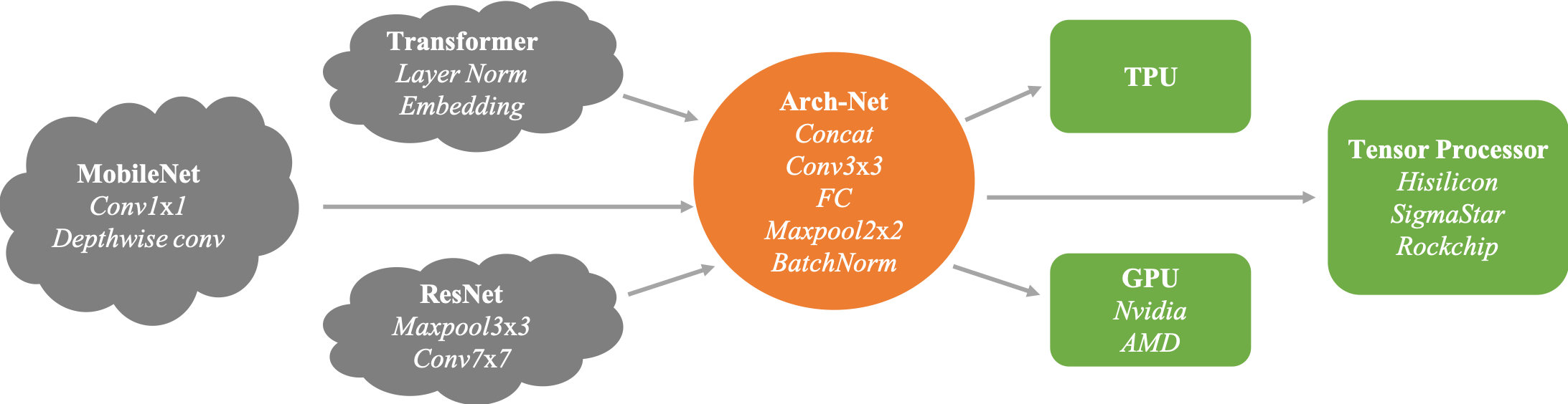
Figure 1: Overview of Arch-Net

Picking the core operator set of Arch-Net can be a challenging task given the plethora of Neural Architectures. Fortunately, the requirement of universal hardware support will make the candidate list very short in the first place. The question next is devising transformation rules to transform less common constructs into more mundane constructs. Thankfully, as the case with PReLU and LeakyRelu, many constructs do not differ during inference time. Further, with our Blockwise Distillation method enhanced by Residual Feature Adaption and Teacher Attention Mechanism, we significantly increase the range of constructs that can be eliminated. For example, Layer Normalization can be mimicked by Batch Normalization. Finally, we arrive at a core set made of only five operators, comprising of only Convolution, Fully-Connected, Max-Pooling, Batch Normalization and Concatenation (both Channelwise and Spatial).

The rest of the paper is organized as follows: Sect. 2 discusses some work related to our own. We introduce the composition and construction of Arch-Net in Sect. 3. Finally, we give the results of experiments in Sect. 4.

2 Related work

Knowledge Distillation Efforts have been made to transfer the learned knowledge from a large network to a smaller one by distillation since hinton2015distilling (1). Following hinton2015distilling (1), knowledge distillation methods focus on assimilating the logits distribution of the teacher and student network, by designing loss function hinton2015distilling (1), distillation strategy zhang2018deep (2, 3) or regularization cho2019efficacy (4). The intermediate features of the networks are then taken into consideration for better transferring the learned knowledge romero2014fitnets (5, 6, 7). There are also works delving into the relations between different features or data and forcing the student to mimic such relations yim2017gift (8, 9, 10). Works that combine at least two of the above ideas have succeeded in tasks including classification shen2020meal (11), object detection chen2017learning (12), semantic segmentation liu2019structured (13, 14) and natural language processing sanh2019distilbert (15, 16, 17). In our proposed method, the student network learns from the teacher’s logits and intermediate features.

Model Quantization Networks of low bit width are computation, memory and energy efficient and therefore hardware friendly. Model Quantization methods compress the networks by mapping the real numbers to a set of discrete ones during or after training. Quantization-aware Training (QAT) methods quantize the networks by uniform zhou2016dorefa (18, 19, 20) or nonuniform polino2018model (21, 22), fixed courbariaux2016binarized (23, 24) or learned choi2018learning (25, 26, 27) quantizers during training. Although these methods enable the networks as low as 1 bit width courbariaux2016binarized (23, 28) to have considerable classification or location performance, they require a similar training process as the training of floating-point networks, which is time and data consuming. It is worth mentioning that under some situations it is difficult to get all of the training data because of privacy concern. On the contrary, Post Training Quantization (PTQ) gholami2021survey (29) quantize the networks with a small calibration set of data sampled from the original training set banner2018aciq (30, 31) or generated by special data generation methods nagel2019data (32, 33). Recently, by introducing an optimizing or finetuning process hubara2020improving (34, 35, 36), PTQ methods succeed in quantizing networks into as low as 4 bit width with a little loss of accuracy. However, when the bit width is lower, these methods seem powerless or need to turn to mixed precision dong2019hawq (37, 38) for help. In addition, when the architectures of the networks are changed, PTQ methods become useless because no existing weights can be used for initialization or statistics. Compared to QAT and PTQ methods, our method enjoys the advantage of low bit width, less data, higher accuracy and architecture agnostic.

Knowledge Distillation and Model Quantization The combination of Knowledge Distillation and Model Quantization offers new ideas to model compression. With the help of distillation, the well learned knowledge of the floating-point networks can be transferred to the quantized ones. In mishra2017apprentice (39, 21), knowledge distillation is directly applied to training as low as 2W8A quantized networks. While in kim2019qkd (40), a three phases method is adopted to get as low as 3W3A quantization of ResNet with little loss of accuracy. However, the data problem is still remaining because these methods rely on large amount of data with ground truth. What’s more, these methods have not taken specific hardware constraints into consideration and therefore the quantized networks cannot be directly deployed in edge devices.

Table 1: The level of support of different chips or toolchains for basic units. ‘×’ represents lack of support; numbers of ‘+’ represents different levels of support; ‘?’ means that the authors cannot ascertain the level of support.

	layer norm	embedding	depthwise conv	conv 7×7	channels constraints	conv 3×3	batch norm	FC
Ethos-N Series	?	?	?	++	?	+++	+++	+++
Hi3559A	×	×	++	+	+	+++	+++	+++
MLU270-S4	×	×	?	++	+	+++	+++	+++
TensorRT	+	+	+	++	++	+++	+++	+++
Movidius SDK	?	?	+	+	+	+++	+++	+++
SSC336Q	×	×	?	++	++	+++	+++	+++
RK3568	×	×	+	+	+	+++	+++	+++

3 Arch-Net

In this section, we firstly present the hardware constraints and the core operator set we build, followed by the transformation, quantization and initialization details. The Blockwise Model Distillation, including the Residual Feature Adaptation, the Teacher Attention Mechanism and the distillation algorithm are presented in turn.

3.1 Hardware Constraints and Core Operator Set

We have investigated ASICs/SDK/Toolchain from different companies and summarize our findings in Table 1. Overall the chips and their toolchains fall behind the development of DNN and can hardly support less common DNN constructs, like Layer Normalization and Embedding Layer which gain popularity due to increasing interests in Transformers. In addition, only convolutions of some kernel sizes are well supported Ding_2021_CVPR (41). For example, we test the relative inference speed of common convolutions on SSC336Q chip from SigmaStar and found that 3×3 convolution is the most efficient (refer to Appendix A.2 for more details). In order to bridge the gap between different DNN’s and ASIC chips, we build the following core operator set, which contains only the well supported operators.

• 3×3 Convolution of stride 1 or 2: we use it to replace all of the other convolutions.

• 2x2 Max-pooling of stride 2: we use it replace all of the other max-pooling layers.

• Batch Normalization ioffe2015batch (42): we use it to replace Layer Normalization.

• Fully-Connected layer: we use it to replace the Embedding layer.

• We assume the limitation for channel number is 512 and split the channel when the number of input/output channels is larger than 512 (Figure 2).

• Concatenation + 3×3 convolution: we use it to replace the residual addition (Figure 2).

Based on this core operator set, we can transform the floating-point networks into simple ones, namely the Arch-Net. For example, we use three 3×3 convolutions to replace a 7×7 convolution. For the Layer Normalization (LN) in Transformer vaswani2017attention (43), we replace the it with Batch Normalization (BN) (Figure 3). To be specific, assuming the shape of the feature before the LN is $[B,W,D]$ (where $B$ is the batch size, $W$ is the number of words, and $D$ is hidden dimension), we permute it to be $[B,D,W,1]$ and feed it to the BN to get a output of shape $[B,D,W,1]$. The output is then quantized and permute back to the shape of $[B,W,D]$. For the embedding layer, it is intuitive to use a fully-connected layer to replace it. As a result, the input data of shape $[B,D]$ should be converted to one-hot form $[B,D,S]$, where $S$ is the vocabulary size. The other transformations details can be found in Appendix A.3.

We choose DoReFa-Net zhou2016dorefa (18) as the quantization method for classification tasks and LSQ esser2019learned (27) for machine translation tasks, to show the robustness of our method to different quantization methods. Before training, the Arch-Net will be initialized with the weights from the floating-point teacher. For the 3×3 convolutions that replace the 3×3 convolutions, we directly copy the floating-point weights for the student. For the 3×3 convolutions that replace the 1×1 convolutions, the floating-point weights are padded to 3×3 with zeros. The other operators that do not have corresponding weights are initialized randomly.

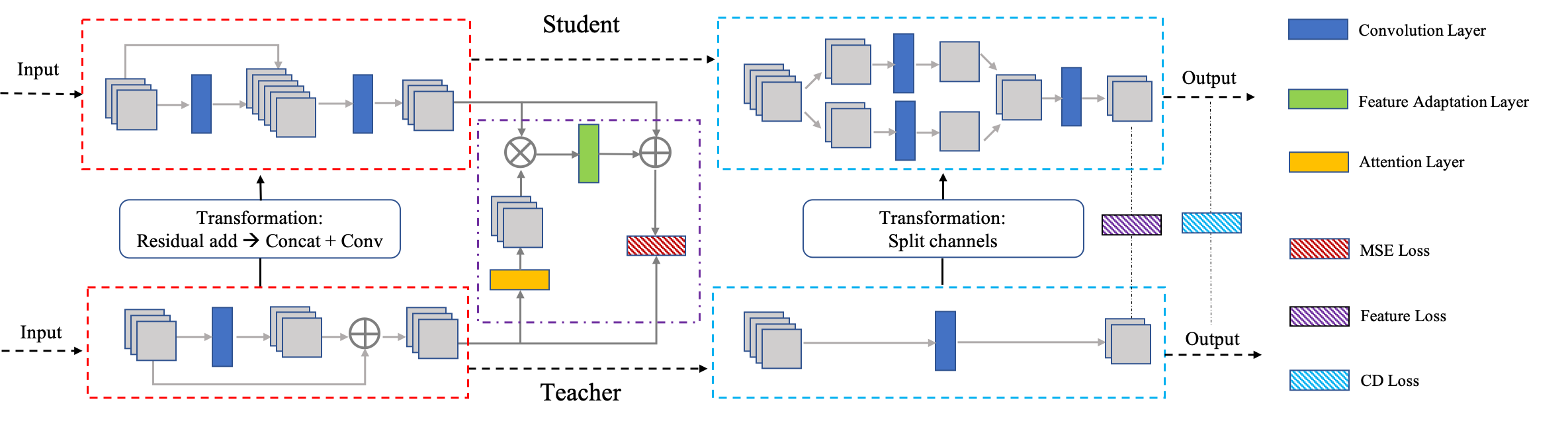
Figure 2: Arch-Net pipeline for image classification

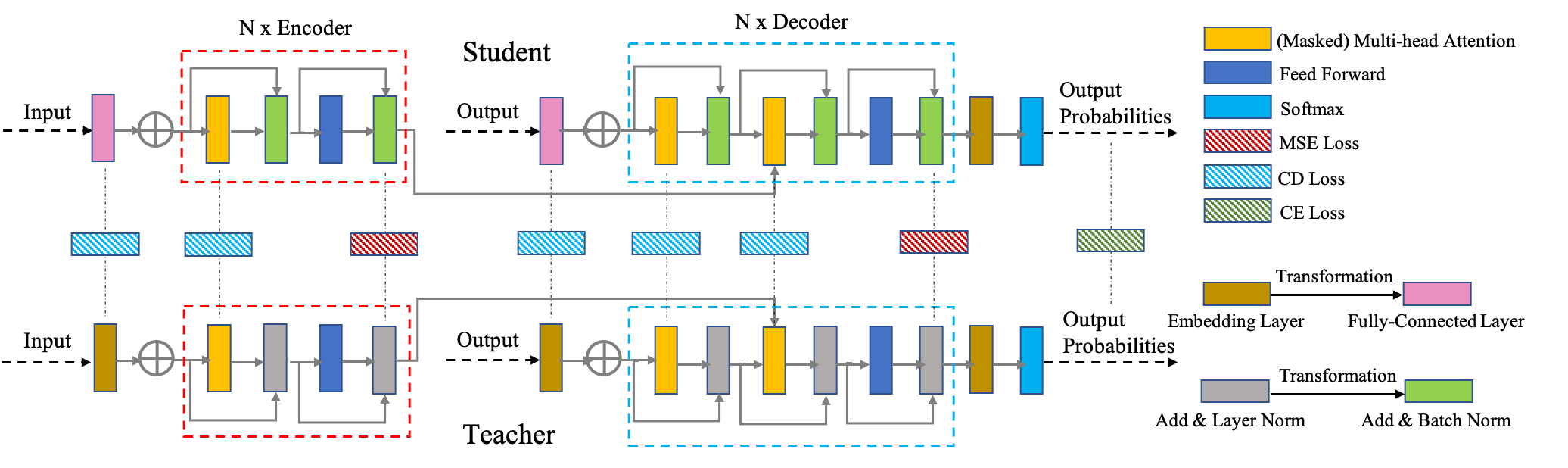
Figure 3: Arch-Net pipeline for machine translation

3.2 Blockwise Model Distillation

Algorithm Different from most of the knowledge distillation framework hinton2015distilling (1, 3, 9, 15, 16), we distill the network in a progressive and block-wise manner, which is architecture agnostic. Inspired by the Block Coordinate Descent algorithm tseng2001convergence (44), we divide the network into blocks, and optimize the student’s blocks stage by stage, by minimizing the outputs of the student’s and teacher’s blocks. The difference is that when optimize a block, the previous blocks are also optimized at the same time. We find that other frameworks does not work well when the architecture of the student network is changed and the bit width is low. We argue that it is because the network has not been well initialized although some of the floating-point weights from the teacher can be directly copied for the student. In addition, when the architecture is changed, no existing weights can be used for initialization. We therefore adopt this block-wise and progressive distillation framework for better initialization. The algorithm is shown in Algorithm 1.

ResNet and MobileNet Take ResNet18 as example. For the first 3 convolutional layers and the 2x2 max-pooling layer of the student, we put them together as $\mathit{block1}$ and force it to learn from the output feature of the $\mathit{block1}$ of the teacher, which consists of the first 7×7 convolutional layer and a 3×3 max-pooling layer. The above distillation procedure is referred as $\mathit{stage1}$. For each of the next stages but the last one, the block contains Convolution + BN + ReLU. For the last stage, we put the average pooling layer and the fully-connected layer together as one block. Starting from $\mathit{stage2}$, the weights of the student is loaded from the previous stage. The block-wise Distillation for MobileNet is similar to that for ResNet, except that there is no 7×7 convolution and max-pooling layer. For the last stage, we use the Cosine Distance as the objective function. For other stages, we use the Mean Square Error (MSE) between the two feature maps. As we want to focus on the distillation of the current block, we reduce the importance of the previous blocks by adding a weighting coefficient $\gamma\in(0,1)$. Assuming that there are $n$ stages, at stage $m$, the objective function is given as Equation (1).

$$\mathit{loss}=\sum_{i=1}^{m}\gamma^{m-i}\mathit{loss}_{i}$$ (1)

$$\text{where}\left\{\begin{array}[]{lr}\mathit{loss}_{i}=\text{MSE}(F_{S}^{i},F_{T}^{i}),&i\in[0,n-1]\\ \mathit{loss}_{i}=\text{D}_{\cos}(L_{S}^{i},L_{T}^{i}),&i=n\end{array}\right.$$ (4)

Where $F_{S}^{i}$ and $F_{T}^{i}$ are the output featuremaps, $L_{S}^{i}$ and $L_{T}^{i}$ are the output logits before softmax of the $i^{\text{th}}$ stage of the student and the teacher network, separately. It is worth mentioning that as we directly use the output logits of the teacher, no ground truth is needed.

Transformer Each encoder or decoder is one distillation block, and the last block contains the final projection layer. For each block except for the last block, we force the output of each BN in the student to assimilate that of each LN in the teacher and MSE is adopted as objective function. For the last block, we take the teacher’s predictions as hard label ($y_{\mathrm{hard}}$) so that the Cross Entropy (CE) loss can be used. Besides, the attention maps and the outputs of the embedding layer are also used for distillation, and the cosine distance is used here. The final objective function can be formulated as follows:

$$\mathit{loss}=\sum_{i=1}^{m}\gamma^{m-i}\mathit{loss}_{i}$$ (5)

$$\text{where}\left\{\begin{array}[]{lr}\mathit{loss}_{i}=\sum_{j}\text{MSE}(N_{S}^{ij},N_{T}^{ij})+\sum_{k}\text{ D}_{\cos}(A_{S}^{ik},A_{T}^{ik})+\text{D}_{\cos}(E_{S},E_{T}),&i\in[0,n-1]\\ \mathit{loss}_{i}=\text{CE}(L_{S}^{i},y_{\mathrm{hard}}),&i=n\end{array}\right.$$ (8)

Where $N_{S}$ and $N_{T}$ represent the outputs of the normalization layer of the student and the teacher, $A_{S}$ and $A_{T}$ are the attention maps, $E_{S}$ and $E_{T}$ are the outputs of the embedding layer, $i$ represents the $i^{\text{th}}$ distillation stage. As there are more than one LN and attention map in each block, we use $j$ and $k$ to represent the number. $L_{S}$ represents the final output of the student.

For image classification tasks, as there is already a well trained teacher, and the student inherits most of the teacher’s weights, we claim that a modest number of images is enough. For the whole distillation procedure, we randomly sample 30k images without ground truth from ImageNet russakovsky2015imagenet (45) training set. Besides, as the stages but the last stage are for better initialization, they require a smaller number of training epochs. In addition, for each epoch, we adopt a training strategy of randomly sampling a small number of images from the 30k images. Further details can be found in Section 4. Under this setting, the need of data is reduced and the training time is greatly shortened.

3.3 Residual Feature Adaptation and Teacher Attention Mechanism

The difficulty of the knowledge distillation between a floating-point teacher and a quantized student results from the fact that the output value range of these two networks is quite different. The quantization method we use clips the output value of the student into $[0,1]$, while the output value of the floating-point operator is much larger. This gap brings the difficulty for the student in mimicking the output distribution of the teacher. In works romero2014fitnets (5, 12) of distillation between two floating-point networks, several convolutional or fully-connected layers are adopted to map the features of the student to that of the teacher, including the mapping of sizes and latent representations. In Arch-Net, similar operation is adopted to map not only the latent representations, but also the output value range. We apply a Residual Feature Adaptation (RFA) block of 3 continuous floating-point convolutional (for ResNet/MobileNet) or fully-connected (for Transformer) layers plus a residual addition, without any batch normalization or non linearity, as shown in Figure 2. We find the residual addition important because the outputs of the feature adaptation blocks is not directly used for inference, and the auxiliary block-wise losses suffer from the vanishing gradient problem without it. By adding the student’s features to the output of the feature adaptation block, not only the value range, but also the latent representations of the teacher’s features can be better mimicked by the student. For ResNet and MobileNet, we add the Residual Feature Adaptation at the output of each block except for the first and the last block. For Transformer, we add it after each BN. The ablation studies in Section 4.4 show the importance of the residual additions. Floating-point operators are adopted here because they are able to better map the value ranges from fixed-point numbers to real numbers.

In addition to the Residual Feature Adaptation Block that helps the student to mimic the feature distribution of the teacher, we think it is also crucial for the student to learn the importance of each channel. It is intuitive that we can extract a series of weighting coefficients of the channel and feed them to the student. Following the attention mechanism in SENet hu2018squeeze (46), we feed the teacher’s features to a block of 2 fully-connected layers to get a sequence of channel weighting coefficients and then multiply these coefficients and the student’s feature. The output of the multiplication is then fed to the Feature Adaptation layers, as shown in Figure 3. As the weighting coefficients come from the teacher, we name it Teacher Attention Mechanism (TAM).

The RFA and the TAM bridge the gap between the quantized student and the floating-point teacher, enabling the student to learn from the distribution of the teacher’s features and the channel-wise relations. In addition, this two methods are applied only during the distillation, bringing no extra computational cost during inference time.

Algorithm 1 Blockwise Model Distillation.

0:    Floating-point teacher network $T_{f}$;Arch-Net $S_{q}$;Number of images for the whole distillation procedure $P_{total}$;Number of images sampled per epoch $P_{epoch}$;Number of stages $N$;Number of epochs for the last stage $E_{last}$;Number of epochs for the stages except for the last stage $E_{middle}$;

0:    Well trained Arch-Net $S_{q}$;

1:  Initialize $S_{q}$ with $T_{f}$, randomly sample $P_{total}$ images from the training set

2:  for $\mathit{Stage}=1,\cdots,N$ do

3:     for $\mathit{Epoch}=1,\cdots,E_{last}$ if $\mathit{Stage}==N$ else $E_{middle}$  do

4:        Randomly sample $P_{epoch}$

5:        Update $S_{q}$ by minimizing objective function (1) and (5)

6:     end for

7:  end for

8:  return  $S_{q}$;

4 Experiments

In this section, we perform experiments on ImageNet russakovsky2015imagenet (45) and Multi30k elliott2016multi30k (47) to evaluate the performance of our proposed method. Networks used in the experiments include ResNet18/34/50 he2016deep (48), MobileNet V1 howard2017mobilenets (49), MobileNet V2 sandler2018mobilenetv2 (50) for image classification task, and Transformer vaswani2017attention (43) for machine translation task. We show that the proposed Arch-Net is able to transform the previous floating-point networks into as low as 2W4A hardware-friendly Arch-Net with as low as 0.9% loss of accuracy for ImageNet classification tasks and no loss of BLEU score for machine translation tasks. Comprehensive ablation studies are also conducted to further investigate the proposed method.

4.1 Experiments Setup

We perform out experiments on NVIDIA Tesla V100 GPU in PyTorch. For the image classification task, we randomly sample 30k images from the original training set as our training sets. At each training epoch, we randomly sample 8192 images from our training set. For the machine translation task, we use the whole Multi30k dataset as our training set and we use all of the data at each training epoch. Multi30k is a small dataset while the vocabulary is relatively large, it will be helpful to use the whole training set.

The optimizer we use for the image classification task is Adam Diederik2015Adam (51) with a learning rate of 1e-3 and the learning rate scheduler is Cosine Annealing with Warm Restart loshchilov2016sgdr (52), that for the machine translation task is AdamW loshchilov2018decoupled (53) with the same learning rate and scheduler. For ResNet18/34/50, the number of epochs for the first stage is 500 (as the first stage contains three 3×3 convolutions that replace the 7×7 convolution, which is not initialized and needs more epochs), that for the last stage is 5110 (5110 is the convergence point of the learning rate scheduler we use) and that for the other stages is 60. For MobileNetV1/V2, the number of epochs for the last stage is 5110, that for the other stages is 60. For Transformer, the number of epochs for the middle stages is 6, and that for the last stage is 50. The source of the teacher networks can be found in Appendix A.4.

4.2 Results on ImageNet

We evaluate our proposed method on ImageNet dataset and the results are shown in Table 2. We firstly compare our method with the DoReFa-Net trained with the whole dataset, and trained with 30k images randomly sample from the whole dataset because we use DoReFa-Net as our quantization method. It is interesting that the results of QAT is worse than that of Arch-Net, even though the former method use the whole ImageNet dataset as training set while the latter use only 30k images without ground truth. We conclude that it reflects the positive influence of the knowledge distillation, where the well learned knowledge is transferred from the floating-point teacher to the quantized student. To be specific, for the reason of hardware-friendly, the structure of the student is greatly restricted. Therefore, without the diversity of the convolutional layers with different kernel sizes and without the residual addition which is helpful for training, it is difficult to train (QAT) a good student of low bit width (2W4A). On the contrary, knowledge distillation is able to empower this student, even with fewer data and even the structure of the student is greatly changed. For all of the students of these 5 floating-point networks, the loss of accuracy is less than 1.6%. For ResNet34, the loss of accuracy is only 0.9%. We attributes this gain to the Residual Feature Adaptation Block, Teacher Attention Mechanism and the Blockwise Distillation. Further analysis is provided in Section 4.4.

Table 2: Imagenet performance of Arch-Net.

Method	Bit width	Resnet18		Resnet34		Resnet50		Mobilenet V1		Mobilenet V2
		Top1	Top5	Top1	Top5	Top1	Top5	Top1	Top5	Top1	Top5
Teacher	32W32A	69.76	89.08	73.30	91.42	76.13	92.86	68.79	88.68	71.88	90.29
Dorefanet (30k)	2W4A	29.93	54.65	12.00	27.95	8.20	20.62	21.28	43.20	6.22	16.38
Dorefanet (whole)		67.19	87.68	67.46	87.78	66.82	87.59	64.36	86.06	59.89	82.77
Ours (30k)		68.77	88.66	72.40	91.01	74.56	92.39	67.29	88.07	69.09	89.13

In order to compare our method with other QAT and PTQ methods, we apply no previous transformations to the teachers but quantize them to 2W4A students based on DoReFa-Net, and then use the Blockwise Model Distillation to train the students. The architectures of the quantized students are therefore the same as that of the teachers, so that they are comparable to other QAT and PTQ methods. Here, we compare our method with QAT methods includes DoReFa-Net, LSQ esser2019learned (27), DSQ gong2019differentiable (20), QKD kim2019qkd (40) and PTQ method includes BRECQ li2021brecq (36), PWLQ fang2020post (54) and ZeroQ cai2017deep (19). As shown in Table 3, for ResNet, Arch-Net outperforms these methods by a big advantage. While for MobileNet, LSQ and DSQ have better performance. We argue that it is because they use the whole training set of ImageNet while we use only 30k. We show in Table 3 that when they use 30k images, the results are much worse. Besides, the quantization method we use, the DoReFa-Net is quite old that it also brings some loss of accuracy. On the whole, compared with the QAT methods, Arch-Net requires less data. Compared with other PTQ methods, Arch-Net enjoys a higher accuracy. Results of higher bit width are shown in Appendix A.5.

Table 3: Imagenet performance of different QAT and PTQ methods without transformations.

Bit Width	Method	ResNet18		ResNet34		ResNet50		MobileNet V1		MobileNet V2
		Top1	Top5	Top1	Top5	Top1	Top5	Top1	Top5	Top1	Top5
32W32A	Teacher	69.76	89.08	73.30	91.42	76.13	92.86	68.79	88.68	71.88	90.29
PTQ
2W4A	BRECQ	64.42	86.22	–	–	69.67	89.47	–	–	18.17	38.66
	PWLQ	19.31	38.95	27.01	48.75	27.90	43.28	–	–	–	–
	ZeroQ	0.13	0.51	0.09	0.48	0.10	0.51	–	–	0.09	0.52
QAT - whole training set
	DoReFa-Net	60.46	83.25	65.93	86.64	66.33	87.35	48.24	73.14	44.87	69.93
	LSQ	63.69	84.75	66.98	87.11	70.23	89.54	66.25	86.58	61.83	83.57
	DSQ	58.18	81.40	62.61	84.42	68.23	88.74	–	–	62.72	84.90
	QKD	64.48	85.68	68.76	88.08	69.39	88.52	–	–	41.21	66.08
QAT - 30k images
	LSQ	1.86	2.29	1.87	2.30	1.90	2.29	1.70	2.24	1.53	2.14
	DSQ	10.61	25.48	12.75	29.03	12.67	29.08	–	–	13.71	31.11
	QKD	23.90	56.37	23.49	56.21	31.04	65.78	–	–	1.83	3.80
	Ours	67.30	87.73	71.58	90.51	74.59	92.29	59.66	83.31	57.63	82.00

4.3 Results on Multi30k

The results are shown in Table 4. Here in the quantized Transformer, we do not replace the residual additions for the reason that there are fully-connected layers in Transformer, if we use concatenating layer + fully-connected layer to replace the residual addition, the computational overhead would be large. The results show that with LN and embedding layers replaced, quantized Arch-Net performs even better than the float teacher. We ascribe this to the initialization of the Blockwise Model Distillation and the alignment of the featuremaps and the output logits.

Table 4: Results on Multi30k

Networks	Bit Width	Task	BLEU	Task	BLEU
Transformer	32W32A	DE-EN	30.32	EN-DE	32.44
	8W8A		34.05		36.44
	4W4A		34.34		34.35
	2W4A		32.50		33.75

4.4 Ablation Study

Importance of the middle epochs in Blockwise Model Distillation (BMD) Is BMD necessary? Will it help to use more epochs for middle stages or harm to use less? As we mentioned above, the purpose of middle stage distillation is a better initialization. Here, we test different numbers of epochs for each middle stage (all stages but the first and the last), as shown in Figure 5(b). At the situation of curve $\text{0}^{\dagger}$ in the figure, the BMD turns to be an one-shot distillation, and the result turns out to be inferior. On the other hand, the result is much better when the numbers of epochs is non-zero, even if it’s as few as 10. It confirms our previous argument that the middle stages of the BMD are for better initialization. While when the initialization is done, more epochs for the middle stages will not bring more gain in accuracy.

Importance of Residual Feature Adaptation We directly remove the residual addition from the Residual Feature Adaptation block, and we also use only the BMD without any feature adaptations. The results are shown in Table 5. The residual addition helps the mapping of the teacher and the student’s featuremaps, especially when the data is not sufficient (trained with 1024 images per epoch). In addition, we count the distribution of the values of the featuremaps of the student and teacher in Figure 4, showing that the Residual Feature Adaptation is better at mapping the value range of the student’s featuremaps to that of the teacher’s.

Table 5: Comparison of the feature adaptation with/without residual addition. Take ResNet18 of 2W4A as example.

Feature Adaptation	Images Per Epoch	Top1	Top5	Images Per Epoch	Top1	Top5
w/ residual addition	1024	67.60	88.32	8192	68.77	88.66
w/o residual addition		65.41	87.47		68.52	87.44
None		62.43	85.96		64.09	86.49

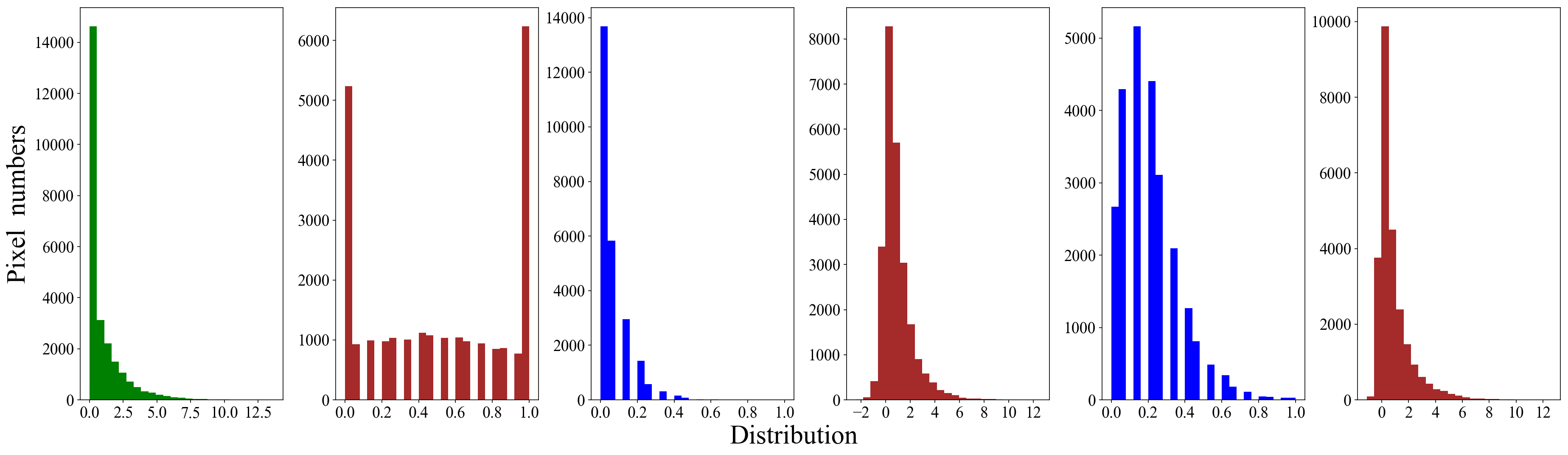
Figure 4: Comparison of the output distributions. Use 25th block of ResNet18 as an example. Left to right: teacher, student w/o feature adaptation, student before feature adaptation, student feature Adaptation, student before residual feature adaptation, student after residual feature adaptation.

Importance of Teacher Attention Mechanism (TAM) We find that the Teacher Attention Mechanism brings a slight increase in accuracy, and it is also helpful in helping the convergence of the student, as shown in Figure 5(a), reflecting the importance of the learning of channel-wise relation.

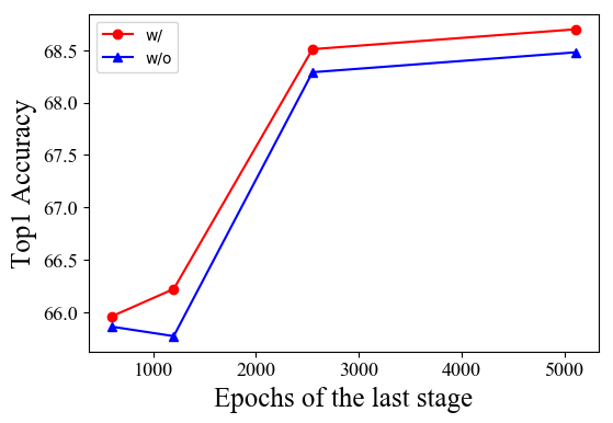
(a) Top1 Accuracy with/without TAM

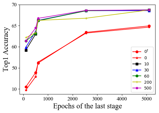
(b) Top1 Accuracy of different middle stage epochs

Figure 5: Comparison of Top1 Accuracy

5 Conclusion

In this paper, we propose Arch-Net to bridge the gap between Computer Architecture of ASIC chips and Neural Network Model Architectures, by transforming existing floating-point DNNs into hardware-friendly quantized Arch-Net, with bit-width as low as 2W4A. The structure of Arch-Net is constructed from the core operator set that consists of only five operators: 3×3 Convolutions, Batch Normalization, Concatenation, 2x2 Max-pooling, and Fully-Connected layers, which are so common, that they are often the least restricted and most efficient operators in the ASIC chips we tested. Labeled data is not required for the conversion to Arch-Net as we employ Blockwise Model Distillation on feature maps. Extensive experiments on image classification and machine translation tasks confirm that Arch-Net is both effective and data-efficient. For example, we are able to transform floating-point networks into 2W4A quantized ones with the loss of accuracy as low as 0.9% on ImageNet Classification tasks, and no loss of BLEU score on Multi30k.

Appendix A Appendix

A.1 Main Constraints of Popular ASIC Chips, SDK and Toolchains for Quantized Networks

We survey some of the popular ASIC chips, SDK and Toolchains for quantized networks and summarize in Table 6. As the public information is difficult to get, we summarize from what we can reach. This table is complementary to Table 1.

Table 6: Main constraints of popular ASIC/SDK/ToolChain for quantized networks.

Company	Type	Main Constraints
ARM	Ethos-N Series	Only support Int16 and Int 8
Hisilicon	Hi3559A	1. As low as Int8 and Uint8 are supported 2. The Number of channels in convolutional layers    is suggested to be the multiples of 32 3. Batch Normalization is suggested to be used as    normalization layer while Layer Normalization is not 4. Early Networks (VGG, Alexnet, etc.) are not    suggested to be used 5. Too many pooling layers among convolutional layers    will harm the networks’ performance
Cambricon	MLU270-S4	As low as Int4 is supported
Nvidia	TensorRT	As low as Int8 is supported
Intel	Movidius Neural Compute SDK	1. Group number of group convolutions needs to be    less than 1024 2. 5x5 convolution of stride 2 is not supported
SigmaStar	SSC336Q	1. Except for the first convolutional layer, the number    of input/output channels should be less than 2048 2. Depthwise convolutions: only kernel size of 3x3    is supported
Rockchip	RK3568	1. 3x3 Convolution is suggested to be used 2. Maxpooling: only 2x2 of stride 2 and 3x3 of stride 2    are supported

A.2 Speed Test on ASIC Chips

A.2.1 SSC336Q ASIC Chip

We use the SSC336Q chip from SigmaStar to test the speed of basic convolutions. Backbones with only one of certain basic convolution are set up. In order to run on the chip successfully, a low-calculation tail is added after backbones. We also use two 3x3 convolutions to replace the 5x5 convolution and three 3x3 convolutions to replace the 7x7 convolution, and keep the FLOPs similar as the original network. The running time on SSC336Q are shown in Table 7. It is clear that the inference speed of two 3x3 convolutions is faster than that of a single 5x5, and that of three 3x3 convolutions is faster than that of a single 7x7, which provides proof for the transformation we make in this paper.

Table 7: Inference speed of different convolutions on Sigmastar SSC336Q

Basic convolutions	1x1	3x3	5x5	two 3x3	7x7	three 3x3
Speed (ms)	0.691	0.906	2.370	1.670	3.889	2.538

A.2.2 Rockchip RK3568 ASIC Chip

We also carry out experiments on Rockchip RK3568 ASIC chip. Firstly, we choose VGG19 to verify the replacement of Max-pooling layer. We direcly replace the 2x2 Max-pooling layers in VGG19 with 3x3 Max-pooling layers test the inference speed. As shown in Table 8, VGG19 with 2x2 Max-pooling layers performs slightly better than that with 3x3 Max-pooling layers in inference speed and consumes less time in each Max-pooling Layer except for the last one.

Table 8: Inference speed of VGG19 on Rockchip RK3568

Max-pooling type	Bit width	Inference Speed (fps)	Time usage (ms) of each Max-pooling layer
			Layer1	Layer2	Layer3	Layer4	Layer5
2x2	8W8A	13.82	3.415	1.737	0.922	0.557	0.254
3x3		13.45	4.569	2.420	1.231	0.658	0.238

A.2.3 Inference Performance of Arch-Net on Different ASICs

We apply our transformations to Resnet18 and Mobilenet V2 to get the corresponding Arch-Net. We calculate the FLOPs (the number of Multiply-Adds) and compare the FLOPs per millisecond between the original networks and the Arch-Nets, under the situation of 8W8A, on different ASICs, including Sigmastar SSC336Q, Rockchip RK3568 and Nvidia Tesla T4. As shown in Table 9, the FLOPs per millisecond of Arch-Net is much better than the original networks .

Table 9: Inference performance of Arch-Net on different ASICs

	Networks	FLOPs (G)	SSC336Q		RK3568		Tesla T4
			Speed (ms)	FLOPs/ms	Speed (ms)	FLOPs/ms	Speed (ms)	FLOPs/ms
Resnet18	Original	1.82	15.68	0.116	18.52	0.098	0.81	2.236
	Arch-Net	5.89	38.11	0.154	41.67	0.141	1.52	3.836
MobilenetV2	Original	0.31	8.23	0.037	19.23	0.016	0.78	0.396
	Arch-Net	2.41	9.70	0.070	55.56	0.043	1.91	4.140

A.3 Transformations Details

For Resnet18/34/50, the 7x7 convolution of stride 2 in the first layer is replaced by three 3x3 convolutions, of which the 3rd convolution is of stride 2 and the others are of stride 1. All of the other 1x1 and 3x3 convolutions are replaced by 3x3 convolutions. Besides, the 3x3 max-pooling of stride 2 is replaced by a 2x2 max-pooling of stride 2. For each residual block, the residual add is replaced by a concatenating layer and a 3x3 convolution of stride 1. When the number of the channels of a featuremap (which is the input of a convolutional layer) is larger than 512, we split it into several featuremaps with channels smaller than or equal to 512, feed them to parallel branches, each of which consists of one 3x3 convolution, and then concatenate the output featuremaps to get a new featuremap that has the same number of channels as that before the split (Figure 2).

For Mobilenet V1 and Mobilenet V2, similar operations are performed. We replace the depthwise and pointwise convolutions with 3x3 convolutions. Residual adds in Mobilenet V2 are replaced by concatenating layers and 3x3 convolutions. Convolutions with number of channels that is large than 512 are split as what we do to Resnet.

For Transformer, except for the Layer Normalization, we use a fully connected layer to replace the embedding layer.

A.4 Source of the Teacher Networks

As for the teacher networks, we use the well trained ResNet18/34/50 and MobileNet V2 from Torchvision , and we train MobileNet V1 and Transformer ourselves based on codebase and codebase .

A.5 Results of Higher Bit Width on ImageNet

We have already proved the effectiveness of our method at 2W4A, here we show the results of our experiments of high bit width. It is intuitive that as the bit width becomes bigger, the transformed networks perform better.

Table 10: Imagenet performance of higher bit width, with transformations.

Method	Bit width	Resnet18		Resnet34		Resnet50		Mobilenet V1		Mobilenet V2
		Top1	Top5	Top1	Top5	Top1	Top5	Top1	Top5	Top1	Top5
Teacher	32W32A	69.76	89.08	73.30	91.42	76.13	92.86	68.79	88.68	71.88	90.29
Ours	4W4A	69.42	88.91	72.89	91.12	74.34	92.31	68.10	88.37	68.58	88.86
Ours	8W8A	69.58	89.11	73.00	91.22	75.09	92.53	68.59	88.67	69.28	89.95

When the transformation is not applied, we also applied our method at higher bit width. The results are appealing because we use only 30k images randomly sampled from the original training set, without ground truth.

Table 11: Imagenet performance of higher bit width, without transformations.

Method	Bit width	Resnet18		Resnet34		Resnet50		Mobilenet V1		Mobilenet V2
		Top1	Top5	Top1	Top5	Top1	Top5	Top1	Top5	Top1	Top5
Teacher	32W32A	69.76	89.08	73.30	91.42	76.13	92.86	68.79	88.68	71.88	90.29
Ours	4W4A	68.89	88.49	72.50	90.87	75.53	92.61	65.44	86.92	69.14	88.86
Ours	8W8A	69.50	88.88	73.08	91.20	75.84	92.81	68.36	88.61	71.46	90.23

A.6 How Does Concatenation + Convolution Affects?

We provide an optional transformation of replacing the residual add with the Concatenation + Convolution architecture and we carry out experiments on ImageNet. What if we apply the other transformations and keep the residual add? We experiment on Resnet18. As shown in Table 12, the quantization after the add operation brings a little loss of accuracy, while the replacement makes up for this loss, at the cost of the increase of computation expanse. On the whole, such a replacement is meaningful when an ASIC chip provides no native supports for the add operation.

Table 12: Comparison of the residual add and the concatenation + convolution.

Method	Bit width	Resnet18
		Top1	Top5
Teacher	32W32A	69.76	89.08
Residual Add	2W4A	67.90	88.14
Concat + Conv		68.77	88.66

References

- (1) Geoffrey Hinton, Oriol Vinyals and Jeff Dean “Distilling the knowledge in a neural network” In arXiv preprint arXiv:1503.02531, 2015
- (2) Ying Zhang, Tao Xiang, Timothy M Hospedales and Huchuan Lu “Deep mutual learning” In Proceedings of the IEEE Conference on Computer Vision and Pattern Recognition, 2018, pp. 4320–4328
- (3) Zhiqiang Shen, Zhankui He and Xiangyang Xue “Meal: Multi-model ensemble via adversarial learning” In Proceedings of the AAAI Conference on Artificial Intelligence, 2019, pp. 4886–4893
- (4) Jang Hyun Cho and Bharath Hariharan “On the efficacy of knowledge distillation” In Proceedings of the IEEE/CVF International Conference on Computer Vision, 2019, pp. 4794–4802
- (5) Adriana Romero et al. “FitNets: Hints for thin deep nets” In 3rd International Conference on Learning Representations, 2015
- (6) Sergey Zagoruyko and Nikos Komodakis “Paying more attention to attention: improving the performance of convolutional neural networks via attention transfer” In 5th International Conference on Learning Representations, 2017
- (7) Zehao Huang and Naiyan Wang “Like what you like: Knowledge distill via neuron selectivity transfer” In arXiv preprint arXiv:1707.01219, 2017
- (8) Junho Yim, Donggyu Joo, Jihoon Bae and Junmo Kim “A gift from knowledge distillation: Fast optimization, network minimization and transfer learning” In Proceedings of the IEEE Conference on Computer Vision and Pattern Recognition, 2017, pp. 4133–4141
- (9) Frederick Tung and Greg Mori “Similarity-preserving knowledge distillation” In Proceedings of the IEEE/CVF International Conference on Computer Vision, 2019, pp. 1365–1374
- (10) Wonpyo Park, Dongju Kim, Yan Lu and Minsu Cho “Relational knowledge distillation” In Proceedings of the IEEE/CVF Conference on Computer Vision and Pattern Recognition, 2019, pp. 3967–3976
- (11) Zhiqiang Shen and Marios Savvides “Meal v2: Boosting vanilla resnet-50 to 80%+ top-1 accuracy on imagenet without tricks” In arXiv preprint arXiv:2009.08453, 2020
- (12) Guobin Chen et al. “Learning efficient object detection models with knowledge distillation” In Proceedings of the 31st International Conference on Neural Information Processing Systems, 2017, pp. 742–751
- (13) Yifan Liu et al. “Structured knowledge distillation for semantic segmentation” In Proceedings of the IEEE/CVF Conference on Computer Vision and Pattern Recognition, 2019, pp. 2604–2613
- (14) Yifan Liu, Changyong Shun, Jingdong Wang and Chunhua Shen “Structured knowledge distillation for dense prediction” In arXiv preprint arXiv:1903.04197, 2019
- (15) Victor Sanh, Lysandre Debut, Julien Chaumond and Thomas Wolf “DistilBERT, a distilled version of BERT: smaller, faster, cheaper and lighter” In arXiv preprint arXiv:1910.01108, 2019
- (16) Wenhui Wang et al. “Minilm: Deep self-attention distillation for task-agnostic compression of pre-trained transformers” In arXiv preprint arXiv:2002.10957, 2020
- (17) Xiaoqi Jiao et al. “TinyBERT: Distilling BERT for natural language understanding” In Findings of the Association for Computational Linguistics: EMNLP 2020, 2020, pp. 4163–4174
- (18) Shuchang Zhou et al. “Dorefa-net: training low bitwidth convolutional neural networks with low bitwidth gradients” In arXiv preprint arXiv:1606.06160, 2016
- (19) Zhaowei Cai, Xiaodong He, Jian Sun and Nuno Vasconcelos “Deep learning with low precision by half-wave gaussian quantization” In Proceedings of the IEEE Conference on Computer Vision and Pattern Recognition, 2017, pp. 5918–5926
- (20) Ruihao Gong et al. “Differentiable soft quantization: Bridging full-precision and low-bit neural networks” In Proceedings of the IEEE/CVF International Conference on Computer Vision, 2019, pp. 4852–4861
- (21) Antonio Polino, Razvan Pascanu and Dan Alistarh “Model compression via distillation and quantization” In 6th International Conference on Learning Representations, 2018
- (22) Chenzhuo Zhu, Song Han, Huizi Mao and William J. Dally “Trained ternary quantization” In 5th International Conference on Learning Representations, 2017
- (23) Matthieu Courbariaux et al. “Binarized neural networks: Training deep neural networks with weights and activations constrained to+ 1 or-1” In arXiv preprint arXiv:1602.02830, 2016
- (24) Steven K Esser et al. “Convolutional networks for fast, energy-efficient neuromorphic computing” In Proceedings of the National Academy of Sciences 113.41, 2016, pp. 11441–11446
- (25) Yoojin Choi, Mostafa El-Khamy and Jungwon Lee “Learning low precision deep neural networks through regularization” In arXiv preprint arXiv:1809.00095 2, 2018
- (26) Jungwook Choi et al. “Pact: Parameterized clipping activation for quantized neural networks” In arXiv preprint arXiv:1805.06085, 2018
- (27) Steven K. Esser et al. “Learned step size quantization” In 8th International Conference on Learning Representations, 2020
- (28) Mohammad Rastegari, Vicente Ordonez, Joseph Redmon and Ali Farhadi “Xnor-net: Imagenet classification using binary convolutional neural networks” In European Conference on Computer Vision, 2016, pp. 525–542
- (29) Amir Gholami et al. “A Survey of Quantization Methods for Efficient Neural Network Inference” In arXiv preprint arXiv:2103.13630, 2021
- (30) R. Banner, Yury Nahshan, E. Hoffer and Daniel Soudry “ACIQ: Analytical Clipping for Integer Quantization of neural networks” In arXiv preprint arXiv:1810.05723, 2018
- (31) Ritchie Zhao et al. “Improving neural network quantization without retraining using outlier channel splitting” In International Conference on Machine Learning, 2019, pp. 7543–7552
- (32) Markus Nagel, Mart van Baalen, Tijmen Blankevoort and Max Welling “Data-free quantization through weight equalization and bias correction” In Proceedings of the IEEE/CVF International Conference on Computer Vision, 2019, pp. 1325–1334
- (33) Xiangguo Zhang et al. “Diversifying sample generation for accurate data-Free quantization” In arXiv preprint arXiv:2103.01049, 2021
- (34) Itay Hubara et al. “Improving post training neural quantization: Layer-wise calibration and integer programming” In arXiv preprint arXiv:2006.10518, 2020
- (35) Markus Nagel et al. “Up or down? adaptive rounding for post-training quantization” In International Conference on Machine Learning, 2020, pp. 7197–7206
- (36) Yuhang Li et al. “BRECQ: Pushing the Limit of Post-Training Quantization by Block Reconstruction” In arXiv preprint arXiv:2102.05426, 2021
- (37) Zhen Dong et al. “Hawq: Hessian aware quantization of neural networks with mixed-precision” In Proceedings of the IEEE/CVF International Conference on Computer Vision, 2019, pp. 293–302
- (38) Zhen Dong et al. “HAWQ-V2: Hessian aware trace-weighted quantization of neural networks” In Proceedings of the 33st International Conference on Neural Information Processing Systems, 2020
- (39) Asit K. Mishra and Debbie Marr “Apprentice: Using knowledge distillation techniques to improve low-precision network accuracy” In 6th International Conference on Learning Representations, 2018
- (40) Jangho Kim et al. “Qkd: Quantization-aware knowledge distillation” In arXiv preprint arXiv:1911.12491, 2019
- (41) Xiaohan Ding et al. “RepVGG: Making VGG-Style ConvNets Great Again” In Proceedings of the IEEE/CVF Conference on Computer Vision and Pattern Recognition (CVPR), 2021, pp. 13733–13742
- (42) Sergey Ioffe and Christian Szegedy “Batch normalization: Accelerating deep network training by reducing internal covariate shift” In International Conference on Machine Learning, 2015, pp. 448–456
- (43) Ashish Vaswani et al. “Attention is all you need” In Proceedings of the 30st International Conference on Neural Information Processing Systems, 2017, pp. 5998–6008
- (44) Paul Tseng “Convergence of a block coordinate descent method for nondifferentiable minimization” In Journal of Optimization Theory and Applications 109.3 Springer, 2001, pp. 475–494
- (45) Olga Russakovsky et al. “Imagenet large scale visual recognition challenge” In International Journal of Computer Vision 115.3 Springer, 2015, pp. 211–252
- (46) Jie Hu, Li Shen and Gang Sun “Squeeze-and-excitation networks” In Proceedings of the IEEE Conference on Computer Vision and Pattern Recognition, 2018, pp. 7132–7141
- (47) Desmond Elliott, Stella Frank, Khalil Sima’an and Lucia Specia “Multi30K: Multilingual English-German image descriptions” In Proceedings of the 5th Workshop on Vision and Language, 2016, pp. 70–74
- (48) Kaiming He, Xiangyu Zhang, Shaoqing Ren and Jian Sun “Deep residual learning for image recognition” In Proceedings of the IEEE Conference on Computer Vision and Pattern Recognition, 2016, pp. 770–778
- (49) Andrew G Howard et al. “Mobilenets: Efficient convolutional neural networks for mobile vision applications” In arXiv preprint arXiv:1704.04861, 2017
- (50) Mark Sandler et al. “Mobilenetv2: Inverted residuals and linear bottlenecks” In Proceedings of the IEEE Conference on Computer Vision and Pattern Recognition, 2018, pp. 4510–4520
- (51) Diederik P. Kingma and Jimmy Ba “Adam: A Method for Stochastic Optimization” In 3rd International Conference on Learning Representations, ICLR 2015, San Diego, CA, USA, May 7-9, 2015, Conference Track Proceedings, 2015
- (52) Ilya Loshchilov and Frank Hutter “SGDR: Stochastic gradient descent with warm restarts” In 5th International Conference on Learning Representations, 2017
- (53) Ilya Loshchilov and Frank Hutter “Decoupled Weight Decay Regularization” In International Conference on Learning Representations, 2019
- (54) Jun Fang et al. “Post-training piecewise linear quantization for deep neural networks” In European Conference on Computer Vision, 2020, pp. 69–86