Kinematic properties of white dwarfs

Abstract

Context. Both kinematic and chemical tagging of stellar populations have revealed a great deal of information on the past and recent history of the Milky Way, including its formation history, merger events, and mixing of populations across the Galactic disk and halo.

Aims. We present the first detailed 3D kinematic analysis of a sample of 3133 white dwarfs that use Gaia astrometry plus radial velocities, which were measured either by Gaia or by ground based spectroscopic observations. The sample includes either isolated white dwarfs that have direct radial velocity measurements, or white dwarfs that belong to common proper motion pairs that contain nondegenerate companions with available radial velocities. A subset of common proper motion pairs also have metal abundances that have been measured by large scale spectroscopic surveys or by our own follow-up observations.

Methods. We used the white dwarfs as astrophysical clocks, by determining their masses and total ages via interpolation with dedicated evolutionary models. We also used the nondegenerate companions in common proper motions to chemically tag of the population. Combining accurate radial velocities with Gaia astrometry and proper motions, we derived the velocity components of our sample in the Galactic rest frame and their Galactic orbital parameters.

Results. The sample is mostly located within $\sim$300 pc from the Sun. It contains predominantly (90–95 %) thin-disk stars with close-to-circular Galactic orbits, while the remaining 5–10 % of stars have more eccentric trajectories and belong to the thick disk. We identified seven isolated white dwarfs and two common proper motion pairs as halo members. We determined the age – velocity dispersion relation for the thin-disk members, which agrees with previous results that were achieved from different white dwarf samples without published radial velocities. The age – velocity dispersion relation shows signatures of dynamical heating and saturation after 4–6 Gyr. We observed a mild anti-correlation between [Fe/H] and the radial component of the average – velocity dispersion, showing that dynamical mixing of populations takes place in the Galactic disk, as was detected via the analysis of other samples of FGK stars.

Conclusions. We have shown that a white dwarf sample with accurate 3D kinematics and well-measured chemical compositions enables a wider understanding of their population in the solar neighborhood and its connection with the Galactic chemodynamics. The legacy of existing spectroscopic surveys will be boosted by the availability of upcoming larger samples of white dwarfs and common proper motion pairs with more uniform high-quality data.

1 Introduction

Our Galaxy, the Milky Way, is a dynamic ensemble of stars, gas, dust, and dark matter. Its complexity is enhanced by the mixing of its components through the Galactic potential (Sellwood & Binney, 2002) or by recent and past interactions with satellite galaxies (Antoja et al., 2018; Helmi et al., 2018; Belokurov et al., 2018). In the current era of large spectroscopic surveys, such as the Radial Velocity Experiment (RAVE; Steinmetz et al., 2006), the Large Sky Area Multi-Object Fiber Spectroscopic Telescope (LAMOST; Deng et al., 2012), the Galactic Archaeology with HERMES (GALAH; De Silva et al., 2015), the Gaia-ESO survey (Randich et al., 2013), and the Apache Point Observatory Galactic Evolution Experiment (APOGEE; Majewski et al., 2017), our advantage point from the inside of the Milky Way favors a direct analysis of stellar populations. This favorable perspective has been enabling key understanding of the correlations among location, kinematics, metallicity, and stellar ages, via the analysis of hundreds to several thousands spectra (Bland-Hawthorn & Gerhard, 2016, and references therein). These large spectroscopic databases have contributed to identifying metallicity gradients along the galactocentric radius and vertical height above the plane, or detailed information on stellar orbits in the Galactic disk and halo (Boeche et al., 2013; Bergemann et al., 2014; Hayden et al., 2020). With increasing distance from the plane, increasing numbers of metal-poor stars are found that also posses enhanced abundances of $\alpha$-elements (Mg, Si, Ca, Ti) with respect to Fe. This leads to the commonly adopted distinction in thin and thick components of the Galactic disk (Hayden et al., 2015; Bland-Hawthorn et al., 2019). The observed differences in abundance patterns of Galactic populations are interpreted as the signature of sequential enrichment of the interstellar medium with the ejecta of core-collapse and thermonuclear supernovae, which occur with different timescales and leave their traces in the atmospheres of present-day stars (Matteucci & Recchi, 2001). Even the solar neighborhood contains mix of stars that have likely formed in situ or migrated from the inner Galaxy (Navarro et al., 2011; Adibekyan et al., 2011). The kinematic analysis of metal-rich or metal-poor and $\alpha$-enhanced or -depleted populations indicates that different mechanisms take place in the Galactic disk, such as secular heating (i.e., an increased velocity dispersion in the radial or vertical directions; Dehnen & Binney, 1998; Aumer & Binney, 2009; Aumer et al., 2016) and radial mixing (migration and blurring of Galactic orbits for stars that were born at different galactocentric radii; Schönrich & Binney, 2009; Minchev et al., 2018; Hayden et al., 2018).

Table 1: Selection criteria adopted for the identification of white dwarf candidates and common proper motion companions.

Quality cuts applied to white dwarfs and common proper motion companions

$\varpi>0$ AND $\sigma_{\varpi}/\varpi\leq 0.2$ AND visibility_periods_used $>10$

phot_bp_mean_mag $<20.5$ AND phot_bp_mean_flux_over_error $>10$

phot_rp_mean_mag $<20$ AND phot_rp_mean_flux_over_error $>10$

$\beta<0.1$ AND $|C*|\leq 5\,\sigma_{C^{*}}(G)$ AND fidelity $>0.5$ AND ruwe $<$ max($\overline{\texttt{ruwe}}$ + $\sigma_{\texttt{ruwe}}$, 1.4)

White dwarf color-magnitude cuts

$G+5-5\times\log{(1000/\varpi)}>9\times(G-G_{\rm RP})-3\times(G-G_{\rm RP})^{2}-0.9\times(G-G_{\rm RP})^{3}+(G-G_{\rm RP})^{4}+8.5$

$G+5-5\times\log{(1000/\varpi)}>6\times(G_{\rm BP}-G_{\rm RP})-0.9\times(G_{\rm BP}-G_{\rm RP})^{2}-0.9\times(G_{\rm BP}-G_{\rm RP})^{3}+0.35\times(G_{\rm BP}-G_{\rm RP})^{4}+8.5$

$G-G_{\rm RP}<0.9$ AND $G_{\rm BP}-G_{\rm RP}<1.9$

Notes: $\beta$ and $C^{*}$ are defined by Riello et al. (2021).

In this dynamic context, white dwarfs can play a prominent role because they are the end products of low- to intermediate-mass stars ($<10$ M_⊙; Doherty et al., 2017; Cummings et al., 2018) and are ubiquitous in the stellar populations of all ages in the Galactic disk and halo, even 100 pc away from the Sun (Torres et al., 2021). Although white dwarfs can potentially trace the kinematics of both the youngest and oldest stellar population because of their billion year long cooling times and their reliability as astrophysical clocks (Althaus et al., 2010), their use for such studies is typically hindered by some of their physical properties. First, white dwarfs only “superficially” lose the memory of the chemical make up of their progenitors because all the elements that are heavier than hydrogen or helium sink in their interiors as a result of their strong gravitational field (Schatzman, 1945). Second, measuring precise and accurate radial velocities of white dwarfs from their pressure-broadened lines is a difficult endeavor that is complicated by the intrinsic redshift of spectral lines due to the gravitational field of white dwarfs (e.g. Greenstein et al., 1977; Schulz, 1977). Various attempts have been made to overcome the problem of the missing radial velocity in various ways (Oppenheimer et al., 2001; Reid et al., 2001; Sion et al., 2014; Rowell & Kilic, 2019; Torres et al., 2021). Some of the earliest works that included radial velocities of hydrogen-atmosphere (DA spectral type) white dwarfs contained small samples of stars that were used to determine the average gravitational redshift and the dispersion of the Galactic velocity components (Trimble & Greenstein, 1972; Wegner, 1974). Another way to study the kinematics of white dwarfs relies on studying those that belong to common proper motion pairs because the systemic radial velocity can be more easily estimated from the nondegenerate companions (Wegner, 1981; Silvestri et al., 2001). However, as a result of the lack of accurate radial velocities, one of the largest sample of white dwarfs that satisfies these requirements came from the ESO supernova type Ia progenitor survey (SPY; Napiwotzki et al., 2020). Out of this sample, 634 DA white dwarfs were categorized in thin and thick disk or halo members in an attempt to estimate the white dwarf contribution to baryonic dark matter (Pauli et al., 2006; Richter et al., 2007; Dimpel, 2018). More recently, a larger sample of 20 247 DA white dwarfs from the Sloan Digital Sky Survey (SDSS) Data Release 12 was thoroughly investigated by Anguiano et al. (2017), who measured their radial velocities. These authors detected the existence of a mean Galactic radial velocity gradient and an additional source of dynamical heating from the analysis of the age – velocity dispersion relation, with respect to the prediction for the secular evolution of the Galactic disk. Later attempts at finding correlations among white dwarf masses, kinematics, and ages found that the most massive white dwarfs have the smallest velocity dispersion, thus appearing to have experienced less dynamical interactions because their lifetimes are shorter (Wegg & Phinney, 2012). More recent work by Cheng et al. (2020) has suggested that the kinematics of massive white dwarfs may carry the imprint of past binary mergers. A significant fraction of massive white dwarfs have a larger velocity dispersion according to this and are therefore older than they appear.

In this paper, we expand the previous kinematic analysis of isolated white dwarfs that we complement with common proper motion pairs that contain white dwarfs and nondegenerate companions that have radial velocity and metallicity measurements. Combining radial velocities with the astrometric data of the European Space Agency Gaia mission (Gaia Collaboration et al., 2016) for the first time, we analyze the full 3D kinematics and derive the Galactic orbital parameters of the sample of isolated white dwarfs and common proper motion pairs. Hence, we analyze their correlations with the white dwarf ages and the chemical composition of their nondegenerate companions. We also discuss a few peculiar systems. Finally, we determine the age – velocity dispersion for these white dwarfs by comparing our results to previous measurements.

2 Sample selection

2.1 Isolated white dwarfs with radial velocity measurements

Figure 1: Hertzsprung-Russel diagrams of our selected white dwarfs with radial velocity measurements (top panel) and the Gaia-selected common proper motion pairs (bottom panel). The cooling tracks for He-, CO-, and ONe-core white dwarfs (Althaus et al., 2013; Camisassa et al., 2016, 2019) and the isochrones are shown. The the corresponding masses and ages are labeled in the top panel, for clarity. The solar metallicity BaSTI isochrones with [Fe/H] $=0.06$ (blue curves; Hidalgo et al., 2018) and $\alpha$-enhancement (orange curves; Pietrinferni et al., 2021) are plotted at 1 and 10 Gyr (dashed and solid curves, respectively).

Our first sample consisted of single white dwarfs that have radial velocity measurements. We cross-matched the latest release of SPY (Napiwotzki et al., 2020), which contains 643 DA white dwarfs, and the sample of 20 247 DA white dwarfs from SDSS (Anguiano et al., 2017) with the Early Data Release 3 of Gaia (EDR3; Gaia Collaboration et al., 2021). We performed our cross-match via the TAP service implemented by the command-line tool, stilts (Taylor, 2006), requesting that parallaxes are strictly positive and are measured with a precision of 20 % ($\varpi>0$ and $\sigma_{\varpi}/\varpi<0.2$), and imposing additional quality cuts that are listed in Table 1. Moreover, we cleaned our selection by requesting that our sources are minimally affected by blending, that is, they have the parameter $\beta<0.1$ (as defined by Riello et al., 2021). We removed the most likely spurious astrometric solutions (fidelity $>0.5$; Rybizki et al., 2021), and imposed a 5$\sigma$ cut on the corrected BP and RP flux excess ($C^{*}$; Riello et al., 2021). As an additional safety measure, we also applied a cut on the renormalized unit weight error (ruwe; Lindegren, 2018) as defined in Table 1. Finally, we collected the geometric distance estimates (Bailer-Jones et al., 2021) for all identified objects. In addition, we removed from the cross-match all the SPY white dwarfs that either are identified as spectroscopic binaries, have other peculiarities, or have problematic data; we also excluded the SDSS white dwarfs with signal-to-noise ratio (S/N) lower than 20 and radial velocity errors larger than 10 km s^-1. The result of this cross-match produced 484 white dwarfs with SPY spectra and 1641 white dwarfs with SDSS DR12 spectra; 48 stars are in common in the two surveys. As shown in the Gaia Hertzsprung-Russell (HR) diagram (top panel of Fig 1), the selected objects encompass the full range of white dwarf masses and a wide spread of cooling ages up to 5 Gyr, although the majority of them are intrinsically bright white dwarfs younger than 0.3 Gyr. The Gaia source identifiers, photometry, and geometric distances of the selected white dwarfs are listed in Table 2. The full table is available at the CDS.

Because it is important for our kinematic study, we note that radial velocities of the SPY and SDSS white dwarfs were measured with two different techniques. On the one hand, Napiwotzki et al. (2020) performed Gaussian fits to the narrow H$\alpha$ and H$\beta$ line cores of SPY white dwarfs (a description of the procedure is detailed in Sect. 3 and Appendix A of Napiwotzki et al., 2020), with the goal of avoiding the pressure shifts and asymmetries due to nonlinear effects in the wings of the strongly Stark-broadened Balmer lines (Halenka et al., 2015, and references therein). On the other hand, Anguiano et al. (2017) used the cross-correlation method employing the entire spectra of SDSS white dwarfs. The two samples contain 48 white dwarfs in common. We compare the radial velocities in Fig 2. The SDSS measurements show an average difference of $+15\pm 13$ km s^-1 with respect to the SPY results. Because the high-resolution SPY sample is better suited for accurate and precise radial velocity measurements, we corrected the SDSS sample for the average offset, and we used the SPY measurements when a star was observed by both surveys.

Table 2: System identifiers in this paper, Gaia identifiers, photometry, and distances of isolated white dwarfs and common proper motion pairs.

System	Gaia EDR3	$G$ [mag]	$G_{\rm BP}$ [mag]	$G_{\rm RP}$ [mag]	$d$ [pc]	Gaia EDR3	$G$ [mag]	$G_{\rm BP}$ [mag]	$G_{\rm RP}$ [mag]	$d$ [pc]
White dwarfs						nondegenerate companions
0001	152935195517952	$17.98$	$18.00$	$18.00$	225
0002	288175125714560	$17.47$	$17.49$	$17.52$	153
.
3148	6907694553263596672	$19.54$	$19.68$	$19.39$	206	6907694690702552576	$13.52$	$14.11$	$12.79$	223
3149	6910805342238827648	$16.37$	$16.28$	$16.59$	158	6910806102448648576	$14.85$	$15.88$	$13.84$	156
3150	6910816513450124288	$17.40$	$17.30$	$17.60$	357
3151	6917473674103954560	$17.53$	$17.69$	$17.24$	75
Notes The full table is available at the CDS. The system number is used as short identifier throughout the paper.

2.2 Common proper motion pairs

Figure 2: Radial velocity comparison for 48 isolated white dwarfs that have been observed by Anguiano et al. (2017) and Napiwotzki et al. (2020). The dashed lines correspond to the equality and a $\pm 10$ km s^-1 radial velocity offset.

The second sample consisted of common proper motion pairs containing white dwarfs and nondegenerate companions that have radial velocity measurements. In order to identify the common proper motion pairs, we began by selecting white dwarf candidates following the methods of Gentile Fusillo et al. (2021), and applying the color- and magnitude-cuts in proximity of the white dwarf cooling sequence in the Gaia EDR3 HR diagram as well as the quality cuts given in Table 1. The resulting query consisted of 168 247 white dwarf candidates.

The identification of common proper motion pairs drew from the recent work of El-Badry et al. (2021), but we used our initial selection of white dwarfs for identifying mutual pairs and nondegenerate companions in the full Gaia EDR3. In contrast with El-Badry et al. (2021), we searched for common proper motion pairs with maximum projected separations of $s\leq 0.5\times 10^{6}$ au and a projected orbital-velocity difference of $\Delta\varv_{\rm orbit}\leq 2.7\times(s\,[{\rm au}]/1000)^{-1/2}$ km s^-1, as it is computed for a total binary mass of $\sim$8.5 M_⊙. We applied the quality cuts of Table 1 to the selection of common proper motion companions, and we cleaned the resulting sample from possible members of open clusters by removing the stars that match the astrometric parameters of those characterized by Cantat-Gaudin & Anders (2020). The resulting sample contains 7256 systems, 40 of which are resolved triple systems containing two nondegenerate stars and six are triplets containing two white dwarfs. These systems are excluded from further analysis because they may have had higher chances of past interactions that affected their evolution (Toonen et al., 2020). As for the single white dwarf sample, we collected the geometric distance estimates for all the identified pairs.

2.3 Companion stars with radial velocity measurements

Among the common proper motion pairs, we identified 976 systems for which the nondegenerate stars have reliable velocity measurements in the Second Data Release of Gaia (DR2; Gaia Collaboration et al., 2018), based on their number of measurements (dr2_rv_nb_transits > 5) and the absence of brighter neighbors within 10 arcsec (reflecting stricter quality criteria than advised by Boubert et al., 2019). This sample includes two double-degenerate binaries with a nondegenerate companion each, and one system containing one white dwarf and two nondegenerate companions that have very similar radial velocities.

Subsequently, we searched for nondegenerate companion stars that may also have been observed by other spectroscopic surveys by cross-matching our sample with the RAVE DR5 (Kunder et al., 2017), LAMOST DR5 (Luo et al., 2019; Xiang et al., 2019), APOGEE DR16 (Jönsson et al., 2020), and GALAH+ DR3 (Buder et al., 2021). Hence, we selected only those stars having iron abundances, [Fe/H], which is a proxy for stellar metallicity, and $\alpha$-element abundances, [$\alpha$/Fe], which is a measure of the chemical nucleosynthetic evolution. The selected data satisfy the quality criteria defined in the relevant references; when more than one spectrum was available for a star in given survey, we chose the best quality observation. The correlation between [Fe/H] and [$\alpha$/Fe] of this sample will be discussed in Sect. 4 because it is relevant for the interpretation of the results. In Table 3 we list the numbers of spectra identified in each survey and the corresponding selection criteria. Finally, we added 61 common proper motion pairs to this sample that have spectra for their nondegenerate companions that were analyzed by Rebassa-Mansergas et al. (2021), hereafter shortened to RM+2021 in figures and tables. The selected stars have spectra with a S/N $>20$ and [Fe/H] measurements. For 48 of these stars we measured radial velocities, and the remaining 13 have reliable Gaia DR2 measurements.

Table 3: Results of our cross-match with spectroscopic surveys for the nondegenerate companions.

Catalogu	Quality criteria	Selected
Gaia	dr2_rv_nb_transits ¿ 5, no bright neighbor	976
RAVE	QK = 0, c1 = c2 = c3 = n	68
LAMOST	S/N ¿ 20	113
APOGEE	Eflag = 0, Aflag = 0	37
GALAH+	flag_sp = 0, flag_fe_h = 0	51

Table 4: Element abundances and radial velocities of the Gaia-selected common proper motion pairs.

System	Survey	[Fe/H]	[$\alpha$/Fe]	$\varv_{\rm rad}$ [km s-1](1)	$\varv_{\rm rad}$ [km s-1](2)
0011	CPMP				$+32.3\,\pm\,1.7$
0020	GALAH+	$+0.03\pm 0.10$	$+0.06\pm 0.07$	$-11.3\,\pm\,0.1$
.
3146	RAVE	$-0.22\pm 0.20$	$+0.14\pm 0.20$	$-23.9\,\pm\,0.9$	$-24.2\,\pm\,0.3$
3148	CPMP				$+32.3\,\pm\,4.9$
Notes. The full table is available at the CDS.
CPMP indicates the nondegenerate stars that do not have available spectra.
The radial velocities from (1) the listed surveys or (2) Gaia DR2.

All in all, our sample of common proper motion pairs with radial velocity measurements includes 1092 systems, which are displayed in the Gaia HR diagram in the bottom panel of Fig. 1. We note that 198 nondegenerate companions have multiple radial velocity measurements from both Gaia DR2 and the other spectroscopic catalogs we considered, while 778 and 116 nondegenerate companions only have radial velocity measurements from either Gaia DR2 or the other spectroscopic surveys, respectively. We also note that 18 isolated white dwarfs from either the SPY or SDSS samples belong to common proper motion pairs. We will comment on the agreement between the radial velocity measurements in Sect. 3.1 after estimating their gravitational-redshift correction. The Gaia source identifiers, photometry, and geometric distances of both white dwarfs and nondegenerate stars in common proper motion pairs, along with the element abundances and radial velocities of the latter, are listed in Table 4. The stars with more than one observation in the spectroscopic surveys have repeated entries.

The comparison between the Gaia DR2 radial velocities and those measured by the other surveys is shown in Fig. 3. It confirms an agreement that is well within 10 km s^-1 and supports the use of Gaia DR2 radial velocities in the kinematic analysis of this sample for the stars that were not observed by other spectroscopic surveys. The LAMOST radial velocities present a systematic offset of $-4.4\pm 3.7$ km s^-1 with respect to the Gaia DR2 values, as was previously noted (Anguiano et al., 2018; Wang et al., 2019). Therefore we compensate for this offset when we analyze the LAMOST stars in Sect. 3. Five data points in Fig. 3 display a stronger disagreement between Gaia DR2 and the other surveys and have Gaia DR2 velocity errors of more than $3$ km s^-1. We note that the sample of common proper motion pairs that only have Gaia DR2 radial velocity measurements contains 81 stars with radial velocity errors that are larger than $3$ km s^-1. We do not know whether these stars have calibration issues or belong to unresolved binaries. In the remainder of the paper, we will include these objects for statistical purposes, but care should be taken when they are analyzed them individually.

Figure 3: Radial velocity comparison for nondegenerate stars in common proper motion pairs that have measurements in Gaia DR2 and the other considered surveys. The dashed lines correspond to the equality line and a $\pm 10$ km s^-1 radial velocity offset.

3 Data analysis

3.1 Physical parameters of white dwarfs

Because we are interested in studying the relations among the Galactic orbital parameters and stellar ages, we use the white dwarfs as cosmic chronometers. This is possible thanks to the well-constrained physical properties of white dwarfs (Althaus et al., 2010, and references therein), which enable us to estimate their masses, $M$, and cooling ages, $\tau_{\rm cool}$, that is, the time since a white dwarf formed, as well as their effective temperatures and surface gravities ($T_{\rm eff}$ and $\log{g}$) based on the white dwarf colors and luminosities. From the white dwarf masses, it is possible to estimate their progenitor masses via the initial-to-final-mass relation (IFMR), and to infer their progenitor ages by means of appropriate stellar evolutionary tracks.

Our approach follows the idea behind the photometric technique for measuring white dwarf atmospheric parameters, which was first developed by Bergeron et al. (1997). It has since been thoroughly validated and tested against numerous datasets. We used the Gaia color-magnitude diagram (Fig. 1) to robustly determine the physical parameters of all white dwarfs in our sample through direct interpolation of the observed Gaia EDR3 magnitudes and colors ($G$, $G_{\rm BP}-G_{\rm RP}$) on the La Plata cooling tracks for He-, CO-, and ONe-core white dwarfs (Althaus et al., 2013; Camisassa et al., 2016, 2017, 2019), which span over a range of $T_{\rm eff}=5000$–80 000 K, and $\log{g}=7$–9.5 or $\log{g}=7.9$–9.5 for H-rich or H-deficient atmospheres, respectively. For this purpose, we computed the absolute magnitudes of the evolutionary models in the Gaia EDR3 passbands by means of appropriate synthetic spectra for the La Plata cooling sequences with H-rich and H-deficient atmospheres (i.e., using synthetic DA and DB spectra, respectively; Koester, 2010, including many unpublished improvements). For the interpolation, we used the scipy module (Virtanen et al., 2020) LinearNDInterpolator, which is based on the Qhull triangulation, and we sampled the observed Gaia EDR3 photometry and parallaxes of each white dwarf with a Monte Carlo method, adopting Gaussian distributions and using the geometric distances of Bailer-Jones et al. (2021) as priors. We corrected the observed Gaia EDR3 magnitudes for the effect of interstellar extinction, which we determined by using the geometric distance estimates in combination with the 3D extinction-distance maps of Lallement et al. (2019). We converted the monochromatic extinctions at 5500 Å of the 3D maps into the Gaia EDR3 passbands through the Fitzpatrick et al. (2019) reddening law with $R_{V}=3.1$.

We adopted cooling tracks of white dwarfs with solar metallicity even when the metallicity of common proper motion pairs was known because the differences in cooling age due to the metallicity content of the white dwarf are typically negligible in contrast to the total age errors or the cooling age differences due to the atmospheric composition (H-rich or H-deficient), which is unknown for most of the white dwarfs in common proper motion pairs. For example, in our sample, a typical white dwarf of 0.6 M_⊙ with a DA spectrum will have a cooling age of $\tau_{\rm cool}=1$ Gyr at a Gaia color of $G_{\rm BP}-G_{\rm RP}=0.35$. In contrast, a white dwarf of the same mass and color, but with a non-DA spectrum, would be 0.4 Gyr older. This cooling age difference reaches $\sim$1 Gyr at $G_{\rm BP}-G_{\rm RP}\approx 0.8$, and it reverts back to zero when the white dwarfs have a $G_{\rm BP}-G_{\rm RP}=1.1$, that is, at $\tau_{\rm cool}\sim 5$ Gyr. Very few white dwarfs in our sample have cooling ages larger than 5 Gyr, when the H-rich white dwarfs start to slow down their aging. When a white dwarf was far outside the limits of the evolutionary tracks, as happened for ten isolated white dwarfs and eight members of common proper motion pairs, we did not estimate their physical parameters. Based on the a priori knowledge of white dwarf spectral types, we used the appropriate cooling tracks for H-rich atmospheres (e.g., for the SPY and SDSS samples that have DA spectral types) or H-deficient tracks. As we previously noted, 18 white dwarfs in common proper motion pairs are also part of the SPY or SDSS samples, and another 82 have previous spectral classification in the Montreal White Dwarf Database (Dufour et al., 2017). For the majority of white dwarfs in common proper motion pairs, which are currently unclassified, we determined the physical parameters by using both H-rich and -deficient cooling tracks.

Figure 4: Comparison between spectroscopic and photometric effective temperatures (top panel) and surface gravities (bottom panel) for the white dwarf sample. The dashed lines represent the 10 % and 0.15 dex differences in the $T_{\rm eff}$ and $\log{g}$ comparison plots, respectively.

Table 5: Physical parameters of white dwarfs, interpolated from H-rich evolutionary models.

System

$\log{T_{\rm eff}\,[{\rm K}]}$

$\log{g\,[{\rm cgs}]}$

$M$/M⊙

$R$/R⊙

$\tau_{\rm cool}$ [Gyr]

$M_{i}$/M⊙ (1)

$\tau_{\rm prog}$ [Gyr](1)

$M_{i}$/M⊙ (2)

$\tau_{\rm prog}$ [Gyr](2)

Name

SpT

$\varv_{\rm rad}$ [km s-1](3)

Sample

0001

$4.066\pm 0.015$

$7.58\pm 0.09$

$0.43\pm 0.03$

0.018

$0.540^{+0.085}_{-0.142}$

J030342.23$+$005310.4

DA

$-30.0\,\pm\,16.3$

SDSS

0002

$4.084\pm 0.015$

$7.89\pm 0.06$

$0.54\pm 0.03$

0.014

$0.331^{+0.017}_{-0.017}$

$1.22^{+0.29}_{-0.22}$

$5.837^{+6.544}_{-2.992}$

$1.02^{+0.24}_{-0.15}$

$11.382^{+9.247}_{-6.155}$

J025709.00$+$004628.1

DA

$-17.8\,\pm\,14.4$

SDSS

.

3151

$3.865\pm 0.005$

$7.92\pm 0.03$

$0.55\pm 0.02$

0.013

$1.254^{+0.039}_{-0.033}$

$1.24^{+0.17}_{-0.15}$

$5.539^{+3.623}_{-1.993}$

$<1.05$

$>9.722$

J205905.90$-$003347.8

DA

$-60.2\,\pm\,14.8$

SDSS

Notes. The full table is available at the CDS.

(1): Progenitor mass determined via the Catalán et al. (2008) IFMR relation and corresponding progenitor age.

(2): Progenitor mass determined via the Cummings et al. (2018) IFMR relation and corresponding progenitor age.

(3): $\varv_{\rm rad}$ is the barycentric radial velocity of the white dwarf, which is corrected for gravitational redshift.

Table 6: Like Table 5, but interpolated from H-deficient evolutionary models.

System

$\log{T_{\rm eff}\,[{\rm K}]}$

$\log{g\,[{\rm cgs}]}$

$M$/M⊙

$R$/R⊙

$\tau_{\rm cool}$ [Gyr]

$M_{i}$/M⊙ (1)

$\tau_{\rm prog}$ [Gyr](1)

$M_{i}$/M⊙ (2)

$\tau_{\rm prog}$ [Gyr](2)

Name

SpT

Sample

0011

$3.856\pm 0.012$

$8.05\pm 0.07$

$0.60\pm 0.05$

0.012

$2.130^{+0.151}_{-0.144}$

$1.74^{+0.47}_{-0.42}$

$1.890^{+2.642}_{-0.831}$

$1.43^{+0.53}_{-0.37}$

$3.402^{+6.513}_{-1.948}$

CPMP

0020

$3.803\pm 0.017$

$7.99\pm 0.11$

$0.56\pm 0.07$

0.013

$2.719^{+0.372}_{-0.228}$

$1.39^{+0.70}_{-0.44}$

$3.813^{+11.296}_{-2.556}$

$1.38^{+0.68}_{-0.41}$

$3.935^{+10.068}_{-2.638}$

GALAH+

.

3148

$3.947\pm 0.033$

$8.19\pm 0.17$

$0.69\pm 0.11$

0.011

$1.472^{+0.404}_{-0.256}$

$2.70^{+0.83}_{-1.24}$

$0.614^{+2.556}_{-0.335}$

$2.70^{+0.66}_{-1.18}$

$0.606^{+2.254}_{-0.285}$

CPMP

Notes. The full table is available at the CDS.

(1): Progenitor mass determined via the Catalán et al. (2008) IFMR relation and corresponding progenitor age.

(2): Progenitor mass determined via the Cummings et al. (2018) IFMR relation and corresponding progenitor age.

Because the photometric interpolation procedure also allows us to derive $T_{\rm eff}$ and $\log{g}$, we compared them with the corresponding spectroscopic values for the SPY and SDSS white dwarfs in Fig. 4 as a way of testing the accuracy of our method. The SPY sample shows a generally good agreement that is mostly within 10 % over the whole $T_{\rm eff}$ range and 0.15 dex for $\log{g}$, although some larger systematic differences are seen for the hottest or the coolest objects with low $\log{g}$. These differences may arise from the difficulty of obtaining reliable photometric fits for hot white dwarfs on the one hand, but on the other hand, they may also indicate that these white dwarfs could be unresolved binaries or have problematic data. Caution should therefore be taken when studying them further. The SDSS white dwarfs display a much larger scatter that is likely due to their lower spectral resolution, which affects the measurement of spectroscopic parameters. The data shown in Fig. 4 can be visually compared with the in-depth analyses performed by Tremblay et al. (2019a) and Bergeron et al. (2019), which showed a similar degree of scatter for the SDSS samples. The comparisons among spectroscopic and photometric measurements of white dwarf masses and cooling ages for the SPY and SDSS samples show average scatter around the zero of $\approx 0.1$ M_⊙ and $\approx 0.3$ Gyr, respectively. The scatter of cooling ages is temperature dependent, increasing towards low $T_{\rm eff}$. The systematic differences among spectroscopic and photometric determinations, which have been analyzed in particular with regards to the mass distribution of the white dwarf population (Tremblay et al., 2019a; Bergeron et al., 2019), are smaller than other dominant sources of error that in turn affect the determination of white dwarf total ages, as we discuss in the following section. By employing the photometric technique to measure the physical parameters of both the isolated white dwarfs and those in common proper motion pairs, we aim to obtain uniform results and to mitigate possible systematic discrepancies affecting the sample, although we pay the price of larger uncertainties in some cases.

The radial velocities of isolated white dwarfs in the SPY and SDSS samples are subject to gravitational redshift. We therefore determined the correction as $\varv_{\rm g}={\rm G}M/cR$, where ${\rm G}$ is the gravitational constant, $c$ is the speed of light, and $M/R$ is the mass-radius ratio as determined via the photometric interpolation. Hence, the apparent white dwarf velocities can be corrected to obtain their radial velocity $\varv_{\rm rad}=\varv_{\rm app}-\varv_{\rm g}$. We verified the radial velocity agreement for the 18 common proper motion pairs that have radial velocities for the white dwarfs, either from SPY or SDSS in Table 5, and for the nondegenerate companions in Table 4. The six pairs containing SPY white dwarfs have $\varv_{\rm rad}({\rm WD})-\varv_{\rm rad}({\rm CPMP})=-0.5\pm 3.8$ km s^-1, while the 12 pairs containing SDSS white dwarfs have that $\varv_{\rm rad}({\rm WD})-\varv_{\rm rad}({\rm CPMP})=-4.8\pm 3.8$ km s^-1. We note that these radial velocity differences are on the same order of magnitude as those measured for tangential velocities implied by the selection criteria of Sect. 2.2.

In total, we were able to determine physical parameters for 2067 out of 2077 isolated white dwarfs. In addition, 25 of these white dwarfs are at the edge of our model grid, causing their parameters to be incompletely determined. We determined physical parameters for 1084 out of 1092 white dwarfs in common proper motion pairs, three of which are at the edge of the H-rich grid and have less accurate parameters. We have determined physical parameters from the H-deficient model grid for only 691 white dwarfs in common proper motion pairs. The white dwarf physical parameters that were determined from H-rich models are listed in Table 5, while those determined from the H-deficient models are listed in Table 6. White dwarfs for which we could not retrieve a spectral type are featured in both tables.

3.2 White dwarf total ages

In order to estimate the white dwarf total ages, we first inferred their progenitor masses ($M_{i}$) using two semi-empirical IFMRs by Catalán et al. (2008) and Cummings et al. (2018). These relations are two- and three-piece linear fits to observations of white dwarfs in open clusters, respectively, and are a good representation of the predominantly solar-metallicity Galactic disk population analyzed in this paper (see e.g. Romero et al., 2015). The adopted IFMRs imply slightly different progenitor masses, with lower limits for progenitor masses of of 1 M_⊙ (Catalán et al., 2008) and 0.83 M_⊙ (Cummings et al., 2018) for white dwarf masses of 0.52 and 0.55 M_⊙, respectively. We extrapolated both relations down to progenitor masses $M_{i}=0.8$ M_⊙, which would be as old as the Milky Way age ($\sim$13.5 Gyr).

The progenitor ages ($\tau_{\rm prog}$) of white dwarfs were estimated from the BaSTI evolutionary tracks of appropriate progenitor mass, [Fe/H], and [$\alpha$/Fe] (Hidalgo et al., 2018; Pietrinferni et al., 2021). We adopted the composition of the nondegenerate companions for the white dwarfs in common proper motion pairs (Table 4). The adopted error on RAVE abundances is 0.2 dex (Kunder et al., 2017). We also adopted an additional 0.05 dex abundance uncertainty that we sum in quadrature with the listed errors for LAMOST (Xiang et al., 2019), APOGEE (Jönsson et al., 2020), and GALAH+ (Buder et al., 2021). When [Fe/H] and [$\alpha$/Fe] lay beyond the grid limits, we assumed the corresponding nearest values. When the metallicity of a white dwarf is unknown (e.g., that of the isolated white dwarfs), we assumed a Gaussian distribution of [Fe/H] $=0.00\pm 0.26$ dex and [$\alpha$/Fe] $=0$ dex, as is typical for our sample (see Section 4). If the nondegenerate companions of white dwarfs in common proper motion pairs were observed by two different spectroscopic surveys, we determined their progenitor parameters for both the measured abundances. While these values typically agree within the errors, we note that the progenitor lifetimes could differ by a few million years to up to billion years, depending on the adopted parameters.

The distributions of cooling ages and total ages for the considered samples are plotted in Fig. 5, where we display the median age bin occupancy and the 16–84% scatter, which we determined through a Monte Carlo sampling of the uncertainties. The histogram bars of common proper motion pairs also take a 2/8 ratio of non-DA/DA white dwarfs into account when the spectral type is undetermined. Isolated white dwarfs have typically younger cooling ages because they were selected from magnitude limited spectroscopic samples, which favor intrinsically bright/young objects. The common proper motion sample is less affected by such a selection bias. However, we note that as expected for a predominantly disk population, both samples have similar total ages distributions. Because of the strong correlation between stellar mass and age, especially in the low mass regime, the progenitor ages corresponding to initial masses computed via the Cummings et al. (2018) IFMR are typically longer than those computed via the Catalán et al. (2008) formulation. White dwarfs of $\approx$0.5 M_⊙ have very uncertain total ages because their progenitors of $\approx$0.8 M_⊙ have long evolutionary time scales and the relation between initial mass and age is very steep for such low-masses. Moreover, because the evolutionary timescales of $\approx 0.8$ M_⊙ are close to or even longer than the age of the Milky Way ($\sim$13.5 Gyr), we were often only able to derive upper limits. Hence, the dominant source of scatter in our age determinations originates from the error propagation through the IFMRs, followed by those implied by [Fe/H] and [$\alpha$/Fe] uncertainties. The estimated progenitor masses and ages are listed in Table 5 and  6, respectively, for H-rich and H-deficient cooling models.

Figure 5: Cooling age and total age ($=\tau_{\rm cool}+\tau_{\rm prog}$) distributions for the white dwarf samples (top panels) and the white dwarfs in common proper motion pairs (bottom panels). The total ages are shown for both our adopted IFMRs. The histogram bars and the error bars account for a standard 2/8 ratio of non-DA/DA spectral types and for the age uncertainties, as they are listed in Tables 5 and 6.

3.3 Galactic orbit integration

We used the python package for galactic dynamics, galpy (v1.6; Bovy, 2015), to compute the Galactic orbital parameters of the white dwarfs. In the galpy framework, we adopted the standard Galactic potential, MWPotential2014, that is defined as a combination of a spherical bulge, plus disk (Miyamoto & Nagai, 1975) and halo components (Navarro et al., 1997), which we scaled to the galactocentric distance of the Sun, $R_{0}=8.178$ kpc (Gravity Collaboration et al., 2019) and adopted the rotation velocity at the solar circle, $\Theta_{\rm 0}=235$ km s^-1 (Reid & Brunthaler, 2004; Gravity Collaboration et al., 2019). The Schönrich et al. (2010) results for the solar motion components were also adopted. We sampled the observed data using a Monte Carlo method (coordinates, proper motions, radial velocities, and geometric distances), and we randomly drew 10 000 combinations of initial parameters for each star, assuming Gaussian distributions and accounting for the Gaia EDR3 correlation matrix. In this way, we computed their Cartesian coordinates ($X$, $Y$, $Z$) and the corresponding velocity components ($U$, $V$, $W$) in a left-handed galactocentric rest frame, that is, with the $x$-axis pointing from the Galactic center towards the Sun and $y$-axis along the direction of the Galactic rotation. For ease of computing time, we used the fast orbit-characterization functionality of galpy (Mackereth & Bovy, 2018) that enables to estimate, as a first guess, the Galactic orbital periods, via the Stäckel approximation (Binney, 2012). Subsequently, using their randomly sampled initial conditions, we integrated the Galactic orbits of each star for ten cycles around the Milky Way that we sampled at fifty time intervals. After the integration, we numerically estimated the Galactic orbital parameters such as eccentricity, azimuthal action (i.e., the vertical component of the angular momentum in the considered axisymmetric potential), Galactic pericenter and apocenter, maximum height above the Galactic plane ($e$, $L_{z}$, $R_{\rm peri}$, $R_{\rm apo}$, $Z_{\rm max}$, respectively). The Galactic Cartesian coordinates and their velocity components, as well as the Galactic orbital parameters for a subset of the studied sample are listed in Table 4.1, while the full table is available at the CDS.

4 Results and discussion

4.1 Spatial distribution and surveyed volume

Table 7: Galactic Cartesian coordinates, Cartesian velocity components in the local standard of rest, and Galactic orbital parameters of isolated white dwarfs and common proper motion pairs.

System

Sample

$X$ [kpc]

$Y$ [kpc]

$Z$ [kpc]

$U$ [km s-1]

$V$ [km s-1]

$W$ [km s-1]

$e$

$L_{z}$ [kpc km s-1]

$R_{\rm peri}$ [kpc]

$R_{\rm apo}$ [kpc]

$Z_{\rm max}$ [kpc]

0001

SDSS

$8.329$

$+0.008$

$-0.144$

$+63.95\,\pm\,10.97$

$+11.47\,\pm\,0.76$

$-0.28\,\pm\,12.03$

$0.21^{+0.03}_{-0.03}$

$2053^{+5}_{-5}$

$7.25^{+0.23}_{-0.21}$

$11.11^{+0.45}_{-0.37}$

$0.21^{+0.13}_{-0.03}$

0002

SDSS

$8.279$

$+0.008$

$-0.094$

$+37.05\,\pm\,9.42$

$+10.02\,\pm\,0.90$

$+8.16\,\pm\,10.80$

$0.13^{+0.03}_{-0.02}$

$2029^{+6}_{-6}$

$7.69^{+0.20}_{-0.20}$

$9.94^{+0.32}_{-0.24}$

$0.17^{+0.16}_{-0.05}$

.

3151

SDSS

$8.134$

$+0.049$

$-0.015$

$-53.32\,\pm\,8.67$

$-35.33\,\pm\,9.70$

$-11.37\,\pm\,7.03$

$0.23^{+0.05}_{-0.05}$

$1622^{+77}_{-80}$

$5.47^{+0.53}_{-0.51}$

$8.83^{+0.07}_{-0.06}$

$0.16^{+0.10}_{-0.09}$

Notes. The full table is available at the CDS.

Figure 6: Spatial distribution of single white dwarfs (top panels) and common proper motion pairs (bottom panels) in the galactocentric rest frame. Each point is color-coded according to the median total age of the represented star, which is mapped in the color bar on the right. The Sun’s location at (X, Y, Z) = (8.178, 0, 0.025) kpc is marked by a cross. White dwarfs with $M+\sigma_{M}\leq 0.52$ M_⊙ are plotted as white symbols.

The two samples we studied have a median geometric distance of $\approx 160$ pc, and spatial distributions with long tails stretching up to 0.5 and 1 kpc away from the Sun for the isolated white dwarfs and the common proper motion pairs, respectively. Due to our strict selection cuts and quality requirements that are presented in Sect. 2, just four common proper motion pairs and 15 isolated white dwarfs are found within 20 pc from the Sun, while 17 common proper motion pairs and 83 isolated white dwarfs are at less than 40 pc away from the Sun (cf. 144 and 1263 systems, which lay within 20 and 40 pc from the Sun, respectively, as identified with Gaia DR2 and EDR3 by Hollands et al., 2018; Tremblay et al., 2020; McCleery et al., 2020; Gentile Fusillo et al., 2021). Similarly, just 561 isolated white dwarfs and 213 common proper motion pairs are within 100 pc from the Sun (cf 13,732 white dwarfs in Gaia DR2; Jiménez-Esteban et al., 2018; Torres et al., 2019b).

The spatial distribution of the studied stars is shown in Fig. 6, where we plot the isolated white dwarfs in the top panels and the common proper motion pairs in the bottom panels, color-coding each point according to their estimated total ages. The two samples are roughly symmetrically distributed around the Sun in the galactocentric $X$ and $Y$ coordinates, with a dispersion of 100–130 pc. In the vertical direction with respect to the Galactic plane, the SDSS white dwarfs extend farther out in the northern hemisphere at an average $Z=120$ pc and with a dispersion of 150 pc, while the SPY white dwarfs and the common proper motion pairs are more symmetrically distributed around $Z=0$ pc with a dispersion of 100 pc. No strong correlations among the spatial coordinates and ages are observed, but some sort of clustering is visible that could be investigated in future work. White dwarfs of $M+\sigma_{M}\leq 0.52$ M_⊙, which are not color-coded in Fig. 6 because their total ages are typically more uncertain, appear slightly more scattered than higher mass white dwarfs, displaying a dispersion of a few 10 pc larger than that of the whole sample. This larger spread is likely due to their intrinsically brighter magnitudes that enabled them to be detected at larger distances. We note that about 5% of the studied white dwarfs also have masses below 0.45 M_⊙ at a 3-$\sigma$ level, which may indicate that their evolution was affected by yet unresolved companions or by their common proper motion companions.

4.2 Kinematic and dynamic properties

Figure 7: Toomre diagram (left panels) and azimuthal action vs. eccentricity (right panels) of single white dwarfs (top panels) and common proper motion pairs (bottom panels). The velocity components are in the rotating rest frame. Colors and symbols are the same as in Fig. 6. The quantiles of the error bar distributions are also plotted for the isolated white dwarfs. The dashed curves in the Toomre diagrams (left panels) are circles with diameters of 100, 200, 300 km s^-1.

The kinematics of single white dwarfs in the SPY and SDSS samples was previously studied by Pauli et al. (2003, 2006), Richter et al. (2007), Dimpel (2018), and Anguiano et al. (2017), respectively, and our results do not drastically change those already obtained. Nevertheless, the higher accuracy and precision of the Gaia EDR3 astrometry significantly reduces the uncertainties on the Galactic orbital parameters. Especially the accuracy for the SDSS sample should have been increased for two reasons: (i) the Gaia parallaxes reduced the scatter of atmospheric parameters, leading to improved estimates of the white dwarf masses, hence gravitational redshifts, and cooling ages, and (ii) we calibrated the radial velocities of the SDSS white dwarfs against those of the high-resolution measurements for the SPY sample.

In Fig. 7, we show two diagrams that are commonly used to study the stellar kinematics: on the left, the Toomre diagram, which uses the Galactocentric Cartesian velocity components, and on the right, the vertical component of the angular momentum versus the eccentricity of Galactic orbits. The single white dwarfs and the common proper motion pairs are displayed in the top and bottom panels, respectively. In general, as for the spatial distribution, there is no strong correlation among velocity components and total ages, as would be expected for a mixed population. We note a larger scatter in the parameter spaces for isolated white dwarfs with respect to common proper motion pairs. The majority of systems belong to a thin disk population, with velocities within $\pm 100$ km s^-1 of the general motion around the Solar circle in the Toomre diagrams. These stars also mostly have quasi-circular Galactic orbits with $e\lesssim 0.3$ in the two right-hand side panels of Fig. 7. Moreover, we also note an unusually high number of isolated white dwarfs of typically old ages ($\geq 10$ Gyr) that have small velocity components ($\sqrt{U^{2}+V^{2}+W^{2}}<100$ km s^-1) and orbits with low eccentricity ($e<0.2$).

Learning from the kinematic classification scheme drawn by Pauli et al. (2006), we more simply considered stars with $e<0.27$ as the most likely thin-disk members, while those with $0.27\leq e\leq 0.7$ as thick-disk members. The candidate halo stars either have the most eccentric Galactic orbits with $e>0.7$ and $L_{Z}>0$ kpc km s^-1 or are retrograde orbits with $L_{Z}<0$ kpc km s^-1. The isolated white dwarf sample accounts for 90 % and 10 % of thin- and thick-disk members, respectively. The common proper motion pairs are instead divided into 95 % and 5 % of thin- and thick-disk members, respectively. There are only seven isolated white dwarfs and two common proper motion pairs that are halo candidates, corresponding to less than 0.3 % of the respective samples. While this result is just a factor of three smaller than the halo fraction identified by Torres et al. (2019b) in their analysis of the 100-pc Gaia DR2 white dwarf sample, pre-Gaia results by Pauli et al. (2006) and Richter et al. (2007) found a 2 % and $<5$ %, respectively, of halo members in the SPY sample. A Gaia DR2 update on this sample, leveled down the estimate to around 1 % (Dimpel, 2018). It is important to precisely establish the fraction of halo white dwarfs because they have long been debated as important contributors to the baryonic dark matter. While the SPY and SDSS samples include relatively warm, younger white dwarfs with Balmer absorption lines that could belong to a smaller population of halo white dwarfs, previous works, although with contrasting results, focused on the kinematic analysis of much cooler white dwarfs that do not possess suitable absorption lines to measure radial velocities (Oppenheimer et al., 2001; Reid et al., 2001). The inclusion of common proper motion pairs, as we do here, may help to solve this issue in future because the nondegenerate companions enable to measure the systemic radial velocities.

The three kinematic sub-groups display a wide range of ages. While those of thin-disk stars strongly peak at young ages, mimicking the distributions displayed in Fig. 5, thick-disk and halo candidates have more scattered age distributions. Within the group of halo candidates, four out of seven isolated white dwarfs have lower masses ($M<0.55$ M_⊙), for which the total ages are rather uncertain and typically very large, as expected for such an old population. The isolated white dwarfs that were identified as halo candidates are numbers 0703, 1461, 1463, 1536, 1762, 2014, 2921, which are known as WD 1448$+$077, WD 2351$-$368, WD 2359$-$324, HE 0201$-$0513, SDSS J225513.66$+$230944.1, WD 1314$-$153, and WD 1524$-$749, respectively. All the SPY white dwarfs except for WD 1314$-$153 were previously classified by Pauli et al. (2006) as thick-disk or halo members; WD 1314$-$153 is a new addiction to the Pauli et al. (2006) sample, but it was also classified as a halo member by Richter et al. (2007) and confirmed by Dimpel (2018). The white dwarf HS 1527+0614, which was classified by Pauli et al. (2006) as another halo member, was re-classified as a thin disk object (confirming previous results based on Gaia DR2; Dimpel, 2018). Another SPY white dwarf, WD 0252–350 which is a suggested halo member (Pauli et al., 2006; Dimpel, 2018), did not pas our quality cuts. The SDSS white dwarf J225513.66$+$230944.1 is a new identification. The two common proper motion pairs that we identified as halo candidates are numbers 0776 and 2561, in which the white dwarfs that do not yet have a spectroscopic classification are SDSS J151530.71$+$191130.8 and LSPM J1756$+$0931S, respectively. The two white dwarfs have relatively low masses of $M\leq 0.5$ M_⊙. These two systems only have Gaia DR2 radial velocity measurements for their nondegenerate members, and that of number 2561, LSPM J1756+0931N, has the largest measurement in our sample, that is $\varv_{\rm rad}=-324.9\pm 0.7$ km s^-1. This value is supported by a relatively large proper motion of 225 mas yr^-1 that corresponds to 77 km s^-1 at a distance of 72 pc.

The random forest classification of the 100-pc sample presented by Torres et al. (2019b) used Gaia DR2 astrometry and ages, but did not include radial velocities. Three of their halo candidates are isolated white dwarfs in our sample (# 0703, 1461, and 2014), which were also classified as halo members above. The other 682 stars in common with the Torres et al. (2019b) sample were classified by these authors as thin- and thick-disk members, which also confirms our results, although with a large overlap between the two samples. In general, we note that future classifications of thin/thick disk and halo members will greatly benefit from precise and accurate radial velocity measurements.

The Galactic orbits of the stars we studied reach a wide range of apocenters and pericenters that mostly span between $R_{\rm peri}=5$–7 kpc, that is, within the solar circle, and $R_{\rm apo}=9$–10 kpc. On the other hand, the high-velocity outliers (ten isolated white dwarfs and four common proper motion pairs with $V<-100$ km s^-1 that also have $e>0.5$ and are likely thick-disk or halo members), reach down to $R_{\rm peri}\lesssim 3$ kpc, but have Galactic orbits mostly constrained within $R_{\rm apo}=8$–12 kpc. Moreover, the common proper motion pair 0776, which hosts a white dwarf of $\approx 0.34$ M_⊙, has the most extreme trajectory spanning between $R_{\rm peri}\approx 1$ kpc and $R_{\rm apo}\approx 25$ kpc. The fact that these 14 systems have $R_{\rm peri}\lesssim 3$ kpc may suggest their dynamical interaction with the Galactic bar and/or bulge potentials. The isolated white dwarf 1762 is the record holder with $R_{\rm peri}\approx 0.5$ kpc. Furthermore, there is a group of four isolated white dwarfs (numbers 0038, 0855, 0885, and 0886) that also reach large $R_{\rm apo}=19$–22 kpc although they reach $R_{\rm peri}=5$–8 kpc and have Galactic thick-disk orbits of moderate eccentricity. The most interesting object in this group is number 0886, which is an ultra-massive DA white dwarf, LP 387–21, which has $M=1.24$ $M_{\odot}$. The total age of this white dwarf is dominated by its cooling age, $\tau_{\rm cool}\approx 2$ Gyr, because the predicted progenitor mass is in excess of 6.5 M_⊙. Nevertheless, this white dwarf could also be a binary-merger product, in which case its progenitor life time and cooling age would be much longer (Wegg & Phinney, 2012; Cheng et al., 2020; Temmink et al., 2020). Moreover, we note that 0886 is located in the “Q branch”, that is, the region of the cooling sequence in which core crystallization takes place in massive white dwarfs (Tremblay et al., 2019b). In this case as well, the cooling time may therefore be longer than what is currently estimated due to the release of latent heat during Ne²² settling in ultra-massive white dwarfs (Bauer et al., 2020; Blouin et al., 2021; Camisassa et al., 2021). A longer total age might therefore push this star towards a halo membership.

The maximum vertical displacements reached by the studied sample of white dwarfs are typically within $Z_{\rm max}<2$ kpc, but 26 isolated white dwarfs and two common proper motion pair stars that reach $Z_{\rm max}>2$ kpc have $|W|>60$ km s^-1. The white dwarfs in this group are mostly thin- and thick-disk members, but there are also two halo candidates (numbers 1463 and 2561).

Figure 8: Histogram distributions of [Fe/H] and [$\alpha$/Fe] (top panels) and their correlation (bottom panel) for the sample. The dashed line is the reference curve from Hayden et al. (2015), which reflects the typical trend of disk stars.

4.3 Common proper motion pairs with abundances

Figure 9: Spatial distribution of the common proper motion pairs that we have color-coded according to the measured [Fe/H] and [$\alpha$/Fe] of the nondegenerate stars in the top and bottom panels, respectively. The adopted color scheme is shown on the right.

In the top panels of Fig. 8, we show the histogram distributions of [Fe/H] and [$\alpha$/Fe] of the 314 common proper motion pairs that have available spectra for the nondegenerate stars. They have [Fe/H] $=0.00\pm 0.26$ dex and predominantly [$\alpha$/Fe] $>0$ dex. The correlation between [Fe/H] and [$\alpha$/Fe] that is seen in the bottom panel of Fig. 8 is typical for thin-disk stars in the Solar neighborhood (cf Navarro et al., 2011; Adibekyan et al., 2011; Hayden et al., 2015), but some interlopers from the thick disk may be present. Moreover, we note that while the stars with LAMOST, APOGEE, and GALAH+ spectra mostly have [$\alpha$/Fe] $<0.2$ dex, which is more common for local thin disk stars, the RAVE spectra have [$\alpha$/Fe] $>0.2$ that is more common for thick disk objects. The iron and $\alpha$-element abundances of stars that have more than one spectra roughly agree within their reported uncertainties. The common proper motion pair # 1145 is not shown in Fig. 8 because its [Fe/H] $=-3.45$ dex is beyond the plot ranges.

Figure 10: Toomre diagram (left panels) and azimuthal action versus eccentricity (right panels) of the common proper motion pairs that are color-coded according to the measured [Fe/H] and [$\alpha$/Fe] of the nondegenerate stars in the top and bottom panels, respectively. The adopted color scheme is shown on the right.

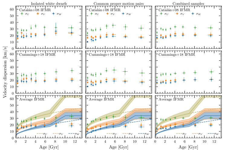
Figure 11: Age – velocity dispersion relations for the isolated white dwarfs (left panels), the white dwarfs in common proper motion pairs (middle panels), and the combined samples (right panels). Each row shows the results obtained by considering two white dwarf progenitor age estimates, which are based on the progenitor masses that we derived via the Catalán et al. (2008) and Cummings et al. (2018) IFMRs, or the average of the two. The three velocity components use different symbols and colors, as is shown in the legend of the top panels. The shaded regions in the bottom panels represent the 16–84% ranges of the Cheng et al. (2019) formulation for the age – velocity dispersion of white dwarfs in the Galactic thin and thick disk. The dashed curves represent the extrapolated thin-disk contribution.

The spatial distribution of these stars is shown in Fig.  9, in which we have color-coded them according to the measured [Fe/H] and [$\alpha$/Fe] of the nondegenerate stars. The spatial distribution of this sub-sample and the median distance from the Sun are roughly the same as those of the entire sample of common proper motion pairs. We note a spatial bias towards $Z<0$ and $\sqrt{X^{2}+Y^{2}}<R_{0}$ for stars of [$\alpha$/Fe] $>0.2$ dex that is due to the RAVE sample, which was observed from the Australian Astronomical Observatory in the Southern Hemisphere. The overall lack of correlation between metallicity and coordinates that is observed here is also seen in much larger samples of stars and is linked to the absence of a well defined age-metallicity relation (Casagrande et al., 2011; Bergemann et al., 2014), which also characterizes the binary sample analyzed by Rebassa-Mansergas et al. (2021). Both aspects are related to the radial mixing and churning that take place in galaxies, where stars of different composition travel far away from their birth sites (Schönrich & Binney, 2009; Minchev et al., 2018; Hayden et al., 2018).

As for the full sample, we also show the Toomre diagram and the azimuthal action versus eccentricity plots in Fig. 10. Even here we do not see any straightforward age versus kinematics relation, but we note two interesting aspects. First, the majority of the systems have $e<0.3$, as is typical for a sample dominated by low-$\alpha$ abundances ([$\alpha$/Fe] $<0.2$ dex). Second, there are five $\alpha$-enriched systems that have $e>0.3$, which could qualify them as members of the thick disk. Four of these systems (2632, 2653, 2655, and 3089) have $-0.7<\mathrm{[Fe/H]}<-0.3$, while 2873 has [Fe/H] $=0.18$ dex. The Galactic orbits of these five star reach $R_{\rm peri}=$ 3.5–4.5 kpc and have apocenters that do not go beyond $10$ kpc. The very metal poor star in our sample, number 1145, has an unusual thin disk kinematics with a basically circular Galactic orbit.

4.4 Age – velocity dispersion relations

We investigated the dynamic properties of the studied sample further by constructing a set of age – velocity dispersion relations that are shown in Fig. 11. Each panel separately shows the age – velocity dispersion for the isolated white dwarfs, the common proper motion pairs, and the combined sample. The age – velocity dispersion relations are considered separately for the Catalán et al. (2008) and Cummings et al. (2018) IFMRs and for the average of the two. To compute the data points shown in the figure, we only considered systems that have $e<0.27$, which we adopted as cut off for the thin disk. We removed dynamically classified thick-disk and halo members because their age uncertainties overlap with that of the thin-disk candidates, and they may therefore affect our results. We also excluded isolated white dwarfs from the SPY sample whose photometric $T_{\rm eff}$ differs by more than 30 % from the spectroscopic measurement. The age – velocity dispersion relations were computed by sampling the white dwarf total ages ($=\tau_{\rm cool}+\tau_{\rm prog}$) with a Monte Carlo method, accounting for the measured uncertainties. For the systems of unknown spectral type, we took a 2/8 ratio of non-DA/DA atmospheres into account by randomly drawing ages from the two estimates given in Tables 5 and 6. When the total ages were constrained by lower limits in these tables, we only included the fraction of the derived distributions that are below 13.5 Gyr, which we assumed to be the total age of the Milky Way. We computed the velocity dispersion for each randomly drawn sample by dividing the stars in nine logarithmically spaced age bins (0, 1, 1.4, 1.9, 2.6, 3.7, 5.1, 7, 9.7, 13.5 Gyr). We computed the median and the 16–84 % uncertainties in each age bin in this way after initially removing the 2-$\sigma$ outliers and requiring at least 35 stars per age bin. We included an age bin older than 10 Gyr for computational purposes and because the age distribution of our thin disk candidates extends beyond the typical estimate for the Galactic disk.

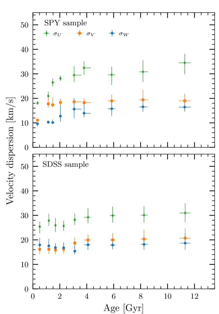
Figure 12: Age – velocity dispersion relations for the isolated white dwarf sub-samples.

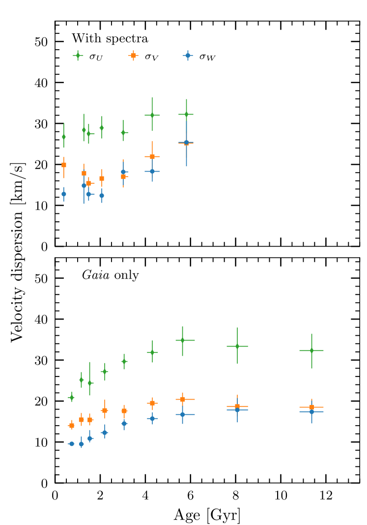
Figure 13: As Fig. 12, but showing the age – velocity dispersion relations for the white dwarfs in common proper motion pairs that have either observations from spectroscopic surveys or Gaia-DR2 radial velocities.

Inspecting Fig. 11 from left to right, we note a general increase in velocity dispersion up to 6 Gyr and a saturation that coincides with relatively flatter velocity dispersion at larger ages. The age – velocity dispersion relation of isolated white dwarfs that uses the Catalán et al. (2008) IFMR shows a slight decrease in the last bins, in contrast to that using the Cummings et al. (2018) IFMR. This difference is likely caused by the larger number of white dwarfs of lower progenitor mass that are obtained with the latter IFMR, which in turn have longer total ages. The observed trends are typically more evident for the $\sigma_{U}$ component, while the $\sigma_{V}$ and $\sigma_{W}$ components are noisier, especially in the first few age bins of the isolated white dwarf sample. The three bottom panels of Fig. 11 show a comparison of our averaged results with the parameterization obtained by Cheng et al. (2019), who modeled thin- and thick-disk contributions by analyzing a Gaia-selected white dwarf sample within 250 pc and using FGK-type stars as reference. Our results are obtained averaging the $\tau_{\rm prog}$, which were inferred from the progenitor masses obtained with the two considered IFMRs. The $\sigma_{U}$ component of the age – velocity dispersion relation for the isolated white dwarfs follows the Cheng et al. (2019) formulation up to 4 Gyr, but it continues on a relatively straight line at older ages. The $\sigma_{V}$ and $\sigma_{W}$ components, instead, are more or less flat throughout the entire age range. The best agreement is obtained for the age – velocity dispersion relation of the common proper motion pairs, which closely follows the Cheng et al. (2019) formulation up to 6-7 Gyr and reaches a flat asymptote for older ages. The asymptotic values are below the extrapolated curves for the thin disk contribution to the age – velocity dispersion relation of Cheng et al. (2019), where these authors impose a dominant contribution from the thick disk for ages $>7$ Gyr, while we excluded the kinematically selected thick-disk and halo members. The age – velocity dispersion of the two combined samples is more strongly dominated by the isolated white dwarf sample, and it therefore compares less well with the Cheng et al. (2019) formulation, especially in the $\sigma_{W}$ component. The three average relations are tabulated in Table 8.

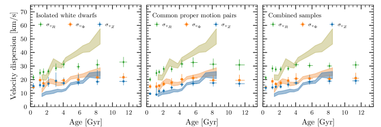
Figure 14: Age – velocity dispersion relations in Galactic cylindrical coordinates. Our results (data points with error bars) are compared to the results of Yu & Liu (2018) for LAMOST FGK-type stars with [Fe/H] $-0.2$ dex. The colored bands represent their 1-$\sigma$ error ranges.

Table 8: Average age – velocity dispersion relations that are shown in the bottom panels of Fig. 11.

Age bin [Gyr]	$\sigma_{U}$ [km s-1]	$\sigma_{V}$ [km s-1]	$\sigma_{W}$ [km s-1]	Age bin [Gyr]	$\sigma_{U}$ [km s-1]	$\sigma_{V}$ [km s-1]	$\sigma_{W}$ [km s-1]	Age bin [Gyr]	$\sigma_{U}$ [km s-1]	$\sigma_{V}$ [km s-1]	$\sigma_{W}$ [km s-1]
Isolated white dwarfs				Common proper motion pairs				Full sample
$0.36^{+0.05}_{-0.04}$	$21.53^{+2.41}_{-1.69}$	$14.19^{+0.83}_{-1.37}$	$15.25^{+2.10}_{-2.31}$	$0.42^{+0.04}_{-0.04}$	$21.15^{+1.52}_{-1.40}$	$14.07^{+2.44}_{-1.40}$	$9.59^{+0.97}_{-0.68}$	$0.36^{+0.08}_{-0.04}$	$22.21^{+1.34}_{-1.20}$	$14.03^{+0.99}_{-1.05}$	$13.87^{+2.12}_{-2.29}$
$1.17^{+0.03}_{-0.03}$	$25.37^{+2.48}_{-1.95}$	$18.39^{+3.77}_{-3.77}$	$15.90^{+3.09}_{-1.82}$	$1.19^{+0.09}_{-0.07}$	$25.13^{+2.11}_{-1.88}$	$14.69^{+2.68}_{-1.48}$	$8.92^{+5.05}_{-1.04}$	$1.17^{+0.07}_{-0.03}$	$28.29^{+2.24}_{-2.39}$	$17.84^{+2.28}_{-2.41}$	$14.19^{+2.43}_{-1.49}$
$1.59^{+0.05}_{-0.04}$	$25.69^{+2.46}_{-2.08}$	$17.09^{+2.78}_{-1.75}$	$15.40^{+3.09}_{-1.00}$	$1.52^{+0.13}_{-0.07}$	$26.12^{+1.73}_{-1.60}$	$14.92^{+1.21}_{-0.96}$	$11.30^{+1.51}_{-1.61}$	$1.58^{+0.04}_{-0.11}$	$27.63^{+2.00}_{-1.72}$	$16.27^{+1.38}_{-1.09}$	$14.69^{+2.65}_{-1.32}$
$2.19^{+0.03}_{-0.12}$	$25.97^{+1.64}_{-2.01}$	$17.13^{+1.61}_{-1.29}$	$17.01^{+4.84}_{-2.37}$	$2.08^{+0.10}_{-0.09}$	$28.52^{+2.01}_{-2.07}$	$16.94^{+2.03}_{-2.04}$	$11.64^{+1.53}_{-1.54}$	$2.18^{+0.03}_{-0.14}$	$27.78^{+1.77}_{-1.51}$	$17.55^{+1.81}_{-1.59}$	$14.72^{+2.32}_{-1.29}$
$3.11^{+0.11}_{-0.09}$	$28.28^{+3.47}_{-2.12}$	$18.51^{+1.93}_{-1.54}$	$18.84^{+6.09}_{-4.34}$	$3.04^{+0.15}_{-0.10}$	$28.02^{+2.02}_{-1.74}$	$17.88^{+2.99}_{-2.89}$	$14.07^{+1.35}_{-1.67}$	$3.08^{+0.15}_{-0.09}$	$28.17^{+1.57}_{-1.43}$	$19.06^{+2.41}_{-2.03}$	$16.25^{+3.63}_{-1.97}$
$4.06^{+0.08}_{-0.33}$	$31.12^{+2.93}_{-2.77}$	$19.26^{+2.05}_{-1.57}$	$17.33^{+3.96}_{-1.81}$	$4.30^{+0.20}_{-0.23}$	$31.13^{+3.24}_{-2.28}$	$20.65^{+3.18}_{-2.68}$	$16.36^{+1.49}_{-1.66}$	$4.06^{+0.32}_{-0.29}$	$30.65^{+1.85}_{-1.58}$	$20.96^{+3.34}_{-2.45}$	$17.52^{+2.49}_{-1.57}$
$5.84^{+0.20}_{-0.23}$	$29.43^{+2.59}_{-2.01}$	$19.73^{+4.93}_{-1.74}$	$17.67^{+6.37}_{-1.98}$	$5.67^{+0.52}_{-0.30}$	$32.63^{+3.54}_{-3.24}$	$21.23^{+2.15}_{-2.31}$	$17.09^{+3.55}_{-1.91}$	$5.70^{+0.38}_{-0.26}$	$30.36^{+2.02}_{-1.71}$	$20.67^{+2.64}_{-1.87}$	$18.37^{+4.65}_{-2.06}$
$8.16^{+0.29}_{-0.22}$	$30.90^{+3.74}_{-2.91}$	$21.43^{+4.36}_{-2.93}$	$18.37^{+8.73}_{-2.37}$	$8.13^{+0.41}_{-0.46}$	$31.50^{+4.04}_{-3.81}$	$19.51^{+3.09}_{-2.80}$	$17.48^{+2.96}_{-2.56}$	$8.13^{+0.29}_{-0.28}$	$30.13^{+2.40}_{-2.09}$	$20.37^{+2.99}_{-2.22}$	$18.84^{+3.37}_{-2.31}$
$11.35^{+0.43}_{-0.50}$	$32.93^{+3.69}_{-3.72}$	$21.48^{+2.97}_{-2.12}$	$18.66^{+4.14}_{-2.91}$	$11.31^{+0.63}_{-0.49}$	$31.13^{+3.86}_{-4.02}$	$19.60^{+3.98}_{-3.09}$	$16.94^{+2.53}_{-2.34}$	$11.34^{+0.39}_{-0.40}$	$30.96^{+2.66}_{-2.64}$	$21.02^{+3.80}_{-2.52}$	$19.00^{+3.45}_{-2.52}$

In Fig. 12 and 13, we break down the contribution of each sub-sample to the age – velocity dispersion relations. Although the SPY sample contains fewer objects than the SDSS sample (top and bottom panels of Fig.12), it clearly shows a rise of the velocity dispersion with increasing age and a saturation that begins at $\sim$4 Gyr. The SDSS sample, as noted by Anguiano et al. (2017), has a much flatter age – velocity dispersion relation at almost all ages, which the authors interpreted as being caused by an unidentified source of dynamical heating in addition to that caused by the secular evolution of the Galactic disk. The still possibly inaccurate radial velocity measurements of the SDSS sample, despite our calibration obtained in Sect. 2.1, may be the cause of the disagreement between the SPY and SDSS samples. However, we note that the SPY sample was cleaned of objects that had discrepant $T_{\rm eff}$ measurements in between the spectroscopic and photometric analyses, while the SDSS sample included all stars initially selected by us in Sect. 2.1. Nevertheless, we also note that the maximum velocity dispersion we have measured for both samples agree with their averages, which were previously determined for the thin-disk stars in the SPY sample (Pauli et al., 2006). The common proper motion pairs with spectra comprise just 314 stars, which limits our ability to determine a meaningful age – velocity dispersion relation beyond 6 Gyr (top panel of Fig. 13). This result is quite noisy, especially in the earliest age bins. The age – velocity dispersion relation of the common proper motion pairs that only have Gaia DR2 radial velocities features a smoother increase. Furthermore, we note that the three components clearly reach an asymptotic behavior in the range of 15–35 km s^-1 at $\sim$6 Gyr, which is expected to be caused by dynamical heating of stars as they interact within the Galactic disk potential (cf. Seabroke & Gilmore, 2007, and references therein). The values we measured for the age – velocity dispersion relation appear to be smaller than those obtained by previous work on wide binaries (Wegner, 1981; Silvestri et al., 2001), which considered much smaller samples without separating stars in age bins or eccentricity ranges, however. They therefore likely included at least some thick-disk members.

We also computed the age – velocity dispersion relation in Galactic cylindrical coordinates, which we compare in Fig. 14 to the age – velocity dispersion relation of LAMOST FGK-type stars with [Fe/H] $>-0.2$ (Yu & Liu, 2018). The studied samples follow the general increasing trend observed for the LAMOST stars up to 4–6 Gyr, where our age – velocity dispersion relations reach saturation. On the other hand, the LAMOST selection, which favors $\alpha$-depleted stars that are more likely thin-disk members, shows a $\sigma_{U}$ component that rises up to 50 km s^-1.

Table 9: Velocity dispersion as function of [Fe/H] and [$\alpha$/Fe].

$[{\rm Fe/H}]$	$\sigma_{U}$ [km s-1]	$\sigma_{V}$ [km s-1]	$\sigma_{W}$ [km s-1]
$(-1.00,-0.50)$	$42.73_{-2.12}^{+2.06}$	$26.24_{-5.74}^{+3.50}$	$20.37_{-0.51}^{+1.42}$
$(-0.50,0.00)$	$31.55_{-1.15}^{+0.73}$	$20.52_{-1.16}^{+0.65}$	$19.88_{-3.54}^{+2.14}$
$(0.00,0.60)$	$28.29_{-1.35}^{+1.50}$	$22.27_{-1.31}^{+1.08}$	$18.40_{-0.77}^{+1.45}$
$[{\rm\alpha/Fe}]$	$\sigma_{U}$ [km s-1]	$\sigma_{V}$ [km s-1]	$\sigma_{W}$ [km s-1]
$(-0.20,0.00)$	$31.59_{-2.69}^{+2.75}$	$24.73_{-1.67}^{+1.93}$	$15.22_{-1.21}^{+1.67}$
$(0.00,0.20)$	$30.82_{-0.91}^{+1.66}$	$19.79_{-1.23}^{+2.29}$	$18.28_{-3.75}^{+4.12}$
$(0.20,0.60)$	$30.83_{-2.56}^{+2.50}$	$19.63_{-2.45}^{+2.78}$	$18.14_{-2.98}^{+3.17}$

To conclude this section, we measured the velocity dispersion of the common proper motion pairs by binning their [Fe/H] and [$\alpha$/Fe]. The results of this exercise are given in Table 9. Here, even taking into account the small size of our sample, we note that the radial component, $\sigma_{U}$, has the largest dispersion in the case of the most metal-poor systems and is anticorrelated with increasing metallicity, while the other two components have the same velocity dispersion within the errors. The observed trend for $\sigma_{U}$ may be related to the radial mixing occurring in the Milky Way, as discussed in the previous sections. The three velocity dispersion components do not show a significant trend with [$\alpha$/Fe]. The average dispersions of each velocity component are in agreement with those from much larger samples of single stars (cf. Hayden et al., 2020).

5 Summary and outlook

We have analyzed, for the first time, the 3D kinematics of 3133 isolated white dwarfs with available radial velocity measurements and white dwarfs in common proper motion pairs that contain one nondegenerate companion with radial velocity measurements. The studied stars have highly reliable Gaia EDR3 data, and in about 30% of the common proper motion pairs, measured metal abundances for the nondegenerate stars. We uniformly estimated the white dwarf physical parameters (mass and cooling age) by interpolation with state of the art evolutionary sequences in the Gaia HR diagram. Using a set of initial-to-final-mass relations and main-sequence evolutionary tracks, we estimated the white dwarf progenitor masses and total ages. This approach has enabled us to identify kinematic members of the Galactic thin and thick disk, and of the halo. The latter group contains seven isolated white dwarfs. Another previously classified halo member is confirmed to belong to the thin disk, thanks to the accurate proper motions of Gaia EDR3. We have measured the age – velocity dispersion relation for the studied sample, breaking it down by sub-samples, in agreement with previous results that used different methods. Moreover, our age – velocity dispersion relations show both signs of dynamical heating and saturation beginning at 4–6 Gyr. Taking advantage of the measured abundances for the nondegenerate companions in common proper motion pairs, we confirmed the presence of overlapping populations in the solar neighborhood, for instance, due to radial mixing, and we measured an anticorrelation between [Fe/H] and the velocity dispersion along the radial direction in the Galactic reference frame. The studied sample can be further exploited to improve classification schemes of white dwarfs belonging to the thin and thick disk and to the halo, and also to study their membership to local streams and moving groups (Torres et al., 2019a).

In the coming years, the legacy of the existing large spectroscopic surveys such as RAVE, LAMOST, APOGEE, and GALAH, will be taken upon by much larger projects as WEAVE (Dalton et al., 2012), 4MOST (de Jong et al., 2012), and SDSS-V (Kollmeier et al., 2017), that will observe at the same time all Gaia white dwarfs and millions of stars for chemical tagging of the Galactic populations. Hence, a more coherent picture of the global chemodynamics of the Milky Way and its connection with the solar neighborhood and the white dwarf population will come within reach.

References

- Adibekyan et al. (2011) Adibekyan, V. Z., Santos, N. C., Sousa, S. G., & Israelian, G. 2011, A&A, 535, L11
- Althaus et al. (2010) Althaus, L. G., Córsico, A. H., Isern, J., & García-Berro, E. 2010, A&A Rev., 18, 471
- Althaus et al. (2013) Althaus, L. G., Miller Bertolami, M. M., & Córsico, A. H. 2013, A&A, 557, A19
- Anguiano et al. (2018) Anguiano, B., Majewski, S. R., Allende Prieto, C., et al. 2018, A&A, 620, A76
- Anguiano et al. (2017) Anguiano, B., Rebassa-Mansergas, A., García-Berro, E., et al. 2017, MNRAS, 469, 2102
- Antoja et al. (2018) Antoja, T., Helmi, A., Romero-Gómez, M., et al. 2018, Nature, 561, 360
- Aumer et al. (2016) Aumer, M., Binney, J., & Schönrich, R. 2016, MNRAS, 462, 1697
- Aumer & Binney (2009) Aumer, M. & Binney, J. J. 2009, MNRAS, 397, 1286
- Bailer-Jones et al. (2021) Bailer-Jones, C. A. L., Rybizki, J., Fouesneau, M., Demleitner, M., & Andrae, R. 2021, AJ, 161, 147
- Bauer et al. (2020) Bauer, E. B., Schwab, J., Bildsten, L., & Cheng, S. 2020, ApJ, 902, 93
- Belokurov et al. (2018) Belokurov, V., Erkal, D., Evans, N. W., Koposov, S. E., & Deason, A. J. 2018, MNRAS, 478, 611
- Bergemann et al. (2014) Bergemann, M., Ruchti, G. R., Serenelli, A., et al. 2014, A&A, 565, A89
- Bergeron et al. (2019) Bergeron, P., Dufour, P., Fontaine, G., et al. 2019, ApJ, 876, 67
- Bergeron et al. (1997) Bergeron, P., Ruiz, M. T., & Leggett, S. K. 1997, ApJS, 108, 339
- Binney (2012) Binney, J. 2012, MNRAS, 426, 1324
- Bland-Hawthorn & Gerhard (2016) Bland-Hawthorn, J. & Gerhard, O. 2016, ARA&A, 54, 529
- Bland-Hawthorn et al. (2019) Bland-Hawthorn, J., Sharma, S., Tepper-Garcia, T., et al. 2019, MNRAS, 486, 1167
- Blouin et al. (2021) Blouin, S., Daligault, J., & Saumon, D. 2021, ApJ, 911, L5
- Boeche et al. (2013) Boeche, C., Siebert, A., Piffl, T., et al. 2013, A&A, 559, A59
- Boubert et al. (2019) Boubert, D., Strader, J., Aguado, D., et al. 2019, MNRAS, 486, 2618
- Bovy (2015) Bovy, J. 2015, ApJS, 216, 29
- Buder et al. (2021) Buder, S., Sharma, S., Kos, J., et al. 2021, MNRAS, 506, 150
- Camisassa et al. (2019) Camisassa, M. E., Althaus, L. G., Córsico, A. H., et al. 2019, A&A, 625, A87
- Camisassa et al. (2016) Camisassa, M. E., Althaus, L. G., Córsico, A. H., et al. 2016, ApJ, 823, 158
- Camisassa et al. (2017) Camisassa, M. E., Althaus, L. G., Rohrmann, R. D., et al. 2017, ApJ, 839, 11
- Camisassa et al. (2021) Camisassa, M. E., Althaus, L. G., Torres, S., et al. 2021, A&A, 649, L7
- Cantat-Gaudin & Anders (2020) Cantat-Gaudin, T. & Anders, F. 2020, A&A, 633, A99
- Casagrande et al. (2011) Casagrande, L., Schönrich, R., Asplund, M., et al. 2011, A&A, 530, A138
- Catalán et al. (2008) Catalán, S., Isern, J., García-Berro, E., & Ribas, I. 2008, MNRAS, 387, 1693
- Cheng et al. (2019) Cheng, S., Cummings, J. D., & Ménard, B. 2019, ApJ, 886, 100
- Cheng et al. (2020) Cheng, S., Cummings, J. D., Ménard, B., & Toonen, S. 2020, ApJ, 891, 160
- Cummings et al. (2018) Cummings, J. D., Kalirai, J. S., Tremblay, P. E., Ramirez-Ruiz, E., & Choi, J. 2018, ApJ, 866, 21
- Dalton et al. (2012) Dalton, G., Trager, S. C., Abrams, D. C., et al. 2012, in Society of Photo-Optical Instrumentation Engineers (SPIE) Conference Series, Vol. 8446, Ground-based and Airborne Instrumentation for Astronomy IV, ed. I. S. McLean, S. K. Ramsay, & H. Takami, 84460P
- de Jong et al. (2012) de Jong, R. S., Bellido-Tirado, O., Chiappini, C., et al. 2012, in Society of Photo-Optical Instrumentation Engineers (SPIE) Conference Series, Vol. 8446, Ground-based and Airborne Instrumentation for Astronomy IV, ed. I. S. McLean, S. K. Ramsay, & H. Takami, 84460T
- De Silva et al. (2015) De Silva, G. M., Freeman, K. C., Bland-Hawthorn, J., et al. 2015, MNRAS, 449, 2604
- Dehnen & Binney (1998) Dehnen, W. & Binney, J. J. 1998, MNRAS, 298, 387
- Deng et al. (2012) Deng, L.-C., Newberg, H. J., Liu, C., et al. 2012, Research in Astronomy and Astrophysics, 12, 735
- Dimpel (2018) Dimpel, M. 2018, Master’s thesis, Friedrich Alexander Universität Erlangen Nürnberg, Schloßplatz 4, 91054 Erlangen, Germany
- Doherty et al. (2017) Doherty, C. L., Gil-Pons, P., Siess, L., & Lattanzio, J. C. 2017, PASA, 34, e056
- Dufour et al. (2017) Dufour, P., Blouin, S., Coutu, S., et al. 2017, in Astronomical Society of the Pacific Conference Series, Vol. 509, 20th European White Dwarf Workshop, ed. P. E. Tremblay, B. Gaensicke, & T. Marsh, 3
- El-Badry et al. (2021) El-Badry, K., Rix, H.-W., & Heintz, T. M. 2021, MNRAS, 506, 2269
- Fitzpatrick et al. (2019) Fitzpatrick, E. L., Massa, D., Gordon, K. D., Bohlin, R., & Clayton, G. C. 2019, ApJ, 886, 108
- Gaia Collaboration et al. (2018) Gaia Collaboration, Brown, A. G. A., Vallenari, A., et al. 2018, A&A, 616, A1
- Gaia Collaboration et al. (2021) Gaia Collaboration, Brown, A. G. A., Vallenari, A., et al. 2021, A&A, 649, A1
- Gaia Collaboration et al. (2016) Gaia Collaboration, Prusti, T., de Bruijne, J. H. J., et al. 2016, A&A, 595, A1
- Gentile Fusillo et al. (2021) Gentile Fusillo, N. P., Tremblay, P. E., Cukanovaite, E., et al. 2021, MNRAS, 508, 3877
- Gravity Collaboration et al. (2019) Gravity Collaboration, Abuter, R., Amorim, A., et al. 2019, A&A, 625, L10
- Greenstein et al. (1977) Greenstein, J. L., Boksenberg, A., Carswell, R., & Shortridge, K. 1977, ApJ, 212, 186
- Halenka et al. (2015) Halenka, J., Olchawa, W., Madej, J., & Grabowski, B. 2015, ApJ, 808, 131
- Hayden et al. (2020) Hayden, M. R., Bland-Hawthorn, J., Sharma, S., et al. 2020, MNRAS, 493, 2952
- Hayden et al. (2015) Hayden, M. R., Bovy, J., Holtzman, J. A., et al. 2015, ApJ, 808, 132
- Hayden et al. (2018) Hayden, M. R., Recio-Blanco, A., de Laverny, P., et al. 2018, A&A, 609, A79
- Helmi et al. (2018) Helmi, A., Babusiaux, C., Koppelman, H. H., et al. 2018, Nature, 563, 85
- Hidalgo et al. (2018) Hidalgo, S. L., Pietrinferni, A., Cassisi, S., et al. 2018, ApJ, 856, 125
- Hollands et al. (2018) Hollands, M. A., Tremblay, P. E., Gänsicke, B. T., Gentile-Fusillo, N. P., & Toonen, S. 2018, MNRAS, 480, 3942
- Hunter (2007) Hunter, J. D. 2007, Computing in Science & Engineering, 9, 90
- Jiménez-Esteban et al. (2018) Jiménez-Esteban, F. M., Torres, S., Rebassa-Mansergas, A., et al. 2018, MNRAS, 480, 4505
- Jönsson et al. (2020) Jönsson, H., Holtzman, J. A., Allende Prieto, C., et al. 2020, AJ, 160, 120
- Koester (2010) Koester, D. 2010, Mem. Soc. Astron. Italiana, 81, 921
- Kollmeier et al. (2017) Kollmeier, J. A., Zasowski, G., Rix, H.-W., et al. 2017, arXiv e-prints, arXiv:1711.03234
- Kunder et al. (2017) Kunder, A., Kordopatis, G., Steinmetz, M., et al. 2017, AJ, 153, 75
- Lallement et al. (2019) Lallement, R., Babusiaux, C., Vergely, J. L., et al. 2019, A&A, 625, A135
- Lindegren (2018) Lindegren, L. 2018, Re-normalising the astrometric chi-square in Gaia DR2, Tech. Rep. GAIA-C3-TN-LU-LL-124-01, Lund Observatory, Lund, Sweden
- Luo et al. (2019) Luo, A. L., Zhao, Y. H., Zhao, G., & et al. 2019, VizieR Online Data Catalog, V/164
- Mackereth & Bovy (2018) Mackereth, J. T. & Bovy, J. 2018, PASP, 130, 114501
- Majewski et al. (2017) Majewski, S. R., Schiavon, R. P., Frinchaboy, P. M., et al. 2017, AJ, 154, 94
- Matteucci & Recchi (2001) Matteucci, F. & Recchi, S. 2001, ApJ, 558, 351
- McCleery et al. (2020) McCleery, J., Tremblay, P.-E., Gentile Fusillo, N. P., et al. 2020, MNRAS, 499, 1890
- Minchev et al. (2018) Minchev, I., Anders, F., Recio-Blanco, A., et al. 2018, MNRAS, 481, 1645
- Miyamoto & Nagai (1975) Miyamoto, M. & Nagai, R. 1975, PASJ, 27, 533
- Napiwotzki et al. (2020) Napiwotzki, R., Karl, C. A., Lisker, T., et al. 2020, A&A, 638, A131
- Navarro et al. (2011) Navarro, J. F., Abadi, M. G., Venn, K. A., Freeman, K. C., & Anguiano, B. 2011, MNRAS, 412, 1203
- Navarro et al. (1997) Navarro, J. F., Frenk, C. S., & White, S. D. M. 1997, ApJ, 490, 493
- Ochsenbein et al. (2000) Ochsenbein, F., Bauer, P., & Marcout, J. 2000, A&AS, 143, 23
- Oppenheimer et al. (2001) Oppenheimer, B. R., Hambly, N. C., Digby, A. P., Hodgkin, S. T., & Saumon, D. 2001, Science, 292, 698
- Pauli et al. (2003) Pauli, E. M., Napiwotzki, R., Altmann, M., et al. 2003, A&A, 400, 877
- Pauli et al. (2006) Pauli, E. M., Napiwotzki, R., Heber, U., Altmann, M., & Odenkirchen, M. 2006, A&A, 447, 173
- Pietrinferni et al. (2021) Pietrinferni, A., Hidalgo, S., Cassisi, S., et al. 2021, ApJ, 908, 102
- Randich et al. (2013) Randich, S., Gilmore, G., & Gaia-ESO Consortium. 2013, The Messenger, 154, 47
- Rebassa-Mansergas et al. (2021) Rebassa-Mansergas, A., Maldonado, J., Raddi, R., et al. 2021, MNRAS, 505, 3165
- Reid et al. (2001) Reid, I. N., Sahu, K. C., & Hawley, S. L. 2001, ApJ, 559, 942
- Reid & Brunthaler (2004) Reid, M. J. & Brunthaler, A. 2004, ApJ, 616, 872
- Richter et al. (2007) Richter, R., Heber, U., & Napiwotzki, R. 2007, in Astronomical Society of the Pacific Conference Series, Vol. 372, 15th European Workshop on White Dwarfs, ed. R. Napiwotzki & M. R. Burleigh, 107
- Riello et al. (2021) Riello, M., De Angeli, F., Evans, D. W., et al. 2021, A&A, 649, A3
- Romero et al. (2015) Romero, A. D., Campos, F., & Kepler, S. O. 2015, MNRAS, 450, 3708
- Rowell & Kilic (2019) Rowell, N. & Kilic, M. 2019, MNRAS, 484, 3544
- Rybizki et al. (2021) Rybizki, J., Green, G., Rix, H.-W., et al. 2021, arXiv e-prints, arXiv:2101.11641
- Schatzman (1945) Schatzman, E. 1945, Annales d’Astrophysique, 8, 143
- Schönrich & Binney (2009) Schönrich, R. & Binney, J. 2009, MNRAS, 396, 203
- Schönrich et al. (2010) Schönrich, R., Binney, J., & Dehnen, W. 2010, MNRAS, 403, 1829
- Schulz (1977) Schulz, H. 1977, A&A, 54, 315
- Seabroke & Gilmore (2007) Seabroke, G. M. & Gilmore, G. 2007, MNRAS, 380, 1348
- Sellwood & Binney (2002) Sellwood, J. A. & Binney, J. J. 2002, MNRAS, 336, 785
- Silvestri et al. (2001) Silvestri, N. M., Oswalt, T. D., Wood, M. A., et al. 2001, AJ, 121, 503
- Sion et al. (2014) Sion, E. M., Holberg, J. B., Oswalt, T. D., et al. 2014, AJ, 147, 129
- Steinmetz et al. (2006) Steinmetz, M., Zwitter, T., Siebert, A., et al. 2006, AJ, 132, 1645
- Taylor (2006) Taylor, M. B. 2006, in Astronomical Society of the Pacific Conference Series, Vol. 351, Astronomical Data Analysis Software and Systems XV, ed. C. Gabriel, C. Arviset, D. Ponz, & S. Enrique, 666
- Temmink et al. (2020) Temmink, K. D., Toonen, S., Zapartas, E., Justham, S., & Gänsicke, B. T. 2020, A&A, 636, A31
- Toonen et al. (2020) Toonen, S., Portegies Zwart, S., Hamers, A. S., & Bandopadhyay, D. 2020, A&A, 640, A16
- Torres et al. (2019a) Torres, S., Cantero, C., Camisassa, M. E., et al. 2019a, A&A, 629, L6
- Torres et al. (2019b) Torres, S., Cantero, C., Rebassa-Mansergas, A., et al. 2019b, MNRAS, 485, 5573
- Torres et al. (2021) Torres, S., Rebassa-Mansergas, A., Camisassa, M. E., & Raddi, R. 2021, MNRAS, 502, 1753
- Tremblay et al. (2019a) Tremblay, P. E., Cukanovaite, E., Gentile Fusillo, N. P., Cunningham, T., & Hollands, M. A. 2019a, MNRAS, 482, 5222
- Tremblay et al. (2019b) Tremblay, P.-E., Fontaine, G., Gentile Fusillo, N. P., et al. 2019b, Nature, 565, 202
- Tremblay et al. (2020) Tremblay, P. E., Hollands, M. A., Gentile Fusillo, N. P., et al. 2020, MNRAS, 497, 130
- Trimble & Greenstein (1972) Trimble, V. & Greenstein, J. L. 1972, ApJ, 177, 441
- Virtanen et al. (2020) Virtanen, P., Gommers, R., Oliphant, T. E., et al. 2020, Nature Methods, 17, 261
- Wang et al. (2019) Wang, R., Luo, A. L., Chen, J. J., et al. 2019, ApJS, 244, 27
- Wegg & Phinney (2012) Wegg, C. & Phinney, E. S. 2012, MNRAS, 426, 427
- Wegner (1974) Wegner, G. 1974, MNRAS, 166, 271
- Wegner (1981) Wegner, G. 1981, AJ, 86, 264
- Wenger et al. (2000) Wenger, M., Ochsenbein, F., Egret, D., et al. 2000, A&AS, 143, 9
- Xiang et al. (2019) Xiang, M., Ting, Y.-S., Rix, H.-W., et al. 2019, ApJS, 245, 34
- Yu & Liu (2018) Yu, J. & Liu, C. 2018, MNRAS, 475, 1093